Carr02 Members earth

1

1

AtholAthol J. CarrJ. CarrProfessorProfessor of Civil of Civil EngineeringEngineering

DepartmentDepartment of Civil of Civil andand Natural Natural ResourcesResources EngineeringEngineeringUniversity of Canterbury,University of Canterbury,

Christchurch, Christchurch, NewNew ZealandZealand..

Análisis Sísmico de Edificios de Hormigón Armado.Respuesta Dentro del Rango No Lineal

ACHISINAAsociación Chilena de Sismología e Ingeniería Antisísmica

Santiago de Chile, 2 al 6 de junio de 2008

Section 2 – Non-linear Stiffness Models

2

Structural Member ModellingThe stiffness of the structure is obtained by assembling the

stiffness matrices of the individual members that constitute the structure and its foundation.

For non-linear models there are many choices that are available to represent the non-linear characteristics.

There is also a large amount of data to provide the post-yield properties of the members. This means that the analyses cannot be carried out until the full design of the structure has been completed.

2

3

Structural Member ModellingThe member may be very non-prismatic in its properties, e.g.

for a typical reinforced concrete beam member as shown below.

The section flexural stiffness varies markedly along the length of the member due to cracking of the concrete and possible yieldingof the steel reinforcement.

4

Realistic SectionProperties

When carrying out an analysis at least use properties that represent the real structure.This may require different data sets for the different limit states

(from NZ Concrete Code NZS 3101:1995)

3

5

Realistic Section Properties

Table C3.1 – Effective Section Properties [NZS 3101:2005]

0.15 Ig0.40 IgIg0.15 Ig-0.1

0.25 Ig0.50 IgIg0.25 Ig0.0

0.45 Ig0.70IgIg0.45 Ig0.2

3. Walls

0.40 Ig0.70 IgIg0.40 Ig-0.05

0.60 Ig0.80 IgIg0.60 Ig0.2

0.80 Ig0.90 IgIg0.80 Ig> 0.5

2. Columns

0.35 Ig0.60 IgIg0.35 Igb) T- and L- beams

0.40 Ig0.70 IgIg0.40 Iga) Rectangular beamsN.A.

1. Beams

μ = 6μ = 3μ = 1.25

Serviceability Limit State

Ultimate Limit State

Axial Load

Type of Member

6

Beam-Column Members

The Giberson, two-component or any of the other beam models may be arranged to form a general beam-column member. The rigid links shown avoid the use of dummy stiff members in the modeling of the structure.

4

7

Beam-Column MembersThe beam with 6 external degrees of freedom {u} has 3 deformation degrees of freedom {v}

{ } [ ] [ ]{ }

1

2

31

42

5

6

uuu

v T T uuuu

⎧ ⎫⎪ ⎪⎪ ⎪Δ⎧ ⎫⎪ ⎪⎪ ⎪ ⎪ ⎪= θ = =⎨ ⎬ ⎨ ⎬

⎪ ⎪ ⎪ ⎪θ⎩ ⎭ ⎪ ⎪⎪ ⎪⎪ ⎪⎩ ⎭

The transformation matrix [T] relates the deformations to the external displacements.

8

Beam-Column Members – Equivalent Nodal ForcesUsing Virtual Displacements it can be shown that the nodal forces {f} are obtained from the internal member forces {s} using the transformation matrix [T]

{ } [ ] [ ] { }

1

2

T T31

42

5

6

ff

Pf

f T M T sf

Mff

⎧ ⎫⎪ ⎪⎪ ⎪ ⎧ ⎫⎪ ⎪⎪ ⎪ ⎪ ⎪= = =⎨ ⎬ ⎨ ⎬⎪ ⎪ ⎪ ⎪

⎩ ⎭⎪ ⎪⎪ ⎪⎪ ⎪⎩ ⎭

The member forces {s} are derived from the member deformations{v} and the hysteresis rule applicable to the member. This method of obtaining the equivalent nodal forces is more reliable than using a secant stiffness matrix approach. These member nodal forces can be combined to obtain the nodal forces for the whole structure.

5

9

Beam-Column Members

For a prismatic linear elastic member

1 1

2 2

AE . .LP

4EI 2EIM .L L

M 2EI 4EI.L L

⎡ ⎤⎢ ⎥

Δ⎧ ⎫ ⎧ ⎫⎢ ⎥−⎪ ⎪ ⎪ ⎪⎢ ⎥= θ⎨ ⎬ ⎨ ⎬⎢ ⎥⎪ ⎪ ⎪ ⎪θ⎢ ⎥⎩ ⎭ ⎩ ⎭−⎢ ⎥

⎢ ⎥⎣ ⎦

where E is the elastic modulus, A is the cross-section area, I is the cross-section second moment of area and L is the length of the beam

10

Beam-Column Members - Including Shear Deformation etc.

1 1 1 1 1s

2 2 2 2 2

L . .AE P 0 . . P 0 . . P

2L L 1. M . 1 1 M . F . M6EI 6EI GA L

M . 1 1 M . . F ML 2L.6EI 6EI

⎡ ⎤⎢ ⎥

Δ⎧ ⎫ ⎧ ⎫ ⎧ ⎫ ⎡ ⎤ ⎧ ⎫⎡ ⎤⎢ ⎥⎪ ⎪ ⎪ ⎪ ⎪ ⎪ ⎪ ⎪⎢ ⎥⎢ ⎥⎢ ⎥θ = + − +⎨ ⎬ ⎨ ⎬ ⎨ ⎬ ⎨ ⎬⎢ ⎥⎢ ⎥⎢ ⎥⎪ ⎪ ⎪ ⎪ ⎪ ⎪ ⎪ ⎪⎢ ⎥⎢ ⎥θ −⎢ ⎥ ⎣ ⎦⎩ ⎭ ⎩ ⎭ ⎩ ⎭ ⎣ ⎦ ⎩ ⎭

⎢ ⎥⎢ ⎥⎣ ⎦

To include the effects of shear deformation and end joint flexibility one needs to add the flexibility due to flexure, the flexibility to shear deformation and the flexibility of the end connections Fi (e.g. bolted connections or plastic hinges).

Once the total flexibility is obtained this matrix is inverted to get the member stiffness matrix.Note: The shear angle is proportional to the shear force V=(M1-M2)/Ldivided by GAs

6

11

If we take a beam of length L and a rectangular cross-section of depth d then the shear terms are proportional to (d/L)2. Assuming G=E/2

[ ]

[ ]

[ ]

[ ]

[ ]

then

then

then

then

then

2.00 1.000 k no shear deformation

1.00 2.00

2.01 0.99d 1 kL 10 0.99 2.01

2.06 0.94d 1 kL 4 0.94 2.06

2.25 0.75d 1 kL 2 0.75 2.25

3.0d 1 kL 1

−⎡ ⎤β = = ⎢ ⎥−⎣ ⎦

−⎡ ⎤= = ⎢ ⎥−⎣ ⎦

−⎡ ⎤= = ⎢ ⎥−⎣ ⎦

−⎡ ⎤= = ⎢ ⎥−⎣ ⎦

= =0 0.00

0.00 3.00−⎡ ⎤

⎢ ⎥−⎣ ⎦i.e. Shear deformations are important for deep beams and for thecase where As/A is small, i.e. large flanges and thin webs.

12

P-Delta EffectsIf there are vertical loads acting on structures that deform laterally then there may be significant P-Delta effects in the response. In most analyses these are regarded as second order effects, i.e. usually small and neglected. To be significant there needs to be large axial compression forces in the columns and the columns need to have a significant inter-storey drift. In the example the moments caused by the lateral load are augmented by the moment caused by the gravity load. The moment at the base is not Ph as would be obtained using small deflection theory but is now Ph+Mgδ

7

13

Beam-Column Members – P-Delta Effects

1 1 1

2 2 2

AE . .LP 0 . .

4EI 2EI PLM . . 4 1L L 30

M . 1 42EI 4EI.L L

⎡ ⎤⎢ ⎥

Δ Δ⎧ ⎫ ⎧ ⎫ ⎧ ⎫⎡ ⎤⎢ ⎥−⎪ ⎪ ⎪ ⎪ ⎪ ⎪⎢ ⎥⎢ ⎥= θ + θ⎨ ⎬ ⎨ ⎬ ⎨ ⎬⎢ ⎥⎢ ⎥⎪ ⎪ ⎪ ⎪ ⎪ ⎪⎢ ⎥θ θ⎢ ⎥ ⎣ ⎦⎩ ⎭ ⎩ ⎭ ⎩ ⎭−⎢ ⎥

⎢ ⎥⎣ ⎦

The axial force in the beam member affects the lateral flexibility of the beam. A tension will try to reduce the lateral displacement, increasing the flexural, or bending, stiffness.

Note that if P is negative (compression) the stiffness of the member is reduced. An alternative to the PL/30 terms is to use stability coefficients. If P equals the buckling load the flexural stiffness of the member becomes zero

14

Beam-Column Members – P-Delta EffectsIf one sets the determinant of the stiffness matrix on the previous slide to zero then the value of the critical buckling load is

2cr LEI

12P =

which is about 21% larger than the correct value of

22

cr LEI

P π=

This is due to the limited (cubic) displacement functions associated with the beam element. This cubic lateral deformation assumed in the beam is an approximation to the sine function usually associated with buckling of beams.In all normal structural analyses the axial forces in the members are usually well below the buckling load and the difference is not significant.

8

15

Beam-Column Members – P-Delta EffectsThe terms on the earlier slide show the effects on the member’s flexural stiffness matrix due to the axial force. The next step is to account for the difference in orientation due to large displacements. In some programs all effects are covered using a geometric stiffness matrix but then the member’s moments are in-correctly computed as the 3 by 3 matrix is missing the axial force effects on the moments.

geomtric

0 . . . . .. 1 . . 1 .. . 0 . . .Pk

L . . . 0 . .. 1 . . 1 .. . . . . 0

⎡ ⎤⎢ ⎥−⎢ ⎥⎢ ⎥

⎡ ⎤ = ⎢ ⎥⎣ ⎦⎢ ⎥⎢ ⎥−⎢ ⎥⎣ ⎦

The axial force in the member affects the lateral stiffness of the beam member. This term is added to the global stiffness of the element.

16

Beam Geometric Stiffness Matrix

2 2

G

2 2

. . . . . .

. 36 3L . 36 3L

. 3L 4L . 3L LPk30L . . . . . .

. 36 3L . 36 3L

. 3L L . 3L 4L

⎡ ⎤⎢ ⎥−⎢ ⎥⎢ ⎥− −

=⎡ ⎤ ⎢ ⎥⎣ ⎦⎢ ⎥⎢ ⎥− − −⎢ ⎥

− −⎣ ⎦

The often quoted geometric stiffness matrix for a 2 dimensional beam member is given by the following expression

The better way of forming this geometric stiffness matrix is to transform the member 3x3 (PL/30) deformation stiffness matrix to a member global matrix and then add the string (or truss) matrix of the previous slide. The two step method described in the preceding slidesproduces the correct actions in the structural members.

9

17

Structural Member ModellingUnder the variation of bending moment generated by lateral

earthquake excitation any yielding of the reinforcement will tend to be concentrated at the ends of the member

Cracking and steel yield will enhance the curvature at the member ends. The stiffness can be obtained either by using moment area methods or by using the Giberson one-component model

18

Giberson One-Component Beam Member (1967)The in-elastic rotation (curvature) is concentrated into the

rotation of an equivalent plastic hinge spring. If the member is elastic the spring does not exist (the plastic hinge acts like a rusty gate hinge, fixed until the moment exceeds the friction).

10

19

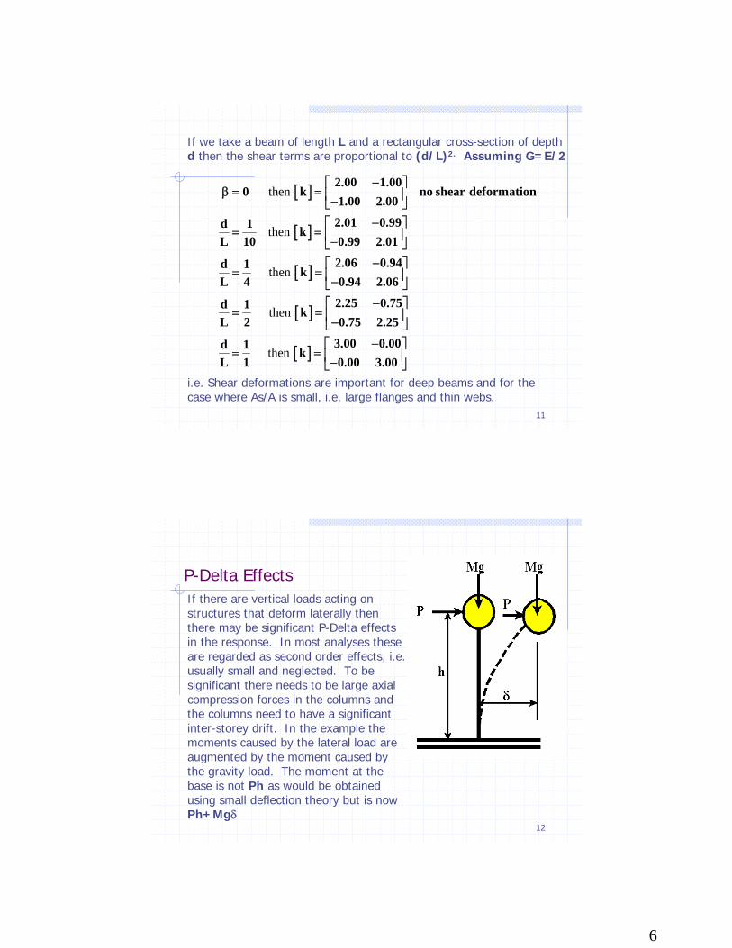
Giberson One-Component Beam MemberThe spring stiffness is arranged so that the elastic rotation

over the hinge length plus the plastic hinge rotation is the same as the rotation implied by the in-elastic curvature over the plastic hinge length.

20

Giberson One-Component Beam MemberOnce the plastic hinge spring stiffness is determined then

the hinge stiffness is inverted to get the spring flexibility and this is then added to the flexibility of the beam member in exactly the same manner as end joint flexibilities are added.

The exception is where there is a perfectly plastic hinge which in the tangent stiffness is infinitely flexible and the beam member then acts as a member with a perfect hinge at one end.

11

21

Two-Component Member Model (1965)

The in-elastic member is assumed to consist of two parallel members, one representing the in-elastic member and the sum of the components representing the elastic member.

22

Two-Component Member Model (1965)r = bi-linear factor

1 1 1

2 2 2

AE AE. . . .L LP

4EI 2EI 3EIM r . (1 r ) . 0L L L

M 2EI 4EI . 0 0.L L

⎡ ⎤ ⎡ ⎤⎢ ⎥ ⎢ ⎥

Δ Δ⎧ ⎫ ⎧ ⎫ ⎧ ⎫⎢ ⎥ ⎢ ⎥−⎪ ⎪ ⎪ ⎪ ⎪ ⎪⎢ ⎥ ⎢ ⎥= θ + − θ⎨ ⎬ ⎨ ⎬ ⎨ ⎬⎢ ⎥ ⎢ ⎥⎪ ⎪ ⎪ ⎪ ⎪ ⎪θ θ⎢ ⎥ ⎢ ⎥⎩ ⎭ ⎩ ⎭ ⎩ ⎭−⎢ ⎥ ⎢ ⎥

⎢ ⎥ ⎢ ⎥⎣ ⎦ ⎣ ⎦

1 1 1

2 2 2

AE AE. . . .L LP

4EI 2EI 4EI 2EIM r . (1 r) .L L L L

M 2EI 4EI 2EI 4EI. .L L L L

⎡ ⎤ ⎡ ⎤⎢ ⎥ ⎢ ⎥

Δ Δ⎧ ⎫ ⎧ ⎫ ⎧ ⎫⎢ ⎥ ⎢ ⎥− −⎪ ⎪ ⎪ ⎪ ⎪ ⎪⎢ ⎥ ⎢ ⎥= θ + − θ⎨ ⎬ ⎨ ⎬ ⎨ ⎬⎢ ⎥ ⎢ ⎥⎪ ⎪ ⎪ ⎪ ⎪ ⎪θ θ⎢ ⎥ ⎢ ⎥⎩ ⎭ ⎩ ⎭ ⎩ ⎭− −⎢ ⎥ ⎢ ⎥

⎢ ⎥ ⎢ ⎥⎣ ⎦ ⎣ ⎦

For the elastic member the stiffness is

When a plastic hinge occurs at end 2 of the beam the stiffness matrix is

12

23

Two-Component Member Model (1965)

1 1 1

2 2 2

AE . . AE . .LP L4EI 2EIM r . (1 r) . 0 0L L

M 3EI2EI 4EI . 0. LL L

⎡ ⎤⎡ ⎤⎢ ⎥⎢ ⎥Δ Δ⎧ ⎫ ⎧ ⎫ ⎧ ⎫⎢ ⎥⎢ ⎥−⎪ ⎪ ⎪ ⎪ ⎪ ⎪⎢ ⎥= θ + − θ⎨ ⎬ ⎨ ⎬ ⎨ ⎬⎢ ⎥⎢ ⎥⎪ ⎪ ⎪ ⎪ ⎪ ⎪⎢ ⎥θ θ⎢ ⎥⎩ ⎭ ⎩ ⎭ ⎩ ⎭− ⎢ ⎥⎢ ⎥ ⎣ ⎦⎢ ⎥⎣ ⎦

When a plastic hinge occurs at end 1 the stiffness matrix is

1 1 1

2 2 2

AE . . AE . .LP L4EI 2EIM r . (1 r ) . 0 0L L

M . 0 02EI 4EI.L L

⎡ ⎤⎡ ⎤⎢ ⎥⎢ ⎥Δ Δ⎧ ⎫ ⎧ ⎫ ⎧ ⎫⎢ ⎥⎢ ⎥−⎪ ⎪ ⎪ ⎪ ⎪ ⎪⎢ ⎥= θ + − θ⎨ ⎬ ⎨ ⎬ ⎨ ⎬⎢ ⎥⎢ ⎥⎪ ⎪ ⎪ ⎪ ⎪ ⎪⎢ ⎥θ θ⎢ ⎥⎩ ⎭ ⎩ ⎭ ⎩ ⎭− ⎢ ⎥⎢ ⎥ ⎣ ⎦⎢ ⎥⎣ ⎦

When plastic hinges occur at both ends the stiffness matrix is

24

Variable Stiffness Member ModelThe effective moment of inertia (second moment of area) is assumed to vary along the member length in some way and the member flexibility or stiffness is obtained. This is done using a series of Giberson hinges or directly using Moment-Area methods

13

25

Variable Stiffness Member ModelThe effective moment of inertia (second moment of area) is assumed to vary along the member length in some way and the member flexibility or stiffness is obtained. This is may also be done using a finite element approach. The integration is usually carried out using Gaussian or Lobatto quadrature.

[ ] [ ] dxNNNN)x(EINNNNk ''4

''3

''2

''1

L

0

T''4

''3

''2

''1 ∫=

i.e.

[ ] [ ]

'' 1''

'' '' '' '' 2 1 2 3 4''

i 1,n 3'' 4

N (i)N (i)

k w(i) EI(i) N (1) N (i) N (i) N (i)N (i)N (i)

=

⎧ ⎫⎪ ⎪⎪ ⎪= ⎨ ⎬⎪ ⎪⎪ ⎪⎩ ⎭

∑

where (i) indicates function evaluated at integration point and w(i)is the integration weight

26

Variable Flexibility Member ModelAnother option is knowing the variation of bending moment along the beam one may use the appropriate hysteresis model to evaluate the effective EI at points along the beam and then assuming a specified variation of EI between assessment points use moment area relationships to generate the beam member flexibility matrix and then invert to get the stiffness matrix.

14

27

Application Using Frame Members

28

Filament Model (e.g. Taylor 1976)The stiffness of each segment of the cross section is

assumed to follow prescribed stress-strain rules and from the current strains, usually assuming plane sections remain plane, the effective tangent modulii of the segments can be obtained as well as the stress so that the members stiffness and actions can be computed.

15

29

Filament ModelThe cross-section stiffness is integrated along the

member length using Newton-Cotes, Lobatto or Gaussian quadrature to obtain the member stiffness.

30

Filament ModelsFilament models are becoming more popular as the

increasing speed of computers means that the computational cost of forming the stiffness matrix becomes less of a problem.

The filament model does represent the behaviour of the longitudinal stress-strain properties across the cross-section and does model the coupling between the rotation and beam elongation.

This rotation-elongation coupling does have the requirement of very small time steps as the longitudinal stiffness is usually high and brings high frequency modes in action.

The filament models still use a very crude shear deformation representation. This can only be properly represented using a finite element model.

16

31

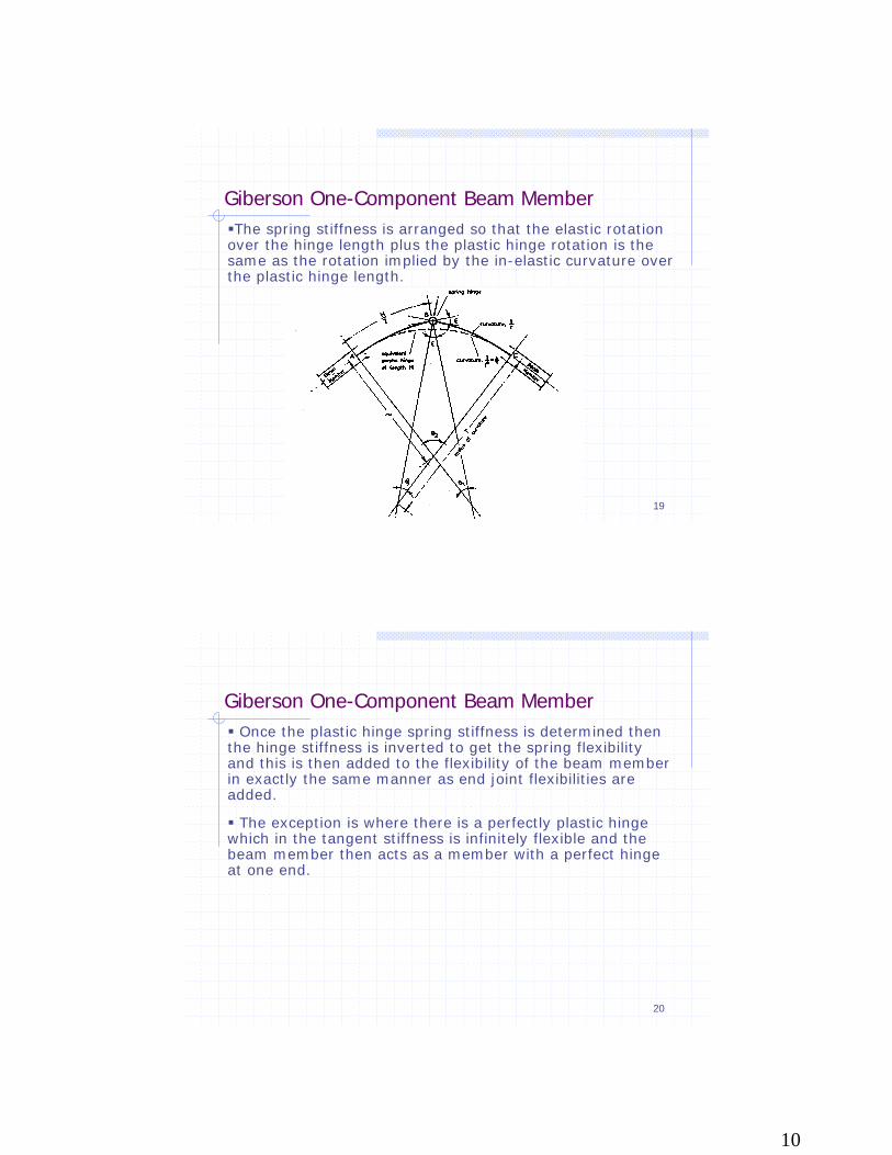
Simple Filament One-Component ModelThe concept of the filament model

can be used to represent the plastic hinges at the ends of the member in a way similar to the Giberson beam.

This example is from Otani and the program Canny3. In the figureaxial spring should read elastic beam.

The original model had 9 springs, (5 concrete and 4 steel springs), later versions used 5 springs, (4 combined steel-concrete and 1 core concrete spring).

32

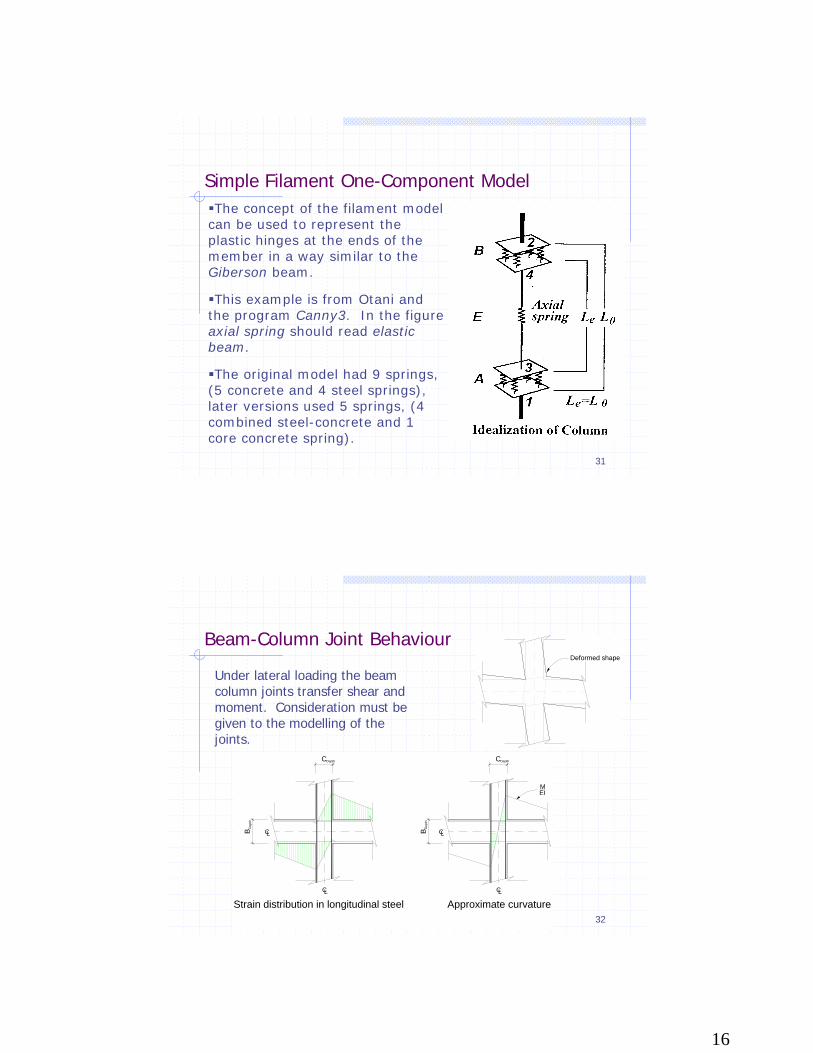
Beam-Column Joint Behaviour

LC

CL CL

LC

CDepth CDepth

EIM

BD

epth

B Dep

th

Approximate curvatureStrain distribution in longitudinal steel

Deformed shape

Under lateral loading the beam column joints transfer shear and moment. Consideration must be given to the modelling of the joints.

17

33

Beam-Column Joint Behaviour

B2I

IB

MEI

MEI

Rigid elements

BI

Rigid elements

rotationsConcentrated

MEI

IB

Flexuralsprings

Different beam-column joint models

Fully Rigid Joint Partially Rigid JointRigid joint with rotational springs

34

Elongation is a phenomenon where member grows in length under inelastic cyclic action

Elongation Background

Vary in order of 2~5% of member depth depending on:• Level of Axial force• Type of plastic hinges (Uni-direction and Reversing)

18

35

Analytical Model

Parameters1) LP (Length of plastic hinge model)

LP

( )s

fAVV

Lvyv

cycP

−=

1500

F

Δ

0=cV

Analytical model in RUAUMOKO

36

-400

-300

-200

-100

0

100

200

300

400

-0.06 -0.04 -0.02 0 0.02 0.04 0.06

Strain

Stre

ss (M

pa)

-40-35

-30-25

-20

-15-10

-5

0

5

-0.006 -0.004 -0.002 0 0.002 0.004

Strain

Stre

ss (M

Pa)

Plastic Hinge Model

Multi-springs elementConcrete and steel springsDiagonal concrete compression

springs

Concrete Hysteresis (Maekawa)

Steel Hysteresis (Dhakal)

19

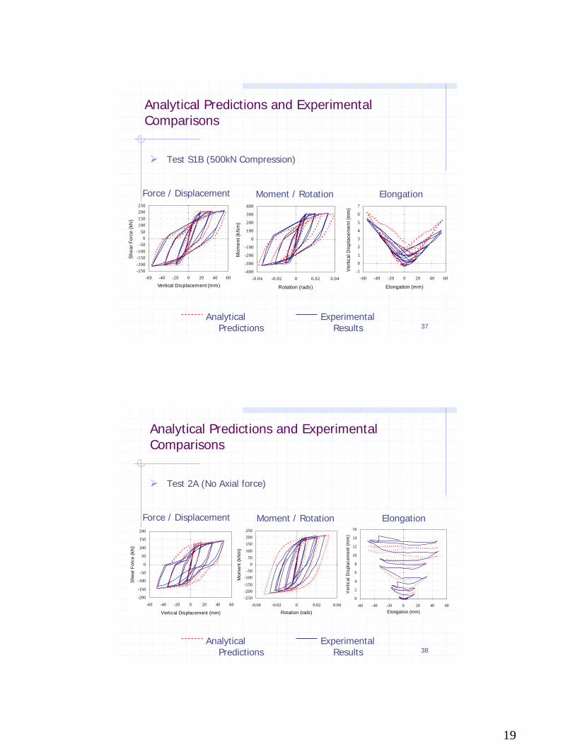
37

Analytical Predictions and Experimental Comparisons

Force / Displacement

Test S1B (500kN Compression)

Analytical Predictions

Experimental Results

ElongationMoment / Rotation

-250-200-150-100

-500

50100150200250

-60 -40 -20 0 20 40 60

Vertical Displacement (mm)

She

ar F

orce

(kN

)

-1

0

1

2

3

4

5

6

7

-60 -40 -20 0 20 40 60

Elongation (mm)

Verti

cal D

ispl

acem

ent (

mm

)

-400

-300

-200

-100

0

100

200

300

400

-0.04 -0.02 0 0.02 0.04

Rotation (rads)

Mom

ent (

kNm

)

38

Analytical Predictions and Experimental Comparisons

Force / Displacement

-200

-150

-100

-50

0

50

100

150

200

-60 -40 -20 0 20 40 60

Vertical Displacement (mm)

She

ar F

orce

(kN

)

Test 2A (No Axial force)

Analytical Predictions

Experimental Results

Elongation

0

2

4

6

8

10

12

14

16

-60 -40 -20 0 20 40 60Elongation (mm)

Ver

tical

Dis

plac

emen

t (m

m)

Moment / Rotation

-250-200-150-100-50

050

100150200250

-0.04 -0.02 0 0.02 0.04

Rotation (rads)

Mom

ent (

kNm

)

20

39

Analytical Predictions and Experimental Comparisons

Force / Displacement

Test I1B (125kN Tension)

Analytical Predictions

Experimental Results

ElongationMoment / Rotation

-300

-200

-100

0

100

200

300

-0.04 -0.02 0 0.02 0.04Rotation (rads)

Mom

ent (

kNm

)

0

5

10

15

20

25

30

-60 -40 -20 0 20 40 60

Elongation (mm)

Verti

cal D

ispl

acem

ent (

mm

)

-200

-150-100

-50

050

100

150200

-60 -40 -20 0 20 40 60Vertical Displacement (mm)

She

ar F

orce

(kN

)

40

Spring MembersSpring type members may be used to represent special

effects such as frictional sliding, contact or concentrated stiffness or spring members. Similar dashpot or damping members are also useful.

21

41

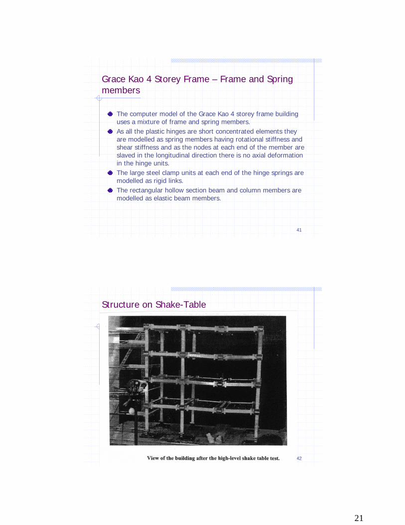
Grace Kao 4 Storey Frame – Frame and Spring members

The computer model of the Grace Kao 4 storey frame building uses a mixture of frame and spring members.As all the plastic hinges are short concentrated elements they are modelled as spring members having rotational stiffness and shear stiffness and as the nodes at each end of the member are slaved in the longitudinal direction there is no axial deformation in the hinge units.The large steel clamp units at each end of the hinge springs aremodelled as rigid links.The rectangular hollow section beam and column members are modelled as elastic beam members.

42

Structure on Shake-Table

22

43

Member Numbering In Frame

Members 1,2,3,4,5,6 etc. are spring members with rigid end links and members 28,29,30 and 40,41 etc are beams.

44

Member Geometry – Beam Hinges

23

45

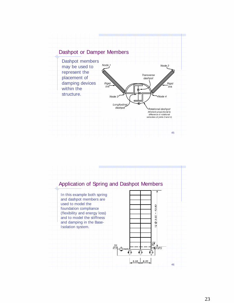
Dashpot or Damper Members

Dashpot members may be used to represent the placement of damping devices within the structure.

46

Application of Spring and Dashpot Members

In this example both spring and dashpot members are used to model the foundation compliance (flexibility and energy loss) and to model the stiffness and damping in the Base-Isolation system.

24

47

Contact ElementsContact elements are used to model possible lift-off situations or for modelling pounding between structures. They have also been extended to model spherical isolation bearing surfaces.

48

‘Winkler’ Distributed Spring Model

To model distributed support conditions such as modelling supporting foundations, soil-pile interaction or soil coupling between buildings a distributed Winkler model is useful. In 3D a 2D matt model would be appropriate.

25

49

Application of Spring and Dashpot MembersIn this example for Union House in Auckland (NZ) both springs and dashpot members are used to model the foundation compliance (flexibility and energy loss) and to model the stiffness and damping in the Base-Isolation system. The piles are modelled as in-elastic columns forming hinges top and bottom, the soil-interaction between the basement and bedrock is with springs and dashpots. The piles continue through the basement and underlying soils in tubes with 200? mm clearance and are filled with bentonite. The superstructure members are assumed to be elastic.

50

Foundation Modelling for Bridge Piers14000

8000

1500

450

1000 10001500

250

200

1000

1500

1500

1500

0

1800

A A

B B

H

1500

in pairs

D12@70 or140mm

Cover = 50mm

48D32 bars

1000

24D24

D10@65mm

Cover = 50mm

Section B-B

Section A-A

The piers are usually supported on a pile-cap which is then supported on a group of piles. An alternative is where the pier continues down as a single caisson member.

26

51

Application of Spring and Dashpot Members

In this example both spring and dashpot members are used to model the pile-soil interaction in a bridge structure. The earthquake motion is applied to the spring members and the bottom of the piles. P = K u P = K u

2500 2500

1100

1220

1100

1220

H

1500

1500

0

xi zixi zixi zi

16001600

52

Modelling of Movement Joints in Long Bridges

LongitudinalTie Bar

TieGap

Joint Gap

(b) Section Through Joint(a) Movement Joint

TransverseShear Key

VerticalRestrainer

BearingPad

ji

d

Joint ImpactSprings

k

F

gap

I

- Springsgap

F

kd

Restrainer Cable FyT

+

+

Springs

F

d

F

-

+Bearing Pad k

yc

Slaved Nodes

Fy

27

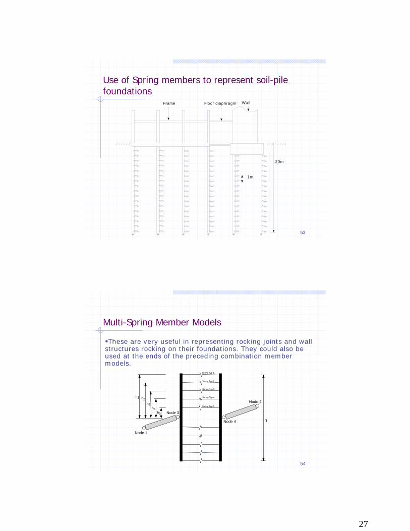
53

Use of Spring members to represent soil-pile foundations

20m

1m

Floor diaphragmFrame Wall

54

Multi-Spring Member Models

These are very useful in representing rocking joints and wall structures rocking on their foundations. They could also be used at the ends of the preceding combination member models.

h

Node 1

Node 3

Node 4

Node 2

Spring Typ 1

Spring Typ 2

Spring Typ 3

Spring Typ 4

Spring Typ 5

h1

h5h4

h3

h2

28

55

Multi-Spring Member Models

Multi-spring members were initially developed to model rocking joints in structures.They have been used to model rocking wall foundationsThey have been used to model uplifting foundation footings in buildings.

56

Application Using Multi-spring Elements

29

57

Application Using Multi-spring Elements

Structure concept and orientation possibilities on shake table.

The slab has opening joints to match location of girder joints to model pre-cast floor units.

The aim is to design a structure which will avoid damage in an earthquake.

58

Application Using Multi-spring ElementsThe structure on the shake-table

30

59

Application Using Multi-spring Elements

Elevation of the frame showing location of opening joints and pre-stressing tendons.

60

Application Using Multi-spring ElementsThe initial member model for the frame showing the opening joints, stabilized by the pre-stress and with spring members modelling the energy dissipatorsacting across the joints.

31

61

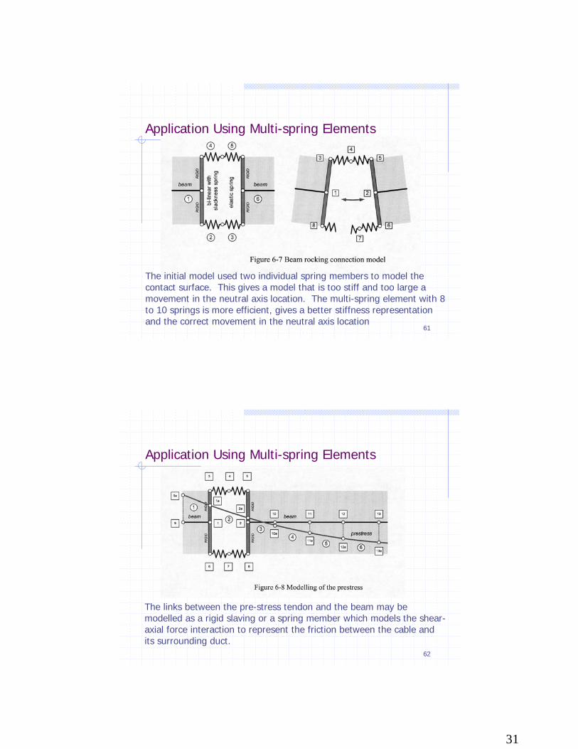
Application Using Multi-spring Elements

The initial model used two individual spring members to model the contact surface. This gives a model that is too stiff and too large a movement in the neutral axis location. The multi-spring element with 8 to 10 springs is more efficient, gives a better stiffness representation and the correct movement in the neutral axis location

62

Application Using Multi-spring Elements

The links between the pre-stress tendon and the beam may be modelled as a rigid slaving or a spring member which models the shear-axial force interaction to represent the friction between the cable and its surrounding duct.

32

63

Application Using Multi-spring Elements

ld

Pd /2

Pd

?d

Pd /2

?d

hb or hc

beam

/col

umn

-8

-6

-4

-2

0

2

4

6

8

-1 0 1 2 3 4 5displacement (mm)

forc

e (k

N)

specimen 1

specimen 2

analyticalprediction

0

5

10

15

20

25

30

0 1 2 3 4 5displacement amplitude (mm)

ener

gy a

bsor

bed

(J)

0

1

2

3

4

5

0 20 40 60 80time (s)

disp

am

plitu

de (m

m)

(a) Testing displacement path

64

Application Using Multi-Spring Elements

-500-400-300-200-100

0100200300400500600700800900

1000

-2 -1.5 -1 -0.5 0 0.5 1 1.5 2

Drift (%)

Neu

tral

Axi

s H

eigh

t (m

m)

Experiment

Simulation Lobatto 10

h

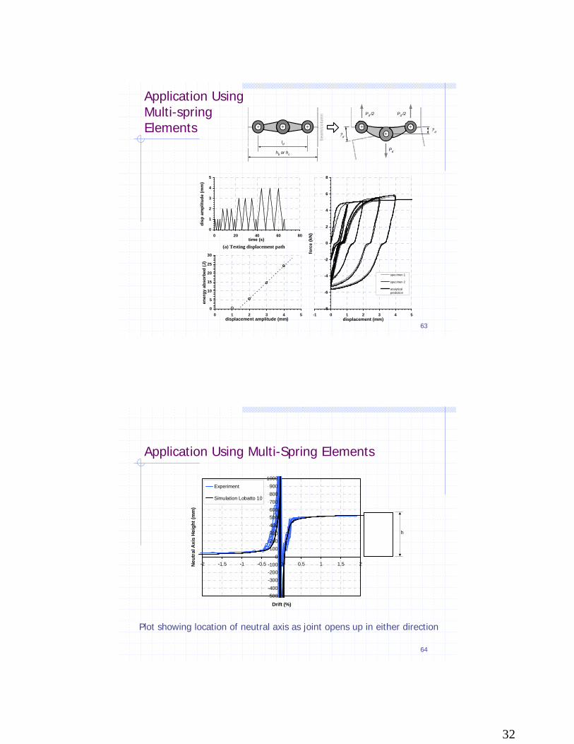
Plot showing location of neutral axis as joint opens up in either direction

33

65

Finite Element ModelsQuadrilateral finite elements with nodal displacement degrees of freedom may be used to model wall structures and similar quadrilateral plate-bending elements may be used to model floor slabs etc. Three-dimensional hexahedral elements may be used to model solid or massive structural components.

If the material is non-linear then the appropriate tangent constitutive properties will have to be obtained at each integration point in the element to compute the tangent element stiffness matrix.

66

Finite Element Models•For more general solid analysis one needs to use a standard iso-parametric finite element based on compatible displacement functions.

•The problem with such elements is that, in general, only displacement (no rotation) degrees of freedom are used which makes it difficult to maintain compatibility with frame type members.

•Such finite elements would be very useful in modelling soil foundations and in complex geometries such as pile cap systems and bridge abutments.

•As the strains at each integration point in the element are defined then general material constitutive relationships are able to be used.

•Such elements could also be used to model the proper shear-axial stress interactions in beam members.

34

67

Finite Element ModelsFinite element models are very efficient in modelling soil-structure interactions but care must be used to ensure that the model used for the foundation model does not lose sight of the results needed for the structure supported by the soils.

68

Use of finite elements to represent deformable floor diaphragms

Floor plan aspect ratio varied to see effects of diaphragm in-plane flexibility on lateral deflections.

35

69

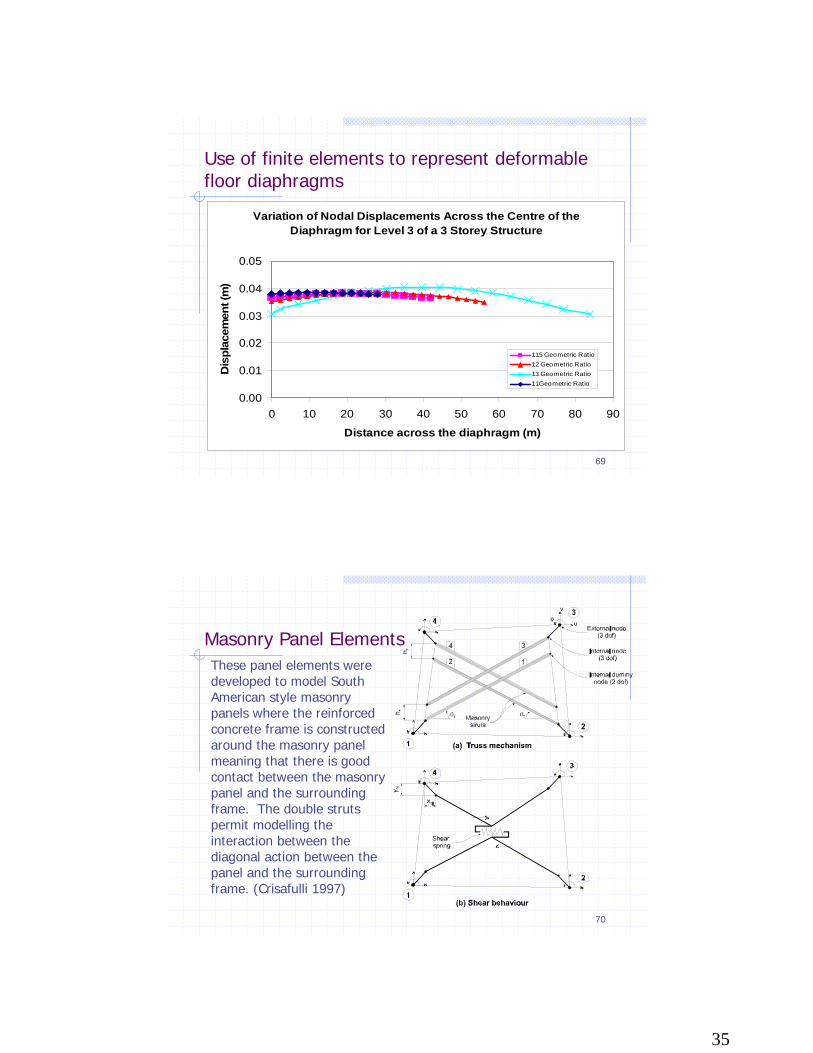
Use of finite elements to represent deformable floor diaphragms

Variation of Nodal Displacements Across the Centre of the Diaphragm for Level 3 of a 3 Storey Structure

0.00

0.01

0.02

0.03

0.04

0.05

0 10 20 30 40 50 60 70 80 90

Distance across the diaphragm (m)

Dis

plac

emen

t (m

)

1:1.5 Geometric Ratio1:2 Geometric Ratio1:3 Geometric Ratio1:1 Geometric Ratio

70

Masonry Panel ElementsThese panel elements were developed to model South American style masonry panels where the reinforced concrete frame is constructed around the masonry panel meaning that there is good contact between the masonry panel and the surrounding frame. The double struts permit modelling the interaction between the diagonal action between the panel and the surrounding frame. (Crisafulli 1997)

36

71

Boundary Elements•Boundary elements are useful in modelling the far field and far boundaries in soil-structure interaction models.

•The boundary elements can have a boundary at infinity.

•The difficulty is that their properties are usually well defined in the frequency domain and we need to use them in the time domain. This requires some approximation but the problems are not insurmountable.

•It is possible to model non-homogeneity by using several different boundary elements in the one model.

•The elements are limited to linear material behaviour so local foundation non-linear effects need to be modelled using finite elements in the near field.