Vol. 6 . 2010 ISSN 1862-9075 BayCEER-online Jan Muhr Carbon dynamics under natural and manipulated meteorological boundary conditions in a forest and a fen ecosystem

Welcome message from author
This document is posted to help you gain knowledge. Please leave a comment to let me know what you think about it! Share it to your friends and learn new things together.
Transcript

Vol. 6 . 2010
ISSN 1862-9075
BayCEER-online
Jan Muhr
Carbon dynamics under natural and manipulated meteorological boundary conditions in a forest and a fen ecosystem

BayCEER-online ISSN 1862-9075 BayCEER-online is the internet publication series of the University of Bayreuth, Bayreuth Center of Ecology and Environmental Research (BayCEER)
© 2010 by Bayreuth Center of Ecology and Environmental Research (BayCEER), University of Bayreuth
The use of general descriptive names, registered names, trademarks, etc. in this publication does not imply, even in the absence of a specific statement, that such names are exempt from the relevant protective laws and regulations and therefore free for general use. Cover design: Schlags & Schlösser Kommunikation GmbH, 95444 Bayreuth, Germany
WorldWideWeb: http://www.bayceer.uni-bayreuth.de BayCEER-online vol 6 / 2010
Carbon dynamics under natural and manipulated
meteorological boundary conditions in a forest and a fen
ecosystem
Dissertation
zur Erlangung des akademischen Grades eines
Doktors der Naturwissenschaften
- Dr. rer. Nat. -
Vorgelegt der
Fakultät für Biologie / Chemie / Geowissenschaften
der Universität Bayreuth
von
Jan Muhr
Geboren am 25.03.1981 in Lauf a. d. Pegnitz
Bayreuth, im Juli 2009

i
Vollständiger Abdruck der von der Fakultät für Biologie, Chemie und Geowissenschaften der
Universität Bayreuth genehmigten Dissertation zur Erlangung des akademischen Grades
Doktor der Naturwissenschaften (Dr. rer. Nat.).
Die vorliegende Arbeit wurde in der Zeit von Januar 2006 bis Juli 2009 unter der Leitung von
PD Dr. Werner Borken am Lehrstuhl für Bodenökologie der Universität Bayreuth angefertigt.
Tag der Einreichung 28.07.2009
Tag des Kolloquiums 8.12.2009
Prüfungsausschuss
PD Dr. Werner Borken (Erstgutachter)
Prof. Dr. Gerhard Gebauer (Zweitgutachter)
Prof. Dr. Egbert Matzner (Vorsitz)
Prof. Dr. Bernd Huwe
Prof. Dr. Stefan Peiffer
Die Untersuchungen fanden im Rahmen der DFG Forschergruppe „Dynamik von
Bodenprozessen bei extremen meteorologischen Randbedingungen“ (DFG FOR 562) unter
der Leitung von Prof. Dr. Egbert Matzner statt und wurden mit Mitteln der Deutschen
Forschungsgemeinschaft gefördert.

Acknowledgements
A lot of people were involved directly and indirectly in the completion of this PhD, and a
general thanks goes out to all of them. However, some of them deserve special mentioning
here, as their contribution was of special importance:
Werner Borken, my supervisor, for he helped me a lot with his advice and his patience. I
certainly strained the latter while seeking the first during innumerous fruitful discussions.
Gerhard Gebauer, on the one hand for his contributions to the Research Group, but even
more important because he was the one who initially encouraged me to apply for this PhD
position and therefore launched the process finally leading to this thesis.
Xiaomei Xu and Sue Trumbore from the University of Irvine, California, because they
introduced me to the technique of radiocarbon measurements and proved reliable co-operation
partners.
Egbert Matzner for coordinating the Research Group ‘Dynamics of soil processes under
extreme meteorological boundary conditions’.
Uwe Hell, Gerhard Müller, Andreas Kolb, and Gerhard Küfner, for without their practical
expertise and their efforts the realization of our experiments would have been impossible.
Ingeborg Vogler, Andrea Schott, Kathrin Göschel, Steve Wunderlich, Lisa Höhn, Tim
Froitzheim, Daniel Maurer, Martin Friedel, Janine Franke, Julia Höhle, and Petra Eckert
because they sort of were the benevolent spirits of this story, all helping me in some way or
the other to get the load of work in the field and the laboratory done.
My family and friends, for their unrestricted support despite my chronic lack of time even
for a short proof of life every now and then.
And last but not least, I certainly have to give a big thanks to Franzi, who proved a whole
lot of patience during the last months, when I was so preoccupied with my work that I
sometimes almost lost trace of the other important things in life.
ii

CONTENTS
CONTENTS
Summary .................................................................................................................................... 1
Zusammenfassung...................................................................................................................... 4
CHAPTER 1 – On this thesis
1 Background .......................................................................................................................... 8
1.1 Motivation.................................................................................................................... 8
1.2 Climate change as expected from climate models ....................................................... 8
1.3 The global carbon cycle ............................................................................................... 9
1.4 Components of soil respiration .................................................................................. 10
1.5 Potential feedbacks of climate change on soil CO2 emissions and vice versa........... 11
2 Objectives of this study ..................................................................................................... 13
3 Materials and Methods ..................................................................................................... 14
3.1 Study sites .................................................................................................................. 14
3.2 Design of the mesocosm experiment to study soil C dynamics under the effect
of drought of varying intensity................................................................................... 14
3.3 Design of the field scale experiments to study C dynamics as affected by
meteorological boundary conditions in a forest and a fen ......................................... 16
3.4 Relevant analytical techniques................................................................................... 17
3.4.1 Measuring CO2 emissions and uptake.............................................................. 17
3.4.2 Measuring radiocarbon signature ..................................................................... 17
4 Synthesis and discussion of the results ............................................................................ 20
4.1 Quantifying soil C dynamics of a Norway spruce forest and a fen under current
boundary conditions (CHAPTER 2) ............................................................................. 20
4.2 Soil carbon dynamics of a Norway spruce soil as affected by soil frost
(CHAPTER 3) ............................................................................................................... 22
4.3 Soil C dynamics in a Norway spruce soil as affected by drying-wetting under
laboratory and field-site conditions (CHAPTER 4) ...................................................... 24
4.4 Ecosystem C dynamics in a fen as affected by natural and manipulative water
table changes (CHAPTER 5)......................................................................................... 26
5 Conclusions ........................................................................................................................ 28
6 References .......................................................................................................................... 31
7 Record of contributions to the included manuscripts .................................................... 37
iii

CONTENTS
iv
CHAPTER 2 - Quantifying soil C dynamics of a forest and a fen under current climatic
conditions
A - Kerstin Schulze, Werner Borken, Jan Muhr and Egbert Matzner (2009). Stock,
turnover time and accumulation of organic matter in bulk and density fractions of a
Podzol soil. European Journal of Soil Science, 60, 567-577............................................. 41
B - Jan Muhr, Juliane Höhle and Werner Borken (2009). Carbon dynamics in a
temperate minerotrophic fen. Biogeochemistry, submitted................................................ 63
CHAPTER 3 - Soil C dynamics in a forest as affected by soil frost
Jan Muhr, Werner Borken and Egbert Matzner (2009). Effects of soil frost on soil
respiration and its radiocarbon signature in a Norway spruce forest soil (Global
Change Biology, 15, 782-793) .......................................................................................... 85
CHAPTER 4 - Soil C dynamics in a forest as affected by drought
A - Jan Muhr, Janine Franke and Werner Borken (2009). Drying-rewetting events
reduce C and N losses from a Norway spruce forest floor (Soil Biology &
Biogeochemistry, submitted. ........................................................................................... 110
B - Jan Muhr and Werner Borken (2009). Delayed recovery of soil respiration after
wetting of dry soil further reduces C losses from a Norway spruce soil. Journal of
Geophysical Research – Biogesciences, submitted.......................................................... 134
CHAPTER 5 - Ecosystem C dynamics in a fen as affected by water table fluctuations
A - Jan Muhr, Juliane Höhle, Dennis O. Otieno and Werner Borken (2009).
Manipulative lowering of the water table during summer does not affect CO2
emissions and uptake in a minerotrophic fen. Ecological Applications, submitted......... 159
B - Dennis O. Otieno, Margarete Wartinger, A. Nishiwaki, M.Z. Hussain, Jan Muhr,
Werner Borken and Gunnar Lischeid (2009). Responses of CO2 Exchange and
Primary Production of the Ecosystem Components to Environmental Changes in a
Mountain Peatland. Ecosystems 12, 590-603................................................................... 180
APPENDIX ............................................................................................................................... 206
SUMMARY
Summary
According to current climate models, we will face changes in the amount, intensity,
frequency and type of precipitation within this century. These changes are very likely to result
in an increasing frequency of severe drought periods in summer, causing irregular and
extreme drought stress in well-drained soils or a lowering of the water table in water-logged
soils. Additionally, rising temperatures will increase the likelihood of precipitation falling as
rain rather than snow, resulting in reduced snowpacks in winter. In some regions, this can lead
to an increasing frequency of soil frost. In summary, changes in the global water cycle are
likely to have a significant impact on boundary conditions within soils. With soils
representing important C stocks and soil respiration being the biggest flux of CO2 from
terrestrial ecosystems to the atmosphere, we have to address the question how these aspects of
climate change will affect C mineralization in soils.
This thesis focused on investigating the impact of extreme meteorological boundary
conditions on CO2 fluxes in two different ecosystems in the Fichtelgebirge in South-eastern
Germany. In a Norway spruce forest, the effect of prolonged periods of summer drought and
of soil frost on soil C dynamics were investigated mainly by field-site manipulation
experiments, but also by laboratory experiments. In a minerotrophic fen located nearby, the
effect of water table lowering (as a result of summer drought) on ecosystem C dynamics was
quantified. To be able to better interpret the results, soil C dynamics at both site were modeled
under current meteorological conditions.
Modeling of soil C dynamics at the two sites helped to understand the site-specific
preconditions under which the field-site manipulation experiments were conducted. Modeling
approaches involved measurements of C stocks and the abundance of radiocarbon. For the
Norway spruce forest, modeling indicated that soil C turnover predominantly occurred within
the organic horizons. During the last decades, the soil has acted as a small sink. The
possibility of altered C dynamics at the site due to undocumented liming has to be considered
when comparing results presented here to results from other sites. For the fen, modeling also
revealed that soil C turnover was clearly dominated by processes occurring within the
uppermost 15 cm of the peat. Root biomass was identified to be a very important soil C stock
at the site. Most important, modeling indicates that the fen is subject to marked disturbance,
most likely of the hydrological conditions, turning the fen into a net C source during the last
decades. Thus, results from this fen can not be regarded as representative for undisturbed
peatlands.
1
SUMMARY
Soil frost was induced at the forest site by removing the snowpack in the winter of
2005/2006. As the following winters were warmer than average, no repetition of this
experiment was possible. Soil frost was observed down to a depth of at least 15 cm and for
the duration of several weeks on the plots where snow had been removed, in contrast to
naturally snow-covered plots where no soil frost occurred. Soil frost resulted in a significant
reduction of soil C losses. Most likely the composition of the microbial community was
markedly affected by soil frost, primarily by a reduction of fungal biomass. This would
explain why the snow-removal plots featured significantly reduced soil respiration rates not
only during the period of soil frost but also in the summer of 2006.
Two different approaches were used to investigate the effect of drought on soil C
dynamics in the Norway spruce soil. Prolonged drought periods were experimentally induced
at the field-site by excluding throughfall with a transparent roof during the summers of 2006-
2008. Additionally, undisturbed soil columns from the site were subjected to drought in the
laboratory. In both experiments, drought reduced total soil C losses in comparison to C losses
from a control. This reduction was mainly owed to decreased soil respiration rates during the
actual drought period, but water repellency also hindered rewetting of the dry soil, thus
further prolonging the period of reduced soil respiration rates. In the past, mobilization of
stabilized C due to drying-wetting has been repeatedly discussed as a possibility to actually
enhance soil C losses. In the studies presented here, no evidence for this assumption was
found. In summary, the influence of drought could be described as a temporary ‘brake’
slowing down soil C mineralization. Rewetting results in a switchback to pre-drought
mineralization rates, possibly delayed by water repellency.
At the fen, two different approaches were used to quantify the impact of water table
changes on C dynamics: (i) Experimental lowering of water tables to measure resulting C
fluxes in comparison to C fluxes under natural conditions (i.e. control plots), and (ii) repeated
measurements under varying natural conditions to be able to later statistically identify the
main drivers of CO2 fluxes. In contrast to the forest site, measurement techniques allowed to
include C uptake and respiration by aboveground vegetation, thus being able to study
ecosystem rather than soil C dynamics at the fen site. In summary, the impact of the water
table on CO2 fluxes in and out of the fen ecosystem was found to be of minor importance. The
site was dominated by grass species, and assimilation of these was not affected at all by water
table. In the interspersed moss species, low water tables were found to cause significant
drought stress, thus decreasing the assimilation of atmospheric CO2. However, water tables at
the site are already naturally low during summer and mosses represent only a minor
2

SUMMARY
3
proportion of the vegetation at the site, so is questionable whether lowering of the water table
due to climate change can markedly affect ecosystem assimilation. Soil respiration was not
affected at all by the manipulative lowering of the water table from ca. 15 cm down to more
than 60 cm, most likely due to low substrate quality in deeper peat. Measurements of the
natural C dynamics indicate that water table could have an impact on soil respiration within
the uppermost 0-15 cm of the soil, but predominantly low water tables during summer under
current boundary conditions make it unlikely that further lowered water tables due to climate
change will markedly affect soil respiration rates at this site. In summary, CO2 fluxes at the
site are presumably very resilient towards an increasing frequency of summer drought
resulting in lowering of the water table.

ZUSAMMENFASSUNG
Zusammenfassung
Ausgehend von aktuellen Klimamodellen werden wir in diesem Jahrhundert mit
Änderungen der Niederschlagsmenge, -intensität, -häufigkeit und -art konfrontiert sein. Es ist
dabei sehr wahrscheinlich, dass diese Änderungen zu einem gehäuften Auftreten von
Sommertrockenheit führen, und damit zu unregelmäßigem und schwerwiegenden
Trockenstress in gut dränierten Böden bzw. zu einem Absinken des Wasserspiegels in
wassergesättigten Böden. Zusätzlich werden steigende Jahresmitteltemperaturen dazu führen,
dass Niederschlag zunehmend in Form von Regen anstelle von Schnee fallen wird, weshalb
mit einer verringerten Mächtigkeit der Schneedecke im Winter zu rechnen ist. In einigen
Gebieten kann dies zum gehäuften Auftreten von Bodenfrost führen. Zusammenfassend ist
davon auszugehen, dass klimawandelbedingte Änderungen im globalen Wasserhaushalt sich
signifikant auf die Randbedingungen in Böden auswirken werden. Da Böden wichtige
Kohlenstoffspeicher darstellen und Bodenrespiration der größte Fluss von CO2 zwischen
terrestrischen Ökosystemen und der Atmosphäre ist, müssen wir uns mit der Frage
beschäftigen, wie diese Aspekte des Klimawandels sich auf die Kohlenstoffmineralisation in
Böden auswirken werden.
Die vorliegende Arbeit hat sich daher mit der Untersuchung des Einfluss von extremen
meteorologischen Randbedingungen auf die CO2 Flüsse in zwei verschiedenen Ökosystemen
im Fichtelgebirge in Südostdeutschland befasst. In einem Fichtenwald wurden die
Auswirkungen von Trockenheit und von Bodenfrost auf die Kohlenstoffumsätze im Boden
mit Hilfe von Freiland- und Laborexperimenten untersucht. In einem nahegelegenen
Niedermoor wurde die Auswirkung von Wasserspiegelabsenkungen auf die
Kohlenstoffumsätze des Ökosystems untersucht. Um die Ergebnisse besser beurteilen zu
können wurden an beiden Standorten die Kohlenstoffumsätze unter augenblicklichen
meteorologischen Randbedingungen modelliert.
Die Modellierung der Kohlenstoffumsätze an den beiden Standorten half dabei, die
Ausgangsbedingungen für die experimentelle Manipulation besser zu verstehen. Die
Modellierungsansätze beinhalteten Messungen der Kohlenstoffvorräte und der
Radiokarbonsignatur. Im Fichtenwald zeigten die Modellergebnisse auf, dass der größte Teil
der Kohlenstoffumsätze in den organischen Horizonten stattfand. Innerhalb des Zeitraums der
letzten Jahrzehnte fungierte der Boden am Waldstandort als schwache Senke für Kohlenstoff.
Im Hinblick auf die Vergleichbarkeit mit Ergebnissen von anderen Standorten muss
berücksichtigt werden, dass mögliche Kalkung des Standorts in der Vergangenheit zu einer
geringfügigen Störung der Kohlenstoffumsätze geführt haben könnte. Für den 4

ZUSAMMENFASSUNG
Niedermoorstandort ergab die Modellierung, dass die Kohlenstoffumsätze eindeutig von
Umsätzen in den obersten 15 cm dominiert wurden. Wurzelbiomasse erwies sich als sehr
bedeutender Kohlenstoffpool. Am bedeutendsten aber war die Tatsache, dass die
Modellierungsergebnisse auf den massiven Einfluss von Störungen im Niedermoor
hinwiesen, höchstwahrscheinlich Störungen der hydrologischen Randbedingungen. Diese
Störungen machten das Niedermoor in den letzten Jahrzehnten zu einer
Nettokohlenstoffquelle. Die Ergebnisse können daher nicht als repräsentativ für ungestörte
Moorstandorte gesehen werden.
Bodenfrost wurde durch die Entfernung der Schneedecke im Winter 2005/2006 induziert.
Da die folgenden Winter überdurchschnittlich warm waren, war eine Wiederholung des
Experimentes nicht möglich. Bodenfrost konnte bis in eine Tiefe von wenigstens 15 cm und
für die Dauer von mehreren Wochen auf den Flächen nachgewiesen werden, auf denen die
Schneedecke entfernt worden war. Im Gegensatz dazu blieben die schneebedeckten Flächen
frostfrei. Bodenfrost führte zu einer signifikanten Verringerung der Verluste von
Bodenkohlenstoff. Höchstwahrscheinlich wurde die Zusammensetzung der mikrobiellen
Zersetzergemeinschaft beträchtlich vom Bodenfrost beeinflusst, vorrangig durch eine
Verringerung des Anteils pilzlicher Biomasse. Das würde erklären, weshalb es auf den
Manipulationsflächen nicht nur während der Bodenfrostperiode, sondern auch im darauf
folgenden Sommer 2006 zu einer erheblichen Verringerung der Bodenrespiration gekommen
ist.
Zwei verschiedene Ansätze wurden gewählt um den Effekt von Trockenheit auf die
Bodenkohlenstoffumsätze im Fichtenwaldstandort zu untersuchen. Im Freiland wurde
Sommertrockenheit experimentell induziert bzw. verlängert, indem mit transparenten Dächern
der Bestandesniederschlag ausgeschlossen wurde. Zusätzlich wurden im Labor Experimente
an ungestörten Bodensäulen durchgeführt. In beiden Experimenten führte Trockenheit zu
einer Verringerung der Gesamtkohlenstoffverluste aus dem Boden im Vergleich zu einer
Kontrollgruppe. Diese Verringerung war in erster Linie zurückzuführen auf verringerte
Bodenrespirationsraten während der eigentlichen Trockenperiode. Es kam jedoch hinzu, dass
Hydrophobizität die Wiederbefeuchtung des Bodens behinderte, was dazu führte, dass die
Verringerung der Bodenrespirationsraten länger anhielt als die eigentliche Trockenperiode. In
der Vergangenheit wurde wiederholt diskutiert, ob es durch den Wechsel von Austrocknung
und Wiederbefeuchtung zu einer Freisetzung von stabilisiertem Bodenkohlenstoff kommen
kann, was letztlich zu einer Erhöhung der Bodenkohlenstoffverluste führen könnte. In der
vorliegenden Arbeit wurde keinerlei Beleg für die Richtigkeit dieser Annahme gefunden. Der
5

ZUSAMMENFASSUNG
6
Haupteffekt von Trockenheit lässt sich also beschreiben als eine vorübergehende
Verlangsamung der Kohlenstoff-Mineralisation im Boden. Bei Wiederbefeuchtung kehren die
Mineralisationsraten auf ihr ursprüngliches Niveau zurück, wobei Hydrophobizität diese
Erholung verzögern kann.
Am Niedermoorstandort wurden zwei unterschiedliche Ansätze verwendet um den
Einfluss des Wasserspiegels auf die Kohlenstoffumsätze zu beurteilen: (i) Experimentelle
Absenkung des Wasserspiegels zur Messung der resultierenden Kohlenstoff-Flüsse im
Vergleich zu Kohlenstoffflüssen unter natürlichen Bedingungen (d.h. auf Kontrollflächen),
und (ii) wiederholte Messungen unter variierenden natürlichen Bedingungen mit dem Ziel, die
Haupteinflussfaktoren für die CO2-Flüsse bestimmen zu können. Im Gegensatz zum
Waldstandort war es hier messtechnisch möglich, die Aufnahme und Abgabe von
Kohlenstoff durch oberirdische Vegetation mit in die Untersuchung aufzunehmen.
Zusammenfassend wurde festgestellt, dass der Wasserspiegel eine geringe Bedeutung für die
Kohlenstoffumsätze im Niedermoor hatte. Die Vegetation am Standort wurde von Gräsern
dominiert, und der Wasserspiegel hatte keinerlei Einfluss auf deren CO2-Assimilation. Bei
den vereinzelt vorkommenden Moosen dagegen konnte niedriger Wasserspiegel zu starkem
Trockenstress führen und so die CO2-Assimilation deutlich verringern. Da allerdings der
Wasserspiegel an diesem Standort im Sommer natürlicherweise niedrig ist und Moose zudem
eine untergeordnete Rolle spielen, ist es fraglich, ob eine weitere Absenkung in Folge
gehäufter Sommertrockenheit sich nennenswert auf die Gesamtkohlendioxidassimilation des
Ökosystems auswirken wird. Die Bodenrespiration wurde durch die manipulative Absenkung
des Wasserspiegels von etwa 15 auf mehr als 60 cm nicht beeinflusst. Die Messungen der
natürlichen saisonalen Dynamik der Bodenrespiration lassen vermuten, dass
Wasserspiegelschwankungen innerhalb der obersten 15 cm des Bodens einen Einfluss auf die
Bodenrespiration haben könnten. Alles in allem macht es der im Sommer vorherrschende
niedrige Wasserspiegel an diesem Standort unwahrscheinlich, dass durch den Klimawandel
bedingte weitere Absenkungen sich nennenswert auf die Bodenrespiration auswirken werden.
Die CO2-Flüsse dieses Ökosystems sind vermutlich sehr stabil gegenüber einer möglichen
Zunahme der Häufigkeit von Sommertrockenheit und damit verbundener Absenkungen des
Wasserspiegels.

CHAPTER 1
Chapter 1
On this thesis
7

CHAPTER 1
1 Background
1.1 Motivation
Soils contain more than twice as much carbon (C) as vegetation or the atmosphere (Batjes
1996, Schlesinger and Andrews 2000). Thus, changes in soil carbon pools can have a large
effect on the global carbon budget. The possibility that climate change is being reinforced by
increased carbon dioxide emissions from soils due to altered boundary conditions emphasizes
the necessity to improve our understanding of climate change feedbacks on soil carbon
processes. Extreme meteorological events like drought, heavy precipitation and soil frost
affect many biological, chemical and physical processes in soils (Schimel et al. 2007), but
little is known about the relevance of these events for the soil C dynamics.
1.2 Climate change as expected from climate models
Changes in the atmospheric abundance of greenhouse gases alter the energy balance of the
climate system. Global atmospheric concentrations of carbon dioxide (CO2), methane and
nitrous oxide have increased significantly as a result of human activities since 1750 and now
far exceed pre-industrial values (IPCC 2007). The IPCC Fourth Assessment report therefore
comes to the conclusion that human activities markedly contributed to current climate change.
Climate change manifests itself in a variety of phenomena, which are summarized in chapter
three of the contribution of working group I to the IPCC Fourth Assessment Report
(Trenberth et al. 2007). Probably the best studied aspect of climate change is the predicted
increase of global mean surface temperature and its effect on ecosystem processes (Doherty et
al. 2009). However, there are other important aspects of climate change like e.g. changes in
the frequency and amplitude of extreme meteorological events, namely summer drought,
heavy precipitation events, and soil frost.
Droughts are likely to occur more frequently in most land areas worldwide, especially
during summer. This is rather due to changing precipitation patterns than due to changes in
total precipitation amounts, so heavy precipitation events before and after drought periods are
also expected to become more frequent. At the same time, as global mean surface temperature
is increasing, less precipitation is expected to occur as snow. With snow being the major
insulator for soils in winter, in some areas of the world this is likely to result in an increasing
frequency of soil frost – an apparent paradox verbalized by Groffman et al. (2001) as the
phenomenon of ‘colder soils in a warmer world’. In summary, following the projections of the
8
CHAPTER 1
IPCC (2007), we are going to live in a world in which weather extremes will occur more
frequently.
1.3 The global carbon cycle
Human activities have markedly contributed to climate change by significantly increasing
the emission of greenhouse gases. Among these, CO2 has been identified as the most
important anthropogenic greenhouse gas. Its concentration has increased from a pre-industrial
value in the year 1750 of ca. 280 ppm to ca. 390 ppm in 2009. The current CO2 concentration
is unparalleled in the last 650,000 years, as analyses of ice cores revealed natural fluctuations
of the CO2 concentration ranging between 180 ppm and 300 ppm (IPCC 2007). The most
important anthropogenic sources of CO2 are the combustion of fossil fuels and land use
change, resulting in a combined annual flux of ca. 6.9 Pg C a-1 (1 Pg = 1015 g) to the
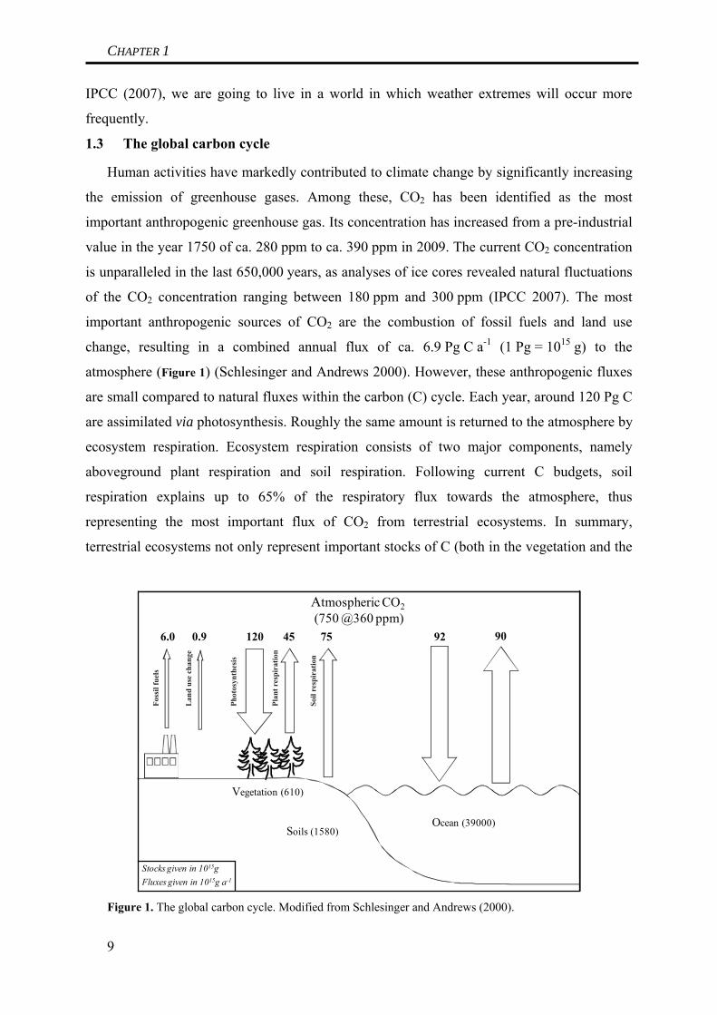
atmosphere (Figure 1) (Schlesinger and Andrews 2000). However, these anthropogenic fluxes
are small compared to natural fluxes within the carbon (C) cycle. Each year, around 120 Pg C
are assimilated via photosynthesis. Roughly the same amount is returned to the atmosphere by
ecosystem respiration. Ecosystem respiration consists of two major components, namely
aboveground plant respiration and soil respiration. Following current C budgets, soil
respiration explains up to 65% of the respiratory flux towards the atmosphere, thus
representing the most important flux of CO2 from terrestrial ecosystems. In summary,
terrestrial ecosystems not only represent important stocks of C (both in the vegetation and the
Ocean (39000)
Atmospheric CO2(750 @360 ppm)
Vegetation (610)
Soils (1580)
Stocks given in 1015gFluxes given in 1015g a-1
92 906.0 0.9 120 45 75
Foss
il fu
els
Lan
d us
e ch
ange
Phot
osyn
thes
is
Plan
t res
pira
tion
Soil
resp
irat
ion
9
Figure 1. The global carbon cycle. Modified from Schlesinger and Andrews (2000).

CHAPTER 1
soil all relative
changes of these fluxes bear the potential to result in significant changes of net C fluxes
ation
ike mentioned before, soil respiration accounts for up to 65% of global ecosystem
biggest terrestrial flux of CO2 to the atmosphere. The
CO
bacteria depend directly on the
wat
), but also exchange C with the atmosphere at high gross rates. Thus, even sm
between ecosystems and the atmosphere, thereby either further increasing or decreasing the
atmospheric CO2 concentration.
1.4 Components of soil respir
L
respiration, and therefore represents the
2 emitted in soil respiration originates from various sources (for a detailed identification of
these sources see Kuzyakov 2006). In a simplifying approximation, soil respiration could be
partitioned into two major components: (i) roots and (ii) heterotrophic micro-organisms
(comprising all kinds of decomposing bacteria, fungi, and other soil inhabitants, but also root-
associated micro-organisms). Although logical, this division is not very suitable in many
experiments, as root-associated micro-organisms (mycorrhizal fungi and bacteria from the
rhizosphere) are inevitably linked to roots. Therefore, in this study I will repeatedly refer to a
different partitioning of soil respiration and distinguish the following two major components
of soil respiration: (i) Heterotrophic respiration (i.e. the respiration of all decomposing micro-
organisms that are not directly associated with roots) and (ii) rhizosphere respiration (i.e. the
respiration of roots, root-associated fungi, and the respiration of decomposers from the
rhizosphere decomposing root exudates and young fine roots).
These two components of soil respiration are expected to react quite individually to
changing environmental conditions. E. g., during drought, soil
er content of their immediate surroundings, and normally have no mechanisms to maintain
high metabolic activity when exposed to dry conditions (Schimel et al. 2007). Plant roots
(especially deep rooting plant species), however, can access water in deeper horizons and
transfer it to other regions of their root system, preferably roots in areas with high nutrient
concentrations (Nadezhdina et al. 2006). Plant roots therefore possess a mechanism to
temporarily alter the soil moisture conditions in their immediate surroundings, thereby being
able to maintain high metabolic activity. Root-associated micro-organisms can also profit
from this so-called hydraulic lift. It therefore is highly recommended to investigate the
individual dynamics of different components of soil respiration when investigating the effects
of extreme weather conditions.
10

CHAPTER 1
1.5 Potential feedbacks of climate change on soil CO2 emissions and vice versa
2005).
On
in changes of soil
par
iscussed for
poo
Soil respiration is governed by a variety of fundamental drivers (Ryan and Law
e of the most important site-specific drivers (explaining site-to-site variability) is probably
substrate supply, a factor being ultimately linked to photosynthesis and above- and
belowground litter input. Other environmental factors are also important (namely soil
moisture, oxygen supply, mean annual temperature, and the belowground community).
Seasonal variability of soil respiration at a specific site is mainly explained by soil
temperature, especially at well drained sites, but soil moisture becomes increasingly important
when being below or above a broad optimum range (Bunnel and Tait 1974, Davidson 1998).
In poorly or non-drained sites, water table and oxygen availability have been described as
additional important factors to explain seasonal variability (Laiho 2006).
Extreme meteorological conditions normally are also reflected
ameters like e.g. soil moisture and thus can strongly affect soil respiration and other
components of the ecosystem C budget. thus bearing the possibility to either reinforce or
mitigate climate change. The exceptional drought in 2003, resulting from the combination of a
heat wave (high evapotranspiration) and precipitation deficit, is a good example to illustrate
this climate-carbon feedback. Ciais et al. (2005) reported that the heat wave of 2003
significantly reduced soil respiration and, even more, also reduced plant productivity in
Central Europe. Thus, it created a strong anomalous net C source to the atmosphere, reversing
the effect of ca. four years of net ecosystem C sequestration. In poorly drained ecosystems,
the potential for climate-carbon feedbacks has long been recognized. Here, the major concern
is an increase of gross respiration fluxes due to increased oxygen availability when water
table is lowered during drought periods (Alm et al. 1999). Thus, the ecosystem can become a
net source because under dry conditions C is lost that before has been stabilized by high water
tables (so-called climatic stabilization of soil organic matter, cf. Trumbore 2009).
Destabilization of C due to extreme climatic conditions has not only been d
rly drained soils, but also for well drained (mineral) soils. The so-called ‘Birch effect’
(Jarvis et al. 2007) describes the rapid mobilization of C substrates during the rewetting of dry
soil. This mobilization can affect previously stabilized substrates as well. Therefore, a number
of studies suggested that dry/wet cycles can accelerate C losses from soil relative to what
would be lost under constant ‘optimum’ conditions (Miller et al. 2005, Curiel Yuste et al.
2005, Schimel et al. 2007). Mechanistic explanations (Fierer and Schimel 2003, Xiang et al.
2008) of this C mobilization discuss the physical disruption of soil aggregates due to
rewetting (Denef et al. 2001a, Denef et al. 2001b, Consentino et al. 2006), resulting in the
11

CHAPTER 1
exposition of previously protected material to microbial attack thus resulting in its
breakdown. Following this mechanistic explanation of enhanced C losses, other extreme
meteorological events exerting strong physical strain on soil aggregates (like e.g. soil frost)
might also result in the mobilization of previously stabilized C in soils (Schimel et al. 2007).
In summary, it has been reported repeatedly that extreme weather conditions can have
tremendous effects on soil C dynamics, but the underlying processes are complex and still
poorly understood. Schulze and Freibauer (2005) subsumed the phenomenon of C
mobilization due to climate or land-use change as ‘carbon unlocked from soils’.
Realizing the importance of soil-atmosphere carbon fluxes, this thesis focuses on the
effect of extreme meteorological boundary conditions on soil respiration in two different
(semi-)natural ecosystem types that are common in Central Europe, namely a Norway spruce
forest and a minerotrophic temperate fen. Norway spruce (Picea abies L.) currently is the
most widespread tree species in Germany (Walentowski 2004). Thus, understanding the effect
of projected climate change on Norway spruce soils is of high ecological relevance. Peatlands,
on the other hand, cover only around 13,000 km2 or 3.6% of the land area in Germany (Byrne
et al. 2004). On a global scale, the proportion is roughly the same, with peatlands comprising
3.5% of the total land surface (Gorham 1991). Despite this relatively small area, peatlands are
important C storage pools, comprising between 270-370 Pg C of the estimated 1580 Pg C
stored in soils worldwide (Turunen et al. 2002). Under natural conditions, peatlands normally
develop slowly (e.g. Hughes and Dumayne-Peaty 2002), but land-use change and/or climatic
change can mediate relatively rapid changes, so peatlands have been characterized as
particularly vulnerable to climate change (Alm et al., 1999; Moore, 2002; Bubier et al., 2003).
12

CHAPTER 1
2 Objectives of this study
To address the uncertainties in current understanding of C dynamics under natural
conditions and under the impact of extreme meteorological boundary conditions, this study
has the following agenda:
(1) Quantify the soil C balance of a forest and a fen ecosystem under current (natural)
climatic conditions by modeling turnover times (TT), size, input and output of soil
organic carbon (SOC) pools of different horizons.
CHAPTER 2
(2) Study the effect of soil frost on the dynamics of soil respiration, total gaseous soil C
losses, and the individual contribution of soil respiration components in a Norway
spruce soil using a field site manipulation approach.
CHAPTER 3
(3) Investigate the importance of drought intensity for total C losses and mobilization of
stabilized C in a laboratory approach with soil from a Norway spruce forest.
CHAPTER 4A
(4) Study the effect of prolonged summer drought on the dynamics of soil respiration,
total gaseous soil C losses, and the individual contribution of soil respiration
components in a Norway spruce soil using a field site manipulation approach.
CHAPTER 4B
(5) Study the effects of varying water table during summer (either due to natural
fluctuation or due to manipulative lowering) on CO2 emissions and CO2 uptake in a
minerotrophic fen.
CHAPTER 5
13

CHAPTER 1
3 Materials and Methods
3.1 Study sites
This study comprises one laboratory study (CHAPTER 4A), three field-studies from a
Norway spruce stand (CHAPTERS 2A, 3, AND 4B), and three field studies from a temperate fen
(CHAPTERS 2B AND 5A+B). Soil columns for the laboratory study originate from the forest
field site, thus all studies are related to two field sites in Northern Bavaria, Germany. Both
sites are located in the Lehstenbach catchment, covering an area of 4.5 km2. The mean annual
air temperature (1971-2000) of the catchment is 5.3°C and the mean annual precipitation
ranges around 1160 mm (Gerstberger et al. 2004). With a total of 133 frost days per year (air
temperature minimum < 0°C), frost is a common event in the Fichtelgebirge (Foken 2003).
The Lehstenbach catchment area is dominated by Norway spruce (Picea abies L.) forest,
therefore site number one (Coulissenhieb II) comprises a small Norway spruce stand located
at 50°08’N, 11°52’E at an elevation of 770m a.s.l. The understorey vegetation at the stand is
dominated by Calamagrostis villosa (Chaix ex Vill), Deschampsia flexuosa (L.), Vaccinium
myrtillus (L.), and Oxalis acetosella (L.). ). According to the FAO soil classification (IUSS
2006), the soil is classified as a Haplic Podzol with a sandy to loamy texture The forest floor
is characterized as mor-like, exhibiting a thickness of 6–10 cm and is composed of Oi, Oe,
and Oa horizons.
Site number two (Schlöppnerbrunnen) is a minerotrophic temperate fen located at
50°08’N, 11°51’E. It is a moderately acidic (pH 3.5-5.5) fen characterized by highly
decomposed soils that are rich in sulphur and iron. The site features a slight slope (5°) from
NNE to SSW, and groundwater is flowing through the site parallel to this slope. The soil is a
Histosol on granite bedrock covered mainly by Molinia caerulea (L. Moench), Nardus stricta
(L.), Agrostis canina (L.), Carex rostrata (Stokes) and Eriophorum vaginatum (L.). The site
feature a ditch of unknown history and origin.
3.2 Design of the mesocosm experiment to study soil C dynamics under the effect of
drought of varying intensity
A total of 20 undisturbed, vegetation-free soil columns (hereafter ‘mesocosms’),
comprising only organic horizons, were harvested in the Coulissenhieb II Norway spruce
stand in the spring of 2006. The mesocosms were incubated in the laboratory at constant
+15°C for a total of ca. 150 days. After an initial pre-treatment period of ca. 40 days (+15°C,
4 mm d-1 irrigation = equivalent to daily mean at site), the mesocosms were grouped into five
14

CHAPTER 1
groups à four mesocosms each (one control and three manipulation groups for measuring soil
C losses, and one ‘batch’ group for destructive sampling of soil at various stages of the
experiment).
Matric potential of the control was kept constant at ca. -0.02 MPa (~pF 2) by customized
irrigation to compensate for evaporation. The manipulation mesocosms were subjected to
ventilation to increase evaporation and stimulate drying of the soil. After 16 days, the matric
potential of the manipulation mesocosms had decreased by ca. one order of magnitude
(~pF 3) compared to the control. At this time, further drying of the drying group one (D1) was
prevented. After 35 days, drying of the second manipulation group (D2) was stopped at
~pF 5. The last manipulation group (D3) was dried further until ~pF 6.5 after 47 days of total
drying. A detailed overview over the adjustment of individual soil moisture conditions can be
found in Figure 2.
We continued to measure soil C losses while maintaining the individual matric potentials
of the various groups at constant levels until day 80 after beginning of the manipulation
period. At this time, irrigation (4 mm d-1) of all mesocosms was started, resulting in a quick
rewetting of the dry soil. We continued to measure soil CO2 emissions and losses of dissolved
organic carbon (DOC).
At various stages of the incubation (end of pre-treatment, end of drying period, a few days
after rewetting) we measured the 14C signature of emitted CO2. Combining these
measurements with the constant measurements of the dynamics of soil C losses allowed us to
investigate whether relevant mobilization of stabilized C contributed to observed C losses
from the soil.
Time [d]0 20 40 60 80 100 120
pF
1
2
3
4
5
6
7
Mat
ric P
oten
tial [
MPa
]
- 0.001
- 0.01
- 0.1
- 1
- 10
- 100
- 1000
Drying Rewetting
a
ControlD1D2D3
Figure 2. Simulating different soil moisture conditions in four groups of mescososms to investigate the effect of drought intensity on soil C dynamics in a Norway spruce soil.
15

CHAPTER 1
3.3 Design of the field scale experiments to study C dynamics as affected by
meteorological boundary conditions in a forest and a fen
To simulate the effects of extreme weather conditions, we manipulated the boundary
conditions at the experimental sites. Although the specific design of the different
manipulation experiments varied, the basic setup always comprised a set of three control plots
to assess natural variability and a set of three corresponding manipulation plots. Differences
between the control and the manipulation plots were used to quantify the manipulation effect.
At the forest site, we conducted two different field scale manipulation experiments.
Approach number one was designed to induce soil frost by snow removal (hereafter ‘SR’).
Approach number two was designed to simulate prolonged summer drought by summer
througfall exclusion (hereafter ‘TE’). Thus, we established a total of 9 plots the forest site
(3x control, 3x SR, 3x TE), each of a size of 20 x 20 m2.
The SR manipulation was only carried out once during the winter of 2005/2006.
Prevailingly warm winter temperatures made a repetition impossible. We removed snow on
the SR plots from December 2005 to February 2006, thus effectively triggering soil frost from
January to April 2006. To investigate the effects of soil frost on soil C dynamics, we
repeatedly measured soil respiration, soil temperature, soil moisture, soil CO2 concentration,
and the 14C signature of total soil respiration and components of soil respiration on all control
and SR plots from September 2005 until May 2007.
The TE manipulation at the forest site was carried out during three subsequent years, in
the summers of 2006 to 2008. To exclude throughfall and induce drought, the TE plots were
covered with a transparent roof construction during the manipulation periods. To investigate
the effects of drought on soil C dynamics, we repeatedly measured soil respiration, soil
temperature, soil moisture, and soil CO2 concentration on all control and TE plots from
September 2005 until October 2008.
At the fen site, we only conducted one type of manipulation experiment. We thus
established one set of control plots and one set of manipulation plots (‘D’ plots), each of a
size of 7.2 x 5 m2. On the manipulation we artificially lowered the water table by actively
pumping the water out of the plots and by excluding precipitation using a roof construction,
thus simulating the effects of prolonged dry periods on the hydrological boundary conditions
of the fen. The experiment was repeated three times in the summers of 2006 to 2008. To
investigate the effects of lowered water tables ecosystem C dynamics, we repeatedly
measured soil respiration, soil temperature, soil moisture, water table, and the 14C signature of
total soil respiration on all control and D plots from June 2006 until January 2009.
16
CHAPTER 1
3.4 Relevant analytical techniques
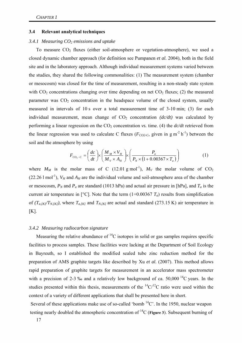
3.4.1 Measuring CO2 emissions and uptake
To measure CO2 fluxes (either soil-atmosphere or vegetation-atmosphere), we used a
closed dynamic chamber approach (for definition see Pumpanen et al. 2004), both in the field
site and in the laboratory approach. Although individual measurement systems varied between
the studies, they shared the following commonalities: (1) The measurement system (chamber
or mesocosm) was closed for the time of measurement, resulting in a non-steady state system
with CO2 concentrations changing over time depending on net CO2 fluxes; (2) the measured
parameter was CO2 concentration in the headspace volume of the closed system, usually
measured in intervals of 10 s over a total measurement time of 3-10 min; (3) for each
individual measurement, mean change of CO2 concentration (dc/dt) was calculated by
performing a linear regression on the CO2 concentration vs. time. (4) the dc/dt retrieved from
the linear regression was used to calculate C fluxes (FCO2-C, given in g m-2 h-1) between the
soil and the atmosphere by using
( )⎟⎟⎠
⎞⎜⎜⎝
⎛×+×
×⎟⎟⎠
⎞⎜⎜⎝
⎛××
×⎟⎠⎞
⎜⎝⎛=−
aN
a
HV
HMCCO TP
PAMVM
dtdcF
00367.012 (1)
where MM is the molar mass of C (12.01 g mol-1), MV the molar volume of CO2
(22.26 l mol-1), VH and AH are the individual volume and soil-atmosphere area of the chamber
or mesocosm, PN and Pa are standard (1013 hPa) and actual air pressure in [hPa], and Ta is the
current air temperature in [°C]. Note that the term (1+0.00367 Ta) results from simplification
of (Ta,[K]/TN,[K]), where Ta,[K] and TN,[K] are actual and standard (273.15 K) air temperature in
[K].
3.4.2 Measuring radiocarbon signature
Measuring the relative abundance of 14C isotopes in solid or gas samples requires specific
facilities to process samples. These facilities were lacking at the Department of Soil Ecology
in Bayreuth, so I established the modified sealed tube zinc reduction method for the
preparation of AMS graphite targets like described by Xu et al. (2007). This method allows
rapid preparation of graphite targets for measurement in an accelerator mass spectrometer
with a precision of 2-3 ‰ and a relatively low background of ca. 50,000 14C years. In the
studies presented within this thesis, measurements of the 14C/12C ratio were used within the
context of a variety of different applications that shall be presented here in short.
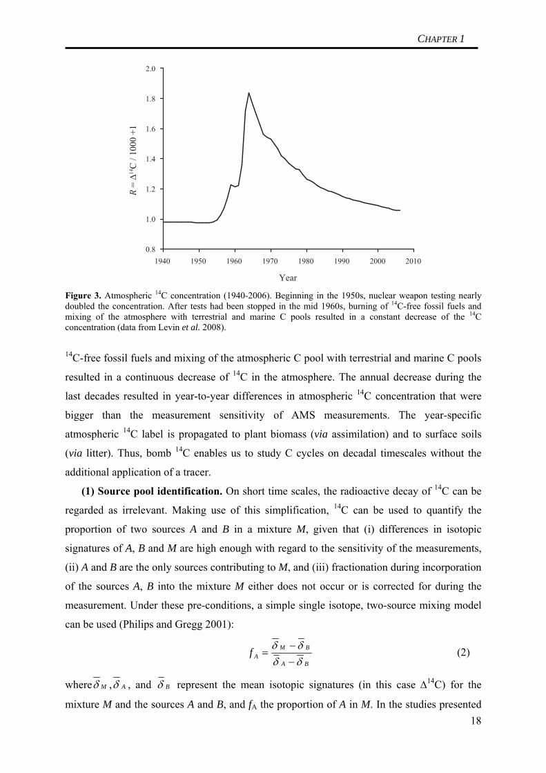
Several of these applications make use of so-called ‘bomb 14C’. In the 1950, nuclear weapon
testing nearly doubled the atmospheric concentration of 14C (Figure 3). Subsequent burning of 17
CHAPTER 1
1940 1950 1960 1970 1980 1990 2000 2010
R = Δ14
C /
1000
+1
0.8
1.0
1.2
1.4
1.6
1.8
2.0
Year Figure 3. Atmospheric 14C concentration (1940-2006). Beginning in the 1950s, nuclear weapon testing nearly doubled the concentration. After tests had been stopped in the mid 1960s, burning of 14C-free fossil fuels and mixing of the atmosphere with terrestrial and marine C pools resulted in a constant decrease of the 14C concentration (data from Levin et al. 2008).
14C-free fossil fuels and mixing of the atmospheric C pool with terrestrial and marine C pools
resulted in a continuous decrease of 14C in the atmosphere. The annual decrease during the
last decades resulted in year-to-year differences in atmospheric 14C concentration that were
bigger than the measurement sensitivity of AMS measurements. The year-specific
atmospheric 14C label is propagated to plant biomass (via assimilation) and to surface soils
(via litter). Thus, bomb 14C enables us to study C cycles on decadal timescales without the
additional application of a tracer.
(1) Source pool identification. On short time scales, the radioactive decay of 14C can be
regarded as irrelevant. Making use of this simplification, 14C can be used to quantify the
proportion of two sources A and B in a mixture M, given that (i) differences in isotopic
signatures of A, B and M are high enough with regard to the sensitivity of the measurements,
(ii) A and B are the only sources contributing to M, and (iii) fractionation during incorporation
of the sources A, B into the mixture M either does not occur or is corrected for during the
measurement. Under these pre-conditions, a simple single isotope, two-source mixing model
can be used (Philips and Gregg 2001):
BA
BMAf
δδδδ
−−
= (2)
where Mδ , Aδ , and Bδ represent the mean isotopic signatures (in this case Δ14C) for the
mixture M and the sources A and B, and fA the proportion of A in M. In the studies presented 18
CHAPTER 1
here, this application of 14C was used to quantify the proportion of rhizosphere and
heterotrophic respiration in total soil respiration. Differences between these two source pools
result from the incorporation of bomb 14C into biomass like described above. A simplified
variety of this approach has been used in the laboratory incubation experiment (CHAPTER
4A). In this approach, only the isotopic signature of the mixture (i.e. soil CO2 emissions) is
measured repeatedly. Significant changes in this isotopic signature are indicative of
qualitative changes in the sources. This approach thus can be used to detect the mobilization
of old, previously stabilized C.
(2) Radiocarbon dating. Prior to 1950, the atmospheric concentration of radiocarbon was
relatively constant and is well documented from reconstructions based on tree-ring calibration
techniques and radiocarbon measurements on foraminifera from marine sediments and corals
(Reimer et al. 2004). The 14C signature of a system that is (actively) exchanging carbon with
its surroundings (e.g. living plants or micro-organisms) is in balance with atmospheric values
(±offsets due to fractionation). In homogeneous systems (i.e. systems in which every C atom
has the same chance to leave the system) without C uptake, the current 14C signature of the
system will be governed by radioactive decay of 14C, leading to a depletion of 14C over time
with a half-life τ1/2 of 5730 years. Thus, the age T of a sample can be calculated as:
⎟⎟⎠
⎞⎜⎜⎝
⎛×⎟⎟
⎠
⎞⎜⎜⎝
⎛−=
)0()(ln1
14 NtNT
λ (3)
where λ14 = ln(2)/τ1/2, N(t) is the number of 14C atoms at the time of measurement and N(0) at
the time when C uptake into the system stopped and decay become the governing process.
N(0) thus is identical with the 14C concentration on the atmosphere at that time. The so-
calculated 14C age therefore has to be corrected for fluctuations in atmospheric 14C
concentration (using software like e.g. OxCal 4.1). In the studies presented here, this approach
was used to determine the age of soil organic matter (SOM) (CHAPTER 2). As SOM is
continuously incorporating fresh carbon, it violates the precondition of an ideally closed
system. Thus, SOM ages from 14C dating have to be interpreted as minimal ages for the length
of soil formation (Wang et al. 1996).
(3) Modelling of soil C turnover. Radiocarbon data may be used in several ways to
estimate input (I) and decomposition (k) rates of C stocks. In the studies presented here, three
different models have been applied. They are presented in detail in the two studies comprised
in CHAPTER 2.
19

CHAPTER 1
4 Synthesis and discussion of the results
4.1 Quantifying soil C dynamics of a Norway spruce forest and a fen under current
boundary conditions (CHAPTER 2)
Using three different models that were based on soil C stock and 14C data, we quantified
the mean soil C dynamics under current climatic conditions at the both field sites. The models
that we applied reflect mean C dynamics on timescales from decades to millennia. These two
studies complement the manipulation studies by identifying horizon specific C stocks and
contribution of these stocks to total C fluxes and thus allowing to estimate the vulnerability of
specific C stocks to changing boundary conditions.
The key findings for the Norway spruce soil were that (i) soil C dynamics at this site were
dominated by C fluxes in and out of the organic horizons (fast turnover, high gross fluxes)
(Table 1), thus organic horizons presumably are more vulnerable to changing boundary
conditions than mineral horizons; (ii) under ‘current’ conditions (i.e. mean conditions of the
last decade), the soil at this site was a small sink for atmospheric CO2 in the order of
4-8 g C m-2 a-1.
Table 1 Horizon specific gross and net C fluxes in a Norway spruce soil derived from the turnover time modeling data presented in Schulze et al. (2009) (cf. CHAPTER 2) Horizon C Input (I ) C Output (kC ) Net C accumulation (I-kC )
(g C m-2 a-1) (g C m-2 a-1) (g C m-2 a-1)Oi 153 153 < 0.1Oe 120 120 0.3Oa 17 11 6Ea 9 9 0Bsh 6 6 0Bsh 5 5 0Bv 3 3 0
Although a relatively high degree of spatial variation of some measured parameters
complicated the interpretation of the results, we were able to establish some general
characteristics of the site. A fundamental finding with regard to the manipulation experiments
carried out at the site was the importance of the organic horizons for overall soil C dynamics
in this soil. Between 19-35% of the total SOC stock (measurement depth 60 cm) were
comprised in the organic horizons. Turnover times of this SOC were relatively fast
(3-10 years), resulting in high gross C fluxes. In fact, total gross C fluxes in this soil
20

CHAPTER 1
(including gaseous losses, DOC leaching and top-down C transfer within the profile) are
clearly dominated by C turnover of the organic horizons (> 90%). Gross C fluxes are several
orders of magnitude higher than calculated net C fluxes. Thus, relatively small changes in the
balance of gross C fluxes of the organic horizons could result in significant changes of the net
C fluxes. In comparison, relative changes in the mineral horizons would have to be much
higher to result in notable changes of the net soil C balance. As organic horizons are situated
directly at the interface between soil and atmosphere, weather extremes like drought or soil
frost can easily have a direct impact on boundary conditions within the organic horizons,
whereas the underlying mineral horizons are to some extent decoupled from changes of
atmospheric boundary conditions. We thus conclude that the organic horizons at this site are
more vulnerable to changing boundary conditions than mineral horizons.
Interestingly, the results of this study also raised the question whether soil C dynamics at
this site reflect undisturbed conditions. The net accumulation we calculated for this site was
only about half the size of net accumulation rates reported for coniferous soil in Sweden
(Ǻgren et al. 2008). Given the history of the site we suspect that the site could be influenced
by undocumented liming, a practice that has been common in the area in the past. Liming has
repeatedly been reported to improve soil conditions, thus increasing mineralization rates of
SOM and thus potentially reducing the net C balance of the soil (Persson et al. 1989, Fuentes
et al. 2006).
The key findings for the fen site were that (i) under current boundary conditions the fen
site is a net C source, indicating that the site is subject to disturbance, (ii) a high amount of C
is stored in root biomass, (iii) fluxes in and out of SOM C stocks occur predominantly in the
uppermost 15 cm, most likely due to low substrate quality in deeper peat layers.
Using a modeling approach, we quantified the soil C balance within the peat body of a
minerotrophic fen. We distinguished three relevant C stock compartments within the peat
body: (i) root biomass (comprising live roots and structurally intact dead roots), (ii) surface
peat SOM (defined by the occurrence of bomb 14C), and (iii) deep peat SOM. We used two
different models to calculate the net C balances of these three compartments (Trumbore and
Harden 1997, Gaudinski et al. 2000). Whereas peatlands in general are reported to be net C
sinks with net accumulation rates between approx. 15-30 g C m-2 a-1 (Vitt et al. 2000, Turunen
et al. 2001, Turunen et al. 2002), we calculated a slightly negative C balance for this fen
under current climatic conditions, indicating disturbance of the boundary conditions at this fen
site. In detail, we calculated (i) a net C loss of -24 g C m-2 a-1 from the root biomass stock, (ii)
a net C loss of -5 g C m-2 a-1 from the surface peat SOM stock, and (iii) a net C accumulation
21

CHAPTER 1
of +3 g C m-2 a-1 in the deep peat SOM stock. The net C losses from the root biomass C stock
most likely reflect changing of boundary conditions on a shorter timescale, given the
relatively fast turnover time of root biomass. Net C losses from the SOM stocks might also
reflect disturbances on a longer timescale (up to several decades). Based on our results we are
unable to identify the actual source of disturbance. The site features a ditch of unknown
history, and a disturbance of the hydrological boundary conditions due to drainage by this
ditch would be a very likely source of disturbance. Results from other experiments at his site
have to be discussed in the context of this disturbance.
4.2 Soil carbon dynamics of a Norway spruce soil as affected by soil frost (CHAPTER 3)
The key findings of this study were that (i) C dynamics during the period of actual soil
frost had a relatively small effect on total C losses from the soil, (ii) freezing-thawing does not
mobilize stabilized C in this soil, (iii) soil frost alters the composition of the microbial
community (preferential reduction of fungal biomass proportion), thus ultimately (iv)
increasing the susceptibility of the soil microbial community towards drought stress.
Due to repeatedly warm temperatures in the winters of 2006/2007 and 2007/2008, the
experimental induction of soil frost at the Coulissenhieb II site could only take place once in
the winter of 2005/2006. In that winter, snow removal effectively induced soil frost on the
manipulation plots. Following snow removal, soil frost occurred down to a depth of 15 cm
and lasted ca. three months. No indication of soil frost was found on the control plots, so the
snow removal successfully simulated increasing soil frost frequency.
We compared total C losses between January 2006 and January 2007 from the
manipulation plots and from the control plots. Total C losses from the manipulation plots
were 5.1 t C ha-1 a-1, compared to 6.2 t C ha-1 a-1 from the control plots. Thus, soil frost
resulted in a reduction of total C losses by 1.1 t C ha-1 a-1. Surprisingly, soil respiration
differences during the actual soil frost period and the subsequent thawing could only explain
14% of this reduction. The major proportion of the differences was explained by significantly
reduced soil respiration fluxes from the manipulation plots during the summer of 2006.
Inherent differences were excluded due to the pre-treatment period and the setup of the plots.
No measurable differences were in soil temperature and soil moisture. Thus, we linked the
reduction of the summer soil respiration fluxes to the stress history of the manipulation plots.
Schmitt et al. (2008) reported that repeated freezing-thawing of soil columns from the
Coulissenhieb II site resulted in a reduction of the relative contribution of fungal to total
microbial biomass. Similar findings have also been reported in several other studies
22
CHAPTER 1
(Nieminen and Setala 2001, Larsen et al. 2002, Feng et al. 2007). Assuming the same
phenomenon occurred under field-site conditions, we postulated that soil frost changed the
composition of the microbial community on the manipulation plots, reducing fungal biomass.
Fungi, in turn, have been reported to be more resistant towards drought than bacteria
(Voroney 2007). Thus, an altered composition of the microbial community is likely to result
in an altered susceptibility towards drought stress. The summer of 2006 was an exceptionally
dry summer. We therefore conclude that soil frost indirectly reduced total soil C losses by
increasing the susceptibility of the soil microbial community towards drought stress. We
conclude that the exceptional combination of severe soil frost in winter and drought stress in
summer were responsible for the remarkable reduction of total C losses in the manipulation
plots.
Several field and laboratory studies reported a pronounced CO2 pulse after thawing of
frozen soil from agricultural, arctic or forest soils (Coxson and Parkinson 1987, Elberling and
Brandt 2003, Dörsch et al. 2004, Goldberg et al. 2008). Different mechanisms have been
discussed to explain this pulse. These mechanisms are very similar to the mechanisms
discussed by Xiang et al. (2008) to explain the occurrence of such a pulse during drying-
rewetting events. Thus, I will use the same terminology here, differentiating between the
‘microbial stress’ and the ‘substrate supply’ mechanism.
Following the logic of the ‘microbial stress’ mechanism, this pulse would originate from
the release of substrates from microbial biomass. This release could be a consequence of cell
death. Alternatively, it could be explained by a reversal of physiological acclimation of micro-
organisms to freezing (Schimel et al. 2007) resulting in a release of solutes like e.g. protective
molecules (Mihoub et al. 2003, Kandror et al. 2004) or antifreeze proteins (Bae et al. 2004).
Following the logic of the ‘substrate supply’ mechanism, the CO2 pulse would be due to
mobilization of previously stabilized C e.g. due to physical disruption of soil aggregates.
Additional mobilization of C substrates would ultimately have to result in an increase of total
C losses. This second mechanism thus bears the possibility of enhanced C losses from soils
due to freezing and thawing.
Based on our results, we neither observed a pulse nor did we find an increase of total C
losses resulting from freezing-thawing of the soil. We therefore have to refuse the idea of
mobilization of stable C due to soil frost. This result is in agreement with findings from
laboratory studies on undisturbed soil columns from this site (Goldberg et al. 2008), but also
with findings from field-site experiments by Groffman et al. (2006) and Coxson and
23

CHAPTER 1
Parkinson (1987), who also reported no effect of freezing-thawing on cumulative soil C
losses.
4.3 Soil C dynamics in a Norway spruce soil as affected by drying-wetting under
laboratory and field-site conditions (CHAPTER 4)
Key findings of these studies: (i) The main effect of drought is a temporary reduction of
decomposition, leading to (ii) a reduction of total soil C losses that can not be compensated
for during subsequent wet periods, and (iii) mobilization of previously stabilized C due to
drying-wetting does not occur. Thus, in summary, drought irrevocably reduces gross soil C
losses in the year of drought. We did not investigate the effects of drought on the CO2 uptake
by plants and litter input. The relatively small net uptake indicates that uptake and emission
fluxes are very similar in size under current climatic conditions. Hence, from the ecosystem
level, we can not exclude the possibility that this forest might turn into a temporary net source
of C during prolonged summer drought if CO2 uptake is reduced stronger than soil respiration
like reported by Ciais et al. (2005).
A laboratory study (CHAPTER 4A) was designed to study the effect of drought intensity on
(i) dynamics of soil C losses, (ii) total quantity of soil C losses, and (iii) mobilization of
stabilized C in the organic horizons in detail. As soil columns from the organic horizons were
used, the study does not allow any conclusions about mineral horizons and comprises only the
effects of drought on heterotrophic respiration (i.e. decomposition). The high temporal
resolution of the measurements revealed that drying of the organic horizons resulted in an
almost immediate reduction of decomposition, either because microorganisms became
inactive or died. The more intense the drought got, the smaller were the observed CO2
emission rates. Under very dry conditions (pF 6-7) heterotrophic respiration was close to zero.
Thus, cumulative soil C losses during the drought period depended substantially from drought
intensity. In contrast to this, C dynamics during rewetting of the dry soil seemed
predominantly independent from precedent drought intensity: Rewetting basically restored the
respiration rates back to pre-drought levels, no transient enhancement of respiration rates was
observed. The effect of drought therefore can be described as a temporary reduction of
decomposition that is not compensated for by enhanced decomposition during subsequent wet
periods. Based on the results of the laboratory experiment, we conclude that the length and
intensity of the dry conditions determine how much less C is lost from the organic horizons in
comparison to what might be lost under optimum moisture conditions (cf. Borken and
Matzner 2009).
24
CHAPTER 1
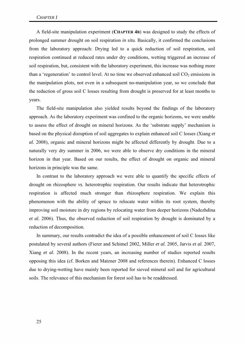
A field-site manipulation experiment (CHAPTER 4B) was designed to study the effects of
prolonged summer drought on soil respiration in situ. Basically, it confirmed the conclusions
from the laboratory approach: Drying led to a quick reduction of soil respiration, soil
respiration continued at reduced rates under dry conditions, wetting triggered an increase of
soil respiration, but, consistent with the laboratory experiment, this increase was nothing more
than a ‘regeneration’ to control level. At no time we observed enhanced soil CO2 emissions in
the manipulation plots, not even in a subsequent no-manipulation year, so we conclude that
the reduction of gross soil C losses resulting from drought is preserved for at least months to
years.
The field-site manipulation also yielded results beyond the findings of the laboratory
approach. As the laboratory experiment was confined to the organic horizons, we were unable
to assess the effect of drought on mineral horizons. As the ‘substrate supply’ mechanism is
based on the physical disruption of soil aggregates to explain enhanced soil C losses (Xiang et
al. 2008), organic and mineral horizons might be affected differently by drought. Due to a
naturally very dry summer in 2006, we were able to observe dry conditions in the mineral
horizon in that year. Based on our results, the effect of drought on organic and mineral
horizons in principle was the same.
In contrast to the laboratory approach we were able to quantify the specific effects of
drought on rhizosphere vs. heterotrophic respiration. Our results indicate that heterotrophic
respiration is affected much stronger than rhizosphere respiration. We explain this
phenomenon with the ability of spruce to relocate water within its root system, thereby
improving soil moisture in dry regions by relocating water from deeper horizons (Nadezhdina
et al. 2006). Thus, the observed reduction of soil respiration by drought is dominated by a
reduction of decomposition.
In summary, our results contradict the idea of a possible enhancement of soil C losses like
postulated by several authors (Fierer and Schimel 2002, Miller et al. 2005, Jarvis et al. 2007,
Xiang et al. 2008). In the recent years, an increasing number of studies reported results
opposing this idea (cf. Borken and Matzner 2008 and references therein). Enhanced C losses
due to drying-wetting have mainly been reported for sieved mineral soil and for agricultural
soils. The relevance of this mechanism for forest soil has to be readdressed.
25

CHAPTER 1
4.4 Ecosystem C dynamics in a fen as affected by natural and manipulative water
table changes (CHAPTER 5)
Key findings of these two studies: (i) Changes in water table affected respiratory C fluxes
only when occurring within the uppermost ca. 0-15 cm soil depth, and (ii) photosynthetic
uptake of atmospheric CO2 was affected by water table fluctuations only in moss species, thus
(iii) this fen is presumably very resilient towards an increasing frequency of summer drought.
However, this resilience most likely results from the fact that the fen already is subject to a
disturbance of the hydrological conditions.
A field-site manipulation experiment was designed (CHAPTER 5A) to quantify the effect of
water table on ecosystem C dynamics by artificially lowering the water table during summer
(thus simulating the effect of summer drought). In contrast to the forest site, we included CO2
related to aboveground vegetation into our analysis. In summary, we measured (i) net
ecosystem exchange (NEE), (ii) ecosystem respiration (REco), and (iii) soil respiration (RSoil)
and furthermore were able to calculate (iv) gross primary production (GPP) and
(v) respiration of the aboveground vegetation. In three subsequent manipulation years (2006-
2008) we found no significant effect of lowered water tables on any of the measured
parameters. Especially with regards to soil respiration, this was in contrast to our
expectations. Generally, C in peatlands is assumed to be stabilized by high water tables, as
they inhibit oxygen diffusion (Päivänen and Vasander 1994). Thus, lowering of the water
table and the consequent increase of oxygen availability supposedly should increase
decomposition rates.
An additional study (CHAPTER 5B) was designed to investigate how naturally occurring
changes of the boundary conditions affected the CO2 fluxes into and out of this ecosystem. In
addition to CO2 fluxes, the study comprised measurements of air and soil temperature,
photosynthetic active radiance, changes in biomass, and water table. I will concentrate here
mainly on findings that are related to changes of the water table. With respect to aboveground
biomass, no evidence was found that natural fluctuations (between 0-20 cm) of the water table
in any way affected gross primary production of grass species at the site. In contrast to this,
biomass production of moss species was depending on water table like indicated by a
significant drop of moss biomass following a periods of low water tables during early spring.
Thus, it is concluded that low water tables can result in a reduction of gross primary
production of mosses. This difference between grasses and roots could be explained by
differences in plant anatomy, as grasses have deep rooting patterns that can guarantee
sufficient water uptake even during times of low water tables (Limpens et al. 2008), whereas
26

CHAPTER 1
mosses depend on water table and precipitation. However, the site is predominantly
characterized by grass species; mosses represent a minor proportion of the vegetation.
Furthermore, water tables at the site are already naturally low during most of summer. Thus,
we expect lowering of water table due to increasing summer droughts to have only a minor
impact on GPP in this ecosystem.
With regard to water table affecting REco, the findings of this study seem to contrast the
findings of the manipulation experiment: Natural lowering of the water table correlated with
increasing values of REco. However, there are two important points to notice with this
correlation: (i) Data comprised in the analysis is clearly dominated by water tables between
0-10 cm below the surface (only two measurement dates with a lower water table); (ii) shifts
in water table were accompanied by changes in peat temperature, making it difficult to
distinguish the effects of water table from the effects of peat temperature changes. Thus, we
carefully conclude that water table might effect when occurring within the uppermost peat
layers (ca. 0-15 cm). This latter conclusion is based on the modeled soil C dynamics of this
site (cf. CHAPTER 2B) and on findings reported by Reiche et al. (2009). As described,
modeling revealed that C turnover during the last decades was clearly dominated by fluxes
occurring within the uppermost 15 cm of the soil. The contribution of C turnover in deeper
peat layers was almost irrelevant. As water table at least in summer (when decomposition is
highest due to high soil temperatures) regularly drops deeper than 15 cm even under natural
conditions, it is unlikely that the small contribution of the deeper peat can be explained only
by a lack of oxygen. Indeed, Reiche et al. (2009) were able to demonstrate that peat in the
deep peat layer (beneath 15 cm) is characterized by low substrate quality, as it has a low
decomposition potential even under optimum conditions. Hence, water table fluctuations can
only affect soil C losses within the uppermost 15 cm, as soil C dynamics in deeper peat are
not governed by oxygen availability but by substrate quality. However, water tables are
already naturally low in summer at this site. In summary, due to the preconditions at the site,
we expect the effect of further lowering of the water table during summer on ecosystem C
dynamics at this site to be minimal.
27

CHAPTER 1
5 Conclusions
This thesis focused on the effect of meteorological boundary conditions on C dynamics of
a forest and a fen ecosystem. Both ecosystems were located in the Fichtelgebirge in South-
eastern Germany. In the forest ecosystem, the focus was on the effects of (i) drought and of
(ii) soil frost on soil C dynamics. In the fen ecosystem, the focus was on the effect of
(iii) water table (especially of lowered water table) on ecosystem C dynamics. Under the
impressions of current climate models, all three scenarios are highly up-to-date. This thesis
was especially interested in the question whether extreme meteorological boundary conditions
could possibly lead to enhanced soil C losses, thus resulting in a reinforcement of climate
change. This concern was based on earlier discussions of this phenomenon in the literature. A
considerable number of studies points at the possibility of climate-carbon feedbacks resulting
from extreme boundary conditions in soils.
However, this concern was not confirmed in the studies presented here. In the forest
ecosystem, all results indicated that extreme boundary conditions like frost and drought
represent significant stress for the soil organisms. As long as this stress is maintained,
metabolic activity is significantly reduced. Soil organisms either die or become less active.
Both types of extreme events seemed to mainly affect the heterotrophic soil organisms in the
forest soil. Roots and presumably root-associated microorganisms seem to be less prone to the
effects of extreme soil boundary conditions. Partially, this could be explained by the ability of
roots to significantly influence soil conditions in their immediate surroundings. Heterotrophic
soil microorganisms are responsible for the decomposition of soil organic matter. Thus, in the
forest ecosystem extreme meteorological events lead to a transient reduction of
decomposition. The more intense the stress regime and the longer it is maintained, the higher
the cumulative impact on decomposition. Thus, extreme conditions like soil frost and drought
primarily lead to a reduction of soil C losses as decomposition is slowed down. Whether or
not such a transient reduction of soil C losses can lead to the long-term net sequestration of C
depends on a variety of other factors.
First of all, net ecosystem C balance is the difference between C uptake and C losses.
Thus, to determine whether reduced soil C losses are equivalent to increased sequestration of
C one, the effects of extreme boundary conditions on C assimilation have to be considered. In
the forest ecosystem, we have been unable to measure assimilation due to technical
limitations. Thus, when observing a transient reduction of the gross C losses due to extreme
meteorological conditions, it still is possible that the net ecosystem C losses are enhanced.
28

CHAPTER 1
Furthermore, a transient reduction of soil C losses can only lead to a long-term
sequestration of C as long as it is not compensated for by enhanced C losses in the aftermath
of the stress period. This could happen when breakdown of complex molecules continues at
high rates during the stress period but substrates are not completely mineralized (e.g. when
they are instead used to produce anti-stress proteins). Furthermore, extreme boundary
conditions within the soil do not only exert stress on microorganisms but also physical stress
on soil aggregates. Soil aggregate breakdown might result in the mobilization of new
substrates that can compensate or even over-compensate for the reduced decomposition
during the stress period. However, our results in the forest disproved both these assumptions.
Apart from uncertainties concerning the effect on assimilation, we therefore can conclude that
soil frost and drought do both result in a clear reduction of soil C losses. Thus, based on our
results, it is more likely to expect a negative climate-carbon feedback resulting from soil frost
and drought than to expect a positive one.
Things were different to some extent for the fen site. Here, we did not measure the direct
effects of drought, but rather the indirect effects (i.e. a possible lowering of the water table
like expected as a result of increased evapotranspiration and decreased precipitation). As
peatlands normally feature great amounts of C that is stabilized predominantly by high water
tables and consequently low rates of decomposition, we expected a significant effect of
lowered water tables on CO2 fluxes in this ecosystem. Surprisingly, CO2 fluxes in this fen
were not affected by water table manipulations. These manipulations, however, were carried
out when the water table was already low. Other data indicated that for higher water tables a
change of the water table might affect the CO2 fluxes. Still, the ‘natural’ water table was
predominantly low under current boundary conditions, especially in summer. Modeling data
indicates, however, that this condition is not actually natural, as this fen has been identified as
a net C source, indicating that present boundary conditions are different compared to what
they have been like during the formation of the peatland. Given the low water table and the
indication of disturbance we assume a direct disturbance of hydrological conditions, probably
due to draining of the site. Thus, conclusions drawn at this site are not valid for undisturbed
peatland sites. The low water tables presumably result in decomposition rates that are no
longer limited by oxygen availability controlled by water table but instead by peat
temperature, substrate quality and the occurrence of micro-environmental structures. Based on
the results here, the site might proof a suitable location for a restoration or flooding
experiment. With regard to peat temperature as an important driver of decomposition, it is
important to mention that manipulative lowering of the water table fails to completely
29

CHAPTER 1
simulate the effects of summer drought. In reality, summer drought is most likely to be
accompanied by high temperature and evapotranspiration. Thus, the combination of a lack of
precipitation, high evapotranspiration and high temperature will not only result in lowering of
the water table but will presumably also increase peat temperature. Lower water tables during
summer alone were found to have no effect on CO2 fluxes in this fen, but it has to be critically
analyzed whether the manipulative approach really reflects all aspects of summer drought.
30

CHAPTER 1
6 References
Ågren, G., Hyvönen, R. and Nilsson, T. 2008. Are Swedish forest soils sinks or sources for
CO2—model analyses based on forest inventory data. Biogeochemistry 89, 139-149.
Alm, J., Schulman, L., Walden, J., Nykanen, H., Martikainen, P. J. and Silvola, J. 1999.
Carbon Balance of a Boreal Bog During a Year With an Exceptionally Dry Summer.
Ecology 80, 161-174, doi:110.1890/0012-9658.
Bae, E. K., Cho, Y. H. and Park, J. Y. 2004. Studies on the Development of a Microbial
Cryoprotectant Formulation Using a W/O/W Multiple Emulsion System. Journal of
Microbiology and Biotechnology 14, 673-679.
Batjes, N. H. 1996. Total carbon and nitrogen in the soils of the world. European Journal of
Soil Science 47, 151-163.
Borken, W. and Matzner, E. 2009. Reappraisal of drying and wetting effects on C and N
mineralization and fluxes in soils. Global Change Biology 15, 808-824.
Bubier, J. L., Bhatia, G., Moore, T. R., Roulet, N. T. and Lafleur, P. M. 2003. Spatial and
Temporal Variability in Growing-Season Net Ecosystem Carbon Dioxide Exchange at a
Large Peatland in Ontario, Canada. Ecosystems 6, 353-367.
Bunnell, F. L. and Tait, E. N. 1974: Mathematical Simulation Models of Decomposition
Processes. In Holding, A. J., editor, Soil Organisms and Decomposition in Tundra,
Stockholm, 207-225.
Byrne, K. A., Chojnicki, B., Christensen, T. R., Drösler, M., Freibauer, A., Friborg, T.,
Frolking, S., Lindroth, A., Mailhammer, J., Malmer, N., Selin, P., Turunen, J., Valentini,
R. and Zetterberg, L. 2004: EU Peatlands: Current Carbon Stocks and Trace Gas Fluxes.
Concerted Action CarboEurope-GHG, 58.
Ciais, P., Reichstein, M., Viovy, N., Granier, A., Ogee, J., Allard, V., Aubinet, M.,
Buchmann, N., Bernhofer, C., Carrara, A., Chevallier, F., De Noblet, N., Friend, A. D.,
Friedlingstein, P., Grunwald, T., Heinesch, B., Keronen, P., Knohl, A., Krinner, G.,
Loustau, D., Manca, G., Matteucci, G., Miglietta, F., Ourcival, J. M., Papale, D.,
Pilegaard, K., Rambal, S., Seufert, G., Soussana, J. F., Sanz, M. J., Schulze, E. D., Vesala,
T. and Valentini, R. 2005. Europe-wide reduction in primary productivity caused by the
heat and drought in 2003. Nature 437, 529-533.
Cosentino, D., Chenu, C. and Le Bissonnais, Y. 2006. Aggregate stability and microbial
community dynamics under drying-wetting cycles in a silt loam soil. Soil Biology and
Biochemistry 38, 2053-2062.
31
CHAPTER 1
Coxson, D. S. and Parkinson, D. 1987. Winter respiratory activity in aspen woodland forest
floor litter and soils. Soil Biology and Biochemistry 19, 49-59.
Curiel Yuste, J., Janssens, I. A. and Ceulemans, R. 2005. Calibration and validation of an
empirical approach to model soil CO2 efflux in a deciduous forest. Biogeochemistry 73,
209-230.
Davidson, E. A., Belk, E. and Boone, R. D. 1998. Soil water content and temperature as
independent or confounded factors controlling soil respiration in a temperate mixed
hardwood forest. Global Change Biology 4, 217-227.
Denef, K., Six, J., Bossuyt, H., Frey, S. D., Elliott, E. T., Merckx, R. and Paustian, K. 2001a.
Influence of dry-wet cycles on the interrelationship between aggregate, particulate organic
matter, and microbial community dynamics. Soil Biology and Biochemistry 33, 1599-
1611.
Denef, K., Six, J., Paustian, K. and Merckx, R. 2001b. Importance of macroaggregate
dynamics in controlling soil carbon stabilization: short-term effects of physical
disturbance induced by dry-wet cycles. Soil Biology and Biochemistry 33, 2145-2153.
Doherty, S. J., Bojinski, S., Henderson-Sellers, A., Noone, K., Goodrich, D., Bindoff, N. L.,
Church, J. A., Hibbard, K. A., Karl, T. R., Kajfez-Bogataj, L., Lynch, A. H., Parker, D. E.,
Prentice, I. C., Ramaswamy, V., Saunders, R. W., Stafford Smith, M., Steffen, K.,
Stocker, T. F., Thorne, P. W., Trenberth, K. E., Verstraete, M. M. and Zwiers, F. W. 2009.
Lessons Learned from IPCC AR4: Scientific Developments Needed to Understand,
Predict, and Respond to Climate Change. Bulletin of the American Meteorological Society
90, 497-513.
Dörsch, P., Palojärvi, A. and Mommertz, S. 2004. Overwinter greenhouse gas fluxes in two
contrasting agricultural habitats. Nutrient Cycling in Agroecosystems 70, 117-133.
Elberling, B. and Brandt, K. K. 2003. Uncoupling of microbial CO2 production and release in
frozen soil and its implications for field studies of arctic C cycling. Soil Biology and
Biochemistry 35, 263-272.
Feng, X., Nielsen, L. L. and Simpson, M. J. 2007. Responses of soil organic matter and
microorganisms to freeze-thaw cycles. Soil Biology and Biochemistry 39, 2027-2037.
Fierer, N. and Schimel, J. P. 2002. Effects of drying-rewetting frequency on soil carbon and
nitrogen transformations. Soil Biology and Biochemistry 34, 777-787.
Fierer, N. and Schimel, J. P. 2003. A Proposed Mechanism for the Pulse in Carbon Dioxide
Production Commonly Observed Following the Rapid Rewetting of a Dry Soil. Soil
Science Society of America Journal 67, 798-805.
32

CHAPTER 1
Foken, T. 2003: Lufthygienisch-bioklimatische Kennzeichnung des oberen Egertales
(Fichtelgebirge bis Karlovy Vary). In: Bayreuther Forum Ökologie, 100.
Fuentes, J. P., Bezdicek, D. F., Flury, M., Albrecht, S. and Smith, J. L. 2006. Microbial
activity affected by lime in a long-term no-till soil. Soil and Tillage Research 88, 123-131.
Gaudinski, J. B., Trumbore, S. E., Davidson, E. A. and Zheng, S. 2000. Soil carbon cycling in
a temperate forest: radiocarbon-based estimates of residence times, sequestration rates and
partitioning of fluxes. Biogeochemistry 51, 33-69.
Gerstberger, P., Foken, T. and Kalbitz, K. 2004: The Lehstenbach and Steinkreuz catchments
in NE Bavaria, Germany. In Matzner, E., editor, Biogeochemistry of forested catchments
in a changing environment, Berlin: Springer, 15-29.
Goldberg, S., Muhr, J., Borken, W. and Gebauer, G. 2008. Fluxes of climate-relevant trace
gases between a Norway spruce forest soil and the atmosphere during repeated freeze-
thaw cycles in mesocosms. Journal of Plant Nutrition and Soil Science 171, 729-739.
Gorham, E. 1991. Northern Peatlands: Role in the Carbon Cycle and Probable Responses to
Climatic Warming. Ecological Applications 1, 182-195.
Groffman, P. M., Driscoll, C., Fahey, T., Hardy, J., Fitzhugh, R. and Tierney, G. 2001. Colder
soils in a warmer world: A snow manipulation study in a northern hardwood forest
ecosystem. Biogeochemistry 56, 135-150.
Groffman, P. M., Hardy, J. P., Driscoll, C. T. and Fahey, T. J. 2006. Snow depth, soil
freezing, and fluxes of carbon dioxide, nitrous oxide and methane in a northern hardwood
forest. Global Change Biology 12, 1748-1760, doi:1710.1111/j.1365-2486.2006.01194.x.
Hughes, P. D. M. and Dumayne-Peaty, L. 2002: Testing theories of mire development using
multiple successions at Crymlyn Bog, West Glamorgan, South Wales, UK. 456-471.
IPCC. 2007: Climate Change 2007: The Physical Science Basis. Contribution of Working
Group I to the Fourth Assessment Report of the Intergovernmental Panel on Climate
Change. Cambridge, United Kingdom and New York, NY, USA: Cambridge University
Press.
IUSS Working Group WRB. 2006: World reference base for soil resources 2006. Rome:
FAO.
Jarvis, P., Rey, A., Petsikos, C., Wingate, L., Rayment, M., Pereira, J., Banza, J., David, J.,
Miglietta, F., Borghetti, M., Manca, G. and Valentini, R. 2007. Drying and wetting of
Mediterranean soils stimulates decomposition and carbon dioxide emission: the “Birch
effect”. Tree Physiology 27, 929-940.
33

CHAPTER 1
Kandror, O., Bretschneider, N., Kreydin, E., Cavalieri, D. and Goldberg, A. L. 2004. Yeast
Adapt to Near-Freezing Temperatures by STRE/Msn2,4-Dependent Induction of
Trehalose Synthesis and Certain Molecular Chaperones. 13, 771-781.
Kuzyakov, Y. 2006. Sources of CO2 efflux from soil and review of partitioning methods. Soil
Biology and Biochemistry 38, 425-448.
Laiho, R. 2006. Decomposition in peatlands: Reconciling seemingly contrasting results on the
impacts of lowered water levels. Soil Biology and Biochemistry 38, 2011-2024.
Larsen, K. S., Jonasson, S. and Michelsen, A. 2002. Repeated freeze-thaw cycles and their
effects on biological processes in two arctic ecosystem types. Applied Soil Ecology 21,
187-195.
Levin, I., Hammer, S., Kromer, B. and Meinhardt, F. 2008. Radiocarbon observations in
atmospheric CO2: Determining fossil fuel CO2 over Europe using Jungfraujoch
observations as background. Science of The Total Environment 391, 211-216.
Limpens, J., Berendse, F., Blodau, C., Canadell, J. G., Freeman, C., Holden, J., Roulet, N.,
Rydin, H. and Schaepman-Strub, G. 2008. Peatlands and the carbon cycle: from local
processes to global implications - a synthesis. Biogeosciences 5, 1475-1491.
Mihoub, F., Mistou, M.-Y., Guillot, A., Leveau, J.-Y., Boubetra, A. and Billaux, F. 2003.
Cold adaptation of Escherichia coli: microbiological and proteomic approaches.
International Journal of Food Microbiology 89, 171-184.
Miller, A. E., Schimel, J. P., Meixner, T., Sickman, J. O. and Melack, J. M. 2005. Episodic
rewetting enhances carbon and nitrogen release from chaparral soils. Soil Biology and
Biochemistry 37, 2195-2204.
Moore, P. D. 2002. The future of cool temperate bogs. Environmental Conservation 29, 3-20,
doi:10.1017/S0376892902000024.
Muhr, J., Borken, W. and Matzner, E. 2009. Effects of soil frost on soil respiration and its
radiocarbon signature in a Norway spruce forest soil. Global Change Biology 15, 782-793.
Muhr, J., Goldberg, S. D., Borken, W. and Gebauer, G. 2008. Repeated drying-rewetting
cycles and their effects on the emission of CO2, N2O, NO, and CH4 in a forest soil.
Journal of Plant Nutrition and Soil Science 171, 719-728.
Nadezhdina, N., Cermák, J., Gašpárek, J., Nadezhdin, V. and Prax, A. 2006. Vertical and
horizontal water redistribution in Norway spruce (Picea abies) roots in the Moravian
Upland. 26, 1277-1288.
Nieminen, J. K. and Setala, H. 2001. Bacteria and microbial-feeders modify the performance
of a decomposer fungus. Soil Biology and Biochemistry 33, 1703-1712.
34
CHAPTER 1
Päivänen, J. and Vasander, H. 1994. Carbon Balance in mire ecosystems. World Resource
Review 6, 102-111.
Persson, T., Lundkvist, H., Wirén, A., Hyvönen, R. and Wessén, B. 1989. Effects of
acidification and liming on carbon and nitrogen mineralization and soil organisms in mor
humus. Water, Air, & Soil Pollution 45, 77-96.
Phillips, D. L. and Gregg, J. W. 2001. Uncertainty in source partitioning using stable isotopes.
Oecologia 127, 171-179, doi: 110.1007/s004420000578.
Pumpanen, J., Kolari, P., Ilvesniemi, H., Minkkinen, K., Vesala, T., Niinisto, S., Lohila, A.,
Larmola, T., Morero, M., Pihlatie, M., Janssens, I., Yuste, J. C., Grunzweig, J. M., Reth,
S., Subke, J.-A., Savage, K., Kutsch, W., Ostreng, G., Ziegler, W., Anthoni, P., Lindroth,
A. and Hari, P. 2004. Comparison of different chamber techniques for measuring soil CO2
efflux. Agricultural and Forest Meteorology 123, 159-176.
Reiche, M., Hädrich, A., Lischeid, G. and Küsel, K. 2009. Impact of manipulated drought and
heavy rainfall events on peat mineralization processes and source-sink functions of an
acidic fen. Journal of Geophysical Research - Biogeosciences 114, G02021,
doi:02010.01029/02008JG000853.
Reimer, P. J., Baillie, M. G. L., Bard, E., Bayliss, A., Beck, J. W., Bertrand, C., Blackwell, P.
G., Buck, C. E., Bur, G., Cutler, K. B., Damon, P. E., Edwards, R. L., Fairbanks, R. G.,
Friedrich, M., Guilderson, T. P., Hughen, K. A., Kromer, B., McCormac, F. G., Manning,
S., Bronk Ramsey, C., Reimer, R. W., Remmele, S., Southon, J. R., Stuiver, M., Talamo,
S., Taylor, F. W., van der Plicht, J. and Weyhenmeyer, C. E. 2004. IntCal04 terrestrial
radiocarbon age calibration, 0-26 cal kyr BP. Radiocarbon 46, 1029-1058.
Ryan, M. G. and Law, B. E. 2005. Interpreting, measuring, and modeling soil respiration.
Biogeochemistry 73, 3-27.
Schimel, J., Balser, T. C. and Wallenstein, M. 2007. Microbial Stress-response Physiology
and its Implications for Ecosystem Function. Ecology 88, 1386-1394.
Schlesinger, W. H. and Andrews, J. A. 2000. Soil respiration and the global carbon cycle.
Biogeochemistry 48, 7-20.
Schulze, E.-D. and Freibauer, A. 2005. Carbon unlocked from soils. Nature 437, 205.
Schulze, K., Borken, W., Muhr, J. and Matzner, E. 2009. Stock, turnover time and
accumulation of organic matter in bulk and density fractions of a podzol soil. European
Journal of Soil Science 60, 567-577.
Trenberth, K. E., Jones, P. D., Ambenje, P., Bojariu, R., Easterling, D., Tank, A. K., Parker,
D., Rahimzadeh, F., Renwick, J. A., Rusticucci, M., Soden, B. and Zhai, P. 2007:
35
CHAPTER 1
Observations: Surface and Atmospheric Climate Change. . In Solomon, S., Qin, D.,
Manning, M., Chen, Z., Marquis, M., Averyt, K. B., Tignor, M. and Miller, H. L., editors,
Climate Change 2007: The Physical Science Basis. Contribution of Working Group I to
the Fourth Assessment Report of the Intergovernmental Panel on Climate Change
Cambridge, United Kingdom and New York, NY, USA.: Cambridge University Press,
235-336.
Trumbore, S. 2009. Radiocarbon and Soil Carbon Dynamics. Annual Review of Earth and
Planetary Sciences 37, 47-66, doi:10.1146/annurev.earth.1136.031207.124300.
Trumbore, S. E. and Harden, J. W. 1997. Accumulation and turnover of carbon in organic and
mineral soils of the BOREAS northern study area. Journal of Geophysical Research 102,
28817-28830.
Turunen, J., Tahvanainen, T., Tolonen, K. and Pitkänen, A. 2001. Carbon Accumulation in
West Siberian Mires, Russia. Global Biogeochemical Cycles 15, 285-296.
Turunen, J., Tomppo, E., Tolonen, K. and Reinikainen, A. 2002. Estimating carbon
accumulation rates of undrained mires in Finland-application to boreal and subarctic
regions. The Holocene 12, 69-80, doi: 10.1191/0959683602hl0959683522rp.
Vitt, D. H., Halsey, L. A., Bauer, I. E. and Campbell, C. 2000. Spatial and temporal trends in
carbon storage of peatlands of continental western Canada through the Holocene.
Canadian Journal of Earth Sciences 37, 683-693.
Voroney, R. P. 2007: The Soil Habitat. In Paul, E. A., editor, Soil Microbiology, Ecology, and
Biochemistry, Oxford: Academic Press, 25-49.
Walentowski, H., Ewald, J., Fischer, A., Kölling, C. and Türk., W. 2004: Handbuch der
natürlichen Waldgesellschaften Bayerns. Freising: Geobotanica.
Wang, Y., Amundson, R. and Trumbore, S. 1996. Radiocarbon Dating of Soil Organic
Matter. Quaternary Research 45, 282-288.
Xiang, S.-R., Doyle, A., Holden, P. A. and Schimel, J. P. 2008. Drying and rewetting effects
on C and N mineralization and microbial activity in surface and subsurface California
grassland soils. Soil Biology and Biochemistry Special Section: Enzymes in the
Environment, Enzymes in the Environment III 40, 2281-2289.
Xu, X., Trumbore, S. E., Zheng, S., Southon, J. R., McDuffee, K. E., Luttgen, M. and Liu, J.
C. 2007. Modifying a sealed tube zinc reduction method for preparation of AMS graphite
targets: Reducing background and attaining high precision. Nuclear Instruments and
Methods in Physics Research Section B: Beam Interactions with Materials and Atoms 259,
320-329.
36
CHAPTER 1
7 Record of contributions to the included manuscripts
CHAPTER 2A - Stock, turnover time and accumulation of organic matter in bulk and density
fractions of a Podzol soil (European Journal of Soil Science (2009), 60, 567-577) Kerstin Schulze, Werner Borken, Jan Muhr and Egbert Matzner
K. Schulze: 60% (concepts, laboratory and field work, interpretation and discussion of
results, manuscript preparation)
W. Borken: 10% (concepts, discussion of results, manuscript preparation)
J. Muhr: 25% (concepts, laboratory and field work, interpretation and discussion of
results, manuscript preparation)
E. Matzner: 5% (discussion of results)
CHAPTER 2B - Carbon dynamics in a temperate minerotrophic fen (Biogeochemistry,
submitted July 09)
Jan Muhr, Juliane Höhle and Werner Borken
J. Muhr: 70% (concepts, laboratory and field work, interpretation and discussion of
results, manuscript preparation)
J. Höhle: 15% (laboratory and field work, discussion of results)
W. Borken: 15% (concepts, discussion of results, manuscript preparation)
CHAPTER 3 - Effects of soil frost on soil respiration and its radiocarbon signature in a Norway
spruce forest soil (Global Change Biology (2009) 15, 782-793)
Jan Muhr, Werner Borken and Egbert Matzner
J. Muhr: 85% (concepts, laboratory and field work, interpretation and discussion of
results, manuscript preparation)
W. Borken: 10% (concepts, discussion of results, manuscript preparation)
E. Matzner: 5% (concepts, discussion of results)
37

CHAPTER 1
CHAPTER 4A - Drying-rewetting events reduce C and N losses from a Norway spruce forest
floor (Soil Biology & Biogeochemistry, submitted December 08)
Jan Muhr, Janine Franke and Werner Borken
J. Muhr: 50% (concepts, laboratory work, interpretation and discussion of results,
manuscript preparation)
J. Franke: 35% (concepts, laboratory work, interpretation and discussion of results)
W. Borken: 15% (concepts, discussion of results, manuscript preparation)
CHAPTER 4B - Delayed recovery of soil respiration after wetting of dry soil further reduces C
losses from a Norway spruce soil (Journal of Geophysical Research – Biogesciences, revision
submitted June 09)
Jan Muhr and Werner Borken
J. Muhr: 85% (concepts, laboratory and field work, interpretation and discussion of
results, manuscript preparation)
W. Borken: 15% (concepts, discussion of results, manuscript preparation)
CHAPTER 5A - Manipulative lowering of the water table during summer does not affect CO2
emissions and uptake in a minerotrophic fen in South-eastern Germany (Ecological
Applications, submitted July 09) Jan Muhr, Juliane Höhle, Dennis O. Otieno and Werner Borken
J. Muhr: 60% (concepts, laboratory and field work, interpretation and discussion of
results, manuscript preparation)
J. Höhle: 15% (laboratory and field work)
D. O. Otieno: 10% (concepts, manuscript preparation)
W. Borken: 10% (concepts, discussion of results, manuscript preparation)
38

CHAPTER 1
39
CHAPTER 5B - Responses of CO2 Exchange and Primary Production of the Ecosystem
Components to Environmental Changes in a Mountain Peatland (Ecosystems (2009) 12, 590-
603) Dennis O. Otieno, Margarete Wartinger, A. Nishiwaki, M.Z. Hussain, Jan Muhr, Werner
Borken and Gunnar Lischeid
D.O. Otieno: 50% (Concepts, field work, interpretation and discussion of results,
manuscript preparation)
M. Wartinger: 15% (field work)
A. Nishiwaki: 10% (field work)
M.Z. Hussain: 10% (field work)
J. Muhr: 10% (concepts, discussion of results, manuscript preparation)
W. Borken: 10% (concepts, discussion of results, manuscript preparation)
G. Lischeid: 5% (field work)

CHAPTER 2
Chapter 2
Quantifying soil C dynamics of a forest and a fen under current climatic conditions
40

CHAPTER 2A
PART A:
Stock, turnover time and accumulation of organic matter in
bulk and density fractions of a Podzol soil Kerstin Schulze1), Werner Borken1*), Jan Muhr1) & Egbert Matzner1)
1)Department of Soil Ecology, University of Bayreuth, Dr.-Hans-Frisch-Straße 1-3, 95448
Bayreuth, Germany
*Corresponding author: Werner Borken (Email: [email protected])
Published in European Journal of Soil Science (2009), 60, 567-577.
Received 26 November 2008, revised version accepted 26 February 2009
Summary
Temperate forest soils store large amounts of organic matter and are considered as net
sinks for atmospheric carbon dioxide. Information about the sink strength and the turnover
time of soil organic carbon (SOC) are required to assess the potential response of soils to
climate change. Here we report on stocks, turnover times and accumulation of SOC in bulk
soil and density fractions from genetic horizons of a Podzol at the Fichtelgebirge, Germany.
Stocks of SOC, total nitrogen and exchangeable cations determined in nine quantitative soil
pits strongly varied with stone content and thickness of horizons in both the organic layer and
mineral soil. On the basis of radiocarbon signatures, mean turnover times (TT) of 4, 9 and 133
years, respectively, were calculated for Oi, Oe and Oa horizons from three soil pits, using a
non-steady state model. The Oa horizons accumulated 4-8 g C m-2 a-1 whereas the Oi and Oe
horizons were close to steady-state during the past decade. Free particulate organic matter
(FPOM) was the most abundant fraction in the Oa and EA horizons with TT of 70-480 years.
In the B horizons, mineral associated organic matter (MAOM) dominated with over 40 % of
total SOC and had TT of 390-2170 years. In contrast to other horizons, MAOM in the Bsh
and Bs horizon had generally faster TT than occluded particulate organic matter (OPOM),
possibly because of sorption of dissolved organic carbon by iron and aluminium
oxides/hydroxides. Our results suggest that organic horizons with relatively short turnover
times could be particularly vulnerable to changes in climate or other disturbances.
41

CHAPTER 2A
Introduction
The accumulation of soil organic matter (SOM) is a characteristic feature of temperate and
boreal forest ecosystems. Frequent soil types of the temperate and boreal zone are Podzols
covering 485 million ha throughout the world (IUSS Working Group WRB, 2006). These
soils developed under heather or coniferous forests and store large amounts of SOM as a
result of slow decomposition processes and accumulation of SOM in organic and spodic
horizons. Referring to 1 m soil depth, Batjes (2002) estimated that Podzols had the second-
largest soil organic carbon (SOC) stocks in Europe after Histosols. There is reason for
concern that climate change will turn these soils from a net sink into a net source for
atmospheric carbon dioxide (CO2).
Soils contain different organic matter fractions with varying stability, turnover time (TT)
and temperature sensitivity (Trumbore, 2000; Kögel-Knabner et al., 2008). Specific SOM
fractions are more vulnerable to climate change and other disturbances than others, but the
characterization of SOM fractions depends on the methodical approach. Physical fractionation
techniques are less destructive than chemical fractionation procedures and relate more directly
to structure and function of SOM (Christensen, 2001). Density fractionation allows the
separation of free particulate (FPOM), occluded (OPOM) and mineral associated organic
matter (MAOM). The FPOM fraction mainly contains recognizable plant material, fungal
hyphae and responds quickly to changes in carbon (C) inputs and environmental conditions
(and represent an active pool), whereas the OPOM and MAOM vary strongly with differences
in soil structure and mineralogy (Baisden et al., 2002; Crow et al., 2007; von Lützow et al.,
2006). Compared with FPOM, slower turnover of OPOM is attributed to chemical
recalcitrance, humification and physical stabilization by occlusion (Poirier, 2005; Kögel-
Knabner et al., 2008). MAOM is the dominating fraction in mineral soil horizons and has
very slow turnover rates because of stabilization by interaction with mineral surfaces,
iron/aluminium (Fe/Al) oxides and hydroxides (Torn et al., 1997; Kögel-Knaber et al., 2008).
However, a critical issue of the density fractionation is the removal of soluble and less
degraded substrate during density fractionation (Crow et al., 2007). This soluble fraction was
generally discarded and therefore not characterized and considered in SOC models.
Mean TT of SOC in bulk soil or fractions can be calculated from its radiocarbon signature
(∆14C), SOC stock or C input, and by using a steady-state or non-steady-state model
(Gaudinski et al., 2000; Trumbore, 2000). The TT of SOC generally increases with increasing
stability and density of the fraction. Estimates of TTs based on bulk mineral soil, however,
may lead to misleading interpretations (Davidson et al., 2000). The radiocarbon signature of 42
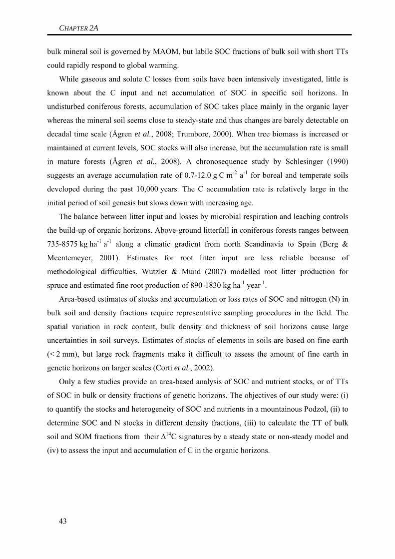
CHAPTER 2A
bulk mineral soil is governed by MAOM, but labile SOC fractions of bulk soil with short TTs
could rapidly respond to global warming.
While gaseous and solute C losses from soils have been intensively investigated, little is
known about the C input and net accumulation of SOC in specific soil horizons. In
undisturbed coniferous forests, accumulation of SOC takes place mainly in the organic layer
whereas the mineral soil seems close to steady-state and thus changes are barely detectable on
decadal time scale (Ågren et al., 2008; Trumbore, 2000). When tree biomass is increased or
maintained at current levels, SOC stocks will also increase, but the accumulation rate is small
in mature forests (Ågren et al., 2008). A chronosequence study by Schlesinger (1990)
suggests an average accumulation rate of 0.7-12.0 g C m-2 a-1 for boreal and temperate soils
developed during the past 10,000 years. The C accumulation rate is relatively large in the
initial period of soil genesis but slows down with increasing age.
The balance between litter input and losses by microbial respiration and leaching controls
the build-up of organic horizons. Above-ground litterfall in coniferous forests ranges between
735-8575 kg ha-1 a-1 along a climatic gradient from north Scandinavia to Spain (Berg &
Meentemeyer, 2001). Estimates for root litter input are less reliable because of
methodological difficulties. Wutzler & Mund (2007) modelled root litter production for
spruce and estimated fine root production of 890-1830 kg ha-1 year-1.
Area-based estimates of stocks and accumulation or loss rates of SOC and nitrogen (N) in
bulk soil and density fractions require representative sampling procedures in the field. The
spatial variation in rock content, bulk density and thickness of soil horizons cause large
uncertainties in soil surveys. Estimates of stocks of elements in soils are based on fine earth
(< 2 mm), but large rock fragments make it difficult to assess the amount of fine earth in
genetic horizons on larger scales (Corti et al., 2002).
Only a few studies provide an area-based analysis of SOC and nutrient stocks, or of TTs
of SOC in bulk or density fractions of genetic horizons. The objectives of our study were: (i)
to quantify the stocks and heterogeneity of SOC and nutrients in a mountainous Podzol, (ii) to
determine SOC and N stocks in different density fractions, (iii) to calculate the TT of bulk
soil and SOM fractions from their ∆14C signatures by a steady state or non-steady model and
(iv) to assess the input and accumulation of C in the organic horizons.
43

CHAPTER 2A
Material and methods
Site description
The study was performed in a mature Norway spruce forest (Picea abies L.) at an
elevation of 770 m above sea level in the Fichtelgebirge, SE Germany (50°08’N, 11°52’E).
The mean annual air temperature is 5.3°C with warm summers and cold continental winters.
Mean annual precipitation is approximately 1160 mm (Foken, 2003).
The natural vegetation consists of beech (Fagus sylvatica L.) and silver fir (Abies alba
Mill.) (Gerstberger et al., 2002). According to the forest administration, the area was almost
completely cleared between the 16th and 18th century in order to supply the mining industry
with construction wood and charcoal. The region was afforested with spruce trees during the
mid 19th century. Tree rings indicate a tree age of 140 years in 2008 for our study area. The
patchy ground vegetation is dominated by Deschampsia flexuosa (L.) and Calamagrostis
villosa (Chaix).
The Fichtelgebirge comprises large granite formations surrounded by metamorphic rock
series of gneiss, mica schists and phyllites. Erosion and solifluction formed the typical rock
and boulder fields. Podzolic soils developed from deeply weathered granite and are overlain
with a relatively thick humus layer (Gerstberger et al., 2002). Base saturations between 52 %
in the EA horizon and 40 % in the Bsh horizon indicate former application of lime to
counteract soil acidification (Hentschel et al., 2007). Carbonates, however, were not
chemically detectable in any soil horizons.
Sampling
Within an area of one hectare, nine randomly distributed (i.e. limited to between-tree and
between-boulder areas) soil pits of 0.7 m x 0.7 m were dug for area-based determination of
rock volume, bulk density (BD) and element contents down to the Cv horizon. The organic
(Oi, Oe, Oa) and mineral (EA, Bsh, Bs, Bv) horizons were consecutively removed and
separately weighed. The volume of stones was estimated by measuring the girth of the stones
at different positions and their total weight. A grid of 0.7 m x 0.7 m with 10 cm x 10 cm
increments was fixed over the surface of the soil pit to measure the height of each removed
soil horizon.
For each horizon, large stones, coarse roots and soil material were separately weighed in
the field. Subsamples of each horizon were sieved (< 2 mm) and then dried at 105°C over
48 hours to determine the gravimetric water content and the stone fraction. The bulk density
44

CHAPTER 2A
of fine earth (< 2 mm) was calculated by dividing its mass by the averaged volume of horizon
minus the volume of rocks and coarse roots. The rock weight was converted to rock volume
using a density of 2.45 g cm-3 for parent granite at the site.
Analyses
Soil pH was determined in a 0.01 M CaCl2 solution (soil:solution ratio 1:2.5).
Exchangeable cations (Na+, K+, Ca2+, Mg2+, Al3+, Fe3+) of the Oa and mineral soil horizons
were extracted with 1 M NH4Cl solution and then analysed by ICP-OES (Jobin-Yvon Horiba
Group, JY2000, USA). The amount of exchangeable H+ was calculated from the difference
between the pH-value of NH4Cl solution and the extracts. For C and N analysis a CNS
analyser (Heraeus Elementar Vario EL, Germany) was used.
Radiocarbon signatures of above-ground litter, bulk soil (including organic and mineral
soil horizons) and density fractions were determined by accelerator mass spectrometry
(AMS). Subsamples of 1 mg C were combusted in 6 mm sealed quartz tubes with 60 mg CuO
oxidizer and 1 cm silver wire for 2 hrs at 900°C. The resulting CO2 was purified from water
and non-condensable compounds. Afterwards, CO2 was reduced to graphite using the zinc
reduction method where TiH2 and Zn with Fe act as catalysts at 550° C for 7.5 hrs (Xu et al.,
2007). All preparations took place at the Department of Soil Ecology at the University of
Bayreuth. The graphite targets were analysed by the Keck-CCAMS facility of University of
California, Irvine, with a precision of 2-3 ‰. Radiocarbon data are expressed as ∆14C (‰
deviation was from the 14C/12C ratio of oxalic acid standard in 1950). The sample has been
corrected to a δ13C value of -25 ‰ to account for any mass dependent fractionation effects
(Stuiver & Polach, 1977).
Density fractionation of soil
Soil samples of the Oa and all mineral horizons from three randomly chosen soil pits were
fractionated by density separation. Dry soil samples were dispersed in sodium polytungstate
solution (SPT, Sometu, Berlin, Germany) using a similar procedure as described in detail by
John et al. (2005). Dry soil samples (< 2 mm, 60°C) were fractionated at densities of
1.6 g cm-3 and 2.0 g cm-3. For the Oa and EA horizon, 10 g soil and 40 ml of SPT with a
density of 1.6 g cm-3 were gently shaken. After sedimentation, the solution was centrifuged at
5085 g for 1 h (Varifuge 3.2RS). The supernatant was filtered through 0.45 µm pre-washed
cellulose-acetate-filter (Schleicher & Schuell, Germany) and the FPOM fraction < 1.6 g cm-3
was washed with 200 ml de-ionized water. Then the pellet was dispersed with 2.0 g cm-3 SPT 45

CHAPTER 2A
and 10 glass beads and was shaken for 16 hrs at 60 rpm and centrifuged at 5085 g for 1 h. The
supernatant with particles < 2.0 g cm-3 (OPOM) was filtered and washed (200 ml distilled
water) through 0.45 µm cellulose-acetate filters. The pellet thus obtained contained the
mineral associated organic matter fraction > 2.0 g cm-3 (MAOM). To remove the salt, the
pellet was washed three times with de-ionized water. For the Bsh, Bs and Bv horizons, 20 g
soil and 80 ml of SPT were used. The FPOM, OPOM, MAOM fractions and the used SPT
solution were freeze-dried and then finely ground with a ball mill for analyses of SOC and N
contents.
Turnover time (TT) of organic carbon
The TT for SOC in each fraction was calculated from its radiocarbon signature. Following
Gaudinski et al. (2000), we used a non-steady state model for the Oi, Oe, and Oa horizons.
We assumed that the buildup of the organic layer primarily started after reforestation in 1867,
but we cannot ignore the possibility that older organic matter is included in the present Oa
horizon (see below). The ∆14C signature of fresh spruce litter from the year 2006 (86 ± 1 ‰)
was close to the ∆14CO2 signature in the atmosphere (88.5 ‰) in the year 2000 (Levin et al.,
2008), indicating an average age of six years. Hence, this shift in the ∆14C was considered in
the calculation of TT.
The C input (I) in kg C m-2 a-1 added by litter production in each year t (since 1867, time
of reforestration) is represented in a sigmoid equation (e.g. Böttcher & Springob, 2001; Ågren
et al., 2008):
⎟⎠⎞
⎜⎝⎛ −−+
=
151900exp1
2006
atI
I t (1)
The term “1900a” in Equation 1 is the year of maximal increase of litter production and the
value “15” describes the slope of the graph.
The SOC stock and the ∆14C measured of each organic horizon in 2006 were then
calculated using Equations 2 and 3 (Gaudinski et al., 2000). We assumed zero initial SOC in
1867 in the Oi and Oe horizon. For the Oa horizon the model revealed an existing SOC stock
between 0.5-0.9 kg C m-2 in 1867 differing within the three soil pits.
(2) (∑=
=
−−−− ×+×=2006
1867
)2006()2006(18672006
t
t
tktk eIteCC )
46

CHAPTER 2A
where C is the SOC stock in a specific year (kg C m-2), I is the annual input rate
(kg C m-2 a-1), k is the decay constant of organic matter and reciprocally proportional to TT,
and t is the year since 1867.
( )
2006
)2006()6(
)18672006(1867)1867(
)2006( C
eIFeCFF
tkttatm
km
m
∑ −−−
−− ××+××= (3)
where Fm is the 14C/12C ratio in the fraction pool per year normalized to oxalic acid standard
and Fatm is the 14C/12C ratio of the atmosphere normalized to a oxalic acid standard (∆14CO2
signature of litter input in year t is equivalent to Fatm six years before).
From Equations 1 and 2 and the measured C stock in each organic horizon, we estimated
the turnover time (1/k) and C input rate (I) of the organic layer. Modern ∆14C has two possible
TTs for each ∆14C value (Trumbore, 2000). The ∆14C of the Oa horizons (107-132 ‰)
corresponds to TTs of either 4-7 or to 100-160 years. Given the type and thickness of the
organic layer we expect longer TTs to be more realistic.
For the mineral soil horizons, we used a time-dependent, steady state model as presented
in Gaudinski et al. (2000):
)1()1()1()()()( −×−×−−+×=× tCtFktFItCtF matmm λ (4)
where λ is the radioactive decay constant for 14C, and equal to 1/8267 year.
If the pool of SOC is at steady-state, then I=kC(t) and C(t) = C(t-1) reduce Equation 4 to:
)1()1()()( −×−−+×= tFktFktF matmm λ (5)
For the values of Fatm, we used radiocarbon data from dendrochronologically dated wood
samples (1844 to 1958) published by Stuiver et al. (1998) and atmospheric ∆14CO2 contents
after 1959 (Levin, 2008). A steady-state model was also used for the MAOM fraction of the
Oa horizon because we assumed that the MAOM fraction in the Oa horizon is partly a result
of biotic or abiotic mixing processes with mineral soil.
Statistics
The soil characterization was made with nine replicates and the data are presented as
mean and standard deviation (Table 1). STATISTICA 6.0 was used to display the
heterogeneity of SOC and N stocks between the nine soil pits (Figure 1). The density
fractionation and determination of ∆14C were made on three of the nine pits (Table 2,
Figure 2).
47

CHAPTER 2A
Results
Variation of physical and chemical properties in soil pits
The 7-10 cm thick organic layer consisted of litter (Oi), fermented (Oe) and humified (Oa)
horizons whereas the 43-60 cm thick mineral soil comprised EA, Bsh, Bs, and Bv horizons.
The mean bulk density increased from 0.07 g cm-3 in the Oi horizon to 1.17 g cm-3 in the Bv
horizon (Table 1). Mean volumetric rock contents increased from 7 % in the Oa horizon to
25 % in the Bv horizon with large variations among individual soil pits.
The SOC and N contents of the soil decreased with increasing depth from 45.8 % C in the
Oi horizon to 1.4 % C in the Bv horizon and from 1.7 % N to 0.2 % N, respectively (Table 1).
The C/N ratio ranged between 19 and 27 in the organic layer whereas C/N ratios (21-22) were
almost constant in the EA, Bsh and Bs horizons. SOC stocks increased from 2.8-4.9 kg C m-2
in the organic layer (sum of Oi, Oe and Oa horizons) to 2.2-7.9 kg C m-2 in the Bv horizon
(Figure 1a). Nitrogen stocks increased from 0.05-0.16 kg N m-2 in the organic layer to
0.17-0.51 kg N m-2 in the Bv horizon (Figure 1b). The total amount of SOC and N stored in
the nine soil pits were 13.1-20.3 kg C m-2 and 0.7-1.1 kg N m-2, where the organic layer
contributed 19–35 % to total SOC and 5–14 % to total N.
C and N in density fractions
The mean recovery of total soil mass after density fractionation varied between 92 % in
the Oa and 98 % in the Bv horizon (data not shown). These losses coincided with the mean
recovery of SOC between 90 and 96 % (Figure 2a). Some SOC was lost in the particulate
fraction during density fractionation but 2–6 % of SOC was dissolved in the SPT solution.
The mean recovery of N was smaller and ranged between 84 and 99 % (Figure 2b).
Consistently throughout the three soil pits, SOC contents ranged between 17-38 % C in
the FPOM and OPOM fraction, whereas the MAOM fraction contained no more than 2.7 % C
(data not shown). In the Oa and EA horizon, the major part of SOC was associated with
FPOM (Oa = 1.6 kg C m-2 and EA = 1.1 kg C m-2), whereas MAOM dominated the Bsh, Bs
and Bv horizons with 0.8-2.2 kg C m-2 (Figure 2). The SOC stock of the OPOM fraction was
the largest in the EA horizon (0.8 kg C m-2) followed by Bv (0.6 kg C m-2), Bsh
(0.6 kg C m-2), Oa (0.4 kg C m-2) and Bs horizons (0.3 kg C m-2). Overall, the soil stored
2.7-5.2 kg C m-2, 2.3-3.3 kg C m-2 and 4.0-4.9 kg C m-2 in the FPOM, OPOM and MAOM
fractions, respectively.
48

CHAPTER 2A
49
-2000 0 2000 4000 6000 8000 10000 12000 14000 16000 18000 20000 22000
SOC stock / kg m-2
Total
Bv
Bs
Bsh
EA
Oa
Oe
Oi
164 80 12 20
a
-200 0 200 400 600 800 1000 1200
N stock / kg m-2
Total
Bv
Bs
Bsh
EA
Oa
Oe
Oi
0 1.00.80.60.2 0.4
b
Figure 1 Box plots representing soil heterogeneity of (a) SOC and (b) N stocks in different genetic horizons of nine soil pits. The open square within the box marks the median, the black circle the mean and the boundaries of the box indicate the 25th and 75th percentile. Whiskers indicate the minimum and maximum SOC and N stocks.
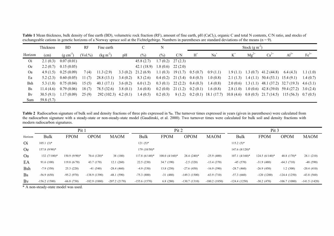
Table 1 Mean thickness, bulk density of fine earth (BD), volumetric rock fraction (RF), amount of fine earth, pH (CaCl2), organic C and total N contents, C/N ratio, and stocks of exchangeable cations in genetic horizons of a Norway spruce soil at the Fichtelgebirge. Numbers in parentheses are standard deviations of the means (n = 9).
HorizonOi 2.1 (0.3) 0.07 (0.01) 45.8 (2.7) 1.7 (0.2) 27 (2.3)Oe 2.2 (0.7) 0.15 (0.05) 42.1 (18.9) 1.8 (0.6) 22 (2.0)Oa 4.9 (1.5) 0.25 (0.09) 7 (4) 11.3 (2.9) 3.3 (0.2) 21.2 (6.9) 1.1 (0.3) 19 (1.7) 0.5 (0.7) 0.9 (1.1) 1.9 (1.1) 1.3 (0.7) 41.2 (44.8) 6.4 (4.3) 1.1 (1.0)Ea 5.2 (2.3) 0.60 (0.05) 11 (7) 28.8 (13.1) 3.4 (0.2) 8.3 (2.6) 0.4 (0.2) 21 (3.4) 0.4 (0.3) 1.0 (0.8) 2.1 (1.3) 1.4 (1.1) 50.4 (53.1) 15.4 (9.1) 1.4 (0.7)Bsh 5.3 (1.8) 0.75 (0.04) 15 (5) 40.1 (17.1) 3.6 (0.2) 6.0 (1.2) 0.3 (0.1) 22 (2.2) 0.4 (0.3) 1.4 (0.8) 2.0 (0.6) 1.3 (1.1) 48.1 (37.2) 32.7 (19.3) 4.6 (3.1)Bs 11.4 (4.6) 0.79 (0.06) 18 (7) 78.5 (32.6) 3.8 (0.1) 3.6 (0.8) 0.2 (0.0) 21 (1.2) 0.2 (0.1) 1.6 (0.8) 2.8 (1.0) 1.0 (0.6) 42.8 (39.0) 59.4 (27.2) 3.0 (2.4)Bv 30.5 (9.1) 1.17 (0.09) 25 (9) 292 (102.3) 4.2 (0.1) 1.4 (0.5) 0.2 (0.3) 8 (1.2) 0.2 (0.1) 18.1 (17.7) 10.8 (4.6) 0.8 (0.5) 21.7 (14.5) 115 (56.3) 0.7 (0.5)
Sum 59.8 (5.7)
Al3+ Fe3+
Stock (g m-2)
H+ Mg2+C/N Na+ K+ Ca2+
Thickness
(cm)
BD
(g cm-3)
RF
(Vol.%)
Fine earth N
(kg m-2) pH
C
(%) (%)
Table 2 Radiocarbon signature of bulk soil and density fractions of three pits expressed in ‰. The turnover times expressed in years (given in parentheses) were calculated from the radiocarbon signature with a steady-state or non-steady-state model (Gaudinski, et al. 2000). Two turnover times were calculated for bulk soil and density fractions with modern radiocarbon signatures.
Horizon
Oi 105.1 (3)* 121 (5)* 115.2 (5)*
Oe 157.8 (9/90)* 179 (10/50)* 147.6 (8/120)*
Oa 132 (7/100)* 150.9 (9/90)* 70.4 (120)* 38 (180) 117.8 (6/140)* 108.0 (4/160)* 28.4 (240)* -25.9 (400) 107.1 (4/160)* 124.5 (6/140)* 48.8 (170)* 28.1 (210)
EA 91.6 (100) 119.8 (6/70) 43.7 (170) 12.1 (260) 22.5 (230) 34.7 (190) -2.5 (320) -13.4 (370) -45 (570) -31.9 (480) -64.3 (710) -48 (590)
Bsh -7.9 (350) 25.3 (220) -41 (540) -28.4 (460) -4.9 (330) 13.8 (250) -27.6 (450) -16.9 (390) -28.7 (460) -26.9 (450) 1.2 (300) -20.4 (410)
Bs -56.9 (650) -95.2 (970) -138.9 (1390) -48.1 (590) -75.3 (800) -31 (480) -149.3 (1500) -63.9 (710) -57.3 (660) -120 (1200) -124.4 (1250) -43.8 (560)
Bv -156.2 (1580) -66.8 (730) -182.9 (1880) -207.2 (2170) -155.6 (1570) 6.8 (280) -130.7 (1310) -180.2 (1850) -124.4 (1250) -30.2 (470) -106.7 (1080) -141.5 (1420)
MAOMBulk FPOM OPOM MAOMPit 1 Pit 2 Pit 3
Bulk FPOM OPOM MAOMBulk FPOM OPOM
* A non-steady-state model was used.
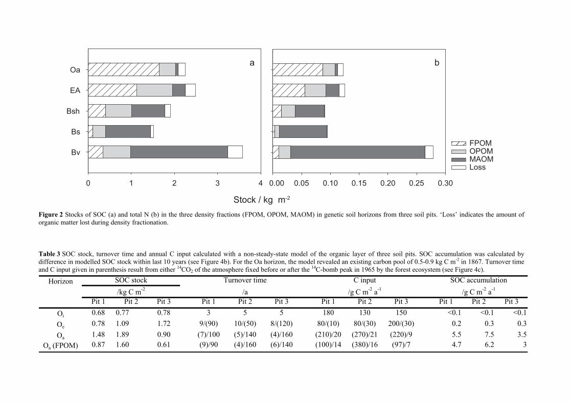
Pit 1 Pit 2 Pit 3 Pit 1 Pit 2 Pit 3 Pit 1 Pit 2 Pit 3 Pit 1 Pit 2 Pit 3Oi 0.68 0.77 0.78 3 5 5 180 130 150 <0.1 <0.1 <0.1Oe 0.78 1.09 1.72 9/(90) 10/(50) 8/(120) 80/(10) 80/(30) 200/(30) 0.2 0.3 0.3Oa 1.48 1.89 0.90 (7)/100 (5)/140 (4)/160 (210)/20 (270)/21 (220)/9 5.5 7.5 3.5
Oa (FPOM) 0.87 1.60 0.61 (9)/90 (4)/160 (6)/140 (100)/14 (380)/16 (97)/7 4.7 6.2 3
Horizon SOC stock/kg C m-2
SOC accumulation/g C m-2 a-1
Turnover time/a
C input /g C m-2 a-1
Table 3 SOC stock, turnover time and annual C input calculated with a non-steady-state model of the organic layer of three soil pits. SOC accumulation was calculated by difference in modelled SOC stock within last 10 years (see Figure 4b). For the Oa horizon, the model revealed an existing carbon pool of 0.5-0.9 kg C m-2 in 1867. Turnover time and C input given in parenthesis result from either 14CO2 of the atmosphere fixed before or after the 14C-bomb peak in 1965 by the forest ecosystem (see Figure 4c).
Figure 2 Stocks of SOC (a) and total N (b) in the three density fractions (FPOM, OPOM, MAOM) in genetic soil horizons from three soil pits. ‘Loss’ indicates the amount of organic matter lost during density fractionation.
b
Stock / kg m-2
0.00 0.05 0.10 0.15 0.20 0.25 0.30
aOa
EA
Bsh
Bs
BvFPOM OPOM MAOM Loss
0 1 2 3 4
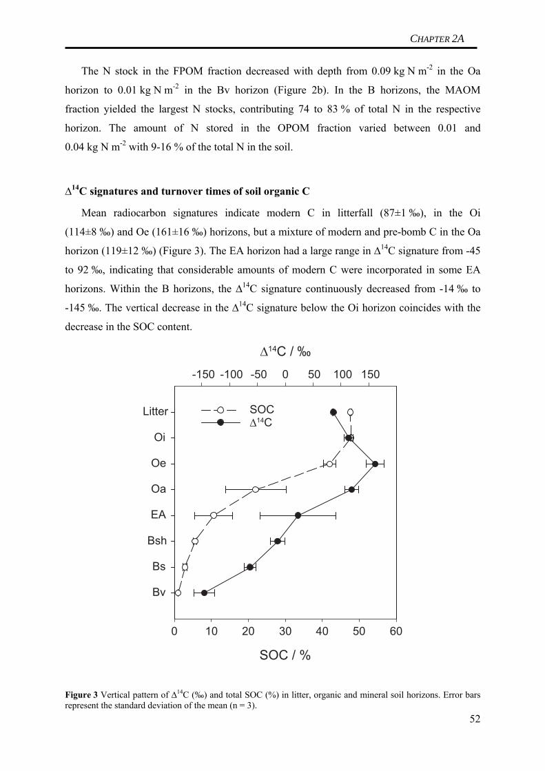
CHAPTER 2A
The N stock in the FPOM fraction decreased with depth from 0.09 kg N m-2 in the Oa
horizon to 0.01 kg N m-2 in the Bv horizon (Figure 2b). In the B horizons, the MAOM
fraction yielded the largest N stocks, contributing 74 to 83 % of total N in the respective
horizon. The amount of N stored in the OPOM fraction varied between 0.01 and
0.04 kg N m-2 with 9-16 % of the total N in the soil.
∆14C signatures and turnover times of soil organic C
Mean radiocarbon signatures indicate modern C in litterfall (87±1 ‰), in the Oi
(114±8 ‰) and Oe (161±16 ‰) horizons, but a mixture of modern and pre-bomb C in the Oa
horizon (119±12 ‰) (Figure 3). The EA horizon had a large range in ∆14C signature from -45
to 92 ‰, indicating that considerable amounts of modern C were incorporated in some EA
horizons. Within the B horizons, the ∆14C signature continuously decreased from -14 ‰ to
-145 ‰. The vertical decrease in the ∆14C signature below the Oi horizon coincides with the
decrease in the SOC content.
SOC / %
Litter
Oi
Oe
Oa
EA
Bsh
Bs
Bv
Δ14C / ‰
-150 -100 -50 50 100 150
SOCΔ14C
0
0 10 20 30 40 50 60
Figure 3 Vertical pattern of ∆14C (‰) and total SOC (%) in litter, organic and mineral soil horizons. Error bars represent the standard deviation of the mean (n = 3).
52

CHAPTER 2A
In Pit 1 and 2, the TT of SOC in bulk soil increased consistently with soil depth from the
organic horizons to the Bv horizon (Table 2). By contrast, Pit 3 had a less negative ∆14C
signature in Bsh (-28.7 ‰) compared with the EA horizon (-45.0 ‰), resulting in a difference
of 110 years in TT. The shorter TT of bulk SOC indicates that the Bsh horizon accumulated
more ‘young’ C than the Ea horizon.
Similar to the bulk soil, ∆14C signatures of density fractions generally decreased with soil
depth in the order FPOM>OPOM>MAOM (Table 2). One exception is the FPOM fraction of
the Bv horizon that had consistently younger SOC (6.8 to -66.8 ‰) with faster TT than the
respective FPOM fraction of the overlaying Bs horizon (-31 to -120 ‰). There was either an
input of ‘young’ SOC in the FPOM fraction of the Bv horizon or reversely an input of ‘old’
SOC or stabilization mechanisms in the FPOM fraction of the Bs horizon. Another exception
is the reverse order of ∆14C signatures and TT in the OPOM and MAOM fractions of the Bsh
(except in Pit 3) and the Bs horizon. In these horizons, MAOM had faster TT (390-710 years)
compared with the OPOM fraction (450-1500 years). The shift in the TT of the MAOM
fraction from the Bs horizon to the Bv horizon was relatively large in all three soil pits.
The isotopic balance approach revealed a wide spectrum for the lost fraction ranging from
modern SOC with mean ∆14C of 477 ‰ to relatively old SOC (-201 ‰) (data not shown).
There is no systematic pattern with soil depth or for specific soil horizons.
C input and storage in organic horizon
The annual C input to organic horizons and the FPOM fractions of the Oa horizon were
calculated from the non-steady-state model (Equation 2) and using the respective SOC stock
and TT (Table 3). Assuming sigmoid increase of litter input (Equation 1), the estimated C
input in the Oi horizon by aboveground litter varied between 130 and 180 g C m-2 a-1 in 2006.
C input rates in the Oe (80 g C m-2 a-1) and Oa (20 and 21 g C m-2 a-1) horizons were similar
in Pit 1 and 2. For the Oe horizon of Pit 3, we calculated (with a TT of 8 years) a much larger
C input of 200 g C m-2 a-1, which reflects the large C stock of 1.7 kg C m-2. Here, the C input
in the Oe horizon is greater than in the Oi horizon (150 g C m-2 a-1). Again, Pit 3 differs with
respect to the C input of 9 g C m-2 a-1 in the Oa horizon.
53
The modelled accumulation of SOC indicates that the Oi and Oe horizons are approaching
a steady-state with C accumulation smaller than 0.3 g C m-2 a-1 in the last 10 years (e.g. Pit 2,
Figure 4). The Oa horizon accumulated small amounts of SOC between 3.5 and
7.5 g C m-2 a-1 (Table 3), where most of that SOC was accumulated in the FPOM fraction
(3.0-6.2 g C m-2 a-1).

CHAPTER 2A
54
Discussion
Heterogeneity of soil chemical properties
The Podzol at our study site contained 13.1-20.3 SOC kg m-2 and 0.7-1.1 N kg m-2 down to a
mean mineral soil depth of 60 cm (Figure 1). These values are smaller than the mean SOC
(29.6 kg m-2) and N stock (1.96 kg N m-2) in the top 1 m of European Podzol soils (Batjes,
2002). Even small SOC and N contents in the subsoil may considerably contribute to total
stocks. Several authors (e.g., Canary et al., 2000; Harrison et al., 2003) have emphasized that
soils should be sampled to a maximum depth for accurate estimates of total SOC and N
stocks. However, big rocks did not allow extending the depth in soil pits, and thus, total SOC
and N stocks are relatively small at our study site.
Large amounts of SOC (19-35 % of total) and N (5-14 % of total) highlight the
importance of the organic layer as SOC and N reservoirs in Podzols. Under coniferous forests,
Podzols may accumulate large amounts of SOM in the organic layer within decades, making
it vulnerable to climate change and other disturbances. An accurate, area-based estimate to
detect changes of SOC and N stocks is hampered by the enormous spatial heterogeneity. In
our study, varying thickness (7-10 cm) was the main reason for the large heterogeneity in C
and N stock of the organic layer whereas bulk density, SOC and N contents were less
variable.
The mineral soil down to 60 cm stores more SOC and N at our site than the organic layer.
Because of slow TTs (see below), changes in the SOC stocks are generally small unless
strong disturbances of the soil structure accelerate the decay of SOM. Changes in the N stock,
however, could possibly be much faster in forests with large atmospheric N deposition. In
view of climatic or other environmental changes, SOC and N stocks of mineral horizons are
required for better understanding of C and N cycling in soils. At our site, the Bv horizon
stored approximately twice as much SOC and N than the EA, Bsh and Bs horizons. The large
heterogeneity of SOC and N stocks in the whole mineral soil is attributed to differences in the
thickness (43-60 cm), rock fraction (12-29 % by volume) and the amount of fine earth
(312-512 kg m-2) among the soil pits.
SOC and N in density fractions
The portion of the FPOM fraction decreases and the portion of the MAOM fraction to
total SOC stock increased with soil depth, whereas the OPOM fraction was almost evenly
distributed throughout the soil pits (Figure 2). Large FPOM fractions in the Oa and EA

CHAPTER 2A
C in
put /
kg
C m
-2 a
-1
0.00
0.05
0.10
0.15
0.20OiOeOa
SO
C s
tock
/ kg
C m
-2
0
1
2
3
Organic HorizonOiOeOa
a
Time / year
1880 1900 1920 1940 1960 1980 2000
Δ14 C
sig
natu
re /
‰
0
200
400
600
800AtmosphereOiOeOa
c
b
Figure 4 Carbon inputs from litter (a), SOC stocks (b), and 14C signature of the atmosphere and of SOC (Pit 2 only) (c) in organic horizons from 1867 to 2006 as estimated from a non-steady state model.
55

CHAPTER 2A
horizon point to low rates of degradability of spruce litter and reduced microbial
activitycompared with other litter types and less acid soils (John et al., 2005). Provided that
the FPOM fraction of 0.7-1.1 kg C m-2 (9-16 %) and 0.02-0.04 kg N m-2 (5-8 %) in the B
horizons is accessible for microbial attack, the soil has a large potential for C and N losses.
However, the slow TT of FPOM suggests that it contains not only fresh and non-decomposed
material, but also charred plant debris (black carbon) as identified by Marschner et al. (2008).
‘Recalcitrant’ compounds such as lignin, lipids, and their derivates could constitute a
considerable proportion of the FPOM fraction although their TTs are much faster than
previously thought (Marschner et al. (2008). Another mechanism, the stabilization of DOC by
precipitation with dissolved aluminium (Scheel et al., 2007) could possibly contribute to the
slow TT of the FPOM fraction from the mineral soil. Our results contradict the concept that
the FPOM fraction corresponds to the active SOC pool with TT < 10 years.
The N content and C/N ratio of SOM fractions may play an important role in their
stability. Decreasing C/N ratios in the order OPOM>FPOM>MAOM (not shown) are in
accordance with the observation by Golchin et al. (1994). The large N content of MAOM is
primarily related to the advanced degradation of organic C compounds. However, a N
fertilization experiment suggests that ‘newly’ added N is partly retained in slow SOM pools,
enhancing thereby its stability against microbial decay (Hagedorn et al., 2003). If this
stabilization mechanism is relevant, then the size and TT of SOM fractions should have been
altered under the large N deposition rate at our study site during recent decades.
The Oa horizon is generally not considered for density fractionation although this horizon
often contains a mineral fraction. Here, MAOM contributes 33 % to total mass in the Oa
horizon, but the SOC stock of 2.3 % was relatively small. Despite the small SOC stock in the
OPOM and MAOM fractions, their ∆14C signatures influence the TT of the Oa horizon (Table
2). In the case of Pit 2, however, all three density fractions had smaller ∆14C signatures than
the bulk Oa horizon. A non-characterized fraction of SOC and N was lost by the density
fractionation either as particulate or as dissolved forms in SPT solution. The mass balance
approach implied that the missing fraction varied from modern SOC with mean ∆14C
signature of 477 ‰ to relatively old SOC (-201 ‰), representing a SOC stock of
approximately 0.9-1.3 kg C m-2 down to 60 cm depth. Crow et al. (2007) found extractable
young organic matter for deciduous forest soil and assumed that less degraded substrates were
removed during density fractionation. Hence, the lost fraction seems to play an important role
in the turnover of SOM in forest soils.
56

CHAPTER 2A
Turnover time (TT), input and accumulation of SOC in organic horizons
The estimated annual C input in the Oi horizon by aboveground litterfall varied between
130 and 180 g C m-2 a-1 in 2006. A mean annual litter input of 107 g C m-2 a-1 (assuming a C
content of 50 %) was measured in an adjacent Norway spruce stand of the same age (Berg,
2004). This input rate, however, does not include branches, twigs, cones and ground
vegetation which may contribute considerably to total above-ground litter input.
The C input in the Oe and Oa horizon comprises the transfer of partly decomposed and
humified aboveground litter from the Oi or Oe horizon, respectively, and the input of root
litter. In case of the Oe and Oa horizon, root litter input probably increased with the build-up
of these horizons. The present input of 200 g C m-2 a-1 in the Oe horizon of Pit 3 can be
explained by the contribution from root litter, cones or twigs to the buildup of this relatively
large SOC stock. In fact, total mass of live coarse roots and cones were 2.5 to 4.5 times
greater in Pit 3 than in Pit 1 and 2.
In the first decades of afforestration, SOC stocks increased rapidly in the Oi and Oe
horizons and reached nearly steady-state after 80-100 years (Figure 4). In the past decade, the
rate of SOC accumulation was smaller than 0.1 g C m-2 a-1 for the Oi horizon and
approximately 0.3 g C m-2 a-1 for the Oe horizon. Fast TT of SOC (3-10 years) highlights the
potential of these horizons to respond rapidly to an increase in temperature. It has been
demonstrated that along an elevation gradient, TT of SOC in the topsoil is controlled by
temperature (Trumbore et al., 1996).
The radiocarbon signature indicates that the Oa horizon was partly formed from SOC
before afforestration. In our model, the SOC stock did not increase during the first 30 years
after afforestration which we attribute to the delay in the production and transfer of humified
organic matter in the Oe horizon. In the present Oa horizon, the turnover rate (100-160 years)
is slow enough to allow the annual C input to result in a SOC accumulation of
3.5-7.5 g C m-2 a-1. Almost all of this C input is accumulating in the FPOM fraction whereas
the OPOM and MAOM fractions yield SOC close to a steady-state condition.
Overall, SOC accumulation rate of the organic layer (3.8-7.8 g C m-2 a-1) is in good
agreement with estimates of 2-7 g C m-2 a-1 for a mixed deciduous forest (Gaudinski et al.,
2000). Slightly larger accumulation rates of 12-13 g C m-2 a-1 were estimated for coniferous
soils in Sweden (Ågren et al., 2008). One reason for small accumulation rates at our study site
could be the application of lime to the soil surface, which is often reported to improve soil
conditions and thus to increase the mineralization of SOM (e.g. Persson, 1989; Fuentes et al.,
2006).
57
CHAPTER 2A
Turnover time (TT) of SOC in mineral soil fractions
The TT of SOC in bulk samples increased with soil depth and exhibited little variation
among the three soil pits. As with Pits 1 and 2, many studies found increasing TT with
increasing soil depth and density (e.g., Bol et al., 1999; Trumbore, 2000; Gaudinski et al.,
2000; Certini et al., 2004; Eusterhues et al., 2007), pointing to increasing stabilization of SOC
by minerals at greater depth.
The FPOM, OPOM and MAOM fractions indicate the existence of C pools with different
turnover times which are associated with the degree of degradation and humification (Baisden
et al., 2002: John et al., 2005). For the EA and Bv horizon, TT followed a typical pattern in
the order FPOM<OPOM<MAOM. In the Bsh and Bs horizon, however, the MAOM fraction
had faster TT than the OPOM fraction. We attribute this finding to the sorption of DOC with
a less negative ∆14C signature by Fe and Al oxides/hydroxides in the MAOM fraction.
Sorption of DOC in spodic horizons is a typical process of Podzols and largely contributes to
the SOC stock of the Bsh and Bs horizon in the long run. The intrinsic TT of the MAOM
fraction in these spodic horizons is probably much faster as predicted by our model approach.
Hentschel et al. (2009) reported radiocarbon signatures of -65 to +38 ‰ for DOC in the soil
solution below the Oa horizon at our study site. The radiocarbon signatures of DOC decreased
to between -25 and -265 ‰ at 90 cm mineral soil depth and these are within the range of the
FPOM fraction. The time span between the formation of DOC from ‘old’ particulate SOM
and sorption by the soil matrix in the Bsh and Bs horizon could be relatively short.
A substantial shift in the ∆14C signature and TT of the MAOM fraction was observed from
the Bs to the Bv horizon in all three soil pits. Again, this shift supports the sorption of DOC in
the MAOM fraction of the Bsh and Bs horizon. Turnover times of 1080-2170 years in the
OPOM and MAOM fractions of the Bv horizon may be explained by small input of
particulate and dissolved organic matter and strong physical and chemical stabilization.
Conclusion
• The present soil was a small sink for atmospheric CO2 in the order of 4-8 g C m-2 a-1
during the past 10 years and might be a net CO2 sink of similar order in the near future at
similar boundary conditions. Most of SOC accumulated in the FPOM fraction of the Oa
horizon whereas other organic and mineral soil horizons were in, or close to, steady-state.
Sorption of DOC in the Bsh and Bs horizon seems to affect the radiocarbon signature of
58

CHAPTER 2A
the MAOM fraction, but turnover times of 390-710 years mask the true contribution to
accumulation of SOC in these spodic horizons.
• The C and N stock of the organic layer is vulnerable to changes in climate conditions or
other disturbances. The turnover time of non-stabilized SOM will probably decrease with
increasing temperature and turn the soil from a small sink to a transient source.
• The density fractionation method revealed some uncertainties. Firstly, a portion of SOM
was either lost as particulate or dissolved SOM in the order of up to 10 % (SOC) and
16 % (N). This lost fraction is generally not characterized, but might participate in the C
and N cycle of soils. Secondly, the FPOM fraction, often associated with the active pool
of SOC, had slow turnover times on the decadal-centennial time scale in all soil horizons.
It seems that recalcitrance of SOM or stabilization processes cause a slow turnover of the
FPOM fraction in this forest soil.
• The spatial variation of SOC and total N stocks in genetic horizons and density fractions
was relatively large in this rocky forest soil, highlighting the importance of representative
sampling approaches. The radiocarbon signatures of bulk soil and density fractions
exhibited a small variation among the three pits, except the EA horizon where differences
in bioturbation have apparently affected the spatial heterogeneity. Even in heterogeneous
soils, measurements of the ∆14C signature provide a powerful tool for the assessment of C
accumulation in forest soils.
Acknowledgements
This research was financially supported by the Deutsche Forschungsgemeinschaft (DFG),
Research Unit 562. We thank the members of the Central Analytic Department of the
Bayreuth Centre of Ecology and Environmental Research (BayCEER) for chemical analysis
of soil extracts and Roland Blasek, Stefanie Goldberg, Uwe Hell, Andreas Puhr, Andrea
Schmitt and Steve Wunderlich for their help in the field.
References
Ǻgren, G.I., Hyvönen, R. & Nilsson, T. 2008. Are Swedish forest soils sinks or sources for
CO2 – model analyses based on forest inventory data. Biogeochemistry, 89, 139–149.
Baisden, W.T., Amundson, R., Cook, A.C. Brenner, D.L. 2002. Turnover and storage of C
and N in five density fractions from California annual grassland surface soils. Global
Biogeochemical Cycles, 16, 1117–1134.
59
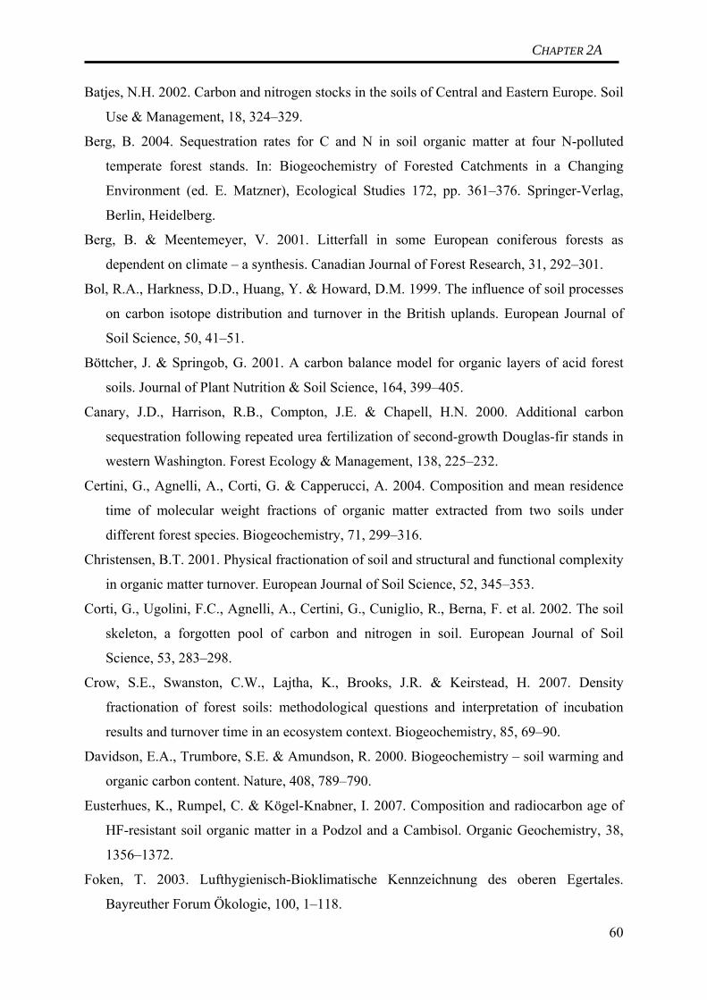
CHAPTER 2A
Batjes, N.H. 2002. Carbon and nitrogen stocks in the soils of Central and Eastern Europe. Soil
Use & Management, 18, 324–329.
Berg, B. 2004. Sequestration rates for C and N in soil organic matter at four N-polluted
temperate forest stands. In: Biogeochemistry of Forested Catchments in a Changing
Environment (ed. E. Matzner), Ecological Studies 172, pp. 361–376. Springer-Verlag,
Berlin, Heidelberg.
Berg, B. & Meentemeyer, V. 2001. Litterfall in some European coniferous forests as
dependent on climate – a synthesis. Canadian Journal of Forest Research, 31, 292–301.
Bol, R.A., Harkness, D.D., Huang, Y. & Howard, D.M. 1999. The influence of soil processes
on carbon isotope distribution and turnover in the British uplands. European Journal of
Soil Science, 50, 41–51.
Böttcher, J. & Springob, G. 2001. A carbon balance model for organic layers of acid forest
soils. Journal of Plant Nutrition & Soil Science, 164, 399–405.
Canary, J.D., Harrison, R.B., Compton, J.E. & Chapell, H.N. 2000. Additional carbon
sequestration following repeated urea fertilization of second-growth Douglas-fir stands in
western Washington. Forest Ecology & Management, 138, 225–232.
Certini, G., Agnelli, A., Corti, G. & Capperucci, A. 2004. Composition and mean residence
time of molecular weight fractions of organic matter extracted from two soils under
different forest species. Biogeochemistry, 71, 299–316.
Christensen, B.T. 2001. Physical fractionation of soil and structural and functional complexity
in organic matter turnover. European Journal of Soil Science, 52, 345–353.
Corti, G., Ugolini, F.C., Agnelli, A., Certini, G., Cuniglio, R., Berna, F. et al. 2002. The soil
skeleton, a forgotten pool of carbon and nitrogen in soil. European Journal of Soil
Science, 53, 283–298.
Crow, S.E., Swanston, C.W., Lajtha, K., Brooks, J.R. & Keirstead, H. 2007. Density
fractionation of forest soils: methodological questions and interpretation of incubation
results and turnover time in an ecosystem context. Biogeochemistry, 85, 69–90.
Davidson, E.A., Trumbore, S.E. & Amundson, R. 2000. Biogeochemistry – soil warming and
organic carbon content. Nature, 408, 789–790.
Eusterhues, K., Rumpel, C. & Kögel-Knabner, I. 2007. Composition and radiocarbon age of
HF-resistant soil organic matter in a Podzol and a Cambisol. Organic Geochemistry, 38,
1356–1372.
Foken, T. 2003. Lufthygienisch-Bioklimatische Kennzeichnung des oberen Egertales.
Bayreuther Forum Ökologie, 100, 1–118.
60
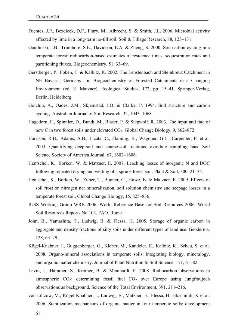
CHAPTER 2A
Fuentes, J.P., Bezdicek, D.F., Flury, M., Albrecht, S. & Smith, J.L. 2006. Microbial activity
affected by lime in a long-term no-till soil. Soil & Tillage Research, 88, 123–131.
Gaudinski, J.B., Trumbore, S.E., Davidson, E.A. & Zheng, S. 2000. Soil carbon cycling in a
temperate forest: radiocarbon-based estimates of residence times, sequestration rates and
partitioning fluxes. Biogeochemistry, 51, 33–69.
Gerstberger, P., Foken, T. & Kalbitz, K. 2002. The Lehstenbach and Steinkreuz Catchment in
NE Bavaria, Germany. In: Biogeochemistry of Forested Catchments in a Changing
Environment (ed. E. Matzner), Ecological Studies, 172, pp. 15–41. Springer-Verlag,
Berlin, Heidelberg.
Golchin, A., Oades, J.M., Skjemstad, J.O. & Clarke, P. 1994. Soil structure and carbon
cycling. Australian Journal of Soil Research, 32, 1043–1068.
Hagedorn, F., Spinnler, D., Bundt, M., Blaser, P. & Siegwolf, R. 2003. The input and fate of
new C in two forest soils under elevated CO2. Global Change Biology, 9, 862–872.
Harrison, R.B., Adams, A.B., Licata, C., Flaming, B., Wagoner, G.L., Carpenter, P. et al.
2003. Quantifying deep-soil and coarse-soil fractions: avoiding sampling bias. Soil
Science Society of America Journal, 67, 1602–1606.
Hentschel, K., Borken, W. & Matzner, E. 2007. Leaching losses of inorganic N and DOC
following repeated drying and wetting of a spruce forest soil. Plant & Soil, 300, 21–34.
Hentschel, K., Borken, W., Zuber, T., Bogner, C., Huwe, B. & Matzner, E. 2009. Effects of
soil frost on nitrogen net mineralization, soil solution chemistry and seepage losses in a
temperate forest soil. Global Change Biology, 15, 825–836.
IUSS Working Group WRB 2006. World Reference Base for Soil Resources 2006. World
Soil Resources Reports No 103, FAO, Rome.
John, B., Yamashita, T., Ludwig, B. & Flessa, H. 2005. Storage of organic carbon in
aggregate and density fractions of silty soils under different types of land use. Geoderma,
128, 63–79.
Kögel-Knabner, I., Guggenberger, G., Kleber, M., Kandeler, E., Kalbitz, K., Scheu, S. et al.
2008. Organo-mineral associations in temperate soils: integrating biology, mineralogy,
and organic matter chemistry. Journal of Plant Nutrition & Soil Science, 171, 61–82.
Levin, I., Hammer, S., Kromer, B. & Meinhardt, F. 2008. Radiocarbon observations in
atmospheric CO2: determining fossil fuel CO2 over Europe using Jungfraujoch
observations as background. Science of the Total Environment, 391, 211–216.
von Lützow, M., Kögel-Knabner, I., Ludwig, B., Matzner, E., Flessa, H., Ekschmitt, K et al.
2006. Stabilization mechanisms of organic matter in four temperate soils: development
61

CHAPTER 2A
62
and application of a conceptual model. Journal of Plant Nutrition & Soil Science, 171,
111–124.
Marschner, B., Brodowski, S., Dreves, A., Gleixner, G., Gude, A., Grootes, P.M. et al. 2008.
How relevant is recalcitrance for the stabilization of organic matter in soils? Journal of
Plant Nutrition & Soil Science, 171, 91–110.
Persson, T., Lundkvist, H., Wiren, A., Hyvönen, R. & Wessen, B. 1989. Effects of
acidification and liming on carbon and nitrogen mineralization and soil organisms in mor
humus. Water, Air & Soil Pollution, 45, 77–96.
Poirier, N., Sohi, S.P., Gaunt, J.L., Mahieu, N., Randall, E.W., Powlson, D.S. et al. 2005. The
chemical composition of measurable soil organic matter pools. Organic Geochemistry, 36,
1174–1189.
Scheel, T., Dörfler, K. & Kalbitz, K. 2007. Precipitation of dissolved organic matter by
aluminium stabilizes carbon in acidic forest soils. Soil Science Society of America
Journal, 71, 64–74.
Schlesinger, W.H. 1990. Evidence from chronosequence studies for a low carbon-storage
potential of soils. Nature, 348, 232–234.
Stuiver, M. & Polach, H.A. 1977. Discussion: reporting of 14C Data. Radiocarbon, 19, 355–
363.
Stuiver, M., Reimer, P.J. & Braziunas, T.F. 1998. High-precision radiocarbon age calibration
for terrestrial and marine samples. Radiocarbon, 40, 1127–1151.
Torn, M.S., Trumbore, S.E., Chadwick, O.A., Vitousek, P.M. & Hendricks, D.M. 1997.
Mineral control of soil organic carbon storage and turnover. Nature, 389, 170–173.
Trumbore, S.E. 2000. Age of soil organic matter and soil respiration: radiocarbon constraints
on belowground C dynamics. Ecological Applications, 10, 399–411.
Trumbore, S.E., Chadwick, O.A. & Amundson, R. 1996. Rapid exchange between soil carbon
and atmospheric carbon dioxide driven by temperature change. Science, 272, 393–396.
Wutzler, T. & Mund, M. 2007. Modelling mean above and below ground litter production
based on yield tables. Silva Fennica, 41, 559–574.
Xu, X., Trumbore, S.E., Zheng, S., Southon, J.R., McDuffee, K.E., Luttgen, M. et al. 2007.
Modifying a sealed tube zinc reduction method for preparation of AMS graphite targets:
reducing background and attaining high precision. Nuclear Instruments & Methods in
Physics Research Section B: Beam Interactions with Materials and Atoms, 259, 320–329.

CHAPTER 2B
PART B:
Carbon dynamics in a temperate minerotrophic fen Jan Muhr1*), Juliane Höhle1) and Werner Borken1)
1) Department of Soil Ecology, University of Bayreuth, Dr.-Hans-Frisch-Strasse 1-3, 95448
Bayreuth, Germany
*Corresponding author: Jan Muhr ([email protected])
Submitted to Biogeochemistry
Received 23 July 2009
Abstract
Globally, peatlands represent important C storage pools that are supposed to be vulnerable
to climate change. Understanding of C dynamics in peatland soils is relevant for predicting
the effects of changing boundary conditions on peatland C pools. Here, we present the C
stocks and turnover rates of vegetation and soil organic matter (SOM) in a minerotrophic
temperate fen in South-eastern Germany. In order to model soil C balance in the peat body we
distinguished four C pools: (1) Aboveground biomass (relevant as input pool only), (2) root
biomass (comprising live and intact dead roots), (3) surface peat soil organic matter (SOM)
between 0-15 cm (defined by the occurrence of bomb 14C), and (4) deeper peat SOM (defined
by the predominance of pre-bomb 14C). We calculated stocks of these pools and input and
output fluxes. For aboveground biomass, we measured a stock of 173 g C m-2. Aboveground
vegetation at the site completely dies off at the end of the year, so annual input and output
fluxes were equal to stock. Root biomass C stock was found to be significantly higher at this
fen, comprising 1315 g C m-2. We found high gross fluxes for the root biomass stock (input
242 versus output 266 g C m-2 a-1) and calculated a negative net C balance. Gross fluxes of the
surface layer SOM stock were also considerably high (total input 308 versus total output
313 g C m-2 a-1), and net C balance was negative. Gross C fluxes of deeper layers were
comparatively small (input 6.1 versus output 3.3 g C m-2 a-1), but indicated a small net C
accumulation. Total SOM C net balance for the whole peat profile was slightly negative (-
2 g C m-2 a-1), total net soil C fluxes (root biomass + SOM) were strongly negative (-
27 g C m-2 a-1). Thus, this fen site has been identified as a net source of C, indicating a
disturbance of boundary conditions. Due to fast turnover of the root biomass and surface
63

CHAPTER 2B
SOM stock, this conclusion is only valid on a decadal timescale, so we can neither determine
how long the fen has been a net C source nor how long it will continue to be one.
Keywords: Soil carbon balance, peat accumulation, radiocarbon, SOM turnover, root turnover
64

CHAPTER 2B
Introduction
Peatlands cover only approximately 3.5% of the earth’s surface (Gorham 1991), but form
an important carbon (C) store, especially in the northern hemisphere. Correcting earlier
calculations made by Gorham (1991), Turunen et al. (2002) estimated global C stores in
peatlands between 270-370 Pg (1015 g) of C, which would account for around 20-25% of the
1500 Pg C stored in soils worldwide (Schlesinger and Andrews 2000). These high amounts of
C stored in peatlands result from an imbalance between input and decomposition of organic
matter in peatlands. Due to high water tables, decomposition in peatland soils often is limited
by oxygen availability. Since the retreat of the last ice age, this has led to the formation of
thick peat bodies. The high amounts of C stored in peatlands has put them into the focus of
interest under the impression of climate change scenarios predicting altered water tables and
temperature increase. The question is whether peatlands, thousands of years after beginning of
their formation due to the retreat of the last ice age, continue to accumulate C under current
climatic conditions, and if so at which rates.
Radiocarbon (14C) has proven to be a powerful tool to investigate ecosystem C dynamics
that has been applied in various studies (Trumbore et al. 1995, Trumbore and Harden 1997,
Gaudinski et al. 2000, Schulze et al. 2009). Natural 14C can be used to determine soil C
dynamics on timescales of centuries to millenia, and therefore is a suitable tool to examine the
C balance of deep organic layers in peatlands. Atmospheric nuclear weapon testing in the
1950s produced high amounts of ‘bomb 14C’, nearly doubling the atmospheric 14C content
(Levin et al. 2008). Due to combustion of 14C-free fossil fuels and mixing of the atmospheric 14C pool with terrestrial and marine C pools, the atmospheric 14C content continuously
decreased since the end of the nuclear weapon testing. Incorporation of atmospheric CO2
(with the specific 14C signature of the year of incorporation) into biomass results in a specific
isotopic ‘labeling’ of annual litter input. Hence, bomb 14C can be used to constrain soil C
balance over the last few decades. Using these two tools, total C accumulation can be resolved
into the balance of short- and long-term-averaged inputs and decomposition. Here, we present
the soil C balance of a temperate fen site (Schlöppnerbrunnen) in southern Germany. This site
has been used in a number of other studies (Knorr et al. 2009; Muhr et al. 2009; Otieno et al.
2009; Reiche et al. 2009) concerning different aspects of the C cycle.
65
CHAPTER 2B
Material and Methods
Site description
The Schlöppnerbrunnen fen site is located in the Lehstenbach catchment (Fichtelgebirge,
Northeastern Bavaria, Germany, 50°07’54’’N, 11°52’51’’E). The site is characterized as a
temperate minerotrophic fen covering an area of 0.8 ha at an elevation of ca. 750 m a.s.l. The
soil is a Histosol on granite bedrock covered mainly by Molinia caerulea (L. Moench),
Nardus stricta (L.), Agrostis canina (L.), Carex rostrata (Stokes) and Eriophorum vaginatum
(L.). Mean annual temperature (1995-2007) is 6.3 ± 0.9 °C and mean annual precipitation
(1995-2007) is 1020 ± 203 mm a-1 (Knorr 2009). The site features a slope from NNE to SSW
and groundwater flows slowly through the site parallel to this slope (Paul et al. 2006). Since
the last deglaciation, a peat body with a thickness between 40-70 cm has accumulated. The
site features a water table gradient, with the north-western part being waterlogged more often
than the south-eastern part. A ditch of unknown origin and history runs through the site
parallel to the slope.
Definition of our system
In this study we were interested in the size and dynamics of C storage pools in the soil of a
temperate fen. A major issue was the question whether the soil under current boundary
conditions is a source or a sink of C. To answer this question, we defined relevant C stocks
and fluxes based on the following considerations: (i) All C that is stabilized in the soil initially
enters the system via photosynthetic assimilation; (ii) only assimilates that are used to form
biomass (above- or below-ground) can result in stabilization of C in the soil, metabolic
respiration of living biomass represents a direct recirculation of assimilates to the atmosphere;
(iii) decomposition of aboveground litter occurs fast and the total aboveground litter pool can
be assumed to be in steady state; (iv) transfer of C from root biomass (live and dead) to soil
organic matter (SOM) can occur with a marked delay due to limited decomposition rates
within the peat; (v) changing boundary conditions can result in non-steady state of the below-
ground litter pool; (vi) input into SOM pools occurs via litter decomposition and due to up-
down transfer between SOM pools within the peat profile. A schematic overview over the C
stocks and fluxes we distinguished to calculate the soil C balance of the peat body of this fen
site is presented in Figure 1.
66

CHAPTER 2B
67
AtmosphericCO2
MetabolicPlantRespiration
(above- and below-ground)
SOM(depth specific
SOM pools)
AssimilatePool
Biomass
Biomass Litter (undecomposed)
0
1
2
3
0
Figure 1. Schematic overview to illustrate the C pools we distinguished when modelling soil C balance in this study. We measured C stocks fluxes of (1) aboveground biomass, (2) below-ground biomass, and (3) depth-specific SOM pools. We did not quantify total C uptake by assimilation and respiration resulting from living biomass (0), as these were regarded irrelevant for the soil C balance. With our approaches, we can determine output fluxes from C stock pools, but we can not distinguish which proportion of these output fluxes is redirected to other soil C pools and which proportion is lost from the system.
Quantifying C stocks and fluxes
We combined a variety of different methods to quantify C stocks in aboveground and
below-ground biomass and in soil organic matter (SOM), annual litter production from above-
and below-ground biomass, and C input and output fluxes into SOM. Combining all results
we quantified the soil C balance of the Schlöppnerbrunnen fen. Table 1 gives an overview
over the different methods used to quantify C stocks fluxes.
Biomass
Aboveground biomass was determined by the harvesting method on a total of 12 plots,
each 39 x 39 cm2. These 12 plots were located in the immediate vicinity of the soil coring
locations. Harvesting took place in September of 2007 at the end of the vegetation period. We
combined this data set with biomass data for the site from Otieno et al. (2009). This second
data set comprises monthly measurements from May to October of 2007. All aboveground
biomass dies off at the end of the vegetation period, so annual aboveground litter input was

CHAPTER 2B
Table 1. Methods applied in this study to quantify C stocks and turnover.
Variable MethodC Stock
Aboveground biomass HarvestingBelow-ground biomass Harvesting (depth specific) (data from Otieno et al. 2009)SOM Soil coring (depth specific, using bulk density and organic C content)
TurnoverAboveground biomass Complete turnover of annual productionBelow-ground biomass Non-steady state 14C based model (Gaudinski et al. 2000)SOM, surface layers Non-steady state 14C based model (Gaudinski et al. 2000)SOM, deeper layers Equation (2) fit to cumulative C stock versus time plot (Trumbore 1999)
assumed to be equal to annual biomass production. The C content of aboveground biomass
was assumed 0.5 of total dry biomass.
Below-ground biomass data (roots) was taken from Otieno et al. (2009), who measured
root biomass in 2007 down to a depth of 30 cm at the Schlöppnerbrunnen fen site. We
measured the mean radiocarbon signature of structural C of the root biomass. As it was
impossible to distinguish intact (undecomposed) dead and live roots at the site, we defined
one universal root C pool comprising live roots and undecomposed root litter (decomposed
root litter is comprised in the SOM pool). Root litter in peatlands can feature long turnover
times due to adverse decomposition conditions. Thus, we used the same 14C based non-steady
accumulation model to describe this root biomass pool that was used to describe the fast-
cycling surface SOM pools (see below). This results in a root biomass C stock that is allowed
to increase or decrease depending on input (biomass production) and output (decomposition)
fluxes. These input and output fluxes were calculated by adjusting a non-steady state
accumulation model to describe best the measured root C stock and 14C ratio (for details see
below).
Soil organic matter (SOM)
In the summer of 2007, six soil cores (0-80 cm) were sampled by using soil corers (Ø
3cm). According to visual criteria and decomposition status, the soil cores were separated into
three subsections (weakly decomposed organic horizon; intermediate horizon; mineral
horizon). Each of these subsections was further divided into 5 cm segments for analysis. We
measured soil pH (in water and in CaCl2) and organic C content (Corg) on all of the resulting
soil samples. Radiocarbon (14C) measurements were carried out on two of the profiles. For the
68

CHAPTER 2B
modelling, we did not use mean values from all profiles to calculate C stocks, instead we used
the specific values of the respective profiles where we measured 14C. Dry bulk density was
determined by taking additional soil samples of known volume (100 ml) and drying them at
60°C. Dry bulk density data was complemented with data for the same site from Knorr
(personal communication).
We defined the peat body from the soil surface until the top of the intermediate horizon
(containing increasing amounts of mineral soil and featuring reduced organic C contens).
Following Trumbore and Harden (1997), we distinguished (i) a surface peat layer, which
contains C fixed in the last 50 years (identified by bomb 14C content), and (ii) a deeper peat
layer that extends to the mineral soil. The C balance of the surface organic layer was modelled
using a non-steady state accumulation model like presented in Trumbore and Harden (1997)
or Gaudinski et al. (2000). As this model depends on the occurrence of bomb 14C, the C
dynamics of the deep organic layers were calculated based on cumulative C vs. calibrated 14C
age profiles.
Detailed model description
Two different models were used in this study: (i) A non-steady state accumulation model
that utilizes the incorporation of bomb 14C into the considered C pool and therefore is
applicable on decadal timescales (cf. Gaudinski et al. 2000), and (ii) a model based on
plotting cumulative C stock versus time. The first model was used for the root biomass pool
and the surface peat layer (0-15 cm), the second model was used for the deeper peat layers
(lack of bomb 14C made it impossible to use the first model there).
Both approaches are based on one common assumption that is important for further
calculation: Net change in C storage (dC/dt) represents the balance between annual C inputs
(I; kg C m-2 a-1) and decomposition (kC, where k is a first-order decomposition rate constant
(a-1) and C(t) is the organic layer C inventory (kg C m-2)). The C balance for a given year then
can be calculated as
dC/dt = I – kC(t) (1)
Solving this equation yields:
C(t) = (I/k) * (1 – exp (-kt)) (2)
In the non-steady state accumulation model we now use 14C to constrain the C dynamics
of the last decades. Basically, the model makes use of the large changes in the atmospheric 14C content in the atmosphere since the late 1950s and the resulting labelling of biomass when
incorporating this atmospheric C. Input and decomposition rate are fitted for an optimum
69

CHAPTER 2B
agreement between modeled and observed total C content and radiocarbon signature of SOM,
using the least-square method. For the non-steady state, I and k were assumed to be different
from each other but constant over time. In this case, the amount of carbon that remains (Cj) in
2007 from what was added in year j can be described as:
Cj = I x e-k(2007-j) (3)
The total amount of carbon in the pool in 2007 therefore can be described as the sum of all
the carbon that has been added in previous years and not yet been decomposed:
(4) ∑=
=
=2007
2007
j
jjj
start
CC
The ratio (R = Δ14C/1000 + 1) of 14C in the atmosphere (Ratm) of a certain year is assumed
to be identical with the ratio of 14C of the C input of that year (i.e. no decoupling between
assimilation and litter production). Due to the presumably fast TTs of the uppermost
centimeters, radioactive decay of 14C is regarded as irrelevant on this timescale, and so the
ratio of 14C in the SOM pool in 2007 (Rsom(2007)) can be described following a simple mass
balance approach:
∑
∑=
=
=
=
×= 2007
2007
)(
)2007( j
jjj
j
jjjjatm
som
start
start
C
CRR (5)
Below a depth of ca. 15 cm we found no bomb 14C in the SOM. To determine the C
balance of these layers, we used a plot of the cumulative C inventory of these layers (starting
from the bottom of the surface organic layers) against time, i.e. the calibrated 14C age of
SOM. The calibrated age was derived from the 14C age by using OxCal 4.1. The atmospheric
calibration curves used for conversion was ‘IntCal04’ for the northern hemisphere (Reimer et
al. 2004). Equation (2) was fit to the resulting plot (C(t) versus t) to determine I and k.
Both 14C based accumulation models are based on the following assumptions: (i) Pools are
homogeneous pools (i.e. all carbon atoms have the same probability to leave the pool); (ii)
There is no time lag between assimilation of carbon and transfer into the considered pool. For
the input of C into the root pool and the input of C via aboveground litter into the SOM pool
this assumption is valid, but for the input of C into the SOM pool via decompostition of roots
this assumption can cause a bias. (iii) Mass dependent fractionation either does not occur or
can be corrected for during the measurements. In our case, mass dependent fractionation is
mathematically corrected for during the measurements.
70

CHAPTER 2B
C dynamics of the intermediate and the mineral horizon
As we were interested mainly in the C dynamics of the peat body, we did not explicitly
model C dynamics of the intermediate and the mineral horizon for this study. Instead, we
fractionated the bulk soil using density fractionation. For a detailed description of the method
see Schulze et al. (2009). Density fractionation resulted in three separate fractions: Free
particulate organic matter (fPOM; < 1.6 g cm-3), occluded particulate organic matter (oPOM;
< 2.0 g cm-3), and mineral associated organic matter (MAOM; > 2.0 g cm-3). The fPOM
fraction is supposed to represent the active pool of the soil, whereas the other two are more
recalcitrant. We measured size and 14C of the different fractions. Differences between the
fractions were taken as an indicator whether relevant C input does occur in the intermediate
and mineral horizons.
Radiocarbon measurements
Soil and root samples were pre-treated before further processing. As non-structural C in
root biomass does not reflect the atmospheric 14C signature of the year the root grew, we
removed it by an acid-base-acid treatment (for details of the method see Gaudinski et al.
2005). Roots were dried at 60°C and homogenized for further processing. Soil samples were
manually freed from stones and roots and homogenized. Further processing followed the
description of the modified sealed tube zinc reduction method for preparation of AMS
graphite targets (Xu et al. 2007). Preparation completely took place in the facilities of the
Department of Soil Ecology at the University of Bayreuth. Graphite targets were analyzed by
the Keck Carbon Cycle AMS facility at UC Irvine, USA with a precision of 2-3 ‰.
Radiocarbon data are expressed as Δ14C, which is the per mil deviation from the 14C/12C ratio
of oxalic acid standard in 1950. Alternatively, we presented 14C values as a 14C ratio (R,
derived from the Δ14C as R = Δ14C/1000 + 1). The sample 14C/12C ratio has been corrected to
a δ13C value of -25‰ to account for any mass dependent fractionation effects (Stuiver and
Polach, 1977).
Results
General description of the soil profiles
Based on visual criteria, the 6 soil profiles were very similar within the uppermost 25 cm
(weakly decomposed peat). This is reflected by very similar organic C (COrg) and nitrogen
contents down to 25 cm depth (Figure 2). The peat dry bulk density ranged around
71

CHAPTER 2B
0.11 g cm-3 in the uppermost ~10 cm of the peat body and increased quickly to relatively
constant 0.29 g cm-3 in deeper peat. Difficulties for summarizing the individual soil profiles
arise mainly from differences in peat body thickness (varying between 27 and > 70 cm). This
results in high variability of Corg beneath a depth of 25 cm, as some profiles still feature peat
in this depth whereas other already feature intermediate horizons (reflected in increasing SEs
in Figure 2).
Corg (%)
Dep
th (c
m)
0
10
20
30
40
50
60
MeanMin, Max
N (%)
0.0 0.5 1.0 1.5 2.0 2.5 3.00
10
20
30
40
50
60
0 10 20 30 40 50 60
Figure 2. Mean (n = 5) organic C and nitrogen content (± SE) measured in 5 soil profiles in a temperate fen. Dotted lines represent the measured minimum and maximum values for the different depths to illustrate how differences in peat body thickness and transition to the intermediate horizon (characterized by low Corg) influence the Corg depth profile of the different soil profiles.
The two profiles chosen for additional 14C analyses (hereafter profile 1 and 2) featured a
peat thickness of 35 cm (profile 1; table 2) and 45 cm (profile 2; table 3). In profile 1, bomb 14C dominated in the uppermost 15 cm, indicated by bulk 14C values between 142 and 166 ‰,
whereas C from before the 1950s dominated in deeper peat layers (bulk 14C values < 0 ‰).
Beneath 35 cm depth, we found an intermediate horizon where peat was intermixed with
mineral soil (C contents around 15%) that continued to a depth of around 80 cm, where we
found mineral soil with a C content of 1.5%. In profile 2, we found evidence for critical
disturbance of the soil profile. The 14C profile was untypical, with surprisingly small 14C
values within the uppermost 10 cm. The 14C values increased significantly in a depth between 72

CHAPTER 2B
Table 2. Detailed data of profile 1 (selected for additional radiocarbon measurements). This data was used in the modelling of the C dynamics (‘nd’ stands for ‘not determined’).
0 - 5 152.3 Modern 38.0 0.11 2.1 2.15 - 10 166.2 Modern 34.6 0.11 1.9 4.1
10 - 15 142.2 Modern 34.8 0.29 5.0 9.115 - 20 -46.6 442 36.4 0.29 5.2 14.320 - 26 -284.8 2816 44.8 0.29 7.7 22.026 - 31 -357.5 3830 49.2 0.29 7.1 29.131 - 36 -501.1 6402 52.6 0.29 7.6 36.636 - 41 -524.1 6788 15.1 0.36 2.7 39.341 - 46 -603.1 8235 15.1 0.53 4.0 43.346 - 51 -606.7 8322 15.0 0.70 5.2 48.5
Mineral 51 - 81 -594.4 8057 1.3 nd nd nd
DeepPeat
Inter-mediate
Dry bulk densitiy(g cm-3)
C Stock (kg m-2)
CumulativeC Stock (kg m-2)
SurfacePeat
Depth(cm)
Δ14C(‰)
Age(cal.
Years BP)
Corg Content
(%)
Table 3. Detailed data of profile 2 (selected for additional radiocarbon measurements). Due to obvious and critical disturbance in the peat body of this soil profile, this data was not used for modelling of the 14C dynamics.
0 - 5 28.9 Modern 20.65 - 10 -2.3 (Modern) 12.5
10 - 15 199.5 Modern 19.715 - 20 224.6 Modern 30.520 - 25 -48.5 456 24.425 - 30 -71.7 631 23.830 - 35 -48.7 456 32.935 - 40 -93.6 736 29.440 - 45 -191.8 1623 22.545 - 50 -375.4 4128 6.950 - 55 -300.1 2970 7.955 - 60 -431.3 5198 8.9
Mineral 60 - 93 -566.3 7595 4.6
Age(cal. yrs BP)
Corg Content(%)
Inter-mediate
DisturbedPeat
Depth(cm)
Δ14C(‰)
73
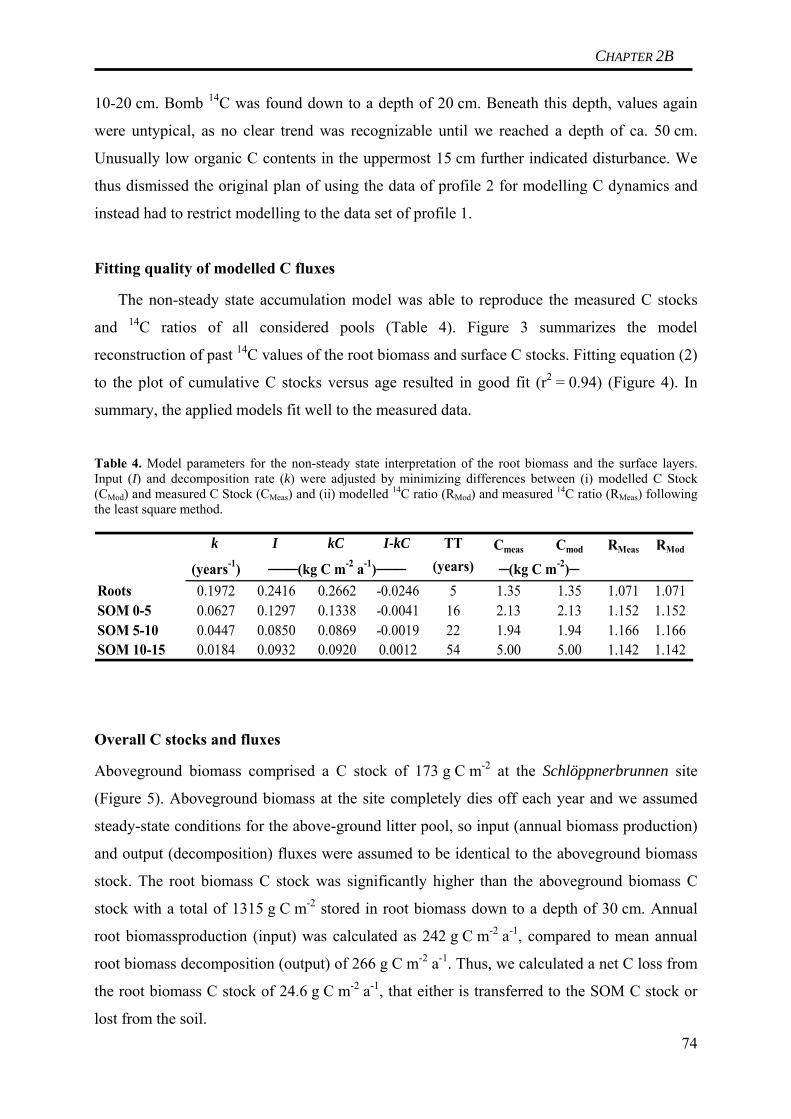
CHAPTER 2B
10-20 cm. Bomb 14C was found down to a depth of 20 cm. Beneath this depth, values again
were untypical, as no clear trend was recognizable until we reached a depth of ca. 50 cm.
Unusually low organic C contents in the uppermost 15 cm further indicated disturbance. We
thus dismissed the original plan of using the data of profile 2 for modelling C dynamics and
instead had to restrict modelling to the data set of profile 1.
Fitting quality of modelled C fluxes
The non-steady state accumulation model was able to reproduce the measured C stocks
and 14C ratios of all considered pools (Table 4). Figure 3 summarizes the model
reconstruction of past 14C values of the root biomass and surface C stocks. Fitting equation (2)
to the plot of cumulative C stocks versus age resulted in good fit (r2 = 0.94) (Figure 4). In
summary, the applied models fit well to the measured data.
Table 4. Model parameters for the non-steady state interpretation of the root biomass and the surface layers. Input (I) and decomposition rate (k) were adjusted by minimizing differences between (i) modelled C Stock (CMod) and measured C Stock (CMeas) and (ii) modelled 14C ratio (RMod) and measured 14C ratio (RMeas) following the least square method.
k I kC I-kC TT Cmeas Cmod RMeas RMod
(years-1) (years)Roots 0.1972 0.2416 0.2662 -0.0246 5 1.35 1.35 1.071 1.071SOM 0-5 0.0627 0.1297 0.1338 -0.0041 16 2.13 2.13 1.152 1.152SOM 5-10 0.0447 0.0850 0.0869 -0.0019 22 1.94 1.94 1.166 1.166SOM 10-15 0.0184 0.0932 0.0920 0.0012 54 5.00 5.00 1.142 1.142
───(kg C m-2 a-1)─── ─(kg C m-2)─
Overall C stocks and fluxes
Aboveground biomass comprised a C stock of 173 g C m-2 at the Schlöppnerbrunnen site
(Figure 5). Aboveground biomass at the site completely dies off each year and we assumed
steady-state conditions for the above-ground litter pool, so input (annual biomass production)
and output (decomposition) fluxes were assumed to be identical to the aboveground biomass
stock. The root biomass C stock was significantly higher than the aboveground biomass C
stock with a total of 1315 g C m-2 stored in root biomass down to a depth of 30 cm. Annual
root biomassproduction (input) was calculated as 242 g C m-2 a-1, compared to mean annual
root biomass decomposition (output) of 266 g C m-2 a-1. Thus, we calculated a net C loss from
the root biomass C stock of 24.6 g C m-2 a-1, that either is transferred to the SOM C stock or
lost from the soil. 74
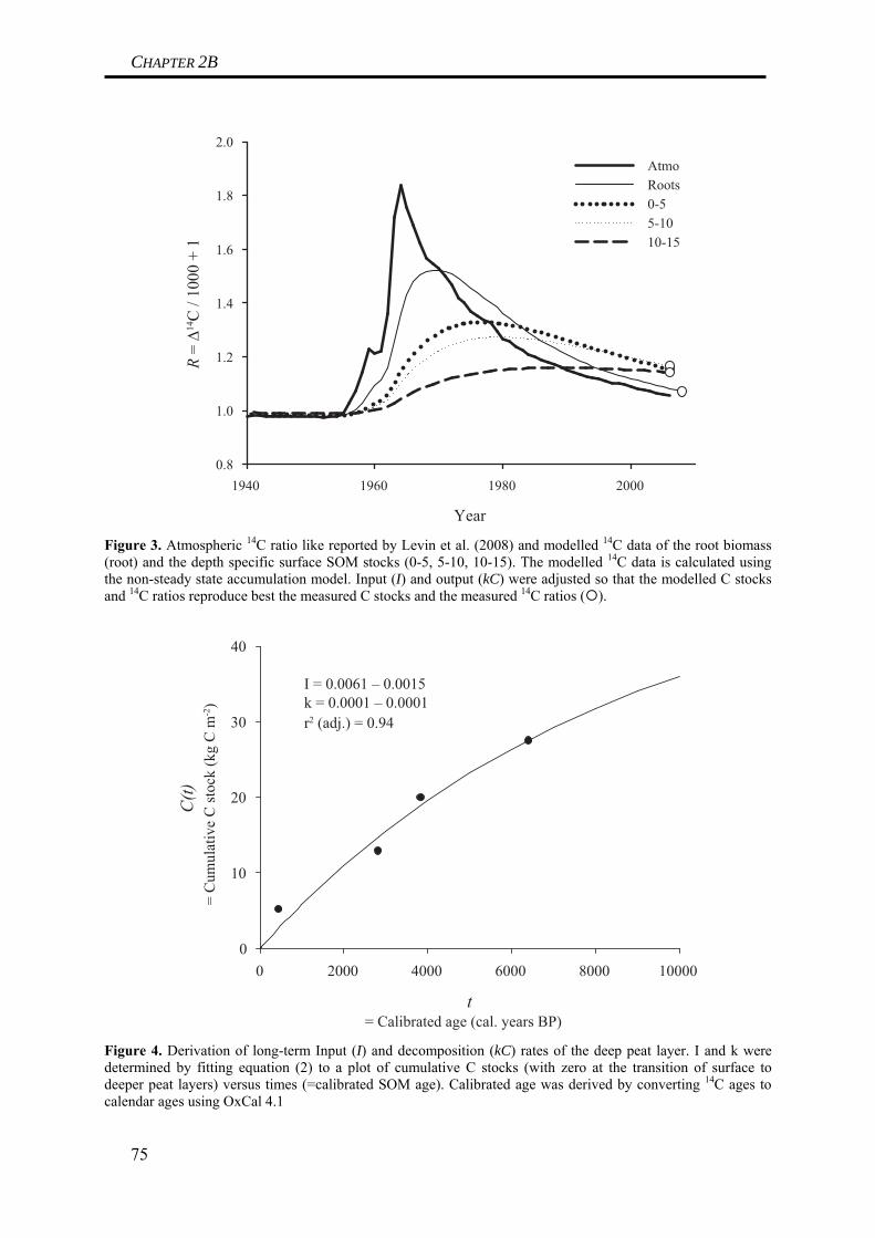
CHAPTER 2B
Year
1940 1960 1980 2000
R = Δ14
C /
1000
+ 1
0.8
1.0
1.2
1.4
1.6
1.8
2.0
AtmoRoots 0-5 5-10 10-15
Figure 3. Atmospheric 14C ratio like reported by Levin et al. (2008) and modelled 14C data of the root biomass (root) and the depth specific surface SOM stocks (0-5, 5-10, 10-15). The modelled 14C data is calculated using the non-steady state accumulation model. Input (I) and output (kC) were adjusted so that the modelled C stocks and 14C ratios reproduce best the measured C stocks and the measured 14C ratios ( ).
t= Calibrated age (cal. years BP)
0 2000 4000 6000 8000 10000
C(t)
= C
umul
ativ
e C
stoc
k (k
g C
m-2)
0
10
20
30
40
I = 0.0061 – 0.0015k = 0.0001 – 0.0001r2 (adj.) = 0.94
Figure 4. Derivation of long-term Input (I) and decomposition (kC) rates of the deep peat layer. I and k were determined by fitting equation (2) to a plot of cumulative C stocks (with zero at the transition of surface to deeper peat layers) versus times (=calibrated SOM age). Calibrated age was derived by converting 14C ages to calendar ages using OxCal 4.1
75

CHAPTER 2B
C lossProd. Stock Decomp. Input Stock Output
C lossAboveg. 173 → 173 → 173
0-5 → 93 → 129.7 → 2134 → 134
5-10 → 461 → 84.96 → 1944 → 87
10-15 → 358 → 93 → 4997 → 92
15-20 → 244 → → 5219 →
20-25 → 7716 →
25-30 → 7067 →
30-35 → 7555 →
─────────────
Bel
ow-g
roun
d ─────────────
(dep
th in
cm
)
→ ∑ 158
Gross C loss = (∑ Biomass Decomp. + ∑ SOM Output) - ∑ SOM Input = 442Net C loss = (∑ Biom. Decomp. + ∑ SOM Output) - (∑ Biom. Prod.+ ∑SOM Input) = 27
C in plant biomass C in SOM
∑ 242 ∑ 266
∑ 6.1 ∑ 3.3→
ND
Figure 5. C stocks in biomass (aboveground and below-ground) and SOM pools, annual litter production from biomass, and annual input and output C fluxes into the SOM pools of different depths calculated on the basis of soil profile data from profile 1. Stocks are given in g C m-2, fluxes (Prod., Decomp., Input, Output) are given in g C m-2 a-1.
For the SOM C stock of the peat body, we calculated a total C stock of 36,633 g C m-2
down to a depth of 36 cm. Roughly 25 % of this C or 9,075 g C m-2 were found in the surface
peat layer SOM stock compared to 27,558 g C m-2 in the deeper peat layer SOM stock. The
mean TT of the surface peat SOM stock ranged from 16 (0-5 cm) to 54 years (10-15 cm) and
thus was several orders of magnitude faster than for the deep peat layer SOM stock
(4,500-23,000 years, derived from stock divided by flux). In the uppermost 5 cm, output
fluxes (134 g C m-2 a-1) were calculated to be higher than input fluxes (130 g m-2 a-1),
resulting in a small net C loss of 4.1 g C m-2 a-1. Likewise, we calculated a net C loss from the
SOM in 5-10 cm depth (output 87 g m-2 a-1; input 85 g m-2 a-1; net C loss 1.9 g m-2 a-1).
Between 10-15 cm, we calculated a small net uptake of ca. 1.2 g m-2 a-1. In summary, SOM C
76

CHAPTER 2B
balance for the entire surface layers therefore was negative, with a net C loss of ca.
4.8 g m-2 a-1.
The deep peat layer SOM stock was found to accumulate C at a net rate of 2.8 g m-2 a-1.
Gross input (6.1 g m-2 a-1) and output (3.3 g m-2 a-1) fluxes were between one and two orders
of magnitude smaller than for the surface layer SOM stock. Combining results for the surface
and deep peat SOM stocks, we calculated a total net SOM C balance for the entire peat body
of -2 g m-2 a-1, indicating a small net C loss from the SOM pool.
Intermediate and Mineral horizon
Measurements of the 14C signature of the bulk soil and the three density fractions (fPOM,
oPOM, MAOM) of the intermediate horizon at profile 1 and profile 2 revealed no differences
between the different fractions (Table 5). In the mineral horizon, the 14C signature of the
fPOM fraction was increased compared to the oPOM and the MAOM fraction, indicating
input of younger carbon, possibly roots. However, the fPOM fraction in the mineral horizon
only accounted for 3-5 % (w/w) of the bulk soil.
Table 5. Radiocarbon signature of bulk soil and density fractions (fPOM, oPOM, MAOM) in the intermediate and the mineral horizon and weight proportion of the fractions in total bulk soil measured in profiles 1 and 2 (‘nd’ stand for ‘not determined’) .
DepthHorizon (cm) Bulk soil fPOM oPOM MAOM fPOM oPOM MAOM
Profile 1Interm. 36-41 -524 -542 -545 -534 20.3 26.1 51.9Interm. 41-46 -603 -595 -603 -593 52.2 21.0 28.7Interm. 46-51 -607 -606 -610 -608 28.6 28.3 43.4Mineral 51-81 -594 -554 -603 -606 5.2 4.1 84.2
Profile 2Interm. 45-50 -375 nd nd nd nd nd ndInterm. 50-55 -300 -303 -315 -322 10.1 42.5 45.5Interm. 55-60 -431 -422 -436 -410 9.8 27.5 60.2Mineral 60-93 -566 -456 -533 -597 3.4 8.9 81.9
Proportion of bulk soil──────(% w/w)──────
Δ14C──────────(‰)──────────
Discussion
Peatlands globally represent important C storage pools due to small but constant net C
accumulation rates. In this study we calculated the net C balance of SOM and below-ground
77

CHAPTER 2B
biomass. We added the latter to our consideration of the soil C pool to represent the fact that
adverse boundary conditions for decomposition (e.g. lack of oxygen due to water tables close
to the peat surface) can lead to a significant (transient) stabilization of C in undecomposed
root layer that would be ignored in root-free SOM samples. We found that SOM and root
biomass pools had a negative net C balance.
Modelled input and output C fluxes at this fen site reveal net C losses of ca. 2 g m-2 a-1.
Although this net C loss appears to be small, it is already unusual for a peatland site not be a
net C sink. In general, peatland sites are reported have a positive net C balance. Turunen et al.
(2002) reported net C accumulation rates of 15-35 g C m-2 a-1 for Finish peatlands. Estimates
for western Canada ranged around 19.4 g C m-2 a-1 (Vitt et al. 2000), and for West Siberia
Turunen et al. (2001) reported a net gain of ca. 17.2 g C m-2 a-1. A net C balance of -
3 g m-2 a-1 thus indicates that boundary conditions at the fen site have been changed by
disturbance, compared to the conditions during previous periods of peat accumulation.
We found significant amounts of C stored in root biomass at this site. As we were unable
to precisely distinguish between live and intact dead roots, root biomass C stock comprises
living roots and undecomposed root litter. Stabilization of C in the soil does not only occur in
SOM C stocks. Especially under the boundary conditions found in waterlogged peatland soils
(high water tables, lack of oxygen), it is possible that litter decomposes very slowly in the
soil, thus root biomass litter represents another important C storage pool, though possibly on
shorter timescales. Changing decomposition conditions can affect the rate of C transfer from
the root biomass C stock to the SOM C stock. This might result in apparent net C losses from
the SOM C stocks. We thus included the root pool into our modelling approach. As we
calculated net C losses from the root biomass C stock we can exclude the possibility that
reduced C transfer from the root biomass C stock to the SOM C stock resulted in apparent
SOM C losses. We are aware of the fact that the fluxes calculated for the root biomass C stock
are biased because we assumed a homogeneous pool. The actual fluxes therefore are
uncertain. For this study it is sufficient, however, to eliminate the possibility that apparent net
C losses from SOM are compensated for by transient increase of the amount of C stored root
biomass. We are also aware of the fact that we lack root biomass data beneath 30 cm.
Although root biomass constantly decreases beneath 10 cm we therefore underestimate the
proportion of root biomass in the total C stock and gross fluxes of the peat body.
Our results reveal that turnover of the SOM C stock in this fen was mainly taking place
between 0-15 cm depth, as 98 % of the gross fluxes in and out of the SOM C stock occurred
there. The contribution of gross fluxes in deeper peat layers to C turnover in the entire SOM C
78

CHAPTER 2B
stock thus is relatively small. The annual mean water table for this fen site has been reported
as -0.13 ± 0.19 m in 2002 (Paul et al. 2006) and -0.11 ± 0.08 and -0.10 ± 0.12 m in the years
of 2007 and 2008 (Muhr et al. 2009), and, thus, is close to the transition between the surface
and the deeper peat layers. Thus, the small contribution of fluxes from the deep peat SOM
stocks to the entire SOM C dynamics might result from a lack of oxygen. However, the water
table is subject to high seasonal fluctuations, and has been reported to drop considerably
during summer: Paul et al. (2006) reported a mean water table of -0.23 ± 0.21 m between May
and August of 2002. Muhr et al. (2009) found values between -0.11 and -0.19 m during the
summers of 2006 to 2008. Thus, it is more likely that the small contribution of the deeper peat
layers to overall SOM C fluxes is due to low substrate quality. This is also indicated by results
reported by Muhr et al. (2009), who found no increase of C fluxes when they experimentally
lowered the water table during summer down to values of 20 to > 60 cm beneath the soil
surface. Incubation of peat samples from the deeper peat layers of this site under completely
oxic conditions also revealed very little decomposition potential (Reiche et al. 2009).
The net C losses from this soil indicate disturbed boundary conditions. Based on our
results, we are unable to determine the actual disturbance. There are, however, three possible
explanations. (1) High nitrogen deposition into the ecosystem (Matzner et al. 2004) could
explain net C losses from the root biomass C stock. Following this interpretation, production
of new root biomass has decreased because nitrogen availability has increased during the last
decades, whereas decomposition rates remained unaffected. (2) Reduced sulphate deposition
(like observed during the last decades as a consequence of new emission laws; for data of the
region cf. Matzner et al. 2004) could increase leaching of DOC from the peatland, explaining
part of the net C losses from the SOM C stocks (Monteith et al. 2007). However, the
difference of the net C balance of this site in comparison to other peatlands is rather big. To
explain differences of that size, the disturbance has to have a critival impact on soil C
dynamics. (3) Changes in hydrology could have such an impact, as stabilization by high water
tables and consequent anoxia is a major reason for the net C accumulation of peatlands. As
mentioned before, the site features a ditch of unknown origin and age. Profile 2 was located
close to this ditch and revealed heavy disturbance within the peat body. Assuming that the
ditch is of anthropogenic origin (due to undocumented peat cutting at the site), this
disturbance of the 14C profile could be the result of digging in that area. Thus, the ditch could
significantly alter the hydrological conditions at the site, thereby possibly resulting in
artificial draining of the site. Climate change could further enhance changes on the
79

CHAPTER 2B
hydrological conditions. Regardless of the cause, this site has to be regarded as a disturbed
site, thereby putting results from experiments at this site in a new perspective.
Based on our model calculations, we amounted gross C fluxes from the peat body around
442 g m-2 a-1. These C fluxes can occur as CO2 and CH4 emissions or as leaching of dissolved
organic carbon (DOC). In 2007 and 2008, Muhr et al. (2009) measured soil respiration at the
site and determined annual fluxes between 490 and 640 g C m-2 a-1. Soil respiration includes
metabolic respiration by living roots, a flux that is not considered in the model calculations of
this study (cf. Figure 1). Still, these measurement data can be used to estimate a maximum
loss of C from the system via CO2 emission. Based on results by Goldberg (personal
communication) and Knorr et al. (2008), CH4 emissions do not contribute significantly to
total C fluxes at this site. Carbon losses from the site via DOC leaching have not been
quantified yet, but based on measurements of DOC concentrations in the soil solution they
can be assumed to be at least one order in magnitude smaller than C losses via CO2 emission
(Schulze, personal communication). In summary, our modelling approach yields gross C
fluxes from the soil that are similar to those estimated by measurements of soil respiration,
CH4 emissions, and DOC leaching.
As we were mainly interested in the C balance of the peat body, we did not model the C
balance for the underlying intermediate and mineral horizons. Root growth, however, can
easily extend down to this depth (at the two profiles chosen for radiocarbon analyses the
intermediate horizon began in depths of 36 and 45 cm already), thus possibly leading to net C
accumulation. However, the results from the density fractions of these horizons contradict the
idea of relevant C input at least in the intermediate horizon. The different fractions analyzed
here are normally considered to represent pools of different activity: The fPOM fraction
mainly contains recognizable plant material and fungal hyphae and responds quickly to
changes in C inputs and environmental conditions (and thus represents an active pool in
contrast to the oPOM and MAOM fraction) (von Lützow et al. 2006). Based on this
differentiation of the three fractions, the input of root biomass would correspond to an input
of C into the fPOM fraction, thus resulting in an input of bomb 14C and a consequent increase
of the 14C signature of this fraction compared to the other two fractions. In other words: The
input of relevant amounts of root C into the intermediate horizon should result in significant
differences in the 14C signature of the three fractions. As we found no differences between the
different fractions in the intermediate horizon, we conclude that no relevant input of young C
into these horizons occurs and that C turnover in the intermediate horizon is irrelevant for the
total soil C balance. In the mineral horizon, we found differences in the 14C signature of the
80

CHAPTER 2B
three fractions, but these differences were small (considering that root C has positive 14C
signatures) and the proportion of the fPOM fraction in bulk soil was very small (3-5 % w/w),
so again we conclude that C turnover in the mineral horizon is irrelevant for the total soil C
balance.
Conclusion
In contrast to most undisturbed peatlands, the total net soil C balance for the
Schlöppnerbrunnen fen site is negative. We take this as indicative of disturbed boundary
conditions. Following our model data, root biomass is a highly important C pool both in terms
of storage and in terms of total soil C dynamics. Radiocarbon has proven as a tool that allows
detecting even small imbalances in the investigated C pools.
Acknowledgements
This study was financially supported by the program 562 ‘Soil processes under extreme
meteorological boundary conditions’ of the Deutsche Forschungsgemeinschaft (DFG). We
thank S. Wunderlich and Lisa Höhn for assistance during sampling and U. Hell, A. Kolb, G.
Küfner, and G. Müller for installations and ongoing service in the field. We thank Dr. K.-H.
Knorr for providing us with additional dry bulk density data for the site. We thank the
Department of Earth System Sciences and the KCCAMS facility at the University of Irvine,
California, for radiocarbon measurements, and namely Prof. S. E. Trumbore and Dr. X. Xu
for support in radiocarbon measurements. We thank Prof. Dr. Gunnar Lischeid, Prof. (adjunct,
McGill) PD Dr. Christian Blodau, and Prof. Dr. Egbert Matzner for coordinating the
experimental efforts of all involved working groups at the Schlöppnerbrunnen fen site.
References
Gaudinski JB, Trumbore SE, Davidson EA & Zheng S (2000) Soil carbon cycling in a
temperate forest: radiocarbon-based estimates of residence times, sequestration rates and
partitioning of fluxes. Biogeochemistry 51: 33-69
Gaudinski JB, Dawson TE, Quideau S, Schuur EAG, Roden JS, Trumbore SE, Sandquist DR,
Oh S-W & Wasylishen RE (2005) Comparative Analysis of Cellulose Preparation
Techniques for Use with 13C, 14C, and 18O Isotopic Measurements. Analytical Chemistry
77: 7212-7224, doi:7210.1021/ac050548u
81
CHAPTER 2B
Gorham E (1991) Northern Peatlands: Role in the Carbon Cycle and Probable Responses to
Climatic Warming. Ecol. Appl. 1: 182-195
Knorr K-H, Oosterwoud MR & Blodau C (2008) Experimental drought alters rates of soil
respiration and methanogenesis but not carbon exchange in soil of a temperate fen. Soil
Biol. Biochem. 40: 1781-1791
Knorr K-H, Lischeid G & Blodau C (2009) Dynamics of belowground redox processes in a
minerotrophic fen exposed to a water table manipulation. Geoderma: submitted
Levin I, Hammer S, Kromer B & Meinhardt F (2008) Radiocarbon observations in
atmospheric CO2: Determining fossil fuel CO2 over Europe using Jungfraujoch
observations as background. Sci. Total Environ. 391: 211-216
Lützow Mv, Kögel-Knabner I, Ekschmitt K, Matzner E, Guggenberger G, Marschner B &
Flessa H (2006) Stabilization of organic matter in temperate soils: mechanisms and their
relevance under different soil conditions - a review. Eur. J. Soil Sci. 57: 426-445
Matzner E, Zuber T, Alewell C, Lischeid G & Moritz K (2004) Trends in deposition and
canopy leaching of mineral elements as indicated by bulk deposition and throughfall
measurements. In: Matzner E (Ed) Biogeochemistry of forested catchments in a changing
environment pp 233-250). Springer, Berlin
Muhr J, Höhle J, Otieno DO & Borken W (2009) Manipulative lowering of the water table
during summer does not affect CO2 emissions and uptake in a minerotrophic fen in South-
eastern Germany. Ecol. Appl.: submitted
Otieno DO, Wartinger M, Nishiwaki A, Hussain MZ, Muhr J, Borken W & Lischeid G (2009)
Responses of CO2 Exchange and Primary Production of the Ecosystem Components to
Environmental Changes in a Mountain Peatland. Ecosystems 12: 590-603
Paul S, Küsel K & Alewell C (2006) Reduction processes in forest wetlands: Tracking down
heterogeneity of source/sink functions with a combination of methods. Soil Biol.
Biochem. 38: 1028-1039
Reiche M, Hädrich A, Lischeid G & Küsel K (2009) Impact of manipulated drought and
heavy rainfall events on peat mineralization processes and source-sink functions of an
acidic fen. J. Geophys. Res. - G 114: G02021, doi:02010.01029/02008JG000853
Reimer PJ, Baillie MGL, Bard E, Bayliss A, Beck JW, Bertrand C, Blackwell PG, Buck CE,
Bur G, Cutler KB, Damon PE, Edwards RL, Fairbanks RG, Friedrich M, Guilderson TP,
Hughen KA, Kromer B, McCormac FG, Manning S, Bronk Ramsey C, Reimer RW,
Remmele S, Southon JR, Stuiver M, Talamo S, Taylor FW, van der Plicht J &
82

CHAPTER 2B
83
Weyhenmeyer CE (2004) IntCal04 terrestrial radiocarbon age calibration, 0-26 cal kyr
BP. Radiocarbon 46: 1029-1058
Schlesinger WH & Andrews JA (2000) Soil respiration and the global carbon cycle.
Biogeochemistry 48: 7-20
Schulze K, Borken W, Muhr J & Matzner E (2009) Stock, turnover time and accumulation of
organic matter in bulk and density fractions of a podzol soil. Eur. J. Soil Sci. 60: 567-577
Stuiver M & Polach HA (1977) Discussion; Reporting of 14C Data. Radiocarbon 19: 355-363
Trumbore SE, Davidson EA, Camargo PBd, Nepstad DC & Martinelli LA (1995)
Belowground Cycling of Carbon in Forests and Pastures of Eastern Amazonia. Global
Biogeochem. Cy. 9:
Trumbore SE & Harden JW (1997) Accumulation and turnover of carbon in organic and
mineral soils of the BOREAS northern study area. J. Geophys. Res. 102: 28817-28830
Turunen J, Tahvanainen T, Tolonen K & Pitkänen A (2001) Carbon Accumulation in West
Siberian Mires, Russia. Global Biogeochem. Cy. 15: 285-296
Turunen J, Tomppo E, Tolonen K & Reinikainen A (2002) Estimating carbon accumulation
rates of undrained mires in Finland-application to boreal and subarctic regions. The
Holocene 12: 69-80, doi: 10.1191/0959683602hl0959683522rp
Vitt DH, Halsey LA, Bauer IE & Campbell C (2000) Spatial and temporal trends in carbon
storage of peatlands of continental western Canada through the Holocene. Can. J. Earth
Sci. 37: 683-693
Xu X, Trumbore SE, Zheng S, Southon JR, McDuffee KE, Luttgen M & Liu JC (2007)
Modifying a sealed tube zinc reduction method for preparation of AMS graphite targets:
Reducing background and attaining high precision. Nucl. Instrum. Meth. Phys. Res. B
259: 320-329

CHAPTER 3
Chapter 3
Soil C dynamics in a forest as affected by soil frost
84

CHAPTER 3
Effects of soil frost on soil respiration and its radiocarbon
signature in a Norway spruce forest soil Jan Muhr1*, Werner Borken1 and Egbert Matzner1 1Department of Soil Ecology, University of Bayreuth, Dr. Hans Frisch Strasse 1-3, 95448
Bayreuth, Germany
*Corresponding author: Jan Muhr ([email protected])
Published in Global Change Biology (2009) 15, 782-793.
Received 28 December 2007; revised version received 8 April 2008 and accepted 24 April
2008
Abstract
Apart from a general increase of mean annual air temperature, climate models predict a
regional increase of the frequency and intensity of soil frost with possibly strong effects on C
cycling of soils. In this study, we induced mild soil frost (up to -5°C in a depth of 5 cm below
surface) in a Norway spruce forest soil by removing the natural snow cover in the winter of
2005/2006. Soil frost lasted from January to April 2006 and was detected down to 15 cm
depth. Soil frost effectively reduced soil respiration in the snow removal plots in comparison
to undisturbed control plots. On an annual basis 6.2 t C ha-1 a-1 were emitted in the control
plots compared with 5.1 t C ha-1 a-1
in the snow removal plots. Only 14% of this difference
was attributed to reduced soil respiration during the soil frost period itself, whereas 63% of
this difference originated from differences during the summer of 2006. Radiocarbon (Δ14C)
signature of CO2 revealed a considerable reduction of heterotrophic respiration on the snow
removal plots, only partly compensated for by a slight increase of rhizosphere respiration.
Similar CO2 concentrations in the uppermost mineral horizons of both treatments indicate that
differences between the treatments originated from the organic horizons. Extremely low water
contents between June and October of 2006 may have inhibited the recovery of the
heterotrophic organisms from the frost period, thereby enhancing the differences between the
control and snow removal plots. We conclude that soil frost triggered a change in the
composition of the microbial community, leading to an increased sensitivity of heterotrophic
respiration to summer drought. A CO2 pulse during thawing, such as described for arable soils
several times throughout the literature, with the potential to partly compensate for reduced
soil respiration during soil frost, appears to be lacking for this soil. Our results from this 85

CHAPTER 3
experiment indicate that soil frost reduces C emission from forest soils, whereas mild winters
may enhance C losses from forest soils.
Keywords: carbon dioxide, freezing, frost, partitioning, radiocarbon, soil respiration, thawing
86
CHAPTER 3
Introduction
Soil respiration is the largest global CO2 flux from the terrestrial biosphere to the
atmosphere (Schlesinger & Andrews, 2000). Around three times more organic C is stored in
soils than in terrestrial plants (Schimel, 1995). With soil temperature being the most important
driver of soil respiration (Raich & Schlesinger, 1992), an increase in the mean annual
temperature as predicted by the IPCC (2001) is likely to affect soil respiration rates. In
addition to a mere increase of the mean annual temperature, the IPCC (2001) also predicted a
changing frequency of extreme meteorological events such as the freezing and thawing of
soils in mountainous regions. In some regions, increasing temperatures will lead to a reduced
frequency of soil frost. In other regions, reduced snowfall together with temperatures below
0°C will lead to an increase in the frequency and intensity of soil frost.
Soil frost creates stress conditions that force organisms to acclimate or die (Schimel et
al., 2007). Roots, especially fine root tips, are frost sensitive (Smit-Spinks et al., 1985) and
normally acclimate to soil frost by accumulation of soluble carbohydrates (Tinus et al., 2000).
Slow growth of roots has been reported throughout the winter for Picea abies (Hansen et al.,
1996), but prolonged soil frost events can increase fine root mortality (Gaul et al., 2008).
Microbial cells can experience frost damage (e.g., by rupturing of cell membranes by ice
crystals; Rivkina et al., 2000), or may suffer from reduced solute availability due to a
reduction of the amount of free water and the diffusion rate of solutes by soil frost. Ice
barriers can also effectively block gas diffusion, thereby creating anaerobic conditions (Clein
& Schimel, 1995). Acclimation of soil microorganisms to soil frost conditions is achieved by
a number of physiological changes, including the storage of compatible solutes (e.g.,
carbohydrates) and the synthesis of protective molecules, including proteins and sugars. The
substrates used to supply these acclimations are available neither for microbial growth nor for
metabolic activity (Schimel et al., 2007). In general, soil respiration is found to be reduced
during periods of soil frost, but nevertheless still occurs at temperatures well below 0°C in
unfrozen water films (Edwards & Cresser, 1992).
During thawing of frozen soil in laboratory experiments, a burst of CO2 was found for
both arable and forest soils and in some experiments also for arctic and tundra soils (Matzner
& Borken, 2008). One explanation for this burst is dying of microorganisms during soil frost,
which are then decomposed by surviving microbes during thawing. Rapid metabolization of
compatible solutes or proteins stored in the cell to acclimate to soil frost is another
explanation. The availability of new substrate due to aggregate disruption and the creation of
new surfaces have also been discussed in this context. Field data confirm the importance of 87
CHAPTER 3
such a CO2 pulse during thawing for arable soils (Dörsch et al., 2004), but not for alpine or
arctic soils (Elberling & Brandt, 2003; Monson et al., 2006). Whereas Coxson & Parkinson
(1987) reported a CO2 burst for a temperate forest soil, Groffman et al. (2006) found no such
pulse in a northern hardwood forest soil. As data for temperate forest ecosystems are scarce
and contradictory, the question remains how these soils will respond to soil freezing and
subsequent thawing. To our knowledge, almost no data on the effects of soil frost on an
annual scale are available.
CO2 respired from soils normally originates from a number of different sources. CO2
respired from live roots, mycorrhiza, or microbes in the rhizosphere that metabolize root
exudates normally has a Δ14C signature that is close to that of CO2 in the atmosphere, as
recent photosynthates are the major C source in this case, and therefore, will be summarized
here as rhizosphere respiration (RR). CO2 respired by heterotrophic microorganisms
metabolizing soil organic matter (SOM) and plant material that has not just recently died
normally has a Δ14C signature that is different from that of atmospheric CO2 in the year of the
measurement and will therefore here be distinguished as heterotrophic respiration (HR). Both
components of soil respiration might be affected by soil frost. Data from Herrmann & Witter
(2002) for arable soils suggest that soil frost has a considerable effect on soil microbes, with
mineralization of microbial biomass explaining up to 65% of the observed C flush following
thawing of frozen soil. On the other hand, it has also been reported that even mild soil frost
can severely damage fine roots and increase fine root mortality and turnover (Tierney et al.,
2001). Experiments with tundra soil (Mikan et al., 2002) revealed an extremely high
temperature sensitivity of microbial activity for temperatures below 0°C. To distinguish the
effects of soil frost on heterotrophic vs. rhizospheric respiration, radiocarbon-based
measurements have been reported to address this question with minimal disturbance (Schuur
& Trumbore, 2006).
This work is testing the following hypotheses in a mountainous Norway spruce forest
soil: (1) A temporary CO2 burst can be observed during thawing of frozen soil, which can be
explained by a rapid increase of microbial activity. (2) Soil frost reduces cumulative soil
respiration on an annual scale. (3) Microorganisms are more severely affected by soil frost
than roots, resulting in a reduction of microbial respiration during freezing. To test these
hypotheses, replicated snow removal and control plots were established in a Norway spruce
forest site at the Fichtelgebirge. The region experienced a significant decrease of days with
snow cover over the last decades (Foken, 2004), while temperatures in winter still drop below
0°C (Foken, 2003), thereby increasing the probability of soil frost in winter and making this
88
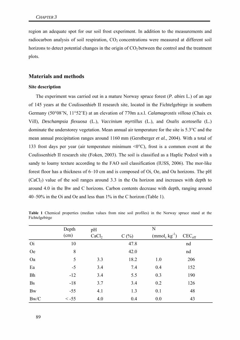
CHAPTER 3
region an adequate spot for our soil frost experiment. In addition to the measurements and
radiocarbon analysis of soil respiration, CO2 concentrations were measured at different soil
horizons to detect potential changes in the origin of CO2 between the control and the treatment
plots.
Materials and methods
Site description
The experiment was carried out in a mature Norway spruce forest (P. abies L.) of an age
of 145 years at the Coulissenhieb II research site, located in the Fichtelgebirge in southern
Germany (50°08’N, 11°52’E) at an elevation of 770m a.s.l. Calamagrostis villosa (Chaix ex
Vill), Deschampsia flexuosa (L.), Vaccinium myrtillus (L.), and Oxalis acetosella (L.)
dominate the understorey vegetation. Mean annual air temperature for the site is 5.3°C and the
mean annual precipitation ranges around 1160 mm (Gerstberger et al., 2004). With a total of
133 frost days per year (air temperature minimum <0°C), frost is a common event at the
Coulissenhieb II research site (Foken, 2003). The soil is classified as a Haplic Podzol with a
sandy to loamy texture according to the FAO soil classification (IUSS, 2006). The mor-like
forest floor has a thickness of 6–10 cm and is composed of Oi, Oe, and Oa horizons. The pH
(CaCl2) value of the soil ranges around 3.3 in the Oa horizon and increases with depth to
around 4.0 in the Bw and C horizons. Carbon contents decrease with depth, ranging around
40–50% in the Oi and Oe and less than 1% in the C horizon (Table 1).
Table 1 Chemical properties (median values from nine soil profiles) in the Norway spruce stand at the Fichtelgebirge
Depth(cm)
pHCaCl2 C (%)
N(mmolc kg-1) CECeff
Oi 10 47.8 ndOe 8 42.0 ndOa 5 3.3 18.2 1.0 206Ea -5 3.4 7.4 0.4 152Bh -12 3.4 5.5 0.3 190Bs -18 3.7 3.4 0.2 126Bw -55 4.1 1.3 0.1 48Bw/C < -55 4.0 0.4 0.0 43
89
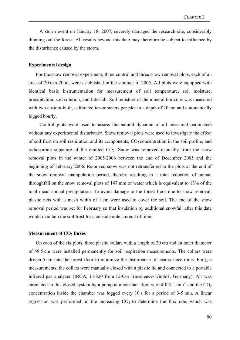
CHAPTER 3
A storm event on January 18, 2007, severely damaged the research site, considerably
thinning out the forest. All results beyond this date may therefore be subject to influence by
the disturbance caused by the storm.
Experimental design
For the snow removal experiment, three control and three snow removal plots, each of an
area of 20 m x 20 m, were established in the summer of 2005. All plots were equipped with
identical basic instrumentation for measurement of soil temperature, soil moisture,
precipitation, soil solution, and litterfall. Soil moisture of the mineral horizons was measured
with two custom-built, calibrated tensiometers per plot in a depth of 20 cm and automatically
logged hourly.
Control plots were used to assess the natural dynamic of all measured parameters
without any experimental disturbance. Snow removal plots were used to investigate the effect
of soil frost on soil respiration and its components, CO2 concentration in the soil profile, and
radiocarbon signature of the emitted CO2. Snow was removed manually from the snow
removal plots in the winter of 2005/2006 between the end of December 2005 and the
beginning of February 2006. Removed snow was not retransferred to the plots at the end of
the snow removal manipulation period, thereby resulting in a total reduction of annual
throughfall on the snow removal plots of 147 mm of water which is equivalent to 13% of the
total mean annual precipitation. To avoid damage to the forest floor due to snow removal,
plastic nets with a mesh width of 1 cm were used to cover the soil. The end of the snow
removal period was set for February so that insulation by additional snowfall after this date
would maintain the soil frost for a considerable amount of time.
Measurement of CO2 fluxes
On each of the six plots, three plastic collars with a length of 20 cm and an inner diameter
of 49.5 cm were installed permanently for soil respiration measurements. The collars were
driven 5 cm into the forest floor to minimize the disturbance of near-surface roots. For gas
measurements, the collars were manually closed with a plastic lid and connected to a portable
infrared gas analyzer (IRGA; Li-820 from Li-Cor Biosciences GmbH, Germany). Air was
circulated in this closed system by a pump at a constant flow rate of 0.5 L min-1 and the CO2
concentration inside the chamber was logged every 10 s for a period of 3-5 min. A linear
regression was performed on the increasing CO2 to determine the flux rate, which was
90
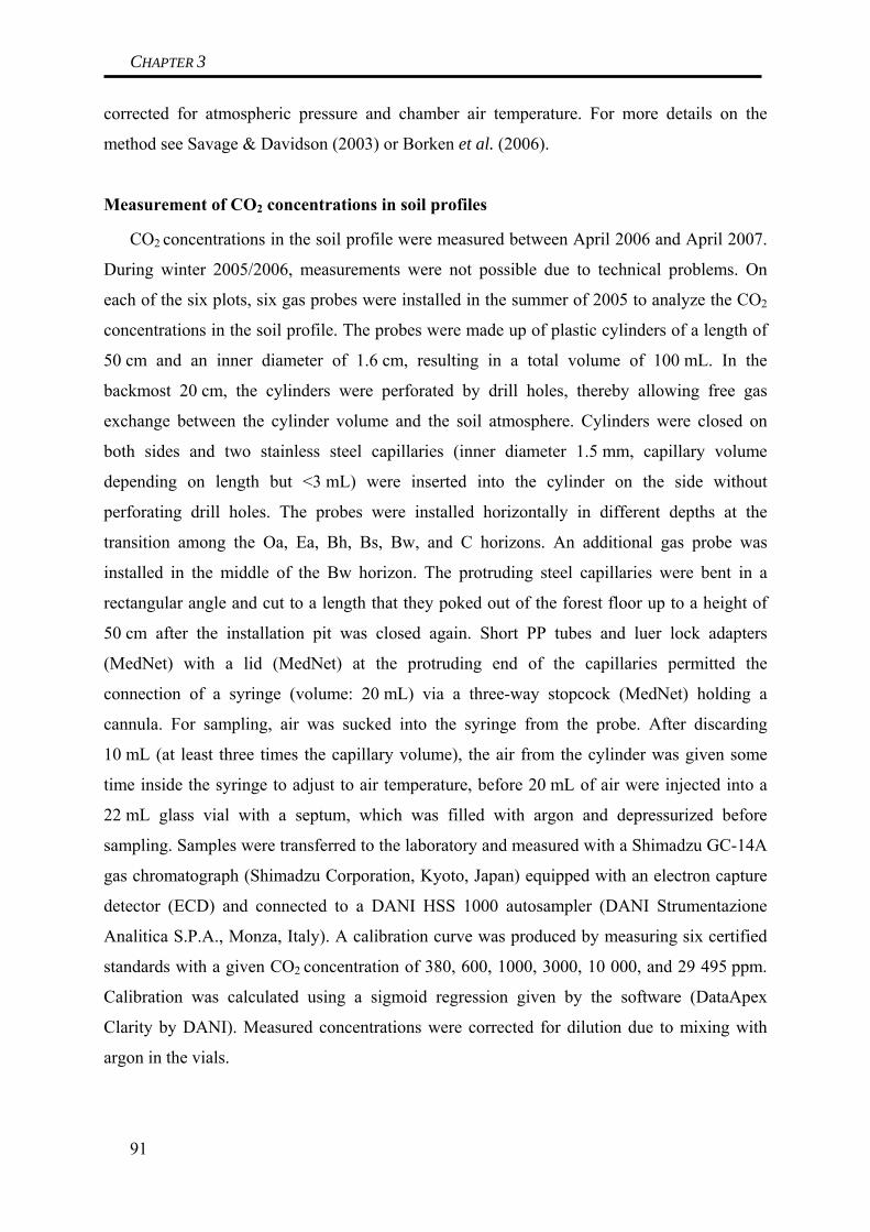
CHAPTER 3
corrected for atmospheric pressure and chamber air temperature. For more details on the
method see Savage & Davidson (2003) or Borken et al. (2006).
Measurement of CO2 concentrations in soil profiles
CO2 concentrations in the soil profile were measured between April 2006 and April 2007.
During winter 2005/2006, measurements were not possible due to technical problems. On
each of the six plots, six gas probes were installed in the summer of 2005 to analyze the CO2
concentrations in the soil profile. The probes were made up of plastic cylinders of a length of
50 cm and an inner diameter of 1.6 cm, resulting in a total volume of 100 mL. In the
backmost 20 cm, the cylinders were perforated by drill holes, thereby allowing free gas
exchange between the cylinder volume and the soil atmosphere. Cylinders were closed on
both sides and two stainless steel capillaries (inner diameter 1.5 mm, capillary volume
depending on length but <3 mL) were inserted into the cylinder on the side without
perforating drill holes. The probes were installed horizontally in different depths at the
transition among the Oa, Ea, Bh, Bs, Bw, and C horizons. An additional gas probe was
installed in the middle of the Bw horizon. The protruding steel capillaries were bent in a
rectangular angle and cut to a length that they poked out of the forest floor up to a height of
50 cm after the installation pit was closed again. Short PP tubes and luer lock adapters
(MedNet) with a lid (MedNet) at the protruding end of the capillaries permitted the
connection of a syringe (volume: 20 mL) via a three-way stopcock (MedNet) holding a
cannula. For sampling, air was sucked into the syringe from the probe. After discarding
10 mL (at least three times the capillary volume), the air from the cylinder was given some
time inside the syringe to adjust to air temperature, before 20 mL of air were injected into a
22 mL glass vial with a septum, which was filled with argon and depressurized before
sampling. Samples were transferred to the laboratory and measured with a Shimadzu GC-14A
gas chromatograph (Shimadzu Corporation, Kyoto, Japan) equipped with an electron capture
detector (ECD) and connected to a DANI HSS 1000 autosampler (DANI Strumentazione
Analitica S.P.A., Monza, Italy). A calibration curve was produced by measuring six certified
standards with a given CO2 concentration of 380, 600, 1000, 3000, 10 000, and 29 495 ppm.
Calibration was calculated using a sigmoid regression given by the software (DataApex
Clarity by DANI). Measured concentrations were corrected for dilution due to mixing with
argon in the vials.
91

CHAPTER 3
Gas sampling for analysis of the Δ14CO2 signature
Sampling of soil respiration for the determination of its Δ14C signature was done on four
dates (March 6, 2006; June 8, 2006; November 14, 2006; March 15, 2007) using the soil
respiration chambers described earlier. For each of the sampling dates, two out of the three
respiration chambers on each plot (resulting in a total of six replicates per treatment) were
closed and then flushed with CO2-free synthetic air for 90 min at a flow rate of 1.5 L min-1,
thereby effectively flushing the respiration chambers with an amount of gas equal to at least
three times the chamber volume. Following flushing, the respiration chambers were sealed
and left until CO2 concentration inside the chambers reached at least 1500 ppm. Incubation
time depended on effective CO2 fluxes at the sampling day. Evacuated stainless steel cylinders
with a volume of 2 L were connected to the respiration chambers and slowly filled with gas
from inside the chambers. Gas samples were then transferred to the laboratory for further
processing. The Δ14CO2 signature of soil respiration (Δ14CSR) of control or snow removal
plots, respectively, was calculated as the mean value of the six replicates of each treatment for
each date.
Besides monitoring changes in the Δ14CSR, due to soil frost, it was the aim of this study
to partition soil respiration into the contribution of RR and HR. The partitioning was achieved
by applying the isotopic method making use of bomb-derived 14C explained in greater detail
by Gaudinski et al. (2000) or Schuur & Trumbore (2006). The basic idea is measuring the
Δ14CO2 signature and the flux of total soil respiration, as well as the Δ14CO2 signature of the
two constituents of soil respiration (RR and HR) and then applying a mass balance to
calculate the fluxes of the two constituents. A major advantage of this method is that it can be
carried out mostly under field site conditions and with minimal disturbances. The basic
equations applied in this approach are Eqns (1) and (2):
RootCOHetCOSRCO FFF ,,, 222+= (1)
(2) RootRootCOHetHetCOSRSRCO CFCFCF 14,
14,
14, 222
Δ×+Δ×=Δ×
where FCO2,SR is the CO2 flux of total soil respiration, FCO2,Het is the flux of HR, and FCO2,Root is
the flux of RR, all in mmol m-2 h-1. Δ14CSR is the radiocarbon signature of the total soil
respiration, Δ14CHet is the radiocarbon signature of the HR, and Δ14CRoot is the radiocarbon
signature of the RR, all given in ‰.
To measure the Δ14CO2 signature of RR (Δ14CRoot), two different approaches were used.
As the Δ14CO2 signature of CO2 respired by roots is normally close to the Δ14CO2 signature of
the atmosphere, atmospheric samples were taken on three different dates (March 6, 2006; 92
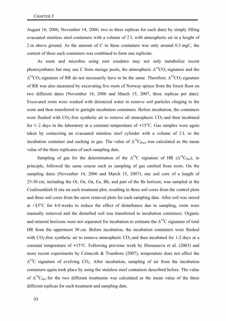
CHAPTER 3
August 16, 2006; November 14, 2006; two to three replicas for each date) by simply filling
evacuated stainless steel containers with a volume of 2 L with atmospheric air in a height of
2 m above ground. As the amount of C in these containers was only around 0.3 mgC, the
content of three such containers was combined to form one replicate.
As roots and microbes using root exudates may not only metabolize recent
photosynthates but may use C from storage pools, the atmospheric Δ14CO2 signature and the
Δ14CO2 signature of RR do not necessarily have to be the same. Therefore, Δ14CO2 signature
of RR was also measured by excavating live roots of Norway spruce from the forest floor on
two different dates (November 14, 2006 and March 15, 2007, three replicas per date).
Excavated roots were washed with deionized water to remove soil particles clinging to the
roots and then transferred to gastight incubation containers. Before incubation, the containers
were flushed with CO2-free synthetic air to remove all atmospheric CO2 and then incubated
for 1–2 days in the laboratory at a constant temperature of +15°C. Gas samples were again
taken by connecting an evacuated stainless steel cylinder with a volume of 2 L to the
incubation container and sucking in gas. The value of Δ14CRoot was calculated as the mean
value of the three replicates of each sampling date.
Sampling of gas for the determination of the Δ14C signature of HR (Δ14CHet), in
principle, followed the same course such as sampling of gas emitted from roots. On the
sampling dates (November 14, 2006 and March 15, 2007), one soil core of a length of
25-30 cm, including the Oi, Oe, Oa, Ea, Bh, and part of the Bs horizon, was sampled at the
Coulissenhieb II site on each treatment plot, resulting in three soil cores from the control plots
and three soil cores from the snow removal plots for each sampling date. After soil was stored
at +15°C for 4-6 weeks to reduce the effect of disturbance due to sampling, roots were
manually removed and the disturbed soil was transferred to incubation containers. Organic
and mineral horizons were not separated for incubation to estimate the Δ14C signature of total
HR from the uppermost 30 cm. Before incubation, the incubation containers were flushed
with CO2-free synthetic air to remove atmospheric CO2 and then incubated for 1-2 days at a
constant temperature of +15°C. Following previous work by Dioumaeva et al. (2003) and
more recent experiments by Czimczik & Trumbore (2007), temperature does not affect the
Δ14C signature of evolving CO2. After incubation, sampling of air from the incubation
containers again took place by using the stainless steel containers described before. The value
of Δ14CHet for the two different treatments was calculated as the mean value of the three
different replicas for each treatment and sampling date.
93

CHAPTER 3
Preparation of gas samples for Δ14C signature
All gas samples sampled in stainless steel containers (originating from soil respiration,
root respiration, or HR) were further processed in the laboratory for measuring the Δ14C
signature. The general course of action was following the zinc reduction method for
preparation of AMS graphite targets described in Xu et al. (2007), but with some
modifications. The steel containers containing the samples were connected to the extraction
line via a digital mass flow controller (Type F-201C-AAA-33-V, Wagner Mess- und
Regeltechnik, Germany) effectively limiting the flow rate to 20 mL min-1. Gas was directed to
a water trap, cooled with a 1:1 mixture of ethanol and dry ice to get rid of the water and
afterwards through a CO2 trap cooled with liquid nitrogen, thereby effectively freezing out all
CO2 from the sample. The rest of the gases, which are noncondensable at the temperatures of
the two cooling traps, were discarded. The remaining procedure followed the method
described in Xu et al. (2007). All preparation took place at the laboratories of the Department
of Soil Ecology at the University of Bayreuth, Germany. Graphite targets were analyzed by
the Keck Carbon Cycle AMS facility at UC Irvine, USA, with a precision of 2-3‰.
Radiocarbon data are expressed as Δ14C, which is the per mil deviation from the 14C/12C ratio
of oxalic acid standard in 1950. The sample 14C/12C ratio has been corrected to a δ13C value of
-25‰ to account for any mass-dependent fractionation effects (Stuiver & Polach, 1977).
Data analysis
With three soil respiration chambers per plot and three plots per treatment (control and
snow removal), mean values were formed by treating the chambers on the same plot as
pseudoreplicates and the different plots as true replicates. Mean values with standard error
were formed for the different plots and then averaged by using error propagation.
Calculation of cumulative CO2 emissions was achieved by linear interpolation among
adjoining measurement dates. For the calculation of CO2 concentrations in the soil profile,
data from the gas probes were pooled according to the horizon. Owing to different thickness
of the horizons at the different plots, depths of the probes may differ among the different
plots, but a horizon specific concentration profile can be created.
Data were analyzed using STATISTICA 6.1 (Statsoft, Tulsa, OK, USA). Differences in
fluxes of soil respiration and its radiocarbon signature between the treatments were tested
using the nonparametric Mann–Whitney U-test. Comparing values of the same treatment at
different dates was achieved by using the Tukey HSD test.
94
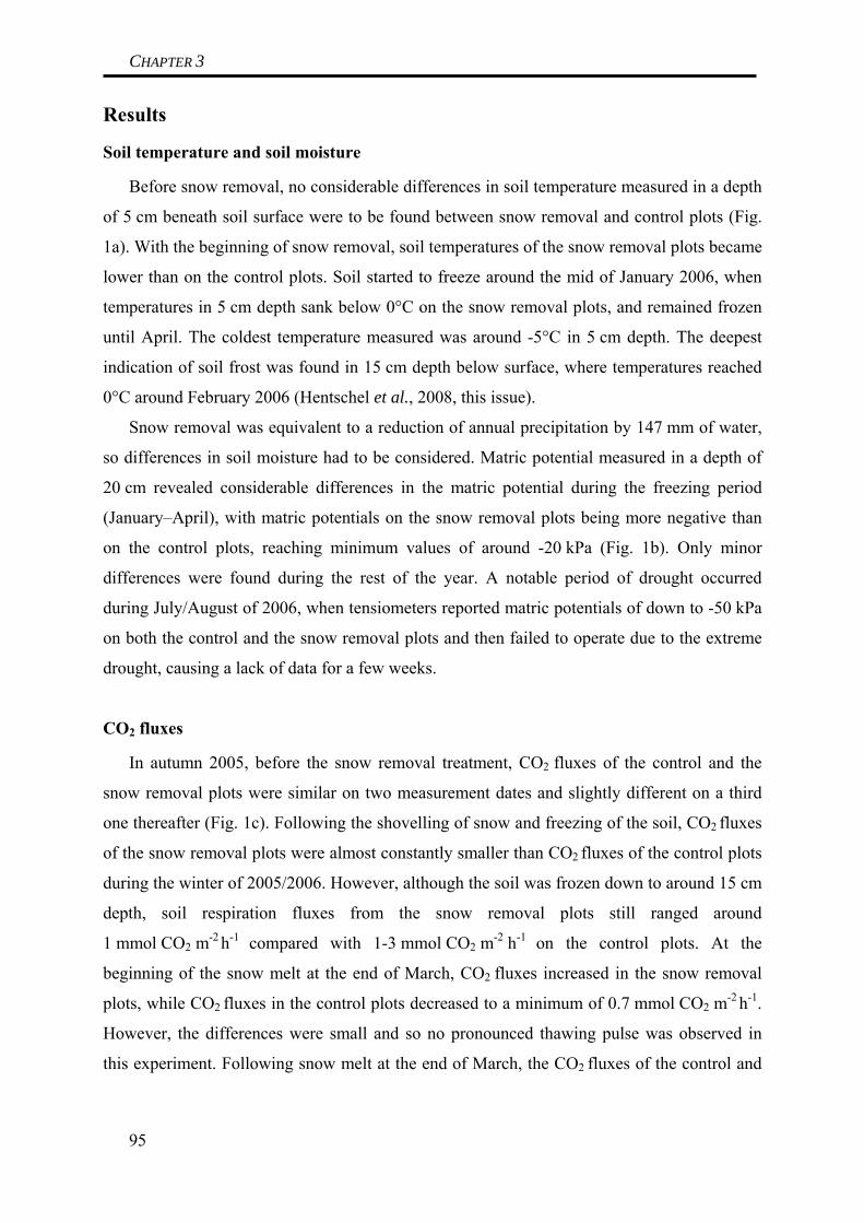
CHAPTER 3
95
Results
Soil temperature and soil moisture
Before snow removal, no considerable differences in soil temperature measured in a depth
of 5 cm beneath soil surface were to be found between snow removal and control plots (Fig.
1a). With the beginning of snow removal, soil temperatures of the snow removal plots became
lower than on the control plots. Soil started to freeze around the mid of January 2006, when
temperatures in 5 cm depth sank below 0°C on the snow removal plots, and remained frozen
until April. The coldest temperature measured was around -5°C in 5 cm depth. The deepest
indication of soil frost was found in 15 cm depth below surface, where temperatures reached
0°C around February 2006 (Hentschel et al., 2008, this issue).
Snow removal was equivalent to a reduction of annual precipitation by 147 mm of water,
so differences in soil moisture had to be considered. Matric potential measured in a depth of
20 cm revealed considerable differences in the matric potential during the freezing period
(January–April), with matric potentials on the snow removal plots being more negative than
on the control plots, reaching minimum values of around -20 kPa (Fig. 1b). Only minor
differences were found during the rest of the year. A notable period of drought occurred
during July/August of 2006, when tensiometers reported matric potentials of down to -50 kPa
on both the control and the snow removal plots and then failed to operate due to the extreme
drought, causing a lack of data for a few weeks.
CO2 fluxes
In autumn 2005, before the snow removal treatment, CO2 fluxes of the control and the
snow removal plots were similar on two measurement dates and slightly different on a third
one thereafter (Fig. 1c). Following the shovelling of snow and freezing of the soil, CO2 fluxes
of the snow removal plots were almost constantly smaller than CO2 fluxes of the control plots
during the winter of 2005/2006. However, although the soil was frozen down to around 15 cm
depth, soil respiration fluxes from the snow removal plots still ranged around
1 mmol CO2 m-2 h-1
compared with 1-3 mmol CO2 m-2 h-1 on the control plots. At the
beginning of the snow melt at the end of March, CO2 fluxes increased in the snow removal
plots, while CO2 fluxes in the control plots decreased to a minimum of 0.7 mmol CO2 m-2 h-1.
However, the differences were small and so no pronounced thawing pulse was observed in
this experiment. Following snow melt at the end of March, the CO2 fluxes of the control and

CHAPTER 3
-5
0
5
10
15
20
25
Snow removal plotsControl plots
Mat
ric p
oten
tial [
kPa]
Tem
pera
ture
[°C
]
-50
-40
-30
-20
-10
0
Snow removal plotsControl plots
CO
2 flux
[mm
ol m
-2 h
-1]
0
2
4
6
8
10
12
14 Snow removal plotsControl plotsSampling dates forΔ14 C measurements
Snow
Rem
oval
Per
iod
Date
Sep 05 Jan 06 May 06 Sep 06 Jan 07 May 07
Cum
ulat
ive
CO
2 em
issi
on[m
ol m
-2]
0
20
40
60
80
100 Snow removal plotsControl plots
Snow
Rem
oval
Per
iod
Snow
Rem
oval
Per
iod
a
b
c
d
Snow
Rem
oval
Per
iod
Figure 1 Measurements of (a) soil temperature in a depth of 5 cm below soil surface (mean values, n = 3), (b) soil matric potential in a depth of 20 cm (mean values, n = 6), (c) daily CO2 fluxes (mean values, n = 9), and (d) cumulative CO2 emissions calculated from daily CO2 fluxes by linear interpolation. Stars on the x-axis of part (c) indicate sampling dates for measurement of the Δ14C signature of soil respiration.
96

CHAPTER 3
the snow removal plots were almost identical. In June 2006, fluxes of the snow removal plots
started to differ again from the fluxes of the control plots, with fluxes from snow removal
plots being smaller than fluxes from control plots throughout the rest of the summer. With
decreasing fluxes in autumn 2006 and rewetting of dry soil, fluxes of the snow removal and
control plots were about the same level and no differences were found throughout the winter
of 2006/2007 and spring 2007.
In total, 70 mol CO2 m-2 were emitted from the control plots throughout the whole
course of the experiment (19 months), which was significantly (P = 0.04) > 58 mol CO2 m-2
from the snow removal plots (Fig. 1d). This is equal to an annual CO2 emission (calculated
from January 2006 to January 2007) of 52 mol CO2 m-2 or 6.2 t C ha-1
a-1 for the control plots
and 42 mol CO2 m-2 or 5.1 t C ha-1
a-1 for the snow removal plots. Thus, on an annual basis,
soil respiration was 1.1 t C ha-1 smaller on the snow removal plots than on the control plots.
The differences during frost period, lasting from beginning of January to mid of April, were
responsible for 14% of this reduction or 0.16 t C ha-1. Compared with this, the summer period
(lasting from beginning of June to beginning of October) accounted for 63% of the difference
between snow removal and control plots or 0.72 t C ha-1.
CO2 concentrations in the soil profile
Measurements of the CO2 concentrations at the end of the frost period revealed increased
CO2 concentrations in the three lowermost horizons of the soil profiles of the snow removal
plots (Fig. 2a) compared with the control plots (Fig. 2b; for differences see Fig. 2c).
Following snow melt, CO2 concentrations decreased on the snow removal plots. CO2
concentrations were similar on manipulation and control plots during summer 2006, with only
minor differences for the lowermost two horizons that were slightly more pronounced during
the winter of 2006/2007 and spring 2007. Almost identical CO2 concentrations in the
uppermost mineral horizons indicate that differences in CO2 emissions from the control and
snow removal plots originate from the organic horizons.
CO2 profiles of the control plots showed a weak seasonal pattern, with an increase in
concentration during spring and winter that was interrupted during the extremely dry summer
of 2006 and reached its maximum during natural rewetting of soil in September 2006. The
CO2 profiles of the snow removal plots did not show the pattern during the summer of 2006,
which might be due to the lack of measurements during September and October, but showed a
clear maximum at the end of the winter of 2005/2006 (Fig. 2). In general, CO2 concentrations
97
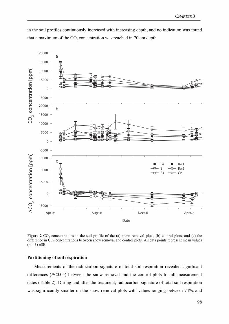
CHAPTER 3
in the soil profiles continuously increased with increasing depth, and no indication was found
that a maximum of the CO2 concentration was reached in 70 cm depth.
c
Date
Apr 06 Aug 06 Dec 06 Apr 07 ΔCO
2 con
cent
ratio
n [p
pm]
-5000
0
5000
10000
15000
a
-5000
0
5000
10000
15000
20000
b
CO
2 con
cent
ratio
n [p
pm]
-5000
0
5000
10000
15000
20000
EaBhBs
Bw1Bw2Cv
Figure 2 CO2 concentrations in the soil profile of the (a) snow removal plots, (b) control plots, and (c) the difference in CO2 concentrations between snow removal and control plots. All data points represent mean values (n = 3) ±SE.
Partitioning of soil respiration
Measurements of the radiocarbon signature of total soil respiration revealed significant
differences (P<0.05) between the snow removal and the control plots for all measurement
dates (Table 2). During and after the treatment, radiocarbon signature of total soil respiration
was significantly smaller on the snow removal plots with values ranging between 74‰ and
98

CHAPTER 3
82‰ compared with 86‰ and 91‰ on the control plots. The mean difference between
control and manipulation plots was constantly around 8–12‰. Radiocarbon signature showed
only a slight annual trend with slightly increased values during late spring and summer and
decreased values during end of winter.
The two different approaches to estimate the Δ14CO2 signature of RR yielded very
similar results on all measurement dates. Atmospheric samples of the three different sampling
dates yielded Δ14CO2 signatures of 50.6‰, 53.0‰, and 55.9‰. Root incubation yielded a
Δ14CO2 signature of RR of 53.3‰ and 55.2‰. As values for both approaches were similar and
no considerable annual trend was to be seen, the results of both approaches were combined to
calculate one uniform Δ14CRR (53.6 ± 2.1‰; Table 2).
Table 2 Radiocarbon signature of total soil respiration (SR), heterotrophic respiration (HR) and rhizospheric respiration (RR) on the snow removal and control plots
Δ14C ± SE
Snow Removal Control
Date SR (‰) HR (‰) SR (‰) HR (‰) RR (‰)
March 6, 2006 78.8 ± 3.2 na 88.8 ± 2.2 na 53.6 ± 2.1
June 8, 2006 81.7 ± 1.8 na 91.4 ± 2.2 na 53.6 ± 2.1
November 14, 2006 78.0 ± 1.6 86.7 ± 7.4 86.0 ± 2.8 91.8 ± 4.5 53.6 ± 2.1
March 15, 2007 73.6 ± 6.1 81.3 ± 1.9 85.8 ± 3.1 88.0 ± 5.8 53.6 ± 2.1
Calculating the contribution of heterotrophic and RR to total soil respiration revealed that
HR was dominating total soil respiration throughout the year and for both the snow
removal and the control plots, accounting for 70% to > 90% of total soil respiration fluxes
(Fig. 3). This dominance of HR was more expressed on the control plots, where rhizosphere
contribution ceased to play a significant role in March 2007 (Fig. 3). Converting the
percentage contribution of HR and RR to actual absolute fluxes (Fig. 3) revealed that absolute
HR fluxes were always considerably smaller on the snow removal plots than on the control
plots. Absolute RR fluxes differed only slightly during 2006, but differences became much
more pronounced in March 2007, when absolute RR fluxes on the control plots became
extremely small.
99

CHAPTER 3
14.11.2006
Snow Removal Control
Cont
ribut
ion
to s
oil r
espi
ratio
n [%
]
0
20
40
60
80
100
15.03.2007
Snow Removal Control0
20
40
60
80
100
HeterotrophicRhizospheric
4.13.7 2.82.7
0.30.7 1.10.9
Figure 3 Relative fluxes of heterotrophic and rhizospheric respiration for two measurement dates (bars) calculated based on the radiocarbon signature of total soil respiration, heterotrophic and rhizospheric respiration. The numbers represent the absolute fluxes (mmol m-2 h-1) for heterotrophic and rhizospheric respiration calculated based on the mean CO2 fluxes of the snow removal plots or the control plots of the measurement day and the relative contribution.
Discussion
Soil respiration was significantly reduced in the snow removal plots during the soil frost
period from January to April 2006 and during the posttreatment period from June to October
2006. No inherent differences were found during the pretreatment period that could explain
these differences in soil respiration. Based on radiocarbon data, we attribute the observed
decrease to damage to heterotrophic soil microbes induced by soil frost.
Differences in soil respiration observed from January to April 2006 can be directly
explained by adverse living conditions for soil microbes due to frost (Schimel et al., 2007)
and reduced soil temperatures. Although soil temperature below 0°C can have drastic effects
on microbial activity (Mikan et al., 2002), the observed differences during freezing have little
effect on the annual C balance, mostly owing to the fact that fluxes on both the control and the
snow removal plots were small.
During thawing of soil, soil respiration for both treatments was almost identical and no
pronounced pulse of CO2 emission was found. All we found was a short-timed inversion of
flux patterns, with fluxes from snow removal plots becoming higher than fluxes from control
plots for a very short time around the end of March 2006 that goes along with the beginning
of the snow melting period. The inversion is owed mainly to a significant reduction of fluxes 100

CHAPTER 3
on the control plots and only partly to an increase of fluxes on the snow removal plots and
insignificant on the annual scale. This lack of a pronounced CO2 pulse during thawing is in
agreement with the findings described by Groffman et al. (2006) for forest soil, but
contradicts the findings of Coxson & Parkinson (1987) for forest soil and Elberling & Brandt
(2003) for arctic soils under natural vegetation. It remains possible that due to the frequency
of measurements, a short lasting pulse might have been missed in our experiment. However,
results from laboratory experiments carried out with soil from our site make the occurrence of
such a pulse appear unlikely (Goldberg et al., 2007). In these laboratory experiments, repeated
freezing of soil at three different temperatures (Group 1: -3°C, Group 2: -8°C, Group 3:
-13°C) revealed that a burst of CO2 only occurred after freezing at -8 and -13°C, but not at
-3°C. Furthermore, this burst was comparatively small and did only occur during the first
freezing–thawing cycle, so even if such a small pulse would have been missed it is unlikely to
be relevant on an annual scale.
Finally, it is also possible that a burst occurred, but was masked by a similar burst on the
control plots. When a frost induced burst of CO2 occurs, it is normally found during the
thawing of soil, which in our experiment did not start before April 2006. During that period,
CO2 fluxes on both the control and the snow removal plots start to increase significantly,
likely simply due to the notable increase in soil temperature and therefore microbial activity.
However, Schimel & Mikan (2005) showed for an arctic tundra soil that the acclimation shift
towards frost conditions in microbial metabolism already occurs between +2 and +0.5°C. If
this holds true for microorganisms of temperate forest soils, it can be assumed that the
microbes on the control plots already started to acclimate to soil frost by storing sugars and
proteins. Schimel et al. (2007) hypothesized that metabolizing of these intracellular solutes
explains a large part of the flush of CO2 during thawing. In this case, the control and snow
removal plots would both react with a rapid burst of CO2 as soon as soil temperatures become
warmer again, thereby both showing what could be defined as a frost-induced CO2 burst. This
scenario remains highly speculative and for our experiment, it would not matter which
scenario holds true (mere temperature increase or CO2 burst on both plot types), but mild
winters with temperatures above 2°C might be affected by this phenomenon.
Differences between the two treatments in the summer of 2006 were surprisingly high.
In fact, the reduction of soil respiration in the snow removal plots between June and October
2006 is almost solely responsible for the decrease of cumulative C emissions in the snow
removal plots. Soil temperature, being the most important driver of soil respiration (Raich &
Schlesinger, 1992), cannot explain these differences, as soil temperature 5 cm beneath the
101
CHAPTER 3
surface was not found to be different on the control and the snow removal plots during that
period. Soil moisture, also being an important driver of soil respiration (Davidson et al.,
1998), was only measured in a depth of 20 cm. No differences in soil moisture between the
control and the snow removal plots were found in this depth during summer. Comparative
measurements of the water content of the organic horizons are lacking for the summer, but
measurements of gravimetric water content made in April 2006 by Hentschel et al. (2008, this
issue) on frozen soil cores revealed significantly higher gravimetric water contents on the
snow removal plots due to frozen water in the forest floor and run-off of melting water. Two
further measurements after thawing, at the beginning and the end of May 2006, revealed no
differences in the water content of the organic horizons of the control and the snow removal
plots (K. Hentschel, unpublished data). These data indicate that during thawing, water
contents on both treatments were reset to equal levels and, therefore, the idea of a permanent
reduction of water content due to snow removal on the snow removal plots can be rejected.
Still, it remains possible that differences in soil moisture did occur in the organic horizons
during summer. It should be mentioned in this context that no differences in root biomass
were found on the two treatments, which would indicate different water uptake by vegetation
(Gaul et al., 2008). Furthermore, it should be noted that differences in soil respiration during
the summer of 2006 coincided with a period of heavy natural drought. With the beginning of
rewetting of the soil in autumn, the differences in soil respiration disappeared. Radiocarbon
data reveal different Δ14CSR signature for the snow removal and the control plots for all four
measurement dates. Data for the pretreatment period are lacking, so inherent differences
between the treatments cannot be completely neglected. Considering the random distribution
of the different treatment plots and the small variation in radiocarbon signature data among
treatment plots of the same type, it still seems more likely that the period of soil frost induced
these differences. In this context, it is interesting to mention additional radiocarbon data
available for the field site (J. Muhr, unpublished data). At the same time as the control plots,
we also installed three additional plots for a throughfall exclusion experiment. Δ14C signature
of soil respiration was measured on these plots before manipulation (i.e., they can be regarded
as additional control plots) on June 8, 2006, at the same time such as Δ14C signature on the
snow removal and control plots. The value for Δ14C signature of soil respiration on these
additional plots was 88.0‰ ( ± 2.4, n = 6), which is very close to the value of the controls of
91.4‰ ( ± 2.2, n = 6) but significantly different (Student’s t-test, P<0.05) from the Δ14C
signature on the snow removal plots, which was 81.7‰ ( ± 1.8, n = 6). These findings further
contradict the idea of inherent differences. 102

CHAPTER 3
Radiocarbon data show a reduction of HR in the snow removal plots. This reduction is
still detectable in the spring of 2007, over 1 year after the manipulation period. Long-term
effects of soil frost on the microbial community have been reported by some authors.
Repeated freezing–thawing cycles seem to induce a shift of the microbial community towards
a dominance of bacteria (Nieminen & Setala, 2001; Larsen et al., 2002). Experiments by Feng
et al. (2007) revealed that repeated lab-stimulated freezing–thawing cycles greatly reduced
fungal biomass in a forest soil, whereas bacteria were unaffected. It has been hypothesized by
Schimel et al. (2007) that this preferential effect of soil frost on fungi is due to mechanical
stress resulting in damaging of fungal hyphae. In a laboratory experiment carried out with soil
from the same site described here, Schmitt et al. (2008, in revision) investigated the effects of
frost on the microbial community. Analyzing phospholipids fatty acid (PLFA) patterns in an
unfrozen control (constantly kept at 15°C) and three different freeze–thaw treatments
(repeatedly frozen at -3, -8, and -13°C and thawed at +5°C), they concluded that fungi were
more susceptible to soil frost, as soil frost resulted in a reduction of the ratio of
fungal/bacterial PLFAs. Such a reduction of fungal biomass might explain the reduction of
HR in our snow removal experiment even during summer. Voroney (2007) reported that fungi
are normally more tolerant towards drought than bacteria. A shift of the microbial community
towards bacterial dominance (due to preferential damaging of fungi by frost), therefore,
would increase the susceptibility of the surviving microbial community towards soil drought.
Whereas HR is reduced in snow removal plots, rhizospheric respiration shows a trend to
increase. These results are in agreement with findings from Gaul et al. (2008), who reported
an increase in fine root mortality and necromass, as well as fine root productivity following
soil frost. Radiocarbon bulk signature of the fine roots was found to be around 85‰, so CO2
produced from fine root decomposition should be considerably different from RR and be
reflected in HR (D. Gaul, personal communication). The fact, that HR actually decreased,
indicates that no significant flush of CO2 arouse from increased decomposition of fine root
necromass. In the spring of 2007, differences in RR between the control and the snow
removal plots become even stronger. This phenomenon is rather unlikely to be explained by
soil frost, but might be due to the mentioned storm that hit the site in January 2007 and
inflicted serious and possibly spatially heterogeneous damage to the spruce stand.
Comparing partitioning data of the two treatments, it becomes evident that even in times
with similar total soil respiration fluxes considerable differences concerning the origin of the
emitted CO2 do occur. The increase of rhizospheric respiration is partly compensating for the
reduced HR in the snow removal plots, thereby masking the effects of soil frost. The
103

CHAPTER 3
increased contribution of RR to total soil respiration reflects in a generally smaller
radiocarbon signature of soil respiration in the snow removal plots, indicating the contribution
of more recent C pools such as photosynthates respired by roots.
Considering the results of this study and of other experiments with soils under natural
vegetation (Matzner & Borken, 2008), a burst of CO2 emission during thawing of soil does not
play a significant role for these soils. Instead, the more important effect of soil frost seems to
be a decrease of cumulative C losses from soils such as shown in this work and others (Larsen
et al., 2002; Monson et al., 2006). Our results for soil in the Fichtelgebirge support the idea
that CO2 emissions from soils are reduced in years with soil frosts as compared with years
with mild winters. The idea of increased substrate availability due to soil frost such as
postulated by Schimel et al. (2007) cannot be confirmed by our findings and also is not
reflected by measurements of the concentration of dissolved organic carbon (DOC) carried
out throughout the experiment (Hentschel et al., 2008, this issue).
Considering results on fine root productivity and mortality (Gaul et al., 2008), as well as
the radiocarbon data presented here, C input into soils via root litter is likely to increase.
However, this increase was not mirrored in an increase of total soil respiration. HR, which
would be expected to increase due to increased root litter input, actually declined for the snow
removal plots. Based on these results, we postulate an increased C sequestration in soils due
to decreased CO2 emissions as a result of the freezing of soils.
Conclusion
In this temperate conifer forest, soil frost reduces CO2 emission via soil respiration by
negatively affecting HR. RR is less affected and even increased probably due to increased
productivity and turnover of fine roots. A pronounced CO2 pulse during thawing of frozen
soil, such as described especially for arable soils, did not occur in this experiment and can
therefore not compensate for reductions of soil respiration. Long-term effects of soil frost,
reducing soil respiration in the summer following the soil frost period, were more important
for the annual C output than effects during soil frost itself. This effect has not been shown
before, and might partly be explained by the sequence of two extreme events within 1 year
(extended period of soil frost in winter and an exceptionally dry summer). Overall, CO2
emissions from the snow removal plots were smaller by 1.1 t C ha-1 a-1 as compared with the
control plots. If the observed effects of soil frost hold true, soil frost reduces the C output of
soils and enhances the sink strength of the soil, considering unchanged litter input.
104
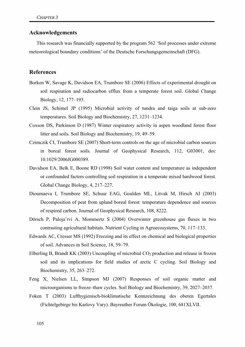
CHAPTER 3
Acknowledgements
This research was financially supported by the program 562 ‘Soil processes under extreme
meteorological boundary conditions’ of the Deutsche Forschungsgemeinschaft (DFG).
References
Borken W, Savage K, Davidson EA, Trumbore SE (2006) Effects of experimental drought on
soil respiration and radiocarbon efflux from a temperate forest soil. Global Change
Biology, 12, 177–193.
Clein JS, Schimel JP (1995) Microbial activity of tundra and taiga soils at sub-zero
temperatures. Soil Biology and Biochemistry, 27, 1231–1234.
Coxson DS, Parkinson D (1987) Winter respiratory activity in aspen woodland forest floor
litter and soils. Soil Biology and Biochemistry, 19, 49–59.
Czimczik CI, Trumbore SE (2007) Short-term controls on the age of microbial carbon sources
in boreal forest soils. Journal of Geophysical Research, 112, G03001, doi:
10.1029/2006JG000389.
Davidson EA, Belk E, Boone RD (1998) Soil water content and temperature as independent
or confounded factors controlling soil respiration in a temperate mixed hardwood forest.
Global Change Biology, 4, 217–227.
Dioumaeva I, Trumbore SE, Schuur EAG, Goulden ML, Litvak M, Hirsch AI (2003)
Decomposition of peat from upland boreal forest: temperature dependence and sources
of respired carbon. Journal of Geophysical Research, 108, 8222.
Dörsch P, Paloja¨rvi A, Mommertz S (2004) Overwinter greenhouse gas fluxes in two
contrasting agricultural habitats. Nutrient Cycling in Agroecosystems, 70, 117–133.
Edwards AC, Cresser MS (1992) Freezing and its effect on chemical and biological properties
of soil. Advances in Soil Science, 18, 59–79.
Elberling B, Brandt KK (2003) Uncoupling of microbial CO2 production and release in frozen
soil and its implications for field studies of arctic C cycling. Soil Biology and
Biochemistry, 35, 263–272.
Feng X, Nielsen LL, Simpson MJ (2007) Responses of soil organic matter and
microorganisms to freeze–thaw cycles. Soil Biology and Biochemistry, 39, 2027–2037.
Foken T (2003) Lufthygienisch-bioklimatische Kennzeichnung des oberen Egertales
(Fichtelgebirge bis Karlovy Vary). Bayreuther Forum Ökologie, 100, 681XLVII.
105

CHAPTER 3
Foken T (2004) Climate change in the Lehstenbach region. In: Biogeochemistry of Forested
Catchments in a Changing Environment (ed. Matzner E), pp. 59–66. Springer, Berlin.
Gaudinski JB, Trumbore SE, Davidson EA, Zheng S (2000) Soil carbon cycling in a
temperate forest: radiocarbon-based estimates of residence times, sequestration rates and
partitioning of fluxes. Biogeochemistry, 51, 33–69.
Gaul D, Hertel D, Leuschner C (2008) Effects of experimental soil frost on the fine root
system of mature Norway spruce. Journal of Plant Nutrition and Soil Science, 171, 688–
696.
Gerstberger P, Foken T, Kalbitz K (2004) The Lehstenbach and Steinkreuz catchments in NE
Bavaria, Germany. In: Biogeochemistry of Forested Catchments in a Changing
Environment (ed. Matzner E), pp. 15–29. Springer, Berlin.
Goldberg S, Muhr J, Borken W, Gebauer G (2007) Fluxes of climate-relevant trace gases
between a Norway spruce forest soil and the atmosphere during repeated freeze-thaw
cycles in mesocosms. Journal of Plant Nutrition and Soil Science, 171, 727–737.
Groffman PM, Hardy JP, Driscoll CT, Fahey TJ (2006) Snow depth, soil freezing, and fluxes
of carbon dioxide, nitrous oxide and methane in a northern hardwood forest. Global
Change Biology, 12, 1748–1760, doi: 10.1111/j.1365-2486.2006.01194.x.
Hansen J, Vogg G, Beck E (1996) Assimilation, allocation and utilization of carbon by 3-
year-old Scots pine (Pinus sylvestris L.) trees during winter and early spring. Trees –
Structure and Function, 11, 83–90.
Hentschel K, Borken W, Zuber T, Bogner C, Huwe B, Matzner E (2008) Soil frost and its
relevance for N mineralization and solute fluxes in a temperate forest soil. Global
Change Biology, this issue.
Herrmann A, Witter E (2002) Sources of C and N contributing to the flush in mineralization
upon freeze–thaw cycles in soils. Soil Biology and Biochemistry, 34, 1495–1505.
IPCC (2001) Climate Change 2001: The Scientific Basis. Contribution of Working Group I to
the Third Assessment Report of the Intergovernmental Panel on Climate Change.
Cambridge University Press, Cambridge, 881 pp.
IUSS Working Group WRB (2006) World reference base for soil resources 2006.World Soil
Resources Reports No. 103. FAO, Rome.
Larsen KS, Jonasson S, Michelsen A (2002) Repeated freeze–thaw cycles and their effects on
biological processes in two arctic ecosystem types. Applied Soil Ecology, 21, 187–195.
Matzner E, Borken W (2008) Do freeze–thaw events enhance C and N losses from soils of
different ecosystems? – a review. European Journal of Soil Science, 59, 274–284.
106

CHAPTER 3
Mikan CJ, Schimel JP, Doyle AP (2002) Temperature controls of microbial respiration in
arctic tundra soils above and below freezing. Soil Biology and Biochemistry, 34, 1785–
1795.
Monson RK, Lipson DL, Burns SP, Turnipseed AA, Delany AC, Williams MW, Schmidt SK
(2006) Winter forest soil respiration controlled by climate and microbial community
composition, 439, 711–714.
Nieminen JK, Setala H (2001) Bacteria and microbial-feeders modify the performance of a
decomposer fungus. Soil Biology and Biochemistry, 33, 1703–1712.
Raich JW, Schlesinger WH (1992) The global carbon dioxide flux in soil respiration and its
relationship to vegetation and climate. Tellus B, 44, 81–99.
Rivkina EM, Friedmann EI, McKay CP, Gilichinsky DA (2000) Metabolic activity of
permafrost bacteria below the freezing point. Applied and Environmental Microbiology,
66, 3230–3233.
Savage KE, Davidson EA (2003) A comparison of manual and automated systems for soil
CO2 flux measurements: trade-offs between spatial and temporal resolution. Journal of
Experimental Botany, 54, 891–899, doi: 10.1093/jxb/erg121.
Schimel DS (1995) Terrestrial ecosystems and the carbon cycle. Global Change Biology, 1,
77–91
Schimel J, Balser TC, Wallenstein M (2007) Microbial stress– response physiology and its
implications for ecosystem function. Ecology, 88, 1386–1394.
Schimel JP, Mikan C (2005) Changing microbial substrate use in Arctic tundra soils through a
freeze–thaw cycle. Soil Biology and Biochemistry, 37, 1411–1418.
Schlesinger WH, Andrews JA (2000) Soil respiration and the global carbon cycle.
Biogeochemistry, 48, 7–20.
Schmitt A, Glaser B, Borken W, Matzner E (2008) Repeated freeze–thaw cycles changed
organic matter quality in a temperate forest soil. Journal of Plant Nutrition and Soil
Science, 171, 705–716.
Schuur EAG, Trumbore SE (2006) Partitioning sources of soil respiration in boreal black
spruce forest using radiocarbon. Global Change Biology, 12, 165–176.
Smit-Spinks B, Swanson BT, Markhart AH III (1985) The effect of photoperiod and
thermoperiod on cold acclimation and growth of Pinus sylvestris. Canadian Journal of
Forest Research, 15, 453–460.
Stuiver M, Polach HA (1977) Discussion; reporting of 14C data. Radiocarbon, 19, 355–363.
107

CHAPTER 3
108
Tierney G, Fahey T, Groffman P, Hardy J, Fitzhugh R, Driscoll C (2001) Soil freezing alters
fine root dynamics in a northern hardwood forest. Biogeochemistry, 56, 175–190.
Tinus RW, Burr KE, Atzmon N, Riov J (2000) Relationship between carbohydrate
concentration and root growth potential in coniferous seedlings from three climates
during cold hardening and dehardening. Tree Physiology, 20, 1097–1104.
Voroney RP (2007) The soil habitat. In: Soil Microbiology, Ecology, and Biochemistry (ed.
Paul EA), pp. 25–49. Academic Press, Oxford.
Xu X, Trumbore SE, Zheng S, Southon JR, McDuffee KE, Luttgen M, Liu JC (2007)
Modifying a sealed tube zinc reduction method for preparation of AMS graphite targets:
reducing background and attaining high precision. Nuclear Instruments and Methods in
Physics Research Section B: Beam Interactions with Materials and Atoms, 259, 320–
329.

CHAPTER 4
Chapter 4
Soil C dynamics in a forest as affected by drought
109

CHAPTER 4A
PART A:
Drying-rewetting events reduce C and N losses from a
Norway spruce forest floor Jan Muhr1*), Janine Franke1) and Werner Borken1) 1) Department of Soil Ecology, University of Bayreuth, Dr.-Hans-Frisch-Strasse 1-3, 95448
Bayreuth
*Corresponding author: Jan Muhr ([email protected])
Submitted to Soil Biology and Biochemistry
Received 17 December 2008
Abstract
Periods of prolonged summer drought are likely to be expected for this century, with
possibly strong effects on carbon (C) and nitrogen (N) mineralization in soils. In this
experiment, undisturbed soil columns from a Norway spruce forest in Bavaria, Germany,
were subjected to an 80 d drought period. Three different drought intensities were
investigated in three treatment groups. During the first weeks, the soil columns were gradually
dried and then kept at constant water potential. Initial water potential was between -0.01 and -
0.1 MPa (pF 2-3), and reduced by drying to -0.6, -80 and -400 MPa (pF 3.5, 5.5 and 6.5) in
the parallel treatment groups. Rewetting of the dry soil was achieved by irrigation (4 mm d-1)
for 40 d.
CO2 fluxes from all groups were identical before drying. Over the 80 d drought period,
drying treatments only emitted 72, 52 or 43 % of the amount of CO2 emitted during the same
time from a constantly moist control. Rewetting resulted in a fast increase of CO2 fluxes to
approx. the same level as in the control. No significant excess C mineralization during
rewetting was observed, so adding up total CO2 fluxes of the 80 d drought and the 40 d
rewetting period, the drought treatments emitted only 88, 71 or 67 % of the CO2 emitted by
the constantly moist control. Measurements of dissolved organic carbon (DOC) did only show
minor differences between control and treatment columns, indicating that no significant
accumulation of DOC took place during the drought period. Radiocarbon signature of emitted
CO2 indicates that C mineralization simply was reduced with decreasing water availability
and no new substrate was made bioavailable. Net N mineralization over the course of the
whole experiment was reduced by drought to 77, 65 or 52 % of the control. Net nitrification 110

CHAPTER 4A
was virtually zero during drought whereas net ammonification continued at reduced levels. In
total, increasing drought intensity resulted in increasingly reduced C and N mineralization.
Neither C nor N mineralization were enhanced by drying-rewetting. The organic horizons
seem well adapted to rapidly fluctuating water availability. The relevance of the so-called
‘Birch effect’ for this soil has to be challenged. Prolonged summer droughts are likely to
conserve soil organic carbon (SOC) and soil organic nitrogen (SON) pools in this soil.
Key Words: Summer Drought Intensity; Drying; Rewetting; Birch-Effect; CO2; DOC;
Nitrogen; Climate Change; Soil respiration; Radiocarbon
111

CHAPTER 4A
Introduction
Soils are known to play an important role as reservoirs for organic C and N. They also are
important sources or sinks, respectively, for several climate relevant gases. Following the
predictions of the IPCC (2007), we not only face an increase of mean annual air temperature
within this century, but also a change of precipitation patterns resulting in an increasing
probability of extended summer droughts followed by heavy rainfall events. This change of
the global water cycle is likely to have an impact on C and N mineralization in soils.
Drying of forest floors is a phenomenon occurring regularly. It is generally understood
that during drying of well-drained soils mineralization decreases, whereas rewetting leads to a
rapid increase of mineralization. Several mechanisms have been proposed to explain both the
reduction of mineralisation during drying and the increase during subsequent rewetting (cf.
Borken and Matzner, 2009).
During drought periods, microorganisms have to respond to reduced soil water potentials.
They can either dehydrate and become dormant, or they acclimate at high costs by
accumulating compatible solutes (Harris, 1981). During drought, total cytoplasmic
constituents can account for 30-40 % of total C and 20-60% of total N of bacteria or fungi,
compared to only 3-6 % of total C and N during non-stress conditions (Schimel et al., 1989;
Schimel et al., 2007). As microorganisms invest substrates into acclimatization, become
inactive or even die due to severe living conditions during periods of drought (Bottner, 1985;
De Nobili et al., 2006), both microbial C and N mineralization decrease. This decrease is
further enhanced by diffusive limitations: Reduced water content decreases substrate diffusion
and hence substrate accessibility for microorganisms (Voroney, 2007).
Drying of soil can also alter soil structure and characteristics of soil surfaces. Aggregate
disruption and desorption of surfaces may occur during periods of drought, rendering new
substrates available (Utomo and Dexter, 1982; Bottner, 1985; Van Gestel et al., 1993; Denef
et al., 2001). At the same time drought is known to increase the hydrophobicity especially of
soils rich in organic matter (Mataix-Solera et al., 2007). Although this is normally not of
importance for the microbial activity during the drought itself, it becomes increasingly
important during the rewetting of soil.
Wetting of the dry soil generally increases microbial activity, but the extent of this wetting
pulse can vary widely depending on soil properties, intensity and length of the drying,
intensity of the rewetting etc. This wetting pulse can occur very fast, even within minutes (e.g.
Borken et al., 2003), and its size and duration are of major importance for the cumulative C
and N net mineralization resulting from drying-rewetting events. 112

CHAPTER 4A
Two fundamentally different mechanisms are currently discussed to explain this wetting
pulse. Following the nomenclature used by Xiang et al. (2008) we name them the “microbial
stress” mechanism vs. the “substrate supply” mechanism.
As mentioned above, active cells have to accumulate compatible solutes to retain water
and survive periods of drought. Rewetting of the soil, resulting in a sudden increase of water
potential, forces cells to dispose of these compatible solutes or risk cell rupture due to massive
water uptake. The no longer needed compatible solutes are set free and can now be easily
mineralized by the microorganisms. The microbial stress mechanism therefore postulates that
the wetting pulse during rewetting is due to the mineralization of substrates that were already
present but used differently.
In contrast to this, the substrate supply mechanism assumes the creation of new substrates
that were not available until the drying-rewetting event occurred. It is mainly build on the fact
that physical processes during rewetting of dry soil can destabilize soil organic matter (SOM),
e.g. by aggregate disruption, organic matter redistribution or desorption.
Like pointed out by Xiang et al. (2008) the effects of these two mechanisms would be
dramatically different: The microbial stress mechanism bears no potential of creating new
substrates, but rather might result in a loss of microbial biomass thereby reducing the
metabolical capability of the microbial pool. The substrate supply mechanism on the other
hand can destabilize former stable or meta-stable SOM pools and enhance C and N losses
from soils (so-called “Birch effect”). In deed, several authors reported a short-term extra
mineralization burst following rewetting, exceeding by far pre-drought mineralization rates
or the rates of a permanently moist control (Birch, 1958; Seneviratne and Wild, 1985; Kieft et
al., 1987; Fierer et al., 2003; Haney et al., 2004; Xiang et al., 2008). Such an extra boost of
microbial activity indicates the creation of additional substrate due to drying-rewetting
(priming effect) and is termed as the “Birch effect” (Jarvis et al., 2007). It is this Birch effect
that repeatedly gave reason to discussions about the net-effect of drying-rewetting (cf. Borken
and Matzner, 2009). Whereas drought generally decreases cumulative C and N fluxes out of
the soil, the release of additional substrate can cause C and N fluxes during the wetting pulse
which more than compensate for this reduction and result in an increase of net mineralization.
Radiocarbon (14C) offers the possibility of detecting changes in the predominant sources
of respired CO2. Substrates from meta-stable or stable C pools that are made bioavailable by
drying-rewetting should differ in their radiocarbon signature (Δ14C) from more recent C
sources, thereby altering the isotopic signature of the emitted CO2 as soon as they are
113

CHAPTER 4A
metabolized. The creation of new substrates from stable or meta-stable pools should therefore
result in measurable changes of Δ14C of respired CO2.
This experiment was designed to investigate the effect of drought intensity followed by
rewetting of the soil on net C and N fluxes. Undisturbed soil columns from underneath a
Norway spruce stand (Picea abies L.) were used to test the following hypotheses: (1)
increasing drought intensity reduces C and N fluxes from the soil during drought; (2)
rewetting leads to a fast wetting pulse; (3) the size of the wetting pulse is depending on the
intensity of the preceding drought; (4) the wetting pulse has only a minor impact on the
overall C and N fluxes from the soil and cannot compensate for reduced C and N fluxes
during the drought.
Material and Methods
Design of the mesocosm experiment
Undisturbed soil columns from underneath a 135 y-old Norway spruce (Picea abies L.)
stand were sampled for this experiment. The stand is located in the “Fichtelgebirge” in NE
Bavaria, Germany (50°8’ N, 11°52’ E) at an elevation of 775 m asl. Mean annual air
temperature at the stand is 5.3°C and mean annual precipitation 1160 mm (Gerstberger et al.,
2004). The forest floor at the stand is covered by ground vegetation, mainly Calamagrostis
villosa and Deschampsia flexuosa, as well as Oxalis acetosella and Vaccinium myrtillus.
According to the FAO soil classification (IUSS Working Group WRB, 2006), the soil at the
stand is classified as a Haplic Podsol with a sandy-loamy texture, covered by a moder of 6-13
cm thickness consisting of Oi, Oe, and Oa horizons. A more detailed soil characterization can
be found in Hentschel et al. (2007).
Soil sampling took place in the spring of 2006 by driving polyacrylic cylinders (ø 17.1
cm, 30 cm high) into the soil. The resulting soil columns were further prepared by removing
all mineral soil and cutting off vegetation, resulting in undisturbed soil columns consisting
only of the organic horizons, ranging in length from 7-13 cm. The prepared soil columns were
stored at +5°C and field water conditions for several weeks before starting the experiment.
For the experiment, 20 soil columns were separated in 5 groups, each consisting of 4
replicas. Four of these groups were designed for regular measurement of CO2 fluxes and soil
solution composition. The first of these groups was designed as a control, the three other
groups were designed to investigate the effects of different drought intensities and subsequent
rewetting and will hereafter be called D1 to D3 (Drought treatment 1 to 3, with drought
114

CHAPTER 4A
intensity during the drying period increasing from D1 to D3). The remaining fifth group was
designed for destructive soil sampling (Batch experiment) during the drying period to be able
to measure important soil parameters.
With the beginning of the experiment, all soil columns were transferred to a climate
chamber at constant +15°C. The cylinders were placed on ceramic base plates and covered
with polyacrylic lids, resulting in gas-tight mesocosms. During a 34 d pre-run period (days -
34 to -1, as day 0 is defined here as the beginning of the drying) we measured inherent
differences between the treatments (for a schematic schedule see Figure 1). During this pre-
run period the soil was irrigated with 4 mm artificial throughfall solution per day,
representing the mean daily precipitation at the field site. The composition of the artificial
throughfall solution was similar to the composition of the natural throughfall at the stand
(Matzner et al., 2004) containing the following components (µmol L-1): DOC 0.0, NH4+
100.0, NO3- 100.0, Ca2+ 27.6, K+ 57.5, Mg2+ 7.5, Na+ 15.5, Cl- 45.0, PO4
3- 1.8, SO42- 48.2 The
solution was applied in 2 mm portions using a syringe with a fine nozzle.
1-Pre-run 2-Drought 3-RewettingC
D1D2D3Tr
eatm
ent
Mea
sure
men
ts CO2 fluxes
Δ14C of CO2
Soil solution
Irrigation(4 mm d-1)
Irrigation(4 mm d-1)
Constantwater
content
Soil batches
Experimental stage
1 2 3 4 5
Drying
-40 -20 0 20 40 60 80 100 120Time (d)
-40 -20 0 20 40 60 80 100 120
Figure 1 Schematic overview of the experimental schedule. During the pre-run period, all soil columns were irrigated with the mean daily precipitation amount at the field site. During drying, the control (C) was kept at constant water content whereas the three drought treatments (D1 to D3) where dried for different lengths of time and then kept at the new, reduced water content. At the beginning of the rewetting period, all soil columns were irrigated with 4 mm d-1 of artificial throughfall.
115
At the end of the pre-run period, the drying period began (days 0 to 80): Whereas the
control was kept at constant water content throughout this period, the base plate and the lid
were removed from the drought treatments for several hours a day and the soil was dried via
ventilation with dry air. To monitor development of the drying, both gravimetric water
content and remaining initial respiration were measured. Experimental design scheduled three
different drought intensities for the three drought treatments, ranging from moderate to heavy
drought. As CO2 fluxes were a major focus of this experiment, the drought treatments were air
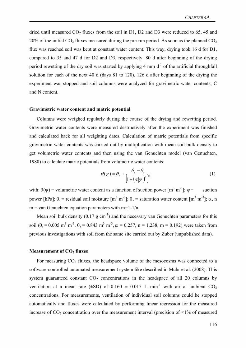
CHAPTER 4A
dried until measured CO2 fluxes from the soil in D1, D2 and D3 were reduced to 65, 45 and
20% of the initial CO2 fluxes measured during the pre-run period. As soon as the planned CO2
flux was reached soil was kept at constant water content. This way, drying took 16 d for D1,
compared to 35 and 47 d for D2 and D3, respectively. 80 d after beginning of the drying
period rewetting of the dry soil was started by applying 4 mm d-1 of the artificial throughfall
solution for each of the next 40 d (days 81 to 120). 126 d after beginning of the drying the
experiment was stopped and soil columns were analyzed for gravimetric water contents, C
and N content.
Gravimetric water content and matric potential
Columns were weighed regularly during the course of the drying and rewetting period.
Gravimetric water contents were measured destructively after the experiment was finished
and calculated back for all weighting dates. Calculation of matric potentials from specific
gravimetric water contents was carried out by multiplication with mean soil bulk density to
get volumetric water contents and then using the van Genuchten model (van Genuchten,
1980) to calculate matric potentials from volumetric water contents:
( )[ ]mn
rsr
ψα
θθθψθ+
−+=
1)( (1)
with: θ(ψ) = volumetric water content as a function of suction power [m3 m-3]; ψ = suction
power [hPa]; θr = residual soil moisture [m3 m-3]; θs = saturation water content [m3 m-3]; α, n
m = van Genuchten equation parameters with m=1-1/n.
Mean soil bulk density (0.17 g cm-3) and the necessary van Genuchten parameters for this
soil (θr = 0.005 m3 m-3, θs = 0.843 m3 m-3, α = 0.257, n = 1.238, m = 0.192) were taken from
previous investigations with soil from the same site carried out by Zuber (unpublished data).
Measurement of CO2 fluxes
For measuring CO2 fluxes, the headspace volume of the mesocosms was connected to a
software-controlled automated measurement system like described in Muhr et al. (2008). This
system guaranteed constant CO2 concentrations in the headspace of all 20 columns by
ventilation at a mean rate (±SD) of 0.160 ± 0.015 L min-1 with air at ambient CO2
concentrations. For measurements, ventilation of individual soil columns could be stopped
automatically and fluxes were calculated by performing linear regression for the measured
increase of CO2 concentration over the measurement interval (precision of <1% of measured
116

CHAPTER 4A
concentration). Using the automated measurement system, up to 14 measurements of each of
the soil columns could be made per day.
As mentioned above, the soil columns varied in size, and therefore in the amount of
available C. To improve comparability, total weight and C content of the soil were determined
at the end of the experiment to calculate the total C pool of each column. The measured CO2
fluxes were then related to the C pool.
Radiocarbon signature
In each period (pre-run, drying, rewetting) gas samples were taken from the headspace
volume above the soil to measure the Δ14C signature of the emitted CO2. Prior to sampling,
ventilation was switched off and the whole system was flushed with CO2 free synthetic air.
CO2 concentration inside the mesocosms was then allowed to increase over night. The next
day, evacuated stainless steel cylinders with a volume of 2 L were connected to the
mesocosms and slowly filled with gas from the headspace volume. Gas samples were then
transferred to the laboratory for further processing.
Processing in general followed the zinc reduction method for preparation of AMS graphite
targets described in Xu et al. (2007). The only notable difference was the injection of the gas
samples into the extraction line: the steel containers containing the samples were connected to
the extraction line via a digital mass flow controller (Type F-201C-AAA-33-V, Wagner
Mess- und Regeltechnik) effectively limiting the flow rate to 20 ml min-1. This way,
extraction of CO2 from the air inside the containers took around 3 hours per cylinder. All
preparation took place at the laboratories of the Department of Soil Ecology at the University
of Bayreuth. Graphite targets were analyzed by the Keck Carbon Cycle AMS facility at UC
Irvine, USA with a precision of 2-3 ‰. Radiocarbon data are expressed as Δ14C, which is the
per mil deviation from the 14C/12C ration of oxalic acid standard in 1950. The sample 14C/12C
ratio has been corrected to a δ13C value of -25‰ to account for any mass dependent
fractionation effects (Stuiver and Polach, 1977).
Analysis of soil solution
117
Via the ceramic base plates (pore size 1 µm), pre-filtered soil solution could be extracted
from the mesocosms. During the pre-run period, the first sampling of soil solution took place
between day -26 and day -13. Soil solution was extracted by applying a negative pressure of -
350 mbar. During drying soil solution sampling was not possible. Soil solution was sampled
again during the rewetting period. Soil columns were freely draining during this period and

CHAPTER 4A
sampling took place without the application of a negative pressure. 4 subsequent samples
were taken during this period, each integrating over 9-13 d of sampling (cf. Figure 1).
Soil solution was filtered using 0.45 µm polycarbonate membrane filters (Millipore), and
stored at +2°C. Soil solution was then analyzed for dissolved organic carbon (DOC) and total
nitrogen (Ntot) by high temperature analyzer (Elementar, high-TOC), for ammonium (NH4+-
N) by flow injection analyzer (MLE, FIA-LAB) and for nitrate (NO3--N) by ion
chromatograph (DIONEX, DX500 Chromatography system). Concentration of dissolved
organic nitrogen (DON) was calculated as the difference between Ntot and inorganic N (the
sum of NH4+-N and NO3
--N). The fluxes were calculated by multiplying the concentrations in
the soil solution with the measured water flux from the soil, with regard to input via artificial
throughfall solution.
Batch experiment
In addition to the regularly measured soil columns, 4 columns for destructive soil
sampling were included in the experiment (hereafter ‘Batch columns’, as batches of soil were
removed on every sampling date). They were dried together with the drought treatments and
used for analyzing concentrations of Ntot, NO3--N and NH4
+-N in the soil during drought.
Sampling took place on four different dates, and on each date, one quarter of each soil column
was sampled. The first sampling took place at the beginning of the drying period (t = 0 d).
The next sampling was carried out by the time when the drying of D1 was finished (t = 16 d).
Sampling day 3 coincided with the end of the drying of D2 (t = 35 d) and sampling day 4 with
the end of the drying of D3 (t = 47 d). Each time soil was removed from the batch columns,
the sampled segment was replaced by foam to avoid lateral drying.
A subsample of each batch sample was used to determine gravimetric water content by
drying the soil at 60°C in the drying oven. The rest of the samples were stored at +2°C until
further analysis. For extraction, soil was mixed with Millipore water. The extract was shaken
for one hour and then centrifuged for 15 min at 5250 rpm (5000 g). The supernatant was
filtered using glass fiber filters (Schleicher and Schuell) and 0.45 µm polycarbonate
membrane filters (Millipore). Analysis was equal to analysis of the soil solution samples.
118

CHAPTER 4A
Results
Matric potential
At the end of the pre-run period, water potential in all groups range between 0.01 and
0.1 MPa (pF 2-3, Figure 2a). During the drying period, matric potential of the control is kept
constant at this level. The three drought treatments are dried out to a matric potential of -0.6, -
80 and -400 MPa, respectively, and kept constantly around these values until rewetting.
Irrigation during the rewetting period increases the water potential of all treatments, even of
the control. This increase in the control to values between -0.001 and 0.01 MPa can be
explained with differences in the soil solution sampling: Whereas soil solution during the
irrigation period was sampled by free drainage, a negative pressure was applied during the
pre-run period resulting in decreased water potentials. Matric potential of D1 to D3 increases
to the pre-drought value of around -0.01 MPa within 8 d (D1) or 20 d (D2 and D3) of
irrigation, respectively.
CO2 fluxes
CO2 fluxes during the pre-run period are similar for all treatments ranging between 8 and 12
mg C kg-1 SOC h-1 (Figure 2b, SOC = soil organic carbon). There is a general trend of
decreasing CO2 fluxes in all groups until day 60. Drying accelerates this decrease of the CO2
fluxes in the drought treatments. During the first 3 d of the drying period, mean daily CO2
fluxes decrease very fast, although mean matric potential of the soil change only slightly
(Figure 3). Further reduction of the matric potential (t = 4-80d) has a smaller effect on
observed CO2 fluxes, but shows a clear logarithmic correlation (r2 = 0.74). Ventilation drying
of the different treatments was stopped after 16, 35 and 47 d but fluxes keep on decreasing for
a few days even after ventilation was stopped. At the end of the drying period, mean CO2
fluxes of the groups are 5.2 (control), 3.3 (D1), 1.4 (D2), and 0.5 (D3) mg C kg-1 SOC h-1, so
fluxes of the drought treatments are equivalent to 63, 27 and 10 % of the control fluxes.
Differences between treatments and control are significant only for D2 and D3 (p<0.05,
ANOVA).
The beginning of the rewetting causes a rapid increase of CO2 fluxes. D1 and D2
regenerate back to the level of the control within around 5 d. CO2 fluxes of D3 even exceed
the level of the control fluxes for a few days. However, this excess is mainly owed to a drastic
increase in only one of the replicas (replica no. 4) and therefore statistically not significant. 20
d after beginning of the rewetting, CO2 fluxes of all treatments stabilize in the same pattern as
119
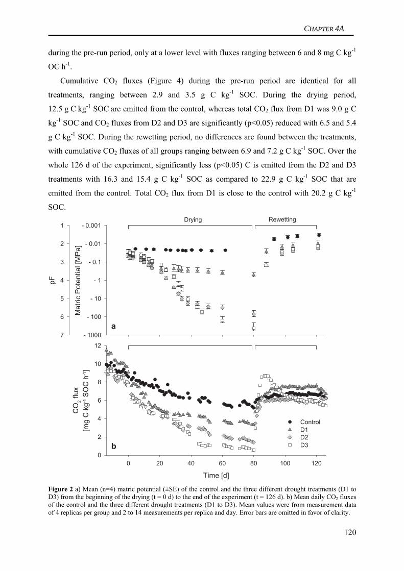
CHAPTER 4A
during the pre-run period, only at a lower level with fluxes ranging between 6 and 8 mg C kg-1
OC h-1.
Cumulative CO2 fluxes (Figure 4) during the pre-run period are identical for all
treatments, ranging between 2.9 and 3.5 g C kg-1 SOC. During the drying period,
12.5 g C kg-1 SOC are emitted from the control, whereas total CO2 flux from D1 was 9.0 g C
kg-1 SOC and CO2 fluxes from D2 and D3 are significantly (p<0.05) reduced with 6.5 and 5.4
g C kg-1 SOC. During the rewetting period, no differences are found between the treatments,
with cumulative CO2 fluxes of all groups ranging between 6.9 and 7.2 g C kg-1 SOC. Over the
whole 126 d of the experiment, significantly less (p<0.05) C is emitted from the D2 and D3
treatments with 16.3 and 15.4 g C kg-1 SOC as compared to 22.9 g C kg-1 SOC that are
emitted from the control. Total CO2 flux from D1 is close to the control with 20.2 g C kg-1
SOC.
Time [d]
0 20 40 60 80 100 120
CO
2 flu
x[m
g C
kg-1
SO
C h
-1]
0
2
4
6
8
10
12
ControlD1D2D3
pF
1
2
3
4
5
6
7
Mat
ric P
oten
tial [
MPa
]
- 0.001
- 0.01
- 0.1
- 1
- 10
- 100
- 1000
Drying Rewetting
a
b
Figure 2 a) Mean (n=4) matric potential (±SE) of the control and the three different drought treatments (D1 to D3) from the beginning of the drying (t = 0 d) to the end of the experiment (t = 126 d). b) Mean daily CO2 fluxes of the control and the three different drought treatments (D1 to D3). Mean values were from measurement data of 4 replicas per group and 2 to 14 measurements per replica and day. Error bars are omitted in favor of clarity.
120

CHAPTER 4A
Matric Potential [MPa]
- 0.001- 0.01- 0.1- 1- 10- 100- 1000
CO
2 flu
x [m
g C
kg-1
SO
C h
-1]
0
2
4
6
8
10
12
Drying, data from days 1-3Drying, data from days 4-80Logarithmic Regression for d 4-80
y = -0.55*ln|x| + 3.9r2 = 0.74
Figure 3 Correlation of observed CO2 fluxes and matric potential in the D1 to D3 columns during the drying period. The correlation shown is calculated for data from d 4-80 of the drying period as data from d 0-3 shows a different correlation.
Pre-run Drying Rewetting Total
Cum
ulat
ive
C fl
ux [g
C k
g-1 S
OC
]
0
5
10
15
20
25
30ControlD1D2D3
a a a a
a
ab
bb
a aa a
a
ab
bb
Figure 4 Mean (n=4) cumulative C fluxes (±SE) for the three separate periods and the whole experiment. Values without identical letters above the bars differ significantly (p<0.05).
121

CHAPTER 4A
Radiocarbon analysis
Mean radiocarbon signature of CO2 emitted from the control shows a constant increase
during the experiment, indicating mineralization of gradually older substrate (Figure 5).
During the pre-run, radiocarbon signature of the control is at 106 ‰, increasing to 115 ‰
(ΔΔ14C = 9 ‰) during the drying period and 123 ‰ in the rewetting period. Radiocarbon
signatures of two of the drought treatments also shows such an increase from pre-run to
drying period, but at a smaller level (D1: ΔΔ14C = 6 ‰; D3: ΔΔ14C = 5 ‰). From drying to
rewetting period, the radiocarbon signature in D3 remains constant. D2 differs from the other
groups: No notable increase of Δ14C from pre-run to drying, and in addition a drop of Δ14C
from drying to rewetting (ΔΔ14C = -10 ‰).
Control D1 D2 D3
Δ14 C
sig
natu
re [‰
]
90
100
110
120
130
140Pre Dry Wet
Not
mea
sure
d
Figure 5 Mean (n=4) radiocarbon signature of emitted CO2 in the control and of the drought treatments (D1, D2, D3) during the pre-run, drying and rewetting period.
It has to be mentioned, that the mean radiocarbon signature of D3 during the drying period
excludes one of the columns (replica no. 4), as this one showed an extreme drop down to
55 ‰, possibly indicating contribution of pre-bomb C to emitted CO2. This occurred only for
one column, and only at extremely dry conditions.
Soil solution
Pre-run DOC concentrations are the same level for all treatments (around 30 mg C l-1, cf.
Figure 6). All treatments show only slightly increased DOC concentrations during the
122
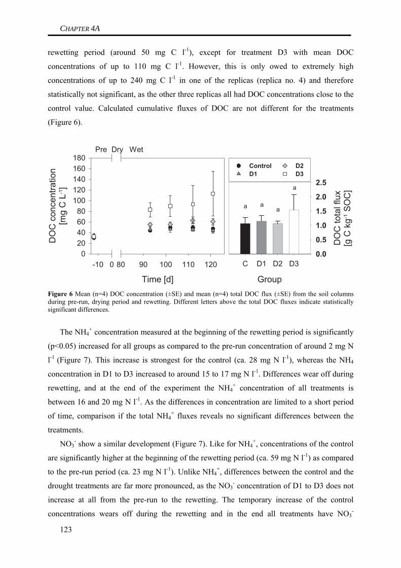
CHAPTER 4A
rewetting period (around 50 mg C l-1), except for treatment D3 with mean DOC
concentrations of up to 110 mg C l-1. However, this is only owed to extremely high
concentrations of up to 240 mg C l-1 in one of the replicas (replica no. 4) and therefore
statistically not significant, as the other three replicas all had DOC concentrations close to the
control value. Calculated cumulative fluxes of DOC are not different for the treatments
(Figure 6).
Time [d]
-10 90 1100 80 100 120
DO
C c
once
ntra
tion
[mg
C L
-1]
020406080
100120140160180
C D1 D2 D3
DO
C to
tal f
lux
[g C
kg-1
SO
C]
0.0
0.5
1.0
1.5
2.0
2.5
aa a
a
Pre Dry Wet
ControlD1
D2D3
Group Figure 6 Mean (n=4) DOC concentration (±SE) and mean (n=4) total DOC flux (±SE) from the soil columns during pre-run, drying period and rewetting. Different letters above the total DOC fluxes indicate statistically significant differences.
The NH4+ concentration measured at the beginning of the rewetting period is significantly
(p<0.05) increased for all groups as compared to the pre-run concentration of around 2 mg N
l-1 (Figure 7). This increase is strongest for the control (ca. 28 mg N l-1), whereas the NH4
concentration in D1 to D3 increased to around 15 to 17 mg N l-1. Differences wear off during
rewetting, and at the end of the experiment the NH4+ concentration of all treatments is
between 16 and 20 mg N l-1. As the differences in concentration are limited to a short period
of time, comparison if the total NH4+ fluxes reveals no significant differences between the
treatments.
NO3- show a similar development (Figure 7). Like for NH4
+, concentrations of the control
are significantly higher at the beginning of the rewetting period (ca. 59 mg N l-1) as compared
to the pre-run period (ca. 23 mg N l-1). Unlike NH4+, differences between the control and the
drought treatments are far more pronounced, as the NO3- concentration of D1 to D3 does not
increase at all from the pre-run to the rewetting. The temporary increase of the control
concentrations wears off during the rewetting and in the end all treatments have NO3-
123

CHAPTER 4A
concentrations similar to the pre-run period again. Total NO3- fluxes are highest for the
control (ca. 19 g N kg-1 N) and show a clear trend of becoming smaller with increasing
drought intensity.
Time [d]
-10 90 1100 80 100 120
NO
3- con
cent
ratio
n[m
g N
L-1]
0
20
40
60
NH
4+ tot
al fl
ux[g
N k
g-1 N
]
02468101214
NH
4+ con
cent
ratio
n[m
g N
L-1]
0
10
20
30
40
C D1 D2 D3N
O3- t
otal
flux
[g N
kg-1
N]
0
5
10
15
20
25
a
a
aa
ab
a
ab
b
ControlD1
D2D3
Pre Dry Wet
Group Figure 7 Mean (n=4; ±SE) concentration and total flux ammonium and nitrate measured in the soil solution samples. Samples were taken once during the pre-run period and four times during rewetting. No soil solution samples were taken during drying.
Batch experiment
The concentrations of both NH4+ and NO3
- in the soil increase during the first 16 d of the
drying period, indicating ongoing production of both NH4+ and NO3
- down to a mean matric
potential of -0.1 MPa (equal to pF 3, Figure 8). During the rest of the drying period, no
significant further increase of NH4+ or NO3
- is found.
The amount of DOC found in the batch columns does not vary over the whole drying and
is stable at around 1.2 mg C kg-1 OC (data not shown).
124

CHAPTER 4A
Matric potential [MPa]- 0.001 - 0.01 - 0.1 - 1 - 10 - 100 - 1000 - 10000
NH
4+ -, N
O3- -
conc
entra
tion
[g N
kg-1
N]
0
2
4
6
8
10
pF
1 2 3 4 5 6 7 8
NH4+
NO3-
Increasing drought
Figure 8 Mean (n=4, ±SE) NH4
+- and NO3--concentration extracted from the soil of the batch columns at
different matric potentials.
Discussion
C mineralization
Drying of the soil reduces the total CO2 fluxes from the soil in all drought treatments
compared to a continuously moist control. CO2 fluxes react quickly to the beginning of the
drying, decreasing from the first day on. This decrease is faster during the first 3 d than during
later stages, which can be explained with the initial drying of the uppermost litter layer where
a relatively high proportion of the respired CO2 originates. Effective matric potential in these
upper horizons is probably far more negative than the mean total matric potential of the soil
columns, leading to an unrealistic correlation during these first 3 d. Subsequent drying in
greater depth does have a smaller effect on the total CO2 flux. The control also shows a
decrease of the CO2 fluxes over time. We explain this decrease with a reduction of the pool of
bioavailable SOC sources due to ongoing mineralization. The observation during drying is in
agreement with findings described by other authors (Degens and Sparling, 1995; Mikha et al.,
2005; Chow et al., 2006; Xiang et al., 2008). Drying leads to a quick reduction of
heterotrophic respiration, either because microorganisms become inactive or die.
Rewetting leads to an immediate increase of CO2 fluxes in all treatments (even in the
control treatments, resulting from decreased matric potentials due to soil solution sampling by
the application of a negative pressure during the pre-run). This rapid increase can be
125

CHAPTER 4A
explained by fast regeneration of microbial activity. Microorganisms can survive even
prolonged periods of drought (80 d in this experiment), e.g. by sporulation (Chen and
Alexander, 1973) or simply by storing compatible solutes (cf. Jarvis et al., 2007; Schimel et
al., 2007; Borken and Matzner, 2009). During rewetting, substrate diffusion increases; C and
N rich osmolytes that are released by the microorganisms in reaction to the hypoosmotic
shock can now be reassimilated by the cells (Halverson et al., 2000). Only the strongest
drought treatment (D3) exceeds the CO2 fluxes of the control for about 10 d, but this excess
can not significantly increase the total CO2 fluxes during the rewetting period and can in no
way compensate for the significant reduction during the drying period, so drying-rewetting
results in an overall reduction of C mineralization.
This contradicts the postulated enhancement of net C losses due to drying-rewetting
events (Fierer and Schimel, 2002; Miller et al., 2005; Jarvis et al., 2007; Xiang et al., 2008).
Our experiment reveals a strong reduction of CO2 fluxes during drought compared to only a
very weak burst for only the strongest drying treatment. These findings are best explained by
the microbial stress mechanism, whereas the substrate supply mechanism is not supported by
our results. In fact, our results indicate that mineralization is simply temporarily reduced by
drought and regenerates again during rewetting. Substrates that were not used during the
drought period, either because microorganisms did not have access (diffusive limitations) or
because they alternatively used them as compatible solutes, can now be easily mineralized.
We measured radiocarbon signature of the emitted CO2 to recognize shifts in the
predominant substrate. The radiocarbon signature of the control steadily increases over the
course of the whole experiment. This can be explained with increasing mineralization of older
material with a higher radiocarbon signature, as the easily available, young substrate
gradually decreases (Trumbore, 2000). D1 and D3 also show an increase of the radiocarbon
signature from the pre-run to the drying period, although at a smaller level. Like in the
control, we attribute this to a gradually increasing mineralization of older material: Following
the Δ14C sampling in the pre-run, soil is irrigated for another 8 d before the drying period
starts, so mineralization of SOC continues at the level of the control for all treatments, before
it decreases with decreasing matric potential. Under really dry conditions, however, when
substrate mineralization is extremely small, Δ14C should be conserved, unless new substrate
was made available that has been physically or chemically protected before, like discussed in
context of the ‘Birch effect’. Such formerly stable substrate would have to be older, thereby
having a significantly different radiocarbon signature and resulting in significantly different
radiocarbon signature of the emitted CO2. Conservation of the Δ14C in D3 therefore supports
126

CHAPTER 4A
the idea that microbial mineralization is simply decreased during drought and increases again
as living conditions improve.
The development of Δ14C of D2 is different from the other groups and does not seem to fit
the idea of a simple reduction of mineralization. This can be explained, however, with
inhomogeneous drying of the soil during the drying period. In 3 additional soil columns we
installed ECH2O probes to measure water potential dynamics during drying in the Oe and the
Oa horizon separately (data not shown). Although we dried the soil columns from the top and
the bottom, drying speed of the Oe and Oa horizon is only identical for the first 20 d of
drying. After this period, drying is faster in the Oe than the Oa. 35 d after beginning of the
drying matric potentials in the Oe reach a constant level indicating complete drying. Drying in
the Oa continues for another 10 d, so after 45 d we can assume homogeneous (dry) moisture
conditions again. This means, that we had homogeneous moisture conditions in the control
(no drying), D1 (16 d drying, <20d) and D3 (47 d drying, >45 d), whereas we have to expect
inhomogeneous moisture patterns in D2 (35 d drying, Oe dried completely, Oa still drying).
These inhomogeneous moisture patterns are likely to lead to a relatively increased
contribution of CO2 originating from the Oa horizon. Mean bulk radiocarbon signature of the
Oa of this soil has been reported to be around 119 ‰, which is smaller than the bulk signature
of the Oe with 161 ‰ (Schulze et al., 2009), so increasing contribution of the Oa to CO2
fluxes is expected to reduce the resulting Δ14C. This reduction most likely masks the increase
due to ongoing mineralization from pre-run to drying and partly explains the drop of Δ14C
from drying to rewetting.
Stable DOC concentrations in the batch columns during the drying period indicate that
DOC production also is reduced during the drying period. Following the microbial stress
mechanism, we would expect a short-timed increase of DOC concentrations due to the
disposal of compatible solutes into the soil solution during rewetting. Owing to the nature of
soil solution sampling we can not tell whether such an increase occurred: The first soil
solution was sampled several days after rewetting, when mineralization would have decreased
the easily available substrates already. Nevertheless we do see an increase of the DOC
concentration in one of the replicas of D3 (replica no. 4). This soil core also shows the most
pronounced CO2 pulse during rewetting and has an extremely small Δ14C of 55 ‰ during
drying. This might encourage the idea that creation of new substrates indeed can take place.
However, it has to be emphasized, that this one soil core also is the one with the most
negative matric potential and the smallest CO2 fluxes during the end of the drying period. In
fact, CO2 fluxes during drying are virtually zero, with respiration probably going on only at 127

CHAPTER 4A
some still moist microsites. The significant switch of Δ14C is only due to a significant change
of the relative contribution of substrates to the (extremely small) total CO2 flux. Substrates at
these microsites either are very young material or a mixture of young material and pre-bomb
material. The pronounced CO2 pulse during rewetting can be explained with a higher degree
of conservation of easily available substrate during drying and with more water stress for the
microorganisms. Therefore, we come to the conclusion that even this most extreme soil core
does in no way support the idea of enhanced C mineralization due to drying-rewetting in this
soil.
N mineralization
NH4+ concentrations during the pre-run period are surprisingly small in all treatments
compared to the irrigation period. This might partly be explained by the fact that soil columns
were sampled at the field site during early spring when the soil microbial community still is
undergoing the change from winter to summer both in quantity and quality.
Net N losses are reduced by drought compared to a constantly moist control. Increasing
NH4+ and NO3
- concentrations in the control indicate accumulation of NH4+ and NO3
- due to
ongoing net N mineralization (defined as the sum of ammonification and nitrification) during
the sampling break between pre-run and rewetting. The increase of NH4+ concentrations in the
drought treatments during the same time is much smaller (only 60% of the control), indicating
that net ammonification is going on during drought but at reduced rates. Net nitrification on
the other hand is virtually zero during drought. Consequently, cumulative N losses from the
drought treatments are reduced compared to the control. This reduction is independent from
drought intensity for net ammonification, whereas net nitrification decreases with increasing
drought intensity. This difference indicates that the reduction of net nitrification is not simply
due to reduced NH4+ availability, but that water stress affects net nitrification rates in this soil
directly.
It is unlikely that this effect can be attributed to increased immobilisation or
denitrification: Previous work showed that NO and N2O fluxes from this soil significantly
decrease during drought (Muhr et al., 2008). This indicates a reduction of gross nitrification
rates. As differences between treatments and control were restricted to the first two sampling
dates after beginning of the rewetting of the dry soil, reduced microbial activity during
drought due to reduced substrate diffusion and adverse living conditions is the most likely
explanation for the reduction of net N mineralization. We therefore assume that autotrophic
nitrifiers, which are known to be highly sensitive to water stress (Killham, 1990; Killham, 128

CHAPTER 4A
1994), play an important role in this soil. Results from our batch experiment reveal that this
reduction net mineralization already occurs during the initial drying: NH4+ and NO3
-
concentrations increased only during the first 16d of drying (down to a minimum matric
potential of around -0.1 MPa), almost no further increase was observed when soil was dried
further.
In contrast to our results, other laboratory experiments investigating the effect of drying-
rewetting repeatedly reported enhanced N losses (Marumoto et al., 1982; Seneviratne and
Wild, 1985; Cabrera, 1993; Gordon et al., 2008; Xiang et al., 2008). This enhance was due to
a significant increase of N mineralization during rewetting of dry soil, even exceeding the
mineralization rates of a constantly moist control or during pre-drought conditions. We did
not find such a wetting pulse. However, the mentioned experiments were carried out solely
with sieved mineral soil from either arable land or grassland. Similar experiments carried out
with intact forest soil cores (Hentschel et al., 2007) or sieved material from forest floor
(Pulleman and Tietema, 1999) reported a reduction of cumulative N losses from the soil.
Mikha et al. (2005), who found a reduction of cumulative N losses from arable land due to
drying-rewetting attributed the occurrence of increased N mineralization in other experiments
to the occurrence of soil physical disruption. This phenomenon is more likely to be of
importance in mineral soil than in forest floor. However, previous experiments with mineral
soil cores from this forest site (Hentschel et al., 2007; Muhr et al., 2008) also resulted in
reduced C and N mineralization rates due to drying-rewetting, so we conclude that enhanced
N mineralization (‘Birch’ effect) due to drying-rewetting events does not occur in this
temperate forest soil. Drought does not make new substrates available but instead, like
discussed for C mineralization, simply reduces N mineralization for some time until living
conditions for the microorganisms improve again.
Conclusion
Drying is a process that regularly occurs in the forest floor of temperate forests and will
even more so according to recent climate models. It could be shown in this work that
prolonged drying (80 d) reduced net C and N losses from a Norway spruce forest soil in
comparison to a constantly wet control. C losses decreased with decreasing matric potential.
Wetting pulses could not compensate for the reduction during drying, and did not
significantly exceed control fluxes. Rewetting seems to only reactivate mineralization that
was reduced by drought. This reactivation by rewetting occurs fast, indicating that
microorganisms in the forest floor are well adapted to regular drying-rewetting events. The 129

CHAPTER 4A
creation of new substrate from stable pools leading to excess C or N mineralization (‘Birch
effect’) was not observed in this experiment. Radiocarbon signature did not indicate a change
of the age of the mineralized C sources. Summarizing, it can be said that prolonged drought
tends to conserve C and N pools in the forest floor. The assumption of enhanced C and N
mineralization due to drying-rewetting can not be supported for this forest floor.
Acknowledgements
This research was financially supported by the program 562 ‘Soil processes under extreme
meteorological boundary conditions’ of the Deutsche Forschungsgemeinschaft (DFG).
References
Birch, H.F., 1958. The Effect of Soil Drying on Humus Decomposition and Nitrogen
Availability. Plant and Soil 10, 9-31.
Borken, W., Matzner, E., 2009. Reappraisal of drying and wetting effects on C and N
mineralization and fluxes in soils. Global Change Biology doi: 10.1111/j.1365-
2486.2008.01681.x.
Borken, W., Davidson, E.A., Savage, K., Gaudinski, J., Trumbore, S.E., 2003. Drying and
wetting effects on carbon dioxide release from organic horizons. Soil Sci Soc Am J 67,
1888-1896.
Bottner, P., 1985. Response of microbial biomass to alternate moist and dry conditions in a
soil incubated with 14C- and 15N-labeled plant material. Soil Biology and Biochemistry 17,
329-337.
Cabrera, M.L., 1993. Modeling the flush of nitrogen mineralization caused by drying and
rewetting soils. Soil Sci Soc Am J 57, 63-66.
Chen, M., Alexander, M., 1973. Survival of soil bacteria during prolonged desiccation. Soil
Biology and Biochemistry 5, 213-221.
Chow, A.T., Tanji, K.K., Gao, S., Dahlgren, R.A., 2006. Temperature, water content and wet-
dry cycle effects on DOC production and carbon mineralization in agricultural peat soils.
Soil Biology and Biochemistry 38, 477-488.
De Nobili, M., Contin, M., Brookes, P.C., 2006. Microbial biomass dynamics in recently air-
dried and rewetted soils compared to others stored air-dry for up to 103 years. Soil
Biology and Biochemistry 38, 2871-2881.
130
CHAPTER 4A
Degens, B.P., Sparling, G.P., 1995. Repeated wet-dry cycles do not accelerate the
mineralization of organic C involved in the macro-aggregation of a sandy loam. Plant and
Soil 175, 197-203.
Denef, K., Six, J., Bossuyt, H., Frey, S.D., Elliott, E.T., Merckx, R., Paustian, K., 2001.
Influence of dry-wet cycles on the interrelationship between aggregate, particulate organic
matter, and microbial community dynamics. Soil Biology and Biochemistry 33, 1599-
1611.
Fierer, N., Schimel, J.P., 2002. Effects of drying-rewetting frequency on soil carbon and
nitrogen transformations. Soil Biology and Biochemistry 34, 777-787.
Fierer, N., Allen, A.S., Schimel, J.P., Holden, P.A., 2003. Controls on microbial CO2
production: a comparison of surface and subsurface soil horizons. Global Change Biology
9, 1322-1332.
Gerstberger, P., Foken, T., Kalbitz, K., 2004. The Lehstenbach and Steinkreuz catchments in
NE Bavaria, Germany. In: Matzner, E. (Ed.), Biogeochemistry of forested catchments in a
changing environment. Springer, Berlin, pp. 15-29.
Gordon, H., Haygarth, P.M., Bardgett, R.D., 2008. Drying and rewetting effects on soil
microbial community composition and nutrient leaching. Soil Biology and Biochemistry
40, 302-311.
Halverson, L.J., Jones, T.M., Firestone, M.K., 2000. Release of intracellular solutes by four
soil bacteria exposed to dilution stress. Soil Sci Soc Am J 64, 1630-1637.
Haney, R.L., Franzluebbers, A.J., Porter, E.B., Hons, F.M., Zuberer, D.A., 2004. Soil Carbon
and Nitrogen Mineralization: Influence of Drying Temperature. Soil Sci Soc Am J 68,
489-492.
Harris, R.F., 1981. The effect of water potential on microbial growth and activity. In: Parr,
J.F., Gardner, W.R., Elliott, L.F. (Eds.), Water potential relations in soil microbiology.
SSSA Special Publication No. 9, Wisconsin, USA, pp. 23-95.
Hentschel, K., Borken, W., Matzner, E., 2007. Leaching losses of inorganic N and DOC
following repeated drying and wetting of a spruce forest soil. Plant and Soil 300, 21-34.
IPCC, 2007. Climate Change 2007: The Physical Science Basis. Contribution of Working
Group I to the Fourth Assessment Report of the Intergovernmental Panel on Climate
Change. Cambridge University Press, Cambridge, United Kingdom and New York, NY,
USA, 996.
IUSS Working Group WRB, 2006. World reference base for soil resources 2006. World Soil
Resources Reports No. 103. FAO, Rome,
131

CHAPTER 4A
Jarvis, P., Rey, A., Petsikos, C., Wingate, L., Rayment, M., Pereira, J., Banza, J., David, J.,
Miglietta, F., Borghetti, M., Manca, G., Valentini, R., 2007. Drying and wetting of
Mediterranean soils stimulates decomposition and carbon dioxide emission: the “Birch
effect”. Tree Physiology 27, 929-940.
Kieft, T.L., Soroker, E., Firestone, M.K., 1987. Microbial biomass response to a rapid
increase in water potential when dry soil is wetted. Soil Biology and Biochemistry 19,
119-126.
Killham, K., 1990. Nitrification in coniferous forest soils. Plant and Soil 128, 31-44.
Killham, K., 1994. Soil Ecology. University Press, Cambridge, 242.
Marumoto, T., Anderson, J.P.E., Domsch, K.H., 1982. Mineralization of nutrients from soil
microbial biomass. Soil Biology and Biochemistry
A. D. McLaren Memorial Issue 14, 469-475.
Mataix-Solera, J., Arcenegui, V., Guerrero, C., Mayoral, A.M., Morales, J., González, J.,
García-Orenes, F., Gómez, I., 2007. Water repellency under different plant species in a
calcareous forest soil in a semiarid Mediterranean environment. Hydrological Processes
21, 2300-2309.
Matzner, E., Zuber, T., Alewell, C., Lischeid, G., Moritz, K., 2004. Trends in deposition and
canopy leaching of mineral elements as indicated by bulk deposition and throughfall
measurements. In: Matzner, E. (Ed.), Biogeochemistry of forested catchments in a
changing environment. Springer, Berlin, pp. 233-250.
Mikha, M.M., Rice, C.W., Milliken, G.A., 2005. Carbon and nitrogen mineralization as
affected by drying and wetting cycles. Soil Biology and Biochemistry 37, 339-347.
Miller, A.E., Schimel, J.P., Meixner, T., Sickman, J.O., Melack, J.M., 2005. Episodic
rewetting enhances carbon and nitrogen release from chaparral soils. Soil Biology and
Biochemistry 37, 2195-2204.
Muhr, J., Goldberg, S.D., Borken, W., Gebauer, G., 2008. Repeated drying-rewetting cycles
and their effects on the emission of CO2, N2O, NO, and CH4 in a forest soil. Journal of
Plant Nutrition and Soil Science 171, 719-728.
Pulleman, M., Tietema, A., 1999. Microbial C and N transformations during drying and
rewetting of coniferous forest floor material. Soil Biology and Biochemistry 31, 275-285.
Schimel, J., Balser, T.C., Wallenstein, M., 2007. Microbial Stress-response Physiology and its
Implications for Ecosystem Function. Ecology 88, 1386-1394.
132
CHAPTER 4A
133
Schimel, J.P., Scott, W.J., Killham, K., 1989. Changes in Cytoplasmic Carbon and Nitrogen
Pools in a Soil Bacterium and a Fungus in Response to Salt Stress. Applied and
Environmental Microbiology 55, 1635-1637.
Schulze, K., Borken, W., Muhr, J., Matzner, E., 2009. Stock, turnover time and accumulation
of organic matter in bulk and density fractions of a podzol soil. European Journal of Soil
Science Submitted,
Seneviratne, R., Wild, A., 1985. Effect of mild drying on the mineralization of soil nitrogen.
Plant and Soil 84, 175-179.
Stuiver, M., Polach, H.A., 1977. Discussion; Reporting of 14C Data. Radiocarbon 19, 355-
363.
Trumbore, S., 2000. Age of Soil Organic Matter and Soil Respiration: Radiocarbon
Constraints on Belowground C Dynamics. Ecological Applications 399-411.
Utomo, W.H., Dexter, A.R., 1982. Changes in soil aggregate water stability induced by
wetting and drying cycles in non-saturated soil. European Journal of Soil Science 33, 623-
637.
Van Genuchten, M.T., 1980. A Closed-form Equation for Predicting the Hydraulic
Conductivity of Unsaturated Soils. Soil Sci Soc Am J 44, 892-898.
Van Gestel, M., Merckx, R., Vlassak, K., 1993. Microbial biomass responses to soil drying
and rewetting: the fate of fast- and slow-growing micoorganisms in soils from different
climates. Soil Biology and Biochemistry 25, 109-123.
Voroney, R.P., 2007. The Soil Habitat. In: Paul, E.A. (Ed.), Soil Microbiology, Ecology, and
Biochemistry. Academic Press, Oxford, pp. 25-49.
Xiang, S.-R., Doyle, A., Holden, P.A., Schimel, J.P., 2008. Drying and rewetting effects on C
and N mineralization and microbial activity in surface and subsurface California grassland
soils. Soil Biology and Biochemistry
Special Section: Enzymes in the Environment, Enzymes in the Environment III 40, 2281-
2289.
Xu, X., Trumbore, S.E., Zheng, S., Southon, J.R., McDuffee, K.E., Luttgen, M., Liu, J.C.,
2007. Modifying a sealed tube zinc reduction method for preparation of AMS graphite
targets: Reducing background and attaining high precision. Nuclear Instruments and
Methods in Physics Research Section B: Beam Interactions with Materials and Atoms
259, 320-329.

CHAPTER 4B
PART B:
Delayed recovery of soil respiration after wetting of dry soil
further reduces C losses from a Norway spruce soil Jan Muhr1*) and Werner Borken1)
1) Department of Soil Ecology, University of Bayreuth, Dr. Hans Frisch Strasse 1-3, 95448
Bayreuth, Germany
*Corresponding author: Jan Muhr ([email protected])
Revision submitted to Journal of Geophysical Research, Biogeosciences
Received 3 March 2009, revised manuscript received 29 May 2009,
Abstract
This experiment investigated the effects of prolonged summer drought on soil respiration
(SR) in a mountainous Norway spruce forest in south Germany. On three manipulation plots
we excluded summer throughfall in the years of 2006/2007 and measured SR fluxes in
comparison to three control plots. Using radiocarbon measurements we quantified the
contribution of rhizoshpere (RR) and heterotrophic respiration (HR) to total SR. In both
manipulation years, mean CO2 emissions (±SE) from the throughfall exclusion (TE) plots
were smaller than from the control plots with 5.7 t C ha-1 (±0.3) compared to 6.7 t C ha-1
(±0.2) in 2006 and 5.9 t C ha-1 (±0.3) compared to 7.0 t C ha-1 (±0.4) in 2007. Under control
conditions, CO2 originated mainly from HR (60-95 % of SR). Prolonged drought reduced HR,
whereas RR was not affected or even increased slightly. Reduction of CO2 emissions on the
TE plots was found up to 6 weeks after differences in matric potential conditions disappeared,
possibly either because water repellency inhibited homogeneous rewetting of the organic
horizons or because of severe damage to the microbial population. No evidence was found for
the release of new, formerly protected substrates by preceding drought. Continuous
measurements in 2008 (no manipulation) did not reveal increased CO2 emissions on the TE
plots that could compensate for the reduction during the years 2006/2007. Based on our
results, we postulate a negative feedback between increased frequency and magnitude of
summer droughts and SR in Norway spruce stands.
Keywords: Soil respiration, summer drought, radiocarbon, carbon dioxide, partitioning.
134

CHAPTER 4B
Introduction
Drought is one of the most common environmental stress that soil microorganisms
experience. According to model simulations we face a globally increasing likelihood of severe
drought periods in central Europe that will cause irregular and extreme water stress for soil
organisms [IPCC, 2007]. This raises the question, how changes in the global water cycle will
affect C mineralization in soils – a highly important question, regarding that soil respiration
(SR) is the largest CO2 flux from the terrestrial biosphere to the atmosphere [Schlesinger and
Andrews, 2000].
Generally, it is understood that SR in well-drained soils is reduced during periods of
drought. Liquid films become smaller and substrate accessibility for microorganisms via
diffusion decreases [Voroney, 2007]. Furthermore, soil organisms have to respond to reduced
soil water potentials. Strategies for surviving drought periods include the formation of
dormant spores [Chen and Alexander, 1973] or the accumulation of compatible solutes
[Harris, 1981, Schimel et al., 2007]. Accumulation of compatible solutes demands high
amounts of C and nitrogen (N) therefore further reducing SR. As soon as the dry soil is
rewetted, these restrictions are lifted and SR regenerates quickly, sometimes within minutes
[Borken et al., 2003].
There are two fundamentally different mechanisms to explain mineralization during
rewetting of dry soil: The “microbial stress” mechanism vs. the “substrate supply” mechanism
[cf. Xiang et al., 2008]. As mentioned above, accumulation of compatible solutes is one way
for cells to survive periods of drought. Rewetting of the soil, resulting in a sudden increase of
water potential, forces cells to dispose of these compatible solutes or risk cell rupture due to
massive water uptake. The no longer needed compatible solutes are set free and can now be
easily mineralized by microorganisms. The microbial stress mechanism postulates that the
fast increase of SR during rewetting is mainly due to the mineralization of these compatible
solutes, i.e. substrates that were already present but not available. The microbial stress
mechanism bears no potential of creating new substrates. Instead, Xiang et al. [2008]
postulated that it should result in a loss of microbial biomass thereby reducing the metabolic
capability of the microbial pool.
However, findings by Birch [1958, 1959] revealed that the effect of drying-rewetting
events can exceed a simple sequence of reduced and increased SR. He was the first to
recognize that the cumulative CO2 loss from soil that was subjected to drying-rewetting
events can be higher than the losses from the same soil under constantly moist conditions.
This indicates that - following the rewetting of dry soil - substrates were mineralized that were 135

CHAPTER 4B
not available before drought. This priming effect has recently been named the ‘Birch effect’
[Jarvis et al., 2007]. This phenomenon is described by the substrate supply mechanism. It
assumes the creation of new substrates that were not available until the drying-rewetting event
occurred. Physical processes during rewetting of dry soil like e.g. aggregate disruption,
organic matter redistribution or desorption result in the destabilization of formerly physically
protected soil organic matter (SOM) pools and enhance labile C availability in soils.
However, the occurrence of the Birch effect does not seem to be a universal phenomenon [cf.
Borken and Matzner, 2009]. Whereas some authors report increased C losses due to drying-
rewetting [Seneviratne and Wild, 1985, Xiang et al., 2008], others did not [Degens and
Sparling, 1995, Muhr et al., 2008].
Radiocarbon (14C) offers the possibility of detecting changes in the predominant sources
of respired CO2. Physically protected substrates that are made bioavailable by drying-
rewetting should differ in their radiocarbon signature (Δ14C) from more recent C sources. The
creation of new substrates from physically protected pools should therefore result in
measurable changes of Δ14C of respired CO2.
The Δ14C of respired CO2 can also help breaking down SR into its components [Dörr and
Münnich, 1986, Gaudinski et al., 2000, Schuur and Trumbore, 2006]. CO2 respired from soils
originates from various sources. The CO2 respired from roots, myccorrhiza or microbes in the
rhizosphere that metabolize root exsudates normally has a Δ14C close to that of CO2 in the
atmosphere, because recent photosynthates are the major C source. We group these sources of
respiration as rhizosphere respiration (RR). The CO2 respired by microorganisms that
metabolize SOM normally has a Δ14C that is different from that of atmospheric CO2 in the
year of the measurement and will here be called heterotrophic respiration (HR). During
droughts source contributions to total SR may change: Whereas microorganisms are
dependent on water in their immediate surroundings, trees, even shallow rooting Picea abies
(L.) Karst. can lift up water from deeper horizons and redistribute it [Nadezhdina et al., 2006].
It may be expected therefore, that RR is more resistant to drought stress than HR.
This experiment was designed to investigate the effect of prolonged summer drought
followed by natural or artificial rewetting of the soil on SR underneath a Norway spruce stand
(Picea abies (L.) Karst.). We excluded summer throughfall in two subsequent years
(2006/2007) and measured one additional year without manipulation (2008) to test the
following hypotheses: (1) SR is reduced during drought; (2) rewetting leads to a fast recovery
of SR; (3) no additional substrates are mineralized by drying-rewetting, so that in the end (4)
the cumulative CO2 losses are reduced by drying-rewetting compared to control conditions; 136

CHAPTER 4B
(5) HR is stronger reduced by drought than RR; (6) reduced C losses in a dry year and the
assumed substrate accumulation is compensated for by increased C losses in subsequent
years.
Materials and Methods
Site description
The research site Coulissenhieb II is located in a mature Norway spruce forest (Picea
abies, (L.) Karst., mean age 145 years) in the Fichtelgebirge in Southern Germany (50°08’N,
11°52’E) at an elevation of 770 m a.s.l. Mean annual air temperature is 5.3 °C and the mean
annual precipitation (1971-2000) ranges around 1160 mm [Gerstberger et al., 2004]. The
understorey vegetation is dominated by Calamagrostis villosa (Chaix ex Vill), Deschampsia
flexuosa (L.), Vaccinium myrtillus (L.) and Oxalis acetosella (L.). The soil is classified as a
Haplic Podzol with a sandy to loamy texture according to the FAO soil classification [IUSS
Working Group WRB, 2006]. The mor-like forest floor has a thickness of 6-10 cm and is
composed of Oi, Oe and Oa horizons (Table 1). The pH (CaCl2) value of the soil ranges
around 3.3 in the Oa horizon and increases with depth to around 4.2 in the Bw and C horizon.
Carbon contents decrease with depth, ranging around 40-50 % in the Oi and the Oe and less
than 1 % in the C horizon [from Schulze et al., 2009].
A storm event on Jan 18, 2007 severely damaged the research site, considerably thinning
out the forest. All results beyond this date may therefore be subject to influence by the
disturbance caused by the storm.
Experimental design
In the summer of 2005, three control and three throughfall exclusion (TE) plots were
established, each covering an area of 20 m x 20 m. We chose one representative plot from
each group for soil moisture measurements in the organic layer. Three ECH2O EC-20 soil
moisture probes (Decagon Devices, WA, USA) per plot were installed within the Oa horizon
and logged automatically every hour. The ECH2O probes were calibrated specifically for the
Oa horizon of our site to calculate of volumetric water contents from the mV signal. To
translate volumetric water contents into matric potentials, we used the van Genuchten model
[van Genuchten, 1980]:
θ (ψ) = θr + (θs – θr)/[1 + (α ψ)n]m (1)
137
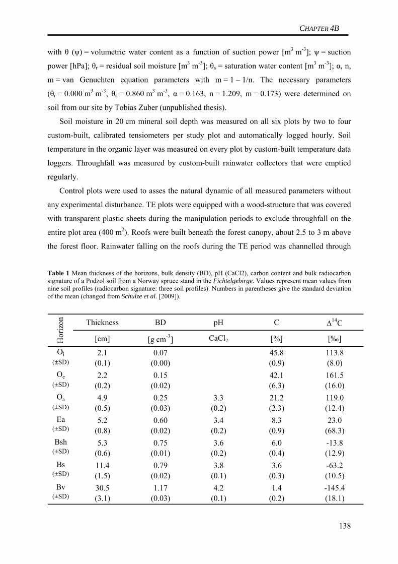
CHAPTER 4B
with θ (ψ) = volumetric water content as a function of suction power [m3 m-3]; ψ = suction
power [hPa]; θr = residual soil moisture [m3 m-3]; θs = saturation water content [m3 m-3]; α, n,
m = van Genuchten equation parameters with m = 1 – 1/n. The necessary parameters
(θr = 0.000 m3 m-3, θs = 0.860 m3 m-3, α = 0.163, n = 1.209, m = 0.173) were determined on
soil from our site by Tobias Zuber (unpublished thesis).
Soil moisture in 20 cm mineral soil depth was measured on all six plots by two to four
custom-built, calibrated tensiometers per study plot and automatically logged hourly. Soil
temperature in the organic layer was measured on every plot by custom-built temperature data
loggers. Throughfall was measured by custom-built rainwater collectors that were emptied
regularly.
Control plots were used to asses the natural dynamic of all measured parameters without
any experimental disturbance. TE plots were equipped with a wood-structure that was covered
with transparent plastic sheets during the manipulation periods to exclude throughfall on the
entire plot area (400 m2). Roofs were built beneath the forest canopy, about 2.5 to 3 m above
the forest floor. Rainwater falling on the roofs during the TE period was channelled through
Table 1 Mean thickness of the horizons, bulk density (BD), pH (CaCl2), carbon content and bulk radiocarbon signature of a Podzol soil from a Norway spruce stand in the Fichtelgebirge. Values represent mean values from nine soil profiles (radiocarbon signature: three soil profiles). Numbers in parentheses give the standard deviation of the mean (changed from Schulze et al. [2009]).
Thickness BD pH C Δ14C
[cm] [g cm-3] CaCl2 [%] [‰]
2.1 0.07 45.8 113.8(0.1) (0.00) (0.9) (8.0)2.2 0.15 42.1 161.5
(0.2) (0.02) (6.3) (16.0)4.9 0.25 3.3 21.2 119.0
(0.5) (0.03) (0.2) (2.3) (12.4)5.2 0.60 3.4 8.3 23.0
(0.8) (0.02) (0.2) (0.9) (68.3)5.3 0.75 3.6 6.0 -13.8
(0.6) (0.01) (0.2) (0.4) (12.9)11.4 0.79 3.8 3.6 -63.2(1.5) (0.02) (0.1) (0.3) (10.5)30.5 1.17 4.2 1.4 -145.4(3.1) (0.03) (0.1) (0.2) (18.1)
Ea(±SD)
Bsh(±SD)
Bs(±SD)
Bv(±SD)
Hor
izon
Oi(±SD)
Oe(±SD)
Oa(±SD)
138
CHAPTER 4B
rain gutters and water pipes over a distance of ca. 35 m before it could soak into the ground
outside the plots. By trenching the TE plots down to a depth of approx. 0.4 m lateral water
inflow or uptake by roots was reduced. Roofs on the TE plots were closed from 22 June to
8 August 2006 and from 2 July to 13 August 2007. In 2006, 67 mm of throughfall were
excluded, compared to 121 mm in 2007. In the year 2006 we irrigated the TE plots for two
days with a total of 67 mm artificial throughfall solution via a sprinkler system at the very
beginning of the post-treatment period. By irrigating the plots, we guaranteed that the total
amount of throughfall was the same on TE and control plots, so we only changed the
precipitation pattern. Based on the results in 2006 and the enormous logistic effort, we
decided to omit irrigation in 2007. The manipulation in 2007 therefore was a combination of
prolonged summer drought and a reduction of total annual througfall.
The period before closure of the roofs, when control and TE plots both received the same
amount of throughfall, will be addressed as the pre-treatment period here, the manipulation
period, when roofs were closed on the TE plots will be called the TE period. The rest of the
year, beginning with the re-opening of the roofs will be addressed as post-treatment period
here. An overview over the exact schedule in the measurements can be found in Table 2.
Table 2 Schedule of the experiment showing starting dates and duration of the different periods in the measurement years (Pre = period before the manipulation of the respective year, TE = manipulation period, when roofs on the TE plots are closed, Post = period from the reopening of the roofs until the end of the year).
Period 2006 2007 2008Pre Start 01.01.2006 01.01.2007
Duration (d) 172 182TE Start 22.06.2006 02.07.2007(Manipulation) Duration (d) 48 43Post Start 09.08.2006 14.08.2007
Duration (d) 144 139 No
man
ipul
atio
n
Measurement of CO2 fluxes
In each of the six plots, three plastic collars with a length of 20 cm and an inner diameter
of 49.5 cm were installed permanently for SR measurements. The collars were driven 5 cm
into the forest floor several months before the first measurements. Positions of the collars
were chosen randomly on the plots. For gas measurements, the collars were manually closed
with a plastic lid and connected to a portable infrared gas analyzer (IRGA, Li-820 from Li-
Cor Biosciences GmbH). Air was circulated in this closed system by a pump at a constant
139

CHAPTER 4B
140
flow rate of 0.5 l min-1 and the CO2 concentration inside the chamber was logged every 10 s
for a period of 3-5 min. A linear regression was performed on the increasing CO2 to determine
a flux rate, which was corrected for atmospheric pressure and chamber air temperature.
Measurements were conducted simultaneously on the control and the TE plots, and always
between 9:00 and 12:00 am. For more details on the method see Borken et al. [2006].
Radiocarbon signature of CO2 from SR, incubated roots and root-free soil
The radiocarbon signature of SR (Δ14CSR) was measured on eight occasions during the
two manipulation years 2006/2007 (Table 3). However, data from one of these dates (Jun 18,
2007) was discarded due to extreme variation. We can not eliminate the possibility that the
damage from a storm in Jan 2007 partly influenced the Δ14C data of 2007 and caused high
variation in late spring.
For measuring Δ14CSR, we used the same chambers as for SR measurements. Two of these
chambers on each plot (resulting in a total of six replicates per treatment) were closed and
then flushed with CO2-free synthetic air for 90 min at a moderate flow rate of 1.5 l min-1
thereby effectively flushing the respiration chambers with an amount of gas equal to at least
three times the chamber volume. Following flushing, the respiration chambers were sealed
and left until the CO2 concentration inside the chambers reached at least 1500 ppmv.
Incubation time depended on CO2 flux rates at the sampling day. Evacuated stainless steel
sampling cylinders (2 l) were connected to the respiration chambers and slowly filled with gas
from inside the chamber. Via mass-flow controllers the cylinders were connected to a high-
vacuum extraction line at the University of Bayreuth. CO2 was cryogenically purified and
converted to graphite targets using the modified sealed tube zinc reduction method described
by Xu et al. [2007]. Graphite targets were analyzed by the Keck Carbon Cycle AMS facility at
UC Irvine, USA with a precision of2-3 ‰. Radiocarbon data are expressed as Δ14C, which is
the per mil deviation from the 14C/12C ratio of oxalic acid standard in 1950. The sample 14C/12C ratio has been corrected to a δ13C value of -25 ‰ to account for any mass dependent
fractionation effects [Stuiver and Polach, 1977].
To measure the radiocarbon signature of rhizosphere respiration (Δ14CRR), we excavated
live roots of Norway spruce from the forest floor from three locations nearby our field plots
and on three dates in 2007 (Table 3). Excavated roots were washed with deionised water to
remove soil particles clinging to the roots and then transferred to gastight incubation
containers. Prior to the incubation the containers were flushed with CO2-free synthetic air to

CHAPTER 4B
Table 3 Sampling dates for the four different types of Δ14C samples.
Atmosphere Roots
Mar 6 2006 - - x -Jun 8, 2006 x - x -Aug 3, 2006 x x x -Aug 16, 2006 x x x -Nov 14, 2006 - - x -Mar 15, 2007 x x x -Jun 19, 2007 x x x xAug 9, 2007 x x x xOct 16, 2007 x x x x
Sample type
Date Soilrespiration Heterotrophic
Rhizosphere
remove all atmospheric CO2 and then incubated for 1-2 days in the laboratory at a constant
temperature of +15 °C. Gas samples again were taken by connecting an evacuated sampling
cylinder that was then opened slowly to take in gas from the incubation container. As the
Δ14C of CO2 respired by roots usually is very close to the Δ14C of CO2 in the atmosphere
[Trumbore, 2006], we also measured the atmospheric Δ14C on nine dates during 2006 and
2007 by filling evacuated sampling cylinders with gas from the atmosphere at 2 m above
ground. No significant differences between the Δ14CO2 of the atmosphere and RR were found
and so Δ14CRR was calculated as the mean of all root-incubation (n=9) and atmospheric
samples (n=20).
Δ14C originating from the mineralization of SOM was determined by incubating root-free
soil cores from the uppermost 25-30 cm of our field plots including the Oi, Oe, Oa, Ea, Bsh
and part of the Bs horizon. After soil was stored at +5 °C for four to six weeks, roots were
manually removed and the disturbed soil from each soil core was transferred to one
incubation container. After flushing the incubation containers with CO2-free synthetic air to
remove atmospheric CO2, the soil was incubated for 1-2 days at a constant temperature of
+15 °C. Following previous work by Dioumaeva et al. [2003] and more recent experiments
by Czimczik and Trumbore [2007], temperature does not affect the Δ14C of evolving CO2. Gas
from the containers was sampled using stainless steel containers and processed like described
before. The Δ14CHR values did not show a high temporal heterogeneity, therefore all results
were used to calculate one uniform mean Δ14CHR value (±SE) of 93.4 ‰ (±1.7; n=33) for
partitioning.
141

CHAPTER 4B
To partition SR into RR and HR, we used the isotopic method making use of bomb
derived 14C explained in greater detail by Gaudinski et al. [2000] or Schuur and Trumbore
[2006]. The basic idea is measuring the Δ14CO2 and the flux of total SR, as well as the Δ14CO2
of the two constituents of SR (RR and HR) and then applying a mass balance to calculate the
fluxes of the two constituents. A major advantage of this method is that it can be carried out
mostly under field site conditions and with minimal disturbances. The basic equations applied
in this approach are equations (2) and (3):
RRCOHRCOSRCO FFF ,,, 222+= (2)
(3) RRRRCOHRHRCOSRSRCO CFCFCF 14,
14,
14, 222
Δ×+Δ×=Δ×
where FCO2,SR is the CO2 flux of total soil respiration, FCO2,HR the flux of heterotrophic
respiration and FCO2,RR the flux of rhizosphere respiration, all in mmol m-2 h-1. Δ14CSR is the
radiocarbon signature of the total soil respiration, Δ14CHR of the heterotrophic respiration and
Δ14CRR of the rhizosphere respiration, all given in ‰.
Data analysis
Mean values for SR and Δ14C measurements were formed for the nine control and the nine TE
chambers. Data were analysed using STATISTICA 6.1. Differences in fluxes of SR and its
Δ14C between the treatments were tested using the non-parametric Mann-Whitney U-Test.
Comparing values of the same treatment at different dates was achieved by using the Tukey
HSD test.
Calculation of cumulative CO2 emissions was achieved by linear interpolation between
adjoining measurement dates for each individual chamber. For statistical analysis, the
cumulative C emissions for the nine control chambers and the nine TE chambers were
compared using the non-parametric Mann-Whitney U-Test.
Source partitioning was calculated by using formulas developed by Philips and Gregg
[2001], accounting for variability in the isotopic signatures of both the sources (Δ14CRR,
Δ14CHR) and the mixture (Δ14CSR). When multiplying the calculated source proportions with
mean SR fluxes, standard errors were calculated accounting for error propagation.
142

CHAPTER 4B
143
Results
Throughfall, soil moisture and soil temperature
The year 2006 was dry, with only 868 mm of throughfall, followed by a relatively wet year
(2007) with 1152 mm and another dry year (2008) with 924 mm (Fig. 1a). During the
manipulation period, 67 mm of throughfall were excluded in 2006, compared to 121 mm in
2007 (no manipulation in 2008). Matric potential measured beneath the Oa horizon varied
between values of pF 2 (moist) and pF 5-6 (very dry) in the observed years (Fig. 1b). Driest
conditions were found during the summer of 2006, when a period of natural drought hit both
the control and the TE plots. A period of low matric potentials in the winter of 2008 is
attributed to freezing of soil water due to deeply penetrating soil frost. Differences between
control and TE plots were found only during summer time: In the summer of 2006, control
plots were naturally dry with pF values around 5 compared to even drier conditions on the TE
plots (pF ca. 6). In 2007, no water stress was observed on the control plots in summer (pF ca.
3), whereas the TE plots experienced a moderate drought (pF ca. 4). Although matric
potentials regenerated quickly after natural rewetting of the TE plots in 2007, the volumetric
water content of the organic horizon on the TE plots remained significantly reduced until
winter (data not shown). It should be emphasized that the measurements represent the matric
potential at the transition between organic and mineral horizon and that differences between
TE and control plots within the organic horizons or even on top of the forest floor are
expected to be more pronounced.
Matric potential in 20 cm mineral soil depth was slightly affected by TE in both manipulation
years, resulting in more negative matric potentials on the TE plots (Fig. 1c). In the naturally
dry year of 2006, TE resulted in a minimum matric potential of at least -650 hPa (tensiometers
failed at this point; pF 2.8) compared to ca. -400 hPa (pF 2.6) on the control plots. In the wet
summer of 2007, matric potential on the control plots ranged around -50 hPa (pF 1.7),
compared to a minimum soil matric potential of -200 hPa (pF 2.3) on the TE plots. In 2008,
TE and control plots showed the exact same minimum soil matric potential of ca. -300 hPa
(pF 2.5). Soil temperature was not affected by the manipulation and therefore followed the
same seasonal dynamic on both the control and the TE plots (Fig. 1d).
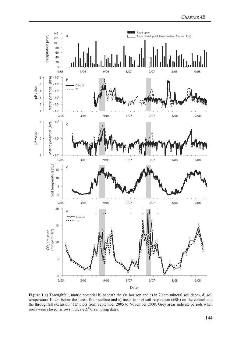
CHAPTER 4B
9/05 3/06 9/06 3/07 9/07 3/08 9/08
Mat
ric p
oten
tial
[hPa
]
- 101
- 102
- 103
- 104
- 105
- 106
pF v
alue
1
2
3
4
5
6
ControlTE
9/05 3/06 9/06 3/07 9/07 3/08 9/08
Prec
ipita
tion
[mm
]
020406080
100120140 Roofs open
Roofs closed (precipitation only on Control plots)
9/05 3/06 9/06 3/07 9/07 3/08 9/08
Soil
tem
pera
ture
[°C]
0
5
10
15
Date
9/05 3/06 9/06 3/07 9/07 3/08 9/08
CO2 e
mis
sion
[mm
ol m
-2 h
-1]
0
5
10
15
20
b
d
a
9/05 3/06 9/06 3/07 9/07 3/08 9/08
Mat
ric p
oten
tial
[hPa
]
- 101
- 102
- 103
pF v
alue
1
2
3
ControlTE
c
TEControl
e
Figure 1 a) Throughfall, matric potential b) beneath the Oa horizon and c) in 20 cm mineral soil depth, d) soil temperature 10 cm below the forest floor surface and e) mean (n = 9) soil respiration (±SE) on the control and the throughfall exclusion (TE) plots from September 2005 to November 2008. Grey areas indicate periods when roofs were closed, arrows indicate Δ14C sampling dates.
144

CHAPTER 4B
145
Soil respiration
In the two manipulation years, significantly less CO2 was emitted from the TE plots
compared to the control plots (p < 0.05; cf. Tab. 4). These differences on an annual basis
resulted from reduced CO2 emissions both during the TE period as well as the post-treatment
period (Fig. 1e; Tab. 4). No significant differences were found during the pre-treatment
period, prior to the closure of the roofs. In the year 2006, 6.7 t C ha-1 (±0.2) were emitted
from the control plots and only 5.7 t C ha-1 (±0.3) from the TE plots (mean values from nine
measurement chambers ±SE), resulting in a difference of ca. 0.9 t ha-1. Of this total difference
of 0.9 t ha-1, 50 % (or approx. 0.5 t C ha-1) can be explained by decreased CO2 emissions
during the TE period itself. Another 44 % of the total reduction (approx. 0.4 t ha-1) can be
explained by reduced CO2 emissions during the post-treatment period.
In 2007, 7.0 t C ha-1 (±0.4) were emitted from the control plots, compared to only
5.9 t C ha-1 (±0.3) from the TE plots, so total emissions from the TE plots in 2007 were
smaller by approx. 1.1 t C ha-1. Again, most of this difference (54 % or approx. 0.6 t C ha-1)
can be explained by reduced emissions during the TE period itself. Reduced CO2 emissions
during the post treatment period explain 33 % or approx. 0.4 t C ha-1.
In the year 2008, no manipulation was carried out. Mean total CO2 emissions from the
control and the TE plots were identical in this year, both ranging around 6.7 t C ha-1.
Dynamics of Δ14C of SR
During the pre-treatment period in the year 2006 (Jun 8, 2006), we measured little variation in
the Δ14CSR on all plots, and we found no significant differences between TE and control plots
with mean values (n = 6, ±SE) of 88 ‰ (±2.4) and 91.4 ‰ (±2.2), respectively (Fig. 2).
Measurements during the first TE manipulation period (Aug 3, 2006) revealed much higher
variation within both treatment groups, and Δ14C values beneath contemporary atmosphere
occured, indicating the influence of pre-bomb carbon. Variation of measured Δ14CSR
decreased considerably as soon as soils were rewet again during the post-treatment period
(Aug 16, 2006), and mean values on TE and control plots revealed no significant differences
with 78.6 ‰ (±3.0) and 81.0 ‰ (±2.4), respectively.

Table 4: Cumulative C emissions from the control and the TE plots. Cumulative C emissions were calculated on an annual basis for the years 2006-2008, and also for the individual periods (pre-, TE-, and post-treatment period) in the two manipulation years (2006, 2007). Mean values were calculated from the data of nine individual SR chambers (n = 9) on each manipulation type (control, TE). Difference between the control and the TE plots were calculated for each period, as well as the relative contribution of differences in a certain period to the total differences of that year. Mean values of control and TE plots were statistically compared by the Mann-Whitney U-Test to detect differences in cumulative C emissions during a certain period. Values of p < 0.05 are considered statistically different (*).
Year Description Duration Mean ± SE Mean ± SE Absolut [%] of annual p
2006 Total 1 year 6.7 ± 0.2 5.7 ± 0.3 0.9 100 0.031 *Pre 172 d 2.1 ± 0.1 2.1 ± 0.1 0.1 6 0.566 -TE 47 d 1.4 ± 0.1 1.0 ± 0.1 0.5 50 0.002 *Post 146 d 3.1 ± 0.1 2.7 ± 0.1 0.4 44 0.047 *
2007 Total 1 year 7.0 ± 0.4 5.9 ± 0.3 1.2 100 0.019 *Pre 182 d 3.0 ± 0.2 2.9 ± 0.1 0.2 13 0.825 -TE 42 d 1.6 ± 0.1 1.0 ± 0.1 0.6 54 0.001 *Post 141 d 2.4 ± 0.1 2.0 ± 0.1 0.4 33 0.031 *
2008 Total 1 year 6.7 ± 0.4 6.7 ± 0.3 0.0 100 0.965 -
StatisticsCumulative C emissions [t C ha-1]
Period Control TE Difference

CHAPTER 4B
Jun 8 Aug 3 Aug 16 Mar 15 Aug 9 Oct 16
Δ14C
sign
atur
e [‰
]
-50
0
50
100
150
2006 2007
TE: SR
Control: SRTE: HR
Control: HR
Figure 2 Radiocarbon signature of total soil respiration (SR) and of heterotrophic (root-free) respiration (HR) on the control and the throughfall exclusion (TE) plots on different sampling dates during 2006 and 2007. The dashed line at 49.2 ‰ represents the mean radiocarbon signature of atmospheric CO2 in the measurement years. Measurements beneath this line indicate that a substantial amount of CO2 originates from the mineralization of old substrate (pre-bomb).
In the year 2007, pre-manipulation measurements of Δ14CSR (Mar 15, 2007) reveal little
variation for the control plots with mean Δ14CSR of 85.1 ‰ (±3.1), but high variation for the
TE plots and the occurrence of CO2 with pre-bomb Δ14C in one of the samples. During the TE
period, Δ14CSR measurements for both TE and control plots show a smaller variation and no
samples with obvious pre-bomb influence are found. Mean values of TE and control plots
during this second manipulation period differ significantly with 73.0 ‰ (±3.6) and 90.2 ‰
(±4.1), respectively. Differences decrease during rewetting with Δ14CSR values around 74.9 ‰
(±1.4) on TE and 85.1 ‰ (±5.2) on control plots.
Partitioning of SR
Partitioning revealed that SR on the control plots was dominated by HR on all
measurement dates, with RR contribution to total SR ranging only between 5 and 40 % (Fig.
3). Absolute RR emissions were constantly small throughout both years in the control plots,
except for the summer of 2006, when RR emissions ranged between 2-3 mmol CO2 m-2 h-1.
Absolute HR emissions in the control plots followed the seasonal trend of SR.
147
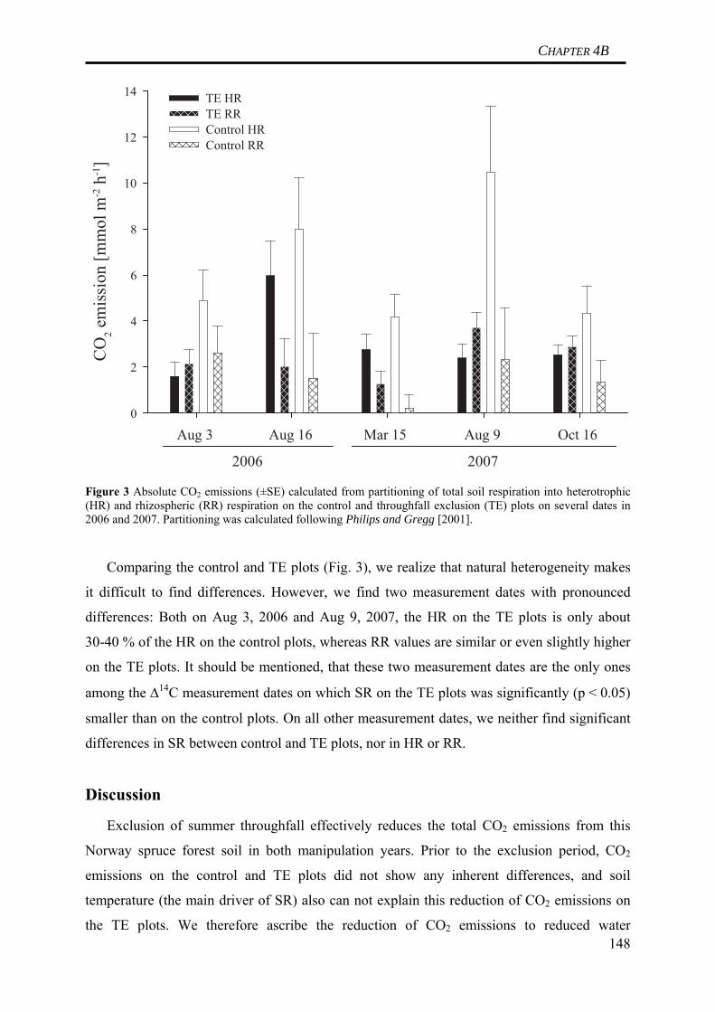
CHAPTER 4B
Aug 3 Aug 16 Mar 15 Aug 9 Oct 16
CO
2 em
issi
on [m
mol
m-2 h
-1]
0
2
4
6
8
10
12
14 TE HR TE RR Control HR Control RR
2006 2007 Figure 3 Absolute CO2 emissions (±SE) calculated from partitioning of total soil respiration into heterotrophic (HR) and rhizospheric (RR) respiration on the control and throughfall exclusion (TE) plots on several dates in 2006 and 2007. Partitioning was calculated following Philips and Gregg [2001].
Comparing the control and TE plots (Fig. 3), we realize that natural heterogeneity makes
it difficult to find differences. However, we find two measurement dates with pronounced
differences: Both on Aug 3, 2006 and Aug 9, 2007, the HR on the TE plots is only about
30-40 % of the HR on the control plots, whereas RR values are similar or even slightly higher
on the TE plots. It should be mentioned, that these two measurement dates are the only ones
among the Δ14C measurement dates on which SR on the TE plots was significantly (p < 0.05)
smaller than on the control plots. On all other measurement dates, we neither find significant
differences in SR between control and TE plots, nor in HR or RR.
Discussion
148
Exclusion of summer throughfall effectively reduces the total CO2 emissions from this
Norway spruce forest soil in both manipulation years. Prior to the exclusion period, CO2
emissions on the control and TE plots did not show any inherent differences, and soil
temperature (the main driver of SR) also can not explain this reduction of CO2 emissions on
the TE plots. We therefore ascribe the reduction of CO2 emissions to reduced water
CHAPTER 4B
availability indicated by matric potential differences between control and TE plots. More than
50 % of the reduction are explained by reduced fluxes during the manipulation period itself.
However, a major proportion of the remaining reduction is due to continuously reduced fluxes
during the post-treatment period. In both years, CO2 emissions on the TE plots remain
reduced until six to seven weeks after the reopening of the roofs, although matric potential
differences disappear a few weeks earlier. Based on Δ14C data, we attribute the reduction of
total CO2 emissions mainly to reduced respiration by heterotrophic soil organisms. It has
already been reported that for this soil C losses via DOC leaching are insignificant compared
to CO2 emissions [Hentschel et al., 2007, Muhr et al., 2008], so it is unlikely that reduced
CO2 emissions are compensated by an increase of alternate C losses in this soil.
The observed reduction of CO2 emissions during the manipulation periods can be
explained best by reduced matric potential in the organic and the uppermost mineral horizons.
In the naturally dry summer of 2006, matric potentials indicate drought stress on both the
control and the TE plots. Nevertheless, exclusion of summer throughfall leads to measurable
differences between control and TE plots with matric potentials being one order of magnitude
more negative on the TE plots than on the control plots. The soil moisture data shown here
reflects the conditions 8 cm below the surface. More pronounced differences between control
and TE plots can be expected in the top of the forest floor, because small precipitation events
(like documented for this period) can lead to temporary increase of soil moisture and therefore
SR in the control plots, whereas the TE plots are constantly dry throughout the whole
manipulation period. On the other hand, when the moisture sensors indicate drought stress
this close to the transition of organic and mineral horizons, we can assume that at least the
uppermost centimeters of the mineral horizon will also be subjected to drought stress. This
assumption is supported by the matric potential measurements in 20 cm mineral soil depth,
which revealed that the manipulation produced measurable matric potential differences even
in this depth.
After we removed the roofs on the TE plots, it took several weeks until the matric
potentials regenerate back to the level of the control plots. In 2007, this could be due to the
fact that we did not irrigate the TE plots to compensate for the excluded amount of
throughfall. However, we observe the same phenomenon during the post-treatment period in
2006, despite irrigation. This indicates that the delayed regeneration of the matric potential is
independent of irrigation. A reason to explain this slow regeneration of matric potential could
be water repellency and preferential flow patterns in the organic layer of this soil like reported
by Bogner et al. [2009]. It is well known that water repellency is increased under conifer
149
CHAPTER 4B
stands [Doerr et al., 2000]. Drying can even further increase water repellency of soils [Dekker
and Ritsema, 1996]. Consequently, CO2 emissions remain smaller on the TE plots as long as
matric potentials have not recovered.
However, we find that differences in SR rates persist much longer than differences in
matric potential. A possible explanation for this observation that we would like to discuss
here addresses the regeneration of the microbial population. Although we do not have direct
measurements of microbial biomass, our Δ14C data (for a detailed discussion see below)
indicates significantly reduced HR rates under dry conditions. To demonstrate the severity of
the drought experienced by the microorganisms, we compare our data to data from a parallel
experiment at the same stand. In this experiment, the contribution of organic horizons to total
SR was quantified by completely removing the organic horizons. This removal reduced SR
rates in summer by maximal 40-45 % [Froitzheim, personal communication], indicating that
CO2 originating from the mineral horizons accounts for a high proportion of the SR
emissions. This observation fits the high organic C contents of the EA, Bsh and Bh horizons
in this Haplic Podzol. However, with our TE manipulation, we achieved a reduction of SR
rates of up to 60 % on several measurement dates. We therefore assume that drought stress
not only affected the organic horizons, but also the respiratory emissions from the uppermost
mineral horizons. In previous laboratory experiments with soil columns from this stand [Muhr
et al., 2008, Muhr et al., 2009] we tested the reaction of organic and mineral horizons to
intensive drying. When intact soil cores consisting only of organic horizons were dried, mean
hourly CO2 emissions always regenerated to the same level as control CO2 emissions after
rewetting. When we subjected soil columns consisting of organic and mineral horizons to
intensive drought, CO2 emissions never regenerated back to control levels even after
rewetting [Muhr et al., 2008]. We attributed this difference to the fact that the microbial
population inhabiting the mineral horizons is less adapted to drought. This agrees with
findings by Fritze et al. [2000], who described that in the organic horizons of typical Podzol
profiles under coniferous forest fungi are relatively abundant, whereas in the uppermost
mineral horizon the relative abundance of bacteria is increasing. Fungi, in turn, are known to
be more drought tolerant than bacteria [Griffin, 1981, Voroney, 2007]. To investigate the
relative abundance of fungi and bacteria at the Coulissenhieb II site, Schmitt et al. [personal
communication] analyzed phospholipid fatty acid (PLFA) patterns in undisturbed soil cores.
Preliminary results from this investigation confirm that the ratio of fungal to bacterial PLFAs
decreases from the organic to the mineral horizon at our research site. We therefore postulate
that SR rates can be reduced persistently by drying because 1) water repellency and
150
CHAPTER 4B
preferential flow patterns hinder fast and complete rewetting, and 2) a part of the microbial
population can be severely damaged and regenerates slowly.
Reduced CO2 emissions during periods of drought are not surprising - it has long been
described that drought reduces the activity of soil microorganisms and therefore SR [Kieft et
al., 1987, Degens and Sparling, 1995, Borken et al., 2006]. However, during the last years an
increasing number of experiments indicated that drought can also trigger the release of
formerly protected, unavailable substrates that can result in a net increase of annual CO2
emissions even if fluxes are significantly reduced during the actual drought period, a
phenomenon recently referred to as the ‘Birch effect’ [Miller et al., 2005, Jarvis et al., 2007,
Xiang et al., 2008]. In this experiment, CO2 emissions from TE plots exposed to summer
drought never exceeded emissions from the control plots. One might argue that due to the
nature of our measurements, we might have missed a short-lasting increase of CO2 emissions.
In the year 2006, e.g., we measured SR a few hours before we started irrigation and then again
36 h after the beginning of irrigation. We found no increase in SR between those two
measurement dates. It still is possible, though, that a pulse with a duration less than 36 h
occurred. However, we would like to emphasize that annual CO2 emissions on the TE plots
were reduced by 0.9 t C ha-1 compared to the control plots. Even when we missed a short-
lasting pulse, it would have to come close to 0.9 t C ha-1 (or about 210 mmol m-2 h-1 on
average) to compensate for this reduction. Laboratory measurements on soil from this site
with high temporal resolution do not indicate that such an enormous SR pulse is likely to
occur [Muhr et al., 2008].
Furthermore, our findings are in agreement with nearly all other field experiments
simulating prolonged drought periods we know of, all reporting reduced C losses due to
drought [cf. Borken and Matzner, 2009]. The only field experiment that reported an increase
of C losses during a drying-rewetting manipulation [Borken et al., 1999] attributed this
increase to artificial rewetting during an extremely warm period, when control plots received
less water and probably were water limited. So far, increasing C losses from soils due to
preceding drought have mainly been reported from laboratory experiments with mineral soil
[cf. Borken and Matzner, 2009 and references therein]. In the majority of these experiments,
the soil has been sieved. This represents a major disturbance, creates new surfaces and can
possibly facilitate the release of formerly protected substrates. Furthermore, it changes the
physical characteristic of the soil, and it has been reported that rewetting of disturbed soil
occurs faster than of undisturbed soil [Schjønning et al., 1999]. Delayed rewetting due to
water repellency and preferential flow patterns, e.g., is not to be expected in disturbed soil.
151

CHAPTER 4B
Reduced C losses in one year do not necessarily have to result in increased C
sequestration. If losses are reduced because of reduced mineralization, material that was not
metabolized during the dry year might simply be mineralized in the subsequent year, resulting
in increased C losses that compensate for the dry year. However, measurements of SR during
2008 do not indicate that reduced C losses in 2006 and 2007 are in any way compensated for
by increased C losses in 2008. One possible explanation might be reduced metabolic capacity
of the microbial community like postulated as a possible effect of drying-rewetting in the
‘microbial stress’ mechanism [Xiang et al., 2008]. Alternatively, drying might result in
stabilization and thus C sequestration of substrates. Based on our results, we so far only can
show that substrates not used in dry years are not immediately metabolized in subsequent wet
years.
Even though decreased SR rates on the TE plots contradict the idea of protected substrates
being released, Δ14CSR data indicate the contribution of old pre-bomb carbon to SR mainly on
the TE plots and mainly during periods of drought, thus indicating a shift in the quality of the
predominant substrate. Without additional information, this might be interpreted as the release
of formerly protected substrate, which would be expected to be older. However, in this
experiment a second explanation is much more likely: CO2 respired in SR originates from
both organic and mineral horizons. Under normal conditions, most of the CO2 emitted in SR
is originating in the organic horizons and the uppermost mineral horizon. Bulk Δ14C of these
horizons is clearly dominated by post-bomb material (cf. Table 1). As soon as CO2 emissions
from organic horizons and uppermost mineral horizons decrease due to drought, the relative
contribution of CO2 originating from deeper mineral horizons increases. This will
consequently lead to a change in the measured Δ14C like observed in this experiment.
The calculation of the source contribution of HR and RR to SR is based on a variety of
parameters (cf. Equ. 2 & 3), all of which are prone to statistical error due to natural
heterogeneity. Interpretation of the results therefore has to be done very critically. However,
there are two very pronounced results: (1) The contribution of HR to SR on the control plots
is always bigger than the contribution of RR; (2) the CO2 emissions from control and TE plots
are always about the same size, except during the TE periods in both manipulation years:
During this period, both SR and HR become considerably smaller on the TE plots than on the
control plots, while RR remains unaffected.
There are two different explanations for the clear dominance of HR over RR. One
explanation might be the thickness of the organic horizons and the high amount of substrate
stored here. In this context, we would like to mention, that Schindlbacher et al. [2009] also
152

CHAPTER 4B
reported rather small contributions of RR to SR in a Norway spruce forest, ranging between
24-28 %. The other explanation might be disturbance resulting from the installation depth
(5 cm) of our measurement chambers. Wang et al. [2005] discussed that the insertion of SR
chambers into the soil cuts off superficial fine roots and thereby reduces RR. It is impossible
for us to quantify this effect in our experiment, so quantitative conclusions about RR have to
be considered with care. However, qualitative conclusions concerning differences in RR
between control and TE plots and the reaction of RR below 5 cm depth still should be valid
(see below).
During the TE periods, SR on the TE plots is significantly smaller than on the control
plots. Partitioning reveals that this reduction can be explained with a corresponding reduction
of HR. At the same time, RR is not affected by the TE manipulation. We therefore can
conclude that drying negatively affects heterotrophic soil microorganisms, whereas roots and
rhizospheric microorganisms seem to be able to withstand the drought stress caused by TE
manipulation.
Summarizing, we conclude that the exclusion of summer throughfall leads to a significant
reduction of SR mainly in the organic and uppermost mineral horizons during the exclusion
period. HR is affected stronger than RR. Regeneration of SR takes several weeks, most likely
due to a combination of water repellency and microbial casualties. The manipulation effect is
strong enough to significantly reduce annual C losses. So far, no evidence has been found that
metabolization of unused substrates can lead to a compensation of these reduced C losses
either during rewetting of the dry soil or during the following years.
Conclusion
Prolonged summer droughts are likely to lead to a significant reduction of annual CO2
losses in this temperate Norway spruce forest. CO2 emissions are not only reduced during the
actual drought period, due to either water repellency or serious damage in the microbial
population it takes several weeks before they are restored back to control levels. Data on Δ14C
indicate that a reduction of SOM mineralization in the organic horizon and the uppermost
mineral horizon is mainly responsible for this reduction. No evidence has been found that
preceding drought can release new, formerly protected substrate and thereby result in
increased carbon losses from soils, like discussed in the context of the so-called ‘substrate
supply’ mechanism. So far, no evidence has been found that reduced C losses are
compensated for by increased CO2 emissions in subsequent years. Based on our results and in
153

CHAPTER 4B
face of the current climate change scenarios, we expect a negative feedback between
increased frequency and magnitude of summer droughts and SR in Norway spruce stands.
Acknowledgements
This research was financially supported by the program 562 ‘Soil processes under extreme
meteorological boundary conditions’ of the Deutsche Forschungsgemeinschaft (DFG).
References
Birch, H. F. (1958), The Effect of Soil Drying on Humus Decomposition and Nitrogen
Availability, Plant and Soil, 10, 9-31.
Birch, H. F. (1959), Furhter observations on humus decomposition and nitrification, Plant
and Soil, 9, 262-286.
Bogner, C., D. Gaul, A. Kolb, I. Schmiedinger and B. Huwe (2009), Investigating flow
mechanisms in a forest soil by mixed-effects modelling, submitted.
Borken, W. and E. Matzner (2009), Reappraisal of drying and wetting effects on C and N
mineralization and fluxes in soils, Global Change Biology, doi: 10.1111/j.1365-
2486.2008.01681.x.
Borken, W., Y.-J. Xu, R. Brumme and N. Lamersdorf (1999), A climate change scenario for
carbon dioxide and dissolved organic carbon fluxes from a temperate forest soil: drought
and rewetting effects, Soil Science Society of America Journal, 63, 1848-1855.
Borken, W., K. Savage, E. A. Davidson and S. E. Trumbore (2006), Effects of experimental
drought on soil respiration and radiocarbon efflux from a temperate forest soil, Global
Change Biology, 12, 177-193.
Borken, W., E. A. Davidson, K. Savage, J. Gaudinski and S. E. Trumbore (2003), Drying and
wetting effects on carbon dioxide release from organic horizons, Soil Science Society of
America Journal, 67, 1888-1896.
Chen, M. and M. Alexander (1973), Survival of soil bacteria during prolonged desiccation,
Soil Biology and Biochemistry, 5, 213-221.
Czimczik, C. I. and S. E. Trumbore (2007), Short-term controls on the age of microbial
carbon sources in boreal forest soils, Journal of Geophysical Research, 112, G03001,
doi:10.1029/2006JG000389.
154

CHAPTER 4B
Degens, B. P. and G. P. Sparling (1995), Repeated wet-dry cycles do not accelerate the
mineralization of organic C involved in the macro-aggregation of a sandy loam, Plant and
Soil, 175, 197-203.
Dekker, L. W. and C. J. Ritsema (1996), Uneven moisture patterns in water repellent soils,
Geoderma, 70, 87-99.
Dioumaeva, I., S. E. Trumbore, E. A. G. Schuur, M. L. Goulden, M. Litvak and A. I. Hirsch
(2003), Decomposition of peat from upland boreal forest: Temperature dependence and
sources of respired carbon, Journal of Geophysical Research, 108, 8222.
Dörr, H. and K. O. Münnich (1986), Annual Variations of the 14C Content of Soil CO2,
Radiocarbon, 28, 338-345.
Doerr, S. H., R. A. Shakesby and R. P. D. Walsh (2000), Soil water repellency: its causes,
characteristics and hydro-geomorphological significance, Earth-Science Reviews, 51, 33-
65.
Fritze, H., J. Pietikäinen and T. Pennanen (2000), Distribution of microbial biomass and
phospholipid fatty acids in Podzol profiles under coniferous forest, European Journal of Soil
Science, 51, 565-573.
Gaudinski, J. B., S. E. Trumbore, E. A. Davidson and S. Zheng (2000), Soil carbon cycling in
a temperate forest: radiocarbon-based estimates of residence times, sequestration rates and
partitioning of fluxes, Biogeochemistry, 51, 33-69.
Gaul, D., D. Hertel, W. Borken, E. Matzner and C. Leuschner (2008), Effects of experimental
drought on the fine root system of mature Norway spruce, Forest Ecology and
Management, 256, 1151-1159.
Gerstberger, P., T. Foken and K. Kalbitz (2004), The Lehstenbach and Steinkreuz catchments
in NE Bavaria, Germany, in Biogeochemistry of forested catchments in a changing
environment, edited by E. Matzner, pp. 15-29, Springer, Berlin.
Griffin, D. M. (1981), Water potential as a selective factor in the microbial ecology of soils.,
in Water Potential Relations in Soil Microbiology., edited by J. F. Parr, et al., pp. 141-151,
Soil Science Society of America, Madison, Wisconsin.
Harris, R. F. (1981), The effect of water potential on microbial growth and activity, in Water
potential relations in soil microbiology, edited by J. F. Parr, et al., pp. 23-95, SSSA
Special Publication No. 9, Wisconsin, USA.
Hentschel, K., W. Borken and E. Matzner (2007), Leaching losses of inorganic N and DOC
following repeated drying and wetting of a spruce forest soil, Plant and Soil, 300, 21-34.
155
CHAPTER 4B
IPCC (2007), Climate Change 2007: The Physical Science Basis. Contribution of Working
Group I to the Fourth Assessment Report of the Intergovernmental Panel on Climate
Change., Cambridge University Press, Cambridge, United Kingdom and New York, NY,
USA.
IUSS Working Group WRB (2006), World reference base for soil resources 2006., World
Soil Resources Reports, No. 103, FAO, Rome.
Jarvis, P., et al. (2007), Drying and wetting of Mediterranean soils stimulates decomposition
and carbon dioxide emission: the “Birch effect”, Tree Physiology, 27, 929-940.
Kieft, T. L., E. Soroker and M. K. Firestone (1987), Microbial biomass response to a rapid
increase in water potential when dry soil is wetted, Soil Biology and Biochemistry, 19,
119-126.
Miller, A. E., J. P. Schimel, T. Meixner, J. O. Sickman and J. M. Melack (2005), Episodic
rewetting enhances carbon and nitrogen release from chaparral soils, Soil Biology and
Biochemistry, 37, 2195-2204.
Muhr, J., J. Franke and W. Borken (2009), Drying-rewetting events reduce C and N losses
from a Norway spruce forest floor, Soil Biology and Biochemistry, submitted.
Muhr, J., S. D. Goldberg, W. Borken and G. Gebauer (2008), Repeated drying-rewetting
cycles and their effects on the emission of CO2, N2O, NO, and CH4 in a forest soil,
Journal of Plant Nutrition and Soil Science, 171, 719-728.
Nadezhdina, N., J. Čermák, J. Gašpárek, V. Nadezhdin and A. Prax (2006), Vertical and
horizontal water redistribution in Norway spruce (Picea abies) roots in the Moravian
Upland, 26, 1277-1288.
Phillips, D. L. and J. W. Gregg (2001), Uncertainty in source partitioning using stable
isotopes, Oecologia, 127, 171-179, doi: 10.1007/s004420000578.
Schimel, J., T. C. Balser and M. Wallenstein (2007), Microbial Stress-response Physiology
and its Implications for Ecosystem Function, Ecology, 88, 1386-1394.
Schindlbacher, A., S. Zechmeister-Boltenstern and R. Jandl (2009), Carbon losses due to soil
warming: Do autotrophic and heterotrophic soil respiration respond equally?, Global
Change Biology, 15, 901-913, doi:10.1111/j.1365-2486.2008.01757.x.
Schjønning, P., I. K. Thomsen, J. P. Møberg, H. de Jonge, K. Kristensen and B. T.
Christensen (1999), Turnover of organic matter in differently textured soils: I. Physical
characteristics of structurally disturbed and intact soils, Geoderma, 89, 177-198.
Schlesinger, W. H. and J. A. Andrews (2000), Soil respiration and the global carbon cycle,
Biogeochemistry, 48, 7-20.
156
CHAPTER 4B
157
Schulze, K., W. Borken, J. Muhr and E. Matzner (2009), Stock, turnover time and
accumulation of organic matter in bulk and density fractions of a podzol soil, European
Journal of Soil Science, accepted.
Schuur, E. A. G. and S. E. Trumbore (2006), Partitioning sources of soil respiration in boreal
black spruce forest using radiocarbon, Global Change Biology, 12, 165-176.
Seneviratne, R. and A. Wild (1985), Effect of mild drying on the mineralization of soil
nitrogen, Plant and Soil, 84, 175-179.
Stuiver, M. and H. A. Polach (1977), Discussion; Reporting of 14C Data, Radiocarbon, 19,
355-363.
Trumbore, S. E. (2006), Carbon respired by terrestrial ecosystems - recent progress and
challenges, Global Change Biology, 12, 141-153.
Van Genuchten, M. T. (1980), A Closed-form Equation for Predicting the Hydraulic
Conductivity of Unsaturated Soils, Soil Science Society of America Journal, 44, 892-898.
Voroney, R. P. (2007), The Soil Habitat, in Soil Microbiology, Ecology, and Biochemistry,
edited by E. A. Paul, pp. 25-49, Academic Press, Oxford.
Xiang, S.-R., A. Doyle, P. A. Holden and J. P. Schimel (2008), Drying and rewetting effects
on C and N mineralization and microbial activity in surface and subsurface California
grassland soils, Soil Biology and Biochemistry, Special Section: Enzymes in the
Environment, Enzymes in the Environment III 40, 2281-2289.
Xu, X., S. E. Trumbore, S. Zheng, J. R. Southon, K. E. McDuffee, M. Luttgen and J. C. Liu
(2007), Modifying a sealed tube zinc reduction method for preparation of AMS graphite
targets: Reducing background and attaining high precision, Nuclear Instruments and
Methods in Physics Research Section B: Beam Interactions with Materials and Atoms,
259, 320-329.

CHAPTER 5
Chapter 5
Ecosystem C dynamics in a fen as affected by water table fluctuations
158
CHAPTER 5A
PART A:
Manipulative lowering of the water table during summer
does not affect CO2 emissions and uptake in a minerotrophic
fen Jan Muhr1*), Juliane Höhle1), Dennis O. Otieno2), and Werner Borken1)
1) Department of Soil Ecology, University of Bayreuth, 95440 Bayreuth, Germany 2) Department of Plant Ecology, University of Bayreuth, 95440 Bayreuth, Germany
*) Corresponding author: Jan Muhr ([email protected])
Submitted to Ecological Applications
Received 10 July 2009
Abstract
We simulated the effect of prolonged summer drought by lowering the water table on
three manipulation plots (D1-3) in a minerotrophic fen in South-eastern Germany in three
subsequent years (2006-2008). Water table was lowered below natural levels by drainage and
by excluding precipitation. Soil respiration (RSoil) measurements predominantly revealed no
differences between the D1-3 plots and three control plots (C1-3). Gross primary production
(GPP) and aboveground respiration (RAG) also were not affected by lowered water tables,
indicating the lack of stress due to drought or anoxia for aboveground biomass. The water
tables on the control plots were naturally low most of the time and especially during the
manipulation periods. The median water table for 2006-2008 was 8 cm beneath the surface on
the control plots. During summer, when respiratory activity was highest, it was even lower,
with median values on the control plots between 11 and 19 cm beneath the surface during the
manipulation periods. We therefore assume that oxygen availability in the uppermost at least
10 cm was not limited by water table. Thus, manipulative lowering of the water table most
likely increased oxygen availability only in deeper peat layers, where we expect RSoil to be
limited by poor substrate quality rather than anoxia. In case that naturally low water tables on
the C1-3 plots masked manipulation effects, we analyzed all available data in a second
approach (irrespective of treatment) to estimate the influence of water table on RSoil. We
found a significant correlation between RSoil and water table, with RSoil decreasing at lower
water tables rather than increasing. Summarizing, we conclude that RSoil is dominated by
159

CHAPTER 5A
decomposition in the litter layer and the uppermost peat layers. Deeper peat layers bear no
significant decomposition potential. We do not expect enhanced C losses from this site due to
increasing frequency of summer droughts. Aboveground vegetation seems to be unaffected by
water table fluctuations beneath 10 cm.
Keywords: Peatland, fen, climate change, water table, CO2 emissions & uptake, ecosystem
manipulation
160

CHAPTER 5A
Introduction Soils store about 1500 Pg (1015 g) of carbon (C), roughly twice as much as the atmosphere
(Schlesinger & Andrews, 2000). Around 30% (270-370 Pg) of this C is found in peatland
soils (Turunen et al., 2002), although they only account for around 3.5% of the earth’s surface
(Gorham, 1991). This phenomenon results from the stabilization of C due to high water levels
in peatlands. Consequent anoxia leads to a limitation of decomposition rates, resulting in an
imbalance between biomass production and decomposition. This imbalance is rather small
(Päivänen & Vasander, 1994), but has led to the formation of thick peat bodies since the last
deglaciation.
As the sink function of peatlands mainly is a consequence of climatic stabilization, it has
been described as labile and vulnerable to climate change (Alm et al., 1999; Moore, 2002;
Bubier et al., 2003). The IPCC (2007) has predicted an increasing likelihood of summer-
drought periods for this century, resulting in lowered water tables. The consequential increase
of oxygen availability during a time of high temperature and, therefore, high microbial
activity will presumably lead to an increase in peat decomposition. It has already been
reported that peatlands can switch rapidly to a source of carbon when water table changes
(Silvola, 1996). However, contrasting results on the effects of water level drawdown on
decomposition have been reported (cf. Laiho, 2006 and references therein). Peatland sites
may become sources of C, but also can remain sinks or even become stronger sinks when
water table is lowered.
The C balance of an ecosystem does not only depend on decomposition but also on CO2
uptake via photosynthetic assimilation (gross primary production or GPP). Some of the
assimilated CO2 quickly returns to the atmosphere via aboveground plant respiration (RAG) or
via root respiration while a fraction leaves the plant as root exudates. The rest of the
assimilated C is used for the production of biomass (roots and leaves), and will finally end up
as litter. Litter and root exudates serve as microbial substrates and become decomposed. All
CO2 leaving the ecosystem via root respiration or decomposition here will be termed soil
respiration (RSoil). The sum of RSoil and RAG is named the total ecosystem respiration (REco)
and summarizes all emissions of CO2 from the ecosystem. The ecosystem C balance depends
on the difference between uptake of C via GPP and emissions via REco. Both parameters can
be influenced by changes in the water table. To determine the effects of lowered water tables
on the CO2 source-sink function of an ecosystem one has to measure uptake and emission
rates.
161

CHAPTER 5A
In this experiment, we simulated periods of prolonged summer-drought by excluding
precipitation and lowering the water table by drainage in a minerotrophic fen in south-east
Germany. We continuously measured soil respiration (RSoil) on three manipulation plots and
compared them to three control plots to assess the effect of lowered water tables on soil
respiration. We also investigated effects of lowered water tables on the vegetation at our site
by measuring gross primary production (GPP) and aboveground autotrophic respiration (RAG)
at various dates.
Material and Methods
Site description
Measurements were carried out at the Schlöppnerbrunnen fen site located in the
Lehstenbach catchment (Fichtelgebirge, Northeastern Bavaria, Germany, 50°07’54’’N,
11°52’51’’E). The site is characterized as a temperate minerotrophic fen covering an area of
0.8 ha at an elevation of about 750 m a.s.l. The soil is a Histosol on granite bedrock covered
mainly by Molinia caerulea (L. Moench), Nardus stricta (L.), Agrostis canina (L.), Carex
rostrata (Stokes) and Eriophorum vaginatum (L.). Mean annual temperature (1995-2007) is
6.3 ± 0.9°C and mean annual precipitation (1995-2007) is 1020 ± 203 mm a-1 (Knorr, 2009).
The site features a water table gradient, with the north-western part being waterlogged more
often than the south-eastern part, and a slope from NNE to SSW. Groundwater flows slowly
through the site parallel to this slope. Since the last deglaciation, a peat body with a thickness
between 40-70 cm has accumulated. A schematic representation of our study site and the
experimental set-up are shown in Figure 1.
Experimental design
Three control plots (named C1, C2, and C3; each 7 x 5 m2) were installed in the summer of
2005 to assess natural dynamics of measured parameters at the site. Three plots of identical
size were installed a few meters downstream in terms of groundwater flow to carry out water-
table drawdown experiments (named D1, D2, and D3). All plots were accessible via wooden
walkways. Each plot was equipped with soil temperature sensors in various depths (5, 10, 20,
30, 40, and 60 cm). Three collars for soil respiration (RSoil) measurements (Ø 50 cm,
installation depth 5 cm), and two collars (39 x 39 cm2) for net ecosystem exchange (NEE) and
ecosystem respiration (REco) measurements were installed on each plot. Biomass was sampled
on the latter at the end of the vegetation period in the year 2007, divided into species and then
162

CHAPTER 5A
Figure 1 Schematic sketch of the study site. The non-treated control plots C1-C3 are located upstream of the treatments plots D1-D3 in terms of groundwater flow direction. Boardwalks to minimize disturbance during access are depicted as grey lines. The site is surrounded by Norway spruce forest, the open area is marked by the dashed line. At the site there is a moisture gradient from north to south. During the manipulation period, D1-D3 were covered with a roof construction and the drainage system was emptied constantly (Knorr et al., 2009).
oven-dried at 60°C before weighing. An existing biomass development curve for the year
2007 (Otieno et al.,2009) measured on additional plots nearby was used to calculate biomass
on our plots at the specific measurement dates, by assuming the same dynamics. Piezometers
(26PCBFA6D, IBA Sensorik GmbH, Seligenstadt, Germany) in the immediate vicinity of the
installations allowed for continuous monitoring of the water table (for this work, the data of
six piezometers per plot was used). Precipitation was measured at a climate station
(Pflanzgarten) at a distance of ca. 1 km from the plots.
163

CHAPTER 5A
To effectively lower the water table in the D1-3 plots, precipitation was excluded by means
of transparent roofs and ground water was actively pumped out of the plots. A drainage
system was installed perpendicularly to the ground water flow both up- and downstream of
the manipulation plots at a depth of 1 m. During the first manipulation period (14 August to
26 September, 2006) draining was facilitated by a pump that was operated manually every
second or third day. The system was automated during the second manipulation period (10
May to 19 July 2007) to achieve better results. The automated system was also used during
the third manipulation period (10 July to 7 August, 2008). A detailed overview of the dates
and duration of the three manipulation periods is shown in Table 1.
Table 1 Manipulation period parameters of the three manipulation years.
Control
Year Start End Duration[d] Total Excluded Irrigation
2006 Aug 14 Sep 26 43 861 109 110
2007 May 10 Jul 19 70 1265 343 182
2008 Jul 10 Aug 07 28 957 65 -
Precipitation [mm]ManipulationManipulation Periods
Regeneration of the water table levels on the D1-3 plots at the end of the manipulation
period was partly achieved by natural precipitation and lateral water inflow. In the years of
2006 and 2007 we further accelerated the rising of the water table by irrigating the D1-3 plots
with 110 and 182 mm of artificial rain water, respectively. Irrigation intensity was kept
constant at 10 and 11 mm h-1 in these two years. The artificial rainwater consisted of
deionised water to which we added (µmol l-1): Na+ 39, K+ 30, NH4+ 34, NO3
- 34, SO42- 12, so
that its chemical composition was close to natural precipitation. Irrigation raised the water
table to the level of the C1-3 plots. In 2008, no irrigation was necessary, as water table levels
quickly regenerated due to natural precipitation.
CO2 fluxes: Measurement details (RSoil, REco, NEE)
On each plot, three non-transparent cylindrical plastic collars (length: 45 cm, Ø 50 cm)
were driven approx. 5 cm into the soil for RSoil measurements. Vegetation in these collars was
removed regularly. For gas measurements, collars were manually closed with a non-
164

CHAPTER 5A
transparent plastic lid and connected to a portable infrared gas analyzer (Li-Cor, Li-820). Gas
concentration was logged every 10 s for a period of 10 min. Measurements of RSoil were
carried out in rotation on the C1-3 and the D1-3 plots between 8:00 am and 12:00 am on
measurement days.
Measurements of REco and NEE were only carried out during one manipulation period in
the summer of 2007, to investigate the effects of water table draw-down on the assimilation
rates of the vegetation. For these measurements, we installed additional rectangular collars
(39 x 39 cm2) to a depth of 7 cm into the soil. Vegetation inside these collars was not removed
during the measurement period. For NEE measurements, we used 38 x 38 x 54 cm3 chambers
built of transparent plexiglass (3 mm XT type 20070, light transmission 95 %). For REco
measurements, we used dark chambers identical in construction, but covered with an opaque
insulation layer and reflective aluminium foil. REco and NEE were always measured directly
one after the other on each plot, and the C1-3 plots were measured in rotation with the D1-3
plots. Measurements were conducted between 9:00 am and 12:00 am on the measurement
dates with a few exceptions due to technical problems.
During measurements, chambers were placed on the permanently installed collars and
firmly secured with two elastic rubber bands fastened onto the ground on two sides of the
chamber. Sealing was achieved with a flexible rubber gasket between chamber and collar.
Increased air pressure inside the chamber was avoided by a 12 mm opening at the top of the
chamber that was closed after placing of the chamber on the collar. Circulation of air inside
the chamber was achieved by three fans creating an air-current of 1.5 m s-1. The air-stream
was directed over mounted ice packs inside the chamber to keep air temperature within 1°C
relative to ambient.
CO2 concentration inside the chamber was measured with a portable infrared gas analyzer
(Li-Cor, Li-820) over a period of 3-5 min and logged every 10 s. Simultaneously, air
temperature (20 cm above ground), peat temperature (10 cm below-ground), and
photosynthetic active radiance (PAR; measured with a LI-190 quantum sensor, Li-Cor, USA)
both inside and outside the chamber were measured. Detailed information on the NEE / REco
measurements can be found in Droesler et al. (2005) and Otieno et al. (2009).
Calculations of CO2 fluxes (RSoil, REco, NEE, GPP)
CO2 fluxes for RSoil, REco and NEE were calculated by performing a linear regression on
the logged CO2 concentration data (with a few exceptions: r2 > 0.95). Data was corrected for
atmospheric pressure and chamber air temperature. In the case of NEE, we limited the linear
165
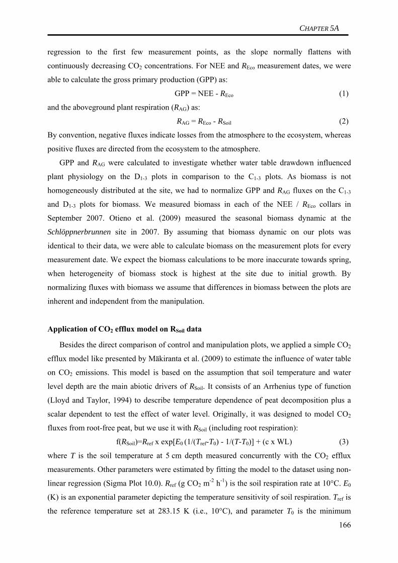
CHAPTER 5A
regression to the first few measurement points, as the slope normally flattens with
continuously decreasing CO2 concentrations. For NEE and REco measurement dates, we were
able to calculate the gross primary production (GPP) as:
GPP = NEE - REco (1)
and the aboveground plant respiration (RAG) as:
RAG = REco - RSoil (2)
By convention, negative fluxes indicate losses from the atmosphere to the ecosystem, whereas
positive fluxes are directed from the ecosystem to the atmosphere.
GPP and RAG were calculated to investigate whether water table drawdown influenced
plant physiology on the D1-3 plots in comparison to the C1-3 plots. As biomass is not
homogeneously distributed at the site, we had to normalize GPP and RAG fluxes on the C1-3
and D1-3 plots for biomass. We measured biomass in each of the NEE / REco collars in
September 2007. Otieno et al. (2009) measured the seasonal biomass dynamic at the
Schlöppnerbrunnen site in 2007. By assuming that biomass dynamic on our plots was
identical to their data, we were able to calculate biomass on the measurement plots for every
measurement date. We expect the biomass calculations to be more inaccurate towards spring,
when heterogeneity of biomass stock is highest at the site due to initial growth. By
normalizing fluxes with biomass we assume that differences in biomass between the plots are
inherent and independent from the manipulation.
Application of CO2 efflux model on RSoil data
Besides the direct comparison of control and manipulation plots, we applied a simple CO2
efflux model like presented by Mäkiranta et al. (2009) to estimate the influence of water table
on CO2 emissions. This model is based on the assumption that soil temperature and water
level depth are the main abiotic drivers of RSoil. It consists of an Arrhenius type of function
(Lloyd and Taylor, 1994) to describe temperature dependence of peat decomposition plus a
scalar dependent to test the effect of water level. Originally, it was designed to model CO2
fluxes from root-free peat, but we use it with RSoil (including root respiration):
f(RSoil)=Rref x exp[E0 (1/(Tref-T0) - 1/(T-T0)] + (c x WL) (3)
where T is the soil temperature at 5 cm depth measured concurrently with the CO2 efflux
measurements. Other parameters were estimated by fitting the model to the dataset using non-
linear regression (Sigma Plot 10.0). Rref (g CO2 m-2 h-1) is the soil respiration rate at 10°C. E0
(K) is an exponential parameter depicting the temperature sensitivity of soil respiration. Tref is
the reference temperature set at 283.15 K (i.e., 10°C), and parameter T0 is the minimum
166

CHAPTER 5A
temperature at which respiration reaches zero, set at 227.13 K (-45.6°C) (Lloyd and Taylor,
1994). WL is the depth of the water level from the peat surface (m) measured concurrently
with RPD, and the parameter c describes the change in RPD related to changes in WL
independently of temperature.
The model developed by Mäkiranta et al. (2009) offers the calculation of other
parameters, e.g. the optimum depth of the water table. However, performing these
calculations did not reveal any additional interesting results and, therefore, are omitted here.
Data analysis and statistics
Due to natural gradients in water table and in peat body thickness, we formed
corresponding pairs of D1-3 and C1-3 plots for analysis (D1-C1; D2-C2; D3-C3). To test for
statistically significant differences in RSoil between D1-3 and C1-3 plots we used the non-
parametric Mann-Whitney U-test.
Cumulative C emissions were calculated on individual chamber basis. We interpolated
linearly between adjacent RSoil measurements and multiplied with time to calculate how much
C was emitted in total between two measurements. By adding up the sums of the different
intervals we calculated total C emissions during longer periods (e.g. years, manipulation
periods). For statistical analysis, the data of the chambers from the D1-3 and the C1-3 plots was
compared using a Mann-Whitney U-test. No cumulative emissions were calculated for GPP
and REco because data was insufficient.
Results
Micrometeorology
Soil temperature followed a clear seasonal trend in all measured depths down to 60 cm
beneath the surface (Fig. 2a). As no differences in soil temperature were found between C1-3
and D1-3 plots (data not shown), we present a uniform soil temperature curve representative
for all plots. Soil temperature in the year 2006 was slightly warmer than in 2007 and 2008, as
maximum values in summer in a depth of 5 cm were about 2°C higher than in the two
subsequent years, but also the measured minimum in 5 cm depth was higher in 2006 than in
the other two years.
Precipitation also varied between the three years (Table 1, Figure 2b). It was lower than
the long-term average of 1160 mm (1971-2000) in 2006 and 2008 with a total of 861 mm and
of 1265 mm. In summary, 2006 can be described as a warm and dry year, whereas 2007 was a
167

CHAPTER 5A
Date
01/06 07/06 01/07 07/07 01/08 07/08 01/09
Prec
ipita
tion
[mm
]
0
20
40
60
01/06 07/06 01/07 07/07 01/08 07/08 01/09
Tem
pera
ture
[°C
]
02468
1012141618
-5 cm-30 cm-60 cm
01/06 07/06 01/07 07/07 01/08 07/08 01/09
Wat
erta
ble
[m]
-0.6
-0.4
-0.2
0.0
C1D1
Date
01/06 07/06 01/07 07/07 01/08 07/08 01/09
Wat
erta
ble
[m]
-0.6
-0.4
-0.2
0.0
C2D2
Date
01/06 07/06 01/07 07/07 01/08 07/08 01/09
Wat
erta
ble
[m]
-0.6
-0.4
-0.2
0.0
C3D3
a
b
c
d
e
168
Figure 2 a) Soil temperature in various depths, b) natural precipitation, c)-e) and water table on the three pairs of control and manipulation plots in the years of 2006-2008. As soil temperature in each depth was identical on control and manipulation plots, all data is summarized in one graph per depth here.
CHAPTER 5A
wet year, still warm but cooler than 2006. Weather conditions in the year 2008 were
intermediate with respect to the two previous years.
Water table on the C1-3 plots was subject to a high natural fluctuation (Figure 2c-e). The
median for all three years (C1-3 plots only, i.e. natural fluctuation) was 0.08 m beneath the
surface. During the manipulation periods, median water table of the C1-3 plots was even lower
than this long-term average with 0.12, 0.11, and 0.19 m beneath the surface in 2006, 2007,
and 2008, respectively. Further lowering of the water table was achieved by drainage and
exclusion of precipitation on the D1-3 plots with varying success. In 2006, we failed to lower
the water table on the D3 plot due to technical problems, so this plot can not be regarded as a
manipulation plot for this year. On the other two plots, however, we achieved a lowering to
the water table to 0.21 m beneath the surface in average. The summer of 2007 was rather wet,
but we still lowered the water table to 0.25 m beneath the surface in average. The
manipulation was most successful in the summer of 2008, when we lowered the water table
beneath the measurement depth of our piezometers for several weeks. Raising of the water
table back to the level of the C1-3 plots at the end of the manipulation period proceeded fast in
all three years.
CO2 emissions via RSoil
CO2 emissions on C1-3 and D1-3 plots followed a seasonal trend with highest emissions in
summer and lowest emissions in winter (Figure 3). Fluxes ranged between 0 and
25 mmol m-2 h-1. Overall, we found little differences between control and manipulation plots
(Figure 3, Figure 4a and b). For the pairs C1-D1 and C2-D2 we found differences only on two
measurement dates in the summer of 2007 when CO2 emissions on D1 and D2 were reduced
(Fig. 3). During that period, we measured extremely low water contents in the aboveground
litter of the D1-3 plots, ranging around 22 g g-1, compared to 225 g g-1 on the control plots
(data not shown). Cumulative C emissions (annual and during the manipulation periods) were
not affected by this short-term reduction (Fig. 4a and b). Differences were slightly more
pronounced for the pair C3-D3, partly due to the fact that CO2 emissions from C3 were higher
than from any of the other plots. The cumulative CO2 emissions on D3 were smaller than on
C3 during the manipulation periods of 2007 and 2008 (statistically significant with p = 0.02
only for the manipulation period in 2007) (Fig. 4b). This difference during the manipulation
periods resulted in a visible but statistically not significant difference in the annual cumulative
C emissions of 2007 and 2008 (Fig. 4a).
169

CHAPTER 5A
06/06 12/06 06/07 12/07 06/08 12/08
CO
2 em
issi
on
[mm
ol m
-2 h
-1]
CO
2 em
issi
on
[mm
ol m
-2 h
-1]
CO
2 em
issi
on
[mm
ol m
-2 h
-1]
0
5
10
15
20
25
30C1D1
06/06 12/06 06/07 12/07 06/08 12/08 0
5
10
15
20
25
30C2D2
Date
06/06 12/06 06/07 12/07 06/08 12/08 0
5
10
15
20
25
30C3D3
Figure 3 Mean emissions of CO2 via RSoil on the three pairs of control and manipulation plots (±SE; n=3).
Shaded areas indicate the duration of the manipulation periods in the three years.
170
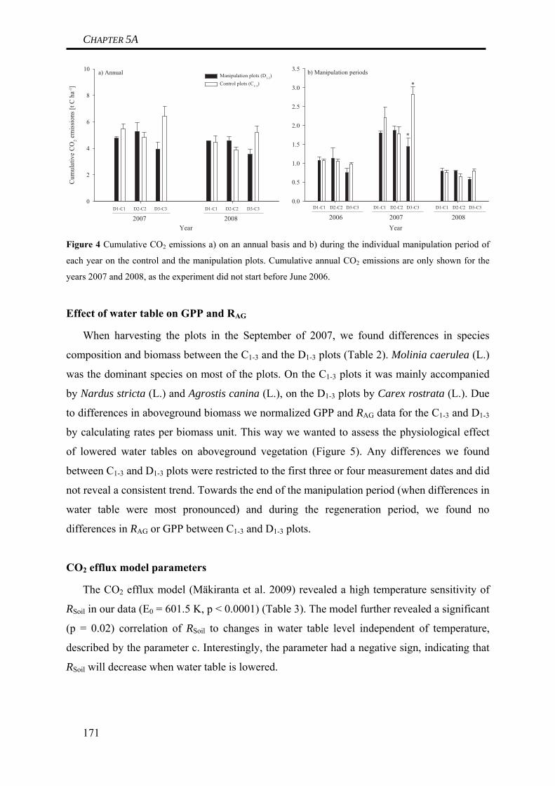
CHAPTER 5A
Year
Cum
ulat
ive
CO
2 em
issi
ons [
t C h
a-1]
0
2
4
6
8
10Manipulation plots (D1-3)Control plots (C1-3)
a) Annual
D1-C1 D2-C2 D3-C3
2008D1-C1 D2-C2 D3-C3
2007Year
0.0
0.5
1.0
1.5
2.0
2.5
3.0
3.5
D1-C1 D2-C2 D3-C3
*
*
b) Manipulation periods
2008D1-C1 D2-C2 D3-C3
2007D1-C1 D2-C2 D3-C3
2006
Figure 4 Cumulative CO2 emissions a) on an annual basis and b) during the individual manipulation period of
each year on the control and the manipulation plots. Cumulative annual CO2 emissions are only shown for the
years 2007 and 2008, as the experiment did not start before June 2006.
Effect of water table on GPP and RAG
When harvesting the plots in the September of 2007, we found differences in species
composition and biomass between the C1-3 and the D1-3 plots (Table 2). Molinia caerulea (L.)
was the dominant species on most of the plots. On the C1-3 plots it was mainly accompanied
by Nardus stricta (L.) and Agrostis canina (L.), on the D1-3 plots by Carex rostrata (L.). Due
to differences in aboveground biomass we normalized GPP and RAG data for the C1-3 and D1-3
by calculating rates per biomass unit. This way we wanted to assess the physiological effect
of lowered water tables on aboveground vegetation (Figure 5). Any differences we found
between C1-3 and D1-3 plots were restricted to the first three or four measurement dates and did
not reveal a consistent trend. Towards the end of the manipulation period (when differences in
water table were most pronounced) and during the regeneration period, we found no
differences in RAG or GPP between C1-3 and D1-3 plots.
CO2 efflux model parameters
The CO2 efflux model (Mäkiranta et al. 2009) revealed a high temperature sensitivity of
RSoil in our data (E0 = 601.5 K, p < 0.0001) (Table 3). The model further revealed a significant
(p = 0.02) correlation of RSoil to changes in water table level independent of temperature,
described by the parameter c. Interestingly, the parameter had a negative sign, indicating that
RSoil will decrease when water table is lowered.
171
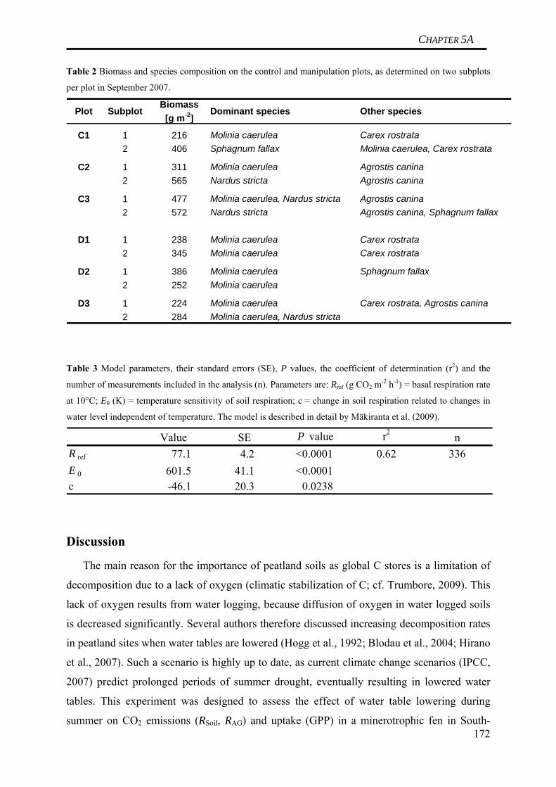
CHAPTER 5A
172
Table 2 Biomass and species composition on the control and manipulation plots, as determined on two subplots
per plot in September 2007.
Plot SubplotBiomass
[g m-2]Dominant species Other species
C1 1 216 Molinia caerulea Carex rostrata2 406 Sphagnum fallax Molinia caerulea, Carex rostrata
C2 1 311 Molinia caerulea Agrostis canina2 565 Nardus stricta Agrostis canina
C3 1 477 Molinia caerulea, Nardus stricta Agrostis canina2 572 Nardus stricta Agrostis canina, Sphagnum fallax
D1 1 238 Molinia caerulea Carex rostrata2 345 Molinia caerulea Carex rostrata
D2 1 386 Molinia caerulea Sphagnum fallax2 252 Molinia caerulea
D3 1 224 Molinia caerulea Carex rostrata, Agrostis canina2 284 Molinia caerulea, Nardus stricta
Table 3 Model parameters, their standard errors (SE), P values, the coefficient of determination (r2) and the
number of measurements included in the analysis (n). Parameters are: Rref (g CO2 m-2 h-1) = basal respiration rate
at 10°C; E0 (K) = temperature sensitivity of soil respiration; c = change in soil respiration related to changes in
water level independent of temperature. The model is described in detail by Mäkiranta et al. (2009).
Value SE P value r2 nR ref 77.1 4.2 <0.0001 0.62 336E 0 601.5 41.1 <0.0001c -46.1 20.3 0.0238
Discussion
The main reason for the importance of peatland soils as global C stores is a limitation of
decomposition due to a lack of oxygen (climatic stabilization of C; cf. Trumbore, 2009). This
lack of oxygen results from water logging, because diffusion of oxygen in water logged soils
is decreased significantly. Several authors therefore discussed increasing decomposition rates
in peatland sites when water tables are lowered (Hogg et al., 1992; Blodau et al., 2004; Hirano
et al., 2007). Such a scenario is highly up to date, as current climate change scenarios (IPCC,
2007) predict prolonged periods of summer drought, eventually resulting in lowered water
tables. This experiment was designed to assess the effect of water table lowering during
summer on CO2 emissions (RSoil, RAG) and uptake (GPP) in a minerotrophic fen in South-
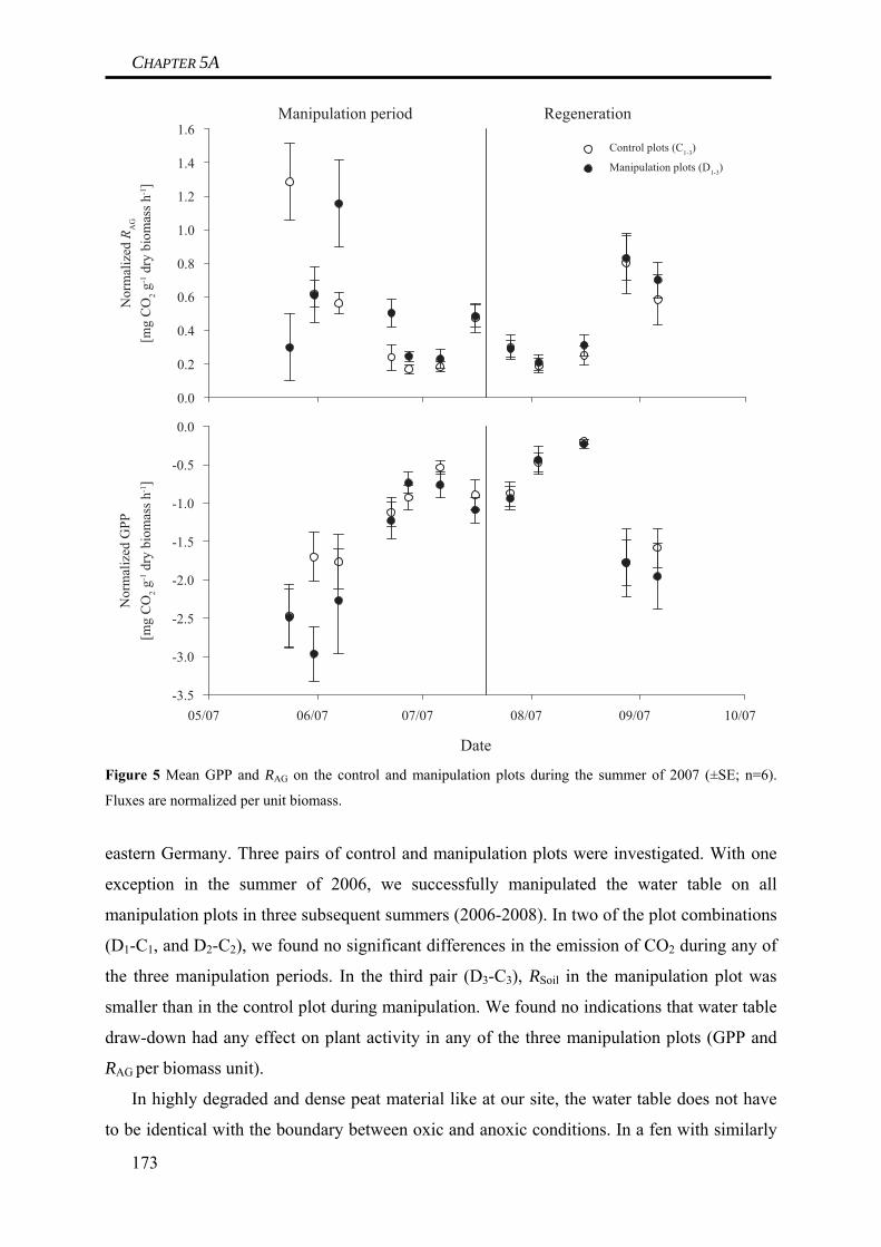
CHAPTER 5A
Date
05/07 06/07 07/07 08/07 09/07 10/07
Nor
mal
ized
GPP
[mg
CO
2 g-1 d
ry b
iom
ass h
-1]
[mg
CO
2 g-1 d
ry b
iom
ass h
-1]
-3.5
-3.0
-2.5
-2.0
-1.5
-1.0
-0.5
0.0
Nor
mal
ized
RA
G
0.0
0.2
0.4
0.6
0.8
1.0
1.2
1.4
1.6Control plots (C1-3)
Manipulation plots (D1-3)
Manipulation period Regeneration
Figure 5 Mean GPP and RAG on the control and manipulation plots during the summer of 2007 (±SE; n=6).
Fluxes are normalized per unit biomass.
eastern Germany. Three pairs of control and manipulation plots were investigated. With one
exception in the summer of 2006, we successfully manipulated the water table on all
manipulation plots in three subsequent summers (2006-2008). In two of the plot combinations
(D1-C1, and D2-C2), we found no significant differences in the emission of CO2 during any of
the three manipulation periods. In the third pair (D3-C3), RSoil in the manipulation plot was
smaller than in the control plot during manipulation. We found no indications that water table
draw-down had any effect on plant activity in any of the three manipulation plots (GPP and
RAG per biomass unit).
In highly degraded and dense peat material like at our site, the water table does not have
to be identical with the boundary between oxic and anoxic conditions. In a fen with similarly
173
CHAPTER 5A
degraded peat, Niedermeier and Robinson (2007) e.g. found an air entry tension of 25 cm,
meaning that the zone of saturated soil would extend 25 cm above a moving water table and
retard air entry to this height. As we have no direct measurements of oxygen, we refer to
findings reported by Reiche et al. (2009) and Knorr et al. (2009) for this site. Reiche et al.
(2009) measured maximum oxygen penetration depth with a relatively low temporal
resolution (using FeS-redox probes) in 2006 and 2007. Those probes closest to our
measurement chambers indicated maximum oxygen penetration of 35 cm on the control and
47 cm on the manipulation plots at the end of the manipulation period in 2006, compared to
4-13 cm on the C1-3 plots, and 6-20 cm on the D1-3 plots in 2007 (Reiche et al., personal
communication). Summarizing, the year 2006 was characterized by generally deeper aeration
of the peat body than the year of 2007. Furthermore, differences in the maximum penetration
depth between C1-3 and D1-3 plots were more pronounced in 2006 than in 2007. Knorr et al.
(2009) measured redox conditions on the plots during our experiments. They found a partial
decoupling of water table and peat aeration, as they described anoxic microenvironments that
were present in the uppermost horizons, regardless of water table. In summary, lowering of
the water table can increase maximum oxygen penetration depth, so that deeper peat layers
become aerated, but it seems not to increase oxygen availability in the uppermost horizons,
where anoxic microenvironments are present regardless of water table. The water table
fluctuation on the C1-3 plots indicates that low water tables in summer with, periodically dry
conditions, seem to be a regular phenomenon at this fen site, a circumstance that is reflected
in the dominant plant species, as Molinia caerulea (L.), Nardus stricta (L.) and Eriophorum
vaginatum (L.) are all reported to be indicators of highly variable soil moisture conditions
(Ellenberg et al., 1992). Paul et al. (2006) came to a similar conclusion for this site, describing
the upper horizons as predominantly oxic. Lowering of the water table during summer
therefore most likely has only an effect on the oxygen availability in deeper peat layers.
Radiocarbon analyses in the soil profile of the Schlöppnerbrunnen site revealed that the
occurrence of young, easily decomposable substrates is restricted to the upper 10-15 cm of the
peat body (Muhr et al., 2009). Reiche et al. (2009) incubated peat samples from the
Schlöppnerbrunnen site in the laboratory to measure basal soil respiration, anaerobic CO2
formation and exoenzymatic activities at different water table levels. The measured
parameters were highest in the upper 0-10 cm and quickly decreased below that. Furthermore,
below 10 cm, all three parameters were very constant over time and no effect of water table
was found. We conclude that RSoil in peat layers below ca. 10-15 cm depth is mostly not
limited by oxygen availability but by poor substrate quality. This is supported by comparing
174

CHAPTER 5A
RSoil data from the manipulation periods of 2006 and 2007. In 2006, we found very deep
oxygen penetration on the C1-3 and the D1-3 plots. Maximum penetration depth in 2007 was
considerably smaller in 2007 by up to 25 cm, but RSoil rates in 2006 and 2007 were not
differing at all. We conclude that aeration of deeper peat layers does not bear the potential to
significantly increase RSoil at the site. In summary, lowering of the water table does not result
in increased CO2 emissions because it can only increase oxygen availability in deeper peat
layers where poor substrate quality rather than oxygen availability limit decomposition.
Our assumptions are supported by data from Hogg et al. (1992), who found that mass
losses from peat taken from 30-40 cm depth were very low, even after 3 months of exposure
to aerated conditions at 24°C. They concluded that peat from greater depths was more
resistant to decomposition than surface peat. Lowered water tables therefore do not
necessarily have to result in an increase of CO2 emissions, particularly in peatlands that
already have a low water table for most of the summer.
Chimner & Cooper (2003) reported similar findings for a Colorado subalpine fen. They
found that CO2 emissions strongly increased with lowered water tables, as long as water
tables ranged between 10 cm above and 5 cm below the peat surface. When water tables were
lowered deeper than 5 cm below the peat surface, no additional effect on the CO2 emissions
was found.
Our results also agree with findings reported by Knorr et al (2008), who investigated peat
monoliths from our fen site in the laboratory. When they artificially lowered the water table
from -10 cm to ca. -50 cm, CO2 emissions at the peat surface were not affected at all by water
table.
To understand future changes in the carbon balance of peatlands, it is important to not
only investigate the dynamics of carbon losses via RSoil, but also the effect of climate change
on the vegetation. In this experiment we carried out very limited measurements of GPP and
RAG that are not sufficient to quantify annual CO2 uptake. To normalize for heterogeneity in
plant biomass on our plots, we calculated fluxes per biomass unit. By doing so, we assume
that differences in biomass on the plots are inherent, and not affected by the manipulation.
Instead of investigating possible changes in total biomass production, our measurements of
GPP and RAG were designed to estimate the effect of stress on the aboveground vegetation.
Due to the predominantly identical results on the C1-3 and the D1-3 plots, we conclude that
lowering of the water table did not significantly alter the stress regime on the D1-3 plots.
Differences during the first measurement dates presumably result from inaccurate biomass
data. As described above, biomass was only measured once in September 2007 and calculated
175

CHAPTER 5A
for the other dates based on data from Otieno et al. (2009). We expect increasing deviation of
the biomass dynamics on our measurement plots from the dynamics on their plots towards
spring, when initial growth results in high variability of biomass at the site.
Direct comparison of the C1-3 and the D1-3 plots revealed predominantly no effect of
lowered water tables. We used a second approach to estimate the effect of the water table on
decomposition by pooling all the data from C1-3 and D1-3 plots and applying the CO2 efflux
model by Mäkiranta et al. (2009). Using this approach, we found a significant correlation
between water table and RSoil. In contrast to our expectations, however, the model indicates
that RSoil decreases when water table is lowered, which could possibly be explained by
drought stress in the litter and uppermost peat layer, as documented for the summer of 2007
on the D1-3 plots. This drought stress presumably results only partly from lowered water
tables. More likely, what we see here is a consequence of the fact that the periods of low
water tables in our data coincide with periods of warm and dry weather during summer.
Neither of the two approaches we used reveals an increase of CO2 emissions due to lower
water table. This is in contrast to additional experiments that Otieno et al. (2009) carried out
in another area of the Schlöppnerbrunnen site. They reported increasing REco when water table
was lowered. The parameter REco includes RSoil and RAG and it remains unclear how the two
parameters reacted individually towards lower water tables. More important, the data they
used comprise water table levels mainly between 0-10 cm below the peat surface and only
some data down to 18 cm beneath the peat surface. Thus, their data differs from ours as our
data includes very little water table levels above 10 cm below peat surface. Therefore, our
findings are restricted to low water table levels.
Generally, findings of the various experiments at this site, as well as those reported in the
literature strongly suggest that water table at the Schlöppnerbrunnen site is an important
determinant of CO2 emissions within the uppermost ca. 10 cm, but becomes increasingly
unimportant below this depth. Therefore, a follow-up experiment was designed to examine
the effect of artificially increased water table on CO2 emissions at the Schlöppnerbrunnen
site. Preliminary results indicate that CO2 emissions on the flooded plots are decreased
compared to control plots (Wunderlich, personal communication). So far, we found no
evidence that lowering of the water table altered the activity of the aboveground vegetation.
We postulate that a moderate increase of summer drought conditions, like simulated in this
experiment will most likely not affect the C balance of the Schlöppnerbrunnen site.
176

CHAPTER 5A
Conclusion
Lowering the water table in a minerotrophic fen in South-eastern Germany during summer
had predominantly no effect on gaseous C fluxes in three subsequent manipulation periods.
An explanation for our findings is that gaseous C fluxes at our site during manipulation
periods mostly are not oxygen limited, most likely due to already low water tables on our
control plots and poor substrate quality in deeper peat layers. Instead of improving conditions
for soil micro-organisms and plants, the lowering of the water table had no effect. Under most
extreme drought conditions (high evapotranspiration), it might even cause drought stress in
the uppermost regions of the peatland (mainly litter layer), thereby reducing decomposition
rates, like observed in the summer of 2007. We anticipate that prolonged summer droughts
could only affect C fluxes at our site if water table was lowered deep and long enough for
drought stress to occur on the soil surface. In this case we mainly expect a reduction of CO2
emissions via RSoil and therefore a transient increase of the sink strength at the
Schlöppnerbrunnen site.
Acknowledgements
We thank D. Maurer, J. Franke, T. Froitzheim, L. Höhn, S. Wunderlich, A. Schott , and K.
Göschel for assistance during sampling and U. Hell, A. Kolb, G. Küfner, and G. Müller for
installations and ongoing service in the field. We thank Prof. Dr. Thomas Foken for providing
us with the precipitation data. We thank Prof. Dr. Gunnar Lischeid, Prof. (adjunct, McGill)
PD Dr. Christian Blodau, and Prof. Dr. Egbert Matzner for coordinating the experimental
efforts of all involved working groups at the Schlöppnerbrunnen fen site. This research was
financially supported by the program 562 ‘Soil processes under extreme meteorological
boundary conditions’ of the Deutsche Forschungsgemeinschaft (DFG).
References
Alm, J., L. Schulman, J. Walden, H. Nykanen, P. J. Martikainen, and J. Silvola. 1999. Carbon
Balance of a Boreal Bog During a Year With an Exceptionally Dry Summer. Ecology
80:161-174, doi:110.1890/0012-9658.
Blodau, C., N. Basiliko, and T. R. Moore. 2004. Carbon turnover in peatland mesocosms
exposed to different water table levels. Biogeochemistry 67:331-351.
177

CHAPTER 5A
Bubier, J. L., G. Bhatia, T. R. Moore, N. T. Roulet, and P. M. Lafleur. 2003. Spatial and
Temporal Variability in Growing-Season Net Ecosystem Carbon Dioxide Exchange at a
Large Peatland in Ontario, Canada. Ecosystems 6:353-367.
Chimner, R. A., and D. J. Cooper. 2003. Influence of water table levels on CO2 emissions in a
Colorado subalpine fen: an in situ microcosm study. Soil Biology and Biochemistry
35:345-351.
Ellenberg, H., H. E. Weber, R. Düll, V. Wirth, W. Werner, and D. Paulißen. 1992. Indicator
values of plants in Central Europe. Verlag Erich Goltze KG, Göttingen, Germany.
Gorham, E. 1991. Northern Peatlands: Role in the Carbon Cycle and Probable Responses to
Climatic Warming. Ecological Applications 1:182-195.
Hirano, T., H. Segah, T. Harada, S. Limin, T. June, R. Hirata, and M. Osaki. 2007. Carbon
dioxide balance of a tropical peat swamp forest in Kalimantan, Indonesia. Global Change
Biology 13:412-425.
Hogg, E. H., V. J. Lieffers, and R. W. Wein. 1992. Potential Carbon Losses From Peat
Profiles: Effects of Temperature, Drought Cycles, and Fire. Ecological Applications
2:298-306, doi:210.2307/1941863.
IPCC. 2007. Climate Change 2007: The Physical Science Basis. Contribution of Working
Group I to the Fourth Assessment Report of the Intergovernmental Panel on Climate
Change. Cambridge University Press, Cambridge, United Kingdom and New York, NY,
USA.
Knorr, K.-H., G. Lischeid, and C. Blodau. 2009. Dynamics of belowground redox processes
in a minerotrophic fen exposed to a water table manipulation. Geoderma:submitted.
Knorr, K.-H., M. R. Oosterwoud, and C. Blodau. 2008. Experimental drought alters rates of
soil respiration and methanogenesis but not carbon exchange in soil of a temperate fen.
Soil Biology and Biochemistry 40:1781-1791.
Laiho, R. 2006. Decomposition in peatlands: Reconciling seemingly contrasting results on the
impacts of lowered water levels. Soil Biology and Biochemistry 38:2011-2024.
Lloyd, J., and J. A. Taylor. 1994. On the temperature dependence of soil respiration.
Functional Ecology 8:315-323.
Mäkiranta, P., R. Laiho, H. Fritze, J. Hytönen, J. Laine, and K. Minkkinen. 2009. Indirect
regulation of heterotrophic peat soil respiration by water level via microbial community
structure and temperature sensitivity. Soil Biology and Biochemistry 41:695-703.
Moore, P. D. 2002. The future of cool temperate bogs. Environmental Conservation 29:3-20,
doi:10.1017/S0376892902000024.
178

CHAPTER 5A
179
Muhr, J., J. Höhle, and W. Borken. 2009. Estimating the carbon accumulation rate of a
minerotrophic fen in South-Eastern Germany. Biogeochemistry:In preparation.
Niedermeier, A., and J. S. Robinson. 2007. Hydrological controls on soil redox dynamics in a
peat-based, restored wetland. Geoderma 137:318-326.
Otieno, D. O., M. Wartinger, A. Nishiwaki, M. Z. Hussain, J. Muhr, W. Borken, and G.
Lischeid. 2009. Responses of CO2 Exchange and Primary Production of the Ecosystem
Components to Environmental Changes in a Mountain Peatland. Ecosystems:doi:
10.1007/s10021-10009-19245-10025.
Päivänen, J., and H. Vasander. 1994. Carbon Balance in mire ecosystems. World Resource
Review 6:102-111.
Reiche, M., A. Hädrich, G. Lischeid, and K. Küsel. 2009. Impact of manipulated drought and
heavy rainfall events on peat mineralization processes and source-sink functions of an
acidic fen. Journal of Geophysical Research - Biogeosciences 114:G02021,
doi:02010.01029/02008JG000853.
Schlesinger, W. H., and J. A. Andrews. 2000. Soil respiration and the global carbon cycle.
Biogeochemistry 48:7-20.
Silvola, J., J. Alm, U. Ahlholm, H. Nykänen, and P. J. Martikainen. 1996. The contribution of
plant roots to CO2 fluxes from organic soils. Biology and Fertility of Soils 23:126-131.
Trumbore, S. 2009. Radiocarbon and Soil Carbon Dynamics. Annual Review of Earth and
Planetary Sciences 37:47-66, doi:10.1146/annurev.earth.1136.031207.124300.
Turunen, J., E. Tomppo, K. Tolonen, and A. Reinikainen. 2002. Estimating carbon
accumulation rates of undrained mires in Finland-application to boreal and subarctic
regions. The Holocene 12:69-80, doi: 10.1191/0959683602hl0959683522rp.

CHAPTER 5B
PART B:
Responses of CO2 Exchange and Primary Production of the
Ecosystem Components to Environmental Changes in a
Mountain Peatland
D.O. Otieno1*, M. Wartinger1, A. Nishiwaki2, M.Z. Hussain1, J. Muhr3, W. Borken3 and G.
Lischeid4
1Department of Plant Ecology, University of Bayreuth, 95440 Bayreuth, Germany 2River Basin Research Center, Gifu University, 1-1 Yanagido, Gifu 501-1193, Japan 3Department of Soil Ecology, University of Bayreuth, 95440, Bayreuth, Germany 4Institute of Landscape Hydrology, Leibniz Centre for Agricultural Landscape Research,
15374 Müncheberg, Germany
*Corresponding author: Dennis O. Otieno ([email protected])
Published in Ecosystems (2009) 12, 590-603.
Received 5 August 2008, accepted 5 February 2009, published online 25 March 2009.
Summary
The complexity of natural ecological systems presents challenges for predicting the
impact of global environmental changes on ecosystem structure and function. Grouping of
plants into functional types, i.e. groups of species sharing traits that govern their mechanisms
of response to environmental perturbations, reduce the complexity of species diversity to a
few key plant types for better understanding of ecosystem responses. Chambers were used to
measure CO2 exchange in grass and moss growing together in a mountain peatland in
southern Germany to assess variations in their response to environmental changes and how
they influence ecosystem CO2 exchange. Parameter fits and comparison for NEE in two
ecosystem components were conducted using an empirical hyperbolic light response model.
Annual green biomass production was 320 and 210 g dwt.m-2, while mean maximum Net
Ecosystem Exchange (NEE) was –10.0 and –5.0 µmol m-2 s-1 for grass and moss respectively.
Grass exhibited higher light use efficiency (α) and maximum gross primary production
[(β+γ)2000]. Leaf Area Index (LAI) explained 93% of light use and 83% of overall production
180

CHAPTER 5B
by the grass. Peat temperature at 10 cm depth explained more than 80% of the fluctuations in
ecosystem respiration (Reco). Compared to grass, moss NEE was more sensitive to ground
water level (GWL) draw-down and hence could be more vulnerable to changes in
precipitation that result into GWL decline and may be potentially replaced by grass and other
vegetation that are less sensitive.
Key words: Carbon dioxide exchange; environmental variables; ground water level;
peatlands; primary production; respiration.
181
CHAPTER 5B
Introduction
Peatlands cover about 3.5% (or 5x10⁶ km2) of the Earth’s land surface (Gorham 1991).
More than 95% of total peatlands occur in cool, humid climates of the temperate belt in
Northern Hemisphere. During the last millennium, northern peatlands have acted as carbon
(C) sinks, with an average annual C uptake of 20-35 g C m-2 per year (Gorham 1991; Turunen
and others 2002). This has resulted in an enormous C pool in peatland soils, amounting to
approximately one-third of the world’s total soil C (4.5×10¹⁷ g) (Turunen and others 2002). As
a result of this large stock of partially decomposed plant material, peatlands are potential CO2
sources (Chapin and others 1992; Smith and others 2004).
Despite their significant role in terrestrial C cycle, the regulation of C flow in peatlands is
still poorly understood (Fenner and others 2004; Riutta and others 2007). The integrated
dynamics of ground water level (GWL) may determine the long-term ecological function of
temperate peatlands as C sinks as in the case of arctic tundra (cf. Ostendorf and others 1996).
Lowering of the GWL could enhance decomposition over assimilation resulting in decreased
net CO2 uptake or even net CO2 loss (Oechel and others 1995; Bubier and others 2003;
Tuitilla and others 2004; Riutta and others 2007). On the other hand, several studies consider
the effect of the water table as minimal and emphasise the significant influence of micro-
climatic parameters such as temperature and light (see Laufleur and others 2005). Finally,
rainfall and water table may indirectly influence carbon balance by modifying phenology,
nutrient availability, and development of aboveground leaf area in a particular season (Shaver
and others 1998; Hastings and others 1989).
Lack of consensus on how CO2 exchange is controlled may arise from the wide range of
methodologies that are employed to assess ecosystem responses (Oechel and others 1995;
Ruimy and others 1995; Frolking and others 1998) and the ability to identify and describe the
objects under study. Some of the methods (e.g. eddy covariance) do not take into account the
inter-specific differences associated with inherent physiological adaptations that are bound to
influence plant responses (Semikhatova and others 1992). Such adaptations may buffer plants
from the impact of short-term habitat changes during the growing season and modify
ecosystem response to environmental changes (Riutta and others 2007). Mosses for example,
have shallow rhizoids and, therefore, are likely to be sensitive to shifts in GWL, with a
significant influence on overall ecosystem CO2 exchange. Moss photosynthesis and growth
should, therefore, be directly influenced by the water table (Clymo and Hayward 1982;
McNeil and Waddington 2003; Robroek and others 2007). This may not be the case with
grass or sedge, which have relatively deep rooting systems (Bortoluzzi and others 2006; 182

CHAPTER 5B
Riutta and others 2007). Thus, characteristics of the vegetation mosaic reflect resource
availability and correlate with aspects of carbon balance and net primary production
(Ostendorf and others 1996; Leadley and Stocklin 1996)
Understanding of the biotic controls over functional groups and ecosystem CO2 exchange
processes and their interaction with the physical environment is crucial and provides a basis
for predicting how functional groups and entire peatland ecosystems may respond to changes
in the habitat. We used chamber methods to examine the variation in ecosystem CO2
exchange response of two dominant functional groups (moss and grass) occurring in a
mountain peatland of Germany. The peatland is gently sloping, homogeneous in terms of
species presence, but characterised by a recurring mosaic in fine scale structure where the
community is either dominated by grass and sedge tussocks with little moss, or relatively
open troughs or inter-tussocks dominated by moss, with little graminoid biomass. Our
objectives were; 1. To monitor annual biomass production of moss and grass in the peatland,
2. To monitor diurnal and seasonal CO2 exchange in grass and moss dominated plots and to
determine how the individual growth forms are influenced by ground water level (GWL),
temperature and light and 3. To examine how grass and moss contribute to the overall net
ecosystem CO2 exchange of the plots and the peatland over the course of the season. While
each plot studied is structurally unique, the exact composition of vegetation included in each
measurement was determined. The average behaviour of the natural mosaic components,
dominated either by moss or graminoid biomass, in gas exchange is compared, which will
allow us to use abundance-weighted estimates of carbon exchange to model the mixed-
functional-type community in subsequent steps.
Materials and methods
Site description
Measurements were conducted in a fen ecosystem at Schlöppner Brunnen site
(50°07’54”N, 11°52’51”E) at an elevation of 700 m a.s.l., where a clearing is surrounded by
spruce trees (Figure 1). The fen is dominated by two main functional groups, which include
moss (Sphagnum fallax and Polytrichum commune) and grass (Agrostis canina, A. stolonifera,
Molinia caerulea). A sedge (Carex nigra) is also found scattered within the vegetation, but it
is overgrown quickly by the grasses and negligible in its contribution to biomass by early
summer. The site structure is relatively flat but gently sloping, with a mosaic of grass-
dominated tussocks and moss-dominated inter-tussock areas.
183

CHAPTER 5B
The soil at the site is classified as Fibric Histosol, moderately acidic (pH 3.5-5.5), with
highly decomposed soils rich in sulphur (up to 4.6 mg kg-1) and iron (up to >16 mg kg-1). The
fen has a slope of 3 % and water flow direction is parallel to the slope from NNE to SSW
(Figure 1). The annual precipitation in the catchment varies between 900 and 1160 mm yr-1
and the mean annual air temperature is 5°C. The mean in-situ water table level varies annually
and was 0.13 ±0.19 m (Paul and others, 2006).
A. C.B.
D.
Figure 1. A. Illustration of the vegetation at the Schlöppner Brunnen wetland. B. Grass-dominated experimental plot as prepared for measurements, showing collars inserted into the organic soil. C. Moss-dominated experimental plot as in 1B. with a metal frame for mounting of cooling packs. D. Map of the Schlöppner Brunnen site indicating drainage channels and groundwater wells. The axes are Gauss-Krüger coordinates in meters.
Measurements
Microclimate
Weather conditions were continuously recorded at a meteorological station set up at the
field site. Precipitation (ARG100 rain gauge, EM Ltd., Sunderland UK), global radiation,
photosynthetic photon flux density (PPFD) (LI-190 Quantum sensor, Li-Cor, USA), air
humidity and temperature (VAISALA HMP45A, Helsinki, Finland), and peat (0, -30, -100
cm) temperature profiles (Thermistor M841 Siemens, Germany). Data were measured every 5
min, averaged and logged every 30 min by data logger (DL2e, Delta-T Devices Ltd.
Cambridge UK). Water level was measured with pressure transducers (Piezometers
26PCBFA6D, IBA Sesorik GmbH, Seligenstadt, Germany) and data recorded daily. 184
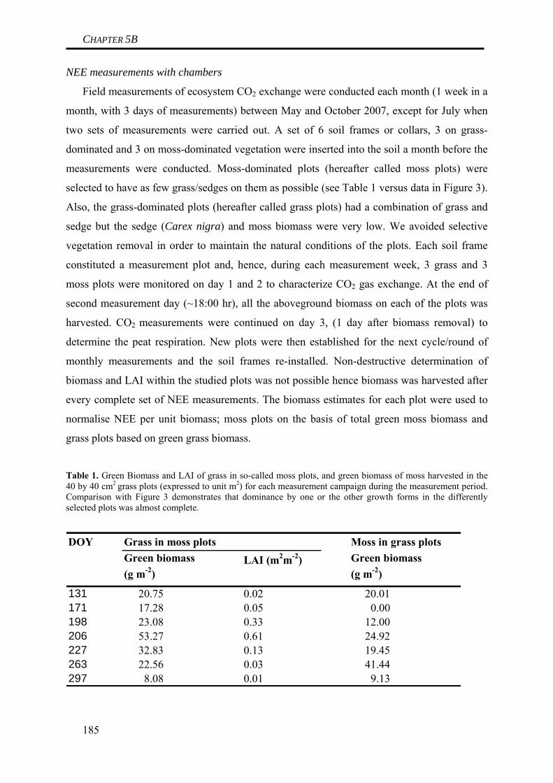
CHAPTER 5B
NEE measurements with chambers
Field measurements of ecosystem CO2 exchange were conducted each month (1 week in a
month, with 3 days of measurements) between May and October 2007, except for July when
two sets of measurements were carried out. A set of 6 soil frames or collars, 3 on grass-
dominated and 3 on moss-dominated vegetation were inserted into the soil a month before the
measurements were conducted. Moss-dominated plots (hereafter called moss plots) were
selected to have as few grass/sedges on them as possible (see Table 1 versus data in Figure 3).
Also, the grass-dominated plots (hereafter called grass plots) had a combination of grass and
sedge but the sedge (Carex nigra) and moss biomass were very low. We avoided selective
vegetation removal in order to maintain the natural conditions of the plots. Each soil frame
constituted a measurement plot and, hence, during each measurement week, 3 grass and 3
moss plots were monitored on day 1 and 2 to characterize CO2 gas exchange. At the end of
second measurement day (~18:00 hr), all the aboveground biomass on each of the plots was
harvested. CO2 measurements were continued on day 3, (1 day after biomass removal) to
determine the peat respiration. New plots were then established for the next cycle/round of
monthly measurements and the soil frames re-installed. Non-destructive determination of
biomass and LAI within the studied plots was not possible hence biomass was harvested after
every complete set of NEE measurements. The biomass estimates for each plot were used to
normalise NEE per unit biomass; moss plots on the basis of total green moss biomass and
grass plots based on green grass biomass.
Table 1. Green Biomass and LAI of grass in so-called moss plots, and green biomass of moss harvested in the 40 by 40 cm2 grass plots (expressed to unit m2) for each measurement campaign during the measurement period. Comparison with Figure 3 demonstrates that dominance by one or the other growth forms in the differently selected plots was almost complete.
DOY Grass in moss plots Moss in grass plotsGreen biomass(g m-2)
LAI (m2m-2) Green biomass(g m-2)
131 20.75 0.02 20.01171 17.28 0.05 0.00198 23.08 0.33 12.00206 53.27 0.61 24.92227 32.83 0.13 19.45263 22.56 0.03 41.44297 8.08 0.01 9.13
185

CHAPTER 5B
During each monthly measurement series (3 measurement days each month), net
ecosystem exchange (NEE) and ecosystem respiration (Reco) were sequentially observed with
a systematic rotation over all plots using manually-operated, closed gas exchange chambers,
modified from the description given by Droesler (2005), Wohlfahrt and others (2005), and Li
and others (2008b) as used in central European bogs and alpine grasslands. The 38 x 38 x 54
cm3 chambers of our system were constructed of transparent plexiglass (3 mm XT type
20070; light transmission 95%). Dark chambers, for measuring ecosystem respiration were
constructed of opaque PVC, and covered with an opaque insulation layer and with reflective
aluminium foil. Using extension bases, chamber height was adjusted to the canopy height.
Chambers were placed on the plastic frames/collars that were inserted 7 cm into the ground.
They were sealed to the chamber with a flexible rubber gasket and the chamber firmly secured
using elastic bands fastened onto the ground from two sides. Tests indicated that leakage did
not occur (see Droesler 2005 for details), however, this could not be examined regularly in the
case of systematic field measurements and required that each set of data must be scrutinised
for abnormalities.
Increased air pressure in the chamber was avoided by a 12 mm opening at the top of the
chamber which was closed after the chamber had been placed onto the frame and before any
records were taken. Circulation of air within the chamber was provided by three fans yielding
a wind speed of 1.5 m s-1. Change in chamber CO2 concentration over time was assessed with
a portable, battery operated IRGA (Li-Cor 820). Measurements were carried out in most cases
within 3-5 minutes of placing the chamber on the frames. Once steady state was attained, data
were logged every 15 s for 2 minutes and CO2 fluxes were calculated from a linear regression
describing the time dependent change in CO2 concentration within the chamber. Influence of
the CO2 concentration change on plant physiological response was ignored. By mounting
frozen ice packs inside and at the back of the chamber in the airflow, temperature during
measurements could be maintained within 1° C relative to ambient. Air (at 20 cm above the
ground surface) and peat (at –10 cm) temperatures inside and outside of the chambers were
monitored during measurement and data logged at the onset and end of every round of NEE
measurement on each plot. Similarly, light levels within the chamber, and above the
vegetation (canopy) were monitored using a quantum sensor (LI-190, Li-Cor, USA) and data
were logged every 15 seconds. Tests conducted in a controlled climate chamber showed that
vapor pressure deficit (VPD) changes within our CO2 measurement chambers were limited to
1 hPa during the period (~3 min) when the chambers were placed on the vegetation. We
186

CHAPTER 5B
therefore assumed that such small VPD changes should not affect CO2 exchange via stomatal
effects.
During each monthly measurement series, repeated light and dark chamber measurements
were conducted from sunrise to sunset over single days comparing three moss and three grass
plots. Eight to eleven measurement cycles were accomplished on individual days. To estimate
Gross Primary Production (GPP), ecosystem respiration was estimated for each NEE
observation time by linearly extrapolating between dark chamber observations (Reco), and
then adding it to NEE (cf. Li and others 2008a). As seen in Figure 5, the measurements of
NEE and Reco were closely associated in time, thus the corrections made in Reco were very
small. Measurements were conducted from the beginning of May until October in order to
develop a picture of the seasonal dynamics of CO2 exchange. Limitation in manpower to carry
out the labour intensive chamber measurements and the nature of our experimental site
prevented continuation of the observations with chambers during nighttime periods.
Estimation of model parameters describing gas exchange response
Empirical description of the measured NEE fluxes was accomplished via a non-linear
least squares fit of the data to a hyperbolic light response model, also known as the Michaelis-
Menten or rectangular hyperbola model (cf. Owen and others 2007):
γβα
αβ+
+−=
QQNEE (1)
187
where NEE is net ecosystem CO2 exchange (μmol CO2 m-2 s-1), α is the initial slope of the
light response curve and an approximation of the canopy light utilisation efficiency (μmol
CO2 m-2 s-1/μmol photon m-2 s-1), β is the maximum NEE of the canopy (μmol CO2 m-2 s-1), Q
is the Photosynthetic Active Radiation, PPFD (μmol photon m-2 s-1), γ is an estimate of the
average ecosystem respiration (Reco) occurring during the observation period (μmol CO2 m-2
s-1), (α/β) is the radiation required for half maximal uptake rate, and (β+γ) is the theoretical
maximum uptake capacity. Since the rectangular hyperbola may saturate very slowly in terms
of light, the term (αβQ)/(αQ+β) evaluated at a reasonable level of high light (Q = 2000 μmol
photons m-2 s-1 is used in this study) approximates the potential maximum GPP and can be
thought of as the average maximum canopy uptake capacity during each observation period,
noted here as (β+γ)2000. The parameters (β+γ)2000 (e.g., NEE at PPFD(Q)=2000) and γ were
estimated for each functional group using NEE data from the three measurement plots per
day. Data were pooled separately for grass and moss.
CHAPTER 5B
Biomass and LAI measurements
After gas exchange measurements on the second day of each campaign, all the
aboveground biomass within the 38 x 38 cm2 area enclosed by the collars was harvested. The
harvested moss and grass biomass was sorted into green and dead material. Leaf area (LA) of
the grass was measured using leaf area meter (CI-202, CID, Camas, WA) before being oven
dried at 80°C for 48 hours and weighed. The rest of the biomass was oven dried at 80°C for
48 hours and weighed to obtain the live and dead dry weight. Due to difficulties in
determining the moss photosynthesising surface area, the green biomass was simply dried and
weighed. Leaf area index (LAI) of the grass was calculated by dividing the LA by plot area.
During the months of July, August and September, root biomass was sampled with an 8
cm-diameter soil corer. Sampling took place in the middle of the grass measurement plots
after CO2 measurements were finished. The 30 cm soil cores were divided into sections of 5
cm each, washed under running tap water using soil sieves (mesh 2 mm) and the collected
roots were oven dried at 80°C before weighing them to obtain root dry weight in each of the
soil profiles. Due to difficulty in separating dead and live biomass, the reported results include
both dead and live root biomass. Moss rhizoid biomass was not quantified.
Results
Meteorology
Weather conditions during the study period are shown in Figure 2. Light conditions inside
and outside the chamber were not significantly different (Figure 2a). Temperature differences
between the inside and outside of the chamber were maintained within ±1°C. Mean annual
VPD was around 5 kPa and VPD fluctuated on a daily basis (Figure 2b). Air and peat
temperatures rose to a maximum in July, with peat temperature lagging behind. Maximum air
temperature (daily mean) of 15°C was recorded in July. Peat temperature varied with depth
and higher fluctuations occurred near the peat surface (Figure 2c). The shallow layers warmed
up faster after the snow thaw, but also cooled down more rapidly in autumn, while
temperatures at 1 m depth lagged behind for several weeks. Compared to 1 m depth, peat
temperatures at 30 cm depth were higher between April and August. Similarly, temperatures
during the day measured at the peat surface were higher than at 30 cm, during the same
period. Later in the year (autumn), the temperature profile inverted, with the warmest
temperatures (~2°C warmer) at 1 m depth and the coldest near the surface, reflecting the
decline in average daily air temperatures at that time.
188

CHAPTER 5B
Annual sum of precipitation was within the range of long-term average. The amount of
rainfall received between April and December was 942 mm (Figure 2d). A dry spell occurred
between March and May leading to a significant decrease (-0.4 m) in the ground water level
(GWL), the lowest water table being recorded in May. Afterwards, GWL remained relatively
high and did not decrease below -0.2 m.
0
500
1000
1500
2000
0
100
200
300
400PPFD inside light chamber
0
5
10
15
20
M A M J J A S O N D
0 m
0.3 m
1.0 m
-10
0
10
20
30
0
5
10
15
20VPD
Ta
-0.60
-0.40
-0.20
0.00
0.20
0
20
40
60
80
100
91 121 151 181 211 241 271Day of year
PPTWL
Month
PP
T (m
m)
Tsoi
l (°C
)V
PD
(hP
a)R
adia
tion
(W m
-2)
WL
(m)
Tair
(°C
)P
PFD
(mm
ol m
-2 s
-1)
b
c
d
a
189
Figure 2. Prevailing weather conditions (a, b, c, d) and ground water level (d) at the study site during the measurement period.

CHAPTER 5B
Biomass development
Biomass did not vary greatly among the selected moss and grass plots during any single
monthly measurement campaign, but changes were large between monthly measurements
(Figure 3a). Green biomass development in grass was recorded from May to July, when the
grasses attained maturity. Maximum green biomass (dry weight) of grass was 320 g m-2. After
July, grass biomass declined significantly with the declining air and peat temperatures and by
the end of October, when the first snowfall occurred, there was almost no green biomass
remaining (Figure 3a). The pattern of LAI development in grass was similar that of biomass
development, since biomass is used as a scaling factor in the conversion from sub-samples to
plot level.
0 .0
1 .0
2.0
3 .0
4 .0
5.0
0
100
200
300
400
131 171 198 206 227 263 297Day of Year
LAI (grass) Grass Moss
0.0
0.5
1.0
1.5
2.0
0-5 5-10 10 -15 15 -20 20 -30 Root depth (cm)
Gre
en b
iom
ass
(g m
-2)
LAI (
m2 m
-2)
Root
bio
mas
s (k
g m
-2)
a
b
Figure 3. Seasonal variation in (a) Green biomass (moss and grass) and LAI (grass only) development. (b) Root biomass of grasses in varying soil depths determined at selected periods during the season. Bars are SE.
190

CHAPTER 5B
Highest LAI of 3.8 occurred in July (Figure 3a). Afterwards, LAI declined significantly,
reaching zero values in October. Root biomass of the grass decreased with depth, but
extended well below 20 cm into the soil profile (Figure 3b). Highest root mass occurred
within the top 5-10 cm layer, totalling to 1.0 kg m-2. The moss rhizoids were shallow and
formed a thick mat within the first 1 cm top soil layer (data not shown). Moss green biomass
changed in a very different manner, declining between DOY 131 and 198. Maximum biomass
of 210 g m-2 occurred in September.
Seasonal and diurnal patterns of CO2 fluxes
The maximum daily values for NEE, Reco and GPP increased significantly between May
(DOY 131) and July (DOY 206) in both moss and grass (Figure 4). Highest Reco (30.0 and
22.0 μmol m-2s-1 for grass and moss respectively) occurred in mid July. Reco declined to near
zero at the end of the growing season. Similar patterns were observed for GPP and NEE.
Compared to grass, maximum NEE attained during the day were lower in moss (close to zero)
between May and June, while moss exhibited higher Reco during the same period. Maximum
NEE, however, occurred later in July. The highest GPP recorded during the season (37.0
μmol m-2 s-1) occurred in the grass plots and was about 10 μmol m-2 s-1 more than in the moss
plots. Parameters derived from the empirical light response model (Equation 1) are shown in
Table 2. Light use efficiency (α) increased between May and June and was significantly
(p<0.05) higher in the grass compared to the moss. The highest α recorded for grass (0.08
±0.01) was in mid summer (DOY 198-204), while the highest for moss (0.04 ±0.01) occurred
much earlier (DOY 171). These values coincide with the highest assimilation capacities (β) of
-18.70 ±2.48 and -10.31 ±4.59 for grass and moss, respectively. Both α and β declined later
during the growing season. Similar responses were observed for γ and (β+ γ)2000. Model
results showed the maximum value of average GPP [(β+ γ)2000] occurring in July both in
moss and grass and both the model derived results and the direct GPP estimates were
comparable.
Observed diurnal courses of NEE and Reco on selected measurement days of the year
along with the prevailing weather conditions on the respective days are shown in Figure 5. On
sunny days, CO2 assimilation increased from its lowest rates in the morning to maximum
around midday, but declined to near zero values later in the day. The daily peaks of carbon
assimilation changed during the season depending on the prevailing air temperature (Tair) and
light (PPFD) conditions. CO2 uptake in grass plots occurred only around midday in May,
191

CHAPTER 5B
192
while moss plots were net CO2 sources throughout the day during May and only became CO2
sinks from June on. July and August were characterised by CO2 uptake by both moss and
grass during most of the day. Ecosystem respiration (Reco) was relatively constant during the
day but changed seasonally. Very low CO2 exchange rates occurred later in the year (see
DOY 263 Figure 5).
0
10
20
30
40
Rec
o m
ax (m
mol
m-2
s-1
)
-20
-10
0
10
NE
E max
( μm
ol m
-2 s
-1)
Grass Moss
0
10
20
30
40
100 150 200 250 300Day of Year
GP
Pm
ax ( μ
mol
m-2
s-1
)
Figure 4. Seasonal variation of maximum NEE, Reco and GPP determined from diurnal course flux measurements conducted on specific days during the year. Bars are SE.
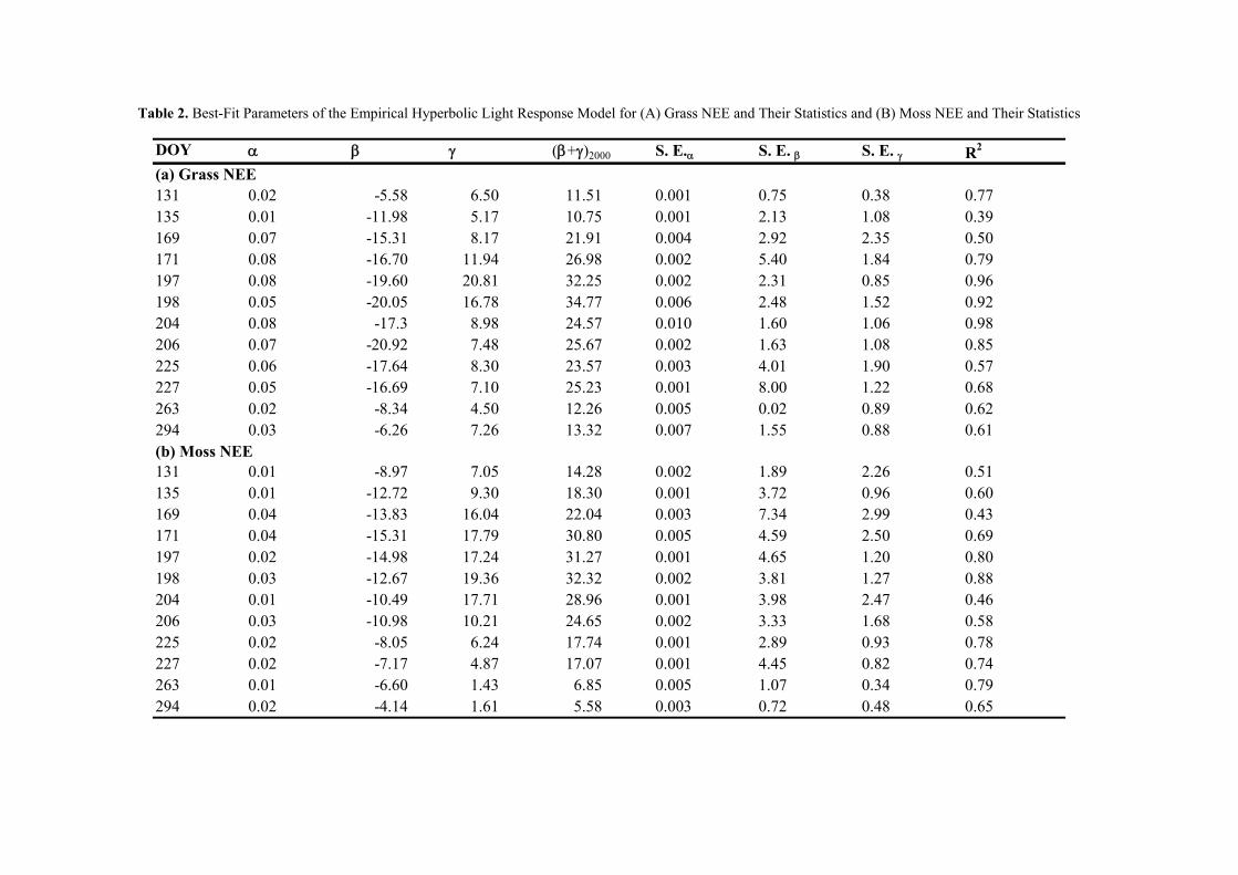
Table 2. Best-Fit Parameters of the Empirical Hyperbolic Light Response Model for (A) Grass NEE and Their Statistics and (B) Moss NEE and Their Statistics
DOY α β γ (β+γ)2000 S. E.α S. E. β S. E. γ R2
(a) Grass NEE131 0.02 -5.58 6.50 11.51 0.001 0.75 0.38 0.77135 0.01 -11.98 5.17 10.75 0.001 2.13 1.08 0.39169 0.07 -15.31 8.17 21.91 0.004 2.92 2.35 0.50171 0.08 -16.70 11.94 26.98 0.002 5.40 1.84 0.79197 0.08 -19.60 20.81 32.25 0.002 2.31 0.85 0.96198 0.05 -20.05 16.78 34.77 0.006 2.48 1.52 0.92204 0.08 -17.3 8.98 24.57 0.010 1.60 1.06 0.98206 0.07 -20.92 7.48 25.67 0.002 1.63 1.08 0.85225 0.06 -17.64 8.30 23.57 0.003 4.01 1.90 0.57227 0.05 -16.69 7.10 25.23 0.001 8.00 1.22 0.68263 0.02 -8.34 4.50 12.26 0.005 0.02 0.89 0.62294 0.03 -6.26 7.26 13.32 0.007 1.55 0.88 0.61(b) Moss NEE131 0.01 -8.97 7.05 14.28 0.002 1.89 2.26 0.51135 0.01 -12.72 9.30 18.30 0.001 3.72 0.96 0.60169 0.04 -13.83 16.04 22.04 0.003 7.34 2.99 0.43171 0.04 -15.31 17.79 30.80 0.005 4.59 2.50 0.69197 0.02 -14.98 17.24 31.27 0.001 4.65 1.20 0.80198 0.03 -12.67 19.36 32.32 0.002 3.81 1.27 0.88204 0.01 -10.49 17.71 28.96 0.001 3.98 2.47 0.46206 0.03 -10.98 10.21 24.65 0.002 3.33 1.68 0.58225 0.02 -8.05 6.24 17.74 0.001 2.89 0.93 0.78227 0.02 -7.17 4.87 17.07 0.001 4.45 0.82 0.74263 0.01 -6.60 1.43 6.85 0.005 1.07 0.34 0.79294 0.02 -4.14 1.61 5.58 0.003 0.72 0.48 0.65

CHAPTER 5B
-30
-20
10
0
10
20DOY 136
Reco NEE
DOY 204
-30
-20
10
0
10
20DOY 204
-30
-20
-10
06:00 12:00 18:00 06:00 12:00 18:00 06:00 12:00 18:00
0
10
20DOY 263 DOY 263
0
500
1000
1500
2000
0
10
20
30
40
0
500
1000
1500
2000
0
10
20
30
40
Tair
Tsoil
PPFD
0
500
1000
1500
2000
0
10
20
30
40
DOY 136
NEE Reco
Flux
(µm
ol m
-2 s
-1)
Flux
(µm
ol m
-2 s
-1)
Flux
(µm
ol m
-2 s
-1)
PP
FD (µ
mol
m-2 s
-1)
PP
FD (µ
mol
m-2 s
-1)
PP
FD (µ
mol
m-2 s
-1)
T (°
C)
T (°
C)
T (°
C)
Time of day (Hours)
Grass Moss
Figure 5. Diurnal variation of measured NEE and Reco for selected periods during the growing season. Parallel air temperature (Tair) at 20 cm above the vegetation, peat temperature (Tsoil) at –10 cm depth and Light conditions (PPFD) inside the chamber are also shown. Bars are SE.
Biotic influence on ecosystem CO2 exchange
Both the biomass and CO2 changed simultaneously during the season. In order to separate
the influence of biomass changes on seasonal ecosystem CO2 fluxes, NEE and Reco were
normalised with biomass in each of the plots (Figure 6). Until July, grass exhibited higher
NEE per unit biomass than moss. After this period, both vegetation types had similar NEE per
unit biomass. An abnormally high Reco per unit biomass occurred in the moss on DOY 198.
There was a strong correlation between LAI and model-derived physiological parameters α
(R2=0.93) and maximum GPP (β+ γ)2000 (R2=0.83) (Figure 7). Peat, which include soil and
roots, contributed a significant proportion (~50%) of the total CO2 output (Reco). Contribution
of the peat to the overall Reco became dominant later in the season (Table 3). Table 3. Mean soil and total ecosystem respiration (μmol m-2 s-1) in grass and moss plots during respective months when measurements were conducted. Month
June 4.9 ± 1.1 2.5 ± 5.3 9.9 ± 2.6 20.2 ± 2.4July 13.0 ± 4.5 7.8 ± 3.3 24.5 ± 2.5 20.8 ± 3.7August 10.5 ± 3.6 6.3 ± 2.0 14.1 ± 1.6 13.7 ± 1.1October 3.8 ± 2.3 2.0 ± 0.9 4.2 ± 2.2 2.0 ± 0.9
Grass Moss Grass MossPeat respiration Reco
194
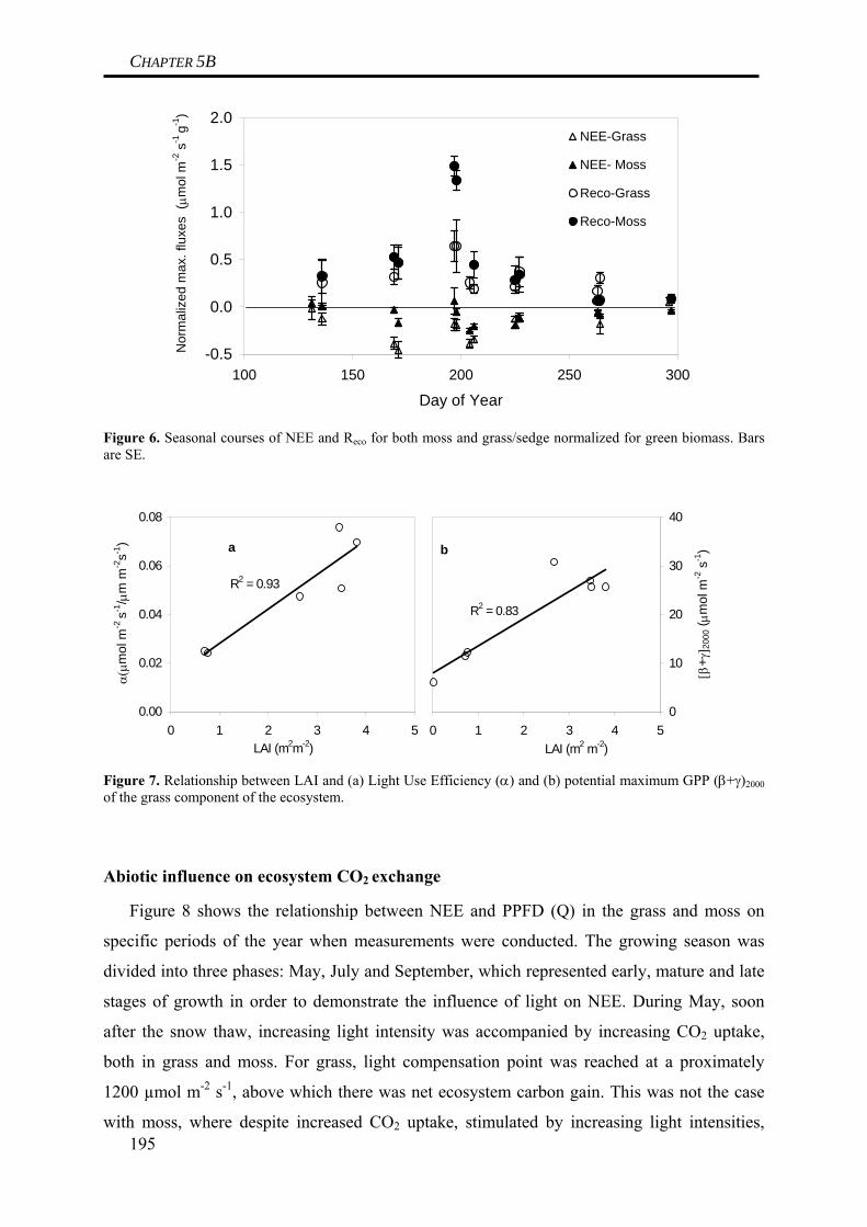
CHAPTER 5B
-0.5
0.0
0.5
1.0
1.5
2.0
100 150 200 250 300
Day of Year
Nor
mal
ized
max
. flu
xes
( μm
ol m
-2 s
-1 g-1
)
NEE-Grass
NEE- Moss
Reco-Grass
Reco-Moss
Figure 6. Seasonal courses of NEE and Reco for both moss and grass/sedge normalized for green biomass. Bars are SE.
R2 = 0.83
0
10
20
30
40
0 1 2 3 4 5LAI (m2 m-2)
[β+ γ
] 200
0 (μm
ol m
-2 s
-1)
R2 = 0.93
0.00
0.02
0.04
0.06
0.08
0 1 2 3 4 5LAI (m2m-2)
α(μ
mol
m-2
s-1/ μ
m m
-2s-1
) a b
Figure 7. Relationship between LAI and (a) Light Use Efficiency (α) and (b) potential maximum GPP (β+γ)2000 of the grass component of the ecosystem.
Abiotic influence on ecosystem CO2 exchange
195
Figure 8 shows the relationship between NEE and PPFD (Q) in the grass and moss on
specific periods of the year when measurements were conducted. The growing season was
divided into three phases: May, July and September, which represented early, mature and late
stages of growth in order to demonstrate the influence of light on NEE. During May, soon
after the snow thaw, increasing light intensity was accompanied by increasing CO2 uptake,
both in grass and moss. For grass, light compensation point was reached at a proximately
1200 µmol m-2 s-1, above which there was net ecosystem carbon gain. This was not the case
with moss, where despite increased CO2 uptake, stimulated by increasing light intensities,
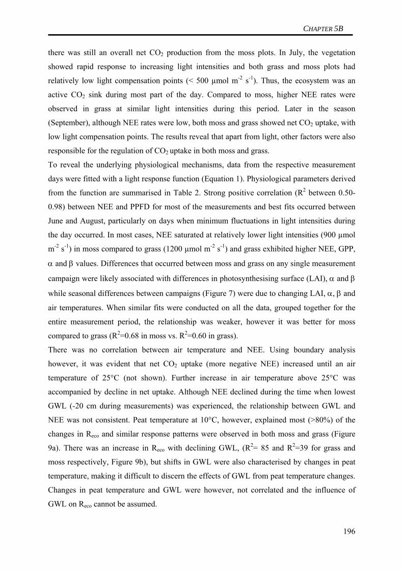
CHAPTER 5B
there was still an overall net CO2 production from the moss plots. In July, the vegetation
showed rapid response to increasing light intensities and both grass and moss plots had
relatively low light compensation points (< 500 µmol m-2 s-1). Thus, the ecosystem was an
active CO2 sink during most part of the day. Compared to moss, higher NEE rates were
observed in grass at similar light intensities during this period. Later in the season
(September), although NEE rates were low, both moss and grass showed net CO2 uptake, with
low light compensation points. The results reveal that apart from light, other factors were also
responsible for the regulation of CO2 uptake in both moss and grass.
To reveal the underlying physiological mechanisms, data from the respective measurement
days were fitted with a light response function (Equation 1). Physiological parameters derived
from the function are summarised in Table 2. Strong positive correlation (R2 between 0.50-
0.98) between NEE and PPFD for most of the measurements and best fits occurred between
June and August, particularly on days when minimum fluctuations in light intensities during
the day occurred. In most cases, NEE saturated at relatively lower light intensities (900 µmol
m-2 s-1) in moss compared to grass (1200 µmol m-2 s-1) and grass exhibited higher NEE, GPP,
α and β values. Differences that occurred between moss and grass on any single measurement
campaign were likely associated with differences in photosynthesising surface (LAI), α and β
while seasonal differences between campaigns (Figure 7) were due to changing LAI, α, β and
air temperatures. When similar fits were conducted on all the data, grouped together for the
entire measurement period, the relationship was weaker, however it was better for moss
compared to grass (R2=0.68 in moss vs. R2=0.60 in grass).
There was no correlation between air temperature and NEE. Using boundary analysis
however, it was evident that net CO2 uptake (more negative NEE) increased until an air
temperature of 25°C (not shown). Further increase in air temperature above 25°C was
accompanied by decline in net uptake. Although NEE declined during the time when lowest
GWL (-20 cm during measurements) was experienced, the relationship between GWL and
NEE was not consistent. Peat temperature at 10°C, however, explained most (>80%) of the
changes in Reco and similar response patterns were observed in both moss and grass (Figure
9a). There was an increase in Reco with declining GWL, (R2= 85 and R2=39 for grass and
moss respectively, Figure 9b), but shifts in GWL were also characterised by changes in peat
temperature, making it difficult to discern the effects of GWL from peat temperature changes.
Changes in peat temperature and GWL were however, not correlated and the influence of
GWL on Reco cannot be assumed.
196
CHAPTER 5B
Figure 8. NEE- light response curves for grass (left panel) and moss (right panel) during early (May), mature (July) and late (September) stages of vegetation development. Regression analysis for light response curves were done with filtered data using Sigma Plot 8.0 (Residuals >5 eliminated). Results are integrated data from the three measured plots for each plant type.
Discussion
Aboveground biomass production occurred between May and October with an annual green
biomass production of 320 g m-2 and 210 g m-2 for grass and moss, respectively. These values
are within the range reported for most cool temperate peatlands of North America and Europe
197

CHAPTER 5B
as summarised by Moore and others (2002). Dyck and Shay (1999) reported moss capitulum
biomass of 278 g m-2 in a peatland of central Canada based on sampling to depth of green
colour. Annual biomass production of the moss capitulum in southern mires of Finland ranged
between 260 and 400 g m-2 (Lindholm and Vasander 1990). Values obtained for eastern
Canada for both vascular plant leaves and moss capitulum range between 114 and 672 g m-2
(Bubier and others 2006). Thus, in terms of biomass production, the studied peatland
ecosystem is not very different from other peatlands occurring within the same latitudinal
range. The results show that mosses are an important component of this community,
representing approximately 30% of the total aboveground biomass during the growing period.
Our findings are in agreement with those reported elsewhere (Shaver and Chapin 1991,
Gordon and others 2001, Douma and others 2007), showing the significant contribution of
moss to the overall community biomass as well as ecosystem function.
R2 = 0.83R2 = 0.85
0
10
20
30
40
0 5 10 15 20
Tsoil (°C)
Rec
o (μm
ol m
-2 s
-1)
R2 = 0.85
R2 = 0.39
-0.20-0.15-0.10-0.050.00
WL (m)
ba
Figure 9. Relationships between daily averages of maximum Reco of grass (open circles) and moss (closed circles) and (a) Peat temperature (Tsoil) measured at 10 cm depth within the collars and (b) Mean ground water level (GWL), Thick regression lines represent moss, while the thin lines are for grass.
A combination of senescence of the grass, low radiation and rapidly dropping
temperatures could be the reasons for the decline in green biomass after August. This was not
the case with moss where green biomass development appeared to be more supported by low
light intensities and air temperatures. The drop in moss green biomass between May (DOY
131) and June (DOY 198) may be due to be due to the early spring drought that led to the
drop in GWL down to –40 cm with possible reduction in soil moisture within the top soil
layers. Recovery of moss however, was a slow process, and it took almost a month before
moss tissues were green and recovered. This may explain the observed 1.5 months’ lag
between GWL recovery and growth resumption. GWL, however, did not have any impact on
198
CHAPTER 5B
biomass development in grass. Reasons for this could be due to (1) unlike moss, green
biomass development in grass started after April when there was rainfall and soil moisture
conditions were already favourable. (2) Grass have deep rooting patterns, which could buffer
them from low GWL compared to the moss (Limpens and others 2008). We observed grass
roots growing down to -30 cm, indicating that even if the GWL drops down to this depth,
grass will still have access to ground water. Moore and others (2002) reported fine root
biomass accumulation of between 0.4 and 1 kg m-2 growing down –50 cm, making the grass
vegetation less responsive to changes in GWL. Rooting depths below -50 cm have also been
reported in Tundra, with mean biomass of 1.5 kg m-2 (Jackson et al. 1996, Canadell et al.
1996).
Green biomass influences NEE and GPP since it determines the photosynthetic surface
area (Street and other 2007, Shaver and other 2007, Limpens and others 2008). Mean seasonal
maximum NEE were around –10.0 and -5 µmol m-2 s-1 for grass and moss respectively, while
the respective GPP were 23 and 12 µmol m-2 s-1. These are within the range of 8-20 µmol m-2
s-1 for NEE (Tuittila and others 2004; Douma and others 2007, Riutta and others 2007;
Lindroth and others 2007, Shaver and others 2007) and 10-40 µmol m-2 s-1 for GPP (Bubier
and others 1998; Lindroth and others 2007) reported for most temperate peatlands of Northern
Hemisphere. The moss plots, in some instances, comprised a few grass populations that could
raise the CO2 fluxes since they are more active and efficient (Douma and others 2007,
Limpens and others 2008). Although NEE data of moss were corrected for contribution by the
grass using aboveground biomass of the grass harvested in the moss plots, our values still
remain at the extreme end of scale for moss fluxes (Tuittila and others 2004; Riutta and others
2007, Douma and others 2007). This could be explained by the high light intensity levels
reaching the moss vegetation at our study site compared to those reported for the Northern
Hemisphere. Our results show that moss contributes approximately 30% of the overall
ecosystem CO2 uptake in this peatland. Douma and others (2007) reported that mosses
contributed between 14 – 96% of the total CO2 assimilated in an arctic ecosystem, depending
on the proportion of vascular plants (shading) growing together with the moss.
When NEE was normalised with biomass we still observed higher NEE for grass during
the active growth phase. These differences result from higher CO2 fixation capacity due to
higher light use efficiency (α) and higher maximum light intensity at which saturation occurs
in grass compared to moss (Street and others 2007). Our analysis showed that light alone
explains more than 70% of NEE during the active phase of development in both moss and
grass and that grass could increase light use efficiency by increasing LAI, with an overall
199

CHAPTER 5B
increase in potential production. At ecosystem level, increased LAI in grass may affect moss
production by reducing the light levels reaching moss, since moss biomass is short and grow
under the grass canopy, with a possible impact on the overall ecosystem production. Similar
conclusions have been arrived at in studies conducted on moss communities in northern
peatlands (Shaver and Chapin 1991, Douma and others 2007).
Ground water level of around –10 cm is regarded as the optimum water level for most
physiological responses in peatland species (Tenhunen and others 1992; Semikhatova and
others 1992; Tuittila and others 2004). Ground water level declined to –40 cm in April and
later to –20 cm in June, with significant influence on moss NEE. Despite resumption of
rainfall in May, NEE by moss remained low and moss plots were net CO2 sources during
most of the day until June. This was not the case with grass that was a CO2 sink during this
period. Differences that occur between moss and grass in response to changing GWL may be
due to differences in their physiological and morphological structures (Schipperges and Rydin
1998). Mosses, unlike grasses lack roots and only possess rhizoids that don’t penetrate into
deeper soil layers and they show more sensitivity to tissue water changes (Schipperges and
Rydin 1998), with narrow tolerance to small draw-down in GWL (Riutta and others 2007).
Grass, however, are deep rooted and are less sensitive to short-term changes in GWL (Lafleur
and others 2005) since they have access to water in a large soil volume. Grass also possess
adaptive strategies such as leaf rolling, as shown by a declining LAI (with no change in
biomass) in early June and stomatal control ability (Busch and Lösch 1999) that minimise
transpiration water loss. Combined with high light use efficiency, these adaptations could
enhance CO2 assimilation during GWL decline and rapid recovery after drought in grass
compared to moss.
Except for the months of June and July, Reco was similar (mean = 10 μmol m-2 s-1) in moss
and grass. Our values are higher compared to those reported for peatlands of Scandinavian
and North American countries (Bubier and others 1998; Tuittila and others 2004; Lafleur and
others 2005; Lindroth and others 2007), but are within the range of 12-20 μmol m-2 s-1
reported by Riutta and others 2007. Higher Reco from our study site could be due to (1) its
southern location i.e. less continental climate with higher temperatures given that there was an
exponential increase in Reco with increasing temperatures. (2) Relatively longer growing
season/extended decomposition period. (3) A large drop in GWL that occurred in early spring
and resulting into the death of moss. Bortoluzzi and others (2006) reported Reco of 8.0 μmol
m-2 s-1 in a mountain bog at an altitude of 867 m.a.s.l. in France with LAI of 1.1 and mean
maximum temperatures of 30°C. The exact contribution of the vegetation to the total
200

CHAPTER 5B
ecosystem respiration at this site is not known, however, measurement of peat respiration
(plus roots) indicated that at least half of the Reco originates from the peat. Compared to moss,
a significantly large proportion of Reco originated from the peat under the grass. Although no
analysis of peat characteristics under the two vegetation types was conducted, we anticipated
similar peat characteristics. Thus differences in Reco that were observed between the two plots
could only be attributed to the large root biomass in the grass plots compared to moss.
Past studies indicate that peat respiration increases with decreasing GWL (McNeil and
Waddington 2003, Bortoluzzi et al. 2004, Riutta et al. 2007). We observed an increase in Reco
with declining GWL, and even though the effects of GWL on Reco might be confounded by
changes in peat temperature, the behaviour response suggested that the two vegetation types
were affected differently (R2=0.85 and 0.39 in grass and moss respectively). This was not the
case with peat temperature, which had similar effects on both moss and grass. The poor
correlation in moss suggests that its respiration could be influenced by GWL changes in a
very narrow uppermost portion of the peat profile. This was different in grass since the
extensive rooting system tracks the changing soil moisture conditions (lagging behind GWL)
as aeration of the soil profiles allows for aerobic respiration of the roots and soil micro-
organisms (Basiliko and others 2006), while CO2 assimilation remained unchanged. Influence
of water table fluctuation on ecosystem respiration is well documented for other ecosystems
(Alm and others 1999), while Lafleur and others (2005) explained the anomalies in such
relationships.
Our results emphasise the significant role of temperature in determining ecosystem CO2
exchange processes in this peatland. At high light intensities, temperature sets the upper
boundary of NEE, which increases steadily with increasing temperature to an optimum of
25°C. Since there was an exponential increase in Reco with increasing temperature, rapid
decline in NEE above 25°C could be the result of an increasing Reco over CO2 assimilation, an
indication that at higher temperatures the peatland is likely to become a net CO2 source.
Conclusion
Green biomass and LAI are important determinants of CO2 assimilation by the mosses and
grasses. Apart from LAI, higher NEE in grasses compared to mosses was also attributed to
more efficient light use. Mosses were more sensitive to GWL draw-down, which had
significant influence on their CO2 assimilation and biomass development. Grasses however,
showed less sensitivity to GWL changes, as a result of their extensive and deep rooting
systems. Increasing peat temperatures at -10 cm depth resulted in exponential increase in Reco. 201
CHAPTER 5B
Since future climate scenarios in Europe indicate reduced precipitation amounts and increased
air temperatures, lower GWL and increased peat temperatures may turn this peatland into a
net CO2 source during most part of the year. Other possible consequences are increased death
of mosses and their replacement with grasses and other vascular plant species that are more
resilient. Mosses however, make significant contribution to the current total community
biomass as well as ecosystem CO2 uptake in this peatland and their decline may disrupt
ecosystem CO2 budget.
References
Alm J, Schulman L, Walden J, Nykänen H, Mauritanian PJ, Silvola J. 1999. Carbon balance
of boreal bog during a year with an exceptionally dry summer. Ecology 80:161-174.
Basiliko N, Moore TR, Jeannotte R, Bubier JL. 2006. Nutrient Input and Carbon and
Microbial Dynamics in an ombrotrophic bog. Geomicrobiology Journal 23:531–543.
Bortoluzzi E, Epron D, Siegenthaler A, Gilbert D, Buttler A. 2006. Carbon balance of a
European mountain Bog at contrasting stages of regeneration. New Phytol 172: 708-718.
Bubier JL, Moore TR, Crosby G. 2006. Fine-scale vegetation distribution in a cool temperate
peatland. Canadian Journal of Botany 84:910-923.
Bubier JL, Crill PM, Moore TR, Savage K, Varner RK. 1998. Seasonal patterns and controls
on net ecosystem CO2 exchange in a boreal peatland complex. Global Biogeochemical
Cycles 12:703-714.
Bubier JL, Bhatia G, Moore TR, Roulet NT, Lafleur PM. 2003. Spatial and Temporal
Variability in Growing-Season Net Ecosystem Carbon Dioxide Exchange at a Large
Peatland in Ontario, Canada. Ecosystems 6:353-367.
Busch J, Lösch R. 1999. The gas exchange of Carex species from eutrophic wetlands and its
dependence on microclimatic and soil wetness conditions. Phs Chem Earth Part B
Hydrology Oceans and Atmosphere 24:117-120.
Canadell J, Jackson RB, Ehleringer JR, Mooney HA, Sala OE, Schulze E-D. 1996. Maximum
rooting depth of vegetation types at the global scale. Oecol 108:583–595.
Chapin FS, Jefferies RL, Reynolds JF, Shaver GR Svoboda J, Editors. 1992. Arctic
Ecosystems in a changing climate: an ecophysiological perspective. San Diego. Academic
Press. 469p.
Clymo and Hayward 1982. The ecology of Sphagnum. In: Smith AJE Ed. Bryophyte Ecology.
Chapman and Hall NY. pp 229-290.
202
CHAPTER 5B
Douma JC, Van Vijk MT, Lang SI, Shaver GR. 2007. The contribution of mosses to carbon
and water exchange in arctic ecosystems: quantification and relationships with system
properties. Plant Cell and Environ 30: 1205-1215.
Droesler M. 2005. Trace gas exchange of bog ecosystems, southern Germany. Lehhrstuhl für
Vegetationsökologie. Doctoral Thesis, Technical University of Munich. Available online
at: http://www.wzw.tum.de/vegoek/publikat/dissdipl.html.
Dyck BS, Shay JM. 1999. Biomass and carbon pools of two bogs in the experimental Lakes
Area, north western Ontario. Canadian Journal of Botany 77:291–304.
Fenner N, Ostle N, Freeman C, Sleep D, Renolds B. 2004. Peatland efflux partitioning reveals
that Sphagnum photosynthate contributes to the DOC pool. Plant and Soil 259:345-354.
Frolking SE, Bubier JL, Moore TR, Ball T, Bellisario LM and others. 1998. Relationship
between ecosystem and photosynthetically active radiation for northern peatlands. Global
Biogeochemical Cycles 12:115-126.
Gorham E. 1991. Northern Peatlands: Role in the carbon balance and probable response to
climate warming. Ecology Applications 1:182-95.
Gordon C, Wynn JM, Woodin SJ. 2004. Impacts of increased nitrogen supply on high arctic
heath: the importance of bryophytes and phosphorus availability. New Phytol 149: 461-
471.
Hastings SJ, Luchessa SA, Oechel WC, Tenhunen JD. (1989). Standing biomass and
production in water drainages of the foothills of the Philip Smith Mountains, Alaska.
Holartic Ecology 12:304-311.
Jackson RB, Canadell J, Ehleringer JR, Mooney HA, Sala OE, Schulze E-D. 1996. A global
analysis of root distributions of terrestrial biomes. Oecol 108:389–411.
Lafleur PM, Moore TR, Roulet NT, Frolking S. 2005. Ecosystem respiration in a cool
temperate bog depends on peat temperature but not water table. Ecosystems 8:619-629.
Leadley PW; Stocklin J. 1996. Effects of elevated CO2 on model calcareous grasslands:
community, species, and genotype level responses Global Change Biology 2:389-397.
Li Y-L, Tenhunen J, Mirzae H, Hussain MZ, Siebicke L, Foken T, Otieno D, Schmidt M,
Ribeiro NA, Aires L, Pio C, Banza J, Pereira J. 2008a. Assessment and up scaling of CO2
exchange by patches of the herbaceous vegetation mosaic in Portuguese cork oak
woodlands. Agric For Meteorol 148:1318-1331
Li Y-L, Tenhunen J, Owen K, Schmitt M, Bahn M, Droesler M, Otieno D, Schmidt M,
Gruenwald Th, Hussain MZ, Mirzae H, Berhofer Ch. 2008b. Patterns of CO2 gas
exchange capacity of grassland ecosystem in the Alps. Agric For Meteorol 148:51-68.
203

CHAPTER 5B
Limpens J, Berendse F, Blodau C, Canadell J G, Freeman C, Holden J, Roulet N, Rydin H,
Schaepman-Strub G. 2008. Peatlands and the carbon cycle: from local processes to global
implications – a Synthesis. Biogeosciences 5:1379–1419
Lindholm T and Vasander H. 1990. Production of eight species of Sphagnum at Suurisuo
mire, southern Finland. Annales Botanici Fennici 27:145–157.
Lindroth A, Lund M, Nilson M, Aurela M, and others. 2007. Environmental controls on CO2
exchange in European Mires. Tellus 59B:812-825.
McNeil P, Waddington JM. 2003. Moisture controls on Sphagnum growth and CO2 exchange
on a cutover bog. Journal of Applied Ecology 40:354-367.
Moore TR, Bubier JL, Frolking SE, Lafleur PM, Roulet NT. 2002. Plant biomass and
production and CO2 exchange in an ombrotrophic bog. Journal of Ecology 90:25-36.
Oechel WC; Vourlitis GL; Hastings SJ; Bocharev SA. 1995. Change in arctic CO2 flux over
two decades: effects of climate change at Barrow, Alaska, Ecology Applications 5:846-
855.
Ostendorf B, Quinn P, Beven K, Tenhunen JD. 1996. Hydrological Controls on Ecosystem
Gas Exchange in an Arctic Landscape. Ecological Studies 120:369-386.
Owen K, Tenhunen J, Reischtein M, Wang Q, Falge E, Gayer R, others. 2007. Comparison of
seasonal changes in CO2 exchange capacity of ecosystems distributed along a north-south
European transect under non water stressed conditions. Global Change Biology. 13:734-
760.
Paul S, Küsel K, Alewell C. 2006. Reduction processes in forest wetlands: Tracking down
heterogeneity of source/sink functions with a combination of methods. Soil Biology and
Biochemistry 38:1028-1039.
Riutta T, Laine J and Tuittila ES. 2007. Sensitivity of CO2 exchange of fen ecosystem
components to water level variation. Ecosystems 10:718-733.
Robroek B, Limpens J, Breeuwer A, Schouten M. 2007. Effects of water level and
temperature on performance of four Sphagnum mosses. Plant Ecology 190:97-107.
Ruimy MG, Jarvis PG, Baldocchi DG, Saugier B. 1995. CO2 fluxes over canopies and solar
radiation: a literature review. Advances in Ecology Research 26:1-68.
Schipperges B, Rydin H. 1998. Response of photosynthesis of Sphagnum species from
contrasting microhabitats to tissue water content and repeated desiccation. New Phytol
140:677-684.
Semikhatova OA, Gerasimenko TV, Ivanova TI. 1992. Photosynthesis, Respiration and
growth of plants in the Soviet Arctic. Chapin FS, Jefferies RL, Reynolds JF, Shaver GR,
204
CHAPTER 5B
205
Svoboda J, editors. Arctic Ecosystems in the changing Climate. San Diego: Academic
Press. pp169-192.
Shaver GR, Chapin FS. 1991. Production-biomass relationships and element cycling in
contrasting arctic vegetation types. Ecological Monographs 61:1-31.
Shaver GR, Johnson LC, Cades DH, Murray G, Laundre JA, Rastetter EB, Nadelhoffer KJ,
Giblin AE. 1998. Biomass and CO2 flux in wet sedge tundras: Responses to nutrients,
temperature, and light. Ecological Monographs 68:75-97.
Shaver GR, Street LE, Rastetter EB, Van Wijk MT, Williams M. 2007. Functional
convergence in regulation of net CO2 flux in heterogeneous Tundra landscapes in Alaska
and Sweden. Journal of Ecology 95:802-817.
Smith LC, MacDonald GM, Velichko AA, Beilman DW, Borisova OK, Frey KE,
Kremenetski KV, Sheng Y. 2004. Siberian Peatlands a Net Carbon Sink and Global
Methane Source Since the Early Holocene. Science 16: 303:353–356.
Street LE, Shaver GR, Williams M and Van Wijk MT. 2007. What is the relationship between
changes in canopy leaf area and changes in photosynthetic CO2 flux in arctic ecosystems.
Journal of Ecology 95:139-150.
Tenhunen J, Lange OL, Hahn S, Siegwolf R, Oberbauer SF. 1992. The ecosystem role of
poikilohydric tundra plants. Chapin FS, Jefferies RL, Reynolds JF, Shaver GR, Svoboda J,
editors. Arctic Ecosystems in the changing Climate. San Diego: Academic Press. pp 213-
237.
Tuittila ES, Vasander H, Laine J. 2004. Sensitivity of C sequestration in reintroduced
Sphagnum to water level variation in a cutaway peatland. Restoration Ecology 12:483-493
Turunen J, Tomppo E, Tolonen K, Reinikainen A. 2002. Estimating carbon accumulation
rates of undrained mires in Finland–application to boreal and subarctic regions. The
Holocene12:69-80.
Wohlfahrt G, Anfang Ch, Bahn M, Haslwanter A, Newesely Ch, Schmitt M, Droesler M,
Pfadenhauer J, Cernusca A. 2005.Quantifying ecosystem respiration of a meadow using
eddy covariance, chambers and modelling. Agric For Meteor 128:141-162.

APPENDIX
APPENDIX
206

APPENDIX
List of further publications
Ye Q, Muhr J, Steudle E (2005). A cohesion/tension model for the gating of aquaporins
allows estimation of water channel pore volumes in Chara. Plant, Cell & Environment,
28, 525-535.
Goldberg SD, Muhr J, Borken W, Gebauer G (2008). Fluxes of climate-relevant trace gases
between a Norway spruce forest soil and atmosphere during repeated freeze/thaw cycles
in mesocosms. Journal of Plant Nutrition and Soil Science, 171, 729-739.
Muhr J, Goldberg SD, Borken W, Gebauer G (2008). Repeated drying/rewetting cycles and
their effects on the emissions of CO2, N2O, NO and CH4 in a forest soil. Journal of Plant
Nutrition and Soil Science, 171, 719-728.
207
Related Documents