caratula working paper - barcelonagse.eu · hire permanent workers up to the point where expected firing costs are equal to the productivity gain with respect to temporary workers.

Centre de Referència en Economia Analítica

Barcelona Economics Working Paper Series

Working Paper nº 266

Financing Constraints and Fixed-Term Employment Contracts

Andrea Caggese and Vicente Cuñat

October 14, 2005

Financing Constraintsand

Fixed-Term Employment Contracts∗

Andrea Caggese and Vicente Cunat†

Universitat Pompeu Fabra

14th October 2005

Abstract

The aim of this paper is to identify the effect of financing constraints onthe employment decisions of firms. We present a theoretical model that deter-mines the optimal use of fixed term and permanent contracts in the presence offinancing constraints. We then estimate the effect of financing constraints onthe dynamics of fixed-term employment contracts versus permanent employ-ment contracts for a sample of Italian manufacturing firms. The results areconsistent with the model and show that financially constrained firms tend touse a larger proportion of fixed term contracts, and that the relative volatilityof fixed term employment versus permanent employment is higher among them.As a consequence, the volatility of total employment is also significantly higherfor financially constrained firms than for financially unconstrained ones.

∗The authors thank Maria Guadalupe, Maia Guell, Barbara Petrongolo and Ernesto Villanuevafor their valuable comments and suggestions. All errors are, of course, the authors own responsibility.

†[email protected] and [email protected], Pompeu Fabra University, Department ofEconomics, Calle Ramon Trias Fargas 25-27, 08005, Barcelona, Spain.

1

Barcelona Economics WP nº 266

1 Introduction

The literature on financing constraints has investigated how financial restrictions may

affect firm decisions. Most of the theoretical and empirical literature has analyzed

fixed capital investment decisions.1 However, there are very few studies on the effects

of financing constraints on the employment policies of firms.2 The dynamic nature of

employment decisions makes them sensitive to financing constraints that firms face or

may expect in the future. The aim of this paper is to propose and test empirically a

new way of identifying the effects of financing constraints on the employment dynam-

ics of firms by exploiting the different hiring and firing costs of fixed-term contracts

and permanent contracts.

We consider the optimal dynamic employment policy of a firm that faces capital

market imperfections when one type of labor (fixed-term contracts) is completely

flexible and another type (permanent contracts) is subject to firing costs. We assume

that the two types of labor are perfect substitutes but permanent employment is

more productive3. This implies that a firm without financing constraints would

hire permanent workers up to the point where expected firing costs are equal to the

productivity gain with respect to temporary workers.

When firms face both significant labor market frictions and financial market in-

efficiencies, the interactions between financing constraints and firing costs amplify

their effects on hiring and firing decisions, with important consequences. We show

that a firm with a binding financing constraint has a higher opportunity cost of fir-

ing permanent workers than a financially unconstrained firm. This discourages the

hiring of permanent workers and gives incentives for the use of fixed-term contracts.

Therefore, financially constrained firms will hire relatively more fixed-term workers

than it would otherwise be optimal in the absence of financing imperfections. But

fixed-term contracts can be costlessly terminated if the firm receives a negative pro-

ductivity shock. This means that financially constrained firms will also exhibit an

1See Hubbard (1998) for a review of this literature.2Exceptions are Nickell and Nicolitsas (1999), Smolny and Winker (1999) and Rendon (2005).3This assumption is equivalent in the model to permanent workers having a higher productivity

per unit of salary paid. We do not provide a microfoundation of this assumption. Nonetheless itarises endogenosly in more complex model where the skill of the workers is heterogeneous.

2

higher volatility of total employment. The consequence is that if both labor market

frictions and financing constraints affect a consistent share of firms in an economy, the

volatility of employment will increase after the introduction of fixed term contracts.

The predictions of the model are then tested on a database of small and medium

Italian manufacturing firms with balance sheet data from 1995 to 2000. This dataset

represents a unique opportunity to verify the joint effect of firing costs, flexible em-

ployment contracts and financing imperfections on the labour demand of firms for

several reasons: i) Italy is a country that traditionally has a very high labour protec-

tion. The OECD 1999 Employment outlook places Italy as the country with the third

strictest employment protection legislation among OECD countries in the 1990s. At

the same time flexible contracts have been gradually more available to Italian firms

in the last 20 years, especially since a new type of fixed term labour contract was

introduced in the mid 1990s. Therefore our dataset is particularly well suited to an-

alyze the effect of the introduction of flexible labor contract in a heavily regulated

environment. ii) The Italian financial system is traditionally underdeveloped (as an

illustration, the market capitalization of the Milan Stock Exchange is several times

smaller than the market capitalization of the stock markets of the other large Euro-

pean countries). Italian firms thus face severe capital market imperfections that are

only partially corrected by the availability of bank credit as the main source of ex-

ternal finance. iii) The dataset analyzed in this paper contains a unique combination

of self-reported measures of financing constraints and information on fixed-term and

permanent labor contracts.

The results show that financially constrained firms rely more on fixed-term con-

tracts, and that the volatility of fixed-term employment is much higher, than in

financially unconstrained firms. Moreover, firms’ employment policy reacts to pro-

ductivity shocks differently depending on their degree of financing constraints: firms

that face capital market imperfections show a positive correlation between a produc-

tivity shock and fixed-term contracts as a share of total employment, while firms that

do not face such imperfections behave in the opposite way.

The paper is organized as follows: section 2 surveys the related literature. Section 3

illustrates the model. Section 4 presents the empirical analysis. Section 5 summarizes

3

the conclusions.

2 Related literature

The findings of this paper are of interest to the literature on the effect of employment

protection on employment dynamics (Bentolila and Bertola 1990, Bentolila and Saint

Paul 1992, Hopenhayn and Rogerson 1993). In particular the issue of fixed-term la-

bor contracts and their interaction with permanent contracts has attracted significant

attention in the preexisting literature. Dolado et al (2002) and Saint Paul (1996) pro-

vide a good survey of the relevant theoretical literature on the topic. The European

countries where both types of contracts coexist and where several labor reforms have

been introduced constitute interesting natural experiments to test the effects of firing

costs and labor market regulations. A significant number of articles have studied

empirically the different country cases: Spain (Dolado et al, 2002; Alonso-Borrego

et al 2005), France (Blanchard and Landier, 2002) and Italy (Kugler and Pica 2004)

among many others. All of these papers explore the changes in volatility of employ-

ment and the relative use of fixed-term versus permanent contracts. However, their

approach does not take into account the possible influence of financing constraints. 4

This paper is related to the literature about the effect of financial imperfections

on the labor demand of firms (Nickell and Nicolitsas 1999, Smolny, and Winker 1999,

Benito and Hernando 2003). These papers explore at the empirical level the rela-

tionship between financing constraints and total employment. The added value of

this paper comes from exploring the interaction between financing constraints, firing

costs, and the joint dynamics of fixed-term and permanent employment contracts.

That is, in contrast with previous papers we explicitly model the existence of both

types of contracts and show how does the presence of financing constraints affect their

use. In this sense our article can be considered as a bridge between the two strands

of the literature mentioned above. 5

4Kugler and Pica 2004 explore the interaction between the introduction of fixed term contractsand entry regulation. As long as financing constraints can restrict the entry of new firms, these twoissues are related although we model the hiring and firing decisions of existing firms.

5Another paper that follows a similar approach is Rendon (2005). The author uses a simulationprocedure and compares the effect, on fixed investment and job creation, of relaxing financing

4

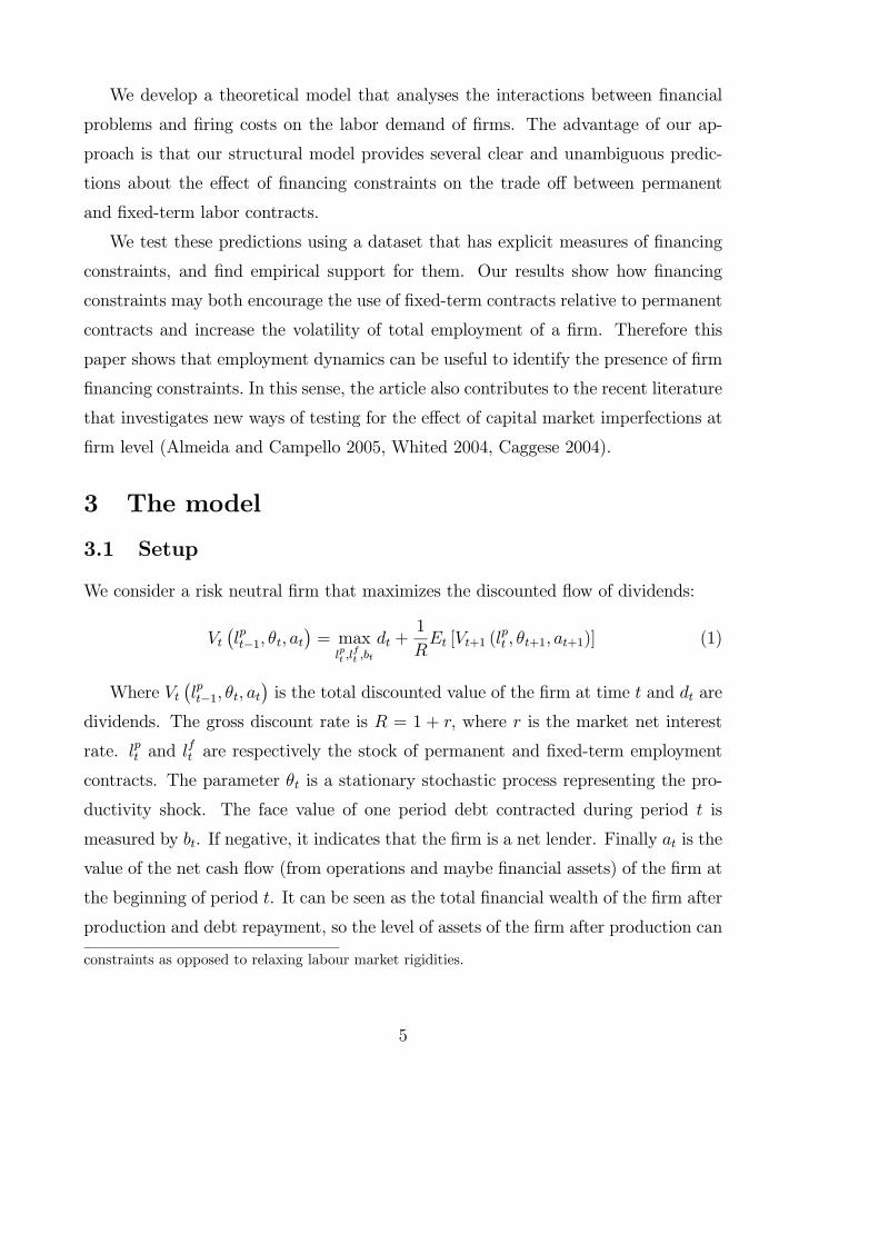
We develop a theoretical model that analyses the interactions between financial

problems and firing costs on the labor demand of firms. The advantage of our ap-

proach is that our structural model provides several clear and unambiguous predic-

tions about the effect of financing constraints on the trade off between permanent

and fixed-term labor contracts.

We test these predictions using a dataset that has explicit measures of financing

constraints, and find empirical support for them. Our results show how financing

constraints may both encourage the use of fixed-term contracts relative to permanent

contracts and increase the volatility of total employment of a firm. Therefore this

paper shows that employment dynamics can be useful to identify the presence of firm

financing constraints. In this sense, the article also contributes to the recent literature

that investigates new ways of testing for the effect of capital market imperfections at

firm level (Almeida and Campello 2005, Whited 2004, Caggese 2004).

3 The model

3.1 Setup

We consider a risk neutral firm that maximizes the discounted flow of dividends:

Vt¡lpt−1, θt, at

¢= max

lpt ,lft ,bt

dt +1

REt [Vt+1 (l

pt , θt+1, at+1)] (1)

Where Vt¡lpt−1, θt, at

¢is the total discounted value of the firm at time t and dt are

dividends. The gross discount rate is R = 1 + r, where r is the market net interest

rate. lpt and lft are respectively the stock of permanent and fixed-term employment

contracts. The parameter θt is a stationary stochastic process representing the pro-

ductivity shock. The face value of one period debt contracted during period t is

measured by bt. If negative, it indicates that the firm is a net lender. Finally at is the

value of the net cash flow (from operations and maybe financial assets) of the firm at

the beginning of period t. It can be seen as the total financial wealth of the firm after

production and debt repayment, so the level of assets of the firm after production can

constraints as opposed to relaxing labour market rigidities.

5

be expressed as:

at = θt−1³lpt−1 + ρlft−1

´α− bt−1 (2)

0 < ρ < 1; 0 < α < 1

The firm uses a concave technology in labor input. lft is the stock of fixed-term

labor contracts. For simplicity we assume that permanent and fixed-term contracts

are perfect substitutes and are paid the same wage. The difference is that permanent

workers are more skilled, but they can be fired only by paying a fixed cost F .6 Fixed

term workers can be fired without restrictions but are less productive (ρ is smaller

than 1). The timing of the model is the following: at the beginning of period t the firm

has a net financial wealth of at and a stock of permanent workers equal to (1− δ) lpt−1,

because permanent workers leave the firm at an exogenous separation rate δ. The firm

observes θt and decides about new borrowing, dividends payments and employment.

The employment decision is summarized in the gross hiring of fixed-term workers ift

and permanent workers ipt :

ipt = lpt − (1− δ) lpt−1 (3)

ift = lft (4)

The budget constraint is as follows:

dt + wlpt + wl

ft − FiptSt = at +

btR

(5)

With

F > 0; St =1 if ipt < 00 otherwise

(6)

6The assumption of identical wages for fixed and temporary workers is a normalization. Anycombination of productivities and wages that makes one efficiency unit of labour more expensivefrom fixed term workers would be equivalent.

6

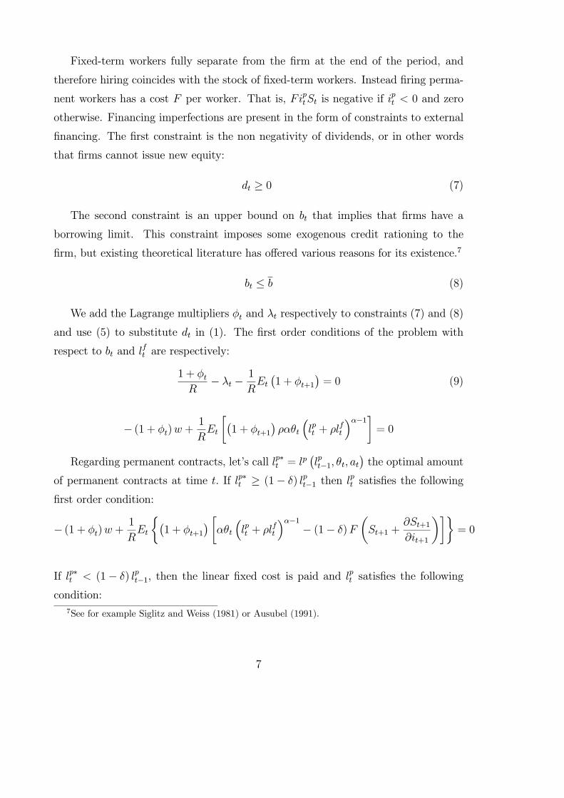
Fixed-term workers fully separate from the firm at the end of the period, and

therefore hiring coincides with the stock of fixed-term workers. Instead firing perma-

nent workers has a cost F per worker. That is, FiptSt is negative if ipt < 0 and zero

otherwise. Financing imperfections are present in the form of constraints to external

financing. The first constraint is the non negativity of dividends, or in other words

that firms cannot issue new equity:

dt ≥ 0 (7)

The second constraint is an upper bound on bt that implies that firms have a

borrowing limit. This constraint imposes some exogenous credit rationing to the

firm, but existing theoretical literature has offered various reasons for its existence.7

bt ≤ b (8)

We add the Lagrange multipliers φt and λt respectively to constraints (7) and (8)

and use (5) to substitute dt in (1). The first order conditions of the problem with

respect to bt and lft are respectively:

1 + φtR− λt − 1

REt¡1 + φt+1

¢= 0 (9)

− (1 + φt)w +1

REt

∙¡1 + φt+1

¢ραθt

³lpt + ρlft

´α−1¸= 0

Regarding permanent contracts, let’s call lp∗t = lp¡lpt−1, θt, at

¢the optimal amount

of permanent contracts at time t. If lp∗t ≥ (1− δ) lpt−1 then lpt satisfies the following

first order condition:

− (1 + φt)w +1

REt

½¡1 + φt+1

¢ ∙αθt

³lpt + ρlft

´α−1− (1− δ)F

µSt+1 +

∂St+1∂it+1

¶¸¾= 0

If lp∗t < (1− δ) lpt−1, then the linear fixed cost is paid and lpt satisfies the following

condition:

7See for example Siglitz and Weiss (1981) or Ausubel (1991).

7

− (1 + φt) [w − F ] +1

REt

½¡1 + φt+1

¢ ∙αθt

³lpt + ρlft

´α−1− (1− δ)F

µSt+1 +

∂St+1∂it+1

¶¸¾= 0

To analyze the influence of financing constraints on firms hiring behavior we an-

alyze separately the case where financing constraints are not binding nor expected

with respect to the case where financing constraints are expected and occasionally

binding. For the following analysis it is useful to solve equation (9) forward:

φt = R∞Xj=0

Et (λt+j) (10)

Where the shadow cost of one additional unit of external finance is equal to 1+φt.

Equation (10) shows that φt is equal to the sum of the current and future cost of a

binding financing constraint. As long as φt > 0, then the firm does not distributes

dividends, and dt = 0.

3.2 The case without financing constraints

Let’s assume that the net financial wealth of the firm at is very large, so that the

firm is never financially constrained (λt+j = 0 for all j ≥ 0). If the firm receives

a negative productivity shock, it will reduce the hiring of fixed-term contracts. If

the shock is small, it will not be necessary to fire also permanent workers. Then

ipt = lpt − (1− δ) lpt−1 ≥ 0 and lft satisfies the following condition:

αθth(1− δ) lpt−1 + ρlft

iα−1=Rw

ρ(11)

The firm decides instead to fire also permanent workers (ipt < 0) when the nega-

tive productivity shock is very large, so that lpt = (1− δ) lpt−1 is an inefficiently

high amount of labor input, and the efficiency loss caused by keeping employed the

marginal permanent worker is bigger than the firing cost F. In this case lft = 0 and

lpt is determined by the following condition:

αθt (lpt )

α−1 = Rw − F∙1− (1− δ)Et

µ∂St+1∂it

+ St+1

¶¸(12)

8

The term (1− δ)FEt³∂St+1∂it

+ St+1´represents future expected firing costs. Since

the productivity shock is stationary, it is very likely that such expected costs are

smaller than F, so that the term in square brackets in equation (12) is positive. This

together with the comparison between equations (11) and (12) implies that lft = 0

and lpt > 0 are the optimal labor choices.

If the productivity shock is positive and the firm is hiring then lft and lpt are jointly

determined by the two following two conditions:

αθt

hlpt−1 + ρlft

iα−1=Rw

ρ(13)

αθt

³lpt + ρlft

´α−1= Rw + (1− δ)FEt

µ∂St+1∂it+1

+ St+1

¶(14)

If the firm has no permanent workers, then there are no expected firing costs

and Et³∂St+1∂it+1

+ St+1´= 0. In this case the right hand side of equation (13) is larger

than the right hand side of equation (14). Therefore such firm will initially hire only

permanent workers. But the term (1− δ)FEth∂St+1∂it+1

+ St+1iincreases in lpt , and

if fixed costs F is large enough relative to ρ, it will be optimal to start hiring also

fixed-term contracts before reaching the optimal employment level in the firm. The

optimal mix lft /lpt will increase in F, in uncertainty (volatility of θt) and in ρ. Small

negative shocks will be completely absorbed by changes in fixed-term contracts, while

large shocks will be absorbed by both a fall in fixed-term and permanent contracts.

3.3 The financing constraints case:

We can now concentrate on the case of interest and solve for the optimal hiring and

firing decisions of the firm in the presence of financing constraints. It is useful to

describe the optimality conditions of the problem by distinguishing two cases:

Case 1: The financing constraint is not currently binding (λt = 0), but it may be

binding in the future with a positive probability (φt > 0). Conditional on a negative

shock the analysis does not differ from the previous case of no financing constraints.

Conditional on a positive shock lft and lpt are jointly determined by the two following

conditions:

9

αθt³lpt + ρlft

´α−1=Rw

ρ(15)

αθt³lpt + ρlft

´α−1= Rw + (1− δ)Et

∙¡1 + φt+1

¢F

µSt+1 +

∂St+1∂it+1

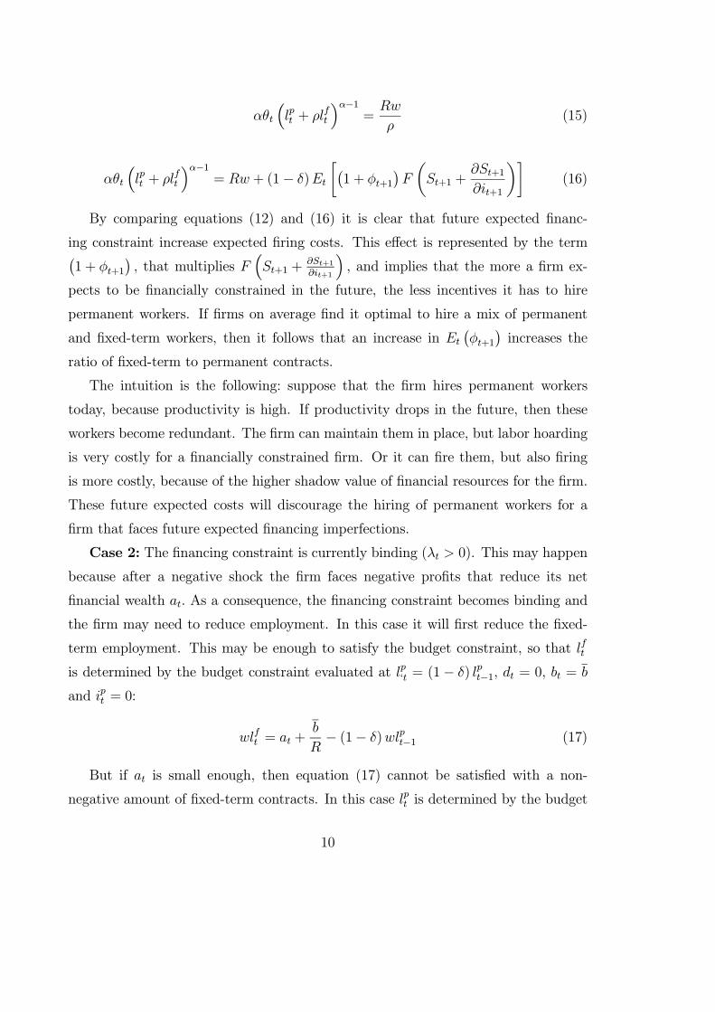
¶¸(16)

By comparing equations (12) and (16) it is clear that future expected financ-

ing constraint increase expected firing costs. This effect is represented by the term¡1 + φt+1

¢, that multiplies F

³St+1 +

∂St+1∂it+1

´, and implies that the more a firm ex-

pects to be financially constrained in the future, the less incentives it has to hire

permanent workers. If firms on average find it optimal to hire a mix of permanent

and fixed-term workers, then it follows that an increase in Et¡φt+1

¢increases the

ratio of fixed-term to permanent contracts.

The intuition is the following: suppose that the firm hires permanent workers

today, because productivity is high. If productivity drops in the future, then these

workers become redundant. The firm can maintain them in place, but labor hoarding

is very costly for a financially constrained firm. Or it can fire them, but also firing

is more costly, because of the higher shadow value of financial resources for the firm.

These future expected costs will discourage the hiring of permanent workers for a

firm that faces future expected financing imperfections.

Case 2: The financing constraint is currently binding (λt > 0). This may happen

because after a negative shock the firm faces negative profits that reduce its net

financial wealth at. As a consequence, the financing constraint becomes binding and

the firm may need to reduce employment. In this case it will first reduce the fixed-

term employment. This may be enough to satisfy the budget constraint, so that lft

is determined by the budget constraint evaluated at lp‘t = (1− δ) lpt−1, dt = 0, bt = b

and ipt = 0:

wlft = at +b

R− (1− δ)wlpt−1 (17)

But if at is small enough, then equation (17) cannot be satisfied with a non-

negative amount of fixed-term contracts. In this case lpt is determined by the budget

10

constraint evaluated at bt = b, lft = 0, dt = 0 and i

pt < 0:

wlpt = at +b

R+ FiptSt (18)

Equation (18) determined the most damaging case for the firm, in which it is forced

to pay the firing cost F when its financial resources are already scarce. Consider

instead the case in which the firm faces a positive shock and wants to hire workers,

but is constrained by the borrowing limit because at is low. In this case lft , l

pt and λt

are jointly determined by the following conditions:

w³lpt + l

ft

´= at +

b

R(19)

αθt³lpt + ρlft

´α−1=Rλt + 1 +Et

¡φt+1

¢1 +Et

¡φt+1

¢ Rw

ρ(20)

αθt³lpt + ρlft

´α−1=Rλt + 1 +Et

¡φt+1

¢1 +Et

¡φt+1

¢ Rw+(1− δ)Et

∙¡1 + φt+1

¢F

µSt+1 +

∂St+1∂it+1

¶¸(21)

Also in this case equations (20) and (21) determine the optimal ratio between

fixed-term and permanent workers. The presence of the shadow cost of financing

constraints λt increases the current component of the marginal cost of labor. But at

the same time, as long as the productivity shock is persistent but mean reverting,

when λt increases also Et¡φt+1

¢increases. The implication is that the financially

constrained firm that wants to hire new workers will be discouraged by future expected

financing constraints and firing costs to hire permanent workers.

3.4 Summary of the predictions of the model

The analysis in sections 2.1-2.4 shows that the interactions between firing costs and

financing constraints have several unambiguous predictions that can be tested us-

ing empirical data. With respect to a financially unconstrained firm, an otherwise

identical firm that faces financing imperfections:

11

prediction 1) has an higher ratio of fixed-term to permanent workers.

prediction 2) Has a higher sensitivity of the fixed-term/permanent employment

ratio to the productivity shocks.

prediction 3) Has a higher variance of total employment.

Predictions 1 and 2 follow directly from the discussion in sections 2.2 and 2.3.

The more a firm expects to be financially constrained in the future, the less it will be

willing to hire permanent workers, and it will prefer the higher flexibility of fixed-term

workers. This implies that the ratio of fixed-term workers with respect to permanent

workers will be increasing in the intensity of financing constraints.

prediction 3 follows from two distinct effects: i) after a negative shock a financially

constrained firms will on average fire an higher fraction of its labor force because it will

employ relatively more fixed-term workers with respect to a financially unconstrained

firms. ii) A financially constrained firm may be forced to fire permanent workers after

a negative shock, while a financially unconstrained firm is able to borrow more and

to keep the permanent workers, thus avoiding the firing costs associated with such

layoffs.

4 Empirical Analysis

This section is divided in four parts parts. Section 4.1 describes the data and variables

used; in Section 4.2 we show a statistical analysis of the differences between financially

constrained and unconstrained firms in terms of different employment ratios, the third

part that corresponds to Section 4.3 presents cross sectional regressions regarding

the influence of financing constraints on employment ratios and volatilities. Finally,

Section 4.4 shows a panel data analysis of the evolution of different employment ratios

whenever firms experience temporary liquidity shocks.

12

4.1 Data Description

In order to test the empirical predictions of the model we use the dataset of the

Mediocredito Centrale surveys.8 The dataset contains a representative sample of

Small and Medium Italian manufacturing firms in an incomplete panel with two

main sources of information:

i) yearly balance sheet data and profit and loss statements from 1989 to 2000.

ii) Qualitative information from four surveys conducted in 1992, 1995, 1998 and

2001.

Each survey is conducted on a sample representative of the population of small

and medium manufacturing firms (smaller than 500 employees). The samples are

selected balancing the criterion of randomness with the one of continuity. The firms

in each survey contain three consecutive years of data, after the third year 2/3 of the

sample is replaced and the new sample is then kept for three years.

Given that a new type of fixed-term contracts became regulated and started to

be widely used from 1995 onwards, we restrict our sample to the last 6 years of the

dataset. That leaves us with 11024 firm-year observations. The complete panel of

firms with six years of balance sheet data and qualitative information from both the

1998 and 2001 surveys contains 420 firms and a total of 2520 observations.

This dataset is particularly well suited to our analysis for several reasons: In the

first place the introduction of fixed-term contracts in Italy meant the coexistence

of two different contractual agreements that had very different firing costs. At the

same time, the database is a representative sample of manufacturing firms of different

industries and sizes, with detailed data about a number of aspects of the firm as well

as direct questions that try to elicit the existence of financing constraints affecting a

particular firm. The dataset contains balance sheet data, profit and loss statements,

and a detailed description of the structure of firm employment by type of contract

and skill level and qualitative questions that investigate a number of issues. Among

other qualitative questions, each firm is asked:

i) whether it had a loan application turned down recently.

8Examples of published papers that use the Mediocredito Centrale survey are Basile, Giunta andNugent (2003) and Piga (2002).

13

ii) Whether it did not ask for a loan for fear of their application being turned

down.

iii) Whether it desires more credit at the market interest rate.

iv) Whether it would be willing to pay an higher interest rate than the market

rate in order to obtain credit.

These questions where asked only in the 1998 and the 2001 surveys, which refer

respectively to the activity in period 1995-1997 and 1998-2000. We select firms into

likely financially constrained groups using questions iii) and iv). This choice is moti-

vated by the fact that very few firms responded positively to questions i) and ii), and

almost none did that without also answer positively to either question iii) or iv).

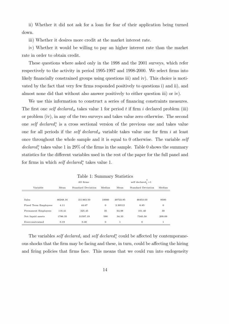
We use this information to construct a series of financing constraints measures.

The first one self declared it takes value 1 for period t if firm i declared problem (iii)

or problem (iv), in any of the two surveys and takes value zero otherwise. The second

one self declared∗i is a cross sectional version of the previous one and takes value

one for all periods if the self declared it variable takes value one for firm i at least

once throughout the whole sample and it is equal to 0 otherwise. The variable self

declared∗i takes value 1 in 29% of the firms in the sample. Table 0 shows the summary

statistics for the different variables used in the rest of the paper for the full panel and

for firms in which self declared∗i takes value 1.

Table 1: Summary StatisticsAll firms self declared

*i =1

Variable Mean Standard Deviation Median Mean Standard Deviation Median

Sales 46248.16 211463.50 10000 20722.85 46453.03 8500

Fixed Term Employees 4.11 44.67 0 2.30512 6.85 0

Permanent Employees 116.41 325.45 35 64.98 101.40 30

Net liquid assets 1786.35 31597.19 590 34.33 7345.50 209.09

Everconstrained 0.19 0.40 0 1 0 1

The variables self declared i and self declared∗i could be affected by contemporane-

ous shocks that the firm may be facing and these, in turn, could be affecting the hiring

and firing policies that firms face. This means that we could run into endogeneity

14

problems whenever we regress contemporaneous employment variables with respect to

the self declared it and self declared∗i variables. To avoid this potential endogeneity we

also run instrumental variable regressions in which the variables that measure financ-

ing constraints are predictions of the self declared ones using only lagged variables.

Among these variables self declaredpredit and self declared ∗ predit are dummy variables

that predict the original ones using discriminant analysis. The variable propensity is

a continuous prediction of self declared it using a linear probability model. To calculate

the Propensity variable we first run a regression of the Self Declaredit measure where

the independent variables are all lagged one period. The lagged variables used are

net liquid assets over total assets, investment over total assets and number of employ-

ees over total assets. We then compute the expected probability of each firm facing

financing constraints for all the relevant sample periods to construct the Propensity

variable which is a function of lagged variables only. This should solve the endogene-

ity problems associated with the co-determination of financing constraints and hiring

decisions by potential omitted variables.

Using self declared measures of financing constraints may also be subject to biases

if respondents tend to underestimate or overestimate their financing constraints. To

get additional reassurance that these biases are not driving our results we construct

a cross sectional measure of financing constraints that are revealed by the accounts

of the firm. To do so we first measure the net liquid assets of the firm, Then we

construct a dummy variable named liquid assets that takes value 0 if the firm has on

average throughout the whole sample more than 40% of its assets in cash or liquid

assets and zero otherwise. According to this measure we consider that a firm that has

liquid assets of more than 40% over total assets cannot be considered as constrained,.

this is probably a quite conservative measure of financing constraints, but it almost

guarantees that firms with such levels of liquid assets are unconstrained.

Given that firm size is a major determinant of financing constraints, with smaller

firms facing higher problems when it comes to getting additional funding, we also

include size in most of our regressions. Whenever size is included as a dependent

variable we use total assets and whenever it is used as a dummy variable or to split

the sample we classify firms as large/unconstrained if assets are larger than 5700

15

million lira9 (2.94 million euro). This is the threshold that splits the sample roughly

in two equal parts.

4.2 Statistical Analysis

In this section we construct cross sectional measures of the level and volatility of

fixed-term employment and permanent employment and we relate them to the cross

sectional measures of financing constraints and to size measures of the firms. Accord-

ing to the size criterion we name the larger firms in the sample as unconstrained.

Columns (1) and (2) contain the statistics for firms that are constrained or uncon-

strained respectively, according to the self declared* financing constraints variable.

Columns (3) and (4) perform the same analysis but splitting the sample according to

the level of liquid assets and finally columns (5) and (6) split the sample according

to firm size.

Table 2: Statistical Analysisself declared

*Liquid Assets Size

Variable Constrained Unconstrained Constrained Unconstrained Constrained Unconstrained

(1) (2) (3) (4) (5) (6)

(1) meanσftσp

0.22*

0.19*

0.20 0.21 0.22*

0.19*

(2) 75%σftσp

0.28**

0.19**

0.26*

0.22*

0.26**

0.19**

(3) meanµftµp

0.045**

0.038**

0.042 0.043 0.050**

0.036**

(4) 75%µftµp

0.056*

0.044*

0.051*

0.058*

0.066**

0.037**

σftσp

is the average ratio of the standard deviation of fixed term employment to the standard devi-

ation of permanent employment;µftµp

is the average ratio of the average fixed term employment to

the average permanent employment. * indicates that the difference in means (or medians) between

constrained and unconstrained firms is significant at a 95% confidence interval. ** Indicates that dif-

ference is significant at 99% confidence interval. 75% indicates the third quartile of the distribution.

Table 1 shows how the volatility of fixed-term employment with respect to the

volatility of permanent employment tends to be higher in constrained firms than in

95700 million lira correspond to $2.94m according to December 1999 exchange rates.

16

unconstrained firms for the self declared and the size measure, while the average ratio

is statistically not higher for financially constrained firms when using the liquidity

based measure of financing constraints. With respect to the average use of the two

different types of contracts, the evidence when we concentrate on the mean of the

ratio is again that self declared measures of financing constraints and size yield a

positive and significant effect of financing constraints on the relative use of fixed-term

contracts with respect to permanent contracts. While on the liquidity based measure

of financing constraints it seems that the more financially constrained firms use less

fixed-term contracts. The difference, being statistically significant is economically

rather small.

Overall, when firms are split according to the self declared* and Size criterion

of financing constraints, financially constrained firms tend to use more fixed-term

contracts and the relative volatility of these contracts is higher. The Liquid Assets

criterion leads to inconclusive results.

4.3 Employment Ratios and Financing Constraints

In this section we perform cross sectional regressions in which the dependent variables

are either the ratio of the standard deviations of fixed-term employment versus per-

manent employment, the ratio of fixed-term employment over permanent employment

and the standard deviation of employment.

In Table 2 we show the results of regressions on the full panel that contains 420

observations per year.

Controls include sector dummies (a 3 digit ATECO92 classification10), total as-

sets, [total assets squared-but this is not in the table] and the standard deviation of

firm sales. The dependent variables are the same ones as in the previous section.

The variables of interest are again the measures of financing constraints. The Self-

Declared* and Liquid Assets variables and a new variable, Propensity, that is the

result of predicting the self declared financing constraints using lagged variables only.

The role of introducing the Propensity is to avoid any potential endogeneity problems

10ATECO 92 ”Classificazione delle attivita economiche” is a standard four digit industrial classi-fication.

17

that could arise from the simultaneous determination of financing constraints and em-

ployment ratios. Given that the Propensity is totally predetermined by variables that

are lagged one period, this endogeneity problem is reduced.

Table 3: Regresions, Complete Panel(1) (2) (3) (4) (5) (6) (7) (8) (9)

sdratio sdratio sdratio meanratio meanratio meanratio sdoccupa sdoccupa sdoccupa

Self-Declared 0.0627 0.0104 1.1801

[2.65]*** [1.38] [2.29]**

Liquid Assets 0.0928 0.0068 -0.5656

[3.42]*** [0.78] [0.95]

Propensity 0.578 .0829 14.708

[2.08]** [0.97] [1.76]*

totalassets 1.573E-07 -1.422E-07 -1.11e-07 -6.277E-08 -9.209E-08 -4.92e-08 3.720E-04 3.726E-04 0.001

[0.35] [0.32] [0.19] [0.42] [0.62] [0.26] [33.28]*** [32.99]*** [30.09]***

sdfattur -1.528E-06 -1.505E-06 -1.28e-06 -1.734E-07 -1.708E-07 -1.79E-07 -2.384E-05 -2.386E-05 -6.59E-05

[2.56]** [2.53]** [1.67]* [0.90] [0.89] [0.76] [1.53] [1.52] [2.44]**

Observations 1928 1928 1290 1963 1963 1307 1962 1962 1298

R-squared 0.05 0.05 0.06 0.05 0.05 0.06 0.42 0.41 0.52

Absolute value of t statistics in brackets

* significant at 10%; ** significant at 5%; *** significant at 1%

The results in table 3 show that once controlling for other factors, firms that de-

clare financing constraints have a significantly higher relative volatility of fixed term

employment (column 1). It also shows that the standard deviation of total employ-

ment is higher among constrained firms (column 7). These results are consistent

with the model prediction of fixed-term contracts being more volatile in financially

constrained firms than in unconstrained firms after controlling for observables. The

results regarding liquid assets as a measure of financing constraints are statistically

significant for the ratio of standard deviations and take the right sign (column 2).

However, the results are insignificant with respect to the other two variables. With

respect to the propensity measure, the results show a higher volatility of fixed-term

contracts versus permanent contracts among constrained firms (column 3) and a

higher volatility of total employment (column 9).

The coefficients associated with the size of firms are only significant with respect

18

to the standard deviation of total employment, showing that larger firms have larger

volatility of total employment when measured as standard deviation.

The next table shows the same set of regressions on the full sample of firms that

constitutes an incomplete panel.

Table 4: Regresions, Full Sample(1) (2) (3) (4) (5) (6) (7) (8) (9)

sdratio sdratio sdratio meanratio meanratio meanratio sdoccupa sdoccupa sdoccupa

Self Declared*

0.0250 0.0035 0.6804

[2.68]*** [1.79]* [4.74]***

Liquid Assets 0.0053 -0.0019 2.0144

[0.52] [0.95] [14.26]***

Propensity 0.201 0.0138 30.957

[1.96]* [0.59] [10.17]***

totalassets -4.957E-08 -5.289E-08 -7.535E-08 -2.507E-08 -2.527E-08 -1.34e-08 3.931E-05 3.854E-05 5.092E-05

[1.56] [1.67]* [1.92]* [3.56]*** [3.59]*** [1.57] [37.06]*** [36.44]*** [16.01]***

sdfattur 4.047E-07 3.919E-07 3.640E-07 1.678E-07 1.683E-07 5.97e-08 8.208E-05 7.945E-05 1.913E-04

[2.19]** [2.12]** [2.26]** [5.89]*** [5.90]*** [.088] [18.39]*** [17.84]*** [17.75]***

Observations 12438 12438 6152 16700 16700 7655 25351 25350 8949

R-squared 0.01 0.01 0.02 0.06 0.06 0.05 0.16 0.16 0.24

Absolute value of t statistics in brackets

* significant at 10%; ** significant at 5%; *** significant at 1%

The results with respect to the total sample show again that the self reported*

measure of financing constraints has a positive and significant effect on the ratio of

the standard deviations of the two types of employment. Relative to permanent em-

ployment, fixed-term employment is more volatile in constrained firms than in uncon-

strained ones. Furthermore columns 4 and 7 show that constrained firms use a higher

proportion of fixed-term contracts and have a higher volatility of total employment.

When we concentrate on the liquid assets measure of financing constraints, we also

see that the volatility of total employment is higher among constrained firms. The

results relative to this measure are inconclusive with respect to the ratio of volatilities

or the relative use of each type of contract.

Finally the propensity measure yields again significant results in this second set

19

of regressions with the complete panel, showing that constrained firms have a higher

volatility of fixed-term contracts versus permanent contracts (column 3) and a larger

overall volatility of employment (column 9).

The coefficients of the size variable show that, conditional on the financing con-

straints variables, larger firms use a lower proportion of fixed-term contracts and have

a larger variance of total employment. They also show that the standard deviations

of fixed-term versus permanent contracts is lower among larger firms, although the

result is only statistically significant when used in conjunction with the liquid assets

measure of financing constraints. Size itself can be seen as one of the major factors of

financing constraints, so these results are also consistent with some of the predictions

of the model.

In the next table we split the analysis of the volatility of employment by analyzing

separately the volatility of fixed-term employment and permanent employment. This

is an interesting dimension because our model predicts that employment should be

more volatile in constrained than unconstrained firms once controlling for other fac-

tors, and that a large fraction of this additional volatility should be borne by flexible

workers.

20

Table 5: Differential Impact on Standard Deviations(1) (2) (3) (4) (5) (6)

sdftterm sdpermanent sdftterm sdpermanent sdftterm sdpermanent

Self Declared*

0.2900 0.7527

[6.12]*** [4.07]***

Liquid Assets 0.3163 1.7989

[6.38]*** [9.29]***

propensity 3.59 26.97

[5.12]*** [9.06]***

totalassets 7.348E-07 4.107E-05 6.570E-07 4.006E-05 -3.458E-07 3.552E-05

[3.81]*** [31.98]*** [3.40]*** [31.21]*** [1.26] [16.04]***

sdfattur 1.815E-05 6.988E-05 1.774E-05 6.862E-05 1.438E-05 6.374E-05

[16.28]*** [14.25]*** [15.89]*** [14.01]*** [12.59]*** [9.62]***

Relative effect

of constraintsβσ

0.42 0.15 0.45 0.36 5.20 5.52

Observations 16207 16240 16207 16240 7511 7509

R-squared 0.05 0.17 0.06 0.17 0.06 0.18

Absolute value of t statistics in brackets

All regressions include 2digit sector dummies

* significant at 10%; ** significant at 5%; *** significant at 1%

The results show how the effect of financing constraints on the volatility of em-

ployment is consistent throughout both types of employment. Constrained firms tend

to adjust employment more often as seen in the previous section and this higher

volatility can be observed both in fixed-term and permanent employment. However,

in proportional terms, the effect is larger among fixed-term workers than among per-

manent workers. Even though the effect is more important in absolute terms for

the permanent workers, this is a normal outcome when we take into account that

the amount of permanent workers is much larger than the total amount of fixed-term

workers. Once we take into account that the average standard deviation of fixed-term

employment and permanent employment is 0.69 and 4.88 respectively the relative size

of the estimated coefficients is much larger for fixed-term contracts than permanent

21

ones.11 For convenience, the relative effect of financing constraints is calculated in

the row entitled βσ, where we show the relative increase in volatility of a financially

constrained firm with respect to a financially unconstrained one according to each of

the criteria used to determine financing constraints. For example the coefficients in

columns 1 and 2 show that fixed-term employment in constrained firms is 42% more

volatile than in unconstrained firms, while permanent employment is only 15% more

volatile. The results in columns 3 and 4 show that in constrained firms fixed-term

employment is 45% more volatile and permanent employment is 36% more volatile.

This results are consistent with the prediction of the model where in constrained

firms a larger share of the employment adjustment is born by fixed-term contracts.

The results with respect to the Propensity measure are large as shown in Tables 2

and 3, but do not seem to show a differential impact on fixed-term versus permanent

contracts. In relative terms, an increase in 10% of the propensity to be constrained

makes fixed-term contracts 52% more volatile and permanent contracts 55% more

volatile.

Overall, the results throughout this section show how constrained firms use a

larger proportion of fixed-term contracts over total employment. Constrained firms

have a larger volatility of total employment and among them, the proportion of this

volatility that is absorbed by fixed-term contracts is larger.

4.4 Response of employment to productivity shocks

So far we have used either purely cross sectional analysis or pure time series analysis.

In this section we exploit the panel dimension of the dataset to test prediction 2 of the

model: ceteris paribus, a positive productivity shock increases fixed-term contracts

relative to permanent contracts, more so for a firm that faces capital markets im-

perfections than for one that does not. The prediction is more ambiguous regarding

a negative shock. In this case both financially constrained and unconstrained firms

will fire fixed-term workers. Regarding permanent workers, on the one hand a firm

that has a financing constraint currently binding may be forced to fire them. On the

11Standard deviations calculated after dropping the same outliers as in the regression.

22

other hand a firm that is currently unconstrained but may become constrained in the

future may prefer labor hoarding to the payment of the firing costs.

In order to test this prediction, we run the following regressions:

regression 1:lfi,tltoti,t

= ai + dt + βtfti,t + εi,t (22)

regression 2:lfi,tltoti,t

= ai + dt + βpostftposi,t + βnegtftnegi,t + εi,t (23)

Where the variable ltoti,t is the total employment the end of period t and the variable

lfi,tcorresponds to the amount of fixed-term contracts at the end of period t. Therefore

the dependent variable in equations (22) and (23) is the ratio of fixed-term to total

employment in period t. As independent variable we use tfti,t, which measures the

productivity shock during period t. The other two variables are tftposi,t and tftnegi,t

where tftposi,t equals tfti,t whenever tfti,t is positive and takes value zero otherwise.

While tftnegi,t equals tfti,t whenever tfti,t is negative and takes value zero otherwise.

Finally we also include firm specific fixed effects ai and time dummies dt.

We use the ratio between fixed-term contracts and total employment, that is

bounded between 0 and 1, rather than the ratio between fixed-term and permanent

contracts to get additional stability in the regression. The productivity shock variable

is computed as a Solow residual. We first estimate the coefficients of a production

function that includes fixed capital, variable capital and labour among the input

factors. We use the estimated elasticities to compute the Solow residual. tfti,t is the

component of the Solow residual that is not determined by firm, year and sector fixed

effects. In order to control for the endogeneity of tfti,t, we estimate equations (22)

and (23) using the System GMM estimation method proposed by Blundell and Bond

(1998). In both cases we restrict the analysis to a subset of firms of the balanced

sample with a sufficiently long time series of accounting data to allow the estimation

of the productivity shock. We expect the coefficient β to be positive for firms that

face financing imperfections and zero or negative for the other firms. If β is found to

be greater than zero, then this positive correlation should be stronger conditional on a

positive productivity shock than on a negative productivity shock. In order to verify

23

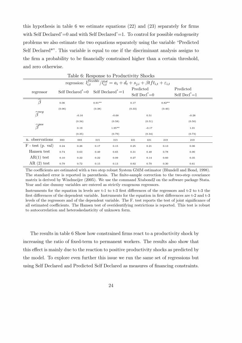
this hypothesis in table 6 we estimate equations (22) and (23) separately for firms

with Self Declared*=0 and with Self Declared*=1. To control for possible endogeneity

problems we also estimate the two equations separately using the variable “Predicted

Self Declared*”. This variable is equal to one if the discriminant analysis assigns to

the firm a probability to be financially constrained higher than a certain threshold,

and zero otherwise.

Table 6: Response to Productivity Shocks

regression: lflexiblei,t /ltoti,t = ai + dt + sj,i + βtfti,t + εi,t

regressor Self Declared*=0 Self Declared*=1Predicted

Self Decl*=0

Predicted

Self Decl*=1bβ 0.06 0.91** 0.17 0.82**

(0.06) (0.38) (0.33) (0.40)bβneg -0.16 -0.68 0.51 -0.28

(0.34) (0.58) (0.51) (0.50)bβpos 0.19 1.95** -0.17 1.01

(0.35) (0.79) (0.34) (0.73)

n. observations 693 693 315 315 431 431 219 219

F - test (p. val) 0.24 0.26 0.17 0.15 0.25 0.21 0.13 0.06

Hansen test 0.74 0.63 0.49 0.65 0.31 0.48 0.78 0.90

AR(1) test 0.10 0.22 0.22 0.09 0.27 0.14 0.60 0.35

AR (2) test 0.79 0.72 0.15 0.13 0.92 0.70 0.30 0.61

The coefficients are estimated with a two step robust System GMM estimator (Blundell and Bond, 1998).The standard error is reported in parenthesis. The finite-sample correction to the two-step covariancematrix is derived by Windmeijer (2005). We use the command Xtabond2 on the software package Stata.Year and size dummy variables are entered as strictly exogenous regressors.

Instruments for the equation in levels are t-1 to t-3 first differences of the regressors and t-2 to t-3 thefirst differences of the dependent variable. Instruments for the equation in first differences are t-2 and t-3levels of the regressors and of the dependent variable. The F. test reports the test of joint significance ofall estimated coefficients. The Hansen test of overidentifying restrictions is reported. This test is robustto autocorrelation and heteroskedasticity of unknown form.

The results in table 6 Show how constrained firms react to a productivity shock by

increasing the ratio of fixed-term to permanent workers. The results also show that

this effect is mainly due to the reaction to positive productivity shocks as predicted by

the model. To explore even further this issue we run the same set of regressions but

using Self Declared and Predicted Self Declared as measures of financing constraints.

24

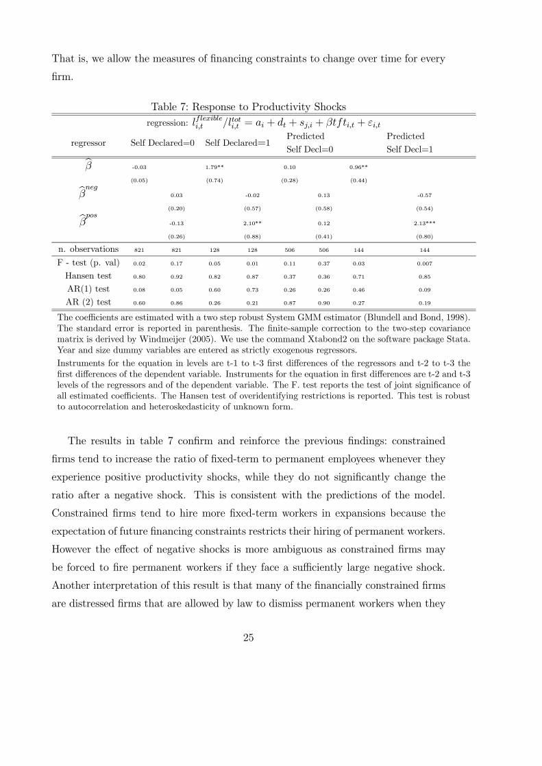
That is, we allow the measures of financing constraints to change over time for every

firm.

Table 7: Response to Productivity Shocks

regression: lflexiblei,t /ltoti,t = ai + dt + sj,i + βtfti,t + εi,t

regressor Self Declared=0 Self Declared=1Predicted

Self Decl=0

Predicted

Self Decl=1bβ -0.03 1.79** 0.10 0.96**

(0.05) (0.74) (0.28) (0.44)bβneg 0.03 -0.02 0.13 -0.57

(0.20) (0.57) (0.58) (0.54)bβpos -0.13 2.10** 0.12 2.13***

(0.26) (0.88) (0.41) (0.80)

n. observations 821 821 128 128 506 506 144 144

F - test (p. val) 0.02 0.17 0.05 0.01 0.11 0.37 0.03 0.007

Hansen test 0.80 0.92 0.82 0.87 0.37 0.36 0.71 0.85

AR(1) test 0.08 0.05 0.60 0.73 0.26 0.26 0.46 0.09

AR (2) test 0.60 0.86 0.26 0.21 0.87 0.90 0.27 0.19

The coefficients are estimated with a two step robust System GMM estimator (Blundell and Bond, 1998).The standard error is reported in parenthesis. The finite-sample correction to the two-step covariancematrix is derived by Windmeijer (2005). We use the command Xtabond2 on the software package Stata.Year and size dummy variables are entered as strictly exogenous regressors.

Instruments for the equation in levels are t-1 to t-3 first differences of the regressors and t-2 to t-3 thefirst differences of the dependent variable. Instruments for the equation in first differences are t-2 and t-3levels of the regressors and of the dependent variable. The F. test reports the test of joint significance ofall estimated coefficients. The Hansen test of overidentifying restrictions is reported. This test is robustto autocorrelation and heteroskedasticity of unknown form.

The results in table 7 confirm and reinforce the previous findings: constrained

firms tend to increase the ratio of fixed-term to permanent employees whenever they

experience positive productivity shocks, while they do not significantly change the

ratio after a negative shock. This is consistent with the predictions of the model.

Constrained firms tend to hire more fixed-term workers in expansions because the

expectation of future financing constraints restricts their hiring of permanent workers.

However the effect of negative shocks is more ambiguous as constrained firms may

be forced to fire permanent workers if they face a sufficiently large negative shock.

Another interpretation of this result is that many of the financially constrained firms

are distressed firms that are allowed by law to dismiss permanent workers when they

25

are hit by a negative productivity shock.

5 Conclusions

We propose a model to study the firing and hiring decisions of firms in the presence of

financing constraints and dual labour markets in which both fixed-term contracts and

permanent contracts coexist. The model shows that financial market imperfections

increase expected firing costs, thus making permanent contracts implicitly more ex-

pensive. In the presence of financing constraints, a larger share of output fluctuations

is absorbed by fixed-term contracts, that also represent a larger proportion of total

employment.

We also find support for the empirical implications of the model. In particular

financially constrained firms have a larger proportion of fixed-term contracts, these

contracts absorb a larger share of employment fluctuations and react to productivity

shocks as predicted by the model. Financing constraints are measured using both self

declared measures and measures extracted from firm accounts. We also construct a

predicted financing constraints measure using lagged variables as a way to avoid pos-

sible endogeneity problems between contemporaneous constraints and productivity

shocks.

Our results shed some light on the role of fixed-term contracts in absorbing pro-

ductivity shocks in the presence of financing constraints. The firing costs associated to

permanent contracts make them less likely to absorb employment fluctuations due to

productivity shocks. We show that the presence of financing constraints emphasizes

this effect by making fixed-term contracts more volatile. Permanent contracts and

total employment are also more volatile in the presence of financing constraints, how-

ever, in relative terms, fixed-term contracts become more unstable than permanent

ones when firms face financing constraints.

The article is also an interesting step forward in understanding how do financing

constraints work. Previous literature has concentrated on the effect of financing

constraints on fixed and working capital investment; we offer a new dimension in

which financing constraints may operate. Our results help to understand the effects

26

of financing constraints on investment in general and can be used to validate some

measures of financing constraints.

The policy implications of our results are interesting. Policies that relax financing

constraints that firms face will have a positive impact on the stability of total em-

ployment and in particular on fixed-term contracts. Furthermore, the model shows

how higher rigidities in permanent employment should lead to a larger volatility of

fixed-term contracts and vice-versa.

27

References

[1] Almeida, H. and M. Campiello, 2005, “Financial Constraints, Asset Tangibility

and Corporate Investment”, Mimeo, New York University.

[2] Alonso-Borrego, C., Fernandez-Villaverde, J. and Galdon-Sanchez, J. E.

(2004),“Evaluating Labor Market Reforms: A General Equilibrium Approach,”

IZA Working Paper N. 1129.

[3] Andrew Benito e Ignacio Hernando (2003) “Labour demand, flexible contracts

and financial factors: new evidence from Spain”. Banco de Espana working paper

0312

[4] Ausubel, Lawrence M. (1991) “The Failure of Competition in the Credit Card

Market,” American Economic Review, Vol. 81, No. 1, pp. 50-81, March.

[5] Basile, R., Giunta, A. and J.B. Nugent, 2003, “Foreign Expansion by Italian

Manufacturing Firms in the Nineties: An Ordered Probit Analysis,” Review of

Industrial Organization, 2003, 23, 1-24

[6] Bentolila,Samuel; Giles Saint Paul (1992) “The Macroeconomic Impact of Flexi-

ble Labor Contracts, with an Application to Spain,” European Economic Review

36.

[7] Bentolila,Samuel and Giuseppe Bertola (1990) “Firing Costs and Labor Demand:

How Bad is Eurosclerosis?” Review of Economic Studies 54.

[8] Blanchard Olivier and Augustin Landier (2002) “The Perverse Effects of Par-

tial Labour Market Reform: Fixed-Term Contracts in France,” The Economic

Journal, 112 (June)

[9] Caggese A., 2004, Testing Financing Constraints on Firm Invest-

ment Using Variable Capital, Pompeu Fabra University working paper,

http://www.econ.upf.es/˜caggese/personal/emppapus2 20122004.pdf

28

[10] Dolado, Juan J.; Carlos Garcıa-Serrano and Juan F. Jimeno (2002) “Drawing

Lessons from the Boom of Temporary Jobs in Spain,” The Economic Journal,

112 (June)

[11] Hopehayn and Rogerson (1993) “Job Turnover and Policy Evaluation: A General

Equilibrium Analysis,” Journal of Political Economy, 101, 5, 915-938

[12] Hubbard, G.R., 1998, “Capital-Market Imperfections and Investment,” Journal

of Economic Literature 36, 193-225.

[13] Kugler, Adriana and Giovanni Pica, “Effects of Employment Protection and

Product Market Regulations on the Italian Labor Market,” forthcoming in J.

Messina, C. Michelacci, J. Turunen, and G. Zoega, eds., “Labour Market Ad-

justments in Europe,” Edward Elgar.

[14] Nickell, Stephen; Nicolitsas, D. (1999) “How Does Financial Pressure Affect

Firms?’ European Economic Review 43, no. 8 (1999), p. 1435

[15] Piga, G., 2002, “Debt and Firms’ Relationships: The Italian Evidence,,” Review

of Industrial Organization, 20, 267-82.

[16] Rendon, Silvio (2005) “Job Creation and Investment in Imperfect Capital and

Labor Markets” Mimeo ITAM

[17] Saint-Paul, G. (1996), “Dual labor markets, a macroeconomic perspective,”

Cambridge,MA: MIT Press.

[18] Smolny, W.; Winker, P.(1999) “Employment Adjustment and Financing Con-

straints,” Dept. of Economics, University of Mannheim, Discussion Paper, Nr.

573-99, 1999

[19] Stiglitz, Joseph E.; Andrew Weiss,(1981) “Credit Rationing in Markets with

Imperfect Information,” American Economic Review, June 1981, v. 71, iss. 3,

pp. 393-410

29

[20] Whited, T., 2004, “External Finance Constraints and the Intertemporal Pattern

of Intermittent Investment,” Mimeo, University of Wisconsin.

30