Capitulo 3 Reservorios de Gas

PART3

GAS RESERVES

3.1 VOLUMETRIC METHODS 3.2

3.2 VOLUMETRIC RESERVOIRS 3.3

3.3 MATERIAL BALANCE METHOD 3.13

3.4 GAS CONDENSA TE RESERVOIRS 3.41

3.5 NUMERICAL APPLICA TI ONS 3.53

APPENDIX A- Figures and Tables 3A-1

3.1

GAS RESERVES AND MATERIAL-BALANCE CALCULATIONS

3.1 VOLUMETRIC METHODS

Volumetric methods consider the reservoir PV occupied by hydrocarbons at initial

conditions and at later conditions after sorne fluid production and associated pressure

reduction. The later conditions often are defmed as the reservoir pressure at which pro­

duction is no longer economical. Volumetric methods are used early in the life of a

reservoir before significant development and production. These methods, however, can

also be applied later in a reservoir's life and often are used to confrrm estimates from

material-balance calculations. The accuracy of volumetric estimates depends on the

availability of sufficient data to characterize the reservoir's areal extent and variations in

net thickness and, ultimately, to determine the gas-bearing reservoir PV. Obviously, early

in the productive life of a reservoir when few data are available to establish subsurface

geologic control, volumetric estimates are least accurate. As more wells are drilled and

more data become available, the accuracy ofthese estimates improves.

Data used to estimate the gas-bearing reservoir PV include, but are not limited to, well

logs, core analyses, bottomhole pressure (BHP) and fluid sample information, and well

tests. These data typically are used to develop various subsurface maps. Of these maps,

structural and stratigraphic cross-sectional maps help to establish the reservoir's areal

extent and to identify reservoir discontinuities, such as pinchouts, faults, or gas/water

contacts. Subsurface contour maps, usually drawn relative to a known or marker

formation, are constructed with lines connecting points of equal elevation and therefore

portray the geologic structure. Subsurface isopachous maps are constructed with lines of

equal net gas-bearing formation thickness. With these maps, the reservoir PV can then be

estimated by planimetering the areas between the isopachous lines and using an

approximate volume calculation technique, such as the pyramidal or trapezoidal methods.

3-2

After the gas-bearing reservoir PV has been estimated, we can calculate the original gas

in place and, for sorne abandonment conditions, estímate the gas reserves. The fonn of

the volumetric equations varies according to the drive rnechanism and type of gas. In the

following sections, we present equations for dty-gas reservoirs, dty-gas reservoirs with

water influx, and wet-gas reservoirs.

3.2 VOLUMETRIC RESERVOIRS.

3 .2.1 Volumetric Dry-Gas Reservoirs.

As the name implies, a volumetric reservoir is cornpletely enclosed by low-penneability

or cornpletely impermeable barriers and does not receive pressure support frorn extemal .

sources, such as an encroaching aquifer. In addition, if the expansion of rock and the

connate water are negligible, then the primal)' source of pressure maintenance is gas

expansion resulting from gas production and the subsequent pressure reduction.

When we use "diy gas," we are referring to a reservoir gas rnade up primarily of rnethane

with sorne intennediate-weight hydrocarbon molecules. The dty-gas-phase diagram in

Fig. 3.1 indicates that, because of this composition, diy gases do not undergo phase

changes following a pressure reduction and therefore are solely gases in the reservoir and

at the surface separator conditions. In this sense, "dty" does not refer to the absence of

water but indicates that no liquid hydrocarbons fonn in the reservoir, wellbore, or surface

equiprnent during production.

Beginning with the real-gas law, the gas volwne at initial reservoir conditions is

V.= z¡nRT g¡ Pi

(3.1)

Similarly. the gas volume at standard conditions is

3-3

V = G = ZscnRTsc se

Psc (3.2)

Equating the number of moles of gas at initial reservoir conditions to the number at

standard conditions and rearranging, we can solve for the initial volume of gas at standard

conditions:

G = p¡Vgi Zsc Tsc

Z¡T Psc

.

(3.3)

Assuming that the PV occupied by the gas is constant during the producing life of the

reservoir gives

Substituting Eq. 3.4 into Eq. 3.3 yields

Ifwe express the reservoir PV in barreis, Eq. 3.5 becomes

G = 7, 758Ahcj>(l- Sw;)

Bgi

where

3-4

(3.4)

(3.5)

(3.6)

B . = 1,000 · Psczi T _ 5.02z¡ T g¡ 5.615·p¡ZscTsc Pi

(3.7)

Eq. 3.7, which assumes standard conditions of Psc = 14.65 psia, Tsc = 60°F = 520°R, and

Zsc = 1.0, also was derived in Chap. l.

W e can estimate the gas reserve or the total cumulative gas production, GP, over the life

of the reservoir as the difference between original gas in place, G, and gas in place at

sorne abandonment conditions, Ga:

(3.8)

In terms ofEq. 3.6, the gas reserve is

G = 7, 7 5 8Ahcp( 1- Sw¡) __ 7 ,_7 5_8_Ah_cp__;(,__l-_S_w~i) P Bgi Bga

(3.9)

_ 7,758Ahcp(1-Sw¡)( BgiJ or G - 1--P Bgi Bga

(3.10)

where the gas recovery factor F = (1- Bgi J Bga

Simple gas expansion is a very efficient drive mechanism. Even though gas saturations at

abandonment can be quite high, ultimate recoveries of 80% to 90% of the original gas in

place are routinely achieved in volumetric gas reservoirs. The percentage of the original

volume of gas in place that can be recovered depends on the abandonment pressure,

which usually is determined by economical rather than technical considerations. Note that

we developed Eq. 3.10 with the assumption that the initial connate water saturation does

3-5

not change. This assumption is valid in volumetric gas reservoirs where the initial connate

water saturation is immobile. (See Example 3 .1)

3.1.2 Dry-Gas Reservoirs With Water Influx.

Many gas reservoirs are not completely closed but are subjected to sorne natural water

influx from an aquifer. Water encroachment occurs when the pressure at the

reservoir/aquifer boundary is reduced following gas production from the reservoir. Recall

that we derived the equation for a volumetric reservoir with the assumption that the

reservoir PV occupied by gas remained constant over the reservoir's productive life.

However, in gas reservoirs with water influx, this PV decreases by an amount equal to the

net volume of water entering the reservoir and remaining unproduced. Therefore, if we

can estímate both the initial gas saturation and the residual gas saturation at abandonment

(i.e., the endpoint saturations ), we can use volumetric equations to calcula te the gas

reserves in a gas reservoir with water influx.

Under these conditions, we consider the initial gas volume and the remaining gas volume

plus the volume of water that has entered the reservoir. Beginning with Eq. 3.8, the

equation for the cumulative gas production in terms of the initial and final water

_ 7,758Ah<j>(1- Swi} 7,758Ah<j>(1- Swa) G- ----~-....:..:.:::~

P Bgi Bga (3.11)

In terms ofthe residual gas saturation, Sgr, at abandonment, Eq. 3.11 becomes

G p

= 7, 758Ah<!>( 1- S wJ B.

gi

7,758Ah<!>( S gr) B

ga

3-6

(3.12)

(3.13)

( B ·S J Here, the recovery factor, F = 1- t- gr . )

Bga 1 Swi

Eqs. 3.11 through 3.13 were derived with the implicit assumption that the volumetric

sweep efficiency for gas is 100%. In fact water may displace gas inefficiently in sorne

cases. Results from early coreflood studies suggest that significant gas volumes can be

bypassed and eventually trapped by an advancing water front. In addition, because of

reservoir heterogeneities (i.e., natural fractures and layering) and discontinuities (i.e.,

sealing faults and low permeability shale stringers ), the encroaching water does not sweep

sorne portions of the reservo ir effectively, resulting in high residual gas saturations in

these unswept areas and higher abandonment pressures than for volumetric dry-gas

reservoirs. To account for the unswept portions of the reservoir, we introduce a

volumetric sweep efficiency, Ev, into the volumetric equation. With Ev, Eq. 3.8 can be

rewritten as

(3.14)

Eq. 3 .14 can be rewritten in a form similar to Eq. 3 .1 O,

(3.15)

3-7

Eq. 3.15 can be rearranged to yield

(3.16)

Here

Because gas often is bypassed and trapped by the encroaching water, recovery factors for

gas reservoirs with water drive can be significantly lower than for volumetric reservoirs

produced by simple gas expansion. In addition, the presence of reservoir heterogeneities,

such as low-permeability stringers or layering, may reduce gas recovery further. As noted

previously, ultimate recoveries of 80% to 90% are common in volumetric gas reservoirs,

while typical recovery factors in water drive gas reservoirs can range from 50% to 70%.

Eq. 3.16 requires estimates of Sg'"' and Ev. Coreflood studies of representative reservoir

samples are the best method for dete!mining residual gas saturations. In the absence of

laboratory studies Agarwal6 proposed the following correlations for estimating the gas

saturation in gas reservoirs with water influx. These correlations, based on multiple

regression analyses of 320 experimental measurements of imbibition residual gas

saturations, are presented in terms of porosity, absolute permeability, initial gas

saturation, and lithology for consolidated sandstones, limestones, and unconsolidated

sandstones.

For consolidated sandstones,

3-8

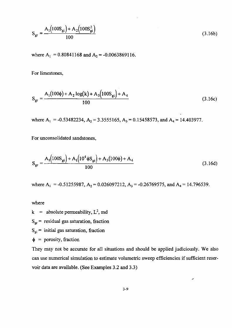
S = A1(100Sg¡)+ A2(100S~¡) ~ 100

(3.16b)

where A1 = 0.80841168 and A2 = -0.0063869116.

F or limestones,

S = A1(100<P)+A2 log(k)+A3(100Sg¡)+A4

~ 100 (3.16c)

where A1 = -0.53482234, A2 = 3.3555165, A3 = 0.15458573, and A4 = 14.403977.

F or unconsolidated sandstones,

S = At(100Sgi) + A1(1o\¡,sgi) + A3(100<P) + A4

~ 100 (3.16d)

where A1 = -0.51255987, A2 = 0.026097212, A3 = -0.26769575, and A4 = 14.796539.

where

k = absolute permeability, L2, md

Sgr = residual gas saturation, :fraction

Sgi = initial gas saturation, fraction

<P = porosity, fraction

They may not be accurate for all situations and should be applied judiciously. We also

can use numerical simulation to estimate volumetric sweep efficiencies if sufficient reser­

voir data are available. (See Examples 3.2 and 3.3)

3-9

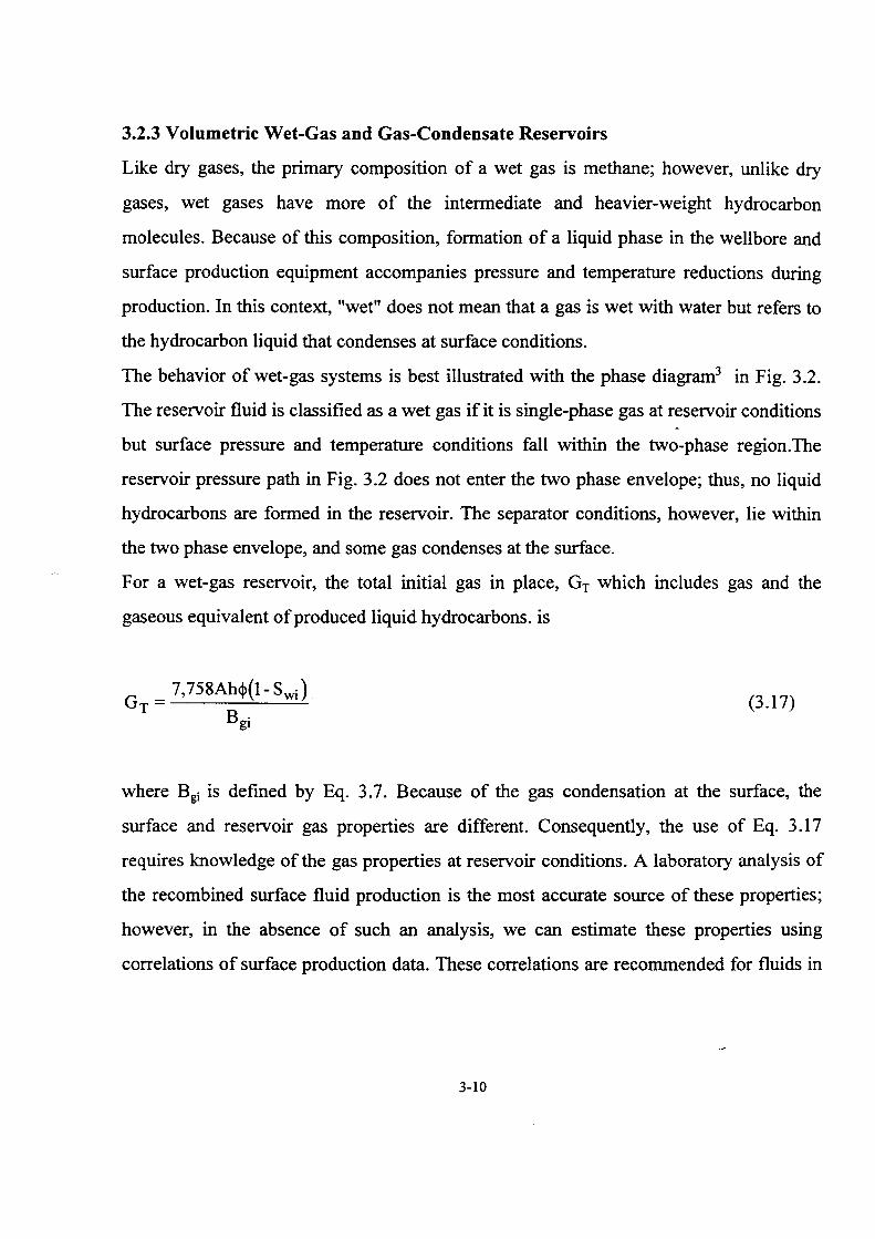
3.2.3 Volumetric Wet-Gas and Gas-Condensate Reservoirs

Like dry gases, the primary composition of a wet gas is methane; however, unlike dry

gases, wet gases have more of the intermediate and heavier-weight hydrocarbon

molecules. Because of this composition, formation of a liquid phase in the wellbore and

surface production equipment accompanies pressure and temperature reductions during

production. In this context, "wet" does not mean that a gas is wet with water but refers to

the hydrocarbon liquid that condenses at surface conditions.

The behavior of wet-gas systems is best illustrated with the phase diagram3 in Fig. 3.2.

The reservo ir fluid is classified as a wet gas if it is single-phase gas at reservo ir conditions

but surface pressure and temperature conditions fall within the two-phase region.The

reservoir pressure path in Fig. 3.2 does not enter the two phase envelope; thus, no liquid

hydrocarbons are formed in the reservoir. The separator conditions, however, lie within

the two phase envelope, and sorne gas condenses at the surface.

For a wet-gas reservoir, the total initial gas in place, GT which includes gas and the

gaseous equivalent of produced liquid hydrocarbons. is

(3.17)

where Bgi is defined by Eq. 3.7. Because of the gas condensation at the surface, the

surface and reservo ir gas properties are different. Consequently, the use of Eq. 3.17

requires knowledge of the gas properties at reservoir conditions. A laboratory analysis of

the recombined surface fluid production is the most accurate source of these properties;

however, in the absence of such an analysis, we can estímate these properties using

correlations of surface production data. These correlations are recommended for fluids in

3-10

which the total non-hydrocarbon components (i.e., C02, H2S, and N2) do not exceed

20%.7

According to Gold et al., for a three-stage separation system consisting of a high-pressure

separator, a low-pressure separator, anda stock tank, the reservoir gas gravity is estimated

from a recombination ofthe Produced well stream.

R 1y1 +4,602y 0 +R2y2 +R3y3 y = w R 133,316y 0 R R

¡+ + 2+ 3 M o

(3.18)

Similarly, for a two-stage separation system consisting of a high pressure separator and

stock tank, the reservoir gas gravity is estimated with

Ra 1 +4,602y 0 +R3y3 y -w- R 133,316y 0 R

1 + + 3 M o

(3.19)

If the molecular weight of the stock-tank liquid (i.e., the condensates produced at the

surface) is unknown, we can estímate it using either

M - 5,954

o-Y API- 8.811

(3.20)

M _ 42.43y 0 or 0 -

1.008 -y 0

(3.21)

Accurate estimates of gas properties at reservoir conditions require that all surface gas

and liquid production be recombined according to Eq. 3.18 or 3.19. However, gas

production from low-pressure separators and stock tanks often is not measured.

Gold et al. developed correlations for estimating the additional gas production from the

secondary separator and stock tank, Gpa , and the vapor equivalent of the primary

3-11

separator liquid, Veq· These correlations, expressed in terms of generally available

production data, are presented in Chap. 1 and are used in Eq. 3.22 to estimate the

reservoir gas gravity:

(3.22)

After the gas gravity at reservoir conditions is known, we can use the method established

previously to estimate the gas deviation factor. Using this value, we can estimate the total

original gas in place with Eq. 3.17.

Because of condensation, sorne gas at reservoir conditions is produced as liquids at the

surface. The fraction of the total initial gas in place that will be produced in the gaseous

phase at the surface is

f = Rt g R 132,800y 0 t + ----'--"-

Mo

(3.23)

where ~ includes gas and condensate production from all separators and the stock tank.

The fraction of the original total gas in place, GT that will be produced in the gaseous

phase is

(3.24)

and the original oil ( condensate) in place is

(3.25)

3-12

Note that this calculation procedure is applicable to gas-condensate reservoirs only when

the reservoir pressure is above the original dewpoint pressure. Gas-condensate reservoir

fluids also are characteristically rich with intennediate- and heavier-weight hydrocarbon

molecules. Because of this composition, a liquid phase fonns not only in the wellbore and

surface equipment but also in the reservoir.

The behavior of a gas-condensate fluid is illustrated with the phase diagram in Fig. 3.3.

U pon discovery, if the reservo ir pressure is above the dewpoint pressure and if the

temperature lies between the critical temperature and the cricondenthenn, then a

single-phase fluid (i.e., gas) exists in the reservoir.

Once the reservoir pressure falls below the dewpoint pressure, however, liquid

hydrocarbons fonn in the reservoir, and we cannot use surface production data to estimate

reservo ir fluid properties accurately. Under these conditions, accurate estimates of the gas

and condensate in place require a laboratory analysis ofthe reservoir fluid.

3.3 MATERIAL BALANCE METHOD

Material-balance methods provide a simple, but effective, altemative to volumetric

methods for estimating not only original gas in place but also gas reserves at any stage of

reservoir depletion. A material-balance equation is simply a statement of the principie of

conservation of mass, or

(original hydrocarbon mass) - (produced hydrocarbon mass) = (remaining hydrocarbon

mass).

In 1941, Schilthuis presented a general fonn of the material balance equation derived as a

volumetric balance based on the simple assumption that the reservoir PV either remains

constant or changes in a manner that can be predicted as a function of change in reservoir

pressure. With this assumption, he equated the cumulative observed surface production ~

3-13

( expressed in terms of fluid production at reservo ir conditions) to the expansion of the

remaining reservo ir fluids resulting from a finite decrease in pressure. W e al so can

include the effects of water in flux, changes in fluid phases, or PV changes caused by rock

and water expansion.

Sometimes called production methods, material-balance methods are developed in terms

of cumulative fluid production and changes in reservoir pressure and therefore require

accurate measurements ofboth quantities.

Unlike volumetric methods, which can be used early in a reservoir's life, material-balance

methods cannot be applied until a:fter sorne development and production. However, an

advantage of material-balance methods is that they estímate only the gas volumes that are

in pressure communication with and that may be ultimately recovered by the producing

wells. Conversely, volumetric estimates are based on the total gas volume in place, part of

which may not be recoverable with the existing wells because of unidentified reservoir

discontinuities or heterogeneities. Therefore, comparisons of estimates from both

methods can provide a qualitative measure of the degree of reservoir heterogeneity and

allow a more accurate assessment of gas reserves for a given field-development strategy.

Another advantage of material-balance methods is that, if sufficient production and

pressure histories are available, application of these methods can provide insight into the

predominant reservoir drive mechanism, whereas the correct use of volumetric methods

requires a priori knowledge ofthe primary source ofreservoir energy. As we shall see in

the next section, a plot of p/z vs. GP will be a straight line for a volumetric gas reservo ir in

which gas expansion is the primary reservoir drive mechanism. However, consistent

deviations from this straight line indicate other interna! or externa! energy sources.

Once the predominant reservoir drive mechanism has been identified, we can apply the

correct material-balance plotting functions to estímate original gas in place and gas

reserves.

Like volumetric methods, the form of the material-balance equation varíes depending on

the drive mechanism. In the following sections, we present the material-balance equations

3-14

for volumetric dry-gas reservoirs, dry-gas reservoirs with water influx, volumetric

geopressured gas reservoirs, and volumetric gas-condensate reservoirs.

3.3.1 Volumetric Dry-Gas Reservoirs.

As stated, volumetric reservoirs are completely enclosed and receive no externa} energy

from other sources, such as aquifers. If rock and connate water expansions are negligible

sources of interna} energy, then the dominant drive mechanism is gas expansion as

reservoir pressure decreases. Comparison of typical values of gas and liquid compres­

sibilities shows that gases can be as muchas 100 or even 1,000 times more compressible

than relatively incompressible liquids, so simple gas expansion is a very efficient drive

mechanism, often allowing up to 90% of in-place gas to be recovered.

Assuming a constant reservoir PV over the producing life of the reservoir, we can derive

a material-balance equation by equating the reservoir PV occupied by the gas at initial

conditions to that occupied by the gas at sorne later conditions following gas production

and the associated pressure reduction. Referring to the tank-type model in Fig. 3.4, we

write the material-balance equation as

(3.26)

where

GBgi = reservoir volume occupied by gas at initial reservmr pressure, res bbl, and

(G-Gp)Bg = reservoir volume occupied by gas after gas production ata pressure below the

initial reservoir pressure, res bbl.

We can rewrite Eq. 3.26 as

3-15

(3.27)

If we substitute the ratio of the gas FVF evaluated at initial and la ter conditions, Bg/Bg =

(z¡p)/(zp¡), into Eq. 3.27, we obtain an equation in terms of the measurable quantities,

surface gas production. and BHP:

(3.27)

where the gas recovery factory is

Further, we can rewrite Eq. 3.28 as

P = Ei(I- Gp) =Pi -La z z. G z. z.G P

1 1 1

(3.29)

Similar to van Everdingen et al. 's and Havlena and Odeh's graphical analysis techniques,

the form ofEq. 3.29 suggests that, ifthe reservoir is volumetric, a plot ofp/z vs. Gp will

be a straight line, from which we can estimate both original gas in place and gas reserve

at sorne abandonment conditions.

As stated earlier, if sufficient pressure and production data are available to defme the

line fully, we also can determine the dominant drive mechanism from the shape of the

plot. Although consistent deviations from a straight line suggest other sources of reservo ir

3-16

energy, errors in pressure and production measurements also can cause departures from a

straight line. Obviously, early in the productive life of a reservoir when few data are

available, this plotting technique may not be accurate. Fig. 3.5 shows typical shapes ofp/z

plots for selected gas reservoir drive mechanisms.

The same material balance is applicable to wet-gas reservoirs, but we must base z and Z¡

on the reservoir gas gravity and Gp must include the vapor equivalent of the condensate

produced. The original gas in place, G, and the gas reserve to abandonment includes the

vapor equivalent of liquid and must be corrected to determine dry-gas and gas-condensate

reserves. (See Example 3.5)

3.3.2 Dry-Gas Reservoirs With Water Influx.

In the previous section, we derived a material-balance equation for a volumetric gas

reservoir. A critica! assumption in this derivation is that the reservoir PV occupied by the

gas remained constant throughout the productive life of the reservoir. However, if the

reservoir is subjected to water influx from an aquifer, this PV is reduced by an amount

equal to the volume of encroaching water. In addition, the water entering the reservoir

provides an important source of energy (i.e., pressure support) that must be considered in

material balance calculations.

We can derive a material-balance equation for a water drive system by equating the

reservoir PV occupied by the gas at initial conditions to that occupied by the gas at later

conditions plus the change in PV resulting from water influx (Fig. 3.7). A general form of

the material-balance equation is

(3.30)

where

GB8¡ = reservoir PV occupied by gas at initial reservoir pressure, res bbl;

3-17

(G-Gp) = reservoir PV occupied by gas following gas production ata pressure below the

initial pressure, res bbl; and

~V P = change in reservo ir PV occupied by gas at la ter conditions due to water influx, res

bbl.

Referring to Fig. 3.7, we can see that the change in reservoir PV at sorne reduced

pressure is affected not only by the volume of water influx but also by the amount of

water produced at the surface:

(3.31)

Combining Eqs. 3.30 and 3.31 yields

(3.32)

lf water influx and production are ignored, a plot of p/z vs. Gp may appear as a straight

line initially but eventually will deviate from the line. The deviation will occur early for a

strong water drive and later for a weak aquifer support system. Chierici and Pizzi 12

studied the effects of weak or partial water drive systems and concluded that accurate

gas-in-place estimates are difficult to obtain, especially early in the production period or

when the aquifer characteristics are unknown. Similarly, Bruns et al. 13 showed that sig­

nificant errors in gas-in-place estimates occur if the effects of water encroachment are

ignored in the material-balance calculations.

Before the effects of water influx on gas reservoir behavior were completely

understood, early deviations from a straight line on a plot of p/z vs. GP often were

attributed to measurement errors. In sorne instances, errors in field pressure

measurements can mask the effects of water influx, especially if a weak water drive is

present; however, consistent deviations from a straight line suggest that the reservoir is

not volumetric and that additional energy is being supplied to the reservoir. Bruns et al. -·

3-18

studied the effects of water influx on the shape of the plot of p/z vs. GP and showed that

the shape and direction of the deviation from straight line depend on the strength of the

aquifer support system and on the aquifer properties and the reservoir/aquifer geometry.

If the initial gas in place is known from other sources, such as volumetric estimates, we

can calculate We from Eq. 3.32. In practice, however, usually both We and G are

unknown, and calculation of initial gas in place requires an independent estímate of water

influx. Therefore, in the next section we discuss three methods for estimating water

in flux.

Methods For Estimating Water Influx.

Water influx results from a reduction in reservo ir pressure following gas production.

Water influx tends to maintain, either partially or wholly, the reservoir pressure.

In general, both the effectiveness ofthe pressure support system and the water influx rates

are govemed by the aquifer characteristics, which principally include the permeability,

thickness, areal extent, and the pressure history along the original reservoir/aquifer

boundary.

Note that, in practice, estimating water influx is very uncertain, primarily because of the

lack of sufficient data to characterize the aquifer ( especially its geometry and areal

continuity) completely.

Because wells are seldom drilled intentionally into an aquifer to gain information, these

data must be either assumed or inferred from the geologic and reservoir characteristics.

Generally, reservoir/aquifer systems are classified as either edgewater or bottomwater

drive. In edgewater-drive systems, water moves into the reservoir flanks, while

bottomwater drive occurs in reservoirs with large areal extents and gently dipping

structures where the aquifer completely underlies the reservo ir. van Everdingen and

Hurst's and Carter and Tracy's methods are applicable only to edgewater-drive geometries

or for combined geometries that can be modeled as edgewater-drive systems, while the

Fetkovich method16 is applicable for all geometries

3-19

l. van Everdingen-Hurst's Method.

In 1949, van Everdingen and Hurst presented an unsteady-state model for predicting

water influx. As Fig. 3.8 shows, the reservoir/aquifer system is modeled as two concentric

cylinders or sectors of cylinders. The inside cylindrical surface, defined by radius rf'

represents the reservoir/aquifer boundary, while the outer surface is the aquifer boundary

defined by ra. Radial flow of water from the aquifer to the reservoir is described

mathematically with the radial diffusivity equation '

(3.33)

where the dimensionless variables are defmed in terms of the aquifer properties. The

dimensionless pressure for constant-rate conditions at the reservoir/aquifer boundary is

0.00708kh{p¡ - p) Po=----""----'--_.:_

QJ.l

For constant-terminal-pressure conditions,

Pi -p Po=--­

Pi- Pr

The dimensionless radius is defined in terms of rr:

r0 = r/rf' ·

and for t in days,

3-20

(3.34)

(3.35)

(3.36)

0.00633kt tn=----

cpJ.l.ctr; (3.37)

van Everdingen and Hurst derived solutions to Eq. 3.33 for two reservoir/aquifer

boundary conditions---constant terminal rate and constant terminal pressure. The water

influx rate for the constant terminal-rate case is assumed constant for a given period, and

the pressure drop at the reservoir/aquifer boundary is calculated. For the constant-pressure

case, the water influx rate is determined for a constant pressure drop over sorne finite time

period. Reservoir engineers usually are more interested in determining the water influx

than the pressure drop at the reservoir/aquifer boundary, so

we will focus on water-influx calculations under constant-pressure conditions.

van Everdingen and Hurst derived the constant-pressure solutions in terms of a

dimensionless water influx rate defined by

q D = 0.00708kMp (3.38)

Integrating both sides ofEq. 3.38 with respect to time yields

tJO d ( Jl J(0.00633k] tJ d 1 tJ d q t = . q t= q t 0 o o 0.00708kMp cpJ.l.C r2 0 W 1.119cpJ.J.C hr2 Llp 0 W

t r t r

(3.39)

In material-balance calculations, we are more interested in the cumulative water influx

than in influx rate. Therefore, beca use cumulative water influx, W e• is

3-21

(3.40)

and dimensionless cumulative water influx is

(3. 41)

we can combine Eqs. 3.39 through 3.41 to obtain

w Q = e

pD 1.119cpJ.!C hr2 Llp t r

(3. 42)

Thus, We = 1.1 19q,cthr ~PQpD (3.43)

If the total productive reservo ir life is divided into a finite number of pressure reductions

or increases, we can use superposition of the solution given by Eq. 3.43 to model the

water-influx behavior for a given pressure history. This method assumes that the pressure

history at the original reservoir/aguifer boundary can be approximated by a series of

step-by-step pressure changes. Fig. 18.9 shows the modeling of a pressure history.

Referring to Fig. 3.9, we define the average pressure in each period as the arithmetic

average of the pressures at the beginning and end of the period. Thus, for an initial aquifer

pressure, p¡, the average pressure during the first time period PI = _!_(p¡ +PI) 2

Similar! y, for the second time period, p2 = _!_(p1 + p 2). In general, for the nth time period, 2

3-22

W e can then calculate the pressure changes between time periods as follows.

Between the initial and first time periods,

Similarly, between the frrst and second time periods,

In general, for the (n-1) and nth time periods,

During each time increment, the pressure is assumed constant (i.e., constant-pressure

solution), and the cumulative water influx for n time periods is

n We(tn) = B_I~PiQpn(tn- t¡_t)0

1=1 (3.44)

where B = 1.1 19cj>c/2r2 r

(3.45)

Ifthe angle subtended by the reservoir is less than 360° (Fig. 3.8). then B is adjusted as

follows:

3-23

(3.46)

The pressure change during each time increment, as explained above, is calculated with

~Pi = _!_(Pi-2 -Pi), i = 1,2 ... n 2

(3.47)

and p¡.2 = p0 = initial pressure. Each Ap¡ in Eg. 3.44 is multiplied by the dimensionless

cumulative water influx, Qp0 . evaluated at a dimensionless time corresponding to the time

for which ~Pi has been in effect. For example, ~Pi will have been in effect for the total

productive life ofthe reservoir, so Qp0 will be evaluated at (t1 - 0)0 • In general, 4>n will

have been in effect for the time period t-Í¡¡.1 so Qp0 that multiplies 4>n will be evaluated

at (t-Í¡¡_1) 0 •

To simplify calculations, Tables 3.1 and 3.2 present values for dimensionless cumulative

water influx as a function oftime for both infinite-acting and fmite aquifers.

Altematively, for the special case of infinite-acting aquifers, Edwardson et al. developed

polynomial expressions for calculating Qp0 • These expressions, Eqs. 3.48 through 3 .50,

depend on dimensionless time:

For t 0 < 0.01,

(3.48)

For 0.01 < t0 < 200,

3-24

( ) _ 12838tg2 + 1.19328t0 + 0269872t~2 + 0.00855294t~

Qpo to - 112 1 + 0.616599t0 + 0.0413008t 0

(3.49)

For t0 > 200,

-429881 + 2.02566t0 Qpo(to) = ln(to) (3.50)

Similarly, Klins et al. 21 developed polynomial approximations for both infmite-acting and

fmite aquifers.

The van Everdingen and Hurst method also is applicable to linear flow geometries

(Fig. 3.10). For linear flow, we defme a dimensionless time in terms of the reservoir

length, L, as

(3.51)

Following a derivation similar to that presented for radial flow, we find that the

cumulative water influx for n time periods is

w ( t ) = B I óp. Q D (t - t. 1) e n i=l 1 p n 1- D

(3.52)

where the parameter R is defmed in terms ofthe reservoir length,

(3.53)

Derived from exact solutions to the diffu.sivity equation, the van Everdingen and Hurst

method models all aquifer flow regimes (i.e., transient and pseudosteady-state) and is

3-25

applicable to both infinite acting and finite aquifers. Example 3.6 illustrates the following

calculation procedure.

l. First, calculate the parameter B for radial flow,

or for a linear flow geometry,

2. Calculate the pressure change, .ó.p¡. between each time

period,

~Pi = _!_(Pi-2- p¡), i = 1,2 ... n 2

(3.46)

(3.53)

3. Calculate the t0 that correspond to each time period on the production history. F or a

radial flow geometry,

(3.37)

and for a linear geometry,

(3.51)

3-26

4. For each t0 computed in Step 3, calculate a dimensionless water cumulative influx,

Qp0 (t0 ). For an infinite-acting aquifer we can use Eqs. 3.50 through 3.52, use Klins et

al.'s21 equations, or read the values directly from Table 3.1. For finite aquifers, we must

use Klins et al.'s equations or Table 3.2.

5. Calculate the water influx:

(3.44)

3. Carter-Trapy Method.

van Everdingen and Hurst's method was developed from exact solutions to the radial

diffusivity equation and therefore provides a rigorously correct technique for calculating

water influx. However, because superposition of solutions is requfred, their method

involves rather tedious calculations. To reduce the complexity of water influx

calculations, Carter and Tracy proposed a calculation technique that does not require

superposition and allows direct calculation of water influx.

If we approximate the water influx process by a series of constant influx intervals, then

the cumulative water influx during the jth interval is

J-1 We(tm) = 2: qon(tDn+1- ton) (3.54)

n=O

Eq. 3.54 can be rewritten as the sum of the cumulative water influx through the ith

interval and between the ith and jth intervals:

J-1 J-1 We(tm) = 2: qnn(tDn+1- ton) + 2:qon(ton+1- ton) (3.55)

n=O n=i

J -1 ( ) W (tD.)=W (tD.)+ ¿ qD tD 1-tD e 11 e 1 • n n + n

J n= 1

(3.56)

3-27

Using the convolution integral, we also can express the cumulative water up to the jth

interval as a function of variable pressure:

( 3. 57)

Combining Eqs. 3.56 and 3.57, we use Laplace transform methods to solve for the

cumulative water influx in terms of the cumulative pressure drop, ~ Pn:

[

B~p - W p' (t ) ] w = w + t -t n en-1 D Dn en en - 1 ( Dn Dn - 1) p (t ) _ t p' {t )

D Dn Dn-1 D Dn

(3.58)

where B and t0 are the same variables defined previously for the van Everdingen-Hurst

method. The subscripts n and n-1 refer to the current and previous timesteps, respectively,

and

(3.59)

P0 is a function of t0 and for an infmite-acting aquifer, can be computed from the

following curve-fit equation:

370j29(t0 t 2 + 137j82(t0 ) + 5.69549(t0 )

312

Po(to)= 112 3/2 328.834+ 265.488(t0 ) + 452157(t0 ) + (t0 )

(3.60)

3-28

In addition, the dimensionless pressure derivative, P' 0 , can be approximated by a

curve-fit equation.

716.441 +46.7984(t0 )112

+ 270.038(t0 ) + 71.0098(t0 )312

P'o(to)= 112 3/2 2 5/2 1,296.86(t0 ) + 1,204.73{t0 ) + 618.618(t0 ) + 538.072(t0 ) + 142.4l(t0 )

(3.61)

Eqs. 3.60 and 3.61 model infinite-acting aquifers; however Klins et al. developed similar

polynomial approximations for both infmite and finite aquifers.

We should stress that, unlike the van Everdingen-Hurst technique,- the Carter-Tracy

method is not an exact solution to the diffusivity equation, but is an approximation.

Research conducted by Agarwal, however, suggests that the Carter-Tracy method is an

accurate altemative to the more tedious van Everdingen-Hurst calculation technique. The

primary advantage of the · Carter-Tracy method is the ability to calculate water influx

directly without superposition.

The Carter-Tracy method, which also is applicable to infmite acting and finite aquifers,

is illustrated with the following calculation procedure and Example 3. 7.

l. First, calculate the van Everdingen-Hurst parameter B for radial flow,

B = 1.119<j)chr2 (~) t r 360

or for a linear flow geometry,

2. Calculate the pressure change, Apn, for each time period,

3-29

(3.46)

(3.53)

(3.59)

3. Calculate the van Everdingen-Hurst dimensionless times, t0 , that correspond to each

time period on the production history. For a radial flow geometry,

0.00633kt to=----

cpJ.!ctr? (3.37)

and for a linear geometry,

(3.51)

4. For each t0 computed in Step 3, calculate a P0 and a P' 0 . For infinite-acting radial

aquifer, we can use Eqs. 3.60 and 3.61 to calculate P0 and P'0 , respectively:

370529(t0 )112 + 137.582(t0 ) + 5.69549(t0 )

312

Po(to) = 112 312 328.834 + 265.488(t0 ) + 452157(t0 ) + (t0 )

(3.60)

In addition, the dimensionless pressure derivative, P' 0 , can be approximated by a

curve-fit equation.

P'o(to)= 112 3/2 2 )5/2 1,296.86(t0 ) + 1,204.73(t0 ) + 618.618(t0 ) + 538.072(t0 ) + 142.41(t0

716.441 + 46.7984(t0 )112 + 270.038(t0 ) + 71.0098(t0 )

312

(3.61)

3-30

We also can use Klins et al' s equations. F or infinite aquifers, we must use Klins et al' s

equations

5. Calculate the water influx:

[

B~p - W p' (t ) ] w = w + ( t _ t ) n en -1 D Dn en en -1 Dn Dn - 1 p (t ) _ t p' (t )

D Dn Dn-1 D Dn (3.58)

3. Ferkovich Method.

To simplify water influx calculations further, Fetkovich proposed a model that uses a

pseudosteady-state aquifer Pl and an aquifer material balance to represent the system

compressibility. Like the Carter-Tracy method, Fetkovich's model eliminates the use of

superposition and therefore is much simpler than van the Everdingen-Hurst method.

However, because Fetkovich neglects the early transient time period in these calculations,

the calculated water influx will always be less than the values predicted by the previous

two models.

Similar to fluid flow from a reservo ir to a well, F etkovich used an inflow equation to

model water influx from the aquifer to the reservoir. Assuming constant pressure at the

original reservoir/aquifer boundary, the rate ofwater influx is

(3.62)

where

n = exponent for inflow equation (for flow obeying Darcy's law, n = l; for fully turbulent

flow, n = 0.5).

3-31

Assuming that the aquifer flow behavior obeys Darcy's law and is at pseudosteady-state

conditions, n = l. Based on an aquifer material balance, the cumulative water influx

resulting from aquifer expansion is

(3.63)

Eq. 3.63 can be rearranged to yield an expression for the average aquifer pressure,

(3.64)

(3.65)

is defined as the initial amount of encroachable water and represents the maximum

possible aquifer expansion.

After differentiating Eq. 3.64 with respect to time and rearranging, we have

dWe = _ Wei dPaq dt p¡ dt

(3.66)

Combining Eqs. 3.62 and 3:66 and integrating yields

-Paq dPaq t JP. f =-f~t'

P . p aq - p O W ei aq,1 r

(3.67)

(3.69)

3-32

Table 3.10 summarizes the equations for calculating the aquifer PI for vanous

reservoir/aquifer boundary conditions and aquifer geometries. Note that we must use the

aquifer properties to calculate J.

From Eq. 3.67, we can derive an expression for (Paq -Pr), and following substitution into

Eq. 3.68 and rearranging, we have

JP.t __ 1_

dW ( ) W. __ e = J p . _ p e et dt aq,t r

which is integrated to obtain the cumulative water influx. W e:

w. ( ) W = __ el_ p . -P e P . aq,1 r

aq,1 1-e

JP .t aq,1

w. e1

(3.69)

(3.70)

Recall that we derived Eq. 3.10 for constant pressure at the reservoir/aquifer boundary.

In reality, this boundary pressure changes as gas is produced from the reservoir. Rather

than using superposition, Fetkovich assumed that, if the reservoir/aquifer boundary

pressure history is divided into a finite number of time intervals, the incremental water

influx during the nth interval is

(3.71)

3-33

where

- ( We n-1) Paq,n-1 = Paq,i 1- ' . weJ

(3.72)

(3.73)

Although it was developed for finite aquifers, F etkovich's method can be extended to

infmite-acting aquifers. F or infinite-acting aquifers, the method requires the ratio of water

influx rate to pressure drop to be approximate1y constant throughout the productive life of

the reservoir. Under these conditions, we must use the aquifer PI for an infmite-acting

aquifer.

The following calculation procedure illustrates this method.

l. Ca1culate the maximum water volume, We¡, from the aquifer that could enter the gas

reservo ir if the reservo ir pressure were reduced to zero.

(3.65)

where W¡ depends on the reservoir geometry and the PV available to store water.

2. Calculate J. Note that the equations summarized in Table 3.10 depend on the boundary

conditions and aquifer geometry.

3. Calculate the incremental water influx, ~ W en , from the aquifer during the nth time

interval.

e1 - -w. ( ) t:.Wen =~ Paq,n-1- Pm 1-e

aq,1

JP . t:.t aq,1 n

w. e1

3-34

(3.71)

4. Calculate Wen:

n

Wen = "'!1..Wei i=l

Estimating Original Gas In Place With Material Balance For A Dry-Gas Reservoir

With Water Influx

Once the water influx has been calculated, we can estimate the original gas in place with

material-balance concepts. The general form of the material-balance equation including

water influx:

(3.74)

which can be rearranged to yield

(3.75)

lf we defme a water influx constant, C, in terms of the cumulative water influx as

We = Cf(p,t), (3.76)

then Eq. 3. 7 5 becomes

(3.77)

3-35

The form of Eq. 3.77 suggests that, if water influx is the predominant reservoir drive

mechanism, then a plot of [(GeBJ+(WpBw)]/(Bg -Bg¡) vs. f(p,t)/(Bg-Bg¡) will be a straight

line with a slope equal to C and an intercept equal to G. The functional form of f(p,t)

varies according to the water influx model used. Any water influx model, such as steady

state, unsteady state, or pseudosteady state, can be used with Eq. 3. 77.

Note that, if the incorrect water influx model is assumed, the data may not exhibit a

straight line. Example 3.9 illustrates the application of Eq. 3.77 for an unsteady-state

water influx model.

3.3.3 Volumetric Geopressured Gas Reservoirs.

We developed the material-balance equation for a volumetric dry-gas reservoir assuming

that gas expansion was the dominant drive mechanism and that expansions of rock and

water are negligible during the productive life of the reservoir. These assumptions are

valid for normally pressured reservoirs (i.e., reservoirs with initial pressure gradients

between 0.43 and 0.5 psilft) at low to moderate pressures when the magnitude of gas

compressibilities greatly exceeds the effects of rock and connate water compressibilities.

However, for abnormally or geopressured reservoirs, pressure gradients often approach

values equal to the overburden pressure gradient (i.e., - 1.0 psilft). In these and other

higher-pressure reservoirs, the changes in rock and water compressibilities may be

important and should be considered in material-balance calculations.

Following Ramagost et al.'s23 derivation, we begin with Eq. 3.26 for a normally

pressured volumetric gas reservoir and include the effects of changing water volume,

~V w• and formation (rock) volume, ~ Vr. As Fig. 3.12 shows, the general form of the

material-balance equation for a volumetric geopressured reservoir is

(3.78)

3-36

where

GBgi = reservoir volume occupied by gas at initial reservoir pressure, RB;

(G-Gp)Bg = reservoir volume occupied by gas after gas production ata pressure below the

initial reservoir pressure, RB;

~V w = increase in reservoir PV occupied by connate water and following water

expansion ata pressure below the initial reservoir pressure, RB; and

~ Vr = increase in reservoir PV occupied by formation (rock) ata pressure below the

initial reservo ir pressure, RB.

The expansion of the connate water following a finite pressure decrease can be modeled

with isothermal water compressibility:

where V wi = initial reservoir volume occupied by the connate water.

We can arrange Eq. 3.79 in terms ofthe change in water volume,

(3.79)

(3.80)

where ~p = p-p¡. We can also write the original water volume in terms ofthe original gas

in place:

(3.81)

Substituting Eq. 3.81 into Eq. 3.80 and notingthat -~p = p¡-pyields

3-37

(3.82)

Similarly, the decrease in PV, Llp, caused by a finite reduction in pore pressure can be

modeled with

cf =-~ (a;J , p T

and thus,

I ~vP Cf=---,

V. ~p pl

-

(3.83a)

(3.83b)

where cr = average formation compressibility over the fmite pressure interval, óp .

In terms ofthe change in PV, Eq. 3.83 becomes

~V =e V .~p p f pl

(3.84)

where óp = p-p¡_ Again, we can write the original rock PV in terms of the original gas in

place as

(3.85)

3-38

Substituting VP¡ from Eq. 3.85 into Eq. 3.84 and noting that -~p = p¡-p, and

~V P = - ~ Vr (the change in rack volume) yields

- GB. -~VP = cr(p¡- p) ( gt) = ~Vr

1-Swi (3.86)

Substituting Eqs. 3.82 and 3.86 into Eq. 3.78, we can now write a general material­

balance equation for a volumetric geopressured reservoir:

( )

e (p. - p)s .GB . cr(p. - p)GB . w 1 Wl g1 1 g1

GB . = G - G B + ( ) + ( ) g1 P g 1 - S . 1 - S .

Wl Wl

(3.87)

After simplification, Eq. 3.87 becomes

(3.88)

(3.89)

Substituting Bg/Bg = pz¡lp¡z into Eq.3.89 and rearranging, we have

(3.90)

Note that, when the effects of rock and water compressibility are negligible, Eq. 3.90

reduces to the material-balance equation in which gas expansion is the primary source of

reservoir energy (Eq. 3.29).

3-39

Failure to include the effects of rock and water compressibilities in the analysis of

high-pressure reservoirs can result in errors in both original gas in place and subsequent

gas reserve estimates.

We present two analysis techniques based on Eq. 3.90 for volumetric geopressured

reservmrs.

Estimating Original Gas in Place When Average Formation compressibility Is

Known.

If cr is assumed to be constant with time, the form ofEq. 3.90 suggests that a plot of

will be a straight line with slope equal to -p¡lz¡ G and an intercept equal to p/Z¡ ..

At p/z =O, GP = G, so extrapolation ofthe line to p/z =O provides an estimate of original

gas in place. Example 3.1 O illustrates this analysis technique.

Simultaneous Determination of Average Formation Compressibility and Original

Gas in Place.

Roach developed a material-balance technique for simultaneously estimating formation

compressibility and original gas in place in geopressured reservoirs. Beginning with Eq.

3 .90, Roach presented the material-balance equation in the following form:

(3.91)

3-40

Again, if cr is constant, the form ofEq. 3.91 suggests that a plot of

1 1 vs 1 1 (P·Z ) [ GP P·Z] (p¡ -p) Z¡p (p¡ -p) Z¡p

will be a straight line with a slope that equals 1/G and an intercept that equals

-(Swicw + Cr /1-Sw¡).

We can then calculate the original gas in place, G, and the average formation

compressibility, cr, using the slope and intercept, respectively.

Poston and Chen26 applied this method to the geopressured gas reservoír data presented in

Example 3.10. Their analysis is reproduced in Example 3.11. o

3.3.4 VOLUMETRIC GAS-CONDENSATE RESERVOIRS.

In this section, we develop material-balance equations for a volumetric gas reservoir

with gas condensation during pressure depletion. We also include the effects of connate

water vaporization. Both phenomena are most prevalent in deep, high-temperature,

high-pressure gas reservoirs and must be included for accurate material-balance

calculations.

Depending on whether the pressure is above or below the dewpoint, two or three fluid

phases may be present in a gas-condensate reservoir. Above the dewpoint, the vapor

phase consists of not only hydrocarbon and inert gases but also water vapor. As the

reservoir pressure declines, the water in the liquid phase continues to vaporize to remain

in equilibrium with the existing water vapor, thus decreasing the saturation of the liquid

water in the reservoir and increasing the PV occupied by the vapor phases. As the

reservoir pressure declines further, the amount of water vapor present in the gas phase

may increase significantly. However, as the reservoir pressure decreases below the

3-41

dewpoint, the fraction of PV available for the vapor phases decreases as liquids condense

from the hydrocarbon vapor phase.

To develop á material-balance equation that considers the effects of gas condensation

and water vaporization requires that we include the changes in reservoir PV resulting

from these phenomena. We begin with a material-balance equation for gas-condensate

reservoirs. We then extend this equation to include the effects of connate water

vaporization. In addition, because changes in formation compressibilities often are

significant in these deep, high-pressure gas reservoirs, we include geopressured effects.

Gas-Condensate Reservoirs.

We derived the material-balance equations in previous sections for dry gases with the

inherent assumption that no changes in hydrocarbon phases occurred during pressure

depletion. Unlike dry-gas reservoirs, gas-condensate reservoirs are characteristically rich

with intermediate and heavier hydrocarbon molecules. At pressures above the dewpoint,

gas condensates e:xist as a single-phase gas; however, as the reservoir pressure decreases

below the dewpoint, the gas condenses and forms a liquid hydrocarbon phase. Often, a

significant volume ofthis condensate is immobile and remains in the reservoir. Therefore,

correct application of material-balance concepts requires that we consider the liquid

volume remaining in the reservoir and any liquids produced at the surface.

Assuming that the initial reservoir pressure is above the dewpoint, the reservoir PV is

occupied initially by hydrocarbons in the gaseous phase (Fig. 3.16), or

Vp¡ = Vhvi (3.92)

The reservoir PV occupied by hydrocarbons in the gaseous phase also can be written as

(3.93)

3-42

where GT includes gas and the gaseous equivalent of produced condensates and Bgi is

defined by Eq. 3.7.

At later conditions following a pressure reduction below the dewpoint, the reservoir PV

is now occupied by both gas and liquid hydrocarbon phases, or

VP = Vhv+VhL

where

V P = reservoir PV at later conditions, RB;

(3.94)

V hv = reservoir volume occupied by gaseous hydrocarbons at later conditions, RB; and

V hL = reservoir PV occupied by liquid hydrocarbons at later conditions, RB.

Eq. 3.94 assumes that rock expansion and water vaporization are negligible. In terms of

the condensate saturation, S0 , we can write

Vhv = (1-So)Vp.

and vhL = sovp.

In addition, the hydrocarbon vapor phase at later conditions is

where Bg is evaluated at later conditions.

Equating Eqs. 3.95 and 3.97, the reservoir PV is

3-43

(3.95)

(3.96)

(3.97)

(3.98)

Substituting Eq. 3.98 into Eq. 3.95 and combining with Eq. 3.97 yields an expression for

the reservoir PV at later conditions:

(3.99)

Now, combining Eqs. 3.92 and 3.99 yields the following material-balance equation:

(3.100)

or, ifwe substitute Bg/Bg = (pz¡)l(p¡z) into Eq. 3.100 and rearrange,

(3.101)

which suggests that a plot of ( l-S0)(p¡z) vs. GpT will be a straight line from which GT can

be estimated.

Correct application of Eq. 3 .1 O 1, however, requires estimates of the liquid hydrocarbon

volumes formed as a function of pressure below the dewpoint. The most accurate source

of these estimates is a laboratory analysis of the reservoir fluid samples. Unfortunately,

laboratory analyses of fluid samples often are not available.

An alternative material-balance technique is

3-44

(3.102)

where

GTBZgi = reservoir PV occupied by the total gas, which includes gas and the gaseous

equivalent of the produced condensates, at the initial reservoir pressure above the

dewpoint, RB;

(GT-GpT)B2g = reservoir PV occupied by hydrocarbon vapor phase and the vapor

equivalent of liquid phase after sorne production at a pressure below the initial reservoir

pressure and dewpoint pressure, RB; and B2gi and B2g =gas FVF's based on two-phase z

factors at initial and later conditions, respectively, RB/Mscf.

Ifwe substitute B2g¡lB2g = (PZ2¡)/(P¡~) into Eq. 3.102 and rearrange, we have

p P¡ pT (

G J z2 = z2i 1- GT

(3.103)

where z2¡ and z2 = two-phase gas deviation factors evaluated at initial reservoir pressure

and ata later pressure, respectively.

The form of Eq. 3.103 suggests that a plot of P/Z2 vs. Gpr will be a straight line for a

volumetric gas-condensate reservoir when two-phase gas deviation factors are used.

Two-phase gas deviation factors account for both gas and liquid phases in the reservoir.

Fig. 3.17 is an example ofthe relationship between the equilibrium gas (i.e., single-phase

gas) and two phase deviation factors for a gas-condensate reservoir.

At pressures above the dewpoint, the single- and two-phase z factors are equal; at

pressures below the dewpoint, however, the two-phase z factors are lower than those for

the single-phase gas.

Ideally, two-phase gas deviation factors are determined from a laboratory analysis of

reservoir fluid samples. Specifically, these two-phase z factors are measured from a

3-45

constant-volume depletion study. However, in the absence of a laboratory study,

correlations are available for estimating two-phase z factors from properties of the

well-stream fluids.

Gas-Condensate Reservoirs With Water Vaporization.

In this section, we develop a material-balance equation for gas-condensate reservoirs in

which both phase changes and water vaporization occur. Similar to Humphreys' work, we

include the effects of rock and water compressibilities, which are often significant in

deep, high-pressure reservoirs. The reservoir PV is occupied initially by hydrocarbon and

water vapor phases as well as the connate liquid phase, or

Vpi = Vvi + Vwi

where

V vi = initial reservo ir PV occupied by hydrocarbon and water vapors, RB, and

V wi = initial reservoir PV occupied by the liquid water, RB.

(3.104)

lf the reservo ir pressure is above the dewpoint, . connate water is the only liquid phase

present. From the definition of water saturation, we can write the initial reservoir PV

occupied by the liquid phase as

Vwi = Swi Vpi (3.105)

Similarly, we can express the initial reservoir volume ofthe vapor phases as

(3.1 06)

3-46

Now, we define the fraction ofthe initial vapor phase volume that is water vapor as

Ywi =V wv/Vvi

and the fraction occupied by the hydrocarbon gases as

(1-Ywi) = VhviNvi

where

V wvi = initial reservoir PV occupied by water vapor, RB, and

Vhvi = initial reservoir PV occupied by hydrocarbon vapor, RB.

(3.107)

(3.1 08)

Substituting Eq. 3.106 into Eq. 3.108 gives an expression for the hydrocarbon

vapor-phase volume in terms of the initial reservo ir PV:

(3.109)

Finally, because the initial hydrocarbon vapor phase is the original gas in place.

(3.110)

(3.111)

The form of the material-balance equation at sorne pressure lower than the initial

reservoir pressure depends on the value of the dewpoint. Therefore, we will develop

material-balance equations for depletion at pressures above and below the dewpoint.

3-47

Depletion at Pressures Above the Dewpoint.

Because the reservoir pressure is still above the dewpoint, no hydrocarbon gas has

condensed. However, as the pressure declines, more of the liquid water vaporizes, thus

reducing the liquid water saturation.

Therefore, the volume ofliquid phase becomes (Fig. 3.18)

(3.112)

where Sw = current value of connate water saturation. Similarly, the volume ofthe vapor

phase is

(3.113)

In addition, we defme the fraction of the vapor phase that is water vapor as

(3.114)

and the :fraction ofvapor phase that is hydrocarbon as

(3.114)

Ifwe substitute Eq. 3.113 into Eq. 3.115, we can write an expression for the hydrocarbon

vapor phase in terms of the current reservo ir PV:

(3.116)

3-48

The current hydrocarbon vapor phase is

Combining Eqs. 3 .116 and 3.117 gives the current reservo ir

(G-GP) Bg

(1-Sw)(1-yw)

(3.117)

(3.118)

Like geopressured gas reservoirs, deep, high-pressured gascondensa~e reservoirs often

experience significant changes in PV during pressure depletion. Therefore, using a

method similar to that presented in the section on geopressured gas reservoirs, we can

express the change in reservoir formation (rock) volume in terms of the formation

compressibility as

= Cr(P¡ -p) GBgi

( 1- swi )(1- y wi ) (3.119)

In terms of Eq. 3. 119, the material-balance equation for pressures above the dewpoint

becomes

GBgi -----="----- = (1- swi )(1- Ywi)

(3.120)

Rearranging terms gives

3-49

(3.121)

Substituting Bg/Bg = PZ¡IP¡Z into Eq. 3.121 and rearranging yields

(3.122)

The form ofEq. 3.122 suggests that a plot of

(1- Sw ) ( 1- y w ) [ 1 - cf (p. -P) ] P vs G (1- swi) (1- y w¡) 1 z p

will be a straight line with a slope equal to -p/z¡G and an intercept equal to P¡IZ¡­

At p/z =O, Gp = G, so extrapolation ofthe straight line to p/z = O provides an estímate

of original gas in place. Note that, if the water saturation remains constant during the life

of the reservoir (i.e., Sw = Swi and Y w = Y wi) and when formation compressibility is

negligible, Bq. 3.122 reduces to Eq. 3.29 for a volumetric dry-gas reservoir.

Depletion at Pressures Below the Dewpoint.

When reservoir pressures decrease below the dewpoint, the gas phase condenses. In many

gas-condensate reservoirs, the liquid hydrocarbons formed in the reservoir remain

immobile. Therefore, we must modify Eq. 3.120 to include this additionalliquid phase

(Fig. 3.19).

Adding the liquid phase gives

GB. __ ___:gl:....__ = e 1- swi )( 1- y wi)

Cr(P¡ - p) GBgi

e 1-swi )( 1- y wi )

3-50

(3.123)

where S0 = liquid hydrocarbon phase (i.e., condensa te) saturation.

After rearranging Eq. 3.123, we write a material-balance equation similar in form to Eq.

3.122:

(3.123)

Again, the form ofEq. 3.124 suggests that a plot of

will be a straight line with a slope equal to p¡lz¡G and an intercept equal to P/Z¡.

At p/z =O, GP = G, so extrapolation ofthe straight line to p/z =O provides an estímate of

original gas in place. Again, the gas deviation factors in Eqs. 3.122 and 3.124 should be

two-phase z factors representing both gas and liquid hydrocarbon phases in the reservoir.

In addition, gas production should include not only production from all separators and the

stock tank but also the gaseous equivalent of the produced condensates.

The water vapor content of a gas has been shown31 to be dependent on pressure,

temperature, and gas composition. Gas composition also has more effect on water vapor

content at higher pressures. Unfortunately, laboratory analyses of gas usually do not

quandfy the amount of water vapor; however , empirical methods are available for

estimating the water vapor content of a gas.

Correct application of Eq. 3.124 also requires estimates of the liquid hydrocarbon

volumes formed at pressures below the dewpoint. The most accurate source of these

estimates is a laboratory analysis of the reservoir fluid samples. These liquid saturations

are obtained from a constant-volume depletion study. Note that this type of laboratory

fluid study assumes that the liquid hydrocarbons formed in the reservoir are immobile.

3-51

This assumption is valid for most gas-condensate reservoirs; however, sorne vety rich

gascondensate fluids may be characterized by mobile liquid saturations. For these

conditions, compositional simulators are required to model the multiphase flow and

predict future performance accurately.

3-52

3.4. NUMERICAL APPLICATIONS

EXAMPLE 3.4.1

Calculating Original Gas In Place in a Volumetric Dry-Gas Reservoir.

The following reservoir data were estimated from subsurface maps, core analysis, well

tests, and fluid samples obtained at severa! wells. U se these data with the volumetric

method to estimate original gas in place.

Assume a volumetric diy-gas reservoir.

P¡ = 2,500 psia.

A= 1,000 acres.

T = 180°F.

<1> = 20%.

Swi= 25%.

h =10ft.

Z¡ = 0.860.

Solution.

l. First, calculate Bgi. Z¡ was estimated with methods presented in Chap. l.

5.02z¡T 5.02(0.860)(180+460) 1

f Bgi = = =1105 RB Msc.

p¡ 2,500

2. The original gas in place for a volumetric diy-gas reservoir is given by Eq. 3.6:

G = 7, 758Ah<l>(1- swi) = 7,758(1,000X10)(020X1- 0.25) = 10 531x103 Mscf = 10.5 Bscf P Bgi 1.105 '

3-53

EXAMPLE 3.4.2

Calculating Gas Reserves and Recovery Factor for a Gas Reservoir With Water

lnflux.

Calcula te the gas reserve and the gas recovery factor using the data given in Example 3.1

and assuming that the residual gas saturation is 35% atan abandonment pressure of 750

psia. Assume that the volumetric sweep efficiency is 100%.

p¡ = 2,500 psia.

A = l. 000 acres.

Z¡ = 0.860.

swi = o.25

Pa = 750 psia.

h =10ft.

Za = 0.550.

Sgr =O. 35

~=20%.

T = 180 °F

Ev = 100

Solution

l. First, calculate the gas FVF at initial and abandonment conditions. The gas FVF at

initial conditions, calculated in Example 3.1, is Bg; = 1.105 Mscf.

The gas FVF at abandonment is

Bga = 5.02z8 T = 5.02(0.550)(180+460) = 2356 RB/Mscf. Pa 750

2. The gas reserve atan abandonment pressure of750 psia is estimated with Eq. 3.16:

3-54

7 758Ah"-(1-S ·)[ Bgi (Sgr (1-Ev})]-G = , "' wt 1-Ev- - + E -p Bgi Bga sgi V

7,758(1,000X10X020X1-0.25)[1- 1105 ( 035 J]=8,226x103 Mscf=82 Bscf 1.105 2.356 (1-025)

3-55

EXAMPLE 3.4.3

Calculating Gas Reservoir and Recovery Factor for a Gas Reservoir With Water

lnflux.

U sing the same data from Example 3 .2, calculate the gas reserve and the gas recovery

factor if Sgr = 35% at P a = 750 psia and Ev = 60%.

A= 1,000 acres.

Z¡ = 0.860.

swi = 25%.

p¡ = 2,500 psia.

Bgi = 1.105 RB/Mscf.

h =10ft.

Za = 0.550

Sgr = 0.35

Pa = 750 psia.

Bga = 2.356 RB/Mscf.

cj)= 20%.

T = 180°F.

Ev= 60%.

Solution

l. Gp is calculated with Eq. 3.16.

_ 7,758Ahcj.{l-Swi) [ Bgi (Sgr {1-Ev))]-GP- - 1-Ev- -+ -Bgi Bga Sgi Ev

= 7,758(1,000){10){020){1-0.25){1-(0.60) 1105 ({035) + 1- 0.60)] = 7172xl03 Mscf = 72 1.105 2.356 (0.75) 0.60 '

3-56

2. The gas recovery factor is

F=[1-Ev Bgi (Sgr + (1-Ev)J]= [1-(0.60) 1.105 ((035) + 1-0.60]] = 0.681 = Bga Sgi Ev 2.356 (0.75) 0.60

68.1%

3-57

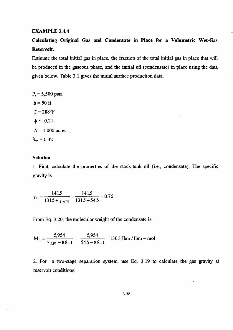
EXAMPLE 3.4.4

Calculating Original Gas and Condensate in Place for a Volumetric Wet-Gas

Resenroir.

Estímate the total initial gas in place, the fraction of the total initial gas in place that will

be produced in the gaseous phase, and the initial oil ( condensate) in place using the data

given below. Table 3.1 gives the initial surface production data.

P¡ = 5,500 psia.

h =50ft

T= 288°F

~ = 0.21.

A= 1,000 acres ..

swi = o.32.

Solution

l. First, calculate the properties of the stock-tank oil (i.e., condensate ). The specific

gravity is

Yo = 141.5 = 141.5 = 0.76 1315+y API 131.5+545

From Eq. 3.20, the molecular weight ofthe condensate is

Mo = 5,954 = y API -8.811

5954 ' = 130.3 lbm 1 lbm -mol

54.5-8.811

2. For a two-stage separation system, use Eq. 3.19 to calculate the gas gravity at

reservoir conditions:

3-58

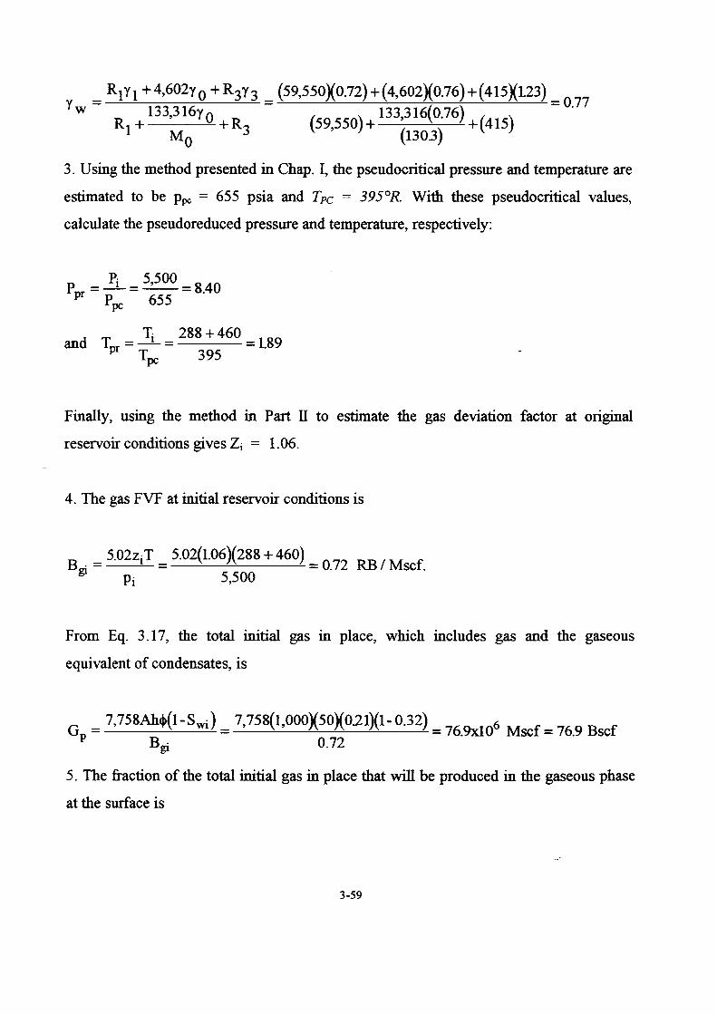
1 = R1r 1 +4,602r 0 +R3r 3 = (59,55oxo.72)+(4,602)(o.76)+(4I5Xt23) =

077 w 133,316y o ( ) 133,316(0.76) ( ) .

R1 + +R3 59,550 + ( ) + 415 M0 1303

3. Using the method presented in Chap. 1, the pseudocritical pressure and temperature are

estimated to be ppc = 655 psia and Tpc = 395°R With these pseudocritical values,

calculate the pseudoreduced pressure and temperature, respectively:

p = P¡ = 5,500 = 8_40 pr P 655

pe

and T. = T¡ = 288 + 460 = 1.89 pr Tpc 395

Finally, using the method in Part II to estimate the gas deviation factor at original

reservoir conditions gives Z¡ = 1.06.

4. The gas FVF at initial reservoir conditions is

Bgi = 5.02z¡T = 5.02{1.06)(288 +460) = 0_72 RB/ Mscf. Pi 5,500

F ro m Eq. 3 .17, the total initial gas in place, which includes gas and the gaseous

equivalent of condensates, is

GP = 7,758Ahcj>(1-Sw¡) = 7,758{1,000X50)(021)(1- 0.32) = 76_9xl06 Mscf = 76_9 Bscf Bgi 0.72

5. The fraction of the total initial gas in place that will be produced in the gaseous phase

at the surface is

3-59

f = Rt g 132,800y 0 Rt +----'--­

Mo

where the total producing GOR is Rt, = R1+R3 = 59,550+415 = 59,965 scf!STB.

Therefore,

59,965 fg = 132 soo( o 76) = 0·99

59,965 + ' o

1303

The volume of surface gas production is

G = fgGT = (0.99)(76.9) = 76.1 Bcf.

6. The original volume of condensate in place is

l,OOO·fgGT 1,000·(0.99X76.9) 6 S B N= = =DrlO T

Rt 59,965 scf 1 STB

3-60

EXAMPLE 3.4.5

Calculating Original Gas in Place Using Material Balance for a Volumetric Dry-Gas

Reservo ir.

Estimate the original gas in place for the reservorr described below usmg the

material-balance equation for a volumetric dry-gas reservoir where the original reservoir

pressure at discovery was p¡ = 4,000 psia. Table 3.2 gives the reservoir pressure and

production history.

Solution

l. First, prepare a plot ofp/z vs. Gp (Fig. 3.6) using the data in Table 3.3 . .

2. Extrapolation of the best-fit line through the data to p/z = O indicates that G = 42

MMscf. Note that, if no measurements of initial reservoir pressure are available, we also

can estimate p¡ from the extrapolation ofthe line to Gp =O. For this example, p¡ = 4,000

psia or p/Z¡ = 5,000 psia.

In addition, the trend of the data (i.e., a straight line) suggests that the reservoir is

volumetric. As mentioned, consistent deviations from a straight line often indicate that

gas expansion is not the predominant reservoir drive mechanism.

3-61

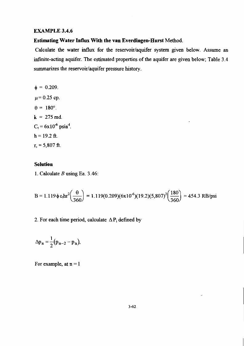
EXAMPLE 3.4.6

Estimating Water Influx With the van Everdingen-Hurst Method.

Calculate the water influx for the reservoir/aquifer system given below. Assume an

infinite-acting aquifer. The estimated properties ofthe aquifer are given below; Table 3.4

summarizes the reservoir/aquifer pressure history.

el> = 0.209.

J..l= 0.25 cp.

e = 180°.

k= 275md.

e = 6x 1 o.Q psia-1•

h = 19.2 ft.

r, = 5,807 ft.

Solution

l. Calculate B using Ea. 3.46:

B = 1.119 cp c.b?(~) = 1.119(0.209)(6x10.Q)(19.2)(5,807)2(

180) = 454.3 RB/psi

360 360

2. For each time period, calculate LlP¡ defined by

F or example, at n = 1

3-62

L\p1 =_!_(p1_2 -p1)=_!_ (3,793- 3,788) = 2.5 psi 2 2

For n = 6,

L\p6 = _!_(P6-2- p6) = _!_ (3, 709- 3,643) = 33.0 psi. 2 2

3. Calculate dimensionless times that correspond to each time on our schedule. Use the

dimensionless time defined by Eq. 3.37 for a radial system:

t = 0.00633kt = 0.00633(275)t = 0.165. t

n c~>J.tctrr2 (o29Xo25~6x1o-6X5,8o7)2

For example, at t = 91.5 days, t0 = 0.165(91.5) = 15.1.

4. For each t0 computed in Step 3, calculate a dimensionless cumulative water influx.

Because we are assuming an infinite-acting aquifer, we can use either Eqs. 3.48 through

3.50 or Table E-4. For this example, we have chosen to use the equations.

The value oft0 determines which equation to use. For example, at 91.5 days (n = 1), t0

= 15.1, so we use Eq. 3.49.

Q (t ) = U838tg2

+ 119328tn + 0.269872t~2 + 0.00855294t~ = pD D 1+0.616599tg2 +0.0413008tn

12838(15.1)112

+ 119328(15.1) + 0.269872(15.1)312

+ 0.00855294(15.1)2

= =101 1+0.616599(15.1)112 +0.0413008(15.1) .

Table 3.5 summarizes the intermediate results from Steps 2 through 4.

3-63

5. Next, calculate We, using Eq. 3.44. Note that, although this calculation procedure

assumes equal time intervals, the method also is applicable for unequal time intervals

with slight modifications.

F or example, at n = 1

Similarly, for n = 6,

We(tnn)= BI;~piQpD(tn -t¡_¡)D = B[~p1QpD(t6 -to)D+I~p2QpD(t6 -t¡)D +~p3QpD(t6 -t- \ 1=1

+~p4QpD(t6 -t3)D +~p5QpD(t6 -t4)D +~p6QpD(t6 -ts)D =

= 454.3[(2.5)(40.0) +(9.5)(34.5) + (20)(29.0)+ (32.5)(23.1) + (34)(17.0) + (33)(10.1)]

= 1,212,890 RB.

6. Table 3.6 summarizes the final results

3-64

EXAMPLE 3.4. 7

Estimating Water Intlux With the Carter-Tracy Method.

Calculate the water influx for the reservoir/aquifer system described in Example 3.6 and

compare the results with those from the van Everdingen-Hurst method. Assume an

infinite-acting aquifer. The properties of the aquifer are given below; Table 3. 7

summarizes the reservoir/aquifer pressure history.

cP= 0.209

J.!= 0.25 cp.

e = 180°.

k= 275 md.

Ct= 6x10-6 psia-1•

h = 19.2 ft.

Tr = 5,807 ft.

Solution.

l. Calculate the parameter B using Eq. 3.46:

B = 1.119cPCtb.?(~) 360

RB/psi.

= 1.119(0.209)(6x 10-6)(19.2)(5,807)2(

180) = 454.3

360

2. For each time perio<L calculate ó.pn defined by Eq. 3.59:

F or example, at n = 1,

3~5

~Pn =paq,i -p1 =3,793-3,788=5 psi

For n = 2,

~Pn =paq,i -p2 =3,793-3,774=19 psi

3. Calculate dimensionless times that correspond to each time on the schedule. Use the

dimensionless time defined by Eq. 3.37 for a radial geomet:ry:

0.00633kt 0.00633{275)t

to = cPJl.Ctr; = (o2o9Xo25X6x1o-{)X5,807)2 = o.165

· t

For example, at t = 91.5 days,

t0 = 0.165(91.5) = 15.1.

4. Calculate dimensionless pressures and pressure derivatives at each of the

dimensionless times computed in Step 3. The dimensionless pressures are calculated with

Eq. 3.60. For example, at

t0 = 15.1,

370529(t0 )112

+ 137582(t0 )+5.69549(t0 f 12

p (t ) = = 0 0 328.834 + 265.488( t 0 Y12

+ 452157( t 0 ) + ( t 0 t'2

37o529(15JY'2

+ 137 582{15.1) + 5.69549{15.If'2

= =183 328.834 + 265.488{15.1)

112 +452157(151) +(15.1)

312

3-66

Similarly, the dimensionless pressure derivatives are calculated with Eq. 3.61. For

example, at t0 = 15.1,

P'o ( to) = 6( )112 )3/2 )2 5/2 = 1,296.8 t0 + 1,204.73(t0 )+ 618.618(t0 + 538.072(t0 + 142.4l(t0 )

716.441 + 46.7984(t0 )112

+ 270.038(t0 )+ 71.0098(t0 f 12

716.441 + 46.7984(15.1)112 + 270.038(15.1) + 71.0098(151f

12

= 1,296.86(151)112 + 1,204.73(15.1) + 618.618(151)312 + 538.072(15.1)2 + 142.41(151)512 =

Table 3.8 summarizes the intermediate results.

5. Calculate the water influx using Eq. 3.58:

F or example, at n = 1,

For n = 2,

_ { B~p1-we1P'o (to2) ] _ we2- we1 +(tD2- tD1 ( ) _ , ( ) -

Po tD2 to1P D tD2

= 18 743 +(15.1J (4543X19)-(18,743XO.l55)] = 84 482 RB ' 'L 2.15 -151(0.0155) '

6. Table 3.9 gives the final results.

3-67

EXAMPLE 3.4.8

Estimating Water lntlux With the Fetkovich Method.

Calculate the water influx for the reservoir/aquifer system described below. Assume a

finite radial aquifer with an area of 250,000 acres and having a no-flow outer boundary.

The estimated aquifer properties are given below; Table 3.11 summarizes the pressure

histmy at the reservoir/aquifer boundary. Note that the aquifer is a sector of a cylinder

where e = 180°.

<P = 0.209.

r, = 5,807 ft

Jl = 0.25 cp.

k= 275 md.

e = 180°.

6 10-6 . -1 Cr = x ps1a .

h = 19.2 ft.

Solution.

l. Calculate the maximum volume of water from the aquifer, W ei, that could enter the

reservoir if the reservoir pressure were reduced to zero. Note that the aquifer shape is a

sector of a cylinder, so the initial volume of water in the aquifer is

n( r; - r; )<Ph( e 1 360) W-=~----~------

1 5.615

where

fa = ( 43,5:0 ·A) ( 3:0) = ( 43,560 )?50,000) ( ~:~) = 83,260 ft

3-68

Therefore,

n(83,2602- 5,8072 X192)(0209)(180 /360) 9 W· = = 7.744x10 RB 1 5.615

From Eq. 3.65,

Wei = CtPaq,¡W¡ = (6x10-ó)(3,793)(7.744x10~ = 176.3x106 RB.

2. Calculate J. For radial flow in an aquifer with a finite no-flow outer bounda.Iy, from

Table 3.10,

J = 0.00708kh(e /360) = (0.00708){275)(192){180/360) = 39.1 STB/ D _psi J.![ ln{ ra 1 rr)- 0.75] 025[ ln( 83,260 /5,807)- 0.75]

3. For each time period, calculate the incremental water influx using Eq. 3.71.

where (from Eq. 3.72)

- ( Wen-1) Paq,n-1 = Paq,i 1- Wei

and from Eq. 3.73,

3-69

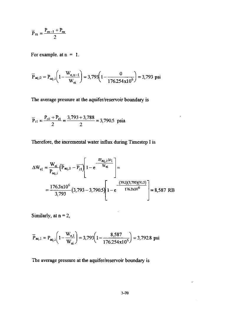
For example. at n = l.

Paqo=Paq¡(1- we,n-1)=3,793(1- o 6)=3,793psi , , wei 176254x10

The average pressure at the aquifer/reservoir boundmy is

P rl = Pro + Pr1 = 3, 793 + 3, 788 = 3, 790.5 psia 2 2

Therefore, the incremental water influx during Timestep 1 is

[

1Paq,iLlt1 ] W·- - w

1:1We1 = ~{Paq,O- Pr1) 1- e ei = Paq,l

[

(39.1)(3,793)(91.5)] = 1763x106 (3 793-3 790.5) 1- e 176.3x106 = 8 587 RB

3 793 ' ' ' '

Similarly, at n = 2,

- ( We 1) ( 8,587 ) . P aq 1 = P aq ¡ 1---' = 3, 793 1- 6 = 3, 792.8 ps1 , , wei 176254x10

The average pressure at the aquifer/reservoir boundmy is

3-70

Pr2 = Prl +Pr2 = 3,788+3,774 3 781 . 2 2

= , psta

Therefore, the incremental water in:tlux during Timestep 1 is

[

1Paq,i~t2 ] ~we2 = wei (Paq,I-Pr2) 1-e Wei =

Paq,i

6 [ (39.1)(3,793)(91.5)] =

1763x

1 0 (3 792.8-3 781) 1- e 176.3xl0

6 = 40 630 RB 3 793 ' ' ' '

4. Calculate the cumulative water in:tlux during each time step. For example, at the end of

the first time step, n = 1

n=l We1 = L~Wei = ~We1 = 8,587 RB

i=l

Similarly, the cumulative water in:tlux at the end ofthe second time step is n = 2

n=2 We2 = Ló.Wei =ó.We1 +~We2 =8,587+40,630=49,217 RB

i=l

Table 3 .12 summarizes the final results.

3-71

EXAMPLE 3.4.9

Estimating Original Gas in Place With Material Balance for a Dry-Gas Reservoir

With Water Intlux.

Estímate the original gas in place and water influx constant using the material balance

equation developed for water influx in a dry-gas reservoir. Assume an unsteady-state,

infinite-acting aquifer. According to McEwen 22, the volumetric estímate of original gas

in place is 200x 106 Mscf. Table 3.13 gives the pressure and production histories; the

estímated aquifer properties are summarized below.

~= 0.24.

Jl= 1.0 cp.

Tr = 3,383 ft.

k= 50 md.

Ct = 6x10-{í psia-1.

e= 360°.

h = 20.0 ft.

Bw =l. O RB/STB.

Solution.

U sing a procedure similar to that illustrated for the van Everdingen and Hurst method,

estímate water influx for each timestep as described below.

l. Calculate 11 P n, where

For example, at n = 1 (i.e., t = 182.5 days),

3-72

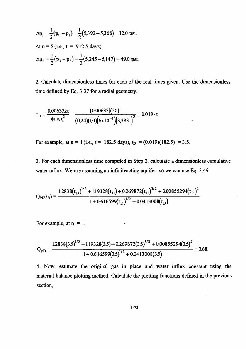
L\p1 =_!_(Po- p1) = _!_(5,392- 5,368) = 12.0 psi. 2 2

At n = 5 (i.e., t = 912.5 days),

L\p5 = _!_(p3 - p5) = _!_(5,245- 5,147) = 49.0 psi. 2 2

2. Calculate dimensionless times for each of the real times given. Use the dimensionless

time defined by Eq. 3.37 for a radial geometry.

tn = 0.0063~kt = (0.00633)(50)t 2

= 0_019 .1 ci>J.!ctrr (024)(toX 6x1o-<í)(3,383 )

For example, at n = 1 (i.e., t = 182.5 days), t0 = (0.019)(182.5) = 3.5.

3. F or each dimensionless time computed in Step 2, calculate a dimensionless cumulative

water influx. We-are assuming an infiniteacting aquifer, so we can use Eq. 3.49.

U838(t0 Y12 + 119328(t0 )+0269872(t0 f12

+0.00855294(t0 )2

Qpo(to) =----------:--:-:o------------1 + 0.616599(t0 )

112 + 0.041300s(t0 )

F or example, at n = 1

12838(3.5)112

+ 119328(3.5) + 0269872(3.5)312

+ 0.00855294(3.5)2

Q = =368 pD 1+0.616599(3.5t2 +0.0413008(3.5) . .

4. Now, estimate the original gas in place and water influx constant using the

material-balance plotting method. Calculate the plotting functions defined in the previous

section,

3-73

where f(p,t) = 1:~pQpD·

For example, at n = 1 the plotting function for the vertical axis, y, is

G s + w sw (677.7x1o3Xo.6796)+(3)(to) 6 y= P( 8 P) = ( · ) = 2.913x10 Mscf = 219.3 Bscf Bt - Bgi 0.6796- 0.6775

The plotting function for the horizontal axis, x, is

L ~ Q D {12){3.68) y= P P = = 21x103 Mscf

(st -sgi) (0.6796-0.6775)

5. The material-balance plotting functions, summarized in Table 3.14, are plotted in Fig.

3.11.

6. From the slope of the line through the data points in Fig. 3 .11, e is estimated to be

1195 RB/psi, and the original gas in place estimated from the intercept is G = 197 Bscf =

197 x 106 Mscf, which agrees with the volumetric estimate of G = 200x 106 Mscf.

The general problem that reservoir engineers face when analyzing gas reservoirs with

water in:flux is simultaneous determination of G, e, aquifer size or an aquifer/reservoir

size ratio, ralrr, and the relationship between real time, t, and dimensionless time, t0 .

Simultaneous determination of these variables that best fit a pressure/production history is

a complex problem in regression analysis.

3-74

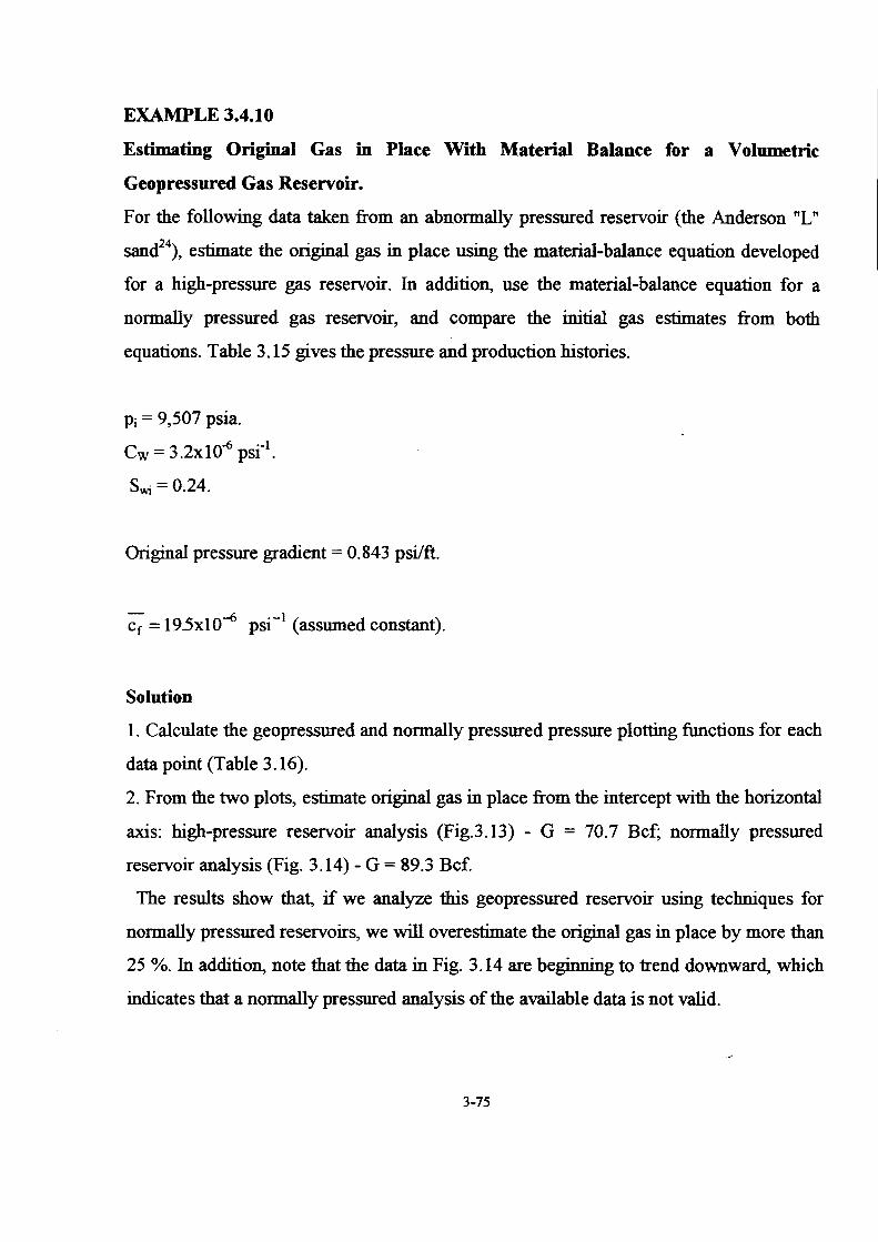
EXAMPLE 3.4.10

Estimating Original Gas in Place With Material Balance for a Volumetric

Geopressured Gas Reservoir.

For the following data taken from an abnormally pressured reservoir (the Anderson "L"

sand24), estímate the original gas in place using the material-balance equation developed

for a high-pressure gas reservoir. In addition, use the material-balance equation for a

normally pressured gas reservoir, and compare the initial gas estímates from both

equations. Table 3.15 gives the pressure and production histories.

p¡ = 9,507 psia.

Cw = 3.2x10-6 psr1.

swi = o.24.

Original pressure gradient = 0.843 psi/ft.

cr = 195x10-6 psi-1 (assumed constant).

Solution

l. Calculate the geopressured and normally pressured pressure plotting functions for each

data point (Table 3.16).

2. From the two plots, estímate original gas in place from the intercept with the horizontal

axis: high-pressure reservoir analysis (Fig.3.13) - G = 70.7 Bcf; normally pressured

reservoir analysis (Fig. 3.14)- G = 89.3 Bcf.

The results show that, if we analyze this geopressured reservoir using techniques for

normally pressured reservoirs, we will overestímate the original gas in place by more than

25 %. In addition, note that the data in Fig. 3.14 are beginning to trend downward, which

indicates that a normally pressured analysis of the available data is not valid.

3-75

W e developed the material-balance equation for a high-pressure gas reservo ir using a

single value for formation compressibility over the life of the reservoir. In reality,

formation compressibility may vary during pressure depletion, especially at the highest

pressures. Further, the previous derivation assumed that values for formation

compressibility are readily available. However, these values are very difficult to measure

accurately in the laboratory, especially as a function of changes in pore pressure.

Therefore, in the next section, we present a graphical technique for simultaneously es­

timating original gas in place and an average value of formation compressibility.

3-76

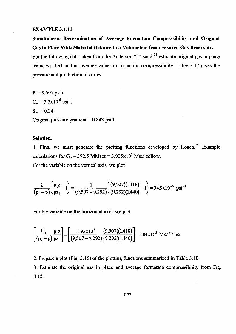
EXAMPLE 3.4.11

Simultaneous Determination of Average Formation Compressibility and Original

Gas in Place With Material Balance in a Volumetric Geopressured Gas Resenroir.

For the following data taken from the Anderson "L" sand, 24 estimate original gas in place

using Eq. 3.91 andan average value for formation compressibility. Table 3.17 gives the

pressure and production histories.

P¡ = 9,507 psia.

Cw = 3.2x10-6 psr1.

swi = o.24.

Original pressure gradient = 0.843 psilft.

Solution.

l. First, we must generate the plotting functions developed by Roach. 25 Example

calculations for Gp = 392.5 MM:scf= 3.925x105 Mscffollow.

F or the variable on the vertical axis, we plot

1 (p¡z -l) = 1 ((9,507)(1418) 1) = 34 9xlO-Q psCl (p¡-p) pz¡ (9,507-9,292) (9,292X1440) ·

F or the variable on the horizontal axis, w.e plot

[ GP p¡z] = [ 3.92x10

5 (9,507)(1418)] = 184x103 Mscf 1 psi

(p¡- p) PZ¡ (9,507- 9,292) (9,292X1.440)

2. Prepare a plot (Fig. 3.15) ofthe plotting functions summarized in Table 3.18.

3. Estimate the original gas in place and average formation compressibility from Fig.

3.15.

3-77

A. The original gas in place, G, is estimated from the slope of the line, m:

_!_ = slope = 13.3xl0-6 (:MMscf)-1,

G

or G = 1/(13.3xl0-6) = 75 ,190 MMscf.

Note that, in Example 3.10, we estimated the original gas in place assuming an average

value of formation compressibility, while in this example we calculated the original gas

in place and formation compressibility simultaneously. As a result, the two estim.ates of

gas in place are slightly different.

B. The average formation compressibility is determined from the intercept ofthe line. b:

[e S . +cr] -6 ·-1 [(3.2x1o-6X0.24)+cr] b=- w Wl =-185x10 pst =- ~--=---...!.___ __ _

1- swi (1- o.24)

The data plotted in Fig. 3.15 do not lie completely on a straight line. Poston and Chen26

concluded that, initially, most of the formation resistance to the overburden pressure is

provided by the fluids in the pore spaces. However, as fluids are withdrawn from these

pore spaces, the formation compacts, resulting in more resistance to the overburden being

transferred to the rock matrix. Under these conditions, the formation compressibility is

not a constant but changes with time, as indicated by the initial nonlinear portion of the

data in Fig. 3.15.

3-78

3.4SUMMARY

Reading this chapter should prepare you to do the following.

l. Calculate original gas in place in a volumetric dry-gas reservoir using volumetric

methods.

2. Calculate gas reserves and recovery factor for a gas reservoir with water influx using

volumetric methods.

3. Calculate original gas in place and condensate in place for a volumetric wet-gas

reservoir using volumetric methods.

4. State the principie of conservation of mass and derive a general material-balance

equation from that principie.

5. Calculate original gas in place using material balance for a volumetric dry-gas

reservorr.

6. Estímate water influx using the van Everdingen-Hurst, Carter Tracy, and Fetkovich

methods and state the assumptions and limitations of each method.

7. Estímate original gas in place using material balance for a dry-gas reservoir with

water influx.

8. Estímate original gas in place using material balance for a volumetric geopressured

gas reservorr.

9. Determine average formation compressibility and original gas in place simultaneously

using material balance in a volumetric geopressured gas reservoir.

10. Derive material-balance relationships for volumetric gascondensate reservorrs,

gas-condensate reservoirs with water vaporization, gas-condensate reservoirs with

depletion at pressures above the dewpoint, and gas-condensate reservoirs with

depletion at pressures below the dewpoint.

3-79

Questions for Discussion

l. Y our company is planning to drill a wildcat well in an area believed to have great

potential for natural gas. In planning for the well ( and assuming gas is discovered), what

data should be gathered? Why?

2. The well does discover gas. Using information from the discovery well alone, you are

asked to estimate reserves and forecast future production. What methods will you use?

What additional data will you need?

3. Several additional wells are planned. What sort of information should be obtained from

these wells? Why?

4. Two years after the discovery well was drilled, the field is highly developed. You are

again asked to estimate reserves and forecast future production. What methods will you

use? What data will you need?

5. How would your strategy be affected if the reservoir is geopressured? Is a retrograde

gas reservoir Has a waterdrive? Is the gas cap of a oil reservoir, a fact discovered only

much later? How can you determine whether any of these possibilities is a fact?

6. How would you determine optimal well spacing? Optimal depletion plan? In answer to

both these questions, what data would you need, and what study methods would you use?

7. What are the potential errors in the volumetric method? The materiall-balance method?

8. What are typical recovecy factors for yolumetric gas reservoirs? How may we estimate

abandonment pressure to calculate recovery factor? At what point does abandonment

pressure enter the recovery factor calculation?

9. Compare typical recoveries in waterdrive gas reservoirs with those from volumetric gas

reservoirs and explain the reasons for the difference.

10. Explain two methods for improving the recovery from waterdrive gas reservoirs.

11. Describe the different types of aquifer that may be in association with a reservoir.

12. How does the aquifer offset pressure decline in the reservoir?

3-80

13. If the time elapsed sin ce production began doubled, do yo u think the amount of water

influx into a gas reservoir would double? Or would it be more or less than double? Why?

If additional information is required to answer this question, what is that additional

information?

3-81

N omenclature

A = well drainage area, L2, acres

b = intercept

B = van Everdingen-Hurst constant, RB/psi

B8 = gas FVF, RB/Mscf

B8a = gas FVF at reservoir abandonment pressure and temperature conditions, RB/Mscf

Bgi = gas FVF at initial reservoir pressure and temperature, RB/Mscf

Bw = water FVF, RB/STB

B2g = gas FVF based on two-phase gas deviation factor, RB/Mscf

B2gi = gas FVF based on two-phase gas deviation factor at initial reservoir pressure and

temperature, RB/Mscf

C = water influx constant from material-balance calculations, RB/psi

Ce = in-situ formation compressibility, Lr/m, psia-1

Ct = total aquifer compressibility, Cr +Cw, Lr/m, psia-1

Cw =water compressibility, Lr/m, psia-1

Ev = volwnetric sweep efficiency, fraction

fg = fraction of reservoir gas produced as liquid at surface, fraction

F = gas recovery factor

G = original gas in place, L3, Mscf

Ga =gas in place at reservoir abandonment, L3, Mscf

Gp = cumulative gas production, L3, Mscf

Gpa = additional gas production from secondary separator and stock tank, L3/L3, scf/STB

GPT = cumulative gas production from primary and secondary separators, stock tank, and

the gaseous equivalent of produced condensates, L3, Mscf

GpT = cumulative gas production from primary separator, L3, Mscf

Gp2 = cumulative gas production from secondary separator, L3, Mscf

3-82

Gp3 = cumulative gas production from stock tank, L3, Mscf

Gt = reservoir volume occupied by gas-trapped by encroaching water, L3, Mscf

GT = total initial gas in place, including gas and gaseous equivalent of produced

condensates, L3, Mscf

h = net formation thickness, L, ft

J = aquifer PI, L3t/m, STB/D-psi

k = reservoir permeability, L2, md

L = length of linear-shaped reservoir, L, R

m = slope

Mo = molecular weight of stock tank liquids, m, 1 b m/ lb m- mol n = number of moles

ofgas

N =original oil (condensate) in place, L3, STB

NP = cumulative oil (condensate) production, L3, STB p = reservoir pressure, m!Lr, psia

Pa = abandonment pressure, m!Lr, psia

paq = aquifer pressure, m!Lr, psia

P aqi = initial aquifer pressure, m/Lt2, psia

P d = dewpoint pressure of gas-condensate reservoir, m/Lr, psia

Po = dimensionless pressure

Po = dimensionless pressure derivative

p¡ = initial reservoir pressure, m/Lt2, psia

Pn = pressure at time interval n, m/Lr, psia

Pr = pressure at aquifer/reservoir interface, m!Lr, psia

P se = pressure at standard conditions, m/Lt2, psia

Ap = difference between initial aquifer pressure and pressure at original reservoir/aquifer

boundary. m!Lr, psia

q0 = dimensionless water influx rate

qw =water influx rate, L3/t, STB/D

Qp0 = dimensionless cumulative water influx

3-83

ra = radius of aquifer, L, ft

re = outer radius of reservoir, L, ft

rr = radius to aquifer/reservoir interface, L, ft

R =universal gas constant, 10.73 psia-ffllbm-mol-0 R

Rt =total gas/stock-tank liquid ratio, scf!STB

R.¡ =ratio ofhigh-pressure separator gas volume to stocktank liquid volume, L3/L3,

scf/STB

R2 =ratio oflow-pressure separator gas volume to stocktank liquid volume, L3/L3,

scf/STB

R3 = ratio of stock-tank gas volume to stock-tank liquid volume, L3 /L3, scf/STB

sgi = initial gas saturation, fraction

Sgr = residual gas saturation, fraction

So = condensate saturation, fraction

Sw = connate water saturation, fraction

Swa = water saturation at abandonment conditions, fraction

Swi = initial connate water saturation, fraction t = time, t, days

t0 = dimensionless time

T = reservoir temperature, T, 0 R

T se = temperature at standard conditions, T' 0 R

V cq =vapor equivalent ofprimai)' separator liquid, L3/ L3

, scf!STB

Vr = reservoir formation (rock) volume,. L3, res bbl

V gf =gas volume at initial conditions, L3, res bbl

VhL = volume ofhydrocarbon liquids, L3, res bbl

Vhv = volume ofhydrocarbon vapors, L3, res bbl

Vhvi = initial volume ofhydrocarbon vapors, L3, res bbl

VP = reservoir PV, L3, res bbl

V pi = initial reservoir PV, L3, res bbl

V se =gas volume at standard conditions, L3, res bbl

3-84

Vv = volume ofvapor phase, L3, res bbl

V vi = initial volume of vapor phase, L3, res bbl

Vw = volume ofwater, L3, res bbl

V wi = initial volume of water, L 3, res bbl

V w = volume of water vapor phase, L3, res bbl

V wvi = initial volume of water vapor phase, L3, res bbl

!). Vr= change in reservoir formation (rock) volume, L3, res bbl

!). V w = change in water volume, L 3, res bbl

w = width of linear reservoir, L, R

We = cumulative water influx volume, L3, res bbl

Wei = initial "encroachable" volume ofwater in aquifer, L3, res bbl

W¡ = initial volume ofwater in aquifer, L3, res bbl

WP = cumulative water production, L3,STB

Y w = fraction of total vapor-phase volume that is water

Y wi = initial fraction of total vapor phase volume that is water

z =gas compressibility factor, dimensionless

Za = gas compressibility factor at abandonment, dimensionless

Z¡ =gas compressibility factor evaluated at initial conditions, dimensionless Z,c =gas

compressibility factor at standard conditions, dimensionless

z2 = two-phase gas compressibility factor, dimensionless

Z2¡ = two-phase gas compressibility factor evaluated at initial conditions, dimensionless

y 0 = specific gravity of condensate (water= LO glcm3)

y g = specific gravity of reservoir gas at reservo ir eonditions ( air = l. O)

y1 = speeific gravity ofhigh-pressure separator gas (air = LO)

y 2 = speeific gravity oflow-pressure separator gas (air = LO)

y 3 = speeific gravity of stock-tank gas (air = LO)

e = angle encompassed by aquifer, degrees

3-85

'A = dununy integration variable for Eq. 10.57

~ = viscosity, m!Lt, ep

~ = Porosity, fraction

Subscript

aq = aquifer

Superscript

=average

3-86