http://www.econometricsociety.org/ Econometrica, Vol. 80, No. 6 (November, 2012), 2469–2509 CAPITAL MOBILITY AND ASSET PRICING DARRELL DUFFIE Graduate School of Business, Stanford University, Stanford, CA 94305, U.S.A. BRUNO STRULOVICI Northwestern University, Evanston, IL 60208, U.S.A. The copyright to this Article is held by the Econometric Society. It may be downloaded, printed and reproduced only for educational or research purposes, including use in course packs. No downloading or copying may be done for any commercial purpose without the explicit permission of the Econometric Society. For such commercial purposes contact the Office of the Econometric Society (contact information may be found at the website http://www.econometricsociety.org or in the back cover of Econometrica). This statement must be included on all copies of this Article that are made available electronically or in any other format.

Welcome message from author
This document is posted to help you gain knowledge. Please leave a comment to let me know what you think about it! Share it to your friends and learn new things together.
Transcript
http://www.econometricsociety.org/
Econometrica, Vol. 80, No. 6 (November, 2012), 2469–2509
CAPITAL MOBILITY AND ASSET PRICING
DARRELL DUFFIEGraduate School of Business, Stanford University, Stanford, CA 94305, U.S.A.
BRUNO STRULOVICINorthwestern University, Evanston, IL 60208, U.S.A.
The copyright to this Article is held by the Econometric Society. It may be downloaded,printed and reproduced only for educational or research purposes, including use in coursepacks. No downloading or copying may be done for any commercial purpose without theexplicit permission of the Econometric Society. For such commercial purposes contactthe Office of the Econometric Society (contact information may be found at the websitehttp://www.econometricsociety.org or in the back cover of Econometrica). This statement mustbe included on all copies of this Article that are made available electronically or in any otherformat.
Econometrica, Vol. 80, No. 6 (November, 2012), 2469–2509
CAPITAL MOBILITY AND ASSET PRICING
BY DARRELL DUFFIE AND BRUNO STRULOVICI1
We present a model for the equilibrium movement of capital between asset marketsthat are distinguished only by the levels of capital invested in each. Investment in thatmarket with the greatest amount of capital earns the lowest risk premium. Intermedi-aries optimally trade off the costs of intermediation against fees that depend on the gainthey can offer to investors for moving their capital to the market with the higher meanreturn. The bargaining power of an investor depends on potential access to alternativeintermediaries. In equilibrium, the speeds of adjustment of mean returns and of capitalbetween the two markets are increasing in the degree to which capital is imbalancedbetween the two markets, and can be reduced by competition among intermediaries.
KEYWORDS: Capital mobility, market frictions, financial intermediation, law of oneprice.
1. INTRODUCTION
WE PRESENT A MODEL for the equilibrium movement of capital between twopartially segmented markets that are identical except for the amounts of capi-tal invested in each. Equilibrium conditional mean rates of return vary acrossthe markets according to the levels of capital invested in the respective mar-kets. As a matter of supply and demand within each market, that market withthe greater amount of capital earns lower conditional mean returns. Given asufficient disparity in the capital levels in the markets, intermediaries find itoptimal to search for investors in the market with “surplus” capital and offerthem the opportunity to move their capital to the other market, which offershigher risk premia. Intermediaries charge investors a fee that is based on theirgain from the move and based on the degree of competition in the market forintermediation. The equilibrium behavior of intermediaries is solved analyti-cally, and characterized. Increased competition among intermediaries can insome cases reduce capital mobility.
In our equilibrium model, the greater the heterogeneity in capital levelsacross the markets, the more intensive are intermediaries’ efforts to rebalancethe distribution of capital across the markets, and the greater is the rate ofconvergence of the mean rates of return of different assets toward a common
1We are grateful for reactions at Oxford University, the Gerzensee European Summer Sym-posium in Financial Markets, the University of Toulouse, The London School of Economics,London Business School, Yale University, NBER Asset Pricing Conference, Columbia Univer-sity, Northwestern University, and especially for comments from Bruno Biais, Eddie Dekel, JulienHugonnier, Jean-Charles Rochet, Larry Samuelson, Avanidhar (Subra) Subrahmanyam, Jean Ti-role, Dimitri Vayanos, and Glen Weyl. The advice of the editor and several anonymous refereeswas very useful. We are thankful for the research assistance of Sergey Lobanov and Felipe Veras.Strulovici acknowledges financial support from the National Science Foundation Grant 1151410.
© 2012 The Econometric Society DOI: 10.3982/ECTA8822
2470 D. DUFFIE AND B. STRULOVICI
level. We study the impact on capital mobility of search costs, discounting, assetvolatility, and other parameters.
This model is motivated by empirical evidence, some of which is reviewedin the last section. The evidence is that supply or demand shocks in asset mar-kets, in addition to causing an immediate price response, also lead to adjust-ments over time in the distribution of capital across markets and adjustmentsover time in relative conditional mean asset returns. This asset price behaviorreflects delays in the adjustments of investors’ portfolios. We are particularlyinterested in how those adjustments are affected by the behavior of intermedi-aries.
An example is the limited mobility of capital into reinsurance markets, doc-umented by Froot and O’Connell (1999), who wrote: “Our results suggest thatcapital market imperfections are more important than shifts in actuarial val-uation for understanding catastrophe reinsurance pricing. Supply, rather thandemand, shifts seem to explain most features of the market in the aftermathof a loss.” In subsequent work, Froot (2001) continued: “We � � � find the mostcompelling (evidence) to be supply restrictions associated with capital marketimperfections and market power exerted by traditional reinsurers.”
A significant body of theory examines the implications of search frictions forasset pricing. For example, differences in search frictions across different assetmarkets were treated by Weill (2008) and Vayanos and Wang (2007). Duffie,Gârleanu, and Pedersen (2005) studied the implications of search frictions ina single asset market with market making. In the context of a single asset mar-ket, Duffie, Gârleanu, and Pedersen (2007) and Lagos, Rocheteau, and Weill(2011) modeled recoveries in mean returns after a shock to the preferencesof investors, corresponding to a gradual reallocation of the asset to more suit-able investors, rather than by cross-market capital dynamics as here. Earliersearch-based models of intermediation include those of Rubinstein and Wolin-sky (1987), Bhattacharya and Hagerty (1987), Moresi (1991), Gehrig (1993),and Yavas (1996).
Related work on the implications of capital market frictions for asset pric-ing dynamics includes the models of Basak and Croitoru (2000) and He andKrishnamurthy (2012). In terms of some objectives and model features, inde-pendent work by Gromb and Vayanos (2012) is closely related to ours. Com-mon to our models, local hedgers are immobile, while arbitrageurs can workacross markets, driving returns toward fundamental levels, subject to frictionsthat prevent them from perfectly equating returns in the two markets. Our re-spective approaches, however, are quite different. We focus on the dynamicsof intermediation, capital movements, and risk premia.
We offer a quick synopsis of the model and results. In each of two marketsthat are partially segmented from each other, a continuum of risk-neutral in-vestors earn a mean rate of return that is strictly decreasing in the total amountof capital invested in that market. Segmentation of the two markets arisesfrom the limited capacity of intermediaries to contact individual investors in
CAPITAL MOBILITY AND ASSET PRICING 2471
the “over-capitalized” market and arrange for the movement of their capitalto the “under-capitalized” market, where they can currently earn higher re-turns. Intermediaries charge investors a fee for this service. The fee is a frac-tion of the gain in present value of future net payoffs to the investor that isachieved by the reallocation of capital. The investor and intermediary bear inmind that, due to the lack of perfect correlation in the future investment re-turns in the two markets, the market that is currently relatively over-capitalizedmay later become relatively under-capitalized, at which point the investor willwish to reallocate his or her capital to the original market, and so on. Interme-diation costs are increasing in the effort made to contact investors. For eachinvestor, the conditional mean arrival intensity of contacts with the interme-diary is strictly increasing in the effort of the intermediary. Intermediaries areassumed to be unable to commit to their future intermediation effort policy.In equilibrium, naturally, intermediation efforts are increasing in the degreeto which capital is imbalanced across the two markets. Thus, the differencein the conditional mean returns of the two markets is mean-reverting. In thesimplest parametric examples that we consider, intermediation efforts are min-imal whenever the ratio of capital in the over-capitalized market to capital inthe under-capitalized market is below a threshold that is characterized analyt-ically, and is maximal otherwise.
We are particularly interested in the impact of competition among interme-diaries on the equilibrium degree of capital mobility, through two channels.First, an intermediary does not internalize the entire impact of its search efforton leveling the distribution of capital across markets because each interme-diary gets only a fraction of the aggregate intermediation fees. This promptsintermediaries to search more as the number of intermediaries increases, allelse equal. Competition among intermediaries has a second and potentiallyoffsetting effect on capital mobility through the impact of fee bargaining onincentives to intermediate. We outline a model in which, as the number of in-termediaries increases, but aggregate search capacity is kept constant, the bar-gaining power of each intermediary is reduced. We show that the second effectof competition, through reduced bargaining power, can dominate, so that insome cases increasing the number of intermediaries reduces capital mobility.
Section 2 describes the market setting. Sections 3 and 4 analyze the monopo-listic and oligopolistic intermediation cases, respectively. Section 5 summarizesthe implications of our model for asset-price dynamics and provides some evi-dence regarding the premise or implications of our model. Proofs and severalextensions of the model are found in the appendices. Appendices D through Lare located in Duffie and Strulovici (2012), the Supplemental Material to thispaper.
2. THE MARKET SETTING
This section presents a stylized model for the endogenous adjustment of cap-ital and risk premia across markets. There are three types of agents: (i) local
2472 D. DUFFIE AND B. STRULOVICI
hedgers; (ii) investors who provide risk-bearing to hedgers in each of two lo-cal markets; and (iii) intermediaries (such as asset managers) who provide thefee-based service to investors of moving capital from one market to another.
We fix a probability space (Ω�F�P) and a common information filtration{Ft : t ∈ [0�∞)} satisfying the usual conditions.2
In each of two financial markets, labeled a and b, a continuum (a non-atomicmeasure space) of local risk-averse agents own short-lived risky assets. These“hedgers” are not mobile across markets. They can be viewed in this respectas relatively unsophisticated in the use of cross-capital-market transactions,or as having high transactions costs for trading outside of their local markets.A continuum of investors that supply capital have access to cross-market trad-ing, subject to intermediation frictions to be described. These suppliers of cap-ital are risk-neutral, and are therefore willing to invest in the risky assets thathedgers sell, provided the risk premium is strictly positive. In an insurance con-text, one might think of these suppliers of capital as stylized versions of the“Names” that supply risk-bearing capacity to the insurance market known as“Lloyd’s of London.”
The total levels of capital available in the two markets at time t are Xat andXbt , respectively. Capital can be reinvested continually in time, at the discre-tion of each investor, in the short-lived assets that are continually made avail-able for sale by hedgers. Each unit of capital that is currently invested in marketi at time t is paid cash at the equilibrium dividend rate π(Xit), where π(·) is astrictly decreasing continuous function. The dividend rate π(Xit) is continuallyreset in double auctions at which the supply and demand for the asset in mar-ket i are matched at each point in time. In Appendix D, we provide an examplein which π(x) is the equilibrium insurance premium in a market with x unitsof insurance capital.
In return for the dividend rate π(Xit), the provider of each unit of capital inmarket i agrees to absorb proportional losses of capital at loss events that ar-rive according to a Poisson process. The proportional losses of different eventsare independently and identically distributed. That is, the cumulative propor-tional loss in market i is a compound Poisson process ρi. (We later extend someof our basic results to allow ρi to be a general Lévy process, allowing, for ex-ample, some role for the diffusive action of Brownian motions.) One unit ofcapital invested at time t therefore pays the supplier of capital 1 +π(Xit) dt attime t + dt, in the usual “instantaneous” sense, if there is no loss event, and ifthere is a loss event, has a recovery value of 1 + �ρit , where �ρit is the jumpsize. The jumps of ρi are bounded below by −1, preserving limited liability. Theloss events have a mean arrival rate η and a loss-size distribution ν with meanν, so the mean loss rate is ην. The risk-neutral investors therefore optimallysupply all of their local capital inelastically so long as the mean rate of return
2See, for example, Protter (2004) for the usual conditions and for other standard properties ofstochastic processes to which we refer.
CAPITAL MOBILITY AND ASSET PRICING 2473
π(x) − ην is strictly larger than their time preference rate r. This necessarycondition on an equilibrium cash payout function π(·) is satisfied in the casesthat we examine, as indicated in Appendix A.
Cash payouts to investors are not reinvested into the capital pool. This as-sumption simplifies the model, as it implies homogeneous capital dynamics.This treatment of cash payouts is typical of asset-management contracts usedby private-equity partnerships.
We assume that ρa = εa + εc and ρb = εb + εc , where the market-specificcompound-Poisson processes εa and εb are independent and have the samedistribution. The independent component εc is common to the two markets.This symmetry simplifies the calculation of an equilibrium and has the furtherillustrative advantage that any differences in the conditional expected returnsin the two markets are due solely to differences in the capital levels of themarkets. We briefly discuss the asymmetric case in Section 5.
If there were no capital-market frictions, investors would instantly move cap-ital between the markets so as to obtain the higher dividend rate, and in doingso would equate the dividend rates π(Xat) and π(Xbt), and thereby equateXat
and Xbt at all times. Indeed, given the symmetrically distributed returns of thetwo markets, investors would do so even if they were risk-averse, provided thatthey have no other hedging motives.
Frictions in the movement of capital may, however, lead to unequal levelsof capital in the two markets, and therefore unequal mean rates of return. If,for example, Xat <Xbt� then the conditional excess mean rate of return of therisky asset in market a exceeds that in market b by π(Xat)− π(Xbt), despitethe identical idiosyncratic and systematic risks of the two assets. Whichevermarket has “too much capital” receives the lower risk premium.
An investor chooses how to deploy reinvested capital between the two mar-kets, subject to the available trading technology. Letting Ct denote the net cu-mulative amount of capital moved by a particular investor from market a intomarket b through time t, this investor’s capital levels, W C
at in market a and W Cbt
in market b, thus satisfy
dW Cat =W C
at− dρat − dCtand
dW Cbt =W C
bt− dρbt + dCt�where W C
it− = lims↑t W Cit is the level of capital “just before” time t. Capital can
be moved only when in contact with an intermediary, as will be explained.A model for a proportional intermediation-fee process K will be determinedin equilibrium. An investor is infinitely lived, and thus has a utility of
E
(∫ ∞
0e−rt([W C
at π(Xat)+W Cbt π(Xbt)
]dt −Kt− d|C|t
))�
2474 D. DUFFIE AND B. STRULOVICI
where |C|t denotes the total variation of C up to time t. For simplicity, we haveassumed that transactions costs are paid directly by investors, and not deductedfrom the capital moved from market to market.
Because there is a continuum of investors, each takes as given the total cap-ital processes Xa and Xb of the respective markets.
Intermediaries contact investors in order to profit from fees for moving theircapital from one market to another. The intermediation fee is a fraction q ofthe gain in present value to an investor associated with redeploying the in-vestor’s capital. For now, we take this bargaining power q as an exogenousparameter. We endogenize q in Section 4 for the case of multiple intermedi-aries.
Conditional on the intensity process λ for contacts of investors by intermedi-aries, investors are contacted pairwise independently3 at the conditional meanrate λt . An intermediary’s rate of cost for applying contact intensity λt is cλt ,for some technological cost coefficient c ≥ 0. For example, doubling the ex-pected rate at which investors are contacted costs the intermediary twice asmuch.4 The maximum feasible contact intensity of the market is some constantλ > 0�
The utility of an intermediary is the expected present value of intermedia-tion fees net of intermediation costs. The intermediary maximizes this utilitywith respect to the choice of intensity process λ. In the next section, we formal-ize this maximization problem in the context of a monopolistic intermediary,in a Markov equilibrium setting. Later, we show how the solution of the mo-nopolistic case can be exploited to more easily address the case of oligopolisticintermediaries.
In the final section, we explain that our results extend easily to handle therandom arrival and departure of capital suppliers, and to allow capital suppli-ers to use their own personal technologies for trading, in addition to obtainingintermediation services.
3. THE MONOPOLISTIC CASE
We begin with the case of a monopolistic intermediary. We restrict attentionto the illustrative example of an insurance market in which each loss eventaffects only one of the two markets and results in a total loss of capital (ν = 1).Appendices treat more general cases, including partial recovery, loss eventsthat can affect both markets simultaneously, as well as proportional losses andgains that are based on Brownian motion.
3That is, conditional on the path {λt : t ≥ 0} of the intermediation intensity process, the timesof contacts of any distinct pair of investors, i and j, are the event times of independent Poissonprocesses Ni and Nj with the common time-varying intensity process λ.
4This can be viewed as a contact technology in which the intermediary adjusts a “broadcast”intensity, for example adjusting the rate of purchase of advertisements or other forms of market-wide intermediation efforts. This differs from a model in which, for example, contacting twice asmany individuals at a given intensity costs twice as much.
CAPITAL MOBILITY AND ASSET PRICING 2475
3.1. Equilibrium
We will define and characterize equilibria in which the intermediation in-tensity is of the symmetric Markov form λt =Λ(Xt�Yt)� for some measurablepolicy function Λ : R2
+ → [0� λ], where
Xt = max(Xat�Xbt)�
Yt = min(Xat�Xbt)�
In equilibrium, at any time, only investors in that market with greater capi-tal agree to have any of their capital moved to the other market. Because aninvestor has linear preferences, it is optimal when contacted to move either nocapital or all capital to the other market.5
In a manner similar to that of Weill (2007), the exact law of large numbersallows us to calculate the aggregate rate of movement of capital. We let Waj(t)and Wbj(t) denote the levels of capital in markets a and b, respectively, of in-vestor j at time t. Letting m(·) denote the non-atomic measure over the spaceof investors, the total rate at which capital is moved from market a to marketb is almost surely6
∫λt1{Xat>Xbt }Waj(t)dm(j)= λt1{Xat>Xbt }
∫Waj(t)dm(j)
= λt1{Xat>Xbt }Xat�
Likewise, the rate at which capital moves from market b to market a isλt1{Xbt>Xat }Xbt�
The continuation value of an investor per unit of capital in the market withexcess capital can be represented as G(Xt�Yt), for some G : R2
+ → [0�∞), andlikewise for the present value H(Xt�Yt) of each unit of capital in the under-capitalized market.
These values, defined from primitive stochastic processes in Appendix A,include the effects of future movements of capital to a market that is under-capitalized and, once that market becomes over-capitalized, back to the othermarket, and so on. Assuming differentiability, which we will verify in equilib-rium, Itô’s formula implies that G and H are characterized as solutions to the
5If he or she has any capital in the market with more total capital, then all of this investor’scapital will be moved, provided the proportional transaction-costs process K is not too large, andthis is the case in any equilibrium for our model, as we shall see once the model is completelyspecified. Thus, although we allow that a given supplier of capital may initially have nonzerocapital in both markets, all of his or her invested capital will optimally be held in just one of thetwo markets at any time after the first time of contact with an intermediary.
6Sun (2006) showed that the probability space, the agent space, and the measurable subsetsof their product can be constructed so as to satisfy the exact law of large numbers. With this, thetotal quantity of contacts of agents by intermediaries up to time t is
∫Nit dm(i)= ∫ t
0 λs ds almostsurely.
2476 D. DUFFIE AND B. STRULOVICI
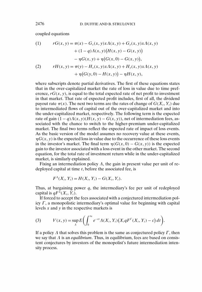
coupled equations
rG(x� y)= π(x)−Gx(x� y)xΛ(x� y)+Gy(x� y)xΛ(x� y)(1)
+ (1 − q)Λ(x� y)(H(x�y)−G(x�y))−ηG(x� y)+η(
G(x�0)−G(x�y))�rH(x� y)= π(y)−Hx(x� y)xΛ(x� y)+Hy(x� y)xΛ(x� y)(2)
+η(G(y�0)−H(x�y)) −ηH(x� y)�
where subscripts denote partial derivatives. The first of these equations statesthat in the over-capitalized market the rate of loss in value due to time pref-erence, rG(x� y), is equal to the total expected rate of net profit to investmentin that market. That rate of expected profit includes, first of all, the dividendpayout rate π(x). The next two terms are the rates of change ofG(Xt�Yt) dueto intermediated flows of capital out of the over-capitalized market and intothe under-capitalized market, respectively. The following term is the expectedrate of gain (1 − q)Λ(x� y)(H(x� y)−G(x�y)), net of intermediation fees, as-sociated with the chance to switch to the higher-premium under-capitalizedmarket. The final two terms reflect the expected rate of impact of loss events.As the basic version of the model assumes no recovery value at these events,ηG(x� y) is the expected loss in value due to the occurrence of these loss eventsin the investor’s market. The final term η(G(x�0)−G(x�y)) is the expectedgain to the investor associated with a loss event in the other market. The secondequation, for the total rate of investment return while in the under-capitalizedmarket, is similarly explained.
Fixing an intermediation policy Λ, the gain in present value per unit of re-deployed capital at time t, before the associated fee, is
FΛ(Xt�Yt)=H(Xt�Yt)−G(Xt�Yt)�
Thus, at bargaining power q, the intermediary’s fee per unit of redeployedcapital is qFΛ(Xt�Yt).
If forced to accept the fees associated with a conjectured intermediation pol-icy Γ , a monopolistic intermediary’s optimal value for beginning with capitallevels x and y in the respective markets is
V (x� y)= supΛ
E
(∫ ∞
0e−rtΛ(Xt�Yt)
(XtqF
Γ (Xt�Yt)− c)dt)�(3)
If a policy Λ that solves this problem is the same as conjectured policy Γ , thenwe say that Λ is an equilibrium. Thus, in equilibrium, fees are based on consis-tent conjectures by investors of the monopolist’s future intermediation inten-sity process.
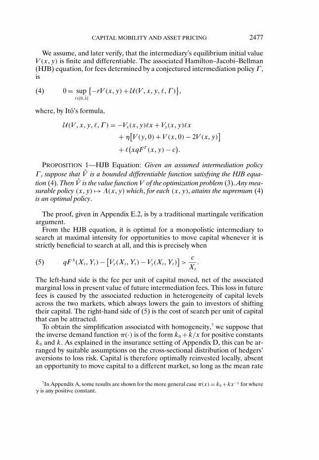
CAPITAL MOBILITY AND ASSET PRICING 2477
We assume, and later verify, that the intermediary’s equilibrium initial valueV (x� y) is finite and differentiable. The associated Hamilton–Jacobi–Bellman(HJB) equation, for fees determined by a conjectured intermediation policy Γ ,is
0 = sup�∈[0�λ]
{−rV (x� y)+ U(V �x� y� ��Γ )}�(4)
where, by Itô’s formula,
U(V �x� y� ��Γ )= −Vx(x� y)�x+ Vy(x� y)�x+η[
V (y�0)+ V (x�0)− 2V (x� y)]
+ �(xqFΓ (x� y)− c)�PROPOSITION 1—HJB Equation: Given an assumed intermediation policy
Γ , suppose that V is a bounded differentiable function satisfying the HJB equa-tion (4). Then V is the value function V of the optimization problem (3). Any mea-surable policy (x� y) �→Λ(x� y) which, for each (x� y), attains the supremum (4)is an optimal policy.
The proof, given in Appendix E.2, is by a traditional martingale verificationargument.
From the HJB equation, it is optimal for a monopolistic intermediary tosearch at maximal intensity for opportunities to move capital whenever it isstrictly beneficial to search at all, and this is precisely when
qFΛ(Xt�Yt)− [Vx(Xt�Yt)− Vy(Xt�Yt)
]>c
Xt
�(5)
The left-hand side is the fee per unit of capital moved, net of the associatedmarginal loss in present value of future intermediation fees. This loss in futurefees is caused by the associated reduction in heterogeneity of capital levelsacross the two markets, which always lowers the gain to investors of shiftingtheir capital. The right-hand side of (5) is the cost of search per unit of capitalthat can be attracted.
To obtain the simplification associated with homogeneity,7 we suppose thatthe inverse demand function π(·) is of the form k0 +k/x for positive constantsk0 and k. As explained in the insurance setting of Appendix D, this can be ar-ranged by suitable assumptions on the cross-sectional distribution of hedgers’aversions to loss risk. Capital is therefore optimally reinvested locally, absentan opportunity to move capital to a different market, so long as the mean rate
7In Appendix A, some results are shown for the more general case π(x)= k0 +kx−γ for whereγ is any positive constant.
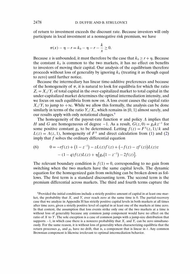
2478 D. DUFFIE AND B. STRULOVICI
of return to investment exceeds the discount rate. Because investors will onlyparticipate in local investment at a nonnegative risk premium, we have
π(x)−η− r = k0 −η− r − k
x≥ 0�
Because x is unbounded, it must therefore be the case that k0 ≥ r+η. Becausethe constant k0 is common to the two markets, it has no effect on benefitsto investors of moving their capital. Our analysis of the equilibrium thereforeproceeds without loss of generality by ignoring k0 (treating it as though equalto zero) until further notice.
Because the intermediary has linear time-additive preferences and becauseof the homogeneity of π, it is natural to look for equilibria for which the ratioZt =Xt/Yt of total capital in the over-capitalized market to total capital in theunder-capitalized market determines the optimal intermediation intensity, andwe focus on such equilibria from now on. A loss event causes the capital ratioXt/Yt to jump to +∞. While we allow this formally, the analysis can be donesimilarly in terms of the ratio Yt/Xt , which remains in [0�1] almost surely, andour results apply with only notational changes.8
The homogeneity of the payout-rate function π and policy Λ implies thatH and G are homogeneous of degree −1. As a result, G(z�0) = g0kz
−1 forsome positive constant g0 to be determined. Letting f (z) = FΛ(z�1)/k andL(z) = Λ(z�1), homogeneity of FΛ and direct calculation from (1) and (2)imply that f solves the ordinary differential equation
0 = −rf (z)+ (1 − z−1
) − zL(z)f ′(z)+ (−f (z)− zf ′(z))L(z)z(6)
− (1 − q)f (z)L(z)+η[g0
(1 − z−1
) − 2f (z)]�
The relevant boundary condition is f (1) = 0, corresponding to no gain fromswitching when the two markets have the same capital levels. The dynamicequation for the homogenized gain from switching can be broken down as fol-lows. The first term is a standard discounting term. The second term is thepremium differential across markets. The third and fourth terms capture the
8Provided the initial conditions include a strictly positive amount of capital in at least one mar-ket, the probability that Xt and Yt ever reach zero at the same time is 0. The partial-recoverycase that we analyze in Appendix H has strictly positive capital levels in both markets at all timesafter time zero, given a strictly positive level of capital in at least one of the markets at time zero.In that context, the assumption that loss events strike only one of the two markets at a time iswithout loss of generality because any common jump component would have no effect on theratio of X to Y . The sole exception is a case of common jumps with a jump-size distribution thatsupports −1, in which case there is a nonzero probability that Xt and Yt can be zero simultane-ously. For the same reason, it is without loss of generality when characterizing equilibria that thereturn processes ρa and ρb have no drift, that is, a component that is linear in t. Any commonBrownian component is likewise irrelevant to optimal intermediation behavior.
CAPITAL MOBILITY AND ASSET PRICING 2479
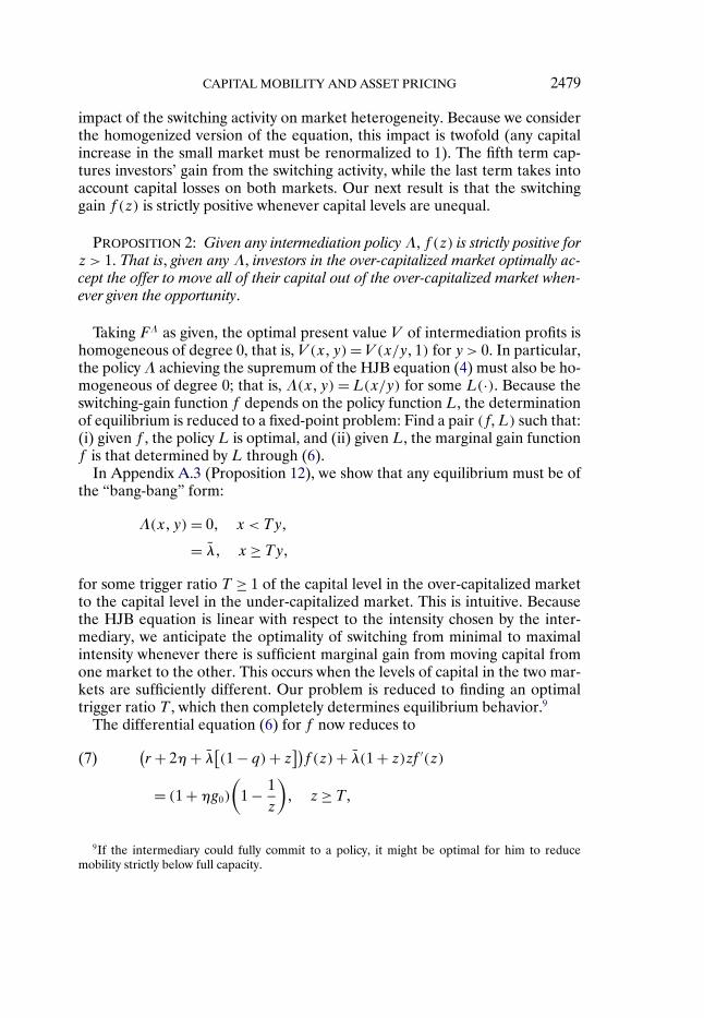
impact of the switching activity on market heterogeneity. Because we considerthe homogenized version of the equation, this impact is twofold (any capitalincrease in the small market must be renormalized to 1). The fifth term cap-tures investors’ gain from the switching activity, while the last term takes intoaccount capital losses on both markets. Our next result is that the switchinggain f (z) is strictly positive whenever capital levels are unequal.
PROPOSITION 2: Given any intermediation policy Λ, f (z) is strictly positive forz > 1. That is, given any Λ, investors in the over-capitalized market optimally ac-cept the offer to move all of their capital out of the over-capitalized market when-ever given the opportunity.
Taking FΛ as given, the optimal present value V of intermediation profits ishomogeneous of degree 0, that is, V (x� y)= V (x/y�1) for y > 0. In particular,the policy Λ achieving the supremum of the HJB equation (4) must also be ho-mogeneous of degree 0; that is, Λ(x� y)= L(x/y) for some L(·). Because theswitching-gain function f depends on the policy function L, the determinationof equilibrium is reduced to a fixed-point problem: Find a pair (f�L) such that:(i) given f , the policy L is optimal, and (ii) given L, the marginal gain functionf is that determined by L through (6).
In Appendix A.3 (Proposition 12), we show that any equilibrium must be ofthe “bang-bang” form:
Λ(x� y)= 0� x < Ty�
= λ� x≥ Ty�for some trigger ratio T ≥ 1 of the capital level in the over-capitalized marketto the capital level in the under-capitalized market. This is intuitive. Becausethe HJB equation is linear with respect to the intensity chosen by the inter-mediary, we anticipate the optimality of switching from minimal to maximalintensity whenever there is sufficient marginal gain from moving capital fromone market to the other. This occurs when the levels of capital in the two mar-kets are sufficiently different. Our problem is reduced to finding an optimaltrigger ratio T , which then completely determines equilibrium behavior.9
The differential equation (6) for f now reduces to(r + 2η+ λ[(1 − q)+ z])f (z)+ λ(1 + z)zf ′(z)(7)
= (1 +ηg0)
(1 − 1
z
)� z ≥ T�
9If the intermediary could fully commit to a policy, it might be optimal for him to reducemobility strictly below full capacity.
2480 D. DUFFIE AND B. STRULOVICI
and
(r + 2η)f (z)= (1 +ηg0)
(1 − 1
z
)� z ∈ [1�T ]�(8)
For z ∈ [1�T ], the solution is trivial:
f (z)= 1 +ηg0
r + 2η
(1 − 1
z
)�(9)
In particular, we verify that f (1)= 0, consistent with the observation that thenet present value of moving capital from one market to the other is 0 when thelevels of capital in the two markets are the same.
We can rewrite (7) as
(a+ z)f (z)+ z(1 + z)f ′(z)=(
1 − 1z
)b� z ≥ T�(10)
where a= (r + 2η+ (1 − q)λ)/λ and b= (1 +ηg0)/λ.Letting v(z)= V (z�1)/k, the HJB equation reduces to
0 = sup�∈[0�λ]
{−rv(z)− �zv′(z)− �z2v′(z)(11)
+ 2η[v0 − v(z)] +
(qzf (z)− c
k
)�
}�
where v0 = V (y�0)/k= V (x�0)/k. Therefore,
v(z)= v1� z ∈ [1�T ]�(12)
where
v1 = 2ηr + 2η
v0 < v0�(13)
and
κv(z)+ v′(z)z(1 + z)= d+ qzf (z)� z ≥ T�(14)
where κ= (r + 2η)/λ and
d = 2ηv0
λ− c
k�
Appendix A.2 contains a proof of the following monotonicity and regular-ity of v(·). Monotonicity of the value v(z) in the capital heterogeneity mea-sure z is not an obvious result, in particular because the switching gain f (z) is
CAPITAL MOBILITY AND ASSET PRICING 2481
not, in general, monotonic. That is, fixing the capital level y = 1 in the marketwith less capital, the marginal gain f (x) from switching capital from the over-capitalized market to the under-capitalized market need not be monotone in xeven though the increase in payout rate π(y)−π(x) is strictly monotone in x.This is the case because, as x gets large, both g(x) and h(x) ≡H(x�1)/k goto zero, and so must therefore f (x) = h(x) − g(x) go to zero. Intuitively, asx gets large, the global amount of capital is large, and although it can be in-termediated from one market to another, the value of being a capitalist is notattractive when there is “too much” capital relative to the demand by hedgersto lay off risk.
The intuition for monotonicity of v(z), however, is that, for any assumedtrigger ratio T , optimal or not, the total rate of activated intermediation feesqλzf (z), per unit of capital in the over-capitalized market, is not relevant on[0�T ] by definition of T , and is strictly increasing in z above T . In particu-lar, even though f (z) need not be monotone in z, zf (z) is monotone in z, asshown in Appendix A.2. Intuitively, zf (z) is the aggregate trade surplus gen-erated by the intermediary’s activity, and that surplus is increasing in marketheterogeneity.
PROPOSITION 3—Value Function Monotonicity: For any trigger capital ratioT , the solution v of (11)–(14) is bounded, increasing, and strictly increasing on[T�∞).
The smooth-pasting condition v′(T)= 0 is equivalent to
qTf(T)= c
k(15)
and implies the trigger capital ratio
T = 1 + c(r + 2η)(1 +ηg0)qk
�(16)
To identify the constant g0, we use a conservation equation: The sum of thevalue functions of all investors and of the intermediary must be equal to thepresent value of all cash dividend payments net of the search costs incurred bythe intermediary. After calculations shown in Appendix A.1, this conservationprinciple is equivalent to
kg0 = 2r
− cλ
r
(1 − e−(2η+r)a(T)) − kv0�(17)
where a(T)= log(1 + 1/T)/λ.A proof of the following result guaranteeing the existence and uniqueness of
a trigger strategy is found in Appendices A.4 (existence) and A.5 (uniqueness).
2482 D. DUFFIE AND B. STRULOVICI
PROPOSITION 4—Existence and Uniqueness: There exists a unique triggercapitalization ratio T satisfying (17), (7), (8), and (16).
An iterative algorithm for computing the equilibrium is presented in Ap-pendix F, whose steps exploit the previous equations as follows: starting fromsome initial level of v0, Equations (16) and (17) are used to determine g0 andthe threshold T . Using these values, the ordinary differential equation (14) isused to determine a new value of v0 as the limit of v(z) as z goes to infinity,concluding the first iteration of the algorithm.
This analysis leads to the following characterization of equilibrium, whichincludes the result that, in the absence of search costs, the intermediary doesnot exploit his position to restrict movement of capital, but rather providesmaximal intermediation, nevertheless generating fee income from his or herimperfect ability to instantaneously move capital from one market to the otherdue to the upper bound λ on contact intensity. As λ becomes large, the capitallevels will be nearly equated across the two markets at all times, as in a com-pletely frictionless market, and in the limit there would be no intermediationrents.
PROPOSITION 5: Suppose that the payout-rate function π is of the form π(x)=k0 + k/x. Then there exists a unique equilibrium. In equilibrium, there is no in-termediation (λt = 0) whenever the ratio of capital levels in the two markets isbetween 1/T and T , for a uniquely determined capital-ratio trigger T . Otherwise,intermediation is at full capacity (λt = λ). The trigger ratio T is given by (16),where the constant g0 is given by (17). If there is no intermediation cost (c = 0),then the intermediary always works at full capacity (i.e., T = 1).
3.2. How Intermediation Depends on Market Parameters
We turn to comparative statics, focusing on the behavior of the thresholdcapital ratio T . A higher trigger ratio T corresponds to less intermediation,because the intermediary waits until Xt/Yt exceeds T before becoming maxi-mally active. We therefore define capital mobility to be increasing in a param-eter whenever the equilibrium threshold T is decreasing in that parameter. Weshow that these comparative statics carry over to the oligopolistic case.
PROPOSITION 6—Comparative Statics for c�k�η� and r: Capital mobility isdecreasing in the intermediation cost coefficient c, increasing in the payout-ratecoefficient k, and decreasing in the discount rate r. Fixing the dividend payoutrate function π(·), capital mobility is decreasing in the loss-event intensity η.
A proof is provided in Appendix G. It is intuitive that increasing the costs ofintermediation, represented by c, reduces the amount of intermediation pro-vided in equilibrium. Once the trigger T is chosen, the costs of search intensity
CAPITAL MOBILITY AND ASSET PRICING 2483
are borne entirely by the intermediary. Other things equal, raising c thereforelowers the desire to search. The coefficients c and k affect the trigger T onlythrough the ratio c/k, explaining the comparative static for k. Intuitively, mul-tiplying c and k by the same factor amounts to a change of currency unit, whichis why only the ratio c/k affects the equilibrium threshold. The comparativestatics for η and r are more subtle because, for a given trigger ratio T , both ηand r have an effect on the value functions of investors. Equation (16) is thekey to understand these comparative statics. A higher after-shock continuationvalue for investors (i.e., a higher g0) results in a lower T and thus a higher cap-ital mobility. A higher r has two effects on investors. The direct effect is thatit reduces their gain from switching capital, which is the role of r in the nu-merator of (16). The indirect effect is that, because the present value of gainfrom switching capital is lower for higher r, investors pay lower fees to the in-termediary, resulting in a higher g0. As we show in our proof, the former effectdominates the latter, so T is decreasing in r. One intuition is that the secondeffect is an indirect consequence of the first, direct effect, so we may expect thenet comparative static to follow the first effect.10
Our proof likewise shows that T is increasing in η, holding π fixed. Ofcourse, increasing the mean loss frequency η would naturally raise the equi-librium loss insurance rate π(Xit), which on its own would tend to increase in-termediation (lower T ). To analyze this effect, we write π(x)= k0(η)+k(η)/xto show the dependence of the coefficients k0(η) and k(η) on the mean lossrate η. The coefficient k0(η) plays no role in intermediation gains. The impacton intermediation intensity of replacing η with some η′ >η is thus equivalentto the effect of leaving π unchanged and replacing the cost coefficient c withc′ ≤ ck(η)/k(η′). This effect can be small or large, depending on the sensitiv-ity of k(η) to η, reflecting how the elasticity of hedging demand varies with theexpected loss frequency. Thus, the overall impact on intermediation intensityof a given increase in the loss-event intensity η is to lower intermediation in-centives (raise T ) precisely when the impact on k(η) is sufficiently small, andotherwise to raise intermediation intensity.
Increasing the bargaining power q of the intermediary increases the fractionof the gains to trade that goes to the intermediary, prompting the intermediaryto search for more investor capital to move, thus setting a lower trigger ratio T ,holding constant the gains to investors for moving capital. Obviously, however,raising q lowers the present value of investors associated with future move-ments of capital, thus lowering the amount of gain they have to share with theintermediary. The proof in Appendix G of the following result demonstratesthat the direct effect dominates the indirect effect on the investors’ values, pro-vided that q remains below 1/2.
10The techniques used for the comparative statics of discounting draw on those introduced byQuah and Strulovici (2009, 2012)
2484 D. DUFFIE AND B. STRULOVICI
PROPOSITION 7—Comparative Statics for q: Capital mobility is increasing inthe bargaining power q of the intermediary, for 0< q < 0�5.
The impact on capital mobility of the capacity λ for search intensity dependson other parameters, and particularly on the discount rate. There are situa-tions in which lowering λ lowers the trigger ratio T , leading the intermediaryto work more often, albeit with a lower capacity. We provide examples andsome intuition for the fact that, depending on the discount rate r, the thresh-old capital ratio T can either increase or decrease with capacity. We focus onthe impact of λ on the threshold T , noting that the level of λ has also a directimpact on capital mobility, through the rate at which capital moves from onemarket to another, when it does.
We argue by continuity from the case of η � 0. Taking π(x) = k0(η) +k(η)/x, we can create a family of economies that keep k(η) fixed at somek as η varies near zero by increasing the loss aversion of hedgers. With this, asη approaches zero, the equilibrium intermediation policy converges to a policythat moves capital until the threshold T is reached (with no changes in capitallevels afterward), so the associated trigger ratio converges to
T = 1 + cr
kq�(18)
which is independent of the capacity λ. Moreover, the associated gain functionsconverge to a gain function f with
f (T)= 1r
(1 − 1
T
)�
Suppose first that agents are patient (have a low discount rate r). As λ goesup, capital heterogeneity goes down, hence the value of moving capital is lower.Moreover, a higher-capacity intermediary will more quickly run out of capitalto be moved, and thus stop receiving fees earlier. Overall, this implies by con-tinuity that we can construct example economies with small η such that, as λis reduced and other parameters are held constant, the intermediary receivesmore fees, and for longer, and hence the value function of investors is lower,resulting in a higher threshold.11
Now, we consider the opposite case of nearly myopic investors (high r). Theprevious argument breaks down: Investors do not care much about future het-erogeneity; they care mainly about the immediate gain from switching, whichdepends on current heterogeneity. Moreover, the immediate fees are increas-ing with capacity λ. A higher-capacity intermediary therefore receives higher
11See Equation (16), which shows that T is decreasing in investors’ after-shock continuationvalue g0.
CAPITAL MOBILITY AND ASSET PRICING 2485
immediate fees, which reduces investors’ overall value of switching capital andincreases the threshold.
Numerical examples support this intuition. For q= 0�5, c = k, and r = 0�04,for η sufficiently small and k(η) = k sufficiently insensitive to η, the capitaltrigger T decreases with λ for 0�01< λ < 0�5. For the same q and c but takingr = 10, however, the trigger ratio T increases with the intermediation capacityλ, over the same interval.
4. INTERMEDIARY COMPETITION
We now solve for equilibria with oligopolistic or perfectly competitive mar-kets for intermediation.
There are two channels through which intermediary competition affects theequilibrium level of intermediation offered by the market. First, an interme-diary internalizes the impact of intermediation intensity on the heterogeneityof capital levels across the two markets, and thus the impact on the interme-diary’s future profits. A given intermediary does not, however, internalize theeffect of increasing its intermediation on reducing the profit opportunities ofother intermediaries. Through this first channel, increasing the number of in-termediaries should therefore weakly increase the total amount of intermedi-ation. In the benchmark case in which a loss event destroys all capital in theaffected market, there is nothing to internalize, because the after-shock situ-ation is independent of the pre-shock heterogeneity level, and our upcomingProposition 8 states that the threshold is independent of the number of inter-mediaries. In Appendix J, we explain why there is a strict increase in capitalmobility from increasing competition if loss events leave some residual cap-ital, because in this case the post-loss heterogeneity depends on the pre-lossheterogeneity.
The second channel by which increasing competition changes capital mobil-ity is as follows. When in contact with an investor, an intermediary considersthe ability of the investor to compare the intermediation fee offered with thefees offered by other intermediaries. This plays a role, in an extension of themodel that is offered later in this section, in determining the effective bargain-ing power of the intermediary, and through that channel, has an impact on theprofitability of intermediation. We start by taking bargaining power as fixedand then endogenize the fees received by the intermediary. As we shall see,in some cases the second channel can dominate the first, that is, in which anincrease in the number of intermediaries lowers capital mobility.
4.1. Intermediary Competition at Fixed Bargaining Power
For a given bargaining power q, we show that equilibrium trigger policiesfor the oligopolistic case can be translated directly from the case of monopo-listic intermediation through a simple inspection of the associated Hamilton–
2486 D. DUFFIE AND B. STRULOVICI
Jacobi–Bellman equations. From this, we also obtain comparative statics di-rectly from those of the monopolistic case.
For the oligopolistic case, we take n identical intermediaries, each with anupper bound λ/n on intermediation intensity, and with the same proportionalcost c of intermediation. The monopolistic case (n= 1) is the special case con-sidered in the previous section. Thus, all cases have the same feasible marketdynamics and costs.
We consider only Markov time-homogeneous equilibria. Equilibrium incor-porates the degree to which intermediaries internalize the impact of their in-termediation intensity on the heterogeneity of capital levels across markets.For an oligopolistic equilibrium in trigger strategies, each of the n intermedi-aries has a reduced value function v, with v(z) = V (z�1)/k, that solves thereduced HJB equation, extending the monopolistic version (11):
0 = sup�∈[0�λ/n]
{−rv(z)+
(−(n− 1)
nλ1{z≥T } − �
)zv′(z)(19)
−((n− 1)n
λz1{z≥T } + �z)zv′(z)
+ 2η[v0 − v(z)] +
(qzf (z)− c
k
)�
}�
reflecting the presumption by the given intermediary that the n− 1 other in-termediaries have adopted a specific trigger capital ratio T . The equilibriumcondition is that the same trigger policy is optimal for the given intermediary.Verification of the HJB solution as the value function and of the optimality ofthe associated candidate policy function is as for the monopolistic case.
Thus, an equilibrium for the n-intermediary problem is again given by bang-bang control for all intermediaries, each exerting no effort when Zt < T andmaximal intermediation intensity λ/n whenever Zt ≥ T , for a trigger capitalratio T . We show that optimality implies that there is no intermediation at orbelow the capital ratio T satisfying the smooth-pasting condition v′(T) = 0.This, along with (19), implies that
qTf(T)− c
k= 0�(20)
From (20), we see that an intermediary’s optimization problem in a set-ting with n intermediaries is equivalent to that of a monopolistic intermedi-ary with maximum intermediation intensity λ. Indeed, for a given thresholdT , the monopolistic and oligopolistic cases yield the same function f deter-mining proportional intermediation fees, and hence the same smooth-pastingcondition (20).
In fact, this is actually the unique equilibrium, even allowing for the possi-bility of non-trigger strategies! To see this, consider any Markov equilibrium,
CAPITAL MOBILITY AND ASSET PRICING 2487
not necessarily of the trigger-ratio form, and let f denote the function deter-mining the associated gain from switching. An intermediary’s HJB equationis of the form (19), except that (i) the aggregate of other intermediaries’ con-tact intensities may be almost arbitrary, and (ii) the value functions may varyacross intermediaries. Owing, however, to the form of the HJB equation, theindifference condition is nevertheless given by (20), and thus is the same forall intermediaries. This shows that any Markov equilibrium must be symmetricand of the trigger form.12 In fact, repeating arguments from the monopolisticcase leads to the following proposition.
PROPOSITION 8: With n intermediaries, there is a unique Markov, homoge-neous equilibrium. This equilibrium is symmetric and determined by a trigger cap-ital ratio equal to that of a monopolistic intermediary with the oligopolistic maxi-mal contact intensity λ.
When shocks lead to a partial recovery of capital, however, the intermedia-tion trigger capital ratio T is strictly decreasing in the number n of intermedi-aries, as shown in Appendix J.
4.2. Endogenous Bargaining Power
Competition to supply intermediation may also have an impact on an inter-mediary’s share of gains from trade when in contact with an investor. We nextconsider the implications of market structure for the intermediary bargainingpower q. With n > 1 intermediaries, we suppose that some fraction ψn of in-vestors are “well connected,” meaning that as they prepare to move capitalfrom one market to another, they are in simultaneous contact with more thanone intermediary. The number of intermediaries with whom a given investor isin contact could also be random, exploiting the law of large numbers, in whichcase ψn can be taken to be the probability that an investor, when contacted,is in contact with more than one intermediary. Intuitively, a well-connectedinvestor has more bargaining power than a “captive” investor, one who is incontact with only one intermediary.
When modeling this intuition with a bargaining game, an issue is whether thecontacted intermediary is assumed to know whether the investor is in contactwith other intermediaries. We take this case.13 Another modeling approach
12The trigger form comes from showing, as in the monopoly case (Lemma 2), that the functionz �→ zf (z) is increasing.
13It would be possible to allow for one-sided information. The fees derived could be obtainedas equilibrium outcomes of a bargaining process, although there may be additional equilibria.See, for example, Sutton (1986). For an alternative approach to treating uncertainty about thedegree to which an intermediary’s customer is in contact with other intermediaries, see Green(2007).
2488 D. DUFFIE AND B. STRULOVICI
is a multilateral bargaining game with complete information, as in Stole andZwiebel (1996).
We consider a bargaining procedure à la Rubinstein (1982), in which theinvestor and a particular intermediary alternate offers. In our continuous-timesetting, the times between offer rounds can be treated as arbitrarily small, sothe inter-round discount factor can be taken to be 1. In that case, the investorand intermediary agree immediately to split the surplus according to the Nashbargaining solution. The investor’s share depends on his outside option. If theinvestor is captive, his outside option is simply G(x�y), the value of remainingin the over-capitalized market. Thus, the normalized Nash product associatedwith a proportional fee of s is
[v(z)+ s− v(z)][h(z)− s− g(z)]�
which is maximal at s = f (z)/2, corresponding to q = 1/2, meaning an equalsplitting of the gains with the intermediary.
For a well-connected investor, the normalized Nash product is[v(z)+ s− v(z)][h(z)− s− g(z)− (1 − q0)f (z)
]�
where q0 is the equilibrium proportion of the gain from trade that the investorwould pay to another intermediary if this first round of bargaining were tobreak down. The Nash product is maximized at s = q0f/2, yielding an equilib-rium intermediary share of q= 0� corresponding to the extraction of all surplusby the well-connected investor.14
If the number of intermediaries in contact with the investor is known only bythe investor, then q is similarly obtained, and depends on the probability thatthe investor is captive.
Assuming pairwise independence of the connectedness of individual in-vestors, the average of an intermediary’s share of gains across the infinite pop-ulation of investors is almost surely
q(n)= 0 ×ψn + 12(1 −ψn)= 1 −ψn
2�(21)
In particular, q(n) is decreasing in n if ψn is increasing in n. Obviously, ψ2 ≥ψ1. Going beyond the case of n = 2, it is somewhat intuitive that an investoris more likely to be well connected as the number of intermediaries increases.Appendix B briefly outlines a model with this natural feature.
Noting from (21) that q(n) < 1/2, Proposition 7 hints that lowering q(n) re-duces an intermediary’s incentive to search, all else equal, because, for given
14Another way to obtain this prediction is to assume that intermediaries connected to a givenintermediary post prices and engage in Bertrand competition. We are grateful to a referee forsuggesting the alternative of Bertrand competition.
CAPITAL MOBILITY AND ASSET PRICING 2489
capital dynamics, lowering q(n) reduces intermediation profits, and thereforelowers the marginal benefit of raising intermediation intensity. We will next il-lustrate the second channel through which oligopolistic intermediation affectscapital mobility: By reducing each intermediary’s bargaining power, the incen-tive to intermediate is lowered.
Endogenous bargaining leads to complex dynamics, in which the number ofintermediaries actively searching for capital varies over time. To see this, con-sider a candidate equilibrium in which n intermediaries search at full capacitywhenever z > T , and no intermediary searches when z ≤ T . If a single inter-mediary deviates by searching for capital when z is in a left neighborhood ofT , then his fee per unit of capital switched is that of a monopolist, not that ofthe n-intermediary case. This increases the value of this deviation. Despite thisadded complexity, we now show that oligopolistic intermediation may reducecapital mobility.
4.3. Reduced Capital Mobility With More Intermediaries
A Markov strategy profile for n intermediaries consists of functions L1�L2�� � � �Ln on [1�∞) into [0� λ/n]. Here, Li(z) denotes the search intensity ofintermediary i when the heterogeneity of capital across the two markets is z =x/y . The associated aggregate capital mobility is
L(z)=n∑i=1
Li(z)�
To exploit the fee share q(n) derived above, we focus on simple strategies,for which Li(z) is either 0 or λ/n. With this restriction,15 we can associatewith any strategy profile an increasing sequence T0�T1� � � � �TJ of capital-ratiothresholds with the property that, whenever the capital ratio Zt is in [Tj�Tj+1),a particular setNj of intermediaries is active. We let nj = |Nj| denote the num-ber of intermediaries in Nj .
Using our previous analysis of the oligopolistic case with fixed bargainingpower, we say that a profile of simple strategies is a Markov equilibrium if, forall j and z ∈ [Tj�Tj+1),
q(nj)zfL(z)− c
k≥ 0�(22)
and
q(nj + 1)zf L(z)− c
k≤ 0�(23)
15Extending the analysis to general Markov strategies would be possible if one computes, forany possible strategy, the expected fee for each intermediary as a function of his search intensityand of the aggregate search intensity.
2490 D. DUFFIE AND B. STRULOVICI
where f L(z) denotes the marginal gain to an investor from switching to themarket with less capital, given an aggregate intensity policy L.
The first inequality means that any intermediary inNj contacting investors atcapital ratio z does so optimally, given equilibrium fee share q(nj). The secondequation states that any intermediary in Nj + 1 is optimally not contacting atcapital ratio z, given the equilibrium fee share q(nj + 1) that he would get if hesearched.
We let T = inf{z :L(z)= λ� z ≥ z}, the smallest level of capital heterogeneityabove which intermediaries search at full capacity. We denote by T1 the mo-nopolistic threshold. For the result to follow, recall that η is the mean arrivalrate of loss events and that T depends, through L, on the particular Markovequilibrium under consideration. In any equilibrium, zf L(z) is strictly increas-ing in z. (For this, see the proof of Proposition 10.) This fact and Equations(22) and (23) imply that when q(n) is decreasing in n (i.e., a more connectedinvestor pays a lower fee), the number of active intermediaries is increasing inz in any equilibrium.
PROPOSITION 9—Monotonicity: Suppose that q(n) is decreasing in n. Then,nj is increasing in j.
If q(n) is strictly decreasing in n, it is possible to prove by a fixed-point ar-gument the existence of a Markov equilibrium, in which, whenever the capitalheterogeneityZt is [Tk�Tk+1), precisely the first k−1 intermediaries are active,and the remainder are inactive.16
The following result applies to all equilibria.
PROPOSITION 10: Suppose that the number n of intermediaries is at least 2.There exists some η > 0 such that, for any loss event intensity η ∈ (0� η) and anyassociated Markov equilibrium trigger capital ratio T , we have T1 < T .
This result states that, for sufficiently infrequent loss events, the reducedbargaining power caused by oligopolistic competition reduces the domain of
16For a sketch of the proof, let T denote a vector (T0� � � � �Tn) in Rn+1 of capital heterogeneity
thresholds, with increasing elements. We let LT and f T denote the associated capital-mobilityand switching-gain functions. Taking T as given, a vector of best-response thresholds is uniquelydetermined by Equations (22) and (23). The best-response function of the respective intermedi-aries induces a new vector B(T) of capital heterogeneity thresholds. It can be checked that B(·) iscontinuous. For this, we endow R
n+1 with the Euclidean topology and the space of switching-gainfunctions (f L) with the sup-norm topology. We have continuity of T �→ f T because of Equations(22) and (23), and because the best-response thresholds depend continuously on fL. Moreover,the best-responses preserve threshold monotonicity. Further, the best-response thresholds areuniformly bounded below by ¯T = rc/(kq(n)2) (using that f L(z) ≤ 2/r for all z), and boundedabove by T = c/(kq(1)
¯f (¯T)), where
¯f (z) is the gain from switching capital when capital moves
at full capacity λ until T = 1, and satisfies¯f (z) ≤ fL(z) for all L and z. The result follows from
Brouwer’s theorem.
CAPITAL MOBILITY AND ASSET PRICING 2491
maximal capital mobility relative to that of the monopolistic case. Our assump-tion of a sufficiently small mean arrival rate η of loss events exploits the factthat intermediation fees are generated from the time of each loss event untilcapital is sufficiently equalized across the markets. Although there are techni-cal steps in the proof of this proposition, found in Appendix C, the argumentrelies on a bound on improvements in the present value of intermediation feesas one changes from one market setting to another. A simple way to providesuch a bound is thus to control the speed with which new fee-generating lossevents occur.
Proposition 10 shows that oligopolistic competition results in less intermedi-ation than achieved by a monopolist, for some range of market heterogeneity.This does not, however, rule out intermediation by oligopolists at capital ratiosbelow the monopolistic trigger level. The next result shows that, provided thatloss events are not expected too frequently, oligopolistic and monopolistic set-tings lead to a cessation of intermediation at approximately the same levels ofmarket heterogeneity.
For any n-intermediary Markov equilibrium with aggregate intermediationstrategy L, let
Sn = inf{z :L(z) > 0
}�
the smallest heterogeneity level above which capital is mobile. A proof of thenext proposition may be found in Appendix C. We will rely on a sufficientlysmall loss-event intensity for the same bounding effect explained after thestatement of Proposition 10.
PROPOSITION 11: For any ε > 0, there exists a strictly positive η such that, forany mean loss-event rate η ∈ (0� η) and any associated Markov equilibrium withn players, we have Sn ≥ T1 − ε.
Propositions 10 and 11 together show that capital mobility is lower, at anylevels of capital, with oligopolistic intermediation than with monopolistic in-termediation, provided that loss events are sufficiently infrequent.17
5. DISCUSSION AND CONCLUDING REMARKS
In a neoclassical model of asset markets, investors continually adjust theirportfolios so as to achieve the highest possible mean return for a given typeof risk. In equilibrium, an investor bearing a given type of risk is therefore
17For the last two results, we have held constant the dependence of the dividend rate functionπ(x) on the capital level x as the mean rate η of loss events is varied. We have the freedom,however, of varying the population of hedgers as η changes, so as to offset the impact of variationof η on π(x), thereby satisfying the stated comparison between monopolistic and oligopolisticintermediation for each fixed economy.
2492 D. DUFFIE AND B. STRULOVICI
compensated by a unique associated excess mean rate of return, no matterthe asset that carries the risk. In practice, however, investors make portfolioadjustments with delays. In our model, the mobility of capital across differentinvestments is increased through the equilibrium efforts of intermediaries. Ourmodel has several implications for asset-price dynamics:
1. With unexpected changes in the amount of capital that is available tobear the risk represented by an asset, risk premia adjust more severely to cap-ital shocks than in a neoclassical (perfect-mobility) setting, and then revertsomewhat over time as capital is redeployed. This time signature, present inessentially any setting with slow moving capital, is dampened to the extent thatintermediaries are active. Consider, for example, our simplest setting in whichcapital levels change only at the times at which all capital in a given asset mar-ket is lost. Perfect capital mobility (c = 0� λ = ∞) implies that Xat = Xbt forall t. A loss event at time τ in market a would cause half of the capital frommarket b to move instantly to market a, so risk premia in both markets jumpup by
π(Xaτ)−π(Xaτ−)= k
Xaτ−�
and then remain constant until the next loss event. With imperfect mobil-ity, however, the risk premium in market a would jump immediately to +∞and then decline at the rate λZt k
Xatuntil the capital heterogeneity ratio Zt =
Xbt/Xat drops to T or until another loss event occurs.2. The degree to which risk premia vary across assets, after controlling for
other determinants of risk premia, is increasing in the degree to which capitalis heterogeneously distributed across assets.
3. The speed of reversion of risk premia across assets toward common levels(after adjustment for other determinants of risk premia) is decreasing in thecost of intermediation. Increasing intermediation capacity, however, can eitherincrease or reduce capital mobility, depending on the setting, as explained inSection 3.2.
4. All else equal, increasing the fraction of gross gains from moving capitalthat accrue to intermediaries increases the speed of adjustment of capital andrisk premia.
5. Lowering time discount rates increases the mobility of capital.6. Increasing the volatility of asset returns, represented in our model by the
mean frequency η of loss events, can either increase or decrease the mobilityof capital through intermediation, depending on the relative magnitudes of theeffects of (i) raising neoclassical risk premia (thus increasing the rents availableto intermediaries), and (ii) increasing the volatility of capital heterogeneity ata given level of intermediation, which lowers the incentive to intermediate.
7. Increasing the scope for intermediary competition by splitting the marketamong more intermediaries can increase or decrease the equilibrium provision
CAPITAL MOBILITY AND ASSET PRICING 2493
of intermediation, depending on the relative magnitudes of the effects of (i) re-ducing the concern of an intermediary regarding the impact of its own activityon lowering capital heterogeneity, and (ii) lowering the bargaining power ofan intermediary vis à vis its customers because of increased competition withother intermediaries. As the number of intermediaries increases, the formereffect raises intermediation incentives, while the latter effect can lower inter-mediation incentives.
Our introduction uses the example of the market for catastrophe risk rein-surance. Froot and O’Connell (1999), Zanjani (2002), and Born and Viscusi(2006) explained how premia for catastrophe risk insurance typically increasedramatically when insurance and reinsurance firms suffer significant damageclaims after natural disasters, such as Hurricane Andrew in 1992. Then, overmany months, premia drop toward “soft-market” levels (absent other shocks tothe capital of insurers) because the replacement of insurance capital is delayedby institutional barriers to capital raising, including the time spent searchingfor suitable new investors. According to Enz (2001), premia swing up and downby as much as 50% over multiyear periods, and are closely linked with changesin the capital levels of insurers, regardless of whether these changes in capitalare caused by damage claims or by unexpected returns to the asset portfoliosof insurers. From this, we know that the dynamics of insurance premia after amajor natural catastrophe are not caused mainly by inference concerning thearrival rate of future such events. We also know that most of the observed priceimpacts are not caused by inference about losses because major changes overtime in insurance premia following shocks to capital levels are highly correlatedacross all major lines of property insurance covered by the same pools of cap-ital covering catastrophe risk.18 These other lines cover, for example, aviation,marine, motor, and proportional property. The link tying premium dynamicsacross the various lines of insurance is the level of capital commonly availableto bear losses. Apparently, these various property-related insurance marketsare not segmented from each other by capital immobility. Rather, they are col-lectively segmented from other types of capital markets. Froot and O’Connell(1999) emphasized the slow speed of capital replacement as the major causeof slow premium adjustments.
That there is scope for intermediaries to mobilize dormant capital is appar-ent from a significant body of evidence that, when left on their own, manyindividual investors adjust their portfolios remarkably infrequently. For exam-ple, Ameriks and Zeldes (2004) reported that, over a 10-year period, 44% ofinvestors in their sample made no changes to their portfolio allocations, andthat an additional 17% of these investors made a single reallocation duringthis period. Mitchell, Mottola, Utkus, and Yamaguchi (2006) found that, of1.2 million U.S. employees covered by over 1,500 401(k) investment plans, ap-proximately 80% initiated no trades over a two-year period, while an additional
18See, for example, Enz (2001, p. 5, Figure 1).
2494 D. DUFFIE AND B. STRULOVICI
10% made only a single trade.19 Based on our theoretical results, one presumesthat investor inattention is more evident in the data when the cost of contactingindividuals and deploying their capital is large relative to the potential associ-ated intermediation profits. For example, high-net-worth individual investorsand institutional investors are likely to receive more attention from interme-diaries because of the amounts of capital they can deploy and the associatedhigher total intermediation fees, than are most of the smaller investors whoseinattention is documented in this literature. This is consistent with evidenceprovided by Bilias, Georgarakos, and Haliassos (2010) and Feldhütter (2009).Further, variation across investors in financial sophistication (not captured inour model) may lead to a negative correlation between the cost of achievinga given level of contact intensity and the level of deployable capital. In ourmodel, intermediaries cannot differentiate among subclasses of investors.
Delays in processing information for purposes of investment decisions arealso in evidence from “price momentum” following fundamental news, asdocumented empirically by Chan (2003), Engelberg, Reed, and Ringgenberg(2012), Dellavigna and Pollet (2009), and Cohen and Lou (2012), among oth-ers. Given that most financial intermediaries are themselves likely to receiveand process fundamental news quickly relative to the time for price reactionsdocumented in this literature, one presumes that there are limits on the aver-age speed with which they can attract potential investors to such investmentopportunities. This inference is also consistent with numerous examples ofslow price adjustments to supply shocks in equity markets, including those ofHolthausen, Leftwich, and Mayers (1990), Scholes (1972), Coval and Stafford(2007), Andrade, Chang, and Seasholes (2008), Kulak (2008); with respect tosupply shocks caused by index recompositions, see Shleifer (1986), Harris andGurel (1986), Kaul, Mehrotra, and Morck (2000), Chen, Noronha, and Singhal(2004), and Greenwood (2005); and with respect to the expiration of commod-ity futures contracts, see Mou (2011).
In corporate bond markets, which are not traded on a central exchange, oneobserves large price drops and delayed price recovery in connection with majordowngrades or defaults, as described by Hradsky and Long (1989) and Chen,Lookman, and Schürhoff (2008), when certain classes of investors have an in-centive or a contractual requirement to sell their holdings. Mitchell, Pedersen,and Pulvino (2007) documented the effect on convertible bond hedge fundsof large capital redemptions in 2005. Convertible bond prices dropped andrebounded over several months. A similar drop-and-rebound pattern was ob-served in connection with the LTCM collapse in 1998. Newman and Rierson(2003) showed that large issuances of European Telecom bonds during 1999–2002 temporarily raised credit spreads throughout the sector, evidence that ittakes time for intermediaries to locate long-term investors.
19For further evidence on the slowness of individual portfolio adjustments, see Lusardi (1999,2003), Brunnermeier and Nagel (2008), and Bilias, Georgarakos, and Haliassos (2010).
CAPITAL MOBILITY AND ASSET PRICING 2495
In these examples, the time pattern of returns or prices after a supply or de-mand shock reveals that the friction at work is not merely a transaction costfor trade. If that were the nature of the friction, then all investors would im-mediately adjust their portfolios, or not, optimally. The new market price andexpected return would be immediately established, and remain constant untilthe next change in fundamentals. In all of the above examples, however, afterthe immediate price response, whose magnitude reflects the size of the shockand the supply of immediately available capital, there is a relatively lengthy pe-riod of time over which the price reverts in mean toward its new fundamentallevel. In the meantime, additional shocks can occur, with overlapping conse-quences. The typical pattern suggests that the initial price response is largerthan would occur with perfect capital mobility, and reflects the demand curveof the limited pool of investors that are quickly available to absorb the shock.The speed of adjustment after the initial price response is a reflection of thetime that it takes more investors to realign their portfolios in light of the newmarket conditions, or for the initially responding investors to gather more cap-ital.
In our setting, as in practice, there can be substantial differences in mean re-turns across assets that are due not only to cross-sectional differences in “fun-damental” cash-flow risks, but are also due to unbalanced distributions of cap-ital, relative to a market without intermediation frictions. Empirical “factor”models of asset returns do not often account for factors related to the distri-bution of ownership of assets, or related to likely changes in the distribution ofownership. Exceptions include the recent work of Coval and Stafford (2007)and Lou (2009), who noted that the conditional mean returns of an equitytend to be lower due to price pressure when mutual funds owning that eq-uity are experiencing liquidation-motivated outflows, and that the conditionalmean returns recover as price pressure abates. Similarly, Bartram, Griffin, andNg (2010) showed that divergent levels of ownership by national domiciles playa role in equity returns.
In our model, delays in portfolio adjustments are due to the time that ittakes for intermediaries to locate suitable investors. This is only an abstrac-tion, which can also proxy for other forms of delay, including time to educateinvestors about assets with which they have limited familiarity (awareness),time for contracting, and time for investors to dispose of their current po-sitions, which could involve similar delays and price shocks, as suggested byChaiserote (2008).
Our results extend almost immediately to a model in which, in addition toobtaining the services of an intermediary, each investor also has a personaltechnology by which opportunities to move capital to the other market arriveat random times, independently across investors, with a constant mean arrivalrate. This would cause only minor modifications to the structure and solutionof our model. Increasing the mean arrival rates of these alternative capital-shifting opportunities reduces the average degree of imbalance of capital and
2496 D. DUFFIE AND B. STRULOVICI
the difference in risk premia between the two markets, and thus reduces theprofitability of intermediation.
Our results also apply with minor alteration to an extension of the model thatallows for randomly timed exit and entrance of investors. For this, investorswould exit at exponentially distributed times that are pairwise independent,and consume their capital at exit. New investors would appear in proportionto the current levels of capital. Any difference between exit and entrance rateswould thus be subtracted from the proportional drifts of the capital accumula-tion processes Xa and Xb.
We could further extend our model so as to treat asymmetric markets. Pro-vided that the local inverse demand function π(·) of each market satisfies sim-ilar homogeneity assumptions, intermediation would be characterized by twodistinct thresholds of capital ratios, one for movement of capital from marketa to market b, and another for the reverse movement. For example, if returnsin market a are riskier than those in market b, then, all else equal, capital willbe less mobile toward market a than toward market b. Asymmetry, for exam-ple, would allow a consideration of capital mobility from a low-risk “moneymarket” into a high-risk market such as that for private equity. Many of thequalitative features of our symmetric model, such as the dynamics of capitalmobility and the impact of intermediation competition, are anticipated to carryover to asymmetric settings, at least under regularity conditions.
Another natural extension concerns the case of three or more markets. Con-sider, for example, three symmetric markets differing only in their capital lev-els, and satisfying our homogeneity conditions. We conjecture that capital willflow exclusively to the highest-premium market, with more mobility from thelowest-premium market than from the mid-premium market.
APPENDIX A: EQUILIBRIUM ANALYSIS
Here, we provide a stochastic analysis of Markov equilibrium that is morecomplete and general than that provided in the main text.
Given an intermediation contact intensity process λ and initial conditionsfor capital in each market, we let Xλ
it denote the total capital in market i attime t. Given an associated transaction-cost process K, the marginal value to asupplier of one additional unit of capital in market i at time t is
θλit =E(∫ ∞
t
e−r(s−t)[Wsπ(XλD(s)�s
)ds−Ws−Ks− dNs
]∣∣Ft
)�(24)
whereNs is the cumulative number of switches back and forth between the twomarkets through time s by the holder of this unit of capital, and the marketindicator D(s) is a or b, depending on whether, at time s, the accumulatedcapital Ws is currently located in market a or b. This capital thus accumulatesaccording to
dWs =Ws− dρD(s−)(s)�
CAPITAL MOBILITY AND ASSET PRICING 2497
with initial conditionWt = 1. The market-indicator processD is a marked pointprocess with an initial condition at time t of D(t)= i, and with an intensity ofjumping from market i to market j at time s of λs1{Xλis>Xλjs}. In the equilibriumthat we shall describe, the value of switching from market i to market j isstrictly positive if and only if Xλ
it > Xλjt � The marginal value of moving capital
is thus
φλt = max(θλat� θ
λbt
) − min(θλat� θ
λbt
)�
At each time t, intermediaries charge investors some fraction q ∈ [0�1] ofthe gain φλt from switching each unit of capital. That is, the proportional inter-mediation fee is Kλ
t = qφλt .We restrict λ to be a progressively measurable process so that, at each time,
the intermediary chooses a contact intensity that depends only on informationthat is currently available.
A monopolistic intermediary’s total rate of fee revenue is λt max(Xat�Xbt)×qΦt , where Φt = φλt is the gain from switching capital under policy λ. Giventhe initial conditions Xλ
a0 = xa and Xλb0 = xb, and given a gain-from-switching
process Φ, the intermediary’s utility for a contact intensity process λ is
U(xa�xb�Φ�λ)=E(∫ ∞
0e−rtλt
[qΦt max
(Xλat�X
λbt
) − c]dt)�
We assume that the parameters are such that this utility is finite, which is thecase in the equilibria that we analyze. We restrict attention to intermediationpolicies that depend on the available information only through the current cap-ital levels (Xat�Xbt). The intermediary might otherwise prefer to commit onceand for all time to a path-dependent intensity policy that could, at some futuretime, be dominated by another policy available at that time, given the currentcapital market conditions at that time.
The inability to commit to an intermediation strategy may, in principle, beovercome by sophisticated punishment threats, as in Ausubel and Deneckere(1989) and Mailath and Samuelson (2006). In such equilibria, if the interme-diary deviates, investors would update their beliefs about the intermediary’sstrategy in a way that harms the intermediary. Such equilibria are based on so-phisticated off-equilibrium-path investor beliefs, which are not in the spirit ofour assumption that investors are less sophisticated than intermediaries. An-other possible justification for our focus on Markov equilibria is the fact thatmore sophisticated equilibria unravel in finite-horizon models where (possiblystate-dependent) stage games have a unique Nash equilibrium.
Given the symmetry of the two markets, it suffices to characterize equilib-rium behavior in terms of
Xt = max(Xat�Xbt)�
Yt = min(Xat�Xbt)�
2498 D. DUFFIE AND B. STRULOVICI
The payoff processes to investments in the “larger” and “smaller” markets are,respectively,
dρXt = 1{Xat>Xbt } dρat + 1{Xat≤Xbt } dρbt�
dρYt = 1{Xat≤Xbt } dρat + 1{Xat>Xbt } dρbt�
From the Lévy property, (ρX�ρY) has the same joint distribution as the primi-tive payoff processes (ρa�ρb).
Because we restrict attention to an intermediation intensity process λ thatdepends only on current capital levels, and because of symmetry, we can sup-pose that λt = Λ(Xt�Yt) for some measurable policy function Λ : R2
+ → [0� λ]with the property that there is a solution to the associated stochastic differen-tial equation
dXt = −Λ(Xt�Yt)Xt dt +Xt dρXt �(25)
dYt =Λ(Xt�Yt)Xt dt +Yt dρYt �(26)
Letting L denote the space of intermediation intensity processes of thisform, and given an assumed gain-from-switching process Φ, the intermediarysolves the problem
supλ∈L
U(x�y�Φ�λ)�(27)
An equilibrium is a pair (λ�Φ) consisting of an intermediation intensity pro-cess λ that attains the supremum (27) given Φ, and such that Φt = φλt . Thisdefinition includes consistency with the optimality for investors to move theircapital, in exchange for the marginal fee determined by Φ, when contacted bythe intermediary, and includes consistency between the conjectured and actualdynamics for capital movements and search intensity.
A.1. Nonnegativity of the Gain From Switching f
We now prove Proposition 2, allowing for general γ. Because the right-handside of (37) is strictly positive, f or f ′ must be strictly positive. This impliesthat f cannot cross 0 from above. Hence, f must be strictly positive on someinterval of the form (z�∞), and is nonpositive on [1� z] for some level z. Itremains to show that z = 1. Because f (1)= 0, the intermediary does not searchwhen the markets have equal levels of capital, given that c > 0. That is, L(z)vanishes on a neighborhood of 1. From (37), this implies that f is positive onthat neighborhood, which concludes the proof.
The total-present-value conservation equation is
V (x� y)+ xG(x� y)+ yH(x� y)=R(x� y)− PT(x� y)�

CAPITAL MOBILITY AND ASSET PRICING 2499
where R(x� y) is the present value of the total future cash flows at rateXtπ(Xt)+Ytπ(Yt), to be divided among the intermediaries and the investors,and PT(x� y) is intermediary’s expected discounted search costs over the infi-nite horizon, given a trigger T .
Because π is homogeneous of degree −1, we have R(x� y) = 2/r. Thesearch-cost present value PT(1�0) solves
PT(1�0)= p+E[e−rτPT (1�0)
]�(28)
where p is present value of search costs from time zero to the exponentiallydistributed time τ of the next loss event. We now show that, for the case of norecovery at loss event,
PT(1�0)= cλ
r
(1 − e−(2η+r)a(T))�(29)
where a(T)= log(1 + 1/T)/λ.Starting with X0 = 1 and Y0 = 0, for t < τ we have
dXt = −λXt1{Zt>T } dt
and
dYt = λXt1{Zt>T } dt�
This yields Xt = e−λt and Yt = 1 − e−λt , for t < τ. The intermediary will stopsearching at that time a(T) at which Za(T) = T , so
e−λa(T)
1 − e−λa(T) = T�
This yields
a(T)= 1λ
log(
1 + TT
)�
The present value of search costs until the next loss event is
p= E[∫ min(a(T)�τ)
0e−rt λc dt
]= λc
r
(1 −E[
e−rmin(a(T)�τ)])�
Because τ is exponentially distributed with parameter 2η,
E(e−rτ) = 2η
2η+ r
2500 D. DUFFIE AND B. STRULOVICI
and
E[e−rmin(a(T)�τ)
] = 2η+ re−r(2η+r)a(T)
2η+ r �
Substitution of these into (28) yields the result (29).
A.2. Proof of Proposition 3
That v is bounded follows from the fact that it is dominated by 2/r. Themonotonicity result is based on two intermediate lemmas.
First, given the function f determining intermediation fees, let
�(z)= (1 − z−γ)(1 +ηg0
r + 2η
)− f (z)�
The first term of �(z) is the present value of switching capital to the under-capitalized market if the intermediary arrests intermediation efforts from thepoint at which the capital ratio Zt is at z until the next loss event occurs, giveng0. (See (9).) Suppose, in particular, a given reduced policyL(z)=Λ(z�1), anda particular z at which L(z) = 0. Then �(z) = 0. As a special case, �(1) = 0(which can also be checked directly from the definition of � and the fact thatf (1) = 0). We note that, since the first term defining � is strictly increasingin z, �′(z) must be positive whenever f ′(z) is negative. Given a policy L, weshow that � is nonnegative. To see this, we observe that, for z ≥ 1, (37) can berewritten as
L(z)[((1 − q)+ zγ)
f + z(1 + z)f ′] = (r + 2η)�(z)�(30)
We already know that �(1)= 0. Since f is positive from Proposition 2, this im-plies that f ′(z) is negative whenever �(z)≤ 0, and hence that �′ > 0 whenever�≤ 0. Therefore, � cannot cross 0 from above, which proves our first lemma.
LEMMA 1: For any policy, � is everywhere nonnegative.
This result is intuitive: other things equal, the expected gain from movingone’s capital is larger if the intermediary immediately stops switching capitalafter that last movement, since the difference between capital levels, and hencebetween premia, is larger in that case. Lemma 1 has a crucial consequence forthe case γ = 1: The rate at which fees are paid to the intermediary when hesearches is strictly increasing in z. The more heterogeneous the markets, thehigher is the intermediary’s immediate profit from switching. Since this rateof fee payment, net of search costs, is qzf (z)− c, we must show that zf (z) isstrictly increasing in z. We can rewrite (30) when γ = 1 as
L(z)(1 + z)(f (z)+ zf ′(z)) = (r + 2η)�(z)+ qL(z)f (z)�
CAPITAL MOBILITY AND ASSET PRICING 2501
Since f is positive and � is nonnegative, this implies that f (z)+ zf ′(z) is pos-itive whenever L(z) > 0, hence that zf (z) is strictly increasing in z. On anyinterval on which L(z)= 0, we have f (z)= (1 +ηg0)/(r + 2η)(1 − 1/z), so fis strictly increasing, and, a fortiori, so is zf (z).
LEMMA 2: For γ = 1 and any policy, the revenue rate zf (z) is strictly increasingin z.
We can now show monotonicity of v for any trigger policy. From (13), v isconstant for z ≤ T . Starting with some capital ratio Z0 = z > T ,
v(z)=E[∫ τ
0e−rt[qf (Zt)Zt − c]1{Zt>T } dt + e−rτv0
]�
where τ is the time of the next loss event. The function z �→ [qf (z)z − c]1z>Tis nondecreasing in z from Lemma 2, and strictly increasing for z > T . ForT < z < z′, this implies that v(z) < v(z′) (because the event time τ has a dis-tribution that does not depend on z or z′). This proves Proposition 3.
A.3. Optimality of a Trigger Policy
This appendix shows that, for any equilibrium pair (f�L), the reduced policyfunctionLmust be a trigger policy. In fact, we show that, for any switching-gainfunction f that can arise as the result of an admissible intermediation policy,equilibrium or otherwise, the optimal policy must be of the trigger form.
From Appendix E.2, we know that, for a given f , any bounded solution ofthe HJB equation is the value to the intermediary of an optimal policy. Wealso know that f is continuous (and, in fact, differentiable) from (10). FromLemma 2, we also know that, for any admissible policy, zf (z) must be increas-ing. Finally, f must be such that the value function v is bounded by 2/r. Theseconditions define what we call “admissibility” of f . In particular, these condi-tions must be satisfied in any equilibrium.
We first show that there exists a solution to the HJB equation that is achievedby a trigger policy. Then we verify that any policy that achieves the value func-tion that solves the HJB equation must be of the trigger form.
For any equilibrium, the function f is bounded, because
f (z)= ∣∣h(z)− g(z)∣∣ ≤ h(z)+ g(z)≤ h(z)+ zg(z)≤ 2r�
Therefore, given any candidates for the capital trigger ratio T and the constantv1, one can integrate the HJB equation (14) on [T�∞). The smooth-pastingcondition is satisfied if v′(T) = 0, and this is equivalent to the condition thatqTf(T)= c. (For this, see (11).) Given f , this uniquely determines T , becauseTf(T) is strictly increasing in T , by Lemma 2. The only difficulty is to show the
2502 D. DUFFIE AND B. STRULOVICI
consistency condition v1 = (2η/2η+ r)v0 (see (13)), where v0 = limz→∞ v(z),noting that v0 enters as a coefficient of ordinary differential equation (ODE)(14) (in the constant d). To show this, we exploit the linearity of the ODE (14).Making the change of variables u(z) = v(z)− v1, we have u(T) = 0. The dy-namics of u do not depend on v0, in that
u(z)+ αz(1 + z)u′(z)= β(z)�(31)
where β(z) = λ(qzf (z) − c)/(r + 2η) and α = λ/(r + 2η) > 0 is positive on(T�∞). Moreover, the limit u∞ is, by construction, equal to v0 −v1. This allowsus to re-express the consistency condition as u∞ = (r/2η + r)v0. Therefore,having integrated u over [T�∞), one may simply read off the values v0 and v1.The resulting function v(t) = u(t)+ v1 solves the initial HJB equation with av0-dependent coefficient, and also satisfies the smooth-pasting condition.
Thus, for any admissible f , there is an optimal policy of the trigger form.To conclude, we show that there are no policies solving the HJB equation thatare not of the trigger form. This follows from the linearity in � of the HJBequation, implying a bang-bang solution, which is strict because indifferenceis characterized by the equation qzf (z) = c, which has a unique solution byLemma 2. This analysis is summarized as follows.
PROPOSITION 12: Suppose that the payout-rate function π is of the formπ(x)= k0 +k/x. Then any equilibrium intermediation policy Λ corresponds to atrigger capital ratio T . That is, Λ(x� y)= λ1{x/y>T }.
A.4. Existence of Equilibrium
So far, we have shown that any equilibrium must be of the trigger form. Inthis appendix, we show that there exists such an equilibrium. Appendix A.5shows uniqueness of such equilibria.
For any candidate trigger capital ratio T , let f (z|T) be the net expected gainfrom switching capital across markets under the policy with trigger T , givencurrent market heterogeneity z. We need to show that there exists some T suchthat qTf(T |T) = c, that is, such that the intermediary ceases intermediation,given the switching-gain function f (·)= f (·|T), exactly when z = T . It sufficesto show that Tf(T |T) takes all values between 0 and ∞ as T varies from 1 to∞.
Because zf (z) is increasing, Equation (9) implies that
f (z|T)≥ (T − 1)T(r + 2η)
� z ≥ T�
This implies that Tf(T |T)≥ (T − 1)/(r + 2η). We note that the lower boundgrows linearly with T . Because Tf(T |T) = 0 for T = 1, we know that T �→Tf(T |T) goes from 0 to ∞ as T goes from 1 to ∞. This function is continuous,so there exists some T ∗ such that T ∗f (T ∗|T ∗)= c/q.
CAPITAL MOBILITY AND ASSET PRICING 2503
PROPOSITION 13: Suppose that the payout-rate function π is of the formπ(x)= k0 + k/x. Then, there exists an equilibrium with a trigger policy.
A.5. Trigger Uniqueness
PROOF OF PROPOSITION 4: Suppose that trigger levels S and T , with S < T ,both satisfy the equations of the proposition. Let φ(z)= f T (z)− f S(z) denotethe difference between the gains from switching capital under policies S and T ,as a function of z. (Throughout, we use superscripts to denote dependence onS or T .) From (16), S < T implies that gS0 > g
T0 . Optimality of S (respectively,
T ) with respect to f S (respectively, f T ) implies that, for any z in (S�T ],qzf S(z)− c− z(1 + z)(vS)′
(z) > 0
and
qzf T (z)− c − z(1 + z)(vT )′(z)≤ 0�
Because (vT )′(z)= 0 for z in this interval (S < T ], while (vS)′(z)≥ 0 by Propo-sition 3, we know that φ(T) < 0. Subtracting the version of Equation (7) for Tfrom the version of the same equation for S yields
(a+ z)φ+ z(1 + z)φ′ = α(
1 − 1z
)� z > T�(32)
where
a= r + 2ηλ
+ (1 − q) > 0
and
α= η(gT0 − gS0)λ
< 0�
Because φ(T) < 0, this20 implies that φ< 0 for z > T , so that φ is everywherenegative.
By definition, g0 is the marginal value of capital held by investors in the over-capitalized market, when x = 1 and y = 0 (i.e., when no investor is initiallypresent in the small market). Therefore,
g0 = 2r
−Φ0�(33)
20Indeed, φ(z)= 0 implies that φ′(z) < 0, so φ cannot cross zero from below.
2504 D. DUFFIE AND B. STRULOVICI
where Φ0 is the expected discounted value of all future fees that investorswill pay to the intermediary. (Recall that 2/r is the expected discountedstream of dividends paid on both markets.) We have seen that φ < 0, thatis, f S(z) > f T (z) for all z > T . This means that investors pay, for any z, morefees with S than with T for z > T . Moreover, for z ∈ [S�T ], investors pay fees(which are positive, from Proposition 2) for trigger S, whereas they pay noth-ing for trigger T . Therefore, ΦS
0 >ΦT0 , which implies from (33) that gS0 < g
T0 , a
contradiction. Q.E.D.
APPENDIX B: CONNECTEDNESS
In this appendix, we outline a model with the natural feature that an investoris increasingly likely to be in contact with multiple intermediaries at the pointof bargaining as the total number of intermediaries is increased.
Suppose that there is an advertising medium handling intermediary ads. Anintermediary’s effort corresponds to the probability p that its advertisementwill place the intermediary in contact with an investor at the time at which theinvestor checks the medium. We assume that p is bounded by some capacityconstraint p < 1. Each investor, pairwise independently across investors, hassome exogenous intensity χ for the times of monitoring his capital and ob-serving the advertising medium.21 This is consistent with the framework of ourmain model: The intensity of times at which an investor is contacted by at leastone intermediary is χφn(p), where
φn(p)= 1 − (1 −p)n�Then, λ= χφn(p) is the intermediation capacity parameter of the basic model.Assuming that a well-connected investor initiates bargaining with a randomlyselected intermediary from among those contacted, each intermediary hasmaximal contact intensity λ/n. The probability that, when in contact with anintermediary, an investor is in contact with at least two intermediaries is
ψn(p)= 1 − (1 −p)n − np(1 −p)n−1�
For a fixed φ ∈ [0�1], let pn solve φn(pn)= φ, so that λ is independent of n, asin our basic model. One may easily check that pn is decreasing in n. Moreover,using that
ψn(pn)= φ− npn(1 −pn)n−1 = φ− (1 − φ)npn1 −pn �
21At such times, the investor observes the medium and plays a bargaining game with advertisedintermediaries. If bargaining breaks down, the investor leaves his capital in the large market, untilthe next monitoring time.
CAPITAL MOBILITY AND ASSET PRICING 2505
one can show that ψn(pn) is increasing in n.22 Therefore, keeping constantthe flow of investors being contacted at any given time, the average numberof intermediaries in contact with any given investor is increasing in n. As thenumber of intermediaries goes to infinity, the probability that investor is wellconnected is
limn→∞
ψn(pn)= φ+ (1 − φ) log(1 − φ)�
The second term is negative. This specification can be generalized to an arbi-trary number of media, with the same result that ψn is increasing in n.
APPENDIX C: PROOFS OF RESULTS IN SECTION 4.3
PROOF OF PROPOSITION 10: As before, we let gL0 =G(1�0), under strategyL. For any equilibrium with aggregate mobility z �→ L(z) and fee z �→ q(z),one can easily modify the proofs of Lemmas 1 and 2 to show that
�L(z)≡(
1 +ηgL0r + 2η
)(1 − 1
z
)− f L(z)
is nonnegative and that zf L(z) is strictly increasing in z. If T ≤ T1, we have
f 1(T )=(
1 +ηg10
r + 2η
)(1 − 1
T
)�
where f 1 and g10 denote the corresponding quantities for the monopolistic case,
since the intermediary does not search at T . Further,
f L(T )≤(
1 +ηgL0r + 2η
)(1 − 1
T
)�
from the nonnegativity of �L(T ). Therefore,
T(f 1(T )− f L(T )) ≥ η
(g1
0 − gL0r + 2η
)(T − 1)�(34)
Since gL0 ≤ 2/r for any policy, there exists, for any ε > 0, some η such that,for all η < η, the right-hand side of (34) is bounded in norm by ε whenever
22To verify this, one is to show that npn/(1 − pn) is decreasing. Expressing pn in terms ofα= (1 − φ)−1 > 1 and letting x= 1/n, this is equivalent to showing that (αx − 1)/x is increasingin x. This is easily done by checking the positivity of the derivative, whose numerator is increasingin u= αx and vanishes for u= 1.
2506 D. DUFFIE AND B. STRULOVICI
T ≤ T1, since we also have an upper bound on T1 from (16). Choosing ε below(1/q(n)− 1/q(1))c and setting η accordingly, we have, for any T ≤ T1,
q(1)Tf 1(T )≥ q(1)q(n)
(q(n)Tf L(T )− q(n)ε) ≥ q(1)
q(n)
(c − q(n)ε)> c�(35)
which shows that it is strictly optimal for the monopolist to search at T , con-tradicting the assumption that T ≤ T1. Q.E.D.
PROOF OF PROPOSITION 11: At Sn, it cannot be strictly profitable for anintermediary to deviate by continuing to search and receive the net payoffq(1)Snf L(Sn) − c per unit of effort, but it was profitable to some intermedi-aries to search at a capital heterogeneity just above Sn. This implies that Snmust satisfy the equation
q(1)Snf L(Sn)= c�In words, there is a single active intermediary just before Sn is reached. Werecall from the monopolistic case that T1 satisfies the equation
q(1)T1f1(T1)= c�
Therefore, it suffices to show that the roots of these two equations are arbi-trarily close if η is arbitrarily small. We have
f L(Sn)=(
1 +ηgL0r + 2η
)(1 − 1
Sn
)
and
f 1(T1)=(
1 +ηg10
r + 2η
)(1 − 1
T1
)�
Therefore, Sn and T1 must satisfy(
1 +ηgL0r + 2η
)(Sn − 1)−
(1 +ηg1
0
r + 2η
)(T1 − 1)= 0�
which may be rewritten as(
1 +ηgL0r + 2η
)(Sn − T1)= η
(gL0 − g1
0
r + 2η
)(1 + T1)�
Because T1 is uniformly bounded from (16) and because both gL0 and g10 are
bounded by 2/r, the right-hand side is less than ε if η is chosen small enough.The first factor of the left-hand side is equivalent to 1/r when η is small
CAPITAL MOBILITY AND ASSET PRICING 2507
enough. Combining these observations shows that |Sn − T1| ≤ ε for any ar-bitrary ε > 0, provided that η is small enough. Q.E.D.
Appendices D through L are located in Duffie and Strulovici (2012), theSupplemental Material to this paper.
REFERENCES
AMERIKS, J., AND S. ZELDES (2004): “How Do Household Portfolio Shares Vary With Age?”Working Paper, Columbia University. [2493]
ANDRADE, S., C. CHANG, AND M. SEASHOLES (2008): “Trading Imbalances, Predictable Rever-sals, and Cross-Stock Price Pressure,” Journal of Financial Economics, 88, 406–423. [2494]
AUSUBEL, L. M., AND R. J. DENECKERE (1989): “Reputation in Bargaining and Durable GoodsMonopoly,” Econometrica, 57, 511–531. [2497]
BARTRAM, S. M., J. GRIFFIN, AND D. NG (2010): “How Important Is Foreign Ownership forInternational Stock Co-Movement?” Working Paper, Wharton School. [2495]
BASAK, S., AND B. CROITORU (2000): “Equilibrium Mispricing in a Capital Market With PortfolioConstraints,” Review of Financial Studies, 13, 715–748. [2470]
BHATTACHARYA, S., AND K. M. HAGERTY (1987): “Dealerships, Trading Externalities, and Gen-eral Equilibrium,” in Contractual Arrangements for Intertemporal Trade. Minnesota Studies inMacroeconomics Series, Vol. 1, ed. by E. Prescott and N. Wallace. Minneapolis: University ofMinnesota Press, 81–104. [2470]
BILIAS, Y., D. GEORGARAKOS, AND M. HALIASSOS (2010): “Portfolio Inertia and Stock MarketFluctuations,” Journal of Money, Credit, and Banking, 42, 715–742. [2494]
BORN, P., AND K. VISCUSI (2006): “The Catastrophic Effects of Natural Disasters on InsuranceMarkets,” Journal of Risk and Uncertainty, 33, 55–72. [2493]
BRUNNERMEIER, M., AND S. NAGEL (2008): “Do Wealth Fluctuations Generate Time-VaryingRisk Aversion? Micro-Evidence on Individuals’ Asset Allocation,” American Economic Review,98, 713–736. [2494]
CHAISEROTE, S. (2008): “Liquidity Provision by International Institutional Investors: EvidenceFrom Brazilian Privatization,” Working Paper, Stanford University. [2495]
CHAN, W. S. (2003): “Stock Price Reaction to News and No-News: Drift and Reversal AfterHeadlines,” Journal of Financial Economics, 70, 223–260. [2494]
CHEN, H., G. NORONHA, AND V. SINGHAL (2004): “The Price Response to S&P 500 Index Addi-tions and Deletions: Evidence of Asymmetry and a New Explanation,” Journal of Finance, 59,1901–1929. [2494]
CHEN, Z., A. LOOKMAN, AND N. SCHÜRHOFF (2008): “Why Ratings Matter: Evidence FromLehman’s Index Inclusion Rule Change,” Working Paper, University of Lausanne. [2494]
COHEN, L., AND D. LOU (2012): “Complicated Firms,” Journal of Financial Economics, 104 (2),383–400. [2494]
COVAL, J., AND E. STAFFORD (2007): “Asset Fire Sales (and Purchases) in Equity Markets,” Jour-nal of Financial Economics, 86, 479–512. [2494,2495]
DELLAVIGNA, S., AND J. M. POLLET (2009): “Investor Inattention and Friday Earnings An-nouncements,” Journal of Finance, 64, 709–749. [2494]
DUFFIE, D., AND B. STRULOVICI (2012): “Supplement to ‘Capital Mobility and AssetPricing’,” Econometrica Supplemental Material, 80, http://www.econometricsociety.org/ecta/Supmat/8822_extensions.pdf. [2471,2507]
DUFFIE, D., N. GÂRLEANU, AND L. H. PEDERSEN (2005): “Over-the-Counter Markets,” Econo-metrica, 73, 1815–1847. [2470]
(2007): “Valuation in Over-the-Counter Markets,” Review of Financial Studies, 20,1865–1900. [2470]
2508 D. DUFFIE AND B. STRULOVICI
ENGELBERG, J. E., A. V. REED, AND M. C. RINGGENBERG (2012): “How Are Shorts Informed?Short Sellers, News, and Information Processing,” Journal of Financial Economics, 105 (2),260–278. [2494]
ENZ, R. (2001): The Insurance Cycle as an Entrepreneurial Challenge. Zurich, Switzerland: SwissRe Technical Publishing. [2493]
FELDHÜTTER, P. (2009): “The Same Bond at Different Prices: Identifying Search Frictions andSelling Pressures,” Review of Financial Studies, 25, 1155–1206. [2494]
FROOT, K. (2001): “The Market for Catastrophe Risk: A Clinical Examination,” Journal of Fi-nancial Economics, 60, 529–571. [2470]
FROOT, K., AND P. O’CONNELL (1999): “The Pricing of US Catastrophe Reinsurance,” in The Fi-nancing of Catastrophe Risk, ed. by K. Froot. Chicago, IL: University of Chicago Press, 195–232.[2470,2493]
GEHRIG, T. (1993): “Intermediation in Search Markets,” Journal of Economics and ManagementStrategy, 2, 97–120. [2470]
GREEN, R. (2007): “Issuers, Underwriter Syndicates, and Aftermarket Transparency,” Journal ofFinance, 62, 1529–1550. [2487]
GREENWOOD, R. (2005): “Short and Long Term Demand Curves for Stocks: Theory and Evi-dence,” Journal of Financial Economics, 75, 607–650. [2494]
GROMB, D., AND D. VAYANOS (2012): “Financially Constrained Arbitrage and Cross-MarketContagion,” Working Paper, London School of Economics. [2470]
HARRIS, L., AND E. GUREL (1986): “Price and Volume Effects Associated With Changes in theS&P 500: New Evidence of Price Pressures,” Journal of Finance, 41, 815–830. [2494]
HE, Z., AND A. KRISHNAMURTHY (2012): “A Model of Capital and Crises,” Review of EconomicStudies, 79 (2), 735–777. [2470]
HOLTHAUSEN, R. W., R. LEFTWICH, AND D. MAYERS (1990): “Large-Block Transactions, theSpeed of Response and Temporary and Permanent Stock-Price Effects,” Journal of FinancialEconomics, 26, 71–95. [2494]
HRADSKY, G. T., AND R. D. LONG (1989): “High-Yield Default Losses and the Return Perfor-mance of Bankrupt Debt,” Financial Analysts Journal, 45, 38–49. [2494]
KAUL, A., V. MEHROTRA, AND R. MORCK (2000): “Demand Curves for Stocks do Slope Down:New Evidence From an Index Weights Adjustment,” Journal of Finance, 55, 893–912. [2494]
KULAK, J. P. (2008): “Price-Pressures and Foreign Investor Biases Revealed Through Firms: Ge-ographical Placement Choices,” Working Paper, University of Lausanne. [2494]
LAGOS, R., G. ROCHETEAU, AND P. WEILL (2011): “Crises and Liquidity in Over-the-CounterMarkets,” Journal of Economic Theory, 146, 2169–2205. [2470]
LOU, D. (2009): “A Flow-Based Explanation for Return Predictability,” Working Paper, YaleUniversity, Review of Financial Studies (forthcoming). [2495]
LUSARDI, A. (1999): “Information, Expectations, and Savings,” in Behavioral Dimensions of Re-tirement Economics, ed. by H. Aaron. Washington, DC: Brookings Institution Press, 81–115.[2494]
(2003): “Planning and Savings for Retirement,” Unpublished Manuscript, DartmouthCollege. [2494]
MAILATH, G., AND L. SAMUELSON (2006): Repeated Games and Reputations: Long-Run Relation-ships. Oxford, U.K.: Oxford University Press. [2497]
MITCHELL, M., L. H. PEDERSEN, AND T. PULVINO (2007): “Slow Moving Capital,” AmericanEconomic Review, Papers and Proceedings, 97, 215–220. [2494]
MITCHELL, O. S., G. R. MOTTOLA, S. P. UTKUS, AND T. YAMAGUCHI (2006): “The InattentiveParticipant: Portfolio Trading Behavior in 401(k) Plans,” Working Paper, University of Penn-sylvania. [2493]
MORESI, S. (1991): “Three Essays in Economic Theory,” Ph.D. Thesis, MIT. [2470]MOU, Y. (2011): “Limits to Arbitrage and Commodity Index Investment: Front-Running the
Goldman Roll,” Working Paper, Columbia University. [2494]
CAPITAL MOBILITY AND ASSET PRICING 2509
NEWMAN, Y., AND M. RIERSON (2003): “Illiquidity Spillovers: Theory and Evidence From Eu-ropean Telecom Bond Issuance,” Working Paper, Graduate School of Business, Stanford Uni-versity. [2494]
PROTTER, P. (2004): Stochastic Integration and Differential Equations (Second Ed.). New York:Springer-Verlag. [2472]
QUAH, J., AND B. STRULOVICI (2009): “Comparative Statics, Informativeness, and the IntervalDominance Order,” Econometrica, 77, 1949–1992. [2483]
(2012): “Discounting, Values, and Decisions,” Working Paper, Northwestern University.[2483]
RUBINSTEIN, A. (1982): “Perfect Equilibrium in a Bargaining Model,” Econometrica, 50, 97–108.[2488]
RUBINSTEIN, A., AND A. WOLINSKY (1987): “Middlemen,” Quarterly Journal of Economics, 102,581–594. [2470]
SCHOLES, M. (1972): “The Market for Securities: Substitution versus Price Pressure and the Ef-fects of Information on Share Prices,” Journal of Business, 45, 179–211. [2494]
SHLEIFER, A. (1986): “Do Demand Curves for Stocks Slope Down?” Journal of Finance, 41,579–590. [2494]
STOLE, L., AND J. ZWIEBEL (1996): “Intra-Firm Bargaining Under Non-Binding Contracts,” Re-view of Economic Studies, 63, 375–410. [2488]
SUN, Y. (2006): “The Exact Law of Large Numbers via Fubini Extension and Characterization ofInsurable Risks,” Journal of Economic Theory, 126, 31–69. [2475]
SUTTON, J. (1986): “Non-Cooperative Bargaining Theory: An Introduction,” Review of EconomicStudies, 53, 709–724. [2487]
VAYANOS, D., AND T. WANG (2007): “Search and Endogenous Concentration of Liquidity in AssetMarkets,” Journal of Economic Theory, 136, 66–104. [2470]
WEILL, P.-O. (2007): “Leaning Against the Wind,” Review of Economic Studies, 74, 1329–1354.[2475]
(2008): “The Liquidity Premium in a Dynamic Bargaining Market,” Journal of EconomicTheory, 140, 66–96. [2470]
YAVAS, A. (1996): “Search and Trading in Intermediated Markets,” Journal of Economics andManagement Strategy, 5, 195–216. [2470]
ZANJANI, G. (2002): “Pricing and Capital Allocation in Catastrophe Insurance,” Journal of Fi-nancial Economics, 65, 283–305. [2493]
Graduate School of Business, Stanford University, Stanford, CA 94305, U.S.A.;[email protected]
andDept. of Economics, Northwestern University, Evanston, IL 60208, U.S.A.;
Manuscript received September, 2009; final revision received January, 2012.
Related Documents


![Dynamic Pricing and Management for Electric Autonomous ... · dynamic joint pricing and routing strategy for non-electric shared mobility on demand services. [28] studies a quadratic](https://static.cupdf.com/doc/110x72/5edf0bafad6a402d666a66a8/dynamic-pricing-and-management-for-electric-autonomous-dynamic-joint-pricing.jpg)