Capital Budgeting and Idiosyncratic Risk Paul H. D´ ecaire * December 1, 2019 ABSTRACT Using an NPV-based revealed-preference strategy, I find that idiosyncratic risk materially affects the discount rate that firms use in their capital budgeting decisions. I exploit quasi-exogenous within-region variation in project-specific idiosyncratic risk and find that, on average, firms inflate their discount rate by 5 percentage points (pp) in response to an 18pp increase in idiosyncratic risk. Moreover, these discount rate adjustments are negatively associated with various measures of firm profitability. I then explore how proxies for costly external financing and agency frictions relate to discount rate adjustments. I find that firms appear to adjust their discount rate upward as a form of risk management when facing costly external financing frictions. Also, I provide evidence that firms partially insure managers against project-specific underperformance to mitigate discount rate adjustments due to agency frictions. JEL classification: G30, G31, G32. Keywords: Capital Budgeting, Corporate Investment, Empirical Corporate Finance, Risk Manage- ment * Department of Finance, The Wharton School, University of Pennsylvania, Steinberg-Dietrich Hall office 2420B, 3620 Locust Walk, Philadelphia, PA 19104. Email: [email protected]. I thank Erik P. Gilje, Michael R. Roberts and Lucian A. Taylor, my dissertation committee, for their continual support and guidance. I also thanks Andrew B. Abel, Jules van Binsbergen, Sylvain Catherine, Vincent Glode, Richard E. Kihlstrom, Nikolai Roussanov, Michael Schwert, Robert F. Stambaugh and J´ erˆ ome P. Taillard for helpful comments and discussions. I am also grateful for the financial support from the Kleinman Center for Energy Policy, The Mack Institute for Innovation Management, and the Social Sciences and Humanities Research Council of Canada.

Welcome message from author
This document is posted to help you gain knowledge. Please leave a comment to let me know what you think about it! Share it to your friends and learn new things together.
Transcript

Capital Budgeting and Idiosyncratic Risk
Paul H. Decaire ∗
December 1, 2019
ABSTRACT
Using an NPV-based revealed-preference strategy, I find that idiosyncratic risk materially affects
the discount rate that firms use in their capital budgeting decisions. I exploit quasi-exogenous
within-region variation in project-specific idiosyncratic risk and find that, on average, firms inflate
their discount rate by 5 percentage points (pp) in response to an 18pp increase in idiosyncratic risk.
Moreover, these discount rate adjustments are negatively associated with various measures of firm
profitability. I then explore how proxies for costly external financing and agency frictions relate to
discount rate adjustments. I find that firms appear to adjust their discount rate upward as a form
of risk management when facing costly external financing frictions. Also, I provide evidence that
firms partially insure managers against project-specific underperformance to mitigate discount rate
adjustments due to agency frictions.
JEL classification: G30, G31, G32.
Keywords: Capital Budgeting, Corporate Investment, Empirical Corporate Finance, Risk Manage-
ment
∗Department of Finance, The Wharton School, University of Pennsylvania, Steinberg-Dietrich Hall office 2420B,3620 Locust Walk, Philadelphia, PA 19104. Email: [email protected]. I thank Erik P. Gilje, Michael R.Roberts and Lucian A. Taylor, my dissertation committee, for their continual support and guidance. I also thanksAndrew B. Abel, Jules van Binsbergen, Sylvain Catherine, Vincent Glode, Richard E. Kihlstrom, Nikolai Roussanov,Michael Schwert, Robert F. Stambaugh and Jerome P. Taillard for helpful comments and discussions. I am alsograteful for the financial support from the Kleinman Center for Energy Policy, The Mack Institute for InnovationManagement, and the Social Sciences and Humanities Research Council of Canada.

One of the most important financial decisions managers face is selecting the best projects among
competing investment proposals. Traditional corporate finance theory holds that, when evaluating
projects, firms’ discount rates should account for the projects’ systematic risk, but not their id-
iosyncratic risk (Bogue and Roll, 1974; Myers and Turnbull, 1977; Constantinides, 1978). Similarly,
textbooks warn managers about the temptation of incorporating a “fudge factor” when calculating
discount rates in an attempt to compensate for idiosyncratic risk1, on the grounds that this kind
of adjustment can significantly distort the firms’ overall allocation of capital. Despite these warn-
ings, surveys conducted by the Association for Financial Professionals (AFP) showed that nearly
half of all respondents had manually adjusted their discount rates to account for project-specific
risk (Jacobs and Shivdasani, 2012). In surveys, many managers report setting discount rates that
are systematically and substantially greater than the cost of capital (Poterba and Summer, 1995;
Graham and Harvey, 2001; Graham et al., 2015; Jagannathan et al., 2016). These revelations are
worrisome, considering that even small deviations from the true discount rate can have sizable
effects on managers’ decision to pursue a given project. In spite of the focus given to calculating
discount rates in managerial training, and the central role it plays in firms’ internal allocation of
capital, there has been relatively little empirical investigation of managers’ actual behavior. This
study is among the first to (i) provide causal empirical evidence about how managers adjust their
projects’ discount rates with respect to idiosyncratic risk, (ii) document the consequences of id-
iosyncratic risk pricing for firm performance, and (iii) shed light on the economic factors that affect
those adjustments.
Measuring firms’ discount rates, as well as the level of idiosyncratic risk associated with individ-
ual projects, presents significant empirical challenges. First, firms do not report this information.
Second, it is not usually possible to observe firms’ individual investment decisions. Third, it is gen-
erally difficult to compare the investment set across and within firms, limiting researchers’ ability
to control for confounding factors that might affect the calculation of discount rates. Finally, it is
rarely possible to obtain precise estimates of individual projects’ expected cash flow.
1The classical corporate finance textbook of Brealey and Myers (1996) discuss this as follows: “We have definedrisk, from the investor’s viewpoint, as the standard-deviation of portfolio return or the beta of a common stock orother security. But in everyday usage risk simply equals bad outcome. People think of the risks of a project as alist of things that can go wrong. For example: ... A geologist looking for oil worries about the risk of a dry hole. ...Managers often add fudge factors to discount rates to offset worries such as these. This sort of adjustment makes usnervous.”
2

I overcome these challenges by employing a comprehensive and detailed dataset of onshore
vertical gas wells drilled in the United States between 1983 and 2010. Each new well represents a
project. Together, the data covers $53 billion in capital expenditures on 114,969 distinct projects.
The dataset has a number of advantages. Specifically, the institutional setting makes it possible
to forecast individual projects’ cash flows and capital expenditures, and to fully characterize each
firm’s investment portfolio annually. In addition, the projects are homogeneous and tend to have
similar characteristics, which allows meaningful comparisons across projects. For instance, every
project in the sample is undertaken using similar drilling technology for which the production
function is simple and transparent, meaning that it is possible to easily compute projects’ expected
monthly production. All projects also produce the same resource, natural gas, further simplifying
cross-project comparisons. And finally, the natural gas industry offers an especially rich literature
on project-level production forecasting techniques, which means that the dataset is well suited to
obtaining plausible estimates of expected cash flow for each project.
First, I provide evidence that, contrary to the recommendations of traditional corporate finance
theory, firms inflate their annual discount rates by an average of 3.8 to 6.0 percentage points (pp)
in response to a one-standard-deviation increase in projects’ idiosyncratic risk. This adjustment is
economically meaningful, considering that the average firm in the sample has an estimated weighted
average cost of capital (WACC) of 9.6pp. Obtaining this result requires measures of projects’
idiosyncratic risk and project-specific discount rates. I measure idiosyncratic risk using a novel
method based on the geographic cross-sectional dispersion of projects’ idiosyncratic productivity
shocks. Specifically, I define each project’s idiosyncratic productivity shock as the ratio of the
first-year production forecast error over the drilling cost, and then estimate the dispersion of that
measure at the regional level every year. I measure discount rates using a revealed-preference
strategy based on the net present value (NPV) rule. This process has four steps. First, for each
well a firm drills during a given year, I estimate the well’s expected cash flows using forecasts
of the well’s production and natural gas prices. Second, I use those forecasts to compute the
project’s expected internal rate of return (IRR). Third, I separate all projects within each firm-
year subsample into two portfolios depending on whether their level of idiosyncratic risk is above
or below the median for that firm-year. And fourth, I estimate the firm’s discount rate to be the
lowest expected IRR across projects in each of these portfolios. The logic is that the firm’s discount
3

rate must be at least that low, otherwise those marginal projects would not have been undertaken.
After assessing wells’ idiosyncratic risk and discount rates, I then test the validity of both measures
by performing multiple sanity checks. Comparing discount rates across the two firm portfolios, I
find a significant relation between discount rates and idiosyncratic risk.
Then, I investigate the consequences of idiosyncratic risk pricing on firms’ performance. I
introduce a novel measure of idiosyncratic risk pricing to directly test its effects on performance
metrics. Precisely, the measure of idiosyncratic risk pricing corresponds to the firm-year discount
rate adjustment for a one-unit increase in projects’ idiosyncratic risk. I find that for the average
firm, a one-standard-deviation increase in the price of idiosyncratic risk is negatively correlated
with firms’ gross profit margin (-5.1pp), investment rate (-0.8pp), year-over-year asset growth (-
0.7pp) and gross profitability (-0.5pp). These results show that adjusting discount rates to account
for idiosyncratic risk has important negative consequences.
Finally, I ask why managers attempt to account for idiosyncratic risk by adjusting discount
rates. Various theories associate managers’ motives to adjust their discount rate to external influ-
ences (frictions between the firms and the financial market) and to internal ones (frictions between
managers and their superiors). It is important to note that the results presented in this final part
of the paper correspond to correlations, as I do not have exogenous variation for the costly external
financing and agency friction proxies.
With respect to the external frictions theory, Froot et al. (1993) predict that in a world with
costly external financing, managers would adjust their discount rates to account for risks that can-
not be offloaded to the financial market. That is, they predict that if firms cannot fully diversify
their exposure to idiosyncratic risk at the firm level, then they should adjust their discount rates
to account for those sources of risk. The authors’ logic is that if the firm is hit by a bad idiosyn-
cratic shock, such as drilling multiple bad wells that fail to produce enough cash flows to fund their
operations next period, it has two options. The firm can either reduce its investment next period,
or turn to the financial market and raise capital, but at a premium because of the costly external
financing constraint. Then, managers should take this additional financing cost into account for
projects with greater exposure to idiosyncratic risk ex-ante, and adjust their discount rate accord-
ingly. To test this hypothesis empirically, this study builds on Hennessy and Whited (2007) by
constructing six proxies of costly external financing and measuring their relation to firms’ pricing
4

of idiosyncratic risk. When using Hennessy and Whited (2007)’s favored proxy of costly external
financing, the results are consistent with the prediction made by Froot et al. (1993). Specifically,
a one-standard-deviation increase in the cost of external financing is associated with an average
increase of 2.3pp in firms’ pricing of idiosyncratic risk. Although the results using the other proxies
are not always statistically significant, they are mainly directionally consistent with the theoretical
prediction.
To examine the role of internal frictions, I relate the pricing of idiosyncratic risk to the size of
field managers’ budget. A manager with a larger budget is arguably more diversified and there-
fore faces less total idiosyncratic risk. Simultaneously, Diamond (1984) predicts that risk-averse
managers with larger budgets should exhibit a lower idiosyncratic risk premium2. In line with
Diamond (1984)’s prediction, I find that managers’ budget size is strongly related to the pricing of
idiosyncratic risk: a one-standard-deviation in firms’ average managerial budget size is associated
with a 1.16pp reduction in the price of idiosyncratic risk.
To mitigate endogeneity concerns, I use several strategies, including multiple sets of fixed effects
and an instrumental variable. With regard to the fixed effect strategy, the nature of the research
design makes it possible to control for factors varying at the frequency of the firm-year, because
I construct two idiosyncratic risk portfolios per firm-year. For instance, in a given year, a firm
may systematically select regions that are riskier, hence the need for a firm-year fixed effect. In
addition, I also include an idiosyncratic risk portfolio fixed effect, as there may be a selection effect
where some unobserved variables (e.g., managers’ experience) may systematically be associated
to better or riskier regions (i.e., regions with better potential projects, lower risk of bad drilling
outcomes). However, the use of those fixed effects does not eliminate the possibility of a within-firm
omitted-variable bias. Confounding variation occurring within a given firm-year, such as variation
in managers’ characteristics may still be correlated with idiosyncratic risk, which is why I also
use an instrumental variable. To better illustrate how my instrumental variable strategy solves
this problem, I consider two types of within-firm omitted variables: (i) the variables correlated
with projects’ geographic characteristics, and (ii) variables uncorrelated with projects’ geographic
characteristics. For instance, field managers’ overall bargaining power might vary across firms,
2Diamond (1984) highlights that a sufficient condition to obtain this phenomenon is to assume that managers havea DARA utility function. This assumption is relatively general since a large class of models assume that managershave a CRRA utility function, and CRRA utility implies DARA utility.
5

which could impact how firms assign managers based on their experience to different regions,
which corresponds to a source of variation related to (i). Alternatively, the production uncertainty
associated with wells drilled by unexperienced managers is higher irrespective of their assigned
region, since their ability to properly forecast wells’ outcome or operate the drilling equipment is
lower than the experienced managers, which corresponds to (ii). In both cases, managers’ experience
would likely be correlated with projects’ riskiness, and thus would be correlated with the overall
level of idiosyncratic risk measured for their associated wells’ outcomes. Failing to account for the
managers’ experience would thus lead to a within-firm omitted-variable bias. To deal with this form
of omitted variable, it is necessary that the instrumental variable and the fixed effects strategies
account for both sources of variation. To address these types of within-firm omitted variables, I
use the following instrument for a well’s idiosyncratic risk: the largest idiosyncratic productivity
shock experienced by any of a firm’s peers within each township-year3. After controlling for the
portfolios’ selection effect and the firm-year factors, the information content of peers’ idiosyncratic
productivity shocks should be uncorrelated with the within-firm omitted variables. Put differently,
the instrumental variable assumption in this paper is that the relative level of characteristics of
a firms’ managers and its peers’ managers is randomly distributed within an idiosyncratic risk
portfolio. Finally, to satisfy the relevance condition, it is reasonable to assume that the largest
idiosyncratic productivity shocks among peer firms would have, on average, a positive relation with
the idiosyncratic risk measure, which equals the dispersion of idiosyncratic productivity shocks for
each township-year.
The rest of this paper proceeds as follows. Section 1 presents an overview of the literature.
Section 2 offers background information on the natural gas industry. Section 3 outlines the data
used in the study. Sections 4 to 6 explain the measurement of managers’ expectations, firms’
discount rates, and projects’ idiosyncratic risk, respectively. Section 7 discusses the results and
the instrumental variable strategy. Section 8 reports the robustness analysis. Section 9 offers
concluding remarks.
3I use the wells’ township to determine the wells’ respective region. Townships are defined as 6 miles by 6 milessquares of land by the American Public Land Survey System (see Figure 6.1). It is important to note that not allstates use the Public Land Survey System. For states not using this system, I construct synthetic township, andassign wells to those township using the wells’ GPS coordinates.
6

I. Literature Review
Although there is a robust theoretical and survey-based literature on capital budgeting and
project evaluation, this is the first observational study of how managers adjust their discount rates
to account for idiosyncratic risk. I summarize in detail the existing literature addressing each of
the paper’s three core contributions, as I introduced them in the previous section.
First, by showing that firms appear to price idiosyncratic risk, this study provides direct em-
pirical backing for the discussions of capital budgeting (e.g., Poterba and Summer (1995), Graham
and Harvey (2001), Graham et al. (2015), and Jagannathan et al. (2016)). Those survey-based pa-
pers document and discuss the existence of a puzzling gap between firms’ estimated weighted cost
of capital (WACC) and the discount rates reported in their surveys. The present study provides
a direct causal estimate based on firms’ actual choices, of how idiosyncratic risk affects discount
rates. In doing so, this paper also contributes to the theoretical literature providing guidance
on the proper way to compute discount rates (e.g., Bogue and Roll (1974), Myers and Turnbull
(1977), and Constantinides (1978)). This paper establishes both that managers appear to include
a project-level idiosyncratic risk premium in the calculation of discount rates, and that doing so
has adverse consequences on performance.
Second, my paper also relates to Kruger et al. (2015) who document a different mistake firms
make when computing discount rates. Kruger et al. (2015) show that a firm often applies a unique
discount rate to its projects, even when projects face different levels of systematic risk. While
Kruger et al. (2015) show that firms adjust their discount rate too little, I find they adjust too
much. Also, when Kruger et al. (2015) focus on systematic risk, I focus on idiosyncratic risk. The
two papers show that these distinct mistakes both have adverse effects on firms’ performance.
Third, this paper contributes to the literature studying the effect of idiosyncratic risk on firms’
behaviors. Panousi and Papanikolaou (2012) point out that firms reduce their overall level of invest-
ment when their firm-level exposure to idiosyncratic risk increases, which is plausibly suboptimal
from the standpoint of a well-diversified investor. The authors identify managers’ remuneration and
ownership structure as important factors to rationalize the observed phenomenon. My paper relates
to Panousi and Papanikolaou (2012)’s main contribution by providing direct evidence as to which
capital-budgeting lever is altered by managers when taking into account project-level idiosyncratic
7
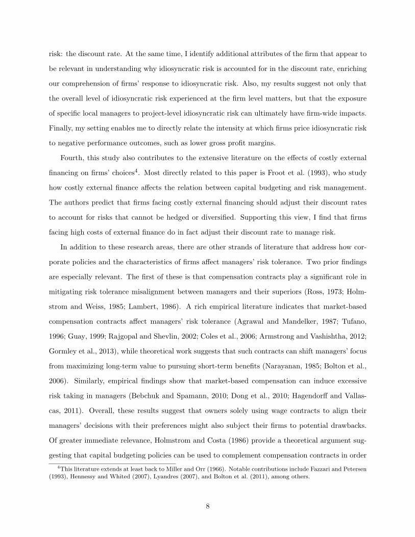
risk: the discount rate. At the same time, I identify additional attributes of the firm that appear to
be relevant in understanding why idiosyncratic risk is accounted for in the discount rate, enriching
our comprehension of firms’ response to idiosyncratic risk. Also, my results suggest not only that
the overall level of idiosyncratic risk experienced at the firm level matters, but that the exposure
of specific local managers to project-level idiosyncratic risk can ultimately have firm-wide impacts.
Finally, my setting enables me to directly relate the intensity at which firms price idiosyncratic risk
to negative performance outcomes, such as lower gross profit margins.
Fourth, this study also contributes to the extensive literature on the effects of costly external
financing on firms’ choices4. Most directly related to this paper is Froot et al. (1993), who study
how costly external finance affects the relation between capital budgeting and risk management.
The authors predict that firms facing costly external financing should adjust their discount rates
to account for risks that cannot be hedged or diversified. Supporting this view, I find that firms
facing high costs of external finance do in fact adjust their discount rate to manage risk.
In addition to these research areas, there are other strands of literature that address how cor-
porate policies and the characteristics of firms affect managers’ risk tolerance. Two prior findings
are especially relevant. The first of these is that compensation contracts play a significant role in
mitigating risk tolerance misalignment between managers and their superiors (Ross, 1973; Holm-
strom and Weiss, 1985; Lambert, 1986). A rich empirical literature indicates that market-based
compensation contracts affect managers’ risk tolerance (Agrawal and Mandelker, 1987; Tufano,
1996; Guay, 1999; Rajgopal and Shevlin, 2002; Coles et al., 2006; Armstrong and Vashishtha, 2012;
Gormley et al., 2013), while theoretical work suggests that such contracts can shift managers’ focus
from maximizing long-term value to pursuing short-term benefits (Narayanan, 1985; Bolton et al.,
2006). Similarly, empirical findings show that market-based compensation can induce excessive
risk taking in managers (Bebchuk and Spamann, 2010; Dong et al., 2010; Hagendorff and Vallas-
cas, 2011). Overall, these results suggest that owners solely using wage contracts to align their
managers’ decisions with their preferences might also subject their firms to potential drawbacks.
Of greater immediate relevance, Holmstrom and Costa (1986) provide a theoretical argument sug-
gesting that capital budgeting policies can be used to complement compensation contracts in order
4This literature extends at least back to Miller and Orr (1966). Notable contributions include Fazzari and Petersen(1993), Hennessy and Whited (2007), Lyandres (2007), and Bolton et al. (2011), among others.
8

to more successfully align managers’ decisions with those of their supervisors. The present study
contributes to this literature by empirically identifying the size of managers’ budgets as a tool to
alter risk tolerance. Specifically, the findings reported here suggest that it is possible to increase
the idiosyncratic risk tolerance of a manager by increasing the size of his allocated budget, in line
with the diversification effect proposed by Diamond (1984).
II. Natural Gas Industry: Institutional Background
A. Project Overview: The Drilling Technology
Two prominent technologies exist to drill natural gas wells: vertical drilling and horizontal
drilling (see Figure 1). In this paper, I focus specifically on vertical-drilling technology. Vertical
drilling is the principal technology employed during the period analyzed for this study, representing
roughly 90% of all natural gas wells in the dataset. Horizontal drilling is more recent, and has only
gradually gained mainstream appeal during the later part of the sample period. Additionally, it is
easier to obtain precise production forecasts for wells drilled using vertical drilling technology, as
horizontal wells are substantial more complex and technologically advanced (Ma et al., 2016). For
example, Covert (2015) provides a clear illustration of the high level of detail necessary to properly
characterize expected monthly production for horizontally drilled wells. Obtaining information at
this level of detail is simply not possible when dealing with a relatively long-term dataset for the
entire United States. At the same time, good production forecasts for vertical wells can be produced
using information available from major data providers such as DrillingInfo. For all of these reasons,
the study focuses exclusively on vertically drilled wells.
B. The Life Cycle of Natural Gas Fields
The commercial life cycle of natural gas has two stages: exploration and development. According
to the U.S. Energy Information Agency (i.e., EIA), the exploration stage involves documenting the
geological potential of the field in question, and determining its economic viability. Once a firm has
sufficient information for confirming the economic potential of the field, it is classified as a proven
9

reserve5 and the development stage begins.
This study focuses on the development stage, during which firms still face a high level of
idiosyncratic risk despite having established that the field in question is a proven reserve. They
do not yet know (i) the exact delineation of the natural gas field, (ii) the structure of the rock
formations within it, (iii) the production potential of each drilling location, or (iv) the technical
expertise required to optimally extract the resource. For firms drilling wells, this lack of knowledge
translates into tangible operational risks, such as the risk of drilling a dry hole6. For example, Figure
2 illustrates the development of the Panhandle field in Texas over the period between 1960 and
2010. Figure 2.1 represents the initial estimation of the field boundary, while Figure 2.2 represents
the field’s finalized boundary 50 years later. There are substantial differences between the expected
and realized boundaries. Large sections that were initially identified as promising appear to have
had limited potential ultimately. This example provides a clear illustration of how idiosyncratic
risk remains at the micro-level even after a field’s economic potential has been confirmed at the
macro-level.
C. The Structure of Natural Gas Exploration and Production Firms
Oil and gas companies establish their strategies at the uppermost levels of the corporate hier-
archy (Graham et al., 2015), but surveying, wells’ selection, and specific drilling decisions require
advanced technical expertise and site-specific information (Kellogg, 2011; Covert, 2015; Decaire
et al., 2019). For this reason, lower-level managers, geologists, and engineers tend to evaluate and
select projects (Bohi, 1998), working within the confines of strategic guidelines from their superiors.
Additionally, oil and gas firms tend to organize their operational units by regions. For example, en-
ergy companies’ shareholder communication documents (e.g., 10-K) provide examples of how those
geographical formations affect operations’ structure (see Figure 3). Finally, by allocating their total
budgets across multiple regional units, firms expose the key on-the-ground decision-makers (i.e.,
the junior managers) to the risks of only a relatively small number of specific projects. This creates
a divide between idiosyncratic risk diversification measured at the firm level, and diversification
5The American Bar Association’s definition of proven reserves is as follows: The amount of oil and gas is estimatedwith reasonable certainty to be economically producible. source: American Bar Association, Oil and Gas Glossary,2019.
6A dry hole is a well that fails to produce enough natural gas to be economically viable.
10

measured at the level of individual managers, potentially creating incongruities in risk preferences.
III. The Dataset
The present study uses a dataset provided by DrillingInfo7 covering all natural gas wells drilled
in the United States between 1983 and 2010 (see Figure 4). Ultimately, the dataset contains
30,420,544 month-well observations used to estimate the well production function, a total of 114,969
distinct gas wells, and 369 distinct firms. The dataset includes monthly production for each project
along with a set of projects’ characteristics such as rock formation features, wells’ GPS location,
the royalty rate8 and the depth of the well. I augment these data points with two hand-collected
datasets. The first covers per-project capital expenditures including per-foot drilling costs, obtained
from public filling from regulatory pooling documents, and estimated operational costs, estimated
from firms’ 10-K. The second is drawn from the EIA and corresponds to the three-year natural
gas price forecasts and two alternative sources of natural gas prices (the Bloomberg natural gas
futures prices, and the EIA wellhead state’s natural gas prices). The EIA is a federal reporting
agency producing an annual economic analysis for the oil and gas industry9. For public firms,
the dataset is further augmented using Compustat. Finally, the information needed to compute
each firm’s weighted cost of capital is drawn from the 10-year risk-free rate available on the Saint-
Louis Federal Reserve website, the Kenneth French oil and gas industry return, the Robert Shiller
price-earnings ratio, and credit rating information from Capital IQ.
Finally, I make several refinements to the dataset. I restrict the analysis to firms drilling at
least 10 wells in a given year10; because discount rates are estimated from the lower boundary of
the firms’ portfolios, it is reasonable to focus on firms that are at least moderately active during
7DrillingInfo is a trusted data provider for multiple federal agencies reporting on environment and energy matters.Studies conducted by the U.S. Environmental Protection Agency (EPA) and the U.S. Energy Information Adminis-tration (EIA) Inventory of U.S. Greenhouse Gas Emissions and Sinks, 1990-2016 by the EPA and Petroleum SupplyMonthly (PSM) by the EIA use this dataset, for example.
8The royalty rates correspond to an expense computed as a percentage of the well’s revenue that goes directlyto the land owners leasing the land for a given well. The royalty rate estimates are based on royalty percentagesobtained from DrillingInfo for the leases signed in the United States in a given year.
9More specifically, the U.S. Energy Information Administration (EIA) is a statistical and analytical agency housedwithin the U.S. Department of Energy. The EIA collects, analyzes, and disseminates independent and impartial energyinformation to promote sound policymaking, efficient markets, and public understanding of energy and its interactionwith the economy and the environment. The EIA is the nation’s premier source of energy information and, by law,its data, analyses, and forecasts are independent of approval by any other officer or employee of the U.S. government.Source: https://www.eia.gov/about/mission_overview.php
10The main result is robust to alternative cut-off value of 6 and 14, for example.
11
the year of analysis. For less-active firms, it is harder to distinguish between the firms’ discount
rate and the quality of their opportunity set when using the revealed-preference strategy. This
adjustment drops only 5% of wells in the initial sample. Additionally, all township-year subgroups
with fewer than three wells drilled are removed, because the measure of idiosyncratic risk employed
here relies on the standard-deviation for each township-year set. Finally, any wells with missing
information are dropped from the dataset, along with any wells for which the initial production
date is prior to the drilling date, as those clearly contain data entry errors.
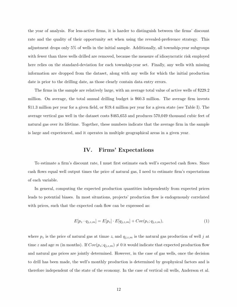
The firms in the sample are relatively large, with an average total value of active wells of $229.2
million. On average, the total annual drilling budget is $60.3 million. The average firm invests
$11.3 million per year for a given field, or $19.4 million per year for a given state (see Table I). The
average vertical gas well in the dataset costs $465,653 and produces 570,049 thousand cubic feet of
natural gas over its lifetime. Together, these numbers indicate that the average firm in the sample
is large and experienced, and it operates in multiple geographical areas in a given year.
IV. Firms’ Expectations
To estimate a firm’s discount rate, I must first estimate each well’s expected cash flows. Since
cash flows equal well output times the price of natural gas, I need to estimate firm’s expectations
of each variable.
In general, computing the expected production quantities independently from expected prices
leads to potential biases. In most situations, projects’ production flow is endogenously correlated
with prices, such that the expected cash flow can be expressed as:
E[pz · qj,z,m] = E[pz] · E[qj,z,m] + Cov(pz; qj,z,m), (1)
where pz is the price of natural gas at timze z, and qj,z,m is the natural gas production of well j at
time z and age m (in months). If Cov(pz; qj,z,m) 6= 0 it would indicate that expected production flow
and natural gas prices are jointly determined. However, in the case of gas wells, once the decision
to drill has been made, the well’s monthly production is determined by geophysical factors and is
therefore independent of the state of the economy. In the case of vertical oil wells, Anderson et al.
12

(2018) show that firms do not alter production rates or delay production due to oil price changes.
Indeed, once a well starts producing, managers have little ability to influence the production level
without risking damage to the well. What this means is that effectively, production flow depends
on local geophysical parameters such as the local rock type, the density of the natural gas deposit,
and so forth, rather than on economic variables affecting natural gas prices. For this reason, I
assume that the production flow is not correlated with variables that affect gas prices. Further
supporting this assumption, the correlation between realized natural gas prices and wells’ realized
production flow is just -0.0034 in my sample11. Thus, estimating expected quantities and expected
prices independently should not result in biased outcomes. The process through which I obtain
these estimates is described below.
A. Firms’ Expected Production
Monthly production of vertical gas wells can be approximated using a petroleum-engineering
model such as the Arp model (Fetkovich, 1996; Li and Horne, 2003). The Arp model is the classical
production-forecasting equation, and nowadays is taught in most energy engineering courses (e.g.,
the University of Pennsylvania course Engineering in Oil, Gas and Coal). According to the Arp
model, the predicted monthly quantities produced by well j equal
qj,m = Aj(1 + bθm)−1b , (2)
where m corresponds to the number of months since the well has been drilled, Aj corresponds
to the well’s baseline production level, and b and θ are decline-rate elasticity parameters. To
approximate the Arp model, I linearize this equation to obtain a regression (see Appendix B for
the full derivation):
ln(qj,m) = α0 + α1 +Aj +K∑k=1
βkmk + εj,m, (3)
11This statistic corresponds to the correlation of the realized natural gas prices )i.e., the wellhead spot price providedon the EIA website) with the realized within-well’s production flow computed for the entire well-month sample.
13

where α0 and α1 are dummy variables for the first and second months of production, used to
account for ramping production12, K is the order of the linear approximation (i.e., 7), and εj,m is
the regression’s error term.
The production baseline (i.e., Aj) represents the expected quantity of gas that will be initially
produced by the well. I allow Aj to depend on the firm’s total experience (i.e., the total number of
wells the firm has drilled before well j ), the firm’s local experience (i.e., the number of wells the firm
has drilled in the given township at the time of drilling j ), the level of local information available
(i.e., the total number of wells that have been drilled in the township at the time of drilling j ), a
firm-year fixed effect, and a township-year fixed effect such that:
Aj = ln(Firm’s Local XPj) + ln(Firm’s Total XPj) + ln(Local Infoj) + αi,t + αp,t (4)
Where i identifies the firms that drilled well j, p identifies the township in which the well is drilled,
and t is the year the well is drilled.
Several recent papers motivate the addition of these controls for the Arp estimation (Covert,
2015; Decaire et al., 2019; Hodgson, 2019). Firms’ experience levels, peer effects, and local access
to information influence the quality and type of projects a firm will undertake. More experienced
firms are more likely to produce high-quality wells and to identify regions with better potential.
Equally, regions with more activity are more likely to have wells of higher quality, while at the same
time affording more precise information about how best to extract the resource. Because the goal
of this part of the analysis is both to obtain precise estimates of the wells’ expected production flow
and to deliver a reasonable measure of the wells’ idiosyncratic productivity shocks, it is important
to control for factors that capture those characteristics.
Finally, to obtain the wells’ expected production flow, I proceed in two steps. First, I use the
Arp model to estimate regression (3), using a sample of 30,420,544 month-well realized output (see
Appendix Table I). Then, I use the Arp model estimates to obtain a measure of the managers’
expectation for each well in the sample. Figure 513 provides a graphical illustration for the median
12A well’s ramping period usually corresponds to the first two months of production, during which firms’ engineersoptimize and adjust the well’s production to reach peak long-term capacity (Dennis, 2017). Production then graduallydeclines until the well is dry.
13The ramping up period, encompassing the first two months of production, is excluded in order to captureproduction decline from peak production to termination.
14

well production function over time and contrasts it with the estimated production output. These
expectations constitute the basis of the analysis to obtain a measure of the discount rate, and a
measure of the wells’ idiosyncratic risk.
B. Firms’ Expected Price
I define the expected gas prices using the EIA’s yearly three-year natural gas price forecast, at
the time of drilling the well14. The EIA forecast is closely followed by governmental organizations,
financial institutions, and energy companies. Section 9 explores alternative price specifications,
such as the Bloomberg natural gas futures prices and wellhead spot prices varying at the level of
individual states, and how these affect the results reported below. The EIA data are preferable
to those other options for two reasons, however. First, the EIA three-year natural gas forecast
has been published consistently since 1983, while the Bloomberg three-year natural gas futures
contracts started trading only in 1995. Thus, the longer period for the EIA forecast allows the
analysis to extend over a correspondingly greater duration. Second, although the wellhead state-
by-state prices provide information on price variation across states during a given year, which helps
to take into account cross-sectional variation of natural gas prices, those wellhead prices fail to
account for managers’ future expectations about price variation, making them unsuitable for the
analysis. Finally, the EIA three-year forecast horizon is well matched to the present study, as the
discounted half-life15 for projects in the sample is 31 months.
V. Estimating Firms’ Discount Rates Using a Revealed
Preference Strategy
A. Estimating Projects’ Expected Rates of Return
To obtain estimates of firms’ discount rates, I proceed in four steps. First, for each well a firm
drills during a given year, I estimate the well’s expected cash flows using forecasts of the well’s
production and natural gas prices. Second, I use those forecasts to compute the expected IRR (µj)
14A similar assumption for the prices is used in Kellogg (2014), Covert (2015) and Decaire et al. (2019).15The discounted project half-life corresponds to the amount of time required for managers to obtain half of the
discounted project’s expected cash flow.
15
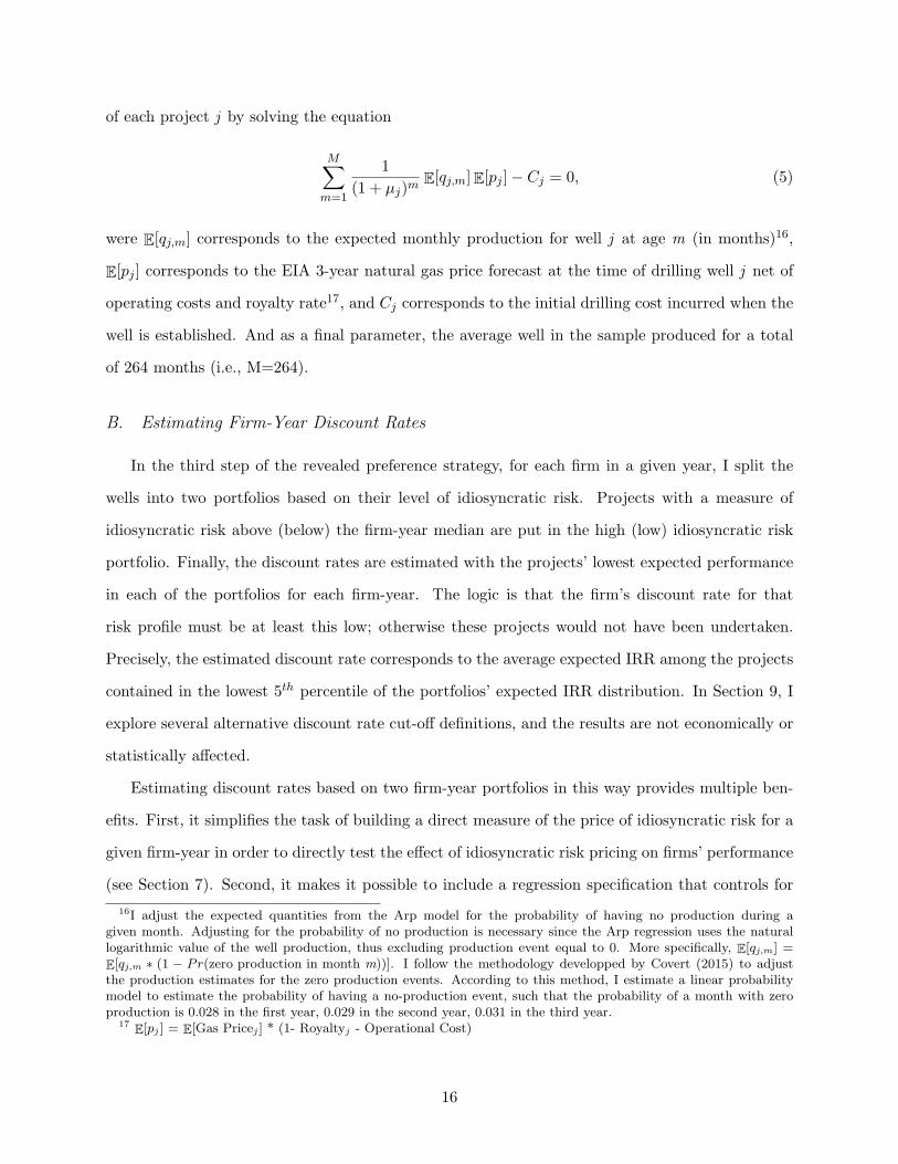
of each project j by solving the equation
M∑m=1
1
(1 + µj)mE[qj,m]E[pj ]− Cj = 0, (5)
were E[qj,m] corresponds to the expected monthly production for well j at age m (in months)16,
E[pj ] corresponds to the EIA 3-year natural gas price forecast at the time of drilling well j net of
operating costs and royalty rate17, and Cj corresponds to the initial drilling cost incurred when the
well is established. And as a final parameter, the average well in the sample produced for a total
of 264 months (i.e., M=264).
B. Estimating Firm-Year Discount Rates
In the third step of the revealed preference strategy, for each firm in a given year, I split the
wells into two portfolios based on their level of idiosyncratic risk. Projects with a measure of
idiosyncratic risk above (below) the firm-year median are put in the high (low) idiosyncratic risk
portfolio. Finally, the discount rates are estimated with the projects’ lowest expected performance
in each of the portfolios for each firm-year. The logic is that the firm’s discount rate for that
risk profile must be at least this low; otherwise these projects would not have been undertaken.
Precisely, the estimated discount rate corresponds to the average expected IRR among the projects
contained in the lowest 5th percentile of the portfolios’ expected IRR distribution. In Section 9, I
explore several alternative discount rate cut-off definitions, and the results are not economically or
statistically affected.
Estimating discount rates based on two firm-year portfolios in this way provides multiple ben-
efits. First, it simplifies the task of building a direct measure of the price of idiosyncratic risk for a
given firm-year in order to directly test the effect of idiosyncratic risk pricing on firms’ performance
(see Section 7). Second, it makes it possible to include a regression specification that controls for
16I adjust the expected quantities from the Arp model for the probability of having no production during agiven month. Adjusting for the probability of no production is necessary since the Arp regression uses the naturallogarithmic value of the well production, thus excluding production event equal to 0. More specifically, E[qj,m] =
E[qj,m ∗ (1 − Pr(zero production in month m))]. I follow the methodology developped by Covert (2015) to adjustthe production estimates for the zero production events. According to this method, I estimate a linear probabilitymodel to estimate the probability of having a no-production event, such that the probability of a month with zeroproduction is 0.028 in the first year, 0.029 in the second year, 0.031 in the third year.
17 E[pj ] = E[Gas Pricej ] * (1- Royaltyj - Operational Cost)
16

a firm-year fixed effect. However, to show that the results are not sensitive to this research design
choice, I provide an alternative specification where I estimate the discount rate from one portfolio
per firm-year in Section 9. The results are robust to this specification.
In this study, I only observe the set of projects each firm completes in a given year. In other
words, I observe a truncated distribution of projects’ expected IRR, because it is not possible
to observe the expected return for projects the firms did not pursue (i.e., those that are not
completed). At the same time, a firm may not have had investment opportunities with an expected
IRR sufficiently close to the firm’s discount rate. This means that my estimate constitutes an upper
bound for the firms’ discount rate. To mitigate concerns about this upper bound, I restrict the
analysis to a subset of firms that drill at least 10 wells in a given year. The intuition is that for
firms that drill many wells, the marginal well is more likely to represent the firms’ lower bound (i.e.,
the firm’s discount rate). Then, to validate that the estimates accurately capture the main features
attributed to firms’ discount rates, I conduct a robustness test. First, I restrict the analysis to the
subset of firms whose full capital structure is observed. For that group, I compute the WACC.
I obtain an estimate for the cost of equity in two steps. First, I use the one-year18 oil and gas
industry capital asset pricing model (CAPM) beta computed at the monthly frequency, obtained
from Kenneth French’s industry return data19. Then, I multiply this variable by the expected equity
premium, estimated from the earning-to-price ratio obtained from the Robert Shiller’s website20.
Finally, to obtain the cost of debt, I collect the firms’ yearly credit rating from Capital IQ (see
Appendix A.2.). Table II presents the results of this test. There is a positive and statistically
significant correlation between the discount rate estimates and the firms’ WACC. Coefficient β1
indicates that a one-percentage point increase to the firm WACC results in a 1.3 to 1.5pp increase
in the discount rate21. The results presented in columns 3 and 4 of Table II suggest that the
idiosyncratic risk premium is added to the discount rate on top of the WACC, and also that the
18Results are robust when using CAPM betas computed with other horizons, such as two-year and three-yearhorizons.
19The oil and gas industry return is available within the 49 industries’ returns breakdown. I verify the robustnessof the results using the various industry breakdowns available on the Kenneth French website, and I obtain similarresults in all cases.
20I estimate the expected equity premium from the fitted value of the regression [EtPt
−rft] = α+β[Et−1
Pt−1−rft−1]+εt,
estimated for the period 1983 to 2010. In an alternative specification, I use Fama and French (2002)’s estimate of theequity premium (4.32%) for the entire sample period, and the results are statistically robust and remain qualitativelysimilar, although the coefficients are slightly smaller.
21In all specifications, the value of 1 is included for the coefficient β1’s confidence interval.
17
discount rate measure behaves in a manner consistent with variations in the cost of capital.
VI. Measure of Wells’ Idiosyncratic Risk
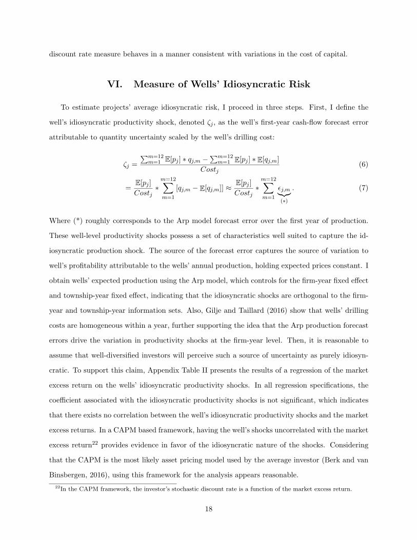
To estimate projects’ average idiosyncratic risk, I proceed in three steps. First, I define the
well’s idiosyncratic productivity shock, denoted ζj , as the well’s first-year cash-flow forecast error
attributable to quantity uncertainty scaled by the well’s drilling cost:
ζj =
∑m=12m=1 E[pj ] ∗ qj,m −
∑m=12m=1 E[pj ] ∗ E[qj,m]
Costj(6)
=E[pj ]
Costj∗m=12∑m=1
[qj,m − E[qj,m]] ≈ E[pj ]
Costj∗m=12∑m=1
εj,m︸︷︷︸(∗)
. (7)
Where (*) roughly corresponds to the Arp model forecast error over the first year of production.
These well-level productivity shocks possess a set of characteristics well suited to capture the id-
iosyncratic production shock. The source of the forecast error captures the source of variation to
well’s profitability attributable to the wells’ annual production, holding expected prices constant. I
obtain wells’ expected production using the Arp model, which controls for the firm-year fixed effect
and township-year fixed effect, indicating that the idiosyncratic shocks are orthogonal to the firm-
year and township-year information sets. Also, Gilje and Taillard (2016) show that wells’ drilling
costs are homogeneous within a year, further supporting the idea that the Arp production forecast
errors drive the variation in productivity shocks at the firm-year level. Then, it is reasonable to
assume that well-diversified investors will perceive such a source of uncertainty as purely idiosyn-
cratic. To support this claim, Appendix Table II presents the results of a regression of the market
excess return on the wells’ idiosyncratic productivity shocks. In all regression specifications, the
coefficient associated with the idiosyncratic productivity shocks is not significant, which indicates
that there exists no correlation between the well’s idiosyncratic productivity shocks and the market
excess returns. In a CAPM based framework, having the well’s shocks uncorrelated with the market
excess return22 provides evidence in favor of the idiosyncratic nature of the shocks. Considering
that the CAPM is the most likely asset pricing model used by the average investor (Berk and van
Binsbergen, 2016), using this framework for the analysis appears reasonable.
22In the CAPM framework, the investor’s stochastic discount rate is a function of the market excess return.
18

Second, I measure the idiosyncratic risk for each township-year by computing the cross-sectional
dispersion of the local wells’ idiosyncratic productivity shocks. The strategy is designed to only
capture the quantity uncertainty contribution to the cash flow uncertainty. It is useful to note that
I achieve this by only using expected prices in ζj calculation, ignoring the price shock from the cal-
culation. This is to ensure that idiosyncratic risk is truly calculated from local idiosyncratic shocks.
This provides a measure of idiosyncratic risk at the township-year level that can be attributed to
each well that is drilled in the specific township in that given year (see Figure 6.1). Third, to obtain
a measure for the firm-year-portfolio level, I take the average of the idiosyncratic risk for all the
projects completed. Ultimately, the sample average of the projects’ average idiosyncratic risk is
equal to 10pp, and its standard-deviation is 18pp.
This measure of idiosyncratic risk has several appealing features. First, it corresponds to the
level of productivity uncertainty managers face in the first year for 1$ of invested capital. Second,
firms tend to pay attention to the drilling outcomes in their wells’ closed vicinity (Decaire et al.,
2019), suggesting that the level of cross-sectional dispersion for the township-year likely reflects the
level of well’s idiosyncratic risk as assessed by local managers. Third, the analysis is conducted at
a yearly frequency. Thus, working with first-year risk provides a measure of risk that is computed
at the frequency of the study’s analysis. And finally, the information contained in the productivity
forecasting errors, ζj , is plausibly orthogonal to the characteristics of the managing firm. The Arp
regression controls include a firm-year fixed effect and a township-year fixed effect as well as the
firm’s local experience, the firm’s global experience, and the amount of local information available at
the time of drilling. Thus, the information contained in a given well’s productivity forecasting errors
likely corresponds to information that is orthogonal to the firm-year and geographic characteristics
already assessed by the model.
To verify the validity of the Arp regression specifications, it is first necessary to test whether
there is any spatial correlation between the production forecast errors across wells. The goal of the
test is to make sure that variation in forecasting errors is not driven by other important spatial-
economic factors omitted from the Arp model. I assess spatial correlations using the Moran’s I
coefficient, which ranges in value from -1 to 1. A coefficient equal to zero indicates no spatial
correlation, while positive coefficients imply clustering of forecasting errors. In the present context,
a positive Moran’s I would suggest that the Arp model has omitted spatial factors. However, the
19

estimate of Moran’s I is close to zero, at 0.01, suggesting that the Arp model properly captures
relevant spatial factors. Finally, Figure 7 plots the distribution of the wells’ idiosyncratic productiv-
ity shocks. The idiosyncratic productivity shocks distribution is centered at zero (i.e., the median
value is 0.0007), but it is slightly leptokurtic.
Next, in order to confirm that the above measure of idiosyncratic risk is positively related to
a greater occurrence of poor drilling outcomes, I examine the number of dry holes per township-
year. For township-year subgroups in the upper half of the idiosyncratic risk distribution, there
are on average 0.39 dry holes drilled; for township-years in the lower half, this value is 0.04.
This corresponds to a one order of magnitude difference between the comparison groups, strongly
suggesting that township-years with greater idiosyncratic risk consistently experience higher rates of
negative drilling outcomes. To control for additional factors, I also estimate a Poisson regression23.
Appendix Table III displays a positive and statistically significant relationship between projects’
idiosyncratic risk and the probability of drilling a dry hole across all specifications. Specifically, a
one-standard-deviation increase in the idiosyncratic risk measure is associated with 1.4 additional
dry holes drilled in the township-year. This result provides further empirical support for the
relationship between the measure of idiosyncratic risk and adverse drilling outcomes.
VII. Results
A. Do Managers Price Idiosyncratic Risk?
To test whether managers price idiosyncratic risk, I first estimate an OLS regression of firms’ dis-
count rates and projects’ idiosyncratic risk. The regression includes two observations per firm-year,
one for each of the firm’s high- and low-idiosyncratic risk portfolios. To simplify the interpretation
of the regression coefficient across all the regression specifications in the paper, I scale the regressor
of interest by its regression-sample standard-deviation24. Table III shows that managers appear
to positively price idiosyncratic risk. Column 1 presents the simple regression with one control,
the portfolios’ potential differential exposure to systematic risk (See Appendix C for a complete
23A Poisson regression is the appropriate model when the dependent variable is a count variable, such as the numberof dry holes in a township-year (Greene, 2003).
24To scale a regressor by a constant does not alter the statistical properties of the estimate (Greene, 2003). Thisstrategy has the added benefit of directly providing me with the magnitude for the effect of a one-standard-deviationincrease in the projects’ idiosyncratic risk.
20

discussion). Columns 2 to 5 introduce a set of controls and show that the regression results are
robust to those further specifications. Column 6 includes a firm-year fixed effect, to control for
the time-varying characteristics of firms, and Column 7 adds the idiosyncratic risk portfolio fixed
effect. The source of variation in those regression is the relationship between average projects’
idiosyncratic risk and the discount rates estimated for high- and low-risk firm-year portfolios. For
the average firm, a one-standard-deviation increase in idiosyncratic risk results in a 6.7 to 8.0pp
increase in the discount rate.
B. Instrumental Variable
The fixed effects included in the above regressions address a few endogeneity concerns. Specifi-
cally, the firm-year fixed effect accounts for the fact that, in a given year, a firm may systematically
select regions that are riskier. At the same time, the idiosyncratic risk portfolio fixed effect helps
address the idea that there might be a selection effect such that some unobserved variables (e.g.,
managers’ experience) might systematically be associated to better or riskier regions (i.e., regions
with better potential projects, lower risk of bad drilling outcomes). However, the fixed effect strat-
egy does not account for the managers’ heterogeneity within the idiosyncratic risk portfolios, which
could plausibly vary by firms. Thus, the previous OLS regression may suffer from a within-firm
omitted-variable bias.
To address these additional endogeneity concerns, I take an instrumental-variable approach.
The strategy is implemented in two steps. First, each well is associated with its corresponding
township-year peers’ largest project’s idiosyncratic productivity shock. Figure 6 provides a graph-
ical example – with three firms (identified in Red, Blue, and Black) – of how these shocks are
identified for one particular township-year; for the wells drilled by the Red firm, the associated
peer’s shock is 0.23. Then, I define the instrumental variable as the average value of those associ-
ated peers’ shocks computed at the level of each firm-year portfolio.
The relevance of the instrumental variable has to do with how the idiosyncratic risk variable is
calculated. In this study, the idiosyncratic risk corresponds to the cross-sectional dispersion of all
21
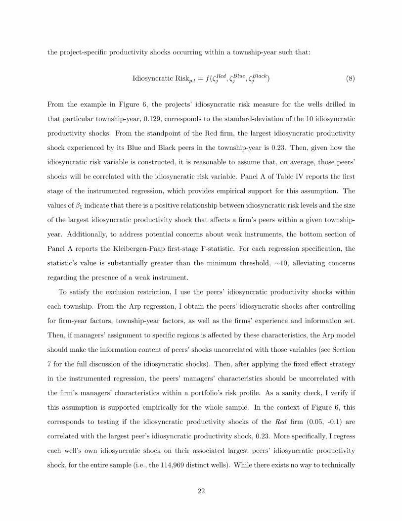
the project-specific productivity shocks occurring within a township-year such that:
Idiosyncratic Riskp,t = f(ζRedj , ζBluej , ζBlackj ) (8)
From the example in Figure 6, the projects’ idiosyncratic risk measure for the wells drilled in
that particular township-year, 0.129, corresponds to the standard-deviation of the 10 idiosyncratic
productivity shocks. From the standpoint of the Red firm, the largest idiosyncratic productivity
shock experienced by its Blue and Black peers in the township-year is 0.23. Then, given how the
idiosyncratic risk variable is constructed, it is reasonable to assume that, on average, those peers’
shocks will be correlated with the idiosyncratic risk variable. Panel A of Table IV reports the first
stage of the instrumented regression, which provides empirical support for this assumption. The
values of β1 indicate that there is a positive relationship between idiosyncratic risk levels and the size
of the largest idiosyncratic productivity shock that affects a firm’s peers within a given township-
year. Additionally, to address potential concerns about weak instruments, the bottom section of
Panel A reports the Kleibergen-Paap first-stage F-statistic. For each regression specification, the
statistic’s value is substantially greater than the minimum threshold, ∼10, alleviating concerns
regarding the presence of a weak instrument.
To satisfy the exclusion restriction, I use the peers’ idiosyncratic productivity shocks within
each township. From the Arp regression, I obtain the peers’ idiosyncratic shocks after controlling
for firm-year factors, township-year factors, as well as the firms’ experience and information set.
Then, if managers’ assignment to specific regions is affected by these characteristics, the Arp model
should make the information content of peers’ shocks uncorrelated with those variables (see Section
7 for the full discussion of the idiosyncratic shocks). Then, after applying the fixed effect strategy
in the instrumented regression, the peers’ managers’ characteristics should be uncorrelated with
the firm’s managers’ characteristics within a portfolio’s risk profile. As a sanity check, I verify if
this assumption is supported empirically for the whole sample. In the context of Figure 6, this
corresponds to testing if the idiosyncratic productivity shocks of the Red firm (0.05, -0.1) are
correlated with the largest peer’s idiosyncratic productivity shock, 0.23. More specifically, I regress
each well’s own idiosyncratic shock on their associated largest peers’ idiosyncratic productivity
shock, for the entire sample (i.e., the 114,969 distinct wells). While there exists no way to technically
22

test for the exclusion restriction, the absence of correlation is generally reassuring. Table V reports
the regression results of the firm’s own idiosyncratic productivity shocks on the largest peers’
idiosyncratic productivity shock in each township-year. I find no statistical relationship between the
two types of shocks, across all the regression specifications. Perhaps the most relevant specification
is the one presented in column 8, because it addresses more directly the underlying assumption of the
instrumental variable strategy: the absence of correlation between firms’ managers’ characteristics
and its peers’ characteristics within a township of a given risk level. Specifically, column 8 suggests
that there exists no statistical relationship between the shocks within a given township, providing
support for the instrument assumption.
Panel B of Table IV reports the results of the second stage of the instrumented regression.
The coefficients are slightly smaller in magnitude than the results obtained from the reduced-form
regression, but they remain economically meaningful. For the instrumented regression, a one-
standard-deviation increase in a project’s idiosyncratic risk results in an increase of 3.8 to 6.0pp in
the firm’s discount rate, compared to 6.7 to 8.0pp for the reduced-form regression.
Regarding the sign of the endogeneity bias, I find that the coefficient of interest (β1) of the
instrumented regression is smaller than the one in the reduced-form regression presented in Table
III, across all specifications (see Appendix D). The direction of the bias for the coefficient of interest
(β∗1) depends on (i) the covariance between the managers’ experience and the level of idiosyncratic
risk associated with the wells, and (ii) β2, the linear relationship between managers’ experience and
the firms’ discount rate. Ultimately, multiple within-firm omitted variables could be affecting my
analysis, with some having opposing effects on the direction of the endogeneity bias. In this sense,
the goal of the following discussion is to provide a concrete example to illustrate the type of omitted
variables that appear to ultimately dominate the direction of the endogeneity bias observed in the
reduced-form regression.
For (i), it is plausible that more experienced managers get assigned to better regions (i.e., better
prospect, lower production risk) because of their greater bargaining power within the firm or that,
given their higher level of experience, the outcome of their wells is less uncertain because they know
better how to optimally extract the natural gas. In this specific framework, this would suggest a
negative relationship between the managers’ level of experience and the observed idiosyncratic risk
variable. For (ii), to obtain a reasonable explanation on the sign of β2, it is helpful to look at it from
23

a career concern standpoint. More experienced managers have a longer list of realizations, which
suggests that each additional signal is less likely to have a large effect on how the firms’ superiors
update their belief of the experienced managers’ worth. In this case, bad drilling outcomes are
less likely to negatively affect how superiors value experienced managers than how they value
unexperienced managers. Chevalier and Ellison (1999) provide empirical evidence in favor of this
career concern explanation, showing that on average, less experienced managers are more likely to
get fired for bad performance. This suggests that for a similar level of exposure to idiosyncratic
risk, more experienced managers would require a smaller idiosyncratic risk premium than their less
experienced counterparts, implying that the sign of β2 should be negative. Ultimately, the combined
effect of these variables would suggest that the reduced-form regression suffers from an upward bias
because of omitted variables such as managers’ experience. In other words, the coefficient obtained
in the reduced-form regression may overestimate the magnitude of the discount rate adjustment to
account for idiosyncratic risk, when compared to the true coefficient.
C. Idiosyncratic Risk Premiums and Firm Performance
The previous results have implications for firms’ performance. If managers inflate their discount
rate when faced with a high level of idiosyncratic risk, firms would then underinvest in wells with
a high level of idiosyncratic risk. As a consequence, pricing idiosyncratic risk could have negative
consequences for firms’ performance, while abstaining from doing so should be correlated with
relatively better performance. However, there is little empirical evidence linking firms’ discount
rate adjustment to adverse performance.
I directly examine that relationship here. To test for the effect of idiosyncratic risk pricing on
firms’ performance (e.g., gross profit margins, gross profitability, asset growth (YoY), and invest-
ment rate), it is necessary to develop a measure of firms’ pricing of idiosyncratic risk, to directly
use it as a regressor. To construct this variable, I define the numerator as the difference between
the discount rates of the high idiosyncratic risk portfolio and the low idiosyncratic risk portfolio,
and I define the denominator as the difference between the idiosyncratic risk measures of the two
24
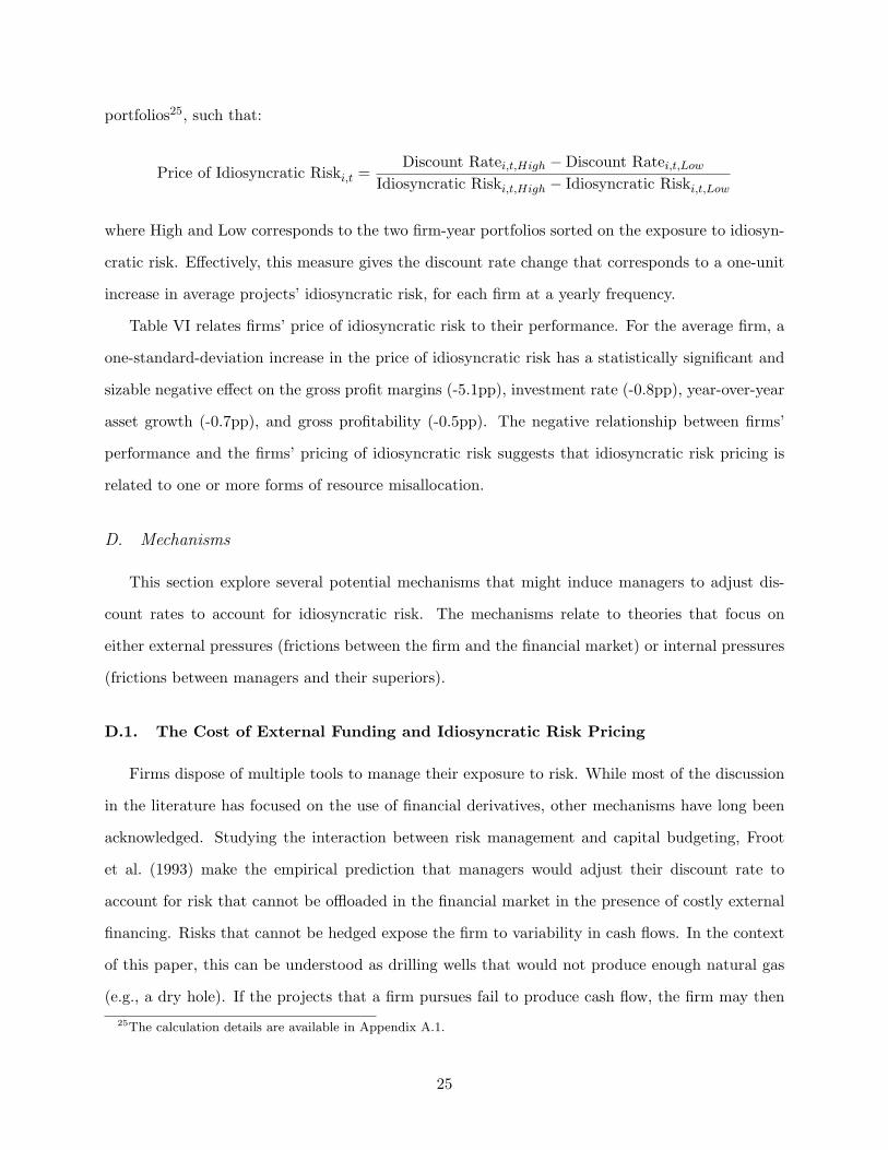
portfolios25, such that:
Price of Idiosyncratic Riski,t =Discount Ratei,t,High −Discount Ratei,t,Low
Idiosyncratic Riski,t,High − Idiosyncratic Riski,t,Low
where High and Low corresponds to the two firm-year portfolios sorted on the exposure to idiosyn-
cratic risk. Effectively, this measure gives the discount rate change that corresponds to a one-unit
increase in average projects’ idiosyncratic risk, for each firm at a yearly frequency.
Table VI relates firms’ price of idiosyncratic risk to their performance. For the average firm, a
one-standard-deviation increase in the price of idiosyncratic risk has a statistically significant and
sizable negative effect on the gross profit margins (-5.1pp), investment rate (-0.8pp), year-over-year
asset growth (-0.7pp), and gross profitability (-0.5pp). The negative relationship between firms’
performance and the firms’ pricing of idiosyncratic risk suggests that idiosyncratic risk pricing is
related to one or more forms of resource misallocation.
D. Mechanisms
This section explore several potential mechanisms that might induce managers to adjust dis-
count rates to account for idiosyncratic risk. The mechanisms relate to theories that focus on
either external pressures (frictions between the firm and the financial market) or internal pressures
(frictions between managers and their superiors).
D.1. The Cost of External Funding and Idiosyncratic Risk Pricing
Firms dispose of multiple tools to manage their exposure to risk. While most of the discussion
in the literature has focused on the use of financial derivatives, other mechanisms have long been
acknowledged. Studying the interaction between risk management and capital budgeting, Froot
et al. (1993) make the empirical prediction that managers would adjust their discount rate to
account for risk that cannot be offloaded in the financial market in the presence of costly external
financing. Risks that cannot be hedged expose the firm to variability in cash flows. In the context
of this paper, this can be understood as drilling wells that would not produce enough natural gas
(e.g., a dry hole). If the projects that a firm pursues fail to produce cash flow, the firm may then
25The calculation details are available in Appendix A.1.
25

have to turn to external markets to raise additional funds and continue its operations. However,
if the cost of marginal funds increases with the amount raised, the firm might have to limit its
investment in the next period or raise capital from increasingly expensive sources. In this sense,
greater variability in the wells’ outcome exposes firms to a greater probability of having to raise
external funds at a premium. Since this source of risk directly translates into a greater cost of
capital, Froot et al. (1993) suggest that managers should adjust their discount rate calculations
accordingly.
Obtaining a measure of the cost of external financing is challenging, as researchers do not directly
observe this variable. To test the hypothesis, this study builds on the work done by Hennessy and
Whited (2007), which provides empirically-based guidance for selecting the best proxy of costly
external financing. The core of their analysis focuses on firms’ size as well as three indexes: (i)
the Cleary index, (ii) the Whited-Wu index, and (iii) the Kaplan-Zingales index. In general, they
conclude that firm size is the best proxy for the costs of external financing, where larger firms face
a lower costs of external financing than do their smaller counterparts. They also, however, find that
the Cleary index and Whited-Wu index properly capture most of the dynamics attributed to the
cost of external financing, but fail to behave adequately with respect to the costs of bankruptcy,
making them inaccurate overall proxies for the cost of external financing. Finally, the authors note
that the Kaplan-Zingales index improperly captures most of the dynamics attributed to the cost
of external financing. On this basis, the authors conclude that firm size is the best proxy for costly
external financing, noting that the three indexes are better suited to act as proxies for the need for
external funding rather than for its cost.
All four of these potential proxies are included here, in an effort to be fully transparent. In
addition, the present study includes firms’ status (i.e., public or private) and the Hadlock-Pierce
index as additional proxies. Private ownership status has been associated with higher financing
frictions in the finance literature (Gao et al., 2013) and thus has the potential to be informative
here. Also, there is empirical evidence suggesting that the Hadlock-Pierce index captures firms’
financial constraints. Although the index has not been tested in the Hennessy and Whited (2007)’s
costly external financing horse race analysis, it is closely related to the firm’s size proxy discussed
by Hennessy and Whited (2007) as it is a function of firm size and age.
Table VII and Appendix Tables IV to VIII present the results of each of the six proxies of costly
26

external financing. For each table, the coefficient β2 measures the effect of costly external financing
on firms’ pricing of idiosyncratic risk. Columns 5 through 8 of each table present the results when
two variables are instrumented: (i) the projects’ idiosyncratic risk variable and (ii) the interaction
of projects’ idiosyncratic risk with the relevant proxy of costly external financing (i.e., β1 and β2).
Table VII reports the results of firm size. Consistent with the analysis of Froot et al. (1993),
it shows that as the cost of external funding decreases, firms tend to price idiosyncratic risk less
aggressively. The results are robust across all specifications, for both reduced form and the instru-
mented regression. On average, a one-standard-deviation reduction in firm size results in a 2.3pp
increase in the price of idiosyncratic risk26. Columns 2, 3, 4, 6, 7, and 8 introduce a proxy for firms’
diversification27, which corresponds to the firm-level idiosyncratic risk diversification among all the
projects that are drilled for a given firm-year. The diversification variable is included because firms’
size has been associated with several other characteristics of firms, such as their ability to diversify
sources of idiosyncratic risk (Demsetz and Strahan, 1997). The firms’ annual budget diversification
variable is constructed in a similar spirit to the diversification index in Seru (2014) (see Appendix
A.1.), and a larger value of the variable indicates that a larger share of the idiosyncratic risk is
diversified at the firm level.
Appendix Table IV reports the results for the Hadlock-Pierce index, which are directionally
consistent with the section hypothesis, and statistically significant. Namely, when the Hadlock-
Pierce index increases, which indicates that firms are more financially constrained, firms’ price
idiosyncratic risk more aggressively. Appendix Table V presents mixed results for the effect of
firms’ ownership status. For the specifications excluding a fixed effect at the firm level, the results
are consistent with the prediction made by Froot et al. (1993), such that private firms’ price
idiosyncratic risk more than public firms, but the difference is not statistically significant. Appendix
Tables VI to VIII report the Cleary, Whited-Wu and Kaplan-Zingales indexes results. They are
directionally consistent with the theoretical prediction developed in Froot et al. (1993), but they
are not all statistically different from zero.
Overall, the results presented in this section suggest that the cost of external financing can have
a meaningful impact on how firms adjust their discount rates. Focusing on Hennessy and Whited
26From Table VII: β2*Average Scaled Idiosyncratic Risk*σAsset= -0.01*0.6*383.8=-2.3.27Appendix A.3. provides the details of the calculations involved.
27

(2007)’s favored measure, the results indicate that costly external financing can induce managers
to price the undiversified quantities of idiosyncratic risk. It is reasonable to assume that this proxy
imperfectly captures attributes associated with firms’ cost of external financing, and thus it could
ultimately suffer from endogeneity bias. However, most of the additional proxies tested in this
section provide results that are directionally consistent with that theoretical prediction (despite
not being all statistically significant), lending further strength to that finding.
D.2. Managers’ Budget Size Diversification and Idiosyncratic Risk Pricing
Survey evidence collected by Graham et al. (2015) suggests that specific investment decisions
are formulated at the lower level of the hierarchical structure, while budget allocation is decided by
the firms’ superiors. Geanakoplos and Milgrom (1991) suggest that delegating investment decision-
making to the agents with the highest amount of information regarding a specific decision improves
resource allocation. Empirically, the delegation of authority has been linked to team specialization
(e.g., Caroli and Reenen (2001); Colombo and Delmastro (2004); Acemoglu et al. (2007)), where
workers in jobs that require technical skills usually benefit from a greater level of authority. In the
context of gas exploration and production companies, this approach increases the likelihood that
people most familiar with the local rock formation specificity will make investment decisions with
limited interference (Bohi, 1998). However, the decoupling between the capital allocation choice
and the decision to invest in specific projects, known as the delegation process, has been argued
as a potential source of agency conflict between managers and their superiors (Aghion and Tirole,
1997). From the lens of Aghion and Tirole (1997), to delegate land surveying and project selection
can be beneficial for firms since specialized on-site managers are more likely to generate quality
information and then identify better drilling opportunities. However, by giving managers a high
level of autonomy, there is a risk that managers might try to abuse their authority and misrepresent
the full set of available wells when pitching them to the firms’ superiors, if monitoring is costly.
For example, managers might prefer to avoid pitching projects with an associated idiosyncratic
risk measure that exceeds their preferred level, although those wells could be value creating from
the firms’ standpoint. This could be the case if managers are evaluated, and ultimately rewarded
or punished, by demonstrating their ability to generate production forecasts that are, on average,
in line with the wells’ realized production. For the firms, managers’ ability to produce reliable
28

production forecasts on average can be appealing since it facilitates the efficient allocation of re-
sources. Firms’ superiors might value this type of ability in managers’ performance reviews. Thus,
for managers, choosing wells with a higher level of idiosyncratic risk increases the probability of
being wrong in the production forecast (above or below) of a given well, which could increase their
risk of receiving bad evaluations. Although my dataset does not enable me to observe managers’
compensation contracts or if they get fired or promoted based on their forecasting performance,
Table VIII provides empirical evidence suggesting that firms’ resource allocation responds to fore-
casting mistakes. Precisely, the regression results reported in Table VIII indicate that firms allocate
a smaller share of the annual budget in the following period to managers for which the realized
production diverges more from the expected production in the current period. This result is robust
when controlling for a region-year fixed effect, a factor that captures regions’ overall production
potential and quality.
A direct consequence of the delegation process is that firms’ high-level decision-makers allocate
the firm’s total budget across multiple managers, each tasked with evaluating, selecting, and pitch-
ing projects to the firms’ superiors that should, in principle, maximize the firm’s value. The fact
that managers receive a fraction of the firm’s budget can result in a loss of diversification at the
manager level, in the sense used by Diamond (1984). The general response from the finance and
economic literature to this type of agency friction is to design a compensation contract that would
mitigate the friction. However, given the complex nature of real life situation, it appears reasonable
to think that such wage contract might not feasible in practice. In this sense, Holmstrom and Costa
(1986) suggest that capital budgeting policies can play a partial role. For a risk-averse manager,
if projects’ idiosyncratic productivity shocks are not perfectly correlated among themselves, being
granted a larger budget has two effects. First, it reduces the total quantity of idiosyncratic risk they
face. And second, it decreases the manager’s idiosyncratic risk premium. The insight developed in
Diamond (1984) would suggest that firms in which managers have larger budgets should, all things
being equal, price idiosyncratic risk less aggressively.
That hypothesis is directly tested here. First, I construct a measure to proxy for managers’
idiosyncratic risk diversification: managers’ budget size. Natural gas exploration and production
companies organize their activities into regional units. Although it is difficult to delineate the exact
region covered by each manager, it is still possible to develop multiple proxies of managers’ budgets
29

based on a plausible definition of region of activity. The procedure followed here considers two
potential scenarios that represent a lower and an upper boundary for the size of their assigned
territory, such that managers could either be assigned to a specific field or to a specific state.
Assuming that managers are assigned to specific gas fields is a reasonable lower boundary, as each
field possesses unique characteristics for which the required technical expertise cannot be directly
mapped onto other locations (Kellogg, 2011). These particularities create a steep learning curve for
managers taking on new fields and limit managers’ ability to transfer their knowledge. At the other
extreme, using states as managers’ assigned territories presents a plausible upper boundary. Indeed,
it matches job postings’ regions of assignment and how organizations determine the territory of
their regional units. For each of these two scenarios, I then estimate the managers’ budget size in
two steps. First, I calculate the total cost for all wells drilled in a given field or state for each firm
and year. Then, I define average managers’ budget as the average value across all fields/states at
the firm and year level. This provides me with the average budget size of the firms’ managers in
that given year, for each of two possible methods of measuring the budget allocation.
Table IX presents the results of the regression assuming that individual fields define managers’
region of activity. Coefficient β2 measures the effect of managers’ budget size on firms’ pricing
of idiosyncratic risk. In line with Diamond’s proposal, managerial budget size appears to have
a meaningful impact on idiosyncratic risk pricing. A one-standard-deviation increase in average
budget size results in a reduction of 1.16pp28 in the price of idiosyncratic risk. Appendix Table
IX presents the results of the same tests when managers are assumed to operate at the level of an
entire state. The results are robust to this alternative specification for the region of activity; the
relationship is similar in both cases. Finally, Appendix Table X shows a positive and statistically
significant relationship between managerial budget size and projects’ levels of idiosyncratic risk.
This is further evidence suggesting that managers’ risk tolerance increases as a result of increasing
budget size.
To further support the agency channel effect, I test how the effect of managers’ budget size varies
as a function of agency friction. To do so, I construct a measure of agency friction building on the
insight that proximity facilitates monitoring and information acquisition by the firm’s superiors.
A rich empirical literature presents evidence illustrating the benefits of proximity in reducing the
28From Table IX: β2*Average Scaled Idiosyncratic Risk*σManagers’ Budget= -0.11*0.6*17.6=-1.16.
30

cost of acquiring information and improving monitoring. Giroud (2013) presents evidence suggest-
ing that proximity between firms’ headquarters and plants reduces agency conflict by improving
the ability of superiors to go on-site and directly monitor plants’ managers. Similarly, Coval and
Moskowitz (1999) and Coval and Moskowitz (2001) show results with mutual fund managers, where
proximity enables funds’ managers to obtain better results with the shares of firms located geo-
graphically closer, suggesting better monitoring capabilities and access to private information. I
obtain the measure of proximity by calculating the median distance between the wells drilled by
a firm in a given year29. In the context of this literature, a greater median distance between the
firms’ wells indicates greater difficulty in monitoring the quality of projects for the firms’ superiors,
thus corresponding to a greater level of agency problem. Given this, if budget size affects managers’
risk tolerance through the agency channel, one would expect that the effect of budget size be more
salient in firms experiencing greater agency conflict. Table X reports the results of this additional
test. The variable of interest is associated with the coefficient β3. The negative coefficient suggests
that as firms face more agency problems (i.e., a greater distance between the wells), the effect of
budget size in mitigating the agency friction becomes stronger.
The results reported in this section suggest that managers’ budget size has a meaningful effect
on managers’ risk tolerance, ultimately reducing managers’ pricing of idiosyncratic risk. It suggests
that, for the average firm, the set of available tools to alter managers risk tolerance extends beyond
compensation contracts. By shifting the allocation of resources among its managers, firms can
provide a form of insurance for those who are, for instance, overly risk-averse.
D.3. Costly External Financing and Agency Frictions
To further explore how the two mechanisms affect the price of idiosyncratic risk, I investigate
their combined effect. Table XI reports the results of the regression that includes proxies for
both mechanisms as well as their interaction term. Across all specifications and for both proxies
of managers’ budget size (i.e., aggregation at the field or state level), I find that the price of
idiosyncratic risk (β1) is positive and statistically significant, such that a one-standard-deviation
increase is associated with a 10.5 to 12.7pp increase in the discount rate. In addition, including
29In a first step, I measure the distance between all the wells a firm drilled in a given year. Then, the agencyfriction value is defined as the median value of those distances, for each firm-year.
31

both mechanisms simultaneously does not eliminate their individual contribution. Particularly,
both mechanisms (β2 and β6) are statistically and economically significant, and their magnitudes
are closed to the ones obtained in Tables VII, IX and Appendix Table IX. These results provide
additional evidence suggesting that both mechanisms operate jointly on frictions associated with
the firms’ price of idiosyncratic risk. Perhaps more interesting is the coefficient β7, which represents
the contribution of the interaction between the two mechanisms to the price of idiosyncratic risk.
The coefficient is positive and statistically significant, although its magnitude is almost zero30. To
interpret this coefficient, it is useful to look at a simple case. For a fixed level of idiosyncratic risk,
we can look at two firms with different sizes: 0 or 1. In this example, managers’ budget size will
be less effective in reducing the price of idiosyncratic risk (β6 + β7) for larger firms (i.e., firms
of size 1). I interpret this result such that, when holding the level of idiosyncratic risk constant,
the marginal benefit for increasing the size of managers’ budget is smaller for firms that are less
exposed to costly external financing frictions. A similar reasoning can be applied to firms’ size.
VIII. Robustness Analysis
In this section, I conduct several robustness tests to rule out alternative explanations.
A. The Effect of Real Options
One potential concern with the strategy adopted here for estimating firms’ discount rates is
whether it adequately accounts for important aspects of firms’ project selection. For example,
managers might use a real option investment threshold, rather than project cost, to calculate
projects’ NPV; the real option literature (Dixit and Pindyck, 1996) explicitly considers idiosyncratic
risk when determining optimal exercise thresholds. If this is the case, failing to account for the firm
projects’ optionality feature could substantially alter the nature of the above results.
Empirical evidence suggests that managers behave in a way that is directionally consistent with
real option theory (Bloom et al., 2007; Kellogg, 2014; Decaire et al., 2019), although they also
systematically exercise their investment opportunities prior to the real option recommendation.
Brennan and Schwartz (1985) (in the case of gold mines), Kellogg (2014)31 (on oil wells), and
30I divided the variable by 1000 to increase the coefficient magnitude and show digits in the regression table.31See Figure 10 of Kellogg (2014).
32

Decaire et al. (2019) (on shale gas wells) provide empirical evidence in support of this claim. This
suggests that managers do not follow the recommendation of real option theory strictly–a situation
that is further supported by multiple survey-based studies (Graham and Harvey, 2001; Jacobs
and Shivdasani, 2012; Graham et al., 2015). Instead, in more than 90% of cases, managers prefer
more straightforward and less capricious valuation strategies such as NPV and IRR when selecting
projects (Graham and Harvey, 2001), with little mention of the use of real options. In this light,
it is reasonable to assume that managers acknowledge to some extent the value and importance of
operational flexibility, but real option models might be too stylized to properly capture the exact
dynamic. Nonetheless, I use two methods here to ensure that the present results are robust to the
effect of operational flexibility and real option.
First, to directly alleviate the concern that this study is biased by a operational flexibility factor,
I repeat the above analysis using a restricted sample of projects that are minimally likely to be
affected. Precisely, I focus on wells for which managers have little time to drill, since real option
valuation directly depends on the flexibility of a project’s timing. Speaking generally, the more
time the managers have to decide when to invest in their projects, the more the real option is
worth. Now, there are two ways a firm can obtain the right to develop a plot of land in the United
States. It can either acquire a lease, providing the exclusive right to the plot during a certain
period, which is, on average, three years, or it can “hold [the development rights] by production”.
This means that as long as a firm has an actively producing well on the plot, they are entitled to
further develop it until they fully deplete the available reserves of natural gas. In these cases, firms
usually have 20 years or more to drill additional wells. Papers investigating real option behavior
have traditionally focused on projects whose lands are controlled through this second mechanism,
because the real option phenomenon is more salient in those cases (Decaire et al., 2019). However,
when operating on a leased plot of land, oil and gas exploration companies tend to drill their first
well immediately prior to the expiration of the lease (Herrnstadt et al., 2019). Thus, for those first
wells, the effective value of the option-to-wait at the time of drilling is marginal. Effectively, as the
real option time to expiration converges toward zero, its value also converges to zero. Given this,
the first strategy used here is to limit the analysis to only those wells that are the first to be drilled
on a given plot of land. For those wells, managers faced limited operational flexibility.
The second strategy is to adjust the revealed preference strategy described above to directly
33
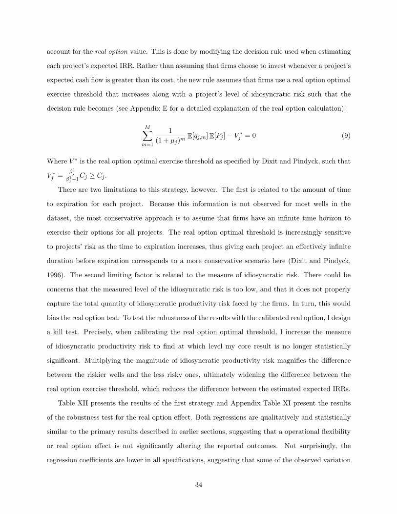
account for the real option value. This is done by modifying the decision rule used when estimating
each project’s expected IRR. Rather than assuming that firms choose to invest whenever a project’s
expected cash flow is greater than its cost, the new rule assumes that firms use a real option optimal
exercise threshold that increases along with a project’s level of idiosyncratic risk such that the
decision rule becomes (see Appendix E for a detailed explanation of the real option calculation):
M∑m=1
1
(1 + µj)mE[qj,m]E[Pj ]− V ∗
j = 0 (9)
Where V ∗ is the real option optimal exercise threshold as specified by Dixit and Pindyck, such that
V ∗j =
β1j
β1j−1
Cj ≥ Cj .
There are two limitations to this strategy, however. The first is related to the amount of time
to expiration for each project. Because this information is not observed for most wells in the
dataset, the most conservative approach is to assume that firms have an infinite time horizon to
exercise their options for all projects. The real option optimal threshold is increasingly sensitive
to projects’ risk as the time to expiration increases, thus giving each project an effectively infinite
duration before expiration corresponds to a more conservative scenario here (Dixit and Pindyck,
1996). The second limiting factor is related to the measure of idiosyncratic risk. There could be
concerns that the measured level of the idiosyncratic risk is too low, and that it does not properly
capture the total quantity of idiosyncratic productivity risk faced by the firms. In turn, this would
bias the real option test. To test the robustness of the results with the calibrated real option, I design
a kill test. Precisely, when calibrating the real option optimal threshold, I increase the measure
of idiosyncratic productivity risk to find at which level my core result is no longer statistically
significant. Multiplying the magnitude of idiosyncratic productivity risk magnifies the difference
between the riskier wells and the less risky ones, ultimately widening the difference between the
real option exercise threshold, which reduces the difference between the estimated expected IRRs.
Table XII presents the results of the first strategy and Appendix Table XI present the results
of the robustness test for the real option effect. Both regressions are qualitatively and statistically
similar to the primary results described in earlier sections, suggesting that a operational flexibility
or real option effect is not significantly altering the reported outcomes. Not surprisingly, the
regression coefficients are lower in all specifications, suggesting that some of the observed variation
34

might be partially attributable to those phenomenon. Also, the number of observations in both
tables is lower than that in the main regression tables. For Table XII, it is because most of the
projects evaluated in this analysis are infill wells (i.e., wells drilled when the plot of land is held by
production), which reduces the number of firms included in the sample. Similarly, for Appendix
Table XI, the number of observations for the real option calibration specification is lower than the
one for the main specification, because implied volatility data is not available on Bloomberg before
the year 2000. Finally, the results of the kill test indicate that the core results of this paper are
robust to the real option calibration up to an increase of 28.8% of the idiosyncratic risk.
B. The Effect of Firms’ Leverage
The cost of debt for a given firm increases with the total amount of risk incurred at the firm
level (Merton, 1974), including both systematic and idiosyncratic forms of risk. Taksler (2003)
presents empirical evidence in favor of Merton’s theory, which is roughly that a firm’s weighted
cost of capital should account for the firm’s idiosyncratic risk, through its debt component. To
test for this alternative interpretation, I design a separate regression that includes firms’ market
leverage and an interaction term of market leverage with project-level idiosyncratic risk, including
only those firms for which the relevant information is available. Table XIII reports the results
of that test, which are that the effects of leverage on the price of projects’ idiosyncratic risk
does not economically or statistically alter the above results. Also, consistent with the effect of
leverage discussed in Merton (1974), the coefficient of the interaction between firms’ leverage and
the projects’ average idiosyncratic risk (i.e., β5) is positive, but not statistically significant in all
regression specifications. The directional effect is consistent with the phenomenon discussed by
Merton, such that idiosyncratic risk should be priced by the debt component of firms’ capital
structure.
C. Asset Pricing and the Idiosyncratic Risk Premium
A well-established asset pricing literature has found that firms’ returns may account for id-
iosyncratic risk. For example, Goyal and Santa-Clara (2003) found a positive relationship between
the quantity of idiosyncratic risk measured at the firm level and the returns on the market, while
Ang et al. (2009) finds that firms with high past idiosyncratic volatility have low future average
35
returns. This literature has discussed the role of investors lack of diversification and the role of real
options to explain the idiosyncratic risk premium. There is a possibility that the results observed
in my study are affected by this dynamic. However, three pieces of evidence presented in the pre-
vious sections provide reassuring evidence regarding such concerns. First, Table II coefficient β2
indicates that firms price idiosyncratic risk after controlling for the WACC or the cost of equity,
which proxies for the idiosyncratic risk premium discussed in the asset pricing literature. Second,
Appendix Table V shows that the results are robust to firms’ listing status (i.e., private or public),
ruling out the idea that the observed phenomenon is driven by a stock market effect, since it is
observed for both types of firms. Finally, the mechanisms explored in this paper indicate that a
plausible explanation for the observed dynamic is attributable to firms’ internal frictions, steering
away from a solely financial market effect.
D. Alternative Price Specifications
The study’s primary results are also robust to two alternative price specifications. The first
alternative uses the three-year Bloomberg natural gas futures contract prices rather than EIA three-
year forecast32. In the second specification, the EIA regional wellhead prices are used to account
for price heterogeneity across states (see Figure 8). Effectively, the price firms obtain for selling
their product can vary across regions, depending on the quality of the resource and the distance
it must be transported in order to reach a refinery site. Tables XIV and XV report the results
of these two additional specifications. In both cases, the primary results are not qualitatively or
quantitatively altered.
E. Alternative Research Design
To address the concern that the above analysis might be affected by the specific nature of the
research design selected here, I test an alternative design. Instead of constructing two portfolios
for each firm-year subsample according to the idiosyncratic risk exposure of each project, this
alternative design includes only one portfolio per firm-year subsample, inclusive of all projects.
Table XVI displays the regression results obtained when estimating firms’ discount rates using this
32The number of observations is smaller than the main specification used above, because Bloomberg’s three-yearnatural gas futures prices are only available from 1995 to 2010, which presents a restricted sampling window.
36

approach. The coefficient estimates are not meaningfully affected by the alternative experimental
design; the only practical difference is that the regression cannot be modified to include a firm-year
fixed effect, as there is only one observation per firm-year.
F. Alternative Discount Rate Thresholds
I introduce two alternative threshold specifications to address the concern that the results of
the analysis can be materially affected by the threshold used to estimate the firm-year portfolios’
discount rate. Determining a reasonable threshold is important in this analysis, because two sources
of bias can potentially affect the discount rate estimate. First, the projects’ expected IRR are
obtained using a noisy measure of the managers’ true expectations. Figure 9 provides a graphical
illustration of the effects of measurement noise on the observed firm-year portfolio’s expected IRR
distribution. For this reason, observations situated on the very left portion of the distribution proxy
for the discount rate with measurement error. Thus, it is reasonable to extend the discount rate
threshold slightly beyond the minimum value of the distribution. Second, taking value too far on
the right side of the distribution would fail to capture the features associated with the discount rate,
as it would more likely capture dynamics associated with the firm’s average profitability and its
opportunity set. Table XVII presents the main results with two alternative threshold specifications,
to show that the results are robust. Columns 1 to 3 present the results using only the lowest bound
of the expected IRR distribution, and columns 4 to 6 present the results using the observations in
the 2.5th lowest percentile of the distribution.
G. Results by Time Period
Finally, I verify that managers price idiosyncratic risk consistently period by period. Precisely,
Table XVIII reports the results for the price of idiosyncratic risk, evaluated per decade (i.e., [1983-
1990), [1990-2000), [2000-2010]). The table shows that managers consistently adjust their discount
rate to account for idiosyncratic risk, across the three decades. This indicates that the main
specification results are not driven by specific events associated with one particular time period.
Rather, the effect is economically significant across all three decades.
It is interesting to note that the price of idiosyncratic risk has been steadily declining over
time, across all regression specifications. Although the goal of this paper is not to explain the time
37

trend for the price of idiosyncratic risk, future research investigating the underlying drivers of such
phenomenon would be interesting.
IX. Conclusion
Choosing discount rates for new investment projects is a fundamental topic in corporate finance,
yet we have almost no evidence on how managers make these choices in practice. This study helps
fill this gap by analyzing the relation between projects’ idiosyncratic risk and firms’ project-specific
discount rates. The primary findings are that (i) managers adjust their discount rates upward when
faced with increased idiosyncratic risk; (ii) pricing idiosyncratic risk is negatively related to several
measures of firm performance; (iii) managers appear to adjust their discount rate calculation to
account for their exposure to undiversified unhedgeable risk, when facing costly external financing;
and (iv) capital budgeting policies, and specifically the size of managers’ budget, appear to provide
firm owners with an additional lever to adjust managers’ effective risk tolerance to desired levels.
An interesting implication of these results relates to the role of alternative tools for aligning
managers’ preferences. Most of the theoretical and empirical work in finance focuses on compensa-
tion contracts as the main means of insuring managers against the potential negative outcomes of
specific projects. Echoing the theoretical insights provided by Holmstrom and Costa (1986), this
analysis finds that capital budgeting policies, such as the size of managers’ budget, can supplement
contracts and other tools, and may even help to achieve this goal more efficiently.
38

Appendix A. Variable Definition
In this appendix, I define how each variable discussed in the paper is constructed. Subscript
i corresponds to a specific firm, t corresponds to the year, j indicates a specific well, f refers to
a region (i.e., a field or a state), p refers to a township, and k refers to the two portfolios at the
firm-year level sorted on the idiosyncratic risk. A subscript with a minus sign, such as X-i, indicates
that the firm’s own observations are excluded from the observations used in the calculation of the
specific variable.
Appendix A.1. Gas Well Variables
1. # of Wells in a Township-Year: Njp,t = Count the number of projects per township p and year t
2. # of Active Regions: Nfi,t = Count the number of fields or states the firm is active in during
the year
3. # of Projects per Firm-Year Portfolio: Nji,t,k = Count the number of projects per firm i, year
t, and portfolio k
4. Costj = The drilling cost of well j
5. Township-Year Average Well’s Costp,t =∑
p,t Costj
Njp,t
6. Asseti,t =∑
iCostj , for all producing wells on year t for firm i
7. Budgeti,t =∑
i,tCostj , for all the wells drilled on year t for firm i
8. Managers’ Budgetf,i,t =∑
f,i,tCostj , for all the wells drilling on year t for firm i in region
(i.e., field or state) f
9. Average Managers’ Budget at the Firm Leveli,t,f =∑
i,t Managers’ Budgeti,t,f
Nfi,t
10. Natural Gas Pricet = Pt
11. Operational Cost (%) = OP
12. Royalty Ratet (%) = Rt
13. Yearly Gas Productioni,t (in 1,000 cf) = Qi,t
14. Operating profiti,t = PtQi,t ∗ (1−Rt −OP )−Budgeti,t15. Gross Profit Margini,t (%) =
OperatingProfiti,tPtQi,t
∗ 100
16. Gross Profitabilityi,t (%) =OperatingProfiti,t
Asseti,t∗ 100
17. Assets Growthi,t+1 (YoY) (%) =Asseti,t+1
Asseti,t∗ 100
18. Investment Ratei,t+1 (%) = Budgeti,t+1Asseti,t
∗ 100
19. Discount Rate: DRi,t,k = Lower region of the firm-year portfolio’s expected IRR distribution.
20. Project’s Productivity Shock: ζj =∑m=12
m=1 E[pt]∗qj,m−∑m=12
m=1 E[pt]E[qj,m]Costj
21. Township-Year Idiosyncratic Risk: IRk,t = = 1
Njp,t−1
∑p,t(ζj − ζp,t)2
39

22. Projects’ Average Idiosyncratic Risk: Average IRi,t,k = 1
Nji,t,k
∑i,t,k IRk,t
23. Price of Idiosyncratic Riski,t =DRi,t,High−DRi,t,Low
Average IRi,t,High−Average IRi,t,Low, where High and Low corre-
sponds to the two firm-year portfolios sorted on the exposure to idiosyncratic risk
24. Largest Peers’ Projects’ Idiosyncratic Productivity Shock: Max Peer IPSp,t = maxp,t[ζ−j ]
25. Average Largest Peers’ Projects’ Idiosyncratic Productivity Shocki,t,k = 1
Nji,t,k
∑i,t,k Max Peer IRp,t
26. Annual Firm’s Budget Diversificationi,t =Nj
i,t−1∑i,t(ζj−ζi,t)2
Appendix A.2. Financial Market Variables
For the regressions using Compustat variables or other financial market variables, the variable
definitions are below. Names are denoted by their Xpressfeed pneumonic in bold, when available.
1. Total Book Assets = at
2. Total Debt = dltt + dlc
3. Market Value of Equity: MVEi,t = pstk + csho*prcc c
4. Market Leverage =Total Debti,t
MVEi,t+Total Debti,t
5. βOGt = One year CAMP Oil and Gas Industry beta, computed at the monthly frequency.
6. Risk-free Rate: rft = 10-year risk-free rate from St-Louis Federal Reserve.
7. Industry Cost of Equity: rEt = rft + βOGt ∗ (E(EtPt
)− rft)
8. Cost of Debt: rDi,t = Interest rate of trading bonds from firms of equivalent credit rating.
9. Weighted Average Cost of Capital: WACCi,t =MVEi,t
MVEi,t+Total Debti,t∗rEt +
Total Debti,tMVEi,t+Total Debti,t
∗rDi,t10. Cash Flow: CF = oancf+intpn
at
11. TLTD = dltt+dlcat
12. TDIV = dvp+dvcat
13. CASH = cheat
14. Market-to-book Ratio: Q = MVE+Total Debt−txditcat
15. DIVPOS = is indicator that equals one if the firm pays dividends, and zero otherwise.
16. LNTA = ln(at)
17. Three-digit Industry YoY Sales Growth: ISG =∑
3 digit SIC salei,t+1∑3 digit SIC salei,t
18. Own-firm Real Year-over-Year (YoY) Sales Growth: SG =Real salei,t+1
Real salei,t
19. CURAT = actlct
20. COVER = oibdp−dp(xint+dvp)/(1−τ c) , where τ c is the tax rate.
21. IMARG = nisale
22. SLACK = che+0.5∗invt+0.7∗rect−dlcppent
40

Appendix A.3. Costly external financial variables
In the paper, I use four indexes to proxy for the level of costly external financing by firms. To
construct each of the first three proxies (Cleary Index, Whited-Wu Index, Kaplan-Zingales index), I
process the data following the methodology presented in Hennessy and Whited (2007). Finally, for
each index to have the same interpretation, I follow the recommendation of Hennessy and Whited
(2007) and multiply the Cleary index by −1, such that it is increasing with the likelihood of facing
costly external finance. Finally, to construct the Hadlock-Pierce index, I follow the methodology
presented in Hadlock and Pierce (2010).
The indexes are constructed in the following way:
Kaplan-Zingales index = −1.001909 ∗ CF + 3.139193 ∗ TLTD − 39.36780 ∗ TDIV (10)
− 1.314759 ∗ CASH + 0.2826389 ∗Q
Whited-Wu index = −0.091 ∗ CF − 0.062 ∗DIV POS + 0.021 ∗ TLTD − 0.044 ∗ LNTA (11)
+ 0.102 ∗ ISG− 0.035 ∗ SG
Cleary index = −0.11905 ∗ CURAT − 1.903670 ∗ TLTD + 0.00138 ∗ COV ER (12)
+ 1.45618 ∗ IMARG+ 2.03604 ∗ SG− 0.04772 ∗ SLACK
Hadlock-Pierce index = −0.737 ∗ log(Asset2004) + 0.043 ∗ log(Asset2004)2 + 0.040 ∗Age (13)
Where Age is measured using the year in which a firm drills its first well in the DrillingInfo raw
data sample, which starts in 1885.
41
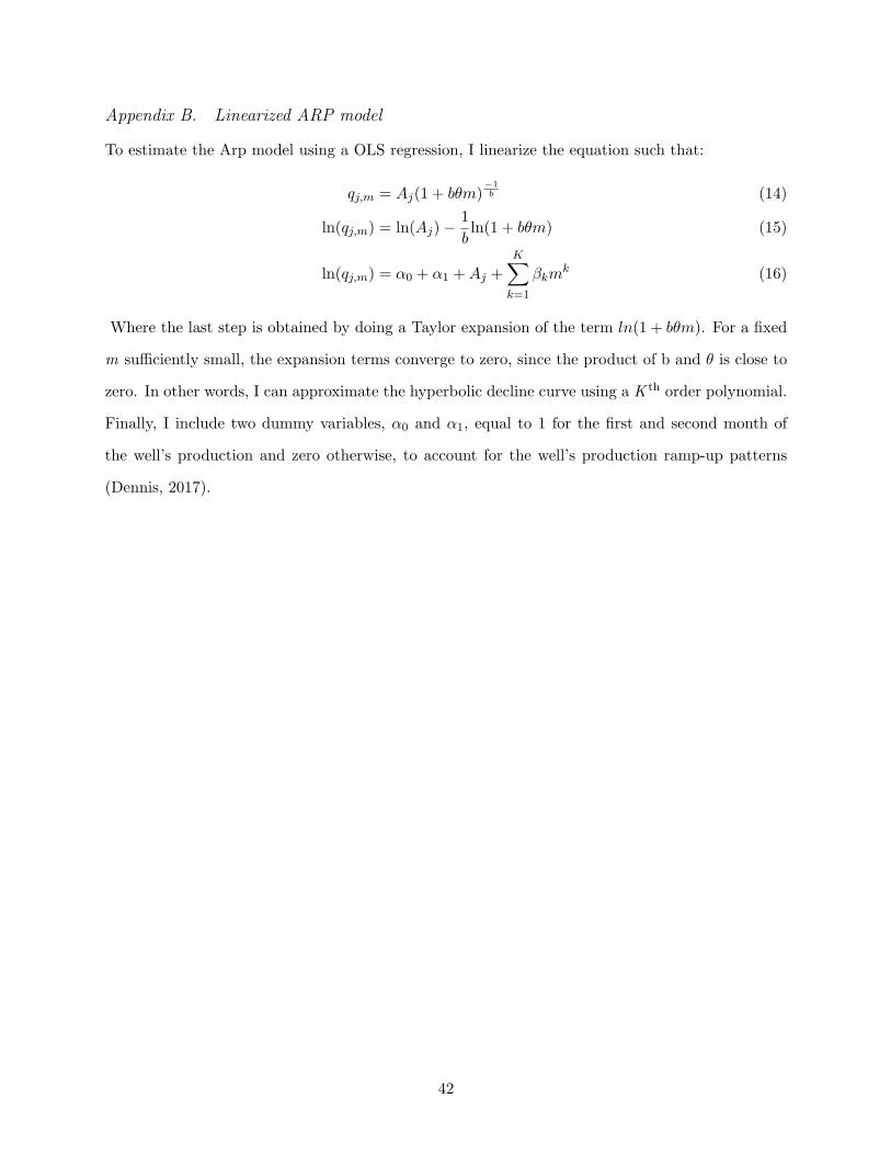
Appendix B. Linearized ARP model
To estimate the Arp model using a OLS regression, I linearize the equation such that:
qj,m = Aj(1 + bθm)−1b (14)
ln(qj,m) = ln(Aj)−1
bln(1 + bθm) (15)
ln(qj,m) = α0 + α1 +Aj +K∑k=1
βkmk (16)
Where the last step is obtained by doing a Taylor expansion of the term ln(1 + bθm). For a fixed
m sufficiently small, the expansion terms converge to zero, since the product of b and θ is close to
zero. In other words, I can approximate the hyperbolic decline curve using a K th order polynomial.
Finally, I include two dummy variables, α0 and α1, equal to 1 for the first and second month of
the well’s production and zero otherwise, to account for the well’s production ramp-up patterns
(Dennis, 2017).
42

Appendix C. Well’s Differential Exposure to Systematic Risk Factors
Wells in my analysis could have different exposure to some potential systematic risk factors
(e.g., natural gas prices). For example, wells with a greater level of idiosyncratic risk are associated
with a greater discount rate, for a given firm-year. Consequently, it is reasonable to expect that, on
average, more risky wells produce larger quantities of natural gas than their smaller counterparts,
all things being equal. Empirically, the correlation between wells’ level of idiosyncratic risk and
their associated level of production is 0.2. Now, wells producing greater quantities of natural
gas are mechanically more exposed to natural gas prices, a potential systematic risk factor. This
relationship can potentially alter how I interpret this study’s core result, since it would imply that
wells with a greater level of idiosyncratic risk are probably more exposed to systematic risk factors
(i.e., natural gas prices), confounding idiosyncratic and systematic risk factors.
To illustrate how wells with different production levels could have a different exposure to natural
gas prices, I use a simple example, such that:
pz ∗ qj,z,m = βWell′sPriceExposurepz + εj,z,m (17)
Where pz corresponds to the price of natural gas at time z, and qj,z,m is well j production at age m
(in months). We can then derive the expression for the coefficient βWell′sPriceExposure, such that:
βWell′sPriceExposure =cov(pz ∗ qj,z,m; pz)
var(pz)(18)
=E[p2
z ∗ qj,z,m]− E[qj,z,m ∗ pz] ∗ E[pz]
var(pz)(19)
=E[qj,z,m](E[p2
z]− E[pz]2)
var(pz)(20)
= E[qj,z,m] (21)
Where I use the fact that wells’ production flow is independent from the natural gas price process
to obtain equation 19. Section IV provides an expansive discussion and some empirical support in
favor of this assumption. This simple framework confirms the intuition that wells with a greater
level of production flow may be more exposed to natural gas prices. This can potentially confound
the true effect of idiosyncratic risk in the main analysis.
43
That being said, the quantity of risk is not the only relevant aspect to consider in this sce-
nario. The price of this potential systematic risk factor is equally important in characterizing the
consequence of a different exposure to systematic risk. There exists mixed evidence on the size of
a natural gas risk premium or, to a more general extant, the risk premium of an energy factor.
First, from a CAPM standpoint, the risk premium of natural gas is virtually zero33. The sample
average one-year CAPM monthly beta coefficient for natural gas is 0.004. Computing the measure
over alternative horizons does not significantly alter the resulting coefficients such that the two-
year horizon beta coefficient is 0.003, the three-year beta is 0.003, and the four-year beta is 0.003.
Second, when looking at other asset pricing models, such as models derived from the arbitrage
pricing theory (APT), there exists little consensus for the existence of an energy factor priced by
the market. On one side, Chen et al. (1986) and Kilian and Park (2009), among others, find little
evidence in favor of an energy factor. Chen et al. (1986) find that oil price risk is not separately
valued in the stock market, while Kilian and Park (2009) find limited explanatory power for oil
supply and demand shocks in explaining stock returns. On the other side, Chiang et al. (2014) and
Ready (2017) provide evidence in favor of an energy factor priced by the market.
Given the lack of general agreement in academic research for the existence of a priced energy
risk factor, I include the wells’ differential exposure to this potential systematic risk factor in my
main specification. To do so, I use the results derived in equation 21. Precisely, for each firm-year
portfolio, I measure the average production of the wells that were drilled, to proxy for their average
exposure to natural gas prices.
33Berk and van Binsbergen (2016) provide empirical evidence suggesting that the representative investor utilizesthe CAPM to determine the risk premium.
44

Appendix D. Sign of the Endogeneity Bias
To guide the analysis of the endogeneity bias sign in the reduced-form regression, it is useful to look
at a simple regression case to work within an intuitive framework. For illustration’s sake, one can
take the example that managers with different level of experience might not be randomly allocated
among the two firm-year portfolios (i.e., the high and low idiosyncratic risk portfolios), such that
Managers’ Experience would be part of the true data generating process:
Discount Ratei,t,k = β1Idiosyncratic Riski,t,k + β2Managers’ Experiencei,t,k + εi,t,k (22)
In the case where Managers’ Experience is omitted from the true regression model, the reduced-form
regression would then be:
Discount Ratei,t,k = β∗1Idiosyncratic Riski,t,k + ε(Managers’ Experience)i,t,k (23)
In this simplified example, the expression of the biased reduced-form β∗1 can be defined as:
β∗1 = β1 + β2
cov(Idiosyncratic Riski,t,k; Managers’ Experiencei,t,k)
var(Idiosyncratic Riski,t,k)(24)
From this simple example, one can note that the direction of the bias for the coefficient of interest
(β∗1) depends on (i) the covariance between the managers’ experience and the level of idiosyncratic
risk associated with the wells, and (ii) β2, the linear relationship between managers’ experience and
the firms’ discount rate.
45

Appendix E. Revealed Preference Strategy with Real Option
To account for the real option effect, I adjust the firms’ decision rule, such that I no longer assume
that it is optimal to invest when the expected discounted cash flows of the wells are greater than
the cost (Cj), but I assume that the wells are exercised when the discounted cash flows are greater
than the real option optimal threshold (V ∗j ), such that:
M∑m=1
1
(1 + µj)mE[qj,m]E[Pj ]− V ∗
j = 0 (25)
To compute the real option optimal threshold (V ∗j ), I follow the methodology introduced in
Dixit and Pindyck (1996, Chapter 5) such that:
V ∗j =
β1j
β1j − 1
∗ Cj (26)
β1j =
1
2− rt − δσ2j + ω2
t
+
√[(rt − δ)σ2j + ω2
t
− 1
2]2 +
2rtσ2j + ω2
t
(27)
where Cj denotes the well’s drilling cost, r denotes the 10-year risk-free rate, δ corresponds to the
project’s dividend rate, σ2j is the project’s idiosyncratic risk, and ω2
t is the natural gas risk.
I follow Brennan and Schwartz (1985) and set the dividend rate (i.e., δ) equal to the natural
gas convenience yield. I compute the convenience yield using the natural gas spot and Bloomberg
Natural Gas Future prices. Precisely, I obtain the sample average natural gas convenience yield
(i.e., δ) such that:
δ =1
11
2010∑t=2000
[rt +1
3(1− Ft
St)] (28)
Where t is the year during which the convenience yield is measure, F t is the Bloomberg three-year
Natural Gas Future Price, and S t is the spot price.
Finally, I define the project’s risks as the combination of the project’s idiosyncratic risk (σ2j )
and price risk (ω2t ). The project’s idiosyncratic risk is the same measure as the one I use throughout
the paper. The measure of price risk corresponds to the three-year Bloomberg Natural Gas Futures
contract implied volatility. Kellogg (2014) has an extensive discussion on which measure of price
uncertainty is best to use in a real option calibration, and concludes that using implied volatility
46

derived from financial derivatives is optimal. However, the financial option for the three-year
horizon contracts are not available on Bloomberg before 2000. For this reason, the number of
observations used in the regression of this section is smaller than that of the main specification.
47

REFERENCES
Daron Acemoglu, Philippe Aghion, Claire Lelarge, John van Reenen, and Fabrizio Zilibotti. Tech-
nology, information, and the decentralization of the firm. The Quarterly Journal of Economics,
2007.
Philippe Aghion and Jean Tirole. Formal and real authority in organizations. Journal of Political
Economy, 1997.
Anup Agrawal and Gershon N. Mandelker. Managerial incentives and corporate investment and
financing decisions. The Journal of Finance, 1987.
Soren T. Anderson, Ryan Kellogg, and Stephen W. Salant. Hotelling under pressure. Journal of
Political Economy, 2018.
Andrew Ang, Robert J. Hodrick, Yuhang Xing, and Xiaoyan Zhang. High idiosyncratic volatility
and low returns: International and further u.s. evidence. Journal of Financial Economics, 2009.
Christopher S. Armstrong and Rahul Vashishtha. Executive stock options, differential risk-taking
incentives, and firm value. Journal of Financial Economics, 2012.
Lucian A. Bebchuk and Holger Spamann. Regulating bankers’ pay. The Georgetown Law Journal,
2010.
Jonathan B. Berk and Jules H. van Binsbergen. Assessing asset pricing models using revealed
preference. Journal of Financial Economics, 2016.
Nick Bloom, Stephen Bond, and John Van Reenen. Uncertainty and investment dynamics. Review
of Economic Studies, 2007.
Marcus C. Bogue and Richard Roll. Capital budgeting of risky projects with ”imperfect” markets
for physical capital. The Journal of Finance, 1974.
Douglas R. Bohi. Changing productivity in u.s. petroleum exploration and development. Charles
River Associates, 1998.
48

Patrick Bolton, Jose Scheinkman, and Wei Xiong. Executive compensation and short-termist
behaviour in speculative markets. The Journal of Finance, 2006.
Patrick Bolton, Hui Chen, and Neng Wang. A unified theory of tobin’s q, corporate investment,
financing, and risk management. The Journal of Finance, 2011.
Richard A. Brealey and Stewart C. Myers. Principles of corporate finance, seventh edition. McGraw
Hill Publisher, 1996.
Michael J. Brennan and Eduardo S. Schwartz. Evaluating natural resource investments. The
Journal of Business, 1985.
Eve Caroli and John Van Reenen. Skill-biased organizational change? evidence from a panel of
british and french establishments. The Quarterly Journal of Economics, 2001.
Nai-Fu Chen, Richard Roll, and Stephen A. Ross. Economic forces and the stock market. The
Journal of Business, 1986.
Judith Chevalier and Glenn Ellison. Career concerns of mutual fund managers. The Quarterly
Journal of Economics, 1999.
I-Hsuan Ethan Chiang, W. Keener Hughen, and Jacob S. Sagi. Estimating oil risk factors using
information from equity and derivatives markets. The Journal of Finance, 2014.
Jeffrey L. Coles, Naveen D. Daniel, and Lalith Naveen. Managerial incentives and risk-taking.
Journal of Financial Economics, 2006.
Massimo G. Colombo and Marco Delmastro. Delegation of authority in business organizations: An
empirical test. The Journal of Industrial Economics, 2004.
George M. Constantinides. Market risk adjustment in project valuation. The Journal of Finance,
1978.
Joshua D. Coval and Tobias J. Moskowitz. Home bias at home: Local equity preference in domestic
portfolios. Journal of Finance, 1999.
Joshua D. Coval and Tobias J. Moskowitz. The geography of investment: Informed trading and
asset prices. Journal of Political Economy, 2001.
49

Thomas R. Covert. Experiential and social learning in firms: The case of hydraulic fracturing in
the bakken shale. Working Paper, 2015.
Paul H. Decaire, Erik P. Gilje, and Jerome P. Taillard. Real option exercise: Empirical evidence.
Review of Financial Studies, 2019.
Rebecca S. Demsetz and Philip E. Strahan. Diversification, size and risk at u.s. bank holding
companies. Journal of Money, Credit and Banking, 1997.
Michael Dennis. Developing synthetic reservoir type curve model for use in evaluating surface
facility and gathering pipe network designs. Journal of Natural Gas Science & Engineering,
2017.
Douglas W. Diamond. Financial intermediation and delegated monitoring. The Review of Economic
Studies, 1984.
Avinash K. Dixit and Robert S. Pindyck. Investment under Uncertainty. Princeton University
Press, 1996.
Zhiyong Dong, Cong Wang, and Fei Xie. Do executive stock options induce excessive risk taking?
Journal of Banking and Finance, 2010.
Eugene F. Fama and Kenneth R. French. The equity premium. The Journal of Finance, 2002.
Steven M. Fazzari and Bruce C. Petersen. Working capital and fixed investment: New evidence on
financing constraints. The RAND Journal of Economics, 1993.
Michael Fetkovich. Useful concepts for decline curve forecasting, reserve estimation, and analysis.
SPE Reservoir Engineering, 1996.
Kenneth A. Froot, David S. Scharfstein, and Jeremy C. Stein. Risk management: Coordinating
corporate investment and financing policies. The Journal of Finance, 1993.
Huasheng Gao, Jarrad Harford, and Kai Li. Determinants of corporate cash policy: Insights from
private firms. Journal of Financial Economics, 2013.
John Geanakoplos and Paul Milgrom. A theory of hierarchies based on limited managerial attention.
Journal of the Japanese and International Economies, 1991.
50

Erik Gilje and Jerome Taillard. Do private firms invest differently than public firms? taking cues
from the natural gas industry. Journal of Finance, 2016.
Xavier Giroud. Proximity and investment: Evidence from plant-level data. The Quarterly Journal
of Economics, 2013.
Todd A. Gormley, David A Matsa, and Todd T. Milbourn. Ceo compensation and corporate
risk-taking: Evidence from a natural experiment. Journal of Accounting and Economics, 2013.
Amit Goyal and Pedro Santa-Clara. Idiosyncratic risk matters! The Journal of Finance, 2003.
John R. Graham and Campbell R. Harvey. The theory and practice of corporate finance: evidence
from the field. Journal of Financial Economics, 2001.
John R. Graham, Campbell R. Harvey, and Manju Puri. Capital allocation and delegation of
decision-making authority within firms. Journal of Financial Economics, 2015.
William H. Greene. Econometric Analysis (Fifth ed.). Prentice-Hall, 2003.
Wayne R. Guay. The sensitivity of ceo wealth to equity risk: an analysis of the magnitude and
determinants. Journal of Financial Economics, 1999.
Charles J. Hadlock and Joshua R. Pierce. New evidence on measuring financial constraints: Moving
beyond the kz index. The Review of Financial Studies, 2010.
Jens Hagendorff and Francesco Vallascas. Ceo pay incentives and risk-taking: Evidence from bank
acquisitions. Journal of Corporate Finance, 2011.
Christopher A. Hennessy and Toni M. Whited. How costly is external financing? evidence from a
structural estimation. The Journal of Finance, 2007.
Evan Herrnstadt, Ryan Kellogg, and Eric Lewis. Royalties and deadlines in oil and gas leasing:
Theory and evidence. Working Paper, 2019.
Charles Hodgson. Information externalities, free riding, and optimal exploration in the uk oil
industry. Working paper, 2019.
51

Bengt Holmstrom and Joan Ricart I Costa. Managerial incentives and capital management. The
Quarterly Journal of Economics, 1986.
Bengt Holmstrom and Laurence Weiss. Managerial incentives, investment and aggregate implica-
tions: Scale effects. The Review of Economic Studies, 1985.
Michael T. Jacobs and Anil Shivdasani. Do you know your cost of capital? harvard Business
Review, 2012.
Ravi Jagannathan, David A. Matsa, Iwan Meier, and Vefa Tarhan. Why do firms use high discount
rates? Journal of Financial Economics, 2016.
Ryan Kellogg. Learning by drilling: Interfirm learning and relationship persistence in the texas
oilpatch. The Quarterly Journal of Economics, 2011.
Ryan Kellogg. The effect of uncertainty on investment: Evidence from texas oil drilling. American
Economic Review, 2014.
Lutz Kilian and Cheolbeom Park. The impact of oil price shocks on the u.s. stock market. Inter-
national Economic Review, 2009.
Philipp Kruger, Augustin Landier, and David Thesmar. The wacc fallacy: The real effects of using
a unique discount rate. The Journal of Finance, 2015.
Richard A. Lambert. Executive effort and selection of risky projects. The RAND Journal of
Economics, 1986.
Kewen Li and Roland N. Horne. A decline curve analysis model based on fluid flow mechanisms.
Society of Petroleum Engineers, 2003.
Evgeny Lyandres. Costly external financing, investment timing, and investment-cash flow sensitiv-
ity. Journal of Corporate Finance, 2007.
Tianshou Ma, Ping Chen, and Jian Zhao. Overview on vertical and directional drilling technolo-
gies for the exploration and exploitation of deep petroleum resources. Springer International
Publishing, 2016.
52

Robert C. Merton. On the pricing of corporate debt: the risk structure of interest rates. The
Journal of Finance, 1974.
Merton H. Miller and Daniel Orr. A model of the demand for money by firms. The Quarterly
Journal of Economics, 1966.
Stewart C. Myers and Stuart M. Turnbull. Capital budgeting and the capital asset pricing model:
good news and bad news. The Journal of Finance, 1977.
M. P. Narayanan. Managerial incentives for short-term results. The Journal of Finance, 1985.
Vasia Panousi and Dimitris Papanikolaou. Investment, idiosyncratic risk, and ownership. The
Journal of Finance, 2012.
James M. Poterba and Lawrence H. Summer. A ceo survey of u.s. companies’ time horizons and
hurdle rates. Sloan Management Review, 1995.
Shivaram Rajgopal and Terry Shevlin. Empirical evidence on the relation between stock option
compensation and risk taking. Journal of Accounting and Economics, 2002.
Robert C. Ready. Oil prices and the stock market. Review of Finance, 2017.
Stephen A. Ross. The economic theory of agency: The principal’s problem. The American Economic
Review, 1973.
Amit Seru. Firm boundaries matter: Evidence from conglomerates and r&d activity. Journal of
Financial Economics, 2014.
John Y. Campbell Glen B. Taksler. Equity volatility and corporate bond yields. The Journal of
Finance, 2003.
Peter Tufano. Who manages risk? an empirical examination of risk management practices in the
gold mining industry. The Journal of Finance, 1996.
53

Figure 1: Vertical versus Horizontal Drilling Technology
This figure provides a graphical illustration of the difference between horizontal and vertical wells.Vertical wells represent the older technology, predominantly used in the first part of the American oiland gas development (i.e.; 1900-2005). During the analyzed period, 89% of the gas wells drilled in mysample where completed using the vertical technology.
Example of Horizontal and Vertical Wells
(1) Horizontal Well (2) Vertical Well

Figure 2. Panhandle Field (Texas) Development Progress between 1961-2010
Figure 2.2. 2010 map of cumulative oil and gas wells drilled in the Panhandle field. Eachdot represents an individual well. Wells' quality is indicated by a color code. Darker shade ofblue indicates wells that were among the most productive of the region, while dots colorcoded in gray indicate lower level of productivity.
This panel of figures plots the evolution of the Panhandle field development over the period1961 to 2010. Figure 2.1. provides the initial expectation of the field boundary, based ongeological surveys. Figure 2.2. provides an updated view of the field development. The redsquare indicates the Hutchinson county to help align the surveyor map with the 2010 map.
Panhandle Field's Development from 1961 to 2010
Figure 2.1. 1961 map of approximate boundary of Panhandle oil and gas field producingregion. Source: Anderson and Hinson, 1961; Boone 1958; and G.B. Shelton, U.S. Bureau ofMines, written communication, 1958 .

Figure 3: Energy Firms' Break Down of Upstream ActivitiesThe figures in the two above panels present examples of how energy firms break down and discuss their activities.Those firms rely heavily on geographical boundaries to define their operations, referring to man-made boundaries (i.e.,states) or naturally occuring ones (i.e., geological structure) in most cases.
Panel 3.1: U.S. Upstream Business of Exxon Mobil Corporation (2018). This figure presents an example of how energy firms break down their exploration and production activities in theUnited-States. There is a strong focus on geographical detail, often refering to states or fields to define their upstreamactivities.
Excerpt from Energy Firms' 10-K Statement for Ongoing U.S. Activities
Panel 3.2: U.S. Upstream Business of British Petroleum Plc. (2018). This figure presents how British Petroleum Plc. breaks down its upstream operations (i.e., exploration and production)in the United-States.

Figure 4: Projects Geographic DistributionThis figure plots the sample of wells included in the analysis. The total sample includes 114,696 vertical gas wells drilled over the period ranging from1983 to 2010. The map provides information on the regions with the most activity during the analyzed period.
Geographic Distribution of the Vertical Gas Wells

Figure 5: Arp Hyperbolic Production Curve This figure plots the wells production decline level over time. The blue line corresponds to the median empirical production, the red linecorresponds to the hyperbolic Arp prediction and the shaded area represent the 10th and 90th confidence interval.
0%
10%
20%
30%
40%
50%
60%
70%
80%
90%
100%
1 26 51 76 101 126 151 176 201 226
Mon
thly
Pro
duct
ion
(as
a %
of
the
Bas
elin
e L
evel
)
Well's Age (in Months)
Expected and Realized Well's Production Decline Over Time
Median Realized Production Decline Median Predicted Production Decline

Figure 6.1. Bird Eye View of a Township-Year (Kansas)
Figure 6.2: Realized Idiosyncratic Productivity Shocks, Idiosyncratic Risk, and Instrumental Variable
Figure 6: Variables Constructed Using the Township-Year Idiosyncratic Productivity ShocksFigure 6.1. presents a simplified example of wells being drilled in a given township-year. In this example, three firms (i.e., Red, Blue, andBlack) were active in the township during that specific year. The adjacent table (Figure 6.2) reports an illustrative example of the potentialidiosyncratic productivity shock, measured for each well. The instrumental variable used in the paper, Average Largest Peers' IdiosyncraticProductivity Shock, corresponds to the biggest shock that was measured for the firm's peers in its wells' township-year, averaged at the firm-year porfolio level. To obtain the Projects' Average Idiosyncratic Risk , I take the average value of Projects' Idiosyncratic Risk for each firm-year porfolio.
Variables Constructed Using the Township-Year Idiosyncratic Productivity Shocks
This figure plots the wells drilled in the township (33S-39W) in Kansas, for the year 1990 to 1991. A township is a 6 miles by 6 milessquare of land. In the Public Land Survey System, each township is constituted of 36 1-squared mile sections. The colored circles representdistinct wells drilled by the three active firms in the township-year (Occidental Petroleum, Linn Energy, and Merit Energy).
This table presents an example of the realized idiosyncratic productivity shocks for the wells drilled in the township-year, for the three activefirms. Sigma (ς) represents the wells' specific idiosyncratic shocks. For each well drilled in the township-year, I determine the well's levelmeasure of idiosyncratic risk, Projects' Idiosyncratic Risk , as the cross-sectional standard deviation measured for the township-year (e.g.,0.129). Finally, the instrumental variable, Largest Peers' Idiosyncratic Productivity Shock , corresponds to the largest idiosyncratic shocksexperienced by a firm's peers. For example, for the Red firm, the largest peers' idiosyncratic shock is 0.23, experienced by the Black firm.
24
13
6 M
iles
6 Miles
36
Vertical Wells
123456
7 8 9 10 11 12
1415161718
19 20 21 22 23
30 29 28 27 26 25
31 32 33 34 35
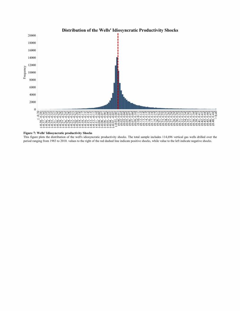
Figure 7: Wells' Idiosyncratic productivity ShocksThis figure plots the distribution of the well's idiosyncratic productivity shocks. The total sample includes 114,696 vertical gas wells drilled over theperiod ranging from 1983 to 2010. values to the right of the red dashed line indicate positive shocks, while value to the left indicate negative shocks.
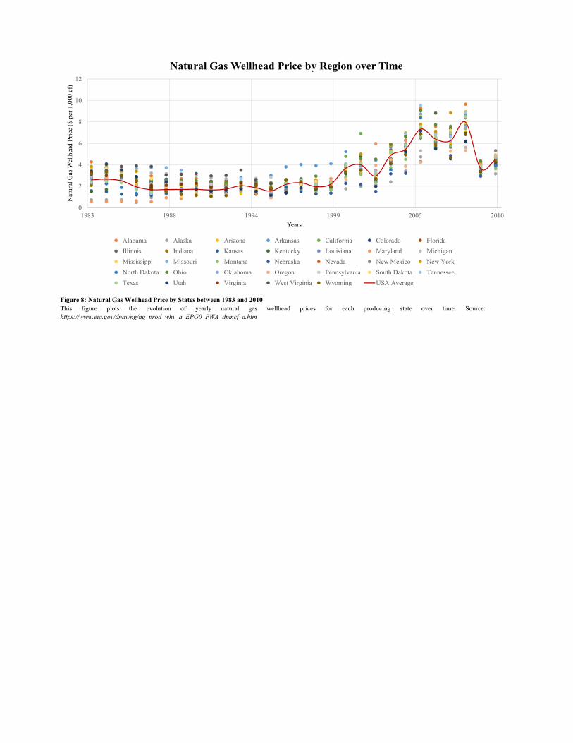
Figure 8: Natural Gas Wellhead Price by States between 1983 and 2010This figure plots the evolution of yearly natural gas wellhead prices for each producing state over time. Source:https://www.eia.gov/dnav/ng/ng_prod_whv_a_EPG0_FWA_dpmcf_a.htm
0
2
4
6
8
10
12
1983 1988 1994 1999 2005 2010
Nat
ural
Gas
Wel
lhea
d P
rice
($
per
1,00
0 cf
)
Years
Natural Gas Wellhead Price by Region over Time
Alabama Alaska Arizona Arkansas California Colorado Florida
Illinois Indiana Kansas Kentucky Louisiana Maryland Michigan
Mississippi Missouri Montana Nebraska Nevada New Mexico New York
North Dakota Ohio Oklahoma Oregon Pennsylvania South Dakota Tennessee
Texas Utah Virginia West Virginia Wyoming USA Average

Figure 9: Observed Distribution of the Project's expected IRRThis figure plots the distribution of the projects' expected IRR for the firm-year portfolios. If there was no measurement error in the projects' expectedIRR, the observed distribution would cut sharply at the red dotted line. However, because of measurement error in the projects' expected IRR, the tailsof the distribution are fatter, and the left tail of the distribution extends beyond the firms true cut-off value.
Firm-Year Portfolio's Projects' Expected IRR Distribution
Expected IRR

Observation Mean Median Std. Dev.
Assets (In millions $) 3,946 229.17 84.87 383.79Annual Budget (In millions $) 3,946 60.34 22.95 108.80Annual Budget per Field (In millions $) 3,946 11.30 6.07 17.57Annual Budget per State (In millions $) 3,946 19.37 10.30 30.09Number of Firms 369
Observation Mean Median Std. Dev.
Drilling Cost ($) 114,696 465,652.90 402,357.30 299,580.20Drilling Cost ($ per foot) 114,696 79.07 81.48 6.94Royalty Rate (%) 114,696 17.32% 18.75% 2.83%Operational Cost (%) 114,696 20.00% 20.00% 0.00%Well Total Gas Production (in 1,000 cf) 114,696 570,049.90 177,654.50 1,608,979.00EIA three-year forecast gas prices (Per 1,000 cf) 114,696 4.05 3.37 1.83
Panel B: Well Level Data
Table ISummary Statistics of Firms' and Wells' Characteristics
This table reports summary statistics of exploration and production gas companies included in the sample. The time period ofthe sample is from 1983 to 2010. The sample consists of all firms drilling at least 10 gas wells in the year of analysis, and wellsdrilled in township-year with at least 3 wells. I exclude from the analysis all wells with missing fields, and wells for which thefirst production date occurs before the drilling date, as they correspond to data entry error. Panel A reports summary statisticsof the firm’s characteristics. Panel B reports well-level characteristics used to estimate the Arp model.
Panel A: Firm Level Data

(1) (2) (3) (4)
(β1) WACC (%)i,t 1.403*** 1.549*** 1.367*** 1.325**
[2.88] [2.80] [3.13] [2.40]
(β2) Project's Average Idiosyncratic Riski,t,k 11.862*** 9.989**
[3.06] [2.43]
Firm Fixed Effecti No Yes No Yes
R-Squared 0.011 0.298 0.152 0.383
F-Statistic 8.308 7.831 19.800 13.866
Observations 748 748 748 748
This table reports coefficient estimates from an OLS regression for the relation between the cost of capitaland firms’ discount rate, and t-statistics robust to heteroskedasticity and within-firm dependence in bracket.The period of the sample is from 1983 to 2010. The unit of observation in the underlying table is at the firmi , and year t level. The Industry Cost of Equity is calculated using the oil and gas industry beta, computedat the monthly frequency on a one-year horizon basis, multiplied by the expected market excess return. Theoil and gas industry returns are obtained from Kenneth French web site. Market excess return isapproximated using the earning-to-price ratio obtained from Robert Shiller web site. The risk-free rate is the10-year risk-free rate, obtained from the St-Louis Federal Reserve website. Finally, to compute theweighted average cost of capital (WACC), I obtain the cost of debt using firms credit rating reported inCapital IQ. See appendix A.2 for the full methodological details. The variable Project's AverageIdiosyncratic Risk is scaled by its standard deviation to simplify the lecture of the table and facilitate itscomparison with the other regression tables. * indicates significance at the 10% level, ** at the 5% level,and *** at the 1% level.
Table IIFirms' Discount Rate and The Cost of Capital
Discount Rate (%)i,t,k

(1) (2) (3) (4) (5) (6) (7)
(β1) Projects' Average Idiosyncratic Riski,t,k 7.968*** 7.059*** 7.042*** 7.013*** 7.014*** 7.110*** 6.681**
[3.60] [3.06] [3.08] [3.07] [3.07] [3.22] [2.58]
(β2) Differential Exposure to Systematic Riski,t,k 0.361 0.396* 0.398* 0.403* 0.403* 0.384 0.378
[1.60] [1.72] [1.72] [1.75] [1.75] [1.54] [1.49]
(β3) Budgeti,t 0.008 0.002
[0.80] [0.24]
(β4) Assetsi,t 0.008 0.007
[1.40] [1.62]
Firm Fixed Effecti Yes Yes Yes Yes Yes No No
Year Fixed Effectt No Yes Yes Yes Yes No No
Firm-Year Fixed Effecti,t No No No No No Yes Yes
Portfolio Fixed Effectk No No No No No No Yes
R-Squared 0.451 0.470 0.471 0.471 0.471 0.738 0.738
F-Statistic 6.942 4.690 6.727 3.671 5.782 6.151 3.713
Observations 3,946 3,946 3,946 3,946 3,946 3,946 3,946
Table IIIManagers' Project's Idiosyncratic Risk Pricing
This table reports coefficient estimates from an OLS regression for the effect of projects' idiosyncratic risk on firms’ discount rate, and t-statistics robust to
heteroskedasticity and within-firm dependence in bracket. The time period of the sample is from 1983 to 2010. The unit of observation in the underlying table is at
the firm i , year t and portfolio k level. Project's Average Idiosyncratic Risk denotes the average projects' idiosyncratic risk measure for each firm-year portfolio
(i.e., the high or low idiosyncratic risk portfolio). The variable Differential Exposure to Systematic Risk correspond to the wells' total production averaged at the
firm-year porfolio level. The variable Project's Average Idiosyncratic Risk is scaled by its standard deviation to simplify the lecture of the table and facilitate its
comparison with the other regression tables. * indicates significance at the 10% level, ** at the 5% level, and *** at the 1% level.Discount Rate (%)i,t,k

Panel A: First Stage
(1) (2) (3) (4) (5) (6) (7)
(β1) Average Largest Peers' Projects' Idiosyncractic Shocki,t,k 0.698*** 0.706*** 0.706*** 0.706*** 0.706*** 0.797*** 0.746***
[11.52] [11.66] [11.65] [11.65] [11.64] [14.38] [13.22]
(β2) Budgeti,t 0.000 0.000
[0.93] [0.30]
(β3) Assetsi,t 0.000 0.000
[0.89] [0.53]
(β4) Differential Exposure to Systematic Riski,t,k 0.009 0.033*** 0.033*** 0.033*** 0.033*** 0.047*** 0.033***
[1.15] [4.72] [4.84] [4.77] [4.81] [5.98] [4.12]
Firm Fixed Effecti Yes Yes Yes Yes Yes No No
Year Fixed Effectt No Yes Yes Yes Yes No No
Firm-Year Fixed Effecti,t No No No No No Yes Yes
Portfolio Fixed Effectk No No No No No No Yes
R-Squared 0.750 0.792 0.792 0.792 0.792 0.903 0.908
Kleibergen-Paap First Stage F-Statistic 111.833 145.591 103.829 97.303 76.646 193.544 104.833
Panel B: Instrumented Regression
(1) (2) (3) (4) (5) (6) (7)
(β1) Projects' Average Idiosyncratic Riski,t,k 3.819** 4.271*** 4.254*** 4.231*** 4.232*** 6.013*** 5.102***
[2.31] [2.67] [2.63] [2.62] [2.62] [4.20] [3.08]
(β2) Budgeti,t 0.008 0.004
[0.74] [0.36]
(β3) Assetsi,t 0.006 0.005
[1.21] [1.28]
(β4) Differential Exposure to Systematic Riski,t,k 1.075** 1.386*** 1.394*** 1.399*** 1.400*** 0.604** 0.451**
[2.05] [2.67] [2.63] [2.65] [2.64] [2.58] [2.02]
Firm Fixed Effecti Yes Yes Yes Yes Yes No No
Year Fixed Effectt No Yes Yes Yes Yes No No
Firm-Year Fixed Effecti,t No No No No No Yes Yes
Portfolio Fixed Effectk No No No No No No Yes
R-Squared 0.435 0.461 0.461 0.461 0.461 0.730 0.731
F-Statistic 10.022 13.903 12.531 10.131 9.581 32.996 11.198
Observations 3,946 3,946 3,946 3,946 3,946 3,946 3,946
Table IVInstrumented Regression - Managers' Project's Idiosyncratic Risk Pricing
Projects' Average Idiosyncratic Riski,t,k
Discount Rate (%)i,t,k
This table reports the effects of project-level idiosyncratic risk on firms’ discount rate based on the exogenous measure of Projects’ Average Idiosyncratic Risk from an
instrument, and t-statistics robust to heteroskedasticity and within-firm dependence in bracket. The time period of the sample is from 1983 to 2010. The unit of observation in
the underlying table is at the firm i , year t, and portfolio k level. The results in Panel A report the first stage coefficient estimates of a two stage OLS regression which uses
the average of the firm's peers' largest idiosyncratic productivity shocks of each wells, to instrument for the variable Projects’ Average Idiosyncratic Risk. The bottom of
Panel A reports the first stage F-statistic on the instrument for the two-stage least-square regression. Panel B reports the second stage regression results of the instrumented
model. Projects' Average Idiosyncratic Risk denotes the average projects' idiosyncratic risk measure for each firm-year portfolio (i.e., the high or low idiosyncratic risk
portfolio). The variable Project's Average Idiosyncratic Risk is scaled by its standard deviation to simplify the lecture of the table and facilitate its comparison with the other
regression tables. * indicates significance at the 10% level, ** at the 5% level, and *** at the 1% level.
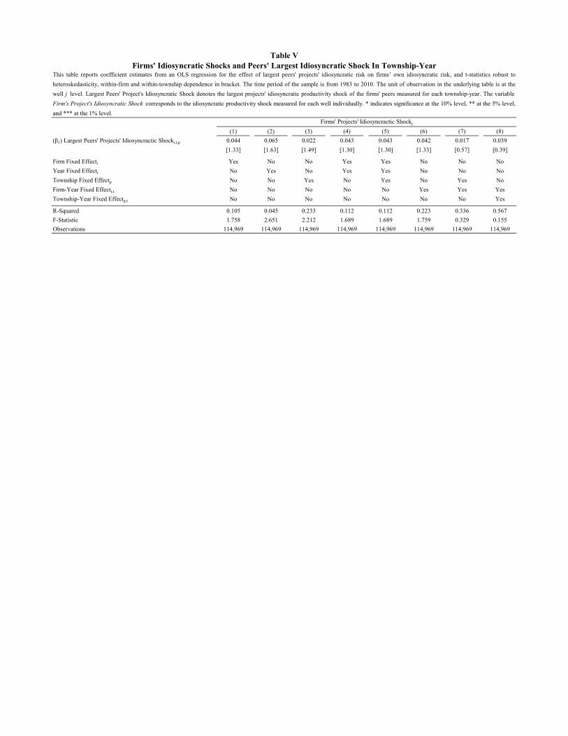
(1) (2) (3) (4) (5) (6) (7) (8)
(β1) Largest Peers' Projects' Idiosyncractic Shocki,t,p 0.044 0.065 0.022 0.043 0.043 0.042 0.017 0.039
[1.33] [1.63] [1.49] [1.30] [1.30] [1.33] [0.57] [0.39]
Firm Fixed Effecti Yes No No Yes Yes No No No
Year Fixed Effectt No Yes No Yes Yes No No No
Township Fixed Effectp No No Yes No Yes No Yes No
Firm-Year Fixed Effecti,t No No No No No Yes Yes Yes
Township-Year Fixed Effectp,t No No No No No No No Yes
R-Squared 0.105 0.045 0.233 0.112 0.112 0.223 0.336 0.567
F-Statistic 1.758 2.651 2.212 1.689 1.689 1.759 0.329 0.155
Observations 114,969 114,969 114,969 114,969 114,969 114,969 114,969 114,969
Table VFirms' Idiosyncratic Shocks and Peers' Largest Idiosyncratic Shock In Township-Year
This table reports coefficient estimates from an OLS regression for the effect of largest peers' projects' idiosyncratic risk on firms’ own idiosyncratic risk, and t-statistics robust to
heteroskedasticity, within-firm and within-township dependence in bracket. The time period of the sample is from 1983 to 2010. The unit of observation in the underlying table is at the
well j level. Largest Peers' Project's Idiosyncratic Shock denotes the largest projects' idiosyncratic productivity shock of the firms' peers measured for each township-year. The variable
Firm's Project's Idiosyncratic Shock corresponds to the idiosyncratic productivity shock measured for each well individually. * indicates significance at the 10% level, ** at the 5% level,
and *** at the 1% level.Firms' Projects' Idiosyncractic Shockj

(1) (2) (3) (4) (5) (6) (7) (8)
(β1) Price of Idiosyncratic Riski,t -5.053** -5.110** -0.511** -0.501** -0.745* -0.747* -0.811* -0.814*
[-2.47] [-2.54] [-2.04] [-1.98] [-1.71] [-1.71] [-1.67] [-1.67]
(β2) Budgeti,t -0.020 -0.055* 0.017 0.024
[-0.26] [-1.76] [1.25] [1.36]
(β3) Assetsi,t -0.092*** 0.008 -0.000 -0.002
[-3.02] [0.62] [-0.05] [-0.30]
Firm Fixed Effecti Yes Yes Yes Yes Yes Yes Yes Yes
Year Fixed Effectt Yes Yes Yes Yes Yes Yes Yes Yes
R-Squared 0.530 0.539 0.808 0.809 0.414 0.415 0.431 0.432
F-Statistic 6.097 8.397 4.144 3.259 2.935 2.447 2.801 2.297
Observations 1,973 1,973 1,973 1,973 1,973 1,973 1,973 1,973
This table reports coefficient estimates from an OLS regression for the effect of the price of idiosyncratic risk on firms’ performance, and t-statistics robust toheteroskedasticity and within-firm dependence in bracket. The time period of the sample is from 1983 to 2010. The unit of observation in the underlying table is at thefirm i and year t level. The variable Price of Idiosyncratic Risk corresponds to the firm’s price of idiosyncratic risk computed at a yearly frequency. The dependentvariables correspond to the firm gross profit margin (%), the gross profitability (%), the YoY asset growth (%), and the investment rate (%), and are winsorized at the 1and 99 percentiles. The variable Project's Average Idiosyncratic Risk is scaled by its standard deviation to simplify the lecture of the table and facilitate its comparisonwith the other regression tables. Detailed calculation of the four dependent variables is available in appendix A.1. * indicates significance at the 10% level, ** at the 5%level, and *** at the 1% level.
Table VIFirms' Performance and Managers' Idiosyncratic Risk Pricing
YoY Asset Growth (%)i,t+1 Gross Profit Margin (%)i,t Investment Rate (%)i,t+1Gross Profitability (%)i,t

(1) (2) (3) (4) (5) (6) (7) (8)
(β1) Projects' Average Idiosyncratic Riski,t,k 3.813*** 4.144*** 4.832*** 4.355*** 4.669*** 5.001*** 6.300*** 5.903***
[4.29] [4.34] [4.41] [4.04] [3.74] [3.69] [4.37] [3.97]
(β2) Projects' Average Idiosyncratic Riski,t,k * Assetsi,t -0.004** -0.004** -0.007*** -0.007*** -0.008*** -0.008*** -0.010*** -0.010***
[-2.42] [-2.34] [-2.89] [-2.81] [-3.05] [-3.08] [-3.82] [-3.74]
(β3) Assetsi,t 0.007* 0.007* 0.011** 0.011**
[1.92] [1.92] [2.23] [2.23]
(β4) Budgeti,t -0.006 -0.006 -0.006 -0.006
[-1.05] [-1.09] [-1.03] [-1.07]
(β5) Firm's Diversificationi,t 0.005 0.006
[0.48] [0.55]
(β6) Projects' Average Idiosyncratic Riski,t,k * Firm's Diversificationi,t -0.030** -0.019 -0.032 -0.031* -0.023 -0.033
[-2.10] [-1.28] [-1.45] [-1.83] [-1.39] [-1.55]
(β7) Differential Exposure to Systematic Riski,t,k 0.860*** 0.861*** 0.768*** 0.637*** 0.833*** 0.834*** 0.680*** 0.599***
[6.25] [6.26] [4.56] [3.70] [5.22] [5.24] [3.59] [3.27]
Firm Fixed Effecti Yes Yes No No Yes Yes No No
Year Fixed Effectt Yes Yes No No Yes Yes No No
Firm-Year Fixed Effecti,t No No Yes Yes No No Yes Yes
Portfolio Fixed Effectk No No No Yes No No No Yes
R-Squared 0.717 0.718 0.880 0.881 0.717 0.717 0.879 0.880
F-Statistics 19.280 13.940 25.857 16.659 19.470 14.463 27.323 17.736
Kleibergen-Paap First Stage F-Statistics N.A. N.A. N.A. N.A. 56.022 34.302 73.83 62.783
Observations 3,946 3,946 3,946 3,946 3,946 3,946 3,946 3,946
Table VII
Discount Rate (%)i,t,k
Reduced Form Regression Instrumented Regression
This table reports coefficient estimates from an OLS regression for the effect of projects' idiosyncratic risk on firms' discount rate, and t-statistics robust to heteroskedasticity and within-firm dependence in
bracket. The time period of the sample is from 1983 to 2010. The unit of observation in the underlying table is at the firm i, year t , and portfolio k level. Project's Idiosyncratic Risk denotes the average
projects' idiosyncratic risk measure for each firm-year portfolio (i.e., the high or low idiosyncratic risk portfolio). The variable Firm's Diversification denotes how much of the wells' idiosyncratic risk
drilled in a given year is diversified at the firm's level. The instrumented regression contains up to three instrumented variables, the Projects' Average Idiosyncratic Risk, the Projects' Average Idiosyncratic
Risk * Assets , and for some specifications the Projects' Average Idiosyncratic Risk * Diversification . The variable Project's Average Idiosyncratic Risk is scaled by its standard deviation to simplify the
lecture of the table and facilitate its comparison with the other regression tables. Detailed calculation of each variable is available in appendix A.1. * indicates significance at the 10% level, ** at the 5%
level, and *** at the 1% level.
Managers' Project's Idiosyncratic Risk Pricing and Firms' Size

(1) (2) (3) (4) (5) (6) (7) (8)(β1) Region's Forecast Dispersioni,t,f -2.651 -2.246 -5.736** -6.385* -5.507* -5.368* -9.721** -7.561*
[-1.60] [-1.34] [-2.10] [-1.81] [-1.84] [-1.77] [-2.29] [-1.70]
(β2) Assetsi,t 0.030 0.039 -0.001 0.004[1.05] [1.31] [-0.03] [0.09]
(β3) Budgeti,t 0.019 0.003 -0.003 -0.001[1.56] [0.23] [-0.17] [-0.02]
Firm Fixed Effecti Yes Yes No No Yes Yes No No
Year Fixed Effectt No Yes No No No Yes No No
Firm-Year Fixed Effecti,t No No Yes Yes No No Yes Yes
Region-Year Fixed Effecti,t No No No Yes No No No YesR-Squared 0.09 0.11 0.49 0.54 0.04 0.05 0.23 0.25F-Statistic 8.315 2.643 4.428 3.262 1.134 1.075 5.227 2.874Observations 6,374 6,374 6,374 6,374 4,419 4,419 4,419 4,419
Table VIIIYear-over-Year Managers' Share of Firm's Budget Variation
This table reports coefficient estimates from an OLS regression for the managers' budget change YoY on the annual region's forecast dispersion, and t-statistics robust to heteroskedasticity, within-firm and within-region (i.e., field or state) dependence in bracket. The time period of the sample is from 1983 to2010. The unit of observation in the underlying table is at the firm i , year t , and region f level. The sample used in the below regression only includesobservations from firms that were active in more than one region during the analyzed year. The variable Region's Forecast Dispersion denotes the standarddeviation of a firm's wells' drilled in a specific region in a given year. The variable Managers' Budget Change YoY corresponds to the change in themanagers' share of the firm's budget between two years. For example, a value of 5% would indicate that the firm's budget allocation to the manager's regionincreased by 5% YoY. The variable Region's Forecast Dispersion is scaled by its standard deviation to simplify the lecture of the table and facilitate thecomparison between the two potential regions of assignment. Detailed calculation of the regression variables is available in appendix A.1. * indicatessignificance at the 10% level, ** at the 5% level, and *** at the 1% level.
Managers' Share of Firm's Budget Change YoY (%)i,t+1,f
Managers' Budget (Region = Field) Managers' Budget (Region = State)
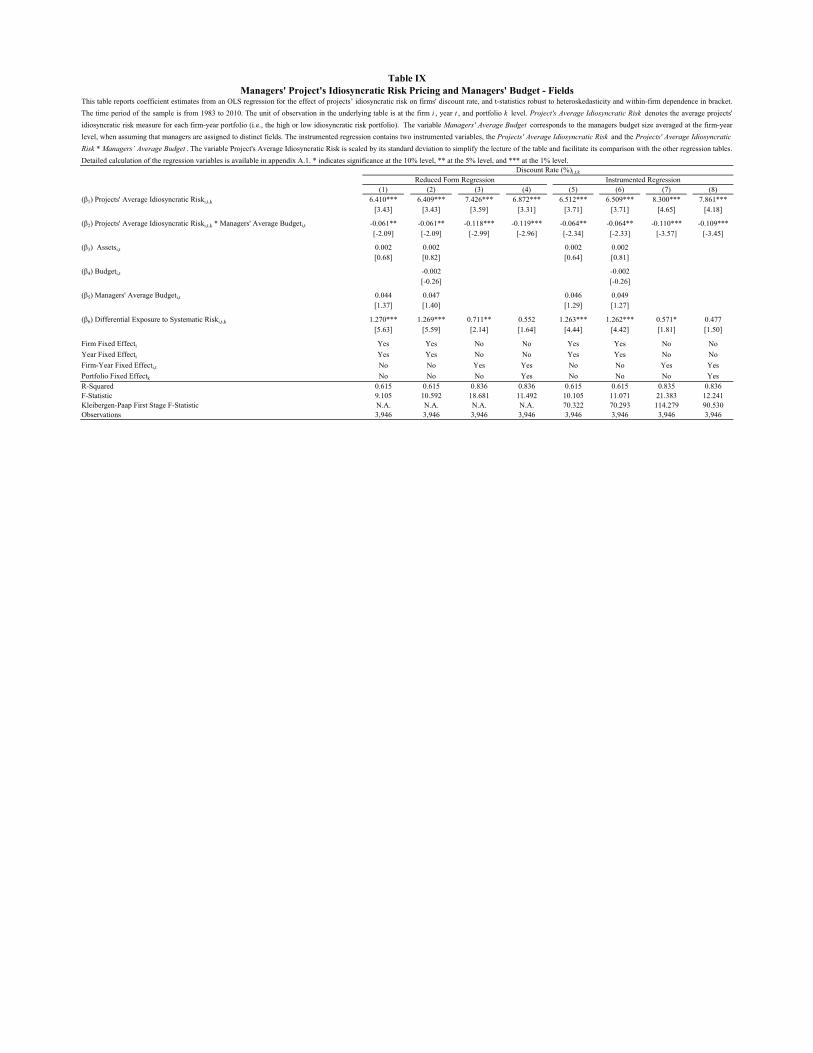
(1) (2) (3) (4) (5) (6) (7) (8)(β1) Projects' Average Idiosyncratic Riski,t,k 6.410*** 6.409*** 7.426*** 6.872*** 6.512*** 6.509*** 8.300*** 7.861***
[3.43] [3.43] [3.59] [3.31] [3.71] [3.71] [4.65] [4.18]
(β2) Projects' Average Idiosyncratic Riski,t,k * Managers' Average Budgeti,t -0.061** -0.061** -0.118*** -0.119*** -0.064** -0.064** -0.110*** -0.109***[-2.09] [-2.09] [-2.99] [-2.96] [-2.34] [-2.33] [-3.57] [-3.45]
(β3) Assetsi,t 0.002 0.002 0.002 0.002[0.68] [0.82] [0.64] [0.81]
(β4) Budgeti,t -0.002 -0.002[-0.26] [-0.26]
(β5) Managers' Average Budgeti,t 0.044 0.047 0.046 0.049[1.37] [1.40] [1.29] [1.27]
(β6) Differential Exposure to Systematic Riski,t,k 1.270*** 1.269*** 0.711** 0.552 1.263*** 1.262*** 0.571* 0.477[5.63] [5.59] [2.14] [1.64] [4.44] [4.42] [1.81] [1.50]
Firm Fixed Effecti Yes Yes No No Yes Yes No No
Year Fixed Effectt Yes Yes No No Yes Yes No No
Firm-Year Fixed Effecti,t No No Yes Yes No No Yes Yes
Portfolio Fixed Effectk No No No Yes No No No YesR-Squared 0.615 0.615 0.836 0.836 0.615 0.615 0.835 0.836F-Statistic 9.105 10.592 18.681 11.492 10.105 11.071 21.383 12.241Kleibergen-Paap First Stage F-Statistic N.A. N.A. N.A. N.A. 70.322 70.293 114.279 90.530Observations 3,946 3,946 3,946 3,946 3,946 3,946 3,946 3,946
This table reports coefficient estimates from an OLS regression for the effect of projects’ idiosyncratic risk on firms' discount rate, and t-statistics robust to heteroskedasticity and within-firm dependence in bracket.
The time period of the sample is from 1983 to 2010. The unit of observation in the underlying table is at the firm i , year t , and portfolio k level. Project's Average Idiosyncratic Risk denotes the average projects'
idiosyncratic risk measure for each firm-year portfolio (i.e., the high or low idiosyncratic risk portfolio). The variable Managers' Average Budget corresponds to the managers budget size averaged at the firm-year
level, when assuming that managers are assigned to distinct fields. The instrumented regression contains two instrumented variables, the Projects' Average Idiosyncratic Risk and the Projects' Average Idiosyncratic
Risk * Managers’ Average Budget . The variable Project's Average Idiosyncratic Risk is scaled by its standard deviation to simplify the lecture of the table and facilitate its comparison with the other regression tables.
Detailed calculation of the regression variables is available in appendix A.1. * indicates significance at the 10% level, ** at the 5% level, and *** at the 1% level.
Table IXManagers' Project's Idiosyncratic Risk Pricing and Managers' Budget - Fields
Discount Rate (%)i,t,k
Reduced Form Regression Instrumented Regression

(1) (2) (3) (4) (5) (6) (7) (8)(β1) Projects' Average Idiosyncratic Riski,t,k 7.429*** 7.393*** 8.298*** 8.118*** 7.249*** 7.216*** 7.965*** 7.789***
[3.37] [3.35] [3.55] [3.21] [3.38] [3.36] [3.49] [3.14]
(β2) Projects' Average Idiosyncratic Riski,t,k * Managers' Average Budgeti,t -0.062* -0.057 -0.089** -0.093** -0.037 -0.030 -0.044* -0.046*
[-1.68] [-1.64] [-2.09] [-2.24] [-1.61] [-1.46] [-1.82] [-1.96]
(β3) Projects' Average Idiosyncratic Riski,t,k * Managers' Average Budgeti,t * Distancei,t -0.088** -0.092** -0.087* -0.084* -0.044** -0.048** -0.044* -0.043
[-2.44] [-2.38] [-1.88] [-1.73] [-2.16] [-2.22] [-1.67] [-1.55]
(β4) Assetsi,t 0.003 0.005
[0.56] [1.03]
(β5) Budgeti,t 0.006 0.010
[0.71] [1.03]
(β6) Managers' Average Budgeti,t 0.097* 0.072 0.047* 0.013
[1.86] [1.49] [1.83] [0.51]
(β7) Distancei,t 0.295 0.336 0.314 0.330
[0.55] [0.63] [0.59] [0.61]
(β8) Managers' Average Budgeti,t * Distancei,t 0.037 0.031 0.006 0.007
[0.70] [0.61] [0.20] [0.26]
(β9) Projects' Average Idiosyncratic Riski,t,k * Distancei,t 0.229 0.278 0.673 0.587 0.295 0.359 0.762 0.683
[0.23] [0.28] [0.62] [0.51] [0.30] [0.35] [0.70] [0.59]
(β10) Differential Exposure to Systematic Riski,t,k 0.886*** 0.902*** 0.578*** 0.547*** 0.884*** 0.911*** 0.600*** 0.570***
[4.31] [4.28] [3.49] [3.41] [4.35] [4.34] [3.66] [3.53]
Firm Fixed Effecti Yes Yes No No Yes Yes No No
Year Fixed Effectt Yes Yes No No Yes Yes No No
Firm-Year Fixed Effecti,t No No Yes Yes No No Yes Yes
Portfolio Fixed Effectk No No No Yes No No No Yes
R-Squared 0.624 0.624 0.840 0.840 0.624 0.625 0.840 0.840F-Statistic 4.309 4.169 8.964 6.096 4.085 3.839 9.192 6.314Observations 3,946 3,946 3,946 3,946 3,946 3,946 3,946 3,946
Table XManagers' Project's Idiosyncratic Risk Pricing and Managers' Budget - Agency Effect
This table reports coefficient estimates from an OLS regression for the effect of projects’ idiosyncratic risk on firms' discount rate, and t-statistics robust to heteroskedasticity and within-firm dependence in bracket. The time
period of the sample is from 1983 to 2010. The unit of observation in the underlying table is at the firm i , year t , and portfolio k level. Project's Average Idiosyncratic Risk denotes the average projects' idiosyncratic risk measure
for each firm-year portfolio (i.e., the high or low idiosyncratic risk portfolio). The variable Managers' Average Budget corresponds to the managers budget size averaged at the firm-year level. Column (1) to (4) reports the
results when assuming that managers are assigned to specific fields, and columns (5) to (8) report to results when assuming that managers are assigned to different states. The variable Distance denotes the median distance
between the firms' wells drilled during a given year in hundreds of miles, winsorised at the 5 th and 95 th percentile . The variable Project's Average Idiosyncratic Risk is scaled by its standard deviation to simplify the lecture of
the table and facilitate its comparison with the other regression tables. Detailed calculation of the regression variables is available in appendix A.1. * indicates significance at the 10% level, ** at the 5% level, and *** at the 1%
level.Discount Rate (%)i,t,k
Managers' Budget (Region = Field) Managers' Budget (Region = State)

(1) (2) (3) (4) (5) (6) (7) (8)(β1) Projects' Average Idiosyncratic Riski,t,k 10.542** 10.531** 12.428** 11.880** 11.077** 11.059** 12.678** 12.143**
[2.49] [2.50] [2.39] [2.31] [2.52] [2.54] [2.40] [2.32]
(β2) Projects' Average Idiosyncratic Riski,t,k * Assetsi,t -0.015* -0.015** -0.018** -0.017** -0.016** -0.015** -0.019*** -0.018***
[-1.96] [-1.98] [-2.45] [-2.40] [-2.09] [-2.10] [-2.68] [-2.65]
(β3) Assetsi,t 0.016* 0.015** 0.019* 0.018*
[1.74] [1.99] [1.76] [1.89]
(β4) Managers' Average Budgeti,t 0.068 0.063 0.043 0.035
[1.02] [1.02] [0.95] [0.89]
(β5) Managers' Average Budgeti,t * Assetsi,t -0.000 -0.000 -0.000 -0.000
[-1.45] [-1.51] [-1.60] [-1.61]
(β6) Projects' Average Idiosyncratic Riski,t,k * Managers' Average Budgeti,t -0.111* -0.111* -0.220** -0.217** -0.106** -0.105** -0.154** -0.153**
[-1.75] [-1.79] [-2.09] [-2.07] [-2.00] [-2.02] [-2.05] [-2.02]
(β7) Projects' Average Idiosyncratic Riski,t,k * Managers' Average Budgeti,t * Assetsi,t / 1000 0.021 0.021 0.034* 0.033* 0.016* 0.016** 0.023** 0.022**
[1.59] [1.64] [1.87] [1.82] [1.94] [1.98] [2.21] [2.17]
(β8) Budgeti,t 0.003 0.006
[0.26] [0.52]
(β9) Firm's Diversificationi,t 0.003 0.003 0.001 0.001
[0.24] [0.24] [0.10] [0.09]
(β10) Projects' Average Idiosyncratic Riski,t,k * Firm's Diversificationi,t -0.082* -0.082* -0.072 -0.086 -0.083* -0.083* -0.073 -0.087
[-1.68] [-1.69] [-1.30] [-1.36] [-1.72] [-1.73] [-1.33] [-1.39]
(β11) Differential Exposure to Systematic Riski,t,k 1.202*** 1.204*** 0.504 0.361 1.209*** 1.215*** 0.515 0.375
[3.89] [3.83] [1.51] [1.06] [3.89] [3.81] [1.55] [1.10]
Firm Fixed Effecti Yes Yes No No Yes Yes No No
Year Fixed Effectt Yes Yes No No Yes Yes No No
Firm-Year Fixed Effecti,t No No Yes Yes No No Yes Yes
Portfolio Fixed Effectk No No No Yes No No No Yes
R-Squared 0.470 0.470 0.737 0.737 0.472 0.472 0.737 0.738F-Statistic 2.642 4.289 9.531 6.280 2.501 3.986 9.314 6.085Observations 3,946 3,946 3,946 3,946 3,946 3,946 3,946 3,946
Table XIManagers' Project's Idiosyncratic Risk Pricing, Internal Agency Frictions and Costly External Financing
This table reports coefficient estimates from an OLS regression for the effect of projects’ idiosyncratic risk on firms' discount rate, and t-statistics robust to heteroskedasticity and within-firm dependence in bracket. The time
period of the sample is from 1983 to 2010. The unit of observation in the underlying table is at the firm i , year t , and portfolio k level. Project's Average Idiosyncratic Risk denotes the average projects' idiosyncratic risk
measure for each firm-year portfolio (i.e., the high or low idiosyncratic risk portfolio). The variable Firm's Diversification denotes how much of the wells' idiosyncratic risk drilled in a given year is diversified at the firm's
level. The variable Managers' Average Budget corresponds to the managers budget size averaged at the firm-year level. Column (1) to (4) reports the results when assuming that managers are assigned to specific fields, and
columns (5) to (8) report to results when assuming that managers are assigned to different states. The variable Project's Average Idiosyncratic Risk is scaled by its standard deviation to simplify the lecture of the table and
facilitate its comparison with the other regression tables. Detailed calculation of the regression variables is available in appendix A.1. * indicates significance at the 10% level, ** at the 5% level, and *** at the 1% level.Discount Rate (%)i,t,k
Managers' Budget (Region = Field) Managers' Budget (Region = State)

(1) (2) (3) (4) (5) (6) (7)
(β1) Projects' Average Idiosyncratic Riski,t,k 6.228*** 5.256*** 5.230*** 5.243*** 5.232*** 5.514*** 4.241***
[5.32] [4.51] [4.51] [4.51] [4.50] [4.89] [3.28]
(β2) Budgeti,t 0.006 0.008
[1.56] [1.60]
(β3) Assetsi,t 0.001 -0.001
[0.91] [-0.46]
(β4) Differential Exposure to Systematic Riski,t,k 0.288*** 0.288*** 0.289*** 0.290*** 0.288*** 0.229** 0.189*
[3.20] [3.23] [3.25] [3.29] [3.25] [2.33] [1.93]
Firm Fixed Effecti Yes Yes Yes Yes Yes No No
Year Fixed Effectt No Yes Yes Yes Yes No No
Firm-Year Fixed Effecti,t No No No No No Yes Yes
Portfolio Fixed Effectk No No No No No No Yes
R-Squared 0.64 0.67 0.67 0.67 0.67 0.84 0.84
F-Statistic 15.082 12.093 8.220 8.255 6.242 14.700 6.632
Observations 1,642 1,642 1,642 1,642 1,642 1,642 1,642
This table reports coefficient estimates from an OLS regression for the effect of projects’ idiosyncratic risk on firms’ discount rate, and t-statistics robust to
heteroskedasticity and within-firm dependence in bracket.. The time period of the sample is from 1983 to 2010. The unit of observation in the underlying table
is at the firm i , year t, and portfolio k level. In this regression specification, the analysis is only performed on a subsample of projects for which the time to
expiration is expected to be close to zero, making the real option optimal exercise threshold (V*) close to the projects investment cost (I). The variable
Project's Average Idiosyncratic Risk is scaled by its standard deviation to simplify the lecture of the table and facilitate its comparison with the other
regression tables. * indicates significance at the 10% level, ** at the 5% level, and *** at the 1% level.Discount Rate (%)i,t,k
Table XIIManagers' Project's Idiosyncratic Risk Pricing - Real Option Effect (1)

(1) (2) (3) (4)
(β1) Projects' Average Idiosyncratic Riski,t,k 6.110** 6.261** 4.372** 4.416**
[2.53] [2.53] [2.13] [2.04]
(β2) Budgeti,t -0.010
[-1.34]
(β3) Assetsi,t 0.002 0.008
[0.38] [1.15]
(β4) Leveragei,t -6.581 -5.588
[-1.25] [-1.06]
(β5) Leveragei,t * Projects' Average Idiosyncratic Riski,t,k 6.459 6.184 17.000** 17.319**
[0.77] [0.72] [2.13] [2.16]
(β6) Differential Exposure to Systematic Riski,t,k 0.371* 0.368* 0.313 0.322
[1.78] [1.79] [1.42] [1.29]
Firm Fixed Effecti Yes Yes No No
Year Fixed Effectt Yes Yes No No
Firm-Year Fixed Effecti,t No No Yes Yes
Portfolio Fixed Effectk No No No Yes
R-Squared 0.644 0.631 0.828 0.828
F-Statistic 5.039 4.920 9.000 5.404
Observations 918 918 918 918
This table reports coefficient estimates from an OLS regression for the effect of projects’ idiosyncratic risk on firms’discount rate, and t-statistics robust to heteroskedasticity and within-firm dependence in bracket. The time period ofthe sample is from 1983 to 2010. The unit of observation in the underlying table is at the firm i , year t , and portfoliok level. The Leverage variable corresponds to the firms' market leverage calculated using the firm 10-k annualstatement and stock market data. Detailed calculations are available in appendix A.2. The analysis is restricted to theset of firms available in Compustat for which the necessary variables were available. The variable Project's Average Idiosyncratic Risk is scaled by its standard deviation to simplify the lecture of the table and facilitate its comparisonwith the other regression tables. * indicates significance at the 10% level, ** at the 5% level, and *** at the 1%level.
Discount Rate (%)i,t,k
Table XIIIManagers' Project-Level Idiosyncratic Risk Pricing - Leverage Effect

(1) (2) (3) (4) (5)
(β1) Projects' Average Idiosyncratic Riski,t,k 7.153*** 7.149*** 7.145*** 7.304*** 6.228***
[3.74] [3.75] [3.74] [4.24] [3.29]
(β2) Budgeti,t -0.003 -0.006
[-0.52] [-0.80]
(β3) Assetsi,t 0.001 0.003
[0.12] [0.48]
(β4) Differential Exposure to Systematic Riski,t,k 0.736* 0.736* 0.737* 0.763 0.728
[1.76] [1.76] [1.76] [1.37] [1.30]
Firm Fixed Effecti Yes Yes Yes No No
Year Fixed Effectt Yes Yes Yes No No
Firm-Year Fixed Effecti,t No No No Yes Yes
Portfolio Fixed Effectk No No No No Yes
R-Squared 0.548 0.548 0.548 0.784 0.784
F-Statistic 6.504 5.021 5.332 8.985 5.404
Observations 3,416 3,416 3,416 3,416 3,416
This table reports coefficient estimates from an OLS regression for the effect of projects' idiosyncratic risk on firms' discount
rate, and t-statistics robust to heteroskedasticity and within-firm dependence in bracket. The time period of the sample is
from 1995 to 2010. The unit of observation in the underlying table is at the firm i , year t , and portfolio k level. Project's
Average Idiosyncratic Risk denotes the average projects' idiosyncratic risk measure for each firm-year portfolio (i.e., the high
or low idiosyncratic risk portfolio). In this regression specification, the project's internal rate of return is estimated using the
36-month Bloomberg Natural Gas Futures prices instead of the EIA three-year price forecast. The variable Project's
Average Idiosyncratic Risk is scaled by its standard deviation to simplify the lecture of the table and facilitate its comparison
with the other regression tables. * indicates significance at the 10% level, ** at the 5% level, and *** at the 1% level.Discount Rate (%)i,t,k
Table XIVManagers' Project's Idiosyncratic Risk Pricing - Futures Price

(1) (2) (3) (4) (5)
(β1) Projects' Average Idiosyncratic Riski,t,k 7.162*** 7.158*** 7.166*** 7.200*** 6.410***
[3.32] [3.31] [3.29] [3.40] [2.76]
(β2) Budgeti,t 0.007 0.008
[0.70] [0.49]
(β3) Assetsi,t 0.002 -0.001
[0.68] [-0.15]
(β4) Differential Exposure to Systematic Riski,t,k 0.690* 0.692* 0.689* 0.547* 0.519
[1.82] [1.83] [1.84] [1.67] [1.56]
Firm Fixed Effecti Yes Yes Yes No No
Year Fixed Effectt Yes Yes Yes No No
Firm-Year Fixed Effecti,t No No No Yes Yes
Portfolio Fixed Effectk No No No No Yes
R-Squared 0.469 0.469 0.469 0.738 0.739
F-Statistic 6.512 5.117 6.083 7.701 4.737
Observations 3,946 3,946 3,946 3,946 3,946
Table XVManagers' Project's Idiosyncratic Risk Pricing - EIA State's Wellhead Price
This table reports coefficient estimates from an OLS regression for the effect of projects' idiosyncratic risk on firms' discount
rate, and t-statistics robust to heteroskedasticity and within-firm dependence in bracket. The time period of the sample is
from 1983 to 2010. The unit of observation in the underlying table is at the firm i , year t, and portfolio k level. Project's
Average Idiosyncratic Risk denotes the average projects' idiosyncratic risk measure for each firm-year portfolio (i.e., the high
or low idiosyncratic risk portfolio). In this regression specification, the project's internal rate of return is estimated using the
wellhead spot price specific to each state (Source: https://www.eia.gov/dnav/ng/ng_prod_whv_a_epg0_fwa_dpmcf_a.htm)
instead of the EIA price forecast. The variable Project's Average Idiosyncratic Risk is scaled by its standard deviation to
simplify the lecture of the table and facilitate its comparison with the other regression tables. * indicates significance at the
10% level, ** at the 5% level, and *** at the 1% level.Discount Rate (%)i,t,k

(1) (2) (3) (4) (5) (6)
(β1) Projects' Average Idiosyncratic Riski,t 11.043*** 7.015*** 5.689*** 5.695*** 5.679*** 5.678***
[6.49] [6.45] [5.81] [5.82] [5.80] [5.79]
(β2) Budgeti,t -0.003 -0.007
[-0.80] [-1.11]
(β3) Assetsi,t 0.002 0.004
[0.59] [1.06]
(β4) Differential Exposure to Systematic Riski,t,k 0.689*** 0.040 0.155** 0.153** 0.156** 0.153**
[3.39] [0.64] [2.50] [2.49] [2.55] [2.52]
Firm Fixed Effecti No Yes Yes Yes Yes Yes
Year Fixed Effectt No No Yes Yes Yes Yes
R-Squared 0.320 0.718 0.745 0.746 0.746 0.746
F-Statistic 29.718 21.326 22.429 14.992 16.697 12.601
Observations 1,973 1,973 1,973 1,973 1,973 1,973
Table XVIManagers' Project's Idiosyncratic Risk Pricing - Alternative Design
This table reports coefficient estimates from an OLS regression for the effect of projects' idiosyncratic risk on firms’ discount rate, and t-statistics
robust to heteroskedasticity and within-firm dependence in bracket. The time period of the sample is from 1983 to 2010. The unit of observation in
the underlying table is at the firm i , and year t level. Projects' Average Idiosyncratic Risk denotes the average projects' idiosyncratic risk measure
for each firm-year, scaled by its standard deviation (i.e., one portfolio per firm-year). The variable Project's Average Idiosyncratic Risk is scaled
by its standard deviation to simplify the lecture of the table and facilitate its comparison with the other regression tables. * indicates significance at
the 10% level, ** at the 5% level, and *** at the 1% level.Discount Rate (%)i,t

(1) (2) (3) (4) (5) (6) (7) (8)
(β1) Projects' Average Idiosyncratic Riski,t,k 6.372*** 6.402*** 6.672*** 6.070** 6.623*** 6.625*** 6.849*** 6.261**
[2.92] [2.92] [3.03] [2.50] [2.98] [2.98] [3.05] [2.51]
(β2) Budgeti,t 0.001 0.004
[0.04] [0.24]
(β3) Assetsi,t -0.002 -0.001
[-0.54] [-0.22]
(β4) Differential Exposure to Systematic Riski,t,k 0.669* 0.663* 0.493* 0.471* 0.659* 0.658* 0.494* 0.472*
[1.94] [1.93] [1.80] [1.68] [1.91] [1.93] [1.81] [1.69]
Firm Fixed Effecti Yes Yes No No Yes Yes No No
Year Fixed Effectt Yes Yes No No Yes Yes No No
Firm-Year Fixed Effecti,t No No Yes Yes No No Yes Yes
Portfolio Fixed Effectk No No No Yes No No No Yes
R-Squared 0.463 0.463 0.730 0.731 0.464 0.464 0.731 0.731
F-Statistic 5.246 10.583 5.147 3.335 5.542 7.739 5.186 3.363
Observations 3,946 3,946 3,946 3,946 3,946 3,946 3,946 3,946
Table XVIIManagers' Project's Idiosyncratic Risk Pricing - Alternative Threshold Value
This table reports coefficient estimates from an OLS regression for the effect of projects' idiosyncratic risk on firms’ discount rate, and t-statistics robust to heteroskedasticity and
within-firm dependence in bracket. The time period of the sample is from 1983 to 2010. The unit of observation in the underlying table is at the firm i , year t level, and portfolio
k level. The columns’ titles refer to the firm-year porfolio percentiles of the idiosyncratic risk distribution used to compute the estimated discount rate. For example, the columns
with Minimum Bound indicate that only to lowest projects' expected IRR was used to estimate the discount rate. Projects' Average Idiosyncratic Risk denotes the average
projects' idiosyncratic risk measure for each firm-year, scaled by its standard deviation (i.e., one portfolio per firm-year). The variable Project's Average Idiosyncratic Risk is
scaled by its standard deviation to simplify the lecture of the table and facilitate its comparison with the other regression tables. * indicates significance at the 10% level, ** at
the 5% level, and *** at the 1% level.Discount Rate (%)i,t,k
Minimum Bound 0th to 2.5th Percentile

(1) (2) (3) (4) (5) (6)
(β1) Projects' Average Idiosyncratic Riski,t,k 8.261*** 8.251*** 8.266*** 8.242*** 9.515*** 8.670***
[2.71] [2.70] [2.72] [2.70] [3.01] [2.68]
(β2) Budgeti,t -0.002 -0.004
[-0.44] [-1.01]
(β3) Assetsi,t 0.002 0.003
[0.71] [1.10]
(β4) Projects' Average Idiosyncratic Riski,t,k * Decade1990 -2.257 -2.250 -2.272 -2.268 -2.888 -3.297
[-0.94] [-0.93] [-0.95] [-0.95] [-1.17] [-1.35]
(β5) Projects' Average Idiosyncratic Riski,t,k * Decade2000 -4.608 -4.593 -4.624 -4.594 -5.843* -5.723*
[-1.56] [-1.55] [-1.57] [-1.56] [-1.87] [-1.82]
(β6) Differential Exposure to Systematic Riski,t,k 0.282*** 0.282*** 0.284*** 0.284*** 0.208** 0.184**
[3.56] [3.55] [3.59] [3.60] [2.58] [2.27]
Firm Fixed Effecti Yes Yes Yes Yes No No
Year Fixed Effectt Yes Yes Yes Yes No No
Firm-Year Fixed Effecti,t No No No No Yes Yes
Portfolio Fixed Effectk No No No No No Yes
R-Squared 0.704 0.704 0.704 0.704 0.873 0.874
F-Statistic 9.393 7.847 7.843 7.298 10.567 6.266
Observations 3,946 3,946 3,946 3,946 3,946 3,946
Table XVIIIManagers' Project's Idiosyncratic Risk Pricing - Time Trend
This table reports coefficient estimates from an OLS regression for the effect of projects' idiosyncratic risk on firms’ discount rate, and t-statistics robust to
heteroskedasticity and within-firm dependence in bracket. The time period of the sample is from 1983 to 2010. The unit of observation in the underlying table
is at the firm i , year t and portfolio k level. Project's Average Idiosyncratic Risk denotes the average projects' idiosyncratic risk measure for each firm-year
portfolio (i.e., the high or low idiosyncratic risk portfolio). Specifically, the variables Decade 1990 and Decade 2000 denote dummy variables equal to 1 if the
observation occured in that decade, and zero otherwise. The variable Project's Average Idiosyncratic Risk is scaled by its standard deviation to simplify the
lecture of the table and facilitate its comparison with the other regression tables. * indicates significance at the 10% level, ** at the 5% level, and *** at the
1% level.Discount Rate (%)i,t,k
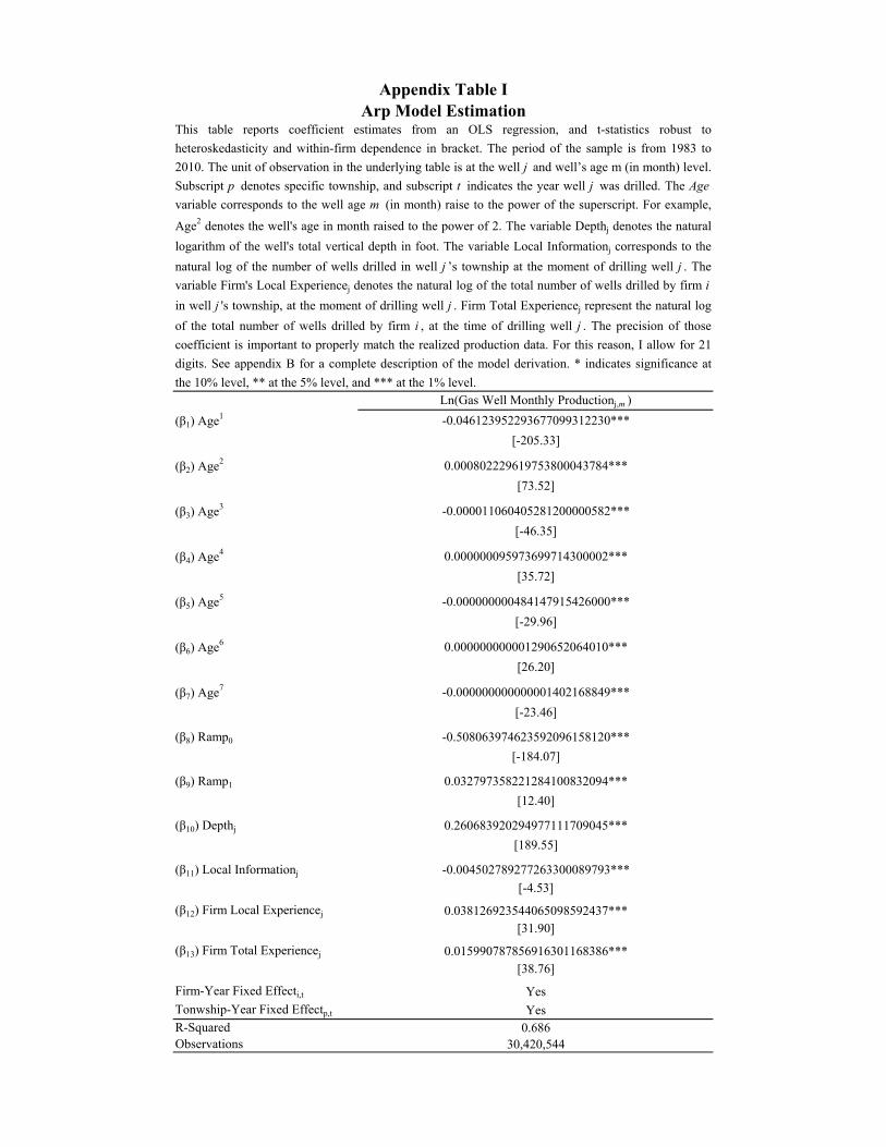
Ln(Gas Well Monthly Productionj,m )
(β1) Age1 -0.046123952293677099312230***
[-205.33]
(β2) Age2 0.000802229619753800043784***
[73.52]
(β3) Age3 -0.000011060405281200000582***
[-46.35]
(β4) Age4 0.000000095973699714300002***
[35.72]
(β5) Age5 -0.000000000484147915426000***
[-29.96]
(β6) Age6 0.000000000001290652064010***
[26.20]
(β7) Age7 -0.000000000000001402168849***
[-23.46]
(β8) Ramp0 -0.508063974623592096158120***
[-184.07]
(β9) Ramp1 0.032797358221284100832094***
[12.40]
(β10) Depthj 0.260683920294977111709045***
[189.55]
(β11) Local Informationj -0.004502789277263300089793***
[-4.53]
(β12) Firm Local Experiencej 0.038126923544065098592437***[31.90]
(β13) Firm Total Experiencej 0.015990787856916301168386***[38.76]
Firm-Year Fixed Effecti,t Yes
Tonwship-Year Fixed Effectp,t YesR-Squared 0.686Observations 30,420,544
This table reports coefficient estimates from an OLS regression, and t-statistics robust to
heteroskedasticity and within-firm dependence in bracket. The period of the sample is from 1983 to
2010. The unit of observation in the underlying table is at the well j and well’s age m (in month) level.
Subscript p denotes specific township, and subscript t indicates the year well j was drilled. The Age
variable corresponds to the well age m (in month) raise to the power of the superscript. For example,
Age2 denotes the well's age in month raised to the power of 2. The variable Depthj denotes the natural
logarithm of the well's total vertical depth in foot. The variable Local Informationj corresponds to the
natural log of the number of wells drilled in well j ’s township at the moment of drilling well j . The
variable Firm's Local Experiencej denotes the natural log of the total number of wells drilled by firm i
in well j 's township, at the moment of drilling well j . Firm Total Experiencej represent the natural log
of the total number of wells drilled by firm i , at the time of drilling well j . The precision of those
coefficient is important to properly match the realized production data. For this reason, I allow for 21
digits. See appendix B for a complete description of the model derivation. * indicates significance at
the 10% level, ** at the 5% level, and *** at the 1% level.
Arp Model EstimationAppendix Table I

(1) (2) (3) (4) (5) (6) (7) (8)
(β1) Idiosyncratic Shocksj -0.472 0.330 0.186 0.318 -0.529 0.179 0.114 0.170
[-1.17] [1.25] [0.78] [1.07] [-1.18] [1.21] [0.55] [0.89]
(β2) Assetsi,t -0.000*** -0.001*** -0.000*** -0.001***
[-3.14] [-3.68] [-3.66] [-3.13]
Township Fixed Effectp No No Yes No No No Yes No
Firm Fixed Effecti No Yes No No No Yes No No
Township-Firm Fixed Effectp,i No No No Yes No No No Yes
R-Squared 0.001 0.240 0.112 0.264 0.009 0.264 0.120 0.280
F-Statistic 1.369 1.569 0.603 1.141 5.470 9.251 7.082 6.381
Observations 114,696 114,696 114,696 114,696 114,696 114,696 114,696 114,696
Appendix Table IIIdiosyncratic Shocks and The Stochastic Discount Factor
This table reports coefficient estimates from an OLS regression for the relation between wells' idiosyncratic shocks and the stochastic discount factor of the CAPM model
(i.e., a function of the Market Excess Return ), and t-statistics robust to heteroskedasticity and within-firm dependence in bracket. The period of the sample is from 1983 to
2010. The unit of observation in the underlying table is at the year t level. The market excess return corresponds to the market earning-to-price ratio net of the 10-year risk-
free rate. The Idiosyncratic shock is measured at the individual well level and corresponds to the well's idiosyncratic productivity shocks. See appendix A.1. and A.2 for the
full methodological details. * indicates significance at the 10% level, ** at the 5% level, and *** at the 1% level.Market Excess Return (%)t

(1) (2) (3) (4)
(β1) Project's Idiosyncratic Riskp,t 1.476*** 1.425*** 1.377*** 1.532***
[9.56] [7.54] [2.66] [2.86]
(β2) Township Average Productionp,t 0.999*** 0.999*** 0.999*** 0.999***
[-4.40] [-4.71] [-3.31] [-2.72]
Year Fixed Effectt No Yes No Yes
Township Fixed Effectp No No Yes Yes
Pseudo R-Squared 0.128 0.170 0.278 0.295
Observations 12,386 12,386 12,386 12,386
This table reports the incidence rate ratio estimates of a Poisson regression, and t-statistics robust to
heteroskedasticity and within-township dependence in bracket. A coefficient value greater that 1 indicate a
positive relation between the variable of interest and the outcome variable, while a value smaller than 1 indicate a
negative relation. The unit of observation is at the township p , and year t level. The dependent variable, Number
of Dry Hole , is a count variable that corresponds to the number of dry wells drilled in a given township-year. For
example, a value of 2 indicates that there were 2 dry holes drilled in the township during that given year. Project's
Idiosyncratic Risk p,t denotes the cross-sectional dispersion of the well's idiosyncratic productivity shock,
computed at the township p and year t level. The variable Project's Idiosyncratic Risk is scaled by its standard
deviation to simplify the lecture of the table and facilitate its comparison with the other regression tables. *
indicates significance at the 10% level, ** at the 5% level, and *** at the 1% level.
Projects' Idiosyncratic Risk and Probability of Dry HoleAppendix Table III
Number of Dry Holesp,t

(1) (2) (3) (4) (5) (6) (7) (8)
(β1) Projects' Average Idiosyncratic Riski,t,k 7.101*** 7.110*** 10.024*** 9.242*** 7.730*** 7.714*** 12.094*** 11.557***
[4.44] [4.44] [3.87] [3.56] [3.94] [3.93] [4.43] [4.10]
(β3) Projects' Average Idiosyncratic Riski,t,k * HPi,t 1.504*** 1.509*** 2.291*** 2.177*** 1.667*** 1.665*** 2.714*** 2.634***
[3.44] [3.43] [3.26] [3.11] [3.18] [3.17] [3.79] [3.63]
(β3) HPi,t 7.195*** 7.083*** 7.104*** 6.998***
[6.03] [6.04] [5.93] [5.95]
(β4) Assetsi,t 0.002 0.002
[0.63] [0.64]
(β5) Budgeti,t -0.004 -0.004
[-1.01] [-1.00]
(β6) Differential Exposure to Systematic Riski,t,k 0.777*** 0.779*** 0.759*** 0.668*** 0.767*** 0.769*** 0.688*** 0.636***
[7.08] [7.13] [5.81] [5.07] [6.34] [6.39] [4.82] [4.62]
Firm Fixed Effecti Yes Yes No No Yes Yes No No
Year Fixed Effectt Yes Yes No No Yes Yes No No
Firm-Year Fixed Effecti,t No No Yes Yes No No Yes Yes
Portfolio Fixed Effectk No No No Yes No No No Yes
R-Squared 0.735 0.735 0.884 0.884 0.735 0.735 0.883 0.884
F-Statistics 31.379 26.100 37.816 24.057 30.577 25.693 40.172 26.604
Kleibergen-Paap First Stage F-Statistics N.A. N.A. N.A. N.A. 69.810 69.964 81.939 95.983
Observations 3,946 3,946 3,946 3,946 3,946 3,946 3,946 3,946
Appendix Table IVManagers' Project's Idiosyncratic Risk Pricing and Hadlock-Pierce Index
This table reports coefficient estimates from an OLS regression and a 2SLS regression for the effect of projects’ idiosyncratic risk on firms' discount rate, and t-statistics robust to heteroskedasticity and within-
firm dependence in bracket. The time period of the sample is from 1983 to 2010. The unit of observation in the underlying table is at the firm i , year t , and portfolio k level. Projects' Average Idiosyncratic
Risk denotes the projects' average idiosyncratic risk measure for each firm-year portfolio (i.e., the high or low idiosyncratic risk portfolio). The Hadlock-Pierce Index is used as a costly external financing
proxy. Its calculation details are available in appendix A.3. The instrumented regression contains two instrumented variables, the Projects' Average Idiosyncratic Risk and the Projects' Average Idiosyncratic
Risk * Hadlock-Pierce Index . The analysis is restricted to the set of firms available in Compustat for which the necessary variables for each indexes was available. The variable Project's Average Idiosyncratic
Risk is scaled by its standard deviation to simplify the lecture of the table and facilitate its comparison with the other regression tables. * indicates significance at the 10% level, ** at the 5% level, and *** at
the 1% level.
Discount Rate (%)i,t,k
Reduced Form Regression Instrumented Regression
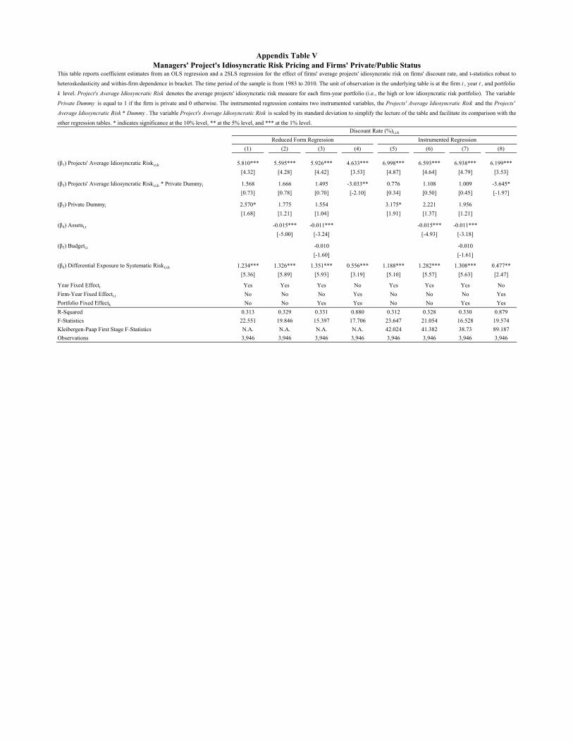
(1) (2) (3) (4) (5) (6) (7) (8)
(β1) Projects' Average Idiosyncratic Riski,t,k 5.810*** 5.595*** 5.926*** 4.633*** 6.998*** 6.593*** 6.938*** 6.199***
[4.32] [4.28] [4.42] [3.53] [4.87] [4.64] [4.79] [3.53]
(β3) Projects' Average Idiosyncratic Riski,t,k * Private Dummyi 1.568 1.666 1.495 -3.033** 0.776 1.108 1.009 -3.645*
[0.73] [0.78] [0.70] [-2.10] [0.34] [0.50] [0.45] [-1.97]
(β3) Private Dummyi 2.570* 1.775 1.554 3.175* 2.221 1.956
[1.68] [1.21] [1.04] [1.91] [1.37] [1.21]
(β4) Assetsi,t -0.015*** -0.011*** -0.015*** -0.011***
[-5.00] [-3.24] [-4.93] [-3.18]
(β5) Budgeti,t -0.010 -0.010
[-1.60] [-1.61]
(β6) Differential Exposure to Systematic Riski,t,k 1.234*** 1.326*** 1.351*** 0.556*** 1.188*** 1.282*** 1.308*** 0.477**
[5.36] [5.89] [5.93] [3.19] [5.10] [5.57] [5.63] [2.47]
Year Fixed Effectt Yes Yes Yes No Yes Yes Yes No
Firm-Year Fixed Effecti,t No No No Yes No No No Yes
Portfolio Fixed Effectk No No Yes Yes No No Yes Yes
R-Squared 0.313 0.329 0.331 0.880 0.312 0.328 0.330 0.879
F-Statistics 22.551 19.846 15.397 17.706 23.647 21.054 16.528 19.574
Kleibergen-Paap First Stage F-Statistics N.A. N.A. N.A. N.A. 42.024 41.382 38.73 89.187
Observations 3,946 3,946 3,946 3,946 3,946 3,946 3,946 3,946
This table reports coefficient estimates from an OLS regression and a 2SLS regression for the effect of firms' average projects' idiosyncratic risk on firms' discount rate, and t-statistics robust to
heteroskedasticity and within-firm dependence in bracket. The time period of the sample is from 1983 to 2010. The unit of observation in the underlying table is at the firm i , year t , and portfolio
k level. Project's Average Idiosyncratic Risk denotes the average projects' idiosyncratic risk measure for each firm-year portfolio (i.e., the high or low idiosyncratic risk portfolio). The variable
Private Dummy is equal to 1 if the firm is private and 0 otherwise. The instrumented regression contains two instrumented variables, the Projects' Average Idiosyncratic Risk and the Projects'
Average Idiosyncratic Risk * Dummy . The variable Project's Average Idiosyncratic Risk is scaled by its standard deviation to simplify the lecture of the table and facilitate its comparison with the
other regression tables. * indicates significance at the 10% level, ** at the 5% level, and *** at the 1% level.Discount Rate (%)i,t,k
Appendix Table VManagers' Project's Idiosyncratic Risk Pricing and Firms' Private/Public Status
Reduced Form Regression Instrumented Regression

(1) (2) (3) (4) (5) (6) (7) (8)
(β1) Projects' Average Idiosyncratic Riski,t,k 7.437*** 7.428*** 8.016*** 7.389*** 8.932*** 8.964*** 10.447*** 10.558***
[3.78] [3.76] [3.95] [3.49] [3.21] [3.24] [3.54] [3.16]
(β2) Projects' Average Idiosyncratic Riski,t,k * Cleary Indexi,t 0.029* 0.029** 0.035* 0.036* 0.032 0.033 0.048 0.048
[1.97] [2.02] [1.73] [1.80] [1.24] [1.30] [1.40] [1.40]
(β3) Cleary Indexi,t -0.029* -0.029* -0.032 -0.031
[-1.91] [-1.88] [-1.43] [-1.41]
(β4) Assetsi,t 0.010 0.009 0.010 0.009
[1.23] [1.23] [1.27] [1.28]
(β5) Budgeti,t -0.011 -0.009 -0.011 -0.009
[-1.43] [-1.40] [-1.45] [-1.42]
(β6) Leveragei,t -13.148 -12.877
[-1.23] [-1.20]
(β7) Differential Exposure to Systematic Riski,t,k 0.362 0.385 0.175 0.044 0.243 0.264 -0.060 -0.045
[1.43] [1.54] [0.72] [0.16] [0.83] [0.91] [-0.20] [-0.15]
Firm Fixed Effecti Yes Yes No No Yes Yes No No
Year Fixed Effectt Yes Yes No No Yes Yes No No
Firm-Year Fixed Effecti,t No No Yes Yes No No Yes Yes
Portfolio Fixed Effectk No No No Yes No No No Yes
R-Squared 0.647 0.649 0.841 0.842 0.644 0.646 0.837 0.837
F-Statistic 4.554 4.276 8.076 4.343 4.353 4.136 8.242 4.473
Kleibergen-Paap First Stage F-Statistic N.A. N.A. N.A. N.A. 26.081 25.885 48.554 37.115
Observations 792 792 792 792 792 792 792 792
Instrumented Regression
Discount Rate (%)i,t,k
This table reports coefficient estimates from an OLS regression and a 2SLS regression for the effect of projects’ idiosyncratic risk on firms' discount rate, and t-statistics robust to
heteroskedasticity and within-firm dependence in bracket. The time period of the sample is from 1983 to 2010. The unit of observation in the underlying table is at the firm i , year t , and
portfolio k level. Projects' Average Idiosyncratic Risk denotes the projects' average idiosyncratic risk measure for each firm-year portfolio (i.e., the high or low idiosyncratic risk portfolio).
The Cleary Index is used as a costly external financing proxy. Its calculation details are available in appendix A.3. The instrumented regression contains two instrumented variables, the
Projects' Average Idiosyncratic Risk and the Projects' Average Idiosyncratic Risk * Cleary Index . The analysis is restricted to the set of firms available in Compustat for which the
necessary variables for each indexes was available. The variable Project's Average Idiosyncratic Risk is scaled by its standard deviation to simplify the lecture of the table and facilitate its
comparison with the other regression tables. * indicates significance at the 10% level, ** at the 5% level, and *** at the 1% level.
Managers' Project's Idiosyncratic Risk Pricing and the Cleary IndexAppendix Table VI
Reduced Form Regression
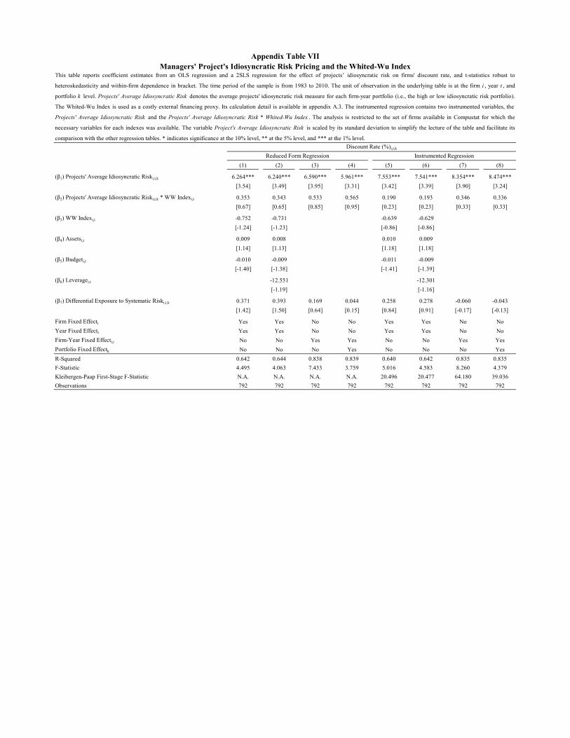
(1) (2) (3) (4) (5) (6) (7) (8)
(β1) Projects' Average Idiosyncratic Riski,t,k 6.264*** 6.240*** 6.590*** 5.961*** 7.553*** 7.541*** 8.354*** 8.474***
[3.54] [3.49] [3.95] [3.31] [3.42] [3.39] [3.90] [3.24]
(β2) Projects' Average Idiosyncratic Riski,t,k * WW Indexi,t 0.353 0.343 0.533 0.565 0.190 0.193 0.346 0.336
[0.67] [0.65] [0.85] [0.95] [0.23] [0.23] [0.33] [0.33]
(β3) WW Indexi,t -0.752 -0.731 -0.639 -0.629
[-1.24] [-1.23] [-0.86] [-0.86]
(β4) Assetsi,t 0.009 0.008 0.010 0.009
[1.14] [1.13] [1.18] [1.18]
(β5) Budgeti,t -0.010 -0.009 -0.011 -0.009
[-1.40] [-1.38] [-1.41] [-1.39]
(β6) Leveragei,t -12.551 -12.301
[-1.19] [-1.16]
(β7) Differential Exposure to Systematic Riski,t,k 0.371 0.393 0.169 0.044 0.258 0.278 -0.060 -0.043
[1.42] [1.50] [0.64] [0.15] [0.84] [0.91] [-0.17] [-0.13]
Firm Fixed Effecti Yes Yes No No Yes Yes No No
Year Fixed Effectt Yes Yes No No Yes Yes No No
Firm-Year Fixed Effecti,t No No Yes Yes No No Yes Yes
Portfolio Fixed Effectk No No No Yes No No No Yes
R-Squared 0.642 0.644 0.838 0.839 0.640 0.642 0.835 0.835
F-Statistic 4.495 4.063 7.433 3.759 5.016 4.583 8.260 4.379
Kleibergen-Paap First-Stage F-Statistic N.A. N.A. N.A. N.A. 20.496 20.477 64.180 39.036
Observations 792 792 792 792 792 792 792 792
Appendix Table VIIManagers' Project's Idiosyncratic Risk Pricing and the Whited-Wu Index
This table reports coefficient estimates from an OLS regression and a 2SLS regression for the effect of projects’ idiosyncratic risk on firms' discount rate, and t-statistics robust to
heteroskedasticity and within-firm dependence in bracket. The time period of the sample is from 1983 to 2010. The unit of observation in the underlying table is at the firm i , year t , and
portfolio k level. Projects' Average Idiosyncratic Risk denotes the average projects' idiosyncratic risk measure for each firm-year portfolio (i.e., the high or low idiosyncratic risk portfolio).
The Whited-Wu Index is used as a costly external financing proxy. Its calculation detail is available in appendix A.3. The instrumented regression contains two instrumented variables, the
Projects' Average Idiosyncratic Risk and the Projects' Average Idiosyncratic Risk * Whited-Wu Index . The analysis is restricted to the set of firms available in Compustat for which the
necessary variables for each indexes was available. The variable Project's Average Idiosyncratic Risk is scaled by its standard deviation to simplify the lecture of the table and facilitate its
comparison with the other regression tables. * indicates significance at the 10% level, ** at the 5% level, and *** at the 1% level.
Discount Rate (%)i,t,k
Reduced Form Regression Instrumented Regression

(1) (2) (3) (4) (5) (6) (7) (8)
(β1) Projects' Average Idiosyncratic Riski,t,k 6.086*** 6.085*** 6.219*** 5.876*** 7.164** 7.185** 7.972*** 8.219**
[3.19] [3.15] [3.57] [3.19] [2.61] [2.59] [3.00] [2.66]
(β2) Projects' Average Idiosyncratic Riski,t,k * KZ Indexi,t 0.928 0.898 0.979 0.850 0.658 0.621 0.456 0.507
[0.69] [0.66] [0.85] [0.75] [0.38] [0.35] [0.26] [0.29]
(β3) KZ Indexi,t -1.569 -0.219 -1.320 0.030
[-0.82] [-0.13] [-0.63] [0.02]
(β4) Assetsi,t 0.011 0.010 0.011 0.011
[1.50] [1.53] [1.53] [1.57]
(β5) Budgeti,t -0.013* -0.011* -0.013* -0.012*
[-1.74] [-1.84] [-1.75] [-1.84]
(β6) Leveragei,t -14.100 -14.027
[-1.05] [-1.04]
(β7) Differential Exposure to Systematic Riski,t,k 0.300 0.320 0.131 0.054 0.213 0.231 -0.061 -0.021
[1.16] [1.24] [0.48] [0.18] [0.70] [0.75] [-0.18] [-0.06]
Firm Fixed Effecti Yes Yes No No Yes Yes No No
Year Fixed Effectt Yes Yes No No Yes Yes No No
Firm-Year Fixed Effecti,t No No Yes Yes No No Yes Yes
Portfolio Fixed Effectk No No No Yes No No No Yes
R-Squared 0.375 0.376 0.376 0.645 0.636 0.637 0.826 0.825
F-Statistic 2.172 2.458 2.237 4.263 5.138 4.623 9.574 5.084
Kleibergen-Paap First Stage F-Statistic N.A. N.A. N.A. N.A. 7.550 7.529 14.908 12.808
Observations 792 792 792 792 792 792 792 792
This table reports coefficient estimates from an OLS regression and a 2SLS regression for the effect of projects’ idiosyncratic risk on firms' discount rate, and t-statistics robust to heteroskedasticity
and within-firm dependence in bracket. The time period of the sample is from 1983 to 2010. The unit of observation in the underlying table is at the firm i , year t and portfolio k level. Projects'
Average Idiosyncratic Risk denotes the average projects' idiosyncratic risk measure for each firm-year portfolio (i.e., the high or low idiosyncratic risk portfolio). The Kaplan-Zingales Index is
used as a costly external financing proxy. Its calculation details are available in appendix A.3. The instrumented regression contains two instrumented variables, the Projects' Average Idiosyncratic
Risk and the Projects' Average Idiosyncratic Risk * Kaplan-Zingales Index . The analysis is restricted to the set of firms available in Compustat for which the necessary variables for each indexes
was available. The variable Project's Average Idiosyncratic Risk is scaled by its standard deviation to simplify the lecture of the table and facilitate its comparison with the other regression tables. *
indicates significance at the 10% level, ** at the 5% level, and *** at the 1% level.
Managers' Project's Idiosyncratic Risk Pricing and the Kaplan-Zingales IndexAppendix Table VIII
Discount Rate (%)i,t,k
Reduced Form Regression Instrumented Regression

(1) (2) (3) (4) (5) (6) (7) (8)
(β1) Projects' Average Idiosyncratic Riski,t,k 6.723*** 6.725*** 7.323*** 6.768*** 6.721*** 6.724*** 8.193*** 7.747***
[3.47] [3.46] [3.53] [3.25] [3.80] [3.80] [4.64] [4.18]
(β2) Projects' Average Idiosyncratic Riski,t,k * Managers' Average Budgeti,t -0.054** -0.054** -0.069** -0.069** -0.048*** -0.048*** -0.065*** -0.064***
[-2.50] [-2.48] [-2.52] [-2.50] [-2.94] [-2.94] [-3.32] [-3.21]
(β3) Assetsi,t 0.005 0.004 0.004 0.004
[1.40] [1.34] [1.38] [1.36]
(β4) Budgeti,t 0.002 0.001
[0.22] [0.21]
(β5) Managers' Average Budgeti,t 0.017 0.015 0.013 0.011
[0.89] [0.73] [0.72] [0.52]
(β6) Differential Exposure to Systematic Riski,t,k 1.282*** 1.283*** 0.746** 0.587* 1.268*** 1.269*** 0.607* 0.511
[5.63] [5.56] [2.24] [1.73] [4.45] [4.41] [1.90] [1.58]
Firm Fixed Effecti Yes Yes No No Yes Yes No No
Year Fixed Effectt Yes Yes No No Yes Yes No No
Firm-Year Fixed Effecti,t No No Yes Yes No No Yes Yes
Portfolio Fixed Effectk No No No Yes No No No Yes
R-Squared 0.616 0.616 0.835 0.836 0.616 0.616 0.835 0.836F-Statistic 9.243 11.160 17.771 10.927 10.127 10.888 20.810 12.182Kleibergen-Paap First Stage F-Statistic N.A. N.A. N.A. N.A. 63.901 63.822 111.074 88.060Observations 3,946 3,946 3,946 3,946 3,946 3,946 3,946 3,946
Appendix Table IXManagers' Project's Idiosyncratic Risk Pricing and Managers' Budget - States
This table reports coefficient estimates from an OLS regression for the effect of projects’ idiosyncratic risk on firms' discount rate, and t-statistics robust to heteroskedasticity and within-firm dependence in bracket. The
time period of the sample is from 1983 to 2010. The unit of observation in the underlying table is at the firm i, year t, and portfolio k level. Project's Average Idiosyncratic Risk denotes the average projects'
idiosyncratic risk measure for each firm-year portfolio (i.e., the high or low idiosyncratic risk portfolio). The variable Managers' Average Budget corresponds to the managers budget size averaged at the firm-year
level, when assuming that managers are assigned to distinct states. The instrumented regression contains two instrumented variables, the Projects' Average Idiosyncratic Risk and the Projects' Average Idiosyncratic
Risk * Managers’ Average Budget . The variable Project's Average Idiosyncratic Risk is scaled by its standard deviation to simplify the lecture of the table and facilitate its comparison with the other regression tables.
Detailed calculation of the regression variables is available in appendix A.1. * indicates significance at the 10% level, ** at the 5% level, and *** at the 1% level.Discount Rate (%)i,t,k
Reduced Form Regression Instrumented Regression

(1) (2) (3) (4) (5) (6)
(β1) Managers' Average Budgeti,t 0.439** 0.645* 0.700* 0.507*** 0.669*** 0.685***
[2.35] [1.96] [1.74] [3.55] [3.21] [3.36]
(β2) Assetsi,t -0.001 -0.001 -0.001 -0.002
[-1.15] [-1.07] [-1.27] [-1.18]
(β3) Budgeti,t -0.000 0.000
[-0.13] [0.16]
(β4) Township-Year Average Well's Costp,t -2.002 -2.062
[-0.85] [-0.87]
Firm Fixed Effecti Yes Yes Yes Yes Yes Yes
Year Fixed Effectt Yes Yes Yes Yes Yes Yes
Township Fixed Effectp Yes Yes Yes Yes Yes Yes
R-Squared 0.474 0.475 0.475 0.475 0.475 0.475
F-Statistic 5.520 2.087 1.337 12.568 6.002 3.756
Observations 20,725 20,725 20,725 20,725 20,725 20,725
Appendix Table XFirms Characteristics and Projects' Risk
This table reports the effects of firm characteristics on the chosen projects’ risk level, and t-statistics robust to heteroskedasticity and within-firm
dependence in bracket. The time period of the sample is from 1983 to 2010. The unit of observation in the underlying table is at the township p , and year
t level. The dependent variable Project's Idiosyncratic Risk p,t denotes the cross-sectional dispersion of the well's Idiosyncratic Productivity Shock ,
computed at the township p and year t level (see appendix A.1. for the detailed calculation). Managers' Average Budget corresponds to the firm-year
average manager's budget when managers are assumed to be assignment to specific fields in columns (1) to (3), or to specific states level in columns (4)
to (6). The variable Manager's Average Budget is scaled by its standard deviation.* indicates significance at the 10% level, ** at the 5% level, and *** at
the 1% level.
Project's Idiosyncratic Riskp,t
Managers' Budget (Region = State)Managers' Budget (Region = Field)
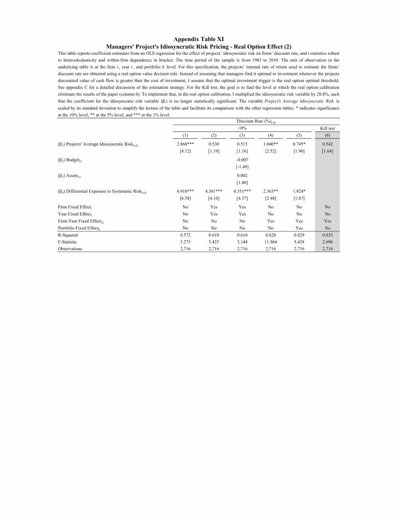
Kill test
(1) (2) (3) (4) (5) (6)
(β1) Projects' Average Idiosyncratic Riski,t,k 2.868*** 0.530 0.515 1.040** 0.745* 0.542
[4.12] [1.19] [1.16] [2.52] [1.90] [1.64]
(β2) Budgeti,t -0.007
[-1.49]
(β3) Assetsi,t 0.002
[1.40]
(β4) Differential Exposure to Systematic Riski,t,k 4.918*** 4.301*** 4.351*** 2.363** 1.924*
[6.58] [4.16] [4.37] [2.48] [1.87]
Firm Fixed Effecti No Yes Yes No No No
Year Fixed Effectt No Yes Yes No No No
Firm-Year Fixed Effecti,t No No No Yes Yes Yes
Portfolio Fixed Effectk No No No No Yes No
R-Squared 0.572 0.610 0.610 0.828 0.829 0.835
F-Statistic 3.275 5.425 3.144 11.964 5.438 2.696
Observations 2,716 2,716 2,716 2,716 2,716 2,716
Appendix Table XIManagers' Project's Idiosyncratic Risk Pricing - Real Option Effect (2)
This table reports coefficient estimates from an OLS regression for the effect of projects’ idiosyncratic risk on firms’ discount rate, and t-statistics robust
to heteroskedasticity and within-firm dependence in bracket. The time period of the sample is from 1983 to 2010. The unit of observation in the
underlying table is at the firm i , year t , and portfolio k level. For this specification, the projects’ internal rate of return used to estimate the firms’
discount rate are obtained using a real option value decision rule. Instead of assuming that managers find it optimal to investment whenever the projects
discounted value of cash flow is greater than the cost of investment, I assume that the optimal investment trigger is the real option optimal threshold.
See appendix C for a detailed discussion of the estimation strategy. For the Kill test, the goal is to find the level at which the real option calibration
eliminate the results of the paper (column 6). To implement that, in the real option calibration, I multiplied the idiosyncratic risk variable by 28.8%, such
that the coefficient for the idiosyncratic risk variable (β1) is no longer statistically significant. The variable Project's Average Idiosyncratic Risk is
scaled by its standard deviation to simplify the lecture of the table and facilitate its comparison with the other regression tables. * indicates significance
at the 10% level, ** at the 5% level, and *** at the 1% level.Discount Rate (%)i,t,k
+0%
Related Documents