Capacity utilisation and profitability: a decomposition of short run profit efficiency

Int. J. Production Economics 79 (2002) 261–278

Capacity utilisation and profitability: A decomposition ofshort-run profit efficiency

Tim Coellia,*,1, Emili Grifell-Tatj!eb, Sergio Perelmanc

aSchool of Economics, University of Queensland, Brisbane, QLD 4072, AustraliabDepartament d’Economia de l’Empresa, Universitat Aut "onoma de Barcelona, Edifici B. 08193 Bellaterra (Cendanyola del Valles),

Barcelona, SpaincCREPP, Department of Economics, Universit!e de Li"ege. Bd. du Rectorat 7 (B31), B-4000 Li"ege, Belgium

Received 15 May 2001; accepted 12 April 2002

Abstract

The principal aim of this paper is to measure the amount by which the profit of a multi-input, multi-output firm

deviates from maximum short-run profit, and then to decompose this profit gap into components that are of practical

use to managers. In particular, our interest is in the measurement of the contribution of unused capacity, along with

measures of technical inefficiency, and allocative inefficiency, in this profit gap. We survey existing definitions of

capacity and, after discussing their shortcomings, we propose a new ray economic capacity measure that involves short-

run profit maximisation, with the output mix held constant. We go on to describe how the gap between observed profit

and maximum profit can be calculated and decomposed using linear programming methods. The paper concludes with

an empirical illustration, involving data on 28 international airline companies. The empirical results indicate that these

airline companies achieve profit levels which are on average US$815m below potential levels, and that 70% of the gap

may be attributed to unused capacity. r 2002 Elsevier Science B.V. All rights reserved.

Keywords: Capacity utilisation; Profit decomposition; Profitability; Technical efficiency; Allocative efficiency

1. Introduction

The principal aims of this paper are to measurethe amount by which the profit of a multi-input,multi-output firm deviates from maximum short-run profit, and then to decompose this profit gap

into components that are of practical use tomanagers. In particular, our interest is in themeasurement of the contribution of unusedcapacity, along with measures of technical ineffi-ciency, and allocative inefficiency, in this profitgap.We are particularly interested in ensuring that

the methods we propose provide information thatis meaningful to managers. In particular, when wetell a manager that his/her observed short-runprofit is $Q below the maximum possible, giventhe available quantity of fixed inputs, and that R%

*Corresponding author.

E-mail addresses: [email protected] (T. Coelli), emili.

[email protected] (E. Grifell-Tatj!e), [email protected]

(S. Perelman).1Tim Coelli was a Research Fellow at CORE, Universit!e

Catholique de Louvain whilst much of this paper was written.

0925-5273/02/$ - see front matter r 2002 Elsevier Science B.V. All rights reserved.

PII: S 0 9 2 5 - 5 2 7 3 ( 0 2 ) 0 0 2 3 6 - 0

of this is due to unused capacity, we want to besure that our measure of capacity is meaningful.As we shall illustrate in this paper, a numberof existing capacity definitions do not providemeaningful information in this situation.This study is by no means the first to attempt to

decompose firm performance measures into thatpart due to unused capacity and other factors. Anumber of authors (Gold, 1955, 1973, 1985; Eilonand Teague, 1973; Eilon, 1975, 1984, 1985; Eilonet al., 1975) have made substantial advances in thisregard. However, in these studies the authorsgrapple with a number of problems. Such as howto define capacity and output in a multi-outputfirm, and how to remove the effects of pricedifferences from the input costs and outputrevenues. In this paper we show that one cansolve all of these problems. First, we propose anew ray economic capacity measure that involvesshort-run profit maximisation, with the output mixheld constant. Second, by making use of adjustedversions of the production frontier methodschampioned by (Farrell, 1957; F.are et al., 1994)and others, we show how this measure can beestimated and decomposed.This paper is organised into sections. In the next

section we review some existing definitions ofcapacity. In Section 3 we illustrate why physicaldefinitions of capacity are not terribly useful inprofit efficiency decompositions. We go on todefine a new profit-based definition of capacityand show how it can be used (as one component)in a decomposition of short-run profit efficiency.In Section 4 we outline the linear programs whichwe use to measure and decompose capacity andshort-run profit efficiency. In Section 5 weillustrate our methods using data on internationalairline companies. Finally, in Section 6 we makesome brief concluding comments.

2. Capacity definitions

A number of analysts in the economics andbusiness literature have looked at the issue ofcapacity measurement in recent decades. Thesestudies can be roughly divided into two groups,those that consider only physical information and

those that also include price information inderiving their measure. We discuss each of thesegroups in turn.

2.1. Physical definitions of capacity

One of the earliest discussions of capacitymeasurement is provided by Gold (1955, p. 103)who states that ‘‘productive capacity estimatesmay take two forms: as an estimate of the totalamount which can be produced of any givenproduct, assuming some specified allocation ofplant facilities to such output; and as an estimateof the composite productive capacity coveringsome specified range of products. The former ofthese may be expressed in purely physical termsand may be used to measure the absolute volumeof capacity as well as relative changes in it’’. This ismade under the assumption that, ‘‘sufficient labor,materials and other inputs are available to servicethe full utilisation of present capital facilities’’(Gold, 1955, p. 102).Johansen (1968), utilising the concept of

the production function, defines the capacityof existing plant and equipment (for a singleoutput production technology) in a similar way toGold. He defines it as: ‘‘the maximum amount thatcan be produced per unit of time with existingplant and equipment, provided that the availabil-ity of variable factors of production are notlimited’’. F.are (1984) labels this definition ofcapacity as a strong definition of capacity. Hegoes on to define a weak definition of capacitywhich only requires that output be bounded, asopposed to insisting on the existence of amaximum, which the Johansen definition requires.The strong definition implies the weak definition,but not vice versa.The methods we propose in this paper involve

production technologies, which have a well-defined maximum. Thus, we can safely use thestrong definition of Johansen. However, note thatin the case of a decreasing returns to scale Cobb–Douglas short-run production function, a produc-tion function that is regularly used in economicanalysis, the weak definition of capacity must beused, because the maximum of this function occurs

T. Coelli et al. / Int. J. Production Economics 79 (2002) 261–278262

when the amount of variable input approachesinfinity.2

The above single-output physical definition ofcapacity has been generalised to multi-outputsituations by some authors. For example, see Gold(1955, 1976) who suggests the use of output pricesas weights in the multi-output case. That is,capacity is defined as the price-weighted sum ofactual production levels over the price-weightedsum of the maximum possible levels of eachoutput. Alternatively, Eilon and Soesan (1976)suggest the construction of a full capacity envelopecurve, which defines the maximum possible outputlevels for each output mix. They then suggestmeasuring capacity utilisation as the ratio ofobserved output to maximum output, holdingthe output mix constant. This concept is closelyrelated to the radial (output-orientated) technicalefficiency measures proposed by Farrell (1957) andthe distance function measures proposed byShephard (1970), that we utilise in this paper.However, they are not identical to these concepts,because the capacity measure allows the variableinputs to be unbounded while the efficiency/distance measures are calculated with all inputsheld fixed.Furthermore, it is interesting to note that Elion

and Soesan (1976) suggest that one could uselinear programming methods to construct thiscurve, but do not expand on this idea. However,F.are, Grosskopf and Kokkelenberg (1989) andF.are, Grosskopf and Valdimanis (1989) do look atthis possibility. They use a variant of the dataenvelopment analysis (DEA) linear programmingmethod to construct a maximum capacity envel-ope curve using observed data on a sample offirms.

2.2. Economic definitions of capacity

As we illustrate later in this paper, the abovephysical definitions of capacity can provide quitestrange information when used in the decomposi-tion of short-run profit inefficiency. In fact, they

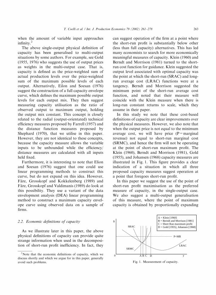
can suggest operation of the firm at a point wherethe short-run profit is substantially below other(less than full capacity) alternatives. This has ledmany economists to search for more economicallymeaningful measures of capacity. Klein (1960) andBerndt and Morrison (1981) turned to the short-run cost function for guidance. Klein suggested theoutput level associated with optimal capacity wasthe point at which the short-run (SRAC) and long-run average cost (LRAC) functions were at atangency. Berndt and Morrison suggested theminimum point of the short-run average costfunction, and noted that their measure willcoincide with the Klein measure when there islong-run constant returns to scale, which theyassume in their paper.In this study we note that these cost-based

definitions of capacity are clear improvements overthe physical measures. However, we also note thatwhen the output price is not equal to the minimumaverage cost, we will have price (P=marginalrevenue) not equal to short-run marginal cost(SRMC), and hence the firm will not be operatingat the point of short-run maximum profit. TheKlein (1960), Berndt and Morrison (1981), Gold(1955), and Johansen (1968) capacity measures areillustrated in Fig. 1. This figure provides a clearindication of a situation in which all threeproposed capacity measures suggest operation ata point that foregoes short-run profit.In this paper we suggest the use of the point of

short-run profit maximisation as the preferredmeasure of capacity, in the single-output case.We also suggest a multi-output generalisationof this measure, where the point of maximumcapacity is obtained by proportionally expanding

SRMC

SRAC

LRAC

P=MR

y

$

0 A B C D

A = Klein [1960]B = Berndt and Morrison [1981]C = Short Run maximum profitD = Gold [1955], Johansen [1968]

Fig. 1. Measurement of capacity.

2Note that the economic definitions of capacity, which we

discuss shortly and which we argue for in this paper, generally

avoid such problems.

T. Coelli et al. / Int. J. Production Economics 79 (2002) 261–278 263

(or contracting) the output vector until the short-run profit is maximised (subject to the constraintthat the output mix remains unchanged). Wediscuss this measure in more detail in the followingsection.However, before continuing, we should quickly

make note of two additional types of capacitymeasures, which are often used. First, there areengineering definitions of capacity, such as thenameplate rating on an electric power generator,which define theoretical maxima rather than real-world practical maxima. These are generally oflimited use to managers, because they tend not toaccount for the need for downtime for main-tenance and repairs and they do not allow for anyunexpected fluctuations in demand and/or inputsupply. Second, there are a number of regularlyquoted macroeconomic capacity measures, such asthe Wharton index, which reports the ratio ofactual US output over potential output, where thelater is derived from information on previouspeaks in the output/capital ratio and subsequentnet investment levels. This macro information is oflimited interest in this paper, given our interest infirm-level information.

3. Methodology

Before we describe our methodology we mustfirst provide a description of the underlyingproduction technology. Since, we wish to be ableto account for multi-output production, we do notuse the standard single-output production func-tion, which has been widely used over the past 70years. We instead follow Shephard (1970) and useset constructs to define the production technologyand use distance functions to provide a functionalrepresentation of the outer boundary of theproduction sets.

3.1. The technology

A multi-input, multi-output production technol-ogy can be described using the technology set, S:Following F.are and Primont (1995), we use thenotation x and y to denote a non-negative K � 1input vector and a non-negative M � 1 output

vector, respectively. The technology set is thendefined as

S ¼ fðx; yÞ : x can produce yg: ð1Þ

That is, the set of all input–output vectors (x; y),such that x can produce y:The production technology defined by the set, S;

may be equivalently defined using output sets,PðxÞ; which represents the set of all output vectors,y, which can be produced using the input vector, x:That is,

PðxÞ ¼ fy : x can produce yg: ð2Þ

These sets are assumed to satisfy the usualproperties. That is, they are assumed to be closed,bounded, and convex, and are assumed to exhibitstrong disposability in outputs and inputs (seeF.are and Primont (1995) for discussion of theseproperties).To measure and decompose short-run profit

efficiency we require a functional representation ofthe technology. An output distance function isused for this purpose. The output distance func-tion is defined on the output set, PðxÞ; as

d0ðx; yÞ ¼ inffd : ðy=dÞAPðxÞg: ð3Þ

The properties of this distance function followdirectly from those of the technology set. Namely,d0ðx; yÞ is non-decreasing in y and increasing in x;and linearly homogeneous in y: We note that if y

belongs to the production possibility set of x (i.e.,yAPðxÞ), then d0ðx; yÞp1; and that the distance isequal to unity (i.e., d0ðx; yÞ ¼ 1) if y belongs to the‘‘frontier’’ of the production possibility set.3

3.2. Short-run profit maximisation

To facilitate the discussion of short-run profitmaximisation, we divide the K � 1 input vector, x;into a Kv � 1 vector of variable inputs, xv; and aKf � 1 vector of fixed inputs, xf ; such that x ¼ðxv;xf Þ: We assume that the manager is able tovary quantities of the variable inputs (e.g. labourand materials) in the short run, but is unable tovary quantities of the fixed inputs (e.g. capital).In the long run all inputs are variable. The length

3Chapter 3 in Coelli et al. (1998) provides further discussion

of distance functions.


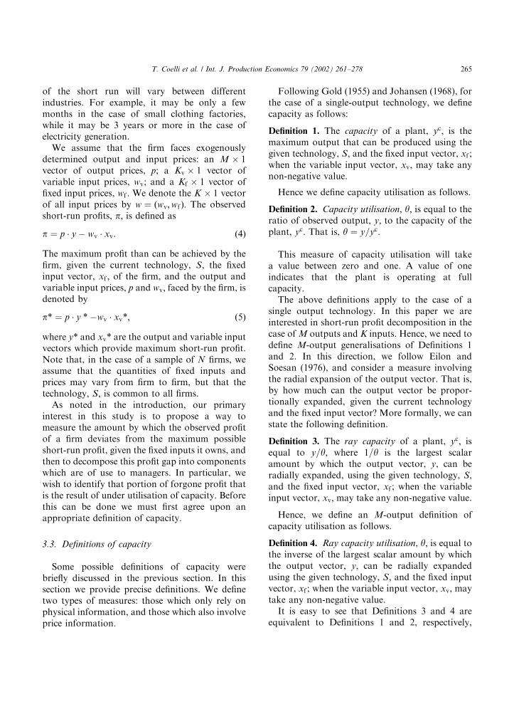
of the short run will vary between differentindustries. For example, it may be only a fewmonths in the case of small clothing factories,while it may be 3 years or more in the case ofelectricity generation.We assume that the firm faces exogenously

determined output and input prices: an M � 1vector of output prices, p; a Kv � 1 vector ofvariable input prices, wv; and a Kf � 1 vector offixed input prices, wf : We denote the K � 1 vectorof all input prices by w ¼ ðwv;wf Þ: The observedshort-run profits, p; is defined as

p ¼ p � y � wv � xv: ð4Þ

The maximum profit than can be achieved by thefirm, given the current technology, S; the fixedinput vector, xf ; of the firm, and the output andvariable input prices, p and wv; faced by the firm, isdenoted by

p ¼ p � y �wv � xv; ð5Þ

where y and xv are the output and variable inputvectors which provide maximum short-run profit.Note that, in the case of a sample of N firms, weassume that the quantities of fixed inputs andprices may vary from firm to firm, but that thetechnology, S; is common to all firms.As noted in the introduction, our primary

interest in this study is to propose a way tomeasure the amount by which the observed profitof a firm deviates from the maximum possibleshort-run profit, given the fixed inputs it owns, andthen to decompose this profit gap into componentswhich are of use to managers. In particular, wewish to identify that portion of forgone profit thatis the result of under utilisation of capacity. Beforethis can be done we must first agree upon anappropriate definition of capacity.

3.3. Definitions of capacity

Some possible definitions of capacity werebriefly discussed in the previous section. In thissection we provide precise definitions. We definetwo types of measures: those which only rely onphysical information, and those which also involveprice information.

Following Gold (1955) and Johansen (1968), forthe case of a single-output technology, we definecapacity as follows:

Definition 1. The capacity of a plant, yc; is themaximum output that can be produced using thegiven technology, S; and the fixed input vector, xf ;when the variable input vector, xv; may take anynon-negative value.

Hence we define capacity utilisation as follows.

Definition 2. Capacity utilisation, y; is equal to theratio of observed output, y; to the capacity of theplant, yc: That is, y ¼ y=yc:

This measure of capacity utilisation will takea value between zero and one. A value of oneindicates that the plant is operating at fullcapacity.The above definitions apply to the case of a

single output technology. In this paper we areinterested in short-run profit decomposition in thecase of M outputs and K inputs. Hence, we need todefine M-output generalisations of Definitions 1and 2. In this direction, we follow Eilon andSoesan (1976), and consider a measure involvingthe radial expansion of the output vector. That is,by how much can the output vector be propor-tionally expanded, given the current technologyand the fixed input vector? More formally, we canstate the following definition.

Definition 3. The ray capacity of a plant, yc; isequal to y=y; where 1=y is the largest scalaramount by which the output vector, y, can beradially expanded, using the given technology, S,and the fixed input vector, xf ; when the variableinput vector, xv; may take any non-negative value.

Hence, we define an M-output definition ofcapacity utilisation as follows.

Definition 4. Ray capacity utilisation, y; is equal tothe inverse of the largest scalar amount by whichthe output vector, y; can be radially expandedusing the given technology, S; and the fixed inputvector, xf ; when the variable input vector, xv; maytake any non-negative value.It is easy to see that Definitions 3 and 4 are

equivalent to Definitions 1 and 2, respectively,


when M ¼ 1:We now provide a simple illustrationof Definition 1.

3.4. A single-output example

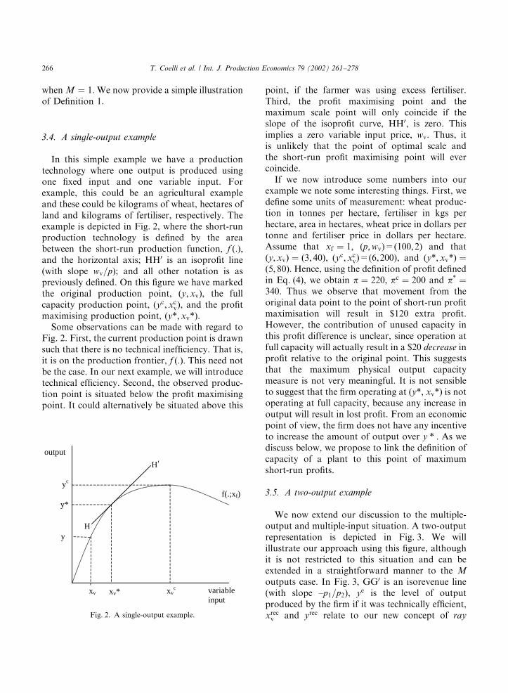
In this simple example we have a productiontechnology where one output is produced usingone fixed input and one variable input. Forexample, this could be an agricultural exampleand these could be kilograms of wheat, hectares ofland and kilograms of fertiliser, respectively. Theexample is depicted in Fig. 2, where the short-runproduction technology is defined by the areabetween the short-run production function, f ð:Þ;and the horizontal axis; HH0 is an isoprofit line(with slope wv=p); and all other notation is aspreviously defined. On this figure we have markedthe original production point, (y;xv), the fullcapacity production point, (yc;xc

v), and the profitmaximising production point, (y; xv).Some observations can be made with regard to

Fig. 2. First, the current production point is drawnsuch that there is no technical inefficiency. That is,it is on the production frontier, f ð:Þ: This need notbe the case. In our next example, we will introducetechnical efficiency. Second, the observed produc-tion point is situated below the profit maximisingpoint. It could alternatively be situated above this

point, if the farmer was using excess fertiliser.Third, the profit maximising point and themaximum scale point will only coincide if theslope of the isoprofit curve, HH0, is zero. Thisimplies a zero variable input price, wv: Thus, itis unlikely that the point of optimal scale andthe short-run profit maximising point will evercoincide.If we now introduce some numbers into our

example we note some interesting things. First, wedefine some units of measurement: wheat produc-tion in tonnes per hectare, fertiliser in kgs perhectare, area in hectares, wheat price in dollars pertonne and fertiliser price in dollars per hectare.Assume that xf ¼ 1; (p;wv)=(100,2) and thatðy;xvÞ ¼ ð3; 40Þ; (yc;xc

v)=(6,200), and (y;xvÞ ¼ð5; 80Þ: Hence, using the definition of profit definedin Eq. (4), we obtain p ¼ 220; pc ¼ 200 and p ¼340: Thus we observe that movement from theoriginal data point to the point of short-run profitmaximisation will result in $120 extra profit.However, the contribution of unused capacity inthis profit difference is unclear, since operation atfull capacity will actually result in a $20 decrease inprofit relative to the original point. This suggeststhat the maximum physical output capacitymeasure is not very meaningful. It is not sensibleto suggest that the firm operating at (y; xv) is notoperating at full capacity, because any increase inoutput will result in lost profit. From an economicpoint of view, the firm does not have any incentiveto increase the amount of output over y : As wediscuss below, we propose to link the definition ofcapacity of a plant to this point of maximumshort-run profits.

3.5. A two-output example

We now extend our discussion to the multiple-output and multiple-input situation. A two-outputrepresentation is depicted in Fig. 3. We willillustrate our approach using this figure, althoughit is not restricted to this situation and can beextended in a straightforward manner to the M

outputs case. In Fig. 3, GG0 is an isorevenue line(with slope –p1=p2), ye is the level of outputproduced by the firm if it was technically efficient,xrecv and yrec relate to our new concept of ray

f(.;xf)

variableinput

H

H

output

yc

y*

y

xv xv* xvc

'

Fig. 2. A single-output example.


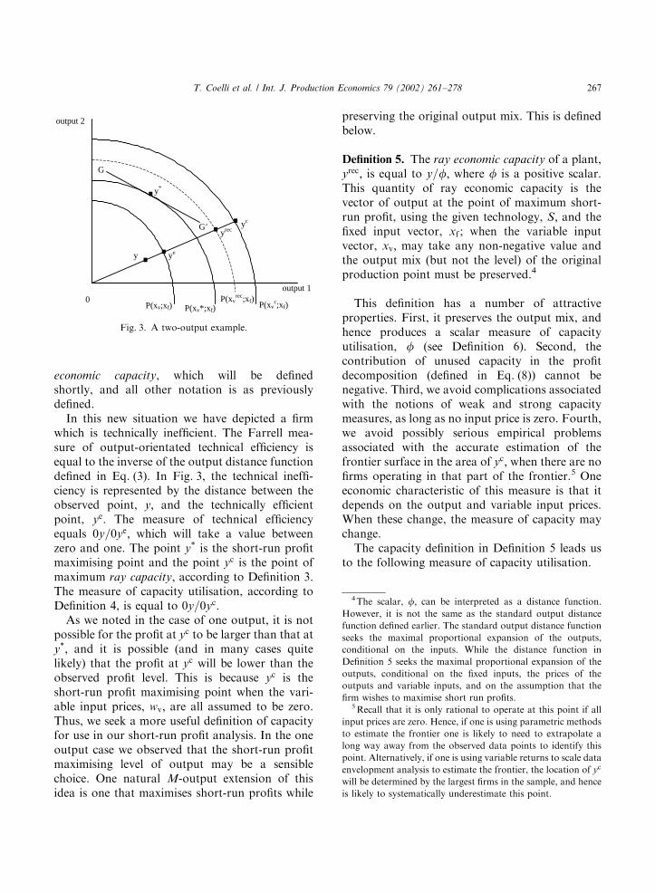
economic capacity, which will be definedshortly, and all other notation is as previouslydefined.In this new situation we have depicted a firm

which is technically inefficient. The Farrell mea-sure of output-orientated technical efficiency isequal to the inverse of the output distance functiondefined in Eq. (3). In Fig. 3, the technical ineffi-ciency is represented by the distance between theobserved point, y; and the technically efficientpoint, ye: The measure of technical efficiencyequals 0y=0ye; which will take a value betweenzero and one. The point y is the short-run profitmaximising point and the point yc is the point ofmaximum ray capacity, according to Definition 3.The measure of capacity utilisation, according toDefinition 4, is equal to 0y=0yc:As we noted in the case of one output, it is not

possible for the profit at yc to be larger than that aty; and it is possible (and in many cases quitelikely) that the profit at yc will be lower than theobserved profit level. This is because yc is theshort-run profit maximising point when the vari-able input prices, wv; are all assumed to be zero.Thus, we seek a more useful definition of capacityfor use in our short-run profit analysis. In the oneoutput case we observed that the short-run profitmaximising level of output may be a sensiblechoice. One natural M-output extension of thisidea is one that maximises short-run profits while

preserving the original output mix. This is definedbelow.

Definition 5. The ray economic capacity of a plant,yrec; is equal to y=f; where f is a positive scalar.This quantity of ray economic capacity is thevector of output at the point of maximum short-run profit, using the given technology, S; and thefixed input vector, xf ; when the variable inputvector, xv; may take any non-negative value andthe output mix (but not the level) of the originalproduction point must be preserved.4

This definition has a number of attractiveproperties. First, it preserves the output mix, andhence produces a scalar measure of capacityutilisation, f (see Definition 6). Second, thecontribution of unused capacity in the profitdecomposition (defined in Eq. (8)) cannot benegative. Third, we avoid complications associatedwith the notions of weak and strong capacitymeasures, as long as no input price is zero. Fourth,we avoid possibly serious empirical problemsassociated with the accurate estimation of thefrontier surface in the area of yc; when there are nofirms operating in that part of the frontier.5 Oneeconomic characteristic of this measure is that itdepends on the output and variable input prices.When these change, the measure of capacity maychange.The capacity definition in Definition 5 leads us

to the following measure of capacity utilisation.

.y ye

y*

output 2

output 1

G

G'

0

yrecyc

P(xv;xf) P(xv*;xf)P(xv

rec;xf)P(xv

c;xf)

. . ..

Fig. 3. A two-output example.

4The scalar, f; can be interpreted as a distance function.

However, it is not the same as the standard output distance

function defined earlier. The standard output distance function

seeks the maximal proportional expansion of the outputs,

conditional on the inputs. While the distance function in

Definition 5 seeks the maximal proportional expansion of the

outputs, conditional on the fixed inputs, the prices of the

outputs and variable inputs, and on the assumption that the

firm wishes to maximise short run profits.5Recall that it is only rational to operate at this point if all

input prices are zero. Hence, if one is using parametric methods

to estimate the frontier one is likely to need to extrapolate a

long way away from the observed data points to identify this

point. Alternatively, if one is using variable returns to scale data

envelopment analysis to estimate the frontier, the location of yc

will be determined by the largest firms in the sample, and hence

is likely to systematically underestimate this point.


Definition 6. The ray economic capacity utilisation

of a plant is equal to the scalar f; where y=f is theoutput vector at the point of short-run profitmaximisation on the ray from the origin throughy: This is conditional on the given technology, S;and the fixed input vector, xf ; while allowing thevariable input vector, xv; to take any non-negativevalue.

It is of interest to link our measure of rayeconomic capacity utilisation to the measure ofcapacity utilisation given by Definition 4. This canbe done via the following decomposition analysis.

3.6. Capacity utilisation decomposition

The measure of capacity utilisation given inDefinition 4 (y ¼ y=yc), can be decomposed into

y

yc¼

y

yrec�

yrec

yc; ð6Þ

where f ¼ y=yrec is the ray economic capacityutilisation of a plant, given in Definition 6, andyrec=yc could be viewed as a measure of the optimal

amount of capacity idleness, which will dependupon the prices of outputs and variable inputs.When an increase in capacity utilisation willproduce a decrease in the level of short-run profits,the optimal behavior of the manager of the firm isto have an idleness. From this point of view theidleness of the capacity utilisation is an economicvariable.6 Note that it is equal to the ratio y=f: Inother words, the ratio of the ray capacity utilisa-

tion (Definition 4) over ray economic capacity

utilisation (Definition 6). The ratio yrec=yc takes avalue between zero and one. A value of oneindicates that the firm maximises short-run profitby producing at the point of ray capacity, yc:However, when profits are maximised by acompletely idle plant (i.e., a closed plant), theratio yrec=yc takes a value equal to zero.The ray economic capacity utilisation measure,

y=yrec; can be additionally decomposed as

y

yrec¼

y

ye�

ye

yrec; ð7Þ

where y=ye is the measure of technical efficiencyand ye=yrec a measure of ray economic capacityutilisation that is net of technical inefficiency of theplant. F.are et al. (1989) have proposed a measureof capacity utilisation where technical efficiency isnot included in the measure. They suggest usingye=yc as a measure of capacity. We prefer to definea capacity measure that includes technical ineffi-ciency. The reasons for this are explained shortlyhereafter.

3.7. Profit decomposition

Now, our desire is to decompose the profitdifference between y and y into meaningfulcomponents. In particular, we wish to identifythe contribution of unused capacity in this profitdifference. Using the definition of ray economiccapacity, we propose the following decompositionof short-run profit:

ðp � pÞ ¼ ðp � precÞ þ ðprec � pÞ

¼ ½pðy � yrecÞ � wvðxv � xrec

v Þ

þ ½pðyrec � yÞ � wvðxrecv � xvÞ : ð8Þ

From Fig. 3 we observe that the first component inthis decomposition is primarily an output mixeffect, while the second component is the compo-nent due to unused capacity. We can furtherdecompose the component of profit due to unusedcapacity into two parts. One part due to technicalinefficiency (movement from y to ye) and aremaining part which we could label an input-mixeffect 7 (movement from ye to yrec). Thus we obtain

ðprec � pÞ ¼ ðprec � peÞ þ ðpe � pÞ

¼ pðyrec � yeÞ � wvðxrecv � xe

vÞ� �

þ pðye � yÞ � wvðxev � xvÞ

� �: ð9Þ

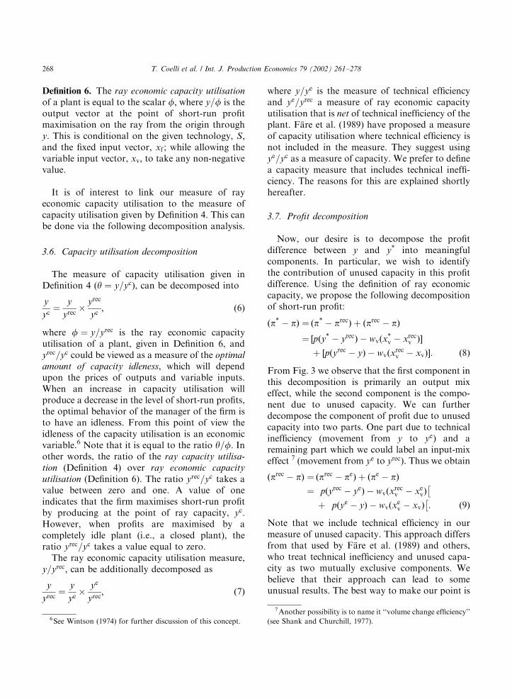
Note that we include technical efficiency in ourmeasure of unused capacity. This approach differsfrom that used by F.are et al. (1989) and others,who treat technical inefficiency and unused capa-city as two mutually exclusive components. Webelieve that their approach can lead to someunusual results. The best way to make our point is

6See Wintson (1974) for further discussion of this concept.

7Another possibility is to name it ‘‘volume change efficiency’’

(see Shank and Churchill, 1977).


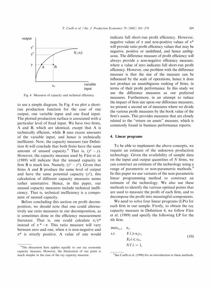
to use a simple diagram. In Fig. 4 we plot a short-run production function for the case of oneoutput, one variable input and one fixed input.The plotted production surface is associated with aparticular level of fixed input. We have two firms,A and B, which are identical, except that A istechnically efficient, while B uses excess amountsof the variable input, and hence is technicallyinefficient. Now, the capacity measure (see Defini-tion 4) will conclude that both firms have the sameamount of unused capacity.8 That is, (yc � y).However, the capacity measure used by F.are et al.(1989) will indicate that the unused capacity infirm B is much less. Namely, (yc � ye). Given thatfirms A and B produce the same level of outputand have the same potential capacity (yc), thiscalculation of different capacity measures seemsrather unintuitive. Hence, in this paper, ourunused capacity measures include technical ineffi-ciency. That is, technical inefficiency is a compo-nent of unused capacity.Before concluding this section on profit decom-

position, we should note that one could alterna-tively use ratio measures in our decomposition, asis sometimes done in the efficiency measurementliterature. That is, one could calculate p=pinstead of p �p: This ratio measure will varybetween zero and one, when p is non-negative andp is strictly positive. A value of one would

indicate full short-run profit efficiency. However,negative values of p and non-positive values of pwill provide ratio profit efficiency values that may benegative, positive or undefined, and hence ambig-uous. The difference measure of profit efficiency willalways provide a non-negative efficiency measure,where a value of zero indicates full short-run profitefficiency. However, one problem with the differencemeasure is that the size of the measure can beinfluenced by the scale of operations, hence it doesnot produce an unambiguous ranking of firms, interms of their profit performance. In this study weuse the difference measures as our preferredmeasures. Furthermore, in an attempt to reducethe impact of firm size upon our difference measures,we present a second set of measures where we dividethe various profit measures by the book value of thefirm’s assets. This provides measures that are closelyrelated to the ‘‘return on assets’’ measure, which iscommonly found in business performance reports.

4. Linear programs

To be able to implement the above concepts, werequire an estimate of the unknown productiontechnology. Given the availability of sample dataon the input and output quantities of N firms, wecan construct an estimate of the technology using arange of parametric or non-parametric methods.9

In this paper we use variants of the non-parametriclinear programming method to construct anestimate of the technology. We also use thesemethods to identify the various optimal points thatare used to measure the profit of each firm, and todecompose the profit into meaningful components.We need to solve four linear programs (LPs) for

each firm in our sample. Firstly, to obtain the raycapacity measure in Definition 4, we follow F.areet al. (1989) and specify the following LP for theith firm.

maxai ;l ai;

s:t: YlXaiyi;

Xflpxf i;

N10l ¼ 1;

ð10Þ

yc

variableinput

ye

output

A By

xv

f(.;xf)

. .

Fig. 4. Measures of capacity and technical efficiency.

8The discussion here applies equally to our ray economic

capacity measure. However, the illustration of our point is

much simpler in the case of the ray capacity measure. 9See Coelli et al. (1998) for an introduction to these methods.


where yi is the M � 1 vector of outputs of the ithfirm, Y is the M�N matrix of outputs of all N

firms, xf i is the Kf � 1 vector of fixed inputs of theith firm, Xf is the Kf � N matrix of fixed inputs ofall N firms, l is a N � 1 vector of weights, N1 is aN � 1 vector of ones, and yi ¼ 1=ai is the measureof ray capacity utilisation, which takes a valuebetween zero and one.10 A value of one indicatesthat the firm is operating at full capacity.Essentially, this LP seeks the maximum feasibleexpansion (ai) in the output vector of the ith firm(yi), subject to the constraint that the optimalpoint must lie within the piece-wise linear capacity

envelope, or capacity possibility frontier, defined bythe data on the other firms. In terms of Fig. 3 theproduct y:y defines the vector yc: The decisionvariables in this LP are ai and l: This LP is almostidentical to the standard output-orientated dataenvelopment analysis (DEA) LP (see below),except that it excludes the variable input con-straints.The application of the above LP, N times, once

for each firm in the sample, will build up a piece-wise linear capacity possibility frontier. For eachfirm, it will identify the maximum possiblecapacity, given the level of fixed inputs (andallowing unlimited variable inputs). The associatedlevel of variable inputs can be obtained aftersolving each LP, via the l weights, as xvi ¼ Xvl;where xvi is the Kv�1 vector of variable inputs ofthe ith firm, Xv is the Kv�N matrix of variableinputs of all N firms.F.are et al. (1989) describe these variable input

levels as the ‘‘optimal level of variable inputs’’. Webelieve this term is potentially misleading, giventhat these values are derived on the assumptionthat the price of these variable inputs are zero.Hence, when one looks at the short-run profitimplications of these ‘‘optimal points’’ one willoften find that they are far from optimal in thissense. This is clearly illustrated in our applicationin the following section.

The above LP was used to obtain a measure ofray capacity. This measure is not used in thepreferred profit decomposition, but it is used in thecapacity decomposition analysis and is also usedfor comparative purposes in our illustration.We now outline the three LP’s that need to be

solved to obtain our preferred capacity measureand profit decomposition. First we calculate theshort-run maximum profit of each firm.11

maxxn

vi;yn

i;l piyi �wvixvi

s:t: YlXyi ;

Xvlpxvi;

Xflpxf i;

N10l ¼ 1;

ð11Þ

where pi is the M � 1 vector of output prices facedby the ith firm, and wvi is the Kv�1 vector ofvariable input prices faced by the ith firm.12 ThisLP is a slight variant of the long-run profit LPpresented in F.are et al. (1994). The only differencehere is that the prices and quantities of the fixedinputs are not included in the objective function.Hence, the decision variables are the outputs andthe variable inputs, y and x in Fig. 3 (along withthe l weights).The output-orientated technical efficiency of the

ith firm is calculated using the standard DEA LPfound, for example, in F.are et al. (1994).

maxui ;lmi

s:t: YlXmiyi ;

Xvlpxvi;

Xflpxf i;

N10l ¼ 1;

ð12Þ

where ci ¼ 1=mi is the technical efficiency score ofthe ith firm, which takes a value between zero and

10Note that we were required to use the parameter a ¼ 1=y inour mathematical program to ensure that the problem was in

linear form. Otherwise we would have been required to solve a

non-linear problem, which involves more complex mathema-

tical optimization methods.

11Note that the LP required to obtain the minimum point on

the short-run average cost curve, required for the Berndt and

Morrison (1981) capacity measure could be obtained by

removing the py term from the objective function in this LP.

However, we do not look at this measure in the empirical

illustration in this paper.12Note that the l values obtained in the four LP’s, considered

in this section, are likely to differ, because they are used to

identify different types of optimal points. The l values are alsolikely to differ from firm to firm.


one. A value of one indicates that the firm isfully efficient. However, a value of 0.85would indicate that the firm is producing only85% of the potential output that could beproduced by the firm, given its (fixed and variable)input levels.In our fourth and final LP we specify a way in

which one can measure the ray economic capacitymeasure presented in Definition 6.

maxxrecvi

;bi ;l pibiyi � wvixrecvi ;

s:t: YlXbiyi;

Xvlpxrecvi ;

Xflpxf i;

N10l ¼ 1:

ð13Þ

This LP can be viewed as a hybrid of the LPs inEqs. (10) and (11), in that it seeks to maximiseshort-run profits, but it is constrained to not alterits original output mix. This is achieved byinsisting that the optimal output vector is aproportional scaling of the observed output vector(i.e., biyi). This prevents the firm from suggesting‘‘optimal’’ capacity levels that result in a reductionin short-run profits. The scalar, fi ¼ 1=bi; is theray economic capacity utilisation measure. Itreflects the amount by which the ith firm canradially expand (or contract) its output vector toachieve higher short-run profits. In terms of Fig. 3,LP (12) is used to calculate ye as the product m:y;and LP (13) is used to calculate yrec as the productb:y.The above four LPs, defined in Eqs. (10)–(13),

need to be solved for each firm in the sample.Thus, if there are N firms in the sample, one mustsolve 4N LPs. We now provide an illustration ofthese methods using data on international airlinecompanies.

5. Application to international airlines

The purpose of this section is to provide anillustration of the above-proposed methods. Ourintention is not to provide a detailed discussion ofthe profitability of these companies, but to providean indication of how useful these methods couldbe in such an analysis. Airlines produce two

distinct output categories: passenger and freightservices, using a range of inputs, including aircraft,labour (pilots, crew, maintenance staff, etc.), fueland other assorted inputs (e.g. various office andmaintenance materials and services). Aircraft arethe principal capital expenditure in these compa-nies. Orders for the purchase (or long-term lease)of aircraft must usually be placed a number ofyears in advance. Thus, in the short run thequantity of aircraft is a fixed input. The otherinput categories, on the other hand, can generallybe altered fairly easily in the short run. Capacityutilisation is a big issue in airline companies. Poordemand forecasts can result in a significantnumber of empty seats (and half-full cargo holds)which will quickly erode profits.

5.1. Data

In this empirical study we have collected data on28 companies in 1990. These data are derived fromthree annual digests: Traffic, Fleet-Personnel andFinancial Data, published by the InternationalCivil Aviation Organization (ICAO, 1992a, b, c).The data used in this study are listed in Table 1.The sample is composed of carriers in whichactivity is concentrated in domestic and interna-tional scheduled services. It was selected torepresent three main regions of the world: Asia/Oceania, Europe and North America, but essen-tially the availability of data determined its finalcomposition. Passenger and freight services aremeasured using passenger-kilometres and tonne-kilometres of freight (ICAO, 1992a). Average fareswere obtained by dividing revenues by thesequantity measures (ICAO, 1992c).We distinguish three variable inputs: staff, fuel

and ‘‘other’’. The staff corresponds to the totalnumber of personnel at the middle of the year, asreported by ICAO (1992b). It includes pilots, co-pilots and cockpit staff, all the personnel involvedin maintenance, ticketing and general administra-tion. Annual average wages were obtained bydividing total personnel expenses by the labourquantity (ICAO, 1992c). Data on quantity of fuelconsumed is not directly available from ICAOstatistics. Thus, we estimate the fuel quantity bydividing total fuel expenditures by average fuel


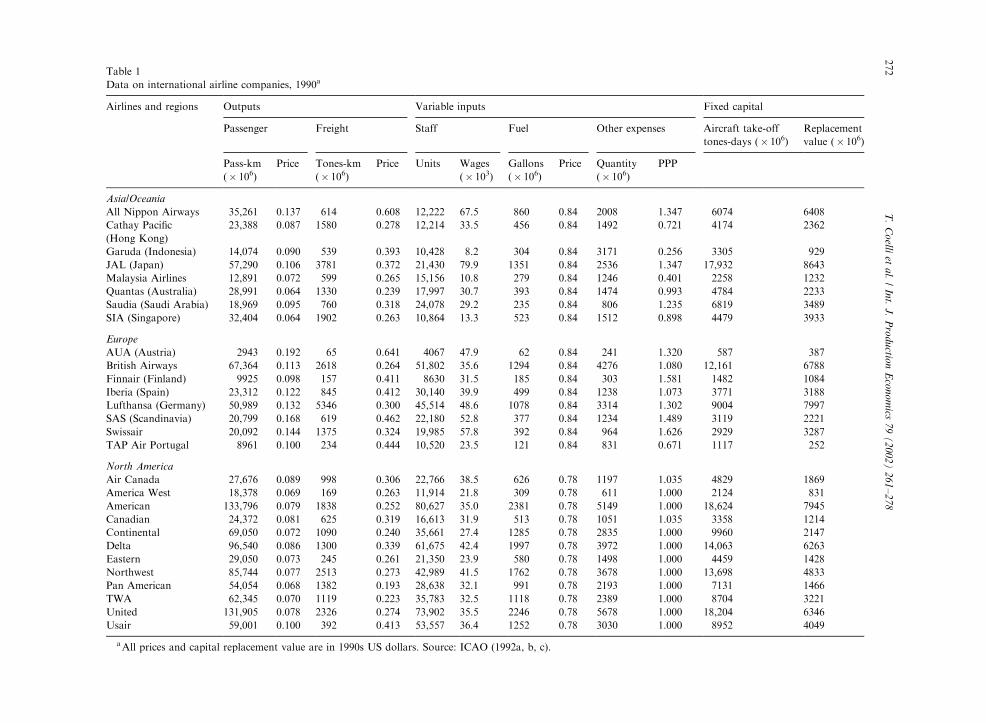
Table 1

Data on international airline companies, 1990a

Airlines and regions Outputs Variable inputs Fixed capital

Passenger Freight Staff Fuel Other expenses Aircraft take-off

tones-days (� 106)

Replacement

value (� 106)

Pass-km

(� 106)

Price Tones-km

(� 106)

Price Units Wages

(� 103)

Gallons

(� 106)

Price Quantity

(� 106)

PPP

Asia/Oceania

All Nippon Airways 35,261 0.137 614 0.608 12,222 67.5 860 0.84 2008 1.347 6074 6408

Cathay Pacific

(Hong Kong)

23,388 0.087 1580 0.278 12,214 33.5 456 0.84 1492 0.721 4174 2362

Garuda (Indonesia) 14,074 0.090 539 0.393 10,428 8.2 304 0.84 3171 0.256 3305 929

JAL (Japan) 57,290 0.106 3781 0.372 21,430 79.9 1351 0.84 2536 1.347 17,932 8643

Malaysia Airlines 12,891 0.072 599 0.265 15,156 10.8 279 0.84 1246 0.401 2258 1232

Quantas (Australia) 28,991 0.064 1330 0.239 17,997 30.7 393 0.84 1474 0.993 4784 2233

Saudia (Saudi Arabia) 18,969 0.095 760 0.318 24,078 29.2 235 0.84 806 1.235 6819 3489

SIA (Singapore) 32,404 0.064 1902 0.263 10,864 13.3 523 0.84 1512 0.898 4479 3933

Europe

AUA (Austria) 2943 0.192 65 0.641 4067 47.9 62 0.84 241 1.320 587 387

British Airways 67,364 0.113 2618 0.264 51,802 35.6 1294 0.84 4276 1.080 12,161 6788

Finnair (Finland) 9925 0.098 157 0.411 8630 31.5 185 0.84 303 1.581 1482 1084

Iberia (Spain) 23,312 0.122 845 0.412 30,140 39.9 499 0.84 1238 1.073 3771 3188

Lufthansa (Germany) 50,989 0.132 5346 0.300 45,514 48.6 1078 0.84 3314 1.302 9004 7997

SAS (Scandinavia) 20,799 0.168 619 0.462 22,180 52.8 377 0.84 1234 1.489 3119 2221

Swissair 20,092 0.144 1375 0.324 19,985 57.8 392 0.84 964 1.626 2929 3287

TAP Air Portugal 8961 0.100 234 0.444 10,520 23.5 121 0.84 831 0.671 1117 252

North America

Air Canada 27,676 0.089 998 0.306 22,766 38.5 626 0.78 1197 1.035 4829 1869

America West 18,378 0.069 169 0.263 11,914 21.8 309 0.78 611 1.000 2124 831

American 133,796 0.079 1838 0.252 80,627 35.0 2381 0.78 5149 1.000 18,624 7945

Canadian 24,372 0.081 625 0.319 16,613 31.9 513 0.78 1051 1.035 3358 1214

Continental 69,050 0.072 1090 0.240 35,661 27.4 1285 0.78 2835 1.000 9960 2147

Delta 96,540 0.086 1300 0.339 61,675 42.4 1997 0.78 3972 1.000 14,063 6263

Eastern 29,050 0.073 245 0.261 21,350 23.9 580 0.78 1498 1.000 4459 1428

Northwest 85,744 0.077 2513 0.273 42,989 41.5 1762 0.78 3678 1.000 13,698 4833

Pan American 54,054 0.068 1382 0.193 28,638 32.1 991 0.78 2193 1.000 7131 1466

TWA 62,345 0.070 1119 0.223 35,783 32.5 1118 0.78 2389 1.000 8704 3221

United 131,905 0.078 2326 0.274 73,902 35.5 2246 0.78 5678 1.000 18,204 6346

Usair 59,001 0.100 392 0.413 53,557 36.4 1252 0.78 3030 1.000 8952 4049

aAll prices and capital replacement value are in 1990s US dollars. Source: ICAO (1992a, b, c).

T.

Co

elliet

al.

/In

t.J

.P

rod

uctio

nE

con

om

ics7

9(

20

02

)2

61

–2

78

272

prices.13 The expenses on ‘‘other’’ inputs iscalculated by subtracting personnel and fuelexpenses from total operating expenses (ICAO,1992c).14 This input includes, among other things:maintenance, ticketing and general administrationcosts (net of any personnel expenses involved). Wedo not have access to a specific price index for this‘‘other’’ inputs category. Hence we use interna-tional PPP (purchasing power parity) indexes as aproxy for this price index. The implicit quantity of‘‘other’’ inputs is then derived by dividing the‘‘other’’ expenses figure by this price index.The fixed capital measure is a key variable for

this particular study. Its definition and measure-ment is always a difficult problem in any empiricalstudy. Some studies use physical measures whileothers use monetary measures. We have reported aphysical and a monetary measure of capital inTable 1. The physical capital variable was com-puted using information provided by ICAOs Fleet-

Personnel digest (ICAO, 1992b). For each com-pany, this measure corresponds to the sum of themaximum take-off weights of all aircraft multi-plied by the number of days the planes have beenable to operate during the year.15 Our financialmeasure of capital comes from the balance sheetsof companies as reported in the Financial Data

digest (ICAO, 1992c). It corresponds to the bookvalue of flight equipment assets before deprecia-tion. Our physical and monetary measures ofcapital are likely to be quite highly correlated inthe situation in which the airline companies havesimilar age profiles of aircraft in their fleets.

However, since these companies have fleets withdiffering average aircraft ages, we find that thismonetary capital measure is not always a goodmeasure of the quantity of aircraft available forservice, because of the effects of inflation uponaircraft values. The monetary measure will tend tooverstate the capital quantity in those companiesthat have newer fleets, and understate the capitalquantity in those companies that have older fleets.We have hence decided to use our physicalmeasure of capital in the calculations in this study.However, we have also reported the monetarymeasure of capital because we use this value todeflate our profit difference measures so as toattempt to reduce the impact of firm size fromthese measures.A number of points can be made about the data

presented in Table 1. First, we observe a greatvariability in company sizes. For instance, theAustrian airline (AUA) is nearly 20 times smaller,in terms of staff members and capital investment,compared with major US carriers like American,United or Delta. Second, it appears that Europeancompanies charged higher fares than NorthAmerican and Asia/Oceania companies (with theexception of Japanese airlines). This can bepartially explained by network characteristics likeshorter average stage length, but also because theairlines deregulation process was still in process inEurope in 1990. Finally, Table 1 also illustrates awide range of variation in factor prices, especiallyin wages and within Asian countries. Threecompanies, Garuda, Malaysia Airlines and SIApaid annual wages of around ten thousand USdollars to their employees in 1990, whereas acompany like JAL paid salaries eight times higher.

5.2. Results

The various measures of technical efficiency andcapacity utilisation are reported in Table 2. Beforewe begin with a discussion of these results we muststress a very important point. The productionfrontiers and capacity frontiers constructed usingLP in this study (and in any other study) reflect theouter boundary of observed best practice in the

sample. Thus, even though we may make state-ments such as: ‘‘JAL is technically efficient’’ and

13The Bureau of Transportation Statistics (2000) estimates

the average price per gallon paid by US carriers (0.78 USD in

1990). We use this price for all North American carriers.

Another piece of information available from the BTS is the

average price per gallon paid by US carriers in international

services (0.84 USD in 1990). We assume that this is the average

fuel price paid by all the companies operating from outside

North America.14Total operating expenses are redefined to exclude current

capital costs like rental of flight equipment and depreciation of

owned capital.15The same definition of physical capital was used in Coelli

et al. (1999). The multiplication by the number of days available

is primarily to account for cases in which a plane was only

available for a fraction of the year because it was bought or sold

during the year.


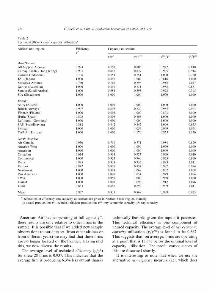
‘‘American Airlines is operating at full capacity’’,these results are only relative to other firms in thesample. It is possible that if we added new sampleobservations to our data set (from other airlines orfrom different years) we may find that these firmsare no longer located on the frontier. Having saidthis, we now discuss the results.The average level of technical efficiency (y=ye)

for these 28 firms is 0.937. This indicates that theaverage firm is producing 6.3% less output than is

technically feasible, given the inputs it possesses.This technical efficiency is one component ofunused capacity. The average level of ray economic

capacity utilisation (y=yrec) is found to be 0.867.This suggests that, on average, firms are operatingat a point that is 13.3% below the optimal level ofcapacity utilisation. The profit consequences ofthis are discussed shortly.It is interesting to note that when we use the

alternative ray capacity measure (i.e., which does

Table 2

Technical efficiency and capacity utilizationa

Airlines and regions Efficiency

yyeCapacity utilization

y=yc y=yrec yrec=yc ye=yrec

Asia/Oceania

All Nippon Airways 0.993 0.758 0.805 0.942 0.810

Cathay Pacific (Hong Kong) 0.905 0.815 0.827 0.985 0.914

Garuda (Indonesia) 0.706 0.551 0.551 1.000 0.780

JAL (Japan) 1.000 0.816 1.000 0.816 1.000

Malaysia Airlines 0.760 0.760 0.796 0.955 1.047

Qantas (Australia) 1.000 0.819 0.831 0.985 0.831

Saudia (Saudi Arabia) 1.000 0.384 0.395 0.972 0.395

SIA (Singapore) 1.000 1.000 1.000 1.000 1.000

Europe

AUA (Austria) 1.000 1.000 1.000 1.000 1.000

British Airways 0.907 0.808 0.820 0.985 0.904

Finnair (Finland) 1.000 0.803 1.000 0.803 1.000

Iberia (Spain) 0.805 0.805 0.805 1.000 1.000

Lufthansa (Germany) 1.000 1.000 1.000 1.000 1.000

SAS (Scandinavian) 0.882 0.842 0.842 1.000 0.955

Swissair 1.000 1.000 1.054 0.949 1.054

TAP Air Portugal 1.000 1.000 1.170 0.855 1.170

North America

Air Canada 0.930 0.759 0.771 0.984 0.829

America West 1.000 1.000 1.000 1.000 1.000

American 1.000 1.000 1.000 1.000 1.000

Canadian 0.914 0.914 0.923 0.990 1.010

Continental 1.000 0.934 0.960 0.973 0.960

Delta 0.945 0.939 0.955 0.983 1.011

Eastern 0.842 0.830 0.837 0.992 0.994

Northwest 1.000 0.889 1.068 0.832 1.068

Pan American 1.000 1.000 1.054 0.949 1.054

TWA 1.000 0.958 1.000 0.958 1.000

United 1.000 1.000 1.096 0.912 1.096

Usair 0.883 0.883 0.892 0.989 1.011

Mean 0.937 0.831 0.867 0.958 0.925

aDefinitions of efficiency and capacity utilization are given in Section 3 (see Fig. 3). Namely,

y: actual production; ye: technical efficient production; yrec: ray economic capacity; yc: ray capacity.


not consider profit issues) we find that the averagelevel of ray capacity utilisation (y=yc) is lower at0.831, or 16.9% unused capacity. The ratio ofthese two capacity measures provides a measure ofthe optimal amount of capacity idleness (yrec=yc),which is equal to 0.958. This figure suggests that,on average, it is optimal to leave 4.2% of the ray

capacity idle, because an increase in capacityutilisation above the ray economic capacity levelwill result in a loss of profit.The final column in Table 2 contains the ratio of

the technically efficient output level to the rayeconomic capacity output level. The average valueof this ratio is 0.925. It indicates that oncetechnical efficiency is removed, there still remainsa 7.5% gap between the technically efficient levelof output and that level of output associated withfull (ray economic) capacity.The results for individual firms in Table 2

provide quite interesting reading. For example,we note that some companies are operating wellbelow ray economic capacity. In particular, Saudiais operating at more than 60% below capacity. Onthe other hand, we note that a few firms areoperating above the optimal ray economic capa-city level. For example, United has a ray economiccapacity utilisation measure of 1.096, indicatingthat it is overusing its fleet by 9.6%. This suggeststhat United can increase short-run profits byreducing output. We will now look at our profitdecomposition analysis to investigate the magni-tude of these profit differences.16

In Table 3 we present profit levels and decom-positions (in US dollars). Note that profit levelsare reported in the first seven columns in this table,while ratio measures (profits divided by capitalstock) are listed in the final seven columns. Fromthe information on observed profits (p), we seethat these 28 airline companies achieve averageoperating profits of US$391m. In terms of theratio measure, we see that this equates to anaverage of 11.4% return on the capital stock.17

The firm by firm results differ substantially, fromGaruda and TAP, with ratios over 30.0%, to thosefirms that make losses, such as Northwest(�19.0%) and Qantas (�8.1%).The second column in Table 3 reports the

differences between observed profit and the max-imum short-run profit (p� p). Note that theestimated levels of maximum short-run profit areconditional on the capital quantity and pricelevels, which vary from firm to firm. These figuresindicate that the average firm is missing out onUS$815m in (short-run) profit. This ranges from$0 for American Airlines to a not insignificant$2,842 for British Airways.This gap between observed and maximum

profits can be decomposed into various compo-nents. In particular, we observe that (for theaverage firm) US$566m, or 70%, of this gap canbe attributed to unused capacity (prec � p), whilethe other 30% (US$249m) is due to a type ofoutput-mix allocative inefficiency (p �prec).18

This 70% due to unused capacity can be furtherdecomposed into two components, that part dueto technical inefficiency (pe � p), which contri-butes US$198m, or 24%, and that part due to atype of input mix allocative efficiency effect(prec � pe),19 which contributes the otherUS$368m, or 46% of the total profit gap.In the seventh column in Table 3 we present an

additional profit difference measure which is notactually utilised in our decomposition. This is ameasure of the effect on profits of moving from thepoint of ray economic capacity, proposed in this

16One possible explanation for this apparent overuse of

capacity, could be that United wished to retain market share,

and hence was willing to accept loss of profit in the short run,

with the intention of making more profit in the longer term.17Note that the capital measure here is undepreciated

nominal capital stock, which differs from the measure of

(footnote continued)

depreciated capital stock which is usually used in reporting

measures of ‘‘return on assets’’ in financial reports.18This is not pure output-mix allocative efficiency because

the variable input quantities can also vary between these two

points. However, we have decided to label this profit difference

as ‘‘output-mix’’ allocative efficiency because it reflects the extra

profit that can be achieved when we relax the restriction that the

original output mix must be maintained.19Again, this is not pure input-mix allocative inefficiency

because the scale of output vector can also change between

these two points. However, we have decided to label this effect

this profit difference as ‘‘input-mix’’ allocative efficiency

because it reflects the extra profit that can be achieved when

we relax the restriction that the original variable input mix must

be maintained.


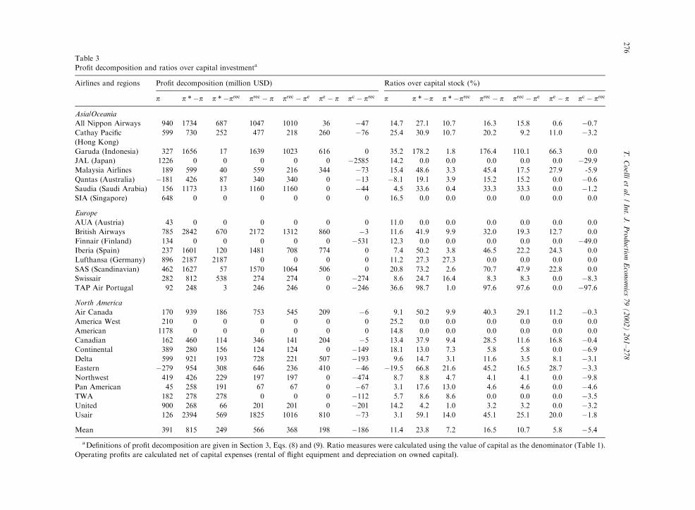
Table 3

Profit decomposition and ratios over capital investmenta

Airlines and regions Profit decomposition (million USD) Ratios over capital stock (%)

p p �p p �prec prec � p prec � pe pe � p pc � prec p p �p p �prec prec � p prec � pe pe � p pc � prec

Asia/Oceania

All Nippon Airways 940 1734 687 1047 1010 36 �47 14.7 27.1 10.7 16.3 15.8 0.6 �0.7Cathay Pacific

(Hong Kong)

599 730 252 477 218 260 �76 25.4 30.9 10.7 20.2 9.2 11.0 �3.2

Garuda (Indonesia) 327 1656 17 1639 1023 616 0 35.2 178.2 1.8 176.4 110.1 66.3 0.0

JAL (Japan) 1226 0 0 0 0 0 �2585 14.2 0.0 0.0 0.0 0.0 0.0 �29.9Malaysia Airlines 189 599 40 559 216 344 �73 15.4 48.6 3.3 45.4 17.5 27.9 -5.9

Qantas (Australia) �181 426 87 340 340 0 �13 �8.1 19.1 3.9 15.2 15.2 0.0 �0.6Saudia (Saudi Arabia) 156 1173 13 1160 1160 0 �44 4.5 33.6 0.4 33.3 33.3 0.0 �1.2SIA (Singapore) 648 0 0 0 0 0 0 16.5 0.0 0.0 0.0 0.0 0.0 0.0

Europe

AUA (Austria) 43 0 0 0 0 0 0 11.0 0.0 0.0 0.0 0.0 0.0 0.0

British Airways 785 2842 670 2172 1312 860 �3 11.6 41.9 9.9 32.0 19.3 12.7 0.0

Finnair (Finland) 134 0 0 0 0 0 �531 12.3 0.0 0.0 0.0 0.0 0.0 �49.0Iberia (Spain) 237 1601 120 1481 708 774 0 7.4 50.2 3.8 46.5 22.2 24.3 0.0

Lufthansa (Germany) 896 2187 2187 0 0 0 0 11.2 27.3 27.3 0.0 0.0 0.0 0.0

SAS (Scandinavian) 462 1627 57 1570 1064 506 0 20.8 73.2 2.6 70.7 47.9 22.8 0.0

Swissair 282 812 538 274 274 0 �274 8.6 24.7 16.4 8.3 8.3 0.0 �8.3TAP Air Portugal 92 248 3 246 246 0 �246 36.6 98.7 1.0 97.6 97.6 0.0 �97.6

North America

Air Canada 170 939 186 753 545 209 �6 9.1 50.2 9.9 40.3 29.1 11.2 �0.3America West 210 0 0 0 0 0 0 25.2 0.0 0.0 0.0 0.0 0.0 0.0

American 1178 0 0 0 0 0 0 14.8 0.0 0.0 0.0 0.0 0.0 0.0

Canadian 162 460 114 346 141 204 �5 13.4 37.9 9.4 28.5 11.6 16.8 �0.4Continental 389 280 156 124 124 0 �149 18.1 13.0 7.3 5.8 5.8 0.0 �6.9Delta 599 921 193 728 221 507 �193 9.6 14.7 3.1 11.6 3.5 8.1 �3.1Eastern �279 954 308 646 236 410 �46 �19.5 66.8 21.6 45.2 16.5 28.7 �3.3Northwest 419 426 229 197 197 0 �474 8.7 8.8 4.7 4.1 4.1 0.0 �9.8Pan American 45 258 191 67 67 0 �67 3.1 17.6 13.0 4.6 4.6 0.0 �4.6TWA 182 278 278 0 0 0 �112 5.7 8.6 8.6 0.0 0.0 0.0 �3.5United 900 268 66 201 201 0 �201 14.2 4.2 1.0 3.2 3.2 0.0 �3.2Usair 126 2394 569 1825 1016 810 �73 3.1 59.1 14.0 45.1 25.1 20.0 �1.8

Mean 391 815 249 566 368 198 �186 11.4 23.8 7.2 16.5 10.7 5.8 �5.4

aDefinitions of profit decomposition are given in Section 3, Eqs. (8) and (9). Ratio measures were calculated using the value of capital as the denominator (Table 1).

Operating profits are calculated net of capital expenses (rental of flight equipment and depreciation on owned capital).

T.

Co

elliet

al.

/In

t.J

.P

rod

uctio

nE

con

om

ics7

9(

20

02

)2

61

–2

78

276

study, to the point of ray capacity, used in someprevious studies. The resulting average profitdifference (pc � prec) is equal to minus US$186m.This clearly illustrates that the use of the raycapacity measure is not very sensible when oneconsiders the profit implications.We conclude this brief discussion of our results

by repeating the warning that we gave at thebeginning of this results section. Namely, that theproduction frontiers and capacity frontiers con-structed using LP in this empirical study reflect theouter boundary of the observed best practice in the

sample. Now, given that the world economy wason a down-cycle in 1990, we have perhaps over-estimated the degree of capacity utilisation andunderestimated the amount of forgone profit. Infuture work, we plan to obtain additional data onthese airline companies for a number of years,including years at the top of the macro cycle.20 Wewill then use this panel data to re-estimate ourfrontiers to see if this has the effect of changingour conclusions regarding the degree of foregoneprofit, and the contribution of unused capacity tothis profit gap21.

6. Conclusions

The main aim of this study was to develop amethodology which would allow us to measure thegap between observed short-run profit and max-imum short-run profit, and to decompose this gapinto meaningful components, with particularinterest in the contribution of capacity utilisation.We began by reviewing a number of previouslyproposed capacity measures, and concluded thatthese measures did not provide meaningful in-

formation when one attempted to use them in aprofit decomposition analysis.As a result of the problems with the existing

capacity measures, we proposed a new measure ofray economic capacity, which involves finding thelargest radial expansion (or contraction) of theoutput vector, coinciding with the largest possibleshort-run profit. We then use this capacitymeasure to decompose the gap between observedshort-run profit and maximum short-run profitinto components due to unused capacity, technicalinefficiency, input-mix allocative efficiency andoutput-mix allocative inefficiency. We then devisea series of DEA-like LP problems which allow usto measure and decompose the short-run profitinefficiency of a group of firms into these variouscomponents.Following this, we have provided an empirical

illustration of these methods using data on 28international airline companies. Our empiricalmodel has two outputs (passengers and freight),one fixed input (aircraft) and three variable inputs(labour, fuel and ‘‘other’’). Our empirical resultsindicate that the average (short-run) profit of these28 firms was US$391m, which equates to an11.4% return relative to the (undepreciated)capital stock. After calculating the maximumlevels of short-run profit, we observe that theaverage profit gap is US$815m. The decomposi-tion analysis then attributes 70% of this gap tounused capacity and 30% to output-mix allocativeinefficiency. A further decomposition of the 70%profit gap due to unused capacity, indicates that24% is due to technical inefficiency and 46% is dueto a type of input mix allocative efficiencyinefficiency effect. The firm-level results indicatesubstantial differences in profit gaps and decom-positions among the firms, and clearly demon-strate the rich quantity of information that can begenerated using these methods.

Acknowledgements

Tim Coelli thanks the Universitat Aut "onomade Barcelona for hosting his sabbatical visit inJanuary, 2000. Emili Grifell-Tatj!e is grateful toCICYT, SEC2001-2793-C03-01, and Generalitat

20The collection and analysis of this extra data will be a very

large amount of work. It was beyond the scope of this study,

which focuses primarily upon the development of the metho-

dology, to consider this additional empirical work.21Alternatively, one could argue that our profit gap measures

may overstate the amount of forgone profit due to unused

capacity. This is because we have assumed that the airlines

could utilize this unused capacity without reducing the average

price of services. This is unlikely to be true for some large

airlines which play a dominant role in setting prices in their

local market.


de Catalunya, 2000SGR 00052, and Sergio Perel-man to Communaut!e Fran-caise de Belgique, PAC98/03-221, for generous financial support. Theauthors thank Kris Kerstens, Diego Prior, Phi-lippe Vanden Eeckaut and the audience at theNorth American Productivity Workshop, June2000, for valuable comments. Any remainingerrors are those of the authors.

References

Berndt, E.R., Morrison, C.J., 1981. Capacity utilization

measures: underlying economic theory and an alternative

approach. American Economic Review 71, 48–52.

Bureau of Transportation Statistics, 2000. Fuel cost and

consumption. US Department of Transportation. http://

www.bts.gov/programs/oai/fuel/fuelyearly.html.

Coelli, T.J., Prasada Rao, D.S., Battese, G.E., 1998. An

Introduction to Efficiency and Productivity Analysis.

Kluwer Academic Publishers, Boston.

Coelli, T.J., Perelman, S., Romano, E., 1999. Accounting for

environmental influences in stochastic frontier models: With

application to international airlines. Journal of Productivity

Analysis 11, 251–273.

Eilon, S., 1975. Changes in profitability components. Omega 3

(3), 353–354.

Eilon, S., 1984. The Art of Reckoning-analysis of Performance

Criteria. Academic Press, London.

Eilon, S., 1985. A framework for profitability and productivity

measures. Interfaces 15, 31–40.

Eilon, S., Soesan, J., 1976. Reflections on measurement and

evaluation. In: Eilon, S., Gold, B., Soesan, J. (Eds.),

Applied Productivity Analysis for Industry. Pergamon

Press, Oxford, pp. 115–133.

Eilon, S., Teague, J., 1973. On measures of productivity. Omega

1 (5), 565–576.

Eilon, S., Gold, B., Soesan, J., 1975. A productivity study in a

chemical plan. Omega 3 (3), 329–343.

F.are, R., 1984. The existence of plant capacity. International

Economic Review 25, 209–213.

F.are, R., Primont, D., 1995. Multi-output Production and

Duality: Theory and Applications. Kluwer Academic

Publishers, Boston.

F.are, R., Grosskopf, S., Kokkelenberg, E.C., 1989. Measuring

plant capacity utilization and technical change: A nonpara-

metric approach. International Economic Review 30 (3),

655–666.

F.are, R., Grosskopf, S., Valdmanis, V., 1989. Capacity

competition and efficiency in hospitals: A nonparametric

approach. Journal of Productivity Analysis 1, 123–128.

F.are, R., Grosskopf, S., Lovell, C.A.K., 1994. Production

Frontiers. Cambridge University Press, Cambridge.

Farrell, M.J., 1957. The measurement of productive efficiency.

Journal of the Royal Statistical Society Series A, General

120, 253–281.

Gold, B., 1955. Foundations of Productivity Analysis. Pitts-

burgh University Press, Pittsburgh, PA.

Gold, B., 1973. Technology productivity and economic

analysis. Omega 1, 5–24.

Gold, B., 1976. Framework for productivity analysis. In: Eilon,

S., Gold, B., Soesan, J. (Eds.), Applied Productivity

Analysis for Industry. Pergamon Press, Oxford, pp. 15–40.

Gold, B., 1985. Foundations of strategic planning for

productivity improvement. Interfaces 15, 15–30.

ICAO, 1992a. International Civil Aviation Organisation.

Traffic, Montreal.

ICAO, 1992b. International Civil Aviation Organisation. Fleet-

Personnel, Montreal.

ICAO, 1992c. International Civil Aviation Organisation.

Financial Data, Montreal.

Johansen, L., 1968. Production functions and the concept of

capacity. In: Recherches R!ecentes sur la Fonction de

Production. Collection !Economie Math!ematique et!Econom!etrie 2, Namur [reprinted in: Førsund, F.R. (Ed.),

1987. Collected Works of Leif Johansen, Vol. 1, North-

Holland, Amsterdam, pp. 359–382].

Klein, L.R., 1960. Some theoretical issues in the measurement

of capacity. Econometrica 28, 272–286.

Shank, J., Churchill, N.C., 1977. Variance analysis: A manage-

ment-oriented approach. Accounting Review 52 (4), 950–

957.

Shephard, R.W., 1970. Theory of Cost and Production

Functions. Princeton University Press, Princeton, NJ.

Winston, G.C., 1974. The theory of capital utilization and

idleness. Journal of Economic Literature 12, 1301–1320.


http://www.bts.gov/programs/oai/fuel/fuelyearly.html

http://www.bts.gov/programs/oai/fuel/fuelyearly.html

Capacity utilisation and profitability: a decomposition of short run profit efficiency

Documents