Capacity Optimization of High-speed Railway Train in ...

Capacity Optimization of High-speed Railway Train in Established Schedule Plan Based on Improved

ACO Algorithm

Hao Li1, Xiaowei Liu2,3,4 and Kun Yang1 1School of Traffic and Transportation, Lanzhou Jiaotong University, LanZhou 730070, China

2School of Transportation and Logistics, Chengdu 610031, China 3National Railway Train Diagram Research and Training Center, Southwest Jiaotong University, Chengdu 610031, China

4National and Local Joint Engineering Laboratory of Comprehensive Intelligent Transportation, Southwest JiaoTong University, Chengdu610031, China

Abstract—In order to improve the transporting ability of high-speed trains, Gave the definition of the minimizing departure interval between trains, and the definition of the drawing compact diagram without considering overtaking conditions. After considering the matching coefficient of train operation, an 0-1 integer programming model was established to maximize capacity of trains and convert the problem into an asymmetric traveling salesman problem (ATSP). Then a improved algorithm-ant colony optimazition(ACO) algorithm is designed to solve the problem. The case of Shanghai to Beijing high-speed trains were taken as an example solving by programming. Computation results show that considering the matching coefficient of train operation, the optimized scheme can shorten the total time by 219 min (about 28.52%) than the existing scheme.

Keywords—high-speed railway; carrying capacity; ATSP; ACO

I. INTRODUCTION

The high-speed rail transport capacity represents the maximum passenger flow that can be transported in a unit of time, The railway train transportation capacity represents the number of pairs of trains that can operate every day and night. The transport ability of the train is restricted by the order of the train running map [1]. For the train passing ability and train timetabling problem, Peng Qiyuan et al [2-7] established a model aiming at the maximum transport capacity ability and train timetabling, and designed a heuristic algorithm to solve.

In order to increase the capacity of railway train transportation, it is necessary to reduce the interval time cost between trains to increase the capacity, and also to meet the needs of passenger flow at stations. In this paper, under the premise of considering the train matching coefficients of different stopping schemes, the goal is to maximize the capacity of the train timetabling, and the problem is transformed into an asymmetric traveling salesman problem. Aiming at the problem of NP complete problem, this paper uses group intelligence algorithm to approximate solution.

The ant colony optimization algorithm (ACO) was first proposed by Macro Dorigo in his doctoral dissertation in

1992. It has a strong ability to search for better solutions [9][10] when solving large-scale combinatorial optimization problems. However, ant colony optimization algorithm (ACO) the initial solution process is slow, and it is prone to premature [11],Therefore, the adaptive pheromone and expected heuristic factor and cross mutation operator are introduced to improve the ant colony optimization algorithm (ACO).

This paper considers the size of passenger flow at different stations, introduces the train matching coefficient, establishes a mathematical model, and then uses the improved ant colony optimization algorithm (ACO) to optimize the problem, finally, simulate with an example.

II. TRANSPORTATION CAPACITY OPTIMIZATION MODEL

A. Symbols and Definitions

Let a high speed railway line L be composed of station set s and interval set. All train collections { | 1,2,..., }

jk j mK

,tf

i k

i,ktd It's the

moment the train k K arrives at the stationi S . Set

its origin and finally arrive at the station 1i , n

i respectively.

Let be the station before station i. The constant ,i k

tcy is

the pure running time of train k in interval ( , )e i k .T is the

total running time of the train,,

x y

ik k

sfj is the minimum

interval between trains i and j at station k. ,i k

tq is the time

when train k is added at the leave of station i.,i k

tt t is the

time when train k is added at the stop of station s.,i k

ts is

theime for the train k at the station i..,i k

is a 0-1 variable, If

train k stops at station i, ,i k

is 1, otherwise ,i k

is 0. The

unknown variables,i k

tf ,,j k

td are the departure and arrival

times of train k at station i and station j

respectively.. x yk k

iId , x y

k k

iIf is the departure time of train k at

station i.

152Copyright © 2018, the Authors. Published by Atlantis Press. This is an open access article under the CC BY-NC license (http://creativecommons.org/licenses/by-nc/4.0/).

3rd International Conference on Modelling, Simulation and Applied Mathematics (MSAM 2018)Advances in Intelligent Systems Research (AISR), volume 160

Definition 1: For the same train ,x y

k k , if

, ,x y

k i k itf tf ( i S ). If there is no

train,makex z y

k i k i k itf tf tf .Then ,

x yk k is called the

tight train of station i, recorded as x y

k k .

Definition 2: For any tight train x y

k k on the

running line. If the train departure interval betweenx

k and

yk of the running line L is equal to the Minimum departure

interval ,

sfjx y

ik k

In this way drawn train line, which is called

a compact drawn..

B. High-speed Train Arrival Time Interval Model

According to the scheduled stop plan of the running line L, for ,k K i S , there are the following relationships:

i, i, i,i , i , i , i ,k k kk k k ktd tf tcy tq tt

(1)

i, i, i,f

k k kt td ts

(2)

According to the recursive relationship, the train originating time

,i ktf is substituted, and the arrival time of

the train k at each station of the running line can be calculated:

1

i, i, , i, ,i , , , ,i

( )n

k k j k k j kk j k j k j kj k

td tf ts tcy tq tt ts

(3)

1

i, , i, ,i , , , ,i

( )n

k j k k j kk j k j k j kj k

tf tf tcy tq tt ts

(4)

Thus establishing running line relationship of the train. Because there is no cross-line relationship between the same speed trains, there is

x yk k for any train

xk on the

running line and its tight trainy

k , and the

stationx y

k ki S S needs to meet a certain time interval,

which has following relationship. :

i, i,kx y

y x

k k

k itd td Id

(5)

i, i,kx y

y x

k k

k itd td Id

(6)

From equations (1)-(6), the minimum starting interval of

train x

k and y

k at station k is,

x y

ik k

sfj , so that the

minimum departure interval ,

x yk k

sfj of train k on the

running line can be calculated.

y

i

, , ,,min ,

x y x x y x yk k k k k k k k

sfj MAX sfj sfj i S S (7)

,min

x yk k

sfj is the minimum starting interval of the train at

different stations in the interval ,which is a constant.

C. Train Matching Coefficient for Different Stop Plans

The passenger flow between different stations of high-speed trains is different. In order to meet the demand of passenger flow, it is necessary to establish a reasonable stop plan to match different passenger flows. According to the different stop-stopping schemes, the train station are divided three levels:

au ,

bu ,

cu .

Define the train matching coefficient, that is, compare the train stop level, and get a train matching coefficient

x yu u

.It

represents the probability of tight train departure which in different levels. That is to say for the tight train

x yk k the tight train

xk departure probability is

x y

au u

b

uu

, The method of obtaining the coefficient is

AHP[12]

The train matching coefficient matrix is as follows:

,( , ( , , ))

a a a b a c

x y b a b b b c

c a c b c c

u u u u u u

u u u u u u u u

u u u u u u

i j a b c

D. Capacity Optimization Model

In order to increase the train transportation capacity, the train matching coefficient must also be considered. To this end, a running time coefficient

x yk k

is defined here.

,1

x y x

x y

k k k ku u

sfj (8)

The smaller the x y

k k the larger the transport capacity of

the train after compact drawn. If each train line is regarded as a node network complete diagram, n is used to indicate the node number, and the path cost of node

xn pointing to

yn is

equal to therunning time coefficient between trains x

k and

xk . Starting from any node

1n , traversing all the nodes and

returning to the path of the initial node once, which is called the tour path, and disconnecting the last node

mn of the tour

path to the initial node 1n will form a chain. The order of

each node can be determined. The optimization goal is to find the total running time coefficient to be the least, The optimization process is shown in Figure 1.

153

Advances in Intelligent Systems Research (AISR), volume 160

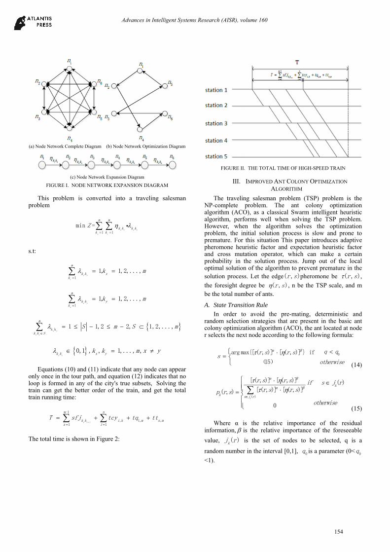
(a) Node Network Complete Diagram (b) Node Network Optimization Diagram

(c) Node Network Expansion Diagram

FIGURE I. NODE NETWORK EXPANSION DIAGRAM

This problem is converted into a traveling salesman problem

1 1

min =x y x y

x y

m m

k k k kk k

Z

s.t:

1

1, 1,2,...,x y

y

m

k k xk

k m

1

1, 1,2,...,x y

x

m

k k yk

k m

k k1 1,2 2, 1,2,...,

x y

x y

m

k k S

S m S m

0,1 , , 1,..., ,x y

k k x yk k m x y

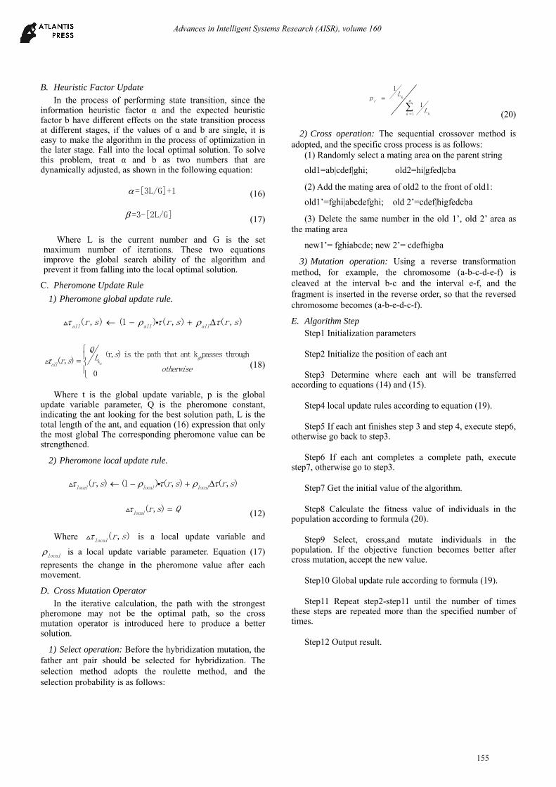
Equations (10) and (11) indicate that any node can appear only once in the tour path, and equation (12) indicates that no loop is formed in any of the city's true subsets, Solving the train can get the better order of the train, and get the total train running time:

1

m-1

, 1, ,1 1

x x

n

k k i k m n mx i

T sfj tcy tq tt

The total time is shown in Figure 2:

FIGURE II. THE TOTAL TIME OF HIGH-SPEED TRAIN

III. IMPROVED ANT COLONY OPTIMIZATION

ALGORITHM

The traveling salesman problem (TSP) problem is the NP-complete problem. The ant colony optimization algorithm (ACO), as a classical Swarm intelligent heuristic algorithm, performs well when solving the TSP problem. However, when the algorithm solves the optimization problem, the initial solution process is slow and prone to premature. For this situation This paper introduces adaptive pheromone heuristic factor and expectation heuristic factor and cross mutation operator, which can make a certain probability in the solution process. Jump out of the local optimal solution of the algorithm to prevent premature in the solution process. Let the edge( , )r s pheromone be ( , )r s ,

the foresight degree be ( , )r s , n be the TSP scale, and m be the total number of ants.

A. State Transition Rule

In order to avoid the pre-mating, deterministic and random selection strategies that are present in the basic ant colony optimization algorithm (ACO), the ant located at node r selects the next node according to the following formula:

0arg max{[ ( , )] [ ( , )] } if

（15）

q qr s r ss

otherwise

(14)

( )

[ ( , )] [ ( , )] ( )[ ( , )] [ ( , )]( , )

0

k

k

k u j r

r s r s if s j rr s r sp r s

otherwise

(15)

Where α is the relative importance of the residual information, is the relative importance of the foreseeable

value, ( )k

j r is the set of nodes to be selected, q is a

random number in the interval [0,1], 0

q is a parameter (0<0

q

<1).

154


B. Heuristic Factor Update

In the process of performing state transition, since the information heuristic factor α and the expected heuristic factor b have different effects on the state transition process at different stages, if the values of α and b are single, it is easy to make the algorithm in the process of optimization in the later stage. Fall into the local optimal solution. To solve this problem, treat α and b as two numbers that are dynamically adjusted, as shown in the following equation:

=[3L/G]+1 (16)

=3-[2L/G] (17)

Where L is the current number and G is the set maximum number of iterations. These two equations improve the global search ability of the algorithm and prevent it from falling into the local optimal solution.

C. Pheromone Update Rule

1) Pheromone global update rule.

( , ) (1 ) ( , ) ( , )all all all

r s r s r s

k（r, ) is the path that ant k passes through

( , )

0

gb

gball

QsLr s

otherwise

(18)

Where t is the global update variable, p is the global update variable parameter, Q is the pheromone constant, indicating the ant looking for the best solution path, L is the total length of the ant, and equation (16) expression that only the most global The corresponding pheromone value can be strengthened.

2) Pheromone local update rule.

( , ) (1 ) ( , ) ( , )local local local

r s r s r s

( , )local

r s Q (12)

Where ( , )local

r s is a local update variable and

local is a local update variable parameter. Equation (17)

represents the change in the pheromone value after each movement.

D. Cross Mutation Operator

In the iterative calculation, the path with the strongest pheromone may not be the optimal path, so the cross mutation operator is introduced here to produce a better solution.

1) Select operation: Before the hybridization mutation, the father ant pair should be selected for hybridization. The selection method adopts the roulette method, and the selection probability is as follows:

1

1

1k

mr

kk

Lp

L

(20)

2) Cross operation: The sequential crossover method is adopted, and the specific cross process is as follows:

(1) Randomly select a mating area on the parent string

old1=ab|cdef|ghi; old2=hi|gfed|cba

(2) Add the mating area of old2 to the front of old1:

old1’=fghi|abcdefghi; old 2’=cdef|higfedcba

(3) Delete the same number in the old 1’, old 2’ area as the mating area

new1’= fghiabcde; new 2’= cdefhigba

3) Mutation operation: Using a reverse transformation method, for example, the chromosome (a-b-c-d-e-f) is cleaved at the interval b-c and the interval e-f, and the fragment is inserted in the reverse order, so that the reversed chromosome becomes (a-b-e-d-c-f).

E. Algorithm Step Step1 Initialization parameters

Step2 Initialize the position of each ant

Step3 Determine where each ant will be transferred according to equations (14) and (15).

Step4 local update rules according to equation (19).

Step5 If each ant finishes step 3 and step 4, execute step6, otherwise go back to step3.

Step6 If each ant completes a complete path, execute step7, otherwise go to step3.

Step7 Get the initial value of the algorithm.

Step8 Calculate the fitness value of individuals in the population according to formula (20).

Step9 Select, cross,and mutate individuals in the population. If the objective function becomes better after cross mutation, accept the new value.

Step10 Global update rule according to formula (19).

Step11 Repeat step2-step11 until the number of times these steps are repeated more than the specified number of times.

Step12 Output result.

155


IV. SIMULATION ANALYSIS

A. Data and Parameter Settings

In order to test the effect of the algorithm, the 2017 Beijing-Shanghai high-speed rail was taken as an example for verification. Take all the 35 trains of the high-speed railway. Trains originating from Shanghai Hongqiao and ending in Beijing South as the research object.

There are 24 stations on the running line, the train

non-stop station direct train time ,

1

n

i ki

tcy =268min, the

starting time is,i k

tq = 2min, and the parking time is,i k

tt =

3min. From equations (1)-(7), the minimum departure interval

,x y

k ksfj between different trains can be obtained.

In 2017, the trains of the Beijing-Shanghai high-speed train in the upward direction of the train were successively paved:

G102,G104,G6,G10,G106,G108,G110,G12,G112,G114,G2,G116,G118,G14,G122,G16,G126,G130,G132,G412,G134,G138,G140,G4,G142,G146,G18,G148,G22,G150,G152,G24,G154,G158,G8. If drawing compact diagram the total time is 768min, and the train level is divided according to the number of stops. As shown in Table 1.

TABLE I. TRAIN LEVEL

number of train stops

Train number Train level

2 G2,G16,G4,G18

au （2-5） 3 G6,G10,G8

5 G12,G22,G24

bu （6-8）

6 G104,G106,G1547 G152 8 G102,G112,G116,G118,G122,G132

, G134,G138，G146,G148,G150

9 G108,G110,G114,G126,G140,G142,G158

cu （9-12）

10 G130 11 G412

Matching factor x for different trains, as shown in Table 2.

TABLE II. MATCHING FACTOR

Train level a

u b

u cu

au 0.1 0.5 0.4

bu 0.3 0.4 0.3

cu 0.2 0.5 0.3

According to the high-speed railway transportation capacity optimization model in 2.4.The improved ant colony optimization algorithm (ACO) is used to solve the model.

The parameters taken in the algorithm are:1

2

,

Q=10,0

q =0.9, 0.1local , 0.1

all ,m=32.

B. Simulation Results and Analysis

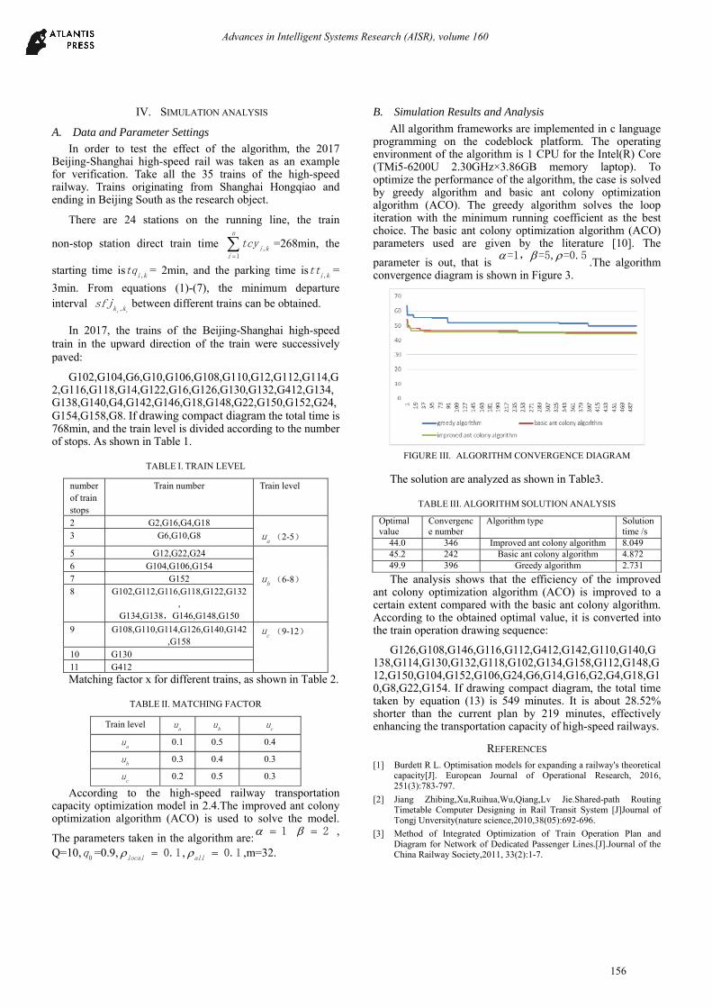
All algorithm frameworks are implemented in c language programming on the codeblock platform. The operating environment of the algorithm is 1 CPU for the Intel(R) Core (TMi5-6200U 2.30GHz×3.86GB memory laptop). To optimize the performance of the algorithm, the case is solved by greedy algorithm and basic ant colony optimization algorithm (ACO). The greedy algorithm solves the loop iteration with the minimum running coefficient as the best choice. The basic ant colony optimization algorithm (ACO) parameters used are given by the literature [10]. The

parameter is out, that is =1， =5, =0.5

.The algorithm convergence diagram is shown in Figure 3.

FIGURE III. ALGORITHM CONVERGENCE DIAGRAM

The solution are analyzed as shown in Table3.

TABLE III. ALGORITHM SOLUTION ANALYSIS

Optimal value

Convergence number

Algorithm type Solution time /s

44.0 346 Improved ant colony algorithm 8.04945.2 242 Basic ant colony algorithm 4.87249.9 396 Greedy algorithm 2.731

The analysis shows that the efficiency of the improved ant colony optimization algorithm (ACO) is improved to a certain extent compared with the basic ant colony algorithm. According to the obtained optimal value, it is converted into the train operation drawing sequence:

G126,G108,G146,G116,G112,G412,G142,G110,G140,G138,G114,G130,G132,G118,G102,G134,G158,G112,G148,G12,G150,G104,G152,G106,G24,G6,G14,G16,G2,G4,G18,G10,G8,G22,G154. If drawing compact diagram,

the total time

taken by equation (13) is 549 minutes. It is about 28.52% shorter than the current plan by 219 minutes, effectively enhancing the transportation capacity of high-speed railways.

REFERENCES [1] Burdett R L. Optimisation models for expanding a railway's theoretical

capacity[J]. European Journal of Operational Research, 2016, 251(3):783-797.

[2] Jiang Zhibing,Xu,Ruihua,Wu,Qiang,Lv Jie.Shared-path Routing Timetable Computer Designing in Rail Transit System [J]Journal of Tongj Unversity(nature science,2010,38(05):692-696.

[3] Method of Integrated Optimization of Train Operation Plan and Diagram for Network of Dedicated Passenger Lines.[J].Journal of the China Railway Society,2011, 33(2):1-7.

156


[4] Liao Zhengwen,Miao Jianrui,MengLingyun,Li Haiying,Zhao lan.An Optimazation Algorithm for Double-track Railway Train Timetabling Based on Lagrangian Relaxation [J].Journal of the China Railway Society, 2016,38(09):1-8. [5]Caprara A, Monaci M, Toth P, et al. A Lagrangian heuristic algorithm for a real-world train timetabling problem[J]. Discrete Applied Mathematics, 2006, 154(5):738-753.

[5] Xu Hong,Ma Jian Jun,Research on the Model and Algorithm of the Train Working Diagram of Dedicated Passenger Line. [J].Journal of the China Railway Society, 2007,(02):1-7.

[6] Zhang Xiaobing,Ni Shaoquan,Pan Jinshan.Optimization of Train Diagram Structure for High-Speed Railway[J].Journal of Southwest Jiaotong University.

[7] Nöhring F. Traveling Salesman Problem[J]. Operations Research, 2007, 4(1):61-75.

[8] Dorigo M,Maniezzo V,Colorni A.The Ant System:Optimization by a Colony of Cooperating Agents[J].IEEE Transactions on Systems,Man,and Cybernetics,Part-B,1996, 26(1):1-13.

[9] Dorigo M,Gambardella L M.Ant Colony System:A Coope-rative Learning Approach to the Traveling Salesman Problem[J]. IEEE Transactions on Evolutionary Computation, 1997,1(1):53-66.

[10] Dong G, Fu X, Li H, et al. Cooperative ant colony-genetic algorithm based on spark ☆[J]. Computers & Electrical Engineering, 2016, 60(C):66-75.

[11] Wang T, Bao W Y. Application of AHP in Performance Evaluation of Freight Train Dispatching Team[J]. Logistics Engineering & Management, 2017.

157


Capacity Optimization of High-speed Railway Train in ...

Documents