CAPACITY OF PEGGED MORTISE AND TENON JOINERY Richard J. Schmidt Joseph F. Miller A report on research co-sponsored by: Department of Civil and Architectural Engineering University of Wyoming Laramie, WY 82071 February 2004 University of Wyoming Laramie, WY 82071 Timber Frame Business Council Hamilton, MT Timber Framers Guild Becket, MA

Welcome message from author
This document is posted to help you gain knowledge. Please leave a comment to let me know what you think about it! Share it to your friends and learn new things together.
Transcript
CAPACITY OF PEGGEDMORTISE AND TENON JOINERY
Richard J. SchmidtJoseph F. Miller
A report on research co-sponsored by:
Department of Civil andArchitectural EngineeringUniversity of WyomingLaramie, WY 82071
February 2004
University of WyomingLaramie, WY 82071
Timber Frame Business CouncilHamilton, MT
Timber Framers GuildBecket, MA

REPORT DOCUMENTATIONPAGE
1. REPORT NO. 2. 3. Recipient’s Accession No.
4. Title and Subtitle 5. Report Date
6.
7. Author(s) 8. Performing Organization Report No.
9. Performing Organization Name and Address 10. Project/Task/Work Unit No.
11. Contract(C) or Grant(G) No.
12. Sponsoring Organization Name and Address 13. Type of Report & Period Covered
14.
15. Supplementary Notes
50272---101
16. Abstract (Limit: 200 words)
17. Document Analysisa. Descriptors
b. Identifiers/Open---Ended Terms
c. COSATI Field/Group
18. Availability Statement 19. Security Class (This Report)
20. Security Class (This Page)
21. No. of Pages
22. Price
(See ANSI---Z39.18) OPTIONAL FORM 272 (4---77)Department of Commerce
February 2004Capacity of Pegged Mortise and Tenon Joints
Joseph F. Miller & Richard J. Schmidt
Department of Civil and Architectural EngineeringUniversity of WyomingLaramie, Wyoming 82071
Timber Frame Business Council217 Main StreetHamilton, MT 59840
traditional timber framing, heavy timber construction, structural analysis, wood peg fasteners,mortise and tenon connections, dowel connections, lateral load response, European yield model,
Release Unlimited
unclassified
unclassified
84
final
Traditional timber frames use hardwood pegs to secure mortise and tenon connections,resulting in shear loading of the peg. Despite the historical usage of such connections, no applicablebuilding codes or guidelines are available for engineers and designers to follow. The object of thisresearch is to quantify the shear capacity of wooden pegs in amortise and tenon joint by both physicaltesting of full ---scale specimens as well as modeling their macroscopic behavior by the finite elementmethod. By testing various species of wood used in both the frame members as well as the pegs, acorrelation between shear strength and the specific gravity of the framematerials is developed. Thiscorrelation is then used to develop a design method for mortise and tenon joints.
(C)
(G)
TimberFramersGuildPO Box 60Becket, MA 01223
University ofWyomingLaramie, WY 82071

Acknowledgments
Acknowledgments and thanks are extended to thank Helmsburg Sawmill and Carl
Miller for their help in providing the timbers along with the Timber Frame Business Council
and the Timber Framers Guild for financial support.
iii
T A B L E O F C O N T E N T S
1.0 INTRODUCTION...................................................................................................................... - 1 - 1.1 HISTORY AND BACKGROUND................................................................................................... - 1 - 1.2 PROBLEM STATEMENT ............................................................................................................. - 2 - 1.3 LITERATURE REVIEW............................................................................................................... - 4 - 1.4 OBJECTIVES AND SCOPE OF WORK .......................................................................................... - 7 -
2.0 TESTING PROCEDURES AND RESULTS........................................................................... - 8 - 2.1 JOINT TESTS............................................................................................................................. - 8 -
2.1.1 Tension Testing................................................................................................................... - 8 - 2.1.2 Shear Testing.................................................................................................................... - 18 - 2.1.3 Direct Bearing Tests......................................................................................................... - 23 -
2.2 DOWEL BEARING TESTS......................................................................................................... - 25 - 3.0 FINITE ELEMENT MODELING ......................................................................................... - 27 -
3.1 OBJECTIVES ........................................................................................................................... - 27 - 3.2 MODEL DEVELOPMENT.......................................................................................................... - 27 - 3.3 RESULTS ................................................................................................................................ - 34 - 3.4 DIRECT BEARING JOINTS ....................................................................................................... - 38 -
4.0 SPECIFIC GRAVITY AND YIELD STRESS CORRELATION ....................................... - 41 - 4.1 BACKGROUND........................................................................................................................ - 41 - 4.2 DEVELOPMENT....................................................................................................................... - 42 - 4.3 RESULTS ................................................................................................................................ - 43 -
5.0 DESIGN OF MORTISE AND TENON JOINTS.................................................................. - 46 - 5.1 INTRODUCTION ...................................................................................................................... - 46 - 5.2 SELECTION OF A FACTOR OF SAFETY ..................................................................................... - 46 - 5.3 LOAD DURATION FACTOR...................................................................................................... - 49 - 5.4 DESIGN EQUATION................................................................................................................. - 51 -
6.0 UTILIZATION OF YELLOW POPLAR.............................................................................. - 52 - 6.1 GENERAL INFORMATION ........................................................................................................ - 52 - 6.2 AVAILABILITY ....................................................................................................................... - 53 - 6.3 MATERIAL PROPERTIES.......................................................................................................... - 53 -
6.3.1 Strength ............................................................................................................................ - 53 - 6.3.2 Drying............................................................................................................................... - 54 - 6.3.3 Workability ....................................................................................................................... - 55 -
6.4 CONCLUSION ON USAGE ........................................................................................................ - 55 - 7.0 SUMMARY AND CONCLUSIONS....................................................................................... - 56 -
7.1 JOINT RESEARCH.................................................................................................................... - 56 - 7.1.1 Physical Testing................................................................................................................ - 56 - 7.1.2 Finite Element Modeling .................................................................................................. - 57 -
7.2 DESIGN EQUATIONS AND CORRELATION................................................................................ - 57 - 7.3 USAGE OF YELLOW POPLAR .................................................................................................. - 58 - 7.4 RECOMMENDATIONS FOR FUTURE RESEARCH ....................................................................... - 58 -
8.0 REFERENCES......................................................................................................................... - 59 - 9.0 APPENDICES .......................................................................................................................... - 61 -
APPENDIX A – TENSION LOAD-DEFLECTION PLOTS............................................................................. - 61 -

iv
APPENDIX B – SHEAR LOAD DEFLECTION PLOTS................................................................................. - 68 - APPENDIX C – DIRECT BEARING LOAD-DEFLECTION PLOTS................................................................ - 72 - APPENDIX D – DOWEL BEARING TEST DATA....................................................................................... - 73 - APPENDIX E – STATISTICAL METHODS FOR CORRELATION.................................................................. - 75 -
v
L I S T O F F I G U R E S
FIGURE 1-1 - MORTISE AND TENON JOINT - 3 - FIGURE 1-2 - NDS DOUBLE SHEAR FAILURE MODES - 3 - FIGURE 2-1 - TENSION LOADING OF MORTISE AND TENON JOINT - 9 - FIGURE 2-2 - TENSION TESTING APPARATUS FROM SCHMIDT AND MACKAY (1997) - 10 - FIGURE 2-3 - JOINT DETAILING - 11 - FIGURE 2-4 - (A) MORTISE SPLITTING FAILURE (B) TENON RELISH FAILURE - 13 - FIGURE 2-5 - (A) PEG BENDING AND (B) SHEAR FAILURES - 13 - FIGURE 2-6 - FIVE PERCENT OFFSET YIELD - 14 - FIGURE 2-7 - YELLOW POPLAR CYCLIC TEST PLOTS - 17 - FIGURE 2-8 - (A) HOUSED JOINT COMMONLY FOUND IN PRACTICE FOR CARRYING SHEAR LOADS - 19 - FIGURE 2-9 - SHEAR TESTING APPARATUS - 20 - FIGURE 2-10 – TENON SPLITTING FAILURE DURING SHEAR LOADING - 21 - FIGURE 2-11 - ROLLING SHEAR FAILURE OF TENON IN SHEAR LOADING - 22 - FIGURE 2-12 - DOWEL BEARING FIXTURE WITH LOADING PERPENDICULAR AND PARALLEL TO GRAIN - 26 - FIGURE 3-1- FINITE ELEMENT MODEL GEOMETRY FOR A MORTISE AND TENON JOINT - 28 - FIGURE 3-2 - STRESS - STRAIN CURVES USED IN FINITE ELEMENT MODELING - 30 - FIGURE 3-3 - MESHING OF MORTISE AND TENON JOINT - 31 - FIGURE 3-4 - 20-NODE BRICK ELEMENT (ANSYS, 2003) - 33 - FIGURE 3-5 - DETAIL OF CONTACT AND TARGET ELEMENTS NEAR PEG - 33 - FIGURE 3-6 - DISPLACED SHAPE OF THE JOINT - 35 - FIGURE 3-7 - SHORTLEAF PINE PHYSICAL AND MODELED LOAD-DEFLECTION CURVES - 36 - FIGURE 3-8 - RED OAK PHYSICAL AND MODELED LOAD-DEFLECTION CURVES - 36 - FIGURE 3-9 - EASTERN WHITE PINE PHYSICAL AND MODELED LOAD-DEFLECTION CURVES - 37 - FIGURE 3-10 - YELLOW POPLAR PHYSICAL AND MODELED LOAD-DEFLECTION CURVES - 37 - FIGURE 3-11 – DOUGLAS FIR PHYSICAL AND MODELED LOAD-DEFLECTION CURVES - 38 - FIGURE 3-12 - MESHING OF DIRECT BEARING MORTISE AND TENON JOINT - 39 - FIGURE 3-13 - EXPERIMENTAL AND MODELED DIRECT BEARING YELLOW POPLAR JOINTS - 40 - FIGURE 3-14 - MODELED DIRECT BEARING CURVES FOR VARIOUS SPECIES - 40 - FIGURE 4-1 - FOUR SHEAR PLANES USED IN CONVERTING YIELD LOAD TO YIELD STRESS - 42 - FIGURE 4-2 - PLOT OF YIELD POINTS WITH CORRELATION SURFACE - 45 - FIGURE 4-3 - CORRELATION SURFACE AND DATA POINTS VIEWED ALONG EDGE - 45 - FIGURE 5-1 - MADISON CURVE SHOWING LOAD DURATION FACTORS - 50 - FIGURE 6-1 - NATURAL RANGE OF YELLOW POPLAR (FS-272) - 52 -

vi
L I S T O F T A B L E S
TABLE 2-1 - RESULTS OF YELLOW POPLAR TENSION TESTING - 15 - TABLE 2-2 - RESULTS OF CYCLIC TESTING OF YELLOW POPLAR - 16 - TABLE 2-3 - MINIMUM DETAILING REQUIREMENTS AS A MULTIPLIER OF THE PEG DIAMETER (D) - 18 - TABLE 2-4 - RESULTS OF YELLOW POPLAR SHEAR TESTING - 23 - TABLE 2-5 - RESULTS OF YELLOW POPLAR DIRECT BEARING TESTS - 24 - TABLE 3-1 - MATERIAL PROPERTIES FROM THE WOOD HANDBOOK - 29 - TABLE 3-2 - RESULTS OF MESH REFINEMENT STUDY USING ORTHOTROPIC YELLOW POPLAR PROPERTIES
AND SUBJECTED TO 3500 POUNDS OF LOAD - 32 - TABLE 3-3 - COMPARISON OF PHYSICAL AND MODELED JOINTS - 35 - TABLE 4-1 - SPECIFIC GRAVITY AND YIELD STRESS DATA USED IN DEVELOPING THE CORRELATION - 44 - TABLE 5-1- RATIO OF YIELD LOAD TO ULTIMATE LOAD FOR FULL-SIZED JOINTS - 47 - TABLE 5-2 - RATIO OF CORRELATION STRENGTH TO EYM MODE IIIS ALLOWABLE LOAD - 48 - TABLE 5-3 - EXAMPLE ON THE PROPER USAGE OF THE CORRELATION - 51 - TABLE 6-1 - DIMENSIONAL CHANGE IN 3" LUMBER (IN INCHES) (FOREST PRODUCTS LAB, 2000) - 54 -
L I S T O F E Q U A T I O N S
EQUATION 4-1 - 42 - EQUATION 4-2 - 43 - EQUATION 5-1 - 51 -

- 1 -
1.0 Introduction
1.1 History and Background
Timber framing consists of large, widely spaced timbers connected together with
all-wood connections, such as mortises, tenons and pegs. It is one of the most traditional
forms of construction, having been practiced since before Christ (Benson and Gruber,
1980). As the quality of tools improved, timber framing expanded to its peak in the 17th
century in Europe. As the United States was settled and timber was plentiful, groups of
immigrants brought their own style of timber framing from the old country (Sobon and
Schroeder, 1984). This influx of styles, combined with the availability of tall, large
diameter trees, allowed for the United States to create its own strong and rich timber-
framing tradition.
With the advent of the industrial revolution, during which commercial sawmills
developed the capacity to mass produce small pieces of lumber, balloon framing methods
developed. In this building style, long pieces of dimensional lumber ran from the sill to
the eave. Currently, platform framing is the most common method for wood frame
construction, in which vertical lumber spans only from floor to floor. The advent of these
other building methods caused timber framing, which required ever harder-to-find large
timbers and skilled labor, to nearly fade into history
In the early 1970s, there was a strong interest in reviving lost folk crafts in the
United States; among them was timber-framing. Early in the revival, the skills needed to
construct a frame were developed by examination of old timber frames and by trial and
error, for there were no longer any experienced craftsman to pass along the trade. Today,
- 2 -
timber framing has grown from the craft revival days of three decades past into a strong,
although niche, industry.
1.2 Problem Statement
Standard mortise and tenon joints (Figure 1-1) can adequately carry shear and
compressive forces from the beam into the post through direct bearing of wood against
wood. Under wind and other loading situations, a joint may experience tensile forces that
attempt to pull the tenon out of the mortise. In this situation, the connection forces must
be transferred between the mortise and tenon through wooden pegs. Pegs are wooden
pins, while the term dowel usually refers to a steel pin.
Current procedures included in the National Design Specification (NDS) for
Wood Construction (AFPA, 2001) specify methods for designing joints in which the
dowel connector is steel, not wood. These procedures are based on the European Yield
Model (EYM) which describe failure modes of dowel connected wood joints. Figure 1-2
shows the standard double shear failure modes. Modes Im and Is are dowel bearing
failures of the base material. Mode IIIs, which is similar to the failure mode commonly
observed in pegged timber joints, occurs when the dowel develops one or two flexural
hinges in the main member while crushing the base material. Mode IV occurs when two
flexural hinges form in the dowel connector for each shear plane. The smallest predicted
load from these failure modes is the value used in design.
The EYM failure modes are based on steel dowel connectors, not wooden pegs.
Hence, designers of timber frames have little guidance when designing wood based
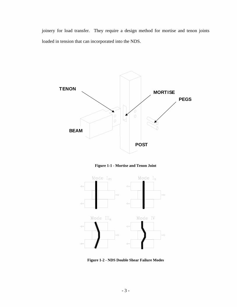
- 3 -
joinery for load transfer. They require a design method for mortise and tenon joints
loaded in tension that can incorporated into the NDS.
Figure 1-1 - Mortise and Tenon Joint
Figure 1-2 - NDS Double Shear Failure Modes
MORTISE PEGS
TENON
POST
BEAM

- 4 -
1.3 Literature Review
Research pertaining to timber framing, in general or in specifics, is very limited,
with most research having been conducted only in the last few years. The all-wood
connections employed in timber-framing render the research conducted on bolted post
and beam construction useful for only comparison’s sake.
Despite long traditions of using timber-frame structures in Europe, little
applicable research has been found, with the exception of research by Kessel and
Augustin in Germany (Kessel & Augustin, 1995) (Kessel & Augustin, 1996). Their work
focused on the tensile load capacity for mortise and tenon joints and appropriate design
values.
The first notable research conducted in the United States on timber frames was by
Brungraber, in which the frame behavior was studied with only limited review of
individual joint tests (Brungraber, 1985).
More recently, research conducted at the Michigan Technological University by
Reid included experimental studies of mortise and tenon joinery (Reid, 1997). These
tests were conducted on full-sized connections mocked up from dimension lumber. Reid
correlated experimental results to predictions from the European Yield Model (EYM)
equations for double shear connections, the current NDS standard. EYM Mode IIIs
predicted the yield load of the mortise and tenon joints quite well Failure modes in the
experimental specimens were similar to common failure modes witnessed in full-sized
mortise and tenon connections.
- 5 -
Drewek, also of the Michigan Technological University, conducted research
based on the modeling of a traditional timber frame bents. Strength parameters for the
individual joints were developed analytically, not experimentally (Drewek, 1997).
At the University of Wyoming, MacKay focused on modification of the EYM
failure modes to more accurately predict connections with wooden dowels (Schmidt and
MacKay, 1997). With the addition of various yield modes, the EYM could be used to
design pegged connections. Tests were also conducted to determine the mechanical
properties of the pegs commonly associated with mortise and tenon joinery. These tests
included dowel bearing, shear, and bending strengths of pegs.
Following MacKay’s work, Daniels conducted research on full-sized traditional
mortise and tenon joints (Schmidt and Daniels, 1999). This work included development
of detailing requirements, such as end and edge distances, to ensure a ductile peg failure.
Mechanical properties of the various materials, including dowel bearing, peg bending,
and peg shear strength were conducted. A method to relate the diameter of a peg to the
diameter of an equal-strength steel bolt was also developed. This allows for the direct
usage of the EYM equations for pegged joints.
Scholl, also of the University of Wyoming, expanded on previous work by
showing that draw-boring increases joint stiffness but does not alter a joint’s yield
capacity (Schmidt and Scholl, 2000). Most timber-framed buildings are constructed from
green timbers and loaded to at least partial capacity for extended amounts of time. Scholl
also explored seasoning and load-duration effects on full-sized joints. These tests resulted
in the modification of the detailing requirements developed by Daniels.

- 6 -
Erikson conducted research on single- and multiple-story bents subjected to
lateral load (Erikson, 2003). Bents covered with stress-skin panels were also tested, and
frame stiffness parameters were developed. No work was performed to isolate behavior
of the individual joints.
Although most finite element modeling of dowel-connected wooden joints had
focused on the use of a steel dowel, by changing material properties, the research
becomes applicable to wooden pegged mortise and tenon joints. Patton-Mallory and her
colleagues studied nonlinear material models for bolted connections and developed a tri-
linear stress-strain constitutive model for the wood behavior (Patton-Mallory et al.,
1997). They developed a three-dimensional model of a bolted wooden connection that
closely followed experimental load deflection curves.
Kharouf, McClure, and Smith also developed an elasto-plastic model for bolted
wood connections loaded in both tension and compression. They derived their
constitutive model from mechanics of materials theories and included anisotropic
hardening. When compared to experimental results, the numerical model slightly over
predicted the stiffness of the joint (Kharouf et al., 2003).
Chen, Lee, and Jeng also explored timber joints with dowel-type fasteners using
the finite element method. They used Hooke’s law to describe the stress-strain
relationship for both normal and fiberglass reinforced joints with a metal dowel fastener.
Experimental results compared fairly well with the models (Chen et al., 2003).

- 7 -
1.4 Objectives and Scope of Work
The primary goal of this research is to develop a design method for pegged
mortise and tenon joints loaded in tension. An accepted design method will give
engineers and designers more confidence in using mortise and tenon joints in tension.
The design method developed here is based on a correlation between the specific
gravities of the wood and the allowable shear stress in the pegs. The correlation is
developed with data from new and previously conducted physical testing of joints, as
well as with data from finite element analyses. The completed design method allows for
the determination of the load capacity of a pegged joint, whether or not physical or
numerical testing has been conducted on that combination of peg and base material.
The secondary goal of this research is to continue previous work conducted at the
University of Wyoming in developing minimum detailing requirements for pegged
mortise and tenon joints. Specifically, detailing requirements for yellow poplar were
developed. This included determining the suitability of yellow poplar as a timber
framing material. Yellow poplar is an eastern hardwood that is fast growing, straight,
easy to work, and economical. Yet yellow poplar has not been used as a timber framing
material in recent times. By conducting physical testing on yellow poplar mortise and
tenon joints, a comparison can be made to other common species, and possibly
confidence can be instilled in using this plentiful and underutilized resource.

- 8 -
2.0 Testing Procedures and Results
Testing consisted of four different types of tests. The first and most extensive
tests were conduced on mortise and tenon joints with the tenon loaded in tension. Tests
were also conducted on the shear loading of a tenon where the load was transferred
through the pegs. Joints were also tested in shear where the tenon beared directly in the
mortise. Dowel bearing tests, used to determine the dowel bearing strength of wood,
were also conducted.
Moisture content and specific gravity tests were conducted on each of the test
specimens used in all of the physical testing, including tensile, shear, direct tenon
bearing, and dowel bearing tests. The moisture content testing was conducted following
ASTM D4442. Samples were cut from the specimens immediately following testing,
weighed, measured and oven-dried for 24 hours. Specific gravity tests, following ASTM
D2395, were conducted with the same samples as in the moisture content test.
2.1 Joint Tests
2.1.1 Tension Testing
2.1.1.1 Introduction
Full-sized joints were tested to determine the strength and stiffness of mortise and
tenon joints tested in tension and shear. The species Liriodendron tulipifera, commonly
known as yellow or tulip poplar, was used for the base material for two main reasons.
First, its specific gravity fills in a gap in data collected previously at the University of
Wyoming. This additional data helped in development of a correlation between the

- 9 -
specific gravity of the joint material, that of the pegs, and the strength of a joint.
Secondly, the feasibility of using yellow poplar in timber framed structures was explored
because of its historical usage in covered bridges and its availability in the eastern and
midwestern United States.
Tension testing consisted of applying a tension force to a tenoned member to
withdraw it from its connection to a mortised member. The connection was secured with
wooden pegs (Figure 2-1). This type of loading can be developed in a timber-framed
structure during lateral loading.
Figure 2-1 - Tension Loading of Mortise and Tenon Joint
2.1.1.2 Procedure
Tension testing on full-sized mortise and tenon joints was conducted using a steel
load frame (Figure 2-2) and an Enerpac RCH 123 hydraulic ram operated by a hand
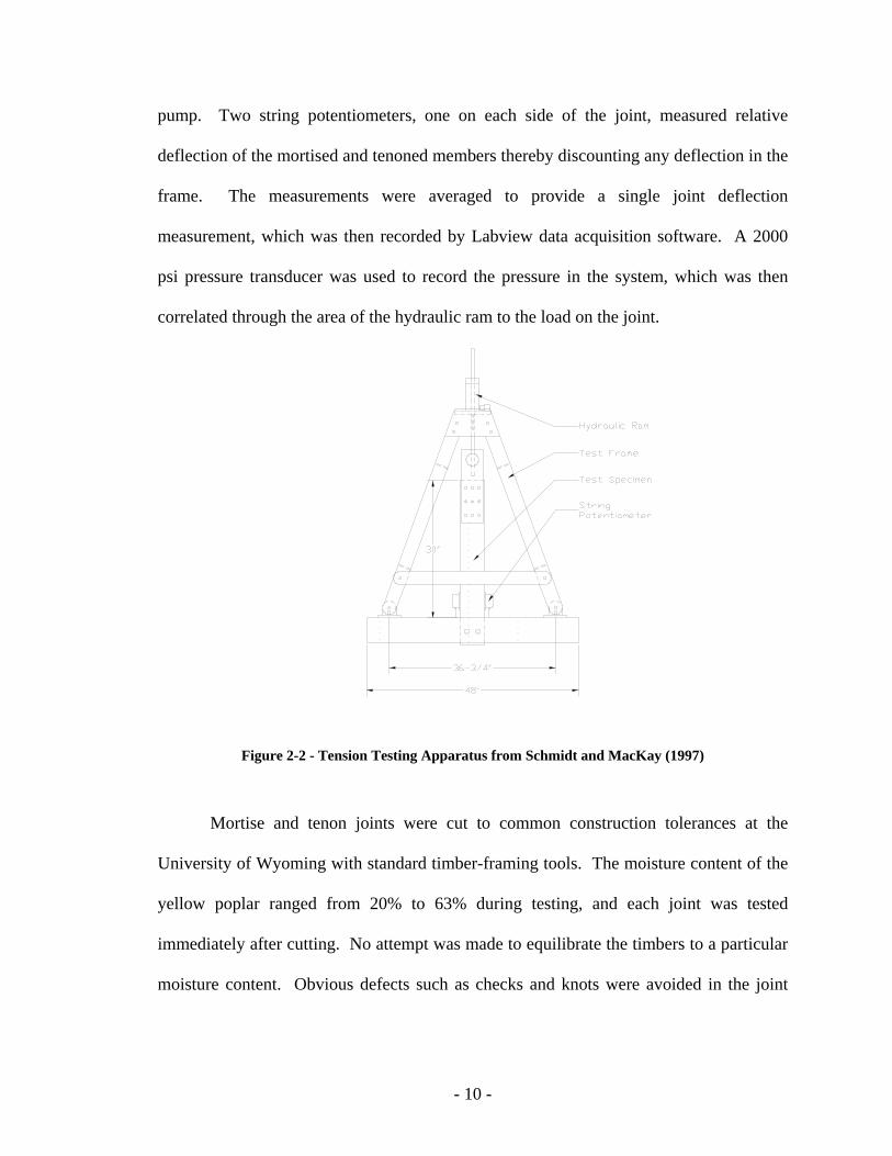
- 10 -
pump. Two string potentiometers, one on each side of the joint, measured relative
deflection of the mortised and tenoned members thereby discounting any deflection in the
frame. The measurements were averaged to provide a single joint deflection
measurement, which was then recorded by Labview data acquisition software. A 2000
psi pressure transducer was used to record the pressure in the system, which was then
correlated through the area of the hydraulic ram to the load on the joint.
Figure 2-2 - Tension Testing Apparatus from Schmidt and MacKay (1997)
Mortise and tenon joints were cut to common construction tolerances at the
University of Wyoming with standard timber-framing tools. The moisture content of the
yellow poplar ranged from 20% to 63% during testing, and each joint was tested
immediately after cutting. No attempt was made to equilibrate the timbers to a particular
moisture content. Obvious defects such as checks and knots were avoided in the joint

- 11 -
area whenever possible. Varying species of pegs, including red oak, white oak, sugar
maple, white ash, and paper birch, were used. All pegs were nominally one inch in
diameter and at an average moisture content of 6.8%.
The tenon thickness was varied between tests from 1.5 to 2 inches, the common
tenon thicknesses for hardwoods and softwoods, respectively. This was to help
determine if yellow poplar, being a relatively soft hardwood, behaved more like a
hardwood or like a softwood.
In addition to strength and stiffness data for the yellow poplar joints, detailing
requirements were also developed to ensure that peg failure preceded member failure.
End (le), edge (lv), and spacing (ls) distances were varied accordingly (Figure 2-3). Pegs
fail in a somewhat ductile manner, whereas failure of the tenon relish or the mortise
cheeks occurs in a sudden and brittle fashion. By ensuring peg failures, a joint can be
repaired after an extreme loading event by replacing the damaged pegs. Joints were
tested with excessive end, edge, and spacing distances to ensure peg failure in the joints
tested first. The detailing was then modified in subsequent tests until relish and mortise
cheek failures occurred, and then backed off for the minimum detailing requirements.
Figure 2-3 - Joint Detailing
- 12 -
Load was applied to the joints at a uniform stroke rate in an attempt to reach
failure in 10 minutes. After failure, the joint was disassembled and inspected to
determine the mode of failure. Several joints were retested using different species of
pegs if there was little or no visible dowel bearing failure in the timbers.
Two joints were loaded cyclically to obtain hysteresis data. The joints were
loaded and unloaded in increasing increments of 0.05 inches until failure. Failure was
determined as when the joint would no longer take on any more load.
2.1.1.3 Joint Failures
Of the twenty-two tests performed on eighteen different yellow poplar joints, four
failure modes were observed during the testing, two in the timber material, two in the
peg. The first timber failure was splitting of the mortised member due to tension
perpendicular to the grain. The load-limiting split started from the peg hole and
propagated outward (Figure 2-4a). The split usually occurred suddenly and audibly, and
continued to grow as the joint was deflected farther. This failure occurred because of
inadequate edge distance on the mortised member.
The other timber failure is known as a relish failure and can either be a single
split, which develops on the end of the tenon behind the peg hole, or a block rupture
failure of the material behind the peg hole (Figure 2-4b). The splitting failure was load
limiting but allowed the joint to hold the failure load. Dual block rupture failures resulted
in loss of load capacity in the joint. Both of these failures, which can occur behind one or
both of the pegs or in combination, are caused from inadequate end distance on the tenon.
- 13 -
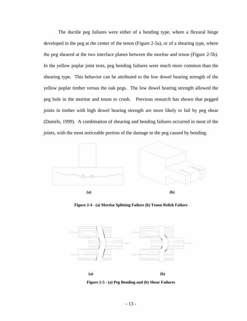
The ductile peg failures were either of a bending type, where a flexural hinge
developed in the peg at the center of the tenon (Figure 2-5a), or of a shearing type, where
the peg sheared at the two interface planes between the mortise and tenon (Figure 2-5b).
In the yellow poplar joint tests, peg bending failures were much more common than the
shearing type. This behavior can be attributed to the low dowel bearing strength of the
yellow poplar timber versus the oak pegs. The low dowel bearing strength allowed the
peg hole in the mortise and tenon to crush. Previous research has shown that pegged
joints in timber with high dowel bearing strength are more likely to fail by peg shear
(Daniels, 1999). A combination of shearing and bending failures occurred in most of the
joints, with the most noticeable portion of the damage to the peg caused by bending.
Figure 2-4 - (a) Mortise Splitting Failure (b) Tenon Relish Failure
Figure 2-5 - (a) Peg Bending and (b) Shear Failures
(a) (b)
(a) (b)

- 14 -
2.1.1.4 5% Offset Analysis
Following ASTM D5652 and ASTM D5764, which are for bolted wood
connections, a 5% offset yield method was used in determining the yield load for each of
the joint tests. To determine the yield load, the initial linear portion of the load-deflection
curve is identified, and then a line with the same slope as the initial linear portion is offset
along the deflection axis 5% of the dowel-connector diameter. The point where this offset
line intercepts the load deflection curve is defined as the yield point. If the offset line
does not intersect the load deflection curve, then the maximum load the joint reaches is
taken as the yield load. Figure 2-6 depicts a load-deflection plot with the 5% offset yield
value.
Due to the nature of load-deflection plots for mortise and tenon joints, choosing
the initial linear portion of the curve is somewhat subjective. To limit the variability in
choosing the initial linear portion, the two data points chosen to describe the line were
taken as far apart on the curve as possible. A line was then plotted between these two
points to ensure that it did in fact describe the linear portion of the plot.
Load vs Deflection YP15
5858
0
1000
2000
3000
4000
5000
6000
7000
8000
0 0.05 0.1 0.15 0.2 0.25 0.3
Deflection
Load
5% DIAMETER OFFSET LINE
Figure 2-6 - Five Percent Offset Yield
- 15 -
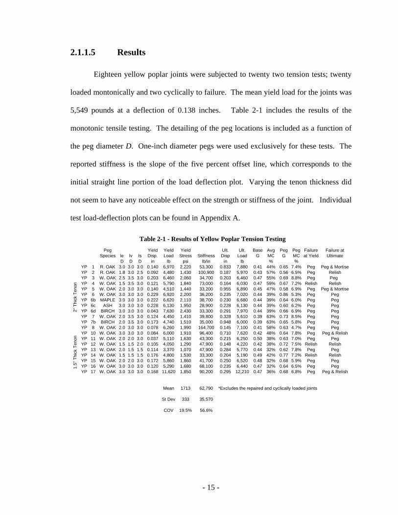
2.1.1.5 Results
Eighteen yellow poplar joints were subjected to twenty two tension tests; twenty
loaded montonically and two cyclically to failure. The mean yield load for the joints was
5,549 pounds at a deflection of 0.138 inches. Table 2-1 includes the results of the
monotonic tensile testing. The detailing of the peg locations is included as a function of
the peg diameter D. One-inch diameter pegs were used exclusively for these tests. The
reported stiffness is the slope of the five percent offset line, which corresponds to the
initial straight line portion of the load deflection plot. Varying the tenon thickness did
not seem to have any noticeable effect on the strength or stiffness of the joint. Individual
test load-deflection plots can be found in Appendix A.
Table 2-1 - Results of Yellow Poplar Tension Testing Peg
Species le lv lsYield Disp.
Yield Load
Yield Stress Stiffness
Ult. Disp
Ult. Load
Base G
Avg MC
Peg G
Peg MC
Failure at Yield
Failure at Ultimate
D D D in lb psi lb/in in lb % %YP 1 R. OAK 3.0 3.0 3.0 0.140 6,970 2,220 53,300 0.833 7,880 0.41 44% 0.65 7.4% Peg Peg & MortiseYP 2 R. OAK 1.8 3.0 2.5 0.092 4,480 1,430 100,900 0.187 5,970 0.43 57% 0.56 6.5% Peg RelishYP 3 W. OAK 2.5 3.5 3.0 0.203 6,460 2,060 34,700 0.203 6,460 0.47 55% 0.69 8.8% Peg Peg YP 4 W. OAK 1.5 3.5 3.0 0.121 5,790 1,840 73,000 0.164 6,030 0.47 59% 0.67 7.2% Relish RelishYP 5 W. OAK 2.0 3.0 3.0 0.140 4,510 1,440 33,200 0.955 6,890 0.45 47% 0.58 6.9% Peg Peg & MortiseYP 6 W. OAK 3.0 3.0 3.0 0.229 6,920 2,200 36,200 0.235 7,020 0.44 39% 0.86 5.3% Peg PegYP 6b MAPLE 3.0 3.0 3.0 0.222 6,620 2,110 38,700 0.230 6,680 0.44 39% 0.64 6.0% Peg PegYP 6c ASH 3.0 3.0 3.0 0.228 6,130 1,950 28,900 0.228 6,130 0.44 39% 0.60 6.2% Peg PegYP 6d BIRCH 3.0 3.0 3.0 0.043 7,630 2,430 33,300 0.291 7,970 0.44 39% 0.66 6.9% Peg PegYP 7 W. OAK 2.0 3.5 3.0 0.124 4,450 1,410 39,800 0.328 5,610 0.39 63% 0.73 8.5% Peg PegYP 7b BIRCH 2.0 3.5 3.0 0.173 4,740 1,510 35,000 0.948 6,000 0.39 63% 0.65 5.8% Peg PegYP 8 W. OAK 2.0 3.0 3.0 0.078 6,260 1,990 164,700 0.145 7,100 0.41 58% 0.63 4.7% Peg PegYP 10 W. OAK 3.0 3.0 3.0 0.084 6,000 1,910 96,400 0.710 7,620 0.42 48% 0.64 7.8% Peg Peg & RelishYP 11 W. OAK 2.0 2.0 3.0 0.037 5,110 1,630 43,300 0.215 6,250 0.50 38% 0.63 7.0% Peg PegYP 12 W. OAK 1.5 1.5 2.0 0.105 4,050 1,290 47,900 0.148 4,220 0.42 38% 0.72 7.5% Relish RelishYP 13 W. OAK 2.0 1.5 1.5 0.114 3,370 1,070 47,900 0.284 5,770 0.44 32% 0.62 7.8% Peg PegYP 14 W. OAK 1.5 1.5 1.5 0.176 4,800 1,530 33,300 0.204 5,190 0.49 42% 0.77 7.2% Relish RelishYP 15 W. OAK 2.0 2.0 3.0 0.172 5,860 1,860 41,700 0.250 6,520 0.48 32% 0.68 5.9% Peg PegYP 16 W. OAK 3.0 3.0 3.0 0.120 5,290 1,680 68,100 0.235 6,440 0.47 32% 0.64 6.5% Peg PegYP 17 W. OAK 3.0 3.0 3.0 0.168 11,620 1,850 90,200 0.295 12,210 0.47 36% 0.68 6.8% Peg Peg & Relish
Mean 1713 62,790 *Excludes the repaired and cyclically loaded joints
St Dev 333 35,570
COV 19.5% 56.6%
2" T
hick
Ten
on1.
5" T
hick
Ten
on

- 16 -
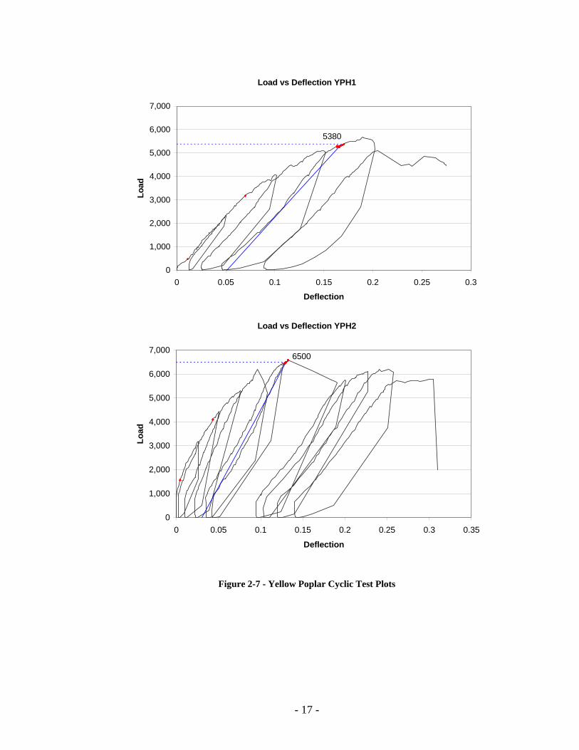
Previous research has shown that joints loaded cyclically perform in a similar
fashion to monotonically loaded joints (Schmidt and Daniels, 1999). In this research, the
cyclic hysterisis tests were conducted to determine if the pegged mortise and tenon joints
in yellow poplar maintained their ductile behavior even with repeated loading. As each
joint was loaded in a subsequent cycle, the envelope of the load-deflection curve closely
matched that of the monotonic tension tests loaded to failure in a single cycle (Figure
2-7). This suggests there is enough toughness in these timber joints to withstand repeated
loading cycles. The mean yield load for two cyclically loaded joints was 5,940 pounds;
slightly higher than the monotonically loaded joints. Other pertinent results of the
hysterisis tests are included in Table 2-2.
Both of the cyclically loaded joints had white oak pegs. The 2.0 inch thick tenon
had 3.5 inches of relish, while the pegs were spaced 2.0 inches apart and placed 2.0
inches from the edge of the mortise.
Table 2-2 - Results of Cyclic Testing of Yellow Poplar Yield Disp.
Yield Load
Yield Stress Stiffness
Ult. Disp
Ult. Load
Base G
Avg MC
Peg G
Peg MC
Failure at Yield
Failure at Ultimate
in lb psi lb/in in lb % %H1 0.163 5,380 1,710 46,100 0.190 5,670 0.461 6.1% 0.64 6.6% Peg PegH2 0.130 6,500 2,070 65,100 0.133 6,590 0.492 11.2% 0.71 7.2% Peg Peg
Mean 1,890 55,600
St. Dev 255 13435
COV 13.5% 24.2%
- 17 -
Load vs Deflection YPH1
5380
0
1,000
2,000
3,000
4,000
5,000
6,000
7,000
0 0.05 0.1 0.15 0.2 0.25 0.3
Deflection
Load
Load vs Deflection YPH2
6500
0
1,000
2,000
3,000
4,000
5,000
6,000
7,000
0 0.05 0.1 0.15 0.2 0.25 0.3 0.35
Deflection
Load
Figure 2-7 - Yellow Poplar Cyclic Test Plots
- 18 -
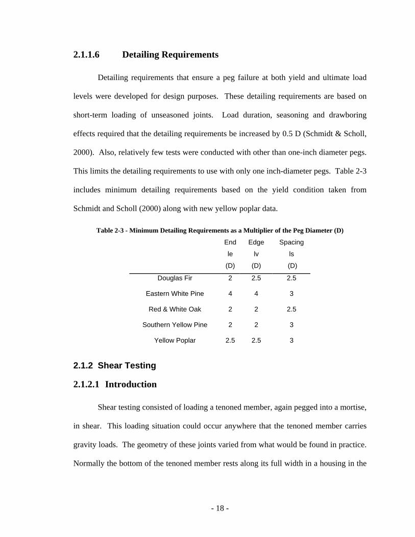
2.1.1.6 Detailing Requirements
Detailing requirements that ensure a peg failure at both yield and ultimate load
levels were developed for design purposes. These detailing requirements are based on
short-term loading of unseasoned joints. Load duration, seasoning and drawboring
effects required that the detailing requirements be increased by 0.5 D (Schmidt & Scholl,
2000). Also, relatively few tests were conducted with other than one-inch diameter pegs.
This limits the detailing requirements to use with only one inch-diameter pegs. Table 2-3
includes minimum detailing requirements based on the yield condition taken from
Schmidt and Scholl (2000) along with new yellow poplar data.
Table 2-3 - Minimum Detailing Requirements as a Multiplier of the Peg Diameter (D)
End
le
(D)
Edge
lv
(D)
Spacing
ls
(D)
Douglas Fir 2 2.5 2.5
Eastern White Pine 4 4 3
Red & White Oak 2 2 2.5
Southern Yellow Pine 2 2 3
Yellow Poplar 2.5 2.5 3
2.1.2 Shear Testing
2.1.2.1 Introduction
Shear testing consisted of loading a tenoned member, again pegged into a mortise,
in shear. This loading situation could occur anywhere that the tenoned member carries
gravity loads. The geometry of these joints varied from what would be found in practice.
Normally the bottom of the tenoned member rests along its full width in a housing in the
- 19 -
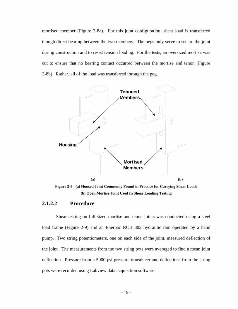
mortised member (Figure 2-8a). For this joint configuration, shear load is transferred
though direct bearing between the two members. The pegs only serve to secure the joint
during construction and to resist tension loading. For the tests, an oversized mortise was
cut to ensure that no bearing contact occurred between the mortise and tenon (Figure
2-8b). Rather, all of the load was transferred through the peg.
Figure 2-8 - (a) Housed Joint Commonly Found in Practice for Carrying Shear Loads
(b) Open Mortise Joint Used In Shear Loading Testing
2.1.2.2 Procedure
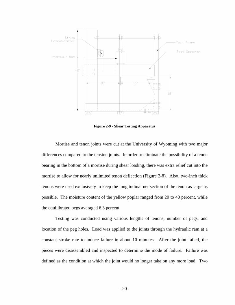
Shear testing on full-sized mortise and tenon joints was conducted using a steel
load frame (Figure 2-9) and an Enerpac RCH 302 hydraulic ram operated by a hand
pump. Two string potentiometers, one on each side of the joint, measured deflection of
the joint. The measurements from the two string pots were averaged to find a mean joint
deflection. Pressure from a 5000 psi pressure transducer and deflections from the string
pots were recorded using Labview data acquisition software.
(a) (b)
Tenoned Members
Mortised Members
Housing
- 20 -
Figure 2-9 - Shear Testing Apparatus
Mortise and tenon joints were cut at the University of Wyoming with two major
differences compared to the tension joints. In order to eliminate the possibility of a tenon
bearing in the bottom of a mortise during shear loading, there was extra relief cut into the
mortise to allow for nearly unlimited tenon deflection (Figure 2-8). Also, two-inch thick
tenons were used exclusively to keep the longitudinal net section of the tenon as large as
possible. The moisture content of the yellow poplar ranged from 20 to 40 percent, while
the equilibrated pegs averaged 6.3 percent.
Testing was conducted using various lengths of tenons, number of pegs, and
location of the peg holes. Load was applied to the joints through the hydraulic ram at a
constant stroke rate to induce failure in about 10 minutes. After the joint failed, the
pieces were disassembled and inspected to determine the mode of failure. Failure was
defined as the condition at which the joint would no longer take on any more load. Two

- 21 -
joints were retested using different species of pegs when inspection showed only peg
failures. Moisture content and specific gravity tests were then performed on specimens
taken from each member.
2.1.2.3 Joint Failures
Twelve tests were performed on eight different joints; only two distinct failure
modes occurred. The most common and least desirable failure mode was tenon splitting
due to tension perpendicular to grain, always through the bottom peg hole (Figure 2-10).
A few rolling shear failures also occurred in combination with the tenon splitting failures
(Figure 2-11). Tenon splitting failures occurred even when only one peg was used.
In a few instances in which long through tenons were used, pegs failed in the
same bending fashion as occurred in the tension testing. There were no shear failures of
the pegs, possibly due to the low dowel bearing strength perpendicular to grain in the
tenon.
Figure 2-10 – Tenon Splitting Failure During Shear Loading

- 22 -
Figure 2-11 - Rolling Shear Failure of Tenon in Shear Loading
2.1.2.4 Results
Five-percent offset yield load analyses were conducted on each of the tests
following the method outlined in the tension testing. This yield data is listed in Table 2-4
along with the joint detailing and failure modes. Load-deflection plots can be found in
Appendix B. The extremely long tenons required to achieve pure peg failures made it
impractical to recommend detailing requirements for these joints. Placing the pegs lower
in the tenon did help increase the strength of the joint. However, the small sample size
made it difficult for a conclusive relation to be drawn. Based on these tests though, it is
clear that shear loads are more appropriately carried through direct bearing in housed
joints (Figure 2-8a) than by load transfer through pegs.
- 23 -
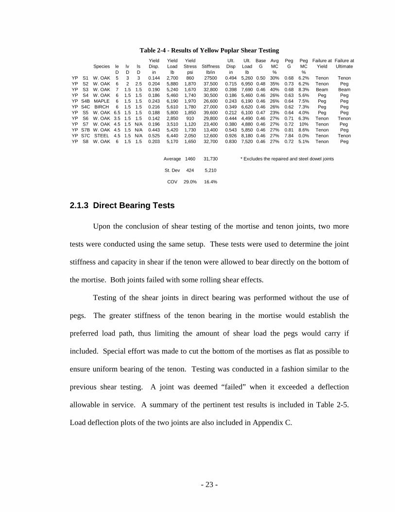
Table 2-4 - Results of Yellow Poplar Shear Testing
Species le lv lsYield Disp.
Yield Load
Yield Stress Stiffness
Ult. Disp
Ult. Load
Base G
Avg MC
Peg G
Peg MC
Failure at Yield
Failure at Ultimate
D D D in lb psi lb/in in lb % %YP S1 W. OAK 5 3 3 0.144 2,700 860 27500 0.494 5,260 0.50 30% 0.68 6.2% Tenon TenonYP S2 W. OAK 6 2 2.5 0.204 5,880 1,870 37,500 0.715 6,950 0.48 35% 0.73 6.2% Tenon PegYP S3 W. OAK 7 1.5 1.5 0.190 5,240 1,670 32,800 0.398 7,690 0.46 40% 0.68 8.3% Beam BeamYP S4 W. OAK 6 1.5 1.5 0.186 5,460 1,740 30,500 0.186 5,460 0.46 26% 0.63 5.6% Peg PegYP S4B MAPLE 6 1.5 1.5 0.243 6,190 1,970 26,600 0.243 6,190 0.46 26% 0.64 7.5% Peg PegYP S4C BIRCH 6 1.5 1.5 0.216 5,610 1,780 27,000 0.349 6,620 0.46 26% 0.62 7.3% Peg PegYP S5 W. OAK 6.5 1.5 1.5 0.188 5,800 1,850 39,600 0.212 6,100 0.47 23% 0.64 4.0% Peg PegYP S6 W. OAK 3.5 1.5 1.5 0.142 2,850 910 29,800 0.444 4,490 0.46 27% 0.71 6.3% Tenon TenonYP S7 W. OAK 4.5 1.5 N/A 0.196 3,510 1,120 23,400 0.380 4,880 0.46 27% 0.72 10% Tenon Peg YP S7B W. OAK 4.5 1.5 N/A 0.443 5,420 1,730 13,400 0.543 5,850 0.46 27% 0.81 8.6% Tenon PegYP S7C STEEL 4.5 1.5 N/A 0.525 6,440 2,050 12,600 0.926 8,180 0.46 27% 7.84 0.0% Tenon TenonYP S8 W. OAK 6 1.5 1.5 0.203 5,170 1,650 32,700 0.830 7,520 0.46 27% 0.72 5.1% Tenon Peg
Average 1460 31,730 * Excludes the repaired and steel dowel joints
St. Dev 424 5,210
COV 29.0% 16.4%
2.1.3 Direct Bearing Tests
Upon the conclusion of shear testing of the mortise and tenon joints, two more
tests were conducted using the same setup. These tests were used to determine the joint
stiffness and capacity in shear if the tenon were allowed to bear directly on the bottom of
the mortise. Both joints failed with some rolling shear effects.
Testing of the shear joints in direct bearing was performed without the use of
pegs. The greater stiffness of the tenon bearing in the mortise would establish the
preferred load path, thus limiting the amount of shear load the pegs would carry if
included. Special effort was made to cut the bottom of the mortises as flat as possible to
ensure uniform bearing of the tenon. Testing was conducted in a fashion similar to the
previous shear testing. A joint was deemed “failed” when it exceeded a deflection
allowable in service. A summary of the pertinent test results is included in Table 2-5.
Load deflection plots of the two joints are also included in Appendix C.
- 24 -
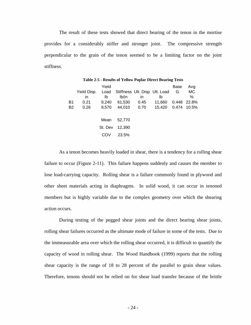
The result of these tests showed that direct bearing of the tenon in the mortise
provides for a considerably stiffer and stronger joint. The compressive strength
perpendicular to the grain of the tenon seemed to be a limiting factor on the joint
stiffness.
Table 2-5 - Results of Yellow Poplar Direct Bearing Tests
Yield Disp.Yield Load Stiffness Ult. Disp Ult. Load
Base G
Avg MC
in lb lb/in in lb %B1 0.21 9,240 61,530 0.45 11,660 0.448 22.8%B2 0.26 9,570 44,010 0.70 15,420 0.474 10.5%
Mean 52,770
St. Dev 12,390
COV 23.5%
As a tenon becomes heavily loaded in shear, there is a tendency for a rolling shear
failure to occur (Figure 2-11). This failure happens suddenly and causes the member to
lose load-carrying capacity. Rolling shear is a failure commonly found in plywood and
other sheet materials acting in diaphragms. In solid wood, it can occur in tenoned
members but is highly variable due to the complex geometry over which the shearing
action occurs.
During testing of the pegged shear joints and the direct bearing shear joints,
rolling shear failures occurred as the ultimate mode of failure in some of the tests. Due to
the immeasurable area over which the rolling shear occurred, it is difficult to quantify the
capacity of wood in rolling shear. The Wood Handbook (1999) reports that the rolling
shear capacity is the range of 18 to 28 percent of the parallel to grain shear values.
Therefore, tenons should not be relied on for shear load transfer because of the brittle
- 25 -
failure mode. Rather, shear transfer is better achieved through housed joints (Figure
2-8a).
2.2 Dowel Bearing Tests
The purpose of dowel bearing tests is to determine the resistance of a specific
wood species to deformation when loaded with a dowel shaped fastener. Due to the
orthotropic nature of wood, the dowel bearing capacity is different when tested parallel to
grain than when tested perpendicular to grain. Lower dowel bearing strength in the
timbers suggest that there will be more bending-type failures of wood pegs rather than
shear failures.
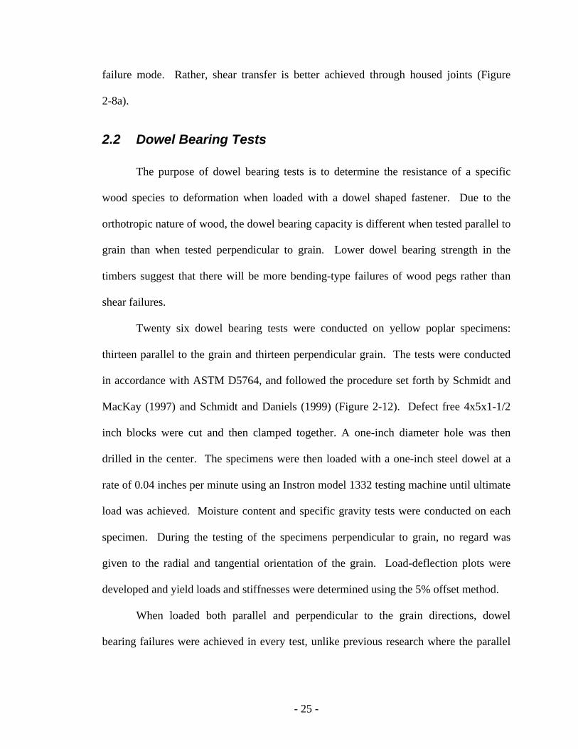
Twenty six dowel bearing tests were conducted on yellow poplar specimens:
thirteen parallel to the grain and thirteen perpendicular grain. The tests were conducted
in accordance with ASTM D5764, and followed the procedure set forth by Schmidt and
MacKay (1997) and Schmidt and Daniels (1999) (Figure 2-12). Defect free 4x5x1-1/2
inch blocks were cut and then clamped together. A one-inch diameter hole was then
drilled in the center. The specimens were then loaded with a one-inch steel dowel at a
rate of 0.04 inches per minute using an Instron model 1332 testing machine until ultimate
load was achieved. Moisture content and specific gravity tests were conducted on each
specimen. During the testing of the specimens perpendicular to grain, no regard was
given to the radial and tangential orientation of the grain. Load-deflection plots were
developed and yield loads and stiffnesses were determined using the 5% offset method.
When loaded both parallel and perpendicular to the grain directions, dowel
bearing failures were achieved in every test, unlike previous research where the parallel
- 26 -
to grain specimens split longitudinally. Results of the dowel bearing tests can be found
in Appendix D. For parallel-to-grain loading, yellow poplar was 3.5 times stiffer and 2.2
times stronger at yield than for perpendicular to grain loading.
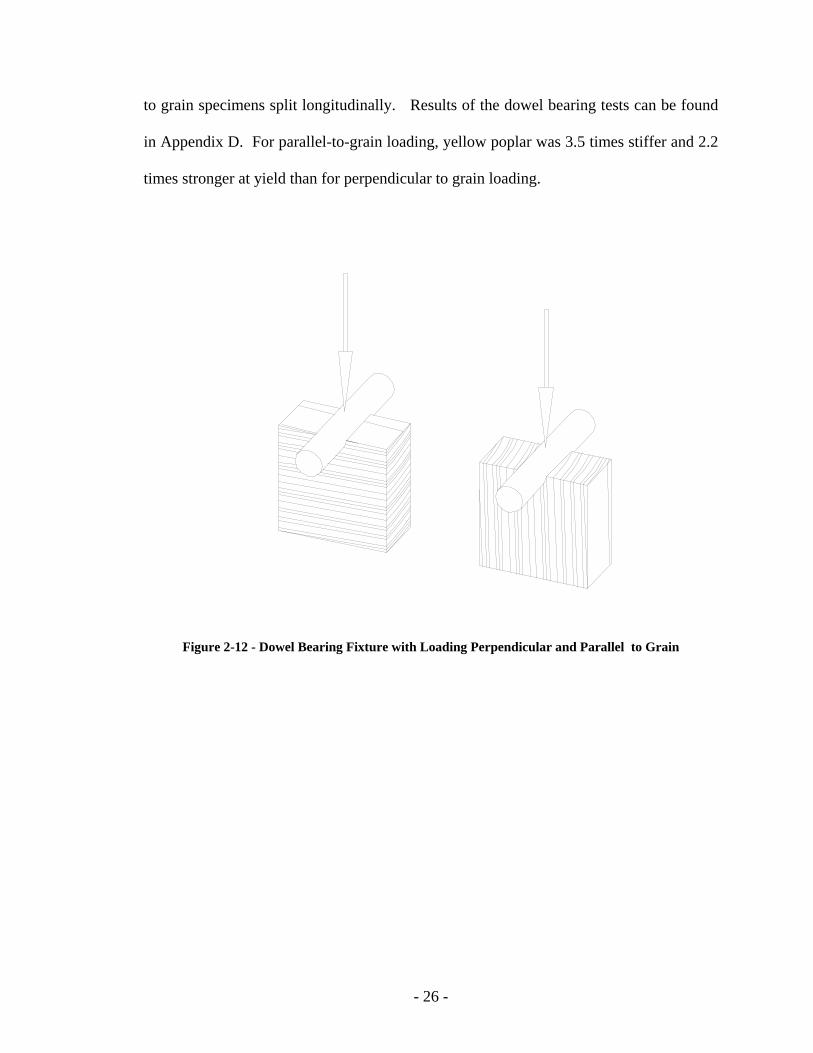
Figure 2-12 - Dowel Bearing Fixture with Loading Perpendicular and Parallel to Grain
- 27 -
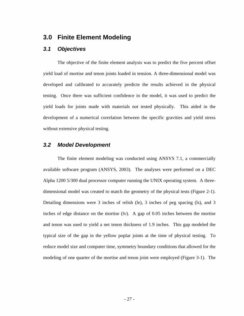
3.0 Finite Element Modeling
3.1 Objectives
The objective of the finite element analysis was to predict the five percent offset
yield load of mortise and tenon joints loaded in tension. A three-dimensional model was
developed and calibrated to accurately predicte the results achieved in the physical
testing. Once there was sufficient confidence in the model, it was used to predict the
yield loads for joints made with materials not tested physically. This aided in the
development of a numerical correlation between the specific gravities and yield stress
without extensive physical testing.
3.2 Model Development
The finite element modeling was conducted using ANSYS 7.1, a commercially
available software program (ANSYS, 2003). The analyses were performed on a DEC
Alpha 1200 5/300 dual processor computer running the UNIX operating system. A three-
dimensional model was created to match the geometry of the physical tests (Figure 2-1).
Detailing dimensions were 3 inches of relish (le), 3 inches of peg spacing (ls), and 3
inches of edge distance on the mortise (lv). A gap of 0.05 inches between the mortise
and tenon was used to yield a net tenon thickness of 1.9 inches. This gap modeled the
typical size of the gap in the yellow poplar joints at the time of physical testing. To
reduce model size and computer time, symmetry boundary conditions that allowed for the
modeling of one quarter of the mortise and tenon joint were employed (Figure 3-1). The
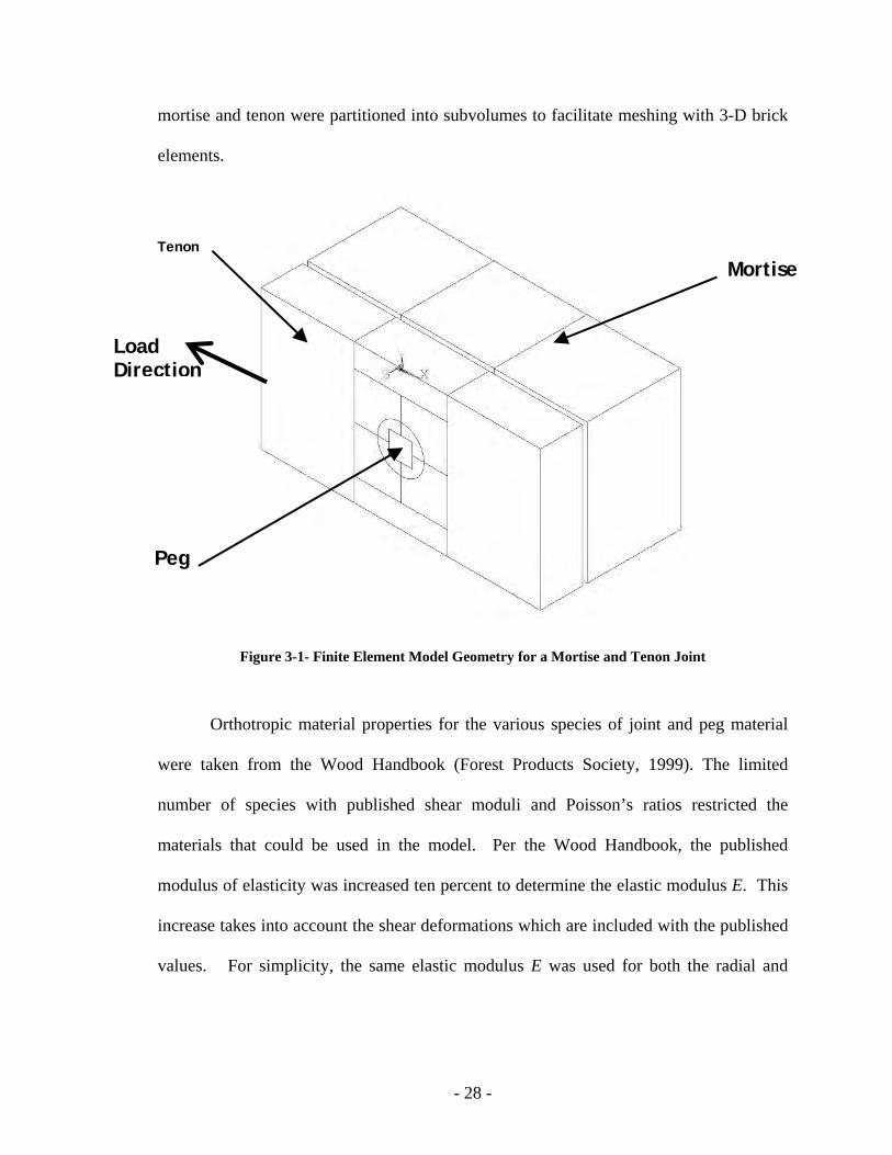
- 28 -
mortise and tenon were partitioned into subvolumes to facilitate meshing with 3-D brick
elements.
Figure 3-1- Finite Element Model Geometry for a Mortise and Tenon Joint
Orthotropic material properties for the various species of joint and peg material
were taken from the Wood Handbook (Forest Products Society, 1999). The limited
number of species with published shear moduli and Poisson’s ratios restricted the
materials that could be used in the model. Per the Wood Handbook, the published
modulus of elasticity was increased ten percent to determine the elastic modulus E. This
increase takes into account the shear deformations which are included with the published
values. For simplicity, the same elastic modulus E was used for both the radial and
Tenon
Peg
Mortise
Load Direction
- 29 -
tangential directions. Likewise, a single Poisson’s ratio µ was used for the radial-
longitudinal and tangential-longitudinal planes.
A bilinear stress-strain relation was used to model the results from the dowel
bearing tests. The initial stiffness of the material loaded parallel to grain (tenon) was the
elastic modulus E with the tangent stiffness set at 0.5E. The initial stiffness for the
material loaded perpendicular to the grain (mortise and pegs) was again based on the
elastic modulus, but the tangent stiffness was closer to perfectly plastic, being 0.1E. The
yield strain for the material loaded parallel to grain was 0.01 inches per inch, while the
material loaded perpendicular to grain had a yield strain of 0.05 inches per inch. Figure
3-2 shows the shape of the assumed stress-strain relation compared to that from dowel
bearing tests. Table 3-1 lists the material constants used. The results of the analysis were
not changed significantly by variations to the tangent slope of the stress-strain curve of
the base materials. However, results were very sensitive to the tangent slope of the
stress-strain curve of the peg, due to the large stress concentrations in the pegs at the
mortise-tenon interface. The plasticity model was based on the von Mises yield criterion,
an associated flow rule, and isotropic hardening.
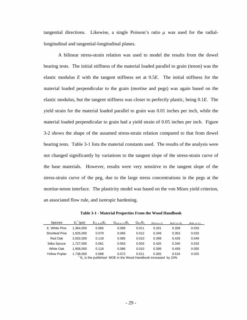
Table 3-1 - Material Properties From the Wood Handbook
Species EL1 (psi) E(T or R)/EL G(LR or LT)/EL GRT/EL µ(LR or LT) µ(RT or TR) µ(RL or TL)
E. White Pine 1,364,000 0.066 0.089 0.011 0.331 0.358 0.033 Shortleaf Pine 1,925,000 0.079 0.066 0.012 0.349 0.363 0.033
Red Oak 2,002,000 0.118 0.085 0.010 0.399 0.426 0.049 Sitka Spruce 1,727,000 0.061 0.063 0.003 0.420 0.340 0.033 White Oak 1,958,000 0.118 0.086 0.010 0.399 0.459 0.055
Yellow Poplar 1,738,000 0.068 0.072 0.011 0.355 0.516 0.025
1 EL is the published MOE in the Wood Handbook increased by 10%

- 30 -
0 0.01 0.02 0.03 0.04 0.05 0.06 0.07 0.08 0.09 0.1
Strain
Stre
ss
Typical Experimental
Idealized
1
E
1
E/10
(a) Stress-Strain Curve for Dowel Bearing Perpendicular to the Grain
0 0.01 0.02 0.03 0.04 0.05
Strain
Stre
ss
Typical Experimental Idealized
1
E
E/2
1
(b) Stress-Strain Curve for Dowel Bearing Parallel to the Grain
Figure 3-2 - Stress - Strain Curves Used in Finite Element Modeling

- 31 -
A mesh refinement study was conducted to determine the coarsest mesh that
could be used to obtain adequate results. Because macroscopic load-deflection behavior
was the information of interest, the applied load and the deflection at a node remote from
the peg location were used to evaluate convergence. A nonlinear-analysis was performed
on each model under a load of 3500 pounds. Mesh refinements were conducted by
changing the minimum number of divisions on the side of a volume. Some volumes had
more divisions to ensure compatibility with adjacent volumes. Figure 3-3 shows the
selected mesh density used for all of the models and Table 3-2 contains the results of the
mesh refinement study. The decreasing joint deflection with mesh refinement can be
attributed to the performance of the contact elements.
Figure 3-3 - Meshing of Mortise and Tenon Joint

- 32 -
Table 3-2 - Results of Mesh Refinement Study Using Orthotropic Yellow Poplar Properties and
Subjected to 3500 Pounds of Load
Element Division
Number of Elements
Number of Nodes
Joint Deflection
Run Time
1 470 1,410 0.284 15 sec 2 620 2,220 0.179 2 min 3 1,082 4,830 0.139 4 min 4 2,202 10,410 0.125 12 min (Used in modeling) 5 5,040 23,820 0.123 4 hours
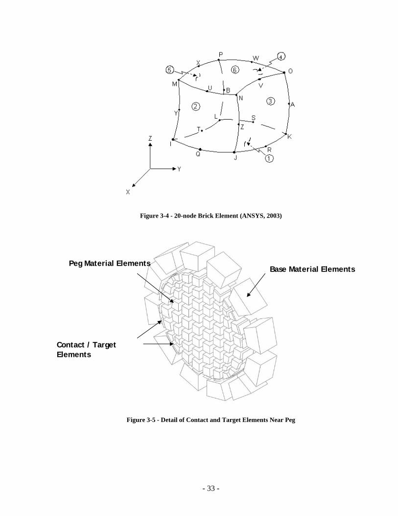
Twenty-node brick elements (Figure 3-4) with large-strain and non-linear
capability were used with a fourteen-point integration rule to model the timber and the
peg.
Contact elements were used wherever the peg might touch the mortise or tenon
(Figure 3-5). The contact elements had no tensile capacity, allowing for gaps to open in
various locations between the peg and the base material. Surface-to-surface contact
elements were used, which allow for surface discontinuities created by different mesh
densities. Figure 3-5 shows a detail of the peg / base material interface with the contact
elements that create compatibility between the two meshes.
- 33 -
Figure 3-4 - 20-node Brick Element (ANSYS, 2003)
Figure 3-5 - Detail of Contact and Target Elements Near Peg
Peg Material Elements Base Material Elements
Contact / Target Elements

- 34 -
After confirming that the model performed appropriately with linear isotropic and
linear orthotropic material properties, the non-linear stress-strain data was added into the
base model. The same geometric model was repeatedly modified with material
properties for the different species combinations. The tenon thicknesses in the physical
tests with oak timber were 1.5 inches. The model geometry was modified to take this
into account. The high dowel bearing capacity of the oak caused peg shearing type
failures and thus the thickness of the tenon had little effect on the yield strength.
Displacement constraints along symmetry planes were employed. The nodes
along the bottom of the mortise were confined from displacement. A unit pressure was
applied over the cross sectional area of the tenon. The average deflection of the nodes
over that area was recorded with the applied load to form a point on the load-deflection
curve. The load was incremented until yield occurred. The five-percent offset method
was used to determine the yield load for each joint model, at which point the analysis was
terminated.
3.3 Results
The model was calibrated by slightly modifying the yield strain of the stress-strain
curve. The changes were all within the variance of the stress-strain data from the dowel
bearing tests. Once the model was calibrated for yellow poplar, the stress-strain function
was not modified for the subsequent eight tests.
The yield load from the finite element models of the pegged mortise and tenon
joints corresponded well with those from physical testing, while the joint stiffnesses from
the models were softer than those from physical tests. The models tended to slightly over
- 35 -
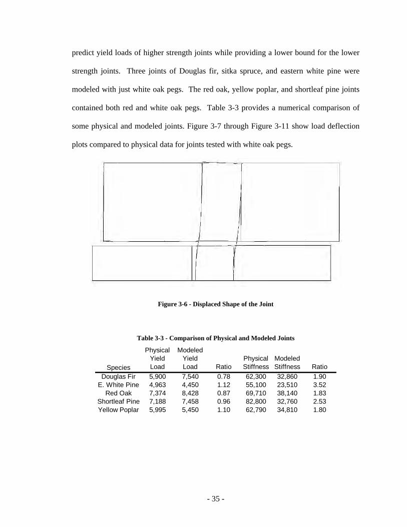
predict yield loads of higher strength joints while providing a lower bound for the lower
strength joints. Three joints of Douglas fir, sitka spruce, and eastern white pine were
modeled with just white oak pegs. The red oak, yellow poplar, and shortleaf pine joints
contained both red and white oak pegs. Table 3-3 provides a numerical comparison of
some physical and modeled joints. Figure 3-7 through Figure 3-11 show load deflection
plots compared to physical data for joints tested with white oak pegs.
Figure 3-6 - Displaced Shape of the Joint
Table 3-3 - Comparison of Physical and Modeled Joints
Species
Physical Yield Load
Modeled Yield Load Ratio
Physical Stiffness
Modeled Stiffness Ratio
Douglas Fir 5,900 7,540 0.78 62,300 32,860 1.90E. White Pine 4,963 4,450 1.12 55,100 23,510 3.52
Red Oak 7,374 8,428 0.87 69,710 38,140 1.83Shortleaf Pine 7,188 7,458 0.96 82,800 32,760 2.53Yellow Poplar 5,995 5,450 1.10 62,790 34,810 1.80

- 36 -
0
1000
2000
3000
4000
5000
6000
7000
8000
9000
10000
0 0.05 0.1 0.15 0.2 0.25 0.3 0.35
Deflection (in)
Load
(lb)
FEA CurveExperimental Curves
Figure 3-7 - Shortleaf Pine Physical and Modeled Load-Deflection Curves
0
1000
2000
3000
4000
5000
6000
7000
8000
9000
10000
0 0.05 0.1 0.15 0.2 0.25 0.3 0.35
Deflection (in)
Load
(lb)
FEA CurveExperimental Curves
Figure 3-8 - Red Oak Physical and Modeled Load-Deflection Curves
- 37 -
0
1000
2000
3000
4000
5000
6000
7000
8000
9000
10000
0 0.05 0.1 0.15 0.2 0.25 0.3 0.35
Deflection (in)
Load
(lb)
FEA CurveExperimental Curves
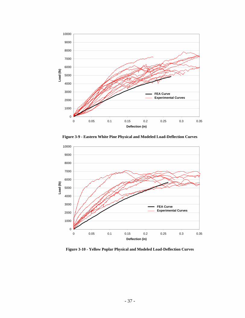
Figure 3-9 - Eastern White Pine Physical and Modeled Load-Deflection Curves
0
1000
2000
3000
4000
5000
6000
7000
8000
9000
10000
0 0.05 0.1 0.15 0.2 0.25 0.3 0.35
Deflection (in)
Load
(lb)
FEA CurveExperimental Curves
Figure 3-10 - Yellow Poplar Physical and Modeled Load-Deflection Curves

- 38 -
0
1000
2000
3000
4000
5000
6000
7000
8000
9000
10000
0 0.05 0.1 0.15 0.2 0.25 0.3 0.35
Deflection (in)
Load
(lb)
FEA CurveExperimental Curves
Figure 3-11 – Douglas Fir Physical and Modeled Load-Deflection Curves
3.4 Direct Bearing Joints
A finite element model was also created for a mortise and tenon joint loaded in
shear. That is to say, a shear load was applied to the tenon member such that the tenon
would bear directly on the bottom of the mortise. The geometry used in modeling the
direct bearing joints followed what was physically tested. To accurately represent the
physical tests, the shoulder of the tenon was kept 0.1 inches from the face of the mortised
member. The entire length of the tenoned member was included in the model. A single
plane of symmetry was used in the model, allowing for one-half of the joint to be
modeled (Figure 3-12). Orthotropic material properties were used as in the tensile joint
model described above, except both materials followed the bilinear stress-strain
distribution with the tangent stiffness of one-half the initial stiffness. The tangent
- 39 -
stiffness had minimal effect on the modeling due to the low strains that were developed.
In addition to the physically tested yellow poplar, models were created for eastern white
pine, shortleaf pine, and white oak to provide results for a good range of specific
gravities. Twenty-node brick and contact elements on the bearing surfaces of the tenon
and mortise were again used. No mesh refinement study was conducted, because the
same mesh density was used as in the pegged joint models, which had adequate
resolution.
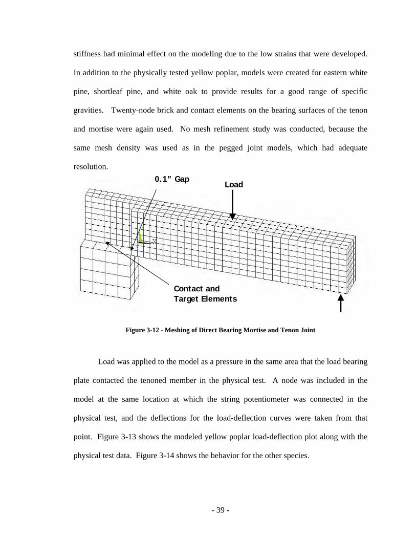
Figure 3-12 - Meshing of Direct Bearing Mortise and Tenon Joint
Load was applied to the model as a pressure in the same area that the load bearing
plate contacted the tenoned member in the physical test. A node was included in the
model at the same location at which the string potentiometer was connected in the
physical test, and the deflections for the load-deflection curves were taken from that
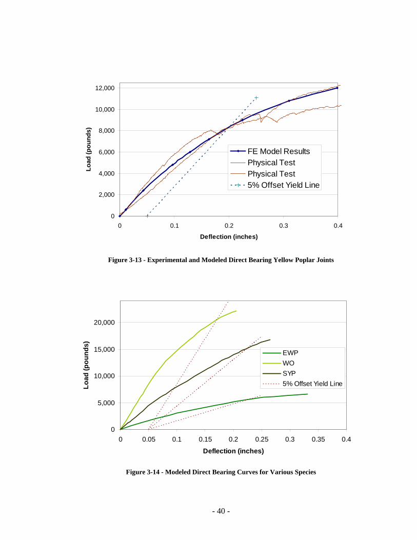
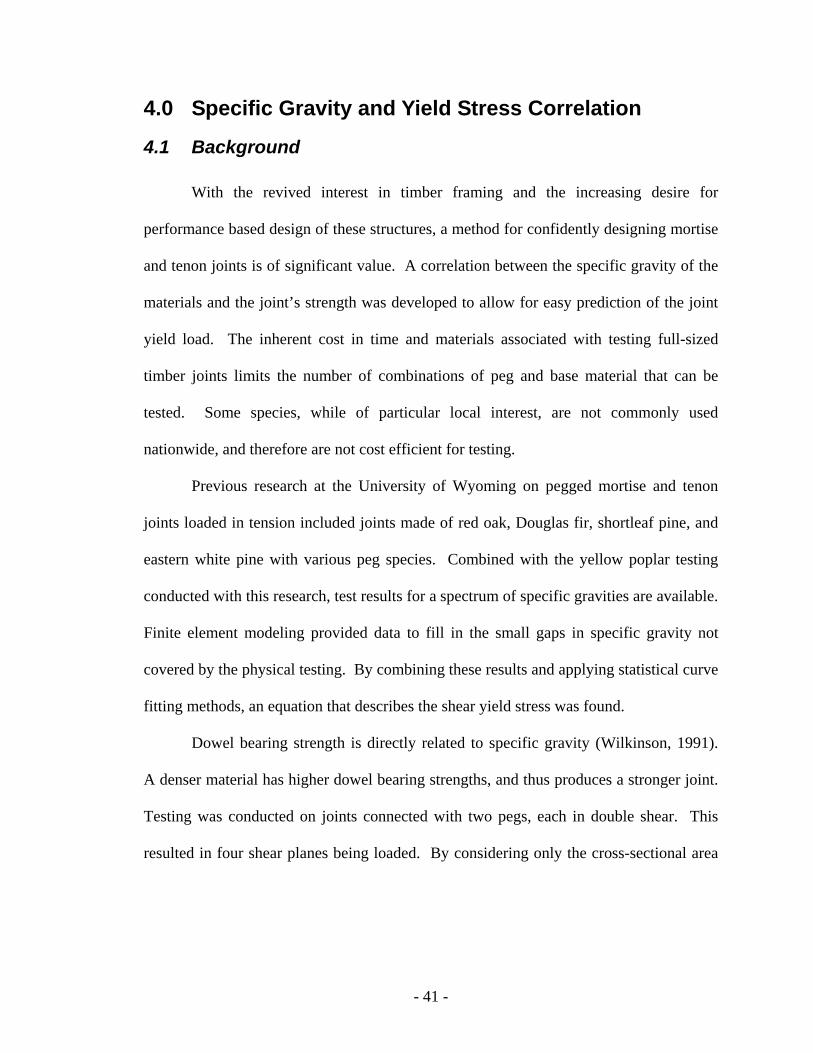
point. Figure 3-13 shows the modeled yellow poplar load-deflection plot along with the
physical test data. Figure 3-14 shows the behavior for the other species.
Contact and Target Elements
Load 0.1” Gap
- 40 -
0
2,000
4,000
6,000
8,000
10,000
12,000
0 0.1 0.2 0.3 0.4
Deflection (inches)
Load
(pou
nds)
FE Model ResultsPhysical TestPhysical Test5% Offset Yield Line
Figure 3-13 - Experimental and Modeled Direct Bearing Yellow Poplar Joints
0
5,000
10,000
15,000
20,000
0 0.05 0.1 0.15 0.2 0.25 0.3 0.35 0.4
Deflection (inches)
Load
(pou
nds)
EWPWOSYP5% Offset Yield Line
Figure 3-14 - Modeled Direct Bearing Curves for Various Species
- 41 -
4.0 Specific Gravity and Yield Stress Correlation
4.1 Background
With the revived interest in timber framing and the increasing desire for
performance based design of these structures, a method for confidently designing mortise
and tenon joints is of significant value. A correlation between the specific gravity of the
materials and the joint’s strength was developed to allow for easy prediction of the joint
yield load. The inherent cost in time and materials associated with testing full-sized
timber joints limits the number of combinations of peg and base material that can be
tested. Some species, while of particular local interest, are not commonly used
nationwide, and therefore are not cost efficient for testing.
Previous research at the University of Wyoming on pegged mortise and tenon
joints loaded in tension included joints made of red oak, Douglas fir, shortleaf pine, and
eastern white pine with various peg species. Combined with the yellow poplar testing
conducted with this research, test results for a spectrum of specific gravities are available.
Finite element modeling provided data to fill in the small gaps in specific gravity not
covered by the physical testing. By combining these results and applying statistical curve
fitting methods, an equation that describes the shear yield stress was found.
Dowel bearing strength is directly related to specific gravity (Wilkinson, 1991).
A denser material has higher dowel bearing strengths, and thus produces a stronger joint.
Testing was conducted on joints connected with two pegs, each in double shear. This
resulted in four shear planes being loaded. By considering only the cross-sectional area

- 42 -
of the pegs in the shear planes (Figure 4-1), a numerical correlation based on shear stress
and the specific gravities of the peg and base materials is possible.
Figure 4-1 - Four Shear Planes Used in Converting Yield Load to Yield Stress
4.2 Development
Regression of the specific gravity data into an equation that predicted the shear
yield stress began by selecting an equation type that fit the shape of the data. With three
variables involved (the specific gravity of the pegs, the specific gravity of the base
material, and the joint yield stress), the equation describes a surface rather than a line. A
multi-variable power equation
γβα BASEPEGvy GGF = Equation 4-1
was chosen to follow the form of the equations relating specific gravity to dowel bearing
strength published in the NDS. Other types of correlation functions were also
investigated, yet the power curve was the most accurate and simplest in form. In

- 43 -
Equation 4.1, where Fvy is the shear yield stress (psi), GPEG is the specific gravity of the
peg, GBASE is the specific gravity of the base material, and α, β, γ are constants.
A least squares regression was used with the data to minimize the error of the
surface and determine the constants. A coefficient of determination, also known as the
R2 value, was the guideline for the goodness of fit. Appendix E includes the MathCAD
worksheet with the calculations.
4.3 Results
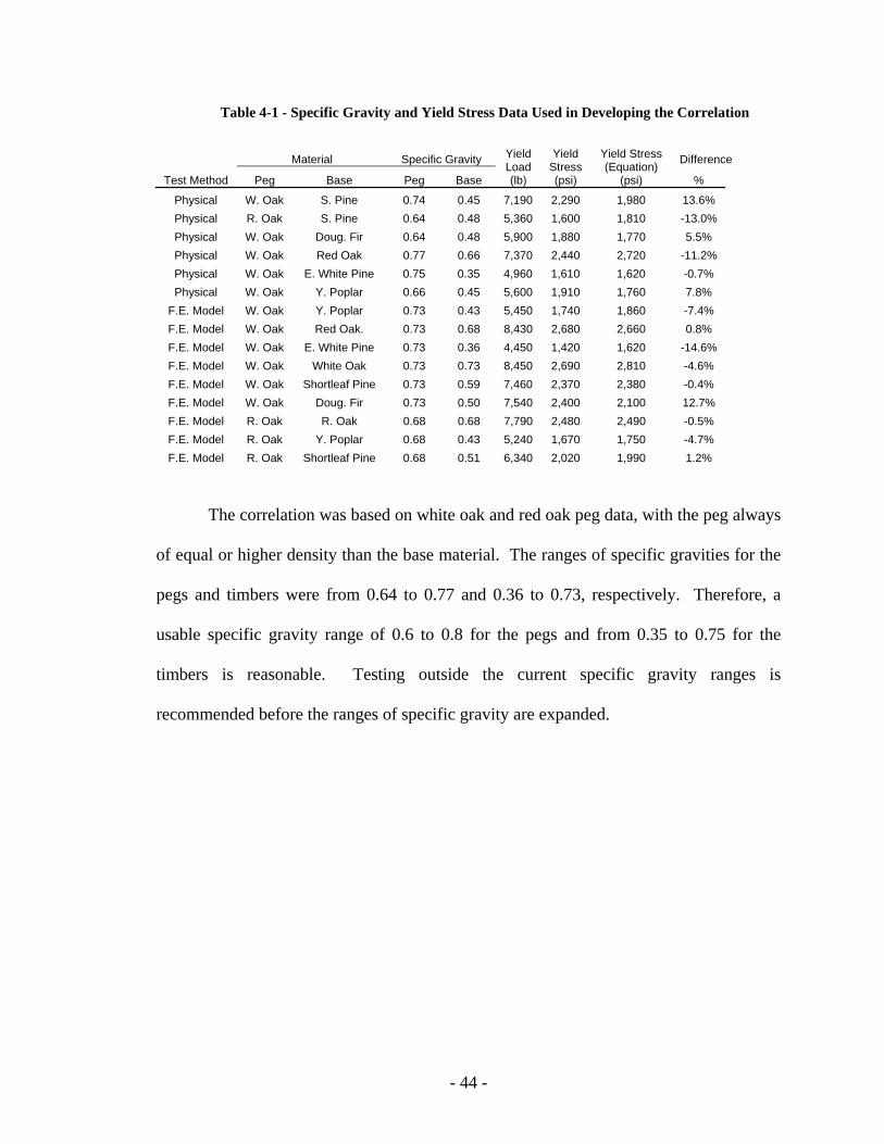
Table 4-1 shows the specific gravities and yield stresses used for determining the
correlation, along with the predicted value from the correlation. The experimental data
included specific gravity data taken during physical testing. For the finite element data,
specific gravity values were taken from the NDS (AFPA, 2001). The NDS’s specific
gravity values are slightly higher than those published for the same species in the Wood
Handbook. Therefore, using the NDS specific gravities is a conservative approach when
developing the correlation.
The regression analysis of the data in Table 4-1gave the relation
778.0926.04810 BASEPEGvy GGF = Equation 4-2 in which Fvy is the shear yield stress in psi. This correlation had a coefficient of
determination of 0.803. Figure 4-2 shows the data in Table 4-1 plotted along with the
resultant correlation surface. Figure 4-3 shows the correlation surface and data plotted on
edge to illustrate the deviation of each point from the surface.
- 44 -
Table 4-1 - Specific Gravity and Yield Stress Data Used in Developing the Correlation
Material Specific Gravity Difference
Test Method Peg Base Peg Base
Yield Load (lb)
Yield Stress (psi)
Yield Stress (Equation)
(psi) %
Physical W. Oak S. Pine 0.74 0.45 7,190 2,290 1,980 13.6% Physical R. Oak S. Pine 0.64 0.48 5,360 1,600 1,810 -13.0% Physical W. Oak Doug. Fir 0.64 0.48 5,900 1,880 1,770 5.5% Physical W. Oak Red Oak 0.77 0.66 7,370 2,440 2,720 -11.2% Physical W. Oak E. White Pine 0.75 0.35 4,960 1,610 1,620 -0.7% Physical W. Oak Y. Poplar 0.66 0.45 5,600 1,910 1,760 7.8%
F.E. Model W. Oak Y. Poplar 0.73 0.43 5,450 1,740 1,860 -7.4% F.E. Model W. Oak Red Oak. 0.73 0.68 8,430 2,680 2,660 0.8% F.E. Model W. Oak E. White Pine 0.73 0.36 4,450 1,420 1,620 -14.6% F.E. Model W. Oak White Oak 0.73 0.73 8,450 2,690 2,810 -4.6% F.E. Model W. Oak Shortleaf Pine 0.73 0.59 7,460 2,370 2,380 -0.4% F.E. Model W. Oak Doug. Fir 0.73 0.50 7,540 2,400 2,100 12.7% F.E. Model R. Oak R. Oak 0.68 0.68 7,790 2,480 2,490 -0.5% F.E. Model R. Oak Y. Poplar 0.68 0.43 5,240 1,670 1,750 -4.7% F.E. Model R. Oak Shortleaf Pine 0.68 0.51 6,340 2,020 1,990 1.2%
The correlation was based on white oak and red oak peg data, with the peg always
of equal or higher density than the base material. The ranges of specific gravities for the
pegs and timbers were from 0.64 to 0.77 and 0.36 to 0.73, respectively. Therefore, a
usable specific gravity range of 0.6 to 0.8 for the pegs and from 0.35 to 0.75 for the
timbers is reasonable. Testing outside the current specific gravity ranges is
recommended before the ranges of specific gravity are expanded.

- 45 -
Figure 4-2 - Plot of Yield Points with Correlation Surface
Figure 4-3 - Correlation Surface and Data Points Viewed Along Edge

- 46 -
5.0 Design of Mortise and Tenon Joints
5.1 Introduction
The correlation between specific gravity of the joint materials and the shear yield
stress of a mortise and tenon joint provides the necessary foundation for developing a
design procedure. The most direct and logical approach is to apply a factor of safety to
the yield stress correlation. The selection of an appropriate factor of safety for these
traditional joints will yield a safe yet simple design equation.
Since 1991, the NDS (AFPA, 2001) has used the European Yield Model to
predict the strength of dowel-type connections with steel fasteners. The EYM is an
ultimate strength model and predicts the load capacity of a joint, assuming elastic
perfectly-plastic behavior. The bending strength of the dowel as well as the dowel
bearing strength of the timber are used in the EYM. These material properties are based
on the five-percent offset yield method.
5.2 Selection of a Factor of Safety
Kessel and Augustin (1996) conducted work in Germany to develop tensile
capacities and appropriate factors of safety for pegged mortise and tenon joints. Their
factors of safety were selected for a particular size joint with a particular timber and peg
species. They recommended that the design load for the joint be the lesser of:
- The mean value of the ultimate loads divided by a factor of safety of 3.0.
- The mean value of the loads at 1.5 mm of deflection, approximately one-half
the proportional limit, with a factor of safety of 1.0.
- 47 -
- The absolute minimum ultimate load divided by a factor of safety of 2.25.
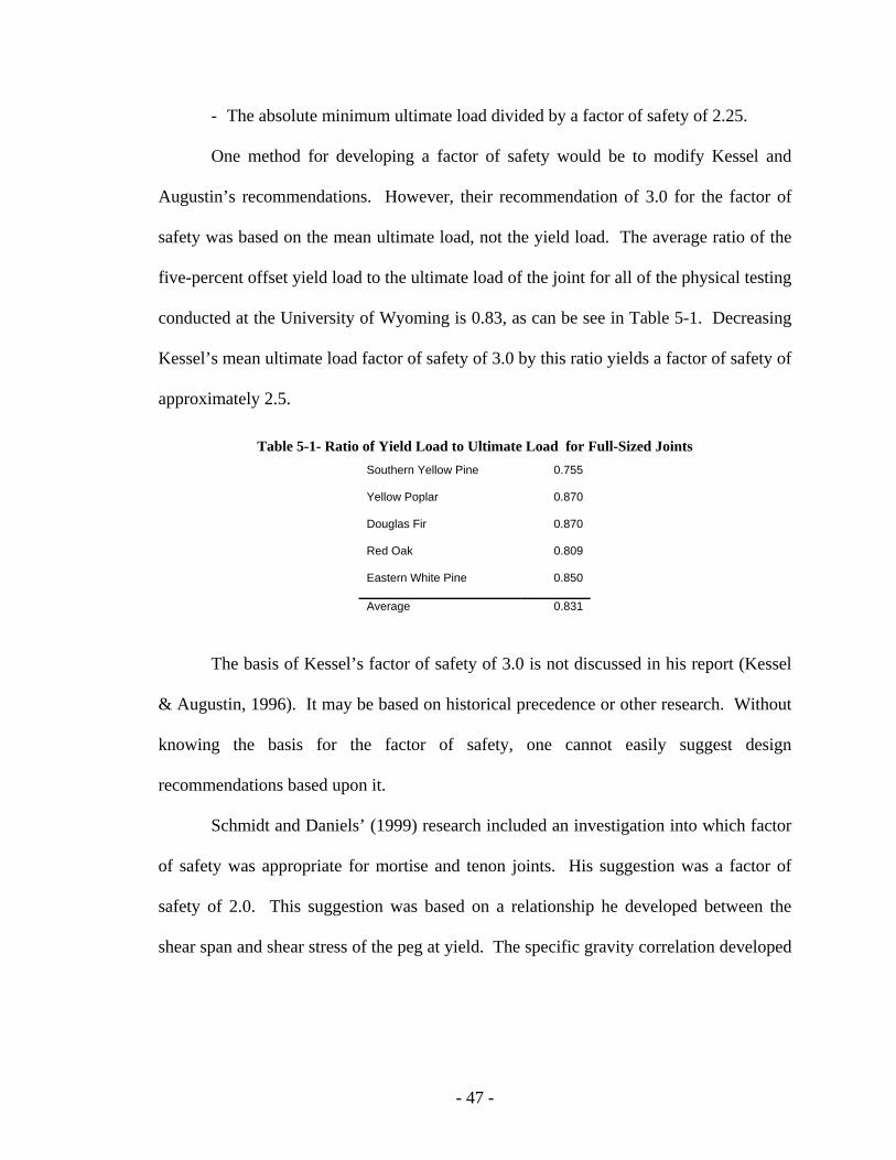
One method for developing a factor of safety would be to modify Kessel and
Augustin’s recommendations. However, their recommendation of 3.0 for the factor of
safety was based on the mean ultimate load, not the yield load. The average ratio of the
five-percent offset yield load to the ultimate load of the joint for all of the physical testing
conducted at the University of Wyoming is 0.83, as can be see in Table 5-1. Decreasing
Kessel’s mean ultimate load factor of safety of 3.0 by this ratio yields a factor of safety of
approximately 2.5.
Table 5-1- Ratio of Yield Load to Ultimate Load for Full-Sized Joints Southern Yellow Pine 0.755
Yellow Poplar 0.870
Douglas Fir 0.870
Red Oak 0.809
Eastern White Pine 0.850
Average 0.831
The basis of Kessel’s factor of safety of 3.0 is not discussed in his report (Kessel
& Augustin, 1996). It may be based on historical precedence or other research. Without
knowing the basis for the factor of safety, one cannot easily suggest design
recommendations based upon it.
Schmidt and Daniels’ (1999) research included an investigation into which factor
of safety was appropriate for mortise and tenon joints. His suggestion was a factor of
safety of 2.0. This suggestion was based on a relationship he developed between the
shear span and shear stress of the peg at yield. The specific gravity correlation developed
- 48 -
with current research is not based on the shear span of the peg, and therefore a factor of
safety of 2.0 may not be appropriate.
A logical approach for developing a new factor of safety would be to use the
current EYM equations in the NDS as a baseline. Research conducted by Reid (1997)
suggested that Mode IIIs failure of the EYM accurately represented physical tests of
mortise and tenon joints with wood pegs. In addition, the failure mode of most pegged
mortise and tenon joints at the University of Wyoming was also Mode IIIs. The ratio of
the yield load predicted by the correlation in Equation 4-2 to the Mode IIIs allowable
joint load should provide a factor of safety that has the same performance as the current
design procedures (Table 5-2).
Table 5-2 - Ratio of Correlation Strength to EYM Mode IIIs Allowable Load
YieldTest Method Peg Base Peg Base Allowable Allowable
(lb) (lb)Physical W. Oak S. Pine 0.74 0.45 3,072 1,297 2.37Physical R. Oak S. Pine 0.64 0.48 2,824 1,369 2.06Physical W. Oak Doug. Fir 0.64 0.48 2,824 1,369 2.06Physical W. Oak Red Oak 0.77 0.66 4,293 1,926 2.23Physical W. Oak E. White Pine 0.75 0.35 2,558 1,063 2.41Physical W. Oak Y. Poplar 0.66 0.45 2,763 1,297 2.13
F.E. Model W. Oak Y. Poplar 0.73 0.43 2,928 1,249 2.34F.E. Model W. Oak Red Oak. 0.73 0.68 4,182 1,986 2.11F.E. Model W. Oak E. White Pine 0.73 0.36 2,550 1,086 2.35F.E. Model W. Oak White Oak 0.73 0.73 4,419 2,138 2.07F.E. Model W. Oak Longleaf Pine 0.73 0.59 3,745 1,644 2.28F.E. Model W. Oak Doug. Fir 0.73 0.5 3,292 1,418 2.32F.E. Model R. Oak R. Oak 0.68 0.68 3,916 1,986 1.97F.E. Model R. Oak Y. Poplar 0.68 0.43 2,742 1,249 2.19F.E. Model R. Oak Longleaf Pine 0.68 0.59 3,507 1,644 2.13
Average (Factor of Safety) 2.20
Mode IIIsCorrelation Yield Load
Specific GravityMaterial
The ratio of the Equation 4-2 correlation yield load to the EYM Mode IIIs
allowable load is 2.20. This is the factor of safety associated with the correlation yield

- 49 -
load when compared to the current NDS standard. Hence, a factor of safety of 2.2 is
recommended for use with Equation 4-2 to determine an allowable design value for peg
shear in mortise and tenon joints.
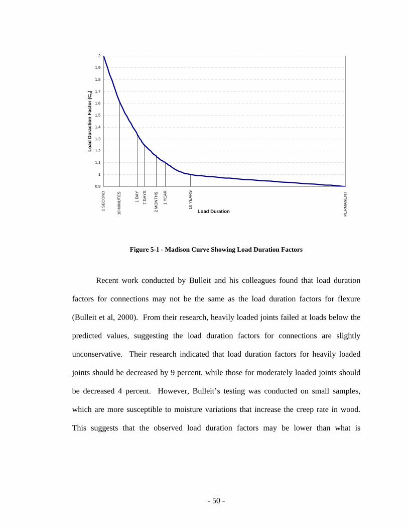
5.3 Load Duration Factor
Long standing research (Wood, 1951) has demonstrated that the strength of wood
flexural members is sensitive to the duration of the load; strength decreases as load
duration increases. Hence, the NDS permits adjustment of many wood design values,
including those for connection design, by load duration factors. These load duration
factors are based on the Madison curve (Figure 5-1), which calibrates all loads relative to
a duration of ten years (AFPA, 2001).
Physical testing in this research was based on a load-to-failure time of
approximately ten minutes. The load duration factor for ten-minute loading is 1.6. The
design equation being developed therefore should be reduced by a factor of 1.6 for
adjustment to the standard ten-year load duration.
Schmidt and Scholl’s research on the long-term behavior of loaded
mortise and tenon joints with wood pegs included suggestions for a load-duration factor
of 1.0 for joints loaded under long term. The recommendation was based on testing of
joints that had been subjected to a static long-term service-level loading.
- 50 -
0.9
1
1.1
1.2
1.3
1.4
1.5
1.6
1.7
1.8
1.9
2
Load Duration
Load
Dur
actio
n Fa
ctor
(CD)
1 S
ECO
ND
10 M
INU
TES
1 D
AY
7 D
AYS
2 M
ON
THS
1 Y
EA
R
10 Y
EAR
S
PER
MAN
ENT
Figure 5-1 - Madison Curve Showing Load Duration Factors
Recent work conducted by Bulleit and his colleagues found that load duration
factors for connections may not be the same as the load duration factors for flexure
(Bulleit et al, 2000). From their research, heavily loaded joints failed at loads below the
predicted values, suggesting the load duration factors for connections are slightly
unconservative. Their research indicated that load duration factors for heavily loaded
joints should be decreased by 9 percent, while those for moderately loaded joints should
be decreased 4 percent. However, Bulleit’s testing was conducted on small samples,
which are more susceptible to moisture variations that increase the creep rate in wood.
This suggests that the observed load duration factors may be lower than what is

- 51 -
experienced in larger joints. Therefore, until further testing is conducted, Bulleit
recommends that the standard load duration factors be used with connections.
5.4 Design Equation
Incorporating the factor of safety of 2.20 and removing the load duration factor of
1.6 from the first constant of the yield stress correlation equation (Equation 4-2) gives the
design equation
778.0926.01365 BASEPEGv GGF = Equation 5-1
where Fv is the allowable shear stress in the peg in psi. GPEG is limited to the range of
0.6 to 0.8 and must always be higher than GBASE. GBASE is limited to the range of 0.35 to
0.75. The load duration factor was included so the design equation reflects a standard
load duration of ten years. The designer can conservatively use the equation as is, or can
increase the allowable stress by the load duration factor, as permitted by the NDS. This
equation can be safely and confidently used for the design of pegged mortise and tenon
joints loaded in tension. A design example is included in Table 5-3.
Table 5-3 - Example on the Proper Usage of the Correlation
Example Design Usage of Correlation GPEG 0.73 (White Oak) GBASE 0.43 (Yellow Poplar) Number of Pegs 2 Peg Diameter 1 inches Load Duration 1.6 (Wind Load - Per the NDS) Shear Stress 529 lb/in2 (per EQ. 5-1)
Shear Area 3.142 in2 Joint Capacity 2659 lb
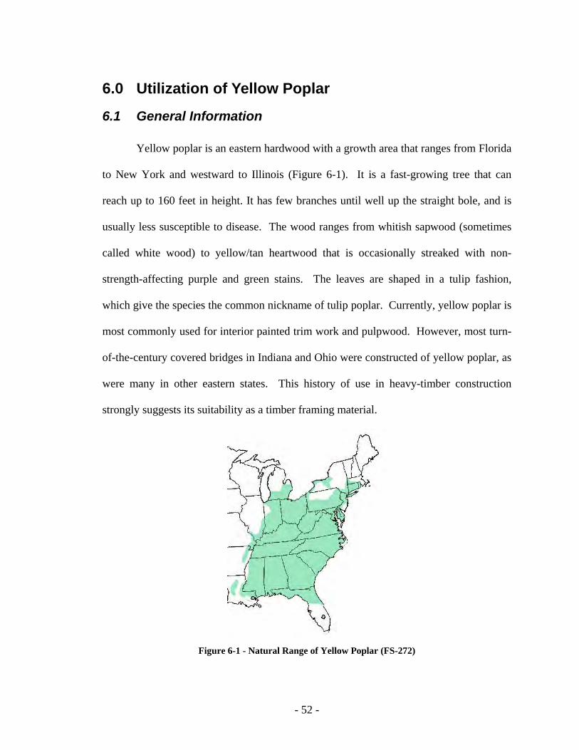
- 52 -
6.0 Utilization of Yellow Poplar
6.1 General Information
Yellow poplar is an eastern hardwood with a growth area that ranges from Florida
to New York and westward to Illinois (Figure 6-1). It is a fast-growing tree that can
reach up to 160 feet in height. It has few branches until well up the straight bole, and is
usually less susceptible to disease. The wood ranges from whitish sapwood (sometimes
called white wood) to yellow/tan heartwood that is occasionally streaked with non-
strength-affecting purple and green stains. The leaves are shaped in a tulip fashion,
which give the species the common nickname of tulip poplar. Currently, yellow poplar is
most commonly used for interior painted trim work and pulpwood. However, most turn-
of-the-century covered bridges in Indiana and Ohio were constructed of yellow poplar, as
were many in other eastern states. This history of use in heavy-timber construction
strongly suggests its suitability as a timber framing material.
Figure 6-1 - Natural Range of Yellow Poplar (FS-272)
- 53 -
6.2 Availability
Production of yellow poplar lumber reached an all time high in 1899 with 1,118
million board feet produced, and production has since declined to 847 million board feet
(FS-272). Growth of yellow poplar lumber has increased to 2,137 million board feet per
year, meaning a net growth of 1,290 million board feet per year. This makes yellow
poplar one of the most abundant hardwoods, and it is becoming more and more abundant
each year. Due to yellow poplar’s abundance, its price is relatively low. Green squared
timbers are currently available for a cost of $45 to $50 per thousand board feet; about half
the cost of oak.
6.3 Material Properties
6.3.1 Strength
The NDS does not include design values for timber sized pieces of yellow poplar
despite being of commercial importance. However, dimension lumber values are
provided, and these values will be used for comparison’s sake. Yellow poplar is in the
lower third of hardwoods when it comes to specific gravity, bending strength, toughness,
shear strength and tensile strength. The modulus of elasticity of yellow poplar is 36
percent higher than that of white oak, and it weighs only 58 percent as much. In many
cases in design, serviceability controls member size selection. Therefore, a stiffer
material such as yellow poplar with lower self weight than oak can be of great interest.
The faster yellow poplar grows, the stronger it is (FS-272, 1985). Old growth
yellow poplar, which grew more slowly, tends to be lighter and weaker than second-
growth material. Yellow poplar from wet, temperate climates grows the fastest and is the

- 54 -
strongest. As the density of yellow poplar increases, so does its strength, and in turn the
color of the heartwood becomes a darker yellow.
Joint testing at the University of Wyoming suggests that yellow poplar is a viable
wood for use as a timber framing material based on strength parameters. The average
yield load for yellow poplar joints with a peg specific gravity of 0.66 was 5995 pounds.
The average yield load for Douglas fir joints with a peg specific gravity of 0.64 was 5900
pounds. This suggests that fast-growing, dense yellow poplar is comparable in strength
to Douglas fir when used in a mortise and tenon joint.
6.3.2 Drying
Yellow poplar typically exceeds 100 percent moisture content when cut and it
shrinks quickly. Even though yellow poplar decreases its void ratio the faster it grows, it
also increases its vessel area. This vessel area is directly related to the longitudinal
permeability (Chen et al, 1998). Higher permeability increases the drying rate, thus
making yellow poplar one of the quickest drying hardwoods. This characteristic makes
yellow poplar suitable for kiln-drying, since little time is needed to reach equilibrium
moisture content. Once dried, yellow poplar is a dimensionally stable wood, in certain
cases twice as stable as red oak (Table 6-1).
Table 6-1 - Dimensional Change in 3" Lumber (in inches) (Forest Products Lab, 2000)
Red Oak Yellow Poplar Ratio Y.P. to R.O. MC Change Radial Tangential Radial Tangential Radial Tangential
1% 0.005 0.011 0.005 0.009 1 0.82 2% 0.014 0.033 0.014 0.017 1 0.52 3% 0.024 0.055 0.024 0.026 1 0.47

- 55 -
The yellow poplar used in physical joint testing at the University of Wyoming
was harvested, squared, and delivered within one week. The extremely low winter
equilibrium moisture content in Laramie, Wyoming (6-8%) along with the lack of any
end sealer caused each of the boxed heart timbers to check to the center within 4 months.
This suggests care must be taken slow the drying rate in arid climates to minimalize
material degradation.
6.3.3 Workability
Yellow poplar is a very easy wood to work. Its widespread usage in interior trim
and turnings attest to this. It cuts easier than most hardwoods and produces a sweet-
smelling sawdust. The relatively straight- and uniform-grain make chiseling and paring
easy to perform. Extensive cutting and chiseling do not noticeably dull edge tools.
Yellow poplar does not sand as well as other hardwoods since it is softer, but planes to a
shiny surface with relative ease.
6.4 Conclusion on Usage
Based on its performance in this research, its physical characteristics, and cost,
yellow poplar has possibilities as a timber framing material. Wide spread usage in
covered bridges bear witness to this. Its low cost, increasing availability and quick
drying should make up for its lack in strength compared to other hardwoods. Therefore,
yellow poplar should be considered a viable option as a timber framing material.
- 56 -
7.0 Summary and Conclusions
7.1 Joint Research
7.1.1 Physical Testing
Pegged yellow poplar mortise and tenon joints physically tested in tension
behaved in a similar fashion to other tests conducted at the University of Wyoming. The
same failure modes in the tenon relish and mortise cheek were observed, as were peg
shearing and bending failures. Use of the same testing frame and setup procedure
ensured that these tests could be directly compared with previous ones. Modification of
the peg hole location during subsequent tests allowed minimum detailing requirements to
be developed for yellow poplar. These detailing requirements can be added to those for
other species.
Shear testing of the mortise and tenon joints, in which the tenoned member was
loaded in shear and the load was transferred through the pegs, gave the expected poor
capacities. Low strength in tension perpendicular to the grain results in undesirable tenon
splitting failures. Large through tenons and single-peg connections were required to
induce peg bending failures. When these peg failures did occur, they occurred at
approximately the same yield stress in the peg as the tension testing.
Direct bearing tests of the mortise and tenon joints were performed with the
tenoned member loaded in shear and the load transferred through direct bearing of the
tenon on the bottom of the mortise. In these tests, the joints were much stiffer and
stronger than the same joint loaded in shear through the pegs. Therefore, direct bearing,
not pegs, should be used to transmit shear loads from the tenon to the mortise.
- 57 -
7.1.2 Finite Element Modeling
Time and materials did not permit testing a wide variety of wood and peg species,
so a finite element model was developed. Once the three-dimensional model was
validated against physical test results, other species of materials were modeled to round
out the spectrum of specific gravities for development of a correlation between specific
gravity and the yield stress of a pegged mortise and tenon joint loaded in tension.
Published orthotropic material properties and a bilinear stress-strain curve were
incorporated into a three-dimensional finite element model of a mortise and tenon joint.
The model provided accurate results when the desired data is the five-percent offset yield
load.
7.2 Design Equations and Correlation
A simple correlation relating the specific gravities of the timbers and pegs to
allowable yield stress was developed. The correlation was based on the direct
relationship between a material’s dowel bearing strength and specific gravity. From the
correlation, a design equation was developed for the allowable shear stress in the pegs of
a mortise and tenon joint loaded in tension. A reasonable factor of safety and load
duration effects were included in the equation so that it can be used like any other
allowable stress from the NDS.
The simple form of the correlation equation should allow for easy adoption by
design professionals. It can be safely and accurately used within the range of specific
gravities tested.
- 58 -
7.3 Usage of Yellow Poplar
In this research, yellow poplar proved to be a viable choice as a timber framing
material. It is low cost and readily available in the eastern United States. It dries quickly
with a minimal amount of degradation. The stiffness to weight ratio is higher than that of
oak, and its strength in tensile loaded mortise and tenon joints is comparable to that of
Douglas fir. Yellow poplar acts as a hardwood, so tenons should be detailed with a
thickness of 1.5 inches.
7.4 Recommendations for Future Research
Mortise and tenon joints with peg materials other than red and white oak should
be studied to allow for confidence in the developed design equation outside of the current
range of specific gravities. Peg diameters other than 1.0 inch should also be tested to
ensure the design yield stress is adequate for a range of peg sizes. These studies could be
performed either experimentally or by the finite element method.
Loading joints at a rate to induce failure in days or weeks may be difficult to
execute, but would provide good insight into the applicability of load duration factors to
the yield stress equation.

- 59 -
8.0 References
AFPA, (2001). “National Design Specification for Wood Construction,” American Forest and Paper Association (AFPA), Washington, DC. ANSYS, (2003). “ANSYS 7.1 User’s Manual,” SAS IP, Inc. Benson, T., Gruber, J., (1980). “Building the Timber Frame House.” Charles Schribner’s Sons, New York. Brungraber, R. L. (1985). “Traditional Timber Joinery: A Modern Analysis,” Ph.D. Dissertation, Stanford University, Palo Alto, California. Bulleit, W.M., Martin, Z.A., Marlor, R.A., (2000). “Load Duration Behavior of Steel- Doweled Wood Connections,” Proceedings, World Conference on Timber Engineering, British Columbia, 2-4-3. Chapra, S.C., Canale, R. P., (1998). “Numerical Methods for Engineers, 3rd Edition,” McGraw Hill, Boston. Chen, C.J., Lee, T.L., Jeng, D.S., (2003). “Finite Element Modeling for the Mechanical Behavior of Dowel-Type Timber Joints,” Computers and Structures, 81, 2731- 2738. Chen, P., Zhang, G., Van Sambeek, J.W., (1998). “Relationships Among Growth Rate, Vessel Lumen Area, and Wood Permeability for Three Central Hardwood Species,” Forest Products Journal, 48:3, 87-90. Drewek, M.W. (1997). “Modeling the Behavior of Traditional Timber Frames,” M.S. Thesis, Michigan Technological University, Houghton, Michigan. Erikson, R.G. (2003). “Behavior of Traditional Timber Frame Structures Subjected to Lateral Load,” Ph.D. Dissertation. University of Wyoming, Laramie, Wyoming. Forest Products Laboratory, (2000). “Drying Hardwood Lumber,” FPL-GTR-118, Madison, Wisconsin. Forest Products Society, (1999). “Wood Handbook,” FPL-GTR-113, Madison, Wisconsin. FS-272, (1985). “Yellow Poplar,” Forest Service, United States Department of Agriculture, Washington, DC.
- 60 -
Kharouf, N., McClure, G., Smith, I., (2003). “Elasto-plastic Modeling of Wood Bolted Connections,” Computers and Structures, 81, 747-754. Kessel, M. H. and Augustin, R. (1995). “Load Behavior of Connections with Oak Pegs,” Peavy, M.D. and Schmidt, R.J., trans. Timber Framing, Journal of the Timber Framers Guild. 38, December, 6-9. Kessel, M. H. and Augustin, R. (1996). “Load Behavior of Connections with Pegs II,” Peavy, M.D. and Schmidt, R.J., trans. Timber Framing, Journal of the Timber Framers Guild. 39, March, 8-11. Patton-Mallory, M., Cramer, S.M., Smith, F.W., Pellicane, P.J., (1997). “Nonlinear Material Models for Analysis of Bolted Wood Connections.” Journal of Structural Engineering, August, 1063-1070. Reid, E. H. (1997). “Behavior of Wood Pegs in Traditional Timber Frame Connections,” M.S. Thesis, Michigan Technological University, Houghton, Michigan. Schmidt, R.J. and Daniels, C.E. (1999). “Design Considerations for Mortise and Tenon Connections,” Research Report, University of Wyoming, Laramie, Wyoming. Schmidt, R.J. and MacKay, R.B. (1997). “Timber Frame Tension Joinery,” Research Report, University of Wyoming, Laramie, Wyoming. Schmidt, R.J. and Scholl, G.F. (2000). “Load Duration and Seasoning Effects on Mortise and Tenon Joints,” Research Report, University of Wyoming, Laramie, Wyoming. Sobon, J., and Schroeder, R., (1984). “Timber Frame Construction.” Garden Way Publishing, Pownal, Vermont. Wilkinson, (1991). “Dowel Bearing Strength,” FPL-RP-505, Madison, Wisconsin. Wood, L.W. (1951). “Relation of Strength of Wood to Duration of Load.” Report 1916, Madison, Wisconsin.
- 61 -
9.0 Appendices
Appendix A – Tension Load-Deflection Plots Load vs Deflection YP01
6972.88
0
1000
2000
3000
4000
5000
6000
7000
8000
0 0.05 0.1 0.15 0.2 0.25 0.3 0.35 0.4 0.45
Deflection
Load
Load vs Deflection YP02
4479
0
1000
2000
3000
4000
5000
6000
7000
8000
0 0.05 0.1 0.15 0.2 0.25 0.3 0.35 0.4 0.45
Deflection
Load
Load vs Deflection YP03
6462.60
0
1000
2000
3000
4000
5000
6000
7000
8000
0 0.05 0.1 0.15 0.2 0.25 0.3 0.35 0.4 0.45
Deflection
Load
- 62 -
Load vs Deflection YP04
5791
0
1000
2000
3000
4000
5000
6000
7000
8000
0 0.05 0.1 0.15 0.2 0.25 0.3 0.35 0.4 0.45
Deflection
Load
Load vs Deflection YP05
4515
0
1000
2000
3000
4000
5000
6000
7000
8000
0 0.05 0.1 0.15 0.2 0.25 0.3 0.35 0.4 0.45
Deflection
Load
Load vs Deflection YP06
6922
0
1000
2000
3000
4000
5000
6000
7000
8000
0 0.05 0.1 0.15 0.2 0.25 0.3 0.35 0.4 0.45
Deflection
Load

- 63 -
Load vs Deflection YP06B
6616
0
1000
2000
3000
4000
5000
6000
7000
8000
0 0.05 0.1 0.15 0.2 0.25 0.3 0.35 0.4 0.45
Deflection
Load
Load vs Deflection YP06C
6135
0
1000
2000
3000
4000
5000
6000
7000
8000
0 0.05 0.1 0.15 0.2 0.25 0.3 0.35 0.4 0.45
Deflection
Load
Load vs Deflection YP06D
7631
0
1000
2000
3000
4000
5000
6000
7000
8000
0 0.05 0.1 0.15 0.2 0.25 0.3 0.35 0.4 0.45
Deflection
Load
- 64 -
Load vs Deflection YP07
4445
0
1000
2000
3000
4000
5000
6000
7000
8000
0 0.05 0.1 0.15 0.2 0.25 0.3 0.35 0.4 0.45
Deflection
Load
Load vs Deflection YP07B
4743
0
1000
2000
3000
4000
5000
6000
7000
8000
0 0.05 0.1 0.15 0.2 0.25 0.3 0.35 0.4 0.45
Deflection
Load
Load vs Deflection YP08
6263
0
1000
2000
3000
4000
5000
6000
7000
8000
0 0.05 0.1 0.15 0.2 0.25 0.3 0.35 0.4 0.45
Deflection
Load

- 65 -
Load vs Deflection YP10
6001
0
1000
2000
3000
4000
5000
6000
7000
8000
0 0.05 0.1 0.15 0.2 0.25 0.3 0.35 0.4 0.45
Deflection
Load
Load vs Deflection YP11
5114
0
1000
2000
3000
4000
5000
6000
7000
8000
0 0.05 0.1 0.15 0.2 0.25 0.3 0.35 0.4 0.45
Deflection
Load
Load vs Deflection YP12
4050
0
1000
2000
3000
4000
5000
6000
7000
8000
0 0.05 0.1 0.15 0.2 0.25 0.3 0.35 0.4 0.45
Deflection
Load
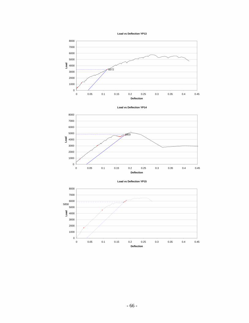
- 66 -
Load vs Deflection YP13
3372
0
1000
2000
3000
4000
5000
6000
7000
8000
0 0.05 0.1 0.15 0.2 0.25 0.3 0.35 0.4 0.45
Deflection
Load
Load vs Deflection YP14
4803
0
1000
2000
3000
4000
5000
6000
7000
8000
0 0.05 0.1 0.15 0.2 0.25 0.3 0.35 0.4 0.45
Deflection
Load
Load vs Deflection YP15
5858
0
1000
2000
3000
4000
5000
6000
7000
8000
0 0.05 0.1 0.15 0.2 0.25 0.3 0.35 0.4 0.45
Deflection
Load
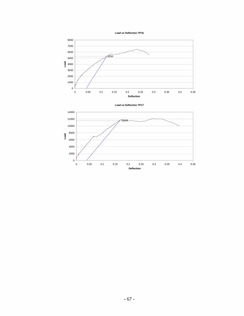
- 67 -
Load vs Deflection YP16
5293
0
1000
2000
3000
4000
5000
6000
7000
8000
0 0.05 0.1 0.15 0.2 0.25 0.3 0.35 0.4 0.45
Deflection
Load
Load vs Deflection YP17
11616
0
2000
4000
6000
8000
10000
12000
14000
0 0.05 0.1 0.15 0.2 0.25 0.3 0.35 0.4 0.45
Deflection
Load

- 68 -
Appendix B – Shear Load Deflection Plots
Load vs Deflection YPS01
2696.06
0
1000
2000
3000
4000
5000
6000
7000
8000
0 0.05 0.1 0.15 0.2 0.25 0.3 0.35 0.4 0.45 0.5
Deflection
Load
Load vs Deflection YPS02
5878.51
0
1000
2000
3000
4000
5000
6000
7000
8000
0 0.05 0.1 0.15 0.2 0.25 0.3 0.35 0.4 0.45 0.5
Deflection
Load
Load vs Deflection YPS03
5242.43
0
1000
2000
3000
4000
5000
6000
7000
8000
0 0.05 0.1 0.15 0.2 0.25 0.3 0.35 0.4 0.45 0.5
Deflection
Load
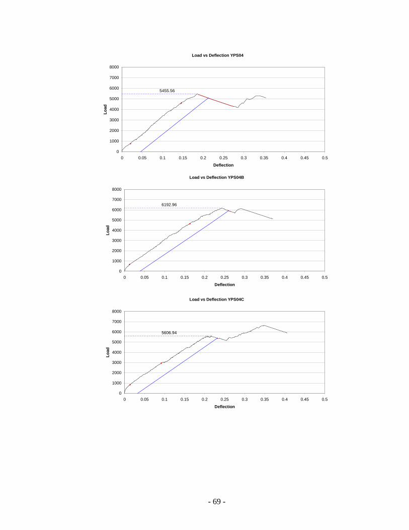
- 69 -
Load vs Deflection YPS04
5455.56
0
1000
2000
3000
4000
5000
6000
7000
8000
0 0.05 0.1 0.15 0.2 0.25 0.3 0.35 0.4 0.45 0.5
Deflection
Load
Load vs Deflection YPS04B
6192.96
0
1000
2000
3000
4000
5000
6000
7000
8000
0 0.05 0.1 0.15 0.2 0.25 0.3 0.35 0.4 0.45 0.5
Deflection
Load
Load vs Deflection YPS04C
5606.94
0
1000
2000
3000
4000
5000
6000
7000
8000
0 0.05 0.1 0.15 0.2 0.25 0.3 0.35 0.4 0.45 0.5
Deflection
Load
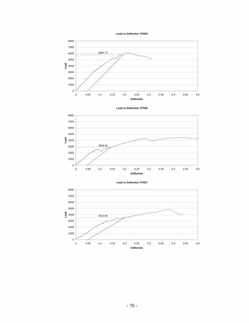
- 70 -
Load vs Deflection YPS05
5802.73
0
1000
2000
3000
4000
5000
6000
7000
8000
0 0.05 0.1 0.15 0.2 0.25 0.3 0.35 0.4 0.45 0.5
Deflection
Load
Load vs Deflection YPS06
2849.34
0
1000
2000
3000
4000
5000
6000
7000
8000
0 0.05 0.1 0.15 0.2 0.25 0.3 0.35 0.4 0.45 0.5
Deflection
Load
Load vs Deflection YPS07
3513.50
0
1000
2000
3000
4000
5000
6000
7000
8000
0 0.05 0.1 0.15 0.2 0.25 0.3 0.35 0.4 0.45 0.5
Deflection
Load

- 71 -
Load vs Deflection YPS07B
5423.35
0
1000
2000
3000
4000
5000
6000
7000
8000
0 0.1 0.2 0.3 0.4 0.5 0.6 0.7
Deflection
Load
Load vs Deflection YPS07C
6437.70
0
1000
2000
3000
4000
5000
6000
7000
8000
0 0.1 0.2 0.3 0.4 0.5 0.6 0.7
Deflection
Load
Load vs Deflection YPS08
5169.16
0
1000
2000
3000
4000
5000
6000
7000
8000
0 0.05 0.1 0.15 0.2 0.25 0.3 0.35 0.4 0.45 0.5
Deflection
Load

- 72 -
Appendix C – Direct Bearing Load-Deflection Plots
Load vs Deflection YPB01
9236.23
0
2000
4000
6000
8000
10000
12000
14000
16000
0 0.1 0.2 0.3 0.4 0.5 0.6 0.7 0.8
Deflection
Load
Load vs Deflection YPB02
9570.46
0
2000
4000
6000
8000
10000
12000
14000
16000
0 0.1 0.2 0.3 0.4 0.5 0.6 0.7 0.8
Deflection
Load
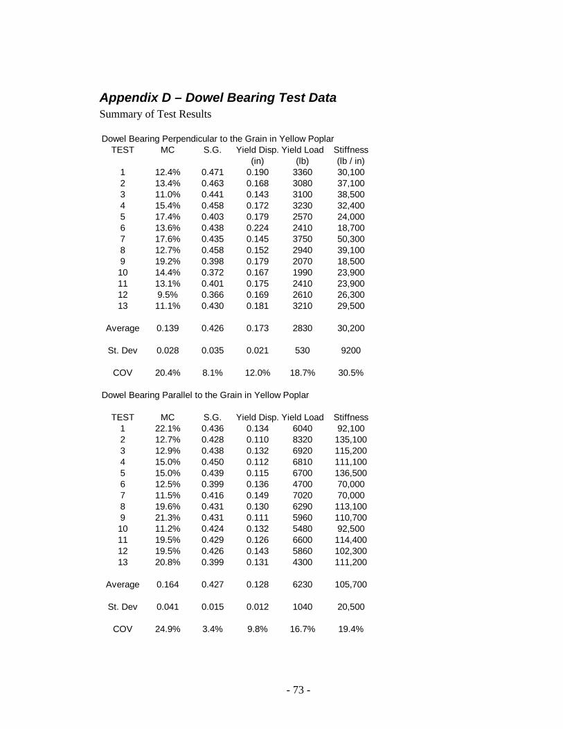
- 73 -
Appendix D – Dowel Bearing Test Data Summary of Test Results Dowel Bearing Perpendicular to the Grain in Yellow Poplar
TEST MC S.G. Yield Disp. Yield Load Stiffness(in) (lb) (lb / in)
1 12.4% 0.471 0.190 3360 30,1002 13.4% 0.463 0.168 3080 37,1003 11.0% 0.441 0.143 3100 38,5004 15.4% 0.458 0.172 3230 32,4005 17.4% 0.403 0.179 2570 24,0006 13.6% 0.438 0.224 2410 18,7007 17.6% 0.435 0.145 3750 50,3008 12.7% 0.458 0.152 2940 39,1009 19.2% 0.398 0.179 2070 18,50010 14.4% 0.372 0.167 1990 23,90011 13.1% 0.401 0.175 2410 23,90012 9.5% 0.366 0.169 2610 26,30013 11.1% 0.430 0.181 3210 29,500
Average 0.139 0.426 0.173 2830 30,200
St. Dev 0.028 0.035 0.021 530 9200
COV 20.4% 8.1% 12.0% 18.7% 30.5%
Dowel Bearing Parallel to the Grain in Yellow Poplar
TEST MC S.G. Yield Disp. Yield Load Stiffness1 22.1% 0.436 0.134 6040 92,1002 12.7% 0.428 0.110 8320 135,1003 12.9% 0.438 0.132 6920 115,2004 15.0% 0.450 0.112 6810 111,1005 15.0% 0.439 0.115 6700 136,5006 12.5% 0.399 0.136 4700 70,0007 11.5% 0.416 0.149 7020 70,0008 19.6% 0.431 0.130 6290 113,1009 21.3% 0.431 0.111 5960 110,70010 11.2% 0.424 0.132 5480 92,50011 19.5% 0.429 0.126 6600 114,40012 19.5% 0.426 0.143 5860 102,30013 20.8% 0.399 0.131 4300 111,200
Average 0.164 0.427 0.128 6230 105,700
St. Dev 0.041 0.015 0.012 1040 20,500
COV 24.9% 3.4% 9.8% 16.7% 19.4%
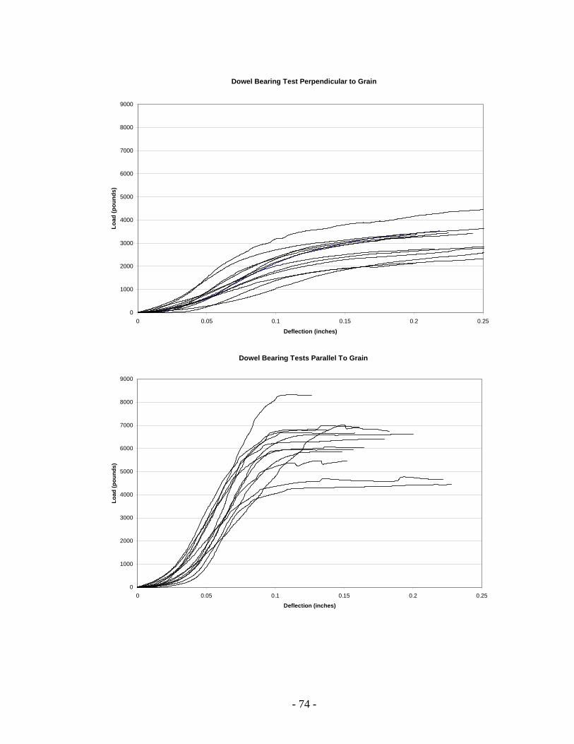
- 74 -
Dowel Bearing Test Perpendicular to Grain
0
1000
2000
3000
4000
5000
6000
7000
8000
9000
0 0.05 0.1 0.15 0.2 0.25
Deflection (inches)
Load
(pou
nds)
Dowel Bearing Tests Parallel To Grain
0
1000
2000
3000
4000
5000
6000
7000
8000
9000
0 0.05 0.1 0.15 0.2 0.25
Deflection (inches)
Load
(pou
nds)

- 75 -
Appendix E – Statistical Methods for Correlation Output from MathCAD worksheet for a two-variable power fit n 15:= i 0 n 1−..:=
τi
228816021878244416101908173526831416269123742400248016672017
:= GPi
.74
.64
.64
.77
.75
.66
.73
.73
.73
.73
.73
.73
.68
.68
.68
:= GBi
.45
.48
.48
.66
.35
.45
.43
.68
.36
.73
.51
.50
.68
.43
.51
:=
logGPi log GPi( ):= logτi log τi( ):= logGBi log GBi( ):= τbar
i
logτi∑:=
GPsbari
logGPi( )2∑:=
GPbari
logGPi∑:=
GBsbari
logGBi( )2∑:=
GBbari
logGBi∑:=
GPGBbari
logGPi logGBi⋅∑:=
GPτbari
logGPi logτi⋅∑:=
Specific Gravity and Yield Stress Data
Converting to a Linear Function
Creating Normal Terms

- 76 -
GBτbari
logGBi logτi⋅∑:=
A
n
GPbar
GBbar
GPbar
GPsbar
GPGBbar
GBbar
GPGBbar
GBsbar
τbar
GPτbar
GBτbar
:=
SOL rref A( ):= a1 SOL1 3,:= a0 SOL0 3,:= a2 SOL2 3,:=
a0 10a0:= fn GP GB,( ) a0 GPa1⋅ GBa2⋅:= a0 4.809 103×= a1 0.926= a2 0.778=
Sti
τi( )2∑ i
τi∑
2
n−:=
St 2.516 106×=
Sri
τi a0 GPi( )a1⋅ GBi( )a2− 2
∑:=
St 2.516 106×=
rSt Sr−
St:=
r2 0.80295244= S CreateMesh fn .6, .8, .3, .8, 10,( ):=
Solving Normal Matrix
Least Squares Regression
Converting back to Power Function

- 77 -
Related Documents