Last updated: 06 April 2017 This project has received funding from the European Union’s Horizon 2020 research and innovation programme under grant agreement n o 633211. Project AtlantOS – 633211 Deliverable number D.1.3 Deliverable title Capacities and Gap analysis Description Analysis of the capacities and gaps of the present Atlantic Ocean Observing System. Work Package number WP1 Work Package title Observing System and requirements and design studies Lead beneficiary IOC/UNESCO Lead authors Erik Buch, Artur Palacz, Johannes Karstensen, Vicente Fernandez, Mark Dickey-Collas, Debora Borges Contributors Michael Ott, Isabel Sousa Pinto, Albert Fischer, Maciej Telszewski, Siv Lauvset Submission data 3 April 2017 Due date Month 24 (March 2017) Comments

Welcome message from author
This document is posted to help you gain knowledge. Please leave a comment to let me know what you think about it! Share it to your friends and learn new things together.
Transcript
Last updated: 06 April 2017
This project has received funding from the European Union’s Horizon 2020 research and
innovation programme under grant agreement no 633211.
Project AtlantOS – 633211
Deliverable number D.1.3
Deliverable title Capacities and Gap analysis
Description Analysis of the capacities and gaps of the present Atlantic Ocean Observing System.
Work Package number WP1
Work Package title Observing System and requirements and design studies
Lead beneficiary IOC/UNESCO
Lead authors Erik Buch, Artur Palacz, Johannes Karstensen, Vicente Fernandez, Mark Dickey-Collas, Debora Borges
Contributors Michael Ott, Isabel Sousa Pinto, Albert Fischer, Maciej Telszewski, Siv Lauvset
Submission data 3 April 2017
Due date Month 24 (March 2017)
Comments

Capacities and Gap Analysis
2
Capacities and Gap Analysis
3
List of content
List of Figures 4
List of Tables 6
Executive summary 7
1 Introduction 8
2 Phenomena 10 2.1 Physical Phenomena 10
2.1.1 Overview map areas of selected physical Phenomena in the Atlantic 15 2.2 Biogeochemical Phenomena 15
2.2.1 Maps of biogeochemical phenomena hot spots 32 2.3 Biological Phenomena 32
2.3.1 Overview map areas of selected Phenomena in the Atlantic 37
3 Essential Ocean Variables 40 3.1 Physical EOVs 41 3.2 Biogeochemical EOVs 42 3.3 Biological EOVs 43
3.3.1 EOVs and indicator development within the Regionals Seas Conventions 50
4 Observing elements/platforms/techniques 52 4.1 Physics 55 4.2 Biogeochemistry 56 4.3 Biology 60
5 Estimate of existing observation capacity in Atlantic per EOV and platform 62 5.1 Sources of information: European and international level 62 5.2 Observing capacity by platform and EOV 68
5.2.1 Physics 69 5.2.2 Biogeochemistry 80 5.2.3 Biology 86
6 Gaps 87 6.1 Examples of gaps in the biogeochemical observing system in the Atlantic 88 6.2 Examples from existing gap identification 93
6.2.1 Climate 93 6.2.2 WMO Rolling Requirement Review 95
7 Summary and conclusions 98
8 References 100
Capacities and Gap Analysis
4
List of Figures
Figure 1-1. Stages of the value chain described in D1.1 (Initial AtlantOS Requirements Report) and current deliverable (D1.3). ............................................................................................................................................. 9 Figure 2-1. A conceptual map roughly delineating potential hot spots for observing the physical phenomena. Other areas not included on this map could be equally important to study given phenomena on a regional basis. Phenomena are likely to operate on different spatio-temporal scales in different regions. ............................................................................................................................................................ 15 Figure 2-2 Global full water column inventories of Cant. From Khatiwala et al. (2013). .................................. 24 Figure 2-3. Schematic of human impacts on ocean biogeochemistry either directly via fluxes of material into the ocean (coloured arrows) or indirectly via climate change and altered ocean circulation (black arrows). Source: Doney (2010). ..................................................................................................................................... 29 Figure 2-4. A conceptual map roughly delineating potential hot spots for observing the 10 biogeochemical phenomena considered in this report, distributed with respect to areas of mean annual biomes adapted from Fay & McKinley (2014). Other areas not included on this map could be equally important to study given phenomena on a regional basis. Phenomena are likely to operate on different spatio-temporal scales when compared across the hot spots. Mean biome map created from mean climatologies of maximum mixed layer depth, sea surface temperature, summer Chl-a concentration, and maximum ice fraction. Blue: subpolar seasonally stratified biome (SPSS); green: subtropical seasonally stratified biome (STSS); yellow: subtropical permanently stratified biome (STPS); orange: equatorial biome (EQU); purple: other ocean areas that do not fit the criteria for any of the above biomes. ....................................................................... 32 Figure 2-5. Location of EBSAs in the Atlantic Ocean. Source: https://www.cbd.int/ebsa/ ............................ 38 Figure 2-6. Current NEAFC vulnerable marine ecosystems, closed to bottom fishing. .................................. 39 Figure 2-7. Current NAFO vulnerable marine ecosystems closed to bottom trawl fishing. ........................ 39 Figure 3-1. Examples of trawl surveys that target fish on the European continental shelf. ........................... 46 Figure 3-2. Kelp forests (part of macroalgal canopy EOV) distribution in the Atlantic. Source: Steneck et al (2002). ............................................................................................................................................................. 48 Figure 3-3. Seagrass distribution in the Atlantic. Source: UNEP-WCMC, Short FT (2016) .............................. 49 Figure 3-4. Mangroves distribution in the Atlantic. Source: http://www.mangrovewatch.org.au/index.php?option=com_content&view=section&layout=blog&id=21&Itemid=300245; .................................................................................................................................................. 50 Figure 4-1. A detailed view of Framework Ocean Observing Systems for Varying Levels of Readiness (From the Framework of Ocean Observing, UNESCO 2012) ...................................................................................... 53 Figure 4-2 Stommel diagram for selected platforms relative to Phenomena in a Time/Space context. Note the Time/Space is a simplification and there characteristic for the phenomena such as temporal evolution in relation to Eulerian/Lagrangian sampling need to be considered. ............................................................. 56 Figure 5-1. Distribution of in-situ observing platforms in the Atlantic measuring Temperature during a one year period available through global and regional CMEMS INSTAC. DB: drifting buoys; PF: Profiling Floats; MO: Moorings; TE: Tesac; ML: Mini Logger; DC: Drifting Buoy Reporting current; BA: Bathythermograph; TS: Thermosalinograph; CT: CTD profiles; GL: Gliders; XB: XBT or XCTD; FB: Ferry Box. ...................................... 70 Figure 5-2. Operational platforms measuring Temperature visible in EMODnet physics portal coming from data networks not present in CMEMS in situ TAC .......................................................................................... 71 Figure 5-3. Distribution of in-situ observing platforms in the Atlantic measuring Salinity during a one year period available through global and regional CMEMS INSTAC. PF: Profiling Floats; TE: Tesac; MO: Moorings; DB: drifting buoys; TS: Thermosalinograph; ML: Mini Logger; CT: CTD profiles; GL: Gliders; FB: Ferry Box; XB: XBT or XCTD; BA: Bathythermograph. ............................................................................................................. 73 Figure 5-4. Distribution of in-situ observing platforms in the Atlantic measuring Currents during a one year period available through global and regional CMEMS INSTAC. DB: drifting buoys; DC: Drifting Buoy Reporting current; MO: Moorings; TE: Tesac; TS: Thermosalinograph........................................................... 75
Capacities and Gap Analysis
5
Figure 5-5. Distribution of in-situ observing platforms in the Atlantic measuring Waves during a one year period available through global and regional CMEMS INSTAC. MO: Moorings; DB: drifting buoys’; TE: Tesac ......................................................................................................................................................................... 77 Figure 5-6. Distribution of tide gauges in the Atlantic measuring Sea Level during a one year period available through global and regional CMEMS INSTAC. ................................................................................................. 79 Figure 5-7. Examples of relevant EOV parameter measurement distributions in the Atlantic, covering the period from 2000 to 2013. All ship-borne data, compiled by the GLODAPv2. Number of measurements displayed on the map is included in Table 5-2. ............................................................................................... 81 Figure 5-8. Distribution of surface ocean fCO2 measurements in (left) the 2000-2013-time period, and (right) the operational 10.2015-10.2016-time period. The left panel map shows 1570 trajectories and the right panel map 27 trajectories. Source: SOCAT. ............................................................................................ 82 Figure 5-9. Unrestricted data on oxygen measurements from the ‘operational’ period, available from SeaDataNet. Total number of points: 1,430. Source: SeaDataNet. ................................................................ 84 Figure 5-10. Distribution of in-situ observing platforms in the Atlantic measuring oxygen during the ‘operational’ period available through global and regional CMEMS INSTAC. PF: Profiling Floats; MO: Moorings; TE: Tesac; TS: Thermosalinograph; GL: Gliders; CT: CTD profiles; XB: XBT or XCTD; FB: Ferry Box 84 Figure 5-11. Distribution of in-situ observing platforms in the Atlantic measuring Chlorophyll during a one year period available through global and regional CMEMS INSTAC. PF: Profiling Floats; TE: Tesac; MO: Moorings; TS: Thermosalinograph; GL: Gliders; CT: CTD profiles ................................................................... 85 Figure 5-12. Fish eggs and larvae observations in the ICES data base http://eggsandlarvae.ices.dk/Map.aspx. ......................................................................................................................................................................... 86 Figure 6-1. Gap analysis strategy ..................................................................................................................... 87 Figure 6-2. Atlantic maps of the almost exact error from DIVA. Black dots indicate the positions of observations, colours indicate the error for all observations in GLODAPv2 (1972-2013). error = (error/avg_error)*100 ..................................................................................................................................... 89 Figure 6-3. Current links between EOVs, models and data products used to generate HAB forecasts and early warning bulletins in Ireland. Biogeochemical EOVs of potential use in improving forecasts are marked in blue. Based on a schematic kindly provided by Caroline Cusack. ............................................................... 91 Figure 6-4. Evolution of Performance Metrics by Observation Network (2004/2010 Targets) ...................... 95
Capacities and Gap Analysis
6
List of Tables
Table 2-1. Links between Societal Drivers, Scientific Questions and corresponding identified biogeochemical EOVs in the Atlantic Ocean. Expanded and updated based on initial linkages identified in Annex 3 in D1.1. 17 Table 3-1. Essential Ocean Variables ............................................................................................................... 40 Table 3-2. Current set of biological EOVs structured in Status and Health ..................................................... 43 Table 4-1 Measurement characteristics of various parameters in different platforms: Horizontal resolution (dx), horizontal range (xr), vertical resolution (dz), vertical range (zr), measurement interval of sensor (sensor dt) and measurement repeat time (repeat dt). For the global arrays, such are Argo and drifters, dx implies resolution for both horizontal dimensions while for the XBT and TSG lines horizontal dimension can be determined only for the one dimension (along track). Repeat time is defined as the time interval between two measurements in processed data (surface drifters, moorings, satellites), the time interval between two profiles (Argo, lower limit in research vessels and gliders), the repeat time of section crossings (TSGs, XBTs, research vessels and gliders). Currents are not measured directly by gliders in most cases, but are derived from drift, as in surface drifters and Argo. (From Liblik et al. 2016) ........................................... 54 Table 5-1. List of European and international observational programmes and data sources. ....................... 63 Table 5-2. Number and type of in-situ platforms in the Atlantic Ocean measuring temperature available through global and regional CMEMS INSTAC .................................................................................................. 69 Table 5-3. Number and type of in-situ platforms in the Atlantic Ocean by observing measuring temperature available through EMODNET physic portal (not included the CMEMS). ......................................................... 71 Table 5-4. Number and type of in-situ platforms in the Atlantic Ocean measuring Salinity available through global and regional CMEMS INSTAC. ............................................................................................................... 72 Table 5-5. Number and type of in-situ platforms in the Atlantic Ocean measuring salinity available through EMODNET physic portal (not included the CMEMS). ...................................................................... 73 Table 5-6. Number and type of in-situ platforms in the Atlantic Ocean Measuring currents available through global and regional CMEMS INSTAC. ............................................................................................................... 74 Table 5-7. Number and type of in-situ platforms in the Atlantic Ocean measuring currents available through EMODNET physic portal (not included the CMEMS). ...................................................................... 75 Table 5-8. Number and type of in-situ platforms in the Atlantic Ocean measuring Waves available through global and regional CMEMS INSTAC. ............................................................................................................... 76 Table 5-9. Number and type of in-situ platforms in the Atlantic Ocean measuring waves available through EMODNET physic portal (not included the CMEMS). .................................................................................... 77 Table 5-10. Number and type of in-situ platforms in the Atlantic Ocean Measuring Sea level available through global and regional CMEMS INSTAC. ................................................................................................. 78 Table 5-11: Data availability based on records from GLODAPv2, SOCAT, SeaDataNet and CMEMS INSTAC. These data come primarily from ship-based observations. Data available from SeaDataNet are unrestricted records only. Observations from GLODAPv2 come from top 25 meters. Surface pCO2 data come from SOCAT. The 1-year period (10.2015 to 10.2016) is considered as an operational last year period for which data can be rescued from CMEMS, SOCAT or SeaDataNet ............................................................................. 83 Table 5-12. Number and type of in-situ platforms in the Atlantic Ocean measuring Biogeochemistry parameters and whose data is available for the last year period through global and regional CMEMS INSTAC. ............................................................................................................................................................ 85 Table 6-1. Evolution of GCOS Essential Climate Variables .............................................................................. 94
Capacities and Gap Analysis
7
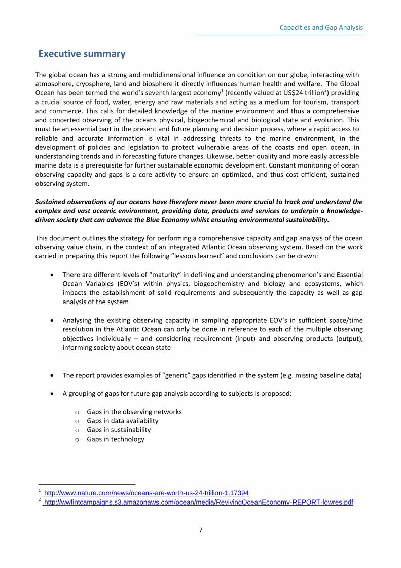
Executive summary
The global ocean has a strong and multidimensional influence on condition on our globe, interacting with atmosphere, cryosphere, land and biosphere it directly influences human health and welfare. The Global Ocean has been termed the world’s seventh largest economy1 (recently valued at US$24 trillion2) providing a crucial source of food, water, energy and raw materials and acting as a medium for tourism, transport and commerce. This calls for detailed knowledge of the marine environment and thus a comprehensive and concerted observing of the oceans physical, biogeochemical and biological state and evolution. This must be an essential part in the present and future planning and decision process, where a rapid access to reliable and accurate information is vital in addressing threats to the marine environment, in the development of policies and legislation to protect vulnerable areas of the coasts and open ocean, in understanding trends and in forecasting future changes. Likewise, better quality and more easily accessible marine data is a prerequisite for further sustainable economic development. Constant monitoring of ocean observing capacity and gaps is a core activity to ensure an optimized, and thus cost efficient, sustained observing system. Sustained observations of our oceans have therefore never been more crucial to track and understand the complex and vast oceanic environment, providing data, products and services to underpin a knowledge-driven society that can advance the Blue Economy whilst ensuring environmental sustainability. This document outlines the strategy for performing a comprehensive capacity and gap analysis of the ocean observing value chain, in the context of an integrated Atlantic Ocean observing system. Based on the work carried in preparing this report the following “lessons learned” and conclusions can be drawn:
There are different levels of “maturity” in defining and understanding phenomenon’s and Essential Ocean Variables (EOV’s) within physics, biogeochemistry and biology and ecosystems, which impacts the establishment of solid requirements and subsequently the capacity as well as gap analysis of the system
Analysing the existing observing capacity in sampling appropriate EOV’s in sufficient space/time resolution in the Atlantic Ocean can only be done in reference to each of the multiple observing objectives individually – and considering requirement (input) and observing products (output), informing society about ocean state
The report provides examples of “generic” gaps identified in the system (e.g. missing baseline data)
A grouping of gaps for future gap analysis according to subjects is proposed:
o Gaps in the observing networks o Gaps in data availability o Gaps in sustainability o Gaps in technology
1 http://www.nature.com/news/oceans-are-worth-us-24-trillion-1.17394 2 http://wwfintcampaigns.s3.amazonaws.com/ocean/media/RevivingOceanEconomy-REPORT-lowres.pdf
Capacities and Gap Analysis
8
1 Introduction
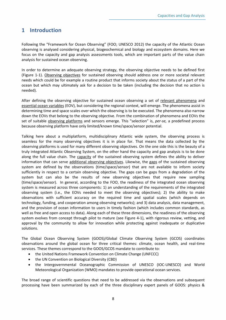
Following the “Framework for Ocean Observing” (FOO; UNESCO 2012) the capacity of the Atlantic Ocean observing is analysed considering physical, biogeochemical and biology and ecosystem domains. Here we focus on the capacity and gap analysis assessments tools, which are important parts of the value chain analysis for sustained ocean observing. In order to determine an adequate observing strategy, the observing objective needs to be defined first (Figure 1-1). Observing objectives for sustained observing should address one or more societal relevant needs which could be for example a routine product that informs society about the status of a part of the ocean but which may ultimately ask for a decision to be taken (including the decision that no action is needed). After defining the observing objective for sustained ocean observing a set of relevant phenomena and essential ocean variables (EOV), but considering the regional context, will emerge. The phenomena assist in determining time and space scales over which the observing is to be executed. The phenomena also narrow down the EOVs that belong to the observing objective. From the combination of phenomena and EOVs the set of suitable observing platforms and sensors emerge. This “selection” is, per-se, a predefined process because observing platform have only limited/known time/space/sensor potential. Talking here about a multiplatform, multidisciplinary Atlantic wide system, the observing process is seamless for the many observing objectives it is in place for. That means the data collected by the observing platforms is used for many different observing objectives. On the one side this is the beauty of a truly integrated Atlantic Observing System, on the other hand the capacity and gap analysis is to be done along the full value chain. The capacity of the sustained observing system defines the ability to deliver information that can serve additional observing objectives. Likewise, the gaps of the sustained observing system are defined by the observations (time/space/sensor) that are not available to inform society sufficiently in respect to a certain observing objective. The gaps can be gaps from a degradation of the system but can also be the results of new observing objectives that require new sampling (time/space/sensor). In general, according to the FOO, the readiness of the integrated ocean observing system is measured across three components: 1) an understanding of the requirements of the integrated observing system (i.e., the EOVs needed to meet the observing objectives); 2) the ability to make observations with sufficient accuracy on the required time and spatial scales (which depends on technology, funding, and cooperation among observing networks); and 3) data analysis, data management, and the provision of ocean information to users in timely fashion (which includes common standards, as well as free and open access to data). Along each of these three dimensions, the readiness of the observing system evolves from concept through pilot to mature (see Figure 4-1), with rigorous review, vetting, and approval by the community to allow for innovation while protecting against inadequate or duplicative solutions. The Global Ocean Observing System (GOOS)/Global Climate Observing System (GCOS) coordinates observations around the global ocean for three critical themes: climate, ocean health, and real-time services. These themes correspond to the GOOS/GCOS mandate to contribute to:
the United Nations Framework Convention on Climate Change (UNFCCC)
the UN Convention on Biological Diversity (CBD)
the Intergovernmental Oceanographic Commission of UNESCO (IOC-UNESCO) and World Meteorological Organization (WMO) mandates to provide operational ocean services.
The broad range of scientific questions that need to be addressed via the observations and subsequent processing have been summarized by each of the three disciplinary expert panels of GOOS: physics &
Capacities and Gap Analysis
9
climate (OOPC), biogeochemistry (IOCCP), and biodiversity and ecosystems (GOOS BioEco) and all somehow address at least one of the three themes.
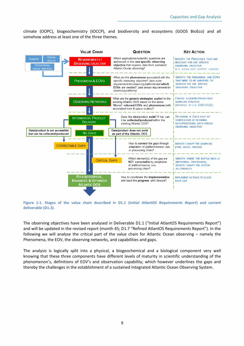
Figure 1-1. Stages of the value chain described in D1.1 (Initial AtlantOS Requirements Report) and current deliverable (D1.3).
The observing objectives have been analysed in Deliverable D1.1 (“Initial AtlantOS Requirements Report”) and will be updated in the revised report (month 45; D1.7 “Refined AtlantOS Requirements Report”). In the following we will analyse the critical part of the value chain for Atlantic Ocean observing – namely the Phenomena, the EOV, the observing networks, and capabilities and gaps. The analysis is logically split into a physical, a biogeochemical and a biological component very well knowing that these three components have different levels of maturity in scientific understanding of the phenomenon’s, definitions of EOV’s and observation capability; which however underlines the gaps and thereby the challenges in the establishment of a sustained Integrated Atlantic Ocean Observing System.
Capacities and Gap Analysis
10
2 Phenomena Phenomena are basic processes that compose/are of relevance to describe observing objectives. The phenomena are closely related to the scientific base of an observing objective. Depending on the phenomena different observing strategies may emerge but for the same observing objective, for example the change in Atlantic Ocean heat content can be observed via temperature profiles (based on phenomena “heat storage” on large scale and EOV subsurface temperature) or via changes in sea level (based on phenomena “sea level” on large scale and EOV “Sea Surface height”) – these two approaches require a different set of observing networks at place. The Global Ocean Observing System (GOOS) uses the following definition of a phenomenon, which also put it in the context of Essential Ocean Variables (EOVs) and thus setting targets for their observations (GOOS Report No. 219, 2016).
Physical processes are important for many of the GOOS observing objectives and therefore the physical phenomena often need to be considered when discussing observing objectives and requirements for the biogeochemical and ecosystem domains. Therefore, when defining the phenomena for biogeochemistry and biology the physical phenomena need to be considered in most cases as well. This is important because, as mentioned above, the phenomena are defined in order to set the time/space scales of sampling. Given the nature of the physics processes that follow a set of equations, a structuring of the phenomena and orientation of the phenomena in time/space (Stommel) diagrams is possible (see Section 4; below).
2.1 Physical Phenomena
Here we present a brief description of the physical phenomena with applications to key features of the
Atlantic Ocean. The Physical Phenomena described here are:
Circulation
Fronts and Eddies
Tides
Coastal Processes
Air-Sea Fluxes
Surface Waves
Freshwater Cycle
Sea Level
Upwelling
Riverine
Heat Storage
Stratification
Mixed layer
Water Masses
Sea Ice Extent
Extreme events
A phenomenon is an observable process, event, or property, measured or derived from one or a combination of EOVs, having characteristic spatial and time scale(s), that addresses at least one GOOS Scientific Question.
Capacities and Gap Analysis
11
Circulation The primary conceptual elements of the ocean circulation are the wind driven and thermohaline driven circulation. The two circulation elements are interwoven in a complex way and not be unrevealed but maybe separated in a conceptual way (Wunsch, 2002). The wind driven circulation include the energetic western boundary currents, swifter eastern boundary flow, elements of the coastal current systems, and the predominately zonal currents of the equatorial current system. The thermohaline circulation includes what has conceptualized in its most basic description as the “global ocean conveyor belt” (Stommel & Arons, 1959), a global meridional flow where less dense surface waters are converted into dense, cold waters that are found at greater depth while in parallel the cold waters are also transformed back to less dense/surface waters. Very much attention is given the thermohaline circulation (THC) in the context of climate variability, because much of the oceanic component of the redistribution of heat from the equator to the polar regions is intimately linked to the THC. In addition “shallow” meridional overturning circulation cells are also found in the subtropics and tropics (Schott, McCreary, & Johnson, 2004) and play an important role in multiannual climate variability or the storage of carbon in the ocean. All these circulation elements are important for redistribution of heat, freshwater and substances in the ocean, which in turn all impact the three overarching GOOS observing. Circulation might be distinguished from other elements as being associated with flows at small Rossby number Ro=v/(l*f), relating the length scale of the flow (l), the flow speed (v), and the earth rotation (f). Part of the circulation is of topographic control, such as the overflow regions that control the exchange between the Nordic Seas and the northern Subpolar gyre or the Mediterranean Sea and Northeast Atlantic or the deep and bottom circulation. Key regions are prone to observed key water masses in a very efficient way (e.g. Vema Channel in South Atlantic for Antarctic Bottom Water flow). Knowledge about the very surface circulation has even centuries ago identified an important prerequisite for efficient shipping as expressed in the Gulf Stream charts by Benjamin Franklin from 1770. Fronts and eddies Fronts and eddies are an “interface” between geostrophically balanced flow (low Rossby number flow) as described in circulation and so called “sub-mesoscale flow” where non-linear terms become more important in the dynamical balances. In practical terms the sub-mesoscale flow describes a “dynamical conduit for energy transfer towards microscale dissipation and diapycnal mixing” (McWilliams 2016). The link to these scales is important not only for the energy balance in the oceanic system but has been identified of particular importance in biological/Physical/biogeochemical interactions that feed back to the ocean health theme. High productivity (Lévy, Klein, & Treguier, 2001) and ecosystem hot spots attracting multiple trophic levels and as such relevant for e.g. tuna fisheries are specifically rich in Eddies and frontal regions. Tides Tides share with the wind stress input the primary source of mechanical energy to drive interior ocean mixing required to convert water masses back from the a dense/deep water into a less dense/near surface characteristic (Munk & Wunsch, 1998). Internal tides interacting with topography transform the energy input directly (Polzin, Toole, Ledwell, & Schmitt, 1997). Barotropical tidal signals are linked to periodic sea level changes that in turn impact coastal as well as open ocean areas. Propagation of tides on to shelf can generate upwelling in particular when critical slopes are met (Lamb, 2014).

Capacities and Gap Analysis
12
Coastal processes The physical realm of the costal ocean includes an extensive set of oscillatory phenomena such as planetary wave propagation, tidal waves, surface waves. The wave propagation is coupled to processes such as local coastal upwelling/downwelling, sea level variability, erosion, and currents. Coastal processes include also fronts, eddies and filaments that export water from the coastal areas into the open ocean. Sediment transport, extensive mudflats all belong to the coastal realm. It is not to believed that the Atlantic shoreline do differ from the rest of the globe and as such no specific Atlantis coastal processes are listed here. Air-sea fluxes The Exchange of heat, freshwater, momentum, and substances across the air/sea interface are couple to several phenomena. Atmospheric boundary layer stability and gradients across the air/sea interface play a key role in the air/sea fluxes. The Atlantic hosts major uptake region for the gases such as carbon dioxide or trace gases such as CFCs. The eastern boundary and equatorial upwelling regions are often sources for gases in the atmosphere (e.g. see map by Takahashi et al., 1997). Momentum flux in boundary regions are one process of great importance for the upwelling of nutrient rich waters. Surface waves Surface waves play a key role for many societal relevant observing topics but also for the momentum flux. Surface wave, white capping, bubble injection are important processes for the exchange of gases across the air/sea interface. Ship routing requires consideration of surface waves. Freshwater cycle The ocean plays a key role in the global hydrological cycle and the ocean is the largest freshwater reservoir on the globe. Freshwater cycle is closely related to riverine input and thus to flooding and coastal processes. The freshwater input is also important in hurricane formation and intensification. Changes in freshwater content indicate changes in the hydrological cycle and have been detected in the North Atlantic (Curry & Mauritzen, 2005). Freshwater has an impact on the momentum and heat exchange – a shallow freshwater layer in the open ocean (Barrier layer; (Foltz & McPhaden, 2009) can provoke intense momentum and heat trapping. Freshwater variability in overturning areas may disturb the surface haline and thermal buoyancy balance and thus changes in water mass formation and water mass characteristic may result (Dickson et al., 2002). Sea level Sea level changes in the open ocean are an imprint of several processes most prominent the changes in heat content. The open ocean sea level change is connected but not directly taken up by coastal sea level changes (Gill & Clarke, 1974; Lorbacher, Dengg, Böning, & Biastoch, 2010).
Upwelling The upward vertical transport of water can be either along (lateral) or across (diapycnal) isopycnals. Upwelling is of paramount importance in the coupling between biogeochemistry/biology and physical processes if the upwelling reaches limiting conditions such as light availability (euphotic depth). In turn upwelling regions are important for primary productivity and fisheries. Key upwelling areas are the eastern boundary regions where a coastal parallel component of the local winds drive upwelling. These regions overlap with the so called shallow zone regions, area of the ocean where, by dynamical constraints as an interplay between wind stress indicted vorticity input and planetary vorticity, fluid has difficulties to enter. Water mass transport is here primarily diffusive and the regions host the large-scale oxygen minimum zones at intermediate depth (J. Karstensen & Tomczak, 1998; Johannes Karstensen, Stramma, & Visbeck, 2008).
Capacities and Gap Analysis
13
Upwelling also has impact of local weather because of cooling the surface ocean. Upwelling of cold water stabilizes the atmospheric boundary layer and often the regions are characterized by foggy conditions. Upwelling also provokes internal adjustment the density field (upper layer densities are bended upward) and hence a dynamical response to upwelling is typically an undercurrent that develops at some depth where an upwelling impact ceases. A special upwelling region is the equatorial upwelling that essentially is driven by the divergence of the Ekman transport of wind that crosses the equator. The signal has a seasonal cycle that is related to the migration of the intertropical convergence zone, which is part of the atmospheric circulation. The equatorial upwelling is important for cooling the equatorial region, and related to tropical rainfall (Kushnir, 1994).
Riverine The riverine (run off) input to the ocean has impact that goes far beyond the river month. The freshwater often is transported far offshore. This is related to the fact that the very light water sits as a lens of water on top and forma a so-called barrier layer (BL). The BL may cause a trapping of momentum in the upper few meters of the ocean and lead to a very efficient and far reaching transport of the freshwater plume. The proximity of the Amazon river to the entrance of the zonal flow of the equatorial current system guarantees that the freshwater and its sources are distributed across the Atlantic Ocean. The momentum trapping may also play an important role in the process of hurricane formation and intensification (Reul et al., 2012). The uptake of carbon/gases is limited by the extend of the riverine flow, again because momentum and as such mechanical stirring is trapped in the surface layer (Salisbury et al., 2011). Moreover, the surface chemistry (Alkalinity) is impacted by the low salinity water. The Amazon river but also the Rio de La Plata, the Mississippi/Missouri, the Niger are important riverine sources for the Atlantic Ocean. Heat storage The heat storage capability of the ocean is essential for our present climate. Globally the ocean has taken up about 93% of the global warming, “removing “the warming from the atmosphere and storing it in the ocean as the warming of the ocean is observed in all depth levels (Abraham et al., 2013). The heat storage capability of seawater also moderates the climate conditions. In general, this is to be seen in coastal areas where the amplitude of the seasonal temperature changes are every much damped by the ocean taking up and releasing heat in the seasonal cycle. In combination with the circulation the heat storage capability of the seawater lead to a certain balance between local uptake/release versus transport of heat which is the reasons why the ocean is not only to be approximated by a slap layer model. The moderate climate in the high latitudes of the western Atlantic, the advection of warm water with the currents into the northern North Atlantic/Nordic Sea is related to the balance between transport and inertia in the heat release of the ocean. Monitoring the upper ocean heat content has been identified as a key element in the global climate monitoring system. However, recently the importance in observing the deep ocean as well was appreciated (Purkey & Johnson, 2010). The deep ocean, in spite the fact that the warming is less intense, is large volume of water. The comparably small changes in temperature pose specific requirements to the sensors to be used for Ocean Observing here, repeat hydrography (GO-SHIP) and high quality moored sensors (OceanSITES) provide critical data. The “Deep Ocean Observing Strategy” (DOOS) summarizes the current global activities.
Capacities and Gap Analysis
14
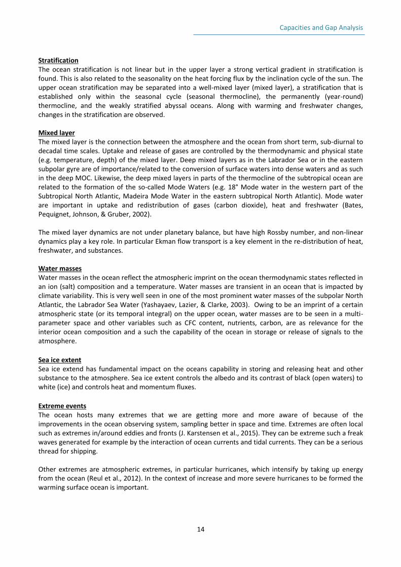
Stratification The ocean stratification is not linear but in the upper layer a strong vertical gradient in stratification is found. This is also related to the seasonality on the heat forcing flux by the inclination cycle of the sun. The upper ocean stratification may be separated into a well-mixed layer (mixed layer), a stratification that is established only within the seasonal cycle (seasonal thermocline), the permanently (year-round) thermocline, and the weakly stratified abyssal oceans. Along with warming and freshwater changes, changes in the stratification are observed. Mixed layer The mixed layer is the connection between the atmosphere and the ocean from short term, sub-diurnal to decadal time scales. Uptake and release of gases are controlled by the thermodynamic and physical state (e.g. temperature, depth) of the mixed layer. Deep mixed layers as in the Labrador Sea or in the eastern subpolar gyre are of importance/related to the conversion of surface waters into dense waters and as such in the deep MOC. Likewise, the deep mixed layers in parts of the thermocline of the subtropical ocean are related to the formation of the so-called Mode Waters (e.g. 18° Mode water in the western part of the Subtropical North Atlantic, Madeira Mode Water in the eastern subtropical North Atlantic). Mode water are important in uptake and redistribution of gases (carbon dioxide), heat and freshwater (Bates, Pequignet, Johnson, & Gruber, 2002). The mixed layer dynamics are not under planetary balance, but have high Rossby number, and non-linear dynamics play a key role. In particular Ekman flow transport is a key element in the re-distribution of heat, freshwater, and substances.
Water masses Water masses in the ocean reflect the atmospheric imprint on the ocean thermodynamic states reflected in an ion (salt) composition and a temperature. Water masses are transient in an ocean that is impacted by climate variability. This is very well seen in one of the most prominent water masses of the subpolar North Atlantic, the Labrador Sea Water (Yashayaev, Lazier, & Clarke, 2003). Owing to be an imprint of a certain atmospheric state (or its temporal integral) on the upper ocean, water masses are to be seen in a multi-parameter space and other variables such as CFC content, nutrients, carbon, are as relevance for the interior ocean composition and a such the capability of the ocean in storage or release of signals to the atmosphere.
Sea ice extent Sea ice extend has fundamental impact on the oceans capability in storing and releasing heat and other substance to the atmosphere. Sea ice extent controls the albedo and its contrast of black (open waters) to white (ice) and controls heat and momentum fluxes.
Extreme events The ocean hosts many extremes that we are getting more and more aware of because of the improvements in the ocean observing system, sampling better in space and time. Extremes are often local such as extremes in/around eddies and fronts (J. Karstensen et al., 2015). They can be extreme such a freak waves generated for example by the interaction of ocean currents and tidal currents. They can be a serious thread for shipping. Other extremes are atmospheric extremes, in particular hurricanes, which intensify by taking up energy from the ocean (Reul et al., 2012). In the context of increase and more severe hurricanes to be formed the warming surface ocean is important.
Capacities and Gap Analysis
15
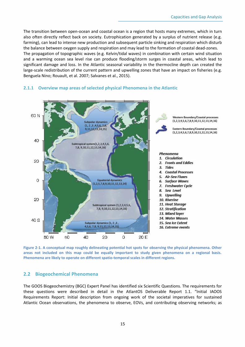
The transition between open-ocean and coastal ocean is a region that hosts many extremes, which in turn also often directly reflect back on society. Eutrophication generated by a surplus of nutrient release (e.g. farming), can lead to intense new production and subsequent particle sinking and respiration which disturb the balance between oxygen supply and respiration and may lead to the formation of coastal dead-zones. The propagation of topographic waves (e.g. Kelvin/tidal waves) in combination with certain wind situation and a warming ocean sea level rise can produce flooding/storm surges in coastal areas, which lead to significant damage and loss. In the Atlantic seasonal variability in the thermocline depth can created the large-scale redistribution of the current pattern and upwelling zones that have an impact on fisheries (e.g. Benguela Nino; Rouault, et al. 2007; Salvanes et al., 2015).
2.1.1 Overview map areas of selected physical Phenomena in the Atlantic
Figure 2-1. A conceptual map roughly delineating potential hot spots for observing the physical phenomena. Other areas not included on this map could be equally important to study given phenomena on a regional basis. Phenomena are likely to operate on different spatio-temporal scales in different regions.
2.2 Biogeochemical Phenomena
The GOOS Biogeochemistry (BGC) Expert Panel has identified six Scientific Questions. The requirements for these questions were described in detail in the AtlantOS Deliverable Report 1.1. “Initial IAOOS Requirements Report: Initial description from ongoing work of the societal imperatives for sustained Atlantic Ocean observations, the phenomena to observe, EOVs, and contributing observing networks; as
Capacities and Gap Analysis
16
guidance for other WPs.” The Report also provides a list of generic ocean phenomena and provides a matrix of relevant EOVs per phenomenon. In this report, we provide a more comprehensive list of biogeochemical phenomena (as defined by GOOS) which control the Atlantic Ocean dynamics each addressing at least one of the scientific questions posed by GOOS. The list of biogeochemical phenomena presented in this report originates from the AtlantOS workshop on “Setting Biogeochemical Observing targets for the Observing System in the Atlantic”, held on 29 November – 1 December 2016 in Sopot, Poland. Defining biogeochemical phenomena is challenging if we consider that many are either primarily driven by physical (e.g. ventilation, air-sea fluxes) or biological and ecosystem mechanisms (organic matter cycling, eutrophication). The process of harmonizing phenomena across the disciplines and across all GOOS EOV Specification Sheets is ongoing. On top of identifying the key phenomena of interest, which should actively drive the design of the observing system in the Atlantic, we discuss the spatial and temporal scales on which these phenomena operate, and point at the key geographical areas of their occurrence. These phenomena ‘hot-spots’ (Figure 2-4) can be overlaid with maps of relevant EOV observations to help analyse our current observing capacities, and thus provide a basis for a comprehensive gap analysis in the future. Although the current observing system setup is not centred around the phenomena, but rather around observing approaches and/or individual EOVs, such a paradigm shift is much needed to move from a fragmented towards an integrated multiplatform and multidisciplinary observing system. An observing system centred on phenomena would also require that observing targets be considered according to the phenomena of interest. The task of setting biogeochemical observing targets was taken up by the participants of the Sopot workshop. A working definition of an observing target has been proposed such that an observing target is set to allow the observing system to detect changes in a given phenomenon sufficiently to address the relevant scientific questions and societal needs. Such a target needs to be set at the spatial and temporal scales the phenomenon is sensitive to, and at a desirable/known level of uncertainty, with consideration of all relevant EOVs. In this report, preliminary outcomes from the Sopot workshop are listed as considerations for setting phenomena-based targets for the ocean observing system in the Atlantic. These are described only in terms of biogeochemical measurements, however acknowledging that parallel physical and biological measurements are also essential. The Biogeochemical Phenomena described here are:
Ventilation (Water Mass Age)
Air-Sea Fluxes
Cross-shelf interactions
Anthropogenic Carbon Sequestration
Ocean Acidity
Inorganic Nutrient Cycling
Organic Matter Cycling
Hypoxia
Eutrophication
Contamination/Pollution
Capacities and Gap Analysis
17
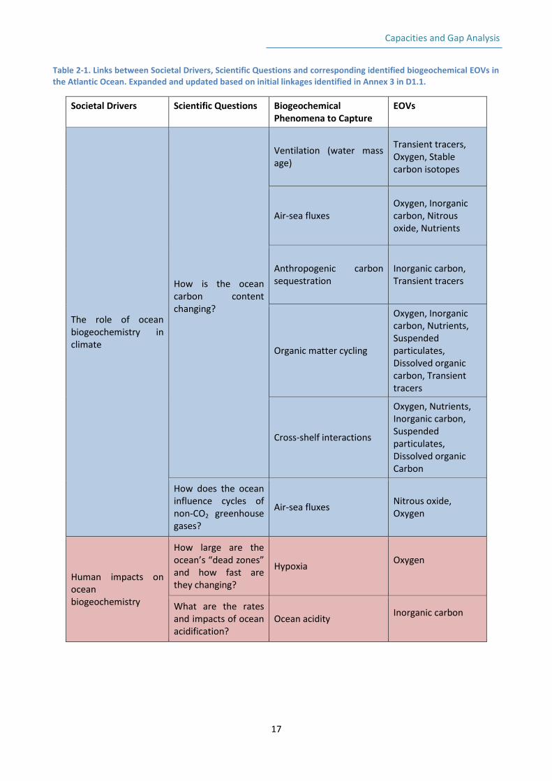
Table 2-1. Links between Societal Drivers, Scientific Questions and corresponding identified biogeochemical EOVs in the Atlantic Ocean. Expanded and updated based on initial linkages identified in Annex 3 in D1.1.
Societal Drivers Scientific Questions Biogeochemical Phenomena to Capture
EOVs
The role of ocean biogeochemistry in climate
How is the ocean carbon content changing?
Ventilation (water mass age)
Transient tracers, Oxygen, Stable carbon isotopes
Air-sea fluxes Oxygen, Inorganic carbon, Nitrous oxide, Nutrients
Anthropogenic carbon sequestration
Inorganic carbon, Transient tracers
Organic matter cycling
Oxygen, Inorganic carbon, Nutrients, Suspended particulates, Dissolved organic carbon, Transient tracers
Cross-shelf interactions
Oxygen, Nutrients, Inorganic carbon, Suspended particulates, Dissolved organic Carbon
How does the ocean influence cycles of non-CO2 greenhouse gases?
Air-sea fluxes Nitrous oxide, Oxygen
Human impacts on ocean biogeochemistry
How large are the ocean’s “dead zones” and how fast are they changing?
Hypoxia Oxygen
What are the rates and impacts of ocean acidification?
Ocean acidity Inorganic carbon
Capacities and Gap Analysis
18
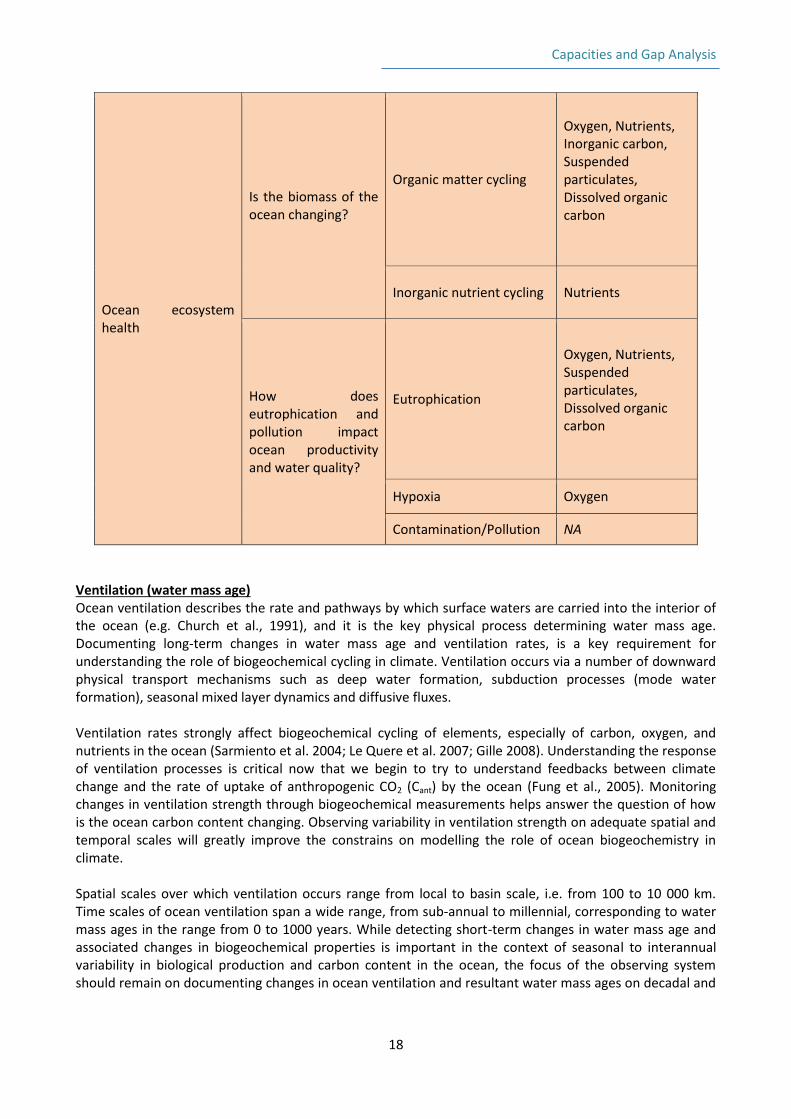
Ocean ecosystem health
Is the biomass of the ocean changing?
Organic matter cycling
Oxygen, Nutrients, Inorganic carbon, Suspended particulates, Dissolved organic carbon
Inorganic nutrient cycling Nutrients
How does eutrophication and pollution impact ocean productivity and water quality?
Eutrophication
Oxygen, Nutrients, Suspended particulates, Dissolved organic carbon
Hypoxia Oxygen
Contamination/Pollution NA
Ventilation (water mass age) Ocean ventilation describes the rate and pathways by which surface waters are carried into the interior of the ocean (e.g. Church et al., 1991), and it is the key physical process determining water mass age. Documenting long-term changes in water mass age and ventilation rates, is a key requirement for understanding the role of biogeochemical cycling in climate. Ventilation occurs via a number of downward physical transport mechanisms such as deep water formation, subduction processes (mode water formation), seasonal mixed layer dynamics and diffusive fluxes. Ventilation rates strongly affect biogeochemical cycling of elements, especially of carbon, oxygen, and nutrients in the ocean (Sarmiento et al. 2004; Le Quere et al. 2007; Gille 2008). Understanding the response of ventilation processes is critical now that we begin to try to understand feedbacks between climate change and the rate of uptake of anthropogenic CO2 (Cant) by the ocean (Fung et al., 2005). Monitoring changes in ventilation strength through biogeochemical measurements helps answer the question of how is the ocean carbon content changing. Observing variability in ventilation strength on adequate spatial and temporal scales will greatly improve the constrains on modelling the role of ocean biogeochemistry in climate. Spatial scales over which ventilation occurs range from local to basin scale, i.e. from 100 to 10 000 km. Time scales of ocean ventilation span a wide range, from sub-annual to millennial, corresponding to water mass ages in the range from 0 to 1000 years. While detecting short-term changes in water mass age and associated changes in biogeochemical properties is important in the context of seasonal to interannual variability in biological production and carbon content in the ocean, the focus of the observing system should remain on documenting changes in ocean ventilation and resultant water mass ages on decadal and
Capacities and Gap Analysis
19
longer time scales. It is this variability that is necessary to quantify long-term trends in Cant ocean uptake, or oxygen and nutrient storage in the ocean interior. Key geographical areas: Ocean ventilation is not limited spatially to the open ocean as it also occurs on the continental shelf and in marginal seas. Areas of strongest ventilation are associated with open ocean deep water formation processes. The formation of the North Atlantic Deep Water (NADW) is controlled by downward physical transport in the Labrador Sea, Irminger Sea and Greenland Sea. Calculating Transient Tracer and Oxygen EOV inventories will be important to detect decadal reduction or strengthening of ventilation in these areas. Although the Southern Ocean is beyond the geographical domain considered by the AtlantOS project, ventilation associated with formation of the Antarctic Bottom Water (AABW) and Antarctic Intermediate Water (AAIW) has a significant influence on the Atlantic biogeochemical cycling and needs to be considered in any Atlantic observing system design. Ventilation time is derived from volume and flux measurements (Bolin, B., Rhode, H., 1973). Often ventilation is connected with water mass ages and transport times, it is not sufficient to focus on sources of water mass formation. Equally important are measurements in the deep portions of oxygen minimum zones which are regions of the ocean where water mass age in the thermocline exceeds several decades. Across basin ship-based hydrography transects fulfil this requirement well. Relevant EOVs: Ventilation rates of a water mass can be estimated using ages derived from Transient Tracer EOV measurements. Following is the list of sub-variables of the Transient Tracers EOV: Chlorofluorocarbons (CFC-12, CFC-11, CFC-113, CCl4), Sulphur hexafluoride (SF6), Tritium-3He, 14C, 39Ar. Likewise, the ventilation can be derived from an estimation of the volume and the flux into that volume (e.g. subduction rates). To derive water mass ages from transient tracers the well-characterized atmospheric histories of the CFCs and SF6 (Walker et al. 2000, Bullister 2015) along with the solubility of these gases in seawater (Warner & Weiss 1985, Bullister et al. 2002) are used. Considering a known equilibrium concentrations of these compounds in the surface ocean in the source region a water ages distribution of all contributing source waters can be modelled as a function of time (e.g., Tanhua et al. 2013b). Decay of tritium to 3He provides an additional radioisotope natural clock for the isolation of water parcels from the atmosphere (Jenkins 1977). Apart from determining ocean ventilation rates, maps and inventories of 14C have been used to determine global mean air-sea exchange rates for CO2 (Naegler et al. 2006, Sweeney et al. 2007), to calibrate global ocean general circulation models. The combination of dissolved oxygen data with transient tracer data provides further evidence regarding the timescales at which the ventilation changes occur. Furthermore, the combination of oxygen data with Inorganic Carbon EOV data (e.g., Sabine et al. 2008) and pH data (e.g., Byrne et al. 2010) has allowed separation of dissolved inorganic carbon (DIC)/pH changes along repeat hydrography sections into anthropogenic and ventilation/remineralization components, including their respective effects on carbon storage and ocean acidification. Finally, changes in deep ocean ventilation state can be determined on geological time scales, based on supporting stable carbon isotope (13C) EOV measurements (Tschumi et al., 2011).
Capacities and Gap Analysis
20
Considerations for setting observing targets: Decadal repeat hydrography measurements are required to determine changes in ocean ventilation strength on a basin scale. Short-term scale observations are needed for studying seasonal and annual changes in ventilation on regional scales (< 1000 km) associated with deep water formation and other downward physical transport mechanisms, both in the open ocean and in the shelf region. It is important to note that this phenomenon is not exclusive to the open ocean (see key geographic areas above) but should be observed in the shelf region as well, though on different spatio-temporal scales. Compared to the basin-scales, decadal changes in Atlantic water mass ages, seasonal and annual ventilation patterns are more important from the perspective of the changing biogeochemical properties of the waters transported away from the surface, and their role in regulating seasonality in biological phenomena. From this perspective, target observations should be near-continuous with a special focus on winter months. Air-sea fluxes The surface turbulent fluxes of momentum, heat, and moisture at the interface between the atmosphere and the oceans represent an exchange of energy between the two. The air-sea fluxes are also an important phenomenon responsible for cycling of several biogeochemical elements. Biogeochemical observations in the Atlantic focus on several types of air-sea fluxes: (i) air-sea fluxes of CO2, (ii) air-sea fluxes of O2, (iii) N2O flux to the atmosphere, and (iv) dust deposition; observations of which help answer one or more of the GOOS Scientific Questions. Air-sea fluxes of CO2 Although currently not as important as ocean circulation and mixing, air-sea CO2 gas exchange is one of the mechanisms controlling Cant uptake by the ocean (Talley et al., 2016). For any particular location, the flux of CO2 between the air and the sea is the product of two principal factors: the difference in partial pressure of CO2 between the air and the bulk water (ΔpCO2), which can be considered as the thermodynamic driving force, and the gas exchange rate or "transfer velocity" (kw), which is the kinetic parameter. The transfer velocity incorporates both the diffusivity of the gas in water (which varies with temperature and between different gases), and the effect of physical processes within the water boundary layer.
The rate of CO2 exchange is determined by the transfer across the water boundary layer, thus the flux is obtained by multiplying the difference between the air and water pCO2 (partial pressure of CO2 in air which is in equilibrium with the water), by the solubility "K0" in mol l-1 atm.
Air-sea fluxes of O2 There are two separate mechanisms that contribute to trends in dissolved oxygen storage in the ocean. The air-sea flux component corresponds directly to the amount of O2 that the ocean is losing or gaining from the atmosphere, i.e., it is that part of the marine O2 that leaves an imprint on atmospheric oxygen [Gruber et al., 2001; Keeling and Garcia, 2002]. It is important to separate this component from that one that includes all processes at the surface and interior that are not associated with the exchange of O2 across the air-sea interface, i.e. as a result of biological consumption and production of O2 in the surface ocean, and through physical transport and mixing (Stendardo and Gruber, 2012, and references therein). To quantify the contributions of these mechanisms driving the changes in oxygen, one needs to calculate trends in the saturation concentration of O2, trends in the apparent oxygen utilization (AOU), and trends in the quasi-conservative tracer O*2, derived from dissolved oxygen and phosphorus concentrations (Keeling and Garcia, 2002).
Capacities and Gap Analysis
21
Dissolved oxygen tends to respond very sensitively to climate variability and change because any perturbation in sea-surface temperature not only changes the solubility of dissolved oxygen, but also alters upper ocean stratification in a way that tends to amplify the solubility effect (e.g. Najjar and Keeling, 2000; Keeling et al., 2010). This high sensitivity to climate forcing makes oxygen one of the best candidates for detecting and better understanding the link between global warming and the resulting biogeochemical and physical changes in the ocean (e.g., Joos et al., 2003; Keeling et al., 2010). N2O flux to the atmosphere Because of the on-going decline of chlorofluorocarbons and the continuous increase of N2O in the atmosphere the contributions of N2O to both the greenhouse effect and ozone depletion will be even more pronounced in the 21st century. The oceans - including its coastal areas such as continental shelves, estuaries and upwelling areas - are a major source of N2O and contribute about 30% to the atmospheric N2O budget. Oceanic N2O is mainly produced as a by-product during archaeal nitrification (i.e. ammonium oxidation to nitrate) whereas bacterial nitrification seems to be of minor importance as source of oceanic N2O. N2O occurs also as an intermediate during microbial denitrification (nitrate reduction via N2O to dinitrogen, N2). Nitrification is the dominating N2O production process, whereas denitrification contributes only 7-35% to the overall N2O water column budget in the ocean. The amount of N2O produced during both nitrification and denitrification strongly depends on the prevailing dissolved oxygen (O2) concentrations and is significantly enhanced under low (i.e. suboxic) O2 conditions. Atmospheric dust deposition Dust is produced primarily in desert regions and transported long distances through the atmosphere to the oceans. Upon deposition of dust, its dissolution can provide an important source of a range of nutrients, particularly nitrogen and iron, to microbes living in open ocean surface waters (Jickels and Moore, 2015). Direct measurements of nitrogen from dust deposition are difficult. Majority of flux estimates used come from particle tracking models, with assumptions on dust deposition solubility and bioavailability. Ship-based oceanic measurements of dissolved nutrients are needed in parallel with atmospheric measurements of dust deposition rates to further validate these models. Spatial and temporal scales, key geographic regions: Air-sea CO2 and O2 flux measurements are key in areas of highest ocean ventilation rates, i.e. in the Irminger, Labrador and Greenland Seas, as well as in the western boundary current regions. The air-sea oxygen flux exhibits significant interannual variability in the North Atlantic, primarily a consequence of variability in winter convection in the subpolar gyre (McKinley et al. 2000).
Significantly enhanced N2O concentrations are generally found at oxic/suboxic or oxic/anoxic boundaries. The strong O2 sensitivity of N2O production is also observed in coastal characterised by seasonal shifts in the O2 regime. Global maps of N2O in the surface ocean show enhanced N2O anomalies (i.e. supersaturation of N2O) in equatorial upwelling regions as well as N2O anomalies close to zero (i.e. near equilibrium) in large parts of the open ocean. Dust deposition in the North Atlantic is characterized by strong variability on sub-annual time scales. Large dust deposition events cover hundreds of kilometres, thus can affect biological production on sub-basin scales. There are some key regions for monitoring dust deposition and its role in controlling ocean phytoplankton biomass production. In regions of high atmospheric iron supply, such as the tropical North Atlantic, stimulation of nitrogen fixation drives the phytoplankton population toward a state in which phosphorus supply rates limit primary production. Atmospheric deposition is also an important source of nitrogen to the low latitude ocean, where it stimulates primary production.
Capacities and Gap Analysis
22
Relevant EOVs: As discussed above, observing changes in air-sea fluxes requires measurements of several EOVs. Measuring pCO2 as a sub-variable of the Inorganic Carbon EOV, Dissolved Oxygen and Nitrous Oxide EOVs are necessary to constrain the air-sea fluxes of biogeochemical elements. Additionally, measurements of Inorganic Macronutrients EOV are needed to constrain or validate the oxygen air-sea fluxes, and to estimate rates of atmospheric deposition of nitrogen. Finally, most of these measurements rely on coincident measurements of surface and subsurface temperature and salinity physical EOVs. Considerations for setting observing targets: Considering high spatial and temporal variability of the signal, the overall target for observing this phenomenon would be to constrain this annual flux to within 10% of the total flux. To constrain this phenomenon, sea surface pCO2 measurements are needed with an accuracy to within 2 µatm. Additionally, requirements for lower atmospheric pCO2 measurements at sea were identified. These are to have observations at every 10º latitude and at two longitudinal points (enter and exit). 0.1 µatm accuracy is required for atmospheric inversions but the air-sea flux related target would be 2 µatm. Furthermore, spatial coverage of ocean pCO2 needs improving in the South Atlantic to match the North Atlantic coverage of every 10º latitude coast to coast. For oxygen fluxes, it is recommended that oxygen measurements be taken on a bi-weekly basis in order to document changes in air-sea fluxes due to phytoplankton bloom dynamics. The main target for ensuring adequate spatial coverage and resolution is to place oxygen sensors on all Argo profiling floats, found on average every 3°. Increased density of floats with oxygen sensors is required outside of the subtropical gyre regions, primarily in the key geographic regions listed above. Cross-shelf interactions This phenomenon describes the biogeochemical exchanges with shelf and marginal seas. In many coastal circulation regimes, the proximity of energetic boundary currents in deep water at the shelf edge is a key dynamic in mediating shelf/open-ocean exchange. On coasts for which estimates exist, fluxes of nutrients and carbon across this boundary are leading order terms in the nitrogen and carbon budgets of shelf ecosystems. The exchange at the ocean boundary, and shelf edge dynamics have immediate impacts on ecosystem function and productivity on weekly to seasonal time scales, but can also drive multi-decadal changes in ecosystem structure through effects on habitat ranges and biodiversity. Direct observations of biogeochemical and physical exchanges across the shelf-open ocean boundary have not been sustained to the extent required to fully complement observations within the ocean interior. In large part, this is due to the particular challenges of maintaining observing networks within energetic regimes, and capturing the significantly shorter time and space scales of variability there. Quantifying nutrient fluxes across the shelf-open ocean boundary, often occurring in pulse form in response to passing fronts and eddies, is an essential requirement for some of the Societal Benefit products developed as part of AtlantOS WP8. Responding to a gap in such measurements would meet the demands for providing better constrained boundary conditions for Marine Strategy Framework (MSFD) indicators. Nutrient flux observations would also help inform, calibrate and validate biogeochemical models which would potentially enhance the capacity for Harmful Algal Bloom forecasting. Of secondary importance to these applications are measurements of carbon and oxygen fluxes.
Capacities and Gap Analysis
23
Key geographic areas: Key areas are all shelf regions and the marginal seas, with focus on the western and eastern boundary current regions. Relevant EOVs: Inorganic macronutrients, Inorganic carbon, Suspended particulates, Dissolved organic carbon. Considerations for setting observing targets: The long-term monitoring of physics, biogeochemistry and biology across the open ocean-shelf boundary, at key locations (i.e. western and eastern boundaries, and upwelling region), will provide a comprehensive reference data set that will measure exchanges across the open ocean-shelf boundary, improve our understanding of the relationship of boundary currents and the basin-scale gyre forcing, and determine the impact of boundary current variability on coastal marine ecosystems. The observation targets need to be driven by the need to generate initialized boundary conditions for high-resolution coupled reanalysis and forecast model of the coastal seas, and asses the simulation of various regional and coastal models. As far as biogeochemical fluxes at these boundaries are concerned, the number one target is to establish a baseline for carbon, nutrient and particulate export fluxes, followed by efforts to better constrain short-term to long-term variability patterns.
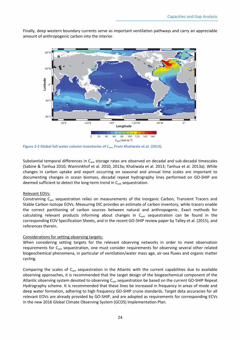
Anthropogenic carbon sequestration The term “carbon sequestration” here describes only the natural oceanic processes by which CO2 is removed from the atmosphere and stored in the ocean interior or buried in marine sediments. Considering the accelerating pace of emissions related to human activities, it is important to explicitly detect changes in the uptake and storage of the anthropogenic component of carbon dioxide in the atmosphere, on top of quantifying ocean’s role as a sink in the global carbon budget. By continuing to take up a substantial fraction of the Cant emissions from fossil fuel combustion and net land-use change, the ocean is a major mediator of global climate change. Observing the phenomenon of anthropogenic carbon sequestration thus directly helps answer the GOOS Scientific Question ‘How is the ocean carbon content changing? Mechanisms of carbon sequestration are either physico-chemical (through the solubility pump) or biological (through the biological pump), and are no different for whether the sources of carbon are natural or anthropogenic. Several methods have been developed and tested to accomplish the separation between changes in dissolved inorganic carbon due to Cant uptake and due to natural variations in circulation and organic matter remineralization (Friis et al., 2005; Locarnini et al. 2013, Zweng et al. 2013). The physico-chemical mechanism is closely related to two other phenomena described in this document, i.e. ventilation and air-sea fluxes. The biological mechanism on the other hand relates to organic matter cycling. In consequence, setting biogeochemical observing targets with respect to Cant sequestration phenomenon should not be done in isolation from considering requirements for observations of these other phenomena. Scales of phenomena, key geographical areas: The Cant column inventory (summed vertically over the full water column depth) exhibits significant spatial variability. Not surprisingly, global Cant inventory distribution reflect the upper-ocean ventilation patterns. Therefore, key geographical areas for Cant sequestration coincide with regions of strongest ocean ventilation, i.e. deep water formation sites in the North Atlantic (Khatiwala et al., 2013). Figure 2-2 shows the global column inventories of Cant, clearly pointing at the North Atlantic as a major place of Cant storage. Additionally, Southern Ocean may be responsible for as much as 30–40% of the global Cant uptake (e.g., Gruber et al. 2009, Khatiwala et al. 2009) but it is debatable whether this carbon is stored or exported.
Capacities and Gap Analysis
24
Finally, deep western boundary currents serve as important ventilation pathways and carry an appreciable amount of anthropogenic carbon into the interior.
Figure 2-2 Global full water column inventories of Cant. From Khatiwala et al. (2013).
Substantial temporal differences in Cant storage rates are observed on decadal and sub-decadal timescales (Sabine & Tanhua 2010; Wanninkhof et al. 2010, 2013a; Khatiwala et al. 2013; Tanhua et al. 2013a). While changes in carbon uptake and export occurring on seasonal and annual time scales are important to documenting changes in ocean biomass, decadal repeat hydrography lines performed on GO-SHIP are deemed sufficient to detect the long-term trend in Cant sequestration. Relevant EOVs: Constraining Cant sequestration relies on measurements of the Inorganic Carbon, Transient Tracers and Stable Carbon Isotope EOVs. Measuring DIC provides an estimate of carbon inventory, while tracers enable the correct partitioning of carbon sources between natural and anthropogenic. Exact methods for calculating relevant products informing about changes in Cant sequestration can be found in the corresponding EOV Specification Sheets, and in the recent GO-SHIP review paper by Talley et al. (2015), and references therein. Considerations for setting observing targets: When considering setting targets for the relevant observing networks in order to meet observation requirements for Cant sequestration, one must consider requirements for observing several other related biogeochemical phenomena, in particular of ventilation/water mass age, air-sea fluxes and organic matter cycling. Comparing the scales of Cant sequestration in the Atlantic with the current capabilities due to available observing approaches, it is recommended that the target design of the biogeochemical component of the Atlantic observing system devoted to observing Cant sequestration be based on the current GO-SHIP Repeat Hydrography scheme. It is recommended that these lines be increased in frequency in areas of mode and deep water formation, adhering to high frequency GO-SHIP cruise standards. Target data accuracies for all relevant EOVs are already provided by GO-SHIP, and are adopted as requirements for corresponding ECVs in the new 2016 Global Climate Observing System (GCOS) Implementation Plan.
Capacities and Gap Analysis
25
An additional target for the Atlantic observing system based on Cant sequestration phenomenon should be to constrain the spread of anthropogenic signal in the deep waters (e.g. in the Antarctic Bottom Water; AABW), which however requires development of new sensors. Ocean Acidity Acidity is hydrogen ion concentration (H+) in a liquid, and pH is the logarithmic scale on which this concentration is measured. Ocean acidification (OA) is a progressive increase in the acidity (decrease in pH) of the ocean over an extended period, typically decades or longer, which is caused primarily by uptake of carbon dioxide (CO2) from the atmosphere. It can also be caused or enhanced by other chemical additions or subtractions from the ocean. Acidification can be more severe in areas where human activities and impacts, such as acid rain and nutrient runoff, further increase acidity. The pH of the open-ocean surface layer is unlikely to ever become acidic (i.e. drop below pH 7.0), because seawater is buffered by dissolved salts. However, OA is changing seawater carbonate chemistry. The concentrations of dissolved CO2, hydrogen ions, and bicarbonate ions are increasing, and the concentration of carbonate ions is decreasing. Changes in pH and carbonate chemistry force marine organisms to spend more energy regulating chemistry in their cells. For some organisms, this may leave less energy for other biological processes like growing, reproducing or responding to other stresses. Many shell-forming marine organisms are very sensitive to changes in pH and carbonate chemistry. Corals, bivalves (such as oysters, clams, and mussels), pteropods (free-swimming snails) and certain phytoplankton species fall into this group. But other marine organisms are also stressed by the higher CO2 and lower pH and carbonate ion levels associated with ocean acidification. The biological impacts of OA will vary, because different groups of marine organisms have a wide range of sensitivities to changing seawater chemistry.
Aragonite saturation state is another indicator of change in ocean acidity. Aragonite is a mineral form of calcium carbonate, a basic building block of corals and many forms of zooplankton. The aragonite saturation state decreases with increasing acidity of ocean water. Below a certain threshold calcifying organisms using aragonite cannot produce shells or skeletons effectively. Thus, changes in aragonite saturation state will become a broad-scale ocean ecosystem stress that will affect a large set of organisms.
Aragonite saturation state in surface and subsurface waters is calculated from dissolved inorganic carbon (DIC) and total alkalinity (TA) data. According to Jiang et al. (2015), through the year 2012 surface aragonite saturation state in the open ocean was always supersaturated (Ω > 1), ranging between 1.1 and 4.2. It was above 2.0 (2.0–4.2) between 40°N and 40°S but decreased toward higher latitude to below 1.5 in polar areas.
Spatio-temporal scales and key geographic regions: Ocean acidity changes on a broad range of time scales. Considering its impact on life in the ocean, monitoring changes in ocean acidity in the coastal regions might require daily monitoring. In the open ocean, the variability signal of interest is that on seasonal to interannual time scales. Based on the results of a modelling study by Henson et al. (2016), the global median value of number of years of data required to detect a climate change-driven trend above background variability in pH is 13.9 years. However, in some areas of the Atlantic Ocean, e.g. in the Southern Ocean and in the Eastern Boundary Current regions, observations could require a 20-30-year record. In the coastal ocean, ocean acidity could change on scales from 0.1 to 100 km. In the open ocean, relevant observations are required on 100 to 1000 km scales.
Capacities and Gap Analysis
26
Key geographic regions: Focus should be placed on monitoring the carbonate system changes in the coastal ocean. In the open ocean, measurements should be directed towards sites of tropical and cold-water coral reefs, and in upwelling regions. Ultimately, exact areas of focus and spatio-temporal sampling targets might depend on the vulnerability of individual organisms most threatened by changes in ocean acidity. Designing an optimal observing system should therefore come through cross-disciplinary discussions. Relevant EOVs: The Inorganic carbon EOV has four sub-variables: pH, DIC, TA and pCO2, two of which are necessary to describe the carbonate system in the ocean at a given time and location. Considerations for setting observing targets: One of the targets set by the Global Ocean Acidification Observing Network (GOA-ON) is for the observing system to detect the change in pH to 0.005 pH unit in open ocean, and to detect the change in pH to 0.02 pH unit in coastal ocean. Separate targets need to be set for detecting changes in aragonite horizon. Moreover, there is a need to establish a baseline distribution of particulate inorganic carbon (PIC) before we can aim to detect patterns of change in PIC. Considering the role of OA in changing ecosystem distributions, biological thresholds of species should be taken into account when setting targets for observing changes in chemical properties of the ocean. Inorganic nutrient cycling Nitrogen occurs naturally in the environment in various forms, including inorganic species, such as ammonium (NH4
+), nitrate (NO3-), nitrite (NO2
-), and nitrogen gas (N2) and organic forms such as amino acids, proteins, DNA and RNA, the latter forms occurring both as particulate and dissolved fractions. The phosphorus and silicon cycles are less complex but are equally important in controlling ocean biomass and carbon content changes. The following processes reflect either sources or sinks of inorganic nitrogen in the ocean and require support from biogeochemical observations and modelling: (i) denitritrication, nitrification and anammox, (ii) N2 fixation, and (iii) non-point and point source nutrient fluxes. Denitrification, nitrification and anammox processes determine the availability of macronutrients for phytoplankton uptake. Denitrification reduces nitrate first to nitrite and then to ammonia, burning oxygen. In oxygen minimum zones (OMZs) and in coastal eutrophicated waters we often observe predominance of denitrification, thus further augmenting the loss of oxygen leading to temporary or persistent hypoxia. Anaerobic ammonium oxidation (Anammox) is a significant component of the biogeochemical nitrogen cycle, whereby ammonia and nitrite are converted directly into nitrogen gas. Globally, this process may be responsible for 30-50% of the N2 gas produced in the oceans (Devol et al., 2003). It is thus a major sink for fixed nitrogen and so limits oceanic primary productivity. In the Atlantic, anammox appears to be closely coupled to denitrification, with regional differences observed between the shelf and continental slope areas (e.g. Trimmer and Nichols, 2009). Nutrient cycling on scales from hours (ammonia production) to seasons (nitrate replenishment in surface waters) affects patterns of phytoplankton community composition and primary productivity on scales from days to months. In combination with changes in the physical transport of new and regenerated nutrients,
Capacities and Gap Analysis
27
interannual or decadal changes in nutrient availability also affect the long-term variability in organic matter cycling. N2 fixation is a biologically mediate process in which atmospheric N2 gas is converted into ammonia by prokaryotes called diazotrophes. N2 fixation provides a means of fixing organic matter under reduced nitrogen availability conditions. Diazotrophes nevertheless have strong requirements for phosphorus and iron. N2 fixation is not directly measured in the ocean, but can be derived from measurements of available phosphate. The importance of this process increases as we move towards the equator and decreases towards the higher latitudes in the Atlantic, with some regional enhancements associated with boundary current regions. Relevant EOVs: Nutrients Considerations for setting observing targets: A key target from the perspective of inorganic nutrient cycling is to be able to resolve the seasonal cycle of macronutrients in the mixed layer depth / euphotic zone. Additionally, when changes in N2 fixation are observed, relevant on-board measurements of phosphate need to be taken routinely. Organic Matter Cycling Organic matter cycling refers to a group of processes, which either biologically transform or physically transport organic matter between the surface and interior ocean, or across the water-sediment interface. Biological transformations of organic matter include gains due to fixation of atmospheric CO2 and inorganic nutrients into particulate organic matter, as well as losses due to grazing and respiration which transform particulate into dissolved organic matter, and organic carbon and nutrients back into their inorganic forms. Organic matter fixation is particularly important with respect to the biological component of anthropogenic carbon dioxide uptake which results from Net Community production (NCP), defined as the gross primary production by autotrophs minus the total respiration by phytoplankton, zooplankton, and the resident microbial community. Globally, the magnitude of the NCP signal is estimated to be in the range of 5-15 Pg-C per year. In the Atlantic, the North Atlantic spring bloom has specifically gained much attention due to the uptake and potential sequestration of CO2 via rapid growth of large phytoplankton cells (i.e., diatoms) and subsequent vertical export of assimilated carbon to depth following nutrient limitation. The highly seasonal nature of the diatom bloom, specifically the rapid growth and equally rapid export of cells during bloom termination, as well as the patchy nature of the bloom makes this phenomenon particularly difficult to study. Higher-resolution sampling in time and space is required to capture the smaller, episodic events describing the coupled physical and biogeochemical dynamics of the spring bloom. The oligotrophic gyres occupy >40% of the Earth’s surface; thus, even relatively low carbon exports in these immense ocean provinces may significantly contribute to the global carbon budget. While surface ocean biology is very similar between two Atlantic central gyres, there is an established spatio-temporal variability in their upper ocean biogeochemistry. Presence of such a signature in the deep ocean has long been unknown due to a lack of direct measurements. Changes in organic matter fixation and remineralization, and resultant amount of particulate carbon export into the ocean interior, occur over a broad range of time scales, from weekly to interannual and longer. However, as shown by Henson et al. (2016) detecting long-term climate-driven trend in changing biological production and export might require temporal records substantially longer than available beyond a few existing time series stations. Except for the Atlantic Equatorial region where natural variability signal is relatively weak, in most areas of the Atlantic, North Atlantic and the Southern Ocean in particular, records
Capacities and Gap Analysis
28
between 25 and 50 years might be necessary to detect climate driven trends in these processes. This is also significantly longer than Chl-a observations available from remote sensing. Considering a limited number of open ocean fixed-point observatories and their limited spatial footprint of 42-43 10^6 km2 (defined as the area over which a station is representative of a broader region; Henson et al. (2016)), this represents a significant gap in the observing system capacity to answer the question of how does the ocean carbon content change, at least on long-term scales. Dissolved organic carbon (DOC) is one of the largest bioreactive pools of carbon in the ocean (Hansell et al. 2009, 2012). The inventory of oceanic DOC is estimated to be ∼662 ± 32 Pg C, 200 times the mass of the organic carbon in suspended particles but approximately 1/50th of the total DIC inventory (Hansell et al. 2009). The majority of the newly produced DOC is rapidly remineralized by heterotrophic bacterioplankton within the ocean’s surface layer (Carlson & Hansell 2015). However, ∼20% of global net community production (∼1.9 Pg C year−1) escapes rapid microbial degradation for periods long enough to be exported from the euphotic zone via convective mixing or isopycnal exchange into the ocean’s interior (e.g., Hansell et al. 2009). DOC export occurs with deep- and mode-water formation in the North Atlantic as mid-latitude, warm, DOC-enriched surface waters are transported with surface currents to subpolar and high latitudes. Here, convective overturn transports the DOC deep into the interior, where it is slowly removed through southward flow. Relevant EOVs: Budgets of O2, NO3
−, and particulate organic carbon (POC) are used to assess NCP, new production, and vertical export fluxes. Understanding of bulk DOC distribution, fractions of DOC lability, and DOC export have been aided by coupled measures of bulk DOC, DOC characterization, water mass age tracers, and other biogeochemical variables. Hence, organic matter cycling observations require coincident measurements of the following biogeochemical EOVs: Oxygen, Nutrients, Suspended particulates, Dissolved organic carbon and potentially Transient tracers and Inorganic carbon. Considerations for setting observing targets: A key consideration for setting observing targets relevant to organic matter cycling is to arrive at a consensus on particulate organic carbon export below the euphotic zone down to 1000 meters. Achieving this consensus is limited by observations of DOC – an EOV with a relative low readiness level. The DOC pool is one of the largest unknowns in the models and in global data-based estimates. Future developments in technology are needed to equip a fleet of profiling floats with Underwater Vision Profilers (UVPs), backscatter measurements and/or drifting sediment traps, to better constrain this phenomenon. Hypoxia Hypoxia is the result of a process of decomposing phytoplankton biomass that uses up dissolved oxygen in the water in equilibrium with a certain rate of oxygen flux by ocean transport processes (phenomena: Circulation, mesoscale transport). It can occur naturally, or be stimulated by anthropogenic nutrient pollution through non-point and point sources (see also Eutrophication below). Changes in oxygen content in the ocean have a direct impact on both the climate and ecosystem health. The concentration of dissolved oxygen (O2) is a major determinant of the distribution and abundance of marine species globally. Open ocean deoxygenation has already been recorded in nearly all ocean basins
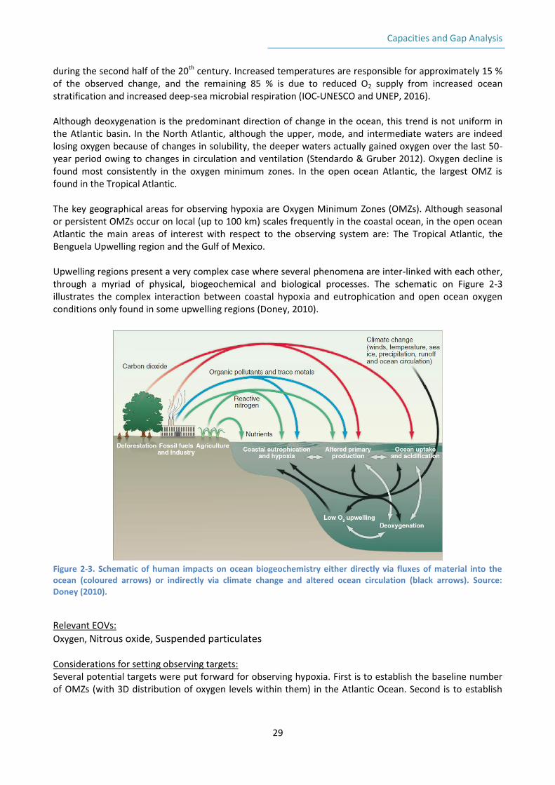
Capacities and Gap Analysis
29
during the second half of the 20th century. Increased temperatures are responsible for approximately 15 % of the observed change, and the remaining 85 % is due to reduced O2 supply from increased ocean stratification and increased deep-sea microbial respiration (IOC-UNESCO and UNEP, 2016). Although deoxygenation is the predominant direction of change in the ocean, this trend is not uniform in the Atlantic basin. In the North Atlantic, although the upper, mode, and intermediate waters are indeed losing oxygen because of changes in solubility, the deeper waters actually gained oxygen over the last 50-year period owing to changes in circulation and ventilation (Stendardo & Gruber 2012). Oxygen decline is found most consistently in the oxygen minimum zones. In the open ocean Atlantic, the largest OMZ is found in the Tropical Atlantic. The key geographical areas for observing hypoxia are Oxygen Minimum Zones (OMZs). Although seasonal or persistent OMZs occur on local (up to 100 km) scales frequently in the coastal ocean, in the open ocean Atlantic the main areas of interest with respect to the observing system are: The Tropical Atlantic, the Benguela Upwelling region and the Gulf of Mexico. Upwelling regions present a very complex case where several phenomena are inter-linked with each other, through a myriad of physical, biogeochemical and biological processes. The schematic on Figure 2-3 illustrates the complex interaction between coastal hypoxia and eutrophication and open ocean oxygen conditions only found in some upwelling regions (Doney, 2010).
Figure 2-3. Schematic of human impacts on ocean biogeochemistry either directly via fluxes of material into the ocean (coloured arrows) or indirectly via climate change and altered ocean circulation (black arrows). Source: Doney (2010).
Relevant EOVs:
Oxygen, Nitrous oxide, Suspended particulates Considerations for setting observing targets: Several potential targets were put forward for observing hypoxia. First is to establish the baseline number of OMZs (with 3D distribution of oxygen levels within them) in the Atlantic Ocean. Second is to establish
Capacities and Gap Analysis
30
the baseline volume of OMZs in the Atlantic Ocean; and the third is to establish vertical extent of OMZs with specific focus on their shallowing. When setting spatio-temporal targets of observations, one should consider the connection of hypoxia with other phenomena such as the inorganic nutrient cycling, and redistribution of species.
Eutrophication Monitoring and predicting the eutrophication status of waters is an important element of determining whether an ecosystem is in a healthy state or not. The eutrophication is driven by a surplus of the nutrients nitrogen and phosphorus in the sea, caused mainly by agriculture activities (fertilizer use and wastes from livestock) and urban wastewater. Nutrient over-enrichment, also referred to as nutrient pollution, causes elevated levels of algal and some plant growth, increased turbidity, oxygen depletion, changes in species composition, and increase in toxins (e.g. through incidence of Harmful Algal Blooms (HABs)). As these properties and events are directly measurable or are easily derived from such measurements, eutrophication is observed based on its impacts on biogeochemistry and biology, rather than being observed from the state of its pressures and drivers such as excess concentration of nutrients in river run-off or atmospheric deposition. This has implications for selecting core indicators of eutrophication, and designing an observing system adequate for monitoring changes in eutrophication status. Observing changes in eutrophication is tightly coupled with three other phenomena considered in this report: inorganic nutrient cycling, hypoxia and organic matter cycling. Relevant EOVs: Core indicators of eutrophication include: concentrations of nutrients in the water, water clarity, Chl-a concentration as a proxy for phytoplankton biomass, as well as oxygen concentration. These indicators are obtained from existing EOVs, their sub-variables or derived products. While water clarity index is often simply derived from Secchi depth measurements, coincident measurements of suspended particulate matter and dissolved organic matter could provide, especially when derived from remote sensing observations, could provide a much better spatial and temporal resolution of observations, much needed for developing operational services aimed at near-real time hazard warning. Not all fractions of inorganic and organic nutrients are measured sufficiently often to provide reliable indicators of nutrient status in the waters. The Methodology for the GEF Transboundary Waters Assessment Programme (TWAP) Report (UNEP-DHI, 2011) suggests that nutrient pollution be assessed based on six nutrient forms: Dissolved Inorganic and Organic Nitrogen & Phosphorus (DIN, DON, DIP, DOP), and Particulate Nitrogen and Phosphorus (PN, PP). This presents an issue when considering the impact and feasibility assessment behind the current biogeochemistry EOVs, with DOP and DON measurements marked with low feasibility, and consequently excluded from the list of EOVs and their sub-variables. Considering the requirements for designing an observing system fit for eutrophication monitoring, this presents a challenge and illustrates a current limitation in implementing a uniform set of EOVs in open and coastal ocean simultaneously. Considerations for setting observing targets: In the EU, the Water Framework Directive (WFD; EC, 2000) sets distinct concentration thresholds beyond which waters are classified as contaminated or polluted (see Annex II in EU WFD). However, setting these thresholds as targets for the biogeochemical observing system for the whole Atlantic is challenging, and perhaps purposeless. First, various coastal ecosystems have different background nutrient inputs and reservoirs, and indicator thresholds will be spatially variable. Second, classifying waters as eutrophicated implies some degree of pollution and thus a reduction in amenity value of a given water body. Such decisions are and will need to be taken on a national level. Therefore, the observing system design should
Capacities and Gap Analysis
31
focus on filling in spatial and temporal gaps in relevant EOV observations to provide sufficient coverage and resolution of commonly agreed eutrophication indicators. Furthermore, an important target for eutrophication observations is to promote shared databases, standards and best practices to ensure intercomparability of relevant parameter measurements for the benefit of determining eutrophication status. Contamination/Pollution Marine water pollution is a significant concern for ocean ecosystem health. We distinguish between the following contaminants: plastics, organic contaminants, heavy metals, hydrocarbons and underwater noise. Plastic debris, or litter, in the ocean is now ubiquitous. Durability is a common feature of most plastics, and it is this property, combined with an unwillingness or inability to manage end-of-life plastic effectively that has resulted in marine plastics and microplastics becoming a global problem. We distinguish between floating macro- and microplastics, and there is also a pool of mid-water microplastics. At the moment, our ability to detect floating plastics is limited to presence/absence data, but future sustained efforts to measure their concentrations, e.g. through under way automated data capture instruments, would help constrain the current very large level of uncertainty on their distribution. Persistent Bioaccumulating and Toxic organic compounds (PBTs) are also ubiquitous in the marine environment, primarily because of human activity. These include a category called Persistent Organic Pollutants (POPs) which are either banned or restricted under the Stockholm Convention. Some are hydrophilic and others hydrophobic. Many of these compounds have chronic impacts on marine organisms especially at higher trophic levels amongst top predators. There are critical human populations, particularly at higher latitudes in the North Atlantic, Nordic Seas and Arctic, who are directly affected due to consumption of traditional foodstuffs. Transport is by both surface ocean circulation and atmosphere, and there is a well-defined transfer to higher latitudes. There has been extensive research and development to produce sensors that can make in-situ sampling by employing a concentration stage, using passive samplers with lower detection limits based on a variety of gel and films (e.g. Burgess et al., 2015). Floating plastics, PBTs and POPs remain in the natural system on similar temporal scales from weeks to tens of years. Due to their wide-spread transport in the ocean, they affect the marine system in spatial scales from meters to thousands of kilometres. Atmospheric deposition is the main source of dissolved heavy metals in the ocean (Cadmium, copper, lead, zinc, cobalt, zinc, mercury, methyl mercury). The partitioning of atmospheric inputs between dissolved and particulate phases within the surface layer strongly determines the behavior of trace metals and their involvement in biogeochemical cycles (Cossa et al. 2009). Basically, the assimilation of metals by biota may be constrained by their solubilisation, resulting from physico-chemical and biological processes (dissolution through zooplankton guts for example). Riverine fluxes are the main source of heavy metal particulates. Distribution of heavy metals changes in annual scales, and spatially, on a 100-3000 km when affected by atmospheric deposition, and from 1 to 1000 km when driven by river inputs.
Relevant EOVs: Marine pollutants/contaminants are currently not a GOOS EOV. Such a development has been initiated on the line between UNEP and GOOS. Several potential sub-variables of such an EOV can be found in the phenomenon description above.
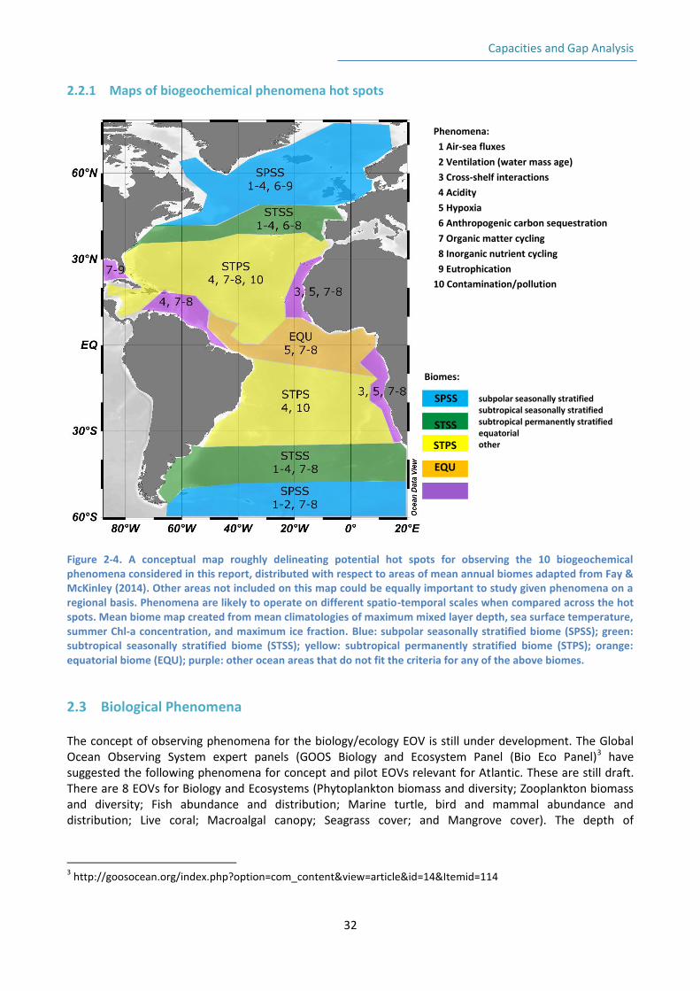
Capacities and Gap Analysis
32
2.2.1 Maps of biogeochemical phenomena hot spots
Figure 2-4. A conceptual map roughly delineating potential hot spots for observing the 10 biogeochemical phenomena considered in this report, distributed with respect to areas of mean annual biomes adapted from Fay & McKinley (2014). Other areas not included on this map could be equally important to study given phenomena on a regional basis. Phenomena are likely to operate on different spatio-temporal scales when compared across the hot spots. Mean biome map created from mean climatologies of maximum mixed layer depth, sea surface temperature, summer Chl-a concentration, and maximum ice fraction. Blue: subpolar seasonally stratified biome (SPSS); green: subtropical seasonally stratified biome (STSS); yellow: subtropical permanently stratified biome (STPS); orange: equatorial biome (EQU); purple: other ocean areas that do not fit the criteria for any of the above biomes.
2.3 Biological Phenomena The concept of observing phenomena for the biology/ecology EOV is still under development. The Global Ocean Observing System expert panels (GOOS Biology and Ecosystem Panel (Bio Eco Panel)3 have suggested the following phenomena for concept and pilot EOVs relevant for Atlantic. These are still draft. There are 8 EOVs for Biology and Ecosystems (Phytoplankton biomass and diversity; Zooplankton biomass and diversity; Fish abundance and distribution; Marine turtle, bird and mammal abundance and distribution; Live coral; Macroalgal canopy; Seagrass cover; and Mangrove cover). The depth of
3 http://goosocean.org/index.php?option=com_content&view=article&id=14&Itemid=114
Phenomena:
1 Air-sea fluxes
2 Ventilation (water mass age)
3 Cross-shelf interactions
4 Acidity
5 Hypoxia
6 Anthropogenic carbon sequestration
7 Organic matter cycling
8 Inorganic nutrient cycling
9 Eutrophication
10 Contamination/pollution
subpolar seasonally stratified subtropical seasonally stratified subtropical permanently stratified equatorial other
SPSS
STSS
STPS
EQU
Biomes:
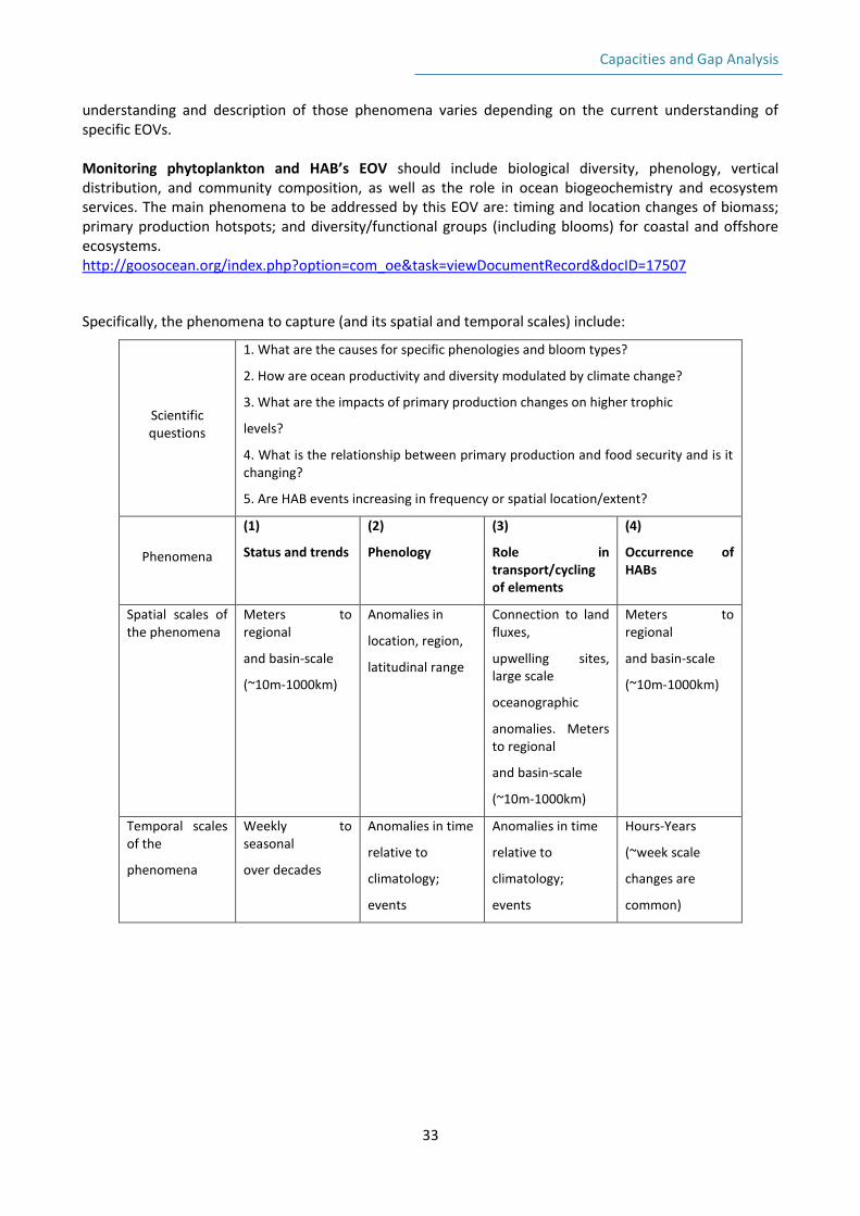
Capacities and Gap Analysis
33
understanding and description of those phenomena varies depending on the current understanding of specific EOVs. Monitoring phytoplankton and HAB’s EOV should include biological diversity, phenology, vertical distribution, and community composition, as well as the role in ocean biogeochemistry and ecosystem services. The main phenomena to be addressed by this EOV are: timing and location changes of biomass; primary production hotspots; and diversity/functional groups (including blooms) for coastal and offshore ecosystems. http://goosocean.org/index.php?option=com_oe&task=viewDocumentRecord&docID=17507
Specifically, the phenomena to capture (and its spatial and temporal scales) include:
Scientific questions
1. What are the causes for specific phenologies and bloom types?
2. How are ocean productivity and diversity modulated by climate change?
3. What are the impacts of primary production changes on higher trophic
levels?
4. What is the relationship between primary production and food security and is it changing?
5. Are HAB events increasing in frequency or spatial location/extent?
Phenomena
(1)
Status and trends
(2)
Phenology
(3)
Role in transport/cycling of elements
(4)
Occurrence of HABs
Spatial scales of the phenomena
Meters to regional
and basin-scale
(~10m-1000km)
Anomalies in
location, region,
latitudinal range
Connection to land fluxes,
upwelling sites, large scale
oceanographic
anomalies. Meters to regional
and basin-scale
(~10m-1000km)
Meters to regional
and basin-scale
(~10m-1000km)
Temporal scales of the
phenomena
Weekly to seasonal
over decades
Anomalies in time
relative to
climatology;
events
Anomalies in time
relative to
climatology;
events
Hours-Years
(~week scale
changes are
common)
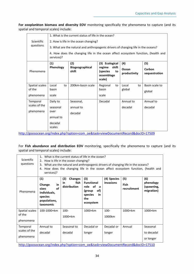
Capacities and Gap Analysis
34
For zooplankton biomass and diversity EOV monitoring specifically the phenomena to capture (and its spatial and temporal scales) include:
Scientific questions
1. What is the current status of life in the ocean?
2. How is life in the ocean changing?
3. What are the natural and anthropogenic drivers of changing life in the oceans?
4. How does the changing life in the ocean affect ecosystem function, (health and services)?
Phenomena
(1) Phenology
(2) Biogeographical shift
(3) Ecological regime shift (species to assemblage scale)
(4)
Ocean productivity
(5)
Carbon sequestration
Spatial scales of the
phenomena
Local to basin
scale
200km-basin scale Regional to basin
scale
Local to global
Basin scale to
global
Temporal scales of the
phenomena
Daily to
seasonal over
annual to
decadal scales
Seasonal,
annual to
decadal
Decadal Annual to
decadal
Annual to
decadal
http://goosocean.org/index.php?option=com_oe&task=viewDocumentRecord&docID=17509
For Fish abundance and distribution EOV monitoring, specifically the phenomena to capture (and its spatial and temporal scales) include:
Scientific questions
1. What is the current status of life in the ocean? 2. How is life in the ocean changing? 3. What are the natural and anthropogenic drivers of changing life in the oceans? 4. How does the changing life in the ocean affect ecosystem function, (health and
services)?
Phenomena
(1)
Change in sizes of individuals, species populations, taxonomic
(2) Changes in fish distribution
(3) Functional role of a (group of) species in the ecosystem
(4) Species invasions
(5)
Fish recruitment
(6) phenology (spawning, migration)
Spatial scales of the
phenomena
100-1000+km 100-
1000+km
1000+km 100-
1000km
1000+km 1000+km
Temporal scales of the
phenomena
Annual to
decadal
Seasonal to
decadal
Decadal or
longer
Decadal or
longer
Annual Seasonal
to decadal
or longer
http://goosocean.org/index.php?option=com_oe&task=viewDocumentRecord&docID=17510
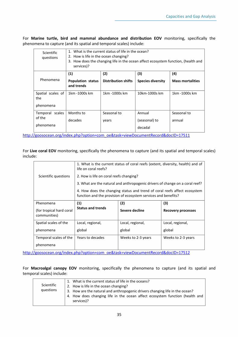
Capacities and Gap Analysis
35
For Marine turtle, bird and mammal abundance and distribution EOV monitoring, specifically the phenomena to capture (and its spatial and temporal scales) include:
Scientific questions
1. What is the current status of life in the ocean? 2. How is life in the ocean changing? 3. How does the changing life in the ocean affect ecosystem function, (health and
services)?
Phenomena
(1)
Population status and trends
(2)
Distribution shifts
(3)
Species diversity
(4)
Mass mortalities
Spatial scales of the
phenomena
1km -1000s km 1km -1000s km 10km-1000s km 1km -1000s km
Temporal scales of the
phenomena
Months to
decades
Seasonal to
years
Annual
(seasonal) to
decadal
Seasonal to
annual
http://goosocean.org/index.php?option=com_oe&task=viewDocumentRecord&docID=17511
For Live coral EOV monitoring, specifically the phenomena to capture (and its spatial and temporal scales) include:
Scientific questions
1. What is the current status of coral reefs (extent, diversity, health) and of life on coral reefs?
2. How is life on coral reefs changing?
3. What are the natural and anthropogenic drivers of change on a coral reef?
4. How does the changing status and trend of coral reefs affect ecosystem function and the provision of ecosystem services and benefits?
Phenomena
(for tropical hard coral communities)
(1) Status and trends
(2)
Severe decline
(3)
Recovery processes
Spatial scales of the
phenomena
Local, regional,
global
Local, regional,
global
Local, regional,
global
Temporal scales of the
phenomena
Years to decades Weeks to 2-3 years Weeks to 2-3 years
http://goosocean.org/index.php?option=com_oe&task=viewDocumentRecord&docID=17512
For Macroalgal canopy EOV monitoring, specifically the phenomena to capture (and its spatial and temporal scales) include:
Scientific questions
1. What is the current status of life in the oceans? 2. How is life in the ocean changing? 3. How are the natural and anthropogenic drivers changing life in the ocean? 4. How does changing life in the ocean affect ecosystem function (health and
services)?
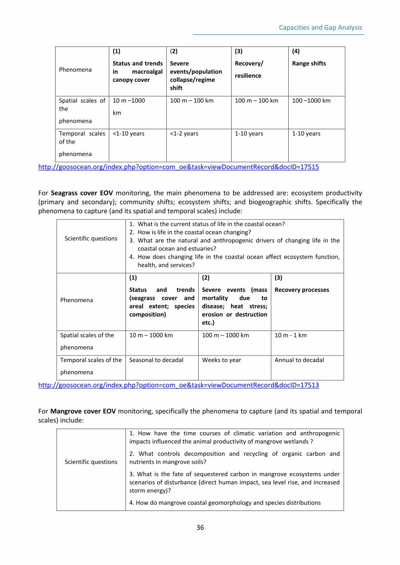
Capacities and Gap Analysis
36
Phenomena
(1)
Status and trends in macroalgal canopy cover
(2)
Severe events/population collapse/regime shift
(3)
Recovery/
resilience
(4)
Range shifts
Spatial scales of the
phenomena
10 m –1000
km
100 m – 100 km 100 m – 100 km 100 –1000 km
Temporal scales of the
phenomena
<1-10 years <1-2 years 1-10 years 1-10 years
http://goosocean.org/index.php?option=com_oe&task=viewDocumentRecord&docID=17515
For Seagrass cover EOV monitoring, the main phenomena to be addressed are: ecosystem productivity (primary and secondary); community shifts; ecosystem shifts; and biogeographic shifts. Specifically the phenomena to capture (and its spatial and temporal scales) include:
Scientific questions
1. What is the current status of life in the coastal ocean? 2. How is life in the coastal ocean changing? 3. What are the natural and anthropogenic drivers of changing life in the
coastal ocean and estuaries? 4. How does changing life in the coastal ocean affect ecosystem function,
health, and services?
Phenomena
(1)
Status and trends (seagrass cover and areal extent; species composition)
(2)
Severe events (mass mortality due to disease; heat stress; erosion or destruction etc.)
(3)
Recovery processes
Spatial scales of the
phenomena
10 m – 1000 km 100 m – 1000 km 10 m - 1 km
Temporal scales of the
phenomena
Seasonal to decadal Weeks to year Annual to decadal
http://goosocean.org/index.php?option=com_oe&task=viewDocumentRecord&docID=17513
For Mangrove cover EOV monitoring, specifically the phenomena to capture (and its spatial and temporal scales) include:
Scientific questions
1. How have the time courses of climatic variation and anthropogenic impacts influenced the animal productivity of mangrove wetlands ?
2. What controls decomposition and recycling of organic carbon and nutrients in mangrove soils?
3. What is the fate of sequestered carbon in mangrove ecosystems under scenarios of disturbance (direct human impact, sea level rise, and increased storm energy)?
4. How do mangrove coastal geomorphology and species distributions
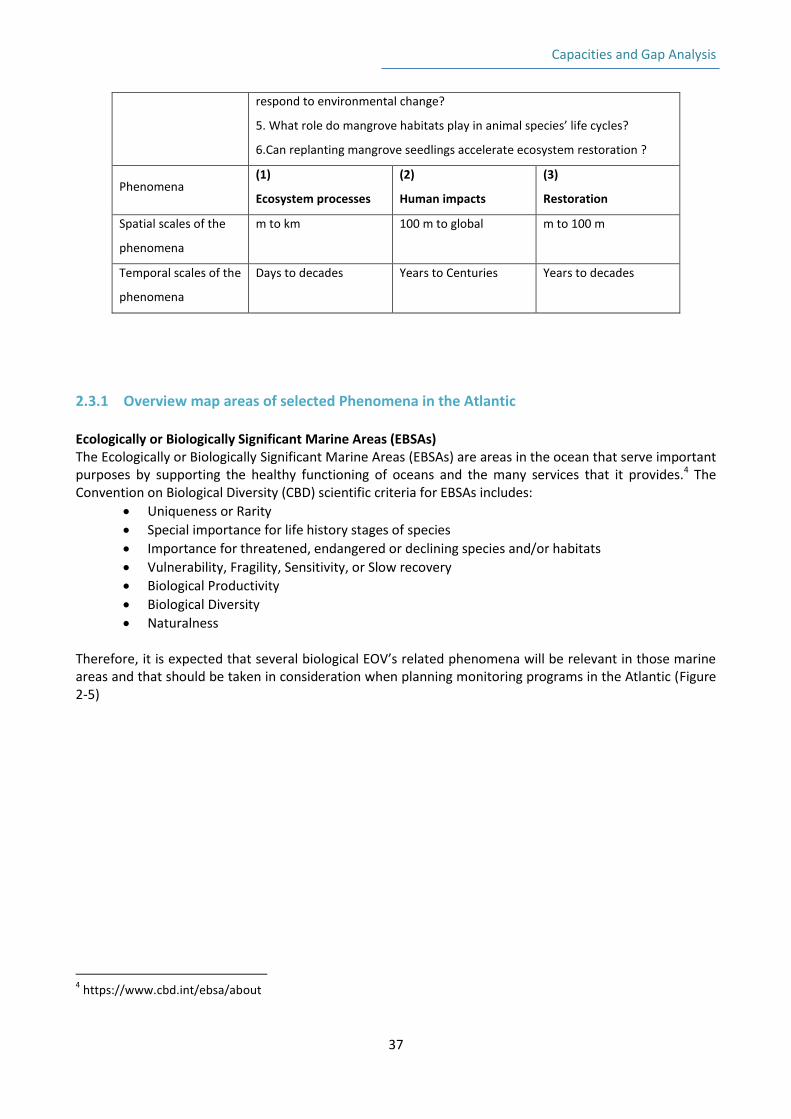
Capacities and Gap Analysis
37
respond to environmental change?
5. What role do mangrove habitats play in animal species’ life cycles?
6.Can replanting mangrove seedlings accelerate ecosystem restoration ?
Phenomena (1)
Ecosystem processes
(2)
Human impacts
(3)
Restoration
Spatial scales of the
phenomena
m to km 100 m to global m to 100 m
Temporal scales of the
phenomena
Days to decades Years to Centuries Years to decades
2.3.1 Overview map areas of selected Phenomena in the Atlantic Ecologically or Biologically Significant Marine Areas (EBSAs) The Ecologically or Biologically Significant Marine Areas (EBSAs) are areas in the ocean that serve important purposes by supporting the healthy functioning of oceans and the many services that it provides.4 The Convention on Biological Diversity (CBD) scientific criteria for EBSAs includes:
Uniqueness or Rarity
Special importance for life history stages of species
Importance for threatened, endangered or declining species and/or habitats
Vulnerability, Fragility, Sensitivity, or Slow recovery
Biological Productivity
Biological Diversity
Naturalness Therefore, it is expected that several biological EOV’s related phenomena will be relevant in those marine areas and that should be taken in consideration when planning monitoring programs in the Atlantic (Figure 2-5)
4 https://www.cbd.int/ebsa/about
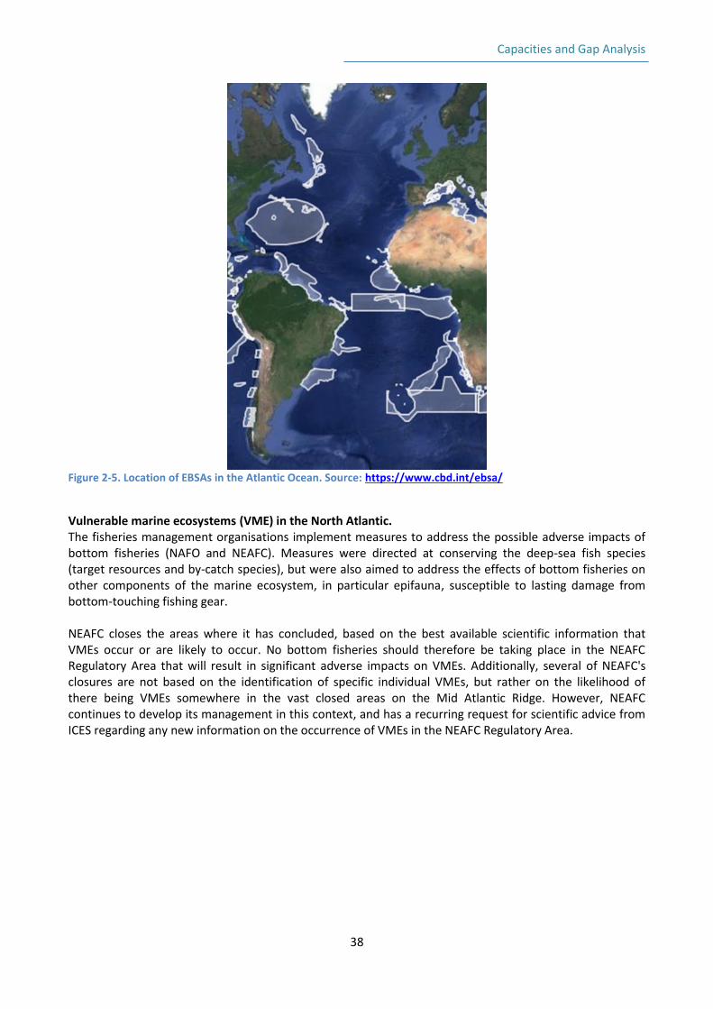
Capacities and Gap Analysis
38
Figure 2-5. Location of EBSAs in the Atlantic Ocean. Source: https://www.cbd.int/ebsa/
Vulnerable marine ecosystems (VME) in the North Atlantic. The fisheries management organisations implement measures to address the possible adverse impacts of bottom fisheries (NAFO and NEAFC). Measures were directed at conserving the deep-sea fish species (target resources and by-catch species), but were also aimed to address the effects of bottom fisheries on other components of the marine ecosystem, in particular epifauna, susceptible to lasting damage from bottom-touching fishing gear. NEAFC closes the areas where it has concluded, based on the best available scientific information that VMEs occur or are likely to occur. No bottom fisheries should therefore be taking place in the NEAFC Regulatory Area that will result in significant adverse impacts on VMEs. Additionally, several of NEAFC's closures are not based on the identification of specific individual VMEs, but rather on the likelihood of there being VMEs somewhere in the vast closed areas on the Mid Atlantic Ridge. However, NEAFC continues to develop its management in this context, and has a recurring request for scientific advice from ICES regarding any new information on the occurrence of VMEs in the NEAFC Regulatory Area.
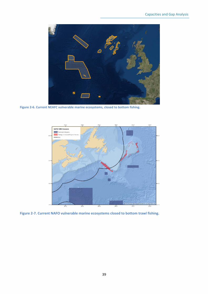
Capacities and Gap Analysis
39
Figure 2-6. Current NEAFC vulnerable marine ecosystems, closed to bottom fishing.
Figure 2-7. Current NAFO vulnerable marine ecosystems closed to bottom trawl fishing.
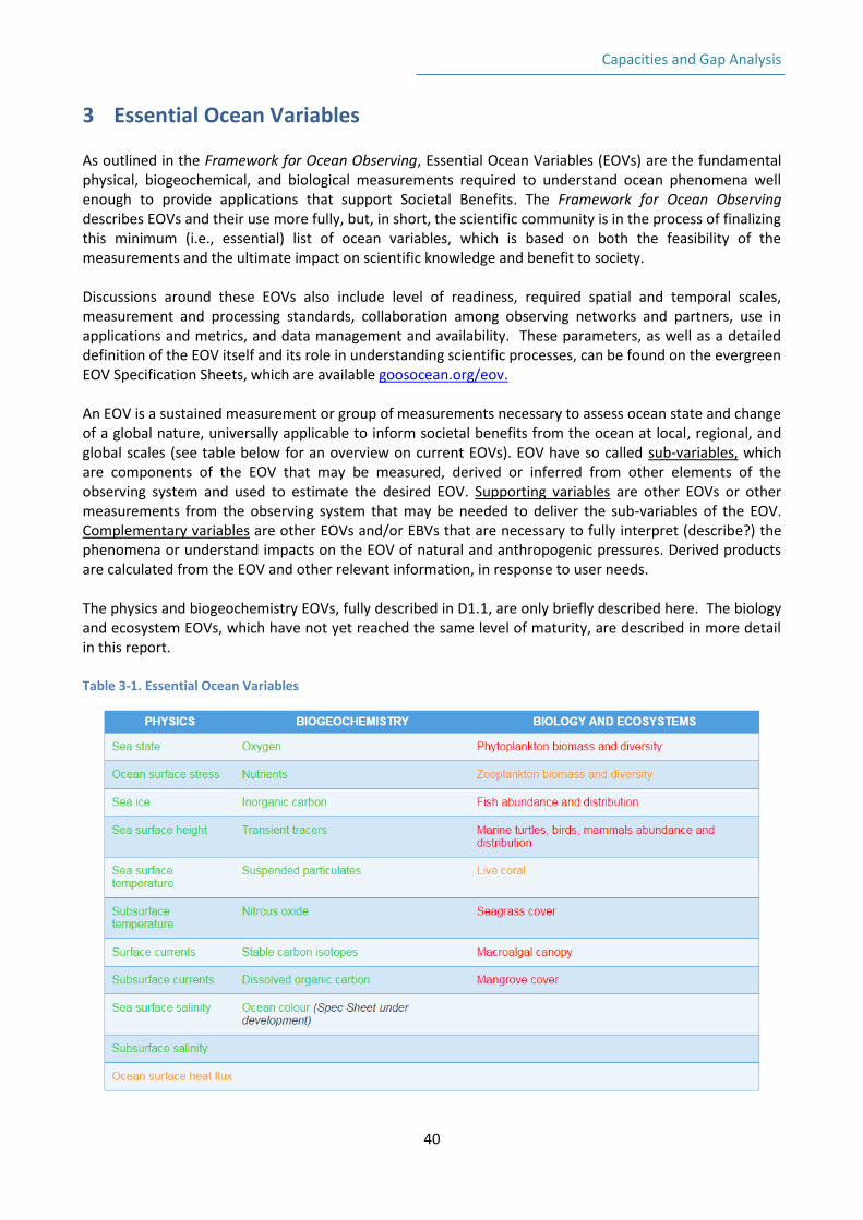
Capacities and Gap Analysis
40
3 Essential Ocean Variables As outlined in the Framework for Ocean Observing, Essential Ocean Variables (EOVs) are the fundamental physical, biogeochemical, and biological measurements required to understand ocean phenomena well enough to provide applications that support Societal Benefits. The Framework for Ocean Observing describes EOVs and their use more fully, but, in short, the scientific community is in the process of finalizing this minimum (i.e., essential) list of ocean variables, which is based on both the feasibility of the measurements and the ultimate impact on scientific knowledge and benefit to society. Discussions around these EOVs also include level of readiness, required spatial and temporal scales, measurement and processing standards, collaboration among observing networks and partners, use in applications and metrics, and data management and availability. These parameters, as well as a detailed definition of the EOV itself and its role in understanding scientific processes, can be found on the evergreen EOV Specification Sheets, which are available goosocean.org/eov. An EOV is a sustained measurement or group of measurements necessary to assess ocean state and change of a global nature, universally applicable to inform societal benefits from the ocean at local, regional, and global scales (see table below for an overview on current EOVs). EOV have so called sub-variables, which are components of the EOV that may be measured, derived or inferred from other elements of the observing system and used to estimate the desired EOV. Supporting variables are other EOVs or other measurements from the observing system that may be needed to deliver the sub-variables of the EOV. Complementary variables are other EOVs and/or EBVs that are necessary to fully interpret (describe?) the phenomena or understand impacts on the EOV of natural and anthropogenic pressures. Derived products are calculated from the EOV and other relevant information, in response to user needs. The physics and biogeochemistry EOVs, fully described in D1.1, are only briefly described here. The biology and ecosystem EOVs, which have not yet reached the same level of maturity, are described in more detail in this report. Table 3-1. Essential Ocean Variables
Capacities and Gap Analysis
41
3.1 Physical EOVs Sea Surface Temperature (SST) SST exerts a major influence on the exchanges of energy, momentum, and gases between the ocean and atmosphere. These heat exchanges are a main driver of global weather systems. The spatial patterns of SST also reveal the structure of underlying ocean dynamics. Subsurface Temperature Changes in subsurface temperature impact a variety of ocean services, including the growth rate, distribution, and abundance of marine species, including farmed and wild fish stocks. In addition, changes in subsurface temperature induce changes in mixed-layer depth, vertical and lateral ocean density stratification, mixing rates, and currents. Sea Surface Salinity (SSS) SSS is a key parameter for monitoring the global water cycle (evaporation, precipitation, and glacier and river runoff) and observations over large scales can be used to infer long-term changes in the hydrological cycle and to quantify the evolution of the ocean in response to climate change. Subsurface Salinity A global subsurface salinity observing system is vital to close the global hydrological cycle and understand sea level change. Subsurface salinity observations, are required to calculate in-situ density and ocean freshwater transports. In addition, changes in subsurface salinity induce changes in mixed-layer depth, vertical and lateral ocean density stratification, mixing rates, and currents. Surface Currents Surface currents transport significant amounts of heat, salt, passive tracers, and ocean pollutants. On basin scales, zonal surface currents and their variations are key in climate to weather fluctuations. On smaller scales, surface currents contribute to vertical motion and mass exchange, and are important for accurate marine sea state forecasts, search and rescue, and oil spill modelling. Subsurface Currents Observations of subsurface ocean velocity are needed to estimate oceanic transport of mass, heat, freshwater, and other properties on local to global scales, and are particularly important in resolving the complex velocity structure of the major boundary currents, at the sea floor, near the equator, in ocean eddies, and in waves. Velocity profile information is also used to estimate ocean mixing. Sea Level or Sea Surface Height (SSH) Sea level is one of the primary indicators of global climate change, providing a measure of the net change in ocean mass due to melting of glaciers and ice sheets and the net change in ocean volume due to thermal expansion. At the coast, meteorological forcing can drive significant departures of SSH from the harmonic tide with consequences for inundation and navigation. Sea State Waves are generated by wind and modified by bathymetry and surface currents. Sea state impacts marine safety, marine transport, and damage marine structures. Waves affect air/sea exchanges of momentum, moisture, and CO2, and impact beach erosion, storm-related water damage, surface albedo, the transport of larva and contaminants such as oil, and the growth and decay of sea ice. Sea Ice Energy budgets are heavily impacted by ice formation and melting and the presence or absence of ice cover (albedo, evaporation). Ice formation and melting modifies surface salinity, altering stratification and local
Capacities and Gap Analysis
42
circulation. Changes in roughness between ice and water impacts differential stress, and are related to relatively strong vertical motions and transports near the ice edge. Ocean Surface stress Stress, the rate at which horizontal momentum is transferred from the atmosphere to the ocean, influences the air/sea exchange of energy (sensible and latent heat), water (evaporation) and carbon (CO2). It leads to the formation of waves and impacts ocean currents and transport, as well as upwelling, downwelling, and primary productivity. OceanSurface Heat Flux The fluxes of latent heat (evaporation) and sensible heat (differences in air-sea temperatures) are major contributors to the energy budget, and are largely responsible for thermodynamic coupling of the ocean and atmosphere at global and regional scales. Variations in these fluxes leads to largescale variability in weather patterns and they are sensitive indicators of changes in climate.
3.2 Biogeochemical EOVs The GOOS Biogeochemistry Expert Panel, led by the International Ocean Carbon Coordination Project, was responsible for designing and carrying out the process of selecting and defining Biogeochemistry EOVs. After an initial technical workshop in 2013, the proposed list of EOVs underwent a multi-stage international community review. The full process of selecting Biogeochemistry EOVs, with results of the analysis of impact and feasibility, is described at http://www.ioccp.org/index.php/foo. Below is a summary of the Biogeochemistry EOVs. Complete information is contained in the Specification Sheets, available in their current version at goosocean.org/eov. These documents will be updated periodically. The nomenclature of the Biogeochemistry EOVs followed here was decided by IOCCP SSG in February 2017. Oxygen Sub-surface oxygen concentrations in the ocean everywhere reflect a balance between supply via circulation and ventilation and consumption by respiratory processes. The large (mostly) decreasing trends in the concentrations of dissolved oxygen over the last few decades affect marine species, including fisheries, and impact our understanding of anthropogenic climate change. Nutrients The availability of inorganic macronutrients (nitrate (NO3), phosphate (PO4), silicon (Si), nitrogen dioxide (NO2)) in the upper ocean frequently limits and regulates the amount of organic carbon fixed by phytoplankton. This is a key control mechanism of primary productivity and thus of carbon and biogeochemical cycling. Measuring nutrient concentrations in coastal waters provides information for deriving indicators of eutrophication status. Inorganic Carbon There are four components of the inorganic carbon EOV: dissolved inorganic carbon (DIC), total alkalinity, partial pressure of carbon dioxide (pCO2) and pH; at least two of which are needed to constrain the ocean carbonate system. The carbon system is in a delicate balance such that high quality, high-resolution and long-term observations are required to estimate changes in ocean acidification, anthropogenic carbon flux and storage, and to distinguish climate change-driven trends from seasonal to decadal variability in these and other processes.
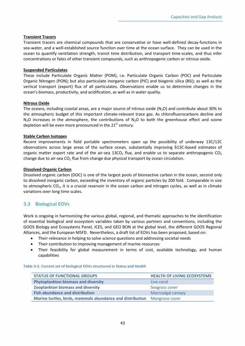
Capacities and Gap Analysis
43
Transient Tracers Transient tracers are chemical compounds that are conservative or have well-defined decay-functions in sea-water, and a well-established source function over time at the ocean surface. They can be used in the ocean to quantify ventilation strength, transit time distribution, and transport time-scales, and thus infer concentrations or fates of other transient compounds, such as anthropogenic carbon or nitrous oxide. Suspended Particulates These include Particulate Organic Matter (POM), i.e. Particulate Organic Carbon (POC) and Particulate Organic Nitrogen (PON); but also particulate inorganic carbon (PIC) and biogenic silica (BSi); as well as the vertical transport (export) flux of all particulates. Observations enable us to determine changes in the ocean’s biomass, productivity, and acidification, as well as in water quality. Nitrous Oxide The oceans, including coastal areas, are a major source of nitrous oxide (N2O) and contribute about 30% to the atmospheric budget of this important climate-relevant trace gas. As chlorofluorocarbons decline and N2O increases in the atmosphere, the contributions of N2O to both the greenhouse effect and ozone depletion will be even more pronounced in the 21st century. Stable Carbon Isotopes Recent improvements in field portable spectrometers open up the possibility of underway 13C/12C observations across large areas of the surface ocean, substantially improving δ13C-based estimates of organic matter export rate and of the air-sea 13CO2 flux, and enable us to separate anthropogenic CO2 change due to air-sea CO2 flux from change due physical transport by ocean circulation. Dissolved Organic Carbon Dissolved organic carbon (DOC) is one of the largest pools of bioreactive carbon in the ocean, second only to dissolved inorganic carbon, exceeding the inventory of organic particles by 200 fold. Comparable in size to atmospheric CO2, it is a crucial reservoir in the ocean carbon and nitrogen cycles, as well as in climate variations over long time scales.
3.3 Biological EOVs Work is ongoing in harmonizing the various global, regional, and thematic approaches to the identification of essential biological and ecosystem variables taken by various partners and conventions, including the GOOS Biology and Ecosystems Panel, ICES, and GEO BON at the global level, the different GOOS Regional Alliances, and the European MSFD. Nevertheless, a draft list of EOVs has been proposed, based on:
Their relevance in helping to solve science questions and addressing societal needs
Their contribution to improving management of marine resources
Their feasibility for global measurement in terms of cost, available technology, and human capabilities
Table 3-2. Current set of biological EOVs structured in Status and Health
STATUS OF FUNCTIONAL GROUPS HEALTH OF LIVING ECOSYSTEMS
Phytoplankton biomass and diversity Live coral
Zooplankton biomass and diversity Seagrass cover
Fish abundance and distribution Macroalgal canopy
Marine turtles, birds, mammals abundance and distribution Mangrove cover
Capacities and Gap Analysis
44
Phytoplankton biomass and diversity5 Several ecosystem services supporting human activities in coastal and ocean waters depend on photosynthetic microorganisms. These, along with other primary producers represent the lowest trophic levels in the ocean, fixing carbon and producing oxygen. Phytoplankton are part of the foundation of the aquatic food web, the primary producers, feeding everything from microscopic, animal-like zooplankton to multi-ton whales. Through photosynthesis, phytoplankton consumes carbon dioxide on a scale equivalent to forests and other land plants. Some of this carbon is carried to the deep ocean when phytoplankton die, and some is transferred to different layers of the ocean as phytoplankton are eaten by other creatures. Acting as a “biological carbon pump” small changes in the abundance of phytoplankton may affect atmospheric carbon dioxide concentrations, which would feed back to global surface temperatures. Monitoring lower trophic levels is crucial since these organisms, have critical roles in global biogeochemistry, and are highly sensitive to ecosystem perturbations both at the bottom and top of the trophic structure. Phytoplankton biomass and productivity are important measures to determine the ecological state of the sea and, phytoplankton is therefore often included in environmental monitoring and scientific studies. This is due to their role in eutrophication, when nutrient loading is altered by human activities and the phytoplankton productivity is altered beyond normal prevailing conditions. Eutrophication can lead to oxygen depletion in the marine environment. Biomass and productivity of phytoplankton measurements provide important information on phytoplankton abundance and growth and their biological status. Phytoplankton biomass is the amount of algal material present, whereas productivity is the rate at which algal cell material is produced. The ecological role of phytoplankton in the seas varies to a high degree in both time and space, therefore monitoring requires frequent and spatially distributed sampling. High-biomass and/or toxic proliferations of some specific cells (“Harmful Algal Blooms” or HABs), are known to be harmful to aquatic ecosystems, including plants and animals, and to humans via direct exposure to water-borne toxins or by toxic seafood consumption. Such potent toxins can persist in the water or enter the food web, leading to illness or death of aquatic animals and/or human seafood consumers. Ecological perturbation by high-biomass blooms may include: disruption of food webs; fish-killing following gill damage; or contribution to low oxygen “dead-zones” after bloom degradation. Many HABs are increasing in severity and frequency, and biogeographical range. Although causes are complex, some may be attributed to climate change and human impacts such as eutrophication, habitat modification, and human mediated introduction of exogenous species. In Europe, monitoring phytoplankton is obliged under the Water Framework Directive (EC, 2000) within the Phytoplankton Biological Quality element. Regional Seas Conventions (e.g. OSPAR and HELCOM) invest a large amount of resources into monitoring phytoplankton as part of the assessment of eutrophication in European waters. The Marine Strategy Framework Directive (EC, 2008a) require assessing, monitoring and targets for eutrophication. The EU Copernicus Marine environment monitoring service also provides monitoring of phytoplankton using satellite information. HABs monitoring is carried out as part of the phytoplankton monitoring within the water Framework Directive were bloom frequency and intensity are part of the Phytoplankton Biological Quality element. There is no global, long-term monitoring of HABs but within Europe the IOC/ICES/ISSHA harmful algae bloom database (HADAT) collect information and the ICES working group WGHABD maps the occurrence of blooms in Northern Europe and North America. The EU Copernicus Marine environment monitoring service also provides monitoring of HABs using satellite information.
5 http://goosocean.org/index.php?option=com_oe&task=viewDocumentRecord&docID=17507
Capacities and Gap Analysis
45
Zooplankton biomass and diversity 6 Zooplankton is a large group of plankton that encompasses all animal or animal-like organisms whose dispersal in the ocean is dominated by processes such as ocean currents. They are the food for many mammals, birds, fish, corals and other invertebrates including zooplankton and consume the phytoplankton or can also be carnivorous. In the food web zooplankton represents an intermediary step between primary productivity and higher trophic levels. The productivity of zooplankton thereby supports many fisheries around the world. Furthermore, zooplankton can limit the growth of blooms by grazing on protozoa and phytoplankton. They have a major role in defining the chemistry of the ocean as nutrients and carbon recyclers in near-surface waters of the ocean and by delivering these materials to deeper ocean waters (through defecation and migrations). They produce fast-sinking faecal pellets which export carbon from the surface layers to the bottom layers of the oceans. Zooplankton are sensitive to changes in their environment. Many species are adapted to external features and a change in zooplankton diversity and biomass in time and space can indicate a change in e.g. temperature, light, salinity or turbulence. Due to the sometime very specific adaptions, determination of zooplankton species also help scientists differentiate between different masses of water. Zooplankton abundance and productivity are generally thought to be more influenced by oceanographic and climatic conditions than by anthropogenic pressures (except in very localised situations). Zooplankton diversity influences ecosystem health and productivity through trophic links and is sensitive to environmental pressures such as climate change, including ocean acidification, warming and deoxygenation. The abundance and functional types of zooplankton, even their presence or absence, are indicators of marine ecosystem responses to climate change. Zooplankton biomass is most commonly measured as wet weight, dry weight, and as carbon content, nitrogen content, protein and lipid content. More recent approaches include acoustic and optical detection of zooplankton biomass. Fish abundance and distribution 7 Fish and fisheries are essential to ecosystems, economies and societies. Fish constitute the largest and most diverse group of marine vertebrates. Fish feed on lower trophic level organisms, including plankton and other fish, and are consumed by marine mammals, seabirds, fish, invertebrates, and microorganisms. The swimming abilities of fish make them able to select favourable conditions in terms of food availability, reproductive sites and associated physical parameters. Many fish are grazers in such diverse ecosystems as coral reefs or rocky bottoms, ensuring their ecological balance. Fish and fisheries are affected by climate variability and therefore are vulnerable to climate change. On the other hand, food security affects fisheries and, reversely, both are affected by human population growth and climate Fish influence the marine ecosystem through carbon transfer and predation. They are important as commercial harvest as sources of food and fish oil. Marine fisheries supply about 20 % of the animal protein consumed by humans. However, unsustainable fishing pose a threat to ocean life, and fisheries management has not always been effective in maintaining fish yields and conserving stocks. For those reasons, the abundance and spatial distribution of fish of different species/trophic levels need to be measured routinely, widely and in a standardized manner. This information will be useful to inform decision makers, including those related to fisheries management, conservation and sustainable use policies, and that affect economic investment and societal resilience facing climate change. Fish abundance (biomass or numbers of fish in the ocean) can be reported in terms of species or taxonomic or functional groups (e.g., small pelagic fish, mesopelagic fish, and tunalike species) in an assemblage,
6 http://goosocean.org/index.php?option=com_oe&task=viewDocumentRecord&docID=17509
7 http://goosocean.org/index.php?option=com_oe&task=viewDocumentRecord&docID=17510
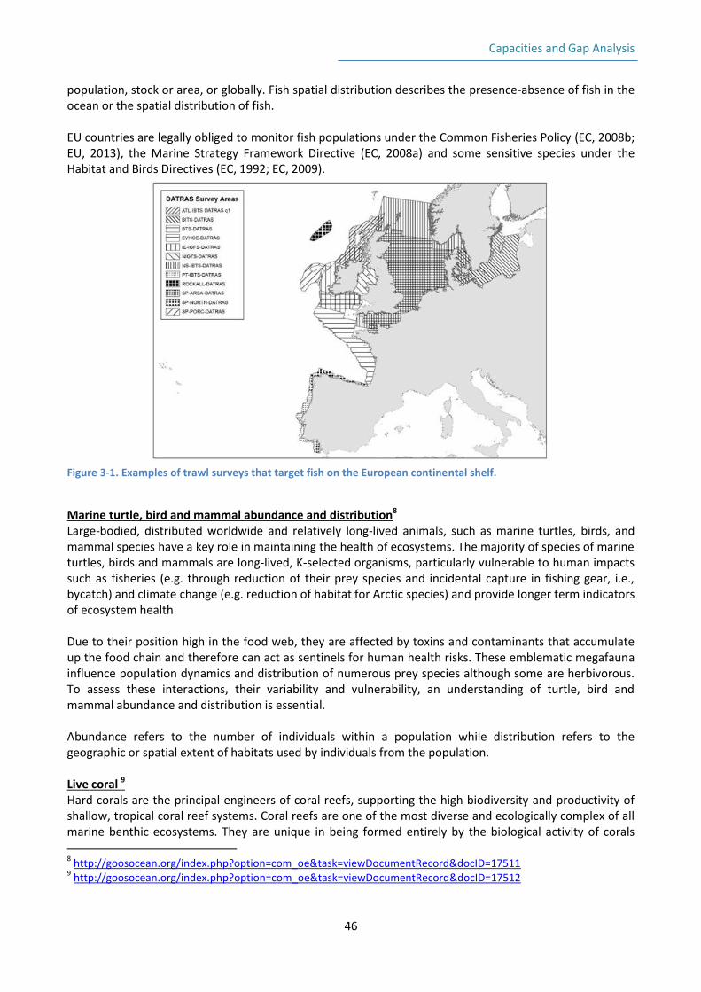
Capacities and Gap Analysis
46
population, stock or area, or globally. Fish spatial distribution describes the presence-absence of fish in the ocean or the spatial distribution of fish. EU countries are legally obliged to monitor fish populations under the Common Fisheries Policy (EC, 2008b; EU, 2013), the Marine Strategy Framework Directive (EC, 2008a) and some sensitive species under the Habitat and Birds Directives (EC, 1992; EC, 2009).
Figure 3-1. Examples of trawl surveys that target fish on the European continental shelf.
Marine turtle, bird and mammal abundance and distribution8 Large-bodied, distributed worldwide and relatively long-lived animals, such as marine turtles, birds, and mammal species have a key role in maintaining the health of ecosystems. The majority of species of marine turtles, birds and mammals are long-lived, K-selected organisms, particularly vulnerable to human impacts such as fisheries (e.g. through reduction of their prey species and incidental capture in fishing gear, i.e., bycatch) and climate change (e.g. reduction of habitat for Arctic species) and provide longer term indicators of ecosystem health. Due to their position high in the food web, they are affected by toxins and contaminants that accumulate up the food chain and therefore can act as sentinels for human health risks. These emblematic megafauna influence population dynamics and distribution of numerous prey species although some are herbivorous. To assess these interactions, their variability and vulnerability, an understanding of turtle, bird and mammal abundance and distribution is essential. Abundance refers to the number of individuals within a population while distribution refers to the geographic or spatial extent of habitats used by individuals from the population. Live coral 9 Hard corals are the principal engineers of coral reefs, supporting the high biodiversity and productivity of shallow, tropical coral reef systems. Coral reefs are one of the most diverse and ecologically complex of all marine benthic ecosystems. They are unique in being formed entirely by the biological activity of corals 8 http://goosocean.org/index.php?option=com_oe&task=viewDocumentRecord&docID=17511
9 http://goosocean.org/index.php?option=com_oe&task=viewDocumentRecord&docID=17512
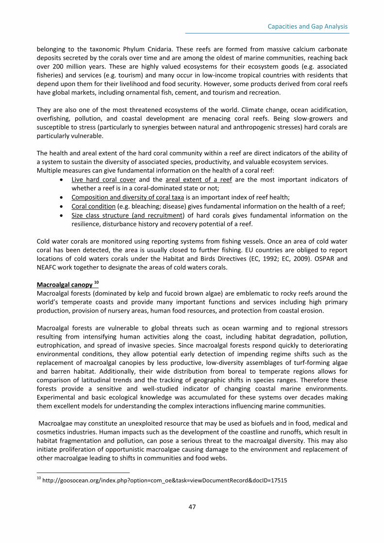
Capacities and Gap Analysis
47
belonging to the taxonomic Phylum Cnidaria. These reefs are formed from massive calcium carbonate deposits secreted by the corals over time and are among the oldest of marine communities, reaching back over 200 million years. These are highly valued ecosystems for their ecosystem goods (e.g. associated fisheries) and services (e.g. tourism) and many occur in low-income tropical countries with residents that depend upon them for their livelihood and food security. However, some products derived from coral reefs have global markets, including ornamental fish, cement, and tourism and recreation. They are also one of the most threatened ecosystems of the world. Climate change, ocean acidification, overfishing, pollution, and coastal development are menacing coral reefs. Being slow-growers and susceptible to stress (particularly to synergies between natural and anthropogenic stresses) hard corals are particularly vulnerable. The health and areal extent of the hard coral community within a reef are direct indicators of the ability of a system to sustain the diversity of associated species, productivity, and valuable ecosystem services. Multiple measures can give fundamental information on the health of a coral reef:
Live hard coral cover and the areal extent of a reef are the most important indicators of whether a reef is in a coral-dominated state or not;
Composition and diversity of coral taxa is an important index of reef health;
Coral condition (e.g. bleaching; disease) gives fundamental information on the health of a reef;
Size class structure (and recruitment) of hard corals gives fundamental information on the resilience, disturbance history and recovery potential of a reef.
Cold water corals are monitored using reporting systems from fishing vessels. Once an area of cold water coral has been detected, the area is usually closed to further fishing. EU countries are obliged to report locations of cold waters corals under the Habitat and Birds Directives (EC, 1992; EC, 2009). OSPAR and NEAFC work together to designate the areas of cold waters corals. Macroalgal canopy 10 Macroalgal forests (dominated by kelp and fucoid brown algae) are emblematic to rocky reefs around the world’s temperate coasts and provide many important functions and services including high primary production, provision of nursery areas, human food resources, and protection from coastal erosion. Macroalgal forests are vulnerable to global threats such as ocean warming and to regional stressors resulting from intensifying human activities along the coast, including habitat degradation, pollution, eutrophication, and spread of invasive species. Since macroalgal forests respond quickly to deteriorating environmental conditions, they allow potential early detection of impending regime shifts such as the replacement of macroalgal canopies by less productive, low-diversity assemblages of turf-forming algae and barren habitat. Additionally, their wide distribution from boreal to temperate regions allows for comparison of latitudinal trends and the tracking of geographic shifts in species ranges. Therefore these forests provide a sensitive and well-studied indicator of changing coastal marine environments. Experimental and basic ecological knowledge was accumulated for these systems over decades making them excellent models for understanding the complex interactions influencing marine communities. Macroalgae may constitute an unexploited resource that may be used as biofuels and in food, medical and cosmetics industries. Human impacts such as the development of the coastline and runoffs, which result in habitat fragmentation and pollution, can pose a serious threat to the macroalgal diversity. This may also initiate proliferation of opportunistic macroalgae causing damage to the environment and replacement of other macroalgae leading to shifts in communities and food webs.
10
http://goosocean.org/index.php?option=com_oe&task=viewDocumentRecord&docID=17515
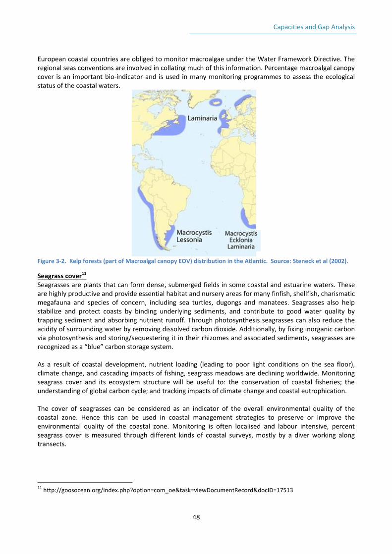
Capacities and Gap Analysis
48
European coastal countries are obliged to monitor macroalgae under the Water Framework Directive. The regional seas conventions are involved in collating much of this information. Percentage macroalgal canopy cover is an important bio-indicator and is used in many monitoring programmes to assess the ecological status of the coastal waters.
Figure 3-2. Kelp forests (part of Macroalgal canopy EOV) distribution in the Atlantic. Source: Steneck et al (2002).
Seagrass cover11 Seagrasses are plants that can form dense, submerged fields in some coastal and estuarine waters. These are highly productive and provide essential habitat and nursery areas for many finfish, shellfish, charismatic megafauna and species of concern, including sea turtles, dugongs and manatees. Seagrasses also help stabilize and protect coasts by binding underlying sediments, and contribute to good water quality by trapping sediment and absorbing nutrient runoff. Through photosynthesis seagrasses can also reduce the acidity of surrounding water by removing dissolved carbon dioxide. Additionally, by fixing inorganic carbon via photosynthesis and storing/sequestering it in their rhizomes and associated sediments, seagrasses are recognized as a “blue” carbon storage system. As a result of coastal development, nutrient loading (leading to poor light conditions on the sea floor), climate change, and cascading impacts of fishing, seagrass meadows are declining worldwide. Monitoring seagrass cover and its ecosystem structure will be useful to: the conservation of coastal fisheries; the understanding of global carbon cycle; and tracking impacts of climate change and coastal eutrophication. The cover of seagrasses can be considered as an indicator of the overall environmental quality of the coastal zone. Hence this can be used in coastal management strategies to preserve or improve the environmental quality of the coastal zone. Monitoring is often localised and labour intensive, percent seagrass cover is measured through different kinds of coastal surveys, mostly by a diver working along transects.
11
http://goosocean.org/index.php?option=com_oe&task=viewDocumentRecord&docID=17513
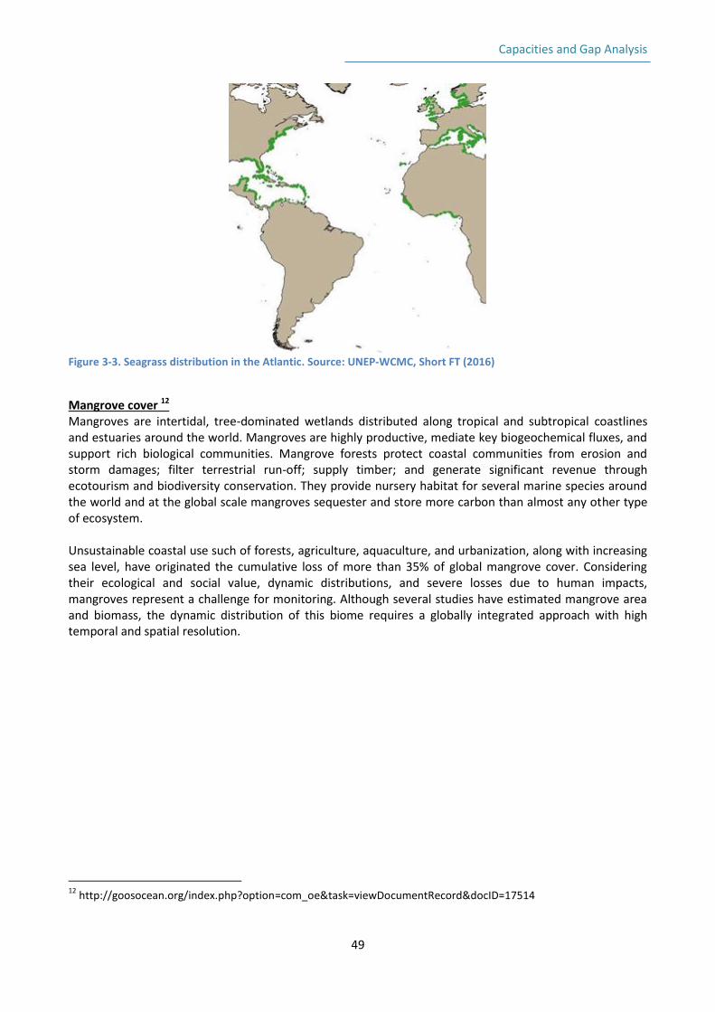
Capacities and Gap Analysis
49
Figure 3-3. Seagrass distribution in the Atlantic. Source: UNEP-WCMC, Short FT (2016)
Mangrove cover 12 Mangroves are intertidal, tree-dominated wetlands distributed along tropical and subtropical coastlines and estuaries around the world. Mangroves are highly productive, mediate key biogeochemical fluxes, and support rich biological communities. Mangrove forests protect coastal communities from erosion and storm damages; filter terrestrial run-off; supply timber; and generate significant revenue through ecotourism and biodiversity conservation. They provide nursery habitat for several marine species around the world and at the global scale mangroves sequester and store more carbon than almost any other type of ecosystem. Unsustainable coastal use such of forests, agriculture, aquaculture, and urbanization, along with increasing sea level, have originated the cumulative loss of more than 35% of global mangrove cover. Considering their ecological and social value, dynamic distributions, and severe losses due to human impacts, mangroves represent a challenge for monitoring. Although several studies have estimated mangrove area and biomass, the dynamic distribution of this biome requires a globally integrated approach with high temporal and spatial resolution.
12
http://goosocean.org/index.php?option=com_oe&task=viewDocumentRecord&docID=17514
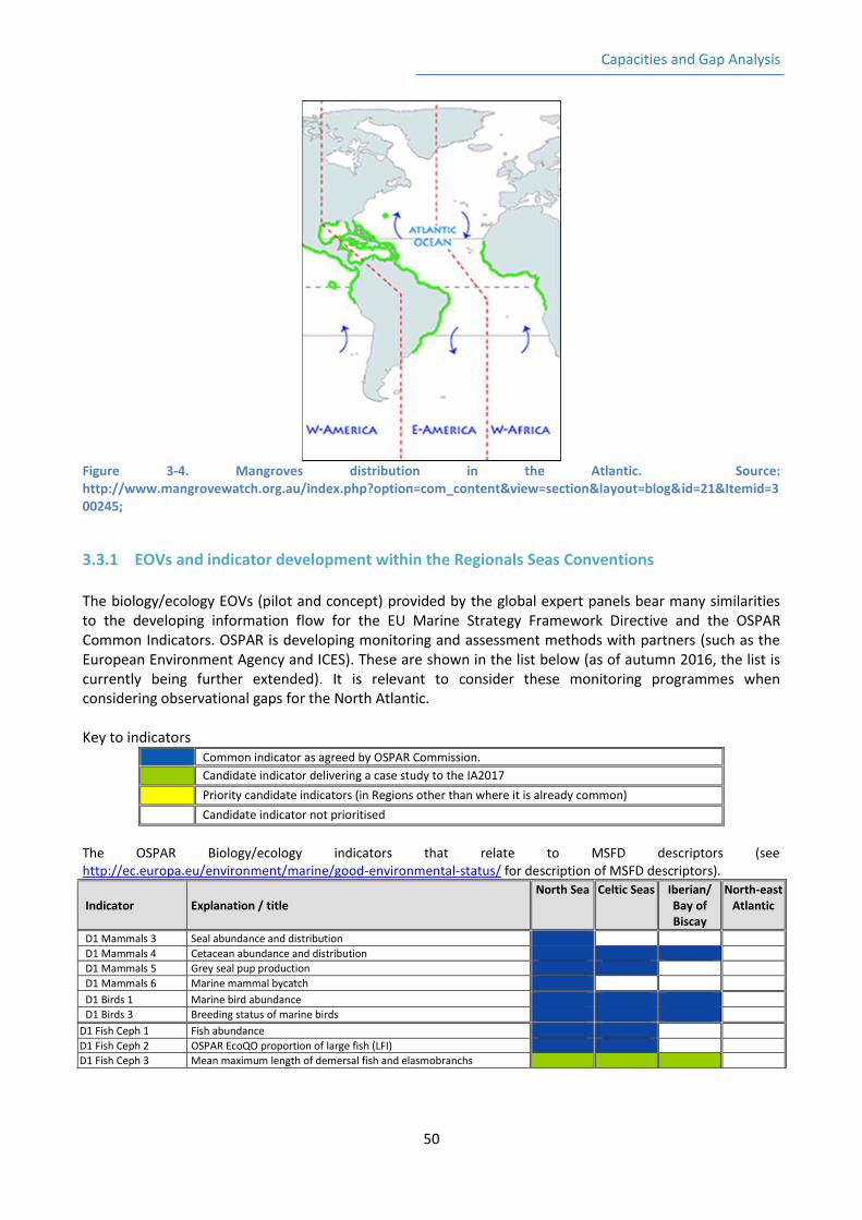
Capacities and Gap Analysis
50
Figure 3-4. Mangroves distribution in the Atlantic. Source: http://www.mangrovewatch.org.au/index.php?option=com_content&view=section&layout=blog&id=21&Itemid=300245;
3.3.1 EOVs and indicator development within the Regionals Seas Conventions The biology/ecology EOVs (pilot and concept) provided by the global expert panels bear many similarities to the developing information flow for the EU Marine Strategy Framework Directive and the OSPAR Common Indicators. OSPAR is developing monitoring and assessment methods with partners (such as the European Environment Agency and ICES). These are shown in the list below (as of autumn 2016, the list is currently being further extended). It is relevant to consider these monitoring programmes when considering observational gaps for the North Atlantic. Key to indicators
Common indicator as agreed by OSPAR Commission.
Candidate indicator delivering a case study to the IA2017
Priority candidate indicators (in Regions other than where it is already common)
Candidate indicator not prioritised
The OSPAR Biology/ecology indicators that relate to MSFD descriptors (see http://ec.europa.eu/environment/marine/good-environmental-status/ for description of MSFD descriptors).
Indicator Explanation / title North Sea Celtic Seas Iberian/
Bay of Biscay
North-east Atlantic
D1 Mammals 3 Seal abundance and distribution
D1 Mammals 4 Cetacean abundance and distribution
D1 Mammals 5 Grey seal pup production
D1 Mammals 6 Marine mammal bycatch
D1 Birds 1 Marine bird abundance
D1 Birds 3 Breeding status of marine birds
D1 Fish Ceph 1 Fish abundance
D1 Fish Ceph 2 OSPAR EcoQO proportion of large fish (LFI)
D1 Fish Ceph 3 Mean maximum length of demersal fish and elasmobranchs
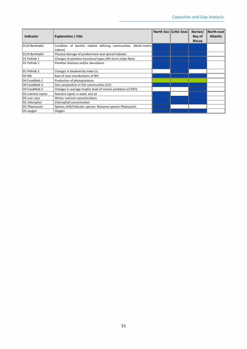
Capacities and Gap Analysis
51
Indicator Explanation / title North Sea Celtic Seas Iberian/
Bay of Biscay
North-east Atlantic
D1/6 BentHab2 Condition of benthic habitat defining communities. (Multi-metric indices)
D1/6 BentHab3 Physical damage of predominant and special habitats
D1 PelHab 1 Changes of plankton functional types (life form) index Ratio
D1 PelHab 2 Plankton biomass and/or abundance
D1 PelHab 3 Changes in biodiversity index (s)
D2 NIS Rate of new introductions of NIS
D4 FoodWeb 2 Production of phytoplankton
D4 FoodWeb 3 Size composition in fish communities (LFI)
D4 FoodWeb 4 Changes in average trophic level of marine predators (cf MTI)
D5 nutrient inputs Nutrient inputs in water and air
D5 nutr conc Winter nutrient concentrations
D5 chlorophyl Chlorophyll concentration
D5 Phaeocystis Species shift/indicator species: Nuisance species Phaeocystis
D5 oxygen Oxygen
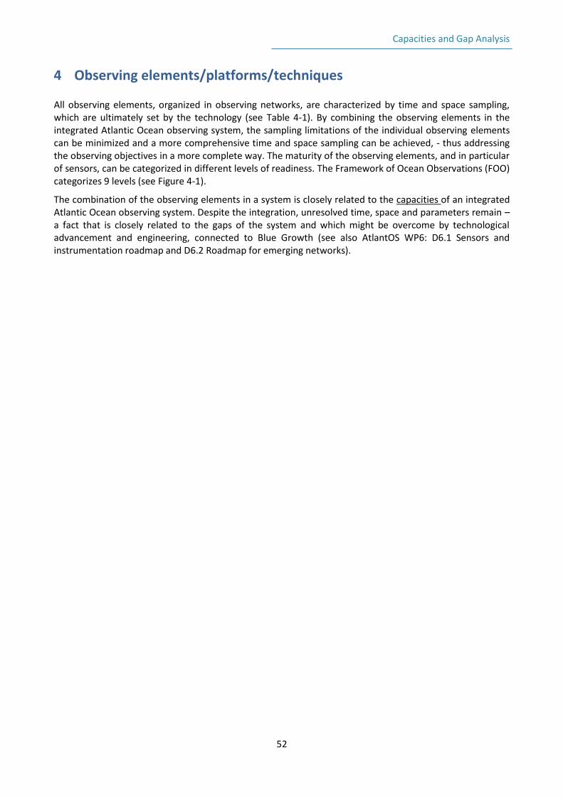
Capacities and Gap Analysis
52
4 Observing elements/platforms/techniques All observing elements, organized in observing networks, are characterized by time and space sampling, which are ultimately set by the technology (see Table 4-1). By combining the observing elements in the integrated Atlantic Ocean observing system, the sampling limitations of the individual observing elements can be minimized and a more comprehensive time and space sampling can be achieved, - thus addressing the observing objectives in a more complete way. The maturity of the observing elements, and in particular of sensors, can be categorized in different levels of readiness. The Framework of Ocean Observations (FOO) categorizes 9 levels (see Figure 4-1).
The combination of the observing elements in a system is closely related to the capacities of an integrated Atlantic Ocean observing system. Despite the integration, unresolved time, space and parameters remain – a fact that is closely related to the gaps of the system and which might be overcome by technological advancement and engineering, connected to Blue Growth (see also AtlantOS WP6: D6.1 Sensors and instrumentation roadmap and D6.2 Roadmap for emerging networks).
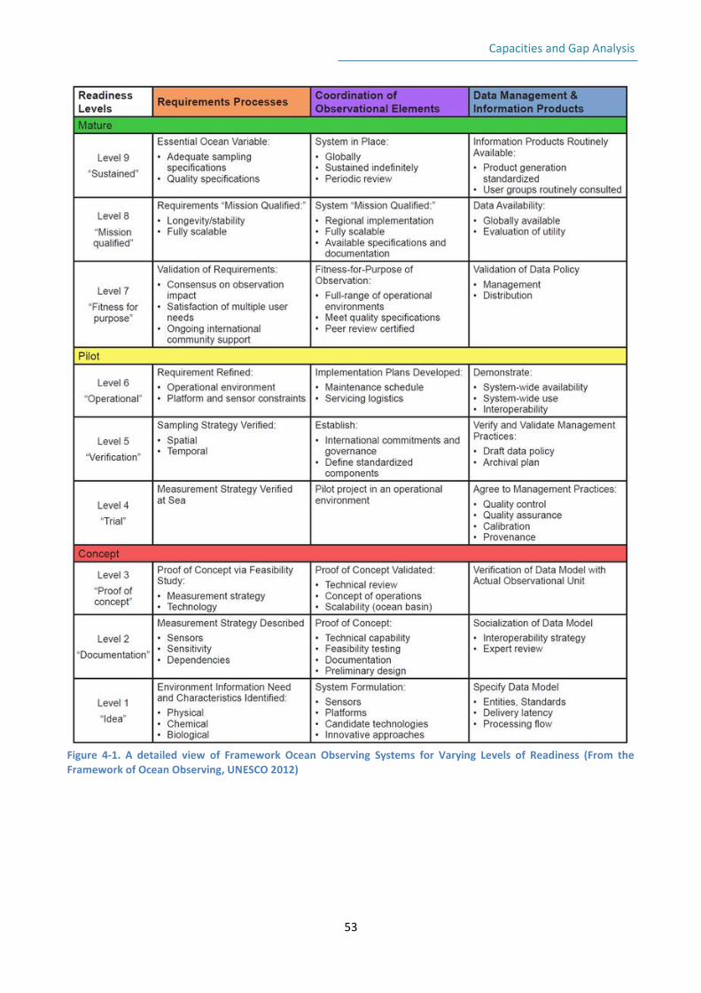
Capacities and Gap Analysis
53
Figure 4-1. A detailed view of Framework Ocean Observing Systems for Varying Levels of Readiness (From the Framework of Ocean Observing, UNESCO 2012)
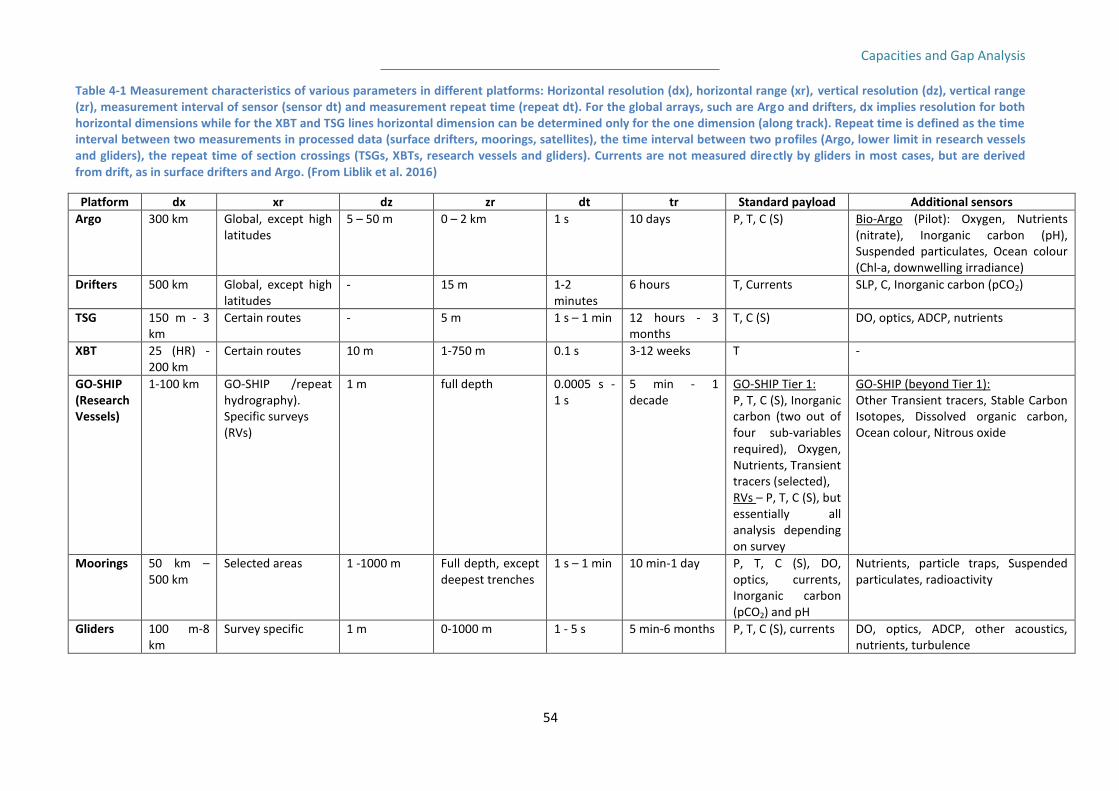
Capacities and Gap Analysis
54
Table 4-1 Measurement characteristics of various parameters in different platforms: Horizontal resolution (dx), horizontal range (xr), vertical resolution (dz), vertical range (zr), measurement interval of sensor (sensor dt) and measurement repeat time (repeat dt). For the global arrays, such are Argo and drifters, dx implies resolution for both horizontal dimensions while for the XBT and TSG lines horizontal dimension can be determined only for the one dimension (along track). Repeat time is defined as the time interval between two measurements in processed data (surface drifters, moorings, satellites), the time interval between two profiles (Argo, lower limit in research vessels and gliders), the repeat time of section crossings (TSGs, XBTs, research vessels and gliders). Currents are not measured directly by gliders in most cases, but are derived from drift, as in surface drifters and Argo. (From Liblik et al. 2016)
Platform dx xr dz zr dt tr Standard payload Additional sensors
Argo 300 km Global, except high latitudes
5 – 50 m 0 – 2 km 1 s 10 days P, T, C (S)
Bio-Argo (Pilot): Oxygen, Nutrients (nitrate), Inorganic carbon (pH), Suspended particulates, Ocean colour (Chl-a, downwelling irradiance)
Drifters 500 km Global, except high latitudes
- 15 m 1-2 minutes
6 hours T, Currents SLP, C, Inorganic carbon (pCO2)
TSG 150 m - 3 km
Certain routes - 5 m 1 s – 1 min 12 hours - 3 months
T, C (S) DO, optics, ADCP, nutrients
XBT 25 (HR) - 200 km
Certain routes 10 m 1-750 m 0.1 s 3-12 weeks T -
GO-SHIP (Research Vessels)
1-100 km GO-SHIP /repeat hydrography). Specific surveys (RVs)
1 m full depth 0.0005 s - 1 s
5 min - 1 decade
GO-SHIP Tier 1: P, T, C (S), Inorganic carbon (two out of four sub-variables required), Oxygen, Nutrients, Transient tracers (selected), RVs – P, T, C (S), but essentially all analysis depending on survey
GO-SHIP (beyond Tier 1): Other Transient tracers, Stable Carbon Isotopes, Dissolved organic carbon, Ocean colour, Nitrous oxide
Moorings 50 km – 500 km
Selected areas 1 -1000 m Full depth, except deepest trenches
1 s – 1 min 10 min-1 day P, T, C (S), DO, optics, currents, Inorganic carbon (pCO2) and pH
Nutrients, particle traps, Suspended particulates, radioactivity
Gliders 100 m-8 km
Survey specific 1 m 0-1000 m 1 - 5 s 5 min-6 months P, T, C (S), currents DO, optics, ADCP, other acoustics, nutrients, turbulence
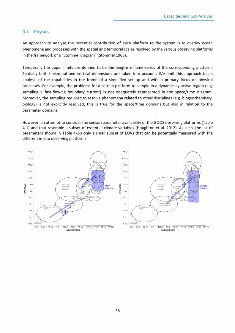
Capacities and Gap Analysis
55
4.1 Physics An approach to analyse the potential contribution of each platform to the system is to overlay ocean
phenomena and processes with the spatial and temporal scales resolved by the various observing platforms
in the framework of a “Stommel diagram” (Stommel 1963).
Temporally the upper limits are defined to be the lengths of time-series of the corresponding platform.
Spatially both horizontal and vertical dimensions are taken into account. We limit this approach to an
analysis of the capabilities in the frame of a simplified set up and with a primary focus on physical
processes. For example, the problems for a certain platform to sample in a dynamically active region (e.g.
sampling a fast-flowing boundary current) is not adequately represented in the space/time diagram.
Moreover, the sampling required to resolve phenomena related to other disciplines (e.g. biogeochemistry,
biology) is not explicitly resolved, this is true for the space/time domains but also in relation to the
parameter domains.
However, an attempt to consider the sensor/parameter availability of the GOOS observing platforms (Table 4-1) and that resemble a subset of essential climate variables (Houghton et al. 2012). As such, the list of parameters shown in Table 4-1is only a small subset of EOVs that can be potentially measured with the different in-situ observing platforms.
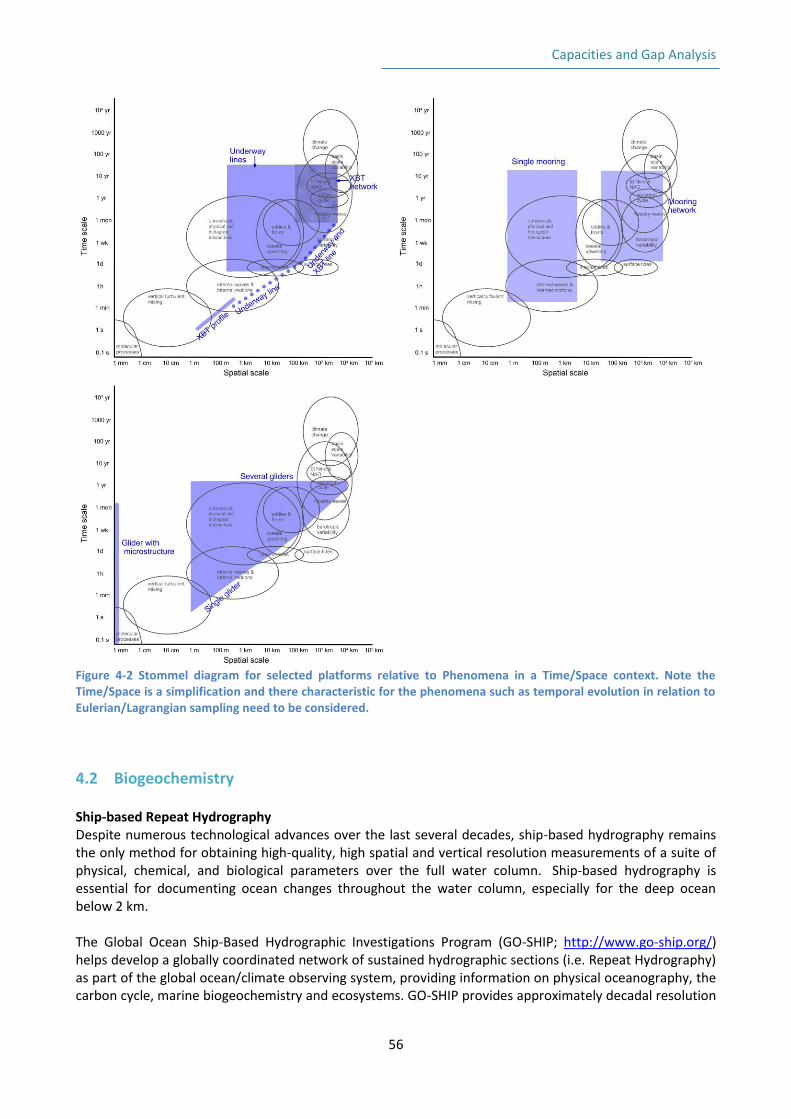
Capacities and Gap Analysis
56
Figure 4-2 Stommel diagram for selected platforms relative to Phenomena in a Time/Space context. Note the Time/Space is a simplification and there characteristic for the phenomena such as temporal evolution in relation to Eulerian/Lagrangian sampling need to be considered.
4.2 Biogeochemistry Ship-based Repeat Hydrography Despite numerous technological advances over the last several decades, ship-based hydrography remains the only method for obtaining high-quality, high spatial and vertical resolution measurements of a suite of physical, chemical, and biological parameters over the full water column. Ship-based hydrography is essential for documenting ocean changes throughout the water column, especially for the deep ocean below 2 km. The Global Ocean Ship-Based Hydrographic Investigations Program (GO-SHIP; http://www.go-ship.org/) helps develop a globally coordinated network of sustained hydrographic sections (i.e. Repeat Hydrography) as part of the global ocean/climate observing system, providing information on physical oceanography, the carbon cycle, marine biogeochemistry and ecosystems. GO-SHIP provides approximately decadal resolution
Capacities and Gap Analysis
57
of the changes in inventories of such biogeochemical variables as carbon, oxygen, nutrients and transient tracers, covering the Atlantic and other ocean basins from coast to coast and full depth (top to bottom), with measurements of the highest required accuracy to detect these changes. Ship-based hydrography observing network is critical to addressing questions of how the ocean will respond to increase in dissolved inorganic carbon, decrease in pH, and changes in ventilation strength processes. Repeated decadal since the 1970s, these observations provide a crucial resource for documenting baselines and patterns of long-term variability in many of the Atlantic Ocean biogeochemical phenomena considered: ocean ventilation, anthropogenic carbon sequestration, organic matter cycling, hypoxia and ocean acidity, both regionally and on basin scale. GO-SHIP data also provide reference data to calibrate autonomous platform sensors that cannot be recovered, and cruises provide a platform for the deployment of many autonomous platforms as well.
Considering only the status of decadal full GO SHIP lines, this observing network has lines distributed every approximately 20 degrees, providing along-section sampling every 30 nautical miles. Such a sampling design is adequate for studying interannual to decadal variability in basin scale signals of many key biogeochemical phenomena discussed above. Considering availability of GO-SHIP data since the 1970s, these records are also long enough to detect climate-driven trends in key biogeochemical EOVs.
Ship-based Underway Observations The Joint Technical Commission for Oceanography and Marine Meteorology (JCOMM) Ship Of Opportunity Programme (SOOP) makes use of volunteer merchant ships which routinely transit strategic shipping routes. A number of biogeochemical EOV measurements depends on the SOOP network coverage. So-called ‘underway’ measurements of pCO2 in surface sea water and in the air are made routinely by the SOOP network with high accuracies achieved. The SOOP pCO2 data, potentially supplemented with underway measurements of pH, dissolved inorganic carbon or total alkalinity in the near future, will be vital in describing basin-wide changes in the carbonate system, thereby improving seasonal and inter-annual climate predictions, and better constraining annually updated calculations of the global carbon budget. Underway surface pCO2 observations provide the capacity to constrain the air-sea CO2 fluxes in the key regions of the North Atlantic, on time scales from monthly to decadal. Combined with ocean interior observations collected on GO-SHIP lines, these measurements thus enable well-constrained estimates of carbon storage in the ocean. The biggest limitation of using the underway ship-based observations from volunteer/commercial ships is the fact that we cannot directly alter the sampling scheme. Therefore, any spatial gaps (e.g. South Atlantic), or seasonal biases (e.g. boreal winter measurements in deep water formation regions in the North Atlantic) cannot be alleviated from the level of observing system design, but require installing a new pCO2 line on an existing commercial vessel. Fixed-point Observatories Single-point time-series stations have increased understanding of the patterns of temporal variability, but by their nature remain limited in the spatial domain. Henson et al. (2016) attempt to analyse the spatial footprint of moored fixed-point observatories with bioeochemical EOVs measured on them. She concluded that depending on the variable of interest, these footprints account for only 10-15% of the global ocean. The fact that existing time-series stations are representative of relatively large surface areas of the ocean confirms their role in estimating sub-basin scale patterns of variability. However, it is clear that much of the
Capacities and Gap Analysis
58
Atlantic as well as the global ocean remains undersampled. There is therefore a need to build and maintain a basin-wide and global network of multi-disciplinary fixed-point surface and subsurface time-series using mooring, ship and other fixed instruments, and to establish a coordinated network of ship-based multidisciplinary time-series that is geographically representative. Implementing this target will depend on the development of units attempting to coordinate fixed-point observatories. The Fixed Point Open Ocean Observatory network (FixO3) seeks to integrate European open ocean fixed point observatories and to improve access to these key installations for the broader community. A similar mission but on the global scale is adopted by OceanSITES whose goal is to collect, deliver and promote the use of high-quality data from long-term, high-frequency observations at fixed locations in the open ocean. OceanSITES typically aim to collect multidisciplinary data worldwide from the full-depth water column as well as the overlying atmosphere. Another key aspect of enhancing the fixed-point observatory capacity is the need to provide accurate information about which moorings measure any of the biogeochemical EOV, and in the long-run, expand on the number of biogeochemical measurements performed routinely at time-series stations. In terms of the key geographic regions samples by fixed-point observatories, there is a gap in such measurements in places of deep water formation. Although resolving sub-decadal variability in basin-scale ventilation is not a key target for the observing system, weekly to seasonal variability in air-sea fluxes, inorganic nutrient cycling and organic matter cycling is crucial to understanding how the ocean carbon content and biomass are changing. While there exist transport mooring arrays in these key locations, there is a lack of coincident biogeochemical observations. Profiling floats Although Argo profiling floats should be considered as a mature observing approach as far as technological readiness level is concerned, the newly formed global Biogeochemical-Argo array as a coordinated observing network remains in pilot stage. There is currently a limited number of floats with biogeochemical sensors deployed. Biogeochemical Argo is set to enable direct observation of the seasonal to decadal-scale variability in NCP, the supply of essential inorganic nutrients transported from deep waters to the sunlit surface layer, ocean acidification, hypoxia and ocean uptake of carbon dioxide. Bio-optical sensors would supplement Ocean Colour satellite observations by providing measurements of chlorophyll, light, and light scattering deep into the ocean interior throughout the year, in cloud- and ice-covered areas, or during the dark of polar winter. The regional profiling float arrays equipped with biogeochemical sensors provide a sampling of ocean conditions around the world that is designed to produce an integrated data set that can be used to address questions related to physical-biogeochemical coupling in eddies, phytoplankton phenology (cyclic and seasonal phenomena), nutrient supply, and climate effects on ocean carbon cycling in selected regions. Some of these arrays include:
the Southern Ocean Carbon and Climate Observations and Modeling (SOCCOM) project
the Remotely Sensed Biogeochemical Cycles in the Ocean (remOcean) project in the North Atlantic subpolar gyre
the Novel Argo Ocean Observing System in the Mediterranean Sea (NAOS)
the Integrated Physical-Biogeochemical Ocean Observation Experiment (INBOX) in the Kuroshio region of the North Pacific
the Australia-India Joint Indian Ocean Bio-Argo Project (IO Bio-ARGO)
Capacities and Gap Analysis
59
When setting targets for and optimizing the biogeochemical Argo array of floats, there is an inherent trade-off between meeting the requirements for observing relevant phenomena on adequate spatial and temporal scales, and the cost of maintaining a sustained observing network. Currently set target of deploying 1000 biogeochemical floats is based on the results of a series of observing system simulation experiments (OSSEs) performed by the SOCCOM Team. It turned out that the biggest gain in terms of reducing the air-sea CO2 flux reconstruction error is for between 500 and 1000 randomly distributed floats. Hence, the target is currently set to 1000. The regional profiling float observation programs are also building the expertise needed to operate a global network that interacts with other components of the global ocean observing system, including satellites (IOCCG, 2011), shipboard programs like the international Global Ocean Ship-Based Hydrographic Investigations Program (GO-SHIP), and various time series stations. Currently, the size of the Biogeochemical Argo array is insufficient to resolve many of the phenomena on basin scale. Until a denser network is developed, they should be viewed as providing high spatial and temporal data on local to regional scales (1 – 1000 km), which are complementary to the basin scale, decadal scale ship-based repeat hydrography observations. Gliders Underwater gliders have enhanced capabilities, when compared with profiling floats, by providing some level of manoeuvrability and hence position control. The gliders perform sawtooth trajectories from the surface to depths of 1000-1500m, along reprogrammable routes (using two-way communication via satellite), and can be operated for a few months. Their role in the integrated observing system is to fill the gaps left by other observing platforms. The mission of the EGO (Everyone’s Gliding Observatories; http://www.egonetwork.org/ ) underwater glider network, initiated by European scientists, is to develop a new observational capacity for process studies and operational monitoring of the ocean physics and biogeochemistry with gliders, and thereby going beyond the marine sciences frontiers. In particular, gliders could be deployed to sample most of the western and eastern boundary circulations and the regional seas of the Atlantic, which are not well covered by the present ocean observing system; and in the vicinity of fixed point time series stations. Gliders can operate at higher resolution than the ca. 300 km/10 day one of the Argo profiling float network, and the even sparser ship-based observations. Therefore, glider-based observations have a great potential to address regional and coastal issues, which are so important for societal applications. Remote sensing observations The space-based observing system is an important component of the Atlantic as well as the Global Observing System. An array of geostationary and polar-orbiting satellites operated by the National Aeronautics and Space Administration (NASA) and the European Space Agency (ESA) sample the Atlantic and global surface ocean on unprecedented spatial and temporal scales, weaving together the requirements for observing surface signatures of key biogeochemical phenomena on short and long time scales, providing basin-wide coverage with a simultaneous high spatial resolution on the order of kilometres. There is several products derived from remote sensing observations which provide often unique information on a number of sub-variables listed under the Suspended Particulates and Dissolved Organic Carbon biogeochemical EOVs. Observations provided by the Ocean Colour Radiometry Virtual Constellation, and recently also by LIDAR, enable near real time monitoring of such phenomena as organic matter cycling and eutrophication. On the other hand, the focus of remote sensing observations is often on the physical and biological phenomena. There are often very few algorithms available to estimate
Capacities and Gap Analysis
60
biogeochemical properties of interest, e.g. DOC or PIC. Promoting new and alternative algorithms should be a target which will lead to decreasing the so far high uncertainty of satellite based measurements of biogeochemical variables. Remote sensing observations are essential to studying surface processes related to organic matter cycling in the key regions of North Atlantic and the boundary current and upwelling regions. Although much more challenging and associated with very large uncertainties, coastal satellite observations also provide information about changing carbon content in the continental shelf and marginal seas regions.
4.3 Biology Phytoplankton biomass and diversity The EU Copernicus Marine environment monitoring service provides monitoring of phytoplankton and HABs using satellite information. Currently, various additional phytoplankton monitoring programmes exist from research vessels and coastal stations. The Continuous Plankton Recorder (CPR) survey, which is the longest continuous time series in the world’s ocean records greenness of netting as an indicator of phytoplankton abundance. Other relevant observing mechanisms are ship based time series, moorings and samplings from coastal waters. The EU Copernicus Marine environment monitoring service also provides monitoring of phytoplankton using satellite derived ocean colour products. The Argo floats form networks free-floating sensors, operating in open ocean areas that provide real-time data on ocean temperature and salinity. Recent 'Bio Argo' floats include additional sensors for dissolved oxygen, nitrate, chlorophyll, dissolved organic matter, and particle scattering. In that sense ‘Bio Argos’ seem a promising tool for monitoring phytoplankton via chlorophyll assessment. The IOC harmful algal bloom programme coordinates monitoring in the Atlantic (http://hab.ioc-unesco.org/) Zooplankton biomass and diversity Zooplankton monitoring is essential in assessing the state of the oceans. An important monitoring programme is the Continuous Plankton Recorder (CPR) survey, run by the Sir Alister Hardy Foundation for Ocean Science (SAHFOS). It has been instrumental in illustrating the role of zooplankton as sentinels of climate change. Their survey measures variables such as biomass, species composition and spatial distribution of zooplankton. Other relevant observing mechanisms are ship based time series, coastal stations, and moorings. Many zooplankton time series can be accessed through the EMODNET biology portal. Fish abundance and distribution The Food and Agriculture Organization (FAO) of the United Nations receives regularly fishery catches data and stock information from most nations. Other sources include many national, multinational and regional fishery management organizations (RFMOs and ICES). See http://www.ices.dk/marine-data/dataset-collections/Pages/Fish-catch-and-stock-assessment.aspx Commercially exploited groups of fish (stocks) are monitored through stock assessments (in the EU, Norway and Iceland, this is done by ICES and STECF, for northern and southern areas respectively) using sampling of the catches and surveys which are integrated together through various population dynamic models. Surveys are used to monitor non-commercial species and ecosystem, structure. This supplement the knowledge base for the ecosystem approach to fishing and also in the EU the marine strategy
Capacities and Gap Analysis
61
framework directive. Recreational fisheries are also monitored. See http://www.ices.dk/marine-data/tools/Pages/stock-assessment-graphs.aspx The methods used to survey marine fish in Europe broadly engage the following techniques: acoustic, net trawls, plankton nets, TV sledges, dredges. The commercial catches are also monitored by port and auction sampling, on-board observers, cameras, fishing industry initiatives, electronic log books on fishing vessels. Marine turtle, bird and mammal abundance and distribution The methods used to survey marine turtles, birds and mammals include satellites; tracking; and vessel surveys Live coral OSPAR and NEAFC work together to designate the areas of cold waters corals. This information is compiled by ICES (WGDEC) and made available through the Vulnerable Marine Ecosystem (VME) data portal (http://ices.dk/marine-data/data-portals/Pages/vulnerable-marine-ecosystems.aspx). For tropical hard coral communities, the Global Coral Reef Monitoring Network (GCRMN) collects data by transects/quadrats, in situ or by photo; and by remote sensing being: aerial; unmanned and manned; satellite; and multispectral for area extent. U.S. National Oceanic and Atmospheric Administration (NOAA) has deployed in the some tropical hard coral communities located in the Atlantic Autonomous Reef Monitoring Structures to assess reef cryptobiota diversity. Macroalgal canopy Macroalgal canopy is usually assessed by quadrats and photo-quadrats but with the advance of hyperspectral imaging might be possible in the future to use that technology to monitor canopy extents. Seagrass cover Seagrass cover monitoring is usually done by manual sampling through different kinds of coastal surveys, mostly by a diver working along transects; photo-quadrates; remote sensing by aircraft (drone, manned); and satellite (Landsat or higher spatial/spectral resolution).
Capacities and Gap Analysis
62
5 Estimate of existing observation capacity in Atlantic per EOV and
platform An overall objective of AtlantOS WP1 is, following the initial definition of requirements for sustained ocean observations (described in Deliverable D.1.1), to analyse the present ocean observing capacities in the Atlantic Ocean. This analysis of present capacities will help to clarify the critical gaps that need to be filled to upgrade and expand the observational system and to refine scientifically an integrated Atlantic Observing System which fulfils the societal and the scientific challenges. In the framework of this observing capacity analysis, it is important to have an overview of the existing ocean observing activities and observing networks as well as the existing observing platforms and to what degree the data are open and free in different databases and data portals. In this chapter, we show a review of the available observing platforms and the ocean variables which are being measured in the Atlantic on a routinely basis. Among all the possible observed parameters, we focus our analysis on the Essential Ocean Variables (EOVs) which have been defined in previous chapters and in AtlantOS Deliverable 1.1, except for the Biological EOVs that are included in this report. It shall be stressed that we only consider in-situ observational data capacities and don’t take into consideration the capacities provided by satellite observations, which are outside AtlantOS project scope.
5.1 Sources of information: European and international level To perform the review of the observational capability in the Atlantic we have collected the information available in the main Pan-European coordinated observations data portals, or integrators, like EMODnet, CMEMS and SeaDataNet. Moreover, we have collected the metadata information available in the international JCOMMOPS data portal, which gathers the data from ocean observing global networks in support of GOOS, GCOS and WMO, as well as other data portals collecting biogeochemistry and biology/Ecosystems observations like GLODAP or ICES. Besides these main data integrators there are observational networks that must been considered when analysing the observational capacities, some of the data networks are already integrated in CMEMS, EMODnet or JCOMMOPS, but some others are not yet fully integrated, this is a task of Work Package 7 in AtlantOS. In this chapter, we present first an overview of the major international, European and intergovernmental monitoring or data collection/management programmes, projects as well as some of the main data portal integrators where this data can be accessed (Table 5-1). By ‘major’ we mean those international collaborative initiatives that include more than one country or individual institution. We have listed the main initiatives collecting physical, biogeochemical and biological parameters. Some of them are only in the Atlantic Ocean but the majority are pan-European, or international, and have the Atlantic Ocean as one of the activity areas. Note that databases listed in Table 5-1 includes in some cases data which is totally unrestricted open data, in some other data is under some kind of license (e.g. registration) and some data is only accessible under negotiation with the data provider. In our further analysis of observational capacities we would consider only totally open data.
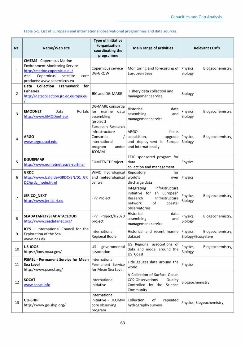
Capacities and Gap Analysis
63
Table 5-1. List of European and international observational programmes and data sources.
№ Name/Web site
Type of initiative /organization
coordinating the programme
Main range of activities Relevant EOV’s
1
CMEMS - Copernicus Marine Environment Monitoring Service http://marine.copernicus.eu/ And Copernicus satellite core products: www.copernicus.eu
Copernicus service DG-GROW
Monitoring and forecasting of European Seas
Physics, Biogeochemistry, Biology
2
Data Collection Framework for Fisheries http://datacollection.jrc.ec.europa.eu/
JRC and DG-MARE Fishery data collection and management service
Biology
3 EMODNET Data Portals http://www.EMODnet.eu/
DG-MARE consortia for marine data assembling (project)
Historical data assembling and management service
Physics, Biogeochemistry, Biology
4
ARGO www.argo.uscd.edu
European Research Infrastructure Consortia / international program under JCOMM
ARGO floats acquisition, upgrade and deployment in Europe and internationally
Physics, Biogeochemistry, Biology
5 E-SURFMAR http://www.eumetnet.eu/e-surfmar
EUMETNET Project EEIG sponsored program for data collection and management
Physics
6 GRDC http://www.bafg.de/GRDC/EN/01_GRDC/grdc_node.html
WMO hydrological and meteorological centre
Repository for world’s river discharge data
Physics
7 JERICO_NEXT http://www.jerico-ri.eu
FP7 Project
Integrating infrastructure initiative for an European Research Infrastructure network of coastal observatories
Physics, Biogeochemistry, Biology
8 SEADATANET/SEADATACLOUD http://www.seadatanet.org/
FP7 Project/H2020 project
Historical data assembling and management service
Physics, Biogeochemistry, Biology
9 ICES – International Council for the Exploration of the Sea www.ices.dk
International Regional Bodie
Historical and recent marine dataset
Physics, Biogeochemistry, Biology/Ecosystem
10 US-IOOS https://ioos.noaa.gov/
US governmental association
US Regional associations of data and model around the US Coast
Physics, Biogeochemistry, Biology
11 PSMSL - Permanent Service for Mean Sea Level http://www.psmsl.org/
International Permanent Service for Mean Sea Level
Tide gauges data around the world
Physics
12 SOCAT www.socat.info
International initiative
A Collection of Surface Ocean CO2 Observations Quality Controlled by the Science Community
Biogeochemistry
13 GO-SHIP http://www.go-ship.org/
International initiative - JCOMM core observing program
Collection of repeated hydrography surveys
Physics, Biogeochemistry,
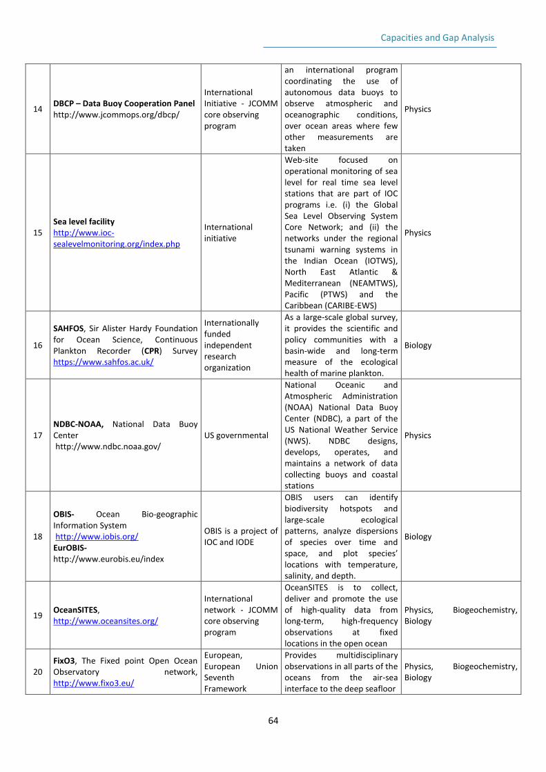
Capacities and Gap Analysis
64
14 DBCP – Data Buoy Cooperation Panel http://www.jcommops.org/dbcp/
International Initiative - JCOMM core observing program
an international program coordinating the use of autonomous data buoys to observe atmospheric and oceanographic conditions, over ocean areas where few other measurements are taken
Physics
15 Sea level facility http://www.ioc-sealevelmonitoring.org/index.php
International initiative
Web-site focused on operational monitoring of sea level for real time sea level stations that are part of IOC programs i.e. (i) the Global Sea Level Observing System Core Network; and (ii) the networks under the regional tsunami warning systems in the Indian Ocean (IOTWS), North East Atlantic & Mediterranean (NEAMTWS), Pacific (PTWS) and the Caribbean (CARIBE-EWS)
Physics
16
SAHFOS, Sir Alister Hardy Foundation for Ocean Science, Continuous Plankton Recorder (CPR) Survey https://www.sahfos.ac.uk/
Internationally funded independent research organization
As a large-scale global survey, it provides the scientific and policy communities with a basin-wide and long-term measure of the ecological health of marine plankton.
Biology
17 NDBC-NOAA, National Data Buoy Center http://www.ndbc.noaa.gov/
US governmental
National Oceanic and Atmospheric Administration (NOAA) National Data Buoy Center (NDBC), a part of the US National Weather Service (NWS). NDBC designs, develops, operates, and maintains a network of data collecting buoys and coastal stations
Physics
18
OBIS- Ocean Bio-geographic Information System http://www.iobis.org/ EurOBIS-http://www.eurobis.eu/index
OBIS is a project of IOC and IODE
OBIS users can identify biodiversity hotspots and large-scale ecological patterns, analyze dispersions of species over time and space, and plot species’ locations with temperature, salinity, and depth.
Biology
19 OceanSITES, http://www.oceansites.org/
International network - JCOMM core observing program
OceanSITES is to collect, deliver and promote the use of high-quality data from long-term, high-frequency observations at fixed locations in the open ocean
Physics, Biogeochemistry, Biology
20 FixO3, The Fixed point Open Ocean Observatory network, http://www.fixo3.eu/
European, European Union Seventh Framework
Provides multidisciplinary observations in all parts of the oceans from the air-sea interface to the deep seafloor
Physics, Biogeochemistry, Biology
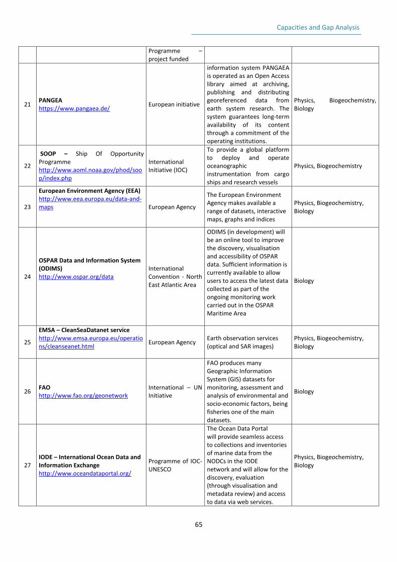
Capacities and Gap Analysis
65
Programme – project funded
21 PANGEA https://www.pangaea.de/
European initiative
information system PANGAEA is operated as an Open Access library aimed at archiving, publishing and distributing georeferenced data from earth system research. The system guarantees long-term availability of its content through a commitment of the operating institutions.
Physics, Biogeochemistry, Biology
22
SOOP – Ship Of Opportunity Programme http://www.aoml.noaa.gov/phod/soop/index.php
International Initiative (IOC)
To provide a global platform to deploy and operate oceanographic instrumentation from cargo ships and research vessels
Physics, Biogeochemistry
23
European Environment Agency (EEA) http://www.eea.europa.eu/data-and-maps
European Agency
The European Environment Agency makes available a range of datasets, interactive maps, graphs and indices
Physics, Biogeochemistry, Biology
24
OSPAR Data and Information System (ODIMS) http://www.ospar.org/data
International Convention - North East Atlantic Area
ODIMS (in development) will be an online tool to improve the discovery, visualisation and accessibility of OSPAR data. Sufficient information is currently available to allow users to access the latest data collected as part of the ongoing monitoring work carried out in the OSPAR Maritime Area
Biology
25
EMSA – CleanSeaDatanet service http://www.emsa.europa.eu/operations/cleanseanet.html
European Agency Earth observation services (optical and SAR images)
Physics, Biogeochemistry, Biology
26 FAO http://www.fao.org/geonetwork
International – UN Initiative
FAO produces many Geographic Information System (GIS) datasets for monitoring, assessment and analysis of environmental and socio-economic factors, being fisheries one of the main datasets.
Biology
27 IODE – International Ocean Data and Information Exchange http://www.oceandataportal.org/
Programme of IOC-UNESCO
The Ocean Data Portal will provide seamless access to collections and inventories of marine data from the NODCs in the IODE network and will allow for the discovery, evaluation (through visualisation and metadata review) and access to data via web services.
Physics, Biogeochemistry, Biology
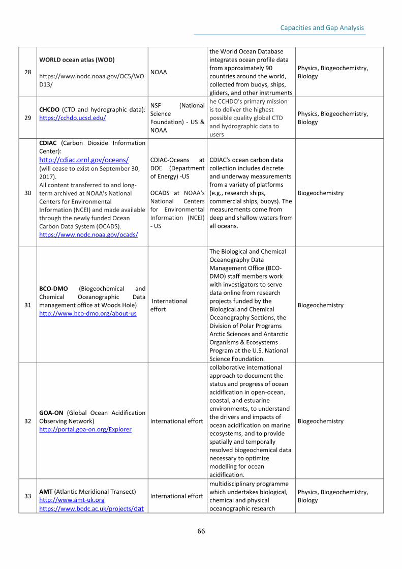
Capacities and Gap Analysis
66
28
WORLD ocean atlas (WOD) https://www.nodc.noaa.gov/OC5/WOD13/
NOAA
the World Ocean Database integrates ocean profile data from approximately 90 countries around the world, collected from buoys, ships, gliders, and other instruments
Physics, Biogeochemistry, Biology
29 CHCDO (CTD and hydrographic data): https://cchdo.ucsd.edu/
NSF (National Science Foundation) - US & NOAA
he CCHDO's primary mission is to deliver the highest possible quality global CTD and hydrographic data to users
Physics, Biogeochemistry, Biology
30
CDIAC (Carbon Dioxide Information Center):
http://cdiac.ornl.gov/oceans/ (will cease to exist on September 30, 2017). All content transferred to and long-term archived at NOAA's National Centers for Environmental Information (NCEI) and made available through the newly funded Ocean Carbon Data System (OCADS). https://www.nodc.noaa.gov/ocads/
CDIAC-Oceans at DOE (Department of Energy) -US OCADS at NOAA's National Centers for Environmental Information (NCEI) - US
CDIAC's ocean carbon data collection includes discrete and underway measurements from a variety of platforms (e.g., research ships, commercial ships, buoys). The measurements come from deep and shallow waters from all oceans.
Biogeochemistry
31
BCO-DMO (Biogeochemical and Chemical Oceanographic Data management office at Woods Hole) http://www.bco-dmo.org/about-us
International effort
The Biological and Chemical Oceanography Data Management Office (BCO-DMO) staff members work with investigators to serve data online from research projects funded by the Biological and Chemical Oceanography Sections, the Division of Polar Programs Arctic Sciences and Antarctic Organisms & Ecosystems Program at the U.S. National Science Foundation.
Biogeochemistry
32 GOA-ON (Global Ocean Acidification Observing Network) http://portal.goa-on.org/Explorer
International effort
collaborative international approach to document the status and progress of ocean acidification in open-ocean, coastal, and estuarine environments, to understand the drivers and impacts of ocean acidification on marine ecosystems, and to provide spatially and temporally resolved biogeochemical data necessary to optimize modelling for ocean acidification.
Biogeochemistry
33
AMT (Atlantic Meridional Transect) http://www.amt-uk.org
https://www.bodc.ac.uk/projects/dat
International effort
multidisciplinary programme which undertakes biological, chemical and physical oceanographic research
Physics, Biogeochemistry, Biology
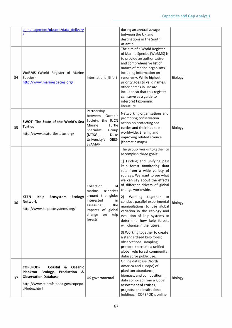
Capacities and Gap Analysis
67
a_management/uk/amt/data_delivery/
during an annual voyage between the UK and destinations in the South Atlantic.
34 WoRMS (World Register of Marine Species) http://www.marinespecies.org/
International Effort
The aim of a World Register of Marine Species (WoRMS) is to provide an authoritative and comprehensive list of names of marine organisms, including information on synonymy. While highest priority goes to valid names, other names in use are included so that this register can serve as a guide to interpret taxonomic literature.
Biology
35
SWOT- The State of the World’s Sea Turtles
http://www.seaturtlestatus.org/
Partnership between Oceanic Society, the IUCN Marine Turtle Specialist Group (MTSG), Duke University’s OBIS-SEAMAP
Networking organisations and promoting conservation action on protecting sea turtles and their habitats worldwide; Sharing and improving related science (thematic maps)
Biology
36
KEEN -Kelp Ecosystem Ecology Network
http://www.kelpecosystems.org/
Collection of marine scientists around the globe interested in assessing the impacts of global change on kelp forests
The group works together to accomplish three goals:
1) Finding and unifying past kelp forest monitoring data sets from a wide variety of sources. We want to see what we can say about the effects of different drivers of global change worldwide.
2) Working together to conduct parallel experimental manipulations to use global variation in the ecology and evolution of kelp systems to determine how kelp forests will change in the future.
3) Working together to create a standardized kelp forest observational sampling protocol to create a unified global kelp forest community dataset for public use.
Biology
37
COPEPOD- Coastal & Oceanic Plankton Ecology, Production & Observation Database
http://www.st.nmfs.noaa.gov/copepod/index.html
US governmental
Online database (North America and Europe) of plankton abundance, biomass, and composition data compiled from a global assortment of cruises, projects, and institutional holdings. COPEPOD's online
Biology
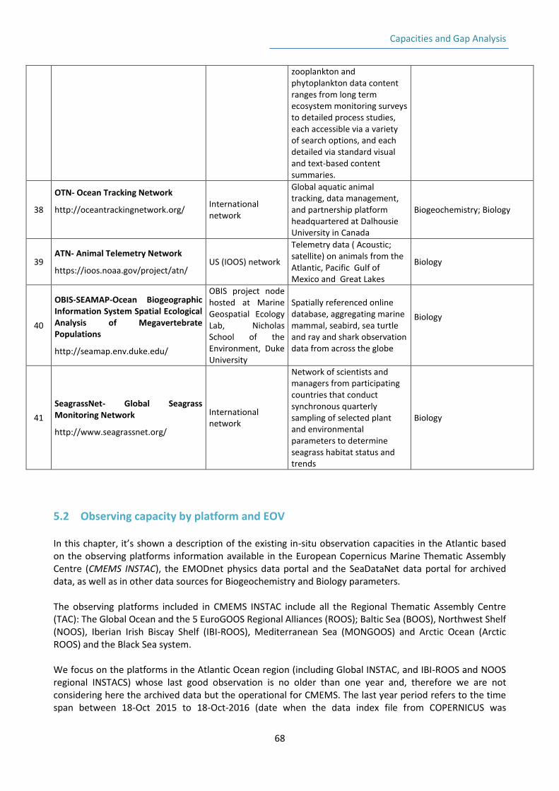
Capacities and Gap Analysis
68
zooplankton and phytoplankton data content ranges from long term ecosystem monitoring surveys to detailed process studies, each accessible via a variety of search options, and each detailed via standard visual and text-based content summaries.
38
OTN- Ocean Tracking Network
http://oceantrackingnetwork.org/
International network
Global aquatic animal tracking, data management, and partnership platform headquartered at Dalhousie University in Canada
Biogeochemistry; Biology
39 ATN- Animal Telemetry Network
https://ioos.noaa.gov/project/atn/ US (IOOS) network
Telemetry data ( Acoustic; satellite) on animals from the Atlantic, Pacific Gulf of Mexico and Great Lakes
Biology
40
OBIS-SEAMAP-Ocean Biogeographic Information System Spatial Ecological Analysis of Megavertebrate Populations
http://seamap.env.duke.edu/
OBIS project node hosted at Marine Geospatial Ecology Lab, Nicholas School of the Environment, Duke University
Spatially referenced online database, aggregating marine mammal, seabird, sea turtle and ray and shark observation data from across the globe
Biology
41
SeagrassNet- Global Seagrass Monitoring Network
http://www.seagrassnet.org/
International network
Network of scientists and managers from participating countries that conduct synchronous quarterly sampling of selected plant and environmental parameters to determine seagrass habitat status and trends
Biology
5.2 Observing capacity by platform and EOV In this chapter, it’s shown a description of the existing in-situ observation capacities in the Atlantic based on the observing platforms information available in the European Copernicus Marine Thematic Assembly Centre (CMEMS INSTAC), the EMODnet physics data portal and the SeaDataNet data portal for archived data, as well as in other data sources for Biogeochemistry and Biology parameters. The observing platforms included in CMEMS INSTAC include all the Regional Thematic Assembly Centre (TAC): The Global Ocean and the 5 EuroGOOS Regional Alliances (ROOS); Baltic Sea (BOOS), Northwest Shelf (NOOS), Iberian Irish Biscay Shelf (IBI-ROOS), Mediterranean Sea (MONGOOS) and Arctic Ocean (Arctic ROOS) and the Black Sea system. We focus on the platforms in the Atlantic Ocean region (including Global INSTAC, and IBI-ROOS and NOOS regional INSTACS) whose last good observation is no older than one year and, therefore we are not considering here the archived data but the operational for CMEMS. The last year period refers to the time span between 18-Oct 2015 to 18-Oct-2016 (date when the data index file from COPERNICUS was
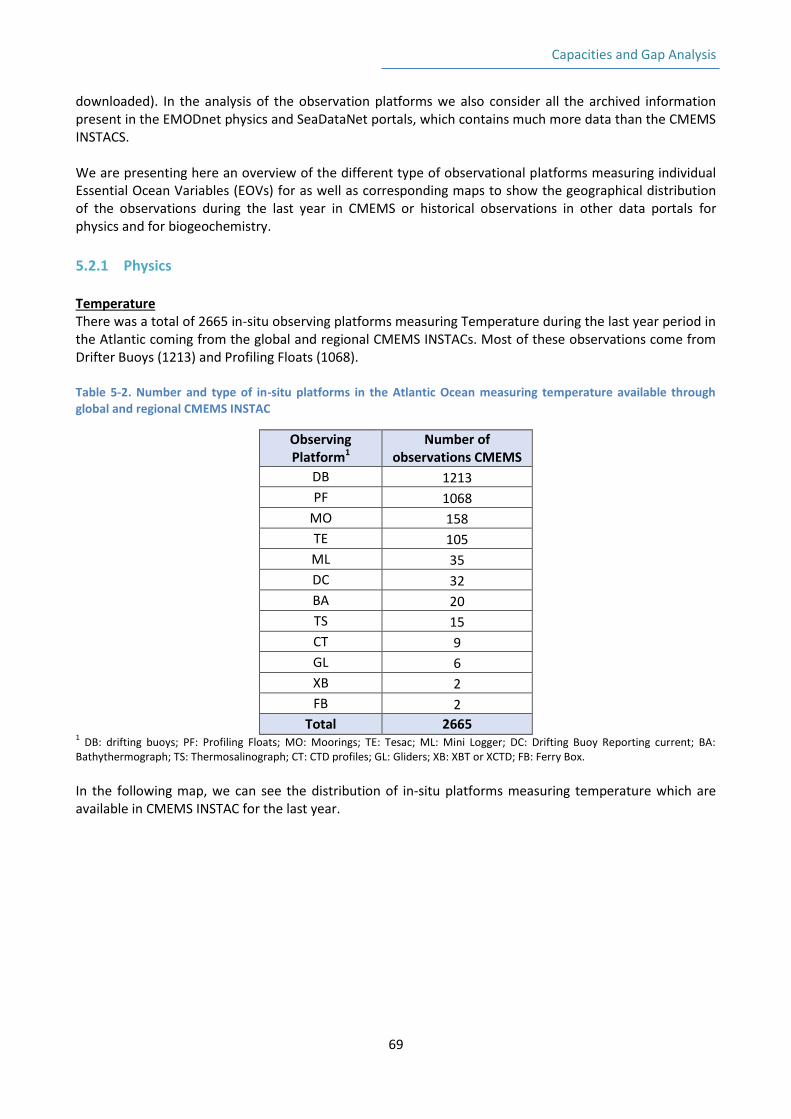
Capacities and Gap Analysis
69
downloaded). In the analysis of the observation platforms we also consider all the archived information present in the EMODnet physics and SeaDataNet portals, which contains much more data than the CMEMS INSTACS. We are presenting here an overview of the different type of observational platforms measuring individual Essential Ocean Variables (EOVs) for as well as corresponding maps to show the geographical distribution of the observations during the last year in CMEMS or historical observations in other data portals for physics and for biogeochemistry.
5.2.1 Physics Temperature There was a total of 2665 in-situ observing platforms measuring Temperature during the last year period in the Atlantic coming from the global and regional CMEMS INSTACs. Most of these observations come from Drifter Buoys (1213) and Profiling Floats (1068). Table 5-2. Number and type of in-situ platforms in the Atlantic Ocean measuring temperature available through global and regional CMEMS INSTAC
Observing Platform1
Number of observations CMEMS
DB 1213
PF 1068
MO 158
TE 105
ML 35
DC 32
BA 20
TS 15
CT 9
GL 6
XB 2
FB 2
Total 2665 1 DB: drifting buoys; PF: Profiling Floats; MO: Moorings; TE: Tesac; ML: Mini Logger; DC: Drifting Buoy Reporting current; BA:
Bathythermograph; TS: Thermosalinograph; CT: CTD profiles; GL: Gliders; XB: XBT or XCTD; FB: Ferry Box.
In the following map, we can see the distribution of in-situ platforms measuring temperature which are available in CMEMS INSTAC for the last year.
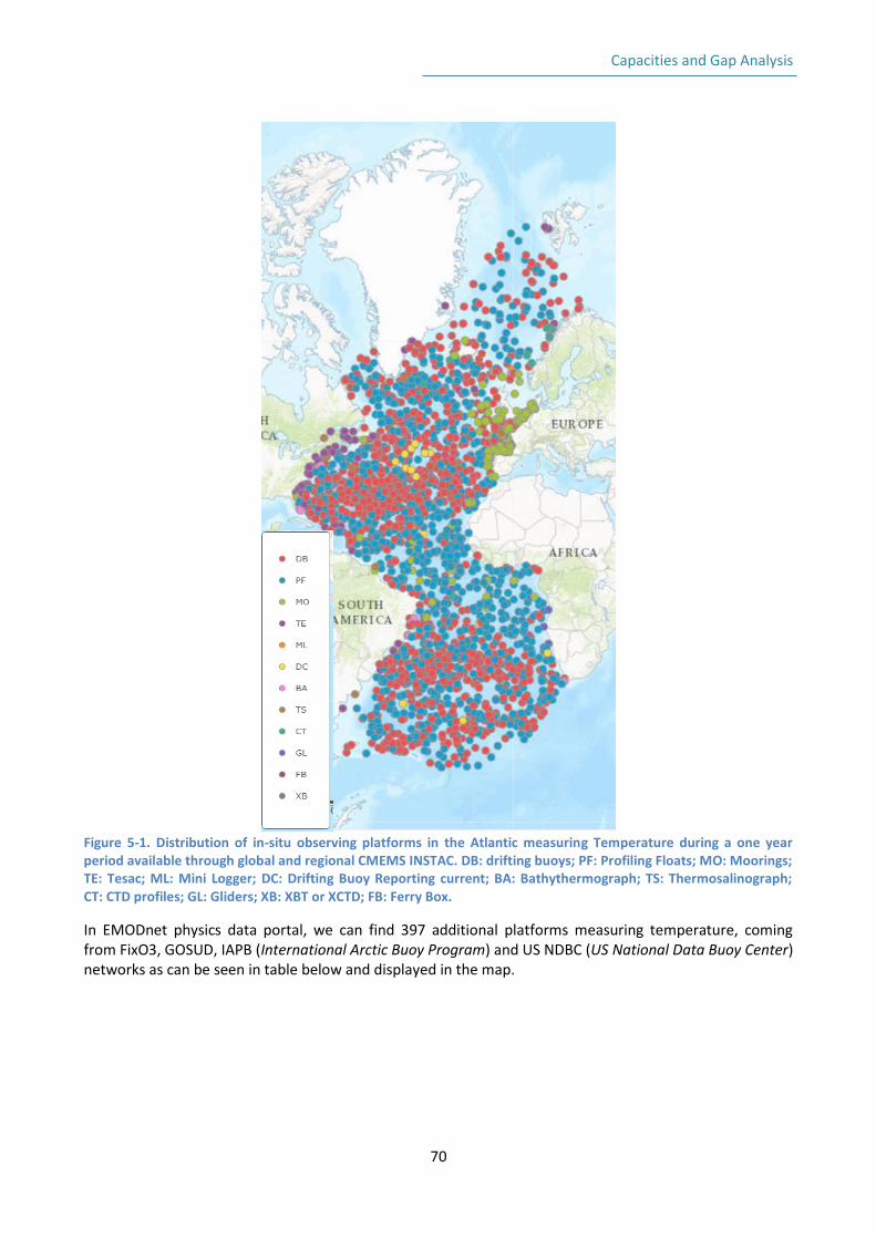
Capacities and Gap Analysis
70
Figure 5-1. Distribution of in-situ observing platforms in the Atlantic measuring Temperature during a one year period available through global and regional CMEMS INSTAC. DB: drifting buoys; PF: Profiling Floats; MO: Moorings; TE: Tesac; ML: Mini Logger; DC: Drifting Buoy Reporting current; BA: Bathythermograph; TS: Thermosalinograph; CT: CTD profiles; GL: Gliders; XB: XBT or XCTD; FB: Ferry Box.
In EMODnet physics data portal, we can find 397 additional platforms measuring temperature, coming from FixO3, GOSUD, IAPB (International Arctic Buoy Program) and US NDBC (US National Data Buoy Center) networks as can be seen in table below and displayed in the map.
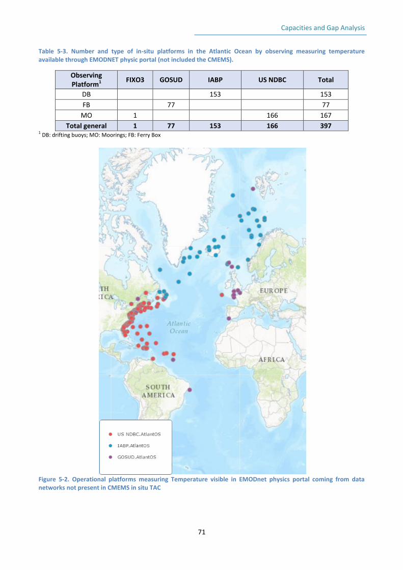
Capacities and Gap Analysis
71
Table 5-3. Number and type of in-situ platforms in the Atlantic Ocean by observing measuring temperature available through EMODNET physic portal (not included the CMEMS).
Observing Platform1
FIXO3 GOSUD IABP US NDBC Total
DB
153
153
FB
77
77
MO 1
166 167
Total general 1 77 153 166 397 1 DB: drifting buoys; MO: Moorings; FB: Ferry Box
Figure 5-2. Operational platforms measuring Temperature visible in EMODnet physics portal coming from data networks not present in CMEMS in situ TAC
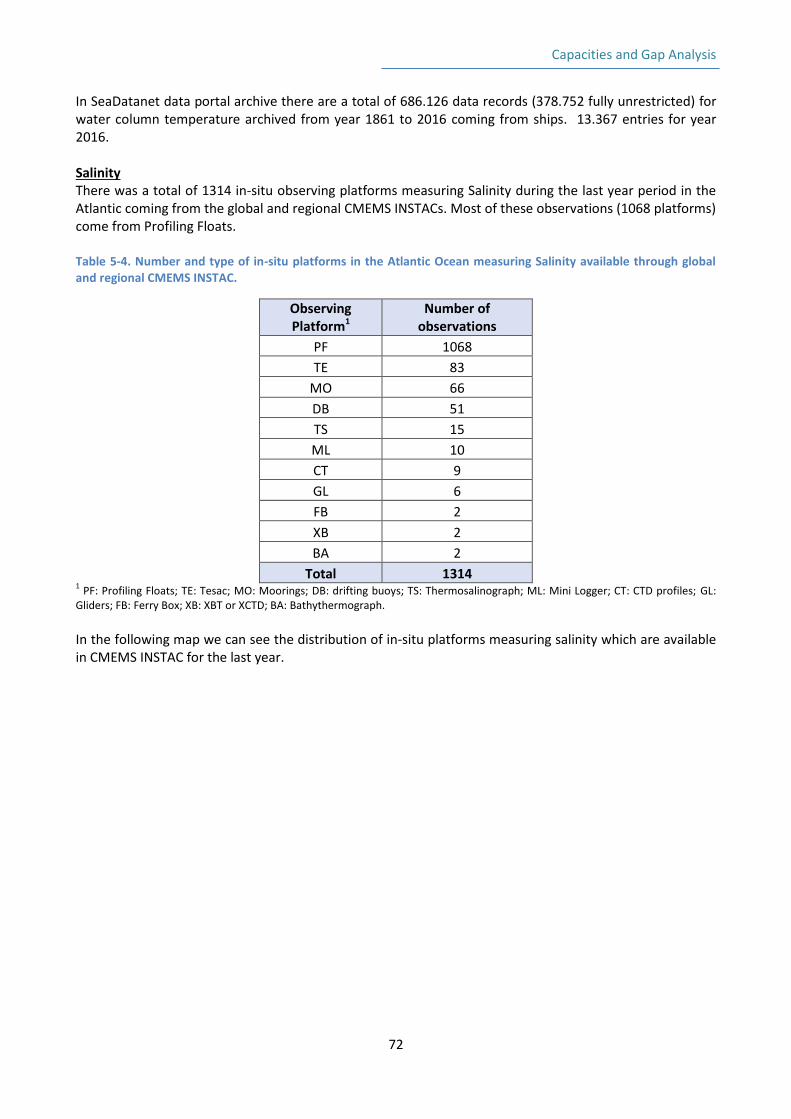
Capacities and Gap Analysis
72
In SeaDatanet data portal archive there are a total of 686.126 data records (378.752 fully unrestricted) for water column temperature archived from year 1861 to 2016 coming from ships. 13.367 entries for year 2016. Salinity There was a total of 1314 in-situ observing platforms measuring Salinity during the last year period in the Atlantic coming from the global and regional CMEMS INSTACs. Most of these observations (1068 platforms) come from Profiling Floats. Table 5-4. Number and type of in-situ platforms in the Atlantic Ocean measuring Salinity available through global and regional CMEMS INSTAC.
Observing Platform1
Number of observations
PF 1068
TE 83
MO 66
DB 51
TS 15
ML 10
CT 9
GL 6
FB 2
XB 2
BA 2
Total 1314 1 PF: Profiling Floats; TE: Tesac; MO: Moorings; DB: drifting buoys; TS: Thermosalinograph; ML: Mini Logger; CT: CTD profiles; GL:
Gliders; FB: Ferry Box; XB: XBT or XCTD; BA: Bathythermograph.
In the following map we can see the distribution of in-situ platforms measuring salinity which are available in CMEMS INSTAC for the last year.
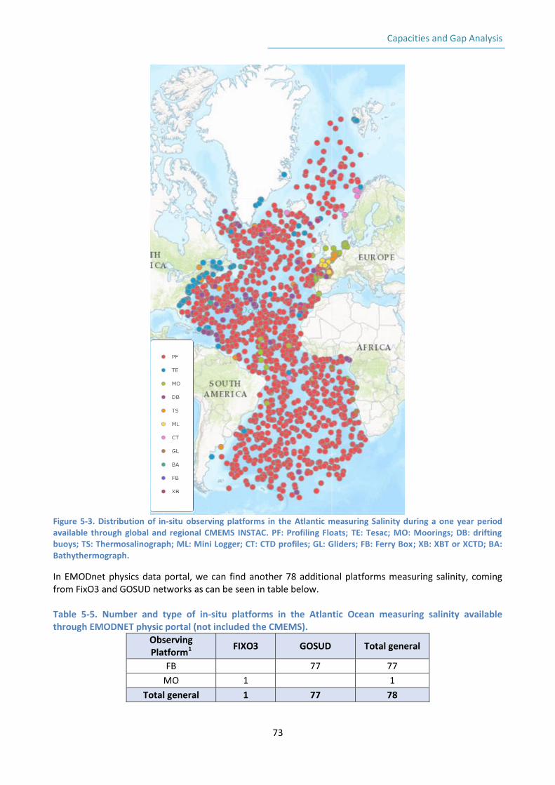
Capacities and Gap Analysis
73
Figure 5-3. Distribution of in-situ observing platforms in the Atlantic measuring Salinity during a one year period available through global and regional CMEMS INSTAC. PF: Profiling Floats; TE: Tesac; MO: Moorings; DB: drifting buoys; TS: Thermosalinograph; ML: Mini Logger; CT: CTD profiles; GL: Gliders; FB: Ferry Box; XB: XBT or XCTD; BA: Bathythermograph.
In EMODnet physics data portal, we can find another 78 additional platforms measuring salinity, coming from FixO3 and GOSUD networks as can be seen in table below. Table 5-5. Number and type of in-situ platforms in the Atlantic Ocean measuring salinity available through EMODNET physic portal (not included the CMEMS).
Observing Platform1
FIXO3 GOSUD Total general
FB
77 77
MO 1
1
Total general 1 77 78
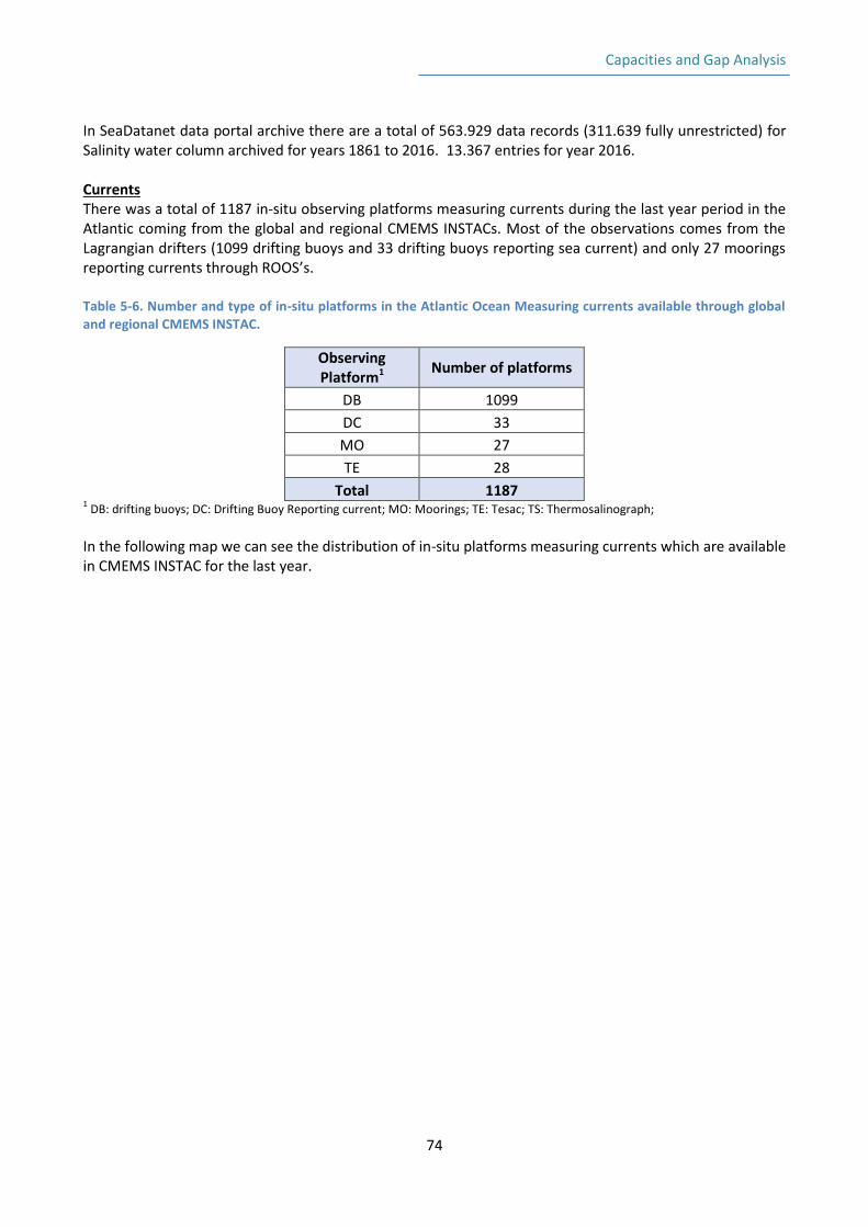
Capacities and Gap Analysis
74
In SeaDatanet data portal archive there are a total of 563.929 data records (311.639 fully unrestricted) for Salinity water column archived for years 1861 to 2016. 13.367 entries for year 2016. Currents There was a total of 1187 in-situ observing platforms measuring currents during the last year period in the Atlantic coming from the global and regional CMEMS INSTACs. Most of the observations comes from the Lagrangian drifters (1099 drifting buoys and 33 drifting buoys reporting sea current) and only 27 moorings reporting currents through ROOS’s. Table 5-6. Number and type of in-situ platforms in the Atlantic Ocean Measuring currents available through global and regional CMEMS INSTAC.
Observing Platform1
Number of platforms
DB 1099
DC 33
MO 27
TE 28
Total 1187 1 DB: drifting buoys; DC: Drifting Buoy Reporting current; MO: Moorings; TE: Tesac; TS: Thermosalinograph;
In the following map we can see the distribution of in-situ platforms measuring currents which are available in CMEMS INSTAC for the last year.
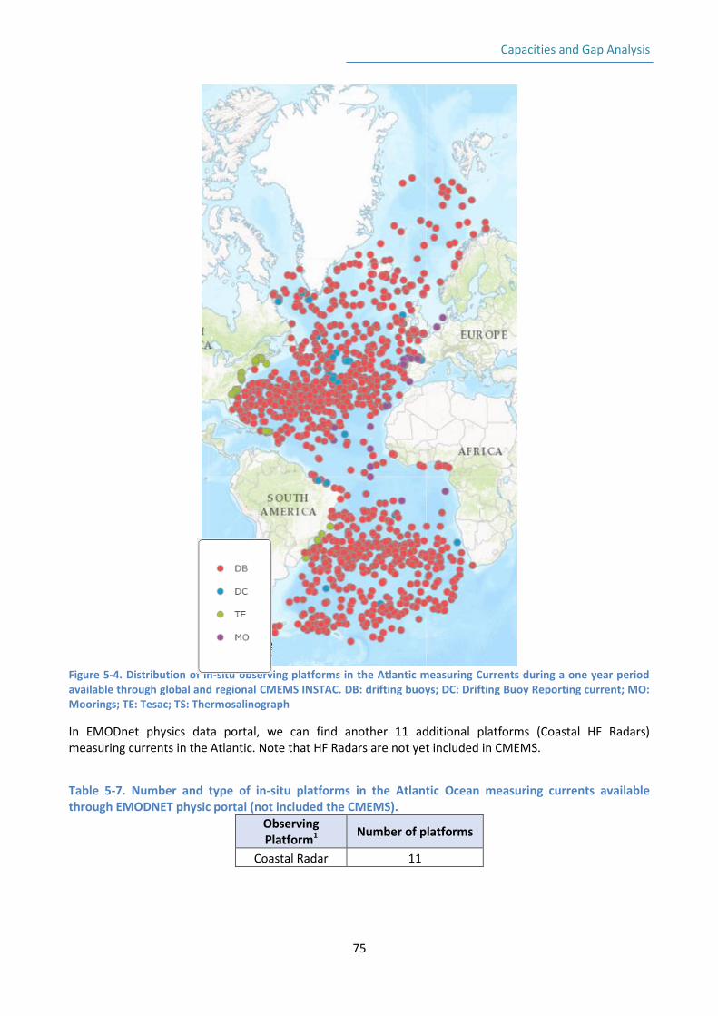
Capacities and Gap Analysis
75
Figure 5-4. Distribution of in-situ observing platforms in the Atlantic measuring Currents during a one year period available through global and regional CMEMS INSTAC. DB: drifting buoys; DC: Drifting Buoy Reporting current; MO: Moorings; TE: Tesac; TS: Thermosalinograph
In EMODnet physics data portal, we can find another 11 additional platforms (Coastal HF Radars) measuring currents in the Atlantic. Note that HF Radars are not yet included in CMEMS.
Table 5-7. Number and type of in-situ platforms in the Atlantic Ocean measuring currents available through EMODNET physic portal (not included the CMEMS).
Observing Platform1
Number of platforms
Coastal Radar 11
Capacities and Gap Analysis
76
In SeaDataNet data portal archive there are a total of 8231 data records for ocean currents (510 totally unrestricted) archived for years 1881 to 2014. 118 entries for year 2014 (only in Canary Islands and Gulf of Biscay). Waves There was a total of 284 in-situ observing platforms measuring waves during the last year period in AtlantOS region coming from regional and global CMEMS INSTACs. Most of the observations comes from moorings (194 stations). Table 5-8. Number and type of in-situ platforms in the Atlantic Ocean measuring Waves available through global and regional CMEMS INSTAC.
Observing Platform1
Number of observations
MO 194
DB 86
TE 4
Total 284 1 MO: Moorings; DB: drifting buoys’: TE: Tesac.
In the following map we can see the distribution of in-situ platforms measuring waves which are available in CMEMS INSTAC for the last year.
Capacities and Gap Analysis
77
Figure 5-5. Distribution of in-situ observing platforms in the Atlantic measuring Waves during a one year period available through global and regional CMEMS INSTAC. MO: Moorings; DB: drifting buoys’; TE: Tesac
In EMODnet physics data portal, we can find another 87 additional platforms measuring waves, coming from US NDBC and MESA (Monitoring for Environment & Security in Africa) networks as can be seen in table below. Table 5-9. Number and type of in-situ platforms in the Atlantic Ocean measuring waves available through EMODNET physic portal (not included the CMEMS).
Observing Platform1
US NDBC MESA (Monitoring for Environment & Security in Africa)
Total
MO 86 1 87
Total 86 1 87
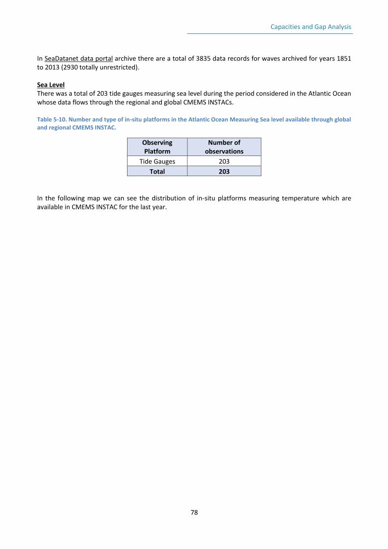
Capacities and Gap Analysis
78
In SeaDatanet data portal archive there are a total of 3835 data records for waves archived for years 1851 to 2013 (2930 totally unrestricted). Sea Level There was a total of 203 tide gauges measuring sea level during the period considered in the Atlantic Ocean whose data flows through the regional and global CMEMS INSTACs. Table 5-10. Number and type of in-situ platforms in the Atlantic Ocean Measuring Sea level available through global and regional CMEMS INSTAC.
Observing Platform
Number of observations
Tide Gauges 203
Total 203
In the following map we can see the distribution of in-situ platforms measuring temperature which are available in CMEMS INSTAC for the last year.
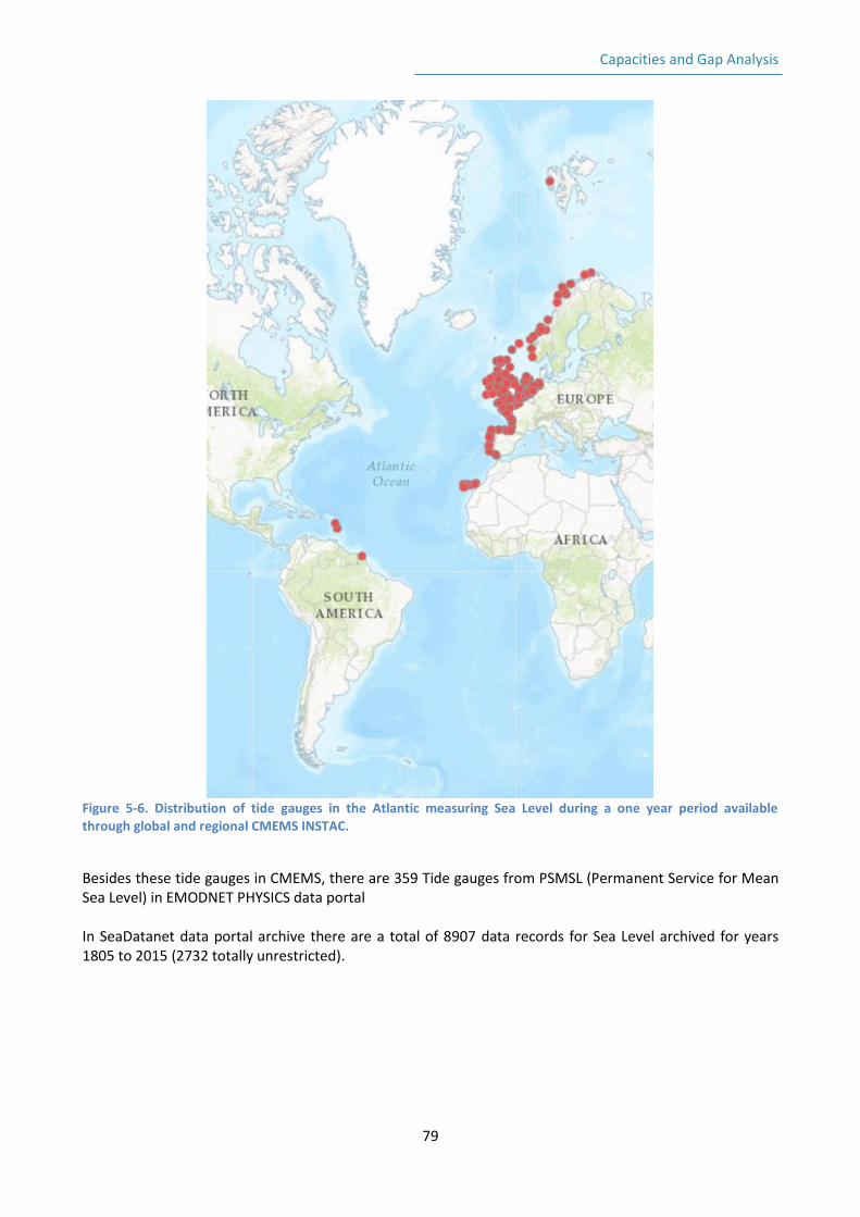
Capacities and Gap Analysis
79
Figure 5-6. Distribution of tide gauges in the Atlantic measuring Sea Level during a one year period available through global and regional CMEMS INSTAC.
Besides these tide gauges in CMEMS, there are 359 Tide gauges from PSMSL (Permanent Service for Mean Sea Level) in EMODNET PHYSICS data portal In SeaDatanet data portal archive there are a total of 8907 data records for Sea Level archived for years 1805 to 2015 (2732 totally unrestricted).
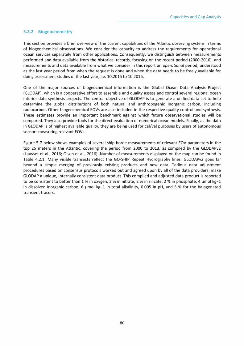
Capacities and Gap Analysis
80
5.2.2 Biogeochemistry This section provides a brief overview of the current capabilities of the Atlantic observing system in terms of biogeochemical observations. We consider the capacity to address the requirements for operational ocean services separately from other applications. Consequently, we distinguish between measurements performed and data available from the historical records, focusing on the recent period (2000-2016), and measurements and data available from what we consider in this report an operational period, understood as the last year period from when the request is done and when the data needs to be freely available for doing assessment studies of the last year, i.e. 10.2015 to 10.2016. One of the major sources of biogeochemical information is the Global Ocean Data Analysis Project (GLODAP), which is a cooperative effort to assemble and quality assess and control several regional ocean interior data synthesis projects. The central objective of GLODAP is to generate a unified data set to help determine the global distributions of both natural and anthropogenic inorganic carbon, including radiocarbon. Other biogeochemical EOVs are also included in the respective quality control and synthesis. These estimates provide an important benchmark against which future observational studies will be compared. They also provide tools for the direct evaluation of numerical ocean models. Finally, as the data in GLODAP is of highest available quality, they are being used for cal/val purposes by users of autonomous sensors measuring relevant EOVs. Figure 5-7 below shows examples of several ship-borne measurements of relevant EOV parameters in the top 25 meters in the Atlantic, covering the period from 2000 to 2013, as compiled by the GLODAPv2 (Lauvset et al., 2016; Olsen et al., 2016). Number of measurements displayed on the map can be found in Table 4.2.1. Many visible transects reflect the GO-SHIP Repeat Hydrography lines. GLODAPv2 goes far beyond a simple merging of previously existing products and new data. Tedious data adjustment procedures based on consensus protocols worked out and agreed upon by all of the data providers, make GLODAP a unique, internally consistent data product. This compiled and adjusted data product is reported to be consistent to better than 1 % in oxygen, 2 % in nitrate, 2 % in silicate, 2 % in phosphate, 4 µmol kg−1 in dissolved inorganic carbon, 6 µmol kg−1 in total alkalinity, 0.005 in pH, and 5 % for the halogenated transient tracers.
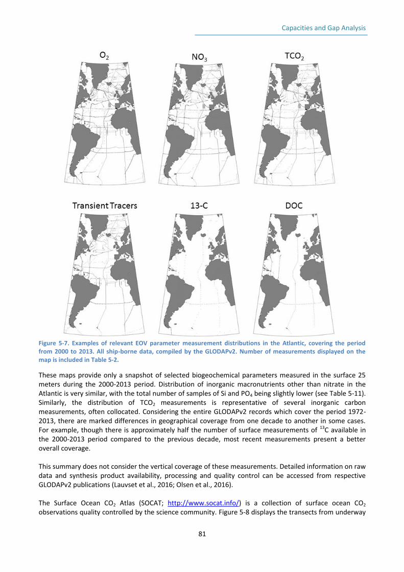
Capacities and Gap Analysis
81
Figure 5-7. Examples of relevant EOV parameter measurement distributions in the Atlantic, covering the period from 2000 to 2013. All ship-borne data, compiled by the GLODAPv2. Number of measurements displayed on the map is included in Table 5-2.
These maps provide only a snapshot of selected biogeochemical parameters measured in the surface 25 meters during the 2000-2013 period. Distribution of inorganic macronutrients other than nitrate in the Atlantic is very similar, with the total number of samples of Si and PO4 being slightly lower (see Table 5-11). Similarly, the distribution of TCO2 measurements is representative of several inorganic carbon measurements, often collocated. Considering the entire GLODAPv2 records which cover the period 1972-2013, there are marked differences in geographical coverage from one decade to another in some cases. For example, though there is approximately half the number of surface measurements of 13C available in the 2000-2013 period compared to the previous decade, most recent measurements present a better overall coverage. This summary does not consider the vertical coverage of these measurements. Detailed information on raw data and synthesis product availability, processing and quality control can be accessed from respective GLODAPv2 publications (Lauvset et al., 2016; Olsen et al., 2016). The Surface Ocean CO2 Atlas (SOCAT; http://www.socat.info/) is a collection of surface ocean CO2 observations quality controlled by the science community. Figure 5-8 displays the transects from underway
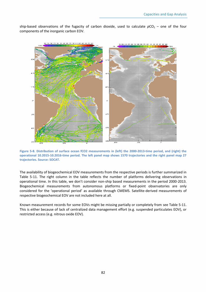
Capacities and Gap Analysis
82
ship-based observations of the fugacity of carbon dioxide, used to calculate pCO2 – one of the four components of the inorganic carbon EOV.
Figure 5-8. Distribution of surface ocean fCO2 measurements in (left) the 2000-2013-time period, and (right) the operational 10.2015-10.2016-time period. The left panel map shows 1570 trajectories and the right panel map 27 trajectories. Source: SOCAT.
The availability of biogeochemical EOV measurements from the respective periods is further summarized in Table 5-11. The right column in the table reflects the number of platforms delivering observations in operational time. In this table, we don’t consider non-ship based measurements in the period 2000-2013. Biogeochemical measurements from autonomous platforms or fixed-point observatories are only considered for the ‘operational period’ as available through CMEMS. Satellite-derived measurements of respective biogeochemical EOV are not included here at all. Known measurement records for some EOVs might be missing partially or completely from see Table 5-11. This is either because of lack of centralized data management effort (e.g. suspended particulates EOV), or restricted access (e.g. nitrous oxide EOV).
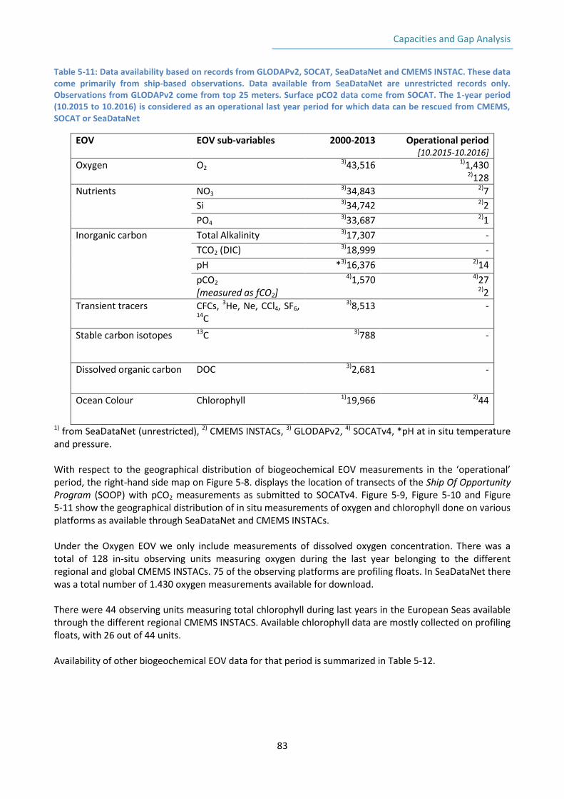
Capacities and Gap Analysis
83
Table 5-11: Data availability based on records from GLODAPv2, SOCAT, SeaDataNet and CMEMS INSTAC. These data come primarily from ship-based observations. Data available from SeaDataNet are unrestricted records only. Observations from GLODAPv2 come from top 25 meters. Surface pCO2 data come from SOCAT. The 1-year period (10.2015 to 10.2016) is considered as an operational last year period for which data can be rescued from CMEMS, SOCAT or SeaDataNet
EOV EOV sub-variables 2000-2013 Operational period [10.2015-10.2016]
Oxygen O2 3)43,516 1)1,430
2)128
Nutrients NO3 3)34,843 2)7
Si 3)34,742 2)2
PO4 3)33,687 2)1
Inorganic carbon Total Alkalinity 3)17,307 -
TCO2 (DIC) 3)18,999 -
pH *3)16,376 2)14
pCO2 [measured as fCO2]
4)1,570 4)27 2)2
Transient tracers CFCs, 3He, Ne, CCl4, SF6, 14C
3)8,513 -
Stable carbon isotopes 13C 3)788 -
Dissolved organic carbon DOC 3)2,681 -
Ocean Colour Chlorophyll 1)19,966 2)44
1) from SeaDataNet (unrestricted), 2) CMEMS INSTACs, 3) GLODAPv2, 4) SOCATv4, *pH at in situ temperature and pressure. With respect to the geographical distribution of biogeochemical EOV measurements in the ‘operational’ period, the right-hand side map on Figure 5-8. displays the location of transects of the Ship Of Opportunity Program (SOOP) with pCO2 measurements as submitted to SOCATv4. Figure 5-9, Figure 5-10 and Figure 5-11 show the geographical distribution of in situ measurements of oxygen and chlorophyll done on various platforms as available through SeaDataNet and CMEMS INSTACs. Under the Oxygen EOV we only include measurements of dissolved oxygen concentration. There was a total of 128 in-situ observing units measuring oxygen during the last year belonging to the different regional and global CMEMS INSTACs. 75 of the observing platforms are profiling floats. In SeaDataNet there was a total number of 1.430 oxygen measurements available for download. There were 44 observing units measuring total chlorophyll during last years in the European Seas available through the different regional CMEMS INSTACS. Available chlorophyll data are mostly collected on profiling floats, with 26 out of 44 units. Availability of other biogeochemical EOV data for that period is summarized in Table 5-12.
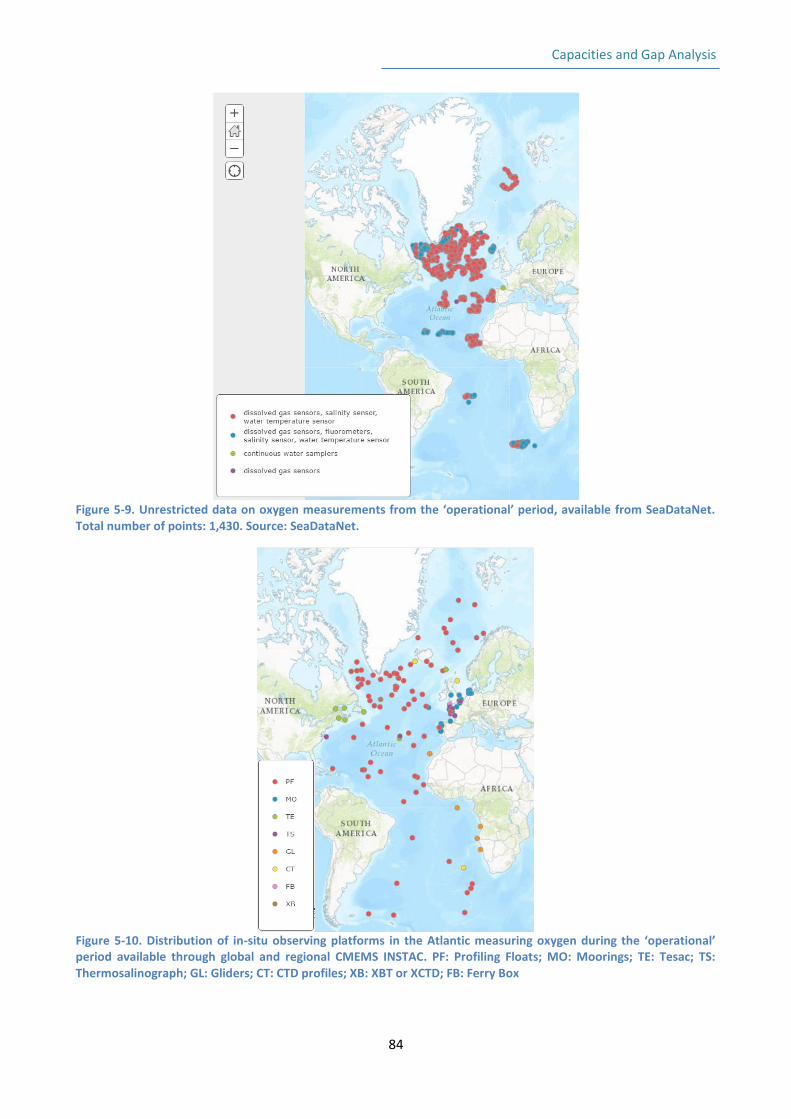
Capacities and Gap Analysis
84
Figure 5-9. Unrestricted data on oxygen measurements from the ‘operational’ period, available from SeaDataNet. Total number of points: 1,430. Source: SeaDataNet.
Figure 5-10. Distribution of in-situ observing platforms in the Atlantic measuring oxygen during the ‘operational’ period available through global and regional CMEMS INSTAC. PF: Profiling Floats; MO: Moorings; TE: Tesac; TS: Thermosalinograph; GL: Gliders; CT: CTD profiles; XB: XBT or XCTD; FB: Ferry Box
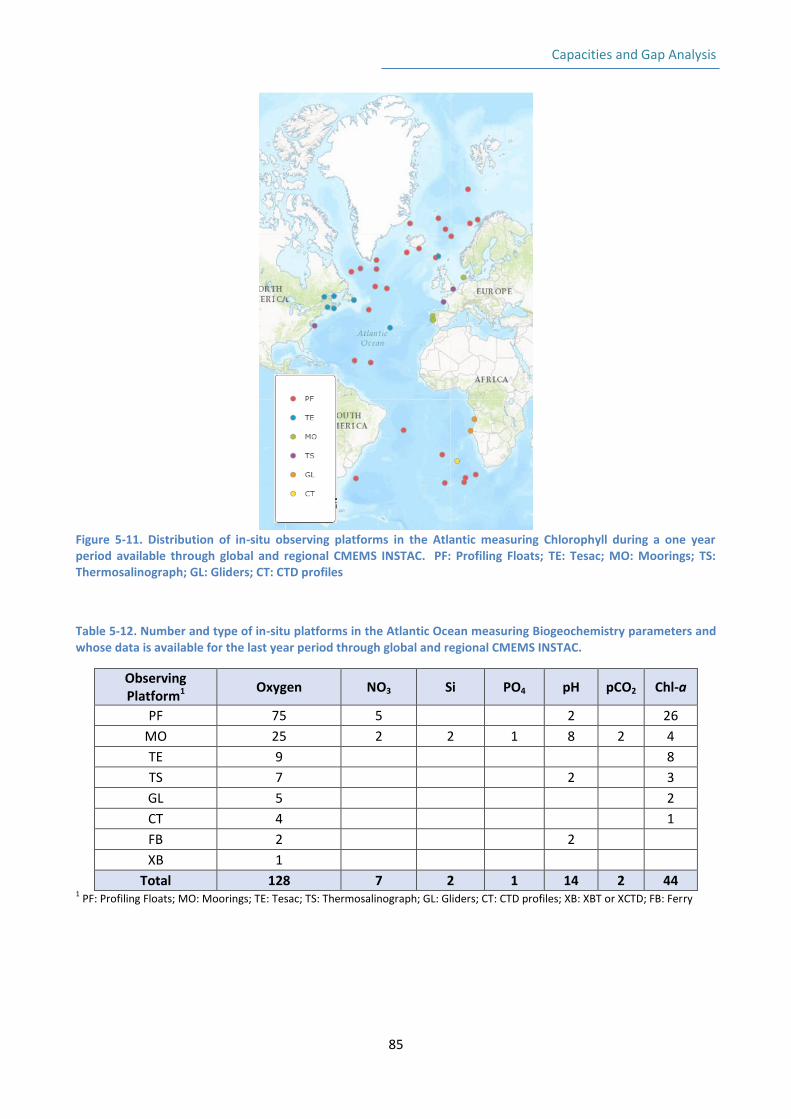
Capacities and Gap Analysis
85
Figure 5-11. Distribution of in-situ observing platforms in the Atlantic measuring Chlorophyll during a one year period available through global and regional CMEMS INSTAC.
PF: Profiling Floats; TE: Tesac; MO: Moorings; TS:
Thermosalinograph; GL: Gliders; CT: CTD profiles
Table 5-12. Number and type of in-situ platforms in the Atlantic Ocean measuring Biogeochemistry parameters and whose data is available for the last year period through global and regional CMEMS INSTAC.
Observing Platform1
Oxygen NO3 Si PO4 pH pCO2 Chl-a
PF 75 5 2 26
MO 25 2 2 1 8 2 4
TE 9 8
TS 7 2 3
GL 5 2
CT 4 1
FB 2 2
XB 1
Total 128 7 2 1 14 2 44 1 PF: Profiling Floats; MO: Moorings; TE: Tesac; TS: Thermosalinograph; GL: Gliders; CT: CTD profiles; XB: XBT or XCTD; FB: Ferry
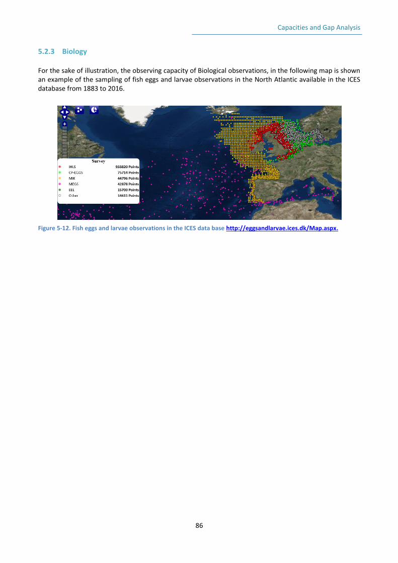
Capacities and Gap Analysis
86
5.2.3 Biology For the sake of illustration, the observing capacity of Biological observations, in the following map is shown an example of the sampling of fish eggs and larvae observations in the North Atlantic available in the ICES database from 1883 to 2016.
Figure 5-12. Fish eggs and larvae observations in the ICES data base http://eggsandlarvae.ices.dk/Map.aspx.
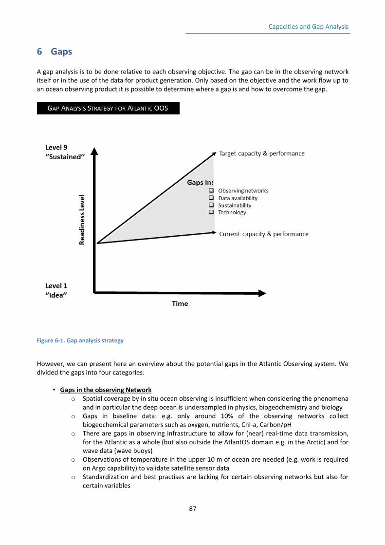
Capacities and Gap Analysis
87
6 Gaps
A gap analysis is to be done relative to each observing objective. The gap can be in the observing network itself or in the use of the data for product generation. Only based on the objective and the work flow up to an ocean observing product it is possible to determine where a gap is and how to overcome the gap.
Figure 6-1. Gap analysis strategy
However, we can present here an overview about the potential gaps in the Atlantic Observing system. We divided the gaps into four categories:
• Gaps in the observing Network o Spatial coverage by in situ ocean observing is insufficient when considering the phenomena
and in particular the deep ocean is undersampled in physics, biogeochemistry and biology o Gaps in baseline data: e.g. only around 10% of the observing networks collect
biogeochemical parameters such as oxygen, nutrients, Chl-a, Carbon/pH o There are gaps in observing infrastructure to allow for (near) real-time data transmission,
for the Atlantic as a whole (but also outside the AtlantOS domain e.g. in the Arctic) and for wave data (wave buoys)
o Observations of temperature in the upper 10 m of ocean are needed (e.g. work is required on Argo capability) to validate satellite sensor data
o Standardization and best practises are lacking for certain observing networks but also for certain variables
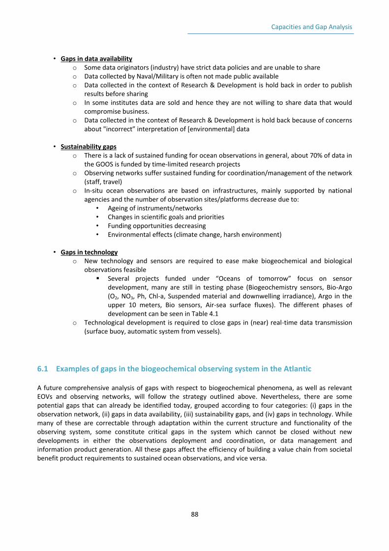
Capacities and Gap Analysis
88
• Gaps in data availability
o Some data originators (industry) have strict data policies and are unable to share o Data collected by Naval/Military is often not made public available o Data collected in the context of Research & Development is hold back in order to publish
results before sharing o In some institutes data are sold and hence they are not willing to share data that would
compromise business. o Data collected in the context of Research & Development is hold back because of concerns
about "incorrect” interpretation of [environmental] data
• Sustainability gaps o There is a lack of sustained funding for ocean observations in general, about 70% of data in
the GOOS is funded by time-limited research projects o Observing networks suffer sustained funding for coordination/management of the network
(staff, travel) o In-situ ocean observations are based on infrastructures, mainly supported by national
agencies and the number of observation sites/platforms decrease due to: • Ageing of instruments/networks • Changes in scientific goals and priorities • Funding opportunities decreasing • Environmental effects (climate change, harsh environment)
• Gaps in technology
o New technology and sensors are required to ease make biogeochemical and biological observations feasible
Several projects funded under “Oceans of tomorrow” focus on sensor development, many are still in testing phase (Biogeochemistry sensors, Bio-Argo (O2, NO3, Ph, Chl-a, Suspended material and downwelling irradiance), Argo in the upper 10 meters, Bio sensors, Air-sea surface fluxes). The different phases of development can be seen in Table 4.1
o Technological development is required to close gaps in (near) real-time data transmission (surface buoy, automatic system from vessels).
6.1 Examples of gaps in the biogeochemical observing system in the Atlantic A future comprehensive analysis of gaps with respect to biogeochemical phenomena, as well as relevant EOVs and observing networks, will follow the strategy outlined above. Nevertheless, there are some potential gaps that can already be identified today, grouped according to four categories: (i) gaps in the observation network, (ii) gaps in data availability, (iii) sustainability gaps, and (iv) gaps in technology. While many of these are correctable through adaptation within the current structure and functionality of the observing system, some constitute critical gaps in the system which cannot be closed without new developments in either the observations deployment and coordination, or data management and information product generation. All these gaps affect the efficiency of building a value chain from societal benefit product requirements to sustained ocean observations, and vice versa.
Capacities and Gap Analysis
89
(i) Gaps in the observation network Gaps in collocated physical, biogeochemical and biological measurements Collocation of physical, biogeochemical and biological measurements is an important sampling design requirement to understand and model complex oceanic phenomena that often operate across the three disciplines. While the availability of coincident physical measurements to study biogeochemical phenomena is high, the low % of biological measurements relative to biogeochemical parameters measured hinders correct interpretation of observed changes in the phenomena of interest. This is particularly true of biological rate measurements relevant to e.g. organic matter cycling and inorganic nutrient cycling.
Gaps in the geographical coverage of the in-situ ocean observing network There are areas of the Atlantic Ocean that are not sampled frequently enough, or are not sampled at all (see section 4.2 for selected maps of BGC EOVs and their sub-variables sampled). The significance of these gaps needs to be evaluated not only in the context of the quality of information products derived from current observations, but also in the context of whether measurements required for some societal benefit product generation are performed at all.
One approach to such evaluation of the current interior ocean observational network would be to use a gap-filling method (DIVA; Troupin et al., 2012; Beckers et al., 2014) and the observational network represented in the Global Ocean Data Analysis Project version 2 (GLODAPv2; Lauvset et al., 2016; Olsen et al., 2016) to estimate the error related to climatology data maps based on the current network of marine biogeochemistry observations. Maps of climatology are important information products which often meet the demands of basic phenomena-based targets, i.e. to establish a baseline signal for a given phenomenon. Figure 6-2 presents two examples of error maps associated with maps of climatology derived from GLODAPv2 data for oxygen and phosphate at 20m depth, expressed as error relative to the average error over the entire domain (60°S-78°N, 68°W-20°E), in percent. Data come from the 1972-2013 period.
Figure 6-2. Atlantic maps of the almost exact error from DIVA. Black dots indicate the positions of observations, colours indicate the error for all observations in GLODAPv2 (1972-2013). error = (error/avg_error)*100
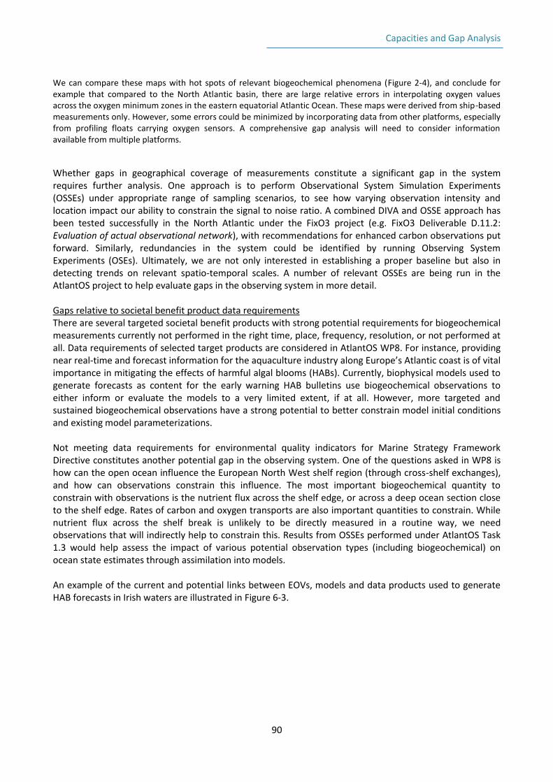
Capacities and Gap Analysis
90
We can compare these maps with hot spots of relevant biogeochemical phenomena (Figure 2-4), and conclude for example that compared to the North Atlantic basin, there are large relative errors in interpolating oxygen values across the oxygen minimum zones in the eastern equatorial Atlantic Ocean. These maps were derived from ship-based measurements only. However, some errors could be minimized by incorporating data from other platforms, especially from profiling floats carrying oxygen sensors. A comprehensive gap analysis will need to consider information available from multiple platforms.
Whether gaps in geographical coverage of measurements constitute a significant gap in the system requires further analysis. One approach is to perform Observational System Simulation Experiments (OSSEs) under appropriate range of sampling scenarios, to see how varying observation intensity and location impact our ability to constrain the signal to noise ratio. A combined DIVA and OSSE approach has been tested successfully in the North Atlantic under the FixO3 project (e.g. FixO3 Deliverable D.11.2: Evaluation of actual observational network), with recommendations for enhanced carbon observations put forward. Similarly, redundancies in the system could be identified by running Observing System Experiments (OSEs). Ultimately, we are not only interested in establishing a proper baseline but also in detecting trends on relevant spatio-temporal scales. A number of relevant OSSEs are being run in the AtlantOS project to help evaluate gaps in the observing system in more detail.
Gaps relative to societal benefit product data requirements There are several targeted societal benefit products with strong potential requirements for biogeochemical measurements currently not performed in the right time, place, frequency, resolution, or not performed at all. Data requirements of selected target products are considered in AtlantOS WP8. For instance, providing near real-time and forecast information for the aquaculture industry along Europe’s Atlantic coast is of vital importance in mitigating the effects of harmful algal blooms (HABs). Currently, biophysical models used to generate forecasts as content for the early warning HAB bulletins use biogeochemical observations to either inform or evaluate the models to a very limited extent, if at all. However, more targeted and sustained biogeochemical observations have a strong potential to better constrain model initial conditions and existing model parameterizations.
Not meeting data requirements for environmental quality indicators for Marine Strategy Framework Directive constitutes another potential gap in the observing system. One of the questions asked in WP8 is how can the open ocean influence the European North West shelf region (through cross-shelf exchanges), and how can observations constrain this influence. The most important biogeochemical quantity to constrain with observations is the nutrient flux across the shelf edge, or across a deep ocean section close to the shelf edge. Rates of carbon and oxygen transports are also important quantities to constrain. While nutrient flux across the shelf break is unlikely to be directly measured in a routine way, we need observations that will indirectly help to constrain this. Results from OSSEs performed under AtlantOS Task 1.3 would help assess the impact of various potential observation types (including biogeochemical) on ocean state estimates through assimilation into models.
An example of the current and potential links between EOVs, models and data products used to generate HAB forecasts in Irish waters are illustrated in Figure 6-3.
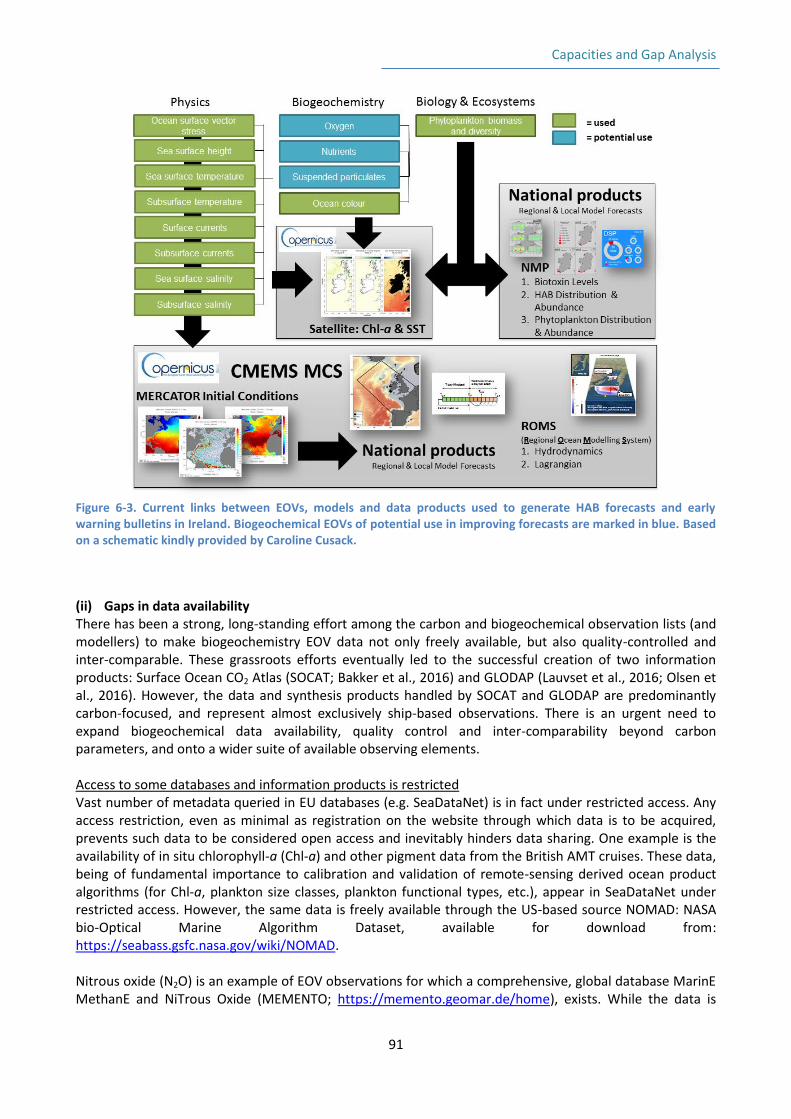
Capacities and Gap Analysis
91
Figure 6-3. Current links between EOVs, models and data products used to generate HAB forecasts and early warning bulletins in Ireland. Biogeochemical EOVs of potential use in improving forecasts are marked in blue. Based on a schematic kindly provided by Caroline Cusack.
(ii) Gaps in data availability There has been a strong, long-standing effort among the carbon and biogeochemical observation lists (and modellers) to make biogeochemistry EOV data not only freely available, but also quality-controlled and inter-comparable. These grassroots efforts eventually led to the successful creation of two information products: Surface Ocean CO2 Atlas (SOCAT; Bakker et al., 2016) and GLODAP (Lauvset et al., 2016; Olsen et al., 2016). However, the data and synthesis products handled by SOCAT and GLODAP are predominantly carbon-focused, and represent almost exclusively ship-based observations. There is an urgent need to expand biogeochemical data availability, quality control and inter-comparability beyond carbon parameters, and onto a wider suite of available observing elements. Access to some databases and information products is restricted Vast number of metadata queried in EU databases (e.g. SeaDataNet) is in fact under restricted access. Any access restriction, even as minimal as registration on the website through which data is to be acquired, prevents such data to be considered open access and inevitably hinders data sharing. One example is the availability of in situ chlorophyll-a (Chl-a) and other pigment data from the British AMT cruises. These data, being of fundamental importance to calibration and validation of remote-sensing derived ocean product algorithms (for Chl-a, plankton size classes, plankton functional types, etc.), appear in SeaDataNet under restricted access. However, the same data is freely available through the US-based source NOMAD: NASA bio-Optical Marine Algorithm Dataset, available for download from: https://seabass.gsfc.nasa.gov/wiki/NOMAD.
Nitrous oxide (N2O) is an example of EOV observations for which a comprehensive, global database MarinE MethanE and NiTrous Oxide (MEMENTO; https://memento.geomar.de/home), exists. While the data is
Capacities and Gap Analysis
92
freely usable, access to MEMENTO is restricted, granted upon request via email. Though this restriction could be considered ‘light’, it is responsible for a gap in the observing system from the perspective of open access to information products which directly answer one of the key biogeochemical scientific questions: ‘How does the ocean influence cycles of non-CO2 greenhouse gases?’.
(iii) Sustainability gaps The issue of gaps in the sustainability of biogeochemical observing system is a critical one. A recent issue related to the closing of Carbon Dioxide Information Analysis Center ocean trace gases section (CDIAC-Oceans) at the U.S. Department of Energy’s Oak Ridge National Laboratory, USA, illustrated the vulnerability of the system, and revealed a critical gap in the sustainability of data management. CDIAC-Oceans provided data management support for ocean carbon measurements from GO-SHIP repeat hydrography cruises, VOS/SOOP lines, time series and moorings data, had accommodated most community requests for data archival and data access and had also actively engaged with the science community, supporting large synthesis projects like SOCAT, the LDEO Database, GLODAP, CARINA, PACIFICA and GLODAPv2. During the transition from CDIAC to NOAA's National Centers for Environmental Information (NCEI)'s Ocean Carbon Data System (OCADS), data continues to be available to the community. However, there are challenges associated with meeting new metadata requirements, ensuring continuation of personnel support for data submission and archival process, and ensuring long-term commitments in maintaining thereof. Gaps in centralized data management The uncertainty of funding for CDIAC-Oceans highlighted the vulnerability of a system that relies too heavily on individual data managers or institutions. Under such circumstances, two flagship products for the biogeochemistry community, SOCAT and GLODAP, cannot be considered sustainable. IOCCP, leading the GOOS BGC Expert Panel, has issued a position statement on data management in which gaps in sustainable data management for global biogeochemical observations were pointed out. Since then, IOCCP has been working towards establishing a system of Global Data Assembly Centers (GDACs) for biogeochemistry data, which would effectively close the critical gap in the observing system. The entire statement can be accessed from here: http://www.ioccp.org/images/08dataANDinfo/IOCCP_position_paper_on_data_management_FINAL.pdf Gaps in quality control and inter-comparability A key recommendation from the AtlantOS WP1 workshop on “Setting Biogeochemical Targets for the Observing System in the Atlantic” held in Sopot, Poland in November 2016, is to set aside 30% of each of the observing networks’ budgets and devote it to making data quality-controlled and readily available to the community, and to developing protocols and user guides which would increase the quality and reproducibility of the results. It is recommended that observing networks should be supported in these efforts by relevant international projects and programs.
Gaps in usage of Certified Reference Materials (CRMs) Another aspect of data sustainability is its interoperability. Currently, there are still significant biases in measurements conducted between different groups of analysts. Inter-laboratory comparison experiments are important in addressing these gaps, as is the availability and common and routine usage of Certified Reference Materials (CRMs). For instance, SCOR-JAMSTEC CRMs for nutrients in seawater (available for purchase from http://www.jamstec.go.jp/scor/), have not been used sufficiently yet. While their use requires extra cost and effort, something not all analysts are willing to bear, their use is highly recommended especially in open ocean measurements where nutrient concentrations are low. Use of CRMs not being a standard operating procedure for members of observing networks could therefore be seen as a gap in the system, but a correctable one.
Capacities and Gap Analysis
93
(iv) Gaps in technology Major gaps in technology consider issues of insufficient accuracy and portability of biogeochemical sensors deployed on autonomous platforms. These gaps are currently addressed by several projects funded under “Oceans of Tomorrow.” Maturity level of instruments follow the step shown in Table 4.1.
Restricted usage of instruments and sensors due to their high cost is identified as another gap, specifically impacting measurements coverage in regions and periods not (readily) accessible by manned platforms. It should be noted that providing adequate training on sensors and instruments is at least as critical as making the technologies available in the first place.
6.2 Examples from existing gap identification
6.2.1 Climate A 2003 report from the Global Climate Observing System (GCOS) to the United Nations Framework Convention on Climate Change (UNFCCC)13 established the scientific requirements for systematic climate observations underlying the needs of the Parties to the UNFCCC and the Intergovernmental Panel on Climate Change (IPCC). The Conference of the Parties (COP) requested, in its decision 11/CP.9, that the Global Climate Observing System (GCOS) develop a 5- to 10-year implementation plan. The GCOS Implementation Plan14, published in 2004 and based on the concept of Essential Climate Variables identified by the Second Adequacy Report, consulted scientists and data users, took into account existing initiatives, included indicators for measuring its implementation, and identified implementation priorities and resource requirements. The ocean portions of this Implementation Plan were developed by the Ocean Observations Panel for Climate, on behalf of GCOS, the Global Ocean Observing System (GOOS) and the World Climate Research Programme (WCRP). The 2010 update of the Implementation Plan15 was prepared in response to a request by Parties to the UNFCCC expressed at the 30th session of the UNFCCC Subsidiary Body for Scientific and Technological Advice (SBSTA) and confirmed in UNFCCC Decision 9/CP.15. While there were minor changes in the ECVs (Table 6-1), the numerical targets associated with the networks were unchanged; a snapshot (Figure 6-4) shows that by June 2016, these targets had not been met in all cases. Both the 2004 and 2010 update of the GCOS Implementation Plan established numerical targets for the individual in situ observing networks that have broad geographic coverage, including:
Voluntary Observing Ship (VOS) marine meteorological observations,
The Data Buoy Cooperation Panel Global Drifter Programme,
the GLOSS tide gauge network,
Ship of Opportunity Programme XBT lines,
Argo profiling floats,
GO-SHIP repeat hydrography lines, and
OceanSITES time series stations.
13
The Second Report on the Adequacy of the Global Observing Systems for Climate in Support of the UNFCCC, GCOS-82, April 2003 (WMO/TD No. 1143). 14
Implementation Plan for the Global Observing System for Climate in Support of the UNFCCC - October, 2004 15
Implementation Plan for the Global Observing System for Climate in Support of the UNFCCC (2010 Update), August 2010
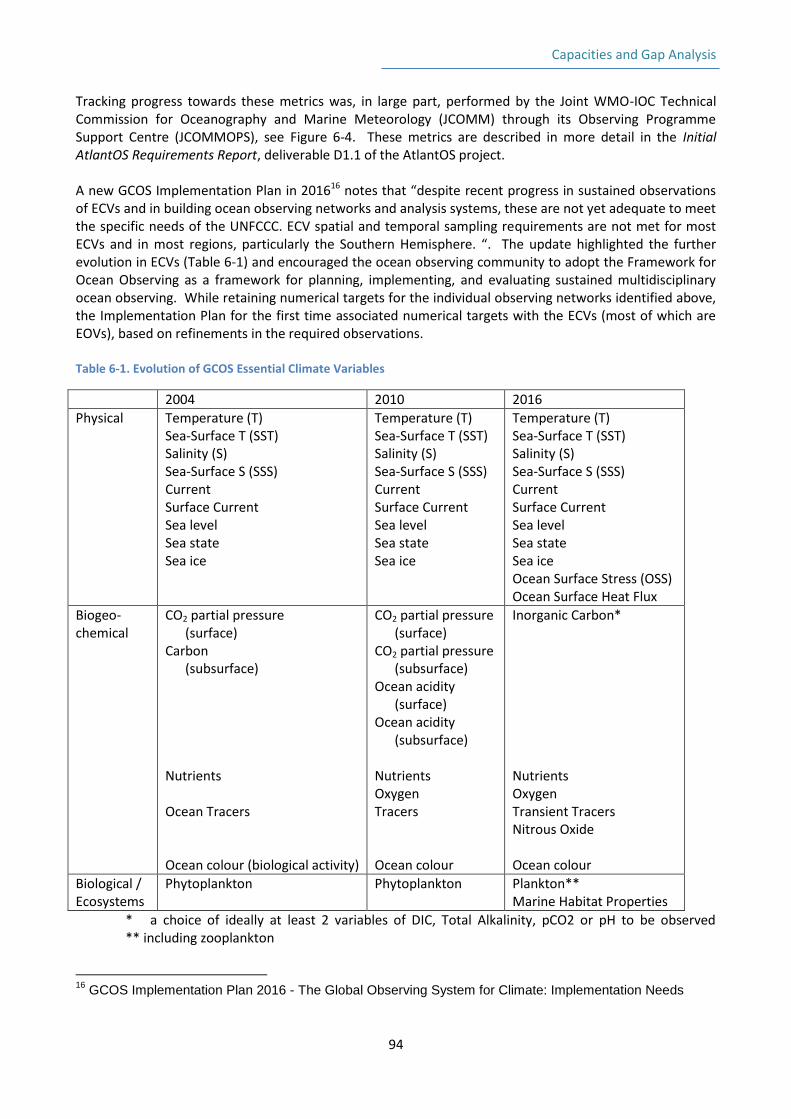
Capacities and Gap Analysis
94
Tracking progress towards these metrics was, in large part, performed by the Joint WMO-IOC Technical Commission for Oceanography and Marine Meteorology (JCOMM) through its Observing Programme Support Centre (JCOMMOPS), see Figure 6-4. These metrics are described in more detail in the Initial AtlantOS Requirements Report, deliverable D1.1 of the AtlantOS project. A new GCOS Implementation Plan in 201616 notes that “despite recent progress in sustained observations of ECVs and in building ocean observing networks and analysis systems, these are not yet adequate to meet the specific needs of the UNFCCC. ECV spatial and temporal sampling requirements are not met for most ECVs and in most regions, particularly the Southern Hemisphere. “. The update highlighted the further evolution in ECVs (Table 6-1) and encouraged the ocean observing community to adopt the Framework for Ocean Observing as a framework for planning, implementing, and evaluating sustained multidisciplinary ocean observing. While retaining numerical targets for the individual observing networks identified above, the Implementation Plan for the first time associated numerical targets with the ECVs (most of which are EOVs), based on refinements in the required observations. Table 6-1. Evolution of GCOS Essential Climate Variables
2004 2010 2016
Physical Temperature (T) Sea-Surface T (SST) Salinity (S) Sea-Surface S (SSS) Current Surface Current Sea level Sea state Sea ice
Temperature (T) Sea-Surface T (SST) Salinity (S) Sea-Surface S (SSS) Current Surface Current Sea level Sea state Sea ice
Temperature (T) Sea-Surface T (SST) Salinity (S) Sea-Surface S (SSS) Current Surface Current Sea level Sea state Sea ice Ocean Surface Stress (OSS) Ocean Surface Heat Flux
Biogeo- chemical
CO2 partial pressure (surface) Carbon (subsurface) Nutrients Ocean Tracers Ocean colour (biological activity)
CO2 partial pressure (surface) CO2 partial pressure (subsurface) Ocean acidity (surface) Ocean acidity (subsurface) Nutrients Oxygen Tracers Ocean colour
Inorganic Carbon* Nutrients Oxygen Transient Tracers Nitrous Oxide Ocean colour
Biological / Ecosystems
Phytoplankton Phytoplankton Plankton** Marine Habitat Properties
* a choice of ideally at least 2 variables of DIC, Total Alkalinity, pCO2 or pH to be observed ** including zooplankton
16
GCOS Implementation Plan 2016 - The Global Observing System for Climate: Implementation Needs
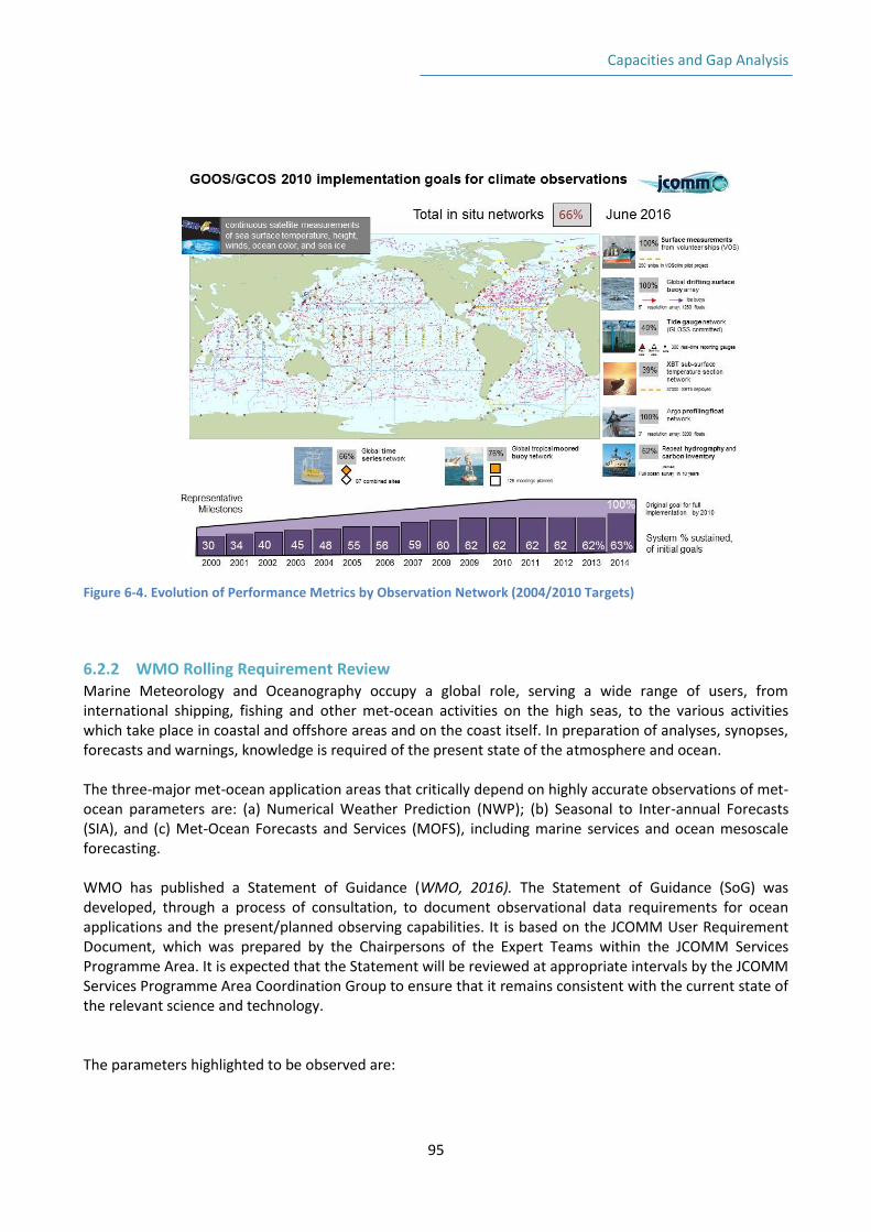
Capacities and Gap Analysis
95
Figure 6-4. Evolution of Performance Metrics by Observation Network (2004/2010 Targets)
6.2.2 WMO Rolling Requirement Review Marine Meteorology and Oceanography occupy a global role, serving a wide range of users, from international shipping, fishing and other met-ocean activities on the high seas, to the various activities which take place in coastal and offshore areas and on the coast itself. In preparation of analyses, synopses, forecasts and warnings, knowledge is required of the present state of the atmosphere and ocean. The three-major met-ocean application areas that critically depend on highly accurate observations of met-ocean parameters are: (a) Numerical Weather Prediction (NWP); (b) Seasonal to Inter-annual Forecasts (SIA), and (c) Met-Ocean Forecasts and Services (MOFS), including marine services and ocean mesoscale forecasting. WMO has published a Statement of Guidance (WMO, 2016). The Statement of Guidance (SoG) was developed, through a process of consultation, to document observational data requirements for ocean applications and the present/planned observing capabilities. It is based on the JCOMM User Requirement Document, which was prepared by the Chairpersons of the Expert Teams within the JCOMM Services Programme Area. It is expected that the Statement will be reviewed at appropriate intervals by the JCOMM Services Programme Area Coordination Group to ensure that it remains consistent with the current state of the relevant science and technology. The parameters highlighted to be observed are:
Capacities and Gap Analysis
96
Wind-Wave parameters (significant wave height, dominant wave period, Wave 1D energy frequency spectrum, and Wave direction energy frequency spectrum)
Sea level
Surface height anomalies (SSHA or Sea Level Anomalies)
Sea-Ice parameters (Thickness, Coverage/Concentration, Type/form, movements)
Sea Surface Temperature (SST)
Sea Surface Salinity (SSS)
Subsurface temperature, salinity and density
Ocean Chlorophyll, nitrate, silicate and phosphate concentrations
3-D ocean currents
Bathymetry, Coastal Topography and Shorelines
Surface Wind Vector over ocean and coastal areas
Surface heat flux over the ocean
Visibility
The SoG documents gives a detailed argumentation for each parameter as well as some guidance on how to get observations. The document end with the following summary:
A large part of marine and ocean observing systems is currently maintained by research funding with limited duration. This has the potential of leaving observational gaps unless ongoing funding for sustained observing networks is guaranteed. The ocean observing community should therefore ensure sustained funding for the key observing systems (e.g. tropical moorings, Argo, surface drifters with barometers, as well as altimeter, scatterometer, microwave SST and sea ice measurements from satellite missions);
The uneven geographical coverage of the in-situ ocean observing network is also an ongoing issue for ocean applications. Considering the regional variability in requirements as well as to ensure optimized planning for observing networks with limited resources, geographical variability in spatial/temporal resolution for ocean observations should be emphasised;
Ocean observing communities should also improve geographical coverage of ocean observing systems, particularly for measuring SST, SSHA, SSS and visibility, along with higher resolution geometry and extend open-ocean and coastal wind-wave observing networks (e.g. 400 time-series reporting in open ocean), possibly developing other existing observing sites (e.g. global sea level and tsunami monitoring network) into multi-purpose stations;
The critical met-ocean variables that are not adequately measured (more accurate and frequent observations and better spatial/temporal resolution are required) by current or planned systems are:
Sea surface height anomaly - noting the high impact of this observation on ocean forecasting systems to derive both the ocean state and circulation of the upper ocean, supporting a large number of applications, it is recommended that the observing system capabilities be given high priority and that a minimum service level target be agreed and sustained;
Wave parameters (significant wave height, dominant wave period, Wave 1-D and wave directional energy frequency spectrum) - noting that extreme wave and wind gusts events significantly constrain shipping and other marine operations, it is recommended to collocate of wind and wave sensors;
Sea level – noting the wide range of requirements for sea level data (from early detection of tsunamis to long-term trends of sea level rise), the requirements for this variable should be carefully addressed;
Capacities and Gap Analysis
97
Surface pressure – noting that sea-surface pressure data from drifting and moored buoys are still limited, particularly in tropical regions where these data are vital to detect and monitor atmospheric phenomena over the oceans (e.g. tropical cyclones) that significantly constrain shipping, it is recommended to install of barometers on all deployed drifters (1250);
Visibility – noting that visibility data are critical for operations and as these are still very limited, the NMHSs are encouraged to measure visibility.
It is therefore recommended that ocean observing communities should
ensure that state-of-art technologies are employed to improve accuracy for all measurements;
extend collaboration among themselves at national/regional levels to enhance wave measurement networks (e.g. moored buoy networks) for validation and evaluation; and
develop visibility measurement capability over the ocean (consultation needed with JCOMM experts on how to practically achieve this).
Satellite data are the only means for providing high-resolution data in key ocean areas where in situ observations are sparse or absent. In general, in situ metocean data and observations are poor for marine services (in particular, for monitoring and warning marine-related hazards) and marginal for assimilation into ocean models, including wave models. There is a need for satellite operators to ensure (i) a combination of both infrared and microwave measurements for better coverage of SST observations; (ii) improved observations in coastal regions (altimetry, SST); (iii) a minimum of two interleaved operational satellites providing SSHA observations to support ocean forecasting applications, and (iv) the development satellite measurements of SSS on an operational basis.
Capacities and Gap Analysis
98
7 Summary and conclusions The design of an optimal observing program for an ocean area – in this case the Atlantic Ocean - includes several logical steps summarized in the Framework for Ocean Observing:
1. Define the Requirements – societal demands for information to address specific questions. 2. Identify the Phenomena associated with the observing objectives that are linked to requirements 3. Identify the Essential Ocean Variables (EOV’s) associated with the observing objectives 4. Use the existing observing infrastructure for data acquisition of the respective set of phenomena
and EOVs 5. Use data to derive information that addresses specific question (point 1) which will provide a
measure for the capacity of present observation system 6. If information cannot be derived perform a Gap analysis (data acquisition, product generation) 7. Ensure a “Fit for Purpose” system, enhanced and optimized observation system
The initial definition of requirements for an Atlantic Ocean Observation System was reported in “Initial AtlantOS Requirement Report”, AtlantOS Deliverable 1.1 (update will be done by the end of the project). The present report focusses on points 2 – 6, while point 7 will be the final outcome the AtlantOS project. It has been decided in the work of AtlantOS design of an Atlantic Ocean Observation System to take basis in the three broad societal benefit areas identified by GOOS/GCOS: operational ocean services, climate and ocean health. Relevant physical, biogeochemical and biological phenomena, EOV’s and observation technology are presented, followed by a presentation of existing observing capacity based on publicly available data. This document outlines the strategy for performing a comprehensive capacity and gap analysis of the ocean observing value chain, in the context of an integrated Atlantic Ocean observing system (Figure 1-1). A critical part of the value chain is presented in this report – namely the Phenomena, the EOV, the observing networks, and capabilities and gaps. Based on the work carried in preparing this report the following “lessons learned” and conclusions can be drawn:
There are different levels of “maturity” in defining and understanding phenomenon’s and EOV’s within physics, biogeochemistry and biology, which impacts the establishment of solid requirements and subsequently the gap analysis. This problem is addressed by leading international expert groups under IOC or GOOS Panels as well as in the context of AtlantOS where a biogeochemical expert meeting was organised in Sopot, Poland in the autumn of 2016, and a biology expert meeting is planned for late summer 2017.
Analysing the existing observing capacity for several EOV’s in the Atlantic Ocean can not be done without considering the respective observing objective. However, “baseline” information is first required before an optimization can be performed. In respect to baseline information we conclude that:
o Basic physical parameters such a s temperature and salinity are relatively well observed in most parts of the Atlantic Ocean although areas of low density of observations can be identified
o When it comes to other EOV’s – physical, biogeochemical and biological – geographical gaps are much more evident
o It shall be stressed that the examples of observing capacity given in this report is reflecting which data is publicly available at databases such as CMEMS INSTAC, EMODnet, SeaDataNet, ICES and data synthesis projects such as SOCAT and GLODAP; which unfortunately do not include all data available for the Atlantic Ocean. Additionally, it is well-known that a substantial amount of data is not, for various reason, made public
Capacities and Gap Analysis
99
available by the data originators. This data is seen as lost data in the framework of a sustained Atlantic Ocean observing system.
The report provides examples of “generic” gaps identified in the system (e.g. missing baseline data). A detailed gap analysis would rely on detailed requirements for an Atlantic Ocean Observing System to be established with clear definitions of spatial and temporal resolution, and quality requirements etc., and this is not possible before some of the “maturity” issues mentioned above are addressed properly. In fact, the ocean observing value chain that is executed in its full through the AtlantOS should ultimately be reflected in its data provision for user needs via e.g. in Copernicus Marine Environment Monitoring Service. Within AtlantOS WP8 task 8.1 to task 8.7 will execute the value chain focussing on specific requirements (HABs, fisheries…). A refined set of requirements are planned for the “Refined AtlantOS Requirement Report” (Deliverable 1.7) due in month 45 (December 2018). Additionally, a comprehensive overview of accessible data will be created along the progressing of the project. The work that is done in WP2 and WP3 and in conjunction with WP7 will ensure that the data throughput from the observing networks increases. This is a measurable outcome that is beyond the scope of this study and also beyond the capabilities of WP1.
It has on this background been suggested to concentrate a future gap analysis around four subjects:
o Gaps in the observing networks o Gaps in data availability o Gaps in sustainability o Gaps in technology
Constant monitoring of ocean observing capacity and gaps is a core activity in order to ensure an optimized, and thus cost efficient, sustained observing system. In this respect, sustained ocean observing is different from ocean observing for fundamental research performed for a defined period only. However, both, the sustained ocean observing system and the observing efforts in the context of fundamental research, shall benefit from each other. The most obvious link is via data exchange - while observing in the sustained system must by definition provide open-access data, the fundamental researchers should make sure that their data is also open-access to integrate this data in the ocean observing value chain. Discussions on observing capacity and gap analysis currently take place in many groups and the AtlantOS group will follow closely the outcomes of activities related to requirement definition, capacity and gap analysis performed by other groups in Europe – such as Copernicus and EMODnet – and non-European countries surrounding the Atlantic Ocean.
Capacities and Gap Analysis
100
8 References Abraham, J. P., Baringer, M., Bindoff, N. L., Boyer, T., Cheng, L. J., Church, J. A., … S. A. Good, 11 J. M.
Gorman, 1 V. Gouretski, 12 M. Ishii, 13 G. C. Johnson, 14 S. Kizu, 15 J. M. Lyman, 14, 16 A. M. Macdonald, 17 W. J.Minkowycz, 18 S. E. Moffitt, 19, 20 M. D. Palmer, 11 A. R. Piola, 21 F. Reseghetti, 22 K. Schuckmann, 23 K. E. Trenbert, 25 and J. K.Willis2. (2013). A review of global ocean temperature observations: Implications for ocean heat content estimates and climate change. Reviews of Geophysics, 51, 450–483. http://doi.org/10.1002/rog.20022.1.INTRODUCTION
Bates, N. R., Pequignet, a C., Johnson, R. J., & Gruber, N. (2002). A short-term sink for atmospheric CO2 in subtropical mode water of the North Atlantic Ocean. Nature, 420(6915), 489–93. http://doi.org/10.1038/nature01253
Beckers, J.-M., Barth, A., Troupin, C., & Alvera-Azcárate, A. (2014). Approximate and efficient methods to assess error fields in spatial gridding with data interpolating variational analysis (DIVA). Journal of Atmospheric and Oceanic Technology, 31, 515-530.
Bolin, B., Rhode, H., 1973. A note on the concepts of age distribution and transit time in natural reservoirs. Tellus 25, 58–62
Borum, J., CM Duarte, D Krause-Jensen and TM Greve., 2004. European seagrasses: an introduction to monitoring and management. A publication by the EU project Monitoring and Managing of European Seagrasses (M&MS) EVK3-CT-2000-00044 Project report ISBN: 87-89143-21-3
Bullister, J. L., Wisegarver, D. P., & Menzia, F. A. (2002). The solubility of sulfur hexafluoride in water and seawater. Deep Sea Research Part I: Oceanographic Research Papers, 49, 175-187.
Bullister, J. L. (2015). Atmospheric Histories (1765-2015) for CFC-11, CFC-12, CFC-113, CCl4, SF6 and N2O. Carbon Dioxide Information Analysis Center, Oak Ridge National Laboratories, US Department of Energy, Oak Ridge, TN. Retrieved from: http://cdiac.ornl.gov/oceans/CFC_ATM_Hist2015.html
Burgess, R. M., Lohmann, R., Schubauer-Berigan, J. P., Reitsma, P., Perron, M. M., Lefkovitz, L., & Cantwell, M. G. (2015). Application of passive sampling for measuring dissolved concentrations of organic contaminants in the water column at three marine superfund sites. Environmental Toxicology and Chemistry, 34, 1720-1733.
Byrne, R. H., Mecking, S., Feely, R. A., & Liu, X. (2010). Direct observations of basin-wide acidification of the North Pacific Ocean. Geophysical Research Letters, 37(2).
Carlson, C. A., & Hansell, D. A. (2014). DOM sources, sinks, reactivity, and budgets. In: Biogeochemistry of Marine Dissolved Organic Matter: Second Edition, pp. 65-126, Elsevier Inc. DOI: 10.1016/B978-0-12-405940-5.00003-0
Church, J.A., Godfrey, J.S., Jackett, D.R., McDougall, T.J., 1991. A model of sea level rise caused by ocean thermal expansion. J. Climate 4, 438–456.
Cossa, D., Averty, B., & Pirrone, N. (2009). The origin of methylmercury in open Mediterranean waters. Limnology and Oceanography, 54(3), 837-844.
Curry, R., & Mauritzen, C. (2005). Dilution of the northern North Atlantic Ocean in recent decades. Science (New York, N.Y.), 308(5729), 1772–1774. http://doi.org/10.1126/science.1109477
Devol, A. H. (2003). Nitrogen cycle: solution to a marine mystery. Nature, 422, 575-576, doi:10.1038/422575a
Dickson, B., Yashayaev, I., Meincke, J., Turrell, B., Dye, S., & Holfort, J. (2002). Rapid freshening of the deep North Atlantic Ocean over the past four decades. Nature, 416(6883), 832–837. doi:10.1038/416832a
Doney, S. C. (2010). The growing human footprint on coastal and open-ocean biogeochemistry. science, 328, 1512-1516.
European Commission (1992). Council Directive 92/43/EEC of 21 May 1992 on the conservation of natural habitats and of wild fauna and flora. Official Journal L 206 , 22/07/1992 P. 0007 – 0050
European Commission (2000). Directive 2000/60/ EC of the European Parliament and of the Council of 23 October 2000 establishing a framework for Community action in the field of water policy. Official Journal of the European Communities L 327/1 22.12.2000.
Capacities and Gap Analysis
101
European Commission (2008a). Directive 2008/56/EC of the European Parliament and of the Council of 17 June 2008 establishing a framework for community action in the field of marine environment policy (Marine Strategy Framework Directive). Official Journal of the European Union, 164: 19–40; 25.6.2008 L.
European Commission (2008b). Commission Regulation No 665/2008 of 14 July 2008 laying down detailed rules for the application of Council Regulation (EC) No 199/2008 concerning the establishment of a Community framework for the collection, management and use of data in the fisheries sector and support for scientific advice regarding the Common Fisheries Policy. Official Journal of the European Union L 186/3 15.7.2008
European Commission (2009). Directive 2009/147/EC of the European Parliament and of the Council of 30 November 2009 on the conservation of wild birds. Official Journal of the European Union L 20/7 26.1.2010
European Commission (2010). Commission Decision of 1 September 2010 on criteria and methodological standards on good environmental status of marine waters. Official Journal of the European Union, 232: 14–24; 2.9.2010 L.
European Union (2013). Regulation (EU) no 1380/2013 of the European Parliament and of the Council of 11 December 2013 on the Common Fisheries Policy, amending Council Regulations (EC) No 1954/2003 and (EC) No 1224/2009 and repealing Council Regulations (EC) No 2371/2002 and (EC) No 639/2004 and Council Decision 2004/585/EC.
EMODNET biology Portal http://www.emodnet-biology.eu/ Foltz, G. R., & McPhaden, M. J. (2009). Impact of barrier layer thickness on SST in the central tropical North
Atlantic. Journal of Climate, 22(2), 285–299. http://doi.org/10.1175/2008JCLI2308.1 FAO vulnerable marine ecosystems http://www.fao.org/in-action/vulnerable-marine-ecosystems/en/ Fay, A. R., & McKinley, G. A. (2014). Global open-ocean biomes: mean and temporal variability. Earth
System Science Data, 6, 273-284. doi:10.5194/essd-6-273-2014 Gill, A. E., & Clarke, A. J. (1974). Wind-induced upwelling , coastal currents and sea-level changes,
21(October 1973), 325–345. Friis, K., Körtzinger, A., Pätsch, J., & Wallace, D. W. (2005). On the temporal increase of anthropogenic CO2
in the subpolar North Atlantic. Deep Sea Research Part I: Oceanographic Research Papers, 52, 681-698.
Fung, I. Y., Doney, S. C., Lindsay, K., & John, J. (2005). Evolution of carbon sinks in a changing climate. Proceedings of the National Academy of Sciences of the United States of America, 102, 11201-11206.
Gille, S. T. (2008). Decadal-scale temperature trends in the Southern Hemisphere ocean. Journal of Climate, 21, 4749-4765.
Gruber, N., Gloor, M., Fan, S.-M., & Sarmiento, J. L. (2001). Air-sea flux of oxygen estimated from bulk data: Implications for the marine and atmospheric oxygen cycles. Global Biogeochemical Cycles, 15, 783-803.
Gruber, N., Gloor, M., Fletcher, M. a., Doney, S. C., Dutkiewicz, S., Follows, M. J., et al. (2009). Oceanic sources, sinks, and transport of atmospheric CO2. Global Biogeochemical Cycles, 23.
Hansell, D. A., Carlson, C. A., & Schlitzer, R. (2012). Net removal of major marine dissolved organic carbon fractions in the subsurface ocean. Global Biogeochemical Cycles, 26 (1), doi:10.1029/2011GB004069
Hansell, D. A., Carlson, C. A., Repeta, D. J., & Schlitzer, R. (2009). Dissolved organic matter in the ocean: A controversy stimulates new insights, Oceanography 22 (4), doi:10.5670/oceanog.2009.109
Henson, S. A., Beaulieu, C., & Lampitt, R. (2016). Observing climate change trends in ocean biogeochemistry: when and where. Global Change Biology 22 (4), doi:10.1111/gcb.13152
ICES IOC. 2016. Interim Report of the ICES - IOC Working Group on Harmful Algal Bloom Dynamics (WGHABD), 19–22 April 2016, Brest, France. ICES CM 2016/SSGEPD:12. 57pp http://haedat.iode.org/
ICES. 2016. Report of the Joint ICES/NAFO Working Group on Deep-water Ecology (WGDEC), 15–19 February 2016, Copenhagen, Denmark. ICES CM 2016/ACOM:28. 82 pp.
IOC-UNESCO and UNEP (2016). Open Ocean: Status and Trends, Summary for Policy Makers. United Nations Environment Programme (UNEP), Nairobi.
Capacities and Gap Analysis
102
IOCCG (2011). Bio-Optical Sensors on Argo Floats. Claustre, H. (ed.), Reports of the International Ocean-Colour Coordinating Group, No. 11, IOCCG, Dartmouth, Canada.
Jiang, L.-Q., Feely, R. A., Carter, B. R., Greeley, D. J., Gledhill, D. K., & Arzayus, K. M. (2015). Climatological distribution of aragonite saturation state in the global oceans. Global Biogeochemical Cycles, 29, 1656-1673.
Jickells, T., & Moore, C. M. (2015). The importance of atmospheric deposition for ocean productivity. Annual Review of Ecology, Evolution, and Systematics, 46, 481-501.
Joos, F., Plattner, G.-K., Stocker, T. F., Körtzinger, A., & Wallace, D. W. (2003). Trends in marine dissolved oxygen: Implications for ocean circulation changes and the carbon budget. Eos, Transactions American Geophysical Union, 84, 197-201.
Karstensen, J., Fiedler, B., Schütte, F., Brandt, P., Körtzinger, a., Fischer, G., … Wallace, D. (2015). Open ocean dead zones in the tropical North Atlantic Ocean. Biogeosciences, 12, 2597–2605. http://doi.org/10.5194/bg-12-2597-2015
Karstensen, J., Stramma, L., & Visbeck, M. (2008). Oxygen minimum zones in the eastern tropical Atlantic and Pacific oceans. Prog. Oceanog., 77(4), 331–350. http://doi.org/10.1016/j.pocean.2007.05.009
Karstensen, J., & Tomczak, M. (1998). Age determination of mixed water masses using CFC and oxygen data. Journal of Geophysical Research: Oceans, 103(C9), 18,599-18,609. http://doi.org/10.1029/98JC00889
Keeling, R. F., & Garcia, H. E. (2002). The change in oceanic O2 inventory associated with recent global warming. Proceedings of the National Academy of Sciences, 99, 7848-7853.
Keeling, R. F., Körtzinger, A., & Gruber, N. (2010). Ocean deoxygenation in a warming world. Annual Review of Marine Science, 2, 199-229.
Khatiwala, S., Primeau, F., & Hall, T. (2009). Reconstruction of the history of anthropogenic CO2 concentrations in the ocean. Nature, 462, 346-349.
Khatiwala, S., Tanhua, T., Fletcher, S. M., Gerber, M., Doney, S. C., Graven, H. D., et al. (2013). Global ocean storage of anthropogenic carbon. Biogeosciences (BG), 10, 2169-2191.
Kushnir, Y. (1994). Interdecadal Variations in North Atlantic Sea Surface Temperature and Associated Atmospheric Conditions. Journal of Climate. http://doi.org/10.1175/1520-0442(1994)007<0141:IVINAS>2.0.CO;2
Lamb, K. G. (2014). Internal Wave Breaking and Dissipation Mechanisms on the Continental Slope/Shelf. Annual Review of Fluid Mechanics, 46(1), 231–254. http://doi.org/10.1146/annurev-fluid-011212-140701
Lamb, K.G., 2014. Internal Wave Breaking and Dissipation Mechanisms on the Continental Slope/Shelf. Annual Review of Fluid Mechanics 46, 231-254.
Lauvset, S. K., Key, R. M., & Perez, F. F. (2016). A new global interior ocean mapped climatology: the 1°× 1° GLODAP version 2. Earth System Science Data, 8, 325.
Le Quéré, C., Rödenbeck, C., Buitenhuis, E. T., Conway, T. J., Langenfelds, R., Gomez, A., et al. (2007). Saturation of the Southern Ocean CO2 sink due to recent climate change. Science, 316, 1735-1738.
Lévy, M., Klein, P., & Treguier, A.-M. (2001). Impact of sub-mesoscale physics on production and subduction of phytoplankton in an oligotrophic regime. Journal of Marine Research, 59(4), 535–565. http://doi.org/10.1357/002224001762842181
Liblik et al., Potential for an underwater glider component as part of the Global Ocean Observing System, Methods in Oceanography (2016), http://dx.doi.org/10.1016/j.mio.2016.05.001
Locarnini, R. A., Mishonov, A. V., Antonov, J. I., Boyer, T. P., Garcia, H. E., Baranova, O. K., Johnson, D. R. (2006). World Ocean Atlas 2005, Vol. 1: Temperature. NOAA Atlas NESDIS 61, edited by S Levitus. Washington, DC: US Government Print. Off.
Lorbacher, K., Dengg, J., B??ning, C. W., & Biastoch, A. (2010). Regional patterns of sea level change related to interannual variability and multidecadal trends in the Atlantic meridional overturning circulation. Journal of Climate, 23(15), 4243–4254. http://doi.org/10.1175/2010JCLI3341.1
Capacities and Gap Analysis
103
McCarthy, G. D., Smeed, D. A., Johns, W. E., Frajka-Williams, E., Moat, B. I., Rayner, D., . . . Bryden, H. L. (2015). Measuring the Atlantic meridional overturning circulation at 26°N. Progress in Oceanography, 130, 91-111.
McKinley, G. A., Follows, M. J., & Marshall, J. (2000). Interannual variability of the air-sea flux of oxygen in the North Atlantic. Geophysical research letters, 27, 2933-2936.
McWilliams, J. C. (2016). Submesoscale currents in the ocean. In Proceedings of the Royal Society A, Vol. 472 (2189), 20160117, doi: 10.1098/rspa.2016.0117.
Munk, W., & Wunsch, C. (1998). Abyssal recipes II: energetics of tidal and wind mixing. Deep-Sea Res., 45(I), 1977–2010.
Naegler, T., Ciais, P., Rodgers, K., & Levin, I. (2006). Excess radiocarbon constraints on air-sea gas exchange and the uptake of CO2 by the oceans. Geophysical Research Letters, 33.
Najjar, R. G., & Keeling, R. F. (2000). Mean annual cycle of the air-sea oxygen flux: A global view. Global biogeochemical cycles, 14, 573-584.
Olsen, A., R. M. Key, S. van Heuven, S. K. Lauvset, A. Velo, X. Lin, C. Schirnick, A. Kozyr, T. Tanhua, M. Hoppema, S. Jutterström, R. Steinfeldt, E. Jeansson, M. Ishii, F. F. Pérez and T. Suzuki (2016) An internally consistent data product for the world ocean: the Global Ocean Data Analysis Project, version 2 (GLODAPv2). Earth System Science. Data, 8: 297-323, doi:10.5194/essd-8-297-2016.
OSPAR (2016) Species and habitats http://www.ospar.org/work-areas/bdc/species-habitats Polzin, K. L., Toole, J. M., Ledwell, J. R., & Schmitt, R. W. (1997). Spatial Variability of Turbulent Mixing in the
Abyssal Ocean. Science, 276, 93–96. Purkey, S. G., & Johnson, G. C. (2010). Warming of global abyssal and deep Southern Ocean waters
between the 1990s and 2000s: Contributions to global heat and sea level rise budgets. Journal of Climate, 23(23), 6336–6351. http://doi.org/10.1175/2010JCLI3682.1
Report of the First Workshop of Technical Experts for the Global Ocean Observing System (GOOS) Biology and Ecosystems Panel: Identifying Ecosystem Essential Ocean Variables (EOVs)
Report of the First Workshop of Technical Experts for the Global Ocean Observing System (GOOS) Biology and Ecosystems Panel: Identifying Ecosystem Essential Ocean Variables (EOVs)
Reul, N., Tenerelli, J., Chapron, B., Vandemark, D., Quilfen, Y., & Kerr, Y. (2012). SMOS satellite L-band radiometer: A new capability for ocean surface remote sensing in hurricanes. Journal of Geophysical Research: Oceans, 117(2), 1–24. http://doi.org/10.1029/2011JC007474
Rouault, M., Illig, S., Bartholomae, C., Reason, C. J. C., & Bentamy, A. (2007). Propagation and origin of warm anomalies in the Angola Benguela upwelling system in 2001. Journal of Marine Systems, 68(3–4), 473–488. http://doi.org/10.1016/j.jmarsys.2006.11.010
Sabine, C. L., & Tanhua, T. (2010). Estimation of anthropogenic CO2 inventories in the ocean. Annual Review of Marine Science, 2, 175-198.
Sabine, C. L., Feely, R. A., Millero, F. J., Dickson, A. G., Langdon, C., Mecking, S., & Greeley, D. (2008). Decadal changes in Pacific carbon. Journal of Geophysical Research: Oceans, 113.
Salisbury, J., Vandemark, D., Campbell, J., Hunt, C., Wisser, D., Reul, N., & Chapron, B. (2011). Spatial and temporal coherence between Amazon River discharge, salinity, and light absorption by colored organic carbon in western tropical Atlantic surface waters. Journal of Geophysical Research: Oceans, 116(7), 1–14. http://doi.org/10.1029/2011JC006989
Salvanes, A. G. V, Bartholomae, C., Yemane, D., Gibbons, M. J., Kainge, P., Krakstad, J. O., … Sundby, S. (2015). Spatial dynamics of the bearded goby and its key fish predators off Namibia vary with climate and oxygen availability. Fisheries Oceanography, 24(S1), 88–101. http://doi.org/10.1111/fog.12068
Sarmiento, J., Gruber, N., Brzezinski, M. A., & Dunne, J. P. (2004). High-latitude controls of thermocline nutrients and low latitude biological productivity. Nature, 427, 56-60.
Schott, F. A., Mccreary, J. P., & Johnson, G. C. (2004). Shallow Overturning Circulations of the Tropical- Subtropical Oceans. In Earth’s Climate (pp. 261–304). http://doi.org/10.1029/147GM15
Sir Alister Hardy Foundation for Ocean Science https://www.sahfos.ac.uk/ Stendardo, I., & Gruber, N. (2012). Oxygen trends over five decades in the North Atlantic. Journal of
Geophysical Research: Oceans, 117, doi:10.1029/2012JC007909
Capacities and Gap Analysis
104
Steneck, R.S., Michael, Graham, H. et al (2002). Kelp forest ecosystems - biodiversity, stability, resilience and future. Environmental Conservation, 29 (4), 436–459.
Stommel, H., & Arons, A. B. (1959). On the abyssal circulation of the world ocean - I. Stationary planetary flow patterns on a sphere. Deep Sea Research (1953), 6(February), 140–154. http://doi.org/10.1016/0146-6313(59)90065-6
Stommel 1963; The variability of oceanic experience, Science 139
Sweeney, C., Gloor, E., Jacobson, A. R., Key, R. M., McKinley, G., Sarmiento, J. L., & Wanninkhof, R. (2007). Constraining global air-sea gas exchange for CO2 with recent bomb 14C measurements. Global Biogeochemical Cycles, 21.
Takahashi, T., Feely, R. a, Weiss, R. F., Wanninkhof, R. H., Chipman, D. W., Sutherland, S. C., & Takahashi, T. T. (1997). Global air-sea flux of CO2: an estimate based on measurements of sea-air pCO2 difference. Proceedings of the National Academy of Sciences of the United States of America, 94(16), 8292–8299. http://doi.org/10.1073/pnas.94.16.8292
Talley, L. D., Feely, R. A., Sloyan, B. M., Wanninkhof, R., Baringer, M. O., Bullister, J. L., et al. (2016). Changes in Ocean Heat, Carbon Content, and Ventilation: A Review of the First Decade of GO-SHIP Global Repeat Hydrography. Annual Review of Marine Science, 8, 185-215. doi:10.1146/annurev-marine-052915-100829
Tanhua, T., Bates, N.R., Körtzinger, A. (2013a). The marine carbon cycle and ocean carbon inventories. In: International Geophysics Series, Vol. 103, Church, J., Gould, J., Griffies, S., Siedler, G. (Eds.), 787-815, Amsterdam: Academic, 2nd edition.
Tanhua, T., Waugh, D. W., & Bullister, J. L. (2013b). Estimating changes in ocean ventilation from early 1990s CFC-12 and late 2000s SF6 measurements. Geophysical Research Letters, 40, 927-932.
Trimmer, M., & Nicholls, J. C. (2009). Production of nitrogen gas via anammox and denitrification in intact sediment cores along a continental shelf to slope transect in the North Atlantic. Limnology and Oceanography, 54, 577-589.
Troupin, C., Barth, A., Sirjacobs, D., Ouberdous, M., Brankart, J.-M., Brasseur, P., et al. (2012). Generation of analysis and consistent error fields using the Data Interpolating Variational Analysis (DIVA). Ocean Modelling, 52, 90-101.
Tschumi, T., Joos, F., Gehlen, M., & Heinze, C. (2011). Deep ocean ventilation, carbon isotopes, marine sedimentation and the deglacial CO2 rise. Climate of the Past, 7, 771-800.
UNEP-DHI, 2011. Methodology for the GEF Transboundary Waters Assessment Programme. Volume 4. Methodology for the Assessment of Transboundary River Basins, UNEP, viii + 147 pp.
UNEP-WCMC, Short FT (2016). Global distribution of seagrasses (version 4.0). Fourth update to the data layer used in Green and Short (2003). Cambridge (UK): UNEP World Conservation Monitoring Centre. URL: http://data.unep-wcmc.org/datasets/7
UNESCO 2012, A Framework for Ocean Observing. By the Task Team for an Integrated Framework for Sustained Ocean Observing, IOC/INF-1284, doi:10.5270/OceanObs09-FOO.
Walker, S. J., Weiss, R. F., & Salameh, P. K. (2000). Reconstructed histories of the annual mean atmospheric mole fractions for the halocarbons CFC-11 CFC-12, CFC-113, and carbon tetrachloride. Journal of Geophysical Research: Oceans, 105, 14285-14296.
Wanninkhof, R., Doney, S. C., Bullister, J. L., Levine, N. M., Warner, M., & Gruber, N. (2010). Detecting anthropogenic CO2 changes in the interior Atlantic Ocean between 1989 and 2005. Journal of Geophysical Research: Oceans, 115.
Warner, M. J., & Weiss, R. F. (1985). Solubilities of chlorofluorocarbons 11 and 12 in water and seawater. Deep Sea Research Part A. Oceanographic Research Papers, 32, 1485-1497.
WMO, 2016. Statement of guidance for ocean applications, Point of contact: Guimei Liu, NMEFC, China, Updated in March 2016 by the PoC, reviewed by IPET-OSDE-2 in April 2016, and approved by the IPET-OSDE Chair in June 2016
Wunsch, C. (2002). What is the thermohaline circulation?. Science, 298(5596), 1179-1181. Yashayaev, I., Lazier, R. N., & Clarke, R. A. (2003). Temperature and salinity in the central Labrador Sea
during the 1990s and in the context of the longer-term change, 32–39.
Capacities and Gap Analysis
105
Zweng, M. M. (2006). World Ocean Atlas 2013, Volume 2: Salinity. S. Levitus, Ed., A. Mishonov Technical Ed., NOAA Atlas NESDIS 74, 39 pp. Washington, DC: US Government Print. Off.
Related Documents