Canonical matrices for linear matrix problems

arX

iv:0

709.

2485

v1 [

mat

h.R

T]

16

Sep

2007

Canonical matrices for linear matrix problems

Vladimir V. Sergeichuk

Institute of MathematicsTereshchenkivska 3, Kiev, Ukraine

[email protected]

Abstract

We consider a large class of matrix problems, which includes theproblem of classifying arbitrary systems of linear mappings. For everymatrix problem from this class, we construct Belitskiı’s algorithm forreducing a matrix to a canonical form, which is the generalization ofthe Jordan normal form, and study the set Cmn of indecomposablecanonical m × n matrices. Considering Cmn as a subset in the affinespace of m-by-n matrices, we prove that either Cmn consists of a finitenumber of points and straight lines for every m × n, or Cmn containsa 2-dimensional plane for a certain m × n.

AMS classification: 15A21; 16G60.Keywords: Canonical forms; Canonical matrices; Reduction; Clas-

sification; Tame and wild matrix problems.

All matrices are considered over an algebraically closed field k; km×n

denotes the set of m-by-n matrices over k. The article consists of threesections.

In Section 1 we present Belitskiı’s algorithm [2] (see also [3]) in a form,which is convenient for linear algebra. In particular, the algorithm permitsto reduce pairs of n-by-n matrices to a canonical form by transformations ofsimultaneous similarity: (A,B) 7→ (S−1AS, S−1BS); another solution of thisclassical problem was given by Friedland [15]. This section uses rudimentarylinear algebra (except for the proof of Theorem 1.1) and may be interestedfor the general reader.

This is the author’s version of a work that was published in Linear Algebra Appl. 317(2000) 53–102.

1

In Section 2 we determine a broad class of matrix problems, which in-cludes the problems of classifying representations of quivers, partially orderedsets and finite dimensional algebras. In Section 3 we get the following geo-metric characterization of the set of canonical matrices in the spirit of [17]: ifa matrix problem does not ‘contain’ the canonical form problem for pairs ofmatrices under simultaneous similarity, then its set of indecomposable canon-ical m × n matrices in the affine space km×n consists of a finite number ofpoints and straight lines (contrary to [17], these lines are unpunched).

A detailed introduction is given at the beginning of every section. Eachintroduction may be read independently.

1 Belitskiı’s algorithm

1.1 Introduction

Every matrix problem is given by a set of admissible transformations thatdetermines an equivalence relation on a certain set of matrices (or sequencesof matrices). The question is to find a canonical form—i.e., determine a ‘nice’set of canonical matrices such that each equivalence class contains exactlyone canonical matrix. Two matrices are then equivalent if and only if theyhave the same canonical form.

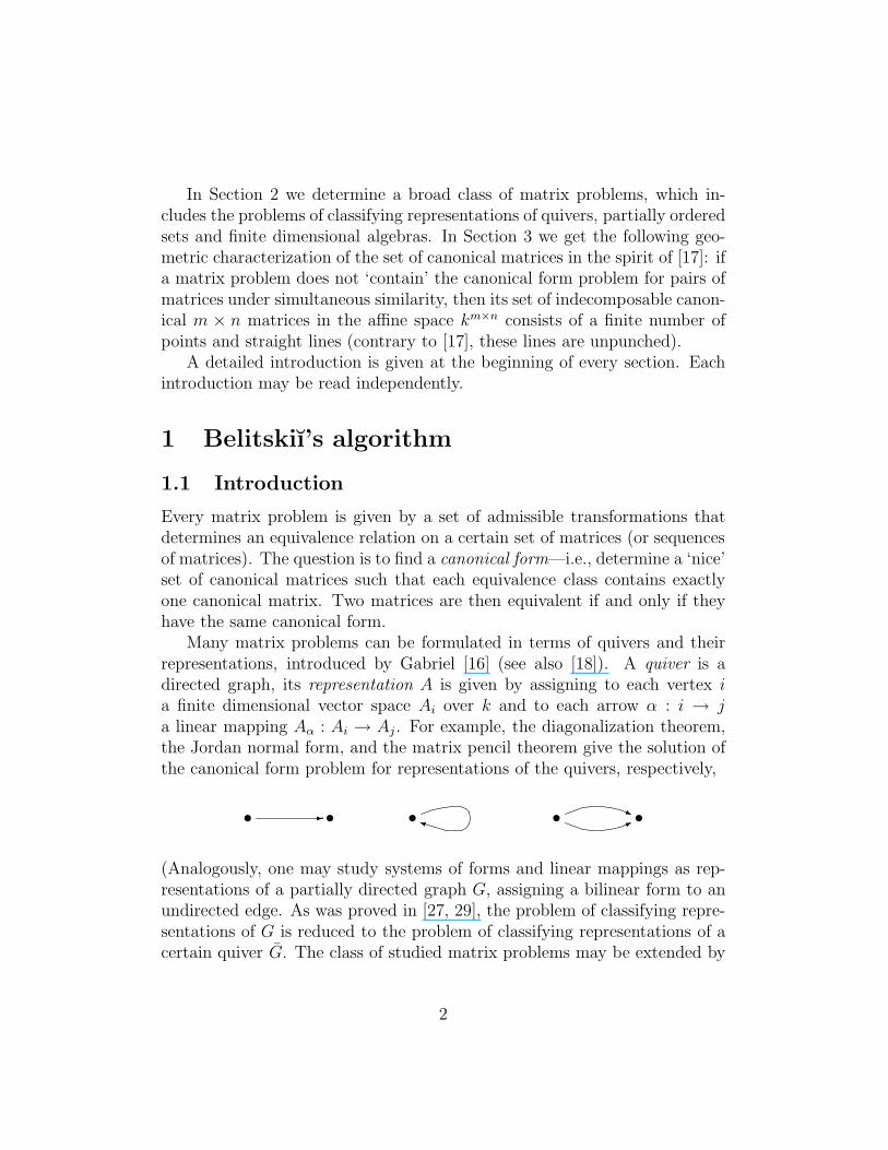
Many matrix problems can be formulated in terms of quivers and theirrepresentations, introduced by Gabriel [16] (see also [18]). A quiver is adirected graph, its representation A is given by assigning to each vertex ia finite dimensional vector space Ai over k and to each arrow α : i → ja linear mapping Aα : Ai → Aj . For example, the diagonalization theorem,the Jordan normal form, and the matrix pencil theorem give the solution ofthe canonical form problem for representations of the quivers, respectively,

• •- • • •j

*i

(Analogously, one may study systems of forms and linear mappings as rep-resentations of a partially directed graph G, assigning a bilinear form to anundirected edge. As was proved in [27, 29], the problem of classifying repre-sentations of G is reduced to the problem of classifying representations of acertain quiver G. The class of studied matrix problems may be extended by

2

considering quivers with relations [18, 25] and partially directed graphs withrelations [29].)

The canonical form problem was solved only for the quivers of so calledtame type by Donovan and Freislich [9] and Nazarova [22], this problem isconsidered as hopeless for the other quivers (see Section 2). Nevertheless, thematrices of each individual representation of a quiver may be reduced to acanonical form by Belitskiı’s algorithm (see [2] and its extended version [3]).This algorithm and the better known Littlewood algorithm [21] (see also[31, 34]) for reducing matrices to canonical form under unitary similarityhave the same conceptual sketch: The matrix is partitioned and successiveadmissible transformations are applied to reduce the submatrices to somenice form. At each stage, one refines the partition and restricts the setof permissible transformations to those that preserve the already reducedblocks. The process ends in a finite number of steps, producing the canonicalform.

We will apply Belitskiı’s algorithm to the canonical form problem formatrices under Λ-similarity, which is defined as follows. Let Λ be an algebraof n × n matrices (i.e., a subspace of kn×n that is closed with respect tomultiplication and contains the identity matrix I) and let Λ∗ be the set ofits nonsingular matrices. We say that two n× n matrices M and N are Λ-similar and write M ∼Λ N if there exists S ∈ Λ∗ such that S−1MS = N(∼Λ is an equivalence relation; see the end of Section 1.2).

Example 1.1. The problem of classifying representations of each quiver can beformulated in terms of Λ-similarity, where Λ is an algebra of block-diagonalmatrices in which some of the diagonal blocks are required to be equal. Forinstance, the problem of classifying representations of the quiver

y:1 3--

2

α ζγ

β ε*

j

δ

(1)

is the canonical form problem for matrices of the form

Aα 0 0 0Aβ 0 0 0Aγ 0 0 0Aδ Aε Aζ 0

under Λ-similarity, where Λ consists of block-diagonal matrices of the formS1 ⊕ S2 ⊕ S3 ⊕ S3.

3

Example 1.2. By the definition of Gabriel and Roiter [18], a linear matrixproblem of size m × n is given by a pair (D∗,M), where D is a subalgebraof km×m×kn×n and M is a subset of km×n such that SAR−1 ∈ M wheneverA ∈ M and (S,R) ∈ D∗. The question is to classify the orbits of M underthe action (S,R) : A 7→ SAR−1. Clearly, two m × n matrices A and Bbelong to the same orbit if and only if

[00A0

]and

[00B0

]are Λ-similar, where

Λ := {S ⊕R | (S,R) ∈ D} is an algebra of (m+ n) × (m+ n) matrices.

In Section 1.2 we prove that for every algebra Λ ⊂ kn×n there exists anonsingular matrix P such that the algebra P−1ΛP := {P−1AP |A ∈ Λ}consists of upper block-triangular matrices, in which some of the diagonalblocks must be equal and off-diagonal blocks satisfy a system of linear equa-tions. The algebra P−1ΛP will be called a reduced matrix algebra. TheΛ-similarity transformations with a matrix M correspond to the P−1ΛP -similarity transformations with the matrix P−1MP and hence it suffices tostudy Λ-similarity transformations given by a reduced matrix algebra Λ.

In Section 1.3, for every Jordan matrix J we construct a matrix J# =P−1JP (P is a permutation matrix) such that all matrices commuting withit form a reduced algebra. Following Shapiro [35], we call J# a Weyr matrixsince its form is determined by the set of its Weyr characteristics (Belitskiı [2]calls J# a modified Jordan matrix; it plays a central role in his algorithm).

In Section 1.4 we construct an algorithm (which is a modification of Be-litskiı’s algorithm [2], [3]) for reducing matrices to canonical form underΛ-similarity with a reduced matrix algebra Λ. In Section 1.5 we study theconstruction of the set of canonical matrices.

1.2 Reduced matrix algebras

In this section we prove that for every matrix algebra Λ ⊂ kn×n there existsa nonsingular matrix P such that the algebra P−1ΛP is a reduced matrixalgebra in the sense of the following definition.

A block matrix M = [Mij ], Mij ∈ kmi×nj , will be called an m×n matrix,where m = (m1, m2, . . .), n = (n1, n2, . . .) and mi, nj ∈ {0, 1, 2, . . .} (we takeinto consideration blocks without rows or columns).

Definition 1.1. An algebra Λ of n × n matrices, n = (n1, . . . , nt), will becalled a reduced n× n algebra if there exist

(a) an equivalence relation

∼ in T = {1, . . . , t}, (2)

4

(b) a family of systems of linear equations

{ ∑

I∋i<j∈J

c(l)ij xij = 0, 1 6 l 6 q

IJ

}

I,J∈T/∼, (3)

indexed by pairs of equivalence classes, where c(l)ij ∈ k and q

IJ≥ 0,

such that Λ consists of all upper block-triangular n× n matrices

S =

S11 S12 · · · S1t

S22. . .

.... . . St−1,t

0 Stt

, Sij ∈ kni×nj , (4)

in which diagonal blocks satisfy the condition

Sii = Sjj whenever i ∼ j , (5)

and off-diagonal blocks satisfy the equalities

∑

I∋i<j∈J

c(l)ij Sij = 0, 1 6 l 6 q

IJ, (6)

for each pair I,J ∈ T/∼ .

Clearly, the sequence n = (n1, . . . , nt) and the equivalence relation ∼ areuniquely determined by Λ; moreover, ni = nj if i ∼ j.

Example 1.3. Let us consider the classical canonical form problem for pairsof matrices (A,B) under simultaneous similarity (i.e., for representations ofthe quiver p

�

�*

�

�Y). Reducing (A,B) to the form (J, C), where J is a Jordan

matrix, and restricting the set of permissible transformations to those thatpreserve J , we obtain the canonical form problem for C under Λ-similarity,where Λ consists of all matrices commuting with J . In the next section, wemodify J such that Λ becomes a reduced matrix algebra.

Theorem 1.1. For every matrix algebra Λ ⊂ kn×n, there exists a nonsingularmatrix P such that P−1ΛP is a reduced matrix algebra.

5

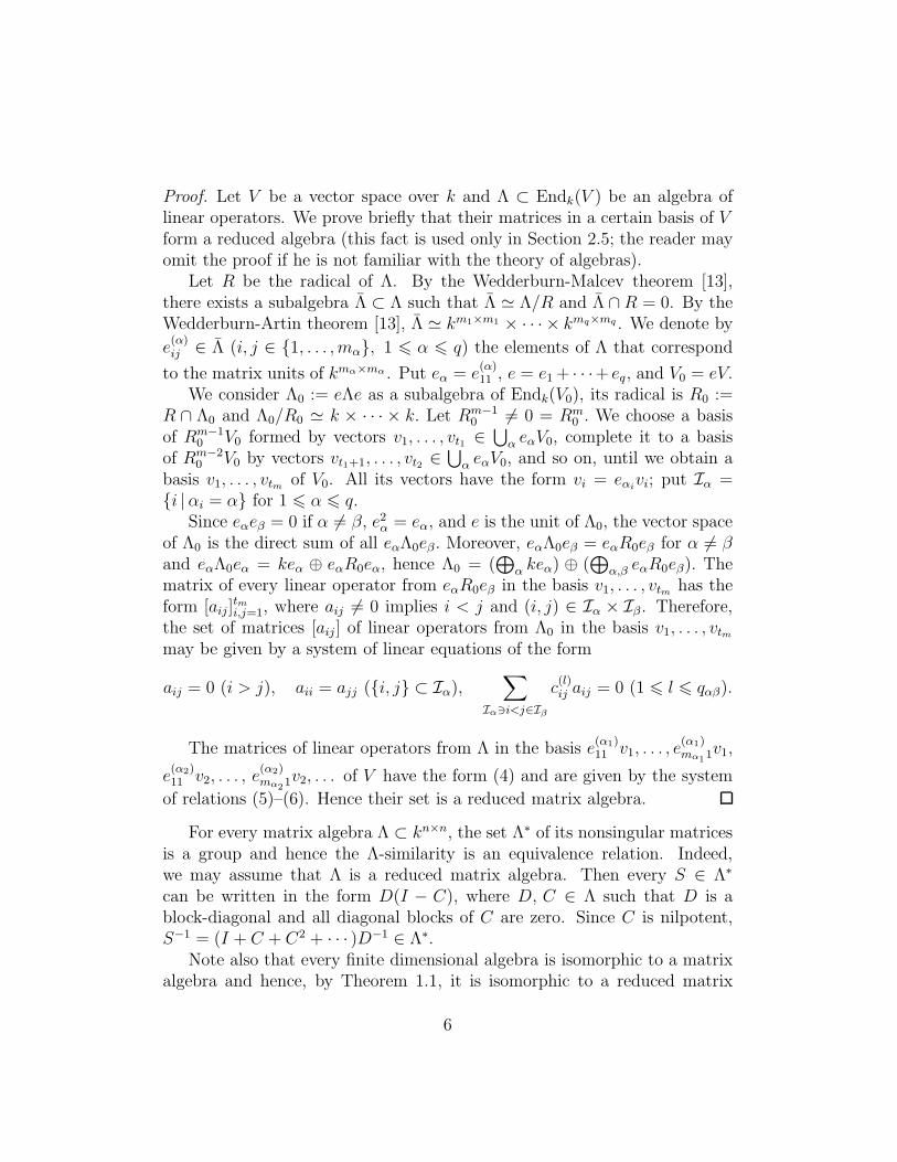
Proof. Let V be a vector space over k and Λ ⊂ Endk(V ) be an algebra oflinear operators. We prove briefly that their matrices in a certain basis of Vform a reduced algebra (this fact is used only in Section 2.5; the reader mayomit the proof if he is not familiar with the theory of algebras).

Let R be the radical of Λ. By the Wedderburn-Malcev theorem [13],there exists a subalgebra Λ ⊂ Λ such that Λ ≃ Λ/R and Λ ∩ R = 0. By theWedderburn-Artin theorem [13], Λ ≃ km1×m1 × · · · × kmq×mq . We denote by

e(α)ij ∈ Λ (i, j ∈ {1, . . . , mα}, 1 6 α 6 q) the elements of Λ that correspond

to the matrix units of kmα×mα . Put eα = e(α)11 , e = e1 + · · ·+ eq, and V0 = eV.

We consider Λ0 := eΛe as a subalgebra of Endk(V0), its radical is R0 :=R ∩ Λ0 and Λ0/R0 ≃ k × · · · × k. Let Rm−1

0 6= 0 = Rm0 . We choose a basis

of Rm−10 V0 formed by vectors v1, . . . , vt1 ∈

⋃

α eαV0, complete it to a basisof Rm−2

0 V0 by vectors vt1+1, . . . , vt2 ∈⋃

α eαV0, and so on, until we obtain abasis v1, . . . , vtm of V0. All its vectors have the form vi = eαi

vi; put Iα ={i |αi = α} for 1 6 α 6 q.

Since eαeβ = 0 if α 6= β, e2α = eα, and e is the unit of Λ0, the vector spaceof Λ0 is the direct sum of all eαΛ0eβ . Moreover, eαΛ0eβ = eαR0eβ for α 6= βand eαΛ0eα = keα ⊕ eαR0eα, hence Λ0 = (

⊕

α keα) ⊕ (⊕

α,β eαR0eβ). Thematrix of every linear operator from eαR0eβ in the basis v1, . . . , vtm has theform [aij ]

tmi,j=1, where aij 6= 0 implies i < j and (i, j) ∈ Iα × Iβ . Therefore,

the set of matrices [aij ] of linear operators from Λ0 in the basis v1, . . . , vtmmay be given by a system of linear equations of the form

aij = 0 (i > j), aii = ajj ({i, j} ⊂ Iα),∑

Iα∋i<j∈Iβ

c(l)ij aij = 0 (1 6 l 6 qαβ).

The matrices of linear operators from Λ in the basis e(α1)11 v1, . . . , e

(α1)mα11v1,

e(α2)11 v2, . . . , e

(α2)mα21v2, . . . of V have the form (4) and are given by the system

of relations (5)–(6). Hence their set is a reduced matrix algebra.

For every matrix algebra Λ ⊂ kn×n, the set Λ∗ of its nonsingular matricesis a group and hence the Λ-similarity is an equivalence relation. Indeed,we may assume that Λ is a reduced matrix algebra. Then every S ∈ Λ∗

can be written in the form D(I − C), where D, C ∈ Λ such that D is ablock-diagonal and all diagonal blocks of C are zero. Since C is nilpotent,S−1 = (I + C + C2 + · · · )D−1 ∈ Λ∗.

Note also that every finite dimensional algebra is isomorphic to a matrixalgebra and hence, by Theorem 1.1, it is isomorphic to a reduced matrix

6

algebra.

1.3 Weyr matrices

Following Belitskiı [2], for every Jordan matrix J we define a matrix J# =P−1JP (P is a permutation matrix) such that all matrices commuting withit form a reduced algebra. We will fix a linear order ≺ in k (if k is the fieldof complex numbers, we may use the lexicographic ordering: a+ bi ≺ c+ diif either a = c and b < d, or a < c).

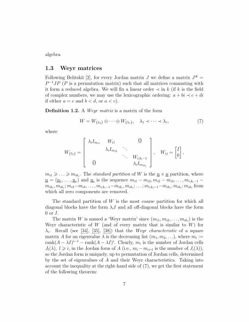
Definition 1.2. A Weyr matrix is a matrix of the form

W = W{λ1} ⊕ · · · ⊕W{λr}, λ1 ≺ · · · ≺ λr, (7)

where

W{λi} =

λiImi1Wi1 0λiImi2

. . .

. . . Wi,ki−1

0 λiImiki

, Wij =

[I0

]

,

mi1 > . . . > miki. The standard partition of W is the n× n partition, where

n = (n1, . . . , nr) and ni is the sequence mi1 −mi2, mi2 −mi3, . . . , mi,ki−1 −miki

, miki;mi2−mi3, . . . , mi,ki−1−miki

, miki; . . . ;mi,ki−1−miki

, miki;miki

fromwhich all zero components are removed.

The standard partition of W is the most coarse partition for which alldiagonal blocks have the form λiI and all off-diagonal blocks have the form0 or I.

The matrix W is named a ‘Weyr matrix’ since (mi1, mi2, . . . , miki) is the

Weyr characteristic of W (and of every matrix that is similar to W ) forλi. Recall (see [34], [35], [38]) that the Weyr characteristic of a squarematrix A for an eigenvalue λ is the decreasing list (m1, m2, . . .), where mi :=rank(A− λI)i−1 − rank(A− λI)i. Clearly, mi is the number of Jordan cellsJl(λ), l > i, in the Jordan form of A (i.e., mi−mi+1 is the number of Ji(λ)),so the Jordan form is uniquely, up to permutation of Jordan cells, determinedby the set of eigenvalues of A and their Weyr characteristics. Taking intoaccount the inequality at the right-hand side of (7), we get the first statementof the following theorem:

7

Theorem 1.2. Every square matrix A is similar to exactly one Weyr matrixA#. The matrix A# is obtained from the Jordan form of A by simultaneouspermutations of its rows and columns. All matrices commuting with A# forma reduced matrix algebra Λ(A#) of n × n matrices (4) with equalities (6) ofthe form Sij = Si′j′ and Sij = 0, where n×n is the standard partition of A#.

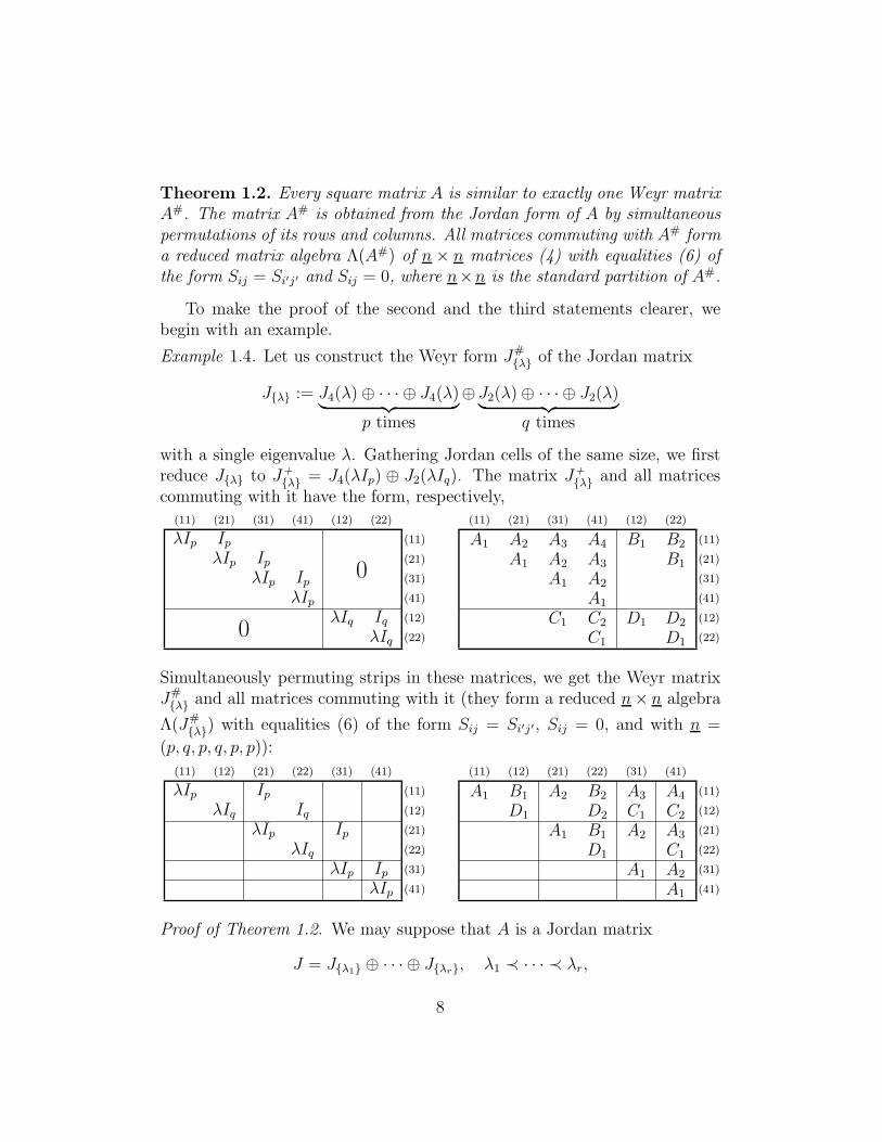
To make the proof of the second and the third statements clearer, webegin with an example.

Example 1.4. Let us construct the Weyr form J#{λ} of the Jordan matrix

J{λ} := J4(λ) ⊕ · · · ⊕ J4(λ)︸ ︷︷ ︸

p times

⊕ J2(λ) ⊕ · · · ⊕ J2(λ)︸ ︷︷ ︸

q times

with a single eigenvalue λ. Gathering Jordan cells of the same size, we firstreduce J{λ} to J+

{λ} = J4(λIp) ⊕ J2(λIq). The matrix J+

{λ} and all matricescommuting with it have the form, respectively,

λIpλIp

λIpλIp

λIqλIq

0

0

(11) (21) (31) (41) (12) (22)

(11)

(21)

(31)

(41)

(12)

(22)

A1

A1

A1

A1

D1

D1

(11) (21) (31) (41) (12) (22)

(11)

(21)

(31)

(41)

(12)

(22)

IpIp

Ip

Iq

A2 A3 A4

A3A2

A2

B1 B2

B1

D2C1 C2

C1

Simultaneously permuting strips in these matrices, we get the Weyr matrixJ#{λ} and all matrices commuting with it (they form a reduced n× n algebra

Λ(J#{λ}) with equalities (6) of the form Sij = Si′j′, Sij = 0, and with n =

(p, q, p, q, p, p)):

λIpλIq

λIpλIq

λIpλIp

(11) (12) (21) (22) (31) (41)

(11)

(12)

(21)

(22)

(31)

(41)

A1

D1

A1

D1

A1

A1

(11) (12) (21) (22) (31) (41)

(11)

(12)

(21)

(22)

(31)

(41)

IpIq

Ip

Ip

B1 A2 B2

D2

A3

C1

A4

C2

A2 A3

C1

A2

B1

Proof of Theorem 1.2. We may suppose that A is a Jordan matrix

J = J{λ1} ⊕ · · · ⊕ J{λr}, λ1 ≺ · · · ≺ λr,

8

where J{λ} denotes a Jordan matrix with a single eigenvalue λ. Then

J# = J#{λ1}

⊕ · · · ⊕ J#{λr}

, Λ(J#) = Λ(J#{λ1}

) × · · · × Λ(J#{λr}

);

the second since SJ# = J#S if and only if S = S1 ⊕ · · · ⊕ Sr and SiJ#{λi}

=

J#{λi}

Si.So we may restrict ourselves to a Jordan matrix J{λ} with a single eigen-

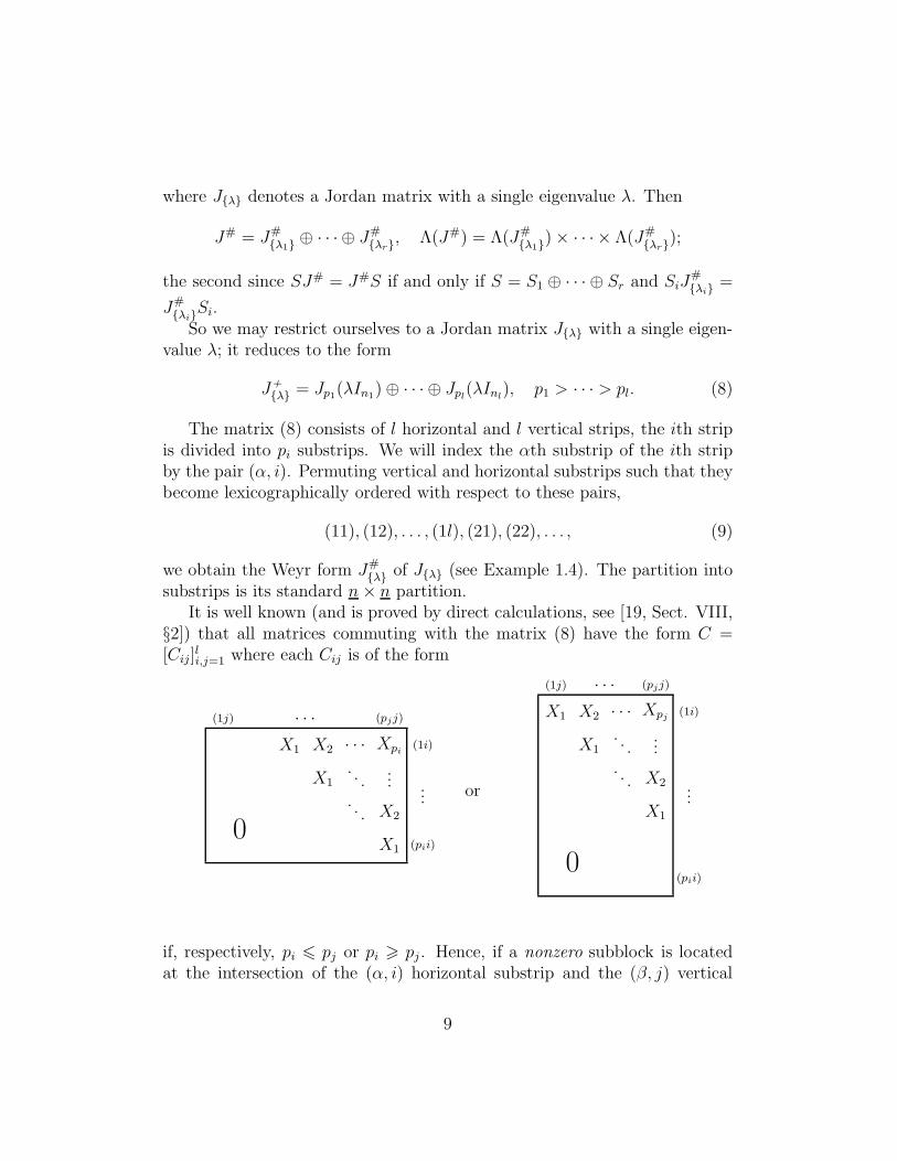
value λ; it reduces to the form

J+

{λ} = Jp1(λIn1) ⊕ · · · ⊕ Jpl(λInl

), p1 > · · · > pl. (8)

The matrix (8) consists of l horizontal and l vertical strips, the ith stripis divided into pi substrips. We will index the αth substrip of the ith stripby the pair (α, i). Permuting vertical and horizontal substrips such that theybecome lexicographically ordered with respect to these pairs,

(11), (12), . . . , (1l), (21), (22), . . . , (9)

we obtain the Weyr form J#{λ} of J{λ} (see Example 1.4). The partition into

substrips is its standard n× n partition.It is well known (and is proved by direct calculations, see [19, Sect. VIII,

§2]) that all matrices commuting with the matrix (8) have the form C =[Cij]

li,j=1 where each Cij is of the form

X1

X2

...

Xpi

(pjj)

· · ·

. . .

.

X1

X2X1

· · ·(1j)

(1i)

...

(pii)

X1 X2 · · · Xpj

X1 ... .... . . X2

X1

00

(1j) · · · (pjj)

(1i)

...

(pii)

..

or

if, respectively, pi 6 pj or pi > pj . Hence, if a nonzero subblock is locatedat the intersection of the (α, i) horizontal substrip and the (β, j) vertical

9

substrip, then either α = β and i 6 j, or α < β. Rating the substrips of C inthe lexicographic order (9), we obtain an upper block-triangular n×n matrixS that commutes with J#

{λ}. The matrices S form the algebra Λ(J#{λ}), which

is a reduced algebra with equations (6) of the form Sij = Si′j′ and Sij = 0.

Note that J#{λ} is obtained from

J{λ} = Jk1(λ) ⊕ · · · ⊕ Jkt(λ), k1 > . . . > kt, (10)

as follows: We collect the first columns of Jk1(λ), . . . , Jkt(λ) on the first t

columns of J{λ}, then permute the rows as well. Next collect the second

columns and permute the rows as well, continue the process until J#{λ} is

achieved.

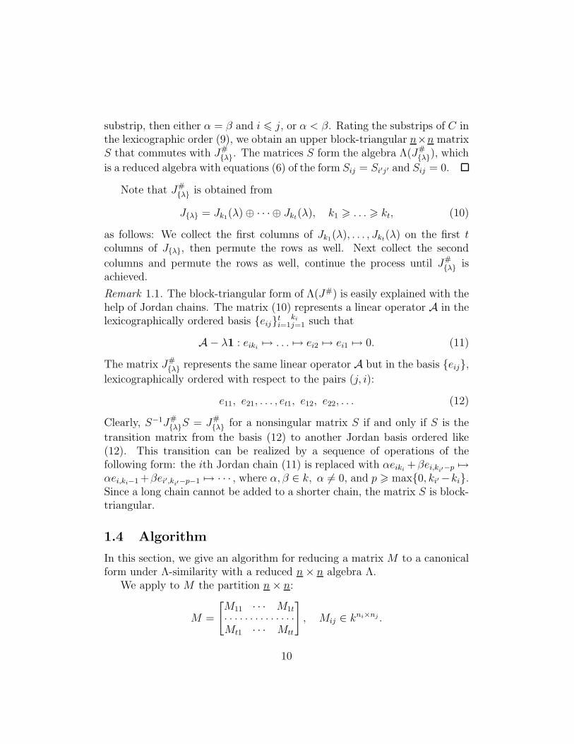
Remark 1.1. The block-triangular form of Λ(J#) is easily explained with thehelp of Jordan chains. The matrix (10) represents a linear operator A in thelexicographically ordered basis {eij}ti=1

ki

j=1 such that

A− λ1 : eiki7→ . . . 7→ ei2 7→ ei1 7→ 0. (11)

The matrix J#{λ} represents the same linear operator A but in the basis {eij},

lexicographically ordered with respect to the pairs (j, i):

e11, e21, . . . , et1, e12, e22, . . . (12)

Clearly, S−1J#{λ}S = J#

{λ} for a nonsingular matrix S if and only if S is the

transition matrix from the basis (12) to another Jordan basis ordered like(12). This transition can be realized by a sequence of operations of thefollowing form: the ith Jordan chain (11) is replaced with αeiki

+βei,ki′−p 7→αei,ki−1 +βei′,ki′−p−1 7→ · · · , where α, β ∈ k, α 6= 0, and p > max{0, ki′ −ki}.Since a long chain cannot be added to a shorter chain, the matrix S is block-triangular.

1.4 Algorithm

In this section, we give an algorithm for reducing a matrix M to a canonicalform under Λ-similarity with a reduced n× n algebra Λ.

We apply to M the partition n× n:

M =

[M11 · · · M1t. . . . . . . . . . . . . .Mt1 · · · Mtt

]

, Mij ∈ kni×nj .

10

A block Mij will be called stable if it remains invariant under Λ-similaritytransformations with M . Then Mij = aijI whenever i ∼ j and Mij = 0 (weput aij = 0) whenever i 6∼ j since the equalities S−1

ii MijSjj = Mij must holdfor all nonsingular block-diagonal matrices S = S11⊕S22⊕· · ·⊕Stt satisfying(5).

If all the blocks of M are stable, then M is invariant under Λ-similarity,hence M is canonical (M∞ = M).

Let there exist a nonstable block. We put the blocks of M in order

Mt1 < Mt2 < · · · < Mtt < Mt−1,1 < Mt−1,2 < · · · < Mt−1,t < · · · (13)

and reduce the first (with respect to this ordering) nonstable block Mlr. LetM ′ = S−1MS, where S ∈ Λ∗ has the form (4). Then the (l, r) block of thematrix MS = SM ′ is

Ml1S1r +Ml2S2r + · · · +MlrSrr = SllM′lr + Sl,l+1M

′l+1,r + · · ·+ SltM

′tr

or, since all Mij < Mlr are stable,

al1S1r + · · ·+ al,r−1Sr−1,r +MlrSrr = SllM′lr + Sl,l+1al+1,r + · · ·+ Sltatr (14)

(we have removed in (14) all summands with aij = 0; their sizes may differfrom the size of Mlr).

Let I,J ∈ T/∼ be the equivalence classes such that l ∈ I and r ∈ J .

Case I: the qIJ equalities (6) do not imply

al1S1r + al2S2r + · · · + al,r−1Sr−1,r = Sl,l+1al+1,r + · · ·+ Sltatr (15)

(i.e., there exists a nonzero admissible addition to Mlr from otherblocks). Then we make M ′

lr = 0 using S ∈ Λ∗ of the form (4) thathas the diagonal Sii = I (i = 1, . . . , t) and fits both (6) and (14) withM ′

lr = 0.

Case II: the qIJ equalities (6) imply (15); i 6∼ j. Then (14) simplifies to

MlrSrr = SllM′lr, (16)

where Srr and Sll are arbitrary nonsingular matrices. We chose S ∈ Λ∗

such that

M ′lr = S−1

ll MlrSrr =

[0 I0 0

]

.

11

Case III: the qIJ equalities (6) imply (15); i ∼ j. Then (14) simplifies tothe form (16) with an arbitrary nonsingular matrix Srr = Sll; M

′lr =

S−1ll MlrSrr is chosen as a Weyr matrix.

We restrict ourselves to those admissible transformations with M ′ thatpreserve M ′

lr. Let us prove that they are the Λ′-similarity transformationswith

Λ′ := {S ∈ Λ |SM ′ ≡M ′S}, (17)

where A ≡ B means that A and B are n × n matrices and Alr = Blr forthe pair (l, r). The transformation M ′ 7→ S−1M ′S, S ∈ (Λ′)∗, preserves M ′

lr

(i.e. M ′ ≡ S−1M ′S) if and only if SM ′ ≡ M ′S since S is upper block-triangular and M ′ coincides with S−1M ′S on the places of all (stable) blocksMij < Mlr. The set Λ′ is an algebra: let S,R ∈ Λ′, then M ′S and SM ′

coincide on the places of all Mij < Mlr and R is upper block-triangular,hence M ′SR ≡ SM ′R; analogously, SM ′R ≡ SRM ′ and SR ∈ Λ′. Thematrix algebra Λ′ is a reduced algebra since Λ′ consists of all S ∈ Λ satisfyingthe condition (14) with M ′

lr instead of Mlr.In Case I, Λ′ consists of all S ∈ Λ satisfying (15) (we add it to the system

(6)). In Case II, Λ′ consists of all S ∈ Λ for which Sll[

00I0

]=

[00I0

]Srr, that

is,

Sll =

[P1 P2

0 P3

]

, Srr =

[Q1 Q2

0 Q3

]

, P1 = Q3.

In Case III, Λ′ consists of all S ∈ Λ for which the blocks Sll and Srr are equaland commute with the Weyr matrix M ′

lr. (It gives an additional partition ofS ∈ Λ in Cases II and III; we rewrite (5)–(6) for smaller blocks and add theequalities that are needed for SllM

′lr = M ′

lrSrr.)

In this manner, for every pair (M,Λ) we construct a new pair (M ′,Λ′)with Λ′ ⊂ Λ. If M ′ is not invariant under Λ′-similarity, then we repeatthis construction (with an additional partition of M ′ in accordance with thestructure of Λ′) and obtain (M ′′,Λ′′), and so on. Since at every step we reducea new block, this process ends with a certain pair (M (p),Λ(p)) in which allthe blocks of M (p) are stable (i.e. M (p) is Λ(p)-similar only to itself). Putting(M∞,Λ∞) := (M (p),Λ(p)), we get the sequence

(M0,Λ0) = (M,Λ), (M ′,Λ′), . . . , (M (p),Λ(p)) = (M∞,Λ∞), (18)

whereΛ∞ = {S ∈ Λ |M∞S = SM∞}. (19)

12

Definition 1.3. The matrix M∞ will be called the Λ-canonical form of M .

Theorem 1.3. Let Λ ⊂ kn×n be a reduced matrix algebra. Then M ∼Λ M∞

for every M ∈ kn×n and M ∼Λ N if and only if M∞ = N∞.

Proof. Let Λ be a reduced n × n algebra, M ∼Λ N , and let Mlr be thefirst nonstable block of M . Then Mij and Nij are stable blocks (moreover,Mij = Nij) for all Mij < Mlr. By reasons of symmetry, Nlr is the firstnonstable block of N ; moreover, Mlr and Nlr are reduced to the same form:M ′

lr = N ′lr. We obtain pairs (M ′,Λ′) and (N ′,Λ′) with the same Λ′ and

M ′ ∼Λ′ N ′. Hence M (i) ∼Λ(i) N (i) for all i, so M∞ = N∞.

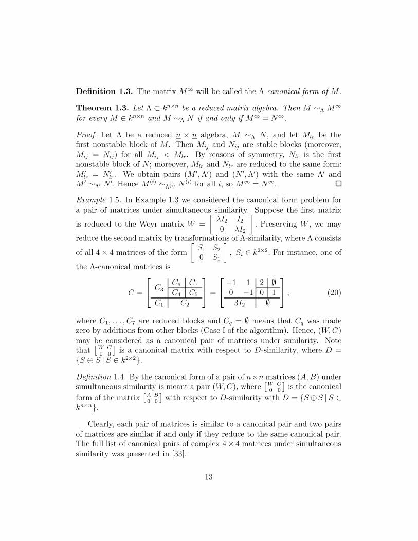
Example 1.5. In Example 1.3 we considered the canonical form problem fora pair of matrices under simultaneous similarity. Suppose the first matrix

is reduced to the Weyr matrix W =

[λI2 I20 λI2

]

. Preserving W , we may

reduce the second matrix by transformations of Λ-similarity, where Λ consists

of all 4× 4 matrices of the form

[S1 S2

0 S1

]

, Si ∈ k2×2. For instance, one of

the Λ-canonical matrices is

C =

C3

C6 C7

C4 C5

C1 C2

=

−1 10 −1

2 ∅0 1

3I2 ∅

, (20)

where C1, . . . , C7 are reduced blocks and Cq = ∅ means that Cq was madezero by additions from other blocks (Case I of the algorithm). Hence, (W,C)may be considered as a canonical pair of matrices under similarity. Notethat

[W0C0

]is a canonical matrix with respect to D-similarity, where D =

{S ⊕ S |S ∈ k2×2}.

Definition 1.4. By the canonical form of a pair of n×n matrices (A,B) undersimultaneous similarity is meant a pair (W,C), where

[W0C0

]is the canonical

form of the matrix[A0B0

]with respect to D-similarity with D = {S⊕S |S ∈

kn×n}.

Clearly, each pair of matrices is similar to a canonical pair and two pairsof matrices are similar if and only if they reduce to the same canonical pair.The full list of canonical pairs of complex 4× 4 matrices under simultaneoussimilarity was presented in [33].

13

Remark 1.2. Instead of (13), we may use another linear ordering in the setof blocks, for example, Mt1 < Mt−1,1 < · · · < M11 < Mt2 < Mt−1,2 < · · · orMt1 < Mt−1,1 < Mt2 < Mt−2,1 < Mt−1,2 < Mt3 < · · · . It is necessary onlythat (i, j) ≪ (i′, j′) implies Mij < Mi′j′, where (i, j) ≪ (i′, j′) indicates theexistence of a nonzero addition from Mij to Mi′j′ and is defined as follows:

Definition 1.5. Let Λ be a reduced n × n algebra. For unequal pairs(i, j), (i′, j′) ∈ T × T (see (2)), we put (i, j) ≪ (i′, j′) if either i = i′ andthere exists S ∈ Λ∗ with Sjj′ 6= 0, or j = j′ and there exists S ∈ Λ∗ withSi′i 6= 0.

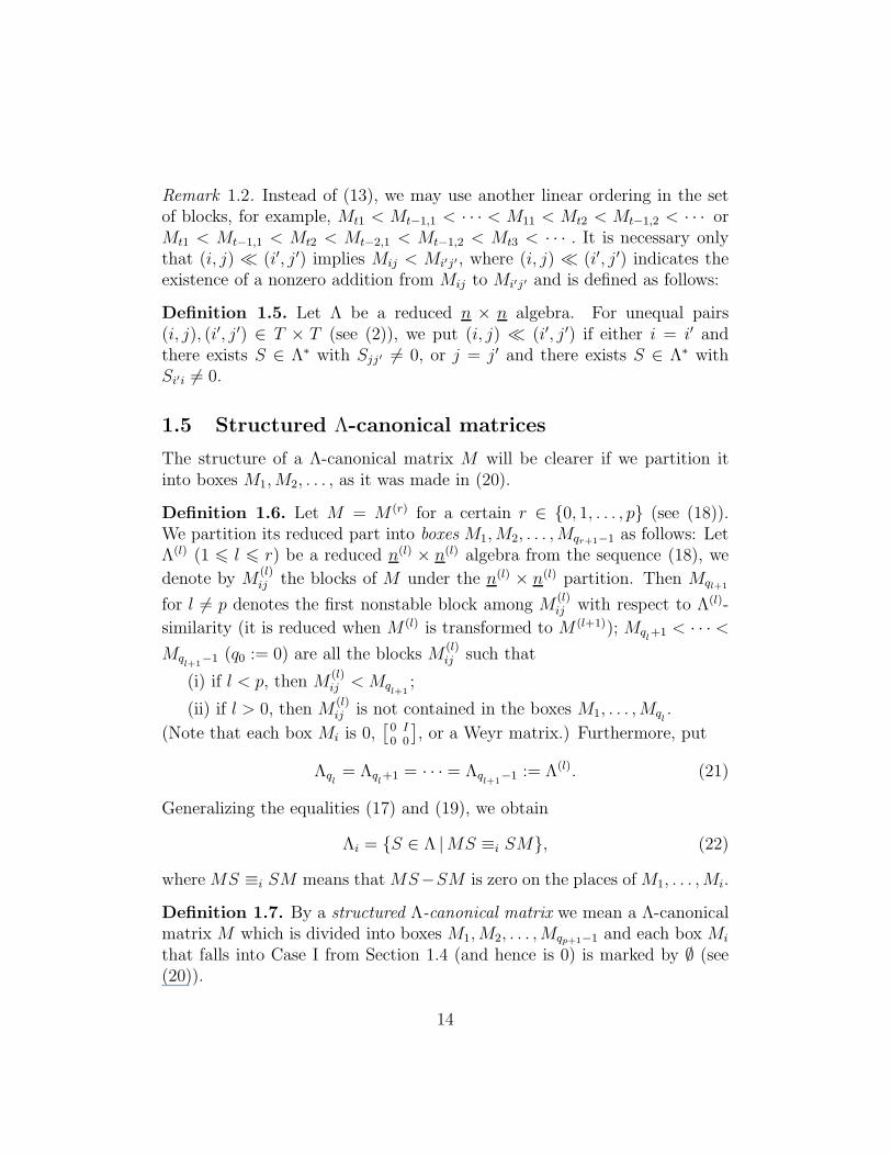
1.5 Structured Λ-canonical matrices

The structure of a Λ-canonical matrix M will be clearer if we partition itinto boxes M1,M2, . . . , as it was made in (20).

Definition 1.6. Let M = M (r) for a certain r ∈ {0, 1, . . . , p} (see (18)).We partition its reduced part into boxes M1,M2, . . . ,Mqr+1−1 as follows: LetΛ(l) (1 6 l 6 r) be a reduced n(l) × n(l) algebra from the sequence (18), we

denote by M(l)ij the blocks of M under the n(l) × n(l) partition. Then Mql+1

for l 6= p denotes the first nonstable block among M(l)ij with respect to Λ(l)-

similarity (it is reduced when M (l) is transformed to M (l+1)); Mql+1 < · · · <

Mql+1

−1 (q0 := 0) are all the blocks M(l)ij such that

(i) if l < p, then M(l)ij < Mq

l+1;

(ii) if l > 0, then M(l)ij is not contained in the boxes M1, . . . ,Mq

l.

(Note that each box Mi is 0,[

00I0

], or a Weyr matrix.) Furthermore, put

Λql= Λq

l+1 = · · · = Λq

l+1−1 := Λ(l). (21)

Generalizing the equalities (17) and (19), we obtain

Λi = {S ∈ Λ |MS ≡i SM}, (22)

where MS ≡i SM means that MS−SM is zero on the places of M1, . . . ,Mi.

Definition 1.7. By a structured Λ-canonical matrix we mean a Λ-canonicalmatrix M which is divided into boxes M1,M2, . . . ,Mqp+1−1 and each box Mi

that falls into Case I from Section 1.4 (and hence is 0) is marked by ∅ (see(20)).

14

Now we describe the construction of Λ-canonical matrices.

Definition 1.8. By a part of a matrix M = [aij]ni,j=1 is meant an arbitrary

set of its entries given with their indices. By a rectangular part we mean apart of the form B = [aij ], p1 6 i 6 p2, q1 6 j 6 q2. We consider a partitionof M into disjoint rectangular parts (which is not, in general, a partition intosubstrips, see the matrix (20)) and write, generalizing (13), B < B′ if eitherp2 = p′2 and q1 < q′1, or p2 > p′2.

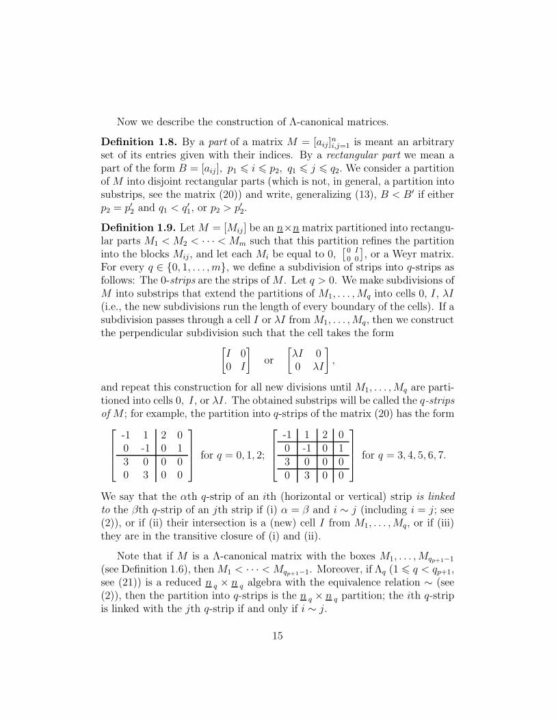
Definition 1.9. Let M = [Mij ] be an n×n matrix partitioned into rectangu-lar parts M1 < M2 < · · · < Mm such that this partition refines the partitioninto the blocks Mij , and let each Mi be equal to 0,

[00I0

], or a Weyr matrix.

For every q ∈ {0, 1, . . . , m}, we define a subdivision of strips into q-strips asfollows: The 0-strips are the strips of M . Let q > 0. We make subdivisions ofM into substrips that extend the partitions of M1, . . . ,Mq into cells 0, I, λI(i.e., the new subdivisions run the length of every boundary of the cells). If asubdivision passes through a cell I or λI from M1, . . . ,Mq, then we constructthe perpendicular subdivision such that the cell takes the form

[I 00 I

]

or

[λI 00 λI

]

,

and repeat this construction for all new divisions until M1, . . . ,Mq are parti-tioned into cells 0, I, or λI. The obtained substrips will be called the q-stripsof M ; for example, the partition into q-strips of the matrix (20) has the form

-1 1 2 00 -1 0 13 0 0 00 3 0 0

for q = 0, 1, 2;

-1 1 2 00 -1 0 13 0 0 00 3 0 0

for q = 3, 4, 5, 6, 7.

We say that the αth q-strip of an ith (horizontal or vertical) strip is linkedto the βth q-strip of an jth strip if (i) α = β and i ∼ j (including i = j; see(2)), or if (ii) their intersection is a (new) cell I from M1, . . . ,Mq, or if (iii)they are in the transitive closure of (i) and (ii).

Note that if M is a Λ-canonical matrix with the boxes M1, . . . ,Mqp+1−1

(see Definition 1.6), then M1 < · · · < Mqp+1−1. Moreover, if Λq (1 6 q < qp+1,see (21)) is a reduced n q × n q algebra with the equivalence relation ∼ (see(2)), then the partition into q-strips is the n q × n q partition; the ith q-stripis linked with the jth q-strip if and only if i ∼ j.

15

Theorem 1.4. Let Λ be a reduced n × n algebra and let M be an arbitraryn×n matrix partitioned into rectangular parts M1 < M2 < · · · < Mm, whereeach Mi is equal to ∅ (a marked zero block),

[00I0

], or a Weyr matrix. Then

M is a structured Λ-canonical matrix with boxes M1, . . . ,Mm if and only ifeach Mq (1 6 q 6 m) satisfies the following conditions:

(a) Mq is the intersection of two (q − 1)-strips.

(b) Suppose there exists M ′ = S−1MS (partitioned into rectangular partsconformal to M ; S ∈ Λ∗) such that M ′

1 = M1, . . . ,M′q−1 = Mq−1, but

M ′q 6= Mq. Then Mq = ∅.

(c) Suppose M ′ from (b) does not exist. Then Mq is a Weyr matrix if thehorizontal and the vertical (q − 1)-strips of Mq are linked; Mq =

[00I0

]

otherwise.

Proof. This theorem follows immediately from the algorithm of Section 1.4.

2 Linear matrix problems

2.1 Introduction

In Section 2 we study a large class of matrix problems. In the theory ofrepresentations of finite dimensional algebras, similar classes of matrix prob-lems are given by vectorspace categories [25, 36], bocses [26, 6], modules overaggregates [18, 17], or vectroids [4].

Let us define the considered class of matrix problems (in terms of ele-mentary transformations to simplify its use; a more formal definition will begiven in Section 2.2). Let ∼ be an equivalence relation in T = {1, . . . , t}. Wesay that a t × t matrix A = [aij ] links an equivalence class I ∈ T/∼ to anequivalence class J ∈ T/∼ if aij 6= 0 implies (i, j) ∈ I × J . Clearly, if Alinks I to J and A′ links I ′ to J ′, then AA′ links I to J ′ when J = I ′, andAA′ = 0 when J 6= I ′.1 We also say that a sequence of nonnegative integersn = (n1, n2, . . . , nt) is a step-sequence if i ∼ j implies ni = nj.

1Linking matrices behave as mappings; one may use vector spaces VI instead of equiv-alence classes I (dim VI = #(I)) and linear mappings of the corresponding vector spacesinstead of linking matrices.

16

Let A = [aij ] link I to J , let n be a step-sequence, and let (l, r) ∈{1, . . . , ni}×{1, . . . , nj} for (i, j) ∈ I ×J (since n is a step-sequence, ni andnj do not depend on the choice of (i, j)); denote by A[l,r] the n × n matrixthat is obtained from A by replacing each entry aij with the following ni×njblock A

[l,r]ij : if aij = 0 then A

[l,r]ij = 0, and if aij 6= 0 then the (l, r) entry of

A[l,r]ij is aij and the others are zeros.

Let a triple(T/∼, {Pi}

pi=1, {Vj}

qj=1) (23)

consist of the set of equivalence classes of T = {1, . . . , t}, a finite or emptyset of linking nilpotent upper-triangular matrices Pi ∈ kt×t, and a finite setof linking matrices Vj ∈ kt×t. Denote by P the product closure of {Pi}

pi=1

and by V the closure of {Vj}qj=1 with respect to multiplication by P (i.e.,

VP ⊂ V and PV ⊂ V). Since Pi are nilpotent upper-triangular t × t ma-trices, Pi1Pi2 . . . Pit = 0 for all i1, . . . , it. Hence, P and V are finite setsconsisting of linking nilpotent upper-triangular matrices and, respectively,linking matrices:

P = {Pi1Pi2 . . . Pir | r 6 t}, V = {PVjP′ |P, P ′ ∈ {It} ∪ P, 1 6 j 6 q}.

(24)For every step-sequence n = (n1, . . . , nt), we denote by Mn×n the vectorspace generated by all n× n matrices of the form V [l,r], 0 6= V ∈ V.

Definition 2.1. A linear matrix problem given by a triple (23) is the canon-ical form problem for n × n matrices M = [Mij ] ∈ Mn×n with respect tosequences of the following transformations:

(i) For each equivalence class I ∈ T/ ∼, the same elementary transfor-mations within all the vertical strips M•,i, i ∈ I, then the inversetransformations within the horizontal strips Mi,•, i ∈ I.

(ii) For a ∈ k and a nonzero matrix P = [pij ] ∈ P linking I to J , thetransformation M 7→ (I + aP [l,r])−1M(I + aP [l,r]); that is, the additionof apij times the lth column of the strip M•,i to the rth column ofthe strip M•,j simultaneously for all (i, j) ∈ I × J , then the inversetransformations with rows of M .

Example 2.1. As follows from Example 1.1, the problem of classifying repre-sentations of the quiver (1) may be given by the triple

({{1}, {2}, {3, 4}}, ∅, {e11, e21, e31, e41, e42, e43}),

17

where eij denotes the matrix in which the (i, j) entry is 1 and the others are0. The problem of classifying representations of each quiver may be given inthe same manner.

Example 2.2. Let S = {p1, . . . , pn} be a finite partially ordered set whoseelements are indexed such that pi < pj implies i < j. Its representation is amatrix M partitioned into n vertical strips M1, . . . ,Mn; we allow arbitraryrow-transformations, arbitrary column-transformations within each verticalstrip, and additions of linear combinations of columns of Mi to a column ofMj if pi < pj. (This notion is important for representation theory and wasintroduced by Nazarova and Roiter [24], see also [18] and [36].) The problemof classifying representations of the poset S may be given by the triple

({{1}, {2}, . . . , {n+ 1}}, {eij | pi < pj}, {en+1,1, en+1,2, . . . , en+1,n}).

Example 2.3. Let us consider Wasow’s canonical form problem for an analyticat the point ε = 0 matrix

A(ε) = A0 + εA1 + ε2A2 + · · · , Ai ∈ Cn×n, (25)

relative to analytic similarity:

A(ε) 7→ B(ε) := S(ε)−1A(ε)S(ε), (26)

where S(ε) = S0 + εS1 + · · · and S(ε)−1 are analytic matrices at 0. Letus restrict ourselves to the canonical form problem for the first t matricesA0, A1, . . . , At−1 in the expansion (25). By (26), S(ε)B(ε) = A(ε)S(ε), thatis S0B0 = A0S0, . . . , S0Bt−1 + S1Bt−2 + · · · + St−1B0 = A0St−1 + A1St−2 +· · ·+ At−1S0, or in the matrix form

S0 S1 · · · St−1

S0. . .

.... . . S1

0 S0

B0 B1 · · · Bt−1

B0. . .

.... . . B1

0 B0

=

A0 A1 · · · At−1

A0. . .

.... . . A1

0 A0

S0 S1 · · · St−1

S0. . .

.... . . S1

0 S0

.

18

Hence this problem may be given by the following triple of one-element sets:

({T}, {Jt}, {It}),

where Jt = e12 + e23 + · · · + et−1,t is the nilpotent Jordan block. Thenall elements of T = {1, 2, . . . , t} are equivalent, P = {Jt, J2

t , . . . , Jt−1t } and

V = {It, Jt, . . . , Jt−1t }. This problem is wild even if t = 2, see [14, 30]. I am

thankful to S. Friedland for this example.

In Section 2.2 we give a definition of the linear matrix problems in a form,which is more similar to Gabriel and Roiter’s definition (see Example 1.2)and is better suited for Belitskiı’s algorithm.

In Section 2.3 we prove that every canonical matrix may be decomposedinto a direct sum of indecomposable canonical matrices by permutations ofits rows and columns. We also investigate the canonical form problem forupper triangular matrices under upper triangular similarity (see [37]).

In Section 2.4 we consider a canonical matrix as a parametric matrixwhose parameters are eigenvalues of its Jordan blocks. It enables us todescribe a set of canonical matrices having the same structure.

In Section 2.5 we consider linear matrix problems that give matrix prob-lems with independent row and column transformations and prove that theproblem of classifying modules over a finite-dimensional algebra may be re-duced to such a matrix problem. The reduction is a modification of Drozd’sreduction of the problem of classifying modules over an algebra to the prob-lem of classifying representations of bocses [11] (see also Crawley-Boevey [6]).Another reduction of the problem of classifying modules over an algebra toa matrix problem with arbitrary row transformations was given in [17].

2.2 Linear matrix problems and Λ-similarity

In this section we give another definition of the linear matrix problems, whichis equivalent to the Definition 2.1 but is often more convenient. The set ofadmissible transformations will be formulated in terms of Λ-similarity; itsimplifies the use of Belitskiı’s algorithm.

Definition 2.2. An algebra Γ ⊂ kt×t of upper triangular matrices will becalled a basic matrix algebra if

a11 · · · a1t

. . ....

0 att

∈ Γ implies

a11 0. . .

0 att

∈ Γ.

19

Lemma 2.1. (a) Let Γ ⊂ kt×t be a basic matrix algebra, D be the set of itsdiagonal matrices, and R be the set of its matrices with zero diagonal. Thenthere exists a basis E1, . . . , Er of D over k such that all entries of its matricesare 0 and 1, moreover

E1 + · · ·+ Er = It, EαEβ = 0 (α 6= β), E2α = Eα. (27)

These equations imply the following decomposition of Γ (as a vector spaceover k) into a direct sum of subspaces:

Γ = D ⊕R =( r⊕

α=1

kEα

)

⊕( r⊕

α,β=1

EαREβ)

. (28)

(b) The set of basic t × t algebras is the set of reduced 1 × 1 algebras,where 1 := (1, 1, . . . , 1). A basic t × t algebra Γ is the reduced 1 × 1 algebragiven by

• T/ ∼= {I1, . . . , Ir} where Iα is the set of indices defined by Eα =∑

i∈Iαeii, see (27), and

• a family of systems of the form (3) such that for every α, β ∈ {1, . . . , r}the solutions of its (Iα, Iβ) system form the space EαREβ.

Proof. (a) By Definition 2.2, Γ is the direct sum of vector spaces D and R.Denote by F the set of diagonal t× t matrices with entries in {0, 1}. Let D ∈D, then D = a1F1 + · · ·+alFl, where a1, . . . , al are distinct nonzero elementsof k and F1, . . . , Fl are such matrices from F that FiFj = 0 whenever i 6= j.The vectors (a1, . . . , al), (a2

1, . . . , a2l ), . . . , (a

l1, . . . , a

ll) are linearly independent

(they form a Vandermonde determinant), hence there exist b1, . . . , bl ∈ ksuch that F1 = b1D + b2D

2 + · · ·+ blDl ∈ D, analogously F2, . . . , Fl ∈ D. It

follows that D = kE1 ⊕ · · · ⊕ kEr, where E1, . . . , Er ∈ F and satisfy (27).Therefore, R = (E1 + · · · + Er)R(E1 + · · · + Er) =

⊕

α,β EαREβ , we getthe decomposition (28). (Note that (27) is a decomposition of the identityof Γ into a sum of minimal orthogonal idempotents and (28) is the Peircedecomposition of Γ , see [13].)

Definition 2.3. A linear matrix problem given by a pair

(Γ,M), ΓM ⊂ M, MΓ ⊂ M, (29)

20

consisting of a basic t×t algebra Γ and a vector space M ⊂ kt×t, is the canon-ical form problem for matrices M ∈ Mn×n with respect to Γn×n-similaritytransformations

M 7→ S−1MS, S ∈ Γ ∗n×n,

where Γn×n and Mn×n consist of n×n matrices whose blocks satisfy the samelinear relations as the entries of all t× t matrices from Γ and M respectively.

More exactly, Γn×n is the reduced n× n algebra given by the same system(3) and T/∼ = {I1, . . . , Ir} as Γ (see Lemma 2.1(b)).2 Next,

M =( r∑

α=1

Eα

)

M( r∑

β=1

Eβ

)

=r⊕

α,β=1

EαMEβ (30)

(see (27)), hence there is a system of linear equations

∑

(i,j)∈Iα×Iβ

d(l)ij xij = 0, 1 6 l 6 pαβ, Iα, Iβ ∈ T/∼, (31)

such that M consists of all matrices [mij]ti,j=1 whose entries satisfy the system

(31). Then Mn×n (n is a step-sequence) denotes the vector space of all n× nmatrices [Mij ]

ti,j=1 whose blocks satisfy the system (31):

∑

(i,j)∈Iα×Iβ

d(l)ij Mij = 0, 1 6 l 6 pαβ , Iα, Iβ ∈ T/∼ .

Theorem 2.1. Definitions 2.1 and 2.3 determine the same class of matrixproblems:

(a) The linear matrix problem given by a triple (T/∼, {Pi}pi=1, {Vj}

qj=1)

may be also given by the pair (Γ,M), where Γ is the basic matrix algebragenerated by P1, . . . , Pp and all matrices EI =

∑

j∈I ejj (I ∈ T/∼) and Mis the minimal vector space of matrices containing V1, . . . , Vq and closed withrespect to multiplication by P1, . . . , Pp.

(b) The linear matrix problem given by a pair (Γ,M) may be also givenby a triple (T/∼, {Pi}

pi=1, {Vj}

qj=1), where T/∼= {I1, . . . , Ir} (see Lemma

2.1(b)), {Pi}pi=1 is the union of bases for the spaces EαREβ (see (28)), and

{Vj}qj=1 is the union of bases for the spaces EαMEβ (see (30)).

2If n1 > 0, . . . , nt > 0, then Γn×n is Morita equivalent to Γ ; moreover, Γ is the basicalgebra for Γn×n in terms of the theory of algebras, see [13].

21

Proof. (a) Let n be a step-sequence. We first prove that the set of admissibletransformations is the same for both the matrix problems; that is, there existsa sequence of transformations (i)–(ii) from Definition 2.1 transforming M toN (then we write M ≃ N) if and only if they are Λ-similar with Λ := Γn×n.

By Definition 2.1, M ≃ N if and only if S−1MS = N , where S is aproduct of matrices of the form

I + aE[l,r]I (a 6= −1 if l = r), I + bP [l,r], (32)

where a, b ∈ k, I ∈ T/∼ and 0 6= P ∈ P. Since S ∈ Λ, M ≃ N impliesM ∼Λ N .

Let M ∼Λ N , that is SMS−1 = N for a nonsingular S ∈ Λ. To proveM ≃ N , we must expand S−1 into factors of the form (32); it suffices toreduce S to I multiplying by matrices (32). The matrix S has the form (4)with Sii = Sjj whenever i ∼ j; we reduce S to the form (4) with Sii = Ini

for all i multiplying by matrices I + aE[l,r]I . Denote by Q the set of all n× n

matrices of the form P [l,r], P ∈ P. Since Q∪ {E[l,r]I }I∈T/∼ is product closed,

it generates Λ as a vector space. Therefore, S = I +∑

Q∈Q aQQ (aQ ∈ k).

Put Ql = {Q ∈ Q |Ql = 0}, then Q0 = ∅ and Qt = Q. Multiplying S by∏

Q∈Q(I − aQQ) = I −∑

Q∈Q aQQ + · · · , we make S = I + · · · , where thepoints denote a linear combination of products of matrices from Q and eachproduct consists of at least 2 matrices (so its degree of nilpotency is at mostt − 1). Each product is contained in Qt−1 since Q is product closed, henceS = I +

∑

Q∈Qt−1bQQ. In the same way we get S = I +

∑

Q∈Qt−2cQQ, and

so on until obtain S = I.Clearly, the set of reduced n×n matrices Mn×n is the same for both the

matrix problems.

Hereafter we shall use only Definition 2.3 of linear matrix problems.

2.3 Krull–Schmidt theorem

In this section we study decompositions of a canonical matrix into a directsum of indecomposable canonical matrices.

Let a linear matrix problem be given by a pair (Γ,M). By the canonicalmatrices is meant the Γn×n-canonical matrices M ∈ Mn×n for step-sequencesn. We say that n × n matrices M and N are equivalent and write M ≃ N

22

if they are Γn×n-similar. The block-direct sum of an m × m matrix M =[Mij ]

ti,j=1 and an n×n matrix N = [Nij ]

ti,j=1 is the (m+n)× (m+n) matrix

M ⊎N = [Mij ⊕Nij]ti,j=1.

A matrix M ∈ Mn×n is said to be indecomposable if n 6= 0 and M ≃M1⊎M2

implies that M1 or M2 has size 0 × 0.

Theorem 2.2. For every canonical n × n matrix M , there exists a permu-tation matrix P ∈ Γn×n such that

P−1MP = M1 ⊎ · · · ⊎M1︸ ︷︷ ︸

q1 copies

⊎ · · · ⊎Ml ⊎ · · · ⊎Ml︸ ︷︷ ︸

ql copies

(33)

where Mi are distinct indecomposable canonical matrices. The decomposition(33) is determined by M uniquely up to permutation of summands.

Proof. Let M be a canonical n × n matrix. The repeated ap-plication of Belitskiı’s algorithm produces the sequence (18):(M,Λ), (M ′,Λ′), . . . , (M (p),Λ(p)), where Λ = Γn×n and Λ(p) = {S ∈Λ |MS = SM} (see (19)) are reduced n× n and m×m algebras; by Defini-tion 1.1(a) Λ and Λ(p) determine equivalence relations ∼ in T = {1, . . . , t}and ≈ in T (p) = {1, . . . , r}. Since M is canonical, M (i) differs from M (i+1)

only by additional subdivisions. The strips with respect to the m × mpartition will be called the substrips.

Denote by Λ(p)0 the subalgebra of Λ(p) consisting of its block-diagonal

m×m matrices, and let S ∈ Λ(p)0 . Then it has the form

S = C1 ⊕ · · · ⊕ Cr, Cα = Cβ if α ≈ β.

It may be also considered as a block-diagonal n×n matrix S = S1 ⊕· · ·⊕Stfrom Λ (since Λ(p) ⊂ Λ); each block Si is a direct sum of subblocks Cα.

Let I be an equivalence class from T (p)/≈. In each Si, we permute itssubblocks Cα with α ∈ I into the first subblocks:

Si = Cα1 ⊕ · · · ⊕ Cαp⊕ Cβ1 ⊕ · · · ⊕ Cβq

, α1 < · · · < αp, β1 < · · · < βq,

where α1, . . . , αp ∈ I and β1, . . . , βq /∈ I (note that Cα1 = · · · = Cαp); it gives

the matrix S = Q−1SQ, where Q = Q1 ⊕ · · · ⊕ Qt and Qi are permutationmatrices. Let i ∼ j, then Si = Sj (for all S ∈ Λ), hence the permutationswithin Si and Sj are the same. We have Qi = Qj if i ∼ j, therefore Q ∈ Λ.

23

Making the same permutations of substrips within each strip of M , weget M = Q−1MQ. Let M = [Mij ]

ti,j=1 relatively to the n× n partition, and

let M = [Nαβ ]rα,β=1 relatively to the m×m partition. Since M is canonical,

all Nαβ are reduced, hence Nαβ = 0 if α 6≈ β and Nαβ is a scalar squarematrix if α ≈ β. The M is obtained from M by gathering all subblocksNαβ, (α, β) ∈ I × I, in the left upper cover of every block Mij , hence Mij =Aij ⊕ Bij , where Aij consists of subblocks Nαβ , α, β ∈ I, and Bij consistsof subblocks Nαβ, α, β /∈ I. We have M = A1 ⊎ B, where A1 = [Aij ] andB = [Bij ]. Next apply the same procedure to B; continue the process untilget

P−1MP = A1 ⊎ · · · ⊎Al,

where P ∈ Λ is a permutation matrix and the summands Ai correspond tothe equivalence classes of T (p)/≈.

The matrix A1 is canonical. Indeed, M is a canonical matrix, by Defini-tion 1.6, each box X of M has the form ∅,

[00I0

], or a Weyr matrix. It may

be proved that the part of X at the intersection of substrips with indices inI has the same form and this part is a box of A1. Furthermore, the matrixA1 consists of subblocks Nαβ , (α, β) ∈ I × I, that are scalar matrices ofthe same size t1 × t1. Hence, A1 = M1 ⊎ · · · ⊎M1 (t1 times), where M1 iscanonical. Analogously, Ai = Mi ⊎ · · · ⊎Mi for all i and the matrices Mi arecanonical.

Corollary (Krull–Schmidt theorem). For every matrix M ∈ Mn×n, thereexists its decomposition

M ≃ M1 ⊎ · · · ⊎Mr

into a block-direct sum of indecomposable matrices Mi ∈ Mni×ni. Moreover,

ifM ≃ N1 ⊎ · · · ⊎Ns

is another decomposition into a block-direct sum of indecomposable matrices,then r = s and, after a suitable reindexing, M1 ≃ N1, . . . ,Mr ≃ Nr.

Proof. This statement follows from Theorems 1.3 and 2.2. Note that thisstatement is a partial case of the Krull–Schmidt theorem [1] for additivecategories; namely, for the category of matrices ∪Mn×n (the union over allstep-sequences n) whose morphisms from M ∈ Mm×m to N ∈ Mn×n arethe matrices S ∈ Mm×n such that MS = SN . (The set Mm×n of m× nmatrices is defined like Mn×n.)

24

Example 2.4. Let us consider the canonical form problem for upper triangularmatrices under upper triangular similarity (see [37] and the references giventhere). The set Γ t of all upper triangular t × t matrices is a reduced 1 ×1 algebra, so every A ∈ Γ t is reduced to the Γ t-canonical form A∞ byBelitskiı’s algorithm; moreover, in this case the algorithm is very simplified:All diagonal entries of A = [aij ] are not changed by transformations; theover-diagonal entries are reduced starting with the last but one row:

at−1,t; at−2,t−1, at−2,t; at−3,t−2, at−3,t−1, at−3,t; . . . .

Let apq be the first that changes by admissible transformations. If there isa nonzero admissible addition, we make apq = 0; otherwise apq is reducedby transformations of equivalence or similarity, in the first case me makeapq ∈ {0, 1}, in the second case apq is not changed. Then we restrict the setof admissible transformations to those that preserve the reduced apq, and soon. Note that this reduction is possible for an arbitrary field k, which doesnot need to be algebraically closed.

Furthermore, Γ t is a basic t × t algebra, so we may consider A∞ as acanonical matrix for the linear matrix problem given by the pair (Γ t, Γ t).By Theorem 2.2 and since a permutation t× t matrix P belongs to Γ t onlyif P = I, there exists a unique decomposition

A∞ = A1 ⊎ · · · ⊎ Ar

where each Ai is an indecomposable canonical ni × ni matrix, ni ∈ {0, 1}t.Let ti × ti be the size of Ai, then Γ t

ni×nimay be identified with Γ ti and Ai

may be considered as a Γ ti-canonical matrix.Let A∞ = [aij ]

ti,j=1, define the graph GA with vertices 1, . . . , t having

the edge i—j (i < j) if and only if both aij = 1 and aij was reduced byequivalence transformations. Then GA is a union of trees; moreover, GA is atree if and only if A∞ is indecomposable (compare with [29]).

The Krull–Schmidt theorem for this case and a description of nonequiv-alent indecomposable t× t matrices for t 6 6 was given by Thijsse [37].

2.4 Parametric canonical matrices

Let a linear matrix problem be given by a pair (Γ,M). The set M may bepresented as the matrix space of all solutions [mij ]

ti,j=1 of the system (31) in

which the unknowns xij are disposed like the blocks (13): xt1 ≺ xt2 ≺ · · · .

25

The Gauss-Jordan elimination procedure to the system (31) starting withthe last unknown reduces the system to the form

xlr =∑

(i,j)∈Nf

c(l,r)ij xij , (l, r) ∈ Nd, (34)

where Nd and Nf are such that Nd ∪ Nf = {1, . . . , t} × {1, . . . , t} and Nd ∩

Nf = ∅; the inequality c(l,r)ij 6= 0 implies i ∼ l, j ∼ r and xij ≺ xlr (i.e.,

every unknown xlr with (l, r) ∈ Nd ∩ (I × J ) is a linear combination of thepreceding unknowns with indices in Nf ∩ (I × J )).

A block Mij of M ∈ Mn×n will be called free if (i, j) ∈ Nf , dependent if(i, j) ∈ Nd. A box Mi will be called free (dependent) if it is a part of a free(dependent) block.

Lemma 2.2. The vector space Mn×n consists of all n×n matrices [Mij ]ti,j=1

whose free blocks are arbitrary and the dependent blocks are their linear com-binations given by (34):

Mlr =∑

(i,j)∈Nf

c(l,r)ij Mij , (l, r) ∈ Nd. (35)

On each step of Belitskiı’s algorithm, the reduced subblock of M ∈ Mn×n

belongs to a free block (i.e., all boxes Mq1,Mq2 , . . . from Definition 1.6 aresubblocks of free blocks).

Proof. Let us prove the second statement. On the lth step of Belitskiı’salgorithm, we reduce the first nonstable block M

(l)αβ of the matrix M (l) =

[M(l)ij ] with respect to Λ(l)-similarity. If M

(l)αβ is a subblock of a dependent

block Mij , then M(l)αβ is a linear combination of already reduced subblocks of

blocks preceding to Mij , hence M(l)αβ is stable, a contradiction.

We now describe a set of canonical matrices having ‘the same form’.

Definition 2.4. Let M be a structured (see Definition 1.7) canonical n ×n matrix, let Mr1 < · · · < Mrs be those of its free boxes that are Weyrmatrices (Case III of Belitskiı’s algorithm), and let λti−1+1 ≺ · · · ≺ λti bethe distinct eigenvalues of Mri . Considering some of λi (resp. all λi) as

parameters, we obtain a parametric matrix M(~λ), ~λ := (λi1 , . . . , λip) (resp.~λ := (λ1, . . . , λp), p := ts), which will be called a semi-parametric (resp.

26

parametric) canonical matrix. Its domain of parameters is the set of all~a ∈ kp such that M(~a) is a structured canonical n× n matrix with the samedisposition of the boxes ∅ as in M .

Theorem 2.3. The domain of parameters D of a parametric canonical n×n matrix M(~λ) is given by a system of equations and inequalities of thefollowing three types:

(i) f(~λ) = 0,

(ii) (d1(~λ), . . . , dn(~λ)) 6= (0, . . . , 0),(iii) λi ≺ λi+1,

where f, dj ∈ k[x1, . . . , xp].

Proof. Let M1 < · · · < Mm be all the boxes of M(~λ). Put A0 := kp anddenote by Aq (1 6 q 6 m) the set of all ~a ∈ kp such that M(~a) coincideswith M(~a)∞ on M1, . . . ,Mq. Denote by Λq(~a) (1 6 q 6 m, ~a ∈ Aq) thesubalgebra of Λ := Γn×n consisting of all S ∈ Λ such that SM(~a) coincideswith M(~a)S on the places of M1, . . . ,Mq.

We prove that there is a system Sq(~λ) of equations of the form (5) and

(6) (in which every c(l)ij is an element of k or a parameter λi from M1, . . . ,Mq)

satisfying the following two conditions for every ~λ = ~a ∈ Aq:(a) the equations of each (I, J) subsystem of (6) are linearly independent,

and(b) Λq(~a) is a reduced nq × nq algebra given by Sq(~a).

This is obvious for Λ0(~a) := Λ(~a). Let it hold for q − 1, we prove it for q.We may assume that Mq is a free box since otherwise Aq−1 = Aq and

Λq(~a) = Λq−1(~a) for all ~a ∈ Aq−1. Let (l, r) be the indices of Mq as a block ofthe nq−1×nq−1 matrix M (i.e. Mq = Mlr). In accordance with the algorithmof Section 1.4, we consider two cases:

Case 1: Mq = ∅. Then the equality (15) is not implied by the systemSq−1(~a) (more exactly, by its (I,J ) subsystem with I × J ∋ (l, r), see (6))for all ~a ∈ Aq. It means that there is a nonzero determinant formed bycolumns of coefficients of the system (6) ∪ (15). Hence, Aq consists of all

~a ∈ Aq−1 that satisfy the condition (ii), where d1(~λ), . . . , dn(~λ) are all such

determinants; we have Sq(~λ) = Sq−1(~λ) ∪ (15).Case 2: Mq 6= ∅. Then (15) is implied by the system Sq−1(~a) for all

~a ∈ Aq. Hence, Aq consists of all ~a ∈ Aq−1 that satisfy the conditionsd1(~a) = 0, . . . , dn(~a) = 0 of the form (i) and (if Mq is a Weyr matrix with theparameters λtq−1+1, . . . , λtq) the conditions λtq−1+1 ≺ · · · ≺ λtq of the form

27

(iii). The system Sq(~λ) is obtained from Sq−1(~λ) as follows: we rewrite (5)–(6) for smaller blocks of Λq (every system (6) with I ∋ l or J ∋ r gives severalsystems with the same coefficients, each of them connects equally disposedsubblocks of the blocks Sij with (i, j) ∈ I×J ) and add the equations neededfor SllMlr = MlrSrr.

Since A0 = kp, Aq (1 6 q 6 m) consists of all ~a ∈ Aq−1 that satisfy a cer-tain system of conditions (i)–(iii) and D := Am is the domain of parameters

of M(~λ).

Example 2.5. The canonical pair of matrices from Example 1.5 has the para-metric form

λ1 10 λ1

0

0 λ2 10 λ2

,

µ2 10 µ2

µ5 ∅µ3 µ4

µ1 00 µ1

∅

.

Its domain of parameters is given by the conditions λ1 ≺ λ2, µ1 6= 0, µ3 = 0,and µ4 6= µ5.

Remark 2.1. The number of parametric canonical n × n matrices is finitefor every n since there exists a finite number of partitions into boxes, andeach box is ∅,

[00I0

], or a Weyr matrix (consisting of 0, 1, and parameters).

Therefore, a linear matrix problem for matrices of size n × n is reduced tothe problem of finding a finite set of parametric canonical matrices and theirdomains of parameters. Each domain of parameters is given by a systemof polynomial equations and inequalities (of the types (i)–(iii)), so it is asemi-algebraic set; moreover, it is locally closed up to the conditions (iii).

2.5 Modules over finite-dimensional algebras

In this section, we consider matrix problems with independent row and col-umn transformations (such problems are called separated in [18]) and reduceto them the problem of classifying modules over algebras.

Lemma 2.3. Let Γ ⊂ km×m and ∆ ⊂ kn×n be two basic matrix algebras andlet N ⊂ km×n be a vector space such that ΓN ⊂ N and N∆ ⊂ N . Denoteby 0�N the vector space of (m+ n) × (m+ n) matrices of the form

[00N0

],

N ∈ N . Then the pair(Γ ⊕ ∆, 0�N )

28

determines the canonical form problem for matrices N ∈ Nm×n in which therow transformations are given by Γ and the column transformations are givenby ∆:

N 7→ CNS, C ∈ Γ ∗m×m, S ∈ ∆∗

n×n.

Proof. Put M =[

00N0

]and apply Definition 2.3.

In particular, if Γ = k, then the row transformations are arbitrary; thisclassification problem is studied intensively in representation theory where itis given by a vectorspace category [25, 36], by a module over an aggregate[18, 17], or by a vectroid [4].

The next theorem shows that the problem of classifying modules over afinite dimensional algebra Γ may be reduced to a linear matrix problem. Ifthe reader is not familiar with the theory of modules (the used results canbe found in [13]), he may omit this theorem since it is not used in the nextsections. The algebra Γ is isomorphic to a matrix algebra, so by Theorem 1.1we may assume that Γ is a reduced matrix algebra. Moreover, by the Moritatheorem [13], the category of modules over Γ is equivalent to the categoryof modules over its basic algebra, hence we may assume that Γ is a basicmatrix algebra. All modules are taken to be right finite-dimensional.

Theorem 2.4. For every basic t × t algebra Γ , there is a natural bijectionbetween:

(i) the set of isoclasses of indecomposable modules over Γ and(ii) the set of indecomposable (Γ ⊕ Γ, 0�R) canonical matrices without

zero n × n matrices with n = (0, . . . , 0, nt+1, . . . , n2t), where R = radΓ (itconsists of the matrices from Γ with zero diagonal).

Proof. We will successively reduce

(a) the problem of classifying, up to isomorphism, modules over a basicmatrix algebra Γ ⊂ kt×t

to a linear matrix problem.Drozd [11] (see also Crawley-Boevey [6]) proposed a method for reducing

the problem (a) (with an arbitrary finite-dimensional algebra Γ ) to a matrixproblem. His method was founded on the following well-known property ofprojective modules [13, p. 156]:

29

For every module M over Γ , there exists an exact sequence

Pϕ

−→ Qψ

−→M −→ 0, (36)

Kerϕ ⊂ radP, Imϕ ⊂ radQ, (37)

where P and Q are projective modules. Moreover, if

P ′ ϕ′

−→ Q′ ψ′

−→M ′ −→ 0

is another exact sequence with these properties, then M is isomorphic to M ′

if and only if there exist isomorphisms f : P → P ′ and g : Q→ Q′ such thatgϕ = ϕ′f .

Hence, the problem (a) reduces to

(b) the problem of classifying triples (P,Q, ϕ), where P and Q are projec-tive modules over a basic matrix algebra Γ and ϕ : P → Q is a ho-momorphism satisfying (37), up to isomorphisms (f, g) : (P,Q, ϕ) →(P ′, Q′, ϕ′) given by pairs of isomorphisms f : P → P ′ and g : Q→ Q′

such that gϕ = ϕ′f .

By Lemma 2.1, Γ is a reduced algebra, it defines an equivalence re-lation ∼ in T = {1, . . . , t} (see (2)). Moreover, if T/ ∼ = {I1, . . . , Ir},then the matrices Eα =

∑

i∈Iαeii (α = 1, . . . , r) form a decomposition (27)

of the identity of Γ into a sum of minimal orthogonal idempotents, andP1 = E1Γ, . . . , Pr = ErΓ are all nonisomorphic indecomposable projectivemodules over Γ .

Let ϕ ∈ HomΓ (Pβ, Pα), then ϕ is given by F := ϕ(Eβ). Since F ∈Pα, F = EαF . Since ϕ is a homomorphism, ϕ(EβG) = 0 implies FG = 0 forevery G ∈ Γ . Taking G = I − Eβ, we have F (I − Eβ) = 0, so F = FEβ =EαFEβ . Hence we may identify HomΓ (Pβ, Pα) and EαΓEβ:

HomΓ (Pβ, Pα) = Γαβ := EαΓEβ. (38)

The set R of all matrices from Γ with zero diagonal is the radical of Γ ;radPα = PαR = EαR. Hence ϕ ∈ HomΓ (Pβ, Pα) satisfies Imϕ ⊂ radPα ifand only if ϕ(Eβ) ∈ Rαβ := EαREβ .

LetP = P

(p1)1 ⊕ · · · ⊕ P (pr)

r , Q = Q(q1)1 ⊕ · · · ⊕Q(qr)

r

be two projective modules, where X(i) := X ⊕ · · · ⊕ X (i times); we mayidentify HomΓ (P,Q) with the set of block matrices Φ = [Φαβ ]

rα,β=1, where

30

Φαβ ∈ Γqα×pβ

αβ is a qα × pβ block with entries in Γαβ . Moreover, Im Φ ⊂ radQ

if and only if Φαβ ∈ Rqα×pβ

αβ for all α, β. The condition Kerϕ ⊂ radP meansthat there exists no decomposition P = P ′ ⊕ P ′′ such that P ′′ 6= 0 andϕ(P ′′) = 0.

Hence, the problem (b) reduces to

(c) the problem of classifying q×p matrices Φ = [Φαβ ]rα,β=1, Φαβ ∈ R

qα×pβ

αβ ,up to transformations

Φ 7−→ CΦS, (39)

where C = [Cαβ ]rα,β=1 and S = [Sαβ]

rα,β=1 are invertible q × q and

p× p matrices, Cαβ ∈ Γqα×qβαβ , and Sαβ ∈ Γ

pα×pβ

αβ . The matrices Φ mustsatisfy the condition: there exists no transformation (39) making a zerocolumn in Φ.

Every element of Γαβ is an upper triangular matrix a = [aij ]ti,j=1; define

its submatrix a = [aij ](i,j)∈Iα×Iβ(by (38), aij = 0 if (i, j) /∈ Iα × Iβ). Let

Φ = [Φαβ ]rα,β=1 with Φαβ ∈ R

qα×pβ

αβ ; replacing every entry a of Φαβ by thematrix a and permuting rows and columns to order them in accordance withtheir position in Γ , we obtain a matrix Φ from Γm×n, where mi := qα ifi ∈ Iα and nj := pβ if j ∈ Iβ. It reduces the problem (c) to

(d) the problem of classifying m × n matrices N ∈ Rm×n (m and n arestep-sequences) up to transformations

N 7→ CNS, C ∈ Γ ∗m×m, S ∈ Γ ∗

n×n. (40)

The matrices N must satisfy the condition: for each equivalence classI ∈ T/∼, there is no transformation (40) making zero the first columnin all the ith vertical strips with i ∈ I.

By Lemma 2.3, the problem (d) is the linear matrix problem given by thepair (Γ⊕Γ, 0�R) with an additional condition on the transformed matrices:they do not reduce to a block-direct sum with a zero summand whose sizehas the form n× n, n = (0, . . . , 0, nt+1, . . . , n2t).

Corollary. The following three statements are equivalent:(i) The number of nonisomorphic indecomposable modules over an algebra

Γ is finite.

31

(ii) The set of nonequivalent n× n matrices over Γ is finite for everyinteger n.

(iii) The set of nonequivalent elements is finite in every algebra Λ that isMorita equivalent [13] to Γ (two elements a, b ∈ Λ are said to be equivalentif a = xby for invertible x, y ∈ Λ).

The corollary follows from the proof of Theorem 2.4 and the secondBrauer–Thrall conjecture [18]: the number of nonisomorphic indecompos-able modules over an algebra Λ is infinite if and only if there exist infinitelymany nonisomorphic indecomposable Λ-modules of the same dimension. Thecondition (37) does not change the finiteness since every exact sequence (36)is the direct sum of an exact sequence P1 → Q1 → M → 0 that satisfiesthis condition and exact sequences of the form eiΓ → eiΓ → 0 → 0 andeiΓ → 0 → 0 → 0, where 1 = e1 + · · · + er is a decomposition of 1 ∈ Γ intoa sum of minimal orthogonal idempotents.

3 Tame and wild matrix problems

3.1 Introduction

In this section, we prove the Tame–Wild Theorem in a form approaching tothe Third main theorem from [17].

Generalizing the notion of a quiver and its representations, Roiter [26]introduced the notions of a bocs (=bimodule over category with coalgebrastructure) and its representations. For each free triangular bocs, Drozd [11](see also [10, 12]) proved that the problem of classifying its representationssatisfies one and only one of the following two conditions (respectively, is oftame or wild type): (a) all but a finite number of nonisomorphic indecom-posable representations of the same dimension belong to a finite number ofone-parameter families, (b) this problem ‘contains’ the problem of classify-ing pairs of matrices up to simultaneous similarity. It confirmed a conjecturedue to Donovan and Freislich [8] states that every finite dimensional algebrais either tame or wild. Drozd’s proof was interpreted by Crawley-Boevey[6, 7]. The authors of [17] got a new proof of the Tame–Wild Theorem formatrix problems given by modules over aggregates and studied a geometricstructure of the set of nonisomorphic indecomposable matrices.

The problem of classifying pairs of matrices up to simultaneous similarity(i.e. representations of the quiver p

�

�*

�

�Y) is used as a measure of complexity

32

since it ‘contains’ a lot of matrix problems, in particular, the problem of clas-sifying representations of every quiver. For instance, the classes of isomorphicrepresentations of the quiver (1) correspond, in a one-to-one manner, to theclasses of similar pairs of the form

I 0 0 00 2I 0 00 0 3I 00 0 0 4I

,

Aα 0 0 0Aβ 0 0 0Aγ 0 0 0Aδ Aε I Aζ

. (41)

Indeed, if (J,A) and (J,A′) are two similar pairs of the form (41), thenS−1JS = J, S−1AS = A′, the first equality implies S = S1 ⊕ S2 ⊕ S3 ⊕ S4

and equating the (4,3) blocks in the second equality gives S3 = S4 (comparewith Example 1.1).

Let A1, . . . , Ap ∈ km×m. For a parametric matrix M(λ1, . . . , λp) =[aij + bijλ1 + · · ·+ dijλp] (aij , bij, . . . , dij ∈ k), the matrix that is obtained byreplacement of its entries with aijIm + bijA1 + · · ·+ dijAp will be denoted byM(A1, . . . , Ap).

In this section, we get the following strengthened form of the Tame–WildTheorem, which is based on an explicit description of the set of canonicalmatrices.

Theorem 3.1. Every linear matrix problem satisfies one and only one of thefollowing two conditions (respectively, is of tame or wild type):

(I) For every step-sequence n, the set of indecomposable canonical matricesin the affine space of n×n matrices consists of a finite number of pointsand straight lines3 of the form {L(Jm(λ)) | λ ∈ k}, where L(x) = [aij +xbij ] is a one-parameter l × l matrix (aij , bij ∈ k, l = n/m) and Jm(λ)is the Jordan cell. Changing m gives a new line of indecomposablecanonical matrices L(Jm′(λ)); there exists an integer p such that thenumber of points of intersections4 of the line L(Jm(λ)) with other linesis p if m > 1 and p or p+ 1 if m = 1.

3 Contrary to [17], these lines are unpunched. Thomas Brustle and the author proved in[Linear Algebra Appl. 365 (2003) 115–133] that the number of points and lines is boundedby 4d, where d = dim(Mn×n). This estimate is based on an explicit form of canonicalmatrices given in the proof of Theorem 3.1 and is an essential improvement of the estimate[5], which started from the article [17].

4 Hypothesis: this number is equal to 0.

33

(II) There exists a two-parameter n× n matrix P (x, y) = [aij + xbij + ycij](aij, bij , cij ∈ k) such that the plane {P (a, b) | a, b ∈ k} consists only ofindecomposable canonical matrices. Moreover, a pair (A,B) of m×mmatrices is in the canonical form with respect to simultaneous similarityif and only if P (A,B) is a canonical mn×mn matrix.

We will prove Theorem 3.1 analogously to the proof of the Tame–WildTheorem in [11]: We reduce an indecomposable canonical matrixM to canon-ical form (making additional partitions into blocks) and meet a free (in thesense of Section 2.4) block P that is reduced by similarity transformations.If there exist infinitely many values of eigenvalues of P for which we cannotsimultaneously make zero all free blocks after P , then the matrix problemsatisfies the condition (II). If there is no matrix M with such a block P , thenthe matrix problem satisfies the condition (I). We will consider the first casein Section 3.3 and the second case in Section 3.4. Two technical lemmas areproved in Section 3.2.

3.2 Two technical lemmas

In this section we get two lemmas, which will be used in the proof of Theorem3.1.

Lemma 3.1. Given two matrices L and R of the form L = λIm + F andR = µIn +G where F and G are nilpotent upper triangular matrices. Define

Af =∑

ij

aijLiARj (42)

for every A ∈ km×n and f(x, y) =∑

i,j>0 aijxiyj ∈ k[x, y]. Then

(i) (Af)g = Afg = (Ag)f ;

(ii) Af =∑bijF

iAGj , where b00 = f(λ, µ), b01 = ∂f∂y

(λ, µ), . . . ;

(iii) if f(λ, µ) = 0, then the left lower entry of Af is 0;

(iv) if f(λ, µ) 6= 0, then for every m× n matrix B there exists a unique Asuch that Af = B (in particular, B = 0 implies A = 0).

34

Proof. (ii) Af =∑aij(λI+F )iA(µI+G)j =

∑aijλ

iµjA+∑aijλ

ijµj−1AG+· · · .

(iii) It follows from (ii).(iv) Let f(λ, µ) 6= 0 and A ∈ km×n. By (ii), B := Af =

∑bijF

iAGj ,where b00 = f(λ, µ). Then A = b−1

00 [B −∑

i+j>1 bijFiAGj]. Substituting this

equality in its right-hand side gives

A = b−100 B − b−2

00 [∑

i+j>1

bijFiBGj −

∑

i+j>2

cijFiAGj].

Repeating this substitution m + n times, we eliminate A on the right sinceFm = Gn = 0 (recall that F and G are nilpotent).

Lemma 3.2. Given a polynomial p × t matrix [fij ], fij ∈ k[x, y], and aninfinite set D ⊂ k × k. For every l ∈ {0, 1, . . . , p}, (λ, µ) ∈ D, and Fl ={m,n, F,G,N1, . . . , Nl}, where F ∈ km×m and G ∈ kn×n are nilpotent uppertriangular matrices and N1, . . . , Nl ∈ km×n, we define a system of matrixequations

Sl = Sl(λ, µ,Fl) : Xfi11 + · · ·+Xfit

t = Ni, i = 1, . . . , l, (43)

(see (42)) that is empty if l = 0. Suppose, for every (λ, µ) ∈ D there existsFp such that the system Sp is unsolvable.

Then there exist an infinite set D′ ⊂ D, a polynomial d ∈ k[x, y] that iszero on D′, a nonnegative integer w 6 min(p − 1, t), and pairwise distinctj1, . . . , jt−w ∈ {1, . . . , t} satisfying the conditions:

(i) For each (λ, µ) ∈ D′ and Fw, the system Sw(λ, µ,Fw) is solvable andevery (t− w)-tuple Sj1, Sj2, . . . , Sjt−w

∈ km×n is uniquely completed toits solution (S1, . . . , St).

(ii) For each (λ, µ) ∈ D′, F0w = {m,n, F,G, 0, . . . , 0}, and for every solu-

tion (S1, . . . , St) of Sw(λ, µ,F0w), there exists a matrix S such that

Sfw+1,1

1 + · · ·+ Sfw+1,t

t = Sd. (44)

Proof. Step-by-step, we will simplify the system Sp(λ, µ,Fp) with (λ, µ) ∈ D.The first step. Let there exist a polynomial f1j , say f1t, that is nonzero

on an infinite set D1 ⊂ D. By Lemma 3.1(iv), for each (λ, µ) ∈ D1 andevery X1, . . . , Xt−1 there exists a unique Xt such that the first equation of

35

(43) holds. Subtracting the fitth power of the first equation of (43) from thef1tth power of the ith equation of (43) for all i > 1, we obtain the system

Xgi11 + · · · +X

gi,t−1

t−1 = Nf1t

i −Nfit

1 , 2 6 i 6 l, (45)

where gij = fijf1t − f1jfit. By Lemma 4.1(iv), the system Sp and the system(45) supplemented by the first equation of Sp have the same set of solutionsfor all (λ, µ) ∈ D1 and all Fp.

The second step. Let there exist a polynomial g2j, say g2,t−1, that isnonzero on an infinite set D2 ⊂ D1. We eliminate Xt−1 from the equations(45) with 3 6 i 6 l.

The last step. After the wth step, we obtain a system

Xr1j1

+ · · ·+Xrt−w

jt−w= N

. . . . . . . . . . . . . . . . . . .

}

(46)

(empty if w = t) and an infinite set Dw such that the projection

(S1, . . . , St) 7→ (Sj1, . . . Sjt−w)

is a bijection of the set of solutions of the system Sp(λ, µ,Fp) into the set ofsolutions of the system (46) for every (λ, µ) ∈ Dw.

Since for every (λ, µ) ∈ D there exists Fp such that the system Sp isunsolvable, the process stops on the system (46) with w < p for which either

(a) there exists ri 6= 0 and r1(λ, µ) = · · · = rt−w(λ, µ) = 0 for almost all(λ, µ) ∈ Dw, or

(b) r1 = · · · = rt−w = 0 or w = t.We add the (w + 1)st equation

Xfw+1,1

1 + · · · +Xfw+1,t

t = Xfw+1,1

1 + · · ·+Xfw+1,t

t

to the system Sw(λ, µ,F0w) with (λ, µ) ∈ Dw and F0

w = {m,n, F,G, 0, . . . , 0}and apply the w steps; we obtain the equation

Xr1j1

+ · · · +Xrt−w

jt−w= (X

fw+1,1

1 + · · ·+Xfw+1,t

t )ϕ (47)

where r1, . . . , rt−w are the same as in (46) and ϕ(λ, µ) 6= 0. Clearly, thesolutions (S1, . . . , St) of Sw(λ, µ,F0

w) satisfy (47); moreover,

(Sρ1j1 + · · ·+ Sρt−w

jt−w)d = (S

fw+1,1

1 + · · · + Sfw+1,t

t )ϕ (48)

36

for (λ, µ) ∈ D′, where ρ1, . . . , ρt−w, d ∈ k[x, y] and D′ define as follows: Inthe case (a), r1, . . . , rt−w have a common divisor d(x, y) with infinitely manyroots in Dw (we use the following form of the Bezout theorem [20, Sect. 1.3]:two relatively prime polynomials f1, f2 ∈ k[x, y] of degrees d1 and d2 haveno more than d1d2 common roots); we put ρi = ri/d and D′ = {(λ, µ) ∈Dw | d(λ, µ) = 0}. In the case (b), the left-hand side of (47) is zero; we putρ1 = · · · = ρt−w = 0 (if w < t), d = 0, and D′ = Dw.

We take (λ, µ) ∈ D′ and put ϕ(x, y) = ϕ(x + λ, y + µ). Since ϕ(0, 0) =ϕ(λ, µ) 6= 0, there exists ψ ∈ k[x, y] for which ϕψ ≡ 1 mod (xs, ys), where sis such that F s = Gs = 0. We put ψ(x, y) = ψ(x− λ, y − µ), then Aϕψ = Afor every m× n matrix A. By (48),

Sfw+1,1

1 + · · ·+ Sfw+1,t

t = (Sρ1j1 + · · ·+ Sρt−w

jt−w)ψd;

it proves (44).

3.3 Proof of Theorem 3.1 for wild problems

A subblock of a free (dependent) block will be named a free (dependent)subblock. In this section, we consider a matrix problem given by a pair(Γ, M) such that there exists a semi-parametric canonical matrixM ∈ Mn×n

having a free box Mq 6= ∅ with the following property:

The horizontal or the vertical (q− 1)-strip of Mq is linked(see Definition 1.9) to a (q−1)-strip containing an infiniteparameter from a free box Mv, v < q, (i.e., the domain ofparameters contains infinitely many vectors with distinctvalues of this parameter).

(49)

We choose such M ∈ Mn×n having the smallest∑n = n1 + n2 + · · ·

and take its free box Mq 6= ∅ that is the first with the property (49). Theneach (q−1)-strip of M is linked to the horizontal or the vertical (q−1)-stripcontaining Mq. Our purpose is to prove that the matrix problem satisfiesthe condition (II) of Theorem 3.1. Let each of the boxes Mq, Mq+1, . . .that is free be replaced by 0, and let as many as possible parameters in theboxesM1, . . . ,Mq−1 be replaced by elements of k (correspondingly we retouchdependent boxes and narrow down the domain of parameters D) such thatthe property (49) still stands (note that all the parameters of a “new” semi-parametric canonical matrix M are infinite and that Mq = 0 but Mq 6= ∅).The following three cases are possible:

37

Case 1: The horizontal and the vertical (q − 1)-strips of Mq are linked to(q − 1)-strips containing distinct parameters λl and λr respectively.

Case 2: The horizontal or the vertical (q − 1)-strip of Mq is linked to no(q − 1)-strips containing parameters.

Case 3: The horizontal and the vertical (q − 1)-strips of Mq are linked to(q − 1)-strips containing the same parameter λ.

3.3.1 Study Case 1

By Theorem 2.2, the minimality of∑n, and since each (q− 1)-strip of M is

linked to a (q − 1)-strip containing Mq, we have that M is a two-parametermatrix (hence l, r ∈ {1, 2}) and, up to permutation of (q − 1)-strips, it hasthe form Hl ⊕ Hr, where Hl = Hl(Jsl

(λlI)) and Hr = Hr(Jsr(λrI)) lie in the

intersection of all (q−1)-strips linked to the horizontal and, respectively, thevertical (q − 1)-strips of Mq, Hl(a) and Hr(a) are indecomposable canonicalmatrices for all a ∈ k, and

Js(λI) :=

λI I 0λI

. . .

. . . I

0 λI

.

We will assume that the parameters λ1 and λ2 are enumerated such thatthe free boxes Mu and Mv containing λ1 and, respectively, λ2 satisfy u 6 v(clearly, Mu and Mv are Weyr matrices).

Let first u < v. Then

Mu = A⊕ Js1(λ1I) ⊕B, Mv = Js2(λ2I), (50)

where A and B lie in H2 (Mv does not contain summands from H1 since everybox Mi with i > u that is reduced by similarity transformations belongs toH1 or H2).

By the n⋆×n⋆ partition of M into blocks M⋆ij (which will be called ⋆-blocks

and the corresponding strips will be called ⋆-strips), we mean the partitionobtained from the partition into (v − 1)-strips by removing the divisionsinside of Js1(λ1I) and the corresponding divisions inside of the horizontaland vertical (u − 1)-strips of Mu and inside of all (u − 1)-strips that are

38

linked with them. Clearly, Js1(λ1I) and Js2(λ2I) are free ⋆-blocks, the other⋆-blocks are zero or scalar matrices, and Mq is a part of a ⋆-block. Denote by

I (resp. J ) the set of indices of ⋆-strips of Hl (resp. Hr) in M = [M⋆ij ]ei,j=1,

then I ∪ J = {1, . . . , e} and I ∩ J = ∅.

Step 1 (a selection of M⋆ζη). On this step we will select both a free ⋆-block

M⋆ζη > Mv with (ζ, η) ∈ I × J and an infinite set of (a, b) ∈ D such that

M⋆ζη cannot be made arbitrary by transformations of M(a, b) preserving all

M1, . . . ,Mv and all M⋆ij < M⋆

ζη. Such M⋆ζη exists since Mq 6= ∅ is a part of a

free M⋆ij with (i, j) ∈ I × J .

Denote by Λ0 the algebra of all S from Λ := Γn×n for which MS and SMare coincident on the places of the boxes M1, . . . ,Mv (see (22)). Then thetransformations

M 7−→ M ′ = SMS−1, S ∈ Λ∗0, (51)

preserve M1, . . . ,Mv. Note that Λ0 is an algebra of upper block-triangularn⋆ × n⋆ (and even nv × nv) matrices.

Let M⋆ζη be selected and let S ∈ Λ∗

0 be such that the transformation(51) preserves all M⋆

ij < M⋆ζη. Equating the (ζ, η) ⋆-blocks in the equality

M ′S = SM gives

M⋆ζ1S

⋆1η + · · ·+M⋆

ζ,η−1S⋆η−1,η +M⋆′

ζηS⋆ηη = S⋆ζζM

⋆ζη + · · ·+ S⋆ζeM

⋆eη, (52)

where e× e is the number of ⋆-blocks in M . Since

M⋆ij 6= 0 implies (i, j) ∈ (I × I) ∪ (J × J ), (53)

the equality (52) may contain S⋆ij only if (i, j) ∈ I × J or (i, j) = (η, η),hence M⋆′

ζη is fully determined by M , S⋆ηη and the family of ⋆-blocks

S⋆IJ := {S⋆ij | (i, j) ∈ I × J }.

We will select M⋆ζη in the sequence

F1 < F2 < · · · < Fδ (54)

of all free M⋆ij such that (i, j) ∈ I × J and M⋆

ij 6⊂ M1 ∪ · · · ∪ Mv. Forα ∈ {1, . . . , δ} denote by Λα the algebra of all S ∈ Λ0 for which MS andSM coincide on the places of all M⋆

ij 6 Fα. Then the transformations

M 7−→M ′ = SMS−1, S ∈ Λ∗α, (55)

39

preserve M1, . . . ,Mv and all M⋆ij 6 Fα.

Let us investigate the family S⋆IJ for each S ∈ Λ∗α.

The algebra Λ = Γn×n consists of all n× n matrices S = [Sij ] whoseblocks satisfy a system of linear equations of the form (5)–(6) completed bySij = 0 for all i > j. Let us rewrite this system for smaller ⋆-blocks S⋆ij .The equations that contain blocks from the family S⋆IJ contain no blocks

S⋆ij /∈ S⋆IJ . (Indeed, by the definition of Case 1, the (q − 1)-strips of H1 are

not linked to the (q − 1)-strips of H2, so the partition of T into I and Jis in agreement with its partition T/∼ into equivalence classes; see (2) andDefinition 1.9.) Hence the family S⋆IJ for S ∈ Λ⋆ is given by a system ofequations of the form

∑

(i,j)∈I×J

α(τ)ij S

⋆ij = 0, τ = 1, . . . , w1. (56)

Denote by Bu (resp. Buv) the part of M consisting of all entries thatare in the intersection of ∪i6uMi (resp. ∪u<i6vMi; by the union of boxeswe mean the part of the matrix formed by these boxes) and ∪(i,j)∈I×JM

⋆ij .

Let us prove that Bu and Buv are unions of ⋆-blocks M⋆ij , (i, j) ∈ I × J . It

is clear for Bu since the partition into ⋆-strips is a refinement of the parti-tion into (u − 1)-strips. It is also true for Buv since Buv is partitioned intorectangular parts (see Definition 1.8) of the form [Mτ+1|Mτ+2| · · · |Mτ+s1] ifr = 1 and [MT

τ1 |MTτ2 | · · · |M

Tτs1

]T if l = 1 (the indices l and r were defined in

the formulation of Case 1); recall that all Mi are boxes and Mu has the form(50).

By the definition of the algebra Λ0, it consists of all S ∈ Λ such thatMS − SM is zero on the places of the boxes Mi 6 Mv. To obtain theconditions on the family S⋆IJ of blocks of S ∈ Λ0, by virtue of the statement(53), it suffices to equate zero the blocks of MS − SM on the places ofall free ⋆-blocks M⋆

ij from Bu and Buv (note that some of them may satisfyM⋆

ij > M⋆ζη). Since all free ⋆-blocks of M except for Js1(λ1I) and Js2(λ2I)

are scalar or zero matrices, we obtain a system of equalities of the form∑

(i,j)∈I×J

α(τ)ij S

⋆ij = 0, τ = w1 + 1, . . . , w2, (57)

for the places from Bu and∑

(i,j)∈I×J

(S⋆ij)g(ν)ij = 0, ν = 1, . . . , w3, (58)

40

for the places from Buv, where (S⋆ij)g(ν)ij , g

(ν)ij ∈ k[x, y] (more precisely, g

(ν)ij ∈

k[x] if l = 1 and g(ν)ij ∈ k[y] if r = 1), are given by (42) with L = Jsl

(λlI)and R = Jsr

(λrI).Applying the Gauss-Jordan elimination algorithm to the system (56)–

(57), we choose S1, . . . , St ∈ S⋆IJ such that they are arbitrary and the otherS⋆ij ∈ S⋆IJ are their linear combinations. Rewriting the system (58) forS1, . . . , St, we obtain a system of equalities of the form

Sfi11 + · · · + Sfit

t = 0, i = 1, . . . , w3. (59)

The algebra Λα (1 6 α 6 δ) consists of all S ∈ Λ0 such that SM andMS have the same blocks on the places of all free M⋆

xy 6 Fα:

M⋆x1S

⋆1y + · · ·+M⋆

xyS⋆yy = S⋆xxM

⋆xy + · · ·+ S⋆xeM

⋆ey. (60)

We may omit the equalities (60) for all (x, y) such that M⋆xy is contained in

M1, . . . ,Mv (by the definition of Λ0), or (x, y) /∈ I ×J (by (53), the equality(60) contains S⋆ij ∈ S⋆IJ only if (x, y) ∈ I × J ). The remaining equalities(60) correspond to (zero) M⋆

xy ∈ {F1, . . . , Fα} and take the form

Sfi11 + · · · + Sfit

t = 0, i = w3 + 1, . . . , w3 + α. (61)

It follows from the preceding that any sequence of matrices S1, . . . , St isthe sequence of corresponding blocks of a matrix S ∈ Λα if and only if thesystem (59)∪(61) holds for S1, . . . , St.

Put α = δ (see (54)), p = w3 + δ, and D = {(al, ar) | (a1, a2) ∈ D}. SinceMq 6= ∅ is a part of a freeM⋆

ij with (i, j) ∈ I×J , for every (al, ar) ∈ D we maychange the right-hand part of the system (59)∪(61) to obtain an unsolvablesystem. Applying Lemma 3.2 to the system (59)∪(61), we get an infiniteD′ ⊂ D, a polynomial d ∈ k[x, y] that is zero on D′, a nonnegative integerw 6 min(p − 1, t), and pairwise distinct j1, . . . , jt−w ∈ {1, . . . , t} satisfyingthe conditions (i)–(ii) of Lemma 3.2. We take Fw+1−w3 as the desired blockM⋆

ζη. Since Mq is the first among free boxes 6= ∅ with the property (49),M⋆

ζη > Mv. The equality (52) takes the form

Sfw+1,1

1 + · · · + Sfw+1,t

t = S⋆ζζM⋆ζη −M⋆′

ζηS⋆ηη. (62)

Step 2 (a construction of P (x, y)). On this step, we construct the two-para-meter matrix P (x, y) from the condition (II) of Theorem 3.1.

41

Let us fix a pair (al, ar) ∈ D′ in the following manner. If the polynomiald ∈ k[x, y] is zero, then (al, ar) is an arbitrary pair from D′. Let d 6= 0; ifd is reducible, we replace it by its irreducible factor. Since d is zero on theinfinite set D′ that does not contain infinitely many pairs (al, ar) with thesame al (otherwise, the lth parameter can be replaced with al, but we havealready replaced as many as possible parameters by elements of k such thatthe property (49) still stands), it follows d /∈ k[x] and so d′y := ∂d/∂y 6= 0.Since d is an irreducible polynomial, (d, d′y) = 1; by the Bezout theorem (seethe proof of Lemma 3.2), we may chose (al, ar) ∈ D′ such that

d(al, ar) = 0, d′y(al, ar) 6= 0. (63)

Denote by P (x, y) the matrix that is obtained from M by replacement ofits ⋆-blocks Jsl

(λlI) and Jsr(λrI) with Weyr matrices

L := Π(J1(al) ⊕ J3(al) ⊕ J5(al) ⊕ J7(al) ⊕ J9(al))Π−1, R := J5(arI2) (64)

(where Π is a permutation matrix, see Theorem 1.2) and the ⋆-block M⋆ζη

with

P ⋆ζη = Π

Q1

Q2

Q3

Q4

Q5

, Qi =

0 0 0 0 0. . . . . . . . . . . . . .0 0 0 0 0Ti 0 0 0 00 0 0 0 0. . . . . . . . . . . . . .0 0 0 0 0

, T =

T1

T2

T3

T4

T5

=

1 y1 x1 11 00 1

, (65)

where Qi is (2i− 1)-by-10 (its zero blocks are 1-by-2) and Ti is in the middlerow. (Each nonzero free ⋆-block M⋆

ij of M , except for Jsl(λlI) and Jsr

(λrI),is a scalar matrix with (i, j) ∈ (I ×I)∪ (J ×J ); it is replaced by the scalarmatrix P ⋆

ij with the same diagonal having the size (1 + 3 + 5 + 7 + 9)× (1 +3 + 5 + 7 + 9) if (i, j) ∈ I ×I and 10× 10 if (i, j) ∈ J ×J .) The dependentblocks are respectively corrected by formulas (35).

Let us enumerate the rows and columns of J = J1(al)⊕ J3(al)⊕ J5(al)⊕J7(al) ⊕ J9(al) and the rows of [Qi]

5i=1 by the pairs of numbers 〈1, 1〉; 〈3, 1〉,

〈3, 2〉, 〈3, 3〉; 〈5, 1〉, 〈5, 2〉, . . . , 〈5, 5〉; . . . ; 〈9, 1〉, 〈9, 2〉, . . . , 〈9, 9〉. Going overto the matrix P , we have permuted them in L = ΠJΠ−1 and P ⋆

ζη = Π [Qi]in the following order:

〈9, 1〉, 〈7, 1〉, 〈5, 1〉, 〈3, 1〉, 〈1, 1〉, 〈9, 2〉, 〈7, 2〉, 〈5, 2〉, 〈3, 2〉,〈9, 3〉, 〈7, 3〉, 〈5, 3〉, 〈3, 3〉, 〈9, 4〉, 〈7, 4〉, 〈5, 4〉,

〈9, 5〉, 〈7, 5〉, 〈5, 5〉, 〈9, 6〉, 〈7, 6〉, 〈9, 7〉, 〈7, 7〉, 〈9, 8〉, 〈9, 9〉(66)

42

(see Section 1.3). In the same manner, we will enumerate the rows andcolumns in every ith ⋆-strip (i ∈ I) of P (x, y).

We will prove that P (x, y) satisfies the condition (II) of Theorem 3.1. Let(W,B) be a canonical pair of m×m matrices under simultaneous similarity;put

K = P (W,B) (67)

and denote by Qi, Ti, L, R the blocks of K that correspond to Qi, Ti, L, R(see (64)) from P (x, y):

L = ΠJΠ−1, R = J5(arI2m), (68)

J := J1(alIm) ⊕ J3(alIm) ⊕ J5(alIm) ⊕ J7(alIm) ⊕ J9(alIm), (69)

where Π is a permutation matrix. It suffices to show that K is a canonicalmatrix (i.e., K is stable relatively to the algorithm of Section 1.4). To proveit, we will construct the partition of K into boxes.

Clearly, the boxes M1, . . . ,Mu of M convert to the boxes K1, . . . , Ku ofK. The box Mv of M is replaced by the box Kv of K. The numbers v andv may be distinct since Mu and Ku may have distinct numbers of cells. Thepart K1 ∪ · · · ∪Kv of K is in canonical form. The partition of K obtainedafter reduction of K1, . . . , Kv is the partition into v-strips; the correspondingblocks will be called v-blocks; for instance, T1, . . . , T5 are v-blocks.

The transformations of K that preserve the boxes K1, . . . , Kv are

K 7−→ K ′ = SKS−1, S ∈ Λ∗0. (70)

For every matrix S from the algebra Λ0, the family S⋆IJ of its ⋆-blocks satisfiesthe system (56)–(58), so S1, . . . , St ∈ S⋆IJ (which correspond to S1, . . . , St forS ∈ Λ0) are arbitrary satisfying the equations (59) and the other S⋆ij ∈ S⋆IJare their linear combinations.

Step 3. We prove the following statement:

Let p ∈ {1, . . . , 5} and let the matrix K be reduced bythose transformations (70) that preserve all v-blocks pre-ceding Tp. Then Tp is transformed into T ′

p = ApTpB,where Ap is an arbitrary nonsingular matrix and B is anonsingular matrix for which there exist nonsingular ma-trices Ap+1, . . . , A5 satisfying Tp+1 = Ap+1Tp+1B, . . . , T5 =A5T5B.

(71)

43

The rows and columns of P (x, y) convert to the substrips ofK = P (W,B).For every i ∈ I, we have enumerated the rows and columns in the ith ⋆-stripof P (x, y) by the pairs (66); we will use the same indexing for the substripsin the ith ⋆-strip of K.

By analogy with (52), equating in K ′S = SK (see (70)) the blocks onthe place of K⋆

ζη gives

K⋆′ζ1S

⋆1η + · · · +K⋆′

ζηS⋆ηη = S⋆ζζK

⋆ζη + · · ·+ S⋆ζeK

⋆eη (72)

For p from (71) and i ∈ I, we denote by Cζi, K′ζi, Kζi (resp. Dζi) the

matrices that are obtained from S⋆ζi, K⋆′ζi, K

⋆ζi (resp. K⋆

ζi) by deletion of allhorizontal (resp., horizontal and vertical) substrips except for the substripsindexed by 〈2p− 1, p〉, 〈2p− 1, p+1〉, . . . , 〈2p− 1, 2p− 1〉. Then (72) implies

K ′ζ1S

⋆1η + · · ·+ K ′

ζηS⋆ηη = CζζK

⋆ζη + · · · + CζeK

⋆eη. (73)

The considered in (71) transformations (70) preserve all v-blocks preced-ing Tp. Since Tp is a v-block from the 〈2p−1, p〉 substrip of the ζth horizontal

⋆-strip whose substrips are ordered by (66), the block Kζi (i < η) is located

in a part of K preserved by these transformations, that is K ′ζi = Kζi. If

η > i ∈ I, then K ′ζiS

⋆iη = DζiCiη since K⋆

ζi is a scalar matrix or L (see (68)).

If η > i ∈ J , then K ′ζi = Kζi = 0. So the equality (73) is presented in the

formη−1∑

i=1

DζiCiη + K ′ζηS

⋆ηη = CζζK

⋆ζη +

e∑

i=ζ+1

CζiK⋆iη. (74)

The equality (74) contains Cij only if (i, j) ∈ I × J , so each of them isa part of S⋆ij ∈ S⋆IJ . We have chosen S1, . . . , St in S⋆IJ such that they arearbitrary and the others are their linear combinations; let C1, . . . , Ct be thecorresponding parts of S1, . . . , St. It is easy to show that C1, . . . , Ct satisfythe system that is obtained from (59)∪(61) with w3 +α = w+1 by replacingS1, . . . , St with C1, . . . , Ct. Each Dζi in (74) is a scalar or zero matrix if K⋆

ζi

is not L and Dζi = Jp(alIm) otherwise, each K⋆iη (i < ζ) is a scalar or zero

matrix or R = J5(arI2m), so the equality (74) may be rewritten in the form

Cfw+1,1

1 + · · ·+ Cfw+1,t

t = CζζK⋆ζη − K ′

ζηS⋆ηη, (75)

where fw+1,j are the same as in (62) and Cfw+1,i

i is defined by (42) withL = Jp(alIm) and R = J5(arI2m). By (44), the left-hand side of (75) has the

44

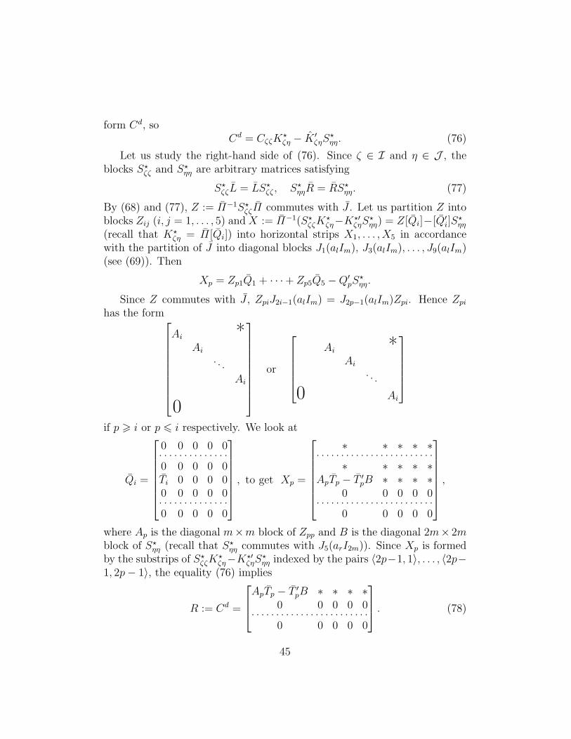
form Cd, soCd = CζζK

⋆ζη − K ′

ζηS⋆ηη. (76)

Let us study the right-hand side of (76). Since ζ ∈ I and η ∈ J , theblocks S⋆ζζ and S⋆ηη are arbitrary matrices satisfying

S⋆ζζL = LS⋆ζζ, S⋆ηηR = RS⋆ηη. (77)

By (68) and (77), Z := Π−1S⋆ζζΠ commutes with J . Let us partition Z intoblocks Zij (i, j = 1, . . . , 5) andX := Π−1(S⋆ζζK

⋆ζη−K

⋆′ζηS

⋆ηη) = Z[Qi]−[Q′

i]S⋆ηη

(recall that K⋆ζη = Π[Qi]) into horizontal strips X1, . . . , X5 in accordance

with the partition of J into diagonal blocks J1(alIm), J3(alIm), . . . , J9(alIm)(see (69)). Then

Xp = Zp1Q1 + · · ·+ Zp5Q5 −Q′pS

⋆ηη.

Since Z commutes with J , ZpiJ2i−1(alIm) = J2p−1(alIm)Zpi. Hence Zpihas the form

Ai *Ai

. . .

Ai

0

or

Ai *Ai

. . .

0 Ai

if p > i or p 6 i respectively. We look at

Qi =

0 0 0 0 0. . . . . . . . . . . . . .0 0 0 0 0Ti 0 0 0 00 0 0 0 0. . . . . . . . . . . . . .0 0 0 0 0

, to get Xp =

∗ ∗ ∗ ∗ ∗. . . . . . . . . . . . . . . . . . . . . . . .

∗ ∗ ∗ ∗ ∗ApTp − T ′

pB ∗ ∗ ∗ ∗0 0 0 0 0

. . . . . . . . . . . . . . . . . . . . . . . .0 0 0 0 0

,

where Ap is the diagonal m×m block of Zpp and B is the diagonal 2m× 2mblock of S⋆ηη (recall that S⋆ηη commutes with J5(arI2m)). Since Xp is formedby the substrips of S⋆ζζK

⋆ζη−K

⋆′ζηS

⋆ηη indexed by the pairs 〈2p−1, 1〉, . . . , 〈2p−

1, 2p− 1〉, the equality (76) implies

R := Cd =

ApTp − T ′pB ∗ ∗ ∗ ∗

0 0 0 0 0. . . . . . . . . . . . . . . . . . . . . . . .

0 0 0 0 0

. (78)

45

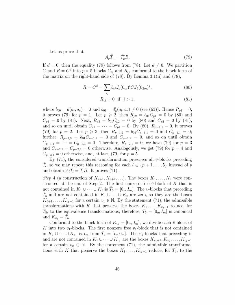
Let us prove thatApTp = T ′

pB. (79)

If d = 0, then the equality (79) follows from (78). Let d 6= 0. We partitionC and R = Cd into p× 5 blocks Cij and Rij conformal to the block form ofthe matrix on the right-hand side of (78). By Lemma 3.1(ii) and (78),

R = Cd =∑

ij

bijJp(0m)iCJ5(02m)j, (80)

Rij = 0 if i > 1, (81)

where b00 = d(al, ar) = 0 and b01 = d′y(al, ar) 6= 0 (see (63)). Hence Rp1 = 0,it proves (79) for p = 1. Let p > 2, then Rp2 = b01Cp1 = 0 by (80) andCp1 = 0 by (81). Next, Rp3 = b01Cp2 = 0 by (80) and Cp2 = 0 by (81),and so on until obtain Cp1 = · · · = Cp4 = 0. By (80), Rp−1,1 = 0, it proves(79) for p = 2. Let p > 3, then Rp−1,2 = b01Cp−1,1 = 0 and Cp−1,1 = 0;further, Rp−1,3 = b01Cp−1,2 = 0 and Cp−1,2 = 0, and so on until obtainCp−1,1 = · · · = Cp−1,3 = 0. Therefore, Rp−2,1 = 0; we have (79) for p = 3and Cp−2,1 = Cp−2,2 = 0 otherwise. Analogously, we get (79) for p = 4 andCp−3,1 = 0 otherwise, and, at last, (79) for p = 5.

By (71), the considered transformation preserves all v-blocks precedingTl, so we may repeat this reasoning for each l ∈ {p + 1, . . . , 5} instead of pand obtain AlTl = TlB. It proves (71).

Step 4 (a construction of Kv+1, Kv+2, . . .). The boxes K1, . . . , Kv were con-structed at the end of Step 2. The first nonzero free v-block of K that isnot contained in K1 ∪ · · · ∪Kv is T5 = [0m Im]. The v-blocks that precedingT5 and are not contained in K1 ∪ · · · ∪ Kv are zero, so they are the boxesKv+1, . . . , Kv1−1 for a certain v1 ∈ N. By the statement (71), the admissibletransformations with K that preserve the boxes K1, . . . , Kv1−1 reduce, forT5, to the equivalence transformations; therefore, T5 = [0m Im] is canonicaland Kv1 = T5.

Conformal to the block form of Kv1 = [0m Im], we divide each v-block ofK into two v1-blocks. The first nonzero free v1-block that is not containedin K1 ∪ · · · ∪Kv1 is Im from T4 = [Im 0m]. The v1-blocks that preceding itand are not contained in K1 ∪ · · · ∪Kv1 are the boxes Kv1+1, Kv2 , . . . , Kv2−1

for a certain v2 ∈ N. By the statement (71), the admissible transforma-tions with K that preserve the boxes K1, . . . , Kv2−1 reduce, for T4, to the

46

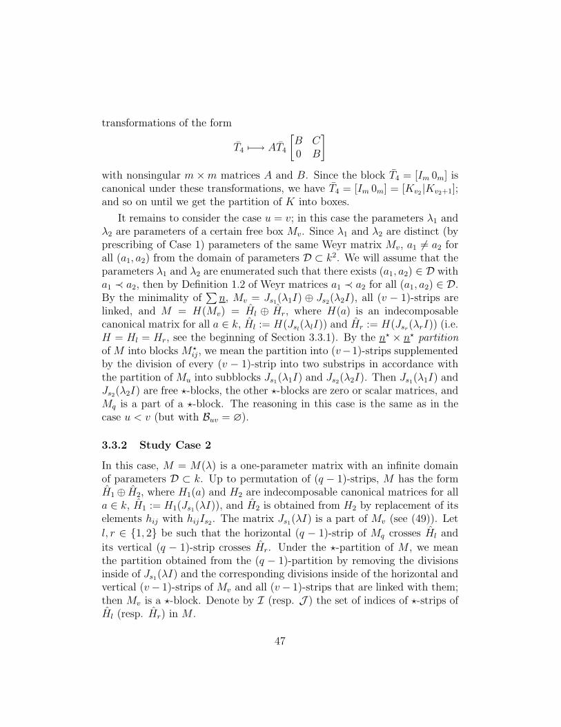
transformations of the form

T4 7−→ AT4

[B C0 B

]

with nonsingular m ×m matrices A and B. Since the block T4 = [Im 0m] iscanonical under these transformations, we have T4 = [Im 0m] = [Kv2 |Kv2+1];and so on until we get the partition of K into boxes.

It remains to consider the case u = v; in this case the parameters λ1 andλ2 are parameters of a certain free box Mv. Since λ1 and λ2 are distinct (byprescribing of Case 1) parameters of the same Weyr matrix Mv, a1 6= a2 forall (a1, a2) from the domain of parameters D ⊂ k2. We will assume that theparameters λ1 and λ2 are enumerated such that there exists (a1, a2) ∈ D witha1 ≺ a2, then by Definition 1.2 of Weyr matrices a1 ≺ a2 for all (a1, a2) ∈ D.By the minimality of

∑n, Mv = Js1(λ1I) ⊕ Js2(λ2I), all (v − 1)-strips are

linked, and M = H(Mv) = Hl ⊕ Hr, where H(a) is an indecomposablecanonical matrix for all a ∈ k, Hl := H(Jsl

(λlI)) and Hr := H(Jsr(λrI)) (i.e.

H = Hl = Hr, see the beginning of Section 3.3.1). By the n⋆ × n⋆ partitionof M into blocks M⋆

ij , we mean the partition into (v−1)-strips supplementedby the division of every (v − 1)-strip into two substrips in accordance withthe partition of Mu into subblocks Js1(λ1I) and Js2(λ2I). Then Js1(λ1I) andJs2(λ2I) are free ⋆-blocks, the other ⋆-blocks are zero or scalar matrices, andMq is a part of a ⋆-block. The reasoning in this case is the same as in thecase u < v (but with Buv = ∅).

3.3.2 Study Case 2

In this case, M = M(λ) is a one-parameter matrix with an infinite domainof parameters D ⊂ k. Up to permutation of (q − 1)-strips, M has the formH1 ⊕ H2, where H1(a) and H2 are indecomposable canonical matrices for alla ∈ k, H1 := H1(Js1(λI)), and H2 is obtained from H2 by replacement of itselements hij with hijIs2. The matrix Js1(λI) is a part of Mv (see (49)). Let

l, r ∈ {1, 2} be such that the horizontal (q − 1)-strip of Mq crosses Hl and

its vertical (q − 1)-strip crosses Hr. Under the ⋆-partition of M , we meanthe partition obtained from the (q − 1)-partition by removing the divisionsinside of Js1(λI) and the corresponding divisions inside of the horizontal andvertical (v− 1)-strips of Mv and all (v− 1)-strips that are linked with them;then Mv is a ⋆-block. Denote by I (resp. J ) the set of indices of ⋆-strips ofHl (resp. Hr) in M .

47

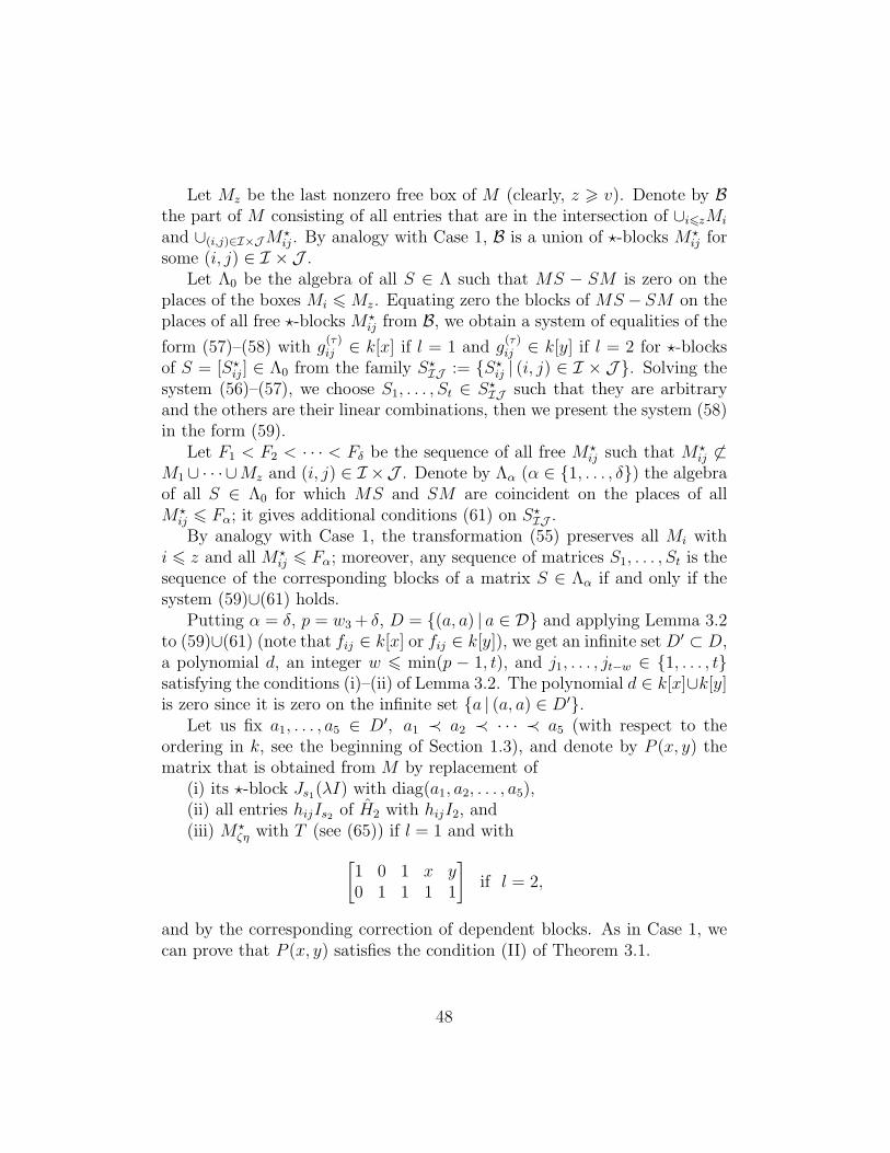
Let Mz be the last nonzero free box of M (clearly, z > v). Denote by Bthe part of M consisting of all entries that are in the intersection of ∪i6zMi

and ∪(i,j)∈I×JM⋆ij . By analogy with Case 1, B is a union of ⋆-blocks M⋆

ij forsome (i, j) ∈ I × J .

Let Λ0 be the algebra of all S ∈ Λ such that MS − SM is zero on theplaces of the boxes Mi 6 Mz. Equating zero the blocks of MS − SM on theplaces of all free ⋆-blocks M⋆

ij from B, we obtain a system of equalities of the

form (57)–(58) with g(τ)ij ∈ k[x] if l = 1 and g

(τ)ij ∈ k[y] if l = 2 for ⋆-blocks

of S = [S⋆ij ] ∈ Λ0 from the family S⋆IJ := {S⋆ij | (i, j) ∈ I × J }. Solving thesystem (56)–(57), we choose S1, . . . , St ∈ S⋆IJ such that they are arbitraryand the others are their linear combinations, then we present the system (58)in the form (59).

Let F1 < F2 < · · · < Fδ be the sequence of all free M⋆ij such that M⋆

ij 6⊂M1 ∪ · · · ∪Mz and (i, j) ∈ I ×J . Denote by Λα (α ∈ {1, . . . , δ}) the algebraof all S ∈ Λ0 for which MS and SM are coincident on the places of allM⋆

ij 6 Fα; it gives additional conditions (61) on S⋆IJ .By analogy with Case 1, the transformation (55) preserves all Mi with

i 6 z and all M⋆ij 6 Fα; moreover, any sequence of matrices S1, . . . , St is the

sequence of the corresponding blocks of a matrix S ∈ Λα if and only if thesystem (59)∪(61) holds.

Putting α = δ, p = w3 + δ, D = {(a, a) | a ∈ D} and applying Lemma 3.2to (59)∪(61) (note that fij ∈ k[x] or fij ∈ k[y]), we get an infinite set D′ ⊂ D,a polynomial d, an integer w 6 min(p − 1, t), and j1, . . . , jt−w ∈ {1, . . . , t}satisfying the conditions (i)–(ii) of Lemma 3.2. The polynomial d ∈ k[x]∪k[y]is zero since it is zero on the infinite set {a | (a, a) ∈ D′}.

Let us fix a1, . . . , a5 ∈ D′, a1 ≺ a2 ≺ · · · ≺ a5 (with respect to theordering in k, see the beginning of Section 1.3), and denote by P (x, y) thematrix that is obtained from M by replacement of

(i) its ⋆-block Js1(λI) with diag(a1, a2, . . . , a5),(ii) all entries hijIs2 of H2 with hijI2, and(iii) M⋆

ζη with T (see (65)) if l = 1 and with

[1 0 1 x y0 1 1 1 1

]

if l = 2,

and by the corresponding correction of dependent blocks. As in Case 1, wecan prove that P (x, y) satisfies the condition (II) of Theorem 3.1.

48

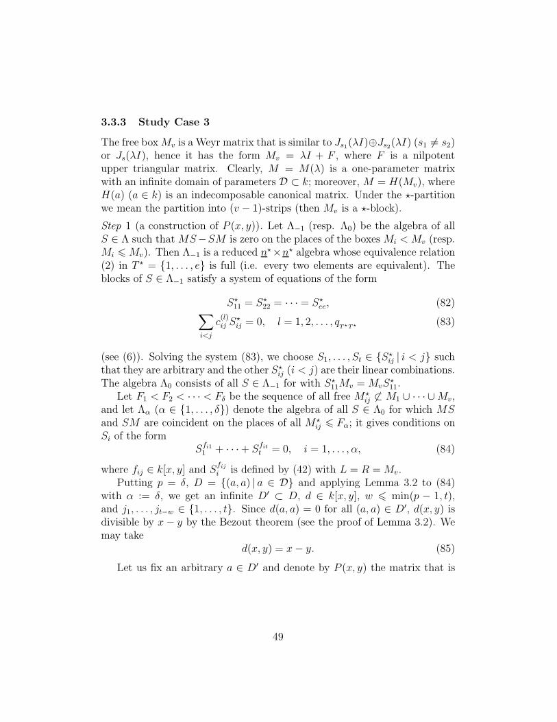
3.3.3 Study Case 3

The free boxMv is a Weyr matrix that is similar to Js1(λI)⊕Js2(λI) (s1 6= s2)or Js(λI), hence it has the form Mv = λI + F , where F is a nilpotentupper triangular matrix. Clearly, M = M(λ) is a one-parameter matrixwith an infinite domain of parameters D ⊂ k; moreover, M = H(Mv), whereH(a) (a ∈ k) is an indecomposable canonical matrix. Under the ⋆-partitionwe mean the partition into (v − 1)-strips (then Mv is a ⋆-block).

Step 1 (a construction of P (x, y)). Let Λ−1 (resp. Λ0) be the algebra of allS ∈ Λ such that MS−SM is zero on the places of the boxes Mi < Mv (resp.Mi 6 Mv). Then Λ−1 is a reduced n⋆×n⋆ algebra whose equivalence relation(2) in T ⋆ = {1, . . . , e} is full (i.e. every two elements are equivalent). Theblocks of S ∈ Λ−1 satisfy a system of equations of the form

S⋆11 = S⋆22 = · · · = S⋆ee, (82)∑

i<j

c(l)ij S

⋆ij = 0, l = 1, 2, . . . , q

T⋆T⋆ (83)

(see (6)). Solving the system (83), we choose S1, . . . , St ∈ {S⋆ij | i < j} suchthat they are arbitrary and the other S⋆ij (i < j) are their linear combinations.The algebra Λ0 consists of all S ∈ Λ−1 for with S⋆11Mv = MvS

⋆11.

Let F1 < F2 < · · · < Fδ be the sequence of all free M⋆ij 6⊂ M1 ∪ · · · ∪Mv,

and let Λα (α ∈ {1, . . . , δ}) denote the algebra of all S ∈ Λ0 for which MSand SM are coincident on the places of all M⋆

ij 6 Fα; it gives conditions onSi of the form

Sfi11 + · · ·+ Sfit

t = 0, i = 1, . . . , α, (84)

where fij ∈ k[x, y] and Sfij

i is defined by (42) with L = R = Mv.Putting p = δ, D = {(a, a) | a ∈ D} and applying Lemma 3.2 to (84)

with α := δ, we get an infinite D′ ⊂ D, d ∈ k[x, y], w 6 min(p − 1, t),and j1, . . . , jt−w ∈ {1, . . . , t}. Since d(a, a) = 0 for all (a, a) ∈ D′, d(x, y) isdivisible by x− y by the Bezout theorem (see the proof of Lemma 3.2). Wemay take

d(x, y) = x− y. (85)

Let us fix an arbitrary a ∈ D′ and denote by P (x, y) the matrix that is

49

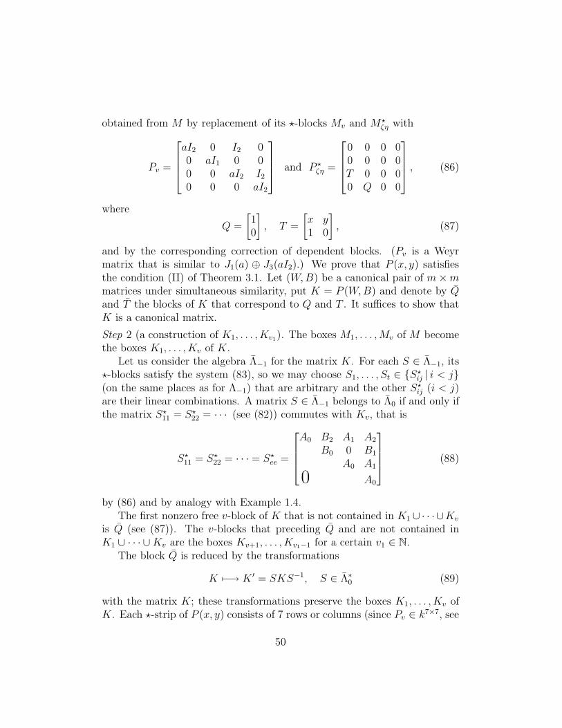
obtained from M by replacement of its ⋆-blocks Mv and M⋆ζη with

Pv =

aI2 0 I2 00 aI1 0 00 0 aI2 I20 0 0 aI2

and P ⋆ζη =

0 0 0 00 0 0 0T 0 0 00 Q 0 0

, (86)

where

Q =

[10

]

, T =

[x y1 0

]

, (87)

and by the corresponding correction of dependent blocks. (Pv is a Weyrmatrix that is similar to J1(a) ⊕ J3(aI2).) We prove that P (x, y) satisfiesthe condition (II) of Theorem 3.1. Let (W,B) be a canonical pair of m×mmatrices under simultaneous similarity, put K = P (W,B) and denote by Qand T the blocks of K that correspond to Q and T . It suffices to show thatK is a canonical matrix.

Step 2 (a construction of K1, . . . , Kv1). The boxes M1, . . . ,Mv of M becomethe boxes K1, . . . , Kv of K.

Let us consider the algebra Λ−1 for the matrix K. For each S ∈ Λ−1, its⋆-blocks satisfy the system (83), so we may choose S1, . . . , St ∈ {S⋆ij | i < j}(on the same places as for Λ−1) that are arbitrary and the other S⋆ij (i < j)are their linear combinations. A matrix S ∈ Λ−1 belongs to Λ0 if and only ifthe matrix S⋆11 = S⋆22 = · · · (see (82)) commutes with Kv, that is

S⋆11 = S⋆22 = · · · = S⋆ee =

A0 B2 A1 A2

B0 0 B1

A0 A1

0 A0

(88)

by (86) and by analogy with Example 1.4.The first nonzero free v-block of K that is not contained in K1 ∪ · · · ∪Kv

is Q (see (87)). The v-blocks that preceding Q and are not contained inK1 ∪ · · · ∪Kv are the boxes Kv+1, . . . , Kv1−1 for a certain v1 ∈ N.

The block Q is reduced by the transformations

K 7−→ K ′ = SKS−1, S ∈ Λ∗0 (89)

with the matrix K; these transformations preserve the boxes K1, . . . , Kv ofK. Each ⋆-strip of P (x, y) consists of 7 rows or columns (since Pv ∈ k7×7, see

50

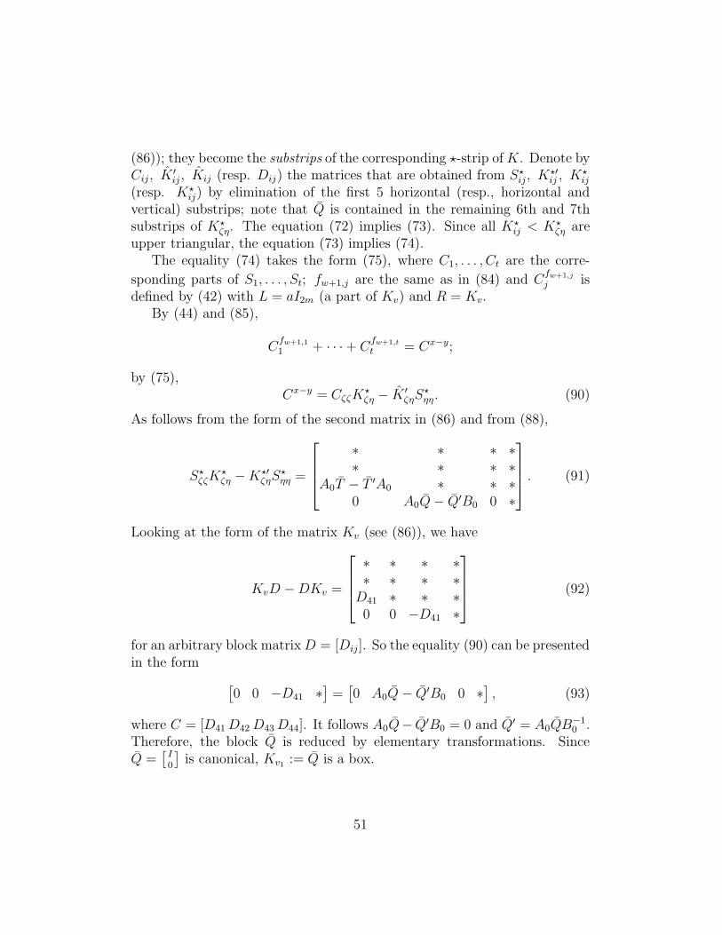
(86)); they become the substrips of the corresponding ⋆-strip ofK. Denote byCij, K

′ij , Kij (resp. Dij) the matrices that are obtained from S⋆ij, K

⋆′ij , K

⋆ij

(resp. K⋆ij) by elimination of the first 5 horizontal (resp., horizontal and

vertical) substrips; note that Q is contained in the remaining 6th and 7thsubstrips of K⋆

ζη. The equation (72) implies (73). Since all K⋆ij < K⋆

ζη areupper triangular, the equation (73) implies (74).

The equality (74) takes the form (75), where C1, . . . , Ct are the corre-

sponding parts of S1, . . . , St; fw+1,j are the same as in (84) and Cfw+1,j

j isdefined by (42) with L = aI2m (a part of Kv) and R = Kv.

By (44) and (85),

Cfw+1,1

1 + · · · + Cfw+1,t

t = Cx−y;

by (75),Cx−y = CζζK

⋆ζη − K ′

ζηS⋆ηη. (90)

As follows from the form of the second matrix in (86) and from (88),

S⋆ζζK⋆ζη −K⋆′

ζηS⋆ηη =

∗ ∗ ∗ ∗∗ ∗ ∗ ∗

A0T − T ′A0 ∗ ∗ ∗0 A0Q− Q′B0 0 ∗

. (91)

Looking at the form of the matrix Kv (see (86)), we have

KvD −DKv =

∗ ∗ ∗ ∗∗ ∗ ∗ ∗D41 ∗ ∗ ∗0 0 −D41 ∗

(92)

for an arbitrary block matrixD = [Dij]. So the equality (90) can be presentedin the form

[0 0 −D41 ∗

]=

[0 A0Q− Q′B0 0 ∗

], (93)

where C = [D41D42 D43D44]. It follows A0Q− Q′B0 = 0 and Q′ = A0QB−10 .

Therefore, the block Q is reduced by elementary transformations. SinceQ =

[I0

]is canonical, Kv1 := Q is a box.

51

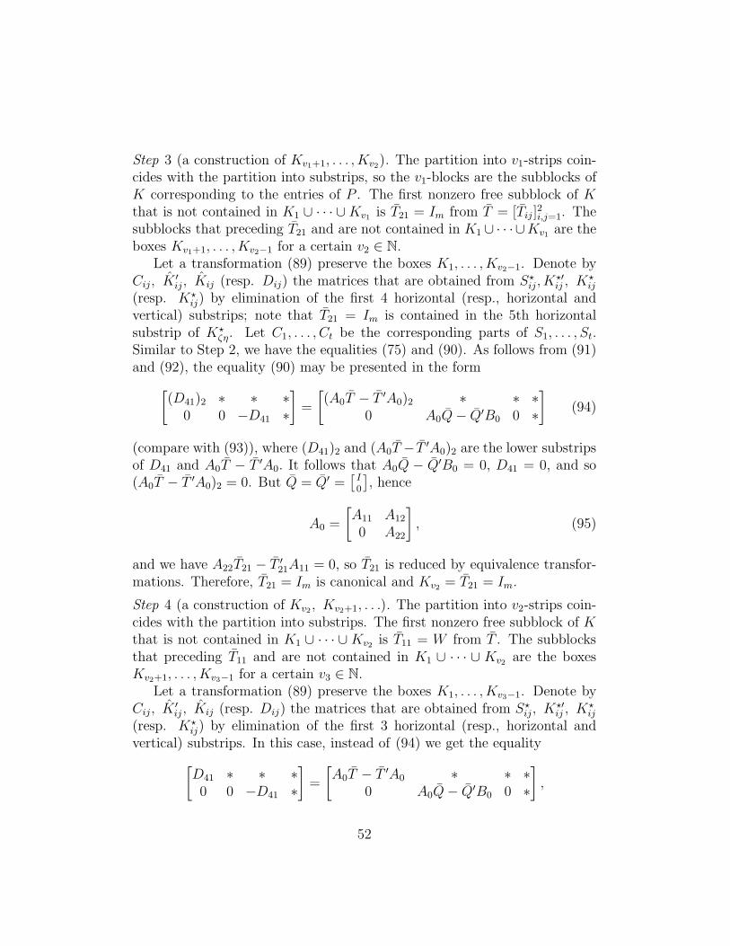
Step 3 (a construction of Kv1+1, . . . , Kv2). The partition into v1-strips coin-cides with the partition into substrips, so the v1-blocks are the subblocks ofK corresponding to the entries of P . The first nonzero free subblock of Kthat is not contained in K1 ∪ · · · ∪Kv1 is T21 = Im from T = [Tij ]

2i,j=1. The

subblocks that preceding T21 and are not contained in K1 ∪ · · · ∪Kv1 are theboxes Kv1+1, . . . , Kv2−1 for a certain v2 ∈ N.

Let a transformation (89) preserve the boxes K1, . . . , Kv2−1. Denote byCij, K

′ij, Kij (resp. Dij) the matrices that are obtained from S⋆ij, K

⋆′ij , K

⋆ij

(resp. K⋆ij) by elimination of the first 4 horizontal (resp., horizontal and

vertical) substrips; note that T21 = Im is contained in the 5th horizontalsubstrip of K⋆

ζη. Let C1, . . . , Ct be the corresponding parts of S1, . . . , St.Similar to Step 2, we have the equalities (75) and (90). As follows from (91)and (92), the equality (90) may be presented in the form

[(D41)2 ∗ ∗ ∗

0 0 −D41 ∗

]

=

[(A0T − T ′A0)2 ∗ ∗ ∗

0 A0Q− Q′B0 0 ∗

]

(94)

(compare with (93)), where (D41)2 and (A0T − T ′A0)2 are the lower substripsof D41 and A0T − T ′A0. It follows that A0Q − Q′B0 = 0, D41 = 0, and so(A0T − T ′A0)2 = 0. But Q = Q′ =

[I0

], hence

A0 =

[A11 A12

0 A22

]

, (95)

and we have A22T21 − T ′21A11 = 0, so T21 is reduced by equivalence transfor-

mations. Therefore, T21 = Im is canonical and Kv2 = T21 = Im.

Step 4 (a construction of Kv2 , Kv2+1, . . .). The partition into v2-strips coin-cides with the partition into substrips. The first nonzero free subblock of Kthat is not contained in K1 ∪ · · · ∪Kv2 is T11 = W from T . The subblocksthat preceding T11 and are not contained in K1 ∪ · · · ∪ Kv2 are the boxesKv2+1, . . . , Kv3−1 for a certain v3 ∈ N.

Let a transformation (89) preserve the boxes K1, . . . , Kv3−1. Denote byCij, K

′ij , Kij (resp. Dij) the matrices that are obtained from S⋆ij, K

⋆′ij , K

⋆ij

(resp. K⋆ij) by elimination of the first 3 horizontal (resp., horizontal and

vertical) substrips. In this case, instead of (94) we get the equality

[D41 ∗ ∗ ∗0 0 −D41 ∗

]

=

[A0T − T ′A0 ∗ ∗ ∗

0 A0Q− Q′B0 0 ∗

]

,

52

so A0T − T ′A0 = 0, where A0 is of the form (95). Since [T21 T22] = [T ′21 T

′22] =

[Im 0m], we have A11 = A22 and A12 = 0, so A11T11 − T ′11A11 = 0 and T11 is

reduced by similarity transformations. Since T11 = W is a Weyr matrix, itis canonical and Kv3 = W .

Furthermore, A11T12 − T ′12A11 = 0, where A11 commutes with W , hence

T12 = B is canonical too. It proves that K is a canonical matrix.

3.4 Proof of Theorem 3.1 for tame problems

In this section, we consider a matrix problem given by (Γ, M) for which thereexists no semi-parametric canonical matrix M having a free box Mq 6= ∅ withthe property (49). Our purpose is to prove that the matrix problem satisfiesthe condition (I) of Theorem 3.1.

Let n be a step-sequence. By Remark 2.1, the number of parametriccanonical n× n matrices is finite. Let M be a parametric canonical n× nmatrix and one of its parameters is a finite parameter λ; that is, the set of λ-components in the domain of parameters is a finite set {a1, . . . , ar}. Puttingλ = a1, . . . , ar gives r semi-parametric canonical matrices. Repeating thisprocedure, we obtain a finite number of semi-parametric canonical n× nmatrices having only infinite parameters or having no parameters.

Let M be an indecomposable semi-parametric canonical n× n matrixthat has no finite parameters but has infinite parameters, and let Mv be thefirst among its boxes with parameters (then Mv is free). By the property(49), if a v-strip is linked with a v-strip containing a parameter λ from Mv,then it does not contain a free box Mi > Mv such that Mi 6= ∅. Since Mis indecomposable, it follows that all its v-strips are linked, all free boxesMi > Mv are equal to ∅, and Mv = Jm(λ). Hence, all free v-blocks exceptingMv are scalar matrices and M = L(Jm(λ)), where L(λ) = [aij + λbij ] is asemi-parametric canonical matrix with a free 1× 1 box Mv = [λ] and all freeboxes after it are 1 × 1 matrices of the form ∅.

Let Dm ⊂ k be the domain of parameters of M . By the property (49),Dm is a cofinite set (i.e. k \ Dm is finite).

If a /∈ Dm, then the matrix M(a) is canonical and there exists a free boxMq > Mv such that Mq 6= ∅. This box Mq is the zero 1 × 1 matrix. SinceM is indecomposable, all its rows and columns are linked, so Mq is reducedby similarity transformations. Replacing it by the parametric box [µ], weobtain a straight line of indecomposable canonical matrices that intersects{M(λ) | λ ∈ k} at the point M(a). Hence, each M(a), a /∈ Dm, is a point

53

of intersection of {M(λ) | λ ∈ k} with a straight line of indecomposablecanonical matrices.

LetM(a), a ∈ Dm, be a point of intersection too; that is, there exists a line{N(µ) |µ ∈ k} of indecomposable canonical matrices such that M(a) = N(b)for a certain b ∈ k. Then M(λ) has a free box Mu (u < v) that is a Weyrmatrix, b is its eigenvalue, and N(µ) is obtained from M(a) by replacementof b with µ. Since M(λ) and N(µ) coincide on M1 ∪ · · · ∪Mu−1, Mu = Nu

for µ = b. By analogy with the structure of M(λ), all free boxes Ni > Nu

are zero, hence Mv = 0 if λ = a. Since Mv = Jm(λ), M(a) with a ∈ Dm canbe a point of intersection only if m = 1 and λ = 0.

Replacing m by an arbitrary integer n gives a new semi-parametric canon-ical matrix L(Jn(λ)) with the domain of parameters Dn. To prove that thecondition (I) of Theorem 3.1 holds, it suffices to show that Dm = Dn. More-over, it suffices to show that Dm = D1.

Let first a ∈ D1. By analogy with Section 3.3.3, under the ⋆-partition wemean the partition into (v − 1)-strips. Then a ∈ Dm if and only if all free⋆-blocks after Mv in M(a) are ∅. The ⋆-blocks of every S ∈ Λ∗

−1 (see Section3.3.3) satisfy the system (82)–(83), where clij do not depend on m and a.Solving the system (83), we choose S1, . . . , St ∈ {S⋆ij | i < j} such that theyare arbitrary and the other S⋆ij (i < j) are their linear combinations.

Let F1 < F2 < · · · < Fδ be the sequence of all free M⋆ij 6⊂ M1 ∪ · · · ∪Mv

and let K be obtained from M by replacing F1, . . . , Fδ with arbitrary m×mmatrices G1, . . . , Gδ. To prove that a ∈ Dm, we must show that F1 = · · · =Fδ = ∅ for M(a); that is, there exists S ∈ Λ∗

0 such that G′1 = · · · = G′

δ = 0in K ′ := SKS−1. It suffices to consider the case G1 = · · · = Gq−1 = 0 6= Gq

(q ∈ {1, . . . , δ}) and to show that there exists S ∈ Λ∗−1 with S⋆11 = S⋆22 =

· · · = Im (then S ∈ Λ∗0) such that G′

1 = · · · = G′q−1 = G′

q = 0. It means thatthe ⋆-blocks S1, . . . , St of S satisfy the system of equations that is obtainedby equating in K ′S = SK the blocks on the places of G1, . . . , Gq:

Sfl11 + · · · + Sflt

t = 0, l = 1, . . . , q − 1, (96)

Sfq1

1 + · · · + Sfqt

t = Gϕq , (97)

where ϕ(a, a) 6= 0 and Sfij

j is defined by (42) with L = R = Jm(a). Notethat the polynomials fij are the same for all m ∈ N and a.

54

Taking 1 instead of m, we obtain the system

fl1(a, a)s1 + · · ·+ flt(a, a)st = 0, l = 1, . . . , q − 1,

fq1(a, a)s1 + · · ·+ fqt(a, a)st = g.

Since a ∈ D1, this system is solvable with respect to s1, . . . , st for all g ∈ k.It holds for all q, so the rows of F := [fij(a, a)] are linearly independent.

Let Sr = [s(r)ij ]mi,j=1 and Gϕ

q = [gij]mi,j=1. Since L = R = Jm(a), the system

of q matrix equations (96)–(97) is equivalent to the m2 systems of q linearequations relatively to the entries of S1, . . . , St, each of them is obtained byequating the (i, j) entries for the corresponding i, j ∈ {1, . . . , m} and has theform:

fl1(a, a)s(1)ij + · · ·+ flt(a, a)s

(t)ij = d

(l)ij , l = 1, . . . , q, (98)

where d(l)ij is a linear combination of s

(1)i′j′, . . . , s

(t)i′j′, (i′, j′) ∈ {(1, j), . . . , (i −

1, j)} ∪ {(i, j + 1), (i, j + 2), . . .}, and (only if l = q) gij. Since the rows ofF = [fij(a, a)] are linearly independent, the system (98) for (i, j) = (m, 1)

is solvable. Let sm1 = (s(1)m1, . . . , s

(t)m1) be its solution. Knowing sm1, we

calculate d(l)m−1,1 and d

(l)m2, then solve the system (98) for (i, j) = (m − 1, 1)

and for (i, j) = (m, 2). We next calculate d(l)ij , i − j = m − 2, and solve

(98) for (i, j) = (m − 2, 1), (m − 1, 2), (m, 3), and so on, until we obtain asolution S1, . . . , St of (96), a contradiction. Hence a ∈ Dm, which clearlyimplies a ∈ D1. It proves Theorem 3.1.

Remark 3.1. We can give a more precise description of the set of canonicalmatrices based on the proof of Theorem 3.1. For simplicity, we restrictourselves to the case M = kt×t.

Namely, a linear matrix problem given by a pair (Γ, kt×t) satisfies oneand only one of the following two conditions (respectively, is of tame or wildtype):

(I) For every step-sequence n, there exists a finite set of semi-parametriccanonical n × n matrices Mn,i(λ), i = 1, . . . , tn, whose domains of pa-rameters Dn,i are cofinite subsets in k and

(a) for every m > 1, Mn,i(Jm(λ)) is a semi-parametric canonical ma-trix with the same domain of parameters Dn,i and the followingpartition into boxes: Jm(λ) is a box, all boxes preceding it arethe scalar matrices B1⊗Im, . . . , Bl⊗Im (where B1, . . . , Bl are the

55

boxes of Mn,i(λ) preceding [λ]), and all boxes after it are the 1×1matrices ∅;

(b) for every n′, the set of matrices of the form Mn,i(Jm(a)), mn = n′,a ∈ Dn,i, is a cofinite subset in the set of indecomposable canonicaln′ × n′ matrices.

(II) There exists a semi-parametric canonical n×nmatrix P (α, β) (in whichtwo entries are the parameters α and β and the other entries are ele-ments of k) such that

(a) two pairs of m×m matrices (A,B) and (C,D) are similar if andonly if P (A,B) ≃ P (C,D); moreover,

(b) a pair of m×m matrices (A, B) is canonical under similarity (seeDefinition 1.4) if and only if the mn × mn matrix P (A, B) iscanonical.

Acknowledgements

I wish to thank P. Gabriel, L. A. Nazarova, A. V. Roiter, and D. Vossieck; ajoint work on the article [17] was a great inspiration for me and introducedme to the theory of tame and wild matrix problems. The idea to prove theTame–Wild Theorem using Belitskiı’s algorithm came from this work andwas first discussed in my talks at the Zurich University in 1993 by invitationof P. Gabriel.

I wish to thank C. M. Ringel for the invitations to speak on the contentsof this paper at the University of Bielefeld in 1998–1999 and stimulatingdiscussions, and for the publication of the preprint [32].

I am grateful to G. R. Belitskiı, T. Brustle, Yu. A. Drozd, S. Friedland,D. I. Merino, and the referee for helpful suggestions and comments.

The work was partially supported by the Long-Term Research Grant No.U6E000 of the International Science Foundation and by Grant No. UM1-314of the U.S. Civilian Research and Development Foundation for the Indepen-dent States of the Former Soviet Union.

References

[1] H. Bass, Algebraic K-theory, Benjamin, New York, 1968.

56

[2] G. R. Belitskiı, Normal forms in a space of matrices, in Analysis inInfinite-Dimensional Spaces and Operator Theory (V. A. Marchenko,Ed.), Naukova Dumka, Kiev, 1983, pp. 3–15 (in Russian).

[3] G. R. Belitskiı, Normal forms in matrix spaces, Integral Equations andOperator Theory, 38 (no. 3) (2000) 251–283.

[4] K. I. Belousov, L. A. Nazarova, A. V. Roiter, and V. V. Sergeichuk, El-ementary and multi-elementary representations of vectroids, UkrainianMath. J. 47 (1995) 1661–1687.

[5] T. Brustle, On the growth function of tame algebra, C. R. Acad. Sci.Paris 322 (Serie I) (1996) 211–215.

[6] W. W. Crawley-Boevey, On tame algebras and bocses, Proc. LondonMath. Soc. 56 (1988) 451–483.

[7] W. W. Crawley-Boevey, Tame algebras and generic modules, Proc. Lon-don Math. Soc. 63 (1991) 241–265.

[8] P. Donovan and M. R. Freislich, Some evidence for an extension ofthe Brauer–Thrall conjecture, Sonderforschungsbereich Theor. Math. 40(1972) 24–26.

[9] P. Donovan and M. R. Freislich, The representation theory of finitegraphs and associated algebras, Carleton Lecture Notes 5, Ottawa, 1973.

[10] Yu. A. Drozd, On tame and wild matrix problems, in Matrix Problems(Yu. A. Mitropol’skiı, Ed.), Inst. Mat. Akad. Nauk Ukrain. SSR, Kiev,1977, pp. 104–114 (in Russian).

[11] Yu. A. Drozd, Tame and wild matrix problems, in Representations andQuadratic Forms (Yu. A. Mitropol’skiı, Ed.), Inst. Mat. Akad. NaukUkrain. SSR, Kiev, 1979, pp. 39–74 (in Russian).

[12] Yu. A. Drozd, Tame and wild matrix problems, Lect. Notes Math. 832(1980) 242–258.

[13] Yu. A. Drozd and V. V. Kirichenko, Finite Dimensional Algebras,Springer-Verlag, 1994.

57

[14] S. Friedland, Analytic similarity of matrices, Lectures in Appl. Math.18, Amer. Math. Soc., 1980, pp. 43–85.

[15] S. Friedland, Simultaneous similarity of matrices, Adv. Math. 50 (1983)189–265.

[16] P. Gabriel, Unzerlegbare Darstellungen I, Manuscripta Math. 6 (1972)71–103.

[17] P. Gabriel, L. A. Nazarova, A. V. Roiter, V. V. Sergeichuk, and D.Vossieck, Tame and wild subspace problems, Ukrainian Math. J. 45(1993) 335–372.

[18] P. Gabriel and A. V. Roiter, Representations of finite-dimensional al-gebras, Encyclopaedia of Math. Sci., Vol 73 (Algebra VIII), Springer-Verlag, 1992.

[19] F. R. Gantmacher, The Theory of Matrices, Vol. 1, Chelsea, New York,1959.

[20] P. Griffits and J. Harris, Principles of Algebraic Geometry, A Wiley-Interscience Publications, New York, 1978.

[21] D. E. Littlewood, On unitary equivalence, J. London Math. Soc. 28(1953) 314–322.

[22] L. A. Nazarova, Representations of quivers of infinite type, Math. USSRIzv. 7 (1973) 749–792.

[23] L. A. Nazarova, Partially ordered sets of infinite type, Math. USSR Izv.9 (1975) 911–938.

[24] L. A. Nazarova and A. V. Roiter, Representations of partially orderedsets, J. Soviet Math. 3 (1975) 585–606.

[25] C. M. Ringel, Tame Algebras and Integral Quadratic Forms, Lect. NotesMath. 1099, Springer, 1984.

[26] A. V. Roiter, Matrix problems and representations of bocses, Inst. Mat.Ukrain. Akad. Nauk, Kiev, 1979, pp. 3–38; English transl., Lect. NotesMath. 831 (1980) 288–324.

58

[27] A. V. Roiter, Bocses with involution, in Representations and QuadraticForms, Inst. Mat. Ukrain. Akad. Nauk, Kiev, 1979, pp. 124–126 (inRussian).

[28] V. V. Sergeichuk, Classification of linear operators in a finite dimensionalunitary space, Functional Anal. Appl. 18 (no. 3) (1984) 224–230.

[29] V. V. Sergeichuk, Classification problems for systems of forms and linearmappings, Math. USSR Izvestiya, 31 (no. 3) (1988) 481–501.

[30] V. V. Sergeichuk, A remark on the classification of holomorphic matricesup to similarity, Functional Anal. Appl. 25 (no. 2) (1991) 135.

[31] V. V. Sergeichuk, Unitary and Euclidean representations of a quiver,Linear Algebra Appl. 278 (1998) 37–62.

[32] V. V. Sergeichuk, Canonical Matrices for Linear Matrix Problems,Preprint 99-070 of SFB 343, Bielefeld University, 1999, 43 p.

[33] V. V. Sergeichuk and D. V. Galinskiı, Classification of pairs of linearoperators in a four-dimensional vector space, in Infinite Groups andRelated Algebraic Structures, Inst. Mat. Ukrain. Akad. Nauk, Kiev, 1993,pp. 413–430 (in Russian).

[34] H. Shapiro, A survey of canonical forms and invariants for unitary sim-ilarity, Linear Algebra Appl. 147 (1991) 101–167.

[35] H. Shapiro, The Weyr characteristic, Amer. Math. Monthly 106 (no. 10)(1999) 919–929.

[36] D. Simson, Linear Representations of Partially Ordered Sets and VectorSpace Categories, Algebra Logic Appl. 4, Gordon and Breach, 1992.

[37] P. Thijsse, Upper triangular similarity of upper triangular matrices, Lin-ear Algebra Appl. 260 (1997) 119–149.

[38] E. Weyr, Repartition des matrices en especes et formation de toutes lesespeces, C. R. Acad. Sci. Paris 100 (1885) 966–969.

59