Copyright 2017 (C) Lamsim Enterprises / Polar Instruments Applying the Cannonball Stack Principle to the Huray Roughness Model in Polar Si9000e This note explains how Cannonball interprets the Rz to provide Huray parameters for Si9000e. However, from version18:05 onwards all the math below is built into Si9000e – all you need to do is provide the correct Rz and select the Cannonball method. In addition to the Hammerstad and Groisse models for predicting the additional attenuation due to surface roughness, Polar Si9000e 2017 and onwards field solver now offers the Huray. Since a Polar Application Note AP8155 has already discussed the use of the Hammerstad and Groisse approach for modeling surface roughness in Si9000e, it will not be covered here. This application note will focus on applying the Cannonball model [1] to determine the input parameters needed for Huray roughness model in Si9000e using data provided solely by manufactures’ data sheets. Background: In recent years, the Huray model [2] has gained popularity due to the continually increasing data rate’s need for better modeling accuracy. It takes a real world physics approach to explain losses due to surface roughness. The model is based on a non-uniform distribution of spherical shapes resembling “snowballs” and stacked together forming a pyramidal geometry. Image courtesy Circuit Foil Luxembourg By applying electromagnetic wave analysis, the superposition of the sphere losses can be used to calculate the total loss of the structure. Since the losses are proportional to the surface area of the roughness profile, an accurate estimation of a roughness correction factor (KSRH) can be analytically solved by [2]: Equation 1 2 2 1 2 4 3 2 ( ) ( ) 1 2 i i j flat matte SRH i flat i i N r A A K f A f f r r Where: KSRH (f) = roughness correction factor, as a function of frequency, due to surface roughness based on the Huray model;

Welcome message from author
This document is posted to help you gain knowledge. Please leave a comment to let me know what you think about it! Share it to your friends and learn new things together.
Transcript

Copyright 2017 (C) Lamsim Enterprises / Polar Instruments
Applying the Cannonball Stack Principle to the Huray Roughness Model in Polar Si9000e This note explains how Cannonball interprets the Rz to provide Huray parameters for Si9000e. However, from version18:05 onwards all the math below is built into Si9000e – all you need to do is provide the correct Rz and select the Cannonball method.
In addition to the Hammerstad and Groisse models for predicting the additional attenuation due to surface roughness, Polar Si9000e 2017 and onwards field solver now offers the Huray. Since a Polar Application Note AP8155 has already discussed the use of the Hammerstad and Groisse approach for modeling surface roughness in Si9000e, it will not be covered here. This application note will focus on applying the Cannonball model [1] to determine the input parameters needed for Huray roughness model in Si9000e using data provided solely by manufactures’ data sheets.
Background:
In recent years, the Huray model [2] has gained popularity due to the continually increasing data rate’s need for better modeling accuracy. It takes a real world physics approach to explain losses due to surface roughness. The model is based on a non-uniform distribution of spherical shapes resembling “snowballs” and stacked together forming a pyramidal geometry.
Image courtesy Circuit Foil Luxembourg
By applying electromagnetic wave analysis, the superposition of the sphere losses can be used to calculate the total loss of the structure. Since the losses are proportional to the surface area of the roughness profile, an accurate estimation of a roughness correction factor (KSRH) can be analytically solved by [2]:
Equation 1
2
21
2
4
3
2 ( ) ( )1
2
i i
jflatmatte
SRH
iflat
i i
N r
AAK f
A f f
r r
Where:
KSRH (f) = roughness correction factor, as a function of frequency, due to surface roughness based on the Huray model;

Copyright 2017 (C) Lamsim Enterprises / Polar Instruments 2
𝐴𝑚𝑎𝑡𝑡𝑒
𝐴𝑓𝑙𝑎𝑡 = relative area of the matte base compared to a flat surface;
ri = radius of the copper sphere (snowball) of the ith size, in meters; 𝑁𝑖
𝐴𝑓𝑙𝑎𝑡 = number of copper spheres of the ith size per unit flat area in sq. meters;
δ (f) = skin-depth, as a function of frequency, in meters. It is theoretically possible to build an accurate snowball model of the surface roughness by extracting parameters through detailed analysis of scanning electron microscopy (SEM) photographs. But practically, it is beyond the capabilities of most companies who do not have access to such equipment. Even if such equipment were available, the size, number of spheres and general tooth shape must be approximated anyways and fitted to measured data to get accurate results. This leads us into the Cannonball model. Using the concept of cubic close-packing of equal spheres, the radius of the spheres (ri) and tile area (Aflat) parameters for the Huray model can now be estimated solely by the roughness parameters published in manufacturers’ data sheets [1]. Recalling that losses are proportional to the surface area of the roughness profile, the Cannonball model can be used to optimally represent the surface roughness. As illustrated below there are three rows of spheres stacked on a square tile base. Nine spheres are on the first row, four spheres in the middle row, and one sphere on top. The height of the Cannonball stack is equal to the 10-point mean roughness RZ as published in foil manufacturer’s datasheet.
Image Courtesy Lamsim Enterprises Inc.
Because the Cannonball model assumes the ratio of Amatte/Aflat = 1, and there are only 14 spheres, the sphere radius can be approximated as: Equation 2
16.73
zRr
Where: Rz is the 10-point mean roughness as published in foil manufacturer’s data sheet.

Copyright 2017 (C) Lamsim Enterprises / Polar Instruments 3
And the area of the square flat base is: Equation 3
2
6flatA r
Example:
The best way to show how to apply the Cannonball model is working through a detailed example test case. An offset stripline geometry and data sheet parameters from [1] are summarized in Table 1. The PCB was fabricated with Isola FR408HR material and reverse treated (RT) 1oz. foil. The dielectric constant (Dk) and dissipation factor (Df), at 10GHz for FR408HR 3313 material, were obtained from Isola’s data sheet. The default foil used on FR408HR core laminates is MLS, Grade 3, controlled elongation RT foil from Oak-Mitsui.
Table 1
Test board parameters obtained from manufacturers’ data sheets and design objective.
Parameter FR408HR / RTF
Dk Core/Prepreg 3.65/3.59 @10GHz
Df Core/Prepreg 0.0094/0.0095 @ 10GHz
Rz Drum side 3.175 μm
Rz Matte side before Micro-etch 5.715 μm
Rz Matte side after Micro-etch 4.443 μm
Trace Thickness, t 31.730 μm
Trace Width, w 11 mils (279.20 μm)
Core thickness, H1 12 mils (304.60 μm)
Prepreg thickness, H2 10.6 mils (269.00 μm)
GMS trace length 6 in (15.23 cm)

Copyright 2017 (C) Lamsim Enterprises / Polar Instruments 4
1. The first step is to input the offset stripline geometry parameters using 1B1A input panel under the “Lossless Calculation” tab at the bottom of the Si9000e window. Worst case etch factor is assumed as W2 = W1-T1.

Copyright 2017 (C) Lamsim Enterprises / Polar Instruments 5
2. Next, select the “Frequency Dependent Calculation” tab at the bottom of the input panel.
Enter the line length, conductivity and frequencies.
Copyright 2017 (C) Lamsim Enterprises / Polar Instruments 6
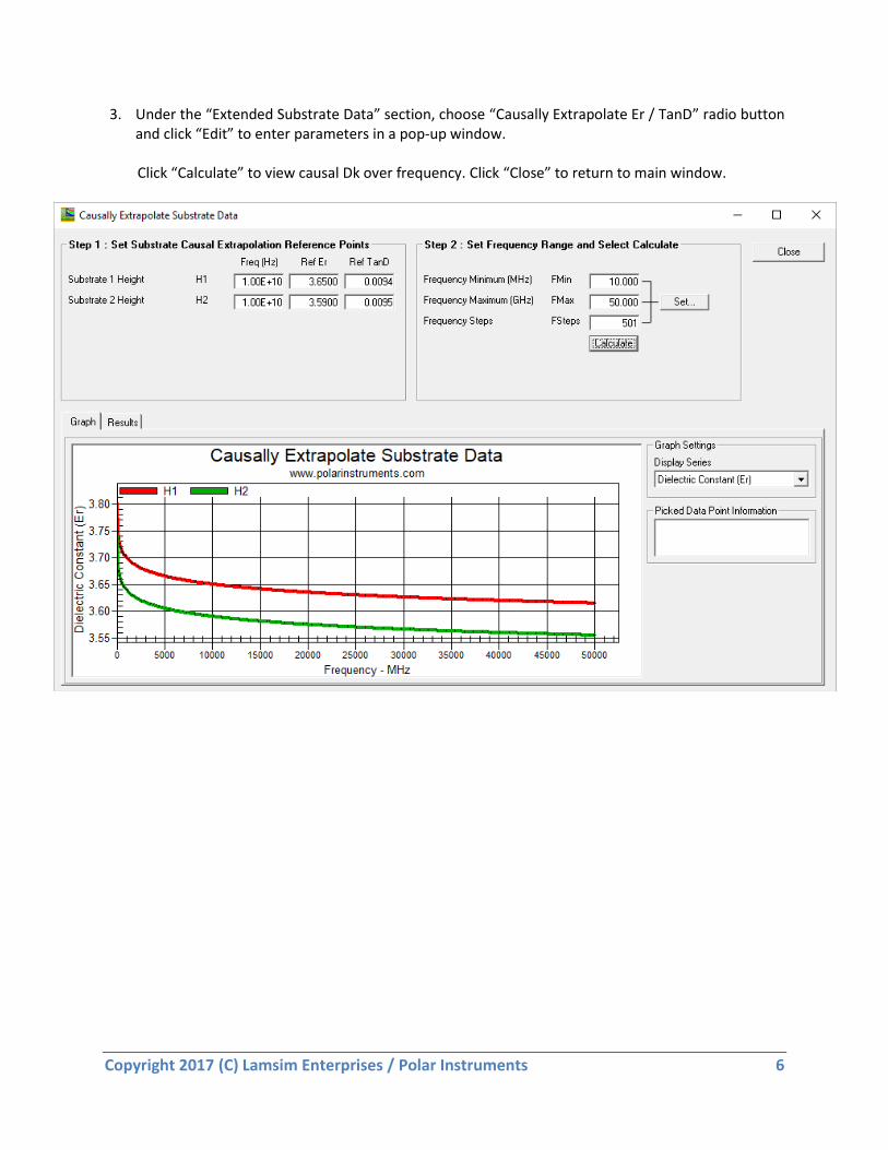
3. Under the “Extended Substrate Data” section, choose “Causally Extrapolate Er / TanD” radio button and click “Edit” to enter parameters in a pop-up window.
Click “Calculate” to view causal Dk over frequency. Click “Close” to return to main window.

Copyright 2017 (C) Lamsim Enterprises / Polar Instruments 7
4. Under the “Surface Roughness Compensation” section from the main window, select Huray radio button and click “Edit”. We are then presented with the following pop-up window. “Ratio of Areas” is Amatte/Aflat from the Huray Equation 1 and is equal to 1.00 because the Cannonball model assumes the relative area of the matte base is a perfectly flat surface.
For microstrip geometry you only need to consider the roughness of the foil bonded to the dielectric
material, usually the matte side. But for stripline geometry, you must factor the roughness for both matt
side and drum side of the foil. Since the roughness is different for each side you first have to calculate the
sphere radius for drum and matte side separately, and then take the average to use as input for the
“Effective Ball Radius”.
Thus:
_ 3.1750.190
16.73 16.73
z drum
drum
R mr m
An oxide or micro-etch treatment is usually applied to the copper surfaces prior to final lamination.
Typically 50 μin (1.27μm) of copper is removed when the treatment is completed. But depending on the
board shop’s process control, this can be 70-100 μin (1.78-2.54μm. Because some of the copper is
removed during the micro-etch treatment, we need to reduce the published roughness parameter of the
matte side by nominal 50 μin for a new thickness of 175μin (4.443μm).
Thus:
_ 4.4430.266
16.73 16.73
z matte
matte
R mr m
And therefore:

Copyright 2017 (C) Lamsim Enterprises / Polar Instruments 8
“Effective Ball Radius”: 0.266 0.190
0.22772 2
matte drumr r m mm
5. Next, calculate “Area of Ball Count”: 2 2(6 0.2277 ) 1.866flatA m m
6. And finally, for the Cannonball model, enter 14 for “Number of Balls in Area”
7. When finished entering all the information, hit the “Apply” button to return to the main window.
After clicking the “Calculate” button you will be presented with the following results:
The main window will display the results of the simulation.
Starting from the top, the red and yellow curves are loss only, without roughness (smooth) and with
roughness respectively. The green curve is the dielectric loss. The dark blue curve is total loss with smooth
copper and the bottom curve in light blue is the total loss with roughness.
Copyright 2017 (C) Lamsim Enterprises / Polar Instruments 9
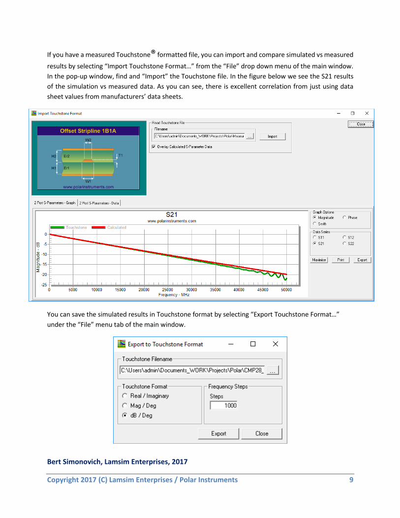
If you have a measured Touchstone® formatted file, you can import and compare simulated vs measured
results by selecting “Import Touchstone Format…” from the “File” drop down menu of the main window.
In the pop-up window, find and “Import” the Touchstone file. In the figure below we see the S21 results
of the simulation vs measured data. As you can see, there is excellent correlation from just using data
sheet values from manufacturers’ data sheets.
You can save the simulated results in Touchstone format by selecting “Export Touchstone Format…”
under the “File” menu tab of the main window.
Bert Simonovich, Lamsim Enterprises, 2017

Copyright 2017 (C) Lamsim Enterprises / Polar Instruments 10
References:
[1] Simonovich, Bert, “Practical Method for Modeling Conductor Surface Roughness Using The Cannonball Stack Principle”, White Paper.
[2] Huray, P. G. (2009) “The Foundations of Signal Integrity”, John Wiley & Sons, Inc., Hoboken, NJ, USA., 2009
Polar Application Note AP8195
lamsimenterprises.com polarinstruments.com
Related Documents