Public Health Monograph Series No. 23 ISSN 1178-7139 CANCER EXCESS MORTALITY RATES OVER 2006-2026 FOR ABC-CBA Burden of Disease Epidemiology, Equity and Cost-Effectiveness Programme (BODE 3 ) Technical Report: Number 10 Tony Blakely Roy Costilla Matt Soeberg May 2012 A technical report published by the Department of Public Health, University of Otago, Wellington ISBN 978-0-473-20656-7 ABC-CBA Team* * Contact Professor Tony Blakely (Principal Investigator of the ABC-CBA component of the BODE 3 Programme, University of Otago, Wellington, New Zealand). Email: [email protected]

Welcome message from author
This document is posted to help you gain knowledge. Please leave a comment to let me know what you think about it! Share it to your friends and learn new things together.
Transcript

Public Health Monograph Series No. 23
ISSN 1178-7139
CANCER EXCESS MORTALITY RATES OVER 2006-2026 FOR ABC-CBA
Burden of Disease Epidemiology, Equity and Cost-Effectiveness Programme (BODE3)
Technical Report: Number 10
Tony Blakely Roy Costilla
Matt Soeberg
May 2012
A technical report published by the Department of Public Health, University of Otago, Wellington
ISBN 978-0-473-20656-7
ABC-CBA Team* * Contact Professor Tony Blakely (Principal Investigator of the ABC-CBA component of the BODE3
Programme, University of Otago, Wellington, New Zealand). Email: [email protected]

Cancer excess mortality rates over 2006-2026 for ABC-CBA
II
Acknowledgements
We thank other BODE3 team colleagues for comments on early versions of this work. This
programme receives funding from the Health Research Council of New Zealand (10/248).
Competing Interests
The authors have no competing interests.

Cancer excess mortality rates over 2006-2026 for ABC-CBA
III
Table of Contents
Introduction ........................................................................................................................ 9 1
Literature Review of Survival Trends Overtime .............................................................. 10 2
2.1 Selected studies ......................................................................................................... 10
2.2 Methods ..................................................................................................................... 12
2.3 Results ....................................................................................................................... 16
Literature Review of Survival Differences by Stage or Disease Severity ........................ 20 3
3.1 Female breast cancer ................................................................................................. 21
3.2 Colon cancer .............................................................................................................. 22
3.3 Rectal cancer ............................................................................................................. 23
3.4 Colorectal cancer ....................................................................................................... 26
Categorisations of Stage or Severity to use in ABC-CBA ............................................... 28 4
4.1 Staging Categories..................................................................................................... 28
4.2 Overview of current New Zealand Cancer Register data .......................................... 30
4.2.1 Summary staging ............................................................................................... 30
4.2.2 TNM staging ...................................................................................................... 31
4.2.3 Cancer site-specific staging variables ................................................................ 32
4.3 Staging used in clinical trial studies for cancer treatment ......................................... 33
4.4 Missingness of extent at diagnosis ............................................................................ 33
4.5 Conclusion on staging systems to use in ABC-CBA ................................................ 54
Excess Mortality Rate Modelling of New Zealand Data .................................................. 55 5
5.1 Methods ..................................................................................................................... 55
5.1.1 Data description ................................................................................................. 55
5.1.2 Count regression models for excess mortality in the context of relative survival .
............................................................................................................................ 60
5.1.3 Modelling survival over time since diagnosis ................................................... 62
5.1.4 Over dispersion .................................................................................................. 68
5.2 Results ....................................................................................................................... 68
5.2.1 Baseline models (model 1)................................................................................. 69
5.2.2 Predictions over 2006-2026 for baseline models ............................................... 80
5.2.3 Models with non-missing observations on stage at diagnosis (model 2) ........... 85

Cancer excess mortality rates over 2006-2026 for ABC-CBA
IV
5.2.4 Models including stage or severity (model 3) .................................................... 87
5.2.5 Models by stage or severity ............................................................................... 89
Conclusion ........................................................................................................................ 98 6
References ................................................................................................................................ 99

Cancer excess mortality rates over 2006-2026 for ABC-CBA
V
List of Tables
Table 1: Studies selected to estimate annual changes in cancer survival across multiple cancer
sites .......................................................................................................................................... 11
Table 2: Approaches used to estimate the annual change (%) in cancer survival from the
seven studies included.............................................................................................................. 15
Table 3: Estimated annual percentage changes (APCs) in excess mortality rates by cancer site
for cancer survival in Australia, Canada, Denmark, England and Wales, Norway, Scotland,
Sweden, and the United Kingdom ........................................................................................... 19
Table 4: Studies selected describe differences by clinical stage or extent of disease for female
breast, colorectal and lung cancers .......................................................................................... 20
Table 5: Four-year RSRs and EMRRs by extent of disease for female breast cancer patients
diagnosed between 2005 to 2007, New Zealand ((McKenzie, Ellison-Loschmann et al. 2010))
.................................................................................................................................................. 22
Table 6: Five-year RSRs and estimated EMRs for colon cancer patients diagnosed 1989-
2006, the Netherlands, by period of diagnosis and stage (Source: (van Steenbergen, Elferink
et al. 2010)) .............................................................................................................................. 23
Table 7: Five-year relative survival for rectal cancer patients diagnosed 1994-2006, Denmark
(Source: (Bulow, Harling et al. 2010)) .................................................................................... 24
Table 8: Excess mortality rate ratio (compared stage II, III, loco-regional, undetermined and
IV to stage I) for rectal cancer patients diagnosed in Switzerland, France and Spain, 1982-
1987 (Source: (Monnet, Faivre et al. 1999)) ............................................................................ 25
Table 9: EMRRs (comparing stage II-IV with stage I) for male and female rectal cancer
patients five-years post diagnosis for patients diagnosed in Nordic countries and Scotland in
1997 (Source: (Folkesson, Engholm et al. 2009)) ................................................................... 25
Table 10: Five-year relative survival and excess mortality rate ratios (comparing stage III
with stage I-II) for colorectal cancer patients diagnosed 1976-99, Cote D’Or, France (Source:
(Mitry, Bouvier et al. 2005)) .................................................................................................... 26
Table 11: EMRRs (comparing patients diagnosed in 1975-1999 to patients diagnose 2000-
2006) colon and rectal cancer patients in the Netherlands, by cancer site, stage and age
(Source: (Lemmens, van Steenbergen et al. 2010)) ................................................................. 27
Table 12: Categories in the TNM staging system .................................................................... 29

Cancer excess mortality rates over 2006-2026 for ABC-CBA
VI
Table 13: Categories in the overall stage category .................................................................. 29
Table 14: Change to extent of disease classification in the New Zealand Cancer Register .... 30
Table 15: SEER summary stage and equivalent for TNM stage for colon cancer .................. 31
Table 16: Cancer site-specific staging variables on the New Zealand Cancer Register .......... 32
Table 17: Overall stage categorisation used in the United States’ NCI clinical trials database
by cancer site............................................................................................................................ 33
Table 18: Number and percentage of patients by severity and year of diagnosis for (female)
breast cancer by ethnicity, deprivation and ethnicity and deprivation..................................... 35
Table 19: Number and percentage of patients by severity and year of diagnosis for colorectal
cancer by ethnicity, deprivation and ethnicity and deprivation ............................................... 37
Table 20: Number and percentage of patients by severity and year of diagnosis for colon
cancer by ethnicity, deprivation and ethnicity and deprivation ............................................... 40
Table 21: Number and percentage of patients by severity and year of diagnosis for rectal
cancer by ethnicity, deprivation and ethnicity and deprivation ............................................... 43
Table 22: Number and percentage of patients by severity and year of diagnosis for lung
cancer by ethnicity, deprivation and ethnicity and deprivation ............................................... 46
Table 23: Number and percentage of patients by severity and year of diagnosis for cervical
cancer by ethnicity, deprivation and ethnicity and deprivation ............................................... 49
Table 24: Number and percentage of patients by severity and year of diagnosis for prostate
cancer by ethnicity, deprivation and ethnicity and deprivation ............................................... 52
Table 25: Number of cases by age, sex, ethnicity, deprivation, calendar year of diagnosis for
each cancer site over 1994-2010 .............................................................................................. 56
Table 26: Number of cases with non-missing stage by age, sex, ethnicity, deprivation, year of
diagnosis for each cancer site .................................................................................................. 58
Table 27: Cases included in the Complete Approach to estimate the Excess Mortality Rates 60
Table 28: Baseline model coefficients for breast cancer – example ........................................ 64
Table 29: Workings for the excess mortality rate (EMR) among 55-64 year old non-Māori,
diagnosed in 2006 and living in areas with deprivation deciles 1-3 ........................................ 66
Table 30: Regressions for all cancer sites (baseline model, model 1) ..................................... 69
Table 31: Regressions with non-missing observations of stage at diagnosis (model 2) for
selected cancer sites ................................................................................................................. 85

Cancer excess mortality rates over 2006-2026 for ABC-CBA
VII
Table 32: Regressions including stage at diagnosis with non-missing observations (model 3)
for selected cancer sites ........................................................................................................... 88
Table 33: Regressions by stage at diagnosis (model 4) for colorectal cancer ......................... 92
Table 34: Regressions by stage at diagnosis (model 4) for colon cancer ................................ 93
Table 35: Regressions by stage at diagnosis (model 4) for rectal cancer ................................ 94
Table 36: Regressions by stage at diagnosis (model 4) for lung cancer .................................. 95
Table 37: Regressions by stage at diagnosis (model 4) for breast cancer ............................... 96
Table 38: Regressions by stage at diagnosis (model 4) for cervical cancer ............................ 97

Cancer excess mortality rates over 2006-2026 for ABC-CBA
VIII
List of Figures
Figure 1: Estimated annual percentage changes (APCs) in excess mortality rates by cancer
site for cancer survival in Australia, Canada, Denmark, England and Wales, New Zealand,
Norway, Scotland, Sweden and the United Kingdom ............................................................. 18
Figure 2: Plot by time (years) since diagnosis of breast cancer: a) linear prediction, ln(EMR);
and b) EMR .............................................................................................................................. 67
Figure 3: Baseline model (model 1) predictions for 55-64 years old, 1-3 deprivation deciles,
Non-Māori female patients diagnosed with breast cancer in 2006 .......................................... 80
Figure 4: Baseline model (model 1) predictions for 55-64 years old, 1-3 deprivation deciles,
Non-Māori female patients diagnosed with colorectal cancer in 2006 .................................... 81
Figure 5: Baseline model (model 1) predictions for 55-64 years old, 1-3 deprivation deciles,
Non-Māori female patients diagnosed with colon cancer in 2006 .......................................... 82
Figure 6: Baseline model (model 1) predictions for 55-64 years old, 1-3 deprivation deciles,
Non-Māori female patients diagnosed with rectal cancer in 2006 .......................................... 83
Figure 7: Baseline model (model 1) predictions for 55-64 years old, 1-3 deprivation deciles,
Non-Māori female patients diagnosed with lung cancer in 2006 ............................................ 83
Figure 8: Baseline model (model 1) predictions for 55-64 years old, 1-3 deprivation deciles,
Non-Māori male patients diagnosed with prostate cancer in 2006 .......................................... 84
Figure 9: Baseline model (model 1) predictions for 55-64 years old, 1-3 deprivation deciles,
Non-Māori females patients diagnosed with cervical cancer in 2006 ..................................... 84
Figure 10: Predicted Excess Mortality Rates by Stage at Diagnosis for 55-64 years old, 1-3
deprivation deciles, Non-Māori female patients diagnosed with breast cancer in 2006 ......... 90
Figure 11: Predicted (Cumulative) Relative Survival by Stage at Diagnosis for 55-64 years
old, 1-3 deprivation deciles, Non-Māori female patients diagnosed with breast cancer in 2006
.................................................................................................................................................. 91

Cancer excess mortality rates over 2006-2026 for ABC-CBA
9
Introduction 1This Report provides the baseline excess mortality rates for modelling in the Aotearora
Burden of Cancer and Comparative Benefit Assessment (ABC-CBA) project, within the
Burden of Disease Epidemiology, Equity and Cost-Effectiveness (BODE3) programme.
These excess mortality rates are then converted to transition probabilities in Markov models,
or time to event distributions in discrete event simulation.
An aim of BODE3 is to estimate impacts of interventions, and cost effectiveness, by sub-
populations. Most importantly, this means separate epidemiological parameters by sex, age,
ethnicity and deprivation. With respect to cancer, stage or disease severity is an additional
strata of heterogeneity. Finally, estimates are required for the baseline year of 2011, but also
annually projected out to 2026.
It is intended that the results presented in this report, and the accompanying tables and
electronic files, will provide the baseline parameter necessary for the majority of future ABC-
CBA analyses. But we cannot foresee all possible analyses. And it would be inefficient to
predict excess mortality rates by stage or severity of cancers that are unlikely to require
modelling by stage; rather we will use the methods demonstrated in this Report on an as need
basis to specify future interventions.
This Report is in four Parts:
1. A brief summary of international and national literature on changes over time in
relative survival, and excess mortality, by cancer sites.
2. A brief summary of international and national literature on differences by stage or
severity in relative survival, and excess mortality, by selected cancer sites.
3. A review of various cancer staging systems, with recommendations as to what to use
in ABC-CBA given data availability.
4. Actual excess mortality rate more outputs using New Zealand data, including
coefficients for sex, age, ethnicity, deprivation, time since diagnosis and calendar year
of diagnosis, with additional models by stage (or severity) or including stage (or
severity) and interactions with key covariates.
Together, four Parts will provide the basis for parameterising future ABC-CBA models.
Cancer excess mortality rates over 2006-2026 for ABC-CBA
10
Literature Review of Survival Trends Overtime 2Trend data informs us what the situation was, currently is, and possibly what it might be in
the future – the latter aspect being particularly important for the purpose of health service
planning and evaluation and for the planning, funding and prioritisation of public health
research. Previous work from the New Zealand Census-Mortality Study (NZCMS) and the
Cancer Trends study have given us estimates for trends by ethnicity and socioeconomic
position on cancer incidence and mortality. However, less is known about changes over time
in cancer survival. The purpose of this section is to estimate annual percentage changes in
cancer survival, expressed as an excess mortality rate, by synthesising findings from selected
cancer survival studies.
2.1 Selected studies Published literature was searched in Medline and PubMed for studies providing estimates of
annual changes in cancer survival (either measured as excess mortality or relative survival)
across the range of cancer sites including in this report. Studies were excluded a) if excess
mortality rates or relative survival ratios were not reported in tabular format in the paper, b) if
the paper only assessed changes over time for less than four cancer sites, and c) the time
periods assessed in the study were not considered to be relevant to the parameter estimation
for the purpose of this report, e.g. survival trends from the 1960s, 1970s, and 1980s.
Six studies were selected for further analyses (see Table 1) (Coleman, Rachet et al. 2004; Yu,
O'Connell et al. 2006; Shack, Rachet et al. 2007; Rachet, Maringe et al. 2009; Coleman,
Forman et al. 2011; Soeberg, Blakely et al. 2012). Two studies included both excess mortality
rate modelling and relative survival analyses (Yu, O'Connell et al. 2006; Soeberg, Blakely et
al. 2012). In both these studies, changes over time in cancer patient survival were measured
as excess mortality rate ratios. The remaining four studies calculated five-year relative
survival ratios but not excess mortality rates or rate ratios. Two studies (Coleman, Rachet et
al. 2004; Shack, Rachet et al. 2007) had calculated the average change for every five-year
period in the five-year RSRs. One study calculated the average year-on-year change in five-
year relative survival (Rachet, Maringe et al. 2009). The other study reported five-year RSRs
for three calendar periods but not the difference, either absolute or relative, between the

Cancer excess mortality rates over 2006-2026 for ABC-CBA
11
earliest and most recent period of cancer diagnosis, or the average change in survival over
time (Coleman, Forman et al. 2011).
Table 1: Studies selected to estimate annual changes in cancer survival across multiple cancer sites
Author and date
Country Number of
patients included
Number of
cancers
Period of incident
cases
Follow up
period
Survival analysis
measures
Comments
Coleman et al., (2004)
England and Wales
2,200,000 20 1986-1999 2001 Five-year RSRs Stratified by sex.
Average change in the five-year RSRs for every 5 calendar years calculated in study
Coleman et al., (2004)
Cross country comparison (Australia, Canada, Denmark, Sweden, Norway, and the UK)
2,500,000 4 1995-2007 2007 Five- year RSRs
Not stratified by sex.
No changes over time in the five-year RSRs calculated in the study.
Rachet et al., (2009)
England and Wales
2,163,000 21 1996-2006 2007 Five-year RSRs Stratified by sex.
Average annual change in the five-year RSR calculated in the study
Shack et al., (2007)
Scotland 357,000 18 1986-2000 2004 Five-year RSR Stratified by sex.
Average change in the five-year RSRs for every 5 calendar years calculated in study
Soeberg et al., (2012)
New Zealand 125,567 21 1991-2004 2004 Five-year RSRs
EMR modelling for estimate changes every ten years in excess mortality with 1991 as the reference year
Social group life tables used
EMR modelling adjusted for ethnicity and/or income, age, sex, follow up since diagnosis, interaction of age and follow up in the first two years
Yu et al., (2006)
Australia 343,000 28 1980-1996 2001 Five-year RSRs.
Excess mortality rate modelling (comparison of the 1993-1996 period with the reference category of patients diagnosed 1980-84).
RSRs not stratified by sex.
Modelling adjusted for age, sex, extent of disease, years since diagnosis, and histological type

Cancer excess mortality rates over 2006-2026 for ABC-CBA
12
2.2 Methods Different approaches were required to estimate the annual change over time in each of these
studies.
Table 2 summarises the three approaches used to estimate the annual change in cancer
survival from the studies listed above. To estimate the year-to-year change (%) in excess
mortality by cancer sites, the excess mortality rate ratios over X years were converted to per
annum rate ratios, then the annual percentage change (APC) estimated. For example, if the
rate ratio for excess mortality in 2006 compared to 1996 was 0.80, then the annual rate ratio
is 0.801/10 = 0.978, and the APC is -2.2%.
If relative survival, and change in relative survival, was the main output in a given study, the
following generic approaches were used. First, some studies (e.g. (Rachet, Maringe et al.
2009)) report the absolute annual change in the five-year relative survival ratio (RSR); that is,
a percentage point change in the relative survival probability five years after diagnosis.
Noting that the proportion of people dying equals 1 – exp[rate × units of time], and that in our
case the proportion is 1-RSR and the rate is the excess mortality rate, we can derive the
following:
where:
EMR is the annual excess mortality rate (assumed here to be constant over the five years,
which is an adequate assumption for determining changes in EMR over time as long as one
assumed the percentage change over time in the EMR is similar by year of follow up)
t is time (in this case number of years = 5)
RSR is the five year RSR (expressed as a proportion, i.e. 0.80 not 80).
Cancer excess mortality rates over 2006-2026 for ABC-CBA
13
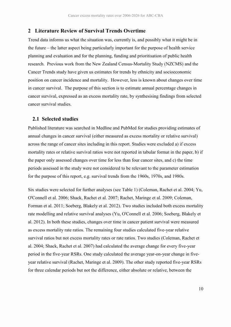
Let EMR0 be the EMR in the time zero, and EMR1 be the EMR one year later. Likewise, let
RSR0 and RSR1 be the five-year RSRs at time zero and one year later. Then:
For example, if the five-year RSR was 0.80 in the initial year, and 0.81 in the subsequent
year, then the APC in the EMR is approximated by:
100% × [–ln(0.80) - -ln(0.81)] / -ln(0.80)
= 100% × [-0.2231 - -0.2107] / 0.2231
= -5.6%
(Note this magnitude of annual percentage change in the EMR is extremely unlikely in
reality.)
For the remaining studies (Coleman, Rachet et al. 2004; Shack, Rachet et al. 2007; Coleman,
Forman et al. 2011), the above calculations apply, a five-year RSR was estimated centred
between the periods of diagnosis on the study. The average year-to-year change in the five-
year RSR was estimated by subtracting the earliest calendar period RSR from the most recent
calendar period RSR and then dividing this difference by the number of years in the study.

Cancer excess mortality rates over 2006-2026 for ABC-CBA
14
This estimated annual change was then added to the new centred RSR to estimate a RSR
equivalent to the centred RSR + 1 year. These RSRs were then converted to excess mortality
rates.
Note that all these calculations have some approximations inherent. For example, there is
rounding in the reported results, the authors’ may have used a linear or multiplicative
methods to calculate the change in RSR over time, and we are making assumptions as noted
above about the constant proportionality of change over time in the EMR by year of follow-
up from diagnosis. And we neither attempt to calculate confidence intervals (random error)
nor assess or quantify likely residual systematic error (e.g. incorrect life tables, exclusion or
not of death certificate only registrations, choice of underlying analytical methods (e.g.
standardisation method, period or cohort)). That all said, by converting the results from these
published studies, we can gain a reasonable overview of changes in cancer survival across
multiple countries and multiple cancers.

Cancer excess mortality rates over 2006-2026 for ABC-CBA
15
Table 2: Approaches used to estimate the annual change (%) in cancer survival from the seven studies included
Author and date Survival analysis methods and measures
Author’s approach in estimating changes in cancer patient survival
Our approach to converting study results to an estimated APC in EMR
Coleman et al., (2004) Relative survival
Five-year RSRs
The average change every five years in five-year relative survival between calendar periods was calculated using linear regression.
A centred RSR was estimated based on the five-year RSR in the most recent period and the value given in the study for the average change for every five years in relative survival. The centred RSR + 1 year was also estimated by dividing the value given for the average change every five years in relative survival by five. These RSRs were then converted to excess mortality rates.
Coleman et al., (2011) Relative survival
Five-year RSRs
Five-year RSRs for the periods 1995-99, 2000-02, 2005-07 were given but no trends over time were calculated
A centred RSR was estimated based on the five-year RSR for the earliest and most recent calendar periods. The centred RSR + 1 year was calculated by subtracting the difference between 1995-99 and 2005-07 RSRs and dividing this by 9. The RSRs were then converted to excess mortality rates with an estimated annual percentage change calculated.
Rachet et al., (2009) Relative survival
Five-year RSRs
The average year-on-year change in five-year relative survival between calendar periods was calculated using linear regression.
The estimated average year-on-year change in five-year relative survival was transformed on to the excess mortality rate scale.
Shack et al., (2007) Relative survival
Five-year RSRs
The average change every five years in five-year relative survival between calendar periods was calculated using linear regression.
A centred RSR was estimated based on the five-year RSR in the most recent period and the value given in the study for the average change for every five years in relative survival. The centred RSR + 1 year was also estimated by dividing the value given for the average change every five years in relative survival by five. These RSRs were then converted to excess mortality rates.
Soeberg et al., (2011) Excess mortality rate modelling
EMRR
An excess mortality rate ratio was given for the change over time in cancer survival for every ten years compared to 1991.
The annual change (%) over time in excess mortality was calculated as (1 – RR^1/10 [10]).
Yu et al., (2007) Excess mortality rate modelling
EMRR
An excess mortality rate ratio was given for the change over time in cancer survival for patients diagnosed 1993-96 compared to patients diagnosed 1980-84.
The annual change (%) over time in excess mortality was calculated as (1 – RR^1/8 [10]).

Cancer excess mortality rates over 2006-2026 for ABC-CBA
16
2.3 Results Table 3 shows the estimated annual percentage changes (APC) in excess mortality rates by
cancer site. These estimated APCs were calculated (using the methods detailed above) from
results of population-based cancer survival studies that present changes over time in either
relative survival ratios or excess mortality rate ratios in Australia, Canada, Denmark, England
and Wales, Norway, Scotland, Sweden, and the United Kingdom.
In Figure 1 and Table 3, an estimated APC below zero indicated that there was a decrease in
excess mortality (cancer survival improved for each year of calendar year). For instance, if
the excess mortality rate in 2010 was 0.250 and the estimated APC was -5.0% (the estimated
decrease in the excess mortality in the next year would be 0.0125) then the excess mortality
rate in 2011 would be 0.2375. But in ten years time, the excess mortality rate would be 0.250
× (1-0.05)^10 = 0.150. An estimated APC above 1.00 indicates that there was an increase in
excess mortality (cancer survival declined for each calendar year). For example, if the excess
mortality rate in 2010 was 0.15 and the estimated APC was 1.5%, then the excess mortality
rate in 2011 would be 0.152.
The light circle in Figure 1 represents the estimated APCs from the individual studies; the
actual estimated APCs for each study are shown in Table 3. The dark square in Figure 1
represents the average estimated APC, using the estimated APCs from each study. The dark
triangle in Figure 1 presents the estimate APC from recent New Zealand data (Soeberg,
Blakely et al. 2012).
The average estimated APCs in these excess mortality rates were interpreted in this thesis as
falling into one of four groups based on: a) no change in the annual APC (i.e. the APC is
0.00); b) a small annual decrease in excess mortality where the estimated APC is between
0.01 and 1.99; c) a moderate annual decrease in excess mortality where the estimated APC is
between 2.00 and 4.99; and d) a large annual decrease in excess mortality where the
estimated APC is 5.00 and above.

Cancer excess mortality rates over 2006-2026 for ABC-CBA
17
Using the average estimated APC, Figure 1 and Table 3 show that there was:
1. small annual decrease in excess mortality (cancer survival improvement) for cancers
of the bladder, brain, head and neck, lung, oesophagus, pancreas and stomach;
2. moderate annual decrease in excess mortality (cancer survival improvement) for
cancers of the female breast, cervix, colon, rectum, colorectum combined, kidney,
ovaries, testis and uterus and patients with Hodgkin’s lymphoma, leukaemia,
melanoma and Non-Hodgkin’s lymphoma;
3. large annual decrease in excess mortality (cancer survival improvement) for cancers
of the liver, prostate and thyroid gland. (However, the large annual decrease for
prostate cancer is probably spurious due to massively increased PSA testing detecting
less severe disease.)

Cancer excess mortality rates over 2006-2026 for ABC-CBA
18
Figure 1: Estimated annual percentage changes (APCs) in excess mortality rates by cancer site for cancer survival in Australia, Canada, Denmark, England and Wales, New Zealand, Norway, Scotland, Sweden and the United Kingdom
-20-19-18-17-16-15-14-13-12-11-10
-9-8-7-6-5-4-3-2-1012345
AP
C i
n t
he e
xcess m
ort
ality
rate
Ute
rus
Thyro
id
Testis
S
tom
ach
Pro
sta
te
Pancre
as
Ovary
O
esophagus
NH
L
Mela
nom
a
Lung
Liv
er
Leukaem
ia
Kid
ney
NH
L
Head a
nd n
eck
Colo
rectu
m
Rectu
m
Colo
n
Cerv
ix
Bre
ast (fe
male
) B
rain
Estimated APCs from individual Average estimated Estimated APCs from NZ

Cancer excess mortality rates over 2006-2026 for ABC-CBA
19
Table 3: Estimated annual percentage changes (APCs) in excess mortality rates by cancer site for cancer survival in Australia, Canada, Denmark, England and Wales, Norway, Scotland, Sweden, and the United Kingdom
Cancer site Average estimated
annual percentage
change (APC) in the excess mortality
rate
Estimated annual percentage change (APC) in the excess mortality rate by country Australia
Canada Denmark England and Wales
(males)
England and Wales
(males)
New Zealand
Norway Scotland (males)
Scotland (females)
Sweden United Kingdom
Yu et al., 2006
Coleman et al., 2011
Coleman et al., 2011
Coleman et al., 2011
Coleman et al., 2004
Coleman et al., 2004
Soeberg et al., 2012
Coleman et al., 2011
Shack et al., 2007
Shack et al., 2007
Coleman et al., 2011
Coleman et al., 2011
Bladder -0.54 1.54 -0.51 0.50 -2.33 -0.99 -1.43 Brain -0.25 -1.87 2.25 0.57 -0.62 -1.22 -0.60 Breast -4.01 -5.99 -2.75 -0.93 -3.36 -5.38 -7.08 -2.75 -6.21 -1.72 -3.91 Cervix -2.73 -4.71 -0.64 -2.84 -2.76 Colon -3.11 -4.19 -3.03 -3.03 -2.55 -2.72 Rectum -4.41 -4.88 -3.98 -4.39 -4.27 -4.52 Colorectum -2.12 -1.92 -2.24 -2.05 -2.46 -3.10 -1.82 -1.49 -1.86 Head neck -1.78 -3.06 -0.51 HL -2.76 -2.01 -3.50 Kidney -2.63 -3.86 -2.44 -2.01 -3.37 -1.20 -2.91 Leukaemia -3.86 -2.45 -2.52 -0.92 -8.76 -4.17 -4.32 Liver -5.49 -7.20 -3.78 Lung -1.03 -2.45 -1.18 -0.99 -1.42 -0.12 -0.11 -1.16 -1.42 -0.33 -0.83 -1.41 -0.98 Melanoma -3.66 -4.02 -3.56 -0.59 -4.82 -4.71 -4.26 NHL -2.89 -1.87 -2.24 -2.05 -5.63 -2.78 -2.77 Oesophagus -1.66 -4.36 -1.98 0.31 -1.05 -2.25 -0.64 Ovary -2.10 -4.71 -0.42 -1.12 -1.38 -1.57 -4.82 -0.90 -2.84 -1.14 Pancreas -0.19 -1.87 -0.21 1.53 -0.20 Prostate -10.51 -7.41 -9.13 -18.46 -7.06 Stomach -1.77 -2.45 -1.63 -1.30 -1.50 -2.01 -1.73 Testis -4.69 -5.61 -5.22 -3.23 Thyroid -6.28 -6.58 -5.98 Uterus -3.64 -5.99 -2.19 -3.37 -3.02

Literature Review of Survival Differences by Stage or Disease Severity 3This section presents findings of a selected literature review on female breast, colon, rectal,
and lung cancer survival by stage. Medline was searched in December 2011 for literature that
documented five-year relative survival, excess mortality rates or excess mortality rate ratios
for female breast, colon, rectal, colorectal, and lung cancers by stage or extent of disease.
Table 4 shows the studies selected in this section of the report (Monnet, Faivre et al. 1999;
Mitry, Bouvier et al. 2005; Folkesson, Engholm et al. 2009; Bulow, Harling et al. 2010;
Lemmens, van Steenbergen et al. 2010; McKenzie, Ellison-Loschmann et al. 2010; van
Steenbergen, Elferink et al. 2010). One study was selected for female breast cancer. Six
studies were selected for either colon, rectal or colorectal cancers combined. No studies were
identified or selected for differences by stage/extent or extent for lung cancer survival,
measured on the excess mortality or relative scales.
Table 4: Studies selected describe differences by clinical stage or extent of disease for female breast, colorectal and lung cancers
Author and date
Country Cancer site
Number of patients included
Period of incident
cases
Follow up
period
Survival analysis methods
Categories of clinical
stage/extent of disease
Bulow et al., 2010
Denmark Rectum 10,632 1994-2006 2007 Five-year RSR
Stage I, II and III *
Folkesson et al., 2009
Denmark, Finland, Iceland, Norway, Sweden, Scotland
Rectum 3,888 1997 2002 Five-year RSR
EMRRs
Stage I, II, III, IV and missing stage *
Lemmens et al., 2010
Netherlands Colorectum 28,826 1975-2007 2008 EMRRs Colon stage III *
Rectum stage II-III *
Mitry et al., 2005
France Colorectum 5,847 1976-1989 and 1988-
1999
2002 Five-year RSR
EMRRs
Stage I-II *
Stage III *
McKenzie et al. 2010
New Zealand Breast 2,968 2005-2007 2009 Four-year RSR
EMRRs
RSR: Local, regional, distant, missing +
EMRR: local (reference category), regional, distant +
Monnet et al., 1999
Switzerland, France and Spain
Rectum 1,005 1982-87 1992 Five-year RSR
EMRRs
Stage I, II, III, IV, loco-regional and not determined *
Van Steenbergen
The Netherlands Colon 103,744 1989-2006 2006 Five-year Stage I, II, III, IV *

Cancer excess mortality rates over 2006-2026 for ABC-CBA
21
Author and date
Country Cancer site
Number of patients included
Period of incident
cases
Follow up
period
Survival analysis methods
Categories of clinical
stage/extent of disease
et al., 2010 RSR
EMRRs * Based on TNM staging. + SEER summary staging.
The following section briefly describes the results of these studies relating to differences by
clinical stage or extent of disease by cancer site for breast, colon, rectum, and colorectum
cancers.
3.1 Female breast cancer Possible explanations for socioeconomic inequalities in female breast cancer survival in New
Zealand were investigated using cancer registration data for 2005 to 2007 (see Table 5).
Four-year relative survival was estimated by stage. Excess mortality rate ratios (EMRRs)
were also calculated by stage with local extent set as the reference category. This study
estimated that the four-year relative survival was 0.98 for local extent, 0.86 for regional
extent, 0.22 for distant extent and 0.86 for missing extent of disease. Using complete-case
data, the EMRRs suggest that patients with regional extent had three times the excess
mortality and patients with distant extent had nine times for more excess mortality compared
to patients with local extent.

Cancer excess mortality rates over 2006-2026 for ABC-CBA
22
Table 5: Four-year RSRs and EMRRs by extent of disease for female breast cancer patients diagnosed between 2005 to 2007, New Zealand ((McKenzie, Ellison-Loschmann et al. 2010))
Extent of disease Four-year RSR
(95% CI)
Excess mortality rate ratios (95% CI)
Imputed data Complete-case data
Local 0.979 (0.959, 0.990) 1.00 1.00
Regional 0.857 (0.825, 0.883) 5.03 (2.57, 9.84) 3.00 (1.59, 5.68)
Distant 0.221 (0.156, 0.294) 48.53 (23.89, 98.60) 9.22 (2.45, 34.66)
Missing 0.862 (0.816, 0.897) - -
3.2 Colon cancer Changes over time in colon cancer survival were examined for patients diagnosed in the
Netherlands between 1989 and 2006, with a focus on the association between cancer survival
improvements over time and changes over time in colon cancer treatment and detection (see
Table 6). Relative survival was estimated by stage, as well as the estimated annual change in
relative survival. In this study, the five-year RSR was estimated to be between 0.91 and 0.96
for stage I male and female colon cancer patients, between 0.74 and 0.80 stage II male and
female colon cancer patients, between 0.46 and 0.60 for stage III male and female colon
cancer patients, and between 0.05 and 0.07 for stage IV male and female colon cancer
patients. For the purpose of this report, these RSR estimates were converted to annual excess
mortality rates (EMRs) where it was assumed the EMR was contant for every year after
diagnosis. Table 6 shows that the EMRR for stage II patients was between 3.6 and 4.1
compared to stage I patients, for stage III patients the EMRR was between 8.6 and 10.1
compared to stage I patients, and for stage IV patients the EMRR was between 38.6 and 45.5
compared to stage I patients.

Cancer excess mortality rates over 2006-2026 for ABC-CBA
23
Table 6: Five-year RSRs and estimated EMRs for colon cancer patients diagnosed 1989-2006, the Netherlands, by period of diagnosis and stage (Source: (van Steenbergen, Elferink et al. 2010))
Stage Sex Five-year relative survival Annual change
1989-
1993
1994-
1998
1999-
2003
2004-
2006
Stage I Male 92 91 94 94 +0.21 (-0.05, 0.46)
Female 96 94 94 92 -0.28 (-0.59, 0.02)
Stage II Male 74 74 78 78 +0.36 (0.07, 0.66)
Female 75 76 80 80 +0.37 (0.13, 0.60)
Stage III Male 46 49 56 59 +0.97 (0.59, 1.34)
Female 48 50 57 60 +0.88 (0.65, 1.12)
Stage IV Male 5 5 5 7 +0.15 (0.02, 0.28)
Female 6 5 6 7 +0.14 (-0.05, 0.33)
Stage Sex EMR [assumed constant per year post
diagnosis]
Average
across time
RR (by
sex)
1989-
1993
1994-
1998
1999-
2003
2004-
2006
Stage I Male 0.017 0.019 0.012 0.012 0.015 1
Female 0.008 0.012 0.012 0.017 0.012 1
Stage II Male 0.060 0.060 0.050 0.050 0.055 3.6
Female 0.058 0.055 0.045 0.045 0.050 4.1
Stage III Male 0.155 0.143 0.116 0.106 0.130 8.6
Female 0.147 0.139 0.112 0.102 0.125 10.1
Stage IV Male 0.599 0.599 0.599 0.532 0.582 38.6
Female 0.563 0.599 0.563 0.532 0.564 45.5
3.3 Rectal cancer Changes over time in rectal cancer survival in Denmark for patients diagnosed 1994 to 2006
were assessed, particularly with regards to surgical treatment for colorectal cancer. A total of
10, 632 patients were included in the study. Five-year relative survival for rectal cancer
patients were estimated by sex and stage at diagnosis (see Table 7). There were substantial
increases for male rectal cancer patients in all stages, but more so for stage III patients where
the five-year RSR increased from 0.36 (95% CI 0.22, 0.51) in 1994 to 0.71 (0.64, 0.78) in
2006. The five-year RSRs for female stage I and II rectal cancer patients were difficult to
Cancer excess mortality rates over 2006-2026 for ABC-CBA
24
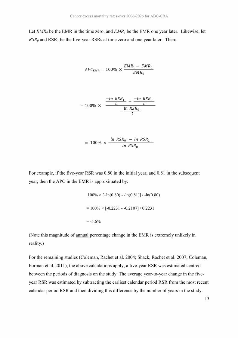
interpret as their survival estimates were close to 1.00 with the confidence intervals extending
beyond 1.00. Compared to male patients, female stage III rectal cancer patients only
experience a small increase in their five-year relative survival over time, with an RSR of 0.42
(0.25, 0.60) in 1994 and 0.49 in 2006 (95% CI 0.41, 0.56). These RSRs were converted to
estimated annual EMRs with an EMRR calculated comparing stage II and III patients to stage
I patients. For patients diagnosed in 1994, the EMRR for stage II patients was between 1.28
and 3.10. The EMRR for stage III patients diagnosed in 1994 was between 2.55 and 28.48.
For patients diagnosed in 2006, only the male EMRR for stage II and III patients could be
calculated due to the negative EMR for Stage I female patients. The EMRR for stage II
patients in 1994 was 1.17 and the EMRR for stage III patients diagnosed in 1996 was 1.535.
Table 7: Five-year relative survival for rectal cancer patients diagnosed 1994-2006, Denmark (Source: (Bulow, Harling et al. 2010))
Stage Sex Five-year RSR (95% CI)
Patients diagnosed 1994 Patients diagnosed 2006
Stage I Male 0.67 (0.40, 0.88) 0.80 (0.72, 0.88)
Female 0.97 (0.74, 1.07) 1.01 (0.93, 1.07)
Stage II Male 0.60 (0.43, 0.75) 0.77 (0.71, 083)
Female 0.91 (0.70, 1.05) 0.92 (0.83, 0.99)
Stage III Male 0.36 (0.22, 0.51) 0.71 (0.64, 0.78)
Female 0.42 (0.25, 0.60) 0.49 (0.41, 0.56)
Stage Sex EMR [assumed constant
per year post diagnosis]
Stage II and III
patients diagnosed
1994 compared to
stage I patients
diagnosed 1994
Stage II and III
patients diagnosed
2006 compared to
stage I patients
diagnosed 2006
Patients
diagnosed
1994
Patients
diagnosed
2006
Stage I Male 0.080 0.045 1 1
Female 0.006 -0.002 1 1
Stage II Male 0.102 0.052 1.286 1.171
Female 0.019 0.017 3.106 -
Stage III Male 0.204 0.068 2.551 1.535
Female 0.174 0.143 28.481 -

Cancer excess mortality rates over 2006-2026 for ABC-CBA
25
The impact of stage at diagnosis on rectal cancer survival in Switzerland, France and Spain
using data for patients diagnosed 1982-1997 was assessed (see Table 8). This study estimated
five-year relative survival and calculated excess mortality rate ratios by stage, including sub-
categories of TNM staging. The estimated five-year relative survival was 0.79 for stage
patients, 0.63 for II patients, 0.28 for stage III patients, 0.05 for loco-regional patients, 0.20
for patients where stage was not determined, and 0.01 for stage IV patients. When examined
from an EMR perspective, the EMRR for state IV compared to stage I was 25.4.
Table 8: Excess mortality rate ratio (compared stage II, III, loco-regional, undetermined and IV to stage I) for rectal cancer patients diagnosed in Switzerland, France and Spain, 1982-1987 (Source: (Monnet, Faivre et al. 1999))
Stage Five-year RSR EMRR (95% CI) I (T1-T2 N0 M0) 0.79 1 II (T3-T4 N0 M0) 0.63 1.88 (1.16, 3.03) III (N1-N2 M0) 0.28 5.23 (3.36, 8.13) Loco-regional 0.05 14.10 (8.31, 23.83) Undetermined (Tx Nx M0) 0.20 8.80 (5.02, 15.43) IV (M1) 0.01 25.40 (16.10, 40.10)
Rectal cancer survival for patients diagnosed in five Nordic countries and in Scotland in 1997
were assessed, with a particular focus on assessing the role of treatment on cancer survival. A
total of 3,888 patients were included in the study. Five-year relative survival was calculated
by stage at diagnosis and sex. Further, Poisson regression modelling was undertaken to
estimate EMRRs for differences in cancer survival by stage and sex (see Table 9). This study
found that stage II rectal cancer patients had approximately 3 times more excess mortality
than stage I patients, stage III patients had 7 times more excess mortality than stage I patients,
and stage IV patients had approximately 36 times more excess mortality than stage I patients.
Patients with missing stage data had approximately 15 times more excess mortality than stage
I patients.
Table 9: EMRRs (comparing stage II-IV with stage I) for male and female rectal cancer patients five-years post diagnosis for patients diagnosed in Nordic countries and Scotland in 1997 (Source: (Folkesson, Engholm et al. 2009))
Stage Sex EMRR I Male 1.0 Female 1.0 II Male 2.9 (1.7, 4.8) Female 3.5 (1.8, 6.8) III Male 7.1 (4.3, 11.6)

Cancer excess mortality rates over 2006-2026 for ABC-CBA
26
Female 7.0 (3.7, 13.3) IV Male 34.8 (21.2, 57.2) Female 37.4 (19.7, 70.9) Missing Male 14.8 (8.9) Female 15.3 (7.9, 29.7)
3.4 Colorectal cancer Changes over time in cancer survival were assessed for colorectal cancer patients diagnosed
in a French population between the periods 1976-1987 and 1988-99. A total of 5,874 patients
were included in the study. Five-year relative survival ratios were calculated. Poisson
regression methods were used to estimate excess mortality rate ratios for changes over time in
colorectal cancer survival by stage and age group (see Table 10). This study found that five-
year relative survival increased between 1976-87 and 1988-99 for patients aged under 75
years with stage I-II and stage III colorectal cancer and for patients aged above 75 with stage
I-II colorectal cancer. This study also found that patients aged below and above 75 years with
stage III colorectal cancer had approximately four times more excess mortality compared to
stage I-II cancer.
Table 10: Five-year relative survival and excess mortality rate ratios (comparing stage III with stage I-II) for colorectal cancer patients diagnosed 1976-99, Cote D’Or, France (Source: (Mitry, Bouvier et al. 2005))
Five-year relative survival ratios EMRRs five-years post diagnosis (pooled for
years 1976-99)
Age Stage Period of diagnosis Age Stage EMRR
Aged
under
75
Stage I-II 1976-1987 0.782 (0.741, 0.817) Aged under
stage 75
I-II 1
1988-1999 0.827 (0.794, 0.855) III 4.01 (3.41, 4.72)
Stage III 1976-1987 0.357 (0.300, 0.415)
1988-1999 0.486 (0.428, 0.542)
Aged
above
75
Stage I-II 1976-1987 0.780 (0.696, 0.844) Aged 75 years
and over
I-II 1
1988-1999 0.822 (0.742, 0.865) III 3.98 (3.05, 5.21)
Stage III 1976-1987 0.369 (0.257, 0.480)
1988-1999 0.341 (0.258, 0.426)
Changes over time in colorectal cancer survival, including analyses by stage, in the
Netherlands was assessed for colorectal cancer cases registered on the Eindhoven Cancer
Registry between 1974 and 2007. A total of 26,826 cases were included in the study. Two-
year and five-year RSRs were estimated along with excess mortality rate ratios to assess

Cancer excess mortality rates over 2006-2026 for ABC-CBA
27
cancer survival over time by stage. The 2002-2006 period of cancer diagnosis was used as the
reference category. Results were presented separately for colon and rectal cancer patients
with stage II and III disease and for those aged below and above 70 years. Poisson regression
modelling was undertaken for survival with cancer treatment excluded and then with
treatment included in the model. From the regression model including treatment, this study
found a steady improvement in cancer survival over time for rectal stage II and III patients
aged below and above 70. The change over time in cancer survival was less clear for colon
stage III patients, particularly for those aged below 70 years. While this study is useful for
assessing trends over time in cancer survival by stage, it does not provide evidence for the
magnitude of the rate ratio difference between different stage categories.
Table 11: EMRRs (comparing patients diagnosed in 1975-1999 to patients diagnose 2000-2006) colon and rectal cancer patients in the Netherlands, by cancer site, stage and age (Source: (Lemmens, van Steenbergen et al. 2010))
Cancer site and age Model Regression model
excluding treatment
Regression model
including treatment
Colon stage III, aged less
than 70 years
1975-1984 2.00 (1.63, 2.52) 1.00 (0.80, 1.35)
1985-1994 1.60 (.132, 200) 0.90 (0.71, 1.16)
1995-1999 1.30 (1.10, 1.64) 1.10 (0.88, 1.33)
2002-2006 1.00 1.00
Colon, stage III, aged
above 70 years
1975-1984 1.80 (1.38, 3.00) 1.40 (1.07, 1.80)
1985-1994 1.20 (0.96, 1.52) 1.00 (0.77, 1.22)
1995-1999 1.20 (0.97, 1.48) 1.10 (0.89, 1.36)
2002-2006 1.00 1.00
Rectal, stage II/III, aged
less than 70 years
1975-1984 2.80 (2.24, 3.43) 3.10 (2.42, 3.85)
1985-1994 1.90 (1.55, 2.29) 2.10 (1.68, 2.53)
1995-1999 1.30 (1.08, 1.63) 1.40 (1.14, 1.78)
2002-2006 1.00 1.00
Rectal, stage II/III, aged
above 70 years
1975-1984 2.00 (1.51, 2.59) 2.10 (1.51, 2.85)
1985-1994 1.40 (1.07, 1.73) 1.40 (1.09, 1.92)
1995-1999 1.20 (0.91, 1.50) 1.20 (0.91, 1.63)
2002-2006 1.00 1.00

Cancer excess mortality rates over 2006-2026 for ABC-CBA
28
Categorisations of Stage or Severity to use in ABC-CBA 4
4.1 Staging Categories
Staging describes the severity of a person’s cancer at diagnosis, based on the extent of the
original (primary) tumour and whether or not cancer has spread in the body. Staging is
important as it can be used to estimate the person’s prognosis (and indicate treatment
options).
Staging systems cover many types of cancer; others focus on a particular type. The common
elements considered in most staging systems are as follows: size of the primary tumour;
lymph node involvement; cell type and tumour grade, and the presence or absence of
metastasis.
Many cancer registries, such as the New Zealand Cancer Register and the Surveillance,
Epidemiology, and End Results Program (SEER) in the United States, use summary staging.
This system is used for all types of cancer. It groups cancer cases into five main categories:
In situ: Abnormal cells are present only in the layer of cells in which they developed.
However, note that this group is often discarded for analyses as there is not yet a malignancy.
Localized: Cancer is limited to the organ in which it began, without evidence of spread.
Regional: Cancer has spread beyond the primary site to nearby lymph nodes or organs and
tissues.
Distant: Cancer has spread from the primary site to distant organs or distant lymph nodes.
Unknown: There is not enough information to determine the stage.
Summary staging is most often used as a variable to help determine prognosis in population-
based cancer patient survival studies, and is often simply referred to as SEER extent of
disease or stage.
In addition to summary staging, there is also the TNM staging system. The TNM system is
based on the extent of the tumour (T), the extent of spread to the lymph nodes (N), and the

Cancer excess mortality rates over 2006-2026 for ABC-CBA
29
presence of distant metastasis (M). A number is added to each letter to indicate the size or
extent of the primary tumour and the extent of cancer spread (see Table 12).
Table 12: Categories in the TNM staging system
Primary tumour (T) TX Primary tumour cannot be evaluated T0 No evidence of primary tumour Tis Carcinoma in situ (CIS; abnormal cells are present but have not
spread to neighboring tissue; although not cancer, CIS may become cancer and is sometimes called preinvasive cancer)
T1, T2, T3, T4 Size and/or extent of the primary tumour Regional lymph nodes (N) NX Regional lymph nodes cannot be evaluated N0 No regional lymph node involvement N1, N2, N3 Involvement of regional lymph nodes (number of lymph nodes
and/or extent of spread) Distant metastasis (M) MX Distant metastasis cannot be evaluated M0 No distant metastasis M1 Distant metastasis is present
For example, breast cancer classified as T3 N2 M0 refers to a large tumour that has spread
outside the breast to nearby lymph nodes but not to other parts of the body. Prostate cancer
T2 N0 M0 means that the tumour is located only in the prostate and has not spread to the
lymph nodes or any other part of the body.
For many cancers, TNM combinations correspond to one of five stages. Criteria for stages
differ for different types of cancer. For example, bladder cancer T3 N0 M0 is stage III,
whereas colon cancer T3 N0 M0 is stage II (see Table 13).
Table 13: Categories in the overall stage category
Stage Definition
Stage 0 Carcinoma in situ.
Stage I, Stage II, and Stage III Higher numbers indicate more extensive disease: Larger tumour
size and/or spread of the cancer beyond the organ in which it first
developed to nearby lymph nodes and/or organs adjacent to the
location of the primary tumour.
Stage IV The cancer has spread to another organ(s).

Cancer excess mortality rates over 2006-2026 for ABC-CBA
30
4.2 Overview of current New Zealand Cancer Register data
4.2.1 Summary staging
Extent of disease is the Cancer Register variable that approximates clinical stage at diagnosis.
In 1999 there was a change in extent of disease variable, with the Cancer Register moving to
the SEER Guide to Summary Staging (see Table 14). The category ‘invasion of adjacent
tissue/organ or regional lymph nodes’ spilt into more clinically relevant ‘invasion of adjacent
tissue/organ’ and ‘regional lymph nodes’. In order to allow consistent analysis of this
information in the excess mortality rate modelling reported here, codes C and D are often
combined – and indeed, it is unclear whether C and D codes in the NZCR are accurately
enough coded to be useful (see Table 14). We also use this aggregation, but the underlying
values remain on files so the SEER extent classification on the post 1 Jan 1999 registrations
can be used if required.
Table 14: Change to extent of disease classification in the New Zealand Cancer Register
Pre-1999 Post-1999 0 In situ A In situ 1 Localised and confined to organ of origin
B Localised and confined to organ of origin
2 Invasion of adjacent tissue/organ or regional lymph nodes
C Invasion of adjacent tissue/organ
D Invasion of regional lymph nodes
3 Distant metastases or lymph nodes E Distant metastases or lymph nodes 5 Not known F Not known 6 Not applicable lymphoma, leukaemia, myeloma
G Not applicable lymphoma, leukaemia, myeloma
There are a number of well-established limitations to the extent of disease variable. Firstly
there are differences in the availability of this information, with Māori being less likely to
have extent recorded in many cancers, including colon, rectal, lung and breast (Robson,
Purdie et al. 2005). Secondly investigation of the cancer registry data shows that extent of
disease recorded is not entirely consistent with other cancer details, for example cancers
coded on ICD-10 as A codes (in-situ cancers) do not always have the ‘in-situ’ extent of
disease code selected. Finally, extent of disease is filled out by the cancer registrars at the
New Zealand Cancer Register and is (by necessity) based on the information available to
them which is pathology and laboratory specimens and death certificates, but not other

Cancer excess mortality rates over 2006-2026 for ABC-CBA
31
investigations such as ultrasound and CT scans. A recent audit examining the accuracy of
information on people with lung cancer on the NZCR showed that only 58% had the extent of
disease information available. (This was more likely to be missing for those with locally
advanced disease, older ages or co-morbidity). For those that had the information available
77% were concordant with a hospital notes review. The discordant cases were more likely to
be over staged (i.e. diagnosed with distant metastases) on the Cancer Register (Stevens,
Stevens et al. 2008). An audit of colon cancer records showed a similar proportion of
discrepancies between the Cancer Register and clinical records. However this review showed
that the Cancer Register down staged tumours (i.e. they were more likely to be diagnosed
with regional disease when they had metastatic) (Cunningham, Sarfati et al. 2008).
4.2.2 TNM staging
The NZCR contains one variable for each component of the TNM staging system. It is
primarily sourced from pathology reports of metastases or from clinical information.
The TNM and summary stage systems are not directly comparable. In a study on New
Zealand colon cancer patient data between 1996 and 2003, it was shown that the distinction
between localised and regional disease in the SEER system divides the T3N0M0 (IIa)
category in two for colon cancer, with some cancers in this category counting as localised and
some as regionally advanced (Table 15). The authors of the colon cancer data audit suggest
that the TNM and SEER summary staging systems have different strengths with the SEER
system having greater stability over time compared to the TNM system (Cunningham, Sarfati
et al. 2008).
Table 15: SEER summary stage and equivalent for TNM stage for colon cancer
SEER summary stage Description Equivalent TNM stage Localised Invasive tumour confined to colon.
Includes tumour extension through musclaris propria and subserosal tissue, but not serosal surface
Stage I and IIa: T1-T3 N0 M0
Regional Tumour extension outside conol and/or invasion of regional lymph nodes. Includes local tumour extension into serosal surface, pericolic or mesenteric fat.
Stge Iia, Iib and III: T3-T4/Any N Any T/N1,2 M0
Distant Tumour spread to distant organs or lymph nodes
Stage IV: Any T

Cancer excess mortality rates over 2006-2026 for ABC-CBA
32
Any N M1
4.2.3 Cancer site-specific staging variables
In addition to the extent of disease variable, there also variables on the NZCR for extent of
disease or staging or severity for some specific cancer sites (see Table 16). Namely, they are:
Breast - Size of tumour which is defined as the tumour at widest point, expressed in
millimetres. Introduced in 1998.
Cervical - FIGO staging, which is defined as a code for staging specific to tumours of the
cervical. This is usually a clinical staging code, which is assigned prior to treatment. It should
not change, regardless of the results of operation or biopsy. Therefore the FIGO staging code
may not correlate with the extent of disease code. Introduced in 2001.
Colorectal - The Astler and Coller staging system code specifies the extent of the colorectal
tumour and was introduced in in the NZCR in 2001. The Duke’s staging system code
specifies the extent of the colorectal tumour and is based on the Duke’s staging system, the
most commonly used staging system for colorectal cancer. It was introduced in 2001, but the
information was previously held in the comments field on the NZCR.
Prostate - The Gleason which is defined as the result of adding the primary and secondary
Gleason pattern codes.
Table 16: Cancer site-specific staging variables on the New Zealand Cancer Register
Breast Cervical Colon Rectum Colorectum Lung Prostate
Extent of disease
(SEER)
TNM
Size of tumour
FIGO
Astler and Coller
Duke’s staging
Gleason score

Cancer excess mortality rates over 2006-2026 for ABC-CBA
33
4.3 Staging used in clinical trial studies for cancer treatment These overall stage categories vary by site. Table 17 shows the overall stage categories used
in the United States’ cancer treatment clinical trials database for cancers of the female breast,
cervical, colon, rectum, lung and prostate.
Table 17: Overall stage categorisation used in the United States’ NCI clinical trials database by cancer site
Breast Cervical Colon Rectum Lung (non-
small cell)
Lung
(small cell)
Prostate
Stage 0
stage I
stage IA
stage IB
stage II
stage IIA
stage IIB
stage IIC
stage III
stage IIIA
stage IIIB
stage IIIC
stage IV
stage IVA
stage IVB
recurrent
Limited stage small cell lung cancer
Extensive stage small cell lung cancer
4.4 Missingness of extent at diagnosis Table 18 to Table 24 show the distribution by SEER stage, and missingness, using NZCR
data for breast, colorectal, colon, rectal, lung, cervical and prostate cancer, respectively. The
distributions are presented separately by ethnicity and deprivation, but pooled by sex and age.

Cancer excess mortality rates over 2006-2026 for ABC-CBA
34
Thus, some of the apparent differences across ethnic groups (say) in stage distribution may be
due to confounding by age.
Focusing on missingness of extent of diagnosis or stage, colon cancer had the least missing
stage (<10% in recent years), followed by breast (about 10%). Lung and cervical cancer
missingness remains poor at around 40%. Prostate cancer is very poor at over 70% missing –
although other disease characteristics (e.g. Gleeson grade) may be more important for
management, survival and prognosis.
Given the missingness for prostate cancer, undertaking survival analyses by stage for prostate
cancer using NZCR data is prone to error – results must be interpreted with considerable
caution, and probably is not wise at all. Caution will also be required for lung and cervical
cancers.
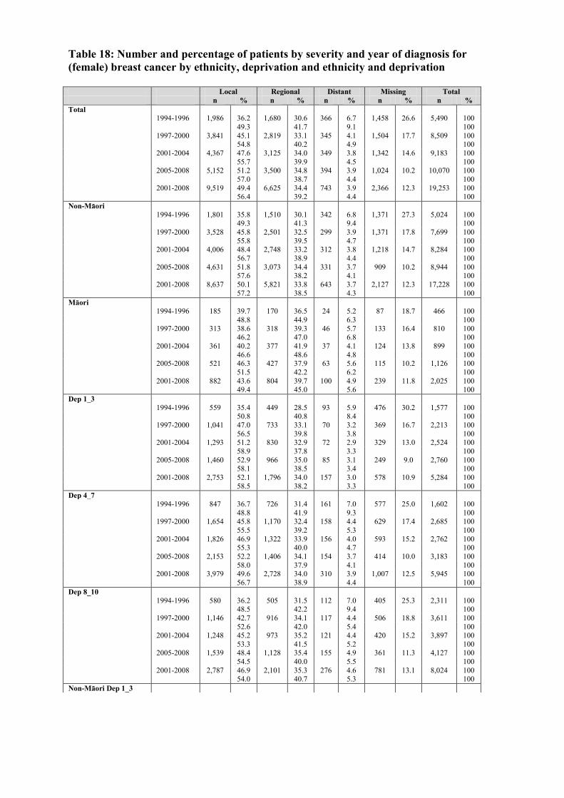
Table 18: Number and percentage of patients by severity and year of diagnosis for (female) breast cancer by ethnicity, deprivation and ethnicity and deprivation
Local Regional Distant Missing Total n % n % n % n % n % Total 1994-1996 1,986 36.2 1,680 30.6 366 6.7 1,458 26.6 5,490 100 49.3 41.7 9.1 100 1997-2000 3,841 45.1 2,819 33.1 345 4.1 1,504 17.7 8,509 100 54.8 40.2 4.9 100 2001-2004 4,367 47.6 3,125 34.0 349 3.8 1,342 14.6 9,183 100 55.7 39.9 4.5 100 2005-2008 5,152 51.2 3,500 34.8 394 3.9 1,024 10.2 10,070 100 57.0 38.7 4.4 100 2001-2008 9,519 49.4 6,625 34.4 743 3.9 2,366 12.3 19,253 100 56.4 39.2 4.4 100 Non-Māori 1994-1996 1,801 35.8 1,510 30.1 342 6.8 1,371 27.3 5,024 100 49.3 41.3 9.4 100 1997-2000 3,528 45.8 2,501 32.5 299 3.9 1,371 17.8 7,699 100 55.8 39.5 4.7 100 2001-2004 4,006 48.4 2,748 33.2 312 3.8 1,218 14.7 8,284 100 56.7 38.9 4.4 100 2005-2008 4,631 51.8 3,073 34.4 331 3.7 909 10.2 8,944 100 57.6 38.2 4.1 100 2001-2008 8,637 50.1 5,821 33.8 643 3.7 2,127 12.3 17,228 100 57.2 38.5 4.3 100 Māori 1994-1996 185 39.7 170 36.5 24 5.2 87 18.7 466 100 48.8 44.9 6.3 100 1997-2000 313 38.6 318 39.3 46 5.7 133 16.4 810 100 46.2 47.0 6.8 100 2001-2004 361 40.2 377 41.9 37 4.1 124 13.8 899 100 46.6 48.6 4.8 100 2005-2008 521 46.3 427 37.9 63 5.6 115 10.2 1,126 100 51.5 42.2 6.2 100 2001-2008 882 43.6 804 39.7 100 4.9 239 11.8 2,025 100 49.4 45.0 5.6 100 Dep 1_3 1994-1996 559 35.4 449 28.5 93 5.9 476 30.2 1,577 100 50.8 40.8 8.4 100 1997-2000 1,041 47.0 733 33.1 70 3.2 369 16.7 2,213 100 56.5 39.8 3.8 100 2001-2004 1,293 51.2 830 32.9 72 2.9 329 13.0 2,524 100 58.9 37.8 3.3 100 2005-2008 1,460 52.9 966 35.0 85 3.1 249 9.0 2,760 100 58.1 38.5 3.4 100 2001-2008 2,753 52.1 1,796 34.0 157 3.0 578 10.9 5,284 100 58.5 38.2 3.3 100 Dep 4_7 1994-1996 847 36.7 726 31.4 161 7.0 577 25.0 1,602 100 48.8 41.9 9.3 100 1997-2000 1,654 45.8 1,170 32.4 158 4.4 629 17.4 2,685 100 55.5 39.2 5.3 100 2001-2004 1,826 46.9 1,322 33.9 156 4.0 593 15.2 2,762 100 55.3 40.0 4.7 100 2005-2008 2,153 52.2 1,406 34.1 154 3.7 414 10.0 3,183 100 58.0 37.9 4.1 100 2001-2008 3,979 49.6 2,728 34.0 310 3.9 1,007 12.5 5,945 100 56.7 38.9 4.4 100 Dep 8_10 1994-1996 580 36.2 505 31.5 112 7.0 405 25.3 2,311 100 48.5 42.2 9.4 100 1997-2000 1,146 42.7 916 34.1 117 4.4 506 18.8 3,611 100 52.6 42.0 5.4 100 2001-2004 1,248 45.2 973 35.2 121 4.4 420 15.2 3,897 100 53.3 41.5 5.2 100 2005-2008 1,539 48.4 1,128 35.4 155 4.9 361 11.3 4,127 100 54.5 40.0 5.5 100 2001-2008 2,787 46.9 2,101 35.3 276 4.6 781 13.1 8,024 100 54.0 40.7 5.3 100 Non-Māori Dep 1_3

Cancer excess mortality rates over 2006-2026 for ABC-CBA
36
Local Regional Distant Missing Total n % n % n % n % n % 1994-1996 538 35.4 421 27.7 92 6.0 470 30.9 1,331 100 51.2 40.1 8.8 100 1997-2000 1,011 47.3 701 32.8 61 2.9 364 17.0 2,186 100 57.0 39.5 3.4 100 2001-2004 1,245 51.2 801 32.9 71 2.9 316 13.0 2,244 100 58.8 37.8 3.4 100 2005-2008 1,414 53.4 917 34.6 80 3.0 237 9.0 2,507 100 58.6 38.0 3.3 100 2001-2008 2,659 52.3 1,718 33.8 151 3.0 553 10.9 4,751 100 58.7 37.9 3.3 100 Non-Māori Dep 4_7 1994-1996 789 36.3 674 31.0 151 7.0 558 25.7 1,521 100 48.9 41.8 9.4 100 1997-2000 1,559 46.2 1,087 32.2 141 4.2 589 17.4 2,137 100 55.9 39.0 5.1 100 2001-2004 1,722 47.7 1,188 32.9 143 4.0 554 15.4 2,433 100 56.4 38.9 4.7 100 2005-2008 1,998 52.7 1,273 33.6 132 3.5 386 10.2 2,648 100 58.7 37.4 3.9 100 2001-2008 3,720 50.3 2,461 33.3 275 3.7 940 12.7 5,081 100 57.6 38.1 4.3 100 Non-Māori Dep 8_10 1994-1996 474 35.6 415 31.2 99 7.4 343 25.8 139 100 48.0 42.0 10.0 100 1997-2000 958 43.8 713 32.6 97 4.4 418 19.1 235 100 54.2 40.3 5.5 100 2001-2004 1,039 46.3 759 33.8 98 4.4 348 15.5 290 100 54.8 40.0 5.2 100 2005-2008 1,219 48.6 883 35.2 119 4.7 286 11.4 338 100 54.9 39.8 5.4 100 2001-2008 2,258 47.5 1,642 34.6 217 4.6 634 13.3 628 100 54.8 39.9 5.3 100 Māori Dep 1_3 1994-1996 21 37.5 28 50.0 1 1.8 6 10.7 2,172 100 42.0 56.0 2.0 100 1997-2000 30 39.5 32 42.1 9 11.8 5 6.6 3,376 100 42.3 45.1 12.7 100 2001-2004 48 52.7 29 31.9 1 1.1 13 14.3 3,607 100 61.5 37.2 1.3 100 2005-2008 46 41.1 49 43.8 5 4.5 12 10.7 3,789 100 46.0 49.0 5.0 100 2001-2008 94 46.3 78 38.4 6 3.0 25 12.3 7,396 100 52.8 43.8 3.4 100 Māori Dep 4_7 1994-1996 58 41.7 52 37.4 10 7.2 19 13.7 271 100 48.3 43.3 8.3 100 1997-2000 95 40.4 83 35.3 17 7.2 40 17.0 499 100 48.7 42.6 8.7 100 2001-2004 104 35.9 134 46.2 13 4.5 39 13.4 518 100 41.4 53.4 5.2 100 2005-2008 155 45.9 133 39.3 22 6.5 28 8.3 676 100 50.0 42.9 7.1 100 2001-2008 259 41.2 267 42.5 35 5.6 67 10.7 1,194 100 46.2 47.6 6.2 100 Māori Dep 8_10 1994-1996 106 39.1 90 33.2 13 4.8 62 22.9 56 100 50.7 43.1 6.2 100 1997-2000 188 37.7 203 40.7 20 4.0 88 17.6 76 100 45.7 49.4 4.9 100 2001-2004 209 40.3 214 41.3 23 4.4 72 13.9 91 100 46.9 48.0 5.2 100 2005-2008 320 47.3 245 36.2 36 5.3 75 11.1 112 100 53.2 40.8 6.0 100 2001-2008 529 44.3 459 38.4 59 4.9 147 12.3 203 100 50.5 43.8 5.6 100

Cancer excess mortality rates over 2006-2026 for ABC-CBA
37
Table 19: Number and percentage of patients by severity and year of diagnosis for colorectal cancer by ethnicity, deprivation and ethnicity and deprivation
Local Regional Distant Missing Total n % n % n % n % n % Total 1994-1996 2,295 32.1 2,376 33.2 1,311 18.3 1,166 16.3 7,148 100 38.4 39.7 21.9 100 1997-2000 2,430 25.1 4,582 47.2 1,758 18.1 928 9.6 9,698 100 27.7 52.2 20.0 100 2001-2004 2,840 27.2 4,499 43.1 2,133 20.4 963 9.2 10,435 100 30.0 47.5 22.5 100 2005-2008 2,776 25.9 4,341 40.5 1,924 17.9 1,684 15.7 10,725 100 30.7 48.0 21.3 100 2001-2008 5,616 26.5 8,840 41.8 4,057 19.2 2,647 12.5 21,160 100 30.3 47.8 21.9 100 Non-Māori 1994-1996 63 30.0 65 31.0 43 20.5 39 18.6 210 100 36.8 38.0 25.1 100 1997-2000 57 16.7 160 46.8 81 23.7 44 12.9 342 100 19.1 53.7 27.2 100 2001-2004 83 18.9 177 40.2 134 30.5 46 10.5 440 100 21.1 44.9 34.0 100 2005-2008 105 21.4 158 32.2 129 26.3 99 20.2 491 100 26.8 40.3 32.9 100 2001-2008 188 20.2 335 36.0 263 28.2 145 15.6 931 100 23.9 42.6 33.5 100 Māori 1994-1996 2,232 32.2 2,311 33.3 1,268 18.3 1,127 16.2 6,938 100 38.4 39.8 21.8 100 1997-2000 2,373 25.4 4,422 47.3 1,677 17.9 884 9.4 9,356 100 28.0 52.2 19.8 100 2001-2004 2,757 27.6 4,322 43.2 1,999 20.0 917 9.2 9,995 100 30.4 47.6 22.0 100 2005-2008 2,671 26.1 4,183 40.9 1,795 17.5 1,585 15.5 10,234 100 30.9 48.4 20.8 100 2001-2008 5,428 26.8 8,505 42.0 3,794 18.8 2,502 12.4 20,229 100 30.6 48.0 21.4 100 Dep 1_3 1994-1996 638 32.7 645 33.1 354 18.2 313 16.1 1,950 100 39.0 39.4 21.6 100 1997-2000 606 25.8 1,105 47.0 421 17.9 220 9.4 2,352 100 28.4 51.8 19.7 100 2001-2004 717 27.0 1,171 44.0 520 19.6 251 9.4 2,659 100 29.8 48.6 21.6 100 2005-2008 706 25.8 1,137 41.6 441 16.1 448 16.4 2,732 100 30.9 49.8 19.3 100 2001-2008 1,423 26.4 2,308 42.8 961 17.8 699 13.0 5,391 100 30.3 49.2 20.5 100 Dep 4_7 1994-1996 996 31.6 1,042 33.1 563 17.9 547 17.4 2,050 100 38.3 40.1 21.6 100 1997-2000 1,111 25.5 2,056 47.2 801 18.4 391 9.0 2,987 100 28.0 51.8 20.2 100 2001-2004 1,240 27.0 2,004 43.6 953 20.7 400 8.7 3,179 100 29.5 47.7 22.7 100 2005-2008 1,236 26.0 1,927 40.6 868 18.3 719 15.1 3,243 100 30.7 47.8 21.5 100 2001-2008 2,476 26.5 3,931 42.1 1,821 19.5 1,119 12.0 6,422 100 30.1 47.8 22.1 100 Dep 8_10 1994-1996 661 32.2 689 33.6 394 19.2 306 14.9 3,148 100 37.9 39.5 22.6 100 1997-2000 713 23.9 1,421 47.6 536 17.9 317 10.6 4,359 100 26.7 53.2 20.1 100 2001-2004 883 27.8 1,324 41.6 660 20.8 312 9.8 4,597 100

Cancer excess mortality rates over 2006-2026 for ABC-CBA
38
Local Regional Distant Missing Total n % n % n % n % n % 30.8 46.2 23.0 100 2005-2008 834 25.7 1,277 39.4 615 19.0 517 15.9 4,750 100 30.6 46.8 22.6 100 2001-2008 1,717 26.7 2,601 40.5 1,275 19.9 829 12.9 9,347 100 30.7 46.5 22.8 100 Non-Māori Dep 1_3 1994-1996 632 32.8 640 33.2 353 18.3 304 15.8 123 100 38.9 39.4 21.7 100 1997-2000 601 25.9 1,091 46.9 415 17.9 217 9.3 202 100 28.5 51.8 19.7 100 2001-2004 708 27.2 1,150 44.1 505 19.4 243 9.3 249 100 30.0 48.7 21.4 100 2005-2008 690 25.7 1,124 41.8 433 16.1 439 16.3 278 100 30.7 50.0 19.3 100 2001-2008 1,398 26.4 2,274 43.0 938 17.7 682 12.9 527 100 30.3 49.3 20.3 100 Non-Māori Dep 4_7 1994-1996 6 28.6 5 23.8 1 4.8 9 42.9 1,929 100 50.0 41.7 8.3 100 1997-2000 5 17.9 14 50.0 6 21.4 3 10.7 2,324 100 20.0 56.0 24.0 100 2001-2004 9 17.0 21 39.6 15 28.3 8 15.1 2,606 100 20.0 46.7 33.3 100 2005-2008 16 34.8 13 28.3 8 17.4 9 19.6 2,686 100 43.2 35.1 21.6 100 2001-2008 25 25.3 34 34.3 23 23.2 17 17.2 5,292 100 30.5 41.5 28.0 100 Non-Māori Dep 8_10 1994-1996 42 34.1 36 29.3 28 22.8 17 13.8 1,927 100 39.6 34.0 26.4 100 1997-2000 36 17.8 99 49.0 41 20.3 26 12.9 2,785 100 20.5 56.3 23.3 100 2001-2004 49 19.7 101 40.6 76 30.5 23 9.2 2,930 100 21.7 44.7 33.6 100 2005-2008 52 18.7 95 34.2 76 27.3 55 19.8 2,965 100 23.3 42.6 34.1 100 2001-2008 101 19.2 196 37.2 152 28.8 78 14.8 5,895 100 22.5 43.7 33.9 100 Māori Dep 1_3 1994-1996 15 22.7 24 36.4 14 21.2 13 19.7 21 100 28.3 45.3 26.4 100 1997-2000 16 14.3 47 42.0 34 30.4 15 13.4 28 100 16.5 48.5 35.1 100 2001-2004 25 18.1 55 39.9 43 31.2 15 10.9 53 100 20.3 44.7 35.0 100 2005-2008 37 22.2 50 29.9 45 26.9 35 21.0 46 100 28.0 37.9 34.1 100 2001-2008 62 20.3 105 34.4 88 28.9 50 16.4 99 100 24.3 41.2 34.5 100 Māori Dep 4_7 1994-1996 619 32.1 653 33.9 366 19.0 289 15.0 3,082 100 37.8 39.9 22.3 100 1997-2000 677 24.3 1,322 47.5 495 17.8 291 10.4 4,247 100 27.1 53.0 19.8 100 2001-2004 834 28.5 1,223 41.7 584 19.9 289 9.9 4,459 100 31.6 46.3 22.1 100 2005-2008 782 26.4 1,182 39.9 539 18.2 462 15.6 4,583 100 31.2 47.2 21.5 100 2001-2008 1,616 27.4 2,405 40.8 1,123 19.1 751 12.7 9,042 100 31.4 46.8 21.8 100 Māori Dep 8_10 1994-1996 981 31.8 1,018 33.0 549 17.8 534 17.3 66 100 38.5 40.0 21.5 100 1997-2000 1,095 25.8 2,009 47.3 767 18.1 376 8.9 112 100 28.3 51.9 19.8 100

Cancer excess mortality rates over 2006-2026 for ABC-CBA
39
Local Regional Distant Missing Total n % n % n % n % n % 2001-2004 1,215 27.2 1,949 43.7 910 20.4 385 8.6 138 100 29.8 47.8 22.3 100 2005-2008 1,199 26.2 1,877 41.0 823 18.0 684 14.9 167 100 30.8 48.1 21.1 100 2001-2008 2,414 26.7 3,826 42.3 1,733 19.2 1,069 11.8 305 100 30.3 48.0 21.7 100

Cancer excess mortality rates over 2006-2026 for ABC-CBA
40
Table 20: Number and percentage of patients by severity and year of diagnosis for colon cancer by ethnicity, deprivation and ethnicity and deprivation
Local Regional Distant Missing Total n % n % n % n % n % Total 1994-1996 1,375 29.2 1,617 34.4 930 19.8 781 16.6 4,703 100 35.1 41.2 23.7 100 1997-2000 1,443 22.6 3,243 50.7 1,252 19.6 458 7.2 6,396 100 24.3 54.6 21.1 100 2001-2004 1,790 26.1 3,124 45.5 1,541 22.4 414 6.0 6,869 100 27.7 48.4 23.9 100 2005-2008 1,866 26.3 3,199 45.1 1,409 19.9 621 8.8 7,095 100 28.8 49.4 21.8 100 2001-2008 3,656 26.2 6,323 45.3 2,950 21.1 1,035 7.4 13,964 100 28.3 48.9 22.8 100 Non-Māori 1994-1996 32 27.6 36 31.0 27 23.3 21 18.1 116 100 33.7 37.9 28.4 100 1997-2000 29 14.9 97 49.7 54 27.7 15 7.7 195 100 16.1 53.9 30.0 100 2001-2004 52 19.9 110 42.1 89 34.1 10 3.8 261 100 20.7 43.8 35.5 100 2005-2008 58 20.9 116 41.7 84 30.2 20 7.2 278 100 22.5 45.0 32.6 100 2001-2008 110 20.4 226 41.9 173 32.1 30 5.6 539 100 21.6 44.4 34.0 100 Māori 1994-1996 1,343 29.3 1,581 34.5 903 19.7 760 16.6 4,587 100 35.1 41.3 23.6 100 1997-2000 1,414 22.8 3,146 50.7 1,198 19.3 443 7.1 6,201 100 24.6 54.6 20.8 100 2001-2004 1,738 26.3 3,014 45.6 1,452 22.0 404 6.1 6,608 100 28.0 48.6 23.4 100 2005-2008 1,808 26.5 3,083 45.2 1,325 19.4 601 8.8 6,817 100 29.1 49.6 21.3 100 2001-2008 3,546 26.4 6,097 45.4 2,777 20.7 1,005 7.5 13,425 100 28.6 49.1 22.4 100 Dep 1_3 1994-1996 391 29.5 463 34.9 253 19.1 220 16.6 1,327 100 35.3 41.8 22.9 100 1997-2000 356 22.7 782 49.9 312 19.9 118 7.5 1,568 100 24.6 53.9 21.5 100 2001-2004 454 25.9 819 46.7 384 21.9 95 5.4 1,752 100 27.4 49.4 23.2 100 2005-2008 477 26.5 852 47.3 317 17.6 156 8.7 1,802 100 29.0 51.8 19.3 100 2001-2008 931 26.2 1,671 47.0 701 19.7 251 7.1 3,554 100 28.2 50.6 21.2 100 Dep 4_7 1994-1996 604 29.1 695 33.5 405 19.5 370 17.8 1,302 100 35.4 40.8 23.8 100 1997-2000 644 22.3 1,462 50.7 569 19.7 208 7.2 1,945 100 24.1 54.7 21.3 100 2001-2004 769 25.4 1,377 45.5 688 22.8 190 6.3 2,093 100 27.1 48.6 24.3 100 2005-2008 831 26.2 1,421 44.9 645 20.4 271 8.6 2,125 100 28.7 49.1 22.3 100 2001-2008 1,600 25.8 2,798 45.2 1,333 21.5 461 7.4 4,218 100 27.9 48.8 23.3 100 Dep 8_10 1994-1996 380 29.2 459 35.3 272 20.9 191 14.7 2,074 100 34.2 41.3 24.5 100 1997-2000 443 22.8 999 51.4 371 19.1 132 6.8 2,883 100 24.4 55.1 20.5 100 2001-2004 567 27.1 928 44.3 469 22.4 129 6.2 3,024 100 28.9 47.3 23.9 100 2005-2008 558 26.3 926 43.6 447 21.0 194 9.1 3,168 100

Cancer excess mortality rates over 2006-2026 for ABC-CBA
41
Local Regional Distant Missing Total n % n % n % n % n % 28.9 48.0 23.1 100 2001-2008 1,125 26.7 1,854 44.0 916 21.7 323 7.7 6,192 100 28.9 47.6 23.5 100 Non-Māori Dep 1_3 1994-1996 5 33.3 2 13.3 0 0.0 8 53.3 1,240 100 71.4 28.6 0.0 100 1997-2000 2 11.1 10 55.6 5 27.8 1 5.6 1,831 100 11.8 58.8 29.4 100 2001-2004 6 17.6 16 47.1 10 29.4 2 5.9 1,941 100 18.8 50.0 31.3 100 2005-2008 9 33.3 11 40.7 6 22.2 1 3.7 1,971 100 34.6 42.3 23.1 100 2001-2008 15 24.6 27 44.3 16 26.2 3 4.9 3,912 100 25.9 46.6 27.6 100 Non-Māori Dep 4_7 1994-1996 8 20.5 15 38.5 9 23.1 7 17.9 15 100 25.0 46.9 28.1 100 1997-2000 6 9.5 29 46.0 20 31.7 8 12.7 18 100 10.9 52.7 36.4 100 2001-2004 13 17.3 34 45.3 26 34.7 2 2.7 34 100 17.8 46.6 35.6 100 2005-2008 19 19.6 43 44.3 24 24.7 11 11.3 27 100 22.1 50.0 27.9 100 2001-2008 32 18.6 77 44.8 50 29.1 13 7.6 61 100 20.1 48.4 31.4 100 Non-Māori Dep 8_10 1994-1996 361 29.1 440 35.5 254 20.5 185 14.9 2,035 100 34.2 41.7 24.1 100 1997-2000 422 23.0 941 51.4 342 18.7 126 6.9 2,820 100 24.8 55.2 20.1 100 2001-2004 534 27.5 868 44.7 416 21.4 123 6.3 2,949 100 29.4 47.7 22.9 100 2005-2008 528 26.8 864 43.8 393 19.9 186 9.4 3,071 100 29.6 48.4 22.0 100 2001-2008 1,062 27.1 1,732 44.3 809 20.7 309 7.9 6,020 100 29.5 48.1 22.5 100 Māori Dep 1_3 1994-1996 386 29.4 461 35.1 253 19.3 212 16.2 39 100 35.1 41.9 23.0 100 1997-2000 354 22.8 772 49.8 307 19.8 117 7.5 63 100 24.7 53.9 21.4 100 2001-2004 448 26.1 803 46.7 374 21.8 93 5.4 75 100 27.6 49.4 23.0 100 2005-2008 468 26.4 841 47.4 311 17.5 155 8.7 97 100 28.9 51.9 19.2 100 2001-2008 916 26.2 1,644 47.1 685 19.6 248 7.1 172 100 28.2 50.7 21.1 100 Māori Dep 4_7 1994-1996 596 29.3 680 33.4 396 19.5 363 17.8 62 100 35.6 40.7 23.7 100 1997-2000 638 22.6 1,433 50.8 549 19.5 200 7.1 114 100 24.4 54.7 21.0 100 2001-2004 756 25.6 1,343 45.5 662 22.4 188 6.4 152 100 27.4 48.6 24.0 100 2005-2008 812 26.4 1,378 44.9 621 20.2 260 8.5 154 100 28.9 49.0 22.1 100 2001-2008 1,568 26.0 2,721 45.2 1,283 21.3 448 7.4 306 100 28.1 48.8 23.0 100 Māori Dep 8_10 1994-1996 19 30.6 19 30.6 18 29.0 6 9.7 1,312 100 33.9 33.9 32.1 100 1997-2000 21 18.4 58 50.9 29 25.4 6 5.3 1,550 100 19.4 53.7 26.9 100 2001-2004 33 21.7 60 39.5 53 34.9 6 3.9 1,718 100 22.6 41.1 36.3 100 2005-2008 30 19.5 62 40.3 54 35.1 8 5.2 1,775 100 20.5 42.5 37.0 100 2001-2008 63 20.6 122 39.9 107 35.0 14 4.6 3,493 100

Cancer excess mortality rates over 2006-2026 for ABC-CBA
42
Local Regional Distant Missing Total n % n % n % n % n % 21.6 41.8 36.6 100

Cancer excess mortality rates over 2006-2026 for ABC-CBA
43
Table 21: Number and percentage of patients by severity and year of diagnosis for rectal cancer by ethnicity, deprivation and ethnicity and deprivation
Local Regional Distant Missing Total n % n % n % n % n % Total 1994-1996 920 37.6 759 31.0 381 15.6 385 15.7 2,445 100 44.7 36.8 18.5 100 1997-2000 987 29.9 1,339 40.6 506 15.3 470 14.2 3,302 100 34.9 47.3 17.9 100 2001-2004 1,050 29.4 1,375 38.6 592 16.6 549 15.4 3,566 100 34.8 45.6 19.6 100 2005-2008 910 25.1 1,142 31.5 515 14.2 1,063 29.3 3,630 100 35.4 44.5 20.1 100 2001-2008 1,960 27.2 2,517 35.0 1,107 15.4 1,612 22.4 7,196 100 35.1 45.1 19.8 100 Non-Māori 1994-1996 31 33.0 29 30.9 16 17.0 18 19.1 94 100 40.8 38.2 21.1 100 1997-2000 28 19.0 63 42.9 27 18.4 29 19.7 147 100 23.7 53.4 22.9 100 2001-2004 31 17.3 67 37.4 45 25.1 36 20.1 179 100 21.7 46.9 31.5 100 2005-2008 47 22.1 42 19.7 45 21.1 79 37.1 213 100 35.1 31.3 33.6 100 2001-2008 78 19.9 109 27.8 90 23.0 115 29.3 392 100 28.2 39.4 32.5 100 Māori 1994-1996 889 37.8 730 31.1 365 15.5 367 15.6 2,351 100 44.8 36.8 18.4 100 1997-2000 959 30.4 1,276 40.4 479 15.2 441 14.0 3,155 100 35.3 47.0 17.6 100 2001-2004 1,019 30.1 1,308 38.6 547 16.1 513 15.1 3,387 100 35.5 45.5 19.0 100 2005-2008 863 25.3 1,100 32.2 470 13.8 984 28.8 3,417 100 35.5 45.2 19.3 100 2001-2008 1,882 27.7 2,408 35.4 1,017 14.9 1,497 22.0 6,804 100 35.5 45.4 19.2 100 Dep 1_3 1994-1996 247 39.6 182 29.2 101 16.2 93 14.9 623 100 46.6 34.3 19.1 100 1997-2000 250 31.9 323 41.2 109 13.9 102 13.0 784 100 36.7 47.4 16.0 100 2001-2004 263 29.0 352 38.8 136 15.0 156 17.2 907 100 35.0 46.9 18.1 100 2005-2008 229 24.6 285 30.6 124 13.3 292 31.4 930 100 35.9 44.7 19.4 100 2001-2008 492 26.8 637 34.7 260 14.2 448 24.4 1,837 100 35.4 45.9 18.7 100 Dep 4_7 1994-1996 392 36.5 347 32.3 158 14.7 177 16.5 748 100 43.7 38.7 17.6 100 1997-2000 467 31.6 594 40.2 232 15.7 183 12.4 1,042 100 36.1 45.9 17.9 100 2001-2004 471 29.9 627 39.9 265 16.8 210 13.4 1,086 100 34.6 46.0 19.4 100 2005-2008 405 25.6 506 32.0 223 14.1 448 28.3 1,118 100 35.7 44.6 19.7 100 2001-2008 876 27.8 1,133 35.9 488 15.5 658 20.9 2,204 100 35.1 45.4 19.5 100 Dep 8_10 1994-1996 281 37.6 230 30.7 122 16.3 115 15.4 1,074 100 44.4 36.3 19.3 100 1997-2000 270 25.9 422 40.5 165 15.8 185 17.8 1,476 100 31.5 49.2 19.3 100 2001-2004 316 29.1 396 36.5 191 17.6 183 16.9 1,573 100 35.0 43.9 21.2 100

Cancer excess mortality rates over 2006-2026 for ABC-CBA
44
Local Regional Distant Missing Total n % n % n % n % n % 2005-2008 276 24.7 351 31.4 168 15.0 323 28.9 1,582 100 34.7 44.2 21.1 100 2001-2008 592 26.9 747 33.9 359 16.3 506 23.0 3,155 100 34.9 44.0 21.1 100 Non-Māori Dep 1_3 1994-1996 246 39.9 179 29.0 100 16.2 92 14.9 27 100 46.9 34.1 19.0 100 1997-2000 247 31.9 319 41.2 108 14.0 100 12.9 49 100 36.6 47.3 16.0 100 2001-2004 260 29.3 347 39.1 131 14.8 150 16.9 63 100 35.2 47.0 17.8 100 2005-2008 222 24.4 283 31.1 122 13.4 284 31.2 70 100 35.4 45.1 19.5 100 2001-2008 482 26.8 630 35.0 253 14.1 434 24.1 133 100 35.3 46.2 18.5 100 Non-Māori Dep 4_7 1994-1996 23 37.7 17 27.9 10 16.4 11 18.0 617 100 46.0 34.0 20.0 100 1997-2000 15 17.0 41 46.6 12 13.6 20 22.7 774 100 22.1 60.3 17.6 100 2001-2004 16 16.5 41 42.3 23 23.7 17 17.5 888 100 20.0 51.3 28.8 100 2005-2008 22 17.7 33 26.6 22 17.7 47 37.9 911 100 28.6 42.9 28.6 100 2001-2008 38 17.2 74 33.5 45 20.4 64 29.0 1,799 100 24.2 47.1 28.7 100 Non-Māori Dep 8_10 1994-1996 7 25.9 9 33.3 5 18.5 6 22.2 687 100 33.3 42.9 23.8 100 1997-2000 10 20.4 18 36.7 14 28.6 7 14.3 954 100 23.8 42.9 33.3 100 2001-2004 12 19.0 21 33.3 17 27.0 13 20.6 989 100 24.0 42.0 34.0 100 2005-2008 18 25.7 7 10.0 21 30.0 24 34.3 994 100 39.1 15.2 45.7 100 2001-2008 30 22.6 28 21.1 38 28.6 37 27.8 1,983 100 31.3 29.2 39.6 100 Māori Dep 1_3 1994-1996 1 16.7 3 50.0 1 16.7 1 16.7 61 100 20.0 60.0 20.0 100 1997-2000 3 30.0 4 40.0 1 10.0 2 20.0 88 100 37.5 50.0 12.5 100 2001-2004 3 15.8 5 26.3 5 26.3 6 31.6 97 100 23.1 38.5 38.5 100 2005-2008 7 36.8 2 10.5 2 10.5 8 42.1 124 100 63.6 18.2 18.2 100 2001-2008 10 26.3 7 18.4 7 18.4 14 36.8 221 100 41.7 29.2 29.2 100 Māori Dep 4_7 1994-1996 258 37.6 213 31.0 112 16.3 104 15.1 1,047 100 44.3 36.5 19.2 100 1997-2000 255 26.7 381 39.9 153 16.0 165 17.3 1,427 100 32.3 48.3 19.4 100 2001-2004 300 30.3 355 35.9 168 17.0 166 16.8 1,510 100 36.5 43.1 20.4 100 2005-2008 254 25.6 318 32.0 146 14.7 276 27.8 1,512 100 35.4 44.3 20.3 100 2001-2008 554 27.9 673 33.9 314 15.8 442 22.3 3,022 100 36.0 43.7 20.4 100 Māori Dep 8_10 1994-1996 385 36.8 338 32.3 153 14.6 171 16.3 6 100 43.9 38.6 17.5 100 1997-2000 457 32.0 576 40.4 218 15.3 176 12.3 10 100 36.5 46.0 17.4 100 2001-2004 459 30.4 606 40.1 248 16.4 197 13.0 19 100 35.0 46.2 18.9 100
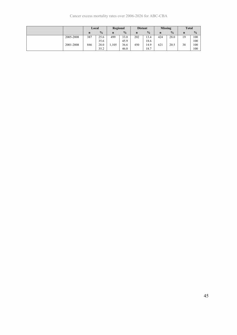
Cancer excess mortality rates over 2006-2026 for ABC-CBA
45
Local Regional Distant Missing Total n % n % n % n % n % 2005-2008 387 25.6 499 33.0 202 13.4 424 28.0 19 100 35.6 45.9 18.6 100 2001-2008 846 28.0 1,105 36.6 450 14.9 621 20.5 38 100 35.2 46.0 18.7 100

Cancer excess mortality rates over 2006-2026 for ABC-CBA
46
Table 22: Number and percentage of patients by severity and year of diagnosis for lung cancer by ethnicity, deprivation and ethnicity and deprivation
Local Regional Distant Missing Total n % n % n % n % n % Total 1994-1996 433 9.4 592 12.9 1,361 29.6 2,214 48.1 4,600 100 18.1 24.8 57.0 100 1997-2000 325 5.3 512 8.4 2,079 34.1 3,176 52.1 6,092 100 11.1 17.6 71.3 100 2001-2004 346 5.3 481 7.3 2,679 40.8 3,058 46.6 6,564 100 9.9 13.7 76.4 100 2005-2008 373 5.6 580 8.6 2,958 44.1 2,803 41.7 6,714 100 9.5 14.8 75.6 100 2001-2008 719 5.4 1,061 8.0 5,637 42.5 5,861 44.1 13,278 100 9.7 14.3 76.0 100 Non-Māori 1994-1996 385 9.6 516 12.9 1,197 29.8 1,917 47.7 4,015 100 18.4 24.6 57.1 100 1997-2000 301 5.9 444 8.7 1,748 34.1 2,639 51.4 5,132 100 12.1 17.8 70.1 100 2001-2004 310 5.6 413 7.5 2,234 40.5 2,559 46.4 5,516 100 10.5 14.0 75.5 100 2005-2008 318 5.8 481 8.7 2,448 44.4 2,268 41.1 5,515 100 9.8 14.8 75.4 100 2001-2008 628 5.7 894 8.1 4,682 42.4 4,827 43.8 11,031 100 10.1 14.4 75.5 100 Māori 1994-1996 48 8.2 76 13.0 164 28.0 297 50.8 585 100 16.7 26.4 56.9 100 1997-2000 24 2.5 68 7.1 331 34.5 537 55.9 960 100 5.7 16.1 78.3 100 2001-2004 36 3.4 68 6.5 445 42.5 499 47.6 1,048 100 6.6 12.4 81.1 100 2005-2008 55 4.6 99 8.3 510 42.5 535 44.6 1,199 100 8.3 14.9 76.8 100 2001-2008 91 4.0 167 7.4 955 42.5 1,034 46.0 2,247 100 7.5 13.8 78.7 100 Dep 1_3 1994-1996 146 8.6 198 11.7 497 29.4 848 50.2 1,689 100 17.4 23.5 59.1 100 1997-2000 118 4.6 188 7.4 851 33.5 1,382 54.4 2,539 100 10.2 16.2 73.6 100 2001-2004 130 4.9 171 6.4 1,060 40.0 1,291 48.7 2,652 100 9.6 12.6 77.9 100 2005-2008 138 5.0 211 7.6 1,217 44.0 1,202 43.4 2,768 100 8.8 13.5 77.7 100 2001-2008 268 4.9 382 7.0 2,277 42.0 2,493 46.0 5,420 100 9.2 13.1 77.8 100 Dep 4_7 1994-1996 89 9.5 127 13.5 272 28.9 453 48.1 1,970 100 18.2 26.0 55.7 100 1997-2000 72 6.6 99 9.1 395 36.2 525 48.1 2,462 100 12.7 17.5 69.8 100 2001-2004 75 6.4 106 9.1 474 40.8 508 43.7 2,749 100 11.5 16.2 72.4 100 2005-2008 85 7.5 120 10.6 491 43.4 436 38.5 2,814 100 12.2 17.2 70.5 100 2001-2008 160 7.0 226 9.8 965 42.0 944 41.1 5,563 100 11.8 16.7 71.4 100 Dep 8_10 1994-1996 198 10.1 267 13.6 592 30.1 913 46.3 941 100 18.7 25.3 56.0 100 1997-2000 135 5.5 225 9.1 833 33.8 1,269 51.5 1,091 100 11.3 18.9 69.8 100 2001-2004 141 5.1 204 7.4 1,145 41.7 1,259 45.8 1,163 100
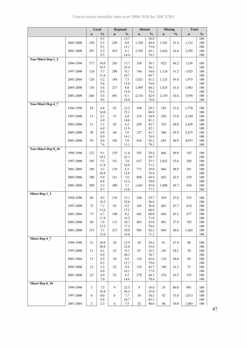
Cancer excess mortality rates over 2006-2026 for ABC-CBA
47
Local Regional Distant Missing Total n % n % n % n % n % 9.5 13.7 76.8 100 2005-2008 150 5.3 249 8.8 1,250 44.4 1,165 41.4 1,132 100 9.1 15.1 75.8 100 2001-2008 291 5.2 453 8.1 2,395 43.1 2,424 43.6 2,295 100 9.3 14.4 76.3 100 Non-Māori Dep 1_3 1994-1996 177 10.0 243 13.7 536 30.1 822 46.2 1,336 100 18.5 25.4 56.1 100 1997-2000 124 5.7 200 9.1 746 34.0 1,124 51.2 1,925 100 11.6 18.7 69.7 100 2001-2004 128 5.2 184 7.5 1,021 41.5 1,125 45.8 1,975 100 9.6 13.8 76.6 100 2005-2008 138 5.6 217 8.8 1,095 44.2 1,025 41.4 1,983 100 9.5 15.0 75.5 100 2001-2008 266 5.4 401 8.1 2,116 42.9 2,150 43.6 3,958 100 9.6 14.4 76.0 100 Non-Māori Dep 4_7 1994-1996 24 6.8 43 12.2 104 29.5 182 51.6 1,778 100 14.0 25.1 60.8 100 1997-2000 13 2.1 37 6.0 214 34.9 350 57.0 2,194 100 4.9 14.0 81.1 100 2001-2004 21 3.1 42 6.2 289 42.7 325 48.0 2,458 100 6.0 11.9 82.1 100 2005-2008 38 4.8 60 7.6 327 41.7 360 45.9 2,475 100 8.9 14.1 76.9 100 2001-2008 59 4.0 102 7.0 616 42.1 685 46.9 4,933 100 7.6 13.1 79.3 100 Non-Māori Dep 8_10 1994-1996 122 9.1 155 11.6 393 29.4 666 49.9 192 100 18.2 23.1 58.7 100 1997-2000 105 5.5 151 7.8 637 33.1 1,032 53.6 268 100 11.8 16.9 71.3 100 2001-2004 109 5.5 129 6.5 771 39.0 966 48.9 291 100 10.8 12.8 76.4 100 2005-2008 100 5.0 151 7.6 890 44.9 842 42.5 339 100 8.8 13.2 78.0 100 2001-2008 209 5.3 280 7.1 1,661 42.0 1,808 45.7 630 100 9.7 13.0 77.3 100 Māori Dep 1_3 1994-1996 86 9.5 118 13.1 268 29.7 429 47.6 353 100 18.2 25.0 56.8 100 1997-2000 72 7.1 93 9.2 365 36.0 483 47.7 614 100 13.6 17.5 68.9 100 2001-2004 73 6.7 100 9.2 442 40.8 468 43.2 677 100 11.9 16.3 71.9 100 2005-2008 80 7.6 113 10.7 463 43.8 401 37.9 785 100 12.2 17.2 70.6 100 2001-2008 153 7.1 213 10.0 905 42.3 869 40.6 1,462 100 12.0 16.8 71.2 100 Māori Dep 4_7 1994-1996 21 10.9 24 12.5 56 29.2 91 47.4 40 100 20.8 23.8 55.4 100 1997-2000 11 4.1 25 9.3 87 32.5 145 54.1 78 100 8.9 20.3 70.7 100 2001-2004 13 4.5 20 6.9 124 42.6 134 46.0 80 100 8.3 12.7 79.0 100 2005-2008 12 3.5 32 9.4 155 45.7 140 41.3 75 100 6.0 16.1 77.9 100 2001-2008 25 4.0 52 8.3 279 44.3 274 43.5 155 100 7.0 14.6 78.4 100 Māori Dep 8_10 1994-1996 3 7.5 9 22.5 4 10.0 24 60.0 901 100 18.8 56.3 25.0 100 1997-2000 0 0.0 6 7.7 30 38.5 42 53.8 1,013 100 0.0 16.7 83.3 100 2001-2004 2 2.5 6 7.5 32 40.0 40 50.0 1,083 100
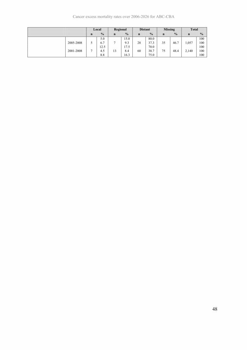
Cancer excess mortality rates over 2006-2026 for ABC-CBA
48
Local Regional Distant Missing Total n % n % n % n % n % 5.0 15.0 80.0 100 2005-2008 5 6.7 7 9.3 28 37.3 35 46.7 1,057 100 12.5 17.5 70.0 100 2001-2008 7 4.5 13 8.4 60 38.7 75 48.4 2,140 100 8.8 16.3 75.0 100
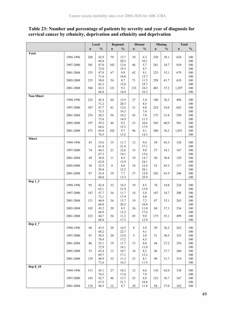
Cancer excess mortality rates over 2006-2026 for ABC-CBA
49
Table 23: Number and percentage of patients by severity and year of diagnosis for cervical cancer by ethnicity, deprivation and ethnicity and deprivation
Local Regional Distant Missing Total n % n % n % n % n % Total 1994-1996 268 42.9 79 12.7 39 6.3 238 38.1 624 100 69.4 20.5 10.1 100 1997-2000 381 47.0 102 12.6 46 5.7 281 34.7 810 100 72.0 19.3 8.7 100 2001-2004 325 47.9 67 9.9 62 9.1 225 33.1 679 100 71.6 14.8 13.7 100 2005-2008 235 38.0 54 8.7 71 11.5 258 41.7 618 100 65.3 15.0 19.7 100 2001-2008 560 43.2 121 9.3 133 10.3 483 37.2 1,297 100 68.8 14.9 16.3 100 Non-Māori 1994-1996 225 45.4 64 12.9 27 5.4 180 36.3 496 100 71.2 20.3 8.5 100 1997-2000 307 47.7 81 12.6 31 4.8 224 34.8 643 100 73.3 19.3 7.4 100 2001-2004 276 50.2 56 10.2 43 7.8 175 31.8 550 100 73.6 14.9 11.5 100 2005-2008 197 39.3 46 9.2 53 10.6 205 40.9 501 100 66.6 15.5 17.9 100 2001-2008 473 45.0 102 9.7 96 9.1 380 36.2 1,051 100 70.5 15.2 14.3 100 Māori 1994-1996 43 33.6 15 11.7 12 9.4 58 45.3 128 100 61.4 21.4 17.1 100 1997-2000 74 44.3 21 12.6 15 9.0 57 34.1 167 100 67.3 19.1 13.6 100 2001-2004 49 38.0 11 8.5 19 14.7 50 38.8 129 100 62.0 13.9 24.1 100 2005-2008 38 32.5 8 6.8 18 15.4 53 45.3 117 100 59.4 12.5 28.1 100 2001-2008 87 35.4 19 7.7 37 15.0 103 41.9 246 100 60.8 13.3 25.9 100 Dep 1_3 1994-1996 95 42.4 32 14.3 19 8.5 78 34.8 224 100 65.1 21.9 13.0 100 1997-2000 147 47.7 36 11.7 18 5.8 107 34.7 308 100 73.1 17.9 9.0 100 2001-2004 121 46.0 36 13.7 19 7.2 87 33.1 263 100 68.8 20.5 10.8 100 2005-2008 102 43.2 20 8.5 26 11.0 88 37.3 236 100 68.9 13.5 17.6 100 2001-2008 223 44.7 56 11.2 45 9.0 175 35.1 499 100 68.8 17.3 13.9 100 Dep 4_7 1994-1996 60 43.5 20 14.5 8 5.8 50 36.2 262 100 68.2 22.7 9.1 100 1997-2000 91 54.5 20 12.0 5 3.0 51 30.5 335 100 78.4 17.2 4.3 100 2001-2004 86 53.1 19 11.7 13 8.0 44 27.2 254 100 72.9 16.1 11.0 100 2005-2008 53 43.4 13 10.7 10 8.2 46 37.7 260 100 69.7 17.1 13.2 100 2001-2008 139 48.9 32 11.3 23 8.1 90 31.7 514 100 71.6 16.5 11.9 100 Dep 8_10 1994-1996 113 43.1 27 10.3 12 4.6 110 42.0 138 100 74.3 17.8 7.9 100 1997-2000 143 42.7 46 13.7 23 6.9 123 36.7 167 100 67.5 21.7 10.8 100 2001-2004 118 46.5 12 4.7 30 11.8 94 37.0 162 100

Cancer excess mortality rates over 2006-2026 for ABC-CBA
50
Local Regional Distant Missing Total n % n % n % n % n % 73.8 7.5 18.8 100 2005-2008 80 30.8 21 8.1 35 13.5 124 47.7 122 100 58.8 15.4 25.7 100 2001-2008 198 38.5 33 6.4 65 12.6 218 42.4 284 100 66.9 11.1 22.0 100 Non-Māori Dep 1_3 1994-1996 82 43.2 28 14.7 13 6.8 67 35.3 179 100 66.7 22.8 10.6 100 1997-2000 129 48.3 34 12.7 13 4.9 91 34.1 227 100 73.3 19.3 7.4 100 2001-2004 111 49.8 28 12.6 16 7.2 68 30.5 176 100 71.6 18.1 10.3 100 2005-2008 91 44.8 16 7.9 19 9.4 77 37.9 190 100 72.2 12.7 15.1 100 2001-2008 202 47.4 44 10.3 35 8.2 145 34.0 366 100 71.9 15.7 12.5 100 Non-Māori Dep 4_7 1994-1996 27 32.5 9 10.8 5 6.0 42 50.6 190 100 65.9 22.0 12.2 100 1997-2000 46 42.6 15 13.9 10 9.3 37 34.3 267 100 64.8 21.1 14.1 100 2001-2004 33 42.3 2 2.6 14 17.9 29 37.2 223 100 67.3 4.1 28.6 100 2005-2008 18 25.7 2 2.9 9 12.9 41 58.6 203 100 62.1 6.9 31.0 100 2001-2008 51 34.5 4 2.7 23 15.5 70 47.3 426 100 65.4 5.1 29.5 100 Non-Māori Dep 8_10 1994-1996 86 48.0 18 10.1 7 3.9 68 38.0 34 100 77.5 16.2 6.3 100 1997-2000 97 42.7 31 13.7 13 5.7 86 37.9 41 100 68.8 22.0 9.2 100 2001-2004 85 48.3 10 5.7 16 9.1 65 36.9 40 100 76.6 9.0 14.4 100 2005-2008 62 32.6 19 10.0 26 13.7 83 43.7 33 100 57.9 17.8 24.3 100 2001-2008 147 40.2 29 7.9 42 11.5 148 40.4 73 100 67.4 13.3 19.3 100 Māori Dep 1_3 1994-1996 57 44.9 18 14.2 7 5.5 45 35.4 83 100 69.5 22.0 8.5 100 1997-2000 81 54.4 16 10.7 5 3.4 47 31.5 108 100 79.4 15.7 4.9 100 2001-2004 80 53.0 18 11.9 11 7.3 42 27.8 78 100 73.4 16.5 10.1 100 2005-2008 44 40.7 11 10.2 8 7.4 45 41.7 70 100 69.8 17.5 12.7 100 2001-2008 124 47.9 29 11.2 19 7.3 87 33.6 148 100 72.1 16.9 11.0 100 Māori Dep 4_7 1994-1996 13 38.2 4 11.8 6 17.6 11 32.4 11 100 56.5 17.4 26.1 100 1997-2000 18 43.9 2 4.9 5 12.2 16 39.0 18 100 72.0 8.0 20.0 100 2001-2004 10 25.0 8 20.0 3 7.5 19 47.5 11 100 47.6 38.1 14.3 100 2005-2008 11 33.3 4 12.1 7 21.2 11 33.3 14 100 50.0 18.2 31.8 100 2001-2008 21 28.8 12 16.4 10 13.7 30 41.1 25 100 48.8 27.9 23.3 100 Māori Dep 8_10 1994-1996 3 27.3 2 18.2 1 9.1 5 45.5 127 100 50.0 33.3 16.7 100 1997-2000 10 55.6 4 22.2 0 0.0 4 22.2 149 100 71.4 28.6 0.0 100 2001-2004 6 54.5 1 9.1 2 18.2 2 18.2 151 100

Cancer excess mortality rates over 2006-2026 for ABC-CBA
51
Local Regional Distant Missing Total n % n % n % n % n % 66.7 11.1 22.2 100 2005-2008 9 64.3 2 14.3 2 14.3 1 7.1 108 100 69.2 15.4 15.4 100 2001-2008 15 60.0 3 12.0 4 16.0 3 12.0 259 100 68.2 13.6 18.2 100

Cancer excess mortality rates over 2006-2026 for ABC-CBA
52
Table 24: Number and percentage of patients by severity and year of diagnosis for prostate cancer by ethnicity, deprivation and ethnicity and deprivation
Local Regional Distant Missing Total
n % n % n % n % n % Total 1994-1996 1,710 25.4 312 4.6 684 10.2 4,016 59.7 6,722 100 63.2 11.5 25.3 100 1997-2000 888 8.8 367 3.6 662 6.5 8,220 81.1 10,137 100 46.3 19.1 34.5 100 2001-2004 1,586 14.7 522 4.8 515 4.8 8,182 75.7 10,805 100 60.5 19.9 19.6 100 2005-2008 1,611 15.3 636 6.0 611 5.8 7,697 72.9 10,555 100 56.4 22.3 21.4 100 2001-2008 3,197 15.0 1,158 5.4 1,126 5.3 15,879 74.3 21,360 100 58.3 21.1 20.5 100 Non-Māori 1994-1996 65 27.5 13 5.5 38 16.1 120 50.8 236 100 56.0 11.2 32.8 100 1997-2000 27 6.2 7 1.6 66 15.0 339 77.2 439 100 27.0 7.0 66.0 100 2001-2004 39 7.5 17 3.3 27 5.2 436 84.0 519 100 47.0 20.5 32.5 100 2005-2008 50 9.4 33 6.2 54 10.2 394 74.2 531 100 36.5 24.1 39.4 100 2001-2008 89 8.5 50 4.8 81 7.7 830 79.0 1,050 100 40.5 22.7 36.8 100 Māori 1994-1996 1,645 25.4 299 4.6 646 10.0 3,896 60.1 6,486 100 63.5 11.5 24.9 100 1997-2000 861 8.9 360 3.7 596 6.1 7,881 81.3 9,698 100 47.4 19.8 32.8 100 2001-2004 1,547 15.0 505 4.9 488 4.7 7,746 75.3 10,286 100 60.9 19.9 19.2 100 2005-2008 1,561 15.6 603 6.0 557 5.6 7,303 72.9 10,024 100 57.4 22.2 20.5 100 2001-2008 3,108 15.3 1,108 5.5 1,045 5.1 15,049 74.1 20,310 100 59.1 21.1 19.9 100 Dep 1_3 1994-1996 508 24.7 96 4.7 190 9.3 1,259 61.3 2,053 100 64.0 12.1 23.9 100 1997-2000 256 9.4 102 3.7 149 5.5 2,219 81.4 2,726 100 50.5 20.1 29.4 100 2001-2004 507 16.9 160 5.3 98 3.3 2,238 74.5 3,003 100 66.3 20.9 12.8 100 2005-2008 544 17.8 214 7.0 124 4.1 2,166 71.1 3,048 100 61.7 24.3 14.1 100 2001-2008 1,051 17.4 374 6.2 222 3.7 4,404 72.8 6,051 100 63.8 22.7 13.5 100 Dep 4_7 1994-1996 724 25.3 140 4.9 293 10.2 1,705 59.6 1,807 100 62.6 12.1 25.3 100 1997-2000 346 8.0 171 4.0 262 6.1 3,549 82.0 3,083 100 44.4 22.0 33.6 100 2001-2004 690 14.7 243 5.2 210 4.5 3,545 75.6 3,114 100 60.4 21.3 18.4 100 2005-2008 686 15.4 273 6.1 262 5.9 3,244 72.7 3,042 100 56.2 22.4 21.5 100 2001-2008 1,376 15.0 516 5.6 472 5.2 6,789 74.2 6,156 100 58.2 21.8 20.0 100 Dep 8_10 1994-1996 478 26.5 76 4.2 201 11.1 1,052 58.2 2,862 100 63.3 10.1 26.6 100 1997-2000 286 9.3 94 3.0 251 8.1 2,452 79.5 4,328 100 45.3 14.9 39.8 100 2001-2004 389 12.5 119 3.8 207 6.6 2,399 77.0 4,688 100 54.4 16.6 29.0 100 2005-2008 381 12.5 149 4.9 225 7.4 2,287 75.2 4,465 100 50.5 19.7 29.8 100

Cancer excess mortality rates over 2006-2026 for ABC-CBA
53
Local Regional Distant Missing Total
n % n % n % n % n % 2001-2008 770 12.5 268 4.4 432 7.0 4,686 76.1 9,153 100 52.4 18.2 29.4 100 Non-Māori Dep 1_3 1994-1996 36 28.3 7 5.5 23 18.1 61 48.0 1,680 100 54.5 10.6 34.8 100 1997-2000 18 6.6 4 1.5 41 15.0 210 76.9 2,810 100 28.6 6.3 65.1 100 2001-2004 20 6.6 12 3.9 17 5.6 255 83.9 2,810 100 40.8 24.5 34.7 100 2005-2008 30 9.7 18 5.8 33 10.7 228 73.8 2,733 100 37.0 22.2 40.7 100 2001-2008 50 8.2 30 4.9 50 8.2 483 78.8 5,543 100 38.5 23.1 38.5 100 Non-Māori Dep 4_7 1994-1996 702 25.3 135 4.9 281 10.1 1,660 59.8 127 100 62.8 12.1 25.1 100 1997-2000 339 8.1 169 4.0 247 5.9 3,444 82.0 273 100 44.9 22.4 32.7 100 2001-2004 675 14.9 238 5.3 200 4.4 3,410 75.4 304 100 60.6 21.4 18.0 100 2005-2008 668 15.6 263 6.1 245 5.7 3,109 72.6 309 100 56.8 22.4 20.8 100 2001-2008 1,343 15.2 501 5.7 445 5.1 6,519 74.0 613 100 58.7 21.9 19.4 100 Non-Māori Dep 8_10 1994-1996 442 26.3 69 4.1 178 10.6 991 59.0 2,028 100 64.2 10.0 25.8 100 1997-2000 268 9.5 90 3.2 210 7.5 2,242 79.8 2,689 100 47.2 15.8 37.0 100 2001-2004 369 13.1 107 3.8 190 6.8 2,144 76.3 2,953 100 55.4 16.1 28.5 100 2005-2008 351 12.8 131 4.8 192 7.0 2,059 75.3 3,006 100 52.1 19.4 28.5 100 2001-2008 720 13.0 238 4.3 382 6.9 4,203 75.8 5,959 100 53.7 17.8 28.5 100 Māori Dep 1_3 1994-1996 22 26.2 5 6.0 12 14.3 45 53.6 2,778 100 56.4 12.8 30.8 100 1997-2000 7 5.4 2 1.6 15 11.6 105 81.4 4,199 100 29.2 8.3 62.5 100 2001-2004 15 9.1 5 3.0 10 6.1 135 81.8 4,523 100 50.0 16.7 33.3 100 2005-2008 18 10.0 10 5.6 17 9.4 135 75.0 4,285 100 40.0 22.2 37.8 100 2001-2008 33 9.6 15 4.3 27 7.8 270 78.3 8,808 100 44.0 20.0 36.0 100 Māori Dep 4_7 1994-1996 501 24.7 95 4.7 187 9.2 1,245 61.4 25 100 64.0 12.1 23.9 100 1997-2000 254 9.4 101 3.8 139 5.2 2,195 81.6 37 100 51.4 20.4 28.1 100 2001-2004 503 17.0 160 5.4 98 3.3 2,192 74.2 50 100 66.1 21.0 12.9 100 2005-2008 542 18.0 209 7.0 120 4.0 2,135 71.0 42 100 62.2 24.0 13.8 100 2001-2008 1,045 17.5 369 6.2 218 3.7 4,327 72.6 92 100 64.0 22.6 13.4 100 Māori Dep 8_10 1994-1996 7 28.0 1 4.0 3 12.0 14 56.0 84 100 63.6 9.1 27.3 100 1997-2000 2 5.4 1 2.7 10 27.0 24 64.9 129 100 15.4 7.7 76.9 100 2001-2004 4 8.0 0 0.0 0 0.0 46 92.0 165 100 100.0 0.0 0.0 100 2005-2008 2 4.8 5 11.9 4 9.5 31 73.8 180 100 18.2 45.5 36.4 100 2001-2008 6 6.5 5 5.4 4 4.3 77 83.7 345 100 40.0 33.3 26.7 100

4.5 Conclusion on staging systems to use in ABC-CBA Often an intervention will be stage specific (e.g. chemotherapy for stage III colon cancer), or
the interventions itself will change the stage distribution (e.g. screening). The actual staging
system to be used in such economic decision modelling will be intervention specific. But
general guidance includes:
1. At this point, reliable and generalizable staging data on the NZCR is only available
for SEER extent of disease, and only for some cancers.
2. It is possible to roughly cross-classify TNM and other staging systems with SEER
extent of disease.
3. It is likely that we will use SEER summary staging and NZCR data as a starting point:
4. for distribution of incident cases, and hence stage-specific incidence rates
5. for approximate excess mortality rate analyses and equations (see next Section of this
Report).
6. However, it is also likely – if not inevitable – that there will often be the need to
adjust or amend NZCR SEER output for specific models.
Regarding the latter point, an example is the modelling of care coordinators where we have
used a combination of NZCR analyse and other data (and literature) to specify TNM-
consistent stage III incidence rates and survival. It will be important to document the
assumptions and methods in each intervention analysis.
Cancer excess mortality rates over 2006-2026 for ABC-CBA
55
Excess Mortality Rate Modelling of New Zealand Data 5This section outlines excess mortality rate modelling on NZCR data to generate baseline
inputs for ABC-CBA modelling.
5.1 Methods
5.1.1 Data description
Analysis included all Cancer Registry (NZCR) individual records for 1994-2008 with
mortality follow-up up to December 20101. Ethnicity was categorised as Māori: non-Māori,
and deprivation as deciles 1-3, 4-7 and 8-10. Cancer site definitions in terms of ICD-10 codes
were the same as the Burden of Cancer report (Blakely, Costilla et al. 2010), but with
additional analyses for colon and rectal cancer separately. Data was excluded if there was
death certificate only (DCO) registration or zero follow-up time from diagnosis to death.
We also ran models adjusting for, and by, SEER extent of disease, but only for colon, rectal,
colorectal, breast, cervical and prostate cancers. These analyses excluded those with missing
stage.
Lifetables by age, sex, ethnicity, and deprivation over 1994-2010 were used to source the
background mortality rates. They are part of BODE3 as well and are described elsewhere
(Kvizhinadze and Blakely 2011)
Table 25 and Table 26 present the final numbers of cases for each cancer site by age, sex,
ethnicity, deprivation and calendar of diagnosis, used in the modelling for all the cases and
those with non-missing SEER extent of disease, respectively.
1 Whilst 2011 mortality data is linked to the cancer registry data, it is not sufficiently complete for robust analyses.
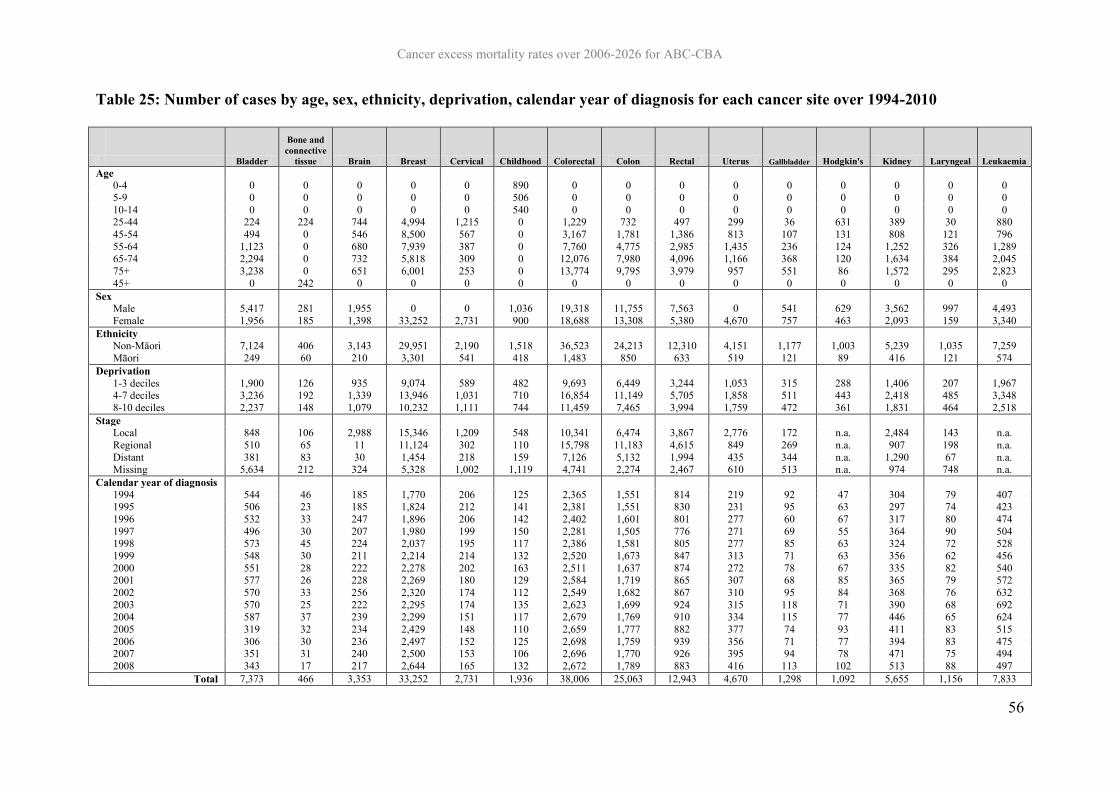
Cancer excess mortality rates over 2006-2026 for ABC-CBA
56
Table 25: Number of cases by age, sex, ethnicity, deprivation, calendar year of diagnosis for each cancer site over 1994-2010
Bladder
Bone and connective
tissue Brain Breast Cervical Childhood Colorectal Colon Rectal Uterus Gallbladder Hodgkin's Kidney Laryngeal Leukaemia Age 0-4 0 0 0 0 0 890 0 0 0 0 0 0 0 0 0 5-9 0 0 0 0 0 506 0 0 0 0 0 0 0 0 0 10-14 0 0 0 0 0 540 0 0 0 0 0 0 0 0 0 25-44 224 224 744 4,994 1,215 0 1,229 732 497 299 36 631 389 30 880 45-54 494 0 546 8,500 567 0 3,167 1,781 1,386 813 107 131 808 121 796 55-64 1,123 0 680 7,939 387 0 7,760 4,775 2,985 1,435 236 124 1,252 326 1,289 65-74 2,294 0 732 5,818 309 0 12,076 7,980 4,096 1,166 368 120 1,634 384 2,045 75+ 3,238 0 651 6,001 253 0 13,774 9,795 3,979 957 551 86 1,572 295 2,823 45+ 0 242 0 0 0 0 0 0 0 0 0 0 0 0 0 Sex Male 5,417 281 1,955 0 0 1,036 19,318 11,755 7,563 0 541 629 3,562 997 4,493 Female 1,956 185 1,398 33,252 2,731 900 18,688 13,308 5,380 4,670 757 463 2,093 159 3,340 Ethnicity Non-Māori 7,124 406 3,143 29,951 2,190 1,518 36,523 24,213 12,310 4,151 1,177 1,003 5,239 1,035 7,259 Māori 249 60 210 3,301 541 418 1,483 850 633 519 121 89 416 121 574 Deprivation 1-3 deciles 1,900 126 935 9,074 589 482 9,693 6,449 3,244 1,053 315 288 1,406 207 1,967 4-7 deciles 3,236 192 1,339 13,946 1,031 710 16,854 11,149 5,705 1,858 511 443 2,418 485 3,348 8-10 deciles 2,237 148 1,079 10,232 1,111 744 11,459 7,465 3,994 1,759 472 361 1,831 464 2,518 Stage Local 848 106 2,988 15,346 1,209 548 10,341 6,474 3,867 2,776 172 n.a. 2,484 143 n.a. Regional 510 65 11 11,124 302 110 15,798 11,183 4,615 849 269 n.a. 907 198 n.a. Distant 381 83 30 1,454 218 159 7,126 5,132 1,994 435 344 n.a. 1,290 67 n.a. Missing 5,634 212 324 5,328 1,002 1,119 4,741 2,274 2,467 610 513 n.a. 974 748 n.a. Calendar year of diagnosis 1994 544 46 185 1,770 206 125 2,365 1,551 814 219 92 47 304 79 407 1995 506 23 185 1,824 212 141 2,381 1,551 830 231 95 63 297 74 423 1996 532 33 247 1,896 206 142 2,402 1,601 801 277 60 67 317 80 474 1997 496 30 207 1,980 199 150 2,281 1,505 776 271 69 55 364 90 504 1998 573 45 224 2,037 195 117 2,386 1,581 805 277 85 63 324 72 528 1999 548 30 211 2,214 214 132 2,520 1,673 847 313 71 63 356 62 456 2000 551 28 222 2,278 202 163 2,511 1,637 874 272 78 67 335 82 540 2001 577 26 228 2,269 180 129 2,584 1,719 865 307 68 85 365 79 572 2002 570 33 256 2,320 174 112 2,549 1,682 867 310 95 84 368 76 632 2003 570 25 222 2,295 174 135 2,623 1,699 924 315 118 71 390 68 692 2004 587 37 239 2,299 151 117 2,679 1,769 910 334 115 77 446 65 624 2005 319 32 234 2,429 148 110 2,659 1,777 882 377 74 93 411 83 515 2006 306 30 236 2,497 152 125 2,698 1,759 939 356 71 77 394 83 475 2007 351 31 240 2,500 153 106 2,696 1,770 926 395 94 78 471 75 494 2008 343 17 217 2,644 165 132 2,672 1,789 883 416 113 102 513 88 497 Total 7,373 466 3,353 33,252 2,731 1,936 38,006 25,063 12,943 4,670 1,298 1,092 5,655 1,156 7,833

Cancer excess mortality rates over 2006-2026 for ABC-CBA
57
Lip, mouth and
pharynx Liver
Lung, trachea and
bronchus Melanoma Myeloma Non-
Hodgkin's Oesophageal Other Ovary Pancreatic Prostate Stomach Testis Thyroid Age 0-4 0 0 0 0 0 0 0 0 0 0 0 0 0 0 5-9 0 0 0 0 0 0 0 0 0 0 0 0 0 0 10-14 0 0 0 0 0 0 0 0 0 0 0 0 0 0 25-44 379 171 512 5,326 105 1,016 65 0 633 150 91 352 1,621 980 45-54 667 366 1,978 4,745 356 1,182 224 1,775 733 389 1,804 562 0 0 55-64 913 550 5,255 5,146 653 1,809 631 2,894 901 895 8,938 955 0 0 65-74 886 654 8,364 5,425 995 2,275 981 4,429 871 1,468 15,088 1,569 0 0 75+ 779 617 7,861 5,616 1,330 2,520 1,437 6,751 991 2,069 12,298 2,101 0 0 45+ 0 0 0 0 0 0 0 0 0 0 0 0 414 1,462 Sex Male 2,370 1,595 14,182 13,450 1,922 4,680 2,194 8,225 0 2,453 38,219 3,441 2,035 629 Female 1,254 763 9,788 12,808 1,517 4,122 1,144 7,624 4,129 2,518 0 2,098 0 1,813 Ethnicity Non-Māori 3,302 1,864 20,178 25,922 3,153 8,256 3,092 14,710 3,766 4,501 36,494 4,685 1,622 2,087 Māori 322 494 3,792 336 286 546 246 1,139 363 470 1,725 854 413 355 Deprivation 1-3 deciles 793 447 4,327 7,938 908 2,309 730 3,746 1,065 1,154 10,830 1,191 489 599 4-7 deciles 1,503 853 9,995 11,467 1,419 3,767 1,470 6,835 1,694 2,153 16,343 2,257 806 948 8-10 deciles 1,328 1,058 9,648 6,853 1,112 2,726 1,138 5,268 1,370 1,664 11,046 2,091 740 895 Stage Local 778 202 1,477 22,416 n.a. n.a. 223 2,394 1,024 149 5,795 642 1,447 1,429 Regional 1,235 71 2,165 1,490 n.a. n.a. 368 1,109 448 438 1,837 1,382 243 571 Distant 235 493 9,077 1,203 n.a. n.a. 692 8,496 2,313 2,287 2,472 1,560 209 150 Missing 1,376 1,592 11,251 1,149 n.a. n.a. 2,055 3,850 344 2,097 28,115 1,955 136 292 Calendar year of diagnosis 1994 203 112 1,558 1,428 158 415 191 1,027 246 280 1,945 345 121 89 1995 210 96 1,496 1,649 208 479 197 1,019 290 287 2,427 359 116 112 1996 207 128 1,546 1,488 211 531 186 1,046 279 314 2,350 391 120 114 1997 221 135 1,488 1,458 207 552 198 1,093 259 306 2,265 386 133 159 1998 226 136 1,464 1,536 229 593 158 1,126 281 318 2,332 406 127 145 1999 235 128 1,537 1,532 217 549 216 1,021 308 287 2,537 378 124 166 2000 233 130 1,603 1,678 241 537 226 1,126 287 319 3,003 359 140 160 2001 228 138 1,489 1,721 242 598 214 1,098 296 296 2,979 370 128 138 2002 229 158 1,571 1,803 265 618 235 1,020 305 315 2,581 406 166 148 2003 251 177 1,716 1,815 235 592 252 1,084 244 337 2,635 373 133 175 2004 250 153 1,788 1,862 236 623 250 1,017 267 351 2,610 356 135 185 2005 246 213 1,615 2,003 240 659 217 1,030 298 377 2,444 337 142 161 2006 293 220 1,633 1,952 251 657 254 1,073 263 370 2,394 359 161 218 2007 293 213 1,715 2,135 250 669 272 975 230 397 2,856 357 143 245 2008 299 221 1,751 2,198 249 730 272 1,094 276 417 2,861 357 146 227 Total 3,624 2,358 23,970 26,258 3,439 8,802 3,338 15,849 4,129 4,971 38,219 5,539 2,035 2,442

Cancer excess mortality rates over 2006-2026 for ABC-CBA
58
Table 26: Number of cases with non-missing stage by age, sex, ethnicity, deprivation, year of diagnosis for each cancer site
Bladder
Bone and connective tissue Brain Breast Cervical
Childhood
Colorectal Colon Rectal Uterus
Gallbladder
Hodgkin's Kidney
Laryngeal
Leukaemia
Age 0-4 0 0 0 0 0 395 0 0 0 0 0 0 0 0 0 5-9 0 0 0 0 0 187 0 0 0 0 0 0 0 0 0 10-14 0 0 0 0 0 235 0 0 0 0 0 0 0 0 0 25-44 70 137 684 4,415 947 0 1,082 695 387 250 31 631 359 11 880 45-54 141 0 513 7,470 356 0 2,772 1,672 1,100 733 88 131 745 50 796 55-64 317 0 629 7,054 223 0 6,993 4,484 2,509 1,328 188 124 1,116 111 1,289 65-74 589 0 654 5,091 138 0 10,930 7,463 3,467 1,037 259 120 1,379 142 2,045 75+ 622 0 549 3,894 65 0 11,488 8,475 3,013 712 219 86 1,082 94 2,823 45+ 0 117 0 0 0 0 0 0 0 0 0 0 0 0 0 Sex Male 1,274 163 1,785 0 0 413 16,959 10,740 6,219 0 325 629 2,947 352 4,493 Female 465 91 1,244 27,924 1,729 404 16,306 12,049 4,257 4,060 460 463 1,734 56 3,340 Ethnicity Non-Māori 1,659 219 2,840 25,082 1,406 637 32,010 22,005 10,005 3,609 708 1,003 4,320 362 7,259 Māori 80 35 189 2,842 323 180 1,255 784 471 451 77 89 361 46 574 Deprivation 1-3 deciles 459 69 843 7,651 398 215 8,461 5,860 2,601 918 199 288 1,171 81 1,967 4-7 deciles 738 92 1,211 11,733 671 302 14,797 10,110 4,687 1,624 306 443 2,002 154 3,348 8-10 deciles 542 93 975 8,540 660 300 10,007 6,819 3,188 1,518 280 361 1,508 173 2,518 Stage Local 848 106 2,988 15,346 1,209 548 10,341 6,474 3,867 2,776 172 n.a. 2,484 143 n.a. Regional 510 65 11 11,124 302 110 15,798 11,183 4,615 849 269 n.a. 907 198 n.a. Distant 381 83 30 1,454 218 159 7,126 5,132 1,994 435 344 n.a. 1,290 67 n.a. Missing 0 0 0 0 0 0 0 0 0 0 0 n.a. 0 0 n.a. Calendar year of diagnosis 1994 342 26 77 1,342 119 63 1,801 1,111 690 159 50 47 203 45 407 1995 335 18 131 1,198 127 66 2,078 1,369 709 167 60 63 222 24 423 1996 83 19 158 1,492 140 65 2,103 1,442 661 236 33 67 257 36 474 1997 66 17 153 1,704 129 67 2,068 1,376 692 240 39 55 313 40 504 1998 62 20 221 1,627 125 55 2,132 1,459 673 247 52 63 279 27 528 1999 82 11 210 1,809 140 62 2,286 1,573 713 267 43 63 293 24 456 2000 45 12 222 1,865 135 74 2,284 1,530 754 232 47 67 276 23 540 2001 72 17 225 1,945 130 61 2,368 1,618 750 278 37 85 291 24 572 2002 101 14 256 1,965 109 48 2,305 1,567 738 276 54 84 319 29 632 2003 103 14 222 1,959 109 50 2,368 1,592 776 284 77 71 337 25 692 2004 86 19 235 1,972 106 46 2,431 1,678 753 303 72 77 376 16 624 2005 78 21 228 2,182 85 37 2,316 1,644 672 333 51 93 346 27 515 2006 93 18 235 2,255 93 49 2,276 1,597 679 321 37 77 333 29 475 2007 102 19 239 2,246 80 32 2,234 1,608 626 338 60 78 409 17 494 2008 89 9 217 2,363 102 42 2,215 1,625 590 379 73 102 427 22 497 Total 1,739 254 3,029 27,924 1,729 817 33,265 22,789 10,476 4,060 785 1,092 4,681 408 7,833

Cancer excess mortality rates over 2006-2026 for ABC-CBA
59
Lip, mouth
and pharynx Liver
Lung, trachea
and bronchus Melanoma Myeloma
Non-Hodgkin's
Oesophageal Other Ovary Pancreatic Prostate Stomach Testis Thyroid
Age 0-4 0 0 0 0 0 0 0 0 0 0 0 0 0 0 5-9 0 0 0 0 0 0 0 0 0 0 0 0 0 0 10-14 0 0 0 0 0 0 0 0 0 0 0 0 0 0 25-44 251 69 363 5,092 105 1,016 42 0 583 122 43 287 1,513 882 45-54 452 142 1,349 4,550 356 1,182 132 1,354 680 292 734 445 0 0 55-64 587 184 3,252 4,927 653 1,809 336 2,205 856 625 3,187 729 0 0 65-74 530 222 4,485 5,209 995 2,275 437 3,412 815 922 3,855 1,111 0 0 75+ 428 149 3,270 5,331 1,330 2,520 336 5,028 851 913 2,285 1,012 0 0 45+ 0 0 0 0 0 0 0 0 0 0 0 0 386 1,268 Sex Male 1,476 492 7,399 12,863 1,922 4,680 938 6,008 0 1,469 10,104 2,268 1,899 550 Female 772 274 5,320 12,246 1,517 4,122 345 5,991 3,785 1,405 0 1,316 0 1,600 Ethnicity Non-Māori 2,036 600 10,795 24,791 3,153 8,256 1,182 11,071 3,450 2,584 9,668 2,975 1,518 1,833 Māori 212 166 1,924 318 286 546 101 928 335 290 436 609 381 317 Deprivation 1-3 deciles 501 159 2,405 7,585 908 2,309 278 2,792 980 685 2,948 772 455 543 4-7 deciles 930 262 5,389 11,004 1,419 3,767 583 5,129 1,540 1,247 4,300 1,486 746 833 8-10 deciles 817 345 4,925 6,520 1,112 2,726 422 4,078 1,265 942 2,856 1,326 698 774 Stage Local 778 202 1,477 22,416 n.a. n.a. 223 2,394 1,024 149 5,795 642 1,447 1,429 Regional 1,235 71 2,165 1,490 n.a. n.a. 368 1,109 448 438 1,837 1,382 243 571 Distant 235 493 9,077 1,203 n.a. n.a. 692 8,496 2,313 2,287 2,472 1,560 209 150 Missing 0 0 0 0 n.a. n.a. 0 0 0 0 0 0 0 0 Calendar year of diagnosis 1994 109 62 925 1,028 158 415 104 825 201 171 1,291 234 70 55 1995 131 47 711 1,621 208 479 98 850 251 168 919 238 109 97 1996 109 44 750 1,422 211 531 52 835 243 163 496 259 107 88 1997 139 52 714 1,388 207 552 87 850 234 174 380 253 125 136 1998 138 38 762 1,483 229 593 49 856 266 170 248 260 118 127 1999 136 30 708 1,503 217 549 69 766 274 152 564 232 118 154 2000 150 25 732 1,635 241 537 79 828 270 151 725 230 132 147 2001 147 39 774 1,690 242 598 87 834 286 175 655 244 123 129 2002 153 54 835 1,784 265 618 94 787 286 195 578 269 155 135 2003 160 49 981 1,751 235 592 92 804 226 181 722 239 130 158 2004 150 41 916 1,806 236 623 93 764 249 212 668 237 132 172 2005 159 69 936 1,950 240 659 94 748 278 227 663 226 137 140 2006 182 80 936 1,903 251 657 101 784 244 229 626 235 158 186 2007 197 67 975 2,111 250 669 99 704 218 237 743 216 142 220 2008 188 69 1,064 2,034 249 730 85 764 259 269 826 212 143 206 Total 2,248 766 12,719 25,109 3,439 8,802 1,283 11,999 3,785 2,874 10,104 3,584 1,899 2,150

Cancer excess mortality rates over 2006-2026 for ABC-CBA
60
5.1.2 Count regression models for excess mortality in the context of relative survival
Count regression models were used to estimate the excess mortality rates of persons
diagnosed with cancer. Models were run in the context of relative survival using the complete
approach over 1994-2010 (Brenner and Racher 2004). In particular, analysis included
incident cases over 1994-2008 with follow-up to 2010. These patients were then followed up
to 10 years after diagnosis. For example, a case diagnosed in 1994 had the full ten years of
follow-up data, but a case diagnosed in 2008 had only two to three years follow-up (i.e. till
the end of 2010. Table 27 shows this diagrammatically, with the cases by year of diagnosis
(rows) and follow-up (across the row to the right) contributing to the analysis. The inclusion
of a continuous variable for calendar year in the regression means that the excess mortality
rates beyond 2010 by year of follow-up (e.g. for cases diagnosed in 2008 followed-up for 3-4
years or more, cases diagnosed in 2007 followed up for 4-5 years or more, etc) were based on
1994-2010 data extrapolated out (grey cells).
Table 27: Cases included in the Complete Approach to estimate the Excess Mortality
Rates
Four sets of models were run for each cancer:
1. The baseline model, namely excess mortality as a function of sex, age, ethnicity,
deprivation and time since diagnosis. The exact model and specification follow.
2. Same as baseline model, but with the dataset restricted to those with complete data on
stage or severity. This allows inspection for any possible selection bias by excluding
those with missing stage, which may impact also on the complete case analyses
including stage as a covariate.
1994 1995 1996 1997 1998 1999 2000 2001 2002 2003 2004 2005 2006 2007 2008 2009 2010
1994 0-1 1-2 2-3 3-4 4-5 5-6 6-7 7-8 8-9 9-10 10-11 11-12 12-13 13-14 14-15 15-16 16-17
1995 0-1 1-2 2-3 3-4 4-5 5-6 6-7 7-8 8-9 9-10 10-11 11-12 12-13 13-14 14-15 15-16
1996 0-1 1-2 2-3 3-4 4-5 5-6 6-7 7-8 8-9 9-10 10-11 11-12 12-13 13-14 14-15
1997 0-1 1-2 2-3 3-4 4-5 5-6 6-7 7-8 8-9 9-10 10-11 11-12 12-13 13-14
1998 0-1 1-2 2-3 3-4 4-5 5-6 6-7 7-8 8-9 9-10 10-11 11-12 12-13
1999 0-1 1-2 2-3 3-4 4-5 5-6 6-7 7-8 8-9 9-10 10-11 11-12
2000 0-1 1-2 2-3 3-4 4-5 5-6 6-7 7-8 8-9 9-10 10-11
2001 0-1 1-2 2-3 3-4 4-5 5-6 6-7 7-8 8-9 9-10
2002 0-1 1-2 2-3 3-4 4-5 5-6 6-7 7-8 8-9
2003 0-1 1-2 2-3 3-4 4-5 5-6 6-7 7-8
2004 0-1 1-2 2-3 3-4 4-5 5-6 6-7
2005 0-1 1-2 2-3 3-4 4-5 5-6
2006 0-1 1-2 2-3 3-4 4-5
2007 0-1 1-2 2-3 3-4
2008 0-1 1-2 2-3
Calendar year of follow-up
Ye
ar o
f d
iagn
osi
s
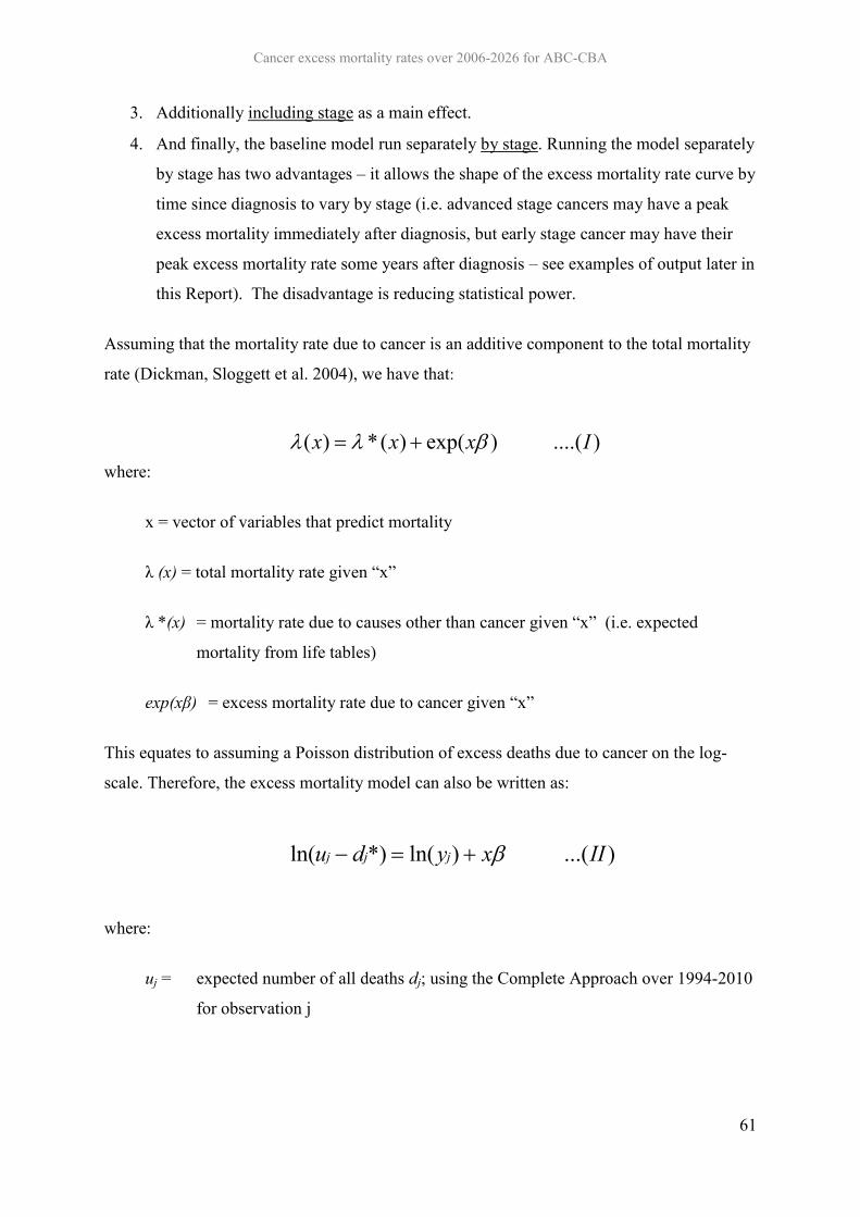
Cancer excess mortality rates over 2006-2026 for ABC-CBA
61
3. Additionally including stage as a main effect.
4. And finally, the baseline model run separately by stage. Running the model separately
by stage has two advantages – it allows the shape of the excess mortality rate curve by
time since diagnosis to vary by stage (i.e. advanced stage cancers may have a peak
excess mortality immediately after diagnosis, but early stage cancer may have their
peak excess mortality rate some years after diagnosis – see examples of output later in
this Report). The disadvantage is reducing statistical power.
Assuming that the mortality rate due to cancer is an additive component to the total mortality
rate (Dickman, Sloggett et al. 2004), we have that:
where:
x = vector of variables that predict mortality
λ (x) = total mortality rate given “x”
λ *(x) = mortality rate due to causes other than cancer given “x” (i.e. expected
mortality from life tables)
exp(xβ) = excess mortality rate due to cancer given “x”
This equates to assuming a Poisson distribution of excess deaths due to cancer on the log-
scale. Therefore, the excess mortality model can also be written as:
where:
uj = expected number of all deaths dj; using the Complete Approach over 1994-2010
for observation j
)....()exp()(*)( Ixxx
)...()ln(*)ln( IIxydu jjj

Cancer excess mortality rates over 2006-2026 for ABC-CBA
62
d*j = expected number of deaths for observation j, due to causes other than the cancer
of interest and estimated from general population mortality rates (i.e. lifetables,
in our case by sex, ethnicity and deprivation)
yj = person time for observation j (ie, offset)
x = vector of variables that predict excess mortality.
5.1.3 Modelling survival over time since diagnosis
For future ABC-CBA modelling, it is important to have smoothed excess mortality rates over
time since diagnosis. This was achieved by incorporating restricted cubic splines to model
time since diagnosis as a continuous variable (Durrleman and Simon 1989; Lambert and
Royston 2009; Royston and Lambert 2009). Restricted cubic splines are piecewise
polynomials that are constrained to be smooth at their juncture points (knots) and are linear
before the first and after the last knot (Durrleman and Simon 1989; Lambert and Royston
2009; Royston and Lambert 2009). Splines also need derived variables called “basis
functions” related to their number of knots. For instance, if we use three interior knots (or
five knots in total including the minimum and maximum, i.e. 0.0833 (end of the first month
of follow-up) and the survival time), we need to calculate four basis functions. Expressing the
excess mortality rate in the log-scale we have:
35
15
4531
15
45344
35
15
3531
15
35333
35
15
2531
15
25322
1
443322110
)()()(
1)()()(
)(
)()()(
1)()()(
)(
)()()(
1)()()(
)(
)...();(ln
ktkkkk
ktkkkk
ktz
ktkkkk
ktkkkk
ktz
ktkkkk
ktkkkk
ktz
tzIaxzzzzxt
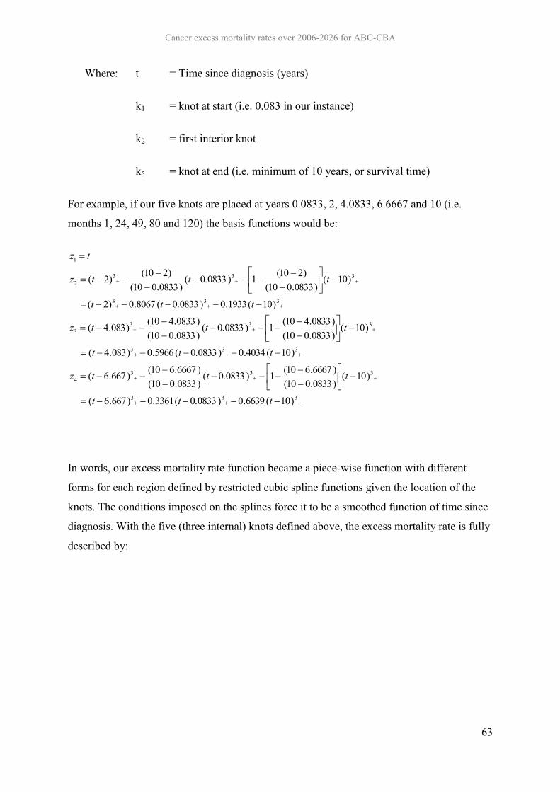
Cancer excess mortality rates over 2006-2026 for ABC-CBA
63
Where: t = Time since diagnosis (years)
k1 = knot at start (i.e. 0.083 in our instance)
k2 = first interior knot
k5 = knot at end (i.e. minimum of 10 years, or survival time)
For example, if our five knots are placed at years 0.0833, 2, 4.0833, 6.6667 and 10 (i.e.
months 1, 24, 49, 80 and 120) the basis functions would be:
333
3334
333
3333
333
3332
1
)10(6639.0)0.0833(3361.0)667.6(
)10()0833.010()6667.610(1)0.0833(
)0833.010()6667.610()667.6(
)10(4034.0)0.0833(5966.0)083.4(
)10()0833.010()0833.410(1)0.0833(
)0833.010()0833.410()083.4(
)10(1933.0)0.0833(8067.0)2(
)10()0833.010(
)210(1)0.0833()0833.010(
)210()2(
ttt
tttz
ttt
tttz
ttt
tttz
tz
In words, our excess mortality rate function became a piece-wise function with different
forms for each region defined by restricted cubic spline functions given the location of the
knots. The conditions imposed on the splines force it to be a smoothed function of time since
diagnosis. With the five (three internal) knots defined above, the excess mortality rate is fully
described by:
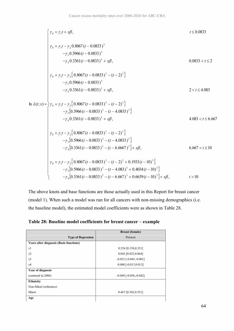
Cancer excess mortality rates over 2006-2026 for ABC-CBA
64
10,)10(6639.0)667.6()0.0833(3361.0
)10(4034.0)083.4()0.0833(5966.0
)10(1933.0)2()0833.0(8067.0
10667.6,)6667.6()0.0833(3361.0
)0833.4()0.0833(5966.0
)2()0833.0(8067.0
667.6083.4,)0833.0(3361.0
)0833.4()0.0833(5966.0
)2()0833.0(8067.0
083.42,)0833.0(3361.0
)0833.0(5966.0
)2()0833.0(8067.0
20833.0,)0833.0(3361.0
)0833.0(5966.0
)0833.0(8067.0
0833.0,
);(ln
3334
3333
333210
334
333
33210
34
333
33210
34
33
33210
34
33
3210
10
txtttttt
tttt
txtttt
ttt
txttt
ttt
txtt
ttt
txtt
tt
txt
xt
The above knots and base functions are those actually used in this Report for breast cancer
(model 1). When such a model was run for all cancers with non-missing demographics (i.e.
the baseline model), the estimated model coefficients were as shown in Table 28.
Table 28: Baseline model coefficients for breast cancer – example
Breast (female)
Type of Regression Poisson
Years after diagnosis (Basis functions)
γ1 0.254 [0.158,0.351]
γ2 0.043 [0.022,0.064]
γ3 -0.023 [-0.045,-0.001]
γ4 0.000 [-0.013,0.013]
Year of diagnosis
(centered in 2006) -0.049 [-0.056,-0.042]
Ethnicity
Non-Māori (reference)
Māori 0.467 [0.382,0.551]
Age

Cancer excess mortality rates over 2006-2026 for ABC-CBA
65
Breast (female)
Type of Regression Poisson
25–44 (reference) 1
45–54 2 -0.332 [-0.412,-0.252]
55–64 -0.364 [-0.450,-0.277]
65–74 -0.156 [-0.275,-0.038]
75+ 0.247 [0.107,0.388]
Deprivation
Deciles 1-3 (reference)
Deciles 4-7 0.153 [0.080,0.225]
Deciles 8-10 0.198 [0.120,0.275]
Interactions
Other (reference)
65-74 and 1st year after diagnosis 0.305 [0.108,0.501]
65-74 and 2nd year after diagnosis 0.108 [-0.083,0.299]
75+ and 1st year after diagnosis 0.809 [0.625,0.993]
75+ and 2nd year after diagnosis 0.086 [-0.131,0.303]
Constant -3.834 [-3.977,-3.692]
Person-time (years) 41,795
Number of cases 33252
AIC 42,161
BIC 42,308
Log-likelihood -21,064
Deviance/DF 0.60
Pearson/DF 2.23
Over dispersion parameter 0.02
Ho: a=0 0.17
Knot positions for years after diagnosis
Knot at start 0.08
Knot at percentile 25 2.00
Knot at percentile 50 4.08
Knot at percentile 75 6.67
Knot at end 10
Consider breast cancer excess mortality by time since diagnosis among 55-64 year old non-
Māori, diagnosed in 2006 and living in areas with deprivation deciles 1-3. Using the above
coefficients and basis functions, one can calculate the excess mortality rate by time since
diagnosis as laid out in Table 30 and graphed in Figure 2.
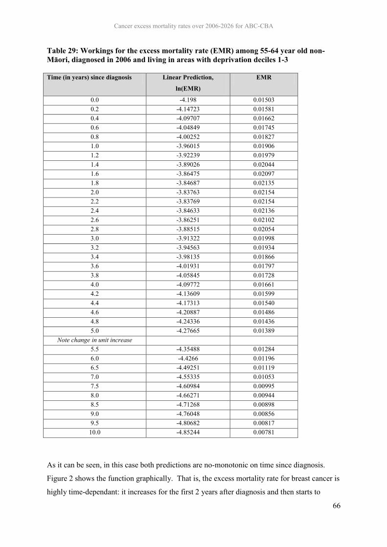
Cancer excess mortality rates over 2006-2026 for ABC-CBA
66
Table 29: Workings for the excess mortality rate (EMR) among 55-64 year old non-Māori, diagnosed in 2006 and living in areas with deprivation deciles 1-3
Time (in years) since diagnosis Linear Prediction,
ln(EMR)
EMR
0.0 -4.198 0.01503 0.2 -4.14723 0.01581 0.4 -4.09707 0.01662 0.6 -4.04849 0.01745 0.8 -4.00252 0.01827 1.0 -3.96015 0.01906 1.2 -3.92239 0.01979 1.4 -3.89026 0.02044 1.6 -3.86475 0.02097 1.8 -3.84687 0.02135 2.0 -3.83763 0.02154 2.2 -3.83769 0.02154 2.4 -3.84633 0.02136 2.6 -3.86251 0.02102 2.8 -3.88515 0.02054 3.0 -3.91322 0.01998 3.2 -3.94563 0.01934 3.4 -3.98135 0.01866 3.6 -4.01931 0.01797 3.8 -4.05845 0.01728 4.0 -4.09772 0.01661 4.2 -4.13609 0.01599 4.4 -4.17313 0.01540 4.6 -4.20887 0.01486 4.8 -4.24336 0.01436 5.0 -4.27665 0.01389
Note change in unit increase 5.5 -4.35488 0.01284 6.0 -4.4266 0.01196 6.5 -4.49251 0.01119 7.0 -4.55335 0.01053 7.5 -4.60984 0.00995 8.0 -4.66271 0.00944 8.5 -4.71268 0.00898 9.0 -4.76048 0.00856 9.5 -4.80682 0.00817
10.0 -4.85244 0.00781
As it can be seen, in this case both predictions are no-monotonic on time since diagnosis.
Figure 2 shows the function graphically. That is, the excess mortality rate for breast cancer is
highly time-dependant: it increases for the first 2 years after diagnosis and then starts to

Cancer excess mortality rates over 2006-2026 for ABC-CBA
67
decrease; reaching a very low level, although not completely disappeared, after 10 years of
diagnosis.
Figure 2: Plot by time (years) since diagnosis of breast cancer: a) linear prediction, ln(EMR); and b) EMR
Linear Prediction
(ln(EMR))
EMR
Of note is the issue of location and number of knots for the restricted cubic splines. In general
the recommendation is to use sensible default locations. In practice, one could achieve this by
placing the knots at the centiles of the distribution of the variable that is being smoothed, i.e.
time since diagnosis. Following (Durrleman and Simon 1989; Lambert and Royston 2009;
Royston and Lambert 2009), five knots (or 3 interior knots2) were chosen and placed at the
minimum, percentiles 25, 50, and 75, and the maximum of time since diagnosis. As
mentioned before, the minimum was always the first month after diagnosis, or the 0.0083
2 An exception to this was the case of cervical cancer where 2 knots, at percentiles 33 and 67, were used.
-5.0
-4.5
-4.0
-3.5
-3.0
-2.5
-2.0
-1.5
-1.0
-0.5
0.0
0 1 2 3 4 5 6 7 8 9 10
Years since diagnosis
0.000
0.005
0.010
0.015
0.020
0.025
0 1 2 3 4 5 6 7 8 9 10
Years since diagnosis

Cancer excess mortality rates over 2006-2026 for ABC-CBA
68
year, and the maximum was survival time or 10 years after diagnosis3. This procedure
allowed us to have enough flexibility to capture the shape of the excess mortality rate
function while preserving parsimony and avoiding over-fitting. The exact locations of the
knots for each cancer site are reported together with the regression outputs (i.e. see end of
Table 28 for example).
5.1.4 Over dispersion
As discussed in section 5.1.2, grouped Poisson regressions were used for all cancer sites.
Over dispersion of the following form was tested:
V[y|x] = E[y|x] + a*(E[y|x]2)
where:
y = excess deaths due to cancer
x = vector of variables that predict excess mortality
V[y|x] = Variance of y given x
E[y|x] = Expected value of y given x
Whenever the coefficient “a” was found to be statistically significant (at the 5% level) an
additional Negative Binomial model was estimated4. The procedure improved the model fit
(lower Log-likelihood, AIC and BIC) although there was still some evidence of lack of fit for
some cancer sites (i.e. ratios of Deviance over degrees of freedom and Pearson over degrees
of freedom different from 1).
5.2 Results This section presents the estimated model’s coefficients and predictions, both excess
mortality rates and relative survival, for all cancer sites.
3 5 years for Testicular cancer. 4 See: Cameron, A., & Trivedi, P. (2005). Microeconometrics: Methods and Applications. New York: Cambridge University Press, Chapter 20 for details on this over dispersion test.

Cancer excess mortality rates over 2006-2026 for ABC-CBA
69
The regression outputs also include: type of regression (Poisson/Binomial, together with the
over dispersion parameter and its statistical significance), several regression’s statistics
(person-time and cases included), measures of model fit (AIC, BIC, Log-likelihood,
Deviance and Pearson statistic divided by the number of degrees of freedom), and the
positions of the knots for time since diagnosis.
5.2.1 Baseline models (model 1)
As detailed in the methods, this first set of models (model 1) include all non-missing data on
sex, age, ethnicity, and deprivation, incorporating also calendar year and time since
diagnosis. Interactions for the oldest age groups (65-74 and 75+) and follow-up time are also
included. This set of models does not include stage/severity; it is incorporated in the
following sections (models 3 and 4).
As an example, in the case of bladder cancer the first column of Table 30 shows the
coefficients for the covariates described above. These coefficients were estimated using 7,373
patients diagnosed between 1994 and 2008, a total of 51,216 person-years. The over
dispersion parameter was not significant (p-value of 0.64) and Poisson regression was used as
a consequence. The knots for the splines for time since diagnosis were placed at years 0.08,
1.92, 4.08, 6.67 and 10 after diagnosis. The Deviance and Pearson statistic divided by the
number of degrees of freedom are lower and higher than one, 0.28 and 1.68 respectively,
indicating some degree of model misfit (a ratio of 1 indicates a perfect fit). This is a likely
consequence of the omission of important covariates, e.g. stage/severity at diagnosis.
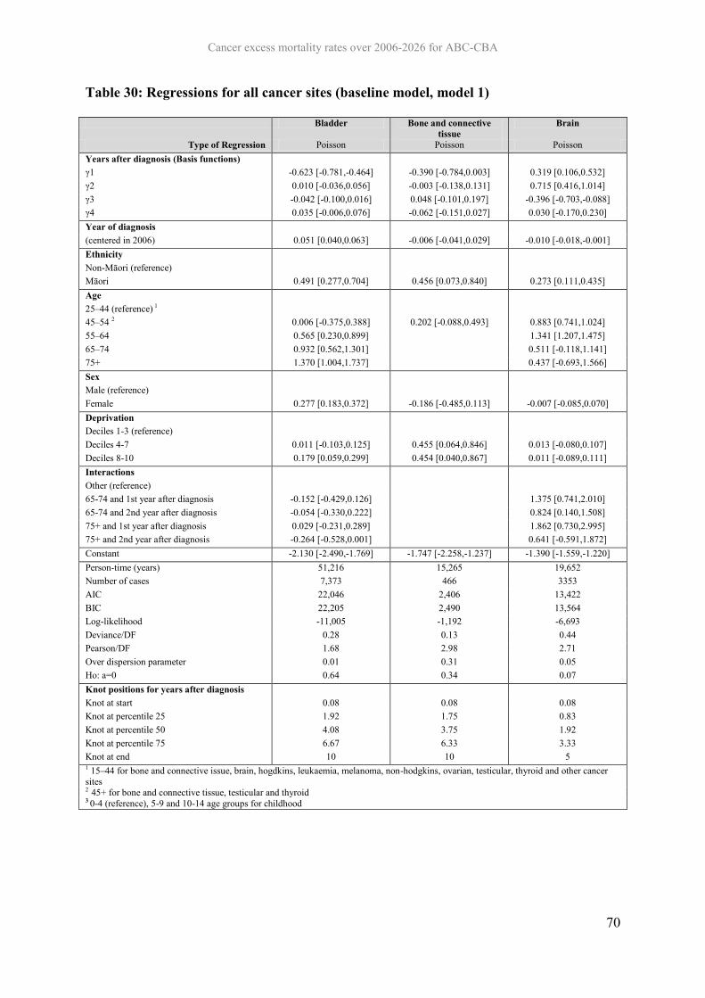
Cancer excess mortality rates over 2006-2026 for ABC-CBA
70
Table 30: Regressions for all cancer sites (baseline model, model 1)
Bladder Bone and connective tissue
Brain
Type of Regression Poisson Poisson Poisson Years after diagnosis (Basis functions) γ1 -0.623 [-0.781,-0.464] -0.390 [-0.784,0.003] 0.319 [0.106,0.532] γ2 0.010 [-0.036,0.056] -0.003 [-0.138,0.131] 0.715 [0.416,1.014] γ3 -0.042 [-0.100,0.016] 0.048 [-0.101,0.197] -0.396 [-0.703,-0.088] γ4 0.035 [-0.006,0.076] -0.062 [-0.151,0.027] 0.030 [-0.170,0.230] Year of diagnosis (centered in 2006) 0.051 [0.040,0.063] -0.006 [-0.041,0.029] -0.010 [-0.018,-0.001] Ethnicity Non-Māori (reference) Māori 0.491 [0.277,0.704] 0.456 [0.073,0.840] 0.273 [0.111,0.435] Age 25–44 (reference) 1 45–54 2 0.006 [-0.375,0.388] 0.202 [-0.088,0.493] 0.883 [0.741,1.024] 55–64 0.565 [0.230,0.899] 1.341 [1.207,1.475] 65–74 0.932 [0.562,1.301] 0.511 [-0.118,1.141] 75+ 1.370 [1.004,1.737] 0.437 [-0.693,1.566] Sex Male (reference) Female 0.277 [0.183,0.372] -0.186 [-0.485,0.113] -0.007 [-0.085,0.070] Deprivation Deciles 1-3 (reference) Deciles 4-7 0.011 [-0.103,0.125] 0.455 [0.064,0.846] 0.013 [-0.080,0.107] Deciles 8-10 0.179 [0.059,0.299] 0.454 [0.040,0.867] 0.011 [-0.089,0.111] Interactions Other (reference) 65-74 and 1st year after diagnosis -0.152 [-0.429,0.126] 1.375 [0.741,2.010] 65-74 and 2nd year after diagnosis -0.054 [-0.330,0.222] 0.824 [0.140,1.508] 75+ and 1st year after diagnosis 0.029 [-0.231,0.289] 1.862 [0.730,2.995] 75+ and 2nd year after diagnosis -0.264 [-0.528,0.001] 0.641 [-0.591,1.872] Constant -2.130 [-2.490,-1.769] -1.747 [-2.258,-1.237] -1.390 [-1.559,-1.220] Person-time (years) 51,216 15,265 19,652 Number of cases 7,373 466 3353 AIC 22,046 2,406 13,422 BIC 22,205 2,490 13,564 Log-likelihood -11,005 -1,192 -6,693 Deviance/DF 0.28 0.13 0.44 Pearson/DF 1.68 2.98 2.71 Over dispersion parameter 0.01 0.31 0.05 Ho: a=0 0.64 0.34 0.07 Knot positions for years after diagnosis Knot at start 0.08 0.08 0.08 Knot at percentile 25 1.92 1.75 0.83 Knot at percentile 50 4.08 3.75 1.92 Knot at percentile 75 6.67 6.33 3.33 Knot at end 10 10 5 1 15–44 for bone and connective issue, brain, hogdkins, leukaemia, melanoma, non-hodgkins, ovarian, testicular, thyroid and other cancer sites 2 45+ for bone and connective tissue, testicular and thyroid 3 0-4 (reference), 5-9 and 10-14 age groups for childhood
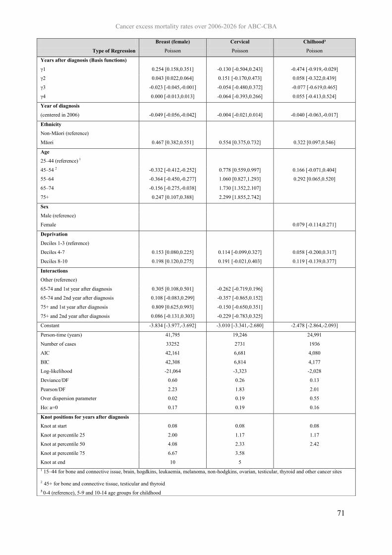
Cancer excess mortality rates over 2006-2026 for ABC-CBA
71
Breast (female) Cervical Chilhood³
Type of Regression Poisson Poisson Poisson
Years after diagnosis (Basis functions)
γ1 0.254 [0.158,0.351] -0.130 [-0.504,0.243] -0.474 [-0.919,-0.029]
γ2 0.043 [0.022,0.064] 0.151 [-0.170,0.473] 0.058 [-0.322,0.439]
γ3 -0.023 [-0.045,-0.001] -0.054 [-0.480,0.372] -0.077 [-0.619,0.465]
γ4 0.000 [-0.013,0.013] -0.064 [-0.393,0.266] 0.055 [-0.413,0.524]
Year of diagnosis
(centered in 2006) -0.049 [-0.056,-0.042] -0.004 [-0.021,0.014] -0.040 [-0.063,-0.017]
Ethnicity
Non-Māori (reference)
Māori 0.467 [0.382,0.551] 0.554 [0.375,0.732] 0.322 [0.097,0.546]
Age
25–44 (reference) 1
45–54 2 -0.332 [-0.412,-0.252] 0.778 [0.559,0.997] 0.166 [-0.071,0.404]
55–64 -0.364 [-0.450,-0.277] 1.060 [0.827,1.293] 0.292 [0.065,0.520]
65–74 -0.156 [-0.275,-0.038] 1.730 [1.352,2.107]
75+ 0.247 [0.107,0.388] 2.299 [1.855,2.742]
Sex
Male (reference)
Female 0.079 [-0.114,0.271]
Deprivation
Deciles 1-3 (reference)
Deciles 4-7 0.153 [0.080,0.225] 0.114 [-0.099,0.327] 0.058 [-0.200,0.317]
Deciles 8-10 0.198 [0.120,0.275] 0.191 [-0.021,0.403] 0.119 [-0.139,0.377]
Interactions
Other (reference)
65-74 and 1st year after diagnosis 0.305 [0.108,0.501] -0.262 [-0.719,0.196]
65-74 and 2nd year after diagnosis 0.108 [-0.083,0.299] -0.357 [-0.865,0.152]
75+ and 1st year after diagnosis 0.809 [0.625,0.993] -0.150 [-0.650,0.351]
75+ and 2nd year after diagnosis 0.086 [-0.131,0.303] -0.229 [-0.783,0.325]
Constant -3.834 [-3.977,-3.692] -3.010 [-3.341,-2.680] -2.478 [-2.864,-2.093]
Person-time (years) 41,795 19,246 24,991
Number of cases 33252 2731 1936
AIC 42,161 6,681 4,080
BIC 42,308 6,814 4,177
Log-likelihood -21,064 -3,323 -2,028
Deviance/DF 0.60 0.26 0.13
Pearson/DF 2.23 1.83 2.01
Over dispersion parameter 0.02 0.19 0.55
Ho: a=0 0.17 0.19 0.16
Knot positions for years after diagnosis
Knot at start 0.08 0.08 0.08
Knot at percentile 25 2.00 1.17 1.17
Knot at percentile 50 4.08 2.33 2.42
Knot at percentile 75 6.67 3.58
Knot at end 10 5 1 15–44 for bone and connective issue, brain, hogdkins, leukaemia, melanoma, non-hodgkins, ovarian, testicular, thyroid and other cancer sites
2 45+ for bone and connective tissue, testicular and thyroid 3 0-4 (reference), 5-9 and 10-14 age groups for childhood

Cancer excess mortality rates over 2006-2026 for ABC-CBA
72
Colorectal Colon Rectal Negative Binomial Negative Binomial Negative Binomial
Years after diagnosis (Basis functions) γ1 -0.982 [-1.053,-0.911] -1.175 [-1.262,-1.088] -0.681 [-0.798,-0.563] γ2 -0.192 [-0.223,-0.160] -0.225 [-0.267,-0.184] -0.143 [-0.191,-0.096] γ3 0.178 [0.138,0.218] 0.202 [0.149,0.256] 0.142 [0.086,0.197] γ4 -0.078 [-0.106,-0.051] -0.085 [-0.124,-0.047] -0.071 [-0.109,-0.033]
Year of diagnosis (centered in 2006) -0.013 [-0.017,-0.008] -0.009 [-0.015,-0.004] -0.018 [-0.026,-0.011]
Ethnicity Non-Māori (reference) Māori 0.453 [0.373,0.533] 0.435 [0.330,0.540] 0.488 [0.367,0.610]
Age 25–44 (reference) 1 45–54 2 0.071 [-0.037,0.179] 0.183 [0.041,0.325] -0.087 [-0.252,0.079] 55–64 0.070 [-0.030,0.170] 0.171 [0.040,0.302] -0.098 [-0.251,0.056] 65–74 0.084 [-0.036,0.205] 0.125 [-0.035,0.285] 0.043 [-0.136,0.222] 75+ -0.009 [-0.154,0.136] -0.024 [-0.219,0.171] 0.092 [-0.116,0.300]
Sex Male (reference) Female -0.069 [-0.107,-0.031] -0.067 [-0.114,-0.020] -0.092 [-0.154,-0.031]
Deprivation Deciles 1-3 (reference) Deciles 4-7 0.048 [0.001,0.095] 0.059 [0.002,0.117] 0.025 [-0.052,0.102] Deciles 8-10 0.104 [0.054,0.155] 0.071 [0.009,0.133] 0.175 [0.094,0.257]
Interactions Other (reference) 65-74 and 1st year after diagnosis 0.092 [-0.011,0.195] 0.070 [-0.063,0.202] 0.093 [-0.066,0.251] 65-74 and 2nd year after diagnosis 0.163 [0.050,0.277] 0.213 [0.067,0.359] 0.085 [-0.089,0.258] 75+ and 1st year after diagnosis 0.594 [0.464,0.723] 0.585 [0.413,0.756] 0.547 [0.360,0.735] 75+ and 2nd year after diagnosis 0.306 [0.158,0.453] 0.357 [0.164,0.549] 0.210 [-0.006,0.425] Constant -1.264 [-1.378,-1.151] -1.092 [-1.237,-0.947] -1.570 [-1.750,-1.390]
Person-time (years) 62,195 56,286 52,366 Number of cases 38006 25063 12943 AIC 61,539 47,204 33,733 BIC 61,702 47,365 33,893 Log-likelihood -30,751 -23,584 -16,849 Deviance/DF 0.51 0.46 0.41 Pearson/DF 3.05 3.67 2.09 Over dispersion parameter 0.14 0.16 0.04 Ho: a=0 0.00 0.00 0.02
Knot positions for years after diagnosis Knot at start 0.08 0.08 0.08 Knot at percentile 25 1.67 1.67 1.58 Knot at percentile 50 3.33 3.33 3.33 Knot at percentile 75 5.42 5.42 5.42 Knot at end 8 8 8 1 15–44 for bone and connective issue, brain, hogdkins, leukaemia, melanoma, non-hodgkins, ovarian, testicular, thyroid and other cancer sites 2 45+ for bone and connective tissue, testicular and thyroid 3 0-4 (reference), 5-9 and 10-14 age groups for childhood

Cancer excess mortality rates over 2006-2026 for ABC-CBA
73
Uterus Gallbladder Hodgkins Negative Binomial Poisson Negative Binomial
Years after diagnosis (Basis functions) γ1 -0.756 [-1.058,-0.453] -1.135 [-1.449,-0.822] -0.713 [-1.209,-0.218] γ2 -0.149 [-0.343,0.045] -0.110 [-0.408,0.188] -0.107 [-0.243,0.029] γ3 0.152 [-0.109,0.413] -0.027 [-0.287,0.234] 0.077 [-0.055,0.208] γ4 -0.086 [-0.295,0.122] 0.056 [-0.082,0.195] -0.024 [-0.090,0.043] Year of diagnosis (centered in 2006) -0.023 [-0.038,-0.007] -0.009 [-0.023,0.006] 0.007 [-0.029,0.042] Ethnicity Non-Māori (reference) Māori 0.511 [0.309,0.714] 0.253 [0.038,0.469] 0.233 [-0.359,0.825] Age 25–44 (reference) 1 45–54 2 0.181 [-0.171,0.533] 0.197 [-0.271,0.664] 0.849 [0.328,1.371] 55–64 0.291 [-0.043,0.625] 0.207 [-0.232,0.645] 1.490 [1.039,1.942] 65–74 0.834 [0.418,1.250] 0.407 [-0.198,1.012] 1.704 [1.034,2.375] 75+ 1.266 [0.804,1.727] 0.553 [-0.117,1.224] 2.265 [1.285,3.245] Sex Male (reference) Female 0.044 [-0.082,0.171] -0.020 [-0.315,0.275] Deprivation Deciles 1-3 (reference) Deciles 4-7 0.102 [-0.081,0.284] 0.156 [-0.006,0.318] -0.015 [-0.371,0.340] Deciles 8-10 0.161 [-0.026,0.348] 0.180 [0.013,0.347] -0.045 [-0.420,0.330] Interactions Other (reference) 65-74 and 1st year after diagnosis -0.186 [-0.568,0.196] 0.148 [-0.359,0.655] 0.559 [-0.277,1.395] 65-74 and 2nd year after diagnosis -0.028 [-0.433,0.377] 0.223 [-0.320,0.765] 0.743 [-0.159,1.644] 75+ and 1st year after diagnosis 0.229 [-0.187,0.645] 0.391 [-0.186,0.968] 1.182 [0.122,2.241] 75+ and 2nd year after diagnosis 0.255 [-0.191,0.701] 0.407 [-0.194,1.008] 0.422 [-0.912,1.755] Constant -2.670 [-3.066,-2.273] -0.265 [-0.733,0.203] -3.401 [-4.007,-2.794] Person-time (years) 23,414 15,136 30,277 Number of cases 4670 1298 1092 AIC 9,506 7,098 3,106 BIC 9,643 7,235 3,256 Log-likelihood -4,736 -3,531 -1,535 Deviance/DF 0.28 0.33 0.08 Pearson/DF 3.14 8.92 4.60 Over dispersion parameter 0.16 -0.04 -0.20 Ho: a=0 0.03 0.55 0.02 Knot positions for years after diagnosis Knot at start 0.08 0.08 0.08 Knot at percentile 25 1.33 0.92 1.75 Knot at percentile 50 2.75 2.25 3.75 Knot at percentile 75 4.25 4.08 6.25 Knot at end 6 7 10 1 15–44 for bone and connective issue, brain, hogdkins, leukaemia, melanoma, non-hodgkins, ovarian, testicular, thyroid and other sites 2 45+ for bone and connective tissue, testicular and thyroid 3 0-4 (reference), 5-9 and 10-14 age groups for childhood

Cancer excess mortality rates over 2006-2026 for ABC-CBA
74
Kidney Laryngeal Luekaemia Poission Poisson Negative Binomial
Years after diagnosis (Basis functions) γ1 -1.314 [-1.455,-1.173] -0.043 [-0.428,0.341] -1.567 [-1.691,-1.443] γ2 -0.166 [-0.213,-0.118] 0.088 [-0.024,0.200] -0.221 [-0.260,-0.182] γ3 0.122 [0.069,0.175] -0.079 [-0.188,0.029] 0.159 [0.116,0.202] γ4 -0.041 [-0.072,-0.009] 0.026 [-0.028,0.081] -0.047 [-0.072,-0.022] Year of diagnosis (centered in 2006) -0.023 [-0.033,-0.013] 0.014 [-0.012,0.039] -0.043 [-0.053,-0.034] Ethnicity Non-Māori (reference) Māori 0.449 [0.295,0.603] 0.415 [0.090,0.740] 0.313 [0.181,0.445] Age 25–44 (reference) 1 45–54 2 0.148 [-0.070,0.365] 0.808 [-0.169,1.785] 0.086 [-0.080,0.252] 55–64 0.385 [0.181,0.588] 0.945 [0.002,1.889] 0.314 [0.167,0.461] 65–74 0.529 [0.247,0.810] 1.306 [0.328,2.284] 0.819 [0.622,1.015] 75+ 0.749 [0.413,1.086] 1.469 [0.424,2.514] 1.170 [0.963,1.376] Sex Male (reference) Female -0.059 [-0.147,0.029] 0.157 [-0.120,0.434] -0.022 [-0.096,0.052] Deprivation Deciles 1-3 (reference) Deciles 4-7 0.056 [-0.051,0.163] 0.134 [-0.159,0.427] -0.032 [-0.125,0.060] Deciles 8-10 0.066 [-0.049,0.181] 0.051 [-0.250,0.352] 0.060 [-0.037,0.157] Interactions Other (reference) 65-74 and 1st year after diagnosis 0.114 [-0.146,0.374] -0.191 [-0.737,0.355] -0.165 [-0.371,0.041] 65-74 and 2nd year after diagnosis 0.096 [-0.212,0.404] -0.089 [-0.608,0.429] -0.281 [-0.549,-0.013] 75+ and 1st year after diagnosis 0.385 [0.071,0.700] 0.445 [-0.189,1.080] -0.116 [-0.326,0.094] 75+ and 2nd year after diagnosis 0.255 [-0.110,0.620] 0.428 [-0.202,1.058] -0.386 [-0.665,-0.107] Constant -1.276 [-1.504,-1.048] -3.159 [-4.195,-2.122] -1.050 [-1.219,-0.881] Person-time (years) 55,219 27,749 58,462 Number of cases 5655 1156 7833 AIC 19,164 5,832 25,949 BIC 19,325 5,980 26,111 Log-likelihood -9,564 -2,898 -12,957 Deviance/DF 0.24 0.16 0.28 Pearson/DF 3.27 2.43 3.90 Over dispersion parameter 0.05 0.14 0.29 Ho: a=0 0.23 0.52 0.00 Knot positions for years after diagnosis Knot at start 0.08 0.08 0.08 Knot at percentile 25 1.83 1.75 1.83 Knot at percentile 50 3.83 3.67 3.83 Knot at percentile 75 6.42 6.25 6.33 Knot at end 10 10 10 1 15–44 for bone and connective issue, brain, hogdkins, leukaemia, melanoma, non-hodgkins, ovarian, testicular, thyroid and other sites 2 45+ for bone and connective tissue, testicular and thyroid 3 0-4 (reference), 5-9 and 10-14 age groups for childhood

Cancer excess mortality rates over 2006-2026 for ABC-CBA
75
Lip, mouth and pharynx Liver Lung, trachea and bronchus
Poisson Poisson Negative Binomial Years after diagnosis (Basis functions) γ1 -0.124 [-0.295,0.047] -2.205 [-2.438,-1.972] -1.018 [-1.085,-0.951] γ2 0.080 [0.028,0.133] -0.793 [-1.029,-0.557] -0.187 [-0.252,-0.122] γ3 -0.078 [-0.133,-0.022] 0.519 [0.305,0.733] 0.179 [0.092,0.265] γ4 0.027 [-0.004,0.058] -0.186 [-0.301,-0.072] -0.106 [-0.174,-0.038] Year of diagnosis (centered in 2006) -0.021 [-0.033,-0.008] -0.022 [-0.033,-0.012] 0.001 [-0.002,0.005] Ethnicity Non-Māori (reference) Māori 0.356 [0.177,0.535] 0.269 [0.151,0.387] 0.195 [0.155,0.236] Age 25–44 (reference) 1 45–54 2 0.570 [0.311,0.828] 0.201 [-0.009,0.411] 0.233 [0.122,0.344] 55–64 0.977 [0.733,1.221] 0.198 [-0.002,0.397] 0.293 [0.188,0.397] 65–74 1.109 [0.802,1.416] 0.748 [0.337,1.158] 0.360 [0.210,0.510] 75+ 1.008 [0.582,1.434] 0.940 [0.382,1.498] 0.708 [0.547,0.869] Sex Male (reference) Female -0.345 [-0.461,-0.229] -0.025 [-0.121,0.072] -0.088 [-0.118,-0.058] Deprivation Deciles 1-3 (reference) Deciles 4-7 0.114 [-0.025,0.253] 0.018 [-0.107,0.144] 0.055 [0.014,0.096] Deciles 8-10 0.081 [-0.064,0.226] 0.037 [-0.088,0.162] 0.102 [0.060,0.144] Interactions Other (reference) 65-74 and 1st year after diagnosis 0.525 [0.239,0.810] -0.352 [-0.751,0.047] 0.076 [-0.047,0.199] 65-74 and 2nd year after diagnosis 0.149 [-0.163,0.461] -0.264 [-0.719,0.190] 0.119 [-0.010,0.247] 75+ and 1st year after diagnosis 1.016 [0.607,1.425] -0.332 [-0.880,0.217] -0.063 [-0.199,0.073] 75+ and 2nd year after diagnosis 0.247 [-0.218,0.712] 0.160 [-0.435,0.756] -0.057 [-0.203,0.088] Constant -2.713 [-3.012,-2.413] 0.683 [0.457,0.908] 0.178 [0.066,0.291] Person-time (years) 51,700 19,598 42,809 Number of cases 3624 2358 23970 AIC 14,734 10,875 46,632 BIC 14,893 11,017 46,788 Log-likelihood -7,349 -5,419 -23,298 Deviance/DF 0.21 0.38 0.55 Pearson/DF 3.50 4.82 4.83 Over dispersion parameter -0.08 0.11 0.03 Ho: a=0 0.21 0.22 0.00 Knot positions for years after diagnosis Knot at start 0.08 0.08 0.08 Knot at percentile 25 1.83 0.92 1.17 Knot at percentile 50 3.83 2.25 2.5 Knot at percentile 75 6.33 4.08 4.08 Knot at end 10 7 6 1 15–44 for bone and connective issue, brain, hogdkins, leukaemia, melanoma, non-hodgkins, ovarian, testicular, thyroid and other cancer sites 2 45+ for bone and connective tissue, testicular and thyroid 3 0-4 (reference), 5-9 and 10-14 age groups for childhood

Cancer excess mortality rates over 2006-2026 for ABC-CBA
76
Melanoma Myeloma Non-Hodgkin's Poisson Negative Binomial Negative Binomial
Years after diagnosis (Basis functions) γ1 -0.297 [-0.534,-0.060] -0.878 [-1.058,-0.697] -1.087 [-1.198,-0.976] γ2 -0.051 [-0.184,0.081] -0.167 [-0.225,-0.109] -0.108 [-0.142,-0.073] γ3 0.073 [-0.084,0.230] 0.104 [0.052,0.157] 0.069 [0.029,0.108] γ4 -0.061 [-0.169,0.047] -0.017 [-0.041,0.007] -0.016 [-0.039,0.008] Year of diagnosis (centered in 2006) 0.000 [-0.011,0.012] -0.039 [-0.050,-0.028] -0.044 [-0.052,-0.035] Ethnicity Non-Māori (reference) Māori 0.857 [0.552,1.163] 0.376 [0.214,0.538] 0.538 [0.410,0.666] Age 25–44 (reference) 1 45–54 2 0.191 [0.027,0.355] 0.460 [0.106,0.814] 0.178 [0.017,0.338] 55–64 0.400 [0.240,0.560] 0.819 [0.482,1.157] 0.508 [0.363,0.652] 65–74 0.723 [0.506,0.939] 1.218 [0.866,1.570] 1.052 [0.867,1.238] 75+ 1.543 [1.342,1.744] 1.606 [1.247,1.965] 1.253 [1.032,1.473] Sex Male (reference) Female -0.639 [-0.744,-0.534] -0.067 [-0.157,0.023] -0.063 [-0.131,0.005] Deprivation Deciles 1-3 (reference) Deciles 4-7 0.185 [0.067,0.304] 0.036 [-0.073,0.146] 0.016 [-0.069,0.101] Deciles 8-10 0.272 [0.142,0.403] -0.036 [-0.153,0.082] 0.071 [-0.020,0.163] Interactions Other (reference) 65-74 and 1st year after diagnosis 0.028 [-0.248,0.303] -0.167 [-0.409,0.075] -0.207 [-0.397,-0.017] 65-74 and 2nd year after diagnosis -0.049 [-0.350,0.251] 0.065 [-0.196,0.326] -0.229 [-0.455,-0.002] 75+ and 1st year after diagnosis -0.503 [-0.780,-0.226] 0.043 [-0.192,0.278] 0.296 [0.078,0.513] 75+ and 2nd year after diagnosis -0.192 [-0.464,0.080] 0.165 [-0.086,0.417] -0.073 [-0.335,0.189] Constant -3.747 [-3.982,-3.512] -1.944 [-2.317,-1.570] -1.729 [-1.897,-1.561] Person-time (years) 41,991 41,680 59,841 Number of cases 26258 3439 8802 AIC 27,474 17,016 26,493 BIC 27,630 17,172 26,655 Log-likelihood -13,719 -8,490 -13,228 Deviance/DF 0.42 0.29 0.30 Pearson/DF 1.42 5.30 5.10 Over dispersion parameter 0.00 0.10 0.06 Ho: a=0 0.88 .016798 0.02 Knot positions for years after diagnosis Knot at start 0.08 0.08 0.08 Knot at percentile 25 1.42 1.58 1.92 Knot at percentile 50 2.75 3.42 3.92 Knot at percentile 75 4.33 5.83 6.42 Knot at end 6 10 10 1 15–44 for bone and connective issue, brain, hogdkins, leukaemia, melanoma, non-hodgkins, ovarian, testicular, thyroid and other cancer sites 2 45+ for bone and connective tissue, testicular and thyroid 3 0-4 (reference), 5-9 and 10-14 age groups for childhood

Cancer excess mortality rates over 2006-2026 for ABC-CBA
77
Oesophageal Other3 Ovary Poisson Negative Binomial Negative Binomial
Years after diagnosis (Basis functions) γ1 -0.213 [-0.409,-0.017] -2.097 [-2.179,-2.015] -0.560 [-0.689,-0.430] γ2 0.364 [0.115,0.613] -0.315 [-0.348,-0.282] -0.061 [-0.100,-0.023] γ3 -0.276 [-0.523,-0.029] 0.256 [0.212,0.300] 0.064 [0.017,0.110] γ4 0.094 [-0.047,0.235] -0.100 [-0.132,-0.069] -0.035 [-0.066,-0.004] Year of diagnosis (centered in 2006) -0.010 [-0.018,-0.001] -0.022 [-0.027,-0.016] 0.004 [-0.007,0.014] Ethnicity Non-Māori (reference) Māori 0.389 [0.246,0.531] 0.421 [0.344,0.497] 0.188 [0.029,0.346] Age 25–44 (reference) 1 45–54 2 -0.022 [-0.342,0.298] 0.409 [0.324,0.493] 0.796 [0.606,0.985] 55–64 0.136 [-0.160,0.432] 0.741 [0.569,0.912] 1.213 [1.034,1.392] 65–74 0.487 [0.086,0.887] 0.790 [0.586,0.995] 1.454 [1.214,1.694] 75+ 0.835 [0.418,1.253] 1.348 [1.030,1.666] Sex Male (reference) Female -0.143 [-0.224,-0.062] -0.030 [-0.074,0.014] Deprivation Deciles 1-3 (reference) Deciles 4-7 0.041 [-0.057,0.139] -0.013 [-0.070,0.044] 0.159 [0.054,0.263] Deciles 8-10 0.093 [-0.010,0.197] 0.100 [0.041,0.159] 0.090 [-0.022,0.202] Interactions Other (reference) 65-74 and 1st year after diagnosis -0.076 [-0.393,0.240] -0.163 [-0.337,0.011] 0.089 [-0.153,0.332] 65-74 and 2nd year after diagnosis -0.269 [-0.605,0.067] 0.170 [-0.030,0.370] 0.288 [0.030,0.545] 75+ and 1st year after diagnosis -0.078 [-0.412,0.257] 0.065 [-0.141,0.270] 1.063 [0.752,1.375] 75+ and 2nd year after diagnosis -0.235 [-0.582,0.113] 0.267 [0.036,0.497] 0.414 [0.053,0.775] Constant -0.273 [-0.584,0.038] -0.002 [-0.097,0.094] -2.138 [-2.356,-1.920] Person-time (years) 18,584 49,693 31,384 Number of cases 3338 15849 4129 AIC 13,414 35,437 14,204 BIC 13,555 35,587 14,346 Log-likelihood -6,689 -17,701 -7,085 Deviance/DF 0.46 0.41 0.30 Pearson/DF 3.44 2.30 1.74 Over dispersion parameter 0.02 0.07 0.07 Ho: a=0 0.61 0.00 0.01 Knot positions for years after diagnosis Knot at start 0.08 0.08 0.08 Knot at percentile 25 0.92 1.83 1.92 Knot at percentile 50 2 3.92 4 Knot at percentile 75 3.67 6.5 6.58 Knot at end 6 10 10 1 15–44 for bone and connective issue, brain, hogdkins, leukaemia, melanoma, non-hodgkins, ovarian, testicular, thyroid and other cancer sites 2 45+ for bone and connective tissue, testicular and thyroid 3 0-4 (reference), 5-9 and 10-14 age groups for childhood

Cancer excess mortality rates over 2006-2026 for ABC-CBA
78
Pancreatic Prostate Stomach Poisson Negative Binomial Poisson
Years after diagnosis (Basis functions) γ1 -1.110 [-1.296,-0.924] -0.469 [-0.612,-0.325] -1.125 [-1.268,-0.982] γ2 0.020 [-0.419,0.460] -0.069 [-0.104,-0.035] -0.150 [-0.287,-0.013] γ3 -0.089 [-0.534,0.355] 0.058 [0.020,0.095] 0.130 [-0.049,0.308] γ4 0.052 [-0.201,0.305] -0.020 [-0.041,0.000] -0.087 [-0.223,0.049] Year of diagnosis (centered in 2006) -0.001 [-0.008,0.006] -0.054 [-0.064,-0.044] -0.009 [-0.016,-0.001] Ethnicity Non-Māori (reference) Māori 0.105 [0.000,0.209] 0.699 [0.561,0.837] 0.193 [0.101,0.284] Age 25–44 (reference) 1 45–54 2 0.308 [0.100,0.517] -0.079 [-0.848,0.689] -0.026 [-0.185,0.134] 55–64 0.382 [0.189,0.576] -0.021 [-0.772,0.731] 0.091 [-0.056,0.238] 65–74 0.466 [0.029,0.903] 0.325 [-0.429,1.080] 0.130 [-0.141,0.401] 75+ 0.536 [0.049,1.023] 1.260 [0.506,2.014] 0.204 [-0.111,0.520] Sex Male (reference) Female -0.004 [-0.063,0.056] -0.025 [-0.090,0.040] Deprivation Deciles 1-3 (reference) Deciles 4-7 0.058 [-0.018,0.134] 0.121 [0.028,0.215] 0.041 [-0.042,0.124] Deciles 8-10 0.105 [0.024,0.186] 0.200 [0.099,0.300] 0.041 [-0.046,0.127] Interactions Other (reference) 65-74 and 1st year after diagnosis 0.141 [-0.273,0.555] 0.097 [-0.129,0.323] 0.049 [-0.214,0.312] 65-74 and 2nd year after diagnosis 0.186 [-0.263,0.636] 0.166 [-0.057,0.389] -0.098 [-0.386,0.191] 75+ and 1st year after diagnosis 0.330 [-0.136,0.796] 0.571 [0.371,0.770] 0.343 [0.037,0.649] 75+ and 2nd year after diagnosis 0.148 [-0.357,0.654] 0.259 [0.062,0.457] 0.104 [-0.227,0.435] Constant 0.432 [0.229,0.635] -3.983 [-4.749,-3.217] 0.086 [-0.077,0.250] Person-time (years) 18,170 35,475 36,032 Number of cases 4971 38219 5539 AIC 15,445 39,803 20,245 BIC 15,586 39,947 20,398 Log-likelihood -7,704 -19,885 -10,105 Deviance/DF 0.50 0.53 0.36 Pearson/DF 15.64 1.38 5.68 Over dispersion parameter -0.01 0.06 0.00 Ho: a=0 0.73 0.00 0.98 Knot positions for years after diagnosis Knot at start 0.08 0.08 0.08 Knot at percentile 25 .75 2 1.17 Knot at percentile 50 1.67 4 2.5 Knot at percentile 75 3.08 6.5 4.08 Knot at end 5 10 6 1 15–44 for bone and connective issue, brain, hogdkins, leukaemia, melanoma, non-hodgkins, ovarian, testicular, thyroid and other cancer sites 2 45+ for bone and connective tissue, testicular and thyroid 3 0-4 (reference), 5-9 and 10-14 age groups for childhood

Cancer excess mortality rates over 2006-2026 for ABC-CBA
79
Testis Thyroid Negative Binomial Poisson
Years after diagnosis (Basis functions) γ1 -0.805 [-1.804,0.194] -2.798 [-3.478,-2.118] γ2 -0.084 [-1.239,1.071] -1.309 [-2.114,-0.504] γ3 -0.068 [-2.217,2.081] 1.599 [0.269,2.929] γ4 0.275 [-1.949,2.499] -1.129 [-2.295,0.038] Year of diagnosis (centered in 2006) 0.018 [-0.038,0.074] -0.027 [-0.061,0.008] Ethnicity Non-Māori (reference) Māori 1.066 [0.544,1.587] 0.166 [-0.286,0.618] Age 25–44 (reference) 1 45–54 2 0.593 [0.015,1.172] 2.345 [1.743,2.947] 55–64 65–74 75+ Sex Male (reference) Female -0.425 [-0.727,-0.122] Deprivation Deciles 1-3 (reference) Deciles 4-7 0.334 [-0.346,1.014] 0.188 [-0.174,0.549] Deciles 8-10 0.178 [-0.536,0.892] -0.125 [-0.530,0.280] Interactions Other (reference) 65-74 and 1st year after diagnosis 65-74 and 2nd year after diagnosis 75+ and 1st year after diagnosis 75+ and 2nd year after diagnosis Constant -3.908 [-4.736,-3.080] -3.264 [-3.991,-2.537] Person-time (years) 8,645 16,775 Number of cases 2035 2442 AIC 1,122 2,504 BIC 1,192 2,589 Log-likelihood -551 -1,241 Deviance/DF 0.10 0.11 Pearson/DF 2.83 1.17 Over dispersion parameter -0.87 0.40 Ho: a=0 0.00 0.09 Knot positions for years after diagnosis Knot at start 0.08 0.08 Knot at percentile 25 1.25 1.25 Knot at percentile 50 2.42 2.42 Knot at percentile 75 3.67 3.67 Knot at end 5 5 1 15–44 for bone and connective issue, brain, hogdkins, leukaemia, melanoma, non-hodgkins, ovarian, testicular, thyroid and other cancer sites 2 45+ for bone and connective tissue, testicular and thyroid 3 0-4 (reference), 5-9 and 10-14 age groups for childhood

Cancer excess mortality rates over 2006-2026 for ABC-CBA
80
5.2.2 Predictions over 2006-2026 for baseline models
This section shows the excess mortality rate (EMR) predictions by time since diagnosis for
one stratum in selected cancer sites and. The sites are breast, colorectal, colon, rectal, lung,
prostate and cervical and the stratum is 55-64 years old non-Māori women (men in the case
of prostate) from deprivation deciles 1-3 diagnosed in 2006.
For instance in the case of breast cancer, Figure 3, the predicted excess mortality rates are
increasing in the first years after diagnosis and then start to decrease, reaching very low levels
after 20 years since diagnosis. This shape, initial increase in excess mortality and monotonic
decrease but not completely to zero, is characteristic of breast cancer (Lambert and Royston
2009) and is consistent with previous findings for New Zealand. The Burden of Cancer
report found a similar pattern ((Blakely, Costilla et al. 2010) Appendix A ), however
analysing data from an earlier period, e.g. 2002-2006, and using a categorical time scale, e.g.
dummies for each year of follow-up. In this Burden of Cancer study the excess mortality rates
increased in the first years after diagnosis, e.g. excess mortality rate ratio of 1.45 up to 4
years after diagnosis, and then decreased monotonically, excess mortality rate ratio of 0.73
after 10 years after diagnosis.
Figure 3: Baseline model (model 1) predictions for 55-64 years old, 1-3 deprivation deciles, Non-Māori female patients diagnosed with breast cancer in 2006
0.000
0.005
0.010
0.015
0.020
0.025
0 1 2 3 4 5 6 7 8 9 10 11 12 13 14 15 16 17 18 19
Years since diagnosis
Ex
ce
ss
Mo
rta
lity
Ra
te

Cancer excess mortality rates over 2006-2026 for ABC-CBA
81
Figure 4 to Figure 9 show the cubic spline estimated excess mortality rate by time since
diagnosis for other cancers, but the same sociodemographic. There are important differences
between the cancers (and figures) in both the actual excess mortality rate on the y-axis (high
for lung cancer, low for prostate) and shape of the curves (delayed peak for breast, highest
initially for other cancers – although this varies by stage). These outputs will be used in the
ABC-CBA modelling to estimate time dependent transition probabilities (i.e. Markov
macrosimulation models), or converted to cumulative probability curves for discrete event
simulation.
Figure 4: Baseline model (model 1) predictions for 55-64 years old, 1-3 deprivation deciles, Non-Māori female patients diagnosed with colorectal cancer in 2006
0.000
0.050
0.100
0.150
0.200
0.250
0.300
0 1 2 3 4 5 6 7
Years since diagnosis
Ex
ce
ss
Mo
rta
lity
Ra
te

Cancer excess mortality rates over 2006-2026 for ABC-CBA
82
Figure 5: Baseline model (model 1) predictions for 55-64 years old, 1-3 deprivation deciles, Non-Māori female patients diagnosed with colon cancer in 2006
0.000
0.050
0.100
0.150
0.200
0.250
0.300
0.350
0.400
0 1 2 3 4 5 6 7
Years since diagnosis
Ex
ce
ss
Mo
rta
lity
Ra
te

Cancer excess mortality rates over 2006-2026 for ABC-CBA
83
Figure 6: Baseline model (model 1) predictions for 55-64 years old, 1-3 deprivation deciles, Non-Māori female patients diagnosed with rectal cancer in 2006
Figure 7: Baseline model (model 1) predictions for 55-64 years old, 1-3 deprivation deciles, Non-Māori female patients diagnosed with lung cancer in 2006
0.000
0.025
0.050
0.075
0.100
0.125
0.150
0.175
0.200
0 1 2 3 4 5 6 7 8 9
Years since diagnosis
Ex
ce
ss
Mo
rta
lity
0.000
0.200
0.400
0.600
0.800
1.000
1.200
1.400
1.600
0 1 2 3 4 5
Years since diagnosis
Ex
ce
ss
Mo
rta
lity
Ra
te

Cancer excess mortality rates over 2006-2026 for ABC-CBA
84
Figure 8: Baseline model (model 1) predictions for 55-64 years old, 1-3 deprivation deciles, Non-Māori male patients diagnosed with prostate cancer in 2006
Figure 9: Baseline model (model 1) predictions for 55-64 years old, 1-3 deprivation deciles, Non-Māori females patients diagnosed with cervical cancer in 2006
0.0000
0.0025
0.0050
0.0075
0.0100
0.0125
0.0150
0.0175
0.0200
0 1 2 3 4 5 6 7 8 9 10 11 12 13 14 15 16 17 18 19
Years since diagnosis
Exce
ss M
ort
alit
y R
ate
0.000
0.020
0.040
0.060
0.080
0.100
0.120
0.140
0.160
0 1 2 3 4
Years since diagnosis
Ex
ce
ss
Mo
rta
lity
Ra
te

Cancer excess mortality rates over 2006-2026 for ABC-CBA
85
5.2.3 Models with non-missing observations on stage at diagnosis (model 2)
As detailed in the methods section, this second set of models (model 2) includes all model 1
data with non-missing data on stage at diagnosis for six selected cancer sites: breast,
colorectal, colon, rectal, lung, and cervical.
Table 31: Regressions with non-missing observations of stage at diagnosis (model 2) for selected cancer sites
Breast Cervical Colorectal
Type of Regression Poisson Negative Binomial Negative Binomial
Years after diagnosis (Basis functions)
γ1 0.245 [0.138,0.352] -0.974 [-1.529,-0.419] -0.982 [-1.058,-0.906]
γ2 0.042 [0.019,0.066] -0.087 [-0.611,0.437] -0.188 [-0.221,-0.154]
γ3 -0.023 [-0.048,0.002] -0.098 [-0.814,0.617] 0.171 [0.129,0.213]
γ4 0.001 [-0.013,0.016] 0.180 [-0.400,0.761] -0.073 [-0.102,-0.044]
Year of diagnosis
(centered in 2006) -0.069 [-0.077,-0.060] 0.032 [0.003,0.061] -0.020 [-0.025,-0.015]
Ethnicity
Non-Māori (reference)
Māori 0.410 [0.315,0.505] 0.810 [0.542,1.078] 0.465 [0.378,0.553]
Age
25–44 (reference) 1
45–54 2 -0.334 [-0.421,-0.247] 0.890 [0.559,1.222] 0.081 [-0.034,0.195]
55–64 -0.355 [-0.448,-0.262] 1.261 [0.912,1.610] 0.046 [-0.060,0.151]
65–74 -0.207 [-0.338,-0.076] 1.648 [0.877,2.418] 0.055 [-0.072,0.181]
75+ -0.099 [-0.300,0.102] 1.540 [-0.389,3.470] -0.148 [-0.309,0.012]
Sex
Male (reference)
Female -0.069 [-0.110,-0.028]
Deprivation
Deciles 1-3 (reference)
Deciles 4-7 0.138 [0.058,0.219] 0.222 [-0.119,0.563] 0.047 [-0.003,0.098]
Deciles 8-10 0.176 [0.088,0.263] 0.323 [-0.017,0.663] 0.090 [0.035,0.144]
Interactions
Other (reference)
65-74 and 1st year after diagnosis 0.209 [-0.016,0.434] 0.274 [-0.578,1.127] 0.064 [-0.044,0.172]
65-74 and 2nd year after diagnosis 0.046 [-0.172,0.263] 0.298 [-0.689,1.284] 0.139 [0.019,0.259]
75+ and 1st year after diagnosis 0.909 [0.653,1.166] 1.314 [-0.658,3.286] 0.544 [0.398,0.691]
75+ and 2nd year after diagnosis -0.011 [-0.352,0.329] 1.474 [-0.572,3.520] 0.304 [0.137,0.470]
Constant -3.923 [-4.080,-3.766] -2.937 [-3.410,-2.464] -1.277 [-1.398,-1.157]
Person-time (years) 41,162.00 15,988.00 60,541.00
Number of cases 27924 1729 33265
AIC 36,336.21 3,175.95 57,307.91
BIC 36,482.84 3,306.50 57,470.11
Log-likelihood -18,151.10 -1,570.97 -28,635.96
Deviance/DF 0.55 0.16 0.50

Cancer excess mortality rates over 2006-2026 for ABC-CBA
86
Breast Cervical Colorectal
Type of Regression Poisson Negative Binomial Negative Binomial
Pearson/DF 2.29 1.75 1.65
Over dispersion parameter 0.04 -0.54 0.13
Ho: a=0 0.08 0.00 0.00
Knot positions for years after diagnosis
Knot at start 0.08 0.08 0.08
Knot at percentile 25 2 1.17 1.67
Knot at percentile 50 4.08 2.33 3.33
Knot at percentile 75 6.58 3.63 5.42
Knot at end 10 5 8
Colon Rectal Lung, trachea and
bronchus
Type of Regression Negative Binomial Poisson Poisson
Years after diagnosis (Basis functions)
γ1 -1.117 [-1.208,-1.026] -0.715 [-0.848,-0.582] -1.430 [-1.521,-1.339]
γ2 -0.205 [-0.248,-0.162] -0.152 [-0.205,-0.099] -0.249 [-0.348,-0.150]
γ3 0.181 [0.125,0.237] 0.147 [0.086,0.208] 0.158 [0.034,0.281]
γ4 -0.073 [-0.113,-0.033] -0.071 [-0.112,-0.030] -0.065 [-0.161,0.030]
Year of diagnosis
(centered in 2006) -0.019 [-0.025,-0.013] -0.026 [-0.035,-0.018] -0.005 [-0.009,-0.001]
Ethnicity
Non-Māori (reference)
Māori 0.458 [0.348,0.568] 0.497 [0.355,0.639] 0.233 [0.178,0.287]
Age
25–44 (reference) 1
45–54 2 0.190 [0.045,0.336] -0.107 [-0.291,0.077] 0.186 [0.055,0.317]
55–64 0.153 [0.019,0.287] -0.159 [-0.329,0.012] 0.246 [0.122,0.370]
65–74 0.097 [-0.066,0.261] -0.016 [-0.212,0.181] 0.201 [-0.012,0.414]
75+ -0.165 [-0.377,0.046] -0.059 [-0.296,0.177] 0.376 [0.096,0.656]
Sex
Male (reference)
Female -0.081 [-0.130,-0.031] -0.079 [-0.150,-0.009] -0.076 [-0.115,-0.037]
Deprivation
Deciles 1-3 (reference)
Deciles 4-7 0.066 [0.005,0.126] 0.008 [-0.079,0.095] 0.098 [0.045,0.151]
Deciles 8-10 0.067 [0.001,0.133] 0.148 [0.055,0.241] 0.159 [0.104,0.213]
Interactions
Other (reference)
65-74 and 1st year after diagnosis 0.063 [-0.074,0.199] 0.044 [-0.130,0.217] 0.251 [0.063,0.439]
65-74 and 2nd year after diagnosis 0.191 [0.041,0.342] 0.036 [-0.155,0.228] 0.070 [-0.136,0.276]
75+ and 1st year after diagnosis 0.567 [0.377,0.757] 0.435 [0.218,0.653] 0.424 [0.162,0.686]
75+ and 2nd year after diagnosis 0.350 [0.136,0.563] 0.205 [-0.047,0.458] 0.091 [-0.202,0.385]
Constant -1.155 [-1.305,-1.006] -1.550 [-1.752,-1.348] 0.421 [0.288,0.555]
Person-time (years) 55,190.00 49,787.00 36,374.00
Number of cases 22789 10476 12719
AIC 44,827.58 29,277.11 30,224.88

Cancer excess mortality rates over 2006-2026 for ABC-CBA
87
Colon Rectal Lung, trachea and
bronchus
Type of Regression Negative Binomial Poisson Poisson
BIC 44,988.11 29,435.79 30,377.91
Log-likelihood -22,395.79 -14,620.55 -15,094.44
Deviance/DF 0.45 0.39 0.46
Pearson/DF 1.80 2.12 2.77
Over dispersion parameter 0.16 0.00 0.01
Ho: a=0 0.00 0.97 0.15
Knot positions for years after diagnosis
Knot at start 0.08 0.08 0.08
Knot at percentile 25 1.67 1.58 1.08
Knot at percentile 50 3.33 3.33 2.42
Knot at percentile 75 5.42 5.42 4.08
Knot at end 8 8 6
5.2.4 Models including stage or severity (model 3)
This section presents models that use the same observations as the ones in the previous
section (model 2) but include stage at diagnosis as covariate. As would be expected based on
the literature reviewed earlier in this Report, there are very strong effects of stage on the
excess mortality. For example, for breast cancer coefficient of 3.612 for distant corresponds
to an excess mortality rate ratio of 37 compared to local. Whilst it is useful to have the stage
as a main effect in the model, it is making the assumption that the shape of the curve does not
vary between stages – just that it shifts up and down with stage. This is likely to often be an
incorrect assumption, as more advanced stage cancer will tend to have the highest excess
mortality initially, whereas local cancer may have a delayed peak. To overcome this, one
could include interaction terms of the cubic splines with the stage, but that would make for an
extremely complex model. Thus, we present analyses by stage in the following section.

Cancer excess mortality rates over 2006-2026 for ABC-CBA
88
Table 32: Regressions including stage at diagnosis with non-missing observations (model 3) for selected cancer sites
Breast Cervical Colorectal Type of regression Poisson Negative Binomial Negative Binomial
Years after diagnosis (Basis functions) γ1 0.252 [0.143,0.361] -0.300 [-0.885,0.285] -0.612 [-0.691,-0.533] γ2 0.026 [-0.001,0.052] 0.054 [-0.506,0.615] -0.146 [-0.181,-0.111] γ3 -0.004 [-0.029,0.022] -0.135 [-0.840,0.571] 0.138 [0.097,0.180] γ4 -0.007 [-0.020,0.007] 0.129 [-0.406,0.665] -0.062 [-0.091,-0.033] Year of diagnosis (centered in 2006) -0.040 [-0.048,-0.032] -0.015 [-0.044,0.015] -0.021 [-0.026,-0.016] Ethnicity Non-Māori (reference) Māori 0.372 [0.280,0.464] 0.682 [0.406,0.958] 0.300 [0.212,0.389] Age 25–44 (reference) 1 45–54 2 -0.212 [-0.299,-0.124] 0.292 [-0.045,0.630] 0.193 [0.078,0.307] 55–64 -0.191 [-0.284,-0.099] 0.428 [0.077,0.779] 0.233 [0.127,0.339] 65–74 -0.065 [-0.195,0.065] -0.036 [-1.118,1.047] 0.265 [0.137,0.394] 75+ -0.226 [-0.420,-0.032] 0.313 [-1.098,1.724] 0.055 [-0.105,0.215] Sex Male (reference) Female -0.065 [-0.105,-0.025] Stage Stage at diagnosis - Regional 1.542 [1.449,1.636] 3.163 [2.448,3.877] 1.378 [1.285,1.471] Stage at diagnosis – Distant 3.612 [3.506,3.718] 5.086 [4.382,5.790] 3.177 [3.085,3.269] Deprivation Deciles 1-3 (reference) Deciles 4-7 0.077 [-0.001,0.156] 0.216 [-0.130,0.561] 0.041 [-0.008,0.091] Deciles 8-10 0.083 [-0.001,0.168] 0.195 [-0.151,0.541] 0.077 [0.023,0.130] Interactions Other (reference) 65-74 and 1st year after diagnosis 0.290 [0.089,0.490] 0.675 [-0.463,1.812] 0.148 [0.039,0.257] 65-74 and 2nd year after diagnosis 0.051 [-0.164,0.266] 0.818 [-0.425,2.062] 0.200 [0.080,0.319] 75+ and 1st year after diagnosis 0.994 [0.761,1.226] 0.806 [-0.659,2.270] 0.732 [0.587,0.877] 75+ and 2nd year after diagnosis 0.043 [-0.262,0.347] 0.935 [-0.641,2.510] 0.530 [0.369,0.690] Constant -5.034 [-5.202,-4.867] -5.829 [-6.651,-5.007] -3.478 [-3.628,-3.328] Person-time (years) 94,936 25,532 137,157 Number of cases 27924 1729 33265 AIC 49,003 3,425 82,175 BIC 49,183 3,580 82,372 Log-likelihood -24,483 -1,694 -41,067 Deviance/DF 0.35 0.11 0.37 Pearson/DF 2.68 4.37 2.45 Over dispersion parameter 0.12 -0.32 0.12 Ho: a=0 0.01 0.00 0.00 Knot positions for years after diagnosis Knot at start 0.08 0.08 0.08 Knot at percentile 25 1.83 1.04 1.5 Knot at percentile 50 3.83 2.25 3.25 Knot at percentile 75 6.42 3.5 5.33 Knot at end 10 5 8
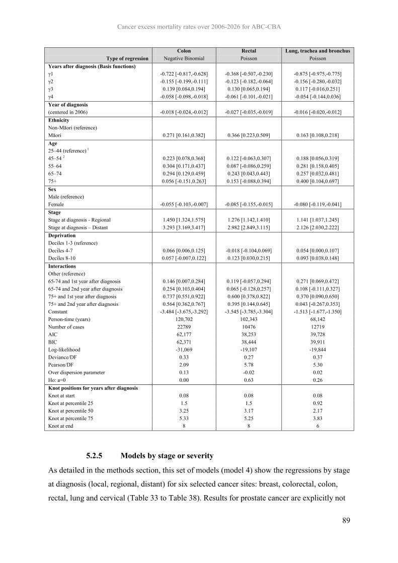
Cancer excess mortality rates over 2006-2026 for ABC-CBA
89
Colon Rectal Lung, trachea and bronchus Type of regression Negative Binomial Poisson Poisson
Years after diagnosis (Basis functions) γ1 -0.722 [-0.817,-0.628] -0.368 [-0.507,-0.230] -0.875 [-0.975,-0.775] γ2 -0.155 [-0.199,-0.111] -0.123 [-0.182,-0.064] -0.156 [-0.280,-0.032] γ3 0.139 [0.084,0.194] 0.130 [0.065,0.194] 0.117 [-0.016,0.251] γ4 -0.058 [-0.098,-0.018] -0.061 [-0.101,-0.021] -0.054 [-0.144,0.036] Year of diagnosis (centered in 2006) -0.018 [-0.024,-0.012] -0.027 [-0.035,-0.019] -0.016 [-0.020,-0.012] Ethnicity Non-Māori (reference) Māori 0.271 [0.161,0.382] 0.366 [0.223,0.509] 0.163 [0.108,0.218] Age 25–44 (reference) 1 45–54 2 0.223 [0.078,0.368] 0.122 [-0.063,0.307] 0.188 [0.056,0.319] 55–64 0.304 [0.171,0.437] 0.087 [-0.086,0.259] 0.281 [0.158,0.405] 65–74 0.294 [0.129,0.459] 0.243 [0.043,0.443] 0.257 [0.032,0.481] 75+ 0.056 [-0.151,0.263] 0.153 [-0.088,0.394] 0.400 [0.104,0.697] Sex Male (reference) Female -0.055 [-0.103,-0.007] -0.085 [-0.155,-0.015] -0.080 [-0.119,-0.041] Stage Stage at diagnosis - Regional 1.450 [1.324,1.575] 1.276 [1.142,1.410] 1.141 [1.037,1.245] Stage at diagnosis – Distant 3.293 [3.169,3.417] 2.982 [2.849,3.115] 2.126 [2.030,2.222] Deprivation Deciles 1-3 (reference) Deciles 4-7 0.066 [0.006,0.125] -0.018 [-0.104,0.069] 0.054 [0.000,0.107] Deciles 8-10 0.057 [-0.007,0.122] 0.123 [0.030,0.215] 0.093 [0.038,0.148] Interactions Other (reference) 65-74 and 1st year after diagnosis 0.146 [0.007,0.284] 0.119 [-0.057,0.294] 0.271 [0.069,0.472] 65-74 and 2nd year after diagnosis 0.254 [0.103,0.404] 0.065 [-0.128,0.257] 0.108 [-0.111,0.327] 75+ and 1st year after diagnosis 0.737 [0.551,0.922] 0.600 [0.378,0.822] 0.370 [0.090,0.650] 75+ and 2nd year after diagnosis 0.564 [0.362,0.767] 0.395 [0.144,0.645] 0.043 [-0.267,0.353] Constant -3.484 [-3.675,-3.292] -3.545 [-3.785,-3.304] -1.513 [-1.677,-1.350] Person-time (years) 120,702 102,343 68,142 Number of cases 22789 10476 12719 AIC 62,177 38,253 39,728 BIC 62,371 38,444 39,911 Log-likelihood -31,069 -19,107 -19,844 Deviance/DF 0.33 0.27 0.37 Pearson/DF 2.09 5.78 5.30 Over dispersion parameter 0.13 -0.02 0.02 Ho: a=0 0.00 0.63 0.26 Knot positions for years after diagnosis Knot at start 0.08 0.08 0.08 Knot at percentile 25 1.5 1.5 0.92 Knot at percentile 50 3.25 3.17 2.17 Knot at percentile 75 5.33 5.25 3.83 Knot at end 8 8 6
5.2.5 Models by stage or severity
As detailed in the methods section, this set of models (model 4) show the regressions by stage
at diagnosis (local, regional, distant) for six selected cancer sites: breast, colorectal, colon,
rectal, lung and cervical (Table 33 to Table 38). Results for prostate cancer are explicitly not

Cancer excess mortality rates over 2006-2026 for ABC-CBA
90
included due to the considerable amount of observations with missing stage (around three
quarters). Additionally, in the case of cervical cancer only Poisson models with 2 interior
knots (percentiles 33 and 67) are presented for regional and distant stages since Negative
Binomial models failed to converge due to the low mortality (literally zero for patients
diagnosed with local stage) of this cancer site.
As an example, Figure 10 below shows the breast cancer excess mortality rate by time since
diagnosis, by stage, on both a unit scale and the log scale. It can be clearly seen that in the
first few years post diagnosis, the shape of the curve differs by stage. Figure 11 shows how
these smoothed excess mortality rate functions translate into predicted relative survival
curves.
Figure 10: Predicted Excess Mortality Rates by Stage at Diagnosis for 55-64 years old, 1-3 deprivation deciles, Non-Māori female patients diagnosed with breast cancer in 2006
a) Unit excess mortality rate scale
0.00
0.10
0.20
0.30
0.40
0.50
0.60
0.70
0.80
0.90
0 1 2 3 4 5 6 7 8 9 10 11 12 13 14 15 16 17 18 19
Years since diagnosis
OverallLocalRegionalDistant

Cancer excess mortality rates over 2006-2026 for ABC-CBA
91
a) Log excess mortality rate scale
Figure 11: Predicted (Cumulative) Relative Survival by Stage at Diagnosis for 55-64 years old, 1-3 deprivation deciles, Non-Māori female patients diagnosed with breast cancer in 2006
0.00
0.00
0.01
0.10
1.00
0 1 2 3 4 5 6 7 8 9 10 11 12 13 14 15 16 17 18 19
Years since diagnosis
Overall
Local
Regional
0.0
0.1
0.2
0.3
0.4
0.5
0.6
0.7
0.8
0.9
1.0
0 1 2 3 4 5 6 7 8 9 10 11 12 13 14 15 16 17 18 19
Rela
tive S
urv
ival
Years since diagnosis
Overall
Local
Regional
Distant

Cancer excess mortality rates over 2006-2026 for ABC-CBA
92
Table 33: Regressions by stage at diagnosis (model 4) for colorectal cancer
Local Regional Distant Type of Regression Poisson Negative Binomial Poisson
Years after diagnosis (Basis functions) γ1 -1.449 [-1.823,-1.074] -0.132 [-0.266,0.001] -0.746 [-0.853,-0.639] γ2 -0.461 [-0.590,-0.332] -0.052 [-0.101,-0.004] -0.147 [-0.217,-0.077] γ3 0.442 [0.305,0.579] 0.074 [0.019,0.128] 0.130 [0.055,0.205] γ4 -0.198 [-0.279,-0.117] -0.040 [-0.077,-0.004] -0.059 [-0.107,-0.011] Year of diagnosis (centered in 2006) -0.089 [-0.110,-0.067] -0.045 [-0.053,-0.037] 0.000 [-0.006,0.006] Ethnicity Non-Māori (reference) Māori 0.777 [0.432,1.121] 0.376 [0.231,0.521] 0.201 [0.089,0.313] Age 25–44 (reference) 1 45–54 2 0.487 [-0.082,1.057] 0.105 [-0.076,0.287] 0.221 [0.069,0.372] 55–64 0.535 [-0.011,1.080] 0.112 [-0.054,0.277] 0.279 [0.139,0.418] 65–74 0.836 [0.277,1.396] 0.111 [-0.070,0.293] 0.332 [0.121,0.543] 75+ 0.510 [-0.165,1.185] 0.056 [-0.150,0.262] 0.040 [-0.237,0.317] Sex Male (reference) Female -0.182 [-0.344,-0.021] -0.105 [-0.167,-0.042] -0.019 [-0.069,0.032] Deprivation Deciles 1-3 (reference) Deciles 4-7 -0.067 [-0.264,0.130] 0.042 [-0.035,0.119] 0.045 [-0.019,0.109] Deciles 8-10 0.078 [-0.132,0.288] 0.090 [0.007,0.174] 0.055 [-0.014,0.124] Interactions Other (reference) 65-74 and 1st year after diagnosis -0.055 [-0.454,0.344] 0.182 [0.019,0.345] 0.154 [-0.035,0.343] 65-74 and 2nd year after diagnosis 0.492 [0.023,0.962] 0.219 [0.061,0.376] 0.162 [-0.042,0.365] 75+ and 1st year after diagnosis 0.955 [0.429,1.482] 0.677 [0.491,0.863] 0.788 [0.528,1.048] 75+ and 2nd year after diagnosis 0.367 [-0.506,1.240] 0.424 [0.231,0.617] 0.583 [0.303,0.863] Constant -3.926 [-4.553,-3.300] -2.587 [-2.795,-2.378] -0.093 [-0.246,0.060] Person-time (years) 50,474 53,379 33,304 Number of cases 10341 15798 7126 AIC 20,062 37,067 24,435 BIC 20,221 37,227 24,586 Log-likelihood -10,013 -18,515 -12,199 Deviance/DF 0.28 0.42 0.44 Pearson/DF 1.67 2.00 5.19 Over dispersion parameter 0.32 0.17 0.03 Ho: a=0 0.20 0.00 0.27 Knot positions for years after diagnosis Knot at start 0.08 0.08 0.08 Knot at percentile 25 1.67 1.58 1.25 Knot at percentile 50 3.42 3.33 2.83 Knot at percentile 75 5.42 5.42 5 Knot at end 8 8 8

Cancer excess mortality rates over 2006-2026 for ABC-CBA
93
Table 34: Regressions by stage at diagnosis (model 4) for colon cancer
Local Regional Distant Type of Regression Negative Binomial Negative Binomial Poisson
Years after diagnosis (Basis functions) γ1 -1.568 [-2.086,-1.050] -0.305 [-0.463,-0.147] -0.896 [-1.027,-0.765] γ2 -0.523 [-0.709,-0.337] -0.053 [-0.113,0.008] -0.214 [-0.308,-0.120] γ3 0.530 [0.326,0.734] 0.051 [-0.021,0.123] 0.170 [0.076,0.264] γ4 -0.267 [-0.394,-0.140] -0.015 [-0.066,0.036] -0.066 [-0.120,-0.012] Year of diagnosis (centered in 2006) -0.074 [-0.103,-0.044] -0.036 [-0.046,-0.026] -0.003 [-0.010,0.004] Ethnicity Non-Māori (reference) Māori 0.695 [0.172,1.217] 0.405 [0.222,0.587] 0.175 [0.037,0.313] Age 25–44 (reference) 1 45–54 2 1.199 [0.225,2.173] 0.226 [-0.012,0.464] 0.179 [-0.006,0.364] 55–64 1.066 [0.111,2.021] 0.246 [0.029,0.464] 0.286 [0.116,0.456] 65–74 1.334 [0.362,2.306] 0.213 [-0.027,0.452] 0.253 [-0.011,0.517] 75+ 1.024 [-0.101,2.149] 0.094 [-0.180,0.367] -0.001 [-0.342,0.340] Sex Male (reference) Female -0.223 [-0.450,0.003] -0.085 [-0.162,-0.009] -0.019 [-0.079,0.040] Deprivation Deciles 1-3 (reference) Deciles 4-7 -0.081 [-0.355,0.193] 0.064 [-0.029,0.158] 0.080 [0.005,0.155] Deciles 8-10 0.033 [-0.260,0.326] 0.074 [-0.028,0.176] 0.047 [-0.035,0.129] Interactions Other (reference) 65-74 and 1st year after diagnosis 0.106 [-0.444,0.656] 0.084 [-0.115,0.283] 0.234 [-0.002,0.470] 65-74 and 2nd year after diagnosis 0.509 [-0.168,1.187] 0.216 [0.020,0.412] 0.293 [0.042,0.545] 75+ and 1st year after diagnosis 0.882 [0.116,1.648] 0.634 [0.401,0.867] 0.820 [0.501,1.139] 75+ and 2nd year after diagnosis 0.187 [-1.205,1.580] 0.396 [0.149,0.642] 0.670 [0.330,1.011] Constant -4.293 [-5.335,-3.252] -2.411 [-2.671,-2.151] -0.004 [-0.188,0.181] Person-time (years) 44,159 48,266 28,277 Number of cases 6474 11183 5132 AIC 14,085 28,584 19,201 BIC 14,241 28,742 19,349 Log-likelihood -7,024 -14,274 -9,582 Deviance/DF 0.21 0.37 0.42 Pearson/DF 1.67 1.84 2.92 Over dispersion parameter 0.49 0.22 0.04 Ho: a=0 0.00 0.00 0.11 Knot positions for years after diagnosis Knot at start 0.08 0.08 0.08 Knot at percentile 25 1.67 1.58 1.17 Knot at percentile 50 3.42 3.33 2.67 Knot at percentile 75 5.5 5.42 4.83 Knot at end 8 8 8

Cancer excess mortality rates over 2006-2026 for ABC-CBA
94
Table 35: Regressions by stage at diagnosis (model 4) for rectal cancer
Local Regional Distant Type of Regression Poisson Poisson Poisson
Years after diagnosis (Basis functions) γ1 -1.150 [-1.680,-0.620] 0.351 [0.106,0.595] -0.480 [-0.721,-0.239] γ2 -0.357 [-0.532,-0.182] -0.002 [-0.082,0.078] -0.140 [-0.347,0.067] γ3 0.324 [0.142,0.506] 0.064 [-0.023,0.151] 0.115 [-0.043,0.273] γ4 -0.128 [-0.233,-0.022] -0.057 [-0.111,-0.004] -0.039 [-0.104,0.025] Year of diagnosis (centered in 2006) -0.110 [-0.143,-0.077] -0.065 [-0.079,-0.051] 0.006 [-0.005,0.018] Ethnicity Non-Māori (reference) Māori 0.854 [0.404,1.304] 0.328 [0.093,0.563] 0.289 [0.097,0.481] Age 25–44 (reference) 1 45–54 2 -0.248 [-0.952,0.456] -0.084 [-0.363,0.195] 0.315 [0.051,0.578] 55–64 0.007 [-0.645,0.659] -0.089 [-0.346,0.167] 0.244 [-0.003,0.491] 65–74 0.367 [-0.302,1.035] 0.035 [-0.240,0.309] 0.435 [0.081,0.789] 75+ 0.041 [-0.817,0.899] 0.165 [-0.138,0.468] 0.121 [-0.345,0.587] Sex Male (reference) Female -0.069 [-0.305,0.167] -0.104 [-0.212,0.003] -0.059 [-0.158,0.040] Deprivation Deciles 1-3 (reference) Deciles 4-7 -0.036 [-0.325,0.253] -0.016 [-0.147,0.114] -0.036 [-0.159,0.088] Deciles 8-10 0.111 [-0.197,0.420] 0.125 [-0.016,0.266] 0.086 [-0.045,0.217] Interactions Other (reference) 65-74 and 1st year after diagnosis -0.254 [-0.860,0.351] 0.350 [0.063,0.636] 0.055 [-0.265,0.374] 65-74 and 2nd year after diagnosis 0.378 [-0.262,1.018] 0.153 [-0.104,0.410] -0.096 [-0.436,0.244] 75+ and 1st year after diagnosis 1.078 [0.327,1.830] 0.619 [0.306,0.933] 0.702 [0.260,1.143] 75+ and 2nd year after diagnosis 0.577 [-0.494,1.647] 0.396 [0.101,0.692] 0.350 [-0.132,0.832] Constant -3.759 [-4.558,-2.961] -3.172 [-3.538,-2.807] -0.296 [-0.574,-0.018] Person-time (years) 41,317 42,136 18,890 Number of cases 3867 4615 1994 AIC 10,008 16,904 11,013 BIC 10,163 17,060 11,154 Log-likelihood -4,986 -8,434 -5,488 Deviance/DF 0.18 0.29 0.40 Pearson/DF 1.82 8.58 9.00 Over dispersion parameter -0.03 -0.09 -.0340928 Ho: a=0 0.81 0.13 0.64 Knot positions for years after diagnosis Knot at start 0.08 0.08 0.08 Knot at percentile 25 1.67 1.67 0.92 Knot at percentile 50 3.42 3.33 2.17 Knot at percentile 75 5.42 5.42 4.25 Knot at end 8.00 8 8

Cancer excess mortality rates over 2006-2026 for ABC-CBA
95
Table 36: Regressions by stage at diagnosis (model 4) for lung cancer
Local Regional Distant Type of Regression Poisson Poisson Poisson
Years after diagnosis (Basis functions) γ1 -0.135 [-0.582,0.313] -0.422 [-0.689,-0.155] -0.895 [-1.041,-0.748] γ2 -0.010 [-0.273,0.254] -0.064 [-0.297,0.169] -0.126 [-0.374,0.121] γ3 0.097 [-0.200,0.394] 0.031 [-0.186,0.248] 0.153 [-0.065,0.371] γ4 -0.088 [-0.239,0.063] 0.009 [-0.088,0.105] -0.078 [-0.177,0.020] Year of diagnosis (centered in 2006) -0.172 [-0.196,-0.147] -0.059 [-0.070,-0.048] -0.001 [-0.006,0.004] Ethnicity Non-Māori (reference) Māori 0.452 [0.182,0.722] 0.321 [0.180,0.463] 0.117 [0.056,0.178] Age 25–44 (reference) 1 45–54 2 0.400 [-0.294,1.094] 0.286 [-0.033,0.605] 0.149 [0.002,0.296] 55–64 0.575 [-0.067,1.217] 0.288 [-0.017,0.593] 0.258 [0.119,0.396] 65–74 0.921 [0.237,1.605] -0.059 [-0.462,0.344] 0.272 [-0.101,0.645] 75+ 0.663 [-0.182,1.508] 0.560 [0.107,1.013] 0.435 [-0.060,0.929] Sex Male (reference) Female -0.352 [-0.541,-0.164] -0.072 [-0.173,0.029] -0.068 [-0.111,-0.025] Deprivation Deciles 1-3 (reference) Deciles 4-7 0.112 [-0.122,0.345] 0.188 [0.055,0.322] 0.022 [-0.037,0.082] Deciles 8-10 0.052 [-0.195,0.299] 0.321 [0.182,0.460] 0.063 [0.002,0.124] Interactions Other (reference) 65-74 and 1st year after diagnosis 0.054 [-0.381,0.490] 0.555 [0.233,0.878] 0.239 [-0.118,0.595] 65-74 and 2nd year after diagnosis -0.016 [-0.457,0.424] 0.491 [0.152,0.829] -0.091 [-0.475,0.293] 75+ and 1st year after diagnosis 0.594 [-0.087,1.274] 0.301 [-0.089,0.692] 0.283 [-0.199,0.766] 75+ and 2nd year after diagnosis 0.303 [-0.441,1.047] -0.022 [-0.465,0.421] -0.056 [-0.572,0.460] Constant -3.556 [-4.296,-2.815] -1.128 [-1.476,-0.781] 0.771 [0.621,0.920] Person-time (years) 25,295 22,264 20,583 Number of cases 1477 2165 9077 AIC 5,968 11,479 21,676 BIC 6,114 11,623 21,819 Log-likelihood -2,966 -5,721 -10,820 Deviance/DF 0.18 0.37 0.56 Pearson/DF 5.31 3.36 7.44 Over dispersion parameter 0.28 0.07 0.01 Ho: a=0 0.25 0.53 0.18 Knot positions for years after diagnosis Knot at start 0.08 0.08 0.08 Knot at percentile 25 1.25 0.92 0.67 Knot at percentile 50 2.58 2.08 1.75 Knot at percentile 75 4.08 3.75 3.5 Knot at end 6 6 6

Cancer excess mortality rates over 2006-2026 for ABC-CBA
96
Table 37: Regressions by stage at diagnosis (model 4) for breast cancer
Local Regional Distant Type of Regression Poisson Poisson Poisson
Years after diagnosis (Basis functions) γ1 1.640 [1.218,2.063] 1.015 [0.850,1.181] -1.158 [-1.392,-0.925] γ2 0.224 [0.153,0.295] 0.145 [0.112,0.178] -0.370 [-0.485,-0.254] γ3 -0.154 [-0.218,-0.090] -0.099 [-0.132,-0.067] 0.252 [0.158,0.345] γ4 0.038 [0.006,0.069] 0.024 [0.007,0.041] -0.063 [-0.101,-0.025] Year of diagnosis (centered in 2006) -0.125 [-0.149,-0.101] -0.048 [-0.058,-0.037] 0.002 [-0.010,0.015] Ethnicity Non-Māori (reference) Māori 0.344 [0.086,0.602] 0.344 [0.228,0.460] 0.331 [0.149,0.513] Age 25–44 (reference) 1 45–54 2 -0.594 [-0.795,-0.392] -0.229 [-0.338,-0.121] 0.221 [0.011,0.430] 55–64 -0.617 [-0.841,-0.394] -0.128 [-0.244,-0.013] 0.135 [-0.075,0.344] 65–74 -0.650 [-0.993,-0.308] 0.079 [-0.067,0.224] 0.195 [-0.161,0.551] 75+ -0.926 [-1.775,-0.077] 0.119 [-0.083,0.320] 0.116 [-0.258,0.491] Sex Male (reference) Female 0.000 [0.000,0.000] Deprivation Deciles 1-3 (reference) Deciles 4-7 -0.029 [-0.228,0.169] 0.131 [0.030,0.231] -0.023 [-0.175,0.129] Deciles 8-10 0.001 [-0.219,0.222] 0.122 [0.013,0.231] 0.005 [-0.154,0.164] Interactions Other (reference) 65-74 and 1st year after diagnosis -15.056 [-2517.996,2487.885] 0.066 [-0.320,0.453] 0.260 [-0.117,0.636] 65-74 and 2nd year after diagnosis 0.112 [-0.618,0.841] 0.157 [-0.091,0.406] 0.015 [-0.466,0.496] 75+ and 1st year after diagnosis -13.689 [-2586.641,2559.263] 0.654 [0.265,1.042] 0.587 [0.207,0.967] 75+ and 2nd year after diagnosis -12.805 [-2284.795,2259.185] 0.128 [-0.216,0.473] -0.001 [-0.497,0.495] Constant -7.105 [-7.761,-6.450] -4.615 [-4.864,-4.367] -0.133 [-0.384,0.119] Person-time (years) 39,169 38,739 17,028 Number of cases 15346 11124 1454 AIC 16,442 23,625 8,048 BIC 16,588 23,770 8,180 Log-likelihood -8,204 -11,795 -4,007 Deviance/DF 0.30 0.42 0.34 Pearson/DF 3.45 1.26 3.48 Over dispersion parameter -0.04 -0.01 0.01 Ho: a=0 0.56 0.81 0.90 Knot positions for years after diagnosis Knot at start 0.08 0.08 0.08 Knot at percentile 25 2 2 1.25 Knot at percentile 50 4.08 4 2.83 Knot at percentile 75 6.67 6.50 5.33 Knot at end 10 10 10

Cancer excess mortality rates over 2006-2026 for ABC-CBA
97
Table 38: Regressions by stage at diagnosis (model 4) for cervical cancer
Regional Distant Type of Regression Poisson Poisson
Years after diagnosis (Basis functions) γ1 0.919 [-0.766,2.605] -0.642 [-4.246,2.961] γ2 0.298 [-0.331,0.927] 0.028 [-3.287,3.343] γ3 -0.197 [-0.713,0.319] -0.041 [-1.499,1.418] Year of diagnosis (centered in 2006) 0.002 [-0.100,0.105] -0.025 [-0.193,0.143] Ethnicity Non-Māori (reference) Māori 0.298 [-0.653,1.250] 0.735 [-0.839,2.309] Age 25–44 (reference) 1 45–54 2 0.093 [-0.876,1.063] 0.318 [-1.766,2.403] 55–64 0.340 [-0.706,1.387] 0.483 [-1.618,2.583] 65–74 -0.661 [-3.534,2.213] 0.521 [-6.809,7.852] 75+ -1.173 [-15.583,13.236] 1.049 [-5.954,8.052] Sex Male (reference) Female Deprivation Deciles 1-3 (reference) Deciles 4-7 0.502 [-0.570,1.574] 0.032 [-1.987,2.051] Deciles 8-10 0.408 [-0.714,1.530] 0.069 [-1.914,2.052] Interactions Other (reference) 65-74 and 1st year after diagnosis -0.855 [-8.772,7.062] 0.193 [-7.295,7.681] 65-74 and 2nd year after diagnosis 0.775 [-2.713,4.264] 0.584 [-7.434,8.603] 75+ and 1st year after diagnosis 2.470 [-12.149,17.089] 0.019 [-7.235,7.273] 75+ and 2nd year after diagnosis 2.438 [-12.084,16.959] 0.302 [-7.546,8.150] Constant -3.641 [-5.541,-1.742] -0.452 [-3.378,2.474] Person-time (years) 8,332 2,808 Number of cases 302 218 AIC 1,180 1,640 BIC 1,293 1,735 Log-likelihood -574 -804 Deviance/DF 0.11 0.44 Pearson/DF 3.15 21.25 Over dispersion parameter -0.36 -0.27 Ho: a=0 0.02 0.03 Knot positions for years after diagnosis Knot at start 0.08 0.08 Knot at percentile 33 1.42 0.67 Knot at percentile 67 3.08 2.00 Knot at end 5 5

Cancer excess mortality rates over 2006-2026 for ABC-CBA
98
Conclusion 6This Report both provides baseline excess mortality rates for cancers in New Zealand, and
demonstrates how they can be calculated. Of note, it is likely that the baseline excess
mortality rates will need to be re-estimated in some instances due to variations in the
proposed intervention and comparator scenario, updated data, and such like. Regardless, the
equations can then be used directly in economic decision software such as TreeAge, be it to
specify time dependent transition probabilities, or transformed into cumulative distribution
functions for time to event simulation with discrete event simulation.

Cancer excess mortality rates over 2006-2026 for ABC-CBA
99
References 1. Blakely, T., R. Costilla, et al. (2010). The Burden of Cancer: New Zealand 2006.
Wellington, Ministry of Health.
2. Brenner, H. and B. Racher (2004). "Hybrid analysis for up-to-date long-term survival
rates in cancer registries with delayed recording of incident cases." European Journal of
Cancer 40(16): 2494-2501.
3. Bulow, S., H. Harling, et al. (2010). "Improved survival after rectal cancer in Denmark."
Colorectal disease : the official journal of the Association of Coloproctology of Great
Britain and Ireland 12(7 Online): e37-42.
4. Coleman, M. P., D. Forman, et al. (2011). "Cancer survival in Australia, Canada,
Denmark, Norway, Sweden, and the UK, 1995-2007 (the International Cancer
Benchmarking Partnership): an analysis of population-based cancer registry data." Lancet
377(9760): 127-138.
5. Coleman, M. P., B. Rachet, et al. (2004). "Trends and socioeconomic inequalities in
cancer survival in England and Wales up to 2001." British Journal of Cancer 90(7): 1367-
1373.
6. Cunningham, R., D. Sarfati, et al. (2008). "An audit of colon cancer data on the New
Zealand Cancer Registry." New Zealand Medical Journal 121: 46-56.
7. Cunningham, R., D. Sarfati, et al. (2008). "An audit of colon cancer data on the New
Zealand Cancer Registry." New Zealand Medical Journal 121(1279): 46-56.
8. Dickman, P., A. Sloggett, et al. (2004). "Regression models for relative survival."
Statistics in Medicine 23: 51-64.
9. Durrleman, S. and R. Simon (1989). "Flexible regression models with cubic splines."
Statistics in Medicine 8: 551-561.
10. Folkesson, J., G. Engholm, et al. (2009). "Rectal cancer survival in the Nordic countries
and Scotland." International journal of cancer. Journal international du cancer 125(10):
2406-2412.
11. Kvizhinadze, G. and T. Blakely (2011). Projected NZ Life Tables. Burden of Disease
Epidemiology, Equity and Cost-Effectiveness Programme, Technical Report No.4. .
Wellington, Department of Public Health, University of Otago, Wellington.
12. Lambert, P. and P. Royston (2009). "Further development of flexible parametric models
for survival analysis." The Stata Journal 9: 265-290.

Cancer excess mortality rates over 2006-2026 for ABC-CBA
100
13. Lemmens, V., L. van Steenbergen, et al. (2010). "Trends in colorectal cancer in the south
of the Netherlands 1975-2007: rectal cancer survival levels with colon cancer survival."
Acta oncologica 49(6): 784-796.
14. McKenzie, F., L. Ellison-Loschmann, et al. (2010). "Investigating reasons for
socioeconomic inequalities in breast cancer survival in New Zealand." Cancer
Epidemiology 34: 702-708.
15. Mitry, E., A.-M. Bouvier, et al. (2005). "Improvement in colorectal cancer survival: a
population-based study." European Journal of Cancer 41(15): 2297-2303.
16. Monnet, E., J. Faivre, et al. (1999). "Influence of stage at diagnosis on survival
differences for rectal cancer in three European populations." British Journal of Cancer
81(3): 463-468.
17. Rachet, B., C. Maringe, et al. (2009). "Population-based cancer survival trends in England
and Wales up to 2007: an assessment of the NHS cancer plan for England.[see
comment]." Lancet Oncology 10(4): 351-369.
18. Robson, B., G. Purdie, et al. (2005). Unequal Impact: Māori and Non-Māori Cancer
Statistics 1996–2001. Wellington, Ministry of Health.
19. Royston, P. and P. Lambert (2009). Flexible Parametric Survival Analysis Using Stata:
Beyond the Cox Model. College Station, Texas, Stata Press.
20. Shack, L. G., B. Rachet, et al. (2007). "Socioeconomic inequalities in cancer survival in
Scotland 1986-2000." British journal of cancer 97(7): 999-1004.
21. Soeberg, M., T. Blakely, et al. (2012). Cancer Trends: Trends in Cancer Survival by
Ethnic and Socioeconomic Group, New Zealand 1991-2004. Wellington, Ministry of
Health.
22. van Steenbergen, L. N., M. A. Elferink, et al. (2010). "Improved survival of colon cancer
due to improved treatment and detection: a nationwide population-based study in The
Netherlands 1989-2006." Annals of oncology : official journal of the European Society
for Medical Oncology / ESMO 21(11): 2206-2212.
23. Yu, X. Q., D. L. O'Connell, et al. (2006). "Trends in survival and excess risk of death
after diagnosis of cancer in 1980-1996 in New South Wales, Australia.[erratum appears in
Int J Cancer. 2006 Dec 15;119(12):2993]." International Journal of Cancer 119(4): 894-
900.
Related Documents