Can static models predict implied volatility surfaces ...

Can static models predict implied volatility

surfaces? Evidence from OTC currency

options∗

Georgios Chalamandaris† Andrianos E. Tsekrekos‡

This version: January, 2009

Abstract

Despite advances in describing the characteristics and dynamics of

non–flat implied volatility surfaces, relatively little has been said re-

garding the practical problem of implied volatility surface forecasting.

Taking an explicitly out–of–sample forecasting approach, we propose

a simple–to–estimate parametric decomposition of the implied volatil-

ity surface that combines and extends previous research in several

respects. Using daily data from OTC options on 22 different cur-

rencies quoted against the U.S. $, we demonstrate that the approach

yields intuitive and easy to communicate factors that achieve excellent

in–sample fit, and whose time–variation capture the dynamics of the

surface. Static econometric models for the factors are estimated and

used for making short and long–term prediction of implied volatility

surfaces. Results indicate that in comparison to leading benchmarks,

the forecasts of 5 to 20–weeks–ahead are much superior across all sur-

faces.

JEL classification: C32; C53; G13; F37

Keywords: Implied volatility surfaces; Factor model; Forecasting.

∗We thank participants and discussants at the Asian FA/NFA conference in Yoko-

hama, Japan, the 2nd Risk Management conference in Singapore, the 15th GFA meeting

in Hangzhou, P. R. China, the 6th HFAA meeting in Patras, Greece and seminar partici-

pants at the Athens University of Economics & Business and the University of Piraeus for

comments and suggestions. Any errors are our own responsibility.†Corresponding author, Department of Accounting & Finance, Athens University of

Economics & Business (AUEB), 76 Patision Str., 104 43, Athens, Greece. Tel:+30-210-

8203758, email: [email protected].‡Tel/Fax:+30-210-8203762, email: [email protected].

1

1 Introduction

Observed option prices implicitly contain information about the volatility

expectations of market participants. Using an option pricing model, these

volatility expectations can be extracted, and if market participants are ra-

tional, then these implied volatilities should contain all the information that

is relevant for the pricing, hedging and management of option contracts and

portfolios.

Contrary to the Black–Scholes–Merton assumption of constant (or de-

terministically time–dependent) volatility, the empirical pattern of option–

implied volatilities has two features that have attracted the interest of re-

searchers and practitioners in financial modeling: First, the volatilities im-

plied from observed contracts systematically vary with the options strike

price K and date to expiration T , giving rise to an instantaneously non–flat

implied volatility surface (hereafter IVS). Canina and Figlewski (1993) and

Rubinstein (1994) provide evidence that when plotted against moneyness,

m = K/S (the ratio of the strike price to the underlying spot price), implied

volatilities exhibit either a ‘smile’ or a ‘skew’, while Heynen et. al. (1994), Xu

and Taylor (1994) and Campa and Chang (1995) show that implied volatili-

ties are a function of time to expiration and thus exhibit a ‘term structure’.

The second feature is that the IVS changes dynamically over time as prices in

the options market respond to new information that affects investors’ beliefs

and expectations.

Three popular approaches to modeling this empirically observed profile

of the IVS can be identified in the literature. The no–arbitrage approach,

inspired by the stochastic interest rate literature, where stochastic volatil-

ity models are calibrated to today’s IVS so as to preclude arbitrage, with

prominent examples offered by Dupire (1993), Derman and Kani (1998) and

Ledoit and Santa–Clara (1998) among others. Secondly, linear parametric

specifications linking implied volatility to time to maturity and moneyness

(Dumas, Fleming and Whaley (1998), Pena, Rubio and Serna (1999), etc.),

and finally (statistical) latent factors that are identified in the dynamics of

the IVS, as in Skiadopoulos et. al. (1999), Cont and da Fonseca (2002) and

Mixon (2002).

Despite the relative success of the approaches for pricing and hedging

purposes, surprisingly little has been said regarding the practical problem of

implied volatility surface forecasting. The arbitrage–free stochastic volatility

literature has little to say about forecasting, as it is concerned primarily with

fitting the IVS at a point in time. Moreover, most contributions offered by

2

latent factor decompositions of the IVS, although concerned with dynamics

and thus potentially useful for forecasting, focus mainly on in–sample fit as

opposed to out–of–sample predictions.1

In this paper, we take an explicitly out–of–sample forecasting approach

that originates from the literature that employs parametric σIV (m,T ) spec-

ifications which have proved very successful in explaining deviations from a

flat IVS in–sample.

Using daily implied volatility surfaces from a cross–section of options

on 22 different currencies quoted against the U.S. $ from the OTC market,

we decompose, period–by–period, each surface into seven linear parameters

that evolve dynamically, and can be interpreted as factors. Unlike existing

factor decompositions of the IVS, in which both the latent factors and the

factor loadings are estimated (e.g. Mixon (2002)), our specification imposes

structure on the factor loadings. This facilitates highly precise estimation of

the factors and their intuitive interpretation.

We propose simple econometric models for the factors that are used for

predicting the future IVS, by forecasting the factors forward. Results are

encouraging; the factors achieve excellent in–sample fit across different FX

options IVSs, and can be used to produce medium to long–term predictions

(from 5 to 20 weeks ahead) that are noticeably more accurate than standard

benchmarks and competing models.

A few existing papers are related to our approach, with Diebold and Li

(2006) and Goncalves and Guidolin (2006) closest in spirit. Both papers first

apply parametric specifications at the cross–sectional level, and then fit time

series models on the factors extracted from the first step. Moreover, both

papers are concerned with forecasting: the yield curve and the IVS of S&P

500 index options respectively.

Diebold and Li (2006) (hereafter DL06) apply a Nelson and Siegel (1987)

type of specification to the yield curve derived from the cross–section of U.S.

government bond prices, and the estimated coefficients of the specification are

fitted to an autoregressive model. Goncalves and Guidolin (2006) (hereafter

GG06) first estimate a five–parameter version of the ad hoc implied volatility

model of Dumas et. al. (1998) on the volatility surface implied by S&P 500

index options. They then model the time evolution of estimated parameters

with a vector autoregressive model.

The decomposition of the IVS we propose here can be though of as an

extension of the GG06 framework in three respects. First, we allow potential

1See however the recent results in Chalamandaris and Tsekrekos (2008).

3

asymmetries in the shape of both the implied volatility smile and the decay

of the smile with respect to the options’ maturity. Secondly, we employ the

DL06 factorisation of the Nelson and Siegel (1987) parsimonious model to

extract factors that govern the dynamics of the IVS term–structure. Finally,

we investigate a number of alternative modeling specifications for the IVS–

extracted factors, with various degrees of in–sample fit and out–of–sample

predicting accuracy. A simple vector autoregressive model of the factors

(with Bayesian updating) appears superior amongst competing model spec-

ifications.

The rest of the paper is organised as follows: Section 2 describes the data,

presents our methodology for decomposing the implied volatility surface into

intuitive dynamic factors and discusses the estimation results of this method-

ology. In section 3 we estimate a series of static econometric models that can

capture the time–series dynamics of the factors. Section 4 is devoted to the

assessment of the out–of–sample forecasting performance of our approach,

while Section 5 concludes the paper.

2 The implied volatility surface

2.1 The data

The data used in this study consist of daily time–series of implied volatilities

for a cross–section of OTC currency options on 24 different currencies quoted

against the U.S. dollar, kindly supplied by a major market participant. The

time series are from 1/1/1999 to 21/5/2007, a total of 2,184 weekdays. The

currencies examined and some exchange rate statistics are reported in Table

1.

In comparison to exchange–traded currency options, the OTC market is

far more liquid. According to a Bank of International Settlements survey

(2007), the outstanding notional amount of OTC currency options on the

U.S. $ in June 2008 was approximately 11.9 trillion US$. The corresponding

amount of exchange–traded currency options was 190.62 billion US$, just

over 1.5% of the notional amount outstanding in the OTC market.

As is typical in such markets, dealers do not quote option prices de-

nominated in currency units but rather implied volatilities, which are then

conventionally converted into prices using the Garman and Kohlhagen (1983)

4

Code Currency Average Min-Max

AUD Australian $ 1.559 1.195-2.071

BRL Brazilian Real 2.426 1.207-3.945

CAD Canadian $ 1.381 1.085-1.613

CHF Swiss Franc 1.431 1.134-1.825

CLP Chilean Peso 592.7 468.0-758.2

CZK Czech Koruny 30.12 20.59-42.04

DKK Danish Krone 6.912 5.455-9.005

EUR Euro 0.929 0.732-1.209

GBP British £ 0.607 0.498-0.728

HUF Hungarian Forint 235.4 179.9-317.1

ILS Israeli (New) Sheqel 4.381 3.938-5.010

JPY Japanese U 115.1 101.5-134.8

KRW South Korean Won 1137.6 913.7-1369.0

NOK Norwegian Kroner 7.469 5.944-9.589

NZD New Zealand $ 1.833 1.340-2.551

PLN Polish Zlotych 3.755 2.751-4.715

SEK Swedish Kronor 8.402 6.594-11.027

SGD Singapore $ 1.703 1.511-1.854

THB Thailand Baht 40.37 31.80-45.82

TWD Taiwanese (New) $ 33.05 30.35-35.16

VEB Venezuelan Bolivar Fuerte 1.401 0.560-2.140

ZAR South African Rand 7.405 5.615-13.60

Table 1: Average, minimum and maximum middle exchange rates of 22

different currencies against the Euro from January 1999 to May 2007. Source:

Federal Reserve Bank of New York & Reuters.

version of the Black and Scholes (1973) option pricing formula:

c = Se−rfTN (d) −Ke−rdTN(d− σ

√T

)(1)

p = Ke−rdTN(−d+ σ

√T

)− Se−rf TN (−d) (2)

where

d =ln (S/K) + (rd − rf + σ2/2)T

σ√T

(3)

with rd, rf the risk–free interest rate in the domestic and the foreign country

respectively, S the spot exchange rate, K the strike price of the option, T the

time to option maturity in years, σ the exchange rate’s volatility and N (.)

the standard cumulative normal distribution.

5

The moneyness of the option is measured by its (Black–Scholes) delta:

∆BS =∂O

∂S=

e−rfTN (d), if the option O is a call

e−rfT [N (d) − 1], if the option O is a put

(4)

The industry convention is to quote, for each maturity, implied volatilities

for portfolios of options such as delta–neutral straddles and risk reversals or

butterfly spreads of a certain ∆BS . From these, the implied volatility for

at–the–money (ATM) options and for out–of–the–money (OTM) calls and

puts can be inferred.2

Our data–set consists of implied volatilities for the following fourteen

expirations: 1 week, 1 month, 2 months, 3 months, 6 months, 9 months,

12 months, 18 months, 2–5 years, 7 years and 10 years. For each of these

maturities, the implied volatility is observed for options with five different

Black–Scholes deltas: OTM puts with ∆BS = −0.10 and ∆BS = −0.25,

ATM calls/puts and OTM calls with ∆BS = 0.10 and ∆BS = 0.25. Hence,

for each exchange rate and on each observation date, a vector of 70×1 implied

volatilities is observed.

Of course, not all currencies in our sample and not all option expirations

are of equal trading intensity and variation. To eliminate the possibility that

thinly–traded segments of an IVS influence our results, we exclude option

maturities whose implied volatility is missing or remains unchanged for more

than 70% of weekdays in our sample period. Then, to ensure that each

IVS is continuous in the time domain, we discard parts of the sample that

cause gaps of missing values longer than 4 weekdays. Applying the above

two criteria ensures that in our reduced (both in maturities and in eligible

weekdays) sample the entire surface under consideration is active. Table 2

reports the starting date and the number of days remaining in our sample

after the above criteria have been applied.

Several different profiles of implied volatility surfaces are observed in our

sample period. As an indication, in Figures 1–4 the average IVS profile

and the daily standard deviation of the IVS from EUR/USD and NZD/USD

options are plotted. In the EUR/USD case, the implied volatility surface

exhibits a clear symmetric “smile” with an increasing term structure on av-

erage, and a fair amount of variability around this average profile (ranging

from a fourth to a tenth of its typical value). In contrast, the NZD/USD

2Carr and Wu (2007a) and Malz (1996) demonstrate this in detail, in their excellent

discussions on OTC currency option quoting and trading conventions.

6

Currency Start Date # of days Currency Start Date # of days

AUD 05-Sep-2000 1744 JPY 04-Jul-2000 1806

BRL 27-Apr-1999 2178 KRW 27-Apr-1999 2178

CAD 27-Apr-1999 2178 NOK 27-Apr-1999 2178

CHF 04-Sep-2000 1745 NZD 27-Apr-1999 2178

CLP 29-Aug-2000 1739 PLN 27-Apr-1999 2178

CZK 27-Apr-1999 2178 SEK 27-Apr-1999 2178

DKK 27-Apr-1999 2178 SGD xx05-Dec-2005 1610

EUR 04-Sep-2000 1745 THB 27-Apr-1999 2178

GBP 05-Sep-2000 1744 TWD 05-Sep-2000 1744

HUF 15-Jun-2000 1506 VEB 14-May-2000 1645

ILS 28-Apr-1999 2177 ZAR 08-Jul-2000 1803

Table 2: For each of the twenty two different currency options in our sample,

the table reports the starting date and the number of trading days in the

time series. The end date in all time series is 21/5/2007.

implied volatility surface exhibits a “skew”, with either an increasing or a

humped–shaped term structure, and a significantly asymmetric variability

for short maturities. Similar patterns emerge in all currencies examined; to

conserve space the corresponding figures for the remaining 22 currencies are

relegated to Appendix D (available from the authors upon request).

Given the origin of the data, one possible criticism is that idiosyncratic

effects, specific to the market participant supplying the quotes, could influ-

ence the analysis. There are however reasons to believe that such effects

(if any) are not strongly affecting our analysis. First, our focus here is on

systematic factors in the volatility surface, not on specific events or outliers

of the surface. Secondly, given the liquidity of the market and the size of the

market participant supplying the data, it should be fairly unlikely that our

data are substantially away from typical values. Cross–checking a randomly

7

01

23

45 0

50

1000.095

0.1

0.105

0.11

0.115

0.12

Moneyness (Delta)

Average IVS EURUSD

Maturity (in years)

Impl

ied

Vola

tility

Figure 1: Average implied volatility surface from EUR/USD options, for theperiod 4/9/2000–21/5/2007.

01

23

45 0

50

1000.014

0.016

0.018

0.02

0.022

0.024

Moneyness (Delta)

Standard Deviation of IVS EURUSD

Maturity (in years)

Impl

ied

Vola

tility

Figure 2: Daily standard deviation of EUR/USD implied volatilities asa function of moneyness and time to maturity for the period 4/9/2000–21/5/2007.

8

0

0.5

1

1.5 0

50

10011.5

12

12.5

13

13.5

Moneyness (Delta)

Average IVS NZDUSD

Maturity (in years)

Impl

ied

Vola

tility

Figure 3: Average implied volatility surface from NZD/USD options, for theperiod XX/12/2003–21/5/2007.

00.5

11.5 0

50

100

1.4

1.6

1.8

2

2.2

2.4

2.6

Moneyness (Delta)

Standard Deviation of IVS NZDUSD

Maturity (in years)

Impl

ied

Vola

tility

Figure 4: Daily standard deviation of NZD/USD implied volatilities as afunction of moneyness and time to maturity for the period XX/12/2005–21/5/2007.

9

selected subsample of our data set with the implied volatility quotes from

another data vendor (Bloomberg) reveals that this is indeed the case.

Of course using OTC data has many advantages in comparison to exchange–

traded data. Besides superior liquidity, OTC currency options are avail-

able for longer maturities than the currency options traded in exchanges.

Moreover, OTC options have a constant time–to–maturity, unlike exchange–

traded options whose maturity varies from day to day. In practical terms,

this alleviates the need for grouping options into maturity bins (see for ex-

ample Skiadopoulos et. al. (1999)) or for creating synthetic fixed–maturity

series via interpolation (as in Alexander (2001)). This should translate to less

noisy IVSs and more precision in the identification of factors affecting their

dynamics. Similar OTC currency options data have been used in previous

studies by Campa and Chang (1995), (1998), Carr and Wu (2007a), (2007b)

and Christoffersen and Mazzotta (2005); the latter study actually concludes

that OTC currency options data are of superior quality for volatility fore-

casting purposes.

2.2 Decomposition of the implied volatility surface

A common practice in describing the implied volatility surface on any given

day, is to fit cross–sectionally a parametric specification of some “moneyness”

metric and time–to–maturity, (Dumas et. al. (1998) for example). Similarly,

in this paper we propose decomposing the daily IVS into seven parametric

indicators, each one with a natural interpretation regarding deviations from

a theoretically flat surface.

Each day, we estimate the following cross–sectional model

σIV,i =

7∑

j=1

βjIi,j + ǫi (5)

where ǫi the random error term, i = 1, . . . , N with N the number of implied

volatilities in each daily cross section (a maximum of 70), and

Ii,1 = 1 Flat level

Ii,2 = 1∆i>0.5∆2i Right “smile”

Ii,3 = 1∆i<0.5∆2i Left “smile”

Ii,4 = 1−e−λTi

λTiShort–term

10

Ii,5 = 1−e−λTi

λTi− e−λTi Medium–term

Ii,6 = 1∆i>0.5∆iTi Right “smile” attenuation

Ii,7 = 1∆i<0.5∆iTi Left “smile” attenuation

In the definitions above, 1x denotes an indicator function that takes the value

of one if statement x is true, and zero otherwise, Ti is the time–to–maturity

of the contract with implied volatility i, while

∆i =∣∣∣∣∣∆BS

i

∣∣ − 1∆BSi <0

∣∣∣ (6)

is a “moneyness” metric, that is one–to–one with the Black–Scholes delta of

contract i in the cross section.3

The interpretation of the seven indicators should be apparent: Ii,1 is flat,

thus β1 captures the (mean) level of the IVS on any given day. Indicators

Ii,2 and Ii,3 are quadratic in ∆, describing the “smile” of the surface. By

dividing the implied volatility smile into a left (from OTM calls) and a right

(from OTM puts) component, we can capture through β2, β3 any asymmetries

due to differential investor risk aversion towards the two currencies of the

exchange rate.

Indicators Ii,4 and Ii,5 are functions of time–to–maturity, and collectively

account for the term–structure of the IVS. They are adopted from the re-

cent Diebold and Li (2006) factorisation of the Nelson and Siegel (1987)

parsimonious term structure model that has been proved quite successful in

forecasting the yield curve. In this parametrisation, λ governs the exponen-

tial decay rate: small values produce slow decay and thus better fit of the

term structure at long maturities, whereas large values produce fast decay

and a better fit at short maturities. The coefficients β4 and β5 capture the

(average) short–end and medium part of the term structure of the IVS on

any given day.

The last two indicators account for a common feature of the IVS, the

“flattening” of the smile as the time to maturity increases.4 Thus, it seems

important to allow the intensity of the smile to vary with the maturity,

independently for each side of the surface. The coefficients β6 and β7 capture

3It should be clear that (6) is a simple transformation of ∆BS ∈ [−1, 1] into ∆ ∈ [0, 1].4An interpretation of this property is usually the increased uncertainty about the di-

rection of future paths: the current exchange rate seems almost equally probable with a

reasonably OTM strike, as long as the time to expiry is long enough.

11

the attenuation of the smile with time–to–maturity, for OTM puts and calls

respectively.

To our knowledge, the parametric decomposition of the IVS we propose in

(5) is novel, in that it combines the possibility of asymmetric and attenuating

smiles with the parsimonious modeling of the term–structure of the IVS.

Pena, Rubio and Serna (1999), in their investigation of volatility implied

from index options in the Spanish market, have shown that allowing for an

asymmetric smile achieves good in–sample fit. However, their work, which

focuses to the closest to maturity options and ignores the term–structure

dimension of the surface, is not concerned with whether such a decomposition

can be employed for forecasting purposes.

Goncalves and Guidolin (2006) have used a similar decomposition of the

IVS of S&P500 index options that has proved successful in predictions. In

comparison to (5), the model they fit in the cross–section is symmetric (i.e. in

our notation, β2 +β3 and β6 +β7 are their smile and attenuation coefficients)

and linear in the time–to–maturity Ti. Although, equation (5) requires es-

timation of two extra parameters in comparison to their model, our results

indicate that this increased modeling flexibility is crucial both for in–sample

fitting performance and for out–of–sample forecasting accuracy.

Before turning to the in–sample fitting results, a notes is in order: Equa-

tion (5) is not linear in λ and can not be estimated with OLS. Instead of

resorting to nonlinear least squares, we use a grid–search procedure for each

surface, where λ is set equal to its median estimated value, by minimising

the sum of squared errors each day. Once λ is determined, equation (5) is

estimated with ordinary least–squares.

Table 3 summarises the goodness of fit of our parametric specification

in (5) to the time series of IVSs. For comparison purposes, we also fit the

simpler specification in Goncalves & Guidolin (2006, eq. (1)). Naturally,

the increased flexibility of our specification results in better in–sample fit-

ting, as the average adjusted R2’s indicate. In none of the surfaces is the

average adjusted R2 less than 95%, a distinct improvement over the corre-

sponding measures of fit of the Goncalves & Guidolin (2006) specifications.

With the exception of the CZK/USD and THB/USD surfaces, our specifica-

tion achieves a minimum goodness of fit of 60% and above; in contrast, the

minimum adjusted R2 of the simpler specification is less than 60% in 14 out

of the 24 surfaces.

Table 4 reports the percentage of sample days in which the estimated

coefficients β ′ =β1, . . . , β7

are statistically significant at α = 5%. This

12

Currency Chalamandaris & Tsekrekos, equation (5) Goncalves & Guidolin (2006, eq. (1))

code Average R2adj. Max R2

adj. Min R2adj. Median R2

adj. Median λ Average R2adj. Max R2

adj. Min R2adj.

AUD 96.87 99.26 79.18 97.32 4.34 81.97 99.15 33.23

BRL 97.69 99.45 62.52 98.35 3.81 95.45 99.76 59.86

CAD 97.38 99.75 87.33 97.68 9.31 92.07 99.75 60.20

CHF 95.32 99.13 78.58 95.68 5.11 77.29 98.34 28.84

CLP 97.19 99.44 66.76 97.44 3.86 94.94 99.88 66.50

CZK 94.77 99.69 14.65 98.24 7.83 87.71 99.43 3.76

DKK 97.28 99.68 73.82 97.64 9.24 89.88 99.33 56.88

EUR 96.08 99.28 85.39 96.42 4.92 77.51 98.53 24.90

GBP 94.60 99.17 67.15 95.31 3.49 80.16 98.38 33.79

HUF 96.84 99.62 62.32 98.47 5.63 94.54 99.81 57.89

ILS 98.44 99.53 62.78 98.82 9.29 96.82 99.54 72.81

JPY 94.40 98.91 66.26 96.27 4.80 89.89 98.02 61.04

KRW 95.97 99.32 64.01 97.09 3.92 92.42 99.30 25.95

NOK 96.99 99.80 73.87 97.31 8.10 89.81 99.27 56.71

NZD 97.84 99.72 80.87 98.30 8.08 90.28 99.57 49.10

PLN 98.38 99.87 94.76 98.50 8.18 96.57 99.76 78.36

SEK 97.07 99.80 74.42 97.46 7.91 89.82 99.37 48.47

SGD 96.96 99.50 77.86 97.51 2.73 92.52 99.42 58.77

THB 96.47 99.65 59.04 96.92 2.77 91.77 99.02 19.11

TWD 96.08 99.65 76.51 96.94 0.84 89.41 99.21 48.90

VEB 97.88 99.51 88.89 98.18 6.86 86.96 98.87 64.75

ZAR 96.42 99.85 83.29 97.78 4.31 91.72 99.28 48.61

Table 3: The table reports the average, maximum, minimum and median adjusted R2 of fitting equation (5) by

ordinary least squares every day, in each of the twenty two exchange rate implied volatility surfaces in our sample,

once λ is fixed at the reported values. The selected values of λ are medians of daily estimates that minimise the

sum of squared errors in the cross section. The length of each time series is reported in Table 2. For comparison

purposes, the average, maximum and minimum adjusted R2 of fitting equation (1) in Goncalves & Guidolin (2006)

are also reported.

13

Currency Percentage of statistically significant (at α = 5%) daily estimates

code Chalamandaris & Tsekrekos, equation (5) Goncalves & Guidolin (2006, eq. (1))

β1 β2 β3 β4 β5 β6 β7 DW β0 β1 β2 β3 β4 DW

AUD 100 82.6 100 95.1 73.3 62.4 86.9 1.74 100 89.5 100 90.0 50.1 0.70

BRL 100 84.3 100 88.8 47.4 24.1 85.0 2.41 100 100 92.1 94.7 76.4 1.35

CAD 100 93.5 98.6 83.6 43.1 30.7 39.7 1.73 100 79.8 100 88.6 31.5 0.93

CHF 100 99.9 89.3 90.0 52.1 75.2 61.0 1.99 100 80.9 100 77.2 37.0 0.79

CLP 100 70.6 99.9 78.3 29.8 4.9 98.4 2.56 100 98.0 100 87.5 96.7 1.50

CZK 100 90.6 84.7 85.4 51.6 30.6 61.3 1.74 100 66.7 96.4 90.1 45.4 0.96

DKK 100 99.0 92.5 87.1 51.3 38.8 25.0 1.93 100 73.0 100 91.9 34.6 0.79

EUR 100 99.9 91.6 93.6 55.9 80.3 54.2 2.10 100 78.9 100 83.4 34.2 0.74

GBP 100 99.5 95.5 94.6 67.8 61.8 42.3 1.73 100 72.3 100 92.2 38.9 0.78

HUF 100 81.7 87.5 84.0 27.1 39.5 46.1 2.00 100 97.3 100 88.8 46.6 1.13

ILS 100 79.0 99.9 81.6 51.4 14.9 37.5 1.81 100 99.1 100 91.7 29.9 1.28

JPY 100 99.3 64.0 77.6 24.4 73.4 83.6 1.96 100 93.0 100 82.8 89.5 1.39

KRW 100 82.0 95.1 84.6 53.5 40.6 49.9 1.77 100 76.9 100 93.0 55.9 1.12

NOK 100 99.2 92.2 87.6 45.3 36.8 25.6 1.87 100 74.3 100 90.2 37.3 0.80

NZD 100 79.2 100 91.2 51.9 42.7 41.0 1.69 100 85.4 100 95.1 26.2 0.68

PLN 100 60.2 100 78.5 22.8 51.1 57.9 2.37 100 100 100 87.0 64.3 1.44

SEK 100 99.2 92.3 87.2 49.3 34.1 25.6 1.90 100 73.7 100 90.1 36.8 0.81

SGD 100 96.3 89.8 78.8 64.7 64.7 63.8 1.98 100 79.3 100 92.2 63.0 1.17

THB 100 79.5 96.8 82.0 63.4 44.5 54.2 1.78 100 72.1 97.4 92.6 56.1 1.20

TWD 100 88.4 80.7 92.5 76.3 51.4 41.8 1.80 100 90.8 99.9 99.9 49.5 0.86

VEB 100 91.9 99.3 95.3 80.9 2.1 22.1 1.89 100 91.6 11.5 97.1 13.7 0.38

ZAR 100 65.9 99.9 82.4 44.8 42.0 69.1 2.37 100 100 100 84.5 58.6 1.54

Table 4: For each of the twenty two exchange rate implied volatility surfaces the table reports the percentage of

in–sample days in which the coefficients of the cross sectional estimation, equation (5), were statistically significant

at 5%. DW is the average, over all sample days, Durbin–Watson statistics of the cross sectional estimation residuals.

The sample size for each implied volatility surface is reported in Table 2. For comparison purposes, the corresponding

percentages and statistics from fitting equation (1) in Goncalves & Guidolin (2006) are also reported.

14

should give readers an indication as to the source of the fitting improved

performance of our specification in (5). Obviously, the level and “smile”

indicators are extremely important in explaining the surfaces in our sample.

In all but three cases (β2 in PLN, ZAR and β3 in JPY) these coefficients add

to the explanatory power of the specification in more than 70% of sample

days.

Similarly, the term–structure indicators appear important in explaining

the daily implied volatility surface, with the short–term one (I4) contribut-

ing slightly more than the medium–term, I5. The two “smile attenuation”

indicators seem the least important in explaining most surfaces cross section-

ally; however, allowing the slope of the smile to be different for OTM puts

and calls seems to add to the fitting performance of (5) (compared to the

“symmetric treatment in Goncalves & Guidolin (2006)).

Table 4 also reports DW , the average Durbin–Watson statistic for the

residuals of the daily cross–sectional regressions. Comparing the average

DW statistics brings forward an important improvement aspect of our spec-

ification over the simpler, symmetric one: unexplained residuals appear un-

correlated on average, much more than the residuals of the alternative spec-

ification. The improvement is universal, across all currency IVSs, and makes

one far more confident regarding the appropriateness of the proposed surface

decomposition.

Having established the appropriateness of the decomposition in (5), we

follow the work of Diebold and Li (2006) and Goncalves & Guidolin (2006)

that interpret the time–varying parameters β ′ =β1, β2, β3, β4, β5, β6, β6

as

factors, whose dynamic evolution drive the implied volatility surface. Doing

so facilitates the precise estimation of the factors (from their loadings, Ii)

and their interpretation as deviations from a Black–Scholes flat surface.

In what follows, we model the dynamics of the factors (for each surface

separately) using simple econometrics specifications. These specifications are

then used to forecast the factors and subsequently the whole surface forward,

and their predicting ability is compared with numerous benchmarks that have

been proposed in the literature.

15

3 Modeling the time–variation of implied vola-

tility surfaces

As a means of determining the appropriate modeling approach for the factors

extracted from the implied volatility surfaces, a number of unit–root tests

are performed on the time series of β’s, with the results reported in Tables 5

and 6.

The p–values of augmented Dickey–Fuller (ADF) and Elliot, Rothenberg

and Stock (1996, ERS) tests are reported, along with LM statistics from the

Kwiatkowski, Phillips, Schmidt, and Shin (1992, KPSS) unit–root test.5

The results suggest that in most of the 24 exchange rate surfaces, β1 may

have unit roots, while β2, β3, β4, β5, β6, β7 not so. Although our approach in

this paper is purely a forecasting one, to account for the mixed stationarity

results we replicate the analysis by fitting the indicators I1, . . . , I7 to the

daily changes of implied volatilities in each surface:

∆σIV,i =

7∑

j=1

γjIi,j + εi (7)

and also use the dynamics of factors γ for forecasting purposes.

We investigate a number of alternative modeling specifications, with re-

gards to the in–sample dynamics of the factors β and β. More specifically,

the following are estimated and used in forecasting:

[a] Univariate AR(1) model of factors extracted from the daily IVS

βi,t = ci + φiβi,t−1 + ui,t (8)

for i = 1, . . . , 7

[b] Univariate AR(1) model of factors extracted from the daily change of the

IVS

γi,t = ci + ψiγi,t−1 + ei,t (9)

with γi,t, i = 1, . . . , 7 from (7)

[c] VAR(1) model of factors extracted from the daily IVS

βt = c + Φβt−1 + ut (10)

5The Bayesian Information Criterion of Schwarz (1978) is used to choose the lags in

the ADF and ERS tests.

16

Currency β1 β2 β3 β4

Code ERS ADF KPSS k⋆ ERS ADF KPSS k⋆ ERS ADF KPSS k⋆ ERS ADF KPSS k⋆

AUD 0.860 0.940 10.78 12 0.067 0.111 13.16 11 0.513 0.069 10.18 8 0.570 0.018 3.66 11

BRL 0.948 0.165 5.03 12 0.883 0.000 18.45 4 0.880 0.000 15.50 2 0.691 0.000 4.28 2

CAD 0.759 0.675 29.93 5 0.003 0.004 10.50 5 0.866 0.015 13.53 12 0.000 0.000 1.16 12

CHF 0.998 0.618 11.21 12 0.226 0.259 13.47 10 0.692 0.017 4.95 11 0.013 0.000 1.02 12

CLP 0.080 0.007 8.85 6 0.449 0.099 30.24 4 0.623 0.009 7.71 7 0.034 0.001 2.20 10

CZK 0.979 0.033 69.23 2 0.931 0.025 8.31 12 0.935 0.109 12.98 6 0.092 0.014 0.00 12

DKK 0.899 0.988 11.03 11 0.897 0.000 22.90 5 0.158 0.000 8.30 10 0.002 0.000 2.41 12

EUR 0.998 0.502 14.00 12 0.200 0.186 10.68 12 0.734 0.028 6.01 11 0.000 0.000 0.00 12

GBP 0.912 0.717 9.55 10 0.243 0.012 20.77 2 0.812 0.005 77.86 1 0.082 0.002 1.03 12

HUF 0.267 0.081 8.17 4 0.591 0.167 19.93 6 0.827 0.543 11.87 6 0.001 0.001 2.18 7

ILS 0.870 0.678 17.58 8 0.847 0.409 25.50 9 0.604 0.731 19.12 8 0.000 0.000 0.00 12

JPY 0.996 0.147 21.22 9 0.611 0.006 8.44 1 0.048 0.030 42.54 2 0.071 0.006 8.84 8

KRW 0.971 0.030 95.06 2 0.314 0.000 28.52 2 0.133 0.000 9.86 7 0.627 0.000 7.43 8

MYR 0.982 0.824 173.80 0 0.785 0.570 22.24 2 0.966 0.367 47.25 4 0.672 0.635 33.47 2

NOK 0.501 0.644 3.87 10 0.876 0.000 56.98 2 0.185 0.003 7.90 11 0.026 0.000 1.74 12

NZD 0.671 0.685 2.52 12 0.011 0.019 12.05 11 0.469 0.005 4.08 11 0.043 0.002 4.90 10

PLN 0.982 0.055 18.62 5 0.524 0.004 6.41 11 0.059 0.044 25.04 7 0.000 0.000 4.38 8

SEK 0.604 0.777 5.25 11 0.924 0.000 12.00 10 0.189 0.002 7.66 11 0.019 0.000 3.22 12

SGD 0.043 0.016 4.23 8 0.139 0.076 14.29 6 0.115 0.017 9.95 12 0.004 0.000 0.00 3

THB 0.793 0.013 26.71 6 0.239 0.002 19.16 3 0.067 0.066 12.70 11 0.542 0.006 10.11 12

TWD 0.113 0.001 24.25 2 0.553 0.444 18.05 6 0.129 0.200 21.79 6 0.002 0.005 10.21 4

VEB 0.785 0.489 32.64 2 0.946 0.432 8.85 11 0.964 0.729 39.77 5 0.110 0.027 17.76 3

ZAR 0.373 0.078 13.38 5 0.475 0.016 4.57 12 0.016 0.025 3.37 12 0.000 0.000 8.02 3

Table 5: The table reports the results of unit–root tests performed on the time series of estimates β1, β2, β3, β4

from equation (5). Under ERS, p–values of the Elliot, Rothenberg and Stock (1996) test are reported; under ADF,

p–values of the augmented Dickey–Fuller test, and under KPSS, LM statistics of the Kwiatkowski, Phillips, Schmidt,

and Shin (1992) test. The critical value of the KPSS test at α = 1% is 0.739. k⋆ stands for the estimated residual

spectrum at frequency zero that is necessary for the KPSS tests.

17

Currency β5 β6 β7

Code ERS ADF KPSS k⋆ ERS ADF KPSS k⋆ ERS ADF KPSS k⋆

AUD 0.000 0.000 1.81 12 0.134 0.061 28.25 6 0.913 0.496 20.44 8

BRL 0.000 0.000 2.69 12 0.029 0.000 3.25 5 0.561 0.102 13.01 8

CAD 0.068 0.000 1.64 12 0.848 0.000 13.03 4 0.521 0.004 8.31 12

CHF 0.030 0.000 1.78 12 0.324 0.406 39.54 5 0.529 0.003 39.24 3

CLP 0.004 0.000 4.00 12 0.005 0.000 18.84 5 0.786 0.066 29.55 5

CZK 0.000 0.000 9.65 3 0.000 0.000 17.58 6 0.070 0.004 8.18 4

DKK 0.000 0.000 5.74 9 0.832 0.000 6.22 9 0.229 0.000 1.32 12

EUR 0.021 0.000 1.86 12 0.663 0.721 23.26 9 0.839 0.061 12.04 11

GBP 0.000 0.000 1.26 10 0.012 0.016 44.26 3 0.846 0.005 14.95 7

HUF 0.000 0.000 2.58 8 0.125 0.096 10.23 7 0.059 0.073 13.78 8

ILS 0.468 0.008 9.32 12 0.049 0.008 10.67 9 0.173 0.004 9.47 8

JPY 0.007 0.000 4.65 12 0.811 0.135 77.06 2 0.635 0.004 3.13 3

KRW 0.385 0.000 2.10 9 0.892 0.000 11.19 3 0.820 0.002 54.75 2

MYR 0.136 0.135 22.11 3 0.358 0.083 26.61 3 0.932 0.310 63.12 2

NOK 0.123 0.000 4.50 11 0.787 0.000 6.34 9 0.197 0.000 1.37 12

NZD 0.108 0.000 2.56 12 0.000 0.000 6.97 12 0.137 0.003 7.12 12

PLN 0.315 0.000 2.02 12 0.496 0.236 24.56 8 0.562 0.092 32.24 6

SEK 0.057 0.000 2.44 12 0.808 0.000 4.63 11 0.238 0.000 1.43 9

SGD 0.191 0.002 15.52 4 0.086 0.050 9.92 7 0.311 0.533 22.46 7

THB 0.069 0.000 1.19 12 0.787 0.008 27.88 4 0.910 0.033 14.12 10

TWD 0.647 0.140 8.01 11 0.293 0.157 13.81 7 0.006 0.011 8.42 6

VEB 0.026 0.039 7.63 12 0.057 0.084 9.79 11 0.757 0.383 17.32 11

ZAR 0.000 0.000 5.93 3 0.000 0.000 6.10 3 0.063 0.041 11.26 12

Table 6: The table reports the results of unit–root tests performed on the time series of estimates β5, β6, β7 from

equation (5). Under ERS, p–values of the Elliot, Rothenberg and Stock (1996) test are reported; under ADF, p–

values of the augmented Dickey–Fuller test, and under KPSS, LM statistics of the Kwiatkowski, Phillips, Schmidt,

and Shin (1992) test. The critical value of the KPSS test at α = 1% is 0.739. k⋆ stands for the estimated residual

spectrum at frequency zero that is necessary for the KPSS tests.

18

with β ′t =

β1, β2, β3, β4, β5, β6, β7

[d] VAR(1) model of factor extracted from the daily change of the IVS

γt = c + Ψγt−1 + et (11)

with γ′t = γ1, γ2, γ3, γ4, γ5, γ6, γ7[e] ECM(1) with r common trends

γt = c + Γγt−1 + Θβt−1 + vt (12)

with βt, γt, d as before and Θ a matrix of coefficients for the cointegrating

vectors (that is of rank r).6

[f] A Bayesian variant of the VAR(1) specification of factors in [c], with the

prior means and variances determined by the Doan, Litterman and Sims

(1984) procedure.7

[g] An ARFI(1, d) model of factors extracted from the daily IVS, with d the

order of fractional integration (see Baillie (?)).

To avoid cluttering the reader, we have decided to suppress the estima-

tion results of the 7 aforementioned econometric specifications. These are of

course included in Appendix D, and are available upon request. However,

the focus of this work is the forecasting ability of such static econometric

models of factor extracted from the daily dynamics of IVSs from the OTC

FX options market, and this is what we turn to in the section that follows.

4 Out–of–sample forecasting performance

An intuitive decomposition of the implied volatility surface like equation (5),

and a parsimonious model of its factor dynamics like the 7 specifications

estimated in the previous section should not only fit well in–sample, but also

forecast well out–of–sample. Because the IVS depends only on βt in (5),

forecasting the future surface is equivalent to producing good forecasts of

βt+h via any of the econometric specifications considered.

In this section we undertake just such a forecasting exercise. For each

IVS in our sample, we first fit equation (5) on the first 100 weeks of our

sample period (approximately the first 500 trading days), and then estimate

6The procedure by MacKinnon (1996) is used to generate critical values for both the

trace and maximal eigenvalue statistics for the ECM(1).7Details regarding the overall tightness and lag–decay hyperparameters of the procedure

are relagated in Appendix D (available from the authors upon request).

19

the 7 econometric specifications introduced earlier, on the time series of the

β factors that are produced in the first step.

Each day, we estimate and forecast recursively for h = 1, 2, 5, 10, 15 and 20

weeks ahead, and the accuracy of the forecasts is assessed through a number

of simple and more sophisticated benchmarks.

The benchmarks we employ for comparisons are:

(1) Random walk:

σIV,i,t+h = σIV,i,t (13)

for i = 1, . . . , N where N the number of options available in each day (at

most 70)

(2) Univariate AR(1) on implied volatility levels:

σIV,i,t+h = ci + ϕiσIV,i,t (14)

(3) Univariate AR(1) on implied volatility first differences:

∆σIV,i,t+h = ci + ϕi∆σIV,i,t (15)

(4) VAR(1) model of IVS principal components:

We first perform a principal components analysis on the full set of (at most)

seventy impled volatilities σ′IV,t = σIV,1,t, . . . , σIV,N,t of each surface for

the first 100 weeks, effectively decomposing the implied volatility covariance

matrix as V LV T , where the diagonal elements of L are the eigenvalues and

the columns of V are the associated eigenvectors. Denote the largest three

eigenvalues by λ1, λ2 and λ3, and denote the associated eigenvectors by v1, v2

and v3. The first three principal components f ′t = f1,t, f2,t, f3,t are then

defined by fj,t = v′jσIV,t. We then use a VAR(1) model to produce forecasts

of the principal components:

ft+1 = c + Ωft−1 (16)

and produce forecasts of implied volatilities as

σIV,t+h = v1f1,t+h + v2f2,t+h + v3f3,t+h (17)

(5) VAR(1) model of first differences IVS principal components:

Exactly the same as (4) above, only principal components analysis is per-

formed on the full set of (at most) seventy impled volatilities first differences

∆σ′IV,t = σIV,1,t − σIV,1,t−1, . . . , σIV,N,t − σIV,N,t−1 of each surface for the

first 100 weeks.

20

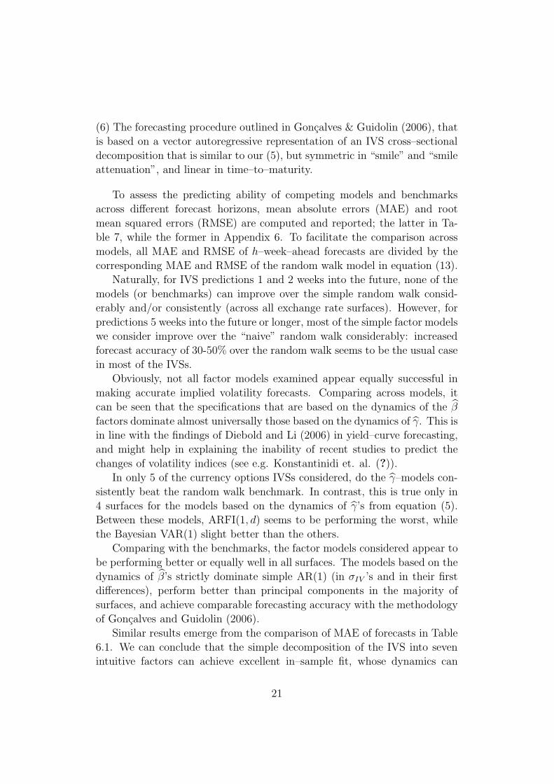
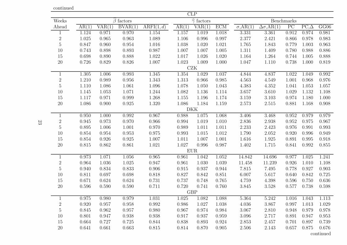
(6) The forecasting procedure outlined in Goncalves & Guidolin (2006), that

is based on a vector autoregressive representation of an IVS cross–sectional

decomposition that is similar to our (5), but symmetric in “smile” and “smile

attenuation”, and linear in time–to–maturity.

To assess the predicting ability of competing models and benchmarks

across different forecast horizons, mean absolute errors (MAE) and root

mean squared errors (RMSE) are computed and reported; the latter in Ta-

ble 7, while the former in Appendix 6. To facilitate the comparison across

models, all MAE and RMSE of h–week–ahead forecasts are divided by the

corresponding MAE and RMSE of the random walk model in equation (13).

Naturally, for IVS predictions 1 and 2 weeks into the future, none of the

models (or benchmarks) can improve over the simple random walk consid-

erably and/or consistently (across all exchange rate surfaces). However, for

predictions 5 weeks into the future or longer, most of the simple factor models

we consider improve over the “naive” random walk considerably: increased

forecast accuracy of 30-50% over the random walk seems to be the usual case

in most of the IVSs.

Obviously, not all factor models examined appear equally successful in

making accurate implied volatility forecasts. Comparing across models, it

can be seen that the specifications that are based on the dynamics of the β

factors dominate almost universally those based on the dynamics of γ. This is

in line with the findings of Diebold and Li (2006) in yield–curve forecasting,

and might help in explaining the inability of recent studies to predict the

changes of volatility indices (see e.g. Konstantinidi et. al. (?)).

In only 5 of the currency options IVSs considered, do the γ–models con-

sistently beat the random walk benchmark. In contrast, this is true only in

4 surfaces for the models based on the dynamics of γ’s from equation (5).

Between these models, ARFI(1, d) seems to be performing the worst, while

the Bayesian VAR(1) slight better than the others.

Comparing with the benchmarks, the factor models considered appear to

be performing better or equally well in all surfaces. The models based on the

dynamics of β’s strictly dominate simple AR(1) (in σIV ’s and in their first

differences), perform better than principal components in the majority of

surfaces, and achieve comparable forecasting accuracy with the methodology

of Goncalves and Guidolin (2006).

Similar results emerge from the comparison of MAE of forecasts in Table

6.1. We can conclude that the simple decomposition of the IVS into seven

intuitive factors can achieve excellent in–sample fit, whose dynamics can

21

Forecast accuracy measure: RMSEAUD

Weeks β factors γ factors BenchmarksAhead AR(1) VAR(1) BVAR(1) ARFI(1, d) AR(1) VAR(1) ECM σ,AR(1) ∆σ,AR(1) PC PC,∆ GG06

1 0.974 0.973 0.972 1.021 1.010 1.021 1.081 9.088 9.218 0.972 1.018 1.0542 0.933 0.924 0.927 0.995 0.988 1.016 1.098 6.778 6.963 0.935 1.003 0.9645 0.790 0.891 0.887 0.964 0.958 0.979 1.093 4.684 4.959 0.871 0.980 0.89410 0.721 0.828 0.821 0.939 0.926 0.942 1.098 3.434 3.756 0.792 0.938 0.82515 0.638 0.679 0.677 0.899 0.894 0.905 1.045 2.912 3.256 0.664 0.901 0.65920 0.574 0.545 0.549 0.886 0.871 0.885 0.993 2.598 2.958 0.559 0.882 0.530

BRL1 0.991 0.987 0.985 1.131 1.048 1.026 1.074 4.432 4.410 0.972 0.994 1.0112 0.928 0.862 0.861 1.086 1.031 1.007 1.039 3.229 3.189 0.943 0.984 0.8685 0.755 0.790 0.784 1.066 1.012 0.989 1.000 2.475 2.376 0.909 0.972 0.77710 0.586 0.712 0.705 1.034 1.015 0.987 0.999 1.935 1.773 0.835 0.974 0.69915 0.501 0.657 0.651 1.016 1.015 0.982 0.988 1.858 1.648 0.774 0.972 0.62820 0.442 0.597 0.593 1.020 1.021 0.990 0.981 1.808 1.556 0.755 0.986 0.560

CAD1 1.087 1.035 1.033 1.058 1.068 1.034 1.041 5.382 5.418 1.002 1.016 1.0422 1.098 1.036 1.036 1.046 1.054 1.025 1.027 3.878 3.930 1.001 1.016 1.0135 1.074 0.997 0.998 1.004 1.023 1.033 1.033 2.418 2.501 0.973 1.028 0.95610 1.066 0.961 0.964 1.037 1.045 1.052 1.055 1.699 1.809 0.940 1.050 0.92615 1.117 1.043 1.046 1.101 1.079 1.074 1.078 1.611 1.771 1.030 1.074 1.02320 1.116 1.076 1.078 1.136 1.111 1.085 1.091 1.505 1.705 1.067 1.086 1.061

CHF1 1.008 0.976 0.973 0.984 0.979 1.022 1.040 8.779 8.660 0.972 1.044 1.1562 1.002 0.949 0.946 0.957 0.971 1.011 0.988 6.868 6.684 0.908 1.017 1.0455 1.004 0.833 0.834 0.923 0.944 0.951 0.929 4.931 4.651 0.822 0.949 0.91610 0.887 0.750 0.752 0.840 0.869 0.875 0.854 4.101 3.732 0.743 0.880 0.79315 0.747 0.704 0.705 0.785 0.791 0.800 0.749 3.379 3.030 0.706 0.803 0.72320 0.672 0.674 0.675 0.763 0.774 0.787 0.719 2.800 2.493 0.675 0.789 0.682

continued

22

continuedCLP

Weeks β factors γ factors BenchmarksAhead AR(1) VAR(1) BVAR(1) ARFI(1, d) AR(1) VAR(1) ECM σ,AR(1) ∆σ,AR(1) PC PC,∆ GG06

1 1.124 0.971 0.970 1.154 1.157 1.019 1.018 3.331 3.361 0.912 0.974 0.9812 1.025 0.965 0.963 1.089 1.106 0.996 0.997 2.377 2.421 0.866 0.978 0.9835 0.847 0.960 0.954 1.016 1.038 1.020 1.021 1.765 1.843 0.779 1.003 0.96310 0.743 0.898 0.893 0.987 1.007 1.007 1.005 1.311 1.409 0.780 0.988 0.88615 0.698 0.890 0.888 1.022 1.017 1.026 1.020 1.164 1.264 0.744 1.005 0.88820 0.726 0.829 0.826 1.007 1.023 1.009 1.000 1.047 1.110 0.738 1.000 0.819

CZK1 1.305 1.006 0.993 1.345 1.354 1.029 1.037 4.844 4.837 1.022 1.049 0.9922 1.210 0.989 0.956 1.343 1.313 0.966 0.985 4.563 4.549 1.001 0.968 0.9765 1.110 1.086 1.061 1.096 1.078 1.050 1.043 4.383 4.352 1.041 1.053 1.05710 1.145 1.053 1.071 1.244 1.082 1.136 1.114 3.657 3.610 1.029 1.132 1.10815 1.117 0.971 0.999 1.268 1.155 1.196 1.174 3.159 3.103 0.974 1.180 1.00020 1.086 0.900 0.925 1.320 1.086 1.184 1.159 2.573 2.515 0.881 1.168 0.908

DKK1 0.950 1.000 0.992 0.967 0.988 1.075 1.068 3.406 3.468 0.952 0.979 0.9792 0.945 0.973 0.970 0.966 0.994 1.019 1.010 2.836 2.938 0.952 0.975 0.9675 0.895 1.006 1.001 0.970 0.989 1.011 1.011 2.233 2.423 0.976 0.991 0.99310 0.854 0.954 0.953 0.975 0.993 1.015 1.012 1.790 2.052 0.920 0.996 0.94915 0.854 0.926 0.925 1.007 1.011 1.007 1.001 1.616 1.925 0.891 0.995 0.91820 0.815 0.862 0.861 1.021 1.027 0.996 0.987 1.402 1.715 0.841 0.992 0.855

EUR1 0.973 1.071 1.056 0.965 0.961 1.042 1.052 14.842 14.696 0.977 1.025 1.2412 0.964 1.036 1.025 0.947 0.961 1.030 1.039 11.458 11.239 0.926 1.010 1.1085 0.940 0.834 0.833 0.906 0.915 0.937 0.944 7.815 7.495 0.778 0.927 0.90310 0.811 0.697 0.698 0.818 0.827 0.842 0.851 6.007 5.617 0.640 0.842 0.72515 0.671 0.624 0.624 0.731 0.737 0.748 0.765 4.759 4.398 0.596 0.750 0.63620 0.596 0.590 0.590 0.711 0.720 0.741 0.760 3.845 3.528 0.577 0.738 0.598

GBP1 0.975 0.980 0.979 1.031 1.025 1.082 1.088 5.364 5.242 1.016 1.043 1.1132 0.920 0.957 0.958 0.992 0.986 1.027 1.038 4.036 3.867 0.997 1.013 1.0295 0.845 0.962 0.957 0.980 0.967 0.974 0.984 3.067 2.810 0.948 0.979 0.97810 0.801 0.947 0.938 0.938 0.917 0.937 0.959 3.096 2.717 0.891 0.947 0.95315 0.664 0.727 0.725 0.844 0.838 0.893 0.924 2.853 2.457 0.701 0.897 0.73920 0.641 0.661 0.663 0.815 0.814 0.870 0.905 2.506 2.143 0.657 0.875 0.676

continued

23

continuedHUF

Weeks β factors γ factors BenchmarksAhead AR(1) VAR(1) BVAR(1) ARFI(1, d) AR(1) VAR(1) ECM σ,AR(1) ∆σ,AR(1) PC PC,∆ GG06

1 1.043 1.076 1.068 1.060 1.082 1.035 1.086 4.722 4.804 1.050 1.087 1.0662 1.019 1.080 1.075 1.032 1.053 1.010 1.056 3.309 3.418 1.024 1.026 1.0695 0.950 0.994 0.990 1.010 1.046 1.031 0.997 2.339 2.516 0.933 1.018 0.98410 0.822 0.791 0.789 0.994 1.072 1.055 0.800 1.538 1.758 0.796 1.035 0.77715 0.760 0.745 0.745 0.981 1.085 1.062 0.815 1.305 1.568 0.769 1.047 0.73720 0.767 0.769 0.769 0.983 1.096 1.082 0.811 1.105 1.360 0.799 1.066 0.767

ILS1 1.083 1.051 1.048 1.095 1.094 1.154 1.147 NaN NaN 1.011 1.017 1.0932 1.040 1.046 1.043 1.069 1.070 1.012 1.011 NaN NaN 1.001 1.006 1.1005 1.000 1.001 0.999 1.052 1.051 1.055 1.048 NaN NaN 0.931 1.012 1.02010 0.969 0.943 0.940 1.079 1.069 1.079 1.066 NaN NaN 0.857 1.047 0.91815 0.967 0.912 0.907 1.141 1.129 1.111 1.094 NaN NaN 0.832 1.085 0.90820 0.910 0.871 0.863 1.140 1.156 1.141 1.121 NaN NaN 0.763 1.117 0.847

JPY1 1.004 1.036 1.031 1.017 1.012 1.015 1.085 6.931 6.924 0.950 0.950 1.0812 0.994 1.028 1.022 1.033 1.021 1.022 1.118 5.312 5.299 0.949 0.984 1.0435 0.898 0.914 0.911 1.034 0.998 1.002 1.030 4.010 3.971 0.846 0.985 0.92510 0.761 0.765 0.764 1.001 0.954 0.982 0.880 3.264 3.185 0.726 0.968 0.79115 0.727 0.729 0.728 0.953 0.939 0.967 0.831 3.056 2.934 0.700 0.949 0.73520 0.647 0.645 0.645 0.928 0.897 0.924 0.824 3.016 2.835 0.624 0.903 0.642

KRW1 1.019 0.979 0.978 1.016 1.016 1.009 1.002 4.040 4.020 0.987 1.023 1.0302 1.007 0.957 0.956 0.995 0.999 1.011 1.007 3.092 3.061 0.947 1.007 1.0095 0.960 0.933 0.931 0.972 0.971 1.021 1.020 2.294 2.235 0.874 1.008 0.97210 0.897 0.890 0.888 0.962 0.963 1.032 1.037 2.022 1.912 0.811 1.022 0.90315 0.865 0.868 0.867 0.936 0.952 1.004 1.013 2.173 1.994 0.813 0.983 0.84920 0.775 0.773 0.772 0.913 0.926 0.988 1.001 1.962 1.761 0.744 0.965 0.758

NOK1 0.992 1.015 1.012 1.014 1.007 1.020 1.036 2.984 3.015 0.982 1.007 1.0062 0.961 1.023 1.021 0.998 0.987 1.016 1.065 2.402 2.453 0.982 0.994 0.9865 0.915 1.022 1.020 1.009 0.999 1.037 1.084 1.878 1.981 0.995 1.019 0.99110 0.883 0.962 0.962 1.002 1.006 1.034 1.017 1.586 1.753 0.960 1.021 0.94315 0.906 0.941 0.943 1.048 1.024 1.030 0.960 1.488 1.716 0.949 1.012 0.93820 0.861 0.889 0.891 1.059 1.048 1.012 0.914 1.292 1.539 0.903 1.004 0.888

continued

24

continuedNZD

Weeks β factors γ factors BenchmarksAhead AR(1) VAR(1) BVAR(1) ARFI(1, d) AR(1) VAR(1) ECM σ,AR(1) ∆σ,AR(1) PC PC,∆ GG06

1 1.023 0.999 0.998 1.058 1.051 1.058 1.056 3.692 3.721 0.994 1.045 1.0482 1.027 0.986 0.984 1.094 1.080 1.041 1.043 2.932 2.980 0.981 1.029 1.0035 0.945 0.936 0.934 1.077 1.049 1.036 1.039 1.897 1.972 0.935 1.026 0.93710 0.887 0.865 0.864 1.086 1.043 1.044 1.045 1.328 1.427 0.869 1.039 0.86915 0.844 0.803 0.803 1.103 1.053 1.060 1.061 1.126 1.247 0.811 1.055 0.80620 0.824 0.760 0.760 1.156 1.078 1.081 1.082 1.038 1.177 0.773 1.075 0.756

PLN1 1.058 1.004 1.002 1.056 1.056 1.058 1.066 4.335 4.357 0.966 1.007 1.0012 1.101 0.935 0.934 1.073 1.071 1.047 1.046 3.467 3.500 0.918 1.022 0.9275 1.130 0.850 0.850 1.099 1.100 1.108 1.104 2.501 2.561 0.863 1.087 0.84210 0.978 0.789 0.789 1.147 1.139 1.122 1.117 1.876 1.962 0.821 1.115 0.78715 0.885 0.764 0.765 1.195 1.182 1.165 1.157 1.750 1.865 0.804 1.161 0.77320 0.840 0.750 0.751 1.210 1.188 1.164 1.157 1.656 1.788 0.798 1.161 0.758

SEK1 1.015 0.945 0.942 1.019 1.013 0.998 1.008 2.735 2.766 0.941 0.968 0.9732 1.059 0.986 0.984 1.062 1.051 1.015 1.145 2.380 2.432 0.963 0.988 0.9965 0.951 0.979 0.977 1.023 1.024 1.010 1.143 1.747 1.842 0.926 1.003 0.98210 0.865 0.955 0.954 1.010 1.018 1.014 1.069 1.450 1.597 0.894 1.005 0.94615 0.863 0.916 0.917 1.064 1.043 1.018 0.985 1.357 1.554 0.883 1.012 0.92120 0.806 0.855 0.855 1.067 1.064 1.010 0.922 1.215 1.436 0.833 1.010 0.859

SGD1 1.071 0.993 0.991 1.071 1.095 1.023 1.021 5.299 5.331 0.973 0.983 1.0132 1.037 0.947 0.945 1.042 1.068 1.004 1.001 3.789 3.828 0.932 0.981 0.9425 0.935 0.784 0.787 0.961 1.024 1.017 1.018 2.476 2.526 0.766 1.003 0.77610 0.731 0.633 0.634 0.907 0.997 1.008 1.015 1.930 2.012 0.628 1.004 0.62615 0.639 0.591 0.592 0.917 1.003 0.997 1.012 1.799 1.902 0.589 0.996 0.58820 0.607 0.598 0.598 0.930 0.983 0.980 1.001 1.790 1.895 0.593 0.978 0.596

THB1 1.070 1.072 1.069 1.078 1.083 1.082 1.089 8.048 8.014 0.985 0.980 1.0882 1.085 1.090 1.087 1.104 1.116 1.093 1.092 5.942 5.888 0.974 1.011 1.0935 0.954 1.052 1.051 1.004 1.033 1.073 1.076 4.060 3.968 0.936 1.042 1.05610 0.990 1.095 1.095 1.084 1.117 1.154 1.158 3.536 3.378 0.982 1.118 1.11215 1.200 1.270 1.270 1.279 1.244 1.272 1.278 3.046 2.824 1.187 1.237 1.28820 1.300 1.329 1.329 1.407 1.354 1.360 1.367 2.450 2.177 1.285 1.322 1.337

continued

25

continuedTWD

Weeks β factors γ factors BenchmarksAhead AR(1) VAR(1) BVAR(1) ARFI(1, d) AR(1) VAR(1) ECM σ,AR(1) ∆σ,AR(1) PC PC,∆ GG06

1 1.046 1.057 1.049 1.026 1.028 1.068 1.145 4.191 4.295 0.976 1.002 1.0642 1.054 1.056 1.044 1.028 1.027 1.029 1.102 2.967 3.103 0.947 0.991 1.0315 0.987 0.917 0.911 1.002 0.970 1.017 0.997 1.944 2.130 0.849 0.999 0.88510 0.988 0.862 0.858 1.063 1.009 1.030 0.921 1.693 1.925 0.812 1.019 0.82315 0.837 0.737 0.733 1.091 1.016 1.068 0.824 1.625 1.870 0.703 1.054 0.70920 0.800 0.735 0.731 1.112 1.030 1.089 0.834 1.634 1.868 0.711 1.082 0.712

VEB1 1.050 1.144 1.102 1.018 1.024 1.029 1.246 14.429 14.373 0.433 0.364 2.6052 1.126 1.278 1.207 1.055 1.070 1.051 1.679 14.399 14.277 0.581 0.433 2.6475 1.405 1.609 1.540 1.266 1.327 1.225 2.284 14.430 14.140 0.850 0.764 2.77710 1.791 1.990 1.989 1.718 1.835 1.697 2.628 14.479 13.947 0.996 1.396 2.95815 2.063 2.181 2.185 2.246 2.437 2.260 2.984 14.485 13.752 1.146 2.039 3.06220 1.170 1.188 1.181 1.200 1.250 1.226 1.341 2.482 2.327 1.128 1.213 1.231

ZAR1 1.021 1.039 1.036 1.017 1.025 0.999 0.998 5.815 5.776 1.032 1.008 1.1042 1.036 1.017 1.013 1.035 1.051 1.010 1.009 3.840 3.790 0.991 1.009 1.0185 0.957 0.965 0.962 1.010 1.047 1.045 1.038 2.545 2.460 0.920 1.049 0.94510 0.930 0.896 0.895 1.102 1.146 1.107 1.091 1.899 1.798 0.854 1.100 0.87315 0.894 0.862 0.861 1.129 1.172 1.163 1.140 1.595 1.492 0.828 1.158 0.84620 0.972 0.931 0.930 1.224 1.258 1.232 1.197 1.539 1.445 0.908 1.237 0.936

Table 7: For the volatility surfaces implied by the twenty two different currency options in our sample, the tablepresents the root mean squared errors (RMSE) of out–of–sample h–week ahead forecasts, of seven models and fivebenchmarks, all divided by the root mean squared errors of h–week ahead forecasts produced by the random walkmodel, equation (13). Models of the β and γ factors refer to cases [a]–[h] on pp. 16–19 and the are estimatedover the first 100 weeks of our sample period; then forecasts and estimates are made recursively until 21/5/2007.Benchmarks refer to cases (1)–(6) on pp. 20–21.

26

assist in making accurate medium to long–term predictions of the future

IVS.

5 Conclusions

No single empirically observed deviation from the Black–Scholes–Merton op-

tion pricing framework has attracted more research effort than the noncon-

stant pattern of implied volatility versus the moneyness and time to maturity

dimensions.

Despite advances in describing the characteristics and dynamics of non–

flat implied volatility surfaces and recent general equilibrium structural mod-

els that have proposed economic justifications for the existence of the phe-

nomenon, relatively little has been said regarding the practical problem of

implied volatility surface forecasting.

In this paper, we take an explicitly out–of–sample forecasting approach.

We propose a simple–to–estimate parametric decomposition of the implied

volatility surface that combines and extends previous research in several re-

spects. Using daily data from a cross–section of options on 22 different cur-

rencies quoted against the U.S. $ from the OTC market, we demonstrate that

the approach yields intuitive and easy to communicate factors that achieve

excellent in–sample fit, and whose time–variation capture the dynamics of

the surface.

Simple econometric models for the factors are estimated and used for

making short and long–term prediction of implied volatility surfaces. Al-

though the 1–month–ahead (5 weeks) forecasting results are no better than

those of random walk and other leading benchmarks, the forecasts of 5 to

20–weeks–ahead are much superior.

In concluding the paper we would like to stress that although the factor

models we consider are not arbitrage–free, they are based on sound theoret-

ical justifications and established empirical practices that can explain their

forecasting success. On the theoretical front, the factor models we examine

can be considered reduced–form analogs of more structural models, such as

that proposed by Garcia, Luger and Renault (2003). There, predictability in

the IVS dynamics arises as a consequence of investors’ learning (from option

prices) about the processes of fundamentals that are driven by persistent

factors. Our simple econometric models seem to pick up this theoretically

justified predictability. Moreover, empirical intuition and experience has es-

tablished that the “shrinkage perspective, which tends to produce seemingly

27

naive but truly sophisticatedly simple models (of which ours is one exam-

ple), may be very appealing when the goal is forecasting”, as Diebold and

Li (2006, p. 362) argue. In our setting, by imposing strict structure on

the factors extracted from the implied volatility surfaces, seems to help in

improving medium to long–term forecasts.

6 Appendix: Additional forecasting results

In the lengthy table that follows, we report forecasting mean absolute errors

(MAE) of competing models and benchmarks. Again, to facilitate compar-

isons across models all h–week–ahead MAE are standardised (divided by)

the corresponding MAE of the random walk model in equation (13).

28

Forecast accuracy measure: MAEAUD

Weeks β factors γ factors BenchmarksAhead AR(1) VAR(1) BVAR(1) ARFI(1, d) AR(1) VAR(1) ECM σ,AR(1) ∆σ,AR(1) PC PC,∆ GG06

1 0.980 0.981 0.980 1.036 1.026 1.006 1.076 10.201 10.359 0.967 1.013 1.0652 0.915 0.934 0.936 0.992 0.985 1.012 1.107 8.061 8.299 0.941 0.987 1.0155 0.767 0.807 0.802 0.959 0.962 0.969 1.060 5.166 5.501 0.790 0.962 0.85010 0.707 0.774 0.769 0.930 0.927 0.938 1.067 3.833 4.244 0.749 0.928 0.79715 0.592 0.609 0.608 0.875 0.892 0.885 0.979 3.077 3.487 0.598 0.875 0.60620 0.525 0.478 0.479 0.862 0.866 0.868 0.916 2.688 3.096 0.483 0.861 0.467

BRL1 1.011 1.050 1.048 1.103 1.055 1.012 1.097 5.672 5.623 0.999 0.997 1.0762 0.957 0.880 0.879 1.057 1.035 0.992 1.025 4.003 3.925 0.970 0.976 0.8935 0.786 0.858 0.851 1.021 1.008 1.005 1.011 3.038 2.868 0.934 0.995 0.84010 0.643 0.838 0.830 1.030 1.036 1.069 1.050 2.508 2.211 0.864 1.067 0.81315 0.544 0.788 0.781 1.021 1.042 1.088 1.058 2.379 2.009 0.787 1.086 0.72920 0.511 0.747 0.742 1.075 1.065 1.168 1.116 2.440 1.983 0.761 1.172 0.684

CAD1 1.056 1.029 1.027 1.057 1.070 1.037 1.044 6.116 6.155 0.988 1.020 1.0232 1.101 1.036 1.036 1.059 1.072 1.027 1.029 4.364 4.421 1.010 1.023 1.0165 1.041 0.962 0.962 1.009 1.031 1.036 1.037 2.587 2.680 0.924 1.033 0.91810 1.007 0.911 0.912 1.043 1.050 1.055 1.058 1.785 1.907 0.892 1.054 0.87615 1.092 1.024 1.027 1.104 1.084 1.060 1.066 1.728 1.897 1.003 1.058 1.01820 1.112 1.081 1.084 1.112 1.104 1.046 1.056 1.644 1.857 1.075 1.045 1.094

CHF1 1.036 0.974 0.972 0.990 0.976 1.022 1.026 12.008 11.814 1.024 1.060 1.2302 0.997 0.930 0.927 0.951 0.962 0.999 0.955 8.896 8.626 0.914 1.016 1.0465 1.003 0.809 0.811 0.932 0.950 0.957 0.902 6.043 5.657 0.801 0.951 0.88410 0.992 0.752 0.755 0.824 0.843 0.851 0.881 5.336 4.806 0.752 0.852 0.81715 0.811 0.687 0.689 0.731 0.743 0.753 0.769 4.307 3.805 0.691 0.758 0.73020 0.687 0.645 0.645 0.702 0.713 0.729 0.704 3.398 2.968 0.648 0.727 0.669

continued

29

continuedCLP

Weeks β factors γ factors BenchmarksAhead AR(1) VAR(1) BVAR(1) ARFI(1, d) AR(1) VAR(1) ECM σ,AR(1) ∆σ,AR(1) PC PC,∆ GG06

1 1.194 1.040 1.038 1.205 1.217 1.050 1.050 4.188 4.233 0.961 1.015 1.0562 1.020 1.027 1.024 1.045 1.097 1.008 1.009 2.883 2.944 0.898 1.000 1.0275 0.847 0.984 0.976 0.987 1.020 1.008 1.009 1.992 2.089 0.793 0.995 0.96010 0.776 0.964 0.957 1.000 1.018 1.009 1.009 1.441 1.555 0.810 0.988 0.92615 0.741 0.913 0.909 1.005 1.008 1.011 1.007 1.255 1.379 0.789 0.981 0.88620 0.708 0.838 0.834 0.990 1.019 0.987 0.977 1.043 1.127 0.726 0.982 0.812

CZK1 1.372 1.080 1.060 1.367 1.365 1.085 1.095 8.015 8.008 1.109 1.118 1.0892 1.257 1.086 1.060 1.277 1.253 0.968 0.988 6.169 6.157 1.089 0.989 1.0925 1.220 1.171 1.146 1.077 1.068 1.045 1.040 5.060 5.039 1.139 1.038 1.17010 1.239 1.132 1.149 1.103 1.056 1.098 1.075 4.007 3.981 1.136 1.090 1.17615 1.155 1.011 1.037 1.118 1.083 1.114 1.094 3.383 3.357 1.047 1.103 1.04420 1.032 0.899 0.923 1.087 0.997 1.082 1.058 2.696 2.676 0.916 1.071 0.923

DKK1 0.948 1.037 1.028 0.980 1.024 1.050 1.043 4.119 4.191 0.981 0.991 1.0322 0.942 1.024 1.018 0.971 1.019 1.028 1.019 3.185 3.298 0.967 0.992 1.0075 0.878 1.022 1.014 0.959 0.992 1.016 1.013 2.352 2.561 0.962 1.001 0.99710 0.875 1.003 1.000 1.003 1.003 1.018 1.016 1.902 2.205 0.954 0.995 0.99515 0.808 0.904 0.903 1.023 1.027 1.012 1.004 1.565 1.904 0.863 1.001 0.88720 0.760 0.820 0.819 1.032 1.029 1.002 0.994 1.326 1.672 0.805 0.999 0.810

EUR1 0.996 1.044 1.028 0.963 0.960 1.046 1.053 20.140 19.929 1.018 1.043 1.2912 0.945 1.016 1.004 0.938 0.953 1.023 1.032 14.706 14.415 0.929 1.016 1.1025 0.949 0.827 0.827 0.920 0.928 0.944 0.951 9.953 9.534 0.773 0.935 0.88410 0.923 0.727 0.730 0.855 0.851 0.860 0.861 8.002 7.469 0.668 0.855 0.75915 0.706 0.595 0.596 0.709 0.719 0.727 0.749 5.809 5.343 0.559 0.734 0.61620 0.636 0.586 0.586 0.704 0.711 0.732 0.748 4.696 4.280 0.570 0.728 0.602

GBP1 0.986 1.025 1.018 1.025 1.020 1.120 1.128 6.993 6.819 1.030 1.055 1.1672 0.942 0.986 0.984 0.997 0.991 1.044 1.051 5.186 4.953 1.019 1.020 1.0605 0.836 0.931 0.924 0.971 0.971 0.985 0.995 3.860 3.514 0.911 0.982 0.96510 0.780 0.916 0.903 0.939 0.924 0.946 0.966 3.825 3.333 0.870 0.946 0.90715 0.640 0.679 0.678 0.828 0.826 0.882 0.909 3.448 2.964 0.688 0.883 0.69820 0.598 0.595 0.597 0.793 0.797 0.862 0.897 2.942 2.515 0.609 0.861 0.618

continued

30

continuedHUF

Weeks β factors γ factors BenchmarksAhead AR(1) VAR(1) BVAR(1) ARFI(1, d) AR(1) VAR(1) ECM σ,AR(1) ∆σ,AR(1) PC PC,∆ GG06

1 1.085 1.066 1.058 1.100 1.122 1.065 1.092 5.257 5.338 1.045 1.090 1.0692 1.022 1.046 1.042 1.017 1.038 1.007 1.028 3.481 3.585 1.004 1.007 1.0385 0.916 0.980 0.976 1.001 1.047 1.045 0.979 2.461 2.638 0.917 1.009 0.97310 0.849 0.808 0.805 1.026 1.104 1.078 0.779 1.607 1.830 0.804 1.065 0.79415 0.781 0.772 0.770 1.010 1.106 1.097 0.819 1.284 1.519 0.788 1.094 0.75920 0.792 0.787 0.787 0.988 1.074 1.075 0.815 1.098 1.307 0.815 1.057 0.789

ILS1 1.138 1.056 1.053 1.122 1.104 1.143 1.136 NaN NaN 1.049 1.014 1.1432 1.093 1.070 1.069 1.121 1.094 1.011 1.008 NaN NaN 1.041 1.002 1.1565 1.023 1.035 1.032 1.083 1.070 1.054 1.046 NaN NaN 0.966 1.006 1.05910 0.952 0.917 0.914 1.070 1.071 1.068 1.058 NaN NaN 0.844 1.046 0.90115 0.982 0.887 0.883 1.135 1.118 1.100 1.087 NaN NaN 0.828 1.087 0.90020 0.932 0.848 0.843 1.137 1.138 1.120 1.104 NaN NaN 0.772 1.107 0.836

JPY1 1.010 1.029 1.023 1.024 1.021 1.010 1.081 8.798 8.782 0.925 0.918 1.0722 1.028 1.043 1.037 1.069 1.058 1.022 1.125 6.908 6.879 0.945 0.958 1.0595 0.892 0.910 0.908 1.067 1.037 1.009 1.039 4.893 4.816 0.824 0.972 0.92110 0.782 0.783 0.782 1.035 0.987 1.018 0.904 3.955 3.796 0.731 0.996 0.80615 0.744 0.730 0.729 0.995 0.959 0.991 0.809 3.660 3.441 0.708 0.960 0.73020 0.607 0.599 0.599 0.896 0.869 0.896 0.781 3.430 3.133 0.578 0.864 0.586

KRW1 1.008 0.986 0.985 1.013 1.012 1.018 1.003 4.917 4.891 0.998 1.025 1.0592 1.003 0.963 0.961 1.011 1.007 0.998 0.987 3.510 3.473 0.945 0.993 1.0235 0.911 0.893 0.891 0.939 0.925 0.970 0.964 2.424 2.360 0.827 0.958 0.94210 0.882 0.865 0.864 0.978 0.984 1.039 1.048 2.101 1.969 0.806 1.043 0.88515 0.839 0.840 0.839 0.937 0.965 0.975 0.992 2.229 2.014 0.784 0.975 0.81920 0.734 0.735 0.734 0.895 0.921 0.970 0.985 1.979 1.751 0.702 0.954 0.715

NOK1 0.976 1.037 1.033 1.009 1.004 0.994 1.056 3.488 3.527 1.008 1.006 1.0462 0.974 1.035 1.033 1.014 1.000 1.020 1.089 2.622 2.680 0.983 0.989 1.0175 0.902 1.032 1.029 1.009 1.006 1.027 1.089 1.970 2.082 0.976 1.014 1.01610 0.886 0.993 0.992 1.014 1.011 1.038 1.039 1.666 1.839 0.980 1.023 0.97515 0.861 0.907 0.909 1.055 1.031 1.016 0.903 1.503 1.734 0.917 1.001 0.90320 0.818 0.858 0.861 1.067 1.057 1.013 0.838 1.306 1.547 0.878 1.001 0.852

continued

31

continuedNZD

Weeks β factors γ factors BenchmarksAhead AR(1) VAR(1) BVAR(1) ARFI(1, d) AR(1) VAR(1) ECM σ,AR(1) ∆σ,AR(1) PC PC,∆ GG06

1 1.048 0.997 0.998 1.067 1.059 1.046 1.046 4.024 4.057 1.001 1.048 1.0632 1.047 0.992 0.990 1.080 1.078 1.044 1.048 3.211 3.265 0.991 1.035 1.0245 0.954 0.941 0.939 1.057 1.043 1.038 1.040 2.065 2.155 0.934 1.026 0.94410 0.917 0.880 0.877 1.085 1.053 1.054 1.053 1.443 1.568 0.869 1.049 0.88215 0.860 0.800 0.799 1.119 1.068 1.069 1.066 1.146 1.296 0.800 1.065 0.79720 0.835 0.753 0.753 1.160 1.078 1.076 1.075 1.015 1.182 0.768 1.071 0.747

PLN1 1.058 1.023 1.020 1.080 1.077 1.056 1.060 5.060 5.088 0.983 1.000 0.9992 1.139 0.982 0.981 1.116 1.108 1.050 1.051 4.113 4.156 0.949 1.020 0.9475 1.178 0.857 0.857 1.123 1.122 1.090 1.088 2.817 2.890 0.875 1.068 0.85310 1.060 0.831 0.831 1.139 1.142 1.130 1.124 2.058 2.162 0.853 1.125 0.83415 0.981 0.823 0.823 1.154 1.186 1.165 1.157 1.909 2.046 0.858 1.160 0.83320 0.939 0.815 0.816 1.162 1.179 1.160 1.151 1.830 1.993 0.876 1.158 0.822

SEK1 1.057 1.010 1.006 1.071 1.081 1.010 1.073 3.377 3.417 0.981 1.016 1.0382 1.011 0.986 0.983 1.039 1.063 1.010 1.128 2.627 2.687 0.952 0.997 1.0085 0.891 0.993 0.990 0.985 1.013 1.001 1.158 1.861 1.966 0.912 0.998 0.98210 0.873 0.985 0.983 1.003 1.008 1.024 1.082 1.532 1.689 0.912 1.015 0.97515 0.836 0.912 0.912 1.067 1.048 1.006 0.955 1.396 1.598 0.863 1.001 0.91420 0.746 0.813 0.813 1.069 1.072 1.016 0.849 1.198 1.405 0.785 1.015 0.814

SGD1 1.062 0.971 0.970 1.082 1.102 1.002 1.003 6.228 6.254 0.935 0.961 1.0182 0.980 0.937 0.932 1.026 1.044 0.993 0.992 4.238 4.270 0.938 0.972 0.9435 0.869 0.765 0.765 0.966 1.025 1.012 1.012 2.692 2.742 0.750 0.999 0.75410 0.706 0.607 0.608 0.893 1.000 1.010 1.012 2.049 2.120 0.599 1.009 0.60015 0.616 0.567 0.567 0.893 0.984 0.959 0.981 1.840 1.927 0.562 0.962 0.56020 0.620 0.608 0.608 0.905 0.965 0.969 0.983 1.900 1.999 0.602 0.972 0.605

THB1 1.161 1.133 1.129 1.123 1.124 1.092 1.104 10.230 10.148 1.022 0.984 1.1562 1.208 1.187 1.184 1.131 1.133 1.096 1.096 7.517 7.396 1.050 1.005 1.1975 1.055 1.159 1.159 1.004 1.019 1.067 1.070 4.830 4.639 1.025 1.024 1.16710 1.042 1.149 1.149 1.073 1.102 1.131 1.139 3.869 3.573 1.015 1.088 1.16115 1.195 1.284 1.284 1.286 1.276 1.294 1.309 3.458 3.068 1.170 1.247 1.29920 1.265 1.314 1.314 1.498 1.487 1.476 1.492 2.823 2.400 1.250 1.430 1.319

continued

32

continuedTWD

Weeks β factors γ factors BenchmarksAhead AR(1) VAR(1) BVAR(1) ARFI(1, d) AR(1) VAR(1) ECM σ,AR(1) ∆σ,AR(1) PC PC,∆ GG06

1 1.021 1.062 1.050 1.011 1.019 1.056 1.145 4.650 4.763 0.976 0.992 1.0962 1.037 1.090 1.075 0.988 1.015 1.021 1.141 3.406 3.562 0.955 0.986 1.0625 0.956 0.938 0.934 0.954 0.948 1.028 1.007 2.107 2.308 0.853 1.005 0.89910 1.050 0.927 0.924 1.057 1.007 1.042 0.971 1.859 2.099 0.872 1.035 0.89115 0.846 0.748 0.745 1.037 0.989 1.072 0.832 1.608 1.816 0.711 1.057 0.72820 0.840 0.768 0.765 1.079 1.020 1.091 0.883 1.640 1.815 0.732 1.088 0.751

VEB1 1.063 1.102 1.090 1.008 1.026 1.033 1.161 16.569 16.508 0.412 0.355 2.8512 1.158 1.240 1.191 1.054 1.090 1.065 1.493 16.574 16.437 0.541 0.404 2.8685 1.468 1.620 1.543 1.310 1.399 1.272 2.093 16.627 16.299 0.822 0.803 2.90210 1.897 2.038 2.053 1.804 1.972 1.814 2.544 16.674 16.072 1.008 1.570 2.93915 2.210 2.273 2.320 2.399 2.666 2.459 2.961 16.685 15.852 1.125 2.335 2.93920 1.526 1.504 1.506 1.717 1.852 1.770 1.914 5.227 4.925 1.154 1.751 1.677

ZAR1 1.092 1.116 1.113 1.037 1.041 1.008 1.001 7.831 7.758 1.097 1.031 1.1512 1.183 1.153 1.148 1.126 1.133 1.030 1.024 5.373 5.274 1.094 1.019 1.1425 1.099 1.116 1.111 1.108 1.130 1.097 1.080 3.492 3.329 1.039 1.080 1.10610 1.003 0.955 0.953 1.189 1.234 1.156 1.131 2.278 2.109 0.885 1.144 0.93215 0.919 0.878 0.876 1.197 1.248 1.204 1.175 1.801 1.639 0.828 1.200 0.86820 1.010 0.959 0.958 1.252 1.308 1.259 1.224 1.677 1.519 0.929 1.260 0.963

Table 6.1: For the volatility surfaces implied by the twenty two different currency options in our sample, thetable presents the mean absolute errors (MAE) of out–of–sample h–week ahead forecasts, of seven models and fivebenchmarks, all divided by the mean absolute errors of h–week ahead forecasts produced by the random walk model,equation (13). Models of the β and γ factors refer to cases [a]–[h] on pp. 16–19 and the are estimated over the first100 weeks of our sample period; then forecasts and estimates are made recursively until 21/5/2007. Benchmarksrefer to cases (1)–(6) on pp. 20–21.

33

References

Alexander, C. (2001): “Principal component analysis of volatility smiles

and skews,” Working Paper, University of Reading.

Baillie, R. T. (1996): “Long memory processes and fractional integration

in econometrics,” Journal of Econometrics, 73, 5–59.

Bank of International Settlements (2007): OTC derivatives market

activity in the second half of 2006. Monetary & Economic Department,

BIS.

Black, F., and M. Scholes (1973): “The pricing of options and corporate

liabilities,” Journal of Political Economy, 81(3), 637–654.

Campa, J. M., and K. P. Chang (1995): “Testing the expectations hy-

pothesis on the term structure of volatilities,” Journal of Finance, 50(2),

529–547.

(1998): “The forecasting ability of correlations implied in foreign

exchange options,” Journal of International Money and Finance, 17(6),

855–880.

Canina, L., and S. Figlewski (1993): “The informational content of

implied volatility,” Review of Financial Studies, 6(3), 659–681.

Carr, P., and L. Wu (2007a): “Stochastic skew in currency options,”

Journal of Financial Economics, 86(1), 213–247.

(2007b): “Theory and evidence on the dynamic interaction between

sovereign credit default swaps and currency options,” Journal of Banking

and Finance, 31(8), 2383–2403.

Chalamandaris, G., and A. E. Tsekrekos (2008): “Predicting the dy-

namics of implied volatility surfaces: A new approach with evidence from

OTC currency options,” Working Paper, Athens University of Economics

& Business.

Christoffersen, P., and S. Mazzotta (2005): “The accuracy of density

forecasts from foreign exchange options,” Journal of Financial Economet-

rics, 3(4), 578–605.

34

Cont, R., and J. da Fonseca (2002): “Dynamics of implied volatility

surfaces,” Quantitative Finance, 2(1), 45–60.

Derman, E., and I. Kani (1998): “Stochastic implied trees: Arbitrage

pricing with stochastic term and strike structure of volatility,” Interna-

tional Journal of Theoretical and Applied Finance, 1(1), 61–110.

Diebold, F., and C. Li (2006): “Forecasting the term structure of govern-

ment bond yields,” Journal of Econometrics, 130(2), 337–364.

Dumas, B., J. Fleming, and R. E. Whaley (1998): “Implied volatility

functions: Empirical tests,” Journal of Finance, 53(6), 153–180.

Dupire, B. (1993): “Model art,” Risk, 6, 118–124.

Elliot, G., T. J. Rothenberg, and J. H. Stock (1996): “Efficient

tests for an autoregressive unit root,” Econometrica, 64, 813–836.

Garcia, R., R. Luger, and E. Renault (2003): “Empirical assessment

of an intertemporal option pricing model with latent variables,” Journal

of Econometrics, 116(1–2), 49–83.

Garman, M. B., and S. W. Kohlhagen (1983): “Foreign currency option

values,” Journal of International Money and Finance, 2(3), 231–237.

Goncalves, S., and M. Guidolin (2006): “Predictable dynamics in the

S&P 500 index options implied volatility surface,” Journal of Business,

79(3), 1591–1635.

Heynen, R. C., A. Kemna, and T. Vorst (1994): “Analysis of the term

structure of implied volatilities,” Journal of Financial and Quantitative

Analysis, 29(1), 31–56.

Kwiatkowski, D., P. C. B. Phillips, P. Schmidt, and Y. Shin (1992):

“Testing the null of stationarity against the alternative of a unit root:

How sure are we that economic time series have a unit root,” Journal of

Econometrics, 54, 159–178.

Ledoit, O., and P. Santa-Clara (1998): “Relative Pricing of Options

with Stochastic Volatility,” Working Paper, UCLA.

Malz, A. M. (1996): “Using option prices to estimate realignment prob-

abilities in the European monetary system: The case of sterling–mark,”

Journal of International Money and Finance, 15(5), 717–748.

35

Mixon, S. (2002): “Factors explaining movements in the implied volatility

surface,” Journal of Futures Markets, 22(10), 915–937.

Nelson, C. R., and A. F. Siegel (1987): “Parsimonious modeling of

yield curves,” Journal of Business, 60(4), 473–489.

Pena, I., G. Rubio, and G. Serna (1999): “Why do we smile? On the

determinants of the implied volatility function,” Journal of Banking and

Finance, 23(8), 1151–1179.

Rubinstein, M. (1994): “Implied binomial trees,” Journal of Finance,

49(3), 781–818.

Schwarz, G. E. (1978): “Estimating the dimension of a model,” Annals of

Statistics, 6(2), 461–464.

Skiadopoulos, G., S. D. Hodges, and L. Clewlow (1999): “The

dynamics of the S&P 500 implied volatility surface,” Review of Derivatives

Research, 3(1), 263–282.

Xu, X., and S. J. Taylor (1994): “The term structure of volatility im-

plied by foreign exchange options,” Journal of Financial and Quantitative

Analysis, 29(1), 57–74.

36