Can New Keynesian Models Survive the Barro-King Curse? * Guido Ascari † Louis Phaneuf ‡ Eric Sims § March 6, 2019 Abstract Barro and King (1984) conjecture that shocks other than those to total factor productivity will have difficulty generating key business cycle comovements between output, consumption, investment and hours worked. Recent years have seen the emergence of a class of DSGE models in which aggregate fluctuations are driven by several shocks, making them particularly vulnerable to the “Barro-King Curse”. These models emphasize monopolistically competitive goods and labor markets, nominal rigidities and real frictions. We show that the standard medium-scale New Keynesian model is vulnerable to the curse predicting anomalous contemporaneous correlations between key variables and wrong profiles of cross-correlations. With the realistic additions of roundabout production and real per capita output growth, the New Keynesian model can survive the curse despite standard preferences and positive trend inflation. JEL classification: E31, E32. Keywords: Monopolistic competition; Nominal wage and price rigidities; Firms networking; Trend output growth; Trend inflation; Business cycle comovements. * We would like to thank Jesper Lind´ e and seminar participants at the De Nederlandsche Bank and at the conference on Applications of DSGE Models in Central Banking, National Bank of Ukraine, 15th November 2018. † Department of Economics, University of Oxford, [email protected]. ‡ Department of Economics, University of Quebec at Montreal, [email protected] (corresponding author). § Department of Economics, University of Notre Dame, [email protected].

Welcome message from author
This document is posted to help you gain knowledge. Please leave a comment to let me know what you think about it! Share it to your friends and learn new things together.
Transcript

Can New Keynesian Models Survive the Barro-King
Curse?∗
Guido Ascari† Louis Phaneuf‡ Eric Sims§
March 6, 2019
Abstract
Barro and King (1984) conjecture that shocks other than those to total factor productivity will have
difficulty generating key business cycle comovements between output, consumption, investment and hours
worked. Recent years have seen the emergence of a class of DSGE models in which aggregate fluctuations
are driven by several shocks, making them particularly vulnerable to the “Barro-King Curse”. These models
emphasize monopolistically competitive goods and labor markets, nominal rigidities and real frictions. We
show that the standard medium-scale New Keynesian model is vulnerable to the curse predicting anomalous
contemporaneous correlations between key variables and wrong profiles of cross-correlations. With the
realistic additions of roundabout production and real per capita output growth, the New Keynesian model
can survive the curse despite standard preferences and positive trend inflation.
JEL classification: E31, E32.
Keywords: Monopolistic competition; Nominal wage and price rigidities; Firms networking; Trend output
growth; Trend inflation; Business cycle comovements.
∗We would like to thank Jesper Linde and seminar participants at the De Nederlandsche Bank and at the conference on
Applications of DSGE Models in Central Banking, National Bank of Ukraine, 15th November 2018.†Department of Economics, University of Oxford, [email protected].‡Department of Economics, University of Quebec at Montreal, [email protected] (corresponding author).§Department of Economics, University of Notre Dame, [email protected].
1 Introduction
In the wake of the seminal contributions of Lucas (1977) and Kydland and Prescott (1982), a litmus
test of general equilibrium macroeconomic models has been their ability to account for the cyclical
comovements between output, consumption, investment and hours worked. Barro and King (1984)
conjecture that shocks other than those to total factor productivity (TFP) will have difficulty
generating business cycle comovements. We refer to this theoretical prediction as the “Barro-King
curse”.
Recent years have witnessed the emergence of a class of dynamic stochastic general equilibrium
(DSGE) models driven by several disturbances other than TFP shocks. These models emphasize
imperfectly competitive goods and labor markets, nominal rigidities and real adjustment frictions
(Erceg et al., 2000; Christiano et al., 2005; Smets and Wouters, 2007) and are commonly known as
Medium-Scale New Keynesian (MSNK) models. They are now widely used in central banks and
for academic research.
A main purpose of this class of models has been to identify the sources of business cycle fluc-
tuations and assess their relative contributions to aggregate fluctuation. The fact that it is often
found that non-TFP shocks explain the bulk of business cycle fluctuations in these models make
them vulnerable to the curse. Thus, our primary goal in this paper is to examine whether this is
in fact the case.
Our analysis focuses on the contemporaneous comovements between the growth rates of output,
consumption and investment and the level of hours (hours being stationary in our model), and on
the profiles of their cross-correlations. We argue that these moments are particularly useful when
judging whether a specific model is prone to the curse.
In a first step, we look at a four-shock version of the model proposed by Christiano et al.
(2005), which also incorporates non-zero trend inflation. Aggregate fluctuations are driven by
shocks to TFP, intertemporal preference, monetary policy and marginal efficiency of investment
(MEI). Consistent with the approach laid out in Justiniano et al. (2011), MEI shocks are orthogonal
to trend reductions in the price of investment relative to consumption. MEI shocks may proxy for
more fundamental disturbances to the intermediation ability of the financial system.
Based on model simulations assigning different percentage contributions of TFP and MEI shocks
to output fluctuations, we compare theoretical volatility and comovement statistics to those obser-
ved in the data. We find that the standard MSNK model is indeed vulnerable to the curse for a
plausible calibration of the model.
1

A first set of substantive findings pertains to the inability of the standard model to account for
the main business cycle comovements. With MEI shocks explaining 50% of business cycles, as often
found in the broader literature, we show the standard model implies a negative contemporaneous
correlation between the growth rates of consumption and investment at −0.05, compared to the po-
sitive correlation found in the data at 0.44. It also generates the wrong profile of cross-correlations.
That is, while the profiles of cross-correlations between consumption growth and investment growth
are substantially positive and decreasing both at leads and lags in the data, the standard model
predicts they are more or less flat around zero.
The standard MSNK model also implies anomalous comovements between consumption growth
and output growth. While in the data the contemporaneous correlation between these variables
is 0.75 and the cross-correlations are very positive and declining, we find that the standard model
predicts a contemporaneous correlation of 0.39 between consumption and output growth. The
standard model also systematically understates the cross-correlations between these variables.
Looking at the comovements between consumption growth and the level of hours (hours being
stationary in the models we study), we find that the standard model predicts a weakly positive
contemporaneous correlation as in the data, but generates the wrong profiles of cross-correlations.
To provide some intuition as to why the standard MSNK model is vulnerable to the curse, we
use the “Hicksian” decomposition proposed by King (1991) for general equilibrium models.1 We
decompose the response of consumption to a MEI shock – which is the main source of the wrong
comovements in the model – into wealth and substitution effects. We show that the standard model
generates a weakly positive income effect and a strongly negative short-run substitution effect on
consumption. On balance, the substitution effect dominates over the income effect, so the response
of consumption is negative on impact of a positive MEI shock and remains negative for about six
quarters.
A significant strand of the literature has paid a particular attention to this “comovement pro-
blem”, or the fact that consumption typically falls following a positive investment shock. To solve
this problem, Greenwood et al. (1997) focus on variable capacity utilization for capital in the ne-
oclassical model. Another avenue explored by Jaimovich and Rebelo (2009) posits non-standard
preferences that restrict the strength of short-run wealth effects on the labor supply.2 Khan and
Tsoukalas (2011) specify the cost of capital utilization in terms of increased depreciation of capital
as a possible solution. By contrast, when the cost of capital utilization is specified in terms of
foregone consumption, as in Christiano et al. (2005) and in our model, they find that solving the
1See also Guerrieri et al. (2014).2Papanikolaou (2011) and Eusepi and Preston (2015) also emphasize departures from utility functions that are
additively separable in consumption and leisure.
2

comovement problem requires the complete absence of a wealth effect on labor supply. Schmitt-
Grohe and Uribe (2011) have pointed to cointegration between TFP and MEI shocks. Furlanetto
and Seneca (2014) suggest combining sticky prices with Edgeworth complementarity between con-
sumption and hours worked. Guerrieri et al. (2014) propose a two-sector model where expansionary
productivity shocks to an investment-producing sector boost consumption in every period.
As our Hicksian decomposition for the standard MSNK model suggests, a potential solution
would be to strengthen the positive income effect on consumption conditioned on a MEI shock,
while weakening the negative short-run substitution effect. Therefore, in a second step, we consider
adding to the standard model two structural ingredients that can potentially do this. One is to
modify the production structure to account for input-output linkages between firms along the lines
of Basu (1995). The other is to account for real per capita output growth. We refer to this
particular model as our benchmark MSNK model. We deliberately omit non-standard preferences
to emphasize the generality of the solution we propose.
We show that these two ingredients have the potential to boost the positive income effect on
consumption while weakening the negative short-run substitution effect. Of the two, roundabout
production has the stronger income effect. But taken separately, neither roundabout production
nor economic growth is sufficient to generate the desired income and substitution effects that would
help to generate a positive response of consumption on impact of a positive MEI shock. It is only
by combining the two that the response of consumption turns positive. Note that contrary to Khan
and Tsoukalas (2011), our benchmark model is able to solve the comovement problem despite a
standard specification of preferences and that the cost of capital utilization is measured in terms
of foregone consumption.3
Our benchmark MSNK model is immune from the curse. With the MEI shock contributing from
between 40% and 60% to output fluctuations, the model generates a contemporaneous correlation
between consumption growth and investment growth ranging between 0.4 to 0.3. Meanwhile, the
contemporaneous correlation between consumption growth and output growth ranges from 0.76
to 0.65. Our benchmark model also matches the profiles of cross-correlations between output,
consumption, investment and hours quite well. Overall, our benchmark model improves significantly
over the standard model.
The paper looks at one final question: a potentially pervasive effect of the interaction between
trend inflation and the persistence of the MEI shock on business cycle comovements. Ascari et al.
(2018) show that a moderate level of trend inflation may alter the impulse responses of output,
3Measuring the cost of capital utilization in terms of increased capital depreciation would boost the income effecton consumption even more in our model.
3

consumption and investment following a MEI shock relative to the responses obtained under zero
trend inflation. This means that even a moderate rate of trend inflation can possibly alter some
key business cycle comovements depending on the persistence of the MEI shock, something that
has thus far been overlooked in the literature.
Estimates of the AR(1) parameter of the MEI shock process typically range from 0.7 to 0.85.
For an AR(1) parameter of the MEI shock varying between 0.7 and 0.9 and a MEI shock explaining
50% of output fluctuations, we show that the contemporaneous correlation between consumption
growth and investment growth predicted by the standard MSNK model will vary from 0.12 to
−0.43, compared to 0.44 in the data. Meanwhile, the contemporaneous correlation between output
growth and consumption growth will range from 0.51 to 0.09, compared to 0.75 in the data. In
comparison, our benchmark MSNK model predicts that the contemporaneous correlation between
consumption growth and investment growth will lie between 0.4 and 0.09 for different levels of trend
inflation and persistence of the MEI shock. It also implies that the contemporaneous correlation
between output growth and consumption growth will range from 0.73 to 0.53, hence making our
benchmark model less vulnerable to potential pitfalls.
The remainder of the paper is organized as follows. Section 2 lays out our medium-scale DSGE
model and discusses some issues related to calibration. Section 3 measures how the standard MSNK
model squares with the Barro-King curse. Section 4 adds roundabout production and trend output
growth to the standard model. Section 5 examines the robustness of our results. Section 6 adds
concluding remarks.
2 Model and Calibration
2.1 The Model
The baseline MSNK model embeds a number of features found in similar models in the literature –
such as standard additively separable preferences, nominal rigidities as Calvo (1983) wage and price
contracts, habit formation in consumption, investment adjustment costs, variable capital utilization
and a Taylor rule. It also allows for non-zero trend inflation.
Our benchmark MSNK model adds to the standard model roundabout production, recently
referred to as “firms networking” (FN) (e.g., Christiano, 2015). Evidence supporting this production
structure is discussed in Basu (1995), Huang et al. (2004) and Nakamura and Steinsson (2010). It
is also confirmed by a recent dataset gathered through the joints efforts of the NBER and the U.S.
Census Bureau’s CES that covers 473 six-digit 1997 NAICS industries for the years 1959-2009.
These data reveal that the share of materials in final sales in the manufacturing sector exceeds
4

50 percent. For simplicity, we will refer to models incorporating this feature as FN-models. Our
model also allows for real per capita output growth stemming from trend growth in neutral and
investment-specific technologies (G). We will refer to models incorporating this particular feature
as G-models. Appendix A contains a detailed description of the model equations, together with the
full set of equilibrium conditions re-written in stationary terms.
Unlike Christiano et al. (2005) and Smets and Wouters (2007), both the standard and bench-
mark models abstract from the automatic indexation of non-reset wages and prices to past inflation
and/or steady-state inflation. Combined with Calvo contracts, either form of indexation implies
that all nominal wages and prices change every quarter. This is inconsistent with evidence that
many wages and prices remain fixed for relatively long periods of time (e.g., Eichenbaum et al.,
2011; Klenow and Malin, 2011; Barattieri et al., 2014). Indexation is also criticized for a lack of
microeconomic foundations (Chari et al., 2009). Moreover, Cogley and Sbordone (2008) find no
evidence of price indexation to the previous period’s rate of inflation when combining sticky prices
with time-varying trend inflation. Therefore, indexation has been omitted from many recent New
Keynesian models such as Christiano et al. (2010), Christiano et al. (2015, 2016) and Ascari et al.
(2018). The presence of FN is able to generate realistic inertia in inflation, without the unrealistic
assumption of backward-looking indexation.
The production function for a typical producer j is given by:
Xt(j) = max
{AtΓt(j)
φ(Kt(j)
αLt(j)1−α)1−φ
−ΥtF, 0
}, (1)
where At is neutral productivity, Γt(j) denotes intermediate inputs, F is a fixed cost, Υt is a growth
factor (see below) and production is required to be non-negative. φ ∈ (0, 1) is the intermediate
input share. Intermediate inputs come from aggregate gross output, Xt. Kt(j) represents capital
services or the product of utilization (Zt) and physical capital (Kt), while Lt(j) is labor input.
The cost minimization problem of a typical firm yields the following expression for real marginal
cost, vt, which is common across firms:
vt = φA−1t
(rkt
)α(1−φ)w
(1−α)(1−φ)t , (2)
where φ is a constant, rkt is the common real rental price on capital services and wt is the real wage
index. This expression for real marginal cost shows that relative to the basic case in the literature,
FN reduces the sensitivity of real marginal cost to factor prices by a factor of 1 − φ. Hence, FN
5

flattens the New Keynesian Phillips Curve, amplifying the stickiness in the economy caused by
nominal rigidities.
The second important feature of our model is real per capita output growth stemming from
two distinct sources: trend growth in neutral technology and in investment-specific technology
(IST). Greenwood et al. (1997) show that investment-specific technological change has been a
major source of U.S. economic growth during the postwar period. In the context of our model,
trend growth in IST realistically captures the downward secular movement in the relative price of
investment observed during the postwar period. First, neutral productivity obeys a process with
both a trending and stationary component.
At = Aτt At, (3)
Aτt is the deterministic trend component that grows at a constant gross rate gA, while At is the
stationary component. The initial level in period 0 is normalized to 1: Aτ0 = 1. The stationary com-
ponent follows an AR(1) process. To introduce IST, we specify the physical capital accumulation
process as follows:
Kt+1 = εI,τt ϑt
(1− S
(ItIt−1
))It + (1− δ)Kt, (4)
where Kt is the physical capital stock and It is investment measured in units of consumption.
S(
ItIt−1
)is an investment adjustment cost that satisfies S (gI) = 0, S′ (gI) = 0, and S′′ (gI) > 0,
where gI ≥ 1 is the steady state (gross) growth rate of investment. 0 < δ < 1 is the depreciation
rate. εI,τt measures the level of IST and it enters the capital accumulation equation by multiplying
investment.4 εI,τt follows a deterministic trend with no stochastic component, where gεI is the gross
growth rate. ϑt is a shock to the marginal efficiency of investment.
Most variables in the model inherit trend growth from the deterministic trends in neutral and
investment-specific productivity.5 Suppose that this trend factor is Υt. Output, consumption,
investment (measured in units of consumption), intermediate inputs, and the real wage all grow at
the rate of this trend factor on a balanced growth path: gY = gI = gΓ = gw = gΥ. The capital stock
grows faster due to growth in investment-specific productivity, with Kt ≡ KtΥtε
I,τt
being stationary.
The trend factor inducing stationarity among transformed variables is:
Υt = (Aτt )1
(1−φ)(1−α)(εI,τt
) α1−α
. (5)
4εI,τt also enters the budget constraint in terms of the resource cost of capital utilization, see Appendix A.2.5Given our specification of preferences, labor hours are stationary.
6

Note the interaction between FN and growth in this expression. When there are no intermediate
inputs, this expression reverts to the conventional trend growth factor in a model with growth
in neutral and investment-specific productivity. (5) implies that a higher value of the share of
intermediate inputs φ amplifies the effects of trend growth in neutral productivity on output and
its components. For a given level of trend growth in neutral productivity, the economy will grow
faster the larger is the share of intermediates in production.
ϑt in (4) is a stochastic MEI shock. Justiniano et al. (2011) distinguish between IST and MEI,
showing that IST growth maps one-to-one into the relative price of investment goods, while MEI
shocks have no impact on the relative price of investment. Their evidence suggests that the MEI
shock is the main disturbance explaining business cycle fluctuations, while the stochastic shock to
IST virtually has no impact on output at business cycle frequencies. Hence, we assume that the
MEI component is stochastic while the IST term affects trend growth only.
Our model includes four shocks: MEI, neutral productivity, intertemporal preference and mo-
netary policy. In Christiano et al. (2005), aggregate fluctuations are driven solely by monetary
policy shocks. In Smets and Wouters (2007) they are driven by seven shocks. Chari et al. (2009),
however, criticize multi-shock New Keynesian models, arguing that of the several shocks used in
these models, only three can be viewed as truly “structural” in the sense of having a clear econo-
mic interpretation: investment, neutral technology, and monetary policy. So, we keep these three
shocks in the model. We also keep the intertemporal preference shock since Justiniano et al. (2011)
find that this shock explains 55 percent of consumption fluctuations. The MEI shock follows a
stationary AR(1) process, with innovation uIt drawn from a mean zero normal distribution with
standard deviation sI :
ϑt = (ϑt−1)ρI exp(sIuIt ), 0 ≤ ρI < 1. (6)
The stationary component of neutral productivity, At, follows an AR(1) process in the log, with
the non-stochastic mean level normalized to unity, and innovation, uAt , drawn from a mean zero
normal distribution with known standard deviation equal to sA:
At =(At−1
)ρAexp
(sAu
At
), 0 ≤ ρA < 1. (7)
The intertemporal preference shock εbt follows a stationary AR(1) process:
εbt = (εbt−1)ρb exp(sbubt), (8)
with innovation ubt drawn from a mean zero normal distribution with standard deviation sb.
7

The monetary policy shock represents a random deviation from the following Taylor rule:
1 + it1 + i
=
(1 + it−1
1 + i
)ρi [(πtπ
)απ ( YtYt−1
g−1Y
)αy]1−ρiεrt . (9)
The central bank adjusts the nominal interest rate, it, in response to deviations of inflation from an
exogenous steady-state inflation target, and to deviations of output growth from its steady-state
level. εrt is the exogenous shock to the policy rule and it is assumed to be white noise. ρi is a
smoothing parameter while απ and αy are two policy parameters. The above rule does not include
a response to the level of the output gap. The reason for this is that Khan et al. (2019) show that
when trend inflation interacts with sticky wages and trend growth, achieving determinacy when
the Taylor rule includes the output gap calls for a response to inflation that significantly exceeds
the original Taylor Principle (απ ≥ 1) and the estimates found in the literature. This is true even
levels of inflation as low as 2% or 3%. By contrast, a rule reacting to output growth, but not to the
output gap, increases the central bank’s ability to ensure determinacy for a wider array of policy
responses to inflation. See also Coibion and Gorodnichenko (2011).
2.2 Calibration
Tables 1 and 2 summarize the calibration of the model, which is rather standard and in line with the
literature (e.g., Christiano, Eichenbaum, and Evans, 2005; Justiniano, Primiceri, and Tambalotti,
2010, 2011). Appendix B discusses it in further detail. In the text, we focus on the central
ingredients of our model: FN, trend growth, and the shocks.
The share of intermediate inputs, φ, is set to 0.61. The values of φ used in the comparable
literature typically range from 0.5 to 0.8. Ours is obtained as follows. Following Nakamura and
Steinsson (2010), we take the weighted average revenue share of intermediate inputs in the U.S.
private sector using Consumer Price Index (CPI) expenditure weights to be roughly 51 percent in
2002. The cost share of intermediate inputs is equal to the revenue share times the price markup.
Since our calibration implies a steady state markup of 1.2, our estimate of the weighted average
cost share of intermediate inputs is roughly 0.61.
Mapping the model to the data, the trend growth rate of the IST term, gεI , equals the negative
of the growth rate of the relative price of investment goods. To measure this in the data, we define
investment as expenditures on new durables plus private fixed investment, and consumption as
consumer expenditures of nondurables and services. These series are from the BEA and cover the
period 1960:I-2007:III, to leave out the financial crisis.6 The relative price of investment is the ratio
6A detailed explanation of how these data are constructed can be found in Ascari et al. (2018).
8
of the implied price index for investment goods to the price index for consumption goods. The
average growth rate of the relative price from the period 1960:I-2007:III is -0.00472, so that gεI =
1.00472. Real per capita GDP is computed by subtracting the log civilian non-institutionalized
population from the log-level of real GDP. The average growth rate of the resulting output per
capita series over the period is 0.005712, so that gY = 1.005712 or 2.28 percent a year. Given the
calibrated growth of IST, we then use (5) to set g1−φA to generate the appropriate average growth
rate of output. This implies g1−φA = 1.0022 or a measured growth rate of TFP of about 1 percent
per year.7
Regarding the calibration of the shocks, we set the autoregressive parameter of the neutral
productivity shock at 0.95. Based on the estimate in Justiniano et al. (2011), we set the baseline
value of the autoregressive parameter of the MEI process at 0.8 and that of the intertemporal
preference shock at 0.6. In the robustness Section 5, we also look at the effects of lowering the
persistence of the MEI shock to 0.7 and increasing it to 0.9.
Our procedure to pin down the standard deviations of the four shocks in our model is to target
the size of shocks sA, sI , sb and sr, for which the model exactly matches the actual standard
deviation of output growth observed in our data (0.0078) assuming an average growth rate of
the price index equal to that in the data over the period 1960:I-2007:III. This implies a positive
steady-state inflation of 3.52 percent annualized (π∗ = 1.0088).8
We then assign to each shock a target percentage contribution to the unconditional variance
decomposition of output growth. Our targets for the contribution of the shocks to the variance of
output growth are based on empirical consensus from the recent literature. In this literature, inves-
tment shocks are the main driver behind business-cycle fluctuations, followed by neutral technology
shocks. In the estimates from Justiniano et al. (2010), the investment shock explains about 50 per-
cent of the variance decomposition of output growth at business cycle frequencies, followed by the
neutral technology shock with 25 percent, the intertemporal preference shock with 7 percent and
the monetary policy shock with 5 percent. This leaves only 13 percent to be explained by other
shocks, which in their model are government-spending, price-markup, and wage-markup shocks.
Justiniano et al. (2011) distinguish between an investment-specific technology (IST) shock and
a shock to the marginal efficiency of investment (MEI). The MEI shock explains 60 percent of
fluctuations in output growth, the neutral technology 25 percent, the intertemporal preference
shock 5 percent and the monetary policy shock 4 percent. This leaves only 6 percent of output
7Note that this is a lower average growth rate of TFP than would obtain under traditional growth accountingexercises. This is due to the fact that our model includes FN, which would mean that a traditional growth accountingexercise ought to overstate the growth rate of true TFP.
8Ascari et al. (2018) study the welfare and cyclical implications of moderate trend inflation.
9

fluctuations to be explained by other types of shocks. Other studies in which investment shocks
explain a larger fraction of output fluctuations than TFP shocks include Fisher (2006), Justiniano
and Primiceri (2008), Altig et al. (2011) and Khan and Tsoukalas (2011).9
To determine the exact numerical values for sA, sI , sb and sr, our baseline calibration assigns
50 percent of the variance of output growth to the MEI shock, 35 percent to the TFP shock, 8
percent to the intertemporal preference shock, and 7 percent to the monetary policy shock. In
the robustness Section 5, we also consider two other different splits for the target contribution of
shocks to the variance decomposition of output growth. That is, we will also assess the sensitivity
of our results to increasing the contribution of the MEI shock to 60 percent while lowering that
of the neutral technology shock to 25 percent, and to increasing the contribution of the neutral
technology shock to 45 percent while lowering that of the MEI shock to 40 percent.
Thus, according to our baseline calibration, the MEI shock is the key disturbance driving
the business cycle, but the TFP shock remains quite important. Table 3 displays the values of the
standard deviations of the shocks generated through this procedure for four different versions of our
model. The first column refers to a model with no FN and no growth, that we name for simplicity
“standard New Keynesian model” in the text. The second column refers to our benchmark model
with FN and growth. The last two columns refer to versions of the model where one of the two
additional features is switched off.
What is striking about these numbers is that, with intermediate inputs and trend output growth,
the standard deviations of the TFP and MEI shocks needed to match the actual volatility of output
growth are much smaller. The neutral technology shock is nearly 61 percent smaller with these
features added to the model. FN is the key factor behind the magnifying effects of a neutral
technology shock. With only FN added to the model, the neutral technology shock is nearly 58
percent smaller. This is not surprising since relative to the standard model, the productivity shock
in essence affects output “twice” with roundabout production, first via its direct effect on output
in the production function and then indirectly through its effect on intermediate inputs. The
standard deviation of the MEI shock is 32 percent smaller than in the standard model, and both
FN and growth contribute to this reduction in roughly equal proportions. The model with FN
and trend growth also magnifies the effects of monetary policy shocks on output, with a standard
9One exception, however, is Smets and Wouters (2007), who report that investment shocks account for less than25 percent of the forecast error variance of GDP at any horizon. Justiniano et al. (2010) explore the reasons for thesedifferences, showing that the smaller contribution of investment shocks in Smets and Wouters (2007) results from theirdefinition of consumption and investment which includes durable expenditures in consumption while excluding thechange in inventories from investment, although not from output. With the more standard definition of consumptionand investment found in the business-cycle literature (e.g., Cooley and Prescott, 1995; Christiano et al., 2005; DelNegro et al., 2007), they find that investment shocks explain more than 50 percent of business-cycle fluctuations.
10

deviation of the shock which is 21 percent smaller than in the standard model. FN and growth
have comparably little effect on the standard deviation of the intertemporal preference shock in
our calibration exercise.
3 The Barro-King Curse in the Standard MSNK Model
This section addresses the following questions. How does the standard MSNK model (abstracting
from FN and trend output growth) square with the stylized facts under our baseline calibration?
Is it prone to the curse? If the answer proves to be affirmative, what are some potential reasons
for this problem?
3.1 Business Cycle Moments
We focus on moments that will help assessing whether the standard MSNK model is vulnerable
to the Barro-King curse. They include volatility and comovement business cycle statistics. The
sample period is 1960:II-2007:III. The variables of interest are output, consumption, investment
and hours.
The first row in Table 4 displays moments in the data. Recall that we require from a model
that it matches the actual volatility of output growth, so that there is no need to report it in the
table. Consumption growth is 40 percent less volatile than output growth. Investment growth is
2.6 times more volatile than output growth. First-differenced hours are about as volatile as output
growth. These relative volatilities are well known stylized facts in the business cycle literature.
The contemporaneous correlation between investment growth and output growth is positive and
high at 0.92. Consumption growth is also quite procyclical, but less than investment growth, with
a contemporaneous correlation of 0.75. The contemporaneous correlation between the growth rates
of consumption and investment is positive and mild in the data at 0.44. The contemporaneous
correlation between output growth and hours in levels is weakly positive at 0.11, and so is the
correlation between consumption growth and the level of hours at 0.075.
Figure 1 displays the cross-correlograms between the growth rates of output, consumption
and investment and the level of hours. The cross-correlations in the data are represented by the
lines with circles. The cross-correlograms involving output growth and consumption growth, out-
put growth and investment growth, and consumption growth and investment growth are positive
and decreasing in the data, both at lags and leads. The profiles of cross-correlations involving
hours in levels are not so uniform at lags and leads. That is, the patterns of cross-correlations
(Lt, dYt−k), (Lt, dCt−k), (Lt, dIt−k), k = 0, ..., 4, are all positive and increasing. By contrast, the
11

patterns of cross-correlations (dYt, Lt−k), (dCt, Lt−k), (dIt, Lt−k), k = 0, ..., 4, are positive contem-
poraneously, but then turn negative for k ≥ 1.
3.2 The Standard MSNK Model: Vulnerable to the Curse
The second row of Table 4 reports the business cycle statistics predicted by the standard MSNK
model (i.e., No FN/No G) for our baseline calibration.10 The standard model nearly matches the
volatility of consumption growth in the data, but significantly overstates the volatility of investment
growth by 23 percent and the volatility of hours by 25 percent.
It fails to match key business cycle comovements. One failure is its prediction of a negative con-
temporaneous correlation between the growth rates of consumption and investment at −0.05. The
standard model also implies incorrect patterns of cross-correlations. That is, the cross-correlations
at lags and leads of 1 to 4 quarters implied by the standard model and denoted by the solid lines in
Figure 1 are more or less flat around zero, which contrasts sharply with the substantially positive
and decreasing pattern of cross-correlations in the data.
Another anomaly of the standard model is that it generates a contemporaneous correlation
between consumption growth and output growth which is mildly positive at 0.39. Furthermore, the
cross-correlations between consumption growth and output growth implied by the standard model
are systematically lower than those found in the data (see Figure 1). As we will later show, these
anomalies are even more severe when the MEI shock is more persistent.
A third anomaly of the standard model pertains to the cross-correlations between consumption
growth and the level of hours. While the contemporaneous correlation between consumption growth
and the level of hours is somewhat understated by the standard model, it is not too far from the
low and positive value observed in the data. The problem is with the profile of cross-correlations.
That is, (dCt, Lt−k), k = 0, ..., 4, is mildly increasing in the model and weakly decreasing in the
data, while (dCt−k, Lt), k = 0, ..., 4, is increasing in the model but much less than in the data.
The most important anomalies of the standard model are related to consumption. What are
the reasons for these anomalies? As shown by the dotted line in the second panel of the first row of
Figure 2, a key factor is the negative short-run response of consumption following a positive MEI
shock. The MEI shock can be seen as an aggregate demand shock that raises the current demand for
(investment) goods relative to supply, pushing output and inflation in the same direction. Moreover,
following a positive MEI shock, investment is more profitable, so agents substitute consumption
for investment. The impulse-response function is hump-shaped, so consumption drops on impact,
10When comparing moments predicted by alternative models to the data, the models are solved via second orderperturbation about the non-stochastic steady state.
12

keeps decreasing for two quarters, and then starts increasing, only turning above steady state after
six quarters. A more persistent MEI shock would make things worse and the anomalies would be
more severe.
3.3 Hicksian Decomposition
Another way to look at the failure of the standard MSNK model to produce comovements is by
considering a “Hicksian” decomposition proposed by King (1991) for general equilibrium models.
Figure 3 decomposes the response of consumption (hours) to a MEI shock into wealth and substi-
tution effects. Following King (1991), the wealth effect on consumption is defined as the log change
in steady-state consumption (hours) that would yield the same change in intertemporal utility as
that generated by the MEI shock keeping prices, wages and the real interest rate constant at their
steady state levels. The substitution effect is the path of consumption that would induce no change
in utility in reaction to price, wage and interest rate changes induced by the MEI shock.
The wealth and substitution effects implied by the standard MSNK model are displayed as dot-
ted lines in the four panels of Figure 3. The standard model implies a weakly positive income effect
on consumption. Meanwhile, it generates a strong, negative short-run substitution effect on con-
sumption, with the substitution effect starting to turn positive only after six quarters. On balance,
the short-run negative substitution effect dominates the positive wealth effect on consumption,
implying that the response of consumption to a positive MEI shock is initially negative.
4 Surviving the Curse in the MSNK Model
Here, we examine how the addition of firms networking (FN) and economic growth (G) impacts
moments vis-a-vis the standard model. The moments from our model are shown in Table 4.
The contemporaneous correlation between the growth rates of consumption and investment is now
positive and close to the one observed in the data at 0.36. The contemporaneous correlation between
consumption growth and output growth also improves substantially, being equal to 0.70. The
contemporaneous correlation between investment growth and output growth implied by the FN/G
model is nearly 0.9. With respect to hours, our model does as well as the standard model, with the
contemporaneous correlation between output growth and the level of hours marginally worsening,
while the one between consumption growth and hours marginally improves. Finally, Table 4 shows
that our benchmark model with firms networking and trend output growth almost exactly matches
the volatilities of consumption growth, investment growth, and the log first difference in hours
worked.
13

Another dimension along which our benchmark model improves over the standard MSNK model
is its ability to broadly reproduce the profiles of all the cross-correlograms which are denoted by
the dashed lines in Figure 1. Note in particular how well it reproduces the positive and decreasing
cross-correlations (dCt, dIt−k) compared to the pattern predicted by the standard model which is
more or less flat around zero. As for the cross-correlations (dCt−k, dIt), the benchmark model also
captures the positive and decreasing profile.
The benchmark model also closely matches the positive and decreasing cross-correlations bet-
ween consumption growth and output growth at both leads and lags. It is also broadly consistent
with the cross-correlations (dCt, Lt−k) and (dCt−k, Lt) found in the data, while the standard model
performs less well along this particular dimension. All in all, the benchmark model outperforms
the standard MSNK model on almost all the cross-correlograms. Its ability to reproduce all the
cross-correlations is quite striking.
The key to these improved results is the short-run response of consumption after a positive
MEI shock. Compared to the baseline MSNK model, this response is markedly different in the
benchmark model with FN and trend output growth, as shown by the solid line in the second panel
of the first row of Figure 2. Here, consumption rises on impact of a positive MEI shock and it
continues to increase over time.
Why does our model generate a positive response of consumption to a MEI shock? Because
of a stronger income effect. Figure 2 shows that the response of output is more persistent in our
benchmark model. The output path is very close to the one of the standard model for the first two
quarters, but our benchmark model creates a larger hump from period three and onward. Output
keeps increasing in our model because the response of the marginal costs, and also of inflation, is
more muted in presence of FN. The MEI shock is ultimately a demand shock whereby investment
increases. FN flattens the Phillips curve, making marginal costs less responsive and the boom
more long-lasting. Moreover, trend growth also contributes to a lower response to inflation because
price-setters are more forward-looking and less sensitive to current conditions.
The higher path of output creates a stronger income effect in our model. This can be seen from
Figure 3 where we use the Hicksian decomposition proposed by King (1991). There, we can see
that the income effect on consumption induced by the MEI shock in our model is twice the income
effect in the standard model (6.9x10⁻⁴ vs. 3.4x10⁻⁴). While the income effect generated by the
standard MSNK model is too low to turn the response of consumption from negative (due to the
substitution effect) to positive, the one generated by our benchmark model is able to overturn the
negative substitution effect on consumption. The income effect on hours has the same absolute
14

value and the opposite sign.11 It follows that households consume more and work less. Hence, the
response of investment is lower on impact, but more persistent in our model.
To conclude, a MSNK model with FN and growth makes the key macroeconomic variables (i.e.,
output, consumption, investment and hours) positively comove after a MEI shock, which is not
the case after a positive TFP shock since output, consumption and investment then increase while
hours decline in the short run. As such, this model breaks the Barro-King’s curse formulated in a
neoclassical framework that only TFP shocks are able to generate the typical positive comovements
between these variables. It actually goes further than surviving the Barro-King curse, because it
reproduces strikingly well business cycle moments between key macroeconomic variables beyond
relative volatilities and contemporaneous correlations. As we have found, it also quite closely ma-
tches the cross-correlograms between the key macroeconomic variables (i.e., output, consumption,
investment and hours) in the data.
4.1 Disentangling the effects of FN and Trend Growth
Next, we disentangle the effect of FN vs. trend output growth on our findings. Table 4 shows
the unconditional moments implied by the following two versions of the model: one with growth
but no FN (No FN/ Growth) and the other with FN but no trend growth (FN/No Growth).12
The Table shows that both trend output growth and FN lead to some improvements in business
cycle comovements with respect to the standard MSNK model. For instance, the contemporaneous
correlation between the growth rates of consumption and investment becomes positive when one of
the two features is added to the model. However, it is much lower than in the data at 0.12 and 0.19,
respectively. Each of these two features represents a step in the right direction, but the presence
of only one of the two is not enough to overcome the anomaly. This also applies to the correlation
between the growth rates of consumption and output.
Figure 2 highlights the relative role of these two features in breaking the Barro-King curse.
Trend growth affects mainly the persistence of the IRFs of the variables to a MEI shock with
respect to the standard model. In this case, the initial responses (see dashed lines) of output
and hours are similar to the standard model, but the IRFs are more persistent. According to
the previous intuition, trend growth makes price-setting more forward-looking and less sensitive
to current conditions, thereby flattening the Phillips curve. Indeed, the response of inflation is
slightly more muted. This generates a stronger wealth effect relative to the standard model, such
11This is because preferences are time separable and the instantaneous utility when χ = 1 implies unit elasticdemand, as noted by King (1991).
12Recall that for each version, we rescale the size of shocks so the model exactly matches that the volatility ofoutput growth in the data, see Table 3.
15

that there is less substitution between consumption and investment: consumption decreases less
and investment increase less with respect to the standard model. FN instead lowers the response
of inflation to a MEI shock by making the response of marginal cost more muted. Hence, FN
affects the initial response of output and other variables, rather than their persistence. As a result,
the consumption response is higher initially with FN rather than with economic growth, but six
quarters after the shock it is the opposite, because trend growth makes the IRFs more persistent.
So while FN and trend output growth each contributes in their own way to fix the anomalies of
the standard MSNK model, it is really the interaction between these two ingredients in the FN/G
model that contributes to break the Barro-King curse within this class of models.
Previously, we have argued that most of the action is due to a muted response of inflation. Hence,
to further illustrate the usefulness of combining FN and economic growth to avoid the short-run
decline in consumption following a positive MEI shock, we now ask what the Calvo probabilities of
wage and price non-reoptimization would need to be in the standard MSNK model to generate the
same increase in consumption on impact in response to a positive investment shock as in the FN/G
model. Here, we consider three different scenarios. In the first scenario, the Calvo probability of
wage non-reoptimization ξw is kept at 2/3, while we search for the appropriate Calvo probability of
price non-reoptimization ξp. The second scenario is a similar exercise, except that this time we keep
ξp at 2/3 while searching for ξw. Lastly, we set ξw = 0.76 following the microeconomic evidence
found in Barattieri et al. (2014) and search for ξp.13
The results are presented in Figure 4. Panel A of the Figure shows the results for the first
scenario. Here we report the response of consumption with ξp = 0.88 and ξw = 2/3.14 For ξp =
0.88, which represents an average waiting time between price adjustments of 25 months, we find
that the increase in consumption is smaller on impact after a MEI shock and is also smaller at all
horizons than in our benchmark model under our baseline calibration. Of course, having prices
adjust once every 25 months on average is empirically implausible. Panel B shows the results
corresponding to the second scenario. With ξp kept at 2/3, ξw would need to be 0.82 to match
the rise in consumption on impact of a positive investment shock in the benchmark model. This
represents an average frequency of nominal wage adjustment of once every 17 months, which is
significantly higher than assumed in the benchmark model under our baseline calibration. Panel
C sets ξw at 0.76, so ξp needs to be 0.86, meaning that prices adjust once every 21.5 months on
average to match the initial rise in consumption in the benchmark model.
13As before, we rescale the size of shocks so that our model matches the postwar volatility of output growth alsofor these exercises.
14The model does not have a determinate solution for ξp higher than 0.88 because of a positive trend inflationrate of 3.52 annually (see Ascari and Ropele, 2009; Coibion and Gorodnichenko, 2011).
16
What do we conclude from these three exercises? We conclude that it takes implausibly high
Calvo probabilities of wage and price non-reoptimization in the standard MSNK model to avoid
the short-run decline in consumption following a positive investment shock.
5 Robustness
We look in this Section at the robustness of our results with respect to: (i) the relative contributions
of the shocks to the variance decomposition of output growth; (ii) the autoregressive coefficient of
the MEI shock.
5.1 Relative Size of Shocks
Here we consider two other different splits of the relative importance of shocks in determining the
variance of output growth. A first split (Split 1) increases the relative importance of MEI shocks, by
setting the target contribution of the MEI shock and TFP shock to 60 and 25 percent, respectively.
This split is broadly consistent with the evidence reported in Justiniano et al. (2011) where the
MEI shock is by far the most important disturbance driving business cycle fluctuations. A second
split (Split 2) increases the importance of TFP shocks relative to our benchmark case, assigning
45 percent to the TFP shock and 40 percent to the MEI shock, so that the TFP shock becomes
the main disturbance driving the business cycle. In both splits, the percentage contributions of the
other two shocks are kept constant. The numerical values for the shock standard deviations for
these two splits for the alternative models are reported in Table 5. As expected, no matter what
the split of shocks is, the standard deviation of the MEI shock is by far the largest, followed by
the standard deviation of the intertemporal preference shock, then of the neutral technology shock,
and last of the monetary policy shock.
Table 6 replicates Table 4 showing selected business cycle moments for the two splits. As
foreseen by Barro and King (1984), the less important the TFP shock is (or the more important
the MEI shock is), the farther away from the data are the correlations between consumption growth
and investment growth and between consumption growth and output growth. However, when the
percentage contribution of the neutral technology shock decreases from 35 to 25 percent, these two
contemporaneous correlations deteriorate more in the standard model (from −0.05 to −0.16 for
ρ(∆C,∆I) and from 0.39 to 0.26 for ρ(∆Y,∆C)) than in the benchmark model (from 0.36 to 0.30
for ρ(∆C,∆I) and from 0.7 to 0.65 for ρ(∆Y,∆C)). In contrast, with a less important TFP shock,
either model better replicates the contemporaneous correlations related to hours.
17

Whatever the split of the shocks: (i) the standard MSNK model remains far off in replicating two
key correlations in the business cycle: the one between consumption growth and investment growth
and the one between consumption growth and output growth; (ii) in comparison, our benchmark
model gets quite close in replicating the data. Moreover, similarly to Figure 1, Figure 5 shows the
cross-correlograms for our benchmark calibration for the two alternative splits. It demonstrates
that the results from our model are quite robust to the changes in the relative importance of the
shocks. Intuitively, the cross-correlograms from our benchmark calibration are between the ones
generated from Splits 1 and 2. The alternative splits have some effects on these cross-correlograms,
but these effects are quite small.
5.2 Persistence of MEI shock
The results are sensitive to the degree of persistence of the MEI shock. Table 7 shows how selected
business cycle moments change when ρI takes on a lower (0.7) or a higher value (0.9). When the
MEI shock is less persistent, the key correlations we have focused on so far improve in both models,
at the expenses of a worse fit of the correlations relative to hours. When the MEI shock is more
persistent, in contrast, the opposite occurs and the performance of the models deteriorates. This
is particularly true for the correlation between consumption growth and investment growth. In the
standard model this correlation becomes quite negative at −0.43, while in our benchmark model it
remains positive. This suggests that a value of ρI as high as 0.9 would have undesirable business
cycle implications for MSNK models.
Why do the anomalies in business cycle comovements become more severe when the MEI shock
is more persistent? A high level of persistence for the MEI shock generates a stronger contractionary
effect on consumption. To see this, Figure 6 compares the impulse responses of consumption and
inflation for different value of the persistence of the MEI shock. The intuition is straightforward: a
higher persistence of the MEI shock triggers a stronger and more persistent response of investment.
Moreover, forward-looking price setters anticipate it and, when they can, they will reset a higher
price generating a stronger and more persistent response of inflation. As a result, the response of
consumption is lower the higher the persistence of the shock. When the degree of persistence of the
MEI shock is 0.9, the impact response of inflation is about two times the one under our baseline
calibration, and still is positive after 15 quarters. Thus consumption drops on impact.15
15Ascari et al. (2018) show that the effect of a more persistent MEI shock on the response of inflation is amplifiedby positive trend inflation, as we have in the model. In the textbook New Keynesian model with sticky prices only,trend inflation makes current inflation more sensitive to expected inflation (Ascari, 2004). A higher persistence ofthe MEI shock generates higher expected future inflation, that feeds into current inflation, the higher trend inflationis.
18

On the one hand, this explains why some business cycle comovements deteriorate with a high
level of persistence of the MEI shock. On the other hand, it takes very high value of persistence
of the MEI shock to generate a drop in consumption: the response of consumption is still positive
when ρI = 0.85. Moreover, again, our main result still holds. Whatever the degree of persistence
of the MEI shock, our benchmark model helps surviving the Barro-King curse.
6 Conclusion
The recent literature shows that medium-scale New Keynesian models, with monopolistic competi-
tion in the goods and labor markets, sticky wages and sticky prices have been empirically successful.
In several multi-shock New Keynesian models, investment shocks are typically identified as the main
driving force behind business cycle fluctuations. But we show that these models are vulnerable to
the Barro-King curse with several anomalous business cycle comovements, especially where con-
sumption is involved, because an improvement in the marginal efficiency of investment typically
triggers a short-run contractionary effect on consumption.
We have proposed a way for the MSNK model to survive the curse. Our alternative approach
is based on two empirically relevant features: roundabout production and trend output growth
stemming from trend growth in neutral technology and investment-specific technology. We think
our approach is more general in that it does not require non-standard preferences that restrict the
strength of short-run wealth effects on the labor supply. It is also general enough to escape the
curse whether the cost of capital utilization is measured in terms of increased depreciation of capital
or foregone consumption. We view these refinements as increasing the empirical plausibility of this
class of models and their usefulness for policy analysis.
19

References
Altig, D., Christiano, L. J., Eichenbaum, M., Linde, J., 2011. Firm-specific capital, nominal rigidi-
ties, and the business cycle. Review of Economic Dynamics 14(2), 225–247.
Ascari, G., 2004. Staggered prices and trend inflation: Some nuisances. Review of Economic dyna-
mics 7 (3), 642–667.
Ascari, G., Phaneuf, L., Sims, E., 2018. On the welfare and cyclical implications of moderate trend
inflation. Journal of Monetary Economics 99, 56–71.
Ascari, G., Ropele, T., 2009. Trend inflation, taylor principle and indeterminacy. Journal of Money,
Credit and Banking 41 (8), 1557–1584.
Barattieri, A., Basu, S., Gottschalk, P., 2014. Some evidence on the importance of sticky wages.
American Economic Journal: Macroeconomics 6(1), 70–101.
Barro, R. J., King, R. G., 1984. Time-separable preferences and intertemporal-substitution models
of business cycles. Quarterly Journal of Economics 99 (4).
Basu, S., 1995. Intermediate goods and business cycles: Implications for productivity and welfare.
American Economic Review 85(3), 512–531.
Bils, M., Klenow, P. J., 2004. Some evidence on the importance of sticky prices. Journal of Political
Economy 112(5), 947–985.
Calvo, G. A., 1983. Staggered prices in a utility-maximising framework. Journal of Monetary Eco-
nomics 12, 383–398.
Chari, V. V., Kehoe, P. J., McGrattan, E. R., 2009. New keynesian models: Not yet useful for
policy analysis. American Economic Journal: Macroeconomics 1(1), 242–266.
Christiano, L. J., 2015. Comment on” networks and the macroeconomy: An empirical exploration”.
In: NBER Macroeconomics Annual 2015, Volume 30. University of Chicago Press.
Christiano, L. J., Eichenbaum, M., Evans, C. L., 2005. Nominal rigidities and the dynamic effects
of a shock to monetary policy. Journal of Political Economy 113 (1), 1–45.
Christiano, L. J., Eichenbaum, M., Trabandt, M., 2015. Understanding the great recession. Ame-
rican Economic Journal: Macroeconomics 7(1), 110–167.
20

Christiano, L. J., Eichenbaum, M., Trabandt, M., 2016. Unemployment and business cycles. Eco-
nometrica 84 (4), 1523–1569.
Christiano, L. J., Trabandt, M., Walentin, K., 2010. Dsge models for monetary policy analysis. In:
Friedman, B., Woodford, M. (Eds.), Handbook of Monetary Economics. Elsevier, pp. 285–367.
Cogley, T., Sbordone, A. M., 2008. Trend inflation, indexation and inflation persistence in the New
Keynesian Phillips Curve. American Economic Review 98 (5), 2101–2126.
Coibion, O., Gorodnichenko, Y., 2011. Monetary policy, trend inflation and the great moderation:
An alternative interpretation. American Economic Review 101 (1), 341–370.
Cooley, T. F., Prescott, E. C., 1995. Economic growth and business cycles. In: Cooley, T. F. (Ed.),
Frontiers of Business Cycle Research. Princeton University Press, Princeton, New Jersey, Ch. 1,
pp. 1–38.
Del Negro, M., Schorfheide, F., Smets, F., Wouters, R., 2007. On the fit of New-Keynesian models.
Journal of Business and Economic Statistics 25 (2), 123–143.
Eichenbaum, M., Jaimovich, N., Rebelo, S., 2011. Reference prices, costs, and nominal rigidities.
The American Economic Review 101 (1), 234–262.
Erceg, C. J., Henderson, D. W., Levin, A. T., 2000. Optimal monetary policy with staggered wage
and price contracts. Journal of Monetary Economics 46, 281–313.
Eusepi, S., Preston, B., 2015. Consumption heterogeneity, employment dynamics and macroecono-
mic co-movement. Journal of Monetary Economics 71, 13 – 32.
Fisher, J., 2006. The dynamic effects of neutral and investment-specific technology shocks. Journal
of Political Economy 114(3), 413–451.
Furlanetto, F., Seneca, M., 2014. Investment shocks and consumption. European Economic Review
66, 111–126.
Greenwood, J., Hercowitz, Z., Krusell, P., 1997. Long-run implications of investment-specific tehno-
logical change. American Economic Review 87(3), 342–362.
Guerrieri, L., Henderson, D., Kim, J., 2014. Modeling investment-sector efficiency shocks: When
does disaggregation matter? International Economic Review 55 (3), 891–917.
Huang, K. X., Liu, Z., Phaneuf, L., 2004. Why does the cyclical behavior of real wages change over
time? American Economic Review 94(4), 836–856.
21

Jaimovich, N., Rebelo, S., 2009. Can news about the future drive the business cycle? The American
Economic Review 99 (4), 1097–1118.
Justiniano, A., Primiceri, G., 2008. The time varying volatility of macroeconomic fluctuations.
American Economic Review 98(3), 604–641.
Justiniano, A., Primiceri, G., Tambalotti, A., 2010. Investment shocks and business cycles. Journal
of Monetary Economics 57(2), 132–145.
Justiniano, A., Primiceri, G., Tambalotti, A., 2011. Investment shocks and the relative price of
investment. Review of Economic Dynamics 14(1), 101–121.
Khan, H., Phaneuf, L., Victor, J. G., 2019. Rules-based monetary policy and the threat of indeter-
minacy when trend inflation is low, mimeo.
Khan, H., Tsoukalas, J., 2011. Investment shocks and the comovement problem. Journal of Econo-
mic Dynamics and Control 35 (1), 115–130.
King, R., 1991. Value and capital in the equilibrium business cycle program. In: McKenzie, L.,
Zamagni, S. (Eds.), Value and Capital Fifty Years Later. MacMillan, London.
Klenow, P. J., Malin, B. A., 2011. Microeconomic evidence on price-setting. In: Friedman, B. M.,
Woodford, M. (Eds.), Handbook of Monetary Economics. Elsevier, Ch. 6, Volume 3A, pp. 231–
284.
Kydland, F. E., Prescott, E. C., 1982. Time to build and aggregate fluctuations. Econometrica
50(6), 1345–1370.
Liu, Z., Phaneuf, L., 2007. Technology shocks and labor market dynamics: Some evidence and
theory. Journal of Monetary Economics 54(8), 2534–2553.
Lucas, R., 1977. Understanding business cycles. In: Carnegie-Rochester Conference Series on Public
Policy. Vol. 5. pp. 7–29.
Nakamura, E., Steinsson, J., 2010. Monetary non-neutrality in a multi-sector menu cost model.
Quarterly Journal of Economics 125 (3), 961–1013.
Papanikolaou, D., 2011. Investment shocks and asset prices. Journal of Political Economy 119 (4),
639–685.
22

Rotemberg, J. J., Woodford, M., 1997. An optimization-based econometric framework for the eva-
luation of monetary policy. In: Rotemberg, J. J., Bernanke, B. S. (Eds.), NBER Macroeconomics
Annual 1997. Cambridge, MA, The MIT Press, pp. 297–346.
Schmitt-Grohe, S., Uribe, M., January 2011. Business Cycles With A Common Trend in Neutral
and Investment-Specific Productivity. Review of Economic Dynamics 14 (1), 122–135.
Smets, F., Wouters, R., 2007. Shocks and frictions in US business cycles: A bayesian DSGE
approach. American Economic Review 97 (3), 586–606.
23

Appendix
A The Model
This section lays out our medium-scale New Keynesian model. As other similar models, ours embeds
standard preferences, nominal rigidities in the form of Calvo (1983) wage and price contracts, habit
formation in consumption, investment adjustment costs, variable capital utilization and a Taylor
rule.
However, relative to the models of Christiano et al. (2005) and Smets and Wouters (2007),
ours adds the following features. The first feature is the use of intermediate inputs in a so-called
“roundabout production” structure ( Basu 1995; Huang et al. 2004) or “firms networking”. The
second feature is real per capita output growth stemming from two distinct sources: trend growth
in investment-specific technology (IST) and neutral technology. In the context of our model, trend
growth in IST realistically captures the downward secular movement in the relative price of invest-
ment observed during the postwar period. The third feature is non-zero trend inflation. We account
for positive steady-state inflation because actual inflation has averaged 4 percent (annualized) more
or less during the postwar period. A major difference with previous New Keynesian models, ho-
wever, is that ours omits wage and price indexation either to past or steady-state inflation. The
subsections below lay out the decision problems, while the optimality conditions of the relevant
model agents are kept for an Appendix.
A.1 Good and Labor Composites
A continuum of firms, indexed by j ∈ [0, 1], produce differentiated goods with the use of a composite
labor input. The composite labor input is aggregated from differentiated labor supplied by a
continuum of households, indexed by i ∈ [0, 1]. The differentiated goods are bundled into a gross
output good, Xt. Some of this gross output good can be used as a factor of production by firms.
Net output is measured as gross output less intermediates, Γt. The households can either consume
or invest the final net output good. The composite gross output and labor input respectively are:
Xt =
(∫ 1
0Xt(j)
θ−1θ dj
) θθ−1
, (10)
Lt =
(∫ 1
0Lt(i)
σ−1σ di
) σσ−1
. (11)
24

The parameters θ > 1 and σ > 1 are the elasticities of substitution between goods and labor. The
demand curves for goods and labor are:
Xt(j) =
(Pt(j)
Pt
)−θXt, ∀j, (12)
Lt(i) =
(Wt(i)
Wt
)−σLt, ∀i. (13)
The aggregate price and wage indexes are:
P 1−θt =
∫ 1
0Pt(j)
1−θdj, (14)
W 1−σt =
∫ 1
0Wt(i)
1−σdi. (15)
A.2 Households
A continuum of households, indexed by i ∈ [0, 1], are monopoly suppliers of labor. They face
a downward-sloping demand curve for their particular type of labor given in (13). Each period
households face a fixed probability, (1− ξw), that they can adjust their nominal wage. The utility
is separable in consumption and labor, and state-contingent securities insure households against
idiosyncratic wage risk arising from staggered wage-setting (Erceg et al. 2000). With this setup,
households are identical along all dimensions other than labor supply and wages.
A typical household solves the following problem, omitting dependence on i except for these
two dimensions:
maxCt,Lt(i),Kt+1,Bt+1,It,Zt
E0
∞∑t=0
βtεbt
(ln (Ct − bCt−1)− ηLt(i)
1+χ
1 + χ
), (16)
subject to the following budget constraint,
Pt
(Ct + It +
a(Zt)Kt
εI,τt
)+Bt+1
1 + it≤Wt(i)Lt(i) +RktZtKt + Πt +Bt + Tt, (17)
and the physical capital accumulation process,
Kt+1 = εI,τt ϑt
(1− S
(ItIt−1
))It + (1− δ)Kt. (18)
Pt is the nominal price of goods, Ct is consumption, It is investment measured in units of consump-
tion, Kt is the physical capital stock, and Zt is the level of capital utilization. Wt(i) is the nominal
25

wage paid to labor of type i, and Rkt is the common rental price on capital services (the product of
utilization and physical capital). Πt and Tt are the distributed dividends from firms and the lump
sum taxes from the government, both of which households take as given. Bt is a stock of nominal
bonds that the household enters the period with. a(Zt) is a resource cost of utilization that satisfies
a(1) = 0, a′(1) = 0, and a′′(1) > 0. This resource cost is measured in units of physical capital.
S(
ItIt−1
)is an investment adjustment cost that satisfies S (gI) = 0, S′ (gI) = 0, and S′′ (gI) > 0,
where gI ≥ 1 is the steady state (gross) growth rate of investment. it is the nominal interest rate.
0 < β < 1 is the discount factor, 0 < δ < 1 is the depreciation rate, and 0 ≤ b < 1 is the parameter
for internal habit formation. χ is the inverse Frisch labor supply elasticity.
εbt is an intertemporal preference shock. εI,τt enters the capital accumulation equation by mul-
tiplying investment and the budget constraint in terms of the resource cost of capital utilization; it
measures the level of IST and follows a deterministic trend with no stochastic component. The de-
terministic trend is necessary to match the actual downward trend in the relative price of investment
goods in the data.16 ϑt is a stochastic MEI shock.
A household given the opportunity to adjust its wage in period t chooses a “reset wage” that
maximizes the expected value of the discounted flow utility, where discounting in period t + s is
(βξw)s, ξsw being the probability that a wage chosen in period t will still be in effect in period t+ s.
Given our assumption on preferences and wage-setting, all updating households choose the same
reset wage, denoted in real terms by w∗t . The optimal reset wage is given by:
w∗t =σ
σ − 1
f1,t
f2,t, (19)
where the terms f1,t and f2,t can be written recursively as:
f1,t = η
(wtw∗t
)σ(1+χ)
L1+χt + βξwEt(πt+1)σ(1+χ)
(w∗t+1
w∗t
)σ(1+χ)
f1,t+1, (20)
and
f2,t = λrt
(wtw∗t
)σLt + βξwEt(πt+1)σ−1
(w∗t+1
w∗t
)σf2,t+1. (21)
A.3 Firms
The production function for a typical producer j is:
16In the model, the relative price of investment goods is 1
εI,τt
. Thus, the division by εI,τt in the resource cost of
utilization is required so that capital is priced in terms of consumption goods.
26

Xt(j) = max
{AtΓt(j)
φ(Kt(j)
αLt(j)1−α)1−φ
−ΥtF, 0
}, (22)
where F is a fixed cost, and production is required to be non-negative. Υt is a growth factor.
Given Υt, F is chosen to ensure zero profits along a balanced growth path, so the entry and
exit of firms can be ignored. Γt(j) is the amount of intermediate inputs, and φ ∈ (0, 1) is the
intermediate input share. Intermediate inputs come from aggregate gross output, Xt. Kt(j) is
capital services or the product of utilization and physical capital, while Lt(j) is labor input. This
production function differs from the standard specification in the New Keynesian DSGE literature
by adding intermediate inputs, Γt(j), allowing for roundaboutness in the production structure or
firms networking.
The firm gets to choose its price, Pt(j), as well as quantities of intermediates, capital services,
and labor input. Each period firms face a probability (1 − ξp) that they can adjust their price.
Regardless of whether a firm is given the opportunity to adjust its price, it will choose inputs to
minimize total cost, subject to the constraint of producing enough to meet demand. The cost
minimization problem of a typical firm is:
minΓt,Kt,Lt
PtΓt +Rkt Kt +WtLt (23)
s.t.
AtΓφt
(Kαt L
1−αt
)1−φ−ΥtF ≥
(Pt(j)
Pt
)−θXt
Applying some algebraic manipulations to the first order conditions for cost-minimization yields
the following expression for real marginal cost, vt, which is common across firms:
vt = φA−1t
(rkt
)α(1−φ)w
(1−α)(1−φ)t , (24)
where φ is a constant. This expression for real marginal cost can be compared to the expression
we get in the standard model that abstracts from intermediate inputs (φ = 0):
vt = αA−1t (rkt )α(wt)
1−α, (25)
where α is a constant.
A firm given the opportunity to adjust its price maximizes the expected discounted value of
profits, where discounting in period t+ s is by the stochastic discount factor as well as ξsp, ξsp being
27

the probability that a price chosen in period t will still be in effect in period t + s. All updating
firms choose the same reset price. Let p∗t ≡P ∗tPt
be the optimal reset price relative to the aggregate
price index. The optimal pricing condition can be written:
p∗t =θ
θ − 1
x1,t
x2,t, (26)
where the auxiliary variables x1,t and x2,t can be written recursively:
x1,t = λrtvtXt + βξpEt(πt+1)θx1,t+1, (27)
x2,t = λrtXt + βξpEt(πt+1)θ−1x1,t+1, (28)
where λrt is the marginal utility of an additional unit of real income received by the household.
A.4 Monetary Policy
Monetary policy is described by the following Taylor rule:
1 + it1 + i
=
(1 + it−1
1 + i
)ρi [(πtπ
)απ ( YtYt−1
g−1Y
)αy]1−ρiεrt . (29)
According to this specification, the FED adjusts the nominal interest rate in response to deviations
of inflation from an exogenous steady-state inflation target, π, and to deviations of output growth
from its steady-state level, gY . εrt is a white-noise exogenous shock to the policy rule. ρi is a
smoothing parameter while απ and αy are two control parameters.
A.5 Shock Processes
The intertemporal preference shock εbt follows a stationary AR(1) process:
εbt = (εbt−1)ρb exp(sbubt), (30)
with innovation ubt drawn from a mean zero normal distribution with standard deviation sb.
Neutral productivity obeys a process with both a trending and stationary component. Aτt is
the deterministic trend component, where gA is the gross growth rate:
At = Aτt At, (31)
Aτt = gAAτt−1. (32)
28

The initial level in period 0 is normalized to 1: Aτ0 = 1. The stationary component of neutral
productivity follows an AR(1) process in the log, with the non-stochastic mean level normalized
to unity, and innovation, uAt , drawn from a mean zero normal distribution with known standard
deviation equal to sA:
At =(At−1
)ρAexp
(sAu
At
), 0 ≤ ρA < 1, (33)
The IST term obeys the following deterministic trend, where gεI is the gross growth rate and the
initial level in period 0 is normalized to unity:
εI,τt = gεIεI,τt−1 (34)
The MEI shock follows a stationary AR(1) process, with innovation uIt drawn from a mean zero
normal distribution with standard deviation sI :
ϑt = (ϑt−1)ρI exp(sIuIt ), 0 ≤ ρI < 1 (35)
The only remaining shock in the model is the monetary policy shock, εrt . We assume that is
drawn from a mean zero normal distribution with known standard deviation sr.
A.6 Functional Forms
The resource cost of utilization and the investment adjustment cost function have the functional
forms:
a(Zt) = γ1(Zt − 1) +γ2
2(Zt − 1)2, (36)
S
(ItIt−1
)=κ
2
(ItIt−1
− gI)2
, (37)
where γ2 > 0 is a free parameter; as γ2 →∞ utilization is fixed at unity. γ1 must be restricted so
that the optimality conditions are consistent with the normalization of steady state utilization of
1. κ ≥ 0 is a free parameter. The functional form for the investment adjustment cost is standard
in the literature (e.g., Christiano et al., 2005).
A.7 Growth
Most variables in the model inherit trend growth from the deterministic trends in neutral and
investment-specific productivity. Suppose that this trend factor is Υt. Output, consumption,
investment, intermediate inputs, and the real wage all grow at the rate of this trend factor on a
29

balanced growth path: gY = gI = gΓ = gw = gΥ. The capital stock grows faster due to growth
in investment-specific productivity, with Kt ≡ KtΥtε
I,τt
being stationary. Given our specification of
preferences, labor hours are stationary.
The trend factor inducing stationarity among transformed variables is:
Υt = (Aτt )1
(1−φ)(1−α)(εI,τt
) α1−α
. (38)
When there are no intermediate inputs, this expression reverts to the conventional trend gro-
wth factor in a model with growth in neutral and investment-specific productivity. The model
then reduces to the standard New Keynesian model. Interestingly, from (38), it is evident that a
higher value of the share of intermediate inputs φ amplifies the effects of trend growth in neutral
productivity on output and its components.
A.8 Full Set of Equilibrium Conditions
This Appendix lists the full set of stationarized equations which characterize the equilibrium of our
model. Variables with a ∼ denote transformed variables which are stationary
λrt =εbt
Ct − bg−1Υ Ct−1
− Etβbεbt+1
gΥCt+1 − bCt(A 1)
rkt = γ1 + γ2(Zt − 1) (A 2)
λrt = µtϑt
1− k
2
(It
It−1
gΥ − gΥ
)2
− κ
(It
It−1
gΥ − gΥ
)It
It−1
gΥ
+βEtg−1Υ µt+1ϑt+1κ
(It+1
ItgΥ − gΥ
)(It+1
ItgΥ
)2
(A 3)
gIgΥµt = βEtλrt+1
(rkt+1Zt+1 −
(γ1(Zt+1 − 1) +
γ2
2(Zt+1 − 1)2
))+ β(1− δ)Etµt+1 (A 4)
λrt = βg−1Υ Et(1 + it)π
−1t+1λ
rt+1 (A 5)
w∗t =σ
σ − 1
f1,t
f2,t
(A 6)
f1,t = η
(wtw∗t
)σ(1+χ)
L1+χt + βξwEt(πt+1)σ(1+χ)
(w∗t+1
w∗t
)σ(1+χ)
gσ(1+χ)Υ f1,t+1 (A 7)
f2,t = λrt
(wtw∗t
)σLt + βξwEt(πt+1)σ−1
(w∗t+1
w∗t
)σgσ−1
Υ f2,t+1 (A 8)
˜Kt = gIgΥα(1− φ)
mct
rkt
(stXt + F
)(A 9)
30

Lt = (1− α)(1− φ)mctwt
(stXt + F
)(A 10)
Γt = φmct
(stXt + F
)(A 11)
p∗t =θ
θ − 1
x1t
x2t
(A 12)
x1t = λrtmctXt + ξpβ
(1
πt+1
)−θx1t+1 (A 13)
x2t = λrt Xt + ξpβ
(1
πt+1
)1−θx2t+1 (A 14)
1 = ξp
(1
πt
)1−θ+ (1− ξp)p∗1−θt (A 15)
w1−σt = ξwg
σ−1Υ
(wt−1
πt
)1−σ+ (1− ξw)w∗1−σt (A 16)
Yt = Xt − Γt (A 17)
stXt = AtΓφt˜Kα(1−φ)
t L(1−α)(1−φ)t g
α(φ−1)Υ g
α(φ−1)I − F (A 18)
Yt = Ct + It + g−1Υ g−1
I
(γ1(Zt − 1) +
γ2
2(Zt − 1)2
)Kt (A 19)
Kt+1 = ϑt
1− κ
2
(It
It−1
gΥ − gΥ
)2 It + (1− δ)g−1
Υ g−1I Kt (A 20)
1 + it1 + i
=
((πtπ
)απ ( Yt
Yt−1
)αy)1−ρi (1 + it−1
1 + i
)ρiεrt (A 21)
˜Kt = ZtKt (A 22)
st = (1− ξp)p∗−θt + ξp
(1
πt
)−θst−1 (A 23)
vwt = (1− ξw)
(w∗twt
)−σ(1+χ)
+ ξw
(wt−1
wtg−1
Υ
1
πt
)−σ(1+χ)
vwt−1 (A 24)
B Calibration
Our baseline calibration of the model’s parameters is divided in two groups: non-shock and shock
parameters.
31

B.1 Non-Shock Parameters
The values of non-shock parameters are summarized in Table 1. β = 0.99 is the discount factor,
b = 0.7 is the habit formation parameter, χ = 1 is the inverse Frisch elasticity, and η = 6 is the
weight on disutility of labor set so that steady-state labor hours are around 1/3. The parameters
in the production function are the share of capital services α = 1/3 and the share of intermediate
inputs φ = 0.61. The φ−values used in the literature broadly range from 0.5 to 0.8. As explained
in the main text, we set the value for φ as follows. Following Nakamura and Steinsson (2010),
we take the weighted average revenue share of intermediate inputs in the U.S. private sector using
Consumer Price Index (CPI) expenditure weights to be roughly 51 percent in 2002. Now, the
cost share of intermediate inputs is equal to the revenue share times the price markup. Since the
elasticities for goods and labor, θ and σ, are both set equal to 6 (e.g., Rotemberg and Woodford,
1997; Liu and Phaneuf, 2007), our calibration of θ implies a markup of 1.2. Therefore, our estimate
of the weighted average cost share of intermediate inputs is roughly 0.61.17 The depreciation rate
on physical capital is δ = 0.025. κ = 3 is the investment adjustment cost parameter. γ1 is set so
that steady state utilization is 1. The parameter γ2 is set to 0.05. The parameter values for δ, κ, γ1
and γ2 are consistent with the evidence reported in Justiniano, Primiceri, and Tambalotti (2010,
2011).
The Calvo probabilities of wage and price non-adjustments, ξw and ξp, are both set equal to
2/3, implying an average duration of wage and price contracts of 3 quarters or 9 months. The
average frequency of price adjustments in our model is therefore lower than suggested by the
evidence in Bils and Klenow (2004) for the years 1995-1997 and Christiano et al. (2005), but can
be viewed as conservative in light of the evidence in Eichenbaum et al. (2011) and Klenow and
Malin (2011) suggesting that prices remain fixed for relatively long periods of time.18 The average
frequency of wage adjustments is somewhat lower than suggested by the estimates in Christiano
et al. (2005), but higher than implied by the estimates in Justiniano, Primiceri, and Tambalotti
(2010, 2011) and Barattieri et al. (2014). Overall, we view these values of ξw and ξp as midway
between microeconomic and macroeconomic evidence on the frequency of wages and price changes.
The last three parameters are the smoothing parameter which is set at 0.8, the coefficient on
the deviations of inflation from the inflation target set at 1.5, and the coefficient on the deviations
of output growth from steady state set at 0.2. These values are fairly standard in the literature.
17The steady-state price markup is for a trend inflation of zero. We find that this markup is almost insensitive totrend inflation between 0 and 4 percent leaving φ unaffected as trend inflation rises.
18We do admit, however, that these authors sometimes question the relevance of the Calvo price-setting frameworkto explain their evidence on nominal price rigidity. We do not address this issue here.
32

B.2 Trend Inflation and Trend Growth
Next, we turn our attention to the calibration of the parameters governing trend inflation and trend
output growth. Table 2 summarizes these parameter values.
The average growth rate of the price index over the period 1960:I-2007:III is 0.008675. This
implies π∗ = 1.0088 or 3.52 percent annualized.
As explained in the main text, mapping the model to the data, the trend growth rate of the
IST term, gεI , equals the negative of the growth rate of the relative price of investment goods. To
measure this in the data, we define investment as expenditures on new durables plus private fixed
investment, and consumption as consumer expenditures of nondurables and services. These series
are from the BEA and cover the period 1960:I-2007:III.19 The relative price of investment is the
ratio of the implied price index for investment goods to the price index for consumption goods. The
average growth rate of the relative price from the period 1960:I-2007:III is -0.00472. This implies
a calibration of gεI = 1.00472. Real per capita GDP is computed by subtracting from the log-level
the log civilian non-institutionalized population. The average growth rate of the resulting output
per capita series over the period is 0.005712. The standard deviation of output growth over the
period is 0.0078. The calculations above imply that gY = 1.005712 or 2.28 percent a year. Given
the calibrated growth of IST from the relative price of investment data (gεI = 1.00472), we then
pick g1−φA to generate the appropriate average growth rate of output. This implies g1−φ
A = 1.0022
or a measured growth rate of TFP of about 1 percent per year.
19A detailed explanation of how these data are constructed can be found in Ascari et al. (2018).
33

Table 1: Non-Shock Parameters
β δ α η χ b κ γ2
0.99 0.025 1/3 6 1 0.7 3 0.005
θ σ ξp ξw φ ρi απ αy6 6 0.66 0.66 0.61 0.8 1.5 0.2
Note: this table gives the baseline values of the parameters unrelated to the stochastic processes used in our quantitative
simulations.
Table 2: Standard Values for Shock Parameters
gA gεI ρb ρI ρA1.00221−φ 1.0047 0.6 0.8 0.95
Note: this table gives the baseline values of the parameters of the stochastic processes used in our quantitative simulations.
The trend growth rate of the IST process is chosen to match the average growth rate of the relative price of investment goods
in the data. The trend growth growth of the neutral productivity process is chosen to match the average growth rate of output
observed in the sample conditional on the growth rate of the IST process.
Table 3: The Size of Shocks in Alternative Models - Benchmark Case
Alternative Models
Shocks No FN/No G FN/G No FN/G FN/No G
sI 0.0287 0.0194 0.0244 0.0234sA 0.0069 0.0027 0.0064 0.0029sb 0.0086 0.0083 0.0084 0.0084sr 0.0019 0.0015 0.0017 0.0016
Note: this table gives the values of the shock standard deviations used in alternative models. Given the assumed values of
autoregressive parameters governing the stochastic processes, the shock standard deviations are chosen to match the volatility
of output growth in the data with an annualized trend inflation of 3.52 percent. Benchmark case: the MEI shock accounts
for 50 percent of the variance of output growth, the neutral technology shock for 35 percent, the monetary policy shock for 7
percent, and the preference shock for 8 percent.
34

Table 4: Moments in the Benchmark and standard New Keynesian Model
σ(∆C) σ(∆I) σ(∆L) ρ(∆Y,∆C)
Data (0.0047) (0.0202) (0.0079) (0.7542)Standard New Keynesian 0.0044 0.0264 0.0105 0.3889Benchmark 0.0048 0.0194 0.0078 0.7030No FN / Growth 0.0045 0.0217 0.0098 0.5262FN / No Growth 0.0045 0.0240 0.0084 0.5840
ρ(∆Y,∆I) ρ(∆C,∆I) ρ(∆Y,L) ρ(∆C,L)Data (0.9192) (0.4362) (0.1105) (0.0746)Standard New Keynesian 0.8892 -0.0481 0.0383 0.0147Benchmark 0.9021 0.3562 -0.0001 0.0298No FN/ Growth 0.8933 0.1256 0.0317 0.0737FN / No Growth 0.8999 0.1941 0.0166 -0.0048
Note: this table shows selected moments generated from the standard New Keynesian model (i.e., No FN/ no Growth),
from our benchmark model with FN and growth, from a model with no FN and growth (i.e., No FN / Growth) and
from a model with FN and no growth (i.e., FN / No Growth) . “σ ” denotes standard deviation, “∆ ” refers to the
first difference operator, and ρ is a coefficient of correlation. The variables Y , I, C, and L are the natural logs of
these series. Moments in the data are computed for the sample 1960q1-2007q3 and are shown in parentheses.
Table 5: The Size of Shocks in Alternative Models - Split 1 and 2
Alternative Models
(a) Shocks Split 1 No FN/No G FN/G No FN/G FN/No G
sI 0.0315 0.0212 0.0267 0.0256sA 0.0058 0.0022 0.0054 0.0024sb 0.0086 0.0082 0.0084 0.0083sr 0.0019 0.0015 0.0017 0.0016
(b) Shocks Split 2sI 0.0257 0.0173 0.0218 0.0210sA 0.0078 0.0030 0.0073 0.0033sb 0.0086 0.0082 0.0084 0.0084sr 0.0019 0.0015 0.0017 0.0016
Note: this table gives the values of the shock standard deviations used in alternative models. The shock standard deviations are
chosen to match the volatility of output growth in the data with an annualized trend inflation of 3.52 percent. Split 1: the MEI
shock accounts for 60 percent of the variance of output growth, the neutral technology shock for 25 percent, the monetary policy
shock for 7 percent, and the preference shock for 8 percent. Split 2: the MEI shock accounts for 40 percent of the variance of
output growth, the neutral technology shock for 45 percent, the monetary policy shock for 7 percent, and the preference shock
for 8 percent.
35

Table 6: Moments for alternative Models for different Splits of relative importance of shocks
Panel A: Split 1
σ(∆C) σ(∆I) σ(∆L) ρ(∆Y,∆C)
Data (0.0047) (0.0202) (0.0079) (0.7542)Standard New Keynesian 0.0042 0.0281 0.0100 0.2610Benchmark 0.0045 0.0205 0.0073 0.6458No FN / Growth 0.0042 0.0231 0.0093 0.4266FN / No Growth 0.0042 0.0254 0.0079 0.4957
ρ(∆Y,∆I) ρ(∆C,∆I) ρ(∆Y,L) ρ(∆C,L)Data (0.9192) (0.4362) (0.1105) (0.0746)Standard New Keynesian 0.9003 -0.1628 0.1146 0.0960Benchmark 0.9117 0.3001 0.0900 0.1551No FN/ Growth 0.9035 0.0303 0.1051 0.1685FN / No Growth 0.9098 0.1090 0.1055 0.1071
Panel B: Split 2
σ(∆C) σ(∆I) σ(∆L) ρ(∆Y,∆C)
Data (0.0047) (0.0202) (0.0079) (0.7542)Standard New Keynesian 0.0046 0.0246 0.0111 0.5075Benchmark 0.0051 0.0181 0.0083 0.7561No FN / Growth 0.0047 0.0203 0.0103 0.6173FN / No Growth 0.0048 0.0224 0.0090 0.6641
ρ(∆Y,∆I) ρ(∆C,∆I) ρ(∆Y, L) ρ(∆C,L)Data (0.9192) (0.4362) (0.1105) (0.0746)Standard New Keynesian 0.8806 0.0720 -0.0458 -0.0681Benchmark 0.8949 0.4176 -0.0987 -0.0898No FN/ Growth 0.8856 0.2248 -0.0479 -0.0183FN / No Growth 0.8925 0.2822 -0.0802 -0.1123
Note: this table shows selected moments generated from the standard New Keynesian model (with no FN and no Growth),
from our benchmark model with FN and growth, from a model with no FN and growth (i.e., No FN / Growth) and from a
model with FN and no growth (i.e., FN / No Growth) . “σ ” denotes standard deviation, “∆ ” refers to the first difference
operator, and ρ is a coefficient of correlation. The variables Y , I, C, and L are the natural logs of these series. Moments in
the data are computed for the sample 1960q1-2007q3 and are shown in parentheses. Split 1: the MEI shock accounts for 60
percent of the variance of output growth, the neutral technology shock for 25 percent, the monetary policy shock for 7 percent,
and the preference shock for 8 percent. Split 2: the MEI shock accounts for 40 percent of the variance of output growth, the
neutral technology shock for 45 percent, the monetary policy shock for 7 percent, and the preference shock for 8 percent.
36

Table 7: Moments for alternative Models for different degree of persistence of the MEI shock
Panel A: ρI = 0.7
σ(∆C) σ(∆I) σ(∆L) ρ(∆Y,∆C)
Data (0.0047) (0.0202) (0.0079) (0.7542)Standard New Keynesian 0.0042 0.0244 0.0105 0.5148Benchmark 0.0048 0.0189 0.0078 0.7302No FN / Growth 0.0043 0.0204 0.0098 0.6142FN / No Growth 0.0044 0.0229 0.0084 0.6454
ρ(∆Y,∆I) ρ(∆C,∆I) ρ(∆Y,L) ρ(∆C,L)Data (0.9192) (0.4362) (0.1105) (0.0746)Standard New Keynesian 0.9011 0.1215 0.0017 -0.0516Benchmark 0.9067 0.4019 -0.0360 -0.0402No FN/ Growth 0.9037 0.2549 0.0019 0.0094FN / No Growth 0.9073 0.2869 -0.0270 -0.0781
Panel B: ρI = 0.9
σ(∆C) σ(∆I) σ(∆L) ρ(∆Y,∆C)
Data (0.0047) (0.0202) (0.0079) (0.7542)Standard New Keynesian 0.0058 0.0328 0.0105 0.0869Benchmark 0.0052 0.0222 0.0078 0.5332No FN / Growth 0.0057 0.0272 0.0098 0.2136FN / No Growth 0.0051 0.0279 0.0085 0.3642
ρ(∆Y,∆I) ρ(∆C,∆I) ρ(∆Y, L) ρ(∆C,L)Data (0.9192) (0.4362) (0.1105) (0.0746)Standard New Keynesian 0.8517 -0.4256 0.1329 0.1382Benchmark 0.8746 0.0871 0.0802 0.1490No FN/ Growth 0.8488 -0.3001 0.1071 0.1673FN / No Growth 0.8714 -0.1183 0.1208 0.1327
Note: this table shows selected moments generated from the standard New Keynesian model (with no FN and no Growth),
from our benchmark model with FN and growth, from a model with no FN and growth (i.e., No FN / Growth) and from a
model with FN and no growth (i.e., FN / No Growth) . “σ ” denotes standard deviation, “∆ ” refers to the first difference
operator, and ρ is a coefficient of correlation. The variables Y , I, C, and L are the natural logs of these series. Moments in the
data are computed for the sample 1960q1-2007q3 and are shown in parentheses.
37
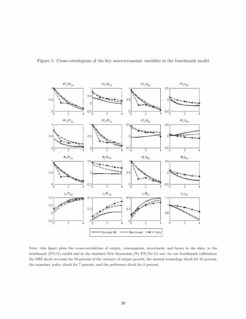
Figure 1: Cross-correlogram of the key macroeconomic variables in the benchmark model
Note: this figure plots the cross-correlations of output, consumption, investment, and hours in the data, in the
benchmark (FN/G) model and in the standard New Keynesian (No FN/No G) one, for our benchmark calibration:
the MEI shock accounts for 50 percent of the variance of output growth, the neutral technology shock for 35 percent,
the monetary policy shock for 7 percent, and the preference shock for 8 percent.
38

Figure 2: Impulse Responses to MEI Schock
Note: this figure plots the impulse response of output, consumption, investment, hours, inflation and marginal costs
for our benchmark calibration: the MEI shock accounts for 50 percent of the variance of output growth, the neutral
technology shock for 35 percent, the monetary policy shock for 7 percent, and the preference shock for 8 percent. It
does so for 4 versions of the model: our benchmark model with FN and growth, the standard New Keynesian model
(with no FN and no Growth), the model with no FN and growth (i.e., No FN / Growth) and the model with FN and
no growth (i.e., FN / No Growth).
39

Figure 3: Hicksian decomposition according to King (1991)
Note: this figure plots the income and substitution effects according to the Hicksian decomposition in King (1991)
for our benchmark calibration. It does so for 4 versions of the model: our benchmark model with FN and growth,
the standard New Keynesian model (with no FN and no Growth), the model with no FN and growth (i.e., No FN /
Growth) and the model with FN and no growth (i.e., FN / No Growth).
40

Figure 4: Impulse Responses of Consumption to a MEI Shock
Note: this figure plots the impulse response of consumption to a positive MEI shock in the benchmark (FN/G)
and standard New Keynesian (No FN/No G) models. For the standard model, we consider values of the Calvo
probabilities of wage and price non reoptimization for which the impact response of consumption to a MEI shock
matches that from the FN/G model.
41

Figure 5: Cross-correlogram of the key macroeconomic variables in the benchmark model for alter-native splits
Note: this figure plots the cross-correlations of output, consumption, investment, and hours for our benchmark
calibration for alternative splits. Benchmark: the MEI shock accounts for 50 percent of the variance of output
growth, the neutral technology shock for 35 percent, the monetary policy shock for 7 percent, and the preference
shock for 8 percent. Split 1: the MEI shock accounts for 60 percent of the variance of output growth, the neutral
technology shock for 25 percent, the monetary policy shock for 7 percent, and the preference shock for 8 percent.
Split 2: the MEI shock accounts for 40 percent of the variance of output growth, the neutral technology shock for 45
percent, the monetary policy shock for 7 percent, and the preference shock for 8 percent.
42

Figure 6: Impulse Responses of Consumption and Inflation to a MEI Shock for different persistence
Note: this figure plots the impulse response of consumption and inflation to a positive MEI shock in the benchmark
model for different levels of persistence of the MEI shock, given our benchmark calibration: the MEI shock accounts
for 50 percent of the variance of output growth, the neutral technology shock for 35 percent, the monetary policy
shock for 7 percent, and the preference shock for 8 percent.
43
Related Documents