arXiv:1110.5701v1 [astro-ph.CO] 26 Oct 2011 Mon. Not. R. Astron. Soc. 000, 000–000 (0000) Printed 27 October 2011 (MN L A T E X style file v2.2) Can galactic outflows explain the properties of Lyα emitters? Alvaro Orsi 1,2,3⋆ , Cedric G. Lacey 3 and Carlton M. Baugh 3 1. Departamento de Astronom´ ıa y Astrof´ ısica, Pontificia Universidad Cat´ olica, Av. Vicu˜ na Mackenna 4860, Santiago, Chile. 2. Centro de Astro-Ingenier´ ıa, Pontificia Universidad Cat´ olica, Av. Vicu˜ na Mackenna 4860, Santiago, Chile. 3. Institute for Computational Cosmology, Department of Physics, University of Durham, South Road, Durham DH1 3LE, UK. 27 October 2011 ABSTRACT We study the properties of Lyα emitters in a cosmological framework by computing the es- cape of Lyα photons through galactic outflows. We combine the GALFORM semi-analytical model of galaxy formation with a Monte Carlo Lyα radiative transfer code. The properties of Lyα emitters at 0 <z< 7 are predicted using two outflow geometries: a Shell of neutral gas and a Wind ejecting material, both expanding at constant velocity. We characterise the differences in the Lyα line profiles predicted by the two outflow geometries in terms of their width, asymmetry and shift from the line centre for a set of outflows with different hydrogen column densities, expansion velocities and metallicities. In general, the Lyα line profile of the Shell geometry is broader and more asymmetric, and the Lyα escape fraction is lower than with the Wind geometry for the same set of parameters. In order to implement the outflow ge- ometries in the semi-analytical model GALFORM, a number of free parameters in the outflow model are set by matching the luminosity function of Lyα emitters over the whole observed redshift range. The resulting neutral hydrogen column densities of the outflows for observed Lyα emitters are predicted to be in the range ∼ 10 18 - 10 23 [cm -2 ]. The models are con- sistent with the observationally inferred Lyα escape fractions, equivalent width distributions and with the shape of the Lyα line from composite spectra. Interestingly, our predicted UV luminosity function of Lyα emitters and the fraction of Lyα emitters in Lyman-break galaxy samples at high redshift are in partial agreement with observations. Attenuation of the Lyα line by the presence of a neutral intergalactic medium at high redshift could be responsible for this disagreement. We predict that Lyα emitters constitute a subset of the galaxy popu- lation with lower metallicities, lower instantaneous star formation rates and larger sizes than the overall population at the same UV luminosity. Key words: galaxies:high-redshift – galaxies:evolution – cosmology:large scale structure – methods:numerical 1 INTRODUCTION Over the past 10 years the Lyα line has proved to be a suc- cessful tracer of galaxies in the redshift range 2 <z< 7 (e.g. Cowie & Hu 1998; Kudritzki et al. 2000; Rhoads et al. 2000; Hu et al. 2002; Gronwall et al. 2007; Ouchi et al. 2008; Nilsson et al. 2009; Shimasaku et al. 2006; Kashikawa et al. 2006; Hu et al. 2010; Guaita et al. 2010). More recently, samples of Lyα emitters at z ∼ 0.2 obtained with the GALEX satellite (Deharveng et al. 2008; Cowie, Barger & Hu 2010), have allowed us to study this galaxy population over an even broader range of redshifts. Star-forming galaxies emit Lyα radiation when ionizing pho- tons produced by massive young stars are absorbed by atomic hy- drogen (HI) regions in the interstellar medium (ISM). These hy- ⋆ Email: [email protected] drogen atoms then recombine leading to the emission of Lyα pho- tons. Therefore, Lyα emission is, in principle, closely related to the star formation rate (SFR) of galaxies. However, in general only a small fraction of Lyα photons manage to escape from galaxies (e.g. Hayes et al. 2011). This makes it difficult to relate Lyα emitters to other star forming galaxy populations at high redshift, such as Lyman-break galaxies (LBGs) or sub-millimetre galaxies (SMGs). The physical properties of galaxies selected by their Lyα emission are inferred from spectral and photometric data (Gawiser et al. 2007; Gronwall et al. 2007; Nilsson et al. 2009; Guaita et al. 2011). Furthermore, Lyα emitters are currently used to study the kinematics of the ISM in high redshift galaxies (Shapley et al. 2003; Steidel et al. 2010, 2011; Kulas et al. 2011), to trace the large scale structure of the Universe (Shimasaku et al. 2006; Gawiser et al. 2007; Kovaˇ c et al. 2007; Orsi et al. 2008; Francke 2009; Ouchi et al. 2010), to constrain the epoch of reionization (Kashikawa et al. 2006; Dayal, Maselli & Ferrara c 0000 RAS

Welcome message from author
This document is posted to help you gain knowledge. Please leave a comment to let me know what you think about it! Share it to your friends and learn new things together.
Transcript
arX
iv:1
110.
5701
v1 [
astr
o-ph
.CO
] 26
Oct
201
1Mon. Not. R. Astron. Soc.000, 000–000 (0000) Printed 27 October 2011 (MN LATEX style file v2.2)
Can galactic outflows explain the properties ofLyα emitters?
Alvaro Orsi1,2,3⋆, Cedric G. Lacey3 and Carlton M. Baugh31. Departamento de Astronomıa y Astrofısica, Pontificia Universidad Catolica, Av. Vicuna Mackenna 4860, Santiago, Chile.2. Centro de Astro-Ingenierıa, Pontificia Universidad Catolica, Av. Vicuna Mackenna 4860, Santiago, Chile.3. Institute for Computational Cosmology, Department of Physics, University of Durham, South Road, Durham DH1 3LE, UK.
27 October 2011
ABSTRACTWe study the properties ofLyα emitters in a cosmological framework by computing the es-cape ofLyα photons through galactic outflows. We combine theGALFORM semi-analyticalmodel of galaxy formation with a Monte CarloLyα radiative transfer code. The propertiesof Lyα emitters at0 < z < 7 are predicted using two outflow geometries: a Shell of neutralgas and a Wind ejecting material, both expanding at constantvelocity. We characterise thedifferences in theLyα line profiles predicted by the two outflow geometries in termsof theirwidth, asymmetry and shift from the line centre for a set of outflows with different hydrogencolumn densities, expansion velocities and metallicities. In general, theLyα line profile of theShell geometry is broader and more asymmetric, and theLyα escape fraction is lower thanwith the Wind geometry for the same set of parameters. In order to implement the outflow ge-ometries in the semi-analytical modelGALFORM, a number of free parameters in the outflowmodel are set by matching the luminosity function ofLyα emitters over the whole observedredshift range. The resulting neutral hydrogen column densities of the outflows for observedLyα emitters are predicted to be in the range∼ 1018 − 1023[cm−2]. The models are con-sistent with the observationally inferredLyα escape fractions, equivalent width distributionsand with the shape of theLyα line from composite spectra. Interestingly, our predictedUVluminosity function ofLyα emitters and the fraction ofLyα emitters in Lyman-break galaxysamples at high redshift are in partial agreement with observations. Attenuation of theLyαline by the presence of a neutral intergalactic medium at high redshift could be responsiblefor this disagreement. We predict thatLyα emitters constitute a subset of the galaxy popu-lation with lower metallicities, lower instantaneous starformation rates and larger sizes thanthe overall population at the same UV luminosity.
Key words: galaxies:high-redshift – galaxies:evolution – cosmology:large scale structure –methods:numerical
1 INTRODUCTION
Over the past 10 years theLyα line has proved to be a suc-cessful tracer of galaxies in the redshift range2 < z <7 (e.g. Cowie & Hu 1998; Kudritzki et al. 2000; Rhoads et al.2000; Hu et al. 2002; Gronwall et al. 2007; Ouchi et al. 2008;Nilsson et al. 2009; Shimasaku et al. 2006; Kashikawa et al. 2006;Hu et al. 2010; Guaita et al. 2010). More recently, samples ofLyα emitters atz ∼ 0.2 obtained with the GALEX satellite(Deharveng et al. 2008; Cowie, Barger & Hu 2010), have allowedus to study this galaxy population over an even broader rangeofredshifts.
Star-forming galaxies emitLyα radiation when ionizing pho-tons produced by massive young stars are absorbed by atomic hy-drogen (HI) regions in the interstellar medium (ISM). Thesehy-
⋆ Email: [email protected]
drogen atoms then recombine leading to the emission ofLyα pho-tons. Therefore,Lyα emission is, in principle, closely related to thestar formation rate (SFR) of galaxies. However, in general only asmall fraction ofLyα photons manage to escape from galaxies (e.g.Hayes et al. 2011). This makes it difficult to relateLyα emittersto other star forming galaxy populations at high redshift, such asLyman-break galaxies (LBGs) or sub-millimetre galaxies (SMGs).
The physical properties of galaxies selected by theirLyα emission are inferred from spectral and photometric data(Gawiser et al. 2007; Gronwall et al. 2007; Nilsson et al. 2009;Guaita et al. 2011). Furthermore,Lyα emitters are currently usedto study the kinematics of the ISM in high redshift galaxies(Shapley et al. 2003; Steidel et al. 2010, 2011; Kulas et al. 2011),to trace the large scale structure of the Universe (Shimasaku et al.2006; Gawiser et al. 2007; Kovac et al. 2007; Orsi et al. 2008;Francke 2009; Ouchi et al. 2010), to constrain the epochof reionization (Kashikawa et al. 2006; Dayal, Maselli & Ferrara
c© 0000 RAS
2 A. Orsi et al.
2011; Ouchi et al. 2010; Stark et al. 2010; Schenker et al. 2011;Pentericci et al. 2011) and to test galaxy formation models(Le Delliou et al. 2005, 2006; Kobayashi, Totani & Nagashima2007; Nagamine et al. 2010; Dayal, Ferrara & Saro 2010).
Despite this progress, understanding the physical mechanismswhich drive the escape ofLyα radiation from a galaxy remains achallenge.Lyα photons undergo resonant scattering when interact-ing with hydrogen atoms, resulting in an increase of the pathlengththat photons need to travel before escaping the medium. Therefore,the probability of photons being absorbed by dust grains is greatlyenhanced, making the escape ofLyα photons very sensitive to evensmall amounts of dust. Furthermore, as a result of the complex ra-diative transfer, the frequency of the escapingLyα photons gen-erally departs from the line centre as a consequence of the largenumber of scatterings with many hydrogen atoms.
Recent observational studies have used various methods to in-fer the escape fraction ofLyα photons,fesc (Atek et al. 2008, 2009;Ostlin et al. 2009; Kornei et al. 2010; Hayes et al. 2010, 2011).This is generally done either by comparing the observed lineratiobetweenLyα and other hydrogen recombination lines, such asHαand Hβ, or by comparing the star formation rate derived from theLyα luminosity to that obtained from the ultraviolet continuum.The first method is the more direct, since the intrinsic fluxesofthe comparison lines can be inferred after correcting the observedfluxes for extinction. Then, the departure from case B recombina-tion of the ratio of theLyα intensity to another hydrogen recom-bination line is attributed to the escape fraction ofLyα differingfrom unity. The second method, on the other hand, relies heavilyon the assumed stellar population model used, the choice of thestellar initial mass function (IMF) and the attenuation of the ultra-violet continuum by dust, and is therefore more uncertain.
These measurements have revealed that the escape fraction ofLyα emitters can be anything between10−3 and1. The observa-tional data listed above also suggest a correlation betweenthe valueof the escape fraction and the dust extinction. The large scatterfound in this relation suggests there is a range of physical parame-ters which determine the value offesc.
Early theoretical models ofLyα emission from galaxies werebased on a static ISM (see, e.g. Neufeld 1990; Charlot & Fall1993). These models explained the difficulty of observingLyαin emission due to its very high sensitivity to dust in such amedium. Moreover, the first observations ofLyα emission in lo-cal starburst dwarf galaxies suggested a strong correlation be-tween metallicity andLyα luminosity (Meier & Terlevich 1981;Hartmann, Huchra & Geller 1984; Hartmann et al. 1988), leadingto the conclusion that metallicity, which supposedly traces theamount of dust in galaxies, is the most important factor driving thevisibility of the Lyα line.
However, subsequent observational studies showed only aweak correlation betweenLyα luminosity and metallicity, sug-gesting instead the importance of the neutral gas distribution andits kinematics (e.g., Giavalisco, Koratkar & Calzetti 1996). Fur-ther analysis of metal lines in local starbursts revealed the pres-ence of outflows which allow the escape ofLyα photons. The ob-served asymmetric P-CygniLyα line profiles are consistent withLyα photons escaping from an expanding shell of neutral gas(Thuan & Izotov 1997; Kunth et al. 1998; Mas-Hesse et al. 2003).This established outflows as the main mechanism responsibleforthe escape ofLyα photons from galaxies. Furthermore, observa-tions at higher redshifts revealLyα line profiles which also re-semble those expected when photons escape through a galactic
outflow (Shapley et al. 2003; Kashikawa et al. 2006; Kornei etal.2010; Hu et al. 2010).
In the last few years there has been significant progress in themodelling ofLyα emitters in a cosmological setting. The first con-sistent hierarchical galaxy formation model which included Lyαemission is the one described by Le Delliou et al. (2005, 2006)and Orsi et al. (2008), which makes use of theGALFORM semi-analytical model. In this model, the simple assumption of a fixedescape fraction,fesc = 0.02, regardless of any galaxy property orredshift, allowed us to predict remarkably well the abundances andclustering ofLyα emitters over a wide range of redshifts and lumi-nosities.
Nagamine et al. (2006, 2010) modelledLyα emitters in cos-mological SPH simulations. In order to match the abundancesof Lyα emitters at different redshifts, they were forced to in-troduce a tunable escape fraction and a duty cycle parameter.Kobayashi, Totani & Nagashima (2007, 2010) developed a sim-ple phenomenological model to computefesc in a semianalyti-cal model. Their analytical prescription forfesc distinguishes be-tween outflows produced in starbursts and static media in qui-escent galaxies. Dayal et. al use an SPH simulation to studyLyα emitters at high redshift and their attenuation by the neu-tral intergalactic medium (IGM). However, they assume theLyα escape fraction is related to the escape of UV continuumphotons (Dayal, Ferrara & Gallerani 2008; Dayal, Ferrara & Saro2010; Dayal, Maselli & Ferrara 2011). Tilvi et al. (2009, 2010)make predictions forLyα emitters using an N-body simulation andthe uncertain assumption that theLyα luminosity is proportional tothe halo mass accretion rate. More recently, Forero-Romeroet al.(2011) presented a model for high redshiftLyα emitters based ona hydrodynamic simulation, approximatingLyα photons to escapefrom homogeneous and clumpy gaseous, static slabs.
Motivated by observational evidence showing thatLyα pho-tons escape through outflows, we present a model that incorporatesa more physical treatment of theLyα propagation than previouswork, whilst at the same time being computationally efficient, soas to allow its application to a large sample of galaxies at differentredshifts.
Such a physical approach to modelling the escape ofLyαphotons requires a treatment of the radiative transfer of photonsthrough an HI region. The scattering and destruction ofLyα pho-tons have been extensively studied due to their many applicationsin astrophysical media. Harrington (1973) studied analytically theemergent spectrum from an optically thick, homogeneous staticslab with photons generated at the line centre. This result was gen-eralised by Neufeld (1990), to include photons generated atanyfrequency, and to provide an analytical expression forfesc in thisconfiguration.
Numerical methods, on the other hand, allow us to studythe line profiles and escape fractions ofLyα photons in awider variety of configurations. The standard approach is touse a Monte Carlo algorithm, in which the paths of a set ofphotons are followed one at a time through many scatteringevents, until the photon either escapes or is absorbed by adust grain. Such calculations have been applied successfullyto study the properties ofLyα emitters in different scenar-ios (see, e.g. Ahn, Lee & Lee 2000; Zheng & Miralda-Escude2002; Ahn 2003, 2004; Verhamme, Schaerer & Maselli 2006;Dijkstra, Haiman & Spaans 2006; Laursen & Sommer-Larsen2007; Laursen, Razoumov & Sommer-Larsen 2009).
Recently, Zheng et al. (2010, 2011) combined a Monte CarloLyα radiative transfer model with a cosmological reionizationsim-
c© 0000 RAS, MNRAS000, 000–000
Can galactic outflows explainLyα emitters? 3
ulation atz ∼ 6, obtaining extendedLyα emission due to spatialdiffusion. Their simulation box is, however, too small to beevolvedto the present day without density fluctuations becoming nonlinearon the box scale, and does not have a volume large enough to sam-ple a wide range of environments.
Previous work has not studiedLyα emitters in a frameworkthat at the same time spans the galaxy formation and evolution pro-cess over a broad range of redshifts and includesLyα radiativetransfer. The need for such hybrid approach is precisely themoti-vation for this paper.
Given the observational evidence that outflows facilitate theescape ofLyα photons from galaxies, here we study the natureof Lyα emitters by computing the escape of photons from galax-ies in an outflow of material by using a Monte CarloLyα radia-tive transfer model. Galactic outflows in our model are defined ac-cording to predicted galaxy properties in a simple way. Thismakesour modelling feasible on a cosmological scale, whilst retaining allthe complexity ofLyα radiative transfer. Following our previouswork, we use the semianalytical modelGALFORM. This paper rep-resents a significant improvement over the treatment ofLyα emit-ters in hierarchical galaxy formation models initially described inLe Delliou et al. (2005, 2006) and Orsi et al. (2008), which all as-sumed a constant escape fraction.
The outline of this paper is as follows: Section 2 describes thegalaxy formation and radiative transfer models used. Also,we de-scribe the two versions of galactic outflow geometries we useandexplain how these are constructed in terms of galaxy parametersthat can be extracted from our semi-analytical model. In Section 3we present the properties of theLyα line profiles and escape frac-tions predicted by our outflow geometries. In Section 4 we describethe galaxy properties that are relevant to ourLyα modelling anddescribe how we combine theLyα radiative transfer model withthe semi-analytical model. In Section 5 we present our main re-sults, where we compare with observational measurements when-ever possible, spanning the redshift range0 < z < 7. In Sec-tion 6 we present the implications of our modelling for the prop-erties of galaxies selected by theirLyα emission, compared to thebulk of the galaxy population. Finally, in Section 7 we discuss ourmain findings. In the Appendix we give details of the implementa-tion of the Monte Carlo radiative transfer model, the effectof theUV background on the outflow geometries and the numerical strat-egy followed to compute the escape fraction ofLyα photons fromgalaxies.
2 MODEL DESCRIPTION
Our approach to modellingLyα emitters in a cosmological frame-work involves combining two independent codes. The backbone ofour calculation is theGALFORM semi-analytical model of galaxyformation, outlined in Section 2.1, from which all relevantgalaxyproperties can be obtained, including the intrinsicLyα luminosity.The second is the Monte CarloLyα radiative transfer code to com-pute both the frequency distribution ofLyα photons and theLyαescape fraction. This code is described briefly in Section 2.2, withfurther information and tests presented in Appendix A. In Section2.3 we describe the outflow geometries and the way these are de-fined in terms of galaxy properties.
2.1 Galaxy formation model
We use the semi-analytical model of galaxy formation,GALFORM,to predict the properties of galaxies and their abundance asafunction of redshift. TheGALFORM model is fully described inCole et al. (2000) and Benson et al. (2003) (see also the review byBaugh 2006). The variant used here was introduced by Baugh etal.(2005), and is also described in detail in Lacey et al. (2008). Themodel computes star formation and galaxy merger histories for thewhole galaxy population, following the hierarchical evolution ofthe host dark matter haloes.
The Baugh et al. (2005) model used here is the sameGALFORM variant used in our previous work onLyα emitters(Le Delliou et al. 2005, 2006; Orsi et al. 2008). A critical assump-tion of the Baugh et al. (2005) model is that stars which formin starbursts have a top-heavy initial mass function (IMF).TheIMF is given bydN/d ln(m) ∝ m−x with x = 0 in this case.Stars formed quiescently in discs have a solar neighbourhood IMF,with the form proposed by Kennicutt (1983) withx = 0.4 form < 1M⊙ andx = 1.5 for m > 1M⊙. Both IMFs cover themass range0.15M⊙ < m < 125M⊙. Within the framework ofΛCDM, Baugh et al. argued that the top-heavy IMF is essentialto match the counts and redshift distribution of galaxies detectedthrough their sub-millimetre emission, whilst retaining the matchto galaxy properties in the local Universe, such as the optical andfar-IR luminosity functions, galaxy gas fractions and metallicities.Lacey et al. (2008) showed that the model predicts galaxy evolu-tion in the IR in good agreement with observations fromSpitzer.Moreover, Lacey et al. (2011) also showed that the Baugh et al.model predicts the abundance of Lyman-break galaxies (LBGs)remarkably well over the redshift range3 < z < 10 (see alsoGonzalez et al. 2011).
In GALFORM, the suppression of gas cooling from ionizingradiation produced by stars and active galactic nuclei (AGNs) dur-ing the epoch of reionization is modelled in a simple way: after theredshift of reionization, taken to bezreion = 10, photoionization ofthe IGM completely suppresses the cooling and collapse of gas inhaloes with circular velocities belowVcrit = 30[km/s].
The Baugh et al. model assumes two distinct modes of feed-back from supernovae, areheating mode, in which cold gas is ex-pelled back to the hot halo, and asuperwind mode, in which coldgas is ejected out of the galaxy halo. We describe both modesof supernova feedback in more detail in section 2.3.2 (see alsoLacey et al. 2008).
Unlike the Bower et al. (2006) variant ofGALFORM, themodel used here does not incorporate feedback from an AGN.The superwind mode of feedback produces similar consequencesto the quenching of gas cooling by the action of an AGN, asboth mechanisms suppress the bright end of the LF. However, theBower et al. (2006) model does not reproduce the observed abun-dances of LBGs or submillimetre galaxies (SMGs) at high redshift,which span a redshift range which overlaps with that of the LFsof Lyα emitters considered in this paper. Therefore, we do not usethisGALFORM variant to make predictions forLyα emitters.
In GALFORM, the intrinsicLyα emission is computed as fol-lows:
(i) The composite stellar spectrum of the galaxy is calculated,based on its predicted star formation history, including the effectof the metallicity with which new stars are formed, and taking intoaccount the IMFs adopted for different modes of star formation.
(ii) The rate of production of Lyman continuum (Lyc) photonsis computed by integrating over the composite stellar spectrum. We
c© 0000 RAS, MNRAS000, 000–000
4 A. Orsi et al.
assume that all of these ionizing photons are absorbed by neutralhydrogen within the galaxy. The mean number ofLyα photons pro-duced per Lyc photon, assuming a gas temperature of104 K for theionized gas, is approximately 0.677, assuming Case B recombina-tion (Osterbrock 1989).
(iii) The observedLyα flux depends on the fraction ofLyαphotons which escape from the galaxy (fesc). Previously we as-sumed this to be constant and independent of galaxy properties.The escape fraction was fixed atfesc = 0.02, resulting in a remark-ably good match to the observedLyα LFs over the redshift range3 < z < 6. In our new model, we make use of a Monte Carloradiative transfer model ofLyα photons to computefesc in a morephysical way. This model is briefly described in the next subsec-tion.
2.2 Monte Carlo Radiative Transfer Model
In order to compute theLyα escape fraction and line profile weconstruct a Monte Carlo radiative transfer model forLyα photons.This simulates the escape of a set of photons from a source as theytravel through an expanding HI region, which may contain dust, byfollowing the scattering histories of individual photons.By follow-ing a large number of photons we can compute properties such astheLyα spectrum and the escape fraction.
Our Monte Carlo radiative transfer code works on a 3D gridin which each cell contains information about the neutral hydrogendensity,nH , the temperature of the gas,T , and the bulk velocity,vbulk. Once aLyα photon is created, a random direction and fre-quency are assigned to it, and the code follows its trajectory andcomputes each scattering event of the photon as it crosses the HIregion until it either escapes or is absorbed by a dust grain.If thephoton escapes, then its final frequency is recorded, a new photonis generated and the procedure is repeated.
Clearly, to get an accurate description of the escape ofLyαphotons from a given geometrical setup, many photons must befol-lowed. The number of photons needed to achieve convergence willdepend on the properties of the medium, but also on the quantityin which we are interested. For example, for most of the outflowsstudied here, only a few thousand photons are needed to computean accurate escape fraction. However, tens of thousand of photonsare needed to obtain a smooth line profile.
Our radiative transfer model of Lyα photonsis similar to previous models in the literature (e.g.Zheng & Miralda-Escude 2002; Ahn 2003, 2004;Verhamme, Schaerer & Maselli 2006; Dijkstra, Haiman & Spaans2006; Laursen, Razoumov & Sommer-Larsen 2009;Barnes & Haehnelt 2010). We describe the numerical imple-mentation of our Monte Carlo model and the validation testsapplied to it in Appendix A.
2.3 Outflow geometries
In our model, the physical conditions in the medium used to com-pute the escape ofLyα photons depend on several properties ofgalaxies predicted byGALFORM. Below we describe two outflowgeometries for the HI region surrounding the source ofLyα pho-tons. They differ in their geometry and the way the properties ofgalaxies fromGALFORM are used. We assume the temperature ofthe medium to be constant atT = 104 K, which sets the thermalvelocity dispersion of atoms, following a Maxwell-Boltzmann dis-tribution, to bevth = 12.85 kms−1 (see Eq. A1 in Appendix A for
more details). For simplicity, the source ofLyα photons is taken tobe at rest in the frame of the galaxy, in the centre of the outflow,and emits photons at the line centre only,λ = 1215.68 A.
2.3.1 Expanding thin shell
Previous radiative transfer studies ofLyα line profiles adoptedan expanding shell in the same way as we used here (see, e.g.Ahn 2003, 2004; Verhamme, Schaerer & Maselli 2006; Schaerer2007; Verhamme et al. 2008, and references therein). This model,hereafter named “Shell”, consists of a homogeneous, expanding,isothermal spherical shell, in which dust and gas are uniformlymixed. The shell, although thin, is described by an inner andouter radiusRin andRout, which satisfyRin = fthRout. We setfth = 0.9. In addition, the medium is assumed to be expandingradially with constant velocityVexp. The column density throughthe Shell is given by
NH(r) =XHMshell
4πmHR2out
, (1)
whereXH = 0.74 is the fraction of hydrogen in the cold gas andmH is the mass of a hydrogen atom. InGALFORM, theLyα lumi-nosity originates in the disk (in quiescent galaxies) or thebulge (instarbursts). Some galaxies may also have contributions from bothcomponents. Therefore,Mshell,Rout andVexp are taken to be pro-portional to the mass of cold gasMcold, half-mass radiusR1/2 andcircular velocityVcirc, respectively, i.e.,
Mshell = fM 〈Mgas〉, (2)
Rout = fR〈R1/2〉, (3)
Vexp = fV 〈Vcirc〉, (4)
wherefM , fR andfV are free parameters. To take into account thecontribution from both components of a galaxy, we define
〈Mgas〉 = F diskLyαM
diskgas + (1− F disk
Lyα )Mbulgegas , (5)
〈R1/2〉 = F diskLyαR
disk1/2 + (1− F disk
Lyα )Rbulge1/2 , (6)
〈Vcirc〉 = F diskLyαV
diskcirc + (1− F disk
Lyα )Vbulgecirc , (7)
F diskLyα ≡ Ldisk
Lyα
LtotalLyα
. (8)
In each term, the superscript indicates the contribution from thedisk, the bulge or the total (the sum of the two). In most galaxies,however, either the disk or bulge term completely dominates.
Likewise, the metallicity of the shellZout is taken to be themetallicity of the cold gasZcold weighted by a combination of themass of cold gas and theLyα luminosity of each component, i.e.,
Zout =Mdisk
gas LdiskLyαZ
diskcold +Mbulge
gas LbulgeLyα Zbulge
cold
Mdiskgas L
diskLyα +Mbulge
gas LbulgeLyα
. (9)
In order to compute the dust content in the outflow we assume thatthe mass of dust in the outflow,Mdust, is proportional to the gasmass and metallicity, i.e.
Mdust =δ∗Z⊙
MshellZout, (10)
where the dust-to-gas ratio is taken to beδ∗ = 1/110 at the solarmetallicityZ⊙ = 0.02 (Granato et al. 2000). The extinction opticaldepth at the wavelength ofLyα can be written as
τd =E⊙
Z⊙NHZout, (11)
c© 0000 RAS, MNRAS000, 000–000
Can galactic outflows explainLyα emitters? 5
whereE⊙ = 1.77 × 10⁻²¹[cm2] is the ratioτd/NH for so-lar metallicity at the wavelength ofLyα (1216 A). Throughoutthis work we use the extinction curve and albedo from Silva etal.(1998), which are fit to the observed extinction and albedo intheGalactic ISM. For a dust albedoA, the optical depth for absorptionis simply
τa = (1− A)τd. (12)
At the wavelength ofLyα,ALyα = 0.39.
2.3.2 Galactic Wind
Supernovae heat and accelerate the ISM through shocks and hencegenerate outflows from galaxies (see, e.g. Frank 1999; Strickland2002). Here we develop an outflow model, hereafter called “Wind”,which relates the density of the outflow to the mass ejection ratefrom galaxies due to supernovae. InGALFORM, this mass ejectionrate is given by
Mej = [βreh(Vcirc) + βsw(Vcirc)]ψ, (13)
where
βreh =
(
Vcirc
Vhot
)−αhot
, (14)
βsw = fswmin[1, (Vcirc/Vsw)−2]. (15)
The termsβreh andβsw define the two different modes of super-nova feedback (thereheatingand superwind), and the constantsαhot, Vhot, fsw and Vsw are free parameters ofGALFORM, cho-sen by fitting the model predictions to observed galaxy LFs. Theinstantaneous star formation rate,ψ is obtained as
ψ =Mgas
τ∗, (16)
whereτ∗ is the star formation time-scale, which is different forquiescent galaxies and starbursts. For a detailed description of thestar formation and supernova feedback processes in this variant ofGALFORM, see Baugh et al. (2005) and Lacey et al. (2008). Sincestar formation can occur in the disk and in the bulge, there isa massejection rate termMej associated with each component.
We construct the wind as an isothermal, spherical flow ex-panding at constant velocityVexp, and inner radiusRwind (the windis empty inside). In a steady-state spherical wind, the massejectionrate is related to the velocity and density at any point of theWindvia the equation of mass continuity, i.e.
Mej = 4πr2Vexpρ(r), (17)
whereρ(r) is the mass density of the medium, andVexp is calcu-lated following equation (4). Since star formation inGALFORM canoccur in both the disk and bulge of galaxies,Mej in equation (17)corresponds to the sum of the ejection rate from the disk and thebulge.
Following equation (17), the number density profilenHI(r)in the Wind geometry varies according to
nHI(r) =
0 r < Rwind
XHMej
4πmHr2Vexpr > Rwind.
(18)
The column densityNH of the outflow is
NH =XHMej
4πmHRwindVexp, (19)
where the inner radius of the wind,Rwind, is computed in an anal-ogous way toRout in the Shell geometry (Eq. 3). Note that bothfRandfV in this case are different free parameters and independentof those used in the Shell geometry. The metallicity of the Wind,Zwind, corresponds to the metallicity of the cold gas in the disk andbulge weighted by their respective mass ejection rates.
For computational reasons, the radiative transfer code requiresus to define an outer radius,Router, for the Wind. However, sincethe number density of atoms decreases as∼ r−2, we expect thatat some point away from the centre the optical depth becomes sosmall that the photons will be able to escape regardless of the ex-act extent of the outflow. We find that an outer radiusRouter =20Rwind yields converged results, i.e. the escape fraction ofLyαphotons does not vary if we increase the value ofRouter further.
3 OUTFLOW PROPERTIES
In this section we explore the properties of theLyα radiative trans-fer in our outflow geometries prior to coupling these to the galaxyformation modelGALFORM. We do this by running our MonteCarlo radiative transfer model over a grid of configurationsspan-ning a wide range of hydrogen column densities, expansion veloci-ties and metallicities. In order to obtain well-definedLyα line pro-files, we run each configuration using5× 104 photons. Therefore,the minimumLyα escape fraction our models can compute in thiscase isfesc = 2× 10⁻⁵.
3.1 Lyα line properties
One important difference between our two outflow geometriesisthe way the column densities are computed. In the Shell geometrythe column density is a function of the total cold gas mass of agalaxy and its size, whereas in the Wind geometry it depends onthe mass ejection rate given by the supernova feedback modelalongwith the size and the circular velocity of the galaxy. This differencetranslates into different predicted properties forLyα emitters, aswill be shown in the next section. However, even when the columndensity, velocity of expansion and outflow metallicity are the same,the two models will give different escape fractions and lineprofileshapes due to their different geometries.
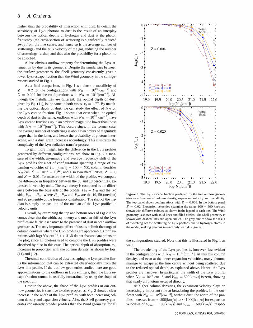
Fig. 1 shows theLyα line profiles obtained with the two mod-els when matching the key properties for outflows at the same col-umn densities. In order to make a fair comparison between theShelland Wind geometries, we compare configurations with the samecolumn density, expansion velocity and metallicity. In addition, theinner radius in the Wind geometry is chosen to be the same as itscounterpart, the outer radius in the Shell geometry. The twopan-els of Fig. 1 display a set of configurations with column densitiesof NH = 1020[cm−2] (left panel) andNH = 1022[cm−2] (rightpanel). In the following, we express the photon’s frequencyin termsof x, the shift in frequency around the line centreν0, in units of thethermal width, i.e.
x ≡ (ν − ν0)
∆νD, (20)
where∆νD = vthν0/c, andc is the speed of light, andvth is thethermal velocity discussed in Section 2.3.
As a general result, outflows with a column density ofNH =1020[cm−2], regardless of the other properties, produce multiplepeaks at frequencies redward of the line centre in both geometries,with different levels of asymmetry. The Shell geometry generates
c© 0000 RAS, MNRAS000, 000–000
6 A. Orsi et al.
x = (ν - ν0)/∆νD
P(x
)
0.00
0.01
0.02
0.03
Wind
V[km s-1] = 200.log(NH[cm-2])=20.0Z = 0.000
fesc = 1.000
Shell
0 BS1 BS2 BS>2 BS
fesc = 1.000
0.00
0.01
0.02
0.03V[km s-1] = 500.log(NH[cm-2])=20.0Z = 0.000
fesc = 1.000
fesc = 1.000
0.00
0.01
0.02
0.03V[km s-1] = 200.log(NH[cm-2])=20.0Z = 0.200
fesc = 0.137
fesc = 0.047
-80 -60 -40 -20 00.00
0.01
0.02
0.03V[km s-1] = 500.log(NH[cm-2])=20.0Z = 0.200
fesc = 0.243
-80 -60 -40 -20 0
fesc = 0.140
x = (ν - ν0)/∆νD
P(x
)
0.000
0.005
0.010
0.015
Wind
V[km s-1] = 200.log(NH[cm-2])=22.0Z = 0.000
fesc = 1.000
Shell
0 BS1 BS2 BS>2 BS
fesc = 1.000
0.000
0.005
0.010
0.015V[km s-1] = 500.log(NH[cm-2])=22.0Z = 0.000
fesc = 1.000
fesc = 1.000
0.000
0.005
0.010
0.015V[km s-1] = 200.log(NH[cm-2])=22.0Z = 0.002
fesc = 0.009
fesc = 0.001
-400 -300 -200 -1000.000
0.005
0.010
0.015V[km s-1] = 500.log(NH[cm-2])=22.0Z = 0.002
fesc = 0.042
-400 -300 -200 -100
fesc = 0.010
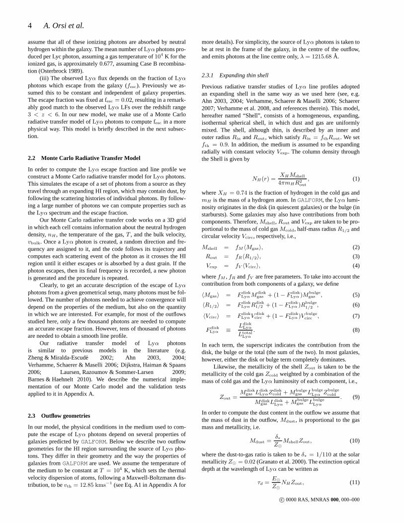
Figure 1. Comparison of theLyα line profile obtained with the Wind and Shell geometries forNH = 1020[cm−2] (leftmost two columns) andNH =1022[cm−2] (rightmost two columns). The red (blue) histogram shows thefull spectrum obtained for the Wind (Shell) outflow geometry. The cyan, green,pink and gray lines show the spectra of photons which experienced 0, 1, 2 and 3 or more back-scatterings before escaping, respectively. Likewise, the samecolours are used to plot vertical dashed lines showing the frequencies corresponding to−xbs,−2xbs,−3xbs and−4xbs, respectively (see text for details).Each row displays a different configuration, characterisedby a givenNH , Vexp andZ, as indicated in the legend. The top two rows correspond to dust-freeconfigurations (Z = 0), whereas the bottom two have different metallicities, chosen to have equal dust optical depth, although having different columndensities of hydrogen. The escape fraction ofLyα photons,fesc, is indicated in each box. TheLyα profiles shown are normalized to the total number ofescaping photons (instead of the total number of photons run), to ease the comparison between the dusty and dust-free cases. Note the different range in thex-axis between the left and right panels.
more prominent peaks than the Wind geometry. The frequency ofthe main peak is, however, the same in both outflow geometries.
On the other hand, outflows withNH = 1022[cm−2] displaybroaderLyα profiles. As opposed to the lower column density case,these profiles display a single peak, also redward of the linecentre.The position of this peak is also the same for both geometries.
The effect of a large expansion velocity is shown in the 2ndand 4th rows in both panels of Fig. 1. Here the configurations haveVexp = 500[km/s]. The differences with the configurations whereVexp = 200[km/s] are evident: the profiles are broader, and theposition of the peaks are displaced to redder frequencies. Further-more, in the left panel of Fig. 1, whereNH = 1020[cm−2], it is
shown that a significant fraction of photons escape at the line cen-tre. The high expansion velocity in this case makes the medium op-tically thin, allowing many photons to escape without undergoingany scattering.
For the configurations withNH = 1020[cm−2], the opticaldepth that a photon at the line centre (x = 0) sees when travelingalong the radial direction isτ0 = 3.63 andτ0 = 0.57 for expan-sion velocitiesVexp = 200[km/s] andVexp = 500[km/s], respec-tively. Accordingly, the configurations withNH = 1022[cm−2]have optical depths a factor100 higher. On the other hand, a staticmedium withNH = 1020[cm−2] has a much higher optical depth,τ0 = 3.31× 10⁶. This illustrates the strong effect of the expansion
c© 0000 RAS, MNRAS000, 000–000
Can galactic outflows explainLyα emitters? 7
19.0 19.5 20.0 20.5 21.0 21.5 22.0log(NH[cm-2])
0
500
1000
1500
2000
2500
3000W
idth
[k
m/
s]Vexp[km/s] = 100Vexp[km/s] = 300Vexp[km/s] = 500
ShellWind
Z = 0.000
19.0 19.5 20.0 20.5 21.0 21.5 22.0log(NH[cm-2])
-600
-400
-200
0
200
Asy
mm
etry
[k
m/
s]
Vexp[km/s] = 100Vexp[km/s] = 300Vexp[km/s] = 500
WindShell
Z = 0.000
19.0 19.5 20.0 20.5 21.0 21.5 22.0log(NH[cm-2])
-3000
-2500
-2000
-1500
-1000
-500
0
Med
ian
sh
ift
[km
/s]
Vexp[km/s] = 500Vexp[km/s] = 300Vexp[km/s] = 100
WindShell
Z = 0.000
19.0 19.5 20.0 20.5 21.0 21.5 22.0log(NH[cm-2])
0
500
1000
1500
2000
2500
3000
Wid
th [
km
/s]
Vexp[km/s] = 100Vexp[km/s] = 300Vexp[km/s] = 500
ShellWind
Z = 0.010
19.0 19.5 20.0 20.5 21.0 21.5 22.0log(NH[cm-2])
-600
-400
-200
0
200
Asy
mm
etry
[k
m/
s]Vexp[km/s] = 100Vexp[km/s] = 300Vexp[km/s] = 500
WindShell
Z = 0.010
19.0 19.5 20.0 20.5 21.0 21.5 22.0log(NH[cm-2])
-3000
-2500
-2000
-1500
-1000
-500
0
Med
ian
sh
ift
[km
/s]
Vexp[km/s] = 500Vexp[km/s] = 300Vexp[km/s] = 100
WindShell
Z = 0.010
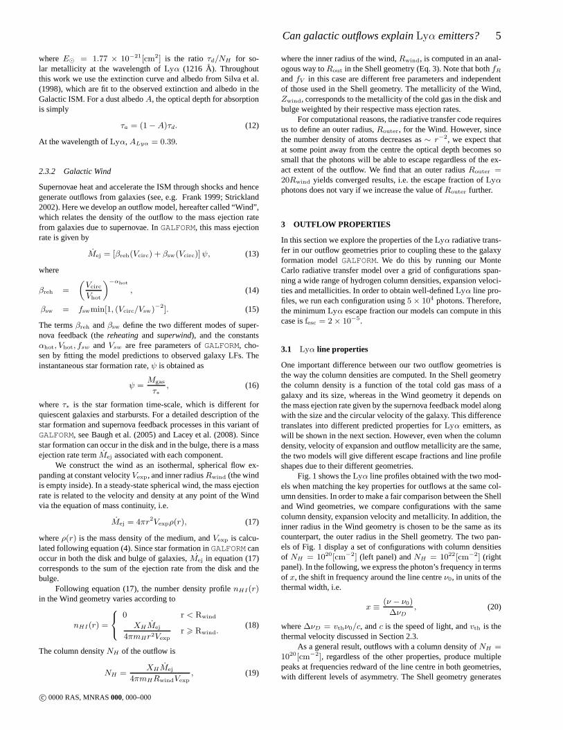
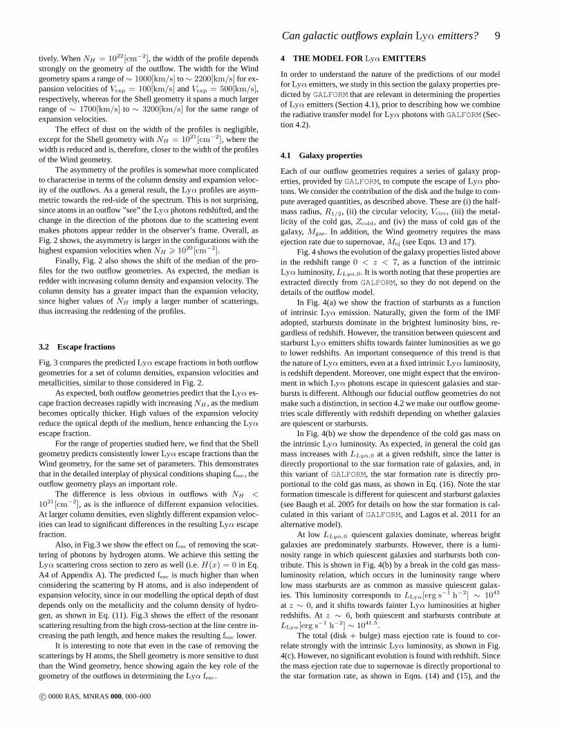
Figure 2. The properties of theLyα profiles predicted by the two outflow geometries for a given column density, expansion velocity and metallicity. Leftpanels: the width of the profiles, defined as the difference between the 90 and 10 percentiles of the frequency distribution of escapingLyα photons, measuredin km/s. Middle panels: the asymmetry, defined in the text, and measured in km/s. Right panels: the shift of the median of the Lyα profiles with respect tothe line centre, measured in km/s. Note that negative velocities indicate redshifting. The top row shows theLyα profile properties in dust-free outflows. Thebottom row shows outflows with a metallicityZ = 0.01. Different expansion velocities spanning the range100− 500 km/s are shown with different colours,as shown by the labels in each panel. The Wind geometry is shown with solid lines and filled circles. The Shell geometry is shown with dashed lines and opencircles.
velocity in reducing the optical depth of the medium, thus allowingphotons to escape.
The Lyα line profiles obtained can be characterised by thefrequency distribution of photons split according to the number ofbackscatterings they experience before escaping (i.e. thenumber oftimes photons bounce back to the inner, empty region). When pho-tons interact for the first time with the outflow, a fraction ofthemwill experience a backscattering. These events are significant sincethe distribution of scattering angles is dipolar (see Eq. A13 in Ap-pendix A). The frequency of a photon after a scattering event, inthe observer’s frame, is given by Eq. (A15). Depending on thedi-rection of the photon after the scattering event, its frequency willfall within the rangex = [−2xbs, 0], wherexbs ≡ Vexp/vth (seealso Ahn 2003; Verhamme, Schaerer & Maselli 2006). Photons thatdo not experience a backscattering, or escape directly, form thecyan curves in Fig. 1. If the photon is backscattered exactlyback-wards, then its frequency will bex = −2xbs. The cross-sectionfor scattering is significantly reduced for these photons, and so afraction escape without undergoing any further interaction with theoutflow. Photons backscattered once form the green curves inFig.1. If a photon experiences a second backscatter in the exact oppo-site direction, then its frequency will becomex = −4xbs, and thecross-section for a further scattering will again reduce significantly.The magenta curves show the distribution of photons that experi-enced 2 backscatterings. Finally, photons that experience3 or morebackscatterings are shown in gray.
In detail, the geometrical differences between the Shell andWind models are translated into each backscattering peak con-tributing in a different proportion and with a different shape tothe overall spectrum for each geometry. Previous studies have alsofound this relation between the peaks of backscattered photonsandxbs in media with column densities of the order ofNH ∼1020[cm−2] (Ahn 2003, 2004; Verhamme, Schaerer & Maselli2006), although they did not study the line profiles for higher op-tical depths as we do here. ForNH = 1022[cm−2], we find thatthe peaks are displaced considerably from their expected positionbased on the simple argument above. This is not surprising, sincein outflows with very large optical depths the number of scatteringsbroadens the profiles and reddens the peak positions.
In the Wind geometry, the contribution of photons featuringno backscatterings dominates most of the total profile forNH =1020[cm−2], whereas in the overall line profile for the Shell ge-ometry there is a clear distinction between a region dominatedby photons suffering no backscatterings and those backscatteredonce (green curve). This illustrates again how theLyα line pro-file in the Shell geometry features clear multiple peaks fromone ormore backscatterings, whereas in the Wind geometry the secondarypeaks are less obvious.
Fig. 1 also shows the effect of including dust in the outflows.Overall, dust absorption has more effect on the redder side of theline profiles than at frequencies closer to the line centre, wherethe probability of scattering with hydrogen atoms is significantly
c© 0000 RAS, MNRAS000, 000–000
8 A. Orsi et al.
higher than the probability of interaction with dust. In detail, thesensitivity of Lyα photons to dust is the result of an interplaybetween the optical depths of hydrogen and dust at the photonfrequency (the cross-section of scattering is significantly reducedaway from the line centre, and hence so is the average number ofscatterings) and the bulk velocity of the gas, reducing the numberof scatterings further, and thus also the probability for a photon tobe absorbed.
A less obvious outflow property for determining theLyα at-tenuation by dust is its geometry. Despite the similaritiesbetweenthe outflow geometries, the Shell geometry consistently gives alowerLyα escape fraction than the Wind geometry in the configu-rations studied in Fig. 1.
As a final comparison, in Fig. 1 we chose a metallicity ofZ = 0.2 for the configurations withNH = 1020[cm−2] andZ = 0.002 for the configurations withNH = 1022[cm−2]. Al-though the metallicities are different, the optical depth of dust,given by Eq. (11), is the same in both cases,τd = 1.77. By match-ing the optical depth of dust, we can study the effect ofNH ontheLyα escape fraction. Fig. 1 shows that even when the opticaldepth of dust is the same, outflows withNH = 1022[cm−2] haveLyα escape fractions up to an order of magnitude lower than thosewith NH = 1020[cm−2]. This occurs since, in the former case,the average number of scatterings is about two orders of magnitudelarger than in the latter, and hence the probability of photons inter-acting with a dust grain increases accordingly. This illustrates thecomplexity of theLyα radiative transfer process.
To gain more insight into the difference in theLyα profilesgenerated by different configurations, we show in Fig. 2 a mea-sure of the width, asymmetry and average frequency shift of theLyα profiles for a set of configurations spanning a range of ex-pansion velocities ofVexp[km/s] = 100 − 500, column densitiesNH [cm−2] = 1019 − 1022, and also two metallicities,Z = 0andZ = 0.01. To measure the width of the profiles we computethe difference in frequency between the 90 and 10 percentiles, ex-pressed in velocity units. The asymmetry is computed as the differ-ence between the blue side of the profile,P90 − P50 and the redside,P50 − P10, whereP10, P50 andP90 are the 10, 50 (median)and 90 percentile of the frequency distribution. The shift of the me-dian is simply the position of the median of theLyα profiles invelocity units.
Overall, by examining the top and bottom rows of Fig.2 it be-comes clear that the width, asymmetry and median shift of theLyαprofiles are fairly insensitive to the presence of dust in both outflowgeometries. The only important effect of dust is to limit therange ofcolumn densities where theLyα profiles are appreciable. Configu-rations withlog(NH [cm−2]) > 21.5 do not feature data points onthe plot, since all photons used to compute theLyα profiles wereabsorbed by dust in this case. The optical depth of absorption, τa,increases in proportion with the column density, as shown byEqs.(11) and (12).
The small contribution of dust in shaping theLyα profiles lim-its the information that can be extracted observationally from theLyα line profile. If the outflow geometries studied here are goodapproximations to the outflows inLyα emitters, then theLyα es-cape fraction cannot be usefully constrained by using the shape ofthe spectrum.
Despite the above, the shape of theLyα profiles in our out-flow geometries is sensitive to other properties. Fig. 2 shows a clearincrease in the width of theLyα profiles, with both increasing col-umn density and expansion velocity. Also, the Shell geometry gen-erates consistently broader profiles than the Wind geometry, for all
19.0 19.5 20.0 20.5 21.0 21.5 22.0log(NH[cm-2])
-5
-4
-3
-2
-1
0
log
(fes
c)
Vexp[km/s] = 500Vexp[km/s] = 300Vexp[km/s] = 100
WindShell
Z = 0.004
19.0 19.5 20.0 20.5 21.0 21.5 22.0log(NH[cm-2])
-5
-4
-3
-2
-1
0
log
(fes
c)
Vexp[km/s] = 500Vexp[km/s] = 300Vexp[km/s] = 100
WindShell
Z = 0.020
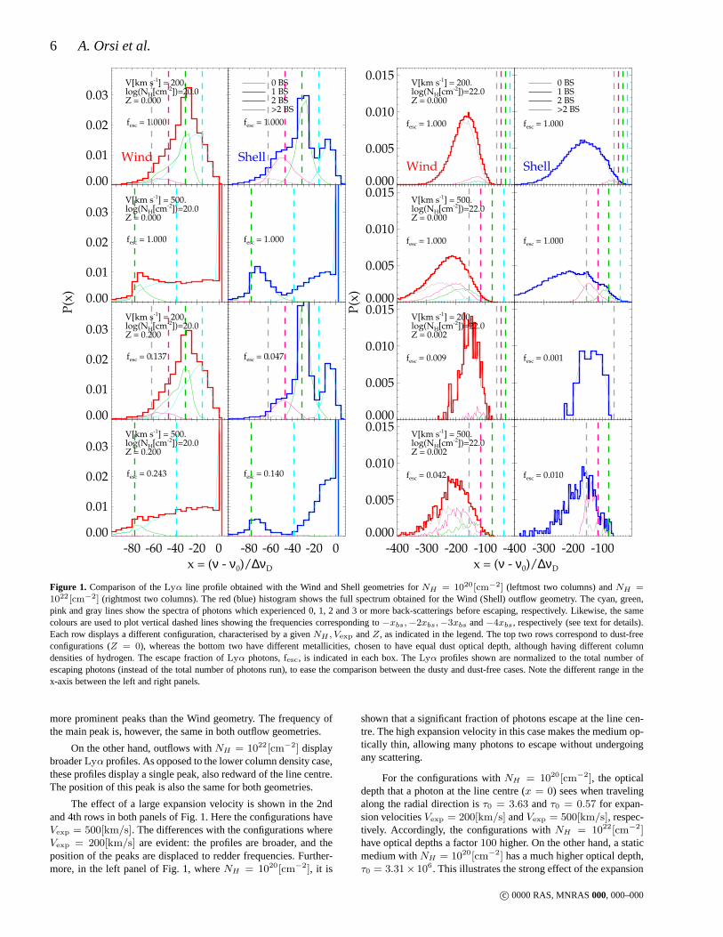
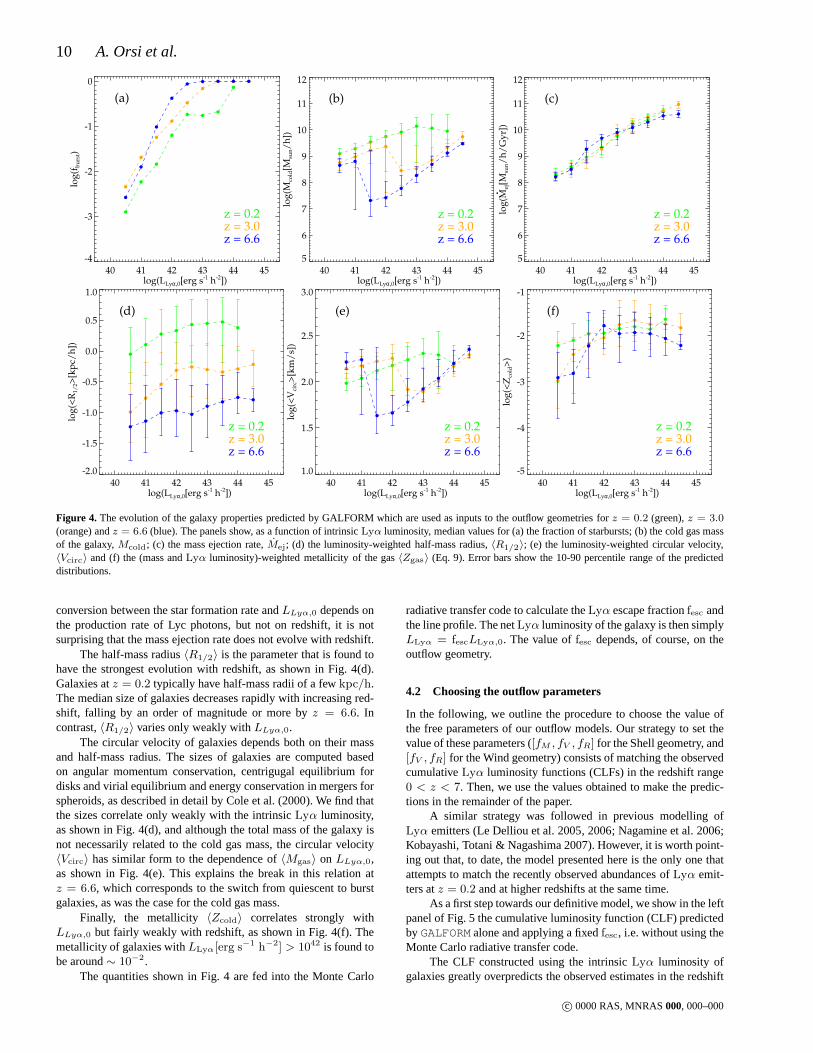
Figure 3. TheLyα escape fraction predicted by the two outflow geome-tries as a function of column density, expansion velocity and metallicity.The top panel shows configurations withZ = 0.004. In the bottom panelZ = 0.02. Expansion velocities spanning the range100 − 500 km/s areshown with different colours, as shown in the legend of each box. The Windgeometry is shown with solid lines and filled circles. The Shell geometry isshown with dashed lines and open circles. The gray circles show the resultof switching off the scattering ofLyα photons due to hydrogen atoms inthe model, making photons interact only with dust grains.
the configurations studied. Note that this is illustrated inFig. 1 aswell.
The broadening of theLyα profiles is, however, less evidentin the configurations withNH = 1019[cm−2]. At this low columndensity, and even at the lower expansion velocities, many photonsmanage to escape at the line centre without being scattered dueto the reduced optical depth, as explained above. Hence, theLyαprofiles are narrower. In particular, the width of theLyα profile,whenNH = 1019[cm−2] andVexp = 500[km/s] is zero, showingthat nearly all photons escaped directly.
At higher column densities, the expansion velocity plays anincreasingly important role at broadening the profiles. In the out-flows withNH = 1020[cm−2], without dust, the width of the pro-files increases from∼ 300[km/s] to∼ 1000[km/s] for expansionvelocities ofVexp = 100[km/s] andVexp = 500[km/s], respec-
c© 0000 RAS, MNRAS000, 000–000
Can galactic outflows explainLyα emitters? 9
tively. WhenNH = 1022[cm−2], the width of the profile dependsstrongly on the geometry of the outflow. The width for the Windgeometry spans a range of∼ 1000[km/s] to∼ 2200[km/s] for ex-pansion velocities ofVexp = 100[km/s] andVexp = 500[km/s],respectively, whereas for the Shell geometry it spans a muchlargerrange of∼ 1700[km/s] to ∼ 3200[km/s] for the same range ofexpansion velocities.
The effect of dust on the width of the profiles is negligible,except for the Shell geometry withNH = 1021[cm−2], where thewidth is reduced and is, therefore, closer to the width of theprofilesof the Wind geometry.
The asymmetry of the profiles is somewhat more complicatedto characterise in terms of the column density and expansionveloc-ity of the outflows. As a general result, theLyα profiles are asym-metric towards the red-side of the spectrum. This is not surprising,since atoms in an outflow ”see” theLyα photons redshifted, and thechange in the direction of the photons due to the scattering eventmakes photons appear redder in the observer’s frame. Overall, asFig. 2 shows, the asymmetry is larger in the configurations with thehighest expansion velocities whenNH > 1020[cm−2].
Finally, Fig. 2 also shows the shift of the median of the pro-files for the two outflow geometries. As expected, the median isredder with increasing column density and expansion velocity. Thecolumn density has a greater impact than the expansion velocity,since higher values ofNH imply a larger number of scatterings,thus increasing the reddening of the profiles.
3.2 Escape fractions
Fig. 3 compares the predictedLyα escape fractions in both outflowgeometries for a set of column densities, expansion velocities andmetallicities, similar to those considered in Fig. 2.
As expected, both outflow geometries predict that theLyα es-cape fraction decreases rapidly with increasingNH , as the mediumbecomes optically thicker. High values of the expansion velocityreduce the optical depth of the medium, hence enhancing theLyαescape fraction.
For the range of properties studied here, we find that the Shellgeometry predicts consistently lowerLyα escape fractions than theWind geometry, for the same set of parameters. This demonstratesthat in the detailed interplay of physical conditions shaping fesc, theoutflow geometry plays an important role.
The difference is less obvious in outflows withNH <1021[cm−2], as is the influence of different expansion velocities.At larger column densities, even slightly different expansion veloc-ities can lead to significant differences in the resultingLyα escapefraction.
Also, in Fig.3 we show the effect onfesc of removing the scat-tering of photons by hydrogen atoms. We achieve this settingtheLyα scattering cross section to zero as well (i.e.H(x) = 0 in Eq.A4 of Appendix A). The predictedfesc is much higher than whenconsidering the scattering by H atoms, and is also independent ofexpansion velocity, since in our modelling the optical depth of dustdepends only on the metallicity and the column density of hydro-gen, as shown in Eq. (11). Fig.3 shows the effect of the resonantscattering resulting from the high cross-section at the line centre in-creasing the path length, and hence makes the resultingfesc lower.
It is interesting to note that even in the case of removing thescatterings by H atoms, the Shell geometry is more sensitiveto dustthan the Wind geometry, hence showing again the key role of thegeometry of the outflows in determining theLyα fesc.
4 THE MODEL FOR Lyα EMITTERS
In order to understand the nature of the predictions of our modelfor Lyα emitters, we study in this section the galaxy properties pre-dicted byGALFORM that are relevant in determining the propertiesof Lyα emitters (Section 4.1), prior to describing how we combinethe radiative transfer model forLyα photons withGALFORM (Sec-tion 4.2).
4.1 Galaxy properties
Each of our outflow geometries requires a series of galaxy prop-erties, provided byGALFORM, to compute the escape ofLyα pho-tons. We consider the contribution of the disk and the bulge to com-pute averaged quantities, as described above. These are (i)the half-mass radius,R1/2, (ii) the circular velocity,Vcirc, (iii) the metal-licity of the cold gas,Zcold, and (iv) the mass of cold gas of thegalaxy,Mgas. In addition, the Wind geometry requires the massejection rate due to supernovae,Mej (see Eqns. 13 and 17).
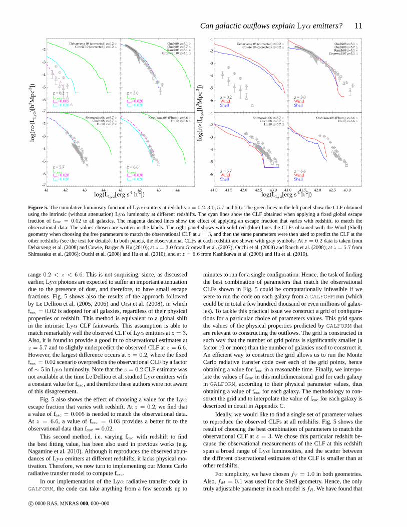
Fig. 4 shows the evolution of the galaxy properties listed abovein the redshift range0 < z < 7, as a function of the intrinsicLyα luminosity,LLyα,0. It is worth noting that these properties areextracted directly fromGALFORM, so they do not depend on thedetails of the outflow model.
In Fig. 4(a) we show the fraction of starbursts as a functionof intrinsic Lyα emission. Naturally, given the form of the IMFadopted, starbursts dominate in the brightest luminosity bins, re-gardless of redshift. However, the transition between quiescent andstarburstLyα emitters shifts towards fainter luminosities as we goto lower redshifts. An important consequence of this trend is thatthe nature ofLyα emitters, even at a fixed intrinsicLyα luminosity,is redshift dependent. Moreover, one might expect that the environ-ment in whichLyα photons escape in quiescent galaxies and star-bursts is different. Although our fiducial outflow geometries do notmake such a distinction, in section 4.2 we make our outflow geome-tries scale differently with redshift depending on whethergalaxiesare quiescent or starbursts.
In Fig. 4(b) we show the dependence of the cold gas mass onthe intrinsicLyα luminosity. As expected, in general the cold gasmass increases withLLyα,0 at a given redshift, since the latter isdirectly proportional to the star formation rate of galaxies, and, inthis variant ofGALFORM, the star formation rate is directly pro-portional to the cold gas mass, as shown in Eq. (16). Note the starformation timescale is different for quiescent and starburst galaxies(see Baugh et al. 2005 for details on how the star formation iscal-culated in this variant ofGALFORM, and Lagos et al. 2011 for analternative model).
At low LLyα,0 quiescent galaxies dominate, whereas brightgalaxies are predominately starbursts. However, there is alumi-nosity range in which quiescent galaxies and starbursts both con-tribute. This is shown in Fig. 4(b) by a break in the cold gas mass-luminosity relation, which occurs in the luminosity range wherelow mass starbursts are as common as massive quiescent galax-ies. This luminosity corresponds toLLyα[erg s−1 h−2] ∼ 1043
at z ∼ 0, and it shifts towards fainterLyα luminosities at higherredshifts. Atz ∼ 6, both quiescent and starbursts contribute atLLyα[erg s−1 h−2] ∼ 1041.5.
The total (disk+ bulge) mass ejection rate is found to cor-relate strongly with the intrinsicLyα luminosity, as shown in Fig.4(c). However, no significant evolution is found with redshift. Sincethe mass ejection rate due to supernovae is directly proportional tothe star formation rate, as shown in Eqns. (14) and (15), and the
c© 0000 RAS, MNRAS000, 000–000
10 A. Orsi et al.
40 41 42 43 44 45log(LLyα,0[erg s-1 h-2])
-4
-3
-2
-1
0lo
g(f
bu
rst)
z = 6.6z = 3.0z = 0.2
(a)
40 41 42 43 44 45log(LLyα,0[erg s-1 h-2])
5
6
7
8
9
10
11
12
log
(Mco
ld[M
sun/
h])
z = 6.6z = 3.0z = 0.2
(b)
40 41 42 43 44 45log(LLyα,0[erg s-1 h-2])
5
6
7
8
9
10
11
12
log
(Mej[M
sun/
h/
Gy
r])
z = 6.6z = 3.0z = 0.2
(c)
40 41 42 43 44 45log(LLyα,0[erg s-1 h-2])
-2.0
-1.5
-1.0
-0.5
0.0
0.5
1.0
log
(<R
1/2>
[kp
c/h
])
z = 6.6z = 3.0z = 0.2
(d)
40 41 42 43 44 45log(LLyα,0[erg s-1 h-2])
1.0
1.5
2.0
2.5
3.0lo
g(<
Vci
rc>
[km
/s]
)
z = 6.6z = 3.0z = 0.2
(e)
40 41 42 43 44 45log(LLyα,0[erg s-1 h-2])
-5
-4
-3
-2
-1
log
(<Z
cold
>)
z = 6.6z = 3.0z = 0.2
(f)
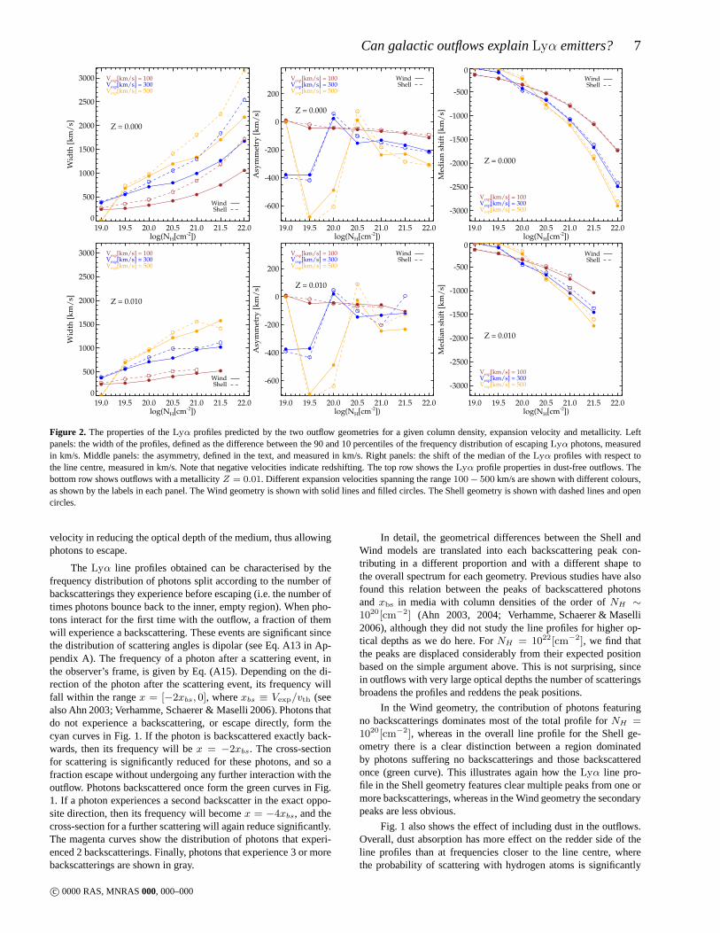
Figure 4. The evolution of the galaxy properties predicted by GALFORMwhich are used as inputs to the outflow geometries forz = 0.2 (green),z = 3.0(orange) andz = 6.6 (blue). The panels show, as a function of intrinsicLyα luminosity, median values for (a) the fraction of starbursts; (b) the cold gas massof the galaxy,Mcold; (c) the mass ejection rate,Mej; (d) the luminosity-weighted half-mass radius,〈R1/2〉; (e) the luminosity-weighted circular velocity,〈Vcirc〉 and (f) the (mass andLyα luminosity)-weighted metallicity of the gas〈Zgas〉 (Eq. 9). Error bars show the 10-90 percentile range of the predicteddistributions.
conversion between the star formation rate andLLyα,0 depends onthe production rate of Lyc photons, but not on redshift, it isnotsurprising that the mass ejection rate does not evolve with redshift.
The half-mass radius〈R1/2〉 is the parameter that is found tohave the strongest evolution with redshift, as shown in Fig.4(d).Galaxies atz = 0.2 typically have half-mass radii of a fewkpc/h.The median size of galaxies decreases rapidly with increasing red-shift, falling by an order of magnitude or more byz = 6.6. Incontrast,〈R1/2〉 varies only weakly withLLyα,0.
The circular velocity of galaxies depends both on their massand half-mass radius. The sizes of galaxies are computed basedon angular momentum conservation, centrigugal equilibrium fordisks and virial equilibrium and energy conservation in mergers forspheroids, as described in detail by Cole et al. (2000). We find thatthe sizes correlate only weakly with the intrinsicLyα luminosity,as shown in Fig. 4(d), and although the total mass of the galaxy isnot necessarily related to the cold gas mass, the circular velocity〈Vcirc〉 has similar form to the dependence of〈Mgas〉 onLLyα,0,as shown in Fig. 4(e). This explains the break in this relation atz = 6.6, which corresponds to the switch from quiescent to burstgalaxies, as was the case for the cold gas mass.
Finally, the metallicity 〈Zcold〉 correlates strongly withLLyα,0 but fairly weakly with redshift, as shown in Fig. 4(f). Themetallicity of galaxies withLLyα[erg s−1 h−2] > 1042 is found tobe around∼ 10−2.
The quantities shown in Fig. 4 are fed into the Monte Carlo
radiative transfer code to calculate theLyα escape fractionfesc andthe line profile. The netLyα luminosity of the galaxy is then simplyLLyα = fescLLyα,0. The value offesc depends, of course, on theoutflow geometry.
4.2 Choosing the outflow parameters
In the following, we outline the procedure to choose the value ofthe free parameters of our outflow models. Our strategy to setthevalue of these parameters ([fM , fV , fR] for the Shell geometry, and[fV , fR] for the Wind geometry) consists of matching the observedcumulativeLyα luminosity functions (CLFs) in the redshift range0 < z < 7. Then, we use the values obtained to make the predic-tions in the remainder of the paper.
A similar strategy was followed in previous modelling ofLyα emitters (Le Delliou et al. 2005, 2006; Nagamine et al. 2006;Kobayashi, Totani & Nagashima 2007). However, it is worth point-ing out that, to date, the model presented here is the only onethatattempts to match the recently observed abundances ofLyα emit-ters atz = 0.2 and at higher redshifts at the same time.
As a first step towards our definitive model, we show in the leftpanel of Fig. 5 the cumulative luminosity function (CLF) predictedbyGALFORM alone and applying a fixedfesc, i.e. without using theMonte Carlo radiative transfer code.
The CLF constructed using the intrinsicLyα luminosity ofgalaxies greatly overpredicts the observed estimates in the redshift
c© 0000 RAS, MNRAS000, 000–000
Can galactic outflows explainLyα emitters? 11
log(LLyα[erg s-1 h-2])
log
(n>
(LL
yα)
[h3 M
pc-3
])
-7
-6
-5
-4
-3
-2
fesc=0.020fesc=0.005LLyα,0
z = 0.2
Deharveng 08 (corrected) z=0.2Cowie 10 (corrected), z=0.2
fesc=0.020fesc=0.020LLyα,0
z = 3.0
Ouchi08 z=3.1Ouchi08 z=3.7Rauch08 z=3.1
Gronwall 07 z=3.1
41 42 43 44-7
-6
-5
-4
-3
-2
fesc=0.020fesc=0.020LLyα,0
z = 5.7
Shimasaku06, z=5.7Ouchi08, z=5.7
Hu10, z=5.7
41 42 43 44
fesc=0.020fesc=0.030LLyα,0
z = 6.6
Kashikawa06 (Photo), z=6.6Hu10, z=6.6
log(LLyα[erg s-1 h-2])lo
g(n
>(L
Ly
α[h
3 Mp
c-3])
-6
-5
-4
-3
-2
-1
ShellWindz = 0.2
Deharveng 08 (corrected) z=0.2Cowie 10 (corrected), z=0.2
ShellWindz = 3.0
Ouchi08 z=3.1Ouchi08 z=3.7Rauch08 z=3.1
Gronwall 07 z=3.1
41.0 41.5 42.0 42.5 43.0
-6
-5
-4
-3
-2
-1
ShellWindz = 5.7
Shimasaku06, z=5.7Ouchi08, z=5.7
Hu10, z=5.7
41.0 41.5 42.0 42.5 43.0
ShellWindz = 6.6
Kashikawa06 (Photo), z=6.6Hu10, z=6.6
Figure 5. The cumulative luminosity function ofLyα emitters at redshiftsz = 0.2, 3.0, 5.7 and6.6. The green lines in the left panel show the CLF obtainedusing the intrinsic (without attenuation)Lyα luminosity at different redshifts. The cyan lines show the CLF obtained when applying a fixed global escapefraction of fesc = 0.02 to all galaxies. The magenta dashed lines show the effect of applying an escape fraction that varies with redshift, to match theobservational data. The values chosen are written in the labels. The right panel shows with solid red (blue) lines the CLFs obtained with the Wind (Shell)geometry when choosing the free parameters to match the observational CLF atz = 3, and then the same parameters were then used to predict the CLF at theother redshifts (see the text for details). In both panels, the observational CLFs at each redshift are shown with gray symbols: Atz = 0.2 data is taken fromDeharveng et al. (2008) and Cowie, Barger & Hu (2010); atz = 3.0 from Gronwall et al. (2007); Ouchi et al. (2008) and Rauch et al. (2008); atz = 5.7 fromShimasaku et al. (2006); Ouchi et al. (2008) and Hu et al. (2010); and atz = 6.6 from Kashikawa et al. (2006) and Hu et al. (2010).
range0.2 < z < 6.6. This is not surprising, since, as discussedearlier,Lyα photons are expected to suffer an important attenuationdue to the presence of dust, and therefore, to have small escapefractions. Fig. 5 shows also the results of the approach followedby Le Delliou et al. (2005, 2006) and Orsi et al. (2008), in whichfesc = 0.02 is adopted for all galaxies, regardless of their physicalproperties or redshift. This method is equivalent to a global shiftin the intrinsicLyα CLF faintwards. This assumption is able tomatch remarkably well the observed CLF ofLyα emitters atz = 3.Also, it is found to provide a good fit to observational estimates atz = 5.7 and to slightly underpredict the observed CLF atz = 6.6.However, the largest difference occurs atz = 0.2, where the fixedfesc = 0.02 scenario overpredicts the observational CLF by a factorof ∼ 5 in Lyα luminosity. Note that thez = 0.2 CLF estimate wasnot available at the time Le Delliou et al. studiedLyα emitters witha constant value forfesc, and therefore these authors were not awareof this disagreement.
Fig. 5 also shows the effect of choosing a value for theLyαescape fraction that varies with redshift. Atz = 0.2, we find thata value offesc = 0.005 is needed to match the observational data.At z = 6.6, a value offesc = 0.03 provides a better fit to theobservational data thanfesc = 0.02.
This second method, i.e. varyingfesc with redshift to findthe best fitting value, has been also used in previous works (e.g.Nagamine et al. 2010). Although it reproduces the observed abun-dances ofLyα emitters at different redshifts, it lacks physical mo-tivation. Therefore, we now turn to implementing our Monte Carloradiative transfer model to computefesc.
In our implementation of theLyα radiative transfer code inGALFORM, the code can take anything from a few seconds up to
minutes to run for a single configuration. Hence, the task of findingthe best combination of parameters that match the observationalCLFs shown in Fig. 5 could be computationally infeasible if wewere to run the code on each galaxy from aGALFORM run (whichcould be in total a few hundred thousand or even millions of galax-ies). To tackle this practical issue we construct a grid of configura-tions for a particular choice of parameters values. This grid spansthe values of the physical properties predicted byGALFORM thatare relevant to constructing the outflows. The grid is constructed insuch way that the number of grid points is significantly smaller (afactor 10 or more) than the number of galaxies used to construct it.An efficient way to construct the grid allows us to run the MonteCarlo radiative transfer code over each of the grid points, henceobtaining a value forfesc in a reasonable time. Finally, we interpo-late the values offesc in this multidimensional grid for each galaxyin GALFORM, according to their physical parameter values, thusobtaining a value offesc for each galaxy. The methodology to con-struct the grid and to interpolate the value offesc for each galaxy isdescribed in detail in Appendix C.
Ideally, we would like to find a single set of parameter valuesto reproduce the observed CLFs at all redshifts. Fig. 5 showstheresult of choosing the best combination of parameters to match theobservational CLF atz = 3. We chose this particular redshift be-cause the observational measurements of the CLF at this redshiftspan a broad range ofLyα luminosities, and the scatter betweenthe different observational estimates of the CLF is smallerthan atother redshifts.
For simplicity, we have chosenfV = 1.0 in both geometries.Also, fM = 0.1 was used for the Shell geometry. Hence, the onlytruly adjustable parameter in each model isfR. We have found that
c© 0000 RAS, MNRAS000, 000–000
12 A. Orsi et al.
log(LLyα[erg s-1 h-2])
log
(n>
(LL
yα)
[h3 M
pc-3
])
-7
-6
-5
-4
-3
-2
StarburstQuiescentShell
Windz = 0.2
Deharveng 08 (corrected) z=0.2Cowie 10 (corrected), z=0.2
StarburstQuiescentShell
Windz = 3.0
Ouchi08 z=3.1Ouchi08 z=3.7Rauch08 z=3.1
Gronwall 07 z=3.1
41.0 41.5 42.0 42.5 43.0-7
-6
-5
-4
-3
-2
StarburstQuiescentShell
Windz = 5.7
Shimasaku06, z=5.7Ouchi08, z=5.7
Hu10, z=5.7
41.0 41.5 42.0 42.5 43.0
StarburstQuiescentShell
Windz = 6.6
Kashikawa06 (Photo), z=6.6Hu10, z=6.6
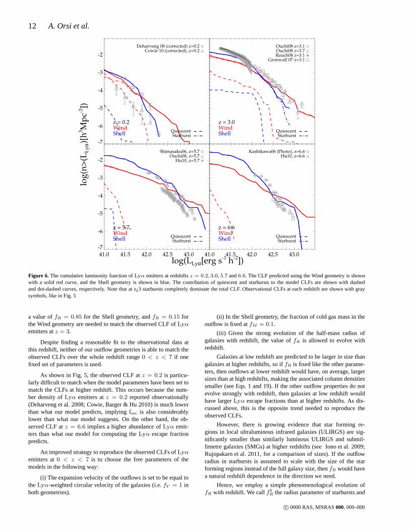
Figure 6. The cumulative luminosity function ofLyα emitters at redshiftsz = 0.2, 3.0, 5.7 and6.6. The CLF predicted using the Wind geometry is shownwith a solid red curve, and the Shell geometry is shown in blue. The contribution of quiescent and starbursts to the model CLFs are shown with dashedand dot-dashed curves, respectively. Note that at z¿3 starbursts completely dominate the total CLF. Observational CLFs at each redshift are shown with graysymbols, like in Fig. 5
a value offR = 0.85 for the Shell geometry, andfR = 0.15 forthe Wind geometry are needed to match the observed CLF ofLyαemitters atz = 3.
Despite finding a reasonable fit to the observational data atthis redshift, neither of our outflow geometries is able to match theobserved CLFs over the whole redshift range0 < z < 7 if onefixed set of parameters is used.
As shown in Fig. 5, the observed CLF atz = 0.2 is particu-larly difficult to match when the model parameters have been set tomatch the CLFs at higher redshift. This occurs because the num-ber density ofLyα emitters atz = 0.2 reported observationally(Deharveng et al. 2008; Cowie, Barger & Hu 2010) is much lowerthan what our model predicts, implyingfesc is also considerablylower than what our model suggests. On the other hand, the ob-served CLF atz = 6.6 implies a higher abundance ofLyα emit-ters than what our model for computing theLyα escape fractionpredicts.
An improved strategy to reproduce the observed CLFs ofLyαemitters at0 < z < 7 is to choose the free parameters of themodels in the following way:
(i) The expansion velocity of the outflows is set to be equal totheLyα-weighted circular velocity of the galaxies (i.e.fV = 1 inboth geometries).
(ii) In the Shell geometry, the fraction of cold gas mass in theoutflow is fixed atfM = 0.1.
(iii) Given the strong evolution of the half-mass radius ofgalaxies with redshift, the value offR is allowed to evolve withredshift.
Galaxies at low redshift are predicted to be larger in size thangalaxies at higher redshifts, so iffR is fixed like the other parame-ters, then outflows at lower redshift would have, on average,largersizes than at high redshifts, making the associated column densitiessmaller (see Eqs. 1 and 19). If the other outflow properties donotevolve strongly with redshift, then galaxies at low redshift wouldhave largerLyα escape fractions than at higher redshifts. As dis-cussed above, this is the opposite trend needed to reproducetheobserved CLFs.
However, there is growing evidence that star forming re-gions in local ultraluminous infrared galaxies (ULIRGS) are sig-nificantly smaller than similarly luminous ULIRGS and submil-limetre galaxies (SMGs) at higher redshifts (see Iono et al.2009;Rujopakarn et al. 2011, for a comparison of sizes). If the outflowradius in starbursts is assumed to scale with the size of the starforming regions instead of the full galaxy size, thenfR would havea natural redshift dependence in the direction we need.
Hence, we employ a simple phenomenological evolution offR with redshift. We callfb
R the radius parameter of starbursts and
c© 0000 RAS, MNRAS000, 000–000
Can galactic outflows explainLyα emitters? 13
fM fV fqR fb
R,0 γ
Shell 0.10 1.00 0.200 0.223 0.925Wind – 1.00 0.015 0.014 2.152
Table 1.Summary of the parameter values of the Shell and Wind geometriesused to fit theLyα cumulative luminosity function at different redshifts (seethe text for details).
allow it to scale with redshift like a power-law:
fbR = fb
R,0(1 + z)γ , (21)
wherefbR,0 andγ are free parameters. Since there is no equivalent
observational evidence for the size of star forming regionsin quies-cent galaxies scaling with redshift, we setfq
R, the radius parameterfor quiescent galaxies, to be an adjustable parameter but fixed (i.e.independent of redshift).
Table 1 summarizes a suitable choice of the parameters valuesused in our model. Also, Fig. 6 shows the predicted cumulativeluminosity functions obtained with that choice of parameters.
Our previous modelling ofLyα emitters used the simple as-sumption of a constantLyα escape fraction, withfesc = 0.02 be-ing a suitable value to reproduce theLyα CLFs at3 < z < 7(Le Delliou et al. 2005, 2006; Orsi et al. 2008). As shown in Fig.5, this simple model overestimates the CLF atz = 0.2, but it re-produces remarkably well the CLFs at higher redshifts. Our out-flow geometries, on the other hand, are consistent with the obser-vational CLFs at all redshifts, although they fail to reproduce theirfull shape. This may be surprising at first, since the intrinsic LyαCLF (shown in green in Fig. 5) roughly reproduces the shape oftheobserved CLFs, although displaced to brighter luminosities (whichis why the constant escape fraction scenario works well at repro-ducing the CLFs). However, in our model, the escape fractionineach galaxy is the result of a complex interplay between severalphysical properties, and this in turn modifies the resultingshape ofthe CLF.
The sizes of the outflows predicted by our model, com-pared to the extent of the galaxies themselves (quantified bythehalf-mass radius〈R1/2〉) are very different between the two out-flow geometries. In quiescent galaxies these are1.5 and 20 per-cent of the half-mass radius of the galaxies, in the Wind andShell geometries respectively. Similarly, atz = 0.2, outflowsin starbursts are2 and 26 percent of the half-mass radius inthe Wind and Shell geometries. The rather small size of out-flows in the Wind geometry appears to be in contradiction withobservations ofLyα in local starbursts which display galactic-scale outflows (see, e.g. Giavalisco, Koratkar & Calzetti 1996;Thuan & Izotov 1997; Kunth et al. 1998; Mas-Hesse et al. 2003;Ostlin et al. 2009; Mas-Hesse et al. 2009). However, local starburstsamples are sparse and still probably not large enough to charac-terise the nature (in a statistical sense) ofLyα emitters at low red-shifts.
At higher redshifts, our model keeps the sizes of outflows inquiescent galaxies unchanged (with respect to their half-mass ra-dius). However, outflows in starbursts grow in radius, relative totheir host galaxy, according to a power law, as given by Eq. (21),with the best fitting values listed in Table 1, so atz = 3 their sizesare 27 and 80 percent of the half-mass radius for the Wind andShell geometries, respectively. Byz = 6.6, the sizes are110 and145 percent of the half-mass radius. Therefore, atz & 3, all out-flows inLyα-emitting starbursts are galactic-scale according to ourmodels.
log(LLyα[erg s-1 h-2])
log
(NH
[cm
-2])
18
20
22
24
Wind z = 0.2
18
20
22
24z = 3.0
38 40 42 4418
20
22
24z = 6.6
Shell
38 40 42 44
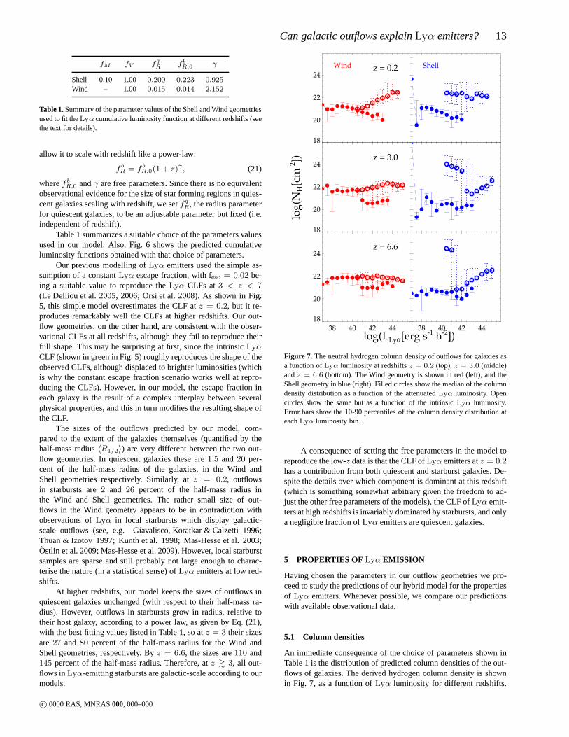
Figure 7. The neutral hydrogen column density of outflows for galaxiesasa function ofLyα luminosity at redshiftsz = 0.2 (top),z = 3.0 (middle)andz = 6.6 (bottom). The Wind geometry is shown in red (left), and theShell geometry in blue (right). Filled circles show the median of the columndensity distribution as a function of the attenuatedLyα luminosity. Opencircles show the same but as a function of the intrinsicLyα luminosity.Error bars show the 10-90 percentiles of the column density distribution ateachLyα luminosity bin.
A consequence of setting the free parameters in the model toreproduce the low-z data is that the CLF ofLyα emitters atz = 0.2has a contribution from both quiescent and starburst galaxies. De-spite the details over which component is dominant at this redshift(which is something somewhat arbitrary given the freedom toad-just the other free parameters of the models), the CLF ofLyα emit-ters at high redshifts is invariably dominated by starbursts, and onlya negligible fraction ofLyα emitters are quiescent galaxies.
5 PROPERTIES OFLyα EMISSION
Having chosen the parameters in our outflow geometries we pro-ceed to study the predictions of our hybrid model for the propertiesof Lyα emitters. Whenever possible, we compare our predictionswith available observational data.
5.1 Column densities
An immediate consequence of the choice of parameters shown inTable 1 is the distribution of predicted column densities ofthe out-flows of galaxies. The derived hydrogen column density is shownin Fig. 7, as a function ofLyα luminosity for different redshifts.
c© 0000 RAS, MNRAS000, 000–000
14 A. Orsi et al.
log(LLyα[erg s-1 h-2])
log
(fes
c(L
yα)
)
-3.0
-2.5
-2.0
-1.5
-1.0
-0.5
0.0
Wind
z = 0.2
-3.0
-2.5
-2.0
-1.5
-1.0
-0.5
0.0
z = 3.0
38 40 42 44
-3.0
-2.5
-2.0
-1.5
-1.0
-0.5
0.0
z = 6.6
Shell
38 40 42 44
Figure 8. The escape fraction as a function ofLyα luminosity atz = 0.2(top),z = 3.0 (middle) andz = 6.6 (bottom). The Wind geometry predic-tions are shown in red (left), and the Shell geometry in blue (right). Solidcircles show the median of the escape fraction at different attenuatedLyαluminosity bins. Open circles show the same relation as a function of in-trinsic Lyα luminosity instead. Error bars represent the 10-90 percentilesaround the median of the escape fraction distribution at a givenLyα lumi-nosity bin.
Here we study this distribution both as a function of intrinsic andattenuatedLyα luminosity.
When studied as a function of intrinsicLyα luminosity, ourmodel displays a large range of column densities, varying fromNH ∼ 1021[cm−2] toNH ∼ 1024[cm−2], depending on the out-flow geometry and the redshift. Typically, in both outflow geome-tries, the column density increases with intrinsicLyα luminosity,which is due to the overall increase in the mass of cold gas andthemass ejection rate with intrinsicLyα luminosity. However, in somecases, there is a noticeable decrease of the column density with in-creasing intrinsicLyα luminosity, reflecting the rather complicatedrelation between the quantities which affect the column density andthe intrinsicLyα luminosity, as shown in Fig. 4.
When including attenuation due to dust, this relation is mod-ified, as shown by the solid circles in Fig. 7. The number of scat-terings scales with the column density of the medium, hence theescape fraction is low (or effectively zero in some cases, accord-ing to our model) for outflows with large column densities. Asaresult, the column density distribution as a function of attenuatedLyα luminosity spansNH ∼ 1019−22 [cm−2]. Also, galaxies withbrighter (attenuated)Lyα luminosities tend to have smaller columndensities.
The column densities predicted by our models are similar tothose inferred by Verhamme et al. (2008) on fitting their models to
a small sample of high redshift galaxies with high resolution spec-tra. These authors fitLyα line profiles with a Monte Carlo radia-tive transfer model using a geometry identical to our Shell geom-etry. In addition, Verhamme et al. present a compilation of resultsfor observationally-measured column densities of local starburstsshowingLyα emission, with values between1019 − 1022[cm−2],which are also consistent with our model predictions.
5.2 Lyα escape fractions
A fundamental prediction of our models is the distribution of Lyαescape fractions, shown in Fig. 8. In terms of the attenuatedLyαemission, we find thatfesc grows monotonically from10−3 inthe faintestLyα emitters (withLLyα ∼ 1038[erg s−1h−2]) tofesc ∼ 0.3 at LLyα ∼ 1040[erg s−1h−2]. Brighter galaxies havein general escape fractions ranging from0.1 to ∼ 1, depending onthe redshift and outflow geometry. Perhaps not surprisingly, bothmodels predict similar distributions of escape fractions as a func-tion of Lyα luminosity, since the models are forced to match theobserved CLFs (Section 4.2).
On the other hand, in terms of the intrinsicLyα emission, Fig.8 shows that only in some cases it is possible to obtain a median fescabove zero. This reflects the complicated interplay of physical con-ditions which shape the escape fraction ofLyα photons. In otherwords, the value of the intrinsicLyα luminosity in a galaxy doesnot determinefesc and, therefore, its attenuatedLyα luminosity.
Fig. 8 illustrates further the contrast betweetn using a phys-ical model to compute theLyα escape fraction, and the constantfesc scenario. In the former, galaxies seen with highLyα luminosi-ties have high escape fractions, so their intrinsicLyα luminositiesare similar to the attenuated ones. Fainter galaxies, on theotherhand, have lower escape fractions, meaning that their intrinsicLyαluminosity is orders of magnitude higher than their observed lumi-nosity. This implies that aLyα emitter with a given intrinsicLyαluminosity could have either a high or low value offesc, dependingon its physical characteristics (galaxy size, metallicity, circular ve-locity, SFR, etc.). In the constant escape fraction scenario, on theother hand, all galaxies at a given observedLyα luminosity havethe same intrinsic luminosity, which means that galaxies need onlyto have a high intrinsicLyα luminosity to be observed asLyαemitters.
We conclude from Fig. 8 that a high production ofLyα pho-tons (or, equivalently, high intrinsic Lyman continuum luminosity)does not guarantee that a galaxy is visible inLyα. Our modellingof the escape fraction selects a particular population of galaxies tobe observed asLyα emitters, which in general is found to havelower metallicities, lower SFRs and larger half-mass radiithan thebulk of the galaxy population. This is discussed in more detail inSection 6.
It is worth asking at this point whether the predicted escapefractions are consistent with observational estimates. Observation-ally, fesc is generally calculated either by inferring the SFRs fromthe Lyα luminosity and comparing to the SFR estimated fromthe UV continuum (e.g. Gawiser et al. 2006; Blanc et al. 2011;Guaita et al. 2010), or by using the ratio betweenLyα and anothernon-resonant hydrogen recombination line. The former requires as-sumptions about the stellar evolution model, the choice of the IMFand the modelling of dust extinction. The second method onlyre-lies on the assumption that the comparison line is not affected byresonant scattering, and thus the extinction can be estimated reli-ably from an extinction curve, and that the intrinsic line ratio cor-
c© 0000 RAS, MNRAS000, 000–000
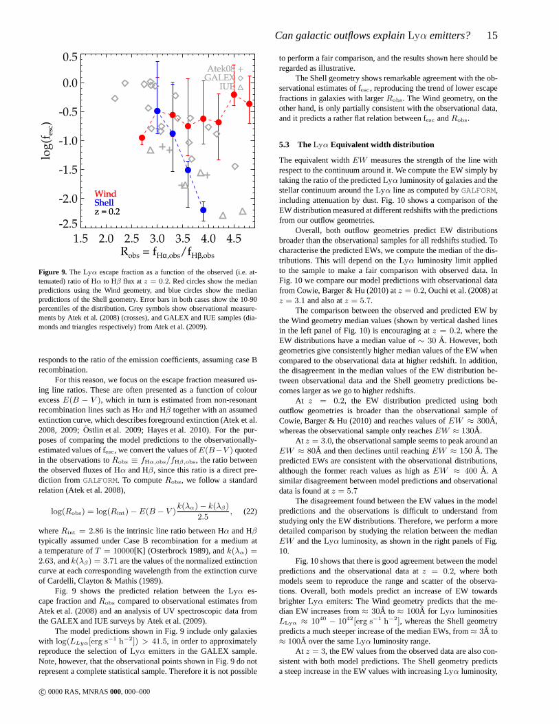
Can galactic outflows explainLyα emitters? 15
1.5 2.0 2.5 3.0 3.5 4.0 4.5Robs = fHα,obs/fHβ,obs
-2.5
-2.0
-1.5
-1.0
-0.5
0.0
0.5lo
g(f
esc)
z = 0.2ShellWind
Atek08GALEX
IUE
z = 0.2ShellWind
Atek08GALEX
IUE
Figure 9. TheLyα escape fraction as a function of the observed (i.e. at-tenuated) ratio of Hα to Hβ flux at z = 0.2. Red circles show the medianpredictions using the Wind geometry, and blue circles show the medianpredictions of the Shell geometry. Error bars in both cases show the 10-90percentiles of the distribution. Grey symbols show observational measure-ments by Atek et al. (2008) (crosses), and GALEX and IUE samples (dia-monds and triangles respectively) from Atek et al. (2009).
responds to the ratio of the emission coefficients, assumingcase Brecombination.
For this reason, we focus on the escape fraction measured us-ing line ratios. These are often presented as a function of colourexcessE(B − V ), which in turn is estimated from non-resonantrecombination lines such as Hα and Hβ together with an assumedextinction curve, which describes foreground extinction (Atek et al.2008, 2009;Ostlin et al. 2009; Hayes et al. 2010). For the pur-poses of comparing the model predictions to the observationally-estimated values offesc, we convert the values ofE(B−V ) quotedin the observations toRobs ≡ fHα,obs/fHβ,obs, the ratio betweenthe observed fluxes ofHα and Hβ, since this ratio is a direct pre-diction fromGALFORM. To computeRobs, we follow a standardrelation (Atek et al. 2008),
log(Robs) = log(Rint)− E(B − V )k(λα)− k(λβ)
2.5, (22)
whereRint = 2.86 is the intrinsic line ratio between Hα and Hβtypically assumed under Case B recombination for a medium ata temperature ofT = 10000[K] (Osterbrock 1989), andk(λα) =2.63, andk(λβ) = 3.71 are the values of the normalized extinctioncurve at each corresponding wavelength from the extinctioncurveof Cardelli, Clayton & Mathis (1989).
Fig. 9 shows the predicted relation between theLyα es-cape fraction andRobs compared to observational estimates fromAtek et al. (2008) and an analysis of UV spectroscopic data fromthe GALEX and IUE surveys by Atek et al. (2009).
The model predictions shown in Fig. 9 include only galaxieswith log(LLyα[erg s−1 h−2]) > 41.5, in order to approximatelyreproduce the selection ofLyα emitters in the GALEX sample.Note, however, that the observational points shown in Fig. 9do notrepresent a complete statistical sample. Therefore it is not possible
to perform a fair comparison, and the results shown here should beregarded as illustrative.
The Shell geometry shows remarkable agreement with the ob-servational estimates offesc, reproducing the trend of lower escapefractions in galaxies with largerRobs. The Wind geometry, on theother hand, is only partially consistent with the observational data,and it predicts a rather flat relation betweenfesc andRobs.
5.3 TheLyα Equivalent width distribution
The equivalent widthEW measures the strength of the line withrespect to the continuum around it. We compute the EW simply bytaking the ratio of the predictedLyα luminosity of galaxies and thestellar continuum around theLyα line as computed byGALFORM,including attenuation by dust. Fig. 10 shows a comparison oftheEW distribution measured at different redshifts with the predictionsfrom our outflow geometries.
Overall, both outflow geometries predict EW distributionsbroader than the observational samples for all redshifts studied. Tocharacterise the predicted EWs, we compute the median of thedis-tributions. This will depend on theLyα luminosity limit appliedto the sample to make a fair comparison with observed data. InFig. 10 we compare our model predictions with observationaldatafrom Cowie, Barger & Hu (2010) atz = 0.2, Ouchi et al. (2008) atz = 3.1 and also atz = 5.7.
The comparison between the observed and predicted EW bythe Wind geometry median values (shown by vertical dashed linesin the left panel of Fig. 10) is encouraging atz = 0.2, where theEW distributions have a median value of∼ 30 A. However, bothgeometries give consistently higher median values of the EWwhencompared to the observational data at higher redshift. In addition,the disagreement in the median values of the EW distributionbe-tween observational data and the Shell geometry predictions be-comes larger as we go to higher redshifts.
At z = 0.2, the EW distribution predicted using bothoutflow geometries is broader than the observational sampleofCowie, Barger & Hu (2010) and reaches values ofEW ≈ 300A,whereas the observational sample only reachesEW ≈ 130A.
At z = 3.0, the observational sample seems to peak around anEW ≈ 80A and then declines until reachingEW ≈ 150 A. Thepredicted EWs are consistent with the observational distributions,although the former reach values as high asEW ≈ 400 A. Asimilar disagreement between model predictions and observationaldata is found atz = 5.7
The disagreement found between the EW values in the modelpredictions and the observations is difficult to understandfromstudying only the EW distributions. Therefore, we perform amoredetailed comparison by studying the relation between the medianEW and theLyα luminosity, as shown in the right panels of Fig.10.
Fig. 10 shows that there is good agreement between the modelpredictions and the observational data atz = 0.2, where bothmodels seem to reproduce the range and scatter of the observa-tions. Overall, both models predict an increase of EW towardsbrighterLyα emiters: The Wind geometry predicts that the me-dian EW increases from≈ 30A to ≈ 100A for Lyα luminositiesLLyα ≈ 1040 − 1042[erg s−1 h−2], whereas the Shell geometrypredicts a much steeper increase of the median EWs, from≈ 3A to≈ 100A over the sameLyα luminosity range.
At z = 3, the EW values from the observed data are also con-sistent with both model predictions. The Shell geometry predictsa steep increase in the EW values with increasingLyα luminosity,
c© 0000 RAS, MNRAS000, 000–000
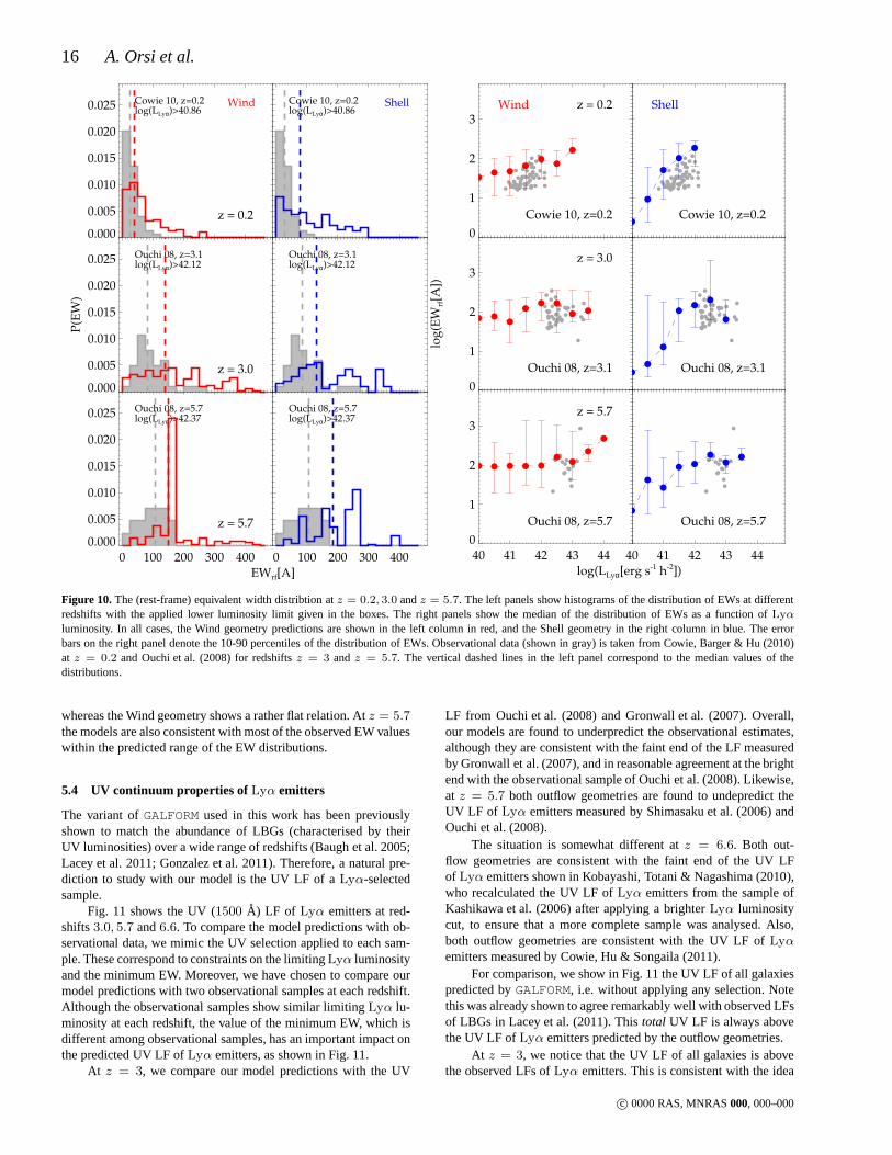
16 A. Orsi et al.
EWrf[A]
P(E
W)
0.000
0.005
0.010
0.015
0.020
0.025 WindCowie 10, z=0.2log(LLyα)>40.86
z = 0.2
0.000
0.005
0.010
0.015
0.020
0.025 Ouchi 08, z=3.1log(LLyα)>42.12
z = 3.0
0 100 200 300 4000.000
0.005
0.010
0.015
0.020
0.025 Ouchi 08, z=5.7log(LLyα)>42.37
z = 5.7
ShellCowie 10, z=0.2log(LLyα)>40.86
Ouchi 08, z=3.1log(LLyα)>42.12
0 100 200 300 400
Ouchi 08, z=5.7log(LLyα)>42.37
log(LLyα[erg s-1 h-2])
log
(EW
rf[A
])
0
1
2
3Wind
Cowie 10, z=0.2
z = 0.2
0
1
2
3
Ouchi 08, z=3.1
z = 3.0
40 41 42 43 440
1
2
3
Ouchi 08, z=5.7
z = 5.7
Shell
Cowie 10, z=0.2
Ouchi 08, z=3.1
40 41 42 43 44
Ouchi 08, z=5.7
Figure 10.The (rest-frame) equivalent width distribtion atz = 0.2, 3.0 andz = 5.7. The left panels show histograms of the distribution of EWs at differentredshifts with the applied lower luminosity limit given in the boxes. The right panels show the median of the distribution of EWs as a function ofLyαluminosity. In all cases, the Wind geometry predictions areshown in the left column in red, and the Shell geometry in the right column in blue. The errorbars on the right panel denote the 10-90 percentiles of the distribution of EWs. Observational data (shown in gray) is taken from Cowie, Barger & Hu (2010)at z = 0.2 and Ouchi et al. (2008) for redshiftsz = 3 andz = 5.7. The vertical dashed lines in the left panel correspond to the median values of thedistributions.
whereas the Wind geometry shows a rather flat relation. Atz = 5.7the models are also consistent with most of the observed EW valueswithin the predicted range of the EW distributions.
5.4 UV continuum properties ofLyα emitters
The variant ofGALFORM used in this work has been previouslyshown to match the abundance of LBGs (characterised by theirUV luminosities) over a wide range of redshifts (Baugh et al.2005;Lacey et al. 2011; Gonzalez et al. 2011). Therefore, a natural pre-diction to study with our model is the UV LF of aLyα-selectedsample.
Fig. 11 shows the UV (1500 A) LF of Lyα emitters at red-shifts3.0, 5.7 and6.6. To compare the model predictions with ob-servational data, we mimic the UV selection applied to each sam-ple. These correspond to constraints on the limitingLyα luminosityand the minimum EW. Moreover, we have chosen to compare ourmodel predictions with two observational samples at each redshift.Although the observational samples show similar limitingLyα lu-minosity at each redshift, the value of the minimum EW, whichisdifferent among observational samples, has an important impact onthe predicted UV LF ofLyα emitters, as shown in Fig. 11.
At z = 3, we compare our model predictions with the UV
LF from Ouchi et al. (2008) and Gronwall et al. (2007). Overall,our models are found to underpredict the observational estimates,although they are consistent with the faint end of the LF measuredby Gronwall et al. (2007), and in reasonable agreement at thebrightend with the observational sample of Ouchi et al. (2008). Likewise,at z = 5.7 both outflow geometries are found to undepredict theUV LF of Lyα emitters measured by Shimasaku et al. (2006) andOuchi et al. (2008).
The situation is somewhat different atz = 6.6. Both out-flow geometries are consistent with the faint end of the UV LFof Lyα emitters shown in Kobayashi, Totani & Nagashima (2010),who recalculated the UV LF ofLyα emitters from the sample ofKashikawa et al. (2006) after applying a brighterLyα luminositycut, to ensure that a more complete sample was analysed. Also,both outflow geometries are consistent with the UV LF ofLyαemitters measured by Cowie, Hu & Songaila (2011).
For comparison, we show in Fig. 11 the UV LF of all galaxiespredicted byGALFORM, i.e. without applying any selection. Notethis was already shown to agree remarkably well with observed LFsof LBGs in Lacey et al. (2011). Thistotal UV LF is always abovethe UV LF ofLyα emitters predicted by the outflow geometries.
At z = 3, we notice that the UV LF of all galaxies is abovethe observed LFs ofLyα emitters. This is consistent with the idea
c© 0000 RAS, MNRAS000, 000–000
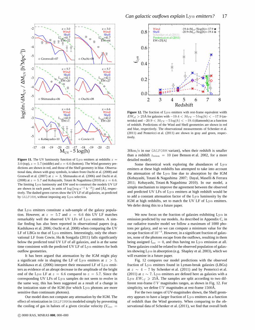
Can galactic outflows explainLyα emitters? 17
MUV - 5 log(h)
log
(dn
/d
MU
V /
∆M
UV [
h3 M
pc-3
])
-5
-4
-3
-2 z = 3.0WindShell
LLyα>41.7EW>22
Gronwall+07
z = 3.0WindShell
LLyα>41.7EW>64
Ouchi+08
-5
-4
-3
-2 z = 5.7WindShell
LLyα>42.1EW>20
Shimasaku+06
z = 5.7WindShell
LLyα>42.1EW>27
Ouchi+08
-17 -18 -19 -20 -21
-5
-4
-3
-2 z = 6.6WindShell
LLyα>42.0EW>7.
Kobayashi+10
-17 -18 -19 -20 -21
z = 6.6WindShell
LLyα>42.2EW>20
Cowie+11
Figure 11. The UV luminosity function ofLyα emitters at redshiftsz =3.0 (top),z = 5.7 (middle) andz = 6.6 (bottom). The Wind geometry pre-dictions are shown in red, and those of the Shell geometry in blue. Observa-tional data, shown with gray symbols, is taken from Ouchi et al. (2008) andGronwall et al. (2007) atz = 3, Shimasaku et al. (2006) and Ouchi et al.(2008) atz = 5.7 and Kobayashi, Totani & Nagashima (2010) atz = 6.6.The limitingLyα luminosity and EW used to construct the models UV LFare shown in each panel, in units oflog([erg s−1 h−2]) and [A], respec-tively. The dashed green curves show the UV LF of all galaxies, as predictedby GALFORM, without imposing anyLyα selection.
that Lyα emitters constitute a sub-sample of the galaxy popula-tion. However, atz = 5.7 and z = 6.6 this UV LF matchesremarkably well the observed UV LFs ofLyα emitters. A sim-ilar finding has also been reported in observational papers (e.g.Kashikawa et al. 2006; Ouchi et al. 2008) when comparing the UVLF of LBGs to that ofLyα emitters. Interestingly, only the obser-vational LF from Cowie, Hu & Songaila (2011) falls significantlybelow the predicted total UV LF of all galaxies, and is at the sametime consistent with the predicted UV LF ofLyα emitters for bothoutflow geometries.
It has been argued that attenuation by the IGM might playa significant role in shaping the LF ofLyα emitters atz > 5.Kashikawa et al. (2006) interpret their measured LF ofLyα emit-ters as evidence of an abrupt decrease in the amplitude of thebrightend of theLyα LF at z = 6.6 compared toz = 5.7. Since thecorresponding UV LFs ofLyα samples do not seem to evolve inthe same way, this has been suggested as a result of a change inthe ionization state of the IGM (for whichLyα photons are moresensitive than continuum photons).
Our model does not compute any attenuation by the IGM. Theeffect of reionization inGALFORM is modeled simply by preventingthe cooling of gas in haloes of a given circular velocity (Vcirc =
2 3 4 5 6 7 8Redshift
0.0
0.2
0.4
0.6
0.8
f Ly
α
WindShellSchenker et al (2011)Pentericci et al (2011)EW>25[A]
-19.4<MUV-5log(h)<-17.9-20.9<MUV-5log(h)<-19.4
Figure 12. The fraction ofLyα emitters with rest-frame equivalent widthEWrf > 25A for galaxies with−19.4 < MUV−5 log(h) < −17.9 (as-terisks) and−20.9 < MUV−5 log(h) < −19.4 (diamonds) as a functionof redshift. Predictions of the Wind and Shell geometries are shown in redand blue, respectively. The observational measurements ofSchenker et al.(2011) and Pentericci et al. (2011) are shown in gray and green, respec-tively.
30km/s in our GALFORM variant), when their redshift is smallerthan a redshiftzreion = 10 (see Benson et al. 2002, for a moredetailed model).
Some theoretical work exploring the abundances ofLyαemitters at these high redshifts has attempted to take into accountthe attenuation of theLyα line due to absorption by the IGM(Kobayashi, Totani & Nagashima 2007; Dayal, Maselli & Ferrara2011; Kobayashi, Totani & Nagashima 2010). In our model, asimple mechanism to improve the agreement between the observedand predicted UV LFs ofLyα emitters at high redshift would beto add a constant attenuation factor of theLyα luminosity by theIGM at high redshifts, set to match the UV LF ofLyα emitters.We defer doing this to a future paper.
We now focus on the fraction of galaxies exhibitingLyα inemission predicted by our models. As described in Appendix C, inour radiative transfer model we follow a maximum of 1000 pho-tons per galaxy, and so we can compute a minimum value for theescape fraction of10−3. However, in a significant fraction of galax-ies, none of the photons escape from the outflows, resulting in thembeing assignedfesc = 0, and thus having noLyα emission at all.These galaxies could be related to the observed population of galax-ies showingLyα in absorption (e.g. Shapley et al. 2003), which wewill examine in a future paper.
Fig. 12 compares our model predictions with the observedfraction of Lyα emitters found in Lyman-break galaxies (LBGs)at z ∼ 4 − 7 by Schenker et al. (2011) and by Pentericci et al.(2011) atz ∼ 7. Lyα emitters are defined here as galaxies with aLyα EWrf > 25A. The samples are split according to two dif-ferent rest-frameUV magnitudes ranges, as shown in Fig. 12. Forsimplicity, we defineUV magnitudes at rest-frame1500A.
For the two ranges of UV-magnitudes shown, the Shell geom-etry appears to have a larger fraction ofLyα emitters as a functionof redshift than the Wind geometry. When comparing to the ob-servational data of Schenker et al. (2011), we find that overall both
c© 0000 RAS, MNRAS000, 000–000
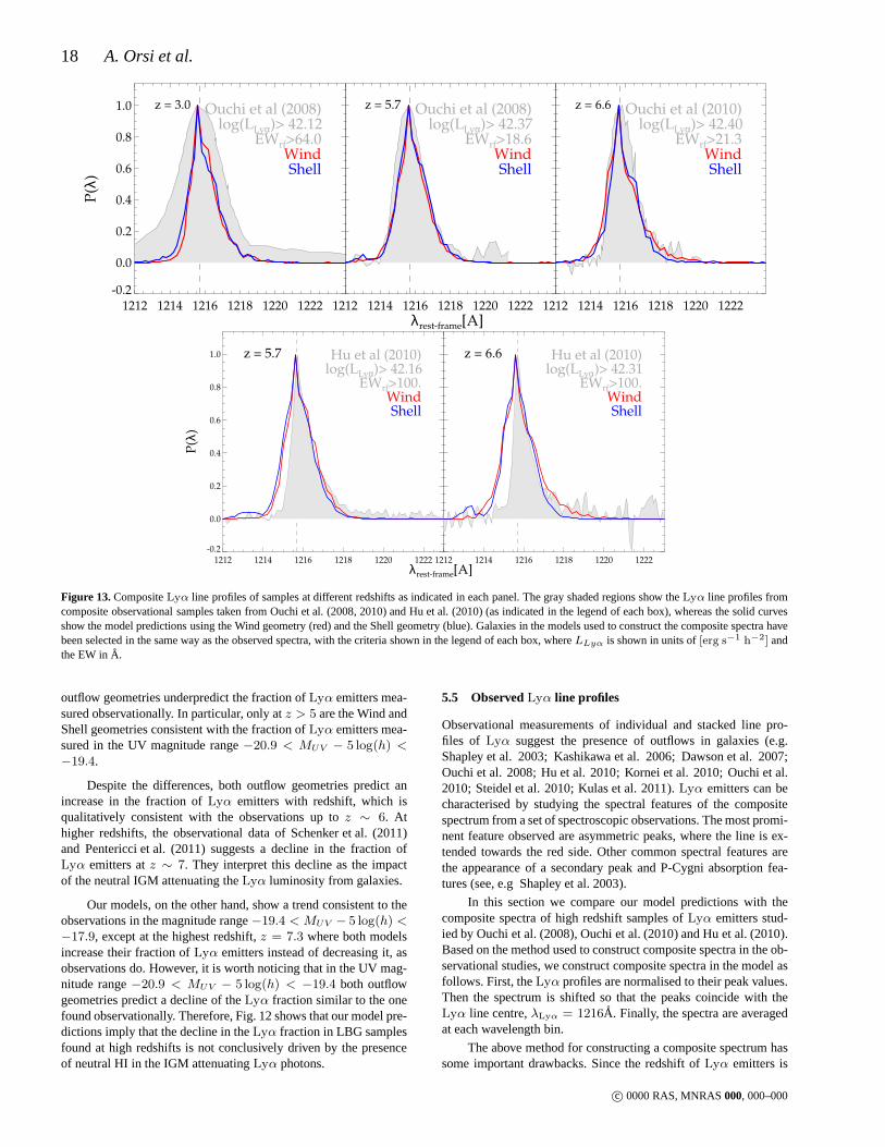
18 A. Orsi et al.
λrest-frame[A]
P(λ
)
1212 1214 1216 1218 1220 1222-0.2
0.0
0.2
0.4
0.6
0.8
1.0 z = 3.0 Ouchi et al (2008)log(LLyα)> 42.12
EWrf>64.0WindShell
1212 1214 1216 1218 1220 1222
z = 5.7 Ouchi et al (2008)log(LLyα)> 42.37
EWrf>18.6WindShell
1212 1214 1216 1218 1220 1222
z = 6.6 Ouchi et al (2010)log(LLyα)> 42.40
EWrf>21.3WindShell
λrest-frame[A]
P(λ
)
1212 1214 1216 1218 1220 1222-0.2
0.0
0.2
0.4
0.6
0.8
1.0 z = 5.7 Hu et al (2010)log(LLyα)> 42.16
EWrf>100.WindShell
1212 1214 1216 1218 1220 1222
z = 6.6 Hu et al (2010)log(LLyα)> 42.31
EWrf>100.WindShell
Figure 13.CompositeLyα line profiles of samples at different redshifts as indicatedin each panel. The gray shaded regions show theLyα line profiles fromcomposite observational samples taken from Ouchi et al. (2008, 2010) and Hu et al. (2010) (as indicated in the legend of each box), whereas the solid curvesshow the model predictions using the Wind geometry (red) andthe Shell geometry (blue). Galaxies in the models used to construct the composite spectra havebeen selected in the same way as the observed spectra, with the criteria shown in the legend of each box, whereLLyα is shown in units of[erg s−1 h−2] andthe EW inA.
outflow geometries underpredict the fraction ofLyα emitters mea-sured observationally. In particular, only atz > 5 are the Wind andShell geometries consistent with the fraction ofLyα emitters mea-sured in the UV magnitude range−20.9 < MUV − 5 log(h) <−19.4.
Despite the differences, both outflow geometries predict anincrease in the fraction ofLyα emitters with redshift, which isqualitatively consistent with the observations up toz ∼ 6. Athigher redshifts, the observational data of Schenker et al.(2011)and Pentericci et al. (2011) suggests a decline in the fraction ofLyα emitters atz ∼ 7. They interpret this decline as the impactof the neutral IGM attenuating theLyα luminosity from galaxies.
Our models, on the other hand, show a trend consistent to theobservations in the magnitude range−19.4 < MUV − 5 log(h) <−17.9, except at the highest redshift,z = 7.3 where both modelsincrease their fraction ofLyα emitters instead of decreasing it, asobservations do. However, it is worth noticing that in the UVmag-nitude range−20.9 < MUV − 5 log(h) < −19.4 both outflowgeometries predict a decline of theLyα fraction similar to the onefound observationally. Therefore, Fig. 12 shows that our model pre-dictions imply that the decline in theLyα fraction in LBG samplesfound at high redshifts is not conclusively driven by the presenceof neutral HI in the IGM attenuatingLyα photons.
5.5 ObservedLyα line profiles
Observational measurements of individual and stacked linepro-files of Lyα suggest the presence of outflows in galaxies (e.g.Shapley et al. 2003; Kashikawa et al. 2006; Dawson et al. 2007;Ouchi et al. 2008; Hu et al. 2010; Kornei et al. 2010; Ouchi et al.2010; Steidel et al. 2010; Kulas et al. 2011).Lyα emitters can becharacterised by studying the spectral features of the compositespectrum from a set of spectroscopic observations. The mostpromi-nent feature observed are asymmetric peaks, where the line is ex-tended towards the red side. Other common spectral featuresarethe appearance of a secondary peak and P-Cygni absorption fea-tures (see, e.g Shapley et al. 2003).
In this section we compare our model predictions with thecomposite spectra of high redshift samples ofLyα emitters stud-ied by Ouchi et al. (2008), Ouchi et al. (2010) and Hu et al. (2010).Based on the method used to construct composite spectra in the ob-servational studies, we construct composite spectra in themodel asfollows. First, theLyα profiles are normalised to their peak values.Then the spectrum is shifted so that the peaks coincide with theLyα line centre,λLyα = 1216A. Finally, the spectra are averagedat each wavelength bin.
The above method for constructing a composite spectrum hassome important drawbacks. Since the redshift ofLyα emitters is
c© 0000 RAS, MNRAS000, 000–000
Can galactic outflows explainLyα emitters? 19
computed from the wavelength of the peak of theLyα line, anyoffset of the peak due to radiative transfer effects is removed (seeFig. 1 and Fig. 2). On the other hand, the normalisation of thelineprofiles to the peak value can help enhance certain spectral featuresinherent toLyα emitters by removing any dependence of the com-posite spectrum onLyα luminosity. This also means that spectralfeatures characteristic of a particularLyα luminosity could be dif-ficult to spot.
The top panels in Fig. 13 show a comparison between com-posite spectra at redshiftsz = 3, 5.7 andz = 6.6 from Ouchi et al.(2008, 2010) with the predictions from both outflow geometries.Overall, both outflow geometries show very similar composite lineprofiles, regardless of redshift or limiting luminosity. A hint of asecondary peak redward of the line centre is weakly displayed forsome configurations, but it is not strong enough to make a cleardistinction between the line profiles predicted by both geometries.
TheLyα line in the composite spectrum estimated atz = 3.1by Ouchi et al. (2008) is broader than our model predictions.Thiscould suggest that these galaxies have a larger column density orexpansion velocity than our model predicts, as Fig. 2 also shows.At z = 5.7 and z = 6.6, Fig. 13 shows remarkable agreementbetween the models and the observations by Ouchi et al. (2008) andOuchi et al. (2010), respectively.
The situation is different when comparing with the compositespectra atz = 5.7 andz = 6.6 estimated by Hu et al. (2010). Theircomposite spectrum is constructed from samples ofLyα emittersof similar limitingLyα luminosity but withEWrf > 100A, signif-icantly greater than the EW limit in the Ouchi et al. (2008) samplesat z > 5, which have (EWrf > 20A).
In this case, the observational composite spectra are narrowerthan our model predictions. Moreover, the observed spectraappearto be more asymmetric than their counterparts in the Ouchi etal.(2008) and Ouchi et al. (2010) samples. The asymmetry of theLyαline varies with the outflow expansion velocity, as discussed in Fig.2.
It is interesting to notice that the composite spectra of Hu et al.(2010) show a sharp cut-off on their blue side, which is not wellreproduced by our outflow geometries. This lack of photons inthe blue side of the spectra could be interpreted as the impactof the IGM at these high redshifts removing the blue-side of theLyα spectrum, as discussed by Dijkstra, Lidz & Wyithe (2007) andmore recently by Laursen, Sommer-Larsen & Razoumov (2011).Since our outflow geometries do not show this feature, it seemslikely to be caused by the presence of a neutral IGM. However,thisdoes not explain the overall good agreement with the Ouchi etal.(2008) composite spectra atz = 5.7 and the Ouchi et al. (2010)composite spectra atz = 6.6.
The predictedLyα profiles shown in Fig. 13 show reasonableagreement with the data, thus supporting the idea thatLyα photonsescape mainly through galactic outflows. It is worth reminding thereader that our outflow geometries are not tuned to reproducetheobserved line shapes, and therefore these represent genuine predic-tions of the outflow geometries.
6 THE NATURE OF Lyα EMITTERS
After performing the detailed comparison between observationaldata and model predictions in the previous section, we concludethat our outflow geometries reproduce at some level the generalfeatures of the observations. We now turn to the question of whatare the physical conditions that make a galaxy observable through
its Lyα emission. As previously shown in Fig. 12, only a fractionof UV -selected galaxies have detectableLyα emission, implyingthat this selection targets galaxies with particular characteristics. Toreveal the properties ofLyα-selected galaxies, we show in Fig. 14a comparison between all galaxies and what we define here as atypicalLyα emitter, i.e. a galaxy withlog(LLyα[erg s−1 h−2]) >41.5 andEWrf > 20A. This corresponds to aLyα luminosity limitwhereLyα emitters are abundant over the redshift range0.2 <z < 6.6, and the EW limit corresponds to a typical EW limit inobservational samples. We use a top-hat filter centered on a rest-frame wavelength ofλ = 1500A to ensure that the rest frameUVmagnitude is the same for all redshifts.
The top row of Fig. 14 shows that, in general, both outflowgeometries predictLyα emitters at high redshift to have similar orsomewhat lower metallicities than the bulk of the galaxy populationat the sameUV magnitude. Atz = 0.2, however, the metallicityof Lyα emitters is larger than that of the overall galaxy populationfor a range of UV magnitudes.
The result thatLyα emitters have lower metallicities at higherredshifts than the overall galaxy population may not be surprising,since to first order we expect galaxies with low metallicities to havea low amount of dust and thus to be less attenuated inLyα emis-sion. However, according to Eq. (11), metallicity is not theonlyfactor controlling the amount of dust, which is why our modelspredict that at some magnitudes, typicalLyα emitters can have thesame (or even higher) metallicities than the bulk of the galaxy pop-ulation.
Observational studies of theLyα emitter population atz ∼0.2 have found that these galaxies have in general lower metal-licities than the bulk of the galaxy population at the samestellar masses instead ofUV magnitude (e.g. Finkelstein et al.2011; Cowie, Barger & Hu 2010). At higher redshifts the sameconclusion is drawn from the observational samples (see, e.g.Gawiser et al. 2006; Pentericci et al. 2007; Finkelstein et al. 2009).The metallicities our outflow geometries predict at different stellarmasses cannot be directly compared with observational estimates,since these compute the stellar mass from SED fitting assuming aSalpeter or similar IMF. Our model, on the other hand, assumes atop-heavy IMF in starbursts, which are the dominant component oftheLyα emitter population in our model (see Fig. 6).
Historically, it was thought that metallicity was the mainparameter driving the observability of theLyα line, imply-ing that Lyα emitters should be essentially metal-free galax-ies (Meier & Terlevich 1981; Hartmann, Huchra & Geller 1984;Hartmann et al. 1988). Our model predictions, on the other hand,imply that the observability of theLyα line depends on the inter-play between more physical properties. Nevertheless, it isnot themetallicity itself that determines the amount of dust that photonsneed to cross through when escaping. In our models, the dust op-tical depth depends both on the metallicity of the galaxies and onthe hydrogen column density of the outflows, which is in turn afunction of several properties, such as size, mass ejectionrate, ex-pansion velocity and cold gas content. Therefore, it is not surprisingthatLyα emitters can be either metal-poor or metal-rich comparedto the bulk of the galaxy population.
Fig. 14 also reveals that typicalLyα emitters in the Wind ge-ometry have overall lower metallicities than their counterparts inthe Shell geometry. This result is consistent with the higher sensi-tivity to dust in the Shell geometry compared with the Wind geom-etry, shown in Fig. 1. Due to the different response to dust ofeachmodel, it is natural that the predicted metallicities are correspond-ingly different.
c© 0000 RAS, MNRAS000, 000–000
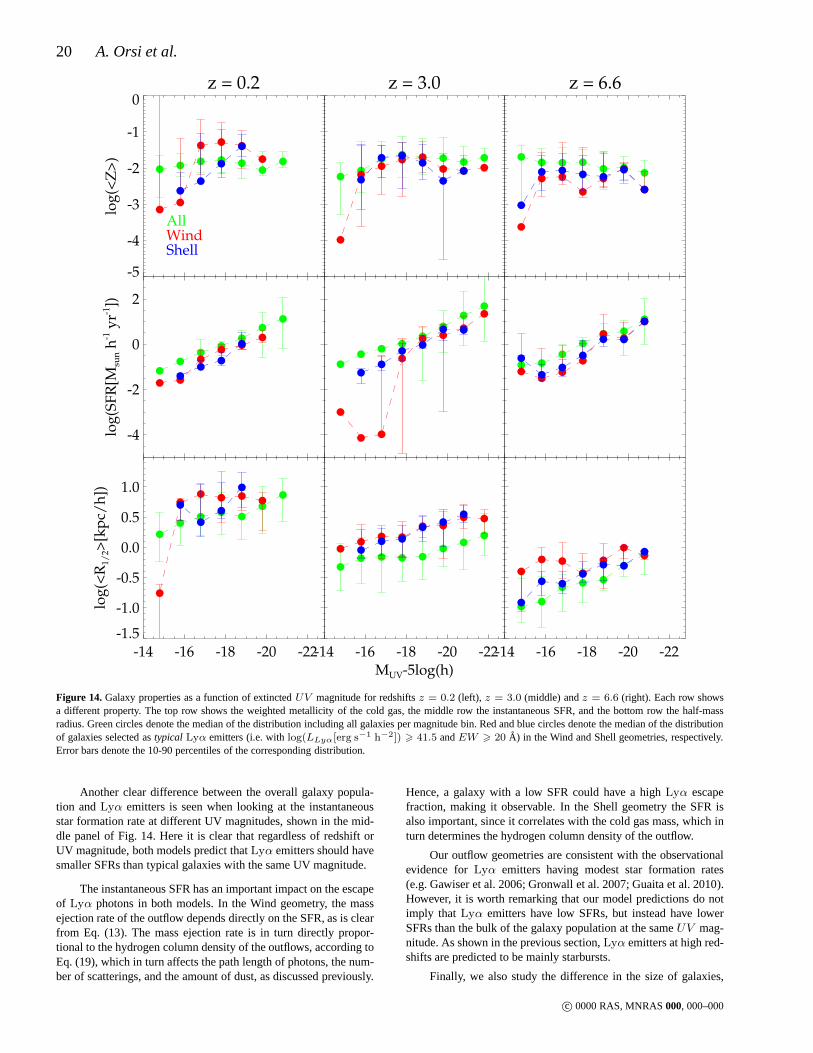
20 A. Orsi et al.
MUV-5log(h)
z = 0.2
-5
-4
-3
-2
-1
0lo
g(<
Z>
)
ShellWindAll
z = 3.0
z = 6.6
-4
-2
0
2
log
(SF
R[M
sun h
-1 y
r-1])
-14 -16 -18 -20 -22-1.5
-1.0
-0.5
0.0
0.5
1.0
log
(<R
1/2>
[kp
c/h
])
-14 -16 -18 -20 -22
-14 -16 -18 -20 -22
Figure 14.Galaxy properties as a function of extinctedUV magnitude for redshiftsz = 0.2 (left), z = 3.0 (middle) andz = 6.6 (right). Each row showsa different property. The top row shows the weighted metallicity of the cold gas, the middle row the instantaneous SFR, and the bottom row the half-massradius. Green circles denote the median of the distributionincluding all galaxies per magnitude bin. Red and blue circles denote the median of the distributionof galaxies selected astypical Lyα emitters (i.e. withlog(LLyα[erg s−1 h−2]) > 41.5 andEW > 20 A) in the Wind and Shell geometries, respectively.Error bars denote the 10-90 percentiles of the corresponding distribution.
Another clear difference between the overall galaxy popula-tion andLyα emitters is seen when looking at the instantaneousstar formation rate at different UV magnitudes, shown in themid-dle panel of Fig. 14. Here it is clear that regardless of redshift orUV magnitude, both models predict thatLyα emitters should havesmaller SFRs than typical galaxies with the same UV magnitude.
The instantaneous SFR has an important impact on the escapeof Lyα photons in both models. In the Wind geometry, the massejection rate of the outflow depends directly on the SFR, as isclearfrom Eq. (13). The mass ejection rate is in turn directly propor-tional to the hydrogen column density of the outflows, according toEq. (19), which in turn affects the path length of photons, the num-ber of scatterings, and the amount of dust, as discussed previously.
Hence, a galaxy with a low SFR could have a highLyα escapefraction, making it observable. In the Shell geometry the SFR isalso important, since it correlates with the cold gas mass, which inturn determines the hydrogen column density of the outflow.
Our outflow geometries are consistent with the observationalevidence forLyα emitters having modest star formation rates(e.g. Gawiser et al. 2006; Gronwall et al. 2007; Guaita et al.2010).However, it is worth remarking that our model predictions donotimply that Lyα emitters have low SFRs, but instead have lowerSFRs than the bulk of the galaxy population at the sameUV mag-nitude. As shown in the previous section,Lyα emitters at high red-shifts are predicted to be mainly starbursts.
Finally, we also study the difference in the size of galaxies,
c© 0000 RAS, MNRAS000, 000–000
Can galactic outflows explainLyα emitters? 21
since our outflow geometries depend strongly on the galaxy half-mass radius. In the Wind geometry, the hydrogen column densityscales as∼ 〈R1/2〉−1, and in the Shell geometry the hydrogencolumn density scales as∼ 〈R1/2〉−2. In order to obtain a highLyα escape fraction,NH has to be low in general, and this couldbe attained by having a large〈R1/2〉. Hence, not surprisingly, ouroutflow geometries predict thatLyα emitters typically have largersizes than the bulk of the galaxy population. This result is indepen-dent of redshift and UV magnitude, although in detail the differencein sizes may vary with these quantities. A similar result is reportedby Bond et al. (2009) atz = 3. They find the sizes ofLyα emitters(in Lyα emission) to be always smaller than∼ 3kpc/h, consis-tent with the half-mass radius of our typicalLyα emitters at thisredshift.
7 SUMMARY AND CONCLUSIONS
In this paper we couple the galaxy properties predicted by theBaugh et al. (2005) version of the semianalytical modelGALFORMwith a Monte Carlo radiative transfer model of the escape ofLyαphotons to study the properties ofLyα emitters in a cosmologicalcontext.
Motivated by observational evidence that galactic outflowsshape the asymmetric profiles of theLyα line, we developed twodifferent outflow geometries, each defined using the predicted prop-erties of galaxies inGALFORM in a slightly different way. Our Shellgeometry, which consists of an expanding thin spherical shell, hasa column densityNH proportional to the cold gas mass in the ISMof galaxies. Our Wind geometry, on the other hand, consists of aspherical expanding wind with number density that decreases withincreasing radius. The column density in the Wind geometry is re-lated to the mass ejection rate from supernovae, which is computedby GALFORM.
We study in detail theLyα line profiles and characterise themin terms of their width, asymmetry and offset with respect totheline centre, as a function of the outflow column density, expansionvelocity and metallicity. TheLyα properties of the outflow geome-tries we study are found to be sensitive to the column density, ex-pansion velocity and the geometry of the outflows, as shown inFig.2. Metallicity is found to have a smaller impact on the line profiles,although it has a great impact on theLyα escape fraction, as shownin Fig. 3.
Both the width and offset from the line centre are found to in-crease for outflows with increasing column densities and expansionvelocities. In both cases, theLyα line profiles in the Shell geome-try are more affected by changes of these properties than theWindgeometry.
TheLyα escape fraction is found to decrease with metallicityand column density, since those two properties are directlypropor-tional to the optical depth of absorption. Also, higher values of theexpansion velocity tend to increase the escape fraction. This rathercomplicated interplay between the column density, expansion ve-locity, metallicity and geometry justifies our choice for computingtheLyα escape fraction from a fully-fledgedLyα radiative transfermodel instead of imposing a phenomenological model.
The drawback is, of course, the difficulty in coupling bothmodels in order to obtain aLyα fesc for each galaxy predictedby GALFORM. One critical step is to choose the free parametersin our models. In order to set these for each model, we attemptto fit the observed cumulative luminosity function ofLyα emit-ters over the redshift range0 < z < 7. We find that a single
choice of parameters applied at all redshifts cannot reproduce theobserved CLFs. Motivated by the observed difference in sizes be-tween the star forming regions in local and high redshift starbursts(e.g. Rujopakarn et al. 2011), we allow the outflow radii in ourmodels to evolve with redshift when the galaxies are starbursts.By doing this we can find a suitable combination of parametersto match the measuredLyα CLF.
It is worth pointing out that the need to invoke a redshift de-pendence in the outflow sizes in starbursts could suggest that otherimportant physical processes which determine the escape ofLyαphotons may not be included in this work. Although outflows havebeen proposed in the past as a mechanism to boost the otherwisevery low escape fraction ofLyα photons, other scenarios have beenproposed. A clumpy ISM could boost the escape ofLyα photonswith respect to that of Lyman continuum photons, since the for-mer have a probability of bouncing off a dust cloud, and thereforehave more chances to escape, whereas in the latter case photonstravel through dust clouds, and hence have more chances of beingabsorbed (Neufeld 1991; Hansen & Oh 2006).
Another physical effect not included in our modelling isthe attenuation ofLyα radiation due to the scattering ofLyαphotons when crossing regions of neutral hydrogen in the IGM.This effect has been shown to be important atz & 6 whenthe fraction of neutral hydrogen in the IGM is thought tohave been significant (see, e.g. Dijkstra, Lidz & Wyithe 2007;Dayal, Ferrara & Saro 2010; Dijkstra, Mesinger & Wyithe 2011;Laursen, Sommer-Larsen & Razoumov 2011). Hence, we do notexpect this to significantly change our model predictions atlowredshifts.
A more fundamental uncertainty lies in the calculation of theintrinsic Lyα luminosity of galaxies, which does not depend uponthe radiative transfer modelling. We can assess whetherGALFORMcomputes the correct intrinsicLyα luminosity by studying the in-trinsic (unattenuated)Hα luminosity function, since both emission-line luminosities are directly related to the production rate of Ly-man continuum photons (see Orsi et al. 2010), and differ onlybytheir case B recombination emission coefficient (Osterbrock 1989).Moreover, theHα emission from galaxies is less sensitive to dustthanLyα since these photons do not undergo multiple scatteringsin the ISM, making their path lengths shorter than the typical pathlengthsLyα photons experience, and thus making it easier to esti-mate their attenuation by dust.
The attenuation by dust can be estimated by computing theratio of the intensity of two or more emission lines and comparingwith the expectation for case B recombination (see, for example,Kennicutt 1983, 1998). By comparing observed dust-attenuatedHαLFs with GALFORM predictions (Orsi et al. 2010) we have foundthat, atz ∼ 0.2, GALFORM roughly overestimates the intrinsicHαluminosities by a factor∼ 3. The scatter in the observedHα lu-minosity functions is large, making it difficult to estimatethis ac-curately. Nevertheless, the intrinsicLyα luminosities predicted atz = 0.2 are a factor∼ 10 or more brighter than what is neededto reproduce the observational results, if we fix the free parametersof the outflow geometries, meaning that the uncertainty in the in-trinsicLyα luminosity is not solely responsible for the discrepancybetween the observed and predicted LFs.
Despite this, our simple outflow geometries are found to be inagreement with a set of different observations, implying that ourmodelling does reproduce the basic physical conditions determin-ing the escape ofLyα photons from galaxies.
A direct prediction of our outflow geometries is the distribu-tion of hydrogen column densities ofLyα emitters. We find that
c© 0000 RAS, MNRAS000, 000–000
22 A. Orsi et al.
both models feature column densities with values ranging fromNH ∼ 1019 − 1023[cm−2], which is consistent with observationalestimates shown in Verhamme et al. (2008). The column densitydistribution is closely related to the predictedLyα escape fractions.We find that brightLyα emitters generally have high escape frac-tions, and faintLyα emitters have low escape fractions. An im-portant consequence of this is that certain galaxy properties whichcorrelate with the intrinsicLyα luminosity (such as the instanta-neous SFR) do not correlate in a simple way with the observedLyα luminosity. In other words, galaxies with the same intrinsicLyα luminosity (or, say, the same SFR) could be observed withdifferentLyα luminosities, making the interpretation of the prop-erties ofLyα emitters complicated.
The predicted escape fractions in the models are remarkablyconsistent with observational measurements (Fig. 9), giving furthersupport to the scenario ofLyα photons escaping through galacticoutflows. Although the Wind geometry is only partially consistentwith the observed escape fractions, it is worth pointing outthat theobservational data used to make the comparison in Fig. 9 doesnotconstitute a representative sample of the galaxy population at thisredshift.
Since our Monte Carlo radiative transfer model records thefrequency with which photons escape from an outflow, we makeuse of this information to study the predictedLyα line profiles fromour outflow geometries and compare them with observational mea-surements. In some cases the agreement is remarkably good, butin others we find significant differences (see Fig. 13). A detailedstudy of the line profiles could reveal important information aboutthe galaxy properties. We plan to undertake such a study ofLyαline profiles in the context of a galaxy formation model in a futurepaper.
Finally, our models predict that only a small fraction of galax-ies should be selected asLyα emitters. We illustrate in Fig. 14 thatLyα emitters are found in general to have low metallicities (exceptat z = 0.2), low instantaneous SFR and large sizes, compared tothe overall galaxy population. These constraints arise naturally asa consequence of the radiative transfer modelling incorporated inGALFORM in this paper. Galaxies need to have low star formationrates and large sizes in order to display an outflow with a small col-umn density. Since the dust content depends on the optical depth ofdust and not the metallicity alone,Lyα emitters are not necessarilylow-metallicity galaxies in our models.
The models presented here for the emission ofLyα representan important step towards a detailed understanding of the physi-cal properties of these galaxies. With the advent of large observa-tional campaigns in the forthcoming years focusing on detectingLyα emitters at high redshifts, new data will help us refine and im-prove our physical understanding of these galaxies, and thus, enableus to improve our knowledge of galaxy formation and evolution,particularly in the high redshift Universe.
ACKNOWLEDGENEMTS
AO acknowledges a STFC-Gemini scholarship. This work wassupported in part by Proyecto Gemini 320900212 and an STFCrolling grant. We thank Peter Laursen for making data from theMoCaLaTA radiative transfer code available for us to test our code,and Nelson Padilla for useful comments and discussions. Part ofthe calculations for this work were performed using the Geryon su-percomputer at AIUC.
REFERENCES
Ahn S., 2003, Journal of Korean Astronomical Society, 36, 145—, 2004, ApJ, 601, L25Ahn S.-H., Lee H.-W., Lee H. M., 2000, Journal of Korean Astro-nomical Society, 33, 29
Atek H., Kunth D., Hayes M.,Ostlin G., Mas-Hesse J. M., 2008,A&A, 488, 491
Atek H., Kunth D., Schaerer D., Hayes M., Deharveng J. M.,Ostlin G., Mas-Hesse J. M., 2009, A&A, 506, L1
Barnes L. A., Haehnelt M. G., 2010, MNRAS, 403, 870Baugh C. M., 2006, Reports on Progress in Physics, 69, 3101Baugh C. M., Lacey C. G., Frenk C. S., Granato G. L., Silva L.,Bressan A., Benson A. J., Cole S., 2005, MNRAS, 356, 1191
Benson A. J., Bower R. G., Frenk C. S., Lacey C. G., Baugh C. M.,Cole S., 2003, ApJ, 599, 38
Benson A. J., Lacey C. G., Baugh C. M., Cole S., Frenk C. S.,2002, MNRAS, 333, 156
Blanc G. A. et al., 2011, ApJ, 736, 31Bolton J. S., Haehnelt M. G., 2007, MNRAS, 382, 325Bond N. A., Gawiser E., Gronwall C., Ciardullo R., Altmann M.,Schawinski K., 2009, ApJ, 705, 639
Bower R. G., Benson A. J., Malbon R., Helly J. C., Frenk C. S.,Baugh C. M., Cole S., Lacey C. G., 2006, MNRAS, 370, 645
Cardelli J. A., Clayton G. C., Mathis J. S., 1989, ApJ, 345, 245Cen R., 1992, ApJS, 78, 341Charlot S., Fall S. M., 1993, ApJ, 415, 580Cole S., Lacey C. G., Baugh C. M., Frenk C. S., 2000, MNRAS,319, 168
Cowie L. L., Barger A. J., Hu E. M., 2010, ApJ, 711, 928Cowie L. L., Hu E. M., 1998, AJ, 115, 1319Cowie L. L., Hu E. M., Songaila A., 2011, ApJ, 735, L38+Dawson S., Rhoads J. E., Malhotra S., Stern D., Wang J., Dey A.,Spinrad H., Jannuzi B. T., 2007, ApJ, 671, 1227
Dayal P., Ferrara A., Gallerani S., 2008, MNRAS, 389, 1683Dayal P., Ferrara A., Saro A., 2010, MNRAS, 402, 1449Dayal P., Maselli A., Ferrara A., 2011, MNRAS, 410, 830Deharveng J. et al., 2008, ApJ, 680, 1072Dijkstra M., Haiman Z., Spaans M., 2006, ApJ, 649, 14Dijkstra M., Lidz A., Wyithe J. S. B., 2007, MNRAS, 377, 1175Dijkstra M., Mesinger A., Wyithe J. S. B., 2011, MNRAS, 414,2139
Finkelstein S. L., Cohen S. H., Moustakas J., Malhotra S., RhoadsJ. E., Papovich C., 2011, ApJ, 733, 117
Finkelstein S. L., Rhoads J. E., Malhotra S., Grogin N., 2009, ApJ,691, 465
Forero-Romero J. E., Yepes G., Gottlober S., Knollmann S. R.,Cuesta A. J., Prada F., 2011, MNRAS, 415, 3666
Francke H., 2009, New Astronomical Reviews, 53, 47Frank A., 1999, New Astronomical Reviews, 43, 31Gawiser E. et al., 2007, ApJ, 671, 278—, 2006, ApJS, 162, 1Giavalisco M., Koratkar A., Calzetti D., 1996, ApJ, 466, 831Gonzalez J. E., Lacey C. G., Baugh C. M., Frenk C. S., BensonA. J., 2011, ArXiv e-prints, 11053731
Granato G. L., Lacey C. G., Silva L., Bressan A., Baugh C. M.,Cole S., Frenk C. S., 2000, ApJ, 542, 710
Gronwall C. et al., 2007, ApJ, 667, 79Guaita L. et al., 2011, ApJ, 733, 114—, 2010, ApJ, 714, 255Haardt F., Madau P., 1996, ApJ, 461, 20—, 2001, in Clusters of Galaxies and the High Redshift Universe
c© 0000 RAS, MNRAS000, 000–000
Can galactic outflows explainLyα emitters? 23
Observed in X-rays, D. M. Neumann & J. T. V. Tran, ed.Hansen M., Oh S. P., 2006, MNRAS, 367, 979Harrington J. P., 1973, MNRAS, 162, 43Hartmann L. W., Huchra J. P., Geller M. J., 1984, ApJ, 287, 487Hartmann L. W., Huchra J. P., Geller M. J., O’Brien P., WilsonR.,1988, ApJ, 326, 101
Hayes M. et al., 2010, Nature, 464, 562Hayes M., Schaerer D.,Ostlin G., Mas-Hesse J. M., Atek H.,Kunth D., 2011, ApJ, 730, 8
Henyey L. G., Greenstein J. L., 1941, ApJ, 93, 70Hjerting F., 1938, ApJ, 88, 508Hu E. M., Cowie L. L., Barger A. J., Capak P., Kakazu Y., TrouilleL., 2010, ApJ, 725, 394
Hu E. M., Cowie L. L., McMahon R. G., Capak P., Iwamuro F.,Kneib J., Maihara T., Motohara K., 2002, ApJ, 568, L75
Hummer D. G., 1962, MNRAS, 125, 21Iono D. et al., 2009, ApJ, 695, 1537Kashikawa N. et al., 2006, ApJ, 648, 7Kennicutt, Jr. R. C., 1983, ApJ, 272, 54—, 1998, ARA&A, 36, 189Kobayashi M. A. R., Totani T., Nagashima M., 2007, ApJ, 670,919
—, 2010, ApJ, 708, 1119Kornei K. A., Shapley A. E., Erb D. K., Steidel C. C., ReddyN. A., Pettini M., Bogosavljevic M., 2010, ApJ, 711, 693
Kovac K., Somerville R. S., Rhoads J. E., Malhotra S., Wang J.,2007, ApJ, 668, 15
Kudritzki R. et al., 2000, ApJ, 536, 19Kulas K. R., Shapley A. E., Kollmeier J. A., Zheng Z., SteidelC. C., Hainline K. N., 2011, ArXiv e-prints, 11074367
Kunth D., Mas-Hesse J. M., Terlevich E., Terlevich R., LequeuxJ., Fall S. M., 1998, A&A, 334, 11
Lacey C. G., Baugh C. M., Frenk C. S., Benson A. J., 2011, MN-RAS, 45
Lacey C. G., Baugh C. M., Frenk C. S., Silva L., Granato G. L.,Bressan A., 2008, MNRAS, 385, 1155
Lagos C. D. P., Lacey C. G., Baugh C. M., Bower R. G., BensonA. J., 2011, MNRAS, 416, 1566
Laursen P., Razoumov A. O., Sommer-Larsen J., 2009, ApJ, 696,853
Laursen P., Sommer-Larsen J., 2007, ApJ, 657, L69Laursen P., Sommer-Larsen J., Razoumov A. O., 2011, ApJ, 728,52
Le Delliou M., Lacey C., Baugh C. M., Guiderdoni B., Bacon R.,Courtois H., Sousbie T., Morris S. L., 2005, MNRAS, 357, L11
Le Delliou M., Lacey C. G., Baugh C. M., Morris S. L., 2006,MNRAS, 365, 712
Loeb A., Rybicki G. B., 1999, ApJ, 524, 527Mas-Hesse J. M., Kunth D., Atek H.,Ostlin G., Leitherer C., Pet-rosian A., Schaerer D., 2009, Ap&SS, 320, 35
Mas-Hesse J. M., Kunth D., Tenorio-Tagle G., Leitherer C., Ter-levich R. J., Terlevich E., 2003, ApJ, 598, 858
Meier D. L., Terlevich R., 1981, ApJ, 246, L109Meiksin A. A., 2009, Reviews of Modern Physics, 81, 1405Nagamine K., Cen R., Furlanetto S. R., Hernquist L., Night C.,Ostriker J. P., Ouchi M., 2006, New Astronomy Review, 50, 29
Nagamine K., Ouchi M., Springel V., Hernquist L., 2010, PASJ,62, 1455
Neufeld D. A., 1990, ApJ, 350, 216—, 1991, ApJ, 370, L85Nilsson K. K., Moller-Nilsson O., Møller P., Fynbo J. P. U.,Shap-ley A. E., 2009, MNRAS, 400, 232
Orsi A., Baugh C. M., Lacey C. G., Cimatti A., Wang Y.,Zamorani G., 2010, MNRAS, 405, 1006
Orsi A., Lacey C. G., Baugh C. M., Infante L., 2008, MNRAS,391, 1589
Osterbrock D. E., 1989, Astrophysics of gaseous nebulae andac-tive galactic nuclei, Osterbrock, D. E., ed.
Ostlin G., Hayes M., Kunth D., Mas-Hesse J. M., Leitherer C.,Petrosian A., Atek H., 2009, AJ, 138, 923
Ouchi M. et al., 2008, ApJS, 176, 301—, 2010, ApJ, 723, 869Peebles P. J. E., 1993, Principles of physical cosmology, Peebles,P. J. E., ed.
Pentericci L. et al., 2011, ArXiv e-prints, 11071376Pentericci L., Grazian A., Fontana A., Salimbeni S., Santini P., deSantis C., Gallozzi S., Giallongo E., 2007, A&A, 471, 433
Rauch M. et al., 2008, ApJ, 681, 856Rhoads J. E., Malhotra S., Dey A., Stern D., Spinrad H., JannuziB. T., 2000, ApJ, 545, L85
Rujopakarn W., Rieke G. H., Eisenstein D. J., Juneau S., 2011,ApJ, 726, 93
Schaerer D., 2007, ArXiv e-prints, 07060139Schenker M. A., Stark D. P., Ellis R. S., Robertson B. E., DunlopJ. S., McLure R. J., Kneib J. ., Richard J., 2011, ArXiv e-prints,11071261
Shapley A. E., Steidel C. C., Pettini M., Adelberger K. L., 2003,ApJ, 588, 65
Shimasaku K. et al., 2006, PASJ, 58, 313Silva L., Granato G. L., Bressan A., Danese L., 1998, ApJ, 509,103
Stark D. P., Ellis R. S., Chiu K., Ouchi M., Bunker A., 2010, MN-RAS, 408, 1628
Steidel C. C., Bogosavljevic M., Shapley A. E., Kollmeier J. A.,Reddy N. A., Erb D. K., Pettini M., 2011, ApJ, 736, 160
Steidel C. C., Erb D. K., Shapley A. E., Pettini M., Reddy N.,Bogosavljevic M., Rudie G. C., Rakic O., 2010, ApJ, 717, 289
Strickland D., 2002, in Astronomical Society of the Pacific Con-ference Series, Vol. 253, Chemical Enrichment of Intraclusterand Intergalactic Medium, R. Fusco-Femiano & F. Matteucci,ed., pp. 387–+
Thuan T. X., Izotov Y. I., 1997, ApJ, 489, 623Tilvi V., Malhotra S., Rhoads J. E., Scannapieco E., ThackerR. J.,Iliev I. T., Mellema G., 2009, ApJ, 704, 724
Tilvi V. et al., 2010, ApJ, 721, 1853Verhamme A., Schaerer D., Atek H., Tapken C., 2008, A&A, 491,89
Verhamme A., Schaerer D., Maselli A., 2006, A&A, 460, 397Zheng Z., Cen R., Trac H., Miralda-Escude J., 2010, ApJ, 716,574
—, 2011, ApJ, 726, 38Zheng Z., Miralda-Escude J., 2002, ApJ, 578, 33
APPENDIX A: DESCRIPTION OF THE MONTE CARLORADIATIVE TRANSFER CODE
In the context ofLyα radiative transfer, photon frequencies,ν, areusually expressed in terms of Doppler unitsx, given by Eq. (20).The thermal velocity dispersion of the gas,vth, is given by
vth =
(
2kBT
mp
)1/2
, (A1)
c© 0000 RAS, MNRAS000, 000–000
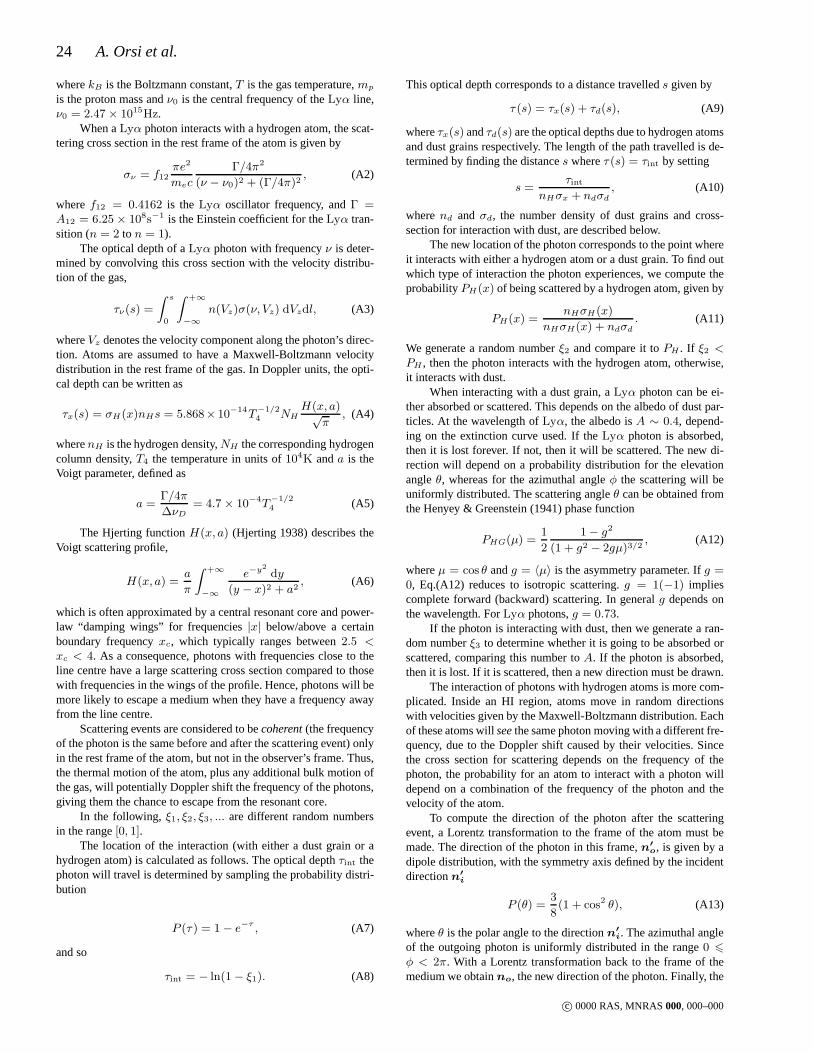
24 A. Orsi et al.
wherekB is the Boltzmann constant,T is the gas temperature,mp
is the proton mass andν0 is the central frequency of theLyα line,ν0 = 2.47× 10¹⁵Hz.
When aLyα photon interacts with a hydrogen atom, the scat-tering cross section in the rest frame of the atom is given by
σν = f12πe2
mec
Γ/4π2
(ν − ν0)2 + (Γ/4π)2, (A2)
wheref12 = 0.4162 is theLyα oscillator frequency, andΓ =A12 = 6.25× 10⁸s−1 is the Einstein coefficient for theLyα tran-sition (n = 2 to n = 1).
The optical depth of aLyα photon with frequencyν is deter-mined by convolving this cross section with the velocity distribu-tion of the gas,
τν(s) =
∫ s
0
∫ +∞
−∞
n(Vz)σ(ν, Vz) dVzdl, (A3)
whereVz denotes the velocity component along the photon’s direc-tion. Atoms are assumed to have a Maxwell-Boltzmann velocitydistribution in the rest frame of the gas. In Doppler units, the opti-cal depth can be written as
τx(s) = σH(x)nHs = 5.868× 10⁻¹⁴T−1/24 NH
H(x, a)√π
, (A4)
wherenH is the hydrogen density,NH the corresponding hydrogencolumn density,T4 the temperature in units of104K anda is theVoigt parameter, defined as
a =Γ/4π
∆νD= 4.7× 10⁻⁴T
−1/24 (A5)
The Hjerting functionH(x, a) (Hjerting 1938) describes theVoigt scattering profile,
H(x, a) =a
π
∫ +∞
−∞
e−y2
dy
(y − x)2 + a2, (A6)
which is often approximated by a central resonant core and power-law “damping wings” for frequencies|x| below/above a certainboundary frequencyxc, which typically ranges between2.5 <xc < 4. As a consequence, photons with frequencies close to theline centre have a large scattering cross section compared to thosewith frequencies in the wings of the profile. Hence, photons will bemore likely to escape a medium when they have a frequency awayfrom the line centre.
Scattering events are considered to becoherent(the frequencyof the photon is the same before and after the scattering event) onlyin the rest frame of the atom, but not in the observer’s frame.Thus,the thermal motion of the atom, plus any additional bulk motion ofthe gas, will potentially Doppler shift the frequency of thephotons,giving them the chance to escape from the resonant core.
In the following, ξ1, ξ2, ξ3, ... are different random numbersin the range[0, 1].
The location of the interaction (with either a dust grain or ahydrogen atom) is calculated as follows. The optical depthτint thephoton will travel is determined by sampling the probability distri-bution
P (τ ) = 1− e−τ , (A7)
and so
τint = − ln(1− ξ1). (A8)
This optical depth corresponds to a distance travelleds given by
τ (s) = τx(s) + τd(s), (A9)
whereτx(s) andτd(s) are the optical depths due to hydrogen atomsand dust grains respectively. The length of the path travelled is de-termined by finding the distances whereτ (s) = τint by setting
s =τint
nHσx + ndσd, (A10)
wherend and σd, the number density of dust grains and cross-section for interaction with dust, are described below.
The new location of the photon corresponds to the point whereit interacts with either a hydrogen atom or a dust grain. To find outwhich type of interaction the photon experiences, we compute theprobabilityPH(x) of being scattered by a hydrogen atom, given by
PH(x) =nHσH(x)
nHσH(x) + ndσd. (A11)
We generate a random numberξ2 and compare it toPH . If ξ2 <PH , then the photon interacts with the hydrogen atom, otherwise,it interacts with dust.
When interacting with a dust grain, aLyα photon can be ei-ther absorbed or scattered. This depends on the albedo of dust par-ticles. At the wavelength ofLyα, the albedo isA ∼ 0.4, depend-ing on the extinction curve used. If theLyα photon is absorbed,then it is lost forever. If not, then it will be scattered. Thenew di-rection will depend on a probability distribution for the elevationangleθ, whereas for the azimuthal angleφ the scattering will beuniformly distributed. The scattering angleθ can be obtained fromthe Henyey & Greenstein (1941) phase function
PHG(µ) =1
2
1− g2
(1 + g2 − 2gµ)3/2, (A12)
whereµ = cos θ andg = 〈µ〉 is the asymmetry parameter. Ifg =0, Eq.(A12) reduces to isotropic scattering.g = 1(−1) impliescomplete forward (backward) scattering. In generalg depends onthe wavelength. ForLyα photons,g = 0.73.
If the photon is interacting with dust, then we generate a ran-dom numberξ3 to determine whether it is going to be absorbed orscattered, comparing this number toA. If the photon is absorbed,then it is lost. If it is scattered, then a new direction must be drawn.
The interaction of photons with hydrogen atoms is more com-plicated. Inside an HI region, atoms move in random directionswith velocities given by the Maxwell-Boltzmann distribution. Eachof these atoms willseethe same photon moving with a different fre-quency, due to the Doppler shift caused by their velocities.Sincethe cross section for scattering depends on the frequency ofthephoton, the probability for an atom to interact with a photonwilldepend on a combination of the frequency of the photon and thevelocity of the atom.
To compute the direction of the photon after the scatteringevent, a Lorentz transformation to the frame of the atom mustbemade. The direction of the photon in this frame,n
′
o, is given by adipole distribution, with the symmetry axis defined by the incidentdirectionn′
i
P (θ) =3
8(1 + cos2 θ), (A13)
whereθ is the polar angle to the directionn′
i. The azimuthal angleof the outgoing photon is uniformly distributed in the range0 6
φ < 2π. With a Lorentz transformation back to the frame of themedium we obtainno, the new direction of the photon. Finally, the
c© 0000 RAS, MNRAS000, 000–000
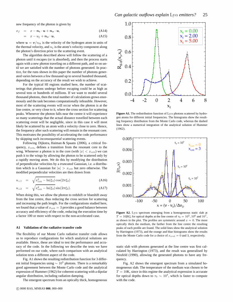
Can galactic outflows explainLyα emitters? 25
new frequency of the photon is given by
xf = x−ni · u+ no · u, (A14)
= x− u‖ +no · u, (A15)
whereu = v/vth is the velocity of the hydrogen atom in units ofthe thermal velocity, andu‖ is the atom’s velocity component alongthe photon’s direction prior to the scattering event.
The algorithm described above will follow the scattering ofaphoton until it escapes (or is absorbed), and then the process startsagain with a new photon traveling on a different path, and so on un-til we are satisfied with the number of photons generated. In prac-tice, for the runs shown in this paper the number of photons gener-ated varies between a few thousand up to several hundred thousand,depending on the accuracy of the result we wish to achieve.
For the typical HI regions studied here, the number of scat-terings that photons undergo before escaping could be as high asseveral tens or hundreds of millions. If we want to model severalthousand photons, then the total number of calculations grows enor-mously and the task becomes computationally infeasible. However,most of the scattering events will occur when the photon is attheline centre, or very close to it, where the cross section for scatteringpeaks. Whenever the photon falls near the centre it will experienceso many scatterings that the actual distance travelled between eachscattering event will be negligible, since in this case it will mostlikely be scattered by an atom with a velocity close to zero. Hence,the frequency after such scattering will remain in the resonant core.This motivates the possibility of accelerating the code performanceby skipping suchinconsequentialscattering events.
Following Dijkstra, Haiman & Spaans (2006), a critical fre-quency,xcrit, defines a transition from the resonant core to thewing. Whenever a photon is in the core (with|x| < xcrit) we canpush it to the wings by allowing the photon to be scattered only bya rapidly moving atom. We do this by modifying the distributionof perpendicular velocities by atruncatedGaussian, i.e. a distribu-tion which is a Gaussian for|u| > xcrit but zero otherwise. Themodified perpendicular velocities are then drawn from
u⊥1 =√
x2crit − ln(ξ4) cos(2πξ2) (A16)
u⊥2 =√
x2crit − ln(ξ4) sin(2πξ2). (A17)
When doing this, we allow the photon to redshift or blueshiftawayfrom the line centre, thus reducing the cross section for scatteringand increasing the path length. For the configurations studied here,we found that a value ofxcrit = 3 provides a good balance betweenaccuracy and efficiency of the code, reducing the execution time bya factor 100 or more with respect to the non-accelerated case.
A1 Validation of the radiative transfer code
The flexibility of our Monte Carlo radiative transfer code allowsus to reproduce configurations for which analytical solutions areavailable. Hence, these are ideal to test the performance and accu-racy of the code. In the following we describe the tests we haveperformed on our code, where each comparison with an analyticalsolution tests a different aspect of the code.
Fig. A1 shows the resulting redistribution function for 3 differ-ent initial frequencies using∼ 105 photons. There is a remarkablygood agreement between the Monte Carlo code and the analyticalexpression of Hummer (1962) for coherent scattering with a dipolarangular distribution, including radiation damping.
The emergent spectrum from an optically thick, homogeneous
-4 -2 0 2 4 6 8xf
0.0
0.2
0.4
0.6
0.8
1.0
RII
-B(x
i,xf)
xi = 0.00xi = 2.00xi = 5.00
Figure A1. The redistribution function ofLyα photons scattered by hydro-gen atoms for different initial frequencies. The histograms show the result-ing frequency distribution from the Monte Carlo code, whereas the dashedlines show a numerical integration of the analytical solution of Hummer(1962).
-100 -50 0 50 100x = (ν - ν0)/∆νD
0.000
0.001
0.002
0.003
0.004
0.005
J(τ 0
,x)
xcrit = 0xcrit = 3
τ0 = 105
τ0 = 106
τ0 = 107
Figure A2. Lyα spectrum emerging from a homogeneous static slab atT = 10[K], for optical depths at the line centre ofτ0 = 105, 106 and107 ,as shown in the plot. The profiles are symmetric aroundx = 0. The moreoptically thick the medium, the farther from the line centrethe resultingpeaks of each profile are found. The solid lines show the analytical solutionby Harrington (1973), and the orange and blue histograms show the resultsfrom the Monte Carlo code for a choice ofxcrit = 0 and3, respectively.
static slab with photons generated at the line centre was first cal-culated by Harrington (1973), and the result was generalised byNeufeld (1990), allowing the generated photons to have any fre-quency.
Fig. A2 shows the emergent spectrum from a simulated ho-mogeneous slab. The temperature of the medium was chosen to beT = 10K, since in this regime the analytical expression is accuratefor optical depths down toτ0 ∼ 104, which is faster to computewith the code.
c© 0000 RAS, MNRAS000, 000–000
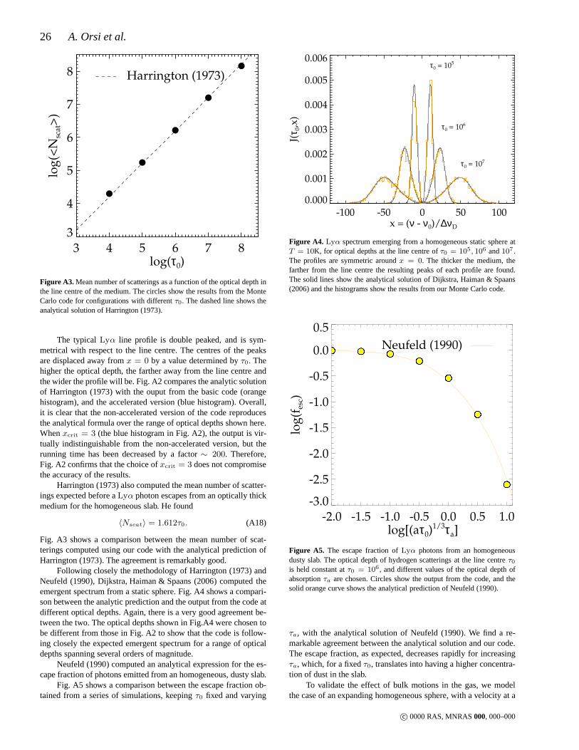
26 A. Orsi et al.
3 4 5 6 7 8log(τ0)
3
4
5
6
7
8
log
(<N
scat
>)
Harrington (1973)
Figure A3. Mean number of scatterings as a function of the optical depthinthe line centre of the medium. The circles show the results from the MonteCarlo code for configurations with differentτ0. The dashed line shows theanalytical solution of Harrington (1973).
The typicalLyα line profile is double peaked, and is sym-metrical with respect to the line centre. The centres of the peaksare displaced away fromx = 0 by a value determined byτ0. Thehigher the optical depth, the farther away from the line centre andthe wider the profile will be. Fig. A2 compares the analytic solutionof Harrington (1973) with the ouput from the basic code (orangehistogram), and the accelerated version (blue histogram).Overall,it is clear that the non-accelerated version of the code reproducesthe analytical formula over the range of optical depths shown here.Whenxcrit = 3 (the blue histogram in Fig. A2), the output is vir-tually indistinguishable from the non-accelerated version, but therunning time has been decreased by a factor∼ 200. Therefore,Fig. A2 confirms that the choice ofxcrit = 3 does not compromisethe accuracy of the results.
Harrington (1973) also computed the mean number of scatter-ings expected before aLyα photon escapes from an optically thickmedium for the homogeneous slab. He found
〈Nscat〉 = 1.612τ0. (A18)
Fig. A3 shows a comparison between the mean number of scat-terings computed using our code with the analytical prediction ofHarrington (1973). The agreement is remarkably good.
Following closely the methodology of Harrington (1973) andNeufeld (1990), Dijkstra, Haiman & Spaans (2006) computed theemergent spectrum from a static sphere. Fig. A4 shows a compari-son between the analytic prediction and the output from the code atdifferent optical depths. Again, there is a very good agreement be-tween the two. The optical depths shown in Fig.A4 were chosentobe different from those in Fig. A2 to show that the code is follow-ing closely the expected emergent spectrum for a range of opticaldepths spanning several orders of magnitude.
Neufeld (1990) computed an analytical expression for the es-cape fraction of photons emitted from an homogeneous, dustyslab.
Fig. A5 shows a comparison between the escape fraction ob-tained from a series of simulations, keepingτ0 fixed and varying
-100 -50 0 50 100x = (ν - ν0)/∆νD
0.000
0.001
0.002
0.003
0.004
0.005
0.006
J(τ 0
,x)
τ0 = 105
τ0 = 106
τ0 = 107
Figure A4. Lyα spectrum emerging from a homogeneous static sphere atT = 10K, for optical depths at the line centre ofτ0 = 105, 106 and107 .The profiles are symmetric aroundx = 0. The thicker the medium, thefarther from the line centre the resulting peaks of each profile are found.The solid lines show the analytical solution of Dijkstra, Haiman & Spaans(2006) and the histograms show the results from our Monte Carlo code.
-2.0 -1.5 -1.0 -0.5 0.0 0.5 1.0log[(aτ0)
1/3τa]
-3.0
-2.5
-2.0
-1.5
-1.0
-0.5
0.0
0.5
log
(fes
c)
Neufeld (1990)
Figure A5. The escape fraction ofLyα photons from an homogeneousdusty slab. The optical depth of hydrogen scatterings at theline centreτ0is held constant atτ0 = 106, and different values of the optical depth ofabsorptionτa are chosen. Circles show the output from the code, and thesolid orange curve shows the analytical prediction of Neufeld (1990).
τa, with the analytical solution of Neufeld (1990). We find a re-markable agreement between the analytical solution and ourcode.The escape fraction, as expected, decreases rapidly for increasingτa, which, for a fixedτ0, translates into having a higher concentra-tion of dust in the slab.
To validate the effect of bulk motions in the gas, we modelthe case of an expanding homogeneous sphere, with a velocityat a
c© 0000 RAS, MNRAS000, 000–000
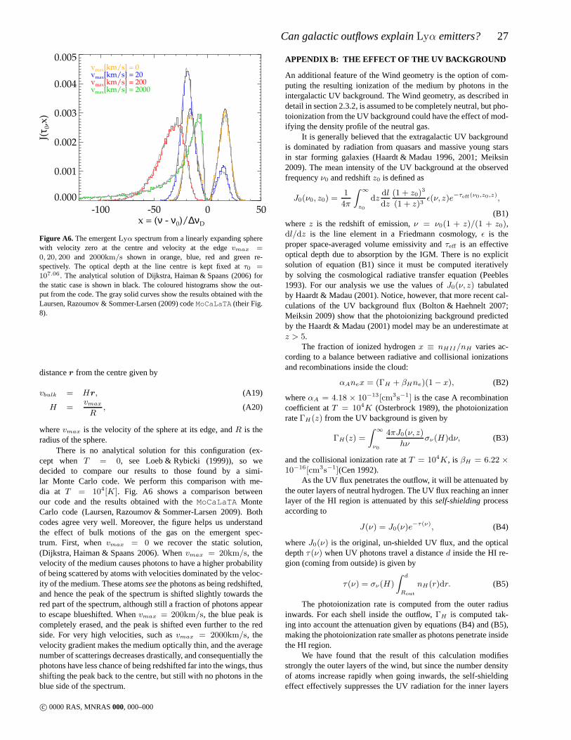
Can galactic outflows explainLyα emitters? 27
-100 -50 0 50x = (ν - ν0)/∆νD
0.000
0.001
0.002
0.003
0.004
0.005
J(τ 0
,x)
vmax[km/s] = 0vmax[km/s] = 20vmax[km/s] = 200vmax[km/s] = 2000
Figure A6. The emergentLyα spectrum from a linearly expanding spherewith velocity zero at the centre and velocity at the edgevmax =0, 20, 200 and 2000km/s shown in orange, blue, red and green re-spectively. The optical depth at the line centre is kept fixedat τ0 =107.06 . The analytical solution of Dijkstra, Haiman & Spaans (2006) forthe static case is shown in black. The coloured histograms show the out-put from the code. The gray solid curves show the results obtained with theLaursen, Razoumov & Sommer-Larsen (2009) codeMoCaLaTA (their Fig.8).
distancer from the centre given by
vbulk = Hr, (A19)
H =vmax
R, (A20)
wherevmax is the velocity of the sphere at its edge, andR is theradius of the sphere.
There is no analytical solution for this configuration (ex-cept when T = 0, see Loeb & Rybicki (1999)), so wedecided to compare our results to those found by a simi-lar Monte Carlo code. We perform this comparison with me-dia at T = 104[K]. Fig. A6 shows a comparison betweenour code and the results obtained with theMoCaLaTA MonteCarlo code (Laursen, Razoumov & Sommer-Larsen 2009). Bothcodes agree very well. Moreover, the figure helps us understandthe effect of bulk motions of the gas on the emergent spec-trum. First, whenvmax = 0 we recover the static solution,(Dijkstra, Haiman & Spaans 2006). Whenvmax = 20km/s, thevelocity of the medium causes photons to have a higher probabilityof being scattered by atoms with velocities dominated by theveloc-ity of the medium. These atomsseethe photons as being redshifted,and hence the peak of the spectrum is shifted slightly towards thered part of the spectrum, although still a fraction of photons appearto escape blueshifted. Whenvmax = 200km/s, the blue peak iscompletely erased, and the peak is shifted even further to the redside. For very high velocities, such asvmax = 2000km/s, thevelocity gradient makes the medium optically thin, and the averagenumber of scatterings decreases drastically, and consequentially thephotons have less chance of being redshifted far into the wings, thusshifting the peak back to the centre, but still with no photons in theblue side of the spectrum.
APPENDIX B: THE EFFECT OF THE UV BACKGROUND
An additional feature of the Wind geometry is the option of com-puting the resulting ionization of the medium by photons in theintergalactic UV background. The Wind geometry, as described indetail in section 2.3.2, is assumed to be completely neutral, but pho-toionization from the UV background could have the effect ofmod-ifying the density profile of the neutral gas.
It is generally believed that the extragalactic UV backgroundis dominated by radiation from quasars and massive young starsin star forming galaxies (Haardt & Madau 1996, 2001; Meiksin2009). The mean intensity of the UV background at the observedfrequencyν0 and redshiftz0 is defined as
J0(ν0, z0) =1
4π
∫ ∞
z0
dzdl
dz
(1 + z0)3
(1 + z)3ǫ(ν, z)e−τeff (ν0,z0,z),
(B1)wherez is the redshift of emission,ν = ν0(1 + z)/(1 + z0),dl/dz is the line element in a Friedmann cosmology,ǫ is theproper space-averaged volume emissivity andτeff is an effectiveoptical depth due to absorption by the IGM. There is no explicitsolution of equation (B1) since it must be computed iterativelyby solving the cosmological radiative transfer equation (Peebles1993). For our analysis we use the values ofJ0(ν, z) tabulatedby Haardt & Madau (2001). Notice, however, that more recent cal-culations of the UV background flux (Bolton & Haehnelt 2007;Meiksin 2009) show that the photoionizing background predictedby the Haardt & Madau (2001) model may be an underestimate atz > 5.
The fraction of ionized hydrogenx ≡ nHII/nH varies ac-cording to a balance between radiative and collisional ionizationsand recombinations inside the cloud:
αAnex = (ΓH + βHne)(1− x), (B2)
whereαA = 4.18 × 10⁻¹³[cm3s−1] is the case A recombinationcoefficient atT = 104K (Osterbrock 1989), the photoionizationrateΓH(z) from the UV background is given by
ΓH(z) =
∫ ∞
ν0
4πJ0(ν, z)
hνσν(H)dν, (B3)
and the collisional ionization rate atT = 104K, is βH = 6.22 ×10⁻¹⁶[cm3s−1](Cen 1992).
As the UV flux penetrates the outflow, it will be attenuated bythe outer layers of neutral hydrogen. The UV flux reaching an innerlayer of the HI region is attenuated by thisself-shieldingprocessaccording to
J(ν) = J0(ν)e−τ(ν), (B4)
whereJ0(ν) is the original, un-shielded UV flux, and the opticaldepthτ (ν) when UV photons travel a distanced inside the HI re-gion (coming from outside) is given by
τ (ν) = σν(H)
∫ d
Rout
nH(r)dr. (B5)
The photoionization rate is computed from the outer radiusinwards. For each shell inside the outflow,ΓH is computed tak-ing into account the attenuation given by equations (B4) and(B5),making the photoionization rate smaller as photons penetrate insidethe HI region.
We have found that the result of this calculation modifiesstrongly the outer layers of the wind, but since the number densityof atoms increase rapidly when going inwards, the self-shieldingeffect effectively suppresses the UV radiation for the inner layers
c© 0000 RAS, MNRAS000, 000–000
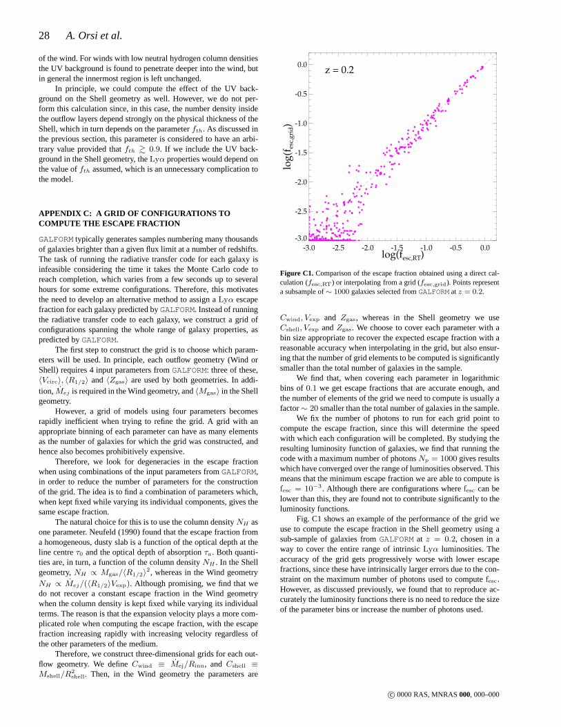
28 A. Orsi et al.
of the wind. For winds with low neutral hydrogen column densitiesthe UV background is found to penetrate deeper into the wind,butin general the innermost region is left unchanged.
In principle, we could compute the effect of the UV back-ground on the Shell geometry as well. However, we do not per-form this calculation since, in this case, the number density insidethe outflow layers depend strongly on the physical thicknessof theShell, which in turn depends on the parameterfth. As discussed inthe previous section, this parameter is considered to have an arbi-trary value provided thatfth & 0.9. If we include the UV back-ground in the Shell geometry, theLyα properties would depend onthe value offth assumed, which is an unnecessary complication tothe model.
APPENDIX C: A GRID OF CONFIGURATIONS TOCOMPUTE THE ESCAPE FRACTION
GALFORM typically generates samples numbering many thousandsof galaxies brighter than a given flux limit at a number of redshifts.The task of running the radiative transfer code for each galaxy isinfeasible considering the time it takes the Monte Carlo code toreach completion, which varies from a few seconds up to severalhours for some extreme configurations. Therefore, this motivatesthe need to develop an alternative method to assign aLyα escapefraction for each galaxy predicted byGALFORM. Instead of runningthe radiative transfer code to each galaxy, we construct a grid ofconfigurations spanning the whole range of galaxy properties, aspredicted byGALFORM.
The first step to construct the grid is to choose which param-eters will be used. In principle, each outflow geometry (WindorShell) requires 4 input parameters fromGALFORM: three of these,〈Vcirc〉, 〈R1/2〉 and 〈Zgas〉 are used by both geometries. In addi-tion,Mej is required in the Wind geometry, and〈Mgas〉 in the Shellgeometry.
However, a grid of models using four parameters becomesrapidly inefficient when trying to refine the grid. A grid withanappropriate binning of each parameter can have as many elementsas the number of galaxies for which the grid was constructed,andhence also becomes prohibitively expensive.
Therefore, we look for degeneracies in the escape fractionwhen using combinations of the input parameters fromGALFORM,in order to reduce the number of parameters for the constructionof the grid. The idea is to find a combination of parameters which,when kept fixed while varying its individual components, gives thesame escape fraction.
The natural choice for this is to use the column densityNH asone parameter. Neufeld (1990) found that the escape fraction froma homogeneous, dusty slab is a function of the optical depth at theline centreτ0 and the optical depth of absorptionτa. Both quanti-ties are, in turn, a function of the column densityNH . In the Shellgeometry,NH ∝ Mgas/〈R1/2〉2, whereas in the Wind geometryNH ∝ Mej/(〈R1/2〉Vexp). Although promising, we find that wedo not recover a constant escape fraction in the Wind geometrywhen the column density is kept fixed while varying its individualterms. The reason is that the expansion velocity plays a morecom-plicated role when computing the escape fraction, with the escapefraction increasing rapidly with increasing velocity regardless ofthe other parameters of the medium.
Therefore, we construct three-dimensional grids for each out-flow geometry. We defineCwind ≡ Mej/Rinn, and Cshell ≡Mshell/R
2shell. Then, in the Wind geometry the parameters are
log(fesc,RT)
log
(fes
c,g
rid)
-3.0 -2.5 -2.0 -1.5 -1.0 -0.5 0.0-3.0
-2.5
-2.0
-1.5
-1.0
-0.5
0.0z = 0.2
Figure C1. Comparison of the escape fraction obtained using a direct cal-culation (fesc,RT) or interpolating from a grid (fesc,grid). Points representa subsample of∼ 1000 galaxies selected fromGALFORM atz = 0.2.
Cwind, Vexp and Zgas, whereas in the Shell geometry we useCshell, Vexp andZgas. We choose to cover each parameter with abin size appropriate to recover the expected escape fraction with areasonable accuracy when interpolating in the grid, but also ensur-ing that the number of grid elements to be computed is significantlysmaller than the total number of galaxies in the sample.
We find that, when covering each parameter in logarithmicbins of 0.1 we get escape fractions that are accurate enough, andthe number of elements of the grid we need to compute is usually afactor∼ 20 smaller than the total number of galaxies in the sample.
We fix the number of photons to run for each grid point tocompute the escape fraction, since this will determine the speedwith which each configuration will be completed. By studyingtheresulting luminosity function of galaxies, we find that running thecode with a maximum number of photonsNp = 1000 gives resultswhich have converged over the range of luminosities observed. Thismeans that the minimum escape fraction we are able to computeisfesc = 10−3. Although there are configurations wherefesc can belower than this, they are found not to contribute significantly to theluminosity functions.
Fig. C1 shows an example of the performance of the grid weuse to compute the escape fraction in the Shell geometry using asub-sample of galaxies fromGALFORM at z = 0.2, chosen in away to cover the entire range of intrinsicLyα luminosities. Theaccuracy of the grid gets progressively worse with lower escapefractions, since these have intrinsically larger errors due to the con-straint on the maximum number of photons used to computefesc.However, as discussed previously, we found that to reproduce ac-curately the luminosity functions there is no need to reducethe sizeof the parameter bins or increase the number of photons used.
c© 0000 RAS, MNRAS000, 000–000
Related Documents