Can Education Subsidies stop School Drop-outs? An evaluation of Education Maintenance Allowances in England

Can Education Subsidies stop School Drop-outs? An evaluation of

Education Maintenance Allowances in England

Lorraine Dearden, Carl Emmerson, Christine Frayne and Costas Meghir∗

August 2004

Abstract

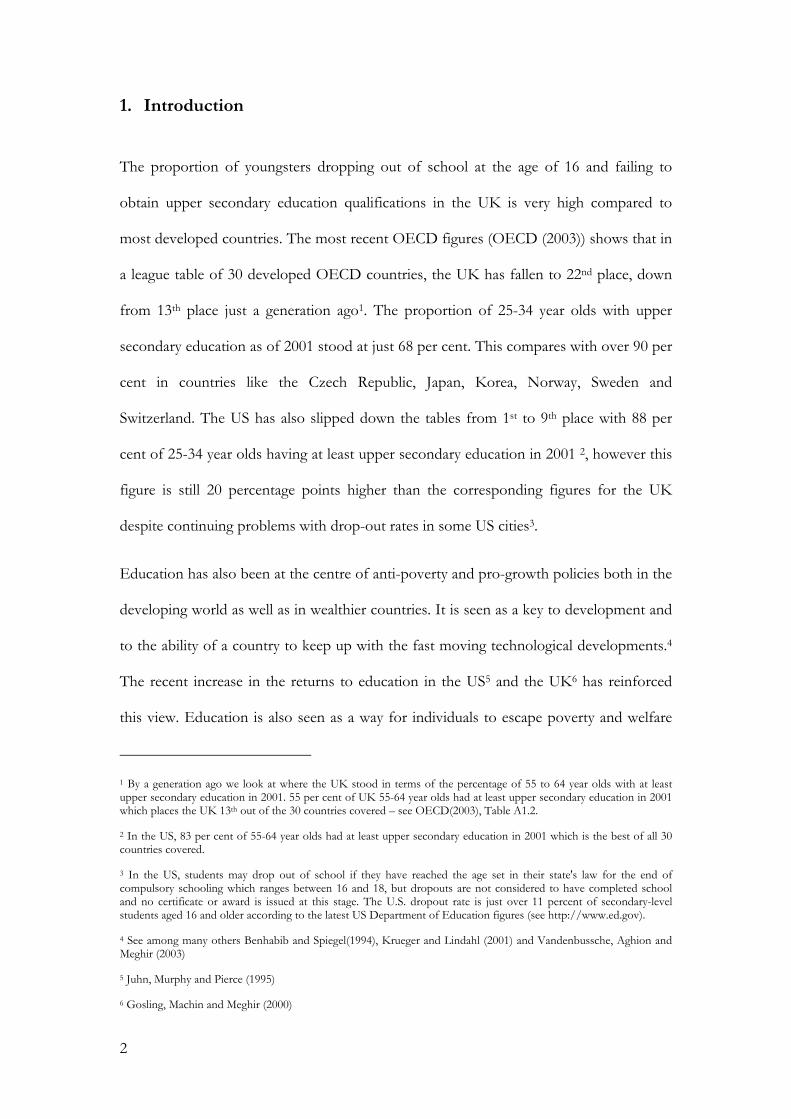
This paper evaluates whether a means tested grants paid to secondary students are an effective way of reducing the proportion of school drop-outs. We look at this problem using matching techniques on a pilot study carried out in England during 1999 and 2000 using a specially designed dataset that ensures that valid comparisons between our pilot and control areas are made. The impact of the subsidy is quite substantial with initial participation rates (at age 16) being around 4.5 percentage points higher. Full-time participation rates one year later are found to have increased by around 6.4 percentage points which is largely due to the EMA having a significant effect on retention in post compulsory education, particularly for boys. These effects vary by eligibility group with those receiving the full payment having the largest initial increase in participation, whilst the effects for those who are partially eligible are only significantly different from the control group in the second year of the program. There is some evidence that participation effect is stronger for boys, especially in the second year, and that the policy goes some way to reducing the gap in drop-out rates between boys and girls. It is also clear that the policy has the largest impact on children from the poorest socio-economic background.

∗ Dearden, Emmerson and Frayne: Institute for Fiscal Studies, 7 Ridgmount St, London, WC1E 7AE, UK (e-mail: [email protected], [email protected], [email protected]); Meghir: Institute for Fiscal Studies and Department of Economics, University College London, Gower St, London WC1E 6BT (e-mail: [email protected] ). The authors would like to Erich Battistin, Richard Blundell, Emla Fitzsimons, Alissa Goodman and Barbara Sianesi for useful comments on earlier versions of this paper. We are also indebted to our evaluation colleagues Sue Middleton, Sue McGuire and Karl Ashworth from the Centre for Research in Social Policy and Stephen Finch from the National Centre for Social Research for their support and advice. We also received invaluable advice and comments from John Elliott and Ganka Mueller from the UK Department for Education and Skills (DfES) who funded the evaluation. Despite all this help, the usual disclaimer applies.

1

1. Introduction

The proportion of youngsters dropping out of school at the age of 16 and failing to

obtain upper secondary education qualifications in the UK is very high compared to

most developed countries. The most recent OECD figures (OECD (2003)) shows that in

a league table of 30 developed OECD countries, the UK has fallen to 22nd place, down

from 13th place just a generation ago1. The proportion of 25-34 year olds with upper

secondary education as of 2001 stood at just 68 per cent. This compares with over 90 per

cent in countries like the Czech Republic, Japan, Korea, Norway, Sweden and

Switzerland. The US has also slipped down the tables from 1st to 9th place with 88 per

cent of 25-34 year olds having at least upper secondary education in 2001 2, however this

figure is still 20 percentage points higher than the corresponding figures for the UK

despite continuing problems with drop-out rates in some US cities3.

Education has also been at the centre of anti-poverty and pro-growth policies both in the

developing world as well as in wealthier countries. It is seen as a key to development and

to the ability of a country to keep up with the fast moving technological developments.4

The recent increase in the returns to education in the US5 and the UK6 has reinforced

this view. Education is also seen as a way for individuals to escape poverty and welfare

1 By a generation ago we look at where the UK stood in terms of the percentage of 55 to 64 year olds with at least upper secondary education in 2001. 55 per cent of UK 55-64 year olds had at least upper secondary education in 2001 which places the UK 13th out of the 30 countries covered – see OECD(2003), Table A1.2.

2 In the US, 83 per cent of 55-64 year olds had at least upper secondary education in 2001 which is the best of all 30 countries covered.

3 In the US, students may drop out of school if they have reached the age set in their state's law for the end of compulsory schooling which ranges between 16 and 18, but dropouts are not considered to have completed school and no certificate or award is issued at this stage. The U.S. dropout rate is just over 11 percent of secondary-level students aged 16 and older according to the latest US Department of Education figures (see http://www.ed.gov).

4 See among many others Benhabib and Spiegel(1994), Krueger and Lindahl (2001) and Vandenbussche, Aghion and Meghir (2003)

5 Juhn, Murphy and Pierce (1995)

6 Gosling, Machin and Meghir (2000)

2

dependency and this perception has motivated numerous policies both in the UK and

worldwide that promote education as the long solution to these problems.

There has been worldwide focus on school drop-out problems and a number of policies

devised to help reduce school drop-out rates. One of the key policy changes in most

OECD countries after World War II, was to introduce free secondary school education

and to increase the compulsory school leaving age. The timing and pace of these reforms

varied tremendously across countries and in the US the most important reforms occurred

between 1910 and 1940 (see Goldin (1999)). In the UK fees for secondary schools were

abolished by the Education Act 1944 (The Butler Act) and the compulsory school

leaving ages was increased from 14 to 15 in 1946 and then from 15 to 16 in 1974 where it

remains today. In the US today, the compulsory school leaving age ranges from 16 to 187

and for the remaining for 28 OECD countries ranges from 14 to 188.

Making secondary education free and increasing the compulsory school leaving age had

an effect on school drop-out and completion rates and a number of these reforms have

been analysed in previous research9. In recent years a number of countries, both

developed and developing, have instead introduced means tested grants in an attempt to

encourage students to stay in school, rather than simply raising the compulsory school

leaving age10. This paper examines the impact of such a program that was first piloted in

7 Compulsory schooling ends by law at age 16 in 30 states, at age 17 in nine states, and at age 18 in 11 states plus the District of Columbia. Source: US Department for Education.

8 See OECD(2003) Table .

9 See for example Goldin (1999) who examines the 1910 to 1940 reforms in the US, Harmon and Walker (1995) who exploit the changes in the compulsory school leaving age in Britain to estimate the returns to schooling and Meghir and Palme (2003) who exploit changes in the Swedish Secondary Education system to estimate the returns to education.

10 Prominent examples are the AUSTUDY program introduced in Australia in 1988 for children in their last 2 years of secondary school (now called YOUTH ALLOWANCE) (see Dearden and Heath (1996)), the PROGRESA program in Mexico which covers children from primary school to the end of high school (see Schultz, 2000, Attanasio, Meghir

3

a number of regions in England in September 1999. Evaluating such interventions is of

course critical to the shaping of education policy and the effectiveness or otherwise of a

conditional cash transfer to 16 and 17 year olds on school drop-out rates is of general

policy interest to policy makers worldwide11.

The presumption of the policy makers has been that these low levels of education are

due to financial constraints rather than to the outcome of an informed choice in an

unconstrained environment.12 The evaluation of this programme cannot provide

information on the importance of liquidity constraints on education, since it changes the

relative costs of remaining in school13. However, it can provide valuable information on

whether such subsidies, which effectively reduce the cost of education, actually reduce

school drop-out rates, which at present is the central policy concern14.

We find that the impact of the subsidy is quite substantial, especially for those who

receive the maximum payment. The subsidy increases the initial education participation

of eligible males by 4.8 percentage points and eligible females by 4.2 percentage points.

In the second year this increases to 7.6 percentage points for eligible males and 5.3

percentage points for females, suggesting that the effect of the policy is not only to

and Santiago, 2002), the recently introduced Familias en Accion program in Colombia modelled on PROGRESA (Attanasio et al. 2003).

11 There is already evidence that financial aid paid to college students has a significant impact on college attendance and completion. See for example Dynarski (2003).

12 “We recognise that for some young people there are financial barriers to participating in education, particularly for those from lower income households.” Education Maintenance Allowance: An Introduction .http://www.dfes.gov.uk/ema/pdfs/003158_A4%20singles.pdf

13 Papers that have attempted to look at this question include Cameron and Heckman (1998), Cameron and Taber (2000) and Dale and Krueger (1999).

14 With respect to dropping out at 16, following the GCSE qualification which is obtained at that age, the minister for Lifelong Learning Margaret Hodge stated in Parliament: “The Real challenge is to increase the number of young people achieving two A-levels. That comes under our schools agenda-our 14-19 agenda. A particular problem is the haemorrhaging of young people, who achieve five A to Cs at GCSE level and then do not stay on to do further education full time”, House of Commons Hansard Debates for 5 July 2001 (pt 3). A recent survey of government policy by Johnson (2004) also highlights this concern. He says “The UK has a relatively low staying-on rate in full time education after age 16.. Given high returns this is, perhaps, surprising and probably economically inefficient. Given

4

increase participation, but also retention in full-time education. The initial effects are

largest for those who receive the maximum payment although the retention effects are

concentrated among individuals who are only partially eligible. We estimate that just over

half of individuals who stayed in education were drawn from inactivity rather than work.

The overall impact of the EMA was not diminished when it was paid to the mother

rather than to the child, though there is some weak evidence that paying to the child is

more effective for those fully eligible whereas the opposite is true for those who are

partially eligible.

We also find that the effect of EMA is largest for children coming from a poorer socio-

economic background. Both girls and boys coming from low-socio economic

backgrounds15 have very high drop out rates and the EMA has proved especially effective

in plugging the drop-out gap for this vulnerable group.

The paper proceeds as follows. In section 2 we describe the programme and its variants

and describe the data we use to evaluate the program. In section 3 we discuss the

evaluation methodology and in section 4 we discuss the results. In section 5 we offer

some concluding remarks.

2. Background and Data

The Education Maintenance Allowance (EMA) pilots were launched in September 1999

in 10 Local Education Authorities. The scheme paid a means-tested benefit to 16–18

year-olds who remained in full-time education after year 11, when education ceases to be

compulsory (i.e. after 16 years of age approximately). The payments consisted of a

very substantial differences in staying-on rates by social background, it is also of concern from an equity point of view” (pp 177-178).

5

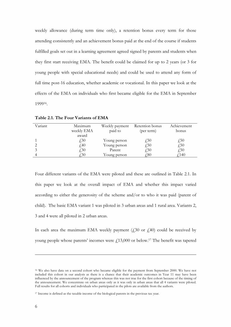
weekly allowance (during term time only), a retention bonus every term for those

attending consistently and an achievement bonus paid at the end of the course if students

fulfilled goals set out in a learning agreement agreed signed by parents and students when

they first start receiving EMA. The benefit could be claimed for up to 2 years (or 3 for

young people with special educational needs) and could be used to attend any form of

full time post-16 education, whether academic or vocational. In this paper we look at the

effects of the EMA on individuals who first became eligible for the EMA in September

199916.

Table 2.1. The Four Variants of EMA

Variant Maximum weekly EMA

award

Weekly payment paid to

Retention bonus (per term)

Achievement bonus

1 £30 Young person £50 £50 2 £40 Young person £50 £50 3 £30 Parent £50 £50 4 £30 Young person £80 £140

Four different variants of the EMA were piloted and these are outlined in Table 2.1. In

this paper we look at the overall impact of EMA and whether this impact varied

according to either the generosity of the scheme and/or to who it was paid (parent of

child). The basic EMA variant 1 was piloted in 3 urban areas and 1 rural area. Variants 2,

3 and 4 were all piloted in 2 urban areas.

In each area the maximum EMA weekly payment (£30 or £40) could be received by

young people whose parents’ incomes were £13,000 or below.17 The benefit was tapered

16 We also have data on a second cohort who became eligible for the payment from September 2000. We have not included this cohort in our analysis as there is a chance that their academic outcomes in Year 11 may have been influenced by the announcement of the program whereas this was not true for the first cohort because of the timing of the announcement. We concentrate on urban areas only as it was only in urban areas that all 4 variants were piloted. Full results for all cohorts and individuals who participated in the pilots are available from the authors.

17 Income is defined as the taxable income of the biological parents in the previous tax year.

6

linearly for family incomes between £13,000 and £30,000 with those from families

earning £30,000 receiving £5 per week. No payment was made for families with income

in excess of £30,000. In addition at the end of a term of regular attendance the child

would receive a non-means tested retention bonus (£50 or £80)18. The children also

received an achievement bonus on successful completion of the course examination. To

put these amounts in context the median net wage among those who opted for full-time

work in our sample was £100 per week, corresponding to just under 40 hours’ work a

week. Thus the maximum eligibility for the EMA, depending on the variant, replaces

around a third of post tax earnings.

The programme was announced in the spring of 1999, just before the end of the school

year and the lateness of the announcement means that it could not have impacted on a

child’s Year 11 examination results19. The data used to evaluate the programme are based

on initial face-to-face interviews with both the parents and the children and follow up

annual telephone interviews with the children. The data set was constructed so as to

include both eligible and ineligible individuals in pilot and control areas20. The first

interview was conducted at the beginning of the school year in which the subsidy became

available. In the following year the same students (but not parents) were followed up

using a telephone interview.

We collected a wealth of variables relating to family income and background, childhood

events (such as ill health and mobility), prior school achievement as well as administrative

18 This bonus was paid to the child in ALL variants (including variant 3).

19 This was not true for our second cohort and for this reason they are excluded from the analysis. We feel that it is important to control for student ability and the only measures we have relate to school outcomes in Year 11.

20 We used data from the British Cohort Studies to choose our control areas so as to ensure the background characteristics of the control areas in terms of historical education participation, background characteristics of parents and neighbourhood characteristics were as similar as possible to those of the selected pilot areas which we knew in advance.

7

data on the quality of schooling in the child’s neighbourhood as well as other measures

of neighbourhood quality measured prior to the introduction of the EMA 21.

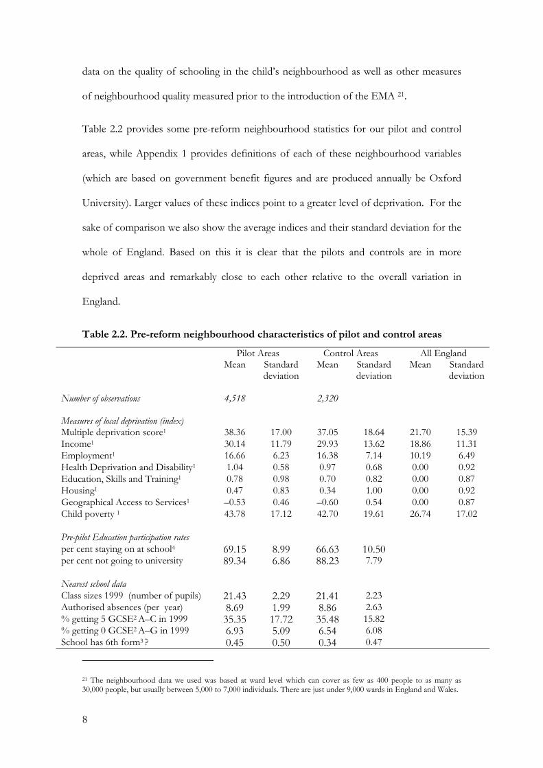
Table 2.2 provides some pre-reform neighbourhood statistics for our pilot and control

areas, while Appendix 1 provides definitions of each of these neighbourhood variables

(which are based on government benefit figures and are produced annually be Oxford

University). Larger values of these indices point to a greater level of deprivation. For the

sake of comparison we also show the average indices and their standard deviation for the

whole of England. Based on this it is clear that the pilots and controls are in more

deprived areas and remarkably close to each other relative to the overall variation in

England.

Table 2.2. Pre-reform neighbourhood characteristics of pilot and control areas

Pilot Areas Control Areas All England Mean Standard

deviationMean Standard

deviation Mean Standard

deviation Number of observations 4,518 2,320 Measures of local deprivation (index) Multiple deprivation score1 38.36 17.00 37.05 18.64 21.70 15.39 Income1 30.14 11.79 29.93 13.62 18.86 11.31 Employment1 16.66 6.23 16.38 7.14 10.19 6.49 Health Deprivation and Disability1 1.04 0.58 0.97 0.68 0.00 0.92 Education, Skills and Training1 0.78 0.98 0.70 0.82 0.00 0.87 Housing1 0.47 0.83 0.34 1.00 0.00 0.92 Geographical Access to Services1 –0.53 0.46 –0.60 0.54 0.00 0.87 Child poverty 1 43.78 17.12 42.70 19.61 26.74 17.02 Pre-pilot Education participation rates per cent staying on at school4 69.15 8.99 66.63 10.50 per cent not going to university 89.34 6.86 88.23 7.79 Nearest school data Class sizes 1999 (number of pupils) 21.43 2.29 21.41 2.23 Authorised absences (per year) 8.69 1.99 8.86 2.63 % getting 5 GCSE2 A–C in 1999 35.35 17.72 35.48 15.82 % getting 0 GCSE2 A–G in 1999 6.93 5.09 6.54 6.08 School has 6th form3 ? 0.45 0.50 0.34 0.47

21 The neighbourhood data we used was based at ward level which can cover as few as 400 people to as many as 30,000 people, but usually between 5,000 to 7,000 individuals. There are just under 9,000 wards in England and Wales.

8

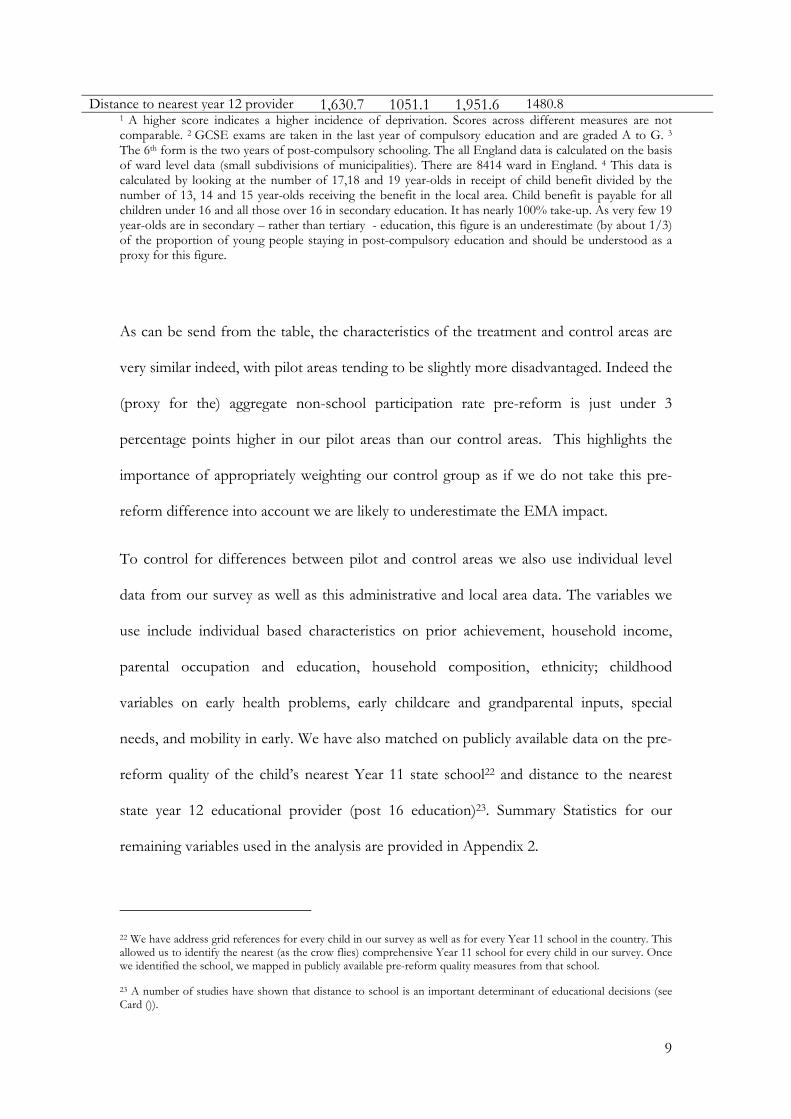
Distance to nearest year 12 provider 1,630.7 1051.1 1,951.6 1480.8 1 A higher score indicates a higher incidence of deprivation. Scores across different measures are not comparable. 2 GCSE exams are taken in the last year of compulsory education and are graded A to G. 3 The 6th form is the two years of post-compulsory schooling. The all England data is calculated on the basis of ward level data (small subdivisions of municipalities). There are 8414 ward in England. 4 This data is calculated by looking at the number of 17,18 and 19 year-olds in receipt of child benefit divided by the number of 13, 14 and 15 year-olds receiving the benefit in the local area. Child benefit is payable for all children under 16 and all those over 16 in secondary education. It has nearly 100% take-up. As very few 19 year-olds are in secondary – rather than tertiary - education, this figure is an underestimate (by about 1/3) of the proportion of young people staying in post-compulsory education and should be understood as a proxy for this figure.

As can be send from the table, the characteristics of the treatment and control areas are

very similar indeed, with pilot areas tending to be slightly more disadvantaged. Indeed the

(proxy for the) aggregate non-school participation rate pre-reform is just under 3

percentage points higher in our pilot areas than our control areas. This highlights the

importance of appropriately weighting our control group as if we do not take this pre-

reform difference into account we are likely to underestimate the EMA impact.

To control for differences between pilot and control areas we also use individual level

data from our survey as well as this administrative and local area data. The variables we

use include individual based characteristics on prior achievement, household income,

parental occupation and education, household composition, ethnicity; childhood

variables on early health problems, early childcare and grandparental inputs, special

needs, and mobility in early. We have also matched on publicly available data on the pre-

reform quality of the child’s nearest Year 11 state school22 and distance to the nearest

state year 12 educational provider (post 16 education)23. Summary Statistics for our

remaining variables used in the analysis are provided in Appendix 2.

22 We have address grid references for every child in our survey as well as for every Year 11 school in the country. This allowed us to identify the nearest (as the crow flies) comprehensive Year 11 school for every child in our survey. Once we identified the school, we mapped in publicly available pre-reform quality measures from that school.

23 A number of studies have shown that distance to school is an important determinant of educational decisions (see Card ()).

9

3. The evaluation Methodology – Matching

The outcome of interest in this paper will be participation in post-compulsory school, i.e.

in year 12 and year 13. As we discuss in the results section below, we are interested in the

impact of financial incentives on the entire target population, on the population of those

partially eligible for the subsidy and on the ineligible population. In each case we will be

comparing the outcomes relative to the appropriate comparison group. Although the

treatment and control areas are very well matched, the distribution of characteristics is

not identical, as they may have been following a successful and large scale randomisation.

To allow for the fact that this was not going to be a randomised experiment, we have

collected a large array of individual and local area characteristics, which should control

for any relevant differences in the treatment and control areas before the program was

introduced.

The method we use to balance the distribution of observable characteristics is propensity

score matching. We provide a brief description in the Appendix.24 It turns out that a

simple fully interacted OLS model (fully interacted linear matching) imposing common

support gives almost identical results to our preferred matching estimator. (Outline

method here).

Difference in Differences based on sibling data

As a final step we also carry out some sensitivity analysis using difference in differences

based on the behaviour of older siblings. In this case we compare the change in school

participation between the younger and the older sibling in pilot and control areas. In

doing this we also control for a number of characteristics. The reason this is not our

24 Rosenbaum and Rubin (1983) , Heckman, Ichimura and Todd (1994).

10

main evaluation method is that not all children have older siblings of the same gender

and secondly the time varying covariates we measure, including income, relate to the date

of the survey, i.e. when the younger sibling was deciding whether to continue with High

school or drop out. Nevertheless, this sensitivity analysis confirms the results we find

with matching.

4. The results

As a first indication of the impact of the EMA we can carry out a simple difference in

differences calculation based on aggregate data for the pilot and control areas25. The

growth in participation before and after the reform in the urban pilot areas is 5.1

percentage points. This can be compared to a decline of 0.2 percentage point in the

urban controls, which implies an EMA effect of 5.3 percentage points increase in

schooling at the age of 17.26

These results are indicative that the policy did have an effect. However, we now

investigate this in greater detail using matched comparisons between the treatment and

control areas. This will ensure that the observable characteristics between the treated and

control areas are balanced.

Impact of the EMA on Year 12 Destinations

In our work we compared the covariate balancing indicators of a number of matching

methods including nearest neighbour matching, Mahalanobis matching and various

kernel based methods. As seen above, the differences in characteristics between our

control and pilot areas was already very good. This meant that our results were not very

25 See Department for Education and Skills (2004), “Statistics of Education: Participation in Education and Training by 16 and 17 Year Olds in Each Local Area in England, End 2001”, February 2004.

26 Since these results are based on four aggregate observations no standard errors can be derived.

11

sensitive to the different methods used, but the best balancing of covariates was achieved

using an Epanechnikov kernel with a bandwidth of 0.0627. Our preferred matching

estimates were in all cases almost identical to fully interacted OLS estimates of the

average treatment on the treated.

Table 4.1 shows estimates of the overall impact of the EMA on young people’s initial

decisions to remain in full-time education, to move into employment or to be inactive

(NEET - Not in Education, Employment or Training). The EMA effect has been

estimated separately for men and women using both matched and unmatched samples.28

We also report OLS and fully interacted OLS estimates of the ATT for purposes of

comparison29,30.

The EMA has had a positive and significant effect on post-compulsory education

participation among eligible young people. The overall estimate for both rural and urban

areas is 3.7 percentage points from a baseline of 67.7% in our sample of controls.31 This

increase has drawn young people from both employment and the inactivity group

(NEET) in equal parts in the urban areas. This is significant because it shows that to a

27 Full details are available from the authors.

28 Unmatched samples refer to just the mean of the relevant variable across the entire subgroup of interest. For example in unmatched samples the average participation in education among cohort 1 urban women in the pilot areas is compared with the mean in the control areas. It differs from the descriptive analysis later in this report since that compares only individuals from areas which have been deemed to have broadly similar characteristics.

29 Of course, in the case of simple OLS the ATT is, by definition, the same as the ATE and ATNT.

30 Our preferred matching estimate uses an Epanechnikov kernel with a bandwidth of 0.06. We tested a number of different methods of matching including Epanechnikov kernels with a variety of bandwidths, nearest neighbour matching, and Mahalanobis-metric matching method and based our decision on which method gave us the best covariance balancing indicators. In all cased our preferred matching estimator gave the best results in terms of various covariance balancing measures (see Appendix 3).

31 The baseline figure is different from the aggregate figure for a number of reasons. First the population is different. Second, the age window that the aggregate figure looks at is different since the aggregate figures work with age and not with school years as we do. Thus the aggregate figures relate to slightly older persons. Finally, we may have had differential non-response between participants and non-participants. Note however that there is no evidence that the non-response is different between pilots and controls. In fact the results on attrition imply that any non-response will be balanced between pilots and controls.

12

large extent the policy is not displacing individuals from work, but from unproductive

activities, thus implying an overall lower cost of providing this incentive to education.

13

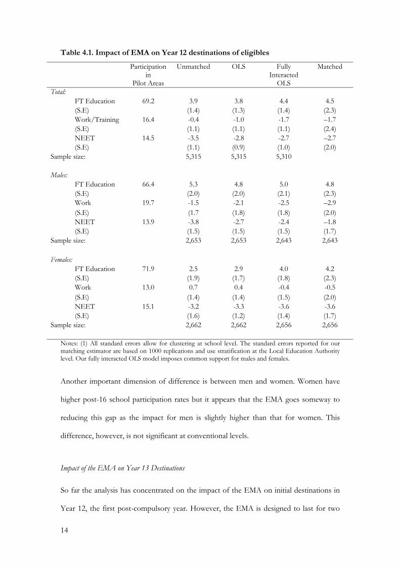
Table 4.1. Impact of EMA on Year 12 destinations of eligibles

Participation in

Pilot Areas

Unmatched OLS Fully Interacted

OLS

Matched

Total: FT Education 69.2 3.9 3.8 4.4 4.5 (S.E) (1.4) (1.3) (1.4) (2.3) Work/Training 16.4 -0.4 -1.0 -1.7 –1.7 (S.E) (1.1) (1.1) (1.1) (2.4) NEET 14.5 -3.5 -2.8 -2.7 –2.7 (S.E) (1.1) (0.9) (1.0) (2.0) Sample size: 5,315 5,315 5,310 Males: FT Education 66.4 5.3 4.8 5.0 4.8 (S.E) (2.0) (2.0) (2.1) (2.3) Work 19.7 -1.5 -2.1 -2.5 –2.9 (S.E) (1.7 (1.8) (1.8) (2.0) NEET 13.9 -3.8 -2.7 -2.4 –1.8 (S.E) (1.5) (1.5) (1.5) (1.7) Sample size: 2,653 2,653 2,643 2,643 Females: FT Education 71.9 2.5 2.9 4.0 4.2 (S.E) (1.9) (1.7) (1.8) (2.3) Work 13.0 0.7 0.4 -0.4 -0.5 (S.E) (1.4) (1.4) (1.5) (2.0) NEET 15.1 -3.2 -3.3 -3.6 -3.6 (S.E) (1.6) (1.2) (1.4) (1.7) Sample size: 2,662 2,662 2,656 2,656

Notes: (1) All standard errors allow for clustering at school level. The standard errors reported for our matching estimator are based on 1000 replications and use stratification at the Local Education Authority level. Our fully interacted OLS model imposes common support for males and females.

Another important dimension of difference is between men and women. Women have

higher post-16 school participation rates but it appears that the EMA goes someway to

reducing this gap as the impact for men is slightly higher than that for women. This

difference, however, is not significant at conventional levels.

Impact of the EMA on Year 13 Destinations

So far the analysis has concentrated on the impact of the EMA on initial destinations in

Year 12, the first post-compulsory year. However, the EMA is designed to last for two

14

years. Thus an important question is whether the impact of the EMA persists in the 2nd

year, altering significantly the entire path post 16. To answer this question, in this section,

we focus on individuals which we observe for a second year, and examine their

destinations in Year 13, one year after the introduction of EMA.

When considering whether the policy has led to longer term increases in participation we

will have to use the 2nd wave of data for our cohort. However, there has been some

attrition. About 25 per cent of the original sample was lost in the follow up. In Appendix

4 we show that the likelihood of remaining in the sample is higher for those who are

eligible for the EMA relative to those who are not. However, the pattern of attrition is

the same for the treatment and control areas, possibly implying that any biases due to

attrition balance out. In Appendix 4 we report the results of running a probit on the

determinants of attrition. We see that those who come from families earning less than

£13,000 per annum (i.e. those in our pilot and control groups who we define as fully

eligible) are slightly more likely to drop out of the panel but there is no difference

conditional on this eligibility between pilot and control areas. These results suggest that

attrition was not directly related to the EMA. When we re-estimate the impact of EMA

in the first year only on the sample who do not drop out of the panel we obtain slightly

lower estimates of the impact of EMA on full-time education participation with our male

estimates being slightly but not significantly larger32 and our female estimates being

slightly but not significantly smaller33. Whilst this is reassuring, it is also clear that the

distribution of observable characteristics has changed, as a result of attrition in the 2nd

wave. In particular the ones who did not drop out of the sample originate from a better

32 5.0 percentage points with a standard error of 2.7, compared to our estimate of 4.8 percentage points for the full sample (see Table 4.1).

33 3.5 percentage points with a standard error or (2.4), compared to our estimate of 4.2 percentage points for the full sample (see Table 4.1).

15

family background and were more likely to be in school in wave 1 of the data (see Table

4.2 below). In this sense the population for which we will be looking at the longer term

outcomes is different than the one for which we can look at the shorter term ones.

However it should be stressed that issues relating to the impact of attrition are only

relevant when we look at the longer-term effects of the program.

We define the potential outcomes that could occur two years after the introduction of

the program as: education in Year 12 and education in Year 13; education in Year 12 and

other activity in Year 13; other activity in Year 12 and education in Year 13; and, finally,

other activities in both year 12 and year 13. Hence the overall impact on full-time

education in Year 12 for this second wave can be found by comparing the outcomes of

those in our first two groups with those in our second two groups in the first year.

Table 4.2 shows the impact of EMA based on the division of the population into the

four mutually exclusive groups described above. The important conclusion that comes

from Table 4.2 is that where the EMA has been effective it has led to increase in both

year 12 and year 13 attendance and thus it is shown to have long-term effects. This is

important because it indicates that those drawn into education due to the EMA are

committed to it. They do not just sample it only to find that it is not for them and to

drop out a few months later. It also shows that the EMA has increased average education

retention rates, defined as the proportion of those in full-time education in Year 12 who

were still in full-time education in Year 13. EMA increased average retention rates by 4.0

percentage points (from 77.9 per cent to 81.9 per cent), with a particularly large effect for

men (6.1 percentage points).

16

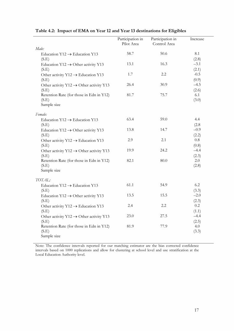
Table 4.2: Impact of EMA on Year 12 and Year 13 destinations for Eligibles

Participation in Pilot Area

Participation in Control Area

Increase

Male: Education Y12 → Education Y13 58.7 50.6 8.1 (S.E) (2.8) Education Y12 → Other activity Y13 13.1 16.3 –3.1 (S.E) (2.1) Other activity Y12 → Education Y13 1.7 2.2 -0.5 (S.E) (0.9) Other activity Y12 → Other activity Y13 26.4 30.9 –4.5 (S.E) (2.6) Retention Rate (for those in Edn in Y12) 81.7 75.7 6.1 (S.E) (3.0) Sample size Female: Education Y12 → Education Y13 63.4 59.0 4.4 (S.E) (2.8 Education Y12 → Other activity Y13 13.8 14.7 –0.9 (S.E) (2.2) Other activity Y12 → Education Y13 2.9 2.1 0.8 (S.E) (0.8) Other activity Y12 → Other activity Y13 19.9 24.2 –4.4 (S.E) (2.3) Retention Rate (for those in Edn in Y12) 82.1 80.0 2.0 (S.E) (2.8) Sample size TOTAL: Education Y12 → Education Y13 61.1 54.9 6.2 (S.E) (3.3) Education Y12 → Other activity Y13 13.5 15.5 –2.0 (S.E) (2.3) Other activity Y12 → Education Y13 2.4 2.2 0.2 (S.E) (1.1) Other activity Y12 → Other activity Y13 23.0 27.5 –4.4 (S.E) (2.5) Retention Rate (for those in Edn in Y12) 81.9 77.9 4.0 (S.E) (3.3) Sample size Note: The confidence intervals reported for our matching estimator are the bias corrected confidence intervals based on 1000 replications and allow for clustering at school level and use stratification at the Local Education Authority level.

17

Impact of EMA in Year 12 and Year 13 by Eligibility Groups

We now turn to comparing the impact of the policy separately for those who are eligible

for the full amount of the EMA, those who are only eligible for a fraction, because their

parents have a higher income. The impact between the two groups may be different for a

number of conflicting reasons. First, because the subsidy is lower it may have a lower

effect. Second, the individuals who receive a lower subsidy do so because they come

from a better off background. This may make them more likely to go to school in the

first place and thus may also affect their sensitivity to monetary incentives. With this

design we cannot distinguish one effect from the other. Thus, in the results that follow

we distinguish between full eligibility, partial eligibility and ineligibility to see if the impact

of EMA differs by whether a person was fully or only partially eligible and to see if there

were any spillovers to those in the ineligible group.

Only just over 47 per cent of individuals in Cohort 1 were eligible for the maximum

EMA payment, around 31 per cent for partial payment whilst 22 per cent were not

eligible. All eligible individuals were entitled to the bonuses which were not means tested.

For the results presented in the following Tables we use fully interacted linear matching

rather than kernel based matching to improve the precision of our estimates. As we saw

above, both methods provide almost identical estimates of the impact of EMA, but for

subgroup analysis precision and the use of analytical standard errors has clear advantages.

Once again this does not affect our results in any significant way. Because we have

imposed common support within each eligibility group, our samples are slightly smaller

than those reported in Table 4.1.

18

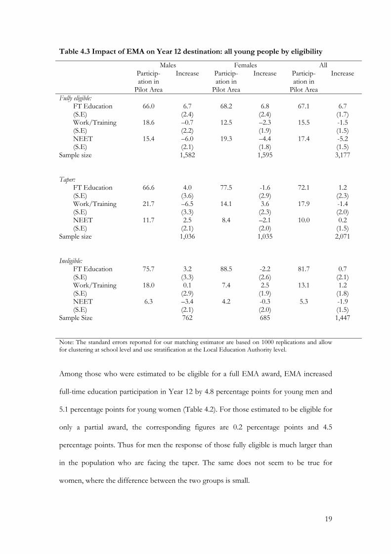
Table 4.3 Impact of EMA on Year 12 destination: all young people by eligibility

Males Females All Particip-

ation in Pilot Area

Increase Particip-ation in

Pilot Area

Increase Particip-ation in

Pilot Area

Increase

Fully eligible: FT Education 66.0 6.7 68.2 6.8 67.1 6.7 (S.E) (2.4) (2.4) (1.7) Work/Training 18.6 –0.7 12.5 –2.3 15.5 -1.5 (S.E) (2.2) (1.9) (1.5) NEET 15.4 –6.0 19.3 –4.4 17.4 -5.2 (S.E) (2.1) (1.8) (1.5) Sample size 1,582 1,595 3,177 Taper: FT Education 66.6 4.0 77.5 -1.6 72.1 1.2 (S.E) (3.6) (2.9) (2.3) Work/Training 21.7 –6.5 14.1 3.6 17.9 -1.4 (S.E) (3.3) (2.3) (2.0) NEET 11.7 2.5 8.4 –2.1 10.0 0.2 (S.E) (2.1) (2.0) (1.5) Sample size 1,036 1,035 2,071 Ineligible: FT Education 75.7 3.2 88.5 -2.2 81.7 0.7 (S.E) (3.3) (2.6) (2.1) Work/Training 18.0 0.1 7.4 2.5 13.1 1.2 (S.E) (2.9) (1.9) (1.8) NEET 6.3 –3.4 4.2 -0.3 5.3 -1.9 (S.E) (2.1) (2.0) (1.5) Sample Size 762 685 1,447 Note: The standard errors reported for our matching estimator are based on 1000 replications and allow for clustering at school level and use stratification at the Local Education Authority level.

Among those who were estimated to be eligible for a full EMA award, EMA increased

full-time education participation in Year 12 by 4.8 percentage points for young men and

5.1 percentage points for young women (Table 4.2). For those estimated to be eligible for

only a partial award, the corresponding figures are 0.2 percentage points and 4.5

percentage points. Thus for men the response of those fully eligible is much larger than

in the population who are facing the taper. The same does not seem to be true for

women, where the difference between the two groups is small.

19

The results of comparing ineligible young people in the pilot and control areas are given

in table 4.3. Although the education participation rates amongst ineligible individuals are

estimated that have increased for both males and females, by 2.8 and –2.5 percentage

points respectively, neither of these results is statistically significant. Even taken for the

entire ineligible samples, there is no evidence of any large or statistically significant

spillover effects. This is to be expected since the effect of the policy on the eligibles is

not large enough to make an impact on others. It is also comforting because it indicates

that there is no serious reason to believe that unobserved area effects are responsible for

the EMA effects we estimated for the eligible population.

.In Table 4.4 we again undertake this analysis for the second to see if the findings of the

previous section are altered when we split by eligibility groups. The results of doing this

are contained in Table 4.4.

20

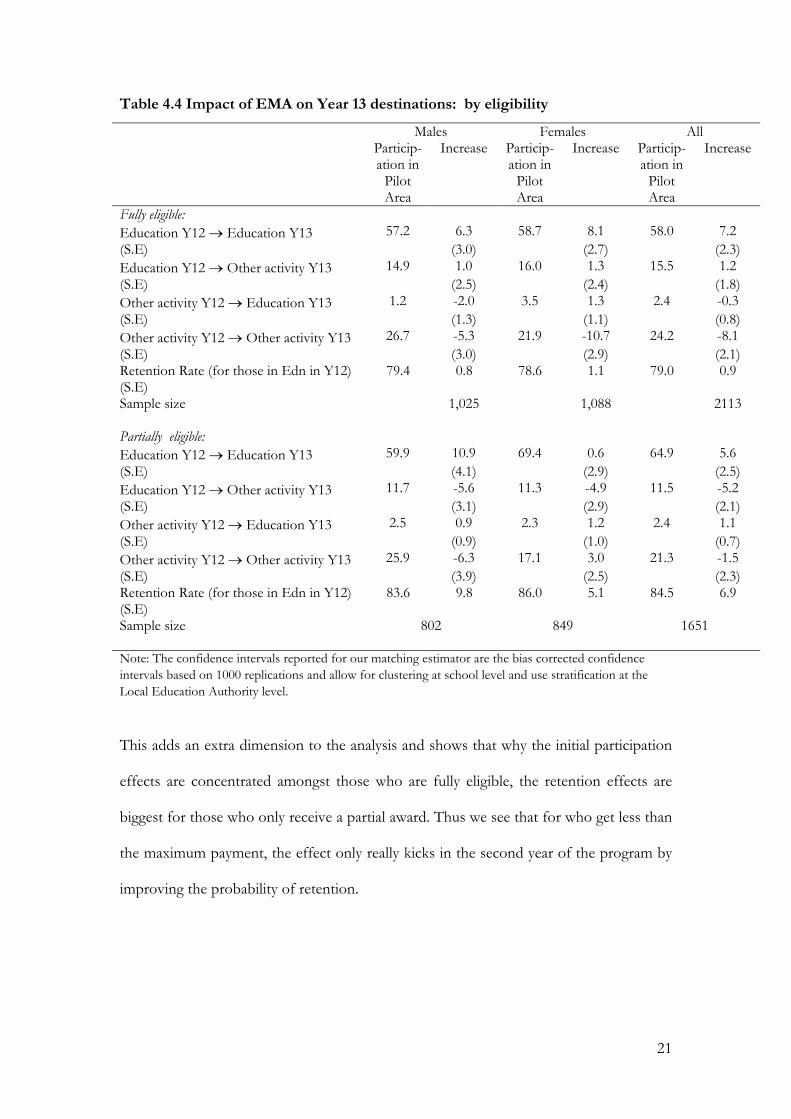
Table 4.4 Impact of EMA on Year 13 destinations: by eligibility

Males Females All Particip-

ation in Pilot Area

Increase Particip-ation in

Pilot Area

Increase Particip-ation in

Pilot Area

Increase

Fully eligible: Education Y12 → Education Y13 57.2 6.3 58.7 8.1 58.0 7.2 (S.E) (3.0) (2.7) (2.3) Education Y12 → Other activity Y13 14.9 1.0 16.0 1.3 15.5 1.2 (S.E) (2.5) (2.4) (1.8) Other activity Y12 → Education Y13 1.2 -2.0 3.5 1.3 2.4 -0.3 (S.E) (1.3) (1.1) (0.8) Other activity Y12 → Other activity Y13 26.7 -5.3 21.9 -10.7 24.2 -8.1 (S.E) (3.0) (2.9) (2.1) Retention Rate (for those in Edn in Y12) 79.4 0.8 78.6 1.1 79.0 0.9 (S.E) Sample size 1,025 1,088 2113 Partially eligible: Education Y12 → Education Y13 59.9 10.9 69.4 0.6 64.9 5.6 (S.E) (4.1) (2.9) (2.5) Education Y12 → Other activity Y13 11.7 -5.6 11.3 -4.9 11.5 -5.2 (S.E) (3.1) (2.9) (2.1) Other activity Y12 → Education Y13 2.5 0.9 2.3 1.2 2.4 1.1 (S.E) (0.9) (1.0) (0.7) Other activity Y12 → Other activity Y13 25.9 -6.3 17.1 3.0 21.3 -1.5 (S.E) (3.9) (2.5) (2.3) Retention Rate (for those in Edn in Y12) 83.6 9.8 86.0 5.1 84.5 6.9 (S.E) Sample size 802 849 1651 Note: The confidence intervals reported for our matching estimator are the bias corrected confidence intervals based on 1000 replications and allow for clustering at school level and use stratification at the Local Education Authority level.

This adds an extra dimension to the analysis and shows that why the initial participation

effects are concentrated amongst those who are fully eligible, the retention effects are

biggest for those who only receive a partial award. Thus we see that for who get less than

the maximum payment, the effect only really kicks in the second year of the program by

improving the probability of retention.

21

Who gets the payment – Does it matter?

In one of the EMA variants piloted the payment was made to the mother instead of the

child. There are many reasons why paying the mother could have a different effect. In

one extreme, if the mother is not expected to pass on the benefit to the child, then the

child will have a lower incentive to attend school. On the other hand, since transfers are

already taking place from the parents to the child, one can argue that even if the benefit

is given to the child it can be clawed back by the parents and hence whether it is paid to

the child or parents it should not make much difference.

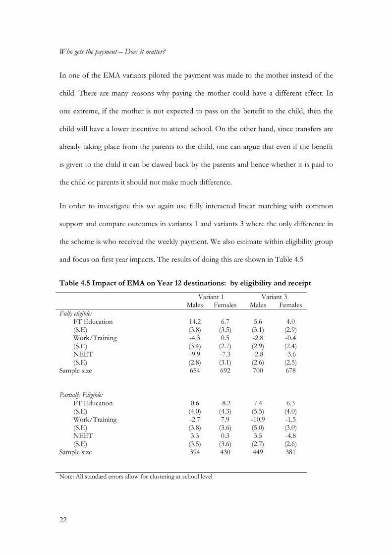
In order to investigate this we again use fully interacted linear matching with common

support and compare outcomes in variants 1 and variants 3 where the only difference in

the scheme is who received the weekly payment. We also estimate within eligibility group

and focus on first year impacts. The results of doing this are shown in Table 4.5

Table 4.5 Impact of EMA on Year 12 destinations: by eligibility and receipt

Variant 1 Variant 3 Males Females Males Females Fully eligible: FT Education 14.2 6.7 5.6 4.0 (S.E) (3.8) (3.5) (3.1) (2.9) Work/Training -4.3 0.5 -2.8 -0.4 (S.E) (3.4) (2.7) (2.9) (2.4) NEET -9.9 -7.3 -2.8 -3.6 (S.E) (2.8) (3.1) (2.6) (2.5) Sample size 654 692 700 678 Partially Eligible: FT Education 0.6 -8.2 7.4 6.3 (S.E) (4.0) (4.3) (5.5) (4.0) Work/Training -2.7 7.9 -10.9 -1.5 (S.E) (3.8) (3.6) (5.0) (3.0) NEET 3.3 0.3 3.5 -4.8 (S.E) (3.5) (3.6) (2.7) (2.6) Sample size 394 430 449 381 Note: All standard errors allow for clustering at school level

22

From Table 4.5 we see that for Variant 1, where the money is paid directly to the child,

the EMA impact is concentrated solely among those who are fully eligible. Participation

in full-time education for males is increased by 14.2 percentage points and full time

education participation for females by 6.7 percentage points. All of this increase in

participation is drawn from the NEET group. There is no significant full-time education

impact for individuals who are partially eligible.

The story is very different for the variant where the payment is made to the child’s

mother. The impact is now spread much more evenly among all groups who are eligible

and is much very similar for boys and girls.

Whilst the overall impact of the EMA on full-time education participation is very similar

for both variants, there is a big difference in impact by eligibility groups. The variant in

which it is paid to the child has a much larger impact on those who are fully eligible

whereas the variant where it is paid to the mother has a much more even effect across all

eligibility groups. This finding has obvious policy interest and suggests that if the key

interest is in increasing participation among those from the poorest backgrounds (those

from families earning less than £13,000 per annum) then payment to the child may be

preferred, whereas if the government is keen to impact across the whole eligibility

distribution then payment to the mother may be more effective – at least in terms of

initial staying on decisions.

In Table 4.6 we look at the results for Year 13 for those who do not drop out of the

panel from our sample. Unfortunately sample sizes are quite small which affects

precision but we see that by the second year, the results across all groups are much more

similar. Again, for those who receive only a partial payment, there appears to be a bigger

retention effect. By Year 13, the only big difference between the variants is that variant 1

is more effective drawing people from the group who would not have otherwise

23

participated in education and that variant 1 is more effective in increasing the

participation of men who are fully eligible.

24

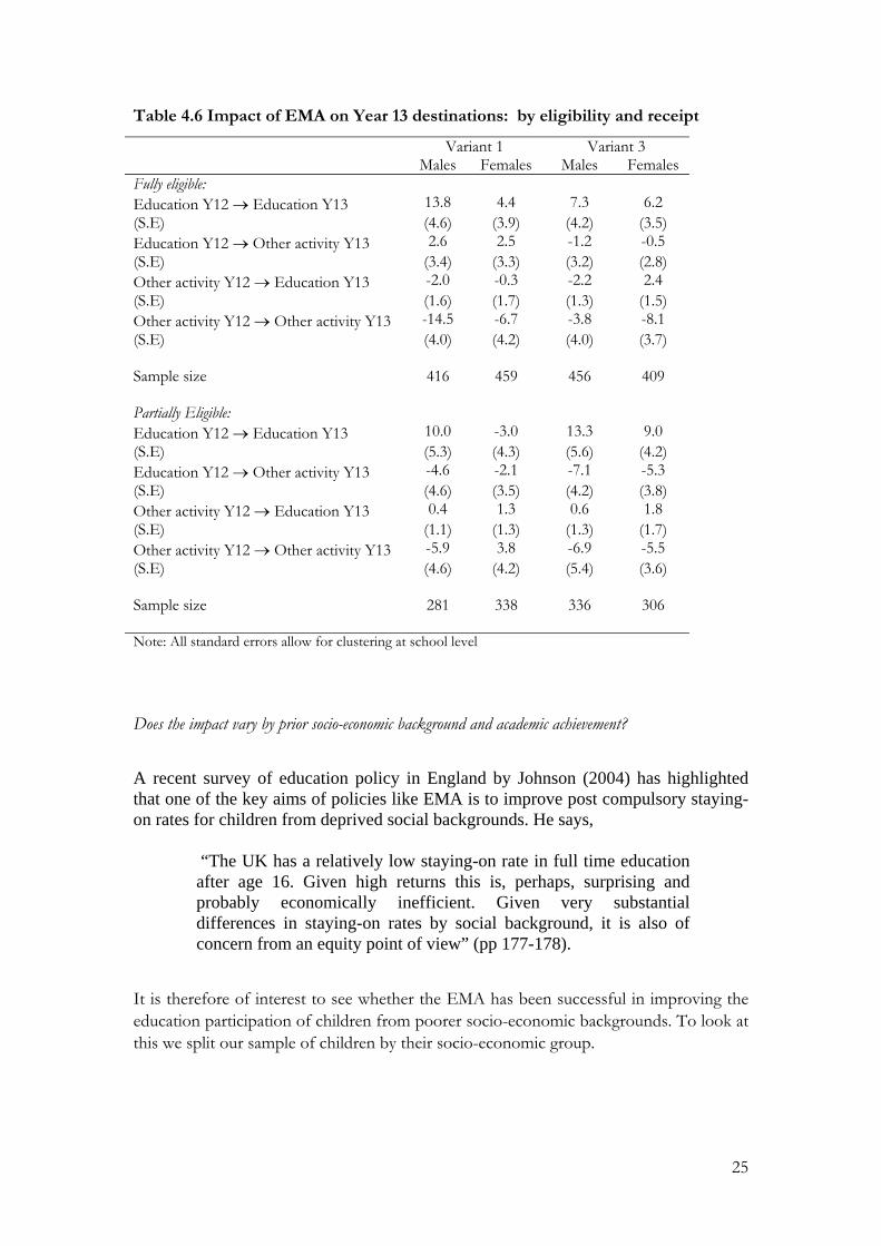
Table 4.6 Impact of EMA on Year 13 destinations: by eligibility and receipt

Variant 1 Variant 3 Males Females Males Females Fully eligible: Education Y12 → Education Y13 13.8 4.4 7.3 6.2 (S.E) (4.6) (3.9) (4.2) (3.5) Education Y12 → Other activity Y13 2.6 2.5 -1.2 -0.5 (S.E) (3.4) (3.3) (3.2) (2.8) Other activity Y12 → Education Y13 -2.0 -0.3 -2.2 2.4 (S.E) (1.6) (1.7) (1.3) (1.5) Other activity Y12 → Other activity Y13 -14.5 -6.7 -3.8 -8.1 (S.E) (4.0) (4.2) (4.0) (3.7) Sample size 416 459 456 409 Partially Eligible: Education Y12 → Education Y13 10.0 -3.0 13.3 9.0 (S.E) (5.3) (4.3) (5.6) (4.2) Education Y12 → Other activity Y13 -4.6 -2.1 -7.1 -5.3 (S.E) (4.6) (3.5) (4.2) (3.8) Other activity Y12 → Education Y13 0.4 1.3 0.6 1.8 (S.E) (1.1) (1.3) (1.3) (1.7) Other activity Y12 → Other activity Y13 -5.9 3.8 -6.9 -5.5 (S.E) (4.6) (4.2) (5.4) (3.6) Sample size 281 338 336 306 Note: All standard errors allow for clustering at school level

Does the impact vary by prior socio-economic background and academic achievement?

A recent survey of education policy in England by Johnson (2004) has highlighted that one of the key aims of policies like EMA is to improve post compulsory staying-on rates for children from deprived social backgrounds. He says,

“The UK has a relatively low staying-on rate in full time education after age 16. Given high returns this is, perhaps, surprising and probably economically inefficient. Given very substantial differences in staying-on rates by social background, it is also of concern from an equity point of view” (pp 177-178).

It is therefore of interest to see whether the EMA has been successful in improving the education participation of children from poorer socio-economic backgrounds. To look at this we split our sample of children by their socio-economic group.

25

We split our sample into two groups: a high socio-economic group and a low socio-

economic group. Our groups are based on the Socio-economic Group (SEG)

classification which is based on individual’s occupational unit group (1990 SOC group),

employment status and the size of establishment in which they work. A full description

of the SEG classification is explained in Office for National Statistics (1991). We classify

the household according to the highest SEG group of their parents (if more than one

parent). Our low group consists of households where no parent is in work or if the

highest occupation of the parents involves only unskilled or semi-skilled manual work.

The results of doing this are presented in Table 4.7. We see that almost all of the impact

of EMA is concentrated on children coming from families from poor socio-economic

backgrounds. For this group, male participation is increased by 6.1 percentage points in

Year 12 and 8.7 percentage points in Year 13. The corresponding figure for females from

this group are 8.2 percentage points and 12.2 percentage points.

What is interesting to see from this table, is that whilst for the higher socio-economic

group, girls are much more likely to stay on than boys, this is not true for girls coming

from poor socio-economic backgrounds. The EMA plays an important role in

significantly improving the participation of both girls and boys from this vulnerable

group.

26

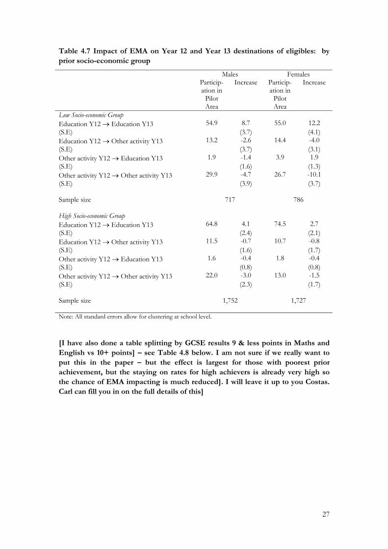
Table 4.7 Impact of EMA on Year 12 and Year 13 destinations of eligibles: by prior socio-economic group

Males Females Particip-

ation in Pilot Area

Increase Particip-ation in

Pilot Area

Increase

Low Socio-economic Group Education Y12 → Education Y13 54.9 8.7 55.0 12.2 (S.E) (3.7) (4.1) Education Y12 → Other activity Y13 13.2 -2.6 14.4 -4.0 (S.E) (3.7) (3.1) Other activity Y12 → Education Y13 1.9 -1.4 3.9 1.9 (S.E) (1.6) (1.3) Other activity Y12 → Other activity Y13 29.9 -4.7 26.7 -10.1 (S.E) (3.9) (3.7) Sample size 717 786 High Socio-economic Group Education Y12 → Education Y13 64.8 4.1 74.5 2.7 (S.E) (2.4) (2.1) Education Y12 → Other activity Y13 11.5 -0.7 10.7 -0.8 (S.E) (1.6) (1.7) Other activity Y12 → Education Y13 1.6 -0.4 1.8 -0.4 (S.E) (0.8) (0.8) Other activity Y12 → Other activity Y13 22.0 -3.0 13.0 -1.5 (S.E) (2.3) (1.7) Sample size 1,752 1,727 Note: All standard errors allow for clustering at school level.

[I have also done a table splitting by GCSE results 9 & less points in Maths and English vs 10+ points] – see Table 4.8 below. I am not sure if we really want to put this in the paper – but the effect is largest for those with poorest prior achievement, but the staying on rates for high achievers is already very high so the chance of EMA impacting is much reduced]. I will leave it up to you Costas. Carl can fill you in on the full details of this]

27

Table 4.8 Impact of EMA on Year 12 and Year 13 destinations of eligibles: by prior academic achievement

Males Females Particip-

ation in Pilot Area

Increase Particip-ation in

Pilot Area

Increase

Low Prior Academic Achievement Education Y12 → Education Y13 47.4 7.7 51.9 6.7 (S.E) (3.1) (3.5) Education Y12 → Other activity Y13 16.9 -4.9 18.9 -2.6 (S.E) (2.8) (3.3) Other activity Y12 → Education Y13 1.8 -2.1 4.1 1.0 (S.E) (1.1) (1.2) Other activity Y12 → Other activity Y13 33.8 -0.7 25.0 -5.1 (S.E) (3.0) (3.3) 1,134 1,100 Sample size High Prior Academic Achievement Education Y12 → Education Y13 84.4 1.6 89.4 2.7 (S.E) (2.4) (2.6) Education Y12 → Other activity Y13 5.7 0.8 5.6 -1.4 (S.E) (1.5) (1.7) Other activity Y12 → Education Y13 1.6 1.5 0.7 -0.2 (S.E) (0.6) (0.8) Other activity Y12 → Other activity Y13 8.4 -3.9 4.3 -1.1 (S.E) (2.0) (1.7) Sample size 1,061 1,244 Note: All standard errors allow for clustering at school level.

Sensitivity Analysis

To validate our results we have carried out a more limited analysis using as a comparison

group the older siblings of the children in our pilot and control areas. In this case the

approach we use is difference in differences conditioning on pre-program characteristics.

We include a full set of cohort and area dummies. We find an EMA effect of 0.0835

(with a standard error of 0.0281), which is similar albeit larger than the effect we reported

above. The difference is not significant at conventional levels.34

28

We also carry out successive difference in differences across siblings reaching the

statutory school leaving age before the period when the policy was in place as well as in

the final year. We find that in all previous periods the “effect” is not significant and the

estimate is close to zero. In the final period we obtain a positive and significant effect,

again corroborating and strengthening our results.

5. Conclusions

Despite a steady increase the participation in education following completion of

compulsory schooling in England remained relatively low at about 57% (is this number

correct? When is it from). The government decided to pilot an incentive scheme to

encourage more pupils from low income families to stay on in school. This schooling

subsidy program lasted for a maximum of two years following the end of compulsory

schooling. It is entitled the Education Maintenance Allowance (EMA) has now become

national policy. In this paper we use a dataset collected by us for the purposes of

evaluating the impact of this schooling subsidy program on school participation in

England. Our results imply that the scope for affecting education decisions using

subsidies to education can be substantial.

More specifically, the results imply that the Educational Maintenance Allowance (EMA)

has raised significantly the stay on rates past the age of 16. The initial impact is around

4.5 percentage points while having no effect on ineligibles. The effect for men is slightly

higher than for women helping to plug the gap in stay-on rates between girls and boys.

Taking into account that this was a time when the labour market was particularly

buoyant, these seem to be quite large effects, although they were achieved with a

replacement rate of 33%-40% of earnings.

34 The standard error allows for serial correlation and cluster effects.

29

The results also suggest that the impact of EMA on participation actually increases in the

following year. For those who get the full payment, the increased participation is

maintained whereas for those who get partial payment, rentention is actually significantlyl

improved. This results is important because it suggests that those who are induced into

extra education do not find the courses unexpectedly difficult or uninteresting and are

willing to stay for the full two years of the program into education. Importantly, about

half of the increase in school participation is due to a decline in inactivity, rather than

work. This reduces the implicit costs of the program since the foregone earnings for

them are zero.

It appears that the overall impact of EMAs is similar regardless of whether it is paid to

the mother or child. But this varies by eligibility and the variant where it is paid to the

child is more effective in improving participation rates amongst those who come from

the poorest families. Finally, it appears that the EMA had its largest impact on children

coming from families from the poorest socio-economic background (based on parents

occupation). This is a particular policy concern and it appears that the EMA has made

important inroad in improving the prospects of these children.

The results in this paper demonstrate that a conditional payment to 16 and 17 year olds

can significantly reduce school drop-out rates. Of course a number of important

questions remain. First, we do not know whether liquidity constraints are an important

factor in driving the estimated effects. A second and related issue is that we do not know

what returns those induced into staying on by the subsidy will enjoy but most recent

estimates in the UK suggest that the return is around 10-11 per cent for men and around

30

18 per cent for females35. Finally, we really have very little idea of how these returns may

change when the programme is rolled out in Setember 2004 and the supply of educated

workers changes. This of course depends on many factors, not least the nature of the

production function. These are all-important research and policy questions that we will

be pursuing in the future.

35 See Dearden, McGranahan and Sianesi (2004). These estimates are their best estimates of the average treatment effect on the non-treated for staying on in school past the compulsory school leaving age.

31

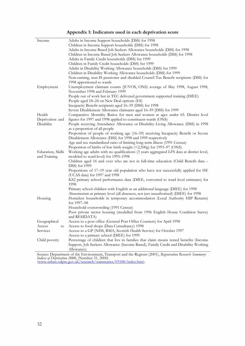
Appendix 1: Indicators used in each deprivation score

Income Adults in Income Support households (DSS) for 1998 Children in Income Support households (DSS) for 1998 Adults in Income Based Job Seekers Allowance households (DSS) for 1998 Children in Income Based Job Seekers Allowance households (DSS) for 1998 Adults in Family Credit households (DSS) for 1999 Children in Family Credit households (DSS) for 1999 Adults in Disability Working Allowance households (DSS) for 1999 Children in Disability Working Allowance households (DSS) for 1999 Non-earning, non-IS pensioner and disabled Council Tax Benefit recipients (DSS) for 1998 apportioned to wards

Employment Unemployment claimant counts (JUVOS, ONS) average of May 1998, August 1998, November 1998 and February 1999 People out of work but in TEC delivered government supported training (DfEE) People aged 18–24 on New Deal options (ES) Incapacity Benefit recipients aged 16–59 (DSS) for 1998 Severe Disablement Allowance claimants aged 16–59 (DSS) for 1999

Health Deprivation and Disability

Comparative Mortality Ratios for men and women at ages under 65. District level figures for 1997 and 1998 applied to constituent wards (ONS) People receiving Attendance Allowance or Disability Living Allowance (DSS) in 1998 as a proportion of all people Proportion of people of working age (16–59) receiving Incapacity Benefit or Severe Disablement Allowance (DSS) for 1998 and 1999 respectively Age and sex standardized ratio of limiting long-term illness (1991 Census) Proportion of births of low birth weight (<2,500g) for 1993–97 (ONS)

Education, Skills and Training

Working age adults with no qualifications (3 years aggregated LFS data at district level, modeled to ward level) for 1995–1998 Children aged 16 and over who are not in full-time education (Child Benefit data – DSS) for 1999 Proportions of 17–19 year old population who have not successfully applied for HE (UCAS data) for 1997 and 1998 KS2 primary school performance data (DfEE, converted to ward level estimates) for 1998 Primary school children with English as an additional language (DfEE) for 1998 Absenteeism at primary level (all absences, not just unauthorised) (DfEE) for 1998

Housing Homeless households in temporary accommodation (Local Authority HIP Returns) for 1997–98 Household overcrowding (1991 Census) Poor private sector housing (modelled from 1996 English House Condition Survey and RESIDATA)

Geographical Access to Services

Access to a post office (General Post Office Counters) for April 1998 Access to food shops (Data Consultancy) 1998 Access to a GP (NHS, BMA, Scottish Health Service) for October 1997 Access to a primary school (DfEE) for 1999

Child poverty Percentage of children that live in families that claim means tested benefits (Income Support, Job Seekers Allowance (Income Based), Family Credit and Disability Working Allowance).

Source: Department of the Environment, Transport and the Regions (2001), Regeneration Research Summary: Indices of Deprivation 2000, (Number 31, 2000) (www.urban.odpm.gov.uk/research/summaries/03100/index.htm).

32

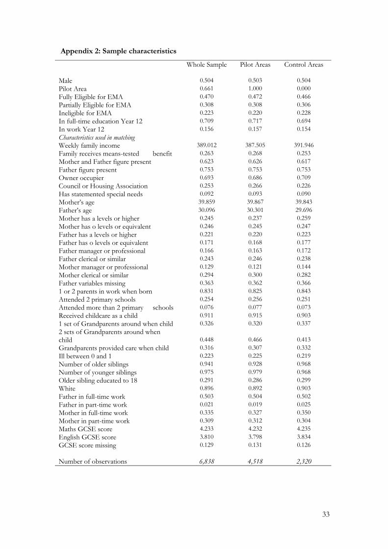
Appendix 2: Sample characteristics

Whole Sample Pilot Areas Control Areas Male 0.504 0.503 0.504 Pilot Area 0.661 1.000 0.000 Fully Eligible for EMA 0.470 0.472 0.466 Partially Eligible for EMA 0.308 0.308 0.306 Ineligible for EMA 0.223 0.220 0.228 In full-time education Year 12 0.709 0.717 0.694 In work Year 12 0.156 0.157 0.154 Characteristics used in matching Weekly family income 389.012 387.505 391.946 Family receives means-tested benefit 0.263 0.268 0.253 Mother and Father figure present 0.623 0.626 0.617 Father figure present 0.753 0.753 0.753 Owner occupier 0.693 0.686 0.709 Council or Housing Association 0.253 0.266 0.226 Has statemented special needs 0.092 0.093 0.090 Mother’s age 39.859 39.867 39.843 Father’s age 30.096 30.301 29.696 Mother has a levels or higher 0.245 0.237 0.259 Mother has o levels or equivalent 0.246 0.245 0.247 Father has a levels or higher 0.221 0.220 0.223 Father has o levels or equivalent 0.171 0.168 0.177 Father manager or professional 0.166 0.163 0.172 Father clerical or similar 0.243 0.246 0.238 Mother manager or professional 0.129 0.121 0.144 Mother clerical or similar 0.294 0.300 0.282 Father variables missing 0.363 0.362 0.366 1 or 2 parents in work when born 0.831 0.825 0.843 Attended 2 primary schools 0.254 0.256 0.251 Attended more than 2 primary schools 0.076 0.077 0.073 Received childcare as a child 0.911 0.915 0.903 1 set of Grandparents around when child 0.326 0.320 0.337 2 sets of Grandparents around when child 0.448 0.466 0.413 Grandparents provided care when child 0.316 0.307 0.332 Ill between 0 and 1 0.223 0.225 0.219 Number of older siblings 0.941 0.928 0.968 Number of younger siblings 0.975 0.979 0.968 Older sibling educated to 18 0.291 0.286 0.299 White 0.896 0.892 0.903 Father in full-time work 0.503 0.504 0.502 Father in part-time work 0.021 0.019 0.025 Mother in full-time work 0.335 0.327 0.350 Mother in part-time work 0.309 0.312 0.304 Maths GCSE score 4.233 4.232 4.235 English GCSE score 3.810 3.798 3.834 GCSE score missing 0.129 0.131 0.126 Number of observations 6,838 4,518 2,320

33

Appendix 3 - Covariate balancing indicators (best specification): before and after matching

Matching

Estimator

N1 N0 Probit pseudo

R2

Probit pseudo

R2

P>χ2 Median bias

Median bias

% lost to common support

Before Before Before After After Before After After

(1) (2) (3) (4) (5) (6)

Males: Nearest Neighbour 1,753 900 0.085 0.029 0.000 3.9 5.3 0.4Mahalanobis-metric 1,753 900 0.085 0.086 0.000 3.9 7.4 0.4Epanechnikov (bw=0.01) 1,753 900 0.085 0.012 0.740 3.9 2.5 0.7Epanechnikov (bw=0.06) 1,753 900 0.085 0.010 0.921 3.9 2.3 0.4 Females: Nearest Neighbour 1,771 891 0.104 0.030 0.000 3.3 3.6 0.2Mahalanobis-metric 1,771 891 0.104 0.103 0.000 3.3 7.8 0.2Epanechnikov (bw=0.01) 1,771 891 0.104 0.015 0.306 3.3 2.2 1.0Epanechnikov (bw=0.06) 1,771 891 0.104 0.014 0.510 3.3 1.5 0.2 Notes: (1) Pseudo R2 from probit estimation of the conditional treatment probability, giving an indication of

how well our matching regressors X explain the relevant educational choice. (2) Pseudo R2 from a probit of D on X on the matched samples, to be compared with (1). (3) P-value of the likelihood-ratio test after matching, testing the hypothesis that the regressors are

jointly insignificant, i.e. well balanced in the two matched groups. (4) and (5)

Median absolute standardised bias before and after matching, median taken over all the matching. Following Rosenbaum and Rubin (1985), for a given covariate X, the standardised difference before matching is the difference of the sample means in the full treated and non-treated subsamples as a percentage of the square root of the average of the sample variances in the full treated and non-treated groups. The standardised difference after matching is the difference of the sample means in the matched treated (i.e. falling within the common support) and matched non-treated subsamples as a percentage of the square root of the average of the sample variances in the full treated and non-treated groups.

( )1 0

1 0

( ) 100( ) ( ) / 2

beforeX X

B XV X V X

−≡

+

( )1 0

1 0

( ) 100( ) ( ) / 2

M Mafter

X XB X

V X V X−

≡+

Note that the standardisation allows comparisons between variables X and for a given variable X, comparisons before and after matching.

(6) Share of the treated group falling outside of the common support, imposed at the boundaries.

34

Appendix 4: Attrition between wave 1 and wave 2

Table A4.1 Probability of Attrition between wave 1 and wave 2.

Marginal Effect

Standard error

Partially Eligible -0.002 0.024 Fully Eligible -0.039 0.015 Pilot Area 0.005 0.012 Male 0.019 0.011 Weekly family 0.000 0.000 Family receives means-tested benefit -0.014 0.017 Mother and Father figure present -0.015 0.032 Father figure present -0.028 0.021 Owner occupier -0.085 0.025 Council or Housing Association -0.031 0.023 Has statemented special needs -0.001 0.018 Mother’s age -0.002 0.001 Father’s age -0.001 0.001 Mother has a levels or higher 0.001 0.017 Mother has o levels or equivalent 0.001 0.014 Father has a levels or higher -0.065 0.018 Father has o levels or equivalent -0.022 0.017 Father manager or professional -0.014 0.021 Father clerical or similar 0.017 0.016 Mother manager or professional -0.029 0.020 Mother clerical or similar -0.014 0.013 Father variables missing -0.015 0.036 1 or 2 parents in work when born -0.011 0.016 Attended 2 primary schools -0.021 0.012 Attended more than 2 primary schools 0.030 0.021 Received childcare as a child 0.002 0.019 1 set of Grandparents around when child -0.008 0.015 1 sets of Grandparents around when child 0.004 0.016 Grandparents provided care when child 0.007 0.012 Ill between 0 and 1 0.010 0.013 Number of older siblings 0.017 0.006 Number of younger siblings -0.010 0.005 Older sibling educated to 18 -0.036 0.013 White -0.020 0.022 Father in full-time work 0.033 0.020 Father in part-time work -0.004 0.039 Mother in full-time work -0.002 0.017 Mother in part-time work -0.030 0.015 Income -0.001 0.002 Employment -0.007 0.003 Health Deprivation and Disability 0.033 0.020 Education, Skills and Training 0.023 0.011 Housing 0.010 0.012 Geographical Access to Services 0.004 0.014

35

Child poverty 0.002 0.001 per cent not staying on post 16 -0.002 0.001 per cent not going to university -0.002 0.002 Class sizes in 1999 -0.003 0.002 Authorised absences 0.000 0.004 % getting 5 GCSE A–C in 1999 0.001 0.001 % getting 0 GCSE A–G in 1999 0.001 0.001 School has 6th form? -0.002 0.013 Distance to nearest year 12 provider 0.000 0.000 Maths GCSE score -0.014 0.006 English GCSE score -0.015 0.005 GCSE score missing -0.003 0.025 Number of observations 6838 Observed probability 0.253

Appendix 4: Identification and Estimation method

Suppose the outcome of an individual with characteristics Xi who is exposed to the EMA

is . The same individual would have outcome were she/he not to be exposed to

the treatment. Obviously, either one or the other outcome is observed. The impact of

the policy for the ith individual ( ) is thus not observed. The main evaluation

parameter that we will estimate is the impact of treatment on the treated, i.e.

, where P is one for individuals in the pilot areas and zero in the

control areas. What we do observe is , which is the average participation

rate for those exposed to the EMA. To construct the counterfactual we

assume that which means that given the

observable characteristics the allocation to treatment and control is random. Under this

assumption it is now well known (see Rosenbaum and Rubin, 1983) that we can reduce

the dimension of the conditioning set from X to just

1iY 0

iY

01ii YY −

)1|( 01 =− iii PYYE

)1|( 1 =ii PYE

)1|( 0 =ii PYE

),0|(),1|( 00iiiiii XPYEXPYE ===

)|1Pr( ii XP = , i.e. the propensity

score which is simply the probability of being allocated to the pilot given observed

characteristics. This makes the computational exercise feasible and simple. Thus, given

36

the original matching assumption we can also write that

It follows that we can

estimate the counterfactual by the sample analogue of

))|,1Pr(,0|())|,1Pr(,1|( 00iiiiiiii XPPYEXPPYE =====

))]|,1Pr(,0|([)1|( 001 iiiiFii XPPYEEPYE ==== ,

where denotes an expectation with respect to the distribution of the propensity

score in the treatment sample.

1FE

Implementing this involves the following steps. In the first step the propensity score is

estimated. In the second step we estimate the conditional expectation of the outcome

in the control areas given the propensity score using a number of methods. It turns out

that for our particular policy experiment, using an Epanechnikov kernel with

bandwidth of 0.06 gives us the best covariate balancing indicators amongst a range of

matching estimators that we considered. We are careful to ensure that all

observations whose value of the propensity score is outside the range of the

propensity score in the treatment sample are deleted. This imposes common support

avoiding a major source of bias (see Heckman, Ichimura and Todd, 1997). Finally the

overall average is constructed using as weights the distribution of the propensity score

in the pilot areas.

References

Attanasio O et al. (2003) Report on the Baseline Survey for the `Familias en Accion’ Programme in Colombia

Attanasio, O, C. Meghir and Ana Santiago (2002) “Education Choices in Mexico: Using a Structural Model and a Randomized Experiment to evaluate Progresa.” UCL mimeo.

Benhabib Jess and Mark M. Spiegel (1994), "The Role of human Capital in Economic Development: Evidence from Aggregate Cross-country Data", Journal of Monetary Economics, 34(2), 143-174.

37

Cameron, S. and Heckman, J., (1998) ‘Life Cycle Schooling and Dynamic Selection Bias: Models and Evidence for Five Cohorts of American Males’, Journal of Political Economy, vol. 106, no. 2, pages 262–333.

Cameron, S. and Taber, C., (2000) ‘Borrowing Constraints and the Returns to Schooling’, NBER Working Paper No. 7761.

Dale, S. and Krueger, A., (1999) ‘Estimating the Payoff to Attending a More Selective College: An Application of Selection on Observables and Unobservables’, NBER Working Paper No. 7322.

Dearden, L, McGranahan, L and Sianesi, B. (2004), “Credit Constraints and Returns to the Marginal Learner), Centre for Economics of Education Discussion Paper, forthcoming.

Dynarski, Susan (2000) Hope for Whom? Financial Aid for the Middle Class and Its Impact on College Attendance, National Tax Journal, vol 53(3), 629-661.

Dynarski, Susan (2003) Does Aid Matter? Measuring the Effects of Student Aid on College Attendance and Completion American Economic Review, March 2003, 279-288.

Gosling, Amanda, Steve Machin and Costas Meghir (2000) “The Changing Distribution of Wages in the UK”, Review of Economic Studies

Goldin, Claudia (1999), ‘Egalitarianism and the Returns to Education during the Great Transformation of American Education’, Journal of Political Economy, vol 107, S65-S94.

Harmon, Colm and Ian Walker (1995), ‘Estimates of the Economic Return to Schooling for the United Kingdom’, The American Economic Review, Vol. 85, No. 5. (Dec., 1995), pp. 1278-1286. Heckman, J., Ichimura, H. and Todd, P., (1997) ‘Matching as an Econometric Evaluation Estimator’, Review of Economic Studies, 65, 261-294.

Heckman, J., Lochner, L. and Taber, C., (1998) ‘Explaining Rising Wage Inequality: Explorations with a Dynamic General Equilibrium Model of Labor Earnings with Heterogeneous Agents’, NBER Working Paper No. 6384.

Johnson, Paul (2004), “Education Policy in England”, Oxford Review of Economic Policy, vol. 20, No. 2, 173—197.

Juhn, Chinhui, Kevin M. Murphy; Brooks Pierce “Wage Inequality and the Rise in Returns to Skill” The Journal of Political Economy, Vol. 101, No. 3. (Jun., 1993), pp. 410-442. Krueger, Alan and Mikael Lindahl (2001), "Education for Growth: Why and For Whom?", Journal of Economic Literature, December, 39, 1101-1136.

Office for National Statistics(1991), Standard Occupational Classification (SOC 1990), Volume 3, London: Office for National Statistics.

38

Rosenbaum P. and Rubin D., (1983) ‘The Central Role of the Propensity Score in Observational Studies for Causal Effects’, Biometrika, 70, 41–55.

Schultz, Paul (2000) “Final Report: The Impact of Progesa on School enrolment”, IFPRI mimeo.

39