Can Cross-Border Funding Frictions Explain Financial ... · requirements (irrespective of investors’ attitude towards foreign exchange (FX) risk), and foreign currency funding or

Can Cross-Border Funding Frictions Explain

Financial Integration Reversals?∗

Amir Akbari

University of Ontario

Francesca Carrieri

McGill University

Aytek Malkhozov

Federal Reserve Board

Current Version: March 2018

Abstract

We examine the role of funding frictions in international investments. Guided by

an international CAPM with funding constraints, we use the differences in the betting-

against-beta portfolio performance between countries to infer the magnitude and the

implicit cost of barriers that impede the funding of cross-border positions. We find

such cross-border funding barriers to be economically significant. Despite an over-

all downward trend, our measure reveals periods when cross-border funding frictions

become more severe. These periods coincide with increases in market segmentation

documented in the literature but not explained by the variation in other international

investment barriers.

Keywords: International Finance, Market Segmentation, Integration Reversals, Funding Liquidity

JEL classification: F36, G01, G12, G15.

∗We thank Patrick Augustin, Ines Chaieb, Benjamin Croitoru, John Doukas, Bernard Dumas, VihangErrunza, Mariassunta Giannetti, Michael Goldstein, Allaudeen Hameed, Alexandre Jeanneret, Aditya Kaul,Hugues Langlois, Marc Lipson, Babak Loftaliei, Lilian Ng, Sergei Sarkissian, David Schumacher, and seminarparticipants at the 2017 NFA meetings, the University of Alberta, and the Federal Reserve Board for theirhelpful comments. Akbari acknowledges financial support from the National Bank Financial Group PhDFellowship. Carrieri acknowledges financial support from SSHRC. The views expressed here are our ownand do not reflect those of the Federal Reserve Board of Governors. Please address correspondence [email protected].

1 Introduction

International financial markets have become more integrated over the past decades. Re-

searchers have attributed this long-run trend to the progressive reduction of barriers to

foreign investment, such as capital controls or taxes on repatriation, around the world.1

However, in the wake of the 2008 financial crisis, concerns over a potential reversal of these

global market integration trends came to dominate the academic and policy debates.2 Yet,

even transitory reversals in integration are at odds with an apparent lack of new barriers to

international capital flows. Nonetheless, when they materialize, such reversals can decrease

international risk sharing and increase the cost of capital around the world.

In this paper, we shed new light on the dynamics of financial integration by considering

the role of funding-constrained investors. The premise of our analysis is that, in addition

to restricted or costly access to foreign assets, international investors are also constrained

in their ability to access funding for their cross-border positions.3 Such constraints arise for

a variety of reasons. For example, foreign collateral may command higher haircuts relative

to domestic collateral (the limiting case being the restrictions on assets eligible as collateral

for central bank refinancing), foreign currency positions imply higher regulatory capital

requirements (irrespective of investors’ attitude towards foreign exchange (FX) risk), and

foreign currency funding or FX risk hedging involve additional costs that ultimately reflect

the balance sheet constraints of financial intermediaries supplying them.4

Our first contribution to the literature is to infer the importance of these frictions from

the effect they have on asset prices. To do so, we construct a novel measure of cross-

1See Bekaert and Harvey (1995), Carrieri, Errunza, and Hogan (2007), Bekaert, Harvey, Lundblad, andSiegel (2011, 2013), Carrieri, Chaieb, and Errunza (2013), and Eiling and Gerard (2015), among others.

2See Rose and Wieladek (2014), Van Rijckeghem and Weder (2014), Giannetti and Laeven (2012, 2016),Jeanne and Korinek (2010), Ostry, Ghosh, Chamon, and Qureshi (2012), Forbes, Fratzscher, and Straub(2013), Pasricha, Falagiarda, Bijsterbosch, and Aizenman (2015), and Bussiere, Schmidt, and Valla (2016).

3Stulz (1981) and Errunza and Losq (1985) introduce holding costs and ownership restrictions for inter-national investments, respectively. Our focus on funding frictions separates us from international integrationliterature based on these two seminal contributions.

4See for example CPSS (2006), BCBS (2016), Corradin and Rodriguez-Moreno (2016), Du, Tepper, andVerdelhan (2018), and Cenedese, Della Corte, and Wang (2016).

1

border funding frictions based on the distance between the expected returns of betting-

against-beta (BAB) portfolios of the countries in our sample. The expected returns of these

BAB portfolios are driven by the lower slope of the security market line, compared to the

risk-based benchmark, and capture the effect of funding considerations on expected returns

in a given country.5 We show that the distance between expected BAB returns of the

countries are informative about cross-border funding frictions, and we find these frictions to

be economically important. Next, we relate the variation in country-level indicators of the

cross-border frictions to available funding liquidity proxies and institutional features that

correlate with the presence of funding constraints. Finally, using our country indicators, we

find that the difficulty to fund cross-border positions can help explain financial integration

reversals (i.e., transitory increases in market segmentation) documented in the literature but

not explained by the variation in other foreign investment barriers.

As a first step, we build an international asset pricing model in which investors have to

fund a fraction of their position in each security with their own capital, and we set these

capital requirements higher for cross-border positions.6 In an equilibrium where funding

constraints bind for at least some investors, the expected excess return on any security

depends not only on its exposure to market risk, but also on the interaction between the

capital required to maintain the position in this security and investors’ funding liquidity as

measured by their shadow price of capital. In turn, the BAB portfolios, which are long the

low-beta assets and short the high-beta assets in their respective countries, are constructed to

have zero exposure to market risk and load on the country funding component only. Because

access to foreign markets is subject to higher capital requirements, domestic funding liquidity

and foreign investors’ funding liquidity have a different effect on a given market. This leads to

differences in expected BAB returns across countries and to imperfect correlation between

expected BAB returns in response to investors’ funding liquidity shocks. The latter in

turn leads to lower correlation between realized BAB returns. In contrast, when capital

5See Black (1972), Frazzini and Pedersen (2014), and Jylha (2017).6The model builds on Frazzini and Pedersen (2014) and Malkhozov, Mueller, Vedolin, and Venter (2017).

2

requirements are the same for foreign and domestic positions, expected BAB returns in all

countries depend on the representative global investor’s shadow price of capital.

Next, we construct the BAB portfolios for 49 countries (21 developed markets and 28

emerging markets) for the period from 1973 to 2014. The average returns of these country

BAB portfolios are positive, at 1.08% monthly for developed markets and 1.31% for emerging

markets, and are statistically significant for most countries. We find important differences

between average BAB returns in our sample of countries. After accounting for the country-

level determinants of expected BAB returns, such as the market volatility and the spread

between high- and low-beta portfolios, the BAB portfolio returns are different from their

global average by 0.26% in developed markets and 0.67% in emerging markets. We also find

that BAB returns are positively correlated between countries, and this correlation is stronger

for developed markets compared to emerging markets, with the average correlation between

developed market BAB returns increasing substantially between 1997 and 2004. However,

we document that in crisis periods BAB portfolios tend to co-move less across countries, in

stark contrast to market-wide stock indices, which tend to co-move more.7,8

Building on our model and the above observations, we create a measure of the severity

of the funding frictions for cross-border positions for each country in our sample. We use

Bayesian methods to estimate the unobserved driver of the expected country BAB returns,

controlling for the country-level market volatility and the spread between high- and low-beta

portfolios. We interpret this latent variable as a proxy for the shadow price of capital. For

every country we measure the distance between its own shadow price of capital and that of

the other countries. In the context of our model, this distance increases either when cross-

border capital requirements increase or when the funding liquidity of investors in different

countries diverge, making a given cross-border capital requirement more costly.

7See Longin and Solnik (2001) and Forbes and Rigobon (2002) for additional evidence on the market-widecorrelations during market distress periods.

8Higher correlation of fundamental shocks during crisis periods has been a challenge for the analysis ofmarket integration dynamics. See Carrieri et al. (2007) and Pukthuanthong and Roll (2009) who discussempirical and theoretical issues with using market-wide correlations as a measure of market integration.

3

The above approach allows us to construct a cross-border funding barrier (CFB) indicator

for multiples countries and over long periods, unlike most existing funding liquidity proxies

that have limited cross-sectional or time-series information, and are also often difficult to

compare internationally. We find that the CFB indicators exhibit properties that are in

line with our expectations. Their magnitude is lower for developed markets, they display

a downward trend across all markets, and this downward trend is more pronounced for

emerging markets. The economic significance of the cross-border funding barriers that can

be inferred from this unobserved component is three times as large for emerging markets,

but interestingly it is also sizeable for developed markets. Furthermore, the indicators reveal

that large increases in the severity of funding barriers, albeit transitory, are a salient feature

of both developed and emerging country stock markets.

In the following step, we examine the drivers of the variation in the CFB measure across

countries and over time. First, we find a strong and positive relationship between the

CFB indicators and global funding liquidity. The differences in expected BAB returns,

at the core of our country indicators, widen when global funding conditions deteriorate. In

particular, proxies from the U.S. funding market, like the leverage of broker-dealers, from the

credit market, like the TED spread, and from the foreign exchange market, like the covered

interest parity (CIP) basis, are all significantly related to the CFB indicators. Second,

there is no significant association between the indicators and standard foreign investment

barrier proxies, suggesting that differences in expected BAB returns captured by our measure

are not driven by these previously studied foreign investment barriers, but rather reveal a

separate channel. Third, for countries and periods where country-level funding condition

proxies are available, these country-level proxies have significant explanatory power over

and above global funding conditions, suggesting that the information on funding frictions

contained in the CFB indicators is not subsumed by a single global factor. Fourth, the

long-run downward trend in the CFB indicators is in line with the progressive liberalization

in cross-border funding that we measure by the number of foreign banks that are primary

4

dealers in the U.S. Treasuries.

Finally, we examine whether cross-border funding frictions contribute to international

stock market segmentation. We note that the empirical properties of the CFB indicators are

broadly in line with market segmentation facts documented in the literature. More formally,

we find a statistically and economically significant relationship between funding barriers

and the segmentation measure proposed by Bekaert et al. (2011, 2013). Furthermore, this

relationship is particularly strong during financial integration reversals identified by the

segmentation measure. While acknowledging such reversals, previous literature has not

directly explored possible explanations. We propose a mechanism based on funding frictions

that can rationalize financial integration reversals. Unlike traditional investment barriers

which vary across countries but change very slowly over time, the shadow cost of a given

cross-border capital requirement can change significantly when funding liquidity conditions

across countries change. The dependence of our measure on the shadow cost of capital

constitutes an important qualitative difference between funding and other barriers. This

dependence explains why we can empirically observe global financial integration reversals

even when investment barriers are not markedly changing.

We perform several robustness checks and we find that our results remain unchanged

when we consider separately the U.S., all the countries in our sample excluding the U.S., or

when we exclude the 2007-2009 global financial crisis period. We also carefully distinguish

between funding and market liquidity. Bekaert, Harvey, and Lundblad (2007) and Lee

(2011), among others, demonstrated the importance of market liquidity for international

investments. However, the effect of funding liquidity is different from the effect of market

liquidity, although the two could potentially be linked (Brunnermeier and Pedersen, 2009).

We control for market liquidity and find only a weak relationship between market liquidity

and the cross-border funding measure, consistent with the results of Goyenko and Sarkissian

(2014).

This paper is related to several literature strands. Brunnermeier and Pedersen (2009),

5

Geanakoplos (2010), Garleanu and Pedersen (2011), He and Krishnamurthy (2012, 2013),

Adrian and Shin (2014), Garleanu, Panageas, and Yu (2015) among many others, study the

effect of constrained investors on asset prices. We apply the theoretical insights of this litera-

ture to an international setting. In this respect, we extend the literature on the dynamics of

financial integration in the post-liberalization period. Carrieri et al. (2007), Pukthuanthong

and Roll (2009), Bekaert et al. (2011, 2013), Carrieri et al. (2013), and Eiling and Gerard

(2015) empirically study the dynamics of financial integration and identify the role of ex-

plicit and implicit barriers to foreign investment in driving it. Relative to these papers, we

propose a new mechanism that contributes to international stock market segmentation and

is useful in explaining integration reversals. Our findings are consistent with the notion that

in periods when leveraging cross-border positions is more difficult and global capital flows

reverse, more risk should be borne by local investors, which would lead to increase in market

segmentation. In fact, the literature on the dynamics of home bias, such as Warnock and

Warnock (2009), Hoggarth, Mahadeva, and Martin (2010), Jotikasthira, Lundblad, and Ra-

madorai (2012), and Giannetti and Laeven (2012, 2016) documents that investors decrease

their international holdings following funding shocks. Similarly, Rey (2015) argues that a

global factor related to the constraints of leveraged global banks and asset managers explains

the dynamics of international capital flows.

The rest of the paper is organized as follows. Section 2 introduces the Cross-border

Funding Barrier indicator. The data and the estimation results are presented in Sections 3

and 4. Section 5 concludes.

6

2 Cross-border Funding Barriers Indicator

2.1 A Model with Funding Barriers to International Investment

We consider an economy with two dates t = 0, 1 and two countries j = d, f .9 In each country

there exist a set Kj of stocks indexed by k and a set Ij of nj competitive investors indexed

by i. We denote K =⋃j Kj, I =

⋃j Ij, and n =

∑j nj.

Each stock k is in fixed supply and its gross return between dates 0 and 1 is denoted

by Rk. Investors also have access to a riskless asset with gross return R0 given exogenously.

Finally, the purchasing power parity holds and all prices are expressed in U.S. dollars.10

Each investor i can invest in all assets of the world economy. She maximizes

max{xi,k}

k∈K

E0 [Wi,1]− α

2Var0 [Wi,1]

subject to her budget constraint

Wi,1 = Wi,0R0 +∑k∈K

(Rk −R0)xi,k, (1)

where Wi,0 is investor’s initial wealth, xi,k is the dollar amount investor i holds in stock k at

time 0.

Investors’ leverage is limited, capturing the combined effect of regulatory constraints and

market discipline.11 Specifically, investing in or shorting securities requires investor i to

commit the amount of capital equal to the multiple mi,k of her position size:

∑k∈K

mi,k |xi,k| ≤ Wi,0 + ζi, (2)

9We can also think about the second country as the rest of the world.10See, e.g., Bekaert et al. (2007) who make a similar assumption.11Investors who are active in international financial markets can be subject to bank capital requirements,

participation constraints imposed by debtholders, margin requirements, etc.

7

where ζi is a shock that tightens or relaxes the leverage constraint before investor chooses

her optimal portfolio. These shocks are a reduced form way to model changes in investors’

capital position through past investment gains/losses and any exogenous shocks to their

funding liquidity. Stock k ∈ Kj capital requirement is given by

mi,k =

m, if i ∈ Ij

m+ κ, if i 6∈ Ij.

When κ > 0, investor have to commit more capital to take foreign leveraged positions relative

to domestic leveraged positions. Finally, in line with Frazzini and Pedersen (2014), we focus

on the case where xi,k > 0.

Conditionally on the realisations of funding liquidity shocks ζi, we have

Theorem 1. The equilibrium expected return on a self-financing market-neutral portfolio

that is long in low-beta securities and short in high-beta securities in country j is

E0

(RBABj

)=

(1

βL− 1

βH

)mΨj, (3)

where

Ψj =1

n

∑i∈I

ψi +κ

m

1

n− nj

∑i 6∈Ij

ψi, (4)

βL, βH are global market betas of the long and short legs of the portfolio, respectively, ψi are

Lagrange multipliers associated with Equation (2).

The proof, presented in Appendix A, follows Stulz (1981) and Frazzini and Pedersen

(2014). From (3) and (4), in addition to the compensation required by all investors for

tied-down capital m, the expected return on country j BAB portfolio depends on the com-

pensation required by foreign investors for the additional cross-border capital requirement

κ. This compensation, and therefore the effect of cross-border capital requirements, is con-

8

ditional on foreign investors’ shadow price of capital. 12

The realisation of funding liquidity shocks ζi determines the shadow prices of capital ψi,

and thereby the expected performance of BAB portfolios. Our first proposition pertains to

the correlation between the BAB portfolio returns.

Proposition 1. The correlation between the expected performance of BAB portfolios across

countries is decreasing in the cross-border funding barriers.

The funding liquidity shocks introduce commonality in the betting-against-beta portfolio

performance, even assuming that these shocks are independent across investors. Indeed,

when κ = 0, (4) implies that Corr ζ (Ψd,Ψf ) = 1. However, the correlation between the

expected performance of BAB portfolios is decreasing in the funding barrier κ. As shown in

the appendix,∂Corrζ(Ψd,Ψf)

∂κ< 0 for κ > 0. Next, we consider a way to capture both the level

of the cross-border funding barriers and their implicit cost.

Proposition 2. The distance between the expected BAB returns of the two countries, ad-

justed for the beta spread and the level of capital requirements, is increasing in the cross-border

funding barriers and the difference in funding liquidity of foreign and domestic investors.

Indeed, from (4) we have

|Ψd −Ψf | =κ

m

∣∣∣∣∣∣ 1

nf

∑i∈If

ψi −1

nd

∑i∈Id

ψi

∣∣∣∣∣∣ . (5)

Finally, we highlight the difference between the funding barriers and the previously stud-

ied barriers arising from costly access to foreign assets. To this end, we assume that, in

addition to cross-border capital requirements, investors are subject to a tax proportional to

12The literature proposed other possible explanations for the low slope of the security market line, includinginvestors’ disagreement (Hong and Sraer, 2016), sentiments (Antoniou, Doukas, and Subrahmanyam, 2016),delegated portfolio management (Brennan, Cheng, and Li (2012), Baker, Bradley, and Wurgler, 2010), lotterydemand (Bali, Brown, Murray, and Tang, 2017), and trading activity of arbitrageurs (Huang, Lou, and Polk,2018). Most recent evidence in Jylha (2017) points to funding frictions as the primary explanation for thelow slope of the security market line.

9

their foreign country positions. Unlike the capital requirements which enter into investors’

funding constraint (2), the tax enters directly into investors’ budget constraint (1). As a

result, the shadow costs of the two cross-border frictions are not the same as they depend

on multipliers associated with the two respective constraints. More formally, investor i the

budget constraint becomes

Wi,1 = Wi,0R0 +∑k∈K

(Rk −R0)xi,k −∑k∈K

τi,k |xi,k| ,

where τi,k for stock k ∈ Kj is given by

τi,k =

0, if i ∈ Ij

τ, if i 6∈ Ij.

As shown in the appendix, the expected BAB return is then given

E 0

(RBABj

)=

(1

βL− 1

βH

)(mΨj + τ

α

n− nj

). (6)

From (6), the tax τ has an effect on expected BAB return but this effect does not depend

on the shadow price of capital and, hence, on the realisation of funding liquidity shocks.

2.2 Empirical Implementation

This section describes the empirical proxies for the latent component of expected BAB

returns Ψj and the distance |Ψd −Ψf |.

We follow Frazzini and Pedersen (2014) in constructing BAB portfolios. At each period

t and in each country j, all securities are grouped according to their beta with respect to

global market into high- and low-beta portfolios. In each portfolio, securities are weighted by

the corresponding portfolio beta. The BAB portfolio for country j is then formed by going

long in the low-beta portfolio, leveraged to beta one, and shorting the high-beta portfolio,

10

de-leveraged to a beta of one. Additional details are provided in Appendix B.

For each country we posit the following BAB return dynamics

RBABj,t+1 = ΨtZj,t + εj,t+1, (7)

Zjt =

(1

βLj,t− 1

βHj,t

)σj,t, (8)

Ψt+1 = φ0 + φ1(Ψt − φ0) + εt+1. (9)

where ΨtZjt and εj,t+1 are the expected and unexpected components of BAB returns, respec-

tively. Ψt is the latent funding liquidity factor that is common across all countries under the

null of κ = 0. The term Zj,t controls for the effect that the variation in the beta spread and

in market volatility has on BAB returns over time and across countries. Following Fostel

and Geanakoplos (2008) and Brunnermeier and Pedersen (2009), we assume that capital

requirements in each country are proportional to that country market volatility mj,t = mσj,t

and, hence, include it in Zj,t.13

Estimated betas and volatility in (8) are available from the BAB portfolio construction.

Assuming persistence in the latent funding liquidity factor captured by the AR(1) process

in (9), we use Markov Chain Monte Carlo (MCMC) and Gibbs Sampling to estimate the

unknown parameters in (7) and (9). Estimation details are provided in Appendix C.14,15

Given the estimated Ψh,t in each country h, we define our cross-border funding barrier

13Jurek and Stafford, 2010 provide further motivation for the link between volatility and funding con-straints. See also Gorton and Metrick (2010), who show evidence of time variation and cross-sectionaldifferences of repo haircuts backed by different securities. In practice, this link is built into Basel bank regu-latory capital requirements and the way exchanges adjust their margin requirements. For instance, ChicagoMercantile Exchange adjusts margin requirements based on historical, intraday, and implied volatilities. SeeFigure A1 in the online appendix.

14Jostova and Philipov (2005) and Ang and Chen (2007) implement a similar methodology to estimateconditional market betas for the single-factor CAPM. The authors use simulation analysis to show that theirapproach generates significantly more precise beta estimates than several competing models. As a simpleralternative, we can use a rolling-window estimate, similar to Lewellen and Nagel (2006). Our results arerobust to using this approach.

15Because of the averaging underlying the methodology, using Gibbs Sampler reduces concerns over the“error-in-variable” issue resulting from noisy estimates for the beta spread and market volatility.

11

(CFB) indicator for country j at date t as

CFBj,t =

∣∣∣∣∣∑h∈J

wh,tΨh,t − Ψj,t

∣∣∣∣∣ ,where wh,t is the weight of country h in the world market portfolio. Under the null of no

funding barriers, the distance between the estimates should be zero up to an estimation

error. Multiplied by the corresponding Zj,t, the country j indicator CFBj,t measures by how

much country j expected BAB returns would have been different had average global funding

conditions∑

h∈J wh,tΨh,t prevailed in that country:

CFBj,tZj,t =

∣∣∣∣∣(∑h∈J

wh,tΨh,t

)Zj,t − Ψj,tZj,t

∣∣∣∣∣ .

3 Data

We collect the dollar denominated total return index, the market capitalization, and the

price-earning ratio for individual stocks at daily frequency from January 1973 to October

2014 from DataStream and WorldScope databases. In addition, we use DataStream market

indexes for country and global market portfolios. Finally, we use the one-month T-bill rates

from Kenneth French’s website as the risk-free rate.

Excluding countries with short or incomplete data history (representing in total 1.3%

of the global market capitalization, as measured by the DataStream’s world total market

index), we have data for 21 developed (Australia, Austria, Belgium, Canada, Denmark,

Finland, France, Germany, Hong Kong, Ireland, Italy, Japan, Netherlands, New Zealand,

Norway, Singapore, Spain, Sweden, Switzerland, the U.K., and the U.S.) and 28 emerging

(Argentina, Brazil, Chile, China, Colombia, Czech Republic, Egypt, Greece, Hungary, India,

Indonesia, Israel, Malaysia, Mexico, Morocco, Pakistan, Peru, Philippines, Poland, Portugal,

Romania, Russia, Slovenia, South Africa, South Korea, Taiwan, Thailand, Turkey) markets

12

according to the FTSE classification of each country prevailing through the sample history.

In total, we have data for 118,300 securities.

We apply additional data filters, similar to Karolyi, Lee, and van Dijk (2012). First, we

include only common equity securities and exclude depositary receipts, real estate investment

trusts, preferred stocks, investment funds, and other stocks with special features. Second,

we require that each security in the sample has at least 750 trading days of non-missing

return data in each five year window. Finally, to limit the survivorship bias, we include the

dead stocks in the sample. The filtered sample includes 58,405 securities.

Motivated by a vast literature, see Adrian and Shin (2010), Garleanu and Pedersen (2011),

Fontaine and Garcia (2012), Hu, Pan, and Wang (2013), Adrian, Muir, and Etula (2014),

Cenedese et al. (2016) among many others, we consider a range of funding liquidity proxies.

These alternative proxies are not uniformly available across countries, frequencies and time

periods, and can potentially capture different dimensions of funding liquidity, despite their

co-movement. Specifically, we consider the following variables: the spread between the

three-month U.S. dollar LIBOR and the three-month Treasury Bill rate (the TED spread),

available at daily frequency from the Federal Reserve Bank of St. Louis from 1986; the CBOE

S&P 500 implied volatility index (the VIX index), available at daily frequency from 1990;

the leverage of U.S. broker-dealers calculated from the Table L.128 of the Federal Reserve

Flow of Funds data, available at quarterly frequency from 1968; the 3-month cross-currency

basis for ten widely traded currencies (AUD, CAD, CHF, DKK, EUR, GBP, JPY, NOK,

NZD, SEK) against the USD from Du et al. (2018), available at monthly frequency from

2000.16 Higher TED spread, VIX index, and absolute value of the cross-currency basis, as

well as lower broker-dealer leverage indicate tighter funding liquidity conditions. In addition,

we use the nominal bilateral exchange rate data from Datastream, the trade weighted U.S.

Dollar exchange rate index from the Federal Reserve Bank of St. Louis, and the data from

the Federal Reserve Bank of New York on its trading counterparties.17.

16We thank Wenxin Du for sharing the data.17https://www.newyorkfed.org/markets/primarydealers

13

Finally, we collect data on foreign investment barrier proxies, other local market char-

acteristics, and global economic condition state variables that have been considered in the

international financial integration literature. See, for instance, Bekaert et al. (2011). We take

measures of country investment profile (expropriation, contract viability, profits repatriation,

and payment delay risks) and of law and order (legal system strength and impartiality, and

law observance) from the International Country Risk Guide by Political Risk Services. We

use the capital account openness measure based on International Monetary Fund data from

Quinn and Toyoda (2008). We obtain the ratio of private credit (financial resources available

to the private sector through loans, purchases of non-equity securities, and trade credit and

other accounts receivable) to GDP, the ratio of market capitalization to GDP, and world

GDP growth data from the World Bank World Development Indicators. We compute a

world growth uncertainty measure as the log of the cross-sectional standard deviation of real

GDP growth across countries from data of the International Monetary Fund World Economic

Outlook.

Appendix D lists all the variables with description and data sources.

4 Empirical Results

In this section we present, in turn, the properties of the BAB portfolios used to construct the

measure of cross-border funding barriers, our indicators of these barriers, the factors driving

the variation in the barriers across countries and through time, and the contribution of these

barriers to the international stock market integration dynamics. In all the panel regressions,

to account for heteroskedasticity, serial autocorrelation, and cross-correlation in error terms,

p-values are calculated based on the double clustered (by time and country) standard errors,

following Petersen (2009).

14

4.1 The Cross-Section of BAB Portfolios

We begin by reviewing the properties of the BAB portfolios that underlie our analysis. We

compute the beta of each stock with respect to the global market portfolio and construct the

BAB portfolios following Frazzini and Pedersen (2014) methodology. The summary statistics

of these portfolios are reported in Table 1.18 The average BAB returns are positive and

statistically significant for most of the countries in our sample, in line with the predictions

of the model with funding constraints, see Theorem 1. The average monthly BAB return is

1.08% with a monthly standard deviation of 4.27% for developed markets and 1.31% with

a monthly standard deviation of 8.04% for emerging markets. The difference between the

leverage applied to the low beta leg and the high beta leg of the BAB portfolio 1/βL−1/βH ,

referred as beta spread, is similar for developed and emerging markets, with an average of

0.57 and 0.63, respectively.

[Place Table 1 about here]

To gauge the range in the correlations and the differences between BAB portfolio returns

for the countries in our sample, we construct a global BAB portfolio as the value-weighted

average of all the countries’ BAB portfolios. In Table 2, we first observe that the correlation

between the country BAB portfolio returns and the global BAB portfolio is lower than

the correlation between the returns of country market portfolios and the global market

portfolio. In addition, both BAB and market-wide correlations are on average lower for

emerging markets compared to developed markets. In the context of our model, this lower

level of BAB correlations for emerging markets can be explained by the presence of higher

cross-border funding barriers between these markets and the rest of the world, as formalized

18Table A1 in the online appendix reports the summary statistics for the local market portfolios. Theproperties of BAB portfolios constructed using betas with the respective local market portfolio are reportedin Table A2 in the online appendix and are both quantitatively and qualitatively similar to BAB portfoliosconstructed using betas with respect to the global market portfolio. This is in line with the evidence inFrazzini and Pedersen (2014) who also examine portfolios constructed with betas with respect to both localand global benchmarks, and find similar results.

15

in Proposition 1.

Table 2 also reveals additional information on the cross-country variation in funding

liquidity implied by BAB returns. After adjusting for differences in beta spread and volatility,

the average absolute value difference, or average distance, between the returns of each country

BAB portfolio and the global BAB portfolio is 0.26% per month for developed markets and

0.67% per month for emerging markets. These figures provide us with a first assessment of the

potential economic significance of the funding barriers. An interesting pattern emerges from

the numbers reported in Table 2. Across countries, lower correlations between a country

BAB portfolio and the global BAB portfolio tend to be associated with higher distance

between the respective country average BAB portfolio return and the global BAB portfolio

return. This pattern is in line with the prediction from Propositions 1 and 2 of our model

that cross-border funding barriers lower the correlation and increase the differences between

BAB expected returns across countries.19

[Place Table 2 about here]

The analysis of the time-variation in return correlations reveals interesting differences

between the correlations of BAB portfolios and the correlations of market portfolios. Figure

1 plots the monthly equal-weighted average of the two-year rolling window correlations be-

tween country BAB returns and the global BAB portfolio. For developed markets, the BAB

portfolio correlations increase substantially from 0.2 to 0.6 from 1997 to 2004. For emerging

markets, we notice an upward trend in BAB correlations throughout, reaching an average

of almost 0.4 at the end of the sample period. Most interestingly, the dynamics of the BAB

correlations often differ noticeably from those between country-level market portfolios and

the global market portfolio, also plotted in Figure 1. In particular, we observe that BAB

portfolio correlations tend to decrease in crisis periods such as the October 1987 stock market

crash, the withdrawal of the pound sterling from the European Exchange Rate Mechanism

in September 1992, the East Asian crisis in July 1997, the Long-Term Capital Management

19An expected BAB return shock is a discount rate shock that is reflected in realized BAB returns.

16

collapse in September 1998, and the subprime crisis in September 2008. This is in stark

contrast to market portfolios that tend to co-move more during those same periods.

[Place Figure 1 about here]

This observation is confirmed by formal regressions in Table 3. While BAB and market

correlations show a positive association in column (2), even after controlling with fixed

effects for unspecified country characteristics, they display opposite reaction to global market

turmoil. Both a crisis dummy variable and the TED spread, a market stress indicator, have a

statistically significant negative coefficient in the regressions of column (3) and (4) where the

BAB correlations are the dependent variable. Conversely in column (1), the crisis dummy

coefficient is positive and significant for the regression of the country market correlations with

the global market portfolio, confirming the extensive evidence of increases in correlations

among markets during financial distress (see, for instance, Longin and Solnik, 2001). In our

model, lower BAB correlations during crisis periods can be explained by higher cross-border

funding barriers during crisis.

[Place Table 3 about here]

4.2 Cross-border Funding Barrier (CFB) Indicator

Motivated by the observations above, we construct a CFB indicator for each country using

the methodology described in Section 2. Empirically, the indicator measures the cross-

country distance between the estimated expected BAB returns adjusted for differences in

beta spread and volatility (Zj). In the model, the indicator is equal to zero in the absence

of cross-border funding barriers. Otherwise, it is increasing in the capital requirements for

cross-border positions and in the differences between shadow cost of capital of investors from

different countries. Thus it aims to capture both the level of the funding barriers and their

shadow cost.

17

Figure 2 illustrates the time series and cross-sectional properties of the CFB indicators.

The top panel of Figure 2 plots the time-series of the CFB indicators averaged across devel-

oped and emerging markets, respectively. Over most of the time sample the indicators are

higher for emerging markets, suggesting that funding barriers, similar to other types of inter-

national investment barriers, are higher for those countries. There is a long-run downward

trend in both developed and emerging market averages, more pronounced for the latter. We

also observe several large but transitory increases in both developed market and emerging

market averages.

The lower panel of Figure 2 helps us in assessing the economic importance of the barriers

obtained from our estimates. The diamond symbol shows for each country the average

over the sample months of its CFB indicator, multiplied at each t by the corresponding beta

spread and market volatility (CFBjZj).20 According to our estimates, had the average global

funding conditions prevailed in all countries, their expected monthly BAB returns would have

been different (higher or lower, depending on country and period) on average by 0.46% for

developed markets and by 1.26% for emerging markets. The lower panel of Figure 2 also

plots with bars the unconditional correlations between the estimated latent funding liquidity

factor that drives the expected BAB returns of each country (Ψj) and those of the world

(ΨG) computed as a value-weighted average of all the Ψjs. Across countries, correlations

and CFB indicators tend to be negatively related, in line with Propositions 1 and 2.

[Place Figure 2 about here]

Table A3 in the online appendix reports the summary statistics for the CFB indicators.

We formally test some of the qualitative conclusions one can reach by visually examining

the CFB series. We strongly reject the null that the average of the CFB indicators for

emerging markets is equal to that of developed markets, both in panel regressions that pool

all, DM or EM cross-sectional observations and in univariate regressions with the time-series

20After multiplying by Zj , the cross-sectional differences in CFBjZj are driven by the estimated effect ofthe barriers, as well as cross-country differences in beta spread and market volatility.

18

of the monthly average of the CFB indicators for the cross-sections above. We also confirm

the statistical significance of the time trends for the CFB series of developed and emerging

markets. These results are not reported for parsimony.

4.3 The Drivers of CFB Indicators

In this section, we examine the extent to which funding liquidity proxies, foreign investment

barrier proxies, other local market characteristics, and global economic conditions explain

the variation in the CFB indicators of our country panel.

Table 4 reports evidence with respect to global funding conditions. Results in Panel A

strongly support the association between CFB j and global funding liquidity proxies. In the

four regression specifications where we use alternatively the TED spread, the VIX index,

the average CIP deviation for a basket of currencies, or the negative of the U.S. broker-

dealer leverage ratio as a funding liquidity proxy, we find a positive and strongly statistically

significant relationship with CFB j. Lower funding liquidity of the global investors who rely

on U.S. markets to fund international investments increases the shadow cost of cross-border

funding barriers, as captured by a higher level of CFB j.

Our model suggests, see equation (5), that we should expect to see non-zero slope co-

efficients of CFB j on funding liquidity proxies only when cross-border funding frictions are

present (κ 6= 0). Indeed, absent such frictions, variation in investors’ funding liquidity has

the same effect on BAB portfolios across all countries, adjusting for differences in beta spread

and volatility, and does not result in any change in CFB j. This is true even in presence of

other barriers (τ in the model). From equation (6), these non-funding barriers do not in-

teract with the funding liquidity and should not have an effect on the slope coefficients on

funding liquidity proxies.

We thus include proxies for foreign investment barriers, other local stock market charac-

teristics, and global economic conditions in the regression specifications of panel B in Table

4. First, consider the evidence on the proxies for funding liquidity. The magnitude and the

19

statistical significance of the slope coefficients for the alternative funding liquidity proxies re-

mains unaffected. On the other hand, none of the additional variables are strongly related to

CFB j. In particular, we find no significant association between CFB indicators and a range

of previously studied foreign investment barrier proxies, indicating that this comprehensive

set of non-funding barriers are not the primary driver of the differences in expected BAB

returns captured by the CFB j in our country panel.21 Similarly, except in the regression

with CIP deviations, we do not find a significant relationship between CFB j and market liq-

uidity, measured by the proportion of zero-return days. Previous work, see e.g. Lee (2011),

points to an important role of market liquidity for international investments. However, our

results suggest that it is not a primary driver of the expected BAB return differences among

countries.

[Place Table 4 about here]

Table A4 in the online appendix confirms the robustness of the above results in subsam-

ples and subperiods. Our findings are the same in the samples with only the CFB indicator

of the U.S. market, with all countries excluding the U.S., with developed as well with emerg-

ing markets. Most interestingly, the results are robust to the exclusion of the global financial

crisis of 2007-2009, a period when the effect of funding frictions is most pronounced.22 In

addition, Table A5 in the online appendix confirms our results using quantile regressions

that identify periods of tight and relaxed funding conditions. This analysis helps alleviate

the concerns linked to persistence in some of the explanatory variables of Table 4 (see Ferson,

Sarkissian, and Simin, 2003). It also verifies that our CFB indicators are able to reproduce

across countries the dynamics of the global funding cycle.

21We follow the recent literature on market segmentation and study de jure and de facto barriers toforeign investment. We include variables proxying the explicit restrictions in accessing local securities,the investment and legal profile of each country, the health of the financial institutions, and stock marketcharacteristics. See Appendix D for detailed description and data sources of these variables. The signs ofthe estimated coefficients for the vast majority of these variables are consistent with our prior. However, thelack of statistical significance suggests they are not driving the variation in CFB j .

22For parsimony, we report the results with the TED spread. The results with alternative global fundingliquidity proxies are qualitatively similar.

20

Next, where possible, we consider the effect of country-specific funding conditions that

we measure by the CIP deviations of the currency of that country against the U.S. dollar.

As reported in Table 5, there is a positive and statistically significant relationship between

local currency CIP deviations and the CFB indicator for the corresponding country. This

association is significant in regression (1) with fixed effects and in regression (2) and (3)

that control for foreign investment barriers and other economic conditions, both at the

country and global level. Moreover, our proxies for local funding conditions remain strongly

significant in regression (4) when we also control for global funding conditions using the TED

spread, suggesting that the information on funding frictions contained in the CFB indicators

is not subsumed by a single global factor. Finally, in regression (5) we focus only on the

period after 2007 as results in Du et al. (2018) suggest that CIP deviations are informative

about funding conditions primarily after the global financial crisis. We find that the CIP

association with CFB j is still present in the more recent time sample. We conclude that

CFB indicators are useful in capturing both the cross-sectional and time series variation in

the effect of funding frictions when other funding liquidity proxies may not be available.

We also explore whether other foreign exchange market variables matter for our measure

of cross-border funding barriers. Avdjiev, Du, Koch, and Shin (2016) and Avdjiev, Bruno,

Koch, and Shin (2018) argue that the strength of the U.S. dollar is a proxy for the financial

institutions’ shadow price of capital, with stronger dollar going hand in hand with tighter

funding conditions (both ∆FX>0 and ∆TWUSD>0 denote a dollar appreciation). The

last column of Table 5 reports a positive and statistically significant relationship between

the trade-weighted U.S. dollar exchange rate index and CFB indicators. At the same time,

bilateral exchange rates with the U.S. dollar are not significant, in line with the above authors

who also find weaker evidence for their channel through bilateral exchange rates.23

[Place Table 5 about here]

23As a check on possible multicollinearity from including the two exchange rates, we also run the same spec-ification with the nominal effective exchange rates in place of the bilateral exchange rates. Our conclusionsremain unaffected.

21

Finally, we investigate whether the variation in the CFB indicators is in line with the

progressive opening around the world of the banking and intermediary sector, that likely

lead to a decrease in the impediments to cross-border funding (κ in our model). To measure

this institutional trend, we use the history of the Federal Reserve Bank of New York trading

counterparties available from 1960 with monthly updates.24 The network of primary dealers

consisted exclusively of U.S. institutions in the 70s, but became progressively more interna-

tional in the 80s and 90s.25 The ratio of international institutions over the total number of

primary dealers ranges from 0 at the beginning of our sample to 0.68 at its end, when 15

of the 22 accredited primary dealers are foreign.26 As reported in Table 6, in regression (1)

and (2) we find a negative and statistically significant relationship between this ratio and

the CFB indicators. Similarly, in regression (3), there is a negative and statistically signif-

icant relationship between the ratio for the eight countries that have primary dealers and

the corresponding country CFB indicator. This association does not change when we also

add the TED spread in regression (4) to account for short-term dynamics in global funding

markets.

[Place Table 6 about here]

We conclude that there is a strong relationship between CFB indicators and institutional

features that correlate with the presence of funding constraints across countries. The asso-

ciation is equally strong with funding liquidity proxies that measure their shadow cost. At

the same time, the information on funding frictions contained in CFB j is not subsumed by

other available variables. In sum, the results in this section suggest that our CFB measure

24He, Kelly, and Manela (2017) focus on the set of Primary Dealers with the Federal Reserve in computingan intermediary equity capital ratio measure.

25The first non-U.S. primary dealer with the Federal Reserve was Midland Montagu (a U.K. merchantbank) in 1975, followed by Kleinwort Benson (another U.K. institution) in 1980 and then Nomura Securities(a Japanese bank) in 1986 and Deutsche Bank (a German bank) in 1988. The first U.S. prime brokeragebusiness abroad was created by Merrill Lynch’s London office in the late 1980s. Comparable informationcan also be gathered from the list of globally systemically important banks (G-SIBs), but only for a shorthistory.

26To identify the headquarter we use the ultimate risk basis criterion that refers to the risk of the ultimatebearer.

22

captures a new dimension of impediments to cross-border investment.

4.4 Funding Frictions and International Financial Integration

In this section, we examine the contribution of funding frictions captured by the CFB indica-

tors to the dynamics of international stock market integration, and in particular to financial

integration reversals. We consider a measure of market segmentation proposed by Bekaert

et al. (2011, 2013). This measure, henceforth referred to as the SEG index, is based on

valuation differentials across international industry portfolios and can be constructed for the

entire history of each country in our sample. As an additional check, we also consider the

parity violations in the American Depositary Receipt (ADR) market.27

We find a significant positive relationship between CFB indicators and Bekaert et al.

(2011) segmentation measure (SEG), suggesting that funding barriers increase market seg-

mentation.28 As reported in Table 7, this relationship is significant in the panel of all

countries and it is stronger in the developed market sub-sample. Specifically, one standard

deviation increase in CFB increases on average the differences in earning yields that underlie

the SEG measure by 53 basis points for developed markets and 43 basis points for emerging

markets. This can be related to the average SEG magnitude of approximately 300 basis

points. Moreover, the relationship remains significant in the sub-sample that excludes the

global financial crisis of 2007-2009, a period when funding frictions were particularly severe.

While significant, the CFB indicators do not drive out other SEG explanatory variables

proposed by the literature: country investment profile, capital account openness, the ratio of

market capitalization to GDP, or past local market performance are significant across most

specifications. These variables are found to be significant determinants of segmentation in

Bekaert et al. (2011), and we confirm their findings in our sample. This result is also in

27We focus primarily on the SEG index and report ADR results in the online appendix because of thelonger time series and larger cross-section for the former.

28It is worth pointing out that the CFB j in all the regressions of the tables that follow are generatedregressors that will be biased downward. Furthermore, in testing all our hypotheses we continue to userobust standard errors and thus we are conservative in reaching our conclusions.

23

line with our measure itself not being related to these variables, as discussed in section 4.3,

highlighting the important independent role of the cross-border funding barriers. In addition,

the relationship between SEG and CFB indicators remains significant and, in fact, becomes

stronger when we control for global funding liquidity, using the TED spread as a proxy.

[Place Table 7 about here]

Table A6 in the online appendix confirms the robustness of the above results to additional

control variables.

Next, we consider the explanatory power of the CFB indicators specifically for financial

integration reversals, i.e. large temporary increases in market segmentation. We note that

the SEG index, plotted on Figure A2 in the online appendix, exhibits such large transitory

increases. To formally define reversal periods, we borrow the criterion Forbes and Warnock

(2012) use to identify large capital flow movements. For each country, we identify a reversal

in a given month if the SEG index is more than one standard deviation higher during three

consecutive months (or more than two standard deviations higher) than its average over the

previous 12 months. For developed markets on aggregate, we identify eight reversal episodes

over 142 months, or 32.4 percent of their sample period. For emerging markets, we identify

six reversals over 94 months, or 36.1 percent of their sample period. We observe prolonged

periods when stock market integration advanced unimpeded, starting at the end of 1989

for five years among developed markets and also between 2003 to 2008 among all markets.

We also notice that the reversal episodes often coincide with periods of financial market

turmoil, such as Black Monday (1987), the Russian default and east Asia crisis (1997-1999),

the global financial crisis (2007-2009) and the European sovereign crisis (2011-2012).

Using probit panel regressions, we find that an increase in CFB j significantly increases

the likelihood of financial integration reversals, as reported in Table 8. The relationship

between the CFB indicators and the probability to observe a reversal is equally strong for

developed and emerging markets, and remains significant in the sub-sample that excludes the

24

global financial crisis of 2007-2009. Moreover, it becomes stronger when we control for global

funding liquidity conditions as measured by the TED spread. With the exception of past

local stock market performance, other foreign investment barrier proxies are not consistently

significant across specifications, pointing to the key role of funding barriers for integration

reversals.

[Place Table 8 about here]

Finally, we illustrate the relationship between funding barriers and reversals at the ag-

gregate global level using the receiver operating characteristic (ROC) curve. We borrow

this tool from Schularick and Taylor (2012) who use it in a different context to assess the

predictive power of credit growth on financial crises. Figure 3 plots the rate of true positive

reversal identifications against the rate of false positive reversal identifications for different

CFB thresholds. The area under the ROC curve measures the diagnostic ability of CFB

for reversals. A value below 0.50 suggests that the classifier (here CFB) on average fails to

identify reversals better than a random classifier. In our case, the area under ROC curve in

Figure 3 is equal to 0.71, similar to the level in Schularick and Taylor (2012).

[Place Figure 3 about here]

We confirm the above conclusions studying an index of ADR parity violations. With no

need for an underlying asset pricing model, Chen and Knez (1995) regard violations of the

Law of One Price as a useful approach to investigate market segmentation between assets

with similar payoff across market types or national borders. Thus, as an alternative to

the valuation based approach of the BHLS measure, we consider deviations from the Law

of One Price in the market of ADRs. Errunza and Losq (1985) highlight the role played

by securities available to global investors like American Depositary Receipts in spanning

markets of inaccessible countries and affecting their integration. Pasquariello (2014) links

ADR parity violations to a range of market indicators, including funding conditions, whereas

25

Pasquariello (2017) considers an alternative explanation for the parity violations based on

market liquidity and government interventions in the foreign exchange market.29

The ADR parity violation index (ADRP) is aggregated from a sample of foreign stocks

cross-listed in the United States (210 home-U.S. pairs of closing stock prices from 41 devel-

oped and emerging countries) between January 1, 1973, and December 31, 2009. Table A8

in the online appendix reports a significant and positive relationship between the global

CFB indicator, computed from the average of the country indicators in each month, and

ADRP. One standard deviation increase in the global CFB indicator increases the index by

14 basis points. Similar to the SEG index, the ADRP series, plotted on Figure A2 in the

online appendix, also exhibits large transitory increases. Using probit regressions, we find a

positive and significant relationship between the global CFB indicator and the probability

to observe reversals identified as ADR parity violations above the preceding historical levels

(also in Table A8 in the online appendix).

We conclude that funding frictions captured by the CFB indicators contribute to the

dynamics of international stock market integration. The nature of funding barriers can

help understand their explanatory power for integration reversals. The previously studied

barriers, such as capital controls or taxes on repatriation, are typically slow moving processes

that help explain the long-run trends in international market segmentation but fail to explain

its short-run dynamics. Unlike these previously studied investment barriers, the effect of

funding barriers on asset prices depends on the interaction between the level of cross-border

capital requirement and their shadow cost. The latter depends on funding conditions across

countries and can vary considerably over short periods of time, as witnessed, for instance,

during the global financial crisis. This feature of the funding barriers is captured by CFB j

and it can explain why we can observe global financial integration reversals even at times

when other investment barriers are not markedly changing.

The importance of funding barriers is consistent with Forbes and Warnock (2012), who

29We thank Paolo Pasquariello for sharing the data. For an exhaustive review of ADRs see Karolyi (2006)and Gagnon and Karolyi (2010).

26

find that factors related to investors’ risk taking capacity are more important in explaining

extreme capital flows than, for instance, capital controls. Similarly, the importance of funding

barriers is consistent with the literature that relates home bias dynamics to market conditions

and finds that investors increase their local holdings following funding shocks.30.

These results are also supported by the theoretical models in the literature of limits

to arbitrage (e.g. Basak and Croitoru (2000), Garleanu and Pedersen, 2011), which show

deviations from Law of One Price during funding distress periods. More specifically related

to our arguments, Gromb and Vayanos (2002) show that when financial intermediaries, as

the liquidity providers in isolated markets, face funding frictions and fail to close the price

gap between similar assets across markets, then the price of assets are governed by the

local supply and demand, as opposed to the aggregate (global) supply and demand. We

would expect that at these times, in the terminology of international finance, we are likely

to observe reversals in market integration.

5 Conclusion

This paper studies the role of funding frictions in an international context. We propose a new

way to measure the constraints on investors’ ability to access funding for their cross-border

positions from the differences between expected BAB returns across countries. We construct

cross-border funding barrier indicators for 49 emerging and developed markets and relate

their variation to available funding liquidity proxies and institutional features that correlate

with the presence of funding constraints. We further show the extent to which funding

barriers are significant for the dynamics of financial integration.

The international finance literature has explored the empirical importance of financial

development and credit for financial integration. Our work contributes to this area of research

by considering an additional financial channel: the role of funding constraints. For instance,

30See for instance, Warnock and Warnock (2009), Hoggarth et al. (2010), Jotikasthira et al. (2012), andGiannetti and Laeven (2012, 2016)

27

the identified funding frictions are helpful in explaining the transitory increases in market

segmentation documented in the literature but not related to other common determinants

of market integration. Focusing on the funding frictions is important going forward, as

most of other impediments affecting international investments have been reduced and even

eliminated. Indeed, our results show that such frictions are more significant in explaining

integration reversals among developed markets.

In the wake of the global financial crisis, a vast literature has highlighted the important

role played by funding frictions for asset prices. The contribution of these frictions to in-

ternational stock market integration has been less explored and our evidence shows that it

is critical to take this dimension into account. From a policy standpoint, the relevance of

cross-border funding barriers arise in part through the regulatory treatment of cross-border,

and in particular foreign currency denominated, positions. In this regard, our work provides

a new element for consideration in the cost-benefit analysis of regulatory capital requirement.

Our results also suggest that global institutional trends in the financial intermediary sector

are related to international funding barriers. Considering explicitly the role of global inter-

mediaries in shaping financial integration dynamics is thus an interesting avenue of future

research.

28

References

Adrian, T., T. Muir, and E. Etula. 2014. Financial Intermediaries and the Cross-Section ofAsset Returns. The Journal of Finance pp. 2557–2596.

Adrian, T., and H. S. Shin. 2010. Liquidity and Leverage. Journal of Financial Intermedia-tion 19:418–437.

Adrian, T., and H. S. Shin. 2014. Procyclical Leverage and Value-at-Risk. Review of Finan-cial Studies 27:373–403.

Ang, A., and J. Chen. 2007. CAPM Over the Long Run: 1926–2001. Journal of EmpiricalFinance 14:1–40.

Antoniou, C., J. A. Doukas, and A. Subrahmanyam. 2016. Investor Sentiment, Beta, andthe Cost of Equity Capital. Managment Science 62:347–367.

Avdjiev, S., V. Bruno, C. Koch, and H. S. Shin. 2018. The Dollar Exchange Rate as a GlobalRisk Factor: Evidence from Investment. Working paper.

Avdjiev, S., W. Du, C. Koch, and H. S. Shin. 2016. The Dollar, Bank Leverage and theDeviation from Covered Interest Parity. Working paper.

Baker, M., B. Bradley, and J. Wurgler. 2010. Benchmarks as Limits to Arbitrage: Under-standing the Low-Volatility Anomaly. Financial Analysts Journal 67:40–54.

Bali, T. G., S. Brown, S. Murray, and Y. Tang. 2017. Betting Against Beta or Demand forLottery. Journal of Financial and Quantitative Analysis 52:2369–2397.

Basak, S., and B. Croitoru. 2000. Equilibrium Mispricing in a Capital Market with PortfolioConstraints. Review of Financial Studies 13:715–748.

BCBS. 2016. Minimum Capital Requirements for Market Risk. Basel Committee on BankingSupervision .

Bekaert, G., and C. R. Harvey. 1995. Time-Varying World Market Integration. The Journalof Finance 50:403–444.

Bekaert, G., C. R. Harvey, and C. Lundblad. 2007. Liquidity and Expected Returns: Lessonsfrom Emerging Markets. Review of Financial Studies 20:1783–1831.

Bekaert, G., C. R. Harvey, C. T. Lundblad, and S. Siegel. 2011. What Segments EquityMarkets? Review of Financial Studies 24:3841–3890.

Bekaert, G., C. R. Harvey, C. T. Lundblad, and S. Siegel. 2013. The European Union, theEuro, and equity market integration. Journal of Financial Economics 109:583–603.

Black, F. 1972. Capital Market Equilibrium with Restricted Borrowing. The Journal ofBusiness 45:444–455.

29

Brennan, M. J., X. Cheng, and F. Li. 2012. Agency and Institutional Investment. EuropeanFinancial Management 18:1–27.

Brunnermeier, M. K., and L. H. Pedersen. 2009. Market Liquidity and Funding Liquidity.Review of Financial Studies 22:2201–2238.

Bussiere, M., J. Schmidt, and N. Valla. 2016. International Financial Flows in the NewNormal: Key Patterns (and Why We Should Care). CEPII Policy Brief, CEPII researchcenter.

Carrieri, F., I. Chaieb, and V. Errunza. 2013. Do Implicit Barriers Matter for Globalization?Review of Financial Studies 26:1694–1739.

Carrieri, F., V. Errunza, and K. Hogan. 2007. Characterizing World Market Integrationthrough Time. The Journal of Financial and Quantitative Analysis 42:915–940.

Cenedese, G., P. Della Corte, and T. Wang. 2016. Limits to Arbitrage in the ForeignExchange Market: Evidence from FX Trade Repository Data. Working Paper.

Chen, Z., and P. J. Knez. 1995. Measurement of market integration and arbitrage. Reviewof Financial Studies 8:287–325.

Corradin, S., and M. Rodriguez-Moreno. 2016. Violating the law of one price: the role ofnon-conventional monetary policy. Working paper, European Central Bank.

CPSS. 2006. Cross Border Collateral Arrangements. Bank for International SettlementCommittee on Payment and Settlement Systems .

Du, W., A. Tepper, and A. Verdelhan. 2018. Deviations from Covered Interest Rate Parity.Journal of Finance forthcoming.

Eiling, E., and B. Gerard. 2015. Emerging Equity Market Comovements: Trends and Macro-Economic Fundamentals. Review of Finance 19:1543–1585.

Errunza, V., and E. Losq. 1985. International Asset Pricing under Mild Segmentation:Theory and Test. The Journal of Finance 40:105–124.

Ferson, W. E., S. Sarkissian, and T. T. Simin. 2003. Spurious Regressions in FinancialEconomics? The Journal of Finance 58:1393–1413.

Fontaine, J.-S., and R. Garcia. 2012. Bond Liquidity Premia. Review of Financial Studies25:1207–1254.

Forbes, K. J., M. Fratzscher, and R. Straub. 2013. Capital Controls and MacroprudentialMeasures: What Are They Good For? Working Paper ID 2364486.

Forbes, K. J., and R. Rigobon. 2002. No Contagion, Only Interdependence: Measuring StockMarket Comovements. The Journal of Finance 57:2223–2261.

30

Forbes, K. J., and F. E. Warnock. 2012. Capital flow waves: Surges, stops, flight, andretrenchment. Journal of International Economics 88:235–251.

Fostel, A., and J. Geanakoplos. 2008. Leverage Cycles and the Anxious Economy. AmericanEconomic Review 98:1211–1244.

Frazzini, A., and L. H. Pedersen. 2014. Betting against beta. Journal of Financial Economics111:1–25.

Gagnon, L., and G. A. Karolyi. 2010. Multi-market trading and arbitrage. Journal ofFinancial Economics 97:53–80.

Garleanu, N., S. Panageas, and J. Yu. 2015. Financial Entanglement: A Theory of Incom-plete Integration, Leverage, Crashes, and Contagion. The American Economic Review105:1979–2010.

Garleanu, N., and L. H. Pedersen. 2011. Margin-based Asset Pricing and Deviations fromthe Law of One Price. Review of Financial Studies 24:1980–2022.

Geanakoplos, J. 2010. The Leverage Cycle. NBER Macroeconomics Annual 24:213–233.

Giannetti, M., and L. Laeven. 2012. Flight Home, Flight Abroad, and International CreditCycles. The American Economic Review 102:219–224.

Giannetti, M., and L. Laeven. 2016. Local Ownership, Crises, and Asset Prices: Evidencefrom US Mutual Funds. Review of Finance 20:947–978.

Gorton, G. B., and A. Metrick. 2010. Haircuts. Federal Reserve Bank of St. Louis Review92:507–519.

Goyenko, R., and S. Sarkissian. 2014. Treasury Bond Illiquidity and Global Equity Returns.Journal of Financial and Quantitative Analysis 49:1227–1253.

Gromb, D., and D. Vayanos. 2002. Equilibrium and Welfare in Markets with FinanciallyConstrained Arbitrageurs. Journal of Financial Economics 66:361–407.

He, Z., B. Kelly, and A. Manela. 2017. Intermediary Asset Pricing: New Evidence fromMany Asset Classes. Journal of Financial Economics 126:1–35.

He, Z., and A. Krishnamurthy. 2012. A Model of Capital and Crises. The Review of EconomicStudies 79:735–777.

He, Z., and A. Krishnamurthy. 2013. Intermediary Asset Pricing. The American EconomicReview 103:732–770.

Hoggarth, G., L. Mahadeva, and J. H. Martin. 2010. Understanding International BankCapital Flows During the Recent Financial Crisis. Tech. rep., Financial Satability PaperNo. 8, Bank of England.

Hong, H. G., and D. A. Sraer. 2016. Speculative Betas. Journal of Finance 71:2095–2144.

31

Hu, G. X., J. Pan, and J. Wang. 2013. Noise as Information for Illiquidity. The Journal ofFinance 68:2341–2382.

Huang, S., D. Lou, and C. Polk. 2018. The Booms and Busts of Beta Arbitrage. LondonSchool of Economics Working Paper .

Jeanne, O., and A. Korinek. 2010. Excessive Volatility in Capital Flows: A PigouvianTaxation Approach. American Economic Review 100:403–407.

Jostova, G., and A. Philipov. 2005. Bayesian Analysis of Stochastic Betas. Journal ofFinancial and Quantitative Analysis 40:747–778.

Jotikasthira, C., C. Lundblad, and T. Ramadorai. 2012. Asset Fire Sales and Purchases andthe International Transmission of Funding Shocks. The Journal of Finance 67:2015–2050.

Jurek, J. W., and E. Stafford. 2010. Haircut Dynamics. Harvard Business School WorkingPaper No. 11-025.

Jylha, P. 2017. Margin Constraints and the Security Market Line. Journal of Financeforthcoming.

Karolyi, G. A. 2006. The World of Cross-Listings and Cross-Listings of the World: Chal-lenging Conventional Wisdom. Review of Finance 10:99–152.

Karolyi, G. A., K.-H. Lee, and M. A. van Dijk. 2012. Understanding Commonality inLiquidity Around the World. Journal of Financial Economics 105:82–112.

Lee, K.-H. 2011. The World Price of Liquidity Risk. Journal of Financial Economics 99:136–161.

Lewellen, J., and S. Nagel. 2006. The Conditional CAPM Does Not Explain Asset-pricingAnomalies. Journal of Financial Economics 82:289–314.

Longin, F., and B. Solnik. 2001. Extreme Correlation of International Equity Markets. TheJournal of Finance 56:649–676.

Malkhozov, A., P. Mueller, A. Vedolin, and G. Venter. 2017. International Illiquidity. Work-ing paper.

Ostry, J. D., A. R. Ghosh, M. Chamon, and M. S. Qureshi. 2012. Tools for managingfinancial-stability risks from capital inflows. Journal of International Economics 88:407–421.

Pasquariello, P. 2014. Financial Market Dislocations. Review of Financial Studies 27:1868–1914.

Pasquariello, P. 2017. Government Intervention and Arbitrage. Review of Financial Studiesforthcoming.

32

Pasricha, G., M. Falagiarda, M. Bijsterbosch, and J. Aizenman. 2015. Domestic and Multi-lateral Effects of Capital Controls in Emerging Markets. Working Paper 20822, NationalBureau of Economic Research.

Petersen, M. A. 2009. Estimating Standard Errors in Finance Panel Data Sets: ComparingApproaches. The Review of Financial Studies 22:435–480.

Pukthuanthong, K., and R. Roll. 2009. Global market integration: An alternative measureand its application. Journal of Financial Economics 94:214–232.

Quinn, D. P., and A. M. Toyoda. 2008. Does Capital Account Liberalization Lead to Growth?The Review of Financial Studies 21:1403–1449.

Rey, H. 2015. Dilemma not Trilemma: The global Financial Cycle and Monetary PolicyIndependence. NBER Working Paper No. 21162.

Rose, A. K., and T. Wieladek. 2014. Financial Protectionism? First Evidence. The Journalof Finance 69:2127–2149.

Schularick, M., and A. M. Taylor. 2012. Credit Booms Gone Bust: Monetary Policy, LeverageCycles, and Financial Crises, 1870-2008. American Economic Review 102:1029–1061.

Stulz, R. M. 1981. On the Effects of Barriers to International Investment. The Journal ofFinance 36:923–934.

Van Rijckeghem, C., and B. Weder. 2014. Deglobalization of Banking: The World is GettingSmaller. Working paper.

Vasicek, O. A. 1973. A Note on Using Cross-Sectional Information in Bayesian Estimationof Security Betas. Journal of Finance 28:1233–1239.

Warnock, F. E., and V. C. Warnock. 2009. International capital flows and U.S. interest rates.Journal of International Money and Finance 28:903–919.

33

Appendix

A Proofs

We consider the general case with non-zero taxes. Investor i ∈ Ij first order conditions for

stocks k ∈ Kj and k 6∈ Kj are respectively

E0 (Rk −R0)− αCov0

(Rk,

∑h∈K

Rhxi,h

)− ψim = 0 (10)

E0 (Rk −R0)− τ − αCov0

(Rk,

∑h∈K

Rhxi,h

)− ψi (m+ κ) = 0 (11)

where the shadow price of investor’s leverage constraint ψi. Combining (10) and (11) with

market clearing, we find that stock k ∈ Kj equilibrium expected stock return is given by

E0 (Rk −R0) = βkE0 (Rm −Bm −R0) +mΨj + τα

n− nj, (12)

where βk = Cov0(Rk,Rm)Var0(Rm)

, Rm =∑h∈K

Rhwh, Bm =∑j

∑h∈Kj

(mΨj + τ α

n−nj

)wh, and wk is the

share of stock k in the global market capitalisation.

Using (12), the expected return on a self-financing market-neutral portfolio that is long

in low-beta securities and short in high-beta securities in country j is

E0

(RBABj

)=

(1

βL− 1

βH

)(mΨj + τ

α

n− nj

),

where βL and βH are betas of the long and short legs of the portfolio, respectively.

Assuming ζi independent across investors and denoting Varζ (ψi) = σ2i , equation (4)

implies

34

Corr ζ (Ψf ,Ψd) =1√√√√√√1 +

(1 + κ

m− 1

1+ κm

)2

∑i∈Id

σ2i

∑i∈If

σ2i ∑

i∈Idσ2i+

∑i∈If

σ2i

2

.

From the above, we have∂Corrζ(Ψd,Ψf)

∂κ< 0 for κ > 0.

B BAB Portfolio Construction

We follow Frazzini and Pedersen’s methodology in constructing BAB portfolios. For each

asset, we compute beta by separately estimating volatilities and correlations. Security j

beta at each period is computed as the product of this security’s correlation with the global

market portfolio in the last five years and the ratio of security volatility to market volatility

in the last year:

βTSj = ρjmσjσm

Since correlations appear to move more slowly than volatilities, we use a shorter window

to estimate volatility. We use one-day log returns for volatility and three-day log returns

for correlation estimation to control for non-synchronous trading. Moreover, at least 120

trading days of non-missing data is required to estimate volatilities. Similarly at least 750

trading days of non-missing return data is required to estimate correlations. Finally, following

Vasicek (1973), betas are shrunk toward the cross-sectional mean (i.e. 1) to reduce the

influence of outliers:

βj = 0.6βTSj + 0.4.

To form the BAB portfolio, at each period, securities are grouped into high- and low-beta

portolios based on their beta relative to the median beta. In each portfolio, securities are

weighted by the ranked betas (i.e., lower-beta securities have larger weights in the low-beta

portfolio and higher-beta securities have larger weights in the high-beta portfolio). The

35

portfolios are rebalanced every calendar month. BAB is then formed by going long the low

beta portfolio, de-leveraged to beta one, and shorting the high beta portfolio, leveraged to a

beta of one. This results in a zero beta portfolio, ex-ante. More formally if Rt is the vector

of monthly asset returns and βt is the vector of betas we have:

1. RHt+1 = R>

t+1wHt , and RL

t+1 = R>t+1w

Lt

2. βHt+1 = β>t+1w

Ht , and βLt+1 = β>

t+1wLt

3. RBABt+1 = 1

βLt

(RLt+1 −Rf

)− 1

βHt

(RHt+1 −Rf

).

C MCMC and Gibbs Sampler Estimation

In the model defined by (7)-(9) we are looking to estimate the parameters φ0, ψ1, and the

variances σ2ε and σ2

ε of the normal shocks εj,t and εt+1, respectively.

First, we choose marginal prior distributions for the model parameters and assume that

the joint prior distribution is the product of the independent priors. For φ0, we posit a normal

prior with mean Ψ and standard deviation 10. Ψ is the OLS estimate of Ψt, assuming time-

invariant process in (7). For φ1, we posit a truncated normal prior with mean 0.5 and

standard deviation 10 that lies in the interval (−1, 1). This range of values for φ1 ensures

stationarity of Ψt. For σ2ε and σ2

ε , we posit inverse gamma priors with shape and scale

parameters equal to 0.001.

Next, in the model Ψt and RBABt are conditionally normally distributed

Ψt|Ψt−1 ∼ N(φ0 + φ1(Ψt−1 − φ0), σ2

ε

)RBABt |Ψt, Zt ∼ N

(ΨtZt, σ

2ε

),

and the likelihood function is given by:

L(Ψ, φ0, φ1, σε, σε|RBAB,Z) ∝T∏t=1

N(φ0 + φ1(Ψt−1 − φ0), σ2

ε

)×

T∏t=1

N(ΨtZt, σ

2ε

),

36

where, Ψ = [Ψ1, . . . ,ΨT ], RBAB = [RBAB1 , . . . , RBAB

T ], and Z = [Z1, . . . , ZT ].

By Bayes’ Law the posterior distribution, p(θ|y), is proportional to the prior distribution

times the likelihood function. Formally, p(θ|y) ∝ p(φ0, φ1, σε, σε) × L(θ|y), where, θ is

defined as a vector of (Ψ, φ0, φ1, σε, σε)> and y is the vector of (RBAB,Z)>. Since the prior

distribution is not a well-defined joint distribution, we use the Gibbs Sampler which enables

us to draw samples from the conditional posterior distributions, p(θk|rest), instead. In each

iteration i = 1, · · · , I of the Gibbs Sampler, and for each model parameter k = 1, · · · , K we

draw samples iteratively from the conditional prior distributions. More specifically, we draw

the current sample of θk conditional on the current samples of θ1, · · · , θk−1 and the previous

samples of θk+1, · · · , θK , where K is the number of unknown parameters:

p(θ(i+1)k |θ(i+1)

1 , · · · , θ(i+1)k , θ

(i)k+1, · · · , θ

(i)K ,y).

We randomly draw 10,000 samples from the posteriors, discarding the first 1,000 draws.

37

D Variable Description

Variable Description

Funding Liquidity Proxies

TED The spread between the three-month U.S. dollar LIBOR and the three-monthTreasury Bill rate. Source: Federal Reserve Bank of St. Louis.

VIX The implied volatility from the cross-section of S&P500 index options. Source:Chicago Board of Option Exchange.

CIP The three-month cross-currency basis for AUD, CAD, CHF, DKK, EUR, GBP,JPY, NOK, NZD, SEK against USD. Source: Du et al. (2018).

BD Lev. The leverage ratio of U.S. broker-dealer defined as their asset to equity values.Source: Federal Reserve Flow of Funds.

FLib. The ratio of non-US primary dealers to U.S. primary dealers with the FederalReserve Bank of New York. Source: Federal Reserve Bank of New York.

∆FX The change in the nominal bilateral exchange rate of the US dollar against thelocal currency. Source: Datastream.

∆TWUSD The change in the trade-weighted US dollar exchange rate index. Source: Fed-eral Reserve Bank of St. Louis.

Country Economic Conditions and Foreign Investment Barrier proxies

Investment Profile A measure of expropriation, contract viability, profits repatriation, and pay-ment delay risks. Source: Political Risk Services International Country RiskGuide.

Law and Order A measure of the legal system strength and impartiality, and law observance.Source: Political Risk Services International Country Risk Guide.

Cap. Account Openness The capital account openness measure constructed from the text of the annualvolume of Exchange Arrangements and Exchange Restrictions published by theInternational Monetary Fund. Source: Quinn and Toyoda, 2008.

Private Credit Financial resources available to the private sector through loans, purchases ofnon-equity securities, and trade credit and other accounts receivable scaled byGDP. Source: World Bank World Development Indicators.

Market Cap. to GDP The ratio of stock market capitalization to GDP. Source: World Bank WorldDevelopment Indicators and Datastream.

Market Liquidity The proportion of zero daily returns over the year. Source: Datastream.Market Return−1 Past-year local stock market index return. Source: Datastream.

Global Economic Conditions

World Market Return Global stock market index return. Source: Datastream.World GDP Growth Source: World Bank World Development Indicators.World Growth Uncertainty Log of the cross-sectional standard deviation of real GDP growth across coun-

tries. Source: International Monetary Fund World Economic Outlook.

38

Table 1. BAB portfolios: The table reports the number of firms (Firms), the number of observations (Obs.), average monthly return in percentage(Mean), monthly return volatility (Vol.), and average beta spread 1/βL − 1/βH (β Sprd.) of the Betting-Against-Beta (BAB) portfolios constructedfor each of the 21 developed markets (DM) and 29 emerging markets (EM). Data run from January 1973 to October 2014. The data source isDataStream.

Country Firms Obs. Mean Vol. β Sprd. Country Firms Obs. Mean Vol. β Sprd.

Australia 2,525 438 1.53 4.35 0.79 Argentina 107 191 0.45 5.81 0.37Austria 161 438 1.10 5.23 0.44 Brazil 258 179 1.16 4.89 0.38Belgium 243 438 0.91 3.80 0.52 Chile 258 240 0.42 5.23 0.70Canada 3,815 438 1.25 5.37 0.78 China 2,578 192 1.28 11.05 1.00Denmark 312 438 1.00 5.39 0.47 Colombia 81 186 -0.29 10.24 0.24Finland 203 256 0.83 4.63 0.58 Czech 85 188 2.33 15.11 0.92France 1,599 438 0.97 3.94 0.53 Egypt 128 153 2.12 8.85 0.77Germany 1,390 438 0.91 3.31 0.59 Greece 374 234 1.07 8.12 0.50Hong Kong 1,078 438 0.68 4.45 0.55 Hungary 62 205 1.07 6.29 0.43Ireland 104 438 1.07 6.67 0.72 India 2,672 234 0.07 10.72 0.88Italy 506 438 0.80 3.29 0.50 Indonesia 538 225 0.59 6.13 0.43Japan 4,823 438 0.80 3.47 0.53 Israel 487 198 1.39 3.85 0.56Netherlands 293 438 1.47 4.01 0.52 Malaysia 1,178 282 1.30 3.59 0.55New Zealand 200 258 1.69 5.36 0.46 Mexico 207 242 1.13 4.93 0.85Norway 437 354 1.34 4.84 0.51 Morocco 79 168 1.84 11.29 0.57Singapore 811 438 1.07 3.64 0.54 Pakistan 210 204 2.04 10.22 0.83Spain 270 268 0.99 3.63 0.58 Peru 168 186 3.67 10.87 1.53Sweden 703 330 1.21 4.50 0.48 Philippines 241 259 1.18 7.17 0.46Switzerland 372 438 0.98 3.68 0.60 Poland 541 184 1.13 3.84 0.38United Kingdom 3,916 438 1.14 3.55 0.56 Portugal 132 234 1.73 8.40 0.77United States 16,406 438 0.95 2.46 0.69 Romania 142 151 3.76 12.92 0.53

Russia 500 138 1.63 8.05 0.64Slovenia 58 125 0.70 9.88 0.41South Africa 681 438 1.34 9.24 0.65South Korea 2,116 262 1.44 6.43 0.56Taiwan 1,914 254 0.01 6.11 0.56Thailand 698 270 1.07 5.47 0.77Turkey 386 257 1.10 10.37 0.43

Mean DM 1,912 403 1.08 4.27 0.57 Mean EM 602 217 1.31 8.04 0.63

39

Table 2. BAB return correlations and differences: The table reports the correlation of each country market portfolio returns with the globalmarket portfolio (ρMkt), the correlation of each country BAB portfolio returns with the global BAB portfolio computed from the value-weightedaverage of all the country BAB portfolios (ρBAB), and the absolute value difference between each country average BAB return and the global BABreturn adjusted for average volatility and beta spreads (∆BAB =

∣∣RBABj − RBAB

G Zj/ZG

∣∣). Data are monthly and run from January 1973 to October2014.

Country ρMkt ρBAB ∆BAB Country ρMkt ρBAB ∆BAB

Australia 0.65 0.28 0.07 Argentina 0.51 0.14 0.51Austria 0.54 0.20 0.14 Brazil 0.67 0.01 0.04Belgium 0.70 0.39 0.07 Chile 0.46 0.08 0.86Canada 0.76 0.39 0.15 China 0.41 0.01 1.72Denmark 0.64 0.32 0.17 Colombia 0.38 0.03 0.93Finland 0.69 0.44 0.61 Czech Republic 0.55 0.13 0.30France 0.74 0.53 0.16 Egypt 0.40 0.01 0.20Germany 0.73 0.53 0.13 Greece 0.52 0.05 0.15Hong Kong 0.54 0.21 0.63 Hungary 0.65 0.15 0.30Ireland 0.69 0.23 0.39 India 0.36 0.12 2.81Italy 0.59 0.38 0.21 Indonesia 0.46 0.09 0.87Japan 0.71 0.55 0.10 Israel 0.56 0.30 0.36Netherlands 0.83 0.52 0.65 Malaysia 0.43 0.19 0.14New Zealand 0.63 0.16 0.91 Mexico 0.59 0.11 0.82Norway 0.68 0.33 0.26 Morocco 0.27 0.10 0.89Singapore 0.64 0.19 0.07 Pakistan 0.15 0.04 0.34Spain 0.77 0.52 0.03 Peru 0.42 -0.08 0.75Sweden 0.76 0.52 0.24 Philippines 0.46 0.14 0.06Switzerland 0.74 0.44 0.14 Poland 0.63 0.30 0.05United Kingdom 0.76 0.62 0.24 Portugal 0.66 0.21 0.48United States 0.86 0.82 0.06 Romania 0.47 0.22 0.89

Russia 0.61 0.18 0.64Slovenia 0.50 0.16 0.09South Africa 0.55 0.17 0.23South Korea 0.56 0.15 0.25Taiwan 0.43 0.26 1.44Thailand 0.52 0.18 1.15Turkey 0.38 0.02 1.62

Mean DM 0.70 0.41 0.26 Mean EM 0.48 0.12 0.67

40

Table 3. BAB return correlations: The table presents the slope coefficients from panel regressions oftime-varying correlations over January 1978 to October 2014. In column (1) and (2), the dependent variable(ρjMkt.) is the time-varying monthly correlation of a country market portfolio with the global market portfolio.

In column (3) through (6) the dependent variable (ρjBAB) is the time-varying monthly correlation of a countryBAB portfolio with the global BAB portfolio computed from the value-weighted average of all the countryBAB portfolios. Other regressors include the international financial market crisis dummy (1Crisis) and theTED spread (TED). The crisis dummy indicates the October 1987 stock market crash, the withdrawal ofthe pound sterling from the European Exchange Rate Mechanism in September 1992, the East Asian crisisin July 1997, the Long-Term Capital Management collapse in September 1998, and the subprime crisis inSeptember 2008. Time-varying correlations are estimated using a two-year rolling window. P-values arecalculated with double clustered standard errors (reported in parenthesis). ***, **, and * denote statisticalsignificance at the 1%, 5%, and 10% levels, respectively.

Reg. 1-2: ρjMkt,t = αj + δ Yt + γ ρjBAB,t + εjt

Reg. 3-6: ρjBAB,t = αj + δ Yt + γ ρjMkt,t + εjt

ρjMkt. ρjBAB

(1) (2) (3) (4) (5) (6)

1Crisis 0.063∗∗∗ −0.023∗ −0.039∗∗∗

(0.009) (0.014) (0.013)TED −0.099∗∗∗ −0.093∗∗∗

(0.018) (0.018)

ρjBAB 0.205∗∗∗

(0.036)

ρjMkt. 0.257∗∗∗ 0.217∗∗∗

(0.046) (0.044)Country FE Yes Yes Yes Yes Yes Yes

Observations 14,103 14,103 14,103 14,103 12,890 12,890Adjusted R2 0.228 0.255 0.287 0.325 0.310 0.338

41

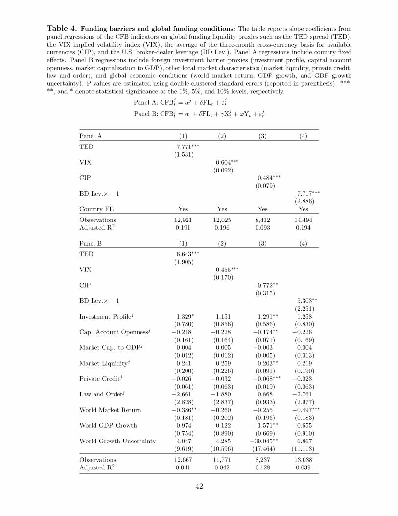
Table 4. Funding barriers and global funding conditions: The table reports slope coefficients frompanel regressions of the CFB indicators on global funding liquidity proxies such as the TED spread (TED),the VIX implied volatility index (VIX), the average of the three-month cross-currency basis for availablecurrencies (CIP), and the U.S. broker-dealer leverage (BD Lev.). Panel A regressions include country fixedeffects. Panel B regressions include foreign investment barrier proxies (investment profile, capital accountopenness, market capitalization to GDP), other local market characteristics (market liquidity, private credit,law and order), and global economic conditions (world market return, GDP growth, and GDP growthuncertainty). P-values are estimated using double clustered standard errors (reported in parenthesis). ***,**, and * denote statistical significance at the 1%, 5%, and 10% levels, respectively.

Panel A: CFBjt = αj + δFLt + εjt

Panel B: CFBjt = α + δFLt + γXj

t + ϕYt + εjt

Panel A (1) (2) (3) (4)

TED 7.771∗∗∗

(1.531)VIX 0.604∗∗∗

(0.092)CIP 0.484∗∗∗

(0.079)BD Lev.×− 1 7.717∗∗∗

(2.886)Country FE Yes Yes Yes Yes

Observations 12,921 12,025 8,412 14,494Adjusted R2 0.191 0.196 0.093 0.194

Panel B (1) (2) (3) (4)

TED 6.643∗∗∗

(1.905)VIX 0.455∗∗∗

(0.170)CIP 0.772∗∗

(0.315)BD Lev.×− 1 5.303∗∗

(2.251)Investment Profilej 1.329∗ 1.151 1.291∗∗ 1.258

(0.780) (0.856) (0.586) (0.830)Cap. Account Opennessj −0.218 −0.228 −0.174∗∗ −0.226

(0.161) (0.164) (0.071) (0.169)Market Cap. to GDPj 0.004 0.005 −0.003 0.004

(0.012) (0.012) (0.005) (0.013)Market Liquidityj 0.241 0.259 0.203∗∗ 0.219

(0.200) (0.226) (0.091) (0.190)Private Creditj −0.026 −0.032 −0.068∗∗∗ −0.023

(0.061) (0.063) (0.019) (0.063)Law and Orderj −2.661 −1.880 0.868 −2.761

(2.828) (2.837) (0.933) (2.977)World Market Return −0.386∗∗ −0.260 −0.255 −0.497∗∗∗

(0.181) (0.202) (0.196) (0.183)World GDP Growth −0.974 −0.122 −1.571∗∗ −0.655

(0.754) (0.890) (0.669) (0.910)World Growth Uncertainty 4.047 4.285 −39.045∗∗ 6.867

(9.619) (10.596) (17.464) (11.113)

Observations 12,667 11,771 8,237 13,038Adjusted R2 0.041 0.042 0.128 0.039

42

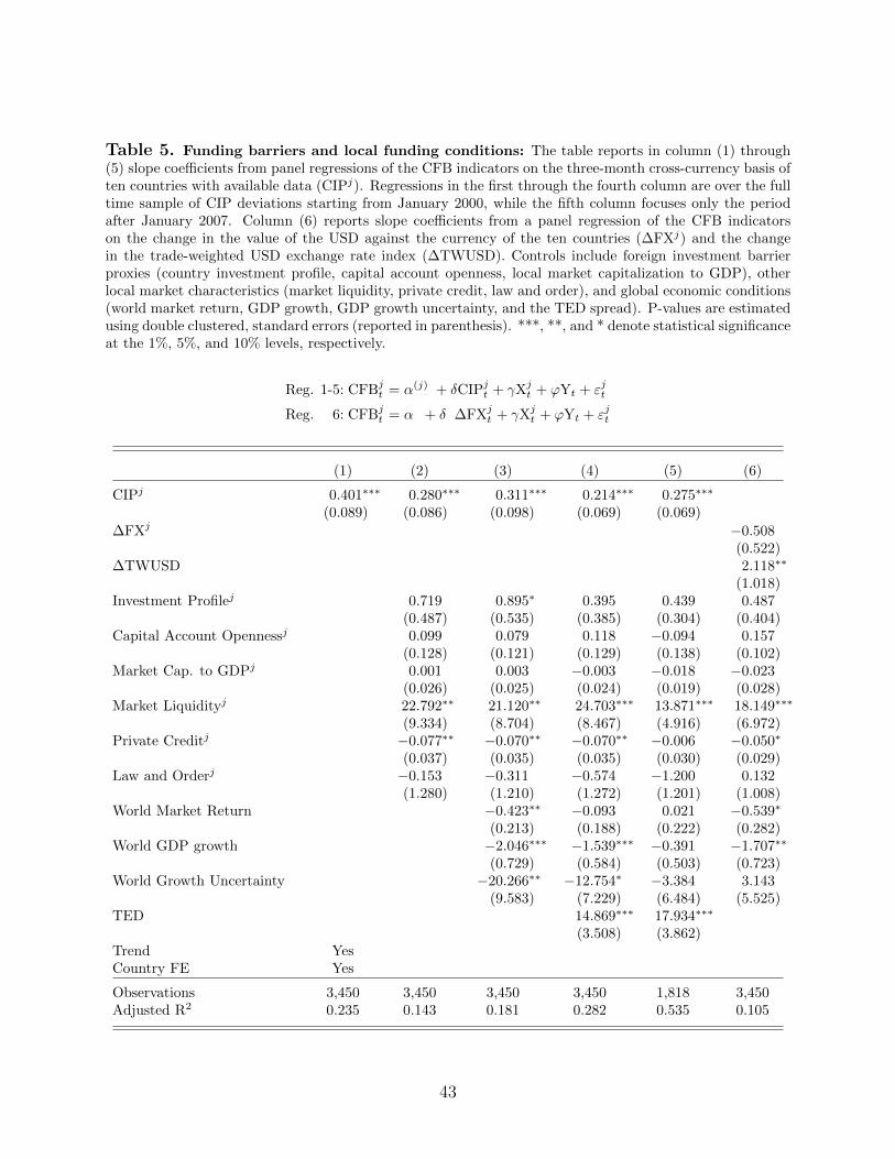
Table 5. Funding barriers and local funding conditions: The table reports in column (1) through(5) slope coefficients from panel regressions of the CFB indicators on the three-month cross-currency basis often countries with available data (CIPj). Regressions in the first through the fourth column are over the fulltime sample of CIP deviations starting from January 2000, while the fifth column focuses only the periodafter January 2007. Column (6) reports slope coefficients from a panel regression of the CFB indicatorson the change in the value of the USD against the currency of the ten countries (∆FXj) and the changein the trade-weighted USD exchange rate index (∆TWUSD). Controls include foreign investment barrierproxies (country investment profile, capital account openness, local market capitalization to GDP), otherlocal market characteristics (market liquidity, private credit, law and order), and global economic conditions(world market return, GDP growth, GDP growth uncertainty, and the TED spread). P-values are estimatedusing double clustered, standard errors (reported in parenthesis). ***, **, and * denote statistical significanceat the 1%, 5%, and 10% levels, respectively.

Reg. 1-5: CFBjt = α(j) + δCIPj

t + γXjt + ϕYt + εjt

Reg. 6: CFBjt = α + δ ∆FXj

t + γXjt + ϕYt + εjt

(1) (2) (3) (4) (5) (6)

CIPj 0.401∗∗∗ 0.280∗∗∗ 0.311∗∗∗ 0.214∗∗∗ 0.275∗∗∗

(0.089) (0.086) (0.098) (0.069) (0.069)

∆FXj −0.508(0.522)

∆TWUSD 2.118∗∗

(1.018)Investment Profilej 0.719 0.895∗ 0.395 0.439 0.487

(0.487) (0.535) (0.385) (0.304) (0.404)Capital Account Opennessj 0.099 0.079 0.118 −0.094 0.157

(0.128) (0.121) (0.129) (0.138) (0.102)Market Cap. to GDPj 0.001 0.003 −0.003 −0.018 −0.023

(0.026) (0.025) (0.024) (0.019) (0.028)Market Liquidityj 22.792∗∗ 21.120∗∗ 24.703∗∗∗ 13.871∗∗∗ 18.149∗∗∗

(9.334) (8.704) (8.467) (4.916) (6.972)Private Creditj −0.077∗∗ −0.070∗∗ −0.070∗∗ −0.006 −0.050∗

(0.037) (0.035) (0.035) (0.030) (0.029)Law and Orderj −0.153 −0.311 −0.574 −1.200 0.132

(1.280) (1.210) (1.272) (1.201) (1.008)World Market Return −0.423∗∗ −0.093 0.021 −0.539∗

(0.213) (0.188) (0.222) (0.282)World GDP growth −2.046∗∗∗ −1.539∗∗∗ −0.391 −1.707∗∗

(0.729) (0.584) (0.503) (0.723)World Growth Uncertainty −20.266∗∗ −12.754∗ −3.384 3.143

(9.583) (7.229) (6.484) (5.525)TED 14.869∗∗∗ 17.934∗∗∗

(3.508) (3.862)Trend YesCountry FE Yes

Observations 3,450 3,450 3,450 3,450 1,818 3,450Adjusted R2 0.235 0.143 0.181 0.282 0.535 0.105

43

Table 6. Funding barriers and funding liberalization: The table reports in column (1) and (2) theslope coefficients from panel regressions of the CFB indicators on the funding liberalization ratio (FLib.).Column (3) and (4) report the slope coefficients from panel regressions of the CFB indicators on the fundingliberalization ratio (FLib.j) for the eight countries that have a primary dealer in our sample. Other regressorsinclude foreign investment barrier proxies (investment profile, capital account openness, market capitalizationto GDP), other local market characteristics (market liquidity, private credit, law and order), and globaleconomic conditions (world market return, GDP growth, and GDP growth uncertainty) and the TED Spread.P-values are estimated using double clustered standard errors (reported in parenthesis). ***, **, and * denotestatistical significance at the 1%, 5%, and 10% levels, respectively.

CFBjt = α(j) + δFLib.

(j)t + γXj

t + ϕYt + εjt

(1) (2) (3) (4)

FLib. −0.181∗∗∗ −0.423∗∗

(0.055) (0.175)FLib.j −0.007∗∗∗ −0.008∗∗∗

(0.002) (0.003)Investment Profilej 1.576∗ 0.738 0.525

(0.855) (0.580) (0.689)Cap. Account Opennessj −0.198 −0.220 −0.157

(0.164) (0.274) (0.346)Market Cap. to GDPj 0.005 0.109∗ 0.107∗

(0.013) (0.057) (0.061)Market Liquidityj 0.274 0.232 0.235

(0.202) (0.170) (0.202)Private Creditj −0.012 −0.122∗ −0.112

(0.065) (0.072) (0.083)Law and Orderj −3.788 3.588 3.536

(3.044) (5.877) (6.340)World Market Return −0.451∗∗∗ −0.455∗∗∗ −0.361∗∗

(0.174) (0.119) (0.152)World GDP Growth −2.412∗∗∗ −1.769∗∗ −2.213∗∗∗

(0.605) (0.759) (0.615)World Growth Uncertainty −8.598 2.387 −1.492

(6.689) (4.515) (3.530)TED 7.386∗∗∗

(1.953)

Country FE Yes

Observations 14,543 13,086 2,905 2,737Adjusted R2 0.197 0.048 0.086 0.090

44

Table 7. Funding barriers and market segmentation: This table reports the slope coefficients from panel regressions of the Bekaert et al.(2011) segmentation index (SEG) on the cross-border funding barrier indicator (CFB). Regressions are over the full time sample (January 1978 toOctober 2014) except in the fourth and sixth column that exclude the year 2007 to 2009. Other regressors include foreign investment barrier proxies(investment profile, capital account openness, market capitalization to GDP), lagged local market index return (Market Returnj

−1), and the TEDspread (TED). P-values are estimated using double clustered, standard errors (reported in parenthesis). ***, **, and * denote statistical significanceat the 1%, 5%, and 10% levels, respectively.

SEGjt = α+ δCFBj

t + γXjt + ϕTEDt + εjt

All DM EM Ex. 07-09 All Ex. 07-09

CFBj 0.562∗∗ 0.918∗∗ 0.343∗ 0.924∗ 0.760∗∗ 1.531∗∗∗

(0.266) (0.459) (0.178) (0.479) (0.376) (0.454)Investment Profilej −0.247∗∗∗ −0.134∗∗∗ −0.513∗∗ −0.256∗∗ −0.241∗∗ −0.265∗∗

(0.095) (0.043) (0.258) (0.100) (0.120) (0.122)Capital Account Opennessj −0.008 −0.049∗∗∗ 0.021 −0.009 −0.003 −0.003

(0.008) (0.016) (0.017) (0.008) (0.009) (0.009)Market Cap. to GDPj −0.012∗∗∗ −0.008∗∗ −0.008∗∗ −0.013∗∗∗ −0.011∗∗∗ −0.012∗∗∗

(0.002) (0.003) (0.004) (0.003) (0.002) (0.003)

Market Returnj−1 −1.107∗∗∗ −1.037∗∗∗ −1.235∗∗∗ −0.913∗∗∗ −1.133∗∗∗ −0.921∗∗∗

(0.238) (0.285) (0.345) (0.261) (0.257) (0.299)TED 0.085 −0.358

(0.169) (0.427)

Observations 13,756 7,931 5,825 12,066 11,476 9,786Adjusted R2 0.113 0.245 0.119 0.112 0.108 0.109

45

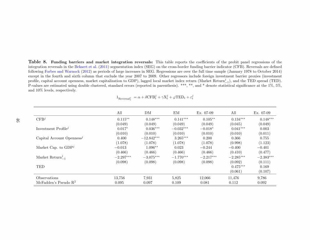
Table 8. Funding barriers and market integration reversals: This table reports the coefficients of the probit panel regressions of theintegration reversals in the Bekaert et al. (2011) segmentation index (SEG) on the cross-border funding barrier indicator (CFB). Reversals are definedfollowing Forbes and Warnock (2012) as periods of large increases in SEG. Regressions are over the full time sample (January 1978 to October 2014)except in the fourth and sixth column that exclude the year 2007 to 2009. Other regressors include foreign investment barrier proxies (investmentprofile, capital account openness, market capitalization to GDP), lagged local market index return (Market Returnj

−1), and the TED spread (TED).P-values are estimated using double clustered, standard errors (reported in parenthesis). ***, **, and * denote statistical significance at the 1%, 5%,and 10% levels, respectively.

1Reversaljt= α+ δCFBj

t + γXjt + ϕTEDt + εjt

All DM EM Ex. 07-09 All Ex. 07-09

CFBj 0.115∗∗ 0.148∗∗∗ 0.141∗∗∗ 0.105∗∗ 0.134∗∗∗ 0.148∗∗∗

(0.049) (0.049) (0.049) (0.049) (0.045) (0.049)Investment Profilej 0.017∗ 0.036∗∗∗ −0.032∗∗∗ −0.018∗ 0.041∗∗∗ 0.003

(0.010) (0.010) (0.010) (0.010) (0.010) (0.011)Capital Account Opennessj 0.400 −12.842∗∗∗ 3.265∗∗∗ 0.200 0.366 0.755

(1.078) (1.078) (1.078) (1.078) (0.998) (1.123)Market Cap. to GDPj −0.013 1.096∗∗ 0.023 −0.244 −0.400 −0.401

(0.466) (0.466) (0.466) (0.466) (0.410) (0.477)

Market Returnj−1 −2.297∗∗∗ −3.075∗∗∗ −1.770∗∗∗ −2.217∗∗∗ −2.285∗∗∗ −2.383∗∗∗

(0.098) (0.098) (0.098) (0.098) (0.092) (0.111)TED 0.475∗∗∗ 0.169

(0.061) (0.107)

Observations 13,756 7,931 5,825 12,066 11,476 9,786McFadden’s Pseudo R2 0.095 0.097 0.109 0.081 0.112 0.092

46

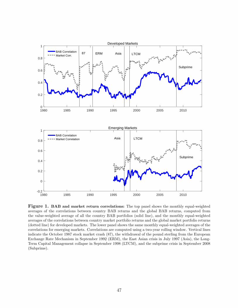
1980 1985 1990 1995 2000 2005 20100

0.2

0.4

0.6

0.8

1Developed Markets

BAB CorrelationMarket Corr.

1980 1985 1990 1995 2000 2005 2010-0.2

0

0.2

0.4

0.6

0.8

1Emerging Markets

BAB CorrelationMarket Correlation

ERM

Subprime

Subprime

LTCM

LTCM

Asia

Asia

87

Figure 1. BAB and market return correlations: The top panel shows the monthly equal-weightedaverages of the correlations between country BAB returns and the global BAB returns, computed fromthe value-weighted average of all the country BAB portfolios (solid line), and the monthly equal-weightedaverages of the correlations between country market portfolio returns and the global market portfolio returns(dotted line) for developed markets. The lower panel shows the same monthly equal-weighted averages of thecorrelations for emerging markets. Correlations are computed using a two-year rolling window. Vertical linesindicate the October 1987 stock market crash (87), the withdrawal of the pound sterling from the EuropeanExchange Rate Mechanism in September 1992 (ERM), the East Asian crisis in July 1997 (Asia), the Long-Term Capital Management collapse in September 1998 (LTCM), and the subprime crisis in September 2008(Subprime).

47

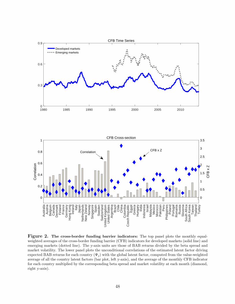
1980 1985 1990 1995 2000 2005 20100

0.3

0.6

0.9CFB Time Series

Developed marketsEmerging markets

Aus

tral

iaA

ustr

iaB

elgi

umC

anad

aD

enm

ark

Fin

land

Fra

nce

Ger

man

yH

ong

Kon

gIr

elan

dIta

lyJa

pan

Net

herla

nds

New

Zel

and

Nor

way

Sin

gapo

reS

pain

Sw

eden

Sw

itzer

land

Uni

ted

Kin

gdom

Uni

ted

Sta

tes

Arg

entin

aB

razi

lC

hile

Chi

naC

olom

bia

Cze

ch R

epub

licE

gypt

Gre

ece

Hun

gary

Indi

aIn

done

sia

Isra

elM

alay

sia

Mex

ico

Mor

occo

Pak

ista

nP

eru

Phi

lippi

nes

Pol

and

Por

tuga

lR

oman

iaR

ussi

aS

love

nia

Sou

th A

fric

aS

outh

Kor

eaT

aiw

anT

haila

ndT

urke

y0

0.2

0.4

0.6

0.8

1

Cor

rela

tion

0

0.5

1

1.5

2

2.5

3

3.5

CF

B x

Z

CFB Cross-section

CFB x ZCorrelation

Figure 2. The cross-border funding barrier indicators: The top panel plots the monthly equal-weighted averages of the cross-border funding barrier (CFB) indicators for developed markets (solid line) andemerging markets (dotted line). The y-axis units are those of BAB returns divided by the beta spread andmarket volatility. The lower panel plots the unconditional correlations of the estimated latent factor drivingexpected BAB returns for each country (Ψj) with the global latent factor, computed from the value-weightedaverage of all the country latent factors (bar plot, left y-axis), and the average of the monthly CFB indicatorfor each country multiplied by the corresponding beta spread and market volatility at each month (diamond,right y-axis).

48

0 0.2 0.4 0.6 0.8 1

False Positive Rate

0

0.2

0.4

0.6

0.8

1T

rue

Pos

itive

Rat

e

Figure 3. Receiver operating characteristic curve: The figure plots the receiver operating char-acteristic curve for reversals in market integration as implied by the SEG Index of Bekaert et al. (2011)detected using the cross-border funding barrier (CFB) measure (solid line). Reversals are defined followingForbes and Warnock (2012) as periods of large increases in SEG above its historical average. The area underthe ROC curve is 0.71.

49

E Online Appendix

50

Table A1. Market portfolios returns: The table reports the starting year of data (Start Year), average monthly return (Mean), monthlystandard deviation (Vol.), lowest monthly return (Min) and highest monthly return (Max) for the local market portfolios in our sample of 21developed markets (DM) and 29 emerging markets (EM). Data end in October 2014 and are collected from Datastream.

Country Start Year Mean Vol. Min Max Country Start Year Mean Vol. Min Max

Australia 1973 0.86 7.36 -56.66 22.41 Argentina 1993 0.36 9.51 -36.23 24.29Austria 1973 0.76 6.65 -41.93 31.69 Brazil 1994 0.86 10.50 -40.82 33.45Belgium 1973 0.87 5.87 -39.05 21.85 Chile 1989 1.18 6.59 -27.49 16.55Canada 1973 0.81 5.52 -30.79 18.51 China 1993 0.94 10.39 -30.88 39.45Denmark 1973 1.01 5.88 -30.64 20.69 Colombia 1992 0.94 7.87 -31.29 19.27Finland 1988 0.75 8.39 -33.82 26.10 Czech Republic 1993 0.87 8.62 -31.28 52.30France 1973 0.93 6.70 -25.76 24.82 Egypt 1996 0.80 8.84 -32.65 33.74Germany 1973 0.81 6.01 -23.13 17.67 Greece 1990 0.37 10.11 -40.95 46.08Hong Kong 1973 0.93 9.70 -60.50 56.21 Hungary 1991 0.58 10.12 -49.67 46.86Ireland 1973 0.88 7.10 -28.84 35.84 India 1990 0.87 10.19 -38.36 43.15Italy 1973 0.66 7.54 -26.28 24.19 Indonesia 1990 0.19 11.52 -53.12 43.78Japan 1973 0.61 6.01 -19.30 23.98 Israel 1993 0.65 6.80 -21.50 15.66Netherlands 1973 0.94 5.65 -36.98 21.64 Malaysia 1986 0.90 8.32 -40.22 37.95New Zealand 1988 0.79 6.23 -20.56 26.20 Mexico 1989 1.21 8.60 -41.20 21.59Norway 1980 0.92 8.08 -36.56 22.14 Morocco 1994 1.01 5.02 -14.45 21.17Singapore 1973 0.71 8.16 -46.24 48.95 Pakistan 1992 0.67 9.78 -48.36 28.40Spain 1987 0.81 6.77 -27.56 19.56 Peru 1994 0.88 6.69 -34.82 27.31Sweden 1982 1.11 7.23 -30.27 20.23 Philippines 1987 0.90 8.51 -31.71 39.62Switzerland 1973 0.94 5.09 -20.14 15.14 Poland 1994 0.38 10.53 -40.58 31.87United Kingdom 1973 0.91 6.21 -23.87 43.79 Portugal 1990 0.41 6.25 -32.85 16.30United States 1973 0.84 4.52 -23.26 16.17 Romania 1997 0.68 13.88 -57.79 61.50

Russian Federation 1998 0.96 13.54 -83.49 39.45Slovenia 1999 0.47 6.43 -26.55 18.04South Africa 1973 0.95 8.29 -43.61 18.05South Korea 1987 0.60 10.28 -38.67 53.41Taiwan 1988 0.42 10.11 -40.36 45.08Thailand 1987 0.98 10.37 -39.34 34.28Turkey 1988 0.78 15.26 -52.47 53.38

Mean DM 0.85 6.70 -32.48 26.56 Mean EM 0.74 9.39 -39.31 34.36

51

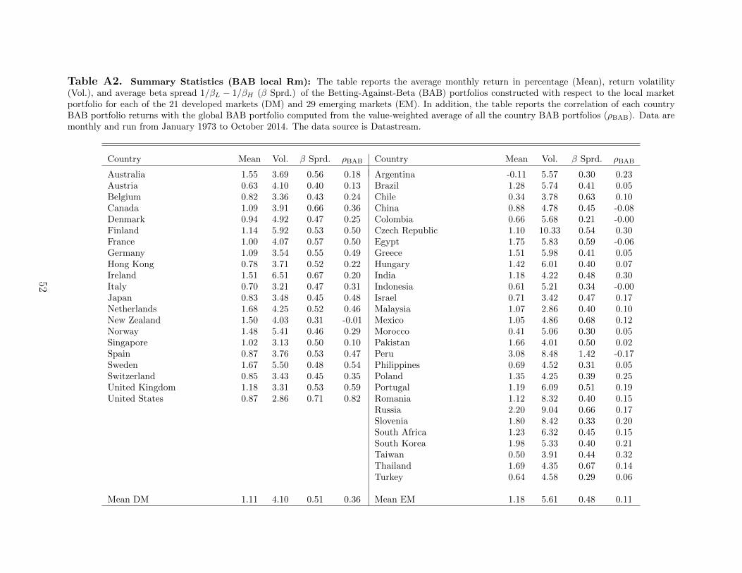
Table A2. Summary Statistics (BAB local Rm): The table reports the average monthly return in percentage (Mean), return volatility(Vol.), and average beta spread 1/βL − 1/βH (β Sprd.) of the Betting-Against-Beta (BAB) portfolios constructed with respect to the local marketportfolio for each of the 21 developed markets (DM) and 29 emerging markets (EM). In addition, the table reports the correlation of each countryBAB portfolio returns with the global BAB portfolio computed from the value-weighted average of all the country BAB portfolios (ρBAB). Data aremonthly and run from January 1973 to October 2014. The data source is Datastream.

Country Mean Vol. β Sprd. ρBAB Country Mean Vol. β Sprd. ρBAB

Australia 1.55 3.69 0.56 0.18 Argentina -0.11 5.57 0.30 0.23Austria 0.63 4.10 0.40 0.13 Brazil 1.28 5.74 0.41 0.05Belgium 0.82 3.36 0.43 0.24 Chile 0.34 3.78 0.63 0.10Canada 1.09 3.91 0.66 0.36 China 0.88 4.78 0.45 -0.08Denmark 0.94 4.92 0.47 0.25 Colombia 0.66 5.68 0.21 -0.00Finland 1.14 5.92 0.53 0.50 Czech Republic 1.10 10.33 0.54 0.30France 1.00 4.07 0.57 0.50 Egypt 1.75 5.83 0.59 -0.06Germany 1.09 3.54 0.55 0.49 Greece 1.51 5.98 0.41 0.05Hong Kong 0.78 3.71 0.52 0.22 Hungary 1.42 6.01 0.40 0.07Ireland 1.51 6.51 0.67 0.20 India 1.18 4.22 0.48 0.30Italy 0.70 3.21 0.47 0.31 Indonesia 0.61 5.21 0.34 -0.00Japan 0.83 3.48 0.45 0.48 Israel 0.71 3.42 0.47 0.17Netherlands 1.68 4.25 0.52 0.46 Malaysia 1.07 2.86 0.40 0.10New Zealand 1.50 4.03 0.31 -0.01 Mexico 1.05 4.86 0.68 0.12Norway 1.48 5.41 0.46 0.29 Morocco 0.41 5.06 0.30 0.05Singapore 1.02 3.13 0.50 0.10 Pakistan 1.66 4.01 0.50 0.02Spain 0.87 3.76 0.53 0.47 Peru 3.08 8.48 1.42 -0.17Sweden 1.67 5.50 0.48 0.54 Philippines 0.69 4.52 0.31 0.05Switzerland 0.85 3.43 0.45 0.35 Poland 1.35 4.25 0.39 0.25United Kingdom 1.18 3.31 0.53 0.59 Portugal 1.19 6.09 0.51 0.19United States 0.87 2.86 0.71 0.82 Romania 1.12 8.32 0.40 0.15

Russia 2.20 9.04 0.66 0.17Slovenia 1.80 8.42 0.33 0.20South Africa 1.23 6.32 0.45 0.15South Korea 1.98 5.33 0.40 0.21Taiwan 0.50 3.91 0.44 0.32Thailand 1.69 4.35 0.67 0.14Turkey 0.64 4.58 0.29 0.06

Mean DM 1.11 4.10 0.51 0.36 Mean EM 1.18 5.61 0.48 0.11

52

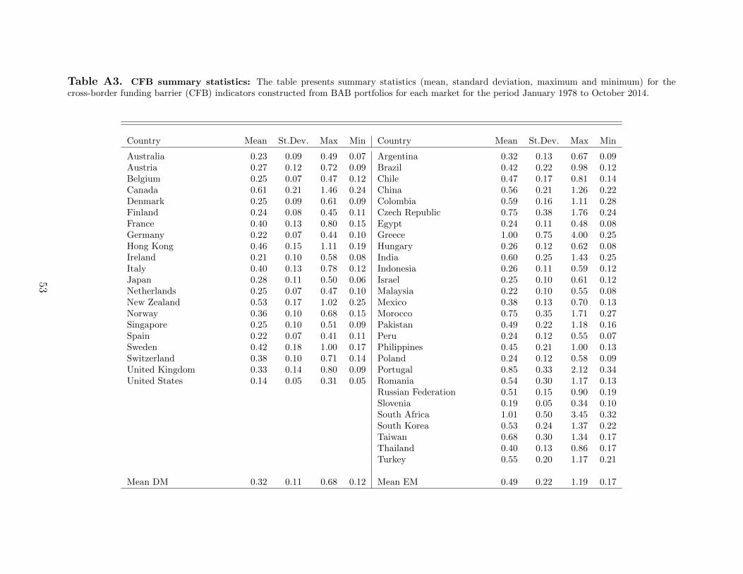
Table A3. CFB summary statistics: The table presents summary statistics (mean, standard deviation, maximum and minimum) for thecross-border funding barrier (CFB) indicators constructed from BAB portfolios for each market for the period January 1978 to October 2014.

Country Mean St.Dev. Max Min Country Mean St.Dev. Max Min

Australia 0.23 0.09 0.49 0.07 Argentina 0.32 0.13 0.67 0.09Austria 0.27 0.12 0.72 0.09 Brazil 0.42 0.22 0.98 0.12Belgium 0.25 0.07 0.47 0.12 Chile 0.47 0.17 0.81 0.14Canada 0.61 0.21 1.46 0.24 China 0.56 0.21 1.26 0.22Denmark 0.25 0.09 0.61 0.09 Colombia 0.59 0.16 1.11 0.28Finland 0.24 0.08 0.45 0.11 Czech Republic 0.75 0.38 1.76 0.24France 0.40 0.13 0.80 0.15 Egypt 0.24 0.11 0.48 0.08Germany 0.22 0.07 0.44 0.10 Greece 1.00 0.75 4.00 0.25Hong Kong 0.46 0.15 1.11 0.19 Hungary 0.26 0.12 0.62 0.08Ireland 0.21 0.10 0.58 0.08 India 0.60 0.25 1.43 0.25Italy 0.40 0.13 0.78 0.12 Indonesia 0.26 0.11 0.59 0.12Japan 0.28 0.11 0.50 0.06 Israel 0.25 0.10 0.61 0.12Netherlands 0.25 0.07 0.47 0.10 Malaysia 0.22 0.10 0.55 0.08New Zealand 0.53 0.17 1.02 0.25 Mexico 0.38 0.13 0.70 0.13Norway 0.36 0.10 0.68 0.15 Morocco 0.75 0.35 1.71 0.27Singapore 0.25 0.10 0.51 0.09 Pakistan 0.49 0.22 1.18 0.16Spain 0.22 0.07 0.41 0.11 Peru 0.24 0.12 0.55 0.07Sweden 0.42 0.18 1.00 0.17 Philippines 0.45 0.21 1.00 0.13Switzerland 0.38 0.10 0.71 0.14 Poland 0.24 0.12 0.58 0.09United Kingdom 0.33 0.14 0.80 0.09 Portugal 0.85 0.33 2.12 0.34United States 0.14 0.05 0.31 0.05 Romania 0.54 0.30 1.17 0.13

Russian Federation 0.51 0.15 0.90 0.19Slovenia 0.19 0.05 0.34 0.10South Africa 1.01 0.50 3.45 0.32South Korea 0.53 0.24 1.37 0.22Taiwan 0.68 0.30 1.34 0.17Thailand 0.40 0.13 0.86 0.17Turkey 0.55 0.20 1.17 0.21

Mean DM 0.32 0.11 0.68 0.12 Mean EM 0.49 0.22 1.19 0.17

53

Table A4. Funding barriers and global funding conditions in subsamples: The table reportsslope coefficients from regressions of the CFB indicators on the TED spread (TED) for U.S. only (US), forall the countries in our sample excluding the U.S. (Ex. US), for developed markets (DM), for emergingmarkets (EM), and for all countries excluding the 2007-2009 financial crisis period (Ex. 07-09). Otherregressors include foreign investment barrier proxies (investment profile, capital account openness, localmarket capitalization to GDP), other local market characteristics (market liquidity, private credit, law andorder), and global economic conditions (world market return, GDP growth, and GDP growth uncertainty).P-values are estimated using double clustered standard errors (reported in parenthesis). ***, **, and *denote statistical significance at the 1%, 5%, and 10% levels, respectively.

CFBjt = α + δTEDt + γXj

t + ϕYt + εjt

US Ex. US DM EM Ex. 07-09

TED 9.391∗∗∗ 6.709∗∗∗ 7.917∗∗∗ 8.116∗ 17.579∗∗∗

(2.204) (1.975) (1.499) (4.167) (4.617)Investment Profilej 1.375∗ 0.277 2.181 1.966∗∗

(0.794) (0.421) (1.531) (0.885)Capital Account Opennessj −0.204 0.120 −0.141 −0.215

(0.160) (0.162) (0.196) (0.167)Market Cap. to GDPj 0.002 0.010 −0.010 0.006

(0.012) (0.007) (0.104) (0.013)Market Liquidityj 0.241 0.190 0.240 0.252

(0.200) (0.118) (0.323) (0.211)Private Creditj −0.006 −0.038 0.071 −0.040

(0.062) (0.039) (0.125) (0.060)Law and Orderj −2.863 0.454 −0.318 −3.617

(2.825) (2.746) (3.781) (2.932)World Market Return −0.392∗∗ −0.180 −0.566∗ −0.368

(0.187) (0.141) (0.312) (0.229)World GDP Growth −0.894 −1.749∗∗∗ 0.718 −4.323∗∗∗

(0.776) (0.471) (1.269) (1.322)World Growth Uncertainty 4.757 −2.481 19.342 −1.665

(9.757) (3.809) (16.416) (8.221)

Observations 343 12,324 6,937 5,730 10,941Adjusted R2 0.116 0.038 0.025 0.025 0.056

54

Table A5. Funding barriers and global funding condition quantiles: The table reports the slopecoefficients from panel regressions the CFB indicators on a dummy variable that takes the value of one whenthe funding liquidity proxy is in its 90th percentile (Panel A) or below its 50th percentile (Panel B). Fundingliquidity proxies include the TED spread (TED), the VIX implied volatility index (VIX), the average of thethree-month cross-currency basis for available currencies (CIP), the U.S. broker-dealer leverage (BD Lev.).∑

1 indicates the sum of dummy variables for all the proxies. Regressions include country fixed effects anda time trend. P-values are estimated using double clustered, standard errors (reported in parenthesis). ***,**, and * denote statistical significance at the 1%, 5%, and 10% levels, respectively.

Panel A: CFBjt = αj + θt+ δ1FLt>0.90th + εjt

Panel B: CFBjt = αj + θt+ δ1FLt∈0.50th + εjt

Panel A (1) (2) (3) (4) (5)

1TED>90th 5.221∗∗∗

(1.388)1VIX>90th 9.558∗∗∗

(1.655)1CIP>90th 10.030∗∗∗

(1.514)1BD Lev.∈10th 5.673∗∗∗

(1.346)∑1FL>90th 4.105∗∗∗

(0.655)

Trend Yes Yes Yes Yes YesCountry FE Yes Yes Yes Yes Yes

Observations 12,921 12,025 8,412 14,494 14,543Adjusted R2 0.205 0.210 0.214 0.205 0.208

Panel B (1) (2) (3) (4) (5)

1TED∈50th −3.071∗∗

(1.484)1VIX∈50th −11.208∗∗∗

(1.849)1CIP∈50th −7.927∗∗∗

(2.019)1BD Lev.BD>50th −2.048∗∗∗

(0.757)∑1FL∈50th −3.378∗∗∗

(0.625)

Trend Yes Yes Yes Yes YesCountry FE Yes Yes Yes Yes Yes

Observations 12,921 12,025 8,412 14,494 14,543Adjusted R2 0.187 0.200 0.166 0.194 0.202

55

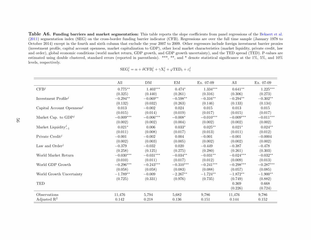
Table A6. Funding barriers and market segmentation: This table reports the slope coefficients from panel regressions of the Bekaert et al.(2011) segmentation index (SEG) on the cross-border funding barrier indicator (CFB). Regressions are over the full time sample (January 1978 toOctober 2014) except in the fourth and sixth column that exclude the year 2007 to 2009. Other regressors include foreign investment barrier proxies(investment profile, capital account openness, market capitalization to GDP), other local market characteristics (market liquidity, private credit, lawand order), global economic conditions (world market return, GDP growth, and GDP growth uncertainty), and the TED spread (TED). P-values areestimated using double clustered, standard errors (reported in parenthesis). ***, **, and * denote statistical significance at the 1%, 5%, and 10%levels, respectively.

SEGjt = α+ δCFBj

t + γXjt + ϕTEDt + εjt

All DM EM Ex. 07-09 All Ex. 07-09

CFBj 0.775∗∗ 1.403∗∗∗ 0.474∗ 1.334∗∗∗ 0.641∗∗ 1.225∗∗∗

(0.325) (0.440) (0.261) (0.316) (0.306) (0.273)Investment Profilej −0.294∗∗ −0.069∗∗ −0.598∗∗ −0.316∗∗ −0.294∗∗ −0.302∗∗

(0.132) (0.032) (0.263) (0.146) (0.133) (0.134)Capital Account Opennessj 0.013 −0.002 0.024 0.015 0.013 0.015

(0.015) (0.014) (0.019) (0.017) (0.015) (0.017)Market Cap. to GDPj −0.009∗∗∗ −0.006∗∗∗ −0.008∗ −0.010∗∗∗ −0.009∗∗∗ −0.011∗∗∗

(0.002) (0.002) (0.004) (0.002) (0.002) (0.002)

Market Liquidityj−1 0.021∗ 0.006 0.033∗ 0.025∗∗ 0.021∗ 0.024∗∗

(0.011) (0.008) (0.017) (0.013) (0.011) (0.012)Private Creditj −0.001 −0.002 0.004 −0.001 −0.001 −0.0004

(0.002) (0.003) (0.005) (0.002) (0.002) (0.002)Law and Orderj −0.379 −0.032 0.020 −0.449 −0.387 −0.478

(0.258) (0.125) (0.275) (0.280) (0.261) (0.303)World Market Return −0.030∗∗∗ −0.031∗∗∗ −0.034∗∗ −0.031∗∗ −0.024∗∗∗ −0.032∗∗

(0.010) (0.011) (0.017) (0.012) (0.009) (0.013)World GDP Growth −0.296∗∗∗ −0.243∗∗∗ −0.310∗∗∗ −0.241∗∗∗ −0.298∗∗∗ −0.287∗∗∗

(0.058) (0.058) (0.083) (0.088) (0.057) (0.085)World Growth Uncertainty −1.789∗∗ −0.009 −2.267∗∗ −1.724∗∗ −1.872∗∗ −1.900∗∗

(0.725) (0.331) (0.976) (0.735) (0.749) (0.882)TED 0.369 0.668

(0.226) (0.724)

Observations 11,476 5,794 5,682 9,786 11,476 9,786Adjusted R2 0.142 0.218 0.136 0.151 0.144 0.152

56

Table A7. Funding barriers and market integration reversals: This table reports the coefficients from probit panel regressions of theintegration reversals in the Bekaert et al. (2011) segmentation index (SEG) on the cross-border funding barrier indicator (CFB). Reversals are definedfollowing Forbes and Warnock (2012) as periods of large increases in SEG. Regressions are over the full time sample (January 1978 to October 2014)except in the fourth and sixth column that exclude the year 2007 to 2009. Other regressors include foreign investment barrier proxies (investmentprofile, capital account openness, market capitalization to GDP), other local market characteristics (market liquidity, private credit, law and order),global economic conditions (world market return, GDP growth, and GDP growth uncertainty), and the TED spread (TED). P-values are estimatedusing double clustered, standard errors (reported in parenthesis). ***, **, and * denote statistical significance at the 1%, 5%, and 10% levels,respectively.

1Reversaljt= α+ δCFBj

t + γXjt + ϕTEDt + εjt

All DM EM Ex. 07-09 All Ex. 07-09

CFBj 0.196∗∗∗ 0.301∗∗∗ 0.144∗∗∗ 0.174∗∗∗ 0.169∗∗∗ 0.116∗∗

(0.044) (0.103) (0.050) (0.047) (0.045) (0.048)Investment Profilej −0.014 −0.015 −0.071∗∗∗ −0.044∗∗∗ −0.024∗∗ −0.023∗

(0.011) (0.015) (0.016) (0.012) (0.011) (0.012)Capital Account Opennessj −0.0001 −0.015∗∗∗ 0.001 0.001 0.0005 0.003∗

(0.001) (0.004) (0.001) (0.001) (0.001) (0.001)Market Cap. to GDPj −0.002∗∗∗ −0.001∗∗ −0.004∗∗∗ −0.002∗∗∗ −0.002∗∗∗ −0.002∗∗∗

(0.0005) (0.001) (0.001) (0.001) (0.0005) (0.001)

Market Liquidityj−1 −0.001 0.002 0.003 0.001 0.0003 0.00003

(0.002) (0.003) (0.002) (0.002) (0.002) (0.002)Private Creditj 0.003∗∗∗ 0.001 0.006∗∗∗ 0.003∗∗∗ 0.003∗∗∗ 0.003∗∗∗

(0.001) (0.001) (0.001) (0.001) (0.001) (0.001)Law and Orderj −0.011 −0.195∗∗∗ 0.036 −0.061∗∗ −0.022 −0.110∗∗∗

(0.023) (0.058) (0.031) (0.024) (0.023) (0.025)World Market Return −0.013∗∗∗ −0.023∗∗∗ −0.007 −0.004 0.003 −0.008

(0.004) (0.006) (0.006) (0.006) (0.005) (0.006)World GDP Growth −0.488∗∗∗ −0.640∗∗∗ −0.360∗∗∗ −0.468∗∗∗ −0.502∗∗∗ −0.615∗∗∗

(0.018) (0.029) (0.024) (0.029) (0.018) (0.033)World Growth Uncertainty −1.276∗∗∗ −2.483∗∗∗ 0.134 −1.220∗∗∗ −1.543∗∗∗ −1.741∗∗∗

(0.111) (0.166) (0.159) (0.115) (0.116) (0.126)TED 0.861∗∗∗ 1.380∗∗∗

(0.060) (0.109)

Observations 11,476 5,794 5,682 9,786 11,476 9,786McFadden’s Pseudo R2 0.085 0.097 0.100 0.050 0.102 0.062

57

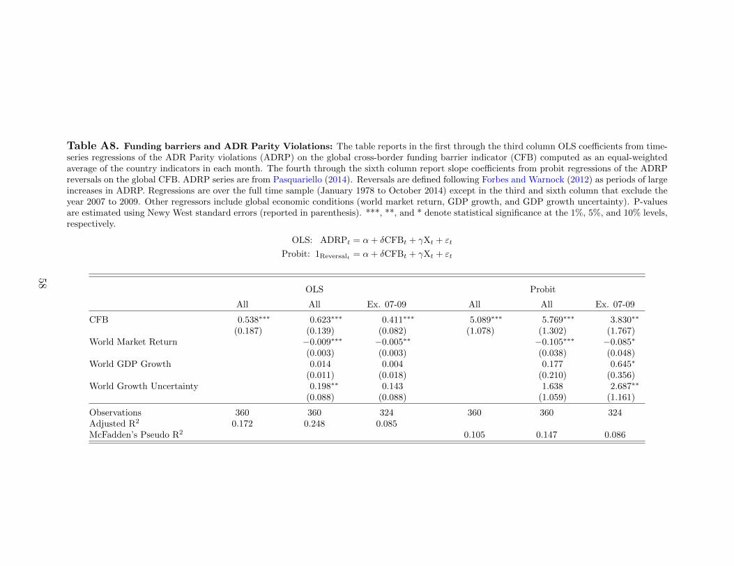
Table A8. Funding barriers and ADR Parity Violations: The table reports in the first through the third column OLS coefficients from time-series regressions of the ADR Parity violations (ADRP) on the global cross-border funding barrier indicator (CFB) computed as an equal-weightedaverage of the country indicators in each month. The fourth through the sixth column report slope coefficients from probit regressions of the ADRPreversals on the global CFB. ADRP series are from Pasquariello (2014). Reversals are defined following Forbes and Warnock (2012) as periods of largeincreases in ADRP. Regressions are over the full time sample (January 1978 to October 2014) except in the third and sixth column that exclude theyear 2007 to 2009. Other regressors include global economic conditions (world market return, GDP growth, and GDP growth uncertainty). P-valuesare estimated using Newy West standard errors (reported in parenthesis). ***, **, and * denote statistical significance at the 1%, 5%, and 10% levels,respectively.

OLS: ADRPt = α+ δCFBt + γXt + εt

Probit: 1Reversalt = α+ δCFBt + γXt + εt

OLS Probit

All All Ex. 07-09 All All Ex. 07-09

CFB 0.538∗∗∗ 0.623∗∗∗ 0.411∗∗∗ 5.089∗∗∗ 5.769∗∗∗ 3.830∗∗

(0.187) (0.139) (0.082) (1.078) (1.302) (1.767)World Market Return −0.009∗∗∗ −0.005∗∗ −0.105∗∗∗ −0.085∗

(0.003) (0.003) (0.038) (0.048)World GDP Growth 0.014 0.004 0.177 0.645∗

(0.011) (0.018) (0.210) (0.356)World Growth Uncertainty 0.198∗∗ 0.143 1.638 2.687∗∗

(0.088) (0.088) (1.059) (1.161)

Observations 360 360 324 360 360 324Adjusted R2 0.172 0.248 0.085McFadden’s Pseudo R2 0.105 0.147 0.086

58

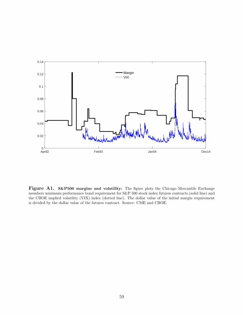
Apr82 Feb93 Jan04 Dec140

0.02

0.04

0.06

0.08

0.1

0.12

0.14

MarginVIX

Figure A1. S&P500 margins and volatility: The figure plots the Chicago Mercantile Exchangemembers minimum performance bond requirement for S&P 500 stock index futures contracts (solid line) andthe CBOE implied volatility (VIX) index (dotted line). The dollar value of the initial margin requirementis divided by the dollar value of the futures contract. Source: CME and CBOE.

59

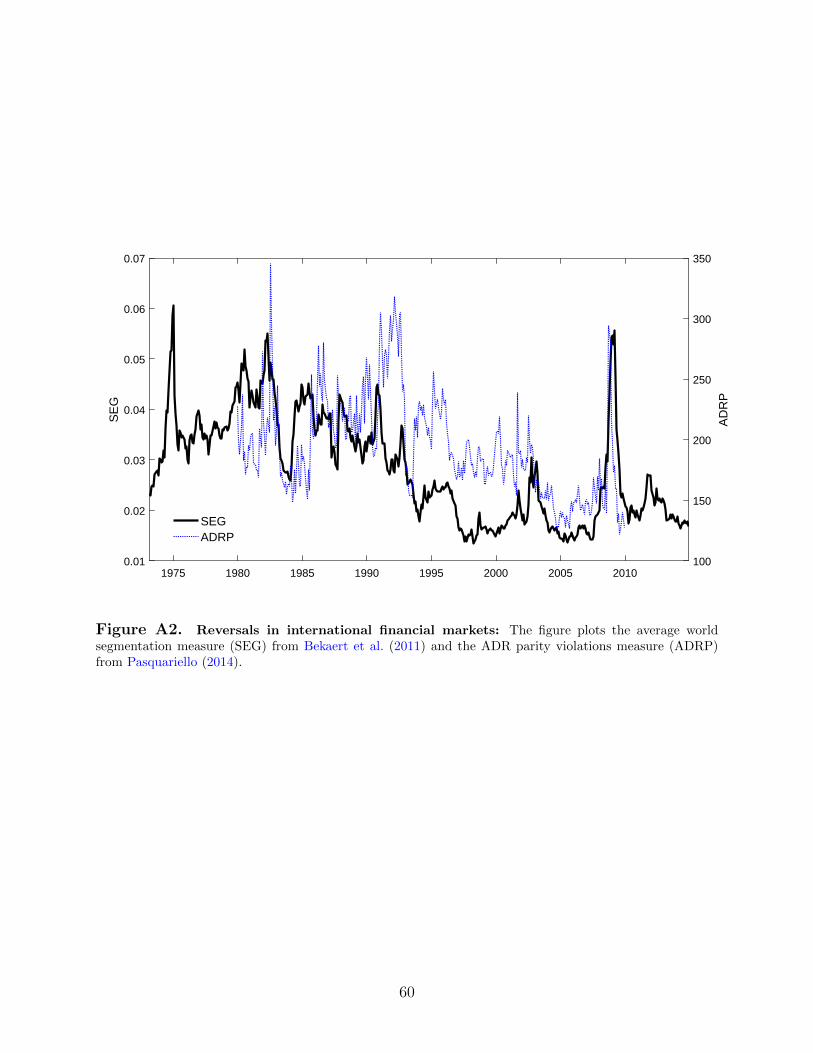
1975 1980 1985 1990 1995 2000 2005 20100.01

0.02

0.03

0.04

0.05

0.06

0.07

SE

G

100

150

200

250

300

350

AD

RP

SEGADRP

Figure A2. Reversals in international financial markets: The figure plots the average worldsegmentation measure (SEG) from Bekaert et al. (2011) and the ADR parity violations measure (ADRP)from Pasquariello (2014).

60