NBER WORKING PAPER SERIES CAN CHANGING ECONOMIC FACTORS EXPLAIN THE RISE IN OBESITY? Charles J. Courtemanche Joshua C. Pinkston Christopher J. Ruhm George Wehby Working Paper 20892 http://www.nber.org/papers/w20892 NATIONAL BUREAU OF ECONOMIC RESEARCH 1050 Massachusetts Avenue Cambridge, MA 02138 January 2015 Monica Deza, Robert Kaestner, Rusty Tchernis, Nathan Tefft, and seminar participants at Georgia State University, University of Illinois-Chicago, the American Society of Health Economists Biennial Conference, and the 5th Annual Meeting on the Economics of Risky Behaviors provided valuable feedback. We thank Xilin Zhou and Antonios Koumpias for excellent research assistance. Ruhm thanks the University of Virginia Bankard Fund for financial support for this research. The views expressed herein are those of the authors and do not necessarily reflect the views of the National Bureau of Economic Research. NBER working papers are circulated for discussion and comment purposes. They have not been peer- reviewed or been subject to the review by the NBER Board of Directors that accompanies official NBER publications. © 2015 by Charles J. Courtemanche, Joshua C. Pinkston, Christopher J. Ruhm, and George Wehby. All rights reserved. Short sections of text, not to exceed two paragraphs, may be quoted without explicit permission provided that full credit, including © notice, is given to the source.

Welcome message from author
This document is posted to help you gain knowledge. Please leave a comment to let me know what you think about it! Share it to your friends and learn new things together.
Transcript

NBER WORKING PAPER SERIES
CAN CHANGING ECONOMIC FACTORS EXPLAIN THE RISE IN OBESITY?
Charles J. CourtemancheJoshua C. Pinkston
Christopher J. RuhmGeorge Wehby
Working Paper 20892http://www.nber.org/papers/w20892
NATIONAL BUREAU OF ECONOMIC RESEARCH1050 Massachusetts Avenue
Cambridge, MA 02138January 2015
Monica Deza, Robert Kaestner, Rusty Tchernis, Nathan Tefft, and seminar participants at GeorgiaState University, University of Illinois-Chicago, the American Society of Health Economists BiennialConference, and the 5th Annual Meeting on the Economics of Risky Behaviors provided valuablefeedback. We thank Xilin Zhou and Antonios Koumpias for excellent research assistance. Ruhm thanksthe University of Virginia Bankard Fund for financial support for this research. The views expressedherein are those of the authors and do not necessarily reflect the views of the National Bureau of EconomicResearch.
NBER working papers are circulated for discussion and comment purposes. They have not been peer-reviewed or been subject to the review by the NBER Board of Directors that accompanies officialNBER publications.
© 2015 by Charles J. Courtemanche, Joshua C. Pinkston, Christopher J. Ruhm, and George Wehby.All rights reserved. Short sections of text, not to exceed two paragraphs, may be quoted without explicitpermission provided that full credit, including © notice, is given to the source.

Can Changing Economic Factors Explain the Rise in Obesity?Charles J. Courtemanche, Joshua C. Pinkston, Christopher J. Ruhm, and George WehbyNBER Working Paper No. 20892January 2015JEL No. I12
ABSTRACT
A growing literature examines the effects of economic variables on obesity, typically focusing on onlyone or a few factors at a time. We build a more comprehensive economic model of body weight, combiningthe 1990-2010 Behavioral Risk Factor Surveillance System with 27 state-level variables related togeneral economic conditions, labor supply, and the monetary or time costs of calorie intake, physicalactivity, and cigarette smoking. Controlling for demographic characteristics and state and year fixedeffects, changes in these economic variables collectively explain 37% of the rise in BMI, 43% of therise in obesity, and 59% of the rise in class II/III obesity. Quantile regressions also point to large effectsamong the heaviest individuals, with half the rise in the 90th percentile of BMI explained by economicfactors. Variables related to calorie intake – particularly restaurant and supercenter/warehouse clubdensities – are the primary drivers of the results.
Charles J. CourtemancheGeorgia State UniversityAndrew Young School of Policy StudiesDepartment of EconomicsP.O. Box 3992Atlanta, GA 30302-3992and [email protected]
Joshua C. PinkstonEconomics DepartmentCollege of BusinessUniversity of LouisvilleLouisville, KY [email protected]
Christopher J. RuhmFrank Batten School ofLeadership and Public PolicyUniversity of Virginia235 McCormick Rd.P.O. Box 400893Charlottesville, VA 22904-4893and [email protected]
George WehbyDepartment of Health Management and PolicyCollege of Public HealthUniversity of IowaN248 CPHB, 105 River StreetIowa City, IA 52242and [email protected]
1
I. Introduction
Obesity, defined as a body mass index (BMI) of at least 30, leads to adverse health
conditions such as heart disease, diabetes, high blood pressure, and stroke (Strum, 2002).1 The
adult obesity rate in the United States skyrocketed from 13% in 1960 to 35% in 2011-2012, with
most of this increase occurring since 1980 (Flegal et al., 1998; Ogden, et al. 2014). Obesity has
become a major public health and public finance concern. Estimates of its annual costs include
112,000 lives and $190 billion, with about half of the medical expenses borne by Medicare and
Medicaid (Flegal et al., 2005; Cawley and Meyerhoefer, 2012; Finkelstein et al., 2003).
This trend has prompted economists to ask whether obesity is an economic phenomenon
involving individuals’ responses to incentives. Technological progress has resulted in an
environment in which food is cheaper and more readily available, while physical activity is
increasingly easy to avoid. Philipson and Posner (1999) formalize this notion by modeling
weight as the result of eating and exercise decisions made through a utility-maximization
process.2 Individuals trade-off the disutility from excess weight with the enjoyment of eating and
having a sedentary lifestyle, subject to a budget constraint. The model predicts that lower food
prices and reduced on-the-job physical activity increase weight, while the effect of additional
income on weight varies across the income distribution. Cutler et al. (2003) point out that time
costs of eating should matter in addition to monetary costs, and discuss how innovations such as
vacuum packing, improved preservatives, and microwaves have reduced the time cost of food
preparation. Later theoretical models (e.g. Komlos, 2004; Ruhm, 2012; Courtemanche et al.,
2012) add an intertemporal dimension, noting that the enjoyment from eating and sedentary
activities occurs in the present but the health costs occur in the future. The prediction that the
1 BMI=weight in kilograms divided by height in squared meters.
2 The paper was later published as Philipson and Posner (2003), but we focus on the working paper version as it
contains a more detailed model.

2
weights of at least some individuals respond to economic incentives persists in these models,
regardless of whether or not preferences are time consistent.
Motivated by these theoretical considerations, a large number of empirical studies
investigate links between various economic factors and obesity.3 Lakdawalla and Philipson
(2002) document an inverted U-shaped association between income and BMI in individual fixed
effects models. Lindahl (2005) and Cawley et al. (2010) find no evidence that income affects
weight using lottery prizes and variations in Social Security payments as natural experiments,
while Schmeiser (2009) finds that Earned Income Tax Credit benefits increase weight.
Several papers document a connection between the costs of eating and BMI. Lakdawalla
and Philipson (2002), Chou et al. (2004), Lakdawalla et al. (2005), Goldman et al. (2011), and
Courtemanche et al. (2012) find an inverse association between food prices and obesity, while
the results from Baum and Chou (2011) and Finkelstein et al. (2012) are less clear. Evidence on
the role of restaurants is mixed. Chou et al. (2004), Rashad et al. (2006), Dunn (2008), and
Currie et al. (2010) find a positive relationship between restaurant prevalence and BMI; but
Anderson and Matsa (2011), Baum and Chou (2011), and Finkelstein et al. (2012) find no
evidence of a connection. Cutler et al. (2003) argues that lower time costs of food preparation are
partly responsible for trends in weight. Additionally, several studies investigate whether food
stamps lead to obesity, with mixed results.4
A variety of other economic factors have been linked to BMI. Chou et al. (2004), Baum
(2008) and Rashad et al. (2006) estimate that higher cigarette prices increase obesity; however,
Gruber and Frakes (2006) and Nonnemaker et al. (2008) find that this result disappears using
3 A separate but related literature studies how economic factors affect childhood obesity. Since our study focuses on
adult obesity, we do not discuss this literature. See Anderson and Butcher (2006) for a survey of this literature, and
Cawley and Ruhm (2011) for a detailed discussion of research on both adult and childhood obesity. 4 See Baum (2011), Baum and Chou (2011), Beydoun et al. (2008), Chen et al. (2005), Fan (2010), Gibson (2003
and 2006); Meyerhoefer and Pylypchuck (2008), Kaushal (2007), and Ver Ploeg et al. (2007).

3
different methodologies, and Courtemanche (2009b) and Wehby and Courtemanche (2011)
suggest the long-run relationship might even be negative. The effect of urban sprawl on obesity
is also the subject of debate, with Ewing et al. (2003), Frank et al. (2004), and Zhou and
Kaestner (2010) obtaining a positive relationship with obesity but Plantinga and Bernell (2007)
and Eid et al. (2008) arguing otherwise. Other factors that have been linked to adult obesity
include on-the-job physical activity (Lakdawalla and Philipson, 2002; Lakdawalla et al., 2005;
Baum and Chou, 2011), state unemployment rates (Ruhm, 2000 and 2005), work hours
(Courtemanche, 2009a), gasoline prices (Courtemanche, 2011), and the proliferation of Walmart
Supercenters (Courtemanche and Carden, 2011).
Most of the aforementioned papers examine only one or a few factors, and it is difficult
to use their results to answer the big-picture question of how well “the economic explanation” of
people responding to changing incentives can explain the rise in obesity. Simply adding the
percentage of the trend explained by separate studies of each potential contributor does not
produce a reliable answer. Many of the economic variables discussed above are highly correlated
with each other, so including only a small subset of them might lead to omitted variable bias.
Summing the effects of those variables would then lead to double counting some of their
contributions to the rise in obesity. For example, the number of stores selling food likely affects
food prices; so if one study estimates the impact of grocery stores while another estimates the
effect of food prices, the portion of food stores’ impact that occurs via prices will be double
counted. Other examples include the influences of restaurant density on restaurant prices, gas
prices on urban sprawl, and income on various aspects of the built environment. To underscore
our point, Table 1 shows that adding estimates from the literature suggests that economists have
already explained 177% of the rise in average BMI.

4
Chou et al. (2004) provide the first attempt at a comprehensive economic model of
obesity that includes several economic factors. They use the 1984-1999 Behavioral Risk Factor
Surveillance System (BRFSS) combined with state-level prices of grocery food, restaurant
meals, cigarettes, and alcohol as well as restaurant density and clean indoor air laws. In models
that control for individual demographic characteristics and state fixed effects, these state-level
economic factors explain essentially all of the growth in BMI and obesity during the period.
However, Chou et al. (2004) do not control for time in any way, which – as noted by Gruber and
Frakes (2006) and Nonnemaker et al. (2009) – likely introduces bias due to the strong upward
trend in weight. In the original working paper version of their work, Chou et al. (2002) show that
including a quadratic time trend leads to smaller coefficient estimates than those from models
without controls for time. When we estimate their model with our data (through 1999, the last
year of their sample), adding year fixed effects substantially attenuates the estimates. Appendix
Table 1 reports these results.
Recognizing this issue, two recent papers aim to develop comprehensive economic
models of obesity while controlling for time. Finkelstein et al. (2012) forecast obesity through
2030 based on a model that includes individual demographic characteristics as well as state-level
unemployment rate, alcohol price, gasoline price, fast food and grocery food prices, the relative
price of healthy to unhealthy foods, restaurant density, and internet access. They find scant
evidence that these state-level economic factors influence obesity. Baum and Chou (2011)
perform a Blinder-Oaxaca decomposition using data from the 1979 and 1997 cohorts of the
National Longitudinal Survey of Youth in an effort to explain the differences in BMI between
the two cohorts. They include economic factors related to employment, on-the-job physical
activity, smoking, food stamp receipt, urban sprawl, food prices, cigarette prices, and restaurant

5
prevalence, but find that these variables explain very little of the rise in obesity, at least among
their sample of young adults.
We contribute to this literature by providing an analysis of body weight trends that is, to
our knowledge, the most comprehensive in terms of the number of economic factors included,
the length of the sample period, and the range of BMI-related outcomes considered. We combine
individual-level survey data from the 1990-2010 waves of the Behavioral Risk Factor
Surveillance System with 27 state-level variables reflecting general economic conditions; labor
supply; and the monetary or time costs of eating, physical activity, and smoking. Factors related
to general economic conditions include the unemployment rate, median income, and measures of
income inequality. Our labor supply variables are female and male labor force participation rates,
average work hours, and proportions of physically active and blue collar jobs. Factors
influencing the monetary or time costs of caloric intake include restaurant, grocery food, and
alcohol prices; the relative price of fruits and vegetables to other foods; restaurant,
supercenter/warehouse club, supermarket, convenience store, and general merchandiser
densities; and per-capita food stamp spending. Variables influencing the relative costs of
physical activity are gasoline prices, fitness center density, and a proxy for urban sprawl.
Cigarette prices and smoking bans capture variation in the costs of smoking.
We estimate how these economic factors are associated with BMI, obesity, and class
II/III obesity (BMI≥35, also known as severe obesity), as well as various percentiles of the BMI
distribution. Our models control for demographic characteristics as well as state and year fixed
effects. Changes in the economic factors collectively explain 37% of the rise in average BMI and
43%, 59% and 51% of the increases in obesity, class II/III (severe) obesity, and the 90th
percentile of the BMI distribution. The high explanatory power for the trends in severe obesity

6
and the 90th
BMI percentile is particularly important, as this is where the strong deleterious
mortality and morbidity consequences of excessive weight occur (Flegal et al., 2013).
Supercenter/warehouse club expansion and increasing numbers of restaurants are the leading
drivers of the results. The decline in blue collar employment and rise in food stamp spending
also explain meaningful portions of the trend in class II/III obesity, with other factors adding
small contributions for particular outcomes.
Robustness checks show that our conclusions remain similar if we drop insignificant
factors, use a quadratic trend instead of year fixed effects, allow for gradual effects, aggregate
the data, or use instrumental variables for the leading contributors to the trend. We conduct
falsification tests that suggest little connection between the key economic factors and other
health behaviors, consistent with a causal interpretation of our main results. We also find that
supercenter and warehouse club density is associated with a higher probability of weight loss
attempts. Since weight loss attempts can be considered an admission of past deviations from
utility-maximizing levels of weight (Ruhm, 2012), this suggests the effect of
supercenters/warehouse clubs on weight may be partly attributable to time inconsistency.
II. Analytical Framework and Econometric Model
We model weight (W) as a function of caloric intake (I), energy expenditure (E), and
metabolism (M):
Greater caloric intake increases weight, while greater energy expenditure and a faster
metabolism reduce weight. Smoking’s ( ) effects are multifaceted: nicotine stimulates the
metabolism and has appetite-suppressing properties that may reduce caloric intake, but smoking
diminishes lung capacity which may reduce physical activity (Courtemanche, 2009b). Caloric

7
intake, exercise, and smoking are in turn influenced by variables related to their monetary and
time costs ( ) as well as general economic ( ) and labor market (L) characteristics.
Therefore,
Substituting equations (2) through (5) into (1) yields
which simplifies to the reduced-form equation
Estimating the full structural model in (6) with a large number of aggregate-level
economic factors is not practical with available data. Datasets that contain sufficient sample sizes
to simultaneously analyze the effects of many state-level economic variables (like the BRFSS)
lack adequate information on the mechanisms (eating, exercise, and/or smoking) through which
these variables influence weight, while sources that contain sufficient information on the
mechanisms (e.g. the National Health and Nutrition Examination Surveys) are too small. Our
empirical analysis therefore focuses on the estimation of the reduced-form model given by (7).
Assuming a linear functional form for (7) yields the estimating equation

8
where i, j, and t index individuals, states, and years. W=BMI, a dummy for obesity (BMI≥30), a
dummy for class II/III (BMI≥35), or various percentiles of the BMI distribution.5 is a set of
controls that includes individual age and age squared; dummies for gender, race/ethnicity (black,
white, Hispanic, or other), marital status (single, married, divorced, or widowed), and education
(less than high school degree, high school degree, some college, or college degree); as well as
state population.6 and are state and year fixed effects.
consists of four variables reflective of general state economic characteristics:
unemployment rate, median income, and the ratios of the 90th
to the 50th
and the 50th
to 10th
percentiles of the earnings distribution.7 Theoretically, income could influence weight in either
direction. Expanding the budget set could raise food consumption and higher weight, or it could
reduce weight by causing substitution from cheap, energy-dense foods to more expensive,
healthy foods. Additional income could also reduce weight by increasing demand for health, as
higher wages increase the value of healthy time (Grossman, 1972). Lakdawalla and Philipson
(2002) documented an inverted U-shaped relationship between income and BMI, with additional
income increasing BMI at the low end of the distribution but decreasing it at the high end. The
non-linearity of this relationship suggests that central tendency might not be the only feature of
the income distribution that influences the weights of a state’s residents; variance (i.e. income
inequality) might also matter. We also include unemployment rates because higher state
5 We have verified that our conclusions are similar if we use logits or probits for the binary dependent variables
rather than linear probability models. We present linear probability model results as they are easier to interpret. 6 We control for population because some of our economic incentive variables are per capita, and we want to ensure
that any estimated effects of these variables can be attributed to the numerator rather than the denominator. 7 The BRFSS does contain a variable for respondents’ household income, but it only gives broad categories and is
top-coded at $75,000. Because of the top-coding, inflation-adjusting this variable suggests that average real income
dropped by over 20% during our sample period, which is inconsistent with other data sources and might therefore
misleadingly suggest that changes in real income have substantially contributed to the obesity trend. We therefore
control for income at the state level rather than the individual level. It is unlikely that this would bias our coefficient
estimates for the regressors of interest since they are also state level. Indeed, these estimates are very similar if we
use the BRFSS individual income measure rather than median state income.

9
unemployment has been linked to lower BMI, with the association not being explained by
income (Ruhm, 2005).
L consists of five state-level variables related to labor supply: female and male labor
force participation rates, average work hours among employees, proportion with a job that
requires at least moderate physical activity (defined as a metabolic equivalent (MET) score of 3
or higher), and proportion of the workforce in blue collar occupations (construction,
manufacturing, or extraction). The first three of these reflect the impact of market work on time
constraints, perhaps leading to less exercise or substitution from home-cooked meals to less
healthy prepared foods. This theory is particularly salient in light of the rise in female labor force
participation during the 20th
Century that was only partially offset by a decline in male labor
force participation (Anderson et al., 2003; Ruhm, 2008; Courtemanche, 2009a). The latter two
variables relate to the notion that the shift from a manufacturing-based economy to more
sedentary jobs may have reduced overall levels of physical activity, as one must now exercise
during leisure time (Philipson and Posner, 2003; Lakdawalla and Philipson, 2005). Proportion in
active jobs captures this hypothesis more directly, while the share in blue collar occupations may
also capture other aspects of such jobs – e.g., their relatively rigid structure may inhibit on-the-
job snacking or going out for lunch.
includes several variables related to the monetary or time costs of calories. These
variables test a leading theory for the rise in obesity: that food has become cheaper and more
readily available, increasing caloric intake and therefore weight. The first three variables in this
category are restaurant, grocery food/non-alcoholic drink, and alcohol prices. At first glance,
lower prices for foods or drinks should increase weight via the law of demand; however,
substitution between types of food and drink needs to also be considered. For example, if the

10
price of grocery food falls while the price of restaurant meals stays the same, individuals might
substitute away from restaurant meals toward home-cooked meals, which are presumably less
caloric. Similar logic applies if the prices of certain types of grocery foods fall further than
others. To that end, our fourth variable in this category is the relative price of fruits and
vegetables to other grocery foods. Fifth, we include per capita food stamp spending, which
effectively lowers the price of food for recipients out to a certain threshold.
Our variables related to the time cost of obtaining food are per capita numbers of
restaurants, supercenters/warehouse clubs, supermarkets, convenience stores, and general
merchandisers. Greater availability of these stores reduces travel time to obtain food, presumably
increasing weight; however, substitutability matters here as well. For example, the food sold in
conventional supermarkets may be on average less energy-dense than food sold at the other
places. A rise in supermarket density could, therefore, reduce weight by lowering the time costs
of buying healthy foods. Food store availability could also influence monetary prices, either
through competitive effects or, in the case of supercenters and warehouse clubs, by selling food
at discounted prices (Courtemanche and Carden, 2011).
includes three state-level variables: gasoline price, fitness centers per capita, and share
of residents living in the central cities of MSAs. Higher gasoline prices increase the cost of
driving relative to walking, bicycling, or taking public transportation, effectively reducing the
opportunity cost of physical activity (Courtemanche, 2011).8 An increase in fitness center density
lowers the time cost of exercising. Share of residents living in central cities proxies for urban
sprawl.9 More sprawl (fewer residents in central cities) typically reduces the amenities accessible
8 Courtemanche (2011) notes that higher gasoline prices could also reduce eating at restaurants.
9 We considered other proxies for urban sprawl, such as population-weighted population density, and share of the
population living in counties with various density cutoffs. The conclusions were similar.

11
through walking or mass transit, increasing the opportunity cost of caloric expenditure (Zhou and
Kaestner, 2010).
Finally, includes state-level cigarette price and dummies for smoking bans in private
workplaces, government workplaces, restaurants, and other locations. Cigarette prices capture
the monetary cost of smoking, while smoking bans affect the time cost since smokers have to go
outside to smoke more often (Chou et al., 2004).
III. Data
Our source of individual-level data is the BRFSS, a telephone survey of the health
conditions and risky behaviors of randomly-selected individuals conducted by state health
departments and the Centers for Disease Control. The BRFSS began in 1984, but did not include
all states until the 1990s. We use the years 1990-2010 to match the years in which all of our
state-level economic factors are available. As already discussed, the sharp rise in obesity began
around 1980, so our sample includes two-thirds of the period during which weights rapidly
increased. Following Gruber and Frakes (2006), we exclude individuals older than 64 out of
concerns that the true model of weight for the elderly is likely different than that for working-age
adults, and that mortality is more likely endogenous to weight for seniors, which has implications
for the composition of the sample.
The BRFSS includes self-reported height and weight. We apply the percentile-based
correction of Courtemanche et al. (2014) to adjust for systematic reporting error, and use the
“corrected” heights and weight to compute BMI and indicators for obesity and severe obesity.
Like the more familiar approach discussed by Cawley (2004), this method uses external
validation samples drawn from the NHANES to predict measured weight and height; however,
percentile ranks of the self-reported variables, instead of the self-reports themselves, are used to
12
predict the actual measures. The resulting predictions are robust to differences in misreporting
between surveys.10
Finally, the BRFSS contains the individual-level demographic variables discussed above,
as well as questions on health behaviors that provide dependent variables for our falsification
tests. These include seatbelt use and utilization of three types of preventive medical care: flu
vaccinations (shot or spray), mammograms, and prostate screenings.
Our price data come from the Council for Community and Economic Research’s (C2ER)
Cost of Living Index (formerly known as the ACCRA Cost of Living Index). The C2ER Cost of
Living Index computes prices for a wide range of grocery, energy, transportation, housing, health
care, and other items in approximately 300 local markets per quarter throughout the US. Most of
these local markets are single cities, but some are combinations of cities or entire counties.
Following Chou et al. (2004), we average over the prices of each item in the given category (e.g.
grocery foods) for each market, weighting by the C2ER shares of each item’s importance in the
basket of goods. We then define state prices as the population-weighted average of the prices in
the state’s C2ER markets. Finally, we convert prices to 2010 dollars using the Consumer Price
Index for all urban consumers from the Bureau of Labor Statistics.
We use data from the Quarterly Census of Employment and Wages (QCEW) for the
numbers of restaurants, supermarkets, convenience stores, and general merchandisers in each
state. The data are collected by the BLS with the cooperation of the state agencies that manage
the Unemployment Insurance system. In our industries, the QCEW captures the universe of
establishments. The only missing values are due to BLS disclosure rules that protect
10
Courtemanche et al. (2014) find that misreporting is more severe in the BRFSS than the NHANES, as one would
expect given the differences in interview context. For example, NHANES respondents are interviewed in person, but
BRFSS respondents are interviewed by phone. We also allow for the possibility that misreporting varies over time
by matching samples from each year of the BRFSS to samples from the closest years of the NHANES.

13
confidentiality in small cells. The number of restaurants includes both fast food and full service.
When we model these two categories separately, we cannot reject the hypothesis that the effects
of both types are the same.11
The QCEW information on supercenters and warehouse clubs is missing for many
observations, so we construct this variable by updating the primary data collected by
Courtemanche and Carden (2011). The key limitation is that this variable only captures Walmart
Supercenters, Sam’s Clubs, Costcos, and BJ’s Wholesale Clubs. It does not, for instance, include
K-Mart or Target Supercenters. However, Walmart is by far the dominant supercenter chain,
while Sam’s Club, Costco, and BJ’s Wholesale Club are the only three major warehouse chains
operating in the U.S. We considered modeling Walmart Supercenters and warehouse clubs
separately but were unable to reject the hypothesis that their effects are the same.
The other state-level variables come from various sources. Median income,
unemployment rate, female and male labor force participation, proportion of the workforce in a
physically active and blue collar job, average work hours, and 90/50 and 50/10 ratios come from
the Current Population Study (CPS), which is conducted by the U.S. Census Bureau for the
Bureau of Labor Statistics. The United States Department of Agriculture provides information on
Supplemental Nutrition Assistance Program (food stamp) benefits. Population and share of the
population living in MSA central cities are taken from the U.S. Census Bureau. Cigarette prices,
inclusive of state and federal excise taxes, come from The Tax Burden on Tobacco (Orzechowski
and Walker, 2010).12
Finally, we construct dummy variables reflecting the extent of state clean
indoor air laws using data from Impacteen and the classification scheme of the 1989 Surgeon
General’s Report (U.S. Department of Health and Human Services, 1989).
11
Chou et al. (2004) combined fast-food and full-service restaurants for the same reason. 12
The Tax Burden on Tobacco reports prices both including and excluding generic brands. Following Chou et al.
(2004), we use the series excluding generics to allow for greater comparability across the sample period.
14
We measure economic factors at the state rather than county level because the state is the
narrowest geographic level for which all determinants are available. The CPS variables are
available at the county level but can be unreliable because the samples are frequently quite small.
The C2ER price data have virtually no coverage of rural counties and only contain a subset of
urban counties. We are not aware of any county-level source of cigarette prices that is available
through our entire sample period, and the smoking ban variables reflect state laws. QCEW
establishment counts are often suppressed in small counties due to confidentiality concerns.13
Additionally, the BRFSS is only designed to be representative at the state level, and county
identifiers are not even available for all counties until the 1998 wave of the public-use data (or
1994 wave of the restricted data).
Combining all of these sources yields a final sample of 2,922,071 person-year
observations. Appendix Table A2 describes the variables further, presents summary statistics,
and reports means in the first and last years of the sample. From 1990 to 2010, average BMI rose
from 26 to 28.5, the obesity rate rose from 18% to 34%, and severe obesity from 7% to 14%.
Figures 1-10 show trends over the same period in the economic factors. The only factors steadily
trending in directions that are consistent with meaningful contributions to the rise in obesity are
restaurant density, supercenter/warehouse club density, proportion of the workforce in a blue
collar job, cigarette price, and smoking bans.14
The proportion in a central city, proportion in
active jobs, female labor force participation, restaurant price, and food stamp spending exhibit
trends that on net work in the direction of the trend in obesity, but are uneven throughout the
13
Some of the QCEW variables (restaurants, supermarkets, and convenience stores) only have a small number of
missing county-year cells. Our Supercenter/warehouse club and central city share variables are available for every
county and year. However, we do not want to use narrower geographic levels for some economic factors than others
because this would amount to giving some variables a “head start in the horse race.” 14
We also decomposed the proportion of the workforce in a blue collar job variable into separate variables for
manufacturing, construction, and extraction; finding that the entire decline is driven by manufacturing. All three
components appear to have similar effects on weight, however, so we elect to combine them.
15
sample period. Gasoline price and fitness center density exhibit trends that should theoretically
work against the trend in weight.15
We observe trends in income inequality during the sample
period – namely, the middle of the income distribution losing ground against both the bottom and
the top – that could have either increased or reduced obesity.
The remaining variables do not exhibit trends that seem consistent with a meaningful
impact on the weight distribution in either direction. Of particular interest is the lack of a
downward trend in grocery prices, which are widely believed to have helped cause the obesity
epidemic. Ruhm (2011) observes the same phenomenon with BLS food price data; however, the
C2ER and BLS both exclude or drastically undersample supercenters and warehouse clubs,
which sell food at deep discounts.16
Since the prevalence of supercenters/warehouse clubs has
rapidly increased, as shown in Figure 8, it is possible that our supercenter/warehouse club
variable better captures changes in food-at-home prices than our grocery price variable.
IV. Baseline Results
Estimating the impacts of such a large number of state-level covariates involves an
inherent trade-off between reducing omitted variable bias and minimizing multicollinearity.
Presumably including all the economic factors together would minimize the extent of omitted
variable bias (though this need not occur if some variables are endogenous and bias spills over to
the other coefficients). On the other hand, given the correlations among the economic factors,
including them all in the same regression along with year and state effects could lead to such
15
Courtemanche (2011) notes that real gasoline prices fell during the 1980s and 1990s, in contrast to the pattern we
observe post-2000. Changes in gasoline prices might therefore have contributed to the increase in obesity during the
earlier stages of the rise, but worked against the trend in the later stages. This would imply, however, that other
factors dwarf the influence of gasoline price. 16
Specifically, the BLS excludes all supercenters and warehouse clubs, while the C2ER’s sampling strategy
excludes all warehouse clubs and aims to include only the supercenters at which upper income consumers regularly
shop. See Hausman and Leibtag (2004) for further discussion of the BLS’ exclusions and Basker and Noel (2009)
and Courtemanche and Carden (2014) for further discussion of the C2ER’s exclusions.

16
severe multicollinearity that the resulting coefficient estimates are too imprecise to be useful.17
We therefore estimate the models two ways: first for each economic factor separately (i.e. 27
separate regressions) and then including all economic factors together in the same regression.
Comparing results from the two approaches helps to shed light on the relative importance of
omitted variable bias and multicollinearity. We standardize all the economic factors to have a
mean of zero and standard deviation of one. Therefore, the coefficient estimates can be
interpreted as effects of one standard deviation increases, enabling the comparison of
magnitudes.
Table 2 reports the results for BMI. Running separate regressions for each economic
factor suggests that a number of the economic factors are associated with BMI, sometimes in
surprising ways. Income inequality, food prices, supermarket density, gasoline price, fitness
centers, cigarette prices, and restaurant smoking bans are all statistically significant and
negatively associated with BMI. Greater supercenter/warehouse club and general merchandiser
densities and miscellaneous smoking bans all predict statistically significant weight gains.
Coefficients on the other 16 economic factors are not statistically significant. However, one of
these insignificant results – the negative estimated effect of proportion central city – is
noteworthy because its magnitude is among the largest of any economic factor.
Including all economic factors in the same regression changes the results dramatically,
eliminating some effects, attenuating others, and causing a couple new patterns to emerge. The
coefficients on income inequality, grocery prices, general merchandiser density, cigarette prices,
smoking bans in restaurants, and miscellaneous smoking bans all decrease in magnitude enough
to become statistically insignificant, despite smaller standard errors. The magnitude of the
coefficient for proportion in a central city also decreases dramatically. The magnitudes of the
17
Chou et al. (2004) use this rationale to justify excluding time trends from their model.

17
parameters on supercenters/warehouse clubs, supermarkets, and fitness centers all shrink but
remain statistically significant. New statistically significant results include positive effects of
median income, alcohol price, and restaurant density on BMI; and a negative effect of proportion
blue collar. Overall, these results suggest that the coefficient estimates in the single-economic-
factor regressions are plagued by omitted variable bias.
Concerns about multicollinearity from including a large number of economic factors
together are not supported by the results in Table 2. The standard errors for 25 of the 27
coefficients shrink with the inclusion of all economic factors together. In the other two cases,
supercenters/warehouse clubs and smoking bans in private workplaces, the increase in standard
errors is inconsequential to the results. For this reason, we consider the regression with all
economic factors together to be the preferred specification.
Table 3 displays the results for obesity. As with BMI, a number of significant
associations observed when running separate regressions for each economic factor disappear
when the variables are included together. In the latter specification, only six economic factors are
statistically significant. 50th
/10th
percentile earnings ratio and supermarket density are negatively
associated with the probability of being obese, while restaurant, supercenter/warehouse club,
general merchandiser densities, and miscellaneous smoking bans are positively associated with
obesity.
Table 4 presents the results for class II/III Obesity. Eight economic factors are significant
in the regression that includes all factors: proportion in blue collar jobs, supermarket and fitness
center densities, and restaurant smoking bans reduce the probability of severe obesity; restaurant,
supercenter/warehouse club, and general merchandiser densities and food stamp benefits
increase it.
18
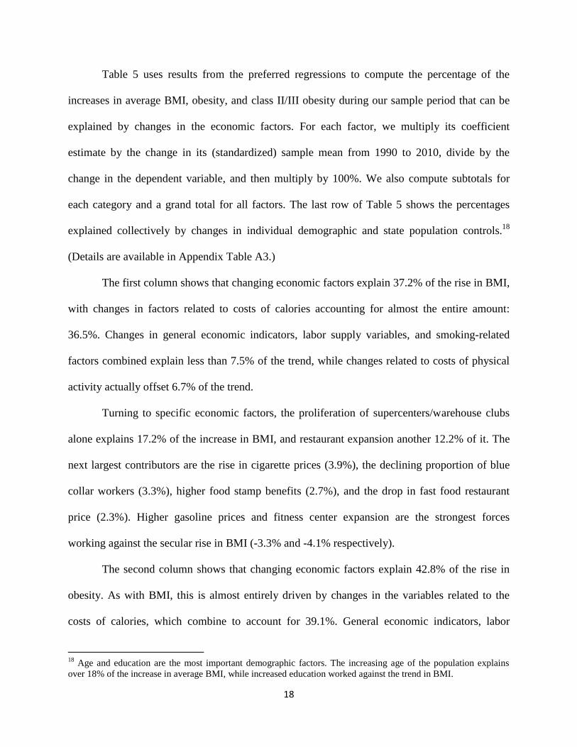
Table 5 uses results from the preferred regressions to compute the percentage of the
increases in average BMI, obesity, and class II/III obesity during our sample period that can be
explained by changes in the economic factors. For each factor, we multiply its coefficient
estimate by the change in its (standardized) sample mean from 1990 to 2010, divide by the
change in the dependent variable, and then multiply by 100%. We also compute subtotals for
each category and a grand total for all factors. The last row of Table 5 shows the percentages
explained collectively by changes in individual demographic and state population controls.18
(Details are available in Appendix Table A3.)
The first column shows that changing economic factors explain 37.2% of the rise in BMI,
with changes in factors related to costs of calories accounting for almost the entire amount:
36.5%. Changes in general economic indicators, labor supply variables, and smoking-related
factors combined explain less than 7.5% of the trend, while changes related to costs of physical
activity actually offset 6.7% of the trend.
Turning to specific economic factors, the proliferation of supercenters/warehouse clubs
alone explains 17.2% of the increase in BMI, and restaurant expansion another 12.2% of it. The
next largest contributors are the rise in cigarette prices (3.9%), the declining proportion of blue
collar workers (3.3%), higher food stamp benefits (2.7%), and the drop in fast food restaurant
price (2.3%). Higher gasoline prices and fitness center expansion are the strongest forces
working against the secular rise in BMI (-3.3% and -4.1% respectively).
The second column shows that changing economic factors explain 42.8% of the rise in
obesity. As with BMI, this is almost entirely driven by changes in the variables related to the
costs of calories, which combine to account for 39.1%. General economic indicators, labor
18
Age and education are the most important demographic factors. The increasing age of the population explains
over 18% of the increase in average BMI, while increased education worked against the trend in BMI.

19
supply, and smoking variables each contribute slightly to the trend, while variables related to
physical activity work marginally against it. Supercenters/warehouse clubs and restaurants are
the single largest contributors to the rise in obesity at 16.3% and 13.8%, respectively. Other
economic factors explaining at least 2% of the trend are higher cigarette prices (4.4%), the rise in
food stamp benefits (3.9%), cheaper fast food (3.4%), and the declining earnings of the middle
class relative to the poorest (2.1%). Fitness center expansion is the only factor meaningfully
working against the trend (-2.7%).
The third column reports that changing economic factors explain 59.3% of the increase in
class II/III obesity – a much greater portion of the trend than for BMI and overall obesity. This is
an important result since excess weight does not begin to substantially increase mortality until
the class II obesity threshold (Flegal et al., 2013). On the other hand, increases in BMI could
actually reflect an improvement in health among previously underweight individuals. Therefore,
the class II/III obesity is most relevant from a public health standpoint.
Changes in factors related to the costs of calories explain 59.6% of the rise in class II/III
obesity, while the labor supply variables contribute another 7.8%. General economic indicators,
physical-activity-related variables, and smoking-related factors each work slightly against the
trend. Among the variables related to the costs of calories, supercenters/warehouse clubs and
restaurants are again the most important, explaining 24.1% and 22.9% of the rise in severe
obesity, respectively. Other factors contributing meaningfully are the rise in food stamp benefits
(8.3%) and the decline in blue collar jobs (6.2%).19
Fitness center expansion offsets 3.6% and
higher gasoline prices 2.8% of the trend.
19
It is interesting that proportion of blue collar workers influences severe obesity (and to a lesser extent average
BMI) while proportion in a physically active job does not. This suggests the effect of blue collar employment is due
to some other aspect of these jobs besides their presumably higher levels of activity. One possibility is that they tend
to have more rigidly structured work days than white collar or service jobs, with fewer opportunities for on-the-job

20
V. Quantile Regressions
Our finding that changing economic factors explain a greater portion of the rise in class
II/III obesity than BMI or obesity suggests that economic variables affect BMI most strongly at
the right extreme of the distribution. This is important for two reasons. First, as mentioned,
weight gain appears to only have strong negative consequences for those who are severely obese
(Flegal et al., 2013). Stronger effects of economic factors at higher BMI levels imply that the
health consequences of changing economic factors are more harmful than suggested by mean
BMI regressions. Second, the BMI distribution did not symmetrically shift to the right over the
past two decades, but instead became more right-skewed. The 10th percentile increased by about
1 BMI point (~5%) between 1990 and 2010, whereas the 90th percentile rose by over 4 points
(~13%).20
If economic factors have the strongest effects on those who already have high BMIs,
they could help to explain the right-skewed growth in the BMI distribution. We use quantile
regression to investigate this possibility more formally.
We estimate determinants of BMI at the 0.1, 0.25, 0.5, 0.75, and 0.9 quantiles using
unconditional quantile regressions (UQR), which were developed by Firpo et al, (2009). UQR
allow us to estimate the marginal effects of right-hand-side variables on the quantiles of the
unconditional distribution of BMI, . In contrast, standard conditional quantile
regressions (CQR, Koenker and Basett, 1978) would estimate effects on the quantiles of the BMI
distribution conditional on the right-hand-side variables, . This
conditional distribution and its quantiles change as the right-hand-side variables change, and
snacking or going out to lunch. In unreported regressions (available upon request), we found some preliminary
support for these hypotheses. Using data from the American Time Use Survey, we find a negative association
between having a blue collar job and time spent in secondary eating. Using data from the DDB Needham Life Style
Surveys, we estimate a negative association between blue collar employment and frequency of eating lunch at
restaurants, but no effect on frequency of eating out for other meals. These patterns deserve further research. 20
For comparison, the 25th, 50th, and 75th BMI percentiles rose by 1.6, 2.4, and 3.4 points, respectively.

21
marginal effects on quantiles of the conditional distribution are not generally the same as
marginal effects of quantiles of the unconditional distribution.21
Therefore, UQR provides
estimates that are more consistent with our goal of evaluating changes in the BMI distribution
over time.22
Table 6 reports the estimated marginal effects of the economic factors on each of the five
BMI quantiles. The effects of the key variables related to costs of caloric intake vary across
quantiles and are usually larger at higher quantiles. This is most apparent for
supercenters/warehouse clubs and restaurants, which have effects that are roughly ten times
larger at the 0.9 quantile than at the 0.1 quantile. This result is consistent with the prominent
effects of these two variables on class II/III obesity. Additionally, general merchandisers have
sizeable positive effects at the 0.75 and 0.9 quantiles but negative (and significant) coefficients at
the 0.1 and 0.25 quantiles, while the food stamp coefficient is largest at the 0.9 quantile and
small and insignificant at lower quantiles. The density of supermarkets appears to lower BMI,
but only at the 0.75 and 0.9 quantiles. Some variables in other categories – such as female labor
participation and fitness centers – exhibit some heterogeneity in effects across quantiles but
without clear patterns. Collectively, these results indicate that the main economic factors
associated with BMI are most relevant for weight changes at the right tail of the distribution.
Table 7 shows the percentage changes in the five BMI quantiles accounted for by
changes in the economic factors, computed in a similar way to those reported in Table 5. The
results are consistent with the differences in effects across quantiles discussed above. The
21
In OLS, the marginal effects on the mean of the outcome conditional on the right-hand-side variables are the same
as the effects on the unconditional mean. See detailed discussion in Firpo et al, (2009). 22
Another practical reason for avoiding CQR in this work is that estimating the variance-covariance matrix for that
model using bootstrap is extremely time-consuming given the large dataset we employ. Following Firpo et al.
(2009), the UQR is estimated using an OLS regression of the re-centered influence function of the unconditional
BMI quantiles on all of the explanatory and control variables described above, including state and year fixed effects.
The regressions are weighted using BRFSS weights and standard errors are obtained using 500 bootstrap
replications.

22
economic factors collectively explain 51% of the 4-point rise in BMI at the 0.9 quantile between
1990 and 2010, but explain less than 15% of the ~ 1 point rises in the 0.1 and 0.25 BMI
quantiles. This pattern is again most pronounced for supercenters/warehouse clubs and
restaurants, which together explain about 45% in the rise of the 0.9 quantile. In contrast,
supercenters/warehouse clubs explain around 13% of the 0.1 quantile change, and restaurants
have no statistically significant effect. Other changes that contribute to the rise in the 0.9 quantile
are the drop in blue collar jobs (~5.3% explained) and increase in food stamp benefits (6.3%).
Interestingly, changes in the control variables explain a larger portion of the trend at
lower quantiles than higher quantiles. Changes in control variables actually have greater
explanatory power than changes in economic factors at the 0.1 and 0.25 quantiles. As in the case
of mean regressions, age accounts for most of the effect of the control variables.
Overall, the results from quantile regressions are consistent with those for class II/III
obesity, indicating that costs of caloric intake are important contributors to the clinically-relevant
portion of the rise in BMI and the shift in the BMI distribution to the right. Costs of caloric
intake – and economic factors in general – explain much less of the changes in the “non-obese”
weight range. These findings imply important heterogeneity in the effects across the BMI
distribution.
VI. Additional Robustness Checks
We estimated a number of additional models to evaluate the sensitivity of the results from
our preferred specification. Our first two robustness checks further evaluate the role of
multicollinearity in influencing our results. First, we drop any economic factors that were not
statistically significant in either the regressions for each factor separately or for all of them
together. The goal is to develop a model that strikes a balance between the two extremes by

23
including some, but not all, of the economic factors. Dropping irrelevant variables may help
reduce the standard errors for the remaining coefficients. This approach leaves 15 of the 27
economic factors in the BMI regression, 14 in the obesity regression, and 15 in the class II/III
obesity regression. Our second robustness check returns to including all 27 economic factors but
replaces the year fixed effects with a quadratic time trend, thereby allowing some time-series
variation to help with identifying so many separate effects at once.
Next, we aggregate all variables to the state level, using the BRFSS sampling weights and
weighting the states by population in the regressions. Since all independent variables of interest
are state-level, it is useful to check whether we reach the same conclusions regardless of whether
or not we leave the dependent and control variables at the individual level.
Our fourth robustness check returns to individual-level data and addresses the possibility
that, since weight is a capital stock accumulated over time, the short- and long-run effects of
changing economic incentives could differ. It is not clear which of these our fixed effects
estimates with contemporaneous economic factors more closely reflect. One approach to
modeling dynamics would be to include lags of the economic factors. However, the strong
correlations between contemporaneous and lagged values of the economic factors creates an
additional multicollinearity concern. Instead, we adopt an approach previously used in the
obesity literature (Anderson et al., 2003; Courtemanche, 2009a; Wehby and Courtemanche,
2012) and model the economic factors as moving averages of their values over the past several
years. We reached similar conclusions using three-, five-, and seven-year averages; and present
results for the seven-year averages. The regressions therefore estimate the impacts of changes in
the economic factors that are sustained for seven years (i.e. long-run effects). Seven-year

24
averages reflect values over the current and six preceding years, so the first six years of our
sample (1990-1995) are dropped.23
Our fifth robustness check addresses the issue of whether our results can be interpreted as
causal effects as opposed to merely associations. Controlling for state and year fixed effects,
individual demographic characteristics, and a wide range of state-level economic factors goes
quite far toward accounting for unobservable confounders; however, potential concerns still
remain. For instance, if a state becomes more health-conscious over time relative to other states,
this may affect some economic factors (e.g. types of foods stores) as well as obesity, leading to
omitted variable bias. Additionally, reverse causality would be an issue if, for example, a state’s
average BMI affects food prices or food retailer entry decisions. We aim to at least partially
address these concerns with an instrumental variables approach. While it is impractical to
simultaneously instrument for 27 different endogenous variables, it is feasible to instrument for
the two economic factors that emerged as the leading drivers of our baseline results:
supercenters/warehouse clubs and restaurants.
Prior research provides guidance on how to do this. Courtemanche and Carden (2011)
estimate the impact of Walmart Supercenters on BMI by exploiting plausibly exogenous
variation from Walmart’s strategy of expanding in concentric circles outwards from its
headquarters in Bentonville, AR. Dunn (2010) and Anderson and Matsa (2011) identified the
effects of restaurants on BMI by utilizing the tendency for restaurants to locate near major
highway exits.
23
As another approach to modeling dynamics, we aggregated the data to the state level and estimated dynamic panel
models that included the lag of the dependent variable as a regressor. When we implement Arrelano-Bond
estimation methods, the coefficient on the lagged dependent variable is imprecisely estimated, making the results
uninformative.

25
Motivated by these approaches, we instrument for supercenter/warehouse club density
and restaurant density using: 1) interactions of the natural log of distance from Bentonville
(measured from the centroid of each state) with each year fixed effect, and 2) the number of
interstate exits per 10,000 residents in the state interacted with year fixed-effects. Interstate exit
information as of May 2014 comes from http://m.roadnow.com/ and we treat exits as being fixed
over time, which is likely almost the case since the original interstate highway plan was
completed by 1992.24
Interactions with year fixed effects prevent these time-invariant variables
from being dropped by the inclusion of state fixed effects. Identification comes from changes
over time in the relationships between these variables and the endogenous regressors. We
recognize that the validity of the exclusion restrictions could be questioned on various grounds
and, for this reason, we include the IV estimates only as a robustness check.
Table 8 reports the results for the robustness checks for BMI. To save space, we present
only the percentage of the rise in BMI explained for each economic factor, along with indicators
of statistical significance. Coefficient estimates and standard errors are available upon request.
The overall percentage of the rise in BMI explained by the economic factors ranges from 27.7%
to 44.5%. Recall that the baseline estimate from Table 5 was 37.2% with a standard error of
10.6%. The estimates from the robustness checks are therefore all within a standard error of the
baseline estimate.
Turning to the subtotals from each category of economic factors, the percentages are very
similar across specifications for the labor supply variables and variables related to calorie intake.
The subtotals for variables related to general economic indicators, physical activity, and smoking
24
Roadnow.com only has data on major interstates, so we are unable to include miles and exits from auxiliary
routes, e.g. the bypass around a city. In some sense this may be preferable, as auxiliary routes are more likely to
have been built or expanded during our sample period, which would be problematic for our assumption that miles
and exits are fixed over time. The date of completion of the interstate highway system (aside from a few parts that
remain unfinished) is from http://logistics.about.com/od/legalandgovernment/a/Interstate-Highway-System.htm.

26
are also generally similar across specifications, with the exception of the model with 7-year
averages. In this regression, the general economic indicators and smoking categories contribute
more to the trend than in the baseline model, while the physical activity category works against
the trend more strongly. However, the caloric intake category remains by far the most substantial
contributor to the rise in BMI. Regarding the individual economic factors, the key result is that
supercenters/warehouse clubs and restaurants remain the two leading contributors to the trend in
all specifications. Interestingly, however, rising cigarette prices explain virtually the same
amount of the rise in BMI as increased restaurant density in the 7-year averages specification.
Also noteworthy is that the IV estimates for restaurants and supercenters/warehouse clubs are
both well within the confidence intervals from the baseline model, with the
supercenters/warehouse clubs estimate being slightly larger in the IV model and the restaurants
estimate being slightly smaller. Supercenters/warehouse clubs remain highly statistically
significant despite the inherent inefficiency of IV estimation, whereas the estimate for restaurant
density becomes insignificant due to the almost 3-fold increase in the standard error. The first
stage F statistics are 34.58 for supercenters/warehouse clubs and 12.41 for restaurants, indicating
that our instruments are sufficiently strong to rule out the possibility that the IV and OLS
estimates are only similar because of weak instrument bias.
Tables 9 and 10 present the results from the robustness checks for obesity and class II/III
obesity. Since the conclusions about robustness are similar to those for BMI, we provide only a
brief discussion. The overall percentage of the rise in obesity explained by all the economic
factors together ranges from 35.5% to 49.4%, in the vicinity of the baseline estimate of 42.8%.
The overall percentage of the increase in class II/III obesity ranges from 50.7% to 67.0%, again
similar to the baseline estimate of 59.3%. Variables related to the costs of calorie intake –

27
particularly restaurants and supercenters/warehouse clubs – remain the most important in all
models. Interestingly, the rise in cigarette prices explains a sizeable 21.4% of the rise in obesity
in the 7-year averages model, but has virtually no effect on class II/III obesity using the same
specification.
VII. Falsification Tests
An important question is the extent to which the previously estimated effects of the
economic factors on BMI, obesity, and class II/III obesity can be considered causal. At issue is
whether movements over time in unobservable state-level characteristics are correlated with
changes over time in the state-level economic variables. We believe that including more
economic factors reduces this possibility, at least relative to the less comprehensive approaches
typically used in the literature. The robustness of our most striking results – those for restaurants
and supercenters/warehouse clubs – to the use of 2SLS is also reassuring. This section attempts
to further mitigate concerns about potential omitted variables bias through a series of
falsification tests.
Ideal dependent variables for falsification tests, in our context, satisfy two criteria: 1)
there should not be any reason for them to be causally affected by the economic factors, and 2)
they should be influenced by the same unobservable characteristics as body weight. Natural
candidates to satisfy the second condition are other health behaviors, as presumably they are also
affected by potentially unobserved confounders such as state residents’ demand for health, health
knowledge, and individual time and risk preferences. However, other health behaviors might not
perfectly satisfy the first condition, especially given the wide scope of the economic factors
included in our analysis. The best candidates in the BRFSS are dummies for whether the
respondent always uses a seatbelt, had a flu vaccine in the past year, and had a mammogram (for

28
women) or digital rectal prostate exam (for men 40 and older) in the past two years.25
However,
it remains possible that these outcomes are affected by some of our economic factors, which
could result in our falsification tests indicating endogeneity when none exists.
Table 11 reports the results from linear probability models regressing each of these four
falsification test outcomes on the economic factors, as well as demographic controls and state
and year fixed effects. The table presents a total of 108 coefficient estimates, so we expect some
statistically significant “effects” even for well-specified models. We obtain slightly more
falsification test failures than expected: 15 (13.9%) coefficients are significant at the 10% level,
and 10 (9.3%) at the 5% level. However, we see no relationship between the coefficients that are
statistically significant in these falsification tests and those that are significant in our main
results. Specifically, none of the estimates for supercenters/warehouse clubs are significant,
while the only significant result for restaurants is an association with higher levels of prostate
screening. This suggests that, if anything, restaurants enter areas with improving health
behaviors. In sum, we view the results from Table 11 as generally supportive of a causal
interpretation of our earlier estimated effects on weight – particularly for the economic factors
that emerged as the most important contributors to the trend.
VIII. Weight Loss Attempts
A lingering question with the results presented thus far is whether or not individual
responses to economic factors are rational. In the standard neoclassical model, with rational
consumers, the utility lost from the additional weight is less than the utility gained from, for
instance, greater enjoyment of tasty foods. Conversely, if preferences are time-inconsistent or
25
The BRFSS specifically imposed the age restriction for men’s prostate exams, but not for women’s
mammogram’s, so we follow their lead and include women of all ages. The results are similar if we impose various
age cutoffs for women.

29
individuals are otherwise irrational, the effects of changing economic incentives may be
exacerbated and increases in weight may be inefficient, even in absence of externalities. Ruhm
(2012) documents the prevalence of weight loss attempts and characterizes these as an admission
of past deviations from one’s lifetime utility maximizing plans, suggesting “internalities” due to
time inconsistency or other sources of not fully rational decision-making. Building on this idea,
we evaluate whether the economic factors identified as major contributors to the rise in BMI,
obesity, or severe obesity are associated with the probability of reporting current weight loss
attempts. Significant effects would be consistent with at least some of the weight gained from
changes in these factors being welfare-decreasing.
Table 12 reports the results. The weight loss attempt variable is only available in 1994,
1996, 1998, 2000, and 2003, so our sample size is smaller than for the main regressions. The first
column includes all 27 economic factors in the same regression. We observe only two significant
effects, both at the 10% level: a higher proportion of the workforce in an active job is associated
with fewer weight loss attempts, while greater supercenter/warehouse club density is associated
with more weight loss attempts.
Since our sample only contains five years (compared to 21 for the main regressions),
multicollearity among the economic factors might help explain the lack of significant results. We
therefore estimate two additional models. The first includes only the “important” economic
factors, which we define as explaining more than 5% of the rise in BMI, obesity, or class II/III
obesity in the baseline regressions (or working against the trend by the same amount). Variables
meeting this criterion are proportion blue collar, restaurants, supercenters/warehouse clubs, food
stamp benefits, gas prices, and fitness centers. Next, we include only restaurants and
supercenters/warehouse clubs, which repeatedly emerged as the two most important factors.

30
These additional specifications do not cause any new results to emerge. Supercenter/warehouse
club density is the only significant economic factor, and its level of significance rises as the
number of other included economic factors shrinks. Discount big box grocers may trigger
impulses that lead to “mistakes,” i.e. deviations from long-run utility maximization. This result is
consistent with Courtemanche et al.’s (2014) finding that present-biased individuals are the most
responsive to falling food prices. It is interesting, however, that we do not observe a similar
effect for restaurants.
IX. Discussion
This paper aims to answer to the big-picture question of how well “the economic
explanation” of individuals responding to changing incentives can explain the rise in obesity. We
develop a model of weight that includes numerous economic factors reflecting the economic
incentives alleged to have contributed to the upward trend in weight in the U.S. These factors
relate to general economic conditions, labor supply, and the monetary or time costs of eating,
physical activity, and smoking. Changes in these economic factors collectively explain 37% of
the rise in body mass index, 43% of the increase in obesity, and 59% of the growth in class II/III
obesity – the category in which the strong mortality consequences of excess weight emerge.
Quantile regressions confirm that the economic factors are most relevant for explaining the rise
in “obese weight” ranges and the greater shifts of the upper BMI percentiles, accounting for 51%
of the change at the 90th
BMI percentile. Variables related to the costs of eating – particularly
supercenter/warehouse club expansion and increasing numbers of restaurants – are the leading
drivers of the results.
Our main conclusions are robust to the exclusion of insignificant economic factors, the
use of a quadratic trend instead of year fixed effects, accounting for the gradual nature of weight

31
accumulation, aggregating the data, and using instruments for the leading contributors to the
trend. Falsification tests show little connection between the aforementioned key economic
factors and other health behaviors, consistent with a causal interpretation of the effects on
weight. Finally we show that supercenter/warehouse club density increases the probability of
weight loss attempts, raising the possibility that cheap food from these retailers triggers self-
control problems.
Several limitations of our study provide opportunities for future research. Most
obviously, while we identify the factors associated with a meaningful portion of the trend in
weight, much of the trend remains unexplained. Measurement error in some economic variables
could lead us to underestimate their contributions. Perhaps most importantly, the C2ER state-
level food and alcohol price data are based on a limited number of products and urban markets,
almost certainly resulting in some measurement error. Additionally, we are not able to evaluate
some potentially important changes in incentives due to technological innovations for which it is
difficult to measure cross-state over-time variation. For instance, Cutler et al. (2003) argue that
the rise in obesity is the result of technological progress in food preparation and preservation that
reduces the time cost of consuming snack foods. However, the specific innovations mentioned
(e.g. microwaving and vacuum packing) occurred well before 1990, so they are not likely to
explain the rise in obesity during our sample period. Another possible explanation is that
electronic innovations – video games, computers, more television channels, cell phones, etc. –
have improved sedentary leisure time options, increasing the opportunity cost of physical
activity. We are skeptical, though, that this explains a large portion of the trend because Cutler et
al. (2003) documented that the rise in obesity is driven by additional caloric intake rather than
reduced energy expenditure.
32
Future research should push further to establish causality. While the inclusion of state and
year fixed effects, robustness of the results for the two leading factors to an instrumental variable
specification, and favorable falsification test results give us confidence that our estimates have a
causal interpretation, it is obviously impossible to make strong claims in the absence of
randomization or quasi-randomization. Further analyses, both using the “one factor at a time”
approach common in the literature and comprehensive models such as the one considered here,
are necessary before a consensus can emerge about the causal effects of the various economic
factors.
Finally, future research should continue to evaluate the appropriate role of policy in light
of an economic explanation for the rise in obesity. We briefly consider one possible justification
for intervention: time-inconsistent preferences. Others include negative externalities from pooled
health care costs and imperfect information about the caloric content of different foods. More
work is needed on the benefits, costs, and welfare effects of various policy options.

33
References
Anderson, M.L. and Matsa, D.A. (2011): “Are Restaurants Really Supersizing America?”
American Economic Journal: Applied Economics, 3, 152-188.
Anderson, P. and Butcher, K. (2006): “Childhood Obesity: Trends and Potential Causes.” The
Future of Children, 16(1), 19-45.
Anderson, P., Butcher, K., and Levine, P. (2003): “Maternal Employment and Overweight
Children.” Journal of Health Economics, 22, 477-504.
Basker, E. and Noel, M. (2009): “The Evolving Food Chain: Competitive Effects of Wal-Mart’s
Entry in to the Supermarket Industry.” Journal of Economics and Management Strategy, 18,
977-1009.
Baum, C. (2009): “The Effects of Cigarette Costs on BMI and Obesity,” Health Economics 18,
3-19.
Baum, C. (2011): “Effects of Food Stamps on Obesity,” Southern Economic Journal, 77, 623-
651.
Baum, C. and Chou, S. (2011): “The Socio-Economic Causes of Obesity,” National Bureau of
Economic Research Working Paper #17423.
Beydoun, M., Powell, L., and Wang, Y. (2008): “The Association of Fast Food, Fruit and
Vegetable Prices with Dietary Intakes among US Adults: Is There Modification by Family
Income,” Social Science and Medicine, 66, 2218-2219.
Cawley, J., Moran, J. and Simon, K. (2010): “The Impact of Income on the Weight of Elderly
Americans.” Health Economics, 19, 979-993.
Cawley, J. and Ruhm, C. (2011): “The Economics of Risky Health Behaviors.” Chapter 3 in
Handbook of Health Economics, Vol. 2, 95-199.
Chen, Z., Yen, S., and Eastwood, D. (2005): “Effects of Food Stamp Participation on Body
Weight and Obesity,” American Journal of Agricultural Economics, 87, 1167-1173.
Chou, S., Grossman, M. and Saffer, H. (2002): “An Economic Analysis of Adult Obesity:
Results from the Behavioral Risk Factor Surveillance System.” National Bureau of Economic
Research Working Paper #9247.
Chou, S., Grossman, M. and Saffer, H. (2004): “An Economic Analysis of Adult Obesity:
Results from the Behavioral Risk Factor Surveillance System.” Journal of Health Economics,
23, 565-587.

34
Courtemanche, C. (2009a): “Longer Hours and Larger Waistlines? The Relationship Between
Work Hours and Obesity,” Forum for Health Economics and Policy, 12, Article 5.
Courtemanche, C. (2009b): “Rising Cigarette Prices and Rising Obesity: Coincidence or
Unintended Consequence?” Journal of Health Economics, 28, 781-798.
Courtemanche, C. (2011): “A Silver Lining? The Connection between Gasoline Prices and
Obesity,” Economic Inquiry, 49, 935-957.
Courtemanche, C.J. and Carden, W.A. (2011): “Supersizing Supercenters? The Impact of
Walmart Supercenters on Body Mass Index and Obesity,” Journal of Urban Economics, 69, 165-
181.
Courtemanche, C.J. and Carden, W.A. (2014): “Competing with Costco and Sam’s Club:
Warehouse Club Entry and Grocery Prices,” Southern Economic Journal, 80, 565-585.
Courtemanche, C.J., Heutel, G. and McAlvanah, P. (2014): “Impatience, Incentives, and
Obesity,” Economic Journal, forthcoming.
Courtemanche, C.J., Pinkston, J., and Stewart, J. (2014): “Adjusting Body Mass for
Measurement Error with Invalid Validation Data,” National Bureau of Economic Research
Working Paper #19928.
Currie, J., DellaVigna, S., Moretti, E. and Pathania, V. (2010): “The Effect of Fast Food
Restaurants on Obesity and Weight Gain.” American Economic Journal: Economic Policy, 2,
32-63.
Cutler, D., Glaeser, E. and Shapiro, J. (2003): “Why Have Americans Become More Obese?”
Journal of Economic Perspectives, 17, 93-118.
Dunn, R. (2010): “Obesity and the Availability of Fast-Food: An Analysis by Gender,
Race/Ethnicity and Residential Location,” American Journal of Agricultural Economics, 92,
1149-1164.
Eid, J., Overman, H., Puga, D. and Turner, M. (2008): “Fat City: Questioning the Relationship
Between Urban Sprawl and Obesity,” Journal of Urban Economics, 63, 385-404.
Ewing, R., Schmid, T., Killingsworth, R., Zlot, A. and Raudenbush, S. (2003): “Relationship
between urban sprawl and physical activity, obesity, and morbidity,” American Journal of
Health Promotion, 18, 47-57.
Fan, M. (2010): “Do Food Stamps Contribute to Obesity in Low-Income Women? Evidence
from the National Longitudinal Survey of Youth 1979,” American Journal of Agricultural
Economics, 92, 1165-1180.

35
Finkelstein, E., Fiebelkorn, I. and Wang, G. (2003): “National Medical Spending Attributable to
Overweight and Obesity: How Much, and Who's Paying?” Health Affairs, Web Exclusives,
W219-W226.
Finkelstein, E., Khavjou, O., Thompson, H., Trogdon, G., Pan, L., Sherry, B., and Dietz, W.
(2012): “Obesity and Severe Obesity Forecasts through 2030.” American Journal of Preventive
Medicine, 42, 563-570.
Firpo, S., Fortin, N. M., and Lemieux, T. (2009): “Unconditional Quantile Regressions.”
Econometrica, 77, 953–973.
Flegal, K., Carroll, M., Kuczmarski, R. and Johnson, C. (1998): “Overweight and Obesity in the
United States: Prevalence and Trends, 1960-1994,” International Journal of Obesity, 22, 39-47.
Flegal, K., Graubard, B., Williamson, D. and Gail, M. (2005): “Excess Deaths Associated with
Underweight, Overweight, and Obesity,” Journal of the American Medical Association, 293,
1861-1867.
Flegal, K., Kit, B., Orpana, H., and Graubard, B. (2013): “Association of All-Cause Mortality
with Overweight and Obesity Using Standard Body Mass Index Categories: A Systematic
Review and Meta-Analysis,” Journal of the American Medical Association, 309, 71-82.
Frank, L., Andresen, M. and Schmid, T., (2004): “Obesity relationships with community design,
physical activity, and time spent in cars,” American Journal of Preventive Medicine, 27, 87-96.
Gibson, D. (2003): “Food Stamp Participation is Positively Related to Obesity in Low Income
Women,” Journal of Nutrition, 133, 2225-2231.
Gibson, D. (2006): “Long-Term Food Stamp Program Participation is Positively Related to
Simultaneous Overweight in Young Daughters and Obesity in Mothers,” Journal of Nutrition,
136, 1081-1085.
Goldman, D., Lakdawalla, D. and Zheng, Y. (2011): “Food Prices and the Dynamics of Body
Weight,” in Economic Aspects of Obesity, Grossman, M. and Mocan, N. eds., Chicago, IL:
University of Chicago Press.
Grossman, M. (1972): “On the Concept of Health Capital and the Demand for Health,” Journal
of Political Economy, 80, 223-255.
Gruber, J. and Frakes, M. (2006): “Does Falling Smoking Lead to Rising Obesity?” Journal of
Health Economics, 25, 183-187.
Hausman, J. and Leibtag, E. (2004): “CPI Bias from Supercenters: Does the BLS Know that
Wal-Mart Exists?” National Bureau of Economic Research Working Paper #10712.
36
Kaushal, N. (2007): “Do Food Stamps Cause Obesity? Evidence from Immigrant Experience,”
Journal of Health Economics, 26, 968-991.
Koenker, R., and Bassett, G. (1978): “Regression Quantiles.” Econometrica, 46, 33-50.
Komlos, J. (2004): “Obesity and the Rate of Time Preference: Is there a Connection?” Journal of
Biosocial Sciences, 36, 209-219.
Kuczmarski, M. F., Kuczmarski, R. J., and Najjar, M. (2001): “Effects of Age on Validity of
Self-Reported Height, Weight, and Body Mass Index: Findings from the Third National Health
and Nutrition Examination Survey, 1988-1994.” Journal of the American Dietetic Association,
101, 28-34.
Lakdawalla, D. and Philipson, T. (2002): “The Growth of Obesity and Technological Change: A
Theoretical and Empirical Investigation,” National Bureau of Economic Research Working
Paper #8965.
Lakdawalla, D., Philipson, T. and Bhattacharya, J. (2005): “Welfare-Enhancing Technological
Change and the Growth of Obesity,” American Economic Review Papers and Proceedings, 95,
253-257.
Lindahl, M. (2005): “Estimating the Effect of Income on Health and Mortality Using Lottery
Prizes as an Exogenous Source of Variation in Income.” Journal of Human Resources, 40(1),
144-168.
Meyerhoefer, C. and Pylypchuck, Y. (2008): “Does Participation in the Food Stamp Program
Increase the Prevalence of Obesity and Health Care Spending,” American Journal of
Agricultural Economics, 90, 287-305.
Nonnemaker, J., Finkelstein, E., Engelen, M., Hoerger, T. and Farrelly, M. (2009): “Have Efforts
to Reduce Smoking Really Contributed to the Obesity Epidemic?" Economic Inquiry, 47, 366-
376.
Ogden, C.L., Carroll, M.D., Kit B.K., and Flegal, K. M. (2014): “Prevalence of Childhood and
Adult Obesity in the United States, 2011-2012,” Journal of the American Medical Association,
311(8), February 26, 2014, 806-814.
Orzechowski, W., & Walker, R. (2010): The Tax Burden on Tobacco, Historical Compilation
(Vol. 45). Arlington, Virginia.
Philipson, T. and Posner, R. (1999): “The Long-Run Growth in Obesity as a Function of
Technological Change,” National Bureau of Economic Research Working Paper #7423.
Philipson, T. and Posner, R. (2003): “The Long-Run Growth in Obesity as a Function of
Technological Change,” Perspectives in Biology and Medicine, 46, S87-S107.

37
Plantinga, A. and Bernell, S. (2007): “The Association Between Urban Sprawl and Obesity: Is it
a Two-Way Street?” Journal of Regional Science, 47, 857-879.
Rashad, I. (2006): “Structural Estimation of Caloric Intake, Exercise, Smoking, and Obesity,”
Quarterly Review of Economics and Finance, 46, 268-283.
Rashad, I., Chou, S., Grossman, M. (2006): “The Super Size of America: An Economic
Estimation of Body Mass Index and Obesity in Adults.” Eastern Economic Journal 32, 133-148.
Ruhm, C. (2000): “Are Recessions Good for Your Health?” Quarterly Journal of Economics,
115(2), 617-650.
Ruhm, C. (2005): “Healthy Living in Hard Times,” Journal of Health Economics, 24(2), 341-
363.
Ruhm, C. (2008): “Maternal Employment and Adolescent Development,” Labour Economics,
15, 958-983.
Ruhm, C. (2012): “Understanding Overeating and Obesity,” Journal of Health Economics, 31,
781-796.
Schmeiser, M. (2009): “Expanding Wallets and Waistlines: The Impact of Family Income on the
BMI of Women and Men Eligible for the Earned Income Tax Credit.” Health Economics, 18,
1277-1294.
Strum, R. (2002): “The Effects of Obesity, Smoking, and Drinking on Medical Problems and
Costs,” Health Affairs, 21, 245-253.
US Department of Health and Human Services (1989): “Reducing the Health Cunsequences of
Smoking: 25 Years of Progress. A Report of the Surgeon General.” U.S. Department of Health
and Human Services, Public Health Service, Centers for Disease Control, Center for Chronic
Disease Prevention and Health Promotion, Office on Smoking and Health, DHHS Publication
No. (CDC) 89-8411.
Ver Ploeg, M., Mancino, L., Lin B., and Wang, C. (2007): “The Vanishing Weight Gap: Trends
in Obesity among Adult Food Stamp Participants,” Economics and Human Biology, 5, 20-36.
Wang, Z., Patterson, C., and Hills, A. (2002): “A Comparison of Self-Reported and Measured
Height, Weight and BMI in Australian Adolescents,” Australian and New Zealand Journal of
Public Health, 26, 473e478.
Wehby, G.L. and Courtemanche, C. (2012): “The Heterogeneity of Cigarette Price Effects on
Body Weight,” Journal of Health Economics, 31, 719-29.
Zhao, Z. and Kaestner, R. (2010): “Effects of Urban Sprawl on Obesity,” Journal of Health
Economics, 29, 779-787.

38
Figure 1 – Trends in BMI, Obesity, and Severe Obesity
Figure 2 – Trends in Economic Factors Measured as Proportions
05
10
15
20
25
30
35
40
1990 1992 1994 1996 1998 2000 2002 2004 2006 2008 2010Year
Average BMI Percent Obese
Percent Severely Obese
.05
.1.1
5.2
.25
1990 1992 1994 1996 1998 2000 2002 2004 2006 2008 2010Year
Unemployment Rate Proportion Active Job
Proportion Blue Collar Proportion Central City

39
Figure 3 – Trends in Labor Force Participation Rates
Figure 4 – Trends in Income Inequality Ratios
.55
.6.6
5.7
.75
1990 1992 1994 1996 1998 2000 2002 2004 2006 2008 2010Year
Female Male
22.5
33.5
44.5
55.5
1990 1992 1994 1996 1998 2000 2002 2004 2006 2008 2010Year
90th/50th Percentile Ratio 50th/10th Percentile Ratio

40
Figure 5 – Trend in Work Hours
Figure 6 – Trends in Price Variables
36.5
36.7
5
37
37.2
53
7.5
37.7
5
38
Hou
rs p
er
We
ek
1990 1992 1994 1996 1998 2000 2002 2004 2006 2008 2010Year
24
68
1990 1992 1994 1996 1998 2000 2002 2004 2006 2008 2010Year
Restaurant Price Food Price
Alcohol Price Gasoline Price
Cigarette Price

41
Figure 7 – Trend in Relative Price of Fruits and Vegatables
Figure 8 – Trends in Store Variables
.6.6
5.7
.75
.8
Rela
tive
Pri
ce o
f F
ruits a
nd V
eg
eta
ble
s
1990 1992 1994 1996 1998 2000 2002 2004 2006 2008 2010Year
0.5
11
.52
2.5
33
.54
4.5
5
1990 1992 1994 1996 1998 2000 2002 2004 2006 2008 2010Year
Restaurants per 1,000 Supermarkets per 10,000
General Merchandisers per 10,000 Supercenters/Ware. Clubs per 100,000
Convenience Stores per 10,000 Fitness Centers per 10,000

42
Figure 9 – Trend in Food Stamp Spending
Figure 10 – Trends in Smoking Ban Variables
50
75
100
125
150
175
200
Foo
d S
tam
p S
pe
nd
ing P
er
Ca
pita
1990 1992 1994 1996 1998 2000 2002 2004 2006 2008 2010Year
0.1
.2.3
.4.5
.6.7
.8
1990 1992 1994 1996 1998 2000 2002 2004 2006 2008 2010Year
Private Workplaces Government Workplaces
Restaurants Other

43
Table 1 – Percentage of Rise in BMI Explained by Prior Studies
Variable Study Data Years Percentage
of Rise in
BMI
Explained
Fast-food price Chou et al. (2004) BRFSS 1984-1999 3.6%+
Grocery food price Lakdawalla and Philipson (2002) NHIS 1976-1994 40.0%
Alcohol price Chou et al. (2004) BRFSS 1984-1999 0.7%+
Restaurants Chou et al. (2004) BRFSS 1984-1999 64.4%+
Walmart Supercenters Courtemanche and Carden (2011) BRFSS 1994-2005 10.5%
Food stamps Baum (2011) NLSY 1985-2000 0.6%+
Work hours Courtemanche (2009b) NLSY 1985-2004 1.4%
Urban sprawl Zhou and Kaestner (2010) NHIS 1976-2001 8.6%+
On-the-job exercise Lakdawalla and Philipson (2002) NHIS 1976-1994 9.8%+
Gasoline prices Courtemanche (2009b) BRFSS 1984-2004 8.0%
Cigarette price Chou et al. (2004) BRFSS 1984-1999 24.9%+
Clean indoor air laws Chou et al. (2004) BRFSS 1984-1999 4.2%+
Total 176.7%
Notes: BRFSS is Behavioral Risk Factor Surveillance System, NHIS is National Health Interview Survey, and
NLSY is National Longitudinal Survey of Youth. + denotes estimate is our calculation based on summary statistics
and coefficient estimates from the paper, as opposed to being directly presented by the paper’s authors.
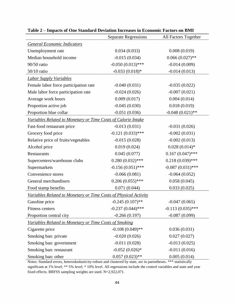
44
Table 2 – Impacts of One Standard Deviation Increases in Economic Factors on BMI
Separate Regressions All Factors Together
General Economic Indicators
Unemployment rate 0.034 (0.033) 0.008 (0.019)
Median household income -0.015 (0.034) 0.066 (0.027)**
90/50 ratio -0.050 (0.013)*** -0.014 (0.009)
50/10 ratio -0.033 (0.018)* -0.014 (0.013)
Labor Supply Variables
Female labor force participation rate -0.040 (0.031) -0.035 (0.022)
Male labor force participation rate -0.024 (0.026) -0.007 (0.021)
Average work hours 0.009 (0.017) 0.004 (0.014)
Proportion active job -0.045 (0.030) 0.018 (0.019)
Proportion blue collar -0.051 (0.036) -0.048 (0.021)**
Variables Related to Monetary or Time Costs of Calorie Intake
Fast-food restaurant price -0.013 (0.031) -0.031 (0.026)
Grocery food price -0.121 (0.033)*** -0.002 (0.031)
Relative price of fruits/vegetables -0.015 (0.028) -0.002 (0.013)
Alcohol price 0.019 (0.024) 0.028 (0.014)*
Restaurants 0.045 (0.077) 0.167 (0.047)***
Supercenters/warehouse clubs 0.280 (0.032)*** 0.218 (0.039)***
Supermarkets -0.156 (0.051)*** -0.087 (0.031)***
Convenience stores -0.066 (0.081) -0.064 (0.052)
General merchandisers 0.206 (0.055)*** 0.058 (0.045)
Food stamp benefits 0.071 (0.044) 0.033 (0.025)
Variables Related to Monetary or Time Costs of Physical Activity
Gasoline price -0.245 (0.107)** -0.047 (0.065)
Fitness centers -0.237 (0.044)*** -0.113 (0.035)***
Proportion central city -0.266 (0.197) -0.087 (0.099)
Variables Related to Monetary or Time Costs of Smoking
Cigarette price -0.108 (0.049)** 0.036 (0.031)
Smoking ban: private -0.020 (0.026) 0.027 (0.027)
Smoking ban: government -0.011 (0.028) -0.013 (0.025)
Smoking ban: restaurant -0.052 (0.026)* -0.011 (0.016)
Smoking ban: other 0.057 (0.023)** 0.005 (0.014) Notes: Standard errors, heteroskedasticity-robust and clustered by state, are in parentheses. *** statistically
significant at 1% level; ** 5% level; * 10% level. All regressions include the control variables and state and year
fixed effects. BRFSS sampling weights are used. N=2,922,071.

45
Table 3 – Impacts of One Standard Deviation Increases in Economic Factors on P(Obese)
Separate Regressions All Factors Together
General Economic Indicators
Unemployment rate 0.002 (0.002) -0.001 (0.001)
Median household income -0.001 (0.002) 0.003 (0.002)
90/50 ratio -0.003 (0.001)*** -0.0004 (0.001)
50/10 ratio -0.004 (0.001)*** -0.002 (0.001)**
Labor Supply Variables
Female labor force participation rate -0.002 (0.002) -0.002 (0.001)
Male labor force participation rate -0.001 (0.002) 0.001 (0.002)
Average work hours 0.0004 (0.001) -0.001 (0.001)
Proportion active job -0.004 (0.002)* -0.002 (0.002)
Proportion blue collar -0.003 (0.002) -0.001 (0.001)
Variables Related to Monetary or Time Costs of Calorie Intake
Fast-food restaurant price -0.001 (0.002) -0.003 (0.002)
Grocery food price -0.006 (0.002)*** 0.002 (0.002)
Relative price of fruits/vegetables -0.001 (0.002) -0.0001 (0.001)
Alcohol price 0.001 (0.002) 0.001 (0.001)
Restaurants 0.004 (0.005) 0.012 (0.004)***
Supercenters/warehouse clubs 0.017 (0.002)*** 0.013 (0.003)***
Supermarkets -0.008 (0.003)** -0.005 (0.003)*
Convenience stores -0.003 (0.005) -0.005 (0.004)
General merchandisers 0.015 (0.004)*** 0.007 (0.003)**
Food stamp benefits 0.003 (0.003)* 0.003 (0.002)
Variables Related to Monetary or Time Costs of Physical Activity
Gasoline price -0.013 (0.006)** -0.001 (0.005)
Fitness centers -0.012 (0.003)*** -0.005 (0.004)
Proportion central city -0.018 (0.011) -0.005 (0.007)
Variables Related to Monetary or Time Costs of Smoking
Cigarette price -0.007 (0.003)* 0.003 (0.003)
Smoking ban: private -0.001 (0.002) 0.001 (0.001)
Smoking ban: government -0.001 (0.002) -0.001 (0.002)
Smoking ban: restaurant -0.003 (0.002)** -0.001 (0.001)
Smoking ban: other 0.005 (0.002)** 0.002 (0.001)* See notes for Table 2.
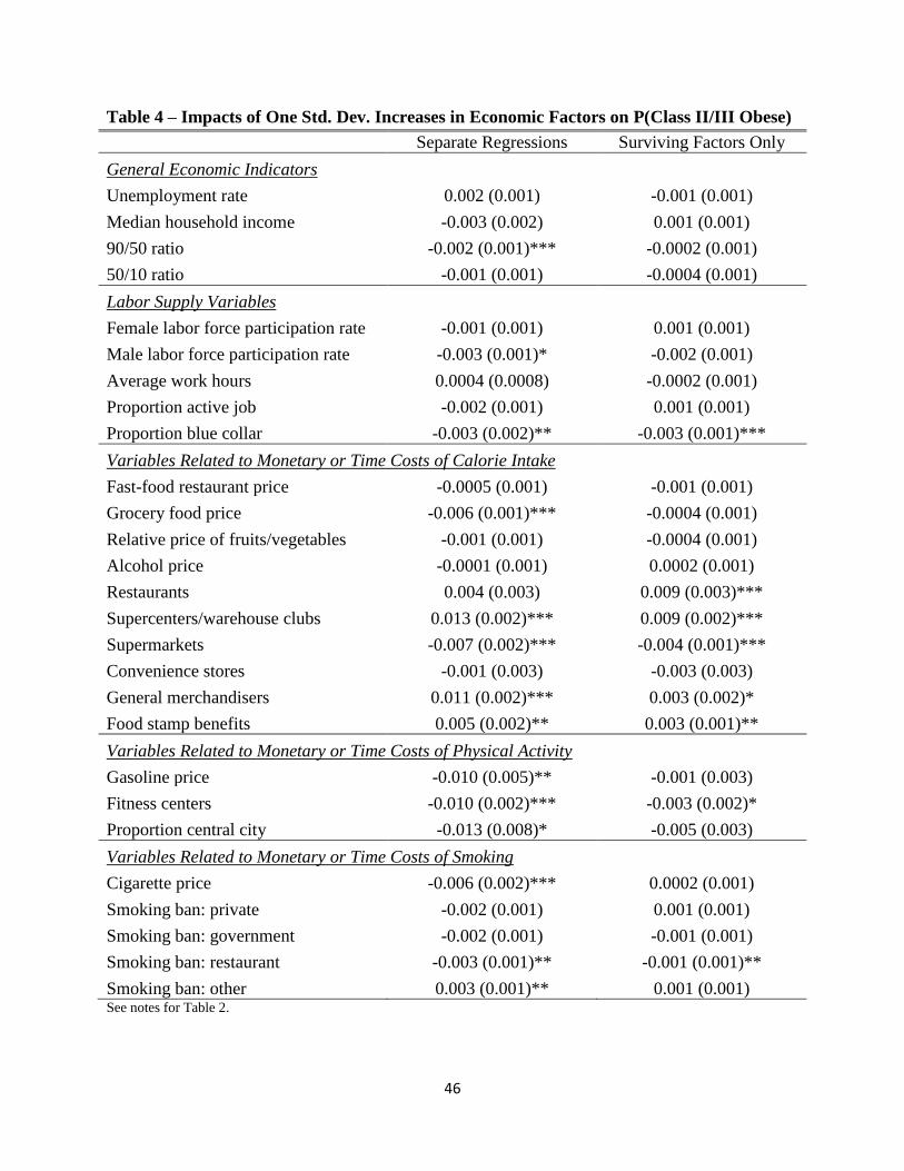
46
Table 4 – Impacts of One Std. Dev. Increases in Economic Factors on P(Class II/III Obese)
Separate Regressions Surviving Factors Only
General Economic Indicators
Unemployment rate 0.002 (0.001) -0.001 (0.001)
Median household income -0.003 (0.002) 0.001 (0.001)
90/50 ratio -0.002 (0.001)*** -0.0002 (0.001)
50/10 ratio -0.001 (0.001) -0.0004 (0.001)
Labor Supply Variables
Female labor force participation rate -0.001 (0.001) 0.001 (0.001)
Male labor force participation rate -0.003 (0.001)* -0.002 (0.001)
Average work hours 0.0004 (0.0008) -0.0002 (0.001)
Proportion active job -0.002 (0.001) 0.001 (0.001)
Proportion blue collar -0.003 (0.002)** -0.003 (0.001)***
Variables Related to Monetary or Time Costs of Calorie Intake
Fast-food restaurant price -0.0005 (0.001) -0.001 (0.001)
Grocery food price -0.006 (0.001)*** -0.0004 (0.001)
Relative price of fruits/vegetables -0.001 (0.001) -0.0004 (0.001)
Alcohol price -0.0001 (0.001) 0.0002 (0.001)
Restaurants 0.004 (0.003) 0.009 (0.003)***
Supercenters/warehouse clubs 0.013 (0.002)*** 0.009 (0.002)***
Supermarkets -0.007 (0.002)*** -0.004 (0.001)***
Convenience stores -0.001 (0.003) -0.003 (0.003)
General merchandisers 0.011 (0.002)*** 0.003 (0.002)*
Food stamp benefits 0.005 (0.002)** 0.003 (0.001)**
Variables Related to Monetary or Time Costs of Physical Activity
Gasoline price -0.010 (0.005)** -0.001 (0.003)
Fitness centers -0.010 (0.002)*** -0.003 (0.002)*
Proportion central city -0.013 (0.008)* -0.005 (0.003)
Variables Related to Monetary or Time Costs of Smoking
Cigarette price -0.006 (0.002)*** 0.0002 (0.001)
Smoking ban: private -0.002 (0.001) 0.001 (0.001)
Smoking ban: government -0.002 (0.001) -0.001 (0.001)
Smoking ban: restaurant -0.003 (0.001)** -0.001 (0.001)**
Smoking ban: other 0.003 (0.001)** 0.001 (0.001) See notes for Table 2.

47
Table 5 – Percentage of Rises in BMI, Obesity, and Severe Obesity Explained by Changes
in Economic Factors
BMI Obesity Class II/III Obesity
General Economic Indicators
Unemployment rate 0.7% (1.5%) -1.1% (1.9%) -2.6% (2.7%)
Median household income 0.5% (0.2%)** 0.4% (0.3%) 0.3% (0.4%)
90/50 ratio -0.7% (0.5%) -0.3% (0.6%) -0.4% (0.8%)
50/10 ratio 0.8% (0.7%) 2.1%** (0.9%)** 0.8% (1.1%)
Subtotal 1.3% (1.7%) 1.1% (2.1%) -1.9% (2.8%)
Labor Supply Variables
Female labor force participation rate -0.5% (0.3%)* -0.4% (0.3%) 0.3% (0.4%)
Male labor force participation rate -0.3% (0.3%) -1.0% (1.2%) 2.1% (1.5%)
Average work hours 0.2% (0.5%) 0.5% (0.7%) 0.2% (0.8%)
Proportion active job -0.5% (0.6%) 0.8% (0.7%) -1.1% (0.9%)
Proportion blue collar 3.3% (1.4%)** 1.0% (1.6%) 6.2% (2.2%)***
Subtotal 2.1% (1.8%) 0.9% (2.0%) 7.8% (2.1%)***
Variables Related to Monetary or Time Costs of Calorie Intake
Fast-food restaurant price 2.3% (2.0%) 3.4% (2.1%) 1.6% (2.2%)
Grocery food price 0.06% (0.8%) -0.6% (0.9%) 0.3% (1.1%)
Relative price of fruits/vegetables 0.1% (0.6%) 0.04% (0.8%) 0.6% (1.0%)
Alcohol price 1.1% (0.6%)* 0.8% (0.8%) 0.3% (0.9%)
Restaurants 12.2% (3.4%)*** 13.8% (4.5%)*** 22.9% (6.2%)***
Supercenters/warehouse clubs 17.2% (3.1%)*** 16.3% (3.4%)*** 24.1% (4.7%)***
Supermarkets -0.1% (0.03%)*** -0.08% (0.04%)* -0.1% (0.04%)***
Convenience stores -0.1% (0.1%) -0.2 (0.1%) -0.2% (0.2%)
General merchandisers 0.9% (0.7%) 1.7% (0.8%)** 1.8% (0.9%)*
Food stamp benefits 2.7% (2.1%) 3.9% (2.9%) 8.3% (3.6%)**
Subtotal 36.5% (5.7%)*** 39.1% (7.1%)*** 59.6% (9.7%)***
Variables Related to Monetary or Time Costs of Physical Activity
Gasoline price -3.3% (4.6%) -0.7% (5.4%) -2.8% (7.6%)
Fitness centers -4.1% (1.3%)*** -2.7% (2.1%) -3.6% (2.2%)*
Proportion central city 0.7% (0.8%) 0.7% (0.9%) 1.2% (0.9%)
Subtotal -6.7% (4.5%) -2.6% (5.9%) -5.2% (7.8%)
Variables Related to Monetary or Time Costs of Smoking
Cigarette price 3.9% (3.9%) 4.4% (4.6%) 0.6% (3.8%)
Smoking ban: private 1.2% (1.2%) 0.9% (1.0%) 1.8% (1.8%)
Smoking ban: government -0.6% (1.1%) -0.5% (1.1%) -1.9% (1.7%)
Smoking ban: restaurant -0.6% (0.9%) -1.3% (0.9%) -2.2% (1.0%)**
Smoking ban: other 0.1% (0.4%) 0.8% (0.5%)* 0.7% (0.9%)
Subtotal 4.0% (3.4%) 4.3% (4.3%) -1.0% (4.2%)
Total from Economic Factors 37.2% (10.6%)*** 42.8% (12.9%)*** 59.3% (16.9%)***
Total from Controls 10.4% (1.1%)*** 6.1% (1.3%)*** 2.7% (1.8%) Notes: Standard errors, heteroskedasticity-robust and clustered by state, are in parentheses. *** indicates statistically
significant at the 1% level; ** 5% level; * 10% level. BRFSS sampling weights are used.

48
Table 6 – Impacts of One Standard Dev. Increases in Economic Factors on BMI Quantiles
0.1 0.25 0.5 0.75 0.9
General Economic Indicators
Unemployment rate 0.022 (0.021) 0.042 (0.019)** 0.016 (0.022) 0.004 (0.032) -0.038 (0.053)
Median household income 0.030 (0.024) 0.034 (0.023) 0.082 (0.025)*** 0.058 (0.036) 0.061 (0.063)
90/50 ratio -0.007 (0.010) -0.011 (0.008) -0.001 (0.009) -0.012 (0.014) -0.030 (0.026)
50/10 ratio -0.018 (0.013) -0.000 (0.011) -0.024 (0.013)* -0.039 (0.018)** -0.011 (0.031)
Labor Supply Variables
Female labor force
participation rate
-0.054 (0.019)*** -0.051 (0.018)*** -0.079 (0.020)*** -0.024 (0.026) 0.049 (0.046)
Male labor force
participation rate
0.024 (0.016) 0.017 (0.016) 0.040 (0.017)** 0.018 (0.023) -0.02 (0.041)**
Average work hours 0.005 (0.012) 0.024 (0.011)** 0.012 (0.012) -0.022 (0.018) 0.003 (0.032)
Proportion active job 0.020 (0.016) 0.025 (0.016) -0.007 (0.017) -0.029 (0.025) 0.067 (0.044)
Proportion blue collar -0.028 (0.018) -0.019 (0.018) -0.053 (0.019)*** -0.020 (0.025) -0.014 (0.049)***
Variables Related to Monetary or Time Costs of Calorie Intake
Fast-food rest. price -0.020 (0.019) -0.017 (0.018) -0.035 (0.019)* -0.046 (0.028) -0.031 (0.048)
Grocery food price 0.016 (0.021) 0.019 (0.019) -0.016 (0.020) 0.003 (0.030) -0.022 (0.055)
Relative price of
fruits/vegetables
0.012 (0.014) 0.007 (0.013) 0.001 (0.014) -0.004 (0.022) -0.019 (0.037)
Alcohol price 0.040 (0.015)*** 0.035 (0.016)** 0.032 (0.017)** 0.026 (0.023) 0.001 (0.043)
Restaurants 0.046 (0.039) 0.016 (0.035) 0.062 (0.038) 0.274 (0.055)*** 0.526 (0.097)***
Supercenters/warehouse
clubs
0.068 (0.025)*** 0.100 (0.024)*** 0.186 (0.027)*** 0.283 (0.039)*** 0.492 (0.067)***
Supermarkets 0.023 (0.030) -0.007 (0.029) -0.034 (0.031) -0.126 (0.046)*** -0.251 (0.073)***
Convenience stores 0.007 (0.041) -0.050 (0.038) -0.031 (0.043) -0.131 (0.059)** -0.143 (0.096)
General merchandisers -0.066 (0.029)** -0.056 (0.028)** -0.014 (0.031) 0.164 (0.043)*** 0.159 (0.076)**
Food stamp benefits 0.010 (0.026) 0.025 (0.025) -0.015 (0.028) 0.043 (0.038) 0.134 (0.069)*
-- CONTINUED ON NEXT PAGE --

49
Table 6 – Impacts of One Standard Dev. Increases in Economic Factors on BMI Quantiles (continued)
0.1 0.25 0.5 0.75 0.9
Variables Related to Monetary or Time Costs of Physical Activity
Gasoline price -0.095 (0.074) -0.103 (0.062)* -0.064 (0.069) -0.019 (0.097) -0.056 (0.165)
Fitness centers -0.100 (0.028)*** -0.095 (0.028)*** -0.060 (0.031)* -0.110 (0.043)** -0.162 (0.078)**
Proportion central city -0.051 (0.047) -0.041 (0.045) -0.060 (0.046) -0.142 (0.064)** -0.181 (0.118)
Variables Related to Monetary or Time Costs of Smoking
Cigarette price 0.017 (0.025) 0.033 (0.023) 0.064 (0.028)** 0.047 (0.040) -0.034 (0.069)
Smoking ban: private -0.019 (0.019) 0.016 (0.017) 0.013 (0.019) 0.050 (0.028)* 0.068 (0.052)
Smoking ban: government 0.025 (0.017) 0.011 (0.016) 0.013 (0.017) -0.037 (0.026) -0.070 (0.045)
Smoking ban: rest. 0.026 (0.019) 0.008 (0.018) -0.005 (0.019) -0.025 (0.028) -0.047 (0.053)
Smoking ban: other -0.025 (0.013)* -0.021 (0.013)* 0.002 (0.014) 0.028 (0.021) 0.027 (0.037) Notes: Standard errors are in parentheses; the variance-covariance matrix of the unconditional quantile regression model is estimated using 500 bootstrap
replications. *** indicates statistically significant at the 1% level; ** 5% level; * 10% level. All regressions include the control variables and state and year fixed
effects. BRFSS sampling weights are used. N=2,922,071.

50
Table 7 – Percentage of Rise in BMI Quantiles Explained
0.1 0.25 0.5 0.75 0.9
General Economic Indicators
Unemployment rate 4.3% 5.4%** 1.4% 0.2% -1.8%
Median household income 0.4% 0.4% 0.7%*** 0.3% 0.3%
90/50 ratio -0.9% -0.9% -0.1% -0.5% -0.9%
50/10 ratio 2.4% 0.03% 1.4%* 1.6%** 0.4%
Subtotal 6.4% 5.0%* 3.4% 1.8% -2.1%
Labor Supply Variables
Female labor force participation rate -1.7%*** -1.1%*** -1.1%*** -0.2% 0.4%
Male labor force participation rate -2.4% -1.1% -1.8%** -0.6% 2.3%**
Average work hours 0.5% -1.4%** -0.4% 0.6% -0.1%
Proportion active job -1.4% -1.1% 0.2% 0.6% -1.1%
Proportion blue collar 4.6% 2.1% 3.8%*** 1.0% 5.3%***
Subtotal -1.3% -2.7% 0.7% 1.4% 6.8%***
Variables Related to Monetary or Time Costs of Calorie Intake
Fast-food restaurant price 3.6% 2.0% 2.7%* 2.5% 1.3%
Grocery food price -1.0% -0.8% 0.4% -0.1% 0.3%
Relative price of fruits/vegetables -1.4% -0.5% -0.03% 0.1% 0.5%
Alcohol price 3.8%*** 2.2%** 1.8%** 0.8% 0.03%
Restaurants 8.1% 1.9% 4.8% 14.8%*** 22.4%***
Supercenters/warehouse clubs 12.9%*** 12.4%**** 15.3%*** 16.4%*** 22.6%***
Supermarkets 0.05% -0.01% -0.03% -0.1%*** -0.1%***
Convenience stores 0.03% -0.2% -0.1% -0.2%** -0.2%
General merchandisers -2.5%** -1.4%** -0.2% 1.9%*** 1.5%**
Food stamp benefits 1.9% 3.2% -1.2% 2.6% 6.3%*
Subtotal 25.6%** 18.8%*** 23.4%*** 38.7%*** 54.7%***
Variables Related to Monetary or Time Costs of Physical Activity
Gasoline price -15.8 -11.3%* -4.6% -1.0% -2.3%
Fitness centers -8.8%*** -5.5%*** -2.3%* -3.0%** -3.5%**
Proportion central city 1.0% 0.5% 0.5% 0.8%** 0.8%
Subtotal -23.6%* -16.3%** -6.4% -3.1% -4.9%
Variables Related to Monetary or Time Costs of Smoking
Cigarette price 4.3 5.6% 7.1%** 3.7% -2.1%
Smoking ban: private -2.1 1.1% 0.6% 1.6%* 1.8%
Smoking ban: government 2.7 0.8% 0.6% -1.2% -1.8%
Smoking ban: restaurant 3.4 0.7% -0.3% -1.0% -1.5%
Smoking ban: other -1.7%* -0.9%* 0.1% 0.6% 0.4%
Subtotal 6.7% 7.3% 8.1%** 3.7% -3.2%
Total from Econ. Factors 13.8% 12.1% 29.1%*** 42.5%*** 51.3%***
Total from Controls 32.4%*** 23.9%*** 13.8%*** 5.3%*** 1.7%
Notes: *** indicates statistically significant at the 1% level; ** 5% level; * 10% level, based on variance-covariance
matrix of the unconditional quantile regression model estimated using 500 bootstrap replications. BRFSS sampling
weights are used.

51
Table 8 – Robustness Checks: Percentage of Rise in BMI Explained
Surviving
Factors
Quadratic
Trend
Aggregate
Data
7-Year
Averages
Instrumental
Variables
General Economic Indicators
Unemployment rate -- -2.0% 0.9% 0.05% 1.3%
Median house. income 0.3% 0.6% 0.4% 5.0%* 0.6%
90/50 ratio -0.4% -0.8% -0.6% -0.3% -0.6%
50/10 ratio 0.9% 0.3% 0.5% 5.5% 0.8%
Subtotal 0.8% -1.9% 1.3% 10.3% 2.1%
Labor Supply Variables
Female labor force participation rate -- -0.7% -0.4% -1.0% -0.3%
Male labor force participation rate -- -0.3% -0.03% -2.7% -0.2%
Average work hours -- 0.3% 0.1% 1.0% 0.1%
Proportion active job -- -0.6% -0.5% -1.0% -0.5%
Proportion blue collar 2.9%** 3.8%** 3.1%** -0.1% 3.5%**
Subtotal 2.9%** 2.4% 2.3% -3.8% 2.4%
Variables Related to Monetary or Time Costs of Calorie Intake
Fast-food restaurant price -- 1.6% 2.8% 0.7% 2.2%
Grocery food price 0.2% 0.1% 0.1% -1.6% -0.1%
Relative price of fruits/vegetables -- 1.3%** 0.02% 0.4% -0.7%
Alcohol price 1.0% 1.7%*** 0.9% -0.5% 0.9%
Restaurants 10.2%*** 10.8%*** 9.7%*** 13.2%** 8.2%
Supercenters/warehouse clubs 18.3%*** 18.9%*** 15.3%*** 18.6%*** 20.9%***
Supermarkets -0.1%*** -0.1%*** -0.1% -0.2% -0.1%**
Convenience stores -- -0.2%* -0.1% 1.1% -0.04%
General merchandisers 1.0% 1.5%** 1.7%*** -0.5% 0.9%
Food stamp benefits -- -1.1% 0.1% 3.3%*** 2.5%
Subtotal 30.5%*** 34.5%*** 30.4%*** 34.4%*** 35.4%***
Variables Related to Monetary or Time Costs of Physical Activity
Gasoline price -3.5% 1.3% 0.4% -14.3% -2.2%
Fitness centers -4.0%*** -1.3% -3.0%** -13.2%*** -3.4%**
Proportion central city -- 0.7% 0.6% 1.7% 0.5%
Subtotal -7.5% 0.7% -2.0% -25.8% -5.1%
Variables Related to Monetary or Time Costs of Smoking
Cigarette price 4.3% 8.3%** 3.0% 13.1%* 6.0%
Smoking ban: private -- 1.4% 0.7% -1.1% 1.1%
Smoking ban: government -- -0.7% -0.03% -2.2% -0.6%
Smoking ban: restaurant 0.1% -1.5%* -1.0% 2.4% -0.3%
Smoking ban: other -0.01% 0.3% 0.3% -0.7% 0.03%
Subtotal 4.3% 7.8%** 3.1% 11.5%* 6.3%*
Total from Econ. Factors 31.0%*** 44.5%*** 35.1%*** 27.7% 41.0 %***
Sample Size 2,922,071 2,922,071 1,013 2,430,831 2,857,581
Notes: *** statistically significant at 1% level; ** 5% level; * 10% level, based on heteroskedasticity-robust
standard errors that are clustered by state. All regressions include the control variables and state fixed effects; all except
the “quadratic trend” regression also include year fixed effects.

52
Table 9 – Robustness Checks: Percentage of Rise in Obesity Explained
Surviving
Factors
Quadratic
Trend
Aggregate
Data
7-Year
Averages
Instrumental
Variables
General Economic Indicators
Unemployment rate -- -4.6%** -0.9% 0.2% -0.8%
Median house. income -- 0.7%** 0.3% 9.8%** 0.5%
90/50 ratio 0.03% -0.3% -0.2% -1.7% -0.1%
50/10 ratio 2.2%** 1.2% 1.8% 8.6%* 2.1%**
Subtotal 2.3%** -3.0% 1.0% 16.9%* 1.6%
Labor Supply Variables
Female labor force participation rate -- -0.5% -0.4% -1.8% -0.4%
Male labor force participation rate -- -0.9% -0.6% -3.5% -1.1%
Average work hours -- 0.7% 0.5% 1.0% 0.6%
Proportion active job 1.0% 0.8% 0.7% -0.2% 0.9%
Proportion blue collar -- 1.3% 1.4% -2.7% 1.0%
Subtotal 1.0% 1.4% 1.6% -7.2% 0.9%
Variables Related to Monetary or Time Costs of Calorie Intake
Fast-food restaurant price -- 2.1% 4.0%* -0.4% 3.3%
Grocery food price -0.6% -0.2% -0.5% -0.4% -0.8%
Relative price of fruits/vegetables -- 1.5%** -0.1% 0.2% -0.2%
Alcohol price -- 1.1% 0.8% 0.9% 0.5%
Restaurants 10.3%** 12.8%*** 10.6%*** 15.4%* 13.0%
Supercenters/warehouse clubs 17.3%*** 16.2%*** 13.7%*** 17.4%** 19.0%***
Supermarkets -0.1%** -0.07%* -0.1%** -0.3% -0.1%*
Convenience stores -- -0.2%** -0.2%** 2.0% -0.1%
General merchandisers 1.6%** 1.8%** 2.7%*** 0.6% 1.8%*
Food stamp benefits 3.4% 2.8% 0.2% 3.8%*** 3.7%
Subtotal 31.9%*** 37.7%*** 31.0% 39.3%*** 40.1%***
Variables Related to Monetary or Time Costs of Physical Activity
Gasoline price -2.1% -1.0% 4.3% -13.0% 0.9%
Fitness centers -2.2% -1.5% -1.7% -10.5%* -2.1%
Proportion central city -- 0.9% 0.5% 0.9% 0.6%
Subtotal -4.3% -1.6% 3.1% -22.6% -0.6%
Variables Related to Monetary or Time Costs of Smoking
Cigarette price 4.6% 5.8% 3.1% 21.4%* 5.7%
Smoking ban: private -- 0.5% 0.4% 1.7% 0.9%
Smoking ban: government -- -0.3% 0.2% -3.1% -0.6%
Smoking ban: restaurant -0.6% -1.7%* -1.9% -1.1% -1.1%
Smoking ban: other 0.7% 0.9%* 1.0%** -0.3% 0.8%
Subtotal 4.6% 5.1% 2.9% 19.2%* 5.8%
Total from Econ. Factors 35.5%*** 39.6%*** 39.6%*** 45.2% 47.8%***
Sample Size 2,922,071 2,922,071 1,013 2,430,831 2,857,581 See notes for Table 8.
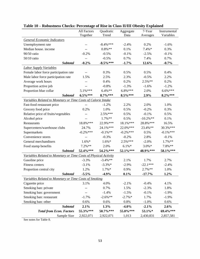
53
Table 10 – Robustness Checks: Percentage of Rise in Class II/III Obesity Explained
All Factors
Together
Quadratic
Trend
Aggregate
Data
7-Year
Averages
Instrumental
Variables
General Economic Indicators
Unemployment rate -- -8.4%*** -2.4% 0.2% -1.6%
Median house. income -- 0.8%** 0.1% 7.4%* 0.3%
90/50 ratio -0.2% -0.5% -0.1% -2.5% -0.1%
50/10 ratio -- -0.5% 0.7% 7.4% 0.7%
Subtotal -0.2% -8.5%*** -1.7% 12.6% -0.7%
Labor Supply Variables
Female labor force participation rate -- 0.3% 0.5% 0.5% 0.4%
Male labor force participation rate 1.5% 2.5% 2.3% -0.5% 2.2%
Average work hours -- 0.4% 0.2% 2.5%** 0.2%
Proportion active job -- -0.8% -1.3% -1.6% -1.2%
Proportion blue collar 5.1%*** 6.4%** 6.8%*** 2.0% 6.6%***
Subtotal 6.5%*** 8.7%*** 8.5%*** 2.9% 8.2%***
Variables Related to Monetary or Time Costs of Calorie Intake
Fast-food restaurant price -- -1.2% 2.2% 2.0% 1.0%
Grocery food price 0.2% 1.0% 0.5% -0.2% 0.3%
Relative price of fruits/vegetables -- 2.5%*** 0.5% -0.1% 0.5%
Alcohol price -- 1.7%** 0.5% -10.2%** 0.1%
Restaurants 18.8%*** 22.9%*** 18.1%*** 28.8%*** 16.5%
Supercenters/warehouse clubs 24.7% 24.1%*** 22.0%*** 23.4%** 30.3%***
Supermarkets -0.2%*** -0.1%** -0.2%*** 0.5% -0.1%***
Convenience stores -- -0.3% -0.2% 2.8% -0.1%
General merchandisers 1.6%* 1.6%* 2.5%*** -2.0% 1.7%**
Food stamp benefits 7.2%** 2.0% 6.1%* 3.0%* 7.8%**
Subtotal 52.4%*** 54.2%*** 52.1%*** 48.9%*** 58.1%***
Variables Related to Monetary or Time Costs of Physical Activity
Gasoline price -3.3% -3.4%** 2.1% 1.7% 2.7%
Fitness centers -3.1% -3.3%* -2.9% -22.1*** -2.4%
Proportion central city 1.2% 1.7%* 0.9% 2.7%** 1.0%
Subtotal -5.5% -4.9% 0.1% -17.7% 1.2%
Variables Related to Monetary or Time Costs of Smoking
Cigarette price 3.1% 4.0% -2.1% -0.4% 4.1%
Smoking ban: private -- 0.7% 1.5% -2.3% 1.8%
Smoking ban: government -- -1.4% -1.5% -0.1% -1.9%
Smoking ban: restaurant -1.7% -2.6%** -2.7%* 1.7% -1.9%
Smoking ban: other 0.6% 0.6% 0.8% -1.0% 0.6%
Subtotal 2.1% 1.3% -4.0% -2.1% 2.6%
Total from Econ. Factors 55.3%*** 50.7%*** 55.0%*** 53.1%* 69.4%***
Sample Size 2,922,071 2,922,071 1,013 2,430,831 2,857,581 See notes for Table 8.

54
Table 11 – Falsification Tests
Seatbelt Flu Vaccine Mammogram Prostate Exam
General Economic Indicators
Unemployment rate -0.003 (0.008) -0.007 (0.004)* -0.002 (0.003) -0.006 (0.005)
Median household income -0.007 (0.006) -0.003 (0.003) -0.004 (0.004) -0.007 (0.010)
90/50 ratio 0.002 (0.003) 0.002 (0.001)* -0.001 (0.001) 0.002 (0.002)
50/10 ratio 0.003 (0.005) 0.001 (0.002) 0.0002 (0.002) 0.006 (0.006)
Labor Supply Variables
Female labor force p. rate 0.004 (0.007) 0.003 (0.002) -0.003 (0.003) -0.003 (0.006)
Male labor force p. rate -0.004 (0.006) -0.001 (0.002) 0.001 (0.003) 0.003 (0.005)
Average work hours 0.007 (0.004)* -0.002 (0.001) -0.00003 (0.001) -0.004 (0.004)
Proportion active job 0.0001 (0.005) -0.002 (0.002) -0.002 (0.003) 0.00001 (0.007)
Proportion blue collar 0.002 (0.006) 0.0001 (0.003) -0.001 (0.003) 0.003 (0.008)
Variables Related to Monetary or Time Costs of Calorie Intake
Fast-food restaurant price -0.005 (0.006) 0.001 (0.003) -0.004 (0.003) 0.0001 (0.005)
Grocery food price 0.004 (0.005) -0.001 (0.006) -0.001 (0.003) -0.0002 (0.005)
Rel. price of fruits/vege. -0.013 (0.006)** -0.001 (0.003) 0.001 (0.003) -0.001 (0.003)
Alcohol price -0.016 (0.004)*** 0.001 (0.003) -0.001 (0.002) -0.010 (0.005)**
Restaurants 0.005 (0.013) 0.013 (0.010) -0.004 (0.005) 0.029 (0.012)**
Supercenters/ware. clubs 0.010 (0.009) 0.003 (0.005) 0.002 (0.004) 0.003 (0.008)
Supermarkets -0.011 (0.008) -0.007 (0.006) 0.007 (0.005) -0.014 (0.010)
Convenience stores -0.005 (0.012) -0.004 (0.013) -0.004 (0.007) -0.024 (0.020)
General merchandisers 0.015 (0.014) 0.004 (0.007) 0.011 (0.005)** -0.015 (0.010)
Food stamp benefits -0.009 (0.009) -0.001 (0.006) -0.011 (0.005)** -0.007 (0.008)
Variables Related to Monetary or Time Costs of Physical Activity
Gasoline price 0.028 (0.016)* -0.003 (0.011) 0.007 (0.005) 0.018 (0.012)
Fitness centers 0.035 (0.010)*** 0.004 (0.008) 0.015 (0.005)*** -0.008 (0.008)
Proportion central city -0.039 (0.013)*** 0.009 (0.012) 0.011 (0.009) 0.059 (0.044)
Variables Related to Monetary or Time Costs of Smoking
Cigarette price 0.002 (0.006) 0.005 (0.003) 0.001 (0.003) 0.008 (0.005)*
Smoking ban: private -0.011 (0.008) 0.0003 (0.003) 0.001 (0.004) -0.005 (0.005)
Smoking ban: government 0.008 (0.010) -0.004 (0.004) 0.005 (0.004) 0.001 (0.006)
Smoking ban: restaurant 0.004 (0.005) 0.002 (0.002) -0.009 (0.002)*** 0.006 (0.005)
Smoking ban: other -0.005 (0.006) -0.004 (0.003) -0.001 (0.002) 0.001 (0.005)
Sample Size 1,275,291 2,454,524 1,167,870 281,820
Notes: Standard errors, heteroskedasticity-robust and clustered by state, are in parentheses. *** indicates statistically
significant at the 1% level; ** 5% level; * 10% level. BRFSS sampling weights are used.

55
Table 12 – Impacts of One Standard Deviation Increases in Economic Factors on P(Trying
to Lose Weight)
All Factors “Important”
Factors Only
Top Two Factors
Only
General Economic Indicators
Unemployment rate 0.0004 (0.007) -- --
Median household income 0.002 (0.011) -- --
90/50 ratio 0.001 (0.003) -- --
50/10 ratio -0.003 (0.004) -- --
Labor Supply Variables
Female labor force participation rate -0.004 (0.005) -- --
Male labor force participation rate 0.006 (0.005) -- --
Average work hours -0.006 (0.004) -- --
Proportion active job -0.008 (0.005)* -0.006 (0.005) --
Proportion blue collar -0.001 (0.005) -- --
Variables Related to Monetary or Time Costs of Calorie Intake
Fast-food restaurant price 0.001 (0.006) -- --
Grocery food price -0.004 (0.008) -- --
Relative price of fruits/vegetables -0.006 (0.004) -- --
Alcohol price 0.005 (0.008) -- --
Restaurants 0.009 (0.017) -0.002 (0.013) 0.0004 (0.010)
Supercenters/warehouse clubs 0.019 (0.011)* 0.020 (0.008)** 0.023 (0.007)***
Supermarkets -0.012 (0.009) -- --
Convenience stores -0.017 (0.019) -- --
General merchandisers 0.008 (0.011) -- --
Food stamp benefits -0.007 (0.015) 0.0003 (0.012) --
Variables Related to Monetary or Time Costs of Physical Activity
Gasoline price -0.014 (0.022) -0.020 (0.023) --
Fitness centers 0.011 (0.015) 0.004 (0.013) --
Proportion central city -0.005 (0.013) -- --
Variables Related to Monetary or Time Costs of Smoking
Cigarette price 0.007 (0.020) -- --
Smoking ban: private -0.001 (0.005) -- --
Smoking ban: government 0.0003 (0.004) -- --
Smoking ban: restaurant 0.001 (0.004) -- --
Smoking ban: other -0.006 (0.005) -- --
Sample Size 515,116 515,116 515,116 Notes: Standard errors, heteroskedasticity-robust and clustered by state, are in parentheses. *** indicates statistically
significant at the 1% level; ** 5% level; * 10% level. BRFSS sampling weights are used.

56
Appendix Table A1 – Replications of Chou et al.’s (2004) Model for BMI
Chou et al’s results
(BRFSS 1984-
1999)
Chou et al’s model
and our data
(BRFSS 1990-
1999)
Add year dummies
Restaurants 0.631 (0.067)*** 0.469 (0.060)*** 0.122 (0.047)***
Restaurants2
-0.011 (0.002)*** -0.007 (0.002)*** -0.004 (0.001)***
Marginal effect at mean 0.339 0.291 0.002
Fast-food restaurant price -1.216 (0.728)* -2.854 (1.011)*** -0.928 (0.786)
Fast-food restaurant price2
0.135 (0.119) 0.434 (0.174)*** 0.142 (0.131)
Marginal effect at mean -0.432 -0.416 -0.135
Food at home price -6.462 (1.918)*** -6.047 (2.322)*** -0.311 (1.535)
Food at home price2
2.244 (0.719)*** 2.644 (1.049)*** 0.172 (0.707)
Marginal effect at mean -0.816 -0.729 0.034
Cigarette price 0.486 (0.355) 1.670 (0.367)*** 0.591 (0.340)*
Cigarette price2
0.009 (0.113) -0.293 (0.114)*** -0.194 (0.101)*
Marginal effect at mean 0.509 0.865 0.056
Alcohol price 1.140 (0.884) -1.654 (0.457)*** -0.971 (0.340)***
Alcohol price2
-0.734 (0.380)* 0.199 (0.067)*** 0.133 (0.051)***
Marginal effect at mean -0.423 -0.401 -0.144
Smoking ban: private 0.015 (0.039) 0.124 (0.128) 0.082 (0.095)
Smoking ban: government 0.115 (0.071) -0.099 (0.088) -0.155 (0.055)***
Smoking ban: restaurant -0.020 (0.056) -0.092 (0.071) -0.199 (0.037)***
Smoking ban: other 0.054 (0.056) 0.253 (0.060)*** 0.020 (0.037)
Observations 1,111,074 912,454 912,454 Notes: Standard errors, heteroskedasticity-robust and clustered at the state*year level, are in parentheses. ***
indicates statistically significant at the 1% level; ** 5% level; * 10% level. Regressions include state fixed effects
and individual-level control variables for age, age squared, real income, real income squared, and dummies for male,
race/ethnicity (black, white, Hispanic, or other), marital status (single, married, divorced, or widowed), and
education (less than high school degree, high school degree, some college, or college degree). Chou et al. also
included full-service restaurant price and its square, but the variable was only available every five years and was
imputed for the other years. Perhaps for this reason, its effect was one of the weakest Chou et al. estimated. We have
not been able to find an annual measure and therefore do not include full-service restaurant prices in our dataset.

57
Appendix Table A2 – Variable Descriptions and Summary Statistics
Variable Source Description Mean (Standard
Deviation)
1990
Mean
2010
Mean
BMI BRFSS Body mass index 26.618 (6.141) 26.027 28.507
Obese BRFSS Dummy for BMI≥30 0.279 (0.449) 0.184 0.339
Severely obese BRFSS Dummy for BMI≥35 0.111 (0.314) 0.066 0.141
Black BRFSS Dummy for race/ethnicity is non-Hispanic black 0.100 (0.300) 0.100 0.104
Hispanic BRFSS Dummy for race/ethnicity is Hispanic 0.120 (0.325) 0.083 0.142
Other BRFSS Dummy for race/ethnicity is not white, black, or Hispanic 0.056 (0.229) 0.030 0.076
Male BRFSS Dummy for sex is male 0.519 (0.500) 0.509 0.520
Some high school BRFSS Dummy for some high school but no degree 0.071 (0.257) 0.093 0.058
High school graduate BRFSS Dummy for high school degree but no college 0.301 (0.459) 0.347 0.260
Some college BRFSS Dummy for some college but no four-year degree 0.282 (0.450) 0.275 0.268
College graduate BRFSS Dummy for college graduate or further 0.315 (0.464) 0.250 0.387
Married BRFSS Dummy for married 0.611 (0.487) 0.618 0.639
Divorced BRFSS Dummy for divorced 0.122 (0.328) 0.111 0.112
Widowed BRFSS Dummy for widowed 0.019 (0.138) 0.022 0.017
Age BRFSS Age in years 39.634 (12.506) 37.623 41.983
Population Census State population (in 10,000s) 12.694 (10.117) 11.557 13.941
Seatbelt BRFSS Dummy for always wears seatbelta 0.746 (0.435) 0.581 0.861
Checkup BRFSS Dummy for preventive doctor checkup in past yearb
0.675 (0.469) 0.671 0.648
Flu shot BRFSS Dummy for got a flu shot within past yearc
0.300 (0.458) 0.138 0.347
Mammogram BRFSS Dummy for mammogram in past two years (women only)
0.509 (0.500) 0.365 0.432
Prostate BRFSS Dummy for digital rectal exam in past two years (men 40+)d
0.432 (0.495) 0.469 0.376
Smoker BRFSS Dummy for currently smokes 0.238 (0.426) 0.260 0.194
Drinks per month BRFSS Number of alcoholic drinks in the past 30 days 11.747 (31.752) 11.974 14.282
Lose weight BRFSS Dummy for currently trying to lose weighte
0.397 (0.489) 0.379 0.419
-Continued on Next Page-
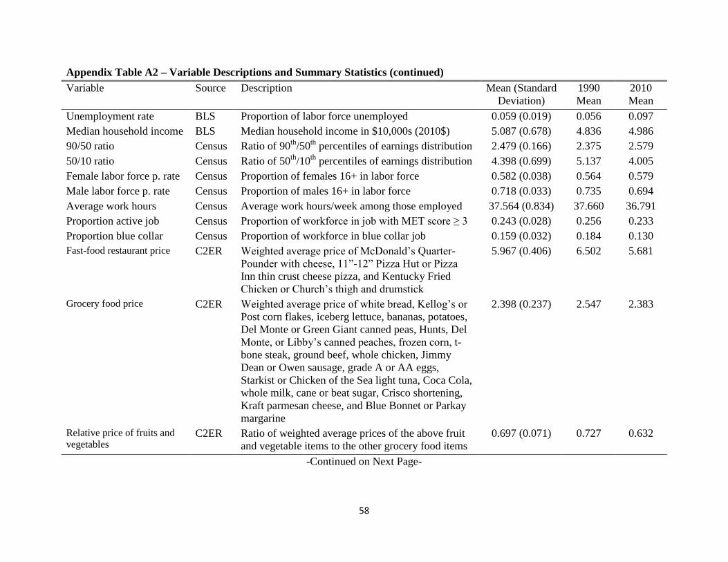
58
Appendix Table A2 – Variable Descriptions and Summary Statistics (continued)
Variable Source Description Mean (Standard
Deviation)
1990
Mean
2010
Mean
Unemployment rate BLS Proportion of labor force unemployed 0.059 (0.019) 0.056 0.097
Median household income BLS Median household income in $10,000s (2010$) 5.087 (0.678) 4.836 4.986
90/50 ratio Census Ratio of 90th
/50th
percentiles of earnings distribution 2.479 (0.166) 2.375 2.579
50/10 ratio Census Ratio of 50th
/10th
percentiles of earnings distribution 4.398 (0.699) 5.137 4.005
Female labor force p. rate Census Proportion of females 16+ in labor force 0.582 (0.038) 0.564 0.579
Male labor force p. rate Census Proportion of males 16+ in labor force 0.718 (0.033) 0.735 0.694
Average work hours Census Average work hours/week among those employed 37.564 (0.834) 37.660 36.791
Proportion active job Census Proportion of workforce in job with MET score ≥ 3 0.243 (0.028) 0.256 0.233
Proportion blue collar Census Proportion of workforce in blue collar job 0.159 (0.032) 0.184 0.130
Fast-food restaurant price C2ER Weighted average price of McDonald’s Quarter-
Pounder with cheese, 11”-12” Pizza Hut or Pizza
Inn thin crust cheese pizza, and Kentucky Fried
Chicken or Church’s thigh and drumstick
5.967 (0.406) 6.502 5.681
Grocery food price C2ER Weighted average price of white bread, Kellog’s or
Post corn flakes, iceberg lettuce, bananas, potatoes,
Del Monte or Green Giant canned peas, Hunts, Del
Monte, or Libby’s canned peaches, frozen corn, t-
bone steak, ground beef, whole chicken, Jimmy
Dean or Owen sausage, grade A or AA eggs,
Starkist or Chicken of the Sea light tuna, Coca Cola,
whole milk, cane or beat sugar, Crisco shortening,
Kraft parmesan cheese, and Blue Bonnet or Parkay
margarine
2.398 (0.237) 2.547 2.383
Relative price of fruits and
vegetables C2ER Ratio of weighted average prices of the above fruit
and vegetable items to the other grocery food items
0.697 (0.071) 0.727 0.632
-Continued on Next Page-

59
Appendix Table A2 – Variable Descriptions and Summary Statistics (continued)
Variable Source Description Mean (Standard
Deviation)
1990
Mean
2010
Mean
Alcohol price C2ER Weighted average price of Heineken 6-pack and
Chablis or Chenin Blanc white
7.401 (0.825) 7.023 7.784
Restaurants QCEW Restaurants per 10,000 residents 13.851 (2.172) 10.813 15.551
Supercenters/
warehouse clubs
Primary Walmart Supercenters, Sam’s Clubs, Costcos, and
BJ’s Wholesale Clubs per 10,000 residents
0.065 (0.051) 0.009 0.127
Supermarkets QCEW Supermarkets/grocery stores per 10,000 residents 2.098 (0.656) 1.928 1.950
Convenience stores QCEW Convenience stores per 10,000 residents 4.029 (1.325) 3.705 3.768
General merchandisers QCEW General merchandise stores (minus
supercenters/warehouse clubs) per 10,000 residents
1.056 (0.404) 0.946 1.135
Food stamp benefits USDA Per capita food stamp benefits (2010$) 112.01 (48.751) 99.162 208.437
Gasoline price C2ER Price of one gallon of regular unleaded gasoline
(including taxes) (2010$)
2.056 (0.587) 1.723 2.796
Fitness centers QCEW Fitness centers/sports clubs per 10,000 residents 0.838 (0.215) 0.706 0.941
Proportion central city Census Proportion of residents in central city of an MSA 0.254 (0.106) 0.273 0.246
Cigarette price Tax Burden
on Tobacco
Weighted average price of pack of cigarettes (2010$) 4.159 (1.318) 2.756 6.265
Smoking ban: private ImpacTeen Dummy for state law prohibiting smoking in private
workplaces
0.143 (0.351) 0 0.471
Smoking ban:
government ImpacTeen Dummy for state law prohibiting smoking in
government workplaces
0.170 (0.376) 0.007 0.521
Smoking ban:
restaurant ImpacTeen Dummy for state law prohibiting smoking in
restaurants
0.243 (0.429) 0 0.621
Smoking ban: other ImpacTeen Dummy for other state smoking bans 0.717 (0.450) 0.547 0.851
Notes: n=2,922,071 in all years, 55,922 in 1990, and 239,215 in 2010. BRFSS sampling weights are used. a indicates variable not available in 1999-2001, 2003-
2005, 2007, and 2009; b not available 2003-2004,
c not available 1990-1992,
d not available 1990-2000,
e only available in 1994, 1996, 1998, 2000, and 2003. If
variables are not available in 1990 their values in the first year they are available are reported in the “1990 mean” column.

60
Appendix Table A3 – Percentage of Rises in BMI, Obesity, and Severe Obesity Explained
by Changes in Controls
BMI Obesity Class II/III Obesity
Age 61.2% (1.0%)*** 48.0% (1.3%)*** 54.6% (1.7%)***
Age squared -42.8% (0.9%)*** -32.1% (1.2%)*** -39.4% (1.5%)***
Subtotal from Age 18.4% (0.3%)*** 15.9% (0.3%)*** 15.3% (0.4%)***
Some high school -0.2% (0.1%) -0.2% (0.1%)** -0.4% (0.3%)
High school graduate 0.6% (0.3%) 0.8% (0.3%)*** 1.2% (0.9%)
Some college 0.1% (0.03%) 0.1% (0.03%)*** 0.2% (0.1%)**
College graduate -8.1% (0.4%)*** -9.2% (0.4%)*** -11.0% (1.3%)***
Subtotal from Education -7.7% (0.2%)*** -8.4% (0.2%)*** -10.0% (0.2%)***
Black 0.3% (0.01%)*** 0.3% (0.01)*** 0.4% (0.01%)***
Hispanic 1.8% (0.2%)*** 1.4% (0.3%)*** 0.4% (0.2%)
Other -1.4% (0.4%)*** -1.3% (0.3%)*** -0.9% (0.4%)**
Male 0.1% (0.02%)*** -0.2% (0.02%)*** -0.7% (0.02%)***
Married -0.04% (0.03%) -0.03% (0.03%) -0.6% (0.04%)***
Divorced -0.01%
(0.001%)***
-0.01%
(0.001%)***
-0.02%
(0.002%)***
Widowed -0.1% (0.02%)*** -0.1% (0.02%)*** -0.1% (0.02%)***
State population -0.9% (1.0%) -1.3% (1.3%) -1.0% (1.7%)
Subtotal from Other Controls -0.3% (1.0%) -1.3% (1.3%) -2.6% (1.6%)
Total from Controls 10.4% (1.1%)*** 6.1% (1.3%)*** 2.6% (1.8%) Notes: Standard errors, heteroskedasticity-robust and clustered by state, are in parentheses. *** indicates statistically
significant at the 1% level; ** 5% level; * 10% level. BRFSS sampling weights are used. + indicates age is modeled
using a quadratic specification; the reported percentage of the trends explained is the sum of the percentages
explained by changes in both age and age squared.
Related Documents