Can basic entrepreneurship transform the economic lives of the poor? Oriana Bandiera a , Robin Burgess b , Narayan Das c , Selim Gulesci d , Imran Rasul e , and Munshi Sulaiman f a London School of Economics ([email protected]), b London School of Economics ([email protected]) and c BRAC ([email protected]), d University of Bocconi ([email protected]), e University College London ([email protected]) and f BRAC ([email protected]) April 2013

Welcome message from author
This document is posted to help you gain knowledge. Please leave a comment to let me know what you think about it! Share it to your friends and learn new things together.
Transcript

Can basic entrepreneurship transform
the economic lives of the poor?
Oriana Bandieraa, Robin Burgess
b, Narayan Das
c, Selim Gulesci
d, Imran Rasul
e, and
Munshi Sulaimanf
a London School of Economics ([email protected]), b London School of Economics ([email protected]) and
c BRAC ([email protected]), d University of Bocconi ([email protected]), e University College London
([email protected]) and f BRAC ([email protected])
April 2013
can basic entrepreneurship transform theeconomic lives of the poor?∗
Oriana Bandiera, Robin Burgess, Narayan Das, Selim Gulesci, Imran Rasul, Munshi Sulaiman
April 2013
AbstractThe world’s poorest people lack capital and skills and toil for others in occupations that
others shun. Using a large-scale and long-term randomized control trial in Bangladesh thispaper demonstrates that sizable transfers of assets and skills enable the poorest women toshift out of agricultural labor and into running small businesses. This shift, which persistsand strengthens after assistance is withdrawn, leads to a 38% increase in earnings. Inculcatingbasic entrepreneurship, where severely disadvantaged women take on occupations which werethe preserve of non-poor women, is shown to be a powerful means of transforming the economiclives of the poor.
Keywords: asset transfers, capital constraints, vocational training, occupa-tional choice, structural change, poverty.
JEL Classification: O12; I30; D50.
∗We thank all BRAC staff and especially Mahabub Hossain, W.M.H. Jaim, Imran Matin and Rabeya Yasminfor their collaborative efforts in this project. Thanks are also due to Wahiduddin Mahmud and the IGC Bangladeshoffice for supporting the project. We thank Arun Advani, Abhijit Banerjee, Vittorio Bassi, Timothy Besley, GharadBryan, Francisco Buera, Bronwen Burgess, Anne Case, Arun Chandrasekhar, Angus Deaton, Greg Fischer, DeanKarlan, Guy Michaels, Ted Miguel, Mushfiq Mobarak, Benjamin Olken, Steve Pischke, Mark Rosenzweig, JeremyShapiro, Chris Udry, Chris Woodruff and numerous seminar and conference participants for useful suggestions.The large-scale survey and data processing which underpins this paper was financed by BRAC and its CFPR-TUPdonors, which include DFID, AusAID, CIDA and NOVIB, OXFAM-AMERICA. The consortium supported boththe intervention costs as well as costs of direct research activities. This document is an output from researchfunding by the UK Department for International Development (DFID) as part of the iiG, a research program tostudy how to improve institutions for pro-poor growth in Africa and South Asia. Support was also provided bythe International Growth Centre. The views expressed are not necessarily those of DFID. All errors remain ourown. Author affiliations and contacts: Bandiera (LSE, [email protected]); Burgess (LSE, [email protected]);Das (BRAC, [email protected]); Gulesci (Bocconi, [email protected]); Rasul (UCL, [email protected]);Sulaiman (BRAC-Africa, [email protected]).
1

1 Introduction
The world's poorest people lack both capital and skills. They tend to engage in low-skilled
wage labor activities that are insecure and seasonal in nature [Banerjee and Du�o 2007].1 The
non-poor, in contrast, tend to be engaged in secure wage employment, or employ others in the
businesses they operate [Banerjee and Du�o 2008]. Any attempt to alleviate extreme poverty on a
large scale therefore requires us to think about catalyzing the process of occupational change and
to understand how this process is linked to a paucity of capital and skills.
Economic theory highlights mechanisms via which expanded access to capital enables individ-
uals to alter their occupational choices and exit poverty [Banerjee and Newman 1993, Besley 1995,
Gine and Townsend 2004, Aghion et al. 2005, Jeong and Townsend 2008, Karlan and Morduch
2010, Townsend 2011, Buera, Kaboski and Shin 2012] and how limited human capital formation
constrains occupational choices and the ability to escape poverty [Becker 1964, Schultz 1961, 1980,
Strauss and Thomas 1995, Behrman 2010]. In line with this, many antipoverty programs target
either a lack of capital, for instance through micro�nance, development banking or asset transfer
programs, or a lack of skills, for instance through vocational training or cash transfers conditioned
on school attendance. Whether these programs can permanently transform the lives of the poor
crucially depends on the existence and strength of the causal link between the lack of capital and
skills and occupational choice and poverty.
Although there is a distinguished and growing literature in macroeconomics that documents
how occupational change and aggregate development proceed together [Kuznets 1966; Chenery and
Syrquin 1975, Murphy, Shleifer and Vishny 1989, Caselli and Coleman 2001, Ngai and Pissarides
2007, Buera and Kaboski 2012], far less is known about whether policy interventions that transfer
capital and skills are capable of bringing about structural transformation through occupational
change.2 This paper attempts to partly �ll the gap between studies of occupational change driving
economic development that concern macroeconomists, and microeconomic work evaluating pro-
grams that relax credit or skills constraints. Our focus is on in situ occupational change where
the rural poor upgrade to more secure, less seasonal business activities rather than on the shift of
rural laborers into manufacturing and service sector jobs in cities.3 We ask whether tackling both
1Agricultural laborers, which often constitute the bottom stratum of society in developing countries, are con-fronted not only with seasonal and weather-dependent demand for their labor but also with barriers to other formsof employment owing to their limited capital and skills [Sen 1981, Dreze and Sen 1989].
2There are of course reasons to be skeptical about whether antipoverty programs of any stripe can a�ect oc-cupational choice. The very poor may not demand any capital if they perceive little use for it [Townsend 2011].They may not wish to invest in human capital if the returns are perceived to be low [Jensen 2010, 2012]. Thescale of the intervention may be insu�cient to enable the very poor to set up new businesses or to engage in securewage employment [Banerjee 2004], a criticism often leveled at micro�nance where loan sizes may be too small toallow borrowers to e�ect a change in business activity [Schoar 2009]. Self-control or other behavioral biases my leadthe very poor to consume transfers without altering their occupational choices [Banerjee and Mullanaithan 2010].Leakage may mean that the poor receive a very small fraction of the intended assistance [Reinikka and Svensson2004]. Finally, social norms and rules might constrain occupational choices, especially of women [Field et al. 2010].
3In situ occupational change involving modest changes in the activities of poor rural citizens, sometimes referred
2

capital and skills constraints simultaneously by providing business asset transfers coupled with
complementary and intensive training, can transform the economic lives of some of the world's
poorest people.
To answer this question, we collaborated with the NGO BRAC to implement a large-scale
and long-term randomized control trial to evaluate their Targeted Ultra-Poor (TUP) program in
rural Bangladesh. Eligible women - identi�ed to be the very poorest in these rural communities4
- are o�ered a menu of possible business activities, ranging from livestock rearing to small retail
operations, coupled with complementary and intensive training in running whichever business
activity they choose.5 The scale of the program combined with the size of the transfers implies
that, taken as a whole, the TUP program in Bangladesh represents a signi�cant attempt to lift
large numbers of women, and their dependents, out of extreme poverty. Indeed, as of 2011, the
TUP program was already reaching close to 400,000 women and a further 250,000 will reached
between 2012 and 2016.6 The program gives a big push to relaxing both capital constraints (at
$140 the value of the asset transfer is worth roughly ten times baseline livestock wealth) and
skills constraints (the value of the two-year training and assistance which women receive is of a
similar magnitude). This is done in a context where eligible bene�ciaries are unable to relax these
constraints through the market. For capital, the value of micro�nance loans available to them is
too low to �nance such large purchases and repayment requirements too stringent to allow them
the time to generate income from a new enterprise. For skills, training programs are not available
and informal arrangements might not be su�cient to deliver all the assistance required to operate
the small businesses that women select.
In our pre-program setting, the rural poor are faced with a choice between wage employment
(mainly as agricultural laborers and domestic servants) and self-employment (mainly in livestock
rearing). The program in�uences this choice by increasing wealth via the asset transfer and the
returns to self-employment via skills training. We develop a simple model to understand the
occupational choices that targeted poor women make at baseline and how the program a�ects
to as subsistence entrepreneurship, can play a major role in poverty reduction. This is distinct from businessstart-ups in manufacturing and services which have the potential to grow to a signi�cant size [Schoar 2009]. Thelatter, which are the traditional focus on the study of entrepreneurship in developed countries are also importantin Bangladesh but tend to be located in urban areas and are therefore not the focus of this study.
4Women are selected on criteria such as not owning land, not having a male adult earner in the household, havingto work outside the household, having school-aged children that work and having no productive assets. Eligiblesmust also not be enrolled with micro�nance organizations or recipients of government anti-poverty programs.
5The majority choose high value livestock businesses which had been mainly operated by non-poor women in thecommunities we study. In value, scale and complexity these businesses were distinct from the more basic livestockrearing that some poor women were engaged in before the program (e.g. cow rearing versus free range poultry).
6In Bangladesh the TUP program is know as the specially targeted ultra poor program. Another variant, knownas the other targeted poor program (OTUP), targets slightly less disadvantaged women with the asset transferbeing purchased using a BRAC loan. This variant reached 600,000 bene�ciaries in 2011 and will reach a further150,000 by 2016 [BRAC 2011]. Non experimental evaluations of the program are reported in Ahmed et al. [2009]and Emran et al. [2009], tracking 5000 households from 2002 to 2005. Both studies �nd positive impacts on percapita consumption and improvements in food security. Das and Misha [2010] extend the panel to 2008 and �ndpositive impacts on income, food security and asset holdings.
3

these choices on the extensive and intensive margins of labor supplied to each activity. This
shows that both asset transfers and skills provision components reduce hours devoted to wage
employment, through income and substitution e�ects. On hours devoted to self-employment, the
model shows how the e�ect of both components is heterogeneous depending on whether individuals
face a binding capital constraint at baseline. In particular, asset transfers can have the unintended
consequence of reducing hours devoted to self-employment through a wealth e�ect. Ultimately the
model shows that the e�ect of the program on occupational choices is theoretically ambiguous.
The evaluation sample covers 1409 communities in 40 regions in rural Bangladesh, half of
which were treated in 2007 and the rest kept as controls until 2011. BRAC program o�cers
select potential bene�ciaries in 2007 following the same selection criteria in treatment and control
communities. We survey and track all poor households (both eligibles and non-eligibles), as
well as a 10% random sample of non-poor households from across other wealth classes in the
same treated and control communities. We identify the e�ect of the program by a di�erence
in di�erence estimate that compares the outcome of the eligible poor in treated versus control
communities before and after program implementation. Given that we sample households from
across the wealth distribution, we benchmark these estimated impacts against the baseline gap
between eligible and non-poor households.
Given our focus on occupational change towards basic entrepreneurship, where new business
activities take time to develop, we survey households two and four years after the program's
implementation. This helps trace out the economic trajectories of poor women over an extended
period, shedding light on whether the labor productivity of poor women improves over time as
they become more adept at running their new businesses. This time scale also means that we move
well beyond the period when targeted women are receiving direct assistance from BRAC.
The data con�rm that the program successfully targets the very poorest women in rural
Bangladesh: at baseline more than half (52%) own no productive assets, 93% are illiterate and
38% are the sole earner in their households. 80% of them live below the global poverty line
(US$1.25). They typically engage in multiple occupations, which are not held regularly through-
out the year and characterized by income seasonality. The precariousness of their economic lives
though striking, is typical of the situation that millions of rural women across the developing
world �nd themselves in.7 In contrast, richer women in the same communities typically shun wage
employment and are engaged in fewer, more regular, activities with most of them specializing in
self-employment either rearing livestock or cultivating land.
Our estimates of the program's impact show evidence of a causal link from the lack of capital
and skills to occupational choice, and ultimately poverty and insecurity. We �nd that, on the
extensive margin, after four years the TUP program reduces the share of women specialized in
7It is well documented that landless agricultural laborers, such as the eligible women here, are exposed to seasonalhunger and famine - monga - as it is referred to Bangladeshi [Bryan et al. 2011; Khandker and Mahmud 2012].Monga is the result of limited demand for agricultural labor in the pre-harvest period.
4

wage employment by 17 percentage points (pp), corresponding to 65% of the baseline mean. Over
the same period, the share of women specialized in self-employment increases by 15pp and those
engaged in both occupations by 8pp. These changes on the extensive margin of occupational choice
correspond to 50% and 31% increases from their baseline values, respectively.
This dramatic change in occupational choice on the extensive margin is accompanied by a
corresponding change in hours devoted to the two occupation categories. After four years, eligible
women work 170 fewer hours per year in wage employment (a 26% reduction relative to baseline)
and 388 more hours in self-employment (a 92% increase relative to baseline). Hence total annual
labor supply increases by an additional 218 hours which represents an increase of 19% relative
to baseline. Given the occupational change induced, their labor supply becomes more regular
throughout the year, while income seasonality is reduced. The change in occupational structure
is associated with a 15% increase in labor productivity and a 38% increase in earnings. This
leads to a 8% increase in household per capita expenditure, and a 15% increase in self-reported
life satisfaction among eligible women. Benchmarked against the global poverty line of $1.25 per
day and recalling that the average eligible lives on 93c per day at baseline, the program lifts 11%
of the eligible women out of extreme poverty. Measures of estimated e�ects are typically more
pronounced after four relative to after two years, indicating that the program sets bene�ciaries on
a sustainable path out of poverty.
To probe further whether all eligible women are equally impacted, we estimate quantile treat-
ment e�ects. These reveal that the e�ect on earnings and expenditures is positive at all deciles,
but both e�ects are substantially larger for the top four deciles after four years. This indicates
that the program increases both the mean and the dispersion of total earnings among the treated.
Second, benchmarking the magnitude of the program impact relative to di�erences in the same
outcome between the eligible poor and other wealth classes we �nd the eligible poor: (i) overtake
the near poor on a host of economic indicators; and (ii) they close around 40% of the gap to middle
class households on metrics related to occupational choice and earnings.
What we observe, therefore, is signi�cant occupational change and a rich set of social dynamics
within these rural communities. Large transfers of capital and skills catapults some of most
disadvantaged women in the world into labor activities which had been the preserve of non-poor
women in the communities they share. Occupational change, which re�ects itself in higher and
less volatile earnings streams, sets these women on a sustainable path out of poverty. On many
margins the program brings their economic lives closer to the middle classes in their communities.
The paper thus joins the macro and micro literatures by pointing to some concrete evidence on
how occupational change can be engineered in the rural settings where the bulk of the world's
poorest people live.
The TUP program is now being piloted in many countries.8 This scale-up is critical to as-
8As of March 2013, ten di�erent pilots were active around the world, http://graduation.cgap.org/pilots/. BRACis piloting the program in both Afghanistan and Pakistan. Other pilots are being carried out in Andhra Pradesh,
5
certaining whether TUP-style programs can be used to �ght poverty on a global scale. Findings
from a pilot in West Bengal are consistent with ours: Banerjee et al. [2011] report impacts on
consumption expenditures, earnings and food security which are of similar magnitude to those we
report. However, Morduch et al. [2012] �nd that a pilot in Andhra Pradesh has weak impacts
on earnings and consumption. This is due, in part, to the fact that the Government of Andhra
Pradesh simultaneously introduced a guaranteed-employment scheme that substantially increased
earnings and expenditures for wage laborers. Our theoretical framework makes precise how such
outside options in wage labor are obviously important determinants of whether TUP-style pro-
grams induce occupational change towards basic entrepreneurship, and we discuss our empirical
�ndings relative to these pilot studies throughout.
The paper is organized as follows. Section 2 develops a framework that highlights the main
channels through which the TUP program impacts occupational choices. Section 3 describes the
program, our research design and data. Section 4 presents our core results that closely map to the
model developed on occupational choice, earnings and labor productivity. Section 5 documents the
impacts on other margins, heterogeneous impacts, and benchmarks the impacts vis-à-vis baseline
di�erences in outcomes between eligibles and other wealth classes. Section 6 conducts a cost bene�t
analysis of the program, comparing it to the counterfactual policy of unconditional cash transfers.
Section 7 concludes. All proofs and robustness checks are in the Appendix.
2 Theoretical Framework
We model how the poor allocate their time between leisure and the two occupations most
common in our setting: wage employment and self-employment. The model makes precise how
the program impacts equilibrium occupational choices through asset transfers, that boost wealth
endowments, and skills training, that boost the returns to self-employment.
2.1 Set-Up
Individuals live one period and are endowed with one unit of time to allocate between wage
employment (Li), self-employment (Si) and leisure (Ri). Individual i decides which occupations to
enter on the extensive margin, and how much labor to supply to each occupation on the intensive
margin. We assume the time devoted to occupational activities is non-negative, and utility is
additively separable in consumption (Ci) and leisure: Ui = u(Ci) + v(Ri), where u(.) and v(.) are
concave. Individuals are price-takers in the labor market receiving an return w per unit of time,
so earnings from wage employment are wLi.9 Time devoted to self-employment (Si) is combined
Ethiopia, Ghana, Haiti, Honduras, Pakistan, Peru and Yemen by other organizations.9We rule out the possibility that labor can be hired in, which is an accurate empirical description for the
eligible poor individuals we focus on. For expositional ease, we also abstract from skill di�erences in the labormarket and assume w is the same for all individuals. This re�ects the fact that the study population is mostlyunskilled and supplies labor in two competitive wage labor markets: for agricultural casual laborers and for domesticservants. The model predictions regarding the program impacts on the treated poor are robust to individuals earning
6

with assets Ki to produce output Yi, according to a production function Yi = f(θi, Ki, Si), where
θi measures individual i's skills. In our study context, this form of self-employment corresponds
to engaging in basic entrepreneurial activities, in which labor is combined with assets in the
form of livestock and related inputs such as feed and fodder. Output from such self-employment
corresponds to milk, meat and eggs produced for sale in local markets. The price of livestock
assets is pk and the price of output is py. Individuals are assumed to be price-takers in input and
output markets. Earnings from self-employment are then given by revenues minus costs, that is
πi = pyf(θi, Ki, Si)− pkKi.
Individuals have a resource endowment (Ii) that can be used to purchase consumption or
assets. The budget constraint for consumption is then wLi + πi + Ii = Ci. Finally, we assume
credit markets are such that individuals face the constraint pkKi ≤ Ii, namely individuals cannot
borrow to �nance assets purchases. This captures the fact that, although some credit is available
in the study communities, the poor only have access to small scale loans. Such microloans are
insu�cient to allow them to purchase lumpy livestock assets. Assuming less severe forms of credit
market imperfections would yield similar results.
This minimalistic set-up is designed to starkly illustrate the two main forces at play: wealth
e�ects due to the asset transfers and substitution e�ects due to training. To do so we abstract from
features that could also a�ect occupational choice but are not directly a�ected by the program.
Most notably in this context demand for wage labor exhibits strong seasonality so that L is
constrained by this and the constraint might be binding at zero in some periods of the year.
Modeling this explicitly would not a�ect the predicted e�ect of the program on occupational
choice. Seasonality, however, has implications for the empirical comparison of w and r as the
observed wage is e�ectively available only for part of the year while income from self-employment
(e.g. through the sale of livestock produce) is more stable through the year.
2.2 Occupational Choices at Baseline
The individual's optimal occupational choices are a function of two exogenous variables: (i)
skills, namely the returns to self-employment relative to wage employment (ri Q w); (ii) resource
endowments, Ii. The former determines the choice between self-employment and wage employ-
ment, whereas the latter determines labor force participation and whether the assets constraint
binds when the individual chooses to engage in self-employment. Substituting Ci from the budget
constraint yields the Lagrangian:
maxLi,Si` = u(wLi + πi + Ii) + v(1− Li − Si) + αLi + βSi + γ(Ii − pkKi), (1)
where α and β are the multipliers associated with the non-negativity constraints on time devoted
di�erent wages. Any predictions regarding the general equilibrium e�ect of the program on wages and the pecuniaryexternalities on non-treated individuals (that are examined in more detail in Bandiera et al. 2013), would howeverdepend on the skill distribution in the two populations and the degree of substitutability between skills.
7

to wage and self-employment and γ is the multiplier associated with the assets constraint. All
multipliers must be non-negative. To obtain closed form solutions we further assume that Y =
θimin(Ki, Si), so that in equilibriumKi = Si and πi = pyθiSi−pkSi = riSi, where ri = pyθi−pk thenmeasures the individual speci�c returns to self-employment.10 Equilibrium baseline occupational
choices in all parts of the parameter space are summarized as follows.
Proposition 1: Individuals will be in one of the four following states:
(i) out of the labor force if: ri > w and Ii ≥ Ii(ri); or ri < w and Ii ≥ Ii(wi)
(ii) engaged solely in self-employment if: ri > w and Ii ∈ [˜Ii(ri, w), Ii(ri));
(iii) engaged in both occupations if: ri > w and Ii ≤˜Ii(ri, w);
(iv) engaged solely in wage employment if: ri < w and Ii < Ii(wi)
Figure 1A illustrates the occupational choice equilibrium if ri ≥ w. The resource endowment
(Ii) is measured on the horizontal axis. The vertical axis shows the wage and self-employment
labor supply functions (L∗i (.), S∗i (.)). The proof of Proposition 1, provided in the Appendix, derives
the resource endowment thresholds (Ii(ri),˜Ii(ri),
˜Ii(ri, w)), the wage and self-employment labor
supply functions, and their comparative statics with respect to wages, returns to self-employment
and resource endowments.
Starting from the extreme right hand side of Figure 1A, we see that individuals with the
highest endowments optimally choose to stay out of the labor force (case (i), where L∗i = S∗i = 0
for Ii ≥ Ii(ri)). In the more central section of Figure 1A we have a group of individuals that
are not asset constrained and so, because we are considering the scenario where ri > w, engage
solely in self-employment (case (ii), where L∗i = 0, S∗i > 0 for Ii ∈ [ ˜Ii(ri), Ii(ri))). For these
individuals the number of hours devoted to self-employment is decreasing in I because of the
income e�ect. The next group of individuals also engage solely in self-employment but are asset
constrained and so limited in scale by their endowment, pkKi = Ii (case (ii), where L∗i = 0, S∗i > 0
for Ii ∈ [˜Ii(ri, w), ˜Ii(ri)))). Finally, on the left hand side of Figure 1A we see that individuals
with the smallest resource endowments engage in both occupations as the feasible scale of self-
employment activities is too small to a�ord the desired level of consumption (case (iii), where
L∗i > 0, S∗i > 0 for Ii ≤˜Ii(ri, w)).11 For these individuals the number of hours devoted to self-
employment is increasing in I because an increase in I relaxes the binding asset constraints thus
10The assumption of Leontief technology is made for expositional convenience to keep track of either the amountof self-employment Si or the amount of capital Ki. Allowing some degree of substitutability between these factorinputs would not alter the qualitative nature of the trade-o�s identi�ed.
11Individuals specialize in one of the two occupations when the asset constraint does not bind because themarginal returns to both activities are linear. The same result would be obtained if the marginal return to one orboth occupations were increasing. Of course, there can be many other motives for diversifying economic activities,such as spreading risk. We focus on asset constraints as being an important driver of occupational choice as thismargin is directly impacted by the TUP program. Other factors driving occupational diversi�cation such as riskaversion are not impacted so are less relevant for understanding the changes over time that we exploit betweentreatment and control communities.
8

allowing individuals to increase the scale of their self-employment business and hence devote more
hours to it.
Figure 1B shows the pattern of equilibrium occupational choices and corresponding labor sup-
plies when ri < w (in the proof we derive the relevant endowment threshold, Ii(wi)). In this
scenario, no individual specializes in self-employment and so the assets constraint plays no role
in determining occupational choice. Figure 1B shows that individuals with su�ciently high re-
source endowments optimally choose to stay out of the labor force (case (i), where L∗i = S∗i = 0
for Ii ≥ Ii(wi)), whereas individuals with smaller resource endowments all engage solely in wage
employment (case (iv), where L∗i > 0, S∗i = 0 for Ii ≤ Ii(wi)).
Even this highly stylized model delivers a rich set of predictions on occupation choices at
baseline. As is empirically validated below, at baseline we observe a wide range of occupational
choice allocations among the poor, ranging from those engaged solely in wage labor or solely
self-employment, those engaged in both, and those out of the labor force. Figures 1A and 1B also
highlight the comparative static properties of the wage and self employment labor supply functions
with respect to wage rates, returns to individual skills, and resource endowments: these last two
channels are the mechanisms through which the TUP program impacts occupational choices.
2.3 The Impact of the Ultra-Poor Program on Occupational Choices
The TUP program has two components. First, livestock asset transfers, that boost resource
endowments from Ii0 at baseline, to Ii1 = Ii0 +A post-intervention. A represents, in reduced form,
the present value of the asset, factoring in the future option value from selling or renting it out.
Second, skills training, that boost the returns to self-employment, θi, and hence ri, from some
baseline level, ri0, to a post-intervention level ri1 > ri0.12
As Figure 1A makes clear, asset transfer impacts the extensive and intensive margins of occupa-
tional choice by causing individuals to cross the various resource thresholds(Ii(ri),˜Ii(ri),
˜Ii(ri, w)).
Figure 2A shows the impact of the program solely though the asset transfer channel (assuming
ri > w), where the baseline wage and self-employment labor supplies are dashed lines, and the post-
intervention labor supplies are solid lines. The left side of Figure 2A shows that individuals with
the smallest resource endowments at baseline remain engaged in both wage and self-employment
12Three points are of note. First, in a dynamic model, individuals might want to retain the asset in the short runif, for instance, selling it quickly would damage their relationship with BRAC. This however would not precludethem from renting it out or hiring labor to tend to it, which would have the same e�ect on Ii and occupationalchoice. We later provide evidence that almost no individuals are observed renting out these assets. Second, we notealso that the asset transfer to women can a�ect Ii through other channels operating within households, for instanceby a�ecting husbands' labor supply. The predictions below are derived for the case in which the net e�ect on Ii ispositive, namely the asset transfer does not reduce the total non-labor income available to the woman. In line withthis, we empirically document that the husbands' labor supply does not decrease following the implementation ofthe program. Third, the program transfers assets (livestock) that are identical to those available locally at baseline.Given that only a relatively small number of households per community are eligible, the program has little impacton the price of livestock assets, pk. Hence skill changes induced by the program translate into changes in theself-employment outcome ri = pyθi − pk if the price of livestock produce, py, does not fall by su�ciently to o�setany increase in θi.
9

activities although their time allocation shifts towards self-employment. The impact on the total
hours they devote to work, L∗i (.) + S∗i (.), is ambiguous.
The middle of Figure 2A shows that among individuals that were initially engaged solely in
self-employment, labor hours might rise or fall depending on the initial resource endowment of the
individual. Among those who were asset constrained at baseline, self-employment hours rise, all
else equal. However, the framework makes clear that for those who were unconstrained at baseline,
the asset transfer will actually reduce hours of self-employment (and total hours devoted to labor
market activities) because of the income e�ect. Finally, the right hand side of Figure 2A shows
that asset transfers alone cause more individuals to stop working.
The skills provision component of the program also shifts the wage and self-employment labor
supply functions (L∗i (.), S∗i (.)). Figure 2B shows the impact of the program solely though the
skills provision channel (assuming ri > w), where the baseline wage and self employment labor
supplies are dashed lines, and the post-intervention labor supplies are solid lines. Figure 2B shows
that among individuals initially engaged in self-employment, self-employment hours do not change
unless the individual was unconstrained at baseline. The left hand side of Figure 2B shows that
among those individuals with the lowest resource endowments, skills provision does not cause the
hours devoted to self-employment to change, although individuals �nd it optimal to reduce wage
labor hours because of the increased returns generated when they engage in self-employment. For
these individuals total work hours unambiguously fall. The combined e�ect of asset transfers and
training can be thus summarized as;
Proposition 2: If ri > w the TUP program weakly reduces wage employment hours for all
individuals. The e�ect on self-employment hours is: (i) weakly negative for all individuals if the
e�ect of the asset transfer is su�ciently large relative to the e�ect of the skills provision; (ii) weakly
positive for all individuals where the e�ect of the asset transfer is su�ciently small relative to the
e�ect of skills provision; (iii) positive for resource-poor individuals and ambiguous for resource-rich
individuals in intermediate cases.
The framework thus makes precise that both program components, asset transfers and skills
provision, need to be carefully targeted in order to have their desired impact on self-employment
activities. On the extensive margin, only skills provision will likely induce individuals with higher
resource endowments to start engaging in self-employment, as shown on the right hand side of
Figure 2B. In contrast, asset transfers will have the opposite impact as shown on the right hand
side of Figure 2A. On the intensive margin, asset transfers have the desired impact to increase S∗i (.)
only among those individuals constrained at baseline; skills provision has this desired impact on the
intensive margin but only among those individuals unconstrained at baseline. The combined e�ect
of the asset transfer and skills training on occupational choices then depends on initial resource
endowments and the relative strength of the two e�ects shown in Figures 2A and 2B.
The proof is in the Appendix, where we compute the thresholds for cases (i)-(iii) as a function
10

of the two program components. The importance of accurately targeting the program to achieve
its desired impacts is put sharply into focus if we consider the remaining case where when ri < w,
shown in Figure 2C. None of these individuals specializes in self-employment at baseline. The
provision of skills does not alter this as long as the post-intervention returns to self-employment, ri1,
remain less than w. Hence only su�ciently e�ective skills provision programs will have the desired
impact of shifting these wage laborers into self-employment. Other things equal, asset transfers
targeted towards these individuals will generate an income e�ect that reduce hours worked and
labor force participation without a�ecting occupational choice.13
The remainder of the paper empirically measures these combined impacts of the TUP program
on the extensive and intensive margins of wage employment and self-employment.
3 The Ultra-Poor Program, Evaluation Design and Data
3.1 The Program
The TUP program o�ers eligible women a menu of possible business activities, ranging from
livestock rearing to small retail operations, coupled with complementary and intensive training in
running their chosen business activity.14 All eligible women in our sample chose one of the six
available livestock packages, which contain di�erent combination of animals (e.g. two cows or a
cow and �ve goats) similarly valued at TK9500 (US$140). Given that the median household had
no productive assets at baseline, this represents an enormous change in the resource endowment
of households, which could fundamentally impact occupational choice as is illustrated in Figure
2A. BRAC encourages program recipients to commit to retain the asset for two years, after which
they can liquidate it. Given that such commitments cannot be enforced, whether the livestock
asset is retained or liquidated (particularly after four years) is itself an outcome of interest that
ultimately determines whether the program has the desired e�ect of permanently transforming the
occupational choices and economic lives of the poor, or merely increases their short run welfare.15
13As mentioned earlier, Morduch et al. [2012] �nd weak impacts of an TUP-style program implemented by SKSin Andhra Pradesh. The model developed provides one way in which to reconcile these �ndings and help under-stand why the impacts of otherwise similarly implemented programs might di�er across economic environments.Speci�cally, if the environment is characterized by high labor wages so that ri < w, then as shown in Figure 2C,an TUP-style program will have limited impact on occupational choices. Indeed, in the study setting for Morduchet al. [2012], the Government of Andhra Pradesh rolled out a guaranteed employment scheme that substantiallyincreased wage labor earnings in the study area.
14The program also provides a subsistence allowance to bene�ciary women for the �rst 40 weeks after the assettransfer to compensate them for the short-run fall in earnings due to occupational changes away from wage laborand into self-employment. This allowance runs out �fteen months before the beginning of our �rst follow-up surveyand is therefore not part of the earnings measures reported below.
15Morduch et al. [2012] report that in Andhra Pradesh, almost 90% of households opt for livestock related assettransfers from the wide ranging menu o�ered, but that many immediately liquidated the assets in order to pay o�debts. The evidence from the TUP-style program in West Bengal in Banerjee et al. [2011] is inconclusive as towhether the liquidation of transferred assets played an important role in income increases experienced by eligiblehouseholds.
11

The training component comprises initial classroom training at BRAC regional headquarters,
followed up by regular assistance: a livestock specialist visits bene�ciaries every one to two months
for the �rst year of the program, and BRAC program o�cers visit bene�ciaries weekly for the �rst
two years. Training is meant to increase in the returns to self-employment, the implications of
which are shown in Figure 2B. In particular, training is designed to help women maintain livestock
health, maximize livestock productivity through best practices relating to feed and water, learn
how to best inseminate animals to produce o�spring and milk, rear calves, and to bring produce
to market. Relative to many skills provision programs, this training is intensive and su�ciently
long-lasting to enable women to learn how to successfully rear livestock through their calving cycle
and across seasonal conditions.
Eligible women are selected by BRAC o�cers from the list of poor households compiled by
community members through a participatory wealth ranking.16 Communities are self-contained
within-village clusters of 84 households on average. Our sample contains 1409 communities, where
we survey all eligible and poor households, and a 10% random sample of households from higher
wealth classes, which we later use to benchmark the size of the program's impact.
3.2 Evaluation and Data
To evaluate the e�ect of the TUP program on the eligible poor women, we estimate the following
di�erence in di�erence speci�cation,
yidt = α +∑2
t=1 βtWtTid + γTi +∑2
t=1 δtWt + ηd + εidt, (2)
where yidt is the outcome of interest for individual i in subdistrict d at time t, where the time
periods refer to the 2007 baseline (t = 0), 2009 midline (t = 1) and 2011 endline (t = 2) survey
waves. Wt are indicators for survey waves. All monetary values are de�ated to 2007 prices using the
Bangladesh Bank's rural CPI estimates. To evaluate the program's impact on occupational choice,
we collect detailed information on all income generating activities of each household member during
the previous year. For each economic activity, we ask whether the individual was self-employed or
hired by a third party, the number of hours worked per day, the number of days worked during the
16To identify the communities where the program operates, BRAC central o�ce �rst selects the most vulnerabledistricts in rural Bangladesh based on the food security maps of the World Food Program; and then BRAC employeesfrom local branch o�ces within those districts select the poorest communities in their branch. Communities arethen asked to rank all households into �ve wealth bins. Evidence from a randomized evaluation of di�erent targetingmethods, Alatas et al. [2011], shows that, compared to proxy means tests, community appraisal methods resulted inhigher satisfaction and greater legitimacy. Their distinctive characteristic was that community methods put a largerweight on earnings potential. To identify eligibles among those ranked poor by their communities BRAC uses threebinding exclusion criteria: (i) already borrowing from an NGO providing micro�nance, (ii) receiving assistance fromgovernment anti-poverty programs, (iii) having no adult women present. Furthermore, to be selected a householdhas to satisfy three of the following �ve inclusion criteria: (i) total land owned including homestead land does notexceed 10 decimals; (ii) there is no adult male income earner in the household; (iii) adult women in the householdwork outside the homestead; (iv) school-aged children have to work; and (v) the household has no productive assets.
12

previous year, wage rates, earnings, and whether earnings varied throughout the year. From this
data we build a complete picture of each individual's occupational choice, labor supply, earnings,
and earnings volatility by economic activity, where all activities can be classi�ed as being a form
of wage labor (Li) or self-employment (Si).
We randomly select one or two sub-districts (upazilas) from each district where the program
operates. Within each of the 20 subdistricts we then randomly assign one BRAC branch o�ce to
treatment (to receive the program in 2007) and one to control (to receive the program in 2011).
Each branch o�ce is responsible for the provision of BRAC services to communities in its area,
so Tid = 1 if individual i lives in a treated community and 0 otherwise. ηd are subdistrict �xed
e�ects and are included to improve e�ciency because the randomization is strati�ed by subdistrict
[Bruhn and McKenzie 2009].17 For robustness we also allow for trends to di�er by sub-district and
all �ndings are quantitatively and qualitatively unchanged.
The program impact, βt, is identi�ed by comparing changes in individual outcomes among eligi-
bles before and after the program in treatment communities, to changes among eligibles in control
communities within the same subdistrict. We thus control for all time-varying factors common to
individuals in treatment and control communities, and for all time-invariant heterogeneity within
subdistrict. βt identi�es the intent to treat parameter, which is close to the average treatment on
the treated e�ect as 87% of selected eligibles take-up the o�er to receive the program. Standard
errors are clustered at the community level throughout to account for the fact that outcomes are
likely to be correlated within community. Results are generally robust to clustering by BRAC
branch o�ce area but this is less appropriate than community level clustering because the geo-
graphical coverage of a single o�ce re�ects BRAC's capacity rather than any underlying feature
of the economic environment common to all communities in the area.
βt identi�es the causal e�ect of the program under the twin assumptions of parallel trends in the
outcomes of interest within subdistrict, and of no contamination between treatment and control
communities. In this regard, three features of the research design are of note. First, eligible women
are identi�ed in the same way in both treatment and control communities using the combination
of participatory wealth ranking and BRAC eligibility criteria described above. As BRAC already
operates in all communities in the evaluation sample, the participatory wealth ranking exercise is
justi�ed as part of BRAC's regular activities. BRAC had no other programs targeted to eligible
households in treatment or control locations, nor is participation to the TUP program conditional
on joining other BRAC activities. Second, to ensure our estimates are not contaminated by
anticipation e�ects, eligible women are informed of their eligibility status only when the program
17The average subdistrict has an area of approximately 250 square kilometers (97 square miles) and constitutesthe lowest level of regional division within Bangladesh with administrative power and elected members. For eachdistrict located in the poorer Northern region we randomly select two subdistricts, and for each district locatedin the rest of the country we randomly select one subdistrict, restricting the draw to subdistricts containing morethan one BRAC branch o�ce. For the one district (Kishoreganj) that did not have subdistricts with more than oneBRAC branch o�ces, we randomly choose on treatment and one control branch without stratifying by subdistrict.
13

starts operating in their community, that is after the baseline survey in treatment communities
and after the endline survey in control communities. Third, using BRAC branches rather than
communities as the unit of randomization minimizes the risk of contamination, both because
communities within the same branch o�ce are geographically closer to each other (in contrast, the
average distance between branches is 12km), and because this minimizes the risk that program
o�cers, who are based at a speci�c branch o�ce, do not comply with the randomization.
At baseline, our evaluation sample contains 7953 eligible women in 1409 communities in 40
BRAC branches, and an additional 19,012 households from all other wealth classes. Over the
four years from baseline to endline, 13% of eligible households attrit.18 Table A1 estimates the
probability of not attriting as a function of treatment status and baseline occupational choice,
the main outcome of interest. Three �ndings are of note. First, attrition rates are the same in
treatment and control communities. As shown in Column 1, the coe�cient on the treatment status
indicator is close to zero and precisely estimated. Second, attrition is correlated to occupational
choice at baseline, in particular women engaged in self-employment activities (either exclusively
or in conjunction with wage labor) are 6pp more likely to be surveyed in all three waves compared
to women who were out of the labor force at baseline. Women engaged solely in wage labor are
equally likely to attrit. Third, and most important, there is no di�erential attrition by baseline
occupational choices between treatment an control communities. The coe�cients of the interaction
terms between treatment status and occupational choice are all precisely estimated and close to
zero. This suggests the program itself does not a�ect the probability that respondents drop out of
the sample (which is most likely due to migration). As some of the models below are estimated
in �rst di�erences, to ease comparability we restrict the sample to households that appear in all
three waves throughout. The working sample thus contains 6732 eligible bene�ciaries and 16,297
households from other wealth classes.
4 Main Results
4.1 Economic Lives at Baseline
Table 1 presents descriptive evidence on the characteristics of eligible women and their households
and how they compare to other wealth classes at baseline. This shows the eligible poor to be
severely disadvantaged relative even to the near poor, never mind those ranked by communities
as middle or upper class. Panel A shows that eligible women are more likely to be sole earners
(38% are) in their households, less likely to be literate (only 7% are) and to own livestock (only
48% do). The asset holdings of eligible households, whether in livestock or land, are negligible
18This attrition rate is comparable to those in other evaluations of TUP-style programs: Banerjee et al. [2011]�nd that of 978 households surveyed at baseline in West Bengal, 17% attrit over an 18-month period (predominantlydue to refusal to sit the endline survey). Morduch et al. [2012] �nd that of 1064 households surveyed at baseline inAndhra Pradesh, 12% attrit over a three year period.
14

and their per capita expenditure lies below that of near poor, middle and upper class households.
Based on all these metrics, the TUP program does appear to successfully target the very poorest
women (and their households) in these rural communities.19 Expenditure levels are low, using
PPP exchange rates (29TK=1US$), the average bene�ciary lives on 93c per day, and 80% of the
eligible women live below the global poverty line of US$1.25 a day. Table 1 also illustrates how
poor these communities are and that the wealth ranking is a relative measure of poverty. Even
among those households classi�ed as upper class, the majority of primary women in the household
are illiterate and one third have expenditures below the global poverty line.
Panel B focuses on the occupational choices of the primary women in each household, by wealth
class. To map to the occupational choice model, we group all activities where the individual is
employed by another party as �wage employment� and activities where the individual runs her
own business as �self-employment�. Within wage employment, the two most frequent occupations
are casual agricultural laborer and domestic servant.20 Within self-employment occupations, most
individuals are engaged in livestock rearing and land cultivation.21 To measure the total hours
devoted to each occupation during the last year we multiply hours worked in a typical day by
the number of days worked and sum within each employment type. Eligible women engage in 2.3
income generating activities over the year prior to the baseline survey. We use annual data as
several of these activities, especially casual labor in agriculture, exhibit strong seasonality.
Looking across the Columns of Panel B of Table 1 it is clear that in these communities wage
employment goes hand in hand with poverty. Middle and upper class women do not labor for others
but rather devote e�ort to self-employment. 52% of eligible women work for a wage, while the share
falls to 35%, 10%, and 2% for near poor, middle and upper class women, respectively. This also
implies that eligible poor, and to a lesser extent near poor, women are often engaged both in self-
employment and wage employment (26% and 21% report both activities) while middle and upper
class women specialize in self-employment. The data are thus consistent with the wealth ordering
across occupational choices implied by the model. This holds both across classes, as described
above, and within eligible women. Indeed, proxying resource endowments by household wealth
19This is in contrast to many poverty-alleviation government policies and some micro�nance programs that havebeen found to mistarget the poorest households or be unable to retain them [Morduch 1998]. In our context, the factthat at baseline the average targeted poor own no livestock assets, particularly of the high value variety transferredby the program, suggests they also lack skills in how to rear livestock. Our evaluation sheds light on whether suchskills can be imparted to these individuals.
20No other occupations apart from agricultural day laborer or domestic servant account for more than 5% ofrespondents. 38% of eligible women work solely as agricultural wage laborers, 43% work solely as domestic servants,and 10% do both. Of those working for daily wage spot contracts, 87% do so in agriculture. Among domesticservants, two factors point to these activities as not being stable forms of employment: (i) the median number ofdays worked per year in domestic service is 180, that is well below full employment; (ii) 86% of eligible womenwhose main occupation is domestic service (de�ned as that accounting for most hours worked), report not havingstable earnings from that occupation, rather they report their earnings varying by month.
21Of those eligible women specialized in self-employment activities at baseline, 82% report engaging in someanimal husbandry, with 8% being tailors and the remaining 10% split across other activities. Among those engagedin animal husbandry at baseline, 13% have one or more cows, 19% have one or more goats, and 81% one or morechickens so that nearly all livestock related self-employment activities at baseline are small-scale poultry rearing.
15

(excluding land and livestock that are mechanically correlated with self-employment), we �nd that
those solely engaged in wage employment own TK1319 of assets, those engaged in both wage and
self employment activities own TK2995, and individuals solely engaged in self-employment own
TK4050 worth of assets. All di�erences are precisely estimated at conventional levels.
Wage employment is less regular and exhibits more earning seasonality than self-employment.
Among eligible women, the average wage employment activity is undertaken for 77 days per year
and 7.4 hours per day, while the average self-employment activity is undertaken for 145 days and
1.96 hours per day. This naturally leads eligible women to have seasonal earnings: indeed two
thirds of income generating activities exhibit earnings seasonality. It is well documented that
landless agricultural laborers, such as the eligible women here, are exposed to seasonal hunger and
famine - monga - as it is referred to Bangladeshi [Bryan et al. 2011, Khandker and Mahmud 2012].
Relative to other women in these communities, targeted poor women are far more reliant on wage
employment as opposed to self-employment, and thus are more exposed to seasonality.
Table 2 compares eligible women resident in treatment and control communities. For each
variable we report both the di�erence (Column 3) and the normalized di�erence of means (Column
4), computed as the di�erence in means divided by the square root of the sum of the variances. This
is a scale-free measure and, contrary to the p-value for the null hypothesis of equal means, does
not increase mechanically with sample size. The results show that eligible women in treated and
control communities are similar on observables, as expected with communities being randomly
assigned to treatment and control status. Column 4 shows that all normalized di�erences are
smaller than 1/6th of the combined sample variation, suggesting that the randomization yields a
balanced sample, on average. Imbens and Wooldridge [2009] suggest normalized di�erences below
.25 imply linear regression methods are unlikely to be sensitive to speci�cation changes.
The one di�erence of note is that the share of women who are sole earners and hours devoted to
wage employment is higher in control communities. While these di�erences are precisely estimated,
they are small relative to the sample variation as shown by the normalized di�erences. In this
regard, it is important to note that the di�erence in di�erence speci�cation described in Section
3.4 above fully accounts for di�erences in levels between treatment and control communities. To
ensure that our estimated program e�ects are not contaminated by the fact that the occupational
choice of sole earners follows a di�erent trend, the Appendix reports estimates of (2) for all our
baseline outcomes, augmented by the interaction of survey waves with a dummy variable for the
eligible woman being a sole earner. To probe the robustness of our �ndings against the concern
that eligible bene�ciaries in control communities might be an imperfect counterfactual for the
poor in treatment communities we repeat the analysis using the entire sample of poor women
in control communities, namely including those who the community ranked as poor but BRAC
o�cials deemed ineligible for the TUP program, as a control group.
16

4.2 Occupational Choice, Earnings and Labor Productivity
The TUP program is designed to promote occupational change at the bottom of the wealth distri-
bution. This is what distinguishes it from most programs that focus on improving skills or access
to capital for poor individuals who remain in a given occupation. It is in this sense that it can be
described as an attempt to transform the economic lives of the poor. The core �ndings on whether
this attempt was successful are contained in Figure 3 and Table 3.
Figure 3 shows the dramatic change in the occupational structure of the eligible poor in treated
communities relative to their counterparts in control communities. At baseline, the distribution
across activities (wage employment only, both wage and self-employment, self-employment only,
out of the labor force) is similar in treatment and control communities. Two years later, all the
eligible women in treated communities were in the labor force, and almost all of them were engaged
in self-employment. In sharp contrast, women in control communities experienced no noticeable
change relative to baseline. Examining occupational choices four years after the program's initia-
tion, reveals that the signi�cant changes in the occupational choices of the targeted poor achieved
two years after program implementation, were maintained four years after implementation. In
contrast, the distribution across occupations in control communities is essentially the same across
the four years suggesting that the natural pace of occupational change is painfully slow in the rural
communities we study. 22
Table 3 reports the ITT impact estimates of the TUP program from speci�cation (2), and
shows the parameters of interest, β1 and β2, measuring the ITT impacts two and four years after
baseline respectively. The foot of the table shows the p-value on the null that β1 = β2, so we
can assess the dynamic responses of individuals and households along each outcome margin. As
described in Section 3.1, households are not obliged to retain the asset two years into the program,
and the intensive training provided also terminates by two years. Hence the comparison of the two
and year four program impacts is indicative of whether the program is self-sustaining and induces
permanent changes in occupational choice, or whether individuals begin to revert back to their
economic lives at baseline once the period of program delivery from BRAC ends. To benchmark
the magnitude of each impact, the foot of the table also shows the mean of the outcome variable at
baseline in treated communities. The working sample contains 6732 eligible women, each surveyed
three times over four years, for a total of 20,196 women-year observations.
We �rst present evidence on the program ITT impacts on the extensive and intensive margins of
22This is in sharp contrast to the setting in Morduch et al. [2012] who �nd no impacts of an TUP-style programin Andhra Pradesh. They highlight that key to understanding this divergence in results, is that in Andhra Pradesh,wage labor opportunities on government programs were dramatically improving over the study period, and therural economy was characterized by a growing movement of labor away from self-employment opportunities andinto government guaranteed wage labor schemes. As such, the introduction of an TUP-style program was verymuch �ghting against such trends, and any gains caused by the program were o�set by lost wage labor marketopportunities. As discussed earlier and in relation to Figure 2C, this is a very di�erent scenario to what we observein rural Bangladesh where wage labor opportunities remain uncertain and insecure.
17

occupational choice as emphasized in the model (Table 3, Columns 1-5), and then on earnings and
their seasonality (Columns 6-9). Appendix Tables A5 and A6 present further robustness checks
on these main results on occupational choice.
On the extensive margin of occupational choice, Columns 1-3 con�rm the transformation shown
in Figure 3. After four years, the share of women specialized in wage employment drops by 17pp,
65% of the baseline mean. Over the same period, the share of women specialized in self-employment
increases by 15pp and those engaged in both occupations by 8pp. These changes on the extensive
margin of occupational choice correspond to 50% and 31% increases from their baseline values,
respectively. As in Figure 3, the e�ect on the extensive margin is largely stable moving from two
to four years after the program's initiation.
This dramatic change in occupational choice on the extensive margin is accompanied by a
corresponding change in hours devoted to the two occupation categories, as shown in Columns
4 and 5. After four years, eligible women work 170 fewer hours in wage employment (a 26%
reduction relative to baseline) and 388 more hours in self-employment (a 92% increase relative to
baseline).23 The comparison of the two and four year e�ects reveals an interesting pattern: the
reduction of wage employment hours is twice as large after four years than after two (p-value .001),
suggesting the long run elasticity of the labor supply of wage employment with respect to asset
transfers and skills provision, is higher than the short run elasticity. One interpretation is that
eligible women hold onto some of their wage employment activities until their livestock businesses
are well-established. In contrast, the increase in self-employment hours is larger after two years
than after four (p-value .00), possibly because between two and four years targeted women became
more e�cient in production as they gain experience in livestock rearing.24
Table A2 shows that the program has minimal spillovers on the occupational choices of other
household members. We �nd small increases in hours devoted to self-employment (presumably
helping out the main bene�ciary) but no e�ect on wage employment, which indicates, reassuringly
that the program does not reduce wage earnings of other household members.25
23A natural concern is that respondents falsely report that they devote time to self-employment only to pleaseBRAC's enumerators. Two considerations allay this concern. First, the magnitude of the increase in self-employmenthours (just over an hour a day) is in line with BRAC's estimate of the time it takes to tend to one cow. Sincerespondents are not told this and are unlikely to �nd out unless they do it themselves, the fact that the magnitudesmatch reassures us that time use responses are truthful. The �nding, reported in the next section, that they stillown a (live) cow after four years also indicates that they must be devoting some time to it. Second, the TUPprogram did not require them to reduce hours in wage labor and given that the average bene�ciaries reportedworking an average of three hours per day at baseline there is no reason to think they would falsely report a dropin wage labor hours.
24These results on the extensive and intensive margins of occupational choice are robust to being estimated usingnon-linear models. Using a probit speci�cation for the outcomes in Columns 1 to 3 yields very similar two and fouryear impacts, with all coe�cients of interest being signi�cant at the 1% signi�cance level. When the hours equationsin Columns 4 and 5 are estimated using a Tobit model, the qualitative results are unchanged with all coe�cients ofinterest being signi�cant at the 1% signi�cance level, and quantitatively all the point estimates are larger in absolutevalue than the OLS estimates as expected. The total increase in annual labor supply is almost identical: 216 hours,so that the �gures used for the later cost-bene�t analysis are robust to these alternative regression models.
25This is not surprising, as Foster and Rosenzweig [1996] document for rural India, rural labor markets tend to
18

In both years the increase in self-employment hours is larger than the fall in wage employment
hours, so that total labor supply, L∗i (.) + S∗i (.), increases throughout. After four years targeted
women work an additional 218 hours, a 19% increase relative to baseline. As Figures 2A and 2B
make clear, there is no ex ante reason for aggregate labor supply to increase. The results in Table 3
imply that the positive impact on self-employment hours that occur through the two channels of the
program: (i) the asset transfer component for households initially capital constrained at baseline
(Figure 2A, region (a)); (ii) the skills provision component for households that are unconstrained
at baseline (Figure 2B, region (b)), more than o�set any wealth e�ects of livestock asset transfers,
despite the transferred livestock being around ten times the value of owned livestock for eligible
households at baseline (or more than double the value of per capita expenditures).
A key advantage of engaging in livestock-based forms of self-employment is that such occupa-
tional activities are not seasonal. Starting such businesses may therefore help the poor to spread
labor e�ort more evenly across the year and to become less reliant on highly seasonal wage em-
ployment in agricultural markets, or more uncertain income streams from working as a domestic
servant. Columns 6 and 7 in Table 3 provide direct evidence on this by estimating the ITT im-
pact of the TUP program on the share of occupational activities held regularly, de�ned as those
performed at least 300 days per year, and on the share of activities with seasonal earnings, de�ned
as the fraction of occupational activities engaged in from which income �uctuates over the year.
Column 6 shows that the share of occupational activities held regularly increases by 17pp after
four years, a 35% increase relative to baseline. Column 7 shows that after four years the targeted
poor have reduced reliance on business activities with seasonal earnings by 8.2pp which represents
a 12% reduction relative to baseline.26
The �nal two Columns of Table 3 provide evidence on the overall impact on earnings caused
through the occupational choice changes induced by the TUP program. Column 8 shows that
total annual earnings of treated poor women rose by TK1548 after two years, and by TK1754
four years after the program's initiation. These represent earnings increases of 34% and 38%
respectively relative to baseline. Column 9 shows how labor productivity - measured by hourly
earnings - increases over time. Two years after the program's initiation, earnings per hour are not
signi�cantly di�erent for eligibles from baseline. Hence the increased earnings after two years can
largely be explained through the arrival of new livestock business opportunities allowing eligible
poor women to work signi�cantly more hours, as shown in Column 5. However, after four years,
earnings per hour are signi�cantly higher, rising by 15% over their baseline level. Hence this longer
term earnings increase is a combined impact of changes on the intensive margin in hours devoted
be highly segmented by gender so that any wage impacts for female occupations do not a�ect wages for occupationsengaged in predominantly by men.
26Bryan et al. [2011] report the impacts of an alternative intervention to help households counter seasonal�uctuations in agricultural labor demand earnings in rural Bangladesh: the provision of cash incentives to out-migrate. Using an RCT design, they �nd this induces 22% of households to send a seasonal migrant, and thattreated households continue to re-migrate at higher rates even after the �nancial incentive is removed.
19

to more productive self-employment activities (ri > w as considered in Figure 1A) and the fact
that labor productivity has also risen (ri1 > ri0).27
To disentangle the e�ect of occupational change from the increase in productivity within self-
employment activities, we estimate (2) separately for individuals specialized in wage employment
and self-employment at baseline, which are also balanced between treatment and control communi-
ties (Table A3). The results in Table A4 indicate that the increase in productivity occurs entirely
within occupation. Women who shift from wage labor to self-employment maintain the same
hourly earnings after four years (Table A4, Panel A, Column 9). For these women total earnings
rise because they work more hours as they shift from wage employment, that is only available for
part of the year, to self-employment that yields the same hourly returns but is available throughout
the year. In contrast, women who were already specialized in self-employment experience a 50%
increase in hourly earnings (Table A4, Panel B, Column 9). Under the assumption of constant
returns to scale to livestock holdings, this implies the skills training was e�ective at increasing
labor productivity.
5 Extended Results
5.1 Asset Accumulation
Women eligible for the TUP program can choose the form the asset transfer takes from a wide-
ranging menu of self-employment activities, including di�erent combinations of livestock, vegetable
cultivation, small-scale retail and crafts like basket weaving. Among those that took-up the o�er,
over 97% of bene�ciaries chose livestock rearing. Of these 50% chose cows, 38% a cow-poultry
or cow-goat combination,and 9% chose a combination not involving cows. Di�erent packages
were similarly valued at TK9500. Table 4 �rst documents the program's impacts on household's
livestock holdings. The second half of the table examines the impact on land holdings, that allows
household to further diversity away from earnings from uncertain wage labor markets, and are an
intrinsic proxy for social status in these communities.
Table 4 indicates that after two and four years households own more livestock despite being free
to liquidate these assets. For cows (the most common transferred asset and one where ownership
amongst the targeted poor was negligible at baseline) households have, on average, one more cow
after both two and four years, which corresponds to the average number of cows transferred by the
program. The number of poultry and goats also increases in line with average program transfers
(2.42 poultry and .74 goats)28 though there is a precisely estimated drop in the holdings of these
27These �ndings on total earnings, combined with those on labor productivity all point in the direction of livestockrearing being a pro�table activity in this setting for treated households. This is somewhat in contrast to recentresults in Anagol et al. [2012] documenting how the ownership of livestock generate relatively low returns forhouseholds in rural India.
28Averages are computed over all bene�ciaries: 23% actually chose a combination with poultry, and 24% chose a
20

assets between two and four years. This might be due to these assets being more divisible, so their
stocks can be adjusted to reach individually optimal holding levels. At endline, fewer than 1% of
these households reports renting out or sharing livestock. As Column 4 shows, the net impact on
the value of livestock holdings is for them to signi�cantly increase by TK9983 and TK10,734 after
two and four years. In the short term this is in line with the asset transfer value of TK9500, but
rises signi�cantly above this after four years, presumably through the production of o�spring and
acquisition of new livestock. The di�erences are signi�cant at conventional levels (p-values of the
test of equality of the coe�cients to TK9500 are .04 and .00, respectively).29
The fact that this upward trajectory continues between two and four years is important as
it shows that targeted poor households are successfully operating and growing their businesses
during a time when direct assistance by BRAC has been withdrawn. The observed retention and
expansion of livestock assets is central to our evaluation as it demonstrates that the poorest women
in Bangladesh are capable of basic entrepreneurship in the form of running small businesses which
hitherto had largely been the preserve of the middle and upper wealth classes in these communities.
A central question concerns whether or not they have diversi�ed away from these businesses
to other activities which are not directly supported by BRAC. Land is the key security asset in
rural communities in Bangladesh. Holdings of land (and livestock), also determine social standing
within the community. Columns 5 and 6 in Table 4 therefore examine whether treated women
diversify into renting or owning land. We �nd that after two and four years treated women are
7pp and 11pp more likely to be renting land and .5pp and 3pp more likely to be owning land. The
upward trend suggests the economic power of these women is rising. These increases which are
very large to baseline levels: 188% for renting land and 38% for owning land. The fact targeted
poor households are increasing engaged in these activities provides a signal that treated women
are not sliding back into poverty but rather are solidifying and strengthening their economic base.
By using the proceeds from BRAC assisted livestock businesses targeted poor women are investing
in the types of assets (land) that provide them with some modicum of long-term security. That
this has happened just four years after the program is indicative of the transformative impact that
easing capital and skills constraints has on the economic lives of the poor.
Finally, Column 7 sheds light on whether the program allows bene�ciaries to accumulate savings
or whether the additional income is entirely spent. We �nd that household savings increase by
TK1051, that is a ten-fold increase with respect to baseline levels. Together with the �ndings on
livestock and land, this reinforces the view that the program succeeds in lifting the extremely poor
from mere subsistence and setting them on a sustainable trajectory out of poverty.
combination with goats.29We cannot say whether these are exactly the same animals they were given at the beginning of the program
or whether they have been replaced with others. What is key for the interpretation of the results is that two yearslater the treated poor hold livestock assets of higher value than those they received, which rules out the possibilitythat they liquidated them to increase short-run consumption.
21

5.2 Expenditure and Subjective Well-Being
Table 4 further documents how the program ultimately impacts household welfare, as proxied by
per capita expenditure and food security. Columns 8 and 9 show that per capita expenditure
on both food and non-food consumption items signi�cantly increase two and four years after the
program's initiation. The impact on non-food expenditure rises over time, increasing by 17% after
two years and by 48% after four years (p-value .000). In contrast, the e�ect on food expenditures
decreases slightly from 6% to 4% of baseline values (p-value .260).30 Total per capita expenditure
increases by 7% and 8% relative to baseline after two and four years, respectively. Benchmarked
against the global poverty line of US$1.25, these changes imply that the share of households living
in extreme poverty drops by 9pp, 11% of its baseline level. This reduction in headcount poverty
is remarkable when we consider that at baseline, the average eligible women started far below the
poverty line, living on 93c per day.
Households are de�ned to be food secure if members can a�ord two meals per day on most
days. Column 10 shows that this measure of food security increases by 18pp after two years, and
8pp after four years, corresponding to a 39% and 18% increase from baseline, respectively. Hence,
the �ndings con�rm that the reduced earnings seasonality documented earlier in Table 3 translate
into smoother patterns of food consumption over the year.31
Finally, Columns 11 and 12 report the e�ect of the program on two contrasting measures of
subjective well-being: life satisfaction, and anxiety. On the �rst measure, individuals were asked
to state how satis�ed they are with their current life on a 1-4 scale, and we classify them as
�satis�ed� if they report to be satis�ed or very satis�ed. The program improves life satisfaction
by 3pp after two years and by 6pp (15% of the baseline mean) after four. The latter e�ect is
signi�cantly di�erent from zero, and highlights that eligible households do, over time, perceive the
dramatic changes in their economic lives. This is despite the fact that on average they supply
signi�cantly more hours to labor market activities, as highlighted in Table 3. We return to this
issue on the monetary and utility gains of the program when we conduct a cost bene�t analysis
below. On anxiety, the outcome in Column 5 is a dummy variable equal to one if the individual
reports experiencing episodes of anxiety over the past year, and zero otherwise. On this measure
of subjective well-being we �nd little impact of the program. The contrasting results in Columns
11 and 12 are in line with recent evidence presenting in Kahneman and Deaton [2010], who argue
these types of question relate to quite distinct aspects of well-being.32
30Children under the age of 10 are given a weight of 0.5 to compute adult equivalent per capita consumption.Given that food consumption is measured on a three day recall, as a robustness check we additionally control forwhether the household was surveyed during the lean season, and �nd very similar impacts at midline and endline.In terms of food quality, price per calorie increases by 3% and then 4% relative to baseline, suggesting that theincrease in expenditure partially re�ects an improvement in food quality.
31These impacts match the �ndings of Banerjee et al. [2011] who evaluate an TUP-style pilot program in WestBengal, tracking 1000 households over an 18 month period. They �nd consumption expenditures to rise by 15%among households o�ered the treatment, and they also document signi�cant improvements in food security.
32In a sample of US residents, Kahneman and Deaton [2010] �nd that life satisfaction correlates to income and
22

5.3 Quantile Treatment E�ects on Earnings and Expenditure
The theoretical framework highlights how the TUP program should induce heterogeneous impacts
across eligible households depending on the balance of skills provision and wealth e�ects induced
by the two components of the program. Households that are less well-o� and more constrained
to begin with might be less impacted by the program. The fact that our data collection exercise
covers all eligible households allows us to precisely document such heterogeneous impacts. To do
so we estimate quantile treatment e�ects on the di�erence in di�erence in earnings and total per
capita expenditures. Figure 4 shows these impacts and the associated 95% con�dence bands using
bootstrapped standard errors clustered at the community level.
The �ndings are dramatic: the e�ect of the program on earnings and expenditures are indeed
heterogeneous but always positive and signi�cantly di�erent from zero at all deciles. On earnings,
as shown in Figure 4A, four years after implementation the program impacts are largest at the
top deciles of the earning distribution. The di�erences are sizable: the e�ect at the ninth decile
of earnings is TK4136, and less than one tenth of this value at TK384 at the �rst decile. The fact
that treatment e�ect on earnings is positive at all deciles also rules out the possibility that because
of endowment e�ects or pressure from BRAC o�cers, treated individuals kept the assets even if
this resulted in a loss of earnings.33
In line with the quantile treatment e�ects on earnings, four years after implementation the
program impacts are largest at the top deciles of the per capita consumption distribution, with the
impact at the top decile being 10 times larger than the point estimate for the �rst decile (Figure
4B). Indeed, four years after its initiation, the TUP does not signi�cantly increase the per capita
consumption of households who were in the lowest two deciles of the distribution of per capita
consumption to begin with, although for each decile the point estimate on the four years impact
is larger than the two year impact.
5.4 Closing the Gap Between the Eligible Poor and Other Wealth Classes
Our partial population experiment and household sampling strategy allows us to compare changes
in outcomes over time for targeted poor women relative to women in higher tiers of Bangladeshi
rural society at baseline. This enables us to provide evidence on whether the program's impact
was large enough to allow eligible women to move signi�cantly up the within-community class
ladder. Figure 5 benchmarks the e�ect of the program vis-à-vis the gap between the treated poor
and other wealth classes on seven key outcomes covering occupational choice, asset holdings and
expenditures. For each outcome k we construct the point estimate and con�dence interval of the
education; emotional well-being correlates to health, care giving and loneliness.33This �nding resonates with the results in Fafchamps et al. [2011], who �nd that asset transfers to female-owned
enterprises in Ghana increase pro�ts only for individuals whose baseline pro�ts were above the median. On theine�cient retention of livestock, Anagol et al. [2012] document how households in rural India appear to receivenegative rates of return from holding cows and bu�alo.
23
following ratio:βkTP2
k0C−k0TP, where βkTP
2 is the ITT impact of the program on outcome k for the
treated poor at endline, estimated from (2), and k0C − k0TP is the baseline di�erence in the mean
of outcome k between class C and the treated poor (TP ) in treated communities, where recall that
households are assigned to wealth classes in the community ranking exercise. Each dot in Figure 5
then represents this ratio of the program e�ect for outcome k. Panel A reports these gaps between
the treated poor and the near poor, and Panel B reports the gaps between the treated poor and
the middle classes, with associated 95% con�dence intervals.
For ease of interpretation, Figure 5 also reports a vertical line at one: that is the size program
e�ects need to be in order to entirely close the gap (so thatβkTP2 = k0C − k0TP ). To be clear, an
estimated impact of one suggests the causal impact of the TUP program is to entirely close the gap
between eligible households and the class of households being compared to (be they near poor or
middle class households). An impact less than one suggests the program causes eligible households
to close part of the gap; and an estimated impact signi�cantly greater than one suggests the
causal impact of the program is large enough so that eligible households overtake the comparison
households on that margin. A negative impact would imply eligible households diverge from
households belonging to other classes on that margin.
Panel A of Figure 5 benchmarks the program impacts on eligible households relative to their
initial gap with near poor households. On land ownership the treated poor close about half the
gap with the near poor and on life satisfaction almost all the gap. For the other key measures
such as specialization in wage employment, livestock ownership and per capita expenditures they
actually overtake the near poor.34
Panel B shows that the impact of the program is such that it goes a long way to reduce the
gap between the treated poor and the middle classes. On key dimensions such as specialization in
wage employment, value of livestock owned, per capita expenditure and life satisfaction, the e�ect
of the program covers, on average, around 40% of the gap with middle class women. The one
exception is land ownership where the share of the targeted poor who have managed to acquire
land is small relative to middle class women.
These results are striking. They indicate that, as a result of the program, the economic cir-
cumstances of the poorest women in the rural communities we study have risen above those of the
near poor and have moved signi�cantly towards those of middle class women. That this has been
achieved after just four years is signi�cant. Figure 5 thus provides us with a stark and striking
picture of the extent of transformation in the economic lives of extreme poor.
34We use baseline di�erences to measure relative gaps. Each di�erence is measured in absolute terms so, forexample, on specialization in wage employment, Panel A shows that eligibles are less specialized in wage laborthan the near poor. We could alternatively have normalized the ITT impacts by survey wave t relative to the gapsbetween classes in control communities measured contemporaneously in wave t. We have not done so because thisconfounds any impacts of the program on the treated poor with potential changes in outcomes among other classesthrough general equilibrium impacts. Such mechanisms and spillovers are considered in Bandiera et al. [2013].
24

6 A Counterfactual Policy: Unconditional Cash Transfers
All the documented evidence suggests the TUP program has large and sustained impacts on the
occupational choices and economic lives of the eligible poor. After four years, eligible womens'
annual earnings increase by TK1754 (Table 3, Column 8), corresponding to a 38% increase over
their baseline levels. At the same time, the program comes at a high cost per potential bene�ciary:
TK20,700 (around US$300) per household, including the value of the livestock asset, training
costs and BRAC operating costs speci�c to the program. Most of these costs are incurred in the
�rst two years of the program, when asset transfers take place and training is provided. Indeed,
BRAC is not involved in the day-to-day running of the program in communities after two years of
intervention. Hence, given the documented stability in annual earnings gains moving from two to
four years post-intervention (Table 3, Column 8) it is reasonable to suppose that the net present
value of gains to eligibles will eventually o�set the lifetime program costs.
The more substantive question is whether the same resources could have been better utilized if
targeted to the same households under the natural counterfactual policy of an unconditional cash
transfer of the same magnitude.35 To compare these, we need assumptions on how an unconditional
cash transfer would be spent. Assuming bene�ciaries can safeguard the transfer, one option is to
deposit the cash in a savings account and consume the accrued interest every year. In our setting,
however, formal bank accounts are rare. While 54% of the sample households across all wealth
classes have savings, only 3.6% keep these in a bank account and in 62% of the communities,
none of the surveyed households have a bank account. Saving accounts with MFIs are more
common: across all sample households 21% of households report having one, and we �nd at least
one household with an MFI saving account in 79% of communities.
Assuming all bene�ciaries would have access to MFI savings accounts, these pay rates of be-
tween 4% and 5% in rural Bangladesh during our study period [Moulick et al. 2011]. An equivalent
cash transfer of TK20,700 at 4.5% then yields an annual �ow payment of TK932 after four years,
which de�ated by the same factor of livestock income (by the rural CPI) is equivalent to TK700.
This is signi�cantly lower than the average program e�ect on annual earnings of TK1754 (p-value
.001) as reported in Column 8 of Table 3.
The earnings comparison however does not capture all the relevant information needed to
compare the change in utility associated with the program with the change in utility that would
accrue with a cash transfer. Besides increasing earnings, the program transforms the occupational
structure of the treated by shifting them from wage employment to self-employment, increasing
the number of days they work per year, reducing the number of hours per day and their exposure
35On other potential counterfactuals, recall that the TUP program BRAC actually o�ers eligible women a menu
of small-scale entrepreneurial activities they could engage in, including livestock rearing options, small retail outlets,or the production of small crafts such as basket weaving. As over 97% of eligibles choose livestock related activities,then by revealed preference and absent informational constraints, this suggests there do not exist other morepro�table forms of self-employment for these households.
25

to earnings volatility across agricultural seasons. If the daily cost of e�ort is convex or the eligible
poor have limited access to consumption smoothing technologies, these changes should increase
utility, other things equal. On the other hand, the program increases total labor supplied and
correspondingly reduces leisure by 218 hours, thus lowering utility, all else equal.
Quantifying utility di�erentials due to these factors is obviously di�cult. Even assuming the
change in occupational structure does not provide any utility gains from being able to smooth
earnings over the year, quantifying the loss of utility due to the increase in hours worked is
challenging because labor demand exhibits strong seasonality and the wage observed in the peak
season is not a good measure of the opportunity cost of leisure throughout the year. The program
causes bene�ciaries to work more hours in periods when there is no demand for their labor in the
agricultural wage labor market, which implies that by this measure the opportunity cost of leisure
is zero. Similarly, opportunities to engage in self-employment are limited by capital constraints,
so the observed hourly return to self-employment activities cannot be used to price leisure either.
To bound the value of foregone leisure we use a revealed preference argument in combination
with the quantile treatment e�ects on earnings in Figure 4A. This varies enormously across the
treated poor and is much higher at higher quantiles. Repeating this for hours, quantile treatment
estimates reveal that the increase in hours worked is roughly constant across the conditional
distribution of hours, as all bene�ciaries receive similar assets that require a similar amount of
time input.
By revealed preference, bene�ciaries at all deciles of the earnings distribution must be at least
as well o� with the program as without it. Assuming the bene�ciaries with the lowest earnings
gain are indi�erent between taking up the program or not, this implies the value of 218 hours of
forgone leisure is equal to TK370. Assuming all bene�ciaries have the same linear preferences for
earnings and leisure, bene�ciaries with earnings higher than 700+370 =TK1070 are then better
o� with the program than with an equivalent cash transfer. The program is thus preferred by the
average bene�ciary and all bene�ciaries at or above the 6th decile of the earnings distribution,
while those below would have been better o� with an unconditional cash transfer.
However, this counterfactual policy scenario likely underestimates the share of bene�ciaries
for whom the program dominates an unconditional cash transfer for two reasons: (i) we have
ignored any utility gains arising from the program enabling households to smooth their earnings
and consumption; (ii) we have assumed bene�ciaries are able to save all of an unconditional cash
transfer, and consume all of the interest payments received from this lump sum. There is however
a body of evidence from developing country settings suggesting households are unable to do this
because of the claims of extended family members on resources obtained by eligible households.36
Clearly, taking into account such issues of earnings smoothing and resources leaking away from
36Using data from the Progresa conditional cash transfer program in rural Mexico, Angelucci et al. [2010] showthat eligible households transfer resources towards non-eligible relatives: for every peso received by eligibles, theirrelatives' food consumption expenditure increases by 13 cents.
26

intended bene�ciaries, implies the TUP program might indeed be preferred by the majority of the
poor relative to an unconditional cash transfer of the same value.
7 Conclusion
The question of what keeps people mired in poverty is one of the oldest in economics. The
development macroeconomics literature is replete with examples of how occupational change, eco-
nomic development and poverty reduction proceed together. The time horizon in these studies is
long-run and the question of how occupational change can be brought about is less than clear.
The development microeconomics literature, in contrast, tends to focus on short-run evaluations
of the impact of programs and policies with little emphasis on occupational change. This paper is
located at the join between these literatures.
Our setting, in rural Bangladesh, is representative of many across the developing world where
vast numbers of very poor people are dependent on insecure, seasonal wage labor. In these settings
the natural progression of in situ occupational change, particularly at the bottom of the wealth
distribution, is often painfully slow.37 Our large-scale and long-run randomized control trial thus
addresses the question of whether sizable transfers of assets and skills can catapult the poorest
members of rural communities in Bangladesh into occupations that had been the preserve of non-
poor women in the communities they share.
What we �nd is that simultaneous transfers of both assets and skills through the TUP program
have quantitatively large and permanent impacts on the occupational choices and earnings of the
targeted poor. Given a menu of choices the poorest women in Bangladeshi villages overwhelmingly
chose to take on the livestock rearing activities practiced by more wealthy women in the commu-
nities they share. Our story is thus one of aspirations realized. The treated poor successfully move
away from being reliant on selling their labor in insecure wage labor markets, towards engaging in
independent basic entrepreneurship activities framed around livestock rearing. That the capital
and skills transferred by the program enable them to make this transition and that they persist
on a higher occupational path long after program assistance is withdrawn constitute the two main
�ndings from this study.
Occupational change, driven by large injections of capital and skills, transforms the economic
lives of the poor to a point where their economic circumstances have risen above those of the
near poor and moved signi�cantly towards those of middle class women. Self-employment hours
increase, wage employment hours decrease, labor supply is spread more evenly across the year,
ownership of land and livestock assets increase and earnings, expenditure and life satisfaction
all rise. The paper thus provides concrete evidence that the extreme poor are not inalienably
dependent on the non-poor via employment and other relationships nor is their position in the
37The plots for control women in Figure 3 demonstrate this.
27
rural societies they inhabit immutable or �xed [Scott 1977, Gulesci 2012]. When provided with
su�cient capital and skills, other constraints (for example related to social norms, self control or
other behavioral biases or misperceived returns to capital or human capital investments), are not
binding enough to prevent extremely disadvantaged women from becoming independent, successful
entrepreneurs.
Three factors are likely to be critical to understanding the transformation of economic lives
wrought by the program. The �rst is the fact that capital and skills arrived together and are
likely to have been complementary. The availability of capital might not be su�cient to start new
businesses in the absence of complementary training, and training might not be su�cient without
capital.38,39 The second is the magnitude of the capital and skill transfers. These both set this
program apart from more standard micro�nance and training programs and also imply that such
transfers are unlikely to be provided via the market.40 The third is that the outside employment
options for the women we study, namely insecure wage labor, are very poor. The self-employment
opportunities provided by the program therefore provide an attractive alternative occupation for
them to supply labor to.
When we think about occupational change and the structural transformation of economies we
tend to think about the shift of people from agriculture into manufacturing and services. From
the countryside to the city. The type of in situ occupational change we are observing here is
probably no less important. We �nd that investments in physical and human capital enable poor
women to move up a clearly de�ned, within village occupational ladder away from the bottom rung
of insecure wage employment and towards more secure self-employment. This may be structural
change writ small but, as documented, the welfare gains from moving up this occupational ladder
are considerable. Given the centrality of occupational change to overall development and growth
it would seem that programs which enable poor people to upgrade occupations, rather than just
make them more productive in a given occupation, deserve greater attention.
38Recent evaluations of business training programs for aspiring entrepreneurs with and without capital grantsprovide evidence of such complementarity [de Mel et al. 2012]. This is also consistent with the fact that manyevaluations of micro�nance suggest it does not help create new businesses [Banerjee et al. 2010, Crepon et al.
2011, Karlan and Zinman 2011, Kaboski and Townsend 2011] and with the disappointing performance of short-term training for existing microentrepreneurs, which have generally been found ine�ective at increasing pro�ts andbusiness growth [Field et al. 2010, Drexler et al. 2010, Karlan and Valdivia 2011, Fairlie et al. 2012, Bruhn et al.
2012, McKenzie and Woodru� 2012]. It is also consistent with the fact that while microloans were o�ered in therural communities we study, the treated women were not using them.
39Argent et al. [2013] present non-experimental evidence from Rwanda on the returns to training related toanimal husbandry as part of the Girinka One Cow policy. They �nd substantial returns to such training on thelikelihood households produce milk, earnings from milk, and asset accumulation.
40On the capital side the lumpiness of the investment required to start a high value livestock business wouldlikely mean that a typical microloan and its associated repayment requirements would not be su�cient to �nanceit [Field et al. 2012, Banerjee et al 2010, Fafchamps et al. 2011]. On the training side the assistance provided ismuch more intensive and long-lasting than the standard classroom based business training programs evaluated inthe literature and very poor women would be unlikely to be able to obtain such expertise from non-poor women inthe communities they share.
28

References
Aghion.P, P.Howitt and D.Mayer-Foulkes (2005) �The E�ect of Financial Development on Con-
vergence: Theory and Evidence,� Quarterly Journal of Economics 120: 173-222.
Ahmed.A.U, M.Rabbani, M.Sulaiman and N.C.Das (2009) The Impact of Asset Transfer on
Livelihoods of the Ultra Poor in Bangladesh, Research Monograph Series, RED, BRAC No 39.
Anagol.S, A.Etang and D.Karlan (2012) Continued Existence of Cows Disprove Central Tenets
of Capitalism?, mimeo, Yale University.
Angelucci.M and G.De Giorgi (2009) �Indirect E�ects of an Aid Program: How Do Liquidity
Injections A�ect Non-Eligibles' Consumption?,� American Economic Review 99: 486-508.
Angelucci.M, G.De Giorgi, M.A.Rangel and I.Rasul (2010) �Family Networks and Schooling
Outcomes: Evidence From a Randomized Social Experiment,� Journal of Public Economics 94:
197-221.
Argent.J, B.Augsburg and I.Rasul (2013) Livestock Asset Transfers With and Without Train-
ing: Evidence from Rwanda, mimeo, UCL.
Alatas.V, A.V.Banerjee, R.Hanna, B.Olken and J.Tobias (2012) �Targeting the Poor: Evidence
from a Field Experiment in Indonesia,� American Economic Review 101: 1206-40.
Bandiera.O, R.Burgess, N.Das, S.Gulesci, I.Rasul and M.Sulaiman (2013) Community Wide
Impacts of an Ultra-Poor Program, mimeo LSE.
Banerjee, A. (2004) �Contracting Constraints, Credit Markets, and Economic Development,�
in M.Dewatripoint,L.Hansen and S.Turnovsky, (eds.) Advances in Economics and Econometrics:
Theory and Applications, Eighth World Congress of the Econometric Society, Vol. III. Cambridge
University Press.
Banerjee.A.V and E.Du�o (2007) �The Economic Lives of the Poor,� Journal of Economic
Perspectives 21: 141-68.
Banerjee.A.V and E.Du�o (2008) �What Is Middle Class About the Middle Classes Around the
World?," Journal of Economic Perspectives 22: 3-28.
Banerjee.A.V, E.Du�o, R.Chattopadhyay and J.Shapiro (2011) Targeting the Hardcore Poor:
An Impact Assesment, mimeo MIT.
Banerjee.A.V, E.Du�o, R.Glennerster and C.Kinnan (2010) The Miracle of Micro�nance? Ev-
idence from a Randomized Evaluation, mimeo MIT.
Banerjee.A.V and S.Mullainathan (2010) The Shape of Temptation: Implications for the Eco-
nomic Lives of the Poor, NBER Working Paper 15973.
Banerjee.A.V and A.F.Newman (1993) �Occupational Choice and the Process of Development,�
Journal of Political Economy 101: 274-98.
Becker.G.S (1964) Human Capital: A Theoretical and Empirical Analysis, with Special Refer-
ence to Education, Chicago: University of Chicago Press.
Besley.T (1995) �Savings, Credit, and Insurance,� in Handbook of Development Economics, Vol.
29

3A. pp2125-207, T.N. Srinivasan and J. Behrman, eds., Amsterdam: Elsevier.
Behrman.J (2010) �Investment in Education - Investment and Incentives� In D.Rodrik and
M.Rosenzweig (eds.), Handbook of Development Economics, Vol. 5, Amsterdam: Elsevier.
BRAC (2011) BRAC Bangladesh Annual Report, Dhaka, BRAC.
Bruhn.M, D.Karlan and A.Schoar (2012) The Impact of Consulting Services on Small and
Medium Enterprises: Evidence from a Randomized Trial in Mexico, mimeo Yale University.
Bryan.G, S.Chowdhury and A.M.Mobarak (2011) Seasonal Migration and Risk Aversion: Ex-
perimental Evidence from Bangladesh, mimeo LSE.
Buera.F and J.P.Kaboski (2012) �The Rise of the Service Economy,� American Economic Re-
view 102: 2540-69.
Buera.F and J.P.Kaboski and Y.Shin (2012) The Macroeconomics of Micro�nance, mimeo
UCLA.
Bruhn.M and D.Mckenzie (2009) �In Pursuit of Balance: Randomization in Practice in Devel-
opment Field Experiments,� American Economic Journal: Applied Economics 1: 200-32.
Caselli.F and W.J.Coleman (2011) �The U.S. Structural Transformation and Regional Conver-
gence: A Reinterpretation.� Journal of Political Economy. 109: 584-61
Chenery.H.B and M.Syrquin (1975) Patterns of Development 1950-1970, London: Oxford Uni-
versity Press.
Crèpon.B, F.Devoto, E.Du�o and W.Parientè (2011) Impact of Microcredit in Rural Areas of
Morocco: Evidence from a Randomized Evaluation, mimeo MIT.
Das.N.C and F.A.Misha (2010) Addressing Extreme Poverty in a Sustainable Manner: Evidence
from the CFPR Programme, CFPR Working Paper 19.
de Mel.S, D.McKenzie and C.Woodru� (2008) �Returns to Capital in Microenterprises: Evi-
dence from a Field Experiment,� Quarterly Journal of Economics 123:1329-372.
Drexler.A, G.Fischer and A.Schoar (2010) Keeping It Simple: Financial Literacy and Rules of
Thumb, CEPR Discussion Paper 7994.
Drèze.J and A.K.Sen (1989) Hunger and Public Action, Oxford University Press.
Emran.M.S, V.Robano and S.C.Smith (2009) Assessing the Frontiers of Ultra-Poverty Reduc-
tion: Evidence from CFPR/TUP, An Innovative Program in Bangladesh, mimeo GWU.
Fafchamps.M, D.J.McKenzie, S.Quinn and C.Woodru� (2011) When is Capital Enough to Get
Female Microenterprises Growing? Evidence from a Randomized Experiment in Ghana, CEPR
Discussion Paper 8466.
Fairlie.R, D.Karlan and J.Zinman (2012) Behind the GATE Experiment: Evidence on E�ects
of and Rationales for Subsidized Entrepreneurship Training, mimeo Yale.
Field.E, S.Jayachandran and R.Pande (2010) �Do Traditional Institutions Constrain Female
Entrepreneurial Investment? A Field Experiment on Business Training in India,� American Eco-
nomic Review Papers and Proceedings : 100:125-29.
Field.E, R.Pande, J.Papp and N.Rigol (2012) �Does the Classic Micro�nance Model Discourage
30

Entrepreneurship Among the Poor? Experimental Evidence from India,� forthcoming American
Economic Review.
Foster.A. and M.Rosenzweig (1996) �Comparative Advantage, Information and the Allocation
of Workers to Tasks: Evidence from an Agricultural Labor Market,� Review of Economic Studies
63: 347-74.
Gine.X and R.Townsend (2004) �Evaluation of Financial Liberalization: A General Equilibrium
Model with Constrained Occupation Choice� Journal of Development Economics 74: 269-307.
Gulesci.S (2012) Labor-Tying and Poverty in a Rural Economy: Evidence from Bangladesh,
mimeo Bocconi University.
Imbens.G. and J.M.Wooldridge (2009) �Recent Developments in the Econometrics of Program
Evaluation,� Journal of Economic Literature 47: 5-86.
Jeong.H and R.Townsend (2008) �Growth and inequality: Model evaluation based on an
estimation-calibration strategy� Macroeconomic Dynamics 12: 231-284.
Jensen.R (2010) �The (Perceived) Returns to Education and the Demand for Schooling,� Quar-
terly Journal of Economics 125: 515-48.
Jensen.R (2012) �Do Labor Market Opportunities A�ect Young Women's Work and Family
Decisions? Experimental Evidence from India,� Quarterly Journal of Economics 127: 753-92.
Kaboski.J and R.M.Townsend (2011) �A Structural Evaluation of a Large-Scale Quasi-Experimental
Micro�nance Initiative,� Econometrica 79: 1357-406.
Kahneman.D. and A.Deaton (2010) �High Income Improves Evaluation of Life but not Emo-
tional Well-being,� Proceedings of the National Academy of Sciences, Early Edition.
Karlan, D and J.Morduch (2010) �Access to Finance� In D.Rodrik and M.Rosenzweig (eds.),
Handbook of Development Economics, Vol. 5, Amsterdam: Elsevier.
Karlan.D and M.Valdivia (2011) �Teaching Entrepreneurship: Impact of Business Training on
Micro�nance Clients and Institutions,� Review of Economics and Statistics 93: 510-27.
Karlan.D and J.Zinman (2011) �Microcredit in Theory and Practice: Using Randomized Credit
Scoring for Impact EvaluAtion,� Science 332: 1278-84.
Khandker.S andW.Mahmud (2012) Seasonal Hunger and Public Policies: Evidence from North-
west Bangladesh, Washington, D.C., World Bank.
Kuznets.S. (1966) Modern Economic Growth, New Haven, CT: Yale University Press
McKenzie.D and C.Woodru� (2012) What Are We Learning from Business Training and En-
trepreneurship Evaluations Around the Developing World?, mimeo, Warwick University.
Morduch.J (1988) Do Micro�nance Programs Really Help the Poor? New Evidence from a
Flagship program in Bangladesh, mimeo, Harvard University.
Morduch.J, S.Ravi and J.Bauchet (2012) Failure vs. Displacement: Why an Innovative Anti-
Poverty Program Showed No Impact�, mimeo CGAP.
Moulick.M,P.Mukherjee, S.M.Rahman and G.A.N.Wright (2011) Deposit Assessment in Bangladesh,
IFC Report.
31

Murphy.K, A.Shleifer and R.Vishny (1989) �Income Distribution, Market Size, and Industrial-
ization,� Quarterly Journal of Economics 104: 537-56.
Ngai.L.R and C. A.Pissarides (2007) �Structural Change in a Multi-Sector Model of Growth,�
American Economic Review 97: 429-43.
Reinikka.R. and J.Svensson (2004) �Local Capture: Evidence from a Central Government
Transfer Program in Uganda,� Quarterly Journal of Economics 119: 679-706.
Schoar.A (2009) The Divide Between Subsistence and Transformational Entrepreneurship,
mimeo MIT.
Schultz.T.W (1961) �Investment in Human Capital,� American Economic Review 51: 1-17.
Schultz.T.W (1980) �Nobel Lecture: The Economics of Being Poor,� Journal of Political Econ-
omy 88: 639-51.
Scott.J (1977) The Moral Economy of the Peasant: Rebellion and Subsistence in Southeast
Asia, Yale: Yale University Press.
Sen.A (1981) Poverty and Famines: An Essay on Entitlements and Deprivation, Oxford:
Clarendon Press.
Strauss.J and D.Thomas (1995). �Human Resources: Empirical Modeling of Household and
Family Decisions� in Handbook of Development Economics, Vol. 3A. pp1883-2023, T.N. Srinivasan
and J. Behrman, eds., Amsterdam: Elsevier.
Townsend.R.M (2011) Financial Systems in Developing Economies: Growth, Inequality and
Policy Evaluation in Thailand, Oxford: Oxford University Press.
32

APPENDICES FOR ONLINE PUBLICATION
Appendix 1: Proofs
Proof of Proposition 1: The FOCs from (1) for Li and Si are, respectively,
wu′(wLi + riSi + Ii)− v′(1− Li − Si) + α = 0
riu′(wLi + riSi + Ii)− v′(1− Li − Si) + β − pkγ = 0.
We �rst solve these assuming ri > w . We show that in this case there are three tresholds of I that
determine whether the individual participates in the labor force, whether the asset constraint is
binding and whether it is optimal to engage in both occupations. This divides the solution space
in four cases.
Case (a): L∗i = S∗i = 0, α ≥ 0 and β ≥ 0 . The FOCs reduce to,
wu′(Ii)− v′(1) + α = 0, (3)
Both �rst order conditions are decreasing in Ii so the smallest endowment at which it remains
optimal to devote no amount of time to self-employment denoted Ii is unique and implicitly solves
riu′(Ii)− v′(1) = 0. Hence for all endowments Ii ≥Ii(ri) it is optimal for the individual to supply
zero time to self-employment. It is straightforward to show that,
dIidri
= − u′(Ii)
riu′′(Ii)> 0,
dIidw
= 0. (4)
Finally note that the smallest endowment level at which α = 0 and (3) is then satis�ed implies
wu′(Ii)− v′(1) = 0, but then (ri − w)u′(Ii) + β − α = 0 cannot be satis�ed. Hence when ri > w,
it will never be optimal for an individual to supply a positive amount of wage employment and
engage in zero self-employment. Hence for all endowments Ii ≥ ˜Ii(ri), L∗i = S∗i = 0.
Case (b): L∗i = 0, S∗i ∈ (0, Iipk
) , α ≥ 0, β = 0 and γ = 0. In this case the individual is not
capital constrained pkKi < Ii and the FOCs reduce to,
wu′(riS∗i + Ii)− v′(1− S∗i ) + α = 0, (5)
riu′(riS
∗i + Ii)− v′(1− S∗i ) = 0. (6)
The FOC for self-employment (6), that is decreasing in Ii, then pins down the smallest endowment
for which the capital constraint for self-employment just begins to bind. However it might be the
case that this constraint binds before the endowment level implicitly de�ned in (6) is reached.
33

To check which is the more binding constraint, note that riS∗i = [pyθi − pk]S
∗i and substituting
this into (6) we have that, riu′([pyθi − pk]S
∗i + Ii) − v′(1 − S∗i ) = 0. As [pyθi − pk]S
∗i + Ii ≥ 0,
then Ii ≥ pkS∗i − pyθiS
∗i so Ii ≥ pkS
∗i is the more binding constraint. Hence we �rst solve for
S∗i from (6) to derive the lowest endowment level in this case, denoted ˜Ii, and then substitute
the solution into the capital constraint to derive the relevant comparative static properties of ˜Ii.
Totally di�erentiating (6) it is straightforward to derive the following results,
dS∗idIi
= − riu′′(riS
∗i + Ii)
r2i u′′(riS∗i + Ii) + v′′(1− S∗i )
< 0,dS∗idri
= − [u′(riS∗i + Ii) + riS
∗i u′′(riS
∗i + Ii)]
r2i u′′(riS∗i + Ii) + v′′(1− S∗i )
, (7)
so sign[dS∗idri
]= sign [u′(riS
∗i + Ii) + riS
∗i u′′(riS
∗i + Ii)] so that
dS∗idri> 0 if the substitution e�ect
dominates in u(.) anddS∗idri
< 0 if the income e�ect dominates. At the lowest endowment level in
this case the capital constraint just starts to bind so,
˜Ii = pkS∗i (ri,
˜Ii). (8)
To see the properties of this boundary endowment level we can totally di�erentiate (8) to show
that,
d ˜Iidri
=pk
dS∗idri
1− pk dS∗i
dIi
> 0, (9)
if the substitution e�ect dominates (asdS∗idri
> 0 in that case), and is negative if the income e�ect
dominates. Finally note that if a positive amount of wage employment is supplied in this range
then α = 0 and both FOCs (5) and (6) cannot simultaneously be satis�ed for ri > w. Hence for
all endowments Ii ∈ [ ˜Ii, Ii), L∗i = 0 and S∗i = S∗i (ri, Ii) ≤ Ii
pk.
Case (c): L∗i = 0, S∗i = Iipk
, α > 0, β = 0 and γ > 0, that is the individual is asset constrained
(pkSi = Ii.) and the FOCs reduce to,
wu′(riIipk
+ Ii)− v′(1−Iipk
) + α = 0, (10)
riu′(ri
Iipk
+ Ii)− v′(1−Iipk
)− γ = 0. (11)
As usual the FOCs are decreasing in Ii and so (10) can be used to implicitly de�ne the smallest
endowment level, denoted˜Ii, at which it just becomes optimal forL∗i > 0,
wu′(ri
˜Iipk
+˜Ii)− v′(1−
˜Iipk
) = 0. (12)
Unlike the endowment thresholds between the cases considered earlier, this threshold depends on
the wage rate as expected. The comparative static properties of this threshold are straightforwardly
34

derived from totally di�erentiating (12),
d˜Iidw
= −u′(ri
˜Iipk
+˜Ii)[
w( ripk
+ 1)u′′(ri˜Iipk
+˜Ii) + 1
pkv′′(ri
˜Iipk
+˜Ii)
] > 0, (13)
d˜Iidri
= −w
˜Iipku′′(ri
˜Iipk
+˜Ii)[
w( ripk
+ 1)u′′(ri˜Iipk
+˜Ii) + 1
pkv′′(ri
˜Iipk
+˜Ii)
] < 0. (14)
As the capital constraint binds, S∗i = Iipk., and so
dS∗idIi
= 1pk> 0, and
dS∗idri
=dS∗idw
= 0. Hence for all
endowments Ii ∈ [˜Ii,
˜Ii), L∗i = 0 and S∗i = Ii
pk.
Case (d): L∗i > 0, S∗i = Iipk
and α = β = 0, γ > 0 . In this case the individual engages in both
occupations the FOCs reduce to,
wu′(wLi + riIipk
+ Ii)− v′(1− Li −Iipk
) = 0, (15)
riu′(wLi + ri
Iipk
+ Ii)− v′(1− Li −Iipk
)− γ = 0. (16)
As Li approaches zero, then the FOC (15) will be satis�ed precisely at˜Ii. For strictly positive
wage employment supply, (15) de�nes the equilibrium wage employment supply function, L∗i =
L∗i (w, ri, Ii). Totally di�erentiating this it is straightforward to show,
dL∗idri
= −w Iipku′′(wLi + ri
Iipk
+ Ii)
[w2u′′(wLi + riIipk
+ Ii) + v′′(1− Iipk− Li)]
< 0, (17)
dL∗idIi
= −
[w(ripk
+ 1)u′′(wLi + ri
Iipk
+ Ii) + 1pkv′′(1− Ii
pk− Li)
]u′′(wLi + ri
Iipk
+ Ii) + v′′(wLi + riIipk
+ Ii)< 0, (18)
dL∗idw
= −
[u′(wLi + ri
Iipk
+ Ii) + wL∗u′′(wLi + riIipk
+ Ii)]
[w2u′′(wLi + riIipk
+ Ii) + v′′(1− Iipk− Li)]
, (19)
hence sign[dL∗idw
]= sign[u′(wL∗i )+wL
∗u′′(wL∗i )] that is positive if the substitution e�ect dominates,
and negative if the income e�ect dominates. As the individual endowment tends to zero, the FOC
for Li reduces to wu′(wLi) − v′(1 − Li) = 0. As the capital constraint binds, S∗i = Ii
pk., and so
dS∗idIi
= 1pk> 0, as in Case (c).
This summarizes the four possible occupational choice combinations for individuals with a skill
endowment such that ri > w. To complete the characterization of the equilibrium, we consider
the choices of those individuals for whom ri < w. There are then two further cases to consider
35

depending on the resource endowment of the individual.
Case (e): L∗i = S∗i = 0, α ≥ 0 and β ≥ 0. The FOCs (3) and (??) apply. From (3), that is
decreasing in Ii, we can then identify the unique threshold level of resource endowment at which
the individual optimally starts to supply wage employment, Ii, that is: wu′(Ii) − v′(1) = 0. It is
then straightforward to see that,dIidw
= − u′(Ii)
wu′′(Ii)> 0. (20)
Case (f): L∗i > 0, S∗i = 0 and α = 0, β > 0 and γ = 0, so the FOCs reduce to,
wu′(wLi + Ii)− v′(1− Li) = 0, (21)
riu′(wLi + Ii)− v′(1− Li) + β = 0. (22)
From the �rst FOC for Li its is straightforward to derive the properties of the labor supply function,
L∗∗i (w, Ii),dL∗∗idIi
= − wu′′(wLi + Ii)
w2u′′(wLi + Ii) + v′′(1− Li)< 0, (23)
dL∗∗idw
= − [u′(wLi + Ii) + wL∗iu′′(wLi + Ii)]
[w2u′′(wLi + Ii) + v′′(1− Li)], (24)
hence sign[dL∗∗idw
]= sign[u′(wLi + Ii) +wL∗∗i u
′′(wLi + Ii)] that is positive if the substitution e�ect
dominates, and negative if the income e�ect dominates. When Ii = 0 the FOC implies the same
amount of wage employment is supplied as in Case (d) when Ii = 0.�
Proof of Proposition 2:
Part I: E�ect on L.1. Individuals for whom w > ri1 > ri0 either specialize in wage employment or are out of the
labor force. For these, the program weakly reduces L through the wealth e�ect. In particular,individuals who were out of the labor force (Ii > I) stay out of the labor force. Individuals with
(Ii − A < Ii < Ii) exit the labor force (labor hours drop by L∗∗) Individuals with (Ii − A > Ii)
remain specialized in wage employment which falls according todL∗∗idIi
= − wu′′(wLi+Ii)w2u′′(wLi+Ii)+v′′(1−Li)
< 0.2. Individuals for whom ri1 > w > ri0 switch from wage employment to self-employment after
the program. Labor hours drop from L∗∗to 0 if Ii >˜Ii and by L∗∗ − L∗ > 0 if Ii ≤
˜Ii.
3. Individuals for whom ri1 > ri0 > w experience no change in wage employment supply if they
were not engaged in wage employment at baseline, that is if Ii >˜Ii. They experience a fall in wage
employment if Ii ≤˜Ii. Indeed, as shown above d
˜Iidri
< 0, thus˜Ii(ri1)− A <
˜Ii(ri0) and dL∗/dI < 0
(from (19)) dL∗/dr < 0 from ((18)).This proves the �rst statement.
Part II: E�ect on S1. Individuals for whom w > ri1 > ri0 do not experience any change in S, as they choose S = 0
before and after treatment.
36

2. Individuals for whom ri1 > w > ri0 switch from wage employment to self-employment aftertreatment and experience an increase in S, the magnitude of which depends on which of cases(a)-(d) they are in as a function of Ii
3. The e�ect on individuals for whom ri1 > ri0 > w depends on the relative size of the trainingand asset transfer e�ects. In particular:
3a. There exists a threshold A de�ned by I(ri1) − A = 0 where ri1 = maxi(ri1), such thatfor all A > A self-employment hours fall for all individuals. To prove this note that for A > A,I(ri1) − A < 0 for all i, thus all individuals exit the labor force as a consequence of the programand for all individuals previously choosing Si > 0, self-employment hours fall. This proves part (i)of the proposition
3b. There exists a threshold A de�ned by the min {A1, A2} where I(ri1) − A1 = I(ri0) and˜I(ri1) − A2 = ˜I(ri0) such that for A < A self-employment hours increase for all individuals. To
prove this note that by de�nition if A < A , ˜I(ri1) − A > ˜I(ri0) and I(ri1) − A > I(ri0) for all
i, namely the threshold level of I below which the asset constraint binds and the level of I below
which individuals participate in the labor force both shift to the right after treatment. Individuals
then fall in one of the following �ve categories:
• Ii ≤ ˜I(ri0) - for these individuals the asset constraint binds before and after treatmentand self-employment hours are de�ned by the constraint S∗i = Ii
pk.. Treatment relaxes the
constraint by A and increases self-employment hours by the same amount;
• ˜I(ri0) < Ii ≤ ˜I(ri1) − A - for these individuals the asset constraint did not bind beforetreatment but binds after treatment, hence it must be that S∗(ri1, Ii + A) > Ii+A
pk> Ii
pk>
S∗(ri0, Ii) , hence self-employment hours increase from S∗(ri0, Ii) toIi+Apk
-
• ˜I(ri1) − A < Ii ≤ I(ri0) - for these individuals the asset constraint does not bind andthey stay in the labor force before and after treatment; self-employment hours are given byS∗(ri1, Ii+A) after treatment and S∗(ri0, Ii) before, point iii above shows that S
∗(ri1, Ii+A) >S∗(ri0, Ii)
• I(ri0) < Ii ≤ I(ri1)−A - for these individuals it is optimal to stay out of the labor force beforetreatment and to join after treatment; self-employment hours increase by S∗(ri1, Ii + A)
• Ii > I(ri1)− A - for these individuals it is optimal to stay out of the labor force before andafter treatment. This proves part (ii) of the proposition.
3c. For intermediate values of A, such that I(ri1) − A > 0 for some i so that after treatment
some individuals stay in the labor force and either (c1) ˜I(ri1) − A < 0, i.e. no individual face
a binding asset constraint or (c2) ˜I(ri0) > ˜I(ri1) − A > 0 and I(ri0) > I(ri1) − A > 0 namely
fewer individuals face a binding constraint and fewer individuals participate in the labor force
or (c3) ˜I(ri0) > ˜I(ri1) − A > 0 and I(ri1) − A > I(ri0) > 0 namely fewer individuals face a
binding constraint and more individuals participate in the labor force� we can show that there
is a threshold level of I , such that self-employment hours unambiguously increase for all Ii < I
37

whereas the e�ect is ambiguous for Ii > I. For brevity we report the proof for case (c2) only,
the other two cases are similar. It is straightforward to show that the treatment increases self-
employment hours for all Ii < I where I = ˜I(ri1)−A < ˜I(ri0), indeed all the individuals who face
a binding constraint before and after treatment will increase S from Iipk
to Ii+Apk
. Next we show
that for Ii > I the the treatment can increase or decrease self-employment hours. In particular
for Ii = ˜I(ri1) − A, S∗(ri1, Ii + A) = Ii+Apk
> Iipk
, thus by continuity there is a range of Ii close to
Ii = ˜I(ri1) − A for which self-employment hours increase. At the other extreme, all individuals
for whom I(ri1) − A < Ii < I(ri0) drop out of the labor force, reducing hours by S∗(ri0, Ii) after
treatment.�
38

Appendix 2: Robustness Checks on the Main Results
Table 2 shows that, compared to their counterparts in treatment communities, eligible women in
control communities are 7 percentage points more likely to be sole earners in their households and,
relatedly, 5 percentage points more likely to specialize in wage labor. While these di�erences are
precisely estimated, their magnitude is small compared to the sample variation: the normalized
di�erences are .11 and .08 respectively. This notwithstanding, the fact that eligibles di�er on this
dimension raises the concern that our estimated program e�ects might be biased if the occupational
choice of sole earners followed a di�erent time trend. To address the practical relevance of this
concern Table A5 reports estimates of the program e�ects for all our baseline outcomes, augmented
by an interaction of the survey wave dummy variables with a dummy variable for the eligible woman
being a sole earner. We estimate:
yidt = α +∑2
t=1 βtWtTid + γTi +∑2
t=1 δtWt +∑2
t=1 ζtWtSEDi + λSEDi + ηd + εidt, (25)
where SEDi = 1 if i is a sole earner and 0 otherwise. Reassuringly, as Table A5 shows, we �nd
that the estimated program impacts on the extensive and intensive margins of occupational choice,
seasonality, total earnings and earnings per hour are all robust to this more �exible speci�cation.
Moreover, we also �nd that all estimated e�ects on asset accumulation, per capita expenditures
and measures of well-being are also robust to allowing for di�erential time trends. These results
are available upon request.
To further check that the estimated impacts are not contaminated by the fact that eligible
bene�ciaries in control communities are too disadvantaged to be a valid counterfactual for the
poor in treatment communities, Table A6 estimates (25) for all our baseline outcomes using the
entire sample of poor women in control communities as a control group instead of the eligible
women only. As described in the text, the participatory wealth ranking exercise identi�es all
households that are deemed to be poor by community members. BRAC o�cers then divide these
in two groups: those who are eligible to receive the TUP program (�eligible poor�) and those who
are not (�near poor�). Table 1 shows that the �near poor� are indeed less disadvantaged: less likely
to be sole earners and engaged in wage labor, more likely to be literate and to own livestock. In
Table A6 we use both the eligible poor and the near poor as control group, taken together these are
less disadvantaged than the eligibles in treatment communities. Table A6 shows that the estimated
program impacts are identical to those obtained using the narrower control group, thus suggesting
that all poor households, regardless of whether they are deemed eligible for the program by BRAC
o�cers, follow similar trends in occupational choices. As for the earlier check, we also �nd that all
estimated e�ects on asset accumulation, per capita expenditures and measures of well-being are
also robust to using this alternative control group. These results are available upon request.
39
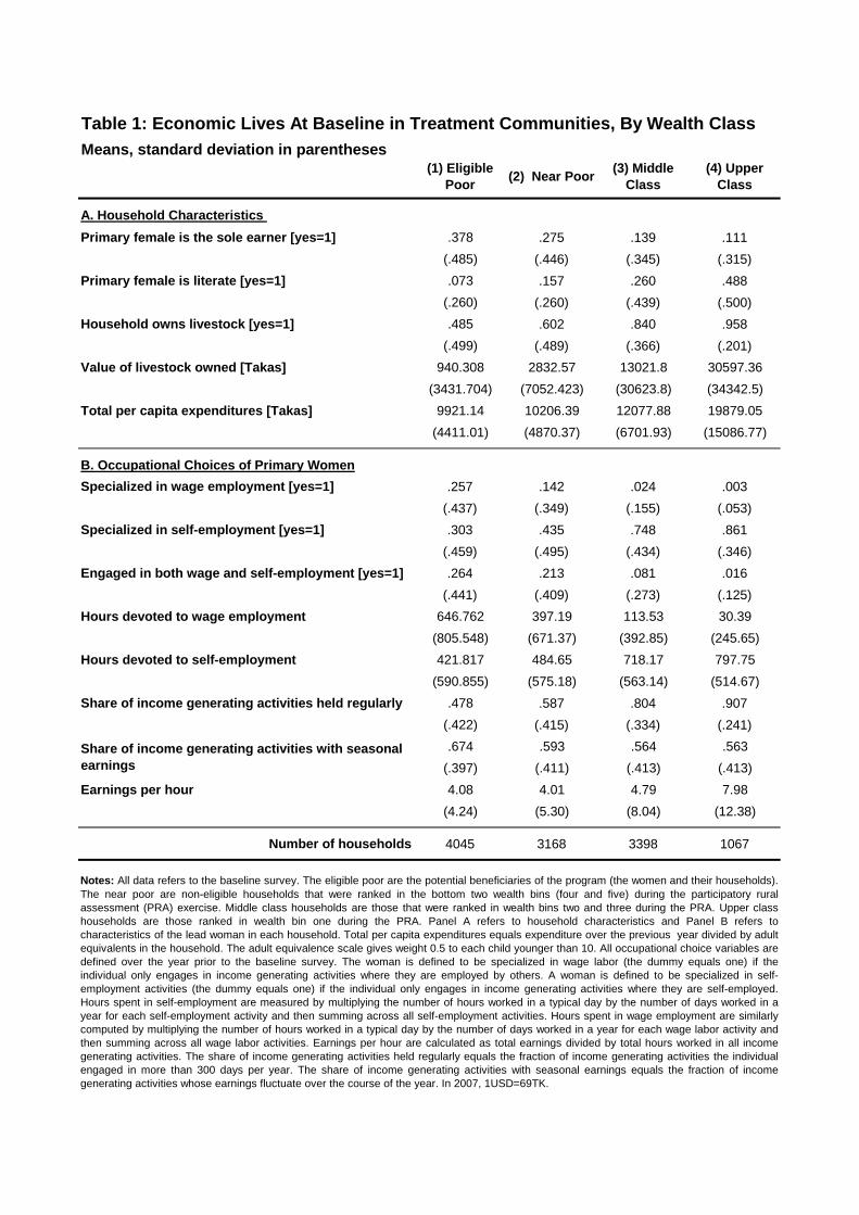
Table 1: Economic Lives At Baseline in Treatment Communities, By Wealth Class
Means, standard deviation in parentheses(1) Eligible
Poor(2) Near Poor
(3) Middle
Class
(4) Upper
Class
A. Household Characteristics
Primary female is the sole earner [yes=1] .378 .275 .139 .111
(.485) (.446) (.345) (.315)
Primary female is literate [yes=1] .073 .157 .260 .488
(.260) (.260) (.439) (.500)
Household owns livestock [yes=1] .485 .602 .840 .958
(.499) (.489) (.366) (.201)
Value of livestock owned [Takas] 940.308 2832.57 13021.8 30597.36
(3431.704) (7052.423) (30623.8) (34342.5)
Total per capita expenditures [Takas] 9921.14 10206.39 12077.88 19879.05
(4411.01) (4870.37) (6701.93) (15086.77)
B. Occupational Choices of Primary Women
Specialized in wage employment [yes=1] .257 .142 .024 .003
(.437) (.349) (.155) (.053)
Specialized in self-employment [yes=1] .303 .435 .748 .861
(.459) (.495) (.434) (.346)
Engaged in both wage and self-employment [yes=1] .264 .213 .081 .016
(.441) (.409) (.273) (.125)
Hours devoted to wage employment 646.762 397.19 113.53 30.39
(805.548) (671.37) (392.85) (245.65)
Hours devoted to self-employment 421.817 484.65 718.17 797.75
(590.855) (575.18) (563.14) (514.67)
Share of income generating activities held regularly .478 .587 .804 .907
(.422) (.415) (.334) (.241)
.674 .593 .564 .563
(.397) (.411) (.413) (.413)
Earnings per hour 4.08 4.01 4.79 7.98
(4.24) (5.30) (8.04) (12.38)
Number of households 4045 3168 3398 1067
Notes: All data refers to the baseline survey. The eligible poor are the potential beneficiaries of the program (the women and their households).
The near poor are non-eligible households that were ranked in the bottom two wealth bins (four and five) during the participatory rural
assessment (PRA) exercise. Middle class households are those that were ranked in wealth bins two and three during the PRA. Upper class
households are those ranked in wealth bin one during the PRA. Panel A refers to household characteristics and Panel B refers to
characteristics of the lead woman in each household. Total per capita expenditures equals expenditure over the previous year divided by adult
equivalents in the household. The adult equivalence scale gives weight 0.5 to each child younger than 10. All occupational choice variables are
defined over the year prior to the baseline survey. The woman is defined to be specialized in wage labor (the dummy equals one) if the
individual only engages in income generating activities where they are employed by others. A woman is defined to be specialized in self-
employment activities (the dummy equals one) if the individual only engages in income generating activities where they are self-employed.
Hours spent in self-employment are measured by multiplying the number of hours worked in a typical day by the number of days worked in a
year for each self-employment activity and then summing across all self-employment activities. Hours spent in wage employment are similarly
computed by multiplying the number of hours worked in a typical day by the number of days worked in a year for each wage labor activity and
then summing across all wage labor activities. Earnings per hour are calculated as total earnings divided by total hours worked in all income
generating activities. The share of income generating activities held regularly equals the fraction of income generating activities the individual
engaged in more than 300 days per year. The share of income generating activities with seasonal earnings equals the fraction of income
generating activities whose earnings fluctuate over the course of the year. In 2007, 1USD=69TK.
Share of income generating activities with seasonal
earnings

Table 2: The Economic Lives of Eligible Women at Baseline, by Treatment Status
Columns 1 and 2: Means and standard deviation in parentheses
Column 3: Difference in means and standard errors in parentheses, clustered by community
Column 4: Normalized difference of means
(1) Treated
Communities
(2) Control
Communities
(3) Raw
Differences
(4) Normalized
Differences
A. Household Characteristics
Primary female is the sole earner [yes=1] .378 .455 -.007*** -.111
(.485) (.498) (.015)
Primary female is literate [yes=1] .073 .067 .006 .017
(.260) (.250) (.007)
Household owns livestock [yes=1] .485 .465 .020 .028
(.499) (.498) (.017)
Value of livestock owned [Takas] 940.308 881.115 59.19 .012
(3431.704) (3325.976) (109.03)
Total per capita expenditures [Takas] 9921.14 9687.54 233.59 .036
(4411.01) (4677.66) (145.58)
B. Individual Occupational Choice
Specialized in wage employment [yes=1] .257 .306 -.049** -.077
(.437) (.461) (.014)
Specialized in self-employment [yes=1] .303 .292 .011 .016
(.459) (.455) (.015)
Engaged in both wage and self-employment [yes=1] .264 .272 -.008 -.012
(.441) (.445) (.015)
Hours devoted to wage employment 646.762 810.360 -163.6*** -.137
(805.548) (886.669) (29.87)
Hours devoted to self-employment 421.817 422.911 -1.09 -.001
(590.855) (592.103) (18.44)
Share of income generating activities held regularly .478 .458 .019 .033
(.421) (.420) (.016)
.674 .663 .011 .021
(.397) (.397) (.016)
Earnings per hour 4.08 4.20 -.117 -.020
(4.24) (3.95) (.144)
Number of households 4045 2687
Notes: *** (**) (*) indicates significance at the 1% (5%) (10%) level. All data refers to the baseline survey. Columns 1 and 2 report statistics based on
eligible in treatment and control communities respectively. Column 3 reports the difference in means and its standard error clustered at the community
level. Column 4 reports normalized differences computed as the difference in means in treatment and control communities divided by the square root of
the sum of the variances. Panel A refers to household characteristics and Panel B refers to characteristics of the lead woman in each household. Total
per capita expenditures equals expenditure over the previous year (on food and non-food items) divided by adult equivalents in the household. The adult
equivalence scale gives weight 0.5 to each child younger than 10.. All occupational choice variables are defined over the year prior to the baseline
survey. The woman is defined to be specialized in wage labor (the dummy equals one) if the individual only engages in income generating activities
where they are employed by others. A woman is defined to be specialized in self-employment activities (the dummy equals one) if the individual only
engages in income generating activities where they are self-employed. Hours spent in self-employment are measured by multiplying the number of hours
worked in a typical day by the number of days worked in a year for each self-employment activity and then summing across all self-employment
activities. Hours spent in wage employment are similarly computed by multiplying the number of hours worked in a typical day by the number of days
worked in a year for each wage labor activity and then summing across all wage labor activities. Earnings per hour are calculated as total earnings
divided by total hours worked in all income generating activities. The share of income generating activities held regularly equals the fraction of income
generating activities the individual engaged in more than 300 days per year. The share of income generating activities with seasonal earnings equals the
fraction of income generating activities whose earnings fluctuate over the course of the year. In 2007, 1USD=69TK.
Share of income generating activities with seasonal
earnings

Table 3: The Impact of the Ultra Poor Program on the Occupational Choices and Earnings of Eligible Women
Difference in Difference ITT Estimates
Standard Errors in Parentheses Clustered by Community
(1) Specialized
in wage
employment
[yes=1]
(2) Specialized in
self-employment
[yes=1]
(3) Engaged in
both occupations
[yes=1]
(4) Hours
devoted to wage
employment
(5) Hours
devoted to
self
employment
(6) Share of
activities
held
regularly
(7) Share of
activities with
seasonal
earnings
(8) Total
annual
earnings
(9) Earnings
per hour
Program effect after 2 years -0.153*** 0.139*** 0.127*** -82.334*** 477.670*** 0.187*** -0.010 1547.712*** -0.189
(0.02) (0.02) (0.02) (27.11) (23.93) (0.02) (0.02) (249.66) (0.19)
Program effect after 4 years -0.168*** 0.154*** 0.084*** -169.139*** 388.410*** 0.174*** -0.082*** 1753.917*** 0.641***
(0.02) (0.02) (0.02) (28.71) (23.40) (0.02) (0.02) (252.02) (0.19)
Mean of outcome variable in treated
communities at baseline0.257 0.303 0.264 646.7 421.81 0.478 0.674 4607.7 4.14
Two year impact = Four year impact
[p-value].217 .336 .011 .001 .000 .447 .000 .464 .000
Adjusted R-squared 0.11 0.089 0.073 0.086 0.156 0.098 0.082 0.078 0.045
Number of eligible poor women 6732 6732 6732 6732 6732 6732 6732 6732 6732
Observations (clusters) 20196 (1309) 20196 (1309) 20196 (1309) 20196 (1309) 20196 (1309) 18672 (1308) 18672 (1308) 20196 (1309) 18387 (1308)
Occupational Choice Seasonality and Earnings
Notes: *** (**) (*) indicates significance at the 1% (5%) (10%) level. The table reports ITT estimates based on a difference-in-difference specification estimated by OLS. The program effect after two (four) years is the coefficient on the
interaction between the treatment indicator and the indicator for the midline (endline) survey wave. All specifications control for the level effect of the treatment, survey waves and subdistrict fixed effects. Standard errors are clustered at
the community level. At the foot of the table we report the mean of each dependent variable as measured at baseline in the treatment communities. We also report the p-value on the hypothesis test that the two and four year program
impacts are equal. The number of eligible poor women is the number of eligibles that are observed at least twice in each specification. All variables are measured on an annual basis. All outcome variables are measured at the individual
level (for the eligible woman in the household). All occupational choice variables are defined over the year prior to the baseline survey. The woman is defined to be specialized in wage labor (the dummy equals one) if the individual only
engages in income generating activities where they are employed by others. A woman is defined to be specialized in self-employment activities (the dummy equals one) if the individual only engages in income generating activities where
they are self-employed. Hours spent in self-employment are measured by multiplying the number of hours worked in a typical day by the number of days worked in a year for each self-employment activity and then summing across all self-
employment activities. Hours spent in wage employment are similarly computed by multiplying the number of hours worked in a typical day by the number of days worked in a year for each wage labor activity and then summing across all
wage labor activities. Earnings per hour are calculated as total earnings divided by total hours worked in all income generating activities. The share of income generating activities held regularly equals the fraction of income generating
activities the individual engaged in more than 300 days per year. The share of income generating activities with seasonal earnings equals the fraction of income generating activities whose earnings fluctuate over the course of the year.
In 2007, 1USD=69TK. All monetary values are deflated to 2007 Takas using the rural CPI published by Bangladesh Bank.

Table 4: The Impact of the Ultra Poor Program on Household Asset Accumulation, Expenditures and Well Being
Difference in Difference ITT Estimates
Standard Errors in Parentheses Clustered by Community
Savings
(1) Cows (2) Poultry (3) Goats(4) Value of All
Livestock
(5) Rents Land
For Cultivation
(6) Owns Land
for Cultivation
(7) Household
savings
(8) PCE Non
Food(9) PCE Food
(10) Food
Security
(11) Satisfied
[yes=1]
(12) Experience
Anxiety [yes=1]
Program effect after 2 years 1.075*** 2.155*** 0.667*** 9983.531*** 0.069*** 0.005 982.7*** 179.633*** 541.35*** 0.176*** 0.031 0.000
(0.02) (0.17) (0.04) (240.00) (0.01) (0.01) (46.05) (64.53) (178.79) (0.03) (0.02) (0.02)
Program effect after 4 years 1.063*** 1.641*** 0.415*** 10734.124*** 0.109*** 0.026*** 1051.1*** 503.356*** 331.32* 0.081*** 0.064** 0.014
(0.03) (0.15) (0.03) (292.77) (0.01) (0.01) (60.45) (83.70) (169.95) (0.03) (0.02) (0.02)
Mean of outcome variable in treated
communities at baseline0.083 1.79 0.147 940.31 .058 .068 121.36 1054.5 8861.1 .457 0.404 0.531
Two year impact = Four year impact
[p-value].588 .001 .000 .007 .000 .000 .281 .000 .260 .000 0.124 0.587
Four year impact = Initial
Programmed Transfer [p-value].541 .000 .000 .000 - - - - - - - -
Adjusted R-squared 0.414 0.090 0.106 0.328 0.059 0.031 0.0873 0.026 0.031 0.185 0.045 0.145
Number of eligible poor women 6732 6732 6732 6732 6732 6732 6732 6732 6732 6732 6732 6732
Observations (clusters) 20196 (1309) 20196 (1309) 20196 (1309) 20196 (1309) 20196 (1309) 20196 (1309) 20196 (1309) 19266 (1309) 18890 (1309) 20194 (1309) 19237(1309) 19279 (1309)
Expenditures Well Being
Notes: *** (**) (*) indicates significance at the 1% (5%) (10%) level. The table reports ITT estimates based on a difference-in-difference specification estimated by OLS. The programmed effect after two (four) years is the coefficient on the interaction between the treatment indicator and the indicator for
the midline (endline) survey wave. All specifications control for the level effect of the treatment, survey waves and subdistrict fixed effects. Standard errors are clustered at the community level. At the foot of the table we report the mean of each dependent variable as measured at baseline in the
treatment communities. We also report the p-value on the hypothesis test that the two and four year programmed impacts are equal. The number of eligible poor women is the number of eligibles that are observed at least twice in each specification. All outcome variables in Columns 1-10 are measured
at the household level. Those in Columns 11 ands 12 are for the eligible female. The value of all livestock is the sum of the value of all cows, goats and chickens owned by the household. Total (non-food) per capita expenditure equals the sum of all (non-food) reported expenditures during the previous
year divided by adult equivalents. The total per capita food expenditure equals the sum of all food expenditures reported during the previous three days divided by adult equivalents and scaled up to one year. The adult equivalence scale gives weight 0.5 to each child younger than 10. The outcome in
Column 10 on food security is a dummy variable equal to one if the household reports being able to afford two meals a day for all members on most days, and zero otherwise. The outcome in Column 11 is a dummy variable equal to one if the individual reports to be satisfied or very satisfied with their
life overall, and zero otherwise. The outcome in Column 12 is a dummy variable equal to one if the individual reports experiencing episodes of anxiety over the past year, and zero otherwise. In 2007, 1USD=69TK. All monetary values are deflated to 2007 Takas using the rural CPI published by
Bangladesh Bank.
Livestock Assets Land

Figure 1A: Occupational Choice Equilibrium: wri
iI
**,
iiSL
Resource Endowment
Time Allocated to Wage Labor, Self-employment
)(~
)(
iirI)(
~~
(?)
iirI),(
~~~
)()(
iirwI
(a): Out of the labor force (b): Self-employment only, unconstrained
(c): Self-employment only, constrained
(d): Both activities,
constrained
0**
iiSL
),(,0)((?)
**
iiii
IrSL
k
i
iip
ISL
**,0
k
i
iiiip
ISIrwL
*
)()((?)
*),,,(
)0(*
iL
Figure 1B: Occupational Choice Equilibrium: wri
iI
**,
iiSL
Resource Endowment
Time Allocated to Wage Labor, Self-employment
)(ˆ)(
wIi
(e): Out of the labor force (f): Wage labor only
0**
iiSL
0),,(*
)((?)
*
iiiSIwL
)0(*
iL

Figure 2A: Impact of the Asset Transfer Component of the Program: wri
iI
**,
iiSL
Resource Endowment
Time Allocated to Wage Labor, Self-employment
)(~
iirI)(
~~ii
rI),(
~~~ii
rwI
(c) Share of individuals
out of the labor force increases
(b) Self-employment hours fall
)0(*
iL
k
ip
AS
*
ArIii)(
~
ArIii)(
~~ArwIii),(
~~~
Wage hours fall
(a) Self-employment hours rise
wri
iI
**,
iiSL
Resource Endowment
Time Allocated to Wage Labor, Self-employment
)0(*
iL
Figure 2B: Impact of the Training Component of the Program:
)(~
0iirI)(
~~0ii
rI),(
~~~0ii
rwI )(~
1iirI
)(~~
1iirI
),(
~~~1ii
rwI
Labor hours fall
(c) Share of individuals
out of the labor force decreases (b) Self-employment
hours rise (a) Self-employment hours are unaffected
Figure 2C: Impact of the Asset Transfer Component of the Program: wri
iI
**,
iiSL
Resource Endowment
Time Allocated to Wage Labor, Self-employment
)(ˆ)(
wIi
)0(*
iL
Share of individuals out of the labor force increases Labor hours fall

Notes: Each histogram shows the proportion of eligible women in each occupational category: solely engaged in wage employment, engaged in both wage and self employment, solely engaged in self employment, and out of the labor force. The woman is defined to be specialized in wage labor (the
dummy equals one) if the individual only engages in income generating activities where they are employed by others. A woman is defined to be specialized in self-employment activities (the dummy equals one) if the individual only engages in income generating activities where they are self-employed.
Panel A shows this for treatment communities, and Panel B shows this for control communities. The left hand side figures in each panel refer to the baseline survey, the middle figures refer to the midline survey (two years after baseline), and the right hand side figures refer to the endline survey (four
years after baseline).
Figure 3: The Extensive Margin Occupational Choices, by Treatment and Control Communities at Baseline, Midline and Endline
Midline: Two years after program implementation Endline: Four years after program implementationBaseline
B. Control Communities
A. Treatment Communities
0.1
.2.3
.4.5
.6
0.1
.2.3
.4.5
.6
0.1
.2.3
.4.5
.60
.1.2
.3.4
.5.6
0.1
.2.3
.4.5
.6
0.1
.2.3
.4.5
.6
Only wage employment
Both wage and self
employment
Only self-employment
Out of the labor force
Only wage employment
Only wage employment
Only wage employment
Only wage employment
Only wage employment
Both wage and self
employment
Both wage and self
employment
Both wage and self
employment
Both wage and self
employment
Both wage and self
employment
Only self-employment
Out of the labor force
Only self-employment
Out of the labor force
Only self-employment
Out of the labor force
Only self-employment
Out of the labor force
Only self-employment
Out of the labor force

Panel A. Annual Earnings of Eligible Women Panel B. Total Per-Capita Expenditures in Eligible Households
Notes: Each dot represents the impact of the program on the outcome on the left hand side column divided by the initial gap between the near poor and the eligible poor (Panel A) and between middle classes and the eligible poor (Panel B).
The vertical line at one indicates the level at which the effect of the program is such to close the gap. The horizontal bars represent 95% confidence intervals based on standard errors clustered by community. All occupational choice variables
are defined over the year prior to the baseline survey. The woman is defined to be specialized in wage labor (the dummy equals one) if the individual only engages in income generating activities where they are employed by others. A woman is
defined to be specialized in self-employment activities (the dummy equals one) if the individual only engages in income generating activities where they are self-employed. The share of income generating activities held regularly equals the
fraction of income generating activities the individual engaged in more than 300 days per year. The share of income generating activities with seasonal earnings equals the fraction of income generating activities whose earnings fluctuate over
the course of the year. Household total per capita expenditure equals expenditure over the previous year (on food and non-food items) divided by adult equivalents in the household. The adult equivalence scale gives weight 0.5 to each child
younger than 10. In 2007, 1USD=69TK.
Figure 4: Quantile Treatment Effects
-500
0
500
1000
1500
2000
1 2 3 4 5 6 7 8 9decile
-200
0
0
200
04
000
600
0
1 2 3 4 5 6 7 8 9decile
Four Year Impact
Two Year Impact
Four Year Impact
Two Year Impact
Decile Decile
Specialised in wage employment
Specialised in self-employment
Share of regular activities
Value of livestock owned
Household owns land [yes=1]
Total per capita expenditures
Happy [yes=1]
Figure 5: The Impact of the Ultra Poor Programme On the Gap Between Other Classes and the Eligible Poor
B. Gap Between Middle Classes and Targeted PoorOutcomes A. Gap Between Near Poor and Targeted Poor
b
0 2 4 6
b
0 .2 .4 .6 .8 1
Notes: Each point represents the treatment effect at the decile on the x-axis, each bar represents the 95% confidence interval. Squares indicate the quantile treatment effect at midline (two years after the baseline), triangles indicate the quantile treatment effect at endline (four years after baseline). Confidence intervals are based on bootstrapped standard errors with 1000 replication clustered at the community level. Panel A refers to annual earnings of eligible women from all labor market activities. Panel B refers to the households total per capita expenditure equals expenditure over the previous year (on food and non-food items) divided by adult equivalents in the household. The adult equivalence scale gives weight 0.5 to each child younger than 10. In 2007, 1USD=69TK.
Life Satisfaction [yes=1]

Table A1: Determinants of Non-attrition
Dependent Variable=1 if Respondent is Surveyed in All Three Waves
Sample Includes All Eligible Poor Women at Baseline
OLS Estimates, Standard Errors Clustered at the Community Level in Parentheses
(1) Treatment
Assignment
(2) Occupational Choice
at Baseline
(3) Heterogeneous Attrition by
Occupational Choice at Baseline
Treatment community 0.031 0.014 0.014
(0.02) (0.01) (0.01)
Specialized in wage employment 0.033 0.011
(0.02) (0.01)
Specialized in self- employment 0.060*** 0.049***
(0.02) (0.01)
Engaged in Both Occupations 0.051** 0.048***
(0.02) (0.01)
Treatment x Specialized in wage employment -0.037
(0.03)
Treatment x Specialized in self employment -0.016
(0.03)
Treatment x Engaged in both occupations -0.004
(0.03)
Subdistrict Fixed Effects Yes Yes Yes
Adjusted R-squared 0.006 0.006 0.003
Observations (number of eligible poor women) 7953 7953 7953
Notes: *** (**) (*) indicates significance at the 1% (5%) (10%) level. The dependent variable is a dummy variable equal to one if the eligible woman is observed
in all three survey waves (baseline, midline, endline), and zero otherwise. All specifications control for the level effect of the treatment and subdistrict fixed
effects. Standard errors are clustered at the community level.

Table A2: The Impact of the Ultra Poor Program on the Occupational Choices of Other Members of Eligible Households
Difference in Difference ITT estimates
Standard Errors in Parentheses Clustered by Community
(1) Hours devoted
to wage labor
(2) Hours devoted
to self-employment
(3) Hours devoted
to wage
employment
(4) Hours devoted
to self-employment
(5) Hours devoted
to wage labor
(6) Hours devoted
to self-employment
Program effect after 2 years -65.955 167.554*** -6.137 70.481*** 5.225 56.635***
(47.78) (11.99) (15.94) (6.43) (8.13) (6.14)
Program effect after 4 years -83.775 58.656*** 8.706 46.938*** 1.124 35.891***
(51.51) (11.02) (17.56) (7.17) (8.33) (6.45)
Mean of outcome variable in treated
communities at baseline633.25 152.57 363.13 24.30 31.83 17.93
Two year impact = Four year impact
[p-value].691 .000 .308 .000 .5739 .000
Adjusted R-squared 0.083 0.125 0.008 0.041 0.002 0.035
Observations (clusters) 11751 (1168) 11751 (1168) 20889 (1239) 20889(1239) 18922 18922 (1204)
Husbands Other Adult Members Children
Notes: *** (**) (*) indicates significance at the 1% (5%) (10%) level. The table reports ITT estimates based on a difference-in-difference specification estimated by OLS. The program effect after two (four)
years is the coefficient on the interaction between the treatment indicator and the indicator for the midline (endline) survey wave. All specifications control for the level effect of the treatment, survey waves
and subdistrict fixed effects. Standard errors are clustered at the community level. At the foot of the table we report the mean of each dependent variable as measured at baseline in the treatment
communities. We also report the p-value on the hypothesis test that the two and four year program impacts are equal. The number of eligible poor women is the number of eligibles that are observed at
least twice in each specification. All variables are measured on an annual basis. Outcome variables in Columns 1 and 2 refer to the husband of the eligible woman. Outcomes in Columns 3 and 4 are
measured at the household level for all other adult household members (excluding the eligible woman and her husband). Outcomes in Columns 5 and 6 are measured at the household level for all children.
All occupational hours variables are defined over the year prior to the baseline survey. Hours spent in self-employment are measured by multiplying the number of hours worked in a typical day by the
number of days worked in a year for each self-employment activity and then summing across all self-employment activities. Hours spent in wage employment are similarly computed by multiplying the
number of hours worked in a typical day by the number of days worked in a year for each wage labor activity and then summing across all wage labor activities.

Table A3: The Economic Lives of the Eligible Women at Baseline, by Treatment Status and Occupation
Columns 1A, 1B, 2A and 2B: Means and standard deviation in parentheses
Columns 3A and 3B: Difference in means and standard errors in parentheses, clustered by community
Columns 4A and 4B: Normalized difference of means
(1A) Treated
Communities
(2A) Control
Communities
(3A) Raw
Differences
(4A) Normalized
Differences
(1B) Treated
Communities
(2B) Control
Communities
(3B) Raw
Differences
(4B) Normalized
Differences
A. Household Characteristics
Primary female is the sole earner [yes=1] .570 .606 -.036 -.052 .287 .369 -.082 -.124
(.495) (.489) (.025) (.452) (.483) (.024)
Primary female is literate [yes=1] .037 .023 .014* .056 .103 .104 -.001 -.003
(.188) (.150) (.008) (.304) (.305) (.015)
Household owns livestock [yes=1] .150 .142 .008 .016 .742 .724 .018 .029
(.357) (.349) (.022) (.438) (.447) (.024)
Value of livestock owned [Takas] 151 95.9 55.1 .044 1771 1648 123 .019
(1104) (607) (42.2) (4843) (4456) (251)
Total per capita expenditures [Takas] 10411.95 9656.88 755.069*** .103 9565.14 9571.79 -6.65 -.001
(5167.35) (4675.469 ) (255.49) (3874.65) (4605.7) (221.68)
B. Individual Occupational Choice
Hours devoted to wage employment 1385 1533 -148*** -.142 - - - -
(741) (730) (43.0)
Hours devoted to self-employment - - - - 889 925 -36.6 -.036
(720) (716) (39.2)
Share of income generating activities held regularly .189 .232 -.043** -.081 .747 .719 .028 .050
(.360) (.391) (.021) (.403) (.403) (.023)
.850 .848 .002 .004 .540 .461 .079 .125
(.329) (.328) (.021) (.458) (.444) (.027)
Earnings per hour 5.67 5.09 .582*** .101 2.50 2.61 -.116 -.019
(4.49) (3.61) (.215) (4.48) (4.35) (.218)
Share of income generating activities with seasonal
earnings
Panel A: Specialized in Wage Labor at Baseline Panel B: Specialized in Self-employment at Baseline
Notes: *** (**) (*) indicates significance at the 1% (5%) (10%) level. All data refers to the baseline survey. The panels of the table split eligible women into their occupational choices at baseline. Panel A refers to those that were
specialized in wage labor; Panel B refers to those that were specialized in self-employment at baseline. Columns 1A and 1B report statistics based on eligibles in treatment communities; Columns 2A and 2B report statistics based on
eligibles in control communities. Columns 3A and 3B report the difference in means and its standard error clustered at the community level. Columns 4A and 4B report normalized differences computed as the difference in means in
treatment and control communities divided by the square root of the sum of the variances. The upper panel of the table (Panel A) refers to household characteristics and Panel B refers to characteristics of the lead woman in each
household. Total per capita expenditures equals expenditure over the previous year (on food and non-food items) divided by adult equivalents in the household. The adult equivalence scale gives weight 0.5 to each child younger than 10.
All occupational choice variables are defined over the year prior to the baseline survey. The woman is defined to be specialized in wage labor (the dummy equals one) if the individual only engages in income generating activities where
they are employed by others. A woman is defined to be specialized in self-employment activities (the dummy equals one) if the individual only engages in income generating activities where they are self-employed. Hours spent in self-
employment are measured by multiplying the number of hours worked in a typical day by the number of days worked in a year for each self-employment activity and then summing across all self-employment activities. Hours spent in
wage employment are similarly computed by multiplying the number of hours worked in a typical day by the number of days worked in a year for each wage labor activity and then summing across all wage labor activities. Earnings per
hour are calculated as total earnings divided by total hours worked in all income generating activities. The share of income generating activities held regularly equals the fraction of income generating activities the individual engaged in

Table A4: The Heterogeneous Impacts of the Ultra Poor Program on the Occupational Choices and Earnings of Eligible Women
Difference in Difference ITT Estimates
Standard Errors in Parentheses Clustered by Community
(1)
Specialized
in wage
employment
[yes=1]
(2)
Specialized
in self-
employment
[yes=1]
(3) Engaged in
both
occupations
[yes=1]
(4) Hours
devoted to
wage
employment
(5) Hours
devoted to
self
employment
(6) Share of
activities
held
regularly
(7) Share of
activities with
seasonal
earnings
(8) Total
annual
earnings
(9) Earnings
per hour
Program effect after 2 years -0.382*** 0.111*** 0.301*** -194.382*** 577.988*** 0.275*** -0.040* 1022.211** -1.016***
(0.02) (0.02) (0.03) (53.49) (32.15) (0.03) (0.02) (408.05) (0.28)
Program effect after 4 years -0.348*** 0.155*** 0.204*** -264.273*** 498.739*** 0.259*** -0.090*** 1336.128*** -0.127
(0.02) (0.02) (0.03) (56.51) (30.08) (0.03) (0.03) (442.78) (0.33)
Mean of outcome variable in treated
communities at baseline1 0 0 1385.35 0 0.189 0.85 7121.38 5.67
Two year impact = Four year impact
[p-value].225 .058 .002 .181 .045 .539 .033 .518 .012
Adjusted R-squared 0.609 0.124 0.328 0.136 0.422 0.172 0.117 0.065 0.054
Number of eligible poor women 1863 1863 1863 1863 1863 1863 1863 1863 1863
Observations (clusters) 5589 (826) 5589 (826) 5589 (826) 5589 (826) 5589 (826) 5499 (826) 5499 (826) 5589 (826) 5475 (826)
(1)
Specialized
in wage
employment
[yes=1]
(2)
Specialized
in self-
employment
[yes=1]
(3) Engaged in
both
occupations
[yes=1]
(4) Hours
devoted to
wage
employment
(5) Hours
devoted to
self
employment
(6) Share of
activities
held
regularly
(7) Share of
activities with
seasonal
earnings
(8) Total
annual
earnings
(9) Earnings
per hour
Program effect after 2 years -0.052*** 0.090*** 0.055*** -38.250* 396.012*** 0.137*** -0.072** 1604.816*** 0.260
(0.01) (0.02) (0.02) (23.12) (43.02) (0.03) (0.03) (352.40) (0.33)
Program effect after 4 years -0.080*** 0.093*** 0.022 -142.253*** 292.388*** 0.092*** -0.133*** 1947.302*** 1.260***
(0.01) (0.02) (0.02) (29.94) (47.06) (0.03) (0.04) (393.20) (0.34)
Mean of outcome variable in treated
communities at baseline1 0 0 0 888.67 0.747 0.54 2878.5 2.49
Two year impact = Four year impact
[p-value].036 .892 .174 .001 .011 .093 .047 .402 .009
Adjusted R-squared 0.047 0.163 0.111 0.093 0.069 0.057 0.096 0.096 0.068
Number of eligible poor women 2012 2012 2012 2012 2012 2012 2012 2012 2012
Observations (clusters) 6036 (809) 6036 (809) 6036 (809) 6036 (809) 6036 (809) 5842 (809) 5842 (809) 6036 (809) 5764 (809)
Notes: *** (**) (*) indicates significance at the 1% (5%) (10%) level. The table reports ITT estimates based on a difference-in-difference specification estimated by OLS. The panels of the table split eligible women
into their occupational choices at baseline. Panel A refers to those that were specialized in wage labor; Panel B refers to those that were specialized in self-employment at baseline. The program effect after two (four)
years is the coefficient on the interaction between the treatment indicator and the indicator for the midline (endline) survey wave. All specifications control for the level effect of the treatment, survey waves and
subdistrict fixed effects. Standard errors are clustered at the community level. At the foot of the table we report the mean of each dependent variable as measured at baseline in the treatment communities. We also
report the p-value on the hypothesis test that the two and four year program impacts are equal. The number of eligible poor women is the number of eligibles that are observed at least twice in each specification. All
variables are measured on an annual basis. All outcome variables are measured at the individual level (for the eligible woman in the household). All occupational choice variables are defined over the year prior to
the baseline survey. The woman is defined to be specialized in wage labor (the dummy equals one) if the individual only engages in income generating activities where they are employed by others. A woman is
defined to be specialized in self-employment activities (the dummy equals one) if the individual only engages in income generating activities where they are self-employed. Hours spent in self-employment are
measured by multiplying the number of hours worked in a typical day by the number of days worked in a year for each self-employment activity and then summing across all self-employment activities. Hours spent in
wage employment are similarly computed by multiplying the number of hours worked in a typical day by the number of days worked in a year for each wage labor activity and then summing across all wage labor
activities. Earnings per hour are calculated as total earnings divided by total hours worked in all income generating activities. The share of income generating activities held regularly equals the fraction of income
generating activities the individual engaged in more than 300 days per year. The share of income generating activities with seasonal earnings equals the fraction of income generating activities whose earnings
fluctuate over the course of the year. In 2007, 1USD=69TK.
Panel A: Specialized in Wage Labor at Baseline
Panel B: Specialized in Self-employment at Baseline

Table A5: The Impact of the Ultra Poor Program on the Occupational Choices and Earnings of Eligible WomenRobustness Check: Allowing for Differential Time Trends for Women who are Sole Earners in the Household
Difference in Difference ITT estimates
Standard Errors in Parentheses Clustered by Community
(1) Specialized
in wage
employment
[yes=1]
(2) Specialized in
self-employment
[yes=1]
(3) Engaged in
both occupations
[yes=1]
(4) Hours
devoted to wage
labor
(5) Hours
devoted to
self
employment
(6) Share of
activities
held
regularly
(7) Share of
activities with
seasonal
earnings
(8) Total
earnings
(9) Earnings
per hour
Program effect after 2 years -0.160*** 0.133*** 0.133*** -88.580*** 473.672*** 0.187*** -0.017 1501.368*** -0.219
(0.01) (0.02) (0.02) (27.53) (24.01) (0.02) (0.02) (252.75) (0.19)
Program effect after 4 years -0.178*** 0.155*** 0.084*** -187.861*** 379.164*** 0.178*** -0.088*** 1637.642*** 0.584***
(0.02) (0.02) (0.02) (28.72) (23.42) (0.02) (0.02) (253.27) (0.20)
Mean of outcome variable in treated
communities at baseline0.257 0.303 0.264 646.7 421.81 0.478 0.674 4607.7 4.14
Two year impact = Four year impact
[p-value].160 .164 .003 .000 .000 .545 .000 .635 .000
Adjusted R-squared 0.137 0.104 0.078 0.158 0.136 0.110 0.091 0.099 0.048
Observations (clusters) 20196 (1309) 20196 (1309) 20196 (1309) 20196 (1309) 20196 (1309) 18672 (1308) 18672 (1308) 20196 (1309) 18387 (1308)
Occupational choice Seasonality and Earnings
Notes: *** (**) (*) indicates significance at the 1% (5%) (10%) level. The table reports ITT estimates based on a difference-in-difference specification estimated by OLS. The program effect after two (four) years is the coefficient on the
interaction between the treatment indicator and the indicator for the midline (endline) survey wave. All specifications control for the level effect of the treatment, survey waves, subdistrict fixed effects, a dummy variable for whether the
eligible woman is the sole earner in the household, and an interaction of survey waves with a dummy variable for the eligible woman being the sole earner. Standard errors are clustered at the community level. At the foot of the table we
report the mean of each dependent variable as measured at baseline in the treatment communities. We also report the p-value on the hypothesis test that the two and four year program impacts are equal. The number of eligible poor
women is the number of eligibles that are observed at least twice in each specification. All variables are measured on an annual basis. All outcome variables are measured at the individual level (for the eligible woman in the household).
All occupational choice variables are defined over the year prior to the baseline survey. The woman is defined to be specialized in wage labor (the dummy equals one) if the individual only engages in income generating activities where
they are employed by others. A woman is defined to be specialized in self-employment activities (the dummy equals one) if the individual only engages in income generating activities where they are self-employed. Hours spent in self-
employment are measured by multiplying the number of hours worked in a typical day by the number of days worked in a year for each self-employment activity and then summing across all self-employment activities. Hours spent in
wage employment are similarly computed by multiplying the number of hours worked in a typical day by the number of days worked in a year for each wage labor activity and then summing across all wage labor activities. Earnings per
hour are calculated as total earnings divided by total hours worked in all income generating activities. The share of income generating activities held regularly equals the fraction of income generating activities the individual engaged in
more than 300 days per year. The share of income generating activities with seasonal earnings equals the fraction of income generating activities whose earnings fluctuate over the course of the year. In 2007, 1USD=69TK.

Table A6: The Impact of the Ultra Poor Program on the Occupational Choices and Earnings of Eligible WomenRobustness Check: Using All Poor in Control Communities as Counterfactual
Difference in Difference ITT estimates
Standard Errors in Parentheses Clustered by Community
(1) Specialized
in wage
employment
[yes=1]
(2) Specialized in
self-employment
[yes=1]
(3) Engaged in
both occupations
[yes=1]
(4) Hours devoted
to wage labor
(5) Hours
devoted to
self
employment
(6) Share of
activities
held
regularly
(7) Share of
activities with
seasonal
earnings
(8) Total
earnings
(9) Earnings
per hour
Program effect after 2 years -0.186*** 0.143*** 0.147*** -103.854*** 521.818*** 0.214*** -0.032** 1845.947*** -0.304*
(0.01) (0.01) (0.01) (21.49) (22.15) (0.01) (0.02) (220.81) (0.18)
Program effect after 4 years -0.184*** 0.172*** 0.084*** -187.103*** 400.580*** 0.181*** -0.039** 1724.635*** 0.560***
(0.01) (0.01) (0.02) (22.43) (21.20) (0.02) (0.02) (230.32) (0.19)
Mean of outcome variable in treated
communities at baseline0.257 0.303 0.264 646.7 421.81 0.478 0.674 4607.7 4.14
Two year impact = Four year impact
[p-value].797 .037 .000 .000 .000 .007 .688 .638 .000
Adjusted R-squared 0.061 0.064 0.074 0.055 0.115 0.068 0.082 0.085 0.051
Number of eligible poor women 10,904 10,904 10,904 10,904 10,904 10,904 10,904 10,904 10,904
Observations (clusters) 32712 (1387) 32712 (1387) 32712 (1387) 32712 (1387) 32712 (1387) 29831 (1386) 29831 (1386) 32712 (1387) 29831 (1386)
Occupational choice Seasonality and Earnings
Notes: *** (**) (*) indicates significance at the 1% (5%) (10%) level. The table reports ITT estimates based on a difference-in-difference specification estimated by OLS, where we also include households classified to be near poor from the
control communities. The program effect after two (four) years is the coefficient on the interaction between the treatment indicator and the indicator for the midline (endline) survey wave. All specifications control for the level effect of the
treatment, survey waves and subdistrict fixed effects. Standard errors are clustered at the community level. At the foot of the table we report the mean of each dependent variable as measured at baseline in the treatment communities. We
also report the p-value on the hypothesis test that the two and four year program impacts are equal. The number of eligible poor women is the number of eligibles that are observed at least twice in each specification. All variables are
measured on an annual basis. All outcome variables are measured at the individual level (for the eligible woman in the household). All occupational choice variables are defined over the year prior to the baseline survey. The woman is
defined to be specialized in wage labor (the dummy equals one) if the individual only engages in income generating activities where they are employed by others. A woman is defined to be specialized in self-employment activities (the
dummy equals one) if the individual only engages in income generating activities where they are self-employed. Hours spent in self-employment are measured by multiplying the number of hours worked in a typical day by the number of
days worked in a year for each self-employment activity and then summing across all self-employment activities. Hours spent in wage employment are similarly computed by multiplying the number of hours worked in a typical day by the
number of days worked in a year for each wage labor activity and then summing across all wage labor activities. Earnings per hour are calculated as total earnings divided by total hours worked in all income generating activities. The share
of income generating activities held regularly equals the fraction of income generating activities the individual engaged in more than 300 days per year. The share of income generating activities with seasonal earnings equals the fraction of
income generating activities whose earnings fluctuate over the course of the year. In 2007, 1USD=69TK.
Related Documents