Call Center Delay Announcement Using a Newsvendor-Like ...

HAL Id: hal-01265196https://hal.archives-ouvertes.fr/hal-01265196

Submitted on 2 Feb 2016

HAL is a multi-disciplinary open accessarchive for the deposit and dissemination of sci-entific research documents, whether they are pub-lished or not. The documents may come fromteaching and research institutions in France orabroad, or from public or private research centers.

L’archive ouverte pluridisciplinaire HAL, estdestinée au dépôt et à la diffusion de documentsscientifiques de niveau recherche, publiés ou non,émanant des établissements d’enseignement et derecherche français ou étrangers, des laboratoirespublics ou privés.

Call Center Delay Announcement Using aNewsvendor-Like Performance Criterion

Oualid Jouini, Zeynep Aksin, Fikri Karaesmen, M Salah Aguir, yves Dallery

To cite this version:Oualid Jouini, Zeynep Aksin, Fikri Karaesmen, M Salah Aguir, yves Dallery. Call Center DelayAnnouncement Using a Newsvendor-Like Performance Criterion. Production and Operations Man-agement, Wiley, 2015, 24, pp.587-604. �10.1111/poms.12259�. �hal-01265196�

https://hal.archives-ouvertes.fr/hal-01265196

https://hal.archives-ouvertes.fr

Call center Delay Announcement Using aNewsvendor-Like Performance Criterion

Oualid Jouini1 • O. Zeynep Aksin2 • Fikri Karaesmen2 • M. Salah Aguir3 •Yves Dallery1

1Laboratoire Genie Industriel, Ecole Centrale Paris, Grande Voie des Vignes, 92290

Chatenay-Malabry, France

2 Koc University, Rumeli Feneri Yolu, 34450 Sariyer-Istanbul, Turkey

3Ecole Superieure de Technologie et d’Informatique

[email protected] • [email protected] • [email protected] •[email protected] • [email protected]

Production and Operations Management, To appear.

The problem of estimating delays experienced by customers with different priorities, and the

determination of the appropriate delay announcement to these customers, in a multi-class

call center with time varying parameters, abandonments and retrials is considered. The sys-

tem is approximately modeled as an M(t)/M/s(t) queue with priorities, thus ignoring some

of the real features like abandonments and retrials. Two delay estimators are proposed and

tested in a series of simulation experiments. Making use of actual state dependent waiting

time data from this call center, the delay announcements from the estimated delay distri-

butions that minimize a newsvendor-like cost function are considered. The performance of

these announcements are also compared to announcing the mean delay. We find that an Er-

lang distribution based estimator performs well for a range of different under-announcement

penalty to over-announcement penalty ratios.

Keywords Queues: call center applications, real-time delay approximations, priority, simu-

lation, newsvendor model

History Received: August 2011; accepted: May 2014 by Michael Pinedo after three revi-

sions.

1

1 Introduction

The interest in prediction and announcement of delays in service systems has intensified as

the call center industry has grown and become technologically sophisticated. Managers have

several objectives in providing such information; modulating demand by signaling times of

high congestion, enhancing satisfaction with inevitable waiting, or both. These objectives

bring with them several challenges: 1. estimating real-time delays for each customer in a

stochastic environment and 2. deciding on what to announce given customer preferences

regarding waiting times and announcements made. This paper presents an analysis of these

two issues in a real call center setting.

Starting with the analyses in Whitt (1999a) and Whitt (1999b), most existing models

have considered single class systems (Jouini et al. (2011); Armony et al. (2009); Ibrahim

and Whitt (2009); Guo and Zipkin (2007); Allon et al. (2011)). Jouini et al. (2009) extends

the model by Whitt (1999a) to one with multiple customer classes having different priori-

ties. Nakibly (2002) considers several different models with multiple customer types having

priorities, and with service times that may depend on the customer. The problem analyzed

in this paper is similar to those analyzed in Jouini et al. (2009) and Nakibly (2002), in

that there are several customer types with different priorities, having similar service times.

However calls are routed to different centers, rather than servers, and due to technological

constraints, state information pertaining to the number of servers available at each site is

not known in real time. This precludes the adaptation of earlier results, and leads us to

pursue an approximation based approach.

Strategic customers in queues react to waiting situations, as first modeled in a stream of

literature starting with Naor (1969). This literature developed substantially over the years,

as surveyed by Hassin and Haviv (2003). Models motivated by call center delay announce-

ments, can be distinguished by whether they only consider prediction and announcement

(Whitt (1999b); Ibrahim and Whitt (2009)), or if customer reactions to these announce-

ments are endogenized in the analysis (Whitt (1999a); Guo and Zipkin (2007); Allon et al.

(2011); Jouini et al. (2011); Armony et al. (2009); Aksin et al. (2013)). While most of the

literature considers systems where customers react to delay information by balking only, a

stream of recent work has incorporated the possibility of reactions in the form of abandon-

ments from the queue as well (Armony et al. (2009); Jouini et al. (2011); Ibrahim and Whitt

(2009)). Even though the setting we study also experiences abandonments, our approxi-

mations will ignore these. Similarly, retrials and time varying arrivals are features which

2

will be approximated away, as done in all of the earlier papers. The possibility of customer

call backs as described and modeled by Armony and Maglaras (2004) is not present in this

setting. Since the existing operation at the call center did not have delay announcements

at the time of study, there is no data on customer reactions to such announcements. Thus,

customer reactions will not be part of the analysis in this paper.

Two different types of analysis have been pursued in papers that deal with prediction

and announcement in queueing systems: the first predicts and announces delays based on

transient queueing analysis (Whitt (1999a); Whitt (1999b); Jouini et al. (2011); Jouini et al.

(2009)) whereas the second considers announcing real-time delay estimators under a fluid

model applicable in large and overloaded systems (Armony et al. (2009); Ibrahim and Whitt

(2009)). The approach herein is closer to the first. Like in the second approach, it employs

a real-time estimation idea, however not directly for the delays but rather for the underlying

model parameters. Since model parameters are unknown, an approximation that makes

use of real-time estimators for the number of servers is employed. We take the approach

of providing simple approximations that are easy to implement in practice. An extensive

simulation experiment as well as real state dependent waiting time data is subsequently used

to test the quality of the developed delay estimators.

Various announcement forms are considered in the literature: delay announcements of

the type “you will wait x minutes”, derived from distributions (Whitt (1999b); Jouini et al.

(2011)); delays based on real time estimators (Armony et al. (2009); Ibrahim and Whitt

(2009)); state occupancy or length of queue information as indirect waiting time announce-

ments (Guo and Zipkin (2007); Xu et al. (2007); Aksin et al. (2013)); or more general,

possibly vague and non-quantitative announcements (Allon et al. (2011)). In this paper,

we focus on delay announcements derived from state-dependent waiting time distributions.

More importantly, we propose a new framework making use of a newsvendor-like perfor-

mance criterion to pick the value to announce from the estimated delay distribution. This

framework enables incorporating asymmetric under and over-announcement penalties that,

compared to symmetric ones, are more consistent with behavioral evidence. Within this

framework, we further propose and test a robust estimator obtained from a robust optimiza-

tion formulation of the newsvendor problem.

Delay announcements that are optimal under the newsvendor framework are tested mak-

ing use of real state dependent waiting time data from the call center being studied. The

current paper is among the first to study delay announcements in a service setting combining

modeling analysis with empirical validation. Most empirical work to date comes from exper-

3

iments in psychology and marketing that analyze people’s reactions to waiting situations,

with and without information, in call centers and elsewhere (see for example Munichor and

Rafaeli (2007); Pazgal and Radas (2008)). The papers by Brown et al. (2005) and Feigin

(2005) analyze call center data where delay announcements are present, however pursue a

more descriptive analysis than the one in this paper. The recent paper Aksin et al. (2013)

is an exception that combines modeling and empirical analysis in an analysis of delay an-

nouncements in a call center.

We describe the operations of the call center in detail in Section 2 and propose the

newsvendor framework for delay announcement from an approximated delay distribution.

The delay estimator for the high priority class is developed in Section 3 and for the lower

priority classes in Section 4. Section 5 explores the performance of these approximations in a

series of simulation experiments, the details of which are provided in the online supplement

(OS) and the supplementary results (SR) document available from the authors. The simu-

lation experiments analyze the proposed approximations in a controlled environment, thus

enabling a clear understanding of how various system features may affect their performance.

In Section 6, we determine what value to announce from the approximated distributions. The

proposed announcements are tested making use of waiting time data from the field in Section

7. This provides a real test of the cost effectiveness of the proposed delay announcements.

The paper ends with concluding remarks.

2 The Setting

The setting is that of a large multi-site call center handling more than 50000 calls daily. Calls

are handled at several sites, differentiated by their size but of identical capability in terms of

the types of calls that can be handled. This multi-site system is not equipped with networked

routing capabilities implying that each site has its own queue. An important objective of

the real time delay estimation is to use these estimates in routing calls to the various sites.

The delay estimators we propose below and subsequently analyze for the purpose of delay

announcement, have indeed been implemented for real-time routing decisions of calls at this

call center. The use for routing purposes is not explored any further in this paper. At the

time of study, the call center was highly congested as manifested by periods with high call

retrial. Abandonment probabilities of around 5 % were experienced.

4

2.1 Operational Features and Approximations

The center responds to three types of calls A, B, and C, distinguished by customer rela-

tionship based criteria (customer valuation based differentiation). A-type calls are the most

valuable. Calls of different types are considered to be statistically similar from a service

time perspective. Strict priority rules are implemented with class A having non-preemptive

priority over B who in turn have non-preemptive priority over C type calls.

An important result of the multi-site with no networked routing feature is that the number

of servers at a site is not known in real time. While this feature is a result of the technology

in place, even in a setting with networked queues, absenteeism (Whitt (2006)) and lack of

discipline or motivation on the part of the servers in properly displaying their availability

status, results in the number of servers in real time to be unknown exactly. A different

reason for lack of knowledge about system capacity is documented in Hasija et al. (2010). In

the e-mail contact center being studied, work rules and incentives motivate servers to slow

down such that work expands to fill the time available for its completion, thus making it

difficult to determine capacity. The system studied herein can however track the number of

clients of each class waiting in queue, as well as the average rate of calls routed towards each

site within a specified time window, and the calls arriving to service within a specified time

window. Our first level of approximation results from this feature.

We approximate the total service rate of s servers sµ, by the mean arrival rate of calls

to service. Since arrivals are time varying, the mean arrival rate in turn is estimated over

a rolling time window, as explained in more detail in Section 3. The approximation results

from the use of a real-time estimator for a basic model parameter, and is different from the

standard approach where all parameters are known or distributions of parameters can be

derived.

The real system is complex. Capturing this complexity through corresponding model

features, and performing an exact analysis through queueing models or simulation may be

possible, but leads to excessive complexity which is not desired from a practical point of

view. Instead, we propose to analyze the system as an M(t)/M/s(t) queue with three

classes having strict priorities. This model ignores abandonments and retrials, and assumes

non-homogeneous Poisson arrivals and exponential service times.

The final layer of complexity results from the priority system in place. Waiting times

have to be estimated for the different types of calls having different priorities. For this

analysis as well, we will prefer the simple and approximate over the exact analysis of the

5

underlying models. We will propose approximating the delay distribution of especially the

lower priority customers by a normal distribution with an appropriately chosen mean and

variance or an Erlang distribution with corresponding parameters, as detailed below.

2.2 Choosing What to Announce

In making announcements, the firm has different objectives for the different call types. The

main concern is to explore announcements to A-type customers and potentially to B-type

callers. Announcements to C-type callers are not considered, as this is deemed unnecessary by

managers at the time of study. The objective for A-type calls is maximizing service experience

and satisfaction, given their high value premium nature. In terms of announcements, ex-

post precision, i.e., correctness of the announced delay viz-a-viz the real delay is important.

Announced delays can shorten or lengthen both a customer’s expectations regarding waiting

and his/her perceptions of the actual wait (Kumar et al. (1997); Hui and Tse (1996); Hui and

Zhou (1996)). As such, over or under-announcement of actual delays may result in a gap

between expectations and perceptions, thus leading to dissatisfaction whenever expected

waits are perceived to be exceeded (Anderson (1973); Parasuraman et al. (1985)). This

possibility for dissatisfaction implies that for these high value customers over or under-

announcement is undesirable.

In choosing a value to announce from the delay distribution, there seem to be a number

of simple options. Throughout the paper delay distributions as well as chosen values for

announcements are conditional on the state in terms of number of callers in the system, as

well as the current time (determining the corresponding arrival rate used in the approxima-

tions). To keep notation more manageable, we will not make these explicit in the notation,

however throughout the paper all delay distributions and delay announcements should be

interpreted as such. Labeling the announced delay as da (single value), the realized delay as

Dr (random variable), one may wish to choose da to minimize

E[(Dr − da)2]. (1)

This would result in d∗a = E[Dr] and estimators for the mean delay can be readily used.

Another alternative is to choose da to minimize E[|Dr − da|]. The optimal announce-

ment corresponds then to the median of Dr. If the delay distribution is approximated by

a symmetrical distribution such as a normal distribution, d∗a would then be selected as the

estimator of mean delay. For non-symmetrical distributions however, the median must be

6

obtained.

The above approaches penalize under announcements and over announcements similarly

and ignore the fact that under announcements and over announcements are perceived dif-

ferently. Our proposed announcement scheme lets the manager choose asymmetric penalties

for under announcing (α per unit time), and over announcing (β per unit time). In this case,

the manager’s decision of what to announce to an A-type customer can be formulated as

Min αE[(Dr − da)+] + βE[(da −Dr)

+]. (2)

Letting γ = α/(α+ β), this leads to the following well-known newsvendor problem’s critical

fractile solution (Zipkin (2000)) for the optimal announcement:

d∗a = F−1Dr

(γ), (3)

where FDr(.) is the cumulative distribution function (cdf) of the random variable Dr. Of

course, FDr in the above expression is unknown, and will be replaced by the approximations

in Sections 3 and 4 to obtain approximately optimal values for da.

3 Predicting Delays for Type A Customers

Consider an M/M/s queue where s denotes the number of servers. Under the assumption

that the service times are exponential and there are s servers, the delay distribution of a

customer who arrives with n waiting customers in front corresponds to the sum of n + 1

independent exponential random variables with rate sµ. This is an Erlang distribution with

n+ 1 stages and rate per stage sµ. Thus, for such an M/M/s system where the number of

servers are known, the delay of the high priority customers will have an Erlang distribution.

In our context, the number of active servers is not known. To approximate the delay

distribution, we propose to approximate the aggregate service rate sµ by the total arrival

rate of all customers λ(t). In relevant applications however, both the arrival rate λ(t) and

the number of servers s(t) may be time varying. In order to obtain a simple point estimate

for the arrival rate at time t, we focus on R(t − τ), the total number of arrivals to service

(i.e., from all customer types) in a time window of (t− τ, t] and propose:

λ(t) =R(t− τ)

τ. (4)

7

In the proposed analysis, we take a rolling time window of ten minutes for τ , as proposed

by managers at the call center. This quantity was determined through earlier experiments

with time windows of different lengths. In Section 5.2.1 we further explore the role of τ in

balancing the tradeoff between stationarity and sensitivity to changes in time. The resulting

approximation for the delay distribution is then an Erlang distribution with n+1 stages and

a rate per stage of λ(t). We denote by Derl the resulting random variable.

We recognize that at times λ(t) may differ from s(t)µ but we think that the most relevant

cases from a delay announcement perspective are those where λ(t) ≈ s(t)µ. In particular, if

λ(t) is significantly smaller than s(t)µ, it is unlikely to see any waiting customers, therefore

waiting time announcement is not an issue. Since λ(t) is based on arrivals to service, it will

be lower than s(t)µ most of the time, except at estimation points with high variations in the

number of servers. For a more detailed discussion, we refer the reader to the explanations

in Section 5.2.2.

The Erlang approximation requires a numerical inversion to compute its fractiles. These

will be needed when choosing a delay to announce from the distribution in Section 6. Instead

of the Erlang, a normal distribution with the same mean and standard deviation can be

employed to yield a simple formula. The resulting random variable Dnorm has a normal

distribution with mean (n+ 1)/λ(t) and standard deviation√n+ 1/λ(t).

4 Predicting Delays for Type B and C Customers

The delay prediction for type B and C customers is more challenging since those customers

not only wait for customers ahead of them at their time of arrival but also have to wait

for higher class customers who arrive during their wait. To outline the approach, let us

focus on a type B customer who arrives to a busy system with no customers in front of

her in the queue. Since type A calls have priority, she has to wait until all future type A

customers that arrive during her delay have cleared. This corresponds to the busy period

duration in an M/M/s queue with arrival rate λA and service rate µ per server. Consider

now an M/M/1 queue with arrival rate λA and service rate sµ. The duration between two

successive service completions in either the M/M/s queue with service rate µ or this M/M/1

queue is exponentially distributed with rate sµ. Thus, these two busy periods coincide. In

summary, the waiting time of a type B customer is equivalent to the busy period duration

in an M/M/1 queue with arrival rate λA and service rate sµ. The Laplace Transform of this

8

busy period (see Kleinrock (1975)) is given by

G∗(z) = B∗(z + λA − λAG∗(z)),

where B∗(z) is the Laplace Transform of the service time distribution, for z ∈ R+. The

moments of the distribution can now be easily found. Denoting by E[X] and V ar[X] the

expected value and the variance of a given random variable X, respectively, we obtain for

the conditional waiting time denoted by DB of a new customer B, given a busy system and

empty queues:

E[DB|nA = 0, nB = 0, nC = 0] =1

sµ− λA

,

and

V ar[DB|nA = 0, nB = 0, nC = 0] =sµ+ λA

(sµ− λA)3.

It is easy to generalize the above to a type B customer who arrives with n1 type A customers

and n2 type B customers already in queue (note that her wait is not affected by the n3 type

C customers in queue). This customer now has to wait for n1 + n2 + 1 busy periods in the

corresponding M/M/1 queue with arrival rate λA and service rate sµ. This leads to

E[DB|nA = n1, nB = n2, nC ] =n1 + n2 + 1

sµ− λA

, (5)

and

V ar[DB|nA = n1, nB = n2, nC ] =(n1 + n2 + 1)(sµ+ λA)

(sµ− λA)3. (6)

As in the previous section since the number of servers and the arrival rates are unknown, we

approximate sµ by λ(t) and similarly λA by

λA(t) =RA(t− τ)

τ,

where RA(t − τ) represents the arrivals to the system for type A calls in the time interval

(t− τ). Note that the call center technology allows to compute the number of arrivals from

any type to the system or to service. We then adapt the definition of R(.) such that it leads

to the best results. We use the number to service in order to estimate the system capacity

sµ, while we use the number to the system in order to estimate the arrival rate λA. The

9

resulting estimators have the following form:

E[DB|nA = n1, nB = n2, nC ] =n1 + n2 + 1

λ(t)− λA(t), (7)

and

V ar[DB|nA = n1, nB = n2, nC ] =(n1 + n2 + 1)(λ(t) + λA(t))

(λ(t)− λA(t))3.

The results for type C customers are similar. The waiting time of a type C customer

arriving with n1, n2 and n3 customers of classes A, B and C, respectively, already waiting in

queue is the equivalent of n1+n2+n3+1 busy periods in an M/M/1 queue that receives both

type A and B arrivals. As before, we approximate λB by λB(t) =RB(t−τ)

τwhere RB(t− τ) is

the number of arrivals to the system of type B calls in a time interval (t− τ). The resulting

estimators, for the conditional waiting time denoted by DC of a new customer C, given n1,

n2 and n3, are

E[DC |nA = n1, nB = n2, nC = n3] =n1 + n2 + n3 + 1

λ(t)− λA(t)− λB(t),

and

V ar[DC |nA = n1, nB = n2, nC = n3] =(n1 + n2 + n3 + 1)(λ(t) + λA(t) + λB(t))

(λ(t)− λA(t)− λB(t))3.

Beyond the moments, the waiting time distribution is difficult to approximate in a simple

way. We propose two approximations. One is a normal approximation with the estimated

means and standard deviations. The other is for the B-type calls and is an Erlang approx-

imation (an analogous approximation can be given for the C-type, see Section 2.3 of the

SR document). In choosing the Erlang distribution we are approximating each busy period

by an exponential random variable with rate (sµ − λA). In particular, we observe that an

Erlang distribution with n1+n2+1 stages with rate per stage equal to sµ−λA, has a mean

as given by (5) and a variance given by

n1 + n2 + 1

(sµ− λA)2. (8)

Since the variance of the delay (sum of n1 + n2 + 1 i.i.d. busy periods) given in (6) is

simply the constant factor sµ+λA

sµ−λAtimes the expression in (8), it gives an additional support to

approximate the waiting time by this Erlang distribution. The approximation underestimates

10

the variance, since (sµ+λA)(sµ−λA)

> 1.

5 Validating the Delay Approximations via Simulation

To assess the validity and robustness of the proposed delay estimators, an extensive simula-

tion experiment is performed, testing for the different layers of approximation in isolation.

The simulation environment allows us to do controlled experiments where we vary one fea-

ture or parameter at a time. In particular, the experiments focus on the following three

approximations made in the analysis:

• Approximation λi(t) ≈ λi(t)

• Approximation s(t)µ ≈ λ(t)

• Approximate delay distributions.

Some numerical illustrations are given herein. Detailed results can be found in the online

supplement (OS). We further provide a supplementary results (SR) document, where analysis

with a more extensive set of parameters and further results are reported (Jouini et al. (2014)).

We refer to Tables and Figures in these documents with an OS or SR extension.

5.1 Description of the Simulation Model

Recall that our original call center is a complex system with balking, abandonments, retrials,

and time varying inter-arrival times and number of agents. Moreover, most of the parameters

are unknown.

In the simulation, the call center is modeled as a 3-classM(t)/M/s(t)+M non-preemptive

priority queue with customer balking and retrials. We focus on the delay prediction, without

considering any information announcement or customer reaction to announcement. For

simplicity we choose the same probability of balking for all customer types, denoted by b.

This means that a customer who arrives to a busy system leaves the system without service

with probability b, independently of any other event. Abandonment times are assumed

to be independent and identically distributed (i.i.d.) for all customer types. They are

exponentially distributed with rate θ. We allow some of the customers who balk or abandon

to call back the call center. We denote by r the probability (same probability for all types)

that one customer will call back, independently of any other event. Delays before customer

call backs are random. They are assumed to be i.i.d. for all types and follow an exponential

11

distribution with rate η. We choose1

η= 15 minutes. Service times for all types are assumed

to be i.i.d. and follow an exponential distribution with rate µ = 1 per minute (we measure

time in units of mean service time).

We divide a 24 hour working day into P identical periods of 10 minutes each (P = 144).

The day starts at time 0 and period j corresponds to the time window [10(j − 1), 10j), for

j = 1, ..., P . As commonly done in practice, we assume that the mean arrival rate for each

customer type and the number of agents are constant over a given period. Here, we are not

assuming a piecewise constant arrival rate but are approximating the continuous arrival rate

by a piecewise constant function. As in Ibrahim and Whitt (2011), we consider sinusoidal

arrival rate intensity functions. For t ∈ [10(j − 1), 10j) (period j), the mean arrival rate of

customers type i, for i ∈ {A,B,C}, is given by

λi(t) = λi,j = λi + a sin(fj), (9)

where λi is the average arrival rate, a is the amplitude, and f is the frequency. Again, we

choose for simplicity customer-type-independent amplitude and frequency. For t ∈ [10(j −1), 10j) (period j), the number of agents is s(t) = sj. We define the server utilization in

period j as ρj =λA,j+λB,j+λC,j

sjµ, for j = 1, ..., P . In the experiments, we consider two different

system staffing choices, namely one where staffing is synchronized with arrival rates, and

another one where staffing is asynchronous.

5.2 Experiments with Synchronized Staffing

The first set of experiments are for the case where staffing is synchronized with the arrival

rates. We vary the staffing level such that the server utilization remains unchanged over

the day. Since the call center parameters are unknown in advance, synchronized situations

are not likely to happen in practice. However unlike the asynchronous staffing experiments

that follow, synchronized staffing enables an understanding of the effect of each factor in

isolation. The understanding gained from this section is then used to interpret the more

realistic asynchronous staffing experiments in Section 5.3.

5.2.1 Approximation λi(t) ≈ λi(t)

In our approximations, we use the time varying arrival rates λi(t), for i ∈ {A,B}. They are

however not known by the real call center. In order to obtain a point estimate for them, we

12

propose λi(t) = Ri(t−τ)τ

, where Ri(t − τ) is the number of arrivals of type i to the system

during a time window of (t− τ, t]. Note that λi(t) is estimated at time t, which is the arrival

epoch of a new customer type i, i ∈ {A,B}.It is clear that this approximation mainly depends on the length of the time window τ ,

the length of a period, and the arrival rates frequency f . It also depends on the position

of the time estimate t within the current period of arrival. The approximation is likely to

be better when t is at the end of a given period than at a previous moment in this period.

Note that the effect of the other system features (balking, abandonment and congestion) are

captured through their effect on retrials. More retrials means more arrivals, but this would

not affect the approximation.

Consider the call center as described in Section 5.1. We choose λA = 10, λB = 8, λC = 6,

a = 2, θ = 0.5, b = 0.2, and ρj = 120% for j = 1, ..., P . The staffing level for a period

j is sj = ⌊λA,j+λB,j+λC,j

µρj⌋ + 1, for j = 1, ..., P , where ⌊x⌋ denotes the greatest integer not

exceeding x, for x ∈ R. Because of the integer character of sj, the actual server utilization

is slightly lower than its initially chosen value. We vary the length of the time window,

τ = 5, 10, 20, 30, 40, and the frequency of the mean arrival rates, f = 0.1, 0.2, 0.5. A low

value of frequency means that the mean arrival rates vary slowly over the day’s periods, and

vice versa. Note that the estimation times are those of arrivals from all types to a busy

system, which occur at arbitrary moments over a period. We then consider 3 representative

estimation time points within each period j (j = 1, ..., P ): the beginning t = 10(j − 1), the

middle t = 10j − 5, and the end 10j.

For each set of parameters, we run 1000 replications. For each one of the three estimation

times in each period and for each customer type i ∈ {A,B}, we compute from simulation

λi(t) by averaging over all replications. We then compare the estimate value λi(t) to the

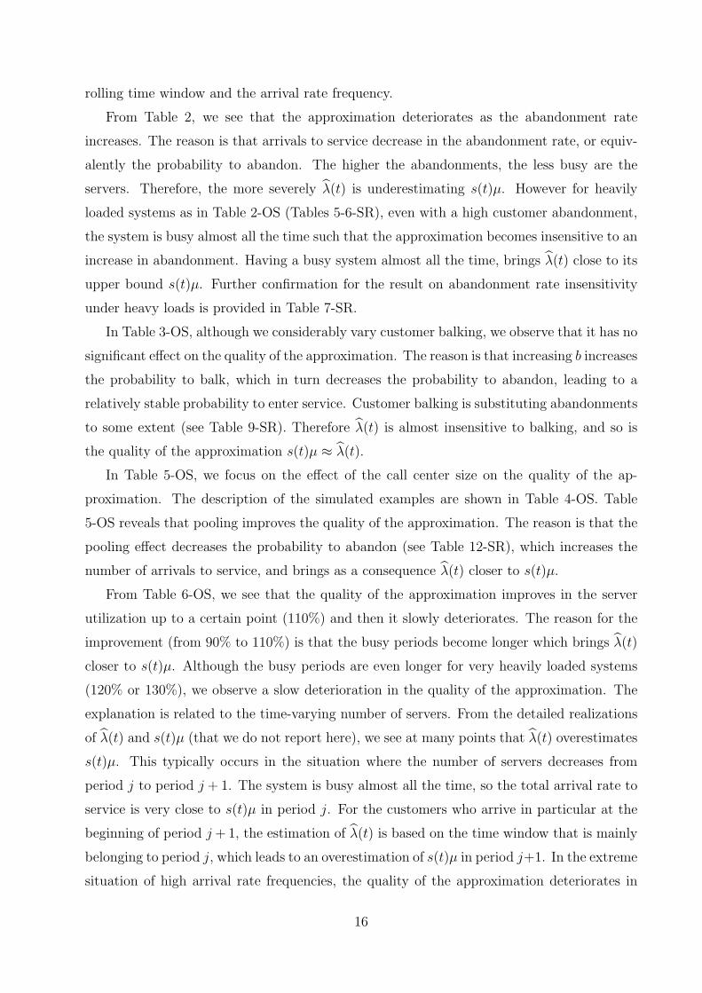
exact one λi(t) (given in Figure 1). An illustration of the results for the case with no retrials

are shown in Table 1. The complete results for different retrial levels are given in Table 1-SR.

Each value in the table is an average of the relative error over all periods. The relative error

in a given period is computed as 100× | λi(t)− λi(t) |λi(t)

, where | x | is the absolute value of

x, for x ∈ R.

Table 1 reveals, for our case with a 10 minute period length, that time windows of 5 or

10 minutes are appropriate for the approximation. A slight preference is for τ = 10, since

it leads to a sufficient number of arrivals allowing to better reach the expected values of

the arrival rates. It is also not too large in order not to cover too many previous periods

where the mean arrival rate can be different. We also see, as expected, that the quality of

13

2

7

12

17

22

27

32

0 20 40 60 80 100 120 140

lambdaA

lambdaB

lambdaC

nbr serveurs

λA(t)λB(t)λC(t)s(t)

period

(a) f = 0.1

2

7

12

17

22

27

32

0 20 40 60 80 100 120 140

lambdaA

lambdaB

lambdaC

nbr serveurs


period

(b) f = 0.2

2

7

12

17

22

27

32

0 20 40 60 80 100 120 140

lambdaA

lambdaB

lambdaC

nbr serveurs


period

(c) f = 0.5

Figure 1: The time varying parameters (λA = 10, λB = 8, λC = 6, a = 2)

the approximation is better for customers who arrive at the end of a period than those who

arrive earlier within the same period. For the former, the time window is indeed included in

the corresponding period, whereas for the latter it overlaps between the period in question

and the previous one where the arrival rate is different. For the same reason of overlap,

we see that the approximation is a bit better for arrivals in the middle of the periods with

τ = 5 than those with τ = 10. For arrivals in the beginning or the middle of a period,

the approximation deteriorates in the frequency. The reason is again related to the overlap

of the time window with previous periods where the mean arrival rate can be considerably

different for high frequencies. Finally, we find as expected that retrials have no impact on

the approximation.

In summary, the experiments confirm that it is appropriate to use the approximation

λi(t) ≈ λi(t) with a time window length similar to that of a period, when t is at the end

of the period, and arrival rate frequencies that are not too high, leading to average relative

errors of around 1%. Retrials do not have an effect on the approximation.

14

5.2.2 Approximation s(t)µ ≈ λ(t)

We investigate the effects of balking, abandonment, retrials, frequencies of the time-varying

arrival rates, the call center size, and the server utilization on the quality of the approximation

s(t)µ ≈ λ(t). Recall that λ(t) = R(t−τ)τ

, where R(t − τ) is the number of arrivals from all

types to service during a time window of (t − τ, t]. Note that λ(t) is estimated at time t,

which is the arrival epoch of a new customer from one of the 3 types.

We consider the call center described in Section 5.2.1 ( 1µ= 1, 1

η= 15, τ = 10 and P = 144

periods of 10 minutes each) and run simulations with various sets of parameters. We assess

the quality of the approximation at the arrival epochs of customers from all types. For each

set of parameters, we run as many replications as needed (with a warm-up period of 40

minutes at the beginning of each replication) in order to collect 3000 conditional realizations

of λ(t), given a busy system and a given number of waiting customers with higher priority

in the queue. More specifically for arrivals type A: for each nA ∈ {0, 1, ..., 10}, we collect

3000 realizations of λ(t) and compare them to their corresponding 3000 realizations of s(t)µ.

We do the same for type B (type C) arrivals for nA + nB ∈ {0, 1, ..., 10} (nA + nB + nC ∈{0, 1, ..., 10}). An illustration of the results pertaining to the effect of abandonments are

shown in Table 2. The detailed results are given in Tables 1-6-OS, and in Tables 2-14-SR.

Each value in the tables corresponds to the average of the relative error over 3000 realizations.

The relative error for a given realization is computed as 100× | λ(t)− s(t)µ |s(t)µ

. To simplify

the presentation in the tables, n denotes nA, nA + nB and nA + nB + nC for types A, B and

C, respectively. Finally note that we choose a given value for ρj for the whole day (same

value for all j) and deduce sj from sj = ⌊λA,j+λB,j+λC,j

µρj⌋+ 1, for j = 1, ..., P .

Table 1-OS reveals that the approximation deteriorates in the frequency of arrival rates.

A high frequency leads to a strong variation of the arrival rates from one period to the next

one. Therefore, a mean arrival rate computed within a time window that overlaps with two

successive periods, i.e., computed at an estimation time at the beginning of a period, may

lead to considerable error. A very small improvement of the approximation can be seen for

the case with retrials. The reason is related to the increase of the arrival load that allows to

counterbalance the negative effect of abandonments as explored below. To see the effect of

the queue lengths on the approximation, we consider high values of n (20, 30, 40 and 50) in

Table 3-SR. This analysis reveals that there is no change in the approximation behavior for

very high queue lengths compared to the results for n = 0, 1, ..., 10. Irrespective of small or

high n, what matters for the approximation s(t)µ ≈ λ(t) is the system busyness during the

15

rolling time window and the arrival rate frequency.

From Table 2, we see that the approximation deteriorates as the abandonment rate

increases. The reason is that arrivals to service decrease in the abandonment rate, or equiv-

alently the probability to abandon. The higher the abandonments, the less busy are the

servers. Therefore, the more severely λ(t) is underestimating s(t)µ. However for heavily

loaded systems as in Table 2-OS (Tables 5-6-SR), even with a high customer abandonment,

the system is busy almost all the time such that the approximation becomes insensitive to an

increase in abandonment. Having a busy system almost all the time, brings λ(t) close to its

upper bound s(t)µ. Further confirmation for the result on abandonment rate insensitivity

under heavy loads is provided in Table 7-SR.

In Table 3-OS, although we considerably vary customer balking, we observe that it has no

significant effect on the quality of the approximation. The reason is that increasing b increases

the probability to balk, which in turn decreases the probability to abandon, leading to a

relatively stable probability to enter service. Customer balking is substituting abandonments

to some extent (see Table 9-SR). Therefore λ(t) is almost insensitive to balking, and so is

the quality of the approximation s(t)µ ≈ λ(t).

In Table 5-OS, we focus on the effect of the call center size on the quality of the ap-

proximation. The description of the simulated examples are shown in Table 4-OS. Table

5-OS reveals that pooling improves the quality of the approximation. The reason is that the

pooling effect decreases the probability to abandon (see Table 12-SR), which increases the

number of arrivals to service, and brings as a consequence λ(t) closer to s(t)µ.

From Table 6-OS, we see that the quality of the approximation improves in the server

utilization up to a certain point (110%) and then it slowly deteriorates. The reason for the

improvement (from 90% to 110%) is that the busy periods become longer which brings λ(t)

closer to s(t)µ. Although the busy periods are even longer for very heavily loaded systems

(120% or 130%), we observe a slow deterioration in the quality of the approximation. The

explanation is related to the time-varying number of servers. From the detailed realizations

of λ(t) and s(t)µ (that we do not report here), we see at many points that λ(t) overestimates

s(t)µ. This typically occurs in the situation where the number of servers decreases from

period j to period j + 1. The system is busy almost all the time, so the total arrival rate to

service is very close to s(t)µ in period j. For the customers who arrive in particular at the

beginning of period j +1, the estimation of λ(t) is based on the time window that is mainly

belonging to period j, which leads to an overestimation of s(t)µ in period j+1. In the extreme

situation of high arrival rate frequencies, the quality of the approximation deteriorates in

16

such a situation. However in another extreme case with zero frequency (constant number

of servers for the whole day), λ(t) would not diverge from s(t)µ as the server utilization

increases. In order to have a more complete picture on the quality of the approximation,

we run further experiments for small and moderately loaded call centers (Table 14-SR). We

observe, as expected, that the approximation deteriorates with lower load (lower utilization

implies shorter busy periods). The relative error is around 28% for ρj = 70% and it decreases

to around 8% for ρj = 100%.

In summary, the quality of the approximation s(t)µ ≈ λ(t) is quite acceptable for a

wide range of parameters, with a relative error of around 2-3%. It mainly deteriorates

to 8-10% for small or light-loaded systems. Since one is usually not interested in delay

announcement in a system that is not very congested, the light-loaded systems are not very

relevant for the application at hand. A lower negative effect is also present for systems with

high abandonments (abandonment rate 3 times higher than the service rate, which is likely

to be an extreme situation in practice), where it deteriorates to around 5%. However for

heavily loaded systems, even with high customer abandonment, the system is busy almost

all the time such that the approximation becomes insensitive to an increase in abandonment.

Having a busy system almost all the time brings λ(t) close to its upper bound s(t)µ. Pooling

can also counteract the negative effect of abandonments to some extent. Customer retrials

slightly improve the approximation by increasing the system load, which counterbalances

the negative effect of abandonment.

5.2.3 Approximation of the Delay Distributions

We next focus on the assessment of the approximation of the conditional distribution of

waiting times, given the queue length, by the proposed distributions (Erlang and normal).

The empirical distributions from the simulation experiments are compared to the proposed

Erlang and normal distributions.

We consider the same simulation experiments as in Section 5.2.2. For a given simulation

run, and a given customer type i ∈ {A,B,C}, we proceed as follows. For customers type

A that arrive to a busy system with a given value of λ(t) and a given number n = nA

of waiting customers, we collect the actual waiting times, which represents the conditional

empirical (exact) distribution, given λ(t) and n. Since λ(t) is a real number, it is difficult

to obtain a sufficient number of observations for one single value of λ(t). Most of the values

of λ(t) are sufficiently high so that it is appropriate to consider for a given n a range of

values of λ(t) belonging to an interval with a length of 2 or 3 and assume that this coincides

17

with the value in the middle of the interval. For example for n = nA = 0, we consider the

actual realizations for λ(t) ∈ [100, 102] and assume that they correspond to λ(t) = 101. The

resulting empirical distribution is then compared to an Erlang and a normal distribution as

proposed herein. The Erlang distribution has n+1 stages with a rate per stage of λ(t). The

normal distribution has mean of (n+ 1)/λ(t) and standard deviation of√n+ 1/λ(t).

We do the same for customers B and C. For customers B, we collect the realizations

of the conditional empirical distribution, given n = nA + nB and a given value of λ(t)

and a given value of λA(t) (we again consider an interval of values of λA(t) with a width

of 2 or 3 and make all the values coincide with the middle of the interval). We compare

this distribution with an Erlang and a normal distribution. The Erlang distribution has

n + 1 stages and a rate of λ(t) − λA(t) per stage. The normal distribution has mean and

standard deviation of n+1

λ(t)−λA(t)and

√(n+1)(λ(t)+λA(t))

(λ(t)−λA(t))3, respectively. For customers C, we

collect the realizations of the conditional empirical distribution, given n = nA + nB + nC

and given values of λ(t) as well as λA(t) + λB(t) (by again considering a range of values of

λA(t)+ λB(t) to obtain a sufficient number of realizations). We then compare this empirical

distribution with an Erlang distribution with n+1 stages and a rate of λ(t)− λA(t)− λB(t)

per stage, a normal distribution with mean and standard deviation of n1+n2+n3+1

λ(t)−λA(t)−λB(t)and√

(n1+n2+n3+1)(λ(t)+λA(t)+λB(t))

(λ(t)−λA(t)−λB(t))3, respectively.

An illustration of the results are shown in Table 3. The complete results are given

in Figures 1-6-OS and Tables 7-12-OS (Further examples are available in Figures 2-23-SR

and Tables 18-39-SR). In the tables, we provide the means and the standard deviations

of the different distributions, and also the probabilities of abandonment for each customer

type (denoted by Pab(i), for i ∈ {A,B,C}). Note that by construction of the approximate

distributions, their expectations as well as the standard deviations are identical. We observe

that the approximate distributions are appropriate except for some extreme situations for C

type customers. Note that the normal approximate distribution in the figures does not start

exactly at t = 0, since this distribution is also defined for negative real values.

For A type customers, the important effects come from abandonment, server utilization

and the call center size. A comparison of Figures 1-2-OS shows that the quality of the

approximation deteriorates for a high abandonment rate and a high n. In such a situation

some customers ahead of the customer of interest may abandon, and our approximation then

leads to an overestimation of the waiting time. Figures 3-4-OS reveal that the approximate

distributions are very accurate for large call centers. For a large call center, the service

18

capacity is sufficiently high so that the conditional waiting time, given n, is shorter than

that in the case of a small call center, which leads to lower abandonments in the former and

as a consequence a better approximation.

For customers B and C (see for example Tables 11-12-OS, Figures 5-6-OS), we find that

the same qualitative conclusions hold. However, the quality of the approximation deteriorates

going from A to C type customers. The reason is related to abandonments. Because of its

lower priority, a newly arriving B call that finds n = nA + nB in the queue has to wait for

those n customers and also all future arrivals A (that will arrive to the queue before her

service) to clear the queue. However, a newly arriving A type caller that finds the same

number n of customers A, has only to wait for those n customers to clear the queue. For

such a situation more customers will therefore abandon in front of a new customer B than

in front of a new customer A, which deteriorates the approximation for type B more than

that of type A. The same conclusion holds for type C, where the approximation seriously

deteriorates for the extreme case of a very high abandonment rate (see for example Figure

15-SR where the abandonment rate is three times the service rate). We also note that this

deterioration is underlined in the chosen numerical examples; the mean arrival rate is the

highest for A, then B and C. The approximation would for example be better for type C

in the case where the arrival rates of types A and B are lower than those in the currently

chosen numerical experiments. Retrials improve the approximation results for B and C type

customers. This is because retrials compensate for abandonments: for a new arrival B, A

callbacks compensate A abandonments. For a new arrival C, A and B callbacks compensate

A and B abandonments. (See Figures 20-23-SR).

In summary and similar to the previous section, we conclude that the approximate distri-

butions are quite appropriate for a wide range of parameters. The approximation deteriorates

in the case of small or light-loaded call centers, or very high abandonment rates. The main

impact comes from abandonments, but again, there should really be an extreme situation of

customer abandonments to seriously deteriorate the approximation. Even in such extreme

cases, the pooling effect in big call centers leads to efficient systems with low probability to

abandon, which allows to improve the quality of the approximation. By compensating for

abandonments, retrials also improve the approximation for B and C customers.

19

5.3 Experiments with Asynchronous Staffing

In the following experiments, the staffing is not synchronized with the arrival rates. This is

more likely to happen in a real life call center, because most of the parameters are unknown

in advance. We construct the simulation scenarios by allowing the server utilization to be

random. For each period j, we randomly pick the value of ρj from a discrete and finite

random distribution, as shown in Table 4. This results in a working day where the staffing

level is either severely underestimated or severely overestimated for most of the periods.

We assess the quality of the different layers of approximation. For the approximation

λi(t) ≈ λi(t), an illustration of the results are shown in Table 5 (Table 41-SR). For the

approximation s(t)µ ≈ λ(t), the results can be found in Table 6, and Tables 13-14-OS

(Tables 42-46-SR). For the approximation of the conditional waiting time distributions, an

illustration of the results are given in Table 7, Tables 15-19-OS and Figures 7-11-OS (Tables

47-54-SR and Figures 24-31-SR).

We observe from Table 5 the same conclusions as those under synchronized staffing. As

one would expect, the asynchronous staffing does not bring any new results. What matters

for the approximation λi(t) ≈ λi(t) are the arrival rate frequency f , the length of the time

window τ , the length of a period, and the position of the time estimate in the period. All of

these are unaffected by the staffing.

Table 13-OS reveals again the same qualitative conclusions with regard to the impact

of the arrival rate frequency on the approximation s(t)µ ≈ λ(t). However the relative

errors are ranging from 10% to 25%, whereas they are only ranging from 3% to 15% under

synchronized staffing situations. The reason is related to the considerable part of the day

with severely under or overstaffed situations. For certain overstaffed periods, λ(t) severely

underestimates s(t)µ. Also, in the beginning of certain overstaffed periods, λ(t) is based on a

previous understaffed period, which makes λ(t) severely underestimate s(t)µ. The opposite

is also true, i.e., in the beginning of certain understaffed periods, λ(t) is based on a previous

overstaffed period, which makes λ(t) severely overestimate s(t)µ. Another new observation is

that the approximation behaves better for types B and C than for type A. Type A customers

are numerous and moreover have the highest priority. Thus, a new type B or C customer is

more likely to find a busy system than an A customer does, which makes the approximation

better for the former.

Table 6 provides the results about the effect of abandonment on the approximation

s(t)µ ≈ λ(t). Similar to the effect of f and for the same reasons, we observe larger errors

20

(mostly ranging between 10-30%) than those for synchronized staffing, and also better results

for types B and C than for type A. The same observations still hold for the effect of the

system size, as shown in Table 14-OS. Tables 6 and 14-OS reveal also that the effect of

abandonment and that of the system size are no longer as clear as they are under the

synchronized staffing. The effects of these parameters are mixed with that of utilization

leading to a non-monotonic behavior. This shows that the effect of utilization is the most

important for the approximation s(t)µ ≈ λ(t), especially for the extreme scenarios as we

consider here.

Although the approximation s(t)µ ≈ λ(t) behaves worse under asynchronous staffing,

the approximate delay distributions behave as in the best cases of synchronized staffing

(see Figures 7-11-OS and Tables 15-19-OS). The explanation is obvious. Since we focus on

conditional distributions, given all the servers are busy, what matters for the approximate

distributions are the situations where the system is busy. Under those situations, the approx-

imation s(t)µ ≈ λ(t) works well, which in turn leads to a good quality for the approximate

delay distributions.

6 Announcing a Delay from the Estimated Delay Dis-

tribution

Recall that the manager’s decision of what to announce to an A-type customer is formulated

as

Min αE[(Dr − da)+] + βE[(da −Dr)

+], (10)

leading to the solution for the optimal announcement as

d∗a = F−1Dr

(γ), (11)

where γ = α/(α + β) and FDr(.) is the cdf of the random variable Dr. Of course, FDr in

the above expression is unknown, and will be replaced by the approximations for A-type

customers in Section 3 to obtain approximately optimal values for da. In particular, the

Erlang approximation then leads to

d∗a,erl = F−1

Derl(γ), (12)

21

and the normal approximation results in

d∗a,norm =n+ 1

λ(t)+ z∗

√n+ 1

λ(t), (13)

where z∗ = Φ−1(γ) and Φ−1(.) denotes the inverse cdf of a standard normal random variable.

As another benchmark, we propose a robust estimator that finds the optimal announce-

ment for the worst-case probability distribution with mean (n + 1)/λ(t) and standard de-

viation√n+ 1/λ(t). The Erlang and normal delay approximations make distributional

assumptions as well as assumptions about the distribution parameters. The distribution

free robust estimator which we propose below provides a benchmark where the worst case

distributional form is found for the given mean and standard deviation. Let DW (da) be the

uncertain delay random variable. Then the penalty maximizing (worst-case) delay distribu-

tion for a given da, is found by solving

maxFDW (da)

αE[DW (da)− da)+] + βE[(da −DW (da))

+],

subject to the constraints E[DW (da)] = (n + 1)/λ(t) and V ar[DW (da)] = (n + 1)/λ(t)2.

No assumptions are made regarding FDW (da) except that it belongs to a class of cumulative

distribution functions with the specified mean and variance.

Let us denote the worst case delay random variable for a given da by D∗W (da). The

decision maker then solves

minda

αE[D∗W (da)− da)

+] + βE[(da −D∗W (da))

+].

The above robust optimization formulation is known as a min-max distribution-free pro-

cedure in the context of the newsvendor problem and leads to a surprisingly simple solution

(Scarf (1958); Gallego and Moon (1993)) for the optimal da. It is given by

d∗a,rob =n+ 1

λ(t)+

√n+ 1

2λ(t)

(√α

β−√

β

α

).

We follow the same approach for the B-type calls, where the estimators for the mean and

standard deviation of the delay, and delay distribution approximations from Section 4 are

used to obtain approximately optimal values for da. For the robust delay announcement of

22

B-type calls we thus obtain

d∗a,rob =n1 + n2 + 1

λ(t)− λA(t)+

1

2

√(n1 + n2 + 1)(λ(t) + λA(t))

(λ(t)− λA(t))3

(√α

β−√

β

α

).

7 Data-Based Validation of Delay Announcements

We explore the performance of delay announcements under the two approximations (Erlang

and normal) for different values of γ = α/(α+ β), by comparing them to the corresponding

announcements for the data on state dependent waiting times. This data based validation

allows us to assess the value of the approximations in making delay announcements in a real

call center setting. Thus we show that under all complexities of a real operation, the earlier

tested simple approximations perform well also when used in making delay announcements.

In our numerical examples, we have fixed β = 1 without loss of generality. We measure

the performance of each estimator with respect to the realized waiting time distribution.

The benchmark cost function is

C∗r = αE[(Dr − d∗a,r)

+] + βE[(d∗a,r −Dr)+]. (14)

For any estimator (e ∈ {erl, norm, rob}), we compute

Ce = αE[(Dr − d∗a,e)+] + βE[(d∗a,e −Dr)

+], (15)

and report the percentage relative difference computed as

∆e =Ce − C∗

r

C∗r

× 100%. (16)

In addition to the two estimators, we also consider the prevalent practice in call centers (and

earlier literature), which is to announce the mean of the delay distribution. In our analysis,

we estimate the mean making use of the estimators that were proposed in Sections 3 and 4.

For the A type calls we have (n+ 1)/λ(t) where we use the n and λ(t) value corresponding

to a given data set. Similarly for the B types we make use of the expression in Equation (7)

with the corresponding n, λ(t) and λA(t) values of each data set.

Our data comes from one of the sites. Each data set is for an observed arrival rate and

a given queue state. Thus, samples of queue length dependent waiting times when the same

local arrival rates (i.e., estimated by the number of arrivals in the last ten minutes) prevail

23

have been collected within a set. The data set is relatively small and limited, however is quite

unique in that such state dependent call by call data is not easily extractable from existing

call center software. The data sets were established manually by an analyst at this call

center. For the B-type calls, the separate call volumes of A-type calls have been estimated

by making use of the average percent of A-type calls received during the data collection

period in that particular call center (43% of the calls were generated by the A-type in the

data collection period at this call center). As such, the B-type data sets are subject to an

additional layer of approximation. For the A-type calls, we make use of eleven sets, under

three different local arrival rates. For the B-type calls we have fourteen sets under different

local arrival rates. The number of observations in each set are tabulated in Tables 8 and 9.

Using the expression in (15) with d∗a,e replaced by the mean delay, we can determine the

cost performance of announcing the mean. The relative error of announcing a given percentile

from the approximated Erlang distribution versus the approximated normal distribution, as

well as the robust benchmark and the relative error of announcing the mean delay, all grouped

by γ values, are tabulated in Tables 10 and 11. We report the mean of the relative errors as

well as the quartile estimates of the relative error values taken in the data sets we consider. In

Tables 12 and 13 we show results grouped by the value of nA and nA+nB respectively, where

the mean and the quartile estimates of relative error values are reported across different γ

values.

Recall that the call center from which this data was collected experienced abandonment

probabilities that could reach 5%. The earlier simulation experiments show that as abandon-

ment probabilities increase, the error in approximated conditional mean delay (and standard

deviations) and thus the error in delay prediction increases, since abandonments are ignored

in the approximations. However as utilization is high and the call center is large, we expect

some of the errors due to abandonments to be mitigated in the data.

For the A-type calls, observe from Table 10 that while announcing the mean delay does

quite well for a γ value that is close to 0.5, its performance deteriorates dramatically as the

customers attach a higher penalty to under-announcements. The Erlang approximation per-

forms well across all γ values. Comparing the normal approximation based announcements

to the robust delay announcement, we observe that once the mean and standard deviation

have been estimated, it is better to use the robust delay announcement, which performs

particularly well for γ values 0.7 and 0.8. When we look at the results in Table 12 averaging

across γ values, the superiority of using the Erlang approximation is further emphasized.

Note that the mean delay announcement does uniformly bad when the results are tabulated

24

this way (due to its bad performance for higher γ values), and once again the robust esti-

mator provides a second-best alternative to the Erlang approximation. Results in Table 12

do not allow us to conclude that there is a systematic effect of the queue length nA on the

performance of the estimators.

For the B-type calls, the relative errors are higher compared to the A-type ones. This

is not surprising due to the increasing level of approximations being performed both in the

data and models. However, the Erlang-based announcement is still quite good for all γ

values, particularly as these are getting higher. Announcing the mean appears to be the

best option for γ values 0.6 and 0.7, but it deteriorates for higher γ values. Thus, without a

good understanding of these penalties, announcing the mean seems risky. This is confirmed

when we look at the results in Table 13, where excluding the case when the queue is long

with nA +nB = 6, the mean announcement is on average outperformed by the Erlang based

one. Both Tables 11 and 13 show that the normal approximation is not competitive for the

B-type calls. According to Table 13, the robust delay announcement ensures an average

relative error of around 10% except in the case of nA + nB = 6. Excluding the latter case,

the robust estimator mostly outperforms the mean and the normal approximation based

announcements.

In the previous analysis, we compared the performance of different delay announcements

and concluded that the choice of which announcement to prefer may depend on the value of

γ. This parameter captures the manager’s understanding of the costs associated with under

or over-announcing the delays. The meaning of these costs may differ by context and in

general estimating these costs may be difficult. Nevertheless, if the manager believes there is

some asymmetry in these costs, our analysis shows that it may be worth using the framework

proposed herein to make announcements, by using a γ value that appropriately reflects this

asymmetry.

What happens if the perceived γ used by the manager is different from the real underlying

γ? We explore this question next. In order to analyze the effect of the misperception of γ

in isolation, we focus on the real delay distribution for the A-type calls and consider the

relative cost when the manager announces the delay that corresponds to the perceived γ, yet

costs are accrued based on the real underlying γ for the four values of γ = 0.6, 0.7, 0.8, 0.9

considered. The results are tabulated in Tables 14 through 16. From these we observe that

for a +/ − 0.1 mistake in γ the relative error in cost is less than 10% in 90% of the cases

and takes the maximum value of 15% relative error in cases where 10% error is exceeded.

The results suggest that unless there is a major misperception of γ, the framework proposed

25

herein can be used.

8 Concluding Remarks

In conclusion, we can state that despite the many simplifying assumptions we have made in

modeling the actual system, the resulting Erlang distribution approximation for the delay

distribution performs very well when we announce the optimal delay from this distribution.

Making use of the physical aspects of the underlying queueing system clearly helps relative to

just estimating the first two moments of the delay distribution and using it within a normal

distribution. The robust delay announcement that makes use of the moment estimators

provides an alternative that protects against the worst case when such queueing analysis

is not available. The idea of a robust delay announcement is new, and should be explored

further in future practice as well as research, particularly in settings with high complexity

and uncertainty like the one we considered.

Finally, with customers that dislike under-announcement, the current practice of an-

nouncing the mean of the delay distribution may lead to high dissatisfaction. For the high

priority calls, both the Erlang and the robust estimators provide a better alternative. Nev-

ertheless, our analysis of the lower priority calls indicates that as long as these customers are

not too sensitive to under-announcement, announcing the estimated mean can be considered.

To the best of our knowledge, this is the first paper that acknowledges the possibility of

asymmetric penalties for over and under announcing in a delay announcement context for

services. Both industry practice and earlier literature consider announcing the mean delay.

While the latter is easy to implement, the former seems more consistent with evidence from

the behavioral literature. Further research that explores this issue empirically needs to be

pursued.

References

Aksin, O.Z., B. Ata, S. Emadi, C.L. Su. 2013. Impact of delay announcements in call centers: An

empirical approach. Working paper.

Allon, G., A. Bassamboo, I. Gurvich. 2011. “we will be right with you”: Managing customers with

vague promises. Operations Research 59 1382–1394.

Anderson, R.E. 1973. Consumer dissatisfaction: The effect of disconfirmed expectancy on perceived

product performance. Journal of Marketing Research 10 38–44.

26

Armony, M., C. Maglaras. 2004. Contact centers with a call-back option and real-time delay

information. Operations Research 52 527–545.

Armony, M., N. Shimkin, W. Whitt. 2009. The impact of delay announcements in many-server

queues with abandonment. Operations Research 57 66–81.

Brown, L., N. Gans, A. Mandelbaum, A. Sakov, H. Shen, S. Zeltyn, L. Zhao. 2005. Statistical

analysis of a telephone call center: A queueing-science perspective. Journal of the American

Statistical Association 100 36–50.

Feigin, P. 2005. Analysis of customer patience in a bank call center. Working paper, The Technion.

Gallego, G., I. Moon. 1993. The distribution free newsboy problem: Review and extensions. The

Journal of the Operational Research Society 44 825–834.

Guo, P., P. Zipkin. 2007. Analysis and comparison of queues with different levels of delay informa-

tion. Management Science 53 962–970.

Hasija, S., E. Pinker, R.A. Shumsky. 2010. Work expands to fill the time available: Capacity estima-

tion and staffing under parkinson’s law. Manufacturing and Service Operations Management

44 1–18.

Hassin, R., M. Haviv, eds. 2003. To Queue or Not to Queue. Kluwer Academic Publishers.

Hui, M., D. Tse. 1996. What to tell customer in waits of different lengths: an integrative model of

service evaluation. Journal of Marketing 60 81–90.

Hui, M., L. Zhou. 1996. How does waiting duration information influence customers’ reactions to

waiting for services? Journal of Applied Social Psychology 26 1702–1717.

Ibrahim, R., W. Whitt. 2009. Real-time delay estimation based on delay history. Manufacturing

& Service Operations Management 11 397–415.

Ibrahim, R., W. Whitt. 2011. Wait-Time Predictors for Customer Service Systems with Time-

Varying Demand and Capacity. Operations Research 59 1106–1118.

Jouini, O., O.Z. Aksin, M.S. Aguir, F. Karaesmen, Y. Dallery. 2014. Supplementary results to

“call center delay announcement using a newsvendor-like performance criterion” Available at

http://www.lgi.ecp.fr/~jouini/documents/AnnouncementNewsvendorSuppResults.pdf.

Jouini, O., Y. Dallery, O.Z. Aksin. 2011. Call centers with delay information: Models and insights.

Manufacturing & Service Operations Management 13 534–548.

Jouini, O., Y. Dallery, O.Z. Aksin. 2009. Queueing models for full-flexible multi-class call centers

with real-time anticipated delays. International Journal of Production Economics 120 389–

399.

Kleinrock, L. 1975. Queueing Systems, Theory , vol. I. A Wiley-Interscience Publication.

27

Kumar, P., M.U. Kalwani, M. Dada. 1997. The impact of waiting time guarantees on customers

waiting experiences. Marketing Science 16 295–314.

Munichor, N., A. Rafaeli. 2007. Numbers or apologies? customer reactions to telephone waiting

time fillers. Journal of Applied Psychology 95 511–518.

Nakibly, E. 2002. Predicting Waiting Times in Telephone Service Systems. Ph.D. Thesis, Technion.

Naor, P. 1969. The regulation of queue size by levying tolls. Econometrica 37 15–24.

Parasuraman, A., V.A. Zeithaml, L. Berry. 1985. A conceptual model of service quality and

implications for future research. Journal of Marketing 64 12–40.

Pazgal, A.I., S. Radas. 2008. Comparison of customer balking and reneging behavior to queueing

theory predictions: An experimental study. Computers and Operations Research 35 2537 –

2548.

Scarf, H. 1958. A min-max solution of an inventory problem. In Studies in The Mathematical

Theory of Inventory and Production. (K. ARROW, S. KARLIN and H. SCARF, Eds) pp

201-209. Stanford University Press, California. .

Whitt, W. 1999a. Improving service by informing customers about anticipated delays. Management

Science 45 192–207.

Whitt, W. 1999b. Predicting queueing delays. Management Science 45 870–888.

Whitt, W. 2006. Staffing a call center with uncertain arrival rate and absenteeism. Production and

Operations Management 15 88–102.

Xu, S.H., L. Gao, J. Ou. 2007. Service performance analysis and improvement for a ticket queue

with balking customers. Management Science 53 971–990.

Zipkin, P.H., ed. 2000. Foundations of Inventory Management . McGraw-Hill Singapore.

28

Table 1: Average relative error for the approximation λi(t) ≈ λi(t) under synchronizedstaffing and no retrials (λA = 10, λB = 8, λC = 6, a = 2, θ = 0.5, b = 0.2, r = 0, andρj = 120% for j = 1, ..., P )

Frequency Time in τ = 5 τ = 10 τ = 20 τ = 30the period A B A B A B A B

Beginning 1.88% 2.13% 1.72% 1.92% 2.48% 2.86% 3.37% 3.92%f = 0.1 Middle 0.78% 0.97% 0.94% 1.14% 1.66% 1.91% 2.52% 2.91%

End 0.78% 0.97% 0.00% 0.00% 0.86% 0.96% 1.66% 1.91%


End 0.83% 0.96% 0.00% 0.00% 1.36% 1.69% 2.85% 3.50%


End 0.80% 0.87% 0.00% 0.00% 3.19% 4.00% 6.36% 7.94%

Table 2: Effect of abandonment under synchronized staffing (ρj = 100% for j = 1, ..., P ,λA = 50, λB = 40, λC = 30, a = 10, f = 0.2, b = 0)

No retrials, r = 0

n = 0 n = 2 n = 4 n = 10θ A B C A B C A B C A B C

0.1 2.30% 2.88% 2.63% 2.74% 2.74% 2.63% 3.01% 2.91% 2.54% 3.08% 3.15% 2.63%0.5 3.00% 3.45% 3.20% 3.98% 3.74% 3.17% 3.49% 3.65% 3.25% 3.69% 3.64% 3.26%1 3.76% 3.99% 3.64% 4.18% 4.25% 3.71% 4.06% 4.08% 3.76% 4.19% 4.33% 3.79%3 4.51% 4.92% 4.55% 4.58% 4.64% 4.40% 4.69% 4.52% 4.52% 4.68% 4.86% 4.60%

With retrials, r = 0.5


0.1 2.12% 2.63% 2.62% 2.83% 2.82% 2.59% 2.91% 3.10% 2.49% 3.37% 3.08% 2.59%0.5 3.19% 3.21% 2.96% 3.32% 3.24% 3.05% 3.49% 3.27% 3.09% 3.70% 3.70% 3.14%1 3.55% 3.80% 3.67% 4.24% 4.12% 3.70% 4.05% 3.92% 3.75% 4.42% 4.26% 3.84%3 5.23% 4.67% 4.49% 4.64% 4.50% 4.34% 4.76% 4.63% 4.53% 4.98% 4.87% 4.70%

Table 3: Conditional delays for type A under synchronized staffing and no retrials (ρj = 100%

for j = 1, ..., P , λA = 50, λB = 40, λC = 30, a = 10, f = 0.2, b = 0, r = 0, λ(t) = 141.5),Pab(A) = 0.105%, Pab(B) = 0.398%, Pab(C) = 5.524%

n = 0 n = 1 n = 4Exact Erlang Normal Exact Erlang Normal Exact Erlang Normal

Expectation 0.0075 0.0071 0.0071 0.0131 0.0141 0.0141 0.0352 0.0353 0.0353Standard deviation 0.0077 0.0071 0.0071 0.0087 0.0100 0.0100 0.0158 0.0158 0.0158



Table 4: Random values for ρj, j = 1, ..., P

ρj 40% 70% 100% 130% 160% 190%

Probability 1/3 1/9 1/18 1/18 1/9 1/3

29

Table 5: Average relative error for the approximation λi(t) ≈ λi(t) under asynchronizedstaffing and no retrials (λA = 50, λB = 40, λC = 30, a = 10, θ = 0.5, b = 0.1, r = 0)

Frequency Time in τ = 5 τ = 10 τ = 20 τ = 30the period A B A B A B A B


End 0.75% 0.90% 0.00% 0.00% 0.84% 1.03% 1.64% 1.94%


End 0.79% 0.84% 0.00% 0.00% 1.37% 1.69% 2.84% 3.46%


End 0.81% 0.84% 0.00% 0.00% 3.18% 4.04% 6.35% 8.03%

Table 6: Effect of abandonment under asynchronized staffing and no retrials (λA = 50,λB = 40, λC = 30, a = 10, f = 0.2, b = 0.1, r = 0)


0.1 27.90% 38.88% 14.80% 18.35% 23.47% 15.06% 19.36% 15.33% 15.88% 23.23% 11.89% 15.96%0.5 18.49% 13.95% 10.10% 17.94% 11.79% 9.58% 18.41% 10.94% 9.97% 24.43% 10.40% 11.28%1 20.66% 9.48% 8.99% 17.39% 9.54% 9.46% 20.23% 10.39% 9.58% 26.55% 11.70% 10.56%3 21.74% 12.28% 10.25% 18.97% 13.16% 10.18% 20.08% 15.24% 10.37% 36.43% 19.14% 11.22%

Table 7: Conditional delays for type A under asynchronized staffing and retrials (λA = 50,

λB = 40, λC = 30, a = 10, b = 0.1, f = 0.2, λ(t) = 71.5, r = 0.5), Pab(A) = 0.486%,Pab(B) = 16.854%, Pab(C) = 31.159%





Table 8: Number of observations in data sets for A-type calls, where n = nA

n=2 n=3 n=4 n=5 n=6

λ(t) = 2.2 264 128 109 - -

λ(t) = 3.2 622 251 227 87 102

λ(t) = 4.2 768 208 228 - -

30

Table 9: Number of observations in data sets for B-type calls, where n = nA + nB

n=2 n=3 n=4 n=6

λ(t) = 3.4, λB + λC = 1.4 94 - - -

λ(t) = 4.0, λB + λC = 1.4 116 - - -

λ(t) = 4.0, λB + λC = 1.8 - - - 83

λ(t) = 4.2, λB + λC = 1.8 - - 92 -

λ(t) = 4.38, λB + λC = 2.5 843 738 649 -

λ(t) = 4.4, λB + λC = 1.8 99 - - -

λ(t) = 5.26, λB + λC = 3.0 1020 489 689 -

λ(t) = 7.0, λB + λC = 4.0 311 74 208 -

Table 10: Relative error mean and quartiles for A-type calls grouped by γ valuesγ = 0.6 γ = 0.7

Erlang Normal Robust Mean Erlang Normal Robust Mean

mean 1.46 4.72 2.73 1.17 1.7 3.82 1.96 4.8925 0.02 1.34 0.19 0.38 0 0.46 0.03 0.4350 0.27 1.51 0.49 0.91 0.61 0.62 0.36 6.3875 3.53 7.95 6.01 2 2.53 5.92 2.46 8.51100 6.4 19.66 12.49 3.2 8.4 18.94 11.57 8.59

γ = 0.8 γ = 0.9

mean 2.42 2.96 1.9 19.81 2.71 2.38 2.46 66.525 0.15 0.01 0.22 11.68 0.10 0.14 0.20 47.5850 0.62 0.53 0.77 19.42 0.94 1.15 1.13 60.9575 2.35 4.98 2.90 24.70 4.45 4.46 5.48 75.11100 12.98 13.91 9.69 29.02 9.66 7.42 6.74 86.86

Table 11: Relative error mean and quartiles for B-type calls grouped by γ valuesγ = 0.6 γ = 0.7


mean 9.94 23.36 17.54 7.27 7.11 20.82 14.25 2.6925 0.96 8.55 3.14 0.60 0.35 6.23 1.53 0.0750 5.83 22.53 10.73 3.54 2.23 17.60 7.93 1.0975 12.66 26.50 22.10 7.32 10.57 27.58 21.04 2.19100 43.48 67.92 60.39 37.15 32.03 53.49 46.09 12.06

γ = 0.8 γ = 0.9

mean 4.83 17.77 12.17 8.11 3.58 11.58 11.58 38.2825 0.50 3.62 0.75 1.77 0.06 0.43 0.18 25.7050 1.83 14.38 7.64 5.43 2.57 7.31 7.05 30.9875 6.08 25.50 19.57 9.51 4.78 19.83 21.36 44.36100 22.77 49.13 40.59 29.19 12.23 31.70 31.26 82.71

Table 12: Relative error mean and quartiles for A-type calls grouped by queue lengthnA = 2 nA = 3 nA = 4

Erlang Normal Robust Mean Erlang Normal Robust Mean Erlang Normal Robust Mean

mean 3.43 5.61 3.73 19.68 1.4 2.76 1.57 23.22 1.58 2.47 1.86 24.7525 0.03 0.51 0.39 1.38 0 0.21 0.21 1.18 0 0.14 0.05 0.9950 0.68 1.97 0.84 5.35 0.16 1.25 0.24 6.52 0.29 0.65 0.68 8.5975 6.4 5.76 6.16 29.02 1.83 3.82 0.91 25.15 2.43 4.86 2.68 27.05100 12.98 19.66 12.49 81.94 7.42 9.41 6.74 80.02 4.86 8.67 6.58 86.86

nA = 5 nA = 6

mean 2.49 3.74 1.94 28.01 0.74 1.67 1.02 28.0625 0.09 0.74 0.54 1.22 0.13 0.06 0.08 0.0450 1.95 1.62 1.23 6.83 0.21 0.44 0.9 375 2.76 5.17 2.35 18.76 0.66 0.74 1.23 23.97100 5.16 7.43 3.64 85.22 1.95 5.45 1.89 85.22

31

Table 13: Relative error mean and quartiles for B-type calls grouped by queue lengthnA + nB = 2 nA + nB = 3


mean 3.43 5.61 3.73 19.68 1.40 2.76 1.57 23.2225 0.03 0.51 0.39 1.38 0.00 0.21 0.21 1.1850 0.68 1.97 0.84 5.35 0.16 1.25 0.24 6.5275 6.40 5.76 6.16 29.02 1.83 3.82 0.91 25.15100 12.98 19.66 12.49 81.94 7.42 9.41 6.74 80.02

nA + nB = 4 nA + nB = 6

mean 1.58 2.47 1.86 24.75 2.49 3.74 1.94 28.0125 0.00 0.14 0.05 0.99 0.09 0.74 0.54 1.2250 0.29 0.65 0.68 8.59 1.95 1.62 1.23 6.8375 2.43 4.86 2.68 27.05 2.76 5.17 2.35 18.76100 4.86 8.67 6.58 86.86 5.16 7.43 3.64 85.22

Table 14: Relative error due to misperceived γ for A-type calls under λ(t) = 2.2nA = 2 nA = 3 nA = 4

Real/perceived 0.9 0.8 0.7 0.6 0.9 0.8 0.7 0.6 0.9 0.8 0.7 0.6

0.9 0.00 0.11 0.32 0.52 0.00 0.14 0.38 0.88 0.00 0.15 0.42 0.800.8 0.13 0.00 0.05 0.13 0.04 0.00 0.03 0.21 0.15 0.00 0.07 0.220.7 0.35 0.05 0.00 0.02 0.23 0.04 0.00 0.05 0.39 0.05 0.00 0.040.6 0.62 0.17 0.03 0.00 0.49 0.18 0.06 0.00 0.71 0.18 0.04 0.00


Real/perceived 0.9 0.8 0.7 0.6 0.9 0.8 0.7 0.6 0.9 0.8 0.7 0.6

0.9 0.00 0.15 0.35 0.53 0.00 0.10 0.20 0.56 0.00 0.09 0.36 0.770.8 0.14 0.00 0.05 0.13 0.11 0.00 0.05 0.17 0.15 0.00 0.06 0.220.7 0.39 0.04 0.00 0.02 0.31 0.04 0.00 0.03 0.35 0.06 0.00 0.050.6 0.69 0.15 0.02 0.00 0.58 0.16 0.03 0.00 0.62 0.19 0.04 0.00

nA = 5 nA = 6

0.9 0.00 0.09 0.19 0.37 0.00 0.09 0.44 0.900.8 0.07 0.00 0.03 0.11 0.06 0.00 0.09 0.260.7 0.21 0.02 0.00 0.03 0.18 0.03 0.00 0.040.6 0.37 0.07 0.02 0.00 0.40 0.18 0.05 0.00


Real/perceived 0.9 0.8 0.7 0.6 0.9 0.8 0.7 0.6 0.9 0.8 0.7 0.6

0.9 0.00 0.11 0.31 0.58 0.00 0.10 0.36 0.67 0.00 0.09 0.22 0.580.8 0.11 0.00 0.05 0.17 0.11 0.00 0.06 0.19 0.05 0.00 0.02 0.180.7 0.29 0.04 0.00 0.03 0.30 0.05 0.00 0.04 0.20 0.04 0.00 0.040.6 0.54 0.15 0.04 0.00 0.56 0.18 0.04 0.00 0.41 0.15 0.05 0.00

32

Call Center Delay Announcement Using a Newsvendor-Like ...

Documents