California Water Demand Scenarios David Groves Pardee RAND Graduate School Scott Matyac and Tom Hawkins Department of Water Resources * * * California Water Plan Update Advisory Committee Meeting January 20, 2005

California Water Demand Scenarios David Groves Pardee RAND Graduate School Scott Matyac and Tom Hawkins Department of Water Resources * * * California.
Dec 18, 2015
Welcome message from author
This document is posted to help you gain knowledge. Please leave a comment to let me know what you think about it! Share it to your friends and learn new things together.
Transcript

California Water Demand Scenarios
David GrovesPardee RAND Graduate School
Scott Matyac and Tom HawkinsDepartment of Water Resources
* * *
California Water Plan Update Advisory Committee Meeting
January 20, 2005
2 - Groves- Jan 20, 05
Purpose of Analysis
• Provide preliminary quantitative estimates of 2004 Water Plan narrative water demand scenarios (not FORMAL estimates)
• Advance conceptual thinking on using a scenario approach for future Water Plans
• Create a scenario estimator for other non-Water Plan related analyses
3 - Groves- Jan 20, 05
History of Collaboration
• Water Plan Staff and Advisory Committee embraced scenario approach for Water Plan phased work plan
• Concurrently, RAND began a scenario-based look at long-term water resources planning in California
• RAND and Water Plan staff now collaborating to create water demand scenario generator and quantify narrative scenarios
• RAND expects to continue to use and develop this model for further analyses
4 - Groves- Jan 20, 05
Approach1) Create model to generate plausible average 2030 water
demand scenarios– Simple, understandable, fast running, and easily
modifiable– Ability to mimic/incorporate results of detailed models– Specify scenarios through unique parameter values
2) Select parameter values congruent to narrative descriptions
3) Quantify, evaluate, and interpret projected water demand– Test for plausibility– Identify aspects needing further study– Gain insight
4) Follow-up with more detailed analysis

5 - Groves- Jan 20, 05
A Few Words About Scenarios
• Scenarios are NOT predictions– No one scenario is expected to predict what will occur– Instead, they reflect multiple plausible views of the future
• Scenarios are useful when– Ability to predict is low due to large uncertainties– Individual outcomes are important
• Desire to avoid low probability, negative events
• Scenarios help analysts and decision-makers:– Evaluate uncertain potential outcomes– Generate new ideas for successful policies
• Scenarios should be evaluated together as a package
6 - Groves- Jan 20, 05
The Water Demand Scenario Estimator
• Three Modules– Urban– Agricultural– Environmental
• Annual time step from 2000 to 2030
• Disaggregated by Hydrologic Region
7 - Groves- Jan 20, 05
Urban Water Demand
• Estimates based upon projections of water use by:– Households– Economic activity (based on employment)– Public activities (based on population)– Losses and intentional groundwater recharge
• Water use per demand unit varies – Water price, income, household size, naturally occurring
conservation, and efficiency adoption
• Initialized using year 2000 data
• Can use detailed models (e.g. IWR-MAIN) for calibration
8 - Groves- Jan 20, 05
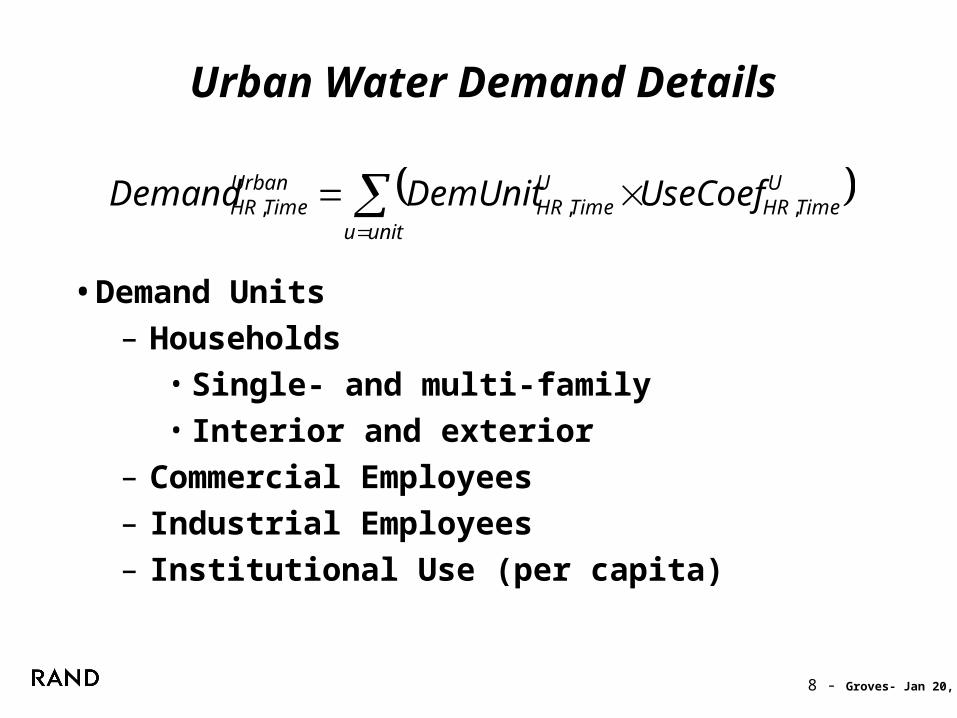
Urban Water Demand Details
• Demand Units– Households
• Single- and multi-family• Interior and exterior
– Commercial Employees– Industrial Employees– Institutional Use (per capita)
unitu
UTimeHR
UTimeHR
UrbanTimeHR UseCoefDemUnitDemand ,,,
9 - Groves- Jan 20, 05
Population Changes DriveHousing and Employment
• SF and MF houses a function of:– Population– Fraction of population housed– Share of SF houses – Household Size
• Commercial & Industrial employees a function of:– Population– Employment rate– Share of commercial versus industrial jobs

10 - Groves- Jan 20, 05
Agricultural Water Demand
• Estimates based on:– Projected future agricultural land use – Changes in crop water needs– Changes in water application technology and
practices
• Uses results of other models for calibration– ETAW (initializing data)– CALAG (when ready)

11 - Groves- Jan 20, 05
Irrigation Demand Calculated by Estimating Crop Demand
• IU = State-wide irrigation water use
• ICA = Irrigated crop area
Irrigated Land Area + Multi-cropped Area
• AW = Required applied water per area by crop
R
HR
C
cropHRcropHRcrop AWICAIU
1 1,,
12 - Groves- Jan 20, 05
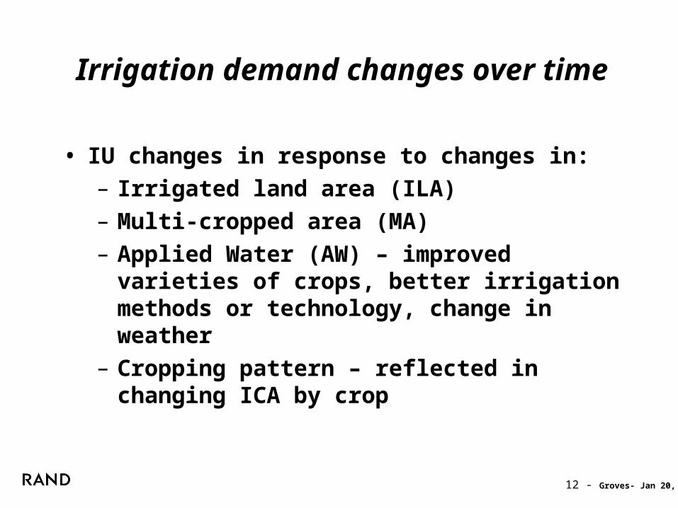
Irrigation demand changes over time
• IU changes in response to changes in:– Irrigated land area (ILA)– Multi-cropped area (MA)– Applied Water (AW) – improved varieties of
crops, better irrigation methods or technology, change in weather
– Cropping pattern – reflected in changing ICA by crop
13 - Groves- Jan 20, 05
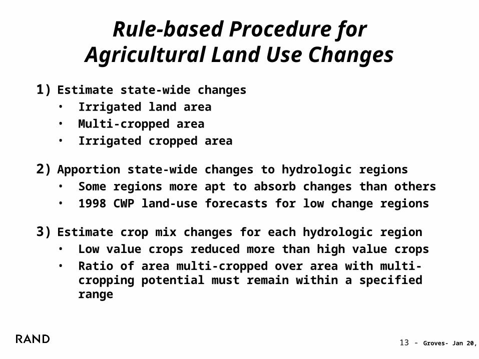
Rule-based Procedure forAgricultural Land Use Changes
1) Estimate state-wide changes• Irrigated land area• Multi-cropped area• Irrigated cropped area
2) Apportion state-wide changes to hydrologic regions• Some regions more apt to absorb changes than others• 1998 CWP land-use forecasts for low change regions
3) Estimate crop mix changes for each hydrologic region• Low value crops reduced more than high value crops• Ratio of area multi-cropped over area with multi-
cropping potential must remain within a specified range

14 - Groves- Jan 20, 05
Environmental Demand
• Very rudimentary procedure– Based on year 2000 unmet needs
(Environmental Defense)
• More complete treatment would incorporate variable hydrology
ED Sites TAFAmerican 55Stanislaus 34ERP #1 0ERP #2 65ERP #4 0Trinity 344SJR @ Vernalis 96SJR below Friant 268Level 4 Refuges 125Total 987
Hydrologic Region TAFNC 344SF 0CC 0SC 0SR 183SJ 461TL 0NL 0SL 0CR 0
Total 987

15 - Groves- Jan 20, 05
Water Plan Narrative Scenarios
SCENARIO 1 SCENARIO 2 SCENARIO 3
DOF DOF Higher than DOFDOF Higher than DOF Lower than DOF
Higher Inland & SouthernLower Coastal & Northern
Current Trend Increase in Trend Increase in Trend (as in 2)Current Trend Decrease in High Water Using Activities Increase in High Water Using ActivitiesCurrent Trend Increase in Trend Increase in Trend (as in 2)Current Trend Decrease in High Water Using Activities Increase in High Water Using ActivitiesCurrent Trend Level Out at Current Crop Area Level Out at Current Crop AreaCurrent Trend Decrease in Crop Unit Water Use Increase in Crop Unit Water UseCurrent Trend High Environmental Protection High Environmental ProtectionCurrent Trend High Environmental Protection High Environmental Protection
NOC Trend in MOUs Higher than NOC Trend in MOUs Lower than NOC Trend in MOUs
FACTORCURRENT TRENDS RESOURCE EFFICIENT RESOURCE INTENSIVE
Total PopulationPopulation Density
Population Distribution DOF DOF
Commercial ActivityCommercial Activity MixTotal Industrial ActivityIndustrial Activity Mix
Total Crop AreaCrop Unit Water Use
Environmental Water-Flow Based
Ag Water Use Efficiency All Cost Effective BMPs in Existing MOUs Implemented by Current Signatories (present commitments)
Environmental Water-Land Based
Naturally Occurring Conservation
Urban Water Use Efficiency All Cost Effective BMPs in Existing MOUs Implemented by Current Signatories (present commitments)
Chapter 3, Table 3-1
16 - Groves- Jan 20, 05
No single method for choosing numerical values for parameters
• There is no “correct” scenario
• Other modeling studies inform quantification– Ex: DOF demographic projections
• Important to quantify drivers independently of scenario results
• Check intermediate results for plausibility

17 - Groves- Jan 20, 05
Scenario Specification (Urban 1)Table 1: Parameters for Urban Demand Drivers for Water Plan Scenarios.
Parameter Current Trends Resource Efficient Resource Intensive DOF Trends Old DOF Trends
Total Population 48.1 million (2030)
As Current Trends 52.3 million (2030)
DOF Trends 125% current DOF Trends Inland and Southern (SC, SL, CR, SR, SJ, TL) 37.3 million (2030)
As Current Trends 41.1 million (2030)
DOF Trends 116% current DOF Trends Coastal and Northern (NC, SF, CC, NL) 10.8 million (2030)
As Current Trends 11.2 million (2030)
DOF trends (varies by HR) Housed Population Fraction Nearly Constant (~98%)
As Current Trends As Current Trends
DOF Trends (varies by HR) DOF Trends + 10% DOF Trends - 5% MF Housing Share
35.5% (2000) 33.9% (2030) 35.5% (2000) 43.9% (2030)
35.5% (2000) 28.9% (2030)
DOF Trends (varies by HR) SF House size
3.13 (2000 ave.) 3.06 (2030 ave.) DOF Trends + 0.2 persons/household
As Current Trends
DOF Trends (varies by HR) MF House size
2.41 (2000 ave.) 2.38 (2030 ave.) DOF Trends + 0.2 persons/household
As Current Trends
DOF Trends (varies by HR) Mean Income (1996 Dollars) $87,225 (2000) $116,269 (2030)
As Current Trends As Current Trends
Employment Fraction Woods and Poole Trends (by HR)
58% (2000, ave) 60% (2030, ave) As Current Trends
+ 2.5% As Current Trends + 2.5%
Woods and Poole Trends (by HR) Commercial Fraction
83% (2000, ave) 86% (2030, ave) As Current Trends As Current Trends

18 - Groves- Jan 20, 05
Scenario Specification (Urban 2)Table 2: Domestic Water Demand Factor Parameters for Water Plan scenarios. Parameter Current Trends Resource Efficient Resource Intensive
Price Elasticity – SF -0.16 [1] As Current Trends As Current Trends Price Elasticity – MF -0.05 [2] As Current Trends As Current Trends Income Elasticity – SF 0.4 [2] As Current Trends As Current Trends Income Elasticity – MF 0.45 [2] As Current Trends As Current Trends HH Size Elasticity – SF 0.4 [2] As Current Trends As Current Trends HH Size Elasticity – MF 0.5 [2] As Current Trends As Current Trends Naturally Occurring Conservation – Interior
-10% [3] -20% [4] -5% [4]
Naturally Occurring Conservation – Exterior
-10% [3] -20% [4] -5% [4]
Efficiency – Interior -5% [4] As Current Trends As Current Trends Efficiency – Exterior -5% [4] As Current Trends As Current Trends
Table 3: Commercial, industrial, and public water demand factor parameters. Parameter Current Trends Resource Efficient Resource Intensive
Price Elasticity* -0.085 [2] As Current Trends As Current Trends Naturally Occurring Conservation -10% [3] -20% [3] -5% [3] Efficiency -5% [4] As Current Trends As Current Trends * Price Elasticity applies only to commercial and industrial water demand.
19 - Groves- Jan 20, 05
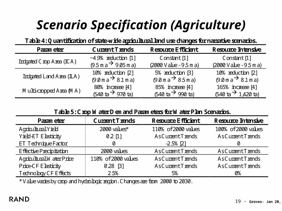
Scenario Specification (Agriculture)Table 4: Quantification of state-wide agricultural land use changes for narrative scenarios.
Parameter Current Trends Resource Efficient Resource Intensive
Irrigated Crop Area (ICA) ~4.9% reduction [1] (9.5 ma 9.05 ma)
Constant [1] (2000 Value - 9.5 ma)
Constant [1] (2000 Value - 9.5 ma)
Irrigated Land Area (ILA) 10% reduction [2] (9.0 ma 8.1 ma)
5% reduction [3] (9.0 ma 8.5 ma)
10% reduction [2] (9.0 ma 8.1 ma)
Multi-cropped Area (MA) 80% increase [4] (540 ta 970 ta)
85% increase [4] (540 ta 990 ta)
165% increase [4] (540 ta 1,420 ta)
Table 5: Crop Water Demand Parameters for Water Plan Scenarios. Parameter Current Trends Resource Efficient Resource Intensive
Agricultural Yield 2000 values* 110% of 2000 values 100% of 2000 values Yield-ET Elasticity 0.2 [1] As Current Trends As Current Trends ET Technique Factor 0 -2.5%[2] 0 Effective Precipitation 2000 values As Current Trends As Current Trends Agricultural Water Price 110% of 2000 values As Current Trends As Current Trends Price-CF Elasticity 0.28 [3] As Current Trends As Current Trends Technology CF Effects 2.5% 5% 0% * Value varies by crop and hydrologic region. Changes are from 2000 to 2030.

20 - Groves- Jan 20, 05
Statewide Results
• Increase in urban demand, decrease in agricultural demand
• Net demand differs by scenario
• Cannot offset state-wide urban increases with state-wide agricultural decreases!!!
• Ag water use reduction is largest in Current Trends due to specification of agricultural land use in narratives.
Statewide Demand Changes (2000 -> 2030)
-4,000
-2,000
0
2,000
4,000
6,000
Current Trends Resource Efficient Resource Intensive
Wa
ter
De
ma
nd
Ch
an
ge
s [
TA
F]
Urban Agriculture Environmental
Statewide Agricultural Land Use Changes
-1,000
-750
-500
-250
0
250
500
750
1,000
Current Trends Resource Efficient Resource Intensive
Th
ou
sa
nd
Ac
res
Irrigated Crop Area Irrigated Land Area Multicropped Area
21 - Groves- Jan 20, 05
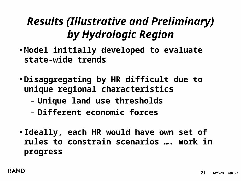
Results (Illustrative and Preliminary)by Hydrologic Region
• Model initially developed to evaluate state-wide trends
• Disaggregating by HR difficult due to unique regional characteristics
– Unique land use thresholds– Different economic forces
• Ideally, each HR would have own set of rules to constrain scenarios …. work in progress

22 - Groves- Jan 20, 05
North Coast Demand Changes (2000 -> 2030)
-100
0
100
200
300
400
Current Trends Resource Efficient Resource Intensive
Wat
er D
eman
d C
han
ges
[T
AF
]
Urban Agriculture Environmental
North Lahontan Demand Changes (2000 -> 2030)
0
50
100
150
Current Trends Resource Efficient Resource Intensive
Wat
er D
eman
d C
han
ges
[T
AF
]
Urban Agriculture Environmental
North Coast and North Lahontan
• NC: Ag demand reduction due to efficiency improvements
• NL: Ag increases due to increased irrigated land area

23 - Groves- Jan 20, 05
San Francisco and Central Coast
• SF: Urban water demand increase [4% -> 32%]
• CC: Ag water use reductions due to reduction in irrigated land area. No changes in multi-cropping
San Francisco Demand Changes (2000 -> 2030)
-100
0
100
200
300
400
Current Trends Resource Efficient Resource Intensive
Wat
er D
eman
d C
han
ges
[T
AF
]
Urban Agriculture Environmental
Central Coast Demand Changes (2000 -> 2030)
-300
-200
-100
0
100
200
Current Trends Resource Efficient Resource Intensive
Wat
er D
eman
d C
han
ges
[T
AF
]
Urban Agriculture Environmental
24 - Groves- Jan 20, 05
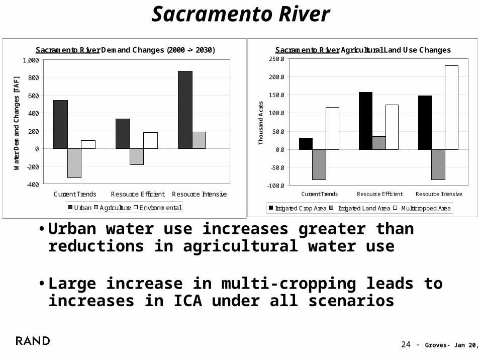
Sacramento River
• Urban water use increases greater than reductions in agricultural water use
• Large increase in multi-cropping leads to increases in ICA under all scenarios
Sacramento River Demand Changes (2000 -> 2030)
-400
-200
0
200
400
600
800
1,000
Current Trends Resource Efficient Resource Intensive
Wat
er D
eman
d C
han
ges
[T
AF
]
Urban Agriculture Environmental
Sacramento River Agricultural Land Use Changes
-100.0
-50.0
0.0
50.0
100.0
150.0
200.0
250.0
Current Trends Resource Eff icient Resource Intensive
Th
ou
san
d A
cres
Irrigated Crop Area Irrigated Land Area Multicropped Area

25 - Groves- Jan 20, 05
San Joaquin River
• Large agricultural demand reductions in Current Trends and Resource Efficient scenarios
• Large urban demand increases
San Joaqin River Demand Changes (2000 -> 2030)
-1,000
-800
-600
-400
-200
0
200
400
600
800
Current Trends Resource Efficient Resource Intensive
Wat
er D
eman
d C
han
ges
[T
AF
]
Urban Agriculture Environmental
San Joaquin River Agricultural Land Use Changes
-300
-200
-100
0
100
200
300
Current Trends Resource Eff icient Resource Intensive
Th
ou
san
d A
cres
Irrigated Crop Area Irrigated Land Area Multicropped Area

26 - Groves- Jan 20, 05
Tulare Lake
• Similar to San Joaquin without environmental water demand increases
Tulare Lake Demand Changes (2000 -> 2030)
-1,400
-1,200
-1,000
-800
-600
-400
-200
0
200
400
600
Current Trends Resource Efficient Resource Intensive
Wat
er D
eman
d C
han
ges
[T
AF
]
Urban Agriculture Environmental
Tulare Lake Agricultural Land Use Changes
-500.0
-400.0
-300.0
-200.0
-100.0
0.0
100.0
200.0
300.0
400.0
Current Trends Resource Eff icient Resource Intensive
Th
ou
san
d A
cres
Irrigated Crop Area Irrigated Land Area Multicropped Area

27 - Groves- Jan 20, 05
South Coast
• Agricultural land reduction drives reductions in agricultural water use
• Urban water demand increases overwhelm agricultural demand decreases except in Resource Efficient scenario
South Coast Demand Changes (2000 -> 2030)
-500
0
500
1,000
1,500
2,000
Current Trends Resource Efficient Resource Intensive
Wat
er D
eman
d C
han
ges
[T
AF
]
Urban Agriculture Environmental
South Coast Agricultural Land Use Changes
-120.0
-100.0
-80.0
-60.0
-40.0
-20.0
0.0
Current Trends Resource Eff icient Resource Intensive
Th
ou
san
d A
cres
Irrigated Crop Area Irrigated Land Area Multicropped Area

28 - Groves- Jan 20, 05
Colorado River
• Large decreases in agriculture offset urban increases in Current Trends and Resource Intensive scenarios
• Increase in multi-cropping ranges from 20%-26%
Colorado River Demand Changes (2000 -> 2030)
-800
-600
-400
-200
0
200
400
600
800
Current Trends Resource Efficient Resource Intensive
Wat
er D
eman
d C
han
ges
[T
AF
]
Urban Agriculture Environmental
Colorado River Agricultural Land Use Changes
-80.0
-60.0
-40.0
-20.0
0.0
20.0
40.0
60.0
80.0
100.0
Current Trends Resource Eff icient Resource Intensive
Th
ou
san
d A
cres
Irrigated Crop Area Irrigated Land Area Multicropped Area

29 - Groves- Jan 20, 05
South Lahontan
• Urban demand increases are greater than agricultural demand reductions
South Lahontan Demand Changes (2000 -> 2030)
-200
-100
0
100
200
300
Current Trends Resource Efficient Resource Intensive
Wat
er D
eman
d C
han
ges
[T
AF
]
Urban Agriculture Environmental
South Lahontan Agricultural Land Use Changes
-25.0
-20.0
-15.0
-10.0
-5.0
0.0
Current Trends Resource Eff icient Resource Intensive
Th
ou
san
d A
cres
Irrigated Crop Area Irrigated Land Area Multicropped Area

30 - Groves- Jan 20, 05
Closing Remarks
• Interpretation of Scenarios– NOT forecasts– Will be evaluated using more detailed analyses and
models for 2008 Water Plan
• Additional scenarios can easily be generated and evaluated (stay tuned…)
• Improvements to scenario generator– Introduce interannual variability due to weather– Couple to water supply and management scenarios
• Reflect annual cycle• Interannual hydrologic variability
Related Documents