Published Quarterly by the California Department of Fish and Wildlife VO LU M E 107 • SPRING 2021 • NU M BE R 2 Journal for the Conservation and Management of California’s Species and Ecosystems California Fish and Wildlife

Welcome message from author
This document is posted to help you gain knowledge. Please leave a comment to let me know what you think about it! Share it to your friends and learn new things together.
Transcript
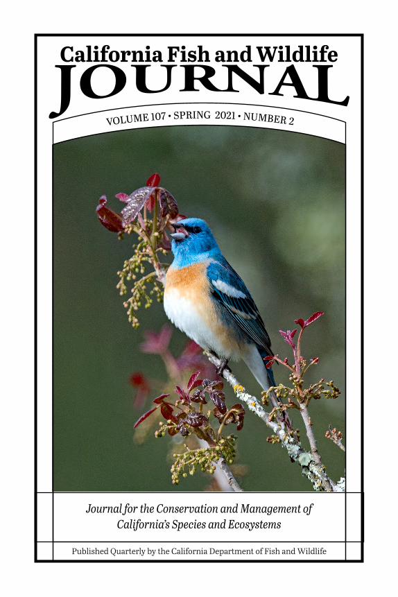
Published Quarterly by the California Department of Fish and Wildlife
VOLUME 107 • SPRING 2021 • NUMBER 2
Journal for the Conservation and Management of California’s Species and Ecosystems
California Fish and Wildlife
STATE OF CALIFORNIAGavin Newsom, Governor
CALIFORNIA NATURAL RESOURCES AGENCYWade Crowfoot, Secretary for Natural Resources
FISH AND GAME COMMISSIONEric Sklar, President
Jacque Hostler-Carmesin, Vice PresidentRussell Burns, MemberPeter S. Silva, Member
Samantha Murray, Member
Melissa Miller-Henson, Executive Director
DEPARTMENT OF FISH AND WILDLIFECharlton “Chuck” Bonham, Director
CALIFORNIA FISH AND WILDLIFEEDITORIAL STAFF
Ange Darnell Baker ...........................................................................Editor-in-ChiefLorna Bernard ...........................Office of Communication, Education and OutreachNeil Clipperton, Scott Osborn, Laura Patterson, Dan Skalos, Katherine Miller Karen Converse, Kristin Denryter, Matt Meshiry, Megan Crane, and Justin Dellinger ................................................. Wildlife BranchFelipe La Luz and Ken Kundargi ........................................................ Water BranchJeff Rodzen, Jeff Weaver, John Kelly, and Erica Meyers ............... Fisheries BranchCherilyn Burton, Katrina Smith and Grace Myers .......................................... Habitat Conservation Planning BranchKevin Fleming ...............................................Watershed Restoration Grants BranchJeff Villepique and Steve Parmenter ...................................... Inland Deserts RegionJames Ray and Peter McHugh ...........................................................Marine RegionDavid Wright and Mario Klip ................................................. North Central RegionKen Lindke, Robert Sullivan, and Jennifer Olson .......................... Northern RegionLauren Damon .............................................................................. Bay Delta RegionRandy Lovell ...........................................................................Aquaculture ProgramJennifer Nguyen ........................................................................... Cannabis Program
VOLUME 107 SPRING 2021 NUMBER 2
Published Quarterly by
STATE OF CALIFORNIACALIFORNIA NATURAL RESOURCES AGENCY
DEPARTMENT OF FISH AND WILDLIFEISSN: 2689-419X (print)
ISSN: 2689-4203 (online)--LDA--
California Fish and Wildlife
California Fish and Wildlife Journal
The California Fish and Wildlife Journal is published quarterly by the Califor-nia Department of Fish and Wildlife. It is a journal devoted to the conservation and understanding of the flora and fauna of California and surrounding areas. If its contents are reproduced elsewhere, the authors and the California Department of Fish and Wildlife would appreciate being acknowledged.
Please direct correspondence to: Ange Darnell Baker Editor-in-Chief California Fish and Wildlife [email protected]
Inquiries regarding the reprinting of articles and publishing in future issues can be directed to the Subscription Manager via email at [email protected].
Alternate communication format is available upon request. If reasonable accommodation is needed, call 916-322-8911 or the California Relay (Telephone) Service for the deaf or hearing-impaired from TDD phones at 800-735-2929.
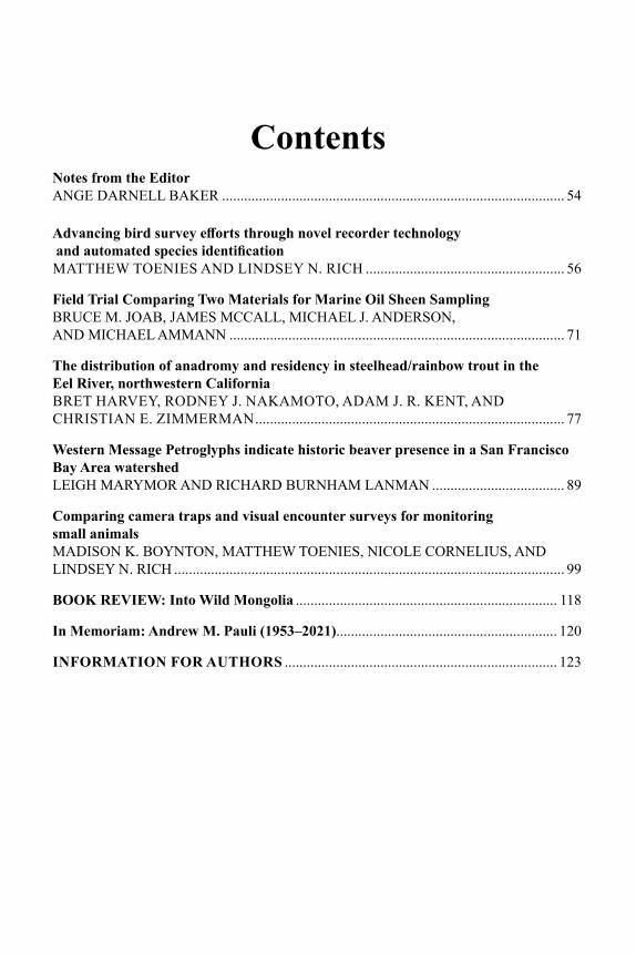
ContentsNotes from the EditorANGE DARNELL BAKER ............................................................................................. 54
Advancing bird survey efforts through novel recorder technology and automated species identificationMATTHEW TOENIES AND LINDSEY N. RICH ...................................................... 56
Field Trial Comparing Two Materials for Marine Oil Sheen SamplingBRUCE M. JOAB, JAMES MCCALL, MICHAEL J. ANDERSON, AND MICHAEL AMMANN ........................................................................................... 71
The distribution of anadromy and residency in steelhead/rainbow trout in the Eel River, northwestern CaliforniaBRET HARVEY, RODNEY J. NAKAMOTO, ADAM J. R. KENT, AND CHRISTIAN E. ZIMMERMAN .................................................................................... 77
Western Message Petroglyphs indicate historic beaver presence in a San Francisco Bay Area watershedLEIGH MARYMOR AND RICHARD BURNHAM LANMAN .................................... 89
Comparing camera traps and visual encounter surveys for monitoring small animalsMADISON K. BOYNTON, MATTHEW TOENIES, NICOLE CORNELIUS, AND LINDSEY N. RICH .......................................................................................................... 99
BOOK REVIEW: Into Wild Mongolia ....................................................................... 118
In Memoriam: Andrew M. Pauli (1953–2021)............................................................ 120
INFORMATION FOR AUTHORS .......................................................................... 123
California Fish and Wildlife 107(2):54; 2021
Notes from the EditorThe spring issue of 2021 is following the same pattern as the winter issue in coming
late, and likely for the same reason—the impact that the COVID-19 pandemic has had on the research community. Amazingly, this is the first issue in quite a while where I have no new Associate Editors to introduce—perhaps I finally have enough to cover the diverse manuscript topics the Journal receives.
This issue begins with a fascinating study examining the effectiveness of four differ-ent acoustic recorders for bird detection as well as assessing the effectiveness of a new AI method of automated species identification. Technology in the wildlife field has advanced significantly in recent years providing researchers with methods that are less invasive, more efficient, and cheaper than ever before. The researchers in this study, who are part of CDFW’s Wildlife Branch, discovered that the lowest-cost recorder (which is also significantly smaller than traditional acoustic recorders) performed just as well as higher-cost recorders—and that species detections were significantly higher than traditional, point-count methods! And the automated species identification platform, BirdNET, was extremely accurate, correctly identifying 96% of species—this truly has significant implications for future bird research.
The next article, a combined effort from CDFW’s Office of Spill Prevention and Response unit and the Chevron Corporation, describes a trial to compare two methods for sampling oil sheens in marine environments. They concluded that the material used by CDFW, a fiberglass material, and that used by the U.S. Coast Guard, a tetrafluoroethylene-fluorocarbon (TFE-fluorocarbon) polymer net, were both suitable methods of collection material for chemical forensic analyses.
The third article, with researchers from the Forest Service, USGS, and Oregon State University, focuses on the distribution of both anadromous (steelhead) and resident (rain-bow) trout in northwestern California. They found a widespread distribution of fish that had resident mothers, suggesting the importance of preserving freshwater conditions that are suitable for resident trout, notably maintaining stream flows throughout the dry season. This information is especially relevant and timely given the state’s current drought-conditions.
Next up, a very interesting article that used Western Message Petroglyphs—a type of picture-writing from the late 1800s/early 1900s, likely used by non-Native Americans with a knowledge of Native American symbols—found in the San Francisco Bay Area to demonstrate the likely presence of a beaver lodge in the area of Alameda Creek in the late 1800s. This record was possibly the last one before beavers were locally extirpated as a result of the fur trade.
The last article, again by CDFW researchers from the Wildlife Branch, compares a commonly used method for surveys of herpetofauna (reptiles and amphibians), visual encounter surveys (VES) with cover boards, to a more novel method which combines a drift fence with camera traps. They determined that the drift fence/camera trap technique outperformed the VES detecting significantly more herp species—as well as a number of other small animals, including small mammals, birds, and invertebrates. Again, as with the first article, many will be pleased to find that a newer method using modern technology can replace the extremely time-intensive method of on-the-ground species surveys—we
55Spring 2021 NOTES FROM THE EDITOR
can get substantially more data with considerably less time and effort, a win-win situation for wildlife researchers.
The issue concludes with a book review of George B. Schaller’s Into Wild Mongolia by Dr. Vernon Bleich (former editor of this journal) and a tribute in memoriam of Andrew M. Pauli, a long-time wildlife biologist for the Department.
Earlier this summer, we were finally able to complete the special issue on CESA (Cali-fornia Endangered Species Act), which, with 27 articles, marked the largest issue the Journal has ever published (473 pages!)—and an issue that I personally am extremely proud of; my special issue guest editorial team put in a huge amount of work to get the issue completed, and it shows! And keep your eyes out for our final special issue of the year which will cover the topic of Human-Wildlife Interactions.
Ange Darnell Baker, PhDEditor-in-ChiefCalifornia Fish and Wildlife Journal
California Fish and Wildlife 107(2):56-70; 2021
FULL RESEARCH ARTICLE
Advancing bird survey efforts through novel recorder technology and automated species identification
MATTHEW TOENIES1* AND LINDSEY N. RICH1
1 California Department of Fish and Wildlife, Wildlife Branch, 1010 Riverside Parkway, West Sacramento, CA 95605, USA
* Corresponding Author: [email protected]
Recent advances in acoustic recorder technology and automated species identification hold great promise for avian monitoring efforts. Assessing how these innovations compare to existing recorder models and traditional species identification techniques is vital to understanding their utility to researchers and managers. We carried out field trials in Mon-terey County, California, to compare bird detection among four acoustic recorder models (AudioMoth, Swift Recorder, and Wildlife Acoustics SM3BAT and SM Mini) and concurrent point counts, and to assess the ability of the artificial neural network BirdNET to correctly identify bird species from AudioMoth recordings. We found that the lowest-cost unit (AudioMoth) performed comparably to higher-cost units and that on aver-age, species detections were higher for three of the five recorder models (range 9.8 to 14.0) than for point counts (12.8). In our assessment of BirdNET, we developed a subsetting process that enabled us to achieve a high rate of correctly identified species (96%). Using longer recordings from a single recorder model, BirdNET identified a mean of 8.5 verified species per recording and a mean of 16.4 verified species per location over a 5-day period (more than point counts conducted in similar habitats). We demonstrate that a combination of long recordings from low-cost recorders and a conservative method for subsetting automated identifications from BirdNET presents a process for sampling avian community composition with low misidentification rates and limited need for human vetting. These low-cost and automated tools may greatly improve efforts to survey bird communities and their ecosystems, and consequently, efforts to conserve threatened indigenous biodiversity.
Los recientes avances en la tecnología de grabación acústica y en la identificación automatizada de especies son muy prometedores para los esfuerzos de monitoreo aviar. Evaluar cómo estas innovaciones se comparan con los modelos de grabadora existentes y las técnicas tradicio-nales de identificación de especies es vital para entender su utilidad para investigadores y gerentes. Realizamos ensayos de campo en el condado
www.doi.org/10.51492/cfwj.107.5
57Spring 2021 57NOVEL RECORDERS AND AUTOMATED BIRD IDENTIFICATION
de Monterey, California, para comparar la detección de aves entre cuatro modelos de grabadora acústica (AudioMoth, Swift Recorder y Wildlife Acoustics SM3BAT y SM Mini) y conteos por puntos simultáneos, y para evaluar la capacidad de la red neuronal artificial BirdNET en iden-tificar correctamente las especies de aves de las grabaciones AudioMoth. Encontramos que la unidad de menor costo (AudioMoth) funcionaba de manera equiparable a unidades de mayor costo y que, en promedio, las detecciones de especies eran más altas para la mayoría de los grabadoras (rango 9.8 a 14.0) que para los conteos por puntos (12.8). En nuestra evaluación de BirdNET, desarrollamos un proceso de subconjuntos que nos permitió alcanzar una alta tasa de especies correctamente identifica-das (96%). BirdNET identificó una media de 8.5 especies verificadas por registro y una media de 16.4 especies verificadas por ubicación (más que conteos por puntos realizados en hábitats similares). Demostramos que una combinación de grabaciones de larga duración con grabadoras de bajo costo y un método conservador para el subconjunto de identificaciones automatizadas de BirdNET presentan un proceso para tomar muestras de la composición de la comunidad aviar con bajas tasas de identificación errónea y necesidad limitada de verificación humana. Estas herramientas automatizadas y de bajo costo pueden facilitar en gran medida esfuerzos en examinar las comunidades de aves y sus ecosistemas y, en consecuen-cia, los esfuerzos para conservar la biodiversidad indígena amenazada.
Key words: acoustic monitoring, ARU, AudioMoth, autoclassification, BirdNET, birds, point count, species identification__________________________________________________________________________
Acoustic monitoring is a non-invasive approach for surveying wildlife that uses remote acoustic technologies to record sounds emitted by vocalizing species (Blumstein et al. 2011). These autonomously triggered tools, also known as autonomous recording units (ARUs), hold many advantages over more traditional approaches like direct observations (e.g., point counts), given they allow scientists to collect information 24 hours per day and on multiple species from multiple taxa, all while minimizing the impacts of observer disturbance and bias during data collection (Brandes 2008; Heinicke et al. 2015; Sebastián-González et al. 2018; Shonfield and Bayne 2017). Further, all acoustic recordings can be permanently stored, allowing them to function as digital archives that can be revisited when new questions or technologies emerge (Chambert et al. 2018). Arrays of fixed acoustic sensors have been used to sample ecosystems (e.g., soundscapes in temperate forests and rainforests [Sethi et al. 2020]), taxonomic groups (Brandes 2008; Ribeiro et al. 2018; Walters et al. 2012; Wood et al. 2019), and individual species (Campos-Cerqueira and Aide 2016; Heinicke et al. 2015). They have also been used to help address questions regarding, for example, species distributions (Campos-Cerqueira and Aide 2016), spatial and temporal dynamics (Bader et al. 2015), phenology (Furnas and McGrann 2018), and spatial variation in habitat quality (Sethi et al. 2020).
Despite the many advantages of acoustic monitoring, there are also several potential limitations. First, differences between acoustic recorders and traditional survey methods
Vol. 107, No. 2CALIFORNIA FISH AND WILDLIFE58
may complicate comparisons of data from acoustic recorders to results from established long-term population monitoring programs employing point counts. For example, while acoustic recorders tend to perform equally to humans conducting point counts in estimat-ing bird species richness (Darras et al. 2018), they tend to underperform in estimating bird density or require a secondary source of information (Stevenson et al. 2015). Research focused on estimating avian density from acoustic recordings is a rapidly growing field, however, which has had success and will likely have even greater success as automated and open-source sound localization software is developed (Blumstein et al. 2011; Sebastián-González et al. 2018; Perez-Granados et al. 2019; Rhinehart et al. 2020; Stevenson et al. 2021). Additionally, researchers have successfully integrated avian survey data from point counts and acoustic recorders and have given specific recommendations on sampling birds with acoustic recorders to achieve results comparable to those from point counts (Darras et al. 2018). For example, Stewart et al. (2020) used statistical offsets, or correction factors, to integrate data from point counts and ARUs.
A second potential limitation is the high cost of acoustic recorders, which can restrict their usage in many contexts (Hill et al. 2019; Rhinehart et al. 2020). Wildlife Acoustics Recorders (Wildlife Acoustics, Maynard, MA, USA) can cost upwards of $1,000, for ex-ample, meaning a project with 100 survey locations would need a minimum budget of over $100,000. Recently, however, low-cost alternatives like the AudioMoth (Open Acoustic Devices 2020) have been developed. The AudioMoth is a full-spectrum recorder that fits in the palm of a hand and has a cost of approximately 60 USD per unit (Hill et al. 2019). AudioMoths have proven successful for a variety of wildlife monitoring and conservation projects (Prince et al. 2019) but for a full understanding of their utility, need to be directly compared to other acoustic recorder models.
A final challenge associated with acoustic monitoring is the terabytes of sound files that can be produced, within which the sound of interest must be located and correctly identified to species (Chambert et al. 2018; Wrege et al. 2017). Accomplishing the latter by manually reviewing the spectrograms of all recordings requires an immense amount of effort (Campos-Cerqueira and Aide 2016). Thus, many researchers now rely on custom designed algorithms or commercially available sound analysis software to automate species identification (Brandes 2008; Gibb et al. 2019; Heinicke et al. 2015; Kalan et al. 2015). One recently developed tool is BirdNET, an artificial neural network that can automatically identify over 900 bird species (Kahl 2020). In an initial assessment of 225 recordings, BirdNET was found to have an overall accuracy (i.e., correctly identified vocalizing bird species) of 91.5% (Arif et al. 2020). Additional assessments of the accuracy of BirdNET are needed, however, given it is an extremely new and evolving tool.
The goal of our study is to help address these research gaps by assessing the ef-ficacy of several acoustic recorder models in detecting birds and one sound analysis tool in identifying birds. Specifically, we 1) compared species-level detection rates among the acoustic recorder models and concurrent point counts; and 2) evaluated BirdNET’s ability to correctly identify bird species from acoustic recordings. Understanding the optimal way to collect and process acoustic recordings of birds will help inform the design and feasibil-ity of future large-scale bird monitoring efforts and enable managers to combat challenges associated with acoustic monitoring head-on.
59Spring 2021 59NOVEL RECORDERS AND AUTOMATED BIRD IDENTIFICATION
METHODS
Study Area
We conducted fieldwork within the Hastings Natural History Reservation in Monterey County, California, USA (36.380, -121.564). This reserve covers 950 ha, and vegetation at the study area is primarily oak (Quercus sp.) woodland and chaparral (Griffon 1990). Mean annual temperature is 13.4 °C, and mean annual precipitation is 522 mm (McMahon et al. 2015).
Field Methods
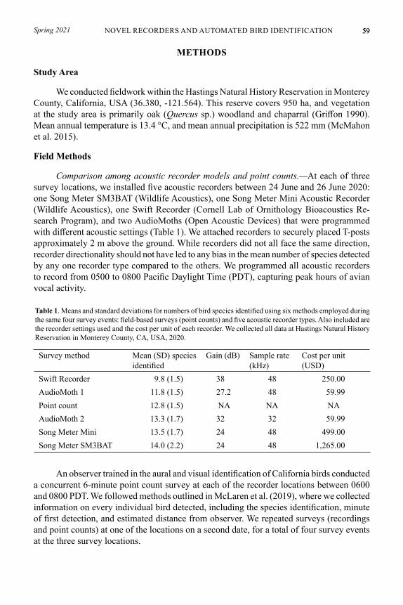
Comparison among acoustic recorder models and point counts.—At each of three survey locations, we installed five acoustic recorders between 24 June and 26 June 2020: one Song Meter SM3BAT (Wildlife Acoustics), one Song Meter Mini Acoustic Recorder (Wildlife Acoustics), one Swift Recorder (Cornell Lab of Ornithology Bioacoustics Re-search Program), and two AudioMoths (Open Acoustic Devices) that were programmed with different acoustic settings (Table 1). We attached recorders to securely placed T-posts approximately 2 m above the ground. While recorders did not all face the same direction, recorder directionality should not have led to any bias in the mean number of species detected by any one recorder type compared to the others. We programmed all acoustic recorders to record from 0500 to 0800 Pacific Daylight Time (PDT), capturing peak hours of avian vocal activity.
Table 1. Means and standard deviations for numbers of bird species identified using six methods employed during the same four survey events: field-based surveys (point counts) and five acoustic recorder types. Also included are the recorder settings used and the cost per unit of each recorder. We collected all data at Hastings Natural History Reservation in Monterey County, CA, USA, 2020.
Survey method Mean (SD) species identified
Gain (dB) Sample rate (kHz)
Cost per unit (USD)
Swift Recorder 9.8 (1.5) 38 48 250.00AudioMoth 1 11.8 (1.5) 27.2 48 59.99Point count 12.8 (1.5) NA NA NAAudioMoth 2 13.3 (1.7) 32 32 59.99Song Meter Mini 13.5 (1.7) 24 48 499.00Song Meter SM3BAT 14.0 (2.2) 24 48 1,265.00
An observer trained in the aural and visual identification of California birds conducted a concurrent 6-minute point count survey at each of the recorder locations between 0600 and 0800 PDT. We followed methods outlined in McLaren et al. (2019), where we collected information on every individual bird detected, including the species identification, minute of first detection, and estimated distance from observer. We repeated surveys (recordings and point counts) at one of the locations on a second date, for a total of four survey events at the three survey locations.
Vol. 107, No. 2CALIFORNIA FISH AND WILDLIFE60
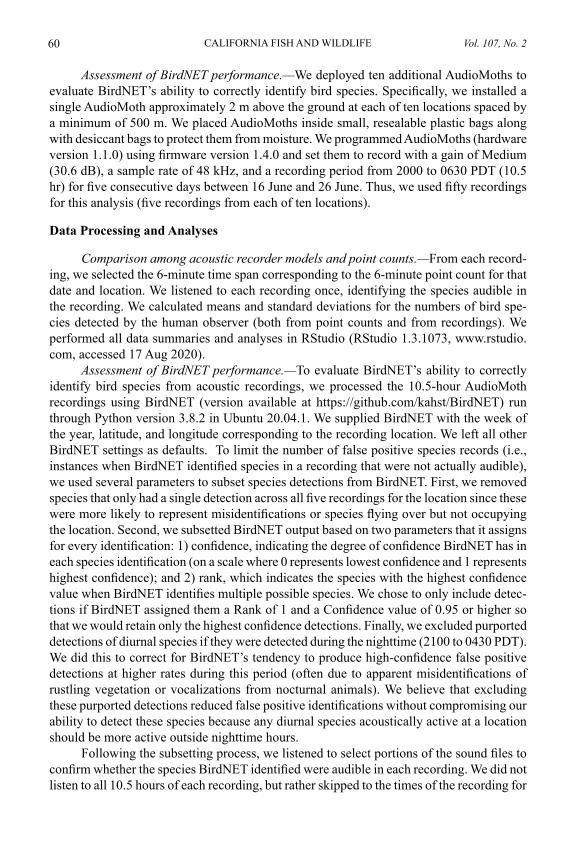
Assessment of BirdNET performance.—We deployed ten additional AudioMoths to evaluate BirdNET’s ability to correctly identify bird species. Specifically, we installed a single AudioMoth approximately 2 m above the ground at each of ten locations spaced by a minimum of 500 m. We placed AudioMoths inside small, resealable plastic bags along with desiccant bags to protect them from moisture. We programmed AudioMoths (hardware version 1.1.0) using firmware version 1.4.0 and set them to record with a gain of Medium (30.6 dB), a sample rate of 48 kHz, and a recording period from 2000 to 0630 PDT (10.5 hr) for five consecutive days between 16 June and 26 June. Thus, we used fifty recordings for this analysis (five recordings from each of ten locations).
Data Processing and Analyses
Comparison among acoustic recorder models and point counts.—From each record-ing, we selected the 6-minute time span corresponding to the 6-minute point count for that date and location. We listened to each recording once, identifying the species audible in the recording. We calculated means and standard deviations for the numbers of bird spe-cies detected by the human observer (both from point counts and from recordings). We performed all data summaries and analyses in RStudio (RStudio 1.3.1073, www.rstudio.com, accessed 17 Aug 2020).
Assessment of BirdNET performance.—To evaluate BirdNET’s ability to correctly identify bird species from acoustic recordings, we processed the 10.5-hour AudioMoth recordings using BirdNET (version available at https://github.com/kahst/BirdNET) run through Python version 3.8.2 in Ubuntu 20.04.1. We supplied BirdNET with the week of the year, latitude, and longitude corresponding to the recording location. We left all other BirdNET settings as defaults. To limit the number of false positive species records (i.e., instances when BirdNET identified species in a recording that were not actually audible), we used several parameters to subset species detections from BirdNET. First, we removed species that only had a single detection across all five recordings for the location since these were more likely to represent misidentifications or species flying over but not occupying the location. Second, we subsetted BirdNET output based on two parameters that it assigns for every identification: 1) confidence, indicating the degree of confidence BirdNET has in each species identification (on a scale where 0 represents lowest confidence and 1 represents highest confidence); and 2) rank, which indicates the species with the highest confidence value when BirdNET identifies multiple possible species. We chose to only include detec-tions if BirdNET assigned them a Rank of 1 and a Confidence value of 0.95 or higher so that we would retain only the highest confidence detections. Finally, we excluded purported detections of diurnal species if they were detected during the nighttime (2100 to 0430 PDT). We did this to correct for BirdNET’s tendency to produce high-confidence false positive detections at higher rates during this period (often due to apparent misidentifications of rustling vegetation or vocalizations from nocturnal animals). We believe that excluding these purported detections reduced false positive identifications without compromising our ability to detect these species because any diurnal species acoustically active at a location should be more active outside nighttime hours.
Following the subsetting process, we listened to select portions of the sound files to confirm whether the species BirdNET identified were audible in each recording. We did not listen to all 10.5 hours of each recording, but rather skipped to the times of the recording for
61Spring 2021 61NOVEL RECORDERS AND AUTOMATED BIRD IDENTIFICATION
which BirdNET had produced detections. We calculated the mean and standard deviation for the number of species identified per recording, including the number of species identified but not confirmed to be audible by the human observer (false positives) and the number of species identified and confirmed to be audible (true positives). We also calculated the mean and standard deviation for the number of species identified (including true and false posi-tives) at the survey location level, by determining the cumulative total number of species identified across the five recordings from each location.
RESULTS
Comparison of Acoustic Recorder Models
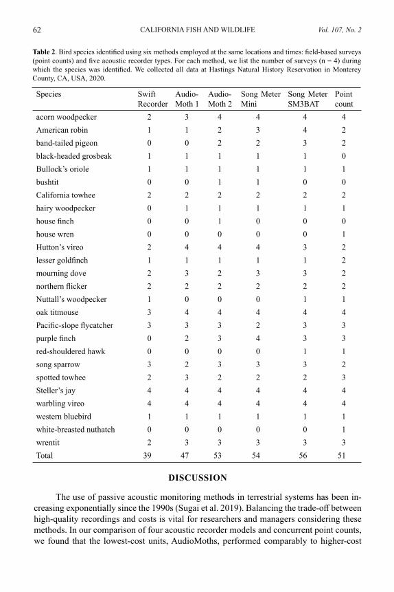
We identified 26 bird species across the concurrent point counts and recordings (Table 2). Steller’s Jay (Cyanocitta stelleri, n = 24) and warbling vireo (Vireo gilvus, n = 24) were detected by all methods during all survey events. We identified two species on point counts but not on recordings: white-breasted nuthatch (Sitta carolinensis) and house wren (Troglodytes aedon), although we detected calls from an unidentified wren species on all recordings. We identified three species on recordings but not on point counts: Black-headed grosbeak (Pheucticus melanocephalus), bushtit (Psaltriparus minimus), and house finch (Haemorhous mexicanus). The highest mean number of species was identified via the Song Meter SM3BAT and the lowest via the Swift Recorder (Table 1). While the mean number of species identified during point counts was higher than that of two recorders, we found that on average, AudioMoths (with higher gain and lower sampling rate programming) and both Wildlife Acoustics recorders resulted in higher mean numbers of species identifications than point counts (Table 1).
Assessment of BirdNET Performance
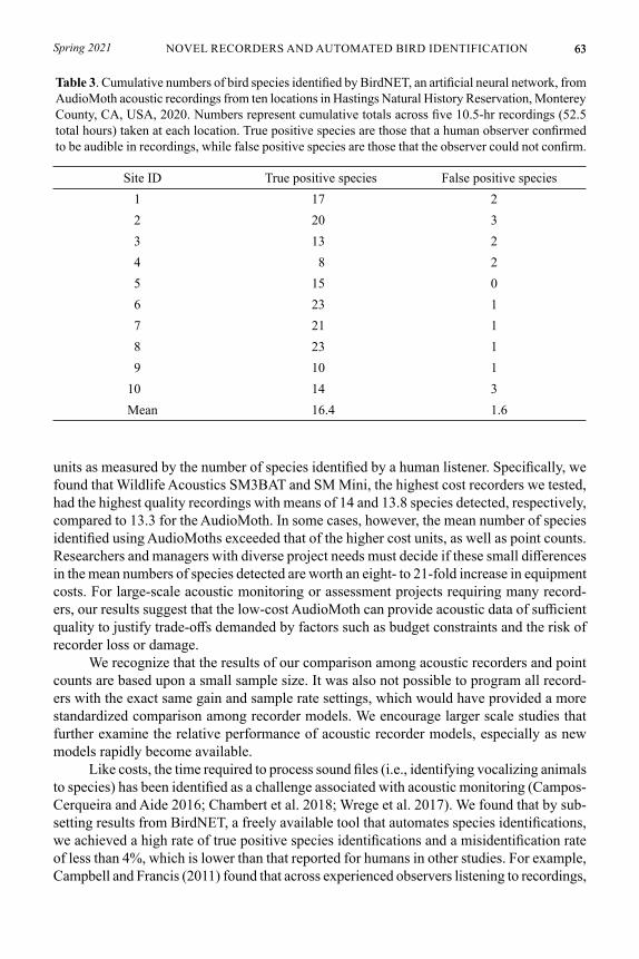
Across the ten locations, BirdNET identified 42 species that we confirmed to be audible in the 10.5-hr AudioMoth recordings (Appendix I). The species identified from the most recordings were Pacific-slope flycatcher (Empidonax difficilis, n = 25), California scrub-jay (Aphelocoma californica, n = 24), and California towhee (Melozone crissalis, n = 24). The mean number of species detected by BirdNET and subsequently confirmed was 8.5 per recording (range 3–15, SD = 3.5). The mean number of false positive species records was 0.3 per recording (range 0–2, SD = 0.6), which equated to a false positive (misidentifica-tion) rate of 3.8% of species records. Cumulative species totals from the five recordings at each location showed that BirdNET correctly identified a mean of 16.4 species per location (range 8–23, SD = 5.3; Table 3) and misidentified 1.6 species per location (range 0–3, SD = 1.0; Table 3).
For two species identified by BirdNET, we removed detections from our results because we could not distinguish sounds to the species level. These species were chestnut-backed chickadee (Poecile rufescens), detected in 5 recordings, where call notes were indistin-guishable from those of oak titmouse (Baeolophus inornatus), and white-crowned sparrow (Zonotrichia leucophrys), with a single unidentifiable call note from one recording. BirdNET identified six species that were not detected by the human observer in any recording, with five of these misidentified in a single recording each (Appendix II).
Vol. 107, No. 2CALIFORNIA FISH AND WILDLIFE62
Table 2. Bird species identified using six methods employed at the same locations and times: field-based surveys (point counts) and five acoustic recorder types. For each method, we list the number of surveys (n = 4) during which the species was identified. We collected all data at Hastings Natural History Reservation in Monterey County, CA, USA, 2020.
Species Swift Recorder
Audio-Moth 1
Audio-Moth 2
Song Meter Mini
Song Meter SM3BAT
Point count
acorn woodpecker 2 3 4 4 4 4American robin 1 1 2 3 4 2band-tailed pigeon 0 0 2 2 3 2black-headed grosbeak 1 1 1 1 1 0Bullock’s oriole 1 1 1 1 1 1bushtit 0 0 1 1 0 0California towhee 2 2 2 2 2 2hairy woodpecker 0 1 1 1 1 1house finch 0 0 1 0 0 0house wren 0 0 0 0 0 1Hutton’s vireo 2 4 4 4 3 2lesser goldfinch 1 1 1 1 1 2mourning dove 2 3 2 3 3 2northern flicker 2 2 2 2 2 2Nuttall’s woodpecker 1 0 0 0 1 1oak titmouse 3 4 4 4 4 4Pacific-slope flycatcher 3 3 3 2 3 3purple finch 0 2 3 4 3 3red-shouldered hawk 0 0 0 0 1 1song sparrow 3 2 3 3 3 2spotted towhee 2 3 2 2 2 3Steller’s jay 4 4 4 4 4 4warbling vireo 4 4 4 4 4 4western bluebird 1 1 1 1 1 1white-breasted nuthatch 0 0 0 0 0 1wrentit 2 3 3 3 3 3Total 39 47 53 54 56 51
DISCUSSION
The use of passive acoustic monitoring methods in terrestrial systems has been in-creasing exponentially since the 1990s (Sugai et al. 2019). Balancing the trade-off between high-quality recordings and costs is vital for researchers and managers considering these methods. In our comparison of four acoustic recorder models and concurrent point counts, we found that the lowest-cost units, AudioMoths, performed comparably to higher-cost
63Spring 2021 63NOVEL RECORDERS AND AUTOMATED BIRD IDENTIFICATION
Table 3. Cumulative numbers of bird species identified by BirdNET, an artificial neural network, from AudioMoth acoustic recordings from ten locations in Hastings Natural History Reservation, Monterey County, CA, USA, 2020. Numbers represent cumulative totals across five 10.5-hr recordings (52.5 total hours) taken at each location. True positive species are those that a human observer confirmed to be audible in recordings, while false positive species are those that the observer could not confirm.
Site ID True positive species False positive species1 17 22 20 33 13 24 8 25 15 06 23 17 21 18 23 19 10 1
10 14 3Mean 16.4 1.6
units as measured by the number of species identified by a human listener. Specifically, we found that Wildlife Acoustics SM3BAT and SM Mini, the highest cost recorders we tested, had the highest quality recordings with means of 14 and 13.8 species detected, respectively, compared to 13.3 for the AudioMoth. In some cases, however, the mean number of species identified using AudioMoths exceeded that of the higher cost units, as well as point counts. Researchers and managers with diverse project needs must decide if these small differences in the mean numbers of species detected are worth an eight- to 21-fold increase in equipment costs. For large-scale acoustic monitoring or assessment projects requiring many record-ers, our results suggest that the low-cost AudioMoth can provide acoustic data of sufficient quality to justify trade-offs demanded by factors such as budget constraints and the risk of recorder loss or damage.
We recognize that the results of our comparison among acoustic recorders and point counts are based upon a small sample size. It was also not possible to program all record-ers with the exact same gain and sample rate settings, which would have provided a more standardized comparison among recorder models. We encourage larger scale studies that further examine the relative performance of acoustic recorder models, especially as new models rapidly become available.
Like costs, the time required to process sound files (i.e., identifying vocalizing animals to species) has been identified as a challenge associated with acoustic monitoring (Campos-Cerqueira and Aide 2016; Chambert et al. 2018; Wrege et al. 2017). We found that by sub-setting results from BirdNET, a freely available tool that automates species identifications, we achieved a high rate of true positive species identifications and a misidentification rate of less than 4%, which is lower than that reported for humans in other studies. For example, Campbell and Francis (2011) found that across experienced observers listening to recordings,
Vol. 107, No. 2CALIFORNIA FISH AND WILDLIFE64
bird species reported by observers but not present on recordings accounted for a mean of 14% of reported species records. Farmer et al. (2012) also examined performance of humans listening to recordings for bird species designated as common or rare and observers with skills ranked from moderate to expert. Across those categories, they reported false positive rates ranging from 6% to 22%. These results demonstrate BirdNET’s promise for providing efficient, automated, and accurate bird identification, reducing reliance on human observers with variable identification abilities.
The few sounds that BirdNET misidentified were generally sounds that a human observer would also have difficulty identifying, such as confusing non-avian sounds and brief call notes that are very similar among species. Examining BirdNET results can reveal certain species that are more likely to be false positives. For example, BirdNET appeared to misidentify rustling vegetation as calls of hooded oriole (Icterus cucullatus) on more than one occasion. We recommend that researchers initially vet identifications from subsetted data to establish study area-specific lists of problematic species that should be vetted (i.e., reviewed by a human observer to confirm or correct species identification), further limiting the need to vet across all recordings and species.
It is important to note that we were unable to assess how our subsetting process af-fected the proportion of false negatives (i.e., instances where our process failed to detect species audible in the recordings). Our conservative approach, which produced a low rate of misidentifications (false positives), likely also produced an elevated rate of missed species (false negatives). However, based on the mean number of true positive species detected per location (16.4), we are confident that our methods enabled BirdNET to produce both low misidentification rates and rigorous samples of avian community composition match-ing or exceeding those typically produced by more traditional methods. For example, the mean number of confirmed species per location recorded by AudioMoths and identified by BirdNET was higher than our mean number of species from point counts (12.8), which were done in very similar habitats using the protocol of one of North America’s largest-scale bird monitoring programs. In addition, the longer species lists from AudioMoths/BirdNET often included species that traditional point count protocols have difficulty sampling, such as nocturnal species (e.g., barn owl [Tyto alba] and great horned owl [Bubo virginianus]). A growing body of research demonstrates that sound recording systems can match and even outperform point counts in their ability to sample birds (Darras et al. 2018; Darras et al. 2019; Wimmer et al. 2013), but to our knowledge this is the first published work to document this comparison for the AudioMoth.
Our study also elucidated several approaches that will likely enhance the number of true positive species detections produced by acoustic recorders and BirdNET. First, we recorded for less than one hour after local sunrise, but recorders could be set to record for more time, especially during the morning hours when avian acoustic activity peaks. Second, logistical constraints prevented us from collecting recordings during the seasonal peak of avian acoustic activity at our study area. Recording during the seasonal peaks of acoustic activity for as many species as possible should increase the number of species that are recorded and subsequently detected by BirdNET. Recording after this peak, as we did, may also increase error in BirdNET by increasing detection of individuals likely to present sound-based identification challenges, such as fledglings. On the other hand, researchers should be cautious about recording early in the breeding season when migrating or un-paired (nonbreeding) individuals are more likely to be present. Finally, we used a single
65Spring 2021 65NOVEL RECORDERS AND AUTOMATED BIRD IDENTIFICATION
conservative confidence threshold to subset detections across all species, eliminating the majority of BirdNET’s detections, including all detections for several species in some of our recordings. Approaches that use species-specific confidence thresholds may optimize the balance between high true positive and low false negative identification rates. Kahl (2020) provided optimal species-specific confidence thresholds in BirdNET, but we found that they resulted in high numbers of false positive identifications from our recordings. BirdNET’s utility for avian acoustic monitoring may benefit greatly from further exploration of optimal species-specific confidence thresholds, especially if these thresholds are established for specific geographic regions. Researchers may also consider establishing lower confidence thresholds for species of special interest, which are often rare species that may be missed by a single, conservative threshold.
The results of this study provide critical information to researchers and managers considering the use of acoustic methods for surveying bird communities. By using a combi-nation of long recordings from low-cost recorders and conservative subsetting of BirdNET’s automated identifications, we have honed a process that shows great promise for sampling avian community composition with low misidentification rates and limited need for human vetting. Together, these tools may greatly improve efforts to survey bird communities and their ecosystems, and consequently, efforts to conserve threatened indigenous biodiversity.
ACKNOWLEDGMENTS
This study was funded by the California Department of Fish and Wildlife. We thank Dr. J. Hunter, Resident Reserve Director at Hastings Natural History Reservation, for her role in facilitating fieldwork for this study. We also thank the following people for their time and assistance in the use of BirdNET: J. Cole (The Institute for Bird Populations), Dr. S. Kahl and Dr. H. Klinck (Center for Conservation Bioacoustics), and S. Peterson (University of California, Berkeley). We thank M. Rodríguez (California Department of Fish and Wildlife) and A. Blasco for providing a Spanish translation of this manuscript’s abstract. We thank the two anonymous reviewers who provided thoughtful feedback on the manuscript. Finally, we thank M. Boynton, N. Cornelius, Dr. B. Furnas, and E. Chappell (California Department of Fish and Wildlife) for their assistance in facilitating this study and conducting fieldwork.
LITERATURE CITED
Arif, M., R. Hedley, and E. Bayne. 2020. Testing the accuracy of a birdNET, automatic bird song classifier. University of Alberta, Alberta, Canada.
Bader, E., K. Jung, E. K. Kalso, R. A. Page, R. Rodriguez, and T. Sattler. 2015. Mobility explains the response of aerial insectivorous bats to anthropogenic habitat change in the Neotropics. Biological Conservation 186:97–106.
Blumstein, D. T., D. J. Mennill, P. Clemins, L. Girod, K. Yao, G. Patricelli, J. L. Deppe, A. H. Krakauer, C. Clark, K. A. Cortopassi, and S. F. Hanser. 2011. Acoustic moni-toring in terrestrial environments using microphone arrays: applications, techno-logical considerations and prospectus. Journal of Applied Ecology 48:758–767.
Brandes, T. S. 2008. Automated sound recording and analysis techniques for bird surveys and conservation. Bird Conservation International 18:S163–S173.
Brandt, A. J., and E. W. Seabloom. 2011. Regional and decadal patterns of native and exotic plant coexistence in California grasslands. Ecological Applications 21:704–714.
Vol. 107, No. 2CALIFORNIA FISH AND WILDLIFE66
Campbell, M., and C. M. Francis. 2011. Using stereo-microphones to evaluate observ-er variation in North American Breeding Bird Survey point counts. The Auk 128(2):303–312.
Campos-Cerqueira, M., and T. M. Aide. 2016. Improving distribution data of threatened species by combining acoustic monitoring and occupancy modeling. Methods in Ecology and Evolution 7:1340–1348.
Chambert, T., J. H. Waddle, D. A. Miller, S. C. Walls, and J. D. Nichols. 2018. A new framework for analysing automated acoustic species detection data: Occupancy estimation and optimization of recordings post‐processing. Methods in Ecology and Evolution 9:560–570.
Darras, K., P. Batáry, B. Furnas, A. Celis‐Murillo, S. L. Van Wilgenburg, Y. A. Mulyani, and T. Tscharntke. 2018. Comparing the sampling performance of sound record-ers versus point counts in bird surveys: a meta‐analysis. Journal of Applied Ecol-ogy 55:2575–2586.
Darras, K., P. Batáry, B. J. Furnas, I. Grass, Y. A. Mulyani, and T. Tscharntke. 2019. Au-tonomous sound recording outperforms human observation for sampling birds: a systematic map and user guide. Ecological Applications 29(6):e01954.
Farmer, R.G., M. L. Leonard, and A. G. Horn. 2012. Observer effects and avian-call-count survey quality: rare-species biases and overconfidence. The Auk 129(1):76–86.
Furnas, B. J., and M. C. McGrann. 2018. Using occupancy modeling to monitor dates of peak vocal activity for passerines in California. The Condor 120:188–200.
Gibb, R., E. Browning, P. Glover-Kapfer, and K. E. Jones. 2019. Emerging opportunities and challenges for passive acoustics in ecological assessment and monitoring. Methods in Ecology and Evolution 10:169–185.
Griffin, J.R. 1990. Flora of Hastings Reservation, Carmel Valley, California. University of California, Berkeley, CA, USA.
Heinicke, S., A. K. Kalan, O. J. Wagner, R. Mundry, H. Lukashevich, and H. S. Kühl. 2015. Assessing the performance of a semi‐automated acoustic monitoring sys-tem for primates. Methods in Ecology and Evolution 6:753–763.
Hill, A. P., P. Prince, J. L. Snaddon, C. P. Doncaster, and A. Rogers. 2019. AudioMoth: A low-cost acoustic device for monitoring biodiversity and the environment. Hard-wareX 6:e00073.
Kahl, S. 2020. Identifying birds by sound: large-scale acoustic event recognition for avian activity monitoring. Dissertation, Chemnitz University of Technology, Chemnitz, Germany.
Kalan, A. K., R. Mundry, O. J. Wagner, S. Heinicke, C. Boesch, and H. S. Kühl. 2015. Towards the automated detection and occupancy estimation of primates using passive acoustic monitoring. Ecological Indicators 54:217–226.
McLaren, M. F., C. M. White, N. J. Van Lanen, J. J. Birek, J. M. Berven, and D. J. Hanni. 2019. Integrated Monitoring in Bird Conservation Regions (IMBCR): field proto-col for spatially-balanced sampling of land bird populations. Unpublished report. Bird Conservancy of the Rockies, Brighton, CO, USA.
McMahon, D.E., I. S. Pearse, W. D. Koenig, and E. L. Walters. 2015. Tree community shifts and Acorn Woodpecker population increases over three decades in a Cali-fornian oak woodland. Canadian Journal of Forest Research 45:1113–1120.
Pavlacky Jr, D.C., P. M. Lukacs, J. A. Blakesley, R. C. Skorkowsky, D. S. Klute, B. A.
67Spring 2021 67NOVEL RECORDERS AND AUTOMATED BIRD IDENTIFICATION
Hahn, V. J. Dreitz, T. L. George, and D. J. Hanni. 2017. A statistically rigorous sampling design to integrate avian monitoring and management within Bird Con-servation Regions. PloS ONE 12(10):e0185924.
Pérez‐Granados, C., G. Bota, D. Giralt, A. Barrero, J. Gómez‐Catasús, D. Bustillo‐De La Rosa, and J. Traba. 2019. Vocal activity rate index: a useful method to infer ter-restrial bird abundance with acoustic monitoring. Ibis 161:901–907.
Prince, P., A. Hill, E. Piña Covarrubias, P. Doncaster, J. L. Snaddon, and A. Rogers. 2019. Deploying acoustic detection algorithms on low-cost, open-source acoustic sen-sors for environmental monitoring. Sensors 19:553.
Rhinehart, T. A., L. M. Chronister, T. Devlin, and J. Kitzes. Acoustic localization of terres-trial wildlife: current practices and future opportunities. Ecology and Evolution 10(13):6794–6818.
Sebastián-González, E., R. J. Camp, A. M. Tanimoto, P. M. de Oliveira, B. B. Lima, T. A. Marques, and P. J. Hart. 2018. Density estimation of sound-producing terrestrial animals using single automatic acoustic recorders and distance sampling. Avian Conservation and Ecology 13:7.
Sethi, S. S., N. S. Jones, B. D. Fulcher, L. Picinali, D. J. Clink, H. Klinck, C. D. L. Orme, P. H. Wrege, and R. M. Ewers. 2020. Characterizing soundscapes across diverse ecosystems using a universal acoustic feature set. Proceedings of the National Academy of Sciences 117:17049–17055.
Shonfield, J., and E. M. Bayne. 2017. Autonomous recording units in avian ecological research: current use and future applications. Avian Conservation and Ecology 12:14.
Stevenson, B. C., D. L. Borchers, R. Altwegg, R. J. Swift, D. M. Gillespie, and G. J. Measey. 2015. A general framework for animal density estimation from acoustic detections across a fixed microphone array. Methods in Ecology and Evolution 6:38–48.
Stevenson, B. C., P. van Dam‐Bates, C. K. Young, and J. Measey. 2021. A spatial capture‐recapture model to estimate call rate and population density from passive acoustic surveys. Methods in Ecology and Evolution 12:432–442.
Stewart, L., D. Tozer, J. McManus, L. Berrigan, and K. Drake. Integrating wetland bird point count data from humans and acoustic recorders. 2020. Avian Conservation and Ecology 15:2.
Sugai, L.S.M., T. S. F. Silva, J. W. Ribeiro Jr, and D. Llusia. 2019. Terrestrial passive acoustic monitoring: review and perspectives. BioScience 69(1):15–25.
Ribeiro, J. W., T. Siqueira, G. L. Brejão, and E. F. Zipkin. 2018. Effects of agriculture and topography on tropical amphibian species and communities. Ecological Applica-tions 28:1554–1564.
Walters, C. L., R. Freeman, A. Collen, C. Dietz, M. B. Fenton, G. Jones, M. K. Obrist, S. J. Puechmaille, T. Sattler, B. M. Siemers, S. Parsons, and K. E. Jones. 2012. A continental-scale tool for acoustic identification of European bats. Journal of Ap-plied Ecology 49:1064–1074.
Wimmer, J., M. Towsey, P. Roe, and I. Williamson. 2013. Sampling environmental acoustic recordings to determine bird species richness. Ecological Applications 23(6):1419–1428.
Wood, C. M., V. D. Popescu, H. Klinck, J. J. Keane, R. J. Guiterrez, S. C. Sawyer, and M.

Vol. 107, No. 2CALIFORNIA FISH AND WILDLIFE68
Z. Peery. 2019. Detecting small changes in populations at landscape scales: a bio-acoustics site-occupancy framework. Ecological Indicators 98:492–507.
Wrege, P. H., E. D. Rowland, S. Keen, and Y. Shiu. 2017. Acoustic monitoring for conser-vation in tropical forests: examples from forest elephants. Methods in Ecology and Evolution 8:1292–1301.
Submitted 12 February 2021Accepted 26 March 2021Associate Editors were J. Olson and G. Myers
69Spring 2021 69NOVEL RECORDERS AND AUTOMATED BIRD IDENTIFICATION
APPENDIX I: BIRD SPECIES CORRECTLY IDENTIFIED BY BIRDNET
Common and scientific names of species correctly identified (verified by a human observer) by the artificial neural network BirdNET following the authors’ subsetting process. Also included is the number of recordings in which each species was detected and confirmed by the observer (out of a total of 50 recordings).
Common name Scientific name Number of recordingsacorn woodpecker Melanerpes formicivorus 12American crow Corvus brachyrhynchos 5American kestrel Falco sparverius 1American robin Turdus migratorius 2ash-throated flycatcher Myiarchus cinerascens 15band-tailed pigeon Patagioenas fasciata 5barn owl Tyto alba 10Bewick’s wren Thryomanes bewickii 10black-headed grosbeak Pheucticus melanocephalus 10black phoebe Sayornis nigricans 10blue-gray gnatcatcher Polioptila caerulea 16brown creeper Certhia americana 5Bullock’s oriole Icterus bullockii 1bushtit Psaltriparus minimus 20California scrub-jay Aphelocoma californica 24California thrasher Toxostoma redivivum 4California towhee Melozone crissalis 24Cooper’s hawk Accipiter cooperii 1dark-eyed junco Junco hyemalis 15great horned owl Bubo virginianus 10hairy woodpecker Dryobates villosus 6house finch Haemorhous mexicanus 3Hutton’s vireo Vireo huttoni 6lark sparrow Chondestes grammacus 1Lawrence’s goldfinch Spinus lawrencei 3lesser goldfinch Spinus psaltria 11mourning dove Zenaida macroura 9northern flicker Colaptes auratus 4Nuttall’s woodpecker Dryobates nuttallii 7oak titmouse Baeolophus inornatus 21orange-crowned warbler Leiothlypis celata 1Pacific-slope flycatcher Empidonax difficilis 25purple finch Haemorhous purpureus 9
Vol. 107, No. 2CALIFORNIA FISH AND WILDLIFE70
Common name Scientific name Number of recordingsred-shouldered hawk Buteo lineatus 3red-tailed hawk Buteo jamaicensis 6spotted towhee Pipilo maculatus 23Steller’s jay Cyanocitta stelleri 23violet-green swallow Tachycineta thalassina 18warbling vireo Vireo gilvus 4western bluebird Sialia Mexicana 5white-breasted nuthatch Sitta carolinensis 13wrentit Chamaea fasciata 24
APPENDIX II: BIRD SPECIES MISIDENTIFIED BY BIRDNET
Common and scientific names of species apparently misidentified by the artificial neural network BirdNET following the authors’ subsetting process. Also included are the number of recordings in which BirdNET was known to have misidentified the species, as well as the apparent true source of the misidentified sound. Six of these species (in bold) were not confirmed to be present in any of the recordings at the study area.
Common name Scientific name Apparent true sound source
Number o f recordings
acorn woodpecker Melanerpes formicivorus Unknown 1American avocet Recurvirostra americana Female wrentit 1American coot Fulica americana Unknown 1band-tailed pigeon Patagioenas fasciata great horned owl 1band-tailed pigeon Patagioenas fasciata Unknown 1belted kingfisher Megaceryle alcyon Unknown 1Bewick’s wren Thryomanes bewickii blue-gray gnatcatcher 1black phoebe Sayornis nigricans Unknown 1Bullock’s oriole Icterus bullockii California thrasher call 1downy woodpecker Dryobates pubescens Unknown 1hooded oriole Icterus cucullatus Rustling vegetation 2Lawrence’s goldfinch Spinus lawrencei California towhee call 1lesser goldfinch Spinus psaltria Unknown 1Savannah sparrow Passerculus sandwichensis Unknown bird call 1white-breasted nuthatch Sitta carolinensis acorn woodpecker 1
APPENDIX I continued
RESEARCH NOTE
Field Trial Comparing Two Materials for Marine Oil Sheen Sampling
BRUCE M. JOAB1*, JAMES MCCALL1, MICHAEL J. ANDERSON1, AND MICHAEL AMMANN2
1 California Department of Fish and Wildlife, Office of Spill Prevention and Response, 1010 Riverside Parkway, West Sacramento, CA 95605, USA
2 Chevron Corporation (retired), Chevron Petroleum Technology, 6001 Bollinger Canyon Rd, San Ramon, CA 94583, USA
*Corresponding Author: [email protected]
The California Department of Fish and Wildlife (CDFW) uses fiberglass mate-rial for forensic analysis of oil sheens, while the United States Coast Guard (USCG) method uses a tetrafluoroetheylene-fluorocarbon (TFE-fluorocarbon) polymer net. We performed a field trial of these two materials by sampling natural oil seeps, two in Santa Monica Bay, and three sheen areas in the Santa Barbara Channel. Though the fiberglass material did collect less mass on some trials, the forensic chemistry results demonstrated that both materials were satisfactory for purposes of chemical forensic analysis as each pair of the sampling materials yielded results that were consistent with a common oil seep source.
Key words: fiberglass, fingerprint, oil, sheen, TFE-fluorocarbon polymer_________________________________________________________________________
The current United States Coast Guard (USCG) method for the collection of petroleum sheens from a water surface utilizes a tetrafluoroetheylene-fluorocarbon (TFE-fluorocarbon polymer), also known as Teflon®, net (Greimann et al. 1995; Plourde et al. 1995). The TFE-fluorocarbon polymer net approach was published in 1995 by USCG staff who sought to improve upon the American Society for Testing and Materials (ASTM) standard practice for Sampling Waterborne Oils (ASTM method D4489) that uses the decanting method and the TFE-fluorocarbon polymer strip adsorption techniques. Their research determined that the TFE-fluorocarbon polymer net captured a greater mass of sheen material than the TFE-fluorocarbon strips. A greater mass of sheen helps improve analyte detection and the resolving power of the subsequent chemical analysis to fingerprint the source of petroleum hydrocarbons collected. They also compared nylon net to TFE-fluorocarbon polymer net and found that the TFE-fluorocarbon polymer net performed better by a factor of three in captur-ing sheen (Plourde et al. 1995; Greimann et al. 1995). At that time, the TFE-fluorocarbon polymer net cost $25; the current market price is $54.
The California Department of Fish and Wildlife (CDFW) Office of Spill Prevention and Response (OSPR) has, since the early 1990s, used a different but still non-reactive
California Fish and Wildlife 107(2):71-76, 2021 www.doi.org/10.51492/cfwj.107.6
Vol. 107, No. 2CALIFORNIA FISH AND WILDLIFE72
material to collect petroleum sheen samples from water. The kits supplied to CDFW law enforcement and field staff contain 3”x12” strips of fiberglass, with four strips per jar. The total material cost of these four strips of fiberglass is approximately $2.18, including the solvent rinse that is done on them in the laboratory prior to use. In the field, the strips are put into contact with the sheen to have it adsorb to the fiberglass material, and then the strips are packed into a certified pre-cleaned glass jar with a TFE-fluorocarbon-lined lid for shipment to the lab where they are analyzed.
In 2012 and 2015, CDFW-OSPR had opportunities to collect environmental samples near the Chevron El Segundo Refinery in a collaborative effort with Chevron staff. The Chevron refinery is located on the Santa Monica Bay in El Segundo, California. There are at least three known natural oil seeps in Santa Monica Bay that our team had interest in sampling for the purposes of a forensic fingerprint analysis, with two of these seeps be-ing known to frequently emit oil. Seeps in Santa Monica Bay have been reported to emit an estimated 100 to 1000 tons (90,718 to 907,185 kg) of oil per year (Kvenvolden and Cooper 2003). In 2015, we added three additional sampling sites at known oil seeps near Santa Barbara California, to allow a more robust comparison of these two sheen sampling materials. Natural oil seeps are common in the Santa Barbara area (Hornafius et al. 1999; Kvenvolden and Cooper 2003; Lorenson et al. 2009). Our goal was to evaluate whether, under field test conditions, the material used to collect the oil sheen affected the results of the forensic analysis.
We obtained fiberglass materials from CDFW-OSPR (fiberglass strips and jar) supplies and purchased TFE-fluorocarbon polymer nets. On 24 April 2012 and 28 January 2015, we set out onto Santa Monica Bay aboard a Chevron owned vessel, and proceeded to Seep 1 where we encountered an oily sheen, and then to Seep 2 where we found another oily sheen (see Table 1 for location coordinates). At each of these seeps, the TFE-fluorocarbon polymer net was attached to a metal clip on the end of a wooden dowel rod approximately 1.2 m (4 ft) in length and swept through the sheen five times. Then the TFE-fluorocarbon polymer net, now containing the oil sheen, was removed from the hoop and packed into a glass jar with a TFE-fluorocarbon-lined lid. Similarly, the four fiberglass strips were attached to the wooden rod in a similar manner and swept through the sheen five times, then removed from the clip and packed into a glass jar with a TFE-fluorocarbon-lined lid. The sampling was performed using both a TFE net and the fiberglass strips at the same location to maximize the probability that the same area of sheen was being sampled with each material. The sheens observed and sampled were a mixture of rainbow-colored sheen and silvery sheen, indicating a variety of oil thicknesses present on the water surface. On 30 January 2015, we sampled the Santa Barbara seeps in the same manner as the Santa Monica Bay locations while onboard a CDFW patrol vessel. The Santa Barbara area locations are known as the Platform A, Coal Oil Point, and Summerland seeps. The sample types and locations are presented and described in Table 1.
We transported the Santa Monica and Santa Barbara sheen samples to the CDFW-OSPR laboratory in Rancho Cordova, CA, for forensic analyses. All location names were removed from the sampling documentation that was delivered to the laboratory with the samples, obscuring the location-specific pairings of the fiberglass and TFE net samples to laboratory staff.
Forensic analysis was performed using methods described in ASTM D5739, Standard Practice for Oil Spill Source Identification by Gas Chromatography and Positive Ion Electron Impact Low Resolution Mass Spectrometry (ASTM, 2006). Samples were extracted and
73Spring 2021 73COMPARING TWO OIL SHEEN SAMPLING MATERIALS
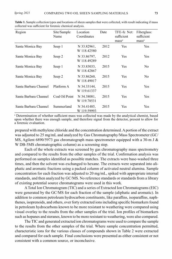
Table 1. Sample collection types and locations of sheen samples that were collected, with result indicating if mass collected was sufficient for forensic chemical analysis.
Region Site/Sample Name
Location Coordinates
Date TFE-fc Net: sufficient massa
Fiberglass: sufficient massa
Santa Monica Bay Seep 1 N 33.82961, W 118.42580
2012 Yes Yes
Santa Monica Bay Seep 2 N 33.86797, W 118.49289
2012 Yes Yes
Santa Monica Bay Seep 1 N 33.83033, W 118.42867
2015 Yes No
Santa Monica Bay Seep 2 N 33.86260, W 118.49017
2015 Yes No
Santa Barbara Channel Platform A N 34.33144, W 119.61337
2015 Yes Yes
Santa Barbara Channel Coal Oil Point N 34.38081, W 119.78531
2015 Yes Yes
Santa Barbara Channel Summerland N 34.41485, W 119.59993
2015 Yes Yes
a Determination of whether sufficient mass was collected was made by the analytical chemist, based upon whether there was enough sample, and therefore signal from the detector, present to allow for a forensic evaluation.
prepared with methylene chloride and the concentration determined. A portion of the extract was adjusted to 25 mg/mL and analyzed by Gas Chromatography/Mass Spectrometer (GC/MS, Agilent 6890/5973 gas chromatograph mass spectrometer equipped with a 30-m J & W DB-5MS chromatographic column) as a screening step.
Each of the whole extracts was screened by gas chromatography mass spectrometry and compared to the results from the other samples of the trial. Confirmation analysis was performed on samples identified as possible matches. The extracts were base-washed three times, and then the solvent was exchanged to hexane. The extracts were separated into ali-phatic and aromatic fractions using a packed column of activated neutral alumina. Sample concentration for each fraction was adjusted to 20 mg/mL, spiked with appropriate internal standards, and then analyzed by GC/MS. No reference standards or standards from a library of existing potential source chromatograms were used in this work.
A Total Ion Chromatogram (TIC) and a series of Extracted Ion Chromatograms (EIC) were generated by the GC/MS for each fraction of the sample (aliphatic and aromatic). In addition to common petroleum hydrocarbon constituents, like paraffins, isoparaffins, naph-thenes, isoprenoids, and others, over forty extracted ions including specific biomarkers found in petroleum hydrocarbons known to be more resistant to weathering were compared using visual overlay to the results from the other samples of the trial. Ion profiles of biomarkers such as hopanes and steranes, known to be more resistant to weathering, were also compared.
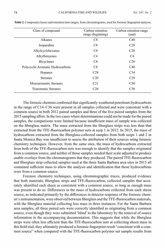
The TIC and generated extracted ion chromatograms were used to compare the sample to the results from the other samples of the trial. Where sample concentration permitted, characteristic ions for the various classes of compounds shown in Table 2 were extracted and compared for each sample. Final conclusions were presented as either consistent or not consistent with a common source, or inconclusive.
Vol. 107, No. 2CALIFORNIA FISH AND WILDLIFE74
Table 2. Compound classes and retention time ranges, from chromatograms, used for forensic fingerprint analysis.
Class of compound Carbon retention range (beginning)
Carbon retention range (end)
Alkanes C8 C40Isoparafins C8 C28
Alkylcyclohexanes C8 C28Alkylbenzenes C4 C4
Bicyclanes C8 C20Polycyclic Aromatic Hydrocarbons C8 C40
Hopanes C28 C34Steranes C20 C29
Monoaromatic Steranes C21 C30Triaromatic Steranes C26 C30
The forensic chemists confirmed that significantly weathered petroleum hydrocarbons in the range of C14–C36 were present in all samples collected and were consistent with a common source in both 2012 paired samples and three of the five paired samples from the 2015 sampling effort. In the two cases where determinations could not be made for the paired samples, the comparisons were limited because insufficient mass of sample was collected on the fiberglass matrix. The mass extracted from the fiberglass strips was less than that extracted from the TFE-fluorocarbon polymer nets at seep 1 in 2012. In 2015, the mass of hydrocarbons extracted from the fiberglass-collected samples from both seeps 1 and 2 in Santa Monica Bay was insufficient to assess the attribution of their sources using forensic chemistry techniques. However, from the same sites, the mass of hydrocarbons extracted from both of the TFE-fluorocarbon nets was enough to identify that the samples originated from a common source, and neither of those samples needed their scale adjusted to produce usable overlays from the chromatograms that they produced. The paired TFE-fluorocarbon and fiberglass strip collected samples used at the three Santa Barbara area sites in 2015 all contained sufficient mass to allow the analysis and identification that those hydrocarbons were from a common source.
Forensic chemistry techniques, using chromatographic traces, produced evidence that both materials, fiberglass strips and TFE-fluorocarbon, collected samples that accu-rately identified each sheen as consistent with a common source, so long as enough mass was present to do so. Differences in the mass of hydrocarbons collected from each sheen source, as indicated primarily by the differences in detector response of the forensic chem-ist’s instrumentation, were observed between fiberglass and the TFE-fluorocarbon materials, with the fiberglass material collecting less mass in three instances. For the Santa Barbara area samples, all three paired sets were correctly identified as originating from a common source, even though they were submitted ‘blind’ to the laboratory by the removal of source information in the accompanying documentation. This suggests that while the fiberglass strips were often less efficient than the TFE-fluorocarbon nets at collecting sheen mass in this field trial, they ultimately produced a forensic fingerprint result “consistent with a com-mon source” when compared with the TFE-fluorocarbon polymer net sample results from
75Spring 2021 75COMPARING TWO OIL SHEEN SAMPLING MATERIALS
the same seep. Samplers made efforts to collect from the same area of sheens with each of the paired TFE net and the fiberglass strip materials. However, because this was a field trial where precise sampling conditions were not controlled, including the proportions of each sheen encountered, the possibility remains that mass differences detected in the laboratory were affected by the sampling materials contacting different masses of sheen during the sampling process.
It is reasonable to expect that a chemically non-reactive substrate used to collect a sample of petroleum sheen would produce the same forensic result as another chemically non-reactive material. Barring evidence of some type of selective or biased adsorption or collection of hydrocarbons based on size ranges, or secondary or tertiary structures (i.e., aromatic rings, straight chain, or branched hydrocarbons), this result would be expected. However, since the literature is lacking in citations related to the use of fiberglass materials for this sampling purpose, this field trial is supportive evidence that this less expensive means of collecting sheen samples produces acceptable results once sufficient sample is adsorbed to the fiberglass. Further testing with more types of petroleum and distillate products and an increased number of replicates would be helpful in further evaluating this preliminary conclusion. Additionally, some form of sampling instructions or training materials for the samplers that is designed to aid them in obtaining a sufficient hydrocarbon mass when using the fiberglass material appears to be warranted.
It was evident that the on-water sampling of sheen using material attached to the end of a pole from a boat deck was simpler with TFE-fluorocarbon polymer nets than with the fiberglass strips. This was because the mechanics of collection were significantly easier with the net shape of the TFE-fluorocarbon polymer nets. The net was simple to maneuver through the sheen, while the fiberglass strips flexed and bent with each sweeping motion, making the strips less effective at collecting sheen material off the water surface. In fact, two samples taken using fiberglass at the Santa Monica area seeps in 2015 contained such a low mass of sheen material that they were not able to be successfully analyzed using forensic chemistry techniques. Nevertheless, considering the cost of the nets is greater than 20 times that of the four fiberglass strips, the comparability of the results suggest that the decision by CDFW to continue to use the fiberglass material is acceptable as long as sufficient mass of the sheen is collected. CDFW uses the fiberglass strips in routine evidence collection activities related to petroleum spill cases or forensic investigations such as when seabirds are found oiled near natural oil seeps. CDFW provides hundreds of oil sheen sampling kits to staff all over the State of California that contain the fiberglass strips, making the cost savings over TFE-fluorocarbon polymer nets significant at this scale of utilization.
ACKNOWLEDGMENTS
The staff time for CDFW employees on the present study was paid for by the CDFW-OSPR, and the laboratory analyses were paid for by Chevron Corporation. We would like to acknowledge and specifically thank Margaret Zalabak, Steven Behenna, Michael Connell, and Santos Cabral for their logistical support, as well as Beckye Stanton and Peter Sabat for their assistance with this field trial.
LITERATURE CITED
American Society of Testing and Materials. 1995. ASTM D4489-95: Standard Practices for Sampling of Waterborne Oils. Available from: https://www.astm.org/DATA-
Vol. 107, No. 2CALIFORNIA FISH AND WILDLIFE76
BASE.CART/HISTORICAL/D4489-95R06.htmAmerican Society of Testing and Materials. 2006. ASTM D5739 Standard Practice for Oil
Spill Source Identification by Gas Chromatography and Positive Ion Electron Im-pact Low Resolution Mass Spectrometry. Available from: https://www.astm.org/DATABASE.CART/HISTORICAL/D5739-06.htm
Greimann D, A. Zohn, K. Plourde, and T. Reilly. 1995. Teflon Nets: A novel approach to thin film oil sampling. Proceedings, Second International Oil Spill Research and Development Forum, London, England, May 23–26:882–883.
Hornafius, J. S., D. Quigley, and B. P. Luyendyk. 1999. The world’s most spectacular marine hydrocarbon seeps (Coal Oil Point, Santa Barbara Channel, California): quantification of emissions. Journal of Geophysical Research 104:20703–20711.
Kvenvolden K. A., and C. K. Cooper. 2003. Natural seepage of crude oil into the marine environment. Geo-marine Letters 23:140–146.
Lorenson, T. D, F. D. Hostettler, R. J. Rosenbauer, K. E. Peters, K. A. Kvenvolden, J. A. Dougherty, C. E. Gutmacher, F. L. Wong, and W. R. Normark. 2009. Natural off-shore seepage and related tarball accumulation on the California coastline; Santa Barbara Channel and the southern Santa Maria Basin; source identification and inventory. U.S. Geological Survey Open-File Report 2009-1225 and MMS report 2009-030. U.S. Geological Survey, Menlo Park, California. Refugio Beach Oil Spill NRDA Administrative Record.
Plourde, K. L., M. S. Hendrick, D. E. Greimann, and T. R. Reilly. 1995. Nets: a novel ap-proach to thin sheen oil sampling. Proceedings, Second International Oil Spill Research and Development Forum, London, England, May 23–26:1–13.
Submitted 8 January 2021Accepted 2 March 2021Associate Editor was P. McHugh
FULL RESEARCH ARTICLE
The distribution of anadromy and residency in steelhead/rainbow trout in the Eel River, northwestern California
BRET C. HARVEY1*, RODNEY J. NAKAMOTO1, ADAM J. R. KENT,2 AND CHRISTIAN E. ZIMMERMAN3
1 USDA Forest Service, Pacific Southwest Research Station, 1700 Bayview Drive, Arcata, CA 95521, USA
2 Oregon State University, College of Earth, Ocean, and Atmospheric Sciences, W. M. Keck Collaboratory for Plasma Mass Spectrometry, Corvallis, OR 97331, USA
3 U.S. Geological Survey, Alaska Science Center, 4230 University Drive Suite 201, Anchor-age, AK 95508, USA
*Corresponding Author: [email protected]
To inform management and conservation of the species, we inves-tigated the distribution of anadromy and residency of steelhead/rainbow trout (Oncorhynchus mykiss) in the Eel River of northwestern California. We determined maternal anadromy versus residency for 106 juvenile O. mykiss using otolith microchemistry. To attempt to relate patterns of anadromy with environmental factors known to influence its distribution in O. mykiss in other places, fish were collected from 52 sites throughout the drainage covering a range of stream size (0.1–7.7 m3/s estimated mean annual run-off) and distance from the ocean (23–219 km). Sixty-one of 91 fish sampled below prospective barriers had anadromous mothers, while 1 of 15 fish sampled above barriers had an anadromous mother. We did not detect any influence of stream size or distance from the ocean on the occurrence of anadromy. Fish with resident mothers were found at 21 of 46 sites below barriers. The current broad distribution of fish with resident mothers indicates the importance of maintaining freshwater conditions suitable for resident adults and juveniles age-1 and older, such as preserv-ing dry-season streamflows.
Key words: anadromy, barriers, isotope analysis, life history, Oncorhynchus mykiss, stron-tium__________________________________________________________________________
Extreme geographic and individual variability characterizes the life history of steel-head/rainbow trout (Oncorhynchus mykiss). For example, resident and anadromous indi-viduals commonly co-occur in California (Donohoe et al. 2008; Zimmerman et al. 2009) and elsewhere (Zimmerman and Reeves 2000, 2002). Anadromous O. mykiss include two
California Fish and Wildlife 107(2):77-88; 2021 www.doi.org/10.51492/cfwj.107.7
Vol. 107, No. 2CALIFORNIA FISH AND WILDLIFE78
fundamentally different life histories, winter- and summer-run. Within these two anadromous life histories, individuals vary in the age of ocean entry, age of return to freshwater, and the extent of iteroparity. While it seems likely that the extreme variability of O. mykiss life history enhances the sustainability of the species, better understanding of this variability is needed to help prioritize conservation efforts (Knudsen and Michael 2009).
Understanding factors that influence the distribution and frequency of anadromy versus residency is an important area of research. Recent efforts have identified genetic variation associated with anadromous versus resident life histories (Hale et al. 2013; Pearse et al. 2014; Kannry et al. 2020; Kelson et al. 2020) and a variety of other individual and environmental factors that can alter the frequency of anadromy (Ohms et al. 2014; Sloat and Reeves 2014; Kendall et al. 2015). One study at the stream network scale in the John Day River Drain-age in Oregon indicated that stream size influences the frequency of anadromy (Mills et al. 2012). Increasing residency in O. mykiss with distance upstream has been observed widely (e.g., McMillan et al. 2007), but in at least one case, the opposite trend has been observed (Liberoff et al. 2015). The influence of distance per se can be difficult to distinguish from other environmental factors. However, in some settings, variation in freshwater migration distance appears to influence anadromy in salmonids even over distances < 10 km (Kristof-fersen 1994). The generality of any patterns of anadromy with stream size and migration distance remains to be resolved. For example, increasing residency with decreasing stream size might not be expected where small streams provide poor conditions for the survival of fish older than age-0.
The presence of barriers to upstream migration obviously influences the extent of anadromy in migratory salmonids, and barriers commonly influence population genetics (Clemento et al. 2009). However, members of upstream populations may become anadromous when transported below barriers (Wilzbach et al. 2012). While barriers are obviously impor-tant, they can be difficult to define with certainty: small changes in the structure of natural barriers can make them passable and the effectiveness of barriers is often flow-dependent. Nevertheless, barriers remain important to resource management, in that regulatory ap-proaches to streams accessible to anadromous fish may differ from approaches applied to streams above barriers.
We examined the distribution of anadromy in O. mykiss in the Eel River Drainage for two main reasons: 1) resource managers sought more information on the effectiveness of a specific prospective barrier (Eaton Roughs on the Van Duzen River) to upstream migration where a large amount of suitable habitat for O. mykiss is available; and 2) we sought to test the applicability of relationships observed in other systems between O. mykiss anadromy and the environmental factors of upstream distance and stream size.
METHODSStudy Area
The Eel River Drainage of northwestern California is the third largest drainage in the state, covering 9542 km2 of largely forest and oak woodland subject to a Mediterranean climate with wet winters and dry summers. It is characterized by unstable underlying rock, significant tectonic activity, and extreme sediment yields (Wheatcroft and Sommerfield 2005). The Eel River historically supported robust populations of anadromous salmonids including Chinook salmon (Oncorhynchus tshawytscha), Coho Salmon (O. kisutch) and steelhead/rainbow trout; all have substantially declined. Yoshiyama and Moyle (2010) sug-
79Spring 2021 79DISTRIBUTION OF STEELHEAD IN THE EEL RIVER
gest that for winter and summer runs of steelhead: “Based on habitat availability and the few population estimates that exist, historic numbers were likely 100,000–150,000 adults per year (both runs combined), declining to 10,000–15,000 by the 1960s. Present numbers are probably considerably less than 1,000 fish in both runs.” However, Yoshiyama and Moyle (2010) also suggest that the distribution of steelhead/rainbow trout in the Eel River has declined much less than the species’ abundance. The Eel River is also the southern-most drainage in the range of coastal cutthroat trout (O. clarki clarki), but that species’ distribu-tion within the drainage is limited to a few tributaries close to the coast.
Field Methods
We collected juvenile O. mykiss by electrofishing at 52 sites in the Eel River Drain-age from July to October of 2012. Water year 2012 was relatively dry, with a mean annual streamflow 65% of the long-term average at two gaging sites in the drainage. We selected sites to cover a broad range of distance to the ocean and stream size (Fig. 1). We also included samples above three prospective barriers, with a particular focus above Eaton Roughs on the Van Duzen River, because resource managers had expressed specific interest in that area of the stream network. Eaton Roughs has been classified as a barrier to anadromous salmonids by resource management agencies. Using information in Reiser and Peacock (1985), we defined additional prospective barriers as features requiring leaps of 3.3 m or more where we judged “take-off” conditions to be good or leaps of 2 m or more where “take-off” conditions were considered poor. After euthanizing them with an overdose of MS-222, we preserved whole fish in 90% ethanol for later extraction of otoliths.
Laboratory Methods
We rinsed one otolith from each fish in deionized water to remove any remaining bio-logical material from the surface and allowed it to air dry. Cleaned otoliths were embedded in Buehler Epothin epoxy and sectioned through the nucleus in the transverse plane with two wafering blades on a Buehler Isomet low-speed saw. We placed the transverse sections face down on a sheet of adhesive paper, then embedded them in epoxy within a 2.54-cm diameter lucite ring. Each ring contained 20 – 22 otolith sections. After curing, we polished the exposed otolith sections with 30-μm, 9-μm, and 3-μm polishing papers and finally in a slurry of 0.05-μm alumina polish.
We determined maternal origin using one or two analytical steps, as needed. First, we analyzed elemental strontium (Sr) concentration in otolith core regions and compared it to Sr concentration in the first-summer growth regions using methods described by Zimmer-man et al. (2009). Otolith Sr concentrations were measured using laser ablation inductively coupled, plasma mass spectrometry (LA-ICP-MS) using an Agilent 7500c, quadrupole mass spectrometer and a New Wave 213 nm excimer laser at the University of Alaska Fairbanks Advanced Instrumentation Laboratory. Starting in the primordia, transects were ablated perpendicular to growth increments in one otolith per captured fish. Transects extended into the otolith mounting medium beyond the distal edge of the otolith. Count (intensity) data were collected for the elements strontium (88Sr) and calcium (43Ca). Calcium was used as an internal standard, and background-subtracted counts of Sr were adjusted to Ca and calibrated to glass standard reference material (NIST 610, National Institute of Standards and Testing). Calibration standards were run between every 10 – 12 samples. Laser speed was set at 5µm/s with a 25-µm spot diameter on a single-pass transect set to 80% power.
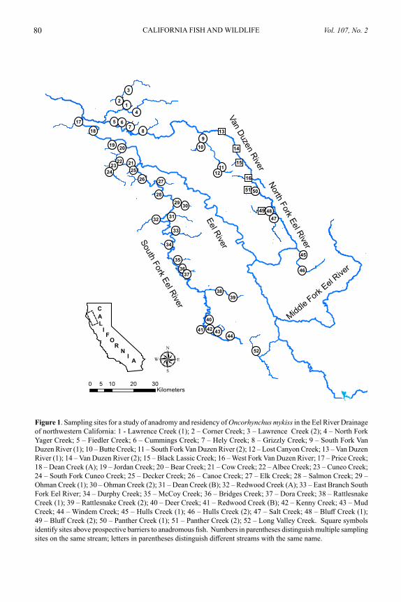
Vol. 107, No. 2CALIFORNIA FISH AND WILDLIFE80
!<
!<
!<
!<
!<!<
!<
!<
!<!<
!<
!<
!<
!<
!(
!(
!(
!(!(
!(
!(!(
!(
!(
!(!(
!(
!(
!(
!(
!(
!(
!(
!(
!(
!(
!(
!(
!(
!(
!(
!(
!(!(
!(
!(
!(
!(
!(
!(
!(
!(
!(
!(
!(
!(
!(
!(!(
!(
!(
!(!(
!(
!(
!(
!(
0 10 20 305Kilometers
µ
Van Duzen River
South Fork Eel River
North Fork Eel River
Eel River
Middle Fork Eel R
iver
114
113
115
116
149
151
910
1112
4748
50
12
3
4
5 67
8
17
18
19 20
212223
24 25
26
29
27
28
3132
33
34
35
3637
3839
40
41 42 4344
45
46
52
30
CAL
IF
OR
NI
A
Figure 1. Sampling sites for a study of anadromy and residency of Oncorhynchus mykiss in the Eel River Drainage of northwestern California: 1 - Lawrence Creek (1); 2 – Corner Creek; 3 – Lawrence Creek (2); 4 – North Fork Yager Creek; 5 – Fiedler Creek; 6 – Cummings Creek; 7 – Hely Creek; 8 – Grizzly Creek; 9 – South Fork Van Duzen River (1); 10 – Butte Creek; 11 – South Fork Van Duzen River (2); 12 – Lost Canyon Creek; 13 – Van Duzen River (1); 14 – Van Duzen River (2); 15 – Black Lassic Creek; 16 – West Fork Van Duzen River; 17 – Price Creek; 18 – Dean Creek (A); 19 – Jordan Creek; 20 – Bear Creek; 21 – Cow Creek; 22 – Albee Creek; 23 – Cuneo Creek; 24 – South Fork Cuneo Creek; 25 – Decker Creek; 26 – Canoe Creek; 27 – Elk Creek; 28 – Salmon Creek; 29 – Ohman Creek (1); 30 – Ohman Creek (2); 31 – Dean Creek (B); 32 – Redwood Creek (A); 33 – East Branch South Fork Eel River; 34 – Durphy Creek; 35 – McCoy Creek; 36 – Bridges Creek; 37 – Dora Creek; 38 – Rattlesnake Creek (1); 39 – Rattlesnake Creek (2); 40 – Deer Creek; 41 – Redwood Creek (B); 42 – Kenny Creek; 43 – Mud Creek; 44 – Windem Creek; 45 – Hulls Creek (1); 46 – Hulls Creek (2); 47 – Salt Creek; 48 – Bluff Creek (1); 49 – Bluff Creek (2); 50 – Panther Creek (1); 51 – Panther Creek (2); 52 – Long Valley Creek. Square symbols identify sites above prospective barriers to anadromous fish. Numbers in parentheses distinguish multiple sampling sites on the same stream; letters in parentheses distinguish different streams with the same name.
81Spring 2021 81DISTRIBUTION OF STEELHEAD IN THE EEL RIVER
The elemental count per second output of the LA-ICP-MS was then converted to concen-tration. Relatively low Sr concentrations (Sr concentration < 1000 ppm) in the summer growth regions of most otoliths allowed the determination of maternal origin using the Sr concentration of the core regions, following the methods of Zimmerman et al. (2009). For these otoliths, if mean Sr concentration in the core region significantly exceeded that of the mean summer growth region (one-tailed t-test), we classified fish as steelhead progeny, otherwise we classified fish as resident progeny.
However, high Sr concentrations in the summer growth regions of some otoliths in-dicated high ambient Sr in some streams. For otoliths with Sr concentrations in the summer growth region > 1000 ppm, we determined maternal origin of otoliths in a second analytical step, using 87Sr/86Sr ratios. We measured otolith 87Sr/86Sr ratios using laser ablation-inductively coupled plasma mass spectrometry (LA-MC-ICP-MS) in the W.M. Keck Collaboratory for Plasma Mass Spectrometry at Oregon State University, using a NuPlasma multi-collector ICP-MS instrument and a New Wave DUV193 excimer laser. Analysis techniques followed Miller and Kent (2009).
Ablation used a pulse rate of 10 Hz, a 70-µm diameter spot size, and the laser spot was translated across the sample at ~2 µm/s. Backgrounds were measured prior to analysis for 60 s and measured background intensities were subtracted from intensities measured during otolith ablation. Mass biases were corrected by reference to an 86Sr/88Sr ratio of 0.1194 using an exponential mass bias correction scheme. The low rubidium (Rb)/Sr ratio of otolith material indicated minor isobaric interference of 87Rb on 87Sr, and we corrected this using measured 85Rb to calculate the contribution of 87Rb. Typical precision and ac-curacy for measured 87Sr/86Sr ratios is ± 0.0001 – 0.0002 (two SE). We assessed accuracy during analyses via measurement of a deep-sea gastropod shell from the Gulf of Mexico with 87Sr/86Sr 0.70919 ± 0.00008. We determined maternal origin using 87Sr/86Sr following methods in Courter et al. (2013): the otolith core regions of steelhead progeny had 87Sr/86Sr ratios > 0.7080 while those of resident progeny matched the 87Sr/86Sr ratio found in the first summer growth region. For the progeny of resident mothers, ratios of 87Sr/86Sr in first sum-mer growth regions ranged from 0.7021 to 0.7050 and thus did not overlap marine values (Brennan et al. 2015).
Analysis
In general, we included two fish from each sampling site in the analysis, one assumed to be age-0 and the other post-age-0, usually age-1. We based age estimates on size-frequency distributions. One below-barrier site (Dora Creek) only yielded one fish. Because of our particular interest in the upper Van Duzen River, we included three sampling sites from that area and as many as four fish per site in the analysis. We selected all fish included in the analysis a priori.
We modeled the occurrence of juvenile steelhead with anadromous mothers using logistic regression and three predictors that have influenced the distribution of anadromy in previous studies of salmonids: distance from the ocean, stream size, and the presence of barriers. We used estimates of mean annual run-off to characterize stream size, using an equation for rainfall-dominated watersheds from Sanborn and Bledsoe (2006) that uses drainage area, precipitation, and potential evapotranspiration as independent variables. We included six candidate models chosen a priori in the model selection process and compared
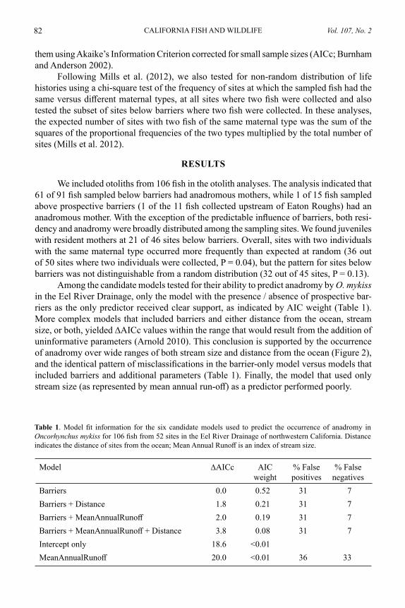
Vol. 107, No. 2CALIFORNIA FISH AND WILDLIFE82
them using Akaike’s Information Criterion corrected for small sample sizes (AICc; Burnham and Anderson 2002).
Following Mills et al. (2012), we also tested for non-random distribution of life histories using a chi-square test of the frequency of sites at which the sampled fish had the same versus different maternal types, at all sites where two fish were collected and also tested the subset of sites below barriers where two fish were collected. In these analyses, the expected number of sites with two fish of the same maternal type was the sum of the squares of the proportional frequencies of the two types multiplied by the total number of sites (Mills et al. 2012).
RESULTS
We included otoliths from 106 fish in the otolith analyses. The analysis indicated that 61 of 91 fish sampled below barriers had anadromous mothers, while 1 of 15 fish sampled above prospective barriers (1 of the 11 fish collected upstream of Eaton Roughs) had an anadromous mother. With the exception of the predictable influence of barriers, both resi-dency and anadromy were broadly distributed among the sampling sites. We found juveniles with resident mothers at 21 of 46 sites below barriers. Overall, sites with two individuals with the same maternal type occurred more frequently than expected at random (36 out of 50 sites where two individuals were collected, P = 0.04), but the pattern for sites below barriers was not distinguishable from a random distribution (32 out of 45 sites, P = 0.13).
Among the candidate models tested for their ability to predict anadromy by O. mykiss in the Eel River Drainage, only the model with the presence / absence of prospective bar-riers as the only predictor received clear support, as indicated by AIC weight (Table 1). More complex models that included barriers and either distance from the ocean, stream size, or both, yielded ∆AICc values within the range that would result from the addition of uninformative parameters (Arnold 2010). This conclusion is supported by the occurrence of anadromy over wide ranges of both stream size and distance from the ocean (Figure 2), and the identical pattern of misclassifications in the barrier-only model versus models that included barriers and additional parameters (Table 1). Finally, the model that used only stream size (as represented by mean annual run-off) as a predictor performed poorly.
Table 1. Model fit information for the six candidate models used to predict the occurrence of anadromy in Oncorhynchus mykiss for 106 fish from 52 sites in the Eel River Drainage of northwestern California. Distance indicates the distance of sites from the ocean; Mean Annual Runoff is an index of stream size.
Model ∆AICc AIC weight
% False positives
% False negatives
Barriers 0.0 0.52 31 7Barriers + Distance 1.8 0.21 31 7Barriers + MeanAnnualRunoff 2.0 0.19 31 7Barriers + MeanAnnualRunoff + Distance 3.8 0.08 31 7Intercept only 18.6 <0.01MeanAnnualRunoff 20.0 <0.01 36 33
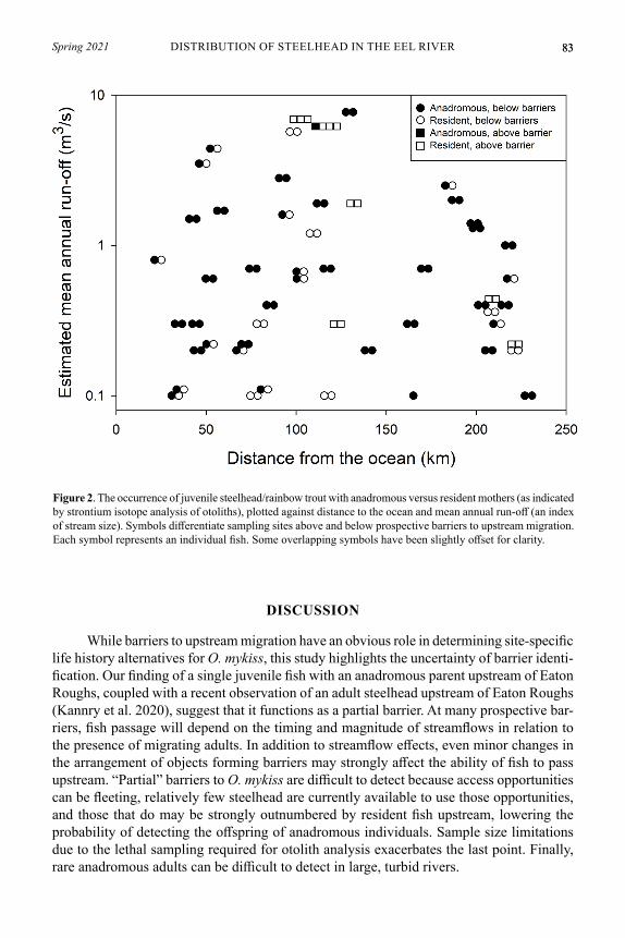
83Spring 2021 83DISTRIBUTION OF STEELHEAD IN THE EEL RIVER
Figure 2. The occurrence of juvenile steelhead/rainbow trout with anadromous versus resident mothers (as indicated by strontium isotope analysis of otoliths), plotted against distance to the ocean and mean annual run-off (an index of stream size). Symbols differentiate sampling sites above and below prospective barriers to upstream migration. Each symbol represents an individual fish. Some overlapping symbols have been slightly offset for clarity.
DISCUSSION
While barriers to upstream migration have an obvious role in determining site-specific life history alternatives for O. mykiss, this study highlights the uncertainty of barrier identi-fication. Our finding of a single juvenile fish with an anadromous parent upstream of Eaton Roughs, coupled with a recent observation of an adult steelhead upstream of Eaton Roughs (Kannry et al. 2020), suggest that it functions as a partial barrier. At many prospective bar-riers, fish passage will depend on the timing and magnitude of streamflows in relation to the presence of migrating adults. In addition to streamflow effects, even minor changes in the arrangement of objects forming barriers may strongly affect the ability of fish to pass upstream. “Partial” barriers to O. mykiss are difficult to detect because access opportunities can be fleeting, relatively few steelhead are currently available to use those opportunities, and those that do may be strongly outnumbered by resident fish upstream, lowering the probability of detecting the offspring of anadromous individuals. Sample size limitations due to the lethal sampling required for otolith analysis exacerbates the last point. Finally, rare anadromous adults can be difficult to detect in large, turbid rivers.
Vol. 107, No. 2CALIFORNIA FISH AND WILDLIFE84
The lack of a detectable influence of stream size on anadromy in O. mykiss in the Eel River Drainage contrasts with the results from the John Day River in Oregon (Mills et al. 2012), where anadromy of O. mykiss increased with stream size. This difference seems reasonable given the sample sites in the present study included small streams where the resident life history could be difficult to maintain because of limited dry-season habitat for adult resident fish. In small tributaries, the combination of low streamflows, high sediment loads and low habitat complexity may create high risk and limited feeding opportunities for O. mykiss older than age-0. Such streams may function principally as nursery areas for age-0 individuals, as suggested by the observed positive relationship between streamflow and density of O. mykiss older than age-0 in tributaries of the South Fork Eel River (Harvey et al. 2002).
Freshwater migration distance also did not influence the frequency of anadromy in our analysis. Freshwater migration distances did not exceed 250 km in our dataset and such distances are modest compared to those traversed by anadromous fish in larger drainages such as the Sacramento/San Joaquin and the Columbia. However, Kristofferson (1994) proposed that severe predation risk for migrant arctic charr (Salvelinus alpinus) could result in a distance effect on the frequency of anadromy even in the range of 0.3 to 7 km of migration distance. Adult steelhead in the Eel River may benefit from relatively modest predation risk in comparison to the arctic charr studied by Kristofferson (1994), because the former usually migrate during high, turbid streamflows.
While studies of anadromy versus residency in O. mykiss often focus on the persistence of the genetic potential for anadromy upstream of barriers, our study indicates the need to consider – under current conditions – the downstream distribution of residency. Juvenile fish with resident mothers were broadly distributed: we found them at 46% of the sites where no downstream barriers obstructed returning anadromous adults. We captured fish with resident mothers at several sites not far downstream from barriers to upstream migration. “Leaky” above-barrier resident populations may be contributing individuals to below-barrier reaches accessible to anadromous fish. In any case, reproduction by resident females made a note-worthy contribution to juvenile O. mykiss abundance in reaches accessible to anadromous fish. In addition, previous research has established that resident O. mykiss can contribute substantially to the anadromous component of some salmonid populations (Christie et al. 2011). These observations support the idea that conditions for fish older than age-0 throughout the stream network of the Eel River Drainage deserve special consideration from resource managers. High-quality freshwater conditions for larger fish benefit the O. mykiss population not only because of the relative value of large smolts to the population, but because of the potentially significant contribution of resident adults to population dynamics throughout the system. Unfortunately, a variety of factors have degraded freshwater conditions for resident salmonids in the Eel River Drainage: higher water temperatures, increased sediment loads that have reduced habitat complexity, the presence of alien species that may increase both competition (Reese and Harvey 2002) and predation (Nakamoto and Harvey 2003), and increased water diversion for domestic and agricultural use.
ACKNOWLEDGMENTS
We received field assistance from B. Nakamoto, J. White, and J. Wiesenfeld. K. Ken-field provided key contributions during the design of the study. K. Pope’s review improved the manuscript. The U.S. Geological Survey Forest and Rangeland Ecosystem Science Center
85Spring 2021 85DISTRIBUTION OF STEELHEAD IN THE EEL RIVER
in Corvallis, Oregon provided funding for the study. Any use of trade, firm, or product names is for descriptive purposes only and does not imply endorsement by the U.S. Government.
LITERATURE CITED
Arnold, T. W. 2010. Uninformative parameters and model selection using Akaike’s Infor-mation Criterion. Journal of Wildlife Management 74:1175–1178.
Brennan, S. R., D. P. Fernandez, C. E. Zimmerman, T. E. Cerling, R. J. Brown, and M. J. Wooller. 2015. Strontium isotopes in otoliths of a non-migratory fish (slimy sculpin): implications for provenance studies. Geochimica et Cosmochimica Acta 149:32–45.
Burnham, K. P., and D. R. Anderson. 2002. Model selection and multimodel inference: a practical information-theoretic approach. 2nd edition. Springer-Verlag, New York, NY, USA.
Christie, M. R., M. L. Marine, and M. S. Blouin. 2011. Who are the missing parents? Grandparentage analysis identifies multiple sources of gene flow into a wild pop-ulation. Molecular Ecology 20:1263–1276.
Clemento, A. J., E. C. Anderson, D. Boughton, D. Girman, and J. C. Garza. 2009. Popula-tion genetic structure and ancestry of Oncorhynchus mykiss populations above and below dams in south-central California. Conservation Genetics 10:1321–1336.
Courter, I. I, D. B. Child, J. A. Hobbs, T. M. Garrison, J. J. G. Glessner and S. Duery. 2013. Resident rainbow trout produce anadromous offspring in a large interior water-shed. Canadian Journal of Fisheries and Aquatic Sciences 70:701–710.
Donohoe, C. J., P. B. Adams, and C. F Royer. 2008. Influence of water chemistry and migratory distance on ability to distinguish progeny of sympatric resident and anadromous rainbow trout (Oncorhynchus mykiss). Canadian Journal of Fish and Aquatic Sciences 65:1060–1075.
Hale, M. C., F. P. Thrower, E. A. Berntson, M. R. Miller, and K. M. Nichols. 2013. Evaluat-ing adaptive divergence between migratory and nonmigratory ecotypes of a sal-monid fish, Oncorhynchus mykiss. G3: Genes, Genomes, Genetics 3:1273–1285.
Harvey, B. C., J. L. White, and R. J. Nakamoto. 2002. Habitat relationships and larval drift of native and nonindigenous fishes in neighboring tributaries of a coastal Califor-nia river. Transactions of the American Fisheries Society 131:159–170.
Kannry, S. H., S. M. O’Rourke, S. J. Kelson, and M. R. Miller. 2020. On the ecology and distribution of Steelhead (Oncorhynchus mykiss) in California’s Eel River. Jour-nal of Heredity 111:548–563.
Kelson, S. J., S. M. Carlson, and M. R. Miller. 2020. Indirect genetic control of migration in a salmonid fish. Biology Letters 16:art20200299.
Kendall, N. W., J. R. McMillan, M. R. Sloat, T. W. Buehrens, T. P. Quinn, G. R. Pess, K. V. Kuzishchin, M. M. McClure, and R. W. Zabel. 2015. Anadromy and residency in steelhead and rainbow trout (Oncorhynchus mykiss): a review of the processes and patterns. Canadian Journal of Fisheries and Aquatic Sciences 72:319–342.
Knudsen, E. E., and J. H. Michael, Jr., editors. 2009. Pacific salmon environmental and life history models: advancing science for sustainable salmon in the future. Sympo-sium 71, American Fisheries Society, Bethesda, MD, USA.
Kristoffersen, K. 1994. The influence of physical watercourse parameters on the degree of anadromy in different lake populations of Arctic charr (Salvelinus alpinus (L.)) in
Vol. 107, No. 2CALIFORNIA FISH AND WILDLIFE86
northern Norway. Ecology of Freshwater Fish 3:80–91.Liberoff, A. L., A. P. Quiroga, C. M. Riva-Rossi, J. A. Miller, and M. A. Pascual. 2015.
Influence of maternal habitat choice, environment and spatial distribution of ju-veniles on their propensity for anadromy in a partially anadromous population of rainbow trout (Oncorhynchus mykiss). Ecology of Freshwater Fish 24:424–434.
McMillan, J. R., S. L. Katz, and G. R. Pess. 2007. Observational evidence of spatial and temporal structure in a sympatric anadromous (winter steelhead) and resident rainbow trout mating system on the Olympic Peninsula, Washington. Transac-tions of the American Fisheries Society 136:736–748.
Miller, J. A., and A. J. R. Kent. 2009. The determination of maternal run time in juvenile Chinook salmon (Oncorhynchus tshawytscha) based on Sr/Ca and 87Sr/86Sr within otolith cores. Fisheries Research 95:373–378.
Mills, J. S., J. B. Dunham, G. H. Reeves, J. R. McMillan, C. E. Zimmerman, and C. E. Jor-dan. 2012. Variability in expression of anadromy by female Oncorhynchus mykiss within a river network. Environmental Biology of Fishes 93:505–517.
Nakamoto, R. J., and B. C. Harvey. 2003. Spatial, seasonal, and size-dependent variation in the diet of Sacramento pikeminnow in the Eel River, northwestern California. California Fish and Game 89:30–45.
Ohms, H.A., M. R. Sloat, G. H. Reeves, C. E. Jordan, and J. B. Dunham. 2014. Influence of sex, migration distance, and latitude on life history expression in steelhead and rainbow trout (Oncorhynchus mykiss). Canadian Journal of Fisheries and Aquatic Sciences 71:70–80.
Pearse, D. E., M. R. Miller, A. Abadía-Cardoso, and J. C. Garza. 2014. Rapid parallel evolution of standing variation in a single, complex, genomic region is associated with life history in steelhead/rainbow trout. Proceedings of the Royal Society of London B 281:20140012.
Reese, C. D., and B. C. Harvey. 2002. Temperature-dependent competition between juve-nile steelhead and Sacramento pikeminnow. Transactions of the American Fisher-ies Society 131:599–606.
Reiser, D. W., and R. T. Peacock. 1985. A technique for assessing upstream fish passage problems at small-scale hydropower developments. Pages 423–432 in F. W. Ol-son, R. G. White, and R. H. Hamre, editors. Proceedings of the Symposium on Small Hydropower and Fisheries. American Fisheries Society, Bethesda, MD, USA.
Sanborn, S. C., and B. P. Bledsoe. 2006. Predicting streamflow regime metrics for un-gauged streams in Colorado, Washington, and Oregon. Journal of Hydrology 325:241–261.
Sloat, M. R., and G. H. Reeves. 2014. Individual condition, standard metabolic rate, and rearing temperature influence steelhead and rainbow trout (Oncorhynchus mykiss) life histories. Canadian Journal of Fisheries and Aquatic Sciences 71: 491–501.
Wheatcroft, R. A., and C. K. Sommerfield. 2005. River sediment flux and shelf sediment accumulation rates on the Pacific Northwest margin. Continental Shelf Research 25:311–332.
Wilzbach, M. A., M. J. Ashenfelter, and S. J. Ricker. 2012. Movement of resident rain-bow trout transplanted below a barrier to anadromy. Transactions of the American Fisheries Society 141:294–304.
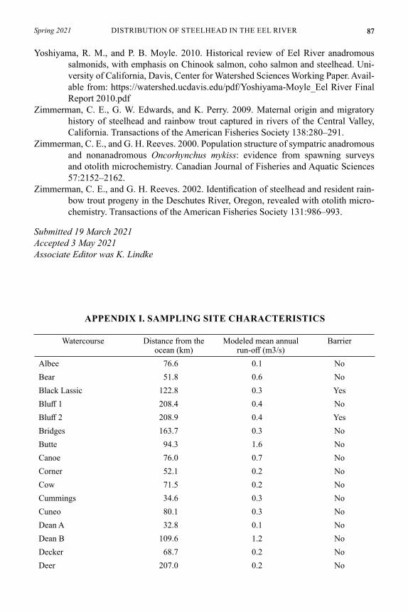
87Spring 2021 87DISTRIBUTION OF STEELHEAD IN THE EEL RIVER
Yoshiyama, R. M., and P. B. Moyle. 2010. Historical review of Eel River anadromous salmonids, with emphasis on Chinook salmon, coho salmon and steelhead. Uni-versity of California, Davis, Center for Watershed Sciences Working Paper. Avail-able from: https://watershed.ucdavis.edu/pdf/Yoshiyama-Moyle_Eel River Final Report 2010.pdf
Zimmerman, C. E., G. W. Edwards, and K. Perry. 2009. Maternal origin and migratory history of steelhead and rainbow trout captured in rivers of the Central Valley, California. Transactions of the American Fisheries Society 138:280–291.
Zimmerman, C. E., and G. H. Reeves. 2000. Population structure of sympatric anadromous and nonanadromous Oncorhynchus mykiss: evidence from spawning surveys and otolith microchemistry. Canadian Journal of Fisheries and Aquatic Sciences 57:2152–2162.
Zimmerman, C. E., and G. H. Reeves. 2002. Identification of steelhead and resident rain-bow trout progeny in the Deschutes River, Oregon, revealed with otolith micro-chemistry. Transactions of the American Fisheries Society 131:986–993.
Submitted 19 March 2021 Accepted 3 May 2021Associate Editor was K. Lindke
APPENDIX I. SAMPLING SITE CHARACTERISTICS
Watercourse Distance from the ocean (km)
Modeled mean annual run-off (m3/s)
Barrier
Albee 76.6 0.1 NoBear 51.8 0.6 NoBlack Lassic 122.8 0.3 YesBluff 1 208.4 0.4 NoBluff 2 208.9 0.4 YesBridges 163.7 0.3 NoButte 94.3 1.6 NoCanoe 76.0 0.7 NoCorner 52.1 0.2 NoCow 71.5 0.2 NoCummings 34.6 0.3 NoCuneo 80.1 0.3 NoDean A 32.8 0.1 NoDean B 109.6 1.2 NoDecker 68.7 0.2 NoDeer 207.0 0.2 No
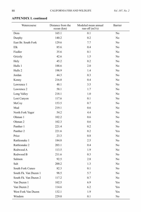
Vol. 107, No. 2CALIFORNIA FISH AND WILDLIFE88
Watercourse Distance from the ocean (km)
Modeled mean annual run-off (m3/s)
Barrier
Dora 165.1 0.1 NoDurphy 140.2 0.2 NoEast Br. South Fork 129.6 7.7 NoElk 85.6 0.4 NoFiedler 35.6 0.1 NoGrizzly 42.6 1.5 NoHely 45.2 0.2 NoHulls 1 188.6 2.0 NoHulls 2 198.9 1.4 NoJordan 44.3 0.3 NoKenny 216.0 0.4 NoLawrence 1 48.1 3.5 NoLawrence 2 58.1 1.7 NoLong Valley 218.1 1.0 NoLost Canyon 117.6 0.1 NoMcCoy 153.5 0.7 NoMud 219.1 0.6 NoNorth Fork Yager 54.2 4.4 NoOhman 1 102.2 0.6 NoOhman 2 102.3 0.6 NoPanther 1 221.4 0.2 NoPanther 2 221.6 0.2 YesPrice 23.3 0.8 NoRattlesnake 1 184.8 2.5 NoRattlesnake 2 203.1 0.4 NoRedwood A 113.5 1.9 NoRedwood B 211.6 0.3 NoSalmon 92.5 2.8 NoSalt 200.2 1.3 NoSouth Fork Cuneo 82.3 0.1 NoSouth Fk. Van Duzen 1 98.5 5.7 NoSouth Fk. Van Duzen 2 117.2 0.7 NoVan Duzen 1 102.5 6.9 YesVan Duzen 2 114.6 6.2 YesWest Fork Van Duzen 132.1 1.9 YesWindem 229.0 0.1 No
APPENDIX I. continued
FULL RESEARCH ARTICLE
Western Message Petroglyphs indicate historic beaver presence in a San Francisco Bay Area watershedLEIGH MARYMOR1 AND RICHARD BURNHAM LANMAN2,3*
1 Museum of Northern Arizona, 1270 45th Street, Emeryville, CA 94608, USA
2 Guadalupe-Coyote Resource Conservation District, 888 North First Street, San Jose, CA 95112, USA
3 Institute for Historical Ecology, 556 Van Buren Street, Los Altos, CA 94022, USA
*Corresponding Author: [email protected]
Recent museum, archaeological, and observer record evidence sug-gests that North American beaver (Castor canadensis) were historically native to the watersheds of California’s coast, including San Francisco Bay. A wide variety of animals are abundantly represented in Native American petroglyphs and pictographs with their representations fulfill-ing intentions ranging from the mundane to ceremonial and mythological purposes. However, beaver symbols are poorly represented in California rock art and absent from the San Francisco Bay Area. A novel record, in the form of Western Message Petroglyphs, suggests that a beaver lodge was present in the late nineteenth century in the Alameda Creek water-shed, potentially the last evidence of beaver prior to their extirpation in the region by the fur trade.
Key words: Alameda Creek, beaver, California, Castor canadensis, historic range, rock art, San Francisco Bay, Western Message Petroglyphs _________________________________________________________________________
Until recently, the historic range of the beaver (Castor canadensis) in California was described as restricted to the watersheds of the Central Valley below 305 m (1,000 ft), the Klamath and Pit River watersheds of furthest northern California, and the Colorado River mainstem in the extreme southeast border of the state (Zeiner et al. 1990). This work cited the claims of early twentieth century zoologists (Grinnell et al. 1937; Tappe 1942) and may have reflected “shifting baselines syndrome” (Pauly 1995) whereby scientists accept as a baseline species occurrence and distribution extant at the beginning of their careers, despite near extirpation of beaver by fur trappers in much of California almost a century and a half earlier. Over the last decade, physical evidence of beaver’s nativity to the high Sierra Nevada and the watersheds of coastal California, including the San Francisco Bay Area, led to recognition of a pre-fur trade distribution of beaver throughout the state (James and Lanman 2012; Lanman et al. 2012, 2013; CDFW 2017). Specific to Bay Area watersheds,
California Fish and Wildlife 107(2):89-98; 2021 www.doi.org/10.51492/cfwj.107.8
Vol. 107, No. 2CALIFORNIA FISH AND WILDLIFE90
physical evidence of beaver nativity included a beaver skull collected on Saratoga Creek in 1855 in Santa Clara County and now in the Smithsonian National Museum of Natural History (USNM 580354), and a beaver tooth at the CA-ALA-555 archaeological site on Arroyo de la Laguna Creek, a tributary of Alameda Creek in Alameda County, dating to 2200–1650 BCE (Lanman et al. 2013). In addition, Ohlone and Coast Miwok indigenous peoples in the Bay Area had words for beaver (Powers 1877; Heizer 1974; Merriam and Heizer 1979) that antedate widespread beaver re-introductions around California from 1923 to 1950 (Hensley 1946; Lundquist and Dolman 2013).
In contrast to the above evidence, depictions of beavers in California’s Native American rock art sites within the state of California are scarce, and absent from the San Francisco Bay Area. Among the numerous Indigenous peoples of California, animal depictions of various kinds (birds, reptiles, canids, ungulates, ursines, and caprids) abound in pictographs and petroglyphs across the state. In the publications cited below, only two rock art images of beaver were noted in California (neither in the Bay Area): a Chumash pictograph found on the Montgomery Potrero of the Cuyama River watershed in the Sierra Madre Mountains of eastern Santa Barbara County (Lee and Horne 1978), and a Yokuts pictograph along the Tule River on the Tule Indian Reservation in Tulare County (Mallery 1893; Grant 1979).
Here we analyze and translate a Western Message Petroglyph (WMP) site depicting a beaver lodge in the Alameda Creek watershed tributary to San Francisco Bay. WMPs appear to represent a “faux- Indian” picture-writing project dating to the last quarter of the nineteenth century and the opening years of the twentieth. Once dismissed as forgeries or a hoax, we now know that WMPs have been identified at 38 sites in eight western states (Marymor in press). WMPs were likely created by non-Native American author(s) with knowledge of a broad range of Native American symbols. The images appear to be ap-propriated from published indigenous picture-writing traditions and were first described as “modern petroglyphs” by the University of California Berkeley Anthropology Department (Elsasser and Contreras 1958). Located along historic wagon roads and rail corridors, WMPs are often associated with mining and quarry sites dating to the period of western expansion (Marymor and Marymor 2016; Marymor in press). A WMP panel of 19 images including a beaver lodge located on a boulder on the Vargas Plateau in the East Bay Hills was studied initially by Sister Mary Paula von Tessen, a Dominican sister and Sanskrit scholar resident at Mission San Jose, between 1930–1950, and included in Elsasser’s publication of the original seven known WMP sites (Elsasser and Contreras 1958). The Vargas Plateau WMP is herein described and interpreted as potential evidence of beaver presence in the Alameda Creek watershed through the late nineteenth century.
METHODSStudy Area
The original petroglyph boulder site was situated on the Vargas Plateau at an elevation of approximately 269 m (880 ft), 4.0 km (2.5 mi) northeast of Fremont, CA, USA (geo-graphic coordinates omitted for site protection). The Plateau is located midway between the Alameda Creek mainstem as it traverses Niles Canyon to the north, and and Interstate 680 as it traverses Mission Pass to the south (Fig. 1). Both of these gaps bordering the Vargas Plateau hold historic significance as major travel corridors. Niles Canyon became the western terminus for the Transcontinental Railroad in 1869 when the Western Pacific Railroad made connection with the Central Pacific Railroad at Sacramento. Mission Pass has served as a
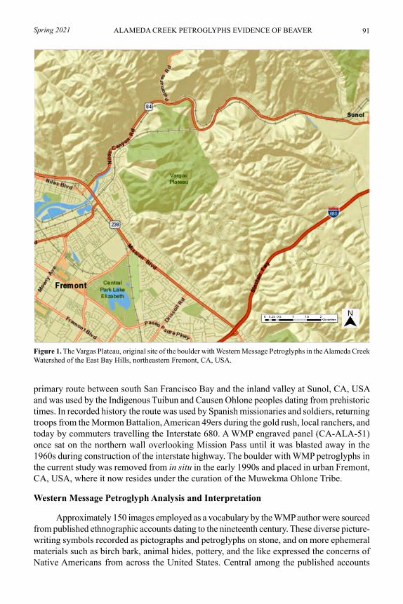
91Spring 2021 ALAMEDA CREEK PETROGLYPHS EVIDENCE OF BEAVER
Figure 1. The Vargas Plateau, original site of the boulder with Western Message Petroglyphs in the Alameda Creek Watershed of the East Bay Hills, northeastern Fremont, CA, USA.
primary route between south San Francisco Bay and the inland valley at Sunol, CA, USA and was used by the Indigenous Tuibun and Causen Ohlone peoples dating from prehistoric times. In recorded history the route was used by Spanish missionaries and soldiers, returning troops from the Mormon Battalion, American 49ers during the gold rush, local ranchers, and today by commuters travelling the Interstate 680. A WMP engraved panel (CA-ALA-51) once sat on the northern wall overlooking Mission Pass until it was blasted away in the 1960s during construction of the interstate highway. The boulder with WMP petroglyphs in the current study was removed from in situ in the early 1990s and placed in urban Fremont, CA, USA, where it now resides under the curation of the Muwekma Ohlone Tribe.
Western Message Petroglyph Analysis and Interpretation
Approximately 150 images employed as a vocabulary by the WMP author were sourced from published ethnographic accounts dating to the nineteenth century. These diverse picture-writing symbols recorded as pictographs and petroglyphs on stone, and on more ephemeral materials such as birch bark, animal hides, pottery, and the like expressed the concerns of Native Americans from across the United States. Central among the published accounts
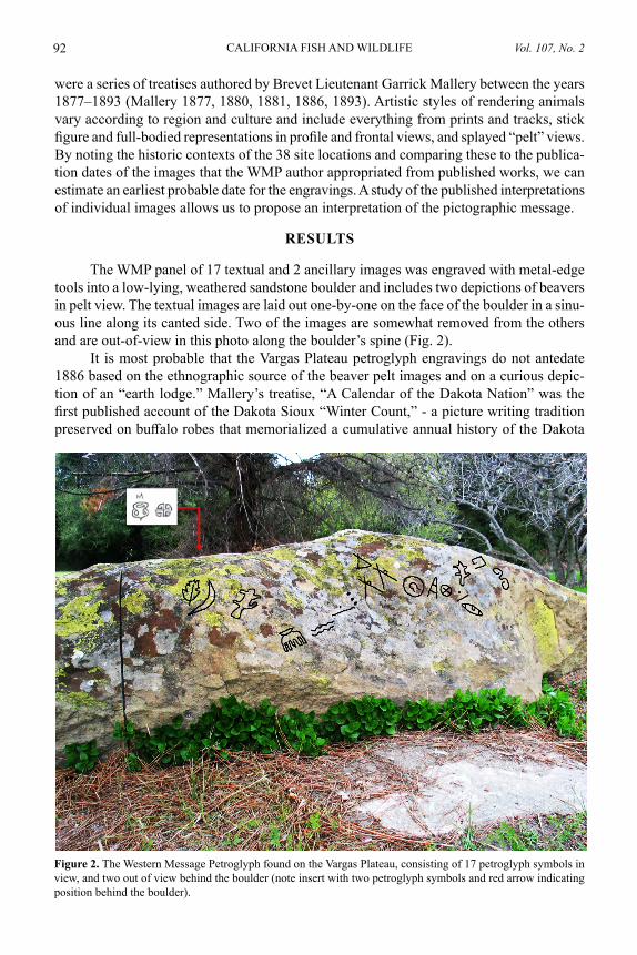
Vol. 107, No. 2CALIFORNIA FISH AND WILDLIFE92
were a series of treatises authored by Brevet Lieutenant Garrick Mallery between the years 1877–1893 (Mallery 1877, 1880, 1881, 1886, 1893). Artistic styles of rendering animals vary according to region and culture and include everything from prints and tracks, stick figure and full-bodied representations in profile and frontal views, and splayed “pelt” views. By noting the historic contexts of the 38 site locations and comparing these to the publica-tion dates of the images that the WMP author appropriated from published works, we can estimate an earliest probable date for the engravings. A study of the published interpretations of individual images allows us to propose an interpretation of the pictographic message.
RESULTS
The WMP panel of 17 textual and 2 ancillary images was engraved with metal-edge tools into a low-lying, weathered sandstone boulder and includes two depictions of beavers in pelt view. The textual images are laid out one-by-one on the face of the boulder in a sinu-ous line along its canted side. Two of the images are somewhat removed from the others and are out-of-view in this photo along the boulder’s spine (Fig. 2).
It is most probable that the Vargas Plateau petroglyph engravings do not antedate 1886 based on the ethnographic source of the beaver pelt images and on a curious depic-tion of an “earth lodge.” Mallery’s treatise, “A Calendar of the Dakota Nation” was the first published account of the Dakota Sioux “Winter Count,” - a picture writing tradition preserved on buffalo robes that memorialized a cumulative annual history of the Dakota
Figure 2. The Western Message Petroglyph found on the Vargas Plateau, consisting of 17 petroglyph symbols in view, and two out of view behind the boulder (note insert with two petroglyph symbols and red arrow indicating position behind the boulder).
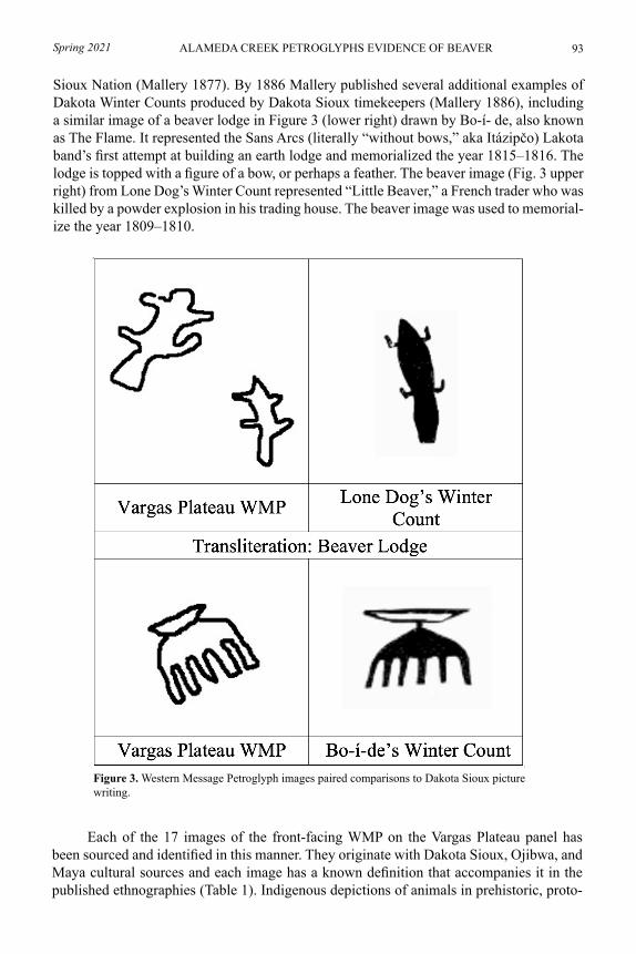
93Spring 2021 ALAMEDA CREEK PETROGLYPHS EVIDENCE OF BEAVER
Sioux Nation (Mallery 1877). By 1886 Mallery published several additional examples of Dakota Winter Counts produced by Dakota Sioux timekeepers (Mallery 1886), including a similar image of a beaver lodge in Figure 3 (lower right) drawn by Bo-í- de, also known as The Flame. It represented the Sans Arcs (literally “without bows,” aka Itázipčo) Lakota band’s first attempt at building an earth lodge and memorialized the year 1815–1816. The lodge is topped with a figure of a bow, or perhaps a feather. The beaver image (Fig. 3 upper right) from Lone Dog’s Winter Count represented “Little Beaver,” a French trader who was killed by a powder explosion in his trading house. The beaver image was used to memorial-ize the year 1809–1810.
Figure 3. Western Message Petroglyph images paired comparisons to Dakota Sioux picture writing.
Each of the 17 images of the front-facing WMP on the Vargas Plateau panel has been sourced and identified in this manner. They originate with Dakota Sioux, Ojibwa, and Maya cultural sources and each image has a known definition that accompanies it in the published ethnographies (Table 1). Indigenous depictions of animals in prehistoric, proto-
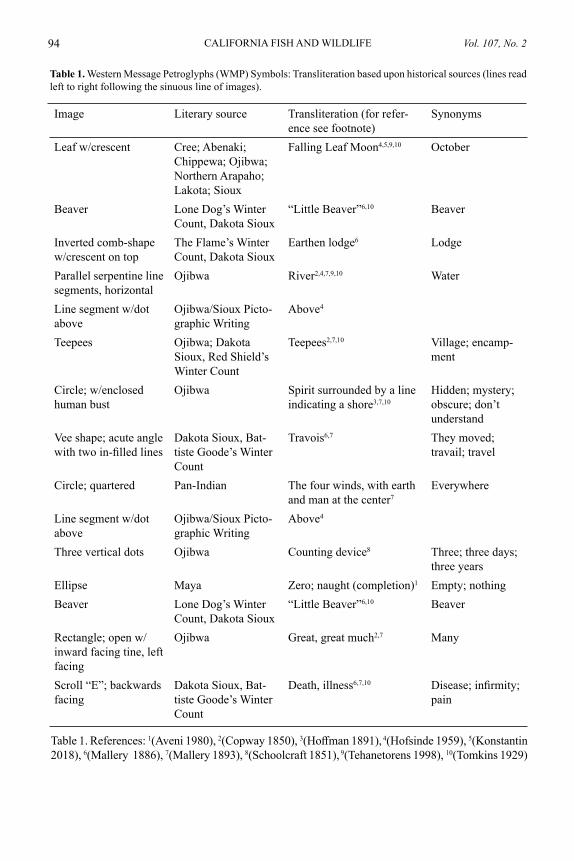
Vol. 107, No. 2CALIFORNIA FISH AND WILDLIFE94
Table 1. Western Message Petroglyphs (WMP) Symbols: Transliteration based upon historical sources (lines read left to right following the sinuous line of images).
Image Literary source Transliteration (for refer-ence see footnote)
Synonyms
Leaf w/crescent Cree; Abenaki; Chippewa; Ojibwa; Northern Arapaho; Lakota; Sioux
Falling Leaf Moon4,5,9,10 October
Beaver Lone Dog’s Winter Count, Dakota Sioux
“Little Beaver”6,10 Beaver
Inverted comb-shape w/crescent on top
The Flame’s Winter Count, Dakota Sioux
Earthen lodge6 Lodge
Parallel serpentine line segments, horizontal
Ojibwa River2,4,7,9,10 Water
Line segment w/dot above
Ojibwa/Sioux Picto-graphic Writing
Above4 None
Teepees Ojibwa; Dakota Sioux, Red Shield’s Winter Count
Teepees2,7,10 Village; encamp-ment
Circle; w/enclosed human bust
Ojibwa Spirit surrounded by a line indicating a shore3,7,10
Hidden; mystery; obscure; don’t understand
Vee shape; acute angle with two in-filled lines
Dakota Sioux, Bat-tiste Goode’s Winter Count
Travois6,7 They moved; travail; travel
Circle; quartered Pan-Indian The four winds, with earth and man at the center7
Everywhere
Line segment w/dot above
Ojibwa/Sioux Picto-graphic Writing
Above4 None
Three vertical dots Ojibwa Counting device8 Three; three days; three years
Ellipse Maya Zero; naught (completion)1 Empty; nothingBeaver Lone Dog’s Winter
Count, Dakota Sioux“Little Beaver”6,10 Beaver
Rectangle; open w/inward facing tine, left facing
Ojibwa Great, great much2,7 Many
Scroll “E”; backwards facing
Dakota Sioux, Bat-tiste Goode’s Winter Count
Death, illness6,7,10 Disease; infirmity; pain
Table 1. References: 1(Aveni 1980), 2(Copway 1850), 3(Hoffman 1891), 4(Hofsinde 1959), 5(Konstantin 2018), 6(Mallery 1886), 7(Mallery 1893), 8(Schoolcraft 1851), 9(Tehanetorens 1998), 10(Tomkins 1929)
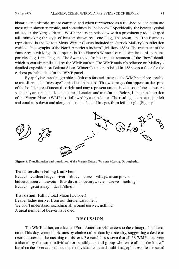
95Spring 2021 ALAMEDA CREEK PETROGLYPHS EVIDENCE OF BEAVER
historic, and historic art are common and when represented as a full-bodied depiction are most often shown in profile, and sometimes in “pelt-view.” Specifically, the beaver symbol utilized in the Vargas Plateau WMP appears in pelt-view with a prominent paddle-shaped tail, mimicking the style of beavers drawn by Lone Dog, The Swan, and The Flame as reproduced in the Dakota Sioux Winter Counts included in Garrick Mallery’s publication entitled “Pictographs of the North American Indians” (Mallery 1886). The treatment of the Sans Arcs earth lodge that appears in The Flame’s Winter Count is similar to his contem-poraries (e.g. Lone Dog and The Swan) save for his unique treatment of the “bow” detail, which is exactly replicated by the WMP author. The WMP author’s reliance on Mallery’s detailed exposition on Dakota Sioux Winter Counts published in 1886 sets a floor for the earliest probable date for the WMP panel.
By applying the ethnographic definitions for each image to the WMP panel we are able to transliterate the “message” embedded in the text. The two images that appear on the spine of the boulder are of uncertain origin and may represent unique inventions of the author. As such, they are not included in the transliteration and translation. Below, is the transliteration of the Vargas Plateau WMP text followed by a translation. The reading begins at upper left and continues down and along the sinuous line of images from left to right (Fig. 4):
Figure 4. Transliteration and translation of the Vargas Plateau Western Message Petroglyphs.
Transliteration: Falling Leaf MoonBeaver – earthen lodge – river – above – three – village/encampment –hidden/obscure – travois – four directions/everywhere – above – nothing – Beaver – great many – death/illness
Translation: Falling Leaf Moon (October) Beaver lodge upriver from our third encampmentWe don’t understand, searching all around upriver, nothing A great number of beaver have died
DISCUSSION
The WMP author, an educated Euro-American with access to the ethnographic litera-ture of his day, wrote in pictures by choice rather than by necessity, suggesting a desire to restrict access to the meaning of his text. Research has shown that all 38 WMP sites were authored by the same individual, or possibly a small group who were all “in the know,” based on the observation that unique individual icons and multi-image phrases often repeated
Vol. 107, No. 2CALIFORNIA FISH AND WILDLIFE96
among sites. Regarding whether the beaver symbol in the Vargas Plateau WMP is, in fact, a beaver, we note that it contains the key differentiating feature of Native American beaver symbols, namely the large, paddle-shaped tail, accurately represented as one-third of the animal’s body length. Beaver images in the other two known rock art images of beaver on the Tule and Cuyama River watersheds also include this key feature (Mallery 1894, Grant 1979, Lee and Horne 1978).
The earliest date that the WMP author would have found published accounts of the beaver and earthen lodge symbols used in the Vargas Plateau petroglyphs would have been Mallery’s 1886 publication. The symbols Mallery illustrated in his five reports were re-published later by authors of several major ethnographic descriptions. For example, Tomkins credited much of his published work on Native American picture-writing to material sourced from Mallery’s 10th Annual Report to the Bureau of Ethnology (Mallery 1893; Tomkins 1926). If our dating of the WMPs to 1886 or later is correct, then the message appears to be the last surviving record of beaver habitation prior to twentieth century re-introductions in the Alameda Creek watershed.
Definitions sourced from the ethnographic literature of the author’s day enabled us to approach his message through an image-by-image transliteration, but to extract an accurate translation, we are constrained by the limited material available on Native American picture-writing conventions from the historic era. The author (or authors) of the WMP are unknown, and exact dating of their inscription is not possible. A family whose ranch neighbors the original location of the Vargas Plateau boulder has indicated that it was at least 100 years old, i.e., before 1921, based on family lore, but this is not a definitive source. Although our translation of the Western Message Petroglyphs relies on limited knowledge as well as subjective interpretation, it is consistent with historical records of beaver trapping on Alameda Creek. In the 1840s, Christopher “Kit” Carson was granted rights to trap beaver on Alameda Creek by the Mission San José padres, where they “abounded...from the mouth of its canyon to the broad delta on the bay” (MacGregor 1976; Gustaitis 1995).
In conclusion, the Vargas Plateau petroglyph message appears to extend, by 30 or more years, the last reliable historical record of beaver in a San Francisco Bay watershed. The latter record was a Smithsonian Museum specimen collected in 1855 on Quito Creek (now Saratoga Creek) on the opposite (west) side of San Francisco Bay (Lanman et al. 2013). The WMP record of a beaver lodge in the absence of the animals upstream or downstream appears to herald their complete extirpation by the nineteenth century fur trade. Ethnographic information sources, such as the Vargas Plateau WMP, may serve as a novel, and previously unexpected, evidence source for better understanding of California’s historical fauna.
ACKNOWLEDGMENTS
The authors wish to acknowledge and extend their appreciation to author and environ-mental journalist, Ben Goldfarb, whose book, Eager: The Surprising, Secret Life of Beavers and Why They Matter, enabled our introduction and collaboration.
LITERATURE CITED
Aveni, A. F. 1980. Skywatchers of Ancient México. University of Texas Press, Austin, TX, USA.
California Department of Fish and Wildlife (CDFW). 2017. Living with Beavers. Avail-
97Spring 2021 ALAMEDA CREEK PETROGLYPHS EVIDENCE OF BEAVER
able from: https://nrm.dfg.ca.gov/FileHandler.ashx?DocumentID=114087 (Ac-cessed 4 Jan 2021)
Elsasser, A. B., and E. Contreras. 1958. Modern petrography in central California and western Nevada. Papers on California Archaeology 41(4):12–18.
Grant, C. 1979. An introduction to Yokuts rock painting. Page 28 in F. G. Bock, editor. An Introduction to Yokuts Rock Painting. American Indian Rock Art. Volume VI. Proceedings of the American Rock Art Research Association, Bottom Hollow, UT, USA.
Gustaitis, R. 1995. San Francisco Bay Shoreline Guide. University of California Press, Berkeley, CA, USA.
Heizer, R. F. 1974. The Costanoan Indians. The Indian culture from the mouth of the Sac-ramento River, south to Monterey and inland past the Salinas River. Local History Studies Volume 18. California History Center, De Anza College, Cupertino, CA, USA.
Hensley, A. L. 1946. A progress report on beaver management in California. California Fish and Game 32:87–99.
Hoffman, W. J. 1891. The Midewiwin or “Grand Medicine Society” of the Ojibwa. 7th Annual Report of the Smithsonian Institution 1891:143-300. Washington, D.C., USA.
Hofsinde, R. (Grey-Wolf). 1959. Indian Picture Writing. William Morrow and Company, New York, NY, USA.
James, C. D., and R. B. Lanman. 2012. Novel physical evidence that beaver historically were native to the Sierra Nevada. California Fish and Game 98:129–132.
Konstantin, P. 2018. Moon Names. Available from: http://americanindian.net/moons.html (Accessed 18 Jan 2021)
Lanman, R. B., H. Perryman, B. Dolman, and C. D. James. 2012. The historical range of beaver in the Sierra Nevada: a review of the evidence. California Fish and Game 98:65–80.
Lanman, C. W., K. Lundquist, H. Perryman, J. E. Asarian, B. Dolman, R. B. Lanman, and M. M. Pollock. 2013. The historical range of beaver (Castor canadensis) in coastal California: an updated review of the evidence. California Fish and Game 99:193–221.
Lee, G., and S. Horne. 1978. The Painted Rock Site (SBa-502 and SBa-526): Sapaksi, the House of the Sun. The Journal of California Anthropology 5:216–224.
Lundquist, K., and B. Dolman. 2013. The historic range of beaver in the North Coast of California: A review of the evidence. The Occidental Arts and Ecology Center WATER Institute. Occidental, The Occidental Arts and Ecology Center WATER Institute
MacGregor, B. A. 1976. The Centennial History of Newark. Newark Days Bicentennial Committee, Newark, CA, USA.
Mallery, G. 1877. A calendar of the Dakota Nation. Bulletin of the United States. Geologi-cal and Geographical Survey of the Territories 3(1):3–26.
Mallery, G. 1880. Introduction to the study of sign language among North American Indi-ans as illustrating the gesture speech of mankind. Bureau of Ethnology Bulletin.
Mallery, G. 1881. Sign language among North American Indians compared with that among other peoples and deaf-mutes. First Annual Report of the Bureau of Eth-
Vol. 107, No. 2CALIFORNIA FISH AND WILDLIFE98
nology, 1879– 1880:270–552. Smithsonian Institution, Washington, D.C., USA.Mallery, G. 1886. Pictographs of the North American Indians. A Preliminary Paper. Fourth
Annual Report of the Bureau of Ethnology, 1882–1883. Smithsonian Institution, Washington, D.C., USA.
Mallery, G. 1894. Picture Writing of the American Indians. Tenth Annual Report of the Bu-reau of Ethnology, 1888-1889. Smithsonian Institution, Washington, D.C., USA.
Marymor, L., and A. Marymor. 2016. Western Message Petroglyphs: Esoterica in the Wild West. American Indian Rock Art 42:67–79.
Marymor, L. In Press. Western Message Petroglyphs: A “Faux Indian” Picture-Writing Project in the American West. Santa Barbara Museum of Natural History, Contri-butions in Anthropology.
Merriam, C. H., and R. Heizer. 1979. Indian names for plants and animals among Califor-nian and other western North American tribes. Ballena Press, Socorro, NM, USA.
Pauly, D. 1995. Anecdotes and the shifting baseline syndrome of fisheries. Trends in Ecol-ogy and Evolution 10(10):430.
Powers, S. 1877. Tribes of California. University of California Press, Berkeley, CA, USA.Schoolcraft, H. R. 1851. Information Respecting the History, Condition and Prospects of
the Indian Tribes of the Unites States: Collected and Prepared Under the Direc-tion of the Bureau of Indian Affairs, Per Act of Congress of March 3d, 1849. Part I. Lippincott, Granbo & Company. Philadelphia, PA, USA.
Tehanetorens (Fadden, Ray). 1998. Legends of the Iroquois. Book Publishing Company, Summertown, TN, USA.
Tomkins, W. 1929. Universal American Indian Sign Language. American Indian Souvenir Edition Boy Scout Jamboree, England 1929. William Tomkins, San Diego, CA, USA.
Zeiner, D. C., W. F. Laudenslayer, Jr., K. Mayer, and M. White. 1990. California’s Wildlife. Volume III: Mammals. California Department of Fish and Game, Sacramento, CA, USA.
Submitted 9 February 2021Accepted 24 May 2021Associate Editor K. Smith
FULL RESEARCH ARTICLE
Comparing camera traps and visual encounter surveys for monitoring small animals
MADISON K. BOYNTON1, MATTHEW TOENIES1, NICOLE COR-NELIUS1, AND LINDSEY N. RICH1
1California Department of Fish and Wildlife, Wildlife Branch, 1010 Riverside Parkway, West Sacramento, CA 95605, USA
*Corresponding Author: [email protected]
Amphibian and reptile species face numerous threats including disease, habitat loss and degradation, invasive species, and global climate change. However, effective management and conservation of herpetofauna largely depends upon resource-intensive survey methodologies. Recent research has shown promise in the use of camera trapping techniques, but these methods must be tested alongside traditional methods to fully understand their advantages and disadvantages. To meet this research need, we tested two herpetofauna survey methods: a modified version of the Adapted-Hunt Drift Fence Technique, which combines a drift fence with camera traps; and a traditional method of visual encounter surveys (VES) with cover boards. Between June and August 2020, we conducted two VES and installed one drift fence with camera traps at ten sites in Monterey County, CA, USA. The drift fence/camera setup outperformed the VES in terms of number of observations and herpetofauna species detected. Drift fences with cameras produced a mean of 248 images of three to six species per site, while VES and cover objects produced a mean of 0.6 observa-tions of zero to one species per site. Across all sites, we detected seven reptile and one amphibian species with the drift fence/camera setup, while VES resulted in identifications of two reptile and one amphibian species. In addition, drift fence/camera setups recorded a minimum of nine non-herpetofauna species including small mammals, birds, and invertebrates. Our research supports that drift fences combined with camera traps offer an effective alternative to VES for large-scale, multi-species herpetofauna survey efforts. Furthermore, we suggest specific improvements to enhance this method’s performance, cost-effectiveness, and utility in remote envi-ronments. These advances in survey methods hold great promise for aiding efforts to manage and conserve global herpetofauna diversity.
Las especies de anfibios y reptiles se enfrentan a numerosas amena-zas, incluyendo enfermedades, pérdida y degradación del hábitat, especies invasoras y cambio climático global. Sin embargo, el manejo efectivo y la
California Fish and Wildlife 107(2):99-117; 2021 www.doi.org/10.51492/cfwj.107.9
Vol. 107, No. 2CALIFORNIA FISH AND WILDLIFE100
conservación de la herpetofauna depende en gran medida de metodologías de encuestas que requieren muchos recursos. Investigaciones recientes han demostrado ser prometedoras en el uso de técnicas de fototrampeo, pero estos métodos deben ser probados junto con los métodos tradicionales para comprender completamente sus ventajas y desventajas. Para satis-facer esta necesidad de investigación, probamos dos métodos de encuesta de herpetofauna: una versión modificada de Adapted-Hunt Drift Fence Technique, que combina una valla de desvío con cámaras de fototrampeo; y un método tradicional de inspección por encuentro visual (IEV) con tableros de cubierta. Entre junio y agosto del año 2020, llevamos a cabo dos IEV e instalamos una valla de desvío con cámaras en diez ubicaciones en el condado de Monterey, CA, EE. UU. La configuración de la valla de desvío/cámara superó al IEV en términos de número de observaciones y especies herpetofauna detectadas. Las vallas de desvío con cámaras produ-jeron una media de 248 imágenes de tres a seis especies por ubicación, mientras que el IEV y los objetos de cubierta produjeron una media de 0.6 observaciones de cero a una especie por ubicación. A través de todas las ubicaciones, detectamos siete especies de reptiles y una especie de anfibios con la configuración de la valla de desvío/cámara, mientras que el IEV resultó en identificaciones de dos especies de reptiles y una especie de anfibios. Además, las configuraciones de la cámara de la valla de desvío registraron un mínimo de nueve especies no herpetofaunas, incluyendo pequeños mamíferos, aves e invertebrados. Nuestra investigación apoya que las vallas de desvío combinadas con cámaras de fototrampeo ofrecen una alternativa efectiva a IEV para los esfuerzos de encuesta de herpeto-fauna a gran escala y de múltiples especies. Además, sugerimos mejoras específicas para incrementar el rendimiento, la rentabilidad y la utilidad de este método en entornos remotos. Estos avances en los métodos de encuestas son muy prometedores para ayudar a los esfuerzos de manejo y conservación de la diversidad mundial de herpetofauna.
Key words: amphibian, camera trap, cover object, drift fence, herpetofauna, invertebrate, reptile, small mammal, visual encounter survey_________________________________________________________________________
Reptiles and amphibians are of conservation concern due to their role as indicator species (Welsh and Ollivier 1998), susceptibility to pathogens (Phillott et al. 2010), and sensitivity to global climate change (Graeter et al. 2013). However, managing and conserving these species is challenging due to their cryptic appearance and elusive behavior (Lovich and Gibbons 1997; Fisher et al. 2008). Further, surveying for reptiles and amphibians tends to be time-intensive as most survey techniques rely on direct observations (Crump and Scott 1994; Graeter et al. 2013).
Traditional herpetofauna monitoring approaches have centered on area- or time-based visual encounter surveys (VES; Graeter et al. 2013), in which researchers physically scan an area and record information about the individuals observed (Crump and Scott 1994). The results are commonly used to assess the composition of herpetofauna communities and to estimate relative abundance for observed species (Crump and Scott 1994; Welsh et al. 2006;
101Spring 2021 TESTING CAMERA TRAPS FOR HERPETOFAUNA SURVEYS
Furnas et al. 2019). VES may incorporate artificial cover objects which, by mimicking natural cover objects (e.g., logs, woody debris, rocks), encourage reptiles and amphibians to seek shelter in a location easily examinable by researchers during a future VES (Parmelee and Fitch 1995; Hampton 2007; Graeter et al. 2013). Cover objects are typically made of wood or corrugated metal, and these two object types can sample different species assemblages (Hampton 2007). Researchers and managers have been implementing these approaches for close to 40 years, but they suffer several limitations including high observer bias (Crump and Forstner 2019; Lardner et al. 2019), challenges with species identification, and extensive staff time requirements (Graeter et al. 2013).
Researchers have also sampled reptiles and amphibians using a drift fence combined with one or more pitfall traps (Fisher et al. 2008). With this method, short fences intersect an animal’s path and redirect the animal toward a discreet underground container (i.e., pitfall trap) along the fence. Researchers then return to collect and identify species that have fallen into the traps. While drift fences combined with pitfall traps offer close-range visualization and biological sampling opportunity, they often result in death or unintended capture myopathy (Sikes et al. 2011; McCleery et al. 2014), risk disease spread (Daszak et al. 2003; Phillott et al. 2010), and require extensive staff resources (e.g., checking traps daily for the survey period; Fisher et al. 2008).
Recently, new approaches have been developed that allow scientists to use camera traps in lieu of pitfall traps to sample herpetofauna (McCleery et al. 2014; Hobbs and Brehme 2017; Martin et al. 2017; Amber et al. 2021). Historically, autonomously triggered camera traps struggled to detect ectotherms via infrared radiation, given their body temperatures match the environment (McCleery et al. 2014; Hobbs and Brehme 2017). Further, many species are small and move quickly so the camera triggers too late. However, recent research and advances in camera trap technology hold great promise for applying camera trapping techniques to herpetofauna.
For example, Martin et al. (2017) developed the Adapted-Hunt Drift Fence Technique (AHDriFT), which combines previous trap designs (Welbourne 2013; McCleery et al. 2014) with traditional drift fence methods. Combining drift fences with autonomously triggered camera traps may function as an effective approach for continuously collecting information on reptile and amphibian species while minimizing the limitations associated with VES, cover boards, and pitfall traps (e.g., observer disturbance and bias; Crump and Forstner 2019).
Our goal was to evaluate the efficacy of visual encounter surveys with cover objects as compared to drift fences with camera traps for detecting reptile and amphibian species. To do this, we compared the number of species and taxonomic groups observed using each method. Secondarily, we sought to explore the design of the drift fence/camera setup, with the goal of developing the most logistically feasible approach possible. Our study will help researchers and conservation managers of diverse projects choose the optimal field method to survey herpetofauna.
METHODSStudy Area
Our fieldwork was carried out in Hastings Natural History Reservation in Monterey County, California, USA (36.380, -121.564). The 9.5-km² reserve is primarily composed of oak woodlands (Quercus spp.) and chaparral (Griffin 1990). Mean annual temperature and precipitation are 13.4°C and 522 mm, respectively (McMahon et al. 2015).
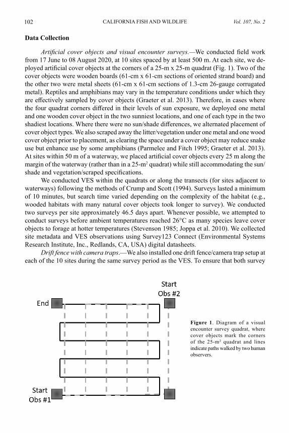
Vol. 107, No. 2CALIFORNIA FISH AND WILDLIFE102
Data Collection
Artificial cover objects and visual encounter surveys.—We conducted field work from 17 June to 08 August 2020, at 10 sites spaced by at least 500 m. At each site, we de-ployed artificial cover objects at the corners of a 25-m x 25-m quadrat (Fig. 1). Two of the cover objects were wooden boards (61-cm x 61-cm sections of oriented strand board) and the other two were metal sheets (61-cm x 61-cm sections of 1.3-cm 26-gauge corrugated metal). Reptiles and amphibians may vary in the temperature conditions under which they are effectively sampled by cover objects (Graeter et al. 2013). Therefore, in cases where the four quadrat corners differed in their levels of sun exposure, we deployed one metal and one wooden cover object in the two sunniest locations, and one of each type in the two shadiest locations. Where there were no sun/shade differences, we alternated placement of cover object types. We also scraped away the litter/vegetation under one metal and one wood cover object prior to placement, as clearing the space under a cover object may reduce snake use but enhance use by some amphibians (Parmelee and Fitch 1995; Graeter et al. 2013). At sites within 50 m of a waterway, we placed artificial cover objects every 25 m along the margin of the waterway (rather than in a 25-m2 quadrat) while still accommodating the sun/shade and vegetation/scraped specifications.
We conducted VES within the quadrats or along the transects (for sites adjacent to waterways) following the methods of Crump and Scott (1994). Surveys lasted a minimum of 10 minutes, but search time varied depending on the complexity of the habitat (e.g., wooded habitats with many natural cover objects took longer to survey). We conducted two surveys per site approximately 46.5 days apart. Whenever possible, we attempted to conduct surveys before ambient temperatures reached 26°C as many species leave cover objects to forage at hotter temperatures (Stevenson 1985; Joppa et al. 2010). We collected site metadata and VES observations using Survey123 Connect (Environmental Systems Research Institute, Inc., Redlands, CA, USA) digital datasheets.
Drift fence with camera traps.—We also installed one drift fence/camera trap setup at each of the 10 sites during the same survey period as the VES. To ensure that both survey
Figure 1. Diagram of a visual encounter survey quadrat, where cover objects mark the corners of the 25-m2 quadrat and lines indicate paths walked by two human observers.
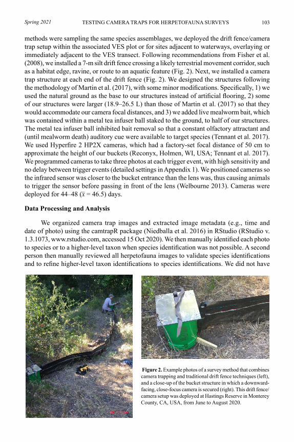
103Spring 2021 TESTING CAMERA TRAPS FOR HERPETOFAUNA SURVEYS
methods were sampling the same species assemblages, we deployed the drift fence/camera trap setup within the associated VES plot or for sites adjacent to waterways, overlaying or immediately adjacent to the VES transect. Following recommendations from Fisher et al. (2008), we installed a 7-m silt drift fence crossing a likely terrestrial movement corridor, such as a habitat edge, ravine, or route to an aquatic feature (Fig. 2). Next, we installed a camera trap structure at each end of the drift fence (Fig. 2). We designed the structures following the methodology of Martin et al. (2017), with some minor modifications. Specifically, 1) we used the natural ground as the base to our structures instead of artificial flooring, 2) some of our structures were larger (18.9–26.5 L) than those of Martin et al. (2017) so that they would accommodate our camera focal distances, and 3) we added live mealworm bait, which was contained within a metal tea infuser ball staked to the ground, to half of our structures. The metal tea infuser ball inhibited bait removal so that a constant olfactory attractant and (until mealworm death) auditory cue were available to target species (Tennant et al. 2017). We used Hyperfire 2 HP2X cameras, which had a factory-set focal distance of 50 cm to approximate the height of our buckets (Reconyx, Holmen, WI, USA; Tennant et al. 2017). We programmed cameras to take three photos at each trigger event, with high sensitivity and no delay between trigger events (detailed settings in Appendix 1). We positioned cameras so the infrared sensor was closer to the bucket entrance than the lens was, thus causing animals to trigger the sensor before passing in front of the lens (Welbourne 2013). Cameras were deployed for 44–48 (x = 46.5) days.
Data Processing and Analysis
We organized camera trap images and extracted image metadata (e.g., time and date of photo) using the camtrapR package (Niedballa et al. 2016) in RStudio (RStudio v. 1.3.1073, www.rstudio.com, accessed 15 Oct 2020). We then manually identified each photo to species or to a higher-level taxon when species identification was not possible. A second person then manually reviewed all herpetofauna images to validate species identifications and to refine higher-level taxon identifications to species identifications. We did not have
Figure 2. Example photos of a survey method that combines camera trapping and traditional drift fence techniques (left), and a close-up of the bucket structure in which a downward-facing, close-focus camera is secured (right). This drift fence/camera setup was deployed at Hastings Reserve in Monterey County, CA, USA, from June to August 2020.
¯
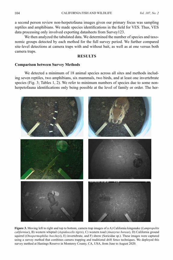
Vol. 107, No. 2CALIFORNIA FISH AND WILDLIFE104
a second person review non-herpetofauna images given our primary focus was sampling reptiles and amphibians. We made species identifications in the field for VES. Thus, VES data processing only involved exporting datasheets from Survey123.
We then analyzed the tabulated data. We determined the number of species and taxo-nomic groups detected by each method for the full survey period. We further compared site-level detections at camera traps with and without bait, as well as at one versus both camera traps.
RESULTS
Comparison between Survey Methods
We detected a minimum of 18 animal species across all sites and methods includ-ing seven reptiles, two amphibians, six mammals, two birds, and at least one invertebrate species (Fig. 3; Tables 1, 2). We refer to minimum numbers of species due to some non-herpetofauna identifications only being possible at the level of family or order. The her-
Figure 3. Moving left to right and top to bottom, camera trap images of a A) California kingsnake (Lampropeltis californiae), B) western whiptail (Aspidoscelis tigris), C) western toad (Anaxyrus boreas), D) California ground squirrel (Otospermophilus beecheyi), E) invertebrate, and F) shrew (Soricidae sp.). These images were captured using a survey method that combines camera trapping and traditional drift fence techniques. We deployed this survey method at Hastings Reserve in Monterey County, CA, USA, from June to August 2020.
105Spring 2021 TESTING CAMERA TRAPS FOR HERPETOFAUNA SURVEYS
petofauna we detected at the most sites using the drift fence/camera setup were western skink (Plestiodon skiltonianus, n = 10) and western fence lizard (Sceloporus occidentalis, n = 10). Western fence lizard was also the species identified at the most sites using VES/cover objects (n = 3). We identified six herpetofauna species using the drift fence/camera setup that we did not identify using VES/cover objects including three species of snake, two species of lizard, and western toad (Anaxyrus boreas, Table 1). We identified one species (ensatina [Ensatina escholtzii]) using VES/cover objects that we did not identify using the drift fence/camera setup.
We recorded more detections and species with the drift fence/camera setup than with VES/cover objects on both a per-site and full survey period basis. Across all sites and the full survey season, we observed a minimum of three species of reptiles and amphibians with the VES/cover objects and eight species of reptiles and amphibians with the drift fence/camera traps (Table 1). From the VES/cover objects, we had a mean of 0.6 detections per survey (range = 0–5) of zero to one identifiable species of herpetofauna. We did not detect any reptile or amphibian species during 60% of our VES. We made several VES observations under natural cover objects but found no individuals at the artificial cover objects. In comparison, the drift fence/camera setup produced a mean of 247.85 herpetofauna images per site (range = 34–1241), with a mean of 4.2 species of herpetofauna (range = 3–6) detected per site.
The drift fence/camera setup had the added benefit of producing many images of non-herpetofauna species with over two-thirds of the images being of mammals, birds, or invertebrates (Table 2; Fig. 4). Specifically, we detected a minimum of six mammal, two bird, and an unknown number of invertebrate species with the camera traps (Table 2). As mentioned above, we refer to minimum numbers of species due to some non-herpetofauna identifications only being possible at the level of family, order, or class. All cameras captured mammals, and all but one also captured invertebrates (Table 2). Unidentified rodents (order Rodentia) and mice (Peromyscus spp.) were the most photographed non-herpetofauna taxa. Only 14.8% of the camera trap images were blank (i.e., non-animal, non-researcher photos;
Table 1. The number of sites (# sites; n = 10) at which reptiles and amphibians were observed via two field methods. The first combined a drift fence with two close-focus camera traps (drift fence/camera) and the second was a visual encounter survey with artificial cover objects (VES/cover object). Sites were located at Hastings Reserve, Monterey County, CA, USA, and surveyed between June and August 2020.
Group Species Common name # sitesDrift fence/ camera
VES/cover object
Reptiles Squamata lizard order 0 2Reptiles Lampropeltis californiae California kingsnake 4 0Reptiles Coluber lateralis striped racer 6 0Reptiles Aspidoscelis tigris western whiptail 7 1Reptiles Plestiodon skiltonianus western skink 10 0Reptiles Elgaria multicarinata southern alligator lizard 1 0Reptiles Sceloporus occidentalis western fence lizard 10 3Reptiles Coluber constrictor North American racer 2 0Amphibians Anaxyrus boreas western toad 2 0Amphibians Ensatina eschscholtzii ensatina 0 1
Vol. 107, No. 2CALIFORNIA FISH AND WILDLIFE106
Table 2. The number of sites (# Sites; n = 10) at which taxa were observed using a drift fence in combination with close-focus camera traps and the total number of images of each taxa (# Images). This study targeted herpetofauna, so other taxa were infrequently identified to species level. Sites were located at Hastings Reserve, Monterey County, CA, USA, and surveyed between June and August 2020.
Taxon Scientific name Common name # Sites # ImagesReptiles Lampropeltis californiae California kingsnake 4 36Reptiles Coluber lateralis striped racer 6 28Reptiles Aspidoscelis tigris western whiptail 7 3,399Reptiles Plestiodon skiltonianus western skink 10 346Reptiles Elgaria multicarinata southern alligator lizard 1 8Reptiles Sceloporus occidentalis western fence lizard 10 1,116Reptiles Coluber constrictor North American racer 2 6Amphibians Anaxyrus boreas western toad 2 18Mammals Rodentia rodent order 10 6,300Mammals Dipodomys sp. kangaroo rat sp. 1 34Mammals Peromyscus sp. mouse sp. 7 2173Mammals Soricidae sp. shrew sp. 5 154Mammals Sylvilagus bachmani brush rabbit 1 60Mammals Otospermophilus beecheyi California ground squirrel 3 803Mammals Mephitis mephitis striped skunk 7 364Birds Oreortyx pictus mountain quail 1 147Birds Aphelocoma californica western scrub-jay 1 6Invertebrates 10 293
Table 3), and many of these blank images were instances where the species moved out of the image frame after the first photo was taken (i.e., first image in the trigger event included the animal and the following two images were blank).
Drift Fence/Camera Setup Improvements
One camera versus two cameras per fence.—Comparisons of herpetofauna detections between pairs of cameras showed that, within individual 24-hour periods, a mean of 46% of species records were captured at both cameras, while 54% were captured at a single camera (Table 4). When compared across the entire survey period, the mean proportions of species records shifted to 71% at both cameras and 29% at a single camera. Across the entire survey period, southern alligator lizard (Elgaria multicarinata) was the only herpetofauna species detected at one camera within a pair, while fence lizard and western whiptail (Aspidoscelis tigris) were always detected at both cameras.
Baited versus non-baited camera traps.—Baited and non-baited structures did not show statistically significant differences (i.e., 95% confidence intervals overlapped) in the numbers of images captured across all taxa or for herpetofauna species. Across all taxa, baited and non-baited structures recorded a mean of 746.3 and 824.1 images, respectively. Across only reptiles and amphibians, baited bucket structures recorded a mean of 266.8 images
107Spring 2021 TESTING CAMERA TRAPS FOR HERPETOFAUNA SURVEYS
Figure 4. Taxa detected using a survey method that combines camera trapping and traditional drift fence techniques. We deployed this method at Hastings Reserve, Monterey, CA, USA from June to August 2020.
and 3.7 species while non-baited bucket structures recorded a mean of 228.9 images and 3.5 species (Table 3). Southern alligator lizard was the only species photographed at one baited camera and no non-baited cameras. In addition, three cameras captured western toad; two baited cameras recorded a combined total of 16 toad photos while one non-baited camera recorded two photos. These results indicate that bait did not increase total detections across all taxa, but it may have increased our probability of photographing some herpetofauna.
DISCUSSION
The drift fence combined with camera traps recorded up to five more species and over 400 times as many observations of reptiles and amphibians than the VES and cover object method. In addition to reptiles and amphibians, it also provided information on at least nine species of birds, small to medium mammals, and invertebrates. Our study results suggest that drift fences combined with camera traps may be the preferred survey method when the goal is to maximize presence-absence information across terrestrial herpetofauna species.
The camera trap/drift fence method outperformed VES in enabling observers to con-fidently identify observed animals to species while also greatly reducing the potential for observer bias. One hundred percent of herpetofauna photos were identifiable to species as compared to only 58% of VES observations. Camera trap photos also allowed for second-ary review of species identifications. By contrast, secondary review of VES identifications was only possible if field staff photographed observed animals with a handheld camera. Despite carrying cameras on our VES, we were unable to photograph any animals due to their speed and/or ability to quickly hide in leaf litter. The camera trap/drift fence method also eliminated biases involved in VES that can arise from variable field observer effort and observers’ ability to correctly and quickly identify detected animals to species.
An additional benefit of camera traps combined with drift fences, as compared to VES, is that they capture greater species diversity. We detected at least 17 animal species with drift fences and camera traps compared to just three species with VES. This improved efficacy is due to camera traps operating 24 hours per day, as compared to VES that are typically done in the morning, meaning cameras provide information on both diurnal and nocturnal
Vol. 107, No. 2CALIFORNIA FISH AND WILDLIFE108Ta
ble 3
. Num
bers
of i
mag
es re
cord
ed b
y cl
ose-
focu
s cam
era t
raps
, whi
ch w
e dep
loye
d in
com
bina
tion
with
drif
t fen
ces a
t Has
tings
Res
erve
in M
onte
rey
Cou
nty,
CA
, USA
, fro
m
June
to A
ugus
t 202
0. E
ach
site
(n =
10)
had
one
bai
ted
and
one
non-
baite
d ca
mer
a. W
e pr
esen
t the
num
ber o
f day
s the
cam
era
was
dep
loye
d (#
day
s) a
nd th
e sp
ecie
s det
ecte
d,
incl
udin
g C
alifo
rnia
kin
gsna
ke (k
ings
nake
), st
riped
race
r (st
riped
race
r), w
este
rn w
hipt
ail (
whi
ptai
l), w
este
rn s
kink
(ski
nk),
sout
hern
alli
gato
r liz
ard
(alli
gato
r liz
ard)
, wes
tern
fe
nce
lizar
d (f
ence
liza
rd),
Nor
th A
mer
ican
race
r (N
. Am
. rac
er),
and
wes
tern
toad
(toa
d). W
e al
so id
entif
y th
e to
tal n
umbe
r of b
lank
imag
es (#
bla
nks)
, tot
al n
umbe
r of a
nim
al
imag
es (#
ani
mal
), an
d to
tal n
umbe
r of h
erpe
tofa
una
spec
ies p
hoto
grap
hed
(# sp
ecie
s).
Site
Bai
t#
Day
sK
ings
nake
Strip
ed ra
cer
Whi
ptai
lSk
ink
Alli
gato
r liz
ard
Fenc
e liz
ard
N. A
m. r
acer
Toad
# B
lank
s#
Ani
mal
# Sp
ecie
s1
Y48
00
2814
011
00
7461
03
N48
02
1212
03
00
8011
024
2Y
470
058
00
70
056
307
2N
470
013
82
028
00
139
775
33
Y48
06
03
85
00
142
1036
4N
480
50
50
20
046
260
34
Y48
30
018
080
00
111
817
3N
482
00
460
650
030
615
273
5Y
454
047
822
047
00
290
1167
4N
450
529
857
012
00
039
318
604
6Y
440
485
94
02
02
7395
65
N44
00
363
20
30
212
452
44
7Y
472
017
217
045
314
112
508
6N
4711
057
720
360
097
466
48
N48
00
113
140
107
00
172
1199
3N
4814
035
96
099
00
6876
64
9Y
450
00
390
327
20
7638
23
N45
03
011
082
10
8320
44
10Y
450
311
72
028
00
156
481
4N
450
034
70
019
00
149
757
2
109Spring 2021 TESTING CAMERA TRAPS FOR HERPETOFAUNA SURVEYS
Table 4. Detections from close-focus camera traps, which were deployed in combination with a drift fence at Hastings Reserve in Monterey County, CA, USA, from June to August 2020. Each site (n = 10) contained two camera traps, one at either end of a drift fence. We present the number of sites at which species were photographed by one vs. two cameras (# sites) and the number of site-days when species were photographed by one vs. two cameras (# site-days), where site-days refer to unique combinations of sites and days for which cameras were active (similar to trap-nights).
Species Scientific name Common name # Sites # Site-days1 camera 2 cameras 1 camera 2 cameras
Reptiles Lampropeltis californiae
California king-snake
2 2 9 0
Reptiles Coluber lateralis striped racer 5 1 9 1Reptiles Aspidoscelis tigris western whiptail 0 7 108 92Reptiles Plestiodon skilto-
nianuswestern skink 2 8 79 12
Reptiles Elgaria multicari-nata
southern alliga-tor lizard
1 0 2 0
Reptiles Sceloporus oc-cidentalis
western fence lizard
0 10 100 29
Reptiles Coluber constric-tor
North American racer
1 1 3 0
Amphibians Anaxyrus boreas western toad 1 1 5 0Total 12 30 315 134Percent of total
28.6 71.4 70.2 29.8
species. Further, because camera traps continuously collect information over the duration of the survey period, they are able to capture more species and more observations than is possible with VES, which require staff to be physically present. Cameras also facilitate data collection on a broader community of species given they photograph all animals that pass underneath them, as compared to VES that specifically target reptiles and amphib-ians. Lastly, the drift fence/camera trap method presents the opportunity to ask questions related to population abundance and density given a subset of the photographed species have uniquely identifiable markings and can be identified to individual by either computer algorithms or trained human observers with identification keys (Silver et al. 2004; Treilibs et al. 2016; Moore et al. 2020).
When compared to other camera-based methods for surveying herpetofauna, we found that our drift fence/camera method had a much lower proportion of non-target to target images. Camera trapping efforts targeting reptiles and amphibians frequently employ time-lapse methodology (Gibson et al. 2015), which can demand an intensive data processing component, as it often produces a very high proportion of non-target images (Hobbs and Brehme 2017). For example, Neuharth et al. (2020) used time-lapse methods to survey snakes and reported an average of 1 target species detection per 16,038 images. Furthermore, our ratio of target to nontarget images exceeds that reported in similar studies employing the AHDriFT method (Amber et al. 2021).
Vol. 107, No. 2CALIFORNIA FISH AND WILDLIFE110
The camera trap/drift fence technique also possesses several disadvantages. Pre-fieldwork preparation and equipment construction require non-negligible staff time, and high-quality camera traps are expensive. In comparison, VES and artificial cover objects require little fieldwork preparation and low-cost materials. Another potential disadvantage is that cameras are only able to detect species that are moving through a landscape whereas with VES and artificial cover object surveys, researchers may have the ability to detect reptiles and amphibians that are seasonally inactive. Mitigating camera theft and vandalism is also difficult since it is challenging to lock cameras to trees or other permanent structures (due to their placement in buckets), but approaches for modifying camera structures to facilitate locking are in development (see Appendix II). Lastly, as is common in all camera trap studies, manual identification of photographed species can be a time-intensive task. However, artificial intelligence algorithms are being developed that will expedite this step by auto-classifying species and removing blank images (Ahumada et al. 2020).
We had limited detections of amphibian species using both survey methods. We had one VES observation of an ensatina and 18 photographic records of western toad across three cameras. This may be because we sampled in June and August when conditions were extremely dry and little water was available. We recommend aligning the timing of any surveys targeting amphibians, whether that be VES and/or drift fences combined with camera traps, to overlap with peak amphibian activity so that there is a higher probability of detecting these species. For example, if we had surveyed earlier in the year, we may have also detected northern pacific treefrog (Pseudacris regilla), California tiger salamander (Ambystoma californiense), and foothill yellow-legged frog (Rana boylii) which are known to be present at Hastings (Hastings Natural History Reservation 2020). Previous research has shown that similar drift fence/camera setups have successfully sampled some amphib-ian species when and where they are active (Martin et al. 2017; Amber et al. 2021). We recommend further investigations aimed at assessing whether the camera trap/drift fence method is effective at sampling amphibians.
Based on the results of our field surveys, we have several recommendations on how the camera trap and drift fence method may be employed most effectively. First, we detected more species from both cameras at a fence versus a single camera, although the advantage of two cameras diminished over the length of the survey period. Given a long enough survey period, researchers could use a single camera at one end of a fence, cutting camera costs in half while still producing data that meets their needs. In addition, recent research shows that drift fence turnarounds can redirect herpetofauna and small mammal movements back along fences (Brehme et al. 2020). This approach could be trialed to redirect animals toward the camera end of a fence, further reducing the need for two cameras. Second, the rigid bucket structures are difficult to carry to remote field locations. We recommend exploring more lightweight or collapsible materials, such as foldable corrugated plastic, which could be used to create “pseudo-buckets” that fit inside a pack when folded (Appendix II). Third, within the camera’s field of view, we recommend clearing vegetation to prevent false trig-gers and securing a ruler to the ground for animal size reference (McCleery et al. 2014). Fourth, we recommend ensuring the factory-adjusted camera focal distance aligns closely with the height of the mounted camera, as we received blurry images of some animals from the shorter bucket structures. Fifth, we recommend that researchers adjust camera settings based on project goals. For example, we received sets of 100+ photos when animals made lengthy visits to camera traps. To avoid this, time between trigger events could be set to
111Spring 2021 TESTING CAMERA TRAPS FOR HERPETOFAUNA SURVEYS
greater than zero seconds. Moreover, studies that must reduce the number of images may limit trigger events to two photos per event rather than three. Finally, we encourage further study to assess the effectiveness of bait on increasing reptile and amphibian detection rates.
Our research suggests that large-scale implementation of the drift fence/camera method would improve knowledge of reptile and amphibian distributions which, in turn, would increase the ability to make informed and expedient conservation and management deci-sions. This is imperative given that reptiles and amphibians are facing widespread declines due to environmental contaminants, disease, invasive species, global climate change, and habitat destruction (Gibbons et al. 2000; Daszak et al. 2003; Maerz et al. 2005; Sparling 2010; Graeter et al. 2013; Ribeiro 2018). New threats to herpetofauna continue to arise, such as snake fungal disease, identified as a major conservation concern (Sutherland et al. 2014) and recently identified in California for the first time (CDFW 2019). The camera trap/drift fence method also holds great promise as it could be expanded to address questions pertaining to population density (Martin et al. 2017; Amber et al. 2021), DNA-coded health data (Henry and Russello 2011; Martin et al. 2017), invertebrate inventorying (Zhong et al. 2018), and small animal distributions (De Bondi et al. 2010; McCleery et al. 2014; Mills et al. 2016). In addition, leaving drift fence/camera setups active across the full annual cycle could provide information on reptile and amphibian temporal activity patterns, both daily and annual, and elucidate how these patterns are influenced by natural and anthropogenic changes. Ultimately, these advances in survey methodology hold the promise of improving confidence and precision in decision-making, resulting in more effective conservation and management of herpetofauna diversity.
ACKNOWLEDGMENTS
The California Department of Fish and Wildlife funded this study as part of the California Environmental Monitoring and Assessment Framework. Our fieldwork would not have been possible without the knowledge and help of Dr. J. Hunter, Resident Reserve Director at Hastings Natural History Reservation. We also thank G. Lipps and S. Martin (Ohio State University) for their insight on the use of the AHDriFT method, G. Nafis (California Herps website) for use of herpetofauna images in our digital datasheets, and our colleagues E. Chappell, L. Patterson, and L. Souza (California Department of Fish and Wildlife) for providing critical background information on California herpetofauna and for facilitating this study. Finally, we thank M. Rodríguez (California Department of Fish and Wildlife) and A. Blasco, who provided a Spanish translation of the manuscript’s abstract.
LITERATURE CITED
Ahumada, J. A., E. Fegraus, T. Birch, N. Flores, R. Kays, T. G. O’Brien, J. Palmer, S. Schuttler, J. Y. Zhao, W. Jetz, M. Kinnaird, S. Kulkarni, A. Lyet, D. Thau, M. Duong, R. Oliver, and A. Dancer. 2020. Wildlife Insights: A platform to maximize the potential of camera trap and other passive sensor wildlife data for the planet. Environmental Conservation 47(1):1–6.
Amber, E. D., G. J. Lipps, and W. E. Peterman. 2021. Evaluation of the AHDriFT camera trap system to survey for small mammals and herpetofauna. Journal of Fish and Wildlife Management 12:197–207.
Brehme, C. S., J. A. Tracey, J. Kingston, J. B. Sebes, T. K. Edgarian, and R. N. Fisher. 2020.
Vol. 107, No. 2CALIFORNIA FISH AND WILDLIFE112
Effectiveness of turnarounds in changing the trajectory of reptiles and amphibians in San Diego, CA. Pages 135–144 in Brehme, C. S. and R. N. Fisher. Research to Inform Caltrans Best Management Practices for Reptile and Amphibian Road Crossings. USGS Cooperator Report to California Department of Transportation, Division of Research, Innovation and System Information 65A0553.
California Department of Fish and Wildlife (CDFW). 2019. Snake fungal disease detect-ed in California. Available from: https://cdfgnews.wordpress.com/2019/11/05/snake-fungal-disease-detected-in-california/
Crump, M. L., and N. J. Scott, Jr. 1994. Visual encounter surveys. Pages 84-92 in W. R. Heyer, M. A. Donnelly, R. W. McDiarmid, L. C. Hayek, and M. S. Foster, editors. Measuring and Monitoring Biological Diversity: Standard Methods for amphib-ians. Smithsonian Institution Press, Washington D.C., USA.
Crump, P. S., and M. R. Forstner. 2019. Bias and precision of lizard occupancy estimates vary among observers and between methods. Journal of Herpetology 53(1)13–21.
Daszak, P., A. A. Cunningham, and A. D. Hyatt. 2003. Infectious disease and amphibian population declines. Diversity and Distributions 9:141–150.
De Bondi, N., J. G. White, M. Stevens, and R. Cooke. 2010. A comparison of the effective-ness of camera trapping and live trapping for sampling terrestrial small-mammal communities. Wildlife Research 37(6):456–465.
Fisher, R., D. Stokes, C. Rochester, C. Brehme, S. Hathaway, and T. Case. 2008. Herpe-tological monitoring using a pitfall trapping design in southern California. Pages 1-44 in D. Kempthorne and M. D. Myers, Secretary and Director. Collection of Environmental Data. U.S. Geological Survey Techniques and Methods.
Furnas, B. J., D. S. Newton, G. D. Capehart, and C. W. Barrows. 2019. Hierarchical dis-tance sampling to estimate population sizes of common lizards across a desert ecoregion. Ecology and Evolution 9(6):3046–3058.
Gibbons, J. W., D. E. Scott, T. J. Ryan, K. A. Buhlmann, T. D. Tuberville, B. S. Metts, J. L. Greene, T. Mills, Y. Leiden, S. Poppy, and C. T. Winne. 2000. The global decline of reptiles, déjà vu amphibians: reptile species are declining on a global scale. Six significant threats to reptile populations are habitat loss and degradation, intro-duced invasive species, environmental pollution, disease, unsustainable use, and global climate change. BioScience 50(8):653–666.
Gibson, S., S. Penniket, and A. Cree. 2015. Are viviparous lizards from cool climates ever exclusively nocturnal? Evidence for extensive basking in a New Zealand gecko. Biological Journal of the Linnean Society 115:882–895.
Graeter, G. J., K. A. Buhlmann, L. R. Wilkinson, and J. W. Gibbons. 2013. Inventory and monitoring: recommended techniques for reptiles and amphibians. Partners in Amphibian and Reptile Conservation Technical Publication IM-1, Birmingham, AL, USA.
Griffin, J. R. 1990. Flora of Hastings Reservation, Carmel Valley, California. 3rd edition. University of California, Berkeley, CA, USA.
Hampton, P. 2007. A comparison of the success of artificial cover types for capturing am-phibians and reptiles. Amphibia-Reptilia 28(3):433–437.
Hastings Natural History Reservation. 2020. Amphibians and Reptiles. Available from: http://hastingsreserve.org/natural-history-resources/amphibians-reptiles.html (Accessed 17 May 2021)
113Spring 2021 TESTING CAMERA TRAPS FOR HERPETOFAUNA SURVEYS
Henry, P., and M. A. Russello. 2011. Obtaining high-quality DNA from elusive small mammals using low-tech hair snares. European Journal of Wildlife Research 57(3):429–435.
Hobbs, M. T., and C. S. Brehme. 2017. An improved camera trap for amphibians, reptiles, small mammals, and large invertebrates. PLoS ONE 12(10):e0185026.
Joppa, L. N., C. K. Williams, S. A. Temple, and G. S. Casper. 2010. Environmental factors affecting sampling success of artificial cover objects. Herpetological Conserva-tion and Biology 5(1):143–148.
Lardner, B., A. A. Yackel Adams, A. J. Knox, J. A. Savidge, and R. N. Reed. 2019. Do observer fatigue and taxon bias compromise visual encounter surveys for small vertebrates? Wildlife Research 46(2):127–135.
Lovich, J. E., and J. W. Gibbons. 1997. Conservation of covert species: protecting species we don’t even know. Proceedings of the New York Turtle and Tortoise Society: Conservation, Restoration, and Management of Tortoises and Turtles—An Inter-national Conference 426–429.
Maerz, J. C., C. J. Brown, C. T. Chapin, and B. Blossey. 2005. Can secondary compounds of an invasive plant affect larval amphibians? Functional Ecology 19:970–975.
Martin, S. A., R. M. Rautsaw, F. Robb, M. R. Bolt, C. L. Parkinson, and R. A. Seigel. 2017. Set AHDriFT: Applying game cameras to drift fences for surveying herpetofauna and small mammals. Wildlife Society Bulletin 41(4):804–809.
McCleery, R. A., C. L. Zweig, M. A. Desa, R. Hunt, W. M. Kitchens, and H. F. Percival. 2014. A novel method for camera-trapping small mammals. Wildlife Society Bul-letin 38(4):887–891.
McMahon, D. E., I. S. Pearse, W. D. Koenig, and E. L. Walters. 2015. Tree community shifts and Acorn Woodpecker population increases over three decades in a Cali-fornian oak woodland. Canadian Journal of Forest Research 45:1113–1120.
Mills, C. A., B. J. Godley, and D. J. Hodgson. 2016. Take only photographs, leave only footprints: novel applications of non-invasive survey methods for rapid detection of small, arboreal animals. PLoS ONE 11(1):e0146142.
Moore, H. A., J. L. Champney, J. A. Dunlop, L. E. Valentine, and D. G. Nimmo. 2020. Spot on: using camera traps to individually monitor one of the world’s largest lizards. Wildlife Research 47(4):326–337.
Niedballa, J., R. Sollmann, A. Courtiol, and A. Wilting. 2016. camtrapR: an R package for efficient camera trap data management. Methods in Ecology and Evolution 7(12):1457–1462.
Neuharth, D. B., W. A. Ryberg, C. S. Adams, T. J. Hibbitts, D. K. Walkup, S. L. Frizzell, T. E. Johnson, B. L. Pierce, J. B. Pierce, and D. C. Rudolph. 2020. Searching for rare and secretive snakes: are camera-trap and box-trap methods interchangeable? Wildlife Research 47(6):476–484.
Parmelee, J., and H. S. Fitch. 1995. An experiment with artificial shelters for snakes: Ef-fects of material, age, and surface preparation. Herpetological Natural History 3(2):187–191.
Phillott, A. D., R. Speare, H. B. Hines, L. F. Skerratt, E. Meyer, K. R. McDonald, S. D. Cashins, D. Mendez, and L. Berger. 2010. Minimising exposure of amphibians to pathogens during field studies. Diseases of Aquatic Organisms 92:175–185.
Ribeiro, J. S., T. Siqueira, G. L. Brejao, and E. F. Zipkin. 2018. Effects of agriculture and
Vol. 107, No. 2CALIFORNIA FISH AND WILDLIFE114
topography on tropical amphibian species and communities. Ecological Applica-tions 28(6)1554–1564.
Sikes, R. S., W. L. Gannon, and the Animal Care and Use Committee of the American Society of Mammalogists. 2011. Guidelines of the American Society of Mam-malogists for the use of wild mammals in research. Journal of Mammalogy 92:235–253.
Silver, S. C., L. E. Ostro, L. K. Marsh, L. Maffei, A. J. Noss, M. J. Kelly, R. B. Wallace, H. Gomez, and G. Ayala. 2004. The use of camera traps for estimating jaguar Panthera onca abundance and density using capture/recapture analysis. Oryx 38(2):148–154.
Sparling, D. W. 2010. Ecotoxicology of organic contaminants to amphibians. Pages 261–288 in D. W. Sparling, G. Linder, C. A. Bishop, and S. K. Krest, editors. Ecotoxi-cology of amphibians and reptiles. CRC Press, Boca Raton, FL, USA.
Stevenson, R. D. 1985. The relative importance of behavioral and physiological adjust-ments controlling body temperature in terrestrial ectotherms. The American Nat-uralist 126(3):362–386.
Sutherland, W. J., R. Aveling, T. M. Brooks, M. Clout, L. V. Dicks, L. Fellman, E. Fleish-man, D. W. Gibbons, B. Keim, F. Lickorish, and K. A. Monk. 2014. A horizon scan of global conservation issues for 2014. Trends in Ecology & Evolution 29(1):15–22.
Tennant, E. N., B. L. Cypher, L. R. Saslaw, T. L. Westall, J. L. Mohay, E. C. Kelly, and C. L. V. H. Job. 2017. Conservation of endangered Buena Vista Lake shrews (Sorex ornatus relictus) through investigation of taxonomic status, distribution, and use of non-invasive survey methods. Wildlife Society Bulletin 44:610–616.
Treilibs, C. E., C. R. Pavey, M. N. Hutchinson, and C. M. Bull. 2016. Photographic identi-fication of individuals of a free-ranging, small terrestrial vertebrate. Ecology and Evolution 6(3):800–809.
Welbourne, D. 2013. A method for surveying diurnal terrestrial reptiles with passive in-frared automatically triggered cameras. Herpetological Review 44(2):247–250.
Welsh, H. H., and L. M. Ollivier. 1998. Stream amphibians as indicators of ecosystem stress: a case study from California’s redwoods. Ecological Applications 8:1118–1132.
Welsh, H. H. Jr., K. L. Pope, and D. Boiano. 2006. Sub-alpine amphibian distributions related to species palatability to non-native salmonids in the Klamath mountains of northern California. Diversity and Distributions 12:298–309.
Zhong, Y., J. Gao, Q. Lei, and Y. Zhou. 2018. A vision-based counting and recognition system for flying insects in intelligent agriculture. Sensors 18(5).
Submitted 1 March 2021Accepted 3 May 2021Associate Editor was K. Smith
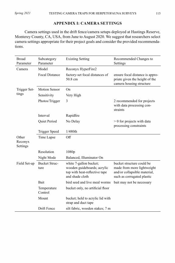
115Spring 2021 TESTING CAMERA TRAPS FOR HERPETOFAUNA SURVEYS
APPENDIX I: CAMERA SETTINGS
Camera settings used in the drift fence/camera setups deployed at Hastings Reserve, Monterey County, CA, USA, from June to August 2020. We suggest that researchers select camera settings appropriate for their project goals and consider the provided recommenda-tions.
Broad Parameter
Subcategory Parameter
Existing Setting Recommended Changes to Settings
Camera Model Reconyx HyperFire2 Focal Distance factory-set focal distances of
50.8 cmensure focal distance is appro-priate given the height of the camera housing structure
Trigger Set-tings
Motion Sensor OnSensitivity Very HighPhotos/Trigger 3 2 recommended for projects
with data processing con-straints
Interval RapidfireQuiet Period No Delay > 0 for projects with data
processing constraintsTrigger Speed 1/480th
Other Reconyx Settings
Time Lapse Off
Resolution 1080pNight Mode Balanced, Illuminator On
Field Set-up Bucket Struc-ture
white 7-gallon bucket; wooden guideboards; acrylic top with heat-reflective tape and shade cloth
bucket structure could be made from more lightweight and/or collapsible material, such as corrugated plastic
Bait bird seed and live meal worms bait may not be necessaryTemperature Control
bucket only, no artificial floor
Mount bucket; held to acrylic lid with strap and duct tape
Drift Fence silt fabric, wooden stakes; 7 m
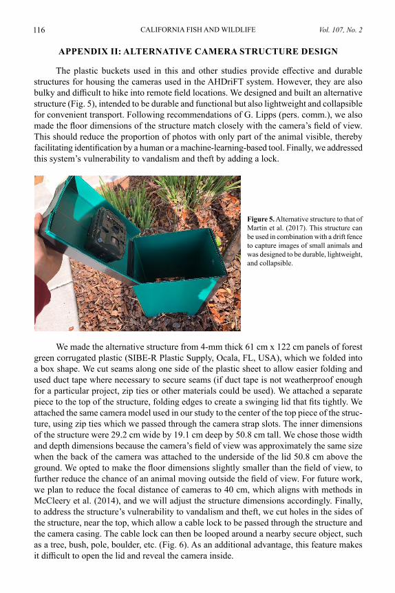
Vol. 107, No. 2CALIFORNIA FISH AND WILDLIFE116
APPENDIX II: ALTERNATIVE CAMERA STRUCTURE DESIGN
The plastic buckets used in this and other studies provide effective and durable structures for housing the cameras used in the AHDriFT system. However, they are also bulky and difficult to hike into remote field locations. We designed and built an alternative structure (Fig. 5), intended to be durable and functional but also lightweight and collapsible for convenient transport. Following recommendations of G. Lipps (pers. comm.), we also made the floor dimensions of the structure match closely with the camera’s field of view. This should reduce the proportion of photos with only part of the animal visible, thereby facilitating identification by a human or a machine-learning-based tool. Finally, we addressed this system’s vulnerability to vandalism and theft by adding a lock.
Figure 5. Alternative structure to that of Martin et al. (2017). This structure can be used in combination with a drift fence to capture images of small animals and was designed to be durable, lightweight, and collapsible.
We made the alternative structure from 4-mm thick 61 cm x 122 cm panels of forest green corrugated plastic (SIBE-R Plastic Supply, Ocala, FL, USA), which we folded into a box shape. We cut seams along one side of the plastic sheet to allow easier folding and used duct tape where necessary to secure seams (if duct tape is not weatherproof enough for a particular project, zip ties or other materials could be used). We attached a separate piece to the top of the structure, folding edges to create a swinging lid that fits tightly. We attached the same camera model used in our study to the center of the top piece of the struc-ture, using zip ties which we passed through the camera strap slots. The inner dimensions of the structure were 29.2 cm wide by 19.1 cm deep by 50.8 cm tall. We chose those width and depth dimensions because the camera’s field of view was approximately the same size when the back of the camera was attached to the underside of the lid 50.8 cm above the ground. We opted to make the floor dimensions slightly smaller than the field of view, to further reduce the chance of an animal moving outside the field of view. For future work, we plan to reduce the focal distance of cameras to 40 cm, which aligns with methods in McCleery et al. (2014), and we will adjust the structure dimensions accordingly. Finally, to address the structure’s vulnerability to vandalism and theft, we cut holes in the sides of the structure, near the top, which allow a cable lock to be passed through the structure and the camera casing. The cable lock can then be looped around a nearby secure object, such as a tree, bush, pole, boulder, etc. (Fig. 6). As an additional advantage, this feature makes it difficult to open the lid and reveal the camera inside.
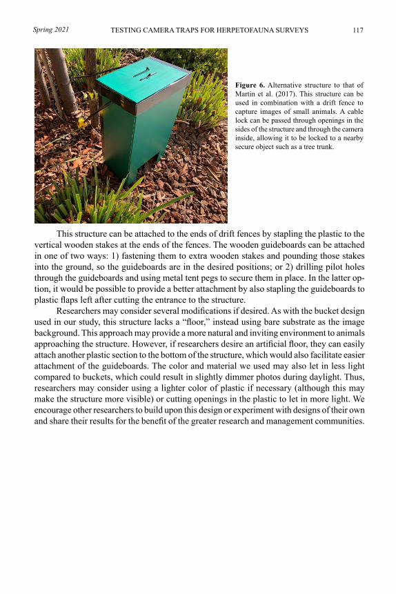
117Spring 2021 TESTING CAMERA TRAPS FOR HERPETOFAUNA SURVEYS
Figure 6. Alternative structure to that of Martin et al. (2017). This structure can be used in combination with a drift fence to capture images of small animals. A cable lock can be passed through openings in the sides of the structure and through the camera inside, allowing it to be locked to a nearby secure object such as a tree trunk.
This structure can be attached to the ends of drift fences by stapling the plastic to the vertical wooden stakes at the ends of the fences. The wooden guideboards can be attached in one of two ways: 1) fastening them to extra wooden stakes and pounding those stakes into the ground, so the guideboards are in the desired positions; or 2) drilling pilot holes through the guideboards and using metal tent pegs to secure them in place. In the latter op-tion, it would be possible to provide a better attachment by also stapling the guideboards to plastic flaps left after cutting the entrance to the structure.
Researchers may consider several modifications if desired. As with the bucket design used in our study, this structure lacks a “floor,” instead using bare substrate as the image background. This approach may provide a more natural and inviting environment to animals approaching the structure. However, if researchers desire an artificial floor, they can easily attach another plastic section to the bottom of the structure, which would also facilitate easier attachment of the guideboards. The color and material we used may also let in less light compared to buckets, which could result in slightly dimmer photos during daylight. Thus, researchers may consider using a lighter color of plastic if necessary (although this may make the structure more visible) or cutting openings in the plastic to let in more light. We encourage other researchers to build upon this design or experiment with designs of their own and share their results for the benefit of the greater research and management communities.
California Fish and Wildlife 107(2):118-119; 2021 www.doi.org/10.51492/cfwj.107.10
BOOK REVIEW
Into Wild MongoliaGeorge B. Schaller. 2020. Yale University Press, New Haven, CT, USA. 210 pages (hard cover). $28.00. ISBN 978-0-300-24617-9
This book was informative and entertaining, and presented an opportunity to learn many things about the ecology, wildlife, and people of Mongolia. George Schaller is well-known for his international exploits and expedi-tions, the majority of which have resulted in contributions to the professional literature in terms of scientific papers, books emphasizing the research conducted during those expeditions, and a number of contributions I would de-scribe as ‘natural history and personal accounts’ based on those travels. Into Wild Mongolia clearly falls into the latter category.
The book consists of a lengthy introduction, followed by 8 chapters, among which are 4 in which Schaller discusses in detail his observations of, and his interactions or exploits with, wild camel (Camelus bactrianus ferus), golden bear (Ursus arctos ssp.), snow leopard (Panthera uncia), and Mongolian gazelle (Procapra gutterosa) during 16 trips to Mongolia from 1989 to 2007. In a separate chapter, he describes a 17th trip, in 2018, during which he renewed “acquaintances, [and noted] changes in the environment, wildlife, and culture”.
Three other chapters cover topics as diverse as foreign relations, hunting and its impacts on the fauna of Mongolia, and the current and future status of the Nomrog Strictly Protected Area, located in Mongolia’s great eastern steppe and one of Schaller’s favorite places. As of 2018, that vast area remained largely as when he first saw it in 1989, but with ominous changes portending. As described, it appears as though the eastern steppe is destined to suffer near irreparable damage, as did the Great Plains of North America dur-ing the 1930s, the result of egregious agricultural practices (Worster 1979). As were the southern plains prior to America’s dustbowl, and as noted by Schaller (p. 180), “The steppe is a gentle landscape without natural defenses against plow and plunder. Mongolia is blun-dering toward disaster. After plowing up its rangelands, neighboring Inner Mongolia has suffered from widespread desertification, erosion, and severe yellow dust storms…which engulf the region as a whole”. In addition to agricultural practices, energy development, transportation infrastructure, and other anthropogenic activities will further alter that once pristine area. Schaller ends the chapter with the realization that the Mongolians seem to have discarded in Nomrog—and elsewhere—any respect for the value of wildlife habitat, and asks (p. 154), “Will the Mongolians some day return to their basic traditional values of respect for the land?”.
I have always admired Schaller’s contributions to international conservation, as well as the intensity with which he has approached wildlife conservation. I also have a great deal of respect for his opinions, and much of that developed nearly 20 years ago during a
119Spring 2021 119BOOK REVIEW
formal dinner party hosted by mutual friends. Nonetheless, there are portions of the book in which Schaller expresses views that I don’t necessarily hold and, to my thinking, may be counter-productive in terms of generating support for wildlife conservation—and perhaps even more importantly the conservation of wildlife habitat in Mongolia. We both disdain the commercial harvest of wildlife, which is a serious problem throughout a country in which animals are killed indiscriminately and in huge numbers for ‘medicinal’ products, meat, and hides that are exported for profit, or are harvested in essentially unlimited numbers for subsistence. But he places seemingly legitimate hunters in the same category as those involved in unregulated killing, noting simply (p. 133) that, “[foreign] trophy hunters kill argali sheep, red deer, and others to decorate their private mortuaries”. In the absence of any quantification, the impacts of those disparate harvest regimes will appear identical to the casual reader. Legal, tightly regulated hunting has the potential to contribute in meaningful ways to the conservation of wildlife in Mongolia. For meaningful benefits to accrue, how-ever, it must be tied to a reduction in the potential for corruption, an increase in ecological sustainability, and must be linked more closely to local communities so that members feel involved and valued, their livelihoods are ensured, and local governments properly redirect revenue back to wildlife conservation (Siebert and Belsky 2002; Maroney 2005; Page 2015). Schaller closes out this chapter by discussing harvest rates among Mongolian gazelles that are killed by local hunters for subsistence and hides and as an unsustainable and illegal com-mercial enterprise; Siberian marmots (Marmota sibericus) that are killed for meat, skins, and medicinal purposes for local use and export; and the illegal capture of Saker falcons (Falco cherrug) to be exported largely to Arab countries for sporting purposes (p. 142). The chapter ends quite bluntly with the statement (p. 145), “Damn the poachers… and damn the falconers who thoughtlessly were depleting a natural resource for their mere amusement”.
All in all, Into Wild Mongolia is a worthwhile read. It calls to light some of the many issues facing wildlife and wildlife conservation in a country with vast natural resources, but that is faced with numerous challenges and opportunities. It will take only a few hours to read this book, as I found it difficult to not ‘turn the page’ to learn what followed. George Schaller has been a stellar advocate for wildlife conservation, this book is but another ex-ample of his efforts and dedication, and is written in plain language. Read it.
LITERATURE CITED
Maroney, R. L. 2005. Conservation of argali Ovis ammon in western Mongolia and the Altai-Sayan. Biological Conservation 121:231–241.
Page, L. 2015. Killing to save: trophy hunting and conservation in Mongolia. Independent Study Project (ISP) Collection 2086. Available from: https://digitalcollections.sit.edu/isp_collection/2086 (Accessed 4 Jan 2021)
Siebert, S. F., and J. M. Belsky. 2002. Livelihood security and protected area management. International Journal of Wilderness 8(3):38–42.
Worster, D. 1979. Dust bowl: the southern plains in the 1930s. Oxford University Press, New York, NY, USA.
VERNON C. BLEICH, Department of Natural Resources and Environmental Science, University of Nevada Reno and Eastern Sierra Center for Applied Population Ecology, Bismarck, ND, USA
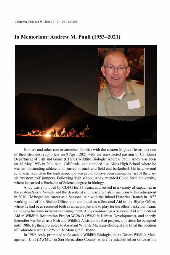
In Memoriam: Andrew M. Pauli (1953–2021)
Hunters and other conservationists familiar with the eastern Mojave Desert lost one of their strongest supporters on 8 April 2021 with the unexpected passing of California Department of Fish and Game (CDFG) Wildlife Biologist Andrew Pauli. Andy was born on 18 May 1953 in Palo Alto, California, and attended Los Altos High School where he was an outstanding athlete, and starred in track and field and basketball. He held several scholastic records in the high jump, and was proud to have been among the last of the clas-sic ‘western roll’ jumpers. Following high school, Andy attended Chico State University, where he earned a Bachelor of Science degree in biology.
Andy was employed by CDFG for 33 years, and served in a variety of capacities in the eastern Sierra Nevada and the deserts of southeastern California prior to his retirement in 2010. He began his career as a Seasonal Aid with the Inland Fisheries Branch in 1977 working out of the Bishop Office, and continued as a Seasonal Aid in the Blythe Office, where he had been recruited both as an employee and to play for the office basketball team. Following his work in fisheries management, Andy continued as a Seasonal Aid with Federal Aid in Wildlife Restoration Project W-26-D (Wildlife Habitat Development), and shortly thereafter was hired as a Fish and Wildlife Assistant on that project, a position he occupied until 1986. He then promoted to Assistant Wildlife Manager-Biologist and filled the position of Colorado River Unit Wildlife Manager at Blythe.
In 1989, Andy promoted to Associate Wildlife Biologist in the Desert Wildlife Man-agement Unit (DWMU) in San Bernardino County, where he established an office at his
California Fish and Wildlife 107(2):120-122; 2021
121Spring 2021 IN MEMORIAM: ANDREW M. PAULI
home in Apple Valley. As part of his duties, Andy oversaw management of the Camp Cady Wildlife Area, and he remained an important contributor to the Department’s efforts to ensure water was available for all species of wildlife inhabiting the eastern Mojave Desert. Andy performed inspections and helped to maintain the many dozens of desert springs and water developments located in the DWMU on which mule deer and bighorn sheep especially were dependent. He very much enjoyed conducting annual brood counts to evaluate quail and chukar production, dove surveys, and being responsible for oversight of the mule deer hunt in Zone D-17, where he continued the long-standing tradition of conducting aerial hunter surveys on opening weekends; those data formed part of his important paper that described the distribution and societal value of recreational hunting in the eastern Mojave Desert. During his assignments as a member of the habitat development crew, as the Colo-rado River Unit Manager, and as the Desert Unit Manager, Andy was a regular participant in aerial surveys to assess bighorn sheep populations. Additionally, he participated in more than 200 telemetry flights while keeping track of the dozens of bighorn sheep that had been collared for research or for translocations.
Andy developed a close working relationship with wildlife protection personnel and his pleasing personality paved the way for increased hunter interest in, and an enhanced appreciation for, the eastern Mojave Desert, which included the first areas to be opened to the hunting of bighorn sheep in California since 1878: Old Dad Peak and the Marble Moun-tains. Thus far, 7 of the 11 zones that have been opened to bighorn sheep hunting are within what once was the DWMU and that—to the dismay of Andy and many others—remains an administrative area to which no one, as yet, has been assigned individual responsibility.
Throughout his career, Andy worked closely with members of the Society for the Conservation of Bighorn Sheep (SCBS) on numerous water development projects, all of which involved volunteers and provided hundreds of interested individuals with opportuni-ties to enhance habitat for bighorn sheep and likely resulted in many life-long commitments to conservation. In all probability, many of those commitments would not have occurred were it not for Andy’s enthusiastic work ethic and his get-it-done approach. Following de-velopment of several of those wildlife water sources, bighorn sheep in the eastern Mojave Desert received increased interest among CDFG administrators, and Andy participated in numerous helicopter surveys while collecting data that resulted in the reintroduction of bighorn sheep to the Eagle Crags, Whipple Mountains, Argus Range, Sheephole Mountains, Bullion Mountains, and the northern Bristol Mountains, as well augmentations of bighorn sheep populations in the Avawatz Range and Chuckwalla Mountains.
Andy helped plan and implement the annual Bighorn Sheep Hunter Clinics that hunt-ers are required to attend, and participated in the first such clinic in 1987, which was held at Camp Cady. He participated in every such event until 2012, at which point the number of hunters fortunate enough to draw a bighorn sheep tag had outgrown the facilities available at Camp Cady. By that time, however, that venture had evolved into an annual event spon-sored by the Society for the Conservation of Bighorn Sheep and the California Wild Sheep Foundation, and had become a tradition that lasted 25 years. During those Hunter Clinics Andy and many other individuals—most of whom volunteered their time—generously shared detailed information on bighorn sheep occupying the hunt zones, access, geography, hunting techniques, equipment, desert safety, taxidermy, photography, and regulations; each of the clinics exceeded, by far, the minimum requirements dictated by the state legislature. In addition, Andy ensured the bunkhouse and associated facilities were in top condition for
Vol. 107, No. 2CALIFORNIA FISH AND WILDLIFE122
each clinic and that, following a generous social hour and hosted supper, extended well into the evening and frequently involved hunt zone ‘show-me’ trips the following day.
Andy Pauli was a dedicated sportsman, a true friend of hunters and other outdoorsmen, and he fulfilled his role as a wildlife biologist very capably. He did not have a penchant for notoriety, but his efforts on behalf of conservation were recognized widely. His work ethic, combined with his tremendous athletic ability and the outstanding eye-hand coordination developed during his athletic career, led to his being among the initial CDFG employees approved as aerial net-gunners. In 1989, he was honored for his service on behalf of desert wildlife by the Society for the Conservation of Bighorn Sheep with the Bicket-Landells Award, which was established in honor of BLM Wildlife Biologist Jim Bicket and Helicopter Pilot Don Landells who died while conducting a bighorn sheep survey at Clark Mountain on 6 October 1986. In 1996, he served as Chair of the 40th meeting of the Desert Bighorn Council in Holtville, California. Upon retirement, Andy received the Society’s Service-Above-Self Award, and the California Wild Sheep Foundation recognized his contributions with its Above-and-Beyond Award.
Following retirement, Andy worked as a retired annuitant for several additional years, and he remained the “go-to” guy for successful bighorn sheep hunters needing their tags to be validated. During his career, Andy likely validated and scored the majority of bighorn sheep that as yet have been harvested in California. He also became the most popular CDFG representative at the annual conventions of the Wild Sheep Foundation—now known as Sheep Week®—where prospective hunters consistently sought his advice on hunting con-ditions and opportunities to harvest desert bighorn sheep in California. Andy also had the privilege of validating at least 20 auction tags that, as of his retirement, had generated more than $2.6 million specifically for the conservation of bighorn sheep. True to his desire to recognize all of those playing important roles in the conservation of bighorn sheep, his first action following each auction was to seek out and thank the runner-up before locating and congratulating the winning bidder.
Desert wildlife and bighorn sheep in particular—along with California’s sportsmen and the public in general—have been the beneficiaries of Andy Pauli’s many contributions to conservation. He was a kind and generous person, a dedicated employee, a fine naturalist and avid sportsman, and he was widely respected by his peers. He was humble and unas-suming, he readily and willingly accepted the sometimes less-than-glamorous tasks to which he was assigned, and he loved his family dearly. His positive attitude, pleasing personality, and many contributions to the conservation of desert wildlife should not be forgotten. Andy will be missed by all that worked with him, knew him, or loved him. In his absence the desert will be less than what it had become, but it will remain far more than it would have been had he not landed there.
—FRIENDS AND COLLEAGUES OF ANDREW M. PAULI
INFORMATION FOR AUTHORS
The California Fish and Wildlife Journal (CFWJ) is a peer-reviewed, scientific journal focused on the biology, ecology, and conservation of the flora and fauna of California and surrounding areas, and the northeastern Pacific Ocean.
The CFWJ now has an online submission system!New! All manuscripts should now be submitted using the online submission system.
Submissions guidelines (PDF) for the Journal have been updated (December 2020) to reflect this change.
The California Fish and Wildlife Journal accepts manuscripts in the following cat-egories:
Original research papersResearch notes and short communicationsMonographsReview papersBook reviewsEssaysCommentaries on previously published papersManuscripts must be submitted following directions provided in the CFWJ Revised
Submission Guidelines (December 2020) (PDF). Please follow these formatting guidelines carefully. Manuscripts that do not conform to the guidelines will be returned for revision.
The CFWJ uses a double-blind peer review process. This means that reviewer identi-ties are concealed from authors as well as author identities being concealed from reviewers throughout the review process. This policy aids in reducing bias during the review process.
Authors of manuscripts that are accepted for publication will be invoiced for charges at the rate of $50 per printed page shortly after page proofs are distributed.* The corresponding author will receive a PDF file of the publication without additional fees and may distribute copies without restriction.
*Page charges may be waived for authors under in certain instances (e.g., for authors from developing countries, researchers without funding, etc.).
Send any questions to:Ange Darnell Baker, PhDEditor-in-Chief, California Fish and Wildlife JournalCalifornia Department of Fish and Wildlife(916) [email protected]
California Fish and Wildlife 107(1):123; 2021

Front. Lazuli bunting (Passerine amoena) on poison oak in Sibley Regional Volcanic Park, Oakland, CA. Photo credit: Doug Greenberg. (CC BY-NC 2.0)
Back. American Beaver (Castor canadensis), Colusa National Wildlife Refuge, Colusa County, California. Photo credit: Ken Schneider. (CC BY-ND 2.0).
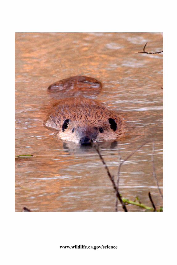
www.wildlife.ca.gov/science
Related Documents