Calibration of hydrological models using flow-duration curves

Hydrol. Earth Syst. Sci., 15, 2205–2227, 2011www.hydrol-earth-syst-sci.net/15/2205/2011/doi:10.5194/hess-15-2205-2011© Author(s) 2011. CC Attribution 3.0 License.

Hydrology andEarth System

Sciences

Calibration of hydrological models using flow-duration curves

I. K. Westerberg1,2, J.-L. Guerrero1,3, P. M. Younger4,5, K. J. Beven1,4, J. Seibert6,7, S. Halldin1, J. E. Freer8, andC.-Y. Xu9

1Department of Earth Sciences, Uppsala University, Villavagen 16, 75236, Uppsala, Sweden2IVL Swedish Environmental Research Institute, P.O. Box 210 60, 10031, Stockholm, Sweden3Civil Engineering Department, National Autonomous University of Honduras, Blv. Suyapa Ciudad Universitaria,F. M. Tegucigalpa, Honduras4Lancaster Environment Centre, Lancaster University, Lancaster, LA1 4YQ, UK5Environmental Research Consultant, 207 Eagle Heights J, Madison, WI, 53705, USA6Department of Physical Geography and Quartenary Geology, Stockholm University, 10691, Stockholm, Sweden7Department of Geography, University of Zurich, Winterthurerstrasse 190, 8057, Zurich, Switzerland8School of Geographical Sciences, University of Bristol, University Road, Bristol, BS8 1SS, UK9Department of Geosciences, University of Oslo, Postboks 1047 Blindern, 0316, Oslo, Norway

Received: 23 November 2010 – Published in Hydrol. Earth Syst. Sci. Discuss.: 9 December 2010Revised: 30 June 2011 – Accepted: 1 July 2011 – Published: 14 July 2011

Abstract. The degree of belief we have in predictions fromhydrologic models will normally depend on how well theycan reproduce observations. Calibrations with traditionalperformance measures, such as the Nash-Sutcliffe model ef-ficiency, are challenged by problems including: (1) uncer-tain discharge data, (2) variable sensitivity of different per-formance measures to different flow magnitudes, (3) influ-ence of unknown input/output errors and (4) inability to eval-uate model performance when observation time periods fordischarge and model input data do not overlap. This pa-per explores a calibration method using flow-duration curves(FDCs) to address these problems. The method focuses onreproducing the observed discharge frequency distributionrather than the exact hydrograph. It consists of applying lim-its of acceptability for selected evaluation points (EPs) on theobserved uncertain FDC in the extended GLUE approach.Two ways of selecting the EPs were tested – based on equalintervals of discharge and of volume of water. The methodwas tested and compared to a calibration using the tradi-tional model efficiency for the daily four-parameter WAS-MOD model in the Paso La Ceiba catchment in Hondurasand for Dynamic TOPMODEL evaluated at an hourly timescale for the Brue catchment in Great Britain. The volumemethod of selecting EPs gave the best results in both catch-ments with better calibrated slow flow, recession and evapo-ration than the other criteria. Observed and simulated time

Correspondence to:I. K. Westerberg([email protected])

series of uncertain discharges agreed better for this methodboth in calibration and prediction in both catchments. Anadvantage with the method is that the rejection criterion isbased on an estimation of the uncertainty in discharge dataand that the EPs of the FDC can be chosen to reflect theaims of the modelling application, e.g. using more/less EPsat high/low flows. While the method appears less sensitive toepistemic input/output errors than previous use of limits ofacceptability applied directly to the time series of discharge,it still requires a reasonable representation of the distributionof inputs. Additional constraints might therefore be requiredin catchments subject to snow and where peak-flow timing atsub-daily time scales is of high importance. The results sug-gest that the calibration method can be useful when observa-tion time periods for discharge and model input data do notoverlap. The method could also be suitable for calibration toregional FDCs while taking uncertainties in the hydrologicalmodel and data into account.

1 Introduction

Hydrologic models are used as a basis for decision makingabout management of water resources with important conse-quences for sectors such as agriculture, land planning, hy-dropower and water supply. The degree of belief we havein model predictions will normally be dependent on howwell the model can reproduce observations. The choice ofthe likelihood measure that measures the agreement betweensimulated and observed data is therefore an important choice

Published by Copernicus Publications on behalf of the European Geosciences Union.

2206 I. K. Westerberg et al.: Calibration of hydrological models using flow-duration curves

in any modelling study. The definition of an appropriate like-lihood measure is not, however, simple. Where all sourcesof uncertainty can be treated as if they are aleatory in na-ture, then a number of frameworks exist for the definitionof formal statistical likelihoods (e.g. Liu and Gupta, 2007;Schoups and Vrugt, 2010; Renard et al., 2010). Where epis-temic errors are important, however, treating all uncertain-ties as if they are aleatory will generally lead to overcon-ditioning of posterior parameter distributions (Beven, 2006,2010; Beven et al., 2008), particularly if some periods of dataare disinformative (Beven and Westerberg, 2011; Beven etal., 2011). Thus, there may be scope for using other formsof likelihood or belief measures in hydrological modelling.Such informal likelihood measures have been defined basedon limits of acceptability defined from evaluation-data uncer-tainty (Blazkova and Beven, 2009; Krueger et al., 2010; Liuet al., 2009) but also based on traditional performance mea-sures (Freer et al., 2003). One of the most widely used per-formance measures in hydrology is the Nash-Sutcliffe modelefficiency (Reff). It is calculated as 1.0 minus the normalisa-tion of the mean squared error by the variance of the observeddata and varies between minus infinity to 1.0 (Nash and Sut-cliffe, 1970). How appropriate this criterion is for measuringgoodness of fit, as well as what is an acceptableReff-value,has been much debated in the literature (Krause et al., 2005;Legates and McCabe, 1999; Seibert, 2001; Criss and Win-ston, 2008; Smith et al., 2008; Gupta et al., 2009). Decompo-sitions ofReff have highlighted several problems associatedwith this criterion in model calibration (Gupta et al., 2009;Smith et al., 2008). Gupta et al. (2009) present a decomposi-tion ofReff into three components representing bias, variabil-ity and correlation and conclude that the variability has to beunderestimated to maximizeReff and that runoff peaks tendto be underestimated when maximizingReff. They, togetherwith many other authors (Garrick et al., 1978; Refsgaard andKnudsen, 1996; Legates and McCabe, 1999; Seibert, 2001;Krause et al., 2005; Schaefli and Gupta, 2007; McMillan andClark, 2009) propose modified versions of the Nash-Sutcliffecriterion or other performance measures to overcome someof these problems. However many of the problems in usinglumped global performance measures remain, for instancethat the measure often is more influenced by the performanceat certain flow magnitudes such as high or low flows. Thisissue has been addressed in multi-criteria approaches wheredifferent aspects of the fit between simulated and observeddischarge are evaluated. A combination of several criteriathen allows an assessment of model performance with re-spect to the different aspects of the hydrograph (e.g. Gupta etal., 1998). Boyle et al. (2000) and later Wagener et al. (2001),suggest distinguishing between three parts of the hydrograph(driven quick flow (during events), non-driven quick flow andslow flow) and to then calculate the performance measureseparately for each flow type. In a related approach, Freeret al. (2003) used several performance measures for a multi-criteria calibration in a Generalised Likelihood Uncertainty

Estimation (GLUE) framework where they differentiated thedataset by season. They found no consistently identified pa-rameters for Dynamic TOPMODEL that could represent therange of processes between seasons in the studied watershed.However, these approaches have not generally taken any ex-plicit account of uncertainty in the observed input and evalu-ation data.

Hydrologic models are simplified conceptualisations ofthe hydrologic processes in a catchment. Such simplifica-tions will necessarily lead to errors in the way the struc-ture of the model represents the real-world hydrologic pro-cesses (Beven, 1989, 2009; Grayson et al., 1992; McDonnell,2003). The temporal and spatial scales of the measured inputdata are also incommensurate with both the real-world quan-tities and the scale of the model. This source of error must beconsidered together with pure measurement errors (e.g. as aresult of lack of calibration or accuracy of the measurementequipment) in input data. Such errors can lead to substantialuncertainty of an epistemic (knowledge) type, e.g. if thereare no rain gauges in the only part of the catchment where itrains, this will create an error that is difficult or impossibleto characterise in an error model. This type of uncertaintyresulting from non-stationary epistemic errors should be ex-pected in most datasets used for hydrological modelling be-cause of the difficulties in measuring the components of thewater balance for a catchment. As discussed by Beven andWesterberg (2011), such errors, if significant, should be ex-pected to have a disinformative effect on model calibration.They suggest that the best strategy to deal with such disin-formative periods of data would be to identify and removethem from the dataset independently of the model, but recog-nise that this identification will be difficult in many cases be-cause of the uncertainties in the measured data. An alterna-tive strategy could therefore be to develop model evaluationcriteria that are robust to moderate disinformation to makesure that models are rejected for the right reason – i.e. poormodel structure and not disinformative data. Model param-eters need to be inversely estimated from data in calibrationwhich will involve substantial uncertainty because of the ef-fect of the types of errors discussed here and their interac-tions. On top of this, the performance measure that is usedfor the model calibration will influence which parameter-value sets are identified as being acceptable given the un-certainties in the modelling application (see e.g. Freer et al.,1996), and is therefore an important consideration.

The reported number of discharge stations in the worldhas gone down substantially from the peak in the late 1970’s(GRDC, 2010). At the same time global precipitation andclimate data such as TRMM and ERA-Interim have becomeavailable for the last 10–20 yr. Traditional model calibrationis impossible if there are no overlapping periods of inputand output data. In regions where the flow regime is sta-tionary over time it would be advantageous to use dischargedata from a previous period (with sufficiently long records)to overcome this temporal mismatch. Calibration approaches

Hydrol. Earth Syst. Sci., 15, 2205–2227, 2011 www.hydrol-earth-syst-sci.net/15/2205/2011/

I. K. Westerberg et al.: Calibration of hydrological models using flow-duration curves 2207

that do not rely on direct time-series versus time-series com-parison are useful in such situations. Prior approaches tomodel calibration without direct time series comparison in-clude calibration to spectral properties (Montanari and Toth,2007), recession curves (Winsemius et al., 2009), slope ofthe flow-duration curve (Yadav et al., 2007; Yilmaz et al.,2008), base-flow index (Bulygina et al., 2009) and the use ofa performance measure based on specified exceedance per-centages of a synthetic regional flow-duration curve (FDC)for calibration at un-gauged sites (Yu and Yang, 2000). How-ever, in these studies uncertainties in observed discharge arenot considered explicitly. Blazkova and Beven (2009) ac-count for discharge uncertainty and use the discharge at nineexceedance percentages between 25 to 90 % exceedance forthe FDC as nine out of 57 limits of acceptability in theextended GLUE approach (Beven, 2006, 2009) in flood-frequency estimation. The latter study notes the importanceof the realization effect in using a discharge data record oflimited length, and the effect this has on the FDC is alsodiscussed by Vogel and Fennessey (1994). The added un-certainty to the FDC stemming from a discharge record oflimited length has to be considered if discharge data fromanother period is used for calibration, especially if the flowregime is not stationary.

Calibrations with traditional performance measures arechallenged by problems including the following: (1) uncer-tainty in discharge data, (2) variable sensitivity of differentperformance measures to different flow magnitudes, (3) in-fluence of input/output errors of an epistemic nature and(4) inability to evaluate model performance when observa-tion time periods for discharge and model input data donot overlap. Uncertainty in discharge data, which has beenshown to be sometimes substantial (Di Baldassarre and Mon-tanari, 2009; Pelletier, 1988; Krueger et al., 2010; Petersen-Overleir et al., 2009) and influence the calibration of hydro-logical models (McMillan et al., 2010; Aronica et al., 2006),is usually not accounted for in model evaluation with tra-ditional performance measures. Novel approaches in envi-ronmental modelling that include evaluation-data uncertaintyin model calibration include Bayesian calibration to an es-timated probability-density function of discharge (McMil-lan et al., 2010), Bayesian calibration with a simplified er-ror model (Huard and Mailhot, 2008; Thyer et al., 2009),fuzzy rule based performance measures (Freer et al., 2004)and limits-of-acceptability calibration in GLUE for rainfall-runoff modelling (Liu et al., 2009), flood mapping (Pappen-berger et al., 2007), environmental tracer modelling (Pageet al., 2007) and flood-frequency estimation (Blazkova andBeven, 2009). Here we explore the limits-of-acceptabilityGLUE approach applied to flow-duration curves, whichcould be a way of dealing with some of the effects of non-stationary epistemic errors on the identification of feasiblemodel parameters in real applications (Beven, 2006, 2010;Beven and Westerberg, 2011; Beven et al., 2008). However,in order to establish the extent to which this approach is ro-

bust to such errors, a more extensive analysis than that pre-sented here is needed. Flow-duration curves have previouslybeen used in model calibration by Sugawara (1979), Yu andYang (2000), as one of the criteria considered by Refsgaardand Knudsen (1996) and by Blazkova and Beven (2009),and as a qualitative measure of model performance, e.g. byHoughton-Carr (1999), Kavetski et al. (2011), and Son andSivapalan (2007).

The aim when calibrating a hydrological model shouldbe to find out whether the model structure can be consid-ered an appropriate conceptualisation or hypothesis of thehydrological processes of interest in that catchment (Beven,2010). Ideally, the reason for rejecting the model as a suit-able hypothesis of these processes should therefore be be-cause the model structure is poor and not because the calibra-tion method does not appropriately account for the uncertain-ties in the input and output data (i.e. avoiding Type II falsenegatives). The aim of this paper was to develop a calibra-tion method that addresses the four problems in model cal-ibration with traditional methods outlined above, within theframework of the limits-of-acceptability approach in GLUEand with a specific focus on accurate simulation of the waterbalance.

2 Study areas and data

The method was first developed for a Honduran catchmentcharacterised by shallow soils and frequent occurrence ofsurface runoff, the Paso La Ceiba catchment. It was thentested for a contrasting flow regime – the Brue catchment inGreat Britain where run-off generation is controlled by sub-surface processes on the hill slopes.

2.1 The Paso La Ceiba catchment

The 7500 km2 Choluteca River basin is located in south-central Honduras (Fig. 1) where the Choluteca River drainsto the Pacific at the Gulf of Fonseca. Two water-supplydams (constructed in 1976 and 1992) are located upstreamof the capital Tegucigalpa in the upper parts of the basin.The discharge data from the station at Paso La Ceiba, witha catchment area of 1766 km2, were used here. This catch-ment has soils that are shallow and eroded (often less thana metre deep) and it is mountainous with elevations rangingfrom 660 to 2320 m above sea level. The discharge stationwas destroyed in October 1998 by the flooding that occurredduring hurricane Mitch and a new station was installed threekilometres upstream.

The bimodal precipitation regime in the basin is char-acterised by a high spatial and temporal variability with adry season November–December to April and a rainy sea-son (with around 80 % of the total precipitation) modulatedby a relative minimum, “the midsummer drought”, in July–August (Westerberg et al., 2010; Portig, 1976; Magana et

www.hydrol-earth-syst-sci.net/15/2205/2011/ Hydrol. Earth Syst. Sci., 15, 2205–2227, 2011

2208 I. K. Westerberg et al.: Calibration of hydrological models using flow-duration curves

35

959

Fig. 1 The Choluteca River Basin and the Paso La Ceiba catchment, the urban area in the 960

upper catchment represents Tegucigalpa, the Honduran capital. Black triangles represent 961

precipitation stations with daily data in 1978–97 within 30 km of the Paso La Ceiba 962

catchment. 963

964 965

Fig. 1. The Choluteca River Basin and the Paso La Ceiba catchment, the urban area in the upper catchment represents Tegucigalpa, theHonduran capital. Black triangles represent precipitation stations with daily data in 1978–1997 within 30 km of the Paso La Ceiba catchment.

al., 1999). Characteristic of the tropics, temperature variabil-ity is low and precipitation is mainly convective. ENSO (ElNino/Southern Oscillation) and Atlantic sea-surface temper-atures modulate climate variability on a longer, inter-annualtime scale (Diaz et al., 2001; Enfield and Alfaro, 1999). Thelong dry season in combination with a fast response of run-off to precipitation and little base flow lead to a flow regimewhere peak flows of short duration account for a large part ofthe total volume of discharged water.

The WASMOD model was driven with daily data of pre-cipitation and potential evaporation. Precipitation data for1978–1997 from 29 stations within a 30 km distance of thePaso La Ceiba catchment (Fig. 1) were interpolated withinverse-distance weighting, this method was chosen becauseof the low correlation between daily precipitation data fromdifferent stations and the varying station density (Westerberget al., 2010). There were almost twice as many active pre-cipitation stations in the end of the 90’s as in the early 80’simplying that there could potentially be time-varying biasesin the interpolated series. Another potential source of datacommensurability errors resulted from the fact that precip-itation is measured at 7 a.m. but registered on the previousday. Since the delay time from rainfall in the upper catch-ment to a peak in run-off at the Paso La Ceiba station is lessthan 24 h and precipitation has a clear diurnal variability witha peak during the second half of the day, the registration ofrainfall had to be changed to the day of the actual measure-ment to agree with the daily time step in the model. The

mean annual areal precipitation for the catchment equalled1060 mm yr−1, with a minimum of 810 mm yr−1 and a max-imum of 1450 mm yr−1 for the studied period.

Potential evaporation was calculated with the Penman-Monteith equation (Monteith, 1965; Allen et al., 1998) usingdaily data of temperature, wind speed, relative humidity andsun hours from the Toncontın station in Tegucigalpa. Therewas a decrease in the measured relative humidity around1984 because of a relocation of the station from a roof-topto the ground and these data were therefore corrected by thedifference in mean value between the first and the second pe-riod. There was also a clear shift in the relative humiditydata when the calculation method was changed from lookuptables to formula in 1 November 1999, which was adjustedfor in the same way. Missing meteorological data were filledwith daily values for a mean year. The correction of the datawas deemed necessary since there was only one station avail-able with data covering the entire modelling period.

The discharge and uncertainty in discharge was previouslycalculated with a fuzzy linear regression of rating data basedon the estimated uncertainty in single discharge and gauge-height measurements by Westerberg et al. (2011) and onlythe key points are given here. The method accounted forthe non-stationarity in the stage-discharge relationship whichwas substantial in the alluvial Choluteca River, as well asthe commensurability error in only having a limited num-ber of gauge-height measurements per day for the calcula-tion of mean daily discharge. The added uncertainty from

Hydrol. Earth Syst. Sci., 15, 2205–2227, 2011 www.hydrol-earth-syst-sci.net/15/2205/2011/

I. K. Westerberg et al.: Calibration of hydrological models using flow-duration curves 2209

36

966

Fig. 2 The Brue catchment and the location of the 28 rain areas (black lines) and the 967

Lovington flow gauge (black dot). 968

969 970

Fig. 2. The Brue catchment and the location of the 28 rain areas(black lines) and the Lovington flow gauge (black dot).

this commensurability error was estimated at 17 %, a factorthat represented 95 % of the errors from calculations usinghigh temporal resolution stage data for a later period. Largeruncertainties could occur at some events if flow peaks passbetween the stage readings, but are not easily estimated. Thedata included 1216 ratings for 1980–1997 at the Paso LaCeiba station and gauge-height measurements three times-a-day, at 06:00, 12:00 and 18:00. Estimated discharge un-certainty was in the form of a time series of triangular fuzzynumbers consisting of a crisp (best-estimate) discharge and alower and upper limit.

2.2 The Brue catchment

The 135 km2 Brue catchment in south-west England (Fig. 2)is characterised by low hills (up to 300 m above sea level) andalternating bands of permeable and impermeable rocks be-neath clayey soils on top of which the land use is dominatedby grasslands (74 %). An extensive precipitation data setfrom the HYREX (HYdrological Radar EXperiment) project(Moore, 2000; Wood et al., 2000) includes 49 gauges as wellas radar data with a 15-min resolution. The mean areal pre-cipitation for the period 1 January 1995 to 31 December 1997equalled 770 mm yr−1. Potential evaporation data from theHYREX project that had been calculated using data from anautomatic weather station in the lowland part of the catch-ment were used and periods with missing data were filledusing a sine-wave function. Flow data were from the Lov-

−3 −2.5 −2 −1.5 −1 −0.5 0 0.5 1 1.5

−2

−1

0

1

2

3

4

5

Log−transformed gauge height

Box

−C

ox−

tran

sfor

med

dis

char

ge

Fig. 3. Uncertain rating curve for the Lovington gauging station inthe Brue catchment derived from the stage-discharge measurementsfrom 1990–1998 (stage in m and discharge in m3 s−1 before trans-formation). The dots represent the measured values and the greyboxes the fuzzy representation of the estimated uncertainty in themeasurements. The upper and lower lines represent the uncertaintylimits for the fitted rating curve.

ington gauging station, for which the rating curve data fromthe UK Environmental Agency showed considerable spread.Discharge uncertainty limits were calculated with the samemethod as for the Paso La Ceiba catchment, but here therating curve was assumed stationary and 15-min stage datawere available for the whole period so no temporal com-mensurability error needed to be estimated. Discharge andthe uncertainty limits were calculated using 79 simultaneousstage-discharge measurements from 1990–1998 that coveredthe flow range well. The gauge heights (in m) were log-transformed and the discharges (in m3 s−1) were Box-Cox-transformed to obtain a linear relationship (Fig. 3). The Box-Cox lambda parameter was optimized to obtain the highestdegree of linearity and a lambda-value of 0.0946 gave a cor-relation of 0.998. The same uncertainties in the stage anddischarge measurements as for the Honduran data were as-sumed (5 % for gauge height and 25 % for discharge), as thefitted curve encompassed the uncertainty in the ratings well(Fig. 3).

3 Hydrological models

Two hydrological models with different time scales but rela-tively parsimonious conceptualisations of the dominant hy-drological processes in the two catchments were chosen,WASMOD (Xu, 2002) for the Honduran catchment and Dy-namic TOPMODEL (Beven and Freer, 2001) for the Britishcatchment.

www.hydrol-earth-syst-sci.net/15/2205/2011/ Hydrol. Earth Syst. Sci., 15, 2205–2227, 2011

2210 I. K. Westerberg et al.: Calibration of hydrological models using flow-duration curves

Table 1. List of equations, parameters and their sampling ranges for the version of WASMOD used in this study.

Model equation Description Parameter Units Sampling range

et = min(ept (1−Awt/(ept×1t)et ),wt/1t)

wherewt = pt ×1t +smt−1 is available water for evaporation,pt is mean areal precipitation for dayt , ept is potentialevaporation, and smt−1 is soil moisture storage at dayt −1

Actual evaporation Aet [-] [0, 1]

st = Sf(smt−1)0.5 Slow flow Sf [mm0.5 day−1] [e−9, 1]ft = Ff ×smt−1×nt

wherent is active precipitation

nt = pt −ept (1−e−

ptept ) if ept > 1

nt = pt −ept if ept ≤ 1

Fast flow Ff [mm−1] [e−7, e−4]

sct = sct−1+ft ×1t

rt = Rf ×sctsct = sct −rt ×1t

where sct is the routing storage for dayt

Routing of fast flow Rf [day−1] [0, 1]

dt = min(st +rt ,wt −et ) Total runoffsmt = smt−1+(pt −et −dt )×1t Water balance

equation

3.1 The model used in the Paso La Ceiba catchment –WASMOD

The lumped conceptual water-balance model WASMOD hasbeen applied to many catchments with different climaticconditions and has been used at various spatial scales –e.g. Widen-Nilsson et al. (2007) and Xu and Halldin (1997).Here it was used for the Honduran catchment with a dailytime step and a model formulation for snow-free catchmentswith potential evaporation and precipitation as input data.This version of the model, identical to the snow-free part ofthe monthly WASMOD model except for the routing scheme,had four parameters for fast flow, slow flow, actual evapora-tion and routing (Table 1). This was the first application ofthis model version using a daily time step. The model wasevaluated in a split-sample test for 1980–1988/1989–1997,where it was first calibrated in the first period and evaluatedin the second and then the reverse. The two years prior to1980 were used as a warming-up period.

3.2 The model used in the Brue catchment – DynamicTOPMODEL

In the Brue catchment the semi-distributed Dynamic TOP-MODEL was run using a 15-min simulation time step. Thesimulated runoff series were aggregated to a mean hourlytime step before the computation of any goodness-of-fit mea-sure or other analysis of the simulated results. Compared tothe original TOPMODEL (Beven and Kirkby, 1979), the dy-namic version enables the distributed response to be repre-sented more explicitly through functional units of the land-

scape. These functional units are not only defined by the to-pographic index (as in the original TOPMODEL version) butalso by similarity in land use, differences in rainfall inputs orother spatial characteristics. In this application, which wasthe same as in Younger et al. (2009), land use was consideredhomogenous and the functional units were a function of slopeand contributing area (i.e. the topographic index was split upto allow dynamic changes in the upslope contributing area)as well as the spatiotemporal variability in rainfall (see alsothe previous application of the Probability Distributed Model(PDM) and Grid to Grid models to the Brue in Bell andMoore, 2000). Data from rainfall stations within the same2 km grid cell were averaged so that 28 “rain areas” were cre-ated from the 49 gauges via a nearest-neighbour approach.The parameter intervals for the Monte Carlo sampling aregiven in Table 2. The model was evaluated in a split-sampletest for 1995–1996/1997–30 June 1998, first with the first pe-riod for calibration and the second for prediction and then thereverse, 1994 was used as a warming-up period.

4 Flow-duration curve calibration

Monte Carlo runs were performed for both test catchmentsas a basis for the subsequent calibration. For the Paso LaCeiba catchment 100 000 parameter-value sets were gener-ated and used to simulate runoff series with WASMOD. Forthe Brue catchment TOPMODEL was run 50 000 times. Forcalibration (i.e. the selection of the behavioural parameter-value sets and their weights for GLUE) the FDCs of thesesimulated time series were then evaluated in a comparison

Hydrol. Earth Syst. Sci., 15, 2205–2227, 2011 www.hydrol-earth-syst-sci.net/15/2205/2011/

I. K. Westerberg et al.: Calibration of hydrological models using flow-duration curves 2211

Table 2. Sampling ranges for dynamic TOPMODEL parameters.

Parameter Units Sampling range Description

SZM [m] [0.01, 0.1] Form of the exponentialdecline in saturatedhydraulic conductivitywith depth

ln (T0) [ln(m2 h−1)] [-8, 0] Effective lateral saturatedtransmissivity

SRmax [m] [0.005, 0.1] Maximum soil root zonedeficit

SRinit [m] [0, 0.01] Initial root zone deficitCHV [m h−1] [500, 2500] Channel routing velocityTd [h] [0.1, 40] Unsaturated zone time

delay12 [-] [0.3, 0.7] Effective porositySmax [m] [0.1, 0.8] Maximum effective deficit

of the subsurface storagezone

with the observed FDCs. The observed FDCs together withlimits of acceptability were constructed from the dischargetime series and the estimated uncertainty bounds. The FDCof each simulated discharge series from the Monte Carlo runswas compared to the limits of acceptability for the observedFDC at selected evaluation points (EPs) along the FDC. Allsimulated FDCs which were inside the limits of acceptabilityfor all EPs were considered behavioural and a performancemeasure was calculated using a triangular evaluation func-tion at each EP. This performance measure was used as aninformal likelihood measure for each behavioural parameter-value set. This FDC calibration was compared to that usingthe model efficiency (Nash and Sutcliffe, 1970) with differ-ent behavioural threshold values. Furthermore, the modelperformance when using an observed FDC from a time pe-riod different to the simulated one was evaluated in the PasoLa Ceiba catchment to assess the ability of the method toaddress mismatching observation time periods. These arecalled “time-shift” calibrations below. Finally, in a pos-terior analysis the simulated discharge uncertainty ranges,which resulted from using the different performance mea-sures, were compared to the observed discharge uncertaintiesfor the simulated periods.

4.1 Selection of evaluation points

The selection of the exceedance percentages that were usedas evaluation points (EPs) – i.e. the points where the sim-ulated FDC was compared to the observed – was an im-portant choice for the FDC calibration. The high-flow partof the FDC, which describes the dynamic response of thecatchment to the effective precipitation input, usually con-tains most of the information about catchment response andmany parameters are therefore sensitive with respect to thesehigh flows. Sufficient points on this part of the FDC thereforeneeds to be set in order to constrain these parameters. Here

0 0.5 10

50

100

150

200

Exceedance percentage

Dis

char

ge (

m3 /s

)

0

50

100

150

200

0 0.5 1

Dis

char

ge (

m3 /s

)

Exceedance percentage

Ai

EPi

Qi

EPi

a) b)

Fig. 4. (a) Selection of EP values using equal intervals of crispdischarge (FDC-Q);(b) selection of EP values using equal intervalsof the area under the FDC (i.e. using equal intervals of water volumecontributed by flows in a certain magnitude range (FDC-V).

39

984

Fig. 5 a) Calculation of the scaled scores, Qmin(i) is the lower limit for the discharge 985

uncertainty at the i:th evaluation point (EP), Qmax(i) the upper limit and Q(i) the crisp 986

discharge. A simulated value that is at the crisp value gets a scaled score of 0, if the value is at 987

the lower limit a scaled score of -1 and at the upper limit it is 1, values within or outside are 988

linearly inter- or extrapolated; b) triangular weighting function applied at each EP such that 989

weights are zero for scaled scores outside the range [-1, 1]. 990

991 992

Fig. 5. (a) Calculation of the scaled scores,Qmin(i) is the lowerlimit for the discharge uncertainty at thei:th evaluation point (EP),Qmax(i) the upper limit andQ(i) the crisp discharge. A simulatedvalue that is at the crisp value gets a scaled score of 0, if the value isat the lower limit a scaled score of−1 and at the upper limit it is 1,values within or outside are linearly inter- or extrapolated;(b) trian-gular weighting function applied at each EP such that weights arezero for scaled scores outside the range [−1, 1].

we explored two methods for EP selection which each em-phasized different aspects of the FDC (Fig. 4). For the firstmethod the crisp discharge values (i.e. the best estimate ofthe uncertain discharges) were classed into N equal classes(Fig. 4a). The minimum and maximum discharge values ofthe entire FDC were excluded and the remainingN −1 dis-charge class boundary values were used to calculate the cor-responding EPs. HereN = 20 intervals were used resultingin 19 EPs. Different ways can be used to calculate specificexceedance percentages or discharge values for the FDC, butthe choice of method is negligible in cases where the FDC isbased on thousands of daily discharges as was the case here(Vogel and Fennessey, 1994). We calculated exceedance per-centages from the sorted discharges based on the percentilevalues 100(0.5/n), 100(1.5/n), ..., 100([n-0.5]/n), wheren

is the number of discharge values. Linear interpolation wasused between the sorted observed discharge values. This cal-culation was first reversed to calculate EPs in terms of ex-ceedance percentages for the discharge class boundary val-ues for the crisp observed discharge. It was finally used to

www.hydrol-earth-syst-sci.net/15/2205/2011/ Hydrol. Earth Syst. Sci., 15, 2205–2227, 2011

2212 I. K. Westerberg et al.: Calibration of hydrological models using flow-duration curves

calculate discharge for the upper and lower acceptability lim-its and for the simulated discharge at these EPs, which werethen used in the calculation of the performance measures.The second method for EP selection consisted of re-scalingthe FDC so that it represented the total volume of water con-tributed by flows smaller than or equal to a given magnitude.These volumes were then divided intoN equal classes andthe EPs were calculated in the same way, again excluding theminimum and maximum discharge values. As the area underthe normal FDC represents the volume of water dischargedduring the time for which the FDC was calculated, this ap-proach equalled a weighting usingN intervals of equal areabelow the curve for the crisp discharge (Fig. 4b). Since weusedN = 20 this resulted in volume increments of 5 %. Theexpectation was that the volume-based EP selection wouldprovide a more appropriate evaluation with respect to theentire FDC than the discharge-based selection, because thelatter meant that the low flows were not constrained for thetypes of flow regimes considered here. The volume methodwas therefore expected to be well-suited for water-balancestudies, whereas the discharge method was more focused onhigh-flow performance.

4.2 Performance measures

Two performance measuresRFDC−Q (for EP selection basedon discharge intervals) andRFDC−V (for EP selection basedon volume intervals) were calculated using the sum of a tri-angular weighting function based on the observed dischargeand its limits of acceptability at each EP (Fig. 5b). Scaledscores were calculated to evaluate the deviations of the sim-ulated discharge with respect to the limits of acceptability. Ifthe simulated discharge value equalled the crisp discharge fora certain EP, the scaled score was zero; if it was at the upperor lower limit the score was 1 and−1 respectively. Valuesbetween and outside these values were calculated based onlinear inter- or extrapolation (Fig. 5a).

In this study behavioural simulations were required to beinside the limits of acceptability (i.e. to have an absolutescaled score≤ 1) at all EPs. The performance measuresRFDC−V andRFDC−Q were calculated as:

RFDC= 1−

∑N−1i=1 |Si |

N−1 where−1≤ Si ≤ 1,i = 1,2,...,N −1 (1)

whereN −1 was the number of EPs andSi the scaled scoreat EPi. This means that a simulation with a perfect fit to thecrisp discharge at all EPs received a value of 1 and if the sim-ulated discharge was at either limit for all EPs, this resultedin a value of 0. There were no values lower than 0 as simula-tions were classed as non-behavioural if the absolute scaledscore was larger than 1 for any EP (Fig. 5b). These per-formance measures were compared to the model efficiency(Reff) calculated based on the crisp discharge (with differentbehavioural thresholds). This form of triangular weightingfunction based on scaled scores has been used before, for ex-ample by Blazkova and Beven (2009) and Liu et al. (2009)

and is analogous to the fuzzy measures used by Pappenbergeret al. (2007) and Page et al. (2007).

4.3 Posterior analysis of simulated and observeddischarges

In a posterior analysis the time series of observed uncertaindischarge were compared to the simulated results from thecalibration and prediction with the two models. A simplemeasure of how well the simulated and observed uncertaindischarge agree, is given by the calculation of the percentageof time that the observed and simulated uncertainty boundsoverlap (here termed OP). A similar measure, calledrelia-bility, has been used previously for single-valued observeddischarge (Yadav et al., 2007). The overlap measure can behigh simply because the simulated uncertainty is overesti-mated. Therefore a combined overlap percentage (COP) wascalculated as the mean of the percentage of the overlappingrange between the observed and simulated discharge relativeto the observed and relative to the simulated discharge range(Eq. 2).

COP=

∑Tt=1

(mean

(QRoverlapQRobs

,QRoverlapQRsim

))T

(2)

T is the number of time steps,QRoverlap the intersection be-tween the simulated and observed discharge ranges, QRobsthe observed discharge range andQRsim the simulated dis-charge range. A perfect match of 100 % can then not beachieved if the simulated uncertainty is overestimated.

More complex measures, such as a PQQ-plot (Thyer etal, 2009) or a rank histogram, analyse the quantiles of theobserved value in the simulated distribution. The generalisedrank histogram (McMillan et al., 2010) is an extension ofthe rank histogram that compares two uncertain distributionsso that uncertainty in the observed data can be accountedfor. However, the generalised rank histogram does not relatehow far simulated values that are outside the observed distri-bution lie. We therefore chose to analyse scaled scores to thelimits of acceptability for the time series of simulated values.These were calculated in the same way as the scaled scoresused in the calculation ofRFDC−V andRFDC−Q, but for eachtime step instead of each EP in the FDC. The scaled scoresof all the behavioural simulations were analysed for differentflow types: base flow, rising limbs, falling limbs, peaks andtroughs, to be able to identify differences in the simulationof different parts of the hydrograph between the criteria. Foreach performance measure the histograms of scaled scoreswere normalised to the number of behavioural simulationsto facilitate comparison. The classification of dischargeinto different flow types was made in the same way as byYounger et al. (2011) for the Brue catchment. However, weused different threshold values since the hydrographs wereanalysed at an hourly instead of 15-minute time step. Theobserved flowQt at timet was classified as:

Hydrol. Earth Syst. Sci., 15, 2205–2227, 2011 www.hydrol-earth-syst-sci.net/15/2205/2011/

I. K. Westerberg et al.: Calibration of hydrological models using flow-duration curves 2213

baseflow ifQt < Qb

rising limb if Qt−T < Qt < Qt+T andQt > Qb

falling limb if Qt−T > Qt > Qt+T andQt > Qb

peak ifQt−T < Qt andQt > Qt+T andQt > Qb

trough ifQt−T > Qt andQt < Qt+T andQt > Qb

The values ofQb andT were determined through visualinspection of the classified hydrographs. The values were de-termined toQb = 1.7 m3 s−1 (= 13 l s−1 km−2) and 5 m3 s−1

(= 2.8 l s−1 km−2) andT = 4 h and 3 days for the Brue andPaso La Ceiba catchment respectively. Plots of the time se-ries of mean scaled scores for each performance measure to-gether with the simulated and observed discharge were alsoused to analyse the simulated results, especially the periodswhere the simulations were outside the uncertainty in the ob-served discharge.

5 Results

5.1 Observed uncertain FDCs

The FDCs for the two catchments illustrate the differences inflow regime. In the Honduran catchment base flow was verylow and a larger part of the total volume of water was con-tributed by high flows than in the British catchment (Fig. 6).At Paso La Ceiba the flow regime (as illustrated by the FDCs)was more or less stable in-between the calibration and eval-uation periods. In the Brue catchment, where the dischargerecord was much shorter, the low-flow part of the FDC wasnot as stable as the high-flow part between the two periods.If a model is calibrated with data from another time period(a “time-shift” calibration) and the FDC is not stable, therecould be a realisation effect in using a limited sample ofdischarge data. Therefore the extremes from a bootstrap ofFDCs for successive nine- and two-year periods of dischargedata (for the Paso La Ceiba and Brue catchment respectively)were plotted to illustrate the extra uncertainty from this real-isation effect – that should be accounted for if the station-arity of the FDC is unknown. As would be expected, therealisation effect was larger for the Brue compared to PasoLa Ceiba. Factors affecting the magnitude of the realisationeffect include the length of the record, the nature of the cli-mate variability and the non-stationarity of the hydrologicalregime. The estimated uncertainty in discharge ranged be-tween−43 to +73 % of the best discharge estimate at PasoLa Ceiba (Westerberg et al., 2011) and±34 % in the Bruecatchment. The EPs of the FDCs ranged from a fraction offlow equalled or exceeded of 0.004 to 0.70 forRFDC−V andfrom 0.0002 to 0.30 forRFDC−Q for the two periods in theBrue and from 0.003 to 0.69 forRFDC−V and from 0.0003 to

0.17 forRFDC−Q for the two periods at Paso La Ceiba. Thevery low values included here reflect the fact that the highflows represent a small fraction of all flows.

5.2 Number of behavioural parameter-value sets

The identification of behavioural parameter-value sets us-ing the performance measures based on the FDC evalua-tion points resulted in more behavioural parameter-value setsfor the discharge-interval selection compared to the volume-interval selection for both catchments (Table 3). The num-bers of behavioural parameter-value sets are those that sur-vived the limits of acceptability for all the EPs considered,of the 100 000 simulations for Paso La Ceiba and 50 000simulations for the Brue. The time-shift calibration resultsfor Paso La Ceiba use the FDC from one period, to pro-vide limits of acceptability for the other period (which inthis case is assumed to have no observed discharges avail-able). The column labelled prediction shows the percent-age of parameter-value sets calibrated in the second periodwhich were behavioural for the first period based on the twoFDC criteria. For the Brue catchment the performance forthe two periods was quite different and only 3 % (RFDC−V)

and 13 % (RFDC−Q) of the parameter-value sets in the sec-ond period were also behavioural in the first. The percent-ages were higher for the Paso La Ceiba with almost 50 % ofthe parameter-value sets behavioural in both periods for bothcriteria. This is likely a result of the higher uncertainty indischarge combined with the less complex rainfall-runoff re-lationship in this catchment compared to the Brue, especiallysince a simpler model and more uncertain precipitation datawere used compared to the semi-distributed model set-up anddense rain-gauge network in the Brue. It might also providean indication that the more complex Dynamic TOPMODELhas been over-fitted to responses and errors in the calibrationperiod that are then rather different in the evaluation period.

Table 4 shows the results based on the Nash-Sutcliffe ef-ficiency performance measure, using different thresholds todefine the behavioural parameter-value sets, and also withan additional constraint based on the absolute volume error(VE) in predicted discharge. With higher thresholds therewas a greater chance that the sets of behavioural parametervalues for the two periods would be non-overlapping, whilethe maximum values for the Brue were generally lower thanat Paso La Ceiba. In the Paso La Ceiba catchment the ad-dition of the VE had a large constraining effect on the num-ber of behavioural parameter-value sets but not in the Bruecatchment. The time-shift calibration was not possible withthis performance measure.

www.hydrol-earth-syst-sci.net/15/2205/2011/ Hydrol. Earth Syst. Sci., 15, 2205–2227, 2011

2214 I. K. Westerberg et al.: Calibration of hydrological models using flow-duration curves

0 0.02 0.04 0.06 0.08 0.10

100

200

300

400

500

600

Fraction of flow equalled or exceeded

Dis

char

ge (

m3 /s

)

a)9−year extremes

Crisp FDC−V 1980−1988

Fuzzy FDC−V 1980−1988

Crisp FDC−V 1989−1997

Fuzzy FDC−V 1989−1997

Crisp FDC−Q 1989−1997

Fuzzy FDC−Q 1989−1997

0.2 0.4 0.6 0.8 10

10

20

30

40

50

60

70

Fraction of flow equalled or exceeded

Dis

char

ge (

m3 /s

)

b)9−year extremes

Crisp FDC−V 1980−1988

Fuzzy FDC−V 1980−1988

Crisp FDC−V 1989−1997

Fuzzy FDC−V 1989−1997

Crisp FDC−Q 1989−1997

Fuzzy FDC−Q 1989−1997

0 0.02 0.04 0.06 0.08 0.10

5

10

15

20

25

30

35

40

Fraction of flow equalled or exceeded

Dis

char

ge (

m3 /s

)

c)2−year extremes

Crisp FDC−V 1995−1996

Fuzzy FDC−V 1995−1996

Crisp FDC−V 1997−1998

Fuzzy FDC−V 1997−1998

Crisp FDC−Q 1997−1998

Fuzzy FDC−Q 1997−1998

0.2 0.4 0.6 0.8 10

1

2

3

4

5

6

Fraction of flow equalled or exceeded

Dis

char

ge (

m3 /s

)

d)2−year extremes

Crisp FDC−V 1995−1996

Fuzzy FDC−V 1995−1996

Crisp FDC−V 1997−1998

Fuzzy FDC−V 1997−1998

Crisp FDC−Q 1997−1998

Fuzzy FDC−Q 1997−1998

Fig. 6. Observed crisp and uncertain FDCs for the Paso La Ceiba catchment,(a–b)upper and lower flow range respectively and for the Bruecatchment,(c–d) upper and lower flow range respectively. The extreme FDC represents the maximum and minimum uncertain FDC for allconsecutive 9- and 2-yr periods for the Paso La Ceiba and Brue catchment respectively. The FDC-V represents volume interval EPs andFDC-Q discharge interval EPs (only plotted for the last period in each catchment). The high and low flows of the FDCs are plotted separatelyfor better visualisation; note the difference in scale on the y-axis.

Table 3. Number of behavioural parameter-value sets for the different FDC performance measures.

Catchment(model)

Paso La Ceiba (WASMOD) Brue (Dynamic TOPMODEL)

Performancemeasures

Calibration Time-shift Calibration1 Prediction2 Calibration Prediction2

1980–1988 1989–1997 1980–1988 1989–1997 1995–1996 1997–1998

RFDC−Q 17 085 24 166 21 932 22 853 48 % (11 575) 983 477 13% (123)RFDC−V 758 1430 871 1408 47 % (673) 360 42 3 % (12)

1 Calibration using the FDC from the previous/later period2 Percentage (number) of behavioural parameter-value sets calibrated in the second period that were also behavioural inthe first period.

5.3 Parameter identifiability

5.3.1 The Paso La Ceiba catchment – WASMOD

In this catchment the performance measures based on theFDC resulted in more overlapping sets of behavioural pa-rameter values between calibration and prediction compared

to the calibration withReff (Tables 3 and 4). The FDCcriterion based on volume EPs,RFDC−V , resulted in muchfewer behavioural parameter-value sets thanRFDC−Q. Thelargest difference in parameter identifiability was seen forthe evaporation and slow-flow parameters which mainly con-trol simulated discharge for low flows and recession peri-ods (Fig. 7). They were better constrained for theRFDC−V

Hydrol. Earth Syst. Sci., 15, 2205–2227, 2011 www.hydrol-earth-syst-sci.net/15/2205/2011/

I. K. Westerberg et al.: Calibration of hydrological models using flow-duration curves 2215

Table 4. Number of behavioural parameter-value sets for different Nash-Sutcliffe based performance measures.

Catchment (model) Paso La Ceiba (WASMOD) Brue (Dynamic TOPMODEL)

Performance measures1 Calibration Prediction2 Calibration Prediction2

1980–1988 1989–1997 1995–1996 1997–1998

Reff > 0.7 & VE < 20% 796 12 477 4 % (464) 2299 240 4 % (82)Reff > 0.7 & VE < 10% 365 6399 2 % (147) 1128 127 0 % (0)Reff > 0.7 1473 28 455 5 % (1,473) 2696 240 4 % (108)Reff > 0.75 89 20 046 0.4 % (89) 985 13 0.4 % (4)Reff > 0.8 0 11 101 0 % (0) 140 0 0 % (0)Reff > 0.85 0 2246 0 % (0) 3 0 0 % (0)

1 VE is the absolute volume error2 Percentage (number) of behavioural parameter-value sets calibrated in the second period that were also behavioural in the first period.

41

1003

Fig. 7 Cumulative informal likelihood distributions for all WASMOD model parameters (Rf - 1004

routing of fast flow, Aet - evaporation, Sf - slow flow, and Ff - fast flow). The informal 1005

likelihood weights for each performance measure were calculated for the calibration in 1989–1006

97 for Reff, RFDC-Q and RFDC-V, and for the calibration in 1989–97 using the FDC for 1980–88 1007

for RFDC-Q-TS, and RFDC-V-TS in the Paso La Ceiba catchment. 1008

1009 1010

Fig. 7. Cumulative informal likelihood distributions for all WASMOD model parameters (Rf – routing of fast flow,Aet – evaporation,Sf – slow flow, andFf – fast flow). The informal likelihood weights for each performance measure were calculated for the calibration in1989–1997 forReff, RFDC−Q andRFDC−V , and for the calibration in 1989–1997 using the FDC for 1980–1988 forRFDC−Q−TS, andRFDC−V−TS in the Paso La Ceiba catchment.

measure compared to theRFDC−Q andReff measures, whichmostly constrained model performance at medium to high-flows. The behavioural parameter-value sets obtained fromcalibrating the model for 1989–1997 using the “time-shift”FDC for 1980–1988 did not differ much from calibrationwith the FDC from 1989–1997, especially for the volumeEP criterion, as the flow regime did not change substantiallyin-between the two periods (Fig. 6–7).

5.3.2 The Brue catchment – Dynamic TOPMODEL

As in the Paso La Ceiba catchment, the largest difference inparameter identifiability between theReff andRFDC−V mea-sures could be seen for the parameters controlling the reces-

sion/slow flow and the evaporation in the model (Fig. 8).In Dynamic TOPMODEL the SZM parameter describesthe exponential decline in saturated hydraulic conductivitywith depth and controls the shape of the hydrograph in therecession periods. It was constrained to much lower valuesfor RFDC−V compared to the other measures. The SRmaxparameter, which controls the water available for evapora-tion, was also more constrained forRFDC−V . The best sim-ulations forReff (Reff > 0.8) showed more constraint on theCHV andSmax parameters. In the case of CHV, the channel-routing velocity parameter, this reflects the sensitivity of theReff measure to timing errors in the higher peak hydrographs.The sensitivity ofSmax, which controls the root zone deficitdue to actual evapotranspiration, might reflect the effect of

www.hydrol-earth-syst-sci.net/15/2205/2011/ Hydrol. Earth Syst. Sci., 15, 2205–2227, 2011

2216 I. K. Westerberg et al.: Calibration of hydrological models using flow-duration curves

0.02 0.04 0.06 0.08 0.10

0.2

0.4

0.6

0.8

1

SZM

CD

F

−8 −6 −4 −2 00

0.2

0.4

0.6

0.8

1

ln(T0)

CD

F

0.02 0.04 0.06 0.08 0.10

0.2

0.4

0.6

0.8

1

SRmax

CD

F

0 0.005 0.010

0.2

0.4

0.6

0.8

1

SRinit

CD

F

500 1000 1500 2000 25000

0.2

0.4

0.6

0.8

1

CHV

CD

F

10 20 30 400

0.2

0.4

0.6

0.8

1

Td

CD

F

0.4 0.5 0.6 0.70

0.2

0.4

0.6

0.8

1

DeltaTheta

CD

F

0.2 0.4 0.6 0.80

0.2

0.4

0.6

0.8

1

Smax

CD

F

R

eff > 0.7

Reff

> 0.8

RFDC−V

RFDC−Q

Fig. 8. Cumulative informal likelihood distributions for all Dynamic TOPMODEL parameters (the parameter names are explained in Table 2).The informal likelihood weights for each performance measure were calculated for the calibration in 1995–1996 in the Brue catchment.

antecedent conditions on peak flow magnitude and timingthat is not so important for theRFDC measures.

5.4 Simulated flow-duration curves

5.4.1 The Paso La Ceiba catchment – WASMOD

TheRFDC−V measure gave simulated FDCs that most closelyresembled the observed FDC for the whole flow range in bothcalibration and prediction. The largest difference betweenthe performance measures occurred at low flows for both thecalibration and evaluation periods (Fig. 9). Here almost allof the simulations for theReff andRFDC−Q measures under-estimated the discharge, but there were a number of simula-tions that had a large overestimation in this flow range. TheRFDC−V simulations were more evenly distributed within therange of the uncertain observed FDC at the low-flow EPs.This difference at low flows was not surprising since thelargest difference in the parameter identifiability (Fig. 7) wasseen for the evaporation and slow-flow parameters that con-trol this part of the FDC. For theRFDC−Q measure this lack of

constraint was not surprising as there were no low-flow EPs.For theReff calibration the low-flow simulation even for be-havioural parameter-value sets with the highestReff valuesresulted in consistent errors for low flows. The calibration in1989–1997 using the “time-shift” FDC in 1980–1988 withtheRFDC−V measure gave results similar to when the 1989–1997 FDC was used for the same measure. TheRFDC−Qmeasure gave good high-flow performance but the poorestperformance for low flows as seen when plotted for the vol-ume EPs.

In prediction 1989–1997Reff gave more consistent under-estimation for high flows compared toRFDC−V andRFDC−Q.As in the calibration period, the low-flow performance wasmuch poorer forReff and RFDC−Q compared toRFDC−V ,which was largely consistent with the observed FDC. Notethat in calibration the lowest EP for which theRFDC−Q wasevaluated in the current study was at a crisp discharge of21 m3 s−1. Figure 9 shows that this still allows sufficientfreedom for the behavioural simulations to depart from theobserved FDC limits at lower flows, in this case for 86 %

Hydrol. Earth Syst. Sci., 15, 2205–2227, 2011 www.hydrol-earth-syst-sci.net/15/2205/2011/

I. K. Westerberg et al.: Calibration of hydrological models using flow-duration curves 2217

43

1017

Fig. 9 a) and b) FDCs for behavioural parameter-value sets for WASMOD in the Paso La 1018

Ceiba catchment for calibration in 1989–97 using RFDC-V (all FDCs plotted as grey lines), Reff, 1019

RFDC-Q, and RFDC-V-TS (maximum and minimum FDC values plotted as lines) and observed 1020

crisp, upper-limit and lower-limit discharge; c) and d) FDCs for prediction in 1989–97 using 1021

behavioural parameter-value sets for RFDC-V (all FDCs plotted as grey lines), Reff and RFDC-Q 1022

calibrated 1980–88 (maximum and minimum FDC values plotted as lines) and observed crisp, 1023

upper limit and lower limit discharge. The FDCs are split in two plots (left – high flows and 1024

right – low flows) at 10% exceedance. All FDCs are plotted for the volume interval EPs. 1025

1026 1027

Fig. 9. (a)and(b) FDCs for behavioural parameter-value sets for WASMOD in the Paso La Ceiba catchment for calibration in 1989–1997usingRFDC−V (all FDCs plotted as grey lines),Reff, RFDC−Q, andRFDC−V−TS (maximum and minimum FDC values plotted as lines)and observed crisp, upper-limit and lower-limit discharge;(c) and(d) FDCs for prediction in 1989–1997 using behavioural parameter-valuesets forRFDC−V (all FDCs plotted as grey lines),Reff andRFDC−Q calibrated 1980–1988 (maximum and minimum FDC values plotted aslines) and observed crisp, upper limit and lower limit discharge. The FDCs are split in two plots (left – high flows and right – low flows) at10 % exceedance. All FDCs are plotted for the volume interval EPs.

of the time, and that these simulated results were similar tothose of theReff calibration.

5.4.2 The Brue catchment – Dynamic TOPMODEL

In the Brue catchment the results were largely similar to thePaso La Ceiba catchment (Fig. 10). TheRFDC−V criterionalso constrained the low-flow part of the FDC which the othercriteria did not. Here, however, the behavioural simulationsdid not cover the entire low-flow range which could indicatethat some of the observed behaviour could not be reproducedby the model. The majority of the flows at the low-flow EPswere overestimated forReff andRFDC−Q in this catchment.Again, the number of increments used in the determinationof RFDC−Q allows significant freedom amongst behaviouralparameter-value sets in the prediction of lower flows and asimilar pattern is seen forReff.

5.5 Posterior analysis of simulated and observeddischarges

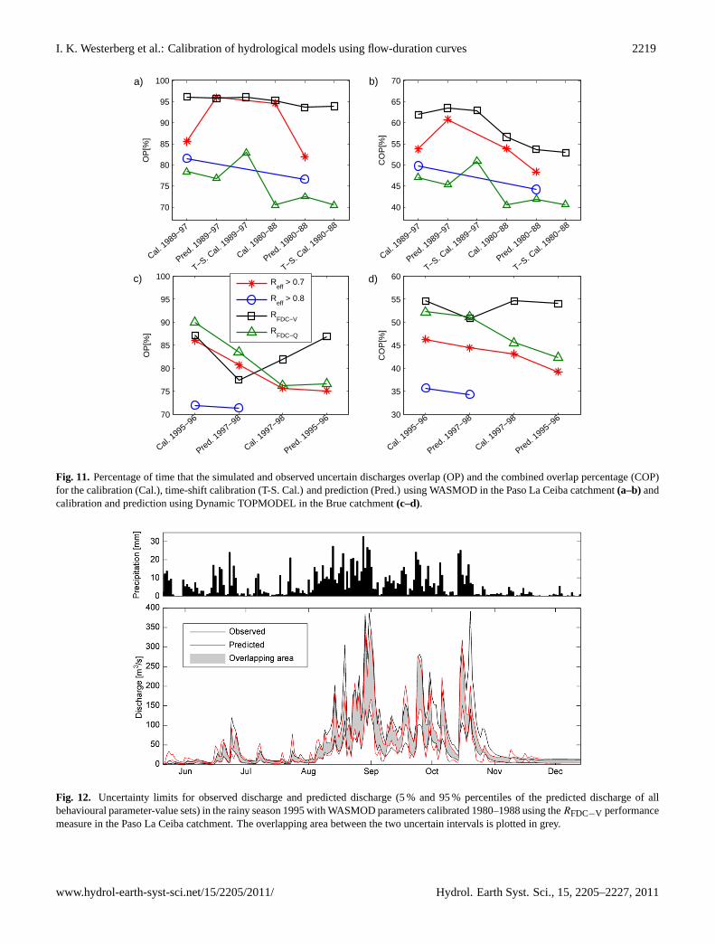
The measures of overlap (OP and COP) between the simu-lated and observed uncertain discharge bounds were gener-ally higher for theRFDC−V measure compared to the othermeasures (Fig. 11). As the COP measure accounted for over-estimated predictive uncertainty a high value of this measurewas more important than for OP. The results for the time-shiftcalibration using the FDC from another time period gave re-sults similar to that of the normal FDC calibration. The bestReff simulations (Reff > 0.8) resulted in a similar number ofbehavioural simulations asRFDC−V at Brue, but gave muchlower overlap than forRFDC−V , which was largely becauseof the poorer low-flow performance. TheRFDC−Q measureresulted in better results in the Brue catchment compared toPaso La Ceiba. This might relate to the fact that there wasmore baseflow at Brue wherefore the EPs for the discharge-interval-selection method covered the low-flow part of theFDC better than at Paso La Ceiba.

www.hydrol-earth-syst-sci.net/15/2205/2011/ Hydrol. Earth Syst. Sci., 15, 2205–2227, 2011

2218 I. K. Westerberg et al.: Calibration of hydrological models using flow-duration curves

44

1028

Fig. 10 a) and b) FDCs for behavioural parameter-value sets for Dynamic TOPMODEL in the 1029

Brue catchment for calibration in 1995–96 using RFDC-V (all FDCs plotted as grey/shaded 1030

lines), Reff, and RFDC-Q (maximum and minimum FDC values plotted as lines) and observed 1031

crisp, upper and lower discharge; c) and d) FDCs for prediction in 1997–98 using the 1032

behavioural parameter-value sets from 1995–96. The FDCs are split in two plots (left – high 1033

flows and right – low flows) at 10% exceedance. All FDCs are plotted for the volume interval 1034

EPs. 1035

1036 1037

Fig. 10. (a)and(b) FDCs for behavioural parameter-value sets for Dynamic TOPMODEL in the Brue catchment for calibration in 1995–1996 usingRFDC−V (all FDCs plotted as grey/shaded lines),Reff, andRFDC−Q (maximum and minimum FDC values plotted as lines) andobserved crisp, upper and lower discharge;(c) and(d) FDCs for prediction in 1997–1998 using the behavioural parameter-value sets from1995–1996. The FDCs are split in two plots (left – high flows and right – low flows) at 10 % exceedance. All FDCs are plotted for thevolume interval EPs.

5.5.1 The Paso La Ceiba catchment – WASMOD

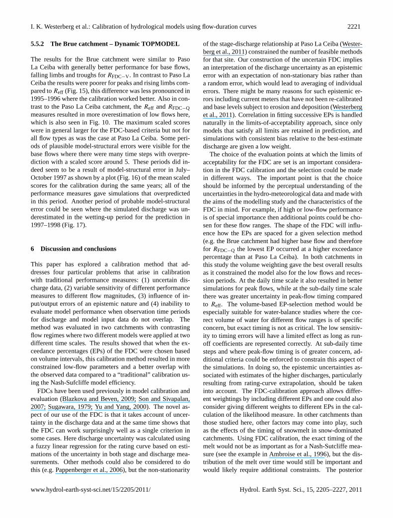
The simulated discharge for the Paso La Ceiba catchmentwas in general in good agreement with the observed dis-charge (Fig. 12). During the low-flow periods of some yearsthe discharge was underestimated for all performance mea-sures, indicating a possible model-structural error in simulat-ing a slower/deeper ground-water response or errors in theinput data.

The posterior analysis of the mean scaled scores for dif-ferent parts of the hydrograph (Fig. 13) for the prediction in1989–1997 showed that when using theRFDC−V calibrationcompared toReff: (1) the distributions of scaled scores weremore centred on zero, (2) there were fewer base flows thatwere underestimated, and (3) the largest difference was seenfor the troughs, falling limbs and base flows that are con-trolled by the slow-flow and evaporation parameters. Thesame results were seen in all the other calibration/predictionperiods. Events where the predicted discharge was under-estimated did not generate as large scaled scores as if thepredicted discharge was overestimated, as the uncertainty

bounds were wider in absolute terms for high flows com-pared to low flows, this explains the skew in the histogramsin Fig. 13. The distributions of the scaled scores forReff andRFDC−Q were always centred on negative scaled scores forall flow types.

A plot of the mean scaled scores and the discharge for1989–1990 revealed the difference in low-flow performance(Fig. 14). A large scaled deviation can be seen for all per-formance measures in the end of 1990 where there is a peakin the predicted discharge but not in the observed. This is atype of epistemic error that could be a result of erroneous dis-charge data, influence of upstream dams or unrepresentativeprecipitation data. This type of event had a large effect ontheReff calibration where it generated a large sum-of-squareserror and a reduction in overall performance. A similar devi-ation is seen in the end of 1989. The maximum scaled scoresfor all the calibration and prediction periods at Paso La Ceibawere consistently larger for the FDC-based measures com-pared toReff which might indicate that the FDC criteria arenot as sensitive to such disinformative events.

Hydrol. Earth Syst. Sci., 15, 2205–2227, 2011 www.hydrol-earth-syst-sci.net/15/2205/2011/

I. K. Westerberg et al.: Calibration of hydrological models using flow-duration curves 2219

30

35

40

45

50

55

60

CO

P[%

]

Cal. 1995−96

Pred. 1997−98

Cal. 1997−98

Pred. 1995−9670

75

80

85

90

95

100

OP

[%]

Cal. 1995−96

Pred. 1997−98

Cal. 1997−98

Pred. 1995−96

R

eff > 0.7

Reff

> 0.8

RFDC−V

RFDC−Q

40

45

50

55

60

65

70

CO

P[%

]

Cal. 1989−97

Pred. 1989−97

T−S. Cal. 1

989−97

Cal. 1980−88

Pred. 1980−88

T−S. Cal. 1

980−88

70

75

80

85

90

95

100

OP

[%]

Cal. 1989−97

Pred. 1989−97

T−S. Cal. 1

989−97

Cal. 1980−88

Pred. 1980−88

T−S. Cal. 1

980−88

a) b)

d)c)

Fig. 11. Percentage of time that the simulated and observed uncertain discharges overlap (OP) and the combined overlap percentage (COP)for the calibration (Cal.), time-shift calibration (T-S. Cal.) and prediction (Pred.) using WASMOD in the Paso La Ceiba catchment(a–b)andcalibration and prediction using Dynamic TOPMODEL in the Brue catchment(c–d).

46

1045

Fig. 12 Uncertainty limits for observed discharge and predicted discharge (5% and 95% 1046

percentiles of the predicted discharge of all behavioural parameter-value sets) in the rainy 1047

season 1995 with WASMOD parameters calibrated 1980–88 using the RFDC-V performance 1048

measure in the Paso La Ceiba catchment. The overlapping area between the two uncertain 1049

intervals is plotted in grey. 1050

1051 1052

Fig. 12. Uncertainty limits for observed discharge and predicted discharge (5 % and 95 % percentiles of the predicted discharge of allbehavioural parameter-value sets) in the rainy season 1995 with WASMOD parameters calibrated 1980–1988 using theRFDC−V performancemeasure in the Paso La Ceiba catchment. The overlapping area between the two uncertain intervals is plotted in grey.

www.hydrol-earth-syst-sci.net/15/2205/2011/ Hydrol. Earth Syst. Sci., 15, 2205–2227, 2011

2220 I. K. Westerberg et al.: Calibration of hydrological models using flow-duration curves

0 5 100

10

20

30

Rising Limbs

Scaled score [−]

Nor

mal

ised

no.

of t

ime

step

s

Reff

> 0.7: max(S): 13

RFDC−Q

: max(S): 22

RFDC−V

: max(S): 22

−2 0 2 4 6 80

50

100

Falling Limbs

Scaled score [−]

Nor

mal

ised

no.

of t

ime

step

s

R

eff > 0.7: max(S): 5

RFDC−Q

: max(S): 10

RFDC−V

: max(S): 9

0 5 100

20

40

60

80

Peaks

Scaled score [−]

Nor

mal

ised

no.

of t

ime

step

s

Reff

> 0.7: max(S): 17

RFDC−Q

: max(S): 24

RFDC−V

: max(S): 25

0 5 100

10

20

30

40

Troughs

Scaled score [−]

Nor

mal

ised

no.

of t

ime

step

s

Reff

> 0.7: max(S): 11

RFDC−Q

: max(S): 15

RFDC−V

: max(S): 18

−2 0 2 4 6 8 10 12 140

200

400

600

800

1000

Base Flows

Scaled score [−]

Nor

mal

ised

no.

of t

ime

step

s

Reff

> 0.7: max(S): 21

RFDC−Q

: max(S): 40

RFDC−V

: max(S): 37

Fig. 13. Scaled scores to limits of acceptability for different parts of the hydrograph at Paso La Ceiba for prediction in 1989–1997 withbehavioural parameter-value sets for 1980–1988 for WASMOD. For each performance measure the histograms were normalised by thenumber of behavioural simulations, which means that the y-axis represents the number of time steps. The upper range of the histogram x-axis was limited to improve the visibility of the lower range, the maximum scaled scores, max(S), for each criterion are given in the legendsand all scaled scores larger or equal to the last bin are plotted in the last bin.

48

1063

Fig. 14 Daily precipitation in 1989–1990 (top) and predicted and observed crisp daily 1064

discharge for behavioural parameter-value sets from using RFDC-V for calibration of 1065

WASMOD in the Paso La Ceiba catchment in 1980–88 (middle). The mean scaled scores for 1066

all performance measures are plotted in the bottom plot where the grey area represents a 1067

scaled score from -1 to 1, i.e. a simulated discharge with a score inside this range is inside the 1068

discharge uncertainty limits. 1069

1070 1071

Fig. 14. Daily precipitation in 1989–1990 (top) and predicted and observed crisp daily discharge for behavioural parameter-value setsfrom usingRFDC−V for calibration of WASMOD in the Paso La Ceiba catchment in 1980–1988 (middle). The mean scaled scores for allperformance measures are plotted in the bottom plot where the grey area represents a scaled score from−1 to 1, i.e. a simulated dischargewith a score inside this range is inside the discharge uncertainty limits.

Hydrol. Earth Syst. Sci., 15, 2205–2227, 2011 www.hydrol-earth-syst-sci.net/15/2205/2011/

I. K. Westerberg et al.: Calibration of hydrological models using flow-duration curves 2221

5.5.2 The Brue catchment – Dynamic TOPMODEL

The results for the Brue catchment were similar to PasoLa Ceiba with generally better performance for base flows,falling limbs and troughs forRFDC−V . In contrast to Paso LaCeiba the results were poorer for peaks and rising limbs com-pared toReff (Fig. 15), this difference was less pronounced in1995–1996 where the calibration worked better. Also in con-trast to the Paso La Ceiba catchment, theReff andRFDC−Qmeasures resulted in more overestimation of low flows here,which is also seen in Fig. 10. The maximum scaled scoreswere in general larger for the FDC-based criteria but not forall flow types as was the case at Paso La Ceiba. Some peri-ods of plausible model-structural errors were visible for thebase flows where there were many time steps with overpre-diction with a scaled score around 5. These periods did in-deed seem to be a result of model-structural error in July–October 1997 as shown by a plot (Fig. 16) of the mean scaledscores for the calibration during the same years; all of theperformance measures gave simulations that overpredictedin this period. Another period of probable model-structuralerror could be seen where the simulated discharge was un-derestimated in the wetting-up period for the prediction in1997–1998 (Fig. 17).

6 Discussion and conclusions

This paper has explored a calibration method that ad-dresses four particular problems that arise in calibrationwith traditional performance measures: (1) uncertain dis-charge data, (2) variable sensitivity of different performancemeasures to different flow magnitudes, (3) influence of in-put/output errors of an epistemic nature and (4) inability toevaluate model performance when observation time periodsfor discharge and model input data do not overlap. Themethod was evaluated in two catchments with contrastingflow regimes where two different models were applied at twodifferent time scales. The results showed that when the ex-ceedance percentages (EPs) of the FDC were chosen basedon volume intervals, this calibration method resulted in moreconstrained low-flow parameters and a better overlap withthe observed data compared to a “traditional” calibration us-ing the Nash-Sufcliffe model efficiency.

FDCs have been used previously in model calibration andevaluation (Blazkova and Beven, 2009; Son and Sivapalan,2007; Sugawara, 1979; Yu and Yang, 2000). The novel as-pect of our use of the FDC is that it takes account of uncer-tainty in the discharge data and at the same time shows thatthe FDC can work surprisingly well as a single criterion insome cases. Here discharge uncertainty was calculated usinga fuzzy linear regression for the rating curve based on esti-mations of the uncertainty in both stage and discharge mea-surements. Other methods could also be considered to dothis (e.g. Pappenberger et al., 2006), but the non-stationarity

of the stage-discharge relationship at Paso La Ceiba (Wester-berg et al., 2011) constrained the number of feasible methodsfor that site. Our construction of the uncertain FDC impliesan interpretation of the discharge uncertainty as an epistemicerror with an expectation of non-stationary bias rather thana random error, which would lead to averaging of individualerrors. There might be many reasons for such epistemic er-rors including current meters that have not been re-calibratedand base levels subject to erosion and deposition (Westerberget al., 2011). Correlation in fitting successive EPs is handlednaturally in the limits-of-acceptability approach, since onlymodels that satisfy all limits are retained in prediction, andsimulations with consistent bias relative to the best-estimatedischarge are given a low weight.

The choice of the evaluation points at which the limits ofacceptability for the FDC are set is an important considera-tion in the FDC calibration and the selection could be madein different ways. The important point is that the choiceshould be informed by the perceptual understanding of theuncertainties in the hydro-meteorological data and made withthe aims of the modelling study and the characteristics of theFDC in mind. For example, if high or low-flow performanceis of special importance then additional points could be cho-sen for these flow ranges. The shape of the FDC will influ-ence how the EPs are spaced for a given selection method(e.g. the Brue catchment had higher base flow and thereforefor RFDC−Q the lowest EP occurred at a higher exceedancepercentage than at Paso La Ceiba). In both catchments inthis study the volume weighting gave the best overall resultsas it constrained the model also for the low flows and reces-sion periods. At the daily time scale it also resulted in bettersimulations for peak flows, while at the sub-daily time scalethere was greater uncertainty in peak-flow timing comparedto Reff. The volume-based EP-selection method would beespecially suitable for water-balance studies where the cor-rect volume of water for different flow ranges is of specificconcern, but exact timing is not as critical. The low sensitiv-ity to timing errors will have a limited effect as long as run-off coefficients are represented correctly. At sub-daily timesteps and where peak-flow timing is of greater concern, ad-ditional criteria could be enforced to constrain this aspect ofthe simulations. In doing so, the epistemic uncertainties as-sociated with estimates of the higher discharges, particularlyresulting from rating-curve extrapolation, should be takeninto account. The FDC-calibration approach allows differ-ent weightings by including different EPs and one could alsoconsider giving different weights to different EPs in the cal-culation of the likelihood measure. In other catchments thanthose studied here, other factors may come into play, suchas the effects of the timing of snowmelt in snow-dominatedcatchments. Using FDC calibration, the exact timing of themelt would not be as important as for a Nash-Sutcliffe mea-sure (see the example in Ambroise et al., 1996), but the dis-tribution of the melt over time would still be important andwould likely require additional constraints. The posterior

www.hydrol-earth-syst-sci.net/15/2205/2011/ Hydrol. Earth Syst. Sci., 15, 2205–2227, 2011

2222 I. K. Westerberg et al.: Calibration of hydrological models using flow-duration curves

49

1072

Fig. 15 Scaled scores to limits of acceptability for different parts of the hydrograph at Brue for 1073

calibration in 1997–98 using Dynamic TOPMODEL. For each performance measure the 1074

histograms were normalised by the number of behavioural simulations, so the y-axis 1075

represents the normalised number of time steps. The upper range of the histogram x-axis was 1076

limited to improve the visibility of the lower range, the maximum scaled scores, max(S), for 1077

each criterion are given in the legends and all scaled scores larger or equal to the last bin are 1078

plotted in the last bin. 1079

1080 1081

Fig. 15. Scaled scores to limits of acceptability for different parts of the hydrograph at Brue for calibration in 1997–1998 using DynamicTOPMODEL. For each performance measure the histograms were normalised by the number of behavioural simulations, so the y-axisrepresents the normalised number of time steps. The upper range of the histogram x-axis was limited to improve the visibility of the lowerrange, the maximum scaled scores, max(S), for each criterion are given in the legends and all scaled scores larger or equal to the last bin areplotted in the last bin.

analysis of the simulated time series employed here can beuseful in deciding whether additional criteria are necessary.

In calibration to “hydrological signatures” such as an FDCcalculated from the discharge series, the simulated uncer-tainty bounds have a direct interpretation relative to the un-certainty in the observed discharge data. This is an advantagecompared to say a behavioural threshold-value ofReff of 0.7that is not easily interpretable (Legates and McCabe, 1999;Seibert, 2001). Winsemius et al. (2009) set limits of accept-ability in GLUE (for different types of signatures such as re-cession curves) based on inter-annual variability but took noexplicit account of the uncertainty in the observed dischargedata.

It is interesting to note that the 19 EPs used for theRFDC−Vcriterion provided better information for the calibration of themodel than the 3288 days or 17544 hours for the first yearsof calibration/prediction used forReff. Limited informationcontent in discharge time series was also demonstrated byJuston et al. (2009) and Seibert and Beven (2009), who foundthat calibration using a small fraction of data points chosenat hydrologically informed times was comparable to whenthe whole time series was used. We choseReff for com-parison with the FDC-calibration as it is sensitive to timing

errors, well-known and commonly used. Other approachessuch as multi-criteria calibration or the calculation ofReffon transformed discharge can of course also be used to con-strain simulations. We also tested log and square-root trans-formed discharge in the calculation ofReff. This resulted ingood simulations for low flows whereas the simulation forthe highest flows was poorer constrained compared toReffand the FDC-calibration. A multi-criteria calibration couldconstrain different aspects simultaneously, but the problemsof deciding on a behavioural threshold value and accountingfor discharge-data uncertainty remain in such approaches.

When the FDC-method was first developed it was testedwith inconsistent satellite-derived precipitation in a Hon-duran basin which resulted in that no simulations were foundthat were consistent with the observed FDC. In such cases atraditional calibration will result in low values for the perfor-mance measure and not point as strongly to where the incon-sistencies in the simulated flow regime occur. This is there-fore an advantage of using constraints based on signatures(such as a FDC) calculated from the flow data, as suggestedelsewhere for use in regionalisation methods for estimatingthe response of ungauged basins (e.g. Yadav et al., 2007).

Hydrol. Earth Syst. Sci., 15, 2205–2227, 2011 www.hydrol-earth-syst-sci.net/15/2205/2011/

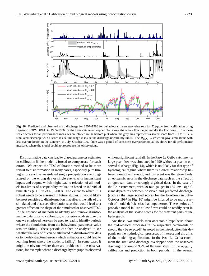
I. K. Westerberg et al.: Calibration of hydrological models using flow-duration curves 2223

Feb Mar Apr May Jun Jul Aug Sep Oct Nov Dec

0

5

10

15

Mea

n sc

aled

sco

re [−

]

Mean scaled score R

eff > 0.7

Mean scaled score Reff

> 0.8

Mean scaled score RFDC−V

Mean scaled score RFDC−Q

0

10

20

30

Dis

char

ge [m

3 /s]

Feb Mar Apr May Jun Jul Aug Sep Oct Nov Dec0

1

2

3

Dis

char

ge [m

3 /s]

0

5

10

Pre

cipi

tatio

n [m

m]

Predicted with RFDC−V

Observed crisp discharge

Fig. 16. Predicted and observed crisp discharge for 1997–1998 for behavioural parameter-value sets forRFDC−V from calibration usingDynamic TOPMODEL in 1995–1996 for the Brue catchment (upper plot shows the whole flow range, middle the low flows). The meanscaled scores for all performance measures are plotted in the bottom plot where the grey area represents a scaled score from−1 to 1, i.e. asimulated discharge with a score inside this range is inside the discharge uncertainty limits. TheRFDC−V criterion gave simulations withless overprediction in the summer. In July–October 1997 there was a period of consistent overprediction at low flows for all performancemeasures where the model could not reproduce the observations.

Disinformative data can lead to biased parameter estimatesin calibration if the model is forced to compensate for sucherrors. We expect the FDC-calibration method to be morerobust to disinformation in many cases, especially pure tim-ing errors such as an isolated single precipitation event reg-istered on the wrong day or single events with inconsistentinputs and outputs which might lead to rejection of all mod-els in a limits-of-acceptability evaluation based on individualtime steps (e.g. Liu et al., 2009). The extent to which it isrobust needs to be assessed in future studies. It would likelybe most sensitive to disinformation that affects the tails of thesimulated and observed distributions, as that would lead to agreater effect on the shape of the simulated or observed FDC.In the absence of methods to identify and remove disinfor-mative data prior to calibration, a posterior analysis like theone we employed here can be used to readily identify periodswhere the simulations from the behavioural parameter-valuesets are failing. These periods can then be analysed to seewhether the lack of fit can be attributed to disinformative dataor to model-structural errors (which in that case could lead tolearning from where the model is failing). In some cases itmight be obvious where there are problems in the observa-tions, for example where a discharge hydrograph is observed

without significant rainfall. In the Paso La Ceiba catchment alarge peak flow was simulated in 1990 without a peak in ob-served discharge (Fig. 14), which is not likely for that type ofhydrological regime where there is a direct relationship be-tween rainfall and runoff, and this event was therefore likelyan epistemic error in the discharge data such as the effect ofan upstream dam or wrongly digitised data. In the case ofthe Brue catchment, with 49 rain gauges in 135 km2, signif-icant departures between observed and predicted discharge(such as the large scaled scores for the low-flows in July–October 1997 in Fig. 16) might be inferred to be more a re-sult of model deficiencies than input errors. These periods ofprobable model failure at low flows could be readily seen inthe analysis of the scaled scores for the different parts of thehydrograph.

Are these two models then acceptable hypothesis aboutthe hydrological processes in the respective catchments orshould they be rejected? As noted in the introduction this de-pends on the hydrological processes of interest and the aimsof the modelling application. In the Paso La Ceiba catch-ment the simulated discharge overlapped with the observeddischarge for around 95 % of the time steps for theRFDC−Vcalibration and prediction in both periods. If the overall

www.hydrol-earth-syst-sci.net/15/2205/2011/ Hydrol. Earth Syst. Sci., 15, 2205–2227, 2011

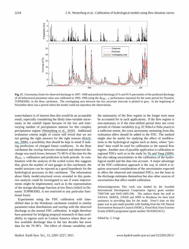
2224 I. K. Westerberg et al.: Calibration of hydrological models using flow-duration curves

51

1094

Fig. 17 Uncertainty limits for observed discharge in 1997–98 and predicted discharge (5% 1095

and 95% percentiles of the predicted discharge of all behavioural parameter-value sets 1096

calibrated in 1995–96 using the RFDC-V performance measure) for the same period for 1097

Dynamic TOPMODEL in the Brue catchment. The overlapping area between the two 1098

uncertain intervals is plotted in grey. In the beginning of November there was a period where 1099

the model could not reproduce the observations. 1100

1101

Fig. 17.Uncertainty limits for observed discharge in 1997–1998 and predicted discharge (5 % and 95 % percentiles of the predicted dischargeof all behavioural parameter-value sets calibrated in 1995–1996 using theRFDC−V performance measure) for the same period for DynamicTOPMODEL in the Brue catchment. The overlapping area between the two uncertain intervals is plotted in grey. In the beginning ofNovember there was a period where the model could not reproduce the observations.

water-balance is of interest then this would be an acceptableresult, especially considering the likely time-variable uncer-tainty in the rainfall inputs because of the low and time-varying number of precipitation stations for this complexprecipitation regime (Westerberg et al., 2010). Additionalevaluation criteria might of course still reveal that we arenot getting the right answers for the right reasons (Kirch-ner, 2006), a possibility that should be kept in mind if mak-ing predictions of changed future conditions. In the Bruecatchment the overlap between simulated and observed dis-charge was much lower, between 75–90 % of the time for theRFDC−V calibration and prediction in both periods. In com-bination with the analysis of the scaled scores this suggeststhat, given the number of rain gauges in this catchment, themodel structure can be rejected as a good hypothesis for thehydrological processes in this catchment. The informationabout likely model-structural errors revealed in this poste-rior analysis could be investigated to see if some improve-ments might be implemented, such as in the representationof the storage-discharge function at low flows (which in Dy-namic TOPMODEL is not restricted to any particular func-tional form).

Experiments using the FDC calibration with time-shifted data in the Honduran catchment resulted in similarparameter-value distributions and overlap with the observeddischarge as the normal FDC calibration. It might thereforehave potential for bridging temporal mismatch of data avail-ability in regions such as Central America where there arefew available discharge data in the last decades but moredata for the 70–90’s. The effect of climate variability and

the stationarity of the flow regime in the longer term mustbe accounted for in such applications. If the flow regime isnon-stationary or if the time-shifted period does not coverperiods of climate variability (e.g. El Nino/La Nina years) toa sufficient extent, the extra uncertainty stemming from thisrealisation effect should be added to the FDC. The methodmight also be useful for studying the effect of modifica-tions to the hydrological regime such as dams, where “pre-dam” data could be used for calibration to the natural flowregime. Another area of possible application is calibration toregional FDCs such as in the study by Yu and Yang (2000),but also taking uncertainties in the calibration of the hydro-logical model and the data into account. A major advantageof the FDC-calibration approach is the way in which it re-quires structured consideration of the uncertainties expectedto affect the observed and simulated FDCs, not the least inthe discharge estimates themselves but also other sources ofuncertainties that affect model calibration.

Acknowledgements.This work was funded by the SwedishInternational Development Cooperation Agency grant number75007349 and SWE-2005-296. The authors thank the staff atSANAA, SERNA, UNAH and SMN in Honduras for their kindassistance in providing data for the study. Freer’s time on thispaper was in part made possible with funding from the UK NaturalEnvironment Research Council (NERC), Flood Risk from ExtremeEvents (FREE) programme (grant number NE/E002242/1).

Edited by: J. Vrugt

Hydrol. Earth Syst. Sci., 15, 2205–2227, 2011 www.hydrol-earth-syst-sci.net/15/2205/2011/

I. K. Westerberg et al.: Calibration of hydrological models using flow-duration curves 2225

References

Allen, R. G., Pereira, L. S., Raes, D., and Smith, M.: Crop evap-otranspiration – guidelines for computing crop water require-ments, FAO, 300 p., 1998.

Ambroise, B., Freer, J., and Beven, K.: Application of a general-ized TOPMODEL to the small Ringelbach catchment, Vosges,France, Water Resour. Res., 32, 2147–2159, 1996.

Aronica, G. T., Candela, A., Viola, F., and Cannarozzo, M.: Influ-ence of rating curve uncertainty on daily rainfall-runoff modelpredictions., in: Predictions in Ungauged Basins: Promise andProgress, edited by: Sivapalan, M., Wagener, T., Uhlenbrook, S.,Liang, X., Lakshmi, V., Kumar, P., Zehe, E., and Tachikawa, Y.,IAHS Publ 303, 116–124, 2006.

Bell, V. A. and Moore, R. J.: The sensitivity of catchment runoffmodels to rainfall data at different spatial scales, Hydrol. EarthSyst. Sci., 4, 653–667,doi:10.5194/hess-4-653-2000, 2000.

Beven, K. J.: Changing Ideas in Hydrology - the Case of Physically-Based Models, J. Hydrol., 105, 157–172, 1989.

Beven, K. J.: A manifesto for the equifinality thesis, J. Hydrol., 320,18–36, 2006.

Beven, K. J.: Environmental Modelling: An Uncertain Future?,Routledge, London, 2009.

Beven, K. J.: Preferential flows and travel time distribu-tions: defining adequate hypothesis tests for hydrologicalprocess models Preface, Hydrol. Process., 24, 1537–1547,doi:10.1002/Hyp.7718, 2010.

Beven, K. J. and Freer, J.: A dynamic TOPMODEL, Hydrol. Pro-cess., 15, 1993–2011, 2001.

Beven, K. J. and Kirkby, M. J.: A physically based, variable con-tributing area model of basin hydrology, Hydrolog. Sci. B., 24,43–69, 1979.

Beven, K. J. and Westerberg, I. K.: On red herrings and real her-rings: disinformation and information in hydrological inference,Hydrol. Process., 25, 1676-1680, 2011

Beven, K. J., Smith, P. J., and Freer, J. E.: So just why woulda modeller choose to be incoherent?, J. Hydrol., 354, 15–32,doi:10.1016/j.jhydrol.2008.02.007, 2008.

Beven, K., Smith, P. J., and Wood, A.: On the colour and spin ofepistemic error (and what we might do about it), Hydrol. EarthSyst. Sci. Discuss., 8, 5355–5386,doi:10.5194/hessd-8-5355-2011, 2011

Blazkova, S. and Beven, K.: A limits of acceptability approachto model evaluation and uncertainty estimation in flood fre-quency estimation by continuous simulation: Skalka catch-ment, Czech Republic, Water Resour. Res., 45, W00b16,doi:10.1029/2007wr006726, 2009.

Boyle, D. P., Gupta, H. V., and Sorooshian, S.: Toward improvedcalibration of hydrologic models: Combining the strengths ofmanual and automatic methods, Water Resour. Res., 36, 3663–3674, 2000.

Bulygina, N., McIntyre, N., and Wheater, H.: Conditioning rainfall-runoff model parameters for ungauged catchments and land man-agement impacts analysis, Hydrol. Earth Syst. Sci., 13, 893–904,doi:10.5194/hess-13-893-2009, 2009.

Criss, R. E. and Winston, W. E.: Do Nash values have value?Discussion and alternate proposals, Hydrol. Process., 22, 2723–2725,doi:10.1002/Hyp.7072, 2008.

Di Baldassarre, G., and Montanari, A.: Uncertainty in river dis-charge observations: a quantitative analysis, Hydrol Earth Syst

Sc, 13, 913-921, 2009.Diaz, H. F., Hoerling, M. P., and Eischeid, J. K.: ENSO variability,

teleconnections and climate change, Int. J. Climatol., 21, 1845–1862, 2001.

Enfield, D. B. and Alfaro, E. J.: The dependence of Caribbean rain-fall on the interaction of the tropical Atlantic and Pacific oceans,J. Climate, 12, 2093–2103, 1999.

Freer, J., Beven, K., and Ambroise, B.: Bayesian estimation of un-certainty in runoff prediction and the value of data: An applica-tion of the GLUE approach, Water Resour. Res., 32, 2161–2173,1996.

Freer, J., Beven, K. J., and Peters, N.: Multivariate seasonal periodmodel rejection within the generalised likelihood uncertainty es-timation procedure, in: Calibration of Watershed Models, editedby: Duan, Q., Gupta, H., Sorooshian, S., Rousseau, A. N., andTurcotte, R., AGU Books, Washington, 69–87, 2003.

Freer, J. E., McMillan, H., McDonnell, J. J., and Beven, K. J.: Con-straining dynamic TOPMODEL responses for imprecise watertable information using fuzzy rule based performance measures,J. Hydrol., 291, 254–277,doi:10.1016/j.jhydrol.2003.12.037,2004.

Garrick, M., Cunnane, C., and Nash, J. E.: A Criterion of Efficiencyfor Rainfall-Runoff Models, J. Hydrol., 36, 375–381, 1978.

Grayson, R. B., Moore, I. D., and Mcmahon, T. A.: PhysicallyBased Hydrologic Modeling .2. Is the Concept Realistic, WaterResour. Res., 28, 2659–2666, 1992.

Global Runoff Data Centre: http://grdc.bafg.de, last access:23 February 2010, 2010.

Gupta, H. V., Sorooshian, S., and Yapo, P. O.: Toward improvedcalibration of hydrologic models: Multiple and noncommensu-rable measures of information, Water Resour. Res., 34, 751–763,1998.

Gupta, H. V., Kling, H., Yilmaz, K. K., and Martinez, G. F.: De-composition of the mean squared error and NSE performancecriteria: Implications for improving hydrological modelling, J.Hydrol., 377, 80–91,doi:10.1016/j.jhydrol.2009.08.003, 2009.

Houghton-Carr, H. A.: Assessment criteria for simple conceptualdaily rainfall-runoff models, Hydrol. Sci. J., 44, 237–261, 1999.

Huard, D., and Mailhot, A.: Calibration of hydrological modelGR2M using Bayesian uncertainty analysis, Water Resour. Res.,44, W02424,doi:10.1029/2007wr005949, 2008.

Juston, J., Seibert, J., and Johansson, P. O.: Temporal samplingstrategies and uncertainty in calibrating a conceptual hydrolog-ical model for a small boreal catchment, Hydrol. Process., 23,3093–3109,doi:10.1002/Hyp.7421, 2009.

Kavetski, D., Fenicia, F., and Clark, M.: Impact of tempo-ral data resolution on parameter inference and model identi-fication in conceptual hydrological modeling: Insights froman experimental catchment, Water Resour. Res., 47, W05501,doi:10.1029/2010WR009525, 2011.

Kirchner, J. W.: Getting the right answers for the right rea-sons: Linking measurements, analyses, and models to advancethe science of hydrology, Water Resour. Res., 42, W03s04,doi:10.1029/2005wr004362, 2006.

Krause, P., Boyle, D. P., and Base, F.: Comparison of different effi-ciency criteria for hydrological model assessment, Adv. Geosci.,5, 89–97, 2005,http://www.adv-geosci.net/5/89/2005/.

Krueger, T., Freer, J., Quinton, J. N., Macleod, C. J. A., Bilotta,

www.hydrol-earth-syst-sci.net/15/2205/2011/ Hydrol. Earth Syst. Sci., 15, 2205–2227, 2011

2226 I. K. Westerberg et al.: Calibration of hydrological models using flow-duration curves

G. S., Brazier, R. E., Butler, P., and Haygarth, P. M.: Ensem-ble evaluation of hydrological model hypotheses, Water Resour.Res., 46, W07516,doi:10.01029/02009WR00784, 2010.

Legates, D. R. and McCabe, G. J.: Evaluating the use of “goodness-of-fit” measures in hydrologic and hydroclimatic model valida-tion, Water Resour. Res., 35, 233–241, 1999.

Liu, Y. Q. and Gupta, H. V.: Uncertainty in hydrologic modeling:Toward an integrated data assimilation framework, Water Resour.Res., 43, W07401,doi:10.1029/2006WR005756, 2007.

Liu, Y., Freer, J., Beven, K. J., and Matgen, P.: Towards a lim-its of acceptability approach to the calibration of hydrologicalmodels: extending observation error, J. Hydrol., 367, 93–103,doi:10.1016/j.jhydrol.2009.01.016, 2009.

Magana, V., Amador, J. A., and Medina, S.: The midsummerdrought over Mexico and Central America, J. Climate, 12, 1577–1588, 1999.

McDonnell, J. J.: Where does water go when it rains? Moving be-yond the variable source area concept of rainfall-runoff response,Hydrol. Process., 17, 1869–1875, 2003.

McMillan, H. and Clark, M.: Rainfall-runoff model calibration us-ing informal likelihood measures within a Markov chain MonteCarlo sampling scheme, Water Resour. Res., 45, W04418,doi:10.1029/2008wr007288, 2009.

McMillan, H., Freer, J., Pappenberger, F., Krueger, T., and Clark,M.: Impacts of uncertain river flow data on rainfall-runoffmodel calibration and discharge predictions, Hydrol. Process.,24, 1270–1284,doi:10.1002/Hyp.7587, 2010.

Montanari, A. and Toth, E.: Calibration of hydrological models inthe spectral domain: An opportunity for scarcely gauged basins?,Water Resour. Res., 43, W05434,doi:10.1029/2006wr005184,2007.

Monteith, J. L.: Evaporation and the Environment, in: The Stateand Movement of Water in Living Organisms., edited by: Fogg,G. E., Cambridge University Press, 205–234, 1965.

Moore, R. J., Jones, D. A., Cox, D. R., and Isham, V. S.: Designof the HYREX raingauge network, Hydrol. Earth Syst. Sci., 4,521–530,doi:10.5194/hess-4-521-2000, 2000.

Nash, J. E. and Sutcliffe, J. V.: River flow forecasting through con-ceptual models 1. A discussion of principles, J. Hydrol., 10, 282–290, 1970.

Page, T., Beven, K. J., Freer, J., and Neal, C.: Modellingthe chloride signal at Plynlimon, Wales, using a modi-fied dynamic TOPMODEL incorporating conservative chemi-cal mixing (with uncertainty), Hydrol. Process., 21, 292–307,doi:10.1022/Hyp.6186, 2007.

Pappenberger, F., Matgen, P., Beven, K. J., Henry, J. B., Pfister, L.,and Fraipont de, P.: Influence of uncertain boundary conditionsand model structure on flood inundation predictions, Adv. WaterResour., 29, 1430–1449, 2006.

Pappenberger, F., Frodsham, K., Beven, K., Romanowicz, R., andMatgen, P.: Fuzzy set approach to calibrating distributed floodinundation models using remote sensing observations, Hydrol.Earth Syst. Sci., 11, 739–752,doi:10.5194/hess-11-739-2007,2007.

Pelletier, P.: Uncertainties in the single determination of river dis-charge: a literature review, Can. J. Civil Eng., 15, 834–850, 1988.

Petersen-Overleir, A., Soot, A., and Reitan, T.: Bayesian RatingCurve Inference as a Streamflow Data Quality Assessment Tool,Water Resour. Manag., 23, 1835–1842,doi:10.1007/s11269-

008-9354-5, 2009.Portig, W. H.: The climate of Central America, in: World Survey of

Climatology, edited by: Schwerdtfeger, W., Elsevier, New York,405–464, 1976.

Refsgaard, J. C. and Knudsen, J.: Operational validation and in-tercomparison of different types of hydrological models, WaterResour. Res., 32, 2189–2202, 1996.

Renard, B., Kavetski, D., Kuczera, G., Thyer, M., and Franks, S.W.: Understanding predictive uncertainty in hydrologic mod-eling: The challenge of identifying input and structural errors,Water Resour. Res., 46, W05521,doi:10.1029/2009wr008328,2010.

Schaefli, B. and Gupta, H. V.: Do Nash values have value?, Hydrol.Process., 21, 2075–2080,doi:10.1002/Hyp.6825, 2007.

Schoups, G. and Vrugt, J. A.: A formal likelihood function for pa-rameter and predictive inference of hydrologic models with cor-related, heteroscedastic, and non-Gaussian errors, Water Resour.Res., 46, W10531,doi:10.1029/2009WR008933, 2010.

Seibert, J.: On the need for benchmarks in hydrological modelling,Hydrol. Process., 15, 1063–1064,doi:10.1002/hyp.446, 2001.

Seibert, J. and Beven, K. J.: Gauging the ungauged basin: howmany discharge measurements are needed?, Hydrol. Earth Syst.Sci., 13, 883–892,doi:10.5194/hess-13-883-2009, 2009.

Smith, P., Beven, K. J., and Tawn, J. A.: Informal like-lihood measures in model assessment: Theoretic develop-ment and investigation, Adv Water Resour, 31, 1087–1100,doi:10.1016/j.advwatres.2008.04.012, 2008.

Son, K. and Sivapalan, M.: Improving model structure and re-ducing parameter uncertainty in conceptual water balance mod-els through the use of auxiliary data, Water Resour. Res., 43,W01415, doi:01410.01029/02006wr005032, 2007.

Sugawara, M.: Automatic calibration of the tank model, Hydrol.Sci. B., 24, 375–388, 1979.

Thyer, M., Renard, B., Kavetski, D., Kuczera, G., Franks, S. W.,and Srikanthan, S.: Critical evaluation of parameter consistencyand predictive uncertainty in hydrological modeling: A casestudy using Bayesian total error analysis, Water Resour. Res.,45, W00b14,doi:10.1029/2008wr006825, 2009.

Wagener, T., Boyle, D. P., Lees, M. J., Wheater, H. S., Gupta, H. V.,and Sorooshian, S.: A framework for development and applica-tion of hydrological models, Hydrol. Earth Syst. Sci., 5, 13–26,doi:10.5194/hess-5-13-2001, 2001.

Westerberg, I., Walther, A., Guerrero, J.-L., Coello, Z., Halldin, S.,Xu, C. Y., Chen, D., and Lundin, L.-C.: Precipitation data ina mountainous catchment in Honduras: quality assessment andspatiotemporal characteristics, J. Theor. Appl. Clim., 101, 381–396,doi:10.1007/s00704-009-0222-x, 2010.

Westerberg, I., Guerrero, J.-L., Seibert, J., Beven, K. J., and Halldin,S.: Stage-discharge uncertainty derived with a non-stationary rat-ing curve in the Choluteca River, Honduras, Hydrol. Process., 25,603–613,doi:10.1002/hyp.7848, 2011.

Widen-Nilsson, E., Halldin, S., and Xu, C. Y.: Global water-balancemodelling with WASMOD-M: Parameter estimation and region-alisation, J. Hydrol., 340, 105–118, 2007.

Winsemius, H. C., Schaefli, B., Montanari, A., and Savenije,H. H. G.: On the calibration of hydrological models in un-gauged basins: A framework for integrating hard and softhydrological information, Water Resour. Res., 45, W12422,doi:12410.11029/12009wr007706, 2009.

Hydrol. Earth Syst. Sci., 15, 2205–2227, 2011 www.hydrol-earth-syst-sci.net/15/2205/2011/

I. K. Westerberg et al.: Calibration of hydrological models using flow-duration curves 2227

Vogel, R. M., and Fennessey, N. M.: Flow-Duration Curves. 1: NewInterpretation and Confidence-Intervals, J Water Res Pl-Asce,120, 485-504, 1994.

Wood, S. J., Jones, D. A., and Moore, R. J.: Accuracy of rainfallmeasurement for scales of hydrological interest, Hydrol. EarthSyst. Sci., 4, 531–543,doi:10.5194/hess-4-531-2000, 2000.

Xu, C.-Y.: WASMOD – The water and snow balance modelingsystem, in: Mathematical Models of Small Watershed Hydrol-ogy and Applications, edited by: Singh, V. J. a. F., D.K., WaterResources Publications LLC, Highlands Ranch, Colorado, US,555–590, 2002.

Xu, C.-Y. and Halldin, S.: The effect of climate change on riverflow and snow cover in the NOPEX area simulated by a simplewater balance model, Nord Hydrol., 28, 273–282, 1997.

Yadav, M., Wagener, T., and Gupta, H.: Regionalization of con-straints on expected watershed response behavior for improvedpredictions in ungauged basins, Adv. Water Resour., 30, 1756–1774,doi:10.1016/j.advwatres.2007.01.005, 2007.

Yilmaz, K. K., Gupta, H. V., and Wagener, T.: A process-based di-agnostic approach to model evaluation: Application to the NWSdistributed hydrologic model, Water Resour. Res., 44, W09417,doi:10.1029/2007wr006716, 2008.

Younger, P. M., Freer, J. E., and Beven, K. J.: Detecting the effectsof spatial variability of rainfall on hydrological modelling withinan uncertainty analysis framework, Hydrol Process, 23, 1988–2003,doi:10.1002/Hyp.7341, 2009.

Younger, P. M., Beven, K. J., and Freer, J. E.: Limits of acceptabilityand complex error reconstruction in a rainfall-runoff simulation,J Hydrol, in review, 2011.

Yu, P. S. and Yang, T. C.: Using synthetic flow duration curvesfor rainfall-runoff model calibration at ungauged sites, Hydrol.Process., 14, 117–133, 2000.

www.hydrol-earth-syst-sci.net/15/2205/2011/ Hydrol. Earth Syst. Sci., 15, 2205–2227, 2011