Calibration of frequency-domain electromagnetic devices used in near-surface surveying

© 2014 European Association of Geoscientists & Engineers 481

Near Surface Geophysics, 2014, 12, 481-491 doi:10.3997/1873-0604.2014012

* [email protected]

Calibration of frequency-domain electromagnetic devices used in near-surface surveying

Julien Thiesson1, Pauline Kessouri1, Cyril Schamper2 and Alain Tabbagh1*

1 UMR 7619, Sisyphe, UPMC/CNRS, Paris, France2 Hydrogeophysics group, Department of Geoscience, Aarhus University, Aarhus, Denmark

Received February 2013, accepted July 2013

ABSTRACTFor the past forty years electromagnetic prospecting instruments have played a growing role in the mapping of soil EM properties in the very low-frequency (VLF) range for a large variety of applica-tions and they are now beginning to be applied in the medium-frequency range. Measurement interpretations, however, necessitate expressing the results in terms of physical properties. This step allows not only comparisons and joint interpretation with data generated by different electromag-netic induction (EMI) instruments but also with other types of field measurements e.g., vertical electrical sounding (VES) or electrical resistivity tomography (ERT) or laboratory tests on samples.

The calibration process here proposed is based on comparisons between the instrument respons-es and: (1) an exact 1D multi-layer analytical modelling that takes the three EM properties into account, i.e., the electrical conductivity, the complex magnetic susceptibility and the complex die-lectric permittivity when the instrument is elevated above a layered ground; (2) the response to purely conductive metallic spheres, which only depends on the diameter of the spheres. It is applied to two instrument prototypes: one in the VLF frequency range and the other in the medium-frequen-cy (MF) range.

ment versus electrical resistivity tomography (ERT). The calibra-tion procedure presented in this paper does not require the time-consuming installation of an electrical DC panel and is more portable to any new survey area.

Calibration is a general problem not limited to EMI devices and since the beginning of applied geophysics prospectors have deployed major efforts to make quantitative measurements and to express their results in term of absolute physical units. Quantification of ground properties allows not only a more accu-rate description of the true space distribution of the physical properties but also the results of the interpretation to be almost independent of the geophysical method. In the particular cases of the electromagnetic methods, calibration is necessary because more and more often geophysicists have to compare and to inter-pret data of different electrical, magnetic and electromagnetic methods together and to compare their interpretations to labora-tory sample studies (Benech et al. 2002).

In DC resistivity prospecting, the expression of the measure-ment results by one quantitative parameter is quite simple: (i) as only one physical property intervenes, the transformation of each measurement into ‘apparent resistivity’ (i.e., the electrical resis-tivity of a homogeneous ground that would deliver the same measurement with the same instrument and the same array geometry) is straightforward and (ii) calibration can be directly achieved by using high- precision resistors that allow ΔV/I ratio

INTRODUCTIONElectrical and magnetic properties of the ground play a growing part in the different aspects of near-surface geophysical survey-ing where, beside developments in direct current (DC) electrical methods such as electrical resistivity tomography (ERT) or 3D resistivity mapping, the application of the so-called electromag-netic induction (EMI) instruments has become widespread over the last ten years. After prior studies in archaeological prospec-tion (Howel 1966; Tite and Mullins 1969; Parchas and Tabbagh 1978), the commercialization of low- induction number (LIN) instruments by Geonics, Ltd, first permitted applications for the characterization of salted soil (de Jong et al. 1979; Rhoades and Corwin 1981) and later led to a large variety of soil studies through electrical conductivity mapping (Williams and Hoey 1987; Brus et al. 1992; Sheets and Hendrickx 1995). However, the use of EMI instruments generally remains limited to the delineation of anomalies because of the difficulty that exists in calibrating these types of devices. Nevertheless, in a few cases calibration of the results of EM surveys was achieved by direct comparison with measurements performed over sampled cores (Corwin and Rhoades 1982; Lesch et al. 1992; Abdu et al. 2007; Moghadas et al. 2012). Only very recently Lavoué et al. (2010) presented a procedure to calibrate a multi-frequency EM instru-

Julien Thiesson et al.482

© 2014 European Association of Geoscientists & Engineers, Near Surface Geophysics, 2014, 12, 481-491

tics, we chose to describe all electrical properties by a real con-ductivity and a complex permittivity.

In the considered frequency range (3 kHz to 3 MHz) electrical conductivity varies from around 1 Ωm in tidal areas to 104 Ωm for permafrost or crystalline rocks (Keller 1988). Magnetic suscepti-bility remains under 10-2 SI for its real part, while its imaginary part’s magnitude does not overpass one tenth of the real part. Dielectric relative permittivity can reach thousands for clayey soils in the lowest part of the considered frequency range but it remains under some hundreds in the uppermost part (Kessouri 2012). Consequently, the roles of these properties in EM measurements significantly change with frequency and this must be taken into account when calibrating the different instruments.

CALCULATION OF A LAYERED GROUND RESPONSEMost often a succession of horizontal layers of different proper-ties is a convenient approximation for the structure of the ground. The theoretical responses of EM instruments to such 1D model-ling can be analytically calculated and, in some cases detailed hereafter, simplified by assumptions that allow a clear illustra-tion of the physical effects of the different properties.

At shallow depth, vertical electrical soundings are easy to achieve and offer the possibility to obtain 1D conductivity mod-els of the ground that can be used to calculate the expected EM responses and, by comparing them to the experimental ones, to calibrate EM instruments.

Response of a layered ground to a dipole source and to a loop sourceThe analytical method that allows calculating the electromag-netic field at the surface of a homogeneous ground for either a magnetic dipole source or an electric dipole source and thus loops, has been known for a long time (Sommerfeld 1926). Without any loss of generality, except the geometrical schemati-zation corresponding to 1D layered modelling, the different expressions of the secondary magnetic field components gener-ated in the air at (x, y, z) point (z being oriented downward) are:(1) For a vertical magnetic dipole, Mz, located at (0, 0, –d):

(1)

In these expressions J0 and J1 are the Bessel’s function of the first kind, , with and

, Y1 being recursively calculated by starting at the

checking; these resistors can even be integrated into the instru-ment to provide a direct field calibration. The electromagnetic case (EM) is different: (i) three different properties can intervene in each measurement and (ii) the measurement of the secondary magnetic field generated by the ground in reaction to the applica-tion of the primary field depends on a large number of geometri-cal and electronic parameters: the locations and orientations of both the transmitter and receiver, their gains, all the characteris-tics of the electronics processing the signal and also on a possible drift of each of these elements.

It is thus of prime importance to define processes that will permit to verify the instrument calibration by controlling its global response to an object or to a medium whose response can be easily calculated. Experimentally, conductive metallic spheres of small diameters and/or comparison with vertical electrical soundings (VES) can be more efficient than either complex elec-tronic EM calibration systems (Tabbagh 1982) or comparisons with vertical auger sampling. In fact, they allow verification of both zero and gain of low-induction number EMI devices, they are easy to apply in the field and the comparison with VES respects the geometric scaling.

Hereafter, we first recall the part of the different properties that may intervene in the measurements. We then reconsider the different approximate calculations developed to interpret EM measurements in the very low (VLF), low-frequency (LF) and medium- frequency (MF) domains by reference to the exact calculation of the responses of a 1D layered ground and of con-ducting metallic spheres. Finally, we give examples of calibra-tion processes for both VLF and MF devices (for the frequency ranges we adopt the International Telecommunication Union radio regulation rules: VLF for 3–30 kHz, LF for 30–300 kHz and MF for 300 kHz –3 MHz).

PHYSICAL PROPERTIES THAT INTERVENEAccording to Maxwell’s equations, three different macroscopic physical properties must be considered to describe the behaviour of the EM field: the electrical conductivity, σ, the dielectric per-mittivity, ε and the magnetic permeability, µ. While the conduc-tivity can be considered as constant over a large range of fre-quencies, the two others exhibit a significant variation with fre-quency and a complex behaviour. The magnetic permeability is usually described as: μ = μ0 (1+κ

ph – iκ

qu), where κ

ph and κ

qu are

the real and imaginary parts of the magnetic susceptibility κ and µ0 the vacuum magnetic permeability, κ

qu being called magnetic

viscosity. The dielectric permittivity can also be split like a com-plex number: ε = ε0 (ε′ – iε′′), where ε0 is the vacuum dielectric permittivity, ε′ the real part of the relative permittivity and ε′′ its imaginary part. Note that the Maxwell-Ampere equation estab-lishes that the conductivity and the permittivity act together through the σ + iωε expression. One can choose thus to consider either the conductivity or the dielectric permittivity, or both, as complex quantities. In the present case, due to the considered frequency range, from 3 kHz to 3 MHz and the soil characteris-

Frequency-domain electromagnetic devices used in near-surface surveying 483


The different Hankel transforms can be easily calculated numerically by several techniques and notably by transforming the integrals into a convolution product and applying linear filtering (Koefoed et al. 1972; Guptasarma and Singh 1997). Such a pro-cessing makes obsolete detailed studies (Callegary et al. 2007; Beamish 2011; Saey et al. 2011) aiming at the definition of the exact limits of the Low Induction Number (LIN) approximation.

However, it remains worthwhile to preserve (1) a good knowl-edge of the physical meaning of the response of the EM instru-ments; and (2) a good understanding of the role of each geo-metrical parameter, electromagnetic property and of the fre-quency, by considering the different approximations.

Low-frequency approximation in absence of magnetic contrastsHere is considered the case where m

i ≈ m0 for each layer and where the displacement currents are neglected against conduc-tive ones: . In the air, it thus corresponds to the static approximation: . Consequently, in equations (1)–(3) one has u0 = λ and RH(λ) = 1, thus all the field components can be calculated with Rv(λ) only.

This approximation lies at the basis of the work undertaken more than sixty years ago (Bellugi 1949; Wait 1951), which played a great role in the interpretation of EM frequency-domain exploration techniques in mining geophysics (Frischknecht et al. 1991). Wait (1958) proposed the use of dimensionless variables by introducing the skin depth associated with the first layer

conductivity, and defining and,

. Rv(λ) is thus transformed in R(g) and the responses of

all the usual coil geometries can be expressed by three basic

integrals: , ,

and .

Moreover, when considering a homogeneous ground (with ) and z = d = 0, it is possible to trans-

form the integrals into series and to obtain very simple expres-sions that illustrate the roles of frequency and conductivity. For example, in the horizontal coplanar (HCP) configuration, the response is expressed as the ratio of the vertical secondary field Hzs to the modulus of the static primary field

It can be transformed, see

Appendix A, into series whose first two terms are:

. Under the LIN assumption, where

, this result establishes that the response is in quadrature and proportional to the conductivity, the frequency and

top of the deepest layer, N, by and using the formula:

In this formula, ei is the thickness of the ith layer and

with .

(2) For an horizontal magnetic dipole, Mx, located at (0, 0, –d):

(2)

where . The function RH(λ) is calculated by , Z1 being

recursively calculated by starting at the top of the deepest layer

by and using the formula:

.

(3) for a horizontal loop of radius a, centred at (0, 0, –d):

(3)

where I is the total electric current in the loop. Note that, when

and the above expressions tend to those of

a vertical magnetic dipole of moment Mz = Ia2π.



Geonics instruments technical note TN-6 (McNeill 1980), it is recalled in Appendix B. A large number of papers dealing with the application of EMI instruments in soil science refer to this technical note and consider this approximation (e.g., Hendrickx et al. 2002).

Returning to the EM31 example, drawn in Fig. 1 are the comparisons between the responses delivered by this approxi-mation and the responses delivered by the exact calculation for: (a) the variation of the responses with the instrument height above the surface of a homogeneous 0.01 S.m-1 ground (here the results are expressed in apparent conductivity at zero eleva-tion), (b) the variation of the response when increasing the thickness of the conductive first layer, 0.1 S.m-1, above a resis-tive, 0.01 S.m-1, second layer and (c) the variation of the response when increasing the thickness of the resistive first layer, 0.01 S.m-1 above a conductive second layer. In cases (b) and (c) the results are expressed in apparent conductivity at 1 m elevation. The approximation is not bad and in many experi-mental studies had facilitated a rapid interpretation of the data but it is not sufficient for an interpretation implying other tech-niques of resistivity/conductivity measurement.

Magnetic susceptibility response approximationThe existence of the magnetic response was a ‘surprise’ when this family of instruments was applied to archaeological prospection (Tite and Mullins 1969). It had been established that the static approximation based on the image method, as proposed in the Keller and Frischknecht reference book (1966), does not fit with experiments (Tabbagh 1974) while the exact calculation is well in agreement. However, as it is useful to be able to evaluate the order of magnitude and the phase of magnetic responses by considering the static approx-imation, the very simple following approach merits citation. Considering a HCP (horizontal coplanar) configuration of the

the square of the coil separation: .

It also illustrates that if one or several of these parameters increase, then the part of the highest term, here the real part to the power of 3, increases, which results in the loss of linearity and in the rota-tion of the phase of the response. This expression is very useful for understanding the physical meaning of the measurement but it cannot be directly used to calibrate any given apparatus because the z = d = 0 approximation is unlikely. For example, if we con-sider the EM31 (Geonics Ltd) parameters, f = 9800 Hz, r = 3.66 m in the HCP configuration, one has over a 0.01 Sm-1

ground = –2591 ppm, while the exact results are –2393 ppm at ground level and –2081 ppm at 1 m height, values usually adopted in the field when the instrument is carried by the operator. The definition of an apparent conductivity always needs to take this height into account. Also the condition

is no more verified at medium frequencies (MF).

General static approximation in absence of magnetic contrastsThis other approach considers the ground as a pile of uncou-pled thin layers and stacks their responses. It is somewhat similar to the one described by Doll (1949) for induction log-ging probes where the response of the medium is approxi-mated by the sum of the secondary fields generated by inde-pendent (no mutual coupling) loops of induced eddy currents. The magnitude of these eddy currents is proportional to the local conductivity and only depends on the free air distance to the transmitter and so for the field they generate. Such an approach allows the consideration of the elevation of the instrument and the definition of a sensitivity function that facilitates the assessment of the depth of investigation. It was first proposed by Wait (1962) and adopted by McNeil in the

FIGURE 1

Comparisons between the exact calculation (in black) and the general static approximation in absence of magnetic contrast (in blue). (a) Variation of

the responses with the instrument height above the surface of a homogeneous 0.01 Sm-1 ground (the results being expressed in apparent conductivity

at zero elevation), (b) variation of the responses with the thickness of the conductive first layer, 0.1 Sm-1, above a resistive second layer 0.01 Sm-1 and

(c) variation of the responses with the thickness of the resistive first layer, 0.01 Sm-1 above a conductive second layer of 0.1 Sm-1. In (b) and (c) the

results are expressed in apparent conductivity at 1 m elevation.



When considering σ = 4.107 Sm-1 (aluminium) and a = 0.05 m, one has at the lowest frequency, 3 kHz, while

and at the highest frequency, 3 MHz, . For most instruments the above

simple expression is thus acceptable to calibrate both the phase and the magnitude of the in-phase responses.

In free air, after having verified that the distances between the sphere and each of the coils are sufficient for dipole and uniform field assumptions to be verified, both the field generated by the transmitter coil at the sphere location and the field generated by the sphere at the receiver location can be calculated under the static assumption.

Examples of calibration of very low-frequency and medium-frequency devicesBoth the calibration process and the usual application of the dif-ferent apparatus are based on the hypothesis that the measured signals stay in the range where the instrument responses are lin-ear. Calibration thus aims at the determination of the offsets of in-phase and quadrature responses and at the determination of the gains of in-phase and quadrature channels. For the gains, except a voluntary choice of the instrument builder, both channels usu-ally have the same electronics and the gains would not be differ-ent. Metallic spheres are very relevant to determine the in-phase gain whatever the frequency range, being aware that especially for the VLF/LF devices, the sphere needs to be in free air far from the ground surface (about 20 radii). The offset determination processes depend on the coil orientation (see after). The elevation experimentation, where the response of the instrument is recorded versus its height above the ground level, allows determining both the in-phase and quadrature offsets and, by comparison with the response calculated from VES data, the quadrature gain.

For example, if one considers a low-induction number HCP (and also VCP by rotating it) instrument of inter coil distance L, one has, for the usual soil conductivity range, σ < 0.1 Sm-1, the ratio between VCP and HCP quadrature responses converg-ing to 0.5 when the instrument is elevated above the ground surface, which makes the zero adjustments of the quadrature readings possible with respect to this ratio. For a PERP (per-pendicular configuration of the coils) instrument it is, for example, theoretically sufficient to rotate it around the x-axis to a null response position where the receiver moves from Hz to Hy while the transmitter stays x-oriented. However, if accepta-ble for the zero in quadrature, rotating the instrument may introduce a slight mechanical distortion that generates a small in-phase variation and it can be wise to keep the instrument in its normal use position and to determine the true zero by con-sidering the response while elevating it above the ground.

In the MF range, both conductivity and permittivity generate in-phase and quadrature responses and the true zeros can only be determined by fitting the responses to the theoretical responses calculated from a VES interpretation while elevating the instrument.

coils or VCP (vertical coplanar) configuration, when the two coils are inside a homogeneous medium of magnetic permea-bility µ, the induction at the receiver location

is: . In free space (i.e., in the air) the induction is

and the response corresponding to the

secondary field is then: . If the two coils

lay at the surface of a homogeneous ground, i.e., a half-space, the

response would be divided by 2 and equals . The application

of the static approximation to the Hankel transform expressions with z = d = 0 is developed in Appendix C, it delivers the same result.

Consequently, the order of magnitude of the responses of soil where κph = 50.10-5 SI and κqu = 4.10-5 SI would be –250 ppm and 20 ppm, respectively. Compared with the con-ductivity response for f = 10 kHz and r = 1 m these magnitudes are equivalent to 12 mS.m-1 and 1 mS.m-1. Even if the in-phase κph influence can be separated by synchronous detection, the magnetic viscosity that corresponds to a quadrature response is an important limitation in the conductivity measurements for metric scale instruments used in soil studies (Tabbagh 1986). However, the influence of the magnetic properties becomes negligible when either the inter-coil spacing or the frequency is significantly increased.

Calculation of a small metallic sphere responseA small metallic nonmagnetic sphere, of several centimetres radius, is isotropic, does not require any electronics and is easy to transport and place at a series of pre-defined positions from the instrument. The calculation of the moment of a sphere in a uniform EM field, H, is well known (Keller and Frischknecht 1966). For a sphere of radius a, placed in the air where , of conductivity σ and with µ = µ0, so that

, one obtains the complete expression of the moment:

where

and .

If and , the expression reduces to:

.

https://www.researchgate.net/publication/249864560_Applications_and_advantages_of_the_Slingram_EM_method_for_archaeological_prospecting?el=1_x_8&enrichId=rgreq-a261a400-a9e9-4081-85cc-aca1d3bbd6af&enrichSource=Y292ZXJQYWdlOzI2MDQzNTg3NDtBUzoxNDU1MzcxOTQwMDg1NzZAMTQxMTcxMDE3OTkxNg==



To obtain the in-phase offset, the instrument was raised until –1.5 m elevation. Indeed, it is well known that the in-phase response of a VLF or LF device is decreasing very rapidly with the height of the coil centre above the ground. The offset found when the CS60 is raised at –1.5 m height was equal to 147.2 digits.

Moreover, the comparison between the evolution of the experimental variation of quadrature response with the clearance above the ground and the corresponding theoretical curve deduced from the electrical sounding (Fig. 3) achieved at the same location allows determining the offset in quadrature and checking the digit-ppm correspondence in quadrature. The offset of the quadrature obtained after linear fitting is –61.8 digits (Fig. 3) and is consistent with the calculation taking into account the factor of two that exists between the VCP and HCP quadra-ture responses when h overpasses 1.4 m, which in our case gives a mean value of –62.6 digits. Finally, the coefficient of 33 ppm/digit (inverse of the slopes estimated in Fig. 3), is in good agree-ment with the value determined by the measurements using the aluminium sphere.

After determining the calibration coefficient (by using both responses of the device to a conducting sphere and an elevation of the CS60 above the ground) and the in-phase and quadrature offsets, the last calibration step is the translation of the secondary

Very low-frequency CS60 deviceThe first considered device is a slingram prototype called CS60 that has been designed for soil studies (Job et al. 1995). With a frequency of 27.96 kHz and a coil separation of 0.60 m, it can simultaneously measure both ground apparent conductivity and apparent magnetic susceptibility (and so the CS denomination). The coils are in the same plane and it can be used either in VCP or in HCP configurations but VCP is used routinely with the trans-mitter dipole being horizontal (My) as well as the receiver (Hy).

The first calibration step was to measure the response generat-ed by a purely conductive aluminium sphere, which was placed at 0.84 m height in order to neglect the coupling with the ground and to consider a free air response. Figure 2 shows the results of the measurements for both VCP (aluminium sphere diameter 0.06 m at z = 0.28 m above the centres of the coils) and HCP (aluminium sphere diameter 0.04 m at z = 0.16 m above the centres of the coils). The centres of the spheres are held at y = 0.0 m and they are moved along the x direction (parallel to the device) from x = –0.15 m to x = 0.75 m (x = 0 corresponding to the transmitter centre location). The theoretical and practical curves clearly fit both for HCP (Fig. 2a,b) and VCP (Fig. 2c,d). The coefficient that permits the best fit between the (Hs/Hp) response in ppm and the output in phase voltage (in digits) is 35 ppm/digit (Fig. 2a,c).

FIGURE 2

Responses of the CS60 device

when an aluminium sphere

(0.04 and 0.06 m diameter for

HCP and VCP, respectively) posi-

tioned at y = 0. m is moved along

the instrument (x direction): a)

HCP in-phase response, b) HCP

quadrature response, c) VCP in-

phase response, 4) VCP quadra-

ture out of phase response.



sphere is set up at y = 0.29 m (from the line joining the coil cen-tres that define the x direction) and z = 0.15 m (above the line joining the coil centres) and moved parallel to the device (along the x direction) from x = –1 m to x = 1 m, the point at x = 0 m being located at the centre between the two coils. The variations of the measured fields correspond to those expected by the model (Fig. 4). Some non-expected variations are detected in the quad-rature part (Fig. 4b), the quadrature part is set to zero by a phase rotation of 2° in the measurements. The aluminium sphere experimentation allows us to determine a coefficient of 3.1 ppm/digit for a working frequency of 1.56 MHz. Since the only vari-ations measured in this experimentation are those of the conduc-tive sphere, the soil response and the in-phase and quadrature offsets cannot be estimated.

In order to determine the zeros, the response of the CE120 is measured at different elevations. This experimentation also allows checking the value of the calibration coefficient previ-ously determined. At the measurement location, an electrical sounding is carried out in order to determine the vertical layering

magnetic fields measured in ppm into electrical properties. Considering that the CS60 is laid on the ground (for h = –0.07 m), the dependence of the in-phase value with the apparent magnetic susceptibility of the ground is strictly linear and its value, direct-ly deduced from theoretical calculation, is 0.217.10-5 S.I. per ppm. Finally, after elimination of the in-phase offset calculated above, the raw data in digits have to be multiplied by 7.38. 10-5 SI per digit to be directly transformed into apparent magnetic sus-ceptibility (the susceptibility of an homogeneous ground). Similarly, the dependence of the quadrature value with the appar-ent electrical conductivity is 0.0657 mSm-1 per ppm and after elimination of the quadrature offset the raw data in digits have to be multiplied by 2.23 mSm-1 per digit.

Medium-frequency CE120 deviceThe second considered device is also a slingram prototype, called CE120, designed for soil studies (Kessouri 2012). Its fre-quency, 1.56 MHz and coil separation, 1.20 m, makes it capable to simultaneously measure both ground apparent electrical resis-tivity and apparent dielectric permittivity (and so the CE denom-ination, C for conductivity and E for permittivity). The coil rela-tive orientation is perpendicular (PERP), the transmitter coil being horizontal and the receiver coil vertical.

As previously for the CS60, the response of the device to a small conductive sphere, placed at 1.4 m above the ground is measured in order to determine the calibration coefficient between the output voltage in digits and the in-phase magnetic field ratio in ppm. The 10 cm diameter aluminium conductive

FIGURE 3

Response of the CS60 device when it is raised at different heights versus

the theoretical response to the electrical conductivity model interpreted

from VES.

FIGURE 4

Response of the CE120 device when a 0.05 m radius aluminium sphere,

positioned at y = 0.29 m and z = 0.15 m, is moved along the device

(x direction): a) in-phase response; b) quadrature response.



of the ground and the electrical conductivity of each layer. Three different electrical layers were detected (Fig. 5) with a more resistive layer (121 Ωm) between two conductive ones (34 and 50 Ωm). This result is in good agreement with the ground nature where the first and third layers contain higher clay contents. CE120 measurements were undertaken at the same location, for a device centre’s height above ground level varying from 0.24–0.75 m (Fig. 6).

In the medium-frequency range, the measured components not only depend on the electrical conductivity but also on the dielectric permittivity. In our example, looking at the models in Fig. 6(a,b), the dielectric permittivity only slightly influences the quadrature parts of the fields at 1.56 MHz (Fig. 6b). It is thus possible to

FIGURE 5

Interpreted vertical electrical sounding (VES) carried out at the point

where the height variation calibration of the CE120 device was done. A

three layer model fits the measurements with a RMS of 3%, the first and

third (34 and 50 Ωm) layers being more conductive than the second one

(121 Ωm).

FIGURE 6

Measures of the CE120 when the device is raised at different heights

between 0.24–0.75 m (distance between the ground and the coils’ centres)

compared with the responses of different three-layer models, the electrical

resistivities being fixed by VES and the relative dielectric permittivity

varying between 20–100: a) in-phase response; b) quadrature response.

TABLE 1

Calibration procedures for different frequency ranges: very low frequency (VLF) and medium frequency (MF).

Frequency range

Coil configuration

In-phase gain Quadrature gain In-phase offset Quadrature offset

VLF/LF

HCP/VCPConductive and amagnetic

metallic sphereSeveral height

measures versus VESSingle high

elev. measureSeveral height measures versus

VES or/and single high elev. measure (ratio HCP/VCP)

PERP Conductive and amagnetic metallic sphere

Several height measures versus VES

Single high elev. measure

Rotating of π/2 along the Tx-Rx axis

MF

HCP/VCP Conductive and amagnetic metallic sphere


Single high elev. measure


PERP Conductive and amagnetic metallic sphere






equal to –43 200 digits. Looking at the in-phase responses (Fig. 6a), for a fixed gain of 3.0 ppm/digit, it is possible to deter-mine not only the in-phase offset but also the apparent dielectric permittivity that best fits the variations. The in-phase offset was estimated to be 34 700 digits. Moreover, after testing different distributions corresponding to the ground structure, a model with a relative dielectric permittivity of 83 was retained.

Once the in-phase and quadrature offsets are known and the in-phase and quadrature gains determined, one has to transform the EM fields measured at low elevation into soil electrical apparent properties. As in this frequency range both electrical conductivity and dielectric permittivity are affecting the in-phase and quadrature components of the secondary magnetic fields, survey prospectors will use either an abacus (Fig. 7) or inversion process to determine the values of the apparent electrical conduc-tivity and the dielectric permittivity at each measurement point.

The two examples of clearly different geometries and frequen-cies are presented here to illustrate the different steps that must be followed in a calibration process; they are summarized in Table 1. The comparison between the altitude variation (as far as the coil separation is not too long) and the theoretical response deduced from a VES, the zero control and the response of a small metallic sphere, are easy to achieve on the field (and to repeat if necessary). The calibration methods applied to the two slingram prototypes were very efficient and useful to quantify electrical parameter variations and to achieve an interpretation of the measurements.

CONCLUSIONEM instruments in VLF, LF and MF ranges offer a wide range of abilities for the measurement of electromagnetic properties of soil and thus for joint utilization with other methods: (1) mag-netic for the identification of different types of magnetization and for a better determination of the depths of anomaly sources, (2) DC resistivity in ERT or VES as a light tool for rapid and complementary conductivity mapping. However, these very important perspectives can be reached only if EM instruments are calibrated with sufficient accuracy.

We propose a simple set of methods to achieve calibration of EM devices that can be tested on every survey area. Despite their utility to understand the physical properties at play and the geometry setup of EM measurements over different ranges of frequencies, the approximate modelling methods are not used for the calibration. Using the complete calculation, two different objects with known characteristics are considered in the calibra-tion process: (1) a layered ground for which the vertical variation of the resistivity can be easily determined by a VES and (2) small metallic non-magnetic spheres whose EM responses only depend on their radius and their position along the device.

For both examples presented in the VLF/LF and MF spectra, the combined results on the two objects allow us to efficiently estimate the calibration coefficient and the in-phase and quadra-ture offsets. Once the correction is applied, the apparent electrical parameters of the soil can be calculated using a linear coefficient

determine the quadrature gain and offset without knowing the values of the dielectric permittivity by fitting the experimental and calculated – models determined using the VES results – quadra-ture responses. The quadrature gain obtained is equal to 2.94 ppm/digit, which is very close to the in-phase gain obtained with the conductive sphere experimentation and the quadrature offset is

FIGURE 7

Abacus proposed to determine the electrical apparent conductivity σ (a)

and the apparent relative dielectric permittivity εr (b) using the in-phase

and quadrature components of the measured fields, for a PERP configu-

ration where the coils’ spacing is equal to 1.2 m, the distance between the

coils’ centres and the ground surface equals 0.2 m and the working fre-

quency equals 1.56 MHz (CE120 device configuration).



Keller G.W. and Frischknecht F.C. 1966. Electrical Methods in Geophysical Prospecting. Pergamon Press, 517.

Kessouri P. 2012. Mesure simultanée aux fréquences moyennes et cartog-raphie de la permittivité diélectrique et de la conductivité électrique du sol. Thesis, Pierre et Marie Curie University, 225.

Koefoed O., Ghosh D.P. and Polman G.J. 1972. Computation of type curves for electromagnetic depth sounding with a horizontal transmit-ting coil by means of digital linear filter. Geophysical Prospecting 20, 406–420.

Lavoué F., van der Kruk J., Rings J., André F., Moghadas D., Huisman J. et al. 2010. Electromagnetic induction calibration using apparent electrical conductivity modeling based on electrical resistivity tomog-raphy. Near Surface Geophysics 8, 553–561.

Lesch S.M., Rhoades J.D., Lund L.J. and Corwin D.L. 1992. Mapping soil salinity using calibrated electromagnetic measurements. Soil Science Society of America Journal 56, 540–548.

McNeill J.D. 1980. Electromagnetic terrain conductivity measurement at low induction numbers. Geonics Limited Technical Note TN–6, 15.

Moghadas D., André F., Bradford J.H., van der Kruk J., Vereecken H. and Lambot S. 2012. Electromagnetic induction antenna modeling using a linear system of complex antenna transfer function. Near Surface Geophysics 10, 237–247.

Parchas C. and Tabbagh A. 1978. Simultaneous measurements of electri-cal resistivity and magnetic susceptibility of the ground in electromag-netic prospecting. Archaeo-Physika 10, 682–691.

Rhoades J.D. and Corwin D.L. 1981. Determining soil electrical conduc-tivity-depth relations using an inductive electromagnetic soil conduc-tivity meter. Soil Science Society of America Journal 45, 255–260.

Saey T. van de Meirvenne M., De Smedt P., Cockx L., Meerschman E., Islam M.M. and Meeuws F. 2011. Mapping depth-to-clay using fitted multiple depth response curves of a proximal EMI sensor. Geoderma 162, 151–158.

Sheets K.R. and Hendrickx J.M.H. 1995. Noninvasive soil water content measurement using electromagnetic induction. Water Resources Research 31, 2401–2409.

Sommerfeld A. 1926. Über die Ausbreitung der Wellen in der drahtlosen Telegrapie. Annalen der Physik 4, 1135–1153.

Tabbagh A. 1974. Définition des caractéristiques d’un appareil électro-magnétique classique adapté à la prospection archéologique. Prospezioni Archeologiche 9, 21–33.

Tabbagh A. 1982. L’interprétation des données en prospection électroma-gnétique avec les appareils SH3 et EM15. Revue d’Archéométrie 6, 1–9.

Tabbagh A. 1986. Applications and advantages of the Slingram electro-magnetic method for archaeological prospecting. Geophysics 51, 576–584.

Tite M.S. and Mullins C.E. 1969. Electromagnetic prospecting: A pre-liminary investigation. Prospezioni Archeologiche 4, 95–102.

Wait J.R. 1951. The magnetic dipole over the horizontally stratified earth. Canadian Journal of Physics 29, 577–592.

Wait J.R. 1958. Induction by an oscillating magnetic dipole over a two layer ground. Applied Science Research B 7, 73–80.

Wait J.R. 1962. A note on the electromagnetic response of a stratified earth. Geophysics 27, 382–385.

Williams B.G. and Hoey D. 1987. The use of electromagnetic induction to detect the spatial variability of the salt and clay contents of soils. Australian Journal of Soil Research 25, 21–27.

in the VLF/LF range or an inversion procedure in the MF range.The calibration method presented here represents a useful

tool to precisely determine the electrical conductivity, the mag-netic susceptibility or the dielectric permittivity of a soil. Moreover, this procedure is not very time-consuming compared to the duration of the normal-size EM survey to achieve measure-ments on the field (and is easy to repeat if necessary) with both prototypes and commercial instruments.

REFERENCESAbdu H., Robinson D.A. and Jones S.B. 2007. Comparing bulk soil

electrical conductivity determination using the DUALEM-S1 and EM38-DD electromagnetic induction instruments. Soil Science Society of America Journal 71, 189–196.

Beamish D. 2011. Low induction number ground conductivity meters: Corrections procedure in the absence of magnetic effects. Journal of Applied Geophysics 75, 244–251.

Belluigi A. 1949. Inductive coupling of a homogeneous ground with vertical coil. Geophysics 14, 501–507.

Benech C., Tabbagh A. and Desvignes G. 2002. Joint interpretation of EM and magnetic data for near-surface studies. Geophysics 67, 1729–1739.

Brus D.J., Knotters M., van Dooremolen W.A., van Kernebeek P. and van Seeters R.J.M. 1992. The use of electromagnetic measurements of apparent soil electrical conductivity to predict the boulder clay depth. Geoderma, 55(1–2), 79–93.

Callegary J.B., Ferré T.P.A. and Groom R.W. 2007. Vertical spatial sen-sitivity and exploration depth of Low-Induction-Number electromag-netic induction instruments. Vadose Zone Journal 6, 158–167.

Corwin D.L. and Rhoades J.D. 1982. An improved technique for deter-mining soil electrical conductivity-depth relation from above-ground electromagnetic measurements. Soil Science Society of America Journal 46, 517–520.

Doll H.G. 1949. Introduction to induction logging and application to logging of wells drilled with oil-based mud. Journal of Petroleum Technology 1, 148–162.

Frischknecht F.C., Labson V.F., Spies B.R. and Anderson W.L. 1991. Profiling method using small sources. In: Electromagnetic Methods in Applied Geophysics, 2, Applications Parts A and B, (ed. M.N. Nabighian), pp. 105–252. Society of Exploration Geophysicists, Investigations in Geophysics 3.

Guptasarma D. and Singh B. 1997. New digital linear filters for Hankel J0 and J1 transforms. Geophysical Prospecting 45, 745–762.

Hendrickx J.M.H., Borchers B., Corwin D.L., Lexch S.M., Hilgendorf A.C. and Schlue J. 2002. Inversion of soil conductivity profiles from electromagnetic induction measurements theory and experimental verification. Soil Science Society of America Journal 66, 673–685.

Howell M.I. 1966. A soil conductivity meter. Archaeometry 9, 20–23.Job J.O., Tabbagh A. and Hachicha M. 1995. Détermination par méthode

électromagnétique de la concentration en sel d’un sol irrigué. Canadian Journal of Soil Science 75, 463–469.

de Jong E., Ballantyne A.K., Cameron R.D. and Read D.W.L. 1979. Measurement of apparent electrical conductivity of soils by an electro-magnetic induction probe to aid salinity surveys. Soil Science Society of America Journal 43, 810–812.

Keller G.W. 1988. Rock and mineral properties. In: Electromagnetic Methods in Applied Geophysics – Theory, Vol. 1, (ed. M.N. Nabighian). SEG, Tulsa, 13–51.



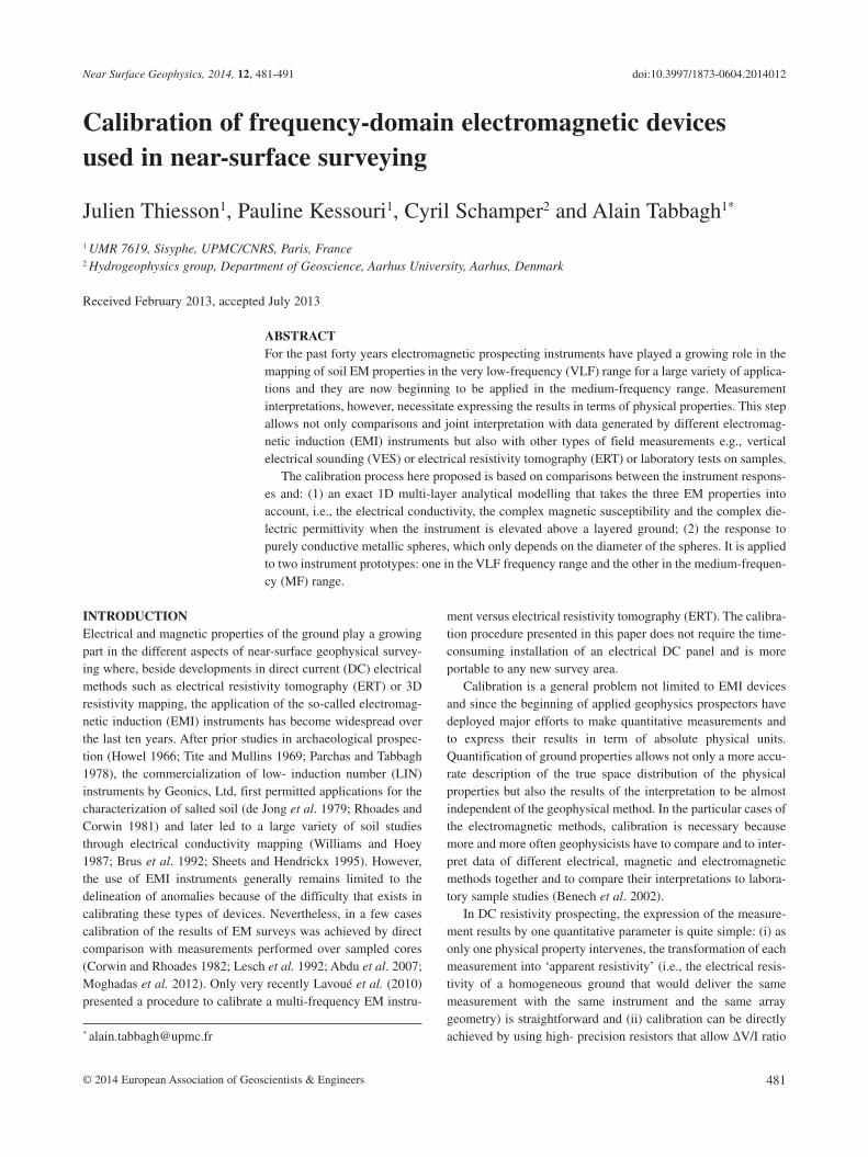
APPENDIX ATo transform the expression: , one

first develops , then applies the identities:

This obtains: . After

developing the exponential in series this yields for the first two

terms: . The sign of the second term

indicates that, when using the first term only, the systematic error corresponds to an overestimation of the magnitude of the response.

APPENDIX BStatic approximation in absence of magnetic contrastThe response, expressed in apparent conductivity, of a thin layer located at z below the coils level and of σ(z) conductivity can be

approximated by or

with , L being the inter-

coil spacing. These functions can be further integrated between ∞ and h for any vertical distribution of the conductivity.

APPENDIX CMagnetic responses under static approximationConsidering a homogeneous ground, in the low-frequency

approximation, where γ2 = iσμω, one has .

Under the static approximation , this yields . Under the z = d = 0 assumption, the responses would

be respectively

, for

VCP and for PERP. Given the

identities: and

, one has for HCP and VCP and 0 for PERP.

CC00224-MA060 Geometrics.indd 1 02-04-14 09:00

CC00477-MA021 RTClark.indd 1 10-07-14 09:27

Calibration of frequency-domain electromagnetic devices used in near-surface surveying

Documents