Calibration of a conceptual rainfall–runoff model using a genetic algorithm integrated with runoff estimation sensitivity to parameters

Automatic calibration of a conceptual rainfall–runoff model usingmultiple objectives

H. Madsen*

DHI Water & Environment, Agern Alle´ 11, DK-2970 Hørsholm, Denmark

Received 2 July 1999; revised 10 March 2000; accepted 31 May 2000

Abstract

Formulation of an automatic calibration strategy for the MIKE 11/NAM rainfall–runoff model is outlined. The calibrationscheme includes optimisation of multiple objectives that measure different aspects of the hydrograph: (1) overall water balance,(2) overall shape of the hydrograph, (3) peak flows, and (4) low flows. An automatic optimisation procedure based on theshuffled complex evolution algorithm is introduced for solving the multi-objective calibration problem. A test example ispresented that illustrates the principles and implications of using multiple objectives in model calibration. Significant trade-offsbetween the different objectives are observed in this case and no single unique set of parameter values is able to optimise allobjectives simultaneously. Instead, the solution to the calibration problem is given as a set of Pareto optimal solutions, whichfrom a multi-objective viewpoint are equivalent. A large variability is observed in the Pareto optimal parameter sets, resulting ina large range of “equally good” simulated hydrographs. From the set of Pareto optimal solutions, one can draw a single solutionaccording to priorities of the different objectives for the specific model application being considered. A balanced aggregatedobjective function is proposed, which provides a compromise solution that puts equal weights to the different objectives.q 2000 Elsevier Science B.V. All rights reserved.

Keywords: Rainfall–runoff models; Calibration; Parameter estimation; Optimisation; Multiple objectives

1. Introduction

For modelling the rainfall–runoff process, modelshave been developed that are based on conceptualrepresentations of the physical processes of thewater flow lumped over the entire catchment area(lumped conceptual type of models). Examples ofthis type of model are the Sacramento model(Burnash, 1995), the Tank model (Sugawara, 1995),the HBV model (Bergstro¨m, 1995), and the MIKE 11/NAM model (Nielsen and Hansen, 1973; Havnø et al.,

1995). The parameters of such models cannot, ingeneral, be obtained directly from measurable quan-tities of catchment characteristics, and hence modelcalibration is needed. To calibrate a model, values ofthe model parameters are selected so that the modelsimulates the hydrological behaviour of the catchmentas closely as possible.

The process of model calibration is normally doneeither manually or by using computer-based auto-matic procedures. In manual calibration, a trial-and-error parameter adjustment is made. In this case, thegoodness-of-fit of the calibrated model is basicallybased on a visual judgement by comparing the simu-lated and the observed hydrographs. For an experi-enced hydrologist it is possible to obtain a very

Journal of Hydrology 235 (2000) 276–288

0022-1694/00/$ - see front matterq 2000 Elsevier Science B.V. All rights reserved.PII: S0022-1694(00)00279-1

www.elsevier.com/locate/jhydrol

* Tel.: 145-45-169200; fax:145-45-169292.E-mail address:[email protected] (H. Madsen).

good and hydrologically sound model using manualcalibration. However, since there is no generallyaccepted objective measure of comparison, andbecause of the subjective judgement involved, it isdifficult to assess explicitly the confidence of themodel simulations. Furthermore, manual calibrationmay be a very time consuming task, especially foran inexperienced hydrologist.

In automatic calibration, parameters are adjustedautomatically according to a specified search schemeand numerical measures of the goodness-of-fit. Ascompared to manual calibration, automatic calibrationis fast, and the confidence of the model simulationscan be explicitly stated. The development of auto-matic calibration procedures has focussed mainly onusing a single overall objective function (e.g. the rootmean square error between the observed and simu-lated runoff) to measure the goodness-of-fit of thecalibrated model. Calibration based on a singleperformance measure, however, is often inadequateto measure properly the simulation of all theimportant characteristics of the system that arereflected in the observations. This aspect is basicallywhat causes a certain scepticism in the hydrologicalprofession for applying automatic calibrationprocedures.

Research on the formulation of appropriate perfor-mance measures that focus on different aspects of thehydrograph, i.e. includes various calibration objec-tives, is rather limited. Notable contributions arethose of Harlin (1991) and Zhang and Lindstro¨m(1997) who formulated automatic routines that inferthe course of a manual calibration by an experiencedhydrologist, focussing on different process descrip-tions, but replacing the visual goodness-of-fit bynumerical measures that are optimised automatically.Recently, automatic routines that use a general multi-objective formulation of the calibration problem havebeen applied in rainfall–runoff modelling (Lindstro¨m,1997; Liong et al., 1996, 1998; Gupta et al., 1998;Yapo et al., 1998).

The objective of the present study is to formulateand analyse an automatic calibration strategy for aconceptual rainfall–runoff model, which focuses ona proper definition of calibration objectives thatreflects the multi-objective nature of model calibra-tion. In Section 2, the applied rainfall–runoff model,the MIKE 11/NAM model, is briefly described. In

Section 3, the formulation of performance measuresis discussed, and a general multi-objective calibrationscheme is outlined. The automatic optimisation algo-rithm applied for solving the calibration problem isdescribed in Section 4. In Section 5, a test example ispresented that illustrates the principles and implica-tions of the proposed calibration strategy. Finally,conclusions are given in Section 6.

2. MIKE 11/NAM rainfall–runoff model

The hydrological model used in this study is theNAM rainfall–runoff that was originally developedat the Institute of Hydrodynamics and HydraulicEngineering at the Technical University of Denmark(Nielsen and Hansen, 1973). The model forms part ofthe MIKE 11 river modelling system for simulation ofthe rainfall–runoff process in subcatchments (Havnøet al., 1995). The model has been applied in a largenumber of engineering projects covering variousclimatic regimes.

The MIKE 11/NAM model represents the variouscomponents of the rainfall–runoff process by continu-ously accounting for the water content in four differ-ent and mutually interrelated storages where eachstorage represents different physical elements of thecatchment. These storages are: (1) snow storage, (2)surface storage, (3) lower zone (root zone) storage,and (4) groundwater storage. The model structure isshown in Fig. 1. In the present application, the ninemost important parameters of the NAM model are tobe determined by calibration. A brief description ofthese parameters is given in Table 1.

3. Formulation of multi-objective calibrationproblem

In general terms, the objective of model calibrationcan be stated as follows:Selection of model para-meters so that the model simulates the hydrologicalbehaviour of the catchment as closely as possible. Formodelling the rainfall–runoff process at the catch-ment scale, normally the only available informationfor evaluating this objective is the total catchmentrunoff. Thus, the amount of information providescertain limitations on how to evaluate the calibrationobjective. In this respect, the quality of the data and

H. Madsen / Journal of Hydrology 235 (2000) 276–288 277

the simplifications and errors inherent in the modelstructure also put limitations on how “close” themodel is actually able to simulate the hydrologicalbehaviour of the catchment.

For a proper evaluation of the calibrated model, it isnecessary to translate the overall calibration objectiveinto more operational terms. The following objectivesare usually considered:

1. A good agreement between the average simulatedand observed catchment runoff volume (i.e. a goodwater balance).

2. A good overall agreement of the shape of thehydrograph.

3. A good agreement of the peak flows with respect totiming, rate and volume.

4. A good agreement for low flows.

In this respect, it is important to note that, ingeneral, trade-offs exist between the different objec-tives. For instance, one may find a set of parametersthat provide a very good simulation of peak flows buta poor simulation of low flows, and vice versa.

In order to obtain a successful calibration by usingautomatic optimisation routines, it is necessary toformulate numerical performance measures thatreflect the calibration objectives. This is done by con-sidering the calibration problem in a multi-objective

H. Madsen / Journal of Hydrology 235 (2000) 276–288278

Fig. 1. NAM model structure.

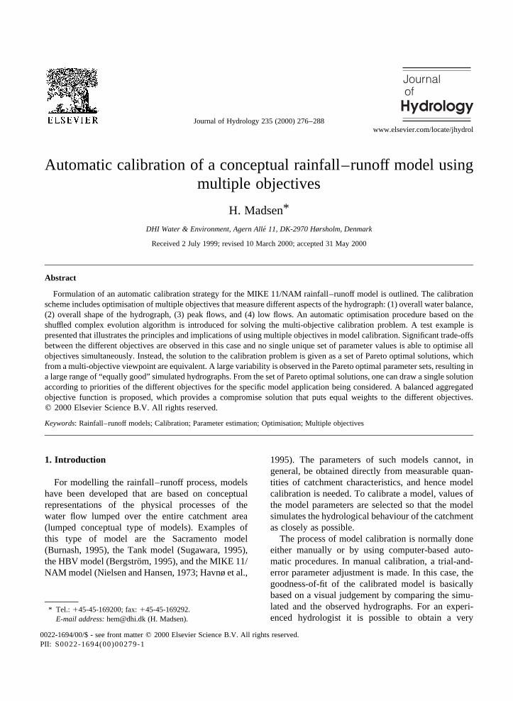
framework. The following numerical performancestatistics that are defined here measure the differentcalibration objectives stated above:

1. Overall volume error

F1�u� �

XNi�1

wi�Qobs;i 2 Qsim;i�u��XNi�1

wi

��

��1�

2. Overall root mean square error (RMSE)

F2�u� �

XNi�1

w2i �Qobs;i 2 Qsim;i�u��2

XNi�1

w2i

26666643777775

1=2

�2�

3. Average RMSE of peak flow events

F3�u� � 1Mp

XMp

j�1

Xnj

i�1


Xnj

i�1

w2i

26666643777775

1=2

�3�

4. Average RMSE of low flow events

F4�u� � 1Ml

XMl

j�1

Xnj

i�1


Xnj

i�1

w2i

26666643777775

1=2

�4�

In Eqs. (1)–(4),Qobs,i is the observed discharge attime i, Qsim,i the simulated discharge,N the totalnumber of time steps in the calibration period,Mp

the number of peak flow events,Ml the number oflow flow events,nj is the number of time steps inpeak/low flow event no.j, u the set of model para-meters to be calibrated, andwi is a weighting function.Peak flow events are defined as periods where theobserved discharge is above a given threshold level.Similarly, low flow events are defined as periodswhere the observed discharge is below a given threshold


Table 1NAM model parameters and hypercube search space

Parameter Description Lowerlimit

Upperlimit

Umax (mm) Maximum water content in thesurface storage. This storagecan be interpreted as includingthe water content in theinterception storage, in surfacedepression storages, and in theuppermost few cm’s of the soil

5 35

Lmax (mm) Maximum water content in thelower zone storage.Lmax can beinterpreted as the maximumsoil water content in the rootzone available for thevegetative transpiration

50 350

CQOF (–) Overland flow runoffcoefficient. CQOF determinesthe distribution of excessrainfall into overland flow andinfiltration

0 1

TOF (–) Threshold value for overlandflow. Overland flow is onlygenerated if the relativemoisture content in the lowerzone storage is larger than TOF

0 0.9

TIF (–) Threshold value for interflow.Interflow is only generated ifthe relative moisture content inthe lower zone storage is largerthan TIF

0 0.9

TG (–) Threshold value for recharge.Recharge to the groundwaterstorage is only generated if therelative moisture content in thelower zone storage is largerthan TG

0 0.9

CKIF (h) Time constant for interflowfrom the surface storage. It isthe dominant routingparameter of the interflowbecause CKIF q CK1,2

500 1000

CK1,2 (h) Time constant for overlandflow and interflow routing.Overland flow and interfloware routed through two linearreservoirs in series with thesame time constant CK1,2

3 72

CKBF (h) Baseflow time constant.Baseflow from thegroundwater storage isgenerated using a linearreservoir model with timeconstant CKBF

500 5000

level. The weights indicate the importance to be givento particular portions of the hydrograph, reflecting theerrors in the data and the model (low weights aregiven to periods where large data or model errorsare present).

The coefficient of determination or the Nash–Sutcliffe coefficient (Nash and Sutcliffe, 1970)which is commonly adopted for evaluating the good-ness-of-fit of the simulated hydrograph is a trans-formed and normalised measure of the overallRMSE (normalised with respect to the variance ofthe observed hydrograph)

R2 � 1 2

XNi�1

w2i �Qobs;i 2 Qsim;i�2

XNi�1

w2i �Qobs;i 2 �Qobs�2

�5�

whereQobs is the average observed discharge.When using multiple objectives, the calibration

problem can be stated as follows:

Min{ F1�u�;F2�u�;…;Fp�u�} ; u [ Q �6�The optimisation problem is said to be constrained inthe sense thatu is restricted to the feasible parameterspaceQ . The parameter space is usually defined as ahypercube by specifying lower and upper limits oneach parameter. These limits are chosen accordingto physical and mathematical constraints in themodel and/or from modelling experiences (priorknowledge). Kuczera (1997) proposed a subspaceprobabilistic search strategy where the search spaceis defined as a hyperellipsoid that uses the correlationbetween the different parameters.

The solution of Eq. (6) will not, in general, be asingle unique set of parameters but will consist of theso-called Pareto set of solutions (non-dominated solu-tions), according to various trade-offs between thedifferent objectives. Formally, any memberu i of thePareto set has the properties (Gupta et al., 1998):

1. For all non-membersu j there exists at least onemember u i where Fk�ui� , Fk�uj� for all k �1;2;…;p:

2. It is not possible to findu j within the Pareto setsuch thatFk�uj� , Fk�ui� for all k � 1;2;…;p:

Thus cf. (1), the parameter spaceQ can be divided

into “good” (Pareto optimal) and “bad” solutions, andcf. (2), none of the “good” solutions can be said to be“better” than any of the other “good” solutions. Amember of the Pareto set will be better than anyother member with respect to some of the objectives,but because of the trade-off between the differentobjectives it will not be better with respect to otherobjectives.

When solving the multi-objective calibrationproblem, the problem is usually transformed into asingle-objective optimisation problem by defining ascalar that aggregates the various objective functions.One such aggregate measure is the Euclidean distance

Fagg�u� � ��F1�u�1 A1�2 1 �F2�u�1 A2�2 1 …

1 �Fp�u�1 Ap�2�1=2 �7�whereAi are transformation constants assigned to thedifferent objectives, which allows the user to selectrelative priorities to certain objectives. The selectionof transformation constants, however, is not straight-forward, since the priority also depends on the valueof Fi itself. For instance, if allAi are set to zero,implicitly larger weights are given to objectiveswith larger F-values. For investigating the entirePareto front, the aggregated distance measure can beadopted by performing several optimisation runsusing different values ofAi.

In practical applications, the entire Pareto set maybe too expensive to calculate, and one is only inter-ested in part of the Pareto optimal solutions. In thiscase, it is proposed to use an aggregated objectivefunction that puts equal weights on the different objec-tives. A balanced measure can be defined by assigningtransformation constants in Eq. (7) such that all�Fi 1Ai� have about the same distance to the origin. Whenusing a population-based optimisation algorithm, suchas the one considered here, an initial populationwithin the feasible region is evaluated. The minimumvalues of Fi (Fi,min) are estimated from this initialpopulation, and each of the objective functions istransformed to having the same distance to the originas the objective function with the largest minimumvalue ofFi, i.e.

Ai � Max{Fj;min; j � 1; 2;…;p} 2 Fi;min;

i � 1;2;…; p:�8�


4. Optimisation algorithm

Optimisation algorithms can, in general, be cate-gorised as “local” and “global” search methods(Sorooshian and Gupta, 1995). Depending on thehill climbing strategy employed, local search algo-rithms may be further divided into “direct” and“gradient-based” methods. Direct search methodsonly use information on the objective functionvalue, whereas gradient-based methods also use infor-mation about the gradient of the objective function.Local search methods are efficient for locating theoptimum of a uni-modal function since in this casethe hill-climbing search will eventually reach theglobal optimum, irrespective of the starting point.One of the more popular direct search methods isthe simplex method (Nelder and Mead, 1965). Gradi-ent-based methods include the steepest descentmethod and various approximations of the Newtonmethod (e.g. the Gauss–Marquardt algorithm).

Lumped conceptual rainfall–runoff models mayhave numerous local optima on the objective functionsurface (Duan et al., 1992), and in such cases localsearch methods are inappropriate because the esti-mated optimum will depend on the starting point ofthe search. For such multi-modal objective functions,global search methods should be applied (“global” inthe sense that these algorithms are especially designedfor locating the global optimum and not being trappedin local optima). Popular global search methods arethe so-called population-evolution-based search stra-tegies such as the shuffled complex evolution (SCE)algorithm (Duan et al., 1992) and genetic algorithms(GA) (Wang, 1991). A number of studies have beenconducted that compare SCE, GA and other globaland local search procedures for calibrating conceptualrainfall–runoff models (e.g. Duan et al., 1992; Ganand Biftu, 1996; Cooper et al., 1997; Kuczera, 1997;Franchini et al., 1998; Thyer et al., 1999). Thesestudies demonstrate that the SCE method is an effec-tive and efficient search algorithm. The SCE methodhas been widely applied for calibration of variousconceptual rainfall–runoff models, including theSacramento model (Sorooshian et al., 1993; Duan etal., 1994; Gan and Biftu, 1996; Yapo et al., 1996; Ganet al., 1997), the Tank model (Tanakamaru andBurges, 1996; Cooper et al., 1997), and the Xinan-jiang model (Gan and Biftu, 1996; Gan et al., 1997).

The SCE method combines different search strate-gies, including (i) competitive evolution, (ii)controlled random search, (iii) the simplex method,and (iv) complex shuffling. The SCE algorithm simul-taneously evolves a number of potential solutionstowards the region of the global optimum of the objec-tive function. Thus, when optimising the aggregatedobjective function in Eq. (7), the SCE algorithm isexpected to provide a reasonable approximation ofthe Pareto front near the point that corresponds tothe global optimum of the objective function. Byperforming several independent optimisation runswith different transformation constants, the entirePareto front can then be explored. It should be notedthat the proposed procedure is different from the SCE-based multi-objective calibration procedure intro-duced by Yapo et al. (1998) that uses the concept ofPareto ranking (Goldberg, 1989) for simultaneousoptimisation of several objectives.

The SCE method includes various algorithmicparameters. The most important parameter is thenumber of complexesp. Sensitivity tests show thatthe dimensionality of the calibration problem (numberof calibration parameters) is the primary factor deter-mining the proper choice ofp (Duan et al., 1994). Ingeneral, the larger the value ofp chosen the higher theprobability of converging into the global optimum butat the expense of a larger number of model simula-tions (the number of model simulations is virtuallyproportional to p), and vice versa. To reduce thechance of premature termination, Kuczera (1997)suggested settingp equal to the number of calibrationparameters. In the application example presentedbelow p was set equal to the number of calibrationparameters, and for the other algorithmic parametersthe recommended values given by Duan et al. (1994)were used.

5. Application example

5.1. Estimation and analysis of Pareto front

The MIKE 11/NAM model was applied to theDanish Tryggevaelde catchment. This catchment hasan area of 130 km2, an average rainfall of 710 mm/year and an average discharge of 240 mm/year. Thecatchment has predominantly clayey soils, implying a


relatively flashy flow regime. For the calibration, a5 year period was used where daily data of precipita-tion, potential evaporation, mean temperature, andcatchment runoff are available.

A number of tests were carried out in order to esti-mate the Pareto front and analyse the trade-offsbetween the different objectives. For all tests thehypercube search space shown in Table 1 was used.Preliminary optimisation runs showed that the entirepopulation converged around the global optimumafter about 2000 model evaluations. Thus, for eachtest, a maximum number of model evaluations equalto 2000 were employed as a stopping criterion. Forevaluation of the objective functions all time stepswere weighted equally, i.e.w�i� � 1 was used inEqs. (1)–(4). Peak flow events were defined as periodswith flow above a threshold value of 4.0 m3/s, and lowflow events were defined as periods with flow below0.5 m3/s. The first 3 months of the calibration periodwere disregarded in the calculation of the objectivefunctions in order to minimise the influence from theinitial conditions.

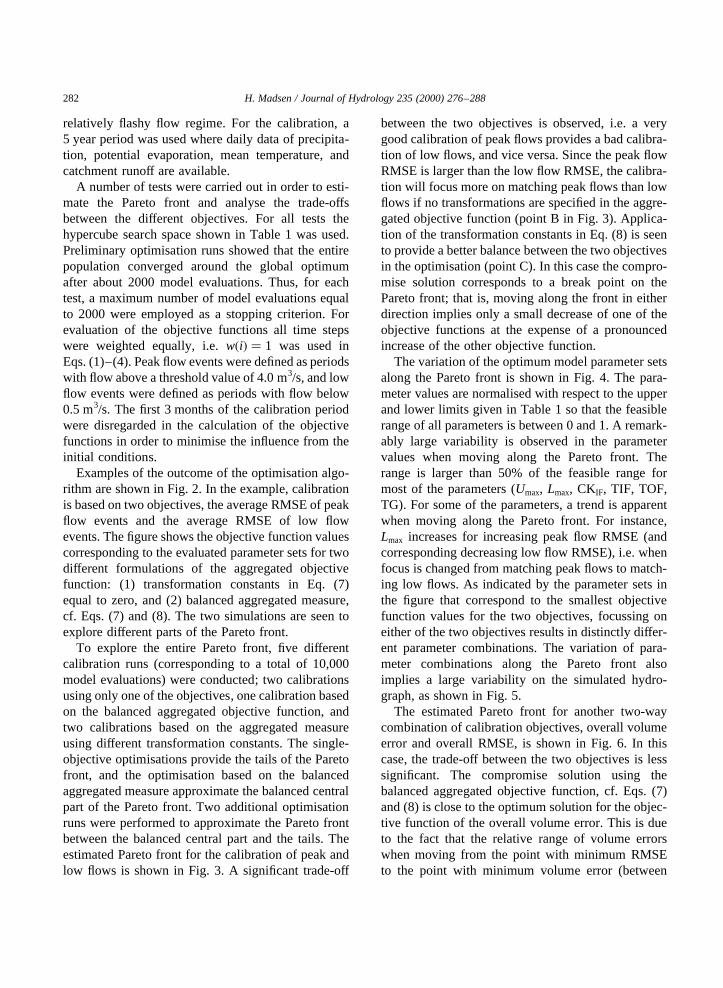
Examples of the outcome of the optimisation algo-rithm are shown in Fig. 2. In the example, calibrationis based on two objectives, the average RMSE of peakflow events and the average RMSE of low flowevents. The figure shows the objective function valuescorresponding to the evaluated parameter sets for twodifferent formulations of the aggregated objectivefunction: (1) transformation constants in Eq. (7)equal to zero, and (2) balanced aggregated measure,cf. Eqs. (7) and (8). The two simulations are seen toexplore different parts of the Pareto front.

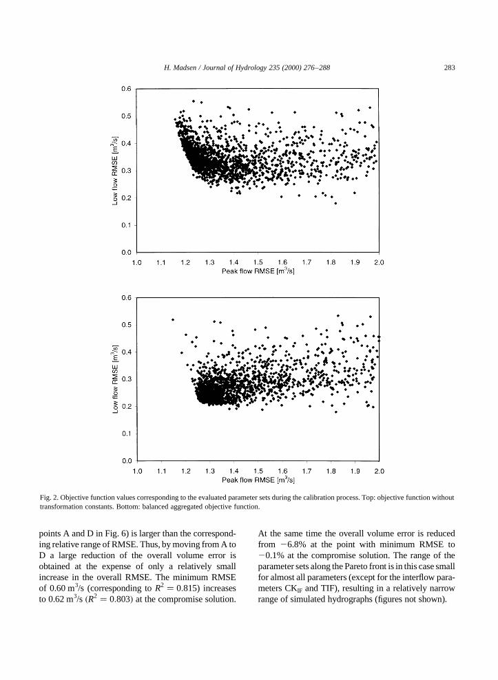
To explore the entire Pareto front, five differentcalibration runs (corresponding to a total of 10,000model evaluations) were conducted; two calibrationsusing only one of the objectives, one calibration basedon the balanced aggregated objective function, andtwo calibrations based on the aggregated measureusing different transformation constants. The single-objective optimisations provide the tails of the Paretofront, and the optimisation based on the balancedaggregated measure approximate the balanced centralpart of the Pareto front. Two additional optimisationruns were performed to approximate the Pareto frontbetween the balanced central part and the tails. Theestimated Pareto front for the calibration of peak andlow flows is shown in Fig. 3. A significant trade-off

between the two objectives is observed, i.e. a verygood calibration of peak flows provides a bad calibra-tion of low flows, and vice versa. Since the peak flowRMSE is larger than the low flow RMSE, the calibra-tion will focus more on matching peak flows than lowflows if no transformations are specified in the aggre-gated objective function (point B in Fig. 3). Applica-tion of the transformation constants in Eq. (8) is seento provide a better balance between the two objectivesin the optimisation (point C). In this case the compro-mise solution corresponds to a break point on thePareto front; that is, moving along the front in eitherdirection implies only a small decrease of one of theobjective functions at the expense of a pronouncedincrease of the other objective function.

The variation of the optimum model parameter setsalong the Pareto front is shown in Fig. 4. The para-meter values are normalised with respect to the upperand lower limits given in Table 1 so that the feasiblerange of all parameters is between 0 and 1. A remark-ably large variability is observed in the parametervalues when moving along the Pareto front. Therange is larger than 50% of the feasible range formost of the parameters (Umax, Lmax, CKIF, TIF, TOF,TG). For some of the parameters, a trend is apparentwhen moving along the Pareto front. For instance,Lmax increases for increasing peak flow RMSE (andcorresponding decreasing low flow RMSE), i.e. whenfocus is changed from matching peak flows to match-ing low flows. As indicated by the parameter sets inthe figure that correspond to the smallest objectivefunction values for the two objectives, focussing oneither of the two objectives results in distinctly differ-ent parameter combinations. The variation of para-meter combinations along the Pareto front alsoimplies a large variability on the simulated hydro-graph, as shown in Fig. 5.

The estimated Pareto front for another two-waycombination of calibration objectives, overall volumeerror and overall RMSE, is shown in Fig. 6. In thiscase, the trade-off between the two objectives is lesssignificant. The compromise solution using thebalanced aggregated objective function, cf. Eqs. (7)and (8) is close to the optimum solution for the objec-tive function of the overall volume error. This is dueto the fact that the relative range of volume errorswhen moving from the point with minimum RMSEto the point with minimum volume error (between


points A and D in Fig. 6) is larger than the correspond-ing relative range of RMSE. Thus, by moving from A toD a large reduction of the overall volume error isobtained at the expense of only a relatively smallincrease in the overall RMSE. The minimum RMSEof 0.60 m3/s (corresponding toR2 � 0:815) increasesto 0.62 m3/s �R2 � 0:803� at the compromise solution.

At the same time the overall volume error is reducedfrom 26.8% at the point with minimum RMSE to20.1% at the compromise solution. The range of theparameter sets along the Pareto front is in this case smallfor almost all parameters (except for the interflow para-meters CKIF and TIF), resulting in a relatively narrowrange of simulated hydrographs (figures not shown).


Fig. 2. Objective function values corresponding to the evaluated parameter sets during the calibration process. Top: objective function withouttransformation constants. Bottom: balanced aggregated objective function.

With respect to optimisation of the other two-waycombinations of calibration objectives, the combina-tions including overall RMSE and peak flow RMSE,overall RMSE and low flow RMSE, and overallvolume error and peak flow RMSE all have significant

trade-offs. For the combination overall volume errorand low flow RMSE no significant trade-off exists,and, in general, a calibration that provides a smalloverall volume error also provides a small low flowRMSE.


Fig. 3. Estimated Pareto front for optimisation of peak and low flow RMSE. Marked optimum points correspond to using, respectively, peakflow RMSE (A), aggregated objective function without transformation constants (B), balanced aggregated objective function (C), and low flowRMSE (D).

Fig. 4. Normalised range of parameter values along the Pareto front shown in Fig. 3. Full bold lines indicate the five parameter sets with thesmallest peak flow RMSE. Dashed bold lines indicate the five parameter sets with the smallest low flow RMSE.

5.2. Analysis of variability and uncertaintyassessment

The traditional concept of model calibration is builton the hypothesis that a unique optimum set of

parameter values exists. It should be clear from theanalysis above that such a unique global solution doesnot exist. In a multi-objective context, there is a multi-tude of parameter combinations that are “equallygood”. Moreover, since most model calibrations are


Fig. 5. Range of simulated hydrographs corresponding to parameter sets along the Pareto front shown in Fig. 3, compared with observations.

Fig. 6. Estimated Pareto front for optimisation of overall volume error and overall RMSE. Marked points correspond to using, respectively,overall RMSE (A), aggregated objective function without transformation constants (B), balanced aggregated objective function (C), and overallvolume error (D).

indeed multi-objective in nature no unique solution tothe calibration problem can generally be given.Instead, a calibrated model should produce a rangeof simulated hydrographs corresponding to the“equally good” parameter sets along the Pareto front(as illustrated in Fig. 5).

Another, and related, new concept in model cali-bration was put forward by Beven and Binley (1992)and Beven (1993) who introduced the concept of“equifinality of parameter sets”. That is, many differ-ent parameter combinations can give acceptable solu-tions, and hence the model simulations shouldgenerate a set of confidence bands that defines therange of expected model response, rather than gener-ating a single solution. Based on this concept Bevenand Binley (1992) introduced the generalised likeli-hood uncertainty estimation (GLUE) procedure. Inthis approach a large number of model simulationsare performed with randomly chosen sets of para-meter values. Each parameter set is assigned a like-lihood weight (e.g. defined by a performancemeasure) which results in a probability density func-tion of model simulations for each time step fromwhich uncertainty bounds can be drawn.

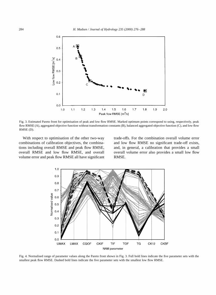
An illustration of the interpretation of the conceptof equifinality of parameter sets is shown in Fig. 7. For

the calibration test based on all the four objectivesusing the balanced aggregated objective function,the range of parameter values for which the aggre-gated objective functions differ by less than 1%from the optimum value is shown. The figure clearlyillustrates that many different parameter sets thatcover a large range of parameter values may producevirtually equally good model simulations according toa specified performance measure.

It is important to emphasise the difference betweenthe results in Fig. 7 and the range of parameter sets forpoints along the Pareto front in Fig. 4. The variabilityof parameter values in Fig. 7 is based on a statisticalinterpretation of parameter uncertainty, whereas thevariability in Fig. 4 is based on the concept ofmulti-objective equivalence of parameter sets. For aproper assessment of the confidence of a model simu-lation, both approaches should be considered.

5.3. Handling data and model errors

Differences between observations and simulatedmodel response are basically caused by four differenterror sources (Refsgaard and Storm, 1996).

1. Errors in meteorological input data.


Fig. 7. Range of parameter sets for which the aggregated objective functions differ by less than 1% from the optimum value. Optimisation isbased on all four objectives. The full bold line indicates the optimum parameter set.

2. Errors in recorded observations.3. Errors and simplifications inherent in the model

structure.4. Errors due to the use of non-optimal parameter

values.

In model calibration only error source (4) should beminimised. In this respect, it is important to distin-guish between the different error sources since cali-bration of model parameters may compensate for theother error sources.

The multi-objective automatic calibration proce-dure introduced herein may explicitly take data andmodel errors into account by defining appropriateweights in the objective functions Eqs. (1)–(4).Some of the uncertainties may be quantified prior tothe calibration, e.g. known problems with the ratingcurve in certain periods, and underestimation of snowprecipitation. However, the model response itselfprovides a lot of information on possible errorsources. For instance, if the range of model simula-tions (e.g. illustrated in Fig. 5) does not envelop theobservations, data and/or model errors may bepresent. In such cases the calibration should berepeated where low (or zero) weights are assigned toperiods with large errors.

In the tests, none of the evaluated parameter setswas able to produce solutions that match the peak flowevents in the beginning of 1987 (see Fig. 5). The firstthree months of 1987 have prolonged periods of frost,and all of the problematic peak flow events are due tosnowmelt. For comparison, the winter 1987/1988 hasonly few days with average temperatures below zero,and hence no large snowmelt events. This suggestsproblems with simulation of snowmelt. In the tests,the snow routine has not been calibrated, and hencesome errors are related to the use of non-optimal para-meters for this routine. Furthermore, the underpredic-tion of snowmelt events may be caused by anunderestimation of the snow precipitation (inputerrors). To account properly for these errors, small(or zero) weights should be given to periods withsnowmelt in the objective functions Eqs. (1)–(4).

6. Conclusions

An automatic calibration scheme for the

MIKE 11/NAM rainfall–runoff model has beenformulated that considers the calibration problem ina general multi-objective framework. The schemeoptimises numerical performance measures of fourdifferent calibration objectives: (1) overall waterbalance, (2) overall shape of the hydrograph, (3)peak flows, and (4) low flows. In practical applica-tions, the user can select any combination of the fourobjective functions, depending on the objectives ofthe specific model application being considered. Anautomatic optimisation procedure based on the SCEalgorithm has been introduced for solving the multi-objective calibration problem.

The application example demonstrated that signifi-cant trade-offs between the different objectives exist,implying that no unique single solution is able tooptimise all four objectives simultaneously. Instead,the solution to the calibration problem is given as a setof Pareto optimal solutions. In this respect, the SCEoptimisation algorithm has been shown to provide anefficient approximation of the Pareto front. For draw-ing a single solution from the Pareto set a balancedaggregated objective function has been proposed,which has been shown to provide an efficient compro-mise solution that puts equal weights to the differentobjectives.

The results clearly showed that the traditionalconcept of automatic model calibration is inappropri-ate. In a multi-objective context there is a multitude ofparameter combinations that are “equally good”,resulting in a large range of simulated hydrographs.Besides variability due to the multi-objective equiva-lence of parameter sets, one should also considerstatistical parameter uncertainty (“equifinality” ofparameter sets) for a general assessment of the confi-dence of the model simulations. The applicationexample revealed that a large range of parametervalues may produce virtually equally good solutionsaccording to a specified objective function.

Finally, the use of the proposed calibration methodfor taking data and model errors into account has beensuggested. In this respect, the variability of the simu-lated hydrograph can be used as an indicator of poten-tial errors. The defined numerical objective functionscan explicitly take data and model errors into accountby defining appropriate weights that indicate theimportance to be given to particular portions of thehydrograph in the calibration process.


Acknowledgements

This work was in part funded by the Danish Tech-nical Research Council (STVF) under the TalentProject No. 9800463 “Data to knowledge — D2K”.The reviews by Hoshin Gupta and two other but anon-ymous referees are gratefully acknowledged.

References

Bergstrom, S., 1995. The HBV model. In: Singh, V.P. (Ed.).Computer Models of Watershed Hydrology, Water ResourcesPublications, Colorado, pp. 443–476.

Beven, K.J., 1993. Prophesy, reality and uncertainty in distributedhydrological modelling. Adv. Water Resour. 16, 41–51.

Beven, K.J., Binley, A.M., 1992. The future of distributed models:model calibration and uncertainty prediction. Hydrol. Process.6, 279–298.

Burnash, R.J.C., 1995. The NWS river forecast system — catch-ment modeling. In: Singh, V.P. (Ed.). Computer Models ofWatershed Hydrology, Water Resources Publications, Color-ado, pp. 311–366.

Cooper, V.A., Nguyen, V.T.V., Nicell, J.A., 1997. Evaluation ofglobal optimization methods for conceptual rainfall–runoffmodel calibration. Water Sci. Technol. 36 (5), 53–60.

Duan, Q., Sorooshian, S., Gupta, V., 1992. Effective and efficientglobal optimization for conceptual rainfall–runoff models.Water Resour. Res. 28 (4), 1015–1031.

Duan, Q., Sorooshian, S., Gupta, V.K., 1994. Optimal use of theSCE-UA global optimization method for calibrating watershedmodels. J. Hydrol. 158, 265–284.

Franchini, M., Galeati, G., Berra, S., 1998. Global optimizationtechniques for the calibration of conceptual rainfall–runoffmodels. Hydrol. Sci. J. 43 (3), 443–458.

Gan, T.Y., Biftu, G.F., 1996. Automatic calibration of conceptualrainfall–runoff models: optimization algorithms, catchmentconditions, and model structure. Water Resour. Res. 32 (12),3513–3524.

Gan, T.Y., Dlamini, E.M., Biftu, G.F., 1997. Effects of modelcomplexity and structure, data quality, and objective functionson hydrological modeling. J. Hydrol. 192, 81–103.

Goldberg, D.E., 1989. Genetic Algorithms in Search, Optimizationand Machine Learning, Addison-Wesley, Reading, MA.

Gupta, H.V., Sorooshian, S., Yapo, P.O., 1998. Toward improvedcalibration of hydrological models: multiple and noncommen-surable measures of information. Water Resour. Res. 34 (4),751–763.

Harlin, J., 1991. Development of a process oriented calibrationscheme for the HBV hydrological model. Nordic Hydrol. 22,15–36.

Havnø, K., Madsen, M.N., Dørge, J., 1995. MIKE 11 — a general-ized river modelling package. In: Singh, V.P. (Ed.). ComputerModels of Watershed Hydrology, Water Resources Publica-tions, Colorado, pp. 733–782.

Kuczera, G., 1997. Efficient subspace probabilistic parameter opti-

mization for catchment models. Water Resour. Res. 33 (1),177–185.

Lindstrom, G., 1997. A simple automatic calibration routine for theHBV model. Nordic Hydrol. 28 (3), 153–168.

Liong, S.Y., Khu, S.T., Chan, W.T., 1996. Construction of multi-objective function response surface with genetic algorithm andneural network. In: Proceedings of the International Conferenceon Water Resources and Environmental Research, 29–31October, Kyoto, Japan, vol. II, pp. 31–38.

Liong, S.Y., Khu, S.T., Chan, W.T., 1998. Derivation of Paretofront with accelerated convergence genetic algorithm, ACGA.In: Babovic, V., Larsen, L.C. (Eds.). Hydroinformatics’98,Balkema, Rotterdam, The Netherlands, pp. 889–896.

Nash, J.E., Sutcliffe, J.V., 1970. River flow forecasting throughconceptual models. Part 1: A discussion of principles. J. Hydrol.10, 282–290.

Nelder, J.A., Mead, R., 1965. A simplex method for function mini-mization. Comput. J. 7 (4), 308–313.

Nielsen, S.A., Hansen, E., 1973. Numerical simulation of therainfall runoff process on a daily basis. Nordic Hydrol. 4,171–190.

Refsgaard, J.C., Storm, B., 1996. Construction, calibration and vali-dation of hydrological models. In: Abbott, M.B., Refsgaard, J.C.(Eds.). Distributed Hydrological Modelling, Kluwer AcademicPress, The Netherlands, pp. 41–54.

Sorooshian, S., Gupta, V.K., 1995. Model calibration. In: Singh,V.P. (Ed.). Computer Models of Watershed Hydrology, WaterResources Publications, Colorado, pp. 23–68.

Sorooshian, S., Duan, Q., Gupta, V.K., 1993. Calibration of rain-fall–runoff models: application of global optimization to theSacramento soil moisture accounting model. Water Resour.Res. 29 (4), 1185–1194.

Sugawara, M., 1995. Tank model. In: Singh, V.P. (Ed.). ComputerModels of Watershed Hydrology, Water Resources Publica-tions, Colorado, pp. 165–214.

Tanakamaru, H., Burges, S.J., 1996. Application of global optimi-zation to parameter estimation of the Tank model. In: Proceed-ings of the International Conference on Water Resources andEnvironmental Research, 29–31 October, Kyoto Japan, vol. II,pp. 39–46.

Thyer, M., Kuczera, G., Bates, B.C., 1999. Probabilistic optimisa-tion for conceptual rainfall–runoff models: a comparison of theshuffled complex evolution and simulated annealing algorithms.Water Resour. Res. 35 (3), 767–773.

Wang, Q.J., 1991. The genetic algorithm and its application tocalibrating conceptual rainfall–runoff models. Water Resour.Res. 27 (9), 2467–2471.

Yapo, P.O., Gupta, H.V., Sorooshian, S., 1996. Automatic calibra-tion of conceptual rainfall–runoff models: sensitivity to calibra-tion data. J. Hydrol. 181, 23–48.

Yapo, P.O., Gupta, H.V., Sorooshian, S., 1998. Multi-objectiveglobal optimization for hydrological models. J. Hydrol. 204,83–97.

Zhang, X., Lindstro¨m, G., 1997. Development of an automatic cali-bration scheme for the HBV hydrological model. Hydrol.Process. 11, 1671–1682.


Calibration of a conceptual rainfall–runoff model using a genetic algorithm integrated with runoff estimation sensitivity to parameters

Documents