NASA MEaSUREs Calibrated Passive Microwave Daily EASE-Grid 2.0 Brightness Temperature ESDR (CETB) ALGORITHM THEORETICAL BASIS DOCUMENT Mary J. Brodzik National Snow and Ice Data Center David G. Long Brigham Young University Revision 1.0 26 April 2018

Welcome message from author
This document is posted to help you gain knowledge. Please leave a comment to let me know what you think about it! Share it to your friends and learn new things together.
Transcript

NASAMEaSUREs
CalibratedPassiveMicrowaveDailyEASE-Grid2.0BrightnessTemperature
ESDR(CETB)
ALGORITHMTHEORETICALBASISDOCUMENT
MaryJ.BrodzikNationalSnowandIceDataCenter
DavidG.Long
BrighamYoungUniversity
Revision1.026April2018

CETBATBD 4/30/18 Page2of103
TableofContents
1 PurposeofthisDocument..............................................................................................6
2 Introduction.......................................................................................................................62.1 ProjectPurpose.......................................................................................................................62.2 HeritageProductsandtheNeedforReprocessing.....................................................7
3 CETBProductDescription..........................................................................................103.1 ProductCharacteristics.....................................................................................................103.1.1 PassiveMicrowaveSensors......................................................................................................103.1.2 TemporalCoverage......................................................................................................................103.1.3 SpatialExtent..................................................................................................................................113.1.4 RadiometerChannelsandGridResolution........................................................................11
3.2 ProductDescription...........................................................................................................133.2.1 InputData.........................................................................................................................................133.2.2 SwathtoGridAlgorithms..........................................................................................................163.2.3 OutputData......................................................................................................................................17
4 AlgorithmDescription.................................................................................................224.1 PreprocessingforSpatialandTemporalSelection..................................................224.1.1 LocalTime-of-Day.........................................................................................................................22
4.2 GriddingandReconstruction..........................................................................................244.2.1 AntennaPatternandMeasurementSpatialResponse..................................................244.2.2 TheoryofReconstructionandGriddingAlgorithms.....................................................25
5 TestProcedures.............................................................................................................335.1 AlgorithmValidation..........................................................................................................33
6 CETBStorageRequirements......................................................................................337 References........................................................................................................................33
8 Appendices.......................................................................................................................378.1 Appendix:ComparisonofRSSandCSUSSM/I-SSMISFCDRs.................................378.1.1 FCDRIntercalibrationDifferences.........................................................................................378.1.2 FCDRGeolocationDifferences.................................................................................................388.1.3 FCDROrbitDefinitionDifferences.........................................................................................388.1.4 FCDRTreatmentofMissingData...........................................................................................39
8.2 Appendix:ImageReconstructionImplementationDetails...................................448.2.1 End-to-endSwathOverlap........................................................................................................448.2.2 DeterminationofMeasurementsUsed................................................................................448.2.3 Ascending/DescendingClassification..................................................................................458.2.4 MeasurementIncidenceandAzimuthAngles..................................................................468.2.5 ExclusionofSelectedMeasurements...................................................................................478.2.6 OccasionalHoleArtifactsinReconstructedImages.......................................................48
8.3 Appendix:RadiometerSpatialResponseFunction..................................................488.3.1 BackgroundTheory......................................................................................................................488.3.2 SignalIntegration..........................................................................................................................518.3.3 SpecialSensorMicrowave/Imager(SSM/I)......................................................................538.3.4 SpecialSensorMicrowaveImager/Sounder(SSMIS)...................................................568.3.5 ScanningMultichannelMicrowaveRadiometer(SMMR)............................................57

CETBATBD 4/30/18 Page3of103
8.3.6 AdvancedMicrowaveScanningRadiometer(AMSRandAMSR-E).........................588.3.7 WindSat.............................................................................................................................................598.3.8 ApproximatingtheMeasurementResponseFunction.................................................61
8.4 Appendix:LocalTime-of-DayAnalysis.........................................................................638.5 Appendix:CETBProductEASE-Grid2.0ProjectionsandGridDimensions.....798.6 Appendix:CETBOutputDataDefinition......................................................................808.6.1 CETBFileRequirements............................................................................................................808.6.2 CETBFilenamingConvention..................................................................................................808.6.3 CETBDataVolume........................................................................................................................828.6.4 CETBv1.xFileContent................................................................................................................84
8.7 Appendix:ComparisonofHeritageDataSetswithCETBESDR...........................978.8 Appendix:References........................................................................................................998.9 Appendix:AbbreviationandAcronymList..............................................................102

CETBATBD 4/30/18 Page4of103
RevisionHistory Revision Date Purpose 0.5 2014-04-30 Initial Revision 0.6 2014-06-18 Figure 2 and 4 placeholders replaced with
figures Quantified EIA drift in Appendix 10.1 New note about CSU vs. RSS orbit definitions Added Appendix 10.5 “Comparison of Heritage Data Sets with CETB ESDR”
0.7 2014-06-19 Section 6.2.2.2: clarified statements on effective resolution Appendix 10.2: clarified/expanded (sensor) measurement response function (MRF) terminology Added new Section 10.2.9: “Local Time-of-Day Analysis” Minor formatting corrections
0.8 2014-08-05 Corrected EASE2_T grid dimensions Minor formatting and grammatical corrections Corrected figure/table cross-references
0.9 2015-02-10 Deleted placeholder paragraph in 4.2.1 with reference to discussion in Section 8.3. Changed Section level of ltod from 8.2.9 to 8.3. Added placeholder sample images.
0.10 2015-06-05 Inserted Section 2.1, Project Purpose. Section 3.2.3 Output Data: corrected reference to CF conventions. Table 3-3: updated FCDR field requirements. Section 3.2.3.1: clarified description of TB file contents. Section 3.2.3.2: inserted sample images. Appendix 8.6: replaced TBD items with actual references, added row describing image recon tuning parameters. Inserted references to recent project white papers. Added Appendix section describing end-to-end swath overlap. Added Appendix with Abbreviation and Acronym List. Updated Appendix with CETB format definitions and filename conventions.
0.11 2016-02-12 Corrected typos & references in EFOVs for SSM/I and AMSR-E; addressed various reviewer comments; finalized some (originally TBD) implementation details; made equation labeling consistent throughout document and appendices; combined separate appendix reference lists into one for all appendix material; replaced DRAFT CETB file CDL with actual CDL describing prototype v0.1 file format
1.0 2018-04-26 This version of the document applies to CETB

CETBATBD 4/30/18 Page5of103
data v1.3 and later. Finalized Appendix information with implementation details, including latest ltod values used; corrected/finalized TBD items throughout; included final details for Storage requirements; made bibliography formatting consistent throughout.

CETBATBD 4/30/18 Page6of103
1 PurposeofthisDocumentThis document is the algorithm theoretical basis for the Calibrated
Passive Microwave Daily EASE-Grid 2.0 Brightness Temperature Earth System Data Record (ESDR) (CETB) product. The CETB product is generated from calibrated swath brightness temperature (TB) data at the National Snow and Ice Data Center (NSIDC), using image reconstruction algorithms developed at Brigham Young University (BYU). The CETB product is archived and available to the public from the NSIDC NASA Distributed Active Archive Center (DAAC). The current CETB release is v1.3 (Brodzik et al., 2016).
We have solicited volunteers in the research community to be Early Adopters of the CETB product. In early 2016, we released a prototype CETB with one year of sample data, which contained a subset of potential data planned for inclusion in the final released product. We used feedback from our Early Adopters in making the final decisions regarding choice of input SSM/I-SSMIS FCDR and choice of image reconstruction technique. Based on that feedback, we include in this ATBD the rationale for decisions on what has been included in the final released product.
Suggestions and concerns from the public and scientists on the contents of this document and CETB product are welcome. (Please note that we have defined each acronym upon first usage, and we include an acronym list in Appendix 8.8.)
2 Introduction2.1 ProjectPurpose
We are funded by the NASA MEaSUREs program to produce an improved, enhanced-resolution, gridded passive microwave ESDR for monitoring cryospheric and hydrologic time series.
Currently available global gridded (Level 3) passive microwave data sets available from the NSIDC DAAC serve a diverse community of hundreds of data users, but do not meet many requirements of modern ESDRs or Climate Data Records (CDRs), most notably in the areas of intersensor calibration and consistent processing methods. The historical

CETBATBD 4/30/18 Page7of103
gridding techniques for these passive microwave sensors (Armstrong et al., 1994, updated yearly; Knowles et al., 2000; Knowles et al., 2006) were relatively primitive and were produced on grids (Brodzik and Knowles, 2002; Brodzik et al., 2012) that are not easily accommodated in modern software packages. Further, since the time that the first Level 3 data sets were developed, the Level 2 passive microwave data on which they are based have been reprocessed as Fundamental CDRs (FCDRs) with improved calibration statistics. This work was proposed to address the great need to regenerate gridded Level 3 products using improved techniques from these modern Level 2 FCDRs.
Using validated, state-of-the-art image reconstruction methods, we have reprocessed the gridded data sets, using the most mature available Level 2 satellite passive microwave records from 1978 to the present. We have reprocessed the complete data record from SMMR, SSM/I-SSMIS and AMSR-E in a single, enhanced-resolution gridded passive microwave ESDR. The ESDR makes use of the latest improvements to the Level 2 SSM/I- SSMIS and AMSR-E data record. The new, gridded ESDR is expected to satisfy the needs of current and future users who require a reliable, consistent, gridded time series of microwave radiometer data.
2.2 HeritageProductsandtheNeedforReprocessingSatellite passive microwave observations are critical to describing and
understanding Earth system hydrologic and cryospheric parameters that include precipitation, soil moisture, surface water, vegetation, snow water equivalent, sea ice concentration and sea ice motion. These observations are available in two forms: swath TB (sometimes referred to as NASA EOSDIS Level 1A or Level 1B) data and gridded (Level 3) data (NASA, 2010). Swath data are valuable to researchers studying phenomena that change at temporal scales of orbital repeat (~90 minutes), while gridded data are more valuable to researchers interested in derived parameters at fixed locations through daily time increments and are widely used in climate studies. Gridded data, however, often perform daily temporal averaging or may ignore overlapping swaths altogether. Both swath and gridded data from the current time series of satellite passive microwave data sets span nearly 40 years of Earth observations, beginning with the Nimbus-7 SMMR sensor in 1978, continuing with the SSM/I and SSMIS series sensors from 1987 onward, and including the completed observational record of Aqua AMSR-E

CETBATBD 4/30/18 Page8of103
from 2002 to 2011. Though there are variations between sensors, this data record is an invaluable asset for studies of climate change.
The National Snow and Ice Data Center (NSIDC) currently distributes several heritage gridded products, including the Nimbus-7 SMMR Pathfinder Daily EASE-Grid Brightness Temperatures (Knowles et al., 2000), the DMSP SSM/I-SSMIS Pathfinder Daily EASE-Grid Brightness Temperatures (Armstrong et al., 1994, updated daily) and the AMSR-E/Aqua Daily EASE-Grid Brightness Temperatures (Knowles et al., 2006). Though widely used in a variety of scientific studies, the processing and spatial resolution of these gridded data sets are inconsistent, which complicates long-term climate studies using them. For example, the SMMR Pathfinder data were produced with an inverse-distance weighting scheme. However, the SSM/I-SSMIS gridded data use two weighting schemes: the SSM/I data (1987-2008) were gridded using a Backus-Gilbert (BG) interpolation scheme (Stogryn, 1978) and the work of Poe (1990), Galantowicz and England (1991) and Galantowicz (1995), but the SSMIS data (2006-present) use an inverse distance weighting scheme.
Each of the currently available gridded data sets suffers from inadequacies as Earth System Data Records (ESDRs, also referred to as CDRs) as most of them were defined prior to the time that the definitions for ESDR/CDR were established. Perhaps most critically for purposes of ESDR development, the significant record of the Pathfinder SSM/I-SSMIS gridded data (1987 to present) was derived from swath data that were not cross-calibrated across satellite platforms. Image reconstruction and interpolation schemes have been developed and improved, and recent research has demonstrated improved methods for computing antenna patterns (for some sensors) needed for the interpolation. All of the existing gridded data sets were projected to the original EASE-Grid projection, (Brodzik and Knowles, 2002), which has been revised in order to be used more easily with standard geospatial mapping programs (Brodzik et al., 2012; 2014).
The Scatterometer Climate Record Pathfinder (SCP) was a NASA-sponsored project to develop scatterometer-based data time series to support climate studies of the Earth’s cryosphere and biosphere. As part of the SCP, a number of enhanced-resolution passive microwave data for selected periods of SSM/I and AMSR-E operations have been produced that combine data based on local-time of day (Long and Stroeve, 2011). This approach minimizes fluctuations in the observed TB due to changes in physical temperature resulting from daily temperature cycling. Two images per day

CETBATBD 4/30/18 Page9of103
are produced, separated by 12 hours (morning and evening), with improved temporal resolution, permitting image resolution of diurnal variations. NSIDC currently distributes enhanced resolution Scatterometer Image Reconstruction (SIR) SSM/I TBs from 1995 through 2008 and AMSR-E TBs from 2002 through 2009, produced by BYU (Long and Stroeve, 2011) using the radiometer version of the SIR algorithm (rSIR). rSIR offers a computational advantage over techniques such as BG (Long and Daum, 1998). Both BG and rSIR use regularization to trade off noise and resolution. Whereas BG depends on a subjectively chosen tradeoff parameter, regularization is accomplished with rSIR by limiting the number of iterations. Such enhanced resolution gridded data are proving useful in a variety of scientific studies (e.g., Agnew et al., 2008; Howell et al., 2008; Meier and Stroeve, 2008; Howell et al., 2010; Frokling et al., 2012).
The SSM/I-SSMIS swath data record has recently been reprocessed and cross-calibrated by two research teams who have published the data as fully-vetted Fundamental CDRs (FCDRs): 1) Remote Sensing Systems (Santa Rosa, CA) under the NASA Earth Science MEaSUREs DISCOVER project, has reprocessed all heritage SSM/I data to a new, calibrated Version 7 baseline (available via the NOAA CLASS system), and 2) CSU researchers Kummerow, Berg, Weng and Yang have been funded by the FY09 NOAA SDS Project and NASA Earth Science MEaSUREs, to produce the best possible Level 2 FCDR, by evaluating and comparing all current calibration procedures. The CSU team has also recently completed a reprocessing and evaluation of the TB Sensor Data Record (SDR) (Semunegus et al., 2010; Sapiano et al., 2013).
Previous gridded passive microwave data sets have used different swath-to-grid interpolation schemes. In addition to recent improvements in the application of BG interpolation, new reconstruction methods have been developed that facilitate improved spatial resolution. One of these is the SIR algorithm (Long et al., 1993; Early and Long, 2001) for reconstructing and enhancing the spatial resolution of scatterometer data. The SIR algorithm has been extended to a radiometer-specific version (Long and Daum, 1998), hereafter referred to as rSIR, and successfully applied to SMMR, SSM/I and AMSR-E data (Long and Stroeve, 2011). These data are being used in sea ice and ice cap studies requiring higher resolution than conventional gridding approaches (e.g., Agnew et al., 2008; Meier and Stroeve, 2008; Howell et al., 2010).

CETBATBD 4/30/18 Page10of103
Finally, while the current gridded TB data products represent a consistently processed time series for an individual sensor, and have benefited from review and feedback from an active user community, the limitations of the current gridded data sets, as well as opportunities for improving them, suggest that a complete reprocessing into a single, consistently processed, multi-sensor ESDR was required.
The Calibrated EASE-Grid 2.0 TB (CETB) ESDR product is a new, multi-sensor gridded ESDR incorporating SMMR, SSM/I-SSMIS, and AMSR-E with all the improved swath data sensor calibrations recently developed, as well as improvements in cross-sensor calibration and quality checking, modern file formats, better quality control, improved grid definition, and local time-of-day processing. The CETB ESDR includes conventional resolution products as well as enhanced-resolution imagery. The CETB product will serve the land surface and polar snow/ice communities that currently use gridded passive microwave data in long-term climate studies. This gridded passive microwave ESDR is designed to replace the above-mentioned heritage gridded satellite passive microwave products at NSIDC with a single, consistently processed ESDR.
3 CETBProductDescription3.1 ProductCharacteristics
The CETB data product consists of Level 3 gridded, twice-daily, calibrated radiometric brightness temperature data for each polarization channel (H and V) on the EASE-Grid 2.0 Azimuthal and Cylindrical projections.
3.1.1 PassiveMicrowaveSensors
Radiometer data from the following sensors is included: Nimbus-7 SMMR; DMSP-F08, -F10, -F11, -F13, -F14, -F15 SSM/I; Aqua AMSR-E; DMSP-F16, -F17, -F18 and -F19 SSMIS (see Figure 3-1Error! Reference source not found.).
3.1.2 TemporalCoverage
Twice-daily grids are produced, by local time of day passes, over the useful life of each sensor (more details on local time of day separation in Section 4.1.1).

CETBATBD 4/30/18 Page11of103
3.1.3 SpatialExtent
Azimuthal grids extend to the full Northern (EASE2-N) and Southern (EASE2-S) hemispheres, respectively. Equal-area cylindrical projections suffer increasing aspect distortion as grid cells approach the poles. For this reason, and to reduce computation time for the CETB product, the cylindrical Temperate and Tropical (EASE2-T) grid is limited to latitudes equatorward of +/-67.1 degrees. The EASE2-T 25 km projection is an exact subset of the standard EASE-Grid 2.0 25 km global projection (EASE2-M), with the upper left corner of the EASE2-T grids extent exactly aligned to the upper left corner of the EASE2-M 25 km grid cell at column 0, row 22. The upper left corner grid cell is defined to be column 0, row 0 (See Figure 3-2).
3.1.4 RadiometerChannelsandGridResolution
We define a radiometer channel as a particular frequency and polarization combination. Separate gridded products are generated for each sensor and radiometer channel. Data from different sensors are not combined in the same grids. All channels are processed as both conventional and enhanced-resolution products; the resolution enhancement is dependent on frequency (more details in Section 4.2.2.2.1). Table 3-1 summarizes the CETB channels for each sensor.
Figure3-1TimelineofCETBpassivemicrowavesensors.Sensorslabeledwith“>>”arestilloperatingasofApril2018.Datesareapproximate.

CETBATBD 4/30/18 Page12of103
Figure3-2RelationshipofCETBEASE2-TprojectiontoglobalEASE2-Mprojection(forrespective25kmgrids).
Table3-1:CETBproductsensorsandchannels
Sensor Channels SMMR 6.6H,6.6V,10.7H,10.7V,18H,18V,21H,21V,37H,37VSSM/I 19H,19V,22V,37H,37V,85H,85VSSMIS* 19H,19V,22V,37H,37V,91H,91VAMSR-E 6.9H,6.9V,10.7H,10.7V,18.7H,18.7V,23.8H,23.8V,36.5H,36.5V,
89.0H,89.0V*SSMIS150-182GHzchannelsarenotincludedintheCETB.
The coarsest grid resolution is 25 km, with enhanced-resolution grids defined in a nested fashion (see Appendix 8.5), in powers of 2, at 12.5, 6.25 and 3.125, according to Brodzik et al. (2012; 2014). The expected level of
Projection/grid relationship of EASE2_M25km to EASE2_T25km
1388 columns
584
row
s
540
row
s
TUL
MLR
TLR
MUL 84.439790 N
67.057541 N
67.057541 S
84.439790 S
180.
0 W
180.
0 E
22 rows
22 rows
!"#$%&"' ()*#+&,%&"'-./-0120345+&647""+6&'$%)*48#"9:4+";<
-./-01=0345+&647""+6&'$%)*48#"9:4+";<
2>!-./-01203?@4"A%)+4#"+')+4"B4A,,)+49)B%4#)99 8CDE3:4CDE3< 'F$
=>!-./-01=03?@4"A%)+4#"+')+4"B4A,,)+49)B%4#)99 8CDE3:40GE3< 8CDE3:4CDE3<
=!H-./-01=03?@4"A%)+4#"+')+4"B49";)+4+&IJ%4#)99 8GKLME3:43NGE3< 8GKLME3:43KME3<
2!H-./-01203?@4"A%)+4#"+')+4"B49";)+4+&IJ%4#)99 8GKLME3:43LKE3< 'F$

CETBATBD 4/30/18 Page13of103
resolution enhancement for the CETB products is channel-dependent, at best 3.125 km (Long, 2015b).
See Appendix 8.5, for the complete list of EASE-Grid 2.0 projections and grid resolutions included in the CETB product.
3.2 ProductDescription3.2.1 InputData
CETB input swath brightness temperatures include the data sets listed in Table 3-2.
Table3-2:CETBinputdatasets
Sensor Years Input Swath Data
Reference
SMMR 1978-1987 Nimbus-7SMMRPathfinderBrightnessTemperatures(nsidc-0036)
Njoku,2003
SSM/I-SSMIS 1987-present CSUFCDR Bergetal.,2013;Sapianoetal.,2013
AMSR-E 2002-2011 AMSR-E/AquaL2AGlobalSwath
AshcroftandWentz,2013
Figure3-3EASE-Grid2.0nestingrelationshipfor25kmand12.5kmazimuthalgridsatthepole.AllCETBgrids
arenestedanalogously.

CETBATBD 4/30/18 Page14of103
Spatially-ResampledBrightnessTemperatures,Version3
The quality of the CETB product depends on using the best available input data sets. In the case of SMMR and AMSR-E, we are unaware of any available alternative swath-level data. For the SSM/I-SSMIS series, however, two recently reprocessed candidate FCDRs are available. (See Appendix 8.1 for comparison of CSU and RSS FCDR content and calibration methods.) As of this writing, we have concluded that either data set is suitable for input to the CETB product. We produced a CETB prototype product with sample files derived from both CSU and RSS FCDRs, for evaluation and comparison by our Early Adopter community. Early Adopter feedback indicated no preference for input swath choice. Due to funding limitations and storage costs of the final CETB product, we could not include both input data stream; for the final CETB product we chose the CSU SSM/I-SSMIS FCDR.
Minimum requirements for input swath data for the CETB processing are listed in Table 3-3.

CETBATBD 4/30/18 Page15of103
Table3-3:CETBinputswathdatarequirements
Variable Coordinate System (units)
Characteristics Requirement
Geolocation(lat/lon)
Decimaldegrees Bymeasurementsample
Positionofthecenterofeachmeasurementfootprint
BrightnessTemperature
Kelvin Bymeasurementsample
Neededforalloutputmethods
Earthincidenceangle
Degreesfromlocalvertical
Bymeasurementsample
NeededbyCETBderivedproductusersforpotentialTBadjustment
Earthazimuthangle
DegreesfromNorth
Bymeasurementsample
Neededforimagereconstructionmethods;canbecalculatedfromspacecraftpositionandmeasurementposition.
Measurementquality
Flag Bymeasurementsample
Booleanqualityindicator,determineswhetherTBwillbeusedforCETBgridcellvalue.
Spacecraftposition Meters,SpacecraftreferencesframeNorth,East,Down(NED)
[1] Neededforimagereconstructionmethods
Measurementtime Seconds Byscanline[1] Neededforoutputtimevariablecalculation
Fractionalorbitnumber
Orbitssincelaunch Byscanline ForFCDRswith1orbitperfileandoverlapsatbeginningandend,thisvalueisusedforeliminatingtimeoverlaps
[1]Thesedatamustbeupdatedatasufficientlyhighratethatquadraticinterpolationcanbeusedtoderivedatabetweenupdates.

CETBATBD 4/30/18 Page16of103
3.2.2 SwathtoGridAlgorithms
All algorithms to transform radiometer data from swath to gridded format are characterized by a tradeoff between noise and spatial resolution. The CETB processing includes both low-noise (low-resolution) gridded data and enhanced-resolution data grids, with potentially higher noise, to enable product users to compare and choose which option better suits a particular research application.
All radiometer channels are gridded to the coarsest resolution (25 km) grids using the GRD drop-in-the-bucket method described in Section 4.2.2.1. This produces gridded data with the smoothest, lowest noise possible, at the expense of resolution.
All channels in the final CETB product are also gridded using the rSIR image reconstruction method, at enhanced resolutions on nested grids at power-of-2 divisors of the base 25 km grid. For comparison, prototype data from both BG and rSIR methods, described in Sections 4.2.2.2.1 and 4.2.2.3 were produced for Early Adopter feedback. The method for determining the finest resolution produced by frequency was developed with feedback from Early Adopters in 2016. See Figure 3-5 for generalized system architecture.
Figure3-4Griddingtechniques(top)withthelowestnoisefactorstaketheaverageofallmeasurementswhoselocationsfallinsidethegriddedpixelarea,producingsmoothbutrelativelycoarse-resolutionoutput.Comparetoimagereconstructionforresolutionenhancement(bottom),whichtakesadvantageofoversampledinformationinoverlappingbrightnesstemperaturefootprintstodeducehigher-resolutiongriddedoutput.

CETBATBD 4/30/18 Page17of103
Figure3-5CETBprocessingsystemarchitecture.
The CETB prototype product contained sample files derived with both BG and SIR methods. Based on feedback from the Early Adopter community, we produced the final enhanced-resolution CETB product using the rSIR method.
3.2.3 OutputData
CETB product data are distributed as NetCDF files, using the Climate and Forecast (CF) Metadata Conventions for product and file metadata. The NetCDF files are not strictly CF-compliant, however, because CF-compliance requires projected data like EASE-Grid 2.0 to include geolocation information for each pixel in the file. This would unnecessarily

CETBATBD 4/30/18 Page18of103
bloat file volumes for the CETB product. We are therefore distributing the EASE-Grid 2.0 geolocation grids as CETB product ancillary data files.
Appendix 8.6 contains details on CETB filenames and metadata content.
3.2.3.1 BrightnessTemperatureFiles
CETB gridded brightness temperature files contain one brightness temperature array variable per file, with additional ancillary variables, including local time-of-day (ltod), measurement count, brightness temperature standard deviation and average incidence angle of contributing measurements.
File-level metadata includes the list of swath files used, SIR iteration or BG tuning parameters (BG was using in prototype processing only), projection definitions, and provenance metadata to identify the source and processing version used to produce the data contents.
For all channels, estimated brightness temperature accuracy is better than 0.5 K worst-case over the entire data set. No correction for atmospheric effects is applied.
The following images include GRD (25 km), SIR (3.125 km) and BGI (3.125 km) brightness temperatures for the Northern (EASE2-N), Southern (EASE2-S) and cylindrical Temperate and Tropical (EASE2-T) projections for SSM/I channel 37H.

GRD (25 km) BGI (3.125 km)SIR (3.125 km)
CSU
FCD
RRS
S FC
DR
Figure3-6NorthernHemispheresampleimages,March2,1997,37GHz,Horizontallypolarizedbrightnesstemperatures,derivedfromCSU(toprow)andRSS(bottomrow)FCDRS,usingGRD(drop-in-the-bucket)resampling(leftcolumn)at25km,andSIR(middlecolumn)andBGI(right
column)at3.125kmenhancedresolution.

CETBATBD 4/30/18 Page20of103
GRD (25 km) BGI (3.125 km)SIR (3.125 km)
CSU
FCD
RRS
S FC
DR
Figure3-7SouthernHemispheresampleimages,March2,1997,37GHz,Horizontallypolarizedbrightnesstemperatures,derivedfromCSU(toprow)andRSS(bottomrow)FCDRS,usingGRD(drop-in-the-bucket)resampling(leftcolumn)at25km,andSIR(middlecolumn)andBGI(right
column)at3.125kmenhancedresolution.

CETBATBD 4/30/18 Page21of103
GRD
(25
km)
BGI (
3.12
5 km
)SI
R (3
.125
km
)CSU FCDR RSS FCDR
Figure3-8Cylindricalprojectionsampleimages,March2,1997,37GHz,Horizontallypolarizedbrightnesstemperatures,derivedfromCSU(toprow)andRSS(bottomrow)FCDRS,usingGRD(drop-in-the-bucket)resampling(leftcolumn)at25km,andSIR(middlecolumn)andBGI(rightcolumn)at
3.125kmenhancedresolution.

3.2.3.2 AncillaryDataFiles
Each CETB file contains 1-dimensional coordinate variables with time, x and y, containing projected locations at the center of each pixel, in meters from the origin of the projection. The file also contains a coordinate reference system (crs) variable with CF-compliant description of the projected data, along with other popular descriptions, including proj.4 strings and EPSG codes used automatically by many popular geolocation packages, including GDAL. File-level metadata geospatial_x_resolution and geospatial_y_resolution contain the spatial resolution of the grid, in meters.
For each CETB projection and grid resolution, an ancillary data file is produced, with geolocation latitude and longitude at the center of each grid cell. Latitude and longitude are determined by projection and grid resolution. Since there is nothing CETB-project specific about these geolocation files, they are released as an ancillary data set, for use by anyone needing this information for these EASE-Grid 2.0 projections/grids.
4 AlgorithmDescriptionThere are two general processing steps in generating the CETB
product. These include (1) data set preprocessing for spatial and temporal selection, and (2) gridding/reconstruction.
4.1 PreprocessingforSpatialandTemporalSelectionThe first stage of processing ingests the raw swath TB and performs
initial data selection and temporal selection. Only TB measurements flagged as “good” (no quality flags set) are used to ensure the most reliable dataset. A few exceptions to this rule were encountered and summarized in Section 8.2.5. Swath data are mapped to output grids by swath sample geolocation and local time-of-day.
4.1.1 LocalTime-of-Day
All of the CETB passive microwave sensors fly on near-polar, sun-synchronous satellites, which maintain an orbit plane with an orientation that is (approximately) fixed with respect to the sun. Thus the satellite crosses the equator on its ascending (northbound) path at the same local time of day

CETBATBD 4/30/18 Page23of103
(within a small tolerance). The resulting coverage pattern yields passes about 12 hours apart in local-time-of-day (ltod) at the equator. Most areas near the pole are covered multiple times per day. Analyzing the data from a single sensor, we find that polar measurements fall into two ltod ranges. The two periods are typically less than 4 hours long, and are spaced 8 or 12 hours apart. Significantly, due to the orbit repeat cycle, two succeeding days at any particular location may make measurements at different ltod, and therefore different times during the diurnal cycle (Gunn, 2007). When not properly accounted for, this introduces undesired variability (noise) into a time series analysis.
Heritage gridded TB products have either (1) selected measurements from only one pass over the day or (2) averaged all measurements during the day into a given grid cell. Microwave brightness temperature is defined as the product of surface physical temperature and surface emissivity. Since surface temperatures can fluctuate widely during the day, the latter is not generally useful, effectively smearing diurnal temperature fluctuations in the averaged TB. The former discards large amounts of potentially useful data. Images were split into “ascending pass-only” and “descending pass-only” data, resulting in two images per day. This is a reasonable approach at low latitudes, but at higher latitudes, the ascending/descending division does not work as well, since adjacent pixels along swath overlap edges can come from widely different ltod (which vary on subsequent days). The gridded field of TB, ostensibly all representing consistent local times of day actually represented different physical temperature conditions.
Another alternative is to split the data into two images per day, based on the ltod approach of Gunn and Long (2008). This ensures that all measurements in any one image have consistent spatial/temporal relationships while retaining as much data as possible.
The CETB adopts the ltod division scheme for the northern and southern hemisphere. In the equatorial region for the EASE2-T grids, ltod is equivalent to ascending/descending. Further, for each channel grid, a temporal grid that describes the effective time average of the measurements combined into the pixel is included. This enables investigators to explicitly account for the ltod temporal variation of the measurements include in a particular pixel. To account for the differences in orbits of the different sensors, the ltod division for the twice-daily images varies between sensors and (if there was a major orbit change), possibly with time. See Section 8.4 for implementation details.

CETBATBD 4/30/18 Page24of103
4.2 GriddingandReconstructionAs previously noted, CETB products are generated on coarse
resolution grids for all channels using a low-noise gridding approach, and for all channels on potentially enhanced-resolution grids, using image reconstruction techniques. The general theory for gridding and reconstruction is described in Section 6.
In generating gridded data, only measurements from a single sensor and channel are processed. Measurements have different azimuth and incidence angles (though the incidence angle variation is small). Measurements from multiple orbit passes over a narrow local time may be combined. When multiple measurements are combined, the resulting images represent a non-linear weighted average of the measurements over the averaging period. There is an implicit assumption that the surface characteristics remain constant over the imaging period and that there is no azimuth variation in the true surface TB.
For enhanced resolution grids, the effective resolution depends on the number of measurements and the precise details of their overlap, orientation, and spatial locations. The azimuth angle sampling varies with pixel location and date and may be affected by missing or low-quality data.
4.2.1 AntennaPatternandMeasurementSpatialResponse
For image reconstruction processing, information about the antenna gain pattern, the scan geometry, and integration period are required to compute the effective measurement response function (MRF). The MRF describes how much the emissions from a particular receive direction affect the observed TB value.
For the CETB product, we tried to obtain reliable actual antenna patterns by sensor, but were unable to do so for all CETB sensors. In the absence of an actual antenna pattern, we are using a default antenna pattern derived from the 3 dB channel footprint size, with a two-dimensional Gaussian fitted to this level. (See Section 8.2 for details.)

CETBATBD 4/30/18 Page25of103
4.2.2 TheoryofReconstructionandGriddingAlgorithms
This section provides a brief summary of the algorithms used for reconstruction and gridding. Gridded data are separately computed for each channel.
4.2.2.1 CoarseResolution(GRD)GriddingAlgorithm
The CETB coarse resolution gridding procedure is a simple, “drop-in-the-bucket” average. The resulting data grids are designated GRD data arrays. For the drop-in-the-bucket gridding algorithm, the key information required is the location of the measurement. The center of each swath geolocation is mapped to an output projected grid cell. All measurements within the specified time period that fall within the bounds of a particular grid cell are averaged. This is the reported TB value for this pixel. Ancillary variables contain the number and standard deviation of included samples.
Note that the effective spatial resolution of the GRD product is defined by a combination of the pixel size and spatial extent of the 3 dB antenna footprint size (Long and Daum, 1998). While the pixel size can be arbitrarily set, the effective resolution is, to first-order, the sum of the pixel size plus the footprint dimension.
4.2.2.2 ReconstructionAlgorithms
In reconstruction algorithms, the effective measurement response function (MRF) is used. The MRF is determined by the antenna gain pattern (which is unique for each sensor and sensor channel, and may vary with scan angle), the scan geometry (notably the antenna scan angle), and the integration period. The latter “smears” the antenna gain pattern due to antenna rotation over the measurement integration period. The MRF describes how much the emissions from a particular receive direction contribute to the observed TB value.
Denote the MRF for a particular channel by R(ϕ,θ; φ) where ϕ and θ are particular azimuth and elevation angles of φ, which is the scan angle (sometimes referred to as the antenna azimuth angle). Note that for a given scan angle the integral of R over all the azimuth and elevation angles is 1. Generally, for the FCDRs that are input to the CETB, the MRF can be treated as zero everywhere but in the direction of the surface. With this assumption, we can write R(ϕ,θ; φ) as R(x,y; φ) where x and y are the location (which we will express in map coordinates) on the surface corresponding to the azimuth and elevation angles. Note that:

CETBATBD 4/30/18 Page26of103
Equation4-1
Then, a particular measurement Ti can be written as
Equation4-2
where the scan angle φi corresponds to the scan angle at the center (or start) of the integration period and TB(x,y; φi) is the nominal brightness temperature in the direction of point x,y on the surface as observed from the scan angle position. Note that if there is no significant difference in the atmospheric contribution as seen from different scan angles, we can treat TB(x,y; φi) as independent of φi so that TB(x,y; φi)= TB(x,y). For convenience TB(x,y) is referred to as the surface brightness temperature.
With this approximation, we can write Equation 4-2 as,
Equation4-3
Each TB measurement is seen to be the MRF-weighted average of TB. The goal of the reconstruction algorithm is to estimate TB(x,y) from the measurements Ti.
In the following, two approaches (Long and Daum, 1998) to inferring the surface brightness temperature are presented. The first is based on signal processing, and treats the surface brightness temperature as a two-dimensional signal to be estimated from irregular samples (the measurements). The second is a least-squares approach to signal estimation based on the Backus and Gilbert (1967) approach.
Note that both approaches enable estimation of the surface brightness on a finer grid than possible with the GRD approach, i.e., the resulting brightness temperature estimate has a finer effective spatial resolution than
€
R(x,y;φi)dxdy =1surface∫∫
€
Ti = R(x,y;φi)TB (x,y;φi)dxdysurface∫∫
€
Ti = R(x,y;φi)TB (x,y)dxdysurface∫∫

CETBATBD 4/30/18 Page27of103
the GRD approach. The results are often called “enhanced resolution,” although reconstruction algorithms merely exploit the available information to reconstruct the original signal at higher resolution than gridding under the assumption of a band-limited signal (Early and Long, 2001). The resolution enhancement possible compared to a gridded product depends on the sampling density and the MRF; however, improvements in the effective resolution of 25% to a factor of 10 have been demonstrated in practice. In order to meet Nyquist requirements for the signal processing, the pixel resolution of the images must be finer than the effective resolution by at least a factor of two.
For comparison, we note that the effective resolution for drop-in-the bucket gridding is the grid size plus the spatial dimension of the measurement (3 dB beamwidth). Reconstruction processing has higher effective resolution. Reconstruction processing does correlate adjacent fine resolution pixels; the effective spatial resolution of the enhanced resolution images is coarser then the pixel dimension, but finer than the GRD products.
In the polar regions, multiple passes over the same area are frequently averaged together. Reconstruction algorithms intrinsically exploit the resulting oversampling of the surface to improve the effective spatial resolution in the final image.
4.2.2.2.1 SignalReconstruction
In the reconstruction/signal processing approach, TB(x,y) is treated as a noisy two-dimensional signal to be estimated from the measurements Ti. For practical reasons, TB(x,y) is treated as a discrete signal sampled at the map pixel spacing. This spacing must be set sufficiently fine so that the generalized sampling requirements (Gröchenig, 1992) are met for the signal and the measurements (Early and Long, 2001). Typically, this is one-fifth to one-tenth the size of antenna footprint size. The product is reported at this fine resolution even though the effective resolution of the enhanced resolution images is coarser than the pixel dimension.
Let TB[x,y] be the discrete brightness temperature we are attempting to estimate. To briefly describe the theory, for convenience we vectorize this two-dimensional signal over an Nx by Ny pixel grid into a single dimensional variable aj where

CETBATBD 4/30/18 Page28of103
Equation4-4
where j=l+Nx j. The measurement equation, Equation 4-3, becomes
Equation4-5
where hij= R(xl,yk; φi) is the discrete measurement response function (MRF) for the ith measurement evaluated at the pixel center and the summation is over the image. We require that the discrete MRF be normalized so that
Equation4-6
In practice, the MRF is negligible some distance from the measurement so this sum need only be computed over an area local to the measurement position. Some care has to be taken near image boundaries.
For the collection of available measurements, Equation 4-5 can be written as the matrix equation
Equation4-7
where H contains the sampled MRF for each measurement. Note that H is (very) large, sparse, and may be underdetermined.
Estimating the brightness temperature is equivalent to inverting Equation 4-7. While a variety of approaches to this have been proposed, in practice, due to the large size of H, iterative methods are used. One advantage of an iterative method is that regularization can be easily implemented by prematurely terminating the iteration; otherwise an explicit regularization method can be used.
The radiometer form of the Scatterometer Image Reconstruction (rSIR) is a particular implementation of an iterative solution to Equation 4-7
€
a j = TB[xl ,yk ]
€
Ti = hija jj∈image∑
€
1 = hijj∈image∑
€
T =H a

CETBATBD 4/30/18 Page29of103
that has proven effective in generating high resolution brightness temperature images (Long and Daum, 1998). The rSIR estimate approximates a maximum-entropy solution to an underdetermined equation and least-squares to an overdetermined system. rSIR provides results similar to the Backus/Gilbert method described below, but with significantly less computation.
For implementation in the CETB, fine map grid resolutions were selected for each channel according to Table 4-1.
Table4-1:CETBfineresolutiongrids
Channel Frequency Fine Grid Scale Factor Fine Grid Resolution 6.6* 2 12.5km10.7* 4 6.25km18*,19,21,22 4 6.25km37 8 3.125km85**,91*** 8 3.125km
*SMMRonly**SSM/Ionly,***SSMISonly
4.2.2.3 Backus/GilbertMethod
Backus and Gilbert (1967; 1968) developed a general method for inverting integral equations, which can be applied to solving sampled signal reconstruction problems (Caccin et al., 1992). First applied to radiometer data by Stogryn (1978) the Backus/Gilbert method has been used extensively for extracting vertical temperature profiles from radiometer data (Poe, 1990). It has also been used for spatially interpolating and smoothing data to match the resolution between different channels (Robinson and Olson, 1992), and improving the spatial resolution of surface brightness temperature fields (Farrar and Smith, 1992; Long and Daum, 1998).
In application to reconstruction, the essential idea is to write an estimate of the surface brightness temperature at a particular pixel as a weighted linear sum of measurements that are collected “close” to the pixel, i.e., using the notation developed in the previous section, the estimate at the jth pixel is
Equation4-8
€
ˆ a j = wijTii∈nearby∑

CETBATBD 4/30/18 Page30of103
where the wij are weights selected so that
Equation4-9
There is no unique solution for the weights; however, regularization permits a subjective tradeoff between the noise level in the image and in the resolution (Long and Daum, 1998). Regularization and selection of tuning parameters are described in detail by Caccin et al. (1992) and Robinson et al. (1992). There are two tuning parameters, an arbitrary dimensional parameter and a noise-tuning parameter γ. The dimensional parameter affects the optimum value of tuning parameter γ. Following Robinson et al. (1992), we set the dimensional-tuning parameter to 0.001. The noise-tuning parameter, which can vary from 0 to π/2, controls the tradeoff between the resolution and the noise. The value of γ must be subjectively selected to “optimize” the resulting image and depends on the measurement noise (standard deviation, ΔT) and the “penalty function” chosen. For use in the CETB, we use the constant penalty function J=1 the reference function F=1 over the pixel of interest, and 0 elsewhere as used by Farrar and Smith (1992) and Long and Daum (1998).
Using our notation, for a particular pixel j, define the squared signal reconstruction error term QR
Equation4-10
and the noise error term
Equation4-11
where E is the TB noise covariance matrix. We assume the noise and signal are independent. To provide a tradeoff between noise and resolution, a value for γ is included to weight the reconstruction error and noise error in the sum of the total error Q, i.e.,
€
1 = wiji∑ ∀j
€
QR = wijhij −1i∈nearby∑
%
& ' '
(
) * *
2
€
QN = w TE w

CETBATBD 4/30/18 Page31of103
Equation4-12
where ω is the dimensional tuning parameter. Since the noise realization is independent from measurement, E is a diagonal matrix with diagonal entries (ΔT)/2 where ΔT is the radiometer channel noise standard deviation.
The total error Q in Equation 4-12 is minimized when the weight vector for the pixel is selected as
Equation4-13
where
Equation4-14
Note that the formulation in our case is somewhat simplified, since the grid cells have constant area. Varying γ alters the solution for the weights between a (local) pure least-squares solution and a minimum noise solution. As noted, γ must be subjectively chosen. The dimensions and measurements included in the equations are those deemed “local” according to the criteria.
In previous applications of Backus/Gilbert to measurement interpolation, (including the heritage SSM/I Pathfinder data, Armstrong et al. 1994), the measurement layout and MRF were limited to small local areas and fixed geometries to reduce computation and enable precomputation of the coefficients (Robinson et al., 2014). Azimuthally averaged antenna gain patterns have also been used (Farrar and Smith, 1992). Figure 4-1 illustrates the variation in antenna gain patterns (which are closely related to the MRF) with location over the swath.
€
Q =QR cosγ +ωQN sinγ
€
w = Z−1 cosγvi +1− cosγ u TZ−1 v u TZ−1 u
$
% &
'
( )
€
u i = hij∑ = v i
Z = cosγG +ω sinγE
G = hijhkj[ ]

CETBATBD 4/30/18 Page32of103
Figure4-1ComparisonofSSM/Ifootprintsatdifferentscananglesoverlaidonmapgrid(LongandDaum,1998).
For CETB products, we are following Long and Daum (1998) to define “nearby” for most sensors and channels as regions where the MRF is within 8 dB of the peak response (some exceptions are described in Section 8.2.6). We compute the solution separately for each output pixel using the particular measurement geometry antenna pattern at the swath location and scan angle. This significantly increases the computational load, but results in the best quality images.
The value of γ was subjectively selected for each channel, but held constant for each of the rows in Table 4-1.
The Backus/Gilbert method occasionally produces artifacts due to poor condition numbers of the matrix that needs to be inverted. To eliminate these, we can use a median-threshold filter that examines a 5x5 pixel window area around each pixel to detect “spikes” defined to be more than a threshold temperature difference, for example,10Kabove the median of the pixels within the window. TB spikes are replaced with the median value.

CETBATBD 4/30/18 Page33of103
5 TestProcedures5.1 AlgorithmValidation
Both actual and simulated synthetic data have been used as input to the prototype algorithm and for testing algorithm implementations, which enable us to determine the effects of various assumptions or approximations. Details and validation results are included in Long and Brodzik (2016).
6 CETBStorageRequirementsIndividual file sizes vary due to internal file compression, but range
from 4 to 106 MB/file. A full day of data ranges in size from 231 MB to 12 GB, with an average of 4.76 GB per day.
The CETB data product at NSIDC includes complete SMMR, AMSR-E, six SSM/I sensors (F08, F10, F11, F13, F14), the complete (short-lived) F19 SSMIS, and the remaining SSM/I (F15) and three SSMIS sensors (F16, F17 and F18) still operating on 30 Jun 2017. The total data volume delivered to NSIDC is 64 TB.
7 ReferencesAgnew,T.,A.LambeandD.Long.2008.EstimatingSeaIceFluxAcrosstheCanadian
ArcticArchipelagoUsingEnhancedAMSR-E,JournalofGeophysicalResearch,Vol113,C10011,12pgs,dio:10.1029/2007JC004582.
Armstrong,R.,K.Knowles,M.BrodzikandM.A.Hardman.1994,updatedcurrentyear.DMSPSSM/I-SSMISPathfinderDailyEASE-GridBrightnessTemperatures.Version2.Boulder,ColoradoUSA:NASADAACattheNationalSnowandIceDataCenter.
Ashcroft,P.andF.J.Wentz.2013,updateddaily. AMSR-E/AquaL2AGlobalSwathSpatially-ResampledBrightnessTemperatures. Version3.Boulder,ColoradoUSA:NASADAACattheNationalSnowandIceDataCenter. http://dx.doi.org/10.5067/AMSR-E/AE_L2A.003.
Backus,G.E.andJ.F.Gilbert.1967.Numericalapplicationsofaformalismforgeophysicalinverseproblems,Geophys.J.R.Astron.Soc.,vol.13,pp.247–276.
Backus,G.E.andJ.F.Gilbert.1968.ResolvingpowerofgrossEarthdata,Geophys.J.R.Astron.Soc.,vol.16,pp.169–205.
Berg,W.,M.Sapiano,J.HorsmanandC.Kummerow.2013.ImprovedGeolocationandEarthIncidenceAngleInformationforaFundamentalClimateDataRecordfotheSSM/ISensors.IEEETrans.Geo.andRem.Sens.51,1504-1513.

CETBATBD 4/30/18 Page34of103
Brodzik,M.J.,B.Billingsley,T.Haran,B.RaupandM.H.Savoie.2012.EASE-Grid2.0:IncrementalbutSignificantImprovementsforEarth-GriddedDataSets.ISPRSInt.J.Geo-Inf.,1:32–45.doi:10.3390/ijgi101003.
Brodzik,M.J.,B.Billingsley,T.Haran,B.RaupandM.H.Savoie.2014.Correction:Brodzik,M.J.,etal.EASE-Grid2.0:IncrementalbutSignif-icantImprovementsforEarth-GriddedDataSets,ISPRSInt.J.Geo-Inf.,1,32-45.ISPRSInt.J.Geo-Inf.,3:1154–1156,2014.doi:10.3390/ijgi3031154.
Brodzik,M.J.andK.W.Knowles.2002.“EASE-Grid:aversatilesetofequal-areaprojectionsandgrids”inM.Goodchild(Ed.)DiscreteGlobalGrids.NationalCenterforGeographicInformation&Analysis,SantaBarbara,CA:USA.[Online]Availableat:http://www.ncgia.ucsb.edu/globalgrids-book/ease_grid/.
Brodzik,M.J.,D.G.Long,M.A.Hardman,A.PagetandR.L.Armstrong.2016.MEaSUREsCalibratedEnhanced-ResolutionPassiveMicrowaveDailyEASE-Grid2.0BrightnessTemperatureESDR,Version1.NationalSnowandIceDataCenter,Boulder,COUSA,2016.doi:10.5067/MEASURES/CRYOSPHERE/NSIDC-0630.001.DigitalMedia.
Caccin,B.,C.Roberti,P.RussoandA.Smaldone.1992.TheBackus–Gilbertinversionmethodandtheprocessingofsampleddata,IEEETrans.SignalProcessing,vol.40,pp.2823–2825.
Carroll,M.,J.Townshend,C.DiMiceli,P.NoojipadyandR.Sohlberg.2009.Anewglobalrasterwatermaskat250meterresolution,InternationalJournalofDigitalEarth,2(4).
EarlyD.S.andD.G.Long.2001.ImageReconstructionandEnhancedResolutionImagingfromIrregularSamples,IEEETransactionsonGeoscienceandRemoteSensing,Vol.39,No.2,pp.291-302.
Farrar,M.R.andE.A.Smith.1992.SpatialresolutionenhancementofterrestrialfeaturesusingdeconvolvedSSM/Ibrightnesstemperatures,IEEETrans.Geosci.RemoteSensing,30,349–355.
Friedl,M.A.,D.Sulla-Menashe,B.Tan,A.Schneider,N.Ramankutty,A.SibleyandX.M.Huang.2010.MODISCollection5globallandcover:Algorithmrefinementsandcharacterizationofnewdatasets.RemoteSensingofEnvironment,114(1),168-182.
Frolking,S.,S.Hagen,T.Milliman,M.Palace,J.Z.ShimboandM.Fahnstock.2012.DetectionofLarge-ScaleForestCanopyChangeinPan-TropicalHumidForests2000-2009withtheSeaWindsKu-bandScatterometer,IEEETrans.GeoscienceandRemoteSensing,Vol.50,Vol1,pp.1-15.doi:10.1109/TGRS.2011.2182516
Galantowicz,J.F.andA.W.England.1991.TheMichiganEarthGrid:Description,RegistrationMethodforSSM/IData,andDerivativeMapProjections.RadiationLaboratory,DepartmentofElectricalEngineeringandComputerScience,TechnicalReport027396-2-T.UniversityofMichigan,AnnArbor,MichiganUSA.
Galantowicz,J.F.1995.MicrowaveRadiometryofSnow-CoveredGrasslandsfortheEstimationofLand-AtmosphereEnergyandMoistureFluxes.PhDThesis,DepartmentofElectricalEngineeringandComputerScienceandDepartment

CETBATBD 4/30/18 Page35of103
ofAtmospheric,Oceanic,andSpaceSciences.UniversityofMichigan,AnnArbor,MichiganUSA.
Gunn,B.2007.TemporalresolutionenhancementforAMSRimages.BYUinternalreportMERS07-002.[Online]Availableat:http://www.mers.byu.edu/docs/reports/MERS0702.pdf
GunnB.A.andD.G.Long.2008.SpatialresolutionenhancementofAMSRTbimagesbasedonmeasurementlocaltimeofday,ProceedingsIGARSS’08,4pp.,Boston,MA,6-11Jul.
GLOBETaskTeamandothers(Hastings,DavidA.,PaulaK.Dunbar,GeraldM.Elphingstone,MarkBootz,HiroshiMurakami,HiroshiMaruyama,HiroshiMasaharu,PeterHolland,JohnPayne,NevinA.Bryant,ThomasL.Logan,J.-P.Muller,GunterSchreierandJohnS.MacDonald),eds.,1999.TheGlobalLandOne-kilometerBaseElevation(GLOBE)DigitalElevationModel,Version1.0.NationalOceanicandAtmosphericAdministration,NationalGeophysicalDataCenter,325Broadway,Boulder,Colorado80305-3328,U.S.A.DigitaldatabaseontheWorldWideWeb(URL:http://www.ngdc.noaa.gov/mgg/topo/globe.html)andCD-ROMs.
Gröchenig,K.1992.Reconstructionalgorithmsinirregularsampling,Math.Comput.59(199),181–194.
Hilburn,K.A.andF.J.Wentz.2008.IntercalibratedPassiveMicrowaveRainProductsfromtheUnifiedMicrowaveOceanRetrievalAlgorithm(UMORA).J.Appl.Met.Clim.47,778-794.
Howell,S.,A.Tivy,J.J.Yackel,B.ElseandC.Duguay.2008.ChangingseaicemeltparametersintheCanadianArcticArchipelago:Implicationsforthefuturepresenceofmulti-yearice.J.Geophys.Res.,doi:10.1029/2008JC004730.
Howell,S.E.L.,C.DerksenandA.Tivy.2010.DevelopmentofawaterclearofseaicedetectionalgorithmfromenhancedSeaWinds/QuikSCATandAMSR-Emeasurements.RemoteSensingofEnvironment,114(11),2594-2609.doi:10.1016/j.rse.2010.05.027.
Knowles,K.,E.G.Njoku,R.ArmstrongandM.Brodzik.2000.Nimbus-7SMMRPathfinderDailyEASE-GridBrightnessTemperatures.Boulder,ColoradoUSA:NASADAACattheNationalSnowandIceDataCenter.
Knowles,K.,M.Savoie,R.ArmstrongandM.Brodzik.2006.AMSR-E/AquaDailyEASE-GridBrightnessTemperatures.Boulder,ColoradoUSA:NASADAACattheNationalSnowandIceDataCenter.
Long,D.G.2015a.AnInvestigationofAntennaPatternsfortheCETB.MEaSUREsProjectWhitePaper,NSIDC.Boulder,CO.Availableonline:http://nsidc.org/pmesdr/files/2015/04/Long_20150302_CETB_Antenna_Patterns.v1.1.pdf(accessedon21May2015).
Long,D.G.2015b.SelectionofReconstructionParameters.MEaSUREsProjectWhitePaper,NSIDC.Boulder,CO.Availableonline:http://nsidc.org/pmesdr/files/2015/04/Long_20150316_Resolution_Enhancement_Tradeoffs.v3.3.pdf(accessedon21May2015).
Long,D.G.andM.J.Brodzik.2016.OptimumImageFormationforSpace-borneMicrowaveRadiometerProducts.IEEETransactionsonGeoscienceandRemoteSensing,54(5):2763–2779.

CETBATBD 4/30/18 Page36of103
Long,D.G.andD.L.Daum.1998.SpatialResolutionEnhancementofSSM/IData,”IEEETransactionsonGeoscienceandRemoteSensing,Vol.36,No.2,pp.407-417.
Long,D.G.,P.HardinandP.Whiting.1993.ResolutionEnhancementofSpaceborneScatterometerData,IEEETransactionsonGeoscienceandRemoteSensing,Vol.31,No.3,pp.700-715.
Long,D.G.andJ.Stroeve.2011.Enhanced-ResolutionSSM/IandAMSR-EDailyPolarBrightnessTemperatures.Boulder,ColoradoUSA:NASADAACattheNationalSnowandIceDataCenter.
Meier,W.andJ.Stroeve.2008.Comparisonofsea-iceextentandice-edgelocationestimatesfrompassivemicrowaveandenhanced-resolutionscatterometerdata.AnnalsofGlaciology,48,65-70.doi:10.3189/172756408784700743.
NASA.2010.DataProcessingLevels.Onlinehttp://science.nasa.gov/earth-science/earth-science-data/data-processing-levels-for-eosdis-data-products/.Accessed24April2014.
Njoku,E.G.2003.Nimbus-7SMMRPathfinderBrightnessTemperatures.Boulder,ColoradoUSA:NASADAACattheNationalSnowandIceDataCenter.
Poe,G.A.,1990.Optimuminterpolationofimagingmicrowaveradiometerdata,IEEETrans.Geosci.RemoteSensing,vol.28,pp.800–810.
Robinson,W.D.,C.KummerowandW.S.Olson.1992.AtechniqueforenhancingandmatchingtheresolutionofmicrowavemeasurementsfromtheSSM/Iinstrument,IEEETrans.Geosci.RemoteSensing,vol.30,pp.419–429.
Sapiano,M.R.P.,W.K.Berg,D.S.McKagueandC.D.Kummerow.2013.TowardanIntercalibratedFundamentalClimateDataRecordoftheSSM/ISensors.IEEETransactionsonGeoscienceandRemoteSensing,51(3):1492–1503.doi:10.1109/TGRS.2012.2206601.
Semunegus,H.,W.Berg,J.J.Bates,K.R.KnappandC.Kummerow.2010.AnExtendedandImprovedSpecialSensorMicrowaveImager(SSM/I).JournalofAppliedMeteorologyandClimatology,49,424-436.DOI: 10.1175/2009JAMC2314.1
Stogryn,A.1978.Estimatesofbrightnesstemperaturesfromscanningradiometerdata,IEEETrans.AntennasPropagat.,AP-26,720–726.

CETBATBD 4/30/18 Page37of103
8 Appendices8.1 Appendix:ComparisonofRSSandCSUSSM/I-SSMIS
FCDRsFor this project we have compared two SSM/I-SSMIS Level 1b
FCDRs as candidate input swath data sets. Both data sets are available via the NOAA CLASS system at www.ncdc.noaa.gov/cdr/operationalcdrs.html. Both datasets are in NetCDF4 format. Although we chose the CSU FCDR for input to the final project deliverable, the CETB software can still be used to produce output images from either source.
Each input FCDR contains brightness temperatures along with the associated earth geolocation point for each instrument channel. Each data set has as the starting point the DMSP (SSM/I or SSMIS) Level 1a data from the US Navy Fleet Numerical Meteorology and Oceanography Command (FNMOC). The FCDR data sets are intercalibrated and geolocated by their respective producers, so that comparisons can be reasonably made between instruments on different satellites.
Both FCDRs report the Earth incidence angle (EIA) for each pixel and leave it up to the user of the data set to incorporate this measurement into their particular algorithm. Hilburn and Shie (2011) have reported that variability in orbital altitude over time results in a decreasing trend in EIA of 0.14o/decade, and a decreasing trend in vertically polarized TB of -0.3 K/decade.
There are some minor differences between the two candidate input data sets, such as the use of different epoch times and different data formats (e.g. scaled integer vs. floating point numbers). The most notable differences between the data sets are in the methods used for both the intercalibration and the geolocation.
8.1.1 FCDRIntercalibrationDifferences
The method used by RSS to intercalibrate the data from F08 through to F17 and beyond is detailed in Wentz (2013). A radiative transfer model (RTM) is used over a known open ocean target to calibrate the sensor data from each satellite instrument to a common standard. The data are also tagged with quality flags that indicate possible bad data as well as land/ice

CETBATBD 4/30/18 Page38of103
and land/water boundaries. This data set is therefore calibrated to an ocean measurement using the output from an RTM.
The method used by CSU to intercalibrate the data is detailed in Sapiano et al. (2013). Their approach is different from that used by RSS. By examining a number of different techniques, they inter-calibrate the full DMSP satellite record using a simple offset based on error characteristics and normalized to the data from F13. This method also takes into account the different Earth incidence angles between the different sensors.
8.1.2 FCDRGeolocationDifferences
We have compared the measurement positions reported in both data sets and found that the geolocations differ by between 0.5 and 5 km along the same scan line at the same time. By plotting the location data side by side we have found that the CSU positions “wobble” along the scan line when compared with the RSS positions. We understand this difference to be a reasonable side-effect of the techniques used by each team to generate the geolocations. The CSU approach (described in Berg et al. 2013) uses North American Aerospace Defense Command (NORAD) Two-Line Element (TLE) spacecraft position data to derive roll, pitch, and yaw adjustment values for each DMSP. These adjustments allow fine-tuning the EIA (earth incidence angle) for the sensor and the path of the spacecraft. The RSS derivation does not include these adjustments. The RSS geolocations are adjusted with a time-varying pitch correction (Hilburn, 2012) that otherwise effectively assumes the satellite flies straight, while the CSU approach uses TLE data to adjust for small perturbations in satellite position.
In addition, the CSU dataset for SSMIS data includes a separate set of geolocation points for the two 37 GHz channels. These points differ from the positions reported for the 19 and 22 GHz channels by between 0.5 and 3 km. The RSS data set for SSMIS notes that the positions are different between the 19/22 GHz and 37 GHz channels. RSS uses optimal interpolation to move the 19/22 GHz footprints to the location of the 37 GHz ones (see RSS Tech Memo 061010).
8.1.3 FCDROrbitDefinitionDifferences
The FCDRs use different definitions for orbit divisions. The CSU FCDR defines an orbit as beginning at the spacecraft ascending node (equator crossing in the northbound direction). The RSS FCDR orbit begins at the southernmost spacecraft position in the orbit, and includes additional

CETBATBD 4/30/18 Page39of103
data at the beginning and end of each orbit, to “facilitate user requirements that involve scan averaging” (Remote Sensing Systems, 2010).
8.1.4 FCDRTreatmentofMissingData
The FCDRs treat missing orbits and scans differently.
During time periods when entire orbits are missing, the CSU FCDR includes a file with dimension variables that indicate zero scans. The RSS FCDR does not include file(s) for the missing orbit(s).
The CSU FCDR files set the scan dimensions to the actual number of scans in the file, which may differ from file to file. The RSS FCDR files include a fixed number of scan lines in each file (1800 low resolution and 3600 high resolution), and indicate missing scans with a combination of brightness temperature _FillValue attribute and quality flag settings.
The table below summarizes the differences between the NetCDF4 files of the candidate input data sets.

Table8-1:ComparisonofCSUvs.RSSFCDRinputdatasetcontents
Parameter Dimensions CSU - SSM/I CSU - SSMIS Parameter Dimensions RSS - SSM/I RSS - SSMIS fractionalorbit
number nscan_lores orbit_lores orbit integerorbitnumber iorbit iorbitsecondssince1987010100:00:00 nscan_lores scan_time_lores scan_time
secondssince2000010100:00:00 scan_number_hires scan_time_lores
dateinISO8601 nscan_lores scan_datetime_lores scan_date_time spacecraftlatitudeatthescantime nscan_lores spacecraft_lat_lores
spacecraftlongitudeatthe
scantime nscan_lores spacecraft_lon_lores spacecraftaltitudeatthescantime nscan_lores spacecraft_alt_lores
lowreslatitude(nscan_lores,npixel_lores) lat_lores lat_env1 lowreslatitude
(scan_number_lores,footprint_number_lo
res) latitude_lores latitude_lores
lowreslongitude(nscan_lores,npixel_lores) lon_lores lon_env1 lowreslongitude
(scan_number_lores,footprint_number_lo
res) longitude_lores longitude_lores
Tb(nscan_lores,npixel_lores) fcdr_tb19v fcdr_tb19v_env1 Tb
(scan_number_lores,footprint_number_lo
res)fcdr_brightness_temperature_19V
fcdr_brightness_temperature_19V
Tb(nscan_lores,npixel_lores) fcdr_tb19h fcdr_tb19h_env1 Tb
(scan_number_lores,footprint_number_lo
res)fcdr_brightness_temperature_19H
fcdr_brightness_temperature_19H
Tb(nscan_lores,npixel_lores) fcdr_tb22v fcdr_tb22v_env1 Tb
(scan_number_lores,footprint_number_lo
res)fcdr_brightness_temperature_22V
fcdr_brightness_temperature_22V
Tb(nscan_lores,npixel_lores) fcdr_tb37v fcdr_tb37v_env2 Tb
(scan_number_lores,footprint_number_lo
res)fcdr_brightness_temperature_37V
fcdr_brightness_temperature_37V
Tb(nscan_lores,npixel_lores) fcdr_tb37h fcdr_tb37h_env2 Tb
(scan_number_lores,footprint_number_lo
res)fcdr_brightness_temperature_37H
fcdr_brightness_temperature_37H
earthincidenceangleperpixel
(nscan_lores,npixel_lores) eia_lores eia_env1
(scan_number_lores,footprint_number_lo
earth_incidence_angle_lores
earth_incidence_angle_lores

CETBATBD 4/30/18 Page41of103
res)
sunglintperpixel(nscan_lores,npixel_lores) sun_glint_lores sun_glint_env1
(scan_number_lores,footprint_number_lo
res)sun_glitter_angle_l
oressun_glitter_angle_lo
resqualityflagper
pixel(nscan_lores,npixel_lores) quality_lores quality_env1
14qualityflagsperloresscan
(14,scan_number_lores) iqual_flag_lores
iscn_flag(11,scan_number)
nscan_hires orbit_hires
nscan_hires scan_time_hires secondssince
2000010100:00:00 scan_number_hires scan_time_hires scan_time_hires
nscan_hires scan_datetime_hires spacecraftlatitudeatthescantime nscan_hires spacecraft_lat_hires
spacecraft_lat(nscan)
spacecraftlatitude(hires) scan_number_hires sc_lat sc_lat
spacecraftlongitudeatthe
scantime nscan_hires spacecraft_lon_hiresspacecraft_lon(nscan
) spacecraftlongitude
(hires) scan_number_hires sc_lon sc_lonspacecraftaltitudeatthescantime nscan_hires spacecraft_alt_hires
spacecraft_alt(nscan)
spacecraftaltitude(hires) scan_number_hires sc_alt sc_alt
hireslatitude(nscan_hires,npixel_hires) lat_hires lat_img2 hireslatitude
(scan_number_hires,footprint_number_hi
res) latitude_hires latitude_hires
hireslongitude(nscan_hires,npixel_hires) lon_hires lon_img2 hireslongitude
(scan_number_hires,footprint_number_hi
res) longitude_hires longitude_hires
Tb(nscan_hires,npixel_hires) fcdr_tb85v fcdr_tb91v_img2 Tb
(scan_number_hires,footprint_number_hi
res)fcdr_brightness_temperature_85V
fcdr_brightness_temperature_92V
Tb(nscan_hires,npixel_hires) fcdr_tb85h fcdr_tb91h_img2 Tb
(scan_number_hires,footprint_number_hi
res)fcdr_brightness_temperature_85H
fcdr_brightness_temperature_92H
(nscan_hires,npixel_hires) eia_hires eia_img2
(scan_number_hires,footprint_number_hi
res)earth_incidence_an
gle_hiresearth_incidence_ang
le_hires
(nscan_hires,npixel_hires) sun_glint_hires sun_glint_img2
(scan_number_hires,footprint_number_hi
res)sun_glitter_angle_h
iressun_glitter_angle_hir
es
(nscan_hires,npixel_hires) quality_hires quality_img2
14qualityflagsperhiresscan
(14,scan_number_hires) iqual_flag_hires
iscn_flag(11,scan_number)
summaryofswathquality ntest(=9) quality_tests
nominalsensorelevangle
nominal_elevation_angle
nominal_elevation_angle

CETBATBD 4/30/18 Page42of103
sensorelevangleoffsetfromnominal delta_elevation_angle
delta_elevation_angle
rolloffsetfromnominal spacecraft_roll spacecraft_roll
pitchoffsetfromnominal spacecraft_pitch spacecraft_pitch
yawoffsetfromnominal spacecraft_yaw spacecraft_yaw
coordinatereferencesystem crs crs
orbitnumand
fractionalposition scan_number_hires orbit_position orbit_position
(scan_number_hires,footprint_number_hi
res)earth_azimuth_ang
le_hiresearth_azimuth_angle
_hires
(scan_number_hires,footprint_number_hi
res)land_percentage_hi
res
(scan_number_hires,footprint_number_hi
res) ice_flag_hires ice_flag_hires(0,1)
earth_azimuth_ang
le_loresearth_azimuth_angle
_lores
(scan_number_lores,footprint_number_lo
res)land_percentage_lo
res
(scan_number_lores,footprint_number_lo
res) ice_flag_lores ice_flag_lores(0,1)midreseiaper
pixel eia_env2 midressunglint
perpixel sunglint_env2 midresqualityper
pixel quality_env2
midreslatitude lat_env2
midreslongitude lon_env2 sensoroffsetfromspacecraftroll
angle sensor_roll(nsensor)

CETBATBD 4/30/18 Page43of103
sensoroffsetfromspacecraftpitch
angle sensor_pitch(nsenso
r) sensoroffsetfromspacecraftyaw
angle sensor_yaw(nsensor)
ical_flag_hires(4,scan_number)
land_flag_hires(0,1,
2)
land_flag_lores(0,1,
2)

8.2 Appendix:ImageReconstructionImplementationDetails
The following sections document selected CETB image reconstruction implementation details.
8.2.1 End-to-endSwathOverlap
Some of the swath FCDR data sets include end-to-end swath data overlap in each swath file. However, the image reconstruction algorithm requires that input measurements not be duplicated. Where needed, we eliminate end-to-end overlaps as follows:
1. When swath data include a full orbit revolution, we ignore scan lines before or after the integer orbit number of the enclosing file.
2. Swath data for half orbit revolutions did not exhibit the overlap issue.
8.2.2 DeterminationofMeasurementsUsed
Each measurement in a swath file is processed onto the underlying grid at a given spatial resolution in the following fashion. A box is defined to be large enough to reasonably include all grid cells that may be affected by the measurement. The MRF is positioned at the nearest grid cell to the measurement location, rotated to the Earth azimuth angle for the measurement, and used to compute the gain response (for that measurement) for each pixel in the box. Each grid cell response is tested to see if it exceeds a threshold and if so, this measurement will be used to reconstruct the TB at the corresponding grid cell. The box size is a function of the semi-major axis of the EFOV (by channel) and the target grid spatial resolution. Through trial-and-error testing with a range of box sizes and SSM/I data, we have determined that box with length of ~4-5 times the semi-major axis of the channel EFOV is sufficient to identify all measurements with significant gain. Table 8-2 lists example CETB box sizes for SSM/I channels on the 3.125 km grid.

CETBATBD 4/30/18 Page45of103
Table8-2ExampleSSM/Iboxsizestodetermineneighborhoodofimagereconstructionmeasurements
Channel (GHz)
EFOV semi-major axis
(km)
Box size (pixels)
Grid resolution
(km)
Box size (km) Ratio of boxsize/EFOV
semi-major axis
19 70 100x100 3.125 312.5 4.46422 60 100x100 3.125 312.5 5.20837 37 60x60 3.125 187.5 5.06885 16 20x20 3.125 62.5 3.906
8.2.3 Ascending/DescendingClassification
CETB files for cylindrical (EASE2-T) grids are classified as “ascending” (A) or “descending” (D) data, which are derived differently, based on the available information in the input swath data as follows:
1) SSM/I and SSMIS data (from either CSU or RSS) for a given scan line are classified as ascending (descending) when the spacecraft latitude of subsequent scan lines is increasing (decreasing).
2) AMSR-E swath data do not contain spacecraft latitude positions by scan line. However, AMSR-E swath data are packaged into half-orbit swaths that are labeled as ascending or descending. This label is assumed to be correct for the half-orbit contents of the file. This classification assumes that the maximum latitude of the target grids is lower than any potential misclassifications of orbital direction for measurements in the same scan line near the poles. The latitude range for the CETB EASE2-T grids is +/-67.06 degrees, so this assumption is reasonable.
3) SMMR Pathfinder data files are packaged into half-orbit swaths that are labeled ascending or descending. This label is assumed to be correct for the half-orbit contents of the file. The same note applies as for item 2) above, regarding interaction with EASE2-T grids.
CETB files for the azimuthal (Northern, EASE2-N, or Southern, EASE2-S) grids are classified as “morning” (M) or “evening” (E) data, which are derived from measurements that are classified using the local time-of-day (ltod) criteria, described in Section 8.4.

CETBATBD 4/30/18 Page46of103
8.2.4 MeasurementIncidenceandAzimuthAngles
The CETB incidence angle for a given grid cell is calculated as the average incidence angle of component measurements used for the reconstructed TB. We investigated sample SSM/I data over Greenland and the Amazon, looking for a potential first-order correction to TB as a function of incidence angle. We found no relationship independent of satellite orbital direction and concluded that there is no simple systematic correction for incidence angle. We therefore did not use incidence angle in the TB image reconstruction. We include as a CETB file variable the average incidence angle for the set of contributing measurements for each pixel, for potential use by producers of derived geophysical products.
The input incidence angles for the CETB are derived differently, based on the available information in the input swath data, as follows:
1) SSM/I and SSMIS swath data (from either CSU or RSS) include incidence angle for every measurement in the swath file.
2) AMSR-E swath data only include incidence angles for low-resolution positions (6-37 GHz channels, encoded as “loc1” positions). Incidence angles for high-resolution positions (89 GHz channels, encoded as “loc2” and “loc3” positions) within the same low-resolution scanlines are calculated as the average of the 2 adjacent incidence angles. Incidence angles for every other high-resolution scanline are copied directly from the previous scanline.
3) SMMR Pathfinder data files only include 30 “Footprint incidence angle” values across each scan that contained 90 measurements. Incidence angles are linearly interpolated across the scan, using the provided angles.
The measurement azimuth angle is used in CETB image reconstruction to rotate the modeled spatial response function to determine the appropriate weight of each measurement affecting a given grid cell, (details in Section 8.3.8). CETB measurement azimuth angles are derived differently, based on the available information in the input swath data, as follows:
1) SSM/I and SSMIS data (from either RSS or CSU) include spacecraft position by scanline and measurement location. The azimuth angle is derived from these locations as the bearing with respect to true north at

CETBATBD 4/30/18 Page47of103
the measurement location of the vector from the spacecraft position to the measurement position.
2) AMSR-E swath data include the required azimuth angle.
3) SMMR Pathfinder data do not include the required azimuth angle. The spacecraft position is provided for each measurement. The azimuth angle is derived from the provided locations, as the bearing with respect to true north at the measurement location of vector from the spacecraft position to the measurement position.
8.2.5 ExclusionofSelectedMeasurements
In most cases, only the highest-quality input measurements are used for the image reconstruction. Highest quality was dependent on the input data producer quality flags, but differed by sensor as follows:
1) SSM/I and SSMIS data were used if none of the CSU quality flags were nonzero.
2) AMSR-E: Based on the discussion of a potential along-scan cold bias described in the “Error Sources” section of the NSIDC User Documentation for Ashcroft and Wentz (2013), the CETB software ignores the first 14 measurements along every AMSR-E scan.
3) SMMR Pathfinder data were used if none of the quality bits were set, with the exception of bit 4, documented as large deviations in incidence angles on adjacent scan lines, and bit 5, documented as “sun-in-the-cold-horn" period. Analysis of SMMR Pathfinder data indicated that bit 4 affected less than 1% of scan lines. We decided to include data with this issue because it was only flagging a potential incidence angle deviation. Initial processing that excluded data for which bit 5 had been set resulted in significant areas of missing gridded data at high latitudes in the Southern Hemisphere. For data affected by the bit 5 problem, SMMR Pathfinder documentation indicated that cold calibration counts may have been interpolated and brightness temperature calibration accuracy may have been reduced (Njoku et al., 1998). Rather than producing no data for these locations, we chose to allow image reconstruction from SMMR measurements if either of quality bit 4 or bit 5 were set.

CETBATBD 4/30/18 Page48of103
8.2.6 OccasionalHoleArtifactsinReconstructedImages
When no swath measurement center locations map to the area of a gridded pixel, GRD images will occasionally include single pixels with no data. Normally, rSIR images do not suffer from this problem, because the rSIR gain threshold is set to a value that almost always ensures at least one component measurement that can be used to derive the pixel brightness temperature.
For most of the CETB input data, we determined that a gain threshold value of -8 dB was sufficient for image reconstruction. However, with this threshold, the relatively small footprint size for all sensor channels above 85 GHz occasionally produced image artifacts as undesirable holes, where no measurements were mapped to an output pixel location. To mitigate this artifact and produce a continuous field of output brightness temperatures, we increased the gain threshold to -12 dB for the following channels: AMSR-E 89 GHz, SSM/I 85 GHz and SSMIS 91 GHz. The actual value used to produce the TB variable in a given file is stored in the TB variable metadata field, “measurement_response_threshold_dB.”
Beginning with AMSR-E data on 04 Nov 2004, the 89 GHz A-horn exhibited a permanent problem that resulted in a loss of observations from this horn for the remainder of the AMSR-E lifespan (Beitsch et al., 2014). Even with the larger gain threshold, the rSIR 3.125 km 89 GHz data after this date will occasionally have missing pixels.
8.3 Appendix:RadiometerSpatialResponseFunctionThis appendix describes how the radiometer spatial measurement response function (MRF) is modeled. It is excerpted from Long and Brodzik, 2016.
8.3.1 BackgroundTheory
Microwave radiometers measure the thermal emission, sometimes called the Plank radiation, radiating from natural objects (Ulaby and Long, 2014). In a typical radiometer, an antenna is scanned over the scene of interest and the output power from the carefully calibrated receiver is measured as a function of scan position. The reported signal is a temporal average of the filtered received signal power.
The observed power is related to the receiver gain and noise figure, the antenna loss, the physical temperature of the antenna, the antenna

CETBATBD 4/30/18 Page49of103
pattern, and the scene brightness temperature. In simplified form, the output power PSYS of the receiver can be written as
P!"! = 𝑘 T!"! B Equation8-1
where k = 1.38×10⁻²⁸ is Boltzmann's constant, B is the receiver bandwidth and TSYS is the system temperature defined as:
T!"! = 𝜂! T! + 1 − 𝜂! T! + L − 1 T! + L T!"# Equation8-2
where ηl is the antenna loss efficiency, Tp is the physical temperature of the antenna and waveguide feed, L is waveguide loss, TREC is the effective receiver noise temperature (determined by system calibration), and TA is the effective antenna temperature. As described below, the effective antenna temperature is dependent on the direction the antenna points and the scene characteristics. Since the other instrument-related terms [i.e., (1 - ηl) Tp + (L - 1) Tp + L TREC] are approximately constant, TSYS is dominated by TA, which depends on the geophysical parameters of interest.
The effective antenna temperature, TA, can be modeled as a product of the apparent temperature distribution TAP(θ,φ) in the look direction θ,φ (see Figure 8-1) and the antenna radiation gain F(θ,φ) which is proportional to the antenna gain pattern G(θ,φ) (Ulaby and Long, 2014). TA (in K) is obtained by integrating the product of apparent temperature distribution TAP (θ,φ) (in K) and the antenna pattern G(θ,φ):
T! = G!!! G! 𝜃,𝜑 T!"(𝜃,𝜑) 𝑑𝜃 𝑑𝜑 Equation8-3
where
G! = G! 𝜃,𝜑 𝑑𝜃 𝑑𝜑 Equation8-4
Gi(θ,φ) is the instantaneous antenna gain for the particular channel and the where the integrals are over the range of values corresponding to the non-negligible gain of the antenna. Note that the antenna pattern acts as a low pass spatial filter of the surface brightness distribution, limiting the primary surface contribution to the observed TB to approximately the 3 dB beamwidth. The observed value can be split into contributions from the mainlobe and the sidelobes,

CETBATBD 4/30/18 Page50of103
T! = 𝜂! T!" + 1 − 𝜂! T!" Equation8-5
where ηM is the main lobe efficiency factor defined as
𝜂! = G!!! G! 𝜃,𝜑 𝑑𝜃 𝑑𝜑
!"#$ !"#$
Equation8-6
where the integral is over (only) the main lobe of the antenna and
T!" = G!!! G! 𝜃,𝜑 T!" 𝜃,𝜑 𝑑𝜃 𝑑𝜑
!"#$ !"#$
Equation8-7
T!" = G!!! G! 𝜃,𝜑 T!" 𝜃,𝜑 𝑑𝜃 𝑑𝜑
!"#$ !"#$%
Equation8-8
For downward-looking radiometers, the apparent brightness temperature distribution includes contributions from the surface and the intervening atmosphere (Ulaby and Long, 2014). For a spaceborne sensor this can be expressed as,
T!" 𝜃,𝜑 = T! 𝜃,𝜑 + T!" 𝜃,𝜑 𝑒!! !"#$ + T!"(𝜃) Equation8-9
where TB(θ,φ) is the surface brightness temperature, Tsc(θ,φ) is the surface scattering temperature, τ is the total effective optical depth of the atmosphere and Tup is the effective atmospheric upwelling temperature. Tup is the effective radiometric temperature of the atmosphere, which depends on the temperature and density profile, atmospheric losses, clouds, rain, etc.
Ignoring incidence and azimuth angle dependence, the surface brightness temperature is,
T! = 𝜖 T! Equation8-10
where ϵ is the emissivity of the surface and TP is the physical temperature of the surface. The emissivity is a function of the surface roughness and the permittivity of the surface, which are related to the geophysical properties of the surface (Ulaby and Long, 2014). In geophysical studies, the key parameter of interest is ϵ or TB.

CETBATBD 4/30/18 Page51of103
The surface brightness temperature, Tsc(θ,φ), is the result of downwelling atmospheric emissions which are scattered off of the rough surface toward the sensor. This signal depends on the scattering properties of the surface (surface roughness and dielectric constant) as well as the atmospheric emissions directed toward the ground. Note that azimuth variation with brightness temperature has been observed over the ocean (Wentz, 1992), sand dunes (Stephen and Long, 2005), and snow in Antarctica (Long and Drinkwater, 2000). Vegetated and sea ice-covered areas generally have little or no azimuth brightness variation.
8.3.2 SignalIntegration
The received signal power is very noisy. To reduce the measurement variance, the received signal power is averaged over a short “integration period.” Even so, the reported measurements are noisy due to the limited integration time available for each measurement. The uncertainty is expressed as ΔT, which is the standard deviation of the temperature
Figure8-1Theapparenttemperaturedistributionasseenbytheradiometerantenna.TheantennatemperatureTAisthenormalizedintegralofproductofthetemperature
distributionandtheantennagainpattern.Theapparenttemperatureofthesurfaceseenthroughtheatmosphereincludestheupwellingradiation,Tup,fromtheatmosphereplusthe
attenuatedsurfacebrightnesstemperature,Tb,andthesurfacescatteredbrightnesstemperature,Tsc.Brightnesstemperaturecontributionsfromextra-terrestrialsourcesare
groupedinTsky(UlabyandLong,2014).

CETBATBD 4/30/18 Page52of103
measurement. ΔT is a function of the integration time and bandwidth used to make the radiometric measurement and is typically inversely related to the time-bandwidth product (Ulaby and Long, 2014). Increasing the integration time and/or bandwidth reduces ΔT. High stability and precise calibration of the system gain is required to accurately infer the brightness temperature TB from the sensor power measurement PSYS.
Because the antenna is scanning during the integration period, the effective antenna gain pattern of the measurements is a smeared version of the antenna pattern. In the smeared case, we replace Gi in Equation 8-3 and Equation 8-4 with the “smeared” version of the antenna, Gs where
G! 𝜃,𝜑 = T!!! G! 𝜃,𝜑 + Δ𝜑 𝑡 𝑑𝑡 Equation8-11
where Ti is the integration period, Δφ is the rotation rate, and the integral limits are -Ti and 0. Note that because Ti is very short, the net effect is primarily to widen the main lobe. Nulls in the pattern tend to be eliminated and the sidelobes widened. Note that the smeared antenna pattern may vary somewhat for different antenna azimuth angles, though we will not consider this effect here.
Because the antenna pattern has been specifically designed to minimize the power from directions not from the surface, we can neglect the antenna smearing from non-surface contributions and concentrate on the pattern smearing at the surface. The smeared antenna pattern Gs(θ, φ) at the surface at a particular time defines the “spatial measurement response function” (MRF) of the corresponding TB measurement.
Note from Equation 8-9that TAP(θ,φ) consists primarily of an attenuated contribution from the surface (i.e., TB) plus scattered and upwelling terms. We note that the reported TA values compensate or correct (to some degree) for these terms. Also, TA is measured over an array of points. Let TA’ denote the corrected TA measurement. It follows that we can re-write Equation 8-9 in terms of the corrected TA and the surface TB value as
T!! = G!!! G! 𝜃,𝜑 T! 𝜃,𝜑 𝑑𝜃 𝑑𝜑 Equation8-12

CETBATBD 4/30/18 Page53of103
We can express this result in terms of the surface coordinates x and y as (noting that for a given x,y location and time, the antenna elevation and azimuth angles can be computed)
T!! = G!!! G! 𝑥, 𝑦 T! 𝑥, 𝑦 𝑑𝑥 𝑑𝑦 Equation8-13
where
G! = G! 𝑥, 𝑦 𝑑𝑥 𝑑𝑦 Equation8-14
We define the MRF to be
MRF 𝑥, 𝑦 = G!!! G!(𝑥, 𝑦)
So that,
T!! = MRF 𝑥, 𝑦 T! 𝑥, 𝑦 𝑑𝑥 𝑑𝑦
Thus, the measurements TA’ can be seen to be the integral of the product of the MRF and the surface brightness temperature.
The “nominal” resolution of the TA’ measurements is considered to be the size of the 3 dB response pattern of the MRF. Our goal is to estimate TB(x,y) from the measurements TA’ at the various sample locations.
8.3.3 SpecialSensorMicrowave/Imager(SSM/I)
The Special Sensor Microwave/Imager (SSM/I) is a total-power radiometer with seven operating channels, see Table 8-3. These channels cover four different frequencies with horizontal and vertical polarizations channels at 19.35, 37.0, and 85.5 GHz and a vertical polarization channel at 22.235 GHz (Hollinger et al., 1990). An integrate-and-dump filter is used to make radiometric brightness temperature measurements as the antenna scans the ground track via antenna rotation (Hollinger, 1989). The 3 dB elliptical antenna footprints range from about 15-70 km in the cross-scan direction and 13-43 km in the along-scan direction depending on frequency (Hollinger et al., 1987). First launched in 1972, SSM/I instruments have flown on multiple spacecraft continuously until the present on the Defense Meteorological Satellite Program (DMSP) (F) satellite series.

CETBATBD 4/30/18 Page54of103
The SSM/I scanning concept is illustrated in Figure 8-2. The antenna spin rate is 31.6 rpm with an along-track spacing of approximately 12.5 km. The measurements were collected at a nominal incidence angle of approximately 53°. The scanning geometry produces a swath coverage diagram as shown in Figure 8-3. A close-in view of the arrangements of the antenna footprints on the surface for different antenna azimuth angles is shown in Figure 8-4. The integrate and dump filters are 3.89 ms long for the 85 GHz channels and 7.95 ms long for the other channels. The time between samples is 4.22 ms long for the 85 GHz channels and 8.44 ms long for the other channels.
Table8-3:SSM/IChannelCharacteristics(Hollingeretal.,1990)
Channel Polarization Center Frequency
(GHz)
Footprint Size (km)
19H H 19.35 43×6919V V 19.35 43×6922 V 22.235 40×6037H H 37.0 29×3737V V 37.0 28×3785H H 85.5 13×1585V V 85.5 13×15
Figure8-2IllustrationoftheSSM/Iscanningconcept.Theantennaandfeedarespunabouttheverticalaxis.OnlypartoftherotationisusedformeasuringthesurfaceTB.Therestisusedforcalibration.Theincidenceangleisessentiallyconstantastheantennascansthesurface(Long,2008).
!

CETBATBD 4/30/18 Page55of103
Figure8-4Illustrationoftheindividualfootprintsofthevariouschannelsshownattwodifferentscanangles.OnlyfootprintsfortheVpolchannelsareshown.Notethechangeinorientationofthefootprints
withrespecttotheunderlyinggrid(LongandDaum,1998).
Figure8-3SSM/Icoverageswath.Thedarkellipseschematicallyillustratestheantenna3dBresponsemainlobeonthesurfaceforaparticularchannel.Notehowtheorientationoftheellipsevariesasafunctionofantennaazimuthangle.

CETBATBD 4/30/18 Page56of103
8.3.4 SpecialSensorMicrowaveImager/Sounder(SSMIS)
The Special Sensor Microwave Imager/Sounder (SSMIS) is a total-power radiometer with 24 operating channels, see Table 8-4 (Kunkee, 2008). The antenna rotation rate is 31.6 rpm with measurements collected at a nominal incidence angle of 53.1° producing a nominal swath width of 1700 km and an along-track spacing of nominal 12.5 km. First launched in 2003, SSMIS instruments have flown on multiple spacecraft (F-16, F-17, F-18 and F-19) in the Defense Meteorological Satellite Program (DMSP) (F) satellite series. The integrate-and-dump filters are 4.2 ms long.

CETBATBD 4/30/18 Page57of103
Table8-4:SelectedSSMISChannelCharacteristics(Kunkee,2008)(imagerchannelsonly)
Channel Polarization Center Frequency
(GHz)
Bandwidth (MHz)
Footprint Size (km)
19H H 19.35 355 44x7219V V 19.35 357 44x7222 V 22.235 401 44x7237H H 37 1615 26x4437V V 37 1545 26x4491H H 91.655 1418 9x1591V V 91.655 1411 9x15
8.3.5 ScanningMultichannelMicrowaveRadiometer(SMMR)
The SMMR instrument is a five frequency Dicke radiometer that first flew on Nimbus-7 and later flew aboard Seasat, both launched in 1978, see Table 8-5. The inherent resolution of the various SMMR channels varies from a coarse 95 km × 148 km to as fine as 18 km × 27 km depending on frequency (Gloersen and Barath, 1977; Njoku et al., 1980). The nominal incidence angles were 53.3° on Nimbus-7 (1978-1987) and 49° on Seasat (1978) with a swath width of 780 km. The antenna rotation rate is 14.6484 rpm.
The CETB product will only include data from the Nimbus-7 SMMR instrument. The methods described here could be used to grid the Seasat SMMR data.

CETBATBD 4/30/18 Page58of103
Table8-5:SMMRChannelCharacteristics(Njokuetal.,1980)
Channel Polarization Center Frequency
(GHz)
Bandwidth (MHz)
Footprint Size (km)
6H H 6.63 250 121×796V V 6.63 250 121×79
10.7H H 10.69 250 74×4910.7V V 10.69 250 74×4918H H 18.0 250 44×2918V V 18.0 250 44×2921H H 21.0 250 38×2421V V 21.0 250 38×2437H H 37.0 250 21×1437V V 37.0 2000 21×14
8.3.6 AdvancedMicrowaveScanningRadiometer(AMSRandAMSR-E)
The Advanced Microwave Scanning Radiometer (AMSR) instrument was designed by the Japanese Aerospace Exploration Agency (JAXA) for the ADEOS-II mission. AMSR first flew on ADEOS-II, which operated from January 2003 through October 2003, before the mission prematurely terminated due to loss of spacecraft power. A second instrument, denoted AMSR-E, was launched aboard the U.S. Aqua mission and operated from May 2002 through 2009. AMSR-E is similar to AMSR but does not include 50 MHz channels (Kawanishi et al., 2003). The nominal incidence angle was 55° with a swath width on AMSR-E of 1450 km. Table 8-6 describes the primary channels of interest. The nominal rotation rate is 40 rpm, though some data was collected with a rotation rate of 2 rpm. The integrate-and-dump filters are 1.2 ms long for the 89 GHz channels and 2.5 ms long for the other channels.
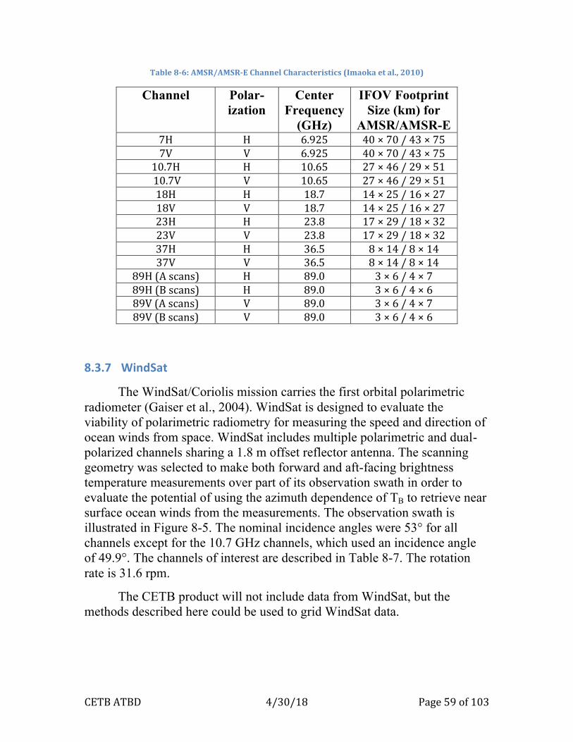
CETBATBD 4/30/18 Page59of103
Table8-6:AMSR/AMSR-EChannelCharacteristics(Imaokaetal.,2010)
Channel Polar-ization
Center Frequency
(GHz)
IFOV Footprint Size (km) for
AMSR/AMSR-E 7H H 6.925 40×70/43×757V V 6.925 40×70/43×75
10.7H H 10.65 27×46/29×5110.7V V 10.65 27×46/29×5118H H 18.7 14×25/16×2718V V 18.7 14×25/16×2723H H 23.8 17×29/18×3223V V 23.8 17×29/18×3237H H 36.5 8×14/8×1437V V 36.5 8×14/8×14
89H(Ascans) H 89.0 3×6/4×789H(Bscans) H 89.0 3×6/4×689V(Ascans) V 89.0 3×6/4×789V(Bscans) V 89.0 3×6/4×6
8.3.7 WindSat
The WindSat/Coriolis mission carries the first orbital polarimetric radiometer (Gaiser et al., 2004). WindSat is designed to evaluate the viability of polarimetric radiometry for measuring the speed and direction of ocean winds from space. WindSat includes multiple polarimetric and dual-polarized channels sharing a 1.8 m offset reflector antenna. The scanning geometry was selected to make both forward and aft-facing brightness temperature measurements over part of its observation swath in order to evaluate the potential of using the azimuth dependence of TB to retrieve near surface ocean winds from the measurements. The observation swath is illustrated in Figure 8-5. The nominal incidence angles were 53° for all channels except for the 10.7 GHz channels, which used an incidence angle of 49.9°. The channels of interest are described in Table 8-7. The rotation rate is 31.6 rpm.
The CETB product will not include data from WindSat, but the methods described here could be used to grid WindSat data.

CETBATBD 4/30/18 Page60of103
Table8-7:WindSatChannelCharacteristics(Gaiseretal.,2004);Onlylinearlypolarizedchannelsshown.
Channel
Polarization Center Frequency
(GHz)
Bandwidth (MHz)
Footprint Size (km)
Integration period
(ms) 6.8H H 6.8 125 40×60 5.006.8V V 6.8 125 40×60 5.0010.7H H 10.7 300 25×38 3.9310.7V V 10.7 300 25×38 3.9318H H 18.7 750 16×27 2.1918V V 18.7 750 16×27 2.1923H H 23.8 500 12×20 1.6323V V 23.8 500 12×20 1.6337H H 37 2000 8×13 1.0837V V 37 2000 8×13 1.08
Figure8-5AnillustrationoftheWindSatobservationgeometryandcoverageasseenfromabove.The
antennahelicallyscansthesurfaceataconstantincidenceangle.The
remainderoftheazimuthanglesareusedforcalibration.

CETBATBD 4/30/18 Page61of103
8.3.8 ApproximatingtheMeasurementResponseFunction
Reconstruction/resolution algorithms require models of the MRF in order to generate enhanced-resolution images. Such models require information about the sensor antenna patterns for each channel. Given the antenna pattern, and information about the rotation rate, the smeared antenna pattern can be computed, from which the MRF is derived. However, in some cases, the amount of information about the detailed antenna pattern is limited (Njoku et al., 1980). In some cases (e.g., SMMR), all that is known is the approximate size of the ½ power footprint. These elliptical footprints have their semi-major axis along the boresite direction, while the semi-minor axis is in the along-rotation direction. The orientation of the footprint semi-major axis varies with the antenna rotation angle, see Figure 8-6 and Figure 8-8.
Lacking a detailed description of the antenna patterns for each sensor, we adopt an approximate model for the MRF based on a rotated, two-dimensional Gaussian function aligned with the footprint orientation where ½ power points of the Gaussian correspond to the footprint sizes reported for each sensor. Each data set provides the azimuth angle of each measurement with respect to north (see Figure 8-6). This is the angle (on the ground) between the vector defined from the sensor and the measurement center location, and true north, and gives the rotation angle of the elliptical footprint relative to north. Based on the sensitivity of the reconstruction when regularization is employed, we find this model to be adequate for our purposes (Long, 2015).

CETBATBD 4/30/18 Page62of103
The algorithm for computing the MRF is given here. A grid of pixels centered at the measurement center is defined. The grid size is chosen large enough so that the MRF gain at the edges of the grid is no more than a small threshold, e.g. -30 dB of the MRF peak. Using the map projection, the relative vector distance from the measurement center to the center of each pixel is computed as the vector Xrel=[xr,yr]T. This vector is rotated by the angle φ relative to north of the ellipse. The rotated system is:
X=[x,y] T =R(φ) Xrel
where
R(φ)=[cos(φ) -sin(φ)]
[sin(φ) cos(φ)]
Define the length of the semi-major axis in km as Lj and the semi-minor axis as Ln. The MRF gain G at the center of the pixel is then
G=ln(1/2) exp[ (2x/Lj)2 + (2y/Ln)2 ]
Figure8-6North-EastreferenceframeusedformeasurementEarthazimuthangle.

CETBATBD 4/30/18 Page63of103
An example of the result for several values of φ is shown in Figure 8-8. Note that ½ power point of G corresponds to the specified ellipse semi-major and semi-minor axes.
This simplified model for the MRF does not exactly model the true MRF (Long, 2015). However, based on the sensitivity of the reconstruction when regularization is employed, this model is adequate for our purposes.
8.4 Appendix:LocalTime-of-DayAnalysisIn this section we consider the division of a coverage swath by local
time-of-day (ltod) compared to ascending/descending. The essential idea is to keep measurements with similar local time of day together. As illustrated Figure 8-8, as a swath passes near the North Pole, the orbit direction changes from ascending (north-bound) to descending (south-bound). This occurs at the point when the ground track of the spacecraft nadir achieves its northernmost extent. In other words, the spacecraft nadir location is used to divide the data into ascending and descending regions. In the ascending/descending division, all data collected before this point is considered “ascending” data, and data collected afterward is considered
Figure8-7AnillustrationofageneralGaussianmodelfortheMRFforaradiometer.ShownistheMRFinlinearspaceforseveralantennarotation
angles.Thefigureisnottoscale.

CETBATBD 4/30/18 Page64of103
“descending.” Because the antenna is rotating and looking outward, data classified as “ascending” can actually be along the descending portion of the swath.
In contrast, in ltod division, the local time of day is computed as the UTC time in minutes plus 4 times the longitude in deg (-180 to +180). Data that is collected before the ltod division point (which in this figure corresponds to 120E) is assigned to the “ascending” data group, while data collected after this time (in ltod) is assigned as “descending” data, see Figure 8-8. Note the division line occurs along a fixed line of longitude. In practice the division line does not have to pass through the nadir position of the transition of the spacecraft from ascending to descending.
Figure8-8Illustrationoftheboundariesinthearealcoveragebetween(left)ascending/descendingdivisionand(right)local-time-of-daydivisionofmeasurementsinasingleorbitpassovertheNorthernHemisphere.
Since the radiometers are in a sun-synchronous orbit, a given point of the Earth’s surface is observed at the same ltod for each pass in the orbit repeat cycle. To illustrate this, consider a 1-deg wide latitude band at 70-71 degrees in the Northern and Southern hemispheres. Note that within a given latitude band, all the measurements fall within one of two narrow ltod periods. The precise value (in ltod) of the band depends on the orbit and is different for different sensors (see figures, below, for each sensor).
It is thus apparent that except at the highest latitudes, the measurements collected from a given sensor can be naturally grouped into two different ltod groups. If we repeated the analysis at the equator the two ltod groups would correspond to ascending and descending passes. At the poles, however, the ascending/descending division discussed previously does not do a good job of properly dividing the data into its natural groups.
!

CETBATBD 4/30/18 Page65of103
This is why we prefer dividing polar data by measurement ltod rather than using the spacecraft ascending/descending flag.
Note that daily average images produced using traditional methods would have included all data regardless of ltod, and thus in the polar regions, would have combined data taken many hours apart. The ltod division ensures that even if data are combined from different passes, the data fall within the natural ltod data grouping. Using the natural ltod data divisions, two images per day can be generated. Unlike daily or ascending/descending division, all measurements averaged into a single pixel come from the same narrow ltod grouping, which minimizes artifacts due to rapidly changing conditions on the surface.
One drawback to using an ltod division scheme is that in a polar image there is a longitude line in the image that divides data from the previous and current day. Temporal changes at the surface can produce discontinuities across this line.
In most cases, the satellite orbit was stable enough to allow a fixed ltod division time for the sensor lifetime; however in some cases orbital drift was significant and justified changes in the ltod settings, to ensure that the twice-daily temporal divisions were capturing the intended groups of local times in the respective files. The following plots summarize this analysis, by sensor and (where necessary) year. Plots for sensors whose ltod did not change significantly are only included for one representative year.

CETBATBD 4/30/18 Page66of103
Figure8-9SMMR(left)andF08(right)ltodboundsfor1984and1990,respectively.Therewasnosignificantdriftinltodoverthelifetimeofthesesensors.

CETBATBD 4/30/18 Page67of103
Figure8-10F10ltodboundsfor1991-1994.TheF10ltodtimesshiftedonce(from1993-1994),duringthelifespanofthissensor.

CETBATBD 4/30/18 Page68of103
Figure8-11F10ltodboundsfor1995-1997.TheF10ltodtimesshiftedonce(from1993to1994)duringthelifespanofthesensor.

CETBATBD 4/30/18 Page69of103
Figure8-12F11(left)andF13(right)ltodboundsfor1994and1997,respectively.Therewasnosignificantdriftinltodoverthelifetimeofthesesensors.

CETBATBD 4/30/18 Page70of103
Figure8-13F14ltodboundsfor1997-2000.TheF14ltodtimesshiftedtwice(from2001to2002andagainfrom2004to2005)duringthelifespanofthesensor.
.
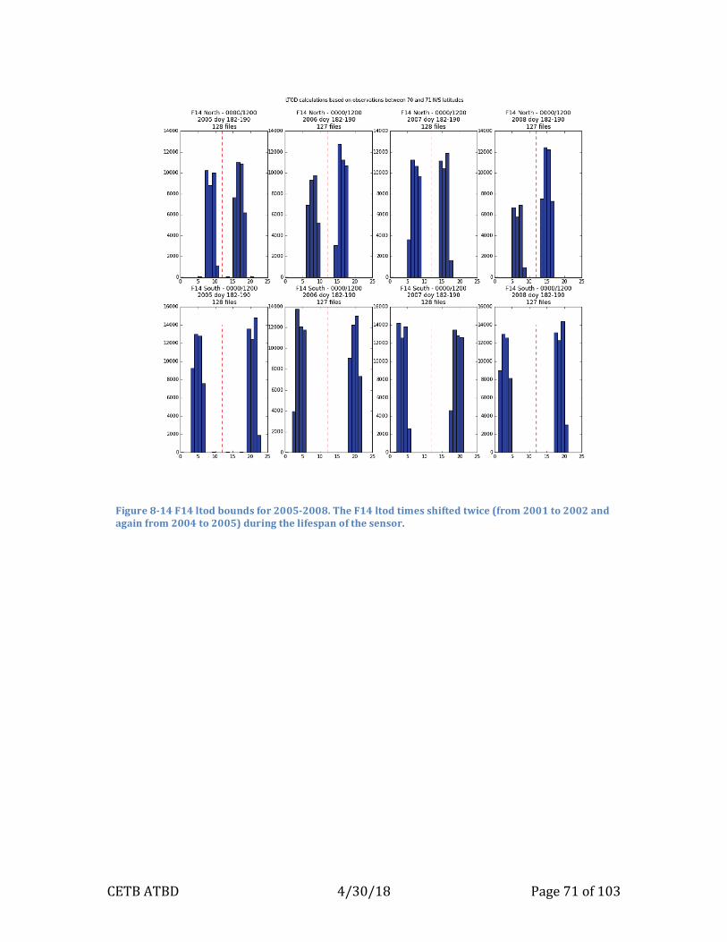
CETBATBD 4/30/18 Page71of103
Figure8-14F14ltodboundsfor2005-2008.TheF14ltodtimesshiftedtwice(from2001to2002andagainfrom2004to2005)duringthelifespanofthesensor.

CETBATBD 4/30/18 Page72of103
Figure8-15F15ltodboundsfor2000-2007.TheF15ltodtimesshiftedseveraltimesduringthelifespanofthesensor.

CETBATBD 4/30/18 Page73of103
Figure8-16F15ltodboundsfor2008-2015.TheF15ltodtimesshiftedseveraltimesduringthelifespanofthesensor.

CETBATBD 4/30/18 Page74of103
Figure8-17F16ltodboundsfor2006-2013.TheF16ltodtimesshiftedseveraltimesduringthelifespanofthesensor.

CETBATBD 4/30/18 Page75of103
Figure8-18F16ltodboundsfor2014-2017.TheF16ltodtimesshiftedseveraltimesduringthelifespanofthesensor.

CETBATBD 4/30/18 Page76of103
Figure8-19F17(left)andF18(right)ltodboundsfor2015and2016,respectively.Therehasbeennosignificantdriftinltodoverthelifetimeofthesesensorssofar.

CETBATBD 4/30/18 Page77of103
Figure8-20F19ltodboundsfor2015.Therehasbeennosignificantdriftinltodtodateforthissensor.

CETBATBD 4/30/18 Page78of103
Figure8-21AMSR-Eltodboundsfor2004.Therewasnosignificantdriftinltodoverthelifetimeofthissensor.

8.5 Appendix:CETBProductEASE-Grid2.0ProjectionsandGridDimensionsTable8-8:CETBproductEASE-Grid2.0projectionsandgriddimensions
Name Projection Resolution (km) Cols Rows Latitude Extent Longitude Extent EASE2-N25km NorthernLambert
Azimuthal25 720 720 0–90 -180-180
EASE2-N12.5km NorthernLambertAzimuthal
12.5 1440 1440 0–90 -180-180
EASE2-N6.25km NorthernLambertAzimuthal
6.25 2880 2880 0–90 -180-180
EASE2-N3.125km NorthernLambertAzimuthal
3.125 5760 5760 0–90 -180-180
EASE2-N1.5625km NorthernLambertAzimuthal
1.5625 11520 11520 0–90 -180-180
EASE2-S25km SouthernLambertAzimuthal
25 720 720 -90-0 -180-180
EASE2-S12.5km SouthernLambertAzimuthal
12.5 1440 1440 -90-0 -180-180
EASE2-S6.25km SouthernLambertAzimuthal
6.25 2880 2880 -90-0 -180-180
EASE2-S3.125km SouthernLambertAzimuthal
3.125 5760 5760 -90-0 -180-180
EASE2-S1.5625km SouthernLambertAzimuthal
1.5625 11520 11520 -90-0 -180-180
EASE2-T25km CylindricalEqual-Area 25.02526 1388 540 +/-67.057541 -180-180EASE2-T12.5km CylindricalEqual-Area 12.51263 2776 1080 +/-67.057541 -180-180EASE2-T6.25km CylindricalEqual-Area 6.256315 5552 2160 +/-67.057541 -180-180EASE2-T3.125km CylindricalEqual-Area 3.128.15750 11104 4320 +/-67.057541 -180-180EASE2-T1.5625km CylindricalEqual-Area 1.56407875 22208 8640 +/-67.057541 -180-180

8.6 Appendix:CETBOutputDataDefinition8.6.1 CETBFileRequirementsCETBoutputfilerequirements:
§ OuroutputfiledefinitionwillbeacceptableforNSIDCDAACtoeasilyingestittoECS.
§ Filesizemaximumwillbe<1GB(largerfilesareallowedinECS,butnetworkspeedsstillaren'twhattheyshouldbe).
§ Wewillfollow netCDF-CF 1.6 conventions forallbuttherequirementthatputsthelat/lonarraysintothefile;however,wewillincludeCF-compliantcoordinatevariableswithprojectedcoordinatelocations.
§ OuroutputfilesshouldpassCF-compliance-checkingforallbutthelat/lonarrays.(WeusedJPLcompliance-checker.)
§ EachCETBfilewillcontain1brightnesstemperature(TB)arrayvariable,withassociatedancillaryvariables,possiblydifferentancillaryvariablesforeachgriddingtechnique.Wemayhaveapracticallimitonthenumberofancillaryvariablestoinclude,limitedbymaximumfilesize.
§ EachCETBfileofthesametype(projection,GRD,SIR,BGI)willcontainthesamefile-levelmetadataforthattype.e.g.aSIRfilewillcontaindifferenttuningparametersthanaBGIfile,butallSIRfileswillcontainconsistentmetadata.
§ WewillfollowtheDRY(Don'tRepeatYourself)principle:Metadatawillnotbeduplicatedatmultipleplacesinthesamefile.Exceptions:
o Timevalueswillbemachine-andhuman-readable.o Someprojectionmetadatamaybeinmultipleforms(aproj4string
and/orawktstring)§ Variable/attributenameswillbeCF-compliantwheneverpossible.§ Our.ncfileswillworkwithgdalutility,gdal_translate,toproduceageoTIFF
versionofeachofthedatavariables<variable_name>inthefile,(detailsinBrodziketal.,2017),asfollows:
gdal_translate -of GTiff -b 1 NETCDF:”cetb.nc”:<variable_name> variable_name.tif
8.6.2 CETBFilenamingConventionCETBdataaredistributedbytheNSIDCDAAC(http://nsidc.org/data/nsidc-0630).CETBfilenamesare: <product_id>-<grid_name>-<platform_sensor>-<yyyyddd>-<channel_id>-<pass_descriptor>-<algorithm>-<input_source>-<version>.nc

CETBATBD 4/30/18 Page81of103
Example: NSIDC-0630-EASE2_N3.125km-F08_SSMI-1987304-37H-M-SIR-RSS-v1.3.nc
where:
Filename part Description Values
<product_id> NSIDC unique data product id
NSIDC-0630
<grid_name> Grid name (NSIDC .gpd filename, without the suffix)
EASE2_[N|S|T][25|6.25|3.125]km
<platform_sensor> Satellite sensor and platform id
NIMBUS7_SMMR,
F[08|10|11|13|15|16]_SSMI,
F17_SSMIS,
AQUA_AMSRE
<yyyyddd> Reference day 4-digit year, 3-digit day of year
<channel_id> Channel ID (frequency and polarization)
2-digit frequency and 1-letter polarization, differs by sensor, e.g. 37H
<pass_descriptor> Satellite pass descriptor 1-letter code:
A = Ascending (T grids only)
D = Descending (T grids only)
M = Morning ltod (NS grids only)
E = Evening ltod (NS grids only)
<algorithm> Image reconstruction algorithm
GRD = drop-in-the-bucket (25 km grids only)
SIR = Scatterometry Image Reconstruction (3.125 km grids only)
BG = Backus-Gilbert (3.125 grids only)
<input_source> Input data producer (only used for Prototype versions
RSS = Remote sensing systems FCDR

CETBATBD 4/30/18 Page82of103
of SSM/I files) CSU = CSU FCDR
<version> Data set version number. Any prototype versions of this product will be v0.xx. Subsequent versions will increment to v1.x or higher
vX.X, for major/minor version numbers
.nc data formatting suffix netCDF data format
8.6.3 CETBDataVolumeFollowingassumesnolat/lonarraysinfiles,andnometadata(thesizeofanyglobalfilemetadatais<<datasize).
8.6.3.1 GRDFiles(25kmonly)
Layer Element Size
TB 2-byte unsigned int
TB_time 2-byte signed int
TB_st_dev 2-byte unsigned int
Incidence_angle 2-byte signed int
TB_num_samples 1-byte unsigned int
Grid cols rows Element size (bytes) Total file data volume*
EASE2-N25km 720 720 9 4,665,600
EASE2-S25km 720 720 9 4,665,600
EASE2-T25km 1388 540 9 6,745,680

CETBATBD 4/30/18 Page83of103
Total per set of grids 16,076,880
*Datavolumelistedhereisuncompressed.WeareusingnetCDFinternalcompression,sothisisanupperboundonfilevolumes.TheGRDfileswillbeproducedfor2passesperdaypergrid.Datavolumefor7-channelradiometerGRDfileswillbe:2passes/day*7channels*16MBperset=224MB/dayForatotalsizeonSSM/Ilowresfilevolumeof224MB/day(about82GB/year/sensor)
8.6.3.2 SIR/BGIFiles6.25kmor3.125kmfiles(dependsonchannel):
Layer Element Size
TB 2-byte unsigned int
TB_time 2-byte signed int
TB_std_dev 2-byte unsigned int
Incidence_angle 2-byte signed int
TB_num_samples 1-byte unsigned int
Grid cols rows Element size
Total data volume (bytes)*
EASE2-N/S6.25km 2880 2880 9 74,649,600
EASE2-T6.25km 5552 2160 9 107,930,880
Total bytes per (1 channel, 1 pass direction, 1 day) set of 6.25 km files
182,580,480

CETBATBD 4/30/18 Page84of103
EASE2-N/S3.125km 5760 5760 9 298,598,400
EASE2-T3.125km 11104 4320 9 431,723,520
Total bytes per (1 channel, 1 pass direction, 1 day) set of 3.125 km files
730,321,920
*Datavolumelistedhereisuncompressed.WeareusingnetCDFinternalcompression,sothisisanupperboundonfilevolumes.ForatypicalSSM/I-SSMISsetofchannels,wewillexpecttoproduce:19/22at6.25km:2passes/day*3channels*183MB/NSTset=1.2GB/dayand37/85at3.125km:2passes/day*4channels*730MB/NSTset=5.8GB/dayForatotalestimateofSSM/Ienhancedresolutionfilevolumeof7.0GB/day(about2.6TB/year/sensor) Dailycompressedfilesizesdependonsensorswathsizeandavailableinputcoverageonagivendata,varyingfrom4-106MB/file/day.Adatadayofdatafromeachsensorrangesfrom230MBto11GBwithanaveragesizeof5GB/day.ThetotalvolumeoftheCETBdataforAMSR-E,sixSSM/Is,fourSSMISsandSMMRis64TB.
8.6.4 CETBv1.xFileContentFollowingaresampleNetCDF“ncdump–h”utilityoutput,describingexamplev1.2GRDandSIRfiles.Therearenoformattingdifferencesbetweenv1.2andv1.3files.

CETBATBD 4/30/18 Page85of103
netcdf NSIDC-0630-EASE2_N25km-F17_SSMIS-2009060-37H-E-GRD-CSU-v1.2 {dimensions:
time = UNLIMITED ; // (1 currently)y = 720 ;x = 720 ;
variables:double time(time) ;
time:standard_name = "time" ;time:coverage_content_type = "coordinate" ;time:long_name = "ANSI date" ;time:units = "days since 1972-01-01 00:00:00" ;time:calendar = "gregorian" ;time:axis = "T" ;time:valid_range = 0., 1.79769313486232e+308 ;
double y(y) ;y:standard_name = "projection_y_coordinate" ;y:coverage_content_type = "coordinate" ;y:long_name = "y" ;y:units = "meters" ;y:axis = "Y" ;y:valid_range = -9000000., 9000000. ;
double x(x) ;x:standard_name = "projection_x_coordinate" ;x:coverage_content_type = "coordinate" ;x:long_name = "x" ;x:units = "meters" ;x:axis = "X" ;x:valid_range = -9000000., 9000000. ;
char crs ;crs:grid_mapping_name =
"lambert_azimuthal_equal_area" ;crs:longitude_of_projection_origin = 0. ;crs:latitude_of_projection_origin = 90. ;crs:false_easting = 0. ;crs:false_northing = 0. ;crs:semi_major_axis = 6378137. ;crs:inverse_flattening = 298.257223563 ;crs:proj4text = "+proj=laea +lat_0=90 +lon_0=0 +x_0=0
+y_0=0 +ellps=WGS84 +datum=WGS84 +units=m" ;crs:srid = "urn:ogc:def:crs:EPSG::6931" ;crs:coverage_content_type = "auxiliaryInformation" ;crs:references = "[\"EASE-Grid 2.0 documentation:
http://nsidc.org/data/ease/ease_grid2.html\", \"Brodzik, Mary J.; Billingsley, Brendan; Haran, Terry; Raup, Bruce; Savoie, Matthew H. 2012.\", \"EASE-Grid 2.0: Incremental but Significant Improvements for Earth-Gridded Data Sets.\", \"ISPRS Int. J. Geo-Inf. 1, no. 1: 32-45.\", \"Brodzik, Mary J.; Billingsley, Brendan; Haran, Terry; Raup, Bruce; Savoie, Matthew H. 2014.\", \"Correction: Brodzik, M. J., et al. EASE-Grid 2.0: Incremental but Significant Improvements for Earth-Gridded Data Sets.\", \"ISPRS Int. J. Geo-Inf. 3, no. 3:

CETBATBD 4/30/18 Page86of103
1154-1156.\"]" ;crs:crs_wkt = "PROJCRS[\"WGS 84 / NSIDC EASE-Grid 2.0
North\", BASEGEODCRS[\"WGS 84\", DATUM[\"World Geodetic System 1984\", ELLIPSOID[\"WGS 84\",6378137,298.257223563,LENGTHUNIT[\"metre\",1.0]]]], CONVERSION[\"US NSIDC EASE-Grid 2.0 North\", METHOD[\"Lambert Azimuthal Equal Area\",ID[\"EPSG\",9820]], PARAMETER[\"Latitude of natural origin\",90,ANGLEUNIT[\"degree\",0.01745329252]], PARAMETER[\"Longitude of natural origin\",0,ANGLEUNIT[\"degree\",0.01745329252]], PARAMETER[\"False easting\",0,LENGTHUNIT[\"metre\",1.0]], PARAMETER[\"False northing\",0,LENGTHUNIT[\"metre\",1.0]]], CS[cartesian,2], AXIS[\"easting (X)\",south,MERIDIAN[90,ANGLEUNIT[\"degree\",0.01745329252]],ORDER[1]], AXIS[\"northing (Y)\",south,MERIDIAN[180,ANGLEUNIT[\"degree\",0.01745329252]],ORDER[2]], LENGTHUNIT[\"metre\",1.0], ID[\"EPSG\",6931]]" ;
crs:long_name = "EASE2_N25km" ;ushort TB(time, y, x) ;
TB:standard_name = "brightness_temperature" ;TB:long_name = "GRD TB" ;TB:units = "K" ;TB:_FillValue = 0US ;TB:missing_value = 60000US ;TB:valid_range = 5000US, 35000US ;TB:packing_convention = "netCDF" ;TB:packing_convention_description = "unpacked =
scale_factor*packed + add_offset" ;TB:scale_factor = 0.01f ;TB:add_offset = 0.f ;TB:grid_mapping = "crs" ;TB:coverage_content_type = "image" ;TB:median_filter = 0 ;TB:measurement_response_threshold_dB = -8.f ;TB:measurement_search_bounding_box_km = 187.5f ;TB:temporal_division = "Evening" ;TB:temporal_division_local_start_time = 12.f ;TB:temporal_division_local_end_time = 0.f ;TB:frequency_and_polarization = "37H" ;
ubyte TB_num_samples(time, y, x) ;TB_num_samples:long_name = "GRD TB Number of
Measurements" ;TB_num_samples:units = "count" ;TB_num_samples:_FillValue = 0UB ;TB_num_samples:valid_range = 1UB, 255UB ;TB_num_samples:flag_values = 255UB ;TB_num_samples:flag_meanings = "num_samples GE 255" ;TB_num_samples:grid_mapping = "crs" ;TB_num_samples:coverage_content_type =
"auxiliaryInformation" ;ushort TB_std_dev(time, y, x) ;
TB_std_dev:long_name = "GRD TB Std Deviation" ;

CETBATBD 4/30/18 Page87of103
TB_std_dev:units = "K" ;TB_std_dev:_FillValue = 65535US ;TB_std_dev:missing_value = 65534US ;TB_std_dev:valid_range = 0US, 65533US ;TB_std_dev:packing_convention = "netCDF" ;TB_std_dev:packing_convention_description = "unpacked
= scale_factor*packed + add_offset" ;TB_std_dev:scale_factor = 0.01f ;TB_std_dev:add_offset = 0.f ;TB_std_dev:grid_mapping = "crs" ;TB_std_dev:coverage_content_type =
"auxiliaryInformation" ;short Incidence_angle(time, y, x) ;
Incidence_angle:long_name = "GRD Incidence Angle" ;Incidence_angle:units = "degree" ;Incidence_angle:_FillValue = -1s ;Incidence_angle:valid_range = 0s, 9000s ;Incidence_angle:packing_convention = "netCDF" ;Incidence_angle:packing_convention_description =
"unpacked = scale_factor*packed + add_offset" ;Incidence_angle:scale_factor = 0.01f ;Incidence_angle:add_offset = 0.f ;Incidence_angle:grid_mapping = "crs" ;Incidence_angle:coverage_content_type =
"auxiliaryInformation" ;short TB_time(time, y, x) ;
TB_time:long_name = "GRD TB Time of Day" ;TB_time:units = "minutes since 2009-03-01 00:00:00" ;TB_time:_FillValue = -32768s ;TB_time:valid_range = -32767s, 32767s ;TB_time:packing_convention = "netCDF" ;TB_time:packing_convention_description = "unpacked =
scale_factor*packed + add_offset" ;TB_time:scale_factor = 1.f ;TB_time:add_offset = 0.f ;TB_time:grid_mapping = "crs" ;TB_time:coverage_content_type =
"auxiliaryInformation" ;TB_time:calendar = "gregorian" ;
// global attributes::Conventions = "CF-1.6, ACDD-1.3" ;:title = "MEaSUREs Calibrated Passive Microwave Daily
EASE-Grid 2.0 Brightness Temperature ESDR" ;:product_version = "v1.2" ;:software_version_id = "0.2.31" ;:software_repository = "[email protected]:nsidc/
measures-byu.git" ;:history = "meas_meta_sir" ;:comment = "Epoch date for data in this file:

CETBATBD 4/30/18 Page88of103
2009-03-01 00:00:00Z" ;:source = "CSU SSMIS FCDR V01R00" ;:references = "Long, D. G. and M. J. Brodzik. 2016.
Optimum Image Formation for Spaceborne Microwave Radiometer Products. IEEE Trans. Geosci. Remote Sensing, 54(5):2763-2779, doi:10.1109/TGRS.2015.2505677.\nAlgorithm Theoretical Basis Document: https://nsidc.org/sites/nsidc.org/files/technical-references/MEaSUREs_CETB_ATBD.pdf\n" ;
:metadata_link = "http://nsidc.org/data/nsidc-0630.html" ;
:summary = "An improved, enhanced-resolution, gridded passive microwave Earth System Data Record for monitoring cryospheric and hydrologic time series\n" ;
:institution = "National Snow and Ice Data Center\nCooperative Institute for Research in Environmental Sciences\nUniversity of Colorado at Boulder\nBoulder, CO" ;
:publisher_name = "NASA National Snow and Ice Data Center Distributed Active Archive Center" ;
:publisher_type = "institution" ;:publisher_url = "http://nsidc.org" ;:publisher_email = "[email protected]" ;:program = "NASA 2012 MEaSUREs (Making Earth System
Data Records for Use in Research Environments)" ;:project = "An improved, enhanced-resolution, gridded
passive microwave ESDR for monitoring cryospheric and hydrologic time series" ;
:standard_name_vocabulary = "CF Standard Name Table (v27, 28 September 2013)" ;
:cdm_data_type = "Grid" ;:keywords = "EARTH SCIENCE > SPECTRAL/ENGINEERING >
MICROWAVE > BRIGHTNESS TEMPERATURE" ;:keywords_vocabulary = "NASA Global Change Master
Directory (GCMD) Earth Science Keywords, Version 8.1" ;:platform = "DMSP 5D-3/F17 > Defense Meteorological
Satellite Program-F17" ;:platform_vocabulary = "NASA Global Change Master
Directory (GCMD) Earth Science Keywords, Version 8.1" ;:instrument = "SSMIS > Special Sensor Microwave
Imager/Sounder" ;:instrument_vocabulary = "NASA Global Change Master
Directory (GCMD) Earth Science Keywords, Version 8.1" ;:time_coverage_resolution = "P1d" ;:geospatial_lat_units = "degree_north" ;:geospatial_lon_units = "degree_east" ;:geospatial_x_units = "meters" ;:geospatial_y_units = "meters" ;:naming_authority = "org.doi.dx" ;:id = "10.5067/MEASURES/CRYOSPHERE/nsidc-0630.001" ;:date_created = "2017-06-04T13:40:12MDT" ;:date_modified = "2017-06-04T13:40:12MDT" ;

CETBATBD 4/30/18 Page89of103
:date_issued = "2017-06-04T13:40:12MDT" ;:date_metadata_modified = "2017-06-04T13:40:12MDT" ;:acknowledgement = "This data set was created with
funding from NASA MEaSUREs Grant #NNX13AI23A.\nData archiving and distribution is supported by the NASA NSIDC Distributed Active Archive Center (DAAC)." ;
:license = "No constraints on data access or use" ;:processing_level = "Level 3" ;:creator_name = "Mary J. Brodzik" ;:creator_type = "person" ;:creator_email = "[email protected]" ;:creator_url = "http://nsidc.org/pmesdr" ;:creator_institution = "National Snow and Ice Data
Center\nCooperative Institute for Research in Environmental Sciences\nUniversity of Colorado at Boulder\nBoulder, CO" ;
:contributor_name = "Mary J. Brodzik, David G. Long, Richard L. Armstrong, Molly A. Hardman, Aaron C. Paget" ;
:contributor_role = "Principal Investigator, Co-Investigator, Co-Investigator, Developer, Contributor" ;
:citation = "Brodzik, M. J., D. G. Long, M. A. Hardman, A. C. Paget, R. L. Armstrong. 2016.\nMEaSUREs Calibrated Passive Microwave Daily EASE-Grid 2.0 Brightness Temperature ESDR.\nVersion 1.2.\n[Indicate subset used].\nBoulder, Colorado USA: NASA DAAC at the National Snow and Ice Data Center." ;
:geospatial_bounds = "EPSG:3475" ;:geospatial_bounds_crs = "EPSG:6931" ;:geospatial_lat_min = 0. ;:geospatial_lat_max = 90. ;:geospatial_lon_min = -180. ;:geospatial_lon_max = 180. ;:geospatial_x_resolution = "25000.00 meters" ;:geospatial_y_resolution = "25000.00 meters" ;:time_coverage_start = "2009-03-02T05:01:00.00Z" ;:time_coverage_end = "2009-03-02T05:01:00.00Z" ;:time_coverage_duration = "P00T00:00:00.00" ;:number_of_input_files = 18 ;:input_file1 =
"CSU_SSMIS_FCDR_V01R00_F17_D20090228_S2346_E0128_R11972.nc (GSX_version:1.10.0)" ;
:input_file2 = "CSU_SSMIS_FCDR_V01R00_F17_D20090301_S0128_E0310_R11973.nc (GSX_version:1.10.0)" ;
:input_file3 = "CSU_SSMIS_FCDR_V01R00_F17_D20090301_S0310_E0452_R11974.nc (GSX_version:1.10.0)" ;
:input_file4 = "CSU_SSMIS_FCDR_V01R00_F17_D20090301_S0452_E0634_R11975.nc (GSX_version:1.10.0)" ;
:input_file5 = "CSU_SSMIS_FCDR_V01R00_F17_D20090301_S0634_E0815_R11976.nc

CETBATBD 4/30/18 Page90of103
(GSX_version:1.10.0)" ;:input_file6 =
"CSU_SSMIS_FCDR_V01R00_F17_D20090301_S0815_E0957_R11977.nc (GSX_version:1.10.0)" ;
:input_file7 = "CSU_SSMIS_FCDR_V01R00_F17_D20090301_S0957_E1139_R11978.nc (GSX_version:1.10.0)" ;
:input_file8 = "CSU_SSMIS_FCDR_V01R00_F17_D20090301_S1139_E1321_R11979.nc (GSX_version:1.10.0)" ;
:input_file9 = "CSU_SSMIS_FCDR_V01R00_F17_D20090301_S1321_E1503_R11980.nc (GSX_version:1.10.0)" ;
:input_file10 = "CSU_SSMIS_FCDR_V01R00_F17_D20090301_S1503_E1645_R11981.nc (GSX_version:1.10.0)" ;
:input_file11 = "CSU_SSMIS_FCDR_V01R00_F17_D20090301_S1645_E1827_R11982.nc (GSX_version:1.10.0)" ;
:input_file12 = "CSU_SSMIS_FCDR_V01R00_F17_D20090301_S1827_E2009_R11983.nc (GSX_version:1.10.0)" ;
:input_file13 = "CSU_SSMIS_FCDR_V01R00_F17_D20090301_S2009_E2151_R11984.nc (GSX_version:1.10.0)" ;
:input_file14 = "CSU_SSMIS_FCDR_V01R00_F17_D20090301_S2151_E2333_R11985.nc (GSX_version:1.10.0)" ;
:input_file15 = "CSU_SSMIS_FCDR_V01R00_F17_D20090301_S2333_E0115_R11986.nc (GSX_version:1.10.0)" ;
:input_file16 = "CSU_SSMIS_FCDR_V01R00_F17_D20090302_S0115_E0257_R11987.nc (GSX_version:1.10.0)" ;
:input_file17 = "CSU_SSMIS_FCDR_V01R00_F17_D20090302_S0257_E0439_R11988.nc (GSX_version:1.10.0)" ;
:input_file18 = "CSU_SSMIS_FCDR_V01R00_F17_D20090302_S0439_E0621_R11989.nc (GSX_version:1.10.0)" ;}
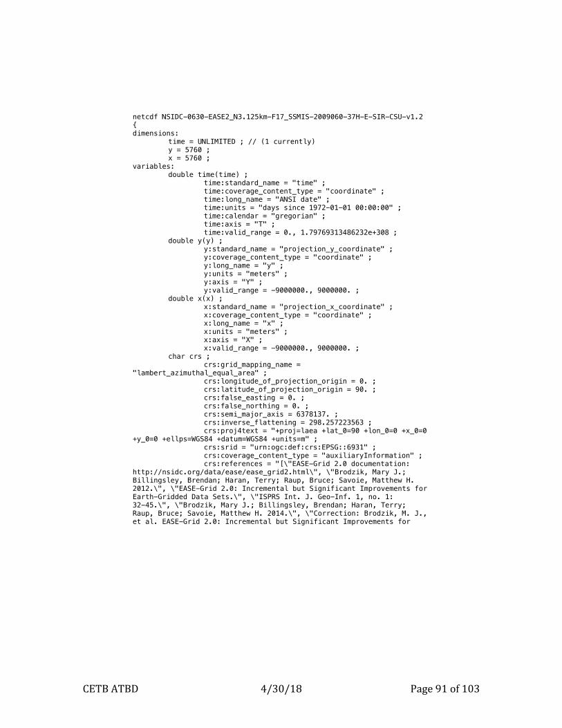
CETBATBD 4/30/18 Page91of103
netcdf NSIDC-0630-EASE2_N3.125km-F17_SSMIS-2009060-37H-E-SIR-CSU-v1.2 {dimensions:
time = UNLIMITED ; // (1 currently)y = 5760 ;x = 5760 ;
variables:double time(time) ;
time:standard_name = "time" ;time:coverage_content_type = "coordinate" ;time:long_name = "ANSI date" ;time:units = "days since 1972-01-01 00:00:00" ;time:calendar = "gregorian" ;time:axis = "T" ;time:valid_range = 0., 1.79769313486232e+308 ;
double y(y) ;y:standard_name = "projection_y_coordinate" ;y:coverage_content_type = "coordinate" ;y:long_name = "y" ;y:units = "meters" ;y:axis = "Y" ;y:valid_range = -9000000., 9000000. ;
double x(x) ;x:standard_name = "projection_x_coordinate" ;x:coverage_content_type = "coordinate" ;x:long_name = "x" ;x:units = "meters" ;x:axis = "X" ;x:valid_range = -9000000., 9000000. ;
char crs ;crs:grid_mapping_name =
"lambert_azimuthal_equal_area" ;crs:longitude_of_projection_origin = 0. ;crs:latitude_of_projection_origin = 90. ;crs:false_easting = 0. ;crs:false_northing = 0. ;crs:semi_major_axis = 6378137. ;crs:inverse_flattening = 298.257223563 ;crs:proj4text = "+proj=laea +lat_0=90 +lon_0=0 +x_0=0
+y_0=0 +ellps=WGS84 +datum=WGS84 +units=m" ;crs:srid = "urn:ogc:def:crs:EPSG::6931" ;crs:coverage_content_type = "auxiliaryInformation" ;crs:references = "[\"EASE-Grid 2.0 documentation:
http://nsidc.org/data/ease/ease_grid2.html\", \"Brodzik, Mary J.; Billingsley, Brendan; Haran, Terry; Raup, Bruce; Savoie, Matthew H. 2012.\", \"EASE-Grid 2.0: Incremental but Significant Improvements for Earth-Gridded Data Sets.\", \"ISPRS Int. J. Geo-Inf. 1, no. 1: 32-45.\", \"Brodzik, Mary J.; Billingsley, Brendan; Haran, Terry; Raup, Bruce; Savoie, Matthew H. 2014.\", \"Correction: Brodzik, M. J., et al. EASE-Grid 2.0: Incremental but Significant Improvements for

CETBATBD 4/30/18 Page92of103
Earth-Gridded Data Sets.\", \"ISPRS Int. J. Geo-Inf. 3, no. 3: 1154-1156.\"]" ;
crs:crs_wkt = "PROJCRS[\"WGS 84 / NSIDC EASE-Grid 2.0 North\", BASEGEODCRS[\"WGS 84\", DATUM[\"World Geodetic System 1984\", ELLIPSOID[\"WGS 84\",6378137,298.257223563,LENGTHUNIT[\"metre\",1.0]]]], CONVERSION[\"US NSIDC EASE-Grid 2.0 North\", METHOD[\"Lambert Azimuthal Equal Area\",ID[\"EPSG\",9820]], PARAMETER[\"Latitude of natural origin\",90,ANGLEUNIT[\"degree\",0.01745329252]], PARAMETER[\"Longitude of natural origin\",0,ANGLEUNIT[\"degree\",0.01745329252]], PARAMETER[\"False easting\",0,LENGTHUNIT[\"metre\",1.0]], PARAMETER[\"False northing\",0,LENGTHUNIT[\"metre\",1.0]]], CS[cartesian,2], AXIS[\"easting (X)\",south,MERIDIAN[90,ANGLEUNIT[\"degree\",0.01745329252]],ORDER[1]], AXIS[\"northing (Y)\",south,MERIDIAN[180,ANGLEUNIT[\"degree\",0.01745329252]],ORDER[2]], LENGTHUNIT[\"metre\",1.0], ID[\"EPSG\",6931]]" ;
crs:long_name = "EASE2_N3.125km" ;ushort TB(time, y, x) ;
TB:standard_name = "brightness_temperature" ;TB:long_name = "SIR TB" ;TB:units = "K" ;TB:_FillValue = 0US ;TB:missing_value = 60000US ;TB:valid_range = 5000US, 35000US ;TB:packing_convention = "netCDF" ;TB:packing_convention_description = "unpacked =
scale_factor*packed + add_offset" ;TB:scale_factor = 0.01f ;TB:add_offset = 0.f ;TB:grid_mapping = "crs" ;TB:coverage_content_type = "image" ;TB:sir_number_of_iterations = 15 ;TB:median_filter = 0 ;TB:measurement_response_threshold_dB = -8.f ;TB:measurement_search_bounding_box_km = 187.5f ;TB:temporal_division = "Evening" ;TB:temporal_division_local_start_time = 12.f ;TB:temporal_division_local_end_time = 0.f ;TB:frequency_and_polarization = "37H" ;
ubyte TB_num_samples(time, y, x) ;TB_num_samples:long_name = "SIR TB Number of
Measurements" ;TB_num_samples:units = "count" ;TB_num_samples:_FillValue = 0UB ;TB_num_samples:valid_range = 1UB, 255UB ;TB_num_samples:flag_values = 255UB ;TB_num_samples:flag_meanings = "num_samples GE 255" ;TB_num_samples:grid_mapping = "crs" ;TB_num_samples:coverage_content_type =
"auxiliaryInformation" ;

CETBATBD 4/30/18 Page93of103
short Incidence_angle(time, y, x) ;Incidence_angle:standard_name =
"angle_of_incidence" ;Incidence_angle:long_name = "SIR Incidence Angle" ;Incidence_angle:units = "degree" ;Incidence_angle:_FillValue = -1s ;Incidence_angle:valid_range = 0s, 9000s ;Incidence_angle:packing_convention = "netCDF" ;Incidence_angle:packing_convention_description =
"unpacked = scale_factor*packed + add_offset" ;Incidence_angle:scale_factor = 0.01f ;Incidence_angle:add_offset = 0.f ;Incidence_angle:grid_mapping = "crs" ;Incidence_angle:coverage_content_type =
"auxiliaryInformation" ;ushort TB_std_dev(time, y, x) ;
TB_std_dev:long_name = "SIR TB Std Deviation" ;TB_std_dev:units = "K" ;TB_std_dev:_FillValue = 65535US ;TB_std_dev:missing_value = 65534US ;TB_std_dev:valid_range = 0US, 65533US ;TB_std_dev:packing_convention = "netCDF" ;TB_std_dev:packing_convention_description = "unpacked
= scale_factor*packed + add_offset" ;TB_std_dev:scale_factor = 0.01f ;TB_std_dev:add_offset = 0.f ;TB_std_dev:grid_mapping = "crs" ;TB_std_dev:coverage_content_type =
"auxiliaryInformation" ;short TB_time(time, y, x) ;
TB_time:standard_name = "time" ;TB_time:long_name = "SIR TB Time of Day" ;TB_time:units = "minutes since 2009-03-01 00:00:00" ;TB_time:_FillValue = -32768s ;TB_time:valid_range = -32767s, 32767s ;TB_time:packing_convention = "netCDF" ;TB_time:packing_convention_description = "unpacked =
scale_factor*packed + add_offset" ;TB_time:scale_factor = 1.f ;TB_time:add_offset = 0.f ;TB_time:grid_mapping = "crs" ;TB_time:coverage_content_type =
"auxiliaryInformation" ;TB_time:calendar = "gregorian" ;
// global attributes::Conventions = "CF-1.6, ACDD-1.3" ;:title = "MEaSUREs Calibrated Passive Microwave Daily
EASE-Grid 2.0 Brightness Temperature ESDR" ;:product_version = "v1.2" ;

CETBATBD 4/30/18 Page94of103
:software_version_id = "0.2.31" ;:software_repository = "[email protected]:nsidc/
measures-byu.git" ;:history = "meas_meta_sir" ;:comment = "Epoch date for data in this file:
2009-03-01 00:00:00Z" ;:source = "CSU SSMIS FCDR V01R00" ;:references = "Long, D. G. and M. J. Brodzik. 2016.
Optimum Image Formation for Spaceborne Microwave Radiometer Products. IEEE Trans. Geosci. Remote Sensing, 54(5):2763-2779, doi:10.1109/TGRS.2015.2505677.\nAlgorithm Theoretical Basis Document: https://nsidc.org/sites/nsidc.org/files/technical-references/MEaSUREs_CETB_ATBD.pdf\n" ;
:metadata_link = "http://nsidc.org/data/nsidc-0630.html" ;
:summary = "An improved, enhanced-resolution, gridded passive microwave Earth System Data Record for monitoring cryospheric and hydrologic time series\n" ;
:institution = "National Snow and Ice Data Center\nCooperative Institute for Research in Environmental Sciences\nUniversity of Colorado at Boulder\nBoulder, CO" ;
:publisher_name = "NASA National Snow and Ice Data Center Distributed Active Archive Center" ;
:publisher_type = "institution" ;:publisher_url = "http://nsidc.org" ;:publisher_email = "[email protected]" ;:program = "NASA 2012 MEaSUREs (Making Earth System
Data Records for Use in Research Environments)" ;:project = "An improved, enhanced-resolution, gridded
passive microwave ESDR for monitoring cryospheric and hydrologic time series" ;
:standard_name_vocabulary = "CF Standard Name Table (v27, 28 September 2013)" ;
:cdm_data_type = "Grid" ;:keywords = "EARTH SCIENCE > SPECTRAL/ENGINEERING >
MICROWAVE > BRIGHTNESS TEMPERATURE" ;:keywords_vocabulary = "NASA Global Change Master
Directory (GCMD) Earth Science Keywords, Version 8.1" ;:platform = "DMSP 5D-3/F17 > Defense Meteorological
Satellite Program-F17" ;:platform_vocabulary = "NASA Global Change Master
Directory (GCMD) Earth Science Keywords, Version 8.1" ;:instrument = "SSMIS > Special Sensor Microwave
Imager/Sounder" ;:instrument_vocabulary = "NASA Global Change Master
Directory (GCMD) Earth Science Keywords, Version 8.1" ;:time_coverage_resolution = "P1d" ;:geospatial_lat_units = "degree_north" ;:geospatial_lon_units = "degree_east" ;:geospatial_x_units = "meters" ;

CETBATBD 4/30/18 Page95of103
:geospatial_y_units = "meters" ;:naming_authority = "org.doi.dx" ;:id = "10.5067/MEASURES/CRYOSPHERE/nsidc-0630.001" ;:date_created = "2017-06-04T13:40:12MDT" ;:date_modified = "2017-06-04T13:40:12MDT" ;:date_issued = "2017-06-04T13:40:12MDT" ;:date_metadata_modified = "2017-06-04T13:40:12MDT" ;:acknowledgement = "This data set was created with
funding from NASA MEaSUREs Grant #NNX13AI23A.\nData archiving and distribution is supported by the NASA NSIDC Distributed Active Archive Center (DAAC)." ;
:license = "No constraints on data access or use" ;:processing_level = "Level 3" ;:creator_name = "Mary J. Brodzik" ;:creator_type = "person" ;:creator_email = "[email protected]" ;:creator_url = "http://nsidc.org/pmesdr" ;:creator_institution = "National Snow and Ice Data
Center\nCooperative Institute for Research in Environmental Sciences\nUniversity of Colorado at Boulder\nBoulder, CO" ;
:contributor_name = "Mary J. Brodzik, David G. Long, Richard L. Armstrong, Molly A. Hardman, Aaron C. Paget" ;
:contributor_role = "Principal Investigator, Co-Investigator, Co-Investigator, Developer, Contributor" ;
:citation = "Brodzik, M. J., D. G. Long, M. A. Hardman, A. C. Paget, R. L. Armstrong. 2016.\nMEaSUREs Calibrated Passive Microwave Daily EASE-Grid 2.0 Brightness Temperature ESDR.\nVersion 1.2.\n[Indicate subset used].\nBoulder, Colorado USA: NASA DAAC at the National Snow and Ice Data Center." ;
:geospatial_bounds = "EPSG:3475" ;:geospatial_bounds_crs = "EPSG:6931" ;:geospatial_lat_min = 0. ;:geospatial_lat_max = 90. ;:geospatial_lon_min = -180. ;:geospatial_lon_max = 180. ;:geospatial_x_resolution = "3125.00 meters" ;:geospatial_y_resolution = "3125.00 meters" ;:time_coverage_start = "2009-03-01T01:52:00.00Z" ;:time_coverage_end = "2009-03-02T04:53:00.38Z" ;:time_coverage_duration = "P01T03:01:00.38" ;:number_of_input_files = 18 ;:input_file1 =
"CSU_SSMIS_FCDR_V01R00_F17_D20090228_S2346_E0128_R11972.nc (GSX_version:1.10.0)" ;
:input_file2 = "CSU_SSMIS_FCDR_V01R00_F17_D20090301_S0128_E0310_R11973.nc (GSX_version:1.10.0)" ;
:input_file3 = "CSU_SSMIS_FCDR_V01R00_F17_D20090301_S0310_E0452_R11974.nc (GSX_version:1.10.0)" ;

CETBATBD 4/30/18 Page96of103
:input_file4 = "CSU_SSMIS_FCDR_V01R00_F17_D20090301_S0452_E0634_R11975.nc (GSX_version:1.10.0)" ;
:input_file5 = "CSU_SSMIS_FCDR_V01R00_F17_D20090301_S0634_E0815_R11976.nc (GSX_version:1.10.0)" ;
:input_file6 = "CSU_SSMIS_FCDR_V01R00_F17_D20090301_S0815_E0957_R11977.nc (GSX_version:1.10.0)" ;
:input_file7 = "CSU_SSMIS_FCDR_V01R00_F17_D20090301_S0957_E1139_R11978.nc (GSX_version:1.10.0)" ;
:input_file8 = "CSU_SSMIS_FCDR_V01R00_F17_D20090301_S1139_E1321_R11979.nc (GSX_version:1.10.0)" ;
:input_file9 = "CSU_SSMIS_FCDR_V01R00_F17_D20090301_S1321_E1503_R11980.nc (GSX_version:1.10.0)" ;
:input_file10 = "CSU_SSMIS_FCDR_V01R00_F17_D20090301_S1503_E1645_R11981.nc (GSX_version:1.10.0)" ;
:input_file11 = "CSU_SSMIS_FCDR_V01R00_F17_D20090301_S1645_E1827_R11982.nc (GSX_version:1.10.0)" ;
:input_file12 = "CSU_SSMIS_FCDR_V01R00_F17_D20090301_S1827_E2009_R11983.nc (GSX_version:1.10.0)" ;
:input_file13 = "CSU_SSMIS_FCDR_V01R00_F17_D20090301_S2009_E2151_R11984.nc (GSX_version:1.10.0)" ;
:input_file14 = "CSU_SSMIS_FCDR_V01R00_F17_D20090301_S2151_E2333_R11985.nc (GSX_version:1.10.0)" ;
:input_file15 = "CSU_SSMIS_FCDR_V01R00_F17_D20090301_S2333_E0115_R11986.nc (GSX_version:1.10.0)" ;
:input_file16 = "CSU_SSMIS_FCDR_V01R00_F17_D20090302_S0115_E0257_R11987.nc (GSX_version:1.10.0)" ;
:input_file17 = "CSU_SSMIS_FCDR_V01R00_F17_D20090302_S0257_E0439_R11988.nc (GSX_version:1.10.0)" ;
:input_file18 = "CSU_SSMIS_FCDR_V01R00_F17_D20090302_S0439_E0621_R11989.nc (GSX_version:1.10.0)" ;}

8.7 Appendix:ComparisonofHeritageDataSetswithCETBESDRThefollowingtableisabriefcomparisonoftheCETBESDRwithrelevantheritagedatasets.
Table8-9ComparisonofCETBESDRwithrelevantheritagedatasets
SMMR EASE-Grid
SSM/I-SSMIS EASE-Grid
Enhanced-Resolution SSM/I & AMSR-E Polar
TBs
Polar Stereographic gridded TBs
AMSR-E Gridded TBs
CETB
DataSetID NSIDC-0071 NSIDC-0032 NSIDC-0464 NSIDC-0001 NSIDC-0301&NSIDC-0302
NSIDC-0630
SpatialCoverage Global Global Global LimitedArctic/Antarctic
regions
Global Global
SpatialCoverage NSMEASE-Grids NSMEASE-Grids NSMEASE-Grids NSpolarstereographic,limitedtohighlatitudes
NSMEASE-Gridsand¼-degreelat/lon
NSTEASE-Grid2.0
SpatialResolution(s) 25km 25km(all),12.5km(85GHzonly)
? 25km(all),12.5km(85GHzonly)
25kmand¼-degree 25km(all),seeforenhancedresolutions
upto~3kmTemporalCoverage 1978-1987 1987-present SSM/I:1995-2008;
AMSR-E:2002-20111987-present 2002-2011 1978-2017
Interpolation(imagereconstruction)
method
ID2 BG(tunedforlownoise),orID2(F13
only)
SIR DITB ID2 DITBat25km(all),andrSIRforenhanced
resolutionsImagereconstructiontuningparameters
N/A BGtunedtomatchresolutionofall
channelsto19V;ID2:N/A
Independentlyoptimizedresolutionforeachchannel
N/A N/A rSIRtunedtooptimizeresolutionforeachoutputchannel
TBfilesperchannelperday
2(ascanddes) 2(ascanddes) 2(ltod) 1(dailyaverages) 2 2(Tgrids:asc/des;N/Sgrids:ltod“morning”and“evening”)
Overlappingorbits Chooseoneorbit Chooseoneorbit Combineorbits(withltod)
Averaged Chooseoneorbit Combineorbitsbyltod
VariableMetadata Timeofsampleused Timeofsampleused Ltod? n/a Timeofsampleused time,measurementcounts,TBstddev,IncidenceAngle,
detailsinSection8.6

CETBATBD 4/30/18 Page98of103
Algorithm
documentationLimitedtouser’s
guideLimitedtouser’s
guideLimitedtouser’s
guideLimitedtouser’s
guideLimitedtouser’s
guideUser’sguide,thisATBD,LongandBrodzik(2016)
Satellitesincluded FullSMMRoperations F08,F11,F13,F17,withlimitedoverlap
periods
F13,AMSR-E F08,F11,F13,F17,withlimitedoverlap
periods
FullAMSR-Eoperations
Allavailablesatellitedataincluded(SMMR,F08,F10,F11,F13,F14,F15SSM/I,F16,F17,F18andF19SSMIS,AMSR-E)
Inputdatacalibration Bestavailable(Njoku2003)
OlderRSScalibration OlderRSScalibration OlderRSScalibration Bestavailableattimeofprocessing
Bestavailable

8.8 Appendix:ReferencesAshcroft,P.andF.J.Wentz.2013.AMSR-E/AquaL2AGlobalSwathSpatially-
ResampledBrightnessTemperatures,Version3.Boulder,ColoradoUSA.NASANationalSnowandIceDataCenterDistributedActiveArchiveCenter.http://dx.doi.org/10.5067/AMSR-E/AE_L2A.003.[Accessedon-line,05Feb2016].
Beitsch,A.,L.KaleschkeandS.Kern.2014.InvestigatingHigh-ResolutionAMSR2SeaIceConcentrationsduringtheFebruary2013FractureEventintheBeaufortSea.RemoteSensing6(5):3841-3856.doi:http://dx.doi.org/10.3390/rs6053841.
Berg,W.,M.R.P.Sapiano,J.HorsmanandC.Kummerow.2013.ImprovedGeolocationandEarthIncidenceAngleInformationforaFundamentalClimateDataRecordoftheSSM/ISensors.IEEETrans.Geo.AndRem.Sens.,51(3),1504-1513.
Brodzik,M.J.,M.A.HardmanandD.G.Long.2017.LeveragingMetadataConventionstoImproveUsabilityofanEASE-Grid2.0PassiveMicrowaveDataProduct.ProceedingsIGARSS2017,Ft.Worth,TX,USA,5197-6200.
Gaiser,P.W.,K.M.St.Germain,E.M.Twarog,G.A.Poe,W.Purdy,D.Richardson,W.Grossman,L.Jones,D.Spencer,G.Golba,J.Cleveland,L.Choy,R.BevilacquaandP.S.Chang.2004.TheWindSatSpaceBornPolarimetricMicrowaveRadiometer:SensordescriptionandearlyOrbitPerformance.IEEETransactionsonGeoscienceandRemoteSensing,42(11),2347-2361.
Gloersen,P.andF.Barath.1977.AscanningmultichannelmicrowaveradiometerforNimbus-GandSeaSat-A.IEEEJournalofOceanicEngineering,OE-2(2),172-178.
Gloersen,P.,D.J.Cavalieri,A.T.C.Chang,T.T.Wilheit,W.J.Campbell,O.M.Johannessen,K.B.Katsaros,K.F.Kunzi,D.B.Ross,D.Staelin,E.P.L.Windsor,F.T.Barth,P.Gudmandsen,E.LanghamandR.O.Ramseier.1987.AsummaryofresultsfromthefirstNIMBUS-7SMMRobservations.JournalofGeophysicalResearch,89,5335-5344.
Hollinger,J.P.,J.L.PierceandG.A.Poe.1990.SSM/IInstrumentEvaluation.IEEETransactionsonGeoscienceandRemoteSensing,28(5),781-790.
Hollinger,J.,R.LoandG.Poe.1987.“SpecialSensorMicrowave/ImagerUser'sGuide,”SpaceandCommunicationsGroup,HughesAircraftCompany:ElSegundo,CA,14September.
Hollinger,J.1989.“DMSPSpecialSensorMicrowave/ImagerCalibration/Validation,FinalReport,Volume1,”NavalResearchLaboratory,Washington,D.C.,July.
Hilburn,K.A.2012.“RSSVersion-7SSM/IGeolocation,”RSSTechnicalReport111312,RemoteSensingSystems,SantaRosa,CA,13November.
Hilburn.K.A.andC.-L.Shie.2011.“DecadalTrendsandVariabilityinSpecialSensorMicrowave/Imager(SSM/I)BrightnessTemperaturesandEarthIncidenceAngle,”RSSTechnicalReport092811,RemoteSensingSystems,SantaRosa,CA,28September.

CETBATBD 4/30/18 Page100of103
Imaoka,K,M.Kachi,M.Kasahara,N.Ito,K.NakagawaandT.Oki.2010.InstrumentPerformanceandCalibrationofAMSR-EandAMSR2.InternationalArchivesofthePhotogrammetry,RemoteSensingandSpatialInformationScience,XXXVIII,Part8,Kyoto,Japan.
Kawanishi,T.,T.Sezai,Y.Ito,K.Imaoka,T.Takeshima,Y.Ishido,A.Shibata,M.Miura,H.InahataandR.W.Spencer.2003.TheAdvancedMicrowaveScanningRadiometerfortheEarthObservingSystem(AMSR-E):NASDA'scontributiontotheEOSforglobalenergyandwatercyclestudies.IEEETransactionsonGeoscienceandRemoteSensing,41,184-194.
Kunkee,D.B.,G.A.Poe,D.J.Boucher,S.D.Swadley,Y.Hong,J.E.WesselandE.A.Uliana.2008.DesignandEvaluationoftheFirstSpecialSensorMicrowaveImager/Sounder.IEEETransactionsonGeoscienceandRemoteSensing,46(4),863–883.
Long,D.G.2008."MicrowaveSensors-ActiveandPassive,"inM.W.Jackson,R.R.JensenandS.A.Morain(eds),ManualofRemoteSensing,Volume1:EarthObservingPlatformsandSensors,4thEdition,AmericanSocietyforPhotogrammetryandRemoteSensing,Bethesda,Maryland,119pp..
Long,D.G.2015.AnInvestigationofAntennaPatternsfortheCETB.MEaSUREsProjectWhitePaper,NSIDC.Boulder,CO.Availableonline:http://nsidc.org/pmesdr/files/2015/04/Long_20150302_CETB_Antenna_Patterns.v1.1.pdf(accessedon21May2015).
Long,D.G.andM.J.Brodzik.2016.OptimumImageFormationforSpaceborneMicrowaveRadiometerProducts.IEEETransactionsonGeoscienceandRemoteSensing,54(5):2763–2779.
Long,D.G.andD.L.Daum.1998.SpatialResolutionEnhancementofSSM/IData.IEEETransactionsonGeoscienceandRemoteSensing,36(2),407-417.
Long,D.G.andM.R.Drinkwater.2000.AzimuthVariationinMicrowaveScatterometerandRadiometerDataoverAntarctica.IEEETransactionsonGeoscienceandRemoteSensing,38(4),1857-1870.
Njoku,E.G.,B.RagueandK.Fleming.1998.“TheNimbus-7SMMRPathfinderBrightnessTemperatureDataSet,”JPLPublication98-4,JetPropulsionLaboratory,CaliforniaInstituteofTechnology,Pasadena,CA.
Njoku,E.G.,J.M.StaceyandF.T.Barath.1980.TheSeasatScanningMultichannelMicrowaveRadiometer:InstrumentDesignandPerformance.IEEEJ.OceanicEng.,OE-5(2),100-115.
RemoteSensingSystems.2010.“User’sManual:SSM/ISV7BrightnessTemperatures,”RSSTech.Memo061010,RemoteSensingSystems,SantaRosa,CA,10June.
Sapiano,M.R.P.,W.K.Berg,D.S.McKagueandC.D.Kummerow.2013.TowardanIntercalibratedFundamentalClimateDataRecordoftheSSM/ISensors.IEEETrans.Geo.andRem.Sens.,51(3),1492-1503.
Stephen,H.andD.G.Long.2005.ModelingMicrowaveEmissionsofErgSurfacesintheSaharaDesert.IEEETransactionsonGeoscienceandRemoteSensing,43(12),2822-2830.
Ulaby,F.andD.G.Long.2014.MicrowaveRadarandRadiometricRemoteSensing,UniversityofMichiganPress,AnnArbor,Michigan.

CETBATBD 4/30/18 Page101of103
Wentz,F.J.1992.Measurementofoceanicwindvectorusingsatellitemicrowaveradiometers.IEEETransactionsonGeoscienceandRemoteSensing,30(5),960-972,1992.
Wentz,F.J.2012.“SSM/IVersion-7CalibrationReport,”RSSTechnicalReport011012,RemoteSensingSystems,SantaRosa,CA,10January.

CETBATBD 4/30/18 Page102of103
8.9 Appendix:AbbreviationandAcronymListAMSR-E AdvancedMicrowaveScanningRadiometer–Earth
ObservingSystemATBD AlgorithmTheoreticalBasisDocumentBG Backus-GilbertBYU BrighamYoungUniversityCDR ClimateDataRecordCETB CalibratedPassiveMicrowaveDailyEASE-Grid2.0
BrightnessTemperatureCLASS ComprehensiveLargeArray-dataStewardshipSystemCSU ColoradoStateUniversityCF ClimateandForecastMetadataConventionsDAAC DistributedActiveArchiveCenterdB decibelDISCOVER DistributedInformationServicesforClimateandOcean
ProductsandVisualizationsforEarthResearchDMSP DefenseMeteorologicalSatelliteProgramEASE-Grid Equal-AreaScalableEarthGrid(OriginalDefinition)EASE-Grid2.0 Equal-AreaScalableEarthGridVersion2.0EASE2-M EASE-Grid2.0,Mid-andLow-LatitudeCylindrical
ProjectionEASE2-N EASE-Grid2.0,NorthernHemisphereProjectionEASE2-S EASE-Grid2.0,SouthernHemisphereProjectionEASE2-T EASE-Grid2.0,TemperateandTropicalCylindrical
ProjectionEIA EarthIncidenceAngleEOSDIS EarthObservingSystemDataandInformationSystemESDR EarthSystemDataRecordFCDR FundamentalClimateDataRecordFNMOC FleetNumericalMeteorologyandOceanography
CommandFY FiscalYearGHz GigaHertzGRD (Drop-in-the-bucket)GriddingMethodltod Local-time-of-dayMEaSUREs MakingEarthSystemDataRecordsforUseinResearch
EnvironmentsMRF MeasurementResponseFunctionNASA NationalAeronauticsandSpaceAdministrationNOAA NationalOceanicandAtmosphericAdministrationNORAD NorthAmericanAerospaceDefenseCommandNSIDC NationalSnowandIceDataCenterNetCDF NetworkCommonDataFrom

CETBATBD 4/30/18 Page103of103
rSIR RadiometerversionofSIRRSS RemoteSensingSystems(SantaRosa,CA)RTM RadiativeTransferModelSCP ScatterometerClimateRecordPathfinderSDR SensorDataRecordSDS ScientificDataStewardshipSIR ScatterometerImageReconstructionSMMR ScanningMultichannelMicrowaveRadiometerSSM/I SpecialSensorMicrowave/ImagerSSMIS SpecialSensorMicrowaveImagerSounderTB brightnesstemperatureTBD TobedeterminedTLE Two-LineElementUTC CoordinatedUniversalTime
Related Documents