CALENDAR ANOMALY IN BSE/NSE INDICES ON ...This paper examines the possible existence and stability of the calendar anomaly for BSE Sensex and NSE Nifty 50 indices on both the mean

CALENDAR ANOMALY IN BSE/NSE INDICES ON MARKET

EFFICIENCY

Mrs.A.Shanthi Assistant Professor

School of Management Studies

Sathyabama Institute of Science and Technology, Chennai – 600 119 Email: [email protected]

Tel: +91-9710306468

Dr. R. Thamilselvan

Associate Professor School of Management Studies

Sathyabama Institute of Science and Technology, Chennai – 600 119

Email: [email protected]

Tel: +91-94427-14150

Abstract

This paper primarily aims to investigate the stability of calendar anomaly for two stock

market index BSE Sensitivity Index of Bombay Stock Exchange and NSE Nifty 50 of

National Stock Exchange in India to check the degree of market efficiency. The dataset

attempted for the study consist of daily market index returns for the period ranging from

1stJanuary 1995 to 31stDecember 2015. The whole dataset for Nifty 50 and BSE Sensex were

divided with pre period starting from 1stJanuary 1995 till 31stDecember 2005 and post period,

respectively. The unit root test is performed to ensure that the index return series have no unit

root. The asymmetric Threshold GARCH regression model was employed by using dummy

variables starting from January to December. The findings of the study observed that the

return is abnormally high during pre period for both the market in the conditional mean

International Journal of Pure and Applied MathematicsVolume 119 No. 15 2018, 355-376ISSN: 1314-3395 (on-line version)url: http://www.acadpubl.eu/hub/Special Issue http://www.acadpubl.eu/hub/

355

equation, which can be addressed to be the turn of the year end effect. On the other hand in

the conditional variance equation, the result shows that the Bombay Sensitivity Index 30 and

Nifty 50 was highly volatility during thefull period. But, the results of the pre and post

indicate that the BSE Sensitivity Index was more volatility in the post period and NSE Nifty

50 indicated with less volatile in the post period. Overall, the conclusion is that monthly

seasonal might simply be in the eye of the beholder.

Keywords: Calendar Anomaly, Volatility, TGARCH Model, Non-Linearity, Market

Efficiency

1. Introduction

In the era of behavioural finance, moral hazard and asymmetry of information,

financial market seems to be affected by different subjective and non-subjective factors. In

case of this work, we try to assess the impact of such elements on the financial market

with striking anomalies like calendar, fundamental and technical anomalies have been

observed by stock market return series across different countries over the period of time. The

research work into calendar anomalies is one of the oldest strands in finance literature that

challenges the foundation of modern finance theory. The presence of calendar anomalies in

stock returns has engrossed the attention of academia and researchers to challenge the

appropriateness of the efficient market efficiency theory by Fama (1970) over the few

decades. Consequently, the calendar anomalies in stock prices have created a need to identify

the causal nexus between the volatility price movements and stock returns. For investors, it is

important to know the total variation in asset returns but also the variances in returns. In

case of calendar anomalies in organized stock market, the market inefficiency is present and

investors should be able to earn abnormal rates of return by predicting the stock market

movement on given days. Hence, the calendar anomalies seem to contradict the weak from of

Efficient Market Hypothesis (EMH). In case of EMH, the stocks are priced in an efficient

manner to reflect all available information about the intrinsic value of the security. The

arbitrage transactions eliminate all the unexploited profit opportunities in an efficient market.

International Journal of Pure and Applied Mathematics Special Issue

356

This paper examines the possible existence and stability of the calendar anomaly for

BSE Sensex and NSE Nifty 50 indices on both the mean and conditional volatility for

attempting degree of market efficiency. In case of market efficiency, the weak form

hypothesis required that there is no consistent patterns in the index returns and have a major

consequence on the returns. The volatility is mainly due to the fact that the efficient market,

the information is price out in such a way that no arbitrage possibilities in any volatility

structure of prices would be possible. Apart from that, the high inflation with challenging

expectations on the future inflation makes it even more complicated to analyses what

determines the requires rate of return by the investors in the stock market. Since, most of the

emerging countries have been witnessing unstable financial environment with high inflation

and deflation, risk free rate of returns have to be considered in the analysis. Since, most of the

emerging markets have a structural predisposed to market inefficiency and leads to further

investigation of return and volatility patterns on market returns. As more empirical research

evidences are obtained through global stock markets around the world, the puzzle still

remains a mystery

Numerous researchers have noticed that the typical propensity of researchers to

concentrate on any unordinary example and findings could prompt the over-disclosure of

anomalies. One such sort of anomaly gives acceptable clarification to the end of the week

impact, a plenty of late papers Levi (1982) and Connolly (1989, 1991), Lakanishok and, Jaffe

and Westerfield (1985), Smirlock and Starks (1986), Agrawal and Tandon (1994) and

Abraham and Ikenberry (1994). Past examinations have announced that regular stock returns,

all thingsconsidered, are strangely low on Mondays and anomalous high on Fridays. The

above-cited references, except Jaffe and Westerfield (1985), Agrawal and Tandon (1994),

provide empirical evidence from the USA. Jaffe and Westerfield (1985) find similar results in

Japanese, Canadian and Australian stock markets as well as in the USA. Agrawal and Tandon

(1994) provide international evidence from stock markets in 18 countries in support of the

day of the week effects. Berument (2003) also considered the influence of public and

provide information as well as unanticipated returns among the reasons for day-of-the week

effects on market volatility. Apolinario, Santana, Sales, and Caro (2006) used the

GARCH and T-GARCH models to examine 13 European stock markets and revealed a

normal behavior of returns is present in these markets. Baker, Rahman, and Saadi (2008)


357

study the conditional volatility on the S&P/TSX Canadian returns index and found that the

day-of-the-week effect is sensitive to both the mean and the conditional volatility.

Seasonal anomalies in stock market returns has been widely studied and documented

in finance literature by the academia, researcher and policy makers during the period starting

from late 1970’s. Seasonality in stock market has covered equity, foreign exchange and the T

– Bill markets. The day of the week end effect attempted by Cross (1973) studied the returns

on the S&P 500 Index over the period of 1953 to 1970 and suggested that the mean return on

Friday is higher than the mean return on Monday. The January effect explains the structural

changes in stock returns in January as an average higher than for the other months. In the US

stock market, the January effect was first documented by Rozeffand Kinney (1976). Later,

Keim (1983) noticed that the January effect is mainly confined to stocks of small firms and to

the first few trading days in the month of January. The study examined by Gultekin and

Gultekin (1983) analyzed for 17 major industrialized economy and observed unusual pattern

in the month of January returns in most of the economy. Wong and Ho (1986) portrayed that

the mean daily return in January is significantly higher than the returns in other months over

the period 1975 -1984. Jaffe and Westterfield (1989) explored an weak monthly effect in

stock returns on many countries.

Brooks (2004) identifies with calendar anomalies at first look may infer inefficiency

of the market; this won't be valid for two reasons. Bildik (2004) uncovers the calendar

anomalies demonstrate either market insufficiencies in the hidden resource valuing model

and reminds thatrecorded anomalies to have a tendency to vanish over some undefined

time frame as demonstrated by Schwert (2001).Some of the studies provided by Ng

and Wang (2004) evidenced the support above the hypothesis that institutional investors

would sell the loser stocks extremely in the last quarter and buy many stocks in the following

quarter, which creates the turn-of-year effect or January effect. Borges (2009) revised the

previous methodologies using the most appropriate application of the bootstrapping and

GARCH model to determine the calendar effects. Sahar Nawaz and NawazishMirza (2012)

inspected the share trading system anomalies by ordering into calendar, key and specialized

anomalies in nature Shanthi, Thamilselvan and Srinivasan (2015) proposed the experts

market watchers who know about the everyday return example ought to change the planning

of their purchasing and pitch to exploit the impact. To our knowledge, there has been no


358

studies have investigated to explore the calendar anomaly by introducing the dummy variable

in mean equation and the conditional variance equation with the application of Asymmetric

Threshold GARCH model by considering pre and post studies in the national level. This is

unfortunate given the importance of to our economies. Despite, the obvious importance of

exploring the calendar anomaly is a paucity of research on this topic in emerging markets.

The remainder of the paper is presented in the following way. Section - 2 reviews the

material and methods employed in this study by using Asymmetric model. Section –

3 discusses the empirical evidence and section - 4 concludes the research work.

2. Material and Methods

Our dataset consists of the daily index returns of two major indexes of Bombay

StockExchange, Sensex and National Stock Exchange, Nifty 50 of India over the period

spanning from1stJanuary 1995 to 31stDecember 2015. The dataset for Nifty 50 and BSE

Sensex were equally divided with pre period starting from 1stJanuary 1995 till 31stDecember

2005 and post period. The Nifty 50 capitalization weighted index consists of most 50 top

liquid stocks traded in NSE. The Sensex 30 is also a capitalized weighted index based on free

float methodology and itsconstituents are the 30 most important stocks listed in the BSE. The

time period of the study were taken evenly due to country specification and depending on the

availability of the data. The data was analysed by using TGARCH regression model based on

dummy variables starting from January to December. The variables considered too measure

of dummy on monthly effects and is set equal to one if the day is in month i and zero

otherwise. The study also reveals from theextensive literature review through prior studies

that most of the work attempted to identify the price behaviour have used last trading price

for return generating procedure with an implied assumption of trading done at the closing or

last trading price. The continuous compounded return is well accepted approach to measure

the daily returns of the time series. Therefore, in this study the equation is used to determine

the continuous daily return of indices for each working day is calculated based on Rt = l n

(Pt/Pt-1), where Pt refers to the price of the index on day t. Pt-1 is the price of the respective

index on day t-1 and l n is the logarithm return of the respective index represents the value of

index at time t. The reason for considering logarithm return is mainly analytically more

traceable when linked together with sub period over longer interval horizon. Moreover, the

logarithmic returns are more likely to be normally distributed and smoothens data series,

which is highly applicable as standard statistical techniques.


359

Unit Root Test

In statistics and econometrics the use of single equation or multi equation regression

models are used frequently to test the time series for modeling economic variables and their

interrelations. The unit root test models employed are based on the Box and Jenkins (1970)

models and their underlying assumptions and their use of time series stationarity is quite

equal to multi model specification with asymptotic distribution. The time series models are

also denoted as integration of order d when they are after the d differentiations stationary.

The determination, order of verifications and integration is quite wide area that includes an

extensive list of test known as Dickey and Fuller test, Augmented Dickey Fuller (1979) test

and Phillips-Perron (1988) test to check the stationarity of the series.

Augmented Dickey Fuller (ADF) test

A basic test for the order of integration is the Dickey Fuller test. The Dickey Fuller

test is simulated on the assumptions pertaining to the alternative is a random walk, with or

without drift terms, and that the residual process is white noise. The Dickey Fuller test is

quite sensitive to the presence of negative MA(1) process (-1). But, in Augmented Dickey

Fuller (ADF) test is considered to be one of the best known and most widely used unit root

test methods. ADF test is based on the model of the first order AR(1) process with white

noise errors. Many financial time series have more complicated and dynamic structure that

have easily captured by a simple AR(1)model. Said and Dickey (1984) suggested the basic

AR(1) unit root test can accommodate general ARMA(p,q) models with unknown orders and

their test is referred to Augmented Dickey Fuller test statistics. In ADF test the null

hypothesis of a time series yt is I(1) against the alternative hypothesis that is also said to be

I(0), assuming that the dynamic in the data series have an Autoregressive Moving Average

structure. The ADF test is based on estimating the testregression

p

t t t 1 j t j t

j 1

Y D y y

Where, Dt is a vector of deterministic terms, which indicate constant or trend. The p

lagged difference terms ∆yt-j, are used to approximate the ARMA structure of the white noise,

and the value of p is set so that the error εtis serially uncorrelated in nature. Due to this, the

error term is also assumed to be homoscedastic. The model stipulation of the verifying terms


360

depends chiefly on the assumed behaviour of the ytunder the alternative hypothesis of trend

stationarity. In the null hypothesis, ytis I (1) which mean φ = 1.

Phillips-Peron (PP) test

The Phillips and Perrson (1988) developed a number of unit roots test, which have

been successful and popular in analysing the financial time series of the data. The Phillips

Perron unit root tests differ from the Augmented Dickey Fuller test and shows how the work

will deal with serial correlation and heteroscedasticity in the errors. Especially, the

Augmented Dickey Fuller test use a parametric autoregression to approximate the ARMA

structure of the errors in the rest regression, the Phillips Perron test discount any issues

related to serial correlation in the rest regression. The PP regression equations are as follows;

Yt 1 0 yt 1 t

Where, the εt is I(0) and may be heteroscedasticity in nature. The Phillips Perron test

correct for any serial correlation and heteroscedasticity in the errors ε tof the test regression by

directly modifying the test statistics. The statistics are all used to test hypothesis γ = 0, i.e.,

there exists a unit root. So, the PP statistics are just modifications of the ADF t statistics that

take into account the less restrictive nature of the error process.

Threshold Generalized Autoregressive Conditional Heteroscedasticity Model

The Autoregressive Conditional Heteroscedasticity (ARCH) model was developed by

Engle (1982), which is widely and extensively used models in the finance literature. The

ARCH model portrays the variance of residuals at time tdepends on the squared error terms

from past time periods. Here, the error term εit is conditional and normally distributed with

serially uncorrelated effect. The major strength of ARCH technique is to establish well

specified models for economic forecasting of various variables; the conditional mean and

conditional variance are the only two specifications employed over here. A useful

generalization of this model is the GARCH parameterization. Bollerslev (1986) extended

Engle’s ARCH model to the GARCH model and it is based on the assumption that forecasts

of time varying variance depend on the lagged variance of the asset. The GARCH model

specification is found to be one of the more appropriate statistical models than the standard

models. Due to the consistent with return distribution the leptokurtic effect will allow the

long-run memory in the conditional variance return distributions. Consequently, the


361

unexpected increase or decrease in returns at time t will generate an increase or decrease in

the expected variability during the next period.

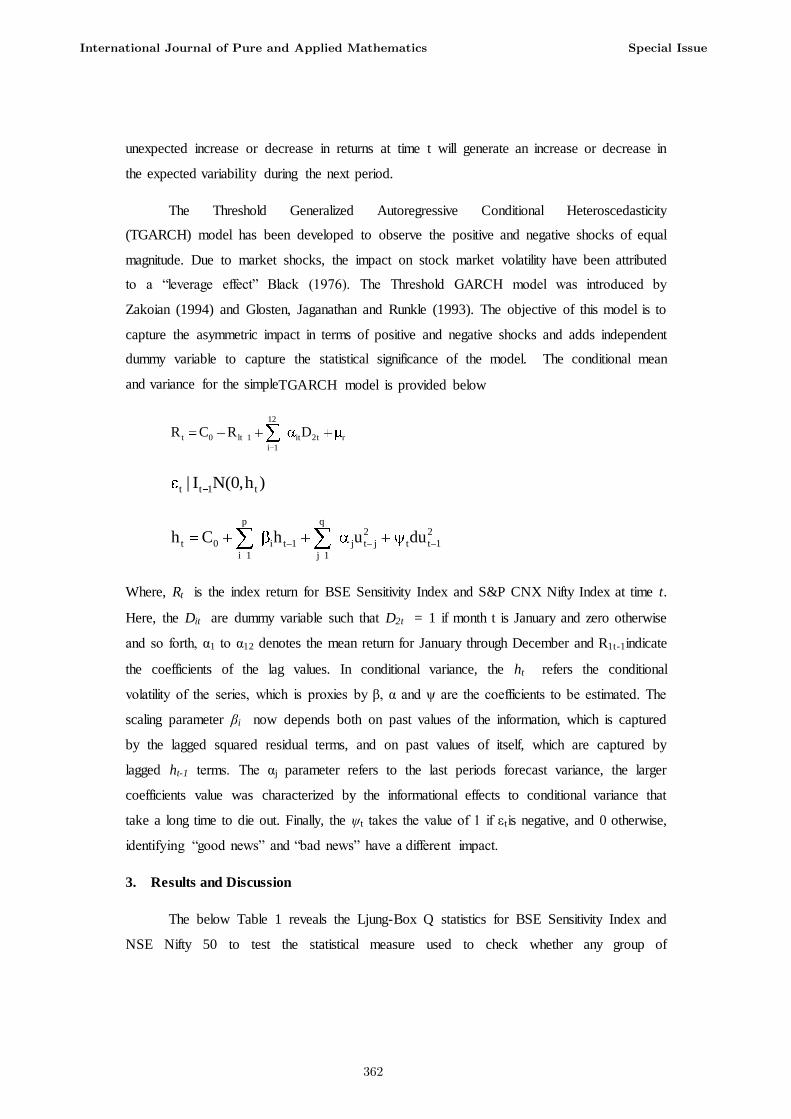
The Threshold Generalized Autoregressive Conditional Heteroscedasticity

(TGARCH) model has been developed to observe the positive and negative shocks of equal

magnitude. Due to market shocks, the impact on stock market volatility have been attributed

to a “leverage effect” Black (1976). The Threshold GARCH model was introduced by

Zakoian (1994) and Glosten, Jaganathan and Runkle (1993). The objective of this model is to

capture the asymmetric impact in terms of positive and negative shocks and adds independent

dummy variable to capture the statistical significance of the model. The conditional mean

and variance for the simpleTGARCH model is provided below

12

t 0 lt 1 it 2t r

i 1

R C R D

t t 1 t| I N(0,h )

p q2 2

t 0 i t 1 j t j t t 1

i 1 j 1

h C h u du

Where, Rt is the index return for BSE Sensitivity Index and S&P CNX Nifty Index at time t.

Here, the Dit are dummy variable such that D2t = 1 if month t is January and zero otherwise

and so forth, α1 to α12 denotes the mean return for January through December and R1t-1indicate

the coefficients of the lag values. In conditional variance, the ht refers the conditional

volatility of the series, which is proxies by β, α and ψ are the coefficients to be estimated. The

scaling parameter βi now depends both on past values of the information, which is captured

by the lagged squared residual terms, and on past values of itself, which are captured by

lagged ht-1 terms. The αj parameter refers to the last periods forecast variance, the larger

coefficients value was characterized by the informational effects to conditional variance that

take a long time to die out. Finally, the ψt takes the value of 1 if εtis negative, and 0 otherwise,

identifying “good news” and “bad news” have a different impact.

3. Results and Discussion

The below Table 1 reveals the Ljung-Box Q statistics for BSE Sensitivity Index and

NSE Nifty 50 to test the statistical measure used to check whether any group of


362

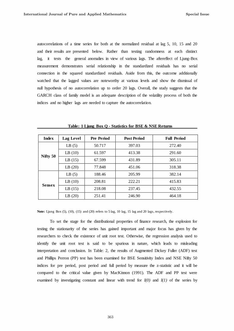
autocorrelations of a time series for both at the normalized residual at lag 5, 10, 15 and 20

and their results are presented below. Rather than testing randomness at each distinct

lag, it tests the general anomalies in view of various lags. The aftereffect of Ljung-Box

measurement demonstrates serial relationship in the standardized residuals has no serial

connection in the squared standardized residuals. Aside from this, the outcome additionally

watched that the lagged values are noteworthy at various levels and show the dismissal of

null hypothesis of no autocorrelation up to order 20 lags. Overall, the study suggests that the

GARCH class of family model is an adequate description of the volatility process of both the

indices and no higher lags are needed to capture the autocorrelation.

Table: 1 Ljung Box Q - Statistics for BSE & NSE Returns

Index Lag Level Pre Period Post Period Full Period

Nifty 50

LB (5) 50.717 397.03 272.40

LB (10) 61.597 413.38 291.60

LB (15) 67.599 431.89 305.11

LB (20) 77.848 451.06 318.38

Sensex

LB (5) 188.46 205.99 382.14

LB (10) 208.81 222.21 415.83

LB (15) 218.08 237.45 432.55

LB (20) 251.41 246.90 464.18

Note: Ljung Box (5), (10), (15) and (20) refers to 5 lag, 10 lag, 15 lag and 20 lags, respectively.

To set the stage for the distributional properties of finance research, the explosion for

testing the stationarity of the series has gained important and major focus has given by the

researchers to check the existence of unit root test. Otherwise, the regression analysis used to

identify the unit root test is said to be spurious in nature, which leads to misleading

interpretation and conclusion. In Table: 2, the results of Augmented Dickey Fuller (ADF) test

and Phillips Perron (PP) test has been examined for BSE Sensitivity Index and NSE Nifty 50

indices for pre period, post period and full period by measure the z-statistic and it will be

compared to the critical value given by MacKinnon (1991). The ADF and PP test were

examined by investigating constant and linear with trend for I(0) and I(1) of the series by


363

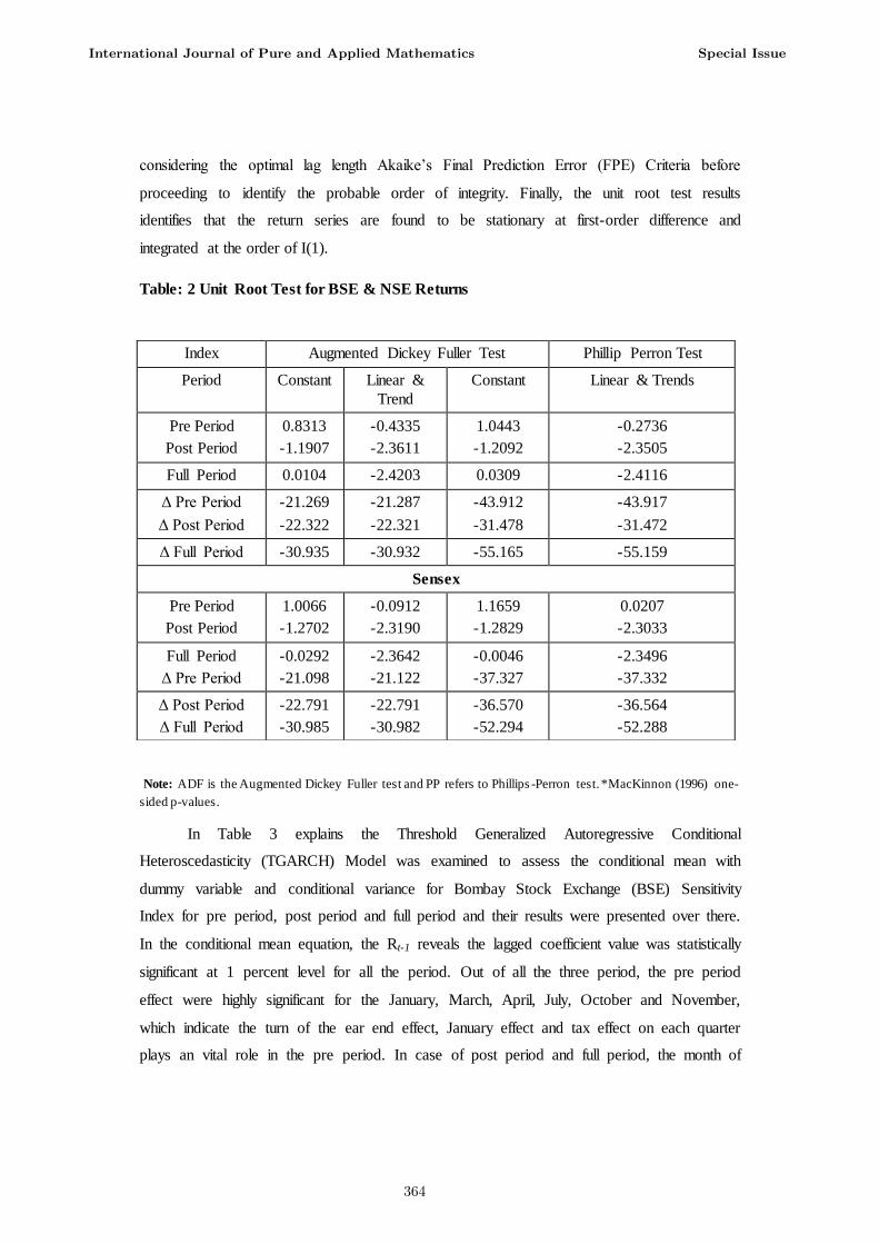
considering the optimal lag length Akaike’s Final Prediction Error (FPE) Criteria before

proceeding to identify the probable order of integrity. Finally, the unit root test results

identifies that the return series are found to be stationary at first-order difference and

integrated at the order of I(1).

Table: 2 Unit Root Test for BSE & NSE Returns

Note: ADF is the Augmented Dickey Fuller test and PP refers to Phillips -Perron test. *MacKinnon (1996) one-

sided p-values.

In Table 3 explains the Threshold Generalized Autoregressive Conditional

Heteroscedasticity (TGARCH) Model was examined to assess the conditional mean with

dummy variable and conditional variance for Bombay Stock Exchange (BSE) Sensitivity

Index for pre period, post period and full period and their results were presented over there.

In the conditional mean equation, the Rt-1 reveals the lagged coefficient value was statistically

significant at 1 percent level for all the period. Out of all the three period, the pre period

effect were highly significant for the January, March, April, July, October and November,

which indicate the turn of the ear end effect, January effect and tax effect on each quarter

plays an vital role in the pre period. In case of post period and full period, the month of

Index Augmented Dickey Fuller Test Phillip Perron Test

Period Constant Linear &

Trend

Constant Linear & Trends

Pre Period

Post Period

0.8313

-1.1907

-0.4335

-2.3611

1.0443

-1.2092

-0.2736

-2.3505

Full Period 0.0104 -2.4203 0.0309 -2.4116

Δ Pre Period

Δ Post Period

-21.269

-22.322

-21.287

-22.321

-43.912

-31.478

-43.917

-31.472

Δ Full Period -30.935 -30.932 -55.165 -55.159

Sensex

Pre Period

Post Period

1.0066

-1.2702

-0.0912

-2.3190

1.1659

-1.2829

0.0207

-2.3033

Full Period

Δ Pre Period

-0.0292

-21.098

-2.3642

-21.122

-0.0046

-37.327

-2.3496

-37.332

Δ Post Period

Δ Full Period

-22.791

-30.985

-22.791

-30.982

-36.570

-52.294

-36.564

-52.288


364

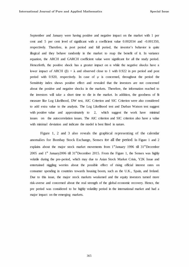
September and January were having positive and negative impact on the market with 1 per

cent and 5 per cent level of significant with a coefficient value 0.002034 and -0.001350,

respectively. Therefore, in post period and full period, the investor’s behavior is quite

illogical and they behave randomly in the market to reap the benefit of it. In variance

equation, the ARCH and GARCH coefficient value were significant for all the study period.

Henceforth, the positive shock has a greater impact on α while the negative shocks have a

lower impact of ARCH (β) + λ and observed close to 1 with 0.922 in pre period and post

period with 0.920, respectively. In case of ψ is concerned, throughout the period the

Sensitivity index shows positive effect and revealed that the investors are not concerned

about the positive and negative shocks in the markets. Therefore, the information reached to

the investors will take a short time to die in the market. In addition, the goodness of fit

measure like Log Likelihood, DW test, AIC Criterion and SIC Criterion were also considered

to add extra value to the analysis. The Log Likelihood test and Durban Watson test suggest

with positive value and approximately to 2, which suggest the work have minimal

issues on the autocorrelation issues. The AIC criterion and SIC criterion also have a value

with minimal deviation and indicate the model is best fitted in nature.

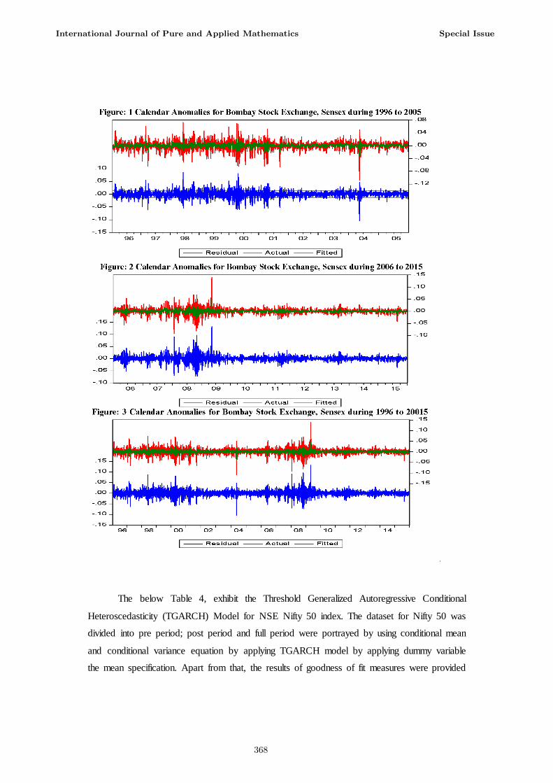
Figure 1, 2 and 3 also reveals the graphical representing of the calendar

anomalies for Bombay Stock Exchange, Sensex for all the period. In Figure 1 and 2

explains about the major stock market movements from 1stJanuary 1996 till 31stDecember

2005 and 1st January2006 till 31stDecember 2015. From the Figure 1, the Sensex was highly

volatile during the pre-period, which may due to Asian Stock Market Crisis, Y2K Issue and

entertained niggling worries about the possible effect of rising official interest rates on

consumer spending in countries towards housing boom, such as the U.K., Spain, and Ireland.

Due to this issue, the major stock markets weakened and the equity investors turned more

risk-averse and concerned about the real strength of the global economic recovery. Hence, the

pre period was considered to be highly volatility period in the international market and had a

major impact on the emerging markets.


365

Table: 3 TGARCH Model for Calendar Anomaly for BSE Sensex Return

Particulars Pre Period Post Period Full Period

Mean Equation

C 0.001948* -0.000173 0.000709

Rt-1 αDJanuary αDFebruary (3.06141)

0.320217*

(15.7735)

-0.003211*

(-3.84044)

-8.31E-05

(-0.34422)

0.348199*

(17.9589)

-0.000222

(-0.35384)

0.000311

(1.77634)

0.337021*

(25.0190)

-0.001350**

(-2.60044)

0.000126

(-0.09884) (0.42867) (0.23220)

αDMarch -0.002611* 0.000835 -0.000358

(-2.67777) (1.14830) (-0.61967)

αDApril -0.002675* 0.000521 -0.000733

(-2.73890) (0.72409) (-1.21641)

αDMay -0.000945 0.000243 -0.000326

(-0.97857) (0.36023) (-0.58507)

αDJune -0.000503 0.000156 0.000010

(-0.51374) (0.22190) (0.01721)

αDJuly -0.001836** 0.00000 -0.000700

(-2.03272) (0.05621) (-1.24988)

αDAugust -0.001521 0.000380 -0.000404

αDSeptember

(-1.63106)

-0.001644

(0.52668)

0.002034*

(-0.69933)

0.000568

(-1.76635) (3.11591) (1.04043)

αDOctober -0.002046** 0.000517 -0.000572

(-2.13870) (0.77277) (-0.99613)

αDNovember -0.000534 0.000177 -0.000056

(-0.50414) (0.24812) (-0.09404)


366

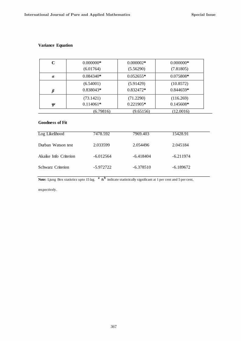
Variance Equation

C 0.000000*

(6.01764)

0.000002*

(5.56290)

0.000000*

(7.81805)

α 0.084340* 0.052655* 0.075808*

β

(6.54001)

0.838043*

(5.91429)

0.832472*

(10.8572)

0.844659*

Ψ

(73.1421)

0.114061*

(71.2290)

0.221905*

(116.269)

0.145608*

(6.79816) (9.65156) (12.0016)

Goodness of Fit

Log Likelihood 7478.592 7969.403 15428.91

Durban Watson test 2.033599 2.054496 2.045184

Akaike Info Criterion -6.012564 -6.418404 -6.211974

Schwarz Criterion -5.972722 -6.378510 -6.189672

Note: Ljung Box statistics upto 15 lag. a

&b

indicate statistically significant at 1 per cent and 5 per cent,

respectively.


367

.

The below Table 4, exhibit the Threshold Generalized Autoregressive Conditional

Heteroscedasticity (TGARCH) Model for NSE Nifty 50 index. The dataset for Nifty 50 was

divided into pre period; post period and full period were portrayed by using conditional mean

and conditional variance equation by applying TGARCH model by applying dummy variable

the mean specification. Apart from that, the results of goodness of fit measures were provided


368

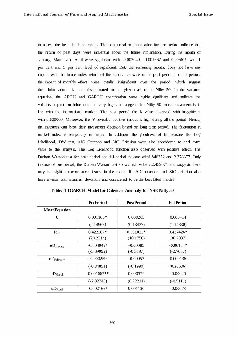
to assess the best fit of the model. The conditional mean equation for pre period indicate that

the return of past days were influential about the future information. During the month of

January, March and April were significant with -0.003049, -0.001667 and 0.005619 with 1

per cent and 5 per cent level of significant. But, the remaining month, does not have any

impact with the future index return of the series. Likewise in the post period and full period,

the impact of monthly effect were totally insignificant over the period, which suggest

the information is not disseminated to a higher level in the Nifty 50. In the variance

equation, the ARCH and GARCH specification were highly significant and indicate the

volatility impact on information is very high and suggest that Nifty 50 index movement is in

line with the international market. The post period the ß value observed with insignificant

with 0.600000. Moreover, the Ψ revealed positive impact is high during all the period. Hence,

the investors can base their investment decision based on long term period. The fluctuation in

market index is temporary in nature. In addition, the goodness of fit measure like Log

Likelihood, DW test, AIC Criterion and SIC Criterion were also considered to add extra

value to the analysis. The Log Likelihood function also observed with positive effect. The

Durban Watson test for post period and full period indicate with1.846252 and 2.278377. Only

in case of pre period, the Durban Watson test shows high value at2.439071 and suggests there

may be slight autocorrelation issues in the model fit. AIC criterion and SIC criterion also

have a value with minimal deviation and considered to be the best fitted model.

Table: 4 TGARCH Model for Calendar Anomaly for NSE Nifty 50

PrePeriod PostPeriod FullPeriod

MeanEquation

C 0.001166* 0.000263 0.000414

(2.14968) (0.13437) (1.14830)

Rt-1 0.422387*

(20.2314)

0.391033*

(10.1756)

0.427426*

(30.7037)

αDJanuary -0.003049*

(-3.89092)

-0.00085

(-0.3197)

-0.00134*

(-2.7087)

αDFebruary -0.000259 -0.00053 0.000136

(-0.34851) (-0.1990) (0.26636)

αDMarch -0.001667** 0.000574 -0.00026

(-2.32748) (0.22211) (-0.5111)

αDApril -0.002166* 0.001180 -0.00073


369

(-2.64552) (0.42841) (-1.2869)

αDMay -0.000936

(-1.07430)

-0.00051

(-0.2024)

-0.00050

(-0.9495)

αDJune -0.000797

(-0.91829)

-0.00024

(-0.0934)

-0.00030

(-0.5491)

αDJuly -0.001548 0.000190 -0.00080

(-1.95537) (0.07166) (-1.5160)

αDAugust -0.001381

(-1.59492)

-0.00039

(-0.1547)

-0.00052

(-0.9492)

αDSeptember -0.001399 0.000775 0.00060

(-1.62837) (0.30962) (1.2020)

αDOctober 0.005619*

(7.17886)

0.000071

(-0.0283)

0.00246*

(5.4504)

αDNovember -0.000294 -0.00014 0.00004

Variance Equation

Goodness of Fit

Log Likelihood 7571.021 7489.424 15573.12

Durban Watson test 2.439071 1.846252 2.278377

Akaike Info Criterion -6.033563 -6.02857 -6.24242

Schwarz Criterion -5.994012 -5.98869 -6.22020

Note: Ljung Box statistics upto 15 lag. a

&b

indicate statistically significant at 1 per cent and 5 per cent,

respectively.

C 0.00001*

(7.11462)

0.000081*

(3.38431)

0.000051*

(9.34271)

α 0.174756*

(7.12889)

0.150000**

(1.99401)

0.106510*

(9.42874)

β 0.632095* 0.600000 0.764057*

(26.0294) (0.60563) (72.3812)

Ψ 0.439506*

(8.98260)

0.050000*

(5.37032)

0.284096*

(12.5480)


370

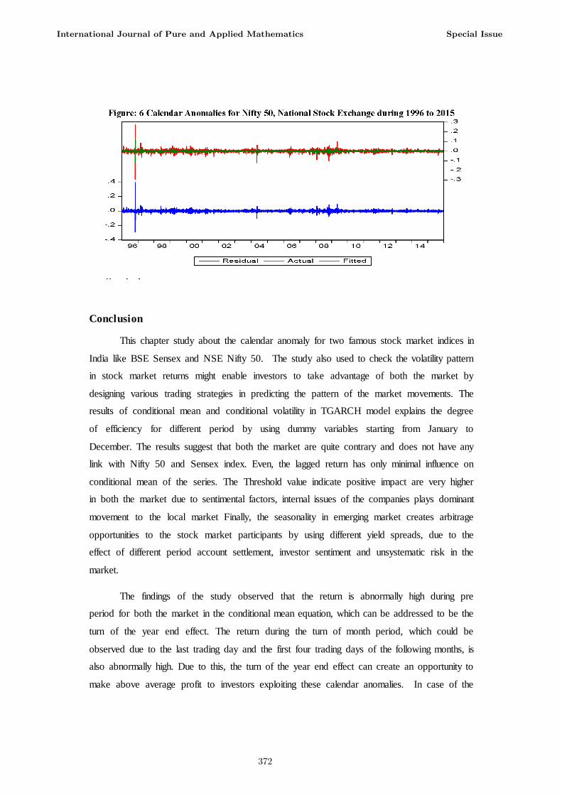
In Figure 4, 5 and 6 also reveals the graphical representing of the calendar anomalies

for National Stock Exchange, Nifty 50 index for all the period. In Figure 4 and 5 explains

about the major stock market movements from 1stJanuary 1996 till 31stDecember 2005 and

1stJanuary2006 till 31stDecember 2015. From the Figure 1, the Nifty 50 script, the volatility

was very low, which indicate reversal pattern when compared to BSE Sensex index. The

market is highly volatility in NSE Nifty 50 index due to recession impact, Oil price crisis,

Chinese Crisis, Russian Crisis all plays a vital role for the major movements in the emerging

stock market.


371

Conclusion

This chapter study about the calendar anomaly for two famous stock market indices in

India like BSE Sensex and NSE Nifty 50. The study also used to check the volatility pattern

in stock market returns might enable investors to take advantage of both the market by

designing various trading strategies in predicting the pattern of the market movements. The

results of conditional mean and conditional volatility in TGARCH model explains the degree

of efficiency for different period by using dummy variables starting from January to

December. The results suggest that both the market are quite contrary and does not have any

link with Nifty 50 and Sensex index. Even, the lagged return has only minimal influence on

conditional mean of the series. The Threshold value indicate positive impact are very higher

in both the market due to sentimental factors, internal issues of the companies plays dominant

movement to the local market Finally, the seasonality in emerging market creates arbitrage

opportunities to the stock market participants by using different yield spreads, due to the

effect of different period account settlement, investor sentiment and unsystematic risk in the

market.

The findings of the study observed that the return is abnormally high during pre

period for both the market in the conditional mean equation, which can be addressed to be the

turn of the year end effect. The return during the turn of month period, which could be

observed due to the last trading day and the first four trading days of the following months, is

also abnormally high. Due to this, the turn of the year end effect can create an opportunity to

make above average profit to investors exploiting these calendar anomalies. In case of the


372

conditional variance, theresult shows that the Bombay Sensitivity Index 30 and Nifty 50 was

highly volatility during the full period. But, the results of the pre and post indicate that the

BSE Sensitivity Index was more volatility in the post period and NSE Nifty 50 indicated with

less volatile in the post period. Therefore, the calendar anomalies may be difficult to be

exploited in practice because of transaction costs and ability to replicate the stock index

return, the existing evidence of calendar anomalies can help investors as the clue for the

timing of investment. Overall, the conclusion is that monthly seasonal might simply be in the

eye of the beholder. As a matter of concern, the research work can be attempted by using

other anomalies in stock market such as turn-of-the- month, Halloween and holiday effect,

could be included to the analysis. In some other cases, the securities could also be analysed

independently or they could be divided into groups based on the impact on various sectors

towards the global economy.

References:

1. Abraham, A. &Ikenberry, D. L. (1994), The Individual Investor and the Weekend Effect,Journal of Financial and Quantitative Analysis, Vol: 29, Pp: 263–77.

2. Agrawal. A.&Tandon, K. (1994), Anomalies or Illusions? Evidence from Stock

Markets inEighteen Countries, Journal of International Money & Finance, Vol: 13, Pp: 83-106.

3. Apollinario, R., Santana, O., Sales, L. and Caro, A. (2006), “Day of the Week Effect onEuropean stock markets, International Research Journal of Finance and Economics, Vol. 2, pp.53–70.

4. Baker. H. Kent, Abdul Rahman and Samir Saadi (2008), “The Day-of-the-Week Effect and Conditional Volatility: Sensitivity of Error Distributional Assumptions”,

Review of Financial Economics, Vol. 17(4), pp. 280-295.

5. Berument, H. and Kiymaz, H. (2003), “The Day-of-the-Week Effect on Stock Market Volatility,Journal of Economics and Finance, Vol. 25, pp. 181–93.

6. Bildik. R (2004), “Are Calendar Anomalies Still Alive? Evidence from Istanbul StockExchange”, Istanbul Stock Exchange.

7. Black. F. (1976), Studies of Stock Market Volatility Changes, Proceedings of the AmericanStatistical Association, Business and Economic Statistics Section, Pp: 177-181.

8. Bollerslev, T. (1986), Generalized Autoregressive Conditional Heteroskedasticity, Journal ofEconometrics, Vol: 31, Pp: 307-327.


373

9. Box, G. E. P. and Jenkins, G. M. (1970), “Time Series Analysis: Forecasting and

Control”, 2nd

Edition. Holden-Day, San Francisco.

10. Brooks, C. (2004), “Introductory Econometrics for Finance”. (6thEdition). The United

Kingdom: Cambridge University Press.

11. Connolly. R. (1989), An Examination of the Robustness of the Weekend Effect,

Journal ofFinancial and Quantitative Analysis, Vol: 24, Pp: 133-69.

12. Connolly. R.A. (1991), A Posterior Odds Analysis of the Weekend Effect ,

Journal ofEconometrics, Vol: 49, Pp: 51-104.

13. Cross, Frank (1973), “The Behavior of Stock Prices on Mondays and Fridays”,

FinancialAnalysts Journal, Vol. 29, pp. 67-69.

14. Dickey. D. A and Fuller. W. A (1979), “Distribution of the Estimators for

Autoregressive TimeSeries with a Unit Root”, Journal of American Statistical Association, Vol. 74, pp. 427 – 431.

15. Engle, R. F. (1982), “Autoregressive Conditional Heteroskedasticity with

estimates of the variance of United Kingdom Inflation”, Econometrica, Vol: 50, Pp: 987-1008.

16. D.Sasikala, R.Roshiniya, Sarishnaratnakaran, Tapati Deb, “Texture Analysis of Plaque in Carotid Artery”, International Journal of Innovations in Scientific and Engineering Research(IJISER), Vol.4, No.2, pp.66-70, 2014.

17. Fama, E. (1970), Efficient Capital Markets: A Review of Theory and Empirical Work Journal ofFinance, Pp. 383-417.

18. Glosten, L. R; Jagannathan, R., &Runkle, D. E, (1993), On the Relation between the

Expected Value and the Volatility of the Nominal Excess Returns on Stocks. Journal of Finance, Vol: 48, No: 5, Pp: 1779-1791.

19. Gultekin, M.N. and Gultekin, N.B (1983), “Stock Market Seasonality: International

Evidence”,Journal of Financial Economics, Vol. 12, pp. 469-481.

20. Jaffe. J. and Westerfield, R. (1985), The Week-End Effect in Common Stock Returns: TheInternational Evidence, Journal of Finance, Vol: 40, Pp: 433–54.

21. Jaffe. J.F. and Westerfield, R. (1989), Is There a Monthly Effect in Stock Market

Returns?,Journal of Banking and Finance, Vol: 13, Pp: 237-44.

22. Keim, D.B (1983), “Size-Related Anomalies and Stock Returns Seasonality: Further EmpiricalEvidence”, Journal of Financial Economics, Vol. 12, pp. 13-32.

23. Lakanishok, J. and Levi, M. (1982), Weekend Effects in Stock Returns: A Note,

Journal ofFinance, Vol: 37, Pp: 883–89.

24. BorgesMaria Ross (2009), “Calendar Effects in Stock Markets: Critique of PreviousMethodologies and Recent Evidence in European Countries” Working Paper

37/2009/DE/UECE

25. Ng Lilian and Qinghai Wang (2004), “Institutional Trading and the Turn-of-the-Year

Effect”,The Journal of Business, Vol. 77(3), pp. 493-509.


374

26. Phillips. R. C. B andPerron. P (1988), Testing for Unit Root in Time Series RegressionBiometrika, Pp: 335 -346.

27. Rozeff, M.S. and Kinney, Jr. W.R., (1976), “Capital Market Seasonality: The Case of StockReturns”, Journal of Financial Economics, Vol. 3, pp. 379-402.

28. Sahar Nawz1andNawazishMirza (2012), “Calendar Anomalies and Stock Returns: A Literature Survey” Journal of Basic. Applied Science Research, Vol.2 (12), pp.12321-12329.

29. Said E. Said and David A. Dickey (1984),”Testing for Unit Roots in Autoregressive MovingAverage Models of Unknown Order” Biometrika, Vol 71(3), pp. 599 – 607.

30. Schwert William G (2001), “Stock Volatility in the New Millenium: How Wacky is NASDAQ?”National Bureau of Economic Research Working Paper 8436.

31. Shanthi, Thamilselvan and Srinivasan (2015), “The Day of the Week Effect and

Conditional Volatility in Indian Stock Market: Evidence from BSE & NSE” International Journal of Applied Engineering Research, Vol 10(3), pp. 7495-7508.

32. Smirlock. M. and Starks, L. (1986), Day-of-the-Week and Intraday Effects in Stock Returns,Journal of Financial Economics, Vol: 17, Pp: 197–210.

33. Wong, K.A. and Ho, H.D. (1986), “The Weekend Effect on Stock Returns in

Singapore”, HongKong Journal of Business Management, Vol. 4, pp. 31-50.

34. Zakoian, J.M. (1994), “Threshold Heteroscedasticity Models”, Journal of Economic

Dynamics and Control, Vol. 18, pp. 931-944.


375

376

CALENDAR ANOMALY IN BSE/NSE INDICES ON ...This paper examines the possible existence and stability of the calendar anomaly for BSE Sensex and NSE Nifty 50 indices on both the mean

Documents