Calculus I Guided Notes, Baylor Fall 2020 - Sites @ Baylor University

Calculus I Guided Notes, Baylor Fall 2020

Jonathan Stanfill

February 23, 2021

Text: Single Variable Calculus: Early Transcendentals, 4th Edition, Jon Rogawski and

Colin Adams

The course covers limits, derivatives, applications of derivatives, and integration:

Functions, Limits, and Rates of Change

• Instantaneous Velocity and Tangent Lines [Section 2.1]

• Investigating Limits [Section 2.2]

• Basic Limit Laws and Continuity [Sections 2.3 and 2.4]

• Indeterminate Forms [Section 2.5]

• The Squeeze Theorem and Trig Limits [Section 2.6]

• Limits at Infinity [Section 2.7]

• Intermediate Value Theorem [Section 2.8]

Differentiation

• Definition of the Derivative [Section 3.1]

• The Derivative as a Function [Section 3.2]

• Product and Quotient Rules [Section 3.3]

• Rates of Change [Section 3.4]

• Higher Derivatives [Section 3.5]

• Trigonometric Functions [Section 3.6]

• The Chain Rule [Section 3.7]

• Implicit Differentiation [Section 3.8]

• Exponential and Logarithmic Functions [Section 3.9]

• Related Rates [Section 3.10]

Applications of the Derivative

• Linear Approximation and Applications [Section 4.1]

• Extreme Values [Section 4.2]

• The Mean Value Theorem and Monotonicity [Section 4.3]

1

• The Second Derivative and Concavity [Section 4.4]

• Analyzing and Sketching Graphs of Functions [Section 4.6]

• Applied Optimization [Section 4.7]

Integration

• Approximating and Computing Area and the Definite Integral [Sections 5.1 and 5.2]

• The Indefinite Integral [Section 5.3]

• The Fundamental Theorem of Calculus [Sections 5.4 and 5.5]

• Net Change as the Integral of a Rate of Change [Section 5.6]

• The Substitution Method and Further Integral Formulas [Sections 5.7 and 5.8]

What is calculus?

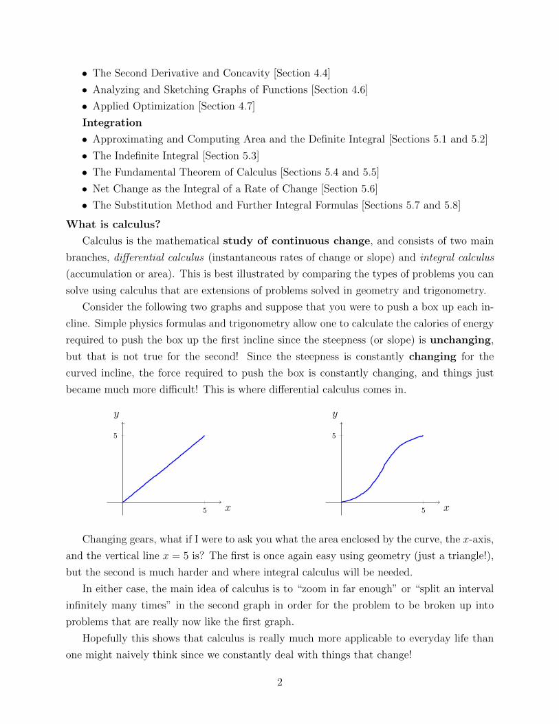
Calculus is the mathematical study of continuous change, and consists of two main

branches, differential calculus (instantaneous rates of change or slope) and integral calculus

(accumulation or area). This is best illustrated by comparing the types of problems you can

solve using calculus that are extensions of problems solved in geometry and trigonometry.

Consider the following two graphs and suppose that you were to push a box up each in-

cline. Simple physics formulas and trigonometry allow one to calculate the calories of energy

required to push the box up the first incline since the steepness (or slope) is unchanging,

but that is not true for the second! Since the steepness is constantly changing for the

curved incline, the force required to push the box is constantly changing, and things just

became much more difficult! This is where differential calculus comes in.

5

5

x

y

5

5

x

y

Changing gears, what if I were to ask you what the area enclosed by the curve, the x-axis,

and the vertical line x = 5 is? The first is once again easy using geometry (just a triangle!),

but the second is much harder and where integral calculus will be needed.

In either case, the main idea of calculus is to “zoom in far enough” or “split an interval

infinitely many times” in the second graph in order for the problem to be broken up into

problems that are really now like the first graph.

Hopefully this shows that calculus is really much more applicable to everyday life than

one might naively think since we constantly deal with things that change!

2

2.1 Instantaneous Velocity and Tangent Lines

RATES OF CHANGE

A rate of change is always a ratio, a comparison of output and input values.

change in output

change in input,

∆y

∆x,y2 − y1

x2 − x1

, etc.

We are very familiar with this idea in the context of slope, speed, and velocity.

Note: Change in position is +/− based on direction, so velocity is more informative than

speed.

Distance = Rate × Time

Change in position = velocity× change in time

Note: This only makes sense if velocity is constant !

But for any problem, we can talk about average velocity over a time frame. What does

average velocity mean?

Example 1: If a flight from Dallas to Los Angeles takes about 3 hours and covers a distance

of 1240 miles, what is the average velocity of the plane?

Average velocity over [t0, t1] =change in position

change in time=

∆s

∆t=s(t1)− s(t0)

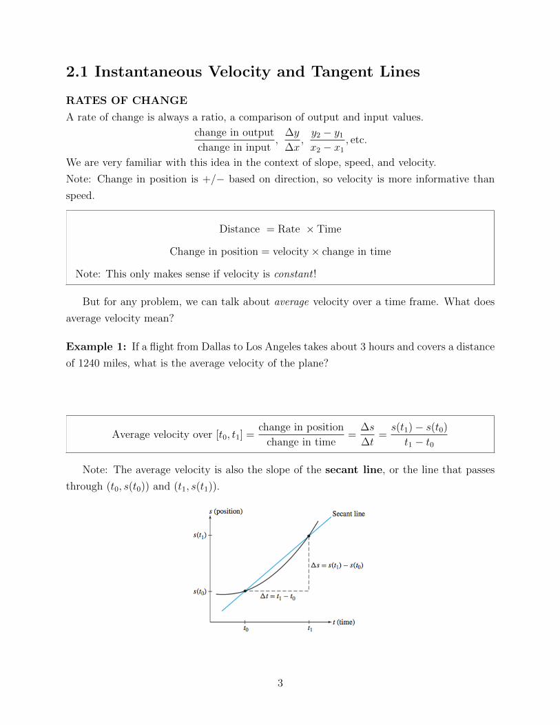
t1 − t0

Note: The average velocity is also the slope of the secant line, or the line that passes

through (t0, s(t0)) and (t1, s(t1)).

3

Example 2: A ball dropped from a state of rest at time t = 0 travels a distance of

s(t) = 4.9t2 m in t seconds.

(a) How far does the ball travel during the time interval [1.5, 2]?

(b) Compute the average velocity over [1.5, 2].

(c) Compute the average velocity for the time intervals in the table and estimate the ball’s

instantaneous velocity at t = 1.5.

Interval [1.5, 1.51] [1.5, 1.505] [1.5, 1.501] [1.5, 1.50001]

Average velocity in m/s 14.749 14.7245 14.7049 14.700049

BUT: What if we want the velocity at a particular instant?

If the function is linear →If the function is NOT linear →

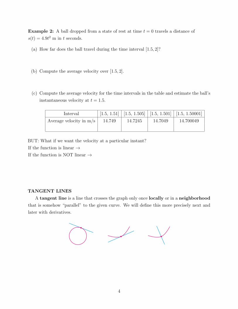
TANGENT LINES

A tangent line is a line that crosses the graph only once locally or in a neighborhood

that is somehow “parallel” to the given curve. We will define this more precisely next and

later with derivatives.

4

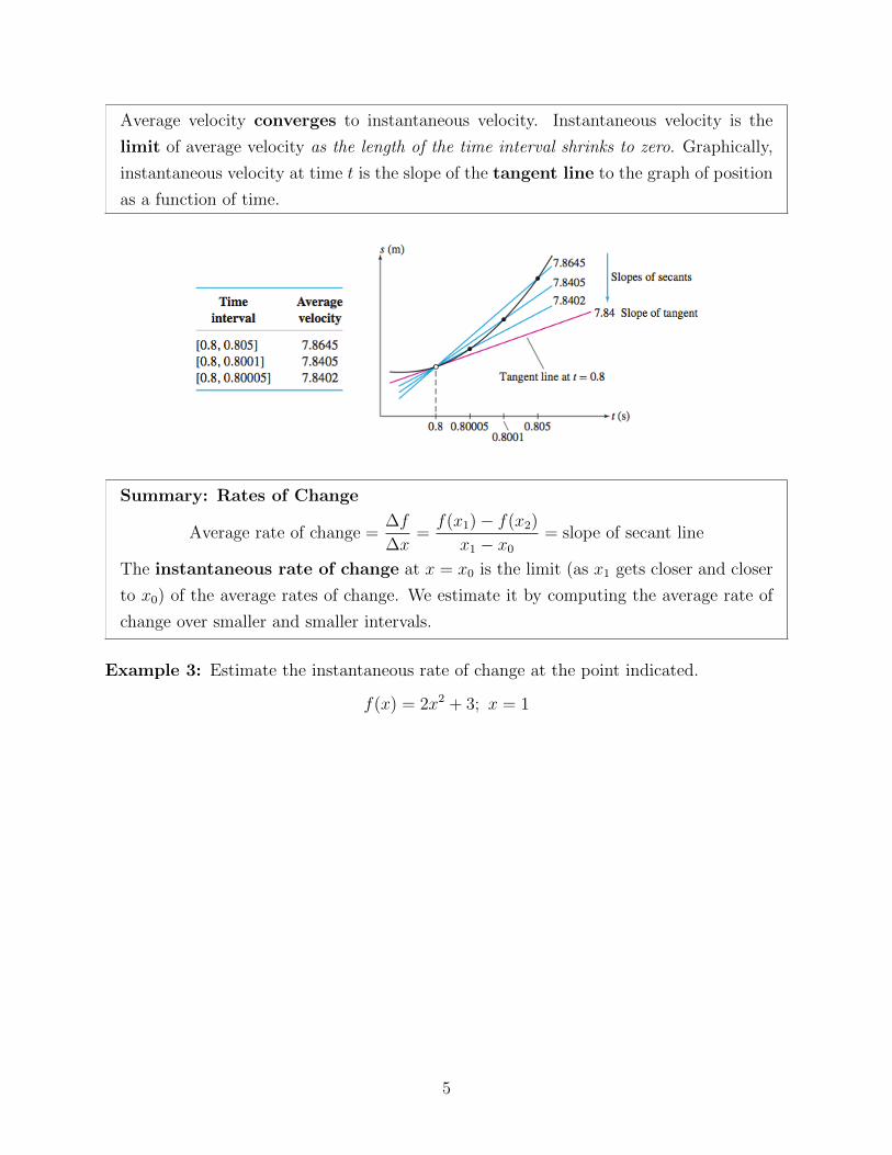
Average velocity converges to instantaneous velocity. Instantaneous velocity is the

limit of average velocity as the length of the time interval shrinks to zero. Graphically,

instantaneous velocity at time t is the slope of the tangent line to the graph of position

as a function of time.

Summary: Rates of Change

Average rate of change =∆f

∆x=f(x1)− f(x2)

x1 − x0

= slope of secant line

The instantaneous rate of change at x = x0 is the limit (as x1 gets closer and closer

to x0) of the average rates of change. We estimate it by computing the average rate of

change over smaller and smaller intervals.

Example 3: Estimate the instantaneous rate of change at the point indicated.

f(x) = 2x2 + 3; x = 1

5

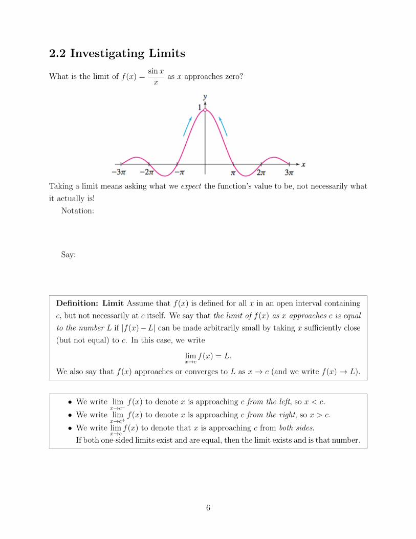
2.2 Investigating Limits

What is the limit of f(x) =sinx

xas x approaches zero?

Taking a limit means asking what we expect the function’s value to be, not necessarily what

it actually is!

Notation:

Say:

Definition: Limit Assume that f(x) is defined for all x in an open interval containing

c, but not necessarily at c itself. We say that the limit of f(x) as x approaches c is equal

to the number L if |f(x)−L| can be made arbitrarily small by taking x sufficiently close

(but not equal) to c. In this case, we write

limx→c

f(x) = L.

We also say that f(x) approaches or converges to L as x→ c (and we write f(x)→ L).

• We write limx→c−

f(x) to denote x is approaching c from the left, so x < c.

• We write limx→c+

f(x) to denote x is approaching c from the right, so x > c.

• We write limx→c

f(x) to denote that x is approaching c from both sides.

If both one-sided limits exist and are equal, then the limit exists and is that number.

6

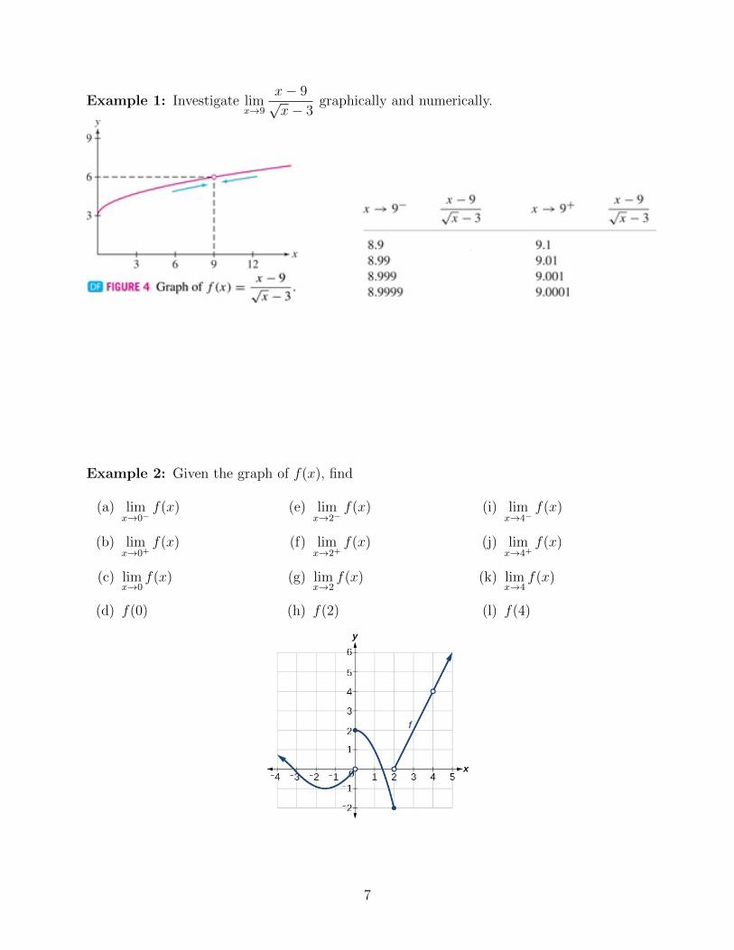
Example 1: Investigate limx→9

x− 9√x− 3

graphically and numerically.

Example 2: Given the graph of f(x), find

(a) limx→0−

f(x)

(b) limx→0+

f(x)

(c) limx→0

f(x)

(d) f(0)

(e) limx→2−

f(x)

(f) limx→2+

f(x)

(g) limx→2

f(x)

(h) f(2)

(i) limx→4−

f(x)

(j) limx→4+

f(x)

(k) limx→4

f(x)

(l) f(4)

7

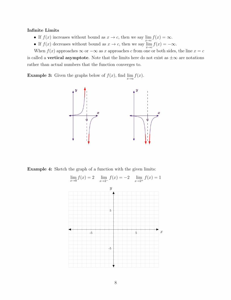
Infinite Limits

• If f(x) increases without bound as x→ c, then we say limx→c

f(x) =∞.

• If f(x) decreases without bound as x→ c, then we say limx→c

f(x) = −∞.

When f(x) approaches∞ or −∞ as x approaches c from one or both sides, the line x = c

is called a vertical asymptote. Note that the limits here do not exist as ±∞ are notations

rather than actual numbers that the function converges to.

Example 3: Given the graphs below of f(x), find limx→a

f(x).

Example 4: Sketch the graph of a function with the given limits:

limx→0

f(x) = 2 limx→2−

f(x) = −2 limx→2+

f(x) = 1

-5 5

-5

5

x

y

8

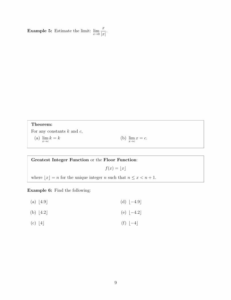
Example 5: Estimate the limit: limx→0

x

|x|.

Theorem:

For any constants k and c,

(a) limx→c

k = k (b) limx→c

x = c.

Greatest Integer Function or the Floor Function:

f(x) = bxc

where bxc = n for the unique integer n such that n ≤ x < n+ 1.

Example 6: Find the following:

(a) b4.9c

(b) b4.2c

(c) b4c

(d) b−4.9c

(e) b−4.2c

(f) b−4c

9

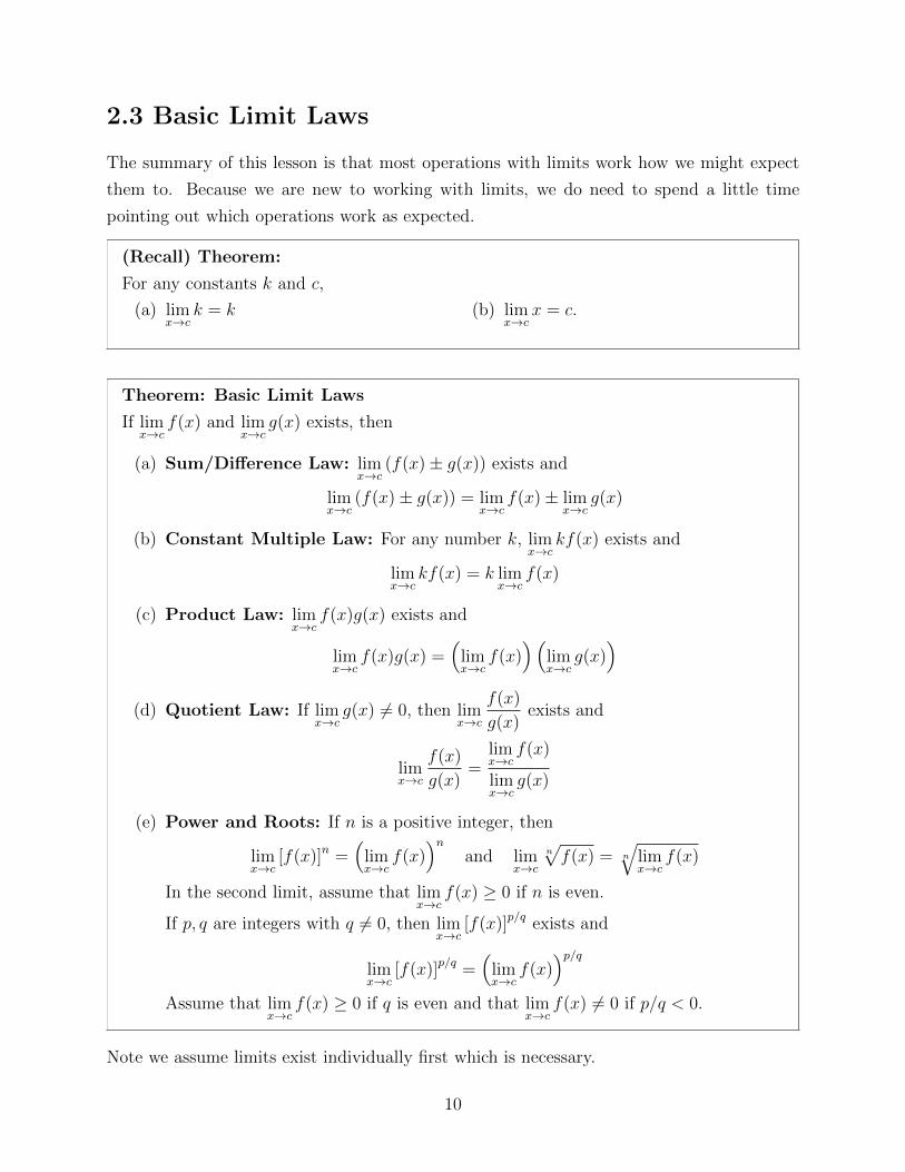
2.3 Basic Limit Laws

The summary of this lesson is that most operations with limits work how we might expect

them to. Because we are new to working with limits, we do need to spend a little time

pointing out which operations work as expected.

(Recall) Theorem:

For any constants k and c,

(a) limx→c

k = k (b) limx→c

x = c.

Theorem: Basic Limit Laws

If limx→c

f(x) and limx→c

g(x) exists, then

(a) Sum/Difference Law: limx→c

(f(x)± g(x)) exists and

limx→c

(f(x)± g(x)) = limx→c

f(x)± limx→c

g(x)

(b) Constant Multiple Law: For any number k, limx→c

kf(x) exists and

limx→c

kf(x) = k limx→c

f(x)

(c) Product Law: limx→c

f(x)g(x) exists and

limx→c

f(x)g(x) =(

limx→c

f(x))(

limx→c

g(x))

(d) Quotient Law: If limx→c

g(x) 6= 0, then limx→c

f(x)

g(x)exists and

limx→c

f(x)

g(x)=

limx→c

f(x)

limx→c

g(x)

(e) Power and Roots: If n is a positive integer, then

limx→c

[f(x)]n =(

limx→c

f(x))n

and limx→c

n√f(x) = n

√limx→c

f(x)

In the second limit, assume that limx→c

f(x) ≥ 0 if n is even.

If p, q are integers with q 6= 0, then limx→c

[f(x)]p/q exists and

limx→c

[f(x)]p/q =(

limx→c

f(x))p/q

Assume that limx→c

f(x) ≥ 0 if q is even and that limx→c

f(x) 6= 0 if p/q < 0.

Note we assume limits exist individually first which is necessary.

10

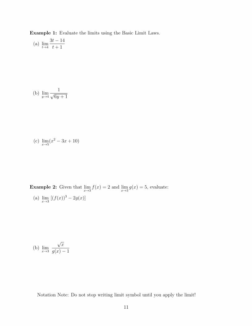
Example 1: Evaluate the limits using the Basic Limit Laws.

(a) limt→4

3t− 14

t+ 1

(b) limy→4

1√6y + 1

(c) limx→5

(x2 − 3x+ 10)

Example 2: Given that limx→3

f(x) = 2 and limx→3

g(x) = 5, evaluate:

(a) limx→3

[(f(x))3 − 2g(x)]

(b) limx→3

√x

g(x)− 1

Notation Note: Do not stop writing limit symbol until you apply the limit!

11

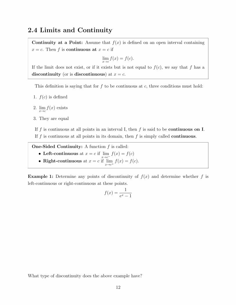
2.4 Limits and Continuity

Continuity at a Point: Assume that f(x) is defined on an open interval containing

x = c. Then f is continuous at x = c if

limx→c

f(x) = f(c).

If the limit does not exist, or if it exists but is not equal to f(c), we say that f has a

discontinuity (or is discontinuous) at x = c.

This definition is saying that for f to be continuous at c, three conditions must hold:

1. f(c) is defined

2. limx→c

f(x) exists

3. They are equal

If f is continuous at all points in an interval I, then f is said to be continuous on I.

If f is continuous at all points in its domain, then f is simply called continuous.

One-Sided Continuity: A function f is called:

• Left-continuous at x = c if limx→c−

f(x) = f(c)

• Right-continuous at x = c if limx→c+

f(x) = f(c).

Example 1: Determine any points of discontinuity of f(x) and determine whether f is

left-continuous or right-continuous at these points.

f(x) =1

ex − 1

What type of discontinuity does the above example have?

12

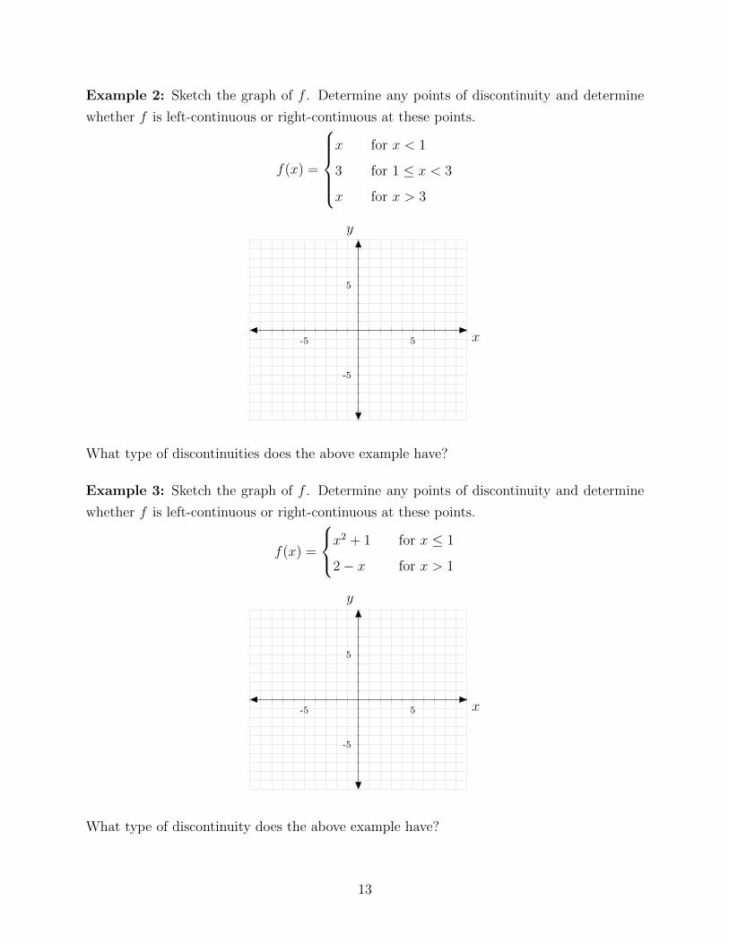
Example 2: Sketch the graph of f . Determine any points of discontinuity and determine

whether f is left-continuous or right-continuous at these points.

f(x) =

x for x < 1

3 for 1 ≤ x < 3

x for x > 3

-5 5

-5

5

x

y

What type of discontinuities does the above example have?

Example 3: Sketch the graph of f . Determine any points of discontinuity and determine

whether f is left-continuous or right-continuous at these points.

f(x) =

x2 + 1 for x ≤ 1

2− x for x > 1

-5 5

-5

5

x

y

What type of discontinuity does the above example have?

13

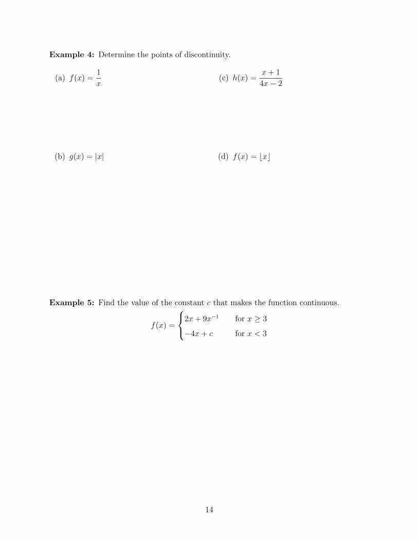
Example 4: Determine the points of discontinuity.

(a) f(x) =1

x

(b) g(x) = |x|

(c) h(x) =x+ 1

4x− 2

(d) f(x) = bxc

Example 5: Find the value of the constant c that makes the function continuous.

f(x) =

2x+ 9x−1 for x ≥ 3

−4x+ c for x < 3

14

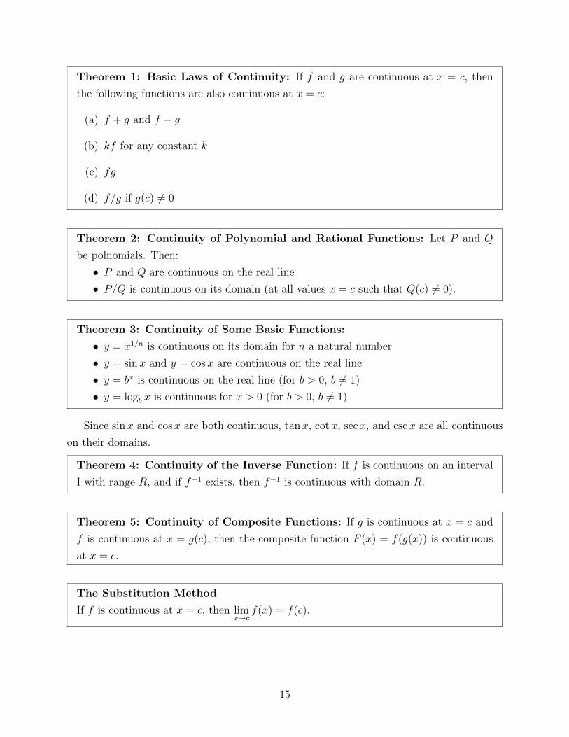
Theorem 1: Basic Laws of Continuity: If f and g are continuous at x = c, then

the following functions are also continuous at x = c:

(a) f + g and f − g

(b) kf for any constant k

(c) fg

(d) f/g if g(c) 6= 0

Theorem 2: Continuity of Polynomial and Rational Functions: Let P and Q

be polnomials. Then:

• P and Q are continuous on the real line

• P/Q is continuous on its domain (at all values x = c such that Q(c) 6= 0).

Theorem 3: Continuity of Some Basic Functions:

• y = x1/n is continuous on its domain for n a natural number

• y = sinx and y = cosx are continuous on the real line

• y = bx is continuous on the real line (for b > 0, b 6= 1)

• y = logb x is continuous for x > 0 (for b > 0, b 6= 1)

Since sinx and cosx are both continuous, tanx, cotx, secx, and csc x are all continuous

on their domains.

Theorem 4: Continuity of the Inverse Function: If f is continuous on an interval

I with range R, and if f−1 exists, then f−1 is continuous with domain R.

Theorem 5: Continuity of Composite Functions: If g is continuous at x = c and

f is continuous at x = g(c), then the composite function F (x) = f(g(x)) is continuous

at x = c.

The Substitution Method

If f is continuous at x = c, then limx→c

f(x) = f(c).

15

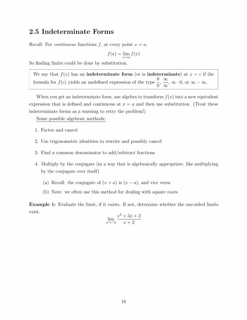
2.5 Indeterminate Forms

Recall: For continuous functions f , at every point x = a,

f(a) = limx→a

f(x)

So finding limits could be done by substitution.

We say that f(x) has an indeterminate form (or is indeterminate) at x = c if the

formula for f(c) yields an undefined expression of the type0

0,∞∞

, ∞ · 0, or ∞−∞.

When you get an indeterminate form, use algebra to transform f(x) into a new equivalent

expression that is defined and continuous at x = a and then use substitution. (Treat these

indeterminate forms as a warning to retry the problem!)

Some possible algebraic methods:

1. Factor and cancel

2. Use trigonometric identities to rewrite and possibly cancel

3. Find a common denominator to add/subtract fractions

4. Multiply by the conjugate (in a way that is algebraically appropriate, like multiplying

by the conjugate over itself)

(a) Recall: the conjugate of (x+ a) is (x− a), and vice versa

(b) Note: we often use this method for dealing with square roots

Example 1: Evaluate the limit, if it exists. If not, determine whether the one-sided limits

exist.

limx→−2

x2 + 3x+ 2

x+ 2

16

Sometimes, you get things that are infinite, but NOT indeterminate. For example,a

∞and

a

0are not indeterminate forms.

Example 2: Evaluate the limit, if it exists.

limx→−1

x2 − 4x+ 7

x+ 1

Example 3:

(a) limx→π/2

tanx

secx

(b) limx→1

(1

1− x− 2

1− x2

)

17

Example 4: Evaluate the limits:

(a) limx→8

√x− 4− 2

x− 8(b) lim

x→9

√x− 3

x− 9

Example 5:

limh→0

(h+ a)2 − a2

h

18

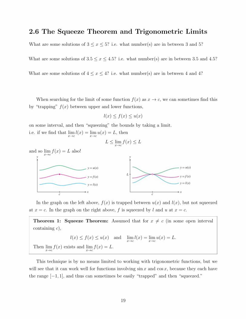
2.6 The Squeeze Theorem and Trigonometric Limits

What are some solutions of 3 ≤ x ≤ 5? i.e. what number(s) are in between 3 and 5?

What are some solutions of 3.5 ≤ x ≤ 4.5? i.e. what number(s) are in between 3.5 and 4.5?

What are some solutions of 4 ≤ x ≤ 4? i.e. what number(s) are in between 4 and 4?

When searching for the limit of some function f(x) as x→ c, we can sometimes find this

by “trapping” f(x) between upper and lower functions,

l(x) ≤ f(x) ≤ u(x)

on some interval, and then “squeezing” the bounds by taking a limit.

i.e. if we find that limx→c

l(x) = limx→c

u(x) = L, then

L ≤ limx→c

f(x) ≤ L

and so limx→c

f(x) = L also!

In the graph on the left above, f(x) is trapped between u(x) and l(x), but not squeezed

at x = c. In the graph on the right above, f is squeezed by l and u at x = c.

Theorem 1: Squeeze Theorem: Assumed that for x 6= c (in some open interval

containing c),

l(x) ≤ f(x) ≤ u(x) and limx→c

l(x) = limx→c

u(x) = L.

Then limx→c

f(x) exists and limx→c

f(x) = L.

This technique is by no means limited to working with trigonometric functions, but we

will see that it can work well for functions involving sinx and cosx, because they each have

the range [−1, 1], and thus can sometimes be easily “trapped” and then “squeezed.”

19

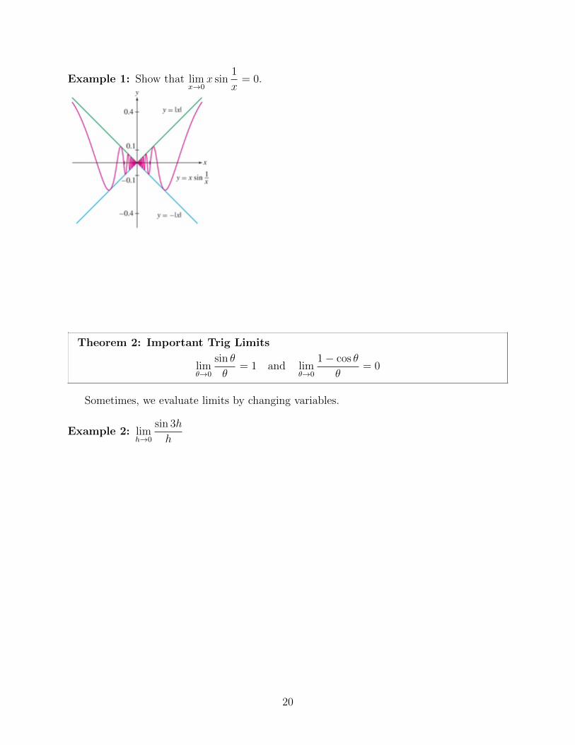
Example 1: Show that limx→0

x sin1

x= 0.

Theorem 2: Important Trig Limits

limθ→0

sin θ

θ= 1 and lim

θ→0

1− cos θ

θ= 0

Sometimes, we evaluate limits by changing variables.

Example 2: limh→0

sin 3h

h

20

Example 3: limx→1

(x− 1) sinπ

x− 1

Example 4: limt→2

(2t − 4) cos1

t− 2

Example 5: limx→0

tan 4x

tan 9x

21

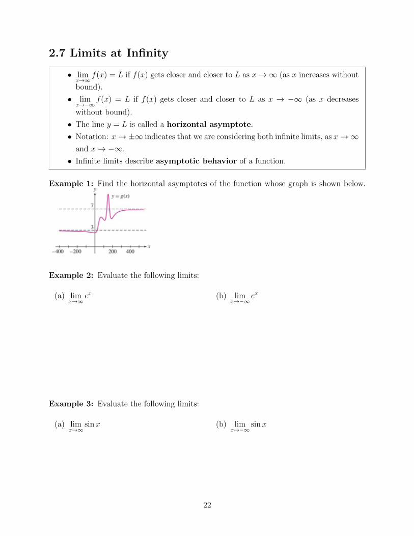
2.7 Limits at Infinity

• limx→∞

f(x) = L if f(x) gets closer and closer to L as x→∞ (as x increases without

bound).

• limx→−∞

f(x) = L if f(x) gets closer and closer to L as x → −∞ (as x decreases

without bound).

• The line y = L is called a horizontal asymptote.

• Notation: x→ ±∞ indicates that we are considering both infinite limits, as x→∞and x→ −∞.

• Infinite limits describe asymptotic behavior of a function.

Example 1: Find the horizontal asymptotes of the function whose graph is shown below.

Example 2: Evaluate the following limits:

(a) limx→∞

ex (b) limx→−∞

ex

Example 3: Evaluate the following limits:

(a) limx→∞

sinx (b) limx→−∞

sinx

22

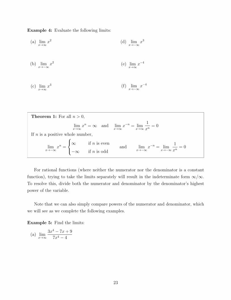
Example 4: Evaluate the following limits:

(a) limx→∞

x2

(b) limx→−∞

x2

(c) limx→∞

x3

(d) limx→−∞

x3

(e) limx→∞

x−4

(f) limx→−∞

x−4

Theorem 1: For all n > 0,

limx→∞

xn =∞ and limx→∞

x−n = limx→∞

1

xn= 0

If n is a positive whole number,

limx→−∞

xn =

∞ if n is even

−∞ if n is oddand lim

x→−∞x−n = lim

x→−∞

1

xn= 0

For rational functions (where neither the numerator nor the denominator is a constant

function), trying to take the limits separately will result in the indeterminate form ∞/∞.

To resolve this, divide both the numerator and denominator by the denominator’s highest

power of the variable.

Note that we can also simply compare powers of the numerator and denominator, which

we will see as we complete the following examples.

Example 5: Find the limits:

(a) limx→∞

3x4 − 7x+ 9

7x4 − 4

23

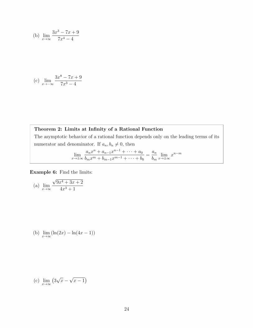
(b) limx→∞

3x3 − 7x+ 9

7x4 − 4

(c) limx→−∞

3x8 − 7x+ 9

7x3 − 4

Theorem 2: Limits at Infinity of a Rational Function

The asymptotic behavior of a rational function depends only on the leading terms of its

numerator and denominator. If an, bn 6= 0, then

limx→±∞

anxn + an−1x

n−1 + · · ·+ a0

bmxm + bm−1xm−1 + · · ·+ b0

=anbm

limx→±∞

xn−m

Example 6: Find the limits:

(a) limx→∞

√9x4 + 3x+ 2

4x3 + 1

(b) limx→∞

(ln(2x)− ln(4x− 1))

(c) limx→∞

(3√x−√x− 1

)

24

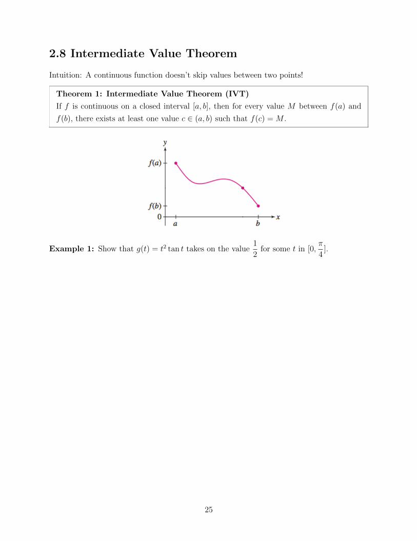
2.8 Intermediate Value Theorem

Intuition: A continuous function doesn’t skip values between two points!

Theorem 1: Intermediate Value Theorem (IVT)

If f is continuous on a closed interval [a, b], then for every value M between f(a) and

f(b), there exists at least one value c ∈ (a, b) such that f(c) = M .

Example 1: Show that g(t) = t2 tan t takes on the value1

2for some t in [0,

π

4].

25

Example 2: Show that f(x) =x2

x7 + 1takes on the value 0.4.

Corollary 2: Existence of Zeros

If f is continuous on [a, b] and if f(a) and f(b) are nonzero and have opposite signs, then

f has a zero in (a, b).

Example 3: Prove, using the IVT, that 2x = bx has a solution if b > 2.

26

Example 4: Show that 2x + 3x = 4x has a solution.

Example 5: Can the IVT be used to show that f(x) =1

xhas a zero on the interval [−1, 1]?

Why or why not?

27

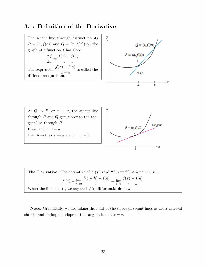
3.1: Definition of the Derivative

The secant line through distinct points

P = (a, f(a)) and Q = (x, f(x)) on the

graph of a function f has slope

∆f

∆x=f(x)− f(a)

x− a.

The expressionf(x)− f(a)

x− ais called the

difference quotient.

As Q → P , or x → a, the secant line

through P and Q gets closer to the tan-

gent line through P .

If we let h = x− a,

then h→ 0 as x→ a and x = a+ h.

The Derivative: The derivative of f (f ′, read “f prime”) at a point a is:

f ′(a) = limh→0

f(a+ h)− f(a)

h= lim

x→a

f(x)− f(a)

x− a.

When the limit exists, we say that f is differentiable at a.

Note: Graphically, we are taking the limit of the slopes of secant lines as the x-interval

shrinks and finding the slope of the tangent line at x = a.

28

Theorem 1: Derivative of Linear and Constant Functions

(a) If f(x) = mx+ b is a linear function, then f ′(a) = for all a.

(b) If f(x) = b is a constant function, then f ′(a) = for all a.

Proof.

Tangent Line: If f is differentiable at a (i.e. the limit of the difference quotient exists),

then the tangent line to the graph of y = f(x) at P = (a, f(a)) is the line through P

of slope f ′(a). The equation of the tangent line in point-slope form is

y − f(a) = f ′(a)(x− a).

Example 1: Compute f ′(a) in two ways:

(a) f(x) = x2 + 3x, a = 0

29

(b) f(x) =1

x+ 1, a = 4

Example 2: (a) If f ′(a) = limh→0

cos(π

4+ h)−√

2

2h

, then f(x) = and a =

(b) If f ′(a) = limh→0

34+h − 81

h, then f(x) = and a =

Example 3: Find the derivative of f at x = 2, 4 where the graph of f is given below.

Now consider the derivative at x = 3.

30

Example 4: Use the limit definition to compute f ′(a). Find an equation of the tangent

line.

(a) f(x) = 4− x2, a = −1

(b) f(x) = x−1, a = 8

(c) f(t) =√

3t+ 5, a = −1

31

3.2: The Derivative as a Function

We have already defined the derivative at a point a with the equation

f ′(a) = limh→0

f(a+ h)− f(a)

h.

By replacing a with x, we can define the derivative as a function:

f ′(x) = limh→0

f(x+ h)− f(x)

h.

We say that f is differentiable on (a, b) if f ′(x) exists for all x in (a, b).

When f ′(x) exists for all x in the interval or intervals on which f(x) is defined, we simply

say that f is differentiable.

Example 1: Compute f ′(x) using the limit definition for f(x) =√x− x2.

32

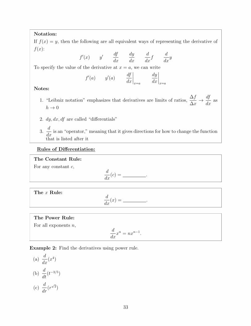
Notation:

If f(x) = y, then the following are all equivalent ways of representing the derivative of

f(x):

f ′(x) y′df

dx

dy

dx

d

dxf

d

dxy

To specify the value of the derivative at x = a, we can write

f ′(a) y′(a)df

dx

∣∣∣∣x=a

dy

dx

∣∣∣∣x=a

Notes:

1. “Leibniz notation” emphasizes that derivatives are limits of ratios,∆f

∆x→ df

dxas

h→ 0

2. dy, dx, df are called “differentials”

3.d

dxis an “operator,” meaning that it gives directions for how to change the function

that is listed after it

Rules of Differentiation:

The Constant Rule:

For any constant c,d

dx(c) = .

The x Rule:d

dx(x) = .

The Power Rule:

For all exponents n,d

dxxn = nxn−1.

Example 2: Find the derivatives using power rule.

(a)d

dx(x4)

(b)d

dt(t−3/5)

(c)d

dr(r√

2)

33

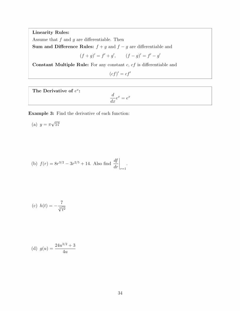
Linearity Rules:

Assume that f and g are differentiable. Then

Sum and Difference Rules: f + g and f − g are differentiable and

(f + g)′ = f ′ + g′, (f − g)′ = f ′ − g′

Constant Multiple Rule: For any constant c, cf is differentiable and

(cf)′ = cf ′

The Derivative of ex:d

dxex = ex

Example 3: Find the derivative of each function:

(a) y = π√

57

(b) f(r) = 8r3/2 − 3r2/5 + 14. Also finddf

dr

∣∣∣∣r=1

.

(c) h(t) = − 73√t2

(d) g(u) =24u3/2 + 3

4u

34

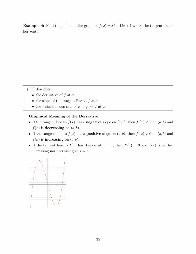
Example 4: Find the points on the graph of f(x) = x3 − 12x+ 1 where the tangent line is

horizontal.

f ′(x) describes:

• the derivative of f at x

• the slope of the tangent line to f at x

• the instantaneous rate of change of f at x

Graphical Meaning of the Derivative:

• If the tangent line to f(x) has a negative slope on (a, b), then f ′(x) < 0 on (a, b) and

f(x) is decreasing on (a, b).

• If the tangent line to f(x) has a positive slope on (a, b), then f ′(x) > 0 on (a, b) and

f(x) is increasing on (a, b).

• If the tangent line to f(x) has 0 slope at x = a, then f ′(a) = 0 and f(x) is neither

increasing nor decreasing at x = a.

35

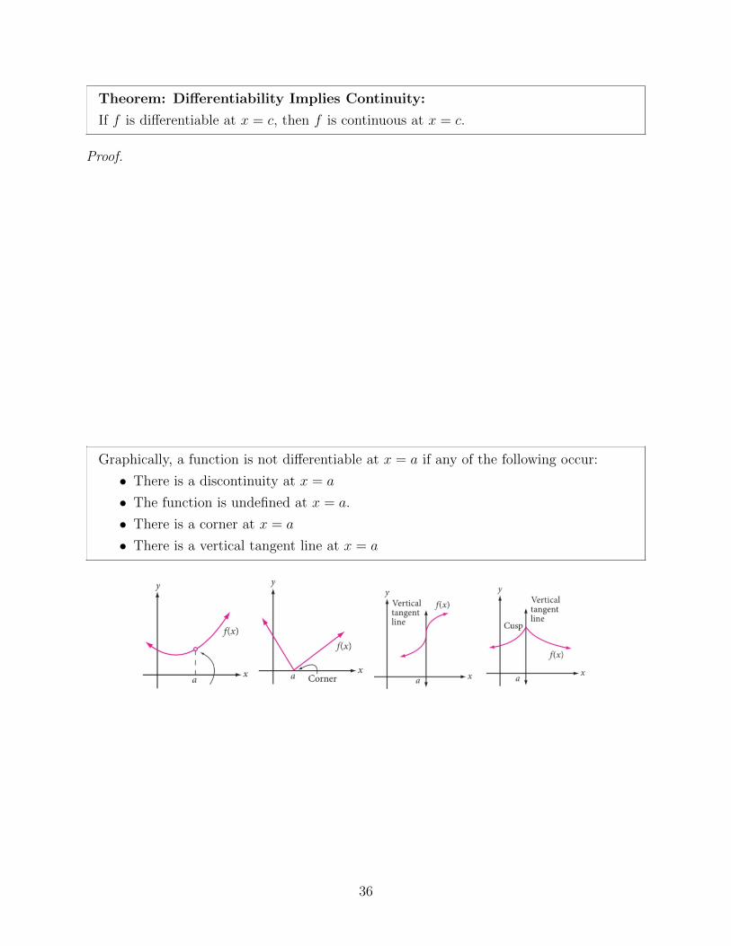
Theorem: Differentiability Implies Continuity:

If f is differentiable at x = c, then f is continuous at x = c.

Proof.

Graphically, a function is not differentiable at x = a if any of the following occur:

• There is a discontinuity at x = a

• The function is undefined at x = a.

• There is a corner at x = a

• There is a vertical tangent line at x = a

36

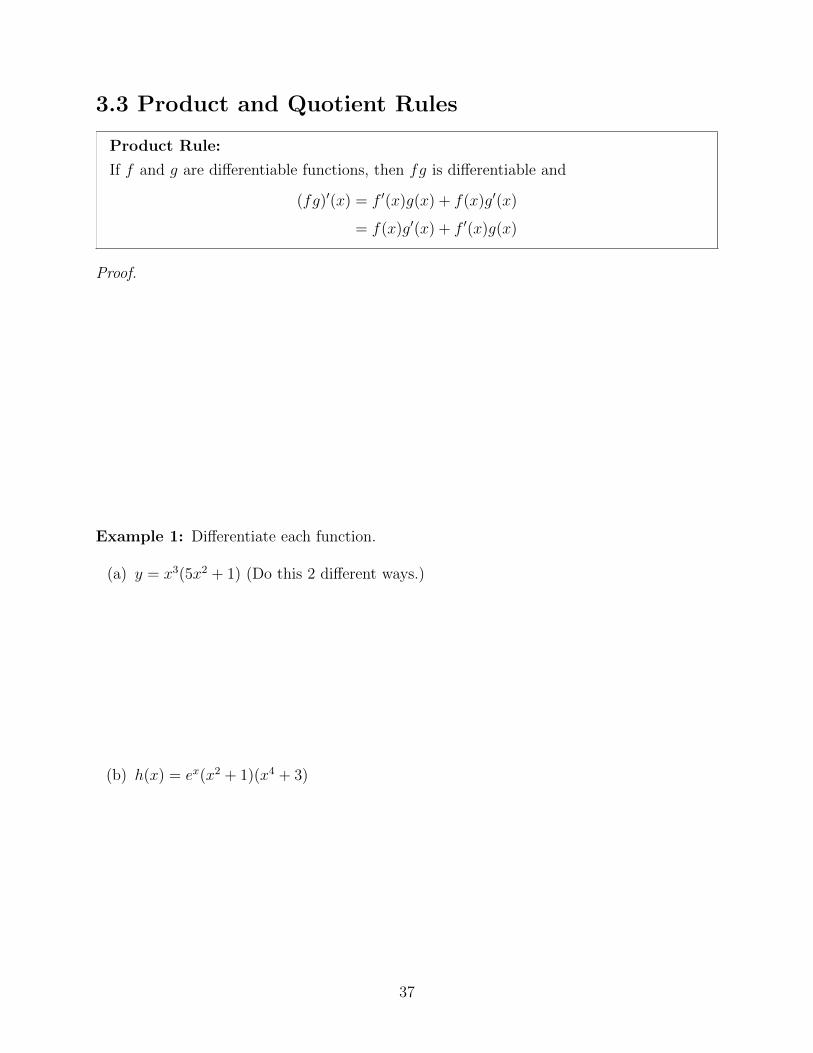
3.3 Product and Quotient Rules

Product Rule:

If f and g are differentiable functions, then fg is differentiable and

(fg)′(x) = f ′(x)g(x) + f(x)g′(x)

= f(x)g′(x) + f ′(x)g(x)

Proof.

Example 1: Differentiate each function.

(a) y = x3(5x2 + 1) (Do this 2 different ways.)

(b) h(x) = ex(x2 + 1)(x4 + 3)

37

Quotient Rule:

If f and g are differentiable functions, then f/g is differentiable for all x such that

g(x) 6= 0, and (f

g

)′=g(x)f ′(x)− f(x)g′(x)

[g(x)]2(Hi

Lo

)′=

Lo · dHi− Hi · dLo

(Lo)2

Example 2: Find the derivative of each function.

(a) f(x) =x

x− 2

(b) g(z) =1

z + 10

(c) h(x) =2x2 − 3x+ 1

5x2 + x

38

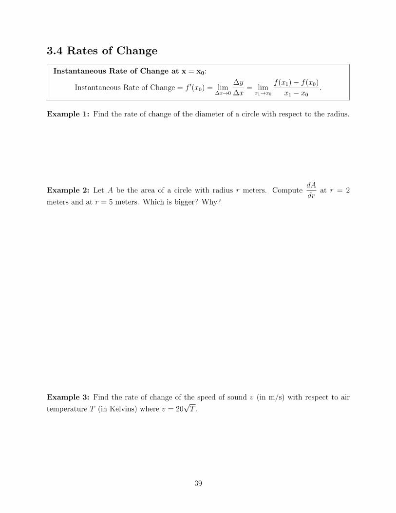
3.4 Rates of Change

Instantaneous Rate of Change at x = x0:

Instantaneous Rate of Change = f ′(x0) = lim∆x→0

∆y

∆x= lim

x1→x0

f(x1)− f(x0)

x1 − x0

.

Example 1: Find the rate of change of the diameter of a circle with respect to the radius.

Example 2: Let A be the area of a circle with radius r meters. ComputedA

drat r = 2

meters and at r = 5 meters. Which is bigger? Why?

Example 3: Find the rate of change of the speed of sound v (in m/s) with respect to air

temperature T (in Kelvins) where v = 20√T .

39

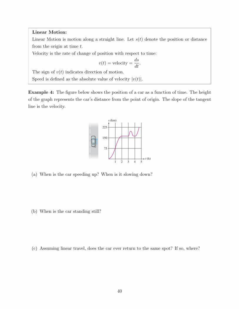
Linear Motion:

Linear Motion is motion along a straight line. Let s(t) denote the position or distance

from the origin at time t.

Velocity is the rate of change of position with respect to time:

v(t) = velocity =ds

dt.

The sign of v(t) indicates direction of motion.

Speed is defined as the absolute value of velocity |v(t)|.

Example 4: The figure below shows the position of a car as a function of time. The height

of the graph represents the car’s distance from the point of origin. The slope of the tangent

line is the velocity.

(a) When is the car speeding up? When is it slowing down?

(b) When is the car standing still?

(c) Assuming linear travel, does the car ever return to the same spot? If so, where?

40

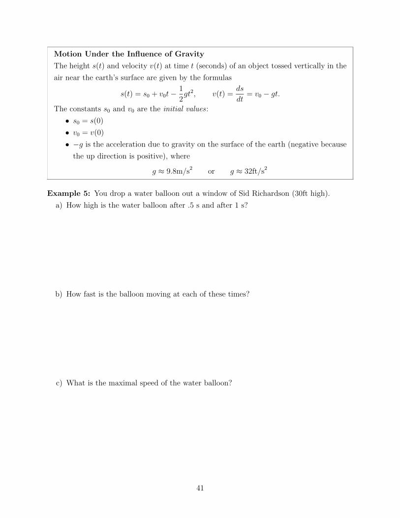
Motion Under the Influence of Gravity

The height s(t) and velocity v(t) at time t (seconds) of an object tossed vertically in the

air near the earth’s surface are given by the formulas

s(t) = s0 + v0t−1

2gt2, v(t) =

ds

dt= v0 − gt.

The constants s0 and v0 are the initial values :

• s0 = s(0)

• v0 = v(0)

• −g is the acceleration due to gravity on the surface of the earth (negative because

the up direction is positive), where

g ≈ 9.8m/s2 or g ≈ 32ft/s2

Example 5: You drop a water balloon out a window of Sid Richardson (30ft high).

a) How high is the water balloon after .5 s and after 1 s?

b) How fast is the balloon moving at each of these times?

c) What is the maximal speed of the water balloon?

41

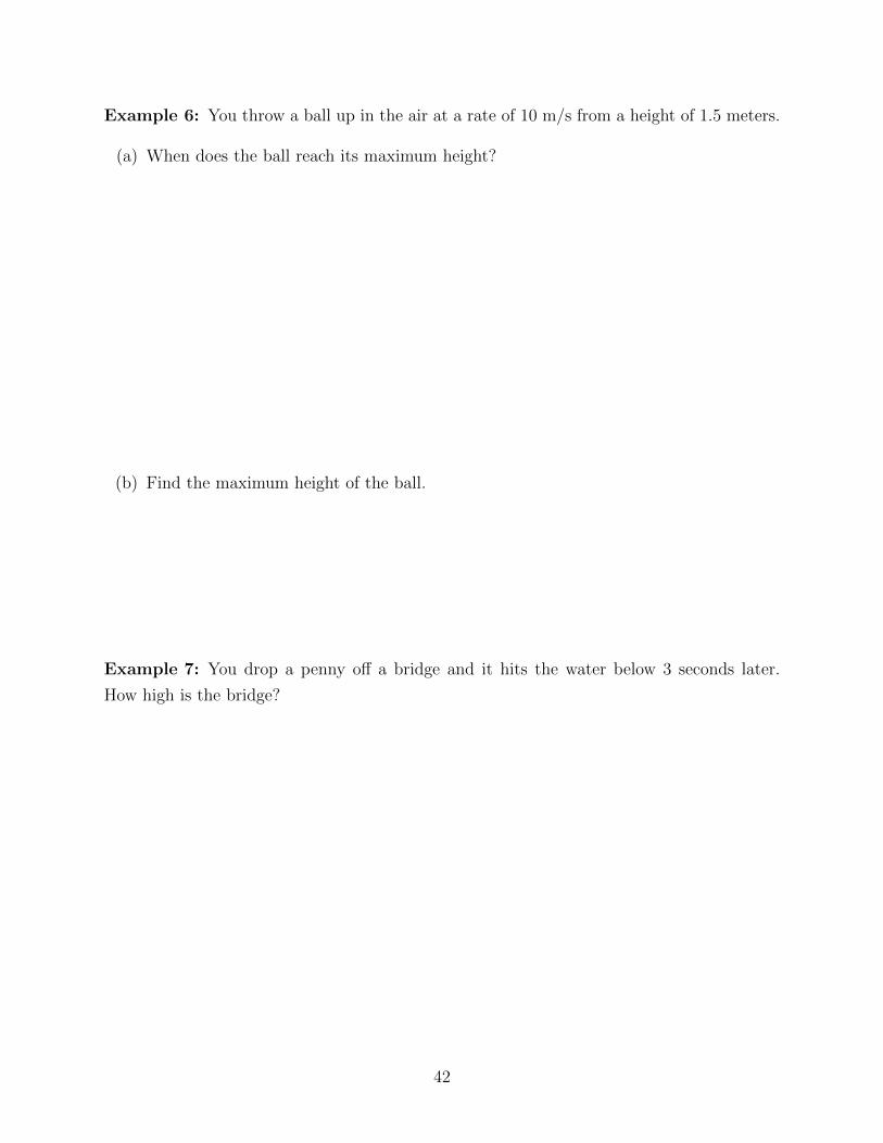
Example 6: You throw a ball up in the air at a rate of 10 m/s from a height of 1.5 meters.

(a) When does the ball reach its maximum height?

(b) Find the maximum height of the ball.

Example 7: You drop a penny off a bridge and it hits the water below 3 seconds later.

How high is the bridge?

42

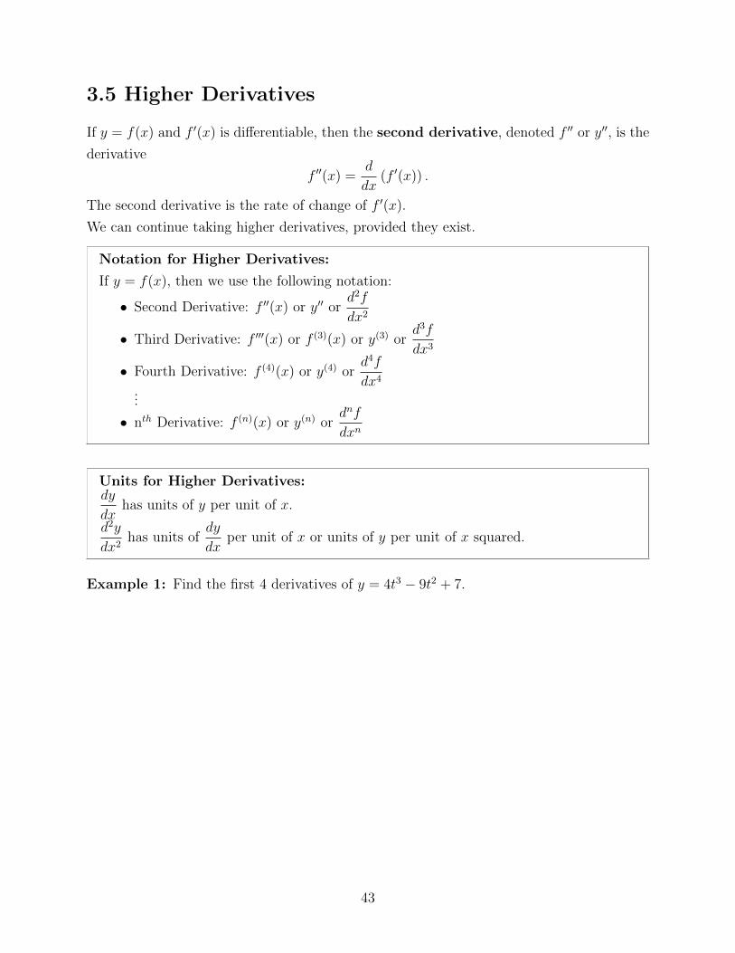
3.5 Higher Derivatives

If y = f(x) and f ′(x) is differentiable, then the second derivative, denoted f ′′ or y′′, is the

derivative

f ′′(x) =d

dx(f ′(x)) .

The second derivative is the rate of change of f ′(x).

We can continue taking higher derivatives, provided they exist.

Notation for Higher Derivatives:

If y = f(x), then we use the following notation:

• Second Derivative: f ′′(x) or y′′ ord2f

dx2

• Third Derivative: f ′′′(x) or f (3)(x) or y(3) ord3f

dx3

• Fourth Derivative: f (4)(x) or y(4) ord4f

dx4

...

• nth Derivative: f (n)(x) or y(n) ordnf

dxn

Units for Higher Derivatives:dy

dxhas units of y per unit of x.

d2y

dx2has units of

dy

dxper unit of x or units of y per unit of x squared.

Example 1: Find the first 4 derivatives of y = 4t3 − 9t2 + 7.

43

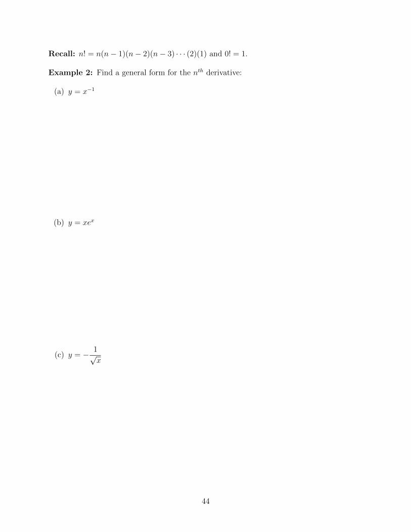
Recall: n! = n(n− 1)(n− 2)(n− 3) · · · (2)(1) and 0! = 1.

Example 2: Find a general form for the nth derivative:

(a) y = x−1

(b) y = xex

(c) y = − 1√x

44

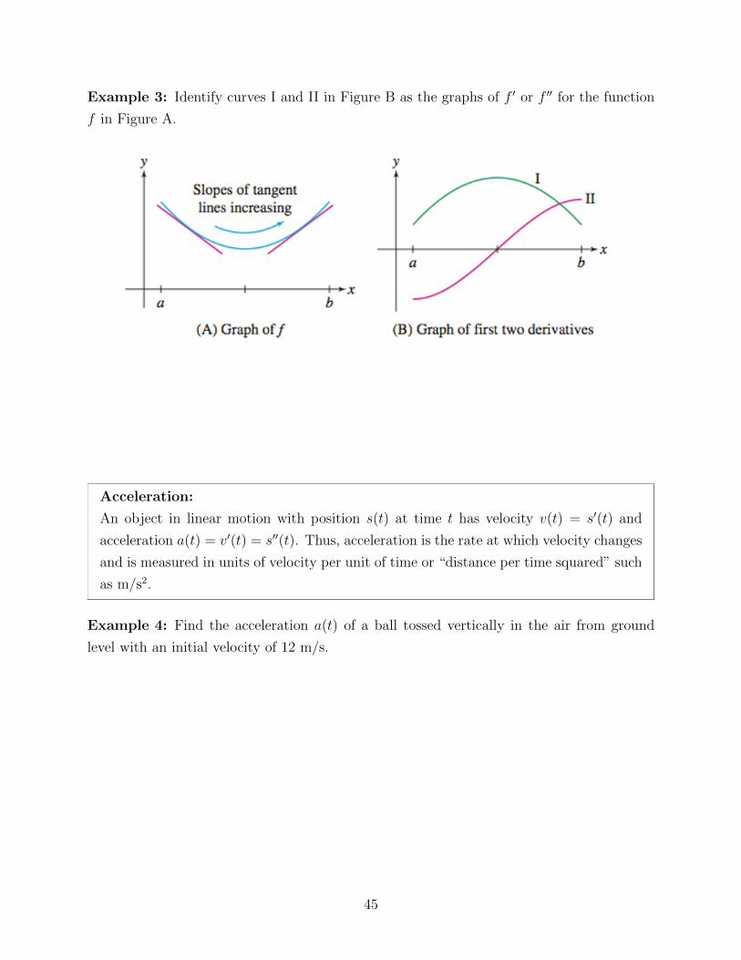
Example 3: Identify curves I and II in Figure B as the graphs of f ′ or f ′′ for the function

f in Figure A.

Acceleration:

An object in linear motion with position s(t) at time t has velocity v(t) = s′(t) and

acceleration a(t) = v′(t) = s′′(t). Thus, acceleration is the rate at which velocity changes

and is measured in units of velocity per unit of time or “distance per time squared” such

as m/s2.

Example 4: Find the acceleration a(t) of a ball tossed vertically in the air from ground

level with an initial velocity of 12 m/s.

45

3.6 Trigonometric Functions

Note: Angles are measured in radians, unless otherwise specified.

Derivatives of Trigonometric Functions:

d

dxsinx = cos x

d

dxcosx = − sinx

d

dxtanx = sec2 x

d

dxsecx = secx tanx

d

dxcotx = − csc2 x

d

dxcscx = − cscx cotx

Proof ford

dxsinx:

Example 2: Find the derivative of the given function.

(a) h(t) = et csc t

46

(b) f(x) = x2ex sinx

(c) f(x) = cos2 x

Example 3: Find the first 4 derivatives of f(x) = sin x. Then determine f (9)(x).

47

Useful Identities

Properties of Logarithms

Let x, y, and a be positive real numbers, a 6= 1, and r any real number. Then we have:

i) loga(1) = 0 and ln(1) = 0 since a0 = 1

ii) loga(a) = 1 and ln(e) = 1 since a1 = a

iii) loga(ar) = r and ln(er) = r since (a)r = (ar)

iv) aloga(x) = x and eln(x) = x

v) loga(xy) = loga(x) + loga(y)

vi) loga

(xy

)= loga(x)− loga(y)

vii) loga(xr) = r · loga(x)

Summary of Trig Identities

i) Reciprocal Identities

cscx =1

sinxsecx =

1

cosxcotx =

1

tanxii) Quotient Identities

tanx =sinx

cosxcotx =

cosx

sinxiii) Pythagorean Identities

sin2 x+ cos2 x = 1 1 + tan2 x = sec2 x 1 + cot2 x = csc2 x

iv) Even-Odd Identities

sin(−x) = − sinx cos(−x) = cos x tan(−x) = − tanx

v) Sum/Difference Formulas

cos(u− v) = cosu cos v + sinu sin v cos(u+ v) = cosu cos v − sinu sin v

sin(u− v) = sinu cos v − cosu sin v sin(u+ v) = sinu cos v + cosu sin v

vi) Double-Angle Formulas

sin(2u) = 2 sinu cosu cos(2u) = cos2 u− sin2 u = 2 cos2 u− 1

tan(2u) =2 tanu

1− tan2 ucos(2u) = cos2 u− sin2 u = 1− 2 sin2 u

48

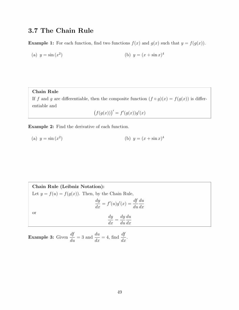
3.7 The Chain Rule

Example 1: For each function, find two functions f(x) and g(x) such that y = f(g(x)).

(a) y = sin (x2) (b) y = (x+ sinx)4

Chain Rule

If f and g are differentiable, then the composite function (f ◦ g)(x) = f(g(x)) is differ-

entiable and (f(g(x))

)′= f ′(g(x))g′(x)

Example 2: Find the derivative of each function.

(a) y = sin (x2) (b) y = (x+ sinx)4

Chain Rule (Leibniz Notation):

Let y = f(u) = f(g(x)). Then, by the Chain Rule,

dy

dx= f ′(u)g′(x) =

df

du

du

dxor

dy

dx=dy

du

du

dx

Example 3: Givendf

du= 3 and

du

dx= 4, find

df

dx.

49

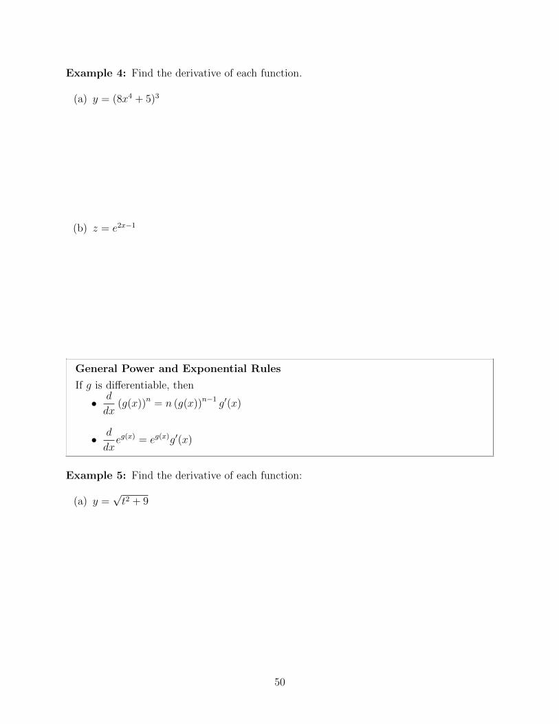
Example 4: Find the derivative of each function.

(a) y = (8x4 + 5)3

(b) z = e2x−1

General Power and Exponential Rules

If g is differentiable, then

• d

dx(g(x))n = n (g(x))n−1 g′(x)

• d

dxeg(x) = eg(x)g′(x)

Example 5: Find the derivative of each function:

(a) y =√t2 + 9

50

(b) y = x cos (1− 3x)

(c) y = e2x2

(d) y = sec(√

t3 − 4)

(e) y = cos7(x5)

51

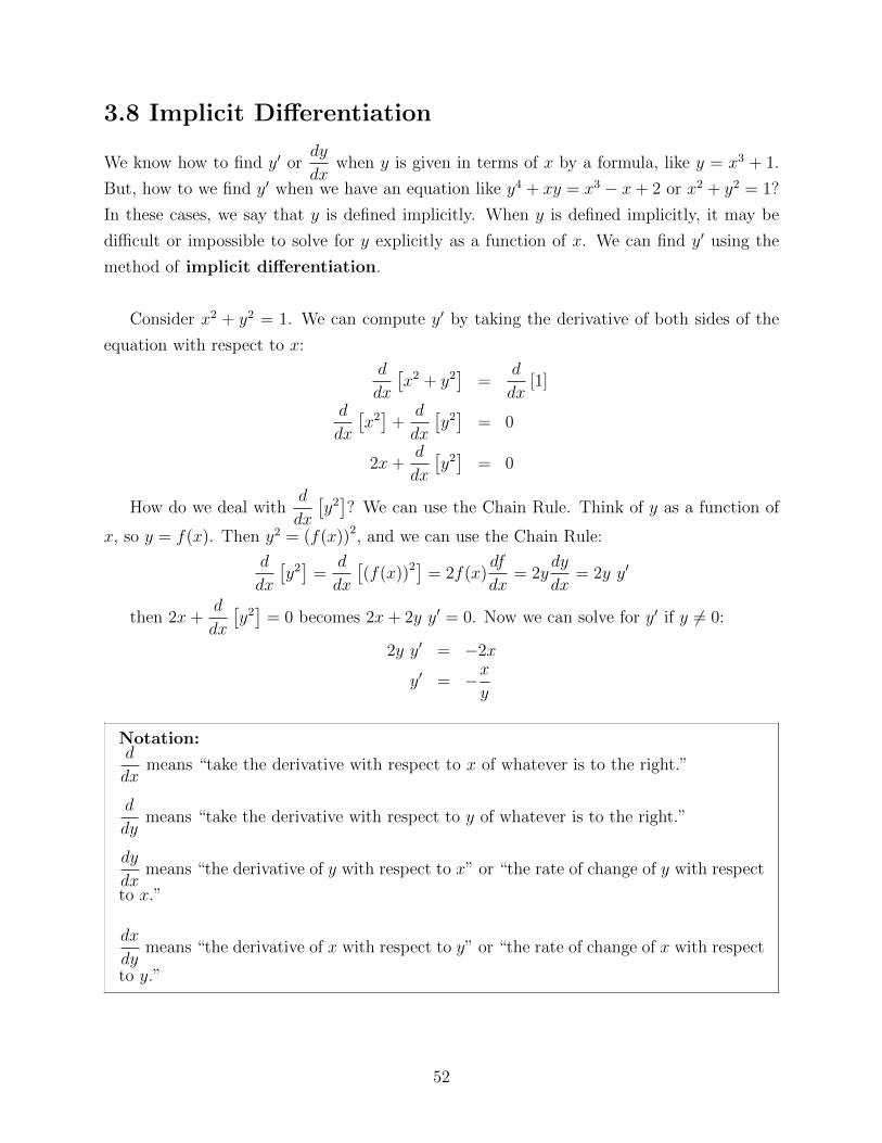
3.8 Implicit Differentiation

We know how to find y′ ordy

dxwhen y is given in terms of x by a formula, like y = x3 + 1.

But, how to we find y′ when we have an equation like y4 + xy = x3 − x+ 2 or x2 + y2 = 1?

In these cases, we say that y is defined implicitly. When y is defined implicitly, it may be

difficult or impossible to solve for y explicitly as a function of x. We can find y′ using the

method of implicit differentiation.

Consider x2 + y2 = 1. We can compute y′ by taking the derivative of both sides of the

equation with respect to x:

d

dx

[x2 + y2

]=

d

dx[1]

d

dx

[x2]

+d

dx

[y2]

= 0

2x+d

dx

[y2]

= 0

How do we deal withd

dx

[y2]? We can use the Chain Rule. Think of y as a function of

x, so y = f(x). Then y2 = (f(x))2, and we can use the Chain Rule:

d

dx

[y2]

=d

dx

[(f(x))2] = 2f(x)

df

dx= 2y

dy

dx= 2y y′

then 2x+d

dx

[y2]

= 0 becomes 2x+ 2y y′ = 0. Now we can solve for y′ if y 6= 0:

2y y′ = −2x

y′ = −xy

Notation:d

dxmeans “take the derivative with respect to x of whatever is to the right.”

d

dymeans “take the derivative with respect to y of whatever is to the right.”

dy

dxmeans “the derivative of y with respect to x” or “the rate of change of y with respect

to x.”

dx

dymeans “the derivative of x with respect to y” or “the rate of change of x with respect

to y.”

52

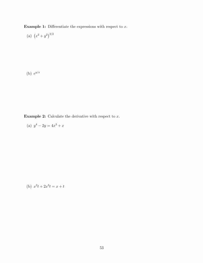
Example 1: Differentiate the expressions with respect to x.

(a)(x2 + y2

)3/2

(b) ey/x

Example 2: Calculate the derivative with respect to x.

(a) y4 − 2y = 4x3 + x

(b) x2t+ 2x3t = x+ t

53

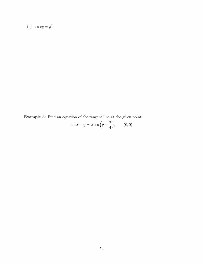
(c) cos xy = y2

Example 3: Find an equation of the tangent line at the given point:

sinx− y = x cos(y +

π

4

), (0, 0)

54

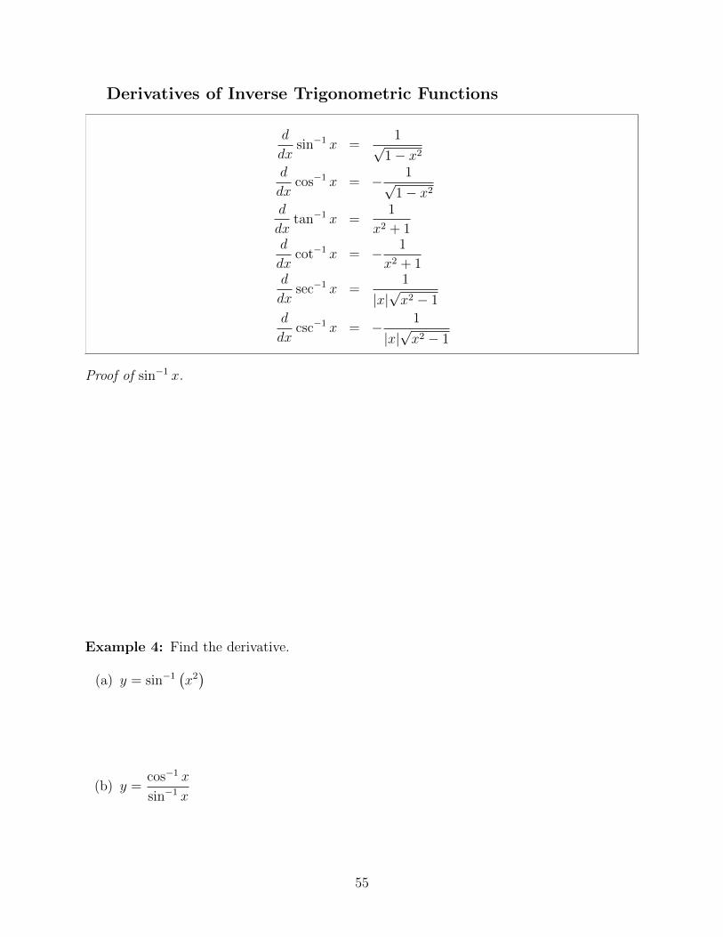
Derivatives of Inverse Trigonometric Functions

d

dxsin−1 x =

1√1− x2

d

dxcos−1 x = − 1√

1− x2

d

dxtan−1 x =

1

x2 + 1d

dxcot−1 x = − 1

x2 + 1d

dxsec−1 x =

1

|x|√x2 − 1

d

dxcsc−1 x = − 1

|x|√x2 − 1

Proof of sin−1 x.

Example 4: Find the derivative.

(a) y = sin−1(x2)

(b) y =cos−1 x

sin−1 x

55

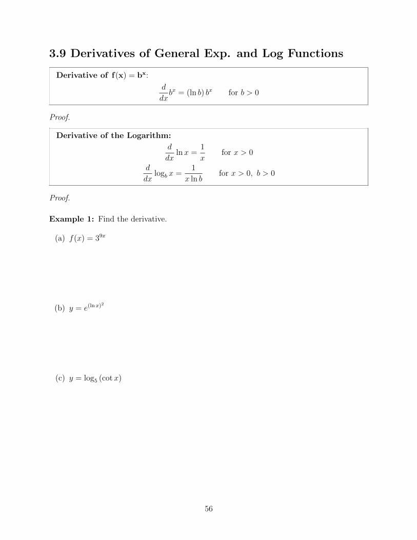
3.9 Derivatives of General Exp. and Log Functions

Derivative of f(x) = bx:

d

dxbx = (ln b) bx for b > 0

Proof.

Derivative of the Logarithm:

d

dxlnx =

1

xfor x > 0

d

dxlogb x =

1

x ln bfor x > 0, b > 0

Proof.

Example 1: Find the derivative.

(a) f(x) = 39x

(b) y = e(lnx)2

(c) y = log5 (cotx)

56

Example 2: Find an equation of the tangent line at x =π

3of g(x) = 16sinx.

Example 3: Calculate the derivative of

lnx+ ln y = x− y

with respect to x.

57

Differentiating Functions of the Form (f(x))g(x)

Example 4: Find the derivative.

(a) f(x) = x2x

(b) f(x) = xsinx

(c) f(x) = xex

58

3.10 Related Rates

Related rate problems present us with situations in which two or more variables are related

and we are asked to compute the rate of change of one of the variables in terms of the rates

of change of the other variable(s).

Strategy for solving related rates problems:

Step 1 Draw a diagram and label the quantities that don’t change with their respective values

and label the quantities that do change with variables.

Step 2 Mathematically specify the rate of change that you are looking for in terms of the

variables on your diagram and record any other given information.

Step 3 Find an equation involving the variables whose rates of change you are looking for and

that you have been given. DO NOT PLUG IN ANYTHING YET.

Step 4 Implicitly differentiate the equation found in Step 3 with respect to time, and then you

may plug in values.

Step 5 State the final answer, being sure to specify the units of the answer. Make sure you

have answered the original question, and not just found something similar or related.

Hint: Use units to double-check your algebra.

You will need to know geometric formulas, possibly including:

• Similar Triangle and Triangle Trig.

• Triangles: a2 + b2 = c2;A =1

2bh

• Rectangles: P = 2l + 2w;A = lw

• Circles: C = 2πr;A = πr2

• Spheres: SA = 4πr2;V =4

3πr3

• Rectangular Prisms: SA = 2lw + 2lh+ 2wh;V = lwh

• Cylinders: SA = 2πr2 + 2πrh;V = πr2h

• Cones: SA = πr2 + πr√r2 + h2;V =

1

3πr2h

59

Example 1: A 5 meter ladder leans against a wall. The bottom of the ladder is 1.5 meters

from the wall at time t = 0 and slides away from the wall at a rate of .8 m/s. Find the

velocity of the top of the ladder at time t = 1.

60

Example 2: Assume that the radius of a sphere is expanding at a rate of 30 cm/min. Find

the rate at which the volume is changing with respect to time when the radius is 15 cm.

61

Example 3: A rocket travels vertically at a speed of 1,200 km/h. The rocket is tracked

through a telescope by an observer located 16 km from the launching pad. Find the rate at

which the angle between the telescope and the ground is increasing 3 min after lift-off.

62

Example 4: An air traffic controller spots 2 planes at the same altitude converging on a

point as they fly at right angles to each other. One plane is 150 miles from the point and

moving at 450 m/hr. The other plane is 200 miles from the point and moving at 600 m/hr.

At what rate is the distance between the planes decreasing?

63

Example 5: The distance between two consecutive bases on a baseball diamond is 90 feet.

A baseball player is running from second to third base at a speed of 28 ft/s. At what rate

is the player’s distance from home plate changing when the player is 30 ft from third base?

64

Example 6: Water pours into an inverted conical tank of height 10 m and radius 4 m at a

rate of 6 m3/min. At what rate is the water level rising when the level is 5 m high?

65

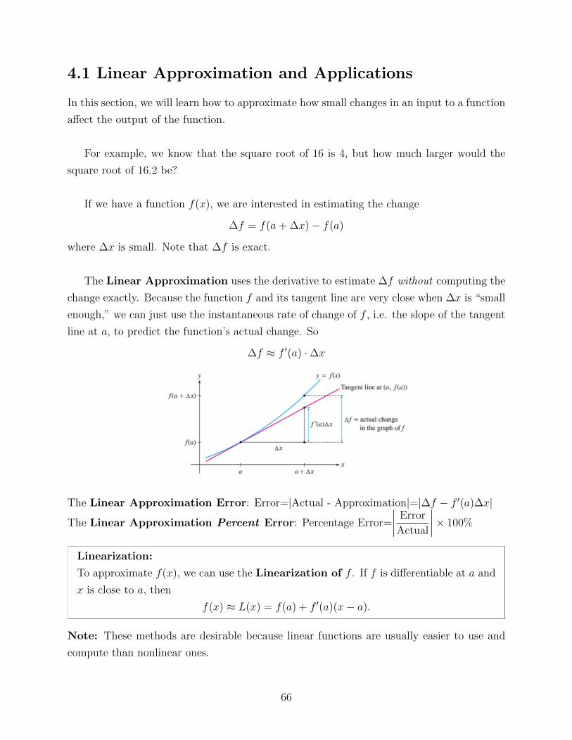
4.1 Linear Approximation and Applications

In this section, we will learn how to approximate how small changes in an input to a function

affect the output of the function.

For example, we know that the square root of 16 is 4, but how much larger would the

square root of 16.2 be?

If we have a function f(x), we are interested in estimating the change

∆f = f(a+ ∆x)− f(a)

where ∆x is small. Note that ∆f is exact.

The Linear Approximation uses the derivative to estimate ∆f without computing the

change exactly. Because the function f and its tangent line are very close when ∆x is “small

enough,” we can just use the instantaneous rate of change of f , i.e. the slope of the tangent

line at a, to predict the function’s actual change. So

∆f ≈ f ′(a) ·∆x

The Linear Approximation Error: Error=|Actual - Approximation|=|∆f − f ′(a)∆x|

The Linear Approximation Percent Error: Percentage Error=

∣∣∣∣ Error

Actual

∣∣∣∣× 100%

Linearization:

To approximate f(x), we can use the Linearization of f . If f is differentiable at a and

x is close to a, then

f(x) ≈ L(x) = f(a) + f ′(a)(x− a).

Note: These methods are desirable because linear functions are usually easier to use and

compute than nonlinear ones.

66

Example 1: Estimate ∆f = f(4.02)−f(4) given f(x) = x3. Then find the actual difference.

Example 2: Find the linearization at x = a and then use it to approximate f(b).

(a) f(x) = 1/x, a = 2, b = 2.02

(b) f(x) = ex lnx, a = 1, b = 1.02

67

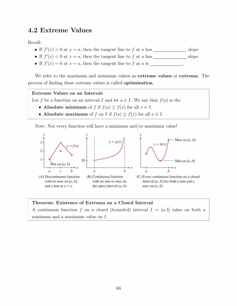
4.2 Extreme Values

Recall:

• If f ′(x) > 0 at x = a, then the tangent line to f at a has slope.

• If f ′(x) < 0 at x = a, then the tangent line to f at a has slope.

• If f ′(x) = 0 at x = a, then the tangent line to f at a is .

We refer to the maximum and minimum values as extreme values or extrema. The

process of finding these extreme values is called optimization.

Extreme Values on an Interval:

Let f be a function on an interval I and let a ∈ I. We say that f(a) is the

• Absolute minimum of f if f(a) ≤ f(x) for all x ∈ I.

• Absolute maximum of f on I if f(a) ≥ f(x) for all x ∈ I.

Note: Not every function will have a minimum and/or maximum value!

Theorem: Existence of Extrema on a Closed Interval

A continuous function f on a closed (bounded) interval I = [a, b] takes on both a

minimum and a maximum value on I.

68

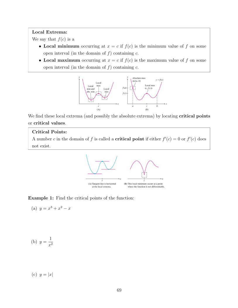
Local Extrema:

We say that f(c) is a

• Local minimum occurring at x = c if f(c) is the minimum value of f on some

open interval (in the domain of f) containing c.

• Local maximum occurring at x = c if f(c) is the maximum value of f on some

open interval (in the domain of f) containing c.

We find these local extrema (and possibly the absolute extrema) by locating critical points

or critical values.

Critical Points:

A number c in the domain of f is called a critical point if either f ′(c) = 0 or f ′(c) does

not exist.

Example 1: Find the critical points of the function:

(a) y = x3 + x2 − x

(b) y =1

x2

(c) y = |x|

69

Theorem: Fermat’s Theorem on Local Extrema

If f(c) is a local minimum or maximum, then c is a critical point of f .

Proof.

BUT: the other way around is not always true! Just because c is a critical point of f

does not mean that f(c) is necessarily a maximum or minimum (sometimes this point is a

“point of inflection,” more on this later).

Optimizing on a Closed Interval

Theorem: Extreme Values on a Closed Interval

Assume that f is continuous on [a, b] and let f(c) be the minimum or maximum value

on [a, b]. Then c is either a critical point or one of the endpoints a or b.

Strategy for Finding Extreme Values on a Closed Interval [a,b]:

1. Find the critical points on [a, b].

2. Find the function value at each critical point and at the two endpoints.

3. The largest function value from Step 2 is the maximum and the smallest function value

from Step 2 is the minimum value. (Min/max values are y-values and they occur at

the corresponding x-values.)

Example 2: Find the extrema of f(x) = 2x3 − 15x2 + 24x+ 7 on [0, 2].

70

Example 3: Find the extrema of y = x2 − 8 lnx on [1, 4].

Example 4: Find the extrema of y = θ − 2 sin θ on [0, 2π].

71

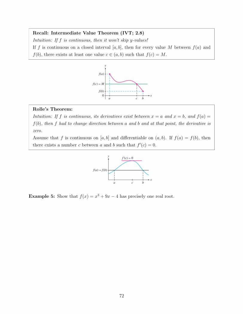
Recall: Intermediate Value Theorem (IVT; 2.8)

Intuition: If f is continuous, then it won’t skip y-values!

If f is continuous on a closed interval [a, b], then for every value M between f(a) and

f(b), there exists at least one value c ∈ (a, b) such that f(c) = M .

Rolle’s Theorem:

Intuition: If f is continuous, its derivatives exist between x = a and x = b, and f(a) =

f(b), then f had to change direction between a and b and at that point, the derivative is

zero.

Assume that f is continuous on [a, b] and differentiable on (a, b). If f(a) = f(b), then

there exists a number c between a and b such that f ′(c) = 0.

Example 5: Show that f(x) = x3 + 9x− 4 has precisely one real root.

72

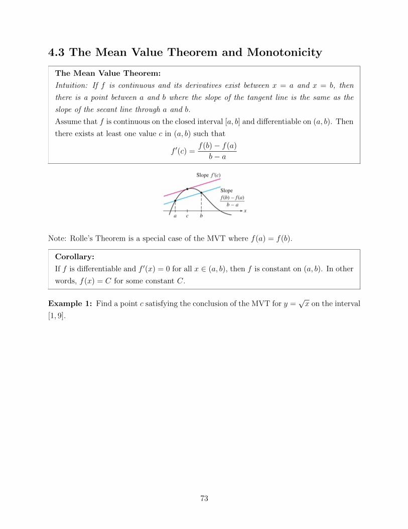
4.3 The Mean Value Theorem and Monotonicity

The Mean Value Theorem:

Intuition: If f is continuous and its derivatives exist between x = a and x = b, then

there is a point between a and b where the slope of the tangent line is the same as the

slope of the secant line through a and b.

Assume that f is continuous on the closed interval [a, b] and differentiable on (a, b). Then

there exists at least one value c in (a, b) such that

f ′(c) =f(b)− f(a)

b− a

Note: Rolle’s Theorem is a special case of the MVT where f(a) = f(b).

Corollary:

If f is differentiable and f ′(x) = 0 for all x ∈ (a, b), then f is constant on (a, b). In other

words, f(x) = C for some constant C.

Example 1: Find a point c satisfying the conclusion of the MVT for y =√x on the interval

[1, 9].

73

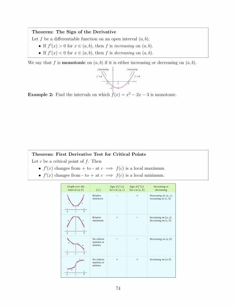
Theorem: The Sign of the Derivative

Let f be a differentiable function on an open interval (a, b).

• If f ′(x) > 0 for x ∈ (a, b), then f is increasing on (a, b).

• If f ′(x) < 0 for x ∈ (a, b), then f is decreasing on (a, b).

We say that f is monotonic on (a, b) if it is either increasing or decreasing on (a, b).

Example 2: Find the intervals on which f(x) = x2 − 2x− 3 is monotonic.

Theorem: First Derivative Test for Critical Points

Let c be a critical point of f . Then

• f ′(x) changes from + to - at c =⇒ f(c) is a local maximum.

• f ′(x) changes from - to + at c =⇒ f(c) is a local minimum.

74

Using the First Derivative Test to Find Local Extrema:

Step 1 Find the critical points.

(a) These are the x-values where f ′(x) = 0 or f ′(x) is undefined (but f(x) is defined).

Step 2 Divide the x-axis into intervals using the critical values and any x-values for which f

is undefined (Note: the latter will not produce extrema.)

Step 3 Find the sign of f ′(x) on the intervals between the critical points.

(a) To do this, pick a test point inside each interval (so don’t pick a critical value).

(b) Plug this test point into f ′(x) (not f(x).)

Step 4 Use the First Derivative Test at each critical point to determine where the local extrema

occur.

(a) The extreme values are the function values, not the x-values where they occur.

Example 3: Find the critical points and the intervals on which the function is increasing

or decreasing. Use the First Derivative Test to determine any local extrema.

(a) f(x) = x3 − 12x

75

(b) y = x3 − 6x2 + 12x

(c) g(θ) = θ − 2 cos θ on [0, 2π]

76

(d) y = 1− (x− 1)2/3

(e) y = x2ex

77

4.4 The Second Derivative and Concavity

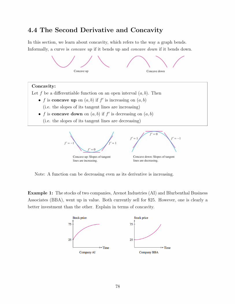
In this section, we learn about concavity, which refers to the way a graph bends.

Informally, a curve is concave up if it bends up and concave down if it bends down.

Concavity:

Let f be a differentiable function on an open interval (a, b). Then

• f is concave up on (a, b) if f ′ is increasing on (a, b)

(i.e. the slopes of its tangent lines are increasing)

• f is concave down on (a, b) if f ′ is decreasing on (a, b)

(i.e. the slopes of its tangent lines are decreasing)

Note: A function can be decreasing even as its derivative is increasing.

Example 1: The stocks of two companies, Arenot Industries (AI) and Blurbenthal Business

Associates (BBA), went up in value. Both currently sell for $25. However, one is clearly a

better investment than the other. Explain in terms of concavity.

78

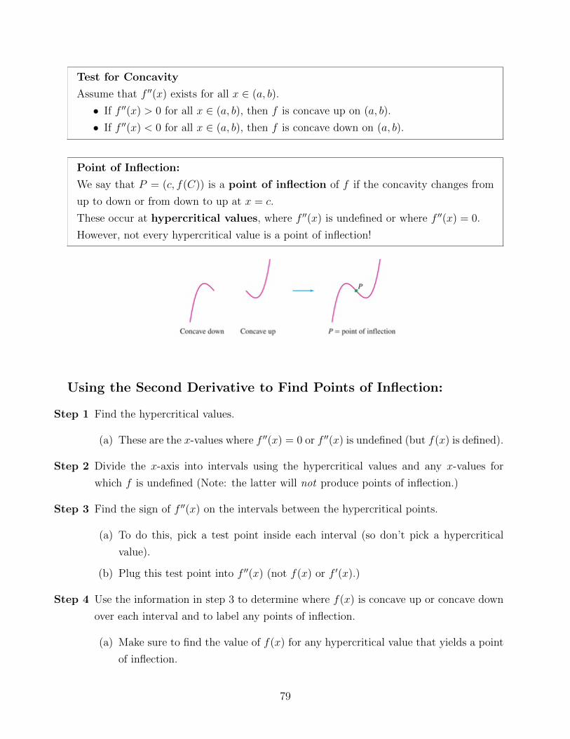
Test for Concavity

Assume that f ′′(x) exists for all x ∈ (a, b).

• If f ′′(x) > 0 for all x ∈ (a, b), then f is concave up on (a, b).

• If f ′′(x) < 0 for all x ∈ (a, b), then f is concave down on (a, b).

Point of Inflection:

We say that P = (c, f(C)) is a point of inflection of f if the concavity changes from

up to down or from down to up at x = c.

These occur at hypercritical values, where f ′′(x) is undefined or where f ′′(x) = 0.

However, not every hypercritical value is a point of inflection!

Using the Second Derivative to Find Points of Inflection:

Step 1 Find the hypercritical values.

(a) These are the x-values where f ′′(x) = 0 or f ′′(x) is undefined (but f(x) is defined).

Step 2 Divide the x-axis into intervals using the hypercritical values and any x-values for

which f is undefined (Note: the latter will not produce points of inflection.)

Step 3 Find the sign of f ′′(x) on the intervals between the hypercritical points.

(a) To do this, pick a test point inside each interval (so don’t pick a hypercritical

value).

(b) Plug this test point into f ′′(x) (not f(x) or f ′(x).)

Step 4 Use the information in step 3 to determine where f(x) is concave up or concave down

over each interval and to label any points of inflection.

(a) Make sure to find the value of f(x) for any hypercritical value that yields a point

of inflection.

79

Example 2: Find all points of inflection and determine the intervals on which the function

is concave up and concave down.

a) y = cosx on [0, 2π]

b) y = x5/3

c) y =1

12x4 + 4x+ 9

80

The Second Derivative Test

Let c be a critical point of f(x). If f ′′(c) exists, then

• f ′′(c) > 0 implies that f(c) is a local minimum

• f ′′(c) < 0 implies that f(c) is a local maximum

• f ′′(c) = 0 means that the test is inconclusive; f(c) may be a local max, a local

min, or neither and we need to go back to the First Derivative Test to find out!

Example 3: Analyze the critical points of g(x) = x5 − 5

4x4 using the Second Derivative

Test.

Example 4: Find all critical points, points of inflection, local extrema, intervals on which

the function is increasing/decreasing, intervals on which the function is concave up/concave

down.

f(x) = x3/2 − 4x−1/2 (x > 0)

81

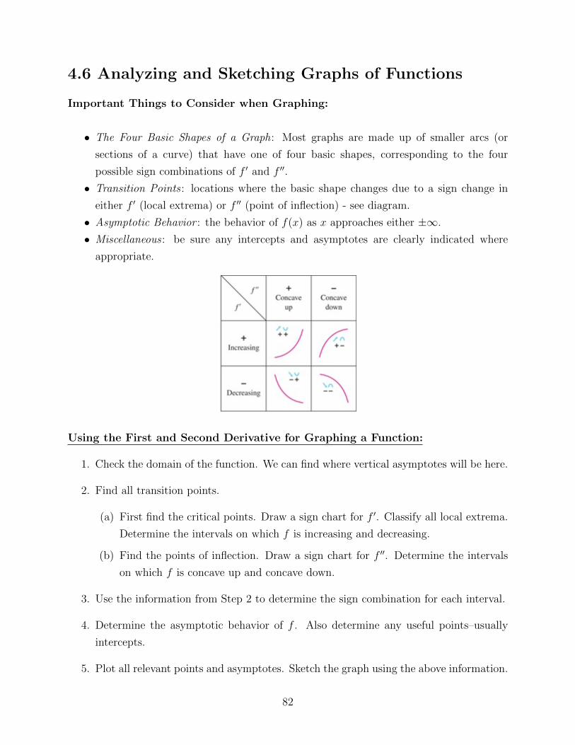
4.6 Analyzing and Sketching Graphs of Functions

Important Things to Consider when Graphing:

• The Four Basic Shapes of a Graph: Most graphs are made up of smaller arcs (or

sections of a curve) that have one of four basic shapes, corresponding to the four

possible sign combinations of f ′ and f ′′.

• Transition Points : locations where the basic shape changes due to a sign change in

either f ′ (local extrema) or f ′′ (point of inflection) - see diagram.

• Asymptotic Behavior : the behavior of f(x) as x approaches either ±∞.

• Miscellaneous : be sure any intercepts and asymptotes are clearly indicated where

appropriate.

Using the First and Second Derivative for Graphing a Function:

1. Check the domain of the function. We can find where vertical asymptotes will be here.

2. Find all transition points.

(a) First find the critical points. Draw a sign chart for f ′. Classify all local extrema.

Determine the intervals on which f is increasing and decreasing.

(b) Find the points of inflection. Draw a sign chart for f ′′. Determine the intervals

on which f is concave up and concave down.

3. Use the information from Step 2 to determine the sign combination for each interval.

4. Determine the asymptotic behavior of f . Also determine any useful points–usually

intercepts.

5. Plot all relevant points and asymptotes. Sketch the graph using the above information.

82

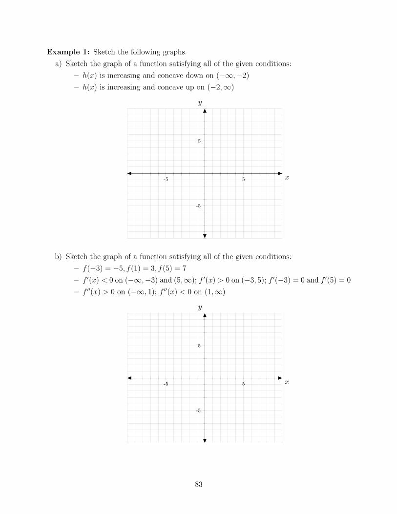
Example 1: Sketch the following graphs.

a) Sketch the graph of a function satisfying all of the given conditions:

– h(x) is increasing and concave down on (−∞,−2)

– h(x) is increasing and concave up on (−2,∞)

-5 5

-5

5

x

y

b) Sketch the graph of a function satisfying all of the given conditions:

– f(−3) = −5, f(1) = 3, f(5) = 7

– f ′(x) < 0 on (−∞,−3) and (5,∞); f ′(x) > 0 on (−3, 5); f ′(−3) = 0 and f ′(5) = 0

– f ′′(x) > 0 on (−∞, 1); f ′′(x) < 0 on (1,∞)

-5 5

-5

5

x

y

83

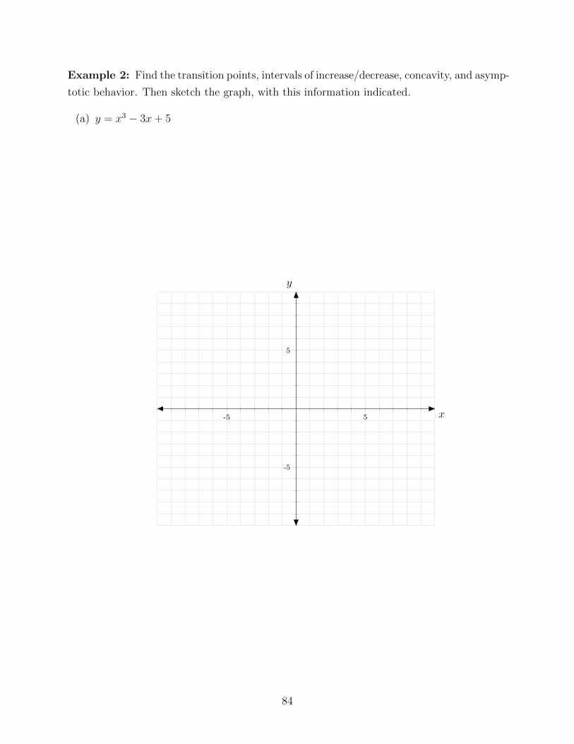
Example 2: Find the transition points, intervals of increase/decrease, concavity, and asymp-

totic behavior. Then sketch the graph, with this information indicated.

(a) y = x3 − 3x+ 5

-5 5

-5

5

x

y

84

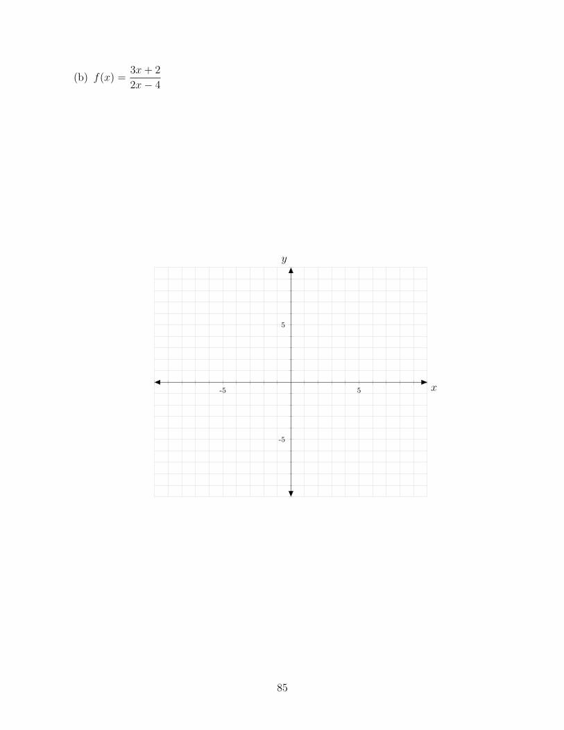
(b) f(x) =3x+ 2

2x− 4

-5 5

-5

5

x

y

85

4.7 Applied Optimization

In applied optimization problems, we need to find the function whose minimum or maximum

we need. This is called the objective function.

We also might need an equation that relates two or more variables in an optimization

problem, called the constraint equation.

We also need to identify which interval we are working on and if it is open or closed.

Solving Applied Optimization Problems:

1. Choose variables.

(a) Draw a picture, if applicable.

(b) Determine which quantities are relevant.

(c) Assign appropriate variables.

2. Find the objective function and the interval.

(a) Restate as an optimization problem for a function over an interval.

(b) If the function depends on more that one variable, use a constraint equation to

write it as a function of just one variable.

3. Optimize the objective function.

(a) If we are working on a closed interval, we need to compare the function values at

the endpoints and at any critical points inside the interval.

(b) If we are working on an open interval, the function doesn’t necessarily take on

a max or min value. If it does, these must occur at critical points within the

interval. We need to analyze the behavior of the function as we approach the

endpoints of the interval.

86

Example 1: A farmer plans to fence a rectangular pasture adjacent to a river. The pasture

must contain 180,000 square meters in order to provide enough grass for the herd. What

dimensions would require the least amount of fencing if no fencing is needed along the river?

Example 2: Determine the dimensions of a rectangular solid (with a square base) of max-

imum volume if its surface area is 150 square inches.

87

Example 3: Find the dimensions of the rectangle of maximum area that can be inscribed

in a circle of radius 4.

Example 4: Find the point on the line y = x that is closest to the point (0,−1).

88

Example 5: Enclose a rectangular pasture with area 16000 m2 with parallel sides made of

chain link fence costing $20/m and wooden fence costing $50/m. Minimize the cost.

Example 6: Your task is to build a road joining a ranch to a highway that enables drivers

to reach the city in the shortest time. How should this be done if the speed limit is 60 km/h

on the road and 110 km/h on the highway? The perpendicular distance from the ranch to

the highway is 30 km and the city is 50 km down the highway.

89

5.1/5.2 Approximating and Computing Area &

The Definite Integral

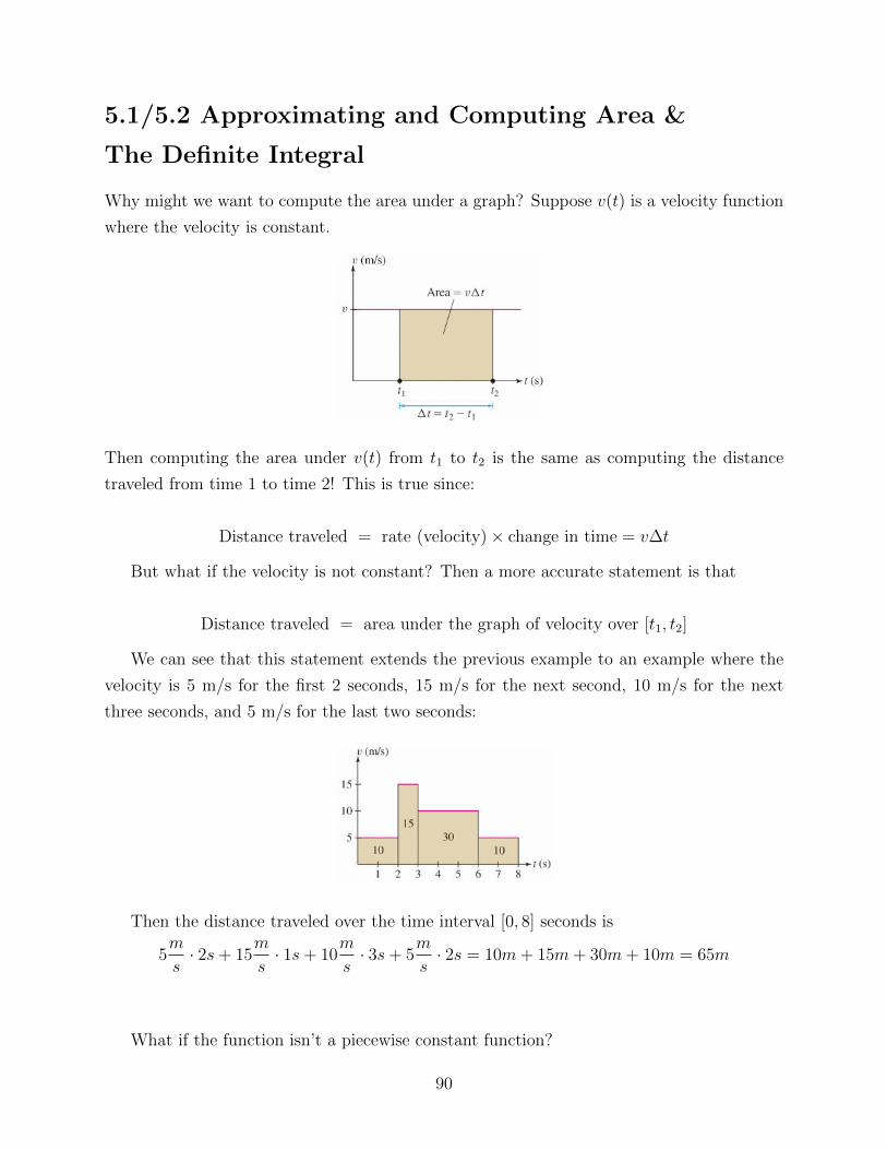
Why might we want to compute the area under a graph? Suppose v(t) is a velocity function

where the velocity is constant.

Then computing the area under v(t) from t1 to t2 is the same as computing the distance

traveled from time 1 to time 2! This is true since:

Distance traveled = rate (velocity)× change in time = v∆t

But what if the velocity is not constant? Then a more accurate statement is that

Distance traveled = area under the graph of velocity over [t1, t2]

We can see that this statement extends the previous example to an example where the

velocity is 5 m/s for the first 2 seconds, 15 m/s for the next second, 10 m/s for the next

three seconds, and 5 m/s for the last two seconds:

Then the distance traveled over the time interval [0, 8] seconds is

5m

s· 2s+ 15

m

s· 1s+ 10

m

s· 3s+ 5

m

s· 2s = 10m+ 15m+ 30m+ 10m = 65m

What if the function isn’t a piecewise constant function?

90

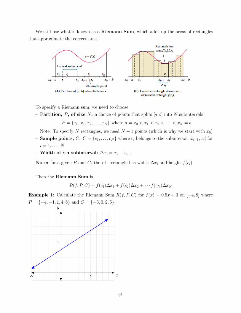
We still use what is known as a Riemann Sum, which adds up the areas of rectangles

that approximate the correct area.

To specify a Riemann sum, we need to choose

– Partition, P , of size N : a choice of points that splits [a, b] into N subintervals

P = {x0, x1, x2, . . . , xN} where a = x0 < x1 < x2 < · · · < xN = b

Note: To specify N rectangles, we need N + 1 points (which is why we start with x0)

– Sample points, C: C = {c1, . . . , cN} where ci belongs to the subinterval [xi−1, xi] for

i = 1, . . . , N

– Width of ith subinterval: ∆xi = xi − xi−1

Note: for a given P and C, the ith rectangle has width ∆xi and height f(ci).

Then the Riemann Sum is

R(f, P, C) = f(c1)∆x1 + f(c2)∆x2 + · · · f(cN)∆xN

Example 1: Calculate the Riemann Sum R(f, P, C) for f(x) = 0.5x + 3 on [−4, 8] where

P = {−4,−1, 1, 4, 8} and C = {−3, 0, 2, 5}.

-5 5

5

x

y

91

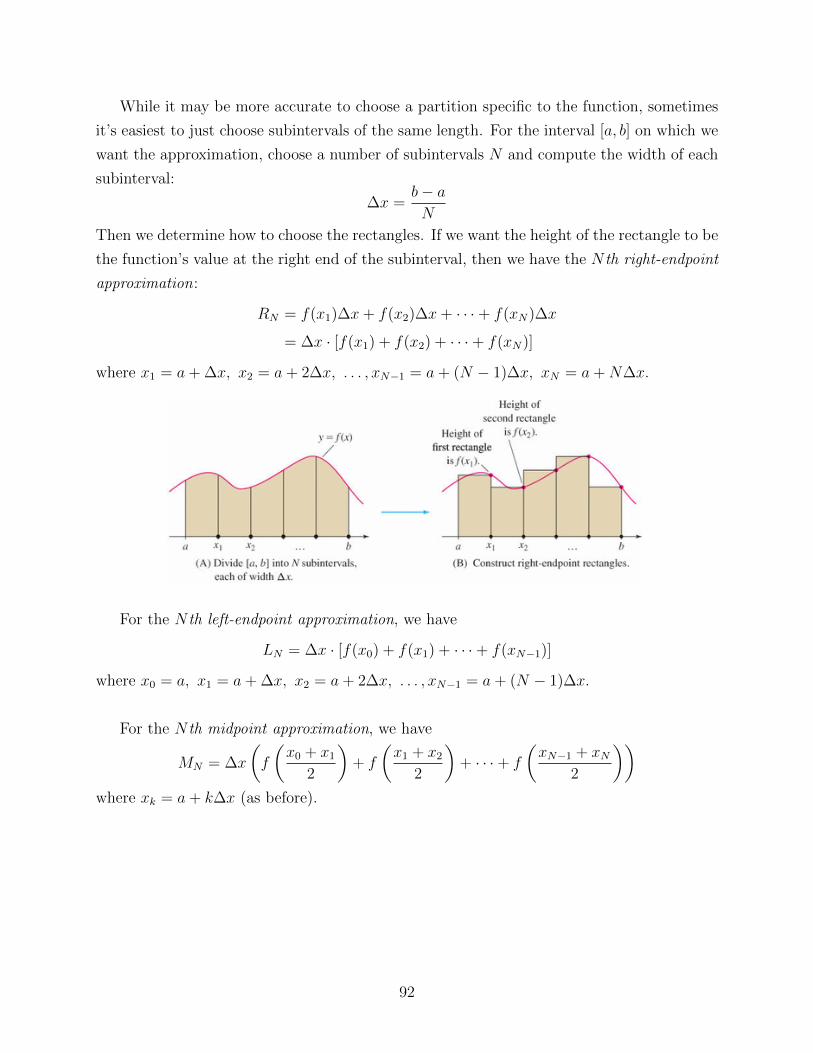
While it may be more accurate to choose a partition specific to the function, sometimes

it’s easiest to just choose subintervals of the same length. For the interval [a, b] on which we

want the approximation, choose a number of subintervals N and compute the width of each

subinterval:

∆x =b− aN

Then we determine how to choose the rectangles. If we want the height of the rectangle to be

the function’s value at the right end of the subinterval, then we have the N th right-endpoint

approximation:

RN = f(x1)∆x+ f(x2)∆x+ · · ·+ f(xN)∆x

= ∆x · [f(x1) + f(x2) + · · ·+ f(xN)]

where x1 = a+ ∆x, x2 = a+ 2∆x, . . . , xN−1 = a+ (N − 1)∆x, xN = a+N∆x.

For the N th left-endpoint approximation, we have

LN = ∆x · [f(x0) + f(x1) + · · ·+ f(xN−1)]

where x0 = a, x1 = a+ ∆x, x2 = a+ 2∆x, . . . , xN−1 = a+ (N − 1)∆x.

For the N th midpoint approximation, we have

MN = ∆x

(f

(x0 + x1

2

)+ f

(x1 + x2

2

)+ · · ·+ f

(xN−1 + xN

2

))where xk = a+ k∆x (as before).

92

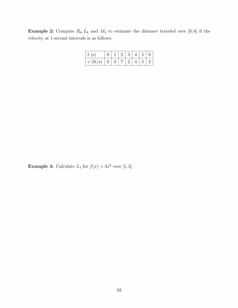
Example 2: Compute R6, L6 and M3 to estimate the distance traveled over [0, 6] if the

velocity at 1-second intervals is as follows:

t (s) 0 1 2 3 4 5 6

v (ft/s) 0 3 7 2 4 5 2

Example 3: Calculate L4 for f(x) = 3x2 over [1, 3].

93

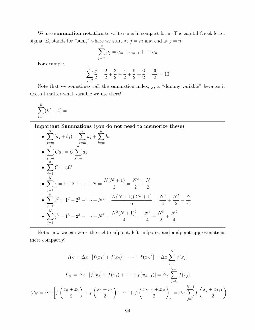
We use summation notation to write sums in compact form. The capital Greek letter

sigma, Σ, stands for “sum,” where we start at j = m and end at j = n:n∑

j=m

aj = am + am+1 + · · · an

For example,6∑j=2

j

2=

2

2+

3

2+

4

2+

5

2+

6

2=

20

2= 10

Note that we sometimes call the summation index, j, a “dummy variable” because it

doesn’t matter what variable we use there!

5∑k=3

(k2 − 4) =

Important Summations (you do not need to memorize these)

•n∑

j=m

(aj + bj) =n∑

j=m

aj +n∑

j=m

bj

•n∑

j=m

Caj = Cn∑

j=m

aj

•n∑j=1

C = nC

•N∑j=1

j = 1 + 2 + · · ·+N =N(N + 1)

2=N2

2+N

2

•N∑j=1

j2 = 12 + 22 + · · ·+N2 =N(N + 1)(2N + 1)

6=N3

3+N2

2+N

6

•N∑j=1

j3 = 13 + 23 + · · ·+N3 =N2(N + 1)2

4=N4

4+N3

2+N2

4

Note: now we can write the right-endpoint, left-endpoint, and midpoint approximations

more compactly!

RN = ∆x · [f(x1) + f(x2) + · · ·+ f(xN)] = ∆xN∑j=1

f(xj)

LN = ∆x · [f(x0) + f(x1) + · · ·+ f(xN−1)] = ∆xN−1∑j=0

f(xj)

MN = ∆x·[f

(x0 + x1

2

)+ f

(x1 + x2

2

)+ · · ·+ f

(xN−1 + xN

2

)]= ∆x

N−1∑j=0

f

(xj + xj+1

2

)

94

Example 4: Write the sum in summation notation:√

1 + 13 +√

2 + 23 + · · ·√

17 + 173

Example 5: Evaluate the sums:

a)4∑i=1

(2i+ 3i−1)

b)5∑

k=3

2k2

Example 6: Express the area under the graph as a limit using the approximation indicated

(in summation notation), but do not evaluate.

LN , f(x) = sinx, [0, π]

95

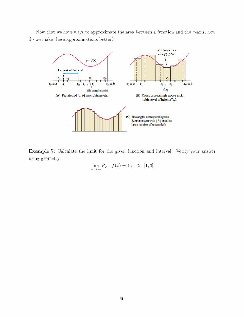
Now that we have ways to approximate the area between a function and the x-axis, how

do we make these approximations better?

Example 7: Calculate the limit for the given function and interval. Verify your answer

using geometry.

limN→∞

RN , f(x) = 4x− 2, [1, 3]

96

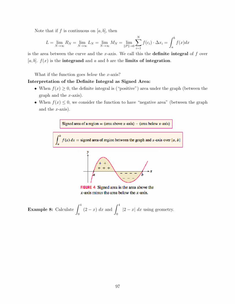
Note that if f is continuous on [a, b], then

L = limN→∞

RN = limN→∞

LN = limN→∞

MN = lim‖P‖→0

N∑i=1

f(ci) ·∆xi =

∫ b

a

f(x)dx

is the area between the curve and the x-axis. We call this the definite integral of f over

[a, b]. f(x) is the integrand and a and b are the limits of integration.

What if the function goes below the x-axis?

Interpretation of the Definite Integral as Signed Area:

• When f(x) ≥ 0, the definite integral is (“positive”) area under the graph (between the

graph and the x-axis).

• When f(x) ≤ 0, we consider the function to have “negative area” (between the graph

and the x-axis).

Example 8: Calculate

∫ 4

0

(2− x) dx and

∫ 4

0

|2− x| dx using geometry.

97

Properties of Definite Integrals:

•∫ b

a

C dx = C(b− a)

•∫ b

a

(f(x) + g(x)) dx =

∫ b

a

f(x) dx+

∫ b

a

g(x) dx

•∫ b

a

Cf(x) dx = C

∫ b

a

f(x) dx

•∫ b

a

f(x) dx = −∫ a

b

f(x) dx

•∫ c

a

f(x) dx =

∫ b

a

f(x) dx+

∫ c

b

f(x) dx

•∫ a

a

f(x) dx = 0

•∫ b

0

x dx =1

2b2

•∫ b

0

x2 dx =1

3b3

Example 9: Assuming

∫ 5

1

f(x) dx = 15,

∫ 3

0

f(x) dx = 10, and

∫ 1

0

f(x) dx = 2,

calculate

∫ 5

3

f(x) dx.

Example 10: Calculate

∫ 5

0

(−3x+ 1) dx and

∫ 0

5

(−3x+ 1) dx.

98

5.3 The Indefinite Integral

Now we begin talking about the inverse process of finding derivatives - finding “antideriva-

tives”! The question here is: given a derivative, can we find the original function?

Common notation:

• A function F is an antiderivative of f on an open interval (a, b) if F ′(x) = f(x) for all

x ∈ (a, b).

•∫f(x) dx = F (x) + C means that F ′(x) = f(x) where C is an arbitrary constant.

Some Examples:

• F (x) = − cosx is an antiderivative of f(x) = sin x because for all values of x,

F ′(x) =d

dx(− cosx) = sinx = f(x).

• F (x) =1

3x3 is an antiderivative of f(x) = x2 because for all values of x,

F ′(x) =d

dx

(1

3x3

)= x2 = f(x).

Question: What is an antiderivative of 2x?

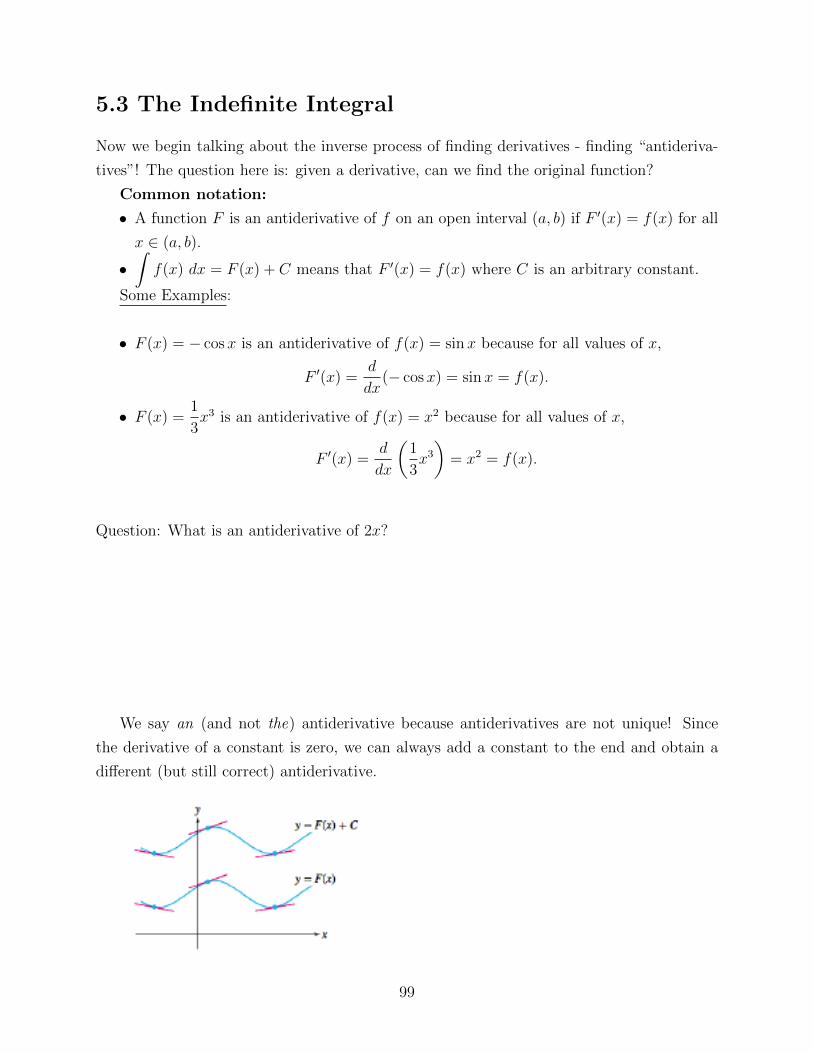
We say an (and not the) antiderivative because antiderivatives are not unique! Since

the derivative of a constant is zero, we can always add a constant to the end and obtain a

different (but still correct) antiderivative.

99

Properties of Integrals:

i) If k is a constant, ∫kf(x) dx = k

∫f(x) dx

ii) If f(x) and g(x) are two funtions,∫(f(x)± g(x)) dx =

∫f(x) dx±

∫g(x) dx

Some Common Integrals:

i) Integral of a Constant: If k is a constant,∫k dx = kx+ C

ii) Integral of a Power Function: For n 6= −1,∫xn dx =

xn+1

n+ 1+ C

iii) Integral of1

xon the domain x > 0:∫

1

xdx = ln |x|+ C

iv) Integral of the Exponential Function:∫ex dx = ex + C and

∫ekx dx =

1

kekx + C

Trigonometric Integrals

•∫

cosx dx = sinx+ C

•∫

sinx dx = − cosx+ C

•∫

sec2 x dx = tanx+ C

•∫

cscx cotx dx = − cscx+ C

•∫

secx tanx dx = secx+ C

•∫

csc2 x dx = − cotx+ C

Note also that∫cos(kx) =

1

ksin(kx) + C and

∫sin(kx) = −1

kcos(kx) + C

100

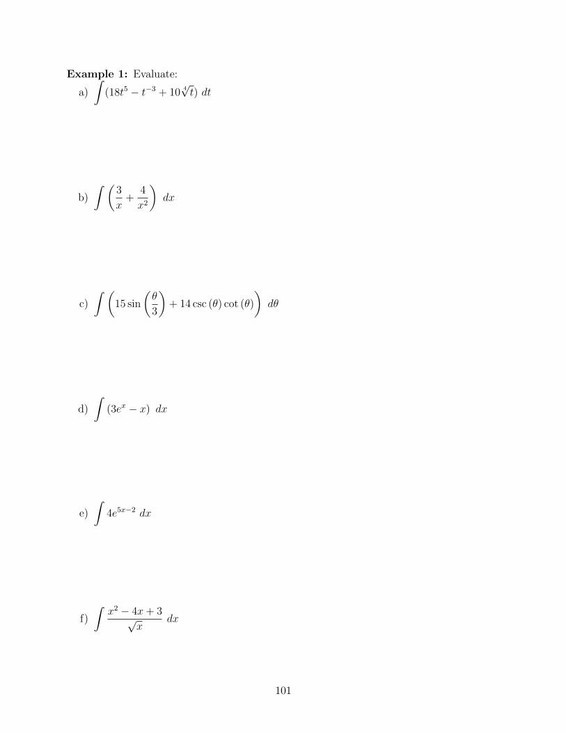
Example 1: Evaluate:

a)

∫(18t5 − t−3 + 10

4√t) dt

b)

∫ (3

x+

4

x2

)dx

c)

∫ (15 sin

(θ

3

)+ 14 csc (θ) cot (θ)

)dθ

d)

∫(3ex − x) dx

e)

∫4e5x−2 dx

f)

∫x2 − 4x+ 3√

xdx

101

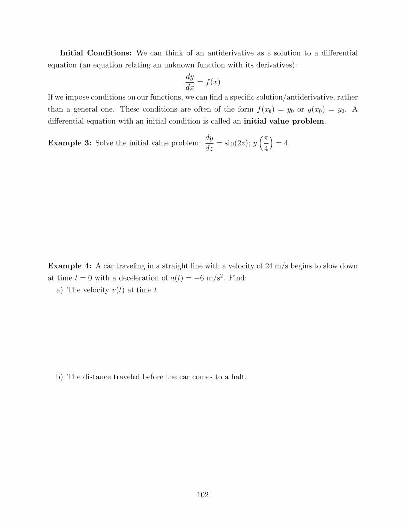
Initial Conditions: We can think of an antiderivative as a solution to a differential

equation (an equation relating an unknown function with its derivatives):

dy

dx= f(x)

If we impose conditions on our functions, we can find a specific solution/antiderivative, rather

than a general one. These conditions are often of the form f(x0) = y0 or y(x0) = y0. A

differential equation with an initial condition is called an initial value problem.

Example 3: Solve the initial value problem:dy

dz= sin(2z); y

(π4

)= 4.

Example 4: A car traveling in a straight line with a velocity of 24 m/s begins to slow down

at time t = 0 with a deceleration of a(t) = −6 m/s2. Find:

a) The velocity v(t) at time t

b) The distance traveled before the car comes to a halt.

102

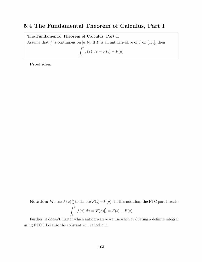
5.4 The Fundamental Theorem of Calculus, Part I

The Fundamental Theorem of Calculus, Part I:

Assume that f is continuous on [a, b]. If F is an antiderivative of f on [a, b], then∫ b

a

f(x) dx = F (b)− F (a)

Proof idea:

Notation: We use F (x)|ba to denote F (b)−F (a). In this notation, the FTC part I reads:∫ b

a

f(x) dx = F (x)|ba = F (b)− F (a)

Further, it doesn’t matter which antiderivative we use when evaluating a definite integral

using FTC I because the constant will cancel out.

103

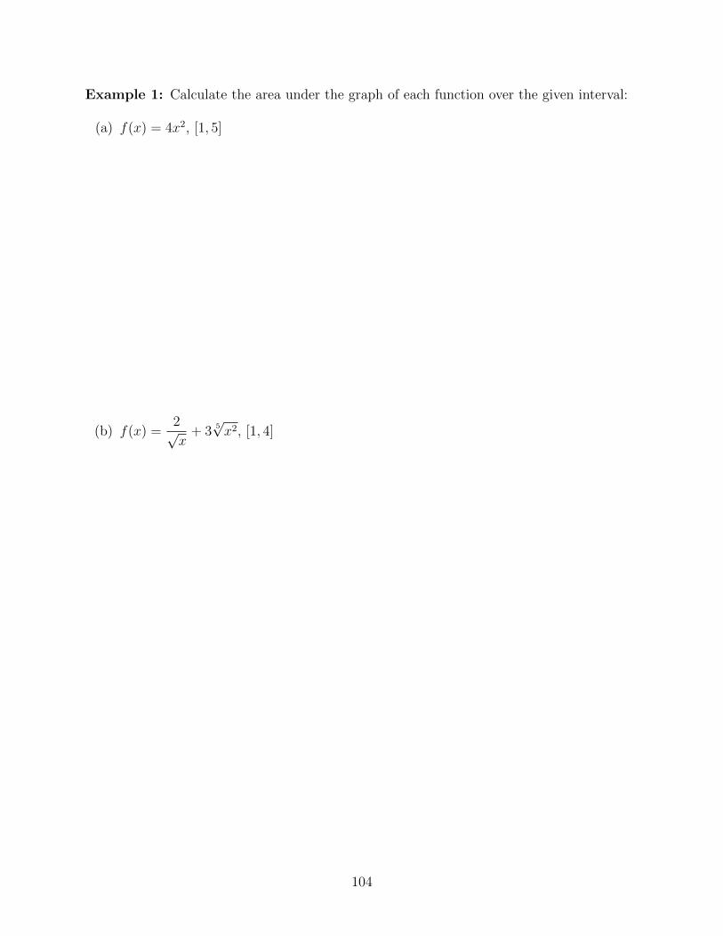
Example 1: Calculate the area under the graph of each function over the given interval:

(a) f(x) = 4x2, [1, 5]

(b) f(x) =2√x

+ 35√x2, [1, 4]

104

Example 2: Evaluate each definite integral.

(a)

∫ π

0

sin(x

2

)dx

(b)

∫ 2π

0

cos

(θ

2

)dθ

(c)

∫ 5

3

2e−4t dt

105

(d)

∫ 8

2

dy

y

(e)

∫ −8

−2

dx

x

(f)

∫ 6

2

(x+

1

x

)dx

106

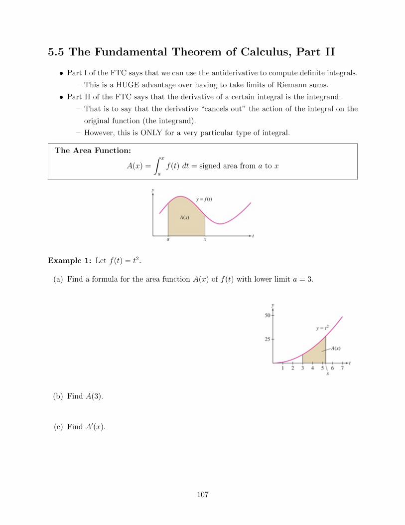
5.5 The Fundamental Theorem of Calculus, Part II

• Part I of the FTC says that we can use the antiderivative to compute definite integrals.

– This is a HUGE advantage over having to take limits of Riemann sums.

• Part II of the FTC says that the derivative of a certain integral is the integrand.

– That is to say that the derivative “cancels out” the action of the integral on the

original function (the integrand).

– However, this is ONLY for a very particular type of integral.

The Area Function:

A(x) =

∫ x

a

f(t) dt = signed area from a to x

Example 1: Let f(t) = t2.

(a) Find a formula for the area function A(x) of f(t) with lower limit a = 3.

(b) Find A(3).

(c) Find A′(x).

107

Example 2: Find the derivative, G′(x).

a) G(x) =

∫ x

−1

cos(t) dt

b) G(x) =

∫ x

4

e−t dt

c) G(x) =

∫ x

1

t1/2 dt

d) What’s the pattern for taking a derivative of a function that is defined like an area

function?

e) G(x) =

∫ x2

−1

cos(t) dt

108

The Fundamental Theorem of Calculus, Part II:

Assume that f is continuous on an open interval I and let a be a point in I. Then the

area function

A(x) =

∫ x

a

f(t) dt

is an antiderivative of f on I; that is, A′(x) = f(x). Equivalently,

d

dx

∫ x

a

f(t) dt = f(x).

Furthermore, A(x) satisfies the initial condition A(a) = 0.

The FTC shows that integration and differentiation are inverse operations. By FTC II,

if you start with a continuous function f and form the integral

∫ x

a

f(t) dt, then you get back

the original function by differentiating:

f(x)Integrate−−−−−→

∫ x

a

f(t) dtDifferentiate−−−−−−−→ d

dx

∫ x

a

f(t) dt = f(x).

On the other hand, by FTC I, if you differentiate first and then integrate, you also recover

f(x) (but only up to a constant f(a)):

f(x)Differentiate−−−−−−−→ f ′(x)

Integrate−−−−−→∫ x

a

f ′(t) dt = f(x)− f(a).

Note: When the upper limit of the integral is a function of x, rather than x

itself, we will require the FTC II and the Chain Rule to differentiate the integral.

Example 3: Calculate the derivative:d

du

∫ 3u

u

e−x dx.

109

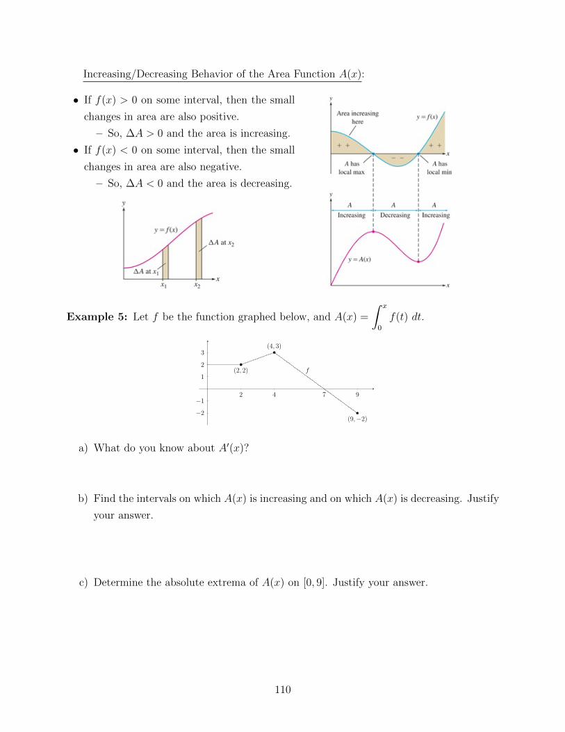
Increasing/Decreasing Behavior of the Area Function A(x):

• If f(x) > 0 on some interval, then the small

changes in area are also positive.

– So, ∆A > 0 and the area is increasing.

• If f(x) < 0 on some interval, then the small

changes in area are also negative.

– So, ∆A < 0 and the area is decreasing.

Example 5: Let f be the function graphed below, and A(x) =

∫ x

0

f(t) dt.

2 4 7 9

−2

−1

1

2

3

f(2, 2)

(4, 3)

(9,−2)

a) What do you know about A′(x)?

b) Find the intervals on which A(x) is increasing and on which A(x) is decreasing. Justify

your answer.

c) Determine the absolute extrema of A(x) on [0, 9]. Justify your answer.

110

5.6 Net Change as the Integral of a Rate of Change

Theorem: Net Change as the Integral of a Rate of Change:

The net change in s(t) over an interval [t1, t2] is given by the integral∫ t2

t1

s′(t) dt︸ ︷︷ ︸Integral of the rate of change

= s(t2)− s(t1)︸ ︷︷ ︸Net change over [t1,t2]

Note: Remember that the integral may be approximated using Riemann Sums if neces-

sary. In these cases, we often calculate the average of the left- and right-endpoint approxi-

mations.

Example 1: A survey shows that a mayoral candidate is gaining votes at a rate of 200t+100

votes per day, where t is the number of days since she announced her candidacy.

(a) How many supporters will the candidate have after 60 days?

(b) How many additional supporters will she gain in the next 30 day period?

111

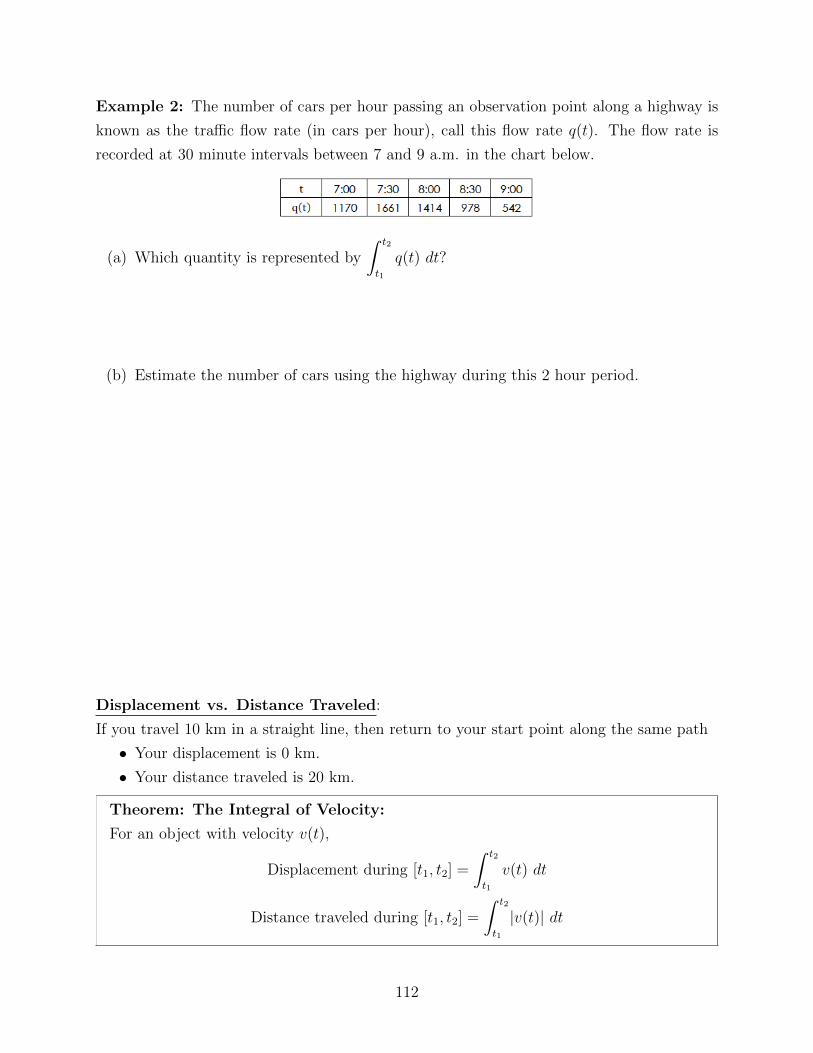
Example 2: The number of cars per hour passing an observation point along a highway is

known as the traffic flow rate (in cars per hour), call this flow rate q(t). The flow rate is

recorded at 30 minute intervals between 7 and 9 a.m. in the chart below.

(a) Which quantity is represented by

∫ t2

t1

q(t) dt?

(b) Estimate the number of cars using the highway during this 2 hour period.

Displacement vs. Distance Traveled:

If you travel 10 km in a straight line, then return to your start point along the same path

• Your displacement is 0 km.

• Your distance traveled is 20 km.

Theorem: The Integral of Velocity:

For an object with velocity v(t),

Displacement during [t1, t2] =

∫ t2

t1

v(t) dt

Distance traveled during [t1, t2] =

∫ t2

t1

|v(t)| dt

112

Example 3: A particle has velocity v(t) = t3 − 10t2 + 24t m/s along a straight path.

Compute:

(a) Displacement over [0, 6].

(b) Total distance traveled over [0, 6].

(c) Indicate the particle’s trajectory with a motion diagram.

113

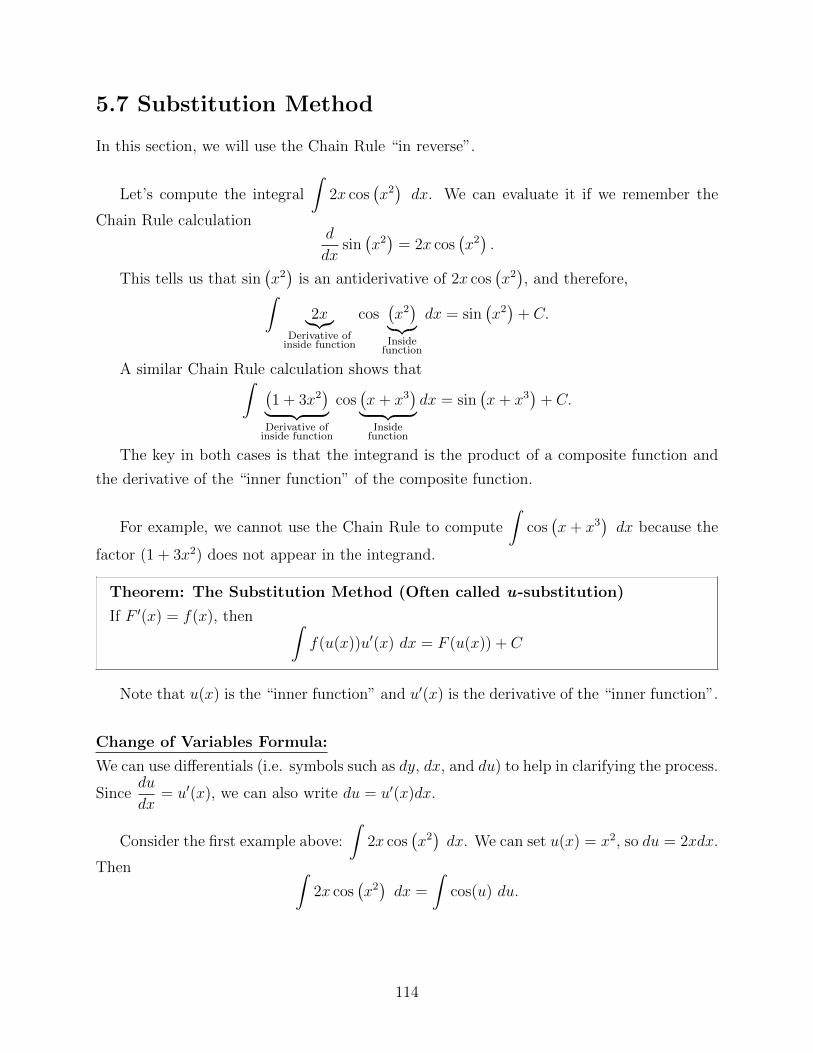
5.7 Substitution Method

In this section, we will use the Chain Rule “in reverse”.

Let’s compute the integral

∫2x cos

(x2)dx. We can evaluate it if we remember the

Chain Rule calculationd

dxsin(x2)

= 2x cos(x2).

This tells us that sin(x2)

is an antiderivative of 2x cos(x2), and therefore,∫

2x︸︷︷︸Derivative of

inside function

cos(x2)︸︷︷︸

Insidefunction

dx = sin(x2)

+ C.

A similar Chain Rule calculation shows that∫ (1 + 3x2

)︸ ︷︷ ︸Derivative of

inside function

cos(x+ x3

)︸ ︷︷ ︸Inside

function

dx = sin(x+ x3

)+ C.

The key in both cases is that the integrand is the product of a composite function and

the derivative of the “inner function” of the composite function.

For example, we cannot use the Chain Rule to compute

∫cos(x+ x3

)dx because the

factor (1 + 3x2) does not appear in the integrand.

Theorem: The Substitution Method (Often called u-substitution)

If F ′(x) = f(x), then ∫f(u(x))u′(x) dx = F (u(x)) + C

Note that u(x) is the “inner function” and u′(x) is the derivative of the “inner function”.

Change of Variables Formula:

We can use differentials (i.e. symbols such as dy, dx, and du) to help in clarifying the process.

Sincedu

dx= u′(x), we can also write du = u′(x)dx.

Consider the first example above:

∫2x cos

(x2)dx. We can set u(x) = x2, so du = 2xdx.

Then ∫2x cos

(x2)dx =

∫cos(u) du.

114

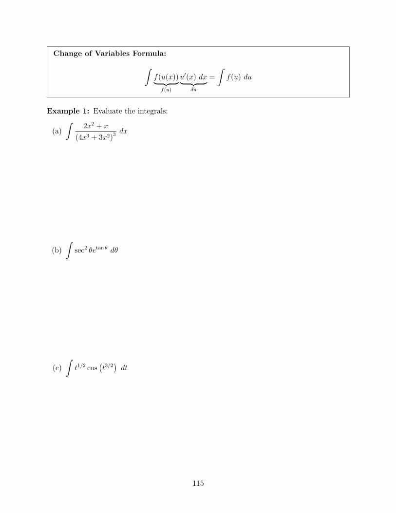
Change of Variables Formula:∫f(u(x))︸ ︷︷ ︸f(u)

u′(x) dx︸ ︷︷ ︸du

=

∫f(u) du

Example 1: Evaluate the integrals:

(a)

∫2x2 + x

(4x3 + 3x2)3 dx

(b)

∫sec2 θetan θ dθ

(c)

∫t1/2 cos

(t3/2)dt

115

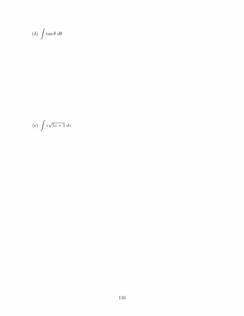
(d)

∫tan θ dθ

(e)

∫z√

5z + 1 dz

116

The Change of Variable Formulas can be applied to definite integrals provided that the limits

of integration are changed.

Change of Variable Formula for Definite Integrals:∫ b

a

f(u(x))u′(x) dx =

∫ u(b)

u(a)

f(u) du

Example 2: Calculate the integral:

(a)

∫ 3

1

x

x2 + 1dx

(b)

∫ π/4

0

tan3 θ sec2 θ dθ

117

5.8 Further Integral Formulas

Inverse Trigonometric Functions:

d

dxsin−1 x =

1√1− x2

,

∫dx√

1− x2= sin−1 x+ C

d

dxtan−1 x =

1

x2 + 1,

∫dx

x2 + 1= tan−1 x+ C

d

dxsec−1 x =

1

|x|√x2 − 1

,

∫dx

|x|√x2 − 1

= sec−1 x+ C

In this list, we omit the integral formulas corresponding to the derivatives of y = cos−1 x,

y = cot−1 x, and y = csc−1 x because the integrals differ only by a minus sign from those

already on the list. For example,

d

dxcos−1 x = − 1√

1− x2,

∫dx√

1− x2= − cos−1 x+ C.

Note: The domain of inverse sine, cosine, secant, and cosecant are x ∈ [−1, 1].

Integral of Exponential Functions (b > 0, b 6= 1):∫ex dx = ex + C∫bx dx =

bx

ln b+ C

Example 1: Evaluate the integral:

(a)

∫ 1

−1

3

x2 + 1dx

118

(b)

∫tan−1 x

1 + x2dx

(c)

∫ 1

0

4−2x dx

119

(d)

∫cotx ln (sinx) dx

(e)

∫(3x+ 2) dx

x2 + 4

Note that even with the tools we learned in this class, we can still only compute a tiny

fraction of integrals! More tools and many applications will be learned in a Calculus II class.

120

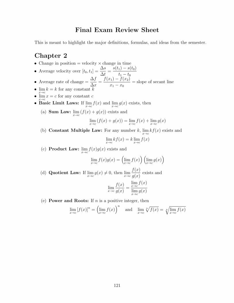
Final Exam Review Sheet

This is meant to highlight the major definitions, formulas, and ideas from the semester.

Chapter 2• Change in position = velocity× change in time

• Average velocity over [t0, t1] =∆s

∆t=s(t1)− s(t0)

t1 − t0• Average rate of change =

∆f

∆x=f(x1)− f(x2)

x1 − x0

= slope of secant line

• limx→c

k = k for any constant k

• limx→c

x = c for any constant c

• Basic Limit Laws: If limx→c

f(x) and limx→c

g(x) exists, then

(a) Sum Law: limx→c

(f(x) + g(x)) exists and

limx→c

(f(x) + g(x)) = limx→c

f(x) + limx→c

g(x)

(b) Constant Multiple Law: For any number k, limx→c

kf(x) exists and

limx→c

kf(x) = k limx→c

f(x)

(c) Product Law: limx→c

f(x)g(x) exists and

limx→c

f(x)g(x) =(

limx→c

f(x))(

limx→c

g(x))

(d) Quotient Law: If limx→c

g(x) 6= 0, then limx→c

f(x)

g(x)exists and

limx→c

f(x)

g(x)=

limx→c

f(x)

limx→c

g(x)

(e) Power and Roots: If n is a positive integer, then

limx→c

[f(x)]n =(

limx→c

f(x))n

and limx→c

n√f(x) = n

√limx→c

f(x)

121

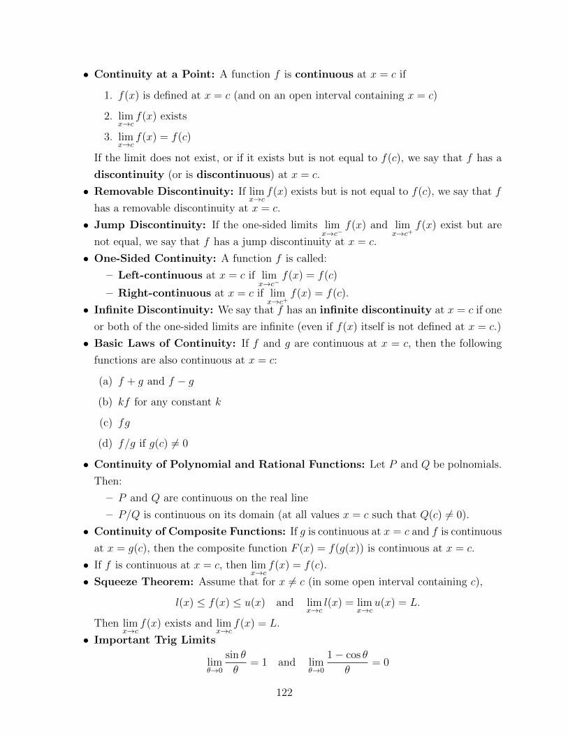
• Continuity at a Point: A function f is continuous at x = c if

1. f(x) is defined at x = c (and on an open interval containing x = c)

2. limx→c

f(x) exists

3. limx→c

f(x) = f(c)

If the limit does not exist, or if it exists but is not equal to f(c), we say that f has a

discontinuity (or is discontinuous) at x = c.

• Removable Discontinuity: If limx→c

f(x) exists but is not equal to f(c), we say that f

has a removable discontinuity at x = c.

• Jump Discontinuity: If the one-sided limits limx→c−

f(x) and limx→c+

f(x) exist but are

not equal, we say that f has a jump discontinuity at x = c.

• One-Sided Continuity: A function f is called:

– Left-continuous at x = c if limx→c−

f(x) = f(c)

– Right-continuous at x = c if limx→c+

f(x) = f(c).

• Infinite Discontinuity: We say that f has an infinite discontinuity at x = c if one

or both of the one-sided limits are infinite (even if f(x) itself is not defined at x = c.)

• Basic Laws of Continuity: If f and g are continuous at x = c, then the following

functions are also continuous at x = c:

(a) f + g and f − g

(b) kf for any constant k

(c) fg

(d) f/g if g(c) 6= 0

• Continuity of Polynomial and Rational Functions: Let P and Q be polnomials.

Then:

– P and Q are continuous on the real line

– P/Q is continuous on its domain (at all values x = c such that Q(c) 6= 0).

• Continuity of Composite Functions: If g is continuous at x = c and f is continuous

at x = g(c), then the composite function F (x) = f(g(x)) is continuous at x = c.

• If f is continuous at x = c, then limx→c

f(x) = f(c).

• Squeeze Theorem: Assume that for x 6= c (in some open interval containing c),

l(x) ≤ f(x) ≤ u(x) and limx→c

l(x) = limx→c

u(x) = L.

Then limx→c

f(x) exists and limx→c

f(x) = L.

• Important Trig Limits

limθ→0

sin θ

θ= 1 and lim

θ→0

1− cos θ

θ= 0

122

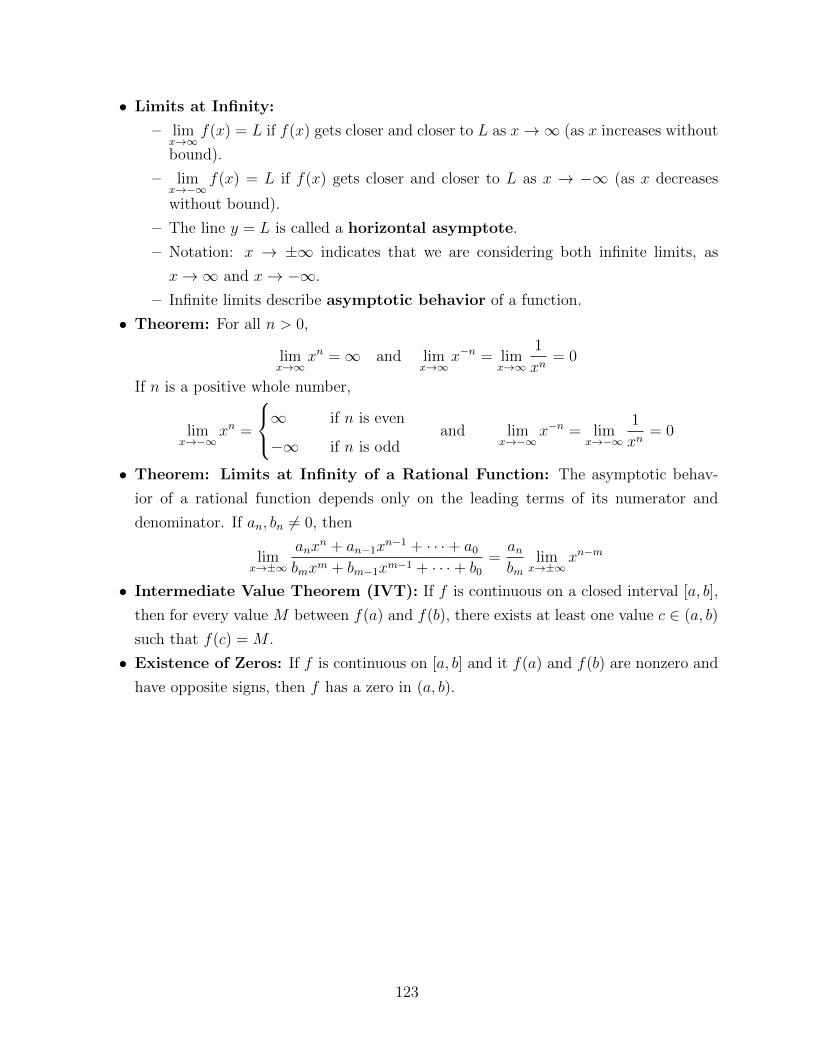
• Limits at Infinity:

– limx→∞

f(x) = L if f(x) gets closer and closer to L as x→∞ (as x increases without

bound).

– limx→−∞

f(x) = L if f(x) gets closer and closer to L as x → −∞ (as x decreases

without bound).

– The line y = L is called a horizontal asymptote.

– Notation: x → ±∞ indicates that we are considering both infinite limits, as

x→∞ and x→ −∞.

– Infinite limits describe asymptotic behavior of a function.

• Theorem: For all n > 0,

limx→∞

xn =∞ and limx→∞

x−n = limx→∞

1

xn= 0

If n is a positive whole number,

limx→−∞

xn =

∞ if n is even

−∞ if n is oddand lim

x→−∞x−n = lim

x→−∞

1

xn= 0

• Theorem: Limits at Infinity of a Rational Function: The asymptotic behav-

ior of a rational function depends only on the leading terms of its numerator and

denominator. If an, bn 6= 0, then

limx→±∞

anxn + an−1x

n−1 + · · ·+ a0

bmxm + bm−1xm−1 + · · ·+ b0

=anbm

limx→±∞

xn−m

• Intermediate Value Theorem (IVT): If f is continuous on a closed interval [a, b],

then for every value M between f(a) and f(b), there exists at least one value c ∈ (a, b)

such that f(c) = M .

• Existence of Zeros: If f is continuous on [a, b] and it f(a) and f(b) are nonzero and

have opposite signs, then f has a zero in (a, b).

123

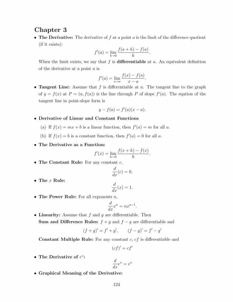
Chapter 3• The Derivative: The derivative of f at a point a is the limit of the difference quotient

(if it exists):

f ′(a) = limh→0

f(a+ h)− f(a)

h.

When the limit exists, we say that f is differentiable at a. An equivalent definition

of the derivative at a point a is

f ′(a) = limx→a

f(x)− f(a)

x− a.

• Tangent Line: Assume that f is differentiable at a. The tangent line to the graph

of y = f(x) at P = (a, f(a)) is the line through P of slope f ′(a). The eqation of the

tangent line in point-slope form is

y − f(a) = f ′(a)(x− a).

• Derivative of Linear and Constant Functions

(a) If f(x) = mx+ b is a linear function, then f ′(a) = m for all a.

(b) If f(x) = b is a constant function, then f ′(a) = 0 for all a.

• The Derivative as a Function:

f ′(x) = limh→0

f(x+ h)− f(x)

h.

• The Constant Rule: For any constant c,

d

dx(c) = 0.

• The x Rule:d

dx(x) = 1.

• The Power Rule: For all exponents n,

d

dxxn = nxn−1.

• Linearity: Assume that f and g are differentiable. Then

Sum and Difference Rules: f + g and f − g are differentiable and

(f + g)′ = f ′ + g′, (f − g)′ = f ′ − g′

Constant Multiple Rule: For any constant c, cf is differentiable and

(cf)′ = cf ′

• The Derivative of ex:d

dxex = ex

• Graphical Meaning of the Derivative:

124

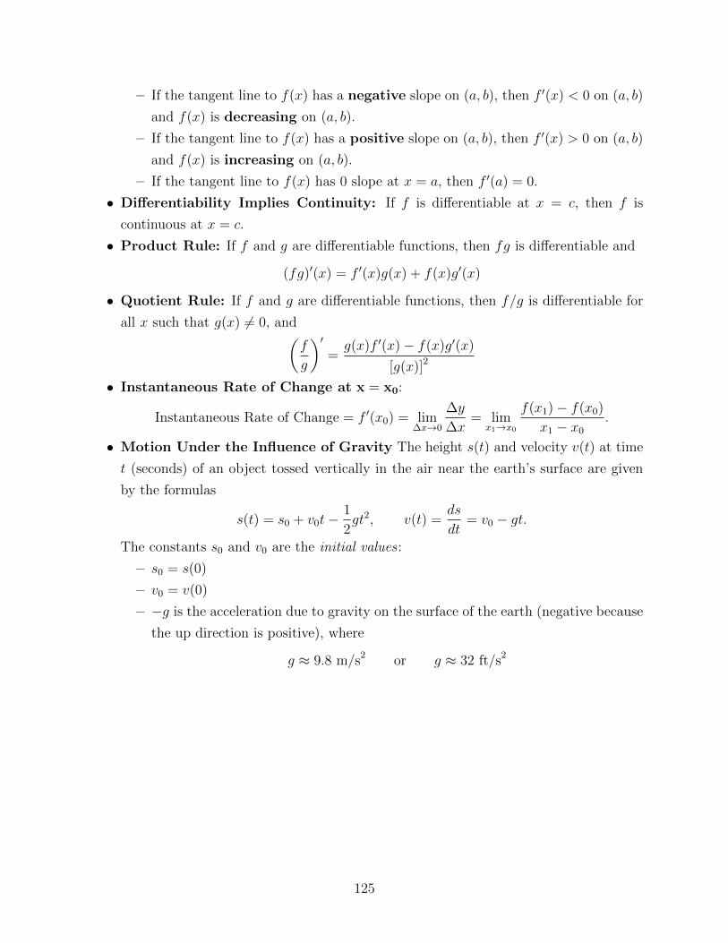
– If the tangent line to f(x) has a negative slope on (a, b), then f ′(x) < 0 on (a, b)

and f(x) is decreasing on (a, b).

– If the tangent line to f(x) has a positive slope on (a, b), then f ′(x) > 0 on (a, b)

and f(x) is increasing on (a, b).

– If the tangent line to f(x) has 0 slope at x = a, then f ′(a) = 0.

• Differentiability Implies Continuity: If f is differentiable at x = c, then f is

continuous at x = c.

• Product Rule: If f and g are differentiable functions, then fg is differentiable and

(fg)′(x) = f ′(x)g(x) + f(x)g′(x)

• Quotient Rule: If f and g are differentiable functions, then f/g is differentiable for

all x such that g(x) 6= 0, and(f

g

)′=g(x)f ′(x)− f(x)g′(x)

[g(x)]2

• Instantaneous Rate of Change at x = x0:

Instantaneous Rate of Change = f ′(x0) = lim∆x→0

∆y

∆x= lim

x1→x0

f(x1)− f(x0)

x1 − x0

.

• Motion Under the Influence of Gravity The height s(t) and velocity v(t) at time

t (seconds) of an object tossed vertically in the air near the earth’s surface are given

by the formulas

s(t) = s0 + v0t−1

2gt2, v(t) =

ds

dt= v0 − gt.

The constants s0 and v0 are the initial values :

– s0 = s(0)

– v0 = v(0)

– −g is the acceleration due to gravity on the surface of the earth (negative because

the up direction is positive), where

g ≈ 9.8 m/s2 or g ≈ 32 ft/s2

125

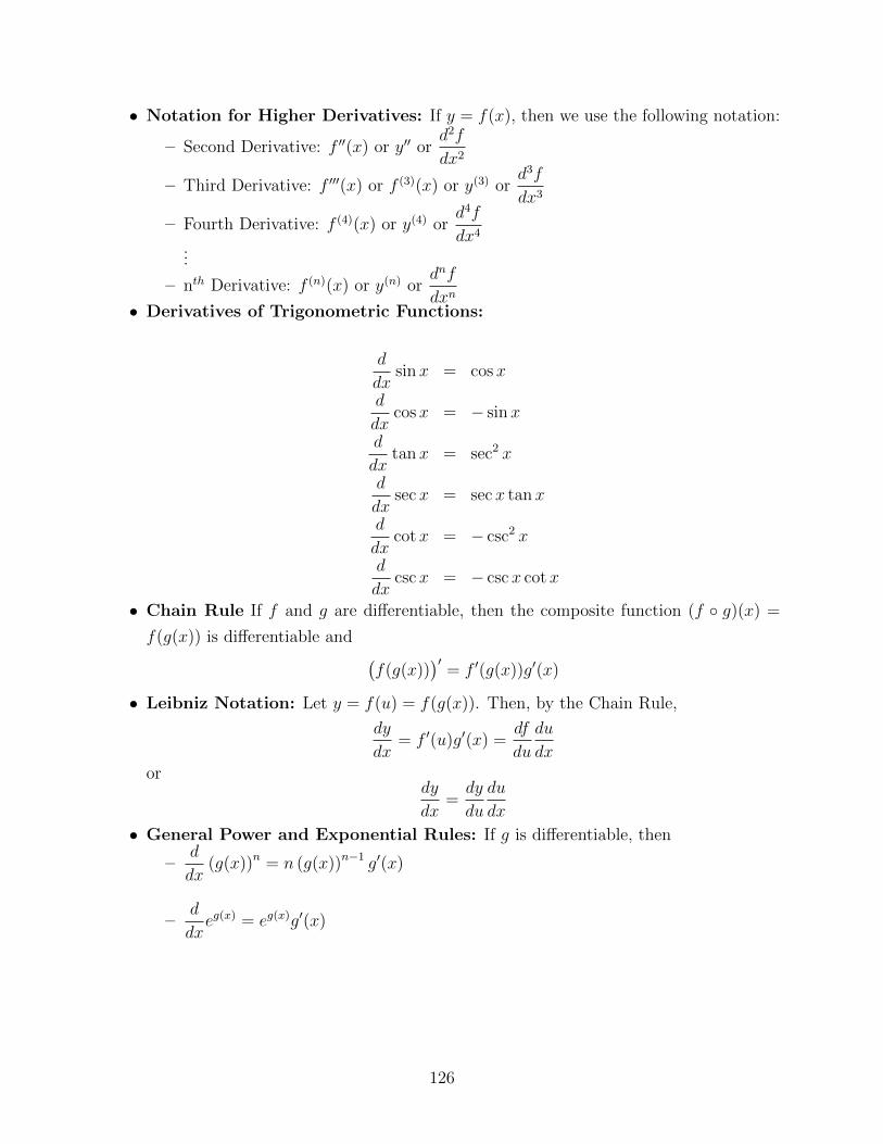
• Notation for Higher Derivatives: If y = f(x), then we use the following notation:

– Second Derivative: f ′′(x) or y′′ ord2f

dx2

– Third Derivative: f ′′′(x) or f (3)(x) or y(3) ord3f

dx3

– Fourth Derivative: f (4)(x) or y(4) ord4f

dx4

...

– nth Derivative: f (n)(x) or y(n) ordnf

dxn• Derivatives of Trigonometric Functions:

d

dxsinx = cos x

d

dxcosx = − sinx

d

dxtanx = sec2 x

d

dxsecx = sec x tanx

d

dxcotx = − csc2 x

d

dxcscx = − cscx cotx

• Chain Rule If f and g are differentiable, then the composite function (f ◦ g)(x) =

f(g(x)) is differentiable and (f(g(x))

)′= f ′(g(x))g′(x)

• Leibniz Notation: Let y = f(u) = f(g(x)). Then, by the Chain Rule,

dy

dx= f ′(u)g′(x) =

df

du

du

dxor

dy

dx=dy

du

du

dx

• General Power and Exponential Rules: If g is differentiable, then

–d

dx(g(x))n = n (g(x))n−1 g′(x)

–d

dxeg(x) = eg(x)g′(x)

126

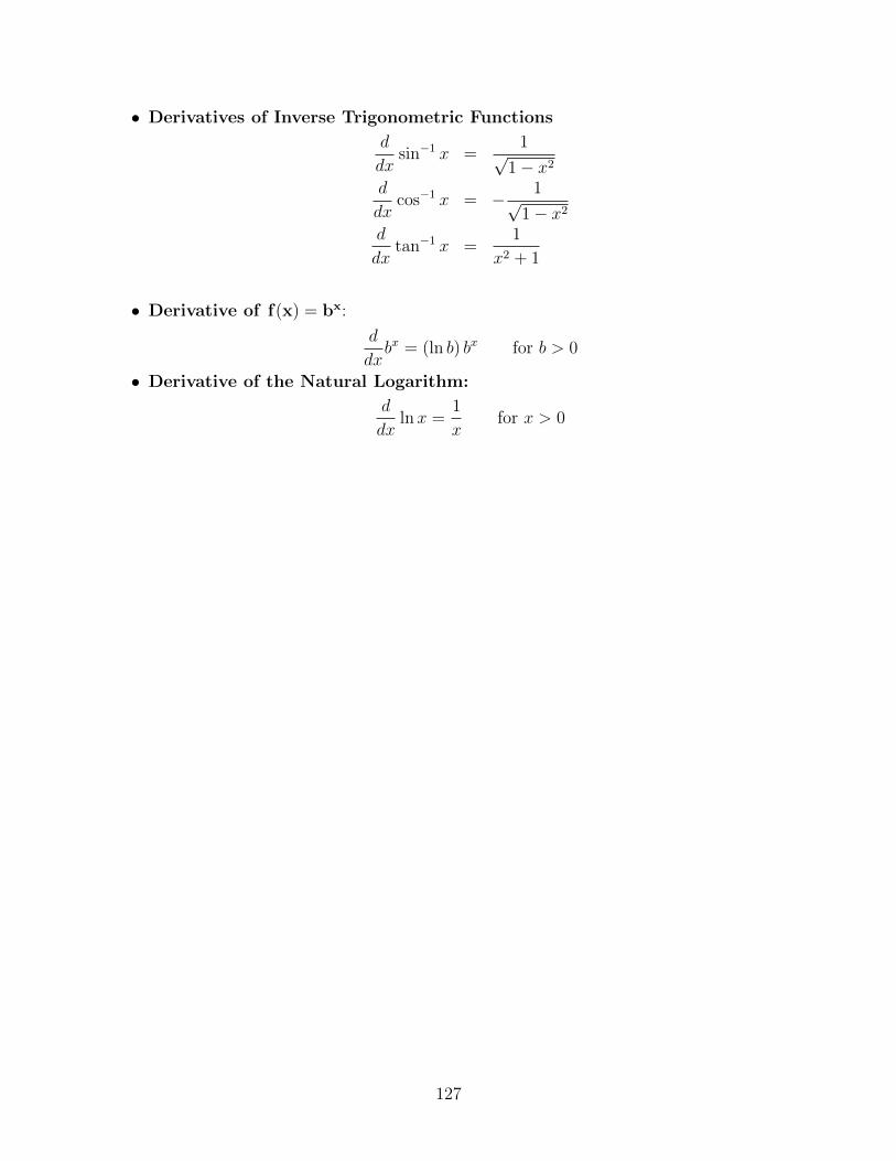
• Derivatives of Inverse Trigonometric Functions

d

dxsin−1 x =

1√1− x2

d

dxcos−1 x = − 1√

1− x2

d

dxtan−1 x =

1

x2 + 1

• Derivative of f(x) = bx:

d

dxbx = (ln b) bx for b > 0

• Derivative of the Natural Logarithm:

d

dxlnx =

1

xfor x > 0

127

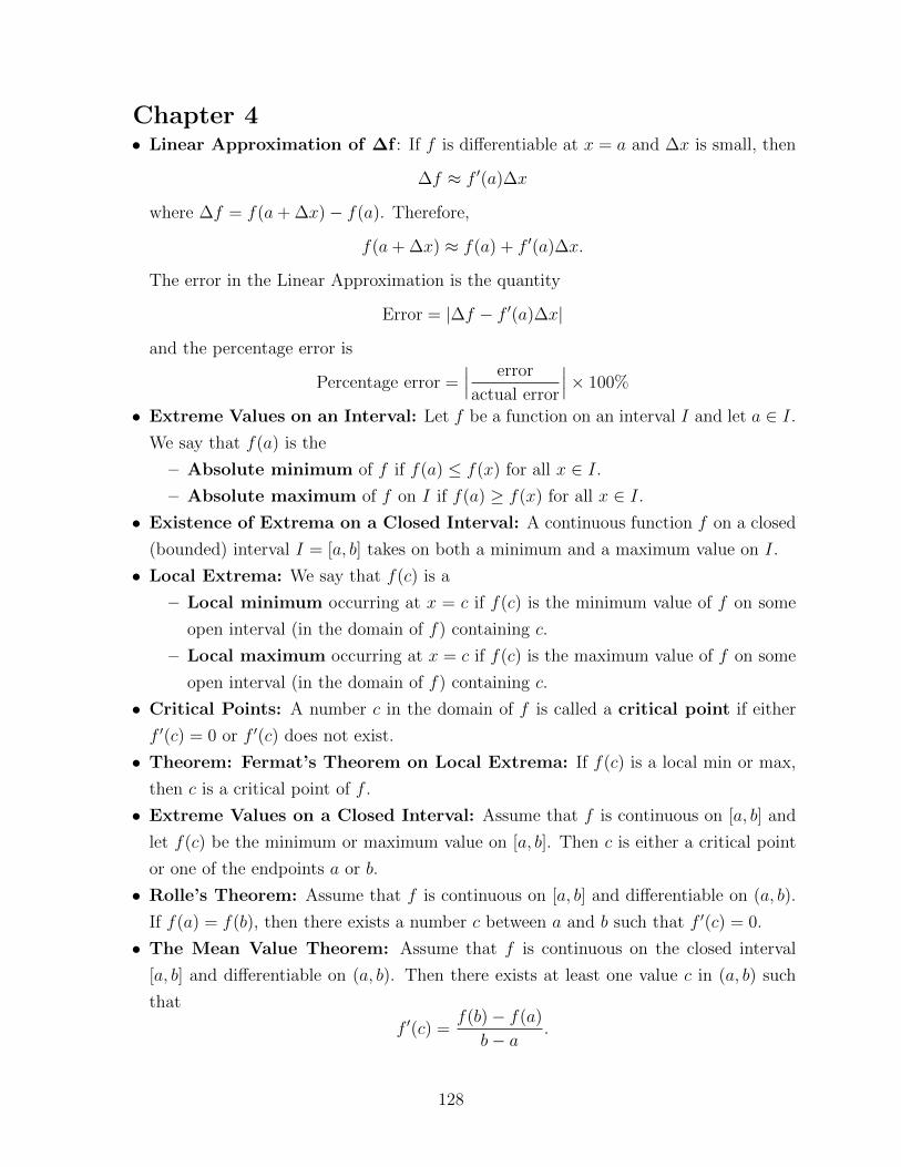
Chapter 4• Linear Approximation of ∆f : If f is differentiable at x = a and ∆x is small, then

∆f ≈ f ′(a)∆x

where ∆f = f(a+ ∆x)− f(a). Therefore,

f(a+ ∆x) ≈ f(a) + f ′(a)∆x.

The error in the Linear Approximation is the quantity

Error = |∆f − f ′(a)∆x|

and the percentage error is

Percentage error =∣∣∣ error

actual error

∣∣∣× 100%

• Extreme Values on an Interval: Let f be a function on an interval I and let a ∈ I.

We say that f(a) is the

– Absolute minimum of f if f(a) ≤ f(x) for all x ∈ I.

– Absolute maximum of f on I if f(a) ≥ f(x) for all x ∈ I.

• Existence of Extrema on a Closed Interval: A continuous function f on a closed

(bounded) interval I = [a, b] takes on both a minimum and a maximum value on I.

• Local Extrema: We say that f(c) is a

– Local minimum occurring at x = c if f(c) is the minimum value of f on some

open interval (in the domain of f) containing c.

– Local maximum occurring at x = c if f(c) is the maximum value of f on some

open interval (in the domain of f) containing c.

• Critical Points: A number c in the domain of f is called a critical point if either

f ′(c) = 0 or f ′(c) does not exist.

• Theorem: Fermat’s Theorem on Local Extrema: If f(c) is a local min or max,

then c is a critical point of f .

• Extreme Values on a Closed Interval: Assume that f is continuous on [a, b] and

let f(c) be the minimum or maximum value on [a, b]. Then c is either a critical point

or one of the endpoints a or b.

• Rolle’s Theorem: Assume that f is continuous on [a, b] and differentiable on (a, b).

If f(a) = f(b), then there exists a number c between a and b such that f ′(c) = 0.

• The Mean Value Theorem: Assume that f is continuous on the closed interval

[a, b] and differentiable on (a, b). Then there exists at least one value c in (a, b) such

that

f ′(c) =f(b)− f(a)

b− a.

128

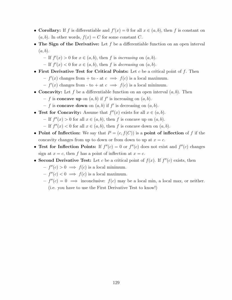
• Corollary: If f is differentiable and f ′(x) = 0 for all x ∈ (a, b), then f is constant on

(a, b). In other words, f(x) = C for some constant C.

• The Sign of the Derivative: Let f be a differentiable function on an open interval

(a, b).

– If f ′(x) > 0 for x ∈ (a, b), then f is increasing on (a, b).

– If f ′(x) < 0 for x ∈ (a, b), then f is decreasing on (a, b).

• First Derivative Test for Critical Points: Let c be a critical point of f . Then

– f ′(x) changes from + to - at c =⇒ f(c) is a local maximum.

– f ′(x) changes from - to + at c =⇒ f(c) is a local minimum.

• Concavity: Let f be a differentiable function on an open interval (a, b). Then

– f is concave up on (a, b) if f ′ is increasing on (a, b).

– f is concave down on (a, b) if f ′ is decreasing on (a, b).

• Test for Concavity: Assume that f ′′(x) exists for all x ∈ (a, b).

– If f ′′(x) > 0 for all x ∈ (a, b), then f is concave up on (a, b).

– If f ′′(x) < 0 for all x ∈ (a, b), then f is concave down on (a, b).

• Point of Inflection: We say that P = (c, f(C)) is a point of inflection of f if the

concavity changes from up to down or from down to up at x = c.

• Test for Inflection Points: If f ′′(c) = 0 or f ′′(c) does not exist and f ′′(c) changes

sign at x = c, then f has a point of inflection at x = c.

• Second Derivative Test: Let c be a critical point of f(x). If f ′′(c) exists, then

– f ′′(c) > 0 =⇒ f(c) is a local minimum.

– f ′′(c) < 0 =⇒ f(c) is a local maximum.

– f ′′(c) = 0 =⇒ inconclusive: f(c) may be a local min, a local max, or neither.

(i.e. you have to use the First Derivative Test to know!)

129

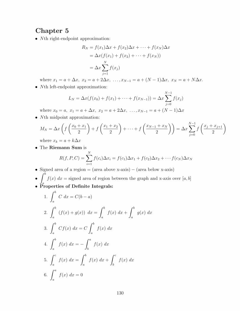
Chapter 5• Nth right-endpoint approximation:

RN = f(x1)∆x+ f(x2)∆x+ · · ·+ f(xN)∆x

= ∆x(f(x1) + f(x2) + · · ·+ f(xN))

= ∆xN∑j=1

f(xj)

where x1 = a+ ∆x, x2 = a+ 2∆x, . . . , xN−1 = a+ (N − 1)∆x, xN = a+N∆x.

• Nth left-endpoint approximation:

LN = ∆x(f(x0) + f(x1) + · · ·+ f(xN−1)) = ∆xN−1∑j=0

f(xj)

where x0 = a, x1 = a+ ∆x, x2 = a+ 2∆x, . . . , xN−1 = a+ (N − 1)∆x

• Nth midpoint approximation:

MN = ∆x

(f

(x0 + x1

2

)+ f

(x1 + x2

2

)+ · · ·+ f

(xN−1 + xN

2

))= ∆x

N−1∑j=0

f

(xj + xj+1

2

)where xk = a+ k∆x

• The Riemann Sum is

R(f, P, C) =N∑i=1

f(ci)∆xi = f(c1)∆x1 + f(c2)∆x2 + · · · f(cN)∆xN

• Signed area of a region = (area above x-axis)− (area below x-axis)

•∫ b

a

f(x) dx = signed area of region between the graph and x-axis over [a, b]

• Properties of Definite Integrals:

1.

∫ b

a

C dx = C(b− a)

2.

∫ b

a

(f(x) + g(x)) dx =

∫ b

a

f(x) dx+

∫ b

a

g(x) dx

3.

∫ b

a

Cf(x) dx = C

∫ b

a

f(x) dx

4.

∫ b

a

f(x) dx = −∫ a

b

f(x) dx

5.

∫ c

a

f(x) dx =

∫ b

a

f(x) dx+

∫ c

b

f(x) dx

6.

∫ a

a

f(x) dx = 0

130

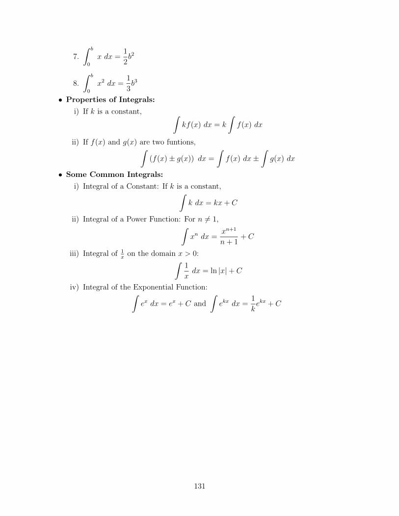
7.

∫ b

0

x dx =1

2b2

8.

∫ b

0

x2 dx =1

3b3

• Properties of Integrals:

i) If k is a constant, ∫kf(x) dx = k

∫f(x) dx

ii) If f(x) and g(x) are two funtions,∫(f(x)± g(x)) dx =

∫f(x) dx±

∫g(x) dx

• Some Common Integrals:

i) Integral of a Constant: If k is a constant,∫k dx = kx+ C

ii) Integral of a Power Function: For n 6= 1,∫xn dx =

xn+1

n+ 1+ C

iii) Integral of 1x

on the domain x > 0:∫1

xdx = ln |x|+ C

iv) Integral of the Exponential Function:∫ex dx = ex + C and

∫ekx dx =

1

kekx + C

131

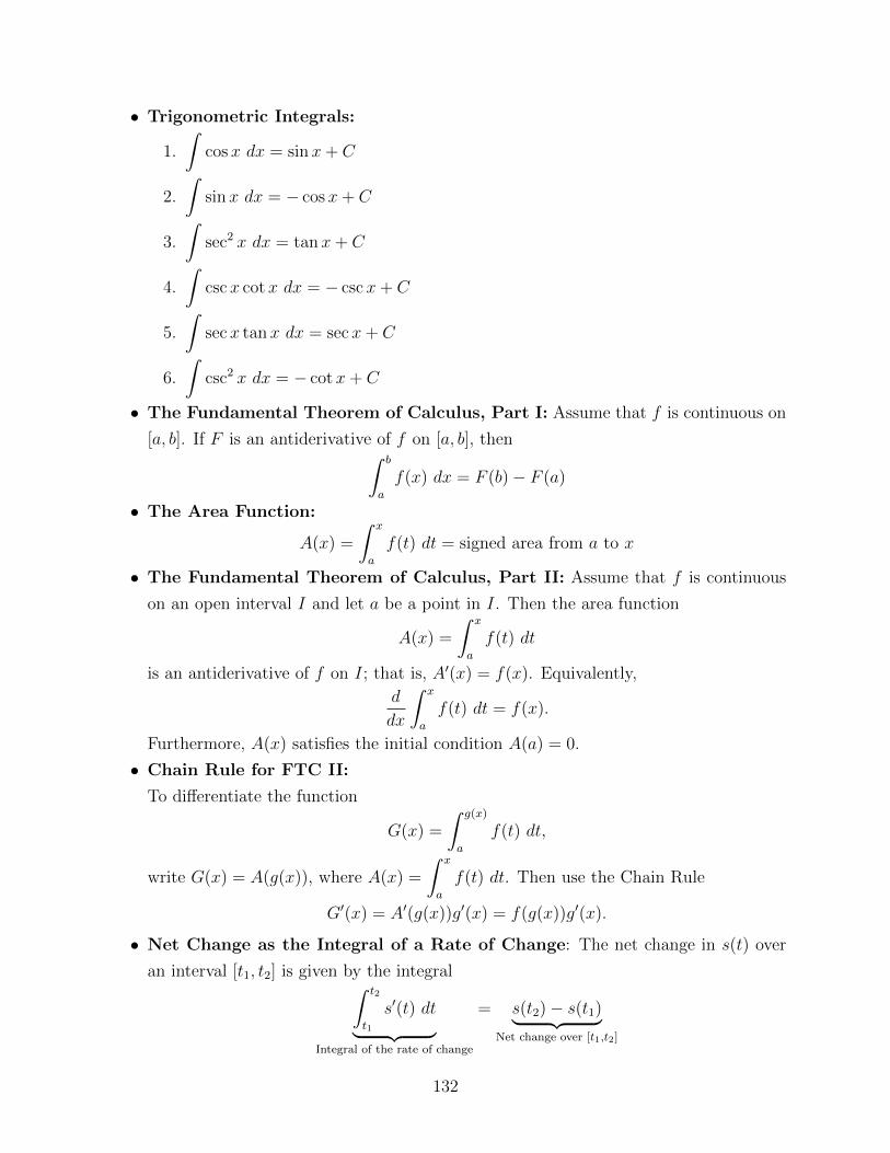
• Trigonometric Integrals:

1.

∫cosx dx = sinx+ C

2.

∫sinx dx = − cosx+ C

3.

∫sec2 x dx = tanx+ C

4.

∫cscx cotx dx = − cscx+ C

5.

∫secx tanx dx = secx+ C

6.

∫csc2 x dx = − cotx+ C

• The Fundamental Theorem of Calculus, Part I: Assume that f is continuous on

[a, b]. If F is an antiderivative of f on [a, b], then∫ b

a

f(x) dx = F (b)− F (a)

• The Area Function:

A(x) =

∫ x

a

f(t) dt = signed area from a to x

• The Fundamental Theorem of Calculus, Part II: Assume that f is continuous

on an open interval I and let a be a point in I. Then the area function

A(x) =

∫ x

a

f(t) dt

is an antiderivative of f on I; that is, A′(x) = f(x). Equivalently,

d

dx

∫ x

a

f(t) dt = f(x).

Furthermore, A(x) satisfies the initial condition A(a) = 0.

• Chain Rule for FTC II:

To differentiate the function

G(x) =

∫ g(x)

a

f(t) dt,

write G(x) = A(g(x)), where A(x) =

∫ x

a

f(t) dt. Then use the Chain Rule

G′(x) = A′(g(x))g′(x) = f(g(x))g′(x).

• Net Change as the Integral of a Rate of Change: The net change in s(t) over

an interval [t1, t2] is given by the integral∫ t2

t1

s′(t) dt︸ ︷︷ ︸Integral of the rate of change

= s(t2)− s(t1)︸ ︷︷ ︸Net change over [t1,t2]

132

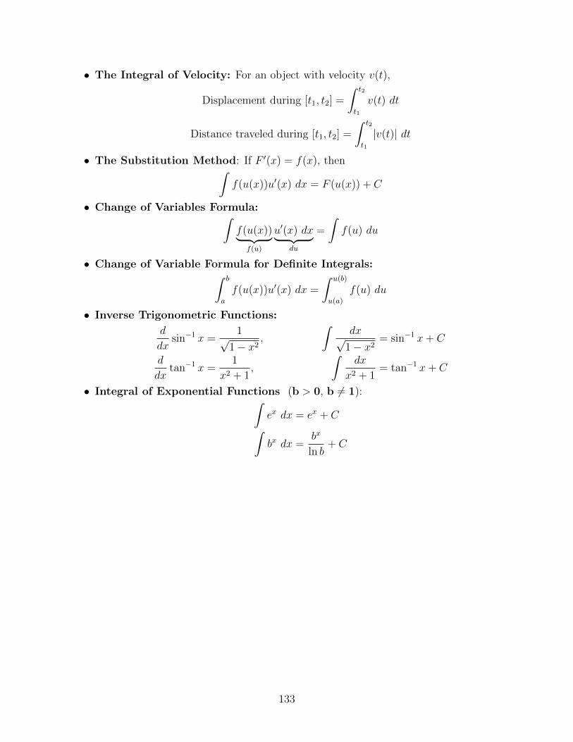
• The Integral of Velocity: For an object with velocity v(t),

Displacement during [t1, t2] =

∫ t2

t1

v(t) dt

Distance traveled during [t1, t2] =

∫ t2

t1

|v(t)| dt

• The Substitution Method: If F ′(x) = f(x), then∫f(u(x))u′(x) dx = F (u(x)) + C

• Change of Variables Formula:∫f(u(x))︸ ︷︷ ︸f(u)

u′(x) dx︸ ︷︷ ︸du

=

∫f(u) du

• Change of Variable Formula for Definite Integrals:∫ b

a

f(u(x))u′(x) dx =

∫ u(b)

u(a)

f(u) du

• Inverse Trigonometric Functions:

d

dxsin−1 x =

1√1− x2

,

∫dx√

1− x2= sin−1 x+ C

d

dxtan−1 x =

1

x2 + 1,

∫dx

x2 + 1= tan−1 x+ C

• Integral of Exponential Functions (b > 0, b 6= 1):∫ex dx = ex + C∫bx dx =

bx

ln b+ C

133