The calculator and calculus packages * Scientific calculations with L A T E X Robert Fuster Universitat Polit` ecnica de Val` encia [email protected] 2014/02/20 Abstract The calculator package allows us to use L A T E X as a calculator, with which we can perform many of the common scientific calculations (with the limitation in accuracy imposed by the T E X arithmetic). This package introduces several new instructions that allow you to do several calculations with integer and decimal numbers using L A T E X. Apart from add, multiply or divide, we can calculate powers, square roots, logarithms, trigonometric and hyperbolic functions . . . In addition, the calculator package supports some elementary calculations with vectors in two and three dimensions and square 2 × 2 and 3 × 3 matrices. The calculus package adds to the calculator package several utilities to use and define various functions and their derivatives, including elementary functions, operations with functions, polar coordinates and vector-valued real functions. Version 2.0 adds new capabilities to both packages. Specifically, now, calculator and calculus can evaluate the inverse trigonometric and the inverse hyperbolic functions (so that we can work with all the classic elementary functions), and also can do some additional calculation with vectors (such as the cross product and the angle between two vectors). Contents 1 Introduction 3 I The calculator package 5 2 Predefined numbers 5 3 Operations with numbers 5 3.1 Assignments and comparisons ............................. 5 3.2 Real arithmetic ..................................... 6 * This document corresponds to calculator v.2.0 and calculus v.2.0, dated 2014/02/20. 1

Welcome message from author
This document is posted to help you gain knowledge. Please leave a comment to let me know what you think about it! Share it to your friends and learn new things together.
Transcript

The calculator and calculus packages∗
Scientific calculations with LATEX
Robert FusterUniversitat Politecnica de Valencia
2014/02/20
Abstract
The calculator package allows us to use LATEX as a calculator, with which we can performmany of the common scientific calculations (with the limitation in accuracy imposed by theTEX arithmetic).
This package introduces several new instructions that allow you to do several calculationswith integer and decimal numbers using LATEX. Apart from add, multiply or divide, we cancalculate powers, square roots, logarithms, trigonometric and hyperbolic functions . . .
In addition, the calculator package supports some elementary calculations with vectorsin two and three dimensions and square 2× 2 and 3× 3 matrices.
The calculus package adds to the calculator package several utilities to use and definevarious functions and their derivatives, including elementary functions, operations withfunctions, polar coordinates and vector-valued real functions.
Version 2.0 adds new capabilities to both packages. Specifically, now, calculator andcalculus can evaluate the inverse trigonometric and the inverse hyperbolic functions (so thatwe can work with all the classic elementary functions), and also can do some additionalcalculation with vectors (such as the cross product and the angle between two vectors).
Contents
1 Introduction 3
I The calculator package 5
2 Predefined numbers 5
3 Operations with numbers 53.1 Assignments and comparisons . . . . . . . . . . . . . . . . . . . . . . . . . . . . . 53.2 Real arithmetic . . . . . . . . . . . . . . . . . . . . . . . . . . . . . . . . . . . . . 6
∗This document corresponds to calculator v.2.0 and calculus v.2.0, dated 2014/02/20.
1

3.2.1 The four basic operations . . . . . . . . . . . . . . . . . . . . . . . . . . . 63.2.2 Powers with integer exponent . . . . . . . . . . . . . . . . . . . . . . . . . 73.2.3 Absolute value, integer part and fractional part . . . . . . . . . . . . . . . 73.2.4 Truncation and rounding . . . . . . . . . . . . . . . . . . . . . . . . . . . 8
3.3 Integers . . . . . . . . . . . . . . . . . . . . . . . . . . . . . . . . . . . . . . . . . 83.3.1 Integer division, quotient and remainder . . . . . . . . . . . . . . . . . . . 93.3.2 Greatest common divisor and least common multiple . . . . . . . . . . . . 103.3.3 Simplifying fractions . . . . . . . . . . . . . . . . . . . . . . . . . . . . . . 10
3.4 Elementary functions . . . . . . . . . . . . . . . . . . . . . . . . . . . . . . . . . . 103.4.1 Square roots . . . . . . . . . . . . . . . . . . . . . . . . . . . . . . . . . . 103.4.2 Exponential and logarithm . . . . . . . . . . . . . . . . . . . . . . . . . . 103.4.3 Trigonometric functions . . . . . . . . . . . . . . . . . . . . . . . . . . . . 113.4.4 Hyperbolic functions . . . . . . . . . . . . . . . . . . . . . . . . . . . . . . 133.4.5 Inverse trigonometric functions(new in version 2.0) . . . . . . . . . . . . . 143.4.6 Inverse hyperbolic functions(new in version 2.0) . . . . . . . . . . . . . . 14
4 Operations with lengths 15
5 Matrix arithmetic 155.1 Vector operations . . . . . . . . . . . . . . . . . . . . . . . . . . . . . . . . . . . . 16
5.1.1 Assignments . . . . . . . . . . . . . . . . . . . . . . . . . . . . . . . . . . 165.1.2 Vector addition and subtraction . . . . . . . . . . . . . . . . . . . . . . . 165.1.3 Scalar-vector product . . . . . . . . . . . . . . . . . . . . . . . . . . . . . 165.1.4 Scalar (dot) product and euclidean norm . . . . . . . . . . . . . . . . . . 175.1.5 Vector (cross) product (new in version 2.0) . . . . . . . . . . . . . . . . . 175.1.6 Unit vector parallel to a given vector (normalized vector) . . . . . . . . . 175.1.7 Absolute value (in each entry of a given vector) . . . . . . . . . . . . . . . 185.1.8 Angle between two vectors (new in version 2.0) . . . . . . . . . . . . . . . 18
5.2 Matrix operations . . . . . . . . . . . . . . . . . . . . . . . . . . . . . . . . . . . 185.2.1 Assignments . . . . . . . . . . . . . . . . . . . . . . . . . . . . . . . . . . 185.2.2 Transposed matrix . . . . . . . . . . . . . . . . . . . . . . . . . . . . . . . 195.2.3 Matrix addition and subtraction . . . . . . . . . . . . . . . . . . . . . . . 195.2.4 Scalar-matrix product . . . . . . . . . . . . . . . . . . . . . . . . . . . . . 205.2.5 Matriu-vector product . . . . . . . . . . . . . . . . . . . . . . . . . . . . . 205.2.6 Product of two square matrices . . . . . . . . . . . . . . . . . . . . . . . . 205.2.7 Determinant . . . . . . . . . . . . . . . . . . . . . . . . . . . . . . . . . . 215.2.8 Inverse matrix . . . . . . . . . . . . . . . . . . . . . . . . . . . . . . . . . 215.2.9 Absolute value (in each entry) . . . . . . . . . . . . . . . . . . . . . . . . 225.2.10 Solving a linear system . . . . . . . . . . . . . . . . . . . . . . . . . . . . 22
II The calculus package 22
6 What is a function? 23
7 Predefined functions 23
2
8 Operations with functions 24
9 Polynomial functions 26
10 Vector-valued functions (or parametrically defined curves) 27
11 Vector-valued functions in polar coordinates 28
12 Low-level instructions 2812.1 The \newfunction declaration and its variants . . . . . . . . . . . . . . . . . . . 2812.2 Vector functions and polar coordinates . . . . . . . . . . . . . . . . . . . . . . . . 29
III Implementation 30
13 calculator 3013.1 Internal lengths and special numbers . . . . . . . . . . . . . . . . . . . . . . . . . 3013.2 Warning messages . . . . . . . . . . . . . . . . . . . . . . . . . . . . . . . . . . . 3113.3 Operations with numbers . . . . . . . . . . . . . . . . . . . . . . . . . . . . . . . 3313.4 Matrix arithmetics . . . . . . . . . . . . . . . . . . . . . . . . . . . . . . . . . . . 56
14 calculus 6914.1 Error and info messages . . . . . . . . . . . . . . . . . . . . . . . . . . . . . . . . 6914.2 New functions . . . . . . . . . . . . . . . . . . . . . . . . . . . . . . . . . . . . . . 7114.3 Polynomials . . . . . . . . . . . . . . . . . . . . . . . . . . . . . . . . . . . . . . . 7314.4 Elementary functions . . . . . . . . . . . . . . . . . . . . . . . . . . . . . . . . . . 7614.5 Operations with functions . . . . . . . . . . . . . . . . . . . . . . . . . . . . . . . 79
1 Introduction
The calculator package defines some instructions which allow us to realize algebraic operations(and to evaluate elementary functions) in our documents. The operations implemented by thecalculator package include routines of assignment of variables, arithmetical calculations withreal and integer numbers, two and three dimensional vector and matrix arithmetics and thecomputation of square roots, trigonometrical, exponential, logarithmic and hyperbolic functions.In addition, some important numbers, such as
√2, π or e, are predefined.
The name of all these commands is spelled in capital letters (with very few exceptions: thecommands \DEGtoRAD and \RADtoDEG and the control sequences that define special numbers,as \numberPI) and, in general, they all need one or more mandatory arguments, the first one(s)of which is(are) number(s) and the last one(s) is(are) the name(s) of the command(s) where theresults will be stored.1 The new commands defined in this way work in any LATEX mode.
By example, this instruction
\MAX{3}{5}{\solution}
1Logically, the control sequences that represent special numbers (as \numberPI) does not need any argument.
3
stores 5 in the command \solution. In a similar way,
\FRACTIONSIMPLIFY{10}{12}{\numerator}{\denominator}
defines \numerator and \denominator as 5 i 6, respectively.The data arguments should not be necessarily explicit numbers; it may also consist in com-
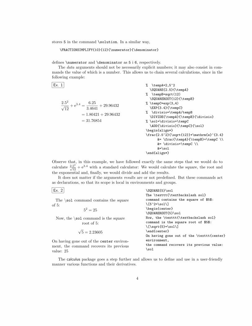
mands the value of which is a number. This allows us to chain several calculations, since in thefollowing example:
Ex. 1
2.52√12
+ e3.4 =6.25
3.4641+ 29.96432
= 1.80421 + 29.96432
= 31.76854
% \tempA=2,5^2
\SQUARE{2.5}{\tempA}
% \tempB=sqrt(12)
\SQUAREROOT{12}{\tempB}
% \tempC=exp(3,4)
\EXP{3.4}{\tempC}
% \divisio=\tempA/tempB
\DIVIDE{\tempA}{\tempB}{\divisio}
% \sol=\divisio+\tempC
\ADD{\divisio}{\tempC}{\sol}
\begin{align*}
\frac{2.5^2}{\sqrt{12}}+\mathrm{e}^{3.4}
&= \frac{\tempA}{\tempB}+\tempC \\
&= \divisio+\tempC \\
&=\sol
\end{align*}
Observe that, in this example, we have followed exactly the same steps that we would do to
calculate 2.52√12
+ e3.4 with a standard calculator: We would calculate the square, the root and
the exponential and, finally, we would divide and add the results.It does not matter if the arguments results are or not predefined. But these commands act
as declarations, so that its scope is local in environments and groups.
Ex. 2
The \sol command contains the squareof 5:
52 = 25
Now, the \sol command is the squareroot of 5:
√5 = 2.23605
On having gone out of the center environ-ment, the command recovers its previousvalue: 25
\SQUARE{5}\sol
The \texttt{\textbackslash sol}
command contains the square of $5$:
\[5^2=\sol\]
\begin{center}
\SQUAREROOT{5}\sol
Now, the \texttt{\textbackslash sol}
command is the square root of $5$:
\[\sqrt{5}=\sol\]
\end{center}
On having gone out of the \texttt{center}
environment,
the command recovers its previous value:
\sol
The calculus package goes a step further and allows us to define and use in a user-friendlymanner various functions and their derivatives.
4
For exemple, using the calculus package, you can define the f(t) = t2et − cos 2t function asfollows:
% \PRODUCTfunction{\SQUAREfunction}{\EXPfunction}{\tempfunctionA}
% \SCALEVARIABLEfunction{2}{\COSfunction}{\tempfunctionB}
% \SUBTRACTfunction{\tempfunctionA}{\tempfunctionB}{\Ffunction}
Then you cau compute any value of the new function \Ffunction and its derivative: typing
\Ffunction{〈num〉}{〈\sol 〉}{〈\Dsol 〉}
the values of f(num) and f ′(num) will be stored in \sol and \Dsol .
Part I
The calculator package
2 Predefined numbers
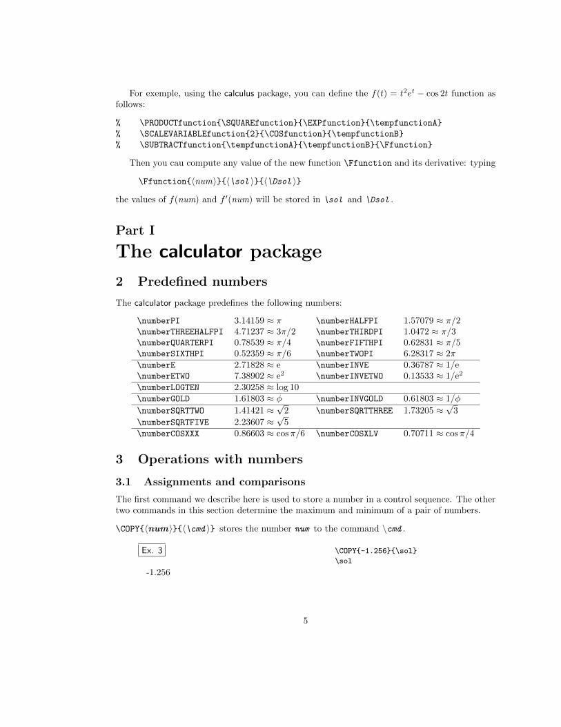
The calculator package predefines the following numbers:
\numberPI 3.14159 ≈ π \numberHALFPI 1.57079 ≈ π/2\numberTHREEHALFPI 4.71237 ≈ 3π/2 \numberTHIRDPI 1.0472 ≈ π/3\numberQUARTERPI 0.78539 ≈ π/4 \numberFIFTHPI 0.62831 ≈ π/5\numberSIXTHPI 0.52359 ≈ π/6 \numberTWOPI 6.28317 ≈ 2π\numberE 2.71828 ≈ e \numberINVE 0.36787 ≈ 1/e\numberETWO 7.38902 ≈ e2 \numberINVETWO 0.13533 ≈ 1/e2
\numberLOGTEN 2.30258 ≈ log 10\numberGOLD 1.61803 ≈ φ \numberINVGOLD 0.61803 ≈ 1/φ
\numberSQRTTWO 1.41421 ≈√
2 \numberSQRTTHREE 1.73205 ≈√
3
\numberSQRTFIVE 2.23607 ≈√
5\numberCOSXXX 0.86603 ≈ cosπ/6 \numberCOSXLV 0.70711 ≈ cosπ/4
3 Operations with numbers
3.1 Assignments and comparisons
The first command we describe here is used to store a number in a control sequence. The othertwo commands in this section determine the maximum and minimum of a pair of numbers.
\COPY{〈num〉}{〈\cmd 〉} stores the number num to the command \cmd .
Ex. 3
-1.256
\COPY{-1.256}{\sol}
\sol
5
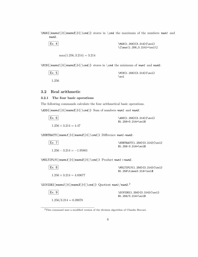
\MAX{〈num1 〉}{〈num2 〉}{〈\cmd 〉} stores in \cmd the maximum of the numbers num1 andnum2 .
Ex. 4
max(1.256, 3.214) = 3.214
\MAX{1.256}{3.214}{\sol}
\[\max(1.256,3.214)=\sol\]
\MIN{〈num1 〉}{〈num2 〉}{〈\cmd 〉} stores in \cmd the minimum of num1 and num2 .
Ex. 5
1.256
\MIN{1.256}{3.214}{\sol}
\sol
3.2 Real arithmetic
3.2.1 The four basic operations
The following commands calculate the four arithmetical basic operations.
\ADD{〈num1 〉}{〈num2 〉}{〈\cmd 〉} Sum of numbers num1 and num2 .
Ex. 6
1.256 + 3.214 = 4.47
\ADD{1.256}{3.214}{\sol}
$1.256+3.214=\sol$
\SUBTRACT{〈num1 〉}{〈num2 〉}{〈\cmd 〉} Difference num1 -num2 .
Ex. 7
1.256− 3.214 = −1.95801
\SUBTRACT{1.256}{3.214}{\sol}
$1.256-3.214=\sol$
\MULTIPLY{〈num1 〉}{〈num2 〉}{〈\cmd 〉} Product num1×num2 .
Ex. 8
1.256× 3.214 = 4.03677
\MULTIPLY{1.256}{3.214}{\sol}
$1.256\times3.214=\sol$
\DIVIDE{〈num1 〉}{〈num2 〉}{〈\cmd 〉} Quotient num1 /num2 .2
Ex. 9
1.256/3.214 = 0.39078
\DIVIDE{1.256}{3.214}{\sol}
$1.256/3.214=\sol$
2This command uses a modified version of the division algorithm of Claudio Beccari.
6

3.2.2 Powers with integer exponent
\SQUARE{〈num〉}{〈\cmd 〉} Square of the number num .
Ex. 10
(−1.256)2 = 1.57751
\SQUARE{-1.256}{\sol}
$(-1.256)^2=\sol$
\CUBE{〈num〉}{〈\cmd 〉} Cube of num .
Ex. 11
(−1.256)3 = −1.98134
\CUBE{-1.256}{\sol}
$(-1.256)^3=\sol$
\POWER{〈num〉}{〈exp〉}{〈\cmd 〉} The exp power of num .
The exponent, exp , must be an integer (if you want to calculate powers with non integerexponents, use the \EXP command).
Ex. 12
(−1.256)−5 = −0.31989
(−1.256)5 = −3.1256
(−1.256)0 = 1
\POWER{-1.256}{-5}{\sola}
\POWER{-1.256}{5}{\solb}
\POWER{-1.256}{0}{\solc}
\[
\begin{aligned}
(-1.256)^{-5}&=\sola
\\
(-1.256)^{5}&=\solb
\\
(-1.256)^{0}&=\solc
\end{aligned}
\]
3.2.3 Absolute value, integer part and fractional part
\ABSVALUE{〈num〉}{〈\cmd 〉} Absolute value of num .
Ex. 13
|−1.256| = 1.256
\ABSVALUE{-1.256}{\sol}
$\left\vert-1.256\right\vert=\sol$
\INTEGERPART{〈num〉}{〈\cmd 〉} Integer part of num .3
Ex. 14
The integer part of 1.256 is 1, but theinteger part of −1.256 is −2.
\INTEGERPART{1.256}{\sola}
\INTEGERPART{-1.256}{\solb}
The integer part of $1.256$ is $\sola$,
but the integer part of $-1.256$ is $\solb$.
3The integer part of x is the largest integer that is less than or equal to x.
7

\FLOOR is an alias of \INTEGERPART.
Ex. 15
The integer part of 1.256 is 1.
\FLOOR{1.256}{\sol}
The integer part of $1.256$ is $\sol$.
\FRACTIONALPART{〈num〉}{〈\cmd 〉} Fractional part of num .
Ex. 16
0.2560.744
\FRACTIONALPART{1.256}{\sol}
\sol
\FRACTIONALPART{-1.256}{\sol}
\sol
3.2.4 Truncation and rounding
\TRUNCATE[〈n〉]{〈num〉}{〈\cmd 〉} truncates the number num to n decimal places.
\ROUND[n ]{〈num〉}{〈\cmd 〉} rounds the number num to n decimal places.
The optional argument n may be 0, 1, 2, 3 or 4 (the default is 2).4
Ex. 17
11.251.2568
\TRUNCATE[0]{1.25688}{\sol}
\sol
\TRUNCATE[2]{1.25688}{\sol}
\sol
\TRUNCATE[4]{1.25688}{\sol}
\sol
Ex. 18
11.261.2569
\ROUND[0]{1.25688}{\sol}
\sol
\ROUND[2]{1.25688}{\sol}
\sol
\ROUND[4]{1.25688}{\sol}
\sol
3.3 Integers
The operations described here are subject to the same restrictions as those referring to decimalnumbers. In particular, although TEX does not have this restriction in its integer arithmetic,the largest integer that can be used is 16383.
4Note than \TRUNCATE[0] is equivalent to \INTEGERPART only for non-negative numbers.
8

3.3.1 Integer division, quotient and remainder
\INTEGERDIVISION{〈num1 〉}{〈num2 〉}{〈\cmd1 〉}{〈\cmd2 〉} stores in the \cmd1 and \cmd2commands the quotient and the remainder of the integer division of the two integers num1and num2 . The remainder is a non-negative number smaller than the divisor.5
Ex. 19
435 = 27× 16 + 327 = 435× 0 + 27−435 = 27× (−17) + 24435 = −27× (−16) + 3−435 = −27× 17 + 24
\INTEGERDIVISION{435}{27}{\sola}{\solb}
$435=27\times\sola+\solb$
\INTEGERDIVISION{27}{435}{\sola}{\solb}
$27=435\times\sola+\solb$
\INTEGERDIVISION{-435}{27}{\sola}{\solb}
$-435=27\times(\sola)+\solb$
\INTEGERDIVISION{435}{-27}{\sola}{\solb}
$435=-27\times(\sola)+\solb$
\INTEGERDIVISION{-435}{-27}{\sola}{\solb}
$-435=-27\times\sola+\solb$
\INTEGERQUOTIENT{〈num1 〉}{〈num2 〉}{〈\cmd 〉} Integer part of the quotient of num1 andnum2 . These two numbers are not necessarily integers.
Ex. 20
160-17
\INTEGERQUOTIENT{435}{27}{\sol}
\sol
\INTEGERQUOTIENT{27}{435}{\sol}
\sol
\INTEGERQUOTIENT{-43.5}{2.7}{\sol}
\sol
\MODULO{〈num1 〉}{〈num2 〉}{〈\cmd 〉} Remainder of the integer division of num1 and num2 .
Ex. 21
435 ≡ 3 (mod 27)
−435 ≡ 24 (mod 27)
\MODULO{435}{27}{\sol}
\[
435 \equiv \sol \pmod{27}
\]
\MODULO{-435}{27}{\sol}
\[
-435 \equiv \sol \pmod{27}
\]
5The scientific computing systems (such as Matlab. Scilab or Mathematica) do not always return a non-negative residue —especially when the divisor is negative—. However, the most reasonable definition of integerquotient is this one: the quotient of the division D/d is the largest number q for which dq ≤ D. With thisdefinition, the remainder r = D − qd is a non-negative number.
9

3.3.2 Greatest common divisor and least common multiple
\GCD{〈num1 〉}{〈num2 〉}{〈\cmd 〉} Greatest common divisor of the integers num1 and num2 .
Ex. 22
gcd(435, 27) = 3
\GCD{435}{27}{\sol}
$\gcd(435,27)=\sol$
\LCM{〈num1 〉}{〈num2 〉}{〈\cmd 〉} Least common multiple of num1 and num2 .
Ex. 23
lcm(435, 27) = 3915
\newcommand{\lcm}{\operatorname{lcm}}
\LCM{435}{27}{\sol}
$\lcm(435,27)=\sol$
3.3.3 Simplifying fractions
\FRACTIONSIMPLIFY{〈num1 〉}{〈num2 〉}{〈\cmd1 〉} {〈\cmd2 〉} stores in the \cmd1 and \cmd2commands the numerator and denominator of the irreducible fraction equivalent tonum1 /num2 .
Ex. 24
435/27 = 145/9
\FRACTIONSIMPLIFY{435}{27}{\sola}{\solb}
$435/27=\sola/\solb$
3.4 Elementary functions
3.4.1 Square roots
\SQUAREROOT {〈num〉}{〈\cmd 〉} Square root of the number num .
Ex. 25
√1.44 = 1.2
\SQUAREROOT{1.44}{\sol}
$\sqrt{1.44}=\sol$
If the argument num is negative, the package returns a warning message.
Instead of \SQUAREROOT, you can use the alias \SQRT.
3.4.2 Exponential and logarithm
The \EXP and \LOG commands compute, by default, exponentials and logarithms of the naturalbase e. They admit, however, an optional argument to choose another base.
10
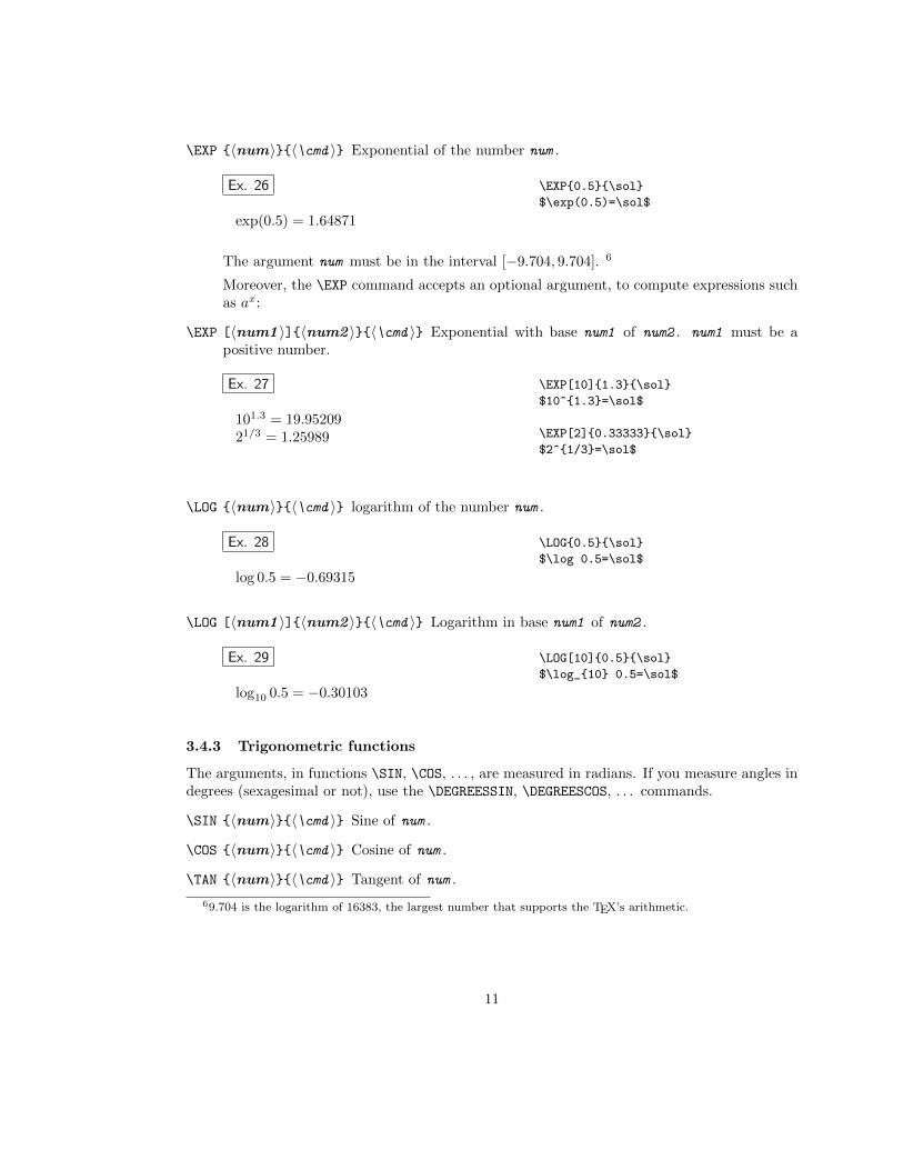
\EXP {〈num〉}{〈\cmd 〉} Exponential of the number num .
Ex. 26
exp(0.5) = 1.64871
\EXP{0.5}{\sol}
$\exp(0.5)=\sol$
The argument num must be in the interval [−9.704, 9.704]. 6
Moreover, the \EXP command accepts an optional argument, to compute expressions suchas ax:
\EXP [〈num1 〉]{〈num2 〉}{〈\cmd 〉} Exponential with base num1 of num2 . num1 must be apositive number.
Ex. 27
101.3 = 19.9520921/3 = 1.25989
\EXP[10]{1.3}{\sol}
$10^{1.3}=\sol$
\EXP[2]{0.33333}{\sol}
$2^{1/3}=\sol$
\LOG {〈num〉}{〈\cmd 〉} logarithm of the number num .
Ex. 28
log 0.5 = −0.69315
\LOG{0.5}{\sol}
$\log 0.5=\sol$
\LOG [〈num1 〉]{〈num2 〉}{〈\cmd 〉} Logarithm in base num1 of num2 .
Ex. 29
log10 0.5 = −0.30103
\LOG[10]{0.5}{\sol}
$\log_{10} 0.5=\sol$
3.4.3 Trigonometric functions
The arguments, in functions \SIN, \COS, . . . , are measured in radians. If you measure angles indegrees (sexagesimal or not), use the \DEGREESSIN, \DEGREESCOS, . . . commands.
\SIN {〈num〉}{〈\cmd 〉} Sine of num .
\COS {〈num〉}{〈\cmd 〉} Cosine of num .
\TAN {〈num〉}{〈\cmd 〉} Tangent of num .
69.704 is the logarithm of 16383, the largest number that supports the TEX’s arithmetic.
11
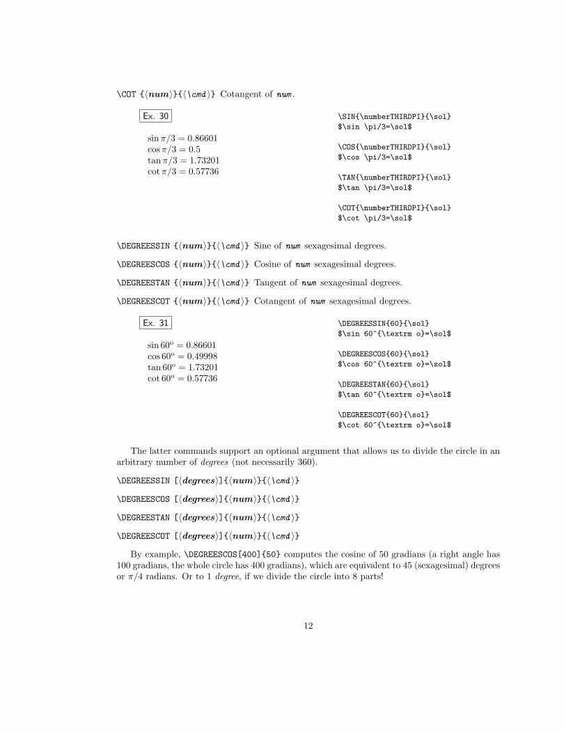
\COT {〈num〉}{〈\cmd 〉} Cotangent of num .
Ex. 30
sinπ/3 = 0.86601cosπ/3 = 0.5tanπ/3 = 1.73201cotπ/3 = 0.57736
\SIN{\numberTHIRDPI}{\sol}
$\sin \pi/3=\sol$
\COS{\numberTHIRDPI}{\sol}
$\cos \pi/3=\sol$
\TAN{\numberTHIRDPI}{\sol}
$\tan \pi/3=\sol$
\COT{\numberTHIRDPI}{\sol}
$\cot \pi/3=\sol$
\DEGREESSIN {〈num〉}{〈\cmd 〉} Sine of num sexagesimal degrees.
\DEGREESCOS {〈num〉}{〈\cmd 〉} Cosine of num sexagesimal degrees.
\DEGREESTAN {〈num〉}{〈\cmd 〉} Tangent of num sexagesimal degrees.
\DEGREESCOT {〈num〉}{〈\cmd 〉} Cotangent of num sexagesimal degrees.
Ex. 31
sin 60o = 0.86601cos 60o = 0.49998tan 60o = 1.73201cot 60o = 0.57736
\DEGREESSIN{60}{\sol}
$\sin 60^{\textrm o}=\sol$
\DEGREESCOS{60}{\sol}
$\cos 60^{\textrm o}=\sol$
\DEGREESTAN{60}{\sol}
$\tan 60^{\textrm o}=\sol$
\DEGREESCOT{60}{\sol}
$\cot 60^{\textrm o}=\sol$
The latter commands support an optional argument that allows us to divide the circle in anarbitrary number of degrees (not necessarily 360).
\DEGREESSIN [〈degrees〉]{〈num〉}{〈\cmd 〉}
\DEGREESCOS [〈degrees〉]{〈num〉}{〈\cmd 〉}
\DEGREESTAN [〈degrees〉]{〈num〉}{〈\cmd 〉}
\DEGREESCOT [〈degrees〉]{〈num〉}{〈\cmd 〉}
By example, \DEGREESCOS[400]{50} computes the cosine of 50 gradians (a right angle has100 gradians, the whole circle has 400 gradians), which are equivalent to 45 (sexagesimal) degreesor π/4 radians. Or to 1 degree, if we divide the circle into 8 parts!
12
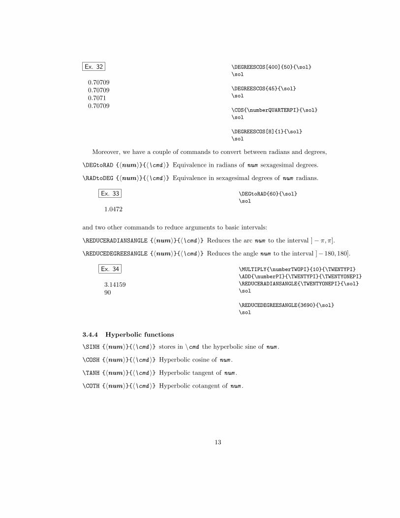
Ex. 32
0.707090.707090.70710.70709
\DEGREESCOS[400]{50}{\sol}
\sol
\DEGREESCOS{45}{\sol}
\sol
\COS{\numberQUARTERPI}{\sol}
\sol
\DEGREESCOS[8]{1}{\sol}
\sol
Moreover, we have a couple of commands to convert between radians and degrees,
\DEGtoRAD {〈num〉}{〈\cmd 〉} Equivalence in radians of num sexagesimal degrees.
\RADtoDEG {〈num〉}{〈\cmd 〉} Equivalence in sexagesimal degrees of num radians.
Ex. 33
1.0472
\DEGtoRAD{60}{\sol}
\sol
and two other commands to reduce arguments to basic intervals:
\REDUCERADIANSANGLE {〈num〉}{〈\cmd 〉} Reduces the arc num to the interval ]− π, π].
\REDUCEDEGREESANGLE {〈num〉}{〈\cmd 〉} Reduces the angle num to the interval ]− 180, 180].
Ex. 34
3.1415990
\MULTIPLY{\numberTWOPI}{10}{\TWENTYPI}
\ADD{\numberPI}{\TWENTYPI}{\TWENTYONEPI}
\REDUCERADIANSANGLE{\TWENTYONEPI}{\sol}
\sol
\REDUCEDEGREESANGLE{3690}{\sol}
\sol
3.4.4 Hyperbolic functions
\SINH {〈num〉}{〈\cmd 〉} stores in \cmd the hyperbolic sine of num .
\COSH {〈num〉}{〈\cmd 〉} Hyperbolic cosine of num .
\TANH {〈num〉}{〈\cmd 〉} Hyperbolic tangent of num .
\COTH {〈num〉}{〈\cmd 〉} Hyperbolic cotangent of num .
13

Ex. 35
1.613281.898070.849951.17651
\SINH{1.256}{\sol}
\sol
\COSH{1.256}{\sol}
\sol
\TANH{1.256}{\sol}
\sol
\COTH{1.256}{\sol}
\sol
3.4.5 Inverse trigonometric functions(new in version 2.0)
\ARCSIN {〈num〉}{〈\cmd 〉} stores in \cmd the arcsin (inverse of sine) of num .
\ARCCOS {〈num〉}{〈\cmd 〉} arccos of num .
\ARCTAN {〈num〉}{〈\cmd 〉} arctan of num .
\ARCCOT {〈num〉}{〈\cmd 〉} arccot of num .
Ex. 36
0.52361.047181.047182.35619
\ARCSIN{0.5}{\sol}
\sol
\ARCCOS{0.5}{\sol}
\sol
\ARCTAN{\numberSQRTTHREE}{\sol}
\sol
\ARCCOT{-1}{\sol}
\sol
3.4.6 Inverse hyperbolic functions(new in version 2.0)
\ARSINH {〈num〉}{〈\cmd 〉} stores in \cmd the arsinh (inverse of hyperbolic sine) of num .
\ARCOSH {〈num〉}{〈\cmd 〉} arcosh of num .
\ARTANH {〈num〉}{〈\cmd 〉} artanh of num .
\ARCOTH {〈num〉}{〈\cmd 〉} arcoth of num .
14

Ex. 37
0.8813800.54930.5493
\ARSINH{1}{\sol}
\sol
\ARCOSH{1}{\sol}
\sol
\ARTANH{0.5}{\sol}
\sol
\ARCOTH{2}{\sol}
\sol
4 Operations with lengths
\LENGTHDIVIDE{〈length1 〉}{〈length2 〉}{〈\cmd 〉}This command divides two lengths and returns a number.
Ex. 38
One inch equals 2.54 centimeters.
\LENGTHDIVIDE{1in}{1cm}{\sol}
One inch equals $\sol$ centimeters.
Commands \LENGTHADD and \LENGTHSUBTRACT return the sum and the difference of twolengths (new in version 2.0).
\LENGTHADD{〈length1 〉}{〈length2 〉}{〈\cmd 〉}
\LENGTHSUBTRACT{〈length1 〉}{〈length2 〉}{〈\cmd 〉}(\cmd must be a predefined length).
Ex. 39
1in+ 1cm = 100.72273pt.1in− 1cm = 43.81725pt.
\newlength{\mylength}
\LENGTHADD{1in}{1cm}{\mylength}
$1in+1cm=\the\mylength$.
\LENGTHSUBTRACT{1in}{1cm}{\mylength}
$1in-1cm=\the\mylength$.
5 Matrix arithmetic
The calculator package defines the commands described below to operate on vectors andmatrices. We only work with two or three-dimensional vectors and 2 × 2 and 3 × 3 ma-trices. Vectors are represented in the form (a1,a2) or (a1,a2,a3);7 and, in the caseof matrices, columns are separated a la matlab by semicolons: (a11,a12;a21,a22) or(a11,a12,a13;a21,a22,a23;a31,a32,a33).
7But they are column vectors.
15

5.1 Vector operations
5.1.1 Assignments
\VECTORCOPY(〈x,y〉)(〈\cmd1,\cmd2 〉) copy the entries of vector (〈x,y〉) to the \cmd1 and\cmd2 commands.
\VECTORCOPY(〈x,y,z 〉)(〈\cmd1,\cmd2,\cmd3 〉) copy the entries of vector (x ,y ,z ) to the\cmd1 , \cmd2 and \cmd3 commands.
Ex. 40
(1,−1)(1,−1, 2)
\VECTORCOPY(1,-1)(\sola,\solb)
$(\sola,\solb)$
\VECTORCOPY(1,-1,2)(\sola,\solb,\solc)
$(\sola,\solb,\solc)$
5.1.2 Vector addition and subtraction
\VECTORADD(〈x1,y1 〉)(〈x2,y2 〉)(〈\cmd1,\cmd2 〉)
\VECTORADD(〈x1,y1,z1 〉)(〈x2,y2,z2 〉) (〈\cmd1,\cmd2,\cmd3 〉)
\VECTORSUB(〈x1,y1 〉)(〈x2,y2 〉)(〈\cmd1,\cmd2 〉)
\VECTORSUB(〈x1,y1,z1 〉)(〈x2,y2,z2 〉) (〈\cmd1,\cmd2,\cmd3 〉)
Ex. 41
(1,−1, 2) + (3, 5,−1) = (4, 4, 1)(1,−1, 2)− (3, 5,−1) = (−2,−6, 3)
\VECTORADD(1,-1,2)(3,5,-1)(\sola,\solb,\solc)
$(1,-1,2)+(3,5,-1)=(\sola,\solb,\solc)$
\VECTORSUB(1,-1,2)(3,5,-1)(\sola,\solb,\solc)
$(1,-1,2)-(3,5,-1)=(\sola,\solb,\solc)$
5.1.3 Scalar-vector product
\SCALARVECTORPRODUCT{〈num〉}(〈x,y〉) (〈\cmd1,\cmd2 〉)
\SCALARVECTORPRODUCT{〈num〉}(〈x,y,z 〉) (〈\cmd1,\cmd2,\cmd3 〉)
Ex. 42
2(3, 5) = (6, 10)2(3, 5,−1) = (6, 10,−2)
\SCALARVECTORPRODUCT{2}(3,5)(\sola,\solb)
$2(3,5)=(\sola,\solb)$
\SCALARVECTORPRODUCT{2}(3,5,-1)(%
\sola,\solb,\solc)
$2(3,5,-1)=(\sola,\solb,\solc)$
16
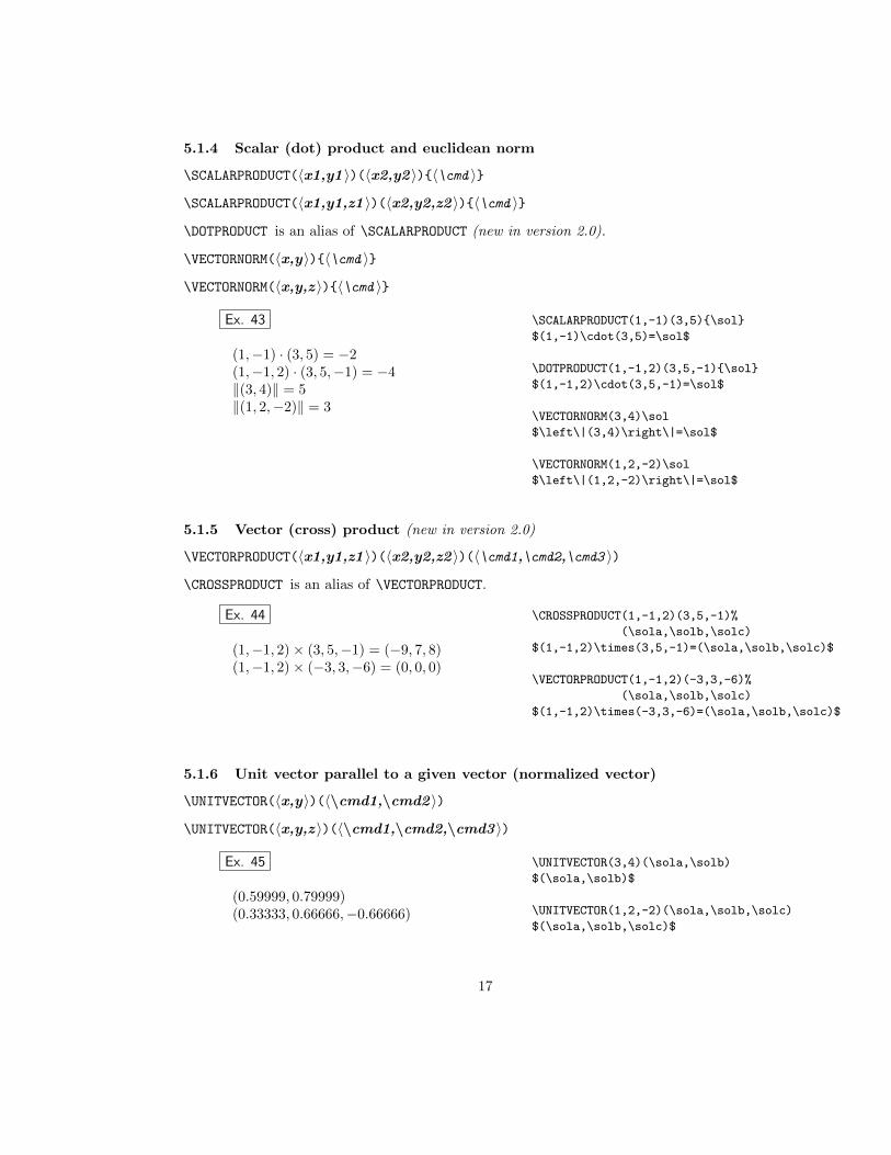
5.1.4 Scalar (dot) product and euclidean norm
\SCALARPRODUCT(〈x1,y1 〉)(〈x2,y2 〉){〈\cmd 〉}
\SCALARPRODUCT(〈x1,y1,z1 〉)(〈x2,y2,z2 〉){〈\cmd 〉}
\DOTPRODUCT is an alias of \SCALARPRODUCT (new in version 2.0).
\VECTORNORM(〈x,y〉){〈\cmd 〉}
\VECTORNORM(〈x,y,z 〉){〈\cmd 〉}
Ex. 43
(1,−1) · (3, 5) = −2(1,−1, 2) · (3, 5,−1) = −4‖(3, 4)‖ = 5‖(1, 2,−2)‖ = 3
\SCALARPRODUCT(1,-1)(3,5){\sol}
$(1,-1)\cdot(3,5)=\sol$
\DOTPRODUCT(1,-1,2)(3,5,-1){\sol}
$(1,-1,2)\cdot(3,5,-1)=\sol$
\VECTORNORM(3,4)\sol
$\left\|(3,4)\right\|=\sol$
\VECTORNORM(1,2,-2)\sol
$\left\|(1,2,-2)\right\|=\sol$
5.1.5 Vector (cross) product (new in version 2.0)
\VECTORPRODUCT(〈x1,y1,z1 〉)(〈x2,y2,z2 〉)(〈\cmd1,\cmd2,\cmd3 〉)
\CROSSPRODUCT is an alias of \VECTORPRODUCT.
Ex. 44
(1,−1, 2)× (3, 5,−1) = (−9, 7, 8)(1,−1, 2)× (−3, 3,−6) = (0, 0, 0)
\CROSSPRODUCT(1,-1,2)(3,5,-1)%
(\sola,\solb,\solc)
$(1,-1,2)\times(3,5,-1)=(\sola,\solb,\solc)$
\VECTORPRODUCT(1,-1,2)(-3,3,-6)%
(\sola,\solb,\solc)
$(1,-1,2)\times(-3,3,-6)=(\sola,\solb,\solc)$
5.1.6 Unit vector parallel to a given vector (normalized vector)
\UNITVECTOR(〈x,y〉)(〈\cmd1,\cmd2 〉)
\UNITVECTOR(〈x,y,z 〉)(〈\cmd1,\cmd2,\cmd3 〉)
Ex. 45
(0.59999, 0.79999)(0.33333, 0.66666,−0.66666)
\UNITVECTOR(3,4)(\sola,\solb)
$(\sola,\solb)$
\UNITVECTOR(1,2,-2)(\sola,\solb,\solc)
$(\sola,\solb,\solc)$
17

5.1.7 Absolute value (in each entry of a given vector)
\VECTORABSVALUE(〈x,y〉)(〈\cmd1,\cmd2 〉)
\VECTORABSVALUE(〈x,y,z 〉)(〈\cmd1,\cmd2,\cmd3 〉)
Ex. 46
(3, 4)(3, 4, 1)
\VECTORABSVALUE(3,-4)(\sola,\solb)
$(\sola,\solb)$
\VECTORABSVALUE(3,-4,-1)(\sola,\solb,\solc)
$(\sola,\solb,\solc)$
5.1.8 Angle between two vectors (new in version 2.0)
\TWOVECTORSANGLE(〈x1,y1 〉)(〈x2,y2 〉){〈\cmd 〉}
\TWOVECTORSANGLE(〈x1,y1,z1 〉)(〈x2,y2,z2 〉){〈\cmd 〉}
Ex. 47
0.78537 radians (or 44.99837 degrees)1.57079 (or 89.99937 degrees)
\TWOVECTORSANGLE(1,1)(0,1){\sol}
$\sol$ radians
\RADtoDEG{\sol}{\degsol}
(or $\degsol$ degrees)
\TWOVECTORSANGLE(1,0,0)(0,1,0){\sol}
$\sol$
\RADtoDEG{\sol}{\degsol}
(or $\degsol$ degrees)
5.2 Matrix operations
5.2.1 Assignments
\MATRIXCOPY (〈a11,a12;a21,a22 〉) (〈\cmd11,\cmd12;\cmd21,\cmd22 〉)
Use this command to store the matrix
[a11 a12a21 22
]in \cmm11 , \cmm12 , \cmm21 , \cmm22 .
The analogous 3× 3 version is
\MATRIXCOPY (〈a11,a12,a13; [. . . ] ,a33 〉) (〈\cmd11,\cmd12,\cmd13; [. . . ] ,\cmd33 〉)
Ex. 48 1 −1 23 0 5−1 1 4
\MATRIXCOPY(1, -1, 2;
3, 0, 5;
-1, 1, 4)%
(\sola,\solb,\solc;
\sold,\sole,\solf;
\solg,\solh,\soli)
$\begin{bmatrix}
\sola & \solb & \solc \\
\sold & \sole & \solf \\
\solg & \solh & \soli
\end{bmatrix}$
18

Henceforth, we will present only the syntax for commands operating with 2× 2 matrices. Inall cases, the syntax is similar if we work with 3 × 3 matrices. In the examples, we will workwith either 2× 2 or 3× 3 matrices.
5.2.2 Transposed matrix
\TRANSPOSEMATRIX (〈a11,a12;a21,a22 〉) (〈\cmd11,\cmd12;\cmd21,\cmd22 〉)
Ex. 49
[1 −13 0
]T=
[1 3−1 0
]\TRANSPOSEMATRIX(1,-1;3,0)%
(\sola,\solb;\solc,\sold)
$\begin{bmatrix}
1 & -1 \\ 3 & 0
\end{bmatrix}^T=\begin{bmatrix}
\sola & \solb \\ \solc & \sold
\end{bmatrix}$
5.2.3 Matrix addition and subtraction
\MATRIXADD (〈a11,a12;a21,a22 〉) (〈b11,b12;b21,b22 〉) (〈\cmd11,\cmd12;\cmd21,\cmd22 〉)
\MATRIXSUB (〈a11,a12;a21,a22 〉) (〈b11,b12;b21,b22 〉) (〈\cmd11,\cmd12;\cmd21,\cmd22 〉)
Ex. 50[1 −13 0
]+
[3 5−3 2
]=
[4 40 2
][1 −13 0
]−[
3 5−3 2
]=
[−2 −66 −2
]\MATRIXADD(1,-1;3,0)(3,5;-3,2)%
(\sola,\solb;\solc,\sold)
$\begin{bmatrix}
1 & -1 \\ 3 & 0
\end{bmatrix}+
\begin{bmatrix}
3 & 5 \\ -3 & 2
\end{bmatrix}=\begin{bmatrix}
\sola & \solb \\ \solc & \sold
\end{bmatrix}$
\MATRIXSUB(1,-1;3,0)(3,5;-3,2)%
(\sola,\solb;\solc,\sold)
$\begin{bmatrix}
1 & -1 \\ 3 & 0
\end{bmatrix}-
\begin{bmatrix}
3 & 5 \\ -3 & 2
\end{bmatrix}=\begin{bmatrix}
\sola & \solb \\ \solc & \sold
\end{bmatrix}$
19

5.2.4 Scalar-matrix product
\SCALARMATRIXPRODUCT{〈num〉} (〈a11,a12;a21,a22 〉) (〈\cmd11,\cmd12;\cmd21,\cmd22 〉)
Ex. 51
3
1 −1 23 0 5−1 1 4
=
3 −3 69 0 15−3 3 12
\SCALARMATRIXPRODUCT{3}(1,-1,2;
3, 0,5;
-1, 1,4)%
(\sola,\solb,\solc;
\sold,\sole,\solf;
\solg,\solh,\soli)
$3\begin{bmatrix}
1 & -1 & 2 \\ 3 & 0 & 5 \\ -1 & 1 & 4
\end{bmatrix}
=\begin{bmatrix}
\sola & \solb & \solc \\
\sold & \sole & \solf \\
\solg & \solh & \soli
\end{bmatrix}$
5.2.5 Matriu-vector product
\MATRIXVECTORPRODUCT (〈a11,a12;a21,a22 〉)(〈x,y〉) (〈\cmd1,\cmd2 〉)
Ex. 52[1 −10 2
] [35
]=
[−210
] \MATRIXVECTORPRODUCT(1,-1;
0, 2)(3,5)(\sola,\solb)
$\begin{bmatrix}
1 & -1 \\ 0 & 2
\end{bmatrix}
\begin{bmatrix}
3 \\ 5
\end{bmatrix}
=\begin{bmatrix}
\sola \\ \solb
\end{bmatrix}$
5.2.6 Product of two square matrices
\MATRIXPRODUCT (〈a11,a12;a21,a22 〉) (〈b11,b12;b21,b22 〉) (〈\cmd11,\cmd12;\cmd21,\cmd22 〉)
20
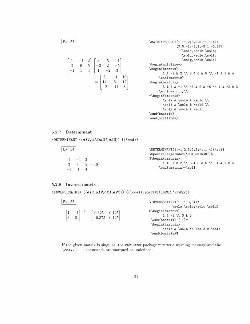
Ex. 53
1 −1 23 0 5−1 1 4
3 5 −1−3 2 −51 −2 3
=
8 −1 1014 5 12−2 −11 8
\MATRIXPRODUCT(1,-1,2;3,0,5;-1,1,4)%
(3,5,-1;-3,2,-5;1,-2,3)%
(\sola,\solb,\solc;
\sold,\sole,\solf;
\solg,\solh,\soli)
\begin{multline*}
\begin{bmatrix}
1 & -1 & 2 \\ 3 & 0 & 5 \\ -1 & 1 & 4
\end{bmatrix}
\begin{bmatrix}
3 & 5 & -1 \\ -3 & 2 & -5 \\ 1 & -2 & 3
\end{bmatrix}\\
=\begin{bmatrix}
\sola & \solb & \solc \\
\sold & \sole & \solf \\
\solg & \solh & \soli
\end{bmatrix}
\end{multline*}
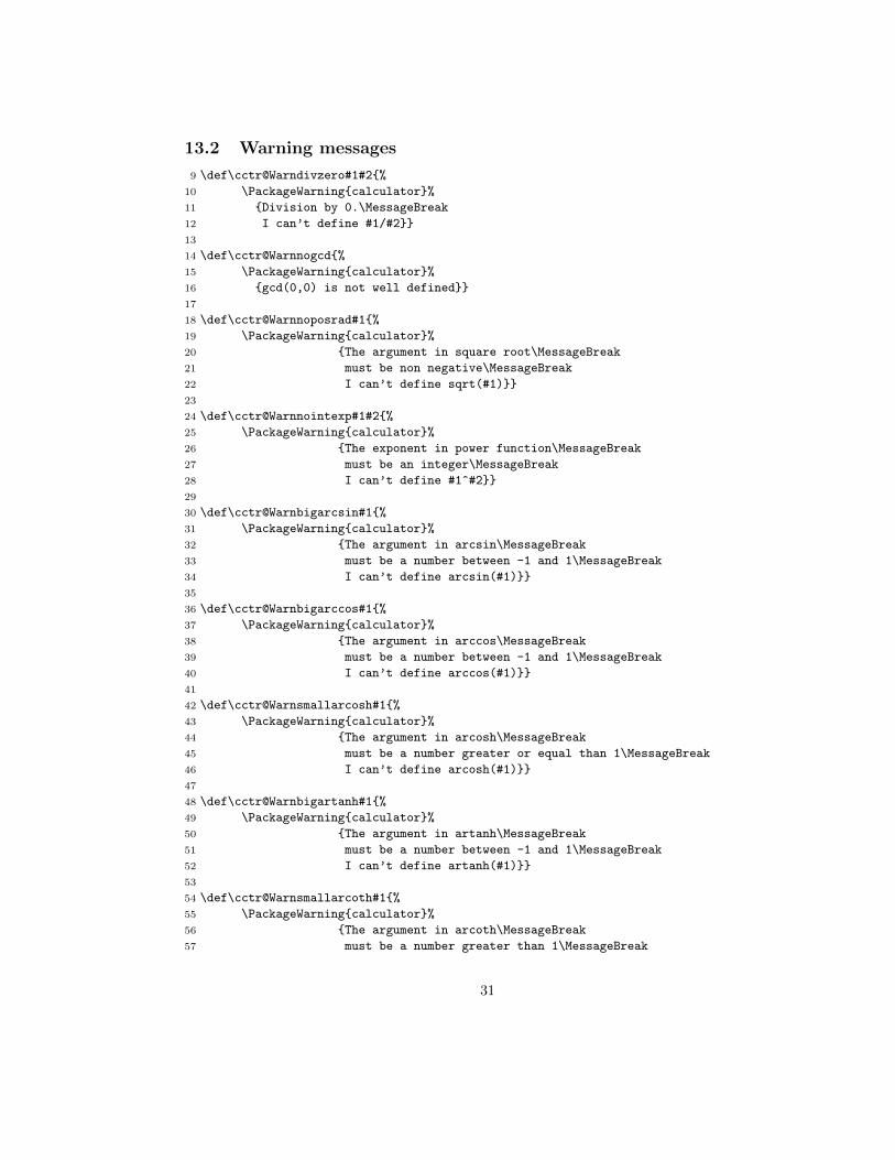
5.2.7 Determinant
\DETERMINANT (〈a11,a12;a21,a22 〉) {〈\cmd 〉}
Ex. 54∣∣∣∣∣∣1 −1 23 0 5−1 1 4
∣∣∣∣∣∣ = 18
\DETERMINANT(1,-1,2;3,0,5;-1,1,4){\sol}
\SpecialUsageIndex{\DETERMINANT}%
$\begin{vmatrix}
1 & -1 & 2 \\ 3 & 0 & 5 \\ -1 & 1 & 4
\end{vmatrix}=\sol$
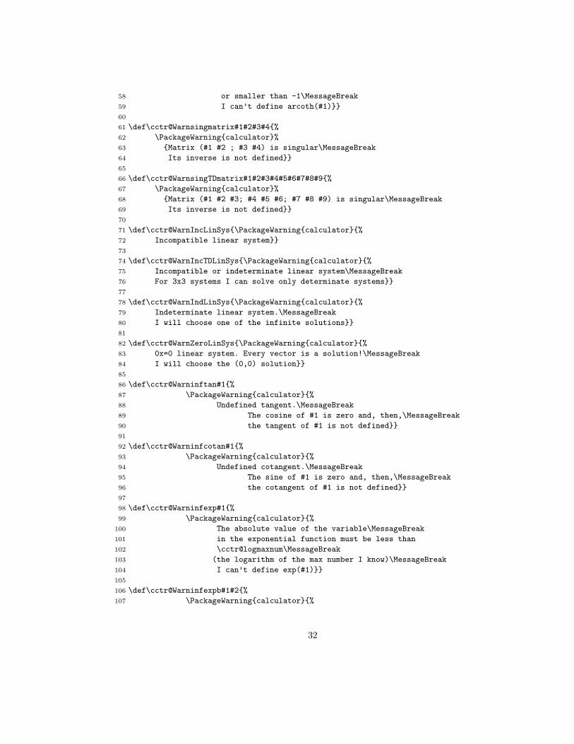
5.2.8 Inverse matrix
\INVERSEMATRIX (〈a11,a12;a21,a22 〉) (〈\cmd11,\cmd12;\cmd21,\cmd22 〉)
Ex. 55
[1 −13 5
]−1=
[0.625 0.125−0.375 0.125
]\INVERSEMATRIX(1,-1;3,5)(%
\sola,\solb;\solc,\sold)
$\begin{bmatrix}
1 & -1 \\ 3 & 5
\end{bmatrix}^{-1}=
\begin{bmatrix}
\sola & \solb \\ \solc & \sold
\end{bmatrix}$
If the given matrix is singular, the calculator package returns a warning message and the\cmd11 , . . . , commands are marqued as undefined.
21

5.2.9 Absolute value (in each entry)
\MATRIXABSVALUE (〈a11,a12;a21,a22 〉) (〈\cmd11,\cmd12;\cmd21,\cmd22 〉)
Ex. 561 1 23 0 51 1 4
\MATRIXABSVALUE(1,-1,2;3,0,5;-1,1,4)%
(\sola,\solb,\solc;
\sold,\sole,\solf;
\solg,\solh,\soli)
$\begin{bmatrix}
\sola & \solb & \solc \\
\sold & \sole & \solf \\
\solg & \solh & \soli
\end{bmatrix}$
5.2.10 Solving a linear system
\SOLVELINEARSYSTEM (〈a11,a12;a21,a22 〉)(〈b1,b2 〉)(〈\cmd1,\cmd2 〉) solves the linear sys-
tem
(a11 a12
a21 a22
)(x
y
)=
(b1
b2
)and stores the solution in (\cmd1 ,\cmd2 ).
Ex. 57
Solving the linear system 1 −1 23 0 5−1 1 4
X =
−44−2
we obtain X =
35−1
\SOLVELINEARSYSTEM(1,-1,2;3,0,5;-1,1,4)%
(-4,4,-2)%
(\sola,\solb,\solc)
Solving the linear system
\[
\begin{bmatrix}
1 & -1 & 2 \\ 3 & 0 & 5 \\ -1 & 1 & 4
\end{bmatrix}\mathsf{X}=\begin{bmatrix}
-4\\4\\-2
\end{bmatrix}
\]
we obtain
$\mathsf{X}=\begin{bmatrix}
\sola \\ \solb\\ \solc
\end{bmatrix}$
If the given matrix is singular, the package calculator returns a warning message. Whensystem is indeterminate, in the bi-dimensional case one of the solutions is computed; if thesystem is incompatible, then the \sola, . . . , commands are marqued as undefined. Forthree equations systems, only determinate systems are solved.8
8This is the only command that does not behave the same way with 2 × 2 and 3 × 3 matrices.
22

Part II
The calculus package
6 What is a function?
From the point of view of this package, a function f is a pair of formulae: the first one calculatesf(t); the other, f ′(t). Therefore, any function is applied using three arguments: the value of thevariable t, and two command names where f(t) and f ′(t) will be stored. For example,
\SQUAREfunction{〈num〉}{〈\sol〉}{〈\Dsol〉}
computes f(t) = t2 and f ′(t) = 2t (where t =num), and stores the results in the commands \soland \Dsol.9
Ex. 58
If f(t) = t2, then
f(3) = 9 and f ′(3) = 6
\SQUAREfunction{3}{\sol}{\Dsol}
If $f(t)=t^2$, then
\[
f(3)=\sol \mbox{ and } f’(3)=\Dsol
\]
For all functions defined here, you must use the following syntax:
\functionname {〈num〉}{〈\cmd1 〉}{〈\cmd2 〉}
being num a number (or a command whose value is a number), and \cmd1 and \cmd2 twocontrol sequence names where the values of the function and its derivative (in this number) willbe stored.
The key difference between this functions and the instructions defined in the calculator pack-age is the inclusion of the derivative; for example, the \SQUARE{3}{\sol} instruction computes,only, the square power of number 3, while \SQUAREfunction{3}{\sol}{\Dsol} finds, also, thecorresponding derivative.
7 Predefined functions
The calculus package predefines the most commonly used elementary functions, and includesseveral utilities for defining new ones. The predefined functions are the following:
9Do not spect any control about the existence or differentiability of the function; if the function or thederivative are not well defined, a TEX error will occur.
23

\ZEROfunction f(t) = 0 \ONEfunction f(t) = 1\IDENTITYfunction f(t) = t \RECIPROCALfunction f(t) = 1/t\SQUAREfunction f(t) = t2 \CUBEfunction f(t) = t3
\SQRTfunction f(t) =√t
\EXPfunction f(t) = exp t \LOGfunction f(t) = log t\COSfunction f(t) = cos t \SINfunction f(t) = sin t\TANfunction f(t) = tan t \COTfunction f(t) = cot t\COSHfunction f(t) = cosh t \SINHfunction f(t) = sinh t\TANHfunction f(t) = tanh t \COTHfunction f(t) = coth t
\HEAVISIDEfunction f(t) =
{0 si t < 0
1 si t ≥ 0
The following functions are added in version 2.0 (new in version 2.0)
\ARCCOSfunction f(t) = arccos t \ARCSINfunction f(t) = arcsin t\ARCTANfunction f(t) = arctan t \ARCCOTfunction f(t) = arccot t\ARCOSHfunction f(t) = arcosh t \ARSINHfunction f(t) = arsinh t\ARTANHfunction f(t) = artanh t \ARCOTHfunction f(t) = arcoth t
In the following example, we use the \LOGfunction function to compute a table of the logfunction and its derivative.
Ex. 59
x log x log′ x1 0 12 0.69315 0.53 1.0986 0.333334 1.38629 0.255 1.60942 0.26 1.79176 0.16666
$\begin{array}{cll}
x & \log x & \log’ x \\
\LOGfunction{1}{\logx}{\Dlogx}
1 &\logx & \Dlogx\\
\LOGfunction{2}{\logx}{\Dlogx}
2 &\logx & \Dlogx\\
\LOGfunction{3}{\logx}{\Dlogx}
3 &\logx & \Dlogx\\
\LOGfunction{4}{\logx}{\Dlogx}
4 &\logx & \Dlogx\\
\LOGfunction{5}{\logx}{\Dlogx}
5 &\logx & \Dlogx\\
\LOGfunction{6}{\logx}{\Dlogx}
6 &\logx & \Dlogx
\end{array}$
8 Operations with functions
We can define new functions using the following operations (the last argument is the name ofthe new function):
\CONSTANTfunction{〈num〉}{〈\Function〉} defines \Function as the constant function num.
Example. Definition of the F (t) = 5 function:
\CONSTANTfunction{5}{\F}
24

\SUMfunction{〈\function1 〉}{〈\function2 〉} {〈\Function〉} defines \Function as the sum offunctions \function1 and \function2.
Example. Definition of the F (t) = t2 + t3 function:
\SUMfunction{\SQUAREfunction}{\CUBEfunction}{\F}
\SUBTRACTfunction{〈\function1 〉}{〈\function2 〉} {〈\Function〉} defines \Function as the dif-ference of functions \function1 and \function2.
Example. Definition of the F (t) = t2 − t3 function:
\SUBTRACTfunction{\SQUAREfunction}{\CUBEfunction}{\F}
\PRODUCTfunction{〈\function1 〉}{〈\function2 〉} {〈\Function〉} defines \Function as the prod-uct of functions \function1 and \function2
Example. Definition of the F (t) = et cos t function:
\PRODUCTfunction{\EXPfunction}{\COSfunction}{\F}
\QUOTIENTfunction{〈\function1 〉}{〈\function2 〉} {〈\Function〉} defines \Function as the quo-tient of functions \function1 and \function2.
Example. Definition of the F (t) = et/ cos t function:
\QUOTIENTfunction{\EXPfunction}{\COSfunction}{\F}
\COMPOSITIONfunction{〈\function1 〉}{〈\function2 〉} {〈\Function〉} defines \Function as thecomposition of functions \function1 and \function2.
Example. Definition of the F (t) = ecos t function:
\COMPOSITIONfunction{\EXPfunction}{\COSfunction}{\F}
(note than \COMPOSITIONfunction{f}{g}{\F} means \F= f ◦ g).
\SCALEfunction{〈num〉}{〈\function〉}{〈\Function〉} defines \Function as the product of num-ber num and function \function.
Example. Definition of the F (t) = 3cos t function:
\SCALEfunction{3}{\COSfunction}{\F}
\SCALEVARIABLEfunction{〈num〉}{〈\function〉} {〈\Function〉} scales the variable by factornum and then applies the function \function.
Example. Definition of the F (t) = cos 3t function:
\SCALEVARIABLEfunction{3}{\COSfunction}{\F}
\POWERfunction{〈\function〉}{〈num〉}{〈\Function〉} defines \Function as the power of func-tion \function to the exponent num (a positive integer). Example. Definition of theF (t) = t5 function:
\POWERfunction{\IDENTITYfunction}{5}{\F}
25

\LINEARCOMBINATIONfunction{〈num1 〉}{〈\function1 〉} {〈num2 〉}{〈\function2 〉}{〈\Function〉}defines \Function as the linear combination of functions \function1 and \function2 mul-tiplied, respectively, by numbers num1 and num2.
Example. Definition of the F (t) = 2t− 3 cos t function:
\LINEARCOMBINATIONfunction{2}{\IDENTITYfunction}{-3}{\COSfunction}{\F}
By combining properly this operations and the predefined functions, many elementary func-tions can be defined.
Ex. 60
Iff(t) = 3t2 − 2e−t cos t
thenf(5) = 74.99619
f ′(5) = 29.99084
% exp(-t)
\SCALEVARIABLEfunction
{-1}{\EXPfunction}
{\NEGEXPfunction}
% exp(-t)cos(t)
\PRODUCTfunction
{\NEGEXPfunction}
{\COSfunction}
{\NEGEXPCOSfunction}
% 3t^2-2exp(-t)cos(t)
\LINEARCOMBINATIONfunction
{3}{\SQUAREfunction}
{-2}{\NEGEXPCOSfunction}
{\myfunction}
\myfunction{5}{\sol}{\Dsol}
If
\[
f(t)=3t^2-2\mathrm{e}^{-t}\cos t
\]
then
\[
\begin{gathered}
f(5)=\sol\\
f’(5)=\Dsol
\end{gathered}
\]
9 Polynomial functions
Although polynomial functions can be defined using linear combinations of power functions, tofacilitate our work, the calculus package includes the following commands to define more easilythe polynomials of 1, 2, and 3 degrees: \newlpoly (new linear polynomial), \newqpoly (newquadratic polynomial), and \newcpoly (new cubic polynomial):
\newlpoly{〈\Function〉}{〈a〉}{〈b〉} stores the p(t) = a + b t function in the \Function com-mand.
26

\newqpoly{〈\Function〉} {〈a〉}{〈b〉}{〈c〉} stores the p(t) = a + b t + c t2 function in the\Function command.
\newcpoly{〈\Function〉}{〈a〉}{〈b〉}{〈c〉}{〈d〉} stores the p(t) = a +b t+c t2 +d t3 function inthe \Function command.
Ex. 61
p′(2) = 8
% \mypoly=1-x^2+x^3
\newcpoly{\mypoly}{1}{0}{-1}{1}
\mypoly{2}{\sol}{\Dsol}
$p’(2)=\Dsol$
These declarations behave similarly to to the declaration \newcommand: If the name you want toassign to the new function is that of an already defined command, the calculus package returnsan error message and do not redefines this command. To obtain any alternative behavior, ourpackage includes three other sets of declarations:
\renewlpoly, \renewqpoly, \renewcpoly redefine the already existing command \Function .If this command does not exist, then it is not defined and an error message occurs.
\ensurelpoly, \ensureqpoly, \ensurecpoly define a new function. If the command \Function
already exists, it is not redefined.
\forcelpoly, \forceqpoly, \forcecpoly define a new function. If the command \Function
already exists, it is redefined.
10 Vector-valued functions (or parametrically defined curves)
The instruction
\PARAMETRICfunction{〈\Xfunction〉}{〈\Yfunction〉} {〈\myvectorfunction〉}
defines the new vector-valued function f(t) = (x(t), y(t)).The first and second arguments are a pair of functions already defined and, the third, the
name of the new function we define. Once we have defined them, the new vector functionsrequires five arguments:
\myvectorfunction {〈num〉}{〈\cmd1 〉} {〈\cmd2 〉}{〈\cmd3 〉}{〈\cmd4 〉}
where
• num is a number t,
• \cmd1 and \cmd2 are two command names where the values of the x(t) function and itsderivative x′(t) will be stored, and
• \cmd3 and \cmd4 will store y(t) and y′(t).
27

In short, in this context, a vector function is a pair of scalar functions.Instead of \PARAMETRICfunction we can use the alias \VECTORfunction.
Ex. 62
For the f(t) = (t2, t3) function we have
f(4) = (16, 64), f ′(4) = (8, 48)
For the $f(t)=(t^2,t^3)$ function we have
\VECTORfunction
{\SQUAREfunction}{\CUBEfunction}{\F}
\F{4}{\solx}{\Dsolx}{\soly}{\Dsoly}
\[
f(4)=(\solx,\soly), f’(4)=(\Dsolx,\Dsoly)
\]
11 Vector-valued functions in polar coordinates
The following instruction:
\POLARfunction{〈\rfunction〉}{〈\Polarfunction〉}
declares the vector function f(φ) = (r(φ) cosφ, r(φ) sinφ). The first argument is the r = r(φ)function, (an already defined function). For example, we can define the Archimedean spiralr(φ) = 0,5φ, as follows:
\SCALEfunction{0.5}{\IDENTITYfunction}{\rfunction}
\POLARfunction{\rfunction}{\archimedes}
12 Low-level instructions
Probably, many users of the package will not be interested in the implementation of the com-mands this package includes. If this is your case, you can ignore this section.
12.1 The \newfunction declaration and its variants
All the functions predefined by this package use the \newfunction declaration. This controlsequence works as follows:
\newfunction{〈\Function〉}{〈Instructions to compute \y and \Dy from \t 〉}
where the second argument is the list of the instructions you need to run to calculate the valueof the function \y and the derivative \Dy in the \t point.
For example, if you want to define the f(t) = t2 + et cos t function, whose derivative isf ′(t) = 2t + et(cos t − sin t), using the high-level instructions we defined earlier, you can writethe following instructions:
\PRODUCTfunction{\EXPfunction}{\COSfunction}{\ffunction}
\SUMfunction{\SQUAREfunction}{\ffunction}{\Ffunction}
But you can also define this function using the \newfunction command as follows:
28

\newfunction{\Ffunction}{%
\SQUARE{\t}{\tempA} % A=t^2
\EXP{\t}{\tempB} % B=e^t
\COS{\t}{\tempC} % C=cos(t)
\SIN{\t}{\tempD} % D=sin(t)
\MULTIPLY{2}{\t}{\tempE} % E=2t
\MULTIPLY{\tempB}{\tempC}{\tempC} % C=e^t cos(t)
\MULTIPLY{\tempB}{\tempD}{\tempD} % D=e^t sin(t)
\ADD{\tempA}{\tempC}{\y} % y=t^2 + e^t cos(t)
\ADD{\tempE}{\tempC}{\tempC} % C=t^2 + e^t cos(t)
\SUBTRACT{\tempC}{\tempD}{\Dy} % y’=t^2 + e^t cos(t) - e^t sin(t)
}
It must be said, however, that the \newfunction declaration behaves similarly to \newcommandor \newlpoly: If the name you want to assign to the new function is that of an already de-fined command, the calculus package returns an error message and does not redefines this com-mand. To obtain any alternative behavior, our package includes three other versions of the\newfunction declarations: the \renewfunction, \ensurefunction and \forcefunction dec-larations. Each of these declarations behaves differently:
\newfunction defines a new function. If the command \Function already exists, it is notredefined and an error message occurs.
\renewfunction redefines the already existing command \Function . If this command doesnot exists, then it is not defined and an error message occurs.
\ensurefunction defines a new function. If the command \Function already exists, it is notredefined.
\forcefunction defines a new function. If the command \Function already exists, it is rede-fined.
12.2 Vector functions and polar coordinates
You can (re)define a vector function f(t) = (x(t), y(t)) using the \newvectorfunction
declaration or any of its variants \renewvectorfunction, \ensurevectorfunction and\forcevectorfunction:
\newvectorfunction{〈\Function〉}{〈Instructions to compute \x, \Dx, \y and \Dy from \t 〉}
For example, you can define the function f(t) = (t2, t3) in the following way:
\newvectorfunction{\F}{%
\SQUARE{\t}{\x} % x=t^2
\MULTIPLY{2}{\t}{\Dx} % x’=2t
\CUBE{\t}{\y} % y=t^3
\MULTIPLY{3}{\x}{\Dy} % y’=3t^2
}
29

Finally, to define the r = r(φ) function, in polar coordinates, we have the declarations\newpolarfunction, \renewpolarfunction, \ensurepolarfunction and \forcepolarfunction.
\newpolarfunction{〈\Function〉}{〈Instructions to compute \r and \Dr from \t 〉}
For example, you can define the cardioide curve r(φ) = 1+cosφ, using high level instructions,
\SUMfunction{\ONEfunction}{\COSfunction}{\ffunction} % y=1 + cos t
\POLARfunction{\ffunction}{\cardioide}
or, with the \newpolarfunction declaration,
\newpolarfunction{\cardioide}{%
\COS{\t}{\r}
\ADD{1}{\r}{\r} % r=1+cos t
\SIN{\t}{\Dr}
\MULTIPLY{-1}{\Dr}{\Dr} % r’=-sin t
}
Part III
Implementation
13 calculator
1 〈∗calculator〉2 \NeedsTeXFormat{LaTeX2e}
3 \ProvidesPackage{calculator}[2014/02/20 v.2.0]
13.1 Internal lengths and special numbers
\cctr@lengtha and \cctr@lengthb will be used in internal calculations and comparisons.
4 \newdimen\cctr@lengtha
5 \newdimen\cctr@lengthb
\cctr@epsilon \cctr@epsilon will store the closest to zero length in the TEX arithmetic: one scaled point(1 sp = 1/65536 pt). This means the smallest positive number will be 0.00002 ≈ 1/65536 =1/216.
6 \newdimen\cctr@epsilon
7 \cctr@epsilon=1sp
\cctr@logmaxnum The largest TEX number is 16383.99998 ≈ 214; \cctr@logmaxnum is the logarithm of this num-ber, 9.704 ≈ log 16384.
8 \def\cctr@logmaxnum{9.704}
30
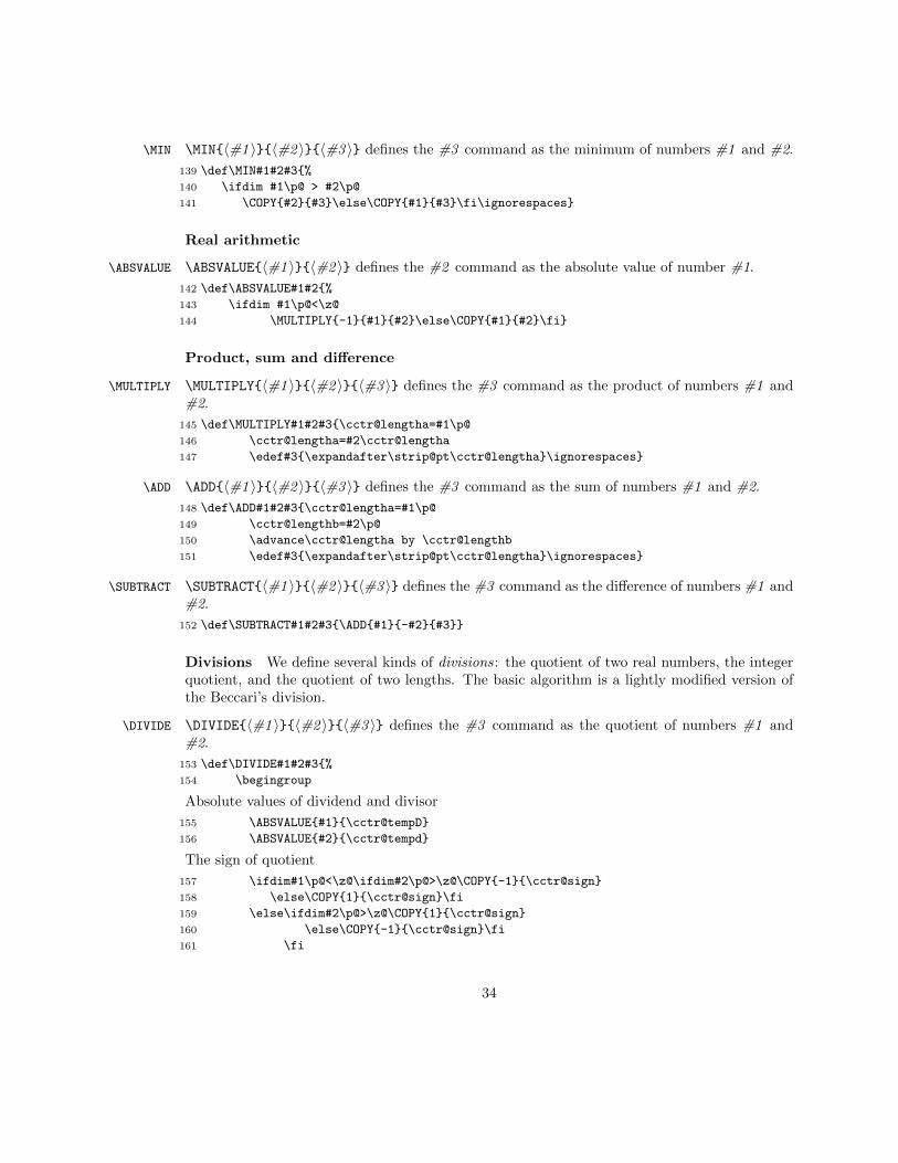
13.2 Warning messages
9 \def\cctr@Warndivzero#1#2{%
10 \PackageWarning{calculator}%
11 {Division by 0.\MessageBreak
12 I can’t define #1/#2}}
13
14 \def\cctr@Warnnogcd{%
15 \PackageWarning{calculator}%
16 {gcd(0,0) is not well defined}}
17
18 \def\cctr@Warnnoposrad#1{%
19 \PackageWarning{calculator}%
20 {The argument in square root\MessageBreak
21 must be non negative\MessageBreak
22 I can’t define sqrt(#1)}}
23
24 \def\cctr@Warnnointexp#1#2{%
25 \PackageWarning{calculator}%
26 {The exponent in power function\MessageBreak
27 must be an integer\MessageBreak
28 I can’t define #1^#2}}
29
30 \def\cctr@Warnbigarcsin#1{%
31 \PackageWarning{calculator}%
32 {The argument in arcsin\MessageBreak
33 must be a number between -1 and 1\MessageBreak
34 I can’t define arcsin(#1)}}
35
36 \def\cctr@Warnbigarccos#1{%
37 \PackageWarning{calculator}%
38 {The argument in arccos\MessageBreak
39 must be a number between -1 and 1\MessageBreak
40 I can’t define arccos(#1)}}
41
42 \def\cctr@Warnsmallarcosh#1{%
43 \PackageWarning{calculator}%
44 {The argument in arcosh\MessageBreak
45 must be a number greater or equal than 1\MessageBreak
46 I can’t define arcosh(#1)}}
47
48 \def\cctr@Warnbigartanh#1{%
49 \PackageWarning{calculator}%
50 {The argument in artanh\MessageBreak
51 must be a number between -1 and 1\MessageBreak
52 I can’t define artanh(#1)}}
53
54 \def\cctr@Warnsmallarcoth#1{%
55 \PackageWarning{calculator}%
56 {The argument in arcoth\MessageBreak
57 must be a number greater than 1\MessageBreak
31
58 or smaller than -1\MessageBreak
59 I can’t define arcoth(#1)}}
60
61 \def\cctr@Warnsingmatrix#1#2#3#4{%
62 \PackageWarning{calculator}%
63 {Matrix (#1 #2 ; #3 #4) is singular\MessageBreak
64 Its inverse is not defined}}
65
66 \def\cctr@WarnsingTDmatrix#1#2#3#4#5#6#7#8#9{%
67 \PackageWarning{calculator}%
68 {Matrix (#1 #2 #3; #4 #5 #6; #7 #8 #9) is singular\MessageBreak
69 Its inverse is not defined}}
70
71 \def\cctr@WarnIncLinSys{\PackageWarning{calculator}{%
72 Incompatible linear system}}
73
74 \def\cctr@WarnIncTDLinSys{\PackageWarning{calculator}{%
75 Incompatible or indeterminate linear system\MessageBreak
76 For 3x3 systems I can solve only determinate systems}}
77
78 \def\cctr@WarnIndLinSys{\PackageWarning{calculator}{%
79 Indeterminate linear system.\MessageBreak
80 I will choose one of the infinite solutions}}
81
82 \def\cctr@WarnZeroLinSys{\PackageWarning{calculator}{%
83 0x=0 linear system. Every vector is a solution!\MessageBreak
84 I will choose the (0,0) solution}}
85
86 \def\cctr@Warninftan#1{%
87 \PackageWarning{calculator}{%
88 Undefined tangent.\MessageBreak
89 The cosine of #1 is zero and, then,\MessageBreak
90 the tangent of #1 is not defined}}
91
92 \def\cctr@Warninfcotan#1{%
93 \PackageWarning{calculator}{%
94 Undefined cotangent.\MessageBreak
95 The sine of #1 is zero and, then,\MessageBreak
96 the cotangent of #1 is not defined}}
97
98 \def\cctr@Warninfexp#1{%
99 \PackageWarning{calculator}{%
100 The absolute value of the variable\MessageBreak
101 in the exponential function must be less than
102 \cctr@logmaxnum\MessageBreak
103 (the logarithm of the max number I know)\MessageBreak
104 I can’t define exp(#1)}}
105
106 \def\cctr@Warninfexpb#1#2{%
107 \PackageWarning{calculator}{%
32

108 The base\MessageBreak
109 in the exponential function must be positive.
110 \MessageBreak
111 I can’t define #1^(#2)}}
112
113 \def\cctr@Warninflog#1{%
114 \PackageWarning{calculator}{%
115 The value of the variable\MessageBreak
116 in the logarithm function must be positive\MessageBreak
117 I can’t define log(#1)}}
118
119 \def\cctr@Warncrossprod(#1)(#2){%
120 \PackageWarning{calculator}%
121 {Vector product only defined\MessageBreak
122 for 3 dimmensional vectors.\MessageBreak
123 I can’t define (#1)x(#2)}}
124
125 \def\cctr@Warnnoangle(#1)(#2){%
126 \PackageWarning{calculator}%
127 {Angle between two vectors only defined\MessageBreak
128 for nonzero vectors.\MessageBreak
129 I can’t define an angle between (#1) and (#2)}}
13.3 Operations with numbers
Assignements and comparisons
\COPY \COPY{〈#1 〉}{〈#2 〉} defines the #2 command as the number #1.
130 \def\COPY#1#2{\edef#2{#1}\ignorespaces}
\GLOBALCOPY Global version of \COPY. The new defined command #2 is not changed outside groups.
131 \def\GLOBALCOPY#1#2{\xdef#2{#1}\ignorespaces}
\@OUTPUTSOL \@OUTPUTSOL{〈#1 〉}: an internal macro to save solutions when a group is closed.The global c.s. \cctr@outa preserves solutions. Whenever we use any temporary param-
eters in the definition of an instruction, we use a group to ensure the local character of thoseparameters. The instruction \@OUTPUTSOL is a bypass to export the solution.
132 \def\@OUTPUTSOL#1{\GLOBALCOPY{#1}{\cctr@outa}\endgroup\COPY{\cctr@outa}{#1}}
\@OUTPUTSOLS Analogous to \@OUTPUTSOL, preserving a pair of solutions.
133 \def\@OUTPUTSOLS#1#2{\GLOBALCOPY{#1}{\cctr@outa}
134 \GLOBALCOPY{#2}{\cctr@outb}\endgroup
135 \COPY{\cctr@outa}{#1}\COPY{\cctr@outb}{#2}}
\MAX \MAX{〈#1 〉}{〈#2 〉}{〈#3 〉} defines the #3 command as the maximum of numbers #1 and #2.
136 \def\MAX#1#2#3{%
137 \ifdim #1\p@ < #2\p@
138 \COPY{#2}{#3}\else\COPY{#1}{#3}\fi\ignorespaces}
33
\MIN \MIN{〈#1 〉}{〈#2 〉}{〈#3 〉} defines the #3 command as the minimum of numbers #1 and #2.
139 \def\MIN#1#2#3{%
140 \ifdim #1\p@ > #2\p@
141 \COPY{#2}{#3}\else\COPY{#1}{#3}\fi\ignorespaces}
Real arithmetic
\ABSVALUE \ABSVALUE{〈#1 〉}{〈#2 〉} defines the #2 command as the absolute value of number #1.
142 \def\ABSVALUE#1#2{%
143 \ifdim #1\p@<\z@
144 \MULTIPLY{-1}{#1}{#2}\else\COPY{#1}{#2}\fi}
Product, sum and difference
\MULTIPLY \MULTIPLY{〈#1 〉}{〈#2 〉}{〈#3 〉} defines the #3 command as the product of numbers #1 and#2.
145 \def\MULTIPLY#1#2#3{\cctr@lengtha=#1\p@
146 \cctr@lengtha=#2\cctr@lengtha
147 \edef#3{\expandafter\strip@pt\cctr@lengtha}\ignorespaces}
\ADD \ADD{〈#1 〉}{〈#2 〉}{〈#3 〉} defines the #3 command as the sum of numbers #1 and #2.
148 \def\ADD#1#2#3{\cctr@lengtha=#1\p@
149 \cctr@lengthb=#2\p@
150 \advance\cctr@lengtha by \cctr@lengthb
151 \edef#3{\expandafter\strip@pt\cctr@lengtha}\ignorespaces}
\SUBTRACT \SUBTRACT{〈#1 〉}{〈#2 〉}{〈#3 〉} defines the #3 command as the difference of numbers #1 and#2.
152 \def\SUBTRACT#1#2#3{\ADD{#1}{-#2}{#3}}
Divisions We define several kinds of divisions: the quotient of two real numbers, the integerquotient, and the quotient of two lengths. The basic algorithm is a lightly modified version ofthe Beccari’s division.
\DIVIDE \DIVIDE{〈#1 〉}{〈#2 〉}{〈#3 〉} defines the #3 command as the quotient of numbers #1 and#2.
153 \def\DIVIDE#1#2#3{%
154 \begingroup
Absolute values of dividend and divisor
155 \ABSVALUE{#1}{\cctr@tempD}
156 \ABSVALUE{#2}{\cctr@tempd}
The sign of quotient
157 \ifdim#1\p@<\z@\ifdim#2\p@>\z@\COPY{-1}{\cctr@sign}
158 \else\COPY{1}{\cctr@sign}\fi
159 \else\ifdim#2\p@>\z@\COPY{1}{\cctr@sign}
160 \else\COPY{-1}{\cctr@sign}\fi
161 \fi
34

Integer part of quotient
162 \@DIVIDE{\cctr@tempD}{\cctr@tempd}{\cctr@tempq}{\cctr@tempr}
163 \COPY{\cctr@tempq.}{\cctr@Q}
Fractional part up to five decimal places. \cctr@ndec is the number of decimal places alreadycomputed.
164 \COPY{0}{\cctr@ndec}
165 \@whilenum \cctr@ndec<5 \do{%
Each decimal place is calculated by multiplying by 10 the last remainder and dividing it by thedivisor. But when the remainder is greater than 1638.3, an overflow occurs, because 16383.99998is the greatest number. So, instead, we multiply the divisor by 0.1.
166 \ifdim\cctr@tempr\p@<1638\p@
167 \MULTIPLY{\cctr@tempr}{10}{\cctr@tempD}
168 \else
169 \COPY{\cctr@tempr}{\cctr@tempD}
170 \MULTIPLY{\cctr@tempd}{0.1}{\cctr@tempd}
171 \fi
172 \@DIVIDE{\cctr@tempD}{\cctr@tempd}{\cctr@tempq}{\cctr@tempr}
173 \COPY{\cctr@Q\cctr@tempq}{\cctr@Q}
174 \ADD{1}{\cctr@ndec}{\cctr@ndec}}%
Adjust the sign and return the solution.
175 \MULTIPLY{\cctr@sign}{\cctr@Q}{#3}
176 \@OUTPUTSOL{#3}}
\@DIVIDE The \@DIVIDE(〈#1 〉) (〈#2 〉)(〈#3 〉)(〈#4 〉) command computes #1/#2 and returns an integerquotient (#3 ) and a real remainder (#4 ).
177 \def\@DIVIDE#1#2#3#4{%
178 \@INTEGERDIVIDE{#1}{#2}{#3}
179 \MULTIPLY{#2}{#3}{#4}
180 \SUBTRACT{#1}{#4}{#4}}
\@INTEGERDIVIDE \@INTEGERDIVIDE divides two numbers (not necessarily integer) and returns an integer (this isthe integer quotient only for nonnegative integers).
181 \def\@INTEGERDIVIDE#1#2#3{%
182 \cctr@lengtha=#1\p@
183 \cctr@lengthb=#2\p@
184 \ifdim\cctr@lengthb=\z@
185 \let#3\undefined
186 \cctr@Warndivzero#1#2%
187 \else
188 \divide\cctr@lengtha\cctr@lengthb
189 \COPY{\number\cctr@lengtha}{#3}
190 \fi\ignorespaces}
\LENGTHADD The sum of two lengths. \LENGTHADD{〈#1 〉}{〈#2 〉}{〈#3 〉} stores in #3 the sum of the lenghts#1 and #2 (#3 must be a length).
191 \def\LENGTHADD#1#2#3{\cctr@lengtha=#1
35
192 \cctr@lengthb=#2
193 \advance\cctr@lengtha by \cctr@lengthb
194 \setlength{#3}{\cctr@lengtha}\ignorespaces}
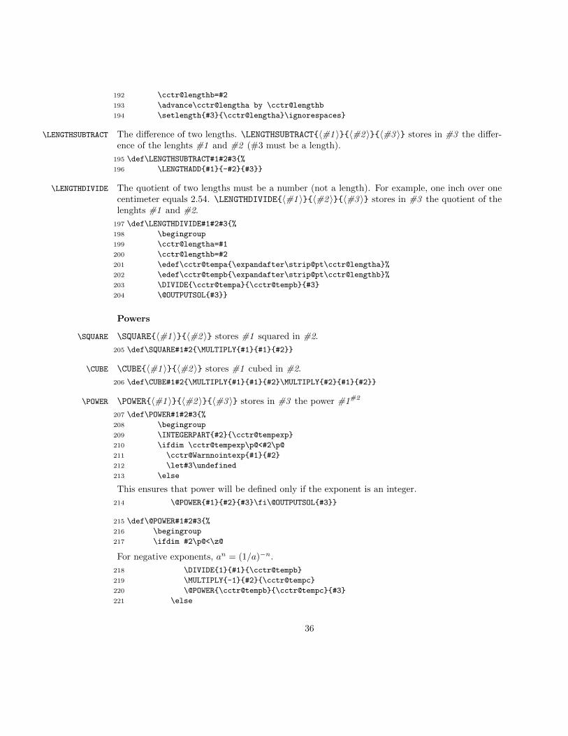
\LENGTHSUBTRACT The difference of two lengths. \LENGTHSUBTRACT{〈#1 〉}{〈#2 〉}{〈#3 〉} stores in #3 the differ-ence of the lenghts #1 and #2 (#3 must be a length).
195 \def\LENGTHSUBTRACT#1#2#3{%
196 \LENGTHADD{#1}{-#2}{#3}}
\LENGTHDIVIDE The quotient of two lengths must be a number (not a length). For example, one inch over onecentimeter equals 2.54. \LENGTHDIVIDE{〈#1 〉}{〈#2 〉}{〈#3 〉} stores in #3 the quotient of thelenghts #1 and #2.
197 \def\LENGTHDIVIDE#1#2#3{%
198 \begingroup
199 \cctr@lengtha=#1
200 \cctr@lengthb=#2
201 \edef\cctr@tempa{\expandafter\strip@pt\cctr@lengtha}%
202 \edef\cctr@tempb{\expandafter\strip@pt\cctr@lengthb}%
203 \DIVIDE{\cctr@tempa}{\cctr@tempb}{#3}
204 \@OUTPUTSOL{#3}}
Powers
\SQUARE \SQUARE{〈#1 〉}{〈#2 〉} stores #1 squared in #2.
205 \def\SQUARE#1#2{\MULTIPLY{#1}{#1}{#2}}
\CUBE \CUBE{〈#1 〉}{〈#2 〉} stores #1 cubed in #2.
206 \def\CUBE#1#2{\MULTIPLY{#1}{#1}{#2}\MULTIPLY{#2}{#1}{#2}}
\POWER \POWER{〈#1 〉}{〈#2 〉}{〈#3 〉} stores in #3 the power #1#2
207 \def\POWER#1#2#3{%
208 \begingroup
209 \INTEGERPART{#2}{\cctr@tempexp}
210 \ifdim \cctr@tempexp\p@<#2\p@
211 \cctr@Warnnointexp{#1}{#2}
212 \let#3\undefined
213 \else
This ensures that power will be defined only if the exponent is an integer.
214 \@POWER{#1}{#2}{#3}\fi\@OUTPUTSOL{#3}}
215 \def\@POWER#1#2#3{%
216 \begingroup
217 \ifdim #2\p@<\z@
For negative exponents, an = (1/a)−n.
218 \DIVIDE{1}{#1}{\cctr@tempb}
219 \MULTIPLY{-1}{#2}{\cctr@tempc}
220 \@POWER{\cctr@tempb}{\cctr@tempc}{#3}
221 \else
36
222 \COPY{0}{\cctr@tempa}
223 \COPY{1}{#3}
224 \@whilenum \cctr@tempa<#2 \do {%
225 \MULTIPLY{#1}{#3}{#3}
226 \ADD{1}{\cctr@tempa}{\cctr@tempa}}%
227 \fi\@OUTPUTSOL{#3}}
Integer arithmetic and related things
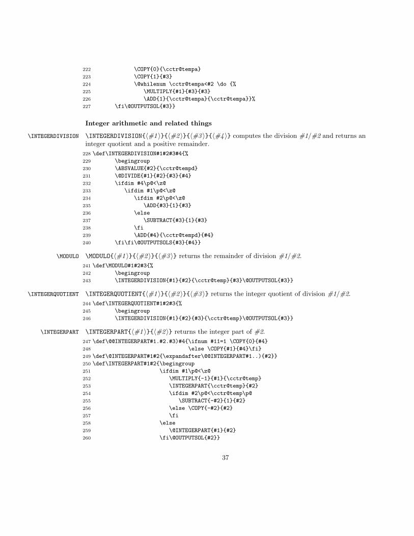
\INTEGERDIVISION \INTEGERDIVISION{〈#1 〉}{〈#2 〉}{〈#3 〉}{〈#4 〉} computes the division #1/#2 and returns aninteger quotient and a positive remainder.
228 \def\INTEGERDIVISION#1#2#3#4{%
229 \begingroup
230 \ABSVALUE{#2}{\cctr@tempd}
231 \@DIVIDE{#1}{#2}{#3}{#4}
232 \ifdim #4\p@<\z@
233 \ifdim #1\p@<\z@
234 \ifdim #2\p@<\z@
235 \ADD{#3}{1}{#3}
236 \else
237 \SUBTRACT{#3}{1}{#3}
238 \fi
239 \ADD{#4}{\cctr@tempd}{#4}
240 \fi\fi\@OUTPUTSOLS{#3}{#4}}
\MODULO \MODULO{〈#1 〉}{〈#2 〉}{〈#3 〉} returns the remainder of division #1/#2.
241 \def\MODULO#1#2#3{%
242 \begingroup
243 \INTEGERDIVISION{#1}{#2}{\cctr@temp}{#3}\@OUTPUTSOL{#3}}
\INTEGERQUOTIENT \INTEGERQUOTIENT{〈#1 〉}{〈#2 〉}{〈#3 〉} returns the integer quotient of division #1/#2.
244 \def\INTEGERQUOTIENT#1#2#3{%
245 \begingroup
246 \INTEGERDIVISION{#1}{#2}{#3}{\cctr@temp}\@OUTPUTSOL{#3}}
\INTEGERPART \INTEGERPART{〈#1 〉}{〈#2 〉} returns the integer part of #2.
247 \def\@@INTEGERPART#1.#2.#3)#4{\ifnum #11=1 \COPY{0}{#4}
248 \else \COPY{#1}{#4}\fi}
249 \def\@INTEGERPART#1#2{\expandafter\@@INTEGERPART#1..){#2}}
250 \def\INTEGERPART#1#2{\begingroup
251 \ifdim #1\p@<\z@
252 \MULTIPLY{-1}{#1}{\cctr@temp}
253 \INTEGERPART{\cctr@temp}{#2}
254 \ifdim #2\p@<\cctr@temp\p@
255 \SUBTRACT{-#2}{1}{#2}
256 \else \COPY{-#2}{#2}
257 \fi
258 \else
259 \@INTEGERPART{#1}{#2}
260 \fi\@OUTPUTSOL{#2}}
37

\FLOOR \FLOOR is an alias for \INTEGERPART.
261 \let\FLOOR\INTEGERPART
\FRACTIONALPART \FRACTIONALPART{〈#1 〉}{〈#2 〉} returns the fractional part of #2.
262 \def\@@FRACTIONALPART#1.#2.#3)#4{\ifnum #2=11 \COPY{0}{#4}
263 \else \COPY{0.#2}{#4}\fi}
264 \def\@FRACTIONALPART#1#2{\expandafter\@@FRACTIONALPART#1..){#2}}
265 \def\FRACTIONALPART#1#2{\begingroup
266 \ifdim #1\p@<\z@
267 \INTEGERPART{#1}{\cctr@tempA}
268 \SUBTRACT{#1}{\cctr@tempA}{#2}
269 \else
270 \@FRACTIONALPART{#1}{#2}
271 \fi\@OUTPUTSOL{#2}}
\TRUNCATE \TRUNCATE[〈#1 〉]{〈#2 〉}{〈#3 〉} truncates #2 to #1 (0, 1, 2 (default), 3 or 4) digits.
272 \def\TRUNCATE{\@ifnextchar[\@@TRUNCATE\@TRUNCATE}
273 \def\@TRUNCATE#1#2{\@@TRUNCATE[2]{#1}{#2}}
274 \def\@@TRUNCATE[#1]#2#3{%
275 \begingroup
276 \INTEGERPART{#2}{\cctr@tempa}
277 \ifdim \cctr@tempa\p@ = #2\p@
278 \expandafter\@@@TRUNCATE#2.00000)[#1]{#3}
279 \else
280 \expandafter\@@@TRUNCATE#200000.)[#1]{#3}
281 \fi
282 \@OUTPUTSOL{#3}}
283 \def\@@@TRUNCATE#1.#2#3#4#5#6.#7)[#8]#9{%
284 \ifcase #8
285 \COPY{#1}{#9}
286 \or\COPY{#1.#2}{#9}
287 \or\COPY{#1.#2#3}{#9}
288 \or\COPY{#1.#2#3#4}{#9}
289 \or\COPY{#1.#2#3#4#5}{#9}
290 \fi}
\ROUND \ROUND[〈#1 〉]{〈#2 〉}{〈#3 〉} rounds #2 to #1 (0, 1, 2 (default), 3 or 4) digits.
291 \def\ROUND{\@ifnextchar[\@@ROUND\@ROUND}
292 \def\@ROUND#1#2{\@@ROUND[2]{#1}{#2}}
293 \def\@@ROUND[#1]#2#3{%
294 \begingroup
295 \ifdim#2\p@<\z@
296 \MULTIPLY{-1}{#2}{\cctr@temp}
297 \@@ROUND[#1]{\cctr@temp}{#3}\COPY{-#3}{#3}
298 \else
299 \@@TRUNCATE[#1]{#2}{\cctr@tempe}
300 \SUBTRACT{#2}{\cctr@tempe}{\cctr@tempc}
301 \POWER{10}{#1}{\cctr@tempb}
302 \MULTIPLY{\cctr@tempb}{\cctr@tempc}{\cctr@tempc}
303 \ifdim\cctr@tempc\p@<0.5\p@
38

304 \else
305 \DIVIDE{1}{\cctr@tempb}{\cctr@tempb}
306 \ADD{\cctr@tempe}{\cctr@tempb}{\cctr@tempe}
307 \fi
308 \@@TRUNCATE[#1]{\cctr@tempe}{#3}
309 \fi
310 \@OUTPUTSOL{#3}}
\GCD \GCD{〈#1 〉}{〈#2 〉}{〈#3 〉} Greatest common divisor, using the Euclidean algorithm
311 \def\GCD#1#2#3{%
312 \begingroup
313 \ABSVALUE{#1}{\cctr@tempa}
314 \ABSVALUE{#2}{\cctr@tempb}
315 \MAX{\cctr@tempa}{\cctr@tempb}{\cctr@tempc}
316 \MIN{\cctr@tempa}{\cctr@tempb}{\cctr@tempa}
317 \COPY{\cctr@tempc}{\cctr@tempb}
318 \ifnum \cctr@tempa = 0
319 \ifnum \cctr@tempb = 0
320 \cctr@Warnnogcd
321 \let#3\undefined
322 \else
323 \COPY{\cctr@tempb}{#3}
324 \fi
325 \else
Euclidean algorithm: if c ≡ b (mod a) then gcd(b, a) = gcd(a, c). Iterating this property, weobtain gcd(b, a) as the last nonzero residual.
326 \@whilenum \cctr@tempa > \z@ \do {%
327 \COPY{\cctr@tempa}{#3}%
328 \MODULO{\cctr@tempb}{\cctr@tempa}{\cctr@tempc}%
329 \COPY\cctr@tempa\cctr@tempb%
330 \COPY\cctr@tempc\cctr@tempa}
331 \fi\ignorespaces\@OUTPUTSOL{#3}}
\LCM \LCM{〈#1 〉}{〈#2 〉}{〈#3 〉} Least common multiple.
332 \def\LCM#1#2#3{%
333 \GCD{#1}{#2}{#3}%
334 \ifx #3\undefined \COPY{0}{#3}
335 \else
336 \DIVIDE{#1}{#3}{#3}
337 \MULTIPLY{#2}{#3}{#3}
338 \ABSVALUE{#3}{#3}
339 \fi}
\FRACTIONSIMPLIFY \FRACTIONSIMPLIFY{〈#1 〉}{〈#2 〉}{〈#3 〉}{〈#4 〉} Fraction simplification: #3/#4 is the irre-ducible fraction equivalent to #1/#2.
340 \def\FRACTIONSIMPLIFY#1#2#3#4{%
341 \ifnum #1=\z@
342 \COPY{0}{#3}\COPY{1}{#4}
343 \else
39
344 \GCD{#1}{#2}{#3}%
345 \DIVIDE{#2}{#3}{#4}
346 \DIVIDE{#1}{#3}{#3}
347 \ifnum #4<0 \MULTIPLY{-1}{#4}{#4}\MULTIPLY{-1}{#3}{#3}\fi
348 \fi\ignorespaces}
Elementary functions
Square roots
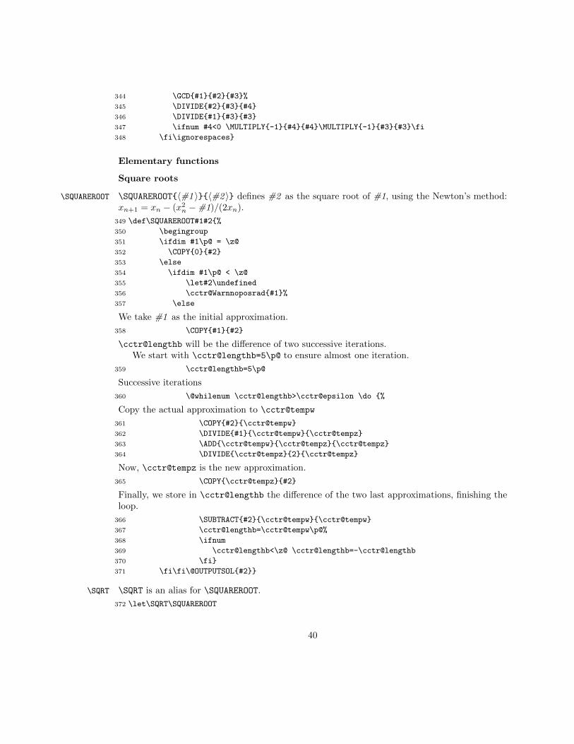
\SQUAREROOT \SQUAREROOT{〈#1 〉}{〈#2 〉} defines #2 as the square root of #1, using the Newton’s method:xn+1 = xn − (x2n −#1)/(2xn).
349 \def\SQUAREROOT#1#2{%
350 \begingroup
351 \ifdim #1\p@ = \z@
352 \COPY{0}{#2}
353 \else
354 \ifdim #1\p@ < \z@
355 \let#2\undefined
356 \cctr@Warnnoposrad{#1}%
357 \else
We take #1 as the initial approximation.
358 \COPY{#1}{#2}
\cctr@lengthb will be the difference of two successive iterations.We start with \cctr@lengthb=5\p@ to ensure almost one iteration.
359 \cctr@lengthb=5\p@
Successive iterations
360 \@whilenum \cctr@lengthb>\cctr@epsilon \do {%
Copy the actual approximation to \cctr@tempw
361 \COPY{#2}{\cctr@tempw}
362 \DIVIDE{#1}{\cctr@tempw}{\cctr@tempz}
363 \ADD{\cctr@tempw}{\cctr@tempz}{\cctr@tempz}
364 \DIVIDE{\cctr@tempz}{2}{\cctr@tempz}
Now, \cctr@tempz is the new approximation.
365 \COPY{\cctr@tempz}{#2}
Finally, we store in \cctr@lengthb the difference of the two last approximations, finishing theloop.
366 \SUBTRACT{#2}{\cctr@tempw}{\cctr@tempw}
367 \cctr@lengthb=\cctr@tempw\p@%
368 \ifnum
369 \cctr@lengthb<\z@ \cctr@lengthb=-\cctr@lengthb
370 \fi}
371 \fi\fi\@OUTPUTSOL{#2}}
\SQRT \SQRT is an alias for \SQUAREROOT.
372 \let\SQRT\SQUAREROOT
40

Trigonometric functions For a variable close enough to zero, the sine and tangent functionsare computed using some continued fractions. Then, all trigonometric functions are derivedfrom well-known formulas.
\SIN \SIN{〈#1 〉}{〈#2 〉}. Sine of #1.
373 \def\SIN#1#2{%
374 \begingroup
Exact sine for t ∈ {π/2,−π/2, 3π/2}375 \ifdim #1\p@=-\numberHALFPI\p@ \COPY{-1}{#2}
376 \else
377 \ifdim #1\p@=\numberHALFPI\p@ \COPY{1}{#2}
378 \else
379 \ifdim #1\p@=\numberTHREEHALFPI\p@ \COPY{-1}{#2}
380 \else
If |t| > π/2, change t to a smaller value.
381 \ifdim#1\p@<-\numberHALFPI\p@
382 \ADD{#1}{\numberTWOPI}{\cctr@tempb}
383 \SIN{\cctr@tempb}{#2}
384 \else
385 \ifdim #1\p@<\numberHALFPI\p@
Compute the sine.
386 \@BASICSINE{#1}{#2}
387 \else
388 \ifdim #1\p@<\numberTHREEHALFPI\p@
389 \SUBTRACT{\numberPI}{#1}{\cctr@tempb}
390 \SIN{\cctr@tempb}{#2}
391 \else
392 \SUBTRACT{#1}{\numberTWOPI}{\cctr@tempb}
393 \SIN{\cctr@tempb}{#2}
394 \fi\fi\fi\fi\fi\fi\@OUTPUTSOL{#2}}
\@BASICSINE \@BASICSINE{〈#1 〉}{〈#2 〉} applies this approximation:
sinx =x
1 +x2
2 · 3− x2 +2 · 3x2
4 · 5− x2 +4 · 5x2
6 · 7− x2 + · · ·395 \def\@BASICSINE#1#2{%
396 \begingroup
397 \ABSVALUE{#1}{\cctr@tempa}
Exact sine of zero
398 \ifdim\cctr@tempa\p@=\z@ \COPY{0}{#2}
399 \else
For t very close to zero, sin t ≈ t.400 \ifdim \cctr@tempa\p@<0.009\p@\COPY{#1}{#2}
401 \else
41

Compute the continued fraction.
402 \SQUARE{#1}{\cctr@tempa}
403 \DIVIDE{\cctr@tempa}{42}{#2}
404 \SUBTRACT{1}{#2}{#2}
405 \MULTIPLY{#2}{\cctr@tempa}{#2}
406 \DIVIDE{#2}{20}{#2}
407 \SUBTRACT{1}{#2}{#2}
408 \MULTIPLY{#2}{\cctr@tempa}{#2}
409 \DIVIDE{#2}{6}{#2}
410 \SUBTRACT{1}{#2}{#2}
411 \MULTIPLY{#2}{#1}{#2}
412 \fi\fi\@OUTPUTSOL{#2}}
\COS \COS{〈#1 〉}{〈#2 〉}. Cosine of #1 : cos t = sin(t+ π/2).
413 \def\COS#1#2{%
414 \begingroup
415 \ADD{\numberHALFPI}{#1}{\cctr@tempc}
416 \SIN{\cctr@tempc}{#2}\@OUTPUTSOL{#2}}
\TAN \TAN{〈#1 〉}{〈#2 〉}. Tangent of #1.
417 \def\TAN#1#2{%
418 \begingroup
Tangent is infinite for t = ±π/2419 \ifdim #1\p@=-\numberHALFPI\p@
420 \cctr@Warninftan{#1}
421 \let#2\undefined
422 \else
423 \ifdim #1\p@=\numberHALFPI\p@
424 \cctr@Warninftan{#1}
425 \let#2\undefined
426 \else
If |t| > π/2, change t to a smaller value.
427 \ifdim #1\p@<-\numberHALFPI\p@
428 \ADD{#1}{\numberPI}{\cctr@tempb}
429 \TAN{\cctr@tempb}{#2}
430 \else
431 \ifdim #1\p@<\numberHALFPI\p@
Compute the tangent.
432 \@BASICTAN{#1}{#2}
433 \else
434 \SUBTRACT{#1}{\numberPI}{\cctr@tempb}
435 \TAN{\cctr@tempb}{#2}
436 \fi\fi\fi\fi\@OUTPUTSOL{#2}}
42

\@BASICTAN \@BASICTAN{〈#1 〉}{〈#2 〉} applies this approximation:
tanx =1
1
x− 1
3
x− 1
5
x− 1
7
x− 1
9
x− 1
11
x− · · ·
437 \def\@BASICTAN#1#2{%
438 \begingroup
439 \ABSVALUE{#1}{\cctr@tempa}
Exact tangent of zero.
440 \ifdim\cctr@tempa\p@=\z@ \COPY{0}{#2}
441 \else
For t very close to zero, tan t ≈ t.442 \ifdim\cctr@tempa\p@<0.04\p@
443 \COPY{#1}{#2}
444 \else
Compute the continued fraction.
445 \DIVIDE{#1}{11}{#2}
446 \DIVIDE{9}{#1}{\cctr@tempa}
447 \SUBTRACT{\cctr@tempa}{#2}{#2}
448 \DIVIDE{1}{#2}{#2}
449 \DIVIDE{7}{#1}{\cctr@tempa}
450 \SUBTRACT{\cctr@tempa}{#2}{#2}
451 \DIVIDE{1}{#2}{#2}
452 \DIVIDE{5}{#1}{\cctr@tempa}
453 \SUBTRACT{\cctr@tempa}{#2}{#2}
454 \DIVIDE{1}{#2}{#2}
455 \DIVIDE{3}{#1}{\cctr@tempa}
456 \SUBTRACT{\cctr@tempa}{#2}{#2}
457 \DIVIDE{1}{#2}{#2}
458 \DIVIDE{1}{#1}{\cctr@tempa}
459 \SUBTRACT{\cctr@tempa}{#2}{#2}
460 \DIVIDE{1}{#2}{#2}
461 \fi\fi\@OUTPUTSOL{#2}}
\COT \COT{〈#1 〉}{〈#2 〉}. Cotangent of #1 : If cos t = 0 then cot t = 0; if tan t = 0 then cot t = ∞.Otherwise, cot t = 1/ tan t.
462 \def\COT#1#2{%
463 \begingroup
464 \COS{#1}{#2}
465 \ifdim #2\p@ = \z@
466 \COPY{0}{#2}
467 \else
43

468 \TAN{#1}{#2}
469 \ifdim #2\p@ = \z@
470 \cctr@Warninfcotan{#1}
471 \let#2\undefined
472 \else
473 \DIVIDE{1}{#2}{#2}
474 \fi\fi\@OUTPUTSOL{#2}}
\DEGtoRAD \DEGtoRAD{〈#1 〉}{〈#2 〉}. Convert degrees to radians.
475 \def\DEGtoRAD#1#2{\DIVIDE{#1}{57.29578}{#2}}
\RADtoDEG \RADtoDEG{〈#1 〉}{〈#2 〉}. Convert radians to degrees.
476 \def\RADtoDEG#1#2{\MULTIPLY{#1}{57.29578}{#2}}
\REDUCERADIANSANGLE Reduces to the trigonometrically equivalent arc in ]−π, π].
477 \def\REDUCERADIANSANGLE#1#2{%
478 \COPY{#1}{#2}
479 \ifdim #1\p@ < -\numberPI\p@
480 \ADD{#1}{\numberTWOPI}{#2}
481 \REDUCERADIANSANGLE{#2}{#2}
482 \fi
483 \ifdim #1\p@ > \numberPI\p@
484 \SUBTRACT{#1}{\numberTWOPI}{#2}
485 \REDUCERADIANSANGLE{#2}{#2}
486 \fi
487 \ifdim #1\p@ = -180\p@ \COPY{\numberPI}{#2} \fi}
\REDUCEDEGREESANGLE Reduces to the trigonometrically equivalent angle in ]−180, 180].
488 \def\REDUCEDEGREESANGLE#1#2{%
489 \COPY{#1}{#2}
490 \ifdim #1\p@ < -180\p@
491 \ADD{#1}{360}{#2}
492 \REDUCEDEGREESANGLE{#2}{#2}
493 \fi
494 \ifdim #1\p@ > 180\p@
495 \SUBTRACT{#1}{360}{#2}
496 \REDUCEDEGREESANGLE{#2}{#2}
497 \fi
498 \ifdim #1\p@ = -180\p@ \COPY{180}{#2} \fi}
Trigonometric functions in degrees Four next commands compute trigonometric func-tions in degrees. By default, a circle has 360 degrees, but we can use an arbitrary number ofdivisions using the optional argument of these commands.
\DEGREESSIN \DEGREESSIN[〈#1 〉]{〈#2 〉}{〈#3 〉}. Sine of #2 degrees.
499 \def\DEGREESSIN{\@ifnextchar[\@@DEGREESSIN\@DEGREESSIN}
\DEGREESCOS \DEGREESCOS[〈#1 〉]{〈#2 〉}{〈#3 〉}. Cosine of #2 degrees.
500 \def\DEGREESCOS{\@ifnextchar[\@@DEGREESCOS\@DEGREESCOS}
44

\DEGREESTAN \DEGREESTAN[〈#1 〉]{〈#2 〉}{〈#3 〉}. Tangent of #2 degrees.
501 \def\DEGREESTAN{\@ifnextchar[\@@DEGREESTAN\@DEGREESTAN}
\DEGREESCOT \DEGREESCOT[〈#1 〉]{〈#2 〉}{〈#3 〉}. Cotangent of #2 degrees.
502 \def\DEGREESCOT{\@ifnextchar[\@@DEGREESCOT\@DEGREESCOT}
\@DEGREESSIN \@DEGREESSIN computes the sine in sexagesimal degrees.
503 \def\@DEGREESSIN#1#2{%
504 \begingroup
505 \ifdim #1\p@=-90\p@ \COPY{-1}{#2}
506 \else
507 \ifdim #1\p@=90\p@ \COPY{1}{#2}
508 \else
509 \ifdim #1\p@=270\p@ \COPY{-1}{#2}
510 \else
511 \ifdim#1\p@<-90\p@
512 \ADD{#1}{360}{\cctr@tempb}
513 \DEGREESSIN{\cctr@tempb}{#2}
514 \else
515 \ifdim #1\p@<90\p@
516 \DEGtoRAD{#1}{\cctr@tempb}
517 \@BASICSINE{\cctr@tempb}{#2}
518 \else
519 \ifdim #1\p@<270\p@
520 \SUBTRACT{180}{#1}{\cctr@tempb}
521 \DEGREESSIN{\cctr@tempb}{#2}
522 \else
523 \SUBTRACT{#1}{360}{\cctr@tempb}
524 \DEGREESSIN{\cctr@tempb}{#2}
525 \fi\fi\fi\fi\fi\fi\@OUTPUTSOL{#2}}
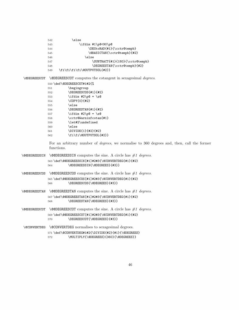
\@DEGREESCOS \@DEGREESCOS computes the cosine in sexagesimal degrees.
526 \def\@DEGREESCOS#1#2{%
527 \begingroup
528 \ADD{90}{#1}{\cctr@tempc}
529 \DEGREESSIN{\cctr@tempc}{#2}\@OUTPUTSOL{#2}}
\@DEGREESTAN \@DEGREESTAN computes the tangent in sexagesimal degrees.
530 \def\@DEGREESTAN#1#2{%
531 \begingroup
532 \ifdim #1\p@=-90\p@
533 \cctr@Warninftan{#1}
534 \let#2\undefined
535 \else
536 \ifdim #1\p@=90\p@
537 \cctr@Warninftan{#1}
538 \let#2\undefined
539 \else
540 \ifdim #1\p@<-90\p@
541 \ADD{#1}{180}{\cctr@tempb} \DEGREESTAN{\cctr@tempb}{#2}
45
542 \else
543 \ifdim #1\p@<90\p@
544 \DEGtoRAD{#1}{\cctr@tempb}
545 \@BASICTAN{\cctr@tempb}{#2}
546 \else
547 \SUBTRACT{#1}{180}{\cctr@tempb}
548 \DEGREESTAN{\cctr@tempb}{#2}
549 \fi\fi\fi\fi\@OUTPUTSOL{#2}}
\@DEGREESCOT \@DEGREESCOT computes the cotangent in sexagesimal degrees.
550 \def\@DEGREESCOT#1#2{%
551 \begingroup
552 \DEGREESCOS{#1}{#2}
553 \ifdim #2\p@ = \z@
554 \COPY{0}{#2}
555 \else
556 \DEGREESTAN{#1}{#2}
557 \ifdim #2\p@ = \z@
558 \cctr@Warninfcotan{#1}
559 \let#2\undefined
560 \else
561 \DIVIDE{1}{#2}{#2}
562 \fi\fi\@OUTPUTSOL{#2}}
For an arbitrary number of degrees, we normalise to 360 degrees and, then, call the formerfunctions.
\@@DEGREESSIN \@@DEGREESSIN computes the sine. A circle has #1 degrees.
563 \def\@@DEGREESSIN[#1]#2#3{\@CONVERTDEG{#1}{#2}
564 \@DEGREESSIN{\@DEGREES}{#3}}
\@@DEGREESCOS \@@DEGREESCOS computes the sine. A circle has #1 degrees.
565 \def\@@DEGREESCOS[#1]#2#3{\@CONVERTDEG{#1}{#2}
566 \DEGREESCOS{\@DEGREES}{#3}}
\@@DEGREESTAN \@@DEGREESTAN computes the sine. A circle has #1 degrees.
567 \def\@@DEGREESTAN[#1]#2#3{\@CONVERTDEG{#1}{#2}
568 \DEGREESTAN{\@DEGREES}{#3}}
\@@DEGREESCOT \@@DEGREESCOT computes the sine. A circle has #1 degrees.
569 \def\@@DEGREESCOT[#1]#2#3{\@CONVERTDEG{#1}{#2}
570 \DEGREESCOT{\@DEGREES}{#3}}
\@CONVERTDEG \@CONVERTDEG normalises to sexagesimal degrees.
571 \def\@CONVERTDEG#1#2{\DIVIDE{#2}{#1}{\@DEGREES}
572 \MULTIPLY{\@DEGREES}{360}{\@DEGREES}}
46
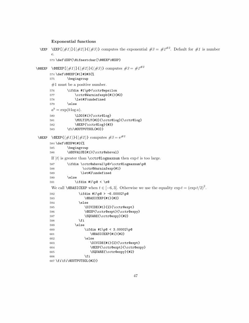
Exponential functions
\EXP \EXP[〈#1 〉]{〈#2 〉}{〈#3 〉} computes the exponential #3 = #1#2. Default for #1 is numbere.
573 \def\EXP{\@ifnextchar[\@@EXP\@EXP}
\@@EXP \@@EXP[〈#1 〉]{〈#2 〉}{〈#3 〉} computes #3 = #1#2
574 \def\@@EXP[#1]#2#3{%
575 \begingroup
#1 must be a positive number.
576 \ifdim #1\p@<\cctr@epsilon
577 \cctr@Warninfexpb{#1}{#2}
578 \let#3\undefined
579 \else
ab = exp(b log a).
580 \LOG{#1}{\cctr@log}
581 \MULTIPLY{#2}{\cctr@log}{\cctr@log}
582 \@EXP{\cctr@log}{#3}
583 \fi\@OUTPUTSOL{#3}}
\@EXP \@EXP{〈#1 〉}{〈#2 〉} computes #3 = e#2
584 \def\@EXP#1#2{%
585 \begingroup
586 \ABSVALUE{#1}{\cctr@absval}
If |t| is greater than \cctr@logmaxnum then exp t is too large.
587 \ifdim \cctr@absval\p@>\cctr@logmaxnum\p@
588 \cctr@Warninfexp{#1}
589 \let#2\undefined
590 \else
591 \ifdim #1\p@ < \z@
We call \@BASICEXP when t ∈ [−6, 3]. Otherwise we use the equality exp t = (exp t/2)2.
592 \ifdim #1\p@ > -6.00002\p@
593 \@BASICEXP{#1}{#2}
594 \else
595 \DIVIDE{#1}{2}{\cctr@expt}
596 \@EXP{\cctr@expt}{\cctr@expy}
597 \SQUARE{\cctr@expy}{#2}
598 \fi
599 \else
600 \ifdim #1\p@ < 3.00002\p@
601 \@BASICEXP{#1}{#2}
602 \else
603 \DIVIDE{#1}{2}{\cctr@expt}
604 \@EXP{\cctr@expt}{\cctr@expy}
605 \SQUARE{\cctr@expy}{#2}
606 \fi
607 \fi\fi\@OUTPUTSOL{#2}}
47

\@BASICEXP \@BASICEXP{〈#1 〉}{〈#2 〉} applies this approximation:
expx ≈ 1 +2x
2− x+x2/6
1 +x2/60
1 +x2/140
1 +x2/256
1 +x2
396
608 \def\@BASICEXP#1#2{%
609 \begingroup
610 \SQUARE{#1}\cctr@tempa
611 \DIVIDE{\cctr@tempa}{396}{#2}
612 \ADD{1}{#2}{#2}
613 \DIVIDE\cctr@tempa{#2}{#2}
614 \DIVIDE{#2}{256}{#2}
615 \ADD{1}{#2}{#2}
616 \DIVIDE\cctr@tempa{#2}{#2}
617 \DIVIDE{#2}{140}{#2}
618 \ADD{1}{#2}{#2}
619 \DIVIDE\cctr@tempa{#2}{#2}
620 \DIVIDE{#2}{60}{#2}
621 \ADD{1}{#2}{#2}
622 \DIVIDE\cctr@tempa{#2}{#2}
623 \DIVIDE{#2}{6}{#2}
624 \ADD{2}{#2}{#2}
625 \SUBTRACT{#2}{#1}{#2}
626 \DIVIDE{#1}{#2}{#2}
627 \MULTIPLY{2}{#2}{#2}
628 \ADD{1}{#2}{#2}\@OUTPUTSOL{#2}}
Hyperbolic functions
\COSH \COSH. Hyperbolic cosine: cosh t = (exp t+ exp(−t))/2.
629 \def\COSH#1#2{%
630 \begingroup
631 \ABSVALUE{#1}{\cctr@absval}
632 \ifdim \cctr@absval\p@>\cctr@logmaxnum\p@
633 \cctr@Warninfexp{#1}
634 \let#2\undefined
635 \else
636 \EXP{#1}{\cctr@expx}
637 \MULTIPLY{-1}{#1}{\cctr@minust}
638 \EXP{\cctr@minust}{\cctr@expminusx}
639 \ADD{\cctr@expx}{\cctr@expminusx}{#2}
640 \DIVIDE{#2}{2}{#2}
641 \fi\@OUTPUTSOL{#2}}
48
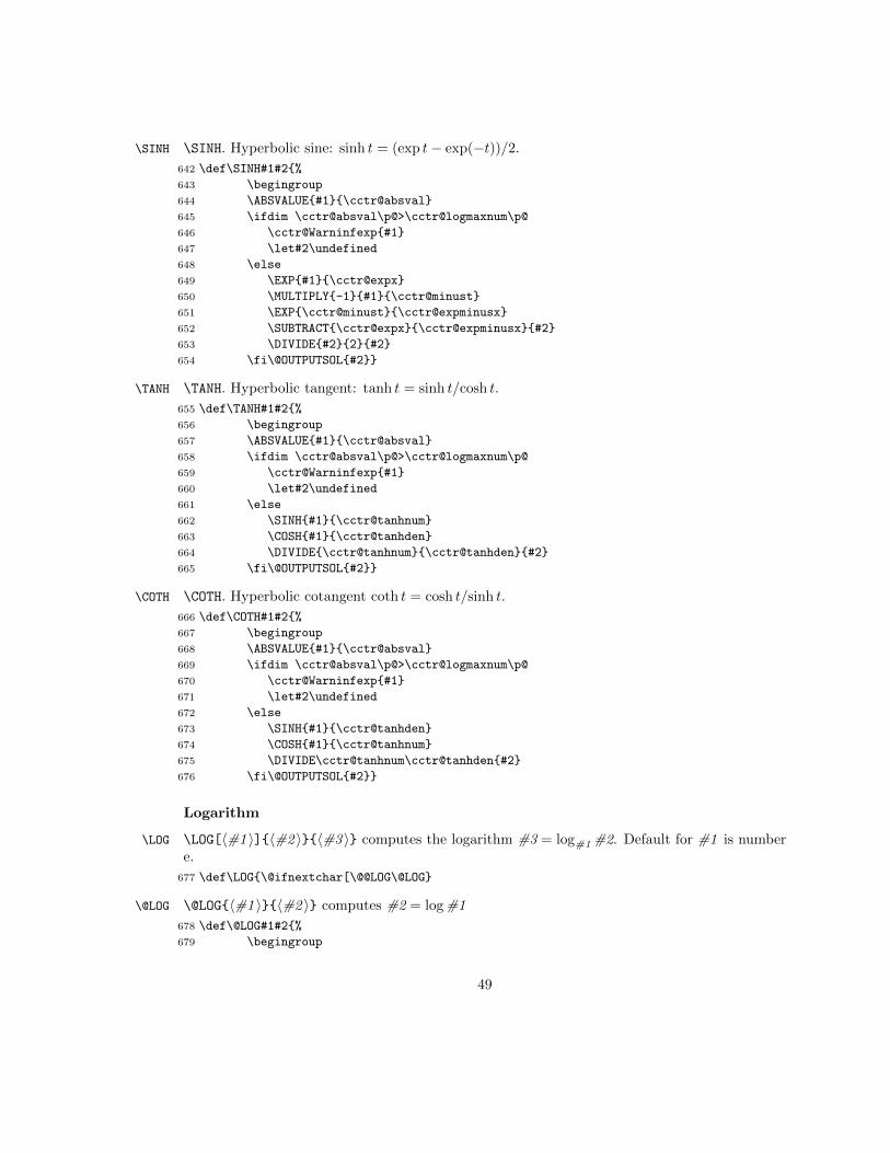
\SINH \SINH. Hyperbolic sine: sinh t = (exp t− exp(−t))/2.
642 \def\SINH#1#2{%
643 \begingroup
644 \ABSVALUE{#1}{\cctr@absval}
645 \ifdim \cctr@absval\p@>\cctr@logmaxnum\p@
646 \cctr@Warninfexp{#1}
647 \let#2\undefined
648 \else
649 \EXP{#1}{\cctr@expx}
650 \MULTIPLY{-1}{#1}{\cctr@minust}
651 \EXP{\cctr@minust}{\cctr@expminusx}
652 \SUBTRACT{\cctr@expx}{\cctr@expminusx}{#2}
653 \DIVIDE{#2}{2}{#2}
654 \fi\@OUTPUTSOL{#2}}
\TANH \TANH. Hyperbolic tangent: tanh t = sinh t/cosh t.
655 \def\TANH#1#2{%
656 \begingroup
657 \ABSVALUE{#1}{\cctr@absval}
658 \ifdim \cctr@absval\p@>\cctr@logmaxnum\p@
659 \cctr@Warninfexp{#1}
660 \let#2\undefined
661 \else
662 \SINH{#1}{\cctr@tanhnum}
663 \COSH{#1}{\cctr@tanhden}
664 \DIVIDE{\cctr@tanhnum}{\cctr@tanhden}{#2}
665 \fi\@OUTPUTSOL{#2}}
\COTH \COTH. Hyperbolic cotangent coth t = cosh t/sinh t.
666 \def\COTH#1#2{%
667 \begingroup
668 \ABSVALUE{#1}{\cctr@absval}
669 \ifdim \cctr@absval\p@>\cctr@logmaxnum\p@
670 \cctr@Warninfexp{#1}
671 \let#2\undefined
672 \else
673 \SINH{#1}{\cctr@tanhden}
674 \COSH{#1}{\cctr@tanhnum}
675 \DIVIDE\cctr@tanhnum\cctr@tanhden{#2}
676 \fi\@OUTPUTSOL{#2}}
Logarithm
\LOG \LOG[〈#1 〉]{〈#2 〉}{〈#3 〉} computes the logarithm #3 = log#1 #2. Default for #1 is numbere.
677 \def\LOG{\@ifnextchar[\@@LOG\@LOG}
\@LOG \@LOG{〈#1 〉}{〈#2 〉} computes #2 = log #1
678 \def\@LOG#1#2{%
679 \begingroup
49
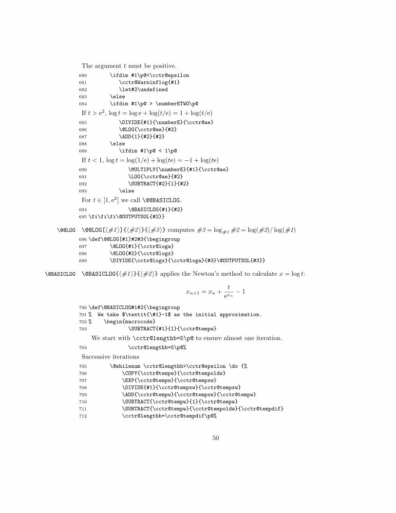
The argument t must be positive.
680 \ifdim #1\p@<\cctr@epsilon
681 \cctr@Warninflog{#1}
682 \let#2\undefined
683 \else
684 \ifdim #1\p@ > \numberETWO\p@
If t > e2, log t = log e + log(t/e) = 1 + log(t/e)
685 \DIVIDE{#1}{\numberE}{\cctr@ae}
686 \@LOG{\cctr@ae}{#2}
687 \ADD{1}{#2}{#2}
688 \else
689 \ifdim #1\p@ < 1\p@
If t < 1, log t = log(1/e) + log(te) = −1 + log(te)
690 \MULTIPLY{\numberE}{#1}{\cctr@ae}
691 \LOG{\cctr@ae}{#2}
692 \SUBTRACT{#2}{1}{#2}
693 \else
For t ∈ [1, e2] we call \@@BASICLOG.
694 \@BASICLOG{#1}{#2}
695 \fi\fi\fi\@OUTPUTSOL{#2}}
\@@LOG \@@LOG[〈#1 〉]{〈#2 〉}{〈#3 〉} computes #3 = log#1 #2 = log(#2)/ log(#1)
696 \def\@@LOG[#1]#2#3{\begingroup
697 \@LOG{#1}{\cctr@loga}
698 \@LOG{#2}{\cctr@logx}
699 \DIVIDE{\cctr@logx}{\cctr@loga}{#3}\@OUTPUTSOL{#3}}
\@BASICLOG \@BASICLOG{〈#1 〉}{〈#2 〉} applies the Newton’s method to calculate x = log t:
xn+1 = xn +t
exn− 1
700 \def\@BASICLOG#1#2{\begingroup
701 % We take $\textit{\#1}-1$ as the initial approximation.
702 % \begin{macrocode}
703 \SUBTRACT{#1}{1}{\cctr@tempw}
We start with \cctr@lengthb=5\p@ to ensure almost one iteration.
704 \cctr@lengthb=5\p@%
Successive iterations
705 \@whilenum \cctr@lengthb>\cctr@epsilon \do {%
706 \COPY{\cctr@tempw}{\cctr@tempoldw}
707 \EXP{\cctr@tempw}{\cctr@tempxw}
708 \DIVIDE{#1}{\cctr@tempxw}{\cctr@tempxw}
709 \ADD{\cctr@tempw}{\cctr@tempxw}{\cctr@tempw}
710 \SUBTRACT{\cctr@tempw}{1}{\cctr@tempw}
711 \SUBTRACT{\cctr@tempw}{\cctr@tempoldw}{\cctr@tempdif}
712 \cctr@lengthb=\cctr@tempdif\p@%
50
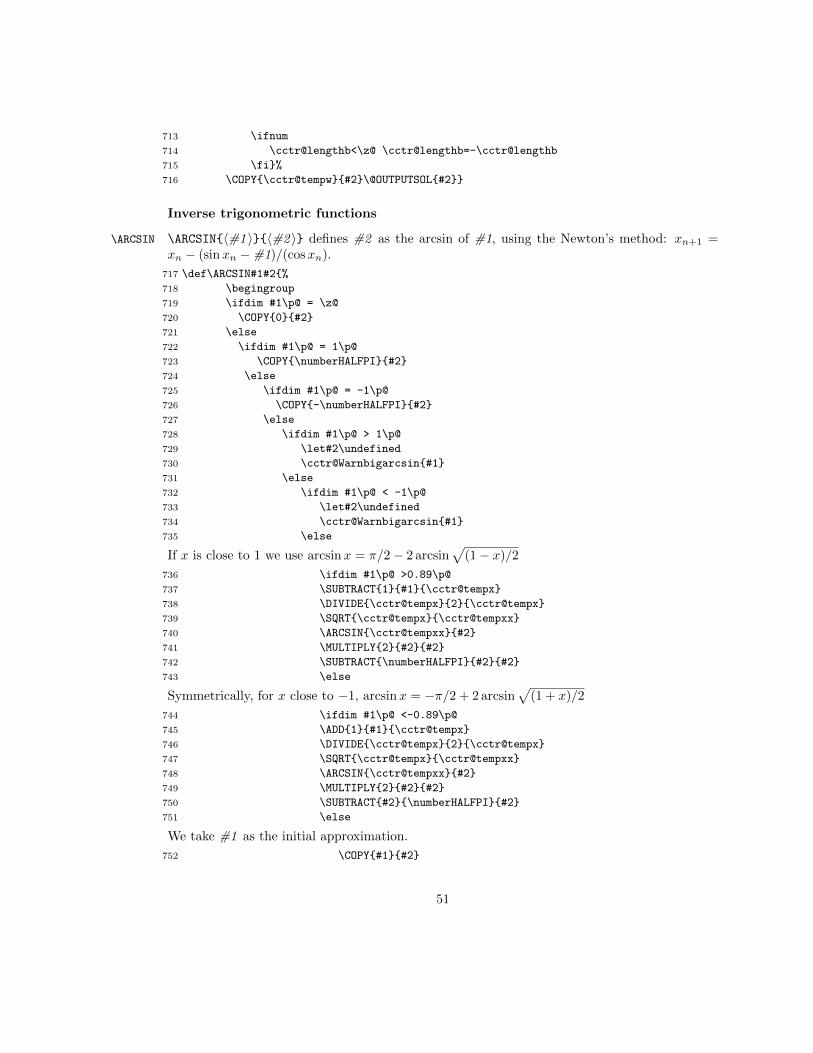
713 \ifnum
714 \cctr@lengthb<\z@ \cctr@lengthb=-\cctr@lengthb
715 \fi}%
716 \COPY{\cctr@tempw}{#2}\@OUTPUTSOL{#2}}
Inverse trigonometric functions
\ARCSIN \ARCSIN{〈#1 〉}{〈#2 〉} defines #2 as the arcsin of #1, using the Newton’s method: xn+1 =xn − (sinxn −#1)/(cosxn).
717 \def\ARCSIN#1#2{%
718 \begingroup
719 \ifdim #1\p@ = \z@
720 \COPY{0}{#2}
721 \else
722 \ifdim #1\p@ = 1\p@
723 \COPY{\numberHALFPI}{#2}
724 \else
725 \ifdim #1\p@ = -1\p@
726 \COPY{-\numberHALFPI}{#2}
727 \else
728 \ifdim #1\p@ > 1\p@
729 \let#2\undefined
730 \cctr@Warnbigarcsin{#1}
731 \else
732 \ifdim #1\p@ < -1\p@
733 \let#2\undefined
734 \cctr@Warnbigarcsin{#1}
735 \else
If x is close to 1 we use arcsinx = π/2− 2 arcsin√
(1− x)/2
736 \ifdim #1\p@ >0.89\p@
737 \SUBTRACT{1}{#1}{\cctr@tempx}
738 \DIVIDE{\cctr@tempx}{2}{\cctr@tempx}
739 \SQRT{\cctr@tempx}{\cctr@tempxx}
740 \ARCSIN{\cctr@tempxx}{#2}
741 \MULTIPLY{2}{#2}{#2}
742 \SUBTRACT{\numberHALFPI}{#2}{#2}
743 \else
Symmetrically, for x close to −1, arcsinx = −π/2 + 2 arcsin√
(1 + x)/2
744 \ifdim #1\p@ <-0.89\p@
745 \ADD{1}{#1}{\cctr@tempx}
746 \DIVIDE{\cctr@tempx}{2}{\cctr@tempx}
747 \SQRT{\cctr@tempx}{\cctr@tempxx}
748 \ARCSIN{\cctr@tempxx}{#2}
749 \MULTIPLY{2}{#2}{#2}
750 \SUBTRACT{#2}{\numberHALFPI}{#2}
751 \else
We take #1 as the initial approximation.
752 \COPY{#1}{#2}
51
If −0.4 ≤ t ≤ 0.4 then arcsinx ≈ x is a good approximation. Else, we apply the Newton method
753 \ABSVALUE{#1}{\cctr@tempy}
754 \ifdim \cctr@tempy\p@ < 0.04\p@
755 \else
\cctr@lengthb will be the difference of two successive iterations, and \cctr@tempoldy,\cctr@tempy will be the two last iterations.
We start with \cctr@lengthb=5\p@ and \cctr@tempy=16383 to ensure almost one iteration.
756 \cctr@lengthb=5\p@
757 \COPY{16383}{\cctr@tempy}
Successive iterations
758 \@whilenum \cctr@lengthb>\cctr@epsilon \do {%
Copy the actual approximation to \cctr@tempw
759 \COPY{#2}{\cctr@tempw}
760 \COPY{\cctr@tempy}{\cctr@tempoldy}
761 \SIN{\cctr@tempw}{\cctr@tempz}
762 \SUBTRACT{\cctr@tempz}{#1}{\cctr@tempz}
763 \COS{\cctr@tempw}{\cctr@tempy}
764 \DIVIDE{\cctr@tempz}{\cctr@tempy}{\cctr@tempz}
765 \SUBTRACT{\cctr@tempw}{\cctr@tempz}{\cctr@tempz}
Now, \cctr@tempz is the new approximation.
766 \COPY{\cctr@tempz}{#2}
Finally, we store in \cctr@lengthb the difference of the two last approximations, finishing theloop.
767 \SUBTRACT{#2}{\cctr@tempw}{\cctr@tempy}
768 \ABSVALUE{\cctr@tempy}{\cctr@tempy}
769 \cctr@lengthb=\cctr@tempy\p@%
770 \ifdim\cctr@tempy\p@=\cctr@tempoldy\p@
771 \cctr@lengthb=\z@
772 \fi}\fi\fi\fi\fi\fi\fi\fi\fi\@OUTPUTSOL{#2}}
\ARCCOS \ARCCOS{〈#1 〉}{〈#2 〉} defines #2 as the arccos of #1, using the well know relation arccosx =π/2− arcsinx.
773 \def\ARCCOS#1#2{%
774 \begingroup
775 \ifdim #1\p@ = \z@
776 \COPY{\numberHALFPI}{#2}
777 \else
778 \ifdim #1\p@ = 1\p@
779 \COPY{0}{#2}
780 \else
781 \ifdim #1\p@ = -1\p@
782 \COPY{\numberPI}{#2}
783 \else
784 \ifdim #1\p@ > 1\p@
785 \let#2\undefined
786 \cctr@Warnbigarccos{#1}
787 \else
52

788 \ifdim #1\p@ < -1\p@
789 \let#2\undefined
790 \cctr@Warnbigarccos{#1}
791 \else
792 \ARCSIN{#1}{#2}
793 \SUBTRACT{\numberHALFPI}{#2}{#2}
794 \fi\fi\fi\fi\fi\@OUTPUTSOL{#2}}
\ARCTAN \ARCTAN{〈#1 〉}{〈#2 〉}. arctan of #1.
795 \def\ARCTAN#1#2{%
796 \begingroup
If |t| > 1, compute arctanx using arctanx = sign(x)π/2− arctan(1/x).
797 \ifdim#1\p@<-1\p@
798 \DIVIDE{1}{#1}{\cctr@tempb}
799 \ARCTAN{\cctr@tempb}{#2}
800 \SUBTRACT{-\numberHALFPI}{#2}{#2}
801 \else
802 \ifdim#1\p@>1\p@
803 \DIVIDE{1}{#1}{\cctr@tempb}
804 \ARCTAN{\cctr@tempb}{#2}
805 \SUBTRACT{\numberHALFPI}{#2}{#2}
806 \else
For −1 ≤ x ≤ 1 call \@BASICARCTAN.
807 \@BASICARCTAN{#1}{#2}
808 \fi
809 \fi\@OUTPUTSOL{#2}}
\@BASICARCTAN \@BASICARCTAN{〈#1 〉}{〈#2 〉} applies this approximation:
arctanx =x
1 +x2
3 +(2x)2
5 +(3x)2
7 +(4x)2
9 + · · ·
810 \def\@BASICARCTAN#1#2{%
811 \begingroup
Exact arctan of zero
812 \ifdim#1\p@=\z@ \COPY{0}{#2}
813 \else
Compute the continued fraction.
814 \SQUARE{#1}{\cctr@tempa}
815 \MULTIPLY{64}{\cctr@tempa}{#2}
816 \ADD{15}{#2}{#2}
817 \DIVIDE{\cctr@tempa}{#2}{#2}
818 \MULTIPLY{49}{#2}{#2}
53
819 \ADD{13}{#2}{#2}
820 \DIVIDE{\cctr@tempa}{#2}{#2}
821 \MULTIPLY{36}{#2}{#2}
822 \ADD{11}{#2}{#2}
823 \DIVIDE{\cctr@tempa}{#2}{#2}
824 \MULTIPLY{25}{#2}{#2}
825 \ADD{9}{#2}{#2}
826 \DIVIDE{\cctr@tempa}{#2}{#2}
827 \MULTIPLY{16}{#2}{#2}
828 \ADD{7}{#2}{#2}
829 \DIVIDE{\cctr@tempa}{#2}{#2}
830 \MULTIPLY{9}{#2}{#2}
831 \ADD{5}{#2}{#2}
832 \DIVIDE{\cctr@tempa}{#2}{#2}
833 \MULTIPLY{4}{#2}{#2}
834 \ADD{3}{#2}{#2}
835 \DIVIDE{\cctr@tempa}{#2}{#2}
836 \ADD{1}{#2}{#2}
837 \DIVIDE{#1}{#2}{#2}
838 \fi\@OUTPUTSOL{#2}}
\ARCCOT \ARCCOT{〈#1 〉}{〈#2 〉} defines #2 as the arccot of #1, using the well know relation arccotx =π/2− arctanx.
839 \def\ARCCOT#1#2{%
840 \begingroup
841 \ARCTAN{#1}{#2}
842 \SUBTRACT{\numberHALFPI}{#2}{#2}
843 \@OUTPUTSOL{#2}}
Inverse hyperbolic functions
\ARSINH \ARSINH{〈#1 〉}{〈#2 〉}. Inverse hyperbolic sine of #1 : arsinhx = log(x+√
1 + x2)
844 \def\ARSINH#1#2{%
845 \begingroup
846 \SQUARE{#1}{\cctr@tempa}
847 \ADD{1}{\cctr@tempa}{\cctr@tempa}
848 \SQRT{\cctr@tempa}{\cctr@tempb}
849 \ADD{#1}{\cctr@tempb}{\cctr@tempb}
850 \LOG\cctr@tempb{#2}
851 \@OUTPUTSOL{#2}}
\ARCOSH \ARCOSH{〈#1 〉}{〈#2 〉}. Inverse hyperbolic sine of #1 : arcoshx = log(x+√x2 − 1
)852 \def\ARCOSH#1#2{%
853 \begingroup
If x < 1, this function is no defined
854 \ifdim#1\p@<1\p@
855 \let#2\undefined
856 \cctr@Warnsmallarcosh{#1}
857 \else
54

858 \SQUARE{#1}{\cctr@tempa}
859 \SUBTRACT{\cctr@tempa}{1}{\cctr@tempa}
860 \SQRT{\cctr@tempa}{\cctr@tempb}
861 \ADD{#1}{\cctr@tempb}{\cctr@tempb}
862 \LOG\cctr@tempb{#2}
863 \fi\@OUTPUTSOL{#2}}
\ARTANH \ARTANH{〈#1 〉}{〈#2 〉}. Inverse hyperbolic tangent of #1 : artanhx = 12 log ((1 + x)− log(1− x))
864 \def\ARTANH#1#2{%
865 \begingroup
If |x| ≥ 1, this function is no defined
866 \ifdim#1\p@<-0.99998\p@
867 \let#2\undefined
868 \cctr@Warnbigartanh{#1}
869 \else
870 \ifdim#1\p@>0.99998\p@
871 \let#2\undefined
872 \cctr@Warnbigartanh{#1}
873 \else
874 \COPY{#1}{\cctr@tempa}
875 \ADD1\cctr@tempa\cctr@tempb
876 \SUBTRACT1\cctr@tempa\cctr@tempc
877 \LOG\cctr@tempb\cctr@tempB
878 \LOG\cctr@tempc\cctr@tempC
879 \SUBTRACT\cctr@tempB\cctr@tempC{#2}
880 \DIVIDE{#2}{2}{#2}
881 \fi
882 \fi\@OUTPUTSOL{#2}}
\ARCOTH \ARCOTH{〈#1 〉}{〈#2 〉}. Inverse hyperbolic cotangent of #1 :
arcothx = sign(x) 12 log ((x+ 1)− log(x− 1))
883 \def\ARCOTH#1#2{%
884 \begingroup
If |x| ≤ 1, this function is no defined
885 \ifdim#1\p@>-0.99998\p@
886 \ifdim#1\p@<0.99998\p@
887 \let#2\undefined
888 \cctr@Warnsmallarcoth{#1}
889 \else
890 \ifdim#1\p@>\p@
For x > 1, calcule arcothx = 12 log ((x+ 1)− log(x− 1))
891 \COPY{#1}{\cctr@tempa}
892 \ADD1\cctr@tempa\cctr@tempb
893 \SUBTRACT\cctr@tempa1\cctr@tempc
894 \LOG\cctr@tempb\cctr@tempB
895 \LOG\cctr@tempc\cctr@tempC
896 \SUBTRACT\cctr@tempB\cctr@tempC{#2}
897 \DIVIDE{#2}{2}{#2}
55

898 \else
899 \fi
900 \fi
901 \else
For x < −1, calcule − artanh(−x)
902 \MULTIPLY{-1}{#1}{\cctr@tempa}
903 \ARCOTH{\cctr@tempa}{#2}
904 \COPY{-#2}{#2}
905 \fi\@OUTPUTSOL{#2}}
13.4 Matrix arithmetics
Vector operations
\VECTORSIZE The size of a vector is 2 or 3. \VECTORSIZE(〈#1 〉){〈#2 〉} stores in #2 the size of (〈#1 〉).Almost all vector commands needs to know the vector size.
906 \def\VECTORSIZE(#1)#2{\expandafter\@VECTORSIZE(#1,,){#2}}
907 \def\@VECTORSIZE(#1,#2,#3,#4)#5{\ifx$#3$\COPY{2}{#5}
908 \else\COPY{3}{#5}\fi\ignorespaces}
\VECTORCOPY \VECTORCOPY(〈#1,#2 〉)(〈#3,#4 〉) stores #1 and #2 in #3 and #4.\VECTORCOPY(〈#1,#2,#3 〉)(〈#4,#5#6 〉) stores #1, #2 and #3 in #4 and #5 and #6.
909 \def\@@VECTORCOPY(#1,#2)(#3,#4){%
910 \COPY{#1}{#3}\COPY{#2}{#4}}
911
912 \def\@@@VECTORCOPY(#1,#2,#3)(#4,#5,#6){%
913 \COPY{#1}{#4}\COPY{#2}{#5}\COPY{#3}{#6}}
914
915 \def\VECTORCOPY(#1)(#2){%
916 \VECTORSIZE(#1){\cctr@size}
917 \ifnum\cctr@size=2
918 \@@VECTORCOPY(#1)(#2)
919 \else \@@@VECTORCOPY(#1)(#2)\fi}
\VECTORGLOBALCOPY \VECTORGLOBALCOPY is the global version of \VECTORCOPY
920 \def\@@VECTORGLOBALCOPY(#1,#2)(#3,#4){%
921 \GLOBALCOPY{#1}{#3}\GLOBALCOPY{#2}{#4}}
922
923 \def\@@@VECTORGLOBALCOPY(#1,#2,#3)(#4,#5,#6){%
924 \GLOBALCOPY{#1}{#4}\GLOBALCOPY{#2}{#5}\GLOBALCOPY{#3}{#6}}
925
926 \def\VECTORGLOBALCOPY(#1)(#2){%
927 \VECTORSIZE(#1){\cctr@size}
928 \ifnum\cctr@size=2
929 \@@VECTORGLOBALCOPY(#1)(#2)
930 \else \@@@VECTORGLOBALCOPY(#1)(#2)\fi}
\@OUTPUTVECTOR
931 \def\@@OUTPUTVECTOR(#1,#2){%
56
932 \VECTORGLOBALCOPY(#1,#2)(\cctr@outa,\cctr@outb)
933 \endgroup\VECTORCOPY(\cctr@outa,\cctr@outb)(#1,#2)}
934
935 \def\@@@OUTPUTVECTOR(#1,#2,#3){%
936 \VECTORGLOBALCOPY(#1,#2,#3)(\cctr@outa,\cctr@outb,\cctr@outc)
937 \endgroup\VECTORCOPY(\cctr@outa,\cctr@outb,\cctr@outc)(#1,#2,#3)}
938
939 \def\@OUTPUTVECTOR(#1){\VECTORSIZE(#1){\cctr@size}
940 \ifnum\cctr@size=2
941 \@@OUTPUTVECTOR(#1)
942 \else \@@@OUTPUTVECTOR(#1)\fi}
\SCALARPRODUCT Scalar product of two vectors.
943 \def\@@SCALARPRODUCT(#1,#2)(#3,#4)#5{%
944 \MULTIPLY{#1}{#3}{#5}
945 \MULTIPLY{#2}{#4}\cctr@tempa
946 \ADD{#5}{\cctr@tempa}{#5}}
947
948 \def\@@@SCALARPRODUCT(#1,#2,#3)(#4,#5,#6)#7{%
949 \MULTIPLY{#1}{#4}{#7}
950 \MULTIPLY{#2}{#5}\cctr@tempa
951 \ADD{#7}{\cctr@tempa}{#7}
952 \MULTIPLY{#3}{#6}\cctr@tempa
953 \ADD{#7}{\cctr@tempa}{#7}}
954
955 \def\SCALARPRODUCT(#1)(#2)#3{%
956 \begingroup
957 \VECTORSIZE(#1){\cctr@size}
958 \ifnum\cctr@size=2
959 \@@SCALARPRODUCT(#1)(#2){#3}
960 \else \@@@SCALARPRODUCT(#1)(#2){#3}\fi\@OUTPUTSOL{#3}}
\DOTPRODUCT \DOTPRODUCT is an alias for \SCALARPRODUCT.
961 \let\DOTPRODUCT\SCALARPRODUCT
\VECTORPRODUCT Vector product of two (three dimensional) vectors.
962 \def\@@VECTORPRODUCT(#1)(#2)(#3,#4){%
963 \let#3\undefined
964 \let#4\undefined
965 \cctr@Warncrossprod(#1)(#2)}
966
967 \def\@@@VECTORPRODUCT(#1,#2,#3)(#4,#5,#6)(#7,#8,#9){%
968 \DETERMINANT(#2,#3;#5,#6){#7}
969 \DETERMINANT(#3,#1;#6,#4){#8}
970 \DETERMINANT(#1,#2;#4,#5){#9}}
971
972 \def\VECTORPRODUCT(#1)(#2)(#3){%
973 \begingroup
974 \VECTORSIZE(#1){\cctr@size}
57
975 \ifnum\cctr@size=2
976 \@@VECTORPRODUCT(#1)(#2)(#3)
977 \else \@@@VECTORPRODUCT(#1)(#2)(#3)\fi\@OUTPUTSOL{#3}}
\CROSSPRODUCT \CROSSPRODUCT is an alias for \VECTORPRODUCT.
978 \let\CROSSPRODUCT\VECTORPRODUCT
\VECTORADD Sum of two vectors.
979 \def\@@VECTORADD(#1,#2)(#3,#4)(#5,#6){%
980 \ADD{#1}{#3}{#5}
981 \ADD{#2}{#4}{#6}}
982
983 \def\@@@VECTORADD(#1,#2,#3)(#4,#5,#6)(#7,#8,#9){%
984 \ADD{#1}{#4}{#7}
985 \ADD{#2}{#5}{#8}
986 \ADD{#3}{#6}{#9}}
987
988 \def\VECTORADD(#1)(#2)(#3){%
989 \VECTORSIZE(#1){\cctr@size}
990 \ifnum\cctr@size=2
991 \@@VECTORADD(#1)(#2)(#3)
992 \else \@@@VECTORADD(#1)(#2)(#3)\fi}
\VECTORSUB Difference of two vectors.
993 \def\@@VECTORSUB(#1,#2)(#3,#4)(#5,#6){%
994 \VECTORADD(#1,#2)(-#3,-#4)(#5,#6)}
995
996 \def\@@@VECTORSUB(#1,#2,#3)(#4,#5,#6)(#7,#8,#9){%
997 \VECTORADD(#1,#2,#3)(-#4,-#5,-#6)(#7,#8,#9)}
998
999 \def\VECTORSUB(#1)(#2)(#3){%
1000 \VECTORSIZE(#1){\cctr@size}
1001 \ifnum\cctr@size=2
1002 \@@VECTORSUB(#1)(#2)(#3)
1003 \else \@@@VECTORSUB(#1)(#2)(#3)\fi}
\VECTORABSVALUE Absolute value of a each entry of a vector.
1004 \def\@@VECTORABSVALUE(#1,#2)(#3,#4){%
1005 \ABSVALUE{#1}{#3}\ABSVALUE{#2}{#4}}
1006
1007 \def\@@@VECTORABSVALUE(#1,#2,#3)(#4,#5,#6){%
1008 \ABSVALUE{#1}{#4}\ABSVALUE{#2}{#5}\ABSVALUE{#3}{#6}}
1009
1010 \def\VECTORABSVALUE(#1)(#2){%
1011 \VECTORSIZE(#1){\cctr@size}
1012 \ifnum\cctr@size=2
1013 \@@VECTORABSVALUE(#1)(#2)
1014 \else \@@@VECTORABSVALUE(#1)(#2)\fi}
\SCALARVECTORPRODUCT Scalar-vector product.
58

1015 \def\@@SCALARVECTORPRODUCT#1(#2,#3)(#4,#5){%
1016 \MULTIPLY{#1}{#2}{#4}
1017 \MULTIPLY{#1}{#3}{#5}}
1018
1019 \def\@@@SCALARVECTORPRODUCT#1(#2,#3,#4)(#5,#6,#7){%
1020 \MULTIPLY{#1}{#2}{#5}
1021 \MULTIPLY{#1}{#3}{#6}
1022 \MULTIPLY{#1}{#4}{#7}}
1023
1024 \def\SCALARVECTORPRODUCT#1(#2)(#3){%
1025 \VECTORSIZE(#2){\cctr@size}
1026 \ifnum\cctr@size=2
1027 \@@SCALARVECTORPRODUCT{#1}(#2)(#3)
1028 \else \@@@SCALARVECTORPRODUCT{#1}(#2)(#3)\fi}
\VECTORNORM Euclidean norm of a vector.
1029 \def\VECTORNORM(#1)#2{%
1030 \begingroup
1031 \SCALARPRODUCT(#1)(#1){\cctr@temp}
1032 \SQUAREROOT{\cctr@temp}{#2}\@OUTPUTSOL{#2}}
\UNITVECTOR Unitary vector parallel to a given vector.
1033 \def\UNITVECTOR(#1)(#2){%
1034 \begingroup
1035 \VECTORNORM(#1){\cctr@tempa}
1036 \DIVIDE{1}{\cctr@tempa}{\cctr@tempa}
1037 \SCALARVECTORPRODUCT{\cctr@tempa}(#1)(#2)\@OUTPUTVECTOR(#2)}
\TWOVECTORSANGLE Angle between two vectors.
1038 \def\TWOVECTORSANGLE(#1)(#2)#3{%
1039 \begingroup
1040 \VECTORNORM(#1){\cctr@tempa}
1041 \VECTORNORM(#2){\cctr@tempb}
1042 \SCALARPRODUCT(#1)(#2){\cctr@tempc}
1043 \ifdim \cctr@tempa\p@ =\z@
1044 \let#3\undefined
1045 \cctr@Warnnoangle(#1)(#2)
1046 \else
1047 \ifdim \cctr@tempb\p@ =\z@
1048 \let#3\undefined
1049 \cctr@Warnnoangle(#1)(#2)
1050 \else
1051 \DIVIDE{\cctr@tempc}{\cctr@tempa}{\cctr@tempc}
1052 \DIVIDE{\cctr@tempc}{\cctr@tempb}{\cctr@tempc}
1053 \ARCCOS{\cctr@tempc}{#3}
1054 \fi\fi\@OUTPUTSOL{#3}}
Matrix operations
Here, we need to define some internal macros to simulate commands with more than ninearguments.
59

\@TDMATRIXCOPY This command copies a 3 × 3 matrix to the commands \cctr@solAA, \cctr@solAB, . . . ,\cctr@solCC.
1055 \def\@TDMATRIXCOPY(#1,#2,#3;#4,#5,#6;#7,#8,#9){%
1056 \COPY{#1}{\cctr@solAA}
1057 \COPY{#2}{\cctr@solAB}
1058 \COPY{#3}{\cctr@solAC}
1059 \COPY{#4}{\cctr@solBA}
1060 \COPY{#5}{\cctr@solBB}
1061 \COPY{#6}{\cctr@solBC}
1062 \COPY{#7}{\cctr@solCA}
1063 \COPY{#8}{\cctr@solCB}
1064 \COPY{#9}{\cctr@solCC}}
\@TDMATRIXSOL This command copies the commands \cctr@solAA, \cctr@solAB, . . . , \cctr@solCC to a 3× 3matrix. This macro is used to store the results of a matrix operation.
1065 \def\@TDMATRIXSOL(#1,#2,#3;#4,#5,#6;#7,#8,#9){%
1066 \COPY{\cctr@solAA}{#1}
1067 \COPY{\cctr@solAB}{#2}
1068 \COPY{\cctr@solAC}{#3}
1069 \COPY{\cctr@solBA}{#4}
1070 \COPY{\cctr@solBB}{#5}
1071 \COPY{\cctr@solBC}{#6}
1072 \COPY{\cctr@solCA}{#7}
1073 \COPY{\cctr@solCB}{#8}
1074 \COPY{\cctr@solCC}{#9}}
\@TDMATRIXGLOBALSOL
1075 \def\@TDMATRIXGLOBALSOL(#1,#2,#3;#4,#5,#6;#7,#8,#9){%
1076 \GLOBALCOPY{\cctr@solAA}{#1}
1077 \GLOBALCOPY{\cctr@solAB}{#2}
1078 \GLOBALCOPY{\cctr@solAC}{#3}
1079 \GLOBALCOPY{\cctr@solBA}{#4}
1080 \GLOBALCOPY{\cctr@solBB}{#5}
1081 \GLOBALCOPY{\cctr@solBC}{#6}
1082 \GLOBALCOPY{\cctr@solCA}{#7}
1083 \GLOBALCOPY{\cctr@solCB}{#8}
1084 \GLOBALCOPY{\cctr@solCC}{#9}}
\@TDMATRIXNOSOL This command undefines a 3× 3 matrix when a matrix problem has no solution.
1085 \def\@TDMATRIXNOSOL(#1,#2,#3;#4,#5,#6;#7,#8,#9){%
1086 \let#1\undefined
1087 \let#2\undefined
1088 \let#3\undefined
1089 \let#4\undefined
1090 \let#5\undefined
1091 \let#6\undefined
1092 \let#7\undefined
1093 \let#8\undefined
1094 \let#9\undefined
1095 }
60
\@@TDMATRIXSOL This command stores or undefines the solution.
1096 \def\@@TDMATRIXSOL(#1,#2,#3;#4,#5,#6;#7,#8,#9){%
1097 \ifx\cctr@solAA\undefined
1098 \@TDMATRIXNOSOL(#1,#2,#3;#4,#5,#6;#7,#8,#9)%
1099 \else
1100 \@TDMATRIXSOL(#1,#2,#3;#4,#5,#6;#7,#8,#9)\fi}
\@NUMBERSOL This command stores the scalar solution of a matrix operation.
1101 \def\@NUMBERSOL#1{\COPY{\cctr@sol}{#1}}
\MATRIXSIZE Size (2 or 3) of a matrix.
1102 \def\MATRIXSIZE(#1)#2{\expandafter\@MATRIXSIZE(#1;;){#2}}
1103 \def\@MATRIXSIZE(#1;#2;#3;#4)#5{\ifx$#3$\COPY{2}{#5}
1104 \else\COPY{3}{#5}\fi\ignorespaces}
\MATRIXCOPY Store a matrix in 4 or 9 commands.
1105 \def\@@MATRIXCOPY(#1,#2;#3,#4)(#5,#6;#7,#8){%
1106 \COPY{#1}{#5}\COPY{#2}{#6}\COPY{#3}{#7}\COPY{#4}{#8}}
1107
1108 \def\@@@MATRIXCOPY(#1,#2,#3;#4,#5,#6;#7,#8,#9){%
1109 \@TDMATRIXCOPY(#1,#2,#3;#4,#5,#6;#7,#8,#9)
1110 \@TDMATRIXSOL}
1111
1112 \def\MATRIXCOPY(#1)(#2){%
1113 \MATRIXSIZE(#1){\cctr@size}
1114 \ifnum\cctr@size=2
1115 \@@MATRIXCOPY(#1)(#2)
1116 \else \@@@MATRIXCOPY(#1)(#2)\fi}
\MATRIXGLOBALCOPY Global version of \MATRIXCOPY.
1117 \def\@@MATRIXGLOBALCOPY(#1,#2;#3,#4)(#5,#6;#7,#8){%
1118 \GLOBALCOPY{#1}{#5}\GLOBALCOPY{#2}{#6}\GLOBALCOPY{#3}{#7}\GLOBALCOPY{#4}{#8}}
1119
1120 \def\@@@MATRIXGLOBALCOPY(#1,#2,#3;#4,#5,#6;#7,#8,#9){%
1121 \@TDMATRIXCOPY(#1,#2,#3;#4,#5,#6;#7,#8,#9)
1122 \@TDMATRIXGLOBALSOL}
1123
1124 \def\MATRIXGLOBALCOPY(#1)(#2){%
1125 \MATRIXSIZE(#1){\cctr@size}
1126 \ifnum\cctr@size=2
1127 \@@MATRIXGLOBALCOPY(#1)(#2)
1128 \else \@@@MATRIXGLOBALCOPY(#1)(#2)\fi}
\@OUTPUTMATRIX
1129 \def\@@OUTPUTMATRIX(#1,#2;#3,#4){%
1130 \MATRIXGLOBALCOPY(#1,#2;#3,#4)(\cctr@outa,\cctr@outb;\cctr@outc,\cctr@outd)
1131 \endgroup\MATRIXCOPY(\cctr@outa,\cctr@outb;\cctr@outc,\cctr@outd)(#1,#2;#3,#4)}
1132
1133 \def\@@@OUTPUTMATRIX(#1,#2,#3;#4,#5,#6;#7,#8,#9){%
61
1134 \MATRIXGLOBALCOPY(#1,#2,#3;#4,#5,#6;#7,#8,#9)(%
1135 \cctr@outa,\cctr@outb,\cctr@outc;
1136 \cctr@outd,\cctr@oute,\cctr@outf;
1137 \cctr@outg,\cctr@outh,\cctr@outi)
1138 \endgroup\MATRIXCOPY(%
1139 \cctr@outa,\cctr@outb,\cctr@outc;
1140 \cctr@outd,\cctr@oute,\cctr@outf;
1141 \cctr@outg,\cctr@outh,\cctr@outi)(#1,#2,#3;#4,#5,#6;#7,#8,#9)}
1142
1143 \def\@OUTPUTMATRIX(#1){\MATRIXSIZE(#1){\cctr@size}
1144 \ifnum\cctr@size=2
1145 \@@OUTPUTMATRIX(#1)
1146 \else \@@@OUTPUTMATRIX(#1)\fi}
\TRANSPOSEMATRIX Matrix transposition.
1147 \def\@@TRANSPOSEMATRIX(#1,#2;#3,#4)(#5,#6;#7,#8){%
1148 \COPY{#1}{#5}\COPY{#3}{#6}\COPY{#2}{#7}\COPY{#4}{#8}}
1149
1150 \def\@@@TRANSPOSEMATRIX(#1,#2,#3;#4,#5,#6;#7,#8,#9){%
1151 \@TDMATRIXCOPY(#1,#4,#7;#2,#5,#8;#3,#6,#9)
1152 \@TDMATRIXSOL}
1153
1154 \def\TRANSPOSEMATRIX(#1)(#2){%
1155 \begingroup
1156 \MATRIXSIZE(#1){\cctr@size}
1157 \ifnum\cctr@size=2
1158 \@@TRANSPOSEMATRIX(#1)(#2)
1159 \else \@@@TRANSPOSEMATRIX(#1)(#2)\fi\@OUTPUTMATRIX(#2)}
\MATRIXADD Sum of two matrices.
1160 \def\@@MATRIXADD(#1;#2)(#3;#4)(#5,#6;#7,#8){%
1161 \VECTORADD(#1)(#3)(#5,#6)
1162 \VECTORADD(#2)(#4)(#7,#8)}
1163
1164 \def\@@@MATRIXADD(#1;#2;#3)(#4;#5;#6){%
1165 \VECTORADD(#1)(#4)(\cctr@solAA,\cctr@solAB,\cctr@solAC)
1166 \VECTORADD(#2)(#5)(\cctr@solBA,\cctr@solBB,\cctr@solBC)
1167 \VECTORADD(#3)(#6)(\cctr@solCA,\cctr@solCB,\cctr@solCC)
1168 \@TDMATRIXSOL}
1169
1170 \def\MATRIXADD(#1)(#2)(#3){%
1171 \begingroup
1172 \MATRIXSIZE(#1){\cctr@size}
1173 \ifnum\cctr@size=2
1174 \@@MATRIXADD(#1)(#2)(#3)
1175 \else \@@@MATRIXADD(#1)(#2)(#3)\fi\@OUTPUTMATRIX(#3)}
\MATRIXSUB Difference of two matrices.
1176 \def\@@MATRIXSUB(#1;#2)(#3;#4)(#5,#6;#7,#8){%
1177 \VECTORSUB(#1)(#3)(#5,#6)
62

1178 \VECTORSUB(#2)(#4)(#7,#8)}
1179
1180 \def\@@@MATRIXSUB(#1;#2;#3)(#4;#5;#6){%
1181 \VECTORSUB(#1)(#4)(\cctr@solAA,\cctr@solAB,\cctr@solAC)
1182 \VECTORSUB(#2)(#5)(\cctr@solBA,\cctr@solBB,\cctr@solBC)
1183 \VECTORSUB(#3)(#6)(\cctr@solCA,\cctr@solCB,\cctr@solCC)
1184 \@TDMATRIXSOL}
1185
1186 \def\MATRIXSUB(#1)(#2)(#3){%
1187 \begingroup
1188 \MATRIXSIZE(#1){\cctr@size}
1189 \ifnum\cctr@size=2
1190 \@@MATRIXSUB(#1)(#2)(#3)
1191 \else \@@@MATRIXSUB(#1)(#2)(#3)\fi\@OUTPUTMATRIX(#3)}
\MATRIXABSVALUE Absolute value (of each entry) of a matrix.
1192 \def\@@MATRIXABSVALUE(#1;#2)(#3;#4){%
1193 \VECTORABSVALUE(#1)(#3)\VECTORABSVALUE(#2)(#4)}
1194
1195 \def\@@@MATRIXABSVALUE(#1;#2;#3)(#4;#5;#6){%
1196 \VECTORABSVALUE(#1)(#4)\VECTORABSVALUE(#2)(#5)\VECTORABSVALUE(#3)(#6)}
1197
1198 \def\MATRIXABSVALUE(#1)(#2){%
1199 \begingroup
1200 \MATRIXSIZE(#1){\cctr@size}
1201 \ifnum\cctr@size=2
1202 \@@MATRIXABSVALUE(#1)(#2)
1203 \else \@@@MATRIXABSVALUE(#1)(#2)\fi\@OUTPUTMATRIX(#2)}
\MATRIXVECTORPRODUCT Matrix-vector product.
1204 \def\@@MATRIXVECTORPRODUCT(#1;#2)(#3)(#4,#5){%
1205 \SCALARPRODUCT(#1)(#3){#4}
1206 \SCALARPRODUCT(#2)(#3){#5}}
1207
1208 \def\@@@MATRIXVECTORPRODUCT(#1;#2;#3)(#4)(#5,#6,#7){%
1209 \SCALARPRODUCT(#1)(#4){#5}
1210 \SCALARPRODUCT(#2)(#4){#6}
1211 \SCALARPRODUCT(#3)(#4){#7}}
1212
1213 \def\MATRIXVECTORPRODUCT(#1)(#2)(#3){%
1214 \begingroup
1215 \MATRIXSIZE(#1){\cctr@size}
1216 \ifnum\cctr@size=2
1217 \@@MATRIXVECTORPRODUCT(#1)(#2)(#3)
1218 \else \@@@MATRIXVECTORPRODUCT(#1)(#2)(#3)\fi\@OUTPUTVECTOR(#3)}
\VECTORMATRIXPRODUCT Vector-matrix product.
1219 \def\@@VECTORMATRIXPRODUCT(#1)(#2,#3;#4,#5)(#6,#7){%
1220 \SCALARPRODUCT(#1)(#2,#4){#6}
1221 \SCALARPRODUCT(#1)(#3,#5){#7}}
63

1222
1223 \def\@@@VECTORMATRIXPRODUCT(#1,#2,#3)(#4;#5;#6)(#7){%
1224 \SCALARVECTORPRODUCT{#1}(#4)(#7)
1225 \SCALARVECTORPRODUCT{#2}(#5)(\cctr@tempa,\cctr@tempb,\cctr@tempc)
1226 \VECTORADD(#7)(\cctr@tempa,\cctr@tempb,\cctr@tempc)(#7)
1227 \SCALARVECTORPRODUCT{#3}(#6)(\cctr@tempa,\cctr@tempb,\cctr@tempc)
1228 \VECTORADD(#7)(\cctr@tempa,\cctr@tempb,\cctr@tempc)(#7)}
1229
1230 \def\VECTORMATRIXPRODUCT(#1)(#2)(#3){%
1231 \begingroup
1232 \VECTORSIZE(#1){\cctr@size}
1233 \ifnum\cctr@size=2
1234 \@@VECTORMATRIXPRODUCT(#1)(#2)(#3)
1235 \else \@@@VECTORMATRIXPRODUCT(#1)(#2)(#3)\fi\@OUTPUTVECTOR(#3)}
\SCALARMATRIXPRODUCT Scalar-matrix product.
1236 \def\@@SCALARMATRIXPRODUCT#1(#2;#3)(#4,#5;#6,#7){%
1237 \SCALARVECTORPRODUCT{#1}(#2)(#4,#5)
1238 \SCALARVECTORPRODUCT{#1}(#3)(#6,#7)}
1239
1240 \def\@@@SCALARMATRIXPRODUCT#1(#2;#3;#4){%
1241 \SCALARVECTORPRODUCT{#1}(#2)(\cctr@solAA,\cctr@solAB,\cctr@solAC)
1242 \SCALARVECTORPRODUCT{#1}(#3)(\cctr@solBA,\cctr@solBB,\cctr@solBC)
1243 \SCALARVECTORPRODUCT{#1}(#4)(\cctr@solCA,\cctr@solCB,\cctr@solCC)
1244 \@TDMATRIXSOL}
1245
1246 \def\SCALARMATRIXPRODUCT#1(#2)(#3){%
1247 \begingroup
1248 \MATRIXSIZE(#2){\cctr@size}
1249 \ifnum\cctr@size=2
1250 \@@SCALARMATRIXPRODUCT{#1}(#2)(#3)
1251 \else \@@@SCALARMATRIXPRODUCT{#1}(#2)(#3)\fi\@OUTPUTMATRIX(#3)}
\MATRIXPRODUCT Product of two matrices.
1252 \def\@@MATRIXPRODUCT(#1)(#2,#3;#4,#5)(#6,#7;#8,#9){%
1253 \MATRIXVECTORPRODUCT(#1)(#2,#4)(#6,#8)
1254 \MATRIXVECTORPRODUCT(#1)(#3,#5)(#7,#9)}
1255
1256 \def\@@@MATRIXPRODUCT(#1;#2;#3)(#4){%
1257 \VECTORMATRIXPRODUCT(#1)(#4)(\cctr@solAA,\cctr@solAB,\cctr@solAC)
1258 \VECTORMATRIXPRODUCT(#2)(#4)(\cctr@solBA,\cctr@solBB,\cctr@solBC)
1259 \VECTORMATRIXPRODUCT(#3)(#4)(\cctr@solCA,\cctr@solCB,\cctr@solCC)
1260 \@TDMATRIXSOL}
1261
1262 \def\MATRIXPRODUCT(#1)(#2)(#3){%
1263 \begingroup
1264 \MATRIXSIZE(#1){\cctr@size}
1265 \ifnum\cctr@size=2
1266 \@@MATRIXPRODUCT(#1)(#2)(#3)
1267 \else \@@@MATRIXPRODUCT(#1)(#2)(#3)\fi\@OUTPUTMATRIX(#3)}
64

\DETERMINANT Determinant of a matrix.
1268 \def\@@DETERMINANT(#1,#2;#3,#4)#5{%
1269 \MULTIPLY{#1}{#4}{#5}
1270 \MULTIPLY{#2}{#3}{\cctr@tempa}
1271 \SUBTRACT{#5}{\cctr@tempa}{#5}}
1272
1273 \def\@@@DETERMINANT(#1,#2,#3;#4,#5,#6;#7,#8,#9){%
1274 \DETERMINANT(#5,#6;#8,#9){\cctr@det}\MULTIPLY{#1}{\cctr@det}{\cctr@sol}
1275 \DETERMINANT(#6,#4;#9,#7){\cctr@det}\MULTIPLY{#2}{\cctr@det}{\cctr@det}
1276 \ADD{\cctr@sol}{\cctr@det}{\cctr@sol}
1277 \DETERMINANT(#4,#5;#7,#8){\cctr@det}\MULTIPLY{#3}{\cctr@det}{\cctr@det}
1278 \ADD{\cctr@sol}{\cctr@det}{\cctr@sol}
1279 \@NUMBERSOL}
1280
1281 \def\DETERMINANT(#1)#2{%
1282 \begingroup
1283 \MATRIXSIZE(#1){\cctr@size}
1284 \ifnum\cctr@size=2
1285 \@@DETERMINANT(#1){#2}
1286 \else \@@@DETERMINANT(#1){#2}\fi\@OUTPUTSOL{#2}}
\INVERSEMATRIX Inverse of a matrix.
1287 \def\@@INVERSEMATRIX(#1,#2;#3,#4)(#5,#6;#7,#8){%
1288 \ifdim \cctr@@det\p@ <\cctr@epsilon % Matrix is singular
1289 \let#5\undefined
1290 \let#6\undefined
1291 \let#7\undefined
1292 \let#8\undefined
1293 \cctr@Warnsingmatrix{#1}{#2}{#3}{#4}%
1294 \else \COPY{#1}{#8}
1295 \COPY{#4}{#5}
1296 \MULTIPLY{-1}{#3}{#7}
1297 \MULTIPLY{-1}{#2}{#6}
1298 \DIVIDE{1}{\cctr@det}{\cctr@det}
1299 \SCALARMATRIXPRODUCT{\cctr@det}(#5,#6;#7,#8)(#5,#6;#7,#8)
1300 \fi}
1301
1302 \def\@@@INVERSEMATRIX(#1,#2,#3;#4,#5,#6;#7,#8,#9){%
1303 \ifdim \cctr@@det\p@ <\cctr@epsilon % Matrix is singular
1304 \@TDMATRIXNOSOL(\cctr@solAA,\cctr@solAB,\cctr@solAC;
1305 \cctr@solBA,\cctr@solBB,\cctr@solBC;
1306 \cctr@solCA,\cctr@solCB,\cctr@solCC)
1307 \cctr@WarnsingTDmatrix{#1}{#2}{#3}{#4}{#5}{#6}{#7}{#8}{#9}%
1308 \else
1309 \@ADJMATRIX(#1,#2,#3;#4,#5,#6;#7,#8,#9)
1310 \@SCLRDIVVECT{\cctr@det}(\cctr@solAA,\cctr@solAB,\cctr@solAC)(%
1311 \cctr@solAA,\cctr@solAB,\cctr@solAC)
1312 \@SCLRDIVVECT{\cctr@det}(\cctr@solBA,\cctr@solBB,\cctr@solBC)(%
1313 \cctr@solBA,\cctr@solBB,\cctr@solBC)
1314 \@SCLRDIVVECT{\cctr@det}(\cctr@solCA,\cctr@solCB,\cctr@solCC)(%
65
1315 \cctr@solCA,\cctr@solCB,\cctr@solCC)
1316 \fi
1317 \@@TDMATRIXSOL}
1318
1319 \def\@SCLRDIVVECT#1(#2,#3,#4)(#5,#6,#7){%
1320 \DIVIDE{#2}{#1}{#5}\DIVIDE{#3}{#1}{#6}\DIVIDE{#4}{#1}{#7}}
1321
1322 \def\@ADJMATRIX(#1,#2,#3;#4,#5,#6;#7,#8,#9){%
1323 \DETERMINANT(#5,#6;#8,#9){\cctr@solAA}
1324 \DETERMINANT(#6,#4;#9,#7){\cctr@solBA}
1325 \DETERMINANT(#4,#5;#7,#8){\cctr@solCA}
1326 \DETERMINANT(#8,#9;#2,#3){\cctr@solAB}
1327 \DETERMINANT(#1,#3;#7,#9){\cctr@solBB}
1328 \DETERMINANT(#2,#1;#8,#7){\cctr@solCB}
1329 \DETERMINANT(#2,#3;#5,#6){\cctr@solAC}
1330 \DETERMINANT(#3,#1;#6,#4){\cctr@solBC}
1331 \DETERMINANT(#1,#2;#4,#5){\cctr@solCC}}
1332
1333 \def\INVERSEMATRIX(#1)(#2){%
1334 \begingroup
1335 \DETERMINANT(#1){\cctr@det}
1336 \ABSVALUE{\cctr@det}{\cctr@@det}
1337 \MATRIXSIZE(#1){\cctr@size}
1338 \ifnum\cctr@size=2
1339 \@@INVERSEMATRIX(#1)(#2)
1340 \else
1341 \@@@INVERSEMATRIX(#1)(#2)\fi\@OUTPUTMATRIX(#2)}
\SOLVELINEARSYSTEM Solving a linear system (two equations and two unknowns or three equations and three un-knowns).
1342 \def\@INCSYS#1#2{\cctr@WarnIncLinSys
1343 \let#1\undefined\let#2\undefined}
1344
1345 \def\@SOLPART#1#2#3#4{\cctr@WarnIndLinSys
1346 \DIVIDE{#1}{#2}{#3}
1347 \COPY{0}{#4}}
1348
1349 \def\@TDINCSYS(#1,#2,#3){\cctr@WarnIncTDLinSys
1350 \let#1\undefined
1351 \let#2\undefined
1352 \let#3\undefined}
1353
1354 \def\@@SOLVELINEARSYSTEM(#1,#2;#3,#4)(#5,#6)(#7,#8){%
1355 \DETERMINANT(#1,#2;#3,#4)\cctr@deta
1356 \DETERMINANT(#5,#2;#6,#4)\cctr@detb
1357 \DETERMINANT(#1,#5;#3,#6)\cctr@detc
1358 \ABSVALUE{\cctr@deta}{\cctr@@deta}
1359 \ABSVALUE{\cctr@detb}{\cctr@@detb}
1360 \ABSVALUE{\cctr@detc}{\cctr@@detc}
1361 \ifdim \cctr@@deta\p@>\cctr@epsilon% Regular matrix. Determinate system
66

1362 \DIVIDE{\cctr@detb}{\cctr@deta}{#7}
1363 \DIVIDE{\cctr@detc}{\cctr@deta}{#8}
1364 \else % Singular matrix \cctr@deta=0
1365 \ifdim \cctr@@detb\p@>\cctr@epsilon% Incompatible system
1366 \@INCSYS#7#8
1367 \else
1368 \ifdim \cctr@@detc\p@>\cctr@epsilon% Incompatible system
1369 \@INCSYS#7#8
1370 \else
1371 \MATRIXABSVALUE(#1,#2;#3,#4)(\cctr@tempa,\cctr@tempb;
1372 \cctr@tempc,\cctr@tempd)
1373 \ifdim \cctr@tempa\p@ > \cctr@epsilon
1374 % Indeterminate system
1375 \@SOLPART{#5}{#1}{#7}{#8}
1376 \else
1377 \ifdim \cctr@tempb\p@ > \cctr@epsilon
1378 % Indeterminate system
1379 \@SOLPART{#5}{#2}{#8}{#7}
1380 \else
1381 \ifdim \cctr@tempc\p@ > \cctr@epsilon
1382 % Indeterminate system
1383 \@SOLPART{#6}{#3}{#7}{#8}
1384 \else
1385 \ifdim \cctr@tempd\p@ > \cctr@epsilon
1386 % Indeterminate system
1387 \@SOLPART{#6}{#4}{#8}{#7}
1388 \else
1389 \VECTORNORM(#5,#6){\cctr@tempa}
1390 \ifdim \cctr@tempa\p@ > \cctr@epsilon
1391 % Incompatible system
1392 \@INCSYS#7#8
1393 \else
1394 \cctr@WarnZeroLinSys
1395 \COPY{0}{#7}\COPY{0}{#8}
1396 % 0x=0 Indeterminate system
1397 \fi\fi\fi\fi\fi\fi\fi\fi}
1398
1399 \def\@@@SOLVELINEARSYSTEM(#1)(#2)(#3){%
1400 \DETERMINANT(#1){\cctr@det}
1401 \ABSVALUE{\cctr@det}{\cctr@@det}
1402 \ifdim\cctr@@det\p@<\cctr@epsilon
1403 \@TDINCSYS(#3)
1404 \else
1405 \@ADJMATRIX(#1)
1406 \MATRIXVECTORPRODUCT(\cctr@solAA,\cctr@solAB,\cctr@solAC;
1407 \cctr@solBA,\cctr@solBB,\cctr@solBC;
1408 \cctr@solCA,\cctr@solCB,\cctr@solCC)(#2)(#3)
1409 \@SCLRDIVVECT{\cctr@det}(#3)(#3)
1410 \fi}
1411
67
1412 \def\SOLVELINEARSYSTEM(#1)(#2)(#3){%
1413 \begingroup
1414 \MATRIXSIZE(#1){\cctr@size}
1415 \ifnum\cctr@size=2
1416 \@@SOLVELINEARSYSTEM(#1)(#2)(#3)
1417 \else
1418 \@@@SOLVELINEARSYSTEM(#1)(#2)(#3)
1419 \fi\@OUTPUTVECTOR(#3)}
Predefined numbers
\numberPI The number π
1420 \def\numberPI{3.14159}
\numberTWOPI 2π
1421 \MULTIPLY{\numberPI}{2}{\numberTWOPI}
\numberHALFPI π/2
1422 \DIVIDE{\numberPI}{2}{\numberHALFPI}
\numberTHREEHALFPI 3π/2
1423 \MULTIPLY{\numberPI}{1.5}{\numberTHREEHALFPI}
\numberTHIRDPI π/3
1424 \DIVIDE{\numberPI}{3}{\numberTHIRDPI}
\numberQUARTERPI π/4
1425 \DIVIDE{\numberPI}{4}{\numberQUARTERPI}
\numberFIFTHPI π/5
1426 \DIVIDE{\numberPI}{5}{\numberFIFTHPI}
\numberSIXTHPI π/6
1427 \DIVIDE{\numberPI}{6}{\numberSIXTHPI}
\numberE The number e
1428 \def\numberE{2.71828}
\numberINVE 1/e
1429 \DIVIDE{1}{\numberE}{\numberINVE}
\numberETWO e2
1430 \SQUARE{\numberE}{\numberETWO}
\numberINVETWO 1/e2
1431 \SQUARE{\numberINVE}{\numberINVETWO}
\numberLOGTEN log 10
1432 \def\numberLOGTEN{2.30258}
68

\numberGOLD The golden ratio φ
1433 \def\numberGOLD{1.61803}
\numberINVGOLD 1/φ
1434 \def\numberINVGOLD{0.61803}
\numberSQRTTWO√
2
1435 \def\numberSQRTTWO{1.41421}
\numberSQRTTHREE√
3
1436 \def\numberSQRTTHREE{1.73205}
\numberSQRTFIVE√
5
1437 \def\numberSQRTFIVE{2.23607}
\numberCOSXLV cos 45o (or cosπ/4)
1438 \def\numberCOSXLV{0.70711}
\numberCOSXXX cos 30o (or cosπ/6)
1439 \def\numberCOSXXX{0.86603}
1440 〈/calculator〉
14 calculus
1441 〈∗calculus〉1442 \NeedsTeXFormat{LaTeX2e}
1443 \ProvidesPackage{calculus}[2014/02/20 v.2.0]
This package requires the calculator package.1444 \RequirePackage{calculator}
14.1 Error and info messages
For scalar functions
Error message to be issued when you attempt to define, with \newfunction, an already definedcommand:
1445 \def\ccls@ErrorFuncDef#1{%
1446 \PackageError{calculus}%
1447 {\noexpand#1 command already defined}
1448 {The \noexpand#1 control sequence is already defined\MessageBreak
1449 If you want to redefine the \noexpand#1 command as a
1450 function\MessageBreak
1451 please, use the \noexpand\renewfunction command}}
Error message to be issued when you attempt to redefine, with \renewfunction, an undefinedcommand:
1452 \def\ccls@ErrorFuncUnDef#1{%
1453 \PackageError{calculus}%
69

1454 {\noexpand#1 command undefined}
1455 {The \noexpand#1 control sequence is not currently defined\MessageBreak
1456 If you want to define the \noexpand#1 command as a function\MessageBreak
1457 please, use the \noexpand\newfunction command}}
Info message to be issued when \ensurefunction does not changes an already defined command:
1458 \def\ccls@InfoFuncEns#1{%
1459 \PackageInfo{calculus}%
1460 {\noexpand#1 command already defined\MessageBreak
1461 the \noexpand\ensurefunction command will not redefine it}}
For polar functions
1462 \def\ccls@ErrorPFuncDef#1{%
1463 \PackageError{calculus}%
1464 {\noexpand#1 command already defined}
1465 {The \noexpand#1 control sequence is already defined\MessageBreak
1466 If you want to redefine the \noexpand#1
1467 command as a polar function\MessageBreak
1468 please, use the \noexpand\renewpolarfunction command}}
1469
1470 \def\ccls@ErrorPFuncUnDef#1{%
1471 \PackageError{calculus}%
1472 {\noexpand#1 command undefined}
1473 {The \noexpand#1 control sequence
1474 is not currently defined.\MessageBreak
1475 If you want to define the \noexpand#1 command as a polar
1476 function\MessageBreak
1477 please, use the \noexpand\newpolarfunction command}}
1478
1479 \def\ccls@InfoPFuncEns#1{%
1480 \PackageInfo{calculus}%
1481 {\noexpand#1 command already defined\MessageBreak
1482 the \noexpand\ensurepolarfunction command does not redefine it}}
For vector functions
1483 \def\ccls@ErrorVFuncDef#1{%
1484 \PackageError{calculus}%
1485 {\noexpand#1 command already defined}
1486 {The \noexpand#1 control sequence is already defined\MessageBreak
1487 If you want to redefine the \noexpand#1 command as a vector
1488 function\MessageBreak
1489 please, use the \noexpand\renewvectorfunction command}}
1490
1491 \def\ccls@ErrorVFuncUnDef#1{%
1492 \PackageError{calculus}%
1493 {\noexpand#1 command undefined}
1494 {The \noexpand#1 control sequence is not currently
1495 defined.\MessageBreak
1496 If you want to define the \noexpand#1 command as a vector
1497 function\MessageBreak
70
1498 please, use the \noexpand\newvectorfunction command}}
1499
1500 \def\ccls@InfoVFuncEns#1{%
1501 \PackageInfo{calculus}%
1502 {\noexpand#1 command already defined\MessageBreak
1503 the \noexpand\ensurevectorfunction command does not redefine it}}
14.2 New functions
New scalar functions
\newfunction The \newfunction{#1}{#2} instruction defines a new function called #1. #2 is the list ofinstructions to calculate the function \y and his derivative \Dy from the \t variable.
1504 \def\newfunction#1#2{%
1505 \ifx #1\undefined
1506 \ccls@deffunction{#1}{#2}
1507 \else
1508 \ccls@ErrorFuncDef{#1}
1509 \fi}
\renewfunction \renewfunction redefines #1, as a new function, if this command is already defined.
1510 \def\renewfunction#1#2{%
1511 \ifx #1\undefined
1512 \ccls@ErrorFuncUnDef{#1}
1513 \else
1514 \ccls@deffunction{#1}{#2}
1515 \fi}
\ensurefunction \ensurefunction defines the new function #1 (only if this macro is undefined).
1516 \def\ensurefunction#1#2{%
1517 \ifx #1\undefined\ccls@deffunction{#1}{#2}
1518 \else
1519 \ccls@InfoFuncEns{#1}
1520 \fi}
\forcefunction \forcefunction defines (if undefined) or redefines (if defined) the new function #1.
1521 \def\forcefunction#1#2{%
1522 \ccls@deffunction{#1}{#2}}
\ccls@deffunction The private \ccls@deffunction command makes the real work. The new functions will havethree arguments: ##1, a number, ##2, the value of the new function in that number, and##3, the derivative.
1523 \def\ccls@deffunction#1#2{%
1524 \def#1##1##2##3{%
1525 \begingroup
1526 \def\t{##1}%
1527 #2
1528 \xdef##2{\y}%
1529 \xdef##3{\Dy}%
1530 \endgroup}\ignorespaces}
71
New polar functions
\newpolarfunction The \newpolarfunction{#1}{#2} instruction defines a new polar function called #1. #2 is thelist of instructions to calculate the radius \r and his derivative \Dr from the \t arc variable.
1531 \def\newpolarfunction#1#2{%
1532 \ifx #1\undefined
1533 \ccls@defpolarfunction{#1}{#2}
1534 \else
1535 \ccls@ErrorPFuncDef{#1}
1536 \fi}
\renewpolarfunction \renewpolarfunction redefines #1 if already defined.
1537 \def\renewpolarfunction#1#2{%
1538 \ifx #1\undefined
1539 \ccls@ErrorPFuncUnDef{#1}
1540 \else
1541 \ccls@defpolarfunction{#1}{#2}
1542 \fi}
\ensurepolarfunction \ensurepolarfunction defines (only if undefined) #1.
1543 \def\ensurepolarfunction#1#2{%
1544 \ifx #1\undefined\ccls@defpolarfunction{#1}{#2}
1545 \else
1546 \ccls@InfoPFuncEns{#1}
1547 \fi}
\forcepolarfunction \forcepolarfunction defines (if undefined) or redefines (if defined) #1.
1548 \def\forcepolarfunction#1#2{%
1549 \ccls@defpolarfunction{#1}{#2}}
\ccls@defpolarfunction The private \ccls@defpolarfunction command makes the real work. The new functions willhave three arguments: ##1, a number (the polar radius), ##2, ##3, ##4, and ##5, the xand y component functions and its derivatives at ##1.
1550 \def\ccls@defpolarfunction#1#2{%
1551 \def#1##1##2##3##4##5{%
1552 \begingroup
1553 \def\t{##1}
1554 #2
1555 \COS{\t}\ccls@cost
1556 \MULTIPLY\r\ccls@cost{\x}
1557 \SIN{\t}\ccls@sint
1558 \MULTIPLY\r\ccls@sint{\y}
1559 \MULTIPLY\ccls@cost\Dr\Dx
1560 \SUBTRACT{\Dx}{\y}{\Dx}
1561 \MULTIPLY\ccls@sint\Dr\Dy
1562 \ADD{\Dy}{\x}{\Dy}
1563 \xdef##2{\x}
1564 \xdef##3{\Dx}
1565 \xdef##4{\y}
1566 \xdef##5{\Dy}
1567 \endgroup}\ignorespaces}
72
New vector functions
\newvectorfunction The \newvectorfunction{#1}{#2} instruction defines a new vector (parametric) function called#1. #2 is the list of instructions to calculate \x, \y, \Dx and \Dy from the \t arc variable.
1568 \def\newvectorfunction#1#2{%
1569 \ifx #1\undefined
1570 \ccls@defvectorfunction{#1}{#2}
1571 \else
1572 \ccls@ErrorVFuncDef{#1}
1573 \fi}
\renewvectorfunction \renewvectorfunction redefines #1 if already defined.
1574 \def\renewvectorfunction#1#2{%
1575 \ifx #1\undefined
1576 \ccls@ErrorVFuncUnDef{#1}
1577 \else
1578 \ccls@defvectorfunction{#1}{#2}
1579 \fi}
\ensurevectorfunction \ensurevectorfunction defines (only if undefined) #1.
1580 \def\ensurevectorfunction#1#2{%
1581 \ifx #1\undefined\ccls@defvectorfunction{#1}{#2}
1582 \else
1583 \ccls@InfoVFuncEns{#1}
1584 \fi}
\forcevectorfunction \forcevectorfunction defines (if undefined) or redefines (if defined) #1.
1585 \def\forcevectorfunction#1#2{%
1586 \ccls@defvectorfunction{#1}{#2}}
\ccls@defvectorfunction The private \ccls@defvectorfunction command makes the real work. The new functions willhave three arguments: ##1, a number, ##2, ##3, ##4, and ##5, the x and y componentfunctions and its derivatives at ##1.
1587 \def\ccls@defvectorfunction#1#2{%
1588 \def#1##1##2##3##4##5{%
1589 \begingroup
1590 \def\t{##1}
1591 #2
1592 \xdef##2{\x}
1593 \xdef##3{\Dx}
1594 \xdef##4{\y}
1595 \xdef##5{\Dy}
1596 \endgroup}\ignorespaces}
14.3 Polynomials
Linear (first degreee) polynomials
\newlpoly The \newlpoly{#1}{#2}{#3} instruction defines the linear polynomial
73

#1 = #2 + #3t.
1597 \def\newlpoly#1#2#3{%
1598 \newfunction{#1}{%
1599 \ccls@lpoly{#2}{#3}}}
\renewlpoly We define also the \renewlpoly, \ensurelpoly and \forcelpoly variants.
1600 \def\renewlpoly#1#2#3{%
1601 \renewfunction{#1}{%
1602 \ccls@lpoly{#2}{#3}}}
\ensurelpoly
1603 \def\ensurelpoly#1#2#3{%
1604 \ensurefunction{#1}{%
1605 \ccls@lpoly{#2}{#3}}}
\forcelpoly
1606 \def\forcelpoly#1#2#3{%
1607 \forcefunction{#1}{%
1608 \ccls@lpoly{#2}{#3}}}
\ccls@lpoly The \ccls@lpoly{#1}{#2} macro defines the new polynomial function.
1609 \def\ccls@lpoly#1#2{%
1610 \MULTIPLY{#2}{\t}{\y}
1611 \ADD{\y}{#1}{\y}
1612 \COPY{#2}{\Dy}}
Quadratic polynomials
\newqpoly The \newqpoly{#1}{#2}{#3}{#4} instruction defines the quadratic polynomial#1 = #2 + #3t+ #4t2.
1613 \def\newqpoly#1#2#3#4{%
1614 \newfunction{#1}{%
1615 \ccls@qpoly{#2}{#3}{#4}}}
\renewqpoly
1616 \def\renewqpoly#1#2#3#4{%
1617 \renewfunction{#1}{%
1618 \ccls@qpoly{#2}{#3}{#4}}}
\ensureqpoly
1619 \def\ensureqpoly#1#2#3#4{%
1620 \ensurefunction{#1}{%
1621 \ccls@qpoly{#2}{#3}{#4}}}
\forceqpoly
1622 \def\forceqpoly#1#2#3#4{%
1623 \forcefunction{#1}{%
1624 \ccls@qpoly{#2}{#3}{#4}}}
74

\ccls@qpoly The \ccls@qpoly{#1}{#2} macro defines the new polynomial function.
1625 \def\ccls@qpoly#1#2#3{%
1626 \MULTIPLY{\t}{#3}{\y}
1627 \MULTIPLY{2}{\y}{\Dy}
1628 \ADD{#2}{\Dy}{\Dy}
1629 \ADD{#2}{\y}{\y}
1630 \MULTIPLY{\t}{\y}{\y}
1631 \ADD{#1}{\y}{\y}}
Cubic polynomials
\newcpoly The \newcpoly{#1}{#2}{#3}{#4}{#5} instruction defines the cubic polynomial#1 = #2 + #3t+ #4t2 + #5t3.
1632 \def\newcpoly#1#2#3#4#5{%
1633 \newfunction{#1}{%
1634 \ccls@cpoly{#2}{#3}{#4}{#5}}}
\renewcpoly
1635 \def\renewcpoly#1#2#3#4#5{%
1636 \renewfunction{#1}{%
1637 \ccls@cpoly{#2}{#3}{#4}{#5}}}
\ensurecpoly
1638 \def\ensurecpoly#1#2#3#4#5{%
1639 \ensurefunction{#1}{%
1640 \ccls@cpoly{#2}{#3}{#4}{#5}}}
\forcecpoly
1641 \def\forcecpoly#1#2#3#4#5{%
1642 \forcefunction{#1}{%
1643 \ccls@cpoly{#2}{#3}{#4}{#5}}}
\ccls@cpoly The \ccls@cpoly{#1}{#2} macro defines the new polynomial function.
1644 \def\ccls@cpoly#1#2#3#4{%
1645 \MULTIPLY{\t}{#4}{\y}
1646 \MULTIPLY{3}{\y}{\Dy}
1647 \ADD{#3}{\y}{\y}
1648 \MULTIPLY{2}{#3}{\ccls@temp}
1649 \ADD{\ccls@temp}{\Dy}{\Dy}
1650 \MULTIPLY{\t}{\y}{\y}
1651 \MULTIPLY{\t}{\Dy}{\Dy}
1652 \ADD{#2}{\y}{\y}
1653 \ADD{#2}{\Dy}{\Dy}
1654 \MULTIPLY{\t}{\y}{\y}
1655 \ADD{#1}{\y}{\y}
1656 }
75

14.4 Elementary functions
\ONEfunction The \ONEfunction: y(t) = 1, y′(t) = 0
1657 \newfunction{\ONEfunction}{%
1658 \COPY{1}{\y}
1659 \COPY{0}{\Dy}}
\ZEROfunction The \ZEROfunction: y(t) = 0, y′(t) = 0
1660 \newfunction{\ZEROfunction}{%
1661 \COPY{0}{\y}
1662 \COPY{0}{\Dy}}
\IDENTITYfunction The \IDENTITYfunction: y(t) = t, y′(t) = 1
1663 \newfunction{\IDENTITYfunction}{%
1664 \COPY{\t}{\y}
1665 \COPY{1}{\Dy}}
\RECIPROCALfunction The \RECIPROCALfunction: y(t) = 1/t, y′(t) = −1/t2
1666 \newfunction{\RECIPROCALfunction}{%
1667 \DIVIDE{1}{\t}{\y}
1668 \SQUARE{\y}{\Dy}
1669 \MULTIPLY{-1}{\Dy}{\Dy}}
\SQUAREfunction The \SQUAREfunction: y(t) = t2, y′(t) = 2t
1670 \newfunction{\SQUAREfunction}{%
1671 \SQUARE{\t}{\y}
1672 \MULTIPLY{2}{\t}{\Dy}}
\CUBEfunction The \CUBEfunction: y(t) = t3, y′(t) = 3t2
1673 \newfunction{\CUBEfunction}{%
1674 \SQUARE{\t}{\Dy}
1675 \MULTIPLY{\t}{\Dy}{\y}
1676 \MULTIPLY{3}{\Dy}{\Dy}}
\SQRTfunction The \SQRTfunction: y(t) =√t, y′(t) = 1/(2
√t)
1677 \newfunction{\SQRTfunction}{%
1678 \SQRT{\t}{\y}
1679 \DIVIDE{0.5}{\y}{\Dy}}
\EXPfunction The \EXPfunction: y(t) = exp t, y′(t) = exp t
1680 \newfunction{\EXPfunction}{%
1681 \EXP{\t}{\y}
1682 \COPY{\y}{\Dy}}
\COSfunction The \COSfunction: y(t) = cos t, y′(t) = − sin t
1683 \newfunction{\COSfunction}{%
1684 \COS{\t}{\y}
1685 \SIN{\t}{\Dy}
1686 \MULTIPLY{-1}{\Dy}{\Dy}}
76
\SINfunction The \SINfunction: y(t) = sin t, y′(t) = cos t
1687 \newfunction{\SINfunction}{%
1688 \SIN{\t}{\y}
1689 \COS{\t}{\Dy}}
\TANfunction The \TANfunction: y(t) = tan t, y′(t) = 1/(cos t)2
1690 \newfunction{\TANfunction}{%
1691 \TAN{\t}{\y}
1692 \COS{\t}{\Dy}
1693 \SQUARE{\Dy}{\Dy}
1694 \DIVIDE{1}{\Dy}{\Dy}}
\COTfunction The \COTfunction: y(t) = cot t, y′(t) = −1/(sin t)2
1695 \newfunction{\COTfunction}{%
1696 \COTAN{\t}{\y}
1697 \SIN{\t}{\Dy}
1698 \SQUARE{\Dy}{\Dy}
1699 \DIVIDE{-1}{\Dy}{\Dy}}
\COSHfunction The \COSHfunction: y(t) = cosh t, y′(t) = sinh t
1700 \newfunction{\COSHfunction}{%
1701 \COSH{\t}{\y}
1702 \SINH{\t}{\Dy}}
\SINHfunction The \SINHfunction: y(t) = sinh t, y′(t) = cosh t
1703 \newfunction{\SINHfunction}{%
1704 \SINH{\t}{\y}
1705 \COSH{\t}{\Dy}}
\TANHfunction The \TANHfunction: y(t) = tanh t, y′(t) = 1/(cosh t)2
1706 \newfunction{\TANHfunction}{%
1707 \TANH{\t}{\y}
1708 \COSH{\t}{\Dy}
1709 \SQUARE{\Dy}{\Dy}
1710 \DIVIDE{1}{\Dy}{\Dy}}
\COTHfunction The \COTHfunction: y(t) = coth t, y′(t) = −1/(sinh t)2
1711 \newfunction{\COTHfunction}{%
1712 \COTANH{\t}{\y}
1713 \SINH{\t}{\Dy}
1714 \SQUARE{\Dy}{\Dy}
1715 \DIVIDE{-1}{\Dy}{\Dy}}
\LOGfunction The \LOGfunction: y(t) = log t, y′(t) = 1/t
1716 \newfunction{\LOGfunction}{%
1717 \LOG{\t}{\y}
1718 \DIVIDE{1}{\t}{\Dy}}
77

\HEAVISIDEfunction The \HEAVISIDEfunction: y(t) =
{0 if t < 0
1 if t ≥ 0, y′(t) = 0
1719 \newfunction{\HEAVISIDEfunction}{%
1720 \ifdim \t\p@<\z@ \COPY{0}{\y}\else\COPY{1}{\y}\fi
1721 \COPY{0}{\Dy}}
\ARCSINfunction The \ARCSINfunction: y(t) = arcsin t, y′(t) = 1/√
1− t21722 \newfunction{\ARCSINfunction}{%
1723 \ARCSIN{\t}{\y}
1724 \SQUARE{\t}{\yy}
1725 \SUBTRACT{1}{\yy}{\yy}
1726 \SQRT{\yy}{\Dy}
1727 \DIVIDE{1}{\Dy}{\Dy}}
\ARCCOSfunction The \ARCCOSfunction: y(t) = arccos t, y′(t) = −1/√
1− t21728 \newfunction{\ARCCOSfunction}{%
1729 \ARCCOS{\t}{\y}
1730 \SQUARE{\t}{\yy}
1731 \SUBTRACT{1}{\yy}{\yy}
1732 \SQRT{\yy}{\Dy}
1733 \DIVIDE{-1}{\Dy}{\Dy}}
\ARCTANfunction The \ARCTANfunction: y(t) = arctan t, y′(t) = 1/(1 + t2)
1734 \newfunction{\ARCTANfunction}{%
1735 \ARCTAN{\t}{\y}
1736 \SQUARE{\t}{\yy}
1737 \ADD{1}{\yy}{\yy}
1738 \DIVIDE{1}{\yy}{\Dy}}
\ARCCOTfunction The \ARCCOTfunction: y(t) = arccot t, y′(t) = −1/(1 + t2)
1739 \newfunction{\ARCCOTfunction}{%
1740 \ARCCOT{\t}{\y}
1741 \SQUARE{\t}{\yy}
1742 \ADD{1}{\yy}{\yy}
1743 \DIVIDE{-1}{\yy}{\Dy}}
\ARSINHfunction The \ARSINHfunction: y(t) = arsinh t, y′(t) = 1/√
1 + t2
1744 \newfunction{\ARSINHfunction}{%
1745 \ARSINH{\t}{\y}
1746 \SQUARE{\t}{\yy}
1747 \ADD{1}{\yy}{\yy}
1748 \SQRT{\yy}{\Dy}
1749 \DIVIDE{1}{\Dy}{\Dy}}
\ARCOSHfunction The \ARSINHfunction: y(t) = arcosh t, y′(t) = 1/√t2 − 1
1750 \newfunction{\ARCOSHfunction}{%
1751 \ARCOSH{\t}{\y}
78

1752 \SQUARE{\t}{\yy}
1753 \SUBTRACT{\yy}{1}{\yy}
1754 \SQRT{\yy}{\Dy}
1755 \DIVIDE{1}{\Dy}{\Dy}}
\ARTANHfunction The \ARTANHfunction: y(t) = artanh t, y′(t) = 1/(t2 − 1)
1756 \newfunction{\ARTANHfunction}{%
1757 \ARTANH{\t}{\y}
1758 \SQUARE{\t}{\yy}
1759 \SUBTRACT{1}{\yy}{\yy}
1760 \DIVIDE{1}{\yy}{\Dy}}
\ARCOTHfunction The \ARCOTHfunction: y(t) = arcoth t, y′(t) = 1/(t2 − 1)
1761 \newfunction{\ARCOTHfunction}{%
1762 \ARCOTH{\t}{\y}
1763 \SQUARE{\t}{\yy}
1764 \SUBTRACT{1}{\yy}{\yy}
1765 \DIVIDE{1}{\yy}{\Dy}}
14.5 Operations with functions
\CONSTANTfunction \CONSTANTfunction defines #2 as the constant function f(t) = #1.
1766 \def\CONSTANTfunction#1#2{%
1767 \def#2##1##2##3{%
1768 \xdef##2{#1}%
1769 \xdef##3{0}}}
\SUMfunction \SUMfunction defines #3 as the sum of functions #1 and #2.
1770 \def\SUMfunction#1#2#3{%
1771 \def#3##1##2##3{%
1772 \begingroup
1773 #1{##1}{\ccls@SUMf}{\ccls@SUMDf}%
1774 #2{##1}{\ccls@SUMg}{\ccls@SUMDg}%
1775 \ADD{\ccls@SUMf}{\ccls@SUMg}{\ccls@SUMfg}
1776 \ADD{\ccls@SUMDf}{\ccls@SUMDg}{\ccls@SUMDfg}
1777 \xdef##2{\ccls@SUMfg}%
1778 \xdef##3{\ccls@SUMDfg}%
1779 \endgroup}\ignorespaces}
\SUBTRACTfunction \SUBTRACTfunction defines #3 as the difference of functions #1 and #2.
1780 \def\SUBTRACTfunction#1#2#3{%
1781 \def#3##1##2##3{%
1782 \begingroup
1783 #1{##1}{\ccls@SUBf}{\ccls@SUBDf}%
1784 #2{##1}{\ccls@SUBg}{\ccls@SUBDg}%
1785 \SUBTRACT{\ccls@SUBf}{\ccls@SUBg}{\ccls@SUBfg}
1786 \SUBTRACT{\ccls@SUBDf}{\ccls@SUBDg}{\ccls@SUBDfg}
1787 \xdef##2{\ccls@SUBfg}%
1788 \xdef##3{\ccls@SUBDfg}%
1789 \endgroup}\ignorespaces}
79
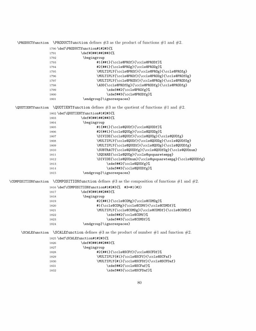
\PRODUCTfunction \PRODUCTfunction defines #3 as the product of functions #1 and #2.
1790 \def\PRODUCTfunction#1#2#3{%
1791 \def#3##1##2##3{%
1792 \begingroup
1793 #1{##1}{\ccls@PROf}{\ccls@PRODf}%
1794 #2{##1}{\ccls@PROg}{\ccls@PRODg}%
1795 \MULTIPLY{\ccls@PROf}{\ccls@PROg}{\ccls@PROfg}
1796 \MULTIPLY{\ccls@PROf}{\ccls@PRODg}{\ccls@PROfDg}
1797 \MULTIPLY{\ccls@PRODf}{\ccls@PROg}{\ccls@PRODfg}
1798 \ADD{\ccls@PROfDg}{\ccls@PRODfg}{\ccls@PRODfg}
1799 \xdef##2{\ccls@PROfg}%
1800 \xdef##3{\ccls@PRODfg}%
1801 \endgroup}\ignorespaces}
\QUOTIENTfunction \QUOTIENTfunction defines #3 as the quotient of functions #1 and #2.
1802 \def\QUOTIENTfunction#1#2#3{%
1803 \def#3##1##2##3{%
1804 \begingroup
1805 #1{##1}{\ccls@QUOf}{\ccls@QUODf}%
1806 #2{##1}{\ccls@QUOg}{\ccls@QUODg}%
1807 \DIVIDE{\ccls@QUOf}{\ccls@QUOg}{\ccls@QUOfg}
1808 \MULTIPLY{\ccls@QUOf}{\ccls@QUODg}{\ccls@QUOfDg}
1809 \MULTIPLY{\ccls@QUODf}{\ccls@QUOg}{\ccls@QUODfg}
1810 \SUBTRACT{\ccls@QUODfg}{\ccls@QUOfDg}{\ccls@QUOnum}
1811 \SQUARE{\ccls@QUOg}{\ccls@qsquaretempg}
1812 \DIVIDE{\ccls@QUOnum}{\ccls@qsquaretempg}{\ccls@QUODfg}
1813 \xdef##2{\ccls@QUOfg}%
1814 \xdef##3{\ccls@QUODfg}%
1815 \endgroup}\ignorespaces}
\COMPOSITIONfunction \COMPOSITIONfunction defines #3 as the composition of functions #1 and #2.
1816 \def\COMPOSITIONfunction#1#2#3{% #3=#1(#2)
1817 \def#3##1##2##3{%
1818 \begingroup
1819 #2{##1}{\ccls@COMg}{\ccls@COMDg}%
1820 #1{\ccls@COMg}{\ccls@COMf}{\ccls@COMDf}%
1821 \MULTIPLY{\ccls@COMDg}{\ccls@COMDf}{\ccls@COMDf}
1822 \xdef##2{\ccls@COMf}%
1823 \xdef##3{\ccls@COMDf}%
1824 \endgroup}\ignorespaces}
\SCALEfunction \SCALEfunction defines #3 as the product of number #1 and function #2.
1825 \def\SCALEfunction#1#2#3{%
1826 \def#3##1##2##3{%
1827 \begingroup
1828 #2{##1}{\ccls@SCFf}{\ccls@SCFDf}%
1829 \MULTIPLY{#1}{\ccls@SCFf}{\ccls@SCFaf}
1830 \MULTIPLY{#1}{\ccls@SCFDf}{\ccls@SCFDaf}
1831 \xdef##2{\ccls@SCFaf}%
1832 \xdef##3{\ccls@SCFDaf}%
80
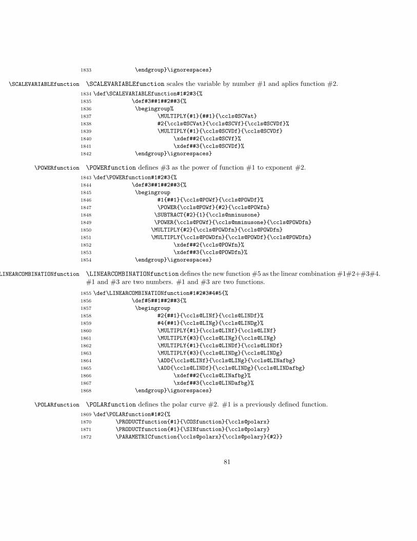
1833 \endgroup}\ignorespaces}
\SCALEVARIABLEfunction \SCALEVARIABLEfunction scales the variable by number #1 and aplies function #2.
1834 \def\SCALEVARIABLEfunction#1#2#3{%
1835 \def#3##1##2##3{%
1836 \begingroup%
1837 \MULTIPLY{#1}{##1}{\ccls@SCVat}
1838 #2{\ccls@SCVat}{\ccls@SCVf}{\ccls@SCVDf}%
1839 \MULTIPLY{#1}{\ccls@SCVDf}{\ccls@SCVDf}
1840 \xdef##2{\ccls@SCVf}%
1841 \xdef##3{\ccls@SCVDf}%
1842 \endgroup}\ignorespaces}
\POWERfunction \POWERfunction defines #3 as the power of function #1 to exponent #2.
1843 \def\POWERfunction#1#2#3{%
1844 \def#3##1##2##3{%
1845 \begingroup
1846 #1{##1}{\ccls@POWf}{\ccls@POWDf}%
1847 \POWER{\ccls@POWf}{#2}{\ccls@POWfn}
1848 \SUBTRACT{#2}{1}{\ccls@nminusone}
1849 \POWER{\ccls@POWf}{\ccls@nminusone}{\ccls@POWDfn}
1850 \MULTIPLY{#2}{\ccls@POWDfn}{\ccls@POWDfn}
1851 \MULTIPLY{\ccls@POWDfn}{\ccls@POWDf}{\ccls@POWDfn}
1852 \xdef##2{\ccls@POWfn}%
1853 \xdef##3{\ccls@POWDfn}%
1854 \endgroup}\ignorespaces}
\LINEARCOMBINATIONfunction \LINEARCOMBINATIONfunction defines the new function #5 as the linear combination #1#2+#3#4.#1 and #3 are two numbers. #1 and #3 are two functions.
1855 \def\LINEARCOMBINATIONfunction#1#2#3#4#5{%
1856 \def#5##1##2##3{%
1857 \begingroup
1858 #2{##1}{\ccls@LINf}{\ccls@LINDf}%
1859 #4{##1}{\ccls@LINg}{\ccls@LINDg}%
1860 \MULTIPLY{#1}{\ccls@LINf}{\ccls@LINf}
1861 \MULTIPLY{#3}{\ccls@LINg}{\ccls@LINg}
1862 \MULTIPLY{#1}{\ccls@LINDf}{\ccls@LINDf}
1863 \MULTIPLY{#3}{\ccls@LINDg}{\ccls@LINDg}
1864 \ADD{\ccls@LINf}{\ccls@LINg}{\ccls@LINafbg}
1865 \ADD{\ccls@LINDf}{\ccls@LINDg}{\ccls@LINDafbg}
1866 \xdef##2{\ccls@LINafbg}%
1867 \xdef##3{\ccls@LINDafbg}%
1868 \endgroup}\ignorespaces}
\POLARfunction \POLARfunction defines the polar curve #2. #1 is a previously defined function.
1869 \def\POLARfunction#1#2{%
1870 \PRODUCTfunction{#1}{\COSfunction}{\ccls@polarx}
1871 \PRODUCTfunction{#1}{\SINfunction}{\ccls@polary}
1872 \PARAMETRICfunction{\ccls@polarx}{\ccls@polary}{#2}}
81
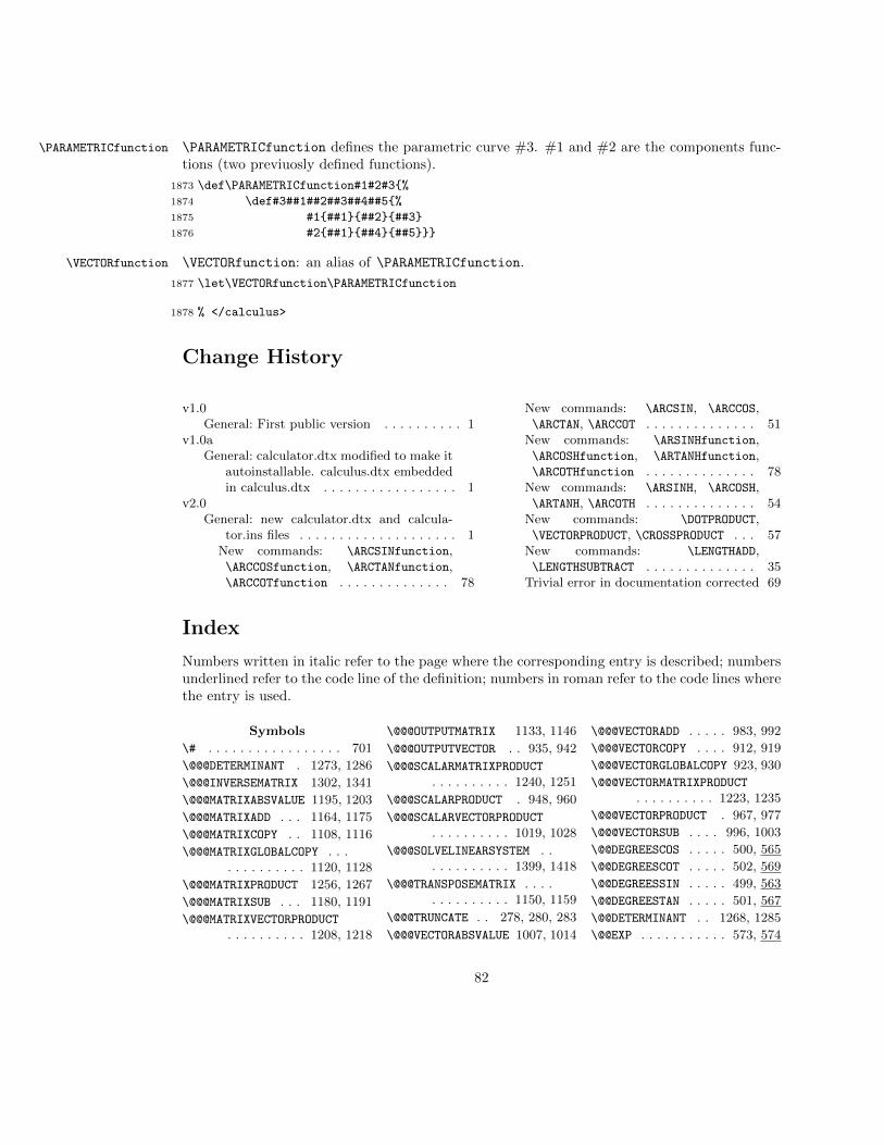
\PARAMETRICfunction \PARAMETRICfunction defines the parametric curve #3. #1 and #2 are the components func-tions (two previuosly defined functions).
1873 \def\PARAMETRICfunction#1#2#3{%
1874 \def#3##1##2##3##4##5{%
1875 #1{##1}{##2}{##3}
1876 #2{##1}{##4}{##5}}}
\VECTORfunction \VECTORfunction: an alias of \PARAMETRICfunction.
1877 \let\VECTORfunction\PARAMETRICfunction
1878 % </calculus>
Change History
v1.0General: First public version . . . . . . . . . . 1
v1.0aGeneral: calculator.dtx modified to make it
autoinstallable. calculus.dtx embeddedin calculus.dtx . . . . . . . . . . . . . . . . . 1
v2.0General: new calculator.dtx and calcula-
tor.ins files . . . . . . . . . . . . . . . . . . . . 1New commands: \ARCSINfunction,\ARCCOSfunction, \ARCTANfunction,\ARCCOTfunction . . . . . . . . . . . . . . 78
New commands: \ARCSIN, \ARCCOS,\ARCTAN, \ARCCOT . . . . . . . . . . . . . . 51
New commands: \ARSINHfunction,\ARCOSHfunction, \ARTANHfunction,\ARCOTHfunction . . . . . . . . . . . . . . 78
New commands: \ARSINH, \ARCOSH,\ARTANH, \ARCOTH . . . . . . . . . . . . . . 54
New commands: \DOTPRODUCT,\VECTORPRODUCT, \CROSSPRODUCT . . . 57
New commands: \LENGTHADD,\LENGTHSUBTRACT . . . . . . . . . . . . . . 35
Trivial error in documentation corrected 69
Index
Numbers written in italic refer to the page where the corresponding entry is described; numbersunderlined refer to the code line of the definition; numbers in roman refer to the code lines wherethe entry is used.
Symbols
\# . . . . . . . . . . . . . . . . . 701
\@@@DETERMINANT . 1273, 1286
\@@@INVERSEMATRIX 1302, 1341
\@@@MATRIXABSVALUE 1195, 1203
\@@@MATRIXADD . . . 1164, 1175
\@@@MATRIXCOPY . . 1108, 1116
\@@@MATRIXGLOBALCOPY . . .. . . . . . . . . . 1120, 1128
\@@@MATRIXPRODUCT 1256, 1267
\@@@MATRIXSUB . . . 1180, 1191
\@@@MATRIXVECTORPRODUCT
. . . . . . . . . . 1208, 1218
\@@@OUTPUTMATRIX 1133, 1146
\@@@OUTPUTVECTOR . . 935, 942
\@@@SCALARMATRIXPRODUCT
. . . . . . . . . . 1240, 1251
\@@@SCALARPRODUCT . 948, 960
\@@@SCALARVECTORPRODUCT
. . . . . . . . . . 1019, 1028
\@@@SOLVELINEARSYSTEM . .. . . . . . . . . . 1399, 1418
\@@@TRANSPOSEMATRIX . . . .. . . . . . . . . . 1150, 1159
\@@@TRUNCATE . . 278, 280, 283
\@@@VECTORABSVALUE 1007, 1014
\@@@VECTORADD . . . . . 983, 992
\@@@VECTORCOPY . . . . 912, 919
\@@@VECTORGLOBALCOPY 923, 930
\@@@VECTORMATRIXPRODUCT
. . . . . . . . . . 1223, 1235
\@@@VECTORPRODUCT . 967, 977
\@@@VECTORSUB . . . . 996, 1003
\@@DEGREESCOS . . . . . 500, 565
\@@DEGREESCOT . . . . . 502, 569
\@@DEGREESSIN . . . . . 499, 563
\@@DEGREESTAN . . . . . 501, 567
\@@DETERMINANT . . 1268, 1285
\@@EXP . . . . . . . . . . . 573, 574
82

\@@FRACTIONALPART . 262, 264\@@INTEGERPART . . . . 247, 249\@@INVERSEMATRIX 1287, 1339\@@LOG . . . . . . . . . . . 677, 696\@@MATRIXABSVALUE 1192, 1202\@@MATRIXADD . . . . 1160, 1174\@@MATRIXCOPY . . . 1105, 1115\@@MATRIXGLOBALCOPY . . . .
. . . . . . . . . . 1117, 1127\@@MATRIXPRODUCT 1252, 1266\@@MATRIXSUB . . . . 1176, 1190\@@MATRIXVECTORPRODUCT .
. . . . . . . . . . 1204, 1217\@@OUTPUTMATRIX . 1129, 1145\@@OUTPUTVECTOR . . . 931, 941\@@ROUND . . . . . 291–293, 297\@@SCALARMATRIXPRODUCT .
. . . . . . . . . . 1236, 1250\@@SCALARPRODUCT . . 943, 959\@@SCALARVECTORPRODUCT .
. . . . . . . . . . 1015, 1027\@@SOLVELINEARSYSTEM . . .
. . . . . . . . . . 1354, 1416\@@TDMATRIXSOL . . 1096, 1317\@@TRANSPOSEMATRIX 1147, 1158\@@TRUNCATE 272–274, 299, 308\@@VECTORABSVALUE 1004, 1013\@@VECTORADD . . . . . . 979, 991\@@VECTORCOPY . . . . . 909, 918\@@VECTORGLOBALCOPY 920, 929\@@VECTORMATRIXPRODUCT .
. . . . . . . . . . 1219, 1234\@@VECTORPRODUCT . . 962, 976\@@VECTORSUB . . . . . 993, 1002\@ADJMATRIX . 1309, 1322, 1405\@BASICARCTAN . . . . . 807, 810\@BASICEXP . . . 593, 601, 608\@BASICLOG . . . . . . . 694, 700\@BASICSINE . . . 386, 395, 517\@BASICTAN . . . 432, 437, 545\@CONVERTDEG . . . . . . . . . .
. 563, 565, 567, 569, 571\@DEGREES . . . . . . . . . . . .
. 564, 566, 568, 570–572\@DEGREESCOS . . . . . . 500, 526\@DEGREESCOT . . . . . . 502, 550\@DEGREESSIN . . 499, 503, 564\@DEGREESTAN . . . . . . 501, 530\@DIVIDE . . 162, 172, 177, 231\@EXP . . . . . . . . 573, 582, 584
\@FRACTIONALPART . . 264, 270
\@INCSYS 1342, 1366, 1369, 1392
\@INTEGERDIVIDE . . . 178, 181
\@INTEGERPART . . . . . 249, 259
\@LOG . . . . . 677, 678, 697, 698
\@MATRIXSIZE . . . . 1102, 1103
\@NUMBERSOL . . . . . 1101, 1279
\@OUTPUTMATRIX . . . 1129,1159, 1175, 1191,1203, 1251, 1267, 1341
\@OUTPUTSOL 132, 176, 204,214, 227, 243, 246,260, 271, 282, 310,331, 371, 394, 412,416, 436, 461, 474,525, 529, 549, 562,583, 607, 628, 641,654, 665, 676, 695,699, 716, 772, 794,809, 838, 843, 851,863, 882, 905, 960,977, 1032, 1054, 1286
\@OUTPUTSOLS . . . . . . 133, 240
\@OUTPUTVECTOR . . . . 931,1037, 1218, 1235, 1419
\@POWER . . . . . . 214, 215, 220
\@ROUND . . . . . . . . . . 291, 292
\@SCLRDIVVECT . . . . 1310,1312, 1314, 1319, 1409
\@SOLPART . . . . . . . 1345,1375, 1379, 1383, 1387
\@TDINCSYS . . . . . 1349, 1403
\@TDMATRIXCOPY . . . . . . . .. 1055, 1109, 1121, 1151
\@TDMATRIXGLOBALSOL . . . .. . . . . . . . . . 1075, 1122
\@TDMATRIXNOSOL . . . . . . .. . . . . 1085, 1098, 1304
\@TDMATRIXSOL . . . . 1065,1100, 1110, 1152,1168, 1184, 1244, 1260
\@TRUNCATE . . . . . . . 272, 273
\@VECTORSIZE . . . . . . 906, 907
A
\ABSVALUE . . . 7, 142, 155,156, 230, 313, 314,338, 397, 439, 586,631, 644, 657, 668,
753, 768, 1005, 1008,1336, 1358–1360, 1401
\ADD . . . . 6, 148, 152, 174,226, 235, 239, 306,363, 382, 415, 428,480, 491, 512, 528,541, 612, 615, 618,621, 624, 628, 639,687, 709, 745, 816,819, 822, 825, 828,831, 834, 836, 847,849, 861, 875, 892,946, 951, 953, 980,981, 984–986, 1276,1278, 1562, 1611,1628, 1629, 1631,1647, 1649, 1652,1653, 1655, 1737,1742, 1747, 1775,1776, 1798, 1864, 1865
\ARCCOS . . 14, 773, 1053, 1729
\ARCCOSfunction . . . . . 1728
\ARCCOT . . . . . . 14, 839, 1740
\ARCCOTfunction . . . . . 1739
\ARCOSH . . . . . . 14, 852, 1751
\ARCOSHfunction . . . . . 1750
\ARCOTH . . . . . . 14, 883, 1762
\ARCOTHfunction . . . . . 1761
\ARCSIN . . . 14, 717, 792, 1723
\ARCSINfunction . . . . . 1722
\ARCTAN . . . 14, 795, 841, 1735
\ARCTANfunction . . . . . 1734
\ARSINH . . . . . . 14, 844, 1745
\ARSINHfunction . . . . . 1744
\ARTANH . . . . . . 14, 864, 1757
\ARTANHfunction . . . . . 1756
C
\ccls@COMDf . 1820, 1821, 1823
\ccls@COMDg . . . . . 1819, 1821
\ccls@COMf . . . . . 1820, 1822
\ccls@COMg . . . . . 1819, 1820
\ccls@cost . 1555, 1556, 1559
\ccls@cpoly . . . . . . 1634,1637, 1640, 1643, 1644
\ccls@deffunction 1506,1514, 1517, 1522, 1523
\ccls@defpolarfunction .. . . . . . . . . . . 1533,1541, 1544, 1549, 1550
83

\ccls@defvectorfunction
. . . . . . . . . . . 1570,1578, 1581, 1586, 1587
\ccls@ErrorFuncDef 1445, 1508
\ccls@ErrorFuncUnDef . . .. . . . . . . . . . 1452, 1512
\ccls@ErrorPFuncDef . . . .. . . . . . . . . . 1462, 1535
\ccls@ErrorPFuncUnDef . .. . . . . . . . . . 1470, 1539
\ccls@ErrorVFuncDef . . . .. . . . . . . . . . 1483, 1572
\ccls@ErrorVFuncUnDef . .. . . . . . . . . . 1491, 1576
\ccls@InfoFuncEns 1458, 1519
\ccls@InfoPFuncEns 1479, 1546
\ccls@InfoVFuncEns 1500, 1583
\ccls@LINafbg . . . 1864, 1866
\ccls@LINDafbg . . 1865, 1867
\ccls@LINDf . 1858, 1862, 1865
\ccls@LINDg . 1859, 1863, 1865
\ccls@LINf . 1858, 1860, 1864
\ccls@LINg . 1859, 1861, 1864
\ccls@lpoly . . . . . . 1599,1602, 1605, 1608, 1609
\ccls@nminusone . 1848, 1849
\ccls@polarx . . . . 1870, 1872
\ccls@polary . . . . 1871, 1872
\ccls@POWDf . . . . . 1846, 1851
\ccls@POWDfn 1849–1851, 1853
\ccls@POWf . 1846, 1847, 1849
\ccls@POWfn . . . . . 1847, 1852
\ccls@PRODf . . . . . 1793, 1797
\ccls@PRODfg 1797, 1798, 1800
\ccls@PRODg . . . . . 1794, 1796
\ccls@PROf . 1793, 1795, 1796
\ccls@PROfDg . . . . 1796, 1798
\ccls@PROfg . . . . . 1795, 1799
\ccls@PROg . 1794, 1795, 1797
\ccls@qpoly . . . . . . 1615,1618, 1621, 1624, 1625
\ccls@qsquaretempg 1811, 1812
\ccls@QUODf . . . . . 1805, 1809
\ccls@QUODfg . . . . . . . . . .. 1809, 1810, 1812, 1814
\ccls@QUODg . . . . . 1806, 1808
\ccls@QUOf . 1805, 1807, 1808
\ccls@QUOfDg . . . . 1808, 1810
\ccls@QUOfg . . . . . 1807, 1813
\ccls@QUOg . . . . . . . . . . .. 1806, 1807, 1809, 1811
\ccls@QUOnum . . . . 1810, 1812\ccls@SCFaf . . . . . 1829, 1831\ccls@SCFDaf . . . . 1830, 1832\ccls@SCFDf . . . . . 1828, 1830\ccls@SCFf . . . . . 1828, 1829\ccls@SCVat . . . . . 1837, 1838\ccls@SCVDf . 1838, 1839, 1841\ccls@SCVf . . . . . 1838, 1840\ccls@sint . 1557, 1558, 1561\ccls@SUBDf . . . . . 1783, 1786\ccls@SUBDfg . . . . 1786, 1788\ccls@SUBDg . . . . . 1784, 1786\ccls@SUBf . . . . . 1783, 1785\ccls@SUBfg . . . . . 1785, 1787\ccls@SUBg . . . . . 1784, 1785\ccls@SUMDf . . . . . 1773, 1776\ccls@SUMDfg . . . . 1776, 1778\ccls@SUMDg . . . . . 1774, 1776\ccls@SUMf . . . . . 1773, 1775\ccls@SUMfg . . . . . 1775, 1777\ccls@SUMg . . . . . 1774, 1775\ccls@temp . . . . . 1648, 1649\cctr@@det . . . . . . 1288,
1303, 1336, 1401, 1402\cctr@@deta . . . . . 1358, 1361\cctr@@detb . . . . . 1359, 1365\cctr@@detc . . . . . 1360, 1368\cctr@absval . . . . . . 586,
587, 631, 632, 644,645, 657, 658, 668, 669
\cctr@ae . . 685, 686, 690, 691\cctr@det . . . 1274–1278,
1298, 1299, 1310,1312, 1314, 1335,1336, 1400, 1401, 1409
\cctr@deta . . . . . . . . . . .. 1355, 1358, 1362–1364
\cctr@detb . 1356, 1359, 1362\cctr@detc . 1357, 1360, 1363\cctr@epsilon 6, 360, 576,
680, 705, 758, 1288,1303, 1361, 1365,1368, 1373, 1377,1381, 1385, 1390, 1402
\cctr@expminusx . . . . . . .. . . . 638, 639, 651, 652
\cctr@expt 595, 596, 603, 604\cctr@expx 636, 639, 649, 652
\cctr@expy 596, 597, 604, 605
\cctr@lengtha . . . . . . . . .. . . 4, 145–148, 150,151, 182, 188, 189,191, 193, 194, 199, 201
\cctr@lengthb . . . . . . . . .5, 149, 150, 183, 184,
188, 192, 193, 200,202, 359, 360, 367,369, 704, 705, 712,714, 756, 758, 769, 771
\cctr@log . . . . . . . . 580–582
\cctr@loga . . . . . . . 697, 699
\cctr@logmaxnum . 8, 102,587, 632, 645, 658, 669
\cctr@logx . . . . . . . 698, 699
\cctr@minust 637, 638, 650, 651
\cctr@ndec . . . 164, 165, 174
\cctr@outa 132, 133, 135,932, 933, 936, 937,1130, 1131, 1135, 1139
\cctr@outb . . . . 134, 135,932, 933, 936, 937,1130, 1131, 1135, 1139
\cctr@outc . . . . 936, 937,1130, 1131, 1135, 1139
\cctr@outd . . . . . . . . . . .. 1130, 1131, 1136, 1140
\cctr@oute . . . . . 1136, 1140
\cctr@outf . . . . . 1136, 1140
\cctr@outg . . . . . 1137, 1141
\cctr@outh . . . . . 1137, 1141
\cctr@outi . . . . . 1137, 1141
\cctr@Q . . . . . . 163, 173, 175
\cctr@sign . . . 157–160, 175
\cctr@size 916, 917, 927,928, 939, 940, 957,958, 974, 975, 989,990, 1000, 1001, 1011,1012, 1025, 1026,1113, 1114, 1125,1126, 1143, 1144,1156, 1157, 1172,1173, 1188, 1189,1200, 1201, 1215,1216, 1232, 1233,1248, 1249, 1264,1265, 1283, 1284,1337, 1338, 1414, 1415
84

\cctr@sol . . . . . . . . . . . .. 1101, 1274, 1276, 1278
\cctr@solAA . . . . . . . . . . .. . 1056, 1066, 1076,1097, 1165, 1181,1241, 1257, 1304,1310, 1311, 1323, 1406
\cctr@solAB . . 1057, 1067,1077, 1165, 1181,1241, 1257, 1304,1310, 1311, 1326, 1406
\cctr@solAC . . 1058, 1068,1078, 1165, 1181,1241, 1257, 1304,1310, 1311, 1329, 1406
\cctr@solBA . . 1059, 1069,1079, 1166, 1182,1242, 1258, 1305,1312, 1313, 1324, 1407
\cctr@solBB . . 1060, 1070,1080, 1166, 1182,1242, 1258, 1305,1312, 1313, 1327, 1407
\cctr@solBC . . 1061, 1071,1081, 1166, 1182,1242, 1258, 1305,1312, 1313, 1330, 1407
\cctr@solCA . . 1062, 1072,1082, 1167, 1183,1243, 1259, 1306,1314, 1315, 1325, 1408
\cctr@solCB . . 1063, 1073,1083, 1167, 1183,1243, 1259, 1306,1314, 1315, 1328, 1408
\cctr@solCC . . 1064, 1074,1084, 1167, 1183,1243, 1259, 1306,1314, 1315, 1331, 1408
\cctr@tanhden . . . . . . . . .. . . . 663, 664, 673, 675
\cctr@tanhnum . . . . . . . . .. . . . 662, 664, 674, 675
\cctr@temp 243, 246, 252–254, 296, 297, 1031, 1032
\cctr@tempA . . . . . . . 267, 268
\cctr@tempa . . . . . . . 201,203, 222, 224, 226,276, 277, 313, 315,316, 318, 326–330,
397, 398, 400, 402,403, 405, 408, 439,440, 442, 446, 447,449, 450, 452, 453,455, 456, 458, 459,610, 611, 613, 616,619, 622, 814, 815,817, 820, 823, 826,829, 832, 835, 846–848, 858–860, 874–876, 891–893, 902,903, 945, 946, 950–953, 1035–1037, 1040,1043, 1051, 1225–1228, 1270, 1271,1371, 1373, 1389, 1390
\cctr@tempB 877, 879, 894, 896
\cctr@tempb . . . . . . . . . . .. 202, 203, 218, 220,301, 302, 305, 306,314–317, 319, 323,328, 329, 382, 383,389, 390, 392, 393,428, 429, 434, 435,512, 513, 516, 517,520, 521, 523, 524,541, 544, 545, 547,548, 798, 799, 803,804, 848–850, 860–862, 875, 877, 892,894, 1041, 1047, 1052,1225–1228, 1371, 1377
\cctr@tempC 878, 879, 895, 896
\cctr@tempc . . . . . . . . . . .. 219, 220, 300, 302,303, 315, 317, 328,330, 415, 416, 528,529, 876, 878, 893,895, 1042, 1051–1053,1225–1228, 1372, 1381
\cctr@tempD . . . . . . . . . . .. 155, 162, 167, 169, 172
\cctr@tempd 156, 162, 170,172, 230, 239, 1372, 1385
\cctr@tempdif . . . . . 711, 712
\cctr@tempe 299, 300, 306, 308
\cctr@tempexp . . . . . 209, 210
\cctr@tempoldw . . . . 706, 711
\cctr@tempoldy . . . . 760, 770
\cctr@tempq 162, 163, 172, 173
\cctr@tempr . . . . . . . . . . .. 162, 166, 167, 169, 172
\cctr@tempw . . . . 361–363,366, 367, 703, 706,707, 709–711, 716,759, 761, 763, 765, 767
\cctr@tempx 737–739, 745–747\cctr@tempxw . . . . . . 707–709\cctr@tempxx 739, 740, 747, 748\cctr@tempy 753, 754, 757,
760, 763, 764, 767–770\cctr@tempz . . . . . . . 362–
365, 761, 762, 764–766\cctr@Warnbigarccos . . . .
. . . . . . . . . 36, 786, 790\cctr@Warnbigarcsin . . . .
. . . . . . . . . 30, 730, 734\cctr@Warnbigartanh . . . .
. . . . . . . . . 48, 868, 872\cctr@Warncrossprod 119, 965\cctr@Warndivzero . . 9, 186\cctr@WarnIncLinSys 71, 1342\cctr@WarnIncTDLinSys . .
. . . . . . . . . . . 74, 1349\cctr@WarnIndLinSys 78, 1345\cctr@Warninfcotan . . . . .
. . . . . . . . . 92, 470, 558\cctr@Warninfexp . . . 98,
588, 633, 646, 659, 670\cctr@Warninfexpb . 106, 577\cctr@Warninflog . . 113, 681\cctr@Warninftan . . . . . .
. . 86, 420, 424, 533, 537\cctr@Warnnoangle . . . . .
. . . . . . 125, 1045, 1049\cctr@Warnnogcd . . . . 14, 320\cctr@Warnnointexp . . 24, 211\cctr@Warnnoposrad . . 18, 356\cctr@Warnsingmatrix 61, 1293\cctr@WarnsingTDmatrix .
. . . . . . . . . . . 66, 1307\cctr@Warnsmallarcosh 42, 856\cctr@Warnsmallarcoth 54, 888\cctr@WarnZeroLinSys 82, 1394\COMPOSITIONfunction 25, 1816\CONSTANTfunction . 24, 1766\COPY 5, 130, 132, 135, 138,
141, 144, 157–160,163, 164, 169, 173,189, 222, 223, 247,
85

248, 256, 262, 263,285–289, 297, 317,323, 327, 329, 330,334, 342, 352, 358,361, 365, 375, 377,379, 398, 400, 440,443, 466, 478, 487,489, 498, 505, 507,509, 554, 706, 716,720, 723, 726, 752,757, 759, 760, 766,776, 779, 782, 812,874, 891, 904, 907,908, 910, 913, 1056–1064, 1066–1074,1101, 1103, 1104,1106, 1148, 1294,1295, 1347, 1395,1612, 1658, 1659,1661, 1662, 1664,1665, 1682, 1720, 1721
\COS . . . 11, 413, 464, 763,1555, 1684, 1689, 1692
\COSfunction . 23, 1683, 1870
\COSH . . . . . . 13, 629, 663,674, 1701, 1705, 1708
\COSHfunction . . . . . 23, 1700
\COT . . . . . . . . . . . . . 12, 462
\COTAN . . . . . . . . . . . . . 1696
\COTANH . . . . . . . . . . . . 1712
\COTfunction . . . . . . 23, 1695
\COTH . . . . . . . . . . . . 13, 666
\COTHfunction . . . . . 23, 1711
\CROSSPRODUCT . . . . . 17, 978
\CUBE . . . . . . . . . . . . . 7, 206
\CUBEfunction . . . . . 23, 1673
D
\DEGREESCOS 12, 500, 552, 566
\DEGREESCOT . . . . 12, 502, 570
\DEGREESSIN . . . . . . . . 12,499, 513, 521, 524, 529
\DEGREESTAN . . . . . . . . 12,501, 541, 548, 556, 568
\DEGtoRAD . 13, 475, 516, 544
\DETERMINANT . . . 21, 968–970, 1268, 1323–1331,1335, 1355–1357, 1400
\DIVIDE . . . . . 6, 153, 203,218, 305, 336, 345,
346, 362, 364, 403,406, 409, 445, 446,448, 449, 451, 452,454, 455, 457, 458,460, 473, 475, 561,571, 595, 603, 611,613, 614, 616, 617,619, 620, 622, 623,626, 640, 653, 664,675, 685, 699, 708,738, 746, 764, 798,803, 817, 820, 823,826, 829, 832, 835,837, 880, 897, 1036,1051, 1052, 1298,1320, 1346, 1362,1363, 1422, 1424–1427, 1429, 1667,1679, 1694, 1699,1710, 1715, 1718,1727, 1733, 1738,1743, 1749, 1755,1760, 1765, 1807, 1812
\DOTPRODUCT . . . . . . . 17, 961
\Dr . . . . . . . . . . . 1559, 1561
\Dx . . 1559, 1560, 1564, 1593
\Dy . . . 1529, 1561, 1562,1566, 1595, 1612,1627, 1628, 1646,1649, 1651, 1653,1659, 1662, 1665,1668, 1669, 1672,1674–1676, 1679,1682, 1685, 1686,1689, 1692–1694,1697–1699, 1702,1705, 1708–1710,1713–1715, 1718,1721, 1726, 1727,1732, 1733, 1738,1743, 1748, 1749,1754, 1755, 1760, 1765
E
\ensurecpoly . . . . . . 27, 1638
\ensurefunction 29, 1461,1516, 1604, 1620, 1639
\ensurelpoly . . . . . . 27, 1603
\ensurepolarfunction . . .. . . . . . . 30, 1482, 1543
\ensureqpoly . . . . . . 27, 1619\ensurevectorfunction . .
. . . . . . . 29, 1503, 1580\EXP . . . . . . . 11, 573, 636,
638, 649, 651, 707, 1681\EXPfunction . . . . . . 23, 1680
F\FLOOR . . . . . . . . . . . . 8, 261\forcecpoly . . . . . . . 27, 1641\forcefunction . . . . . 29,
1521, 1607, 1623, 1642\forcelpoly . . . . . . . 27, 1606\forcepolarfunction 30, 1548\forceqpoly . . . . . . . 27, 1622\forcevectorfunction 29, 1585\FRACTIONALPART . . . . 8, 262\FRACTIONSIMPLIFY . 10, 340
G\GCD . . . . . . 10, 311, 333, 344\GLOBALCOPY . . . . . . . . . . .
. 131, 132–134, 921,924, 1076–1084, 1118
H\HEAVISIDEfunction . 23, 1719
I\IDENTITYfunction . 23, 1663\ifcase . . . . . . . . . . . . . 284\INTEGERDIVISION . . . . . .
. . . . . . 9, 228, 243, 246\INTEGERPART . . . . . . . . 7,
209, 247, 261, 267, 276\INTEGERQUOTIENT . . . 9, 244\INVERSEMATRIX . . . . 21, 1287
L\LCM . . . . . . . . . . . . . 10, 332\LENGTHADD . . . . 15, 191, 196\LENGTHDIVIDE . . . . . 15, 197\LENGTHSUBTRACT . . . 15, 195\LINEARCOMBINATIONfunction
. . . . . . . . . . . 26, 1855\LOG . . . . . . . . . . 11, 580,
677, 691, 850, 862,877, 878, 894, 895, 1717
\LOGfunction . . . . . . 23, 1716
M\MATRIXABSVALUE 22, 1192, 1371
86

\MATRIXADD . . . . . . . 19, 1160
\MATRIXCOPY . . . . . . . . . . .. . . 18, 1105, 1131, 1138
\MATRIXGLOBALCOPY . . . . .. . . . . 1117, 1130, 1134
\MATRIXPRODUCT . . . . 20, 1252
\MATRIXSIZE . . . . . . 1102,1113, 1125, 1143,1156, 1172, 1188,1200, 1215, 1248,1264, 1283, 1337, 1414
\MATRIXSUB . . . . . . . 19, 1176
\MATRIXVECTORPRODUCT 20,1204, 1253, 1254, 1406
\MAX . . . . . . . . . . . 6, 136, 315
\MIN . . . . . . . . . . . 6, 139, 316
\MODULO . . . . . . . . 9, 241, 328
\MULTIPLY . . . 6, 144, 145,167, 170, 175, 179,205, 206, 219, 225,252, 296, 302, 337,347, 405, 408, 411,476, 572, 581, 627,637, 650, 690, 741,749, 815, 818, 821,824, 827, 830, 833,902, 944, 945, 949,950, 952, 1016, 1017,1020–1022, 1269,1270, 1274, 1275,1277, 1296, 1297,1421, 1423, 1556,1558, 1559, 1561,1610, 1626, 1627,1630, 1645, 1646,1648, 1650, 1651,1654, 1669, 1672,1675, 1676, 1686,1795–1797, 1808,1809, 1821, 1829,1830, 1837, 1839,1850, 1851, 1860–1863
N
\NeedsTeXFormat . . . . 2, 1442
\newcpoly . . . . . . . . 27, 1632
\newfunction . . . . . . . 29,1457, 1504, 1598,1614, 1633, 1657,1660, 1663, 1666,
1670, 1673, 1677,1680, 1683, 1687,1690, 1695, 1700,1703, 1706, 1711,1716, 1719, 1722,1728, 1734, 1739,1744, 1750, 1756, 1761
\newlpoly . . . . . . . . 26, 1597\newpolarfunction . . . . .
. . . . . . . 30, 1477, 1531\newqpoly . . . . . . . . 27, 1613\newvectorfunction . . . . .
. . . . . . . 29, 1498, 1568\numberCOSXLV . . . . . 5, 1438\numberCOSXXX . . . . . 5, 1439\numberE . . . . . . . 5, 685,
690, 1428, 1429, 1430\numberETWO . . . . 5, 684, 1430\numberFIFTHPI . . . . 5, 1426\numberGOLD . . . . . . . 5, 1433\numberHALFPI 5, 375, 377,
381, 385, 415, 419,423, 427, 431, 723,726, 742, 750, 776,793, 800, 805, 842, 1422
\numberINVE . . . 5, 1429, 1431\numberINVETWO . . . . 5, 1431\numberINVGOLD . . . . 5, 1434\numberLOGTEN . . . . . 5, 1432\numberPI . . . 5, 389, 428,
434, 479, 483, 487,782, 1420, 1421–1427
\numberQUARTERPI . . 5, 1425\numberSIXTHPI . . . . 5, 1427\numberSQRTFIVE . . . 5, 1437\numberSQRTTHREE . . 5, 1436\numberSQRTTWO . . . . 5, 1435\numberTHIRDPI . . . . 5, 1424\numberTHREEHALFPI . . . . .
. . . . . 5, 379, 388, 1423\numberTWOPI . . . . . . . . 5,
382, 392, 480, 484, 1421
O\ONEfunction . . . . . . 23, 1657\or . . . . . . . . . . . . . 286–289
P\PackageError 1446, 1453,
1463, 1471, 1484, 1492\PackageInfo 1459, 1480, 1501
\PackageWarning . . . . . . .. . . . 10, 15, 19, 25,31, 37, 43, 49, 55, 62,67, 71, 74, 78, 82, 87,93, 99, 107, 114, 120, 126
\PARAMETRICfunction . . . .. . . 27, 1872, 1873, 1877
\POLARfunction . . . . 28, 1869\POWER 7, 207, 301, 1847, 1849\POWERfunction . . . . 25, 1843\PRODUCTfunction . . . . . .
. . . 25, 1790, 1870, 1871\ProvidesPackage . . . 3, 1443
Q\QUOTIENTfunction . 25, 1802
R\r . . . . . . . . . . . . 1556, 1558\RADtoDEG . . . . . . . . 13, 476\RECIPROCALfunction 23, 1666\REDUCEDEGREESANGLE 13, 488\REDUCERADIANSANGLE 13, 477\renewcpoly . . . . . . . 27, 1635\renewfunction 29, 1451,
1510, 1601, 1617, 1636\renewlpoly . . . . . . . 27, 1600\renewpolarfunction . . . .
. . . . . . . 30, 1468, 1537\renewqpoly . . . . . . . 27, 1616\renewvectorfunction . . .
. . . . . . . 29, 1489, 1574\ROUND . . . . . . . . . . . . 8, 291
S\SCALARMATRIXPRODUCT . . .
. . . . . . . 20, 1236, 1299\SCALARPRODUCT . . . . . 17,
943, 961, 1031,1042, 1205, 1206,1209–1211, 1220, 1221
\SCALARVECTORPRODUCT . . .. . . . 16, 1015, 1037,1224, 1225, 1227,1237, 1238, 1241–1243
\SCALEfunction . . . . 25, 1825\SCALEVARIABLEfunction .
. . . . . . . . . . . 25, 1834\setlength . . . . . . . . . . 194\SIN . . . 11, 373, 416, 761,
1557, 1685, 1688, 1697
87

\SINfunction . 23, 1687, 1871\SINH . . . . . . 13, 642, 662,
673, 1702, 1704, 1713\SINHfunction . . . . . 23, 1703\SOLVELINEARSYSTEM . 22, 1342\SQRT . . . . . . 10, 372, 739,
747, 848, 860, 1678,1726, 1732, 1748, 1754
\SQRTfunction . . . . . 23, 1677\SQUARE . . . . . 7, 205, 402,
597, 605, 610, 814,846, 858, 1430, 1431,1668, 1671, 1674,1693, 1698, 1709,1714, 1724, 1730,1736, 1741, 1746,1752, 1758, 1763, 1811
\SQUAREfunction . . . 23, 1670\SQUAREROOT 10, 349, 372, 1032\SUBTRACT . . . . . . 6, 152,
180, 237, 255, 268,300, 366, 389, 392,404, 407, 410, 434,447, 450, 453, 456,459, 484, 495, 520,523, 547, 625, 652,692, 703, 710, 711,737, 742, 750, 762,765, 767, 793, 800,805, 842, 859, 876,879, 893, 896, 1271,1560, 1725, 1731,1753, 1759, 1764,1785, 1786, 1810, 1848
\SUBTRACTfunction . 25, 1780\SUMfunction . . . . . . 25, 1770
T\t . . . . 1526, 1553, 1555,
1557, 1590, 1610,1626, 1630, 1645,1650, 1651, 1654,1664, 1667, 1671,1672, 1674, 1675,1678, 1681, 1684,1685, 1688, 1689,1691, 1692, 1696,1697, 1701, 1702,1704, 1705, 1707,1708, 1712, 1713,1717, 1718, 1720,1723, 1724, 1729,1730, 1735, 1736,1740, 1741, 1745,1746, 1751, 1752,1757, 1758, 1762, 1763
\TAN . . . . . . 11, 417, 468, 1691\TANfunction . . . . . . 23, 1690\TANH . . . . . . . . 13, 655, 1707\TANHfunction . . . . . 23, 1706\textit . . . . . . . . . . . . . 701\TRANSPOSEMATRIX . . 19, 1147\TRUNCATE . . . . . . . . . 8, 272\TWOVECTORSANGLE . . 18, 1038
U\UNITVECTOR . . . . . . . 17, 1033
V\VECTORABSVALUE . . . . . . .
. . . 18, 1004, 1193, 1196\VECTORADD . . . . 16, 979,
994, 997, 1161, 1162,1165–1167, 1226, 1228
\VECTORCOPY 16, 909, 933, 937\VECTORfunction . . . 28, 1877\VECTORGLOBALCOPY . . . . .
. . . . . . . . 920, 932, 936
\VECTORMATRIXPRODUCT . . .. . . . . 1219, 1257–1259
\VECTORNORM . . . 17, 1029,1035, 1040, 1041, 1389
\VECTORPRODUCT . 17, 962, 978
\VECTORSIZE 906, 916, 927,939, 957, 974, 989,1000, 1011, 1025, 1232
\VECTORSUB . . . . 16, 993,1177, 1178, 1181–1183
X
\x . . . 1556, 1562, 1563, 1592
Y
\y . . . . 1528, 1558, 1560,1565, 1594, 1610,1611, 1626, 1627,1629–1631, 1645–1647, 1650, 1652,1654, 1655, 1658,1661, 1664, 1667,1668, 1671, 1675,1678, 1679, 1681,1682, 1684, 1688,1691, 1696, 1701,1704, 1707, 1712,1717, 1720, 1723,1729, 1735, 1740,1745, 1751, 1757, 1762
\yy . . . 1724–1726, 1730–1732, 1736–1738,1741–1743, 1746–1748, 1752–1754,1758–1760, 1763–1765
Z
\ZEROfunction . . . . . 23, 1660
88
Related Documents


