Calculating the water and heat balances of the Eastern Mediterranean Basin using ocean modelling and available eteorological, hydrological and ocean data

Calculating the water

and heat balances of the

Eastern Mediterranean

Basin using ocean

modelling and available

meteorological,

hydrological and ocean

data

doi:10.5697/oc.54-2.199OCEANOLOGIA, 54 (2), 2012.

pp. 199–232.

©C Copyright by

Polish Academy of Sciences,

Institute of Oceanology,

2012.

KEYWORDS

Mediterranean SeaHeat budgetWater budgetSicily Channel

Climate

Mohamed Shaltout1⋆

Anders Omstedt2

1 Faculty of Science,Department of Oceanography,University of Alexandria,Alexandria, Egypt;

currently:

Department of Earth Sciences,University of Gothenburg,P.O. Box 460, Gotenburg 40530, Sweden;

e-mail: [email protected]

⋆corresponding author

2 Department of Earth Sciences,University of Gothenburg,P.O. Box 460, Gotenburg 40530, Sweden

Received 11 October 2011, revised 25 January 2012, accepted 12 March 2012.

Abstract

Eastern Mediterranean water and heat balances were analysed over 52 years. Themodelling uses a process-oriented approach resolving the one-dimensional equationsof momentum, heat and salt conservation; turbulence is modelled using a two-equation model. The results indicate that calculated temperature and salinityfollow the reanalysed data well. The water balance in the Eastern Mediterraneanbasin was controlled by the difference between inflows and outflows through theSicily Channel and by net precipitation. The freshwater component displayed

The complete text of the paper is available at http://www.iopan.gda.pl/oceanologia/

200 M. Shaltout, A. Omstedt

a negative trend over the study period, indicating increasing salinity in the basin.The heat balance was controlled by heat loss from the water surface, solar radiationinto the sea and heat flow through the Sicily Channel. Both solar radiation and netheat loss displayed increasing trends, probably due to decreased total cloud cover.In addition, the heat balance indicated a net import of approximately 9 W m−2 ofheat to the Eastern Mediterranean Basin from the Western Basin.

1. Introduction

New initiatives are being taken in the Mediterranean region, whereclimate change may pose a severe threat. In the Hydrological cycle in theMediterranean Experiment (HyMex) programme (http://www.hymex.org/),the water cycle is of major concern. To support this initiative, we willadapt the knowledge gained from the Baltic Sea Experiment (BALTEX)programme to make it applicable to the Mediterranean region. This paperis the first such attempt and addresses the water and heat balances ofthe Eastern Mediterranean Basin (EMB). The approach follows that ofOmstedt & Nohr (2004), who used a process-based ocean model togetherwith available meteorological, hydrological and in situ ocean data to analysethe water and heat cycles of the Baltic Sea.The Eastern Mediterranean Basin (EMB), which extends from 11◦E to

36◦E and from 30◦N to 46◦N, is a semi-enclosed basin with a negative waterbalance (i.e. evaporation greater than precipitation plus river runoff). TheSicily Channel (149 km wide) and Strait of Messina (4 km wide) connect theEastern and Western Mediterranean Sea basins (Figure 1). The Bosphorus-Marmara-Dardanelles system connects the Black Sea with the EMB. Theexchange through the Strait of Messina is much smaller than that through

Figure 1. Bathymetric chart of the Eastern Mediterranean Basin

Calculating the water and heat balances . . . 201

the Sicily Channel and is therefore neglected. The present study will treat

the Black Sea solely as river runoff with a salinity 18 PSU lower than thatof the Mediterranean. The EMB will be regarded as a single natural basin

with in- and outflows, and processes such as air-sea interaction, land-sea

interaction (i.e. river runoff), diapycnal mixing, overturning circulation (i.e.Atlantic water inflows, intermediate and deep water formation), exchange

through the Sicily Channel and brackish water outflow from the Black Sea

will be emphasized. The River Nile and Black Sea play important roles inchanging the freshwater content of the EMB. The model will be driven by

available meteorological and hydrological data and validated using available

oceanographic observations. Based on the calculations, conclusions will bedrawn regarding the water (salinity) and heat (temperature) balances.

The thermohaline water structure in the Eastern Mediterranean isan important climatic issue, as its changes may affect marine systems

through changes in deep water formation, current systems and sea level

variations. Freshwater input to the EMB mixes with sea surface waterand surface water flows from the Western Mediterranean Basin through

the Sicily Channel. The outflow of water over the Sicily Channel sill

(Figure 2b, page 205) is responsible for water loss from the EMB. Thenegative value of net precipitation (precipitation P minus evaporation E)

influences the salinity balance. In the winter, because of evaporation and

heat loss, the Levantine surface water may become dense enough to formLevantine intermediate-depth water (200–500 m) or Levantine deep water.

However, deep water forms only occasionally. Roether & Schlitzer (1991)

demonstrated that the average deep water formation rate in the EMB isapproximately 0.3× 106 m3 s−1. Malanotte-Rizzoli et al. (1999) found that

deep water formation takes place in the Adriatic, Aegean and Levantine

sub-basins. Zervakis et al. (2000) demonstrated that the enhanced negativewater balance of the Eastern Mediterranean leads to a new source of deep

water formation, especially in the Aegean Sea.

Beranger et al. (2002) investigated the mean inflow to the EMBthrough the Sicily Channel using numerical modelling. They estimated

that the mean inflow through the Channel was approximately 1.05± 0.35×106 m3 s−1 over a 13-year period. Stansfield et al. (2002) estimated the

surface flow to the Eastern basin using observations from conductivity-

temperature-depth (CTD) data. They found a surface flow of Atlantic water(AW) origin flowing through the Sicily Channel above a depth of 150 m. The

outflow of Levantine intermediate water (LIW) through the Sicily Channel

occurred in deeper layers. Sorgente et al. (2003) used the Princeton OceanModel (POM) to study the flow through the Sicily Channel. This modelling

identified two main AW veins, one in the south along the African coast

https://www.researchgate.net/publication/258243412_Seasonal_variability_in_the_Central_Mediterranean_Sea_circulation?el=1_x_8&enrichId=rgreq-c8aa65ca-0131-4fdc-a7d3-fdd42a22b648&enrichSource=Y292ZXJQYWdlOzI2MjA5ODQ4MDtBUzo5ODcwMzc3MTcwMTI1M0AxNDAwNTQ0MjIxMjEw


and the other in the north along the Sicilian coast. Based on geostrophic

calculations using CTD data from April 2003–October 2003, Ferjani & Gana

(2010) indicated that the mean inflow and outflow through the western side

of the Sicily Channel were 0.5 and 0.4×106 m3 s−1 respectively. Stanev et al.

(2000) characterized the water exchange through the Bosphorus-Marmara-

Dardanelles system as a two-layer flow, in which Black Sea water occupied

the surface layer (average flow of 0.019 × 106 m3 s−1) and Mediterranean

water occupied the deep layer (average flow of 0.009 × 106 m3 s−1). Recent

estimates indicate a reduction in inflow of approximately 0.003×106 m3 s−1,

which affects the North Aegean Sea circulation (Stanev & Peneva 2002).

Nixon (2003) and Ludwig et al. (2009) estimated that the average discharge

of the River Nile to the Mediterranean basin after the construction of the

Aswan High Dam decreased by a factor of more than two.

The paper aims to: (1) examine the water exchange through the Sicily

Channel, (2) calculate the long-term change in vertical temperature and

salinity distribution in the Eastern Mediterranean Basin, and (3) examine

the heat and water balances of the Eastern Mediterranean Basin. The study

uses a simple ocean model to analyse a large set of meteorological and

hydrological data used for forcing. The model simulations are validated

and the main conclusions are drawn using independent oceanographic

observations. The paper is structured as follows: section 2 presents the data

and models used; section 3 presents the results, while section 4 discusses

them; finally, the appendices provide a full description of the model.

2. Material and methods

2.1. Data sources

The study relies on the numerical modelling of the heat and water

balances of the Eastern Mediterranean Basin and the water exchange

through the Sicily Channel. The present version of the model is vertically

resolved and time-dependent, based on horizontally-averaged input data

over the study area and with in- and outflows controlling the vertical

circulation. The meteorological data were horizontally averaged using linear

interpolation over the EMB to describe the general features of the forcing

data. Exchange through the Sicily Channel was modelled using: (1) current

speeds across the Sicily Channel calculated from satellite recordings, (2)

evaporation rates calculated from the model, (3) observed precipitation

rates, and (4) observed river data. The period studied was 1958–2009.

Several data sources have been used in this study, as follows:

https://www.researchgate.net/publication/222296818_River_discharges_of_water_and_nutrients_to_the_Mediterranean_and_Black_Sea_Major_drivers_for_ecosystem_changes_during_past_and_future_decades?el=1_x_8&enrichId=rgreq-c8aa65ca-0131-4fdc-a7d3-fdd42a22b648&enrichSource=Y292ZXJQYWdlOzI2MjA5ODQ4MDtBUzo5ODcwMzc3MTcwMTI1M0AxNDAwNTQ0MjIxMjEw

https://www.researchgate.net/publication/222646958_Regional_sea_level_response_to_global_climatic_change_Black_Sea_examples_Glob_Planet_Change?el=1_x_8&enrichId=rgreq-c8aa65ca-0131-4fdc-a7d3-fdd42a22b648&enrichSource=Y292ZXJQYWdlOzI2MjA5ODQ4MDtBUzo5ODcwMzc3MTcwMTI1M0AxNDAwNTQ0MjIxMjEw


1. Mediterranean Sea absolute dynamic topography data from May 2006to October 2009. These data were extracted from the Archiving, Val-idation and Interpretation of Satellite Oceanographic data (AVISO)database available at http://www.aviso.oceanobs.com/en/home/index.html. The absolute dynamic topography was calculated as thesum of the sea level anomaly and mean dynamic topography. Thedata were calculated using a 1-day temporal scale and 1/3◦ spatialscale and used to study exchange through the Sicily Channel.

2. Digitized bathymetric data obtained from the British OceanographicData Centre with a 0.5-min grid (http://www.bodc.ac.uk/data/online delivery/gebco/). These data were used when calculating thecross-sectional area of the Sicily Channel and the areadepth distribu-tion of the EMB.

3. Data on river runoff into the EMB and Black Sea covering the 1976–1987 period obtained from the Center for Sustainability and the GlobalEnvironment (SAGE) and available at www.sage.wisc.edu, togetherwith the Ludwig et al. (2009) river database covering the 1958–2000period, were used as forcing for the model simulations.

4. Data on sea surface temperature, air temperature at a height of2 m [◦C], horizontal wind components at a height of 10 m [m s−1],percentage of total cloud cover, precipitation and relative humidity forthe EMB were extracted from the European Centre for Medium-RangeWeather Forecasts (ECMWF) data server for meteorological data witha 6-h temporal resolution. These data have a spatial resolution of2.5◦ × 2.5◦ and 1.5◦ × 1.5◦ over the 1958–1988 and 1989–2009 periodsrespectively.

5. Data on evaporation rates for EBM over the 1958–2009 periodextracted at 6-h intervals with a 2.5◦ × 2.5◦ spatial resolution wereobtained using the National Center for Environmental Prediction’s(NCEP) meteorological database (http://www.esrl.noaa.gov/psd/data/) and used in the validation study only.

6. Two datasets were used to validate the model results: the Mediter-ranean Data Archaeology (MEDAR) annual temperature and salinityreanalysed database (Rixen et al. 2005) with a 0.2◦ resolution from1958 to 2002 and vertical resolutions of 0, 5, 10, 20, 30, 50, 75, 100,125, 150, 200, 250, 300, 400, 500, 600, 800, 1000, 1200, 1500, 2000,2500, 3000 and 4000 m; reanalysed temperature (1958–2008) andsalinity (1958–1998) data for the EMB taken at one-month intervalswith a spatial distribution of 1◦ × 1◦, obtained from the NationalOceanographic Data Center (NODC, http://www.nodc.noaa.gov).

https://www.researchgate.net/publication/222296818_River_discharges_of_water_and_nutrients_to_the_Mediterranean_and_Black_Sea_Major_drivers_for_ecosystem_changes_during_past_and_future_decades?el=1_x_8&enrichId=rgreq-c8aa65ca-0131-4fdc-a7d3-fdd42a22b648&enrichSource=Y292ZXJQYWdlOzI2MjA5ODQ4MDtBUzo5ODcwMzc3MTcwMTI1M0AxNDAwNTQ0MjIxMjEw


2.2. Volume and salt conservation

Starting from the volume conservation principle, we can formulate thewater balance equation as follows:

As∂η

∂t= Qin −Qout +As(P − E) +Qf , (1)

where As is the Eastern Mediterranean surface area,∂η

∂tthe change in sea

level with time and Qf the river discharge to the basin, calculated as thesum of total river runoff to the EMB and the Black Sea brackish water. Inthe present application, we assume that the volume fluxes related to surfaceelevation changes are small relative to the other contributions, which meansthat the left-hand side of equation (1) is close to zero, which is valid forlong-term scales.

2.3. Heat balance

From conservation principles, we can formulate the heat balance equa-tion for a semi-enclosed sea area, as follows (e.g. Omstedt 2011):

dH

dt= (Fi − Fo − Floss)As, (2)

where H =∫ ∫

ρcpTdzdA is the total heat content of the EMB, Fin andFout the heat fluxes associated with in- and outflows through the SicilyChannel respectively (calculated according to Fin = ρcpTinQin and Fout =ρcpToutQout respectively), Tin and Tout the respective temperatures of thein- and outflowing surface water from the Western Mediterranean Basin,cp the heat capacity and Floss the total heat loss to the atmosphere (thefluxes are positive when going from the water to the atmosphere). Floss isformulated as follows:

Floss = Fn + Fws , (3)

where

Fn = Fh + Fe + Fl + Fprec. (4)

The various terms in equations (3) and (4) stand for the following: Fh is thesensible heat flux, Fe the latent heat flux, Fl the net long-wave radiation,and Fw

s the solar radiation to the water surface. The various heat fluxcomponents are presented in greater detail in Appendix A2.

2.4. Water exchange through the Sicily Channel

To calculate the heat and water balances of the EMB, the waterexchanges through the Sicily Channel are needed. These exchanges areapproximated as a two-layer exchange flow, including a surface inflow (Qin)


from the Western Mediterranean Basin and a deeper outflow (Qout) fromthe Eastern to Western basins over the Sicily Channel sill. To calculatethe surface inflow, satellite sea level data (η) across the Channel were used,assuming geostrophic flows:

Ug =−gf

∂η

∂y, Vg =

g

f

∂η

∂xand W 2

g = U2g + V 2

g ,

where f is the Coriolis parameter, g the gravity force, Ug and Vg thevelocity components in the x and y directions respectively, and Wg thesurface geostrophic speed. For simplification, we assumed that the depth ofthe surface layer was 150 m (see e.g. Stansfield et al. 2002). Moreover,a fixed depth of the surface layer (150 m) is acceptable in view of thevery small cross-sectional area of the channel between 100 to 150 m depthcompared with the cross-sectional area between the surface and 100 m depth(Figure 2b).

wat

er d

epth

[m

]

0

1000

2000

3000

4000

5000

0 2 4 6 8 10 12 14 16 18

[10 km ]5 2

wat

er d

epth

[m

]

0

1000

2000

3000

4000

5000

0 20 40 60 80 100 120 140 160

horizontal distance from southern partof Sicily Channel

a b

Figure 2. a) Aarea-depth distribution in the Eastern Mediterranean Basin, b)vertical bathymetric cross section across the Sicily Channel (see Figure 1, page 200)

The surface flow from the Western to the Eastern Mediterranean basins(Qin) was calculated by dividing the horizontal distance from the northernto southern Sicily Channel into cross-sectional sectors:

Qin =

17∑

i=1

3∑

j=1

Wni, jAi, j , (5)

whereWn is the normal cross-channel component of the geostrophic flow, Athe corresponding cross-sectional area (Figure 1), and i and j the respectiveindexes for the horizontal and vertical cross-sections, assuming three 50-m-thick vertical homogeneous layers distributed according to the bathymetriccross-section in the Sicily Channel (Figure 2b).


From water volume conservation in the EMB (equation (1)), the deeperflows were then calculated using climatological oceanographic data.

2.5. Model, forcing, and lateral boundary conditions

The model simulated the properties of the EMB based on horizontallyaveraged advective-diffusive conservation equations for volume, heat, mo-mentum, and salinity, including a two-equation turbulent model. TheProgram for Boundary Layers in the Environment (PROBE) equationsolver, documented and available in Omstedt (2011), was used; the presentapplication for the EMB is called PROBE-EMB and the equations are fullydescribed in Appendix A1. The model used the area-depth distribution ofthe Eastern Mediterranean Basin and was forced using meteorological andriver runoff data. EMB water and heat cycles were simulated by running thePROBE-EMB model from 1958 to 2009 with a 600-s temporal resolutionand a vertically resolved grid with 190 grid cells, expanding from surface tobottom.

Satellite sea level observations across the Sicily Channel and surfacetemperature and salinity on the western side of the Channel were used aslateral boundary conditions. Meteorological data, comprising surface airtemperature [◦C], zonal and meridional wind speed [m s−1], total cloudcover percentage, relative humidity and precipitation rate [m s−1], wereused as forcing data. Air temperature data were corrected for land influenceby comparing them with sea surface temperatures. River runoff data werecalculated from available data as monthly means. The most important riverdischarges into the EMB at present are from the Po (1583.1 m

3 s−1), Adige(203.2 m3 s−1), Drin (219.4 m3 s−1), Vjose (145.8 m3 s−1), Shkumbini (35.7m3 s−1), Marista (111.4 m3 s−1), Buyuk Menderes (98.5 m3 s−1), Ceyhan(222.5 m3 s−1) and Nile (2275.5 and 1245.4 m3 s−1, before and after 1964respectively). The annual averaged river runoff values are 5000 and 3850m3 s−1, before and after 1964 respectively, the change being due to thebuilding of the Aswan High Dam. The Black Sea is modelled as river runoffbut with a salinity 18 PSU lower than that of the EMB. The most significantrivers flowing into the Black Sea are the Danube (6766 m3 s−1), Dnieper(1506 m3 s−1), Rioni (408 m3 s−1), Dniester (375 m3 s−1), Kizilirmak (202m3 s−1), Sakarya (193 m3 s−1) and southern Bug (110 m3 s−1). The averageannual Black Sea discharge into the EMB is 7212.9 m3 s−1.

To represent the southern Tyrrhenian Basin, lateral boundary para-meters for surface salinity and water temperature were applied. Surfacesalinity was calculated as monthly means using data obtained from theNational Oceanographic Data Center. Surface temperature was calculatedusing the European Centre for Medium-Range Weather Forecasts database


with a 6-h temporal resolution. The monthly average southern Tyrrheniansurface temperature and salinity were 13.4–28.5◦C and 37.15–38.07 PSUrespectively over the study period.

Equation (5) was applied in calculating daily Qin values from May2006 to June 2009 using the AVISO satellite database. These valueswere then used for the whole period studied; although this representsan approximation, it is supported as tides are mainly short-term andperiodic and the differences between the monthly average values of surfacetemperature and salinity for the eastern and western sides of the SicilyChannel are small. In future work, the Mediterranean climate system will bemodelled using a large number of coupled sub-basin models, with the SicilyChannel flow being treated as a baroclinic exchange flow. The sensitivityof the assumption will be further analysed by running several sensitivityexperiments (see section 3.2).

Bathymetric information and the area-depth distribution of the studiedbasin are depicted in Figures 1 and 2. The surface area is 1.67×1012 m2, thewater volume 2.4 × 1015 m3, the average depth 1430 m and the maximumdepth 5097 m. The annual average freshwater runoff was 12 943 m3 s−1,and the average precipitation and evaporation were 1.58 and 3.76 mm day−1

respectively. Moreover, the average monthly surface salinity and watertemperature over the entire basin ranged from 38.3 to 38.8 PSU and 14.8to 27◦C respectively. The cross-sectional area of the Sicily Channel wascalculated from bathymetric data (Figure 2b). Figure 2b shows that theChannel width from the southern to the northern parts is approximately149 km and that the southern part is deeper than the northern part. Themaximum depth across the Channel is 830 m.

3. Results

3.1. Water exchange through the Sicily Channel

Satellite data on the sea level across the Sicily Channel were used tocalculate the surface current flow from the western to eastern basins usingequation (5). Figure 3 depicts some examples from these calculations ofhow the surface currents can take various routes. These routes must beconsidered when measuring or calculating the Channel exchange. To resolvethe mesoscale currents passing through the channel, the area was dividedinto 17 grid cells from which the Qin values were calculated.

The temporal variations in the surface- and deep-layer flows are shownin Figure 4. The calculated surface flows over the period (early June 2006–late June 2009) ranged from 0.25 to 2.56 × 106 m3 s−1, averaging 1.16 ±0.34 × 106 m3 s−1, while the deep flows were in the same range but with


10 12 14 16 18o o o o o

longitude E

40

35

30

o

o

o

lati

itude

N

10 12 14 16 18o o o o o

longitude E

40

35

30

o

o

o

10 12 14 16 18o o o o o

longitude E

40

35

30

o

o

o

lati

itude

N

10 12 14 16 18o o o o o

40

35

30

o

o

o

longitude E

Figure 3. Calculated surface geostrophic current speeds near the Sicily Channelon four dates (arrow length increases linearly with increasing current speed). Thesedates were selected to illustrate the most important transport systems from theWestern to Eastern basins

a slightly lower averaged value of 1.13± 0.36× 106 m3 s−1, indicating a lossof water in the EMB due to evaporation.

3.2. Model validation and sensitivity

The PROBE-EMB model results were first examined by comparingmodelled and reanalysed monthly surface temperatures and salinities(i.e. the MEDAR and NODC datasets), and the results are illustratedin Figure 5. The modelled seasonal and interannual variations in thesurface temperatures and salinities realistically follow the observations.However, the observations indicate periods of high surface salinity that


0 90 180 270 360 450 540 630 720 810 900 990 1080 1170 1260 1350

Julian day from 2006

[10

ms

]6

3-1

3.00

2.50

2.00

1.50

1.00

0.50

0.00

Figure 4. Time series of average surface flow (Qin) and deep outflow (Qout)through the Sicily Channel. The monthly average Qin is shown in the upper rightcorner

[C

]o

28

26

24

22

20

18

16

141958 1968 1978 1988 1998 2008

time

a surface temperature

[PS

U]

39.0

38.7

38.4

38.1

37.81958 1968 1978 1988 1998 2008

time

b surface salinity

Figure 5. Surface modelled and reanalysed a) temperatures and b) salinities inthe Eastern Mediterranean Basin

are underestimated by the model. Yearly averaged temperatures andsalinities for the surface (0–150 m), intermediate (150–600 m) and deep(below 600 m) layers are presented in Figure 6. The modelled surfacetemperature follows the reanalysed temperature closely with a correlation


[C

]o

18.0

17.5

17.0

16.5

16.0

15.5

15.01958 1968 1978 1988 1998 2008

a average temperature (surface layer)[

C]

o

16.0

15.6

15.2

14.8

14.4

14.01958 1968 1978 1988 1998 2008

b average temperature (intermediate layer)

[C

]o

14.0

13.8

13.6

13.4

13.2

13.01958 1968 1978 1988 1998 2008

c average temperature (deep layer)[P

SU

]

39.0

38.8

38.6

38.4

38.2

38.01958 1968 1978 1988 1998 2008

d average salinity (surface layer)

[PS

U]

39.0

38.8

38.6

38.4

38.2

38.01958 1968 1978 1988 1998 2008

e average salinity (intermediate layer)

[PS

U]

39.0

38.8

38.6

38.4

38.2

38.01958 1968 1978 1988 1998 2008

f average salinity (deep layer)

Figure 6. Yearly average temperatures and salinities of different layers of theEastern Mediterranean Basin: surface layer (0–150 m depth), intermediate-depthlayer (150–600 m depth) and deep layer (below 600 m depth)

(R) of 0.98 and a standard error of 0.7◦C. The mean modelled andreanalysed surface temperatures over the study period were calculated to be20.65± 3.7 and 20.3± 3.7◦C respectively. Average modelled and reanalysedsurface salinities were calculated to be 38.34 ± 0.14 and 38.39 ± 0.14 PSUrespectively, with a correlation of 0.6 and a standard error of 0.11 PSU.In the intermediate layer, the yearly simulated temperate and salinity areover- and underestimated by 0.7◦C and −0.37 PSU respectively, indicatingthat local processes such as deep-water convection need to be considered.Moreover, the MEDAR data set shows an insignificant trend of intermediatelayer salinity content, while our model results indicate a small negativetrend. This could be explained by the horizontal averaging for the wholeEMB, which leads to reduced deep water formation. However, there isonly a negligible bias between the simulated and calculated deep layertemperatures/salinities.

To investigate the heat balance in some detail, PROBE-EMB modelledevaporation rates were compared with meteorological modelled evaporation


time

E [

mm

day

]-1

5.5

5.0

4.5

4.0

3.5

3.0

2.5

2.0

1.5

1.01958 1968 1978 1988 1998 2008

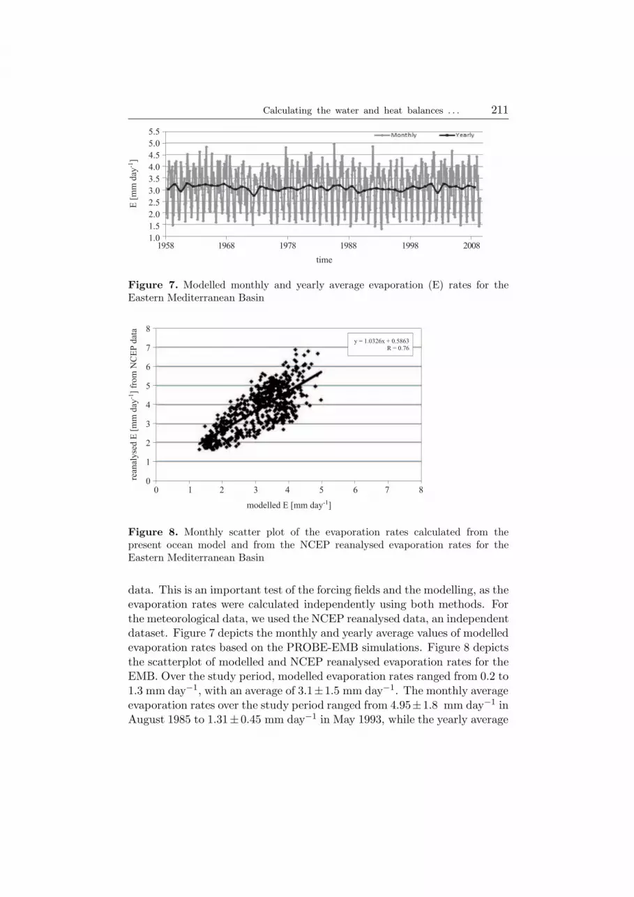
Figure 7. Modelled monthly and yearly average evaporation (E) rates for theEastern Mediterranean Basin

rean

alyse

d E

[m

m d

ay]

from

NC

EP

dat

a-1

modelled E [mm day ]-1

0 1 2 3 4 5 6 7 8

8

7

6

5

4

3

2

1

0

y = 1.0326x + 0.5863R = 0.76

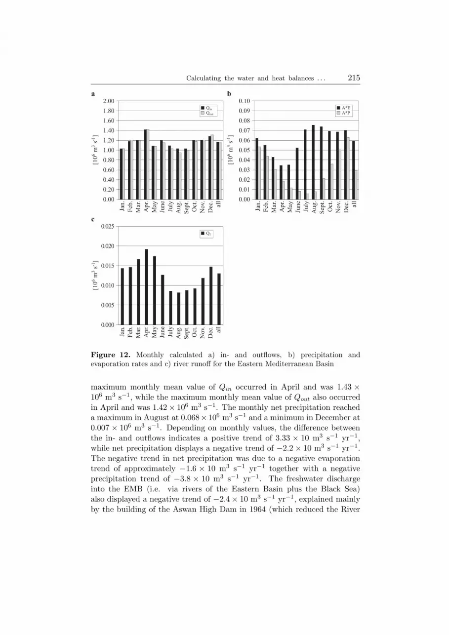
Figure 8. Monthly scatter plot of the evaporation rates calculated from thepresent ocean model and from the NCEP reanalysed evaporation rates for theEastern Mediterranean Basin

data. This is an important test of the forcing fields and the modelling, as theevaporation rates were calculated independently using both methods. Forthe meteorological data, we used the NCEP reanalysed data, an independentdataset. Figure 7 depicts the monthly and yearly average values of modelledevaporation rates based on the PROBE-EMB simulations. Figure 8 depictsthe scatterplot of modelled and NCEP reanalysed evaporation rates for theEMB. Over the study period, modelled evaporation rates ranged from 0.2 to1.3 mm day−1, with an average of 3.1±1.5 mm day−1. The monthly averageevaporation rates over the study period ranged from 4.95±1.8 mm day−1 inAugust 1985 to 1.31± 0.45 mm day−1 in May 1993, while the yearly average


evaporation rates ranged from 3.26 mm day−1 in 1961 to 2.74 mm day−1 in1972. The reanalysed and modelled monthly evaporation rates agreed fairlywell, with a correlation of 0.76 and a standard error of 0.5 mm day−1.The PROBE-EMB model results for surface temperature, salinity and

evaporation rates were also calculated as monthly means (Figure 9): themonthly average surface temperature ranged from 15.8 ± 0.32◦C in Marchto 25.98 ± 0.44◦C in August; the monthly average surface salinity rangedfrom 38.19 ± 0.09 PSU in May to 38.5 ± 0.09 PSU in September; and themonthly average evaporation rates over the study period ranged from 1.78±0.78 mm day−1 in April to 3.91± 1.08 mm day−1 in August. In the summer,surface temperature and evaporation reached their maximum values, as didsurface salinity values.

38.9

38.6

38.3

38.0

[PS

U]

b surface salinity

Jan.

Feb

.

Mar

.

Apr.

May

June

July

Aug.

Sep

t.

Oct

.

Nov.

Dec

.

all

28

26

24

22

20

18

16

14

[C

]o

a surface temperature

Jan.

Feb

.

Mar

.

Apr.

May

June

July

Aug.

Sep

t.

Oct

.

Nov.

Dec

.

all

4.5

4.0

3.5

3.0

2.5

2.0

1.5

1.0

0.5

0.0

[mm

day

]-1

c evaporation

Jan.

Feb

.

Mar

.

Apr.

May

June

July

Aug.

Sep

t.

Oct

.

Nov.

Dec

.

all

Figure 9. Monthly average a) surface temperatures, b) salinities and c) evap-oration rates

Another test of the model simulations was to investigate the water massstructure throughout the EMB. By comparing modelled and observed oceandata, an independent test of the approach could be performed. The resultsare presented in Figure 10a, in which three water masses, i.e. Atlantic water(AW) at the surface, Levantine intermediate water (LIW) at an intermediate


37 37.5 38 38.5 39 39.5 40

salinity [PSU]

30

28

26

24

22

20

18

16

14

12

tem

per

ature

[C

]o

reanalisedmodelled

37 37.5 38 38.5 39 39.5 40

salinity [PSU]

30

28

26

24

22

20

18

16

14

12

tem

per

ature

[C

]o

reanalisedmodel+15%model -15%

a b

Figure 10. Monthly calculated and reanalysed temperatures and salinities of theEastern Mediterranean Basin

Figure 11. Illustrations of modelled Eastern Mediterranean Basin a) surfacetemperatures and b) surface salinities with changes in the Sicily Channel volumeflows

depth, and deep water, can be identified in the T–S diagram. Deep watermasses are more obvious in the observations than in the modelled dataowing to the coarse model resolution.To analyse the sensitivity of the PROBE-EMB model to changes in

inflows, two sensitivity runs were performed by adding ±15% of the meanvalue of Qin (1.16 × 106 m3 s−1) to all Qin values (Figures 10 and 11).


We conclude that changes in Qin within the ±15% range bring about onlyminor changes in the vertical distribution of salinity and temperature, whichindicates that the assumption of extrapolating the 4-year period of theAVISO database over the whole period studied is acceptable.

3.3. Modelled water components for the

Eastern Mediterranean Basin

The water balance of EBM is controlled by the Sicily Channel exchange(Qin and Qout), river runoff (Qf ), and net precipitation, i.e. the differencebetween the precipitation and evaporation rates (equation (1)). Thevarious water balance components, except precipitation and river runoff, aremodelled using the PROBE-EMB model. Table 1 and Figure 12 show theestimated monthly and annual mean water balances of the EMB averagedover 52 years. Moreover, the annual mean of the difference between inflowand outflow and the net precipitation flow, i.e. As(P − E), are illustratedtogether with Qf in Figure 13.

Table 1. Modelled monthly and annual mean water balance of the EasternMediterranean Basin averaged over 52 years

Months Qf P E As(P − E) Qin Qout

[106 m3 s−1] [mm day−1] [106 m3 s−1]

January 0.012 2.80 3.24 −0.009 1.03 1.02February 0.013 2.27 2.87 −0.011 1.18 1.20March 0.015 1.60 2.23 −0.012 1.20 1.19April 0.018 0.95 1.79 −0.016 1.43 1.42May 0.016 0.59 1.85 −0.024 1.09 1.06June 0.010 0.41 2.70 −0.044 1.19 1.15July 0.007 0.30 3.70 −0.066 1.09 1.04August 0.006 0.39 3.91 −0.068 1.03 0.95September 0.007 1.06 3.84 −0.054 1.04 0.99October 0.008 1.89 3.58 −0.033 1.20 1.17November 0.010 2.60 3.57 −0.019 1.22 1.20December 0.012 3.27 3.63 −0.007 1.28 1.31annual 0.011 1.50 3.08 −0.030 1.16 1.14

The results indicate that the in- and outflows are of the order of106 m3 s−1, while the difference between them is approximately twoorders less. This difference between the in- and outflows was balancedmainly by net precipitation and river runoff, the net precipitation beingapproximately 3 times greater than the river discharge. The water balancewas thus mainly controlled by the in- and outflows through the SicilyChannel and by the net precipitation. The results also indicate that the


2.00

1.80

1.60

1.40

1.20

1.00

0.80

0.60

0.40

0.20

0.00

[10

ms

63

-1]

a

Jan.

Feb

.

Mar

.

Apr.

May

June

July

Aug.

Sep

t.

Oct

.

Nov.

Dec

.

all

QQ

in

out

0.10

0.09

0.08

0.07

0.06

0.05

0.04

0.03

0.02

0.01

0.00

[10

ms

63

-1]

b

Jan.

Feb

.

Mar

.

Apr.

May

June

July

Aug.

Sep

t.

Oct

.

Nov.

Dec

.

all

A*EA*P

0.025

0.020

0.015

0.010

0.005

0.000

[10

ms

63

-1]

c

Jan.

Feb

.

Mar

.

Apr.

May

June

July

Aug.

Sep

t.

Oct

.

Nov.

Dec

.

all

Qf

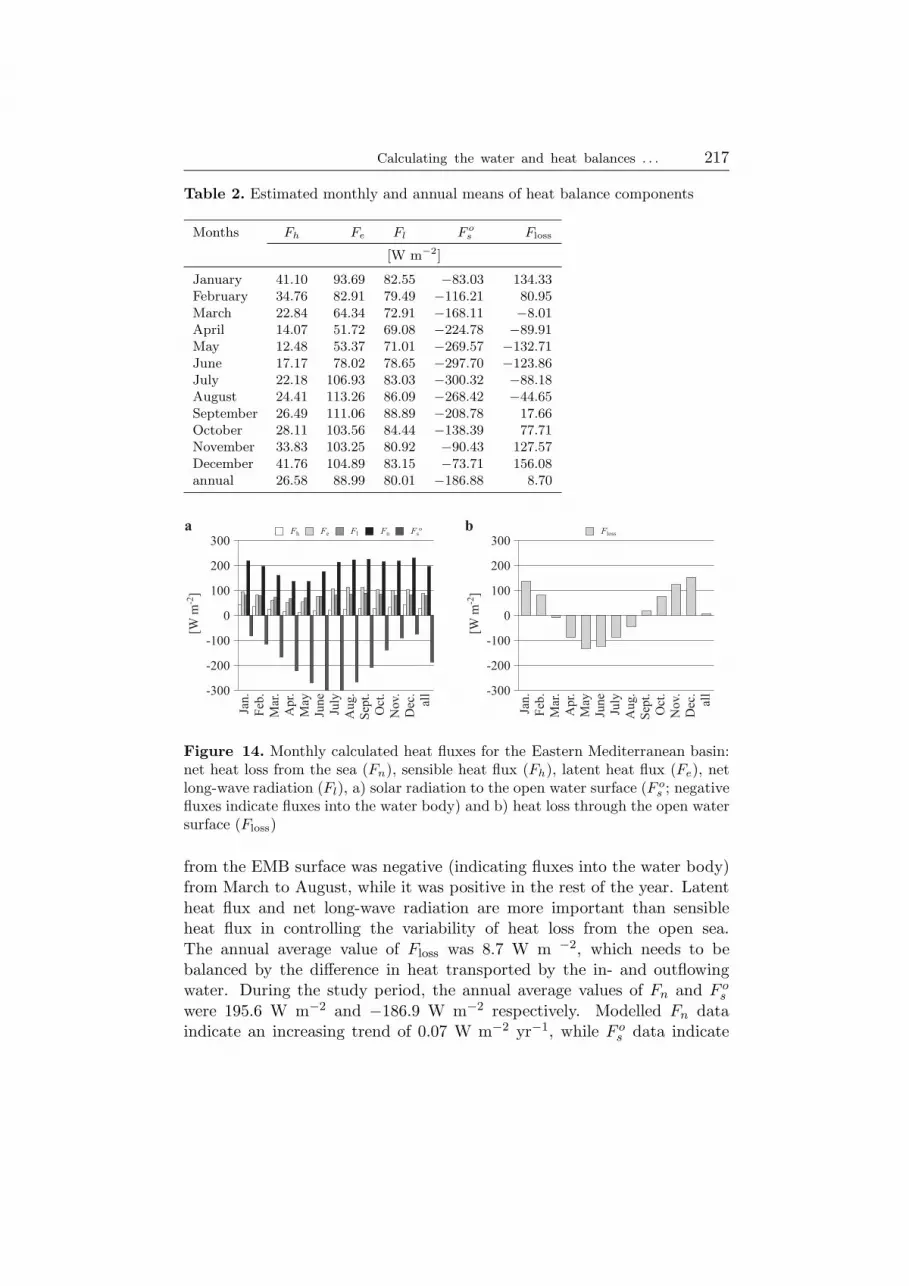
Figure 12. Monthly calculated a) in- and outflows, b) precipitation andevaporation rates and c) river runoff for the Eastern Mediterranean Basin

maximum monthly mean value of Qin occurred in April and was 1.43 ×106 m3 s−1, while the maximum monthly mean value of Qout also occurredin April and was 1.42× 106 m3 s−1. The monthly net precipitation reacheda maximum in August at 0.068×106 m3 s−1 and a minimum in December at0.007 × 106 m3 s−1. Depending on monthly values, the difference betweenthe in- and outflows indicates a positive trend of 3.33 × 10 m3 s−1 yr−1,while net precipitation displays a negative trend of −2.2 × 10 m3 s−1 yr−1.The negative trend in net precipitation was due to a negative evaporationtrend of approximately −1.6 × 10 m3 s−1 yr−1 together with a negativeprecipitation trend of −3.8 × 10 m3 s−1 yr−1. The freshwater dischargeinto the EMB (i.e. via rivers of the Eastern Basin plus the Black Sea)also displayed a negative trend of −2.4× 10 m3 s−1 yr−1, explained mainlyby the building of the Aswan High Dam in 1964 (which reduced the River


0.05

0.04

0.03

0.02

0.01

0.00

[10

ms

63

-1]

1958 1968 1978 1988 1998 2008

a

y = 9E-05x - 0.1532

Q -Qoutin

annuallinear (annual)

0.00

-0.01

-0.02

-0.03

-0.04

[10

ms

63

-1]

1958 1968 1978 1988 1998 2008

b

y = -4E-05x + 0.0445

A (P-E)s


0.014

0.012

0.010

0.008

0.006

0.004

0.002

0.000

[10

ms

63

-1]

1958 1968 1978 1988 1998 2008

c

y = -2E-05x + 0.0604

Qf


Figure 13. Annual calculated mean of the water balance components for theEastern Mediterranean Basin: a) difference between in- and outflows, b) netevaporation rates and c) river discharge

Nile’s discharge by approximately half) and decreasing net precipitationover the Black Sea Basin (the decrease in Black Sea discharge was estimatedto be approximately −9.8 × 10 m3 s−1 yr−1). The negative trends in thefreshwater components indicating increasing EMB salinity agree with thefindings of Skliris et al. (2007). The EMB monthly mean river runoffranged from 0.006 × 106 m3 s−1 in August to 0.018 × 106 m3 s−1 in April,with an annual average of 0.011 × 106 m3 s−1. Over the studied 52-yearperiod, Qin − Qout averaged 0.023 ± 0.84 × 106 m3 s−1, while As(P − E)averaged −0.03 ± 0.04 × 106 m3 s−1, the difference being balanced by theriver discharge (Table 1).

3.4. Modelled heat balance components

The monthly means of the heat budget components are presented inTable 2 and Figure 14, while the annual means of Fn, F

os and Floss are

presented in Figure 15. The heat balance simulations indicate that the heatloss from the open sea was almost balanced by the solar radiation to theopen water surface. Heat loss from the open sea ranged from 134.9 W m−2

to 229.8 W m−2, while solar radiation to the open water surface ranged from−300.3 W m−2 in July to −73.3 W m−2 in December. The total heat flux


Table 2. Estimated monthly and annual means of heat balance components

Months Fh Fe Fl F os Floss

[W m−2]

January 41.10 93.69 82.55 −83.03 134.33February 34.76 82.91 79.49 −116.21 80.95March 22.84 64.34 72.91 −168.11 −8.01April 14.07 51.72 69.08 −224.78 −89.91May 12.48 53.37 71.01 −269.57 −132.71June 17.17 78.02 78.65 −297.70 −123.86July 22.18 106.93 83.03 −300.32 −88.18August 24.41 113.26 86.09 −268.42 −44.65September 26.49 111.06 88.89 −208.78 17.66October 28.11 103.56 84.44 −138.39 77.71November 33.83 103.25 80.92 −90.43 127.57December 41.76 104.89 83.15 −73.71 156.08annual 26.58 88.99 80.01 −186.88 8.70

300

200

100

0

-100

-200

-300

[Wm

]-2

a

Jan.

Feb

.

Mar

.

Apr.

May

June

July

Aug.

Sep

t.

Oct

.

Nov.

Dec

.

all

Fh Fe Fl Fn Fso

300

200

100

0

-100

-200

-300

[Wm

]-2

bJa

n.

Feb

.

Mar

.

Apr.

May

June

July

Aug.

Sep

t.

Oct

.

Nov.

Dec

.

all

Floss

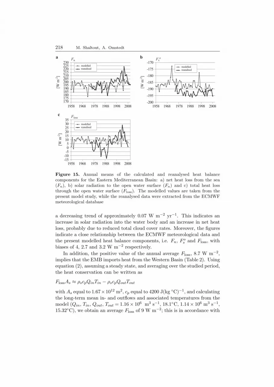
Figure 14. Monthly calculated heat fluxes for the Eastern Mediterranean basin:net heat loss from the sea (Fn), sensible heat flux (Fh), latent heat flux (Fe), netlong-wave radiation (Fl), a) solar radiation to the open water surface (F

os ; negative

fluxes indicate fluxes into the water body) and b) heat loss through the open watersurface (Floss)

from the EMB surface was negative (indicating fluxes into the water body)from March to August, while it was positive in the rest of the year. Latentheat flux and net long-wave radiation are more important than sensibleheat flux in controlling the variability of heat loss from the open sea.The annual average value of Floss was 8.7 W m

−2, which needs to bebalanced by the difference in heat transported by the in- and outflowingwater. During the study period, the annual average values of Fn and F

os

were 195.6 W m−2 and −186.9 W m−2 respectively. Modelled Fn dataindicate an increasing trend of 0.07 W m−2 yr−1, while F o

s data indicate


230225220215210205200195190185180175170

[Wm

-2]

1958 1968 1978 1988 1998 2008

aFn

35302520151050

-5-10-15

[Wm

]-2

1958 1968 1978 1988 1998 2008

cFloss

modelledreanalised

-170

-175

-180

-185

-190

-195

-200

[Wm

-2]

1958 1968 1978 1988 1998 2008

bFs

o

modelledreanalised

modelledreanalised

Figure 15. Annual means of the calculated and reanalysed heat balancecomponents for the Eastern Mediterranean Basin: a) net heat loss from the sea(Fn), b) solar radiation to the open water surface (Fn) and c) total heat lossthrough the open water surface (Floss). The modelled values are taken from thepresent model study, while the reanalysed data were extracted from the ECMWFmeteorological database

a decreasing trend of approximately 0.07 W m−2 yr−1. This indicates anincrease in solar radiation into the water body and an increase in net heatloss, probably due to reduced total cloud cover rates. Moreover, the figuresindicate a close relationship between the ECMWF meteorological data andthe present modelled heat balance components, i.e. Fn, F

os and Floss, with

biases of 4, 2.7 and 3.2 W m−2 respectively.

In addition, the positive value of the annual average Floss, 8.7 W m−2,

implies that the EMB imports heat from the Western Basin (Table 2). Usingequation (2), assuming a steady state, and averaging over the studied period,the heat conservation can be written as

FlossAs ≈ ρocpQinTin − ρocpQoutTout

with As equal to 1.67×1012 m2, cp equal to 4200 J(kg◦C)−1, and calculating

the long-term mean in- and outflows and associated temperatures from themodel (Qin, Tin, Qout, Tout = 1.16× 106 m3 s−1, 18.1◦C, 1.14× 106 m3 s−1,15.32◦C), we obtain an average Floss of 9 W m

−2; this is in accordance with


the value presented in Table 2 and indicates that the net heat loss at thesurface was compensated for by the heat transported through the SicilyChannel.

Finally, to evaluate the modelling approach, the heat and salt contentsof the whole EMB water column changes were simulated using the PROBE-EMB model and compared with observations from the MEDAR oceandatabase (Figure 16). The comparison indicates a close correlation, with thecalculated total heat content deviating approximately 1% from the MEDARvalue. For the salt content, the modelled value deviates by less than 0.3%from the MEDAR value. The PROBE-EMB can realistically reproduce thewater and heat balances of the EMB.

1958 1968 1978 1988 1998 2008

16.0

15.6

15.2

14.8

14.4

14.0

[J]

a heat content normalized by 1E22 J PROBE_EMB MEDAR

1958 1968 1978 1988 1998 2008

39.0

38.8

38.6

38.4

38.2

38.0

[PS

U m

3]

b salt content normalized by 2.31 E15 PSU m× 3 PROBE_EMB MEDAR

Figure 16. Yearly calculated heat and salt contents based on the model and onobservations of the Eastern Mediterranean Basin

4. Discussion

The connection between atmospheric conditions over the MediterraneanBasin and the large-scale atmospheric circulation in the Northern Hemi-sphere is generally strong, for example, as represented by the North AtlanticOscillation (NAO). There is a significant link (R = 0.45, n = 52) betweenwinter precipitation over the EMB and the NAO (data not shown butavailable from the National Oceanic and Atmospheric Administration –NOAA – database). Moreover, there is a link (R = 0.3, n = 52) between


winter NAO and winter evaporation. Wet (dry) winters are associatedwith positive (negative) NAO index values. On the other hand, negative

(positive) NAO index values are associated with increased (decreased)evaporation rates in the winter. Changes in the NAO index greatly affectthe winter water and heat balances of the EMB, which is in agreement with,

for example, the results of Turkes (1996a,b).

The study analyses the large-scale features of the EMB using oceanmodelling and available meteorological and hydrological datasets. Local

features (e.g., the Eastern Mediterranean Transient, EMT) are thereforenot included. It is a budget-type method building on horizontal averaging,i.e. strong local forcing might trigger convections that reach the bottom,

while the same forcing averaged over the whole basin may have a minorinfluence. In the future, we will model the EMB as a number of sub-basins

and also address local EMB features that may influence the water and heatbalances. For example, the Southern Aegean Basin is significantly affectedby deep water formation and needs to be considered when modelling deep

water formation.

The individual terms of the water and heat balances were analysedtogether with how the climate change signals affect the heat and water

cycles. Individual water and heat component values are presented infigures and tables. There were strong monthly and interannual variationsin most of the water and heat balance components. The results indicate

that atmospheric climate conditions, rather than exchange through theSicily Channel, dominated the heat and water balances of the Eastern

Mediterranean.

Using satellite dynamic height observations across the Sicily Channel,together with the assumptions of geostrophic flows and volume conservation,the exchanges through the channel were realistically modelled. The

calculated water inflow (Qin = 1.05± 0.35× 106 m3 s−1) to the EMB was ingood agreement with the results of Beranger et al. (2002) and Buongiorno

Nardelli et al. (2006), but greater than those of Ferjani & Gana (2010) byapproximately 0.6 × 106 m3 s−1, partly due to the better resolution of theSicily channel in the present study.

An important trend in the water balance components was the reduced

freshwater discharge into the EMB, which implies increasing salinity. Thiswas partly due to the decrease in the River Nile’s discharge into the EMB

after the building of Aswan High Dam and partly due to a decrease in theBlack Sea discharge as a result of a negative net precipitation trend overthat sea. The decreased Black Sea discharge into the EMB will be of major

interest in future studies, as it will influence the Aegean Sea water dynamics,especially the Eastern Mediterranean Transient phenomena.


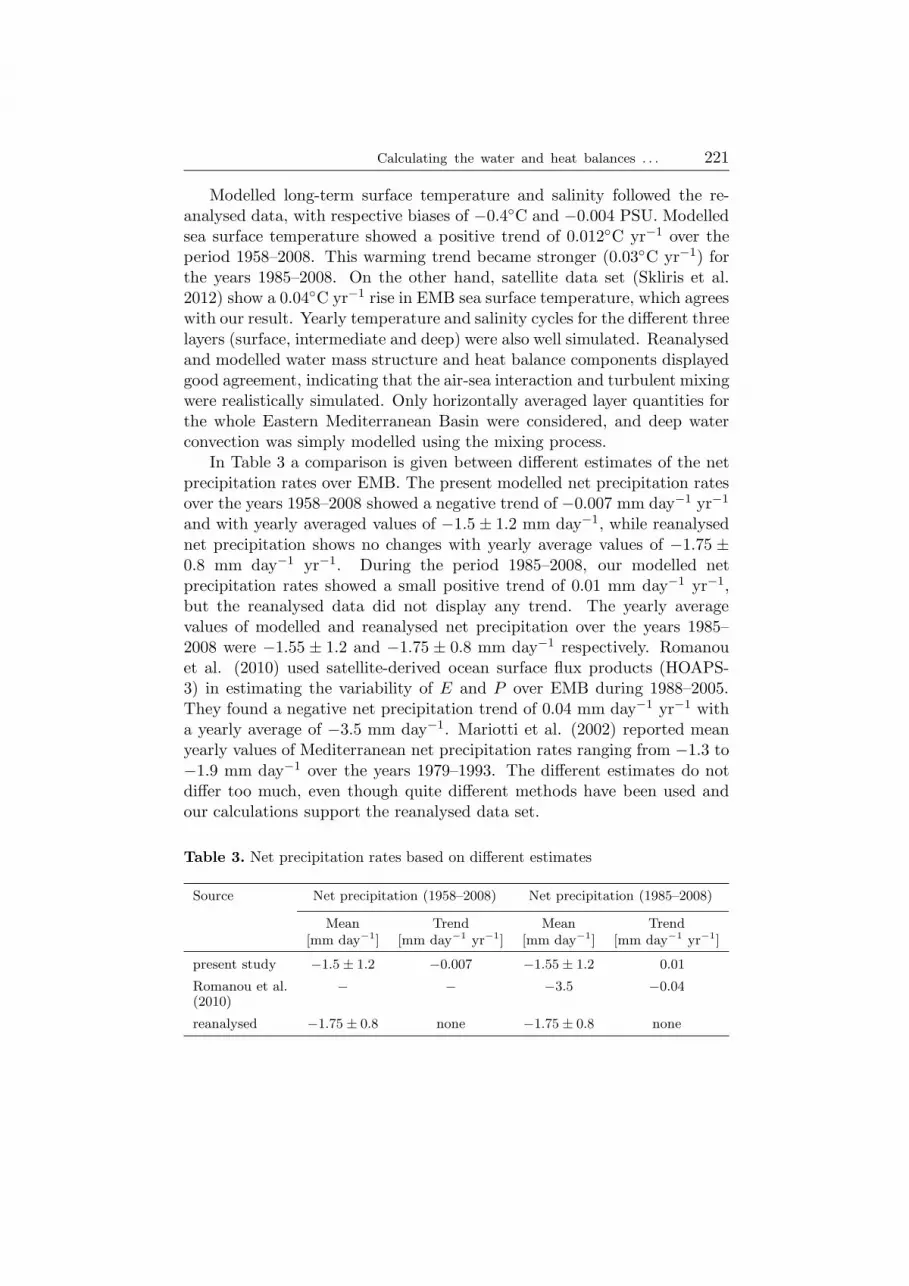
Modelled long-term surface temperature and salinity followed the re-analysed data, with respective biases of −0.4◦C and −0.004 PSU. Modelledsea surface temperature showed a positive trend of 0.012◦C yr−1 over theperiod 1958–2008. This warming trend became stronger (0.03◦C yr−1) forthe years 1985–2008. On the other hand, satellite data set (Skliris et al.2012) show a 0.04◦C yr−1 rise in EMB sea surface temperature, which agreeswith our result. Yearly temperature and salinity cycles for the different threelayers (surface, intermediate and deep) were also well simulated. Reanalysedand modelled water mass structure and heat balance components displayedgood agreement, indicating that the air-sea interaction and turbulent mixingwere realistically simulated. Only horizontally averaged layer quantities forthe whole Eastern Mediterranean Basin were considered, and deep waterconvection was simply modelled using the mixing process.In Table 3 a comparison is given between different estimates of the net

precipitation rates over EMB. The present modelled net precipitation ratesover the years 1958–2008 showed a negative trend of −0.007 mm day−1 yr−1

and with yearly averaged values of −1.5 ± 1.2 mm day−1, while reanalysednet precipitation shows no changes with yearly average values of −1.75 ±0.8 mm day−1 yr−1. During the period 1985–2008, our modelled netprecipitation rates showed a small positive trend of 0.01 mm day−1 yr−1,but the reanalysed data did not display any trend. The yearly averagevalues of modelled and reanalysed net precipitation over the years 1985–2008 were −1.55 ± 1.2 and −1.75 ± 0.8 mm day−1 respectively. Romanouet al. (2010) used satellite-derived ocean surface flux products (HOAPS-3) in estimating the variability of E and P over EMB during 1988–2005.They found a negative net precipitation trend of 0.04 mm day−1 yr−1 witha yearly average of −3.5 mm day−1. Mariotti et al. (2002) reported meanyearly values of Mediterranean net precipitation rates ranging from −1.3 to−1.9 mm day−1 over the years 1979–1993. The different estimates do notdiffer too much, even though quite different methods have been used andour calculations support the reanalysed data set.

Table 3. Net precipitation rates based on different estimates

Source Net precipitation (1958–2008) Net precipitation (1985–2008)

Mean Trend Mean Trend[mm day−1] [mm day−1 yr−1] [mm day−1] [mm day−1 yr−1]

present study −1.5 ± 1.2 −0.007 −1.55 ± 1.2 0.01

Romanou et al. − − −3.5 −0.04(2010)

reanalysed −1.75 ± 0.8 none −1.75 ± 0.8 none


The water balance in the Eastern Mediterranean basin was found tobe controlled by (in order of importance): (1) the net precipitation rates(annual average of −0.03 × 106 m3 s−1), (2) the difference between thein- and outflows through the Sicily Channel (annual average of 0.02 ×106 m3 s−1), and (3) the river runoff (annual average of 0.01× 106 m3 s−1).The heat balance was controlled by (in order of importance): (1) the heatloss from the water surface (annual average of 195 W m−2), (2) the solarradiation into the sea (annual average of −187Wm−2), and (3) the heat flowthrough the Sicily Channel, the first two displaying evidence of both climatetrends. An annual net heat loss of approximately 8.7 W m−2 was balancedby the net heat flow through the Channel. The study demonstrated thatocean modelling, together with available meteorological and river runoffdata, provides a powerful method for analysing heat and water cycles. Thewater and heat balances, together with trend analysis of a long time series,will be used as climate change tools in future studies.

Acknowledgements

This research was undertaken when Dr Mohamed Shaltout was a visitingscientist at the Ocean Climate Group, Department of Earth Sciences,University of Gothenburg, Sweden. The work is a contribution to theGEWEX/BALTEX and HyMex programmes. We would to thank LarsArneborg and the reviewers for their valuable comments. Financial supportwas gratefully received from the Swedish Institute, the University ofGothenburg, and the Swedish Research Council (contract No. 621-2007-3750).

References

Beranger K., Mortier L., Crepon M., 2002, Seasonal transport variability throughGibraltar, Sicily and Corsica Straits, The 2nd Meeting on the PhysicalOceanography of Sea Straits, 15–19 April 2002 (pp. 77–81), Villefranche,France.

Bodin S., 1979, A predictive numerical model of the atmospheric boundary layerbased on the turbulent energy equation, Norrkoping, Sweden: SMHI (Report:Meteorology and Climatology No. 13, SE-601 76).

Buongiorno Nardelli B., Cavalieri O., Rio, M.H., Santoleri R., 2006, Subsurfacegeostrophic velocities inference from altimeter data: Application to theSicily Channel (Mediterranean Sea), J. Geophys. Res., 111, C04007,doi:10.1029/2005JC003191.

Burchard H., Petersen O., 1999, Models of turbulence in the marine environment:a comparative study of two-equation turbulence models, J. Marine Syst.,

21 (1–4), 29–53.


Ferjani D., Gana S., 2010, Seasonal circulation and mass flux estimates in thewestern Sicily Strait derived from a variational inverse section model, DeepSea Res. Pt. I, 57, 1177–1191.

Hasselmann S., Hasselmann K., Bauer E., Janssen P.A. E.M., Komen G. J.,Bertotti L., Lionelli P., Guillome A., Cardone V.C., Greenwood J.A., ReistadM., Zambresky L., Ewing J.A., 1988, The WAM Model – a third generationocean wave prediction model, J. Phys. Oceanogr., 18 (12), 1775–1810.

Jerlov N.G., 1968, Optical oceanography, Oceanography Ser., Vol. 5, Elsevier,Amsterdam.

Launiainen J., 1995, Derivation of the relationship between the Obukhov stabilityparameter and the bulk Richardson number for flux profiles, Bound.-Lay.Meteorol., 76 (1–2), 165–179, doi:10.1007/BF00710895.

Ludwig W., Dumont E., Meybeck M., Heussner S., 2009, River discharges of waterand nutrients to the Mediterranean and Black Sea: Major drivers for ecosystemchanges during past and future decades?, Prog. Oceanogr., 80 (3–4), 199–217,doi:10.1016/j.pocean.2009.02.001.

Malanotte-Rizzoli P., Manca B., d’Alcala M., Theocharis A., Brenner S., BudillonG., Ozsoy E., 1999, The eastern Mediterranean in the 80s and in the 90s:The big transition in the intermediate and deep circulations, Dynam. Atmos.Oceans, 29 (2–4), 365–395, [http:/dx.doi.org/10.1016/S0377-0265(99)00011-1].

Mariotti A., Struglia M., Zeng N., Lau K., 2002, The hydrological cycle in theMediterranean region and implications for the water budget of the Mediter-ranean Sea, J. Climate, 15, 1674–1690, [http://dx.doi.org/10.1175/1520-0442(2002)015<1674:THCITM>2.0.CO;2].

Nixon S.W., 2003, Replacing the Nile: are anthropogenic nutrients providing thefertility once brought to the Mediterranean by a great river?, Ambio, 32 (1),30–39.

Omstedt A., 2011, Guide to process based modelling of lakes and coastal seas,Springer-Praxis books in Geophysical Sciences, Springer-Verlag, Berlin,Heidelberg, doi:10.1007/978-3-642-17728-6.

Omstedt A., Axell L. B., 2003, Modeling the variations of salinity and temperaturein the large gulfs of the Baltic Sea, Cont. Shelf. Res., 23 (3–4), 265–294,doi:10.1016/S0278-4343(02)00207-8.

Omstedt A., Nohr C., 2004, Calculating the water and heat balances of the BalticSea using ocean modelling and available meteorological, hydrological and oceandata, Tellus, 56A, 400–414, doi:10.1111/j.1600-0870.2004.00070.x.

Rixen J., Beckers M., Levitus S., Antonov J., Boyer T., Maillard C., FichautM., Balopoulos E., Iona S., Dooley H., Garca M. J., Manca B., Giorgetti A.,Manzella G., Mikhailov N., Pinardi N., Zavatarelli M., 2005, The WesternMediterranean deep water: A proxy for climate change, Geophys. Res. Lett.,32, L12608, doi:10.1029/2005GL022702.

Roether W., Schlitzer R., 1991, Eastern Mediterranean deep water renewal on thebasis of chlorofluoromethane and tritium data, Dynam. Atmos. Oceans, 15,333–354, [http://dx.doi.org/10.1016/0377-0265(91)90025-B].


Romanou A., Tselioudis G., Zerefos C., Clayson C., Curry J., Andersson A., 2010,Evaporation-precipitation variability over the Mediterranean and the BlackSeas from satellite and reanalysis estimates, J. Climate, 23 (19), 5268–5287,[http://dx.doi.org/10.1175/2010JCLI3525.1].

Skliris N., Sofianos S., Gkanasos A., Mantziafou A., Vervatis V., Axaopoulos P.,Lascaratos A., 2012, Decadal scale variability of sea surface temperature inthe Mediterranean Sea in relation to atmospheric variability, Ocean Dynam.,62 (1), 13–30, doi:10.1007/s10236-011-0493-5.

Skliris N., Sofianos S., Lascaratos A., 2007, Hydrological changes in theMediterranean Sea in relation to changes in the freshwater budget:A numerical modelling study, J. Marine Syst., 65 (1–4), 400–416.

Sorgente R., Drago A. F., Ribotti A., 2003, Seasonal variability in the CentralMediterranean Sea circulation, Ann. Geophys., 21, 299–322.

Stanev E.V., Le Traon P.Y., Peneva E.L., 2000, Sea level variations and theirdependency on meteorological and hydrological forcing: Analysis of altimeterand surface data for the Black Sea, J. Geoph. Res., 105, C7, 17203–17216.

Stanev E., Peneva E.L., 2002, Regional sea level response to global climaticchange: Black Sea examples, Global Planet. Change, 32 (1), 33–47,[http://dx.doi.org/10.1016/S0921-8181(01)00148-5].

Stansfield K., Smeed D.A., Gasparini G. P., 2002, The path of the overflows fromthe sills in the Sicily Strait, The 2nd Meeting on the Physical Oceanographyof Sea Straits, 15–19 April 2002 (pp. 211–215), Villefranche, France.

Turkes M., 1996a, Meteorological drought in Turkey: A historical perspective,1930–1993, Drought Network News, 8, 17–21, [http://digitalcommons.unl.

edu/droughtnetnews/84].

Turkes M., 1996b, Spatial and temporal analysis of annual rainfall variations inTurkey, Int. J. Climatol., 16, 1057–1076.

Zervakis V., Georgopoulos D., Drakopoulos P., 2000, The role of the North Aegeanin triggering the recent Eastern Mediterranean climatic changes, J. Geophys.Res., 105, C11, 26103–26116, doi:10.1029/2000JC900131.


Appendix A1. Model description

The Eastern Mediterranean Basin (EMB) is influenced by variousphysical processes (see the Introduction). A useful initial approach is tomodel the EMB as one basin and separately examine the effects of localfactors and of interactions with surrounding basins (i.e. the Tyrrhenianand Black Sea basins). The modelling starts by using the PROBE equationsolver, a well-documented and freely available program for studies of lakesand coastal seas (Omstedt 2001). This equation solver is based on thefinite volume method and can easily solve a large number of equations fornetworks of sub-basins. In the present version, PROBE-EMB version 1.0,the EMB is treated as one basin coupled to surrounding basins by in- andoutflows; the program is freely available from the present authors.

Mathematical formulation

The transport equations for momentum read:

∂ρU

∂t+W

∂ρU

∂z=

∂

∂z

[

µeff

ρ

∂ρU

∂z

]

+ fρV, (1)

∂ρV

∂t+W

∂ρV

∂z=

∂

∂z

[

µeff

ρ

∂ρV

∂z

]

− fρU, (2)

W =(Qin −Qout)

Area, (3)

where U and V are the current components in the easterly and northerly di-rections respectively, W the vertical velocity calculated from the differencesbetween in- and outflows (U , V andW are horizontally averaged velocities),f the Coriolis parameter, ρ the sea water density, µeff the effective dynamicviscosity, Qin, Qout and A the inflows, outflows and areas at different levelsrespectively, z the vertical coordinate (positive upward) and t time.

Equations (1)–(3) apply a transient Ekman flow model with verticalvelocity due to in- and outflows and including density effects. As the in-and outflows may act at different levels, they generate vertical motions inthe model.

The water-air boundary conditions are:

τax =µeff

ρ

∂ρU

∂z, (4a)

τay =µeff

ρ

∂ρV

∂z, (4b)


where τax and τay denote the eastward and northward wind stress compo-nents respectively, calculated using a standard bulk formulation:

τax = ρaCDUaWa, (5a)

τay = ρaCDVaWa, (5b)

where ρa (1.3 kg m−3) is the air density, CD the air drag coefficient, Ua

and Va the wind components in the x and y directions respectively, andWa the wind speed =

√

U2a + V 2

a . The air drag coefficient for the naturalatmosphere (CDN ) is calculated according to Hasselmann et al. (1988) by

CDN = [0.8 + 0.065max(Wa, 7.5)] × 10−3. (5c)

The roughness lengths for momentum (Zo), heat (ZH) and humidity (ZE)are assumed to be dependent on the neutral values as

Zo =zref

exp

(

κ√CDN

) , (5d)

ZH =zref

exp

(

κ√CDN

CHN

) , (5e)

Zo =zref

exp

(

κ√CDN

CEN

) , (5f)

where Zref is the reference height (= 10 m), κ(= 0.4) is von Karman’sconstant, CHN (= 1.14× 10−3) is the neutral bulk coefficient for the sensibleheat flux and CEN (= 1.12 × 10−3) is the neutral bulk coefficient for thelatent heat flux. According to Launiainen (1995), the stability dependenceof the bulk coefficients is:

CD =κ2

[

ln

(

Zref

Zo

)

− ψm

]2, (5g)

CH =κ2

[

ln

(

Zref

Zo

)

− ψm

][

ln

(

Zref

ZH

)

− ψh

]

, (5h)

CH =κ2

[

ln

(

Zref

Zo

)

− ψm

][

ln

(

Zref

ZE

)

− ψh

]

, (5i)


where ψm, (ψh) are the integrated forms of the non-dimensional gradientsof momentum (heat). They are calculated as follows:

For stable and neutral conditions the Richardson number (Rb) is usedto define a stable (Rb > 0) and an unstable condition (Rb < 0):

Rb =gZref (Ta − Ts)

(Ts + 273.15)W 2a

. (5j)

The non-dimensional fraction (ς) is calculated by knowing the airtemperature at 2 m height (Ta) and the sea surface temperature (Ts):

ς =

[

Rb

(

1.18 ln(Zref

Zo

)

− 1.5 ln( Zo

ZH

)

− 1.37)

]

+

+

[

R2b

(

1.891 ln(Zref

Zo

)

+4.22)

]

, (5k)

where L is the Monin-Obukov length. During a strongly stablesituation, ς is less than or equal to 0.5, and

ψm ≈ ψh = −(cψ2cψ3

cψ4

)

− (ςcψ1) −((

cψ2

(

ς −cψ3

cψ4

))

exp(−ςcψ4))

,

(5l)

where cψ1, cψ2, cψ3 and cψ4 are 0.7, 0.75, 5 and 0.35 respectively.

For unstable conditions ς is calculated as

ς = Rb

[

ln2(Zref/Zo)

ln(Zref/ZH)− 0.55

]

. (5m)

For strongly unstable conditions, ς is larger than −5; the integratedforms of the gradients are then given by

ψm = 2 ln

(

1 + (1 − 16ς)0.25

2

)

+

+ ln

(

1 + (1 − 16ς)0.5

2

)

− 2 arctan((1 − 16ς)0.25) +π

4, (5n)

ψh = 2 ln

(

1 + (1 − 16ς)0.5

2

)

. (5o)

The conservation equation for heat reads:

∂ρcpT

∂t+W

∂ρcpT

∂z=

∂

∂z

[

µeff

ρσeffT

∂(ρcpT )

∂z

]

+ Γsum + Γh, (6)

where T and cp are the temperature of sea water and the heat capacity(4200 J Kg−1 K−1), respectively, σeffT the turbulent Prandtl number (set


equal to one in the present version of the model), and Γsum and Γh therespective source terms associated with solar radiation in- and outflows.The source terms Γsum and Γh are given by

Γsum = Fws (1 − η1)e

−β(D−z), (7a)

Γh = ρcp

(

QinTin

∆Vin−QoutTout

∆Vout

)

, (7b)

where Fws is the short-wave radiation through the water surface, η1(= 0.4)

the infrared fraction of short-wave radiation trapped in the surface layer, βthe bulk absorption coefficient of the water (0.3 m−1), D the total depth,Tin and Tout the respective temperatures of the in- and outflowing water,and ∆Vin and ∆Vout the respective volumes of the grid cells at the in- andoutflow levels.The boundary condition at the surface for heat reads:

Fnet =µeff

ρσeffT

∂(ρCpT )

∂z, (8a)

Fnet = Fh + Fe + Fl + δFWs , (8b)

where Fh is the sensible heat flux, Fe the latent heat flux, Fl the net long-wave radiation and δFW

s the short-wave radiation part absorbed in thesurface layer.The conservation equation for salinity reads:

∂S

∂t+W

∂S

∂z=

∂

∂z

[

µeff

ρσeffS

∂S

∂z

]

+ ΓS , (9a)

ΓS =QinSin

∆Vin−QoutSout

∆Vout−QfSsur

∆Vsur, (9b)

where ΓS is the source term associated with in- and outflows, σeffS theturbulent Schmidt number (equal to one), Qf the river discharge to thebasin, Sin and Sout the salinity of the in- and outflowing water respectively,Ssurf the sea surface salinity, and ∆Vsur the volume of the upper surfacegrid cell.The boundary conditions at the surface for salinity (S) read:

µeff

ρσeffS

∂S

∂z= Fsalt, (10a)

Fsalt = Ss(P − E), (10b)

where Fsalt is the salt flux associated with net precipitation, Ss thesurface salinity and P the precipitation rate (calculated from given values).Evaporation (E) is calculated by the model as


E =Fe

Leρo, (10c)

where Fe is the latent heat flux, Le the latent heat of evaporation, and ρo

the reference density of sea water (i.e. 103 kg m−3). It should be noted thatequation (10a) connects the water and heat balances.

The turbulence model

The vertical turbulent transports in the surface boundary layer arecalculated using the well-known k-ε model (e.g. Burchard & Petersen 1999),a two-equation model of turbulence in which transport equations for theturbulent kinetic energy k and its dissipation rate ε are calculated. Thetransport equations for k and ε read:

∂k

∂t+W

∂k

∂z=

∂

∂z

[

µeff

ρσk

∂k

∂z

]

+ Ps + Pb − ε, (11)

∂ε

∂t+W

∂ε

∂z=

∂

∂z

[

µeff

ρσε

∂ε

∂z

]

+ε

k[cε1Ps + cε3Pb − cε2ε], (12)

where Ps and Pb are the production/destruction due to shear and stratifi-cation respectively, σk (=1) the Schmidt number for k, and σε (=1.11) theSchmidt number for ε. The various terms are modelled as

Ps =µeff

ρ

[

(∂U

∂z

)2

+(∂V

∂z

)2]

, (13a)

Pb =µT

σT

g

ρ

∂ρ

∂z, (13b)

µeff

σeff=µ

σ+µT

σT, (13c)

µeff = Cµρk2

ε+ ρσT v

dT , (13d)

vdT = min(αN−1, vo), (13e)

where α, Cµ, C1ε, C2ε, and C3ε are empirical constants, N the buoyancyfrequency, vd

t the turbulent deep water eddy viscosity, vo a constant valueto avoid singularity in the buoyancy frequency, and Cε3 is −0.4 for stablestratification and equal to 1 for unstable stratification.The boundary conditions for k and ε read:

k =

[

u3∗

C3/4µ

+max(B, 0)κd1

C3/4µ

]2/3

, (14a)


ε =u3∗

κd1, (14b)

u2∗

=τsρo, (14c)

B =g

ρo

[

∂ρ

∂T

Fn

ρocp+∂ρ

∂SFsalt

]

, (14d)

where d1 is the distance from the boundary to the centre of the near-boundary grid cell, κ von Karman’s constant, u∗ the friction velocity, τs thewind surface stress and B the buoyancy flux due to net heat (Fn) and salt(Fsalt) fluxes. In the absence of momentum and buoyancy fluxes, minimumvalues of k and ε are applied. The constants are discussed in greater detailin Omstedt & Axell (2003).

Initial conditions

The initial temperature and salinity conditions for the EMB were takenfrom January 1958. The temperature and salinity were 16.6◦C and 38.5 PSUrespectively, from the surface to a depth of 150 m. Then temperature andsalinity changed linearly to 14.1◦C and 38.7 PSU respectively, at a depthof 600 m. From a depth of 600 m to the bottom, temperature and salinitywere set to 14.1◦C and 38.7 PSU respectively. The initial conditions for theturbulent model assumed only constant and small values for the turbulentkinetic energy and its dissipation rate.


Appendix A2. Heat flux components

The sensible heat flux Fh is given by

Fh = CHρacpaWa(Ts − Ta), (15)

where CH is the heat transfer coefficient and cpa the heat capacity of air.The latent heat flux Fe is calculated as

Fe = CEρaLeWa(qs − qa), (16)

where qs is the specific humidity of air at the sea surface, assumed to beequal to the saturation value at temperature Ts, calculated as

qs =0.622Rs

Paexp

(

cq1Ts

Ts + 273.15 − cq2

)

, (17)

where Rs = 611, cq1 = 17.27, cq2 = 35.86, and Pa is the air pressure atthe reference level. The specific humidity of air at the reference level qa isaccordingly calculated as

qa =0.622RsRh

Paexp

(

cq1Ta

Ta + 273.15 − cq2

)

, (18)

where Rh is the relative humidity (0 ≤ Rh ≤ 1).

The heat flux due to net long-wave radiation Fl is given by the differencebetween the upward and downward propagation of long-wave radiation(Bodin 1979), according to:

Fl = εsσs(Ts +273.15)4 −σs(Ta +273.15)4(a1 +a2e1/2a )(1+a3N

2),(19)

where εs is the emissivity of the sea surface, σs the Stefan-Boltzmanncoefficient, and a1, a2 and a3 = 0.68, 0.0036 and 0.18 are constants.Furthermore, Nc is the cloud coverage and ea is the water vapour pressurein the atmosphere, related to qa as follows:

ea =Pa

0.622qa. (20)

The solar radiation to the water surface Fs is also calculated accordingto Bodin (1979):

Fs = εtS0 cos Θa(ft − fa)(1 − fcNc), (21)

where εt is the atmospheric turbidity, S0 the solar constant, Θa the zenithangle, ft and fa the transmission and absorption functions respectively, andfc a cloud function.

The short-wave radiation flux penetrating the open-water surface isgiven by

Fws = Fs(1 − αw), (22)


where αw is the surface-water albedo calculated from the Fresnel formulas(Jerlov 1968):

αw =1

2

[

tan2(Θa − Θw)

tan2(Θa + Θw)+

sin2(Θa − Θw)

sin2(Θa + Θw)

]

, (23)

where Θa and Θw are the angles between the z-axis and the rays in theatmosphere and water respectively. Further details concerning the heatfluxes and constants are given in Omstedt & Axell (2003).

Calculating the water and heat balances of the Eastern Mediterranean Basin using ocean modelling and available eteorological, hydrological and ocean data

Documents