University of Canterbury Masters Thesis Calcium Dynamics and Wave Propagation in Coupled Cells Author: Allanah Kenny Supervisors: Prof. Tim David Dr. Michael J. Plank A thesis submitted in fulfillment of the requirements for the degree of Masters in Mathematics February 29, 2016

Welcome message from author
This document is posted to help you gain knowledge. Please leave a comment to let me know what you think about it! Share it to your friends and learn new things together.
Transcript
University of Canterbury
Masters Thesis
Calcium Dynamics and Wave
Propagation in Coupled Cells
Author:
Allanah Kenny
Supervisors:
Prof. Tim David
Dr. Michael J. Plank
A thesis submitted in fulfillment of the requirements
for the degree of Masters in Mathematics
February 29, 2016
Contents
Acknowledgements i
Abstract ii
Abbreviations iii
1 Introduction 1
1.1 Thesis Overview . . . . . . . . . . . . . . . . . . . . . . . . . . . . . . . . 3
2 Literature Review 4
2.1 Cell Anatomy . . . . . . . . . . . . . . . . . . . . . . . . . . . . . . . . . 4
2.2 Calcium Dynamics . . . . . . . . . . . . . . . . . . . . . . . . . . . . . . 5
2.3 Neurovascular Coupling . . . . . . . . . . . . . . . . . . . . . . . . . . . 10
2.4 Wave Propagation in Spatial Media . . . . . . . . . . . . . . . . . . . . . 13
2.5 Geometry . . . . . . . . . . . . . . . . . . . . . . . . . . . . . . . . . . . 16
3 Goldbeter Model 23
3.1 Method . . . . . . . . . . . . . . . . . . . . . . . . . . . . . . . . . . . . 23
3.2 Single Cell Results . . . . . . . . . . . . . . . . . . . . . . . . . . . . . . 25
3.3 Coupled Cell Results . . . . . . . . . . . . . . . . . . . . . . . . . . . . . 28
3.4 Other Models . . . . . . . . . . . . . . . . . . . . . . . . . . . . . . . . . 38
3.5 Summary . . . . . . . . . . . . . . . . . . . . . . . . . . . . . . . . . . . 41
4 NVU Based SMC/EC Model 43
4.1 Method . . . . . . . . . . . . . . . . . . . . . . . . . . . . . . . . . . . . 43
4.2 Single SMC/EC Results . . . . . . . . . . . . . . . . . . . . . . . . . . . 45
4.3 Coupled SMC/EC Results . . . . . . . . . . . . . . . . . . . . . . . . . . 53
4.4 Summary . . . . . . . . . . . . . . . . . . . . . . . . . . . . . . . . . . . 60
5 Wave Propagation in Spatial Media 62
5.1 Method . . . . . . . . . . . . . . . . . . . . . . . . . . . . . . . . . . . . 62
5.2 FitzHugh-Nagumo model . . . . . . . . . . . . . . . . . . . . . . . . . . . 65
5.3 Goldbeter model . . . . . . . . . . . . . . . . . . . . . . . . . . . . . . . 66
CONTENTS
5.4 Summary . . . . . . . . . . . . . . . . . . . . . . . . . . . . . . . . . . . 71
6 Geometry 73
6.1 Method . . . . . . . . . . . . . . . . . . . . . . . . . . . . . . . . . . . . 73
6.2 Effect on Diffusion . . . . . . . . . . . . . . . . . . . . . . . . . . . . . . 75
6.3 FitzHugh-Nagumo model . . . . . . . . . . . . . . . . . . . . . . . . . . . 76
6.4 Goldbeter model . . . . . . . . . . . . . . . . . . . . . . . . . . . . . . . 77
6.5 Summary . . . . . . . . . . . . . . . . . . . . . . . . . . . . . . . . . . . 80
7 Conclusions 84
7.1 Discussion . . . . . . . . . . . . . . . . . . . . . . . . . . . . . . . . . . . 84
7.2 Research Summary . . . . . . . . . . . . . . . . . . . . . . . . . . . . . . 89
Bibliography 90
Acknowledgements
First of all thank you to the University of Canterbury and UC HPC for providing me with
the funds to go through with all this! Thank you to my supervisors Tim David and Mike
Plank – this wouldn’t have been possible without you both. Thank you to my wonderful
research group at UC HPC: Kathi, Elshin, Jai, Christine, Tim, Michelle, Stewart, Kon.
Thank you to all the interns who have come and gone: Philip, Eva, Moritz, Joerik,
Dominic, Jan. Thank you to the UC HPC team who put up with us students everyday:
Angela, Dan, Francois, Robert, Sung, Vlad, Tony. Thank you to anyone else who I may
have forgotten. And finally thank you to my family, friends and partner Valentin, for
your continued support of my neverending study.
Thank you!
i
Abstract
Intercellular waves of calcium (Ca2+) are an important signalling mechanism in a wide
variety of cells within the body, crucial for cellular coordination and control. In particular
the Ca2+ concentration within smooth muscle cells (SMCs) lining the blood vessel walls
controls the cell dilation and contraction and thus the vessel radius. The process of func-
tional hyperaemia by which neuronal activity results in a localised response of increased
blood flow via the dilation of SMCs is associated with multiple pathologies such as cor-
tical spreading depression (CSD). This process can be modelled by a ‘neurovascular unit
(NVU)’ containing a neuron, astrocyte, and the SMC and endothelial cell (EC) within
the vessel wall.
Our research consists of modelling the Ca2+ dynamics of a both a single SMC and
two coupled SMCs (via an intercellular Ca2+ flux) mainly with the minimal nonspatial
Goldbeter et al. (1990) cell model. This is compared with the more complex model of a
SMC/EC ‘unit’ which also includes the influence of neuronal stimulation on the SMC. The
Ca2+ dynamics of both models are found to be similar in structure: the system will be
either excitable, nonexcitable or oscillatory depending on a model dependent parameter
controlling the rate of inotisol trisphosphate (IP3) induced Ca2+ release into the cell.
However the SMC/EC model also produces small amplitude oscillations and bistability
when neuronal stimulation is high and the model parameter is low. The behaviour of a
coupled cell system is seemingly model independent: in particular an excitable coupled
with an oscillatory or two nonidentical coupled oscillatory cells will exhibit qualitatively
different behaviour when weakly coupled such as variable amplitude oscillations.
The formation and propagation of Ca2+ waves are simulated by the Goldbeter et al.
(1990) model in a two dimensional (2D) spatial medium; spatial curvature is then intro-
duced by simulating the model on a torus. When the local dynamics of the medium are
spatially constant a new wave solution in the form of a stable wave segment when there
is some gradient in Gaussian curvature. When the local dynamics of the medium are
spatially varied, spiral waves or apparent spatiotemporal chaos are produced when the
rate of diffusion is low and either the surface is strongly curved or the initial conditions
(ICs) of the medium are sufficiently inhomogeneous. Based on the similarities in the
nonspatial results the spatial Goldbeter et al. (1990) model could provide insight into the
behaviour of the corresponding complex spatial SMC/EC model.
ii
Abbreviations
Ca2+ calcium
IP3 inotisol trisphosphate
K+ potassium
Na+ sodium
2D two dimensional
AC astrocyte
ATP adenosine triphosphate
BC boundary condition
BK big potassium
BT Bogdanov-Takens
CBF cerebral blood flow
CICR Ca2+ induced Ca2+ release
CP Cusp
CSD cortical spreading depression
EC endothelial cell
ER endoplasmic reticulum
FHN FitzHugh-Nagumo
FP fixed point
GHK Goldman Hodgkin Katz
IC initial condition
iii
Abbreviations
KIR inward rectifying potassium
LC limit cycle
LP limit point
LPC limit point cycle
MPI Message Passing Interface
NE neuron
NVC neurovascular coupling
NVU neurovascular unit
ODE ordinary differential equation
PD Period Doubling
PDE partial differential equation
PLC phospholipase-C
PVS perivascular space
RHS right hand side
SC synaptic cleft
SMC smooth muscle cell
SR sarcoplasmic reticulum
VOCC voltage operated Ca2+ channel
VTK Visualisation Toolkit
iv
Chapter 1
Introduction
Intracellular and intercellular calcium (Ca2+) is an important signalling messenger in a
wide variety of cells. Many cells in the body are known to exhibit periodic increases
in Ca2+ concentration level (Wilkins and Sneyd, 1998), otherwise known as Ca2+ os-
cillations. In addition, these cells are also known to exhibit singular ‘spikes’ in Ca2+
in response to external stimulation; this is known as excitable behaviour (Wilkins and
Sneyd, 1998). A population of cells, in particular smooth muscle cells (SMCs) lining
the arterial wall, are known to support an oscillating wave of Ca2+ propagating through
the cell population referred to as a ‘travelling wave’ (Sneyd and Atri, 1993). When a
population of cells are known to exhibit excitable behaviour or Ca2+ oscillations they are
able to support such a travelling wave.
Propagating Ca2+ waves through the arterial wall via SMCs are an important sig-
nalling mechanism (Meyer and Stryer, 1988) and evidence exists that intracellular and
intercellular Ca2+ signalling is one of the crucial methods of cellular coordination and
control (Wilkins and Sneyd, 1998). For example it is known that synchronised oscilla-
tions of Ca2+ in a population of SMCs will induce vasomotion, the rhymthic dilation and
contraction of the blood vessel wall via the relaxation and contraction of the SMCs. The
contraction of a SMC is caused by an increase in Ca2+ concentration via the process of
Ca2+ initiated formation of crossbridges between the myosin and actin filaments of the
cell (Hai and Murphy, 1988).
The cerebral cortex, a highly complex component of the human brain composed of
folded grey matter, is composed mainly of neurons, glial cells such as astrocytes, and a
vast network of blood vessels that provide oxygen and glucose throughout the brain tissue.
These blood vessels are composed of a thin layer of endothelial cells (ECs) on the interior
surface and an outer layer of SMCs controlling the vessel radius. The process of functional
hyperaemia or ‘neurovascular coupling (NVC)’ is the self regulation of blood flow in the
brain; specfically, the relationship between neural activity and the local increase in blood
flow to that area caused by dilation in the blood vessels via the SMCs (which is in
1

turn due to a decrease in Ca2+ concentration within the cell). This coupling is achieved
through the intercellular communication through ions such as Ca2+ and potassium (K+)
and signalling molecules such as glutamate and inotisol trisphosphate (IP3) between a
group of cells known as a neurovascular unit (NVU): the neuron, astrocyte, SMC and
EC.
Propagating Ca2+ waves through a population of SMCs may play a role in patholo-
gies associated with impaired functional hyperaemia such as cortical spreading depression
(CSD), migraine, and stroke (Girouard and Iadecola, 2006), as the SMCs effectively con-
trol the local supply of oxygen and glucose necessary for cellular function.
The dynamics of Ca2+ concentration in a single and two coupled SMC system are
investigated in order to further our understanding of the influence that one cell has on
another adjacent cell, and consequently the effect their interaction has on the individual
cell dynamics. These cells are modelled by a selection of three simple minimal Ca2+
cell models based on different fundemental cell mechanisms by Goldbeter et al. (1990),
Meyer and Stryer (1988) and Gonzalez-Fernandez and Ermentrout (1994). These models
are then compared to a more complex, physiologically realistic and up to date model of
both the SMC and adjacent EC based on a model of the so-called ‘NVU’ describing the
process of functional hyperaemia in the brain tissue (Farr and David, 2011; Dormanns
et al., 2015). If the dynamics of this complex SMC/EC model are similar to those of
a simpler SMC model then this may provide insight into the behaviour of the complex
model, of which analysis is more difficult.
The resulting cell dynamics of a single and coupled cell system may in turn further our
understanding of the dynamics behind the formation and propagation of Ca2+ waves; the
spatial and temporal dynamics of a large population of cells in a two dimensional (2D)
spatial domain are investigated in silico in order to gain insight into the Ca2+ signalling
through the arterial wall and throughout the brain cortex. This population of cells is
simulated using the Goldbeter et al. (1990) model on a 2D spatial domain. The term
in silico refers to computer simulations of the dynamics of complex biological systems
as opposed to in vivo or in vitro. These simulations can provide insight into observed
experimental data.
The concept of spatial curvature is introduced to these simulations as the cerebral
cortex composed of folded grey matter is a strongly curved structure and an artery
contains areas of strong curvature, in particular at an arterial bifurcation. This is achieved
by simulating the Goldbeter et al. (1990) model on a toroidal surface as a torus contains
areas of both negative (on the inside of the torus) and positive Gaussian curvature (on
the outside of the torus).
2
1.1. THESIS OVERVIEW
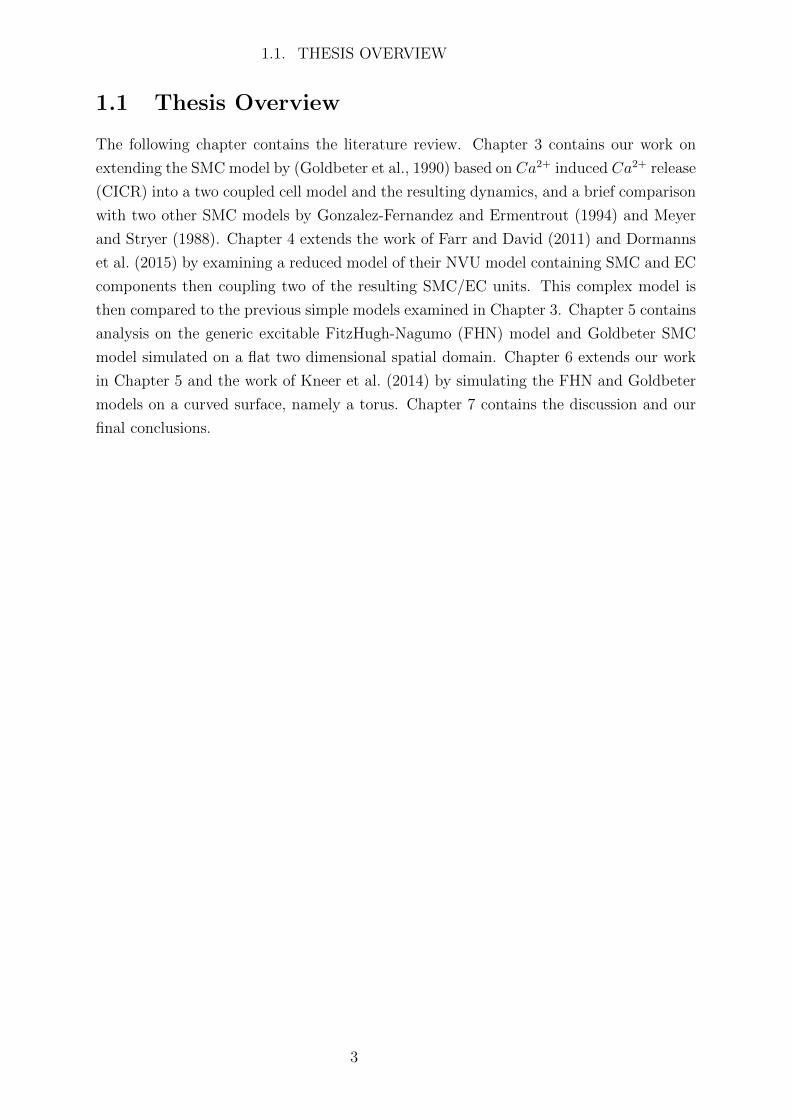
1.1 Thesis Overview
The following chapter contains the literature review. Chapter 3 contains our work on
extending the SMC model by (Goldbeter et al., 1990) based on Ca2+ induced Ca2+ release
(CICR) into a two coupled cell model and the resulting dynamics, and a brief comparison
with two other SMC models by Gonzalez-Fernandez and Ermentrout (1994) and Meyer
and Stryer (1988). Chapter 4 extends the work of Farr and David (2011) and Dormanns
et al. (2015) by examining a reduced model of their NVU model containing SMC and EC
components then coupling two of the resulting SMC/EC units. This complex model is
then compared to the previous simple models examined in Chapter 3. Chapter 5 contains
analysis on the generic excitable FitzHugh-Nagumo (FHN) model and Goldbeter SMC
model simulated on a flat two dimensional spatial domain. Chapter 6 extends our work
in Chapter 5 and the work of Kneer et al. (2014) by simulating the FHN and Goldbeter
models on a curved surface, namely a torus. Chapter 7 contains the discussion and our
final conclusions.
3

Chapter 2
Literature Review
2.1 Cell Anatomy
Smooth muscle cells (SMCs) are found in the outer walls of various organs and tubes in
the body, in particular arteries and veins. Arteries are composed of layers of SMCs and
within them endothelial cells (ECs) adjacent to the lumen where the blood flows, as seen
in Figure 2.1.
These SMCs are able to contract or relax generating rhythmic dilations and contrac-
tions. This behaviour known as vasomotion occurs both in vitro and in vivo independently
of any rhythmic movements in the body such as the heartbeat or the respiratory cycle
(Haddock and Hill, 2005). Vasodilation widens the arteries and so increases blood flow
to tissue areas in need, while vasoconstriction narrows the arteries and thus is critical
to staunching haemorrhage and blood loss. These two mechanisms combined produce
vasomotion and are used by the body to regulate blood flow and in some cases maintain
mean arterial pressure.
Figure 2.1: A section of artery wall containing SMCs and ECs (Hahn and Schwartz, 2009).
4
2.2. CALCIUM DYNAMICS
A general eukaryotic cell consists of components including the membrane, the cytosol,
the nucleus, and the sarcoplasmic reticulum (SR) or endoplasmic reticulum (ER) which
contain large stores of calcium (Ca2+) inside the cell. Ions (and hence electrical current)
are able to pass between adjacent cells through channels known as gap junctions. The
membrane separates the inside of the cell from the external environment and acts as
a capacitor as it can support a potential difference across the membrane (the so called
‘membrane potential’). Ions such as Ca2+, potassium (K+) and sodium (Na+) travel
across the membrane from regions of high to low voltage, and by Fick’s Law from regions
of high to low concentration. These ions move through passageways from channel proteins
where the passageways have selective permeability to allow only certain ions through.
In many of these channels, passage is governed by a ‘gate’ which may open or close
in response to chemical or electrical signals. The cytosol is the intracellular fluid that
contains a complex mixture of substances such as ions and molecules dissolved in water
and makes up the bulk of the cell.
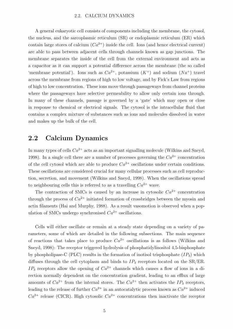
2.2 Calcium Dynamics
In many types of cells Ca2+ acts as an important signalling molecule (Wilkins and Sneyd,
1998). In a single cell there are a number of processes governing the Ca2+ concentration
of the cell cytosol which are able to produce Ca2+ oscillations under certain conditions.
These oscillations are considered crucial for many cellular processes such as cell reproduc-
tion, secretion, and movement (Wilkins and Sneyd, 1998). When the oscillations spread
to neighbouring cells this is referred to as a travelling Ca2+ wave.
The contraction of SMCs is caused by an increase in cytosolic Ca2+ concentration
through the process of Ca2+ initiated formation of crossbridges between the myosin and
actin filaments (Hai and Murphy, 1988). As a result vasomotion is observed when a pop-
ulation of SMCs undergo synchronised Ca2+ oscillations.
Cells will either oscillate or remain at a steady state depending on a variety of pa-
rameters, some of which are detailed in the following subsections. The main sequence
of reactions that takes place to produce Ca2+ oscillations is as follows (Wilkins and
Sneyd, 1998): The receptor triggered hydrolysis of phosphatidylinositol 4,5-bisphosphate
by phospholipase-C (PLC) results in the formation of inotisol trisphosphate (IP3) which
diffuses through the cell cytoplasm and binds to IP3 receptors located on the SR/ER.
IP3 receptors allow the opening of Ca2+ channels which causes a flow of ions in a di-
rection normally dependent on the concentration gradient, leading to an efflux of large
amounts of Ca2+ from the internal stores. The Ca2+ then activates the IP3 receptors,
leading to the release of further Ca2+ in an autocatalytic process known as Ca2+ induced
Ca2+ release (CICR). High cytosolic Ca2+ concentrations then inactivate the receptor
5
2.2. CALCIUM DYNAMICS
and Ca2+ pumps actively remove Ca2+ from the cytosol, pumping it back into the stores
or out of the cell until the cell returns to steady state. This process repeats periodically,
causing oscillations in the cytosolic Ca2+ concentration and other variables such as the
membrane potential (voltage) or other ion concentrations.
If a cell is not oscillatory then the Ca2+ concentration and other variables will remain
at a steady state. If the cell is at a steady state then it may be either excitable or
nonexcitable, as the cytosol is an excitable medium with respect to Ca2+ release (Wilkins
and Sneyd, 1998). If the cell is excitable then for a weak stimulus such as an input of Ca2+
to the cytosol, the Ca2+ concentration will more or less return directly to the resting state.
However for a stronger stimulus above some threshold value the Ca2+ concentration will
rapidly increase before slowly returning to the resting state, i.e. it emits a spike. If the
cell is nonexcitable then no spikes will occur when the cell is stimulated.
In mathematical terminology, an excitable system contains a stable fixed point (FP)
(i.e. the resting state), and small perturbations from the FP give rise to trajectories that
make small excursions in the phase space or return directly to the FP in a short time
period. However, perturbations that exceed some excitation threshold value give rise to
trajectories that make a large excursion in phase space before slowly returning to the
resting state. In a nonexcitable system any perturbations from the FP will simply return
to the FP with no large excursions.
The dynamics of Ca2+ in a SMC may be modelled by a set of ordinary differential
equations (ODEs) based on conservation of mass, and if the membrane potential of the
cell is included, Kirchoff’s Law. Minimal SMC Ca2+ models may be split into different
catagories. For example there are models based on CICR, models based on IP3 dynamics,
and models based on the membrane potential and its effect on the ion fluxes and channels.
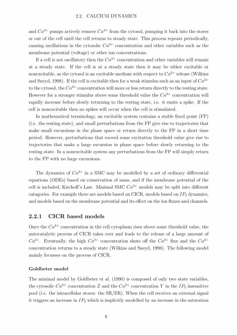
2.2.1 CICR based models
Once the Ca2+ concentration in the cell cytoplasm rises above some threshold value, the
autocatalytic process of CICR takes over and leads to the release of a large amount of
Ca2+. Eventually, the high Ca2+ concentration shuts off the Ca2+ flux and the Ca2+
concentration returns to a steady state (Wilkins and Sneyd, 1998). The following model
mainly focusses on the process of CICR.
Goldbeter model
The minimal model by Goldbeter et al. (1990) is composed of only two state variables,
the cytosolic Ca2+ concentration Z and the Ca2+ concentration Y in the IP3 insensitive
pool (i.e. the intracellular stores: the SR/ER). When the cell receives an external signal
it triggers an increase in IP3 which is implicitly modelled by an increase in the saturation
6

2.2. CALCIUM DYNAMICS
function β, leading to a rise in cytosolic Ca2+ concentration. A ‘bifurcation’ occurs when
a change in parameter causes a qualitative change in the dynamics of the system. This
parameter β may be varied between 0 and 1 in order to achieve different dynamics, e.g.
as a bifurcation parameter. The cell variables will either oscillate or tend to a steady
state depending on the value of β. The ODEs for this model are as follows.
dZ
dt= v0 + v1β − v2 + v3 + kfY − kZ (2.1)
dY
dt= v2 − v3 − kfY (2.2)
with algebraic variables
v2 = VM2Zn
Kn2 + Zn
(2.3)
v3 = VM3Y m
KmR + Y m
Zp
KpA + Zp
(2.4)
where v2 and v3 are the rate of Ca2+ pumping into the internal store and release from
the internal store, respectively. v0 and kZ relate, respectively, to the influx and efflux of
Ca2+ into and out of the cell. The term kfY refers to a nonactivated, leaky transport of
Ca2+ from the internal stores to the cytosol and the term v1β refers to the flux of Ca2+
from the IP3 sensitive pool.
The parameters are listed in Table 2.1. For further details on the model see Goldbeter
et al. (1990). Chapter 3 contains analysis on this model and its extension into a two
coupled cell system.
Parameter Unit Value Description
β − 0 to 1 Saturation function of the IP3 receptor
v0 µMs−1 1 Ca2+ influx into the cell
k s−1 10 Rate of Ca2+ efflux out of the cell
kf s−1 1 Rate of nonactivated, leaky transport of Ca2+ into the internal stores
v1 µMs−1 7.3 Rate of Ca2+ influx from the IP3 sensitive pool
VM2 µMs−1 65 Maximum rate of Ca2+ pumping into the internal store
VM3 µMs−1 500 Maximum rate of Ca2+ release from the internal store
K2 µM 1 Pumping threshold constant
KR µM 2 Release threshold constant
KA µM 0.9 Activation threshold constant
n − 2 Pumping cooperativity coefficient
m − 2 Release cooperativity coefficient
p − 4 Activation cooperativity coefficient
Table 2.1: Parameter values for the Goldbeter et al. (1990) model
7
2.2. CALCIUM DYNAMICS
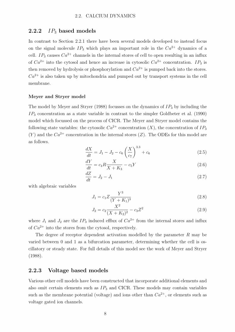
2.2.2 IP3 based models
In contrast to Section 2.2.1 there have been several models developed to instead focus
on the signal molecule IP3 which plays an important role in the Ca2+ dynamics of a
cell. IP3 causes Ca2+ channels in the internal stores of cell to open resulting in an influx
of Ca2+ into the cytosol and hence an increase in cytosolic Ca2+ concentration. IP3 is
then removed by hydrolysis or phosphorylation and Ca2+ is pumped back into the stores.
Ca2+ is also taken up by mitochondria and pumped out by transport systems in the cell
membrane.
Meyer and Stryer model
The model by Meyer and Stryer (1988) focusses on the dynamics of IP3 by including the
IP3 concentration as a state variable in contrast to the simpler Goldbeter et al. (1990)
model which focussed on the process of CICR. The Meyer and Stryer model contains the
following state variables: the cytosolic Ca2+ concentration (X), the concentration of IP3
(Y ) and the Ca2+ concentration in the internal stores (Z). The ODEs for this model are
as follows.
dX
dt= J1 − J2 − c6
(X
c7
)3.3
+ c6 (2.5)
dY
dt= c4R
X
X +K3
− c5Y (2.6)
dZ
dt= J2 − J1 (2.7)
with algebraic variables
J1 = c1ZY 3
(Y +K1)3(2.8)
J2 = c2X2
(X +K2)2− c3Z2 (2.9)
where J1 and J2 are the IP3 induced efflux of Ca2+ from the internal stores and influx
of Ca2+ into the stores from the cytosol, respectively.
The degree of receptor dependent activation modelled by the parameter R may be
varied between 0 and 1 as a bifurcation parameter, determining whether the cell is os-
cillatory or steady state. For full details of this model see the work of Meyer and Stryer
(1988).
2.2.3 Voltage based models
Various other cell models have been constructed that incorporate additional elements and
also omit certain elements such as IP3 and CICR. These models may contain variables
such as the membrane potential (voltage) and ions other than Ca2+, or elements such as
voltage gated ion channels.
8
2.2. CALCIUM DYNAMICS
Gonzalez-Fernandez and Ermentrout Model
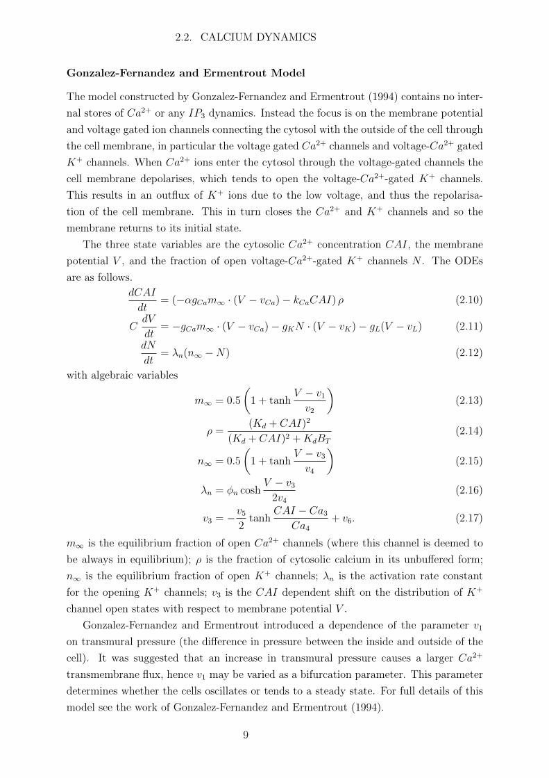
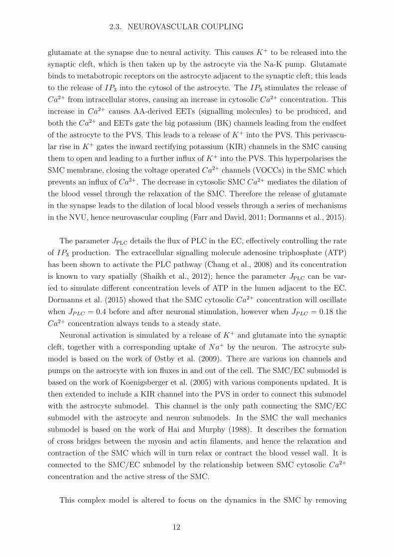
The model constructed by Gonzalez-Fernandez and Ermentrout (1994) contains no inter-
nal stores of Ca2+ or any IP3 dynamics. Instead the focus is on the membrane potential
and voltage gated ion channels connecting the cytosol with the outside of the cell through
the cell membrane, in particular the voltage gated Ca2+ channels and voltage-Ca2+ gated
K+ channels. When Ca2+ ions enter the cytosol through the voltage-gated channels the
cell membrane depolarises, which tends to open the voltage-Ca2+-gated K+ channels.
This results in an outflux of K+ ions due to the low voltage, and thus the repolarisa-
tion of the cell membrane. This in turn closes the Ca2+ and K+ channels and so the
membrane returns to its initial state.
The three state variables are the cytosolic Ca2+ concentration CAI, the membrane
potential V , and the fraction of open voltage-Ca2+-gated K+ channels N . The ODEs
are as follows.
dCAI
dt= (−αgCam∞ · (V − vCa)− kCaCAI) ρ (2.10)
CdV
dt= −gCam∞ · (V − vCa)− gKN · (V − vK)− gL(V − vL) (2.11)
dN
dt= λn(n∞ −N) (2.12)
with algebraic variables
m∞ = 0.5
(1 + tanh
V − v1v2
)(2.13)
ρ =(Kd + CAI)2
(Kd + CAI)2 +KdBT
(2.14)
n∞ = 0.5
(1 + tanh
V − v3v4
)(2.15)
λn = φn coshV − v3
2v4(2.16)
v3 = −v52
tanhCAI − Ca3
Ca4+ v6. (2.17)
m∞ is the equilibrium fraction of open Ca2+ channels (where this channel is deemed to
be always in equilibrium); ρ is the fraction of cytosolic calcium in its unbuffered form;
n∞ is the equilibrium fraction of open K+ channels; λn is the activation rate constant
for the opening K+ channels; v3 is the CAI dependent shift on the distribution of K+
channel open states with respect to membrane potential V .
Gonzalez-Fernandez and Ermentrout introduced a dependence of the parameter v1
on transmural pressure (the difference in pressure between the inside and outside of the
cell). It was suggested that an increase in transmural pressure causes a larger Ca2+
transmembrane flux, hence v1 may be varied as a bifurcation parameter. This parameter
determines whether the cells oscillates or tends to a steady state. For full details of this
model see the work of Gonzalez-Fernandez and Ermentrout (1994).
9
2.3. NEUROVASCULAR COUPLING
2.2.4 More complex models
The preceding minimal models all contain at most 3 state variables and only consider the
dynamics in the SMC. However the arterial wall also contains ECs which provide a flux
of Ca2+ and IP3 into or out of the SMCs, potentially influencing the SMC dynamics.
One such model of a coupled SMC/EC unit is constructed by Koenigsberger et al.
(2005). This 9 dimensional model incorporates IP3 concentration, membrane potential,
the open probability of Ca2+-gated K+ channels, and Ca2+ concentration of both the
SMC and EC and their internal stores of Ca2+ (the SR and ER, respectively). The
important cellular mechanisms governing the Ca2+ dynamics in this model are the Ca2+
release from IP3 sensitive stores, the Ca2+ uptake in the SR/ER, the Ca2+ extrusion from
the cytosol (voltage dependent in SMCs), and the leak of Ca2+ from the SR/ER. This
model effectively combines all important elements from the three minimal SMC models
described earlier.
However the model of a so called ‘neurovascular unit (NVU)’ originally constructed
by Farr and David (2011) and later extended by Dormanns et al. (2015) incorporates and
updates the SMC/EC model by Koenigsberger et al. (2005). In addition it includes the
influence of neuronal activity in the brain on the dynamics of the SMC via the process
known as functional hyperaemia, and the effect of the SMC cytosolic Ca2+ concentration
on the vessel radius, making it a more versatile and physiologically realistic model. The
mechanisms behind the important process of functional hyperaemia and the components
of the NVU model are detailed in the following section.
2.3 Neurovascular Coupling
The cerebral cortex, a highly complex component of the brain, contains a multitude of
blood vessels that provide the brain tissue with oxygen and glucose essential for cellular
function. Arteries in the brain are able to regulate their blood supply in response to
local changes in a process known as functional hyperaemia. An increase in neuronal
activity is followed by a rapid dilation of local blood vessels via the relaxation of the
SMCs and hence an increased supply of oxygen and glucose via the blood flow, where the
relaxation of the SMCs is caused by a decrease in cytosolic Ca2+ concentration. Impaired
functional hyperaemia is associated with several pathologies such as Alzheimer’s disease,
cortical spreading depression (CSD), atherosclerosis, stroke, and hypertension (Girouard
and Iadecola, 2006). These begin with a defective relationship between neural activity
and the cerebral blood flow (CBF).
Functional hyperaemia is achieved through the process of neurovascular coupling, an
intercellular communication system based on ion exchange through pumps and channels
and involving neurons, astrocytes (glial cells), SMCs and ECs. Together these cells
comprise a NVU (see Figure 2.2).
10
2.3. NEUROVASCULAR COUPLING
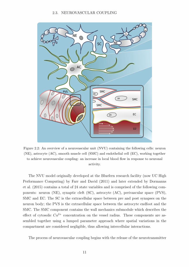
Figure 2.2: An overview of a neurovascular unit (NVU) containing the following cells: neuron
(NE), astrocyte (AC), smooth muscle cell (SMC) and endothelial cell (EC), working together
to achieve neurovascular coupling: an increase in local blood flow in response to neuronal
activity.
The NVU model originally developed at the Bluefern research facility (now UC High
Performance Computing) by Farr and David (2011) and later extended by Dormanns
et al. (2015) contains a total of 24 state variables and is comprised of the following com-
ponents: neuron (NE), synaptic cleft (SC), astrocyte (AC), perivascular space (PVS),
SMC and EC. The SC is the extracellular space between pre and post synapses on the
neuron body; the PVS is the extracellular space between the astrocyte endfoot and the
SMC. The SMC component contains the wall mechanics submodule which describes the
effect of cytosolic Ca2+ concentration on the vessel radius. These components are as-
sembled together using a lumped parameter approach where spatial variations in the
compartment are considered negligible, thus allowing intercellular interactions.
The process of neurovascular coupling begins with the release of the neurotransmitter
11
2.3. NEUROVASCULAR COUPLING
glutamate at the synapse due to neural activity. This causes K+ to be released into the
synaptic cleft, which is then taken up by the astrocyte via the Na-K pump. Glutamate
binds to metabotropic receptors on the astrocyte adjacent to the synaptic cleft; this leads
to the release of IP3 into the cytosol of the astrocyte. The IP3 stimulates the release of
Ca2+ from intracellular stores, causing an increase in cytosolic Ca2+ concentration. This
increase in Ca2+ causes AA-derived EETs (signalling molecules) to be produced, and
both the Ca2+ and EETs gate the big potassium (BK) channels leading from the endfeet
of the astrocyte to the PVS. This leads to a release of K+ into the PVS. This perivascu-
lar rise in K+ gates the inward rectifying potassium (KIR) channels in the SMC causing
them to open and leading to a further influx of K+ into the PVS. This hyperpolarises the
SMC membrane, closing the voltage operated Ca2+ channels (VOCCs) in the SMC which
prevents an influx of Ca2+. The decrease in cytosolic SMC Ca2+ mediates the dilation of
the blood vessel through the relaxation of the SMC. Therefore the release of glutamate
in the synapse leads to the dilation of local blood vessels through a series of mechanisms
in the NVU, hence neurovascular coupling (Farr and David, 2011; Dormanns et al., 2015).
The parameter JPLC details the flux of PLC in the EC, effectively controlling the rate
of IP3 production. The extracellular signalling molecule adenosine triphosphate (ATP)
has been shown to activate the PLC pathway (Chang et al., 2008) and its concentration
is known to vary spatially (Shaikh et al., 2012); hence the parameter JPLC can be var-
ied to simulate different concentration levels of ATP in the lumen adjacent to the EC.
Dormanns et al. (2015) showed that the SMC cytosolic Ca2+ concentration will oscillate
when JPLC = 0.4 before and after neuronal stimulation, however when JPLC = 0.18 the
Ca2+ concentration always tends to a steady state.
Neuronal activation is simulated by a release of K+ and glutamate into the synaptic
cleft, together with a corresponding uptake of Na+ by the neuron. The astrocyte sub-
model is based on the work of Østby et al. (2009). There are various ion channels and
pumps on the astrocyte with ion fluxes in and out of the cell. The SMC/EC submodel is
based on the work of Koenigsberger et al. (2005) with various components updated. It is
then extended to include a KIR channel into the PVS in order to connect this submodel
with the astrocyte submodel. This channel is the only path connecting the SMC/EC
submodel with the astrocyte and neuron submodels. In the SMC the wall mechanics
submodel is based on the work of Hai and Murphy (1988). It describes the formation
of cross bridges between the myosin and actin filaments, and hence the relaxation and
contraction of the SMC which will in turn relax or contract the blood vessel wall. It is
connected to the SMC/EC submodel by the relationship between SMC cytosolic Ca2+
concentration and the active stress of the SMC.
This complex model is altered to focus on the dynamics in the SMC by removing
12
2.4. WAVE PROPAGATION IN SPATIAL MEDIA
the neuron and astrocyte compartments and simplifying the neuronal input to a single
parameter, then analysed and compared in Chapter 4 with simpler SMC models (detailed
in Section 2.2).
2.4 Wave Propagation in Spatial Media
Wave propagation has widespread applications in many fields such as biology and chem-
istry. One such area of interest is the pathology CSD associated with impaired functional
hyperaemia where waves of depolarisation spread throughout the brain cortex. Waves of
extracellular K+ ions are released from depolarized neurons. The high extracellular K+
concentration depolarises adjacent neurons so that more K+ is released and the process
spreads slowly thoughout the cortex. In particular the phenomenon of Ca2+ wave prop-
agation through cells such as SMCs is an area of interest; as stated earlier synchronised
oscillations in a population of SMCs will induce vasomotion. Ca2+ waves through SMCs
may also play a role in other pathologies associated with functional hyperaemia as the
SMC is an important component of the NVU, effectively controlling the vessel radius
and local blood flow. Hence our interest is in the dynamics behind the formation and
propagation of Ca2+ waves through a medium such as an arterial wall, or the brain cortex
permeated with a network of blood vessels.
2.4.1 Excitable Media
Wave propagation on a surface (i.e. in a two dimensional (2D) spatial system) is possible
when the medium is either oscillatory or excitable. An excitable system is characterised
by a stable resting state, an excitation threshold and a refractory period. In a spatial
medium, when the rate of diffusion (defined as the rate at which a particular substance
can spread throughout a particular medium) is high enough, an initial perturbation to
the system with conditions above the excitation threshold is able to spread the excitation
throughout the medium, triggering the transition from resting to excited state. The
different levels of excitability in 2D spatial media are as follows (Kneer et al., 2014):
• Excitable: a wave will propagate and the ends will grow in length
• Sub excitable: a wave will propagate but the ends will shrink in length
• Non excitable: a wave will not propagate at all.
The size of a propagating wave decreases as the system becomes less excitable or as the
diffusive strength decreases.
Patterns in spatial excitable media arise from the mutual annihilation of waves when
colliding with one another, a property due to the refractory period corresponding to the
region immediately behind a travelling wavefront (a.k.a. the ‘waveback’). This region
is in the recovery phase so it cannot be immediately stimulated by another excitation
13
2.4. WAVE PROPAGATION IN SPATIAL MEDIA
wavefront. A spatially-distributed system whose local kinetics is excitable is an excitable
medium and the coupling among the locally excitable elements gives rise to a number of
distinctive types of wave propagation processes such as Turing patterns and spiral waves
(Kapral, 1995).
2.4.2 Spiral Formation
Spiral waves are commonly observed in excitable reaction diffusion systems. They gen-
erally emerge in an excitable or oscillatory medium as a result of a wave break (Hill
and Morgan, 2014), as spiral rotors (generators of outward rotating spiral waves) can
emerge from free ends of a travelling wave front. The rotor sends robust rotating spiral
waves outward. The thickness of the wave and tightness of the spiral increases with the
excitability of the medium (Sinha and Sridhar, 2014).
Regions of inexcitability can also cause breaks in wave fronts (Weise and Panfilov,
2012), or breaks can be formed as a result of wave interaction. When one wave comes close
to a slower travelling wave in front, part of the wave vanishes because of the refractory
waveback of the slower wave. This causes a break in the wave and as a result spirals can
form.
Some examples of spiral wave formation are the Belousov-Zhabotinskii reaction (Keener,
1986), spiral intercellular waves of Ca2+ in slices of hippocampal tissue (Wilkins and
Sneyd, 1998), and spiral waves in models of CSD (Gorelova, 1983). Spiral waves will be
seen in the results of Chapters 5 and 6.
2.4.3 Fitz-Hugh Nagumo model
The FHN model is a classic generic model for excitable systems with known dynam-
ics (Kneer et al., 2014), first suggested by FitzHugh (1961) and later independently by
Nagumo et al. (1962). It is a simplification of the Hodgkin-Huxley model (Hodgkin and
Huxley, 1990) and was originally based on a single neuron, mainly used to model spikes
and pulses in electrical potential across a neuron. The activator variable u models the fast
changes in electrical potential across the axon membrane, while the inhibitor variable v
is a slow variable related to the gating mechanism of the membrane channels. In general,
the fast variable is called the activator variable, whereas the slow variable is generally
called the inhibitor variable.
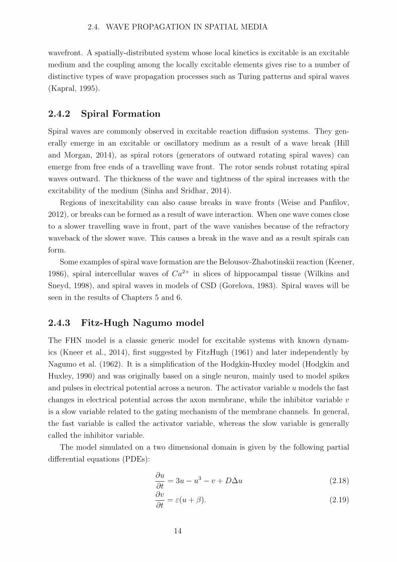
The model simulated on a two dimensional domain is given by the following partial
differential equations (PDEs):
∂u
∂t= 3u− u3 − v +D∆u (2.18)
∂v
∂t= ε(u+ β). (2.19)
14

2.4. WAVE PROPAGATION IN SPATIAL MEDIA
The parameter ε � 1 represents the difference in time scales between the variables u
and v. The parameter D controls the rate of diffusion modelled simply by the Laplace
operator (i.e. Fick’s Law). The parameter β simply determines the stability of the non
spatial system; when β < 1 the system is oscillatory, while for β > 1 the system is stable.
This is due to a supercritical Hopf bifurcation at β = 1 (Kneer et al., 2014). Note that
all variables and parameters of this model are assumed to be nondimensional (including
time) as Kneer et al. (2014) do not mention any dimensional units.
When the system is excitable then a wave will propagate outwards from an initial
perturbation, when it is subexcitable then a wave will propagate outwards but shrink in
length until it disappears, and when it is nonexcitable then no wave will propagate. For
approximately 1 < β < 1.34 the system is excitable and for approximately 1.34 < β <
1.39 the system is subexcitable; the larger the parameter β the less excitable the system.
The regions of excitability on a 2D flat surface are given in Figure 2.3 (Kneer et al.,
2014). There is some dependence of the level of excitability on the wave size S, where
the wave size is defined as the area where the activator u is greater than zero. A critical
wave size S∗ exists below which the wave is subexcitable and above which the wave is
excitable.
Chapter 5 contains our work on the FitzHugh-Nagumo (FHN) and Goldbeter spatial
models simulated on a flat surface.
0
60
wav
esiz
e S
β
excitable
subexcitable
nonexcitable
1.391.34
S*
Figure 2.3: The different domains of excitability of the FHN model for D = 0.12 on a flat 2D
spatial medium. The dotted line represents the critical wave size S∗ below which a wave will
shrink in length and above which a wave will grow in length. Adapted from Kneer et al.
(2014).
15

2.5. GEOMETRY
2.5 Geometry
Ca2+ wave formation and propagation is an important area of interest, however the areas
in which these waves propagate are rarely flat surfaces. The Gaussian curvature of a sur-
face is intuitively defined as the amount an object deviates from being flat; for example a
convex lens or a sphere has a positively curved surface, while a concave lens has a nega-
tively curved surface. In reality arteries and arterioles are curved structures, in particular
the surface is negatively curved at an arterial bifurcation where the artery splits in two.
In addition, the cerebral cortex is composed of tightly folded grey matter and as such
also contains areas of strongly positive and negative curvature. Various pathologies are
associated with impaired functional hyperaemia, in particular the pathology CSD where
waves of depolarisation spread throughout the brain cortex. The aspect of curvature in a
spatial domain is one not always incorporated into spatial models, however as shown by
Kneer et al. (2014) it can have a noticable effect on the dynamics of wave propagation.
The work of Kneer et al. (2014) and our work in Chapter 6 use a torus to represent a
curved surface as it contains areas of both positive and negative Gaussian curvature.
The surface of a torus in the Euclidean space R3 can be parameterised by coordinates
(θ, ϕ) as follows:
(θ, ϕ) 7→
(R + r cos θ) cosϕ
(R + r cos θ) sinϕ
r sin θ
=
x
y
z
, (2.20)
where θ, ϕ ∈ [0, 2π) and R and r are the major and minor curvature radii respectively.
The torus is visualised in Figure 2.4. The outside of the torus corresponds to θ = 0 and
the inside corresponds to θ = π. The Gaussian curvature at a point (θ, ϕ) on a torus
surface is a function of θ:
Γ(θ) =cos θ
r(R + r cos θ)(2.21)
and may be either positive or negative. The curvature is visualised in Figure 2.5.
2.5.1 Toroidal Coordinates
In addition to the standard coordinates (θ, ϕ) there exists the so-called toroidal coordi-
nates (θ, ϕ). This is a global isothermal orthgonal coordinate system, that is, coordinates
where the metric is locally conformal to the Euclidean metric. Using these coordinates
the surface of a torus may be mathematically interpreted as a flat medium with a spatial
coupling dependent only on θ. A parameterisation is isothermal if the derived coordinate
system is orthogonal and conformal. The following formulation follows that of Kneer
et al. (2014).
16

2.5. GEOMETRY
Figure 2.4: Visualisation of a torus in R3 with coordinates (θ, ϕ), where R and r are the major
and minor curvature radii (Kneer et al., 2014).
0 1 2 3 4 5 6θ
0.10
0.08
0.06
0.04
0.02
0.00
0.02
0.04 Gaussian Curvature G(θ)
R=80/2π
R=40/2π
Flat
Figure 2.5: Gaussian curvature on a flat surface, and weakly curved (R = 80/2π) and strongly
curved (R = 40/2π) tori.
17
2.5. GEOMETRY
The Laplace-Beltrami operator for a parameterisation f : αi 7→ xj is given by
∆LB =∑i,k
1√g
∂
∂αi
(gik√g∂
∂αk
), (2.22)
where J is the Jacobian matrix of f , G = JTJ , g = detG, and gik are the elements of G.
The components gik are
gik =∑j
∂fj∂αi
∂fj∂αk
=:
⟨∂f
∂αi
∣∣∣∣ ∂f∂αk⟩. (2.23)
A parameterisation f of a 2D manifold in 3D space,
f : (α1, α2) 7→
x
y
z
(2.24)
is orthgonal if, for i 6= k, ⟨∂f
∂αi
∣∣∣∣ ∂f∂αk⟩
= 0, (2.25)
and conformal if ⟨∂f
∂αi
∣∣∣∣ ∂f∂αi⟩
=
⟨∂f
∂αk
∣∣∣∣ ∂f∂αk⟩. (2.26)
Hence the Laplace-Beltrami operator for an isothermal parameterisation in two spatial
dimensions is
∆LB =∑i,k
1√g
∂
∂αi∂
∂αkδik (2.27)
=∑i
1√g
∂2
∂αi2=
1√g
∆, (2.28)
where the Kronecker delta δik is defined by
δik =
{0 i 6= k
1 i = k(2.29)
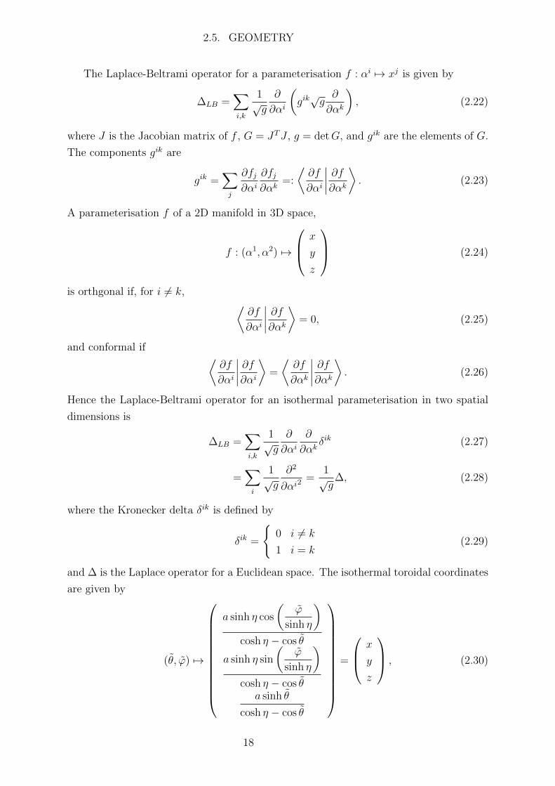
and ∆ is the Laplace operator for a Euclidean space. The isothermal toroidal coordinates
are given by
(θ, ϕ) 7→
a sinh η cos
(ϕ
sinh η
)cosh η − cos θ
a sinh η sin
(ϕ
sinh η
)cosh η − cos θ
a sinh θ
cosh η − cos θ
=
x
y
z
, (2.30)
18

2.5. GEOMETRY
with
a =√R2 − r2 (2.31)
η = tanh−1( aR
). (2.32)
The coordinates (θ, ϕ) in terms of (θ, ϕ) are
θ(θ) = cos−1(R
r− a2
r(R + r cos θ)
)·
{+1 θ ≥ 0
−1 θ < 0(2.33)
ϕ(ϕ) = ϕ sinh η. (2.34)
This coordinate systems yields
gθ,θ = gϕ,ϕ =√g =
a2
(cosh η − cos θ)2. (2.35)
Thus the Laplace-Beltrami operator may be written as
∆LB =(cosh η − cos θ)2
a2
(∂2
∂θ2+
∂2
∂ϕ2
). (2.36)
We define the coupling strength as
C(θ) =(cosh η − cos θ)2
a2(2.37)
given in Figure 2.6. For further details on the derivation of this coordinate system see
Kneer et al. (2014).
A reaction diffusion system simulated on a torus will have some diffusion term D∆u
for some diffusing variable u. This diffusion term may be written in toroidal coordinates,
i.e.
D∆u = DC(θ)
(∂2u
∂θ2+∂2u
∂ϕ2
)(2.38)
so thatDC(θ) is effectively the spatially varying rate of diffusion on a torus. The Gaussian
curvature of a surface has a dramatic effect on the rate of diffusion as shown in the
following section.
2.5.2 Effect of Geometry on Fitz-Hugh Nagumo model
The FHN model was simulated on a curved surface with spatially constant parameter β by
Kneer et al. (2014) with the following parameter values: D = 0.12, ε = 0.36. All variables
used (including time) are seemingly dimensionless as no units are ever mentioned in their
work. In Chapter 6 we extend their results by simulating both the FHN and Goldbeter
models on a curved surface with spatially constant and linearly varied dynamics via the
parameter β.
19

2.5. GEOMETRY
0 1 2 3 4 5 6θ
0.0
0.5
1.0
1.5
2.0
2.5
3.0 Coupling Strength C(θ)
R=80/2π
R=40/2π
Flat
Figure 2.6: Coupling strength C(θ) defined as (2.37) on a flat surface, weakly curved
(R = 80/2π) and strongly curved (R = 40/2π) torus. The coupling strength is highest on the
inside of the torus (θ = π) and lowest on the outside (θ = 0). The strongly curved torus has a
larger gradient in C(θ) .
Kneer et al. (2014) generated propagating waves from an initial perturbation simu-
lated by an increase in the values of the initial conditions (ICs) in a small rectangular
area in terms of (θ, ϕ) on the torus surface. For the majority of the spatial domain the
ICs were set to the stable state us, vs and the rectangular area simulating to the initial
perturbation was set to us + 2, vs + 1.5 corresponding to a supra-threshold excitation.
As with a flat surface, when β in is the nonexcitable domain an initial perturbation
will not propagate. When β is subexcitable an initial perturbation will propagate but
retract in length, and when β is excitable a perturbation will grow to a ring wave.
A consequence of the curvature dependent rate of diffusion is that an initial perturba-
tion centred on the inside of the torus (where diffusion is highest) will be more inclined
to grow in the θ-direction. DC(θ) will be higher at the centre of the perturbation than
at the ends so that the diffusion in the θ-direction is directed outwards, enhancing the
growth of the open ends as the wave propagates in the ϕ-direction. Conversely, an initial
perturbation centred on the outside of the torus will be more inclined to retract. This
means that the excitable domain for an inside torus wave is slightly larger than on a flat
medium, while it is slightly smaller for an outside torus wave; hence the surface curvature
effectively extends the regime of propagating excitation waves beyond the threshold of
flat surfaces.
An increase in the Gaussian curvature of a torus causes a greater coupling strength
(and hence greater diffusion) on the inside and lower diffusion rate on the outside, and
a larger gradient in diffusion rate over the toroidal surface (see Figure 2.6). Greater
20
2.5. GEOMETRY
diffusion causes an increase in wave velocity and hence excitability, therefore an area of
strongly negative curvature will have a larger excitable domain and the opposite for an
area of strongly positive curvature.
The spatially varying diffusion also leads to additional stable wave solutions for the
FHN model on a torus, namely a stable propagating wave segment with temporally
constant wave size and shape (Figure 2.7a) and an oscillating wave segment whose wave
size oscillates periodically in a self-sustained way (Figure 2.7b). These solutions do not
exist on a flat surface because there is no variation in the rate of diffusion over the
surface when there is no spatial curvature. The solutions only exist for β in a small
subregion of the excitable domain and only on the outside of the torus where the surface
is postively curved. A wave centred on the outside of the torus has lower diffusion rate
at the centre (θ = 0) than at its ends, causing enhanced retraction of the wave ends as
it propagates in the ϕ-direction. At the same time, when β is in the excitable parameter
regime then a perturbation will grow in length. The stable wave segment and stable
oscillating wave segment exist due to the balance between β induced growth (excitability)
and retraction induced by thespatially varied rate of diffusion; these two are effectively
in equilibrium and produce the two wave solutions in Figures 2.7a, 2.7b. These figures
have been reproduced with the numerical code used in Chapters 5, 6 to validate our code
and resulting simulations. Note that there also exist propagating wave segments on the
inside of the torus when β is subexcitable but this solution is unstable and was found via
mathematical analysis by Kneer et al. (2014).
21

2.5. GEOMETRY
(a) Stable wave segment of constant wave size and shape, β = 1.322.
(b) Wave segment oscillating in size, β = 1.32.
Figure 2.7: Propagating wave segments of activator concentration u(t, θ, ϕ) moving clockwise
on a torus with major radius R = 80/2π and minor radius r = 20/2π. Generated using the
FHN model with D = 0.12 using the code implemented in Chapters 5 and 6.
22
Chapter 3
Goldbeter Model
In this chapter we analyse the model constructed by Goldbeter et al. (1990) detailing the
dynamics of calcium (Ca2+) in a cell and which specifically focusses on the intracellular
process of Ca2+ induced Ca2+ release (CICR). This model is explained in detail in Sec-
tion 2.2.1 and contains the state variables Z, the cytosolic Ca2+ concentration, and Y ,
the Ca2+ concentration in the internal stores of the cell. The system is first nondimen-
sionalised in order to remove any dependence on units and as there are only two variables
we can analyse the nullclines of the system. We then vary the parameter β to perform a
bifurcation analysis and the single cell model is then extended to include two cells cou-
pled together with some nondimensional coupling strength D. We vary the parameter
β for each cell and analyse how the dynamics change with the coupling strength D by
considering the changing trajectories in the phase space and the power spectra of each
cell.
3.1 Method
The single cell and coupled cell systems are solved in Matlab using ODE45. The time
series graphs, nullcline diagrams, trajectory plots, and power spectra are all produced
in Matlab. The bifurcation analysis is achieved using the continuation package AUTO
(Champneys et al., 2002).
3.1.1 Coupled Cell Model
For the coupled cell model we consider two adjacent cells coupled by the gap junctions
connecting the cytosol of the two cells. There are two cells hence two sets of the single
cell model, using Z1, Y1 for cell 1 and Z2, Y2 for cell 2. We let β1 be the saturation
function for cell 1 and similarly β2 for cell 2.
A linear diffusion term modelling the flux of Ca2+ from cell to cell is added to the
ordinary differential equations (ODEs) for Z1 and Z2 which mimics Fick’s law where ions
23

3.1. METHOD
move from high to low concentrations. This coupling term is d(Z2 − Z1) for cell 1 and
similarly d(Z1−Z2) for cell 2. This parameter d is the rate of diffusion of Ca2+ from one
cell to the other (a.k.a. the coupling strength) with units of s−1.
For a row of cells the flux of Ca2+ comes from its two adjacent cells; hence the total
flux for a cell i in a row of cells is
d(Zi+1 − 2Zi + Zi−1).
If we let d = P/h2 where h = 50 µm is the length of a smooth muscle cell (SMC) and
letting x be the spatial variable we can regard the above as
PZi(x+ h, t)− 2Zi(x, t) + Zi(x− h, t)
h2,
which is a discrete approximation to
P∂2Z
∂x2
as h→ 0. Here P plays the role of the effective Ca2+ diffusivity. Values for this diffusion
coefficient P are known for various substances and are typically measured in cm2s−1.
However, at the present time no precise value for the effective diffusion coefficient for
Ca2+ has been found so a range of values for d = P/h2 is considered. If d = 0, then there
is effectively no coupling and the cells are independent of one another.
There is no change to the equations for Ca2+ in the stores (Y1, Y2) as the gap junctions
connect only the cytosol of each cell.
3.1.2 Non-dimensionalisation
In order to remove the dependence on units and hence gain a better understanding of the
magnitude of the parameters we non-dimensionalise the equations of the system. The
following parameters and variables are defined:
τ = kf t, v1 =v1v0, V M2 =
VM2
v0, V M3 =
VM3
v0, k =
k
kf, Z =
kfv0z, Y =
kfv0y.
Then the non-dimensional single cell system becomes
dZ
dt= 1 + v1β − v2 + v3 + Y − kZ, (3.1)
dY
dt= v2 − v3 − Y, (3.2)
with
v2 = VM2
( v0kfZ)n
Kn2 + ( v0
kfZ)n
, (3.3)
v3 = VM3
( v0kfY )m
KmR + ( v0
kfY )m
( v0kfZ)p
KpA + ( v0
kfZ)p
. (3.4)
24
3.2. SINGLE CELL RESULTS
To nondimensionalise the coupled cell system we define D = dkf
where kf is the time
constant of the nonactivated leaky transport of Ca2+ from the store into the cytosol.
The nondimensional coupled system is given by:
dZ1
dt= 1 + v1β1 − v2 + v3 + Y1 − kZ1 +D(Z2 − Z1), (3.5)
dZ2
dt= 1 + v1β2 − v2 + v3 + Y2 − kZ2 +D(Z1 − Z2), (3.6)
dY1dt
= v2 − v3 − Y1, (3.7)
dY2dt
= v2 − v3 − Y2, (3.8)
with equations 3.3, 3.4 for each cell. From here on we drop the overline for all variables
for ease of use.
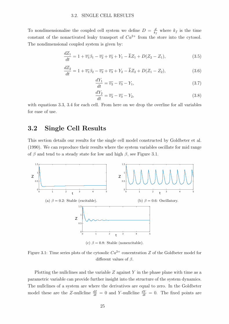
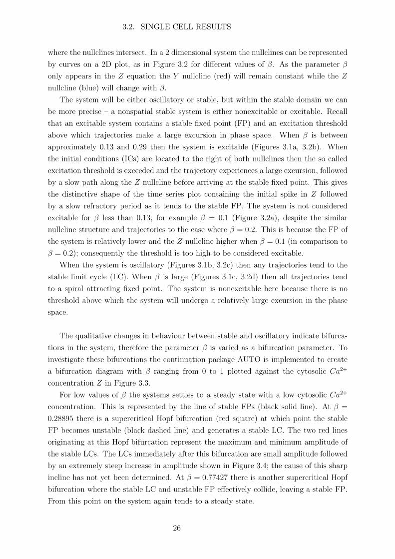
3.2 Single Cell Results
This section details our results for the single cell model constructed by Goldbeter et al.
(1990). We can reproduce their results where the system variables oscillate for mid range
of β and tend to a steady state for low and high β, see Figure 3.1.
Z
t
(a) β = 0.2: Stable (excitable).
Z
t
(b) β = 0.6: Oscillatory.
t
Z
(c) β = 0.8: Stable (nonexcitable).
Figure 3.1: Time series plots of the cytosolic Ca2+ concentration Z of the Goldbeter model for
different values of β.
Plotting the nullclines and the variable Z against Y in the phase plane with time as a
parametric variable can provide further insight into the structure of the system dynamics.
The nullclines of a system are where the derivatives are equal to zero. In the Goldbeter
model these are the Z-nullcline dZdt
= 0 and Y -nullcline dYdt
= 0. The fixed points are
25
3.2. SINGLE CELL RESULTS
where the nullclines intersect. In a 2 dimensional system the nullclines can be represented
by curves on a 2D plot, as in Figure 3.2 for different values of β. As the parameter β
only appears in the Z equation the Y nullcline (red) will remain constant while the Z
nullcline (blue) will change with β.
The system will be either oscillatory or stable, but within the stable domain we can
be more precise – a nonspatial stable system is either nonexcitable or excitable. Recall
that an excitable system contains a stable fixed point (FP) and an excitation threshold
above which trajectories make a large excursion in phase space. When β is between
approximately 0.13 and 0.29 then the system is excitable (Figures 3.1a, 3.2b). When
the initial conditions (ICs) are located to the right of both nullclines then the so called
excitation threshold is exceeded and the trajectory experiences a large excursion, followed
by a slow path along the Z nullcline before arriving at the stable fixed point. This gives
the distinctive shape of the time series plot containing the initial spike in Z followed
by a slow refractory period as it tends to the stable FP. The system is not considered
excitable for β less than 0.13, for example β = 0.1 (Figure 3.2a), despite the similar
nullcline structure and trajectories to the case where β = 0.2. This is because the FP of
the system is relatively lower and the Z nullcline higher when β = 0.1 (in comparison to
β = 0.2); consequently the threshold is too high to be considered excitable.
When the system is oscillatory (Figures 3.1b, 3.2c) then any trajectories tend to the
stable limit cycle (LC). When β is large (Figures 3.1c, 3.2d) then all trajectories tend
to a spiral attracting fixed point. The system is nonexcitable here because there is no
threshold above which the system will undergo a relatively large excursion in the phase
space.
The qualitative changes in behaviour between stable and oscillatory indicate bifurca-
tions in the system, therefore the parameter β is varied as a bifurcation parameter. To
investigate these bifurcations the continuation package AUTO is implemented to create
a bifurcation diagram with β ranging from 0 to 1 plotted against the cytosolic Ca2+
concentration Z in Figure 3.3.
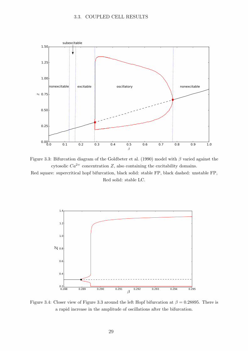
For low values of β the systems settles to a steady state with a low cytosolic Ca2+
concentration. This is represented by the line of stable FPs (black solid line). At β =
0.28895 there is a supercritical Hopf bifurcation (red square) at which point the stable
FP becomes unstable (black dashed line) and generates a stable LC. The two red lines
originating at this Hopf bifurcation represent the maximum and minimum amplitude of
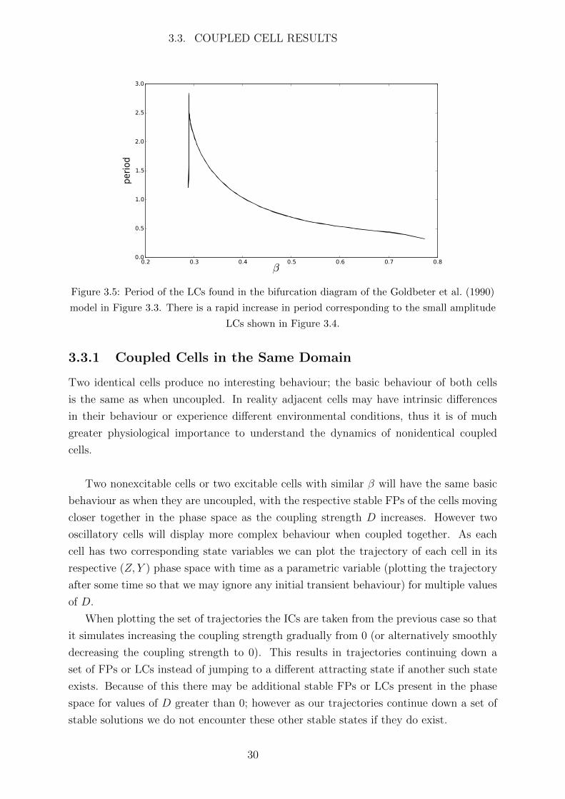
the stable LCs. The LCs immediately after this bifurcation are small amplitude followed
by an extremely steep increase in amplitude shown in Figure 3.4; the cause of this sharp
incline has not yet been determined. At β = 0.77427 there is another supercritical Hopf
bifurcation where the stable LC and unstable FP effectively collide, leaving a stable FP.
From this point on the system again tends to a steady state.
26

3.2. SINGLE CELL RESULTS
z0 0.5 1 1.5
y
0
0.5
1
1.5
2
2.5
(a) β = 0.1: Stable.
z0 0.5 1 1.5
y
0
0.5
1
1.5
2
2.5
(b) β = 0.2: Stable (excitable).
z0 0.5 1 1.5
y
0
0.5
1
1.5
2
2.5
(c) β = 0.6: Oscillatory.
z0 0.5 1 1.5
y
0
0.5
1
1.5
2
2.5
(d) β = 0.8: Stable (spiral attractor).
Figure 3.2: The (Z, Y ) phase space of the single cell system using the Goldbeter et al. (1990)
model. The nullclines (blue: dZdt = 0, red: dY
dt = 0), sample trajectories (black dotted) and
limit cycles (LCs) (black solid are shown for various values of β. The dynamics qualitatively
change when β is varied.)
27
3.3. COUPLED CELL RESULTS
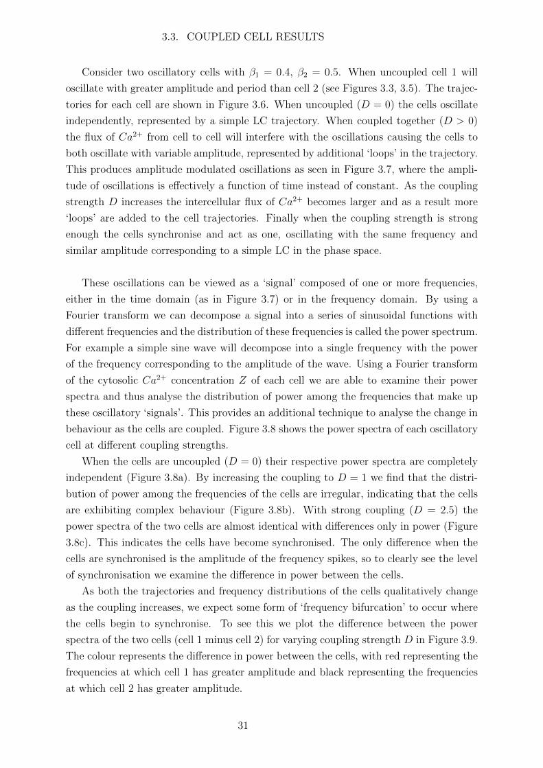
The period of oscillations is shown in Figure 3.5. The steep increase in period cor-
responds to the small amplitude LCs; again the cause of this steep increase is unknown.
The period then smoothly decreases as β increases.
Goldbeter et al. (1990) found the oscillatory region to be β ∈ [0.291, 0.775] where
the period is greatest at β = 0.291 and decreases as β increases. Our more accurate
numerical analysis gives the oscillatory region β ∈ [0.28895, 0.77427], with a small ampli-
tude region [0.28895, 0.28948] where the period increases with β, and the large amplitude
region [0.28948, 0.77427] where the period decreases with β.
The excitability of the model is also shown in Figure 3.3. When β is either very low
or very high the system is nonexcitable, when β is in the oscillatory domain the system
oscillates, and when β is in the excitable/subexcitable domains then the system experi-
ences a large excursion in phase space when perturbed from the FP, i.e. a small increase
in Ca2+ results in a large spike of Ca2+ concentration. The small subexcitable domain is
essentially the same as the excitable domain for nonspatial and one dimensional spatial
systems; however in the two dimensional (2D) spatial systems discussed in Chapters 5, 6
a wave will propagate in an excitable medium but will shrink in length in a subexcitable
medium. Hence for the remainder of this chapter the subexcitable subdomain will no
longer be referenced but is included in the excitable domain.
3.3 Coupled Cell Results
In this section we couple two cells via their gap junctions where cell 1 has the parameter
β1 and cell 2 has β2. Physiologically, adjacent cells must be similar so we only consider
cells with either identical β or similar values of β. There are 3 different domains of
behaviour dependent on β (seen in Figure 3.3), namely nonexcitable, excitable, and
oscillatory. We consider identical cells with the same β, cells in the same domain, and
cells in neighbouring domains.
The maximum value of the coupling coefficient D used in the following analysis is
relatively large. When modelling nonidentical cells, quite different β values and a large
range of D are used to effectively exaggerate the dynamics occuring between the state
with no coupling (D = 0) and eventual synchronisation. In reality, we would find cells
with much closer parameter values and hence need much lower D to synchronise. This
means our range of D is not physiologically chosen, it is simply large enough to clearly
observe the different dynamical states that occur.
28
3.3. COUPLED CELL RESULTS
oscillatory nonexcitableexcitablenonexcitable
subexcitable
Figure 3.3: Bifurcation diagram of the Goldbeter et al. (1990) model with β varied against the
cytosolic Ca2+ concentration Z, also containing the excitability domains.
Red square: supercritical hopf bifurcation, black solid: stable FP, black dashed: unstable FP,
Red solid: stable LC.
Figure 3.4: Closer view of Figure 3.3 around the left Hopf bifurcation at β = 0.28895. There is
a rapid increase in the amplitude of oscillations after the bifurcation.
29
3.3. COUPLED CELL RESULTS
Figure 3.5: Period of the LCs found in the bifurcation diagram of the Goldbeter et al. (1990)
model in Figure 3.3. There is a rapid increase in period corresponding to the small amplitude
LCs shown in Figure 3.4.
3.3.1 Coupled Cells in the Same Domain
Two identical cells produce no interesting behaviour; the basic behaviour of both cells
is the same as when uncoupled. In reality adjacent cells may have intrinsic differences
in their behaviour or experience different environmental conditions, thus it is of much
greater physiological importance to understand the dynamics of nonidentical coupled
cells.
Two nonexcitable cells or two excitable cells with similar β will have the same basic
behaviour as when they are uncoupled, with the respective stable FPs of the cells moving
closer together in the phase space as the coupling strength D increases. However two
oscillatory cells will display more complex behaviour when coupled together. As each
cell has two corresponding state variables we can plot the trajectory of each cell in its
respective (Z, Y ) phase space with time as a parametric variable (plotting the trajectory
after some time so that we may ignore any initial transient behaviour) for multiple values
of D.
When plotting the set of trajectories the ICs are taken from the previous case so that
it simulates increasing the coupling strength gradually from 0 (or alternatively smoothly
decreasing the coupling strength to 0). This results in trajectories continuing down a
set of FPs or LCs instead of jumping to a different attracting state if another such state
exists. Because of this there may be additional stable FPs or LCs present in the phase
space for values of D greater than 0; however as our trajectories continue down a set of
stable solutions we do not encounter these other stable states if they do exist.
30
3.3. COUPLED CELL RESULTS
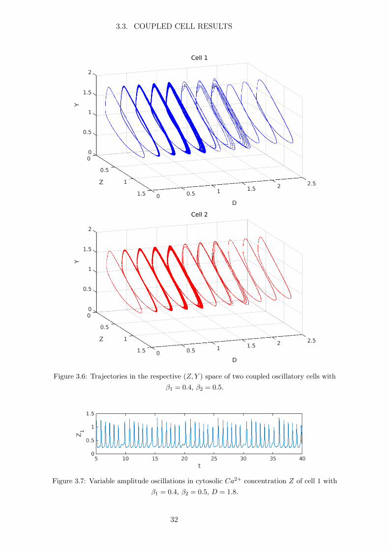
Consider two oscillatory cells with β1 = 0.4, β2 = 0.5. When uncoupled cell 1 will
oscillate with greater amplitude and period than cell 2 (see Figures 3.3, 3.5). The trajec-
tories for each cell are shown in Figure 3.6. When uncoupled (D = 0) the cells oscillate
independently, represented by a simple LC trajectory. When coupled together (D > 0)
the flux of Ca2+ from cell to cell will interfere with the oscillations causing the cells to
both oscillate with variable amplitude, represented by additional ‘loops’ in the trajectory.
This produces amplitude modulated oscillations as seen in Figure 3.7, where the ampli-
tude of oscillations is effectively a function of time instead of constant. As the coupling
strength D increases the intercellular flux of Ca2+ becomes larger and as a result more
‘loops’ are added to the cell trajectories. Finally when the coupling strength is strong
enough the cells synchronise and act as one, oscillating with the same frequency and
similar amplitude corresponding to a simple LC in the phase space.
These oscillations can be viewed as a ‘signal’ composed of one or more frequencies,
either in the time domain (as in Figure 3.7) or in the frequency domain. By using a
Fourier transform we can decompose a signal into a series of sinusoidal functions with
different frequencies and the distribution of these frequencies is called the power spectrum.
For example a simple sine wave will decompose into a single frequency with the power
of the frequency corresponding to the amplitude of the wave. Using a Fourier transform
of the cytosolic Ca2+ concentration Z of each cell we are able to examine their power
spectra and thus analyse the distribution of power among the frequencies that make up
these oscillatory ‘signals’. This provides an additional technique to analyse the change in
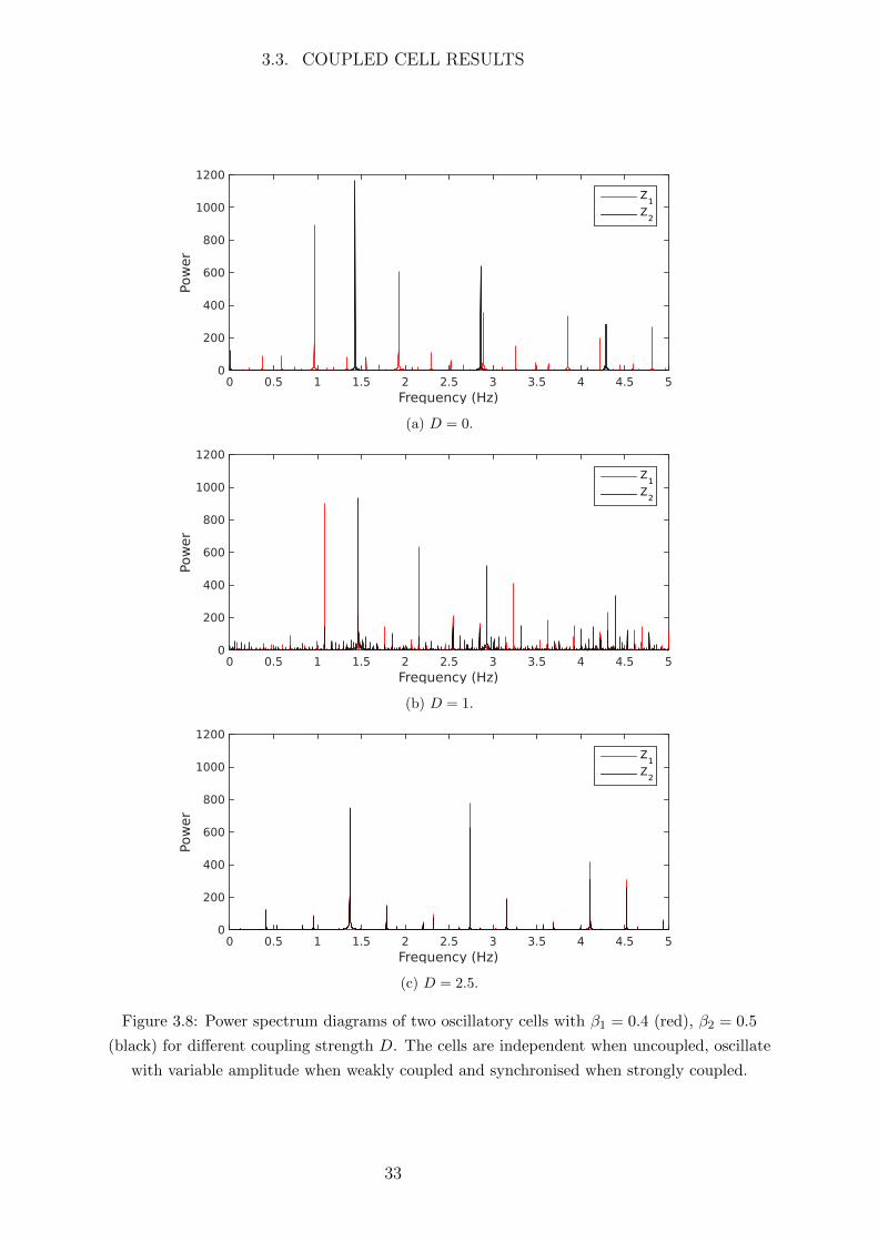
behaviour as the cells are coupled. Figure 3.8 shows the power spectra of each oscillatory
cell at different coupling strengths.
When the cells are uncoupled (D = 0) their respective power spectra are completely
independent (Figure 3.8a). By increasing the coupling to D = 1 we find that the distri-
bution of power among the frequencies of the cells are irregular, indicating that the cells
are exhibiting complex behaviour (Figure 3.8b). With strong coupling (D = 2.5) the
power spectra of the two cells are almost identical with differences only in power (Figure
3.8c). This indicates the cells have become synchronised. The only difference when the
cells are synchronised is the amplitude of the frequency spikes, so to clearly see the level
of synchronisation we examine the difference in power between the cells.
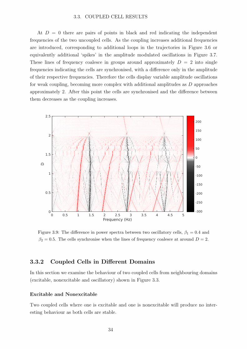
As both the trajectories and frequency distributions of the cells qualitatively change
as the coupling increases, we expect some form of ‘frequency bifurcation’ to occur where
the cells begin to synchronise. To see this we plot the difference between the power
spectra of the two cells (cell 1 minus cell 2) for varying coupling strength D in Figure 3.9.
The colour represents the difference in power between the cells, with red representing the
frequencies at which cell 1 has greater amplitude and black representing the frequencies
at which cell 2 has greater amplitude.
31
3.3. COUPLED CELL RESULTS
Figure 3.6: Trajectories in the respective (Z, Y ) space of two coupled oscillatory cells with
β1 = 0.4, β2 = 0.5.
Figure 3.7: Variable amplitude oscillations in cytosolic Ca2+ concentration Z of cell 1 with
β1 = 0.4, β2 = 0.5, D = 1.8.
32
3.3. COUPLED CELL RESULTS
Frequency (Hz)0 0.5 1 1.5 2 2.5 3 3.5 4 4.5 5
Pow
er
0
200
400
600
800
1000
1200
Z1
Z2
(a) D = 0.
Frequency (Hz)0 0.5 1 1.5 2 2.5 3 3.5 4 4.5 5
Pow
er
0
200
400
600
800
1000
1200
Z1
Z2
(b) D = 1.
Frequency (Hz)0 0.5 1 1.5 2 2.5 3 3.5 4 4.5 5
Pow
er
0
200
400
600
800
1000
1200
Z1
Z2
(c) D = 2.5.
Figure 3.8: Power spectrum diagrams of two oscillatory cells with β1 = 0.4 (red), β2 = 0.5
(black) for different coupling strength D. The cells are independent when uncoupled, oscillate
with variable amplitude when weakly coupled and synchronised when strongly coupled.
33
3.3. COUPLED CELL RESULTS
At D = 0 there are pairs of points in black and red indicating the independent
frequencies of the two uncoupled cells. As the coupling increases additional frequencies
are introduced, corresponding to additional loops in the trajectories in Figure 3.6 or
equivalently additional ‘spikes’ in the amplitude modulated oscillations in Figure 3.7.
These lines of frequency coalesce in groups around approximately D = 2 into single
frequencies indicating the cells are synchronised, with a difference only in the amplitude
of their respective frequencies. Therefore the cells display variable amplitude oscillations
for weak coupling, becoming more complex with additional amplitudes as D approaches
approximately 2. After this point the cells are synchronised and the difference between
them decreases as the coupling increases.
Frequency (Hz)0 0.5 1 1.5 2 2.5 3 3.5 4 4.5 5
D
0
0.5
1
1.5
2
2.5
-300
-250
-200
-150
-100
-50
0
50
100
150
200
Figure 3.9: The difference in power spectra between two oscillatory cells, β1 = 0.4 and
β2 = 0.5. The cells synchronise when the lines of frequency coalesce at around D = 2.
3.3.2 Coupled Cells in Different Domains
In this section we examine the behaviour of two coupled cells from neighbouring domains
(excitable, nonexcitable and oscillatory) shown in Figure 3.3.
Excitable and Nonexcitable
Two coupled cells where one is excitable and one is nonexcitable will produce no inter-
esting behaviour as both cells are stable.
34
3.3. COUPLED CELL RESULTS
Oscillatory and Nonexcitable
Weakly coupling a nonexcitable cell with an oscillatory cell induces a small flux of Ca2+
into the nonexcitable cell causing it to immediately oscillate with small amplitude and
the same frequency as the oscillatory cell for D > 0 in Figure 3.10. As the coupling
strength increases the amplitude of oscillations of the nonexcitable cell increases as it
becomes more similar in behaviour to the oscillatory cell. Note that the average β of the
two cells lies in the oscillatory domain of Figure 3.3 and hence when strongly coupled the
cells will both oscillate. If the average β was instead in the nonexcitable domain then
the cells would tend to a stable state when strongly coupled.
As the cells always oscillate with the same frequency the power spectra of each cell
are identical in frequency distribution and differ only in power.
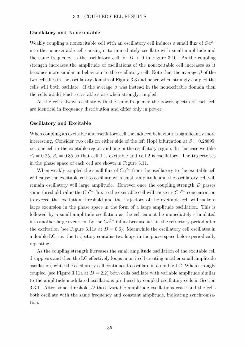
Oscillatory and Excitable
When coupling an excitable and oscillatory cell the induced behaviour is significantly more
interesting. Consider two cells on either side of the left Hopf bifurcation at β = 0.28895,
i.e. one cell in the excitable region and one in the oscillatory region. In this case we take
β1 = 0.25, β2 = 0.35 so that cell 1 is excitable and cell 2 is oscillatory. The trajectories
in the phase space of each cell are shown in Figure 3.11.
When weakly coupled the small flux of Ca2+ from the oscillatory to the excitable cell
will cause the excitable cell to oscillate with small amplitude and the oscillatory cell will
remain oscillatory will large amplitude. However once the coupling strength D passes
some threshold value the Ca2+ flux to the excitable cell will cause its Ca2+ concentration
to exceed the excitation threshold and the trajectory of the excitable cell will make a
large excursion in the phase space in the form of a large amplitude oscillation. This is
followed by a small amplitude oscillation as the cell cannot be immediately stimulated
into another large excursion by the Ca2+ influx because it is in the refractory period after
the excitation (see Figure 3.11a at D = 0.6). Meanwhile the oscillatory cell oscillates in
a double LC, i.e. the trajectory contains two loops in the phase space before periodically
repeating.
As the coupling strength increases the small amplitude oscillation of the excitable cell
disappears and then the LC effectively loops in on itself creating another small amplitude
oscillation, while the oscillatory cell continues to oscillate in a double LC. When strongly
coupled (see Figure 3.11a at D = 2.2) both cells oscillate with variable amplitude similar
to the amplitude modulated oscillations produced by coupled oscillatory cells in Section
3.3.1. After some threshold D these variable amplitude oscillations cease and the cells
both oscillate with the same frequency and constant amplitude, indicating synchronisa-
tion.
35

3.3. COUPLED CELL RESULTS
(a) Nonexcitable cell 1 with β1 = 0.8
(b) Oscillatory cell 2 with β2 = 0.7
Figure 3.10: Trajectories in the (Z, Y ) space of each cell. The nonexcitable cell 1 oscillates
with the same frequency as cell 1 when coupled due to the Ca2+ flux from the oscillatory cell
2. The amplitude of these oscillations increases as the coupling D increases.
36
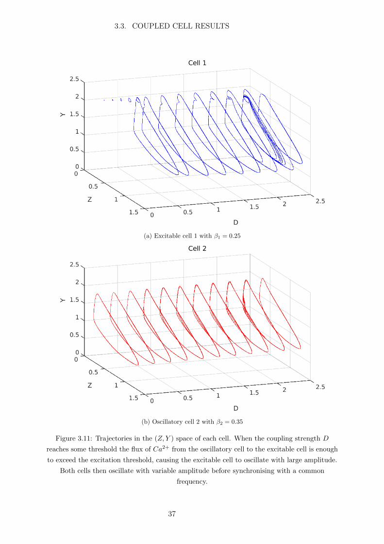
3.3. COUPLED CELL RESULTS
(a) Excitable cell 1 with β1 = 0.25
(b) Oscillatory cell 2 with β2 = 0.35
Figure 3.11: Trajectories in the (Z, Y ) space of each cell. When the coupling strength D
reaches some threshold the flux of Ca2+ from the oscillatory cell to the excitable cell is enough
to exceed the excitation threshold, causing the excitable cell to oscillate with large amplitude.
Both cells then oscillate with variable amplitude before synchronising with a common
frequency.
37
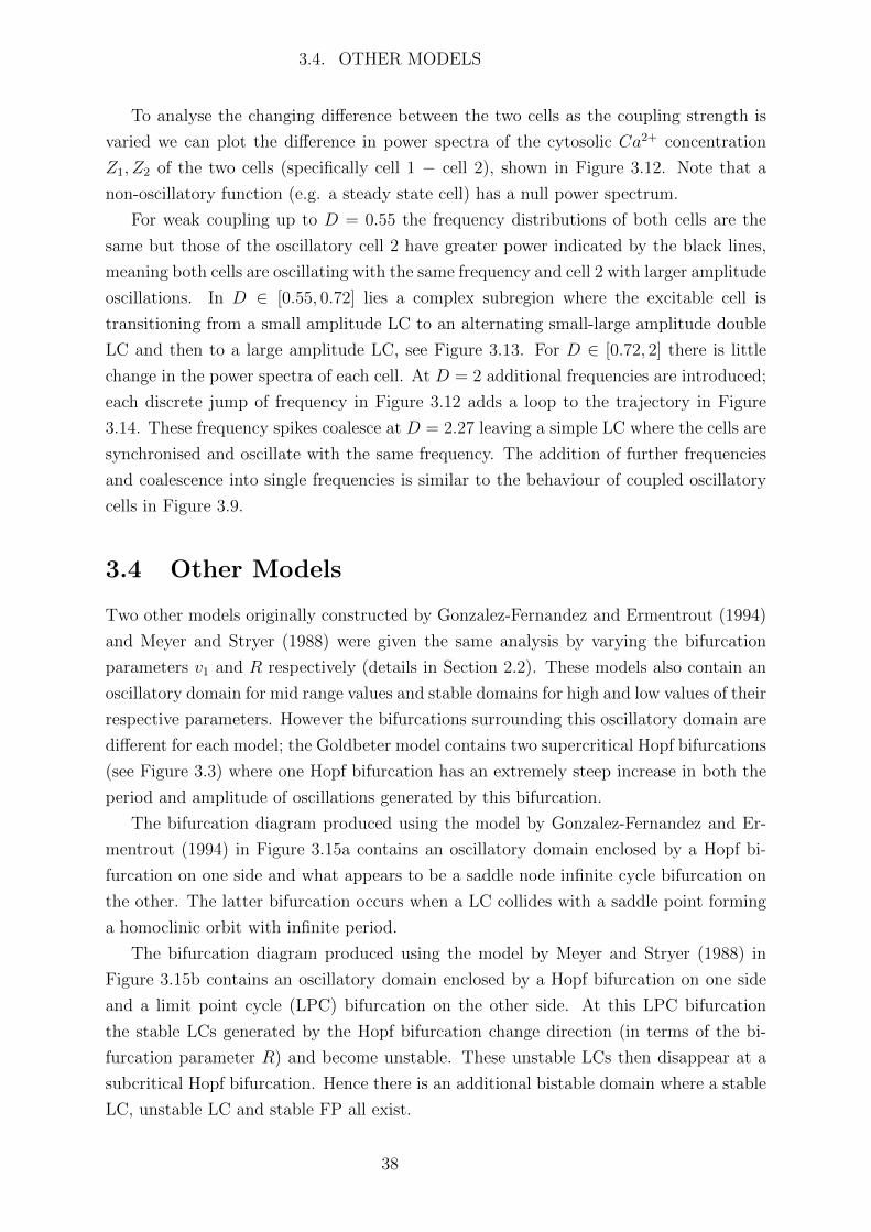
3.4. OTHER MODELS
To analyse the changing difference between the two cells as the coupling strength is
varied we can plot the difference in power spectra of the cytosolic Ca2+ concentration
Z1, Z2 of the two cells (specifically cell 1 − cell 2), shown in Figure 3.12. Note that a
non-oscillatory function (e.g. a steady state cell) has a null power spectrum.
For weak coupling up to D = 0.55 the frequency distributions of both cells are the
same but those of the oscillatory cell 2 have greater power indicated by the black lines,
meaning both cells are oscillating with the same frequency and cell 2 with larger amplitude
oscillations. In D ∈ [0.55, 0.72] lies a complex subregion where the excitable cell is
transitioning from a small amplitude LC to an alternating small-large amplitude double
LC and then to a large amplitude LC, see Figure 3.13. For D ∈ [0.72, 2] there is little
change in the power spectra of each cell. At D = 2 additional frequencies are introduced;
each discrete jump of frequency in Figure 3.12 adds a loop to the trajectory in Figure
3.14. These frequency spikes coalesce at D = 2.27 leaving a simple LC where the cells are
synchronised and oscillate with the same frequency. The addition of further frequencies
and coalescence into single frequencies is similar to the behaviour of coupled oscillatory
cells in Figure 3.9.
3.4 Other Models
Two other models originally constructed by Gonzalez-Fernandez and Ermentrout (1994)
and Meyer and Stryer (1988) were given the same analysis by varying the bifurcation
parameters v1 and R respectively (details in Section 2.2). These models also contain an
oscillatory domain for mid range values and stable domains for high and low values of their
respective parameters. However the bifurcations surrounding this oscillatory domain are
different for each model; the Goldbeter model contains two supercritical Hopf bifurcations
(see Figure 3.3) where one Hopf bifurcation has an extremely steep increase in both the
period and amplitude of oscillations generated by this bifurcation.
The bifurcation diagram produced using the model by Gonzalez-Fernandez and Er-
mentrout (1994) in Figure 3.15a contains an oscillatory domain enclosed by a Hopf bi-
furcation on one side and what appears to be a saddle node infinite cycle bifurcation on
the other. The latter bifurcation occurs when a LC collides with a saddle point forming
a homoclinic orbit with infinite period.
The bifurcation diagram produced using the model by Meyer and Stryer (1988) in
Figure 3.15b contains an oscillatory domain enclosed by a Hopf bifurcation on one side
and a limit point cycle (LPC) bifurcation on the other side. At this LPC bifurcation
the stable LCs generated by the Hopf bifurcation change direction (in terms of the bi-
furcation parameter R) and become unstable. These unstable LCs then disappear at a
subcritical Hopf bifurcation. Hence there is an additional bistable domain where a stable
LC, unstable LC and stable FP all exist.
38
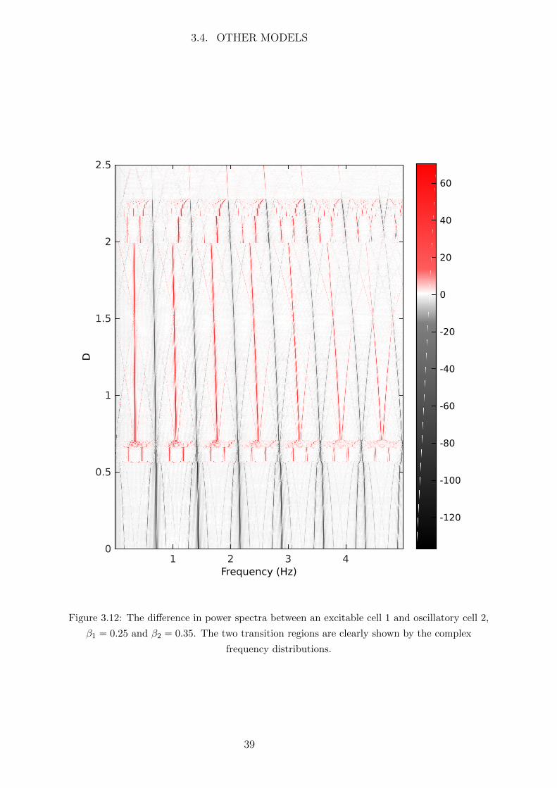
3.4. OTHER MODELS
Frequency (Hz)1 2 3 4
D
0
0.5
1
1.5
2
2.5
-120
-100
-80
-60
-40
-20
0
20
40
60
Figure 3.12: The difference in power spectra between an excitable cell 1 and oscillatory cell 2,
β1 = 0.25 and β2 = 0.35. The two transition regions are clearly shown by the complex
frequency distributions.
39
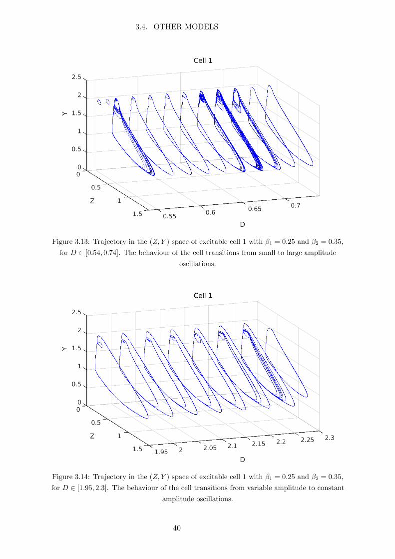
3.4. OTHER MODELS
Figure 3.13: Trajectory in the (Z, Y ) space of excitable cell 1 with β1 = 0.25 and β2 = 0.35,
for D ∈ [0.54, 0.74]. The behaviour of the cell transitions from small to large amplitude
oscillations.
Figure 3.14: Trajectory in the (Z, Y ) space of excitable cell 1 with β1 = 0.25 and β2 = 0.35,
for D ∈ [1.95, 2.3]. The behaviour of the cell transitions from variable amplitude to constant
amplitude oscillations.
40
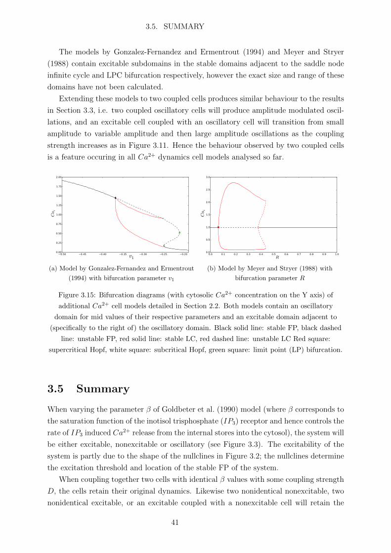
3.5. SUMMARY
The models by Gonzalez-Fernandez and Ermentrout (1994) and Meyer and Stryer
(1988) contain excitable subdomains in the stable domains adjacent to the saddle node
infinite cycle and LPC bifurcation respectively, however the exact size and range of these
domains have not been calculated.
Extending these models to two coupled cells produces similar behaviour to the results
in Section 3.3, i.e. two coupled oscillatory cells will produce amplitude modulated oscil-
lations, and an excitable cell coupled with an oscillatory cell will transition from small
amplitude to variable amplitude and then large amplitude oscillations as the coupling
strength increases as in Figure 3.11. Hence the behaviour observed by two coupled cells
is a feature occuring in all Ca2+ dynamics cell models analysed so far.
(a) Model by Gonzalez-Fernandez and Ermentrout
(1994) with bifurcation parameter v1
(b) Model by Meyer and Stryer (1988) with
bifurcation parameter R
Figure 3.15: Bifurcation diagrams (with cytosolic Ca2+ concentration on the Y axis) of
additional Ca2+ cell models detailed in Section 2.2. Both models contain an oscillatory
domain for mid values of their respective parameters and an excitable domain adjacent to
(specifically to the right of) the oscillatory domain. Black solid line: stable FP, black dashed
line: unstable FP, red solid line: stable LC, red dashed line: unstable LC Red square:
supercritical Hopf, white square: subcritical Hopf, green square: limit point (LP) bifurcation.
3.5 Summary
When varying the parameter β of Goldbeter et al. (1990) model (where β corresponds to
the saturation function of the inotisol trisphosphate (IP3) receptor and hence controls the
rate of IP3 induced Ca2+ release from the internal stores into the cytosol), the system will
be either excitable, nonexcitable or oscillatory (see Figure 3.3). The excitability of the
system is partly due to the shape of the nullclines in Figure 3.2; the nullclines determine
the excitation threshold and location of the stable FP of the system.
When coupling together two cells with identical β values with some coupling strength
D, the cells retain their original dynamics. Likewise two nonidentical nonexcitable, two
nonidentical excitable, or an excitable coupled with a nonexcitable cell will retain the
41

3.5. SUMMARY
dynamics of their uncoupled state. However an oscillatory coupled with a nonexcitable
cell will cause the nonexcitable cell to oscillate with small amplitude when weakly cou-
pled; their behaviour when strongly coupled is dependent on the dynamics of a cell with
the average β value of the two cells. Two nonidentical oscillatory cells will experience
variable amplitude oscillations when weakly coupled, and synchronise by oscillating with
constant amplitude and frequency when strongly coupled. An oscillatory and excitable
cell coupled together will cause the excitable cell to oscillate with small amplitude when
weakly coupled. When the coupling strength exceeds some threshold value the Ca2+ flux
from the oscillatory cell will be high enough to exceed the excitation threshold of the ex-
citable cell, causing it to alternate between large and small amplitude oscillations. As the
coupling strength increases both cells oscillate with variable amplitude and synchronise
when strongly coupled. These coupled cell dynamics occur for each of the three SMC
models.
42
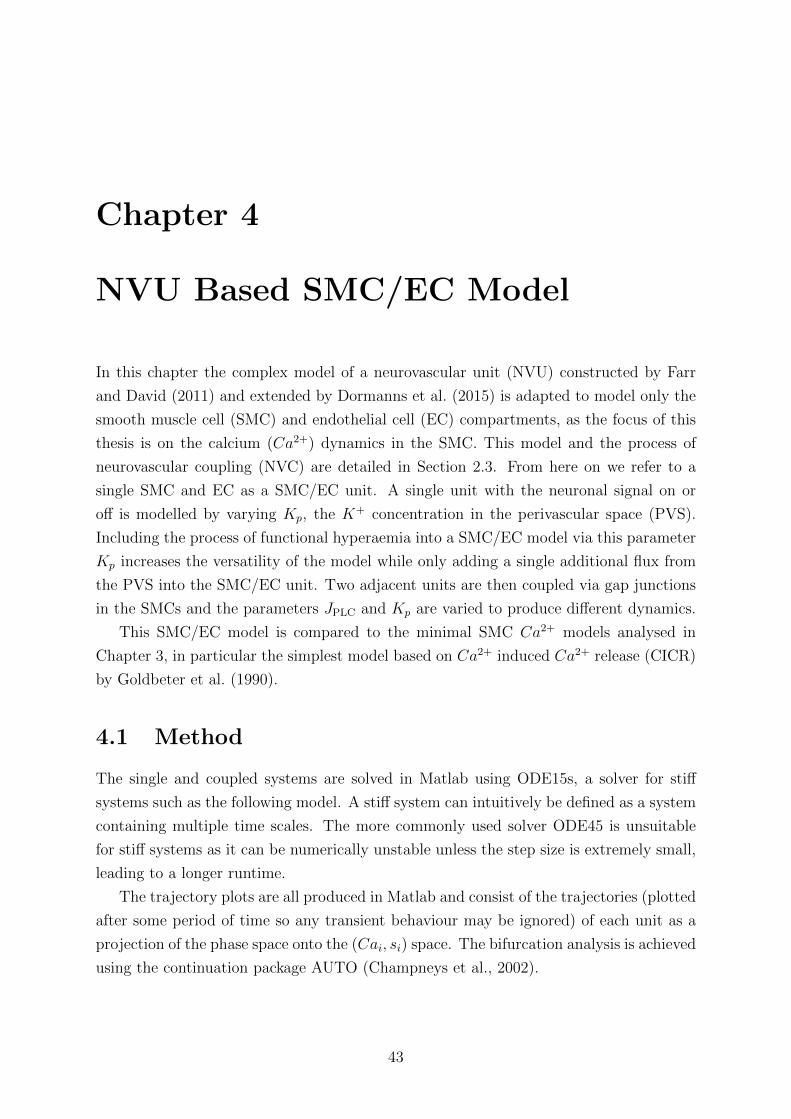
Chapter 4
NVU Based SMC/EC Model
In this chapter the complex model of a neurovascular unit (NVU) constructed by Farr
and David (2011) and extended by Dormanns et al. (2015) is adapted to model only the
smooth muscle cell (SMC) and endothelial cell (EC) compartments, as the focus of this
thesis is on the calcium (Ca2+) dynamics in the SMC. This model and the process of
neurovascular coupling (NVC) are detailed in Section 2.3. From here on we refer to a
single SMC and EC as a SMC/EC unit. A single unit with the neuronal signal on or
off is modelled by varying Kp, the K+ concentration in the perivascular space (PVS).
Including the process of functional hyperaemia into a SMC/EC model via this parameter
Kp increases the versatility of the model while only adding a single additional flux from
the PVS into the SMC/EC unit. Two adjacent units are then coupled via gap junctions
in the SMCs and the parameters JPLC and Kp are varied to produce different dynamics.
This SMC/EC model is compared to the minimal SMC Ca2+ models analysed in
Chapter 3, in particular the simplest model based on Ca2+ induced Ca2+ release (CICR)
by Goldbeter et al. (1990).
4.1 Method
The single and coupled systems are solved in Matlab using ODE15s, a solver for stiff
systems such as the following model. A stiff system can intuitively be defined as a system
containing multiple time scales. The more commonly used solver ODE45 is unsuitable
for stiff systems as it can be numerically unstable unless the step size is extremely small,
leading to a longer runtime.
The trajectory plots are all produced in Matlab and consist of the trajectories (plotted
after some period of time so any transient behaviour may be ignored) of each unit as a
projection of the phase space onto the (Cai, si) space. The bifurcation analysis is achieved
using the continuation package AUTO (Champneys et al., 2002).
43

4.1. METHOD
4.1.1 SMC/EC Model
The SMC/EC model based on the NVU model removes the neuron (NE), synaptic cleft
(SC) and astrocyte (AC) compartments reducing the number of state variables from 24
to 14. These variables are: SMC cytosolic Ca2+ concentration (Cai), SMC Ca2+ concen-
tration in the internal stores (si), SMC membrane potential (vi), open state probability of
Ca2+-activated potassium (K+) channels (wi), SMC cytosolic inotisol trisphosphate (IP3)
concentration (Ii), SMC cytosolic K+ concentration (Ki), EC cytosolic Ca2+ concentra-
tion (Caj), EC Ca2+ concentration in the internal stores (sj), EC membrane potential
(vj), EC cytosolic IP3 concentration (Ij), fraction of free phosphorylated cross-bridges
(Mp), fraction of attached phosphorylated cross-bridges (AMp), fraction of attached
dephosphorylated cross-bridges (AM), and vessel radius (R). The variable Ki (SMC
cytosolic K+ concentration) does not appear in any other differential equation, so if not
needed it can be omitted to reduce the number of variables to 13.
The hydrolysis of phosphatidylinositol 4,5-bisphosphate by phospholipase-C (PLC)
results in the formation of IP3 which stimulates the release of Ca2+ from the internal
stores of the EC. The flux of PLC in the EC is denoted JPLC. This is our bifurcation
parameter - when JPLC is varied between 0 and 1 there are qualitative changes in the
dynamics of the system.
The only connecting input in the NVU model from the NE, SC and AC compartments
to the SMC/EC submodule is Kp, the K+ concentration in the PVS. Neuronal activity
causes an increase in K+ concentration in the SC resulting in an increased K+ uptake by
the AC and consquently an efflux of K+ into the PVS through the big potassium (BK)
channel at the endfeet of the AC. Therefore neuronal activity will cause an increase in K+
concentration in the PVS and Kp may be used as an input parameter for the neuronal
signal in the SMC/EC model. This parameter Kp modifies the flux of K+ through the
inward rectifying potassium (KIR) channel at the interface of the PVS and SMC.
Kp has a very slight dependency on JPLC in the full NVU model as follows: when the
neuronal signal is on the minimum is Kp = 9141, the maximum is Kp = 9277, and the
average (for JPLC ∈ [0, 1]) is Kp = 9176. When the neuronal signal is off the minimum is
Kp = 3381, the maximum is Kp = 3404, and the average (for JPLC ∈ [0, 1]) is Kp = 3395.
Hence we use Kp = 9200 corresponding to having the neuronal signal on and Kp = 3400
for neuronal signal off. In Section 4.2.3 it is shown that the bifurcation structure of the
model does not qualitatively change within these two ranges.
4.1.2 Coupled SMC/EC Model
The two units are coupled through gap junctions between the SMCs. There are several
options for coupling, namely Ca2+, IP3 and membrane potential V . We find that coupling
44

4.2. SINGLE SMC/EC RESULTS
only Ca2+ is sufficient to induce synchronisation when strongly coupled and complex
behaviour when weakly coupled. Adding IP3 and/or V coupling makes little difference
in behaviour and was therefore deemed unnecessary. Coupling with only IP3 or only V
does not allow synchronisation of the coupled units (results not shown). Therefore to
couple the two SMC/EC units we include only a flux of Ca2+ to and from the SMCs of
the coupled system. For simplicity any coupling term between the gap junctions of the
two ECs has been omitted as there is no significant difference from just SMC coupling
(results not shown).
The Ca2+ flux from SMC to SMC is modelled similarly to the coupling fluxes between
the SMC and EC:
JSMC−SMCCa2+coupling = D(Cai1 − Cai2), (4.1)
where this flux is added or subtracted onto the two SMC Ca2+ differential equations:
dCai1dt
= . . .− JSMC−SMCCa2+coupling,
dCai2dt
= . . .+ JSMC−SMCCa2+coupling, (4.2)
and D is the coupling coefficient with units of s−1. The physiological value of the param-
eter D is unknown so a range of values are used.
When we couple two units we mainly consider them with different JPLC values in the
EC as in reality adjacent cells are not identical. The same value of Kp is used for both
units but later we consider the possibility of two units with different Kp corresponding to
different levels of neuronal activity in Section 4.3.3. There is no non-dimensionalisation
for this model. As there are 14 variables it is not easily implemented like the previous
2D or 3D models studied in Chapter 3. The coupled SMC/EC model diagram depicting
the various compartments and ion channels is shown in Figure 4.1.
4.2 Single SMC/EC Results
The resulting bifurcation diagrams of the system with both Kp = 3400 (neuronal signal
off) and Kp = 9200 (neuronal signal on) are shown in Figure 4.2a for easy comparison.
The period of oscillations for both cases are shown in Figure 4.2b.
4.2.1 Signal off (Kp = 3400)
The bifurcation diagram of the system with Kp = 3400 is denoted by red in Figure 4.2a.
For low and high JPLC the system tends to a stable fixed point (FP) while for medium
values of JPLC the system oscillates. The qualitative change in behaviour between stable
and oscillatory is due to two supercritical Hopf bifurcations that change the stability of
the FP from stable to unstable and generate stable limit cycles (LCs).
The period of the oscillations is given in Figure 4.2b, denoted in red. The period
increases from the left Hopf and reaches a maximum at approximately JPLC = 0.26
45
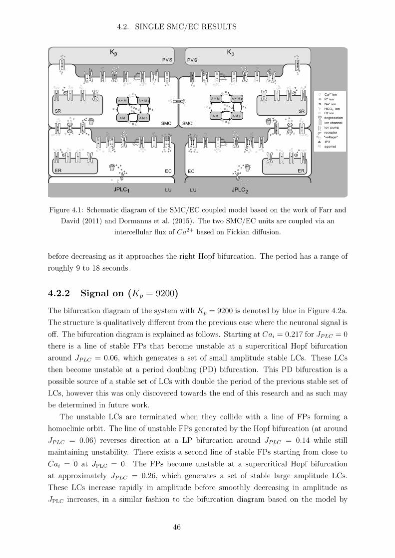
4.2. SINGLE SMC/EC RESULTS
PVS
EC
SMC
ER
SR
A s M A s M p
A M pA M
K 1
K 2K 7 K 3 K 4K 5
K 6
LU
PVS
EC ER
SR
LUJPLC JPLC1 2
A s M A s M p
A M pA M
K 1
K 2K 7 K 3 K 4K 5
K 6SMC
s _
Ca2slion
Kslionl
Naslionl
HCO3vlionl
Clvlionl
degradationl
ionlchannell
ionlpumpl
receptorl
IP3l
agonistl
evoltageel
Kp Kp
Figure 4.1: Schematic diagram of the SMC/EC coupled model based on the work of Farr and
David (2011) and Dormanns et al. (2015). The two SMC/EC units are coupled via an
intercellular flux of Ca2+ based on Fickian diffusion.
before decreasing as it approaches the right Hopf bifurcation. The period has a range of
roughly 9 to 18 seconds.
4.2.2 Signal on (Kp = 9200)
The bifurcation diagram of the system with Kp = 9200 is denoted by blue in Figure 4.2a.
The structure is qualitatively different from the previous case where the neuronal signal is
off. The bifurcation diagram is explained as follows. Starting at Cai = 0.217 for JPLC = 0
there is a line of stable FPs that become unstable at a supercritical Hopf bifurcation
around JPLC = 0.06, which generates a set of small amplitude stable LCs. These LCs
then become unstable at a period doubling (PD) bifurcation. This PD bifurcation is a
possible source of a stable set of LCs with double the period of the previous stable set of
LCs, however this was only discovered towards the end of this research and as such may
be determined in future work.
The unstable LCs are terminated when they collide with a line of FPs forming a
homoclinic orbit. The line of unstable FPs generated by the Hopf bifurcation (at around
JPLC = 0.06) reverses direction at a LP bifurcation around JPLC = 0.14 while still
maintaining unstability. There exists a second line of stable FPs starting from close to
Cai = 0 at JPLC = 0. The FPs become unstable at a supercritical Hopf bifurcation
at approximately JPLC = 0.26, which generates a set of stable large amplitude LCs.
These LCs increase rapidly in amplitude before smoothly decreasing in amplitude as
JPLC increases, in a similar fashion to the bifurcation diagram based on the model by
46

4.2. SINGLE SMC/EC RESULTS
(a) Bifurcation diagram with JPLC as the bifurcation parameter and the cytosolic SMC Ca2+
concentration on the Y axis.
(b) Period of oscillations (note the different x axis scale to Figure 4.2a).
Figure 4.2: Different dynamics of the SMC/EC model (based on the NVU model by Farr and
David (2011), Dormanns et al. (2015)) with the parameter JPLC varied and the neuronal input
signal either on or off, modelled by a change in the parameter Kp.
Red line: signal off (Kp = 3400), blue line: signal on (Kp = 9200). Solid: stable, Dashed:
unstable. Black square: supercritical Hopf bifurcation, yellow diamond: Period Doubling (PD)
bifurcation, green triangle: limit point (LP) bifurcation.
47

4.2. SINGLE SMC/EC RESULTS
Goldbeter et al. (1990) in Section 3.2. The unstable line of FPs become stable again at a
second supercritical Hopf bifurcation at approximately JPLC = 0.57, and the stable LCs
are terminated.
For small JPLC less than approximately 0.06 there is bistability present as there are
two stable FPs that exist. The Ca2+ concentration can either settle to a FP at approxi-
mately Cai = 0.217 or at a FP close to Cai = 0. For JPLC between approximately 0.06
and 0.14 there is bistability present again as there exists one stable FP and one stable
LC. The Ca2+ concentration will either oscillate with small amplitude or settle to a FP
with lower Cai. Note that these two bistable domains do not exist when the neuronal
signal is off.
The period of oscillations for both the small and large amplitude LCs found when
Kp = 9200 are given in Figure 4.2b, denoted in blue. The period of the large amplitude
LC when the neuronal signal is on has a range of about 10 to 40 seconds, approximately
double than when the signal is off. The period of the small amplitude stable LC is less
than 10 seconds. However as JPLC approaches approximately 0.12 the period of the small
amplitude unstable LC increases to infinity. This is characteristic of a homoclinic orbit
where the LCs collide with the line of FPs and disappear. The period for the large am-
plitude LCs sharply increases from the Hopf bifurcation at JPLC = 0.26 and reaches a
maximum at approximately JPLC = 0.27, smoothly decreasing as JPLC increases. This is
similar to where the neuronal signal is off but with a steeper increase in period after the
left Hopf bifurcation.
The sharp increase in amplitude and period of oscillations after the Hopf bifurcation
is similar to the bifurcation diagram of the Goldbeter model in Section 3.2, especially
when Kp = 9200. This suggests that the behaviour of the system for JPLC close to
the bifurcation may be similar to the Goldbeter model as well, i.e. the system will be
excitable (see Section 2.2 for details on excitability). Simulations (not included) have
shown that this is in fact correct, there is an excitable region for JPLC close to the Hopf
bifurcation but the exact size and range of this region has not been calculated.
However the system is only weakly excitable when the neuronal signal is turned off
(Kp = 3400), meaning the ‘spike’ of Ca2+ produced by an initial perturbation to the
system (such as a small input of Ca2+) will not be as large as that produced when the
neuronal signal is on (Kp = 9200). It appears the steeper the increase in amplitude and
period of oscillations after the Hopf bifurcation in the SMC/EC model and the SMC
model by Goldbeter et al. (1990), the more excitable the system (i.e. a larger range of
JPLC where the system is excitable, lower excitation threshold and larger ‘spike’ produced
by an initial perturbation over this threshold).
48
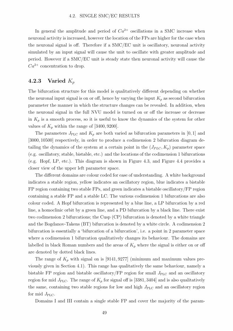
4.2. SINGLE SMC/EC RESULTS
In general the amplitude and period of Ca2+ oscillations in a SMC increase when
neuronal activity is increased, however the location of the FPs are higher for the case when
the neuronal signal is off. Therefore if a SMC/EC unit is oscillatory, neuronal activity
simulated by an input signal will cause the unit to oscillate with greater amplitude and
period. However if a SMC/EC unit is steady state then neuronal activity will cause the
Ca2+ concentration to drop.
4.2.3 Varied Kp
The bifurcation structure for this model is qualitatively different depending on whether
the neuronal input signal is on or off, hence by varying the input Kp as second bifurcation
parameter the manner in which the structure changes can be revealed. In addition, when
the neuronal signal in the full NVU model is turned on or off the increase or decrease
in Kp is a smooth process, so it is useful to know the dynamics of the system for other
values of Kp within the range of [3400, 9200].
The parameters JPLC and Kp are both varied as bifurcation parameters in [0, 1] and
[3000, 10500] respectively, in order to produce a codimension 2 bifurcation diagram de-
tailing the dynamics of the system at a certain point in the (JPLC , Kp) parameter space
(e.g. oscillatory, stable, bistable, etc.) and the locations of the codimension 1 bifurcations
(e.g. Hopf, LP, etc.). This diagram is shown in Figure 4.3, and Figure 4.4 provides a
closer view of the upper left parameter space.
The different domains are colour coded for ease of understanding. A white background
indicates a stable region, yellow indicates an oscillatory region, blue indicates a bistable
FP region containing two stable FPs, and green indicates a bistable oscillatory/FP region
containing a stable FP and a stable LC. The various codimension 1 bifurcations are also
colour coded. A Hopf bifurcation is represented by a blue line, a LP bifurcation by a red
line, a homoclinic orbit by a green line, and a PD bifurcation by a black line. There exist
two codimension 2 bifurcations; the Cusp (CP) bifurcation is denoted by a white triangle
and the Bogdanov-Takens (BT) bifurcation is denoted by a white circle. A codimension 2
bifurcation is essentially a ‘bifurcation of a bifurcation’, i.e. a point in 2 parameter space
where a codimension 1 bifurcation qualitatively changes its behaviour. The domains are
labelled in black Roman numbers and the areas of Kp where the signal is either on or off
are denoted by dotted black lines.
The range of Kp with signal on is [9141, 9277] (minimum and maximum values pre-
viously given in Section 4.1). This range has qualitatively the same behaviour, namely a
bistable FP region and bistable oscillatory/FP region for small JPLC and an oscillatory
region for mid JPLC. The range of Kp for signal off is [3381, 3404] and is also qualitatively
the same, containing two stable regions for low and high JPLC and an oscillatory region
for mid JPLC.
Domains I and III contain a single stable FP and cover the majority of the param-
49

4.2. SINGLE SMC/EC RESULTS
HopfLP
Signal on
Signal off
II IIII
Figure 4.3: Codimension 2 bifurcation diagram of the (JPLC ,Kp) parameter space. The space
is subdivided into domains of different dynamics by various codimension 1 bifurcations such as
Hopf and LP bifurcations. There is an excitable subdomain to the left of the Hopf seperating
domain I and II, not shown as the exact size has not been calculated.
White area: stable, yellow area: oscillatory, blue area: bistable FPs, green area: bistable
oscillatory/FP. Blue line: supercritical Hopf bifurcation, red line: LP bifurcation.
50
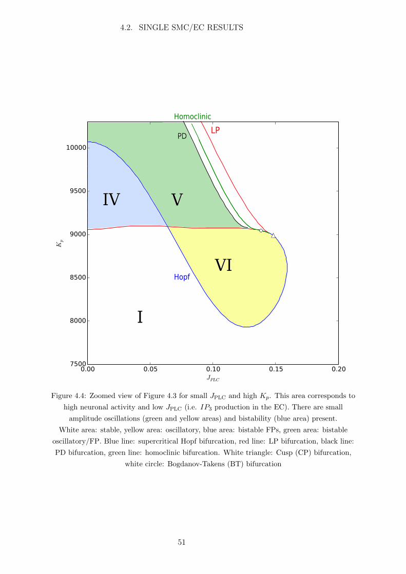
4.2. SINGLE SMC/EC RESULTS
LP
Hopf
Homoclinic
PD
I
IV V
VI
Figure 4.4: Zoomed view of Figure 4.3 for small JPLC and high Kp. This area corresponds to
high neuronal activity and low JPLC (i.e. IP3 production in the EC). There are small
amplitude oscillations (green and yellow areas) and bistability (blue area) present.
White area: stable, yellow area: oscillatory, blue area: bistable FPs, green area: bistable
oscillatory/FP. Blue line: supercritical Hopf bifurcation, red line: LP bifurcation, black line:
PD bifurcation, green line: homoclinic bifurcation. White triangle: Cusp (CP) bifurcation,
white circle: Bogdanov-Takens (BT) bifurcation
51
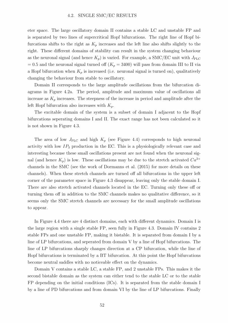
4.2. SINGLE SMC/EC RESULTS
eter space. The large oscillatory domain II contains a stable LC and unstable FP and
is separated by two lines of supercritical Hopf bifurcations. The right line of Hopf bi-
furcations shifts to the right as Kp increases and the left line also shifts slightly to the
right. These different domains of stability can result in the system changing behaviour
as the neuronal signal (and hence Kp) is varied. For example, a SMC/EC unit with JPLC
= 0.5 and the neuronal signal turned off (Kp = 3400) will pass from domain III to II via
a Hopf bifurcation when Kp is increased (i.e. neuronal signal is turned on), qualitatively
changing the behaviour from stable to oscillatory.
Domain II corresponds to the large amplitude oscillations from the bifurcation di-
agrams in Figure 4.2a. The period, amplitude and maximum value of oscillations all
increase as Kp increases. The steepness of the increase in period and amplitude after the
left Hopf bifurcation also increases with Kp.
The excitable domain of the system is a subset of domain I adjacent to the Hopf
bifurcations seperating domains I and II. The exact range has not been calculated so it
is not shown in Figure 4.3.
The area of low JPLC and high Kp (see Figure 4.4) corresponds to high neuronal
activity with low IP3 production in the EC. This is a physiologically relevant case and
interesting because these small oscillations present are not found when the neuronal sig-
nal (and hence Kp) is low. These oscillations may be due to the stretch activated Ca2+
channels in the SMC (see the work of Dormanns et al. (2015) for more details on these
channels). When these stretch channels are turned off all bifurcations in the upper left
corner of the parameter space in Figure 4.3 disappear, leaving only the stable domain I.
There are also stretch activated channels located in the EC. Turning only these off or
turning them off in addition to the SMC channels makes no qualitative difference, so it
seems only the SMC stretch channels are necessary for the small amplitude oscillations
to appear.
In Figure 4.4 there are 4 distinct domains, each with different dynamics. Domain I is
the large region with a single stable FP, seen fully in Figure 4.3. Domain IV contains 2
stable FPs and one unstable FP, making it bistable. It is separated from domain I by a
line of LP bifurcations, and seperated from domain V by a line of Hopf bifurcations. The
line of LP bifurcations sharply changes direction at a CP bifurcation, while the line of
Hopf bifurcations is terminated by a BT bifurcation. At this point the Hopf bifurcations
become neutral saddles with no noticeable effect on the dynamics.
Domain V contains a stable LC, a stable FP, and 2 unstable FPs. This makes it the
second bistable domain as the system can either tend to the stable LC or to the stable
FP depending on the initial conditions (ICs). It is separated from the stable domain I
by a line of PD bifurcations and from domain VI by the line of LP bifurcations. Finally
52
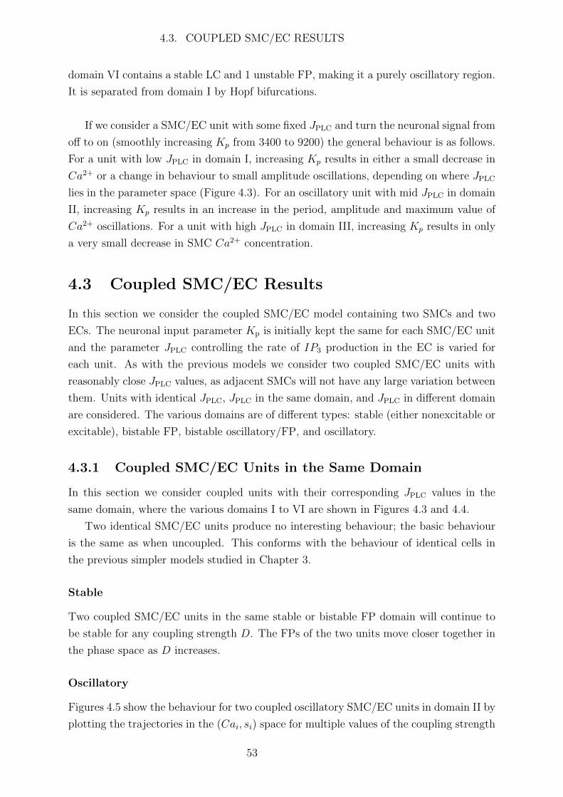
4.3. COUPLED SMC/EC RESULTS
domain VI contains a stable LC and 1 unstable FP, making it a purely oscillatory region.
It is separated from domain I by Hopf bifurcations.
If we consider a SMC/EC unit with some fixed JPLC and turn the neuronal signal from
off to on (smoothly increasing Kp from 3400 to 9200) the general behaviour is as follows.
For a unit with low JPLC in domain I, increasing Kp results in either a small decrease in
Ca2+ or a change in behaviour to small amplitude oscillations, depending on where JPLC
lies in the parameter space (Figure 4.3). For an oscillatory unit with mid JPLC in domain
II, increasing Kp results in an increase in the period, amplitude and maximum value of
Ca2+ oscillations. For a unit with high JPLC in domain III, increasing Kp results in only
a very small decrease in SMC Ca2+ concentration.
4.3 Coupled SMC/EC Results
In this section we consider the coupled SMC/EC model containing two SMCs and two
ECs. The neuronal input parameter Kp is initially kept the same for each SMC/EC unit
and the parameter JPLC controlling the rate of IP3 production in the EC is varied for
each unit. As with the previous models we consider two coupled SMC/EC units with
reasonably close JPLC values, as adjacent SMCs will not have any large variation between
them. Units with identical JPLC, JPLC in the same domain, and JPLC in different domain
are considered. The various domains are of different types: stable (either nonexcitable or
excitable), bistable FP, bistable oscillatory/FP, and oscillatory.
4.3.1 Coupled SMC/EC Units in the Same Domain
In this section we consider coupled units with their corresponding JPLC values in the
same domain, where the various domains I to VI are shown in Figures 4.3 and 4.4.
Two identical SMC/EC units produce no interesting behaviour; the basic behaviour
is the same as when uncoupled. This conforms with the behaviour of identical cells in
the previous simpler models studied in Chapter 3.
Stable
Two coupled SMC/EC units in the same stable or bistable FP domain will continue to
be stable for any coupling strength D. The FPs of the two units move closer together in
the phase space as D increases.
Oscillatory
Figures 4.5 show the behaviour for two coupled oscillatory SMC/EC units in domain II by
plotting the trajectories in the (Cai, si) space for multiple values of the coupling strength
53

4.3. COUPLED SMC/EC RESULTS
D. Domain II contains large amplitude stable LCs and covers the area in the parameter
space where JPLC is mid range. For low coupling strength D the units oscillate with
variable amplitude indicated by the additional ‘loops’ of the trajectory, and for higher
coupling strength D the units synchronise and oscillate with the same frequency.
The exact point at which the units synchronise can be seen by plotting the difference
in power spectra of the SMC cytosolic Ca2+ concentration of each unit for different val-
ues of D, where the power spectrum is the distribution of the frequencies that compose
an oscillatory function (see Section 3.3.1 for further details on power spectra). The dif-
ference in power spectra is shown in Figure 4.6. As the coupling strength D increases
more frequencies are introduced corresponding to additional loops in the trajectories. At
approximately D = 0.056 the lines of frequency coalesce in groups into single frequen-
cies, indicating the cells are synchronised with a difference only in the amplitude of their
respective frequencies.
Two coupled oscillatory units in domain VI behave the same way, oscillating with
variable amplitude for low coupling and synchronisation occuring for strong coupling.
These trajectory plots and the power spectrum graph are very similar to that of two
coupled oscillatory SMCs in the previous models of Chapter 3. For a more in depth and
detailed analysis of this behaviour refer to Section 3.3.1.
Bistable Oscillatory/FP
Domain V is bistable as it contains both a stable FP and LC, meaning a SMC/EC unit
with JPLC and Kp in this domain can either be stable or oscillatory depending on the
ICs.
Two stable units when coupled will remain stable. One stable unit and one oscillatory
unit will in general both oscillate for weak coupling D and when more strongly coupled
they both either oscillate or tend to a stable state.
Two oscillatory units in this bistable domain act similarly to other coupled oscillatory
units in Section 4.3.1, coupled oscillatory SMCs using the model by Goldbeter et al.
(1990) in Section 3.3.1, and coupled oscillatory cells using the two other models discussed
in Section 3.4. For weak coupling the units oscillate with variable amplitude as shown in
in Figure 4.7. However the trajectories are more complex and the power spectrum graph
has additional components, such as the frequency shift around D = 0.27 (see Figure
4.8). This is most likely due to the shape of the trajectories when the cells are initially
uncoupled at D = 0. The SMC Ca2+ concentration in the internal store oscillates twice
for every oscillation of the SMC cytosolic Ca2+ concentration forming a LC in a figure-
of-8 shape. This is unlike the previous simple LCs of the oscillatory domains II and VI
and is possibly caused by the bistability in this domain that is not present in any other
cases.
54
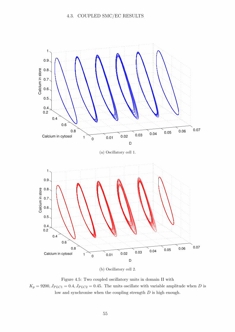
4.3. COUPLED SMC/EC RESULTS
0.2
0.4
0.6
0.8
1 0 0.01 0.02 0.03 0.04 0.05 0.06 0.07
0.4
0.5
0.6
0.7
0.8
0.9
1
D
Calcium in cytosol
Cal
cium
in s
tore
(a) Oscillatory cell 1.
0.2
0.4
0.6
0.8
1 0 0.01 0.02 0.03 0.04 0.05 0.06 0.07
0.4
0.5
0.6
0.7
0.8
0.9
1
D
Calcium in cytosol
Cal
cium
inst
ore
(b) Oscillatory cell 2.
Figure 4.5: Two coupled oscillatory units in domain II with
Kp = 9200, JPLC1 = 0.4, JPLC2 = 0.45. The units oscillate with variable amplitude when D is
low and synchronise when the coupling strength D is high enough.
55

4.3. COUPLED SMC/EC RESULTS
Frequency (Hz)
D
0 0.05 0.1 0.15 0.2 0.25 0.3 0.35 0.4 0.45 0.50
0.01
0.02
0.03
0.04
0.05
0.06
0.07
−600
−400
−200
0
200
400
600
Figure 4.6: The difference in power spectra (unit 1 minus unit 2) between the Cai of two
oscillatory units in domain II as the coupling strength D varies, where
Kp = 9200, JPLC1 = 0.4, JPLC2 = 0.45. The variable amplitude oscillations of Figure 4.5 are
represented by additional lines of frequency coalescing at approximately D = 0.056 where the
units synchronise with identical frequency.
4.3.2 Coupled SMC/EC Units in Different Domains
The different domains of stability can be further categorised into excitable, nonexcitable,
and oscillatory. A SMC/EC unit with parameter values for JPLC and Kp in the bistable
oscillatory/FP domain V will fall under nonexcitable or oscillatory depending on the ICs.
Recall that the excitable domain is a subset of the stable domain I and located directly
to the left of the line of Hopf bifurcations seperating domains I and II.
Excitable and Nonexcitable
Two coupled units where one is excitable and one is nonexcitable will produce no inter-
esting behaviour as both are stable. This conforms with the behaviour of an excitable
and nonexcitable cell in Section 3.3.2 using the SMC model by Goldbeter et al. (1990).
Oscillatory and Nonexcitable
By weakly coupling two units where one is oscillatory and one is nonexcitable, the flux of
Ca2+ from the oscillatory into the nonexcitable unit will cause it to immediately oscillate
with small amplitude and the same frequency. As the coupling strength D increases the
amplitude of oscillations of the nonexcitable cell increases as it becomes more similar to
56
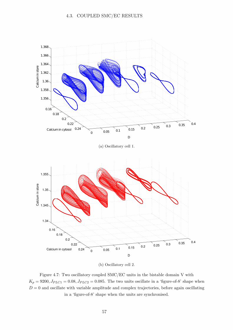
4.3. COUPLED SMC/EC RESULTS
0.16
0.18
0.2
0.22
0.240 0.05 0.1 0.15 0.2 0.25 0.3 0.35 0.4
1.356
1.358
1.36
1.362
1.364
1.366
1.368
D
Calcium in cytosol
Cal
cium
in s
tore
(a) Oscillatory cell 1.
0.16
0.18
0.2
0.22
0.24 0 0.05 0.1 0.15 0.2 0.25 0.3 0.35 0.4
1.34
1.345
1.35
1.355
D
Calcium in cytosol
Cal
cium
in s
tore
(b) Oscillatory cell 2.
Figure 4.7: Two oscillatory coupled SMC/EC units in the bistable domain V with
Kp = 9200, JPLC1 = 0.08, JPLC2 = 0.085. The two units oscillate in a ‘figure-of-8’ shape when
D = 0 and oscillate with variable amplitude and complex trajectories, before again oscillating
in a ‘figure-of-8’ shape when the units are synchronised.
57
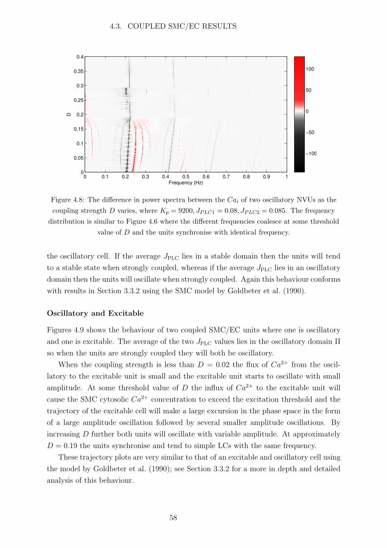
4.3. COUPLED SMC/EC RESULTS
Frequency (Hz)
D
0 0.1 0.2 0.3 0.4 0.5 0.6 0.7 0.8 0.9 10
0.05
0.1
0.15
0.2
0.25
0.3
0.35
0.4
−100
−50
0
50
100
Figure 4.8: The difference in power spectra between the Cai of two oscillatory NVUs as the
coupling strength D varies, where Kp = 9200, JPLC1 = 0.08, JPLC2 = 0.085. The frequency
distribution is similar to Figure 4.6 where the different frequencies coalesce at some threshold
value of D and the units synchronise with identical frequency.
the oscillatory cell. If the average JPLC lies in a stable domain then the units will tend
to a stable state when strongly coupled, whereas if the average JPLC lies in an oscillatory
domain then the units will oscillate when strongly coupled. Again this behaviour conforms
with results in Section 3.3.2 using the SMC model by Goldbeter et al. (1990).
Oscillatory and Excitable
Figures 4.9 shows the behaviour of two coupled SMC/EC units where one is oscillatory
and one is excitable. The average of the two JPLC values lies in the oscillatory domain II
so when the units are strongly coupled they will both be oscillatory.
When the coupling strength is less than D = 0.02 the flux of Ca2+ from the oscil-
latory to the excitable unit is small and the excitable unit starts to oscillate with small
amplitude. At some threshold value of D the influx of Ca2+ to the excitable unit will
cause the SMC cytosolic Ca2+ concentration to exceed the excitation threshold and the
trajectory of the excitable cell will make a large excursion in the phase space in the form
of a large amplitude oscillation followed by several smaller amplitude oscillations. By
increasing D further both units will oscillate with variable amplitude. At approximately
D = 0.19 the units synchronise and tend to simple LCs with the same frequency.
These trajectory plots are very similar to that of an excitable and oscillatory cell using
the model by Goldbeter et al. (1990); see Section 3.3.2 for a more in depth and detailed
analysis of this behaviour.
58
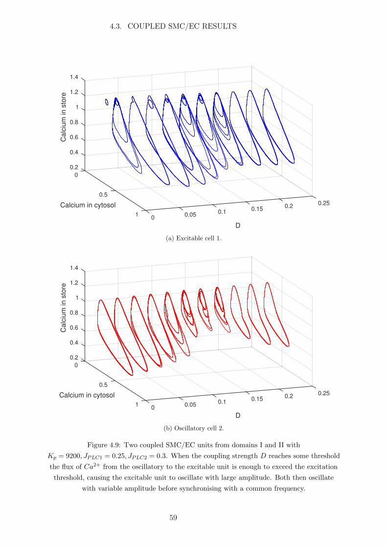
4.3. COUPLED SMC/EC RESULTS
0.250.20.15
D
0.10.0501
0.5
Calcium in cytosol
1.2
0.2
0.4
0.6
0.8
1
1.4
0
Cal
cium
in s
tore
(a) Excitable cell 1.
0.250.20.15
D
0.10.0501
0.5
Calcium in cytosol
1.4
1.2
1
0.8
0.6
0.4
0.20
Cal
cium
in s
tore
(b) Oscillatory cell 2.
Figure 4.9: Two coupled SMC/EC units from domains I and II with
Kp = 9200, JPLC1 = 0.25, JPLC2 = 0.3. When the coupling strength D reaches some threshold
the flux of Ca2+ from the oscillatory to the excitable unit is enough to exceed the excitation
threshold, causing the excitable unit to oscillate with large amplitude. Both then oscillate
with variable amplitude before synchronising with a common frequency.
59
4.4. SUMMARY
4.3.3 Different Kp
If we consider two coupled SMC/EC units with different values of Kp and hence different
levels of neuronal activity, it is trivial to find the behaviour induced by coupling based
on the previous cases. To do so simply consider where the JPLC and Kp values of each
unit lie in the parameter space (Figure 4.3). If they both lie in an oscillatory domain
(domains II, V, VI) they will have the corresponding behaviour of two coupled oscillatory
units described earlier, and so on.
4.4 Summary
For any level of neuronal activity (Kp) the system tends to a stable state for high JPLC
and oscillates for medium values of JPLC; the amplitude and period of these oscillations
increase with neuronal activity (Kp). For a stable unit with high JPLC increasing Kp
results in a very small decrease in SMC Ca2+ concentration.
For low JPLC and low to medium neuronal activity (Kp) the system tends to a stable
state. For low JPLC and high neuronal activity (Kp) the system can also oscillate. The
amplitude and period of these oscillations are small compared to the oscillations present
for medium values of JPLC.
The behaviour between two coupled units in this model is dependent on their be-
haviour when uncoupled. They can be catagorised into the following three groups:
nonexcitable, excitable and oscillatory. Note that the excitable region in the (JPLC , Kp)
parameter space is a section of domain I directly to the left of the line of Hopf bifurcations
separating domains I and II.
Two nonexcitable units will remain nonexcitable when coupled and two excitable
units will remain excitable when coupled. All coupled oscillatory SMC/EC units have the
same type of behaviour and power spectrum, i.e. oscillations that vary in amplitude and
increase in complexity for small coupling strength D. The complexity disappears at some
value of D and the units synchronise by oscillating at the same frequency. The SMC/EC
units with parameters JPLC and Kp in domain V have the most complex trajectories,
possibly because of the bistability present in the domain.
A coupled nonexcitable unit and excitable unit will remain stable. A nonexcitable
unit coupled with an oscillatory unit will oscillate when weakly coupled and either be
stable or oscillatory when strongly coupled depending on the average JPLC of the two
units.
An excitable unit coupled with an oscillatory unit will cause the excitable unit to tran-
sition through the following stages as the coupling strength is increased: small amplitude
oscillations, variable amplitude oscillations, and finally fixed amplitude oscillations when
strongly coupled. The oscillatory unit will transition through variable amplitude oscilla-
60

4.4. SUMMARY
tions to fixed amplitude oscillations when strongly coupled.
The behaviour of the SMC cytosolic Ca2+ concentration of two coupled SMC/EC units
(excitable, nonexcitable, and oscillatory) is qualitatively the same as that of two coupled
SMCs in Section 3.3 using the model by Goldbeter et al. (1990). The only components
present in the SMC/EC model not found in the Goldbeter model are the small amplitude
oscillations and bistability for low JPLC and high neuronal activity (Kp), believed to exist
due to the stretch activated Ca2+ channels not included in the simpler Goldbeter model.
Therefore the majority of the dynamics of this coupled SMC/EC model containing a
total of 28 individual ordinary differential equations (ODEs) may be explained by the
dynamics of the Goldbeter minimal coupled cell model containing only 4 ODEs.
61

Chapter 5
Wave Propagation in Spatial Media
In this chapter we investigate the dynamics of reaction diffusion systems with propagating
waves on a flat two dimensional (2D) plane with periodic boundary conditions (BCs) on
all boundaries of the domain. The two models chosen are the generic model by FitzHugh
(1961) as it is a classical excitable system and the calcium (Ca2+) dynamics model by
Goldbeter et al. (1990) as it is the simplest Ca2+ model studied thus far with known
excitable properties (Wilkins and Sneyd, 1998), and has the most similarity in behaviour
to the more complex SMC/EC model of Chapter 4.
A population of cells will rarely be identical in nature, therefore it is of interest to look
at surfaces with the local dynamics of the system varied, controlled by the spatially varied
parameter β. Hence this chapter contains simulations on a flat surface with periodic BCs
and constant or spatially varying parameter β (controlling the stability and excitability
of the system), while in following chapter the models are simulated on a curved surface,
namely a torus.
5.1 Method
A 2 variable partial differential equation (PDE) system on a continuous 2D spatial domain
is transformed into a set of 2 ordinary differential equations (ODEs) for each mesh point
with Fickian diffusion (via the Laplace operator) connecting each point, numerically
solved using the method of lines. The spatial coordinates are discretised as follows:
xi = x0 + iδx, i = 0, 1, . . . , I (5.1)
yj = y0 + jδy, j = 0, 1, . . . , J (5.2)
for an I ×J mesh. Then the ODEs for each mesh point in the FitzHugh-Nagumo (FHN)
model are
dui,jdt
= 3ui,j − (ui,j)3 − vi,j +D∆ui,j (5.3)
dvi,jdt
= ε(ui,j + β), (5.4)
62
5.1. METHOD
where ui,j := u(xi, yj), and similarly for the Goldbeter model. The Laplace operator in
Cartesian coordinates is approximated by
∆ui,j =∂2ui,j∂x2
+∂2ui,j∂y2
≈ui+1,j − 2uni,j + ui−1,j
(δx)2+ui,j+1 − 2ui,j + ui,j−1
(δy)2. (5.5)
There are two ODEs per mesh point for both models, producing a 2∗I ∗J dimensional
ODE system. This large set of ODEs is solved in C using the library ARKode provided
by SUNDIALS (Hindmarsh et al., 2005). ARKode is an adaptive-step additive Runge
Kutta solver for initial value problems capable of solving systems both explicitly and
implicitly by partitioning the right hand side (RHS) of the system into ‘slow’ time scale
and ‘fast’ time scale components respectively. Our simulations were run using only the
explicit solver; as both models used only contained two state variables it was deemed
unnecessary, however if a more complex model were to be used then the runtime of the
solver could be optimised by making use of the explicit and implicit additive solver.
Message Passing Interface (MPI) is used to parallelise the code, enabling faster com-
putation by running on multiple cores. MPI is a standardised message passing library
designed to function on a variety of parallel computers (Walker, 1994). The spatial
domain with mesh size I × J is split into multiple quads with neighbouring quads ex-
changing information on their edge points after each time iteration. The number of quads
determines how the domain is subdivided using a built in MPI function which decides
the optimal way to subdivide the domain. For example a mesh of 200 × 800 run on
4 cores would be split into quads of size 100 × 400. Our simulations were reasonably
small so they could be achieved on a local computer using only 4 quads. The 2D vi-
sualisations are produced in Python. The source code for this project can be found at
www.github.com/BlueFern/CRDModel. All generated videos corresponding to the fig-
ures in this chapter can be found at the UC High Performance Computing YouTube
channel at http://bit.ly/1TgPNgq.
5.1.1 Spatially constant β
To investigate propagating waves using the Goldbeter model where the domain is spatially
constant (i.e. when the parameter β is constant) an initial perturbation to the system is
simulated by setting the values of the initial conditions (ICs) higher in a small rectangular
area (specifically Zs + 1, Ys + 1 corresponding to a supra-threshold excitation) than on
the rest of the plane (set to Zs, Ys, the stable fixed point (FP) of the system). This
perturbation will cause a wave to propagate throughout the medium if the system is
excitable. For simulations with spatially constant β the spatial domain is set to x ∈ [0, 40],
y ∈ [0, 40].
The x boundary is periodic. There are additional Dirichlet BCs at the lower and
upper y boundaries for time t < TBOUNDARY , where TBOUNDARY is large enough so that
63
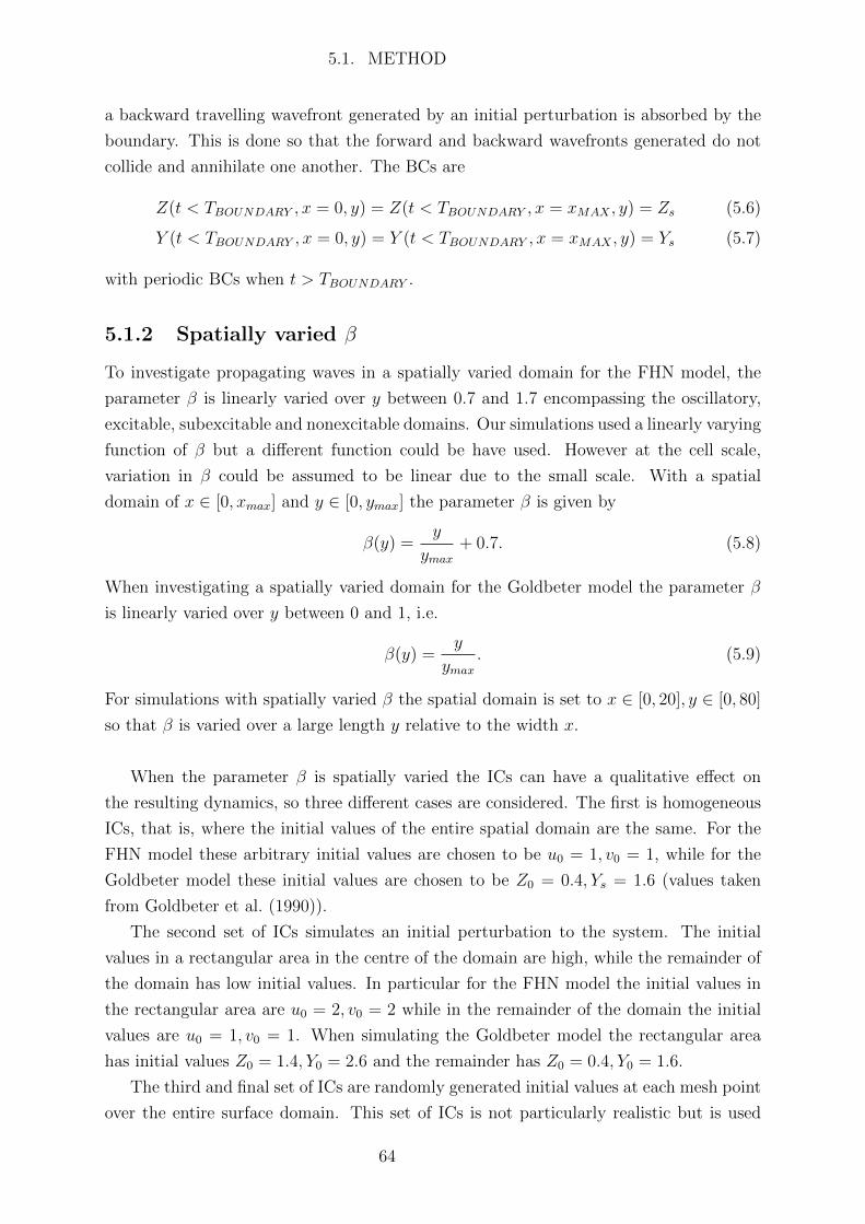
5.1. METHOD
a backward travelling wavefront generated by an initial perturbation is absorbed by the
boundary. This is done so that the forward and backward wavefronts generated do not
collide and annihilate one another. The BCs are
Z(t < TBOUNDARY , x = 0, y) = Z(t < TBOUNDARY , x = xMAX , y) = Zs (5.6)
Y (t < TBOUNDARY , x = 0, y) = Y (t < TBOUNDARY , x = xMAX , y) = Ys (5.7)
with periodic BCs when t > TBOUNDARY .
5.1.2 Spatially varied β
To investigate propagating waves in a spatially varied domain for the FHN model, the
parameter β is linearly varied over y between 0.7 and 1.7 encompassing the oscillatory,
excitable, subexcitable and nonexcitable domains. Our simulations used a linearly varying
function of β but a different function could be have used. However at the cell scale,
variation in β could be assumed to be linear due to the small scale. With a spatial
domain of x ∈ [0, xmax] and y ∈ [0, ymax] the parameter β is given by
β(y) =y
ymax+ 0.7. (5.8)
When investigating a spatially varied domain for the Goldbeter model the parameter β
is linearly varied over y between 0 and 1, i.e.
β(y) =y
ymax. (5.9)
For simulations with spatially varied β the spatial domain is set to x ∈ [0, 20], y ∈ [0, 80]
so that β is varied over a large length y relative to the width x.
When the parameter β is spatially varied the ICs can have a qualitative effect on
the resulting dynamics, so three different cases are considered. The first is homogeneous
ICs, that is, where the initial values of the entire spatial domain are the same. For the
FHN model these arbitrary initial values are chosen to be u0 = 1, v0 = 1, while for the
Goldbeter model these initial values are chosen to be Z0 = 0.4, Ys = 1.6 (values taken
from Goldbeter et al. (1990)).
The second set of ICs simulates an initial perturbation to the system. The initial
values in a rectangular area in the centre of the domain are high, while the remainder of
the domain has low initial values. In particular for the FHN model the initial values in
the rectangular area are u0 = 2, v0 = 2 while in the remainder of the domain the initial
values are u0 = 1, v0 = 1. When simulating the Goldbeter model the rectangular area
has initial values Z0 = 1.4, Y0 = 2.6 and the remainder has Z0 = 0.4, Y0 = 1.6.
The third and final set of ICs are randomly generated initial values at each mesh point
over the entire surface domain. This set of ICs is not particularly realistic but is used
64
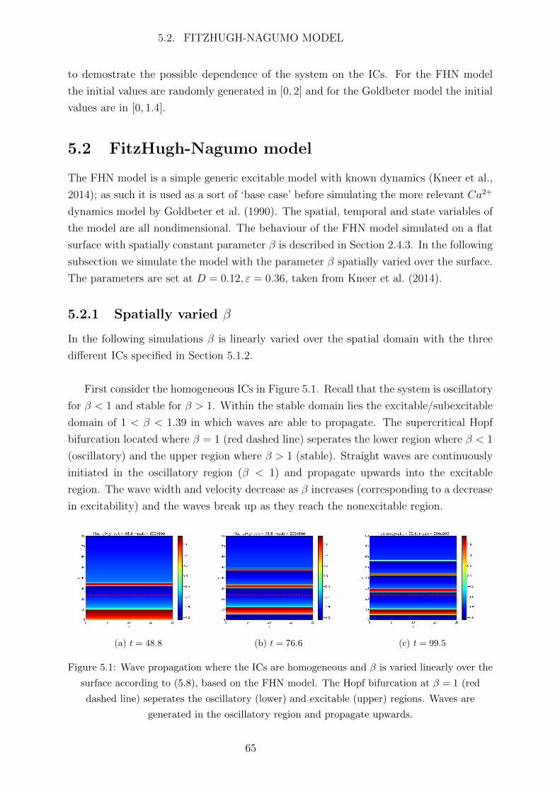
5.2. FITZHUGH-NAGUMO MODEL
to demostrate the possible dependence of the system on the ICs. For the FHN model
the initial values are randomly generated in [0, 2] and for the Goldbeter model the initial
values are in [0, 1.4].
5.2 FitzHugh-Nagumo model
The FHN model is a simple generic excitable model with known dynamics (Kneer et al.,
2014); as such it is used as a sort of ‘base case’ before simulating the more relevant Ca2+
dynamics model by Goldbeter et al. (1990). The spatial, temporal and state variables of
the model are all nondimensional. The behaviour of the FHN model simulated on a flat
surface with spatially constant parameter β is described in Section 2.4.3. In the following
subsection we simulate the model with the parameter β spatially varied over the surface.
The parameters are set at D = 0.12, ε = 0.36, taken from Kneer et al. (2014).
5.2.1 Spatially varied β
In the following simulations β is linearly varied over the spatial domain with the three
different ICs specified in Section 5.1.2.
First consider the homogeneous ICs in Figure 5.1. Recall that the system is oscillatory
for β < 1 and stable for β > 1. Within the stable domain lies the excitable/subexcitable
domain of 1 < β < 1.39 in which waves are able to propagate. The supercritical Hopf
bifurcation located where β = 1 (red dashed line) seperates the lower region where β < 1
(oscillatory) and the upper region where β > 1 (stable). Straight waves are continuously
initiated in the oscillatory region (β < 1) and propagate upwards into the excitable
region. The wave width and velocity decrease as β increases (corresponding to a decrease
in excitability) and the waves break up as they reach the nonexcitable region.
(a) t = 48.8 (b) t = 76.6 (c) t = 99.5
Figure 5.1: Wave propagation where the ICs are homogeneous and β is varied linearly over the
surface according to (5.8), based on the FHN model. The Hopf bifurcation at β = 1 (red
dashed line) seperates the oscillatory (lower) and excitable (upper) regions. Waves are
generated in the oscillatory region and propagate upwards.
65

5.3. GOLDBETER MODEL
An initial perturbation to the system causes waves to form that are very slightly
curved. However this is not enough to affect the dynamics (results not shown). When
the ICs are randomly generated initial values at each mesh point the ‘noise’ produced
is also not sufficient to alter the wave propagation in any significant way (results not
shown). Hence in the FHN model for D = 0.12 the behaviour of the generated waves on
a spatially varied surface have no significant dependence on the ICs.
5.3 Goldbeter model
The main interest of our research is on Ca2+ dynamics and wave propagation; as such we
now apply the Goldbeter et al. (1990) Ca2+ model to a 2D spatial domain. We cannot use
the FHN model to explain Ca2+ wave propagation as some biological excitable systems
may behave in qualitatively different ways to classical excitable systems like the FHN
model (Sneyd and Atri, 1993). The interaction of ions in the cell cytoplasm forms an in-
herently excitable system (Wilkins and Sneyd, 1998), but the structure of the Goldbeter
model equations are quite different to the FHN model as the nullclines do not have the
same shape (Kneer et al., 2014). As shown in Section 3.2 the Goldbeter model is excitable
for a range of β near the left Hopf bifurcation (Figure 3.3) due to the shape of the null-
clines (Figure 3.2). Like the FHN model there are oscillatory, excitable, subexcitable and
nonexcitable regions and some critical wave size S∗ seperating the excitable and subex-
citable domains; however it has not been calculated for this model. The nondimensional
equations for the Goldbeter model in a 2D spatial domain are as follows:
∂Z
∂t= 1 + v1β − v2 + v3 + Y − kZ +D∆Z (5.10)
∂Y
∂t= v2 − v3 − Y, (5.11)
where Z is the cytosolic Ca2+ concentration, Y is the Ca2+ concentration in the inter-
nal stores, the algebraic variables and parameters are explained in Section 2.2.1 and the
nondimensionalisation is explained in Section 3.1.2. Note that time is also nondimen-
sional. The nondimensional spatial coordinates x, y are discretised as in Equations 5.1,
5.2 and the ODEs for each mesh point are
dZi,jdt
= 1 + v1β − v2 + v3 + Yi,j − kZi,j +D∆Zi,j (5.12)
dYi,jdt
= v2 − v3 − Yi,j, (5.13)
with
v2 = VM2(Zi,j)
n
Kn2 + (Zi,j)n
(5.14)
v3 = VM3(Yi,j)
m
KmR + (Yi,j)m
(Zi,j)p
KpA + (Zi,j)p
, (5.15)
66
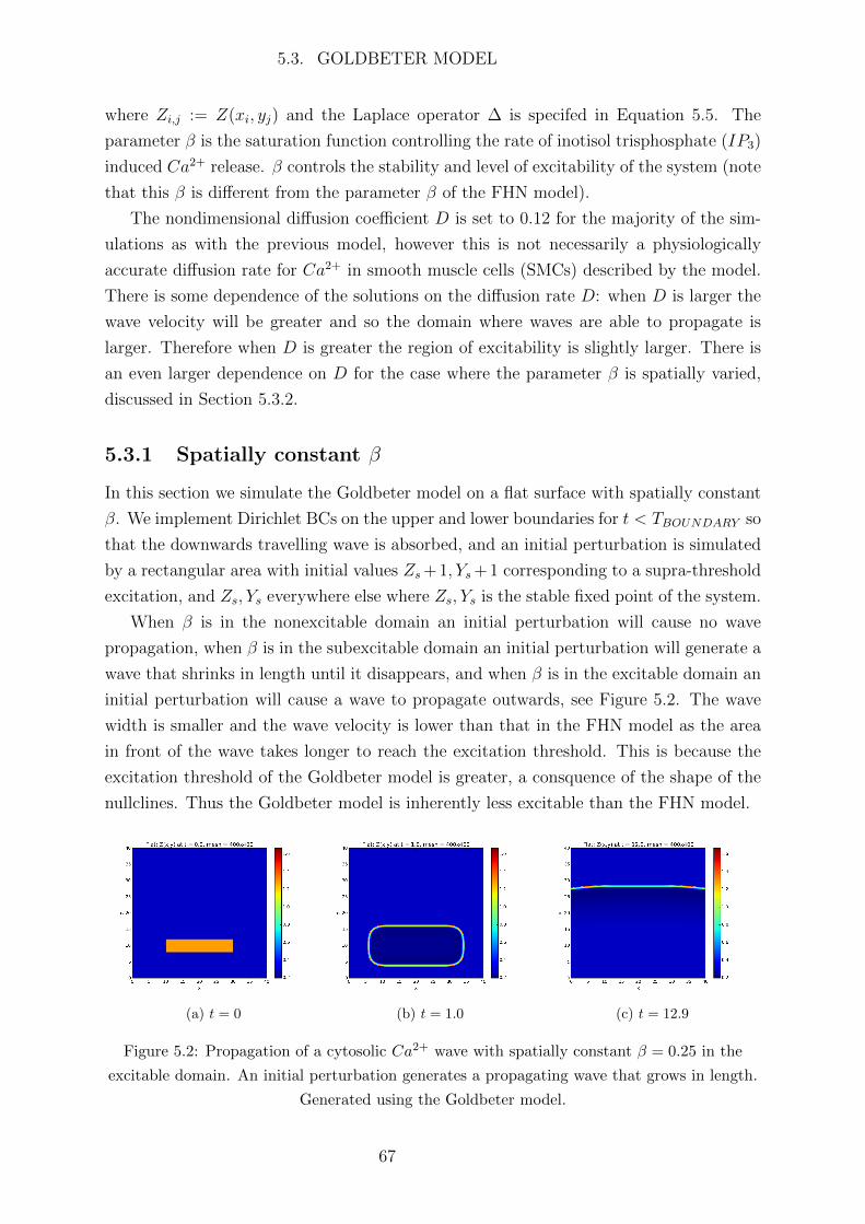
5.3. GOLDBETER MODEL
where Zi,j := Z(xi, yj) and the Laplace operator ∆ is specifed in Equation 5.5. The
parameter β is the saturation function controlling the rate of inotisol trisphosphate (IP3)
induced Ca2+ release. β controls the stability and level of excitability of the system (note
that this β is different from the parameter β of the FHN model).
The nondimensional diffusion coefficient D is set to 0.12 for the majority of the sim-
ulations as with the previous model, however this is not necessarily a physiologically
accurate diffusion rate for Ca2+ in smooth muscle cells (SMCs) described by the model.
There is some dependence of the solutions on the diffusion rate D: when D is larger the
wave velocity will be greater and so the domain where waves are able to propagate is
larger. Therefore when D is greater the region of excitability is slightly larger. There is
an even larger dependence on D for the case where the parameter β is spatially varied,
discussed in Section 5.3.2.
5.3.1 Spatially constant β
In this section we simulate the Goldbeter model on a flat surface with spatially constant
β. We implement Dirichlet BCs on the upper and lower boundaries for t < TBOUNDARY so
that the downwards travelling wave is absorbed, and an initial perturbation is simulated
by a rectangular area with initial values Zs+ 1, Ys+ 1 corresponding to a supra-threshold
excitation, and Zs, Ys everywhere else where Zs, Ys is the stable fixed point of the system.
When β is in the nonexcitable domain an initial perturbation will cause no wave
propagation, when β is in the subexcitable domain an initial perturbation will generate a
wave that shrinks in length until it disappears, and when β is in the excitable domain an
initial perturbation will cause a wave to propagate outwards, see Figure 5.2. The wave
width is smaller and the wave velocity is lower than that in the FHN model as the area
in front of the wave takes longer to reach the excitation threshold. This is because the
excitation threshold of the Goldbeter model is greater, a consquence of the shape of the
nullclines. Thus the Goldbeter model is inherently less excitable than the FHN model.
(a) t = 0 (b) t = 1.0 (c) t = 12.9
Figure 5.2: Propagation of a cytosolic Ca2+ wave with spatially constant β = 0.25 in the
excitable domain. An initial perturbation generates a propagating wave that grows in length.
Generated using the Goldbeter model.
67

5.3. GOLDBETER MODEL
When β in the excitable domain and a wave segment is broken with two open ends,
rotating spirals will form from each end, see Figure 5.3. The same result can be achieved
with the FHN model (results not shown).
Spiral waves are able to form from open wave ends as follows. After the formation of
a broken wave, the wave can propagate in all directions except the waveback where the
medium is temporarily nonexcitable, i.e. it can propagate forward and to the sides. This
causes the wave to become slightly curved at the ends. The inability to propagate into
the waveback causes the broken wave to eventually form spirals as seen in Figure 5.3.
Spiral formation is further discussed in Section 2.4.2.
Figure 5.3: Spiral waves of cytosolic Ca2+ concentration forming from open wave ends with
spatially constant β = 0.25 in the excitable domain. The wave is unable to propagate into the
‘waveback’ (dark blue region of low Ca2+ concentration) where the cells are temporarily
nonexcitable, causing spiral shaped waves to form. Generated using the Goldbeter model.
5.3.2 Spatially varied β
As with the FHN model we consider β (and hence the level of excitability) spatially
varied over a surface according to Equation 5.9. This includes the oscillatory, excitable,
subexcitable, and two nonexcitable regions shown in Figure 3.3. The three sets of ICs
used are detailed in Section 5.1.2.
Figure 5.4 presents the case with homogeneous ICs. The red dashed lines represent
the two Hopf bifurcations in the system with the lower line seperating the excitable and
oscillatory regions (refer to Figure 3.3). The waves are initiated in the oscillatory region
with frequency according to Figure 3.5 (note that frequency is the inverse of period).
68
5.3. GOLDBETER MODEL
Near the lower Hopf bifurcation the frequency is low while near the upper bifurcation
the frequency is high. Note that the oscillations of the Goldbeter model are a higher
frequency than those in the FHN model (Kneer et al., 2014). The amplitude of the waves
are dependent on β as per Figure 3.3; the amplitude is lowest near the upper bifurcation
and highest near the lower bifurcation.
The straight waves propagate upwards towards the upper Hopf bifurcation but cease
when they reach the nonexcitable region just past the bifurcation, as wave propagation
is not possible when the medium is nonexcitable. The waves also propagate downwards
towards the lower Hopf bifurcation and into the excitable domain. As they continue
to propagate the wave width and velocity decrease as the excitability decreases, before
disappearing at the lower nonexcitable domain where waves are unable to propagate
(Figure 5.4a).
The high frequency of wave generation results in a high density of waves. When one
wave reaches the (temporarily nonexcitable) waveback of a wave travelling in front, the
wave behind will disappear. Consequently there will be a brief time period where there
are no propagating waves in the excitable region and in the oscillatory region just above
the lower Hopf bifurcation (Figure 5.4b). After this a large amplitude wave near the
lower bifurcation is generated that travels in both directions, colliding with the wave
above (Figure 5.4c). This continues for a short period of time before returning to the
normal state and the cycle begins again.
Figure 5.5 shows the behaviour when the system has an initial perturbation to the
system. The difference in initial values within the medium causes a curve in the nearby
generated waves (Figure 5.5b). The high density of waves and the wave curvature from
the initial perturbation results in some waves colliding with one another. This eventually
causes waves to break and form open ends. If these open ends lie in the oscillatory or
excitable regions then they will grow in length and curl. These open ends will form full
spiral rotors as long as they do not collide with any other waves (Figure 5.5c).
When the ICs are randomly generated initial values at each mesh point we observe
similar behaviour, shown in Figure 5.6. The ‘noise’ created causes uneven propagating
waves (Figure 5.6b) that collide and break. The resulting asymmetric pattern (Figure
5.4c) is due to many open wave ends forming spiral waves that interact with one another,
causing further open wave ends and hence more spirals.
There are multiple theories to explain the fascinating patterns generated by our models
with the parameter β spatially varied. One possibility considered was Turing instability.
While diffusion alone tends to create uniform stable states, when coupled with chemical
reactions as in reaction-diffusion systems spatial patterns can appear (Biosa et al., 2006).
Turing instability requires different nonzero diffusion rates for each state variable (Kapral,
69
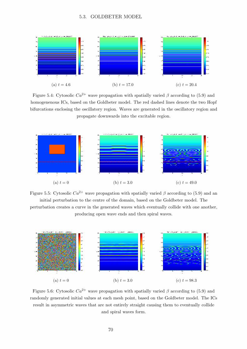
5.3. GOLDBETER MODEL
(a) t = 4.6 (b) t = 17.0 (c) t = 20.4
Figure 5.4: Cytosolic Ca2+ wave propagation with spatially varied β according to (5.9) and
homogenenous ICs, based on the Goldbeter model. The red dashed lines denote the two Hopf
bifurcations enclosing the oscillatory region. Waves are generated in the oscillatory region and
propagate downwards into the excitable region.
(a) t = 0 (b) t = 3.0 (c) t = 49.0
Figure 5.5: Cytosolic Ca2+ wave propagation with spatially varied β according to (5.9) and an
initial perturbation to the centre of the domain, based on the Goldbeter model. The
perturbation creates a curve in the generated waves which eventually collide with one another,
producing open wave ends and then spiral waves.
(a) t = 0 (b) t = 3.0 (c) t = 98.3
Figure 5.6: Cytosolic Ca2+ wave propagation with spatially varied β according to (5.9) and
randomly generated initial values at each mesh point, based on the Goldbeter model. The ICs
result in asymmetric waves that are not entirely straight causing them to eventually collide
and spiral waves form.
70
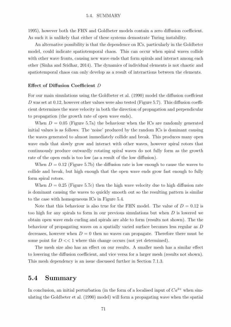
5.4. SUMMARY
1995), however both the FHN and Goldbeter models contain a zero diffusion coefficient.
As such it is unlikely that either of these systems demostrate Turing instability.
An alternative possibility is that the dependence on ICs, particularly in the Goldbeter
model, could indicate spatiotemporal chaos. This can occur when spiral waves collide
with other wave fronts, causing new wave ends that form spirals and interact among each
other (Sinha and Sridhar, 2014). The dynamics of individual elements is not chaotic and
spatiotemporal chaos can only develop as a result of interactions between the elements.
Effect of Diffusion Coefficient D
For our main simulations using the Goldbeter et al. (1990) model the diffusion coeffcient
D was set at 0.12, however other values were also tested (Figure 5.7). This diffusion coeffi-
cient determines the wave velocity in both the direction of propagation and perpendicular
to propagation (the growth rate of open wave ends).
When D = 0.05 (Figure 5.7a) the behaviour when the ICs are randomly generated
initial values is as follows. The ‘noise’ produced by the random ICs is dominant causing
the waves generated to almost immediately collide and break. This produces many open
wave ends that slowly grow and interact with other waves, however spiral rotors that
continuously produce outwardly rotating spiral waves do not fully form as the growth
rate of the open ends is too low (as a result of the low diffusion).
When D = 0.12 (Figure 5.7b) the diffusion rate is low enough to cause the waves to
collide and break, but high enough that the open wave ends grow fast enough to fully
form spiral rotors.
When D = 0.25 (Figure 5.7c) then the high wave velocity due to high diffusion rate
is dominant causing the waves to quickly smooth out so the resulting pattern is similar
to the case with homogeneous ICs in Figure 5.4.
Note that this behaviour is also true for the FHN model. The value of D = 0.12 is
too high for any spirals to form in our previous simulations but when D is lowered we
obtain open wave ends curling and spirals are able to form (results not shown). The the
behaviour of propagating waves on a spatially varied surface becomes less regular as D
decreases, however when D = 0 then no waves can propagate. Therefore there must be
some point for D << 1 where this change occurs (not yet determined).
The mesh size also has an effect on our results. A smaller mesh has a similar effect
to lowering the diffusion coefficient, and vice versa for a larger mesh (results not shown).
This mesh dependency is an issue discussed further in Section 7.1.3.
5.4 Summary
In conclusion, an initial perturbation (in the form of a localised input of Ca2+ when sim-
ulating the Goldbeter et al. (1990) model) will form a propagating wave when the spatial
71
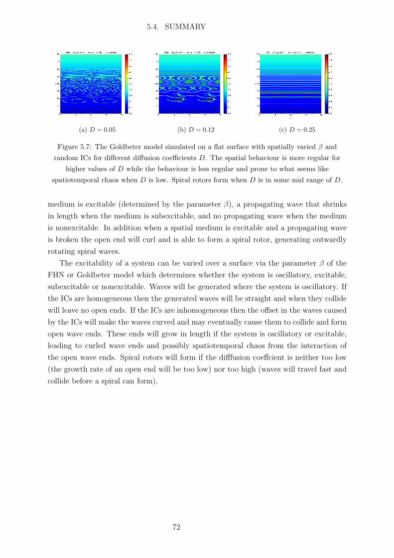
5.4. SUMMARY
(a) D = 0.05 (b) D = 0.12 (c) D = 0.25
Figure 5.7: The Goldbeter model simulated on a flat surface with spatially varied β and
random ICs for different diffusion coefficients D. The spatial behaviour is more regular for
higher values of D while the behaviour is less regular and prone to what seems like
spatiotemporal chaos when D is low. Spiral rotors form when D is in some mid range of D.
medium is excitable (determined by the parameter β), a propagating wave that shrinks
in length when the medium is subexcitable, and no propagating wave when the medium
is nonexcitable. In addition when a spatial medium is excitable and a propagating wave
is broken the open end will curl and is able to form a spiral rotor, generating outwardly
rotating spiral waves.
The excitability of a system can be varied over a surface via the parameter β of the
FHN or Goldbeter model which determines whether the system is oscillatory, excitable,
subexcitable or nonexcitable. Waves will be generated where the system is oscillatory. If
the ICs are homogeneous then the generated waves will be straight and when they collide
will leave no open ends. If the ICs are inhomogeneous then the offset in the waves caused
by the ICs will make the waves curved and may eventually cause them to collide and form
open wave ends. These ends will grow in length if the system is oscillatory or excitable,
leading to curled wave ends and possibly spatiotemporal chaos from the interaction of
the open wave ends. Spiral rotors will form if the difffusion coeffcient is neither too low
(the growth rate of an open end will be too low) nor too high (waves will travel fast and
collide before a spiral can form).
72
Chapter 6
Geometry
In this chapter we introduce the concept of spatial curvature to our 2D spatial domain
simulations using the FitzHugh-Nagumo (FHN) and Goldbeter models. To do so we
simulate our models on a torus, a surface with both negative and positive Gaussian
curvature. A torus was also chosen as it can be mapped to a global isothermal coordinate
system, meaning that it can be mathematically interpreted as a flat surface with spatially
dependent diffusion. Global isothermal coordinates are more difficult to find for other
types of surfaces.
Spatial curvature is especially relevant to our work on calcium (Ca2+) wave propaga-
tion in smooth muscle cells (SMCs) as arteries and arterioles are curved structures, and
in particular the cerebral cortex of the brain is a strongly curved structure. The pathol-
ogy cortical spreading depression (CSD) associated with functional hyperaemia occurs in
the cerebral cortex, where functional hyperaemia is controlled by neurovascular coupling
involving the intercellular communication between SMCs and other cells in the brain
tissue.
Our analysis is initially based off of the work of Kneer et al. (2014) who simulated
the FHN model on a torus and found that positive and negative Gaussian curvature have
opposite effects on the effective diffusion rate, resulting in new wave solutions such as
stable propagating wave segments as discussed in Section 2.5.2.
6.1 Method
The computation of a model on a torus is identical to on a flat surface in the previous
chapter, with the exception of the spatial coordinates and Laplace operator. See Section
5.1 for full details on the method of computation. The Laplace-Beltrami operator in torus
coordinates (θ, ϕ) is
∆LB = − sin θ
r(R + r cos θ)
∂
∂θ+
1
r2∂2
∂θ2+
1
(R + r cos θ)2+
∂2
∂ϕ2. (6.1)
73
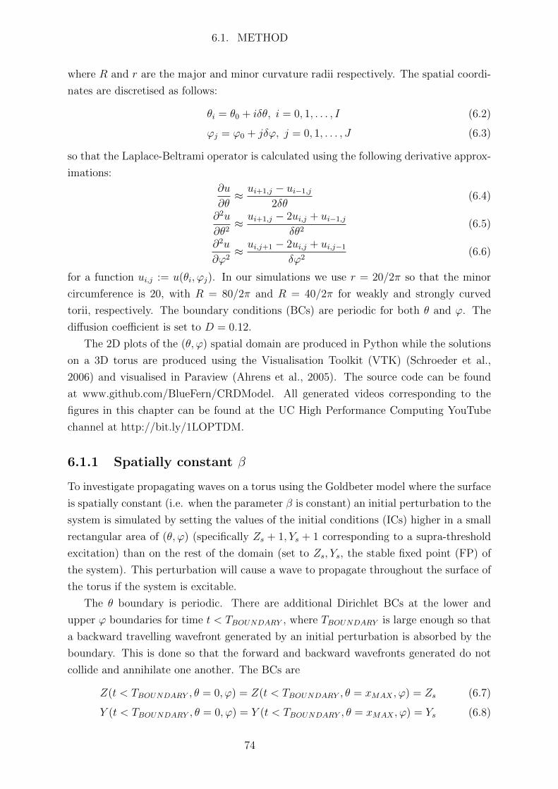
6.1. METHOD
where R and r are the major and minor curvature radii respectively. The spatial coordi-
nates are discretised as follows:
θi = θ0 + iδθ, i = 0, 1, . . . , I (6.2)
ϕj = ϕ0 + jδϕ, j = 0, 1, . . . , J (6.3)
so that the Laplace-Beltrami operator is calculated using the following derivative approx-
imations:
∂u
∂θ≈ ui+1,j − ui−1,j
2δθ(6.4)
∂2u
∂θ2≈ ui+1,j − 2ui,j + ui−1,j
δθ2(6.5)
∂2u
∂ϕ2≈ ui,j+1 − 2ui,j + ui,j−1
δϕ2(6.6)
for a function ui,j := u(θi, ϕj). In our simulations we use r = 20/2π so that the minor
circumference is 20, with R = 80/2π and R = 40/2π for weakly and strongly curved
torii, respectively. The boundary conditions (BCs) are periodic for both θ and ϕ. The
diffusion coefficient is set to D = 0.12.
The 2D plots of the (θ, ϕ) spatial domain are produced in Python while the solutions
on a 3D torus are produced using the Visualisation Toolkit (VTK) (Schroeder et al.,
2006) and visualised in Paraview (Ahrens et al., 2005). The source code can be found
at www.github.com/BlueFern/CRDModel. All generated videos corresponding to the
figures in this chapter can be found at the UC High Performance Computing YouTube
channel at http://bit.ly/1LOPTDM.
6.1.1 Spatially constant β
To investigate propagating waves on a torus using the Goldbeter model where the surface
is spatially constant (i.e. when the parameter β is constant) an initial perturbation to the
system is simulated by setting the values of the initial conditions (ICs) higher in a small
rectangular area of (θ, ϕ) (specifically Zs + 1, Ys + 1 corresponding to a supra-threshold
excitation) than on the rest of the domain (set to Zs, Ys, the stable fixed point (FP) of
the system). This perturbation will cause a wave to propagate throughout the surface of
the torus if the system is excitable.
The θ boundary is periodic. There are additional Dirichlet BCs at the lower and
upper ϕ boundaries for time t < TBOUNDARY , where TBOUNDARY is large enough so that
a backward travelling wavefront generated by an initial perturbation is absorbed by the
boundary. This is done so that the forward and backward wavefronts generated do not
collide and annihilate one another. The BCs are
Z(t < TBOUNDARY , θ = 0, ϕ) = Z(t < TBOUNDARY , θ = xMAX , ϕ) = Zs (6.7)
Y (t < TBOUNDARY , θ = 0, ϕ) = Y (t < TBOUNDARY , θ = xMAX , ϕ) = Ys (6.8)
74
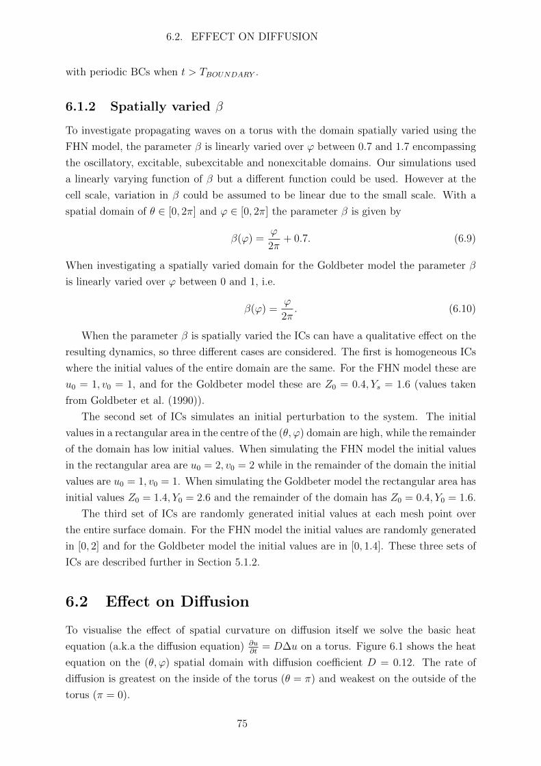
6.2. EFFECT ON DIFFUSION
with periodic BCs when t > TBOUNDARY .
6.1.2 Spatially varied β
To investigate propagating waves on a torus with the domain spatially varied using the
FHN model, the parameter β is linearly varied over ϕ between 0.7 and 1.7 encompassing
the oscillatory, excitable, subexcitable and nonexcitable domains. Our simulations used
a linearly varying function of β but a different function could be used. However at the
cell scale, variation in β could be assumed to be linear due to the small scale. With a
spatial domain of θ ∈ [0, 2π] and ϕ ∈ [0, 2π] the parameter β is given by
β(ϕ) =ϕ
2π+ 0.7. (6.9)
When investigating a spatially varied domain for the Goldbeter model the parameter β
is linearly varied over ϕ between 0 and 1, i.e.
β(ϕ) =ϕ
2π. (6.10)
When the parameter β is spatially varied the ICs can have a qualitative effect on the
resulting dynamics, so three different cases are considered. The first is homogeneous ICs
where the initial values of the entire domain are the same. For the FHN model these are
u0 = 1, v0 = 1, and for the Goldbeter model these are Z0 = 0.4, Ys = 1.6 (values taken
from Goldbeter et al. (1990)).
The second set of ICs simulates an initial perturbation to the system. The initial
values in a rectangular area in the centre of the (θ, ϕ) domain are high, while the remainder
of the domain has low initial values. When simulating the FHN model the initial values
in the rectangular area are u0 = 2, v0 = 2 while in the remainder of the domain the initial
values are u0 = 1, v0 = 1. When simulating the Goldbeter model the rectangular area has
initial values Z0 = 1.4, Y0 = 2.6 and the remainder of the domain has Z0 = 0.4, Y0 = 1.6.
The third set of ICs are randomly generated initial values at each mesh point over
the entire surface domain. For the FHN model the initial values are randomly generated
in [0, 2] and for the Goldbeter model the initial values are in [0, 1.4]. These three sets of
ICs are described further in Section 5.1.2.
6.2 Effect on Diffusion
To visualise the effect of spatial curvature on diffusion itself we solve the basic heat
equation (a.k.a the diffusion equation) ∂u∂t
= D∆u on a torus. Figure 6.1 shows the heat
equation on the (θ, ϕ) spatial domain with diffusion coefficient D = 0.12. The rate of
diffusion is greatest on the inside of the torus (θ = π) and weakest on the outside of the
torus (π = 0).
75
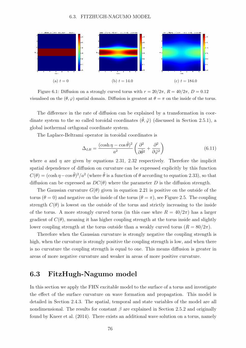
6.3. FITZHUGH-NAGUMO MODEL
(a) t = 0 (b) t = 14.0 (c) t = 184.0
Figure 6.1: Diffusion on a strongly curved torus with r = 20/2π, R = 40/2π, D = 0.12
visualised on the (θ, ϕ) spatial domain. Diffusion is greatest at θ = π on the inside of the torus.
The difference in the rate of diffusion can be explained by a transformation in coor-
dinate system to the so called toroidal coordinates (θ, ϕ) (discussed in Section 2.5.1), a
global isothermal orthgonal coordinate system.
The Laplace-Beltrami operator in toroidal coordinates is
∆LB =(cosh η − cos θ)2
a2
(∂2
∂θ2+
∂2
∂ϕ2
)(6.11)
where a and η are given by equations 2.31, 2.32 respectively. Therefore the implicit
spatial dependence of diffusion on curvature can be expressed explicitly by this function
C(θ) = (cosh η−cos θ)2/a2 (where θ is a function of θ according to equation 2.33), so that
diffusion can be expressed as DC(θ) where the parameter D is the diffusion strength.
The Gaussian curvature G(θ) given in equation 2.21 is positive on the outside of the
torus (θ = 0) and negative on the inside of the torus (θ = π), see Figure 2.5. The coupling
strength C(θ) is lowest on the outside of the torus and strictly increasing to the inside
of the torus. A more strongly curved torus (in this case whre R = 40/2π) has a larger
gradient of C(θ), meaning it has higher coupling strength at the torus inside and slightly
lower coupling strength at the torus outside than a weakly curved torus (R = 80/2π).
Therefore when the Gaussian curvature is strongly negative the coupling strength is
high, when the curvature is strongly positive the coupling strength is low, and when there
is no curvature the coupling strength is equal to one. This means diffusion is greater in
areas of more negative curvature and weaker in areas of more positive curvature.
6.3 FitzHugh-Nagumo model
In this section we apply the FHN excitable model to the surface of a torus and investigate
the effect of the surface curvature on wave formation and propagation. This model is
detailed in Section 2.4.3. The spatial, temporal and state variables of the model are all
nondimensional. The results for constant β are explained in Section 2.5.2 and originally
found by Kneer et al. (2014). There exists an additional wave solution on a torus, namely
76
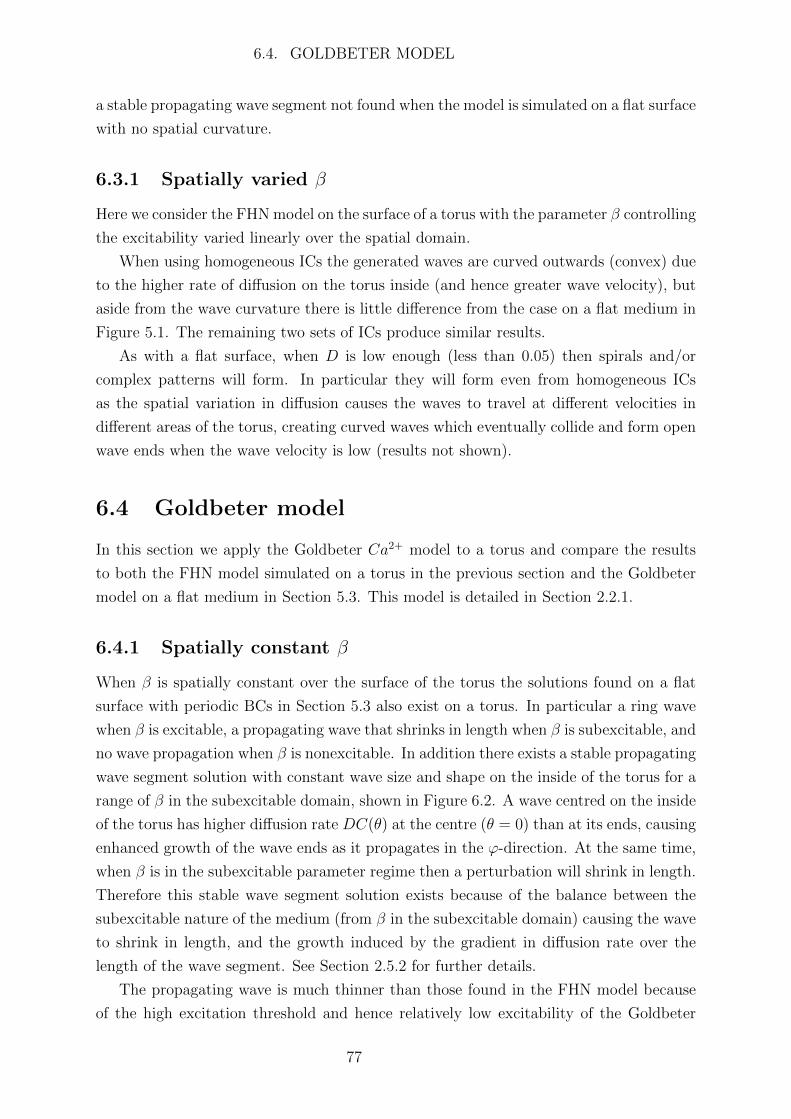
6.4. GOLDBETER MODEL
a stable propagating wave segment not found when the model is simulated on a flat surface
with no spatial curvature.
6.3.1 Spatially varied β
Here we consider the FHN model on the surface of a torus with the parameter β controlling
the excitability varied linearly over the spatial domain.
When using homogeneous ICs the generated waves are curved outwards (convex) due
to the higher rate of diffusion on the torus inside (and hence greater wave velocity), but
aside from the wave curvature there is little difference from the case on a flat medium in
Figure 5.1. The remaining two sets of ICs produce similar results.
As with a flat surface, when D is low enough (less than 0.05) then spirals and/or
complex patterns will form. In particular they will form even from homogeneous ICs
as the spatial variation in diffusion causes the waves to travel at different velocities in
different areas of the torus, creating curved waves which eventually collide and form open
wave ends when the wave velocity is low (results not shown).
6.4 Goldbeter model
In this section we apply the Goldbeter Ca2+ model to a torus and compare the results
to both the FHN model simulated on a torus in the previous section and the Goldbeter
model on a flat medium in Section 5.3. This model is detailed in Section 2.2.1.
6.4.1 Spatially constant β
When β is spatially constant over the surface of the torus the solutions found on a flat
surface with periodic BCs in Section 5.3 also exist on a torus. In particular a ring wave
when β is excitable, a propagating wave that shrinks in length when β is subexcitable, and
no wave propagation when β is nonexcitable. In addition there exists a stable propagating
wave segment solution with constant wave size and shape on the inside of the torus for a
range of β in the subexcitable domain, shown in Figure 6.2. A wave centred on the inside
of the torus has higher diffusion rate DC(θ) at the centre (θ = 0) than at its ends, causing
enhanced growth of the wave ends as it propagates in the ϕ-direction. At the same time,
when β is in the subexcitable parameter regime then a perturbation will shrink in length.
Therefore this stable wave segment solution exists because of the balance between the
subexcitable nature of the medium (from β in the subexcitable domain) causing the wave
to shrink in length, and the growth induced by the gradient in diffusion rate over the
length of the wave segment. See Section 2.5.2 for further details.
The propagating wave is much thinner than those found in the FHN model because
of the high excitation threshold and hence relatively low excitability of the Goldbeter
77
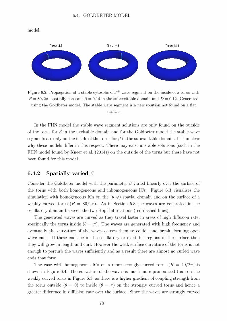
6.4. GOLDBETER MODEL
model.
Figure 6.2: Propagation of a stable cytosolic Ca2+ wave segment on the inside of a torus with
R = 80/2π, spatially constant β = 0.14 in the subexcitable domain and D = 0.12. Generated
using the Goldbeter model. The stable wave segment is a new solution not found on a flat
surface.
In the FHN model the stable wave segment solutions are only found on the outside
of the torus for β in the excitable domain and for the Goldbeter model the stable wave
segments are only on the inside of the torus for β in the subexcitable domain. It is unclear
why these models differ in this respect. There may exist unstable solutions (such in the
FHN model found by Kneer et al. (2014)) on the outside of the torus but these have not
been found for this model.
6.4.2 Spatially varied β
Consider the Goldbeter model with the parameter β varied linearly over the surface of
the torus with both homogeneous and inhomogeneous ICs. Figure 6.3 visualises the
simulation with homogeneous ICs on the (θ, ϕ) spatial domain and on the surface of a
weakly curved torus (R = 80/2π). As in Section 5.3 the waves are generated in the
oscillatory domain between the two Hopf bifurcations (red dashed lines).
The generated waves are curved as they travel faster in areas of high diffusion rate,
specifically the torus inside (θ = π). The waves are generated with high frequency and
eventually the curvature of the waves causes them to collide and break, forming open
wave ends. If these ends lie in the oscillatory or excitable regions of the surface then
they will grow in length and curl. However the weak surface curvature of the torus is not
enough to perturb the waves sufficiently and as a result there are almost no curled wave
ends that form.
The case with homogeneous ICs on a more strongly curved torus (R = 40/2π) is
shown in Figure 6.4. The curvature of the waves is much more pronounced than on the
weakly curved torus in Figure 6.3, as there is a higher gradient of coupling strength from
the torus outside (θ = 0) to inside (θ = π) on the strongly curved torus and hence a
greater difference in diffusion rate over the surface. Since the waves are strongly curved
78
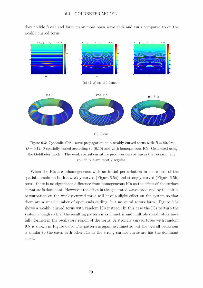
6.4. GOLDBETER MODEL
they collide faster and form many more open wave ends and curls compared to on the
weakly curved torus.
(a) (θ, ϕ) spatial domain.
(b) Torus.
Figure 6.3: Cytosolic Ca2+ wave propagation on a weakly curved torus with R = 80/2π,
D = 0.12, β spatially varied according to (6.10) and with homogeneous ICs. Generated using
the Goldbeter model. The weak spatial curvature produces curved waves that ocassionally
collide but are mostly regular.
When the ICs are inhomogeneous with an initial perturbation in the centre of the
spatial domain on both a weakly curved (Figure 6.5a) and strongly curved (Figure 6.5b)
torus, there is no significant difference from homogeneous ICs as the effect of the surface
curvature is dominant. Howvever the offset in the generated waves produced by the initial
perturbation on the weakly curved torus will have a slight effect on the system so that
there are a small number of open ends curling, but no spiral rotors form. Figure 6.6a
shows a weakly curved torus with random ICs instead. In this case the ICs perturb the
system enough so that the resulting pattern is asymmetric and multiple spiral rotors have
fully formed in the oscillatory region of the torus. A strongly curved torus with random
ICs is shown in Figure 6.6b. The pattern is again asymmetric but the overall behaviour
is similar to the cases with other ICs as the strong surface curvature has the dominant
effect.
79
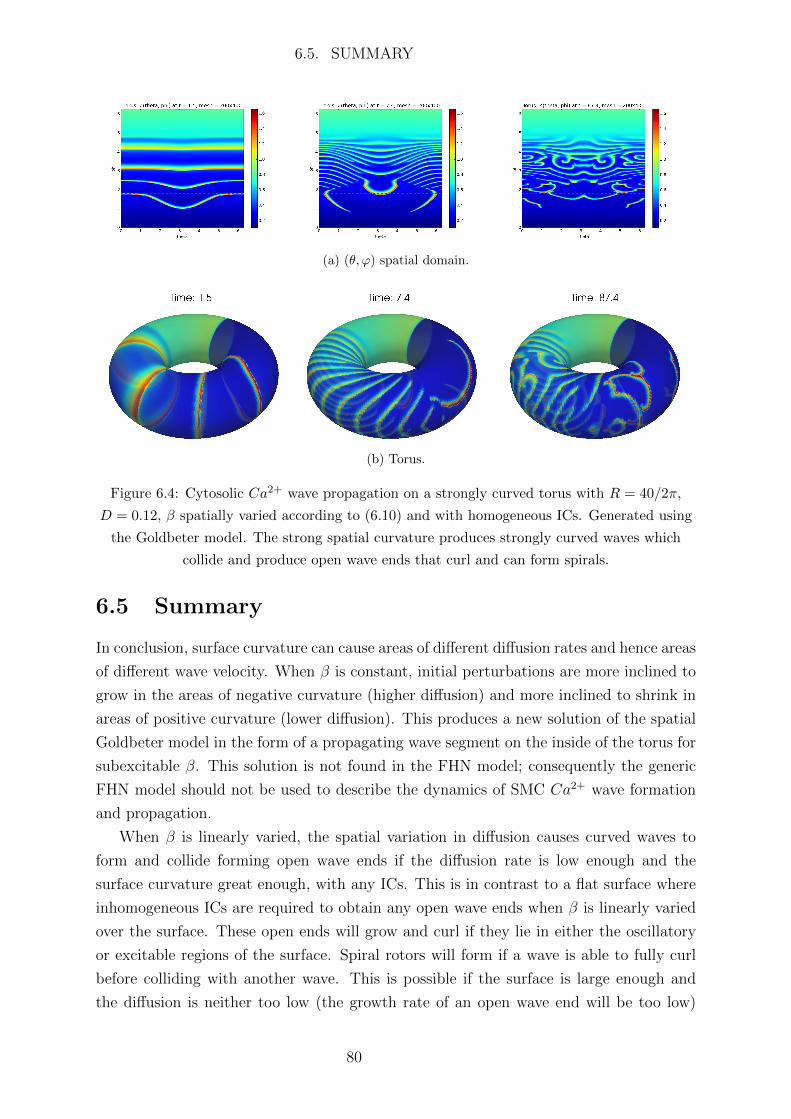
6.5. SUMMARY
(a) (θ, ϕ) spatial domain.
(b) Torus.
Figure 6.4: Cytosolic Ca2+ wave propagation on a strongly curved torus with R = 40/2π,
D = 0.12, β spatially varied according to (6.10) and with homogeneous ICs. Generated using
the Goldbeter model. The strong spatial curvature produces strongly curved waves which
collide and produce open wave ends that curl and can form spirals.
6.5 Summary
In conclusion, surface curvature can cause areas of different diffusion rates and hence areas
of different wave velocity. When β is constant, initial perturbations are more inclined to
grow in the areas of negative curvature (higher diffusion) and more inclined to shrink in
areas of positive curvature (lower diffusion). This produces a new solution of the spatial
Goldbeter model in the form of a propagating wave segment on the inside of the torus for
subexcitable β. This solution is not found in the FHN model; consequently the generic
FHN model should not be used to describe the dynamics of SMC Ca2+ wave formation
and propagation.
When β is linearly varied, the spatial variation in diffusion causes curved waves to
form and collide forming open wave ends if the diffusion rate is low enough and the
surface curvature great enough, with any ICs. This is in contrast to a flat surface where
inhomogeneous ICs are required to obtain any open wave ends when β is linearly varied
over the surface. These open ends will grow and curl if they lie in either the oscillatory
or excitable regions of the surface. Spiral rotors will form if a wave is able to fully curl
before colliding with another wave. This is possible if the surface is large enough and
the diffusion is neither too low (the growth rate of an open wave end will be too low)
80
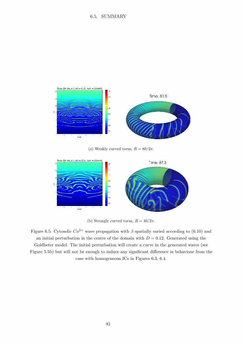
6.5. SUMMARY
(a) Weakly curved torus, R = 80/2π.
(b) Strongly curved torus, R = 40/2π.
Figure 6.5: Cytosolic Ca2+ wave propagation with β spatially varied according to (6.10) and
an initial perturbation in the centre of the domain with D = 0.12. Generated using the
Goldbeter model. The initial perturbation will create a curve in the generated waves (see
Figure 5.5b) but will not be enough to induce any significant difference in behaviour from the
case with homogeneous ICs in Figures 6.3, 6.4.
81

6.5. SUMMARY
(a) Weakly curved torus, R = 80/2π.
(b) Strongly curved torus, R = 40/2π.
Figure 6.6: Cytosolic Ca2+ wave propagation with β spatially varied according to (6.10) and
randomly generated initial values at each mesh point with D = 0.12. Generated using the
Goldbeter model. The strongly inhomogeneous ICs perturb the system enough so that the
waves generated are irregularly shaped (see Figure 5.6b) and consequently will collide and
form open wave ends leading to spiral rotors and asymmetric wave patterns regardless of the
spatial curvature.
82

6.5. SUMMARY
nor too high (waves collide before spirals can form). The waves will quickly collide and
form open wave ends when the waves are more strongly curved. This will occur when the
surface curvature is strongly curved or the ICs are inhomogeneous.
As with a flat surface, increasing the diffusion coefficient from D = 0.12 will increase
the wave velocity and the generated waves will be more regular. Decreasing the dif-
fusion coefficient will decrease the wave velocity and any inhomogeneous ICs will have
the dominant effect causing the generated waves to be less regular and more seemingly
‘chaotic’.
83

Chapter 7
Conclusions
7.1 Discussion
In this thesis the dynamics of calcium (Ca2+) within a single and coupled smooth muscle
cell (SMC)system and the propagation of intercellular Ca2+ waves were studied. The
first was achieved using the minimal model by Goldbeter et al. (1990) based on Ca2+
induced Ca2+ release (CICR). By varying a single parameter of the model, qualitatively
different dynamics (stable or oscillatory) were produced. Two other minimal models
by Gonzalez-Fernandez and Ermentrout (1994) and Meyer and Stryer (1988) based on
different mechanisms in the cell were also briefly studied and compared.
The dynamics of these minimal models were then compared to the complex and more
realistic model based on the work of Farr and David (2011) and Dormanns et al. (2015)
of a SMC and endothelial cell (EC) ‘unit’, the model of which includes the influence of
neuronal activity on the Ca2+ dynamics via the process of neurovascular coupling (NVC).
The models were then extended to two adjacent coupled SMCs (or coupled SMC/EC
units) via a linear coupling term, where the cells/units have different parameter values
and with variable rate of diffusion of Ca2+ between the two.
The formation and propagation of Ca2+ waves was simulated in a two dimensional
(2D) spatial domain using the minimal model by Goldbeter et al. (1990), where the do-
main was either constant or spatially varying in its local dynamics (oscillatory, excitable,
subexcitable or nonexcitable). This was compared to the generic excitable FitzHugh-
Nagumo (FHN) model (FitzHugh, 1961; Nagumo et al., 1962) with known spatial dy-
namics (Kneer et al., 2014).
Finally the concept of spatial curvature was introduced to the 2D spatial domain
via simulations on a toroidal surface containing both negative and positive Gaussian
curvature. Both the Goldbeter et al. (1990) and FHN models were simulated on a torus
to study the effects of spatial curvature on the dynamics of Ca2+ waves in SMCs.
84

7.1. DISCUSSION
7.1.1 Non Spatial Models
The bifurcation structure of the SMC cytosolic Ca2+ concentration in each of the four
models are of a similar form even though each model has a different bifurcation parameter
varied. Excluding the Gonzalez-Fernandez and Ermentrout (1994) model the different
parameters all serve a similar function, that is, raising the inotisol trisphosphate (IP3)
induced Ca2+ flux from the internal stores (sarcoplasmic reticulum (SR) or endoplasmic
reticulum (ER)) into the cytosol of the cell. When these parameters are either low or
high the system tends to a steady state (stable), otherwise the system variables oscillate.
Within the stable domain lies the excitable subdomain adjacent to the oscillatory domain.
Therefore a single cell or SMC/EC unit will be either nonexcitable, excitable or oscillatory.
In particular the bifurcation structure of the Goldbeter et al. (1990) model is the most
comparable to that of the more complex SMC/EC model. The oscillatory domain of both
models are enclosed by Hopf bifurcations and there is a steep increase in both the ampli-
tude and period of oscillations directly after the lower Hopf bifurcation. There also exists
an excitable domain below the lower Hopf bifurcation in both models. The Goldbeter
model is only two dimensional and yet the dynamics produced in a SMC are very similar
the dynamics of the 14 dimensional SMC/EC model. The only additional components
present in the SMC/EC model are the small amplitude oscillations and bistability when
JPLC is low and neuronal activity high, believed to exist due to the stretch activated Ca2+
channels not included in the minimal Goldbeter model.
The dynamics of a system of two coupled cells or SMC/EC units are seemingly inde-
pendent of the model implemented, dependent only on their dynamics when uncoupled
(either excitable, nonexcitable or oscillatory). The behaviour of two coupled cells/units
when strongly coupled is determined by where the average of their two parameters lie in
the parameter space. For example using the Goldbeter et al. (1990) model, two coupled
cells with β1 = 0.5 and β2 = 0.6 will both behave like a cell with β = 0.55 (behaviour
determined by the bifurcation diagram in Figure 3.3).
Identical coupled cells/units will remain the same. Two nonidentical nonexcitable
cells/units will remain nonexcitable and two nonidentical excitable cells/units will re-
main excitable when coupled. Two nonidentical oscillatory cells/units will oscillate with
variable amplitude when weakly coupled and when strongly coupled they synchronise by
oscillating at the same frequency.
A coupled nonexcitable and excitable cell/unit will remain stable. A coupled nonex-
citable and oscillatory cell/unit will both oscillate when weakly coupled and either be
stable or oscillatory when strongly coupled depending on their average JPLC. A coupled
excitable and oscillatory cell/unit will cause the excitable one to oscillate with small
amplitude when weakly coupled. When the coupling strength reaches some threshold
value the excitable cell/unit experiences a large amplitude oscillation when the coupling
85
7.1. DISCUSSION
strength (and hence the intercellular Ca2+ flux) is enough to cause the SMC Ca2+ con-
centration of the excitable cell/unit to exceed the excitation threshold; as the coupling
strength increases the cells/units exhibit variable amplitude oscillations, and finally syn-
chronisation when strongly coupled.
Therefore when weakly coupled it appears the movement of ions between two cells
can produce new complex behaviour fundamentally different from what one would predict
looking at either cell in isolation, in particular two coupled oscillatory cells or an excitable
coupled with an oscillatory cell.
While these models have similar bifurcation structure for a single cell/unit and similar
behaviour for two coupled cells, it must be noted that their respective spatial models of
many cells or units simulated on some surface may have qualitatively different behaviour
to one another.
7.1.2 Spatial Models
The formation and propagation of waves in a flat spatial medium with spatially constant
local dynamics is dependent on the nature of those dynamics, specifically whether the
medium is oscillatory, excitable, subexcitable or nonexcitable (determined by the param-
eter β of the Goldbeter et al. (1990) model). An initial perturbation in the form of a
localised input of Ca2+ will form a propagating wave when the spatial medium is ex-
citable and a propagating wave that shrinks in length when the medium is subexcitable.
When a propagating wave is broken and the medium is excitable then the open wave end
will curl and is able to form a spiral rotor, generating outwardly rotating spiral waves.
The local dynamics of a system can be varied over a surface via the parameter β as
a linear function of the spatial coordinate y. Waves will be generated where the system
is oscillatory and propagate into the excitable domain. If the initial conditions (ICs) are
homogeneous then the generated waves will be straight and when they collide will leave
no open ends. If the ICs are inhomogeneous then the offset in the waves caused by the
ICs will make the waves curved and may eventually cause them to collide and form open
wave ends. These ends will grow in length if the system is oscillatory or excitable, leading
to curled wave ends and possibly spatiotemporal chaos from the interaction of the open
wave ends. Spiral rotors will form if a wave is able to fully curl before colliding with
another wave. This is possible if the surface is large enough and the diffusion is neither
too low (the growth rate of an open wave end will be too low) nor too high (waves collide
before spirals can form).
Including the concept of spatial curvature via a toroidal surface can produce areas of
different diffusion rates (low diffusion when the surface has positive curvature and high
diffusion for areas of negative curvature), and hence areas of different wave velocity. When
the local dynamics are spatially constant (via the parameter β), initial perturbations are
86
7.1. DISCUSSION
more inclined to grow on the torus inside (negative curvature and thus higher diffusion)
and more inclined to shrink on the torus outside (positive curvature and thus lower
diffusion). This produces a new solution of the spatial Goldbeter model in the form of
a propagating wave segment with stable wavesize on the inside of the torus when the
medium is subexcitable. This solution is not found when the FHN model is simulated
on a torus; consequently the dynamics of the generic FHN model should not be used to
describe the dynamics of SMC Ca2+ wave formation and propagation.
When the local dynamics are varied over the toroidal surface via the parameter β
as a linear function of the spatial coordinate ϕ, the spatial variation in diffusion causes
outwardly curved waves to form as the waves travel faster on the torus inside. When the
waves are strongly curved they will collide and interact, forming open wave ends. This will
occur when the surface curvature is strongly curved and/or the ICs are inhomogeneous.
This is in contrast to a flat surface where inhomogeneous ICs are required to obtain any
significant wave interaction.
Therefore wave interaction (causing complex wave patterns such as spiral waves and
possibly spatiotemporal chaos) on a spatially varied domain will occur if the diffusion
rate is low enough, and either the spatial domain is strongly curved or the ICs are inho-
mogeneous.
Low coupling strength in the coupled cell models of Chapters 3, 4 lead to complex be-
haviour such as variable amplitude oscillations. Low diffusion rate in the spatial models
of Chapters 5, 6 lead to low wave velocity causing irregular propagating waves with ample
wave interaction. High coupling strength in the coupled cell models caused synchronisa-
tion between the two cells. High diffusion rate lead to high wave velocity causing regular
propagating waves with little to no wave interaction. In both cases the ‘interesting’
behaviour was found when the coupling/diffusion strength was low.
7.1.3 Limitations and Future Work
A limitation of our work is the use of a simple linear coupling term corresponding to
Fick’s Law, i.e. the Ca2+ moves from high to low concentration. A more complex
coupling mechanism such the Goldman Hodgkin Katz (GHK) equation for the movement
of ions and membrane potential may be used. This describes the ionic flux carried by
an ionic species across a cell membrane as a function of the membrane potential (as ions
are electrically charged) in addition to the concentrations of the ion inside and outside of
the cell. An example of this coupling mechanism is used by Kapela et al (Kapela et al.,
2009) to model the flow of ions (specifically Ca2+, K+, Na+ and Cl−) between two cells.
A similar coupling expression could be applied to examine whether a more accurate and
complex coupling term would affect the underlying dynamics of the system.
Our simulations on a flat and curved surface in Chapters 5, 6 were computed on
87
7.1. DISCUSSION
a relatively small mesh (200 × 800) in order to have a feasible runtime on our local
computer. However increasing or decreasing this mesh size resulted in a qualitative change
in behaviour; decreasing the mesh to 100× 400 caused the same effect as decreasing the
diffusion coefficient and increasing the mesh to 300× 1200 was similar to increasing the
diffusion coeffcient. This is known as mesh dependency, a problem well known in areas
such as compuational fluid dynamics. Future work may involve increasing the mesh
until the solution converges and there is no further dependence on the mesh size. These
large mesh simulations will most likely require parallel architecture to run with a feasible
runtime.
The diffusion coefficient D for the spatial simulations using the Goldbeter et al. (1990)
model was chosen to be consistent with the FHN model, however it is not physiologically
accurate for Ca2+ diffusion through SMCs even though the Goldbeter model is nondi-
mensional. In reality the diffusion coefficient is likely to be much smaller than the value
of D = 0.12 used in the majority of our results; such a coefficient would make our sim-
ulations more physiologically accurate as the patterns resulting from wave propagation
and interaction on a surface with spatially varied local dynamics are dependent on the
rate of diffusion.
Our spatial simulations implementing the Goldbeter et al. (1990) model used a linear
function for the spatial variation in local dynamics (via the bifurcation parameter β),
however it would be interesting to run our simulations with a more realistic parameter
distribution. As an example, Zakkaroff et al. (2015) applied the SMC/EC model by
Shaikh et al. (2012) (originally based on the model by Koenigsberger et al. (2005)) to
the surface of an arterial bifurcation; both a synthetic agonist map of JPLC (based on the
wall shear stress) and a computational fluid dynamics (CFD) based JPLC map were used
in their simulations.
It would be worthwhile simulating the complex SMC/EC model on a spatial domain,
in particular a curved surface since this model includes the influence of neuronal activity
on SMC Ca2+ dynamics and the brain cortex is a strongly curved medium. As this
model contains a total of 14 state variables it is much more complex than the previously
simulated Goldbeter et al. (1990) model and any simulations on a 2D spatial domain
would most likely require parallel architecture in order to have a feasible runtime. In
addition the system is stiff so the full capabilities of the ARKode additive solver could
be implemented by partitioning the system equations into ‘fast’ and ‘slow’ timescale
components, decreasing the runtime. The nonspatial results of a single and coupled
system using either the Goldbeter et al. (1990) and SMC/EC models are similar in nature;
would this still be true when simulated on a spatial domain?
88
7.2. RESEARCH SUMMARY
7.2 Research Summary
The minimal Goldbeter et al. (1990) model of Ca2+ dynamics within a SMC produces
similar behaviour to that of a more complex and physiologically realistic model of a
SMC/EC ‘unit’ based on the model of a full neurovascular unit (NVU) by Farr and David
(2011) and Dormanns et al. (2015). The cell or unit will exhibit excitable, nonexcitable or
oscillatory behaviour depending on the rate of IP3 induced Ca2+ release from the internal
stores into the cytosol of the cell. However small amplitude oscillations and bistability are
found in the SMC/EC model when neuronal activity is high and the rate of IP3 induced
Ca2+ release is low; these dynamics are thought to be a result of the stretch activated
Ca2+ channels not found in the Goldbeter et al. (1990) model.
The behaviour of two coupled cells or SMC/EC units are seemingly model indepen-
dent; an excitable coupled with an oscillatory cell or two nonidentical coupled oscillatory
cells will exhibit qualitatively different behaviour when weakly coupled such as variable
amplitude oscillations.
When the Goldbeter et al. (1990) model is simulated on a 2D spatial domain with the
local dynamics of the system spatially varied, Ca2+ waves are initiated where the domain
is oscillatory and propagate where the domain is excitable. The curvature of a spatial
domain can have an effect on the local rate of diffusion; positive curvature decreases the
rate of diffusion, negative curvature increases the rate of diffusion. This produces a new
wave solution of the Goldbeter et al. (1990) model in the form of a propagating wave
segment of constant wave size and shape. Wave interaction causing patterns such as spiral
waves and seemingly spatiotemporal chaotic behaviour on a spatially varied domain will
occur if the diffusion rate is low enough, and either the spatial domain is strongly curved
or the ICs are inhomogeneous.
As the single and coupled Goldbeter et al. (1990) model produces similar behaviour
to the SMC/EC model based on a NVU, it is possible that the dynamics of the Goldbeter
model simulated on both a flat and curved 2D spatial domain may provide some insight
into the dynamics of Ca2+ wave formation and propagation of the more complex and
physiologically realistic SMC/EC model.
89
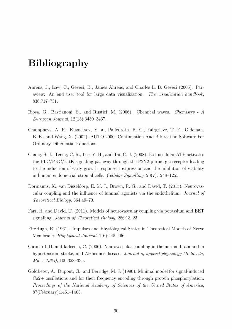
Bibliography
Ahrens, J., Law, C., Geveci, B., James Ahrens, and Charles L. B. Geveci (2005). Par-
aview: An end user tool for large data visualization. The visualization handbook,
836:717–731.
Biosa, G., Bastianoni, S., and Rustici, M. (2006). Chemical waves. Chemistry - A
European Journal, 12(13):3430–3437.
Champneys, A. R., Kuznetsov, Y. a., Paffenroth, R. C., Fairgrieve, T. F., Oldeman,
B. E., and Wang, X. (2002). AUTO 2000: Continuation And Bifurcation Software For
Ordinary Differential Equations.
Chang, S. J., Tzeng, C. R., Lee, Y. H., and Tai, C. J. (2008). Extracellular ATP activates
the PLC/PKC/ERK signaling pathway through the P2Y2 purinergic receptor leading
to the induction of early growth response 1 expression and the inhibition of viability
in human endometrial stromal cells. Cellular Signalling, 20(7):1248–1255.
Dormanns, K., van Disseldorp, E. M. J., Brown, R. G., and David, T. (2015). Neurovas-
cular coupling and the influence of luminal agonists via the endothelium. Journal of
Theoretical Biology, 364:49–70.
Farr, H. and David, T. (2011). Models of neurovascular coupling via potassium and EET
signalling. Journal of Theoretical Biology, 286:13–23.
FitzHugh, R. (1961). Impulses and Physiological States in Theoretical Models of Nerve
Membrane. Biophysical Journal, 1(6):445–466.
Girouard, H. and Iadecola, C. (2006). Neurovascular coupling in the normal brain and in
hypertension, stroke, and Alzheimer disease. Journal of applied physiology (Bethesda,
Md. : 1985), 100:328–335.
Goldbeter, A., Dupont, G., and Berridge, M. J. (1990). Minimal model for signal-induced
Ca2+ oscillations and for their frequency encoding through protein phosphorylation.
Proceedings of the National Academy of Sciences of the United States of America,
87(February):1461–1465.
90
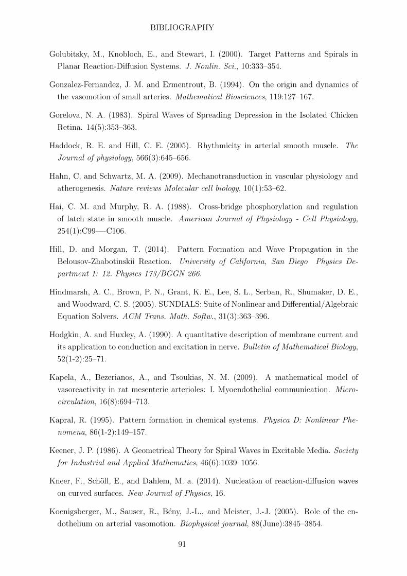
BIBLIOGRAPHY
Golubitsky, M., Knobloch, E., and Stewart, I. (2000). Target Patterns and Spirals in
Planar Reaction-Diffusion Systems. J. Nonlin. Sci., 10:333–354.
Gonzalez-Fernandez, J. M. and Ermentrout, B. (1994). On the origin and dynamics of
the vasomotion of small arteries. Mathematical Biosciences, 119:127–167.
Gorelova, N. A. (1983). Spiral Waves of Spreading Depression in the Isolated Chicken
Retina. 14(5):353–363.
Haddock, R. E. and Hill, C. E. (2005). Rhythmicity in arterial smooth muscle. The
Journal of physiology, 566(3):645–656.
Hahn, C. and Schwartz, M. A. (2009). Mechanotransduction in vascular physiology and
atherogenesis. Nature reviews Molecular cell biology, 10(1):53–62.
Hai, C. M. and Murphy, R. A. (1988). Cross-bridge phosphorylation and regulation
of latch state in smooth muscle. American Journal of Physiology - Cell Physiology,
254(1):C99—-C106.
Hill, D. and Morgan, T. (2014). Pattern Formation and Wave Propagation in the
Belousov-Zhabotinskii Reaction. University of California, San Diego Physics De-
partment 1: 12. Physics 173/BGGN 266.
Hindmarsh, A. C., Brown, P. N., Grant, K. E., Lee, S. L., Serban, R., Shumaker, D. E.,
and Woodward, C. S. (2005). SUNDIALS: Suite of Nonlinear and Differential/Algebraic
Equation Solvers. ACM Trans. Math. Softw., 31(3):363–396.
Hodgkin, A. and Huxley, A. (1990). A quantitative description of membrane current and
its application to conduction and excitation in nerve. Bulletin of Mathematical Biology,
52(1-2):25–71.
Kapela, A., Bezerianos, A., and Tsoukias, N. M. (2009). A mathematical model of
vasoreactivity in rat mesenteric arterioles: I. Myoendothelial communication. Micro-
circulation, 16(8):694–713.
Kapral, R. (1995). Pattern formation in chemical systems. Physica D: Nonlinear Phe-
nomena, 86(1-2):149–157.
Keener, J. P. (1986). A Geometrical Theory for Spiral Waves in Excitable Media. Society
for Industrial and Applied Mathematics, 46(6):1039–1056.
Kneer, F., Scholl, E., and Dahlem, M. a. (2014). Nucleation of reaction-diffusion waves
on curved surfaces. New Journal of Physics, 16.
Koenigsberger, M., Sauser, R., Beny, J.-L., and Meister, J.-J. (2005). Role of the en-
dothelium on arterial vasomotion. Biophysical journal, 88(June):3845–3854.
91
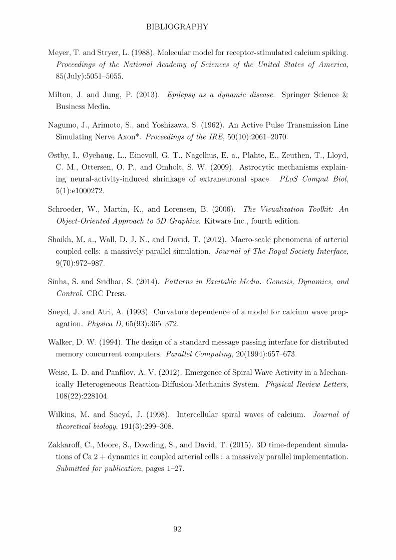
BIBLIOGRAPHY
Meyer, T. and Stryer, L. (1988). Molecular model for receptor-stimulated calcium spiking.
Proceedings of the National Academy of Sciences of the United States of America,
85(July):5051–5055.
Milton, J. and Jung, P. (2013). Epilepsy as a dynamic disease. Springer Science &
Business Media.
Nagumo, J., Arimoto, S., and Yoshizawa, S. (1962). An Active Pulse Transmission Line
Simulating Nerve Axon*. Proceedings of the IRE, 50(10):2061–2070.
Østby, I., Øyehaug, L., Einevoll, G. T., Nagelhus, E. a., Plahte, E., Zeuthen, T., Lloyd,
C. M., Ottersen, O. P., and Omholt, S. W. (2009). Astrocytic mechanisms explain-
ing neural-activity-induced shrinkage of extraneuronal space. PLoS Comput Biol,
5(1):e1000272.
Schroeder, W., Martin, K., and Lorensen, B. (2006). The Visualization Toolkit: An
Object-Oriented Approach to 3D Graphics. Kitware Inc., fourth edition.
Shaikh, M. a., Wall, D. J. N., and David, T. (2012). Macro-scale phenomena of arterial
coupled cells: a massively parallel simulation. Journal of The Royal Society Interface,
9(70):972–987.
Sinha, S. and Sridhar, S. (2014). Patterns in Excitable Media: Genesis, Dynamics, and
Control. CRC Press.
Sneyd, J. and Atri, A. (1993). Curvature dependence of a model for calcium wave prop-
agation. Physica D, 65(93):365–372.
Walker, D. W. (1994). The design of a standard message passing interface for distributed
memory concurrent computers. Parallel Computing, 20(1994):657–673.
Weise, L. D. and Panfilov, A. V. (2012). Emergence of Spiral Wave Activity in a Mechan-
ically Heterogeneous Reaction-Diffusion-Mechanics System. Physical Review Letters,
108(22):228104.
Wilkins, M. and Sneyd, J. (1998). Intercellular spiral waves of calcium. Journal of
theoretical biology, 191(3):299–308.
Zakkaroff, C., Moore, S., Dowding, S., and David, T. (2015). 3D time-dependent simula-
tions of Ca 2 + dynamics in coupled arterial cells : a massively parallel implementation.
Submitted for publication, pages 1–27.
92
Related Documents