CABLES

VTT PUBLICATIONS 302

Derating of cables at high temperatures

Olavi Keski-Rahkonen, Jouni Björkman & Juho Farin

Second, revised edition, May 2008

ISBN 951-38-5043-9 (soft back ed.) ISSN 1235-0621 (soft back ed.)

ISBN 951-38-5044-7 (1st electronic ed.) ISBN 978-951-38-7101-7 (2nd electronic ed.) ISSN 1455-0849 (URL: http://www.vtt.fi/publications/index.jsp) Copyright © Valtion teknillinen tutkimuskeskus (VTT) 1997

JULKAISIJA UTGIVARE PUBLISHER

VTT, Vuorimiehentie 3, PL 1000, 02044 VTT puh. vaihde 020 722 111, faksi 020 722 4374

VTT, Bergsmansvägen 3, PB 1000, 02044 VTT tel. växel 020 722 111, fax 020 722 4374

VTT Technical Research Centre of Finland, Vuorimiehentie 3, P.O. Box 1000, FI-02044 VTT, Finland phone internat. +358 20 722 111, fax + 358 20 722 4374

VTT, Biologinkuja 7, PL 1000, 02044 VTT puh. vaihde 020 722 111, faksi 020 722 7026

VTT, Biologgränden 7, PB 1000, 02044 VTT tel. växel 020 722 111, fax 020 722 7026

VTT Technical Research Centre of Finland, Biologinkuja 7, P.O. Box 1000, FI-02044 VTT, Finland phone internat. +358 20 722 111, fax +358 20 722 7026

Technical editing Kerttu Tirronen VTT OFFSETPAINO, ESPOO 1997

3

Keski-Rahkonen, Olavi, Björkman, Jouni & Farin, Juho. Derating of cables at high temperatures. Espoo 1997, Technical Research Centre of Finland, VTT Publications 302. 57 p. + app. 2 p.

UCD 621.315.2:614.841.2 Keywords power lines, caple insulation, fire safety, nuclear power plants, high temperature

tests

ABSTRACT A method to characterize behaviour of cables used in nuclear power plants at temperatures exceeding the long-term rating was developed. The problem is to predict how long and at what temperatures cables function in emergency situations. The structure and materials of the relevant cables were reviewed and the properties of these materials at high temperatures were described from literature sources. The physical and chemical processes to be expected were outlined for designing tests. Initially we carried out a real-scale equivalent test with a closed circuit, where the pair cable was connected to a pressure transmitter. The instrument PVC cable under investigation worked normally up to 196 °C, where a short circuit occurred, and leakage current suddenly rose to a high value. However, we could not get any evidence of continuous insulation derating from room temperature to the short circuit temperature. This may be due to the experimental arrangements not being sensitive enough to slight phenomenan or to leakages at connections in the electrical circuit. In order to obtain data about the conductivity of PVC cable insulation at elevated temperatures, a part of the open circuit was heated in a test furnace step by step from room temperature to the short circuit temperature region of 200 °C. We discovered leakage current and insulation conductivity improvement in the PVC cable by using a sensitive electrometer and an insulation resistance meter applied in the open circuit experiment for pure cable. Electrical conductivity of PVC cable insulation materials from the literature and electrical conductivity of the PVC cable insulation layer as a function of inverse absolute temperature match quite well. The first series of tests was carried out for a PVC cable to check the validity of the theory and the test method. The testing programme continued and included seven different types of cables.

4

PREFACE This report consists of a description of cable experiments at rising temperature carried out at VTT. The authors would like to thank K. Taimisalo and H. Juutilainen for technical assistance. Advice and assistance by U. Pulkkinen, VTT Automation, O. Ikkala, Helsinki University of Technology, M. Terho, Nokia Cables, and M. Hirvensalo, Borealis Oy is gratefully acknowledged.

The sponsors of the project have been the Ministry of Trade and Industry, the Finnish Centre for Radiation and Nuclear Safety, IVO International Oy, Teol-lisuuden Voima Oy and the Finnish Fire Research Board.

5

CONTENTS

ABSTRACT...................................................................................................3 PREFACE ......................................................................................................4 LIST OF SYMBOLS .....................................................................................7

1 INTRODUCTION ......................................................................................9

1.1. GENERAL ..........................................................................................9

1.2 MALFUNCTION OF COMPONENTS AND CABLES IN CASE OF FIRE ..............................................................................9

2 STRUCTURES OF AND MATERIALS USED IN CABLES ................11

2.1 TYPES OF CABLES.........................................................................11

2.2 CABLE MATERIALS.......................................................................12 2.2.1 Polyvinylchloride (PVC) ............................................................12 2.2.2 Crosslinked polyethylene (PE-X, PEX, XPE) ............................12 2.2.3 Chlorosulphonated polyethylene (CSP)......................................13 2.2.4 Ethylene-propylene copolymer (E/P, EPR) ................................13 2.2.5 Ethylene-propylene-diene monomer (EPDM)............................14 2.2.6 Polymethyl methacrylate (PMMA).............................................14 2.2.7 Silicone rubbers...........................................................................15 2.2.8 Polyolefins ..................................................................................16 2.2.9 Polychloroprene (PCP-rubber)....................................................16

3 PROPERTIES OF CABLE MATERIALS AT HIGH TEMPERATURES18

3.1 GLASS TRANSITION......................................................................19

3.2 ELECTRICAL CONDUCTION IN POLYMERS............................20 3.2.1 Ionic conduction..........................................................................21 3.2.2 Electronic conduction .................................................................22 3.2.3 Conducting composites ...............................................................22

4 TESTS OF CABLES AT HIGH TEMPERATURES ..............................24

4.1 THEORETICAL MODEL.................................................................24 4.1.1 Transmission characteristics .......................................................24 4.1.2 Equivalent circuit of transmitter line ..........................................26 4.1.3 Modelling of lumped parameters for a pair cable.......................27

4.2 NUMERICAL ESTIMATES OF PARAMETERS...........................29 4.2.1 Copper wire resistance ................................................................30 4.2.2 Leakage current of a pair cable ...................................................30

6

4.3 ELECTRIC TEST SET-UP ...............................................................32 4.3.1 Test-set up: closed circuit including the pressure transmitter.....32

4.3.1.1 Inaccuracies of the closed circuit test .............................34 4.3.2 Test set-up for measuring conductivity of insulation layer of cables at elevated temperatures..................................................35 4.3.3 Improved second test set-up........................................................36

5 EXPERIMENTAL RESULTS..................................................................40 5.1. The first test series ........................................................................40 5.2. The conductivity of the insulation layer of cables at elevated temperatures .................................................................................42

6 DISCUSSION AND CONCLUSIONS ....................................................53

REFERENCES.............................................................................................54

APPENDIX

7

LIST OF SYMBOLS A area (m2), pre-exponential factor a distance (m) C capacitance (F) c constant E power supply voltage (V) f fractional degree of dissociation, frequency (Hz) G conductance (S/m) I electric current (A) j imaginary unit (j2=-1) K equilibrium constant k Bolzmann constant (J/K) L inductance (H) l physical length (m) n concentration (1/m3) p percent (%) q charge (C) R resistance (Ω) r radius (m) T temperature (K) t time (s) v velocity (m/s) Z impedance (Ω) ∆W energy required to separate the ions from each other in a medium of

unit permittivity (J) Greek symbols: α angular constant, temperature coefficient (1/K) β damping constant ε permittivity (F/m) δ loss angle γ propagation constant ν volume, angular velocity (1/s) µ mobility (m2/Vs), permeability (H/m) ρ resistivity (Ωm) Φ electrical length σ electrical conductivity (S/m) ω angular frequency (1/s) Subscripts: c cable f free g gas i source

8

L lumped l leakage o initial, zero, characteristic, unit pd propagation delay r relative s static, source

9

1 INTRODUCTION

1.1. GENERAL

The purpose of this study is to collect knowledge for fire risk analysis to estimate how long a cable or electric instrument works at temperatures exeeding ratings which could be caused by fire in the vicinity. Knowledge of damage thresholds for nuclear qualified electrical cable insulation is critical to proper modelling of fire growth and fire-induced damage in nuclear power plants. Cable and instrument manufacturers give electrical parameters only for environment limits in normal long-term use. Emergency and short circuit temperature limits are based on mechanical strength tests, and information on the electrical properties (conductivity) is insufficient for real cables. In case of fire, when temperatures exceed limits applied in normal situations, equipment may still work for some time, which is important for the safety measures of the plant. The time beyond the use limit of temperature, heat release rate or smoke density can be investigated by carrying out realistic simulations or experiments. In this study we searched the literature for functional limits for cables important to the PSA (Probability Safety Assessment) work of nuclear power plants. These data are not easily available. We investigated more closely cable materials and phenomena occurring in cables. Here we survey general characteristics of cable behaviour as a function of temperature and time from the maximum temperature rating up to temperatures occurring during fires, where cables are already burning. In Chapter 2 the structure and materials of the relevant cables are reviewed. In Chapter 3 properties of these materials at high temperatures are described. The physical and chemical processes to be expected are outlined for the design of testing measurements. In Chapter 4 the test set up, in Chapter 5 the test results are described, and in Chapter 6 conclusions are drawn.

1.2 MALFUNCTION OF COMPONENTS AND CABLES IN CASE OF FIRE

In the open literature only a very limited amount of information was available concerning the function of components in case of fire. The literature survey yielded a few references of work carried out at Factory Mutual (FMRC), Lawrence Livermore Laboratory (LLL) and Sandia National Laboratories (SNL) in the USA. Fire damage to electrical cables could potentially occur due to several mechanisms: temperature, heat radiation, smoke, corrosive gases and fire suppression effects. Alvares et al. (1983) at LLL carried out an extensive series of studies on thermal degradation of cable and wire insulations using variants both bench-scale and full-scale tests. Some data are available on the damaging

10

potentials of the thermal effects (FMRC) (temperature and heat radiation) but only very limited data on other effects (Tewarson 1995). Cable failure data have been collected in a series of convective heating tests at SNL (Nicolette 1988), where cable ignition and failure were recorded as functions of ambient temperature and time. The qualified cable tested had a cross-linked polyethylene jacket and insulation. The unqualified jacket had a PVC jacket and polyethylene PE/PVC insulation. The results indicate that average electrical failure times at 623 K were 13.2 ± 6.9 minutes for the qualified cables. The unqualified cables failed in temperature environments as low as 523 K an average of 6.9 ± 4.4 minutes. At higher ambient temperatures, failure times were shorter, as expected. The main limitation to the above mentioned SNL test data is the fact that only two types of cables were tested, and the results are not directly applicable to cables with other jacket or insulation materials. Disruption of signals within cable trays resident in DOE nuclear facilities caused by effects from fire were studied at LLL (Hasegawa et al. 1992). Such malfunctions could adversely affect or prevent the safe shutdown or other critical control functions. Four cable bundles comprised of a power cable, coaxial, and two multiconductor cables were laid in fully loaded 1.8 m ladder type cable trays and energized with dc current. The power cable in each bundle was energized while the remaining cables in the bundle along with the cable tray were monitored for current transfer. Five full-scale tests of grouped cables in trays were conducted to address the potential occurrence of various types of electrical failures. The cable tray was supported above a test fire produced by a natural gas fired burner. Two tests were conducted at 24 Vdc and 3 tests at 120 Vdc. The following primary failures occurred in the tests: direct short circuits between cables or cable and tray, intermittent direct short circuits between cables or cable and tray, high impedance short circuits between cables or cables and tray, open circuit in cabling, production of electromagnetic fluxes. Many of the types and numbers of electrical failures listed above would increase the probability of a variety of control malfunctions in the event of a cable tray fire. The results show that in some cases, less than 5 minutes after fire exposure, a cable tray could potentially result in the loss of control or the unwanted activation of control system components.

11

2 STRUCTURES OF AND MATERIALS USED IN CABLES

2.1 TYPES OF CABLES

In this study we concentrate on instrument and power cables used in Finnish nuclear power plants. In Table 1 information presented from the utilities on the types of most general cables is obtained.

Table 1. Cable types used frequently in Finnish nuclear power plants.

Cable type Structure insul/fill/sheath/jacket YXCH 1x185 mm2 PEX/Cu/Hypalon YHLH 1x185 mm2 PEX/Pb/Hypalon 3x70+35 mm2 EPR/jute/Cu/CSP LJNCM3x70+35 mm2 EPDM/PCP/Cu/PVC LJNSM3x2,5 mm2 EPDM/PCP/Cu/PVC MHMS-SI(2-20)x2x0,8 mm2 PVC/Al/PVC (2-8)x2x0,6 mm2 FRPO/Cu/FRPOX (8-16)x1,5 mm2 SiR/SiR SSJS(8-16)x1,5 mm2 SiR/SiR MHMS-SI PVC/Al/PVC MAMSI PVC/PVC MAMSI-E PVC/PVC MKHMS PVC/PVC MONETTE SiR/SiR MMJ 4x2.5N PVC/fil/LinylPVC MCMK 3x PVC/fil/PVC AMCMK 3x PVC/PVC APYAKMM 3x185 mm2 paper/PE/PE MMAO-A PVC/polyes.Al/PVC MMO-A 37x1.0 PVC/PVC MMAAM-A PVC/polyes.Al/PVC MMO PVC MMJ PVC HHJ Hypalon/Hypalon HHO Hypalon/Hypalon HHSO Hypalon/Hypalon JFJ PVC RXSR-G PEX/Hypalon FSSJ Hypalon/Hypalon FXPK PEX/Pb/PVC HCHKEM Lipalon/Hypalon MXS PEX/Hypalon FSPK Lipalon/Hypalon MLJM PVC/PVC AHXDMK PEX/PVC AHXDMKG PEX/PVC

12

2.2 CABLE MATERIALS

The cable properties are a combination of material properties and the structure of the cable. For conduction at elevated temperatures it is believed material properties overrule the structural features. Therefore, in this chapter we have a literature review of the most important of the materials of cables used in Finnish nuclear power plants listed in Table 1. Electrical properties and thermal properties of those cable materials are listed in Tables 2 and 3 (p. 17), respectively.

2.2.1 Polyvinylchloride (PVC)

The vinyl chloride monomer CH2=CHCl polymerizes to partially syndiotactic, irregular thermoplastic material leading to low crystallinity (Billmeyer 1984, Tanaka & Wolter 1983). Syndiotacticity is a form of tacticity. PVC is relatively unstable in heat. Thermal initiation involves loss of chlorine atoms adjacent to some structural abnormality, which reduces the stability of the C-Cl bond (Grassie 1964). The chlorine radical so formed abstracts a hydrogen atom to form HCl. The resulting chain radical then reacts to form chain unsaturation with regeneration of the chlorine radical. In the cables the PVC sheaths contain about 50 wt% of PVC, 25% dioctyl phthalate (2-HO2CC6H4CO2[CH(CH3)C6H13]) or diisodecylphthalate (C2H4[COOCH2CH(CH3)CH2CH(CH3)CH(CH3)CH2CH3]2) as plasticizer. The rest is stabilizers, inorganic lead sulphate (PbSO4) or organic lead phthalate C6H4(COO)2Pb-2PbO, fillers (CaCO3), and some minor chemicals. Ageing of PVC cable materials is caused by evaporation of plasticizer, mainly causing the material to become brittle (Ullmann 1967).

2.2.2 Crosslinked polyethylene (PE-X, PEX, XPE)

Polyethylene [-CH2=CH2 -]n can be converted to a thermosetting material either by using peroxide chemicals or by irradiation with high energy electrons (Billmeyer 1984). The basic process of crosslinking polyethylene is via a free radical mechanism. Either a peroxide degrades thermally to provide the free radical (chemical crosslinked polyethylene), or the free radical is generated within a polymer chain by the displacement of hydrogen from the chain by high-energy irradiation (irradiated crosslinked polyethylene) (Schwartz and Goodman 1982). The peroxides are stable at normal processing temperatures but decompose to provide free radicals for crosslinking at higher temperatures in a post-processing vulcanization and curing reaction. Radiation crosslinking is used in production of e.g. insulating films combining the properties of polyethylene with form stability up to 200 oC and a significant increase in tensile strength (Billmeyer 1984).

13

2.2.3 Chlorosulphonated polyethylene (CSP)

When polyethylene [-CH2=CH2 -]n is treated with a mixture of chlorine and SO2, some chlorine atoms are substituted on chains and some sulphonyl chloride groups (-SO2Cl) are formed. The chloride atoms break up the polyethylene chain structure so that crystallization is no longer possible, and thus polymer becomes an elastomer. Sulphonyl chloride groups provide sites for crosslinking. A typical polymer contains one chlorine atom for every seven carbon atoms, and one -SO2Cl for every 90 carbon atoms (Billmeyer 1984). The elastomer can be crosslinked by a large variety of compounds, including many rubber accelerators. Metallic oxides are recommended for commercial cures. Fillers are not needed to obtain optimum strength properties (Billmeyer 1984). The useful temperature range is -50 ... 120 °C (Billmeyer 1984) and -46 ... 149 oC for Hypalon (elastomer) (Schwartz and Goodman 1982), which is a trade name of DuPont of chlorosulphonated polyethylene.

2.2.4 Ethylene-propylene copolymer (E/P, EPR)

Catalysed copolymerization of ethylene (CH2=CH2) with propylene (CH3CH=CH2) yields rubbery elastomers, where monomers are randomly distributed. They do not contain long blocks of either ethylene or propylene units. Thus, crystallization cannot occur and these products are completely amorphous. In the copolymer there are virtually no double bonds, and vulcanization is only possible using peroxides (Saunders 1973). The ethylene-propylene copolymer can be crosslinked in order to obtain EPR. The two most common crosslinking agents are dicumyl peroxide (C6H5C(CH3)2OOC(CH3)2C6H5) and ditertiarybutyl peroxide ((CH3)3COOC(CH3)3) (Tanaka and Wolter 1983). The tensile strength and stiffness of the material are improved by the crosslinking (also called vulcanization or curing) process. Two basic types of fillers: inert fillers and reinforcing fillers are used. Inert fillers such as clay do not enhance the mechanical properties of the material but are cheap and make the mixture easier to handle before crosslinking. EPR cable insulation contains 4050 % clay filler. The best and most widely used reinforced filler is carbon black although the mechanism of improving the mechanical properties of EPR is not well understood. The proportion of carbon black in EPR for electrical insulation use must be carefully monitored in order to ensure against electrical failure. Typical EPR cable insulation might contain several percentage points of carbon black (Tanaka and Wolter 1983).

14

2.2.5 Ethylene-propylene-diene monomer (EPDM)

Copolymerization of propylene (CH3CH=CH2) with ethylene (CH2=CH2) yields non crystalline products of rubbery behaviour, which are chemically inert because of their saturation. They must be crosslinked by use of peroxides or radiation. To gain sites for crosslinking, a diene monomer is often added (Billmeyer 1984). The third monomer is a non-conjugated diene; one of its double bonds enters into the polymerizaton process becoming incorporated in the main polymer chain whilst the other double bond does not react and is left in a side chain and is available for subsequent vulcanization (Saunders 1973). Resulting terpolymers are known as ethylene-propylene-diene monomer (EPDM). Ethylene-propylene-diene terpolymers (EPTR or EPDM) are sulphur-curable and now important commercial rubbers (Saunders 1973). The major comonomers are 1,4-hexadiene, dicyclopentadiene, and ethyldiene norbornene. Their structures are described in Figure 1 (Billmeyer 1984). Fillers, which may be organic (such as wood flour) or more commonly inorganic (such as clays, silica and carbon black), are added to improve either the mechanical or electrical (conductive) behaviour and also to lessen the costs of the final product (Bartnikas 1983). Fillers most relevant to electrical properties are the carbon blacks used in semiconductive shields and the clays used to fill noncrystalline EPDMs. The useful temperature range is -55 ... 149 oC.

dicyclopentadiene ethyldiene norbornene

CH2CH - CH3CH3CH = CHCH2CH = CH2

1,4-hexadiene

CH2

Figure 1. Structures of EPDM copolymers (Billmeyer 1984).

2.2.6 Polymethyl methacrylate (PMMA)

Polymethyl methacrylate (PMMA) (CH8O2)n is composed of acrylic or methacrylic ester units (Figure 2a) to form a linear thermoplastic. Because of its lack of stereoregularity and its bulky side groups, it is amorphous (Billmeyer 1984). PMMA burns with a luminous yellow, slightly crackling flame with slight smoke development. The material melts and volatilizes on pyrolysis without any residue. The fire gases have a sweet fruit-like smell. PMMA undergoes over 90 %

15

depolymerization to the monomer which burns in the gas phase (Troitsch, Cullis 1981). The main mechanism of decomposing is random chain stripping (Beyler and Hirschler 1995). Free radical polymerized PMMA decomposes around 545 K, with initiation occurring at double bonds at chain ends. A second peak between 625 and 675 K in dynamic TGA thermograms is the result of a second initiation reaction. The rate of decomposition is also dependent on the tacticity of the polymer. The symmetry of the asymmetric monomer units in the polymer chain is described by (Fessenden and Fessende 1994, Tanaka and Wolter 1983). PMMA is about 7075 % syndiotactic (Billmeyer 1984). The oxygen of the ester group results in almost complete combustion of the pyrolysis products and is the reason for the low smoke development of the burning polymer (Troitsch, Cullis 1981, Beyler 1995). PMMA is not often used in cables, but its burning has been studied so intensively, it is included here for comparison.

[ - CH2 - C - ]n

CH3

CH3

O

C = O

a)

[ - Si - O - ]n

CH3

CH3

b)

Figure 2. Molecular structure of a) PMMA (Bartnikas 1983), and b) polydimethylsiloxane (Tanaka and Wolter 1983).

2.2.7 Silicone rubbers

Silicone rubber elastomers are based on polydimethyl siloxanes, which form linear molecules of very high molecular weight (300 000 700 000) (Saunders 1973). Structure is given in Figure 2b (Tanaka and Wolter 1983). Silicon elastomers can be cured in several ways: a) By free radical crosslinking with, for example, benzoyl peroxide (C6H5CO-OO-COC6H5) through the formation of ethylenic bridges between chains, b) by crosslinking of vinyl, (CH2 = CH-) or allyl, (CH2 = CHCH2-) groups attached to silicon through reaction with silylhydride (Si-H) groups, c) by crosslinking linear or slightly branched siloxane (-SiOSiOSi-) chains having reactive end groups such as silanols (H2SiOH). This yields Si-O-Si crosslinks. Silicon elastomers must be reinforced by a finely divided material such as silica if useful properties are to be obtained. These materials are outstanding in low-temperature flexibility (to -80 o C), stability at high temperatures (up to 250 o C), and resistance to weathering and to lubricating oils. They are used as gaskets and seals, wire and cable insulation, and hot gas and liquid conduits (Billmeyer 1984).

16

2.2.8 Polyolefins

Polyolefines can be defined as polymers based on unsaturated aliphatic hydrocarbons containing one double bond per molecule. The principal commercial polyolefins are: polyethylene (CH2=CH2), polypropylene (CH3CH=CH2), polyisobutene, polybut-1-ene, poly-4-methylpent-1-ene and related copolymers (Saunders 1973, Billmeyer 1984).

2.2.9 Polychloroprene (PCP-rubber)

Polydienes constitute an extremely important group of polymers. This group comprises natural rubber and its derivatives together with the products of polymerization and copolymerization of conjugated dienes. The importance of the polydienes lies in the fact that they encompass the bulk of the commercial elastomers currently in use. One of these synthetic elastomers is polychloroprene (PCP-rubber, CR-rubber). Polychloroprene is a polymer of chloroprene (CH2=CCl-CH=CH2). The structure of polychloroprene is similar to that of gutta-percha except that the molecules are oriented differently with respect to one another in the crystal because of differences in polarity between the chlorine and metyl groups (Billmeyer 1984). Present commercial processes for the manufacture of chloroprene are based on either acetylene or butadiene. Chloroprene is prepared by the catalytic addition of hydrogen chloride to vinylacetate (CH3CO2CH=CH2) which in turn is made by the catalytic dimerization of acetylene. Chloroprene can also be produced from butadiene. One process utilizes chlorination to 3,4-dichlorobutene-1, followed by dehydrochlorination (Saunders 1973). The pendant unsaturated groups along the polychloroprene chain are potential sites for branching and crosslinking and the probability of such reactions increases as the ratio of polymer to monomer in the system increases. Thus at conversions above about 70%, unmodified polychloroprene is quite highly crosslinked and is difficult to process. Polychloroprenes differ from other polydienes in that conventional sulphur vulcanization is not very effective. Polychloroprenes give vulcanizates which are broadly similar to those of natural rubber in physical strength and elasticity. However, the polychloroprenes show much better heat resistance in that these physical properties are reasonably well maintained up to about 150 oC in air. As might be expected from the highly regular structure of polychloroprene, normal grades readily crystallize and become stiff when cooled below -10 oC. The high chlorine content of the polymer results in products which are generally self-extinguishing. Polychloroprene rubbers are found in use as cable-sheaths.

17

Table 2. Electrical properties: conductivity (σ) and permittivity of cable materials at room temperature and maximum normal operation temperature. A blank space indicates no value was found for the property.

Cable σ (S/m) εr Materials 20 °C 60 oC 20 °C 60 oC

PVC 5·10-62.13·10-14,a 1.38·10-10, h 3.39b 3.61b PE-X 1.67·10-14,b 5·10-15, g 2.282.32b 2.19g CSP E/P 1·10-15c 3.03.5c,e EPDM PMMA <10-12, j 3.03.6d,f FMQ, FMVQ 10-1210-14, j 2.954.00e,j PO 10-14, a PCP-rubber 1·10-92·10-11, i 810i

a Handbook of Polymer Chemistry 1989, b Plastics 1986, c Tanaka and Wolter 1983, d Phillips 1983, e at 60 Hz, f at 1 kHz, g Borealis (private communication), h Nokia (private communication), i Kamm and Schüller 1987, j Schwartz & Goodman 1982

Table 3. Limiting temperatures (oC) of some cable materials (superscripts the same as for Table 2). Blank spaces indicate no value were found for the property.

Material GT MT U E S plastic

PVC 182...199b 70l 160l TP PE-X NA 90l 130m 250l TS CSP NA TS E/P - 55 c 150c NA 90l 250l TS EPDM NA 90h 250h TS PMMA 104a 70i TP FMQ, FMVQ NA 250k TS PE 110h 70l 90m 130l PCP-rubbers 60...90i EL

GT = glass transition, MT = melting temperature, U = normal operation temperature, E = emergency operation temperature, S = short-circuit temperature, TP = thermoplastics, TS = thermoset, EL = elastomer

a Handbook of Polymer Chemistry 1989, b Plastics 1986, c Tanaka and Wolter 1983, d Phillips 1983, e at 60 Hz, f at 1 kHz, g Borealis (private communication), h Nokia (private communication), i Kamm and Schüller 1987, j Schwartz & Goodman 1982, k Billmeyer 1984, l International standard CEI IEC 502: 1994, m AEIC CS5

18

3 PROPERTIES OF CABLE MATERIALS AT HIGH TEMPERATURES

The interrelation of physical states of bulk polymers is indicated diagrammatically in Figure 3 (Billmeyer 1984). The arrows indicate the directions in which changes from one state to another can take place. Comprehensive treatment of polymer properties, structure, physics and chemistry is given by Blythe (1979), and in the articles in ASTM STP 783 (Bartnikas 1983, Phillips 1983, Wintle 1983, Tanaka and Wolter 1983, Mathes 1988, Parrini 1973). Degradation of PVC is treated extensively in a monograph of Wypych (1985). Study of thermal degradation of cables and wire insulations using thermogravimetric analysis and differential scanning calorimetric analysis as well as small-scale flammability tests has been carried out by Alvares et al. 1983). Cable manufacturens use three different temperature regions when rating cables: normal maximum operation temperature (U), maximum emergency operation temperature (E) and short-circuit temperature (S) (International standard IEC 502, 1994, AEIC CS5-87, 1987). These temperatures depend mainly on properties (ageing) of the insulation material, but other properties of the whole cable contribute to them. In Table 3 these temperatures are given for some of the materials mentioned in Chapter 2 in addition to relevant phase transition temperatures.

HIGH

LOW

ENGINEERING PLASTIC

MELT RUBBER OR

FLEXIBLE PLASTIC

THERMOSET

GLASSCRYSTALLINE

PLASTIC FIBRE

TEM

PE

RA

TUR

E

LOW INTERMOLECULAR FORCES

HIGH

Figure 3. The interrelation of states of bulk polymers. The arrows indicate the directions in which changes from one state to another can take place (Billmeyer 1984).

19

3.1 GLASS TRANSITION

At low temperatures most polymers are hard and brittle, whereas at high temperatures they are rubbery or leathery and have great flexibility and toughness. The change from one form to another is found to take place over a comparatively narrow range of temperature. The change at temperature Tg is a glass transition. It is a second order transition, because it does not involve latent heat exchange nor discontinuities in density or other properties. It manifests most easily in the abrupt change of the slope of the volume expansion as a function of temperature as shown in Figure 4. (Blythe 1979).

Figure 4. Volume expansion of polymer at glass transition (Blythe 1979).

The interpretation of the glass transition is a major change in the mobility of segments of the polymer chains. Above Tg there is sufficient mobility, a sort of micro-Brownian motion, which enables large-scale reorganisation of the chains to occur in response to applied stress such as change of temperature. Below Tg the chains are frozen in position. At the onset of molecular mobility above Tg permanent dipoles attached rigidly to the polymer backbone become free to orient in the electric field, and the glass transition is accompanied by a major dielectric dispersion (Blythe 1979). The temperature dependence of the dielectric relaxation time of the molecular process associated with Tg does not conform with the simple Arrhenius law. This is interpreted that a rearrangement of a long chain molecule involves a co-operative mechanism. One way of looking at this is in terms of free volume vf defined by

v v vf = − 0 (1)

where v is the actual volume occupied by a segment and vo is the close packed sphere volume at absolute zero temperature (Blythe 1979).

20

3.2 ELECTRICAL CONDUCTION IN POLYMERS

Electrical conductivity σ [S/m] in a solid depends on three factors: charge q [C], concentration n [1/m3], and mobility µ [m2/Vs] of the charge carried (Blythe 1979, Dakin 1983, Frommer and Chance 1988).

σ µ= qn (2)

The majority of polymers are electric insulators. Insulating ability is a natural consequence of covalent bonding. Conductivity is generally caused by polar or ionic impurity molecules. Intrinsic electronic conduction can occur in polymers containing alternating single and double bonds in their backbone. This type of structure can give rise to a conjugated π-bond system. A pathway is formed along which an electron can travel. The actual measured conductivity will be controlled by the ability of the electrons to hop from one chain to the next. There may be contributions to current from several types of charge carriers: electrons and holes in electronic conductors, and cation and anion pairs in ionic conductors. The conductivity depends on the movement of adventitious ions. Ionic impurities, products of oxidation and dissociable end groups determine ionic conductivity.

Figure 5. Different forms of electrical conduction in polymers. Ohmic conduction mechanisms: a) an array of potential barriers before and after the application of an electric field, b) hopping between localized states, and c) overlap of impurity (trap) potentials due to high concentrations (Wintle 1983).

21

3.2.1 Ionic conduction

The most probable conduction in cables at least at high temperatures is ionic conduction (Blythe 1979). Let us consider a dissociation reaction

AB A Bf n fn fn

⇔ +−

+ −

( )1 0 0 0

(3)

where an ionic compound AB of original concentration n0 dissociates into two pieces. The fractional degree of the dissociation is f. The lower row of Equation (3) gives the concentrations after dissociation. Applying mass action, the equilibrium constant K is obtained in terms of concentrations of the reactants

[ ] [ ][ ]

KA B

ABf n

ff n= =

−≈

+ − 20 2

01

(4)

where the approximate last part is valid for a small degree of dissociation. The equilibrium will be governed by the change of Gibbs free energy for the reaction, leading to (Bartnikas 1983)

K K WkTs

∝ −⎛⎝⎜

⎞⎠⎟0 exp ∆

ε

(5)

where ∆W is the energy required to separate the ions from each other in a medium of unit permittivity, and εs static dielectric constant. Entropy terms are included in constant K0. If AB is the only ionizable species present, the conductivity is given by generalization of Equation (2)

σ µ µ= ++ −fn e0 ( ) (6)

where µ+ and µ- are the mobilities of the positive and negative ions, and e is the elementary charge. Combining Equations (4)(6) yields

σ µ µε

= + −⎛⎝⎜

⎞⎠⎟+ −K n e W

kTs0 0 2

( )exp ∆ (7)

The presence of the dielectric function in the exponent of Equation (7) means that it will exert a strong influence on conductivity. In this way the absorption of water, which has a relatively high dielectric constant, generally greatly enhances the conductivity of a polymer. Equation (7) will be used for checking temperature dependence of measured conductivities throughout this work.

22

So far it has been difficult to identify the ions experimentally. We may reasonably assume that they are mainly derived from fragments of polymerization catalyst, degradation and dissociation products of the polymer itself, and adsorbed water. On this basis, a polymer like PVC most probably contains H3O+, Na+, K+ cations, and OH-, Cl-, Br- anions.

3.2.2 Electronic conduction

Electronic conduction can be a part of total conduction in many polymers. Ohmic conduction may be caused by jumping charge carriers in an array of potential barriers, hopping between localized states above the Fermi surface, and tunnelling through impurity trap potential barriers at high impurity levels (Wintle 1983, Duke and Gibson 1982). At low electrical field strengths it is difficult to distinguish it from ionic conduction, because both have an Arrhenius type of temperature dependence due to Boltzmann energy distribution factor. Although the theory of it is very interesting, we do not go into any more detail here. Furthermore, for the materials treated here, it is unlikely to be a major component of conductivity.

3.2.3 Conducting composites

Composite insulating materials are at least an order of magnitude more diverse and perhaps as much more complex in their behaviour than simple one-component materials. The composites consist of a fibrous or flake reinforcing material in an organic resin. Fibrous materials may be in the form of a simple long bundle, a two-dimensional nonwoven mat or paper, or a woven fabric, depending on the desired manufacturing process or final mechanical characteristics. The fibres used, depending on the cost and the mechanical and thermal characteristics desired, are cellulosic, polyester, aramid, or inorganic glass or asbestos. Use of the latter is being increasingly discontinued because of health hazards. The flake reinforcing material primarily used is mica, principally for its resistance to partial discharges but also for its mechanical characteristics. Glass flake has also been used but is inferior in both respects to mica. It is a common characteristic of composite insulation to absorb or adsorb water, which significantly reduces their insulation value. The water reduces the dc resistivity and the dielectric strength; it increases the dissipation factor appreciably and the dielectric constant (permittivity) a little. When either of the components in the composite has a significant ionic conductivity (with the exception of one unique condition to be discussed later), a phenomenon known as interfacial polarization occurs. Mobile charges, usually impurity ions, diffuse under the influence of the applied electric field across the more conducting component up to the interface with the less conducting component, where they become stationary and build up a surface charge until the applied field reverses with the alternating voltage. With direct applied voltage and relatively long stress

23

application times, a much larger charge build-up proceeds until a very significant reverse electric field develops from this surface interface charge, eventually arresting the current flow to a value determined by the less conducting component. This type of polarization is quite common in composites since in typical composites many boundaries occur throughout the composite (Dakin 1983). However, the time constants of that phenomenon are small. Composites based on silver powder can be made with conductivities as high as 1 MS/m at a loading of 85% by weight, when the insulating matrix, which may be an epoxy resin, serves essentially as a glue to hold the metal powder in position without altogether disrupting the metal-metal particle contact. The upper limit to the conductance between opposite faces of a composite block is the conductance of a uniform wire of the conductor whose length equals the distance between the faces whose volume equals the total volume of conductor in the block. In accordance with this equivalent-wire limit, the maximum conductivity in a composite can be obtained by multiplying a volume fraction of a conductor by conductivity (Blythe 1979).

24

4 TESTS OF CABLES AT HIGH TEMPERATURES

4.1 THEORETICAL MODEL

4.1.1 Transmission characteristics

The characteristic impedance Z0 and unloaded propagation delay tpd of a transmission line (wires, cables, connectors) are determined by the unit resistance R0, inductance L0, conductance G0, and capacitance C0, as well as the physical length l of transmission line (Novak 1992, Siemens 1965). The unit quantities of a transmission line depend on frequency and temperature, and they represent distributed components while the loads in the circuits are discrete. In a loss case, the characteristic impedance and propagation constant γ are complex and depend on angular frequency ω = 2πf (f is the frequency of observation):

( ) ( )Z R j L G j Co = + +0 0 0 0ω ω/ (8)

γ ω ω β α= + + = +( )( )R j L G j C jo o o o (9)

where β = damping constant and α = angular constant. Electrical length of a transmission line is given with an unloaded propagation delay tpd

φ = ω tpd (10)

or we can use an angular velocity v

v = ω/α (11)

For lossless transmission lines, the resistance R0 and conductance G0 are zero; this yields the following frequency-independent resistive characteristic impedance, and imaginary propagation constant and propagation delay (or angular velocity):

Z0 = L / C0 0 (12)

25

This is valid for Z0 also at high frequencies.

γ = jα = jω L C0 0 ; β = 0 (13)

tpd = d L C LC0 0 = (14)

L, C, R and G are the real values of the cable with a length of d

v = 1/ L C0 0 (15)

The lossless transmission line is nondispersive, i.e. the time-domain shape of a wave travelling down a homogeneous line does not vary with location. For a cable which has small inductance (compared to the resistance tan ε = ωL/R is small) and small conductance (compared to capacitance tan δ = G/ωC is small) we have

( ) ( )[ ] ( ) ( )[ ] ZRC

j00

0

4 2 4 2= − + − − +ω

δε

π ε δ π ε δcoscos '

cos / / sin / ' /'

(16)

γ ω ε δ ω ε δ β α= −

−⎛⎝⎜

⎞⎠⎟

+ +−⎛

⎝⎜⎞⎠⎟

= +R C j R C j0 0 0 0

21

2 21

2' '

(17)

v = 2

0 0

ωR C

at high frequencies: v = 12

18

20 0− − −⎡

⎣⎢⎤⎦⎥

( ' ) /π ε δ L C

(18)

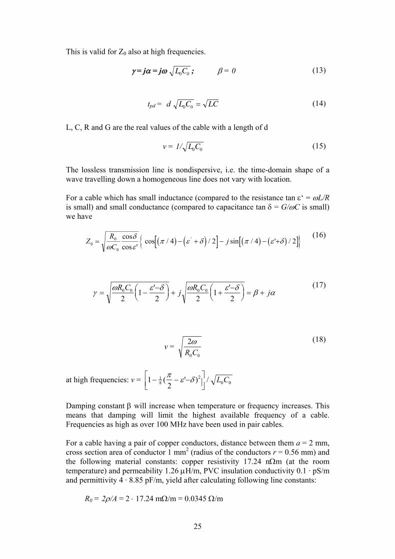
Damping constant β will increase when temperature or frequency increases. This means that damping will limit the highest available frequency of a cable. Frequencies as high as over 100 MHz have been used in pair cables. For a cable having a pair of copper conductors, distance between them a = 2 mm, cross section area of conductor 1 mm2 (radius of the conductors r = 0.56 mm) and the following material constants: copper resistivity 17.24 nΩm (at the room temperature) and permeability 1.26 µH/m, PVC insulation conductivity 0.1 · pS/m and permittivity 4 · 8.85 pF/m, yield after calculating following line constants:

R0 = 2ρ/A = 2 ⋅ 17.24 mΩ/m = 0.0345 Ω/m

26

L0 = µo/π [ln(a/r)+µr /4] = 0.54 µH/m

C0 =πε / ln ar

ar2 2

12

+ ⎛⎝⎜

⎞⎠⎟

−⎡

⎣⎢⎢

⎤

⎦⎥⎥

= 94 pF/m

G0 =πσ / ln ar

ar2 2

12

+ ⎛⎝⎜

⎞⎠⎟

−⎡

⎣⎢⎢

⎤

⎦⎥⎥

= 0.27 pS/m

In these example calculations the conducting objects have been neglected in the vicinity of the cable conductor pair. For lossless lines the characteristic impedance Z0 = 76 Ω and propagation delay tpd = l · 7.1 ns/m and v = 1.4 · 108 m/s. The propagation delay forms the most important electric time constant of the pair cable. So, as a function of the length of the cable, the time constant varies respectively:

l = 1 m tpd = 7.1 ns l = 10 m tpd = 71 ns l = 100 m tpd = 710 ns l = 1 000 m tpd = 7.1 µs.

As we see here, the electric time constants of a cable are negligible in our cable heating test.

4.1.2 Equivalent circuit of transmitter line

An oven was used to test cables in hot conditions. In Figure 6 the electrical equivalent circuit of the test set-up is given where distributed transmission line parameters are lumped (Bartnikas 1983, Doebelin 1990). On the right is a transmitter with nominal ratings: current source Is = 4 20 mA=, and source impedance Zi. Physically in the transmitter, an operational amplifier is coupled to a current source; the voltage over the source impedance Zi is the power supply of the transmitter. On the left is an indicating instrument in the control room with a power source voltage E, an impedance ZL, and a cable outside the warm area: two lumped resistances ½RL, a stray capacitance C between the conductor pair, and two inductances ½L. The leakage resistance parallel to the capacitance C is omitted in the case of the cold cable. The hot part of the cable is modelled by a separate set of lumped parameters: two series resistances ½Rc, and a leakage resistance Rl, which both depend on temperature T. Additionally, a temperature dependent parallel stray capacitance Cl, and two series stray inductances ½Lc each

27

are taken in the model. The capacitances towards the environmental conducting objects such as the aluminium foil above the conductor pair are neglected from the equivalent circuit.

ZLZi

Rl(T)Is

Cl(T)

½Rc

½Lc(T)

½RL

Hot cableCold cable TransmitterControl

½Lc(T)

½Rc

½L½L

½RLE

C

Figure 6. Lumped parameter equivalent circuit of the transmitter and cable to control room.

Calculating numerical values for the stray inductance, one notices it is very small, and for low frequencies (< 100 Hz) has a very small effect on the behaviour of the circuit. The simplified electrical equivalent circuit is presented in Figure 7, where additionally the line resistances of the pair conductor have been joined to a single resistance in cold and hot cables. For very low frequencies the capacitancies between the lines can also be removed. In Figure 7 the hot part is assumed to be close to the transmitter. It could be at any part. Therefore, the most serious situation for the malfunction should be studied by dividing C arbitrarily on both sides of the hot zone.

Zi

Is

Transmitter

Rl(T)Cl(T)

Hot cable

Rc

ZL

Control

E

Cold cable

RL

C

Figure 7. Simplified lumped parameter electrical equivalent circuit of the test arrangement.

4.1.3 Modelling of lumped parameters for a pair cable

In the first phase, only the resistive DC part is modelled. We take the cable of length l to be a parallel pair of insulated copper wires (radius r) imbedded in an insulator l being much larger than the distance a between the wires. In that case, the conductivity between the wires is modelled in an infinite space. The resistance Rc of the pair is given by

28

R T lrc c= ρ

π( ) 2

2 (19)

where ρc(T) is the resistivity of copper, which is only a weak function of temperature in the range relevant here. The leakage resistance Rl(T) for a parallel pair of wires is given by (Hallen 1953)

R T ar

ar

l Tl ( ) ln ( ) / ( )= + −⎡

⎣⎢

⎤

⎦⎥2 2

12 π σ (20)

where the conductivity of the cable insulation material has a strong temperature dependence, study of which is the key question here. The leakage resistance Rl (T) is in reality smaller than the value just calculated from the Equation (20), because the earthed metal screens in the cable enable easier leakage paths for the leak currents compared to the original infinite space case (Figure 8). We use here the following expression for the leakage resistance of a pair cable

R T ar

ar

l Tl ( ) . ln ( ) / ( )≈ + −⎡

⎣⎢

⎤

⎦⎥0 5

2 212 π σ

(21)

Similarly, for the capacitance between only the pair conductors without any earth influences, one obtains (Hallen 1953)

C T l T ar

arl ( ) ( ) / ln ( )= + −

⎡

⎣⎢

⎤

⎦⎥π ε

2 212

(22)

In practice, the earthed metal screens around the pair conductors give approximately as great capacitance addition to the capacitance value as Equation (22) has, so here the capacitance is simply calculated with the equation

C T l T ar

arl ( ) ( ) / ln ( )≈ + −

⎡

⎣⎢

⎤

⎦⎥2

2 212π ε

(23)

where permittivity ε of the insulation material is a slowly varying function of temperature, but has a complicated dependence on frequency. Here we limit the study to very low frequencies. Then the effect of the capacitances becomes small.

29

Figure 8. Cross section of a pair cable.

The inductance for two long parallel straight wires with small diameters is (Smythe 1950, Weber 1950, Hallen 1953)

][L l a ro r= +µ π µ/ ( ) ln( / )4 4 (24)

where µo is the permeability in a medium outside the wires ( = vacuum permeability = 0.4π · µH/m) and µr the relative permeability of the wires. Equation (24) is valid when the current of the circuit changes so slowly that the current corresponds to the dc current so that it is uniformly distributed in the whole cross-section area of the wire without any skin effect. (Hallen 1953) gives at very high frequencies for the inductance an expression

L l ar

ar

= + −⎡

⎣⎢

⎤

⎦⎥µ π0

2

2 21/ ln ( )

(25)

where the first term has been dropped from Equation (24) due to the current on the infinitely thin upper layer of the wire; the logarithmic term has been specified, too. If the radius r of the wire is much smaller than the distance between the wires, the logarithmic terms will approach the same value in Equations (24) and (25).

4.2 NUMERICAL ESTIMATES OF PARAMETERS

When the distance between the pair conductors is a = 2 mm, radius of both conductors r = 0.56 mm and the pair cable length l = 100 m, the inductance will be L ≈ 60 µH. (e.g. a current of 20 mA at 1 kHz frequency will give a voltage drop of 2π - 1 kHz - 60 µH - 20 mA ≈ 7.5 mV; the operating voltages in the transmitter case are typically 24 V dc, maximum 55 V dc). The skin effect and

a

radius r

jacket

foil

wire

insulator

1,3 mm

2,5 mm

0,55 mm

30

proximity effect are neglected. As we are later interested in the slow phenomena during the cable measurements we drop the small inductances away from the further investigations.

4.2.1 Copper wire resistance

The temperature dependence of the resistivity of copper is (Equation 29) at a temperature of t (resistivity is an inverse quantity of conductivity). At t = 15 oC the temperature dependence is 0.004 /K. If the temperature of a copper conductor rises from 20 oC to 100 oC then the resistance of the conductor rises about 30 %. Because the resistance values of copper conductors are small (about 3.5 Ω at the room temperature when a pair cable has a length of 100 m and the cross section area of 1 mm2) compared to the other resistances of the electric circuit, we may adopt constant values for conductor resistances or even consider them as zero valued resistances in the temperature range relevant here, especially when the cable length is short (< 10 m in our oven test set-up).

4.2.2 Leakage current of a pair cable

For operation safety we could ask at what temperature more than p % (= 10%) of 5 mA dc leaks between the wires of the pair cable. To obtain an order of magnitude estimate for the region, we calculate leakage current for a PVC instrument cable of 2 x 1 mm2 copper wire area, r = 0.56 mm, distance between wires a = 2 mm, l = 10 m long in a cold, and 1 m in a hot environment. Resistivity of copper conductors = ρc(+20 oC) = 17.241 nΩm, permittivity of PVC = ε ≈ (3 ... 6( ... 8)) · ε0 = (3 ... 6( ... 8)) · 8.85 pF/m is dependent on temperature. Here we may use for the permittivity of PVC the value of 4 ⋅ ε0 ≈ 35 pF/m. The maximum leakage current Il, when the hot zone is situated adjacent to the control room is given by

I l T E ar

arl ≈ + −

⎡

⎣⎢

⎤

⎦⎥2

2 212π σ ( ) / ln ( )

(26)

where E is the power supply voltage. From Equation (26) we can solve the conductivity σ(T); when Il = 0.1 ⋅ 5 mA = 0.5 mA, l = 1 m, a = 2 mm, r = 0.56 mm and the supply voltage E = 24 V dc over the hot cable pair wires, we get σ(T) = 3.9 µS/m. If we assume for the conductivity

31

conductivity σ(T) Arrhenius type behaviour of Equation (7) at hot cable temperature T, we can write it in the simplified form

σ ( ) /T Ae c T= − (27)

where A and c are constants. They can be determined from the data points of PVC material I6 in Figure 15; here from the point pair (σ = 6.54 nS/m, when 1000/T = 2.83/K) and (σ = 0.833 pS/m, when 1000/T = 3.30/K in the temperature range 30 ... 80 °C). We obtain from the above point pair for the constant A = 1.84 ⋅ pS/m and the constant c = 19 080 K. If σ(T) = 3.9 µS/m, the temperature T will be about 401 K = 128 oC. This point pair represents rather poor PVC. The better more accurately measured point pairs will probably give better values for constants A and c, and through them for the wanted temperature T. Adamec (1971) states that the temperature dependence of PVC in the temperature range of 75110 °C is not a single straight line on an Arrhenius plot, but is convex and may not be approximated by two straight lines without the risk of introducing an appreciable error. When using another point pair from Chapter 4.3.2 of this report for Nokia MMAO-A 2 x 1 + 1 instrumentation cable, namely σ(186 oC) = 9.9 µS/m, 1000/T = 2.18/K) and σ(19 oC) = 0.11 pS/m, 1000/T = 3.43/K, we have the constants A = 740 mS/m and c = 14 650 K and lastly the sought temperature T = 446 K = 173 oC, where according to the above calculations, the leakage current of the hot cable would become 0.5 mA. Power source voltage E = 24 V, RL + Rc = 17.241 nΩm - 211 m/1 mm2 = 0.379 Ω from which for the hot cable Rc = 0.034 Ω. As long as the voltage at the terminals of the transmitter is larger than or equal to 12 V dc, the leakage resistance Rl , when the leakage current is p % from 5 mA, is given in another way by

R E R I p pIa! = − +⎡⎣⎢

⎤⎦⎥

100 1100

( ) / (28)

where E is power supply voltage, Ra (= RL+ ZL) is resistance of the electric circuit between the voltage source and the leakage resistance Rl of the hot cable, I is transmitter output current and p is leakage percentage from the transmitter output current I. As we see from Equation (28), the leakage current Il (and the leakage resistance Rl) depend on the power supply voltage, transmitter output current I and the percentage p and also on the resistance Ra of the electric circuit. As long as the transmitter has at least 12 V over its terminals, the transmitter is able to function properly, and give the transmitter output current signal proportional to the pressure to be measured. If the power supply voltage E = 24 V and the sum of the circuit resistances at the control (and cold cable) side in Figure 7 is equal to Ra = 100 Ω, then the voltage demand at the transmitter terminals is fulfilled even if the

32

leakage resistance Rl decreased drastically: that is, the leak resistance Rl may decrease nearly to the value of Ra, if the electric circuit has rather small resistances between the leakage place and the transmitter. The circuit seems still to operate correctly. For the leakage current to become p = 10% of the 5 mA in the above arrangement, the resistance Rl should decrease to about 47 kΩ. (This resistance placed into Equation (21) will give for the conductivity of the instrumentation cable a value of 4.0 µS/m.) The measuring control indicator will in this leak case given p = 10% too much output current compared to the real original transmitter output current of 5.0 mA; thus the pressure will also show too high values.

4.3 ELECTRIC TEST SET-UP

4.3.1 Test-set up: closed circuit including the pressure transmitter

The response time between the pressure and the output current signal is adjustable from 0.3 s to 6.6 s (CMR Transmitter 15750-600416). The supply voltage is connected to the transmitter with an output circuit load resistance (ZL+RL+Rc) that has the largest permissible value; the supply and measurement circuits have common leads (two wire system). The electric time constant concerning the supply voltage source and the output circuit of the transmitter is very small, when considering the leakage current in the hot cable pair during heating. This electric time constant is mainly determined by the resistances of RL, ZL, Rl(T) and partly Rc and the inner capacitances of the voltage supply and the indicator as well as the cable pair capacitances, typically 500 Ω ⋅ 100 µF ≈50 ms (here we have assumed that the outer resistance of the output circuit is 500 Ω and the capacitance 100 µF (= the inner capacitance of the voltage supply). The first test had been carried out according to Figure 7. The aluminium foil of the pair cable type MMAO-A 2x1.0 was left unconnected, ungrounded or floating, while the other copper conductor was connected to the ground.

33

104 Ω

CMR

Rl(T)Cl(T)

Hot and cold cableControl and measurementTransmitter 15750-600416

E = 24 V

Measurement

E = 24 V

4.757 Ω

7.85 kΩ

10 kΩ

47.02 Ω

680 kΩ

1MΩ

Grounded

Figure 9. Principal test set-up of the pair cable heating. The leakage phenomena were measured as voltages over the resistors of 680 kΩ and over the resistive shunts of 47.02 Ω and 4.757 Ω (transmitter current and indicator current measurements). The voltage of the supply was measured with resistive voltage division over the resistor of 7.85 kΩ.

The cable type used with pressure transmitter CMR Transmitter 15750 for differential pressure with diaphragm measuring cell 050 in a nuclear power plant is MMAO-A 2x1.0. The transmitter is used for measuring differential pressure, pressure and vacuum. Measuring range for the transmitter is 02 bar. The pressure gauge can be connected to a pressurized wall or pipe. Output signal varies 420 mA (CMR Transmitter 1979). The cable segment of 1140 mm (hot cable in Figure 9) was installed in the test furnace (Heraeus, Typ RL 200, Nenntemperatur 650 C). Furnace diameter was 200 mm and depth 300 mm. Furnace temperature was controlled by using PID-controlled (Eurotherm Controller/Programmer, Type 812). The opening of the furnace was closed by using insulation wool layer of 55 mm. The cable was conducted into and out of the furnace via holes in the insulation layer. The furnace temperature was raised slowly and steadily up to 450 °C over a period of 18 hours at a rate of 6.7 mK/s. Furnace temperature and surface temperature of the cable jacket were measured using a K-type thermocouple under heating. Temperature at the Cu-wire in the core of the adjacent identical cable was also measured using a thermocouple. There were four voltage measurements: one over the resistance at the power supply end and one over the resistance at the gauge end of the electrical circuit. Power supply voltage was also measured. In addition, the voltage between the two wires (leakage way) were measured. Environment temperature of resistances on the metal plate was also measured in order to achieve temperature correction for resistances due to changing environment temperature.

34

The measured electric parameters of the cable pair were the voltages and the currents on both sides of the hot cable. When increasing the temperature slowly, the leak current was almost throughout the test time nearly zero and suddenly at a temperature of about 196 oC, it increased to the value of the short circuit current. (See Chapter 5.) The measurement did not succeed as was expected. Probably the cable wires had some tension or strain left that quickly discharged and joined the wires together as soon as the elevated temperature had softened the PVC insulation between the wires.

4.3.1.1 Inaccuracies of the closed circuit test

At the current measurements, the data logger had the following maximum inaccuracies in the range of 20 mV ± 9 µV and in the range of 200 mV ± 60 µV. The shunt resistances measured at + 23 oC temperature were 4.7582 Ω and 47.029 Ω. The temperature dependencies of the shunts were 50 ppm/K. As the shunts were near each other during the measurements on a metal plate, they had the same temperature, which in turn followed the temperature of the environment with a time constant of the order of 10 min. As the test lasted many hours, the shunt temperature changed with the environmental temperature. If we had a temperature range of the environment between +17 oC and +20 oC the relative inaccuracies of the shunt resistances 4.757 Ω and 47.02 Ω were ± -0.0002 = ± - 200 ppm. The inaccuracy of a current measurement obtained from the worst case is given by dI/I = dU/U + dR/R, where I is the current to be measured, and U the measured voltage over the shunt resistance R. For the transmitter output current and correspondingly for the control indicator current, we have the inaccuracies dI/I = 60 µV/188 mV + 0.0002 ≈ 0.0005 dI/I = 9 µV/19 mV + 0.0002 ≈ 0.0007 The sum of these inaccuracies (≈ 0.0012 = 0.12 %) gives the total inaccuracy of the measurement as a difference in calculated leakage current. The leakage current is calculated from the transmitter output current and the control indicator current. From this difference the current through the voltage division has to be subtracted. At the beginning of the test this correction current is about (24 V 4 mA x 109Ω)/(1.00 MΩ + 680 kΩ) ≈ 14 µA which is 0.0035 = 0.35 % from the transmitter output current 4 mA. Later on during the test the voltage over the leakage place of the hot cable determines the correction current. Earlier in this report, a case of 0.5 mA leakage current during the heating of a cable was calculated. According to the results of the heating test, the short circuit occurred between the cable wires before the leak current had time to reach this value of 0.5 mA, which should be easily measured with the above mentioned test arrangement.

35

4.3.2 Test set-up for measuring conductivity of insulation layer of cables at elevated temperatures

In order to study the conductivity of PVC-cable insulation at high temperatures, we arranged a preliminary test set-up to measure the basic electric material property, conductivity, of the cable. Here we had an instrumentation cable - Nokia MMAO-A 1 x 2 + 1.0 length of 23.11 m from which 1 m was heated step by step. Also, another cable MMJ 3 x 2.5 mm2 was measured. Pieces of cable, 1 m long, were kept at the desired temperature a little longer than one hour before the measurements when the temperatures were below +196 oC. Above this temperature, the heating times were at least two hours. No points in the measurement circuit were galvanically grounded, the Al foil of the instrumentation cable was also floating. The test arrangement is shown in Figure 10.

Hot cable with open ends

Rl(T)Cl(T)

Voltage source and measurement cable

E Series resistor

Cold cable

Ω

Switch

Insulation resistance

meter

Electro- meter

Figure 10. A set-up of measuring the conductivity of PVC cable with both an insulation resistance meter and an electrometer.

The measured quantities were the insulation resistance between the conductor pair and between the Al foil and both the conductors separately. In MMJ 3 x 2.5 cable, the resistances were measured between the red and blue coloured conductors. In principle the measuring voltage was 500 V dc when the resistances to be measured were greater than 30 MΩ, and 85 V dc when the corresponding resistances were between 0.3 MΩ and 30 MΩ. The measurement was taken one minute after applying the measuring voltage. With the electrometer, we measured the current that leaked between the selected conductors; the steady-state leakage current indicates the insulation resistance. The initial current that flows during the test is much higher than the steady-state leakage current. There are three distinct components of the current which all depend on the dielectric properties of the insulation and are therefore dependent on temperature (Electrical Review 1995):

36

1. a rapidly decaying capacitive charging current due to the capacitance of the

cable being tested, 2. polarization current also falls (exponentially), but much more slowly than the

capacitive charge. The current is caused by electrons migrating to barriers in the dielectric, and by molecular dipoles which align with the electric field,

3. steady-state leakage current. Humidity or condensation also affects leakage. The inner temperature of the instrumentation cable was measured by an excess piece of cable that was wholly inside the oven. Although the piece was in the oven all the time and even four hours (4 h) at the desired constant temperature, the temperature inside the cable was still about 67 oC lower than the oven air. Of course at room temperature, this inner temperature of the cable was the same as in the oven air after cooling overnight, when measurements were not carried out. Proposals for future measurements: 1. Possible heat leakage and uneven temperature distribution in the cable to be

measured will be prevented by placing the specimen cable entirely inside the oven. No specimen bushings are allowed, the measuring leads go through the oven door or wall.

2. The measurements of small currents (typically smaller than 10 nA) must be

carried out in an electrically protected room (Faraday cage), the ambient interference levels should be as low as possible. At least the inmediate environment of the whole test set-up has to be kept at the same potential, e.g. surrounding the set-up with conducting metal plates, which are isolated from the outer environment but connected to each other at certain points and to the outer environment only at a single point.

4.3.3 Improved second test set-up

When carrying out measurements successfully with MMAO-A cable, we measured the electrical conductivity of insulations of another seven different cables at temperatures beyond their normal operation temperature from room temperature 20 °C up to 230 °C. The cables and their properties data are given in Table 4.

37

Table 4. Properties of the cables studied.

Cable type Cable insulation material

Cable diameter (mm)

Conductor diameter (mm)

Cu-wire diameter (mm)

Type

MMJ 3 x 2.5 mm2 300/580V

PVC 10 1.5 1.8 Power

MMO 7 x 2.5 mm2 450/750 V

PVC 13 3.5 2 Instr.

NOMAK 4 x 2 x 0.5 + 0.5 10/1995

PVC 8 1.5 0.798 Instr.

MAMSI-E 4 x 1

PVC 7 1.5 1.128 Instr.

MHMS-SI 8 x 1+S

PVC 8.5 1.5 1.128 Instr.

HHO Max 90°C Lipalon 4 x 1

Lipalon 9 2.4 1.128 Instr.

HCHKEM Max 90°C Lipalon 1 x 3 + 5

Lipalon 23.4 8 5 Power

We rationalized the measuring process by using two heating furnaces and setting several cables in the same furnace. We could not use the electrically protected room (Faraday cage) as a measuring environment, but we installed all measuring instruments, cables and furnaces on a metal plate in order to couple items in the same electric potential. Thus we achieved a partial shield against environmental disturbances and noise, when measuring very small currents even in nA and pA-ranges. Air temperature in the measuring room varied from 19 ... 21 °C, and air relative humidity was 1925% during the measurements.

Table 5. Installation parameters of the cables.

Cable type Total length of the cable

(m)

Cable segment in the furnace

(m)

Bending radius (mm) in the

furnace

Furnace used

MMJ 46.335 0.985 200 KTFU-K MMO 26.400 0.988 225 KTFU-K NOMAK 40.965 1.005 4350 RL200 MAMSI-E 24.000 1.005 3353 RL200 MHMS-SI 46.335 0.984 150 KTFU-K HHO 30.560 1.000 5772 RL200 HCHKEM 42.165 0.985 440 KTFU-K

38

The 1 m cable segments of four cables were placed in a test tube furnace1 and of three cables in a cubic furnace.2 Furnace temperature was PID-controlled.3 The openings of the furnaces were closed using a mineral wool layer of 100 mm. The cable was conducted in and out of the furnace via holes in the insulation layer. The furnace temperature near the centre of the ceiling, and the temperature in the insulation layer of Cu-wire in the adjacent piece of each cable type were measured using K-type thermocouples during heating. The temperature was raised from room temperature 20 °C to 230 °C step by step carrying out the electrical measurements for each cable at each temperature step. The insulation resistance between a conductor pair in the cables was measured using a commercial instrument.4 Leakage current between conductor pairs as measured using an electrometer.5 In principle, the measuring voltage when using the insulation resistance meter was 500 V dc, when resistances to be measured were greater than 30 MΩ, and 85 V dc, when corresponding resistances were 0.330 MΩ. The measurement was carried out generally in 35 minutes of applying the measuring voltage. With the electrometer, we measured the current which leaked between the selected conductors. The applied voltage in the electrometer measurements was usually 100 V, with some exceptions when lower voltage had to be used. The steady-state leakage current indicates the insulation resistance calculated by means of voltage. The initial current that flows during the test is much higher than the steady-state leakage current. Three distinct components of the current can be identified, as discussed above, which all depend on the dielectric properties of the insulation and are dependent on temperature (Electrical Review 1995): rapidly decaying capacitive charging current, polarization current and steady-state leakage current. Experimental arrangements are given in Figure 11.

1 Heraeus, Typ RL 200, nominal temperature 650 C, diameter 200 mm and depth 300 mm 2 Heraeus KTFU-K, opening 400 mm x 500 mm, depth 400 mm. 3 Eurotherm Controller/Programmer, Type 812. 4 20 million megohmmeter, model 29A, Electronic Instruments Ltd. Richmond, Surrey, England. 5 Model 617 Programmable Electrometer, Keithley Instruments Inc., Serial No. 0557570, USA.

39

Figure 11. Measurement arrangements. The protective earth conductors (PE) for the equipotential levels of the set-up are marked in the figure with thick lines, also when a power cord contains the PE conductor.

40

5 EXPERIMENTAL RESULTS

5.1. THE FIRST TEST SERIES

Voltage over the four locations in the electrical circuit was measured during 18 hours continuous heating from 19 °C up to 310 °C. Supply voltage 24 V was rather stable during the whole measurement. Temperature at the cable surface and in the Cu-wire inside the cable is given in Figure 12. We can see that cable temperature follows the oven temperature well. Current over resistance at the supply end and gauge end of the circuit are in Figure 13. We obtain leakage current as the difference between these currents (Figure 14). We carried out temperature correction on the resistance by using formula

[ ]R T R T To o( ) ( )= + −1 α (29)

where R is the resistance at elevated temperature T, Ro is resistance at temperature To, where resistance is measured and α is the temperature coefficient. A short circuit appeared suddenly at 196 °C. Then leakage current went up to its maximum discretely. No monotonous change in leakage current was discovered before the collapse at 196 °C. Thus no evidence of increasing conductivity of insulation material of the studied PVC-cable could be determined as expected (Figure 14). This was caused by too coarse measurement arrangements as well as noise and leakages in the connections of the circuit. A doubt: The cable inside the oven has had too small curvature causing extra tension between the Cu-wires and the electric insulating materials. When the temperature increased the tension had broken suddenly away.

41

0

50

100

150

200

250

300

350

0 50 100 150 200 250 300 350OVEN TEMPERATURE (oC)

CA

BLE

TEM

PER

ATU

RE

(oC

)

cable wire

cable surface

Figure 12. Temperature at the cable surface and in Cu-wire inside the cable MMAO-A versus the furnace temperature.

0

0.05

0.1

0.15

0.2

0.25

0 50 100 150 200 250 300 350

OVEN TEMPERATURE (oC)

CU

RR

ENT

(A)

supply

gauge

Figure 13. Current at supply and gauge end of the circuit.

42

0

50

100

150

200

250

0 50 100 150 200 250 300 350OVEN TEMPERATURE (oC)

LEA

KA

GE

CU

RR

ENT

(mA

)

Figure 14. Leakage current between wires through cable insulation.

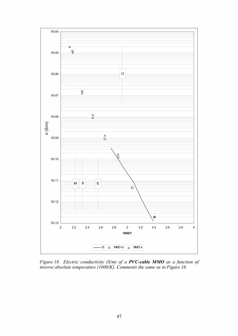
5.2. THE CONDUCTIVITY OF THE INSULATION LAYER OF CABLES AT ELEVATED TEMPERATURES

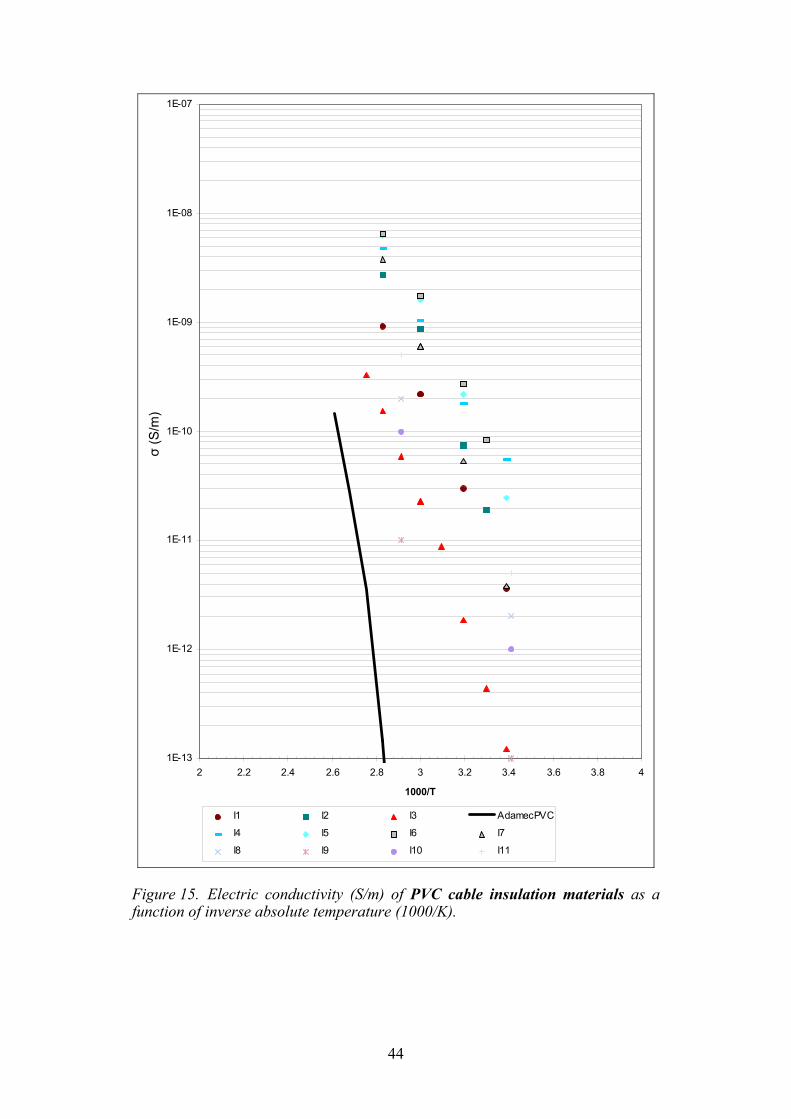
We calculated conductivity of the insulation layer of six PVC-cables and two CSP (Hypalon/Lipalon) -cables on the basis of measured insulation resistance, leakage current and dimensions of the cable using Equations (20) or (21). We corrected in a proper way the value of insulation resistance measured from the whole cable located partly in the normal ambient temperature, partly at elevated temperatures. The insulation resistance was normalized into room temperature. Insulation resistance was calculated by dividing the applied voltage by the measured leakage current. Insulation conductivities measured from cables seem to match well conductivities measured for cable materials. The results are presented in Figures 1623. The abbreviations m and e after the studied cable names in the legends of the figures refer to measuring instruments: (m) insulation resistance meter, and (e) electrometer. The vertical bars indicate limit temperatures for PVC: U, utility, E, emergency, S, short circuit, and M, melting. The measured points fall approximately on a line on an Arrhenius plot from room temperature up to melting temperature, indicating ionic and electronic conduction components (according to Equation (7)) prevail. The accuracy of the measurements was not determined well enough, but scattering of nearby data points indicates roughly the order of magnitude of the inaccuracy. In extreme cases the difference between electrometer, and insulation resistance measurements

43

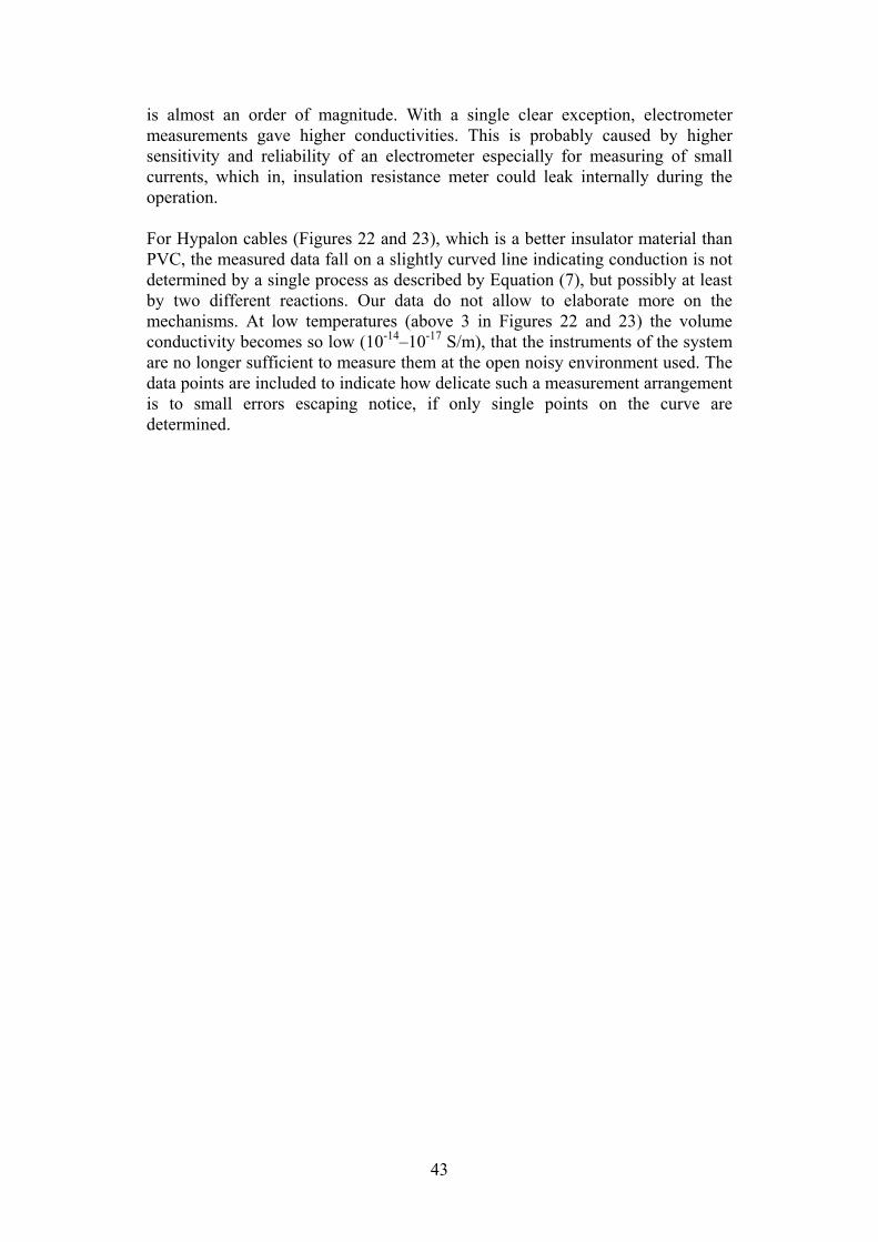
is almost an order of magnitude. With a single clear exception, electrometer measurements gave higher conductivities. This is probably caused by higher sensitivity and reliability of an electrometer especially for measuring of small currents, which in, insulation resistance meter could leak internally during the operation. For Hypalon cables (Figures 22 and 23), which is a better insulator material than PVC, the measured data fall on a slightly curved line indicating conduction is not determined by a single process as described by Equation (7), but possibly at least by two different reactions. Our data do not allow to elaborate more on the mechanisms. At low temperatures (above 3 in Figures 22 and 23) the volume conductivity becomes so low (10-1410-17 S/m), that the instruments of the system are no longer sufficient to measure them at the open noisy environment used. The data points are included to indicate how delicate such a measurement arrangement is to small errors escaping notice, if only single points on the curve are determined.

44

1E-13

1E-12

1E-11

1E-10

1E-09

1E-08

1E-07

2 2.2 2.4 2.6 2.8 3 3.2 3.4 3.6 3.8 4

1000/T

(S/m

)

I1 I2 I3 AdamecPVC

I4 I5 I6 I7

I8 I9 I10 I11

Figure 15. Electric conductivity (S/m) of PVC cable insulation materials as a function of inverse absolute temperature (1000/K).

σ (S

/m)

45

1E-13

1E-12

1E-11

1E-10

1E-09

1E-08

1E-07

1E-06

1E-05

1E-04

1E-03

2 2.2 2.4 2.6 2.8 3 3.2 3.4 3.6 3.8 4

1000/T

(S/m

)

I3 MMAO-A

S

E

U

M

Figure 16. Electric conductivity (S/m) of a PVC-cable MMAO-A as a function of inverse absolute temperature (in units of 1000/K). For comparison literature data (I3) are drawn in a full line. After melting, the wires of the cable could become air insulated, which explains the high rise in conductivity observed below 2.2.

σ (S

/m)

46

1E-14

1E-13

1E-12

1E-11

1E-10

1E-09

1E-08

1E-07

1E-06

1E-05

1E-04

2 2.2 2.4 2.6 2.8 3 3.2 3.4 3.6 3.8 4

1000/T

S/m

I3 MMJ m MMJ e

M

S

E

U

Figure 17. Electric conductivity (S/m) of a PVC-cable MMJ as a function of inverse absolute temperature (1000/K). Comments the same as in Figure 16.

σ (S

/m)

47

1E-13

1E-12

1E-11

1E-10

1E-09

1E-08

1E-07

1E-06

1E-05

1E-04

2 2.2 2.4 2.6 2.8 3 3.2 3.4 3.6 3.8 4

1000/T

S/m

I3 MMO m MMO e

S E

U

M

Figure 18. Electric conductivity (S/m) of a PVC-cable MMO as a function of inverse absolute temperature (1000/K). Comments the same as in Figure 16.

σ (S

/m)

48

1E-15

1E-14

1E-13

1E-12

1E-11

1E-10

1E-09

1E-08

1E-07

2 2.2 2.4 2.6 2.8 3 3.2 3.4 3.6 3.8 4

1000/T

S/m

)

I3 NOMAK m NOMAK e

M S E U

Figure 19. Electric conductivity (S/m) of a PVC-cable NOMAK as a function of inverse absolute temperature (1000/K). Here the whole range measured falls on a line. The conductivity at high temperatures is three orders of magnitude smaller than for Figures 16 to 18.

σ (S

/m)

49

1E-14

1E-13

1E-12

1E-11

1E-10

1E-09

1E-08

1E-07

1E-06

2 2.2 2.4 2.6 2.8 3 3.2 3.4 3.6 3.8 4

1000/T

S/m

)

I3 MAMSI-E m MAMSI-E e

M S E U

Figure 20. Electric conductivity (S/m) of a PVC-cable MAMSI-E as a function of inverse absolute temperature (1000/K). Comments as for Figure 19.

σ (S

/m)

50

1E-14

1E-13

1E-12

1E-11

1E-10

1E-09

1E-08

1E-07

1E-06

1E-05

1E-04

1E-03

2 2.2 2.4 2.6 2.8 3 3.2 3.4 3.6 3.8 41000/T

S/m

I3 MHMS-SI m MHMS-SI e

M

S E U

Figure 21. Electric conductivity (S/m) of a PVC-cable MHMS-SI as a function of inverse absolute temperature (1000/K). Comments the same as in Figure 16.

σ (S

/m)

51

1E-13

1E-12

1E-11

1E-10

1E-09

1E-08

2 2.2 2.4 2.6 2.8 3 3.2 3.4 3.6 3.8 4

1000/T

S/m

HHO m HHO e

Figure 22. Electric conductivity (S/m) of a CSP-cable HHO as a function of inverse absolute temperature (1000/K). No CSP-material data were available for reference. Measured points below 3 fall on a slightly curved line. Data above 3 might be erroneous caused by modes of current transfer other than volume conduction, see text.

σ (S

/m)

52

1E-14

1E-13

1E-12

1E-11

1E-10

1E-09

1E-08

1E-07

1E-06

2 2.2 2.4 2.6 2.8 3 3.2 3.4 3.6 3.8 4

1000/T

S/m

HCHKEM m HCHKEM e

Figure 23. Electric conductivity (S/m) of a CSP-cable HCHKEM as a function of inverse absolute temperature (1000/K). No CSP-material data were available for reference. Datum at 3.1 might be erroneous caused by modes of current transfer other than volume conduction.

σ (S

/m)

53

6 DISCUSSION AND CONCLUSIONS The PVC cable (MMAO-A) in the first investigation in a closed circuit worked normally up to 196°C, where there was a short circuit. Then leakage current suddenly rose to a high value. However, we could not obtain any evidence of continuous insulation derating from room temperature to short circuit temperature. This was due to robust experimental arrangements, not sensitive to slight phenomena or leakages at connections in the electrical circuit. Thus, we can give preliminary evaluation of a proper working range of the cable without short circuit as 19196 °C. Leakage current was observed at elevated temperatures by measuring the insulation resistance and leakage current in the open circuit experiment of the PVC cables MMAO-A, MMJ, MMO, NOMAK, MAMSI-E and MHMS-SI. We also measured two cables HHO and HCHKEM, where CSP (Lipalon) was used as insulation material. Unfortunately no data of conductivity of CSP-material were available for reference in the literature. It was observed that measured data fall approximately on an Arrhenius plot below melting temperature for all PVC materials tested. For CSP materials, data formed an upward convex curve on an Arrhenius plot. Conductivity of the insulation layer of these cables did not fit a simple Arrhenius plot as neatly as for the studied PVC-cables. Our data are neither accurate nor numerous enough to elaborate on these observations. The procedure used gives a systematic way to determine leakage conductance of a cable reducing the problem to determination of the volume conductance of the cable insulation material. Determining the slope of conductance on the Arrhenius plot allows quantitative determination of the effects of cable leakage currents on the electric circuitry as a function of temperature. It was observed that all materials tested here retained their insulation to some degree until the melting of the material, after which a direct short circuit became possible. Tests were performed for mechanically unloaded cables over a relatively short time period, so long-term mechanical deformations as plastic flow of the insulation material as a cause of short circuit were not included. In conclusion, the rating of electrical performance of cables at high temperatures can be simplified to measurements of conductivity of cable insulation material, where Arrhenius-type temperature behaviour is not followed strictly but is useful as guidance.

54

REFERENCES Adamec, V. 1971. Electric polarization and conduction in polymethyl methacrylate and in polyvinyl chloride in unidirectional electric field. Kolloid Zeitschrift und Zeitschrift für Polymere 249, pp. 10851095. Alvares, N. J., Lipska-Quinn, A. E. and Hasegawa, H. K. 1983. Thermal degradation of cable and wire insulations. In: Schaffer, E. L. (ed.). Behavior of polymeric materials in fire. ASTM Special Technical Publication, Philadelphia, PA 816, American Society for Testing and Materials. Pp. 4266. Bartnikas, R. 1983. Dielectric loss in solids. In: Bartnikas, R. and Eichorn, R. M. (eds). Engineering dielectrics, Vol IIA, Electrical properties of solid insulating materials: molecular structure and electrical behaviour. ASTM Special Technical Publication 783, Philadelphia, PA. Pp. 3117. Beyler, C. L and Hirschler, M. M. 1995. Thermal decomposition of polymers. In: Nenno, P. J. et al. (eds). The SFPE Handbook of Fire Protection Engineering. Quincy, MA National Fire Protection Association and Boston, MS, Second Edition. Pp. 1-991-119. Billmeyer, F. W. Jr. 1984. Textbook of polymer science. New York, Wiley, Third Ed. 578 p. Blythe, A. R. 1979. Electrical properties of polymers. Cambridge: Cambridge University Press. 191 p. CMR Transmitter 15750 for differential pressure with diaphragm measuring cell 050. 1979. Technical data sheet (1 of 2) 15-2.22 EN. 5 p. Cullis, C. F. and Hirschler, M. M. 1981. The combustion of organic polymers. Oxford: Clarendon Press. Dakin, T. W. 1983. Composite insulating materials and systems. In: Bartnikas, R. and Eichorn, R. M. (eds). Engineering dielectrics. Vol IIA, Electrical properties of solid insulating materials: Molecular structure and electrical behaviour. ASTM Special Technical Publication 783. Philadelphia, PA. Pp. 663695.

Dean, J. A. (ed.). Langes handbook of chemistry. New York: McGraw-Hill, 13th ed., Section 8, Infrared spectroscopy. Doebelin, E. O. 1990. Measurement systems. New York: McGraw-Hill, 4th ed. 960 p. Duke, C. B. and Gibson, H. W. 1982. Polymers, conductive. In: Kirk-Othmer encyclopedia of chemical technology. New York: Wiley, Third Edition, Vol. 18. Pp. 755793. Electrical Review 1995. Vol. 228, No 21. As easy as PI, an article about predictive maintenance.

55

Fessenden, R. J. and Fessenden, J. S. 1994. Organic Chemistry. Brooks/Cole Publ. Co., Pacific Growe, CA, 5th ed. P. 265. Frommer, J. E. and Chance, R. R. 1988. Electrically conducting polymers. In: Kroschwitz, J. I. (ed.). Electrical and electronic properties of polymers: A state of the art compendium. New York: Wiley. Pp. 56101. Grassie, N. 1964. Thermal degradation. In: Fettes, E.M. (ed.). Chemical reactions of polymers. New York: Wiley, Chapter 8B. Hallen, E. 1953. Uppsala; Electricitetslära. Almqvist & Wiksells boktryckeri Ab, 556 p. (In Swedish.) Handbook of polymer chemistry. 1989. Brandrup, J. & Immergut, E. H. (eds). 3rd ed., New York: Wiley. Hasegawa, H. K., Staggs K. J. and Doughty, S. M. 1992. Fire tests of wire and cable for DOE nuclear facilities. Lawrence Livermore National Laboratory. Report UCRL-ID-110598. September 1992. 128 p. International standard IEC 1994. 502. Extruded solid dielectric insulated power cables for rated voltages from 1 kV up to 30 kV. Kamm, A. and Schüller, K. H. 1987. Insulation, electric. In: Ullmanns encyclopedia of industrial chemistry. Weinheim: VHC Verlagsgesellschaft, 5th ed. Vol. A14. Pp. 321364. Ku, C. C. and Liepins, R. 1987. Electrical properties of polymers. Munich: Hanser Publishers. 389 p. Mathes, K. N. 1988. Electrical properties. In: Kroschwitz, J. I. (ed.). Electrical and Electronic Properties of Polymers: A State of the Art Compendium. New York: Wiley. Pp. 101181. Moscovici, A. 1995. Insulation, electric. In: Kirk-Othmer encyclopedia of chemical technology. New York: Wiley, 4th ed. Vol. 14. Pp. 627647. Nicolette, V. F. 1988. A critical look at nuclear qualified electrical cable insulation ignition and damage thresholds. Sandia National Laboratories, Report SAND88-2161C. USA. Novak, I. 1992. Modeling, simulation, and measurement considerations of high-speed digital buses. IEEE Transactions on Instrumentation and Measurement, Vol. 41. No. 6, pp. 921925. Parrini, P. 1973. Electrical conductivity in poly(vinyl chloride). Polymer, Vol. 14, pp. 445450.

56

Phillips, P. J. 1983. Morphology and molecular structure of polymers and their dielectric behaviour. In: Bartnikas, R. and Eichorn, R.M. (eds). Engineering dielectrics, Vol. IIA, Electrical properties of solid insulating materials: Molecular structure and electrical behaviour. ASTM Special Technical Publication 783, Philadelphia, PA. Pp. 119237. Plastics. 1986. Thermoplastics and thermosets, desk-top data book. D.A.T.A San Diego, CA, 8th ed. Saunders, K. J. 1973. Organic polymer chemistry. London: Chapman and Hall. 473 p. Siemens, 1966. Formel- und Tabellenbuch für Starkstrom-Ingenieure. Essen: Verlag W. Girardet, 3. überarbeitete Auflage. (In German.) Schwartz, S. S. and Goodman, S. H. 1982. Plastic materials and processes. New York: Van Nostrand. 965 p. Smythe, W. R. 1950. Static and dynamic electricity. 2nd ed., 2nd impression. New YorkTorontoLondon: McGraw-Hill. 616 p. Specifications for thermoplastic and crosslinked polyethylene insulated shielded power cables rated 5 trough 35 kV. 1987. Association of Edison Illuminating Companies. AEIC CS5-87. 9th ed. New York. Sähkötarkastuskeskuksen julkaisu E HD21.S2-1984. Polyvinyylikloridieristeiset johdot: nimellisjännite enintään 450/750 V. Helsinki 1984. 112 p. [Finnish translation from CENELEC Publication HD21.S2 Polyvinyl Chloride Insulated Cables of Rated Voltages up to and Including 450/750 V]. Tanaka, J. and Wolter, K. 1983. Composition and structure of dielectric solids. In: Bartnikas, R. and Eichorn, R. M. (eds). Engineering dielectrics, Vol. IIA, Electrical properties of solid insulating materials: Molecular structure and electrical behaviour. ASTM Special Technical Publication 783, Philadelphia: PA. Pp. 521618. Troitzsch, J. 1981. International plastics flammability handbook. Principles Regulations Testing and Approval. Munich: Hanser Publishers, 2nd ed.

Tewarson, A. 1995. Generation of heat and chemical compounds in fires. In: Nenno, P. J. et al. (eds). The SFPE Handbook of Fire Protection Engineering. Quincy, MA: National Fire Protection Association and Boston, MS, 2nd ed. Pp. 353 and 3124.

Ullmanns Encyklopädie der technischen Chemie, 1967. Urban & Schwarzenberg, München, 18. Band. Pp. 547.

57

Weber, E. 1954. Electromagnetic fields theory and applications. Volume I Mapping of fields. New York: John Wiley & Sons, and London: Chapman & Hall, 2nd printing, USA. 590 p. Wintle, H. J. 1983. Conduction processes in polymers. In: Bartnikas, R. and Eichorn, R. M. (eds). Engineering dielectrics. Vol. IIA, Electrical properties of solid insulating materials: Molecular structure and electrical behaviour. ASTM Special Technical Publication 783, Philadelphia, PA. Pp. 239354. Wypych, J. 1985. Polyvinyl chloride degradation. Amsterdam: Elsevier. 264 p.

APPENDIX 1/1

DEFINITIONS Some definitions concerning cable design and materials are included in Appendix 1.

Figure 1. Cable designs: a) coaxial cable; b) twisted pair cable can be unshielded, as in regular telephone wiring, or shielded (as shown here) with braiding or foil; c) fibre optics cable (Moscovici).

Figure 2. Specialty wires: a) appliance wires; b) instrumentation wires; c) distribution wires; and d) aerial self-supporting wires.

APPENDIX 1/2

CABLE MATERIALS

Table 1. Chemical compounds, corresponding acronyms and trade names of polymers used in cables (Muovitermit 1992, Ullmanns 1967, Plastics 1986).

CHEMICAL COMPOUND ACRONYM TRADE NAMES

Poly(vinylchloride) PVC Vestolit, Trosiplast, Vinoflex, Duval, Corvic, Nipolit

Crosslinked polyethylene PE-X, (PEX, XPE) Lubonyl, Alveolit, Alveolux, Blanex, Evapor

Chlorosulphonated polyethylene

CSP Hypalon

Ethylene/propylene copolymer

E/P

Ethylene/propylene/ diene monomer

EPDM

Poly(methyl methacrylate)

PMMA Lucite, Plexiglas, Altulite, Sumipex

Silicone rubbers FMQ, FMVQ, PVMQ TPX, RTP, Pethrotehe, Bakelite (Plastics 8ed)

Polyolefins (PO)

PCP-rubber

Reference: Muovitermit, Muoviyhdistys ry, Gummerus, Jyväskylä 1992. 477 p. (In Finnish.)

Series title, number and report code of publication

VTT Publications 302 VTT-PUBS-302

Author(s) Keski-Rahkonen, Olavi, Björkman, Jouni & Farin, Juho Title Derating of cables at high temperatures Abstract A method to characterize behaviour of cables used in nuclear power plants at temperatures exceeding the long-term rating was developed. The problem is to predict how long and at what temperatures cables function in emergency situations. The structure and materials of the relevant cables were reviewed and the properties of these materials at high temperatures were described from literature sources. The physical and chemical processes to be expected were outlined for designing tests. Initially we carried out a real-scale equivalent test with a closed circuit, where the pair cable was connected to a pressure transmitter. The instrument PVC cable under investigation worked normally up to 196 °C, where a short circuit occurred, and leakage current suddenly rose to a high value. However, we could not get any evidence of continuous insulation derating from room temperature to the short circuit temperature. This may be due to the experimental arrangements not being sensitive enough to slight phenomenan or to leakages at connections in the electrical circuit. In order to obtain data about the conductivity of PVC cable insulation at elevated temperatures, a part of the open circuit was heated in a test furnace step by step from room temperature to the short circuit temperature region of 200 °C. We discovered leakage current and insulation conductivity improvement in the PVC cable by using a sensitive electrometer and an insulation resistance meter applied in the open circuit experiment for pure cable. Electrical conductivity of PVC cable insulation materials from the literature and electrical conductivity of the PVC cable insulation layer as a function of inverse absolute temperature match quite well. The first series of tests was carried out for a PVC cable to check the validity of the theory and the test method. The testing programme continued and included seven different types of cables.

ISBN ISBN 951-38-5043-9 (soft back ed.) ISBN 951-38-5044-7 (1st electronic ed.) ISBN 978-951-38-7101-7 (2nd electronic ed., URL: http://www.vtt.fi/publications/index.jsp)

Series title and ISSN Project number VTT Publications 1235-0621 (soft back ed.) 1455-0849 (URL: http://www.vtt.fi/publications/index.jsp)

R5SU00480

Date Language Pages 2nd, rev. ed., May 2008 English 57 p. + app. 2 p.

Name of project Commissioned by Ydinvoimalaitosten rakenteellinen turvallisuus (RATU); Paloturvallisuus (PALOTU)

Ministry of Trade and Industry, Finland (KTM); Finnish Centre for Radiation and Nuclear Safety (STUK); IVO International Oy; Teollisuuden voima Oy; the Finnish Fire Research Board

Keywords Publisher power lines, caple insulation, fire safety, nuclear power plants, high temperature tests

VTT Technical Research Centre of Finland P.O. Box 1000, FI-02044 VTT, Finland Phone internat. +358 20 722 4520 Fax +358 20 722 4374