Natural Sciences Tripos Part II MATERIALS SCIENCE C15: Fracture and Fatigue Dr C. Rae Lent Term 2012-13 II Name............................. College..........................

Welcome message from author
This document is posted to help you gain knowledge. Please leave a comment to let me know what you think about it! Share it to your friends and learn new things together.
Transcript

Natural Sciences Tripos Part II
MATERIALS SCIENCE
C15: Fracture and Fatigue
Dr C. Rae
Lent Term 2012-13
II
Name............................. College..........................

Part II Lent 2013 FRACTURE AND FATIGUE
1
C15: FRACTURE AND FATIGUE Catherine Rae 9 Lectures Synopsis Introduction: This course examines the use of fracture mechanics in the prediction of mechanical failure. We explore the range of macroscopic failure modes; brittle and ductile behaviour. We take a closer look at fast fracture in brittle and ductile materials – characteristics of fracture surfaces; inter-‐granular and intra-‐granular failure, cleavage and micro-‐ductility. We describe the range of fatigue failure and apply fracture mechanics to the growth of fatigue cracks. Introduction: Revision of concept of energy release rate, G, and fracture energy, R. Obreimoff’s experiment. Timeline for developments. Linear Elastic Fracture Mechanics, (LEFM). We look at the three loading modes and hence the state of stress ahead of the crack tip. This leads to the definition of the stress concentration factor, stress intensity factor and the material parameter the critical stress intensity factor. Superposition principle, prediction of crack growth direction. Plasticity at the crack tip and the principles behind the approximate derivation of plastic zone shape and size. Limits on the applicability of LEFM. The effect of Constraint, definition of plane stress and plane strain and the effect of component thickness. Concept of G -‐ R curves, measuring G and K. Elastic-‐Plastic Fracture Mechanics; (EPFM). The definition of alternative failure prediction parameters, Crack Tip Opening Displacement, and the J integral. Measurement of parameters and examples of use. The effect of Microstructure on fracture mechanism and path, cleavage and ductile failure, factors improving toughness, Fatigue: definition of terms used to describe fatigue cycles, High Cycle Fatigue, Low Cycle Fatigue, mean stress R ratio, strain and load control. S-‐N curves. Total life and damage tolerant approaches to life prediction, Paris law. Adapting data to real conditions: Goodmans rule and Miners rule. Micro-‐mechanisms of fatigue damage, fatigue limits and initiation and propagation control, leading to a consideration of factors enhancing fatigue resistance. Factors affecting crack growth rates.

Part II Lent 2013 FRACTURE AND FATIGUE
2
Booklist: T.L. Anderson, Fracture Mechanics Fundamentals and Applications, 3rd Ed. CRC press, (2005) (Fracture mechanics and it’s application to fatigue, very thorough and readable) B. Lawn, Fracture of Brittle Solids, Cambridge Solid State Science Series 2nd ed 1993. (Exactly as it says on the label very good on LEFM) J.F. Knott, P Withey, Worked examples in Fracture Mechanics, Institute of Materials. (Excellent short summary of fracture mechanics and good worked examples) H.L. Ewald and R.J.H. Wanhill Fracture Mechanics, Edward Arnold, (1984). (Provides very clear explanations – different perspective from Anderson) S. Suresh, Fatigue of Materials, Cambridge University Press, (1998) (Excellent on fatigue but not very readable) G. E. Dieter, Mechanical Metallurgy, McGraw Hill, (1988) (Good entry-‐level text on mechanical properties)

Part II Lent 2013 FRACTURE AND FATIGUE
3
FRACTURE AND FATIGUE SYNOPSIS This course examines the use of fracture mechanics in the prediction of mechanical failure. We explore macroscopic failure modes; brittle and ductile behaviour, and take a closer look at fast fracture in brittle and ductile materials – characteristics of fracture surfaces; inter-‐granular and intra-‐granular failure, cleavage and micro-‐ductility. Fatigue causes 90% of engineering failures: we examine how we characterise the susceptibility of materials to fatigue and estimate lifetimes. GRIFFITH’S THEORY, REVISION FROM 1B COURSE. Griffith’s Theory provides the thermodynamic or energetic criterion for failure: it does not consider the mechanism by which failure occurs. The basic premise is that a crack will propagate in a material when the elastic energy released as a result of that propagation exceeds the energy required to propagate the crack. In the first instance just the surface energy needed to create two new surfaces was considered, but this applies only to ideal brittle solids i.e. those where fracture occurs without any plastic deformation. Subsequently this was widened to include the work required to perform the plastic deformation associated with ductile failure and, in principle, can include any work necessary such as de-‐cohesion on composites phase changes etc.
σ
σ
2a
If we introduce a crack of length 2a into an infinite plate of thickness B under a uniform stress σ, the elastic stresses relax around the crack and reduce the elastic potential energy UE stored in the plate. Extra surface is created at the crack, US, and, if the grips are fixed, no external work, UF, is done by the applied force, UF = 0.
( ) sEF UUUaU ++=

Part II Lent 2013 FRACTURE AND FATIGUE
4
At equilibrium:
€
dUda
=dUE
da+
dUS
da= 0
The change in the potential energy is estimated from an elastic analysis of the stresses around the crack:
€
UE ≈ −πσ2a2B
E
And the work done to propagate the crack is:
sS aB4U γ=
Where the area of the crack is 2aB, the surface area is 4aB and the surface energy is γs.
Thus: d(UE )da
= −2Bπσ 2aE
and
€
dUS
da= 4Bγs :
hence: Ea22
sπσ
=γ
Rearranging: aE2 s
π
γ=σ Griffith’s Equation
This is for an ideal brittle solid; for a ductile material the plastic work of deformation gp , is introduced:
a
E)2( ps
π
γ+γ=σ
Modification of the fracture criterion to include plastic work leads to the more general definition of the energy release rate or the crack extension force: G. This is the change in the potential energy, U, of the system per unit increase in crack area, A, and has the dimensions of force/length.
Energy Release Rate:
€
G = −dUdA
= −dU
2Bda= −
πσ2aE
According to Griffiths crack extension occurs when this equals the work to fracture, 2γs + γp .
psc 2GG γ+γ==
Gc is a material constant and a measure of the fracture toughness. The RHS is the resistance to crack growth termed R where R = 2γs + γp. Very few fractures are truly brittle i.e. have no permanent deformation, but fracture is still determined by the energy balance and the energy driving the cracking process is still the elastic energy stored in the cracked body. Fast fracture is a more accurate term than ‘brittle’ fracture to use for rapid failure. Where local deformation occurs the cracking process is not reversible but we can deal with a great many materials and situations using simple elastic assumptions. This is known as linear elastic fracture mechanics.

Part II Lent 2013 FRACTURE AND FATIGUE
5
OBREIMOFF’S EXPERIMENT A real example illustrates two important points: firstly that brittle fracture is reversible under the right circumstances and secondly, that whether it occurs or not is governed by balancing stored elastic energy with the work of fracture. In 1930 Obreimoff split a thin sheet of mica off a larger piece by inserting a wedge of thickness h beween the layers. The crystal cleaves along the weak interfaces between the layers to give a thin upper fillet and a thick lower section. As the wedge is driven into the crack the crack grows to keep the length constant. The elastic energy stored as the wedge is forced into the open crack is principally in the thin upper fillet, and is balanced by the cohesive forces at the crack tip. The crack opens until these are balanced. The energy is calculated easily from the elastic properties of the mica, and the geometry of the set-‐up.
The elastic strain in the cantilever is given by beam theory:
€
U = UE =Ed3h2
8a3 where the constants are given in the diagram.
The surface energy needed to grow the crack is
€
US = 2aγ where γ is the surface energy.
Equating the elastic energy to the surface energy gives an equilibrium crack length ao of:
€
ao = 3Ed3h2 /16γ4
As the wedge is withdrawn the crack closes and the damage is pretty much repaired if the process is done in vacuum. This can be shown by reopening the crack and noting that the value of ao for the re-‐opened crack is almost the same. As air and moisture are introduced, the quality of the ‘repair’ deteriorates and the equilibrium length ao increases.

Part II Lent 2013 FRACTURE AND FATIGUE
6
TIME LINE
Fatigue Fracture
~1500 -‐ Leonardo da Vinci – failure stress of iron wires depends on length – i.e. on probability of flaw
1842 -‐ Railway accident Versailles -‐ failure of axle
1843 -‐ significance of fatigue striations recognized WJM Rankin
1852-‐1869 -‐ Wohler systematic experiments on bending and torsion development of S-‐N curves
1874 & 1899 Gerber and Goodman – life prediction methodologies
1886 Baushinger effect noted
1900 Ewing and Rosenberg – recognition of persistent slip bands extrusions and intrusions
1913 Inglis – elastic stress field around elliptical hole
1920 Griffiths equation for brittle materials
1930
1938
Obreimoff’s experiment
Westergaarde – elastic solution of the stress distribution at a sharp crack
1945 Constance Tipper and the Liberty ships -‐ Recognition of the Ductile –Brittle transition ‘Tipper test’ and the role of crystal structure in failure
1945 Minor – accumulation of fatigue damage
1953 -‐54 Comet airliner losses due to fatigue failure
1954 Coffin Manson empirical laws for HCF and LCF
1956 1956 Wells applies fracture mechanics to fatigue to explain the Comet fatigue fractures
1956 Irwin – development of the concept of energy release rate based on Westergarde’s work
1956 Demonstration of the role of PSB in initiating fatigue failure
1957 Fracture mechanics predicts disc failures for GE
1960 1960 Paris law relating the crack growth rate to the stress intensity factor
1960-‐61 Irwin/Dugdale/Wells – development of LEFM and effect of plastic zone size and shape
1968 Proposal of the J integral by rice and the CTOD by Wells to cope with the failure of ductile materials
1976 Shih and Hutchinson establish the theoretical basis of the J-‐Integral and link it to the CTOD
1980 → Chaboche Development of time dependant fracture – interactions between creep and fatigue.

Part II Lent 2013 FRACTURE AND FATIGUE
7
LINEAR ELASTIC FRACTURE MECHANICS When a crack occurs in a material the local stress around the crack is raised. LEFM relies on the sufficient of the specimen/component being elastic such that the energy release rate can be calculated from the elastic displacements around the crack tip. Hence if you can solve for the elastic stress in any configuration you can (in principle) calculate G from – dUE/da. STRESS CONCENTRATION AT FEATURES In some simple situations the equations governing elastic deformation can be solved analytically:
i. Expressing the stresses in terms of complex potentials ii. Specifying the boundary conditions iii. Finding functions to satisfy the above
Or, more generally, solving the problem using finite element analysis. One problem for which there is a solution is that of a circular hole in an infinite thin plate subject to a stress σo.
In polar co-‐ordinates the stresses are given by:
€
σrr =σo
21 +
ro2
r2+ 1 + 3ro
4
r4− 4 ro
2
r2
$
% & &
'
( ) ) cos2θ
+ , -
. -
/ 0 -
1 -
€
σθθ =σo
21 +
ro2
r2− 1 + 3ro
4
r4
%
& ' '
(
) * * cos2θ
+ , -
. -
/ 0 -
1 -
σ rθ = −σ o
21−3
ro4
r 4+ 2ro2
r 2"
#$$
%
&''sin2θ
()*
+*
,-*
.*
Substituting r = ro and θ = 90° and 0°: gives the maximum and minimum hoop stresses σθθ, at the edge of the notch as 3σo and -‐σo. Thus the presence of a round hole in the plate increases the tensile stress by a factor of three in one direction and introduces a compressive stress at the top of the hole equal to the distant tensile stress. Because all the stresses are elastic and therefore small, the imposed stress fields, and the solutions for those stress fields, can be added: this is known as the PRINCIPLE OF SUPERPOSITION. Hence, in biaxial stress the two stresses σo at right angles are added to each other to produce a 2D hydrostatic tension and the stresses around the hole in the plate are constant:
3σo-‐ σo = 2σo.

Part II Lent 2013 FRACTURE AND FATIGUE
8
Another important situation for which an exact solution exists is that of an elliptical hole, semi-‐axes a and b, in a plate, subject to a distant stress σo. In this case the maximum stress is at the tip of the ellipse:
2a
2b 2ρ
σo
€
σmax = σo 1+2ab
#
$ %
&
' ( or
€
σmax = σo 1+ 2aρ
$
% & &
'
( ) )
where ab2
=ρ the radius tangential at the tip.
Hence for a long thin crack where a >>b,
€
σmax = σo 2aρ
$
% & &
'
( ) )
This is slightly modified for a half crack at the edge of a plate by the factor 1.12 because the free surface (zero stress) allows the ellipse to open rather wider than for the embedded crack. The factor σmax/σo by which the elastic stress is raised by a feature such as a crack or a hole is the stress concentration factor kt. This is dimensionless.

Part II Lent 2013 FRACTURE AND FATIGUE
9
SHARP CRACKS The above is very useful for finding the effect of features (intended or unintended) in the structure, but most cracks are long and have sharp tips. These can be of atomic dimensions in brittle materials. In 1939 Westergaard solved the stress field for an infinitely sharp crack in an infinite plate. The elastic stresses were given by the equations;
σ xx =σ o πa
2πrcos θ
2
!"#
$%&1− sin θ
2
!"#
$%&sin 3θ
2
!"#
$%&
(
)*
+
,-
σ yy =σ o πa
2πrcos θ
2
!"#
$%&1+ sin θ
2
!"#
$%&sin 3θ
2
!"#
$%&
'
()
*
+,
τ xy =σ o πa
2πrsin θ
2
!"#
$%&cos θ
2
!"#
$%&cos 3θ
2
!"#
$%&
+ similar expressions for displacements u [Equations for the polar stresses as a function of r and θ are in the data-‐book.] All the equations separate into a geometrical factor and the stress intensity factor:
€
K = σo πa K determines the amplitude of the additional stress due to the crack over the whole specimen, but particularly at the crack tip where growth has to occur. When θ = 0º the stress opening the crack has the value :
σ yy =σ o πa
2πr=
K
2πr
The value of K at which fracture occurs is the material-‐dependant
Fracture Toughness: KIc =σ f πa
For a fixed stress this defines the maximum stable crack length or for a fixed crack length the maximum stress.
r

Part II Lent 2013 FRACTURE AND FATIGUE
10
You have come across K in 1A and 1B: Be careful, there are a number of parameters K:
kt =σmax
σ o
stress concentration factor (dimensionless)
K =σ o πa stress intensity factor Pa m½
KIc =σ f πa critical stress intensity factor Pa m½ or Fracture Toughness
The equations indicate an infinite stress at the crack tip when r = 0. This is not a problem as the stored elastic energy forms a finite interval. A small volume at the crack tip will be above the yield stress and thus in a plastic state. The form for the stress intensity is for a crack in an infinite plate, but more generally the dimensionless constant Y is added to account for the geometry of loading in a wide range of more realistic crack geometries:
K =Yσ o πa
K =1.12σ o πa Edge crack of length a, normal to σapp in a semi–infinite body:
K =2πσ o πa Circular internal crack, radius a in an infinite body lying normal to σapp
K =1.12 2πσ o πa Semi-‐circular surface crack, radius a in a semi-‐infinite body, normal to σapp:
OTHER MODES OF FAILURE – PRINCIPLE OF SUPERPOSITION The above equations considered only a stress normal to the crack surface but much more complex states of stress will exist at cracks. These can be resolved in to three distinct crack opening modes, termed with extraordinary imagination, modes I II and III. Combinations of these can describe any state of stress and the stresses are additive as they remain elastic.
For example the mode II stress equations include the factorσ =KII πr .
Crack opening modes I, II and III.

Part II Lent 2013 FRACTURE AND FATIGUE
11
WORKING OUT THE ENERGY – RELATING G TO K The stress intensity K is the key value defining the stresses around the crack tip arising from that crack. There is a very simple relationship between K and the energy release rate G. It is this simplicity that makes K such a useful value to know. The energy release rate is given by integrating stress × strain over the volume of the cracked body, and has the value:
G =K 2
EFor plain stress, or G =
K 2
E(1−υ2) for plane strain.
To show how this works we take the example of a simple through-‐thickness centre crack. We calculate G from the work necessary to close the open crack. The displacement, u, of the surface of the crack is given by the equation:
u =2σ o
Ea2 − x2( )
1/2
Hence the elastic energy is the negative of the work done:
UE = −2σ ou2
"
#$
%
&'
0
a
∫ × 2dx
UE = −4σ o
222E
a2 − x2( )0
a
∫1/2
dx
UE = −4σ o
222E
a 1− sin2θ( )0
π /2∫
1/2 dxdθdθ
UE = −4σ o
2
Ea cosθ( )0
π /2
∫ ×acosθdθ
UE = −4σ o
2a2
E12
(cos20
π /2
∫ θ + sin2θ)dθ
UE = −4σ o
2a2
2Eθ"# $%0
π /2= −
4σ o2a2π
2× 2E= −
σ o2a2πE
Differentiating the elastic energy gives the energy release rate:
G = −dUEdA
= −dUE2da
=2aσ o
2π
2E=K 2
E
Hence, the values of K for each opening mode, KI, KII, KIII, can each be assessed separatly by adding all the contributing K values for each mode. Thus it is possible to assess complex shapes and loading by calculating the Ks for each of the applied loads.

Part II Lent 2013 FRACTURE AND FATIGUE
12
But, the total change in energy in the body as a whole can be expressed directly in terms of the individual stress intensities which characterise the crack tip stress and displacement fields. The total energy release rate is given by the expression:
€
EG = KI2 + KII
2 + (1+υ )KIII2 For plane stress or:
€
EG = (1−υ2 )KI2 + (1−υ2 )KII
2 + (1+υ )KIII2 For plane strain.
i.e. for a given mode add the K values, but to assess the total energy release rate add the G values for each modes (sum the squares of K).
Note: These equations do not include the background stress which must be added.
σys
σo
K dominated
Overall stress
r Plastic zone
Diagram showing the net stress resulting from the remote stress and the stress intensity . For σo << σys the plastic zone is dominated by the stress concentration effect of the crack.
DIRECTION OF CRACK GROWTH Cracks grow at the minimum stress necessary. If there is an easier route they take it. So for instance, if fracture along a grain boundary requires less energy then all things being equal the crack will be intergranular. However, the energy for the crack growth comes from the elastic energy released and this is a function of the growth direction of the crack. In this section we calculate how the energy release rate varies with direction.

Part II Lent 2013 FRACTURE AND FATIGUE
13
PREDICTING DIRECTION FOR A MODE I CRACK: If we know the value of K for a crack under specific loading conditions then we can calculate G as a function of the direction of growth and by differentiating this as a function of the growth direction figure out the path the crack will take. This calculation also gives the energy penalty a crack will pay for taking a different path -‐ a grain boundary or a cleavage plane for instance.
Take a simple through thickness sharp crack of length 2a. Add to this a tiny virtual crack at an arbitrary angle θ to the plane of the main crack. This virtual crack is too small to affect the stress state at the tip, but Westergaard’s equations can be used to work out the local state of stress.
!KI =σθθπa !KII =σ rθ πa and G =
!KI( )2
E+
!KII( )2
E
Using the polar versions of Westergaard’s equations to give the local stress state at the crack tip under the MODE I loading:
MODE I:
€
σrr
σθθσrθ
$
%
& & &
'
(
) ) )
=KI
2πr( )1 2
cos(θ / 2)[1+ sin2(θ / 2)]cos3(θ / 2)
sin(θ / 2) cos2(θ / 2)
$
%
& & &
'
(
) ) )

Part II Lent 2013 FRACTURE AND FATIGUE
14
!KI =σ o πao2πr
cos3 θ2
"
#$%
&'
(
)
**
+
,
--πa and !KII =
σ o πao2πr
sin θ2
"
#$%
&'cos2
θ2
"
#$%
&'
(
)**
+
,--πa
Hence: G =σ 2oπao2πr
cos3 θ2
!
"#$
%&
!
"##
$
%&&
2
+ sin θ2
!
"#$
%&cos2
θ2
!
"#$
%&
!
"##
$
%&&
2'
(
))
*
+
,,πaE
To predict the angle we only need consider the θ-‐dependent terms in the centre: Plotting these gives the following graph:
!0.2%
0%
0.2%
0.4%
0.6%
0.8%
1%
1.2%
!180% !90% 0% 90% 180%
KI% KII% G%

Part II Lent 2013 FRACTURE AND FATIGUE
15
ANGLED CRACKS – USE OF THE SUPERPOSITION PRINCIPLE As an example of how this applies we can look at mixed mode loading on an angled crack: (the proof of this is not examinable) A crack lies at φ = 45º to the principal stress so in an effectively infinite thin sheet (i.e. in plane stress). We want to find the angle θ at which the crack will propagate under a sufficiently high stress σo.
[Note that the stress equations as a function of θ, are relative to the frame of reference of the main crack are being used to calculate the local stresses at a tiny crack taking off at an angle θ from the end of the main crack. The stress intensity K for a crack continuing in the same direction is not a function of the angle θ.] RESOLVE THE LOADING STRESSES The stress on a crack inclined at 45º can be resolved into a component acting perpendicular to the crack, i.e. in Mode I, and a component acting parallel to the crack plane, i.e. in Mode II. CALCULATE THE STRESS INTENSITIES ON THE TIP The stress fields from each are considered separately to calculate KI and KII and these are squared and added to give the overall energy release rate for the new crack. COMBINE THE STRESS INTENSITIES TO GIVE THE ENERGY RELEASE RATE: The path the crack takes in propagating further will be that which maximizes the total energy released. We can find this by differentiating the energy release rate with respect to the angle θ.

Part II Lent 2013 FRACTURE AND FATIGUE
16
This time we need both Mode I and Mode II stresses in polar co-‐ordinates.
Mode I:
€
σrr
σθθσrθ
$
%
& & &
'
(
) ) )
=KI
2πr( )1 2
cos(θ / 2)[1+ sin2(θ / 2)]cos3(θ / 2)
sin(θ / 2) cos2(θ / 2)
$
%
& & &
'
(
) ) )
Mode II:
€
σrr
σθθσrθ
$
%
& & &
'
(
) ) )
=KII
2πr( )1 2
sin(θ / 2)[1−3sin2(θ / 2)]−3sin(θ / 2) cos2(θ / 2)
cos(θ / 2)[1−3sin2(θ / 2)]
$
%
& & &
'
(
) ) )
The axes for the above equations are located in line with the existing crack. We have two independent stress fields from the mode I and II stresses on this crack. We use these stresses to work out what the energy release rate for a small (virtual) crack taking off at an angle θ from the end of the main crack. For the crack continuing in the same direction θ would be zero etc, see diagram above. We extract the stresses which will cause mode I opening of the virtual crack; these are the sθθ values from each of the stress fields.
From perpendicular stress: σθθ=σ o
2
πao2πr
cos3 θ2
where the factor 1/√2 = cos φ
From parallel stress: σθθ=σ o
2
πao2πr
−3sinθ2cos2 θ
2
"
#$
%
&'
σθθ=σ o
2
πao2πr
cos2 θ2cosθ
2−3sinθ
2
"
#$
%
&'
Similarly the stress to cause mode II opening comes from the σrθ components:
σ rθ =σ o
2
πao2πr
sinθ2cos2 θ
2+ cosθ
21−3sin2 θ
2
"
#$
%
&'
"
#$
%
&'

Part II Lent 2013 FRACTURE AND FATIGUE
17
These stresses give the Kʹ′ values: !KI θ( ) =σθθπa and !KII θ( ) =σ rθ πa
The K relates to the very small new crack growing at the end of the main crack. We now have to find the value of θ for which the energy release rate will be a maximum, and do this by adding the G values for each of the two modes of opening:
G(θ) =KI2
E+KII2
E=σ
θθ2 πa+σ rθ
2 πa
We are concerned with the angle θ and can plot the contributions for Mode I and Mode II opening combined, normalised by the values at θ = 0.
0"
0.5"
1"
1.5"
2"
2.5"
3"
3.5"
(200" (150" (100" (50" 0" 50" 100" 150" 200"
G"/C"""
Angle"from"crack"(clockwise"posi=ve)"
G/C"against"angle"of"propaga=on:"""
G"mode"I"
G"modeII"
G"
Plot of normalised energy release rate for propagation of a crack angles at 45º to the principal stress
direction: . C =σ o2πa2E
!
"##
$
%&&
These are plotted above, and it can be seen that the mode I crack opening mode has a very strong maximum at ~-‐55º corresponding to a minimum in the Mode II crack. Nevertheless, the sum of the two, denoted by the bold line, is dominated by the energy released from Mode I (as is nearly always the case). It should be stressed that K still remains s√πa: the inclusion of the angular function in calculating K is a result of using the stress field from the main crack to generate the energy release rate of the new crack going off at an angle θ. This illustrates how the principle of superposition works – both Mode I and Mode II cracks could grow given sufficient stress. The KIC and KIIC values for a particular material are different and characteristic of that material. In practice nearly all cracks grow in Mode I this normally generating the highest energy release rate as is seen in the graphs.

Part II Lent 2013 FRACTURE AND FATIGUE
18
PLASTIC ZONE SIZE The equations above indicate an infinite stress at the crack tip when r=0. Thus a small volume at the crack tip will be above the yield stress and thus in a plastic state. This has two effects:
1. The deformation occurring in the plastic zone as the crack grows greatly increases R, the work to propagate the crack.
2. The nominal elastic energy stored in the plastic zone is not released as the crack grows, but, provided the plastic zone remains small, this is a small proportion of the integral evaluating the energy release rate. Hence, for small plastic zone size linear elastic fracture mechanics can be applied to ductile failure.
How big does the plastic zone size need to be before we need to modify the energy release rate equation? This occurs when the elastic energy not stored in the plastic zone represents a sizeable proportion of the total energy release rate G. Calculating the plastic zone size is not easy, and we rely on a couple of approximations (Dugdale and Irwin, see Ewalds page 56) to estimate the effect. They give similar results and so we will look briefly at only one method, that due to Irwin. The simplest estimate is made by assuming that the area ahead of the crack tip where the stress exceeds the yield stress is plastic; (see previous diagram). Thus ignoring the remote stress, the size of the plastic zone rp is:
€
σys =KI
2πry
hence
€
ry =1
2πKI
σ ys
$
% & &
'
( ) )
2
This, however, takes no account of the redistribution of the stress which would have been carried by the material at the crack tip which has yielded and can only carry the yield stress. We can estimate the error by assuming a plastic zone, width 2ry ahead of the crack tip. The effect of the plastic flow is to open the crack more widely than the purely elastic response would predict, thus the elastic field of the crack behaves as if it were Da longer than it really is. The tip of the “virtual crack” acts as the nominal centre for the stress and strain fields resulting from the crack and for the associated plastic zone.
Diagram showing elastic stress redistribution as a result of yielding – Irwin model. The extent of the extended plastic zone is defined by the yield stress.
€
ry =1
2πKI
σ ys
$
% & &
'
( ) )
2
=σ 2
2σ ys2 a + Δa( )
A

Part II Lent 2013 FRACTURE AND FATIGUE
19
Where
€
KI = σ π a + Δa( ) and the new plastic zone size is:
€
rp = Δa + ry
Irwin determined Da on the basis that the average of the nominal stress in the plastic zone in the plane perpendicular to the stress axis should equal the real stress, i.e. the yield stress. Then the load is being supported by the cracked component remains the same with and without the plastic zone. In effect the area under the stress graph, A, is set equal to sysDa.
€
σysΔa =σ π a + Δa( )
2πrdr −σy ry
0
ry
∫ Þ
€
σys Δa + ry( ) =σ π a + Δa( )
2πrdr
0
ry
∫
€
σys Δa + ry( ) =2σ a + Δa
2ry but
€
σys 2ry = σ a + Δa( ) from above
€
σys Δa + ry( ) =2σys 2ry
2ry Þ
€
Δa = ry and
€
Δa =1
2πKI
σ ys
%
& ' '
(
) * *
2
and
€
rp =1π
KI
σ ys
$
% & &
'
( ) )
2
= 2ry
Thus the virtual crack tip determining the elastic stress/strain field ends at the centre of the plastic zone. Dugdale’s analysis is rather more sophisticated but also assumes that the crack is longer than it really is and superimposes point closure forces onto each end of the crack onto the overall elastic solution for the enlarged crack. The criterion for the imposed closure stress is that the sum of the closure and remote stresses cancel at the crack tip removing the singularity. (see Anderson page 77)
Dugdale’s analysis gives a slightly larger plastic zone size:
rp = 0.392KIσ ys
!
"##
$
%&&
2
instead of rp = 0.318KIσ ys
!
"##
$
%&&
2
from Irwin.
It is not worth worrying too much about these factors as both analysis are predicated on perfect plastic behavior, i.e no work hardening. In fact materials will work harden to different extents and would thus be able to sustain higher loads in the plastic zone than these analyses predict. FE analysis provides a better method of assessing the plastic zone size for each material from its particular plasticity characteristics.

Part II Lent 2013 FRACTURE AND FATIGUE
20
REAL PLASTIC ZONE SIZES We can use this to estimate the error introduced by the plasticity at various ratios of the stress to the yield stress. sys MPa KIC MPam1/2 ASM
Crit. rpplane stress
rp Plane strain
High strength Steel 1200 60 Structural steel
400 150
Alumina
5000 1
Perspex
30 1
For most components the size of the plastic zone is fairly small but concerns must be raised for the validity of LEFM in the case of structural steels. In practice the ASM standard requires that the crack length a, the specimen thickness B, and the residual specimen width of a test-‐piece are all greater
than 2.5KIσ ys
!
"##
$
%&&
2
.
This means that, in effect, rp < a/8 for LEFM to apply. The plastic zone should be less than 20% of the area dominated by the crack tip stresses (rather than the remote stresses) which is about 10% of the crack length. Alternatively we can look at the effect of the plastic zone on the fracture stress
σ f =EGcrit
π a+ ry( )!
"
##
$
%
&&or σ f =
EGcrit
π a+σ f2a / 2σ ys
2( )!
"
##
$
%
&&
The plastic zone has the effect of dividing by the factor 1+σ f2
2σ ys2
!
"##
$
%&&
For σ f
σ ys
= 0.4 the error is 4%; for 0.6 the error is 8.5% and for 0.8 the error reaches 15%.
Hence the closer the fracture stress gets to the yield stress the more ductile the failure and the greater the influence of the plastic zone.

Part II Lent 2013 FRACTURE AND FATIGUE
21
REAL SHAPE OF PLASTIC ZONE The plastic zone is not going to be circular since the largest shear stresses occur at 45° to the crack (equations page 10). The exact shape is tricky to calculate and depends on the yield criterion used. Using the Von Mises criterion for yield :
σ ys =12
σ1 −σ 2( )2+ σ1 −σ 3( )
2+ σ 2 −σ 3( )
2"#$
%&'
12
and substituting the Mode I principal stresses in polar co-‐ordinates:
σ1 =KI2πr
cos θ2
!
"#$
%& 1+ sin
θ2
!
"#$
%&
'
()
*
+,
σ 2 =KI2πr
cos θ2
!
"#$
%& 1− sin
θ2
!
"#$
%&
(
)*
+
,-
σ 3 = 0 for plane stress, and σ 3 =2νKI2πr
cos θ2
!
"#$
%& for plane strain
we are able to solve for rp and obtain the limits of the plastic zone:
rp θ( ) = 14π
KIσ ys
!
"##
$
%&&
2
1+ cosθ + 32sin2θ
'
()
*
+, For plane stress
rp θ( ) = 14π
KIσ ys
!
"##
$
%&&
2
1− 2ν( )21+ cosθ( )+ 32 sin
2θ(
)*
+
,- For plane strain
plotting this gives the shapes for the plastic zone. Note the value for plane strain will be smaller by some (1-‐2ν)2 which is 0.16 for ν = 0.3. Thus the plastic zone is of a slightly different shape and smaller in size for the constrained central part of the crack.
Diagram of the plastic zone and the effect of through thickness crack.
Plane stress at outside edge Plane strain in centre

Part II Lent 2013 FRACTURE AND FATIGUE
22
Plastic Zone shape for Mode I, II and III crack opening, calculated from von Mises yield criterion.
Similarly the plastic zone size and shape can be derived for the other crack opening modes and these are shown in the above Figure. In general the most likely cause of crack growth is mode I opening, and consideration of this is able to solve most problems. Again it must be emphasized that the exact solution depends on the plasticity of the material and that there is a gradual transition from plane stress to plane strain. A high work-‐hardening rate reduces the plastic zone size as more stress can be sustained by the plastic material. When the plastic zone size becomes comparable with the thickness of the specimen, plain strain is not achieved at the centre of the crack. However, provided the plastic zone size is small compared to the thickness the stress intensity factor KIc provides a reasonable fracture criterion. As the thickness decreases the measured KIc increases from a plane strain plateau value to a higher value characteristic of plane stress. Thus to define KIc a small plastic zone size and plane strain conditions are required. But use can be made of LEFM in situations of plane stress i.e. thin plates, provided the values of KIc that are used are found in material of similar thickness, In these circumstances KIc is not a material constant as it varies with the dimensions of the specimen.

Part II Lent 2013 FRACTURE AND FATIGUE
23
KIc
Specimen Thickness
Plane strain Plane stress
The effect of specimen thickness on the critical stress intensity. The constraint at the centre of a thick sample causes the crack to progress the furthest at the centre of the crack and the sides fail by plastic shear forming two lips which will point up or down randomly as in the cup and cone fracture. The centre part of the crack will be normal to the tensile axis on average, (this masks valleys and ridges on a smaller scale). As the load on the sample increases the plastic zone size increases and the width in plane strain decreases. Eventually the plane stress conditions extend across the sample and a diagonal shear failure results. This leads to the kind of fracture surface seen below where the crack starts at a notch propagating by ductile cleavage at right angles to the stress . Two ‘shear lips’ develop: in this case one sloping up and the other down.

Part II Lent 2013 FRACTURE AND FATIGUE
24
R AND G CURVES: The material resistance to crack extension, R, consists of the energy to create two new surfaces, 2gs together with any mechanism which absorbs energy as the crack grows. In the case of brittle fracture R does not depend on the size of the crack, but where plastic work is done developing a plastic zone R may well vary with the crack size, increasing or decreasing. The increase could result from an increase in the plastic zone size as we saw on the previous page. Initially the constraint due to the thickness of the specimen inhibits plastic flow, restricts the size of the plastic zone and keeps R low. As a plastic zone develops at the sides of the sample R increases reducing the area of ‘ductile cleavage’ until the entire crack fails by shear. At this point R reaches a maximum value.
[Alternatively, a decrease could result from the strain rate sensitivity of the flow stress reducing the plastic zone size as the crack grows faster.] G varies with the size of the crack and the geometry of loading. For fixed grips the load drops as the crack extends and thus the energy release rate, G, will drop. But for the same specimen at fixed load, G increases as the crack grows.
G
a
LOAD CONTROL
STRAIN CONTROL FIXED GRIPS

Part II Lent 2013 FRACTURE AND FATIGUE
25
MEASURING G: Consider two simple situations, a fixed strain where a growing crack reduces the load (strain control) and a fixed load where the crack growth increases the length of the specimen (load control).
G = −1BdUda
"
#$
%
&'u
for strain control and G = −1BdUda
"
#$
%
&'P
for load control.
*Note U = potential energy and u = displacement and P = load. Consider a plate, thickness B, loaded with a force P. This contains a crack length a and as a result of the crack the plate has extended a distance u. The crack extends by da. Under load control the specimen lengthens by du, and the work done by the external force is dUF = -‐ Pδu. The extra work stored elastically by virtue of the change in crack length and the consequent change in specimen length dUE = 1/2Pδu. Thus half the work done is stored in the regular way as in an un-‐cracked body and the rest is released as the elastic response of the body changes as a result of the crack growth. Under strain control the load is reduced by dP and the energy released: dUF = -‐1/2uδP as no external work is done (dP is negative).
LC: dUE =12Pdu−Pdu = − 1
2Pdu SC: dUE =
12udP
LC: GBδa = + 12Pδu SC: GBδa = − 1
2uδP
We now introduce the Compliance: the inverse stiffness C = u/P.
LC: G = +P2B
duda!
"#
$
%&P
= +P2B
dudC!
"#
$
%&P
dCda
!
"#
$
%&p
=P2
2BdCda
!
"#
$
%&p
SC: G = −u2B
dPda"
#$
%
&'u
= −u2B
dPdC"
#$
%
&'u
dCda
"
#$
%
&'u
=P2
2BdCda
"
#$
%
&'u
The expression for G is the same in both cases. The compliance depends on the specimen shape, in particular on the crack geometry and length, remember the sample is assumed to be elastic at all points. By measuring the compliance as a function of the crack length the energy release rate can be calculated from the load P.

Part II Lent 2013 FRACTURE AND FATIGUE
26
Let’s look at this graphically: for a specimen under strain control (the grips are fixed) the crack growth causes a fall in the external force P which is equal to the energy released by the crack in growing δa. This is equal to the area of the shaded triangle OAC.
a
P
P
u
Pdu
du
dUE = 1/2Pdu
a
a+da
Fixed Load A B
O
C
For Load control, the specimen extends at fixed load and the energy released is the area of the triangle OAB. Thus the only difference between the two cases is the area of the triangle ABC which is of the order 1/2δPδu and approaches zero in the limit. Thus the value of G depends only on the geometry of the sample: shape, crack length etc, and the loading, P.
--
-

Part II Lent 2013 FRACTURE AND FATIGUE
27
MEASURING R: For brittle materials R does not change as the crack grows and failure occurs when the stress rises to the point where G equals R.
The R curve can be measured from a plot of load P against extension u, using the gradient of the
‘unloading line’ at any point to give the compliance as the crack extends. G =P2
2BdCda
!
"#
$
%&u
For a rising R curve G must exceed R at any crack length, but as the crack grows R can exceed G. Hence, for fast fracture, G must increase with the crack length faster than the resistance to crack growth. Fast fracture will occur when dG/da > dR/da. If dG/da = dR/da the crack will continue growing in a controlled manner (so-‐called stable crack growth).

Part II Lent 2013 FRACTURE AND FATIGUE
28
MEASURING KIc In principle k can be measured from the load at failure and the crack length in a standard sized specimen containing a sharp crack grown usually by fatigue. However, for the test to be valid three criteria must be satisfied: • the specimen must be large enough for the plastic zone size to be a small proportion of the
sample and we have the criterion for the dimensions a, B and W discussed earlier:
o a, B and W ≥ 2.5KIσ ys
!
"##
$
%&&
2
• The maximum fatigue stress intensity K is less than 80% of KIc
• the crack is still roughly in the middle of the sample, 0.45≤ a/W ≤ 0.55.
If the testpiece were entirely elastic and the load displacement curve would be linear, it is generally not as the tip of the crack begins to yield. The value of the load, PQ, to be used to assess KIC is taken as the point at which the curve crosses a line drawn with a gradient 95% of the initial tangeant. Sometimes there is a small amount of unstable crack growth prior to failure at a higher load, ‘pop-‐in’ behaviour. In this case or if the sample fails before a 5% deviation from linearity, the pop-‐in stress or the ultimate stress prior to failure are used.
The provisional value of KIc, KQ can then be calculated from the equation:
KQ =PQB W
f a /W( )
where f(a/W) is a dimensionless function of the specimen dimensions specific to the testpiece design. These are all set out in the ASTM standard E399.

Part II Lent 2013 FRACTURE AND FATIGUE
29
As an example, for the most common ‘compact specimen’ testpiece the equation is:
f a /W( ) = 2+a /W
1−a /W( )3/20.866+ 4.64 a /W( )−13.32 a /W( )
2+14.72 a /W( )
3−5.6 a /W( )
4"#$
%&'

Part II Lent 2013 FRACTURE AND FATIGUE
30
ELASTIC PLASTIC FRACTURE MECHANICS The requirements for the minimum specimen test-‐piece size for LEFM to be valid are very stringent for ductile materials. In fact the size of test-‐piece needed to produce a valid and representative value of KIc are such that large amounts of material and huge machines are required for testing. More importantly, the scale could well exceed the size of the component the results are to be applied to. Under these circumstances we still need a measure of the fracture toughness of these materials in order to predict and avoid possible failure. Two methods have been developed which enable small scale testing to be applied to the failure of ductile materials. These are the Crack Opening Displacement and the J Integral method. CRACK TIP OPENING DISPLACEMENT Back in 1961 Wells had been trying unsuccessfully to obtain reliable KIc measurements for ductile steels, when he noticed that the crack tips showed considerable blunting which increased with the toughness of the material. He proposed measuring the critical diameter of the crack tip and using this directly as a measure of the toughness. We will see that for limited plastic zone size the crack tip opening is related directly and simply to the LEFM energy release rate, but the really useful extension of this to a much larger plastic zone size was at that point purely empirical. It has since been demonstrated rigorously that the use of the CTOD is valid even for very extensive plasticity and the method is now widely used to test and design components.
Additional crack opening as a result of plasticity at crack tip.
We saw earlier that the effect of a plastic zone at the crack tip is to extend the effective length of the crack by ry ~ half the diameter of the plastic zone. Hence the opening of the crack at it’s real tip can be approximated from the calculated elastic displacements of the virtual (extended) crack evaluated at a point some ry from the virtual crack tip. See Figure above.

Part II Lent 2013 FRACTURE AND FATIGUE
31
The CTOD δ is given by double the displacement uyy in the tensile direction, for plane stress this is given by the equation:
uyy =KI2µ
r2πsin θ
2
!
"#$
%& κ +1− 2cos2
θ2
!
"#$
%&
(
)*
+
,-where κ =
3−ν1+ν
for plane stress
evaluating this at ry from the crack tip θ = 180°:
uyy =KI κ +1( )2µ
ry2π
and substituting for the plastic zone size from the Irwin value (second estimate, page 18):
ry =12π
KIσ ys
!
"##
$
%&&
2
gives: uyy =κ +1( )2µ
KI2
2πσ ys
where κ +1( )2µ
=41+ν( )
×1+ν( )E
=4E
and hence δ = 2uyy =4EKI2
πσ ys
=4πGσ ys
where G is the energy release rate.
Again the Dugdale model gives a similar result:
δ =Gmσ ys
where m is a constant 1 for plane stress and 2 for plane strain. Remember that this is all derived from the elastic solution surrounding a small plastic zone (page 10) but it has since been demonstrated from plasticity theory that this is generally true even if the plastic zone is extensive. The critical value of the CTOD thus gives a reliable measure of the fracture toughness of the material. Clearly this will be a function of the specimen thickness but provided the thickness of the test-‐piece is similar to the component the test result can be used.

Part II Lent 2013 FRACTURE AND FATIGUE
32
MEASURING CTOD This is very difficult to measure directly and is usually inferred from the width of the crack opening V of a three point bending specimen. It is assumed that the specimen behaves as a rigid hinge pivoting about some point in the uncracked ligament of the specimen the displacement δ is then proportional to V:
δ
ρ W −a( )=
Vρ W −a( )+a
where ρ is a dimensionless constant between 0 and 1.
δ
W
V
a
r(W-a)
P
CTOD measured from a three point bend specimen. Painstaking experiments measuring the value of V and then δ by sectioning the crack established this relationship. But beware -‐ it depends on the specimen thickness and the width of the slot and the length of the crack. There are four values of δ recognised by the ASTM standards:
• δi the CTOD at the onset of stable ductile crack growth. • δc the CTOD at the onset of unstable cleavage failure, • δu the CTOD at the onset of unstable crack growth following extensive ductile stable crack
growth • δ m the CTOD at maximum load where the specimen does not break.
The first is hard to detect; the only clue in the load curve being a slight change in gradient. The next two are identified by the failure of the sample and the last by a maximum in the load curve without the failure of the sample.
ρ (W-a)

Part II Lent 2013 FRACTURE AND FATIGUE
33
V
LOAD P
Vc Vi
Vm
Vi
Vu
cleavage stable crack growth + cleavage
stable crack growth + plastic collapse
Mouth Opening Displacement v Load curves.
J INTEGRALS The J integral is the equivalent of the G for the elastic-‐plastic case. It is the rate of energy absorbed per unit area as the crack grows; it is not however the energy release rate because the plastic energy is not recoverable as it would be in the elastic case. The definition is:
J = −dUdA
where U is the potential energy of the system and A the area of the crack.
PP
a
a + dadU
Displacement Δ
dPdΔ
Load
Energy release rate for non-‐linear deformation.
An analogy with the Linear elastic case can be made; compare the Figure above with those on page 25. The stress strain curve is no longer linear, but the area under the curve represents the work done in extending the cracked body (without extending the crack).

Part II Lent 2013 FRACTURE AND FATIGUE
34
Plotting two curves for specimens differing only in the length of the crack, a and a+Δa, the energy required to grow the crack is the difference in the areas under the two graphs shaded in the Figures on page 25. Since the area decreases as the crack grows dU/da is negative and J =-‐dU/da at unit thickness. Although this is the same as the definition of the energy release rate we used earlier, the J integral for the plastic case does not represent the energy released as the crack grows because much of the energy used performs plastic deformation. This is fine so long as you are just loading the specimen but becomes tricky if you try and reverse the stress. The term ‘J integral’ comes from the property of J which can be expressed and evaluated as a closed line integral around the crack tip. J is the strain energy density within the line minus the surface integral of the normal traction stress forces normal to the surface defined and is independent of the path the integral takes.
y
x
Diagram showing the line integral around the crack tip – J integral.
It can be evaluated experimentally by measuring the stress strain curves for a number of identical specimens containing cracks of different lengths and plotting the area under the graph U for each specimen as a function of the crack length and thus evaluating dU/dA and hence J. There are also specific specimen geometries (deeply double notched and notched three point bending specimens) that allow J to be measured from a single specimen. These experiments allow J to be plotted as a function of the crack extension. Thus although J is defined in similar terms to the energy release rate G, and indeed reduces to G for linear elastic behavior, J for elastic-‐plastic materials is closer to R, the resistance to crack growth, in both interpretation and form. The curve plotted against the crack growth from the original crack length Δa, shows three distinct regions; an initial zone where the original crack blunts but does not grow and the curve rises steeply, a secondary region initiating at JIc, where a new crack nucleates and grows developing the elastic-‐plastic zone at the crack tip, until finally steady state crack tip conditions are achieved and the crack propagates at a constant value of the J resistance JR.

Part II Lent 2013 FRACTURE AND FATIGUE
35
JR
Crack blunting
Fracture Initiation
Steady state crack growth Δa
A
C
B
A B C
Diagram indicating the J curve during crack growth. The validity of this approach has limits, just as the LEFM has. These are reached, in general terms, when the extent of plastic yielding becomes a large proportion of the remaining ligament length. At this point a single parameter for crack growth is not sufficient and even more complicated analysis is necessary.

Part II Lent 2013 FRACTURE AND FATIGUE
36
FRACTURE MORPHOLOGY DUCTILE FAILURE: Ductile failure in uni-‐axial specimen is characterised macroscopically by cup and cone failure, and on a microscopic scale by the formation and coalescence of voids generally nucleated at second phase particles. This occurs after the point of plastic instability has been reached when the rate of work hardening can no longer compensate for the increase in the stress as the section decreases. Voids nucleate and grow most rapidly in the centre of the sample where the state of triaxial stress exists. These grow and coalesce to produce a circular internal crack which grows, and finally fails by shear in the plane stress outer regions of the sample. Where void formation is difficult, (for example in pure metals) much more ductility is observed and the sample can thin almost to a point before failure occurs.
Diagram showing cup and cone failure in tensile specimen
Voids almost always nucleate at second-‐phase particles either by decohesion at the interface or by fracture of the second phase or inclusion. A number of models have been developed which look at the effect of dislocation pile-‐ups at second-‐phase precipitates formed during plastic flow as the trigger to void nucleation but fail to predict the observation that voids appear to nucleate most readily at larger particles. This is not entirely surprising because the largest precipitates are likely to be those with the highest interface energy and thus the largest incentive to reduce surface to volume ratio, and, in addition, are also those most likely to crack under extensive plastic flow in the surrounding matrix. This latter process is the most likely to occur where large precipitates are present and can be readily observed. The 45º sides of the cone fail last as the central crack propagates outwards. In the absence of general yielding across the full remaining section of the sample the progress of a crack by ductile means relies upon the nucleation and growth of voids ahead of the crack tip. The stress ahead of the crack tip is raised to about 4 times the stress at approximately two times the ‘crack tip opening displacement’ or CTOD from the tip. Voids form in this area of raised stress ahead of the crack tip.

Part II Lent 2013 FRACTURE AND FATIGUE
37
Once formed, the voids grow, becoming elliptical and undergoing extensive plastic flow at the sides. The ligaments between the voids fail by shear on the plane of highest shear stress at 45° to the tensile axis. CLEAVAGE FRACTURE IN DUCTILE MATERIALS. The cleavage fracture surface is characterised by a planar inter-‐granular crack which changes plane by the formation of discrete steps. Facets correspond to the individual grains and in single crystals an entire slip plane can consist of one facet.
Facetted brittle failure showing river lines. The steps or river lines on the facets converge and eventually disappear in the direction of crack growth. They are formed at a grain boundary where the cleavage plane in one grain is not parallel to the plane in the adjacent grain; the difference being accommodated by a series of steps. These gradually diminish as the crack propagates adopting the cleavage plane of the new grain before being re-‐formed at the next grain boundary. If a cleavage crack is to propagate across a grain boundary distinct new cracks must be nucleated ahead of the interface before sufficient plasticity in the material is achieved to relieve those stresses.

Part II Lent 2013 FRACTURE AND FATIGUE
38
Polycrystalline Ni-‐Based superalloy RR1000, Fatigue failure at Room temperature showing transgranular cleavage Ductile failure at high temperature in IN 738 showing gross tearing. AlMg Si alloy failed by microvoid coalescence

Part II Lent 2013 FRACTURE AND FATIGUE
39
Conditions favoring brittle fracture are:
• high yield stress,
• reduced slip systems (HCP and BCC metals, low temperature),
• high constraint (plane strain) and rapid deformation.
However, for metals, in particular for iron , it has been shown that the fracture stress follows the value of yield stress measured in compression (even though in tension the material demonstrates brittle failure). For small grains sizes yielding precedes failure, at larger grains sizes the two occur together. At the tip, the crack becomes blunted through plasticity and thus the potentially very high stresses are reduced (see next section). As a result the stresses achieved ahead of the crack tip do not in effect exceed 3-‐4 times the yield stress. This is way below the theoretical strength of most materials:
π
≈σE
c
Hence the crack cannot simply propagate as it would in a brittle ceramic. (e.g. the wedging discussed on page 5. There must be a crack or defect ahead of the crack to further raise the stress and propagate the crack if cleavage is to occur. Under conditions of plane strain i.e. constraint, the critical length for a crack from the Griffith’s criterion is:
acrit =2Eγs
π 1−ν 2( )σ f2= 0.3µm
where, for example in iron, σf = 1GNm
-‐2 and E = 200GNm-‐2, and γs = 2Jm-‐2.
Hence some plasticity at the crack tip is necessary to form cracks of roughly this size in order to propagate the crack further. A number of mechanisms by which micro-‐cracks can form have been proposed and are illustrated on the next page. The micro-‐crack is limited to a single grain due to the difficulty in propagating across the boundary. Hence the stress intensity ahead of a micro-‐crack is limited by the √(grain size), this limits the stress to nucleate further cracks and propagate the failure. This results in a Hall-‐Petch type relationship between the failure stress and the grain size:
σ f ≈πEγgb1−ν 2#$
%&d
'
(
))
*
+
,,
12
where γgb is the plastic work to propagate across the grain boundary and generally exceeds the usual γp term. There are other mechanisms by which grain refinement to affect the fracture stress; in mild steels the cleavage fracture is controlled by the fracture of grain boundary carbides, and an increase in the overall grain boundary area with smaller grain size leads to smaller carbides and thus a higher fracture stress. Grain size is hence the one of the best strengthening mechanisms as it increases both strength and ductility.

Part II Lent 2013 FRACTURE AND FATIGUE
40

Part II Lent 2013 FRACTURE AND FATIGUE
41
BRITTLE DUCTILE TRANSITION. Macroscale: The brittle ductile transition represents the change from general plastic yielding to the propagation of a distinct crack – this so-‐called brittle failure can be very ductile and the fracture surface show evidence of extensive plasticity. The brittle ductile transition is governed by the macroscopic yield in the specimen, not what is going on at the crack tip. Hence values depend, within limits, on the particular geometry of the specimens. Tests such as the impact test of which there are several standards (Charpy, Izod etc) provide relative rather than quantitative data. They are nevertheless extremely useful as they are quick and simple to perform can be compared with reference data to provide excellent quality control. If the energy absorbed by rapid failure is plotted against the temperature for steels a transition is observed from a high to a low value over a limited temperature range.
Temperature
Ene
rgy
abso
rbed
% Cleavage failure
Energy absorbed
FATT NDT
Two of the transition temperature defined are: the nil ductility temperature where the curve just begins to rise, and the fracture-‐surface appearance transition temperature, FATT, based on 50% of the surface being cleavage failure. The former corresponds to the point at which general yield occurs throughout the remaining width of the sample. Factors promoting cleavage failure are:
1 high yield stress – large amount of stored elastic energy
2 large grain size – large build up of stress from pile-‐ups
3 coarse carbides – can crack
4 deep notches -‐ constraint
5 thick specimens (plane strain).

Part II Lent 2013 FRACTURE AND FATIGUE
42
At the nano-‐micro scale: Fracture of very small components is crucial to the development of small devices and it is here that much interest in fracture is currently focused. Here plasticity is also crucial, particularly in materials with limited dislocation mobility (Si, Ge, Fe, Cr, Al2O3, and inter-‐metallics) – essentially everything other than fcc metals. All these materials display very brittle behaviour at low temperatures and a transition to a more ductile behaviour as temperature rises. Rice introduced the concept that brittleness was determined by the competition at the crack tip between the generation of dislocations in the very high stress field at the crack tip and cleavage. His paper of 1974 explains the issue very lucidly (skip the mathematics in the middle) J.R. Rice and R Thomson, Phil Mag 29, 1, p73, (1974), with a more modern interpretation given by J.R. Rice, Journal of the Mechanics and Physics of Solids, V.40, Iss.2 p.239-‐271 (1992). This is demonstrated by a series of experiments performed by Prof Steve Roberts on pure iron single crystals. (Acta. Mat. 56 (2008) 5123)
• 4Pt bending with pre-‐cracked single crystals of specific orientation (2 slip planes at 45º to the crack tip)
• Strain rate varied from 4 x 10-‐3 to 4 x 10-‐5 s-‐1
• KIc calculated from failure stress and geometrical factors
• DBT indentified from examination of the fracture surface and evidence of slip bands
• Plotting 1/TDBT against strain rate shows an Arhenius relationship
• Activation energy correlates very well with that for dislocation movement
The DBT decreases from 130K at the lowest strain rate to 154K at the highest.
The observed behaviour can be modeled very accurately by ‘dislocation dynamics’. This means calculating the distribution and movement of dislocations during the test from their initial positions, the complete stress field and an exponential equation for dislocation velocity.
Essentially the DBT occurs when the ‘shielding effect’ of the dislocations on the two slip planes (i.e. the elastic stress fields from those generated) reduces the stress at the crack tip sufficiently rapidly to prevent the stress at the tip reaching the cleavage stress.
Part II Lent 2013 FRACTURE AND FATIGUE 43
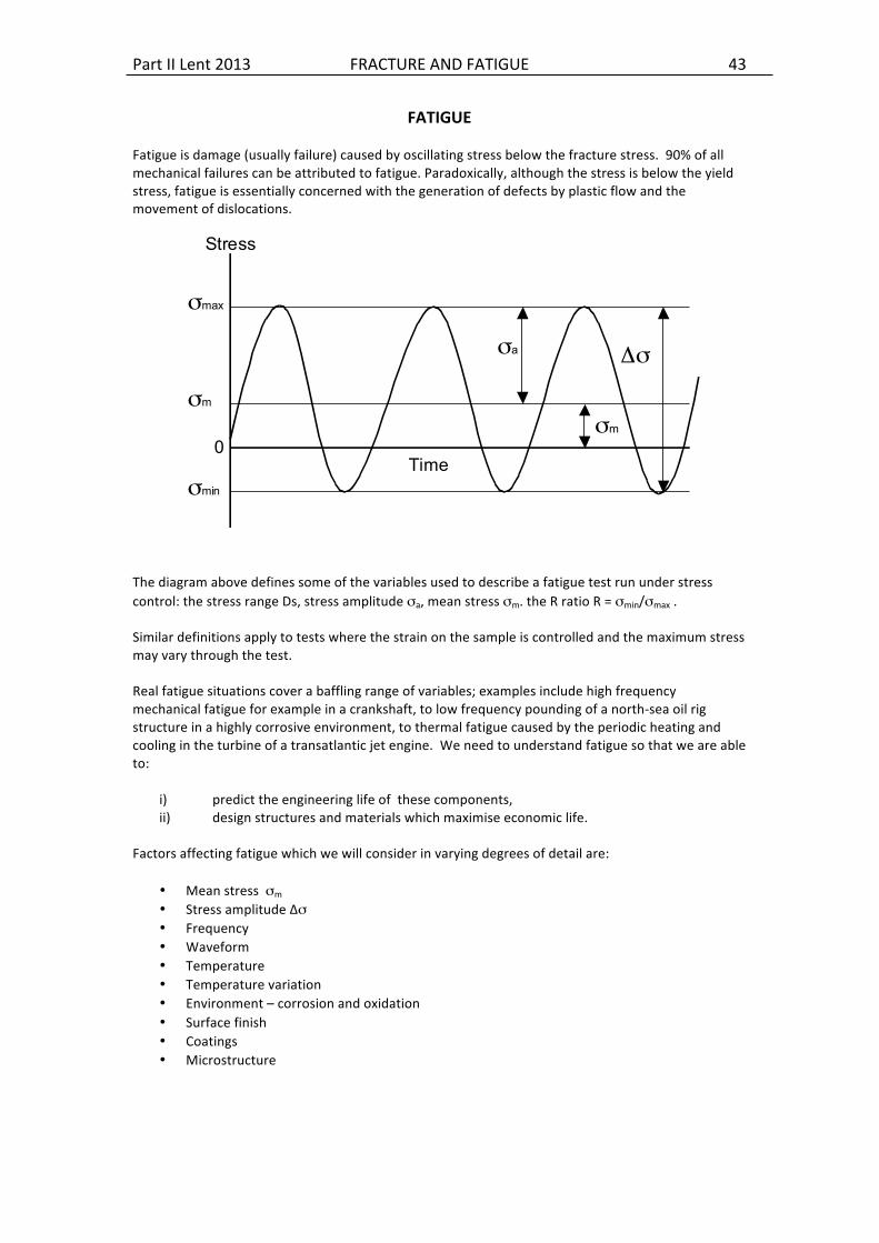
FATIGUE Fatigue is damage (usually failure) caused by oscillating stress below the fracture stress. 90% of all mechanical failures can be attributed to fatigue. Paradoxically, although the stress is below the yield stress, fatigue is essentially concerned with the generation of defects by plastic flow and the movement of dislocations.
Time
Stress
σmax
σm
σmin
0
Δσ
σm
σa
The diagram above defines some of the variables used to describe a fatigue test run under stress control: the stress range Ds, stress amplitude σa, mean stress σm. the R ratio R = σmin/σmax . Similar definitions apply to tests where the strain on the sample is controlled and the maximum stress may vary through the test. Real fatigue situations cover a baffling range of variables; examples include high frequency mechanical fatigue for example in a crankshaft, to low frequency pounding of a north-‐sea oil rig structure in a highly corrosive environment, to thermal fatigue caused by the periodic heating and cooling in the turbine of a transatlantic jet engine. We need to understand fatigue so that we are able to:
i) predict the engineering life of these components, ii) design structures and materials which maximise economic life.
Factors affecting fatigue which we will consider in varying degrees of detail are:
• Mean stress σm • Stress amplitude ∆σ • Frequency • Waveform • Temperature • Temperature variation • Environment – corrosion and oxidation • Surface finish • Coatings • Microstructure

Part II Lent 2013 FRACTURE AND FATIGUE 44
Test procedures have been developed which address these variables and by the use of a number of mostly empirical laws these are able to provide some degree of predictability in most situations. Fatigue conditions fall into a number of regimes: High Cycle Fatigue HCF: Low amplitude stresses induce primarily elastic strains which results in long life, i.e. endurance in excess of 10,000cycles Low Cycle Fatigue LCF: Considerable plastic deformation during cyclic loading results in an endurance limit below 10,000 cycles and behavior dominated by plastic deformation. Thermo-‐mechanical Fatigue TMF: varying both stress and temperature to give strain cycles in phase, out of phase (and all things in between) with the temperature cycle.
APPROACHES TO FATIGUE We can break Fatigue in ductile materials into several stages:
1. Initial micro-‐structural changes leading to the nucleation of permanent damage
2. Nucleation of the first micro-‐cracks
3. Growth and coalescence of these flaws to produce a dominant crack.
4. Stable propagation of the dominant crack.
5. Failure
Macroscopically there are ambiguities in defining the initiation and growth stages of cracks – depending on the resolution of the techniques being used to investigate. Generally stages 1-‐3 constitute crack initiation and stages 4-‐5 crack growth. Depending on the conditions, these stages occupy widely differing fractions of the sample life and thus require different strategies to determine life. The method adopted also depends on the consequences of failure.

Part II Lent 2013 FRACTURE AND FATIGUE 45
TOTAL-‐LIFE OR SAFE-‐LIFE: This strategy is to predict the total life and retire the component at a fixed proportion of this, to include a considerable margin for error. The aim is to retire the component before a crack forms and it is used where fatigue failure would result in component failure. Total-‐life can be wasteful as much useful life remains unused where the scatter in the data is large. This approach focuses on predicting the number of cycles to failure, N for an initially un-‐cracked specimen. This is most appropriate where the initiation of the dominant crack occupies the majority of the total life (as much as 90%). For HCF where the stress range is low and the stresses principally elastic, the stress range is used to characterise the component and produce a reference S-‐N curve. For higher stresses resulting in LCF plastic strain is extensive and the strain range is typically (but not always) used. DAMAGE–TOLERANT OR FAIL-‐SAFE: This approach recognises that all structures contain defects and that these grow at stable and predictable rates. The strategy involves periodic inspection of the structure and repairs or replaces components as cracks are found. This is generally used where failure would not result in component failure due to structural redundancy. A greater proportion of the useful life is used and the risk of wrong assumptions in the predictive process are dimished. Thus if the maximum size of the initial defects in the structure is known (amax) the interval between inspections is determined by the time predicted for this crack to achieve critical size (t1). The component may survive several iterations (two in the case below) before being replaced.
Following the development of fracture mechanics for monotonic deformation Paris recognised in the 1960’s that the same concepts of stress intensity could be applied to fatigue to estimate the fatigue crack growth rate and thus predict the time taken for the crack to reach an unstable size.
Part II Lent 2013 FRACTURE AND FATIGUE 46
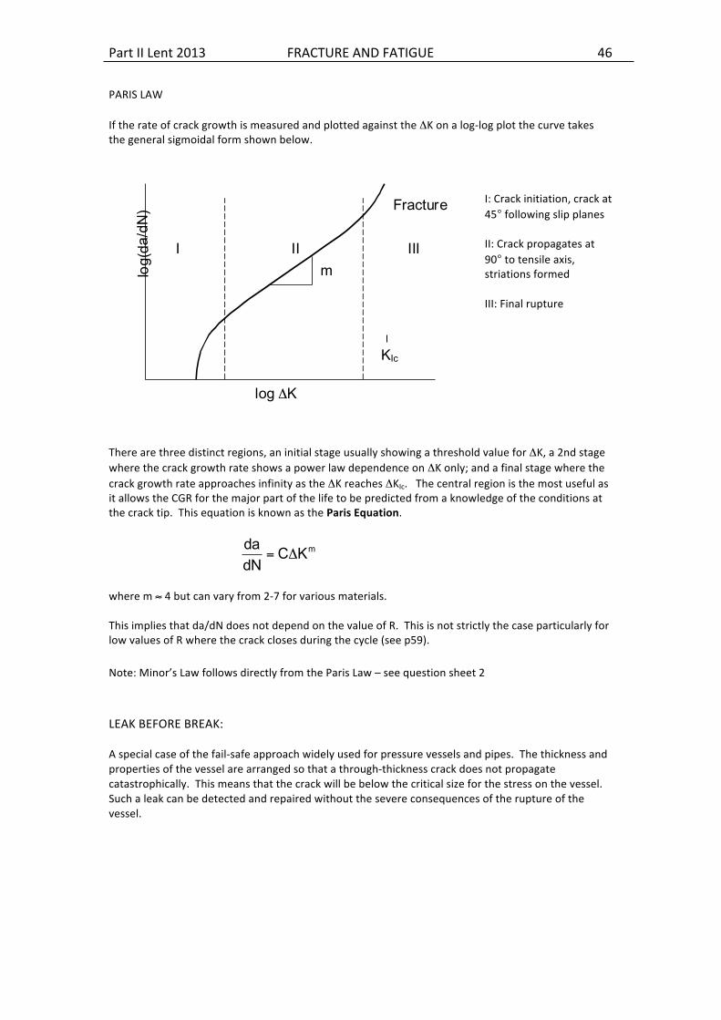
PARIS LAW If the rate of crack growth is measured and plotted against the ΔK on a log-‐log plot the curve takes the general sigmoidal form shown below.
I: Crack initiation, crack at 45° following slip planes II: Crack propagates at 90° to tensile axis, striations formed III: Final rupture
There are three distinct regions, an initial stage usually showing a threshold value for ΔK, a 2nd stage where the crack growth rate shows a power law dependence on ΔK only; and a final stage where the crack growth rate approaches infinity as the ΔK reaches ΔKIc. The central region is the most useful as it allows the CGR for the major part of the life to be predicted from a knowledge of the conditions at the crack tip. This equation is known as the Paris Equation.
mKCdNda
Δ=
where m ≈ 4 but can vary from 2-‐7 for various materials. This implies that da/dN does not depend on the value of R. This is not strictly the case particularly for low values of R where the crack closes during the cycle (see p59). Note: Minor’s Law follows directly from the Paris Law – see question sheet 2 LEAK BEFORE BREAK: A special case of the fail-‐safe approach widely used for pressure vessels and pipes. The thickness and properties of the vessel are arranged so that a through-‐thickness crack does not propagate catastrophically. This means that the crack will be below the critical size for the stress on the vessel. Such a leak can be detected and repaired without the severe consequences of the rupture of the vessel.
log(
da/d
N)
log ΔK
Fracture
I II III m
KIc

Part II Lent 2013 FRACTURE AND FATIGUE 47
TOTAL LIFE APPROACH If we perform a series of tests at varying stress ranges and plot the number of cycles to failure the life increases as the stress range decreases. Some materials (typically low alloy steels and Titanium alloys) show an asymptote to a fatigue limit, otherwise (high alloy steels and aluminium), an endurance limit is set.
Δσ
ln N
Fatigue limit
10 Endurance limit
S-N curve
7
BASQUIN’S LAW The curve can be approximated by an empirical expression due to Basquin:
Δσ2
=σ a = "σ f 2Nf( )b Nf is the number of complete cycles to failure.
where σf’ is the fatigue strength coefficient ≈ σf the static fracture strength and b takes the value –0.05 to –0.12 for metals. COFFIN MANSON LAW. Under conditions of high plastic deformation we have low cycle fatigue conditions and for strain controlled tests, Coffin and Manson independently noted an empirical relation very similar to Basquin’s law. The total strain amplitude can be split into plastic and elastic components:
222pe εΔ
+εΔ
=εΔ
where the plastic component is linear when plotted against the log (number of load reversals), 2Nf :
Δεp2
= "εf 2Nf( )c
Here εf’ is the fatigue ductility component and roughly equal to the failure ductility in tension, and c takes the value –0.5 to –0.7 for metals. Adding in the Basquin’s law for the ‘elastic’ (high cycle fatigue) component we have:
Δε2=
"σ f
E2Nf( )
b+ "εf 2Nf( )
c
Plotting log(Δε) against log (2Nf) gives two distinct regimes, at low strain and long life the gradient b

Part II Lent 2013 FRACTURE AND FATIGUE 48
(-‐0.1) dominates, HCF conditions, and at high strain and short life the gradient is c (-‐0.5). The transition is gradual but extrapolating the asymptotes allows a transition number of cycles, 2Nt, to be identified.
log 2Nf
logΔε c
b
εf
2Nt Note: fatigue is inherently variable variation in life of 100% is not unusual for nominally the same test. This is masked by the widespread use of log plots. The intercepts of the two ‘parts’ of the curve correspond roughly to:
1. LCF: the total strain, plastic and elastic, at failure. 2. HCF: the elastic component of the strain at failure
Let’s put some figures in here: E σf’ εf’ b c Aluminium 7075 72GPa 193MPa 1.8 -‐0.106 -‐0.690 Steel 0.15%C 210GPa 827MPa 0.95 -‐0.110 -‐0.640
Aluminium: Δε2=19372000
2Nf( )−0.106
+1.8 2Nf( )−0.69
(HCF intercept 666 times less than the LCF intercept -‐ note log scale)
Steel: Δε2=
827210000
2Nf( )−0.11
+0.95 2Nf( )−0.64
(HCF intercept 240 times less than LCF)

Part II Lent 2013 FRACTURE AND FATIGUE 49
TOTAL LIFE APPROACH -‐ COPING WITH FATIGUE VARIABLES There is a huge number of variables in fatigue – far to many to construct S/N curves for all combinations even if they did not change during the lifetime of the component. The challenge is to understand how the damage produced by fatigue varies with these parameters and adds together over a complex life cycle. The effect of increasing the mean stress is to decrease the fatigue life. Several relations exist to link the stress range and the mean stress for a given life. The simplest are linear extrapolations indicating that the sample will fail at the static yield stress in the absence of a stress range and at the fatigue strain at zero mean strain.
€
σa = σa |σ m =0 1− σm
σ y
⎧ ⎨ ⎩
⎫ ⎬ ⎭ Soderberg: original and most conservative
€
σa = σa |σ m =0 1− σm
σTS
⎧ ⎨ ⎩
⎫ ⎬ ⎭ Goodman relation: good for Brittle materials
conservative for metals
(Other expressions exist giving non-‐linear extrapolations

Part II Lent 2013 FRACTURE AND FATIGUE 50
GOODMAN DIAGRAM The effect of mean stress and R value can be expressed on a ‘Goodman diagram’ shown below:
σmin
σmax
MEAN STRESS: THE ROLE OF RESIDUAL STRESS Stresses formed internally in a material, for example during quenching or by Shot peening can have a profound influence on the fatigue life – both positive and negative. Effectively this sets up a mean stress varying throughout the microstructure which can extend the life when compressive and shorten it when tensile. For example; bombarding the surface with ball bearings ia widely used to extend fatigue life by setting up compressive stresses in the surface layers. Conversely, tensile stresses deep within a quenched component can lead to accelerated fatigue crack growth and premature failure. Hence a great deal of effort and resources are devoted to measuring residual stress and relieving it where necessary. Residual stress can be measured by the following methods X-‐ray diffraction –usually using high intensity synchrotron sources to reach the thick sections as this has to be done in-‐situ. The stress can be measured directly from the change in the lattice parameter from the elastic strain. Hole drilling – by drilling holes the distortion in the vicinity can be measured as the stress relaxes by the use of strain gauges or direct measurement. Modeling: increasingly accurate models of the elastic and plastic deformation occurring during processing allow us to estimate residual stress. TEMPERATURE Temperature has environmental effects on fatigue developed later. It is possible to adjust for the simple effect on yield stress where the nature of fatigue does not change by normalizing the applied stress with the yield stress. Plotting against σ/σy often collapses datasets to the same curve.

Part II Lent 2013 FRACTURE AND FATIGUE 51
COPING WITH VARIABLE STRESS -‐ MINERS LAW: In real situations components very rarely experience constant regular damage. The level of stress or strain can vary throughout life and the simplest way of dealing with this is by the use of Miners law. This proposes that the life of a component experiencing fatigue at various stress amplitudes can be assessed by expressing the number of cycles at each amplitude as a proportion of total life and summing the fractions. When the fraction reaches 1, the fatigue life is exhausted. The order of exposure is not taken into account.
σ
time
niNfi
=1i=1
m
∑ Miner’s Law
This is useful as a first approximation but has serious shortcomings. The most important being that no account can be taken of the impact of prior damage on the later exposure at a different stress (or strain) amplitude. In particular the balance between crack initiation and crack growth can vary considerably with stress, thus brief exposure to high amplitude may nucleate damage which at a lower stress would not occur until a much later stage and thus accelerate the damage rate at a subsequent lower stress. Conversely, early exposure to low stress amplitude may strain harden the material and thus prolong life during later high amplitude exposure. This emphasizes the importance of looking at the specific mechanisms of damage and how it accumulates in the material.

Part II Lent 2013 FRACTURE AND FATIGUE 52
DEVELPOMENT OF INTERNAL MICROSTRUCTURE DURING FATIGUE For some situations the loading conditions are controlled by the amplitude of the strain rather than the stress. This is reflected in the tests which are done under strain control. These are also most likely to be the conditions where plastic deformation forms a considerable proportion of the strain, LCF. Where the strain is kept constant the stress can either increase (cyclic hardening) decrease (cyclic softening) or stay the same.
Typically materials harden if σUTSσ ys
>1.4 and soften if σUTSσ ys
<1.2
To understand why this occurs we need to consider dislocation microstructure of the material.
• From the above materials where the initial state is highly work hardened the dislocation density is high, the effect of the cyclic strain is to allow the rearrangement of the dislocations into stable networks, reducing the stress at which the plastic component occurs, and thus the effective stress.
• Conversely where the initial dislocation density is low, (soft material) the cyclic strain increases the dislocation density increasing the amount of elastic strain and the stress on the material.
For a given alloy both hard and soft materials tend to a stable dislocation configuration. For example, detailed work on the development of dislocation configurations in copper and shows that a stable ‘Labyrinth’ structure develops (see the figure on page 52 from Suresh, chapter 2)
σt
σc
εt
εc σc <σt
σt
σc
εt
εc σc <σt
σσ
Cyclic hardening Cyclic softening

Part II Lent 2013 FRACTURE AND FATIGUE 53
As the fatigue establishes a stable microstructure the hysteresis loop becomes stable at some point during the test. When this ‘stable loop’ is plotted as a function of increasing stress (or strain) the locus of the maximum values from a series of tests defines a ‘cyclic stress strain curve’.

Part II Lent 2013 FRACTURE AND FATIGUE 54
BAUSCHINGER EFFECT
Strain control first cycle showing the Bauschinger effect. During cyclic deformation the material can retain a ‘memory’ of the initial plastic strain which reduces the stress at which plastic yield occurs in the reverse cycle. This effect can persist for many cycles and is known as the BAUSCHINGER EFFECT. This reversible but plastic deformation can occur by dislocation pile-‐ups at, for example, incoherent or semi-‐coherent precipitates exerting a back-‐stress which assists plastic yield in compression. This reduces the yield stress in compression.
σt
σc
εt
εc σc <σt
σt
σc
εt
εc σc <σt
Δσb

Part II Lent 2013 FRACTURE AND FATIGUE 55
The picture above shows a single crystal superalloy CMSX-‐4 fatigued in LCF at 750ºC and interrupted at about half the expected life. In this section cut on the primary slip plane dislocation loop enter the γ’ phase precipitates trailing Anti-‐Phase Boundary faults – under max stress the loops expand contracting as the stress decreases.

Part II Lent 2013 FRACTURE AND FATIGUE 56
THE EFFECT OF STACKING FAULT ENERGY: The material response is closely linked to the stacking fault energy since this governs the ability of the dislocation to cross-‐slip between planes and thus form stable cell structures. High SFE ⇒ easy cross-‐slip ⇒ rapid formation of stable cell structure.
For high SFE materials the cell size is a decreasing function of the strain range and ultimately does not depend on the starting microstructure. Very low SFE e.g. Cu 7.5% Al, materials do not form stable cell structures, the highly dissociated dislocations being arranged in planar arrays where the spacing depends on the initial state. The microstructures and lives are thus very sensitive to the prior deformation state.

Part II Lent 2013 FRACTURE AND FATIGUE 57
CYCLIC SOFTENING OF PRECIPITATION HARDENED ALLOYS: Another cause of cyclic softening of major importance is the cutting of coherent precipitates in precipitation-‐hardened alloys. Small coherent precipitates provide very effective hardening in aluminium alloys and in nickel based superalloys. The small size maximises the cutting/bowing stress for dislocations in the matrix and the coherency enhances the stability of these small precipitates. However when a dislocation does cut the precipitate the fault produced in the precipitates decreases the stress for the following dislocation since the energy penalty of the fault no longer applies and indeed may be negative. Thus slip is concentrated in narrow slip bands cutting the precipitates in two. These smaller precipitates may dissolve in these areas leaving the un-‐strengthened matrix vulnerable to high plastic deformation and early crack formation.
Here cutting of precipitates early in this test (TMF of Nimonic 90) has caused the γ’ to dissolve leaving precipitate free channels in the alloy. The precipitates are visible from the dislocations wrapped around them
(a) OP (±0.4)
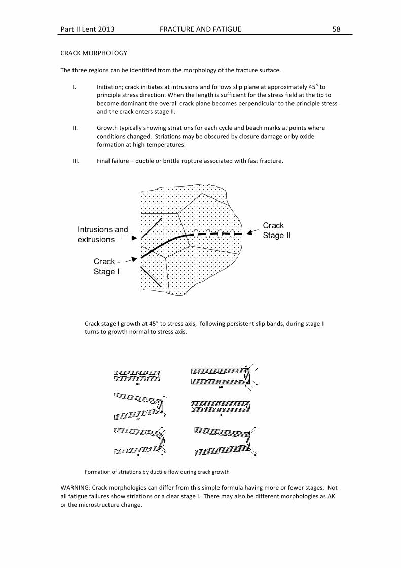
Part II Lent 2013 FRACTURE AND FATIGUE 58
CRACK MORPHOLOGY The three regions can be identified from the morphology of the fracture surface.
I. Initiation; crack initiates at intrusions and follows slip plane at approximately 45° to principle stress direction. When the length is sufficient for the stress field at the tip to become dominant the overall crack plane becomes perpendicular to the principle stress and the crack enters stage II.
II. Growth typically showing striations for each cycle and beach marks at points where conditions changed. Striations may be obscured by closure damage or by oxide formation at high temperatures.
III. Final failure – ductile or brittle rupture associated with fast fracture.
Intrusions and extrusions
Crack -Stage I
Crack Stage II
Crack stage I growth at 45° to stress axis, following persistent slip bands, during stage II turns to growth normal to stress axis.
Formation of striations by ductile flow during crack growth WARNING: Crack morphologies can differ from this simple formula having more or fewer stages. Not all fatigue failures show striations or a clear stage I. There may also be different morphologies as ΔK or the microstructure change.

Part II Lent 2013 FRACTURE AND FATIGUE 59
STRUCTURAL FEATURES OF FATIGUE CRACK INITIATION: Here we look briefly at the effect of surface condition, the evolution of damage, and the effect of coatings and surface treatments on the initiation and propagation of fatigue cracks. INITIATION BY DEFORMATION Fatigue failures can occur at stress of 1/3 the tensile yield stress, yet the nucleation of cracks requires that there be local yielding. We thus need heterogeneous nucleation sites for cracks within the structure.
• Pre-‐existing defects such as inclusions, porosity, surface damage • Defects generated during cyclic straining for example at stress concentrations: persistent slip
bands, Fracture of carbides, oxidation of carbides. In pure metals the major source of fatigue cracks is the persistent slip bands or PSBs: so called because traces of the bands persist even after surface damage is polished away. The plastic strain in the PSB is 100 times greater than that in the surrounding material and results from specific arrangements of dislocations as parallel walls with relatively low dislocation density between. An equilibrium is maintained between nucleation and annihilation of mobile edge dislocations bowing out from the walls. Thus the cyclic strain is concentrated in these zones leading to their persistence. Although the strain is reversed within the PSB the distribution is not even and this leads to the formation of intrusions and extrusions where PSBs intersect the surface. These may act as nucleation sites for cracks. The initial stages of crack growth therefore often follow the slip planes and lie at 45° to the tensile axis (see later).
Diagram showing the formation of intrusions and extrusions at a persistent slip band. In the vast majority of cases fatigue initiates on the surface, however cracks can sometimes initiate internally at defects cracked precipitates of internal porosity. The crack then grows under vacuum until it reaches an external surface. This gives a characteristic circular area on the fracture surface. Once the crack becomes a surface crack and air is admitted and the stress intensity increases and the growth rate increases. This sometimes leads to immediate failure.

Part II Lent 2013 FRACTURE AND FATIGUE 60
EFFECTS OF OXIDATION AND CORROSION The absence of a fatigue limit is normally and indication of material which is immune from corrosion or oxidation effects – otherwise the mere passage of time will eventually allow the initiation and propagation of cracks even at very low stress.
! At high temperatures oxidation at grain boundaries, Carbides or as in the single crystal above, in areas where the composition varies slightly, results in crack initiation. The oxide layer cracks and the crack propagates into the substrate thus allowing further oxidation.
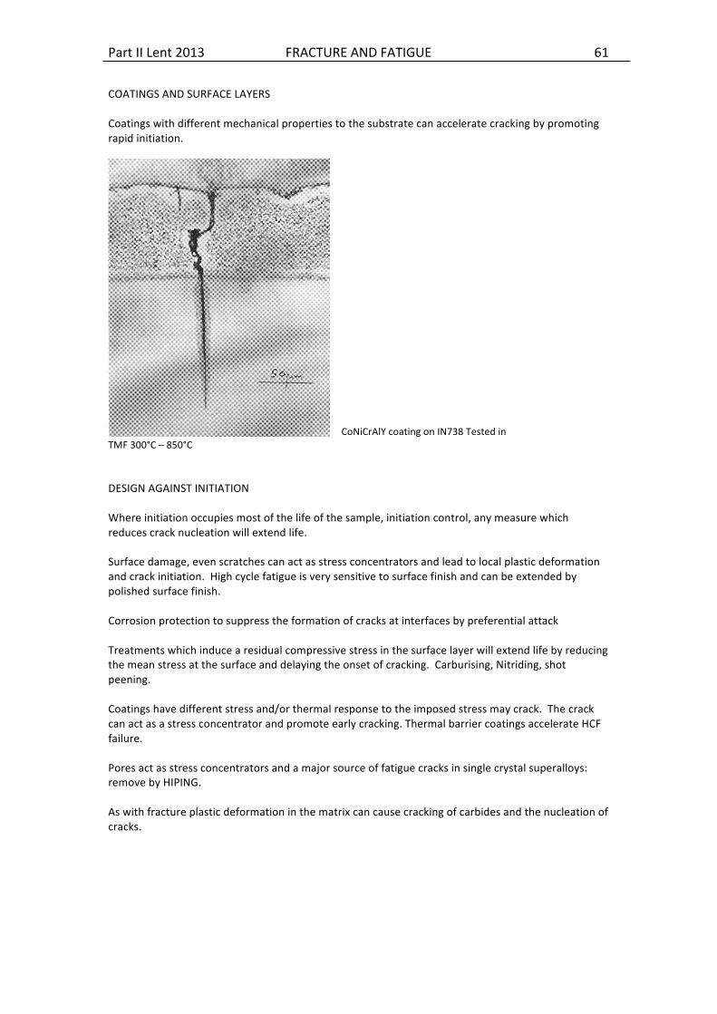
Part II Lent 2013 FRACTURE AND FATIGUE 61
COATINGS AND SURFACE LAYERS Coatings with different mechanical properties to the substrate can accelerate cracking by promoting rapid initiation.
CoNiCrAlY coating on IN738 Tested in
TMF 300°C – 850°C DESIGN AGAINST INITIATION Where initiation occupies most of the life of the sample, initiation control, any measure which reduces crack nucleation will extend life. Surface damage, even scratches can act as stress concentrators and lead to local plastic deformation and crack initiation. High cycle fatigue is very sensitive to surface finish and can be extended by polished surface finish. Corrosion protection to suppress the formation of cracks at interfaces by preferential attack Treatments which induce a residual compressive stress in the surface layer will extend life by reducing the mean stress at the surface and delaying the onset of cracking. Carburising, Nitriding, shot peening. Coatings have different stress and/or thermal response to the imposed stress may crack. The crack can act as a stress concentrator and promote early cracking. Thermal barrier coatings accelerate HCF failure. Pores act as stress concentrators and a major source of fatigue cracks in single crystal superalloys: remove by HIPING. As with fracture plastic deformation in the matrix can cause cracking of carbides and the nucleation of cracks.

Part II Lent 2013 FRACTURE AND FATIGUE 62
FACTORS EFFECTING CRACK GROWTH RATES In predicting the life of a component we have to consider the possibility that the material is subject to other degradation processes such as corrosion, oxidation or creep which affect the crack growth. Damage usually accelerates crack growth, but can repair and mitigate the effects of the other process. Tests investigating these effects compare behaviour in vacuum with that in air or other damaging environments. Alternatively, introducing a dwell time at maximum and or minimum stress can change the crack growth rate. The higher the test frequency the smaller the possible contribution from creep/corrosion will be and a strong dependence of life on the frequency can indicate some other contribution. (This may also show up as a mismatch between HCF and LCF data when plotted on the same graph as on page 47.) CREEP Creep can increase or decrease fatigue life: possible mechanisms of interaction are:
• An increase in dislocation density due to fatigue can increase creep rate through dislocation movement and /or enhanced diffusion.
• Increasing dislocation density can also decrease primary creep (see earlier). • Cutting of grain boundary porosity increasing the growth rate of the pores • Blunting of crack tip by creep can reduce crack growth rate and hence fatigue • damage rate.
Graph of a constant strain fatigue test with a dwell at both the upper and lower temperatures. During the dwell the specimen creeps to reduce the stress.
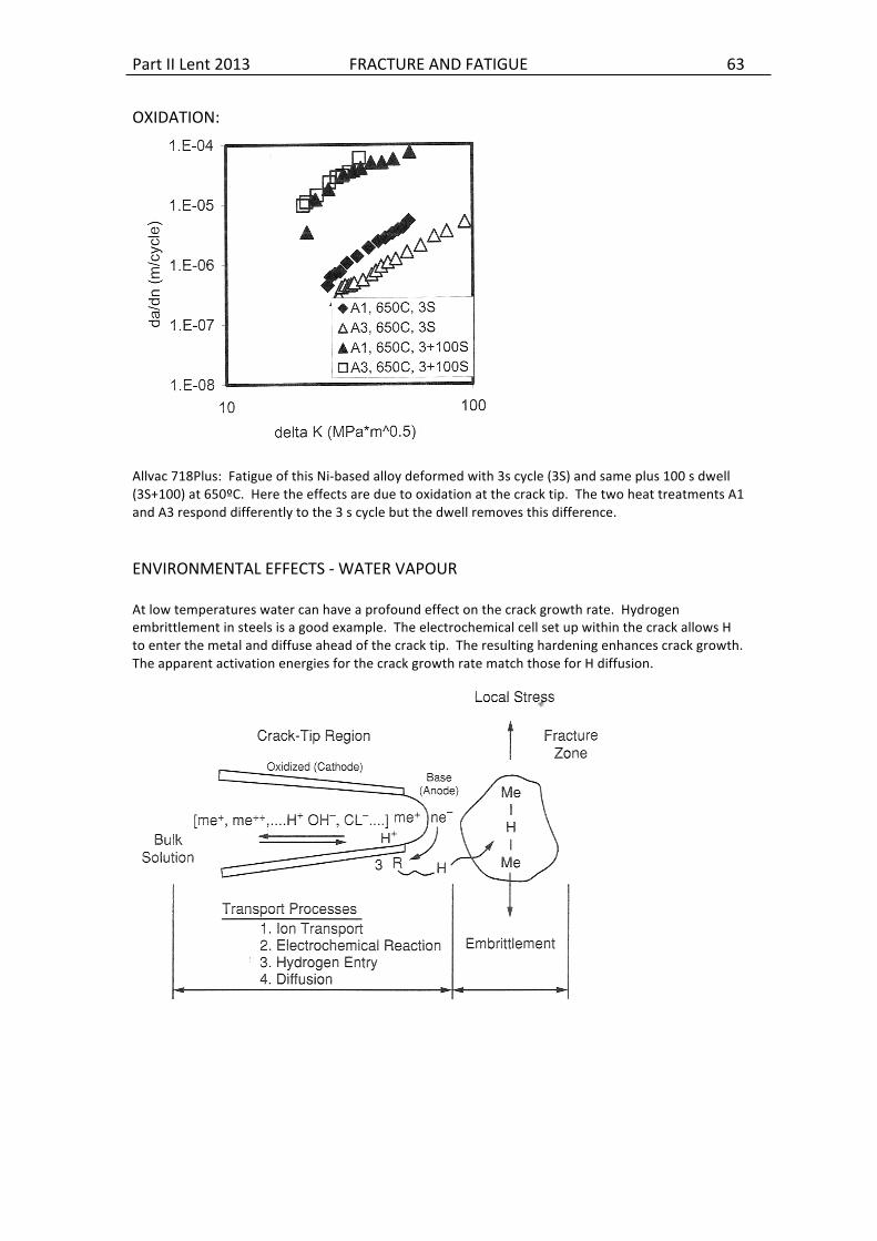
Part II Lent 2013 FRACTURE AND FATIGUE 63
OXIDATION:
Allvac 718Plus: Fatigue of this Ni-‐based alloy deformed with 3s cycle (3S) and same plus 100 s dwell (3S+100) at 650ºC. Here the effects are due to oxidation at the crack tip. The two heat treatments A1 and A3 respond differently to the 3 s cycle but the dwell removes this difference. ENVIRONMENTAL EFFECTS -‐ WATER VAPOUR At low temperatures water can have a profound effect on the crack growth rate. Hydrogen embrittlement in steels is a good example. The electrochemical cell set up within the crack allows H to enter the metal and diffuse ahead of the crack tip. The resulting hardening enhances crack growth. The apparent activation energies for the crack growth rate match those for H diffusion.

Part II Lent 2013 FRACTURE AND FATIGUE 64
Al alloy fatigue tested in Argon and damp air – the water vapour accelerates crack growth above a threshold of ~ 2.0 Pa but the effect becomes saturated at 6.9 Pa. Studies analysing the surface show a similar trend in the oxides formed at the newly exposed crack tips. CRACK CLOSURE The plastic deformation at the fracture surface, distortion or oxide growth during exposure can all act to cause the crack faces to touch before the elastic deformations of the sample would predict. This means that the stress intensity range is effectively reduced. Clearly this will have a greater effect the closer the minimum stress intensity is to zero.
Kmax
Kop
Kmin
Time
ΔKeff
Closure
Crack Closure: Effective stress range where crack does not fully close.
The Paris equation can be modified to use a reduced value of the stress intensity factor ΔKeff.
( )mmeff KUCKC
dNda
Δ=Δ= where KKU eff
Δ
Δ=

Part II Lent 2013 FRACTURE AND FATIGUE 65
Mechanisms proposed to cause crack closure:
Plasticity Stress induced transformation
Mode II displacement Oxide debris
Using crack closure to adjust for R ratio: The crack growth rate curves below have been measured at different R ratios – this gives rise to different amounts of crack closure. All the data can by condensed onto a single line by judicious use of ∆Keff. Usually suitable U values are fitted experimentally.

Part II Lent 2013 C15 FRACTURE AND FATIGUE QUESTION SHEETS
QUESTION SHEET 1 (Lectures 1-6)
1. (a) The singular terms in the equation for the elastic stress field around the tip of a sharp crack under Mode I loading in plane stress are:
€
σ11 =σo πa
2πrcos θ
2
% & '
( ) *
1+ sin θ2
% & '
( ) *
sin 3θ2
% & '
( ) *
+
, -
.
/ 0
€
σ22 =σo πa
2πrcos θ
2
% & '
( ) *
1− sin θ2
% & '
( ) *
sin 3θ2
% & '
( ) *
,
- .
/
0 1
€
τ12 =σo πa
2πrsin θ
2
& ' (
) * +
cos θ2
& ' (
) * +
cos 3θ2
& ' (
) * +
where the crack lies in the x2 direction along the x2x3 plane. Convince yourself that at a general position (r, q) the shear stress τ12 is finite, where is the shear stress zero? Assuming a state of plane stress, i.e. σ3 = 0, find the expressions for the principal stresses σ1 and σ2, i.e. the maximum values of the normal stresses when the shear stresses are zero. This can be done by diagonalising the stress tensor or more simply by using Mohr’s circle, (θ is the angle between the direction vector and the y axis 2). For conditions of plane strain write down an estimate for the out-of-plane principal stress σ3 (σ3 = υ [σ1 + σ2]) and thus demonstrate that it is non-zero. Hence demonstrate that the hydrostatic component of the stress tensor is larger in plane strain that in plane stress. (b) Using the result from (a) for the principal stresses combine these using the Tresca yield criteria (σmax – σmin) = σy. Hence plot out the shapes and relative sizes of the plastic zone in the x1x2 plane under conditions of (i) plane stress and, (if time and patience allow) (ii) plane strain, for a non-work-hardening material. On which planes does the plastic deformation occur in the two cases? The Tresca yield criterion looks at the maximum difference between the principal stresses and assumes that yield occurs when this reaches the tensile yield stress. Take Poisson’s ratio as 0.3. For a reminder on the use of Mohr’s circle try the DoITPoMS site:
http://www.doitpoms.ac.uk/tlplib/metal-forming-1/index.php
1
2
3

Part II Lent 2013 C15 FRACTURE AND FATIGUE QUESTION SHEETS
2. A directionally solidified inter-metallic has a grain structure which can be modelled as a series of hexagonal prisms separated by high angle grain boundaries. The material has limited ductility and fails in a brittle manner. By considering the value of G, the energy release rate and R, the energy of fracture, evaluate whether the intermetallic will fail in an inter-granular of a trans-granular manner for the two different orientations of the grain structure below loaded in pure mode I opening. You can assume that the energy of fracture R is reduced by the grain boundary energy for intergranular failure. The grain boundary energy is half the surface energy of the material and equal for all the boundaries. The variation of the energy release rate, G, as the fracture plane deviates from the plane normal to the loading axis, is given by the graphs on page 16 of the handout.
Would there be any difference for propagation parallel to the grain axes?
Following your conclusions from the above, describe the fracture path you would expect in a more realistic structure where the grains were not so regular.

Part II Lent 2013 C15 FRACTURE AND FATIGUE QUESTION SHEETS
3 a) A wedge driven into a pre-existing crack along the grain of piece of wood opens up the crack and eventually causes the wood to split along the grain. Sketch how the stored elastic energy varies as the wedge is driven in both before and after the crack starts to grow. Plot U against x. Assume that the crack lies very close and parallel to the straight edge of the wood and that all the strain is in the thinner layer of wood. The elastic energy stored, UE, in a cantilevered beam of depth d opened by a
wedge of height h is given by:
€
UE =Ed3h2B
8a3 (B is the width into the page)
b) Derive an expression for the energy release rate as the crack grows. Will the crack grow in a stable or unstable manner as the wedge is driven in at a steady rate? It is found that the crack starts to grow when the wedge is on average 100 mm from the crack tip, i.e. a = 100 mm. If the modulus of the wood along the grain is 10 GPa, d = 5 mm and h = 3 mm estimate the resistance to crack growth R of the wood along the grain. Hence estimate the toughness.

Part II Lent 2013 C15 FRACTURE AND FATIGUE QUESTION SHEETS
c) A manufacturer of disposable chopsticks makes them from the same wood leaving a small section of wood joining the pair for the user to break. He wants to ensure that the two sticks will be easy to separate along the grain. Show that the force required to pull the two sticks apart as shown in the diagram
is given by the expression
If the length of the cut between the two sticks is 200 mm and the sticks are a square section of 5 mm calculate the force.
4. a) A cylindrical pressure vessel of diameter 1 m is made from a steel of toughness 70 MPa m1/2 and with a yield strength of 440 MPa. What is the maximum possible thickness that the vessel can be made if it were to leak before break? The internal pressure is 10 MPa. Design criteria specify a safety margin of 10% for the thickness – what thickness would you specify to ensure leak before break? What is the maximum stress and does this exceed the yield stress? b) The inside of the vessel is given a proprietary laser treatment to double the hardness and improve the resistance to chemical attack. This coating reaches a depth of 2 mm. Unfortunately it also decreases the toughness to 35 MPa m1/2. What is the critical crack size in the laser treated material? Describe what will happen to a crack propagating from the inside through the hardened layer and into the untreated steel of the pressure vessel. Does the layer affect the safety of the vessel? Consider the effects of the coating on both static loading and fatigue.
Estimate the plastic zone size i) in the coating and ii) in the main body of the vessel and explain the basis of your calculation.
€
Fmax =Ed3R4 × 3
#
$ %
&
' (
1/ 2Ba

Part II Lent 2013 C15 FRACTURE AND FATIGUE QUESTION SHEETS
QUESTION SHEET 2 (LECTURES 7-9) 1. In a thermal expansion joint a component is subjected to a large plastic strain
range and fails after 2000 cycles. If the plastic strain range is halved, by how many cycles is the life of the component increased. Assume a Coffin Manson exponent, c, of -0.5.
2. An aeroplane fuselage is subjected to fluctuating stresses of range (minimum to maximum) 150 MNm-2, with a maximum tensile stress of 200 MNm-2. If ultrasonic NDT techniques can only be guaranteed to detect internal defects greater than 1 mm in total length, recommend appropriate periods for major inspection of the fuselage. Clearly state any assumptions. [The material has a fracture toughness of 32 MPam1/2 for this thickness of fuselage. The growth of a fatigue crack of length a metres with respect to the number of cycles, N, is given by the expression:
€
dadN
= 4.08 ×10⁻¹¹ ΔK4
1−R( )0.7
Where ΔΚ is given by ( Kmax - Kmin ) and is in MPam1/2. The correction (1 - R)0.7 is an empirical expression for converting data obtained at different R values.]
3. In a structural steel the fatigue-crack growth per cycle da/dN, is given by:
€
dadN
=10−13ΔK3 m/cycle
Where ΔΚ is the alternating stress intensity in MPam1/2. The initial crack size (half length) a = 2mm and the critical size at which failure occurs acrit = 10mm. By integrating the expression between fixed limits show that the S-N curve is given by: logN = -3logΔσ + 13.647 A component of this steel containing initial cracks of half length 2mm is subjected to 5 × 10⁵ cycles at an alternating tensile stress, Δσ, of 354 MNm-2 and to 5 × 10⁶ cycles at 164.3 MNm-2. Given a critical crack length of 10 mm show, by integration of the crack growth rate or otherwise, that Miner’s law is satisfied regardless of the order in which the fatigue cycles occur. (You might like to try proving Minor’s law generally for any combination of stresses)
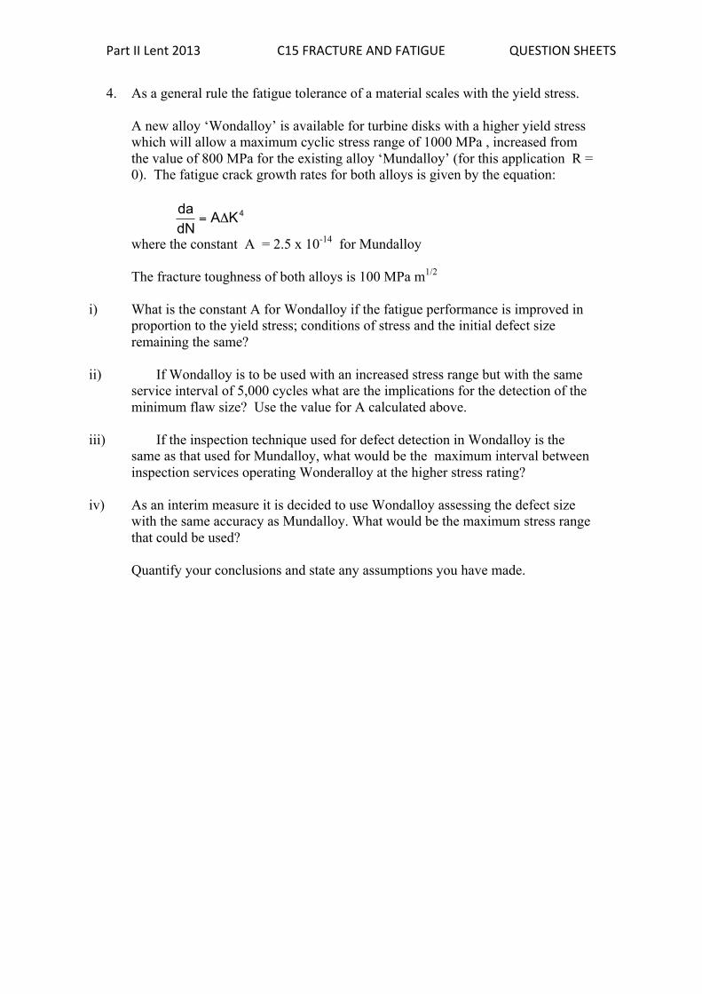
Part II Lent 2013 C15 FRACTURE AND FATIGUE QUESTION SHEETS
4. As a general rule the fatigue tolerance of a material scales with the yield stress.
A new alloy ‘Wondalloy’ is available for turbine disks with a higher yield stress which will allow a maximum cyclic stress range of 1000 MPa , increased from the value of 800 MPa for the existing alloy ‘Mundalloy’ (for this application R = 0). The fatigue crack growth rates for both alloys is given by the equation:
€
dadN
= AΔK4
where the constant A = 2.5 x 10⁻¹⁴ for Mundalloy The fracture toughness of both alloys is 100 MPa m1/2
i) What is the constant A for Wondalloy if the fatigue performance is improved in proportion to the yield stress; conditions of stress and the initial defect size remaining the same?
ii) If Wondalloy is to be used with an increased stress range but with the same service interval of 5,000 cycles what are the implications for the detection of the minimum flaw size? Use the value for A calculated above.
iii) If the inspection technique used for defect detection in Wondalloy is the same as that used for Mundalloy, what would be the maximum interval between inspection services operating Wonderalloy at the higher stress rating?
iv) As an interim measure it is decided to use Wondalloy assessing the defect size
with the same accuracy as Mundalloy. What would be the maximum stress range that could be used?
Quantify your conclusions and state any assumptions you have made.