(C) R G Bingham 2005. All rights reserved. Optics and Optical Design Richard G. Bingham Session 1 Introduction Coordinates Rays that may appear odd Image.

(C) R G Bingham 2005. All rights reserved.

Optics and Optical DesignRichard G. Bingham

Session 1

Introduction

Coordinates

Rays that may appear odd

Image rotation and parity and an image slicer

Spherical Trigonometry – advanced option


The beginning

Six pages of introductory notes


AimsRay-tracing software is amazingly accurate and comprehensive, but practising with the buttons on the toolbar is not enough. Our aims are: to understand optical systems; to understand what the program is doing; to gain a feeling for what problems are tractable and what optical capabilities are provided by existing designs; to assess the performance of optical designs constructively; to see how complex optics may be comprised of sub-systems exploiting local aberration correction or special cases; to express our ideas with the program; to handle the tools that are available for designing new systems; to see what factors may stop optical aberrations from being made smaller; to be aware of cost and weight; to avoid redundant complexity in a design or its manufacturing specification; and to be practical and economic as regards the optics that we design and the use of our time. We hope to achieve all this by properly understanding the designer’s methods, so that we can learn and keep up to date in our own new designs or others that we may evaluate.


Format of this textThis material, although created in PowerPoint, was not intended for, and is not suitable for, projection as slides. PowerPoint was used to encapsulated successive ideas and topics in a format that ultimately will be neatly separate screens. A slide is referred to here as a “page”.

The material is arranged separate “sessions” of about 25 pages each. A few sessions may include one or two .doc files as well.

As mentioned above, the material could be viewed as successive screens by an individual user, but initially, it will be printed (quite large), again to be read individually. The suggested procedure is to first to read a session individually and to follow that by discussing it with others in a group, or if possible, to arrange some kind of tutorial following the individual reading.


How to handle thisI think that it is impossible fully to practise each topic before moving on. Perhaps material can be skimmed over if it does not seem helpful. Or perhaps the concepts and terminology from complex areas may be acquired in an effortless osmosis, later.

Most equations are given here without derivations; the aims of this particular course are such that we need to press on to the work of the designer. The fundamentals, however, may be useful for a physicist or engineer to understand. They are written up by Welford in “Aberrations of Optical Systems”, Hilger 1986. It may be worth considering whether to work systematically through the whole book, as indeed I did with the previous edition, for a comprehensive foundation. I refer to the book as ‘Welford’ throughout.

Examples are given in Zemax. If both the .zmx and the .ses files are in the same folder, graphics windows should open when the Lens Data Editor opens. Also explore any of the other Zemax features, their local help files and the main manual (.pdf).

Within the ZEMAX examples, there is a window called Title/Notes that appears on a tab after the Gen button is pressed. As you view one of the examples, it is vital to read those notes that are within the Zemax data, as I have often put critical information there.

I recommend that you do not personalise the default toolbar buttons in your own copy of Zemax. If you do, you may find that a different computer is slower to use, and it will become markedly more difficult to demonstrate things to other users.


How can I get to practise on some real designs?

If you are already working with any optics, a way to practice on real optics without spending money is to create a ray-tracing model of your experiment as soon as there is even a minor modification to explore. So for example, if some existing instrument needs merely to be differently focused or to have a thicker colour filter, or some as-made data becomes available, use that as a reason to set up a ZEMAX lens data file, however simple, and then use your ZEMAX file to check the modification. Once you have a few ZEMAX models, you will also be better placed to solve any further problems arising with your experiment, and will be able to create realistic graphics for publication. However, I would say that whilst setting up and using ZEMAX yourself for even simple purposes is very instructive, collecting complex data files from other people would be a waste of time.


ZEMAX• ZEMAX was created by Ken Moore from 1990 to date.

•It is for PCs only.

•We shall use Zemax in this course.

•The ‘hard key’ allows only one person to access it at once. It is worth the whole value of the software.

•You can open Zemax twice on the same machine (except with Remote Desktop). The second instance of Zemax is useful for running long computations whilst getting on with something else, or for cutting and pasting between systems.

•You need individual, unrestricted, continuous access to the program, along with technical support and updates, to do much productive work in optical design, if that is your task. Sharing a system is frustrating and hinders the design of real lenses.


Example – setting up a ball lensThe example is a glass ball, as available from Melles Griot. It is used as a lens (e.g. for fibre-optics work). It can be set up by following the details in Ball_lens_data.doc. This is the main example with such instructions for creating it from absolute scratch, which will provide a useful exercise if you have not previously set up lenses in ZEMAX. In any case, please find the further notes that I wrote within that .zmx file. They can be found on the General / Title/Notes tab ( on the ‘Gen’ button). Such further notes are held within all my ZEMAX examples in these lectures, so it will be useful to

be able to find them. To check your results, the intended data is in file: Ex00-Ball_Lens.zmx. If the Ex00-Ball_Lens.SES file is also present, it will bring up relevant graphics as below.


Coordinate systems

13 pages


+z

In Zemax, light must leave the object surface in the +z direction. The thickness of the object

surface must be positive.

x, y, z

+y

+z+x

inwards

Right-handed axes

Positive ‘sag’ z

Positive radius of curvature

Surface of a lens+y

Negative sag, negative radius

of curvature


Lens. Sequential ray tracing

1. The ‘thickness’ or ‘axial thickness’ is

measured positive in the +z direction

2. The curvature of the front surface is positive here

Example file: Ex01-Lens.ZMX

+z

+y

5. This is an ‘optical system’4. Lens drawings in most diagrams are cross-sections that are not shaded

3. The ‘front’ of a lens is the face that the light

hits first


•Local coordinates. A surface S1 has an origin (O1 here) that serves to locate this surface within the optical system.

•The ‘figure’ of surface S1 is defined by its sag z(x,y) that is thus measured orthogonal to the x,y plane.

•Each surface also has a following ‘thickness’. For sequential ray tracing, the origin O2 of the next optical surface S2 is positioned by this thickness of S1 along the z axis.

•Each surface can be positioned in this way with reference to the previous surface.

Defining surfaces for ray tracing

+y

+z+x is inwards

z(x,y)Some weird lens

O1O2

S1

S2

thickness


Thickness after a mirror

The thickness of glass or an air space entered into ZEMAX’s Lens Data Editor

changes sign at a mirror.


Sequential ray tracing - a Mangin mirror

This one piece of glass has to appear in the data twice for sequential ray tracing. It has positive thickness before the mirror but negative thickness after the mirror ; in the second pass, the thickness is measured in the minus z direction from the preceding surface, the mirror.

+y

+z

Example file: Ex02-Mangin.ZMX

1 2 3

4

The three rays in this 2D layout are drawn optionally from a flat surface numbered 1 that is in the data file. This surface 1 is a ‘dummy surface’ here. A dummy surface is one that has the same refractive index on both sides.

The signs of these curvatures are all

negative

Glass A back-surface Mirror

The three rays started from an object at infinity at surface number 0.

5


The manufacturing specification is different

rz

z‘Glass removal’ might correspond to positive z in the ray-tracing data but negative z on a machine.

Lens on machineLens in the ray-tracing

data

Wrongly made convex because a positive sign was quoted? A curvature with a positive sign is not necessarily convex in Zemax!

There is a necessary intermediate stage where we supply an engineering drawing or at least a sketch. Zemax will output a good starting point for a proper drawing.

Lens

Aspheric lens


Local Tilts and Decentres

The program provides for surfaces that are tilted or moved (‘decentred’). The local frame of reference can be tilted or moved, leaving the function z(x,y) unchanged.

+z+x is inwards

O2

+y

For example, the weird lens can have a right-hand surface that is tilted around its local x axis. The tilt shown is positive around the local +x axis. Combinations of two or three tilts can be used. The origin O2 can also be locally shifted in x and y, but not z – we have already chosen a z position, based on the previous surface.


Rotations that are consistent with the above:

1. In the x, y Argand diagram a positive angle is drawn anticlockwise, but it is clockwise looking along a +z axis emerging from the paper. A sign like that of the Argand diagram is also used for the angle of a ray in some optical diagrams, and for position angle on the sky, e.g. for the plane of sky polarisation measured anticlockwise (from north).

2. International standards for machine tools such as milling machines also use this sign.

x, y, z rotations – signs

+y

+z

•We rotate the axes in which subsequent surfaces are then defined, so the subsequent surfaces move with the rotation.

•A positive rotation in ZEMAX is clockwise as viewed in a positive axis direction.

A positive rotation around the x axis. The relevant matrix expression is in the ZEMAX manual.


x, y, z rotations that are different1. OPTICA (Mathematica) is the opposite. It applies a positive rotation looking

towards the origin, that is, in the negative axis direction. The difference arises from rotating an object the other way in global axes. The global axes in ZEMAX can also be unaffected, and often one need not be aware of them anyway. Check how they are defined. In ZEMAX, with a coordinate break, fresh local axes are obtained for following parts of the system.

2. In the Code V optical design code (current), a rotation around either the local x or the local y axis is negative as compared to the right-hand convention used in ZEMAX, whilst rotation around z is not affected.

3. In the GRT optical design code (obsolescent university FORTRAN), the x rotation is reversed as in Code V. However, the y rotation is not reversed. The z rotation appeared to be reversed when I rotated the lines on a diffraction grating.

4. Other codes may be different again.

5. Doubts can be resolved by inspecting 3D graphics that the program will draw!


Sequential ray tracing – a prism

The Lens Data Editor contains a sequence of optical surfaces. The path of any ray is calculated to intercept the next optical surface, in the order in which they are listed in the Lens Data Editor. See next slide for an example in ZEMAX.


-35° +40°

Coordinate breaks - a prism1. The prism angles are defined by ‘coordinate breaks’. A coordinate break is placed at a dummy optical surface, taking up one line of data in the Lens Data Editor. That line has boxes for x & y shifts and for x, y & z tilts in degrees. Other boxes on the same line hold the thickness to the next surface and a flag for reversing the order of the tilts.

Axes

-25°

2. The coordinate breaks are: 2 the tilt of the front surface; 4 the tilt of the z axis leading to the required centre of the exit surface; 5 the tilt of the exit surface; and 7 the tilt of the z axis leading to the required centre of the image surface.

+60°

Example file: Ex03-Seq_Prism.ZMX

3. The rays refract passively according to Snell's law. The rays do not affect the tilts of the axes in these data.

Rays

Thickness 4

2

45 7


Coordinate breaks again

1. If we place a coordinate break immediately before an optical surface, it is sometimes useful to put in another one with the opposite sign immediately after that surface, undoing the tilt etc. Then we can continue with the previous axis direction.

2. Reversing multiple tilt angles needs be done in the reverse sequence. Read the manual!


Tilts and shifts again1. SEQUENTIAL RAY TRACING uses local coordinates:

• ‘Coordinate breaks’ are inserted in the Lens Data Editor ahead of optical surfaces that need moving. The values of the angles and shifts can be varied in optimisation.

• Again for sequential ray tracing, individual optical surfaces can be given an intrinsic tilt or shift on a Surface Properties tab. The effect is the same as with with coordinate breaks but the data are not currently optimisable.

2. For NON-SEQUENTIAL RAY TRACING, a whole object can have its own tilt and position set up in a line of data for that object within the Non-Sequential Components Editor. This is essentially a global reference system, although alternatively, one component can be referred to another.


Rays that may appear odd

Two pages about geometrical rays in a ray-tracing program


A geometrical ray is a line to the next surface, but …

A

E

F

A

D

B

•AA is a normal ray path

•In sequential ray tracing, ray B is a valid extrapolation to a virtual image in a negative space. It has to end the ray trace or to be reversed.

But in a sequential ray trace, rays can fail or“crash”:

•Ray C misses a defined surface aperture

•Ray D, if reflected by TIR, terminates unless the surface is defined as a mirror

•Ray E misses the sphere altogether

•Ray F may intersect the sphere at the wrong point.

C

Lens


Non-sequential ray tracing – a prismExample: Ex04-NSC_Prism.ZMX

This ‘Rectangular Volume’ object is defined on a single line of the Non-Sequential Components Editor. The faces of this object would form a cuboid by default, but they can be angled as they are

here, and the whole thing is tilted 30º around x. Rays shown here intercept 0, 2 or 3 surfaces.

There are many types of NSC objects. They can be positioned with respect to a single origin, or individually with respect to other defined objects. NSC rays can split, scatter, etc., but don’t crash.

Two sorts of rays appear that go through this prism but are not dispersed in angle.


Image Rotation and Parity and an image slicer

Ten Pages


•Inverting the image means rotating it 180 degrees around the axis. Notice that ZEMAX views the image in the +z direction.

•If there is an intermediate real image, the final image is erect.

• The same applies to mirrors as to lenses.

•Thus a Cassegrain telescope gives an inverted image but a Gregorian telescope, which has one intermediate image, gives an erect final image.

Inverted real image in an axially symmetrical system

F

Fz


Image Parity•Reversal of parity is a three-dimensional effect.

•If the total number of mirrors is odd, the image parity is reversed.

•With an odd number of mirrors in an axially symmetrical system, the three-dimensional image must be reversed in depth, because neither lateral direction is special.

•Thus in a 3-mirror camera, if the object moves one way, the image moves in the opposite direction to the object, just as in a single plane mirror.

•Using these ideas, in a Cassegrain telescope, which way does the focus move between infinity and a laser guide star?


Image rotators

Field of view

We have a few objects around a field of view that is fixed in space.

Image 1

The image rotator flips their images across a

diameter A. That is what it does.

A

Image 2

Then if the flipping diameter rotates by an angle to line B, the field of view rotates by 2 as compared

with Image 1.

AB


Three-mirror image rotator (K-mirror)

++–

–

Directions of the z axis and the signs of the thicknesses. The unusual, reversed final thickness affects the sign of the

final z rotation in the data file.

Ex08-Rotator.ZMX

Animate with Tools, Slider


Two other devices with flat mirrors

Three pages


Dihedral mirrors

Ex06-Dihedral.ZMX

The direction of the emergent rays is unchanged when tilting a pair of plane mirrors together. Furthermore, if the tilt is around the line of intersection of the mirrors, the directions, positions and total path lengths of the emergent rays are all unchanged. So for example, mounting a pair of flat mirrors on the same base can provide stability.

The example uses both coordinate breaks and a tilt on a Surface Properties tab.


Image slicer / assembler

Side view

View into emerging beam Enlarged View into beam

The slit formed

This modified Walraven-type

image slicer cuts a patch of light

into 5 slices to fit the slit of a

spectrometer.

Ex07-5-Slicer.ZMX

Two mirrors simulating TIR


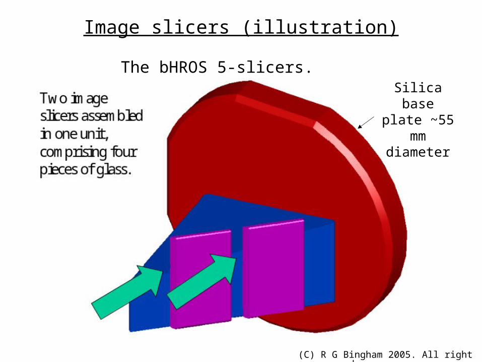
Image slicers (illustration)

Silica base plate ~55 mm

diameter

The bHROS 5-slicers.


Spherical Trigonometry - Advanced option

Note. I joined a project that had been running six months, only to find that no one had been using the correct 3D geometry in ZEMAX. As a result, nothing was quite right and no correct 3D layouts could be drawn. Spherical Trigonometry may seem a forbidding subject area to step into, but personally, I don’t expect to solve these problems in an hour or a morning. Even if it takes a few days to puzzle out the Spherical Trigonometry, it may be well worth the effort. Ten pages.


Great and small circles and spherical triangles

•Several ‘great circles’

•One ‘small circle’

•Spherical Triangles. Their angles add to more than 180 degrees. The sides of the triangles are great circles. They are also angles.

Notice the spherical triangles in which at least one of the angles is a right angle. These triangles are often needed and can be solved by Napier’s rules.


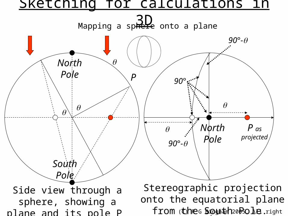
Sketching for calculations in 3D

North Pole

South Pole

Stereographic projection onto the equatorial plane from the South Pole.

P

P as projected

Mapping a sphere onto a plane

Side view through a sphere, showing a plane and its pole P

North Pole

90°-

90°

90°-


Good News about the Stereographic Projection

1. We never need to calculate the actual projection. It serves as a way of sketching diagrams of 3D objects.

2. Angles measured locally on the surface of the sphere are the same angle in the projection.

3. A circle drawn on the sphere appears as a circle in the projection.


Napier’s rules for a right-angled triangle (C=90º)

(C)

90-c90-B90-A

b a

C = 90º

b

Ac B

a

Arrange the symbols in five “parts” as shown on the right. Then

sin(middle part) = prod tan adjacent parts

= prod cos opposite parts

e.g. sin(90-c) = cos a cos b = tan(90-A) tan(90-B)

This is the one that we shall use

for the example


Napier’s rules for a quadrantal triangle (c=90º)

C

b

Ac = 90º B

a

(c)

C-9090-b90-a

B A

sin(middle part) = prod tan adjacent parts

= prod cos opposite parts


Other useful formulae for a right-angled spherical triangle:

sin a / sin A = sin b / sin B = sin c / sin C

cos a = cos b cos c + sin b sin c cos A

cos A = – cos B cos C + sin B sin C cos a

There are others but I have never needed them for optics.


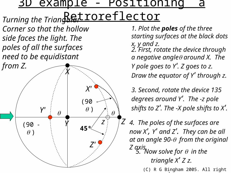
3D example - Positioning a Retroreflector

Use NSC object Triangular Corner – but we want the hollow side to face the light.


z

3D example - Positioning a Retroreflector

Y

X

Z

Turning the Triangular Corner so that the hollow side faces the light. The poles of all the surfaces need to be equidistant from Z.

1. Plot the poles of the three starting surfaces at the black dots x, y and z.

2. First, rotate the device through a negative angle around X. The Y

pole goes to Y'. Z goes to z. Draw the

equator of Y' through z.

Y'

3. Second, rotate the device 135

degrees around Y'. The -z pole shifts

to Z'. The -X pole shifts to X'.

Z'

X'

4. The poles of the surfaces are now

X', Y' and Z'. They can be all at an angle 90- from the original Z axis.

(90 - )

5. Now solve for in the triangle

X' Z z.

(90 - )

45º


Solving the right-angled triangle

z Z

X'

90-45º

a ( )

c (90- )

b (45º)

C

A

B

One of Napier’s rules for a right-angled triangle says:

cos c = cos a cos b (if C = 90 º)

So in this case:

sin = cos cos 45º , therefore:

tan = 1/2

= 35.2644 degrees

90 - = 54.7356 degrees

Re-draw it:


Result of positioning the retroreflector using theTriangular Corner

Ex05-RR1.ZMX

This example is developed for the advanced topic on Spherical Trigonometry.

(C) R G Bingham 2005. All rights reserved. Optics and Optical Design Richard G. Bingham Session 1 Introduction Coordinates Rays that may appear odd Image.

Documents

c r g bingham

bingham session

aberrations of optical

optical aberrations

optical capabilities

optical design richard

performance of optical

new systems