c 2013 Javad Ghaderi Dehkordi - Columbia Universityjghaderi/PhDThesis.pdfJAVAD GHADERI DEHKORDI DISSERTATION Submitted in partial ful llment of the requirements for the degree of Doctor

c© 2013 Javad Ghaderi Dehkordi

FUNDAMENTAL LIMITS OF RANDOM ACCESSIN WIRELESS NETWORKS

BY

JAVAD GHADERI DEHKORDI

DISSERTATION

Submitted in partial fulfillment of the requirementsfor the degree of Doctor of Philosophy in Electrical and Computer Engineering

in the Graduate College of theUniversity of Illinois at Urbana-Champaign, 2013

Urbana, Illinois

Doctoral Committee:

Professor Rayadurgam Srikant, ChairProfessor Bruce HajekAssistant Professor Angelia NedichProfessor Ness ShroffProfessor Pramod Viswanath

Abstract

Random access schemes are simple and inherently distributed, yet could

provide the striking capability to match the optimal throughput perfor-

mance (maximum stability region) of centralized scheduling mechanisms.

The throughput optimality however has been established for activation rules

that are relatively sluggish, and may yield excessive queues and delays. More

aggressive/persistent access schemes have the potential to improve the delay

performance, but it is not clear if they can offer any universal throughput

optimality guarantees. In this thesis, we identify a fundamental limit on

the aggressiveness of nodes, beyond which instability is bound to occur in a

broad class of networks.

We will mainly consider adapting transmission lengths by considering a

weight for each node as a function of its queue size. The larger the weight,

the longer the node will hold on to the channel once it starts a transmission.

We first show that it is sufficient for weights to behave as logarithmic func-

tions of the queue sizes, divided by an arbitrarily slowly increasing function.

This result indicates that the maximum-stability guarantees are preserved for

weights that are essentially logarithmic for all practical queue sizes, although

asymptotically the weight must grow slower than any logarithmic function

of the queue size. We then demonstrate instability for weights that grow

faster than logarithmic functions of queue sizes in networks with sufficiently

many nodes. Our stability and instability results hence imply that the “near-

logarithmic growth condition” on the weights is a fundamental limit on the

aggressiveness of nodes to ensure maximum stability in any general topol-

ogy. We will conduct simulation experiments to illustrate and validate the

analytical results. Finally, we will combine the random access scheme with

window-based flow control mechanisms to provide maximum throughput and

Quality-of-Service in multihop wireless networks with dynamic flows.

ii

Acknowledgments

First and foremost, I would like to thank my advisor Professor R. Srikant for

his support in the course of my PhD studies. Without his guidance, carrying

out this research would have been impossible. I will miss our numerous meet-

ings and discussions that shaped my ideas. I have been also very fortunate

to collaborate with Dr. Sem Borst and Dr. Phil Whiting at Alcatel-Lucent

Bell Labs. I am grateful to them for their insightful discussions and contri-

butions to my research. Part of this thesis was done during my internship at

Alcatel-Lucent Bell Labs where I was supervised by Sem and Phil. I would

like to thank the members of my doctoral committee, Professor Bruce Ha-

jek, Professor Angelia Nedich, Professor Ness Shroff, and Professor Pramod

Viswanath for their time and thoughtful comments. I express my deep ap-

preciation to the great teachers at the University of Illinois with impressive

teaching styles. My career path has been influenced by such teachers and I

can still feel their impact on my thinking and problem solving methodology.

My sincere thanks go to my parents for their support and dedication

through my life. There is no way that I can express my gratitude to them. I

am also really grateful to Majid, my brother, for his inspiration and guidance.

I would also like to thank my colleagues at the Coordinated Science Lab

(CSL) for their support and friendship. They provided an excellent environ-

ment for me during my studies at the University of Illinois.

I would like to thank the University of Illinois, Alcatel-Lucent, the US

National Science Foundation, Army Research Office, and the Air Force Office

of Scientific Research for their financial support.

iii

Table of Contents

Chapter 1 Introduction . . . . . . . . . . . . . . . . . . . . . . . . . . 1

Chapter 2 System Model and Description of Random Access Mechanism 62.1 System model . . . . . . . . . . . . . . . . . . . . . . . . . . . 62.2 Description of random access mechanism . . . . . . . . . . . . 7

Chapter 3 Stability of Random Access for Tame Weight Functions . . 113.1 Statement of stability result . . . . . . . . . . . . . . . . . . . 113.2 Proof of stability result . . . . . . . . . . . . . . . . . . . . . . 123.3 Simulation experiments . . . . . . . . . . . . . . . . . . . . . . 233.4 Conclusions . . . . . . . . . . . . . . . . . . . . . . . . . . . . 273.5 Additional proofs . . . . . . . . . . . . . . . . . . . . . . . . . 28

Chapter 4 Instability of Random Access for Aggressive WeightFunctions . . . . . . . . . . . . . . . . . . . . . . . . . . . . . . . . 364.1 Qualitative discussion of fluid limits . . . . . . . . . . . . . . . 384.2 Fluid limits for broken-diamond network . . . . . . . . . . . . 454.3 Instability results for broken-diamond network . . . . . . . . . 564.4 Simulation experiments . . . . . . . . . . . . . . . . . . . . . . 694.5 Instability in general interference graphs . . . . . . . . . . . . 704.6 Instability for de-activation functions with polynomial decay . 724.7 Conclusions . . . . . . . . . . . . . . . . . . . . . . . . . . . . 744.8 Additional proofs . . . . . . . . . . . . . . . . . . . . . . . . . 75

Chapter 5 Stability for Multihop Networks with Dynamic Flows . . . 1105.1 From single-hop to multihop . . . . . . . . . . . . . . . . . . . 1125.2 Network control policy . . . . . . . . . . . . . . . . . . . . . . 1135.3 System stability . . . . . . . . . . . . . . . . . . . . . . . . . . 1165.4 Distributed implementation . . . . . . . . . . . . . . . . . . . 1255.5 Conclusions . . . . . . . . . . . . . . . . . . . . . . . . . . . . 1365.6 Additional proofs . . . . . . . . . . . . . . . . . . . . . . . . . 137

Chapter 6 Conclusions and Open Problems . . . . . . . . . . . . . . . 144

References . . . . . . . . . . . . . . . . . . . . . . . . . . . . . . . . . . 146

iv

Chapter 1

Introduction

Scheduling in wireless networks is of fundamental importance due to the in-

herent broadcast nature of the wireless medium. Two radios that are close

to each other might not be able to transmit simultaneously, as they can in-

terfere with each other. In other words, the simultaneous transmissions of

such radios may cause the Signal-to-Noise-plus-Interference-Ratio (SINR) at

their corresponding receivers to go below the required threshold for success-

ful decoding of data packets. Therefore, in order to operate wireless systems

efficiently, scheduling algorithms are needed to facilitate simultaneous trans-

missions of different radios.

The metrics used to evaluate the performance of a scheduling algorithm

are throughput and delay. Throughput is characterized by the largest set of

service rates that can be provided to the radio nodes. Delay is characterized

by the average time that packets spend in the network’s buffers, once they en-

ter the network until they reach their destinations. It is also essential for the

scheduling algorithm to be distributed and to have low complexity/overhead.

This is because in many wireless networks there is no centralized entity and

the resources at the nodes are very limited.

Scheduling algorithms for wireless networks have been widely studied since

Tassiulas and Ephremides [1] proposed the Max Weight Scheduling (MWS)

algorithm. MWS algorithm assigns a weight to each link as a function of the

number of packets queued at the link, and then, at each instant of time, se-

lects the schedule with the maximum weight, where the weight of a schedule

is computed by summing the weights of the links that the schedule will serve.

Tassiulas and Ephremides establish that the MWS algorithm is throughput

optimal in the sense that it can stabilize the queues of the network for the

largest set of arrival rates possible, without actually knowing the arrival rates.

However, finding the maximum weight schedule is a complex combinatorial

problem, and hence, the MWS algorithm is not typically implementable in

1

practice. This has led to a rich amount of literature on the design of ap-

proximate algorithms to alleviate the computational complexity of the MWS

algorithm.

A popular mechanism for distributed scheduling is provided by the so-

called Carrier Sense Multiple Access (CSMA) protocol. In the CSMA proto-

col, each node attempts to access the medium after a certain back-off time,

but nodes that sense activity of interfering nodes freeze their back-off timer

until the medium is sensed idle. Due to their simplicity of implementation,

CSMA schemes have been widely used in practice, e.g., in WLANs (IEEE

802.11 Wi-Fi) or emerging wireless mesh networks. From a local perspective,

the CSMA algorithm might seem easy to understand, but, at a global per-

spective, interactions among different nodes can lead to a very complicated

behavior that makes the performance characterization difficult.

In recent years, fairly simple models have been proposed that are useful in

predicting the throughput of the CSMA algorithm [2, 3, 4, 5, 6]. Although the

representation of the IEEE 802.11 back-off mechanism in these models is less

detailed than in [7], they accommodate a general interference graph and thus

cover a broad range of topologies. Experimental results in [8] demonstrate

that these models, while idealized, provide throughput estimates that match

remarkably well with measurements in actual systems.

Despite their asynchronous and distributed nature, CSMA-like algorithms

have been shown to offer the remarkable capability of achieving the full ca-

pacity region and thus match the optimal throughput performance of cen-

tralized scheduling mechanisms operating in slotted time [9, 10, 11]. More

specifically, any throughput vector in the interior of the convex hull associ-

ated with the independent sets in the underlying interference graph can be

achieved through suitable back-off rates and/or transmission lengths. Based

on this observation, various ingenious algorithms have been developed for

finding the back-off rates that yield a particular target throughput vector or

that optimize a certain concave throughput utility function in scenarios with

saturated buffers [9, 11, 12]. In particular, Jiang and Walrand [11] develop an

algorithm that adaptively chooses the back-off rates under a time-scale sep-

aration assumption, i.e., the CSMA dynamics converges to its equilibrium

instantaneously compared to the time-scale of adaptation of the back-off

rates. This time-scale separation assumption was later verified by a stochas-

tic approximation type argument [9, 10]. In the same spirit, several effective

2

approaches have been devised for adapting the transmission lengths based on

queue-length information, and been shown to guarantee maximum stability

[13, 14, 15, 16].

Roughly speaking, the maximum-stability guarantees were established un-

der the condition that the various nodes are relatively sluggish in attempting

to access the channel or in continuing transmission once they obtain the

channel. In particular, a very exciting work by Rajagopalan, Shah, and Shin

[13] demonstrates the maximum stability under the condition that the mean

transmission length is chosen to be a logarithmic function of the queue length.

In the language of [13], each link has a weight of the form log log(Q) (Q is

the queue length) that the link uses to determine its transmission length.1

Unfortunately, such activation rules can induce excessive queue lengths and

delays, as the resulting scheduling algorithm reacts very slowly to changes

in queue lengths. This issue has triggered a strong interest in developing

approaches for improving the delay performance [17, 18, 19, 20, 21, 22] and

has also provided the motivation of this thesis. More aggressive/persistent

access schemes have the potential to improve the delay performance, but it

is not clear if they can offer any universal maximum-stability guarantees.

In this thesis, we explore the scope for using more aggressive activation

rules (more aggressive weights) in order to improve the delay performance

while preserving the maximum-stability guarantees. To this end, we will

analyze stability and instability of the network under the random access

mechanism with different activation rules.

In Chapter 3, we first tighten the condition required for CSMA-like al-

gorithms to achieve maximum throughput (maximum stability region). We

show that it is in fact sufficient for weights to be logarithmic functions of

the queue lengths, divided by an arbitrarily slowly increasing, unbounded

function. For example, weights of the form log1−εQ, with ε > 0 arbitrary

small, are sufficient to ensure maximum throughput in any general network

topology. This result indicates that the maximum-throughput guarantees are

preserved for weight functions that are essentially logarithmic for all prac-

tical queue lengths, although asymptotically weights must grow slower than

any logarithmic function of the queue length.

Since the “near-logarithmic growth condition” is only a sufficient condition,

1In this thesis, all logarithms are in base e.

3

it is not clear to what extent it is actually a strict requirement for maximum

stability to be maintained. In Chapter 4, we will consider the fluid limits of

the system where dynamics are scaled in both space and time. For weights

which grow slower than any logarithmic function of queue lengths, “fast mix-

ing” is guaranteed in any general topology, where the activity process evolves

on a much faster time scale than the scaled queue lengths. Qualitatively simi-

lar fluid limits can arise for more aggressive weight functions as well, provided

the topology is benign. However, aggressive weight functions can cause “slug-

gish mixing,” where the activity process evolves on a much slower time scale

than the scaled queue lengths, yielding random oscillatory fluid limits. Such

fluid limits can force the system into inefficient states for extended periods

of time and produce instability. We will demonstrate instability for weights

that grow faster than γ logQ (Q is the queue length), for any γ > 1, but

our proof arguments suggest that it can occur for any γ > 0, in networks

with sufficiently many nodes. In other words, “the near-logarithmic growth

condition” on the weights is a fundamental limit on the aggressiveness of

nodes to ensure maximum stability (throughput optimality) in any general

topology.

In Chapter 5, we will investigate the stability of the system when flows/users

randomly arrive and depart. To achieve flow-level stability, prior works

[23, 24, 25] require that a specific form of congestion control based on α-fair

utility functions has to be used, namely the rate at which a flow generates

packets into its ingress queue must maximize an α-fair utility subject to a

linear penalty (price). We will show that α-fair congestion control is not

necessary for flow-level stability, and, in fact, very general congestion control

mechanisms are sufficient to ensure flow-level stability. In establishing this

result, we will use link weights which are log-differentials of queue lengths,

i.e., the weight of link (i, j) is roughly in the form of log(1+Qi)− log(1+Qj),

with Qi and Qj the queue lengths of nodes i and j. The use of such weights

naturally suggests the use of a random access mechanism, as in Chapter 3, to

implement the algorithm in a distributed fashion. We will indeed show that

the maximum-stability result of the random access mechanism can be eas-

ily extended to multihop flows with log-differential weights and very general

congestion control mechanisms.

Our stochastic model in this thesis considers the dynamics of flows, pack-

ets, and random access simultaneously, with no time-scale separation as-

4

sumptions among the dynamics.

The remainder of this thesis is organized as follows. In Chapter 2, we

introduce our model for wireless networks and describe the random access

mechanism in its most general form. Chapter 3 is devoted to the stability

result for near-logarithmic weight functions. In Chapter 4, we will demon-

strate instability of the system for weight functions which grow faster than

the near-logarithmic functions. In Chapter 5, we will investigate stability

of the system with flow arrivals and departures. In each chapter, we will

conduct simulation experiments to verify our analytical results.

5

Chapter 2

System Model and Description of RandomAccess Mechanism

2.1 System model

For now, we consider a singlehop communication model, i.e., each source is

directly connected to its destination via a wireless link. In Chapter 5, we will

show how to extend the results to the multihop scenario.

Suppose the total number of source-destination pairs (wireless links) is N .

We use the notion of the conflict graph G(V,E) to represent the interfer-

ence/operating constraints. Each node of the conflict graph is a communica-

tion link in the wireless network and there is an edge (l, k) ∈ E between nodes

l and k if simultaneous transmissions over communication links l and k cannot

be successful. Therefore, at each time instant, the active links should form

an independent set of G, i.e., no two scheduled nodes can share an edge in G.

Formally, a schedule can be represented by a vector X = [xs : s = 1, ..., N ]

such that xs ∈ 0, 1 and xi + xj ≤ 1 for all (i, j) ∈ E. We useM to denote

the set of all feasible schedules.

Packets arrive at link l according to some stochastic process with rate

λ = [λl; l = 1, . . . , N ]. To be specific, assume packets arrive according to the

Poisson process for the continuous-time system and the Bernoulli process

for the discrete-time system. Each link l is associated with a queue Ql(t),

representing the number of packets of link l waiting for transmission at time

t. The vector of queue lengths at each time t is denoted by Q(t) = [Ql(t) :

l = 1, ..., N ].

A scheduling algorithm is a policy to determine which schedule to be used

in each time instant; correspondingly, which links can transmit a packet in

each time instant. The capacity region of the network is defined to be the

largest set of arrival rates that can be supported by the network, i.e., for

which there exists a scheduling algorithm that can stabilize the queues. It is

6

known, e.g. [1], that the capacity region is given by

Λ = λ ≥ 0 : ∃µ ∈ Co(M), λ < µ, (2.1)

where Co(·) is the convex hull operator. When dealing with vectors, inequal-

ities are interpreted component-wise.

A scheduling algorithm is throughput-optimal if it can stabilize the network

for any arrival rate in Λ. An important class of the throughput-optimal

algorithms are the Max Weight Scheduling (MWS) algorithms where at any

time t, the scheduling decision X(t) satisfies

X(t) = arg maxX∈M

N∑l=1

xlwl(t),

where wl(t) is the weight of link l at time t. In [1], it was proved that the MWS

algorithm is throughput-optimal for wl(t) = Ql(t). A natural generalization

of the MWS algorithm in [26] uses a weight f(Ql) instead of Ql with the

following properties:

1. f : [0,∞]→ [0,∞] is a nondecreasing continuous function with

limx→∞

f(x) =∞.

2. Given any M1,M2 > 0, and 0 < ε < 1, there must exist a Q <∞ such

that for x > Q:

(1− ε)f(x) ≤ f(x−M1) ≤ f(x+M2) ≤ (1 + ε)f(x).

The following lemma is fairly easy to prove [27] and thus its proof is omitted.

Lemma 2.1. Suppose f is a strictly concave and increasing function, with

f(0) = 0, then it satisfies the conditions (1) and (2) above.

2.2 Description of random access mechanism

The various nodes in the conflict graph share the medium in accordance

with a random access mechanism. The random access mechanism in its most

general form can be described as follows.

7

Consider the conflict graph G(V,E) of the network. Denote the neighbors

of i by a set C(i) = k ∈ V : (i, k) ∈ E. When a node ends an activity

period (consisting of possibly several back-to-back packet transmissions), it

starts a back-off period. At the end of the back-off period at time t, the

node can start a new packet transmission only if none of its neighbors are

active, with probability pi(Qi(t)), pi(0) = 0, and begins a next back-off

period otherwise. When a transmission of node i ends at time t, it releases

the medium and begins a back-off period with probability ψi(Qi(t−)), or

starts the next transmission otherwise, with ψi(1) = 1. For conciseness, the

probabilities pi(·) and ψi(·) will be referred to as activation and de-activation

probabilities, respectively.

The mechanism can be implemented in continuous-time or discrete-time,

as we explain in Sections 2.2.1 and 2.2.2.

2.2.1 Continuous-time system

For simplicity, we assume packet arrivals are independent Poisson processes

with rate λ = [λi; i = 1, . . . , N ]. The packet sizes of node i are exponentially

distributed with mean 1/µi. Let ρi := λi/µi.

In continuous-time mechanism, the back-off times of node i are indepen-

dent and exponentially distributed with mean 1/νi. Equivalently, node i

may be thought of as activating at an exponential rate ri(Qi(t)), with ri(·) =

νipi(·),1 whenever it senses the channel idle at time t, and de-activating at

rate ri(Qi(t)), with ri(·) = µiψi(·), whenever it is active at time t.

There are two special cases worth mentioning that correspond to continuous-

time random access schemes considered in the literature before. First, in case

pi(Qi) = 1 and ψi(Qi) = 0 for all Qi ≥ 1, node i starts a transmission each

time a back-off period ends and its neighbors are silent, and does not re-

lease the medium until its entire queue has been cleared. This corresponds

to the random-capture scheme considered in [28]. In case µi = 1, νi = 1,

pi(Qi) = 1−ψi(Qi), and ψi(Qi) = 1/(1+exp(wi(Qi))), node i may be thought

1It is in general possible to consider νi to be also queue dependent, however, in realitythe back-off period cannot be made arbitrarily small so the mentioned version seems morepractical.

8

of as becoming (or continuing to be) active with probability

pi(Qi(t)) =exp(wi(Qi(t)))

1 + exp(wi(Qi(t))), (2.2)

each time a unit-rate Poisson clock ticks and its neighbors are silent. This

roughly corresponds to the scheme considered in [27, 16, 13, 14, 15] based on

Glauber dynamics with a “weight” function wi(Qi). The weight of node i is

chosen to be

wi(Qi(t)) = max(f(Qi(t)),

ε

2Nf(Qmax(t))

), (2.3)

where Qmax(t) is the length of the largest queue in the network at time t

which is assumed to be known. The function f is a strictly concave and

monotonically increasing function, with f(0) = 0, as in Lemma 2.1.

2.2.2 Discrete-time system

Time is slotted and packets arrive at each node according to a discrete-time

process. Let Ai(t) be the number of packets arriving at node i in time slot

t. For simplicity, assume that Ai(t)∞t=0, for i = 1, . . . , N , are independent

Bernoulli processes with parameter λ = [λl; l = 1, . . . , N ]. In each time slot,

one packet could be successfully transmitted over a link.

2.2.3 Discrete-time mechanism with one-node update

Consider an activation probability pi(t) ≡ pi(Qi(t)) for node i at time slot t

as in (2.2) with weight w as in (2.3).

At each time slot t, a node i is chosen uniformly at random, with proba-

bility 1N

, then

(i) If all the neighbors of i are silent, i.e., xj(t − 1) = 0 for all j ∈ C(i),

then xi(t) = 1 with probability pi(t), and xi(t) = 0 with probability

pi(t) = 1− pi(t). Otherwise, xi(t) = 0.

(ii) xj(t) = xj(t− 1) for all j 6= i.

9

2.2.4 Discrete-time mechanism with multi-node update

The previous mechanism is based on Glauber-dynamics with one node up-

date at each time. For distributed implementation, we need a randomized

mechanism to select a node uniformly at each time slot. We use the Q-CSMA

idea [20] to perform the link selection as follows. Each time slot is divided

into a control slot and a data slot. In the control slot, each node i that

wishes to transmit data transmits a short message called INTENT message

with some probability ai. Those nodes that transmit INTENT messages and

do not hear any INTENT messages from the neighboring nodes constitute a

decision schedule. In the data slot, each node i that is included in the deci-

sion schedule can transmit a data packet with probability pi(t), as in (2.2),

only if none of its neighbors has been transmitting in the previous data slot

(see the description of the algorithm below).

(i) In the control slot, randomly select a decision schedule m(t) ⊆ M by

using access probabilities aiNi=1.

(ii) ∀ i in m(t):

If no links in C(i) were active in the previous data slot, i.e.,∑

j∈C(i) xj(t−1) = 0:

– xi(t) = 1 with probability pi(t).

– xi(t) = 0 with probability pi(t) = 1− pi(t).

Else xi(t) = 0.

∀i /∈ m(t): xi(t) = xi(t− 1).

(iii) In the data slot, use X(t) as the transmission schedule.

10

Chapter 3

Stability of Random Access for Tame WeightFunctions

Consider the continuous-time/discrete-time random access mechanism, de-

scribed in Chapter 2, based on activation probability (2.2) and weight (2.3).

We are interested to determine under what conditions the system is stable,

i.e., the process (X(t), Q(t))t≥0 is positive-recurrent, for all arrival rates λ

in the capacity region Λ.

3.1 Statement of stability result

The following theorem states the main result regarding the throughput op-

timality of such random access mechanisms.

Theorem 3.1. Consider any ε > 0. The random access mechanism can

stabilize the network for any λ ∈ (1− ε)Λ, if the weight function is chosen to

be in the form of f(x) = log(1+x)g(x)

. The function g(x) is a strictly increasing

function chosen such that f is a strictly concave increasing function. In

particular, the algorithm with the following weight functions is throughput-

optimal: f(x) = log(1+x)log(e+log(1+x))

or f(x) = log1−θ(1+x) for any arbitrary small

θ > 0.

To determine the weight at each node i, Qmax(t) is needed. Instead, each

node i can maintain an estimate of it. We can use a gossip procedure, as

suggested in [13], to estimate Qmax(t), and use Lemma 2 of [13] to complete

the stability proof. So we do not pursue this issue here. In practical networksε

2Nlog(1 +Qmax) is small and we can use the weight function f directly, and

thus, there may not be any need to know Qmax(t).

Corollary 3.1. Under the weight function f specified in Theorem 5.2, the

discrete-time mechanism with multi-node update can stabilize the network for

any λ ∈ (1− ε)Λ.

11

3.2 Proof of stability result

We present the proof for the discrete-time model. The proof of the continuous-

time model follows similarly. The queue dynamics for each link l is given by

Ql(t) = (Ql(t− 1)− xl(t))+ + Al(t),

for t ≥ 0 and l = 1, ..., N where (·)+ = max·, 0. For notational convenience,

we define

wi(t) = f(Qi(t)),

wmin(t) =ε

2Nf(Qmax(t)).

Before we start the proof, some preliminaries, regarding stationary distribu-

tion and mixing time of Glauber dynamics, are needed.

3.2.1 Preliminaries

Consider a time-homogeneous discrete-time Markov chain over the finite state

space M. For simplicity, we index the elements of M by 1, 2, ..., r, where

r = |M|. Assume the Markov chain is irreducible and aperiodic, so that a

unique stationary distribution π = [π(1), ..., π(r)] always exists, with π(i) > 0

for all 1 ≤ i ≤ r.

Distance between probability distributions

First, we introduce two convenient norms on Rr that are linked to the sta-

tionary distribution. Let `2(π) be the real vector space Rr endowed with the

scalar product

〈z, y〉π =r∑i=1

z(i)y(i)π(i).

Then, the norm of z with respect to π is defined as

‖z‖π =

(r∑i=1

z(i)2π(i)

)1/2

.

12

We shall also use `2( 1π), the real vector space Rr endowed with the scalar

product

〈z, y〉 1π

=r∑i=1

z(i)y(i)1

π(i),

and its corresponding norm. For any two strictly positive probability vectors

µ and π, the following relationship holds

‖µ− π‖ 1π

= ‖µπ− 1‖π ≥ 2‖µ− π‖TV ,

where ‖π − µ‖TV is the total variation distance

‖π − µ‖TV =1

2

r∑i=1

|π(i)− µ(i)|.

Glauber dynamics

Consider a graph G(V,E). Glauber dynamics is a Markov chain to generate

the independent sets of G. So, the state spaceM consists of all independent

sets of G. Let |V | = N . Given a weight vector W = [w1, w2, ..., wN ], at each

time t, a node i is chosen uniformly at random, with probability 1N

, then

(i) If xj(t− 1) = 0 for all nodes j ∈ N (i), then xi(t) = 1 with probabilityexp(wi)

1+exp(wi), or xi(t) = 0 with probability 1

1+exp(wi).

Otherwise, xi(t) = 0.

(ii) xj(t) = xj(t− 1) for all j 6= i.

The corresponding Markov chain is irreducible, aperiodic, and reversible over

M, and its stationary distribution is given by

π(X) =1

Zexp

(∑i∈X

wi

); X ∈M, (3.1)

where Z is the normalizing constant (It is easy to check that (3.1) indeed

satisfies the detailed balance equations and thus is the stationary distribu-

tion).

The random access mechanism with one-node update uses a time-varying

version of the above Glauber dynamics, where the weights change with time.

13

This yields a time-inhomogeneous Markov chain but we will see that, for the

proper choice of weights, it behaves similarly to the Glauber dynamics.

Mixing time of Glauber dynamics

The convergence to steady state distribution is geometric with a rate equal to

the second largest eigenvalue modulus (SLEM) of the transition probability

matrix as it is described next (see e.g. Chapter 6 of [29]).

Lemma 3.1. Let P be an irreducible, aperiodic, and reversible transition

matrix on the finite state space M with the stationary distribution π. Then,

the eigenvalues of P are ordered in such a way that

λ1 = 1 > λ2 ≥ ... ≥ λr > −1,

and for any initial probability distribution µ0 on M, and for all n ≥ 1

‖µ0Pn − π‖ 1

π≤ σn‖µ0 − π‖ 1

π, (3.2)

where σ = maxλ2, |λr| is the SLEM of P.

The following Lemma gives an upper bound on the SLEM σ(P ) of Glauber

dynamics.

Lemma 3.2. For the Glauber dynamics with the weight vector W on a graph

G(V,E) with |V | = N ,

σ ≤ 1− 1

16N exp(4Nwmax),

where wmax = maxi∈V wi.

The proof is provided at the end of the chapter. We define the mixing time

as T = 11−σ , so

T ≤ 16N exp(4Nwmax). (3.3)

Simple calculation, based on Lemma 3.1, reveals that the amount of time

needed to get close to the stationary distribution is proportional to T .

14

3.2.2 A key lemma

At any time slot t, given the weight vector W (t) = [w1(t), ..., wN(t)], the

MWS algorithm should solve

maxX∈M

∑i∈X

wi(t),

instead, our algorithm tries to simulate a distribution

πt(X) =1

Zexp(

∑i∈X

wi(t)); X ∈M, (3.4)

i.e., the stationary distribution of Glauber dynamics with the weight vector

W (t) at time t.

Let Pt denote the transition probability matrix of Glauber dynamics with

the weight vector W (t). Also let µt be the true probability distribution of the

inhomogeneous-time chain, over the set of schedulesM, at time t. Therefore,

we have µt = µt−1Pt. Let πt denote the stationary distribution of the time-

homogeneous Markov chain with P = Pt as in (3.1). By choosing proper

wmin and f(.), we aim to ensure that µt and πt are close enough, i.e.,

‖πt − µt‖TV ≤ δ/4

for some δ arbitrary small.

Let wmax(t) = f(Qmax(t)). The following lemma gives a sufficient condi-

tion under which the probability distribution of the inhomogeneous Markov

chain is close to the stationary distribution of the homogeneous chain.

Lemma 3.3. Given any δ > 0, ‖πt − µt‖TV ≤ δ4

holds for all t ≥ t∗, if

αtTt+1 ≤ δ/16 for all t > 0, (3.5)

where

(i) αt = 2Nf ′(f−1(wmin(t+ 1))− 1),

(ii) t∗ is the smallest t such that

t∑k=1

1

T 2k

≥ ln(4/δ) +N(wmax(0) + log 2)/2, (3.6)

15

and Tk is the mixing time of the Glauber dynamics with the weight vector

W (k).

The proof of Lemma 3.3 is provided at the end of the chapter. Lemma 3.3

states a condition under which ‖πt − µt‖TV ≤ δ4

for all t ≥ t∗. The key idea

in the proof is that, for αt small, the weights change at the rate αt while the

system responds to these changes at the rate 1/Tt+1. Condition (3.5) is to

ensure that the weight dynamics are slow enough compared to response time

of the chain such that the chain remains close to its equilibrium (stationary

distribution). Now assume that (3.5) holds only when ‖Q(t)‖ ≥ Qth1 for a

constant Qth > 0. Let t1 be the first time that ‖Q(t)‖ hits Qth. Then, after

that, it takes t∗ time slots for the chain to get close to πt if ‖Q(t)‖ remains

above Qth for t1 ≤ t ≤ t1 + t∗. Alternatively, we can say that ‖πt−µt‖TV ≤ δ4

if ‖Q(t)‖ ≥ Qth+t∗ since at each time slot at most one departure can happen

and this guarantees that ‖Q(t)‖ ≥ Qth for, at least, the past t∗ time slots.

This immediately implies the following Lemma that we will use in the proof

of the main result.

Lemma 3.4. Given any δ > 0, ‖πt−µt‖TV ≤ δ4

holds when ‖Q(t)‖ ≥ Qth+t∗,

if there exists a Qth such that

αtTt+1 ≤ δ/16 whenever ‖Q(t)‖ > Qth, (3.7)

where

(i) αt = 2Nf ′(f−1(wmin(t+ 1))− 1)

(ii) Tt ≤ 16N exp(4Nwmax(t))

(iii) t∗ is the smallest t such that

t1+t∗∑k=t1:‖Q(t1)‖=Qth

1

T 2k

≥ ln(4/δ) +N(f(Qth) + log 2)/2. (3.8)

In Lemma 3.4, condition (ii) is based on the upper bound of (3.3) and the

fact that wmax(t) = wmax(t).

1In this section, ‖y‖ = ‖y‖∞ = maxi yi(t) = ymax.

16

In other words, Lemma 3.4 states that when queue lengths are large, the

observed distribution of the schedules is close to the desired stationary dis-

tribution.

Remark 3.1. We will later see that, to satisfy condition (3.7) and to find

a finite t∗ satisfying (3.8) in Lemma 3.4, the function f(.) cannot be faster

than log(.). In fact, the function f must be slightly slower than log(.) to

ensure a finite t∗ always exists.

Remark 3.2. The above Lemma is a generalization of Lemma 12 (Network

Adiabatic Theorem) of [13]. Here we consider general functions f(.), whereas

[13] considers a particular function log log(.). The generalization allows us to

use functions which are close to log(.) and perform much better than log log(.)

in simulations. The proof of Lemma 3.3 is presented in Section 3.5.

3.2.3 Throughput optimality

We will use the following Lemma [26] to prove the throughput-optimality of

the algorithm.

Lemma 3.5. For a scheduling algorithm, if given any 0 < ε < 1 and 0 <

δ < 1, there exists a B(δ, ε) > 0 such that: in any time slot t, with probability

larger than 1−δ, the scheduling algorithm chooses a schedule X(t) ∈M that

satisfies ∑i∈X(t)

wi(t) ≥ (1− ε) maxY ∈M

∑i∈Y

wi(t)

whenever ‖Q(t)‖ > B(δ, ε), then the scheduling algorithm is throughput-

optimal.

Remark 3.3. Throughput optimality in Lemma 3.5 means that, for all the

rates inside the capacity region, system will be stable in the mean (see [26]

for more details), i.e.,

lim supT→∞

1

T

T−1∑t=0

E

( N∑i=1

f 2(Qi(t))

) 12

<∞. (3.9)

In our setting, the queuing system is an irreducible and aperiodic Markov

chain, and therefore stability-in-the mean property (3.9) implies that the

Markov chain is also positive recurrent [30] .

17

Let w∗(t) = maxX∈M∑

i∈X wi(t). Let us define the following set:

χt = Y ∈M :∑i∈Y

wi(t) < (1− ε)w∗(t).

Therefore, we need to show that

µt(χt) =∑Y ∈χt

µt(Y ) ≤ δ,

for ‖Q(t)‖ large enough. Suppose f(.) and wmin are chosen such that αtTt+1 ≤δ/16 whenever ‖Q(t)‖ > Qth for some constant Qth > 0 to be determined

later. Then, it follows from Lemma 3.4 that whenever ‖Q(t)‖ > Qth + t∗,

2‖µt − πt‖TV ≤ δ/2,

and consequently, ∑Y ∈M

|µt(Y )− πt(Y )| ≤ δ/2.

Thus,

|∑Y ∈χt

(µt(Y )− πt(Y ))| ≤∑Y ∈χt

|µt(Y )− πt(Y )|

≤ δ/2,

which yields ∑Y ∈χt

µt(Y ) ≤∑Y ∈χt

πt(Y ) + δ/2.

Therefore, to ensure that∑

Y ∈χt µt(Y ) ≤ δ, it suffices to have∑Y ∈χt

πt(Y ) ≤ δ/2.

But ∑Y ∈χt

πt(Y ) =∑Y ∈χt

1

Ztexp(

∑i∈Y

wi(t)),

where

wi(t) = maxwi(t), wmin(t) ≤ wi(t) + wmin(t).

18

So ∑Y ∈χt

πt(Y ) ≤∑Y ∈χt

1

Ztexp(

∑i∈Y

(wi(t) + wmin(t)))

=∑Y ∈χt

1

Ztexp(

∑i∈Y

wi(t)) exp(|Y |wmin(t))

≤∑Y ∈χt

1

Ztexp((1− ε)w∗(t)) exp(Nwmin(t)),

and

Zt =∑Y ∈M

exp(∑i∈Y

wi(t)) >∑Y ∈M

exp(∑i∈Y

wi(t)) > ew∗(t).

Therefore, ∑Y ∈χt

πt(Y ) ≤ 2N exp(Nwmin(t)− εw∗(t)),

and w∗(t) ≥ wmax(t). So, it suffices to have

2N exp(Nwmin(t)− εwmax(t)) ≤ δ/2,

when ‖Q(t)‖ > Qth + t∗. The choice of wmin(t) = ε2Nwmax(t), satisfies the

above condition for ‖Q(t)‖ > B, where

B = max

Qth + t∗, f−1

(N log 2 + log 2

δ

ε/2

). (3.10)

3.2.4 A class of weight functions with the maximumthroughput property

In this section, we describe a family of weight functions f that yield maximum

throughput.

The function f needs to satisfy Lemma 3.4. Roughly speaking, since the

mixing time T is exponential in wmax, f′(f−1(wmin)) must be in the form

of e−wmin ; otherwise it will be impossible to satisfy αtTt+1 < δ/16 for any

arbitrarily small δ as ‖Q(t)‖ → ∞. The only function with such a property

is the log(.) function. In fact, it turns out that f must grow slightly slower

than log(.) as we show next to satisfy (3.7), and to ensure the existence of a

19

finite t∗ in Lemma 3.4.

Consider weight functions of the form f(x) = log(1+x)g(x)

where g(x) is a

strictly increasing function, chosen such that f satisfies the conditions of

Lemma 2.1. For example, by choosing functions that grow much slower

than log(1 + x), like g(x) = log(e + log(1 + x)), we can make f(x) behave

approximately like log(1 + x) for large ranges of x.

Assume g(0) ≥ 1, then

f ′(x) ≤ 1

1 + x. (3.11)

The inverse of f cannot be expressed explicitly, however, it can be written

as

f−1(x) = exp(xg(f−1(x)))− 1. (3.12)

Therefore,

f ′(f−1(wmin)− 1) ≤ 1

f−1(wmin)(3.13)

=1

exp(wming(f−1(wmin)))− 1. (3.14)

Using (3.14), the conditions of Lemma 3.4 are satisfied if there exists a Qth

large enough such that

2N16N exp(4Nwmax)1

exp(wming(f−1(wmin)))− 1≤ δ/16, (3.15)

for ‖Q(t)‖ ≥ Qth.

Using (3.12) and noting that wmin = ε2Nwmax, (3.15) can be written as

2N16N exp

(wmin

[8N2

ε− g(f−1(wmin))

])(1 +

1

f−1(wmin)

)≤ δ/16.

(3.16)

Consider fixed, but arbitrary, N and ε. As Qmax → ∞, wmax → ∞, and

consequently wmin → ∞ and f−1(wmin) → ∞. Therefore, the exponent8N2

ε− g(f−1(wmin)) is negative for Qmax large enough, and thus, there is a

threshold Qth such that for all Qmax > Qth, the condition (3.16) is satisfied.

To be more accurate, it suffices to choose

Qth = f−1

(2N

ε×max

log(

64N16N

δ), f(g−1(

16N2

ε))

). (3.17)

20

Then, it follows from Lemma 3.4 that ‖πt − µt‖TV ≤ δ4, whenever ‖Q(t)‖ >

Qth + t∗.

Remark 3.4. The assumption g(0) ≥ 1 is not required, since, as we saw

in the above analysis, only the asymptotic behavior of g is important. If we

choose Qth large enough such that

g(f−1(wmin(t))− 1) ≥ 1, (3.18)

when ‖Q(t)‖ ≥ Qth, then (3.13) holds and the rest of the analysis follows

exactly. In particular, in order to get an explicit formula for f−1, we can

choose g(x) = log(1 + x)θ for some 0 < θ < 1. The weight function for such

a g is f(x) = (log(1 + x))1−θ, and f−1 has the closed form

f−1(x) = exp(x1

1−θ )− 1.

Then (3.17) yields

Qth = exp

(max

2N

εlog(

64N16N

δ),

2N

ε(16N2

ε)1θ

11−θ). (3.19)

It is easy to check that for Q(t) ≥ exp(

(2Nε

)1

1−θ log(1 + e))

, wmin(t) ≥ f(e)

which satisfies (3.18). Therefore, obviously, (3.18) also holds for Qth of

(3.19).

The last step of the proof is to determine the constant B in (3.10), so we

need to find t∗. Let t1 be the first time that Qmax(t) hits Qth, then

t1+t∑k=t1

1

T 2k

≥ 16−2N

t1+t∑k=t1

e−8Nf(Qmax(k))

= 16−2N

t1+t∑k=t1

e−8Nlog(1+Qmax(k))g(Qmax(k))

= 16−2N

t1+t∑k=t1

(1 +Qmax(k))−8N

g(Qmax(k))

≥ 16−2N

t∑k=1

(1 +Qth + k)− 8Ng(Qth)

≥ 16−2N t(1 +Qth + t)− 8Ng(Qth) .

21

Therefore, by Lemma 3.4, it suffices to find the smallest t that satisfies

16−2N t(1 +Qth + t)− 8Ng(Qth) ≥ log(4/δ) +

N

2log(2(1 +Qth)),

for a threshold Qth large enough satisfying (3.17). Recall that g(.) is an

increasing function, therefore, by choosing Qth large enough, 8Ng(Qth)

can be

made arbitrary small. Then a finite t∗ always exists since

limt∗→∞

t∗(1 +Qth + t∗)− 8Ng(Qth) =∞.

In particular, for the function f(Q) = (log(1 +Q))1−θ, 0 < θ < 1, and the

choice of Qth in (3.19), we have

8N

g(Qth)=

8N

log(1 +Qth)θ<

ε

2N.

Note thatt

(t+ 1 +Qth)ε/2N≥ t1−ε/2N

(2 +Qth)ε/2N,

and therefore, it is sufficient to choose t∗ to be

t∗ =

[(2 +Qth)

ε2N 16N log

(4

δ(2(1 +Qth))

N/2

)] 11− ε

2N

. (3.20)

3.2.5 Extension of the proof to the random access withmulti-node update

The distributed algorithm is based on multiple node-update (or parallel op-

erating) Glauber dynamics as defined next. Consider the graph G(V,E) as

before and a weight vector W = [w1, w2, ..., wN ]. At each time t, a decision

schedule m(t) ⊆M is selected at random with positive probability α(m(t)).

Then, for all i ∈ m(t),

(i) If xj(t− 1) = 0 for all nodes j ∈ N (i), then xi(t) = 1 with probabilityexp(wi)

1+exp(wi), or xi(t) = 0 with probability 1

1+exp(wi).

Otherwise, xi(t) = 0.

(ii) xj(t) = xj(t− 1) for all j /∈ m(t).

22

The Markov chain X(t) is aperiodic and irreducible if ∪m∈M0 = V [20].

Also, it can be shown that X(t) is reversible, and has the same stationary

distribution as the one-node Glauber dynamics in (3.4). Here, we will assume

that αmin := minm α(m) ≥ (1/2)N . Then, the mixing time of the chain is

charachterized by the following Lemma.

Lemma 3.6. For the multiple site-update Glauber dynamics with the weight

vector W on a graph G(V,E) with |V | = N ,

T ≤ 64N

2exp(4Nwmax), (3.21)

where wmax = maxi∈V wi.

See Section 3.5 for the proof. The distributed algorithm uses a time-

varying version of the multiple-node update Glauber dynamics, where the

weights change with time. Although the upperbound of Lemma 3.6 is loose,

it is sufficient to prove the optimality of the algorithm. The analysis is the

same as the argument for the random access with one-node update. Let D

and W denote the lengths of the data slot and the control slot. Thus, the

distributed algorithm can achieve a fraction DD+W

of the capacity region. In

particular, recall the simple randomized machanism, in Section 2.2.4, where

each node joins the decison schedule by sending an INTENT message with

probability 1/2. Note that in this case αmin ≥ (1/2)N , and also it sufficies

to allocate a short mini-slot at the begining of the slot for the purpose of

control. By choosing the data slot to be much larger than the control slot,

the algorithm can approach the full capacity.

3.3 Simulation experiments

In this section, we evaluate the performance of different weight functions via

simulations. For this purpose, we have considered the grid network of Figure

3.1, which has 16 nodes and 24 links, under one hop interference constraint.

Consider the following maximal schedules:

23

Figure 3.1: A grid network with 24 links.

M1 = 1, 3, 8, 10, 15, 17, 22, 24,M2 = 4, 5, 6, 7, 18, 19, 20, 21,M3 = 1, 3, 9, 11, 14, 16, 22, 24,M4 = 2, 4, 7, 12, 13, 18, 21, 23.

With minor abuse of notation, let Mi also be a vector that its i-th element

is 1 if i ∈ Mi and 0 otherwise. We consider arrival rates that are a convex

combination of the above maximal schedules scaled by 0 ≤ ρ < 1, e.g.,

λ = ρ4∑i=1

ciMi, c = [0.2, 0.3, 0.2, 0.3].

Note that, as ρ → 1, λ approaches a point on the boundary of the capacity

region. We simulate the distributed algorithm, and use the following ran-

domized mechanism, as in [20], similar to IEEE 802.11 DCF standard, to

generate the decision schedules in the control slots. At time slot t:

1. Link i selects a random back-off time Ti uniformly in [0,W − 1] and

waits for Ti control mini-slots.

2. If link i hears an INTENT message from a link in N (i) before the

(Ti + 1)-th control mini-slot, i will not be included in m(t) and will not

transmit an INTENT message anymore.

3. If link i does not hear an INTENT message from any link inN (i) before

the (Ti + 1)-th control mini-slot, it will broadcast an INTENT message

at the beginning of the (Ti + 1)-th control mini-slot. Then, if there are

24

0 2 4 6 8 10

x 104

0

50

100

150

200

250

300

350

400

450

Time steps

Q(p

acke

ts p

er li

nk)

log, ρ = 0.8

log log, ρ = 0.8

log, ρ = 0.82

log log, ρ = 0.82

Figure 3.2: The evolution of average queue-length for log log andlog

log log(called log in the plots).

0 0.5 1 1.5 2 2.5 3

x 105

0

500

1000

1500

2000

2500

3000

3500

4000

4500

Time steps

Q(p

acke

ts p

er li

nk)

loglog log

Figure 3.3: The evolution of average queue-lengths for ρ = 0.85.

no collisions (i.e., no other link in N (i) transmits an INTENT message

in the same mini-slot), link i will be included in m(t).

Once m(t) is found, the access probabilities are determined as described in

the distributed algorithm in Section 2.2.4. Here, we choose W = 32 (which

is compatible with the back-off window size specified in IEEE 802.11 DCF).

In our simulations, the performance of log(1 + x) and log(1+x)log(e+log(1+x))

are

very close to each other, so in the plots, for brevity, we use the name log

25

0.2 0.3 0.4 0.5 0.6 0.7 0.80

5

10

15

20

25

30

ρQ(packetsper

link)

loglog log

Figure 3.4: Time-average of queue-length per link for low and moderatevalues of ρ.

0.8 0.82 0.84 0.86 0.88 0.90

2000

4000

6000

8000

10000

12000

14000

16000

18000

ρ

Q(packetsper

link)

loglog log

Figure 3.5: Time-average of queue-length per link for high values of ρ.

while the results actually belong to the function log(1+x)log(e+log(1+x))

. Figure 3.2

shows the average queue-length evolution (total queue-length divided by the

number of links), for the weight functions f(x) = log(1+x)log(e+log(1+x))

and f(x) =

log log(e + x) and for loadings ρ = 0.8 and 0.82. While both functions keep

the queues stable, however as it is expected, the average-queue lengths for the

weight function loglog log

are much smaller than those for log log. Moreover, loglog log

yields a faster convergence to the steady state. The performance gap of two

functions, in terms of the average queue-length and the convergence speed,

increases significantly for larger loadings; for example see Figure 3.3 for ρ =

0.85. Figures 3.4 and 3.5 show the delay performance (time-average queue-

length per link) of the two weight functions under different loadings. As it

is evident from the figures, log has a significantly smaller delay than what

26

0 2 4 6 8 10

x 105

0

1

2

3

4

5

6x 10

4

Time steps

Q(p

acke

ts p

er li

nk)

logq√q

Figure 3.6: The weight function√Q makes the system unstable (ρ = 0.92).

is incurred by using the weight log log. A natural question is whether there

exists a function growing faster than log-type functions that still stabilizes

any general network. If such a function exists, then one will expect to get a

better delay performance. Our conjecture is that, since the mixing time is, in

general, exponential in wmax, log is the fastest weight function that can make

the network change in an adiabatic manner, and hence keep the system close

to its equilibrium (stationary distribution). We tried faster weight functions,

such as Q and√Q, but they resulted in unstable systems (for example see

Figure 3.6). In Chapter 4, we will investigate this conjecture rigorously.

3.4 Conclusions

In this chapter, we considered the design of efficient random access algorithms

that are throughput optimal and have a good delay performance. Activation

probabilities depend on link weights, where the weight of each link is chosen

to be an appropriate function f(·) of its queue length. We showed that weight

functions of the form f(Q) = log(Q)/g(Q) (and thus f(Q) = log1−ε(Q)) yield

throughput-optimality and low delay performance. The function g(Q) can

grow arbitrarily slowly (and ε can be arbitrarily small) such that f(Q) ≈log(Q) for the range of practical queue lengths.

27

3.5 Additional proofs

Proof of Lemma 3.2. The upper-bound in Lemma 3.2 is based on the conduc-

tance bound [31, 29]. First, for a nonempty set B ⊂ E, define the following:

π(B) =∑i∈B

π(i),

F (B) =∑

i∈B,j∈Bcπ(i)pij.

Then, conductance is defined as

φ(P ) = infB:πt(B)≤1/2

F (B)

π(B).

Lemma 3.7. (Conductance Bounds)

1− 2φ(P ) ≤ λ2 ≤ 1− φ2(P )

2.

The conductance can be further lower bounded as follows:

φ(P ) = infB:π(B)≤1/2

∑X∈B,Y ∈Bc π(X)P (X, Y )

π(B)

≥ 2 infB⊆M

∑X∈B,Y ∈Bc

π(X)P (X, Y )

≥ 2 minxπ(X) min

X 6=YP (X, Y ).

For our Glauber dynamics, the stationary distribution is lower bounded by

π(Y ) ≥ 1∑Y exp(

∑i∈Y wi)

≥ 1

|M| exp(Nwmax).

In addition, X and Y can differ in at only one site, and it is easy to see that

P (X, Y ) ≥ 1

N

1

1 + exp(wmax).

28

So

φ(P ) ≥ 1

N2N−1(1 + exp(wmax)) exp(Nwmax)

≥ 1

N2N exp((N + 1)wmax).

Therefore,

λ2(P ) ≤ 1− 1

2N24N exp(2(N + 1)wmax)

≤ 1− 1

16N exp(4Nwmax).

By Gershgorin’s theorem (e.g. see the appendix of [29]), for a stochastic

matrix [Pij],

λr ≥ −1 + 2 miniPii.

For our Glauber dynamics,

PY Y ≥ 1− 1

N

∑i∈Y

1

1 + exp(wi)− 1

N

∑i∈V \Y

exp(wi)

1 + exp(wi)

≥ 1− 1

N

N∑i=1

exp(wmax)

1 + exp(wmax)

=1

1 + exp(wmax).

So,

λr ≥ −1 +2

1 + exp(wmax)=

1− exp(wmax)

1 + exp(wmax).

Therefore,

maxλ2, |λr| = λ2,

and the SLEM of P is upperbounded by

σ ≤ 1− 1

16N exp(4Nwmax). (3.22)

Consequently

T ≤ 16N exp(4Nwmax). (3.23)

29

Proof of Lemma 3.3. The corresponding stationary distributions at times t

and t+ 1 are respectively given by

πt(Y ) =1

Ztexp(

∑i∈Y

wi(t)),

and

πt+1(Y ) =1

Zt+1

exp(∑i∈Y

wi(t+ 1)).

Soπt+1(Y )

πt(Y )=

ZtZt+1

exp(∑i∈Y

wi(t+ 1)− wi(t)),

where

ZtZt+1

=

∑Y ∈M exp(

∑i∈Y wi(t))∑

Y ∈M exp(∑

i∈Y wi(t+ 1))

≤ maxY

exp(∑i∈Y

wi(t)− wi(t+ 1))

≤ exp(N∑i=1

(wi(t)− wi(t+ 1))).

Let Q∗t denote f−1(wmin(t)), and Q(t) = maxQ∗t , Q(t), where Q(t) is the

vector of queue lengths at time t. Recall that f is a concave and increasing

function. Hence,

wi(t+1)−wi(t) = f(Qi(t+1))−f(Qi(t)) ≤ f ′(Qi(t))(Qi(t+1)−Qi(t)) ≤ f ′(Qi(t)).

(Note that Qi(t+ 1) and Qi(t) at most differ by one since there can at most

one packet arrival or departure in a time slot.) Similarly,

wi(t)− wi(t+ 1) ≤ f ′(Qi(t+ 1)),

and thus,

πt+1(Y )

πt(Y )≤ exp

(N∑i=1

f ′(Qi(t)) + f ′(Qi(t+ 1))

).

30

Similarly, we have

πt(Y )

πt+1(Y )≤ exp

(N∑i=1

f ′(Qi(t)) + f ′(Qi(t+ 1))

).

Note that

f ′(Qi(t)) + f ′(Qi(t+ 1)) ≤ 2f ′(Q∗(t+ 1)− 1).

Therefore, if we define

αt = 2Nf ′(Q∗(t+ 1)− 1), (3.24)

then

e−αt ≤ πt+1(Y )

πt(Y )≤ eαt . (3.25)

The drift in πt is given by

‖πt+1 − πt‖21/πt+1

= ‖ πtπt+1

− 1‖2πt+1

=∑Y

πt+1(Y )(πt(Y )

πt+1(Y )− 1)2

≤∑Y

πt+1(Y ) max(eαt − 1)2, (1− e−αt)2

≤ max(eαt − 1)2, (1− e−αt)2= (eαt − 1)2,

for αt < 1. Thus,

‖πt+1 − πt‖1/πt+1 ≤ 2αt, (3.26)

for αt < 1, where

αt = 2Nf ′(f−1(wmin(t+ 1))− 1). (3.27)

The distance between the true distribution and the stationary distribution

at time t can be bounded as follows. First, by triangle inequality,

‖µt − πt‖1/πt ≤ ‖µt − πt−1‖1/πt + ‖πt−1 − πt‖1/πt

≤ ‖µt − πt−1‖1/πt + 2αt−1.

31

On the other hand,

‖µt − πt−1‖21/πt =

∑Y

1

πt(Y )(µt(Y )− πt−1(Y ))2

=∑Y

πt−1(Y )

πt(Y )

1

πt−1(Y )(µt(Y )− πt−1(Y ))2

≤ eαt−1‖µt − πt−1‖21/πt−1

.

Therefore, for αt < 1,

‖µtπt− 1‖πt ≤ (1 + αt−1)‖µt − πt−1‖1/πt−1 + 2αt−1.

Suppose αt ≤ δ/16, then ‖µtπt− 1‖πt ≤ δ/2 holds for t > t∗, if

‖µt − πt−1‖1/πt−1 ≤ δ/4,

for all t > t∗.

Define at = ‖µt+1 − πt‖1/πt . Then

at+1 = ‖µt+2 − πt+1‖1/πt+1

= ‖µt+1Pt+1 − πt+1‖1/πt+1

≤ σt+1‖µt+1 − πt+1‖1/πt+1 ,

where σt+1 is the SLEM of Pt+1, since (Pt+1, πt+1) is reversible. Therefore,

at+1 ≤ σt+1[(1 + αt)at + 2αt].

Suppose at ≤ δ/4. Defining Tt = 11−σt , we have

at+1 ≤ (1− 1

Tt+1

)[δ/4 + (2 + δ/4)αt].

Thus, at+1 ≤ δ/4, if

(2 + δ/4)αt <1

Tt+1

(δ/4 + (2 + δ/4)αt),

32

or equivalently if

αt <

δ/4Tt+1

(2 + δ/4)(1− 1/Tt+1).

Butδ/4Tt+1

(2 + δ/4)(1− 1/Tt+1)>

δ/4Tt+1

4(1− 1/Tt+1)>

δ

16

1

Tt+1

,

so, it is sufficient to have

αtTt+1 ≤ δ/16.

Therefore, if there exists a time t∗ such that at∗ ≤ δ/4, then at ≤ δ/4 for all

t ≥ t∗. To find t∗, note that at > δ/4 for all t < t∗. So, for t < t∗, we have

at ≤ (1− 1

Tt)[(1 + αt−1)at−1 + 2αt−1]

≤ (1− 1

Tt)[(1 + αt−1)at−1 + 2αt−14

at−1

δ]

≤ (1− 1

Tt)(1 + αt−1 +

8

δαt−1)at−1

≤ (1− 1

Tt)(1 +

δ/16

Tt(1 +

8

δ))at−1

≤ (1− 1

Tt)(1 +

1

Tt)at−1

= (1− 1

T 2t

)at−1

≤ e− 1

T2t at−1.

Thus,

at ≤ a0e−

∑t∗k=1

1

T2k ,

where

a0 = ‖µ1

π0

− 1‖π0= ‖µ0P0 − π0‖1/π0

≤ σ(P0)‖µ0 − π0‖1/π0

≤√

1

πmin0

33

and

πmin0 = minYπ0(Y )

≥ 1∑Y exp(

∑i∈Y wi(0))

≥ 1

|M| exp(Nwmax(0)),

which yields

a0 ≤ (2ewmax(0))N/2.

Putting everything together, t∗ must satisfy

(2ewmax(0))N/2e−

∑t∗k=1

1

T2k ≤ δ/4,

or as a sufficient condition,

t∗∑k=1

1

T 2k

≥ log(4/δ) +N(wmax(0) + log 2)/2.

Proof of Lemma 3.6. LetM0 ⊆M be the set of all possible decision sched-

ules. Given X(t) = X, for some X ∈ M, the next state/schedule could be

X(t+ 1) = Y with the following transition probability

P (X, Y ) =∑

m∈M0:X∆Y⊆m

α(m)∏

i∈m\(Y ∪N (X∪Y ))

1

1 + exp(wi)

∏j∈m∩Y

exp(wj)

1 + exp(wj),

where X∆Y = (X\Y ) ∪ (Y \X).

The upper-bound in Lemma 3.6 is based on the conductance bound as in

the proof of Lemma 3.2. Recall that the conductance can be lower bounded

as follows:

φ(P ) ≥ 2 minX π(X) minX 6=Y P (X, Y ).

As in the regular Glauber dynamics,

π(X) ≥ 1

2N exp(Nwmax),

34

and

P (X, Y ) ≥ αmin

(1

1 + exp(wmax)

)N,

where αmin = minm∈M0 α(m) ≥ 12N

. Hence,

φ(P ) ≥ 2

4N(1 + exp(wmax))N exp(Nwmax)

≥ 2

8N exp(2Nwmax).

Therefore, based on the conductance upperbound,

λ2(P ) ≤ 1− 2

64N exp(4Nwmax),

and by Gershgorin’s theorem,

λr ≥ −1 +2

2N(1 + exp(wmax))N.

Therefore,

maxλ2, |λr| = λ2,

and the SLEM of P is upperbounded by

σt ≤ 1− 2

64N exp(4Nwmax).

Consequently

T ≤ 64N

2exp(4Nwmax). (3.28)

35

Chapter 4

Instability of Random Access for AggressiveWeight Functions

In Chapter 3, we showed that to ensure maximum stability, it is sufficient for

weights to behave as logarithmic functions of the queue lengths, divided by an

arbitrarily slowly increasing, unbounded function. The result indicated that

the maximum-stability guarantees are preserved for weight functions that

are essentially linear for all practical values of the queue lengths, although

asymptotically the growth rate must be slower than any logarithmic function

of the queue length. A careful inspection reveals that the proof arguments

leave little room to weaken the stated growth condition. Since the growth

condition is only a sufficient one, however, it is not clear to what extent it is

actually a strict requirement for maximum stability to be maintained.

In this chapter, we explore the scope for using more aggressive weight

functions in order to improve the delay performance while preserving the

maximum-stability guarantees. Since the earlier proof methods do not eas-

ily extend to more aggressive weight functions, we will instead adopt fluid

limits where the dynamics of the system are scaled in both space and time.

Fluid limits may be interpreted as first-order approximations of the original

stochastic process, and provide valuable qualitative insight and a powerful

approach for establishing (in)stability properties [32, 33, 34, 35].

As observed in [36], qualitatively different types of fluid limits can arise,

depending on the structure of the interference graph, in conjunction with the

functional shape of the weight function. For sufficiently tame weight func-

tions as in [13, 14, 15, 27], “fast mixing” is guaranteed, where the activity

process evolves on a much faster time scale than the scaled queue lengths.

Qualitatively similar fluid limits can arise for more aggressive weight func-

tions as well, provided the topology is benign in a certain sense, which im-

plies that the maximum-stability guarantees are preserved in those cases. In

different regimes, however, aggressive weight functions can cause “sluggish

mixing”, where the activity process evolves on a much slower time scale than

36

the scaled queue lengths, yielding oscillatory fluid limits that follow random

trajectories. It is highly unusual for such random dynamics to occur, as in

queueing networks typically the random characteristics vanish and determin-

istic limits emerge on the fluid scale. A few exceptions are known for various

polling-type models as considered in [37, 38, 39].

The random nature of the fluid limits gives rise to several complications

in the convergence proofs that are not commonly encountered. Since the

random access networks that we consider are fundamentally different from

the polling type-models in the above-mentioned references, the fluid limits

are qualitatively different as well, and require a substantially different ap-

proach to establish convergence. Specifically, we develop an approach based

on stopping time sequences to deal with the switching probabilities governing

the sample paths of the fluid limit process. While these proof arguments are

developed in the context of random access networks, several key components

extend far beyond the scope of the present problem. Hence, we believe that

the proof constructs are of broader methodological value in handling random

fluid limits and of potential use in establishing both stability and instability

results for a wider range of models. For example, the methodology that we

develop could be easily applied to prove the stability results for the random

capture scheme as conjectured in [28].

The possible oscillatory behavior of the fluid limit itself does not necessarily

imply that the system is unstable, and in some situations maximum stability

is in fact maintained. In other scenarios, however, the fluid limit reflects that

more aggressive weight functions may force the system into inefficient states

for extended periods of time and produce instability. We will demonstrate

instability for weight functions of the form γ log(·), for γ > 1, but our proof

arguments suggest that it can potentially occur for any γ > 0, in networks

with sufficiently many nodes. In other words, the growth conditions for

maximum stability depend on the number of nodes, which seems loosely

related to results in [40, 41, 42] characterizing how (upper bounds for) the

mean queue length and delay scale as a function of the size of the network.

The remainder of the chapter is organized as follows. We introduce fluid

limits and discuss the various qualitative regimes in Section 4.1. We then use

the fluid limits to demonstrate the potential instability of aggressive activity

functions in Sections 4.2 and 4.3. Simulation experiments are conducted in

Section 4.4 to support the analytical results. We will focus on the continuous-

37

time model but the results naturally hold for the discrete-time model as well.

Under the continuous-time random access scheme, the process (X(t), Q(t))

evolves as a continuous-time Markov process with state space M × NN0 .

Transitions (due to arrivals) from a state (X,Q) to (X,Q + ei) occur at

rate λi, transitions (due to activations) from a state (X,Q) with Qi ≥ 1,

Xi = 0, and Xj = 0 for all neighbors of node i, to (X + ei, Q) occur at

rate ri(Qi) := νipi(Qi), transitions (due to transmission completions followed

back-to-back by a subsequent transmission) from a state (X,Q) with Xi = 1

(and thus Qi ≥ 1) to (X,Q − ei) occur at rate µi(1 − ψi(Qi)), transitions

(due to transmission completions followed by a back-off period) from a state

(X,Q) with Xi = 1 (and thus Qi ≥ 1) to (X − ei, Q − ei) occur at rate

ri(Qi) := µiψi(Qi).

We are interested to determine under what conditions the system is sta-

ble, i.e., the process (X(t), Q(t))t≥0 is positive-recurrent. It is easily seen

that (ρ1, . . . , ρN) ∈ Λ is a necessary condition for that to be the case. In

Chapter 3, we showed that this condition is in fact also sufficient for weight

functions of the form wi(Qi) = log(1 + Qi)/gi(Qi), where gi(Qi) is allowed

to increase to infinity at an arbitrarily slow rate. Results in [36] suggest

that more aggressive choices of the functions pi(·) and ψi(·), which translate

into functions wi(·) that grow faster to infinity, can improve the delay per-

formance. In view of these results, we will be particularly interested in such

weight functions wi(·), where the stability results of Chapter 3 do not apply.

In order to examine under what conditions the system will remain stable, we

will examine fluid limits for the process (X(t), Q(t))t≥0 as introduced in

the next section.

4.1 Qualitative discussion of fluid limits

Fluid limits may be interpreted as first-order approximations of the original

stochastic process, and provide valuable qualitative insight and a powerful

approach for establishing (in)stability properties [32, 33, 34, 35]. In this

section we discuss fluid limits for the process (X(t), Q(t))t≥0 from a broad

perspective, with the aim to informally exhibit their qualitative features in

various regimes, and we deliberately eschew rigorous claims or proofs.

38

4.1.1 Fluid-scaled process

In order to obtain fluid limits, the original stochastic process is scaled in

both space and time. More specifically, we consider a sequence of processes

(X(R)(t), Q(R)(t))t≥0 indexed by a sequence of positive integers R, each

governed by similar statistical laws as the original process, where the initial

states satisfy∑N

i=1 Q(R)i (0) = R and Q

(R)i (0)/R → Qi as R → ∞. The

process (X(R)(Rt), 1RQ(R)(Rt))t≥0 is referred to as the fluid-scaled version of

the process (X(R)(t), Q(R)(t)t≥0. Note that the activity process is scaled in

time as well but not in space. For compactness, denote QR(t) = 1RQ(R)(Rt).

Any (possibly random) weak limit q(t)t≥0 of the sequence QR(t)t≥0, as

R→∞, is called a fluid limit.

It is worth mentioning that the above notion of fluid limit based on the

continuous-time Markov process is only introduced for the convenience of the

qualitative discussion that follows. For all the proofs of fluid limit properties

and instability results we will rely on a rescaled linear interpolation of the

uniformized jump chain (as will be defined in Section 4.8.3), with a time-

integral version of the X(·) component. This construction yields convenient

properties of the fluid limit paths and allows us to extend the framework of

Meyn [35] for establishing instability results for discrete-time Markov chains.

(The original continuous-time Markov process has in fact the same fluid limit

properties, but this is not directly relevant in any of the proofs.)

The process (X(R)(Rt), 1RQ(R)(Rt))t≥0 comprises two interacting compo-

nents. On the one hand, the evolution of the (scaled) queue length process1RQ(R)(Rt) depends on the activity process X(R)(Rt). On the other hand,

the evolution of the activity process X(R)(Rt) depends on the queue length

process Q(R)(Rt) through the activation and de-activation functions fi(·) and

gi(·). In many cases, a separation of time scales arises as R → ∞, where

the transitions in X(R)(Rt) occur on a much faster time scale than the vari-

ations in QR(t) = 1RQ(R)(t). Loosely phrased, the evolution of QR(t) is then

governed by the time-average characteristics of X(R)(·) in a scenario where

QR(t) is fixed at its instantaneous value.

In other cases, however, the transitions in X(R)(Rt) may in fact occur on

a much slower time scale than the variations in QR(t), or there may not be

a separation of time scales at all. As a result, qualitatively different types of

fluid limits can arise, as observed in [36], depending on the mixing properties

39

of the activity process. These mixing properties, in turn, depend on the

functional shape of the activation and de-activation probabilities pi(·) and

ψi(·), in conjunction with the structure of the interference graph G.

4.1.2 Fast mixing: Stability result revisited

We first consider the case of fast mixing. In this case, the transitions in

X(R)(Rt) occur on a much faster time scale than the variations in QR(t), and

completely average out on the fluid scale as R → ∞. Informally speaking,

this entails that the mixing time of the activity process in a scenario with

fixed activation rates ri(Rqi) and de-activation rates ri(Rqi) grows slower

than R as R → ∞. In order to obtain a rough bound for the mixing time,

assume that ri(·) ≡ ri(·), ri(·) ≡ r(·), and denote h(x) = r(x)/r(x). Further

suppose that h(R) → ∞ as R → ∞, and h(aR)/h(R) → h(a) as R → ∞,

with h(a) > 0 for any a > 0. The latter assumptions are satisfied, for

example, when h(x) = xγ, γ > 0, with h(a) = aγ, or when h(x) = log(x)

with h(a) ≡ 1. Without proof, we claim that the mixing time then grows

at most at rate r(R)m∗−1r(R)−m

∗as R → ∞, with m∗ the cardinality of a

maximum-size independent set. Thus, fast mixing behavior is guaranteed

when r(·) does not grow too fast, r(·) does not decay too fast, or m∗ is

sufficiently small, e.g.,

(i) r(x) = r and m∗ = 1;

(ii) r(x) = x1/(m∗−1)−δ, r(x) = r, and m∗ ≥ 2;

(iii) r(x) = r and r(x) ≥ x−1/m∗+δ;

(iv) r(x) = r, r(x) = 1/ log(1 + x);

(v) r(x) = log(1 + x) and r(x) = r.

The fluid limit then follows an entirely deterministic trajectory, which is

described by a differential equation of the form

d

dtqi(t) = λi − µiui(q(t)),

40

as long as q(t) > 0 (component-wise), with the function ui(·) representing

the fraction of time that node i is active. We may write

ui(q) =∑s∈S

siπ(s; q),

with π(s; q) denoting the fraction of time that the activity process resides in

state s ∈ S in a scenario with fixed activation rates rj(Rqj) and de-activation

rates rj(Rqj) as R→∞. Let S∗ = s ∈ S :∑N

i=1 si = m∗ correspond to the

collection of all maximum-size independent sets. Under the above-mentioned

assumptions,

π(s; q) = limR→∞

N∏i=1

h(Rqi)si

∑u∈S∗

N∏i=1

h(Rqi)ui

=

N∏i=1

h(qi)si

∑u∈S∗

N∏i=1

h(qi)ui

=exp(

∑Ni=1 si log(h(qi)))∑

u∈S∗ exp(∑N

i=1 ui log(h(qi))),

for s ∈ S∗, while π(s; q) = 0 for s 6∈ S∗. In particular, if h(x) = xγ, γ > 0,

then

π(s; q) =

N∏i=1

qγsii∑u∈S∗

N∏i=1

qγuii

=exp(γ

∑Ni=1 si log(qi))∑

u∈S∗ exp(γ∑N

i=1 ui log(qi)),

for s ∈ S∗. Also, if h(x) = log(1 + x), then π(s; q) = 1/|S∗| for s ∈ S∗.When some of the components of q are zero, i.e., some of the queue lengths

are zero at the fluid scale, it is considerably harder to characterize ui(q), since

the competition for medium access from the queues that are zero at the fluid

scale still has an impact. It may be shown though that

N∑i=1

ρiIqi > 0 ≤ (1− ε)N∑i=1

ui(q)Iqi > 0

41

for some ε > 0, assuming that (ρ1, . . . , ρN) < σ ∈ C. The latter inequality

also holds when q > 0, noting that then∑N

i=1 ui(q) = m∗, while∑N

i=1 ρi ≤(1− ε)m∗ for some ε > 0.

We conclude that almost everywhere

N∑i=1

1

µi

dqi(t)

dt≤

N∑i=1

(ρi − ui(q(t)))Iqi(t) > 0

≤ −εN∑i=1

ρiIqi(t) > 0,

as long as q(t) 6= 0. This means that q(t) = 0 for all t ≥ T for some finite

T <∞, which implies that the original Markov process is positive-recurrent

[32, 34].

For the discrete-time/continuous-time random access mechanism based on

Glauber dynamics, p(x) = 1−ψ(x), and ψ(x) = 1/(1+exp(w(x))). Thus the

mixing time scales as em∗w(R) as R→∞, which is consistent with our mixing

time calculations in Chapter 3. Thus, fast mixing behavior is guaranteed

when

(i) w(x) = γ log(1 + x), and γ ≤ 1m∗− ε;

(ii) w(x) = log(1 + x)/g(x), when g(·) can grow at an arbitrary slow rate;

(iii) w(x) = log1−ε(x);

(iv) w(x) = log log(e+ x).

This agrees with the stability results in Chapter 3 and suggests that these

results in fact hold without the need to know the maximum queue size Qmax.

Of course, in order to convert the above arguments into an actual stability

proof, the informal characterization of the fluid limit needs to be rigorously

justified. This is a major challenge, and not the real goal of this chapter, since

we aim to demonstrate the opposite, namely that more aggressive activity or

de-activation functions can cause instability. Strong evidence of the technical

complications in establishing the fluid limits is provided by recent work of

Robert and Veber [43]. Their work focuses on the simpler case of a single

work-conserving resource (which corresponds to a full interference graph in

the present setting) without any back-off mechanism, where the service rates

42

𝑀1

𝑀2

𝑀3

5

6

1

2

3

4

Figure 4.1: The diamond network : A complete partite graph with K = 3components, each containing two nodes.

of the various nodes are determined by a logarithmic function of their queue

lengths.

4.1.3 Sluggish mixing: Random oscillatory fluid limits

With the aim of demonstrating instability for more aggressive schemes, we

now turn to the case of sluggish mixing. In this case, the transitions in

X(R)(Rt) occur on a much slower time scale than the variations in QR(t),

and vanish on the fluid scale as R → ∞, except at time points where some

of the queues hit zero. The detailed behavior of the fluid limit in this case

depends delicately on the specific structure of the interference graph G and

the shape of the functions ri(·) and ri(·). This prevents a characterization

in any degree of generality, and hence we focus attention on some particular

scenarios.

In order to show that sluggish mixing behavior itself need not imply in-

stability, we first examine a complete K-partite graph as considered in [28],

where the nodes can be partitioned into K ≥ 2 components. All nodes are

connected except those belonging to the same component. Figure 4.1 depicts

an example of a complete partite graph with K = 3 components, each con-

taining two nodes. We will refer to this network as the diamond network,

since the edges correspond to those of an eight-faced diamond structure, with

the node pairs constituting the three components positioned at the opposite

43

ends of three orthogonal axes.

Denote by Mk ⊆ 1, . . . , N the subset of nodes belonging the k-th compo-

nent. Once one of the nodes in component Mk is active, other nodes within

Mk can become active as well, but none of the nodes in the other components

Ml, l 6= k, can be active. The necessary stability condition then takes the

form ρ =∑K

k=1 ρk < 1, with ρk = maxi∈Mkρi denoting the maximum traffic

intensity of any of the nodes in the k-th component.

Now consider the case that each node operates with an activation function

r(x) with limx→∞ r(x) > 0 and a de-activation function r(x) = o(x−γ), with

γ > 1. This subsumes the Glauber dynamics with weight functions of the

form wi(x) = γ log(1 + x), with γ > 1. The random-capture scheme of [28]

is a special case of our activation/decativation functions with r(x) ≡ 0 for

all x ≥ 1. Since the de-activation rate decays so sharply, the probability of

a node releasing the medium once it has started transmitting with an initial

queue length of order R, is vanishingly small, until the queue length falls

below order R or the total number of transmissions exceeds order R (but the

latter implies the former). Hence, in the fluid limit, a node must completely

empty its queue almost surely before it releases the medium. Because of

the interference constraints, it further follows that once the activity process

enters one of the components, it remains there until all the queues in that

component have entirely drained (on the fluid scale), and then randomly

switches to one of the other components. For conciseness, the fluid limit

process is said to be in an Mk-period during time intervals when at least one

of the nodes in component Mk is served at full rate (on the fluid scale).

Based on the aforementioned informal observations, we now proceed with

a more detailed description of the dynamics of the fluid limit process. We do

not aim to provide a proof of the stated properties, since the main goal of this

chapter is to demonstrate the potential for instability rather than establish

stability. However, the proof arguments that we will develop for a similar

but more complicated interference graph in the remainder of this chapter,

could easily be applied to provide a rigorous justification of the fluid limit

and establish the claimed stability results.

Assume that the system enters an Mk-period at time t, then

(a) It spends a time period Tk(t) = maxi∈Mk

qi(t)µi−λi in Mk.

(b) During this period, the queues of the nodes in Mk drain at a linear rate

44

(or remain zero)

qi(t+ u) = maxqi(t) + (λi − µi)u, 0, ∀i ∈Mk,

while the queues of the other nodes fill at a linear rate

qi(t+ u) = qi(t) + λiu, ∀i 6∈Mk,

for all u ∈ [0, Tk(t)].

(c) At time t + Tk(t), the system switches to an Ml-period, l 6= k, with

probability

pkl(t+ Tk(t)) = limR→∞

∑i∈Ml

r(Rqi(t+ Tk(t)))∑l′ 6=k,l

∑i∈Ml′

r(Rqi(t+ Tk(t))).

Thus the fluid limit follows a piece-wise linear sample path, with switches

between different periods governed by the transition probabilities specified

above. Figure 4.2 depicts an example of the fluid limit sample path for the

network of Figure 4.1 with r(x) = 1, for all x ≥ 1.

Now define the Lyapunov function L(t) :=∑K

k=1 qk(t), with

qk(t) = maxi∈Mk

qi(t)/µi.

Then,

d

dtL(t) ≤

K∑k=1

ρk − 1 = ρ− 1 < 0

almost everywhere when ρ < 1, as long as L(t) > 0. Therefore, L(t) = 0, and

hence q(t) = 0, for all t ≥ T , with T = L(0)1−ρ <∞, implying stability [32, 34],

even though the fluid limit behavior is not smooth at all.

4.2 Fluid limits for broken-diamond network

In Section 4.1 we discussed qualitative features of fluid limits in various sce-

narios, and in particular for so-called complete partite graphs. We now pro-

ceed to consider a “nearly” complete partite graph, and will demonstrate that

if some of the edges between two components Mk and Ml are removed (thus

45

M1 M2 M1 M3 M1 M2 M1 M3

𝑞 1

𝑞 2

𝑞 3

Figure 4.2: A fluid limit sample path for the diamond network of Figure 4.1.

5

6

1

3

4

2

Figure 4.3: The broken-diamond network, obtained by removing one edgefrom the diamond network of Figure 4.1, yielding an additional scheduleM4.

reducing interference), the network might become unstable for “aggressive”

activation and/or de-activation functions! Specifically, we will consider the

diamond network of Figure 4.1, and remove the edge between nodes 4 and 5

to obtain a broken-diamond network with an additional component/maximal

schedule M4, as depicted in Figure 4.3.

The intuitive explanation for the potential instability may be described as

follows. Denote ρ0 = maxρ1, ρ2, and assume ρ3 ≥ ρ4 and ρ6 ≥ ρ5. It is

easily seen that the fraction of time that at least one of the nodes 1, 2, 3 and

6 is served, must be no less than ρ = ρ0 + ρ3 + ρ6 in order for these nodes

to be stable. During some of these periods nodes 4 or 5 may also be served,

but not simultaneously, i.e., schedule M4 cannot be used. In other words,

the system cannot be stable if schedule M4 is used for a fraction of the time

larger than 1− ρ. As it turns out, however, when the de-activation function

is sufficiently aggressive, e.g., r(x) = o(x−γ), with γ > 1 (correspondingly

46

weight functions of the form wi(x) = γ log(1 + x), γ > 1), schedule M4 is in

fact persistently used for a fraction of the time that does not tend to 0 as ρ

approaches 1, which forces the system to be unstable.

Although the above arguments indicate that invoking schedule M4 is a

recipe for trouble, the reason may not be directly evident from the system

dynamics, since no obvious inefficiency occurs as long as the queues of nodes 4

and 5 are nonempty. However, the fact that the Lyapunov function

L(t) =3∑

k=1

maxi∈Mk

qi(t)

may increase while serving nodes 4 and 5, when q3(t) ≥ q4(t) and q6(t) ≥q5(t), is already highly suggestive. (Such an increase is depicted in Figure 4.4

during the M4 period of the switching sequence M1 → M2 → M1 → M4 →M3 → M1.) Indeed, serving nodes 4 and 5 may make their queues smaller

than those of nodes 3 and 6, leaving these queues to be served by themselves

at a later stage, at which point inefficiency inevitably occurs.

In the sequel, the fluid limit process is said to be in a natural state when

q3(t) ≥ q4(t) and q6(t) ≥ q5(t), with equality only when both sides are zero.

We will assume λ3 > λ4 and λ6 > λ5, and will show that the process must

always reside in a natural state after some finite amount of time. As described

above, instability is bound to occur when schedule M4 is used repeatedly for

substantial periods of time while the fluid limit process is in a natural state.

Since the process is always in a natural state after some finite amount of time,

it is intuitively plausible that such events occur repeatedly with positive

probability, but a rigorous proof that this leads to instability is far from

simple. Such a proof requires detailed analysis of the underlying stochastic

process (in our case via fluid limits), and its conclusion crucially depends on

the de-activation function. Indeed, the stability results in [27, 16, 13, 14, 15]

indirectly indicate that the broken-diamond network is not rendered unstable

for sufficiently cautious de-activation functions.

Just like for the complete partite graphs, the fluid limit process is said to

be in an M1-period when node 1 or node 2 (or both) is served at full rate.

The process is in an M2- or M3-period when node 3 or 6 is served at full rate,

respectively. The process is in an M4-period when nodes 4 and 5 are both

served at full rate simultaneously.

47

q1

q3

q4 q6

M1 M2 M1 M4 M3 q5

Figure 4.4: A fluid limit sample path for the broken-diamond network ofFigure 4.3, corresponding to the switching sequenceM1 →M2 →M1 →M4 →M3.

In Section 4.2.1 we will provide a detailed description of the dynamics of

the fluid limit process once it has reached a natural state and entered an

M1-, M2-, M3- or M4-period. The justification for the description follows

from a collection of lemmas and propositions which are stated and proved

in Sections 4.8.3–4.8.6, with a high-level outline provided in Section 4.2.2.

In Section 4.3 we will exploit the properties of the fluid limit process in

order to prove that the harmful behavior described above indeed occurs for

sufficiently aggressive de-activation functions, implying instability of the fluid

limit process as well as the original stochastic process.

4.2.1 Description of the fluid limit process

We now provide a detailed description of the dynamics of the fluid limit

process once it has reached a natural state and entered an M1-, M2-, M3- or

M4-period. For sufficiently high load, i.e., ρ sufficiently close to 1, a natural

state and such a period occur in uniformly bounded time almost surely for

any initial state. As will be seen, for de-activation functions ri(x) = o(x−γ)

(correspondingly weight functions wi(x) = γ log(1+x)), with γ > 1, the fluid

limit process then follows similar piece-wise linear trajectories, with random

switches, as described in the previous section for complete partite graphs and

further illustrated in Figure 4.4. For notational convenience, we henceforth

assume µi ≡ 1, so that ρi ≡ λi, for all i = 1, . . . , N , and additionally assume

activation functions ri(x) ≡ 1, for x ≥ 1, for all i = 1, . . . , N .

48

M1-period

Assume the system enters an M1-period at time t, then

(a) It spends a time period T1(t) = maxq1(t)1−ρ1 ,

q2(t)1−ρ2

in M1.

(b) During this period, the queues of nodes 1 and 2 drain at a linear rate

(or remain zero)

qi(t+ u) = maxqi(t)− (1− ρi)u, 0, for i = 1, 2,

while the queues of nodes 3, 4, 5, 6 fill at a linear rate

qi(t+ u) = qi(t) + ρiu, for i = 3, 4, 5, 6,

for all u ∈ [0, T1(t)]. In particular, q1(t+ T1(t)) = q2(t+ T1(t)) = 0.

(c) At time t + T1(t), the system switches to an M2-, M3- or M4-period

with transition probabilities p12 = 38, p13 = 3

8, and p14 = 1

4, respectively.

M2-period

Assume that the system enters an M2-period at time t, then

(a) The system spends a time period T2(t) = q3(t)1−ρ3 in M2.

(b) During this period, the queues of nodes 3 and 4 drain (or remain zero)

qi(t+ u) = maxqi(t)− (1− ρi)u, 0, for i = 3, 4,

while the queues of nodes 1, 2, 5, 6 fill at a linear rate

qi(t+ u) = qi(t) + ρiu, for i = 1, 2, 5, 6,

for all u ∈ [0, T2(t)]. In particular, q3(t+ T2(t)) = 0.

(c) At time t + T2(t), the system switches to an M1- or M3-period. Note

that q3(t)1−ρ3 >

q4(t)1−ρ4 by the assumption that λ3 > λ4 and that the process

has reached a natural state, so that q3(t) > q4(t) (since q3(t) = q4(t) = 0

cannot occur at the start of an M2-period). Thus node 4 has emptied

before time t+T2(t), and remained empty (on the fluid scale) since then,

49

precluding a switch to an M4-period except for a negligible duration on

the fluid scale), only allowing the system to switch to either an M1- or

M3-period. The corresponding transition probabilities can be formally

expressed in terms of certain stationary distributions, but are difficult

to obtain in explicit form. Note that in order for any of the nodes 1,

2, 5 or 6 to activate, node 3 must be inactive. In order for nodes 1, 2

or 6 to activate, node 4 must be inactive as well, but the latter is not

necessary in order for node 5 to activate. Since node 4 may be active

even when it is empty on the fluid scale, it follows that node 5 enjoys

an advantage in competing for access to the medium over nodes 1, 2

and 6. While it may be argued that node 4 is active with probability ρ4

by the time node 3 becomes inactive for the first time, the resulting

probabilities for the various nodes to gain access to the medium first

do not seem to allow a simple expression.

Remark 4.1. If the process had not yet reached a natural state, the

case q3(t)1−ρ3 ≤

q4(t)1−ρ4 could also arise. In case that inequality is strict, i.e.,

q3(t)1−ρ3 <

q4(t)1−ρ4 , the queue of node 4 is still nonempty by time t + T2(t),

simply forcing a switch to an M4-period with probability 1.

In case of equality, i.e., q3(t)1−ρ3 = q4(t)

1−ρ4 , however, the situation would be

much more complicated, which serves as the illustration for the signifi-

cance of the notion of a natural state. In order to describe these difficul-

ties, note that the queues of nodes 3 and 4 both empty at time t+T2(t),

barring a switch to an M4-period, and permitting only a switch to either

an M1- or M3-period. Just like before, node 5 is the only one able to

activate during periods where node 3 is inactive while node 4 is active,

and hence enjoys an advantage in competing for access to the medium.

In fact, node 5 will gain access to the medium first almost surely if

node 3 is the first one to become inactive (in the pre-limit). The proba-

bility of that event, and hence the transition probabilities to an M1- or

M3-period, depends on queue length differences between nodes 3 and 4

at time t that can be affected by the history of the process and are not

visible on the fluid scale.

50

M3-period

The dynamics for an M3-period are entirely symmetric to those for an M2-

period, but will be replicated below for completeness.

Assume that the system enters an M3-period at time t, then

(a) The system spends a time period T3(t) = q6(t)1−ρ6 in M3.

(b) During this period, the queues of nodes 5 and 6 drain (or remain zero)

qi(t+ u) = maxqi(t)− (1− ρi)u, 0, for i = 5, 6,

while the queues of nodes 1, 2, 3, 4 fill at a linear rate

qi(t+ u) = qi(t) + ρiu, for i = 1, 2, 3, 4,

for all u ∈ [0, T3(t)]. In particular, q6(t+ T3(t)) = 0.

(c) At time t + T3(t), the system switches to an M1- or M2-period. Note

that q5(t)1−ρ5 <

q6(t)1−ρ6 by the assumption that λ5 > λ6 and that the process

has reached a natural state, so that q5(t) < q6(t) (since q5(t) = q6(t) = 0

cannot occur at the start of an M3-period).

Thus node 5 has emptied before time t+T3(t), and remained empty (on

the fluid scale) since then, precluding a switch to an M4-period (except

for a negligible period on the fluid scale), only allowing the system to

switch to either an M1- or M2-period. The corresponding transition

probabilities are difficult to obtain in explicit form for similar reasons

as mentioned in case 2(c).

Remark 4.2. If the process had not yet reached a natural state, the

case q5(t)1−ρ5 ≥

q6(t)1−ρ6 could also arise. In case that inequality is strict, i.e.,

q5(t)1−ρ5 <

q6(t)1−ρ6 , the queue of node 5 is still nonempty by time t + T3(t),

forcing a switch to an M4-period with probability 1.

In case of equality, i.e., q5(t)1−ρ5 = q6(t)

1−ρ6 , the queues of nodes 5 and 6 both

empty at time T3(t), barring a switch to an M4-period, and permitting

only a switch to either an M1- or M2-period. For similar reasons as

mentioned in case 2(c), the corresponding transition probabilities de-

pend on queue length differences that are affected by the history of the

process and are not visible on the fluid scale.

51

M4-period

Assume that the system enters an M4-period at time t, then

(a) It spends a time period T4(t) = minq4(t)1−ρ4 ,

q5(t)1−ρ5

in M4.

(b) During this period, the queues of nodes 4 and 5 drain at a linear rate

qi(t+ u) = qi(t)− (1− ρi)u, for i = 4, 5,

while the queues of nodes 1, 2, 3, 6 fill at a linear rate

qi(t+ u) = qi(t) + ρiu, for i = 1, 2, 3, 6,

u ∈ [0, T4(t)]. In particular, minq4(t+ T4(t)), q5(t+ T4(t)) = 0.

(c) At time t + T4(t), the system switches to either an M2- or M3-period.

In order to determine which of these events can occur, we need to

distinguish between three cases, depending on whether q4(t)1−ρ4 is (i) larger

than, (ii) equal to, or (iii) smaller than q5(t)1−ρ5 .

In case (i), i.e., q4(t)1−ρ4 >

q5(t)1−ρ5 , we have q4(t + T4(t)) > 0, i.e., the queue

of node 4 is still nonempty by time t + T4(t), causing a switch to an

M2-period with probability 1.

In case (ii), i.e., q4(t)1−ρ4 = q5(t)

1−ρ5 , we have q4(t+ T4(t)) = q5(t+ T4(t)) = 0,

i.e., the queues of nodes 4 and 5 both empty at time t + T4(t). Even

though both queues empty at the same time on the fluid scale, there

will with overwhelming probability be a long period in the pre-limit

where one of the nodes has become inactive for the first time while the

other one has yet to do so. Since both nodes 4 and 5 must be inactive

in order for nodes 1 and 2 to activate, these nodes have no chance to

activate during that period, but either node 3 or node 6 does, depending

on whether node 5 or node 4 is the first one to become inactive. As a

result, the system cannot switch to an M1-period, but only to an M2- or

M3-period. In fact, a switch to M2 will occur almost surely if node 5 is

the first one to become inactive, while a switch to M3 will occur almost

surely if node 4 is the first one to become inactive. The probabilities

of these two scenarios, and hence the transition probabilities to M2

and M3, depend on queue length differences between nodes 4 and 5 at

52

time t that are affected by the history of the process and are not visible

on the fluid scale.

In case (iii), i.e., q4(t)1−ρ4 <

q5(t)1−ρ5 , we have q5(t+ T4(t)) > 0, i.e., the queue

of node 5 is still nonempty by time t + T4(t), forcing a switch to an

M3-period with probability 1.

Remark 4.3. As noted in the above description of the fluid limit process, in

cases 2(c), 3(c), and 4(c)(ii) the transition probabilities from an M2-period to

an M1- or M3-period, from an M3-period to an M1- or M2-period, and from

an M4- to an M2- or M3-period, depend on queue length differences that are

affected by the history of the process and are not visible on the fluid scale.

Depending on whether or not the initial state and parameter values allow

for these cases to arise, it may thus be impossible to provide a probabilistic

description of the evolution of the resulting fluid limit process, even in terms

of its entire own history.

4.2.2 Overview of fluid limit proofs

In the previous subsection we provided a description of the dynamics of the

fluid limit process once it has reached a natural state and entered an M1,

M2-, M3- or M4-period. As was further stated, for ρ sufficiently close to 1,

a natural state and such a period occurs in uniformly bounded time almost

surely for any initial state. The justification for all these properties follows

from a series of lemmas and propositions stated and proved in Sections 4.8.3–

4.8.6. In this subsection we present a high-level outline of the fluid limit

statements and proofs.

First of all, recall that the description of the fluid limit process referred

to the continuous-time Markov process representing the system dynamics as

introduced at the beginning of this chapter. For all the proofs of fluid limit

properties and instability results however we consider a rescaled linear inter-

polation of the uniformized jump chain (as defined in Section 4.8.3). This

construction yields convenient properties of the fluid limit paths and allows

us to extend the framework of Meyn [35] for establishing instability results for

discrete-time Markov chains. (The original continuous-time Markov process

has in fact the same fluid limit properties, but this is not directly relevant in

any of the proofs.)

53

The proofs of the fluid limit properties consist of four main parts. Part A

identifies several basic properties of the fluid limit paths, and in particular

establishes that the queue length trajectory of each of the individual nodes

exhibits “sawtooth” behavior. This fundamental property in fact holds in

arbitrary interference graphs, and only requires an exponent γ > 1 in the

backoff probability. Part B of the proof shows a certain dominance property,

saying that if all the interferers of a particular node also interfere with some

other node that is currently being served at full rate, then the former node

must be empty or served at full rate (on the fluid scale) as well. Under the

assumption λ3 > λ4, λ5 < λ6, the dominance property implies that after a

finite amount of time the fluid limit process for the broken-diamond network

must always reside in a natural state as defined in the previous subsection.

Part C of the proof centers on the M1-, M2-, M3- and M4-periods, and estab-

lishes that at the end of any such period, the process immediately switches

to one of the other types of periods with the probabilities indicated in the

previous subsection. In particular, it is deduced that an M4-period cannot be

entered from an M2- or M3-period, and must always be preceded by an M1-

period once the process has reached a natural state. The combination of the

sawtooth queue length trajectories and the switching probabilities provides

a probabilistic description of the dynamics of the fluid limit once the process

has reached a natural state and entered an M1-, M2-, M3- or M4-period.

Part B already established that the process must always reside in a natural

state after a finite amount of time, but it remains to be shown that the pro-

cess will inevitably enter an M1-, M2-, M3- or M4- period, which constitutes

the final Part D of the proof. The core argument is that interfering empty

and nonempty queues can not coexist, since the empty nodes will frequently

enter back-off periods, offering the nonempty nodes abundant opportunities

to gain access, drain their queues, and cause the empty nodes to build queues

in turn.

Part A of the proof starts with the simple observation that, by the “skip-

free” property of the original pre-limit process, the sample paths of the in-

terpolated version of the uniformized jump chain are Lipschitz continuous,

and hence so are the sample paths of the fluid-scaled process. The fluid limit

paths inherit the Lipschitz continuity, and are thus differentiable almost ev-

erywhere with probability one.

Then fluid limit paths are determined by a countable set of “entrance”

54

times and “exit” times of (0,∞) with probability one. The proof then pro-

ceeds to show that if a nonempty node (on the fluid scale) receives any

amount of service during some time interval, then it must in fact be served

at the full rate until it has completely emptied (on the fluid scale), assuming

γ > 1. This implies that when node i is nonempty (on the fluid scale), its

queue must either increase at rate λi or decrease at rate 1 − λi until it has

entirely drained. In other words, the queue length trajectory of each of the

individual nodes exhibits sawtooth behavior (Theorem 4.5).

Part B of the proof pertains to the joint behavior of the fluid limit tra-

jectories of the various queue lengths. First of all, the natural property is

proved that whenever a particular node is served, none of its interferers can

receive any service (Lemma 4.3). Second, it is established that whenever a

particular node is served, any node whose interferers are a subset of those of

the node served, must either be empty or be served at full rate as well (on the

fluid scale) (Corollary 4.3). For example, in the broken-diamond network,

whenever node 3 is served, node 4 must either be empty or be served at full

rate as well, and similarly for nodes 5 and 6. These two properties combined

yield a dominance property, saying that if all the interferers of a particular

node also interfere with some other node that is currently being served at

full rate, then the former node must be empty or served at full rate (on the

fluid scale) as well. In the case of the broken-diamond network, under the

assumption λ3 > λ4, the queue of node 3 will therefore never be smaller than

that of node 4 after some finite amount of time, and similarly for nodes 4

and 5. Thus the fluid limit process will always reside in a natural state after

some finite amount of time.

Part C of the proof focuses on the M1-, M2-, M3- and M4-periods as

described above. Because of the sawtooth behavior, an M1-period can only

end when both nodes 1 and 2 are empty (on the fluid scale). Likewise, an M2-

or M3-period can only end when node 3 or node 6 is empty, respectively. An

M4-period can only end when node 4 or node 5 (or both) is empty. It is then

proven that at the end of an M1-period, the fluid limit process immediately

switches to an M2-, M3- or M4-period with the probabilities specified in the

previous subsection (Theorem 4.7). When the process resides in a natural

state, an M2-period is always instantaneously followed by an M1- or M3-

period, while an M3-period is always instantaneously followed by an M1-

or M2-period. In particular, it is concluded that an M4-period cannot be

55

entered from an M2- or M3-period, and must always be preceded by an M1-

period once the process has reached a natural state. After an M4-period, the

process always immediately switches to an M2- or M3-period.

There is no reason a priori, however, that the process is guaranteed to

actually ever enter an M1-, M2-, M3- or M4- period. In fact, the process

may very well spend time in different kinds of states, but the final Part D

of the proof establishes that these kinds of states are transient, and cannot

occur once a natural state has been reached, which is forced to happen in

a finite amount of time for particular arrival rates as was already shown in

Part B. Note that an M1-, M2-, M3- or M4- period occurs as soon as node 1,

node 2, node 3, node 6 or nodes 4 and 5 simultaneously are served at full

rate. In other words, the only ways for the process to avoid an M1-, M2-, M3-

or M4-period, are: (i) for node 4 to be served at full rate, but not nodes 3

and 5; (ii) for node 5 to be served at full rate, but not nodes 4 and 6; (iii)

for none of the nodes to be served at full rate. Scenario (i) requires node 3

to be empty (on the fluid scale) and node 4 to be nonempty, which cannot

occur in a natural state. Likewise, scenario (ii) cannot arise in a natural state

either. Scenario (iii) requires that every empty node i is served at rate ρi

(on the fluid scale), while all nonempty nodes are served at rate 0. Such a

scenario is not particularly plausible, but a rigorous proof turns out to be

quite involved. The insights rely strongly on the specific properties of the

broken-diamond network, and an extension to arbitrary graphs does not seem

straightforward. The core argument is that interfering empty and nonempty

queues can not coexist, since the empty nodes will frequently enter back-off

periods, offering the nonempty nodes abundant opportunities to gain access,

drain their queues, and cause the empty nodes to build queues in turn.

4.3 Instability results for broken-diamond network

In Section 4.2, we provided a detailed description of the dynamics of the

fluid limit process, once it has reached a natural state and entered an M1-,

M2-, M3-, or M4-period. In this section we exploit the properties of the fluid

limit process in order to prove that it is unstable for ρ sufficiently close to 1,

and then show how the instability of the original stochastic process can be

deduced from the instability of the fluid limit process.

56

4.3.1 Instability of the fluid limit process

In order to prove instability of the fluid limit process, we first revisit the

intuitive explanation discussed earlier in Section 4.2, see Figure 4.4 for an

illustration. Denote ρ0 = maxρ1, ρ2, and recall that ρ3 ≥ ρ4 and ρ5 ≤ ρ6

by assumption. Since nodes 1, 2, 3 and 6 are only served during M1-, M2-

and M3-periods, and not during M4-periods, it is easily seen that the fraction

of time that the system spends in M1-, M2- and M3-periods must be no less

than ρ = ρ0 + ρ3 + ρ6 in order for these nodes to be stable. Thus, the

system cannot be stable if it spends a fraction of the time larger than 1− ρin M4-periods. As it turns out, however, when the de-activation function is

sufficiently aggressive, e.g., r(x) = o(x−γ) (correspondingly weight functions

wi(x) = γ log(1 +x)), with γ > 1, M4-periods in fact persistently occur for a

fraction of time that does not tend to 0 as ρ approaches 1, which forces the

system to be unstable.

Figure 4.4 shows a fluid-limit sample path corresponding to the switching

sequence M1 → M2 → M1 → M4 → M3 → M1. The aggregate queue size

starts building up in the M3-period that follows the M4-period.

In order to prove instability of the fluid limit process, we adopt the Lya-

punov function L(t) =∑3

k=1 maxi∈Mkqi(t), and will show that the load L(t)

grows without bound almost surely. Note that the load L(t) increases during

M4-periods while the process is in a natural state.

In preparation for the instability proof, we first state two auxiliary lemmas.

It will be convenient to view the evolution of the fluid limit process, and

in particular the Lyapunov function L(t), over the course of cycles. The

i-th cycle is the period from the start of the (i − 1)-th M1-period to the

start of the i-th M1-period once the fluid limit process has reached a natural

state. Denote by ti the start time of the i-th cycle, i = 1, 2, . . . . Each ti is

finite almost surely for ρ sufficiently close to 1, and in particular an infinite

number of cycles must occur almost surely. In order to see that, recall that

the fluid limit process will reach a natural state and enter an M1-, M2-,

M3- or M4-period in finite time almost surely for any initial state as stated

in Section 4.2.1. The description of the dynamics of the fluid limit process

provided in that section then implies that M1-periods and hence cycles must

occur infinitely often (and if only finitely many M1-periods occurred, then at

least one of the nodes would in fact never be served again after some finite

57

time, implying that the fluid limit process is unstable regardless).

The next lemma shows that the duration of a cycle and the possible in-

crease in the load over the course of a cycle are linearly bounded in the load

at the start of the cycle.

Lemma 4.1. The duration of the i-th cycle, ∆ti = ti+1− ti, and the increase

in the load over the course of the i-th cycle, L(ti+1)− L(ti) = L(ti + ∆ti)−L(ti), are bounded from above by

∆ti ≤ CTL(ti) and L(ti+1)− L(ti) ≤ CLL(ti),

for all ρ ≤ 1, where CT = 11−ρ3−ρ6

(1

1−ρ0 + 11−maxρ4,ρ5

)and CL = ρ

1−maxρ4,ρ5 .

The proof of Lemma 4.1 is presented in Section 4.8.1.

In order to establish that the durations of M4-periods are non-negligible, it

will be useful to introduce the notion of “weakly-balanced” queues, ensuring

that the queues of nodes 4 and 5 are not too small compared to the queues

of nodes 3 and 6.

Definition 4.1. Let βmin and βmax be fixed positive constants. The queues

are said to be weakly balanced in a given cycle (with respect to βmin and βmax)

if βmin ≤ q3(t)q5(t)

, q6(t)q4(t)≤ βmax, with t denoting the time when the M1-period ends

that initiated the cycle.

The next lemma shows that over two consecutive cycles, the queues will

be weakly balanced with probability at least 1/3.

Lemma 4.2. Let

ε =ρ2

2(ρ2 + (ρ3 + ρ6) 1−minρ4,ρ5

1−maxρ4,ρ5

) ≥ ρ2

ρ

1−maxρ4, ρ51−minρ4, ρ5

.

Then over two consecutive cycles, with probability at least 1/3, the queues

will be weakly balanced in at least one of these cycles with

βmax =maxρ3, ρ6+ (1− ρ2)(1− ε)/ε

minρ4, ρ5,

and βmin = 1βmax .

The proof of Lemma 4.2 is presented in Section 4.8.2.

58

M1 M1

𝐷𝑘

M1

Lk-1 , Tk-1 Lk , Tk

Figure 4.5: A cycle Dk consisting of a pair of consecutive cycles.

As suggested by Lemma 4.2, it will be convenient to consider pairs of two

consecutive cycles in order to prove instability of the fluid limit process.

Let Dk be the pair of cycles consisting of cycles 2k − 1 and 2k as in

Figure 4.5, k = 1, 2, . . . . With minor abuse of notation, denote by Tk = t2k−1

the start time of Dk and Lk = L(Tk). Denote by ∆Tk = Tk+1 − Tk the

duration of Dk and by ∆Lk = Lk+1−Lk the increase in L(t) over the course

of Dk.

The next proposition shows that for ρ sufficiently close to 1 the load cannot

significantly decrease over a pair of cycles and will increase by a substantial

amount with non-zero-probability. We henceforth assume (ρ1, ρ2, ρ3, ρ4, ρ5, ρ6) =

ρ(κ1, κ2, κ3, κ3 − α, κ6 − α, κ6), with maxκ1, κ2+ κ3 + κ6 = 1 and 0 < α <

minκ3, κ6, so that ρ = ρ0 + ρ3 + ρ6.

Proposition 4.1. Let CLT = CT (2 + CL), with CT and CL as specified in

Lemma 4.1, θ = 1−(1−ρ)CLT , p = 1/12. Over cycle pairs Dk, k = 1, 2, . . . ,

(i) ∆Tk ≤ CLTLk;

(ii) L(t) ≥ θLk for all t ∈ [Tk, Tk+1];

(iii) P(Lk+1 − θLk ≥ δ(ρ)θLk|Lk

)≥ p,

with δ(ρ) a constant, depending on ρ, and δ(ρ) ↑ δ = 1βmax(1+βmax)(1+α−minκ3,κ6) ,

as ρ ↑ 1.

Proof. We first show part (i). Using Lemma 4.1, we find

∆Tk = ∆t2k−1 + ∆t2k ≤ CT (L(t2k−1) + L(t2k)) ≤ CT (2 + CL)Lk.

In order to prove part (ii), note that L(t) cannot decrease at a larger rate

than 1− ρ, so that in view of part (i),

L(t) ≥ Lk − (1− ρ)(t− Tk) ≥ Lk − (1− ρ)∆Tk ≥ (1− (1− ρ)CLT )Lk = θLk,

59

for all t ∈ [Tk, Tk+1].

We now turn to part (iii). Suppose that the following event occurs: the

queues are weakly balanced at the end of an M1-period, say time τ , during Dk

(which according to Lemma 4.2) happens with at least probability 1/3) and

the system then enters an M4-period (which happens with probability 1/4).

Recalling that ρ3 > ρ4, q3(t) ≥ q4(t), ρ5 < ρ6 and q5(t) ≤ q6(t), we find that

during the M4-period L(t) increases by

ρmin

q4(τ)

1− ρ4

,q5(τ)

1− ρ5

≥ ρ

minq4(τ), q5(τ)1− ρminκ3, κ6+ ρα

.

Since the queues are weakly balanced, we deduce q3(τ) ≤ βmaxq5(τ) ≤βmaxq6(τ) ≤ (βmax)2q4(τ) and q6(τ) ≤ βmaxq4(τ) ≤ βmaxq3(τ) ≤ (βmax)2q5(τ).

Noting that q1(τ) = q2(τ) = 0, we obtain

L(τ) = q3(τ) + q6(τ) ≤ (1 + βmax)q6(τ) ≤ βmax(1 + βmax)q4(τ),

and also

L(τ) = q3(τ) + q6(τ) ≤ (1 + βmax)q3(τ) ≤ βmax(1 + βmax)q5(τ).

So

L(τ) ≤ βmax(1 + βmax) minq4(τ), q5(τ),

and thus the increase in L(t) during the M4-period is no less than δ(ρ)L(τ),

with

δ(ρ) =ρ

βmax(1 + βmax)(1− ρminκ3, κ6+ ρα).

Using part (i) once again, we conclude that with at least probability 1/12,

Lk+1 ≥ Lk + δ(ρ)L(τ)− (1− ρ)∆Tk ≥ Lk + δ(ρ)(Lk − (1− ρ)∆Tk)− (1− ρ)∆Tk

= (1 + δ(ρ))(Lk − (1− ρ)∆Tk) ≥ (1 + δ(ρ))(Lk − (1− ρ)CLTLk)

= (1 + δ(ρ))θLk.

Armed with the above proposition, we now proceed to prove that the fluid

limit process is unstable, in the sense that L(T ) → ∞ as T → ∞. In fact,

L(T ) grows faster than any sub-linear function T1m , m > 1, as stated in the

60

next theorem.

Theorem 4.1. For any m > 1, there exists a constant ρ∗ = ρ∗(κ,m) < 1,

such that for all ρ ∈ (ρ∗, 1],

lim supT→∞

E[

T

Lm(T )

]= 0,

for any initial state q(0) with ||q(0)|| = 1, and ||·|| denoting the L1-norm.

Proof. Consider the cycle pairs Dk, k = 1, 2, . . . , as defined right before

Proposition 4.1. Assume ρ ∈ (1− 1CLT

, 1], so that θ ∈ (0, 1] in Proposition 4.1.

For any time t > T1, we can define a stopping time Nt such that TNt < t ≤TNt+1, i.e., t is within the Nt-th cycle pair. (This is possible almost surely,

since Tk →∞ as k →∞ almost surely, as will be proven below.) Recall that

TNt+1 ≤ TNt+CLTLNt and L(t) ≥ θLNt by parts (i) and (ii) of Proposition 4.1,

respectively, and trivially LNt ≤ L(0) + ρTNt ≤ 2TNt for t sufficiently large.

Thus,

lim supt→∞

E[tL−m(t)

]≤ lim sup

t→∞E[TNt+1θ

−mL−mNt]

≤ θ−m lim supt→∞

E[TNtL

−mNt

]+ θ−mCLT lim sup

t→∞E[L−m+1Nt

]≤ θ(1 + 2CLT ) lim sup

t→∞E[TNtL

−mNt

]. (4.1)

So it suffices to prove that there exists ρ∗ = ρ∗(κ,m) < 1 such that (4.1) is

zero for ρ > ρ∗, which we now proceed to show.

First of all, by Proposition 4.1, for any m > 0,

E[L−mk+1|Fk

]≤ (1− p)(θLk)−m + p((θ + δ)Lk)

−m

= αmL−mk , (4.2)

where Fk is a suitable filtration and αm := (1− p)θ−m + p(θ + δ)−m.

Since θ(ρ) → θ(1) = 1 and δ(ρ) → δ(1) = δ > 0 as ρ ↑ 1, αm(ρ) is a

continuous function of ρ in the vicinity of 1. Because αm(1) < 1, there must

exist a ρ∗m = ρ∗(κ,m) < 1 such that αm < 1 for all ρ > ρ∗. This shows that,

for ρ > ρ∗m, L−mk is a positive (geometric) super-martingale with parameter

αm < 1. Taking expectations on both sides of (4.2) yields

E[L−mk

]≤ αkmL

−m0 . (4.3)

61

with L0 = L(ti0) > 0 as noted earlier. In particular, limk→∞ E[L−mk

]= 0,

and 1/Lk → 0 almost surely as k → ∞ by the Doob’s super-martingale-

convergence theorem (page 147 of [44]). This implies that Tk → ∞ almost

surely because Lk ≤ ρTk + 1 ≤ Tk + 1. Therefore, the stopping time TNt is

well-defined.

Next, consider the sequence of random variables TkL−mk . Using Proposi-

tion 4.1,

E[TkL

−mk |Fk−1

]≤ (Tk−1 + CLTLk−1)E

[L−mk |Fk−1

]≤ (Tk−1 + CLTLk−1)αmL

−mk−1

= αmTk−1L−mk−1 + αmCLTL

−m+1k−1 . (4.4)

Define εk := CLTαmL−m+1k , then, by (4.2) and (4.3), εk is a positive (geomet-

ric) super-martingale with parameter αm−1 < 1 for ρ > ρ∗m−1 = ρ∗(κ,m− 1).

Then,∑∞

k=1 E [εk] ≤ CLTαm∑∞

k=1 αkm−1 <∞, which shows that

limk→∞

TkL−mk = 0,

almost surely. In particular, define α := max(αm, αm−1) and ρ∗ = maxρ∗m, ρ∗m−1,then taking expectations on both sides of (4.4) yields

E[TkL

−mk

]≤ αE

[Tk−1L

−mk−1

]+ αCLTα

k−1, (4.5)

which, by induction, shows that

E[TkL

−mk

]≤ αk−1(E

[T1L

−m1

]+ CLT (k − 1)α), (4.6)

for ρ ∈ (ρ∗, 1]. Now observe that T1 is strictly bounded and L1 is bounded

away from zero, since a natural state is reached in finite time, before the

system can empty, almost surely. It then follows that limk→∞ E[TkL

−mk

]= 0.

The fact that TkL−mk converges in L1 implies that the sequence of ran-

dom variables TkL−mk is Uniformly Integrable (UI) (page 147, Theorem 50.1

of [44]). It therefore follows, by adapting the arguments of Doob’s optional

sampling theorem (page 159 of [44]), that the family of random variables

TNtL−mTNt is also UI. Thus by definition, given ε > 0, there exists Kε such

62

that

E[TNtL

−mNt

ITNtL−mNt ≥ Kε

] ≤ ε, ∀t > 0.

We deduce

E[TNtL

−mNt

]≤

∞∑k=1

E[TkL

−mk INt = kITNtL−mNt ≤ Kε

]+ ε

≤ KεP Nt ≤ D+∞∑

k=D+1

CLTkαk−1 + ε.

Fixing ε and D, we find that

lim supt→∞

E[TNtL

−mNt

]≤ (D + 1)

αD

1− α + ε

by the Monotone Convergence Theorem [45], and thus, letting D → ∞ and

ε→ 0, we have lim supt→∞ E[TNtL

−mNt

]= 0 for ρ > ρ∗.

Corollary 4.1. For any m > 1, there exists a constant ρ∗ = ρ∗(κ,m) < 1,

such that for all ρ ∈ (ρ∗, 1],

lim infT→∞

L(T )

T 1/m=∞,

almost surely for any initial state q(0) with ||q(0)|| = 1.

Proof. Note that for any initial state q(0) with ||q(0)|| = 1,

lim infT→∞

L(T )

T 1/m≥ lim inf

k→∞

θLk

T1/mk+1

,

as can be seen from Proposition 4.1, and so it suffices to show that

lim supk

Tk+1L−mk = 0.

But Tk+1 ≤ Tk + CLTLk, thus,

lim supk→∞

Tk+1L−mk ≤ lim sup

k→∞TkL

−mk + CLT lim sup

k→∞L−m+1k . (4.7)

The right-hand side is zero because, as we saw in the proof of Theorem 4.1,

both TkL−mk and L−m+1

k converge to zero almost surely for ρ ∈ (ρ∗(κ,m), 1].

63

4.3.2 Instability of the original stochastic process

In Theorem 4.1 we established that the fluid limit process in unstable, in the

sense that L(T )→∞ as T →∞. We now proceed to show how the instabil-

ity of the original stochastic process can be deduced from the instability of

the fluid limit process. The original stochastic process is said to be unstable

when (X(t), Q(t))t≥0 is transient, and ‖Q(t)‖ → ∞ almost surely for any

initial state Q(0).

We will exploit similar arguments as developed in Meyn [35]. A notable

distinction is that the result in [35] requires that a suitable Lyapunov function

exhibits strict growth over time. In our setting the fluid limit is random,

and the growth behavior as stated in Theorem 4.1 is not strict, but only

in expectation and in an asymptotic sense, which necessitates a somewhat

delicate extension of the arguments in [35].

The next theorem states the main result of the present section, indicating

that aggressive de-activation functions cause the network of Figure 4.3 to be

unstable for load values ρ sufficiently close to 1.

Theorem 4.2. Consider the network of Figure 4.3, and suppose that ri(x) ≡1, x ≥ 1, and ri(x) = o(x−γ), with γ > 1. Let (ρ1, ρ2, ρ3, ρ4, ρ5, ρ6) =

ρ(κ1, κ2, κ3, κ3 − α, κ6 − α, κ6), with maxκ1, κ2 + κ3 + κ6 = 1, and 0 <

α < minκ3, κ6. Then there exists a constant ρ?(κ, α) < 1, such that for all

ρ ∈ (ρ?(κ, α), 1]:

lim‖Q(0)‖→∞

PQ(0)lim inft→∞

‖Q(t))‖ =∞ = 1.

Since our Markov chain is irreducible, the theorem immediately implies

that it is transient.

Remark 4.4. Recall that the class of de-activation functions ri(x) = o(x−γ)

includes the random-capture scheme with r(x) ≡ 0, x ≥ 1, as considered

in [28]. The result in Theorem 4.2 thus disproves the conjecture that the

random-capture scheme is throughput-optimal in arbitrary topologies.

The proof of Theorem 4.2 relies on similar arguments as developed in the

proof of Theorem 3.2 in [35]. A crucial role is played by Theorem 3.1 of [35],

which is reproduced for completeness in the following.

64

Theorem 4.3. Suppose that for a Markov chain Y (n);n = 0, 1, 2, . . . with

discrete state space S, there exist positive functions W (·) and ∆(·) on S, and

a positive constant c0, such that

E [W (Y (n+ 1))|Fn] ≤ W (Y (n))−∆(Y (n)), (4.8)

whenever Y (n) ∈ Sc0 = y ∈ S : W (y) ≤ c0, with Fn := σ(Y (0), Y (1), . . . , Y (n)).

Then for all x ∈ S,

Py

∞∑n=0

∆(Y (n)) <∞≥ 1−W (y)/c0.

In order to apply Theorem 4.3, we need to construct suitable functions

W (·) and ∆(·). The proof details follow.

Proof of Theorem 4.2. Let (X(n), Q(n)) denote the jump chain obtained from

the continuous-time Markov process by uniformization according to a Poisson

clock of rate β as described in Section 4.8.3. In order to prove Theorem 4.2

for the original stochastic process, it suffices to establish a similar result for

the jump chain:

lim‖Q(0)‖→∞

PQ(0)lim infn‖Q(n)‖ =∞ = 1. (4.9)

In order to apply Theorem 4.3, consider the functionW (y) = E [W|Q(0) = y],

where the random variable W is defined as

W :=

‖Q(0)‖T∑n=0

[1 + ‖Q(0)‖+ a‖Q(n)‖]−m

for some positive constants a and T to be determined later and m > 1. Note

that, with minor abuse of notation, W (Q(0) = y,X(0) = x) = W (y), i.e., W

only depends on the queue and not on the activity vector. The function W (y)

may be interpreted as the following approximation to a Lyapunov function

for the fluid limit process

‖y‖m−1W (y) ≈ Ey[∫ T

0

(1 + a‖qy(t/β)‖)−mdt

]= V (qy(t)), (4.10)

with equality when ‖y‖ → ∞, and y = y‖y‖ is the initial state of the fluid

65

limit process. Then it follows from the instability of the fluid limit process

that we can choose a and T large enough such that V (qy(t + r)) < V (qy(t))

for any r > 0 and any initial state y. This implies that

‖y‖mE [W (Q(n+ 1))−W (Q(n))|Fn] ≤ −constant

when y = Q(n) and ‖y‖ is sufficiently large. Thus, we can apply Theorem 4.3.

The detailed arguments may be described as follows. First of all, note that

E [W (Q(1))−W (Q(0))|Q(0) = y,X(0) = x] = E[θ1W −W|Q(0) = y

],

where θ1 is the usual backward shift operator on the sample path space [35].

We write θ1W −W = A+B + C, where

A = −[1 + ‖Q(0)‖+ a‖Q(0)‖]−m,

B =

‖Q(0)‖T∑n=1

[1 + ‖Q(1)‖+ a‖Q(n)‖]−m

− [1 + ‖Q(0)‖+ a‖Q(n)‖]−m,

and

C =

‖Q(1)‖T∑n=‖Q(0)‖T+1

[1 + ‖Q(1)‖+ a‖Q(n)‖]−m.

The term “A” provides the negative drift and the other terms can be bounded

as follows. Using the fact that ‖Q(1)‖ ≥ ‖Q(0)‖ − 1, and noting that [·]−mis a convex decreasing function, we have

B ≤‖Q(0)‖T∑n=1

m[‖Q(0)‖+ a‖Q(n)‖]−m−1. (4.11)

Multiplying both sides by ‖Q(0)‖m, we see that

‖Q(0)‖mB ≤ m

‖Q(0)‖

‖Q(0)‖T∑n=1

(1 + a

‖Q(n)‖‖Q(0)‖

)−m−1

. (4.12)

66

Let Q(0) = y and y := y/‖y‖. For any y, the random variable in the right-

hand side (RHS) of (4.12) is bounded by mT , and hence

lim sup‖y‖→∞

Ey [‖y‖mB] ≤ Ey[m

∫ T

0

[1 + a‖q(s/β)‖]−m−1ds

],

because of the weak limit convergence of 1‖y‖Q

(‖y‖)(‖y‖t)⇒ q(t/β) over [0, T ]

and uniform integrability of the random variables of the form RHS of (4.12).

Next, for “C”, it is sufficient to consider the case that ‖Q(1)‖ = ‖Q(0)‖+1,

where

C ≤ T [1 + ‖y‖+ 1 + a(‖Q(‖y‖T )‖ − T )]−m.

Similarly to “B”, multiplying both sides with ‖y‖m and taking the limit gives

lim sup‖y‖→∞

Ey [‖y‖mC] ≤ Ey[T [1 + a‖q(T/β)‖]−m

], (4.13)

again, because ‖y‖mC < T (thus, uniform integrability holds) and by the

weak limit convergence. Putting the bounds together, we obtain

lim sup‖y‖→∞

‖y‖mEy[θ1W −W

]≤ −(1 + a)−m +mEy

[∫ ∞0

(1 + aL(s/β))−m−1ds

]+Ey

[T (1 + aL(T/β))−m

],

because ‖q(s)‖ ≥ L(s) based on our notation with some initial state q(0) = y

such that ‖y‖ = 1. Consider the cycle pairs Dk, k = 1, 2, . . . , as defined for

Theorem 4.1. Then,

Ey[∫ ∞

0

(1 + aL(s/β))−m−1ds

]≤ βEy

[∞∑k=0

∫ Tk+1

Tk

(1 + aL(s))−m−1ds

]

≤ βEy

[∞∑k=0

∫ Tk+1

Tk

(1 + aθLk)−m−1ds

]

≤ βEy

[∞∑k=0

∆Tk(aθLk)−m−1

]

≤ βCLT (aθ)−m−1

∞∑k=0

Ey[L−mk

].

Note that the times Tk are random variables in general and we have used the

67

fact that Lk+1 ≥ θLk with 0 < θ ≤ 1. As we saw in the proof of Theorem 4.1,

for ρ ∈ (ρ∗, 1], E[L−mk

]≤ αk. Therefore,

mEy[∫ ∞

0

(1 + aL(s/β))−m−1ds

]≤ mβCLT (aθ)−m−1 1

1− α. (4.14)

So, we can choose a large enough to ensure that the RHS of (4.14) is less

than 13(1+a)−m. Next we show that we can choose T large enough such that

Ey[T [1 + aL(T/β)]−m

]≤ 1

3(1 + a)−m. (4.15)

Note that

Ey[T [1 + aL(T/β)]−m

]≤ a−mEy

[TL−m(T/β)

], (4.16)

and by Theorem 4.1, lim supT→∞ Ey[TL−m(T )

]= 0, for ρ ∈ (ρ∗, 1]. Hence,

we can choose T large enough such that (4.15) holds.

Therefore,

lim sup‖y‖→∞

‖y‖mE [W (Q(1))−W (Q(0))|(Q(0), X(0)) = (y, x)] ≤ −1

3(1 + a)−m.

This means that there exists a a positive constant ‖y0‖ such that,

E [W (Y (1))−W (Y (0))|Y (0) = (y, x)] ≤ −1

6(1 + a)−m‖y‖−m,

whenever ‖y‖ > ‖y0‖. Let c0 = W (y0) = W (‖y0‖). On the other hand, it

follows from (4.10) that lim sup‖y‖→∞W (y) = 0, which means that Ac0 is

well-defined and also c0 can be made arbitrary small by letting ‖y0‖ → ∞.

Therefore, the conditions of Theorem 4.3 are satisfied with ∆(y) = 16(1 +

a)−m‖y‖−m. This shows that

PQ(0)

∞∑n=0

constant

‖Q(n)‖m <∞→ 1, (4.17)

as ‖Q(0)‖ → ∞, which implies (4.9).

68

0 1 2 3 4 5 6 7 8 9 10

x 104

0

500

1000

1500

2000

2500

3000

Queue s

ize

time

Q0

Q1

Q2

Q4

Q3

Figure 4.6: Queue sizes at the various nodes as a function of time for thenetwork of Figure 4.3.

4.4 Simulation experiments

We now discuss the simulation experiments that we have conducted to sup-

port and illustrate the analytical results. Consider the broken-diamond net-

work as depicted Figure 4.3 and considered in the previous sections. In

the simulation experiments, the relative traffic intensities are assumed to be

κ1 = κ2 = 0.4, κ3 = 0.4, and κ6 = 0.2 with α = 0, for the components M1,

M2, and M3, respectively, with a normalized load of ρ = 0.97. At each node

i, the initial queue size is Qi(0) = 500, the activation function is ri(x) ≡ 1,

x ≥ 1, and the de-activation function is ri(x) = (1 + x)−γ (or the weight

function is wi(x) = γ log(1 + x)), where we set γ = 2.

Figure 4.6 plots the evolution of the queue sizes at the various nodes over

time, and shows that once a node starts transmitting, it will continue to do

so until the queue lengths of all nodes in its component have largely been

cleared. This characteristic, and the associated oscillations in the queues,

strongly mirror the qualitative behavior displayed by the fluid limit.

Although Figure 4.6 suggests an upward trend in the overall queue lengths,

the fluctuations make it hard to discern a clear picture. Figure 4.7 there-

fore plots the evolution of the node-average queue size over time, and reveals

a distinct growth pattern. Evidently, it is difficult to make any conclu-

sive statements concerning stability/instability based on simulation results

alone. However, the saw-tooth type growth pattern in Figure 4.7 demon-

strates strong signs of instability, and corroborates the qualitative growth

69

0 1 2 3 4 5 6 7 8 9 10

x 104

400

500

600

700

800

900

1000

Avera

ge Q

ueue s

ize

time

Figure 4.7: Node-average queue size as function of time for the network ofFigure 4.3.

behavior exhibited by the fluid limit. Indeed, careful inspection of the two

figures confirms that the large increments in the node-average queue size oc-

cur immediately after M4-periods, exactly as predicted by the fluid limit. We

further observe that in between these periods, the node-average queue size

tends to follow a slightly downward trend, consistent with the negative drift

of rate (ρ− 1)/3 in the fluid limit.

4.5 Instability in general interference graphs

We have used fluid limits to demonstrate the potential instability of queue-

based random access algorithms. For the sake of transparency, we focused on

a specific six-node network. Similar instability issues, however, can arise in

a far broader class of interference graphs, as we will discuss in the following.

Consider a general interference graph G = (V,E). Without loss of gener-

ality, we can assume G is connected, because otherwise we can consider each

connected subgraph separately. For γ > 1, the fluid limit sample paths still

exhibit the sawtooth behavior, i.e., when a node starts transmitting, it does

not release the channel until its entire queue is cleared (on the fluid scale).

Let M = M1, . . . ,MK denote the set of maximal independent sets (maxi-

mal schedules) of G. We say the network operates in Mi if a subset W ⊆Mi

of nodes are served at full rate (on the fluid scale), and W does not belong to

any other maximal schedules Mj, j 6= i. Under the random access algorithm,

70

at any point in time the network operates in one of the maximal schedules

and switches to another maximal schedule when one or several of the queues

in the current maximal schedule drain (on the fluid scale). More specifically,

assume the network operates in a maximal schedule Mi. If Mi interferes with

all other maximal schedules, i.e., Mi ∩Mj = ∅ for all 1 ≤ j ≤ K, j 6= i, then

a transition from Mi to any maximal schedule Mj, j 6= i, is possible when all

the queues in Mi hit zero (on the fluid scale). On the other hand, if Mi over-

laps with a subset of maximal schedules M′i := Mj ∈ M : Mi ∩Mj 6= ∅,

then the activity process can make a transition to Mj ∈ M′i when all the

queues in Mi\Mj drain (on the fluid scale).

The capacity region of the network Λ is full-dimensional because all the

basis vectors of RN belong to that set. The incidence vectors of the sets Mcorrespond to the extreme points of C as they cannot be expressed as convex

combinations of other points. Consider a covering of V = 1, 2, . . . , N using

the maximal schedules. Formally, a set cover C of V is a collection of maximal

schedules such that V ⊆ ∪Mi∈CMi. A set cover C is minimal if removal of

any of the elements Mi ∈ C leaves some nodes of V uncovered. Consider

the class of graphs in which |C| ≤ K − 1 for some minimal set cover C,

i.e., we do not need all Mi’s for covering V . Without loss of generality, let

M∗ = M1,M2, . . . ,MK∗ denote such a minimal cover with K∗ ≤ K − 1.

Consider a (strictly positive) vector of arrival rates λ = ρ∑K∗

i=1 σi1Miwhere

σi > 0, 1 ≤ i ≤ K∗, such that∑K∗

i=1 σi = 1, and 0 < ρ < 1 is the load factor.

Hence, a centralized algorithm can stabilize the network by scheduling each

Mi ∈ M∗ for at least a fraction ρσi of the time. However, under the random

access algorithm, the network might spend a non-vanishing fraction of time

in the schedules M\M∗, which can cause instability as ρ approaches 1. This

phenomenon is easier to observe in graphs with a unique minimal set cover

M∗ and with a maximal schedule M1 interfering with all the other maximal

schedules, hence M1 ∈ M∗.

This means any valid covering of V must contain M∗. Therefore, consid-

ering arrival rate vectors of the form λ = ρ∑K∗

i=1 σi1Mi, σi > 0,

∑K∗

i=1 σi = 1,

the only way to stabilize the network is to use Mi for a time fraction greater

than ρσi. Visits to M1 have to occur infinitely often, otherwise the network

is trivially unstable, and at the end of such visits, a transition to any other

maximal schedule is possible, including the schedules in M\M∗ with posi-

tive probability. Then, upon entrance to schedules in M\M∗, the network

71

1

2

5

3

4

(a) 1, 2, 3, 4, 5

1

2

6

3

5

4

(b) 1, 2, 3, 4, 5, 6

1

2

6

4

5

3

(c) 1, 2, 3, 4, 5, 6

1

2

6

4

5

3

7

(d) 1, 2, 3, 4, 5, 6, 7

Figure 4.8: A few unstable networks with their unique minimal cover M∗

using the maximal schedules.

spends a positive time in such schedules because the queues in M\M1build up during visits to M1. Hence, the arguments in the instability proof

of the broken-diamond network can be extended to such networks, although

a rigorous proof of the fluid limits in such general cases remains a formidable

task. Figure 4.8 shows a few examples of such unstable networks with unique

minimal set covers.

4.6 Instability for de-activation functions with

polynomial decay

Our instability arguments suggest that instability can in fact occur for any

activity factor that grows as a positive power 1/k of the queue length for

network sizes of order k. In terms of weight functions of Chapter 3, the results

imply that weight functions γ log(·), with γ > 1/k, can cause instability for

network sizes of order k, as will be described below.

72

Consider any unstable networkG = (V,E), for example the broken-diamond

network or a graph as described in Section 4.5. Let I(i) denote the set of

neighbors of node i in G. We construct a k-duplicate graph G(k), k ∈ N,

of G as follows. For each node i ∈ V , add k duplicate nodes d(i)1 , . . . , d

(i)k to

the graph, with the same arrival rate λi and the same initial queue length

Qi(0), such that each node d(i)j is connected to all the neighbors of node i and

their duplicates, i.e., I(d(i)j ) = I(i) ∪l∈I(i) d(l)

1 , · · · , d(l)k , for all 1 ≤ j ≤ k.

For notational convenience, we define D(k)i := i, d(i)

1 , . . . , d(i)k and call it the

duplicate collection of node i. Note that the duplicate graph has the same

number of maximal schedules as the original graph. In fact, each maximal

schedule M(k)i of G(k) consists of nodes in the maximal schedule Mi of G

and their duplicates, i.e., M(k)i = ∪l∈Mi

D(k)l . Next, we show that the dupli-

cate graph is unstable for de-activation functions that decay as o(x−γ), for

γ > 1/(k + 1). Essentially, for such a range of γ, each duplicate collection

acts as a super node with γ > 1, i.e., (i) if one of the queues in a duplicate

collection D(k)i starts growing, all the queues in D

(k)i grow linearly at the same

rate λi (on the fluid scale), (ii) if a nonempty queue in D(k)i starts draining,

then all the queues in D(k)i drain at full rate until they all hit zero (on the

fluid scale). Then the instability follows from that of the original network, as

we can simply regard the duplicate collections as super nodes. An informal

proof of claims (i) and (ii) is presented next.

Claim (i) is easy to prove as all the queues in a duplicate collection share

the same set of conflicting neighbors and the fact that one of the queues

grows, over a small time interval, implies that some conflicting neighbors are

transmitting over such interval. To show (ii), note that if one of the queues

in the duplicate collection drains over a nonzero time interval, no matter how

small the interval is, all the conflicting neighbors must be in backoff for O(R)

units of time in the pre-limit process. This guarantees that all the queues in

the duplicate collection will start a packet transmission during such interval

almost surely. As long as the duplicate collection does not lose the channel,

each queue of the collection follows the fluid limit trajectory of an M/M/1

queue. Suppose all the queues of the duplicate collection are above a level ε

on the fluid scale for some fixed small ε > 0. Thus, in the pre-limit process,

the amount of time required for the queues to fall below a threshold εR is

O(R) with high probability as R → ∞. The duplicate collection loses the

channel if and only if all k + 1 nodes in the collection are in backoff and a

73

conflicting node acquires the channel by winning the competition between

the backoff timers. The probability that a node goes into backoff at the end

of a packet transmission is O((εR)−γ), or approximately the fraction of time

that a node spends in backoff is O((εR)−γ). Therefore, the fraction of time

that all k+1 nodes of the duplicate collection are simultaneously in backoff is

O((εR)−kγ) because the nodes in the duplicate collection act independently

from each other. Therefore, over an interval of duration O(R), the amount

of time that all k + 1 nodes are in backoff is O(R1−(k+1)γ), which goes to

zero as R→∞ if γ > 1/(k + 1). Thus, the nodes in the duplicate collection

follow the fluid limits of an M/M/1 queue until their backlog is below ε on

the fluid scale. Since ε could be made arbitrarily small, we can view the

duplicate collection as a super node that does not release the channel until

its backlog hits zero. This demonstrates the instability of fluid limits for the

initial queue lengths described above for the duplicate network.

To rigorously prove instability of the original process using the framework

of Meyn [35], we need to show instability of the fluid limit for any initial state.

Handling arbitrary initial states for general activity functions and interfer-

ence graphs is more involved than in the specific broken-diamond network

considered here. An alternative option would be to extend the methodology

and develop a proof apparatus where it suffices to show instability of the

fluid limit for one particular initial state. The framework of Dai [33] offers

the advantage that instability of the fluid limit only needs to be shown for

an all-empty initial state. However the characterization of the fluid limit for

an all-empty initial state appears to involve additional complications.

The above proof arguments suggest that instability can in fact occur for any

γ > 0 as k can be chosen arbitrarily large. This indicates that the growth

conditions in Ghaderi and Srikant [27] (Chapter 3) are sharp in the sense

that the weight functions of the form w(x) = log(1 + x)/g(x), where g(x) is

an arbitrarily slowly increasing function, are essentially the most aggressive

weight functions that guarantee maximum stability in any general topology.

4.7 Conclusions

We have used fluid limits to demonstrate the potential instability of queue-

based random access mechanisms. For the sake of transparency, we focused

74

on instability for weights that grow faster than γ log(·), for any γ > 1, but

proof arguments suggest that instability can occur for any γ > 0, in networks

with sufficiently many nodes. In other words, the “near-logarithmic growth

condition” on the weights is a fundamental limit on the aggressiveness of

nodes to ensure maximum stability in any general topology.

4.8 Additional proofs

4.8.1 Proof of Lemma 4.1

The proof relies on basic sample path properties of the fluid limit process

q(t) as described in Section 4.2.1. First of all, the M1-period that initiates

the i-th cycle ends at time ti + Ti1, with

Ti1 = max

q1(ti)

1− ρ1

,q2(ti)

1− ρ2

≤ maxq1(ti), q2(ti)

1− ρ0

≤ L(ti)

1− ρ0

.

Define K(t) = maxq3(t), q4(t) + maxq5(t), q6(t) and recall that ρ =

ρ0 + ρ3 + ρ6. Then

K(ti + Ti1) ≤ K(ti) + (ρ3 + ρ6)Ti1

≤ L(ti)−maxq1(ti), q2(ti)+ (ρ3 + ρ6)maxq1(ti), q2(ti)

1− ρ0

= L(ti)−(1− ρ) maxq1(ti), q2(ti)

1− ρ0

= L(ti)− (1− ρ)Ti1,

which may also be seen from the fact that L(t) decreases at a rate 1 − ρ or

larger during the time interval [ti, ti +Ti1] and K(ti +Ti1) = L(ti +Ti1) since

q1(ti + Ti1) = q2(ti + Ti1) = 0.

Define T0 = K(ti+Ti1)1−ρ3−ρ6 . We distinguish between two cases, depending on

whether an M4-period starts before time ti + Ti1 + T0 or not.

If no M4-period occurs before time ti + Ti1 + T0, then K(t) decreases at a

rate 1 − ρ3 − ρ6 or larger for all t ∈ [ti + Ti1, ti + Ti1 + T0] and reaches zero

no later than time ti +Ti1 +T0, unless an M1-period intervenes. This implies

that the next M1-period must start no later than time ti + Ti1 + T0.

75

Using the above results, a simple calculation shows that

∆ti ≤ Ti1 +T0 ≤ Ti1 +L(ti)− (1− ρ)Ti1

1− ρ3 − ρ6

≤ L(ti)

(1− ρ0)(1− ρ3 − ρ6)≤ CTL(ti).

Also, L(t) has continuously decreased during the cycle, so L(ti+1)−L(ti) ≤ 0.

Now suppose that an M4-period does start at some time t0 ∈ [ti + Ti1, ti +

Ti1 + T0], and ends at time u0.

Since K(t) decreases at a rate 1−ρ3−ρ6 or larger during the time interval

[ti + Ti1, t0], it follows that

K(t0) ≤ K(ti + Ti1)− (1− ρ3 − ρ6)(t0 − ti − Ti1).

Noting that q4(t0), q5(t0) ≤ K(t0), we conclude that the duration of the

M4-period is no longer than

u0 − t0 ≤ min

q4(t0)

1− ρ4

,q5(t0)

1− ρ5

≤ K(t0)

1−maxρ4, ρ5.

Since K(t) increases at a rate no larger than ρ3+ρ6 during the time interval

[t0, u0], it follows that

K(u0) ≤ K(t0) + (ρ3 + ρ6)(u0 − t0).

The M4-period will cause the queue of node 4 to empty at some point

and become smaller than the queue of node 3, and likewise the queue of

node 5 must empty at some point and become smaller than the queue of

node 6. Because M4-periods can no longer be initiated from M2 and M3,

K(t) decreases at a rate 1−ρ3−ρ6 or larger from time u0 onward, and reaches

zero no later than time u0 + K(u0)1−ρ3−ρ6 , unless an M1-period intervenes. This

implies that the next M1-period must start no later than time u0 + K(u0)1−ρ3−ρ6 .

76

Combining the above results, we obtain

∆ti ≤ u0 +K(u0)

1− ρ3 − ρ6

− ti = Ti1 + (t0 − ti − Ti1) + (u0 − t0) +K(u0)

1− ρ3 − ρ6

≤ Ti1 + (t0 − ti − Ti1) +K(t0) + (u0 − t0)

1− ρ3 − ρ6

≤ Ti1 + (t0 − ti − Ti1) +

(1 +

1

1−maxρ4, ρ5

)K(t0)

1− ρ3 − ρ6

≤ Ti1 −t0 − ti − Ti1

1−maxρ4, ρ5+

(2−maxρ4, ρ5)K(ti + Ti1)

(1−maxρ4, ρ5)(1− ρ3 − ρ6)

≤ Ti1 +(2−maxρ4, ρ5)(L(ti)− (1− ρ)Ti1)

(1−maxρ4, ρ5)(1− ρ3 − ρ6)

≤ (2−maxρ4, ρ5)L(ti) + ρ0(1−maxρ4, ρ5)Ti1)

(1−maxρ4, ρ5)(1− ρ3 − ρ6)

=L(ti)

(1−maxρ4, ρ5)(1− ρ3 − ρ6)+L(ti) + ρ0Ti11− ρ3 − ρ6

≤ L(ti)

(1−maxρ4, ρ5)(1− ρ3 − ρ6)+

L(ti)

(1− ρ0)(1− ρ3 − ρ6)

=L(ti)

1− ρ3 − ρ6

(1

1− ρ0

+1

1−maxρ4, ρ5

)= CTL(ti).

Also, L(t) has only increased during the M4-period at a rate no larger than

ρ = ρ0 + ρ3 + ρ6, so

L(ti+1)−L(ti) ≤ ρ(u0−t0) ≤ ρK(t0)

1−maxρ4, ρ5≤ ρL(ti)

1−maxρ4, ρ5= CLL(ti).

4.8.2 Proof of Lemma 4.2

Denote by t1 and t2 the times that the cycles start and by u1 and u2 the

times that the M1-periods end. First assume maxq1(t1), q2(t1) ≤ εL(t1).

Then, maxq3(t1), q4(t1) + maxq5(t1), q6(t1) ≥ (1 − 2ε)L(t1), so we must

have maxq3(t1), q4(t1) ≥ (1 − 2ε)L(t1)/2 or maxq5(t1), q6(t1) ≥ (1 −2ε)L(t1)/2. In the former scenario, with probability 3/8 the M1-period is

followed by an M2-period, which will last for an amount of time no less

than max q3(t1)1−ρ3 ,

q4(t1)1−ρ4 ≥

maxq3(t1),q4(t1)1−ρ4 ≥ (1−2ε)L(t1)

2(1−ρ4). Likewise, in the latter

scenario, with probability 3/8 the M1-period is followed by an M3-period,

which will last for an amount of time no less than max q5(t1)1−ρ5 ,

q6(t1)1−ρ6 ≥

maxq5(t1),q6(t1)1−ρ5 ≥ (1−2ε)L(t1)

2(1−ρ5). Thus, in either scenario, with probability at

77

least 3/8, the time until the start of the next cycle is at least (1−2ε)L(t1)2(1−minρ4,ρ5) ,

so that

maxq1(t2), q2(t2) ≥ q2(t2) ≥ ρ2(1− 2ε)L(t1)

2(1−minρ4, ρ5).

Invoking the fact that L(t2) ≤ CLL(t1), with CL as defined in Lemma 4.1,

we find that

maxq1(t2), q2(t2) ≥ εL(t2),

with ε as specified in the statement of the lemma.

Now consider a cycle with maxq1(tk), q2(tk) ≥ εL(tk), k = 1, 2. Then

qi(uk) = qi(tk) + ρimaxq1(tk), q2(tk)

1− ρ2

, for i = 3, 4, 5, 6.

Note that 0 ≤ qi(tk) ≤ (1−ε)L(tk), i = 3, 4, 5, 6, and εL(tk) ≤ maxq1(tk), q2(tk) ≤L(tk). Then it is easily verified that the queues are weakly balanced at time uk

with βmin and βmax as given in the statement of the lemma.

4.8.3 Fluid limit proofs: Part A

Prelimit model

We start with the time-homogeneous Markov process (X(t),Q(t)), t ≥ 0 with

state space M× NN0 where N = 6 and M ⊆ 0, 1N is the set of feasible

schedules. We recap to state that service times are unit exponential as are

backoff periods. In addition the Poisson arrival processes are determined by

the vector of arrival rates λ and the probability of backoff is determined as

a function of queue length 1/(1 +Q)γ with γ ∈ (1,∞).

The fluid limit will not be obtained directly from the above process but

rather via the jump chain of a uniformized version with “clock ticks” from a

Poisson clock with constant rate,

β.=

N∑`=1

λ` +N, (4.18)

independent of state, with null (dummy) events introduced as needed.

With minor abuse of notation, denote by (X(n),Q(n)) ∈ S to be the state

of the jump chain at nth clock tick. For our subsequent construction, it will

78

be convenient to replace X(n) with the cumulative state I(n) =∑n

k=0 X(n) ∈NN

0 , which is by definition increasing. It determines and is determined by the

sequence X(n) and the associated jump chain is Markov if the state is altered

to be (I(n), I(n− 1),Q(n)) with I(−1) = 0. From the jump chain, we obtain

a continuous stochastic process in C[0,∞) by linear interpolation and by

accelerating time by a factor β. To be specific, at an arbitrary intermediate

time t > 0 between two clock ticks tl = (k − 1)/β ≤ t ≤ tu = k/β, k ∈ N,

the interpolated process takes the values

Q(t).= β(tu − t)Q(k − 1) + β(t− tl)Q(k),

I(t).= β(tu − t)I(k − 1) + β(t− tl)I(k).

From this construction we can obtain a sequence of such processes, indexed

by R ∈ N, with the usual fluid limit scaling

(QR(t), IR(t)

) .=

(1

RQ

(R)(Rt),

1

RI

(R)(Rt)

). (4.19)

This is obtained together with a corresponding sequence of initial queue

lengths

QR(0) =1

RQ

(R)(0)→ q(0). (4.20)

Recall that the underlying jump chain (Q(n),X(n))n≥0 is affected only through

the initial state. Its transition probabilities are unaffected. The convergence

in (4.20) is with respect to the Euclidean norm and without loss of generality

we may take ||q(0)|| = 1.

For every R and time t ≥ 0,(QR(t), IR(t)

)take values in E

.= RN

+ × RN+ ,

which is therefore the state space of the process. E has the usual Euclidean

metric and associated topology and we will denote the Borel sets by BE.

Furthermore the underlying jump chain (Q(n),X(n))n≥0 of the uniformized

Markov process satisfies the “skip-free property” [35] which ensures that the

jumps between states are bounded in L1. It follows that the interpolated

paths are Lipschitz continuous with Lipschitz constant 3β <∞. This prop-

erty is conferred on the sample paths ω themselves as stated below

||QR(t, ω)−QR(s, ω)||+ ||IR(t, ω)− IR(s, ω)|| ≤ 3β (t− s) , (4.21)

which holds ∀ω, 0 ≤ s < t,R ∈ N. The factor 3 appears since at most two

79

queues can be active at the same time and at each clock tick at most one

queue can be in(de)cremented.

To summarize, the scaled sequence of processes as defined in (4.19) take

values in the space C[0,∞) of continuous paths taking values in E, endowed

with the supnorm topology, and σ-algebra C generated by the open sets.

This is obtained through the usual metric ρC as defined in [46], page 6. This

space is both separable and complete, see [46] Theorem 2.1. The probability

measure induced on C by the Rth interpolated process (4.19) is denoted µR

so that µR(A) is the probability of an event A ∈ C. Finally, it is of course

the case that the jump chain sequence determines and is determined by the

corresponding interpolated path. Hence µR and the jump chain probabilities

are equivalent, given the initial conditions.

Fluid limit

If there is an infinite subsequence, Rk1 , Rk2 , . . . such that µRkn ⇒ µ where

⇒ denotes weak convergence, then µ is said to be a fluid limit measure. If

such a fluid limit exists then the corresponding process can be defined as

follows. Its state space is again E with underlying sample space C[0,∞) and

corresponding σ-algebra C generated by the open sets under the metric, ρC ,

as mentioned earlier. This is the same space as for the sequence of prelimit

processes. With the fluid limit measure µ (including the deterministic ini-

tial conditions) we have an underlying probability space (C[0,∞), C, µ). The

stochastic process, (q, I) is the mapping [0,∞) × C[0,∞) → E with values

(q(t, ω), I(t, ω)) ∈ E. The curves (q(., ω), I(., ω)) and ω itself are the same.

While these definitions are somewhat redundant, nevertheless in what fol-

lows, it will be convenient to think of a sample path as either a point ω or

as a random function. Finally, on some occasions, we will use the notation

X ∈ mC to indicate that X : C[0,∞)→ R is measurable.

The proof of the next theorem is standard and follows from Lipschitz

continuity, Theorem 8.3 of [1], and Lemma 3.1 of [40]. The details are omitted

for brevity.

Theorem 4.4. The sequence of measures µR defined on (C[0,∞), C) is tight.

Thus, it follows from Prohorov’s Theorem (Theorem 6.1 of [45]) that the

sequence µR is relatively compact and fluid limit measure µ must exist. We

80

suppose without loss of generality that µR ⇒ µ. The sample paths under µ

have the same Lipschitz constant 3β. It follows that the sample paths of µ

are differentiable a.e., almost surely [47].

Lipschitz continuity also implies that there are only a countable number

of closed intervals [a, b], 0 ≤ a < b, such that q`(a, ω) = q`(b, ω) = 0, ` =

1, · · · , N , and q`(x, ω) > 0,∀x ∈ (a, b), ` = 1, · · · , N , holding almost surely.

We denote by Ftt∈[0,∞) , Ft ⊂ C, the filtration of sub σ-algebras gener-

ated by the open sets restricted to the interval [0, t]. The process (q, I) is

adapted to Ftt∈[0,∞).

By consideration of the weak law of large numbers and the existence of

the fluid limit measure µ, it holds that

q(t) = q(0) + λt− 1

βI(t), t ≥ 0. (4.22)

This equation can be thought of as an accounting identity. If queue ` is active

for a unit interval then I` increases by β, which corresponds (almost surely)

to departures at unit rate. During the same period the arrival rate is λ` of

course.

Since I`(t+h)− I`(t) ≤ βh for any node `, and any times t ≥ 0 and h > 0,

it follows from (4.22) that

q`(t+ h) ≥ q`(t) + λ`h− h, µ a.s. (4.23)

We now derive an elementary property of the fluid limit process. Given

t ≥ 0, h > 0, define

Y `t,h

.= ω : I`(t+ h, ω)− I`(t, ω) = βh (4.24)

to be the event that queue ` is being served (at maximum rate) during the

interval [t, t+h], i.e., the node is fully active during the given interval. Since

many of the events that we consider later are in terms of activity, we adapt

the following notation throughout the paper. In the case of (4.24),

Y `t,h = J (`)

= (t, h, βh), (4.25)

where the superscript “`” denotes the node, “t” time and “h” duration. “βh”

is the amount of activity which must be met with equality here, as indicated

81

by the subscript “=”. The subscript “=” may be replaced by >, ≥, <, or ≤,

depending on the event.

Lemma 4.3 (No Conflict Lemma). Let `1 6= `2 ∈ 1, . . . , N be two neigh-

bors in the interference graph G, and h > 0, t ≥ 0, then

µY `1t,h ∩ Y `2

t,h

= 0. (4.26)

Proof. This follows by definition, and the existence of the fluid limit. The

event Y `1t,h ∩ Y `2

t,h contradicts the inequality that for all t ≥ 0, h > 0,

[I`1(t+ h, ω)− I`1(t, ω)] + [I`2(t+ h, ω)− I`2(t, ω)] ≤ βh,

which holds µ almost surely.

To obtain more detailed information with respect to the sample paths of

µ, we proceed to the construction of sequences of stopping times.

Sequences of stopping times

The following definition is in connection with the amount of time a sample

path for q` is positive, immediately prior to a time z > 0.

Definition 4.2. Given a time z > 0, and v, 0 < v ≤ z, and an ` = 1, . . . , N ,

define

K(`)z,v

.= ω : q`(z − s, ω) > 0, ∀s ∈ (0, v) .

In words, K(`)z,v is the set of sample paths for q` which are strictly positive in

the interval (z − v, z); if z = 0, K(`)z,v is taken to be ∅.

Observe that it could be the case that either q`(z, ω) = 0 or q`(z−v, ω) = 0

(or both) and still ω ∈ K(`)z,v. Finally note that it is possible for a given ω

that no such v can be found, which requires that q`(z, ω) = 0 on account of

continuity.

Definition 4.3. Given a time z ≥ 0 and a path ω, we define the mapping

A(`)(z, ω) : C[0,∞)→ [0, z] to be

A(`)(z, ω).= sup

[v : ω ∈ K(`)

z,v

∪ 0

],

which is the time for which q` was positive immediately prior to z.

82

By definition, if z ≥ u > 0 thenω : A(`)(z, ω) ≥ u

= K

(`)z,u, from which

it follows that A(`)(z, ω) ∈ mFz. So far z has been fixed. However A(`) :

[0,∞) × C[0,∞) → R+ is a stochastic process carried by the underlying

probability space (C[0,∞), C, µ) and Ft-adapted. This process is piecewise

linear and left-continuous (it falls to 0 immediately after q` returns to 0 from

being positive). It follows that A(`) is Ft-progressive, see for example [48].

We are now in a position to make the following definition.

Definition 4.4. Given an Ft stopping time σ, a queue ` ∈ 1, · · · , N and

m ∈ Z0.= Z− 0, define T`,m(ω, σ) : C[0,∞)× [0,∞]→ [0,∞] as follows

T`,m(ω, σ).= inf

z ≥ σ(ω) : q`(z) = 0, A(`)(z, ω) ∈ (em, fm]

≤ ∞,

where

fm =1

m, em =

1

m+ 1; for m ∈ Z0, m > 0,

fm = |m− 1|, em = |m|; for m ∈ Z0, m < 0,

where again empty sets have an infinite infimum.

In words, T`,m is the earliest right-hand end of an open interval, with value

z, such that q` is positive for a period A(`)(z, ω) ∈ (em, fm], immediately prior

to T`,m. If z − fm is the first time prior to z that q` = 0, then z is in the set

on the RHS. However, if this occurs at z − em, this is not the case.

It is plausible that T`,m is also an Ft stopping time, and we will subse-

quently prove this with particular choices for σ. We now state a construction

lemma using a sequence of stopping times. These are returns to 0 following

a fixed positive interval, in which we wait for a particular event Ak to occur.

Lemma 4.4 (Stop and Look Back). Let σ ≥ 0 be an Ft stopping time and

a > 0 a constant. Proposition 1.5 in Ethier and Kurtz [48] ensures that

the following inductively defined sequence is a sequence of Ft stopping times:

s0, s1, s2, . . .,

s0.= σ (4.27)

sk.= τc(0 , sk−1 + a), k = 1, 2, . . .

Here, given an Ft stopping time σ1 > 0, τc(0 , σ1) = inf t ≥ σ1, q(t, ω) = 0.Now let Ak ∈ Fsk , k = 1, 2, . . . be a sequence of events in the pre-T σ-algebras

83

of the above stopping time sequence. Finally, define τ.= sk if Ak occurs for

the first time at step k and τ =∞ otherwise. Then τ is an Ft stopping time.

Note that we do not check to see if Ak has occurred if sk =∞ at any stage,

as τ is assigned this value regardless.

We now proceed to show the following.

Lemma 4.5. Let σ0 ≥ 0 be an Ft stopping time such that q`(σ0(ω), ω) = 0

or σ0 =∞ and suppose `,m are given. Let a = em and σ.= a + σ0 which is

therefore an Ft stopping time, and T`,m be the mapping given in Definition

4.4. Then T`,m(ω, σ) is an Ft stopping time.

Proof. Given σ we will obtain a sequence of stopping times as in the first part

of Lemma 4.4. However as we have already discussed, A(`) is Ft-progressive,

from which it follows by Proposition 1.4 of [48] that

Ak := A(`)(sk(ω), ω) ∈ mFsk , ∀ k = 1, 2, 3, . . .

so that A(`)(sk(ω), ω) ∈ (em, fm] ∈ Fsk . Hence τ as defined in Lemma 4.4 is

an Ft stopping time.

It remains to show that τ coincides with T`,m as defined. First suppose τ <

∞, and immediately, τ ≥ σ, q`(τ, ω) = 0, A(`)(τ, ω) ∈ (em, fm] by definition.

The fact that there is no earlier time satisfying these conditions follows since

each sk is a zero of q` and the construction rules out that the event could

have taken place at any earlier time. The case τ = ∞ coincides with there

being no zero satisfying the required conditions.

We now make the following recursive definitions.

Definition 4.5. Given m ∈ Z0 and queue ` ∈ 1, . . . , N, let τ0 be the first

entry of q`(t, ω) into 0 (τ0 is an Ft stopping time). Then Z`m,0 is defined as

Z`m,0

.= T`,m(ω, 0); if q`(0, ω) = 0

Z`m,0

.= τ0; if q`(0, ω) > 0, τ0 ∈ (em, fm]

Z`m,0

.= T`,m(ω, τ0); if q`(0, ω) > 0, τ0 /∈ (em, fm],

and subsequent stopping times are defined as

Z`m,n

.= T`,m(ω, Z`

m,n−1), n = 1, 2, 3, . . . .

84

The value of the stopping time is taken to be ∞ if the events do not occur.

With obvious notation, we also define

A`m,n(ω).= A(`)(Z`

m,n, ω)

to be the actual amount of time that the queue ` is positive prior to Z`m,n,

and A`m,n = ∞ in case Z`m,n = ∞. Finally define the time at which q` last

enters (0,∞) prior to Z`m,n to be

V `m,n

.= Z`

m,n − A`m,n,

when Z`m,n < ∞ and V `

m,n = ∞ otherwise. Note that V `m,n ∈ mFZ`m,n and is

thus a non-negative random variable but not a stopping time.

The following corollary follows immediately from Lemma 4.5 and Defini-

tion 4.5.

Corollary 4.2. Z`m,n, n ∈ N0 is a strictly increasing sequence of Ft stopping

times, ∀` ∈ N,m ∈ Z0.

This completes our goal of constructing sequences of stopping times for

the queue processes. For any queue `, by construction and by Lipschitz con-

tinuity, it follows that the set of stopping times, Z`m,n determine all intervals

where q` is positive for any sample path almost surely.

For each m ∈ Z0, and ` ∈ 1, · · · , N, define

B`m.= sup

n

Z`m,n : Z`

m,n <∞

to be the supremum of the finite stopping times for positive intervals with

duration in (em, fm]. If there is an m such that B`m =∞, then q` returns to

0 infinitely often. Otherwise there is a B > 0, B > B`m,∀m ∈ Z0. In this

case, either q` remains at 0 as t→∞, or queue ` never returns to 0.

Piecewise linearity and no backoff until empty

So far the backoff exponent γ > 1 has not been taken into consideration, but

from now on it will be. The following lemma bounds the probability, for the

jump chain, that node ` has a backoff before its queue gets “small” provided

85

that it was active earlier. Given some number QT ∈ N define,

KQT.= ∃n : Q`(k) ≥ QT , 0 ≤ k ≤ n,X`(n) = 0, X`(n− 1) = 1

to be the event that queue ` has remained above QT and has had a backoff

at step n. We then have the following lemma.

Lemma 4.6 (No Early Backoff). Given any Q0 > QT ,

P (KQT |Q`(0) ≥ Q0) ≤ 1

1− λ`×

∞∑r=QT

1

(1 + r)γ= εQT . (4.28)

Notice that since the sum is convergent, εQT ↓ 0 as QT ↑ ∞.

Proof. It is convenient to consider the packets being served in generations.

That is given a target packet, suppose that we serve the packets which arrive

during its service with preemptive priority up to and including the target

packet. This makes no difference to queue behavior as the service times are

exponential and we are only interested in the first occasion when node ` goes

into backoff.

Suppose there are QT > 0 packets in the queue at the time the service

of a given target packet starts. Consider the busy period of this packet, i.e.

the time to serve the target packet and the subsequent high-priority packets

(without backoff). It is easy to see that the mean number of packet arrivals

during this busy period is 11−λ`

, including the target packet itself.

The service of each packet ends with a random decision to backoff with

probability less than 1(1+QT )γ

, since the queue length is never shorter than QT

until the target packet has departed. Thus, by the union bound, the prob-

ability of a backoff occurring before or immediately after the target packet

departs, is less than 1(1+QT )γ

× 11−λ`

. The probability of a backoff, starting

with Q0 > QT packets, and before the queue drops below the level QT , is

therefore smaller than 11−λ`

∑r=Q0

r=QT1

(1+r)γwhich implies the statement of the

lemma.

The following lemma will also be useful. First given times t2 > t1 ≥ 0 on

the fluid scale, let B`([t1, t2]) be the event that node ` starts a backoff in the

interval [t1, t2]. This event occurs in the prelimit process(QR` , I

R`

)if for some

86

jump chain index n,X`(n) = 1, X`(n + 1) = 0 with bRt1βc ≤ n ≤ dRt2βe.Let D`,ς([t1, t2]) be the event that QR

` (u) > ς (or equivalently Q`(Ru) ≥ Rς)

for all u in the interval [t1, t2].

Lemma 4.7. Given the above definitions,

limR→∞

µR B`[t1, t2] ∩D`,ς([t1, t2]) = 0. (4.29)

Proof. First we may suppose node ` becomes active at some stage or there

is nothing to prove. The lemma then follows from the union bound. Since

there are at most Rt1,t2.= dR(t2− t1)βe+ 2 departures in the entire interval,

the union bound implies that the probability of a backoff is smaller than,

µR B`[t1, t2] ∩D`,ς([t1, t2]) ≤ Rt1,t2

(1 +Rς)γ→ 0.

This completes the proof.

Definition 4.6. Given a queue `, a time t ∈ [0,∞) on the fluid scale, and

a queue length q`(t) = Q > 0, we say that t is a point of increase for the

activity process of queue ` if the event

P(`)t,Q

.= ∩∞M=1

J

(`)> (t,

1

M, 0)

∩Q(`)

t,Q

occurs, with Q(`)t,Q

.= ω : q`(t, ω) > Q. In words, queue ` is active in any

arbitrarily small interval (t, t+ 1/M) and q` is greater than Q at time t.

Furthermore, given a time s ∈ [0,∞) and h > 0, we say that queue ` is

under active, with duration h > 0 if the following event occurs

G(`)s,h

.= J

(`)< (s, h, βh). (4.30)

Points of increase rule out that there is a sequence tn ↓ t such that

I`(tn, ω) = I`(t, ω), as there is activity no matter how small the interval.

Under activity means that there was some idling during the interval. Given

our choice of γ, it will be shown that a point of increase cannot be followed

by a period of under activity until queue q` has drained. This is because the

probability of even a single backoff once service has begun, is effectively 0

until the queue has drained on the fluid scale.

87

Lemma 4.8. Suppose s ∈ (t, t+Q/(1− λ`)). Then ∀h, 0 < h < t+Q/(1−λ`)− s, and for all sufficiently large M ,

µJ

(`)> (t, 1/M, 0) ∩Q(`)

t,Q ∩G(`)s,h

= 0. (4.31)

Proof. Consider the sequence of prelimit processes. We will choose M large

enough and ς small enough so that [s, s+h] ⊂ (t+ 1/M, t+ (Q− ς)/(1−λ`)](for some small constant ς > 0). Then for R,M sufficiently large, and

then by definition, occurrence of G(`)s,h, for the R-th prelimit process, implies

occurrence of B`([t+ 1/M, s+ h]). Hence we obtain,

µR

J

(`)> (t, 1/M, 0) ∩Q(`)

t,Q ∩G(`)s,h

≤ µR

J

(`)> (t, 1/M, 0) ∩Q(`)

t,Q

∩B`([t+ 1/M, s+ h])

≤ µB,R + µF,D,R,

where

µB,R.= µR

J

(`)> (t, 1/M, 0) ∩B(`) (t+ 1/M, s+ h) ∩D`,ς([t, s+ h])

,

(4.32)

and

µF,D,R.= µR

Q

(`)t,Q ∩ (D`,ς([t, s+ h]))c

. (4.33)

Thus, in order to prove the lemma, it is sufficient to show that both µB,R → 0

and µF,D,R → 0, as R→∞, because then we may conclude (4.31) by applying

Theorem 2.1 in [45] and since the sets J(`)> (t, 1/M, 0), Q

(`)t,Q, G

(`)s,h are all open.

The fact that µF,D,R → 0 follows from (4.22) and then by definition of

Q(`)t,Q and additionally by the choice of s, h, ς. As far as µB,R is concerned,

the event J(`)> (t, 1/M, 0) implies that service has started during the interval

[t, t+1/M ]. On the other hand, the event B`([t+1/M, s+h]) implies that at

some time in [t, s+h] node ` starts to backoff. Setting t1 = t and t2 = s+h,

we may invoke Lemma 4.7 as by definition the event D`,ς([t, s + h]) implies

q` did not go below ς in the interval [t1, t2]. It follows that µB,R → 0 as

required.

The implication of Lemma 4.8 is that any positive period of transmission,

no matter how short, must be followed by full activity until the queue has

drained on the fluid scale. This implies that there is no period of under

88

activity, until the queue has drained, with probability 1.

Piecewise linear paths with probability 1

The aim of this section is to show that the queue sample paths follow a

certain bilinear path during the interval prior to the queue becoming zero

again. The bilinear path depends on the duration of the interval and on the

arrival rate for the given queue.

To make the above statements precise, given ` ∈ 1, · · · , N define the

bilinear path Φ`t0,t1

for the interval [t0, t1] to be,

Φ`t0,t1

(s) =

λ` (s− t0) ; t0 ≤ s ≤ s0,

λ` (s− t0)− (1− λ`)(s− s0); s0 ≤ s ≤ t1,(4.34)

where s0.= t1 − λ`(t1 − t0). In words, q` builds up linearly in the interval

[t0, s0] at rate λ` and drains at rate 1− λ` in the interval [s0, t1].

Given η > 0, and ` ∈ 1, · · · , N, define 1(η,`)t0,t1 to be the indicator for the

event ω : sup

s∈[t0,t1]

|q`(s, ω)− Φ`t0,t1

(s)| < η

∈ Ft1 .

In words, 1(η,`)t0,t1(ω) = 1 iff the absolute difference between Φ`

t0,t1and the

sample path for q` is smaller than η in supnorm over the interval [t0, t1].

We now examine the conditional probability that 1(η,`)

V `m,n,Z`m,n

(ω) = 1, given

Z`m,n < ∞ and A`m,n (the case Z`

m,n = ∞ is irrelevant). Define, Z`m,n.=

σ(Z`m,n, A

`m,n

)⊂ C and also Z`,∞m,n = Z`m,n ∩

ω : Z`

m,n(ω) <∞

.

It will be enough to show that the sample paths lie in an arbitrarily small

tube around Φ`V `m,n,Z

`m,n

conditional on A`m,n, Z`m,n lying in some small rectan-

gle Z(a,b)(s,t)

.=ω : A`m,n(ω) ∈ (a, b], Z`

m,n(ω) ∈ (s, t]∈ Z`,∞m,n.

Theorem 4.5. Given n ≥ 1,m ∈ Z0, then ∀η > 0,

µ

1(η,`)

V `m,n,Z`m,n

= 1|Z`,∞m,n

= 1 a.s. (4.35)

In words, given the stopping time Z`m,n and the time prior to this that q` was

positive, A`m,n, the probability that Φ`V `m,n,Z

`m,n

is followed, starting at V `m,n and

ending at Z`m,n, is 1 under the fluid limit measure µ.

89

Proof. For any given ε > 0, the sets Z(a,b)(s,t) 0 < s < t, 0 < a < b, 0 <

t − s, b − a < ε, are a π-system [49] (i.e. closed under finite intersections)

and which generate Z`,∞m,n. Hence we only need to show that

µ

1(η,`)

V `m,n,Z`m,n

(ω) = 1;Z(a,b)(s,t)

= µ

Z

(a,b)(s,t)

,

for suitably chosen ε given η > 0. Let B`m,n(ω) ≤ A`m,n be the additional

time, following strict entry of q` into (0,∞) at V `m,n, until the first point of

increase of I` is reached. B`m,n ∈ mFZ`m,n as can be seen on consideration of

its definition,

B`m,n(ω)

.= inf

u ∈ (0, A`m,n(ω)) ∩Q : I`(V

`m,n + u, ω)− I`(V `

m,n, ω) > 0,

(4.36)

when Z`m,n <∞.

By definition of B`m,n, Lemma 4.8 and then (4.22), we may deduce that for

ω ∈ Z(a,b)(s,t)

q`(V`m,n(ω) + u, ω) = λ`u, u ∈ [0, B`

m,n(ω)],

q`(V`m,n(ω) + u, ω) = λ`B

`m,n(ω)− (1− λ`)(u−B`

m,n), u ∈ [B`m,n(ω),

B`m,n(ω)

1− λ`],

µ almost surely. Moreover B`m,n(ω) must satisfy

t− s+ b ≥ B`m,n(ω)

1− λ`≥ s− t+ a, µ a.s.

in order to reach 0 in [s, t].

Therefore, given any η > 0, we may choose εη > 0 such that for all

v ∈ [s− b, t− a], z ∈ [s, t] with b− a, t− s < εη

supu∈[v,z]

|q`(u, ω)− Φ`v,z(u)| < η,

µ almost surely, using Lipschitz continuity. Since ω ∈ Z(a,b)(s,t) implies V `

m,n ∈[s− b, t− a], Z`

m,n ∈ [s, t], we obtain that

µ

1(η,`)

V `m,n,Z`m,n

(ω) = 1;Z(a,b)(s,t)

= µ

Z

(a,b)(s,t)

,

90

for all such a, b, s, t as required.

A similar result can be obtained when n = 0, where the possibility occurs

that q`(V`m,0) > 0.

Theorem 4.5 applies to general networks and relies only on the assumption

that γ > 1. The theorem implies that the sample paths are more or less

determined given the sequences of stopping times Z`m,n. Since there are only

countably many stopping times, and since for each finite Z`m,n <∞ the queue

sample paths follow Φ`.,. for some finite interval with probability 1, we may

confine sample path realizations to countable successions of such intervals.

These either determine the entire sample path; or the queue remains at 0

following the final return; or as the final alternative, the queue remains zero

for some interval and then increases linearly at rate λ` thereafter. We define

the set of such sample paths by P ⊂ C[0,∞). The probability of any event

F ∈ C can as well be taken as

µ F = µ F ∩ P ,

and, therefore, we suppose that the probability space is defined on (P, CP )

with topology relativized in the usual way to P which is a subset of C[0,∞).

This establishes that the queue-length trajectory of each of the individual

nodes exhibits sawtooth behavior in the fluid limit. This concludes Part A.

In Part B, we will show that we can in fact confine ourselves to a smaller

set of paths which reflect the constraints resulting from the underlying inter-

ference graph.

4.8.4 Fluid limit proofs: Part B

No idling property and zero delay capture

Given a node `, let I` be the set of its interfering nodes, i.e. the set of its

neighbors in the interference graph G. The following lemma shows that if

q`(s) > Q, and all its interferers are idle in some interval [s, t] then node ` is

fully active until its queue drains.

Lemma 4.9 (No Idling Property). Given a node ` with interference set I`

91

and an interval [s, t], define

D(`)s,t

.= ∩j∈I`J (j)

= (s, t− s, 0),

that is, no activity for any node in I` during [s, t]. Further, given Q > 0,

define h(`)s,t,Q

.= Q/(1 − λ`) ∧ (t − s) so that the queue at most empties over

this period, and let

S(`)s,t

.= J

(`)< (s, h

(`)s,t,Q, βh

(`)s,t,Q),

which implies that node ` is under active. Then

µD

(`)s,t ∩ S(`)

s,t ∩Q(`)s,Q

= 0,

where Q(`)s,Q is the event ω : q`(s, ω) > Q, as defined earlier.

Proof. Given n ∈ N such that n > 1/(t− s), fix an arbitrary ζ, 0 < ζ < 12N

(recall that N is the number of nodes in the network). Clearly,

D(`)s,t ⊂ D

(`)ζ,n := ∩j∈I`J

(j)< (s, 1/n, ζ/n).

Hence, for arbitrary εn > 0 depending on n, to be fixed later,

D(`)s,t ⊆ J

(`)> (s, 1/n, 0) ∪

(J

(`)< (s, 1/n, εn) ∩ D(`)

ζ,n

).

Next, observe that for all nS ∈ N sufficiently large,

S(`)s,t = ∪n>nSGn,

with Gn.= G

(`)

s+2/n,h(`)s,t,Q−2/n

and G(`)s,h as defined in (4.30). The union bound

thus implies that

µD

(`)s,t ∩ S(`)

s,t ∩Q(`)s,Q

≤

∑n>nS

µGn ∩Q(`)

s,Q ∩ J(`)> (s, 1/n, 0)

(4.37)

+∑n>nS

µD

(`)ζ,n ∩ J

(`)< (s, 1/n, εn) ∩Q(`)

s,Q

.

Provided nS is sufficiently large, each term in the first sum must be 0, else

Lemma 4.8 is contradicted. To complete the proof, it is therefore sufficient

to show that each of the terms in the second sum is 0 as well by suitable

92

choice of εn.

Given n, it is sufficient to find εn > 0 so that

limR→∞

µR

D

(`)ζ,n ∩ J

(`)< (s, 1/n, εn) ∩Q(`)

s,Q

= 0,

because D(`)ζ,n, J

(`)< (s, 1/n, ε), and Q

(`)s,Q are all open, so that Theorem 2.1 [45]

implies that

µD

(`)ζ,n ∩ J

(`)< (s, 1/n, εn) ∩Q(`)

s,Q

= 0.

The event D(`)ζ,n implies that there must have been at least

Rβ

n(1−Nζ) >

Rβ

2n(4.38)

steps in the jump chain (if we allow for no overlap between active periods

and since |I`| < N) at which all queues in I` are in backoff for the interval

[s, s+ 1/n]. Also,

QR` > Q− β

n> ς > 0, (4.39)

throughout [s, s+ 1/n] since there can be at most Rβ/n departures.

But if (4.38) occurs, we may suppose that node ` becomes active within

Rβ/(4n) such steps, as the probability converges to 1 as R → ∞ that it

does so. But if we take 0 < εn < β/(4n) the implication is that there is a

subsequent backoff. Since (4.39) also occurs, Lemma 4.7 with t1 = s, t2 =

s+ 1/n and ς above shows that the probability of a subsequent backoff goes

to 0 which establishes the result.

Since s, t, Q are arbitrary in Lemma 4.9, it follows from continuity that

node ` begins service the instant its interferers become idle, if it has a positive

queue-length.

Lemmas 4.3 and 4.9 carry an implication for the node pairs (1, 2), (3, 4), (5, 6)

in our network. We say that node `1 dominates node `2, `1 6= `2 if I`2 ⊆ I`1 .Hence, if (say) queue 3 (the dominant queue) is draining, then no other queue

than 4 may be active as a consequence of Lemma 4.3. But this implies all

interferers of queue 4 are inactive. Hence, if q4 > 0, it will therefore begin

to drain immediately, i.e. if queue 3 is draining so is queue 4. Also if q4

becomes 0 before q3, then it must remain at 0, until queue 3 drains.

This result is formally stated in the following corollary, the proof of which

93

is omitted for brevity.

Given any node k ∈ 1, · · · , N, qk ≥ 0, and time t define,

Ψkt,qk

(u).= [qk − (u− t)(1− λk)]+ , u ≥ t, (4.40)

and given v > t, let F kt,v,η be the event that |Ψk

t,qk(t,ω)(u)− qk(u, ω)| < η for

u ∈ [t, v].

Corollary 4.3. Given a queue `, let k be any other queue with Ik ⊆ I`.∀t ≥ 0, Q > 0, η > 0, define v = t + Q/(1 − λ`), then with P

(`)t,Q as in

Definition 4.6, it holds that,

µP

(`)t,Q ∩

(F

(k)t,v,η

)c= 0.

Corollary 4.3 implies that µ almost surely the dominated node k follows

Ψk the moment that dominating node ` becomes active.

In case the arrival rates satisfy, λ1 = λ2 = λ > 0, λ4 = λ5, λ6 > λ5,

and λ3 > λ4, we show that the network enters a natural state (as defined in

Section 4.3) µ a.s. This result is proved in the following theorem.

Theorem 4.6 (Almost Sure Natural State). Given the initial condition q(0)

with ||q(0)|| = 1, there exits a TN <∞ such that µ a.s. for all t ≥ TN ,

q3(t) ≥ q4(t),

q6(t) ≥ q5(t).

Moreover (recalling the definition of ρ given in Section 4.2) ∃ρ∗ < 1 such

that for all ρ ∈ [ρ∗, 1), ∨`q`(TN) > 0 i.e. the network is nonempty at time

TN .

Proof. This result follows from Lipschitz continuity and more particularly

from the fact that the sample paths are piecewise linear. Hence, apart from

a set of measure 0, the derivatives of all queue lengths exist.

Consider now nodes 3 and 4. Where the derivatives exist and q4 > 0, it

holds thatdq3

dt>dq4

dt,

since λ3 > λ4 and since q4 is decreasing at linear rate whenever q4 > 0 and

q3 is decreasing at a linear rate, as shown in Lemma 4.9. We may therefore

94

deduce µ a.s. and where differentiability holds that,

d [q4(t)− q3(t)]+dt

≤ λ4 − λ3 < 0,

until some time T3, such that [q4(t)− q3(t)]+ = 0, t ≥ T3. The same holds

for queues 5 and 6, with corresponding time T6 and the following inequalities

are satisfied,

T3 ≤[q4(0)− q3(0)]+

λ3 − λ4

, T3 ≤[q5(0)− q6(0)]+

λ6 − λ5

.

We may therefore take

TN = T3 ∨ T6,

and by taking worst case values in the above inequalities, we obtain a uniform

bound on TN . This concludes the first part of the lemma.

We now show that TE, the time to empty, can be taken arbitrarily large.

Define LP (t).= max (q1(t), q2(t)) + q3(t) + q6(t). Then LP can be reduced at

most at rate 1, since service of nodes (1, 2), 3 and 6 is mutually exclusive,

and grows at rate ρ = ρ0 + ρ3 + ρ6, which can be made arbitrarily close to 1.

Hence TE →∞ as ρ ↑ 1 if LP (0) > 0. It can be the case that LP (0) = 0 but

then q4(0) + q5(0) = 1, so that LP (1/2) = ρ0/2 and TE ≥ 12

(1 + ρ0

1−ρ

)and

again TE →∞ as ρ ↑ 1.

This shows that a nonempty natural state can be reached in finite time.

Given Theorem 4.6, we can and will suppose that the state is natural at time

0, without loss of generality.

We define the set of paths which additionally satisfy the constraints of

Lemmas 4.3 and 4.9 to be PL ⊂ P ⊂ C[0,∞). We now restrict the set

of sample paths to PL, so that the probability of an event F ∈ C can be

determined as µ F = µ F ∩ PL.We now give a largely informal description of the paths in PL. Section

4.2.1 gives a detailed description of the periods Mk, k = 1, 2, 3, 4. The

ends of periods M1,M2,M3 are marked by the corresponding stopping times

Z(1,2)m,n , Z

(3)m,n, Z

(6)m,n. For M4 periods, the following construction is needed. (It is

needed because Z(4)m,n stopping times may be part of an M2 period and hence

do not mark the end of a M4 period.)

We first define P(`)m,n = V

(`)m,n +B

(`)m,n ∈ mF

Z(`)m,n

to be the time prior to Z(`)m,n

95

when service begins (recall the definition of B(`)m,n in (4.36)).

Definition 4.7. A stopping time Z(4)m,n is a M

(5)4 stopping time, denoted

Z4,M

(5)4

m,n if the following holds,

q5(Z4m,n − P (4)

m,n) ≥ q4(Z4m,n − P (4)

m,n), (4.41)

I`(Z4m,n − P (4)

m,n) = I`(Z4m,n), ` = 3, 6. (4.42)

That Z4,M

(5)4

m,n is an Ft stopping time follows as both the above events lie in

FZ

(4)m,n

.

This is consistent with an M4-period taking place in which queue 4 emptied

first (or at the same time as queue 5) by (4.41). If this is a strict inequality

then we say this is a strict M(5)4 stopping time. Equation (4.42) ensures that

queue 5 is being served throughout [P(4)m,n, Z

(4)m,n] as a consequence of Lemma

4.9. Similary we may define Z5,M

(4)4

m,n .

This concludes Part B. In Part C, we will derive the probabilities according

to which one period is followed by another with no delay (on the fluid scale)

in switching from one period to the next.

4.8.5 Fluid limit proofs: Part C

We begin with some preliminary results. The first is for measures constructed

from closed continuity sets. Given a set of sample paths G, define the mea-

sures,

µG F .= µ F ∩G , µ(R)G (F ) = µR F ∩G .

The following lemma shows that weak convergence is conferred on µ(R)G pro-

vided G is closed and a µ-continuity set.

Lemma 4.10. Suppose µ(R) is a sequence of probability measures on a metric

space, (Ω,F), such that

µ(R) ⇒ µ,

where µ is also a probability measure on the same space. Let G ∈ F be closed

and a µ-continuity set. Then it holds that

µ(R)G ⇒ µG.

96

In particular, the weak convergence definitions (iii), (iv), and (v), in The-

orem 2.1 of [45], all equivalently hold.

Suppose a pair of non-interfering queues in the network are operating in

isolation e.g. queues (1, 2). Then each queue will be empty and in fact

will then subsequently be empty infinitely often, almost surely. Given that

the evolutions of the two queues are independent, we prove next that the

total number of steps in the jump chain for which both queues are backed

off together increases to infinity in a period which is negligible on the fluid

scale.

Given a start time taken to be 0, define WR(u) to be the total number of

steps that queues 1 and 2 are both in backoff, starting at time 0 and ending

at time u > 0 on the fluid scale, in(QR(t), IR(t)

).

Lemma 4.11 (Total Backoff). Given Q > 0, define t.= Q/(1 − λ), and

suppose that QR` (0) ≤ Q, ` = 1, 2, and both queues are active at time 0.

Then for any Q, ξ > 0,

limR→∞

µR

WR(t+ 2ξ) ≥ 2

√R

= 1.

Proof. Let τ0,0 be the stopping index in the jump chain for the first occurrence

of

Q1(τ0,0) = Q2(τ0,0) = 0. (4.43)

Given any ξ > 0, define pRξ,Q.= P (τ0,0 ≤ bβ(t+ ξ)Rc|Q`(0) ≤ RQ) . It will be

enough to show that pRξ,Q → 1 as R → ∞. To see this, note that any queue

in isolation is positive recurrent, as a consequence of Lemma 4.6. Thus,

the jump chain restricted to nodes 1 and 2 in isolation (i.e., with remaining

queues barred from gaining the medium) is also positive recurrent. Let m0

be the mean number of steps between indices k such that (4.43) is again

satisfied. Also let KRξ be the random number of such steps in the next

interval of bβξRc steps. It is easily seen from the weak law of large numbers

that

limR→∞

µR

KRξ >

bβξRc2m0

= 1,

which implies the statement of the lemma.

Thus, to complete the proof, we just need to show that pRξ,Q → 1. Fix

εQT > 0 and choose QT := QT (λ, γ) <∞ as in (4.28) so that the probability

of even a single backoff before either queue reaches QT is no more than εQT .

97

Moreover let τT,`, ` = 1, 2 be the stopping indices for Q`(τT,`) = QT . Then,

given any η > 0, and εR,η > 0, it can be seen that τT,1 ∨ τT,2 ≤ βR(t + η)

occurs with probability larger than 1−2εR,η−2εQT , with εR,η → 0 as R→∞by the weak law of large numbers.

Next, given any εL > 0, there exists a QL large enough such that

P (Q`(τT,` + k) ≤ QL) > 1− εL

for all k ∈ N. This follows from the fact that the jump chain in isolation is

positive recurrent, and thus the corresponding sequence of infinite probability

vectors is tight as they are converging to the steady-state distribution. Hence,

with probability larger than 1−2εR,η−2εQT −2εL, Q`(bβR(t+η)c ≤ QL, ` =

1, 2.

Moreover, again by the positive recurrence of the isolated jump chain, the

mean number of steps for queues 1 and 2 both to become 0, starting from any

state with Q` ≤ QL, ` = 1, 2, is bounded by some constant mL := mL(QL) <

∞. Thus, by Markov’s inequality, with a probability less than mL/(ηR), in

a further ηR steps both queues will become 0 (and thus inactive).

Finally, given any ε > 0, choose QT and QL large enough so that εQT < ε/8

and εL < ε/8 and then R sufficiently large so that εR,η < ε/8 and mL/(ηR) <

ε/8. Hence, with probability larger than 1 − ε, τ0,0 < (t + 2η)R for all R

sufficiently large. Since ε and η are arbitrary, the proof is complete.

Transition from an M1-period

In what follows we will further suppose that the lengths of queues 1 and

2 and their activity are both equal, as the following arguments are readily

modified where this is not the case. We therefore denote their common queue

length as q(u) = q1(u) = q2(u) in what follows and similarly for the activity

I(u) = I1(u) = I2(u). Finally, in the following t, c and hence s are fixed,

s.= t− c

1− λ,δk

.= αkc, 0 < αk < 1, k = 0, 1,

h.= νc,

ζ.= χc, ν > χ > 0,

98

for some small positive constants αk, ν, and χ to be determined later. We

define the following closed set of paths that correspond to an M1-period

Gc,t.= ω : 0 < c− δ0 ≤ q(s, ω) ≤ c+ δ1∩ ω : I(s+ h, ω)− I(s, ω) ≥ β(h− ζ) . (4.44)

Now given 0 < s1 < s2, and t (which will be specified later), define

I(3,4)c,t

.= J (3)

= (t+s1, s2−s1, β(s2−s1))∩J (4)= (t+s1, s2−s1, β(s2−s1)). (4.45)

I(3,4)c,t is a (closed) set of paths for which queue 3 (and also queue 4) are fully

active during the interval [t+ s1, t+ s2]. Similar definitions, using the same

s1, s2, and t, can be made for I(4,5)c,t , I

(5,6)c,t .

Note all sample paths must pass through the interval [c−δ0, c+δ1] at time

s, but may continue to increase for a brief period at the beginning. After

s+ h the two queues must be draining at rate 1− λ almost surely as shown

in Lemma 4.8. One of the other three queue pairs are expected to have the

medium during the interval [t+ s1, t+ s2]. Only one such pair will be active

during this period as a result of the forthcoming construction.

The following is the earliest time that queues 1 and 2 can drain if the

sample paths are constrained to lie in Gc,t,

t.= t− α0

1− λc. (4.46)

As far as additional queue build up is concerned, under the fluid limit,

q(s+ h, ω) ≤ q(s, ω) + λh = q(s, ω) + λνc

holds for sample paths in Gc,t (see (4.22)). It then follows that queues 1 and

2 will reach 0 under the fluid limit no later than

t.= t+

α1 + λν

1− λ c, (4.47)

which is the definition for t. We thus conclude that, under the fluid limit,

queues 1 and 2 will reach 0 in the interval (t, t) (for the first time after s+ h

on occurrence of the event Gc,t). We formalize the above in the following

lemma.

99

Lemma 4.12 (Queue Bounds). Let τ 0c,s

.= τc(s, 0) = inf t ≥ s : q(t) = 0

be the first contact time with 0 for q = q1 = q2. Then,

µGc,t ∩

ω : τ 0

c,s(ω) 6∈ [t, t]

= 0.

Additionally, ∀` = 3, 4, 5, 6,

µ Gc,t ∩ ω : q`(t, ω) < ∆tλ` = 0, (4.48)

where,

∆t.= t− (s+ h) = c(1− α0 − ν(1− λ))/(1− λ).

Proof. By definition of Gc,t, q(s, ω) ≥ c− δ0,∀ω ∈ Gc,t. It follows that q can-

not reach 0 before t, as sample paths by definition lie in PL (see Section 4.8.4,

following Theorem 4.5). A similar argument applies to t.

For the last part, Lemma 4.3, shows that nodes 3, 4, 5, 6 must be idle in

the period [s + h, t]. Since the sample paths are restricted to lie in PL, it

follows that their queues must satisfy the stated inequality at time t. The

proof is complete.

The time for queue ` to reach 0 following t is therefore at least,

f`.= ∆t× λ`

1− λ`, ` = 3, 4, 5, 6.

Clearly f` → (c×λ`)/ ((1− λ)× (1− λ`)) as α0, ν ↓ 0, and so this expression

is bounded from below as α0, α1, ν > χ are made arbitrarily small. For future

use, we define

f.= ∆t ∧6

`=3 λ`/(1− λ`),

as a lower bound on the time needed to drain any queue ` = 3, 4, 5, 6.

Our results thus far do not rule out the possibility that there is an idle

period during which queues 3, 4, 5, 6 fail to obtain the medium. In order

to make allowance for this, we introduce a period ξc, ξ > 0, which comes

following queues 1 and 2 draining, and to be definite, we set ξc = f/8. Hence,

if it is the case that

t− t < f/4 (4.49)

and that service of queue ` cannot start before t− ξc and must have started

no later than t+ ξc, then it follows that service will continue throughout the

100

interval [t + ξc, t + ξc + f/2]. In this case, we may take s1 = f/4, s2 = f/2

again to be definite. Further, set s3 = ξc + f/2. To summarize, if (4.49)

holds, on occurrence of Gc,t and that service of queues 3 and 4 commences

in the interval [t − ξc, t + ξc], then the event I(3,4)c,t must take place. The

same is true in case service commences for either queue pair (4, 5) or (5, 6)

in [t− ξc, t+ ξc].

Let Ck, k = 3, 4, 5, 6, be the residual time to backoff for queues 3, 4, 5, 6,

at time s+h, with C1 = C2 = 0 as these queues will be almost surely active.

Define SM to be the number of steps in the jump chain before one of these

nodes gains the medium and also define

W (3,4) .=

C3 < ∧6

k=4Ck

∪(C4 < C3 ∧ C5 ∧ C6

∩C3 < C5

),

C(3,4)c,t,R

.= W (3,4) ∩

SM ≤

√R.

W (3,4) is the event that queues 3 and 4 win the backoff competition to take

the medium first from queues 1 and 2. Similar definitions can be made for

queues (4, 5) and for queues (5, 6) in addition. The probabilities of these

events are

P(W (3,4)

)=

3

8= P

(W (5,6)

), P(W (4,5)

)=

1

4, (4.50)

as the backoff periods are unit mean i.i.d. exponential random variables.

C(3,4)c,t,R is the event that queues (3, 4) win the backoff competition and that it

does so in no more than√R of the jump chain steps when queues 1 and 2

are in backoff together.

Next let

B(1,2)R

.= N

(1,2)R (s+ h, t− ξc) ∩ WR(s+ h, t+ ξc) ≥ 2

√R

be the intersection of the event N(1,2)R (s+ h, t− ξc) that neither queue 1 nor

queue 2 starts to backoff during the time interval [s+h, t− ξc] and the event

WR(s+h, t+ ξc) ≥ 2√R that queues 1 and 2 operating in isolation would

be simultaneously in backoff for a cumulative period of time of at least 2√R

during the interval [s+h, t+ξc]. Informally speaking, the event B(1,2)R ensures

that there is sufficient backoff by queues 1 and 2 and that they do not begin

to backoff while there are a significant number of queue 1 or queue 2 packets

remaining.

101

Next define cQ to be,

cQ.=s3 − s2

2× (1− λ3) > 0,

which is at least half the content of queues 3 and 4 on the fluid scale at time

t+ s2, given our construction. Further, define the following event

Q(3,4)R (t, t+ s2)

.=ω : inf

QRm(u, ω), u ∈ [t, t+ s2]

> cQ,m = 3, 4

∈ Ft+s2 ,

for which we obtain the following corollary.

Corollary 4.4.

limR→∞

µR

Gc,t ∩

(Q

(3,4)R

)c= 0

Proof. Lemma 4.12 implies that for all n sufficiently large,

lim supR→∞

µRGc,t ∩

ω : QR

` (t, ω) ≤ ∆tλ` − 1/n

= 0, ` = 3, 4,

on using Theorem 2.1 in [45] and that both the above sets are closed. Hence

we need only show that,

limR→∞

µR

ω : QR

` (t, ω) > ∆tλ` − 1/n, ` = 3, 4∩(Q

(3,4)R

)c= 0, (4.51)

for sufficiently large n. However (4.51) follows from the weak law of large

numbers, from the definition of ∆t, cQ, and the event Q(3,4)R .

Finally, define N(3,4)R (t, t + s2) to be the event that neither queue 3 nor

queue 4 has a backoff during the time interval [t, t+ s2] (on the fluid scale).

Clearly, equivalent definitions for this and the above corollary can be made

for queue pairs (4, 5) and (5, 6).

In what follows it will be convenient to write G := Gc,t.

Our aim now is to show that no matter what trajectory the fluid limit path

followed earlier, if it lies in G so that queues 1 and 2 almost surely reach 0

in the interval [t, t], marking the end of an M1 period, then the probability

of the next period depends only on the residual backoff times, which is a

Markov property.

Lemma 4.13. Suppose that G is a set of paths as defined in (4.44), with

parameter values so that (4.49) holds, and is also a µ-continuity set. In

102

addition, let F ∈ Fs be an arbitrary closed, finite-dimensional set of paths

defined by times s and earlier. It then holds that

µG

F ∩ I(3,4)

c,t

≥ 3

8µG F o

µG

F ∩ I(5,6)

c,t

≥ 3

8µG F o

µG

F ∩ I(4,5)

c,t

≥ 1

4µG F o .

In case F is a µ-continuity set, the interior can be dropped and ≥ replaced

with equality.

Proof. We first show the last part of the lemma, assuming the first part to be

true. If F is a µ-continuity set, then by definition, 0 = µ ∂F ≥ µ G ∩ ∂Fand it follows that F is a µG-continuity set as well. Since the factors sum to

1 and the events on the left are almost surely exclusive as a consequence of

Lemma 4.3, we can now replace the inequality sign with equality.

We move to the first part of the lemma, which we will prove for queues 3

and 4. The proof for the other queue pairs is similar.

First observe that

C(3,4)c,t,R ∩B

(1,2)R ∩N (3,4)

R (t, t+ s2) ⊆ I(3,4)c,t ,

since C(3,4)c,t,R ∩ B

(1,2)R implies that queues 3 and 4 activate before time t + s1,

while N(3,4)R (t, t+ s2) ensures that neither queue 3 nor queue 4 has a backoff

during the time interval [t, t + s2]. We thus obtain the following chain of

inequalities

µ(R)G

F ∩ I(3,4)

c,t

≥ µ

(R)G

F ∩ C(3,4)

c,t,R ∩B(1,2)R ∩N (3,4)

R

(4.52)

≥ µ(R)G

F ∩W (3,4)

−µ(R)

G

(SM ≤

√R∩B(1,2)

R ∩N (3,4)R

)c≥ 3

8µ

(R)G F − µ

(R)G

SM >

√R

−µ(R)G

(B

(1,2)R

)c− µ(R)

G

(N

(3,4)R

)c,

with N(3,4)R ≡ N

(3,4)R (t, t+s2) for compactness. The first inequality follows by

inclusion, the second using µG A ∩B ≥ µG A − µG Bc, and the third

103

from (4.50) by independence of the back-off clocks and by using the union

bound in conjunction with de Morgan’s laws. We now proceed to show that

µ(R)G,1

.= µR

SM >

√R→ 0

µ(R)G,2

.= µR

(B

(1,2)R

)c∩Gc,t

→ 0

µ(R)G,3

.= µR

(N

(3,4)R

)c∩Gc,t

→ 0.

The first limit is immediate. In order to deal with the second limit, define

the event

Q(1,2)R (s+ h, t− ξc) .

=ω : inf

QRm(u, ω), u ∈ [s+ h, t− ξc]

> ς,m = 1, 2

for some small constant ς > 0, and use the upper bound

µ(R)G,2 ≤ µR

(B

(1,2)R

)c∩Q(1,2)

R (s+ h, t− ξc) ∩Gc,t

+µR

(Q

(1,2)R (s+ h, t− ξc)

)c∩Gc,t

.

The limit of the second term is 0 by definition of t as the earliest time that

queues 1 and 2 can drain under the event Gc,t and on making a suitable

choice for ς. It suffices then to show that the limit of the first term is 0. In

order to prove this, we invoke the definition of the event B(1,2)R to obtain that

the first term is bounded from above by

µR

(N

(1,2)R (s+ h, t− ξc)

)c∩Q(1,2)

R (s+ h, t− ξc)

+µR

WR(s+ h, t+ ξc) ≤ 2

√R ∩Gc,t

.

That the first term converges to 0 follows by definition of the events and

Lemma 4.7. Lemma 4.11 shows that the limit of the second term (i.e. the

event there is insufficient backoff by queues 1 and 2 on occurrence of Gc,t) is

0.

In order to handle the third limit, we apply the upper bound

µ(R)G,3 ≤ µR

(N

(3,4)R (t, t+ s2)

)c∩Q(3,4)

R

+ µR

(Q

(3,4)R

)c∩Gc,t

.

Lemma 4.7 shows that the limit of the first term is 0, while the statement of

Corollary 4.4 is that the limit of the second term is 0.

104

Taking limits in (4.52) with respect to R, and using Lemma 4.10, it follows

that,

µG

F ∩ I(3,4)

c,t

≥ 3

8lim sup

Rµ

(R)G F (4.53)

≥ 3

8lim inf µ

(R)G F o

≥ 3

8µG F o ,

where the first inequality follows from the fact that F and I(3,4)c,t are both

closed and the third since F o is open and again from Lemma 4.10.

Let µ be the fluid limit measure and proceed to define for any given t ≥ 0

the following class of sets, the finite-dimensional continuity rectangles Kµ,twhich are a subset of the finite-dimensional sets, Ht.

Definition 4.8. Define the class of finite closed rectangles R to be the sets,(N∏j=1

[sj,L, sj,H ]

)×(

N∏j=1

[rj,L, rj,H ]

)⊂ RN

+ × RN+ ,

where sj,L ≤ sj,H , rj,L ≤ rj,H , otherwise we obtain the empty set.

Given times 0 ≤ t1 < t2 < · · · < tJ ≤ t, define πJ,t : C[0,∞) → EJ to

be the (continuous) projection map taking the sample path to its position at

times t1, · · · , tJ

πK,t(ω) =(

(q(t1, ω), I(t1, ω)) , · · · , (q(tJ , ω), I(tJ , ω))).

Finally, take RJ to be J-products of closed rectangles. Define Kt to be sets

of the form π−1K,tRJ , RJ ∈ RJ and finally Kµ,t ⊂ Kt to be those H ∈ Kt such

that µ ∂H = 0. Clearly Kµ,t ⊂ Kt ⊂ Ft.

Returning to Lemma 4.13, we see that it is satisfied by all sets F ∈ Kµ,swith equality since they are by definition closed µ-continuity sets. Further-

more, since the terms on the left and on the right are measures and since

Kµ,s generates Fs, the following corollary holds.

105

Corollary 4.5. ∀F ∈ Fs, Lemma 4.13 holds with equality, i.e.

µG

F ∩ I(3,4)

c,t

=

3

8µG F

µG

F ∩ I(5,6)

c,t

=

3

8µG F

µG

F ∩ I(4,5)

c,t

=

1

4µG F .

Proof. First note that the measures on the LHS and RHS are both finite

and are therefore both σ-finite, with respect to the sets in Kµ,s. It is readily

shown that Kµ,s is a π-system and σ(Kµ,s) = Fs. Theorem 10.3 in [49] thus

shows that LHS and RHS agree on Fs.

To continue toward Theorem 4.7, we now define paths that one of which

is followed immediately on completion of a (positive) M1-period at time s, µ

a.s. First define

ϑ(q,Mk)s,t (u), u ∈ [s, t], k = 2, 3, 4, (4.54)

to be the path which is at q at time s and then follows Mk until time t, e.g.,

if k = 1, queues 1 and 2 are decreasing linearly at rate (1−λ) and any other

queue ` = 3, 4, 5, 6 is increasing at rate λ`. Precise definitions we omit as the

form of the sample paths have already been discussed. The next definition is

for an indicator function that the above path is being followed in an interval

[s, s+ h], h > 0.

1(s,h,η)Mk,q

.= 1

ω : ||q(v, ω)− ϑ(q(s,ω),Mk)

s,s+h (v)|| < η, v ∈ [s, s+ h]. (4.55)

In words Mk is “followed” for an interval of duration h starting at s to a

closeness η.

Note that the result of Corollary 4.5 applies only to events in some σ-

algebra Fw where w ≥ 0 is fixed. However, the equivalent results can be

established for all events F ∈ FZ

(1,2)m,n

as stated by the following theorem. The

proof can be found in [50].

106

Theorem 4.7. ∀n ∈ N0,m ∈ Z0, ∃ηm such that ∀η, ηm > η > 0,

µ

1(M1,η)M2,m,n

|F∞Z

(1,2)m,n

=

3

8, µ a.s.,

µ

1(M1,η)M3,m,n

|F∞Z

(1,2)m,n

=

3

8,

µ

1(M1,η)M4,m,n

|F∞Z

(1,2)m,n

=

1

4.

Since η > 0 can be taken arbitrarily small, the conclusion is that one of the

periods M2,M3,M4 start immediately at Z(1,2)m,n on occurrence of Z

(1,2)m,n < ∞

and with probabilities determined solely by the residual backoff times.

Switchover from M2,M3,M4

Here we will only state our results, moreover M2- and M3-periods are anal-

ogous and so we will only deal with the former. To state our theorem for

switching out of aM2-period, define 1(M2,η)Mk,m,n

, k = 1, 3 as was done for switching

out of M1. Also define F∞Z3m,n

.= FZ3

m,n∩Z3m,n <∞

.

Theorem 4.8. ∀n ∈ N0,m ∈ Z − 0, ∃p, q > 0, p + q = 1 and ∃ηm such

that ∀η, ηm > η > 0

µ

1(M2,η)M1,m,n

|F∞Z3m,n

= p, µ a.s.,

µ

1(M2,η)M3,m,n

|F∞Z3m,n

= q.

The quantities p and q are determined as follows,

p =∞∑Q=0

∞∑Q4=0

∑X4=0,1

b(3)(Q)π∞4 (Q4, X4)cQ1 (Q4, X4) (4.56)

q =∞∑Q=0

∞∑Q4=0

∑X4=0,1

b(3)(Q)π∞4 (Q4, X4)cQ5 (Q4, X4),

where π∞4 (Q4, X4) is the equilibrium jump chain probability that node 4 is in

state (Q4, X4) when operating in isolation (i.e., when node 4 is the only node

in the network). The b(3)(Q) is the limiting probability as Q30 ↑ ∞ that a

107

first backoff of node 3 occurs when Q3 = Q, service starting with Q30 packets.

cQ1 (Q4, X4) is the probability that node 1 or 2 first gain the medium when

node 3 has a first backoff with Q3 = Q packets and the state of node 4 as

given. The remaining definitions for q are similar. Thus in this case there is

no simple formula and p, q depend on the backoff parameter γ as well as the

arrival rates to nodes 3 and 4.

For the case of switching out of M4 we have the following result, again

making the corresponding definitions as in Theorem 4.7.

Theorem 4.9. For any Z(4,M

(5)4 )

m,n stopping time, there is a ηm > 0 sufficiently

small so that, for all ηm > η > 0

µ

1(M2,η)M4,m,n

∨ 1(M3,ηM4,m,n) | F∞

Z(4,M

(5)4 )

m,n

= 1 µ a.s.,

and so that

µ

1(M1,η)M4,m,n

|F∞Z

(4,M(5)4 )

m,n

= 0, µ a.s.

A similar result holds for Z(5,M

(4)4 )

m,n stopping times.

This concludes Part C.

4.8.6 Fluid limit proofs: Part D

In Parts A-C we have established (a) sawtooth properties and some con-

straints on those sample paths, (b) what will occur at the end of a given

Mk-period, k = 1, 2, 3, 4 and (c) that a natural state will be entered in finite

time before the network can empty almost surely. What has not been shown,

is whether any M1-period would ensue at all. We can indeed show that M1-

periods will occur µ a.s. following a natural state, provided ρ is sufficiently

close to 1.

In fact, establishing this result is not strictly needed to prove instability.

If there is a last visit to queues 1 and 2 (which might occur when they

are both empty), then these two queues must grow linearly and therefore

the fluid system is unstable. Nevertheless, we have shown in [50] that an

infinite sequence of M1-periods will occur µ almost surely and in strictly

108

bounded time, following TN to enter a nonempty natural state. Our main

result from [50] is the following.

Denote by τ(1,2)p : C[0,∞] → [0,∞] as the first point of increase of either

I1, I2, as in Definition 4.6, following TN . It is easily shown that τ(1,2)p is a Ft+

stopping time, and corresponds to the start of a positive M1-period.

Theorem 4.10. There exists a 0 < TV < ∞ such that τ(1,2)p < TN + TV ,

µ a.s.

Thus an M1-period occurs within bounded fluid time following a natural

state. This concludes Part D.

109

Chapter 5

Stability for Multihop Networks with DynamicFlows

In Chapters 1–4, we described the Max Weight Scheduling (MWS) algorithm

of Tassiulas and Ephremides [1] and our random access mechanism. The

stability results so far have been concerned with packet-level dynamics when

flows (users) are not arriving/departing. In real networks however, flows

arrive randomly to the network, have only a finite amount of data, and

depart the network after the data transfer is completed. Moreover, there is

no notion of congestion control in MWS and the random access mechanism

while most modern communication networks use some congestion control

mechanism for fairness purposes or to avoid excessive congestion inside the

network [23].

In this chapter, we will examine stability of the system in presence of flow

arrivals/departures. Here, by stability, we mean that the number of flows and

the queue sizes in the network remain finite is some appropriate sense. We

will also show how the stability results for the single-hop model in previous

chapters can be extended to the multihop model.

Stability of wireless networks under flow-level dynamics has been studied

in, e.g., [23, 24, 25]. Under flow-level dynamics, if the scheduler has ac-

cess to the total queue-length information at nodes, then it can use max

weight/back-pressure algorithm to achieve throughput optimality, but this

information is not typically available to the scheduler because it is imple-

mented as part of the MAC layer. Moreover, without congestion control,

queue sizes at different nodes could be widely different. This could lead to

long periods of unfairness among flows because links with long flows/files1

(large weights) will get priority over links with short flows/files (small weights)

for long periods of time. Therefore, we need to use congestion control to pro-

vide better Quality-of-Service (QoS). With congestion control, only a few

packets from each file are released to the MAC layer at each time instant,

1The terms file, flow, and user can be used interchangeably here.

110

and scheduling is done based on these MAC layer packets. Specifically, the

network control policy consists of two parts: (a) “congestion control” which

determines the rate of service provided to each flow, and (b) “packet schedul-

ing” which determines the rate of service provided to each link in the network.

However, to achieve flow-level stability, prior works [23, 24, 25] require

that a specific form of congestion control has to be used, namely, ingress

queue based rate adaptation using α-fair utility functions. More accurately,

(a) the rate at which a flow/file generates packets into its ingress queue must

maximize its utility subject to a linear penalty (price). The utility function of

each flow is assumed to be in the form x1−α/(1−α), for some α > 0, with x the

flow rate, and the penalty (price) charged is the number of packets queued

at the ingress queue associated with the flow, (b) scheduling of packets is

performed using the max weight/back-pressure algorithm, where the weight

of each link is the queue size (or the queue size raised to the power α).

The main contributions of this chapter can be summarized as follows:

1. We show that α-fair congestion control is not necessary for stability,

and, in fact, very general ingress queue based congestion control mech-

anisms are sufficient to ensure stability. A key ingredient of our result

is the use of the difference between the logarithms of queue lengths as

the link weights.

2. The design of efficient scheduling and congestion control algorithms

can be decoupled. This separation result would allow using different

congestion control mechanisms at the edge of the network for providing

different fairness or QoS considerations without need to change the

scheduling algorithm implemented at internal routers of the network.

3. A by-product of the weight function that we use for each link is that

one can use random access (CSMA-type) mechanisms, as in Chapter 2,

to implement the scheduling algorithm in a distributed fashion. In

particular, unlike [51] which also considers flow-level stability, we do not

have to assume time-scale separation between the dynamics of flows,

packets, and CSMA algorithm.

The rest of this chapter is organized as follows. In Section 5.1, we describe

our models for the multihop wireless network and file arrivals/departures.

We describe our network control policy (congestion control mechanism and

111

scheduling mechanism) in Section 5.2.2. Section 5.3 is devoted to the formal

statement about the throughput-optimality of our network control policy. In

Section 5.4, we consider the distributed implementation of our policy using

random access mechanisms.

5.1 From single-hop to multihop

A multihop wireless network consist of a set of nodes N = 1, 2, .., N and a

set of links L between the nodes. There is a link from i to j, i.e., (i, j) ∈ L,

if transmission from i to j is allowed. There is a set of users/source nodes

U ⊆ N and each user/source transfers data to a destination over a fixed

route in the network.2 For a user/source u ∈ U , we use d(u)(6= u) to denote

its destination. Let D := d(U) denote the set of all destinations.

We consider a time-slotted system. At each time slot t, files of different

sizes arrive at the source nodes. As in the standard congestion control algo-

rithm, TCP, files inject packets into their MAC-layer queues. The packets

then travel to their respective destinations in a multihop fashion, i.e., along

links in the network with queueing in buffers at intermediate nodes. Trans-

mission of each packet along its route is subject to physical layer constraints

such as interference and limited link capacity.

Recall from Chapter 2 that M denotes the set of feasible schedules X =

[xij : (i, j) ∈ L] at each time slot. Thus, xij is the number of packets

that can be transmitted from i to j during time slot t if the schedule X is

selected at time slot t. Note that each transmission schedule X corresponds

to a set of node power assignments chosen by the network. Note that if

γ = [γij : (i, j) ∈ L] be the average rate of service provided to the links,

then, γ ∈ Co(M).

We use as(t) to denote the number of files that arrive at source s at time

t and assume that the process as(t); s ∈ Ut=1,2,··· is i.i.d. over time

and independent across users with rate [κs; s ∈ U ] and has bounded second

moments. Moreover, we assume that there are K possible file types where

the files of type i are geometrically distributed with mean 1/ηi packets. The

2The final results can be extended to case when each source has multiple destinationsor to the cases of multi-path routing and adaptive routing. Here, to expose the mainfeatures, we have considered a simpler model.

112

file arrived at source s can belong to type i with probability psi, i = 1, 2, .., K,

psi ≥ 0,∑k

i=1 psi = 1. Our motivation for selecting such a model is due to

the large variance distribution of file sizes in the Internet. It is believed,

see e.g., [52], that most of bytes are generated by long files while most of

the files are short files. By controlling the probabilities psi, for the same

average file size, we can obtain distributions with very large variance. Let

ms :=∑K

i=1 psi/ηi denote the mean file size at node s, and define the workload

at source s by ρs := κsms. Let ρ := [ρs : s ∈ U ] be the vector of such

workloads in the network.

5.2 Network control policy

Upon arrival of a file at a source Transport layer, a TCP-connection is es-

tablished that regulates the injection of packets into the MAC layer. Once

transmission of a file ends, the file departs and the corresponding TCP-

connection will be closed. The MAC-layer is responsible for making the

scheduling decisions to deliver the MAC-layer packets to their destinations

over their corresponding routes. Each node has a fixed routing table that

determines the next hop for each destination.

At each source node, we index the files according to their arriving order

such that the index 1 is given to the earliest file. This means that once

transmission of a file ends, the indices of the remaining files are updated

such that indices again start from 1 and are consecutive. Note that the

indexing rule is not part of the algorithm implementation and it is used here

only for the purpose of analysis.

5.2.1 Description of congestion control algorithm

We useWsf (t) to denote the TCP congestion window size for file f at source

s at time t. Hence, Wsf is a time-varying sequence which changes as a

result of TCP congestion control. If the congestion window of file f is not

full, TCP will continue injecting packets from the remainder of file f to

the congestion window until file f has no packets remaining at the Transport

layer or the congestion window becomes full. We consider ingress queue-based

congestion control meaning that when a packet of congestion window departs

113

the ingress queue, it is replaced with a new packet from its corresponding

file at the Transport layer. It is important to note that the MAC layer

does not know the number of remaining packets at the Transport layer, so

scheduling decisions have to be made based on the MAC-layers information

only. It is reasonable to assume that 1 ≤ Wsf (t) ≤ Wcong, i.e., each file

has at least one packet waiting to be transferred and all congestion window

sizes are bounded from above by a constantWcong. We only require that the

congestion window dynamics could be described as some function of queue

lengths of the network. Even in the case that the congestion window is a

function of the delayed queue lengths of the network up to T time slots

earlier, due to the feedback delay of at most T from destination to source,

the proof could be easily modified by including the queues up to T time slots

before in the network state (details in Section 5.3).

5.2.2 Description of scheduling algorithm

At the MAC layer of each node n ∈ N , we consider separate queues for

the packets of different destinations. Let q(d)n , d ∈ D, denote the packets of

destination d at the MAC-layer of n. Also let R(d)N×N be the routing matrix

corresponding to packets of destination d where R(d)ij = 1 if the next hop of

node i for destination d is node j, for some j such that (i, j) ∈ L, and 0

otherwise. Routes are acyclic meaning that each packet eventually reaches

its destination and leaves the network. A packet of destination d that is

transmitted from i to j is removed from q(d)i and added to q

(d)j . The packet

that reaches its destination is removed from the network. Note that packets

in q(d)n could be generated at node n itself (if n is a source with destination

d) or belong to other sources that use n as an intermediate relay along their

routes to destination d.

The scheduling algorithm is essentially the back-pressure algorithm [1] but

it only uses the MAC-layer information. The key step in establishing the

optimality of such an algorithm is using an appropriate weight function of the

MAC-layer queues instead of using the total queues. In particular, consider

a log-type function as in Chapter 3, which is

g(x) :=log(1 + x)

h(x), (5.1)

114

where h(x) is an arbitrary increasing function which makes g(x) an increasing

concave function. Assume that h(0) > 0 and g(x) is continuously differen-

tiable on (0,∞): for example, h(x) = log(e+log(1+x)) or h(x) = logε(e+x)

for some ε > 0. For each link (i, j) with R(d)ij = 1, define

w(d)ij (t) := g

(q

(d)i (t)

)− g(q

(d)j (t)

). (5.2)

Note that if d ∈ D : R(d)ij = 1 = ∅, then we can remove the link (i, j)

from the network without reducing the capacity region since no packets are

forwarded over it. So without loss of generality, we assume that d ∈ D :

R(d)ij = 1 6= ∅, for every (i, j) ∈ L.

Let x(d)ij (t) denote the scheduling variable that shows the rate at which the

packets of destination d can be forwarded over the link (i, j) at time slot t.

The scheduling algorithm is as follows.

At each time t:

• Each node n observes the MAC-layer queue sizes of itself and its next

hop, i.e., for each d ∈ D, it observes q(d)n and q

(d)j for a j such that

R(d)ij = 1.

• For each link (i, j), calculate a weight

wij(t) := maxd∈D:R

(d)ij =1

w(d)ij (t), (5.3)

and

d∗ij(t) := arg maxd∈D:R

(d)ij =1

wdij(t). (5.4)

• Find the optimal rate vector x∗ ∈M that solves

x∗(t) = arg maxr∈M

∑(i,j)∈L

rijwij(t). (5.5)

• Finally, assign x(d)ij (t) = x∗ij if d = d∗ij(t), and zero otherwise (break ties

at random).

115

5.3 System stability

In this section, we analyze the system and prove its stability under the net-

work control policy described in Section 5.2.

For the analysis, we use Q(d)n (with capital Q) to denote the total per-

destination queues, i.e., the total number of packets of destination d at node

n, in its MAC or Transport layer. Note that, for each node n, the MAC (or

total) per-destination queues q(d)n (or Q

(d)n ) fall into three cases: (i) n is source

and d is its destination, (ii) n is a source but d is not its destination, and

(iii) n is not a source. In the case (i), it is important to distinguish between

the MAC-layer queue and the total queue associated with d, i.e., Q(d)n 6= q

(d)n ,

because of the existing packets of destination d at the Transport layer of n.

However, Q(d)n = q

(d)n holds in case (ii), and for all destinations in case (iii).

Let zij(t) denote the number of packets transmitted over link (i, j) ∈ L at

time t. Then, the total-queue dynamics for a destination d, at each node n,

is given by

Q(d)n (t+ 1) = Q(d)

n (t)−N∑j=1

R(d)nj z

(d)nj (t) +

N∑i=1

R(d)in z

(d)in (t) + A(d)

n (t), (5.6)

where A(d)n (t) is the total number of packets for destination d that new files

bring to node n at time slot t. Note that A(d)n (t) ≡ 0 in the cases (ii) and (iii)

above. With minor abuse of notation, we write E[A(d)n (t)

]= ρ

(d)n with ρ

(d)n :=

ρn in the case (i) and ρ(d)n := 0 otherwise. Also z

(d)ij (t) = min

x

(d)ij (t), q

(d)i (t)

obviously, because i cannot send more than its MAC-layer queue content at

each time.

Definition 5.1. The capacity region of the network C is defined as the set

of all load vectors ρ that under which the total queues in the network can be

stabilized. Note that under our flow-level model, stability of total queues will

imply that the number of files in the network is also stable. It is well-known,

see e.g. [53], that a vector ρ belongs to C if and only if there exits an average

116

service rate vector γ ∈ Co(M) such that

γ(d)ij ≥ 0; ∀d ∈ D and ∀(i, j) ∈ L,

ρ(d)n −

N∑j=1

R(d)nj γ

(d)nj +

N∑i=1

R(d)in γ

(d)in ≤ 0; ∀d ∈ D, ∀n 6= d,∑

d∈D

γ(d)ij ≤ γij; ∀(i, j) ∈ L.

Theorem 5.1. For any ρ strictly inside C, the scheduling algorithm can

stabilize the network independent of congestion control mechanism and the

(non-idling) service discipline used to transmit packets from active nodes.

Remark 5.1. Theorem 5.1 holds even when h ≡ 1 in (5.1), however, for

the distributed implementation of the algorithm in Section 5.4, we need g to

grow slightly slower than log.

Theorem 5.1 shows that it is possible to design the ingress queue-based

congestion controller regardless of the scheduling algorithm implemented in

the core network. This will allow using different congestion control mecha-

nisms at the edge of the network for different fairness or QoS considerations

without need to change the scheduling algorithm implemented at internal

routers of the network. As we will see, a key ingredient of such a decompo-

sition result is the use of difference between the logarithms of queue lengths,

as in (5.2), for the link weights in the scheduling algorithm.

The rest of this section is devoted to proof of Theorem 5.1.

5.3.1 Proof of Theorem 5.1

Order of events

Since we use a discrete-time model, we have to specify the order in which

files/packets arrive and depart, which we do below:

1. At the beginning of each time slot, a scheduling decision is made by the

scheduling algorithm. Packets depart from the MAC layers of scheduled

links.

117

2. File arrivals occur next. Once a file arrives, a new TCP connection is

set up for that file with an initial pre-determined congestion window

size.

3. For each TCP connection, if the congestion window is not full, packets

are injected into the MAC layer from the Transport layer until the

window size is fully used or there are no more packets at the Transport

layer.

We re-index the files at the beginning of each time slot because some files

might have been departed during the last time slot.

State of the system

Define the state of node n as

Sn(t) =

(q(d)n (t), I(d)

n (t)) : d ∈ D, (ξnf (t), Wnf (t), σnf (t)) : 1 ≤ f ≤ Nn(t).

Here Nn(t) is the number of existing files at node n at the beginning of time

slot t, σnf (t) ∈ 1/η1, · · · , 1/ηK is its mean size (or type), and Wnf (t) is its

corresponding congestion window size. Note that σnf (t) is a function of time

only because of re-indexing since a file might change its index from slot to

slot. ξnf (t) ∈ 0, 1 indicates whether file f has still packets in the Transport

layer. More accurately, if Unf (t) is the number of remaining packets of file

f at node n, then ξnf (t) = 1Unf (t) > Wnf (t). Obviously, if n is not a

source node, then we can remove (ξnf ,Wnf , σnf ) from the description of Sn.

I(d)n (t) denotes the information required about q

(d)n (t) to serve the MAC-

layer packets which depends on the specific service discipline implemented

in MAC-layer queues. In the rest of the chapter, we consider the case of

FIFO (First In-First Out) service discipline in MAC-layer queues. In this

case, I(d)n (t) is simply the ordering of packets in q

(d)n (t) according to their

entrance times. As it will turn out from the proof, the system stability will

hold for any none-idling service discipline. Define the state of the system to

be S(t) = Sn(t) : n ∈ N. Now, given the scheduling algorithm in Section

5.2.2, and our system model in Section 5.1, S(t) evolves as a discrete-time

Markov chain.

Next, we analyze the Lyapunov drift to show that the network Markov

118

chain is positive recurrent and, as a result, the number of files in the system

and queue sizes are stable.

Lyapunov analysis

Define Q(d)n (t) := E

[Q(d)n (t)|Sn(t)

]to be the expected total queue length at

node n given the state Sn(t). Then, if n is a source, and d is its destination,

Q(d)n (t) = q(d)

n (t) +

Nn(t)∑f=1

[σnf (t)ξnf (t)

]. (5.7)

Otherwise, if d 6= d(n) or n is not a source, then Q(d)n (t) = q

(d)n (t). Note that

given the state S(t), Q(d)n is known.

The dynamics of Q(d)n (t) involves the dynamics of q

(d)n (t), ξn(t), and Nn(t),

and, thus, it consists of: (i) departure of MAC-layer packets, (ii) new file

arrivals (if n is a source), (iii) arrival of packets from previous hops that use

n as an intermediate relay, (iv) injection of packets into the MAC layer (if

n is a source), and (v) departure of files from the Transport layer (if n is a

source). Hence,

Q(d)n (t+ 1) = Q(d)

n (t)−N∑j=1

R(d)nj z

(d)nj (t) + A(d)

n (t) +N∑i=1

R(d)in z

(d)in (t)

+A(d)n (t)− D(d)

n (t), (5.8)

where A(d)n (t) =

∑Nn(t)+an(t)f=Nn(t)+1 σnf (t) is the expected number of packet ar-

rivals due to new files, A(d)n (t) is the total number of packets injected into

the MAC layer to fill up the congestion window after scheduling and new

file arrivals, and D(d)n (t) =

∑Nn(t)+an(t)f=1 σnf (t)Inf (t) is the Transport-layer

“expected packet departure” because of the MAC-layer injections. Here,

Inf (t) = 1 indicates that the last packet of file f leaves the Transport layer

during time slot t; otherwise, Inf (t) = 0.3 Note that E[A(d)n (t)

]= ρ

(d)n .

Let B(d)n (t) := A

(d)n (t)− D(d)

n (t) in (5.8), and ES [·] := ES [·|S(t)]. It should

3To notice the difference between the indicators Inf (t) and ξnf (t), consider a specificfile and assume that its last packet enters the Transport layer at time slot t0, departs theTransport layer during time slot t1 and departs the MAC layer during time slot t2, thenits corresponding indicator I is 1 at time t1 and is 0 for t0 ≤ t < t1 and t1 < t ≤ t2, whileits indicator ξ is 0 for all time t1 ≤ t ≤ t2, and 1 for t0 ≤ t < t1.

119

be clear that when n is a source but d 6= d(n), or when n is not a source,

A(d)n (t) = A

(d)n (t) = D

(d)n (t) = B

(d)n (t) ≡ 0. Let rmax denote the maximum

link capacity over all the links in the network. Lemma 5.1 characterizes the

first and second moments of B(d)n (t).

Lemma 5.1. Let ηmin := min1≤i≤K ηi. For the process B(d)n (t),

(i) ES(t)

[B

(d)n (t)

]= 0.

(ii) ES(t)

[B

(d)n (t)2

]≤ (κn +N2r2

max) maxW2cong, 1/η

2min.

Therefore, we can write

Q(d)n (t+ 1) = Q(d)

n (t)−N∑j=1

R(d)nj z

(d)nj (t) + A(d)

n (t) +N∑i=1

R(d)in z

(d)in (t), (5.9)

where A(d)n (t) := A

(d)n (t) +B

(d)n (t). Note that A

(d)n (t) has mean ρ

(d)n and finite

second moment.

Let G(u) :=∫ u

0g(x)dx for the function g defined in (5.1). Then G is a

strictly convex and increasing function. Consider a Lyapunov function

V (S(t)) =N∑n=1

∑d∈D

G(Q(d)n (t)).

Let ∆V (t) := V (S(t + 1)) − V (S(t)). Using convexity and monotonicity of

G, we get

∆V (t) ≤N∑n=1

∑d∈D

g(Q(d)n (t+ 1))

(Q(d)n (t+ 1)− Q(d)

n (t)).

Next, observe that, using (5.9),

|Q(d)n (t+ 1)− Q(d)

n | ≤ A(d)n (t) +Nrmax.

Hence, because g is strictly increasing,

g(Q(d)n (t+ 1)) ≤ g

(Q(d)n (t) + A(d)

n (t) +Nrmax

)≤ g(Q(d)

n (t)) + (A(d)n (t) +Nrmax),

120

where the last inequality follows from concavity of g and the fact that g′ ≤ 1.

Hence,

∆V (t) ≤N∑n=1

∑d∈D

g(Q(d)n (t))(Q(d)

n (t+ 1)− Q(d)n (t)) +

N∑n=1

∑d∈D

(A(d)n (t) +Nrmax)

2.

Define u(d)n (t) := max

∑Nj=1R

(d)nj x

(d)nj (t)− q(d)

n (t), 0, to be the wasted ser-

vice for packets of destination d, i.e., when n is included in the schedule but

it does not have enough packets of destination d to transmit. Then, we have

∆V (t) ≤N∑n=1

∑d∈D

g(Q(d)

n (t))[ N∑i=1

R(d)in x

(d)in (t) + A(d)

n (t)−N∑j=1

R(d)nj x

(d)nj (t)

]+

N∑n=1

∑d∈D

g(Q(d)n (t))u(d)

n (t) +N∑n=1

∑d∈D

(A(d)n (t) +Nrmax)

2.

Taking the expectation of both sides, given the state at time t is known,

yields

ES(t)

[∆V (t)

]≤ ES(t)

[ N∑n=1

∑d∈D

g(Q(d)n (t))u(d)

n (t)]

+N∑n=1

∑d∈D

g(Q(d)

n (t))ES(t)[ρ(d)n +

N∑i=1

R(d)in x

(d)in (t)−

N∑j=1

R(d)nj x

(d)nj (t)]

+ C1,

where C1 = E

[N∑n=1

∑d∈D

(A(d)n (t) +Nrmax)

2

]<∞, because E

[A(d)n (t)2

]<∞.

Lemma 5.2. There exists a positive constant C2 such that, for all S(t),

N∑n=1

∑d∈D

ES(t)

[g(Q(d)

n (t))u(d)n (t)

]≤ C2.

Using Lemma 5.2 and changing the order of summations, we have

ES(t)

[∆V (t)

]≤ C1 + C2 +

∑Nn=1

∑d∈D g(Q

(d)n (t))ρ

(d)n

−ES(t)

[∑(i,j)∈L

∑d∈D x

(d)ij (t)(g(Q

(d)i (t))− g(Q

(d)j (t)))

]. (5.10)

Recall that the link weight that is actually used in the algorithm is based

121

on the MAC-layer queues as in (5.2)-(5.3). For the analysis, we also define a

new link weight based on the state as

Wij(t) = maxd∈D:R

(d)ij =1

W(d)ij (t), (5.11)

where, for a link (i, j) ∈ L with R(d)ij = 1,

W(d)ij (t) := g(Qd

i (t))− g(Qdj (t)). (5.12)

Then, the two types of link weights only differ by a constant as stated by the

following lemma.

Lemma 5.3. Let Wij(t) and wij(t), (i, j) ∈ L, be the link weights defined by

(5.11)-(5.12) and (5.2)-(5.3) respectively. Then at all times

|Wij(t)− wij(t)| ≤log(1 + 1/ηmin)

h(0).

Proof. Recall that, at each node n, for all destinations d 6= d(n), we have

Qdn(t) = qdn(t). If d = d(n) is the destination of n, then Qd

n(t) consists of:

(i) packets of d received from upstream flows that use n as an intermediate

relay, and (ii) MAC-layer packets received from the files generated at n itself.

Since 1 ≤ Wnf (t) ≤ Wcong, the number of files with destination d that are

generated at node n or have packets at node n as an intermediate relay, is at

most q(d)n (t). Therefore, it is clear that qdn(t) ≤ Qd

n(t) ≤ qdn(t) + qdn(t) 1ηmin

. In

the rest of the proof, we drop the dependence of queues on t for compactness.

For all n and d, using a log-type function, as the function g in (5.1), yields

g(qdn) ≤ g(Qdn) ≤ g

(qdn(1 + 1/ηmin)

)≤ log

((1 + qdn)(1 + 1/ηmin)

)h(qdn(1 + 1/ηmin))

≤ g(qdn) +log(1 + 1/ηmin)

h(0). (5.13)

It then follows that, ∀d ∈ D, and ∀(i, j) ∈ L with R(d)ij = 1,

|W (d)ij − w(d)

ij | ≤ log(1 + 1/ηmin)/h(0). (5.14)

122

Let d∗ij := arg maxd:R

(d)ij =1

W(d)ij and d∗ij as in (5.4). Then, using (5.14)

wij ≥ w(d∗ij)

ij ≥ Wij − log(1 + 1/ηmin)/h(0),

and, similarly,

Wij ≥ W(d∗ij)

ij ≥ wij − log(1 + 1/ηmin)/h(0).

This concludes the proof.

Let x∗(t) be the max weight schedule based on weights Wij(t) : (i, j) ∈ L,i.e.,

x∗(t) = arg maxx∈M

∑(i,j)∈L

xijWij(t). (5.15)

Note the distinction between x∗ and x∗ as we used x∗(t) in (5.5) to denote

the max weight schedule based on MAC-layer queues. The weights of the

schedules x∗ and x∗ differ only by a constant for all queue values as we show

next. From definition of x∗, in (5.15),∑(i,j)∈L

x∗ijWij(t)−∑

(i,j)∈L

x∗ijWij(t) ≥ 0. (5.16)

On the other hand, we can write∑(i,j)∈L

x∗ijWij(t)−∑

(i,j)∈L

x∗ijWij(t) = A+B + C

where

A =∑

(i,j)∈L

x∗ijWij(t)−∑

(i,j)∈L

x∗ijwij(t)

B =∑

(i,j)∈L

x∗ijwij(t)−∑

(i,j)∈L

x∗ijwij(t)

C =∑

(i,j)∈L

x∗ijwij(t)−∑

(i,j)∈L

x∗ijWij(t).

By Lemma 5.3, “A” and “C” are less than N2rmax log(1+1/ηmin)/h(0) each,

123

and “B” is negative by definition of x∗ in (5.5). Thus,∑(i,j)∈L

x∗ijWij(t)−∑

(i,j)∈L

x∗ijWij(t) ≤ 2N2rmax log(1 + 1/ηmin)/h(0). (5.17)

Hence, using (5.10), (5.11), and (5.17), under MAC scheduling x∗, the Lya-

punov drift is bounded as follows

ES(t)

[∆V (t)

]≤

N∑n=1

∑d∈D

g(Q(d)

n (t))ρ(d)n

− ES(t)

[ ∑(i,j)∈L

x∗ij(t)Wij

]+ C,

where C = C1 + C2 + 2N2rmax log(1 + 1/ηmin)/h(0).

Accordingly, using (5.11)-(5.12), and changing the order of summations in

the right-hand side of the above inequality yields

ES(t)

[∆V (t)

]≤

N∑n=1

∑d∈D

g(Q(d)

n (t))ES(t)

[ρ(d)n +

N∑i=1

R(d)in x

∗(d)in (t)−

N∑j=1

R(d)nj x

∗(d)nj (t)

]+ C,

where x∗(d)ij (t) = x∗ij(t) for d = d∗ij(t) (ties are broken at random) and is zero

otherwise. The rest of the proof is standard. Since load ρ is strictly inside

the capacity region, there must exist a ε > 0 and a γ ∈ Co(M) such that

ρ(d)n + ε ≤

N∑j=1

R(d)nj γ

(d)nj −

N∑i=1

R(d)in γ

(d)in ;∀n ∈ N ,∀d ∈ D. (5.18)

Hence, for any δ > 0,

ES(t)

[∆V (t)

]≤

N∑n=1

∑d∈D

g(Q(d)n (t))

[N∑i=1

R(d)in x

∗(d)in (t)−

N∑j=1

R(d)nj x

∗(d)nj (t)

]

−N∑n=1

∑d∈D

g(Q(d)n (t))

[N∑i=1

R(d)in γ

(d)in (t)−

N∑j=1

R(d)in γ

(d)nj (t)

]

−εN∑n=1

∑d∈D

g(Q(d)n (t)) + C.

But from the definition of x∗(t) and convexity of Co(M),∑

(i,j)∈L x∗ijWij(t) ≥

124

∑(i,j)∈L γijWij(t), ∀γ ∈ Co(M), hence,

ES(t)

[∆V (t)

]≤ −ε

N∑n=1

∑d∈D

g(Q(d)n (t)) + C ≤ −δ,

whenever maxn,d Q(d)n ≥ g−1

(C2+δε

)or, as a sufficient condition, whenever

maxn,d q(d)n ≥ g−1

(C2+δε

). Therefore, it follows that the system is stable by

an extension of the Foster-Lyapunov criteria [54] (Theorem 3.1 in [1]). In

particular, queue sizes and the number of files in the system are stable.

Remark 5.2. Although we have assumed that file sizes follow a mixture of

geometric distributions, our results also hold for the case of bounded file sizes

with general distribution. The proof argument for the latter case is obtained

by minor modifications of the proof presented in this chapter (see [55]) and,

hence, has been omitted for brevity.

5.4 Distributed implementation

The optimal scheduling algorithm in Section 5.2.2 can be implemented in a

distributed manner using the discrete-time random access mechanism (Chap-

ter 2) as we show next.

For simplicity, we consider the following criterion for successful packet

reception: packet transmission over link (i, j) ∈ L is successful if none of the

neighbors of node j are transmitting. Furthermore, we assume that every

node can transmit to at most one node at each time, receive from at most one

node at each time, and cannot transmit and receive simultaneously (over the

same frequency band). This especially models the packet reception in the case

that the set of neighbors of node i, i.e., C(i) = j : (i, j) ∈ L, is the set of

nodes that are within the transmission range of i and the interference caused

by i at all other nodes, except its neighbors, is negligible. Moreover, the

packet transmission over (i, j) is usually followed by an ACK transmission

from receiver to sender, over (j, i). Hence, for a synchronized data/ACK

system, we can define a Conflict Set (CS) for link (i, j) as

CS(i,j) = (a, b) ∈ L : a ∈ C(j), or b ∈ C(i), or a ∈ i, j, or b ∈ i, j.

125

This ensures that when the links in CS(i,j) are inactive, the data/ACK trans-

mission over (i, j)/(j, i) is successful. Thus, we can represent the interference

constraints by using a conflict graph G(V , E), where each vertex in V is a

communication link, and there is an edge between vertices (i, j) and (a, b) if

simultaneous transmissions over the communication links (i, j) and (a, b) are

not successful.

Furthermore, for simplicity, assume that in each time slot, at most one

packet could be successfully transmitted over a link (i, j), i.e., xij(t) ∈ 0, 1.Let |L| denote the number of wireless links.

We say that a node is active if it is a sender or a receiver for some active

link. Inactive nodes can sense the wireless medium and know if there is

an active node in their neighborhood. This is possible because we use a

synchronized data/ACK system and detecting active nodes can be performed

by sensing the data transmission of active senders and sensing the ACK

transmission of active receivers. Hence, using such carrier sensing, nodes i

and j know if the channel is idle, i.e.,∑

(a,b)∈CS(i,j)xab(t) = 0, or if the channel

is busy, i.e.,∑

(a,b)∈CS(i,j)xab(t) ≥ 1.

Remark 5.3. For the case of single-hop networks, the link weight (5.3) is

reduced to wij(t) = g(1 + qi(t))/h(qi(t)) where i is the source and j is the

destination of flow over (i, j). Such a weight function is exactly the one that

under which throughput optimality of random access has been established in

Chapter 3. Next, we will propose a slightly modified version of the random

access mechanism that is suitable for the general case of multihop flows.

5.4.1 Basic random access mechanism for multihop networks

For our algorithm, based on the MAC layer information, we define a modified

weight for each link (i, j) as

wij(t) = maxd:R

(d)ij =1

w(d)ij (t), (5.19)

where

w(d)ij (t) = g

(q

(d)i (t)

)− g

(q

(d)j (t)

), (5.20)

126

and,

g(q

(d)i (t)

)= max

g(q

(d)i (t)

), g∗(t)

, (5.21)

where the function g is the same as (5.1) defined for the centralized algorithm,

and

g∗(t) :=ε

4N3g(qmax(t)), (5.22)

where qmax(t) := maxi,d q(d)i (t) is the maximum MAC-layer queue length in

the network at time t and assumed to be known, and ε is an arbitrary small

but fixed positive number. Note that if we remove g∗(t) from the above

definition, then wij is equal to wij in (5.2)-(5.3).

Consider the conflict graph G(V , E) of the network as defined earlier. At

each time slot t, a link (i, j) is chosen uniformly at random, then

(i) If xab(t − 1) = 0 for all links (a, b) ∈ CS(i,j), then xij(t) = 1 with

probability pij(t), and xij(t) = 0 with probability 1− pij(t).Otherwise, xij(t) = 0.

(ii) xab(t) = xab(t− 1) for all (a, b) 6= (i, j).

(iii) x(d)ij (t) = xij(t) if d = arg max

d:R(d)ij =1

w(d)ij (t) (break ties at random),

and zero otherwise.

We choose pij(t) to be

pij(t) =exp(wij(t))

1 + exp(wij(t)). (5.23)

The following theorem states the main result regarding the throughput op-

timality of the above algorithm.

Theorem 5.2. Under the function g specified in (5.1), the basic random

access mechanism, with any ε > 0, can stabilize the network for any ρ ∈(1−3ε)C, independent of Transport-layer ingress queue-based congestion con-

trol (as long as the minimum window size is one and the window sizes are

bounded) and the (non-idling) service discipline used to serve packets of ac-

tive queues.

127

5.4.2 Distributed implementation

The basic algorithm is based on Glauber dynamics with one node update

at each time. For distributed implementation, we use the random access

mechanism with multiple node updates as described in Chapter 2. Next,

we describe the mechanisms for generation of decision schedules and data

transmission schedules in more detail.

Generation of decision schedule

We divide the control slot into two mini-slots. In the first mini-slot, each

node i chooses one of its neighbors j ∈ C(i) uniformly at random, then it

transmits a RTD (Request-To-Decide) packet, containing the ID(index) of

node j, with probability βi. If RTD is received successfully by j (i.e., j and

none of the neighbors of j transmit RTD messages), in the second mini-slot,

j sends a CTD (Clear-To-Decide) packet back to i, containing the ID of node

i. The CTD message is received successfully at i if there is no collision with

other CTD messages. Given a successful RTD/CTD exchange over the link

(i, j), the link (i, j) will be included in the decision schedule m and no link

from CS(i,j) will be included in m. Hence, m is a valid schedule. So each

node i needs to maintain the following memories:

• ASi(t)/ARi(t): Node i is included in m(t) as a sender/receiver for some

link.

• IDi(t): The index of the node which is paired with i as its sender (when

ARi(t) = 1) or its receiver (when ASi(t) = 1).

• NRi(t)/NSi(t): Carrier sense by node i, i.e., node i has an active

receiver/sender in it neighborhood during data slot t.

The CTD message sent back from a node j to i also contains the carrier

sense information of node j, i.e., NRj(t− 1) and NSj(t− 1), and the vector

of MAC layer queue sizes of node j at time t, i.e, q(d)j (t).

Generation of data transmission schedule

After the control slot, every node i knows if it is included in the decision

schedule m(t), as a sender, and also knows its corresponding receiver IDi = j.

128

Algorithm 1 Decision schedule at control slot t

1: For every node i, set ASi(t) = ARi(t) = 0.2: In the first mini-slot:

- ASi(t) = 1 with probability βi; otherwise ASi(t) = 0.-If ASi(t) = 1, choose a node j ∈ C(i) uniformly at random and send aRTD to j and set IDi(t) = j; otherwise listen for RTD messages.

3: In the second mini-slot:-If received a RTD from j in the first mini-slot, send a CTD to j and setARi(t) = 1 and IDi = j; nodes with ASi(t) = 1 listen for CTD messages.-If ASi(t) = 1 and CTD received successfully from IDi(t), include(i, IDi(t)) in m(t), otherwise ASi(t) = 0.

The data transmission schedule at time t, i.e., x(t), is generated based on

x(t− 1) and m(t). Only those links that are in m(t) can change their states

and the state of other links remain unchanged. A link (i, j) that is included

in m(t), can start a packet transmission with probability pij(t) only if its

conflict set has been silent during the previous time slot, as in the basic

CSMA algorithm.

Algorithm 2 Data transmission schedule at slot t

1: - ∀ i with ASi(t) = 1 and receiver j = IDi:If no links in CS(i,j) were active in the previous data slot, i.e., xij(t−1) = 1or NRi(t− 1) = NSj(t− 1) = 0,

• xij(t) = 1 with probability pij(t),

• xij = 0 with probability pij(t) = 1− pij(t).

Else xij(t) = 0.- ∀(i, j) /∈ m(t): xij(t) = xij(t− 1).

2: In the data slot, use x(t) as the transmission schedule.

Data transmission and carrier sensing

In the data slot, we use x(t) for the data transmission. In this slot, every

node i will perform of the following.

xij(t) = 1: Node i will send a data packet to node j.

xji(t) = 1: Node i will send an ACK to node j after receiving a data packet

from j.

129

All other nodes are inactive and perform carrier sensing. Since the data/ACK

transmissions are synchronized in our system, every inactive node i will set

NSi(t) = 0 is it does not sense any transmission during the data transmission

period and set NSi(t) = 1 otherwise. Similarly, node i will set NRi(t) = 0 if

it senses no signal during the ACK transmission period and set NRi(t) = 1

otherwise.

Remark 5.4. In IEEE 802.11 DCF, the RTS/CTS exchange is used to re-

duce the Hidden Terminal Problem. However, even with RTS/CTS, the hid-

den terminal problem can still occur. Since, in our synchronized system,

RTD and CTD messages are sent in two different mini-slots, this completely

eliminates the hidden terminal problem.

Corollary 5.1. Under the weight function g specified in (5.1), the distributed

algorithm can stabilize the network for any ρ ∈ (1 − 3ε)C, independently of

the congestion control mechanism.

The rest of this section is devoted to proof of Theorem 5.2. The proof of

Corollary 5.1 is almost identical.

5.4.3 Proof of Theorem 5.2

The proof uses ideas from Chapter 3, thus we focus only on the main differ-

ences here. First, recall that when weights are fixed, the basic algorithm is

essentially an irreducible, aperiodic, and reversible Markov chain to generate

the independent sets of G(V , E), with the stationary distribution

π(s) =1

Zexp

( ∑(i,j)∈s

wij

); s ∈M, (5.24)

where Z is the normalizing constant.

We start with the following lemma that relates the modified link weight

and the original link weight.

Lemma 5.4. For all links (i, j) ∈ L, the link weights (5.19) and (5.3) differ

at most by g∗(t), i.e.,

|wij(t)− wij(t)| ≤ g∗(t). (5.25)

130

Proof is simple and has been omitted. Next, we characterize the amount

of change in the stationary distribution as a result of queue/file evolutions.

Lemma 5.5. For any schedule s ∈M, e−αt ≤ πt+1(s)πt(s)

≤ eαt , where,

αt = 2(1 +Wcong)|L|g′(g−1(g∗(t+ 1))− 1−Wcong

), (5.26)

and Wcong is the maximum congestion window size.

Now, equipped with Lemmas 3.2 and 5.5, we make use of the following key

proposition from Chapter 3 that is reproduced below for completeness.

Proposition 5.1. Given any δ > 0, ‖πt−µt‖TV ≤ δ/4 holds when qmax(t) ≥qth + t∗, if there exists a qth such that

αtTt+1 ≤ δ/16 whenever qmax(t) > qth, (5.27)

where

(i) Tt ≤ 16|L| exp(4|L|wmax(t)),

(ii) t∗ is the smallest t such that

1√mins πt1(s)

exp(−t1+t∗∑k=t1

1

T 2k

) ≤ δ/4, (5.28)

with qmax(t1) = qth.

We will also use the following lemma that relates the maximum queue

length and the maximum weight in the network. Hence, when one grows,

the other one increases as well.

Lemma 5.6. Let wmax(t) = max(i,j)∈Lwij(t). Then

1

Ng (qmax(t)) ≤ wmax(t) ≤ g (qmax(t)) .

Some useful properties of the basic algorithm

Lemma 5.7. The Basic random access algorithm, with function g as in

(5.1), satisfies the requirements of Proposition 5.1.

131

The formal proof can be found in Section 5.6. Next, the following lemma

states that, with high probability, the basic algorithm chooses schedules that

their weights are close to the max weight schedule.

Lemma 5.8. Given any 0 < ε < 1 and 0 < δ < 1, there exists a B(δ, ε) > 0

such that whenever qmax(t) > B(δ, ε), the basic random access algorithm

chooses a schedule s(t) ∈M such that∑(i,j)∈s(t)

wij(t) ≥ (1− ε) maxs∈M

∑(i,j)∈s

wij(t),

with probability larger than 1− δ.

Proof. Proof is in parallel with the arguments in Section 3.2.3. Let w∗(t) =

maxs∈M∑

(i,j)∈swij(t) and define χt := s ∈ M :∑

(i,j)∈swij(t) < (1 −ε)w∗(t). Therefore, we need to show that µt(χt) ≤ δ, for qmax(t) large

enough. For our choice of g(·) and g∗, it follows from Proposition 5.1 that,

whenever qmax(t) > qth + t∗,∑s∈χt

µt(s) ≤∑s∈χt

πt(s) + δ/2.

Therefore, it suffices to have∑

s∈χt πt(s) ≤ δ/2. But, by Lemma 5.4, wij(t) ≤wij(t) + g∗(t), so,

∑s∈χt

πt(s) ≤∑s∈χt

1

Zte∑

(i,j)∈s wij(t)e|s|g∗(t)

≤∑s∈χt

1

Zte(1−ε)w∗(t)e|L|g

∗(t),

and

Zt =∑s∈M

e∑

(i,j)∈s wij(t) >∑s∈M

e∑

(i,j)∈s(wij(t)−g∗(t)) > ew∗(t)−|L|g∗(t).

Therefore, ∑s∈χt

πt(s) ≤ 2|L|e2|L|g∗(t)−εw∗(t),

when qmax(t) > qth + t∗. Note that w∗(t) ≥ wmax(t) ≥ g(qmax(t))/N , and

132

g∗(t) = ε4N3 g(qmax(t)), so∑

s∈χt

πt(s) ≤ 2N2

e−ε

2Ng(qmax(t)) ≤ δ/2,

whenever qmax(t) > B(δ, ε) with

B(δ, ε) = max

qth + t∗, g−1

(2N

ε(N2 log 2 + log

2

δ))

.

Lyapunov analysis

Now we are ready to prove the stability of the network under our network

policy, when we use the basic random access mechanism instead of the cen-

tralized scheduling algorithm. Let x∗ and x∗ be the optimal schedules based

on total queues and MAC queues respectively, given by (5.15) and (5.5), and

x be the schedule generated by the basic random access mechanism. The

proof is parallel to the stability argument of the centralized algorithm. In

particular, the inequality (5.10) still holds, which is

ES(t)

[∆V (t)

]≤

N∑n=1

∑d∈D

g(Q(d)n (t))ρ(d)

n − ES(t)

[ ∑(i,j)∈L

∑d∈D

x(d)ij (t)W

(d)ij

]+ C1 + C2

=N∑n=1

∑d∈D

g(Q(d)n (t))ρ(d)

n − ES(t)

[ ∑(i,j)∈L

xij(t)Wij(t)]

+ C1 + C2.

Next, observe that∑(i,j)∈L

x∗ijWij(t)− ES(t)

[ ∑(i,j)∈L

xijWij(t)]

= A+B + C,

133

where

A = ES(t)

[ ∑(i,j)∈L

x∗ijWij(t)−∑

(i,j)∈L

x∗ijwij(t)]

B = ES(t)

[ ∑(i,j)∈L

x∗ijwij(t)−∑

(i,j)∈L

xijwij(t)]

C = ES(t)

[ ∑(i,j)∈L

xijwij(t)−∑

(i,j)∈L

xijWij(t)].

Each of the terms “A” and “C” are less than |L| log(1 + 1/ηmin)/h(0) by

Lemma 5.3. The term “B” is bounded from above, by using Lemma 5.8, as

follows.

B ≤∑

(i,j)∈L

x∗ijwij(t)− (1− δ)(1− ε)∑

(i,j)∈L

x∗ijwij(t)

≤∑

(i,j)∈L

x∗ijwij(t)− (1− δ)(1− ε)∑

(i,j)∈L

x∗ijwij(t)

≤ (1− (1− δ)(1− ε))∑

(i,j)∈L

x∗ijWij(t) + |L| log(1 + 1/ηmin)/h(0),

whenever qmax(t) ≥ B(δ, ε), for any δ > 0. Thus, using the above bounds for

terms A, B and C, we get

ES(t)

[ ∑(i,j)∈L

xijWij(t)]≥ (1− δ)(1− ε)

∑(i,j)∈L

x∗ijWij(t)

−3|L| log(1 + 1/ηmin)/h(0). (5.29)

Using (5.29) yields

ES(t)

[∆V (t)

]≤

N∑n=1

∑d∈D

g(Q(d)n (t))ρ(d)

n − (1− δ)(1− ε)∑

(i,j)∈L

x∗ijWij(t)

+C3, (5.30)

134

where C3 := C1 +C2 + 3|L| log(1 + 1/ηmin)/h(0). Using (5.11) and rewriting

the right-hand side of (5.30), by changing the order of summations, yields

ES(t)

[∆V (t)

]≤

N∑n=1

∑d∈D

g(Q(d)n (t))

[ρ(d)n + (1− δ)(1− ε)

( N∑i=1

R(d)in x

∗(d)in (t)

−N∑j=1

R(d)nj x

∗(d)nj (t)

)]+ C3,

whenever qmax(t) ≥ B(δ, ε). The rest of the proof is standard. For any load

ρ strictly inside (1 − 3ε)C, there must exist a γ ∈ Co(M) such that for all

1 ≤ n ≤ N , and all d ∈ D,

ρ(d)n < (1− 3ε)

( N∑j=1

R(d)nj γ

(d)nj −

N∑i=1

R(d)in γ

(d)in

). (5.31)

Let ρ∗

1−3ε= minn∈N ,d∈D

(∑j R

(d)nj γ

(d)nj −

∑iR

(d)in γ

(d)in

)for some positive ρ∗.

Hence,

ES(t)

[∆V (t)

]≤ (1− δ)(1− ε)

N∑n=1

∑d∈D

g(Q(d)

n (t))[ N∑i=1

R(d)in x

∗(d)in (t)−

N∑j=1

R(d)nj x

∗(d)nj (t)

]+ (1− 3ε)

N∑n=1

∑d∈D

g(Q(d)

n (t))[ N∑j=1

R(d)nj γ

(d)nj −

N∑i=1

R(d)in γ

(d)in

]+ C3.

For any fixed small ε > 0, we can choose δ < ε/(1−ε) to ensure (1−δ)(1−ε) >1−2ε. Moreover, from definition of x∗(t) and convexity of Co(M), it follows

that

N∑n=1

∑d∈D

g(Q(d)n (t))

[ N∑j=1

R(d)nj x

∗(d)nj (t)−

N∑i=1

R(d)in x

∗(d)in (t)

]≥

N∑n=1

∑d∈D

g(Q(d)n (t))

[ N∑j=1

R(d)nj γ

(d)nj −

N∑i=1

R(d)in γ

(d)in

], (5.32)

135

for any γ ∈ Co(M). Hence, for any fixed ε′ > 0,

ES(t)

[∆V (t)

]≤ −ε

N∑n=1

∑d∈D

g(Q(d)n (t))

[ N∑j=1

R(d)nj γ

(d)

nj−

N∑i=1

R(d)in γ

(d)in

]+ C3

≤ −ρ∗ ε

1− 3ε

N∑n=1

∑d∈D

g(Q(d)n (t)) + C3 ≤ −ε′,

whenever maxn,d Q(d)n ≥ g−1

(C3+ε′

ρ∗1−3εε

)and qmax(t) ≥ B(δ, ε) or, as a suffi-

cient condition, whenever

qmax(t) ≥ max

B(δ, ε), g−1

(C3 + ε′

ρ∗1− 3ε

ε

).

In particular, to get negative drift, −ε′, it suffices that

maxn

Nn > max

g−1(C3 + ε′

ρ∗1− 3ε

ε

), B(δ, ε)

,

because qmax(t) ≥ maxnNn, and g is an increasing function. This concludes

the proof of Theorem 5.2.

5.5 Conclusions

In this chapter, we showed that α-fair congestion control is not necessary

for flow-level stability. In fact, by using back-pressure with link weights

that are log-differentials of (MAC-layer) queue lengths, the network stability

is guaranteed for very general congestion control mechanisms. Hence, one

can use different congestion control mechanisms for providing different QoS,

without need to change the scheduling algorithm implemented at the internal

routers of the network. The choice of log-differential link weights also enables

us to implement our algorithm in a distributed fashion using random access

schemes of Chapter 2, without loss of throughput optimality.

Our constraining assumptions regarding the congestion control mecha-

nisms are very mild and compatible with the standard implementations like

TCP. It is observed in [56] in the context of multiclass queueing systems

that a fixed congestion window size implicitly solves an optimization prob-

lem in an asymptotic regime. It would be interesting to investigate how the

136

congestion window dynamics and the links weights impact the system QoS

performance for wireless networks. Our simulation results in [55] show that

log-differential link weights, with a fixed congestion window size, reduce the

file transfer delays. It will be certainly interesting to establish the validity of

such an observation rigorously as a future research.

5.6 Additional proofs

5.6.1 Proof of Lemma 5.1

Let A(d)nf (t) denote the number of packets of file f injected into the MAC layer

of node n, and D(d)nf (t) = σnf (t)Inf (t) denote the expected “packet departure”

of file f from the Transport layer. Let Bnf (t) = A(d)nf (t) − D(d)

nf (t) for file f .

From the definition of Bn(t), we have

Bn(t) =∑Nn(t)

f=1 Bnf (t) +∑Nn(t)+an(t)

f=Nn(t)+1 Bnf (t).

Part (i)

It suffices to show that for each individual file 1 ≤ f ≤ Nn(t), ES(t)

[Bnf (t)

]=

0. We only need to focus on files f with ξnf (t) = 1, i.e., existing files in the

Transport layer, or new files, i.e, f ∈(Nn(t) + 1, Nn(t) + an(t)

), because

ES(t)

[Bnf (t)

]= 0 if file f has no packets in the Transport layer.

Let Wrnf (t) be the remaining window size of file f at node n after MAC-

layer departure but before the MAC-layer injection. We want to show that,

for any w ≥ 0,

ES(t)

[Bnf (t)

∣∣∣Wrnf (t) = w

]= 0, (5.33)

then (5.33) implies ES(t)

[Bnf (t)

]= 0. Because the number of remaining

packets at the Transport layer at each time is geometrically distributed with

mean size σnf (t), the Transport layer will continue to inject packets into the

MAC layer with probability ςnf (t) = 1− 1/σnf (t) = 1− ηnf (t) as long as all

previous packets are successfully injected and the window size is not full.

Clearly, if w = 0, no packet can be injected into the MAC layer. Therefore,

137

A(d)nf (t) = 0 and D

(d)nf (t) = 0, and (5.33) is satisfied. Next, consider the case

w > 0. Let

pw(k, j) := P(A

(d)nf (t) = k, Inf (t) = j|Wr

nf (t) = w),

for j ∈ 0, 1 and k ≥ 1. For k ≤ w, pw(k, 1) directly follows the geometric

distribution of the remaining packets of file f , i.e., for 1 ≤ k ≤ w,

pw(k, 1) = P(A

(d)nf (t) = k|Wr

nf (t) = w)

= ςk−1nf (t)(1− ςnf (t)).

Note that from the definition of Inf (t), we have

P(Inf (t) = 0|Wr

nf (t) = w)

= 1−w∑k=1

pw(k, 1) = ςwnf (t).

Then, a simple calculation shows that

ES(t)

[Bnf (t)|Wr

nf (t) = w]

=w∑k=1

pw(k, 1)(k − σnf (t)

)+P(Inf (t) = 0|Wr

nf (t) = w)w

=w∑k=1

kςk−1nf (t)(1− ςnf (t))

−(1− ςwnf (t))σnf (t) + wςwnf (t) = 0,

because ςnf (t) = 1− 1/σnf (t) by definition.

Part (ii)

Using the fact that new arriving files are mutually independent, and are

also independent of current network state, we can write ES(t)

[Bn(t)2

]=

“G” + “H” with

“G” := ES(t)

[(∑Nn(t)f=1 Bnf (t)

)2],

“H” := ES(t)

[∑Nn(t)+an(t)f=Nn(t)+1 Bnf (t)

2],

138

where we have also used the fact that ES(t)

[Bnf (t)

]= 0. Note that Bnf (t)

2 ≤maxA(d)

nf (t)2, D(d)nf (t)2. Since the congestion window size is bounded byWcong

and the mean file size is bounded by 1/ηmin, we get

ES(t)

[Bnf (t)

2]≤ maxW2

cong, 1/η2min.

Thus

“H” < κn maxW2cong, 1/η

2min.

Next, we bound the “G” term. Let Fn(t) denote the set of files at node n

that are served at time t. Because Bnf (t) = 0 if the existing file is not served,

we have

∣∣∣Nn(t)∑f=1

Bnf (t)∣∣∣ ≤ max

∑f∈Fn(t)

A(d)nf (t),

∑f∈Fn(t)

σnf (t)

≤∣∣Fn(t)

∣∣ ·maxWcong, 1/ηmin

.

Note that |Fn(t)| ≤∑j:(n,j)∈L xnj(t) ≤ Nrmax because the number of existing

files that are served cannot exceed the sum of outgoing link capacities. Thus,

“G” ≤ N2r2max max

W2

cong, 1/η2min

.

This completes the proof.

5.6.2 Proof of Lemma 5.2

Note that u(d)n (t) = 0 if q

(d)n (t) ≥ Nrmax, and u

(d)n (t) ≤ Nrmax if q

(d)n (t) ≤

Nrmax. In the latter case, since the congestion window size for every file is

at least one, there are at most Nrmax files in the Transport layer of node n

intended for destination d. Hence, using the definition of Q(d)n (t), Q

(d)n (t) ≤

Q0 := Nrmax +Nrmax/ηmin. So,

ES(t)

[g(Q(d)

n (t))u(d)n (t)

]= ES(t)

[g(Q(d)

n (t))u(d)n (t)1

q(d)n (t) ≤ Nrmax

]≤ ES(t)

[g(Q(d)

n (t))Nrmax1q(d)n (t) ≤ Nrmax

]≤ Nrmaxg(Q0).

139

Therefore C2 = N3rmaxg(Nrmax(1 + 1/ηmin)).

5.6.3 Proof of Lemma 5.5

Note that

πt+1(s)

πt(s)=

ZtZt+1

exp( ∑

(i,j)∈s

(wij(t+ 1)− wij(t))),

where

ZtZt+1

=

∑s∈M exp(

∑(i,j)∈s wij(t))∑

s∈M exp(∑

(i,j)∈s wij(t+ 1))

≤ maxs

exp( ∑

(i,j)∈s

(wij(t)− wij(t+ 1)))

≤ exp( ∑

(i,j)∈L

(wij(t)− wij(t+ 1))).

Let q∗(t) denote g−1(g∗(t)), and define q(d)i (t) := maxq∗(t), q(d)

i (t). Then,

w(d)ij (t+ 1)− w(d)

ij (t) = g(q(d)i (t+ 1))− g(q

(d)j (t+ 1))− g(q

(d)i (t)) + g(q

(d)j (t))

=[g(q

(d)i (t+ 1))− g(q

(d)i (t))

]+[g(q

(d)j (t))− g(q

(d)j (t+ 1))

].

Recall that the link service rate is at most one and the congestion window

sizes are at mostWcong, thus ∀i ∈ N , ∀d ∈ D, |q(d)i (t+1)−q(d)

i (t)| ≤ 1+Wcong.

Hence,

|w(d)ij (t+ 1)− w(d)

ij (t)|1 +Wcong

≤ g′(q(d)i (t)) + g′(q

(d)j (t+ 1))

≤ 2g′(q∗(t+ 1)− 1−Wcong),

where we have also used the fact that g is a concave increasing function.

Therefore,

πt+1(s)

πt(s)≤ e2(1+Wcong)|L|g′(q∗(t+1)−1−Wcong).

140

A similar calculation shows that also

πt(s)

πt+1(s)≤ e2(1+Wcong)|L|g′(q∗(t+1)−1−Wcong).

This concludes the proof.

5.6.4 Proof of Lemma 5.6

The second inequality immediately follows from definition of wij. To prove

the first inequality, consider a destination d, with routing matrix R(d) ∈0, 1N×N , and let w(d) = [w

(d)ij (t) : R

(d)ij = 1], then, based on (5.2), we have

w(d) = (I−R(d))g(q(d)),

where g(q(d)) = [g(q(d)i ) : i ∈ N ]. Note that every row of R(d) has exactly one

“1” entry except the row corresponding to d which is all zero, so (R(d))N = 0.

Therefore, (I − R(d))−1 = I + R(d) + (R(d))2 + · · · exists and I − R(d) is

nonsingular. So g(q(d)) = (I −R(d))−1w(d). Let ‖ · ‖∞ denote the ∞-norm.

Then we have

‖(I−R(d))−1‖∞ = ‖N∑k=0

(R(d))k‖∞ ≤N∑k=0

‖(R(d))k‖∞

≤N∑k=0

‖R(d)‖k∞ ≤ N,

where we have used the basic properties of the matrix norm, and the fact

that ‖R(d)‖∞ = 1. Therefore,

‖g(q(d))‖∞ ≤ ‖(I−R(d))−1‖∞‖w(d)‖∞ ≤ N‖w(d)‖∞,

for every d ∈ D. Taking the maximum over all d ∈ D, and noting that g is

a strictly increasing function, yields the result.

5.6.5 Proof of Lemma 5.7

The h(·) is strictly increasing so h(x) ≥ 1 for all x ≥ h−1(1). So g′(x) ≤ 11+x

for x ≥ h−1(1). The inverse of g cannot be expressed explicitly, however, it

141

satisfies

g−1(x) = exp(xh(g−1(x)))− 1. (5.34)

Therefore,

αt ≤2(1 +Wcong)|L|g−1(g∗)−Wcong

(5.35)

=2(1 +Wcong)|L|

exp(g∗h(g−1(g∗)))− 1−Wcong

, (5.36)

for g∗ ≥ g(1 +Wcong + h−1(1)). Next, note that

Tt+1 ≤ 16|L|e4|L|(wmax+g∗)

≤ 16|L|e4|L|(g(qmax)+ ε4|L|N g(qmax))

≤ 16|L|e8|L|g(qmax). (5.37)

Consider the product of (5.36) and (5.37) and let K := 2(Wcong + 1)|L|16|L|.

Using (5.34) and (5.22), the condition (5.27) is satisfied if

Keg∗[ 32|L|N

3

ε−h(g−1(g∗))]

(1 +

1 +Wm

g−1(g∗)−Wm

)≤ δ/16. (5.38)

Consider fixed, but arbitrary, |L|, N and ε. As qmax → ∞, g(qmax) → ∞,

and consequently g∗ → ∞ and g−1(g∗) → ∞. Therefore, the exponent32|L|N3

ε− h(g−1(g∗)) is negative for qmax large enough, and thus, there is a

threshold qth such that for all qmax > qth, the condition (5.38) is satisfied.

The last step of the proof is to determine t∗. Let t1 be the first time that

qmax(t) hits qth, then

t1+t∑k=t1

1

T 2k

≥ 16−2|L|t1+t∑k=t1

e−16|L|g(qmax(t))

= 16−2|L|t1+t∑k=t1

(1 + qmax(t))− 16|L|h(qmax(t))

≥ 16−2|L|t(1 + qth + t)− 16|L|h(qth) ,

142

and

minsπt1(s) ≥

1∑s exp(

∑i∈s wij(t1))

≥ 1

|M| exp(|L|(wmax(t1) + g∗(t1)))

≥ 1

2N2 exp(2N2g(qth)).

Therefore, by Proposition 5.1, it suffices to find the smallest t that satisfies

16−2N2

t(1 + qth + t)− 16N2

g(qth) ≥ log(4/δ) +N2 log(2(1 + qth)),

for a threshold qth large enough. Recall that h(.) is an increasing function,

therefore, by choosing qth large enough, 16N2

h(qth)can be made arbitrary small.

Then a finite t∗ always exists since limt∗→∞ t∗(1 + qth + t∗)

− 16N2

h(qth) =∞.

143

Chapter 6

Conclusions and Open Problems

In this thesis, we first established that CSMA-like algorithms can achieve

maximum throughput in any general network topology under a “near loga-

rithmic growth condition” on the weights. In words, to achieve throughput

optimality, it is sufficient for weights to be logarithmic functions of the queue

lengths, divided by an arbitrarily slowly increasing, unbounded function. For

example, weights of the form log1−ε(·), with any 0 < ε 1, are sufficient

to ensure throughput optimality. This result indicates that the maximum-

throughput guarantees are preserved for weight functions that are essentially

logarithmic for all practical queue lengths, although asymptotically weights

must grow slower than any logarithmic function of the queue length.

We further demonstrated that the “near-logarithmic growth condition”

is indeed tight, in the sense that weights that grow faster than γ log(·), for

any γ > 0 will cause instability in some network topology. Thus our stability

and instability results imply that “the near-logarithmic growth condition” on

the weights is a fundamental limit on the aggressiveness of nodes to ensure

maximum stability (throughput optimality) in any general topology.

Finally, we showed that the above maximum-stability results can be easily

extended to multihop networks with dynamic flows by using very general

congestion control mechanisms.

In this thesis, we have enforced the requirement that the CSMA algorithm

must provide maximum throughput in any arbitrary topology with possibly

very large number of nodes, i.e., the algorithm is robust against worst case

scenarios. The “near-logarithmic growth condition” on the weights could be

potentially relaxed if one imposes some restrictions on the class of topolo-

gies or could obtain some information about the topology. For example, in

complete graphs, and more generally in complete partite networks with any

number of components, the “near-logarithmic growth” is not a restriction

and nodes could use weight functions that are arbitrarily more aggressive. It

144

is also possible that one can use more aggressive weight functions in bounded

degree graphs. Moreover, it is plausible that the “near-logarithmic growth

condition” on weights can be mitigated if the network operator is not inter-

ested in the maximum stability region and he/she is willing to sacrifices a

fraction of the capacity region to obtain better delay performance. In gen-

eral, we are still far from a comprehensive characterization of the throughput-

delay-complexity tradeoff and much more research is needed to design better

algorithms and to reduce the gap.

For flow-level stability, our constraining assumptions regarding the con-

gestion control mechanisms are very mild and compatible with the standard

implementations like TCP. We did not discuss what type of window dynamics

to use to achieve a certain QoS metric. It would be interesting to investi-

gate how the congestion window dynamics and the links weights impact the

system QoS performance for wireless networks. It is observed in [56] in the

context of multiclass queueing systems that a fixed congestion window size

implicitly solves an optimization problem in an asymptotic regime. Our sim-

ulation results in [55] show that log-differential link weights, with a fixed

congestion window size, reduce the file transfer delays. It will be certainly

interesting to establish the validity of such an observation rigorously as a

future research.

145

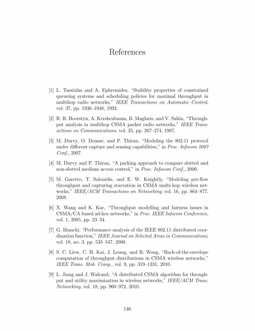
References

[1] L. Tassiulas and A. Ephremides, “Stability properties of constrainedqueueing systems and scheduling policies for maximal throughput inmultihop radio networks,” IEEE Transactions on Automatic Control,vol. 37, pp. 1936–1948, 1992.

[2] R. R. Boorstyn, A. Kershenbaum, B. Maglaris, and V. Sahin, “Through-put analysis in multihop CSMA packet radio networks,” IEEE Trans-actions on Communications, vol. 35, pp. 267–274, 1987.

[3] M. Durvy, O. Dousse, and P. Thiran, “Modeling the 802.11 protocolunder different capture and sensing capabilities,” in Proc. Infocom 2007Conf., 2007.

[4] M. Durvy and P. Thiran, “A packing approach to compare slotted andnon-slotted medium access control,” in Proc. Infocom Conf., 2006.

[5] M. Garetto, T. Salonidis, and E. W. Knightly, “Modeling per-flowthroughput and capturing starvation in CSMA multi-hop wireless net-works,” IEEE/ACM Transactions on Networking, vol. 16, pp. 864–877,2008.

[6] X. Wang and K. Kar, “Throughput modelling and fairness issues inCSMA/CA based ad-hoc networks,” in Proc. IEEE Infocom Conference,vol. 1, 2005, pp. 23–34.

[7] G. Bianchi, “Performance analysis of the IEEE 802.11 distributed coor-dination function,” IEEE Journal on Selected Areas in Communications,vol. 18, no. 3, pp. 535–547, 2000.

[8] S. C. Liew, C. H. Kai, J. Leung, and B. Wong, “Back-of-the-envelopecomputation of throughput distributions in CSMA wireless networks,”IEEE Trans. Mob. Comp., vol. 9, pp. 319–1331, 2010.

[9] L. Jiang and J. Walrand, “A distributed CSMA algorithm for through-put and utility maximization in wireless networks,” IEEE/ACM Trans.Networking, vol. 18, pp. 960–972, 2010.

146

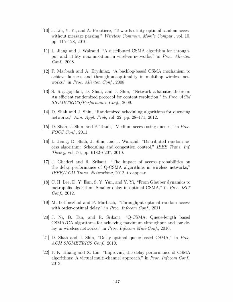
[10] J. Liu, Y. Yi, and A. Proutiere, “Towards utility-optimal random accesswithout message passing,” Wireless Commun. Mobile Comput., vol. 10,pp. 115–128, 2010.

[11] L. Jiang and J. Walrand, “A distributed CSMA algorithm for through-put and utility maximization in wireless networks,” in Proc. AllertonConf., 2008.

[12] P. Marbach and A. Eryilmaz, “A backlog-based CSMA mechanism toachieve fairness and throughput-optimality in multihop wireless net-works,” in Proc. Allerton Conf., 2008.

[13] S. Rajagopalan, D. Shah, and J. Shin, “Network adiabatic theorem:An efficient randomized protocol for content resolution,” in Proc. ACMSIGMETRICS/Performance Conf., 2009.

[14] D. Shah and J. Shin, “Randomized scheduling algorithms for queueingnetworks,” Ann. Appl. Prob, vol. 22, pp. 28–171, 2012.

[15] D. Shah, J. Shin, and P. Tetali, “Medium access using queues,” in Proc.FOCS Conf., 2011.

[16] L. Jiang, D. Shah, J. Shin, and J. Walrand, “Distributed random ac-cess algorithm: Scheduling and congestion control,” IEEE Trans. Inf.Theory, vol. 56, pp. 6182–6207, 2010.

[17] J. Ghaderi and R. Srikant, “The impact of access probabilities onthe delay performance of Q-CSMA algorithms in wireless networks,”IEEE/ACM Trans. Networking, 2012, to appear.

[18] C. H. Lee, D. Y. Eun, S. Y. Yun, and Y. Yi, “From Glauber dynamics tometropolis algorithm: Smaller delay in optimal CSMA,” in Proc. ISITConf., 2012.

[19] M. Lotfinezhad and P. Marbach, “Throughput-optimal random accesswith order-optimal delay,” in Proc. Infocom Conf., 2011.

[20] J. Ni, B. Tan, and R. Srikant, “Q-CSMA: Queue-length basedCSMA/CA algorithms for achieving maximum throughput and low de-lay in wireless networks,” in Proc. Infocom Mini-Conf., 2010.

[21] D. Shah and J. Shin, “Delay-optimal queue-based CSMA,” in Proc.ACM SIGMETRICS Conf., 2010.

[22] P.-K. Huang and X. Lin, “Improving the delay performance of CSMAalgorithms: A virtual multi-channel approach,” in Proc. Infocom Conf.,2013.

147

[23] X. Lin, N. Shroff, and R. Srikant, “On the connection-level stability ofcongestion-controlled communication networks,” IEEE Transactions onInformation Theory, vol. 54, pp. 2317–2338, 2008.

[24] J. Liu, A. Proutiere, Y. Yi, M. Chiang, and V. Poor, “Flow-level stabilityof data networks with non-convex and time-varying rate regions,” inProc. ACM SIGMETRICS, 2007.

[25] C. Moallemi and D. Shah, “On the flow-level dynamics of a packet-switched network,” in Proc. ACM SIGMETRICS, 2010.

[26] A. Eryilmaz, R. Srikant, and J. R. Perkins, “Stable scheduling policiesfor fading wireless channels,” IEEE/ACM Transactions on Networking,vol. 13, pp. 411–424, 2005.

[27] J. Ghaderi and R. Srikant, “On the design of efficient CSMA algorithmsfor wireless networks,” in Proc. CDC Conf., 2010.

[28] M. Feuillet, A. Proutiere, and P. Robert, “Random capture algorithms:Fluid limits and stability,” in Proc. ITA Workshop, 2010.

[29] P. Bremaud, Markov chains, Gibbs fields, Monte Carlo simulation, andqueues. Springer-Verlag, 1999.

[30] S. P. Meyn and R. L. Tweedie, “Criteria for stability of Markovian pro-cesses I: Discrete time chains,” Advances in Applied Probability, vol. 24,pp. 542–574, 1992.

[31] M. Jerrum and A. Sinclair, “Approximating the permanent,” SIAMJournal of Computing, vol. 18, pp. 1149–1178, 1989.

[32] J. Dai, “On positive harris recurrence of multiclass queueing networks:A unified approach via fluid limit models,” Ann. Appl. Prob., vol. 5, pp.49–77, 1995.

[33] J. G. Dai, “A fluid limit model criterion for instability of multiclassqueueing networks,” Ann. Appl. Prob., vol. 6, pp. 751–757, 1996.

[34] J. G. Dai and S. P. Meyn, “Stability and convergence of momentsfor multiclass queueing networks via fluid limit models,” IEEE Trans.Aut.Control, vol. 40, pp. 1889–1904, 1995.

[35] S. P. Meyn, “Transience of multiclass queueing networks via fluid limitmodels,” Ann. Appl. Prob., vol. 5, pp. 946–957, 1995.

[36] N. Bouman, S. C. Borst, J. S. H. van Leeuwaarden, and A. Proutiere,“Backlog-based random access in wireless networks: Fluid limits anddelay issues,” in Proc. ITC Conf., 2011.

148

[37] S. G. Foss and A. P. Kovalevskii, “A stability criterion via fluid limitsand its application to a polling model,” Queueing Systems, vol. 32, pp.131–168, 1999.

[38] M. Frolkova, S. G. Foss, and B. Zwart, “Random fluid limit of an over-loaded polling model,” 2013, Submitted for publication.

[39] A. P. Kovalevskii, V. A. Topchii, and S. G. Foss, “On the stability ofa queueing system with uncountable branching fluid limits,” Prob. Inf.Trans., vol. 41, pp. 254–279, 2005.

[40] L. Jiang, M. Leconte, J. Ni, R. Srikant, and J. Walrand, “Fast mixing ofparallel Glauber dynamics and low-delay CSMA scheduling,” in Proc.Infocom Mini-Conf., 2010.

[41] D. Shah, D. N. C. Tse, and J. N. Tsitsiklis, “Hardness of low delaynetwork scheduling,” IEEE Trans. Inf. Theory, vol. 57, pp. 7810–7817,2011.

[42] V. Subramanian and M. Alanyali, “Delay performance of CSMA in net-works with bounded degree conflict graphs.” in Proc. ISIT Conf., 2011.

[43] P. Robert and A. Veber, “On the fluid limits of a resource sharing algo-rithm with logarithmic weights,” arXiv:1211.5968v1, 2012.

[44] L. C. G. Rogers and D. Williams, Diffusions, Markov Processes andMartingales II. Wiley, London, 1989.

[45] P. Billingsley, Weak Convergence of Probability Measures. Wiley-Interscience, 1986.

[46] W. Whitt, “Weak convergence of probability measures on the functionspace C[0,∞).” Stanford University, Tech. Rep., 1969.

[47] H. L. Royden, Real Analysis. Prentice Hall, 3rd edition, 1987.

[48] N. Ethier and T. Kurtz, Markov Processes: Characterization and Con-vergence. Wiley-Interscience, 1985.

[49] P. Billingsley, An Introduction to Probability and Measure. Wiley-Interscience, 1995.

[50] J. Ghaderi, S. C. Borst, and P. A. Whiting, “Queue-based random-accessalgorithms: Fluid limits and stability issues,” Stochastic Systems, 2013,Submitted for publication.

[51] T. Bonald and M. Feuillet, “On the stability of flow-aware CSMA,”Performance Evaluation, vol. 67, pp. 1219–1229, 2010.

149

[52] M. Crovella and A. Bestavros, “Self-similarity in world wide web traffic:Evidence and possible causes,” IEEE/ACM Transactions on Network-ing, vol. 5, pp. 835–846, 1997.

[53] M. J. Neely, E. Modiano, and C. E. Rohrs, “Dynamic power alloca-tion and routing for time varying wireless networks,” IEEE Journal onSelected Areas in Communications, vol. 23, pp. 89–103, 2005.

[54] S. Asmussen, Applied Probability and Queues. Springer, 2003.

[55] J. Ghaderi, T. Ji, and R. Srikant, “Connection-level scheduling in wire-less networks using only MAC-layer information,” in Proc. IEEE Info-com Mini-Conf., 2012.

[56] N. S. Walton, “Utility optimization in congested queueing networks,”Applied Probability, vol. 48, pp. 68–89, 2011.

150