c 2011 Deepak Ramachandran - IDEALS

c© 2011 Deepak Ramachandran

KNOWLEDGE AND IGNORANCE IN REINFORCEMENT LEARNING

BY

DEEPAK RAMACHANDRAN

DISSERTATION

Submitted in partial fulfillment of the requirementsfor the degree of Doctor of Philosophy in Computer Science

in the Graduate College of theUniversity of Illinois at Urbana-Champaign, 2011

Urbana, Illinois

Doctoral Committee:

Professor Dan Roth, Chair, Director of ResearchAssociate Professor Eyal AmirProfessor Gerald DeJongProfessor Satinder Singh Baveja, University of Michigan at Ann Arbor

ABSTRACT

The field of Reinforcement Learning is concerned with teaching agents to take op-timal decisions to maximize their total utility in complicated environments. A Re-inforcement Learning problem, generally described by the Markov Decision Pro-cess formalism, has several complex interacting components, unlike in other ma-chine learning settings. I distinguish three: the state-space/ transition model, thereward function, and the observation model. In this thesis, I present a frameworkfor studying how the state of knowledge or uncertainty of each component affectsthe Reinforcement Learning process. I focus on the reward function and the ob-servation model, which has traditionally received little attention. Algorithms forlearning good policies when these components are completely specified are wellunderstood. However, it is less clear what to do when they are unknown, uncer-tain or irrelevant. In this thesis, I describe how to adapt Reinforcement Learningalgorithms to cope with these situations.

Recently there has been great interest in the Inverse Reinforcement Learning

problem where the objective is to learn the reward function from evidence of anagent’s reward-maximizing policy. The usual goal is to perform apprenticeship

learning where the agent learns the optimal action to perform from an expert.However, sometimes the reward function is of independent interest as well. Idescribe a Bayesian Inverse Reinforcement Learning approach to this problem.BIRL uses a generative model to describe the decision-making process and byinverting it we can infer the reward function from action observations. It is dis-tinguished from other IRL approaches by placing emphasis on the accuracy of thereward function in itself, and not just as an intermediate step to apprenticeshiplearning. BIRL is also able to handle incomplete and contradictory informationfrom the expert. It has been applied successfully to preference elicitation prob-lem for computer games and robot manipulation. In a recent comparison of IRLapproaches, BIRL was the best-performing general IRL algorithm.

I also extend this model to do a related task, Reward Shaping. In reward

ii

shaping, we seek to adjust a known reward function to make the learning agentconverge on the optimal policy as fast as possible. Reward shaping has beenproposed and studied previously in many applications, typically using additivepotential functions. However the requirement of absolute policy-invariance is toostrict to admit many useful cases of shaping. I define Bayesian Reward Shaping,which is a generalization to a soft form of reward shaping, and provide algorithmsfor achieving it.

The impact of observation models on reinforcement learning has been studiedeven less than reward functions. This is surpising, considering how adding partialobservability to an MDP model blows up the computational complexity and hencea better understanding of the tradeoffs between representational accuracy and ef-ficiency would be helpful. In this work, I describe how in certain cases POMDPscan be approximated by MDPs or slightly more complicated models with boundedperformance loss. I also present an algorithm, called Smoothed Q-Learning forlearning policies when the observation models are uncertain. Smoothed Sarsa isbased on the idea that in many real-world POMDPs better state estimates canbe made at later time steps and thus delaying the backup step of a temporaldifference-based algorithm can shortcut the uncertainty in the obervation modeland approximate the underlying MDP better.

Combining these approaches together (Bayesian Reward Shaping and SmoothedSarsa), a mobile robot was trained to execute delivery tasks in an office environ-ment.

iii

For Acha and Amma

iv

ACKNOWLEDGMENTS

First, I would like to thank my advisor Eyal Amir for having fired up my interestin the field of Artificial Intelligence and giving me the understanding and skillsI needed to contribute to it. Looking back, I am particularly grateful for the en-couragement he gave for me in pursuing my own research direction and willingme to believe in my abilities. I would like to thank my committee members, Pro-fessors Dan Roth, Jerry Dejong and Satinder Singh, for all that they have taughtme over the years and for their perserverance while I got this thesis done. Also,thanks to other professors at UIUC I was fortunate to collaborate with or learnfrom, particular David Forsyth, Chandra Chekuri and Douglas West.

My fellow group members and collaborators share so much of the credit (andnone of the blame) for the work I have done with them during my time at UIUC:Afsaneh Shirazi, Hannaneh Hajishirzi, Adam Vogel, Dafna Shahaf, Matt Young,Brian Hlubbocky, Megan Nance, Allan Chang, Nicolas Loeff and Alex Sorokin.Also, particular thanks to people I have worked with on internships at Cycorp,IBM Research and Honda Research: Pace Regan, Keith Goolsbey, Isaac Cheng,Savitha Srinivasan, Rakesh Gupta, Jongwoo Lim and Antoine Raux.

To even begin to thank my parents for all they have been to me and all theyhave done over the years would be a hopeless endeavour. Suffice to say, they werein my thoughts while I began and ended this thesis and every step in between.

My friends in Illinois and California were my bedrock of support and san-ity through the good and the not-so-good times. Thanks to Jacob Thomas, Ni-tish Korula, Rob Bocchino, Joe Tucek, Patrick Meredith, Anjali Menon, RuchikaSethi, Ranjith Subramanian, Gaurav and Sanjukta Mathur, Sridhar Venkatakrish-nan, Kavya Rakhra and Lynda Huynh for just being there.

And finally for Anusha - Would it have meant anything without you? Quiteprobably not.

v

TABLE OF CONTENTS

LIST OF TABLES . . . . . . . . . . . . . . . . . . . . . . . . . . . . . . viii

LIST OF FIGURES . . . . . . . . . . . . . . . . . . . . . . . . . . . . . . ix

CHAPTER 1 INTRODUCTION . . . . . . . . . . . . . . . . . . . . . . 11.1 Contributions of this thesis . . . . . . . . . . . . . . . . . . . . . 21.2 Notation and Terminology . . . . . . . . . . . . . . . . . . . . . 5

CHAPTER 2 BAYESIAN INVERSE REINFORCEMENT LEARNING . 92.1 Introduction . . . . . . . . . . . . . . . . . . . . . . . . . . . . . 92.2 Bayesian IRL . . . . . . . . . . . . . . . . . . . . . . . . . . . . 112.3 Inference . . . . . . . . . . . . . . . . . . . . . . . . . . . . . . 152.4 Experiments . . . . . . . . . . . . . . . . . . . . . . . . . . . . . 202.5 Applications of BIRL . . . . . . . . . . . . . . . . . . . . . . . . 212.6 Contributions . . . . . . . . . . . . . . . . . . . . . . . . . . . . 23

CHAPTER 3 A SURVEY OF INVERSE REINFORCEMENT TECH-NIQUES . . . . . . . . . . . . . . . . . . . . . . . . . . . . . . . . . . 273.1 Max-margin Methods . . . . . . . . . . . . . . . . . . . . . . . . 273.2 Maximum Entropy Methods . . . . . . . . . . . . . . . . . . . . 293.3 Natural Gradients . . . . . . . . . . . . . . . . . . . . . . . . . . 313.4 Direct Imitation Learning . . . . . . . . . . . . . . . . . . . . . . 323.5 Comparison . . . . . . . . . . . . . . . . . . . . . . . . . . . . . 323.6 Related Areas . . . . . . . . . . . . . . . . . . . . . . . . . . . . 33

CHAPTER 4 BAYESIAN REWARD SHAPING . . . . . . . . . . . . . 354.1 Reward Shaping . . . . . . . . . . . . . . . . . . . . . . . . . . . 354.2 Bayesian Reward Shaping . . . . . . . . . . . . . . . . . . . . . 374.3 Priors . . . . . . . . . . . . . . . . . . . . . . . . . . . . . . . . 394.4 Priors from Domain Knowledge . . . . . . . . . . . . . . . . . . 414.5 Extracting Common sense knowledge . . . . . . . . . . . . . . . 424.6 Experiments . . . . . . . . . . . . . . . . . . . . . . . . . . . . . 454.7 Using common sense in RL . . . . . . . . . . . . . . . . . . . . . 464.8 Related Work . . . . . . . . . . . . . . . . . . . . . . . . . . . . 484.9 Contributions . . . . . . . . . . . . . . . . . . . . . . . . . . . . 49

vi

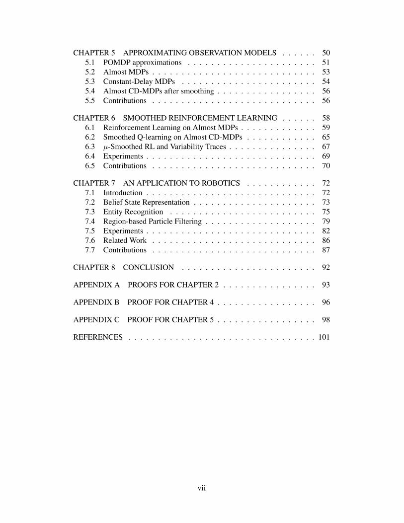
CHAPTER 5 APPROXIMATING OBSERVATION MODELS . . . . . . 505.1 POMDP approximations . . . . . . . . . . . . . . . . . . . . . . 515.2 Almost MDPs . . . . . . . . . . . . . . . . . . . . . . . . . . . . 535.3 Constant-Delay MDPs . . . . . . . . . . . . . . . . . . . . . . . 545.4 Almost CD-MDPs after smoothing . . . . . . . . . . . . . . . . . 565.5 Contributions . . . . . . . . . . . . . . . . . . . . . . . . . . . . 56

CHAPTER 6 SMOOTHED REINFORCEMENT LEARNING . . . . . . 586.1 Reinforcement Learning on Almost MDPs . . . . . . . . . . . . . 596.2 Smoothed Q-learning on Almost CD-MDPs . . . . . . . . . . . . 656.3 µ-Smoothed RL and Variability Traces . . . . . . . . . . . . . . . 676.4 Experiments . . . . . . . . . . . . . . . . . . . . . . . . . . . . . 696.5 Contributions . . . . . . . . . . . . . . . . . . . . . . . . . . . . 70

CHAPTER 7 AN APPLICATION TO ROBOTICS . . . . . . . . . . . . 727.1 Introduction . . . . . . . . . . . . . . . . . . . . . . . . . . . . . 727.2 Belief State Representation . . . . . . . . . . . . . . . . . . . . . 737.3 Entity Recognition . . . . . . . . . . . . . . . . . . . . . . . . . 757.4 Region-based Particle Filtering . . . . . . . . . . . . . . . . . . . 797.5 Experiments . . . . . . . . . . . . . . . . . . . . . . . . . . . . . 827.6 Related Work . . . . . . . . . . . . . . . . . . . . . . . . . . . . 867.7 Contributions . . . . . . . . . . . . . . . . . . . . . . . . . . . . 87

CHAPTER 8 CONCLUSION . . . . . . . . . . . . . . . . . . . . . . . 92

APPENDIX A PROOFS FOR CHAPTER 2 . . . . . . . . . . . . . . . . 93

APPENDIX B PROOF FOR CHAPTER 4 . . . . . . . . . . . . . . . . . 96

APPENDIX C PROOF FOR CHAPTER 5 . . . . . . . . . . . . . . . . . 98

REFERENCES . . . . . . . . . . . . . . . . . . . . . . . . . . . . . . . . 101

vii

LIST OF TABLES

3.1 Performance of various IRL approaches on the Taxicab do-main. Scores report are %ages of routes matched correctly.Reproduced from [ZBD10] . . . . . . . . . . . . . . . . . . . . . 33

6.1 Performance of POMDP Q-Learning. For each column a pol-icy was learned using the corresponding observation model.The average value acheived by that policy tested with each ofthe other observation models (along each row) is shown. . . . . . 65

6.2 Performance of AMDP Q-Learning. For each column a policywas learned using the corresponding observation model. Theaverage value acheived by that policy tested with each of theother observation models (along each row) is shown. . . . . . . . 66

7.1 Region-based Particle Filter update at time step t + 1. Pt isthe particle set at time t. p.r, p.x, p.y are the region, x and ypositions respectively of particle p. . . . . . . . . . . . . . . . . 80

7.2 Mean completion times for delivery tasks with Smoothed Sarsaand Manual policy . . . . . . . . . . . . . . . . . . . . . . . . . 86

viii

LIST OF FIGURES

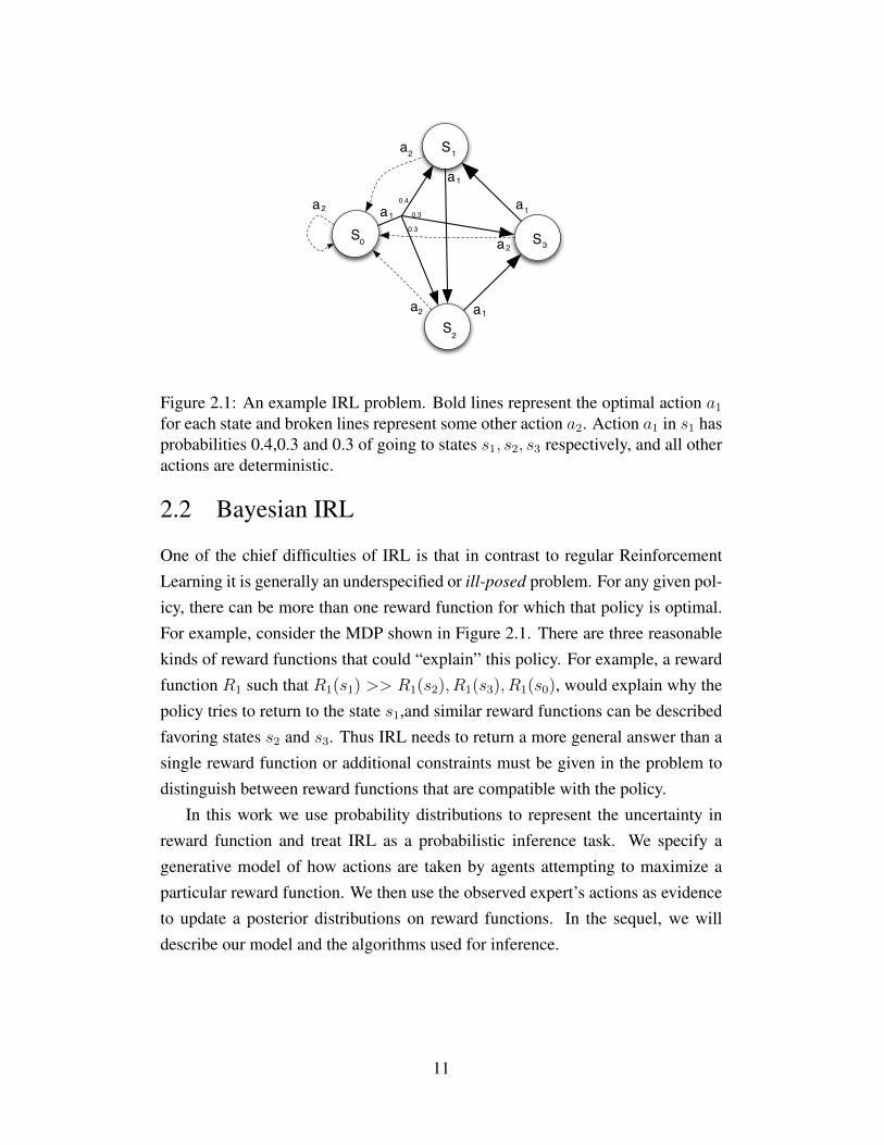
2.1 An example IRL problem. Bold lines represent the optimalaction a1 for each state and broken lines represent some otheraction a2. Action a1 in s1 has probabilities 0.4,0.3 and 0.3 ofgoing to states s1, s2, s3 respectively, and all other actions aredeterministic. . . . . . . . . . . . . . . . . . . . . . . . . . . . . 11

2.2 The BIRL model . . . . . . . . . . . . . . . . . . . . . . . . . . 142.3 GridWalk Sampling Algorithm . . . . . . . . . . . . . . . . . . . 182.4 PolicyWalk Sampling Algorithm . . . . . . . . . . . . . . . . . . 192.5 Reward Loss. . . . . . . . . . . . . . . . . . . . . . . . . . . . . 202.6 Policy Loss. . . . . . . . . . . . . . . . . . . . . . . . . . . . . . 212.7 Scatter diagrams of sampled rewards of two arbitrary states for

a given MDP and expert trajectory. Our computed posterior isshown to be close to the true distribution. . . . . . . . . . . . . . 22

2.8 Comparison of reward function inferred by BIRL on an 4x4gridworld problem with true rewards. . . . . . . . . . . . . . . . 24

2.9 Ising versus Uninformed Priors for Adventure Games . . . . . . . 252.10 Affordance model for grasping and tapping different objects. . . . 252.11 Human demonstrating actions to take with different objects. . . . 262.12 BALTHAZAR robot imitating human actions learned by BIRL

over the affordance model. . . . . . . . . . . . . . . . . . . . . . 26

3.1 The Taxicab domain from [ZBD10]. IRL algorithms wereused to infer drivers’ utilities for different routes from thechoices made at intersections. . . . . . . . . . . . . . . . . . . . 33

4.1 The Banana Game . . . . . . . . . . . . . . . . . . . . . . . . . . 364.2 The BRS process for a 9-state Gridworld MDP . . . . . . . . . . 404.3 Average value obtained by learned policy for both reward func-

tions after a fixed number of learning steps using Q-learning.The experiments were done over a set of 100 randomly gener-ated transition models. . . . . . . . . . . . . . . . . . . . . . . . 41

4.4 A projection of the ConceptNet term “open door” finds theconcept “key” for the binary relation “CapableOf”. . . . . . . . . 44

4.5 Extracting Relevant Features . . . . . . . . . . . . . . . . . . . . 454.6 Reward Shaping with Common Sense. . . . . . . . . . . . . . . . 47

ix

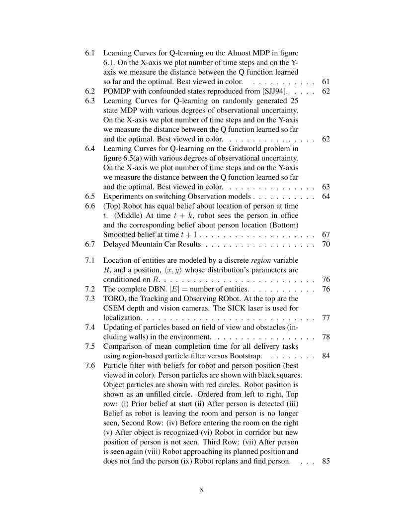
6.1 Learning Curves for Q-learning on the Almost MDP in figure6.1. On the X-axis we plot number of time steps and on the Y-axis we measure the distance between the Q function learnedso far and the optimal. Best viewed in color. . . . . . . . . . . . 61

6.2 POMDP with confounded states reproduced from [SJJ94]. . . . . 626.3 Learning Curves for Q-learning on randomly generated 25

state MDP with various degrees of observational uncertainty.On the X-axis we plot number of time steps and on the Y-axiswe measure the distance between the Q function learned so farand the optimal. Best viewed in color. . . . . . . . . . . . . . . . 62

6.4 Learning Curves for Q-learning on the Gridworld problem infigure 6.5(a) with various degrees of observational uncertainty.On the X-axis we plot number of time steps and on the Y-axiswe measure the distance between the Q function learned so farand the optimal. Best viewed in color. . . . . . . . . . . . . . . . 63

6.5 Experiments on switching Observation models . . . . . . . . . . . 646.6 (Top) Robot has equal belief about location of person at time

t. (Middle) At time t + k, robot sees the person in officeand the corresponding belief about person location (Bottom)Smoothed belief at time t+ 1 . . . . . . . . . . . . . . . . . . . . 67

6.7 Delayed Mountain Car Results . . . . . . . . . . . . . . . . . . . 70

7.1 Location of entities are modeled by a discrete region variableR, and a position, 〈x, y〉 whose distribution’s parameters areconditioned on R. . . . . . . . . . . . . . . . . . . . . . . . . . . 76

7.2 The complete DBN. |E| = number of entities. . . . . . . . . . . . 767.3 TORO, the Tracking and Observing RObot. At the top are the

CSEM depth and vision cameras. The SICK laser is used forlocalization. . . . . . . . . . . . . . . . . . . . . . . . . . . . . . 77

7.4 Updating of particles based on field of view and obstacles (in-cluding walls) in the environment. . . . . . . . . . . . . . . . . . 78

7.5 Comparison of mean completion time for all delivery tasksusing region-based particle filter versus Bootstrap. . . . . . . . . 84

7.6 Particle filter with beliefs for robot and person position (bestviewed in color). Person particles are shown with black squares.Object particles are shown with red circles. Robot position isshown as an unfilled circle. Ordered from left to right, Toprow: (i) Prior belief at start (ii) After person is detected (iii)Belief as robot is leaving the room and person is no longerseen, Second Row: (iv) Before entering the room on the right(v) After object is recognized (vi) Robot in corridor but newposition of person is not seen. Third Row: (vii) After personis seen again (viii) Robot approaching its planned position anddoes not find the person (ix) Robot replans and find person. . . . 85

x

7.7 Manual policy using Stage simulator. The top image in eachframe is a snapshot from the simulator and the bottom is a vi-sualization of the robot’s belief state and current action. Theline joining the robot to the region shows the region that therobot is moving to. Ordering from left to right (best viewed incolor). TOP ROW (a) Robot initialized with priors (b) Robotlooking for the first object in the left room based on prior (c)first object not found but first person found. MIDDLE LOW(d) Robot looking for the first object in right room (e) sec-ond object found. Robot next navigates to top part of room.BOTTOM ROW (f) First object found and picked up. Robotnavigating to first person in left room (g) After delivering firstobject, robot navigating to second object (h) Robot picks upsecond object and navigates to second person in the right room(i) Second object delivered. . . . . . . . . . . . . . . . . . . . . . 89

7.8 Smoothed Sarsa policy using Stage simulator. The top imagein each frame is a snapshot from the simulator and the bottomis a visualization of the robot’s belief state and current action.The line joining the robot to the region shows the region thatthe robot is moving to. Ordering from left to right (best viewedin color). TOP ROW (a) Robot going to left room to look forfirst object (b) Robot sees second object and picks it up (c)Second object is being delivered to the second person BOT-TOM ROW (d) Robot moving to the first object in the sameright room (e) Robot looking for first person in the left room(f) First object delivered. . . . . . . . . . . . . . . . . . . . . . . 90

7.9 Smoothed Sarsa policy on the TORO robot. The line join-ing the robot to the region shows the region that the robot ismoving to. Ordering from left to right (best viewed in color).TOP ROW (a) Robot going to left room to look for object (b)Robot looking at a different region for object (c) Robot findsthe first object in the corner of the left room SECOND ROW(d) First object picked up (e) Robot navigating to the first per-son (f) First person as seen through the glass THIRD ROW (g)First object delivered to the first person. (h) Robot looking forthe second object (i) Robot navigating to the second object.FOURTH ROW (j) Robot picks the second object and looksfor second person in the right room (k) Robot navigating toperson in the second room (l) Robot delivered second objectto second person. . . . . . . . . . . . . . . . . . . . . . . . . . . 91

xi

CHAPTER 1

INTRODUCTION

There is, it seems to us,

At best, only a limited value

In the knowledge derived from experience.

The knowledge imposes a pattern, and falsifies,

For the pattern is new in every moment

And every moment is a new and shocking

Valuation of all we have been.

– T S Eliot, “East Coker”

Reinforcement Learning (RL) is a popular framework for studying complexdecision making problems in AI. In reinforcement learning, an agent is faced witha sequence of states and must take decisions at each state to maximize its longterm utility. Reinforcement learning has been an active area of research for over20 years (perhaps even longer, see [Bel57]). The field has reached maturity infinding solutions of decision-making problems in the “classic” Markov DecisionProcess setting [How60]. However, many more realistic variations of the problemare under active investigation and a systematic study of the components of thedecision making process is in its infancy.

Unlike more typical machine learning problems such as classification or re-gression, Reinforcement Learning has many moving parts. In a real-world decision-making problem we are often tasked with choosing actions when there is igno-rance or uncertainty about one or more of them. In the most general Partially

Observable Markov Decision Problem formulation [Son78], we can identify threerelevant components:

1. The state space, action space and transition function describe the environ-ment and its dynamics. When these are fully known to the agent, the prob-lem of finding optimal policies is called Solving the (PO)MDP and it isa purely computational task. When they are not known, we have to learn

1

from experience, and this is the classical Reinforcement Learning problem.RL is generally distinguished into two types - model-based[KS02, BT01]where we attempt to learn the model in addition to learning a policy, andmodel-free[RN94, Wat89] where a policy is learned directly.

2. The reward function captures the objectives, goals and motivation for theagent’s choice of actions. Uncertainty in the reward function in the formof a probability distribution can be easily handled in the MDP frameworkby taking the expectation of the reward function. However, ignorance ofthe reward function can be encountered as well. In Inverse Reinforcement

learning [Rus98], we try to learn a suitable reward function by observingthe actions of experts. In Reward Shaping [CH94], a teacher modifies thereward signal of the learning agent to encourage intended behaviors.

3. The observation model describes the state of knowledge of the agent. This isa layer of uncertainty that is often omitted yielding the classical MDP whichis far more tractable though unrealistic in real-world decision making prob-lems. In full blown POMDPs, the addition of the observation model intro-duces a level of complexity (polynomail-time to PSPACE-complete [PT87]) that severely restrict practical applications of current state of the art algo-rithms [SV04]. Despite that, models with intermediate levels of complexityhave gotten little attention.

In this thesis, I study how knowledge, ignorance and uncertainty of these in-dividual components affect the overall Reinforcement learning process. Since re-ward functions and observation models are the least understood, I focus on these.I show that Reinforcement Learning is a very flexible paradigm and adaptationsof many standard RL approaches can be used in more complex formulations.

1.1 Contributions of this thesis

Broadly speaking, in this thesis I study the implications for reinforcement learningof knowledge of the reward function and ignorance of the observation model. Ishow that insight into these situation (and hence solutions) can be obtained bystudying the process by which decision making is done in basic MDP models. Aconcise statement of my thesis is:

2

Solutions for more general Reinforcement Learning problems can be found by

analyzing models of the decision making process in simpler ones.

1. Bayesian Inverse Reinforcement Learning

The key idea of my approach is to treat IRL as an inference problem, wherethe actions of the agent we are learning from are used as evidence to modifyour belief about its reward function. By modeling the decision making pro-cess probabilistically we can use Bayes theorem to do this inference. Unlikeother approaches to IRL [AN04, NS07], our method gives cental impor-tance to learning the reward function itself, and is not solely motivated byapprenticeship learning. This is useful in tasks where the reward functionis of independent interest such as preference elicitation. It can be used incases where the expert gives incomplete or contradictory advice. Our rep-resentation makes it easy to incorporate domain knowledge or declarativeadvice about the reward function through informative priors. BIRL has beenused for eliciting player preferences in adventure games, teaching a robotto manipulate objects [LMM08] and performed competitively in a recentcomparison of IRL methods [ZMBD08]. Since the field of IRL has showna surge of interest in the recent past, I also include a comprehensive surveyand comparison of IRL methods in the literature.

2. Bayesian Reward Shaping

In reward shaping [CH94], we seek to modify the (fixed) reward functionof a learning agent in order to help it learn the optimal policy at a faster rate.Reward shaping has been suggested to alleviate the temporal credit assign-

ment problem typical of MDPs with sparse rewards [RA98]. It is usual toassume that the optimal policy remains invariant under the reward shap-ing process. Most methods acheive this by using a potential-based shapingfunction [NHR99].

I extend my generative model for BIRL to give a solution for reward shap-ing. By plugging in the original reward function into the likelihood modelfor actions, a soft form of policy invariance is obtained. Meanwhile the prioris constructed to favor fast learning. This can be done in two ways: by usingan Ising-type distribution with an anti-ferromagnetic phase that spreads therewards around the state space as much as possible, or by using clues fromcommon-sense knowledge of the domain.

3

Unlike previous reward shaping constructions, my approach enforces a softform of policy invariance, allowing us to use a richer space of possible shap-ing functions. It also makes it possible to partially specify the portion of thepolicy that we wish to keep invariant, which makes it useful in cases wherethe teacher is only interested in the student’s behaviour on subsets of thestate space.

3. Approximating Observation models

In this part of my thesis, I analyze some approximate heuristics for solv-ing POMDPs and show non-trivial bounds on the loss of performance ver-sus the optimal POMDP solutions in certain cases. Surprisingly I showthe first bound on the performance of the Most-likely-state (MLS) heuris-tic on what I call Almost MDPs, i.e. POMDPs with bounded uncertaintyin reachable belief states. This can be generalized to a heuristic that ap-proximates a POMDP with a constant-delay MDP (CMDP), a formulationintroduced and studied by [WNL07] for POMDP. I call POMDPs that canbe well-approximated by CMDPs Almost CMDPs and show similar boundson these.

4. Smoothed Reinforcement Learning

Using the intuition developed above I discuss an improved reinforcementlearning algorithm for POMDPs applicable in cases where we have im-perfect access to the observation model. The aim of our Smoothed Sarsa

algorithm is to shortcut the observation model and learn a policy for theunderlying MDP directly. The key idea is to delay the learning step untilbetter information about our current state is obtained. In many cases (suchas those where the assumptions of the previous section are valid) this willlead to faster convergence because of variance reduction. Smoothed Sarsacan be generalized to a variability traces framework, similar to eligibilitytraces for TD(λ), where the smoothing is done across multiple time steps.

5. Delivery tasks on a mobile robot

I successfully demonstrated the use of Reinforcement Learning in traininga Pioneer robot to do errands and deliveries in an office environment. Thetask required navigation and task-level decision-making. Smoothed Sarsawas used to learn a policy independent of the observation model (simulation

4

or real robot) along with a novel heirarchical representation of location thatseperated the state spaces into layers relevant for each step of decision-making.

1.2 Notation and Terminology

In this section I will lay out the theoretical machinery used for reinforcementlearning. The main object of interest is the Markov Decision Process (MDP), themost common theoretical framework used for representing sequential decisionmaking tasks.

It was first introduced in Belman’s seminal paper on Dynamic Programming[Bel57] although much of the research in this area was stimulated, and indeed theterm MDP popularized, by [How60]. MDPs are an extremely flexible mechanismfor representing complex decision making tasks and have found applications inareas as diverse as robotics [TBF05a], economics [Lav66], neurobiology [AD01]and numerous others [Put94].

In this thesis I am primarily concerned with the use of MDPs for Reinforce-

ment Learning. Recall the earlier description of RL as learning optimal behaviourthrough experience. RL is often cast concretely in the MDP domain as learningthe policy for an unknown MDP through experience. The experience consists ofan agent situated in the state space of an MDP, taking actions and observing theiroutcomes. The agent eventually learns a good policy to operate in the environ-ment either by building a model of the MDP and solving it or by finessing it toget the optimal policy directly. In the later sections I briefly survey reinforcementalgorithms for MDP’s developed over the last 20 years, which will serve as a basisfor the rest of my research.

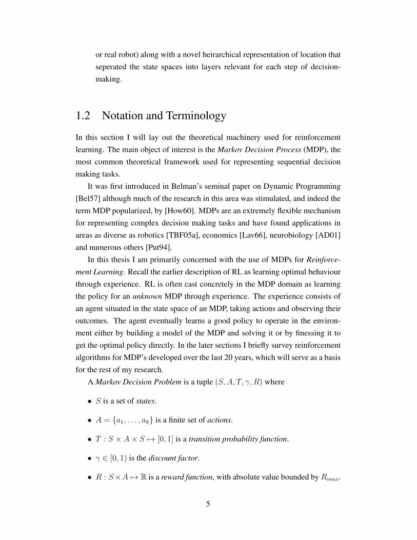
A Markov Decision Problem is a tuple (S,A, T, γ, R) where

• S is a set of states.

• A = {a1, . . . , ak} is a finite set of actions.

• T : S × A× S 7→ [0, 1] is a transition probability function.

• γ ∈ [0, 1) is the discount factor.

• R : S×A 7→ R is a reward function, with absolute value bounded byRmax.

5

A Markov Decision Process (MDP) is a tuple (S,A, T, γ), with the terms de-fined as before but without a reward function. In general, I will use the abbre-viation MDP to refer to both Markov Decision Processes and Markov DecisionProblems, unless it is not clear from the context which term is meant.

We adopt the following compact notation from [NR00] for MDPs with finitestate spaces : Fix an enumeration s1 . . . sN of the finite state space S. The rewardfunction (or any other function on the state-space) can then be represented as anN -dimensional vectorR, whose ith element is R(si).

A (stationary) policy is a map π : S 7→ A and the (discounted, infinite-horizon)value of a policy π for reward functionR at state s ∈ S,denoted V π(s,R) is givenby:

V π(st1 ,R) = R(st1 , at+1) + Est1 ,st2 ,...[γR(st2) + γ2R(st3) + . . . |π]

where Pr(sti+1|sti , π) = T (sti , π(sti), sti+1

). To solve an MDP means to find anoptimal policy π∗ such that V π(s,R) is maximized for all s ∈ S by π = π∗.Indeed, it can be shown (see for example [SB98]) that at least one such policyalways exists for ergodic MDPs. For the solution of Markov Decision Problems,it is useful to define the following auxilliary Q-function:

Qπ(s, a,R) = R(s, a) + γEs′∼T (s,a,·)[Vπ(s′,R)]

We also define the optimalQ-functionQ∗(·, ·,R) as theQ-function of the optimalpolicy π∗ for reward functionR.

We also state the following result concerning Markov Decision Problems (see[SB98]) :

Theorem 1.1 (Bellman Equations). Given a Markov Decision Problem M =

(S,A, T, γ, R) and a policy π : S 7→ A. Then,

1. For all s ∈ S, a ∈ A, V π and Qπ satisfy

V π(s) = R(s, π(s)) + γ∑

s′

T (s, π(s), s′)V π(s′) (1.1)

Qπ(s, a) = R(s, a) + γ∑

s′

T (s, a, s′)V π(s′)

2. π is an optimal policy for M iff, for all s ∈ S,

6

π(s) ∈ argmaxa∈A

Qπ(s, a) (1.2)

1.2.1 POMDPs

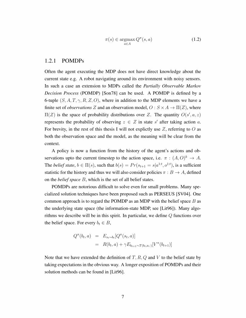
Often the agent executing the MDP does not have direct knowledge about thecurrent state e.g. A robot navigating around its environment with noisy sensors.In such a case an extension to MDPs called the Partially Observable Markov

Decision Process (POMDP) [Son78] can be used. A POMDP is defined by a6-tuple (S,A, T, γ, R, Z,O), where in addition to the MDP elements we have afinite set of observations Z and an observation model, O : S×A→ Π(Z), whereΠ(Z) is the space of probability distributions over Z. The quantity O(s′, a, z)

represents the probability of observing z ∈ Z in state s′ after taking action a.For brevity, in the rest of this thesis I will not explictly use Z, referring to O asboth the observation space and the model, as the meaning will be clear from thecontext.

A policy is now a function from the history of the agent’s actions and ob-servations upto the current timestep to the action space, i.e. π : (A,O)k → A.The belief state, b ∈ Π(s), such that b(s) = Pr(st+1 = s|a1:t, o1:t), is a sufficientstatistic for the history and thus we will also consider policies π : B → A, definedon the belief space B, which is the set of all belief states.

POMDPs are notorious difficult to solve even for small problems. Many spe-cialized solution techniques have been proposed such as PERSEUS [SV04]. Onecommon approach is to regard the POMDP as an MDP with the belief space B asthe underlying state space (the information-state MDP, see [Lit96]). Many algo-rithms we describe will be in this spirit. In particular, we define Q functions overthe belief space. For every bt ∈ B,

Qπ(bt, a) = Est∼bt [Qπ(st, a)]

= R(bt, a) + γEbt+1∼T (bt,a,·)[Vπ(bt+1)]

Note that we have extended the definition of T,R,Q and V to the belief state bytaking expectations in the obvious way. A longer exposition of POMDPs and theirsolution methods can be found in [Lit96].

7

Algorithm 1 Tabular Q-learning.Input: Initial belief state b0.Initialize Q(b, a) arbitrarily.for t = 0, 1, 2, . . . until Q converges do

Choose at for bt using policy derived from Q (e.g. ε-greedy).Take action at, observe rt, bt+1.Q(bt, at)

α← rt + γmaxaQ(bt+1, a)−Q(bt, at)end forReturn Q

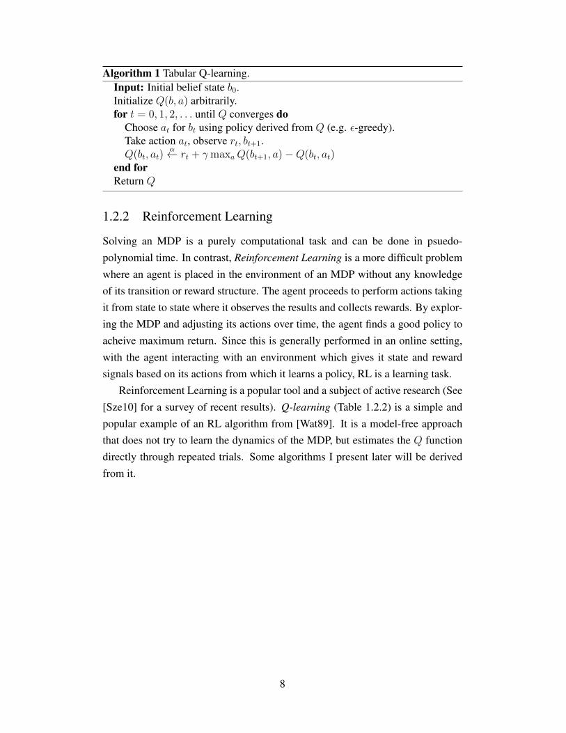
1.2.2 Reinforcement Learning

Solving an MDP is a purely computational task and can be done in psuedo-polynomial time. In contrast, Reinforcement Learning is a more difficult problemwhere an agent is placed in the environment of an MDP without any knowledgeof its transition or reward structure. The agent proceeds to perform actions takingit from state to state where it observes the results and collects rewards. By explor-ing the MDP and adjusting its actions over time, the agent finds a good policy toacheive maximum return. Since this is generally performed in an online setting,with the agent interacting with an environment which gives it state and rewardsignals based on its actions from which it learns a policy, RL is a learning task.

Reinforcement Learning is a popular tool and a subject of active research (See[Sze10] for a survey of recent results). Q-learning (Table 1.2.2) is a simple andpopular example of an RL algorithm from [Wat89]. It is a model-free approachthat does not try to learn the dynamics of the MDP, but estimates the Q functiondirectly through repeated trials. Some algorithms I present later will be derivedfrom it.

8

CHAPTER 2

BAYESIAN INVERSE REINFORCEMENTLEARNING

Inverse Reinforcement Learning (IRL) is the problem of learning the reward func-tion underlying a Markov Decision Process given the dynamics of the system andthe behaviour of an expert. IRL is motivated by situations where knowledge ofthe rewards is a goal by itself (as in preference elicitation) and by the task of ap-prenticeship learning (learning policies from an expert). In this chapter I showhow to combine prior knowledge and evidence from the expert’s actions to derivea probability distribution over the space of reward functions. I present efficientalgorithms that find solutions for the reward learning and apprenticeship learn-ing tasks that generalize well over these distributions. Experimental results showstrong improvement for our methods over previous heuristic-based approaches.

2.1 Introduction

The Inverse Reinforcement Learning (IRL) problem is defined in [Rus98] as fol-lows:

Determine The reward function that an agent is optimizing.Given

1. Measurement of the agent’s behaviour over time, in a variety of circum-stances.

2. Measurements of the sensory inputs to that agent

3. A model of the environment.

In the context of Markov Decision Processes, this translates into determiningthe reward function of the agent from knowledge of the policy it executes and thedynamics of the state-space.

The first, utility elicitation, is estimating the unknown reward function as ac-curately as possible. It is useful in situations where the reward function is of

9

interest by itself, for example when constructing models of animal and humanlearning or modelling opponent in competitive games. Pokerbots can improveperformance against suboptimal human opponents by learning reward functionsthat account for the utility of money, preferences for certain hands or situationsand other idiosyncrasies [BPSS98]. There are also connections to various prefer-ence elicitation problems in economics [Sar94].

The second task is apprenticeship learning - using observations of an expert’sactions to decide one’s own behaviour. It is possible in this situation to directlylearn the policy from the expert [AS97]. However the reward function is generallythe most succint, robust and transferable representation of the task, and completelydetermines the optimal policy (or set of policies). In addition, knowledge of thereward function allows the agent to generalize better i.e. a new policy can be com-puted when the environment changes. IRL is thus likely to be the most effectivemethod here.

Here I model the IRL problem from a Bayesian perspective. I consider theactions of the expert as evidence that I use to update a prior on reward functions. Isolve reward learning and apprenticeship learning using this posterior. I performinference for these tasks using a modified Markov Chain Monte Carlo (MCMC)algorithm. I show that the Markov Chain for our distribution with a uniformprior mixes rapidly, and that the algorithm converges to the correct answer inpolynomial time. The original IRL formulation of [NR00] arises as a special caseof Bayesian IRL (BIRL) with a Laplacian prior.

There are a number of advantages of this technique over previous work: wedo not need a completely specified optimal policy as input to the IRL agent, nordo we need to assume that the expert is infallible. Also, we can incorporate ex-ternal information about specific IRL problems into the prior of the model, or useevidence from multiple experts.

IRL was first studied in the machine learning setting by [NR00] who describedalgorithms that found optimal rewards for MDPs having both finite and infinitestates. Experimental results show improved performance by our techniques in thefinite case.

10

S

S

S

S

1

3

2

0

a2

a10.4

0.3

0.3

a1

a1a2

a2

a2 a1

Figure 2.1: An example IRL problem. Bold lines represent the optimal action a1for each state and broken lines represent some other action a2. Action a1 in s1 hasprobabilities 0.4,0.3 and 0.3 of going to states s1, s2, s3 respectively, and all otheractions are deterministic.

2.2 Bayesian IRL

One of the chief difficulties of IRL is that in contrast to regular ReinforcementLearning it is generally an underspecified or ill-posed problem. For any given pol-icy, there can be more than one reward function for which that policy is optimal.For example, consider the MDP shown in Figure 2.1. There are three reasonablekinds of reward functions that could “explain” this policy. For example, a rewardfunction R1 such that R1(s1) >> R1(s2), R1(s3), R1(s0), would explain why thepolicy tries to return to the state s1,and similar reward functions can be describedfavoring states s2 and s3. Thus IRL needs to return a more general answer than asingle reward function or additional constraints must be given in the problem todistinguish between reward functions that are compatible with the policy.

In this work we use probability distributions to represent the uncertainty inreward function and treat IRL as a probabilistic inference task. We specify agenerative model of how actions are taken by agents attempting to maximize aparticular reward function. We then use the observed expert’s actions as evidenceto update a posterior distributions on reward functions. In the sequel, we willdescribe our model and the algorithms used for inference.

11

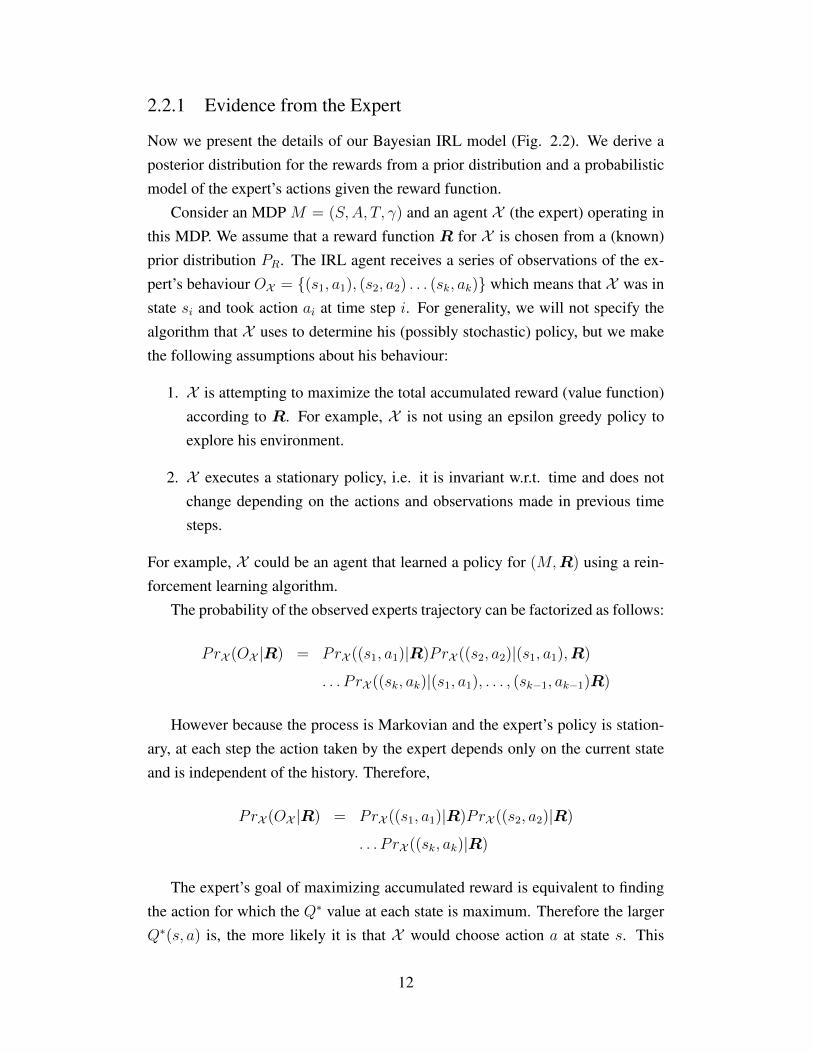
2.2.1 Evidence from the Expert

Now we present the details of our Bayesian IRL model (Fig. 2.2). We derive aposterior distribution for the rewards from a prior distribution and a probabilisticmodel of the expert’s actions given the reward function.

Consider an MDP M = (S,A, T, γ) and an agent X (the expert) operating inthis MDP. We assume that a reward function R for X is chosen from a (known)prior distribution PR. The IRL agent receives a series of observations of the ex-pert’s behaviour OX = {(s1, a1), (s2, a2) . . . (sk, ak)} which means that X was instate si and took action ai at time step i. For generality, we will not specify thealgorithm that X uses to determine his (possibly stochastic) policy, but we makethe following assumptions about his behaviour:

1. X is attempting to maximize the total accumulated reward (value function)according to R. For example, X is not using an epsilon greedy policy toexplore his environment.

2. X executes a stationary policy, i.e. it is invariant w.r.t. time and does notchange depending on the actions and observations made in previous timesteps.

For example, X could be an agent that learned a policy for (M,R) using a rein-forcement learning algorithm.

The probability of the observed experts trajectory can be factorized as follows:

PrX (OX |R) = PrX ((s1, a1)|R)PrX ((s2, a2)|(s1, a1),R)

. . . P rX ((sk, ak)|(s1, a1), . . . , (sk−1, ak−1)R)

However because the process is Markovian and the expert’s policy is station-ary, at each step the action taken by the expert depends only on the current stateand is independent of the history. Therefore,

PrX (OX |R) = PrX ((s1, a1)|R)PrX ((s2, a2)|R)

. . . P rX ((sk, ak)|R)

The expert’s goal of maximizing accumulated reward is equivalent to findingthe action for which the Q∗ value at each state is maximum. Therefore the largerQ∗(s, a) is, the more likely it is that X would choose action a at state s. This

12

likelihood increases the more confident we are in X ’s ability to select a goodaction. We model this by an exponential distribution for the likelihood of (si, ai),with Q∗ as a potential function:

PrX ((si, ai)|R) =1

ZieαXQ

∗(si,ai,R)

where αX is a parameter1 representing the degree of confidence we have in X ’sability to choose actions with high value. This distribution satisfies our assump-tions and is easy to reason with. The likelihood of the entire evidence is :

PrX (OX |R) =1

ZeαXE(OX ,R)

where E(OX ,R) =∑

iQ∗(si, ai,R) and Z is the appropriate normalizing con-

stant. We can think of this likelihood function as a Boltzmann-type distributionwith energy E(OX ,R) and temperature 1

αX.

Now, we compute the posterior probability of reward function R by applyingBayes theorem,

PrX (R|OX ) =PrX (OX |R)PR(R)

Pr(OX )

=1

Z ′eαXE(OX ,R)PR(R) (2.1)

Computing the normalizing constant Z ′ is hard. However the sampling algo-rithms we will use for inference only need the ratios of the densities at two points,so this is not a problem.

2.2.2 Priors

When no other information is given, we may assume that the rewards are indepen-dently identically distributed (i.i.d.) by the principle of maximum entropy. Mostof the prior functions considered here will be of this form. The exact prior to usehowever, depends on the characteristics of the problem:

1. If we are completely agnostic about the prior, we can use the uniform dis-

1Note that the probabilities of the evidence should be conditioned on αX as well (Fig 2.2). Butit will be simpler to treat αX as just a parameter of the distribution.

13

X

RαX

(s1, a1) (s2, a2) (sk, ak)

Figure 2: The BIRL model

value. This distribution satisfies our assumptions and is easyto reason with. The likelihood of the entire evidence is :

PrX (OX |R) =1

ZeαX E(OX ,R)

where E(OX , R) =∑

i Q∗(si, ai, R) and Z is the appropriatenormalizing constant. We can think of this likelihood func-tion as a Boltzmann-type distribution with energy E(OX , R)and temperature 1

αX.

Now, we compute the posterior probability of reward func-tionR by applying Bayes theorem,

PrX (R|OX ) =PrX (OX |R)PR(R)

Pr(OX )

=1

Z ′ eαX E(OX ,R)PR(R) (3)

Computing the normalizing constant Z ′ is hard. Howeverthe sampling algorithms we will use for inference only needthe ratios of the densities at two points, so this is not a prob-lem.

3.2 PriorsWhen no other information is given, we may assume that therewards are independently identically distributed (i.i.d.) bythe principle of maximum entropy. Most of the prior func-tions considered in this paper will be of this form. The exactprior to use however, depends on the characteristics of theproblem:1. If we are completely agnostic about the prior, we canuse the uniform distribution over the space −Rmax ≤R(s) ≤ Rmax for each s ∈ S. If we do not want to spec-ify any Rmax we can try the improper prior P (R) = 1for allR ∈ Rn.

2. Many real world Markov decision problems have parsi-monious reward structures, with most states having neg-ligible rewards. In such situations, it would be better toassume a Gaussian or Laplacian prior:

PGaussian(R(s) = r) =1√2πσ

e− r2

2σ2 , ∀s ∈ S

on αX as well (Fig 2). But it will be simpler to treat αX as just aparameter of the distribution.

PLaplace(R(s) = r) =1

2σe− |r|

2σ , ∀s ∈ S

3. If the underlying MDP represented a planning-typeproblem, we expect most states to have low (or negative)rewards but a few states to have high rewards (corre-sponding to the goal); this can be modeled by a Beta dis-tribution for the reward at each state, which has modesat high and low ends of the reward space:

PBeta(R(s) = r) =1

( rRmax

)12 (1 − r

Rmax)

12

, ∀s ∈ S

In section 6.1, we give an example of how more informa-tive priors can be constructed for particular IRL problems.

4 InferenceWe now use the model of section 3 to carry out the two tasksdescribed in the introduction: reward learning and appren-ticeship learning. Our general procedure is to derive minimalsolutions for appropriate loss functions over the posterior (Eq.3). Some proofs are omitted for lack of space.

4.1 Reward LearningReward learning is an estimation task. The most common lossfunctions for estimation problems are the linear and squarederror loss functions:

Llinear(R, R) = ‖ R − R ‖1

LSE(R, R) = ‖ R − R ‖2

whereR and R are the actual and estimated rewards, respec-tively. IfR is drawn from the posterior distribution (3), it canbe shown that the expected value ofLSE(R, R) is minimizedby setting R to the mean of the posterior (see [Berger, 1993]).Similarily, the expected linear loss is minimized by setting Rto the median of the distribution. We discuss how to computethese statistics for our posterior in section 5.It is also common in Bayesian estimation problems to use

the maximum a posteriori (MAP) value as the estimator. Infact we have the following result:Theorem 2. When the expert’s policy is optimal and fullyspecified, the IRL algorithm of [Ng and Russell, 2000] isequivalent to returning the MAP estimator for the model of(3) with a Laplacian prior.However in IRL problems where the posterior distribution

is typically multimodal, a MAP estimator will not be as rep-resentative as measures of central tendency like the mean.

4.2 Apprenticeship LearningFor the apprenticeship learning task, the situation is more in-teresting. Since we are attempting to learn a policy π, we canformally define the following class of policy loss functions:

Lppolicy(R, π) =‖ V ∗(R) − V π(R) ‖p

where V ∗(R) is the vector of optimal values for each stateacheived by the optimal policy for R and p is some norm.We wish to find the π that minimizes the expected policy lossover the posterior distribution for R. The following theoremaccomplishes this:

Figure 2.2: The BIRL model

tribution over the space −Rmax ≤ R(s) ≤ Rmax for each s ∈ S. If we donot want to specify any Rmax we can try the improper prior P (R) = 1 forallR ∈ Rn.

2. Many real world Markov decision problems have parsimonious reward struc-tures, with most states having negligible rewards. In such situations, itwould be better to assume a Gaussian or Laplacian prior:

PGaussian(R(s) = r) =1√2πσ

e−r2

2σ2 ,∀s ∈ S

PLaplace(R(s) = r) =1

2σe−|r|2σ ,∀s ∈ S

3. If the underlying MDP represented a planning-type problem, we expectmost states to have low (or negative) rewards but a few states to have highrewards (corresponding to the goal); this can be modeled by a Beta distri-bution for the reward at each state, which has modes at high and low endsof the reward space:

PBeta(R(s) = r) =1

( rRmax

)12 (1− r

Rmax)12

,∀s ∈ S

In section 2.5.1, we give an example of how more informative priors can beconstructed for particular IRL problems.

14

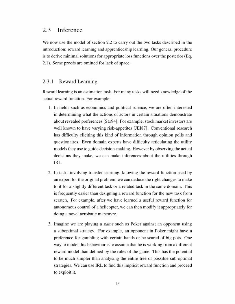
2.3 Inference

We now use the model of section 2.2 to carry out the two tasks described in theintroduction: reward learning and apprenticeship learning. Our general procedureis to derive minimal solutions for appropriate loss functions over the posterior (Eq.2.1). Some proofs are omitted for lack of space.

2.3.1 Reward Learning

Reward learning is an estimation task. For many tasks will need knowledge of theactual reward function. For example:

1. In fields such as economics and political science, we are often interestedin determining what the actions of actors in certain situations demonstrateabout revealed preferences [Sar94]. For example, stock market investors arewell known to have varying risk-appetites [JEI87]. Conventional researchhas difficulty eliciting this kind of information through opinion polls andquestionaires. Even domain experts have difficulty articulating the utilitymodels they use to guide decision-making. However by observing the actualdecisions they make, we can make inferences about the utilities throughIRL.

2. In tasks involving transfer learning, knowing the reward function used byan expert for the original problem, we can deduce the right changes to maketo it for a slightly different task or a related task in the same domain. Thisis frequently easier than designing a reward function for the new task fromscratch. For example, after we have learned a useful reward function forautonomous control of a helicopter, we can then modify it appropriately fordoing a novel acrobatic maneuvre.

3. Imagine we are playing a game such as Poker against an opponent usinga suboptimal strategy. For example, an opponent in Poker might have apreference for gambling with certain hands or be scared of big pots. Oneway to model this behaviour is to assume that he is working from a differentreward model than defined by the rules of the game. This has the potentialto be much simpler than analysing the entire tree of possible sub-optimalstrategies. We can use IRL to find this implicit reward function and proceedto exploit it.

15

Since we are picking one reward function to return from a distribution, weneed to specify a loss function. The loss function represents the cost of choosingan estimated reward function R when the true reward function is R. The mostcommon loss functions for estimation problems are the linear and squared errorloss functions:

Llinear(R, R) = ‖ R− R ‖1LSE(R, R) = ‖ R− R ‖2

where R and R are the actual and estimated rewards, respectively. If R is drawnfrom the posterior distribution (2.1), it can be shown that the expected value ofLSE(R, R) is minimized by setting R to the mean of the posterior (see [Ber93]).Similarily, the expected linear loss is minimized by setting R to the median ofthe distribution. We discuss how to compute these statistics for our posterior insection 2.3.3.

It is also common in Bayesian estimation problems to use the maximum aposteriori (MAP) value as the estimator. However in IRL problems where theposterior distribution is typically multimodal, a MAP estimator will not be as rep-resentative as measures of central tendency like the mean. For further discussionon this topic see [Ber93].

2.3.2 Apprenticeship Learning

In apprenticeship learning our goal is to learn a optimal policy for the MDP fromthe evidence of the experts actions. It is possible to do so by a more conventionalmachine learning approach i.e. learning a classifier to predict the experts actionfor each state. There are many examples of this approach, which we call imitation

learning, particularly in the robotics literature (See section 3.4 for an overview).However, there are some disadvantages to blind imitiation learning strategies:

1. We might not have enough data to learn the expert’s policy. For example,we might not have evidence for some parts of the state space. In such cases,having a model of the decision making process lets us do inference to im-prove the learned policy.

2. The experts policy might in fact be sub-optimal or inconistent. Our genera-tive model of the decision process can compensate for this by probabalistic

16

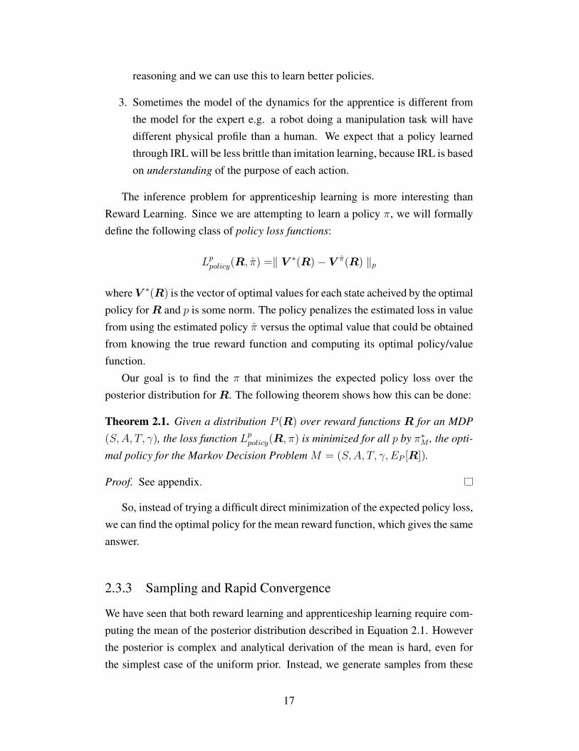
reasoning and we can use this to learn better policies.

3. Sometimes the model of the dynamics for the apprentice is different fromthe model for the expert e.g. a robot doing a manipulation task will havedifferent physical profile than a human. We expect that a policy learnedthrough IRL will be less brittle than imitation learning, because IRL is basedon understanding of the purpose of each action.

The inference problem for apprenticeship learning is more interesting thanReward Learning. Since we are attempting to learn a policy π, we will formallydefine the following class of policy loss functions:

Lppolicy(R, π) =‖ V ∗(R)− V π(R) ‖p

whereV ∗(R) is the vector of optimal values for each state acheived by the optimalpolicy forR and p is some norm. The policy penalizes the estimated loss in valuefrom using the estimated policy π versus the optimal value that could be obtainedfrom knowing the true reward function and computing its optimal policy/valuefunction.

Our goal is to find the π that minimizes the expected policy loss over theposterior distribution forR. The following theorem shows how this can be done:

Theorem 2.1. Given a distribution P (R) over reward functions R for an MDP

(S,A, T, γ), the loss function Lppolicy(R, π) is minimized for all p by π∗M , the opti-

mal policy for the Markov Decision Problem M = (S,A, T, γ, EP [R]).

Proof. See appendix.

So, instead of trying a difficult direct minimization of the expected policy loss,we can find the optimal policy for the mean reward function, which gives the sameanswer.

2.3.3 Sampling and Rapid Convergence

We have seen that both reward learning and apprenticeship learning require com-puting the mean of the posterior distribution described in Equation 2.1. Howeverthe posterior is complex and analytical derivation of the mean is hard, even forthe simplest case of the uniform prior. Instead, we generate samples from these

17

Algorithm PolicyWalk(Distribution P , MDP M , Step Size δ )1. Pick a random reward vectorR ∈ R|S|/δ.2. Repeat

(a) Pick a reward vector R uniformly at random from the neighbours ofR in R|S|/δ.(b) SetR := R with probability min{1, P (R,π)

P (R,π)}3. ReturnR

Figure 2.3: GridWalk Sampling Algorithm

distributions and then return the sample mean as our estimate of the true meanof the distribution. The sampling technique we used is based on a Markov ChainMonte Carlo (MCMC) algorithm GridWalk from [Vem05] . Gridwalk uses aMetropolis-Hastings type Markov chain on the intersection points of a grid oflength δ in the region R|S| (denoted R|S|/δ). Since the equilibrium distribution ofthis chain corresponds to our posterior, the distribution of samples will convergeto this distribution after some suitable mixing time (However it is not always clearthat this mixing time is short. We will return to this issue later.)

Using Gridwalk on our posterior distribution requires the computation of theposterior at each step of the Markov chain, which defines a reward function R.Since the algorithm only needs the ratio of probabilities between two points, thepartition function Z cancels out and can be ignored. However we still have tocalculate the optimal Q-function at every R, which is an expensive operation.Solving an MDP for every step in the Markov chain is not a feasible approach.

Instead, we can use a modified version of GridWalk called PolicyWalk(Figure 2.4) that is more efficient: While moving along a Markov chain, the sam-pler also keeps track of the optimal policy π for the current reward vector R.Observe that when π is known, the Q function can be reduced to a linear functionof the reward variables, similar to equation A.1. Thus step 3b can be performedefficiently. A change in the optimal policy can easily be detected when movingto the next reward vector in the chain R, because then for some (s, a) ∈ (S,A),Qπ(s, π(s), R) < Qπ(s, a, R) by Theorem 1.1. When this happens, the new opti-mal policy is usually only slightly different from the old one and can be computedby just a few steps of policy iteration (see [SB98]) starting from the old policy π.Hence, PolicyWalk is a correct and efficient sampling procedure. Note that theasymptotic memory complexity is the same as for GridWalk.

The second concern for the MCMC algorithm is the speed of convergenceof the Markov chain to the equilibrium distribution. The ideal Markov chain israpidly mixing (i.e. the number of steps taken to reach equilibrium is polynomially

18

Algorithm PolicyWalk(Distribution P , MDP M , Step Size δ )1. Pick a random reward vectorR ∈ R|S|/δ.2. π := PolicyIteration(M,R)3. Repeat

(a) Pick a reward vector R uniformly at random from the neighbours ofR in R|S|/δ.(b) Compute Qπ(s, a, R) for all (s, a) ∈ S,A.(c) If ∃(s, a) ∈ (S,A), Qπ(s, π(s), R) < Qπ(s, a, R)

i. π := PolicyIteration(M, R, π)

ii. SetR := R and π := π with probability min{1, P (R,π)P (R,π)}

Elsei. SetR := R with probability min{1, P (R,π)

P (R,π)}4. ReturnR

Figure 2.4: PolicyWalk Sampling Algorithm

bounded), but theoretical proofs of rapid mixing are rare. We will show that inthe special case of the uniform prior, the Markov chain for our posterior (2.1) israpidly mixing using the following result from [AK93] that bounds the mixingtime of Markov chains for pseudo-log-concave functions.

Lemma 2.2. Let F (·) be a positive real valued function defined on the cube {x ∈Rn| − d ≤ xi ≤ d} for some positive d, satisfying for all λ ∈ [0, 1] and some α, β

|f(x)− f(y)| ≤ α ‖ x− y ‖∞

and

f(λx+ (1− λ)y) ≥ λf(x) + (1− λ)f(y)− β

where f(x) = logF (x). Then the Markov chain induced by GridWalk (and

hence PolicyWalk) on F rapidly mixes to within ε of F in O(n2d2α2e2β log 1ε)

steps.

Proof. See [AK93].

Theorem 2.3. Given an MDP M = (S,A, T, γ) with |S| = N , and a distribu-

tion over rewards P (R) = PrX (R|OX ) defined by (2.1) with uniform prior PRover C = {R ∈ Rn| − Rmax ≤ Ri ≤ Rmax}. If Rmax = O(1/N) then P

can be efficiently sampled (within error ε) in O(N2 log 1/ε) steps by algorithm

PolicyWalk.

Proof. See appendix.

Note that having Rmax = O(1/N) is not really a restriction because wecan rescale the rewards by a constant factor k after computing the mean with-

19

0

10

20

30

40

50

60

70

80

10 100 1000

L

N

Reward Loss

QL/BIRLk-greedy/BIRL

QL/IRLk-greedy/IRL

Figure 2.5: Reward Loss.

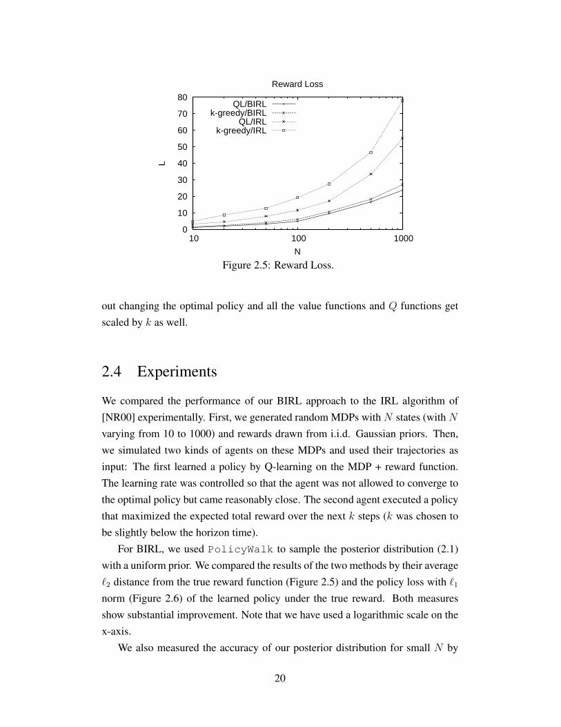
out changing the optimal policy and all the value functions and Q functions getscaled by k as well.

2.4 Experiments

We compared the performance of our BIRL approach to the IRL algorithm of[NR00] experimentally. First, we generated random MDPs with N states (with Nvarying from 10 to 1000) and rewards drawn from i.i.d. Gaussian priors. Then,we simulated two kinds of agents on these MDPs and used their trajectories asinput: The first learned a policy by Q-learning on the MDP + reward function.The learning rate was controlled so that the agent was not allowed to converge tothe optimal policy but came reasonably close. The second agent executed a policythat maximized the expected total reward over the next k steps (k was chosen tobe slightly below the horizon time).

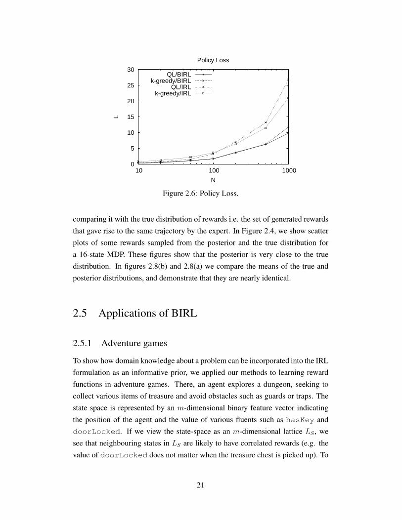
For BIRL, we used PolicyWalk to sample the posterior distribution (2.1)with a uniform prior. We compared the results of the two methods by their average`2 distance from the true reward function (Figure 2.5) and the policy loss with `1norm (Figure 2.6) of the learned policy under the true reward. Both measuresshow substantial improvement. Note that we have used a logarithmic scale on thex-axis.

We also measured the accuracy of our posterior distribution for small N by

20

0

5

10

15

20

25

30

10 100 1000

L

N

Policy Loss

QL/BIRLk-greedy/BIRL

QL/IRLk-greedy/IRL

Figure 2.6: Policy Loss.

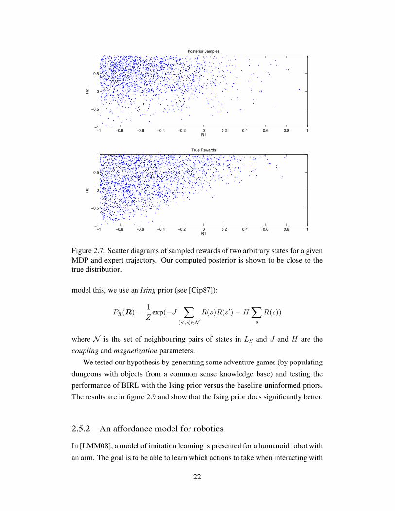
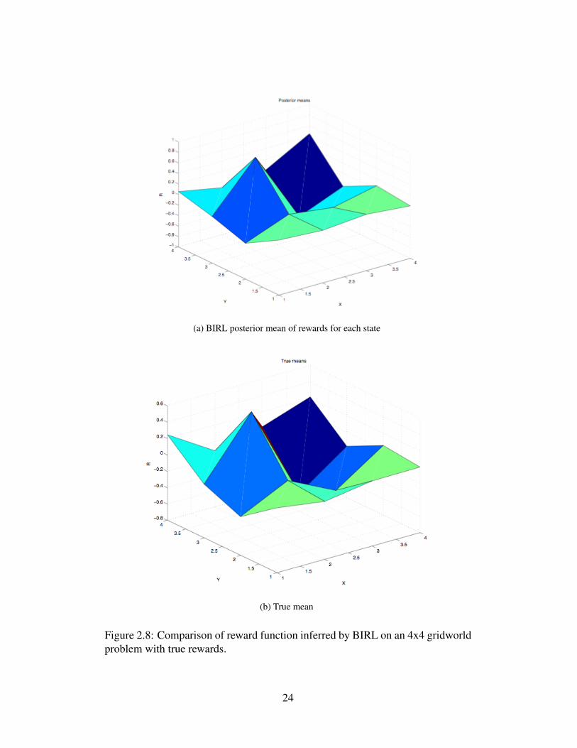
comparing it with the true distribution of rewards i.e. the set of generated rewardsthat gave rise to the same trajectory by the expert. In Figure 2.4, we show scatterplots of some rewards sampled from the posterior and the true distribution fora 16-state MDP. These figures show that the posterior is very close to the truedistribution. In figures 2.8(b) and 2.8(a) we compare the means of the true andposterior distributions, and demonstrate that they are nearly identical.

2.5 Applications of BIRL

2.5.1 Adventure games

To show how domain knowledge about a problem can be incorporated into the IRLformulation as an informative prior, we applied our methods to learning rewardfunctions in adventure games. There, an agent explores a dungeon, seeking tocollect various items of treasure and avoid obstacles such as guards or traps. Thestate space is represented by an m-dimensional binary feature vector indicatingthe position of the agent and the value of various fluents such as hasKey anddoorLocked. If we view the state-space as an m-dimensional lattice LS , wesee that neighbouring states in LS are likely to have correlated rewards (e.g. thevalue of doorLocked does not matter when the treasure chest is picked up). To

21

1 0.8 0.6 0.4 0.2 0 0.2 0.4 0.6 0.8 11

0.5

0

0.5

1

R1

R2

Posterior Samples

1 0.8 0.6 0.4 0.2 0 0.2 0.4 0.6 0.8 11

0.5

0

0.5

1

R1

R2

True Rewards

Figure 2.7: Scatter diagrams of sampled rewards of two arbitrary states for a givenMDP and expert trajectory. Our computed posterior is shown to be close to thetrue distribution.

model this, we use an Ising prior (see [Cip87]):

PR(R) =1

Zexp(−J

∑

(s′,s)∈NR(s)R(s′)−H

∑

s

R(s))

where N is the set of neighbouring pairs of states in LS and J and H are thecoupling and magnetization parameters.

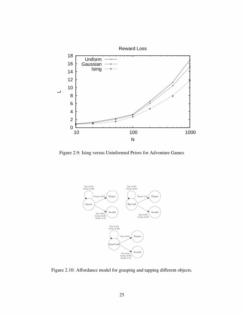
We tested our hypothesis by generating some adventure games (by populatingdungeons with objects from a common sense knowledge base) and testing theperformance of BIRL with the Ising prior versus the baseline uninformed priors.The results are in figure 2.9 and show that the Ising prior does significantly better.

2.5.2 An affordance model for robotics

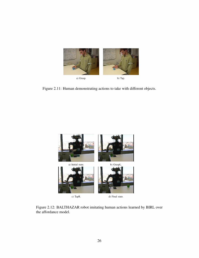
In [LMM08], a model of imitation learning is presented for a humanoid robot withan arm. The goal is to be able to learn which actions to take when interacting with

22

different objects by observing a human expert e.g. balls can be tapped away but ablock has to be picked up and set aside. The approach used is to first learn smallMDPs describing the properties and mechanics of different objects (called affor-

dances (figure 2.10)) and then apply BIRL to do apprenticeship learning. Imagesfrom an example demonstration and subsequent imitation is shown in figure 2.12.

2.6 Contributions

The main contribution of this chapter is the Bayesian Inverse Reinforcement Learn-ing approach. I derived a novel probabilistic model of the decision making pro-cess and showed how reward learning and apprenticeship learning can be donein this model. I also showed how inference in this model can be done efficientlyusing the PolicyWalk Sampling algorithm which is shown to be rapidly mixing.I described experiments using BIRL on synthetic data set, adventure games andimitation learning in robots.

23

(a) BIRL posterior mean of rewards for each state

(b) True mean

Figure 2.8: Comparison of reward function inferred by BIRL on an 4x4 gridworldproblem with true rewards.

24

0

2

4

6

8

10

12

14

16

18

10 100 1000

L

N

Reward Loss

UniformGaussian

Ising

Figure 2.9: Ising versus Uninformed Priors for Adventure Games

since this behavior arises from the presence of two objects,it is not captured in the transition model obtained from theaffordances. This means that the transition model extractedfrom the affordances necessarily includes some inaccuracies.

Big ball

Empty

Invalid

Tap (0.35)Grasp (0.60)

Tap (0.65)Grasp (0.40)

Touch (1.0)

Small ball

Empty

Invalid

Tap (0.35)Grasp (0.08)

Tap (0.01)Grasp (0.92)Touch (1.0)

Tap (0.64)

Square

Empty

Invalid

Tap (0.35)Grasp (0.20)

Tap (0.65)Grasp (0.25)Touch (1.0)

Grasp (0.55)

Fig. 6. Transition diagrams describing the transitions for each slot/object.

To test the imitation, we provided the robot with an error-free demonstration of the optimal behavior rule. As expected,the robot was successfully able to reconstruct the optimalpolicy. We also observed the learned behavior when therobot was provided with two different demonstrations, bothoptimal, as described in Table I. Each state is represented as apair (S1, S2) where each Si can take one of the values “Ball”(Big Ball), “ball” (Small Ball), “Box” (Box) or ∅ (empty).The second column of the table lists the observed actionsfor each state, and the third column lists the learned policy.Notice that, once again, the robot was able to reconstruct anoptimal policy, by choosing one of the demonstrated actionsin those states where different actions were observed.

In another experiment, we provided the robot with anincomplete and inaccurate demonstration. In particular, theaction at state (∅, Ball) was never demonstrated and theaction at state (Ball, Ball) was wrong. Table I shows thedemonstrated and learned policies. Notice that in this partic-ular case the robot was able to recover the correct policy,even with an incomplete and inaccurate demonstration,.

In Figure 7 we illustrate the execution of the optimallearned policy for the initial state (Box, SBall).2

We then tested the action recognition capabilities of therobot when using the information provided by the affor-dances. A demonstrator performed several actions upon dif-ferent objects and the robot classified these actions accordingto the observed effects (see Figure 8). The accuracy of therecognition varied, depending on the performed action, onthe demonstrator and on the speed of execution, but for allactions the recognition was successful with an error ratebetween 10% and 15%. The errors in action recognition

2For videos showing additional experiences seehttp://vislab.isr.ist.utl.pt/baltazar/demos/

TABLE IEXPERIMENT 1: ERROR FREE DEMONSTRATION (DEMONSTRATED AND

LEARNED POLICIES). EXPERIMENT 2: INACCURATE, INCOMPLETE

DEMONSTRATION (DEMONSTRATED AND LEARNED POLICIES), THE

BOXED DEMONSTRATION CORRESPOND TO THE INCOMPLETE AND

INACCURATE DEMONSTRATIONS.

State Demo1 Learned Demo2 Learned

(∅, Ball) TcR TcR - TcR(∅, Box) GrR GrR GrR GrR(∅, ball) TpR TpR TpR TpR(Ball, ∅) TcL TcL TcL TcL

(Ball, Ball) TcL,TcR TcL,TcR GrR TcL(Ball, Box) TcL,GrR GrR TcL TcL(Ball, ball) TcL TcL TcL TcL(Box, ∅) GrL GrL GrL GrL

(Box, Ball) GrL,TcR GrL GrL GrL(Box, Box) GrL,GrR GrR GrL GrL(Box, ball) GrL GrL GrL GrL

(ball, ∅) TpL TpL TpL TpL(ball, ball) TpL,TcR TpL TpL TpL(ball, Box) TpL,GrR GrR TpL TpL(ball, ball) TpL TpL TpL TpL

a) Initial state. b) GraspL.

c) TapR. d) Final state.

Fig. 7. Execution of the learned policy in state (Box, SBall).

are not surprising and are justified by the different view-points during the learning of the affordances and duringthe demonstration. In other words, the robots learns theaffordances by looking at its own body motion, but the actionrecognition is conducted from an external point-of-view. Interms of the image, this difference in viewpoints translatesin differences on the observed trajectories and velocities,leading to some occasional mis-recognitions. We refer to [6]for a more detailed discussion of this topic.

To assess the sensitivity of the imitation learning moduleto the action recognition errors, we tested the learningalgorithm for different error recognition rates. For each errorrate, we ran 100 trials. Each trial consists of 45 state-actionpairs, corresponding to three optimal policies. The obtained

Figure 2.10: Affordance model for grasping and tapping different objects.

25

a) Grasp. b) Tap.

Fig. 8. Testing action recognition from a demonstrator.

results are depicted in Figure 9.

0 0.1 0.2 0.3 0.4 0.5 0.6 0.7 0.80

0.1

0.2

0.3

0.4

0.5

0.6

0.7

action recognition error (%)

polic

y er

ror

Fig. 9. Percentage of wrong actions in the learned policy as the actionrecognition errors increase.

As expected, the error in the learned policy increases asthe number of wrongly interpreted actions increases. Notice,however, that for small error rates (≤ 15%) the robot isstill able to recover the demonstrated policy with an errorof only 1%. In particular, if we consider the error rates ofthe implemented action recognition method (between 10%and 15%), the optimal policy is accurately recovered. Thisallows us to conclude that action recognition using theaffordances is sufficiently precise to ensure the recovery ofthe demonstrated policy.

VI. CONCLUSIONS

In this paper we presented a combined architecture forrobotic imitation, based on an affordances model [9], [11]and a general imitation learning method/formalism [7]. Themodel of interaction provided by the affordances endows therobot with sufficient knowledge to be able to learn complexbehaviors by imitation.

We implemented our methodology in humanoid robotictorso. The robot had to learn a sequential task after ob-serving a person execute it. We emphasize that there is noreinforcement given to the robot by any external user andno supervision is conducted on any step of the learningprocess. The task description is extracted by observing thedemonstrator execute it. In the conducted experiments, therobot was able to successfully determine the underlying taskby relying on the knowledge provided by the affordances,

relating the actions of the robot with the resulting effects onobjects.

The results showed the method to be robust even in thepresence of incomplete and incoherent demonstractions andalso under action-recognition errors.

Future work should address the problem of recovering the(task-specific) transition model from the (task-independent)model provided by the affordances. At the present stage, thisis accomplished by an external user. We are interested indeveloping an automated method to perform this task.

REFERENCES

[1] S. Schaal, A. Ijspeert, and A. Billard, “Computational approaches tomotor learning by imitation,” Phil. Trans. of the Royal Society ofLondon: Series B, Biological Sciences, vol. 358, no. 1431, 2003.

[2] A. Alissandrakis, C. L. Nehaniv, and K. Dautenhahn, “Action, stateand effect metrics for robot imitation,” in 15th IEEE InternationalSymposium on Robot and Human Interactive Communication (RO-MAN 06), Hatfield, United Kingdom, 2006, pp. 232–237.

[3] H. Kozima, C. Nakagawa, and H. Yano, “Emergence of imitationmediated by objects,” in 2nd Int. Workshop on Epigenetic Robotics,2002.

[4] P. Fitzpatrick, G. Metta, L. Natale, S. Rao, and G. Sandini., “Learningabout objects through action: Initial steps towards artificial cognition,”in IEEE International Conference on Robotics and Automation, Taipei,Taiwan, 2003.

[5] A. Billard, Y. Epars, S. Calinon, G. Cheng, and S. Schaal, “Discover-ing optimal imitation strategies,” Robotics and Autonomous Systems,vol. 47:2-3, 2004.

[6] M. Lopes and J. Santos-Victor, “Visual transformations in gestureimitation: What you see is what you do,” in IEEE Int. Conf. Roboticsand Automation, 2003.

[7] F. Melo, M. Lopes, J. Santos-Victor, and M. I. Ribeiro, “A unifiedframework for imitation-like behaviors,” in 4th International Sympo-sium in Imitation in Animals and Artifacts, Newcastle, UK, April 2007.

[8] D. Ramachandran and E. Amir, “Bayesian inverse reinforcementlearning,” in 20th Int. Joint Conf. Artificial Intelligence, 2007.

[9] L. Montesano, M. Lopes, A. Bernardino, and J. Santos-Victor, “Model-ing affordances using bayesian networks,” in IEEE - Intelligent RoboticSystems (IROS’06), USA, 2007.

[10] J. J. Gibson, The Ecological Approach to Visual Perception. Boston:Houghton Mifflin, 1979.

[11] L. Montesano, M. Lopes, A. Bernardino, and J. Santos-Victor, “Affor-dances, development and imitation.” in IEEE - International Confer-ence on Development and Learning, London, UK, July 2007.

[12] S. Schaal, “Is imitation learning the route to humanoid robots,” Trendsin Cognitive Sciences, vol. 3(6), pp. 233–242, 1999.

[13] R. W. Byrne, “Imitation of novel complex actions: What does theevidence from animals mean?” Advances in the Study of Bahaviour,vol. 31, pp. 77–105, 2002.

[14] M. Lopes and J. Santos-Victor, “A developmental roadmap for learningby imitation in robots,” IEEE Transactions on Systems, Man, andCybernetics - Part B: Cybernetics, vol. 37, no. 2, April 2007.

[15] A. Y. Ng and S. J. Russel, “Algorithms for inverse reinforcementlearning,” in Proc. 17th Int. Conf. Machine Learning, 2000.

[16] P. Abbeel and A. Y. Ng, “Apprenticeship learning via inverse reinforce-ment learning,” in Proceedings of the 21st International Conferenceon Machine Learning (ICML’04), 2004, pp. 1–8.

[17] J. Pearl, Probabilistic Reasoning in Intelligent Systems: Networks ofPlausible Inference. Morgan Kaufmann, 1988.

[18] D. Heckerman, “A tutorial on learning with bayesian networks,” in InM. Jordan, editor, Learning in graphical models. MIT Press, 1998.

[19] C. Huang and A. Darwiche, “Inference in belief networks: A procedu-ral guide,” International Journal of Approximate Reasoning, vol. 15,no. 3, pp. 225–263, 1996.

[20] R. S. Sutton and A. G. Barto, Reinforcement Learning: An Introduc-tion. MIT Press, 1998.

[21] M. Lopes, R. Beira, M. Praça, and J. Santos-Victor, “An anthro-pomorphic robot torso for imitation: design and experiments.” inInternational Conference on Intelligent Robots and Systems, Sendai,Japan, 2004.

Figure 2.11: Human demonstrating actions to take with different objects.

since this behavior arises from the presence of two objects,it is not captured in the transition model obtained from theaffordances. This means that the transition model extractedfrom the affordances necessarily includes some inaccuracies.

Big ball

Empty

Invalid

Tap (0.35)Grasp (0.60)

Tap (0.65)Grasp (0.40)

Touch (1.0)

Small ball

Empty

Invalid

Tap (0.35)Grasp (0.08)

Tap (0.01)Grasp (0.92)Touch (1.0)

Tap (0.64)

Square

Empty

Invalid

Tap (0.35)Grasp (0.20)

Tap (0.65)Grasp (0.25)Touch (1.0)

Grasp (0.55)

Fig. 6. Transition diagrams describing the transitions for each slot/object.

To test the imitation, we provided the robot with an error-free demonstration of the optimal behavior rule. As expected,the robot was successfully able to reconstruct the optimalpolicy. We also observed the learned behavior when therobot was provided with two different demonstrations, bothoptimal, as described in Table I. Each state is represented as apair (S1, S2) where each Si can take one of the values “Ball”(Big Ball), “ball” (Small Ball), “Box” (Box) or ∅ (empty).The second column of the table lists the observed actionsfor each state, and the third column lists the learned policy.Notice that, once again, the robot was able to reconstruct anoptimal policy, by choosing one of the demonstrated actionsin those states where different actions were observed.

In another experiment, we provided the robot with anincomplete and inaccurate demonstration. In particular, theaction at state (∅, Ball) was never demonstrated and theaction at state (Ball, Ball) was wrong. Table I shows thedemonstrated and learned policies. Notice that in this partic-ular case the robot was able to recover the correct policy,even with an incomplete and inaccurate demonstration,.

In Figure 7 we illustrate the execution of the optimallearned policy for the initial state (Box, SBall).2

We then tested the action recognition capabilities of therobot when using the information provided by the affor-dances. A demonstrator performed several actions upon dif-ferent objects and the robot classified these actions accordingto the observed effects (see Figure 8). The accuracy of therecognition varied, depending on the performed action, onthe demonstrator and on the speed of execution, but for allactions the recognition was successful with an error ratebetween 10% and 15%. The errors in action recognition

2For videos showing additional experiences seehttp://vislab.isr.ist.utl.pt/baltazar/demos/

TABLE IEXPERIMENT 1: ERROR FREE DEMONSTRATION (DEMONSTRATED AND

LEARNED POLICIES). EXPERIMENT 2: INACCURATE, INCOMPLETE

DEMONSTRATION (DEMONSTRATED AND LEARNED POLICIES), THE

BOXED DEMONSTRATION CORRESPOND TO THE INCOMPLETE AND

INACCURATE DEMONSTRATIONS.

State Demo1 Learned Demo2 Learned

(∅, Ball) TcR TcR - TcR(∅, Box) GrR GrR GrR GrR(∅, ball) TpR TpR TpR TpR(Ball, ∅) TcL TcL TcL TcL

(Ball, Ball) TcL,TcR TcL,TcR GrR TcL(Ball, Box) TcL,GrR GrR TcL TcL(Ball, ball) TcL TcL TcL TcL(Box, ∅) GrL GrL GrL GrL

(Box, Ball) GrL,TcR GrL GrL GrL(Box, Box) GrL,GrR GrR GrL GrL(Box, ball) GrL GrL GrL GrL

(ball, ∅) TpL TpL TpL TpL(ball, ball) TpL,TcR TpL TpL TpL(ball, Box) TpL,GrR GrR TpL TpL(ball, ball) TpL TpL TpL TpL

a) Initial state. b) GraspL.

c) TapR. d) Final state.

Fig. 7. Execution of the learned policy in state (Box, SBall).

are not surprising and are justified by the different view-points during the learning of the affordances and duringthe demonstration. In other words, the robots learns theaffordances by looking at its own body motion, but the actionrecognition is conducted from an external point-of-view. Interms of the image, this difference in viewpoints translatesin differences on the observed trajectories and velocities,leading to some occasional mis-recognitions. We refer to [6]for a more detailed discussion of this topic.

To assess the sensitivity of the imitation learning moduleto the action recognition errors, we tested the learningalgorithm for different error recognition rates. For each errorrate, we ran 100 trials. Each trial consists of 45 state-actionpairs, corresponding to three optimal policies. The obtained

Figure 2.12: BALTHAZAR robot imitating human actions learned by BIRL overthe affordance model.

26

CHAPTER 3

A SURVEY OF INVERSEREINFORCEMENT TECHNIQUES

IRL and apprenticeship learning has become a very popular topic in recent yearsand there is much active research in this area. In this chapter, I present a com-prehensive overview of IRL solutions to date in the literature. I also cover relatedtopics such as imitation learning and biological inspirations.

The main problem that all IRL approaches have to grapple with is ill-posedness.For the original formulation of the problem ([Rus98]), an infinite set of rewardfunctions are feasible solutions (In particular, the trivial all-zero reward functionis a solution for any optimal policy). The approaches summarized below are dis-tinguished by how they choose a preferred answer or answers from the feasibleset. This is done by some combination of:

1. Additional constraints based on some principle of minimality or parsimony(e.g. regularization or maximum entropy).

2. Prior knowledge or Domain knowledge.

3.1 Max-margin Methods

BIRL is a generative approach to the problem of Reward Learning. [AN04], oneof the earliest papers on this topic, describes a discriminative approach. The set-ting is similar to ours, where the algorithm is given as input observations froman expert’s trajectories. The expert is assumed to be attempting to maximize anunknown reward function represented as a linear combination of known featureswith unknown weights, R∗(s) = w∗ · φ(s). However, they are ultimately not con-cerned with the accuracy of the reward function if the performance of the resultingpolicy is close to that of the expert. In their formulation, policies are defined tobe mappings from states to probability distributions over actions (stochastic poli-

27

cies). The feature expectation vector is defined to be

µ(π) = E[∞∑

t=0

γtφ(st)|π].

And therefore, the value function is

Eso∼D[V π(s0)] = w · µ(π).

The apprenticeship learning algorithm aims to find a policy π such that ‖ µ(π)−µE ‖2≤ ε for some small ε, where µE is the empirical estimate of the featurevector µ over the expert trajectories:

µE =1

m

m∑

i=1

∞∑

t=0

γtφ(s(i)t ).

It can then be shown that for any w ∈ Rk, (‖ w ‖1≤ 1)

|E[∞∑

t=0

γtR(st)|πE]− E[∞∑

t=0

γtR(st)|π]| ≤ ε

and thus the learned policy performs at least as well as the expert’s empirical per-formance. The algorithm for finding this policy proceeds by iteratively guessingreward functions on which the expert does better by a fixed margin than any previ-ously found policy. This “max-margin” step can be a posed as a quadratic programsimilar to Support Vector Machines [CV95]. [AN04] also present a projection-based algorithm for finding this optimal policy. Using this algorithm they weresuccesfully able to teach an agent different styles of driving (e.g. aggressive, cau-tious) in a car driving simulator.

[ADNT08] applied this algorithm to the problem of motion planning in park-ing lots for Junior, the Stanford DARPA urban challenge entry. The features ofthe reward function are associated with potential fields a common trick used inreal-time robot motion control to model the objectives of progressing towards thegoal while steering clear of obstacles. The IRL algorithm learns the weight to beassociated with each potential field term to get a good tradeoff between the costterms and safely steer the car. In [CAN09], autonomous execution of a wide rangeof challenging aerobatic manuevers on a helicopter is demonstrated using appren-ticeship learning. The reward weights are adjusted following the “philosophy, but

28

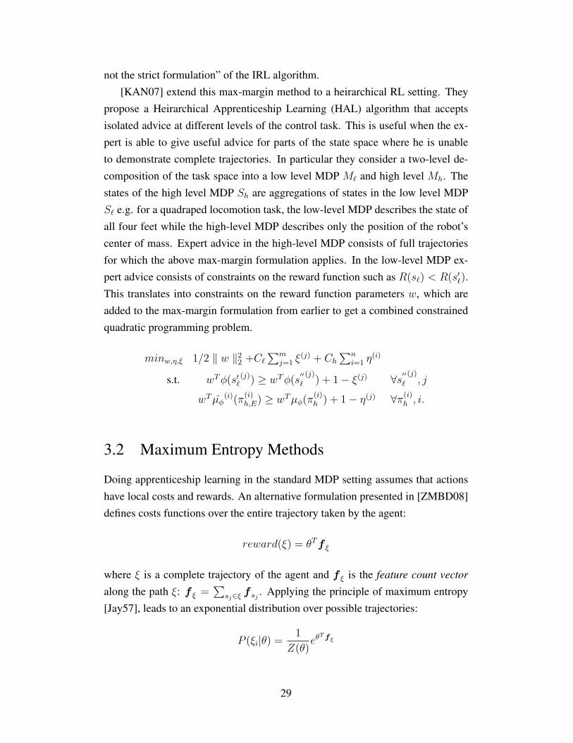
not the strict formulation” of the IRL algorithm.[KAN07] extend this max-margin method to a heirarchical RL setting. They

propose a Heirarchical Apprenticeship Learning (HAL) algorithm that acceptsisolated advice at different levels of the control task. This is useful when the ex-pert is able to give useful advice for parts of the state space where he is unableto demonstrate complete trajectories. In particular they consider a two-level de-composition of the task space into a low level MDP M` and high level Mh. Thestates of the high level MDP Sh are aggregations of states in the low level MDPS` e.g. for a quadraped locomotion task, the low-level MDP describes the state ofall four feet while the high-level MDP describes only the position of the robot’scenter of mass. Expert advice in the high-level MDP consists of full trajectoriesfor which the above max-margin formulation applies. In the low-level MDP ex-pert advice consists of constraints on the reward function such as R(s`) < R(s′`).This translates into constraints on the reward function parameters w, which areadded to the max-margin formulation from earlier to get a combined constrainedquadratic programming problem.

minw,η,ξ 1/2 ‖ w ‖22 +C`∑m

j=1 ξ(j) + Ch

∑ni=1 η

(i)

s.t. wTφ(s′`(j)) ≥ wTφ(s

′′`

(j)) + 1− ξ(j) ∀s′′`

(j), j

wT µφ(i)(π

(i)h,E) ≥ wTµφ(π

(i)h ) + 1− η(j) ∀π(i)

h , i.

3.2 Maximum Entropy Methods

Doing apprenticeship learning in the standard MDP setting assumes that actionshave local costs and rewards. An alternative formulation presented in [ZMBD08]defines costs functions over the entire trajectory taken by the agent:

reward(ξ) = θTf ξ

where ξ is a complete trajectory of the agent and f ξ is the feature count vector

along the path ξ: f ξ =∑

sj∈ξ f sj . Applying the principle of maximum entropy[Jay57], leads to an exponential distribution over possible trajectories:

P (ξi|θ) =1

Z(θ)eθT fξ

29

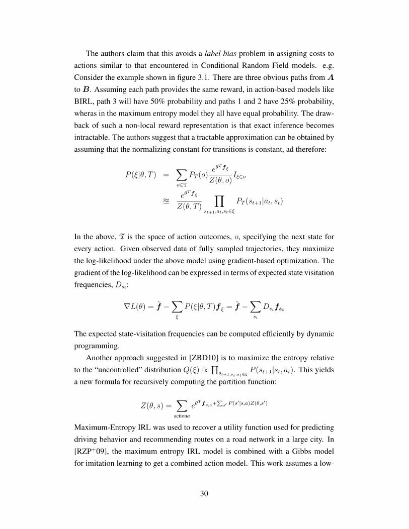
The authors claim that this avoids a label bias problem in assigning costs toactions similar to that encountered in Conditional Random Field models. e.g.Consider the example shown in figure 3.1. There are three obvious paths from A

toB. Assuming each path provides the same reward, in action-based models likeBIRL, path 3 will have 50% probability and paths 1 and 2 have 25% probability,wheras in the maximum entropy model they all have equal probability. The draw-back of such a non-local reward representation is that exact inference becomesintractable. The authors suggest that a tractable approximation can be obtained byassuming that the normalizing constant for transitions is constant, ad therefore:

P (ξ|θ, T ) =∑

o∈TPT (o)

eθT fξ

Z(θ, o)Iξ∈o

ueθT fξ

Z(θ, T )

∏

st+1,at,st∈ξPT (st+1|at, st)

In the above, T is the space of action outcomes, o, specifying the next state forevery action. Given observed data of fully sampled trajectories, they maximizethe log-likelihood under the above model using gradient-based optimization. Thegradient of the log-likelihood can be expressed in terms of expected state visitationfrequencies, Dsi:

∇L(θ) = f −∑

ξ

P (ξ|θ, T )f ξ = f −∑

si

Dsifsi

The expected state-visitation frequencies can be computed efficiently by dynamicprogramming.

Another approach suggested in [ZBD10] is to maximize the entropy relativeto the “uncontrolled” distribution Q(ξ) ∝ ∏

st+1,st,at∈ξP (st+1|st, at). This yields

a new formula for recursively computing the partition function:

Z(θ, s) =∑

actiona

eθT fs,a+

∑s′ P (s′|s,a)Z(θ,s′)

Maximum-Entropy IRL was used to recover a utility function used for predictingdriving behavior and recommending routes on a road network in a large city. In[RZP+09], the maximum entropy IRL model is combined with a Gibbs modelfor imitation learning to get a combined action model. This work assumes a low-

30

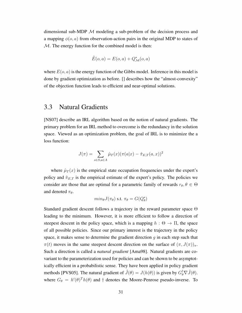
dimensional sub-MDP M modeling a sub-problem of the decision process anda mapping φ(o, a) from observation-action pairs in the original MDP to states ofM. The energy function for the combined model is then:

E(o, a) = E(o, a) +Q∗M(o, a)

whereE(o, a) is the energy function of the Gibbs model. Inference in this model isdone by gradient optimization as before. [] describes how the “almost-convexity”of the objection function leads to efficient and near-optimal solutions.

3.3 Natural Gradients

[NS07] describe an IRL algorithm based on the notion of natural gradients. Theprimary problem for an IRL method to overcome is the redundancy in the solutionspace. Viewed as an optimization problem, the goal of IRL is to minimize the aloss function:

J(π) =∑

s∈S,a∈AµT (x)(π(a|x)− πE,T (a, x))2

where µT (x) is the empirical state occupation frequencies under the expert’spolicy and πE,T is the empirical estimate of the expert’s policy. The policies weconsider are those that are optimal for a parametric family of rewards rθ, θ ∈ Θ

and denoted πθ.minθJ(πθ) s.t. πθ = G(Q∗θ)

Standard gradient descent follows a trajectory in the reward parameter space Θ

leading to the minimum. However, it is more efficient to follow a direction ofsteepest descent in the policy space, which is a mapping h : Θ → Π, the spaceof all possible policies. Since our primary interest is the trajectory in the policyspace, it makes sense to determine the gradient direction g in each step such thatπ(t) moves in the same steepest descent direction on the surface of (π, J(π))π.Such a direction is called a natural gradient [Ama98]. Natural gradients are co-variant to the parameterization used for policies and can be shown to be asymptot-ically efficient in a probabilistic sense. They have been applied in policy gradientmethods [PVS05]. The natural gradient of J(θ) = J(h(θ)) is given by G†θ∇J(θ).where Gθ = h′(θ)Th(θ) and † denotes the Moore-Penrose pseudo-inverse. To

31

compute the natural gradient, we need the partial derivatives ∂Q∗θ(x, a)/∂θk. Us-ing Frechet subdifferentials, it is shown that these can be calculated by solving thefollowing fixed point equation:

φθ(s, a) = (r′θ(s, a))T + γ∑

s′∈SP (s′|s, a)

∑

a′∈Aπ(a′|s′)φθ(s′, a′)

3.4 Direct Imitation Learning

Direct imitation learning is an attempt to mimic the policy of the expert directlywithout understanding objectives or motivation. As explained in chapter 2, it ismuch less robust to error and fails to generalize well in situations where we donot have access to the expert’s entire policy or when there is a difference in theoperating environment of the expert and the learner. Nevertheless it is a popu-lar approach in robotics because of its simplicity and the presence of analogs inbiology [MRB+99] and developmental psychology [MD03].

[AS97] combines a direct imitation learning with a model-based RL algorithmand a crude form of reward learning to do a pendulum balancing task with theactuators of a robot. They provide a good discussion on the interplay betweenthese different methods and show that all 3 were necessary to attain success atthis task. [HD94] built a robot controller using imitation learning, where a robotlearns to follow another through a maze and learns to associate its perceptions withthe at locations where the teacher carries out a significant action with the actionit subsequently undertakes as a result of its innate teacher-following behaviour.In [SHKM92], the complex motor skills necessary for autopiloting an aircraft islearned directly using a decision tree with input from logs of human subjects ina flight simulator. [AM02] presents an apporach for imitation learning of humanmotion using a heirarchy of motion primitives. The learning process is HMM-based and inspired by mirror neuron models [MRB+99] in cognitive science.

3.5 Comparison

Recently, a comparison of existing IRL approaches was made and the results re-ported in [ZBD10]. The application was modeling the route preferences of Taxi-cab drivers in an inner city (figure 3.1). The sequential choices made by drivers at

32

for IRL. For instance, the highest reward policy may not bethe most probable policy in the model, and policies withthe same expected reward can have different probabilities.Compared to our maximum entropy distribution over paths,this model gives higher probability mass to paths with asmaller branching factor and lower probability mass to thosewith a higher branching factor.

Comparative EvaluationWe now evaluate each model’s ability to model paths in thewithheld testing set after being trained on the training setgiven the path’s origin and destination. We use three differ-ent metrics. The first compares the model’s most likely pathestimate with the actual demonstrated path and evaluates theamount of route distance shared. The second shows whatpercentage of the testing paths match at least 90% (distance)with the model’s predicted path. The final metric measuresthe average log probability of paths in the training set un-der the given model. For path matching, we evaluate boththe most likely path within the action-based model and thelowest cost path using the weights learned from the action-based model. We additionally evaluate a model based onexpected travel times that weights the cost of a unit distanceof road to be inversely proportional to the speed of the road,and predicts the fastest (i.e., lowest cost) route given thesecosts.

Matching 90% Match Log ProbTime-based 72.38% 43.12% N/AMax Margin 75.29% 46.56% N/AAction 77.30% 50.37% -7.91Action (costs) 77.74% 50.75% N/AMaxEnt paths 78.79% 52.98% -6.85

Table 1: Comparison of different models’ abilities to matchmost likely path predictions to withheld paths (average per-centage of distance matching and percentage of exampleswhere at least 90% of the paths’ distances match) and theprobability of withheld paths (average log probability).

The results of this analysis are shown in Table 1. For eachof these metrics, our maximum entropy model shows signif-icant (α < .01) improvements over the other models.

Interstate Local Road0

50

100

150

200

Road type

Seco

nds

Learned Road Costs

Figure 3: Learned costs of turns (left) and miles of differ-ent road types (right) normalized to seconds (with interstatedriving fixed to 65 miles per hour).

The learned cost values using our MaxEnt model areshown in Figure 3. Additionally, we learn a fixed per edge

cost of 1.4 seconds that helps to penalize paths composed ofmany short roads.

Applications

Beyond the route recommendation application describedabove, our approach opens up a range of possibilities fordriver prediction. Route recommendation can be easily per-sonalized based on passive observation of a single user. Fur-ther, by learning a probability distribution over driver pref-erences, destinations, and routes the MaxEntIRL model ofdriver behavior can go beyond route recommendation, tonew queries like: “What is the probability the driver willtake this street?” This enables a range of new applications,including, e.g., warning drivers about unanticipated trafficproblems on their route without ever explicitly having toquery the user about route or destination; optimizing bat-tery and fuel consumption in a hybrid vehicle; and activatingtemperature controls at a home prior to the driver’s arrival.

So far, we have not described situations where the driver’sintended destination is unknown. Fortunately we can reasoneasily about intended destinations by applying Bayes’ the-orem to our model of route preference. Consider the casewhere we want the posterior probability of a set of destina-tions given a partially traveled path from A to B.

P (dest|ζA→B) ∝ P (ζA→B |dest)P (dest)

∝∑

ζB→desteθ"fζ

∑ζA→dest

eθ"fζP (dest)

These quantities can easily be computed using our inferencealgorithm (Algorithm 1).

Figure 4: Destination distribution (from 5 destinations) andremaining path distribution given partially traveled path.The partially traveled path is heading westward, which isa very inefficient (i.e., improbable) partial route to any ofthe eastern destinations (3, 4, 5). The posterior destinationprobability is split between destinations 1 and 2 primarilybased on the prior distribution on destinations.

Figure 4 shows one particular destination prediction prob-lem. We evaluate our model’s ability to predict destinationsfor routes terminating in one of five locations around the city(Figure 4) based on the fraction of total route observed (Fig-ure 5). We use a training set to form a prior over destinationsand evaluate our model on a withheld test set. Incorporatingadditional contextual information into this prior distribution,like time of day, will be beneficial for predicting the desti-nations of most drivers.

Figure 3.1: The Taxicab domain from [ZBD10]. IRL algorithms were used toinfer drivers’ utilities for different routes from the choices made at intersections.

Approach Match 90% MatchTime-based 72.38% 43.12 %

[AN04] 75.29% 46.56 %[NS07] 77.30% 50.37%[RA07] 77.74% 50.75 %

[ZMBD08] 78.79% 52.98%

Table 3.1: Performance of various IRL approaches on the Taxicab domain. Scoresreport are %ages of routes matched correctly. Reproduced from [ZBD10]

intersections can be formulated as a decision-making problem and the perceivedutilites of different routes can be inferred by tracking their behaviour over timewith GPS sensors and applying IRL. One caveat is that the choice of route is aglobal choice made at the beginning of the journey. Applying IRL based on se-quential decision model introduces a label-bias problem. This was overcome in[ZBD10] by using an appropriate prior. The results (partially reproduced in table3.5 show that BIRL performs quite competitively on two measures (full matchand 90% match with the designated route). Apart from the Max Entropy methodof [ZBD10], which in part was developed for this particular problem, BIRL doesbest on both measures. However, all the approaches did quite well.

3.6 Related Areas

In [CKO01], distributions are considered over influence diagrams, which are moregeneral structures than MDPs. [PB03] discusses a Bayesian approach to imitat-ing the actions of a mentor during reinforcement learning whereas the traditionalliterature on apprenticeship learning tries to mimic the behaviour of the expertdirectly [AS97].

33

Outside of computer science, IRL-related problems have been studied in var-ious guises. In the physical sciences, there is a body of work on inverse problem

theory, i.e. infering values of model parameters from observations of a physi-cal system [Tar05]. In control theory, [BGFB94] solved the problem, posed byKalman, of recovering the objective function for a deterministic linear systemwith quadratic costs. There is also a lot of work on the structural estimation ofMDPs in econometrics e.g. [Sar94].

34

CHAPTER 4

BAYESIAN REWARD SHAPING

In this chapter we continue the discussion of the role played by reward functionsin Reinforcement Learning. Here, we discuss reward shaping which involves twoagents, a teacher and student operating in some environment. The student is per-forming a conventional Reinforcement Learning algorithm in some environmentwhile the teacher is trying to modify or shape the reward signal he receives tospeed up the learning process. I discuss how the generative model described in2 can be adapted to finding good shaped Reward functions. I discuss two typesof reward priors that encourage fast convergence of RL: one based on a anti-ferromagnetic Ising model and another on using common sense knowledge aboutthe problem features.

4.1 Reward Shaping

The example that we will use to motivate this work will be the following (calledthe “Banana game” for historical reasons) (Figure 4.1): Our agent is trapped in adungeon, and he can only escape through a door in one of the cells. The door islocked but fortunately there is a key that can be found in one of the rooms of thedungeon. The agent must locate this key, pick it up and carry it to the room withthe door, use it to open the door and exit to freedom. There is also a banana inone of the other rooms that the agent could try opening the door with (Though hewouldn’t get very far).

The agent must execute a complicated series of actions involving finding andpicking up the key, then using it to unlock the door and exit the dungeon he istrapped in. The reward is only received at the end of a successful run, however alearning algorithm must be able to assign credit for success to the earlier actions.Without any other guidance or domain knowledge, RL would take many trialsbefore it successfully learns the value of these actions. This is called the temporal

35

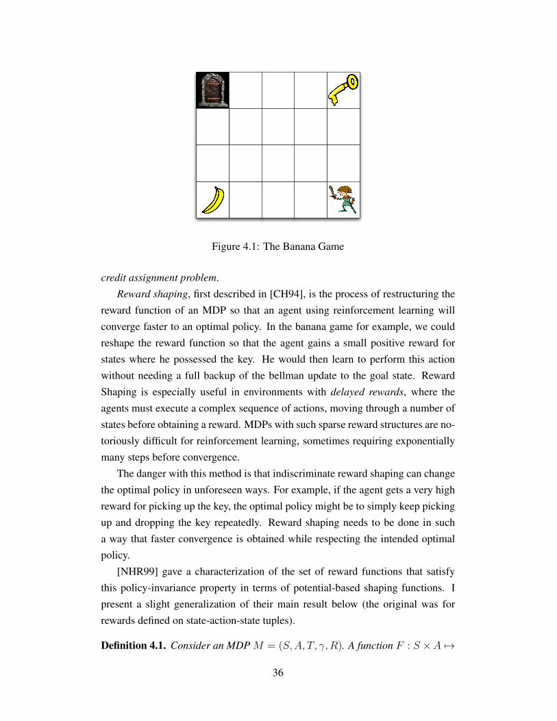
Figure 4.1: The Banana Game

credit assignment problem.Reward shaping, first described in [CH94], is the process of restructuring the

reward function of an MDP so that an agent using reinforcement learning willconverge faster to an optimal policy. In the banana game for example, we couldreshape the reward function so that the agent gains a small positive reward forstates where he possessed the key. He would then learn to perform this actionwithout needing a full backup of the bellman update to the goal state. RewardShaping is especially useful in environments with delayed rewards, where theagents must execute a complex sequence of actions, moving through a number ofstates before obtaining a reward. MDPs with such sparse reward structures are no-toriously difficult for reinforcement learning, sometimes requiring exponentiallymany steps before convergence.

The danger with this method is that indiscriminate reward shaping can changethe optimal policy in unforeseen ways. For example, if the agent gets a very highreward for picking up the key, the optimal policy might be to simply keep pickingup and dropping the key repeatedly. Reward shaping needs to be done in sucha way that faster convergence is obtained while respecting the intended optimalpolicy.

[NHR99] gave a characterization of the set of reward functions that satisfythis policy-invariance property in terms of potential-based shaping functions. Ipresent a slight generalization of their main result below (the original was forrewards defined on state-action-state tuples).

Definition 4.1. Consider an MDP M = (S,A, T, γ, R). A function F : S ×A 7→

36

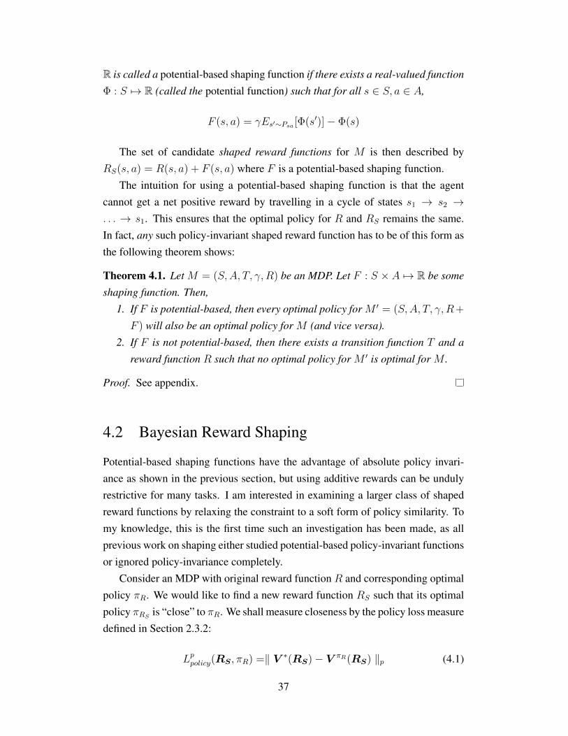
R is called a potential-based shaping function if there exists a real-valued function

Φ : S 7→ R (called the potential function) such that for all s ∈ S, a ∈ A,

F (s, a) = γEs′∼Psa [Φ(s′)]− Φ(s)

The set of candidate shaped reward functions for M is then described byRS(s, a) = R(s, a) + F (s, a) where F is a potential-based shaping function.

The intuition for using a potential-based shaping function is that the agentcannot get a net positive reward by travelling in a cycle of states s1 → s2 →. . . → s1. This ensures that the optimal policy for R and RS remains the same.In fact, any such policy-invariant shaped reward function has to be of this form asthe following theorem shows:

Theorem 4.1. Let M = (S,A, T, γ, R) be an MDP. Let F : S × A 7→ R be some

shaping function. Then,

1. If F is potential-based, then every optimal policy for M ′ = (S,A, T, γ, R+

F ) will also be an optimal policy for M (and vice versa).

2. If F is not potential-based, then there exists a transition function T and a

reward function R such that no optimal policy for M ′ is optimal for M .

Proof. See appendix.

4.2 Bayesian Reward Shaping

Potential-based shaping functions have the advantage of absolute policy invari-ance as shown in the previous section, but using additive rewards can be undulyrestrictive for many tasks. I am interested in examining a larger class of shapedreward functions by relaxing the constraint to a soft form of policy similarity. Tomy knowledge, this is the first time such an investigation has been made, as allprevious work on shaping either studied potential-based policy-invariant functionsor ignored policy-invariance completely.

Consider an MDP with original reward function R and corresponding optimalpolicy πR. We would like to find a new reward function RS such that its optimalpolicy πRS is “close” to πR. We shall measure closeness by the policy loss measuredefined in Section 2.3.2:

Lppolicy(RS, πR) =‖ V ∗(RS)− V πR(RS) ‖p (4.1)

37

where p is some norm. Recall that this measures the difference in value betweenusing the optimal policy for RS and using the policy πR while collecting rewardsaccording to RS . The larger this difference, the worse RS is as a motivation forpursuing the policy πR.

We will in fact describe a probability distribution over candidate shaped re-ward functions RS . The distribution is motivated by the derivation of section2.2.1. There, we showed that for a set of observations from an expert policy, OX ,the corresponding likelihood model for reward functions is:

PrX (OX |R) =1

ZeαXE(OX ,R)

where E(OX ,R) =∑

(si,ai)∈QX Q∗(si, ai,R). For our Bayesian Reward Shaping

formulation, we are interested in a distribution over RS and we set OX = πR i.e.we use knowledge of the entire original policy as evidence when shaping:

PrπR(πR|RS) =1

ZeαXE(πR,RS)

This likelihood model for RS enforces a soft form of the policy invariance wewanted.

Next we introduce a shaping prior PRS(·) on reward functions RS designed toencourage intelligent directed exploration by the student. The choice of this prioris made by the teacher and can be done in either a domain-independent or domain-dependent manner. For example, a prior can be chosen that “spreads” the totalreward to all parts of the state space alleviating the temporal credit-assignmentproblem. Or the teacher can use knowledge of the problem domain to bias towardsstate-action pairs he expects will have high Q-values. I will show examples of bothapproaches in subsequent sections.

Using Bayes theorem again, we obtain a posterior distribution over shapedreward functions:

Pr(RS|πR) =PrX (πR|RS)PRS

(RS)

Pr(πR)

=1

Z ′eαXE(OX ,R)PRS(RS) (4.2)

Either by sampling from this distribution or computing and using the expec-tation as in section 2.3.3, we obtain a reward function suitable for shaping. ByTheorem 2.1, this minimizes the policy loss(Equation 4.1) as well.

38

If for some reason we wish to only keep part of the intended policy constantand not be concerned about other parts of the state space, we can do so by restrict-ing the evidence OX appropriately.

4.3 Priors

The BRS model described above shows how to sample from a distribution of re-ward functions similar in policy space to an initial reward function. The purposeof shaping however is to find shaped rewards that can make the agent learn thepolicy faster. This is done by choosing an appropriate prior that selects rewardfunctions that are easy to learn from. I suggest two kinds of priors that are help-ful in this regard. The first one is an uninformed prior that tries to “spread” thetotal reward around the state space as much as possible. It is based on the intu-ition that a denser reward function encourages faster exploration and convergence.The second one uses descriptive knowledge of the problem domain to encouragebehaviours that we expect to be part of an optimal policy.

4.3.1 Anti-ferromagnetic Ising Priors

In section 2.5.1, I describe the Ising prior for BIRL based on the Ising model ofelectron spin configurations in statistical physics:

PR(R) =1

Zexp(−J

∑

(s′,s)∈NR(s)R(s′)−H

∑

s

R(s))

where N is the set of neighbouring pairs of states in LS and J and H arethe coupling and magnetization parameters. For BIRL, we used H, J < 0. Thiscorresponds to the ferromagnetic phase in the Ising model where neighbouringatoms have correlated spins. In the MDP, this translates to neighbouring stateshaving correlated rewards, which corresponds to our intuitions about real rewardfunctions.

Shaped reward functions are synthetic reward functions designed not to be re-alistic but to promote faster convergence of learning. Therefore, I suggest usingthe Ising model in its anti-ferromagnetic phase (J,H > 0). In molecular dynam-ics, this corresonds to the state where neighbouring atoms have opposite spins. Inour case, neighbouring states in the MDP will have opposite rewards. In combina-

39

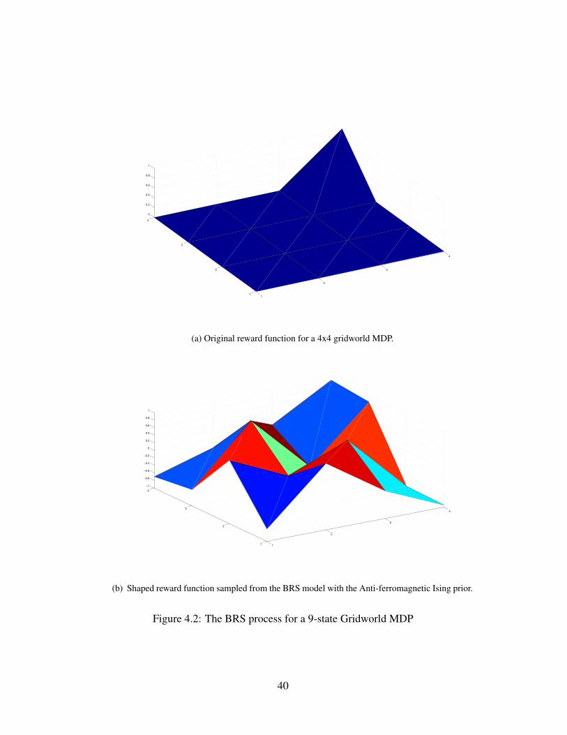
1

2

3

4

1

2

3

4

0

0.2

0.4

0.6

0.8

1

(a) Original reward function for a 4x4 gridworld MDP.

1

2

3

4

1

2

3

4

−1

−0.8

−0.6

−0.4

−0.2

0

0.2

0.4

0.6

0.8

1

(b) Shaped reward function sampled from the BRS model with the Anti-ferromagnetic Ising prior.

Figure 4.2: The BRS process for a 9-state Gridworld MDP

40

0 2000 4000 6000 8000 10000 120000

0.1

0.2

0.3

0.4

0.5

0.6

0.7

Number of learning steps

Avera

ge v

alu

e

shaped reward

original reward

Figure 4.3: Average value obtained by learned policy for both reward functionsafter a fixed number of learning steps using Q-learning. The experiments weredone over a set of 100 randomly generated transition models.

tion with the likelihood model that biases towards the designated optimal policy,the effect of this prior is to spread the total reward of the MDP to as many statesas possible yielding a denser reward function that is easier to learn from.

As an example, consider the reward function for a 9-state Gridworld MDPshown in figure 4.2(a). In figure 4.2(b) I show the mean reward E[RS] of the BRSposterior (Equation 4.2). This reward function preserves the optimal policy of theoriginal reward function but is denser. Reinforcement learning algorithms such asQ-learning receive their feedback eariler in the training process and converge tothe optimal policy faster (Figure 4.3).

4.4 Priors from Domain Knowledge

One of the challenges of RL is understanding how learning algorithms can exploitrelevant domain knowledge about a specific problem. Domain knowledge couldbe information about the problem provided by an expert in declarative form, or itcould be common sense knowledge from a Knowledge Base (KB) such as CYC[RRG05] or ConceptNet [LS04]. We expect that the more knowledge there isabout a learning problem the easier the problem should become since less explo-

41

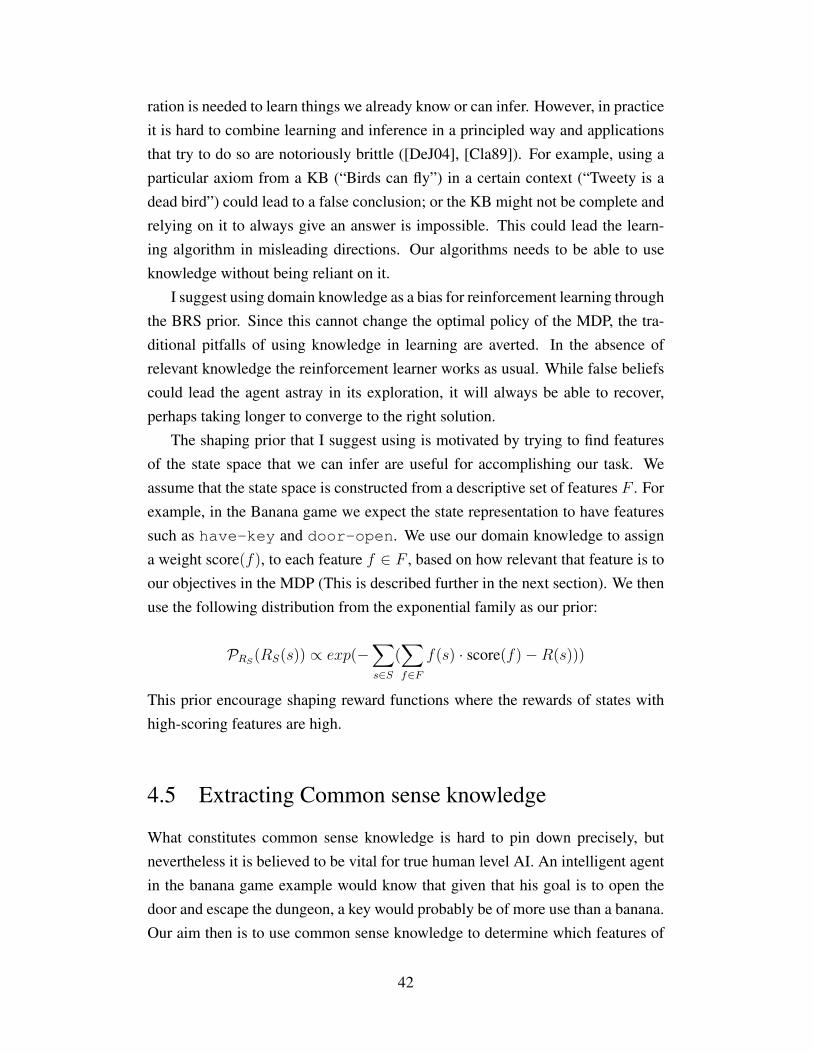
ration is needed to learn things we already know or can infer. However, in practiceit is hard to combine learning and inference in a principled way and applicationsthat try to do so are notoriously brittle ([DeJ04], [Cla89]). For example, using aparticular axiom from a KB (“Birds can fly”) in a certain context (“Tweety is adead bird”) could lead to a false conclusion; or the KB might not be complete andrelying on it to always give an answer is impossible. This could lead the learn-ing algorithm in misleading directions. Our algorithms needs to be able to useknowledge without being reliant on it.

I suggest using domain knowledge as a bias for reinforcement learning throughthe BRS prior. Since this cannot change the optimal policy of the MDP, the tra-ditional pitfalls of using knowledge in learning are averted. In the absence ofrelevant knowledge the reinforcement learner works as usual. While false beliefscould lead the agent astray in its exploration, it will always be able to recover,perhaps taking longer to converge to the right solution.

The shaping prior that I suggest using is motivated by trying to find featuresof the state space that we can infer are useful for accomplishing our task. Weassume that the state space is constructed from a descriptive set of features F . Forexample, in the Banana game we expect the state representation to have featuressuch as have-key and door-open. We use our domain knowledge to assigna weight score(f), to each feature f ∈ F , based on how relevant that feature is toour objectives in the MDP (This is described further in the next section). We thenuse the following distribution from the exponential family as our prior:

PRS(RS(s)) ∝ exp(−∑

s∈S(∑

f∈Ff(s) · score(f)−R(s)))

This prior encourage shaping reward functions where the rewards of states withhigh-scoring features are high.

4.5 Extracting Common sense knowledge

What constitutes common sense knowledge is hard to pin down precisely, butnevertheless it is believed to be vital for true human level AI. An intelligent agentin the banana game example would know that given that his goal is to open thedoor and escape the dungeon, a key would probably be of more use than a banana.Our aim then is to use common sense knowledge to determine which features of

42

the state space are relevant to the task at hand.There have been a number of initiatives to construct large common sense

knowledge bases. At present the largest and most comprehensive of these is Cy-corp Inc’s CYC [RRG05]. The representation language for CYC is a higher-order predicate logic that includes support for contexts, modal extensions andnon-monotonicity. An example of a common sense axiom in CYC relevant to thedoor example above is:

(implies (and

(agent-Possesses ?Agent ?Key)

(isa ?Key Key)

(isa ?Door Door)

(opensWith ?Agent ?Door ?Key ?T1)

(immediatelyAfter ?T1 ?T2))

(holdsIn ?T2 (isOpen ?Door)))

The ideal way to exploit this knowledge in the Banana game is to performabduction (backward inference) on the above axiom and the goal condition:

(holdsIn END (isOpen Dungeon-Door)))

One of the conclusions of this abduction would be the statement:

(agent-Possesses Agent Dungeon-Door-Key)

From this, we can conclude that actions involving the key are relevant to theagent’s goals and proceed to shape them with positive rewards.

The idea of using inference in a logical KB to construct shaping rewards iscompelling but difficult to implement. Translating between the state representa-tion used in our MDP to the logical axioms required by CYC to do inference is themain difficulty. In contrast, the semantic network representation of ConceptNet[LS04] is much easier to work with. Knowledge in ConceptNet is less structuredthan in CYC, and is closer to natural language. An example of ConceptNet’srepresentation (for the concept ’key’) is shown in figure 4.4.

Our algorithm for determining relevant features of the state space from Con-ceptNet is shown in figure 4.5. Given the underlying MDP, we first find the fea-tures of the goal states that define the goal condition. Our method (algorithm

43

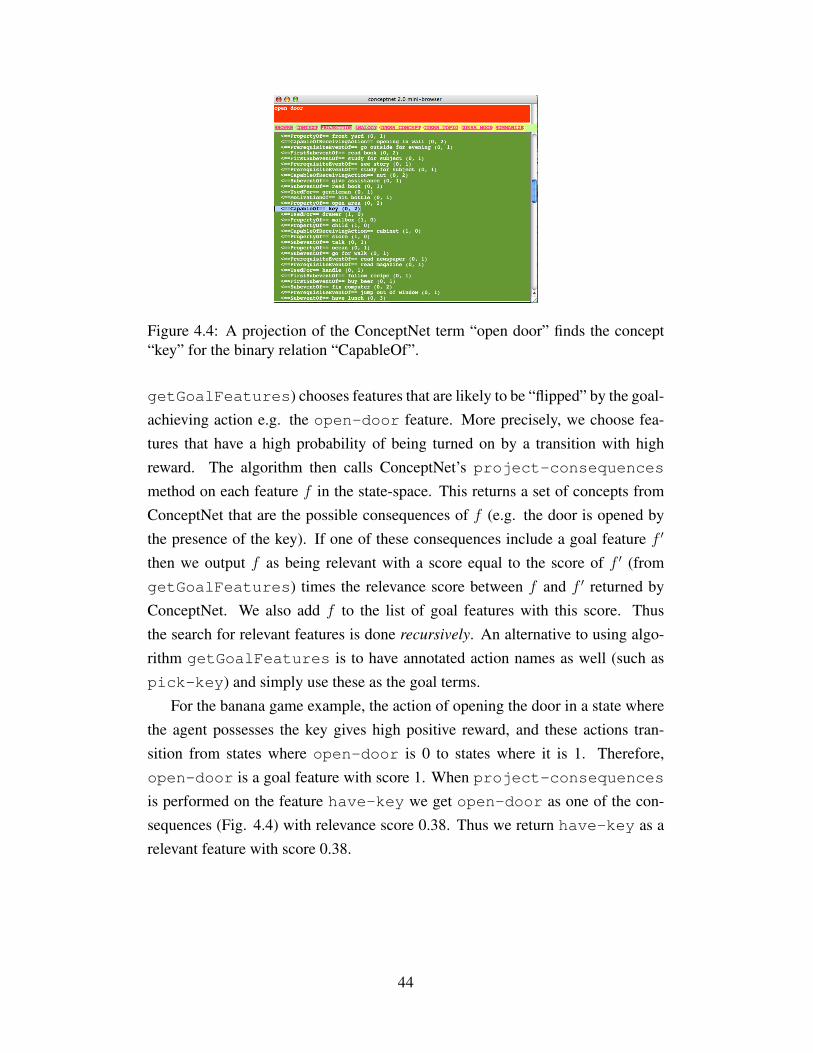
Figure 4.4: A projection of the ConceptNet term “open door” finds the concept“key” for the binary relation “CapableOf”.

getGoalFeatures) chooses features that are likely to be “flipped” by the goal-achieving action e.g. the open-door feature. More precisely, we choose fea-tures that have a high probability of being turned on by a transition with highreward. The algorithm then calls ConceptNet’s project-consequences

method on each feature f in the state-space. This returns a set of concepts fromConceptNet that are the possible consequences of f (e.g. the door is opened bythe presence of the key). If one of these consequences include a goal feature f ′

then we output f as being relevant with a score equal to the score of f ′ (fromgetGoalFeatures) times the relevance score between f and f ′ returned byConceptNet. We also add f to the list of goal features with this score. Thusthe search for relevant features is done recursively. An alternative to using algo-rithm getGoalFeatures is to have annotated action names as well (such aspick-key) and simply use these as the goal terms.

For the banana game example, the action of opening the door in a state wherethe agent possesses the key gives high positive reward, and these actions tran-sition from states where open-door is 0 to states where it is 1. Therefore,open-door is a goal feature with score 1. When project-consequencesis performed on the feature have-key we get open-door as one of the con-sequences (Fig. 4.4) with relevance score 0.38. Thus we return have-key as arelevant feature with score 0.38.

44

Algorithm FindRelevantConcept (MDP M = (S,A, T, γ,R) )1. GF := getGoalFeatures(M)2. For each feature f of S not in GF3. For (f ′, t′) ∈ GF4. If (f ′, t′) ∈ ConceptNet.

project-consequences(f) and tt′ > 0.015. RF := RF ∪ (f, tt′)6. GF := GF ∪ (f, tt′)7. Return RF

Algorithm getGoalFeatures (MDP M = (S,A, T, γ, R))1. GF := ∅2. For (s, a) ∈ S,A s.t. R(s, a) > 0.53. For each feature f of S4. If s.f = 0 and Es′∼Tsa [s′.f ] > 0.55. GF := GF ∪ (f, Es′∼Tsa [s

′.f ])6. return GF

Figure 4.5: Extracting Relevant Features

4.6 Experiments

The kind of problems we will be considering are those arising from text-based

adventure games. In this popular sub-genre of computer games, the user plays acharacter who is placed in a controlled environment and has certain objectives toachieve (collect treasure, defeat enemies etc.). The emphasis is on solving puzzlesthat require the use of complex decision-making and everyday reasoning. Adven-ture games are attractive testbeds for trying out various AI techniques because theyrepresent a circumscribed environment where general ideas can be experimentallyverified without facing the full complexity of the real world [HA04].

The Banana game is an example of such a problem. The state representa-tion will be a combination of the position of the agent and the items he pos-sesses. We define the state-space through binary features such as has-key anddoor-open. It is crucial for our techniques that the feature names are descriptiveand accessible to the algorithm. The available actions at each state are: moving,picking up or dropping items in the current room and attempting to open the door.These actions lead to probabilistic state transitions because each action has a smallprobability of failing even if its preconditions are satisfied.

In this setting various tools from the MDP literature can be used to solve anddo reinforcement learning on the MDP. However on application to larger problems

45

these methods become intractable. Observe that our game can be made arbitrarilycomplicated not only by increasing the number of rooms, but by adding extrane-ous objects to confuse and slow down the learner.

The other problem for which I show experimental results is the “flashlightgame”. Briefly, a certain room needs to be lighted up. Scattered around the envi-ronment are a flashlight and a set of batteries. They must be picked up (in eitherorder) and then combined together in the obvious way to illuminate the room.Note the similarity of this problem with partial order planning.

One issue that we have finessed for now is the reference problem : how toconnect the features in the state-based representation in the MDP to the languageof the common sense KB. Here we have assumed that both representations use thesame vocabulary.

As shown in figure 4.6, there is roughly a 60% improvement in the conver-gence times. The reinforcement learner in these experiments implemented a Q-learning algorithm (see [SB98]) with a Boltzmann exploration strategy.

4.7 Using common sense in RL

Here I discuss some more methods of incorporating common sense knowledgeinto probabilistic decision making:

1. Value Function Approximation : In domains where the state space is solarge that the value function cannot be efficiently represented in tabularform, a linear basis function is used to compactly represent an approxi-mate value function. An LBF is a weighted sum of basis functions of statevariables. Solution techniques exists for determining the weights by gradi-ent descent, but the choice of the basis functions themselves must be madeby the domain expert. Common sense knowledge can be used to deduce arelevant sets of basis functions for the value function from the specific na-ture of the problem e.g. a basis function that measured the distance fromeach item in the dungeon.

2. Exploration Strategy : Reward shaping is a strategy for a teacher. Thereinforcement learning agent has no control itself over the reinforcementgiven by the environment. However one aspect of the system that it doescontrol is the exploration strategy. Typically, agents try to find a balance

46

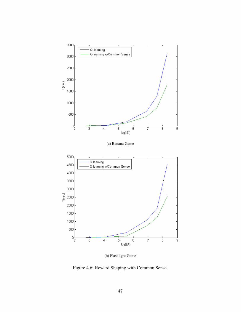
(a) Banana Game

(b) Flashlight Game

Figure 4.6: Reward Shaping with Common Sense.

47

between greedy exploitation strategies and exploration strategies that per-form sub-optimal actions in the hope of eventually discovering higher valueregions of the state-space. Common sense could guide the exploration strat-egy used by the agent e.g. such a strategy would prescribe attempting theaction pick-key more often than pick-banana.

3. Factoring MDPs : Recently there has been a lot of interest in factoredMDPs [GKP01]. These are formalisms that decompose the state represen-tations into sets of independent features and do reinforcement learning onthese sub-spaces semi-independently. Common sense information could beused to determine how to decompose large state-spaces e.g. pairs of fea-tures that have low relevance scores (like have-banana and open-doorcould be factored into separate MDPs.)

The challenge is to do this in sufficient generality that it can be usefully re-applied to a number of different problems. The advantage that using commonsense for decision making has over most other uses of common sense is its robust-ness to error and incompleteness. We might not find any useful common sense atall in which case our reinforcement learning algorithm will work as usual. Makingthe wrong conclusions from the KB might cause the learning agent to go astray.But if the knowledge is used carefully (e.g. with potential-based reward shaping),it will always be able to recover and still find the optimal policy. Thus the com-mon sense would hopefully be beneficial most of the time or it might slow downthe reinforcement learner sometimes, but it will not cause a catastrophic failure.It might turn out that supporting decision making might be the first truly usefulapplication for common sense knowledge bases that are large but incomplete i.e.not comprehensive enough to cover all of common sense knowledge.

4.8 Related Work

The idea of reward shaping was first suggested in [CH94] for a foraging robot.[RA98] first described the problems that can arise with indiscriminate shaping ina navigation problem, where a robot made endless cyclic motions around the startstate because there was no penalty for moving away from the goal (In fact IsaacAsimov first described this phenomenon in his short story “Runaround” [Asi50]).

48

[NHR99] showed that policy invariance is acheived by exactly the class of addi-tive potential shaping rewards. Since then, most work (e.g. [Mar07] ) in rewardshaping has foused on finding useful potential functions. In contrast, [SSL10]takes reward shaping beyond the idea of faster convergence and show that addinginternal rewards can alleviate problems caused by computational boundedness ofRL agents.

To our knowledge, there has been no work so far on using common senseknowledge for improved decision making in stochastic domains, but there hasbeen work on reward shaping by explanation-based learning [LD02]. The ideaof using domain knowledge for traditional planning problems has been exploredin relatively more depth. For example TALPlanner [KD01] is a forward-chainingplanner that utilizes domain-dependent knowledge to control search in the statespace.

There is some relation to the work on Relational MDPs [MW03] and First-Order MDPs [BRP01]. While both these formalisms seem to be better suitedto the task of exploiting knowledge (especially in logical form) we did not usethem for this work, because as of now neither of them have been developed to thepoint where useful implementations exist and there has not been sufficient workon reinforcement learning or reward shaping for them.

4.9 Contributions

In this chapter I introduce the first principled approach to shaping reward func-tions that relaxes the strict criterion of absolute policy-invariance. Our probabilis-tic model of reward shaping is a natural extension of the BIRL model described inchapter 2. Accelerated convergence is obtained by using prior distributions on re-wards that direct the RL process in fruitful directions. We showed an uninformedprior, the Anti-ferromagnetic Ising prior that biases shaping towards denser re-wards and an informed prior constructed from common-sense knowledge of theentities in the domain. Our results demonstrate that when used judiciously, it ispossible to exploit common sense knowledge to improve reinforcement learningalgorithms.

49

CHAPTER 5

APPROXIMATING OBSERVATIONMODELS

Very few decision-making problems in the real world can be modeled perfectly byMDPs because of the unrealistic assumption of perfect state estimation. For exam-ple, the sensors on a robot can be noisy, a dialog management system might haveimperfect speech recognition or an agent might be in an unkown part of the en-vironment. Partially Obervable Markov Decision Processes (POMDPs) [Son78]have been proposed to model the extra layer of observational uncertainty that real-world agents have to deal with. In a POMDP, the agent only has access to the stateindirectly through an observation model. The observation model will contain onlypartial information about the state and is generally not a sufficient statistic. Theagents objective is to maximize its total expected reward under the state dynamicsand observational uncertainty.

While POMDPs model the real world more accurately, they come at the priceof a dramatic increase in computational efficiency. The usual approach to solvinga POMDP is to treat it as an MDP over the belief state of the agent. This leadsto an explosion in the size of the problem space (in particular, the belief space iscontinuous, even for simple discrete MDP state spaces) which is reflected in thebig gap in computational complexity: Wheras MDP solution algorithms such asvalue iteration are essentialy polynomial time, POMDPs are PSPACE-complete[PT87].

It is natural to look for a middle ground between POMDPs and MDPs withsome of the representational accuracy of the former and the computational ad-vantanges of the latter. One approach that is sometimes taken in many practicalsystems is to use a belief tracker to maintain state information but apply the opti-mal policy for the MDP to the most likely state at each time step. This has beenused successfully for example in robotics ( [NPB95], [JUA+07]) and dialog man-agement ([ZCMG01]). Some more general models have also been proposed in theliterature such as Q-MDPs [KLC98], Oracular POMDPs [ACV08] and Fast Infor-mation bound heuristics [Pin04]. However, virtually no theoretically results exist

50

on the quality of these POMDP approximations. None of these methods fully ac-count for the value of information gained by taking particular actions. Ideally onewould like to know how much value is lost by doing this, but surprising none ofthese methods provide bounds. In this work, I provide the first result that boundsthe loss of value between a POMDP and its approximating scheme.

In this chapter, I analyse the difference in value of optimal policies for POMDPsand their underlying MDPs. First we present a bound on the difference in optimalvalues between MDPs and almost MDPs and show how this is connected to thehorizon times. The characteristic quantity for this gap is the lookahead k of a“Smoothed” POMDP (an imaginary POMDP where observations from k steps inthe future are received at the current state). k is shown to quantify the look aheadhorizon of the POMDP and thus in some sense its difficulty. By knowing k wecan use the Constant-delay MDP formulation of [WNLL09] with delay k.

5.1 POMDP approximations

By ignoring uncertainty in the state estimate there are crudely speaking, twosources of error we introduce. First, if our state estimate is indeed wrong werisk taking the wrong action for the current state. Further, by not accounting forour state of ignorance at future time states, we might choose over-optimistic plansof action that rely on infallible sensors or perfect state estimation. This can leadto substantial differences between the optimal policies of a POMDP and its fullyobservable version. This is demontstrated in the Girl-in-the-Woods problem from[Lit96]. A girl returning home from town has two choices. She can either godirectly through the woods and risk getting lost or take the long way around theforest on the fully observable road. Even though the route through the woodsis shorter and would be preferred by an optimal MDP policy, in the presence ofobservational uncertainty, chosing the path along the road is preferable to avoidmaking a mistake in later states. This example shows that POMDP solution tech-niques must account fundamentally for the value of information during planning.Intuitively, the maximum value attainable in the POMDP can never be more thanin the corresponding MDP, as the following result formalizes.

Lemma 5.1. For all POMDPs P with belief space B, and every b0 ∈ B.

V ∗P [b0] ≤ Es∼b0 [V∗(s)]

51

Proof.

V ∗P [b0] = maxa0,a1,...,an

{Esi∼bi [r(s0, a0) + γr(s1, a1) + . . .]}≤ Esi∼bi [ max

a0,a1,...,an{r(s0, a0) + γr(s1, a1) + . . .}] (Jensen’s Inequality)

= Esi∼bi [maxa0{r(s0, a0) + max

a1{r(s1, a1) + . . .]

= Es∼b0 [V∗(s)]

One way to measure the success of an approximation scheme is to measurethe “value gap” between a policy in the POMDP and the corresponding policy inthe scheme. For the underlying MDP, this gap is maximum. More sophisticatedmodels have been suggested that attempt to estimate the value of information moreaccurately and hence reduce this gap. I review these models and what is knownabout them below.

5.1.1 Memoryless policies

Memoryless policies are defined on the current observation and take the form:π : O → A. In effect, the entire history of the process until the current timestep is discarded and the observation is treated as if it encapsulated the entirestate. Memoryless policies were first suggested by [Lit94] as a simple way toapply standard MDP machinery to RL tasks with mild partial observability. How-ever, even for problems with just 2 states, the optimal memoryless policy can bearbitrarily bad compared to the optimal POMDP policy though [LS98] showedempirically on a variety of domains that Sarsa(λ) with eligibility traces was ableto find good memoryless policies in short time. They suggest that eligibility tracesare useful in reintroducing history information into the learning process.

In fact, memoryless policies are a special case of the Maximum likelihoodState estimate method discussed below. The belief tracker in a memoryless policysimply ignores all previous evidence and considers only the current observationin estimating state. Hence, the results of section 5.2 apply to memoryless policiesas well.

52

5.1.2 Most Likely State

Information-state MDP algorithms require some kind of belief tracker to updatethe belief state at each time step. Depending on the features of the state space thiscould be implemented by Hidden Markov Models [BP66], Kalman Filters [Kal60]or Dynamic Bayesian Networks [Pro93].

One simple approach to decision-making is to keep the belief tracker intactbut apply the optimal MDP policy to the state with Maximum-Likelihood (MLS).Since this approach completely discards all other information about the belief statedistribution and ignores the value of information, it is liable to give bad resultswhen uncertainty in belief states is high. Despite this, MLS has been succesfullyused in a number of applications where uncertainty is only a small feature. Itwas first described by Nourbaksh [NPB95] who used it successfully for a robotnavigation task. [ZCMG01] applies MLS to building a dialog manager. Moregenerally, many applications in the literature that claim to use MDPs are betterviewed as applying an MDP policy to the MLS of an uncertain belief state [Pin04].

5.1.3 QMDP

The QMDP heuristic ([KLC98]) attempts to account for partial observability atthe current step but assumes full observability on future steps:

πQMDP (b) = argmaxa∈A

∑

s∈Sb(s)QMDP (s, a)

The resulting policy can thus handle immediate uncertainty but still does notfactor in the value of information for planning. Its performance is similar to theMLS heuristic and is used interchangably with it in many applications.

5.2 Almost MDPs

In this section I analyze the behaviour of POMDP approximation models on prob-lems that are Almost MDPs. Almost MDPs are decision making problems withvery mild uncertainty:

Definition 5.1. An Almost MDP (AMDP)MA is a POMDP (S,A, T, γ, R,O) with

the following property: At every time step t, after the action at is taken, the next

53

(hidden) state st+1 is chosen, and the observation ot is made, we are assured that

Pr(st = s|o1:t, a1:t) > θ for some s and uniform constant θ < 1.

In other words, at every time step the error in our belief state bt is at most1 − θ. Thus we can consider our POMDP as being almost an MDP upto anobservational uncertainty 1−θ and it is natural to ask how well the optimal policyof the underlying MDP M performs on it. By this we mean how well does thefollowing policy on the belief states of the POMDP perform:

πAMDP (bt) = π∗MDP (MLS(bt)) (5.1)

where MLS(b) is the most likely state in b. In fact, we have the following result:

Theorem 5.2. For MDPsM with all rewards positive, the value of the AMDPMA

at belief state b using the policy defined by 5.1 is less than the expected optimal

value ofM atMLS(b) by at most (1−θ)Rmax1−γ−γθ+γ2θ whereRmax is the maximum reward

of any state-action pair. In other words,

V π∗M (MLS(b))− V πAMDP

MA(b) <

(1− θ)Rmax

1− γ − γθ + γ2θ

Proof. See appendix.

It is somewhat surprising that this result hasn’t been demonstrated before. Infact, many real world applications (e.g. [NPB95], [ZCMG01]) that claim to useMDPs are actually POMDPs where the state uncertainty is ignored. In effect theyare treated as AMDPs.

5.3 Constant-Delay MDPs

In some cases, the state estimation of our observation model is perfect but arriveswith a delay. In a complex system, the information from sensors might arriveat the processing unit with some latency. In such cases, we can again use thePOMDP formulation but such an approach seems overkill because there is noneed to assume a probabilistic belief state. [WNLL09] introduced the followingformalism called the Constant-Delay MDP to treat these situations:

Definition 5.2. A constant delay MDP (CD-MDP) is a 6-tuple 〈S,A, T, γ, R, k〉,where k is a non-negative integer indicating the number of timesteps between an

54

agent occupying a state and receiving its feedback (state observation and reward).

A policy for the CD-MDP is a mapping, π : S×Ak 7→ A, which defines an action

for every state and k-step action history.

We assume that k is bounded by a polynomial in size of the MDP. It is readilyapparent that this definition of policy π is sufficient since

Pr(st|at−1, ot−1) = Pr(st|s0, a0, . . . , st−k, at−k, at−k+1, . . . , at−1)

= Pr(st|st−k, at−k:t−1)

Thus the solution of Constant-Delay MDPs reduces to finding the optimal policyin a MDP with state space I = S × Ak. Unfortunately this is a significantlylarger problem than the original MDP and can be quite intractable depending onthe value of k. In particular, just to compute the reward function R(it, at), it ∈ Iwill require:

R((st−k, at−k:t−1), at) =

∑

st−k+1,...,st

P at−k(st−k+1|st−k)·. . .·P at−1(st|st−1)R(st, at)

(5.2)[WNLL09] introduced algorithms for solution of CD-MDPs in various settings(Deterministic MDPs, mildly stochastic MDPs and bounded-noise MDPs). Thegeneral approach is called Model-Based Simulation (MBS). [KE03] showed howany constant-delay MDP can be solved more efficiently than the naive approachby using a transformed cost function. For completeness, I sketch their approachbelow.

For any CD-MDP M with step size k, we define the corresponding time-shifted MDP Mk as the MDP identical to M but where the reward obtained attime step t+k is given by R(st−k, at−k). The Bellman equations for Mk are givenby

V (i) = maxa

[R(st−k, at−k) + γ∑

i′

P a(i′|i)V (i)],∀i ∈ I

Since st−k and at−k are included in the information state it, the first term iseasy to compute (unlike in M which requires the summation over the history ofstates in Equation 5.2). Therefore, these equations are much easier to solve thanthe Bellman equations for Mk. But it can be shown that the optimal policies forM and Mk are the same:

Theorem 5.3. Let M and Mk be as defined above. Then an optimal policy for

55

Mk, π∗k : I → A is also an optimal policy for M .

Proof. This follows from Theorem 1 of [KE03].

5.4 Almost CD-MDPs after smoothing

If there is no θ that satisfies the condition for an Almost MDP, a more sophisticatedapproximation for the POMDP is needed. We consider a hypothetical POMDPwhere we are given observations until a certain time step in the future t + k.Suppose there is a value for k such that the uncertainty in the smoothed belief statebt+kt = Pr(st|a1:t+k, o1:t+k) is always less than some uniform number θ < 1. Thenk represents a fundamental quantity for this POMDP - the “horizon of ignorance”.Within this horizon we must take into account our observational uncertainty toplan effectively in the POMDP. Beyond the time step k, the POMDP behavesalmost like a CD-MDP with parameter k:

Definition 5.3. An Almost CD-MDP M is a POMDP (S,A, T, γ, R,O) with the

following property: There are uniform constants θ < 1 and k ≥ 1 s.t. for every

time step t, after the action at+k is taken at time st+k, and the observation ot+k is

made, we are assured that Pr(st = s|a1:t+k, o1:t+k) > θ for some s ∈ S.

Thus, an AMDP is a special case of an almost CD-MDP with k = 0. In fact,we have an analogous result for CD-MDPs:

Theorem 5.4. The expected value of the Almost CD-MDP MA with parameter k

is less than that of the underlying CD-MDP M by at most (1−θ)Rmax1−γ−γθ+γ2θ .

Proof. See appendix.

5.5 Contributions

In this chapter, I provided what I believe is the first positive result on boundingthe difference between the value of a POMDP and its approximation scheme. ThePOMDP classes I considered were the Almost MDP and the Almost Constant-Delay MDP. I showed that using the MLS heuristic on these types of POMDPscomes close to attaining the value of the underlying MDP. This may give someinsight into why using MLS heuristics has been a relatively successful strategy

56

over a range of POMDP problems even compared to more sophisticated schemesthat try to model the value of information (See [NPB95]). It would be interestingto find if our results extend to these more complicated schemes.

57

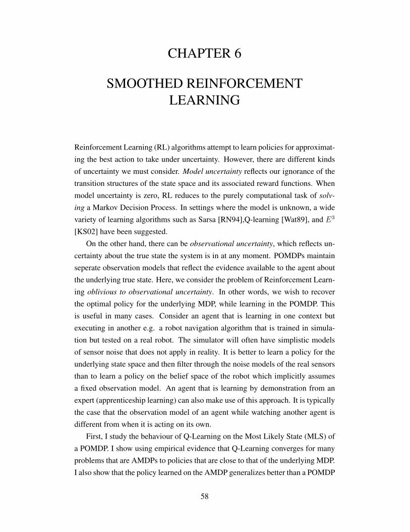
CHAPTER 6

SMOOTHED REINFORCEMENTLEARNING

Reinforcement Learning (RL) algorithms attempt to learn policies for approximat-ing the best action to take under uncertainty. However, there are different kindsof uncertainty we must consider. Model uncertainty reflects our ignorance of thetransition structures of the state space and its associated reward functions. Whenmodel uncertainty is zero, RL reduces to the purely computational task of solv-

ing a Markov Decision Process. In settings where the model is unknown, a widevariety of learning algorithms such as Sarsa [RN94],Q-learning [Wat89], and E3

[KS02] have been suggested.On the other hand, there can be observational uncertainty, which reflects un-

certainty about the true state the system is in at any moment. POMDPs maintainseperate observation models that reflect the evidence available to the agent aboutthe underlying true state. Here, we consider the problem of Reinforcement Learn-ing oblivious to observational uncertainty. In other words, we wish to recoverthe optimal policy for the underlying MDP, while learning in the POMDP. Thisis useful in many cases. Consider an agent that is learning in one context butexecuting in another e.g. a robot navigation algorithm that is trained in simula-tion but tested on a real robot. The simulator will often have simplistic modelsof sensor noise that does not apply in reality. It is better to learn a policy for theunderlying state space and then filter through the noise models of the real sensorsthan to learn a policy on the belief space of the robot which implicitly assumesa fixed observation model. An agent that is learning by demonstration from anexpert (apprenticeship learning) can also make use of this approach. It is typicallythe case that the observation model of an agent while watching another agent isdifferent from when it is acting on its own.

First, I study the behaviour of Q-Learning on the Most Likely State (MLS) ofa POMDP. I show using empirical evidence that Q-Learning converges for manyproblems that are AMDPs to policies that are close to that of the underlying MDP.I also show that the policy learned on the AMDP generalizes better than a POMDP

58

Algorithm 2 Q-learning on Almost MDPsInput: Almost MDP 〈S,A, T, γ, R,O, θ〉, Initial state s0.Initialize Q(s, a) arbitrarily for all s ∈ S, a ∈ A, s0 ← s0.for t = 0, 1, 2, . . . until Q converges do

Choose at from st using policy derived from Q (e.g. ε-greedy).Take action at, collect reward rt and observation ot+1.Compute bt+1 from bt and ot+1 using the belief tracker. Set st+1 ←MLS(bt+1).Q(st, at)

α← rt + γmaxaQ(st+1, a)−Q(st, at)end forReturn Q.

policy when the observation model is changed.For Almost CD-MDPs, I introduce the notion of a Smoothed reinforcement

learning algorithm. Many RL algorithms such as Sarsa [RN94] and Q-learning[Wat89] make aggressive use of bootstrapping i.e. the Q-value of a state-actionpair at time t is adjusted to the value of the next state at time t+1, called the backup

value. In a Smoothed RL algorithm (Section 6.2), we delay the learning step untila better MLS state estimate is obtained at the later time step t+ k (i.e. after moreobservations are made). Again, this learning procedure converges to a policy thatis close to optimal for the underlying MDP, since it ignores the instantanenousobservational uncertainty at t. Smoothing can be applied to any RL algorithmthat uses temporal differencing. It can also be generalized into a variability trace

framework that spreads the smoothing over multiple future time steps analogousto eligibility traces or TD(λ) methods.

6.1 Reinforcement Learning on Almost MDPs

In Table 6.1 we present our algorithm for RL on Almost MDPs which is astraightforward adaptation of standard online Q-learning [Wat89]. We keep trackof the current belief state of the AMDP while learning, but our goal is find a closeto optimalQ function for the underlying MDP. A belief tracker is used to maintainthe belief state over the current underlying state as observations are collected. Theupdate of the belief state is given by:

bt+1(s|ot+1) =Pr(ot+1|s, at)Pr(ot+1|at, bt)

∑

s′∈SPr(s|s′, at)bt(s′)

59

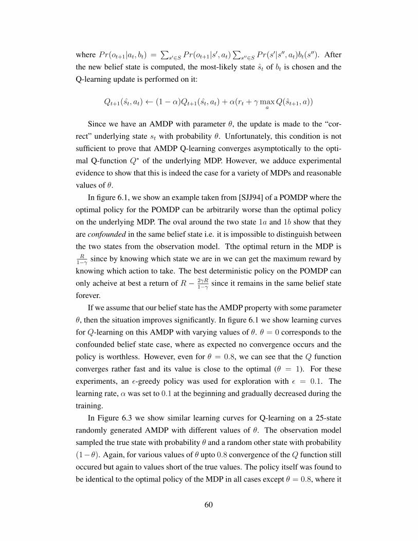
where Pr(ot+1|at, bt) =∑

s′∈S Pr(ot+1|s′, at)∑

s′′∈S Pr(s′|s′′, at)bt(s′′). After

the new belief state is computed, the most-likely state st of bt is chosen and theQ-learning update is performed on it:

Qt+1(st, at)← (1− α)Qt+1(st, at) + α(rt + γmaxaQ(st+1, a))

Since we have an AMDP with parameter θ, the update is made to the “cor-rect” underlying state st with probability θ. Unfortunately, this condition is notsufficient to prove that AMDP Q-learning converges asymptotically to the opti-mal Q-function Q∗ of the underlying MDP. However, we adduce experimentalevidence to show that this is indeed the case for a variety of MDPs and reasonablevalues of θ.

In figure 6.1, we show an example taken from [SJJ94] of a POMDP where theoptimal policy for the POMDP can be arbitrarily worse than the optimal policyon the underlying MDP. The oval around the two state 1a and 1b show that theyare confounded in the same belief state i.e. it is impossible to distinguish betweenthe two states from the observation model. Tthe optimal return in the MDP isR

1−γ since by knowing which state we are in we can get the maximum reward byknowing which action to take. The best deterministic policy on the POMDP canonly acheive at best a return of R − 2γR

1−γ since it remains in the same belief stateforever.

If we assume that our belief state has the AMDP property with some parameterθ, then the situation improves significantly. In figure 6.1 we show learning curvesfor Q-learning on this AMDP with varying values of θ. θ = 0 corresponds to theconfounded belief state case, where as expected no convergence occurs and thepolicy is worthless. However, even for θ = 0.8, we can see that the Q functionconverges rather fast and its value is close to the optimal (θ = 1). For theseexperiments, an ε-greedy policy was used for exploration with ε = 0.1. Thelearning rate, α was set to 0.1 at the beginning and gradually decreased during thetraining.

In Figure 6.3 we show similar learning curves for Q-learning on a 25-staterandomly generated AMDP with different values of θ. The observation modelsampled the true state with probability θ and a random other state with probability(1−θ). Again, for various values of θ upto 0.8 convergence of the Q function stilloccured but again to values short of the true values. The policy itself was found tobe identical to the optimal policy of the MDP in all cases except θ = 0.8, where it

60

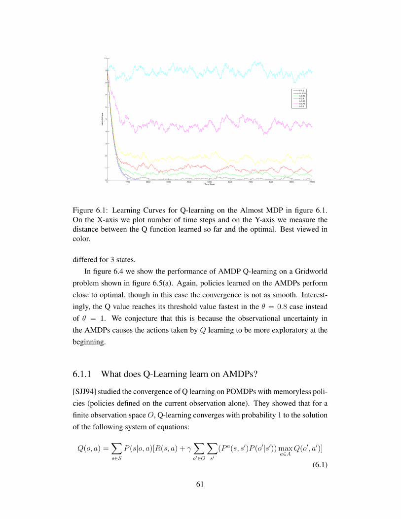
0 1000 2000 3000 4000 5000 6000 7000 8000 9000 100000

1

2

3

4

5

6

7

8

9

10

Time Steps

Mea

n Q

Va

lue

t=1.0

t=.0.99

t=0.95

t=0.9

t=0.85

t=0.75

t=0.0

Figure 6.1: Learning Curves for Q-learning on the Almost MDP in figure 6.1.On the X-axis we plot number of time steps and on the Y-axis we measure thedistance between the Q function learned so far and the optimal. Best viewed incolor.

differed for 3 states.In figure 6.4 we show the performance of AMDP Q-learning on a Gridworld

problem shown in figure 6.5(a). Again, policies learned on the AMDPs performclose to optimal, though in this case the convergence is not as smooth. Interest-ingly, the Q value reaches its threshold value fastest in the θ = 0.8 case insteadof θ = 1. We conjecture that this is because the observational uncertainty inthe AMDPs causes the actions taken by Q learning to be more exploratory at thebeginning.

6.1.1 What does Q-Learning learn on AMDPs?

[SJJ94] studied the convergence of Q learning on POMDPs with memoryless poli-cies (policies defined on the current observation alone). They showed that for afinite observation spaceO, Q-learning converges with probability 1 to the solutionof the following system of equations:

Q(o, a) =∑

s∈SP (s|o, a)[R(s, a) + γ

∑

o′∈O

∑

s′

(P a(s, s′)P (o′|s′)) maxa∈A

Q(o′, a′)]

(6.1)

61

1a

b1

A

A

B

B

R

-R

R

-R

Figure 6.2: POMDP with confounded states reproduced from [SJJ94].

0 0.5 1 1.5 2 2.5 3

x 104

0

0.5

1

1.5

2

2.5

3

Time Steps

Mean Q

Valu

e

t=1.0

t=0.99

t=0.95

t=0.9

t=0.8

Figure 6.3: Learning Curves for Q-learning on randomly generated 25 state MDPwith various degrees of observational uncertainty. On the X-axis we plot numberof time steps and on the Y-axis we measure the distance between the Q functionlearned so far and the optimal. Best viewed in color.

62

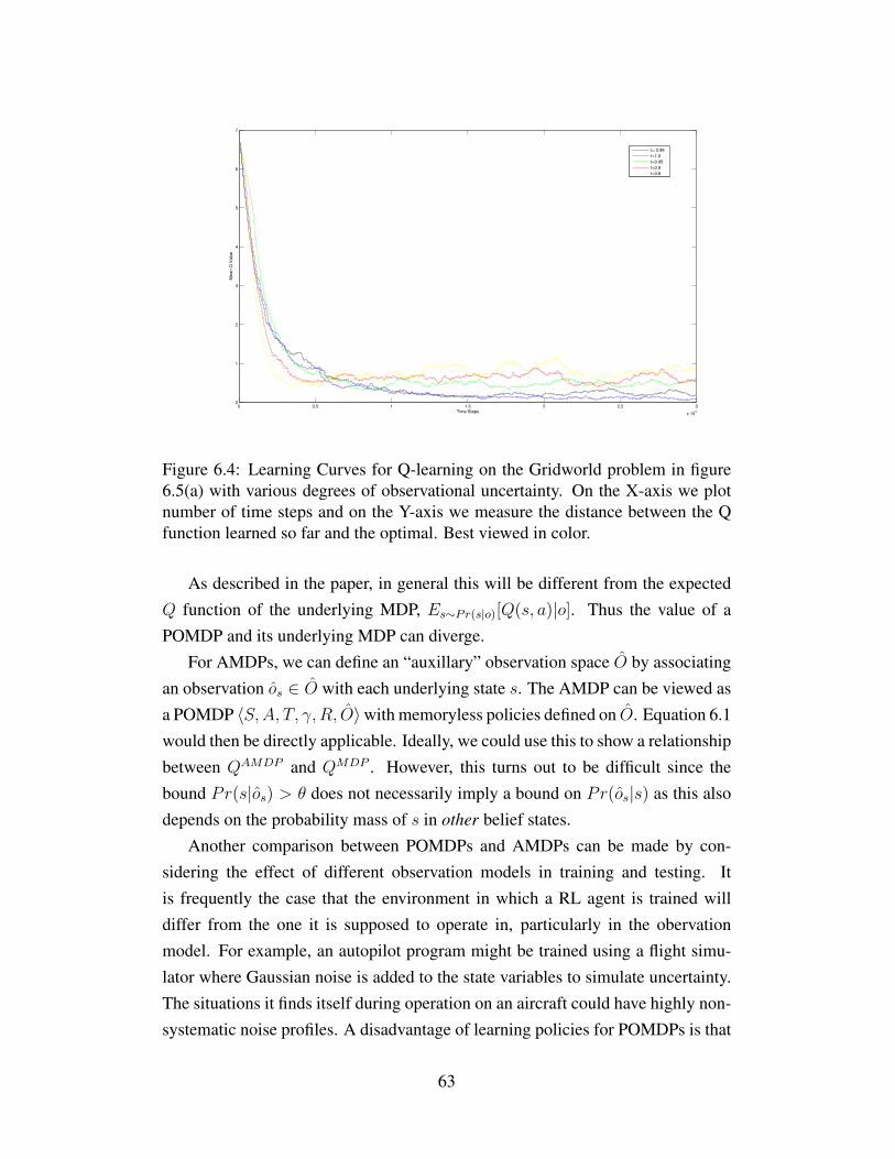
0 0.5 1 1.5 2 2.5 3

x 104

0

1

2

3

4

5

6

7

Time Steps

Mea

n Q

Va

lue

t= 0.99

t=1.0

t=0.95

t=0.9

t=0.8

Figure 6.4: Learning Curves for Q-learning on the Gridworld problem in figure6.5(a) with various degrees of observational uncertainty. On the X-axis we plotnumber of time steps and on the Y-axis we measure the distance between the Qfunction learned so far and the optimal. Best viewed in color.

As described in the paper, in general this will be different from the expectedQ function of the underlying MDP, Es∼Pr(s|o)[Q(s, a)|o]. Thus the value of aPOMDP and its underlying MDP can diverge.

For AMDPs, we can define an “auxillary” observation space O by associatingan observation os ∈ O with each underlying state s. The AMDP can be viewed asa POMDP 〈S,A, T, γ, R, O〉with memoryless policies defined on O. Equation 6.1would then be directly applicable. Ideally, we could use this to show a relationshipbetween QAMDP and QMDP . However, this turns out to be difficult since thebound Pr(s|os) > θ does not necessarily imply a bound on Pr(os|s) as this alsodepends on the probability mass of s in other belief states.

Another comparison between POMDPs and AMDPs can be made by con-sidering the effect of different observation models in training and testing. Itis frequently the case that the environment in which a RL agent is trained willdiffer from the one it is supposed to operate in, particularly in the obervationmodel. For example, an autopilot program might be trained using a flight simu-lator where Gaussian noise is added to the state variables to simulate uncertainty.The situations it finds itself during operation on an aircraft could have highly non-systematic noise profiles. A disadvantage of learning policies for POMDPs is that

63

(a) A 5x5 Gridworld problem.

(b) Observation Models for Gridworld Prob-lems. When the agent is at the state representedby the black square, he observes his location asthe black square with probability θ = 0.8 andas the hatched square with probability 0.2.

Figure 6.5: Experiments on switching Observation models

64

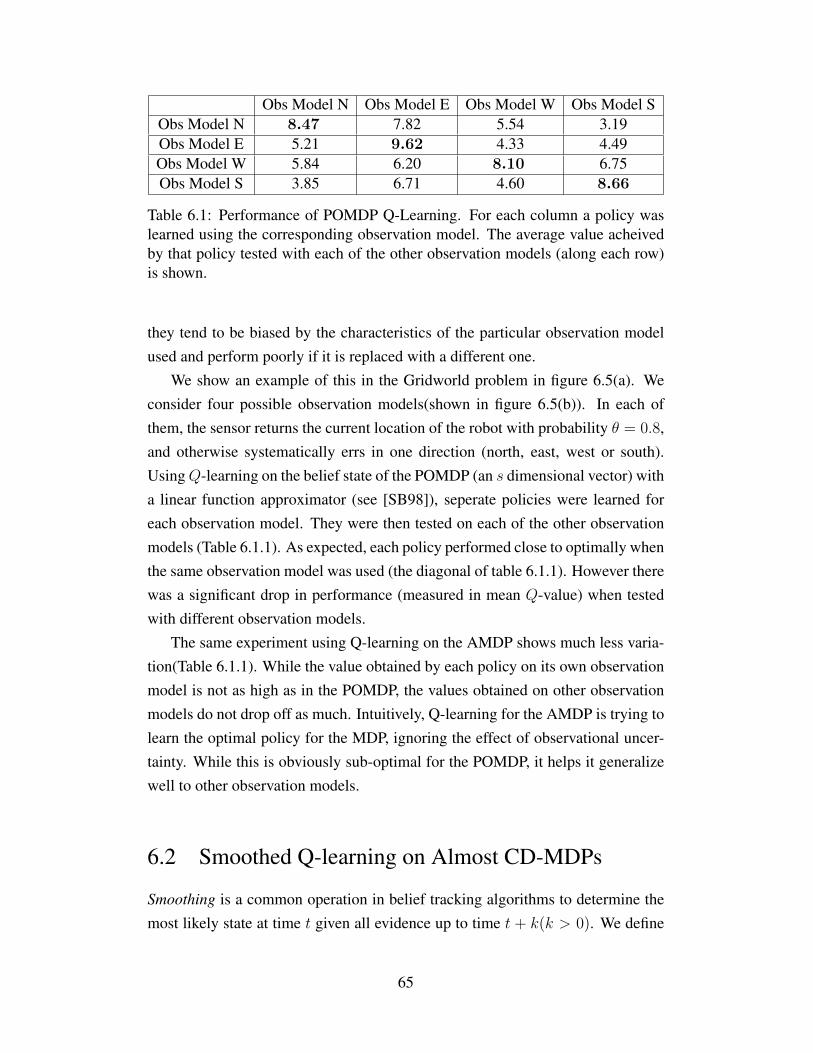
Obs Model N Obs Model E Obs Model W Obs Model SObs Model N 8.47 7.82 5.54 3.19Obs Model E 5.21 9.62 4.33 4.49Obs Model W 5.84 6.20 8.10 6.75Obs Model S 3.85 6.71 4.60 8.66

Table 6.1: Performance of POMDP Q-Learning. For each column a policy waslearned using the corresponding observation model. The average value acheivedby that policy tested with each of the other observation models (along each row)is shown.

they tend to be biased by the characteristics of the particular observation modelused and perform poorly if it is replaced with a different one.

We show an example of this in the Gridworld problem in figure 6.5(a). Weconsider four possible observation models(shown in figure 6.5(b)). In each ofthem, the sensor returns the current location of the robot with probability θ = 0.8,and otherwise systematically errs in one direction (north, east, west or south).UsingQ-learning on the belief state of the POMDP (an s dimensional vector) witha linear function approximator (see [SB98]), seperate policies were learned foreach observation model. They were then tested on each of the other observationmodels (Table 6.1.1). As expected, each policy performed close to optimally whenthe same observation model was used (the diagonal of table 6.1.1). However therewas a significant drop in performance (measured in mean Q-value) when testedwith different observation models.

The same experiment using Q-learning on the AMDP shows much less varia-tion(Table 6.1.1). While the value obtained by each policy on its own observationmodel is not as high as in the POMDP, the values obtained on other observationmodels do not drop off as much. Intuitively, Q-learning for the AMDP is trying tolearn the optimal policy for the MDP, ignoring the effect of observational uncer-tainty. While this is obviously sub-optimal for the POMDP, it helps it generalizewell to other observation models.

6.2 Smoothed Q-learning on Almost CD-MDPs

Smoothing is a common operation in belief tracking algorithms to determine themost likely state at time t given all evidence up to time t + k(k > 0). We define

65

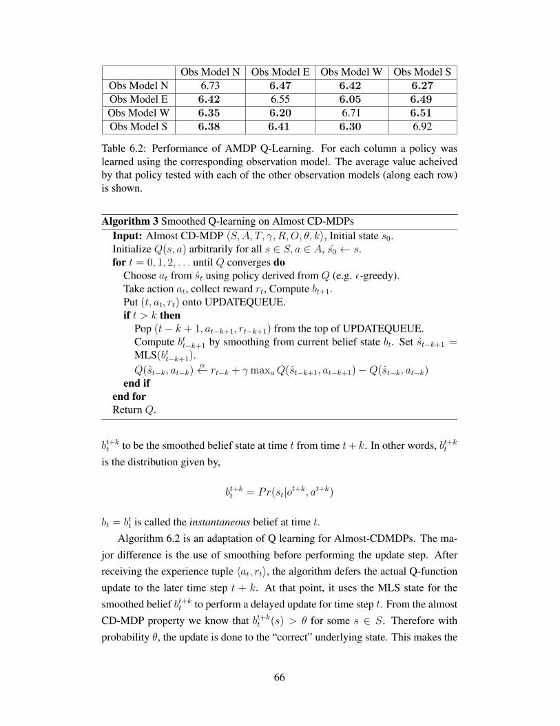
Obs Model N Obs Model E Obs Model W Obs Model SObs Model N 6.73 6.47 6.42 6.27Obs Model E 6.42 6.55 6.05 6.49Obs Model W 6.35 6.20 6.71 6.51Obs Model S 6.38 6.41 6.30 6.92

Table 6.2: Performance of AMDP Q-Learning. For each column a policy waslearned using the corresponding observation model. The average value acheivedby that policy tested with each of the other observation models (along each row)is shown.

Algorithm 3 Smoothed Q-learning on Almost CD-MDPsInput: Almost CD-MDP 〈S,A, T, γ, R,O, θ, k〉, Initial state s0.Initialize Q(s, a) arbitrarily for all s ∈ S, a ∈ A, s0 ← s.for t = 0, 1, 2, . . . until Q converges do

Choose at from st using policy derived from Q (e.g. ε-greedy).Take action at, collect reward rt, Compute bt+1.Put (t, at, rt) onto UPDATEQUEUE.if t > k then

Pop (t− k + 1, at−k+1, rt−k+1) from the top of UPDATEQUEUE.Compute btt−k+1 by smoothing from current belief state bt. Set st−k+1 =MLS(btt−k+1).Q(st−k, at−k)

α← rt−k + γmaxaQ(st−k+1, at−k+1)−Q(st−k, at−k)end if

end forReturn Q.

bt+kt to be the smoothed belief state at time t from time t+ k. In other words, bt+kt

is the distribution given by,

bt+kt = Pr(st|ot+k, at+k)

bt = btt is called the instantaneous belief at time t.Algorithm 6.2 is an adaptation of Q learning for Almost-CDMDPs. The ma-

jor difference is the use of smoothing before performing the update step. Afterreceiving the experience tuple 〈at, rt〉, the algorithm defers the actual Q-functionupdate to the later time step t + k. At that point, it uses the MLS state for thesmoothed belief bt+kt to perform a delayed update for time step t. From the almostCD-MDP property we know that bt+kt (s) > θ for some s ∈ S. Therefore withprobability θ, the update is done to the “correct” underlying state. This makes the

66

Figure 6.6: (Top) Robot has equal belief about location of person at time t. (Mid-dle) At time t + k, robot sees the person in office and the corresponding beliefabout person location (Bottom) Smoothed belief at time t+ 1

algorithm exactly analogous to Algorithm 6.1 on AMDPs and so the results ofsection 6.1 directly apply.

We illustrate the use of smoothing in RL with a simple example (Figure 6.6).Consider a mobile service robot learning to perform multiple delivery tasks. Sup-pose it has picked up a letter and is trying to decide whether to look for the re-cepient in his office or the kitchen. In the true state st (unknown to the robot), theperson is in the office but in the robot’s belief state, bt, there is uncertainty overhis location. Suppose the robot does ordinary Q-learning on the state space (theinformation-state MDP). It takes an action at which moves it from true state stto st+1, and from belief state bt to bt+1. It now adjusts Q(bt, at) to be closer tort + γmaxaQ(bt+1, a). This is called a backup in RL. Unfortunately, the backuptarget could be very different from the true value rt + γQ(st+1, a), due to uncer-tainty over the location of the person in bt+1. Using Algorithm 6.2 on the AlmostCD-MDP however uses the observation made at time t+k to improve the state es-timate st used in learning. Thus the algorithm will converge faster to the Q-valueof the underlying MDP.

6.3 µ-Smoothed RL and Variability Traces

The smoothed RL algorithm requires knowing the smoothing delay parameter k.If our problem is not a CD-MDP, we can not be sure what value to assign tok. However we can generalize Algorithm 6.2 to a procedure that smooths over

67

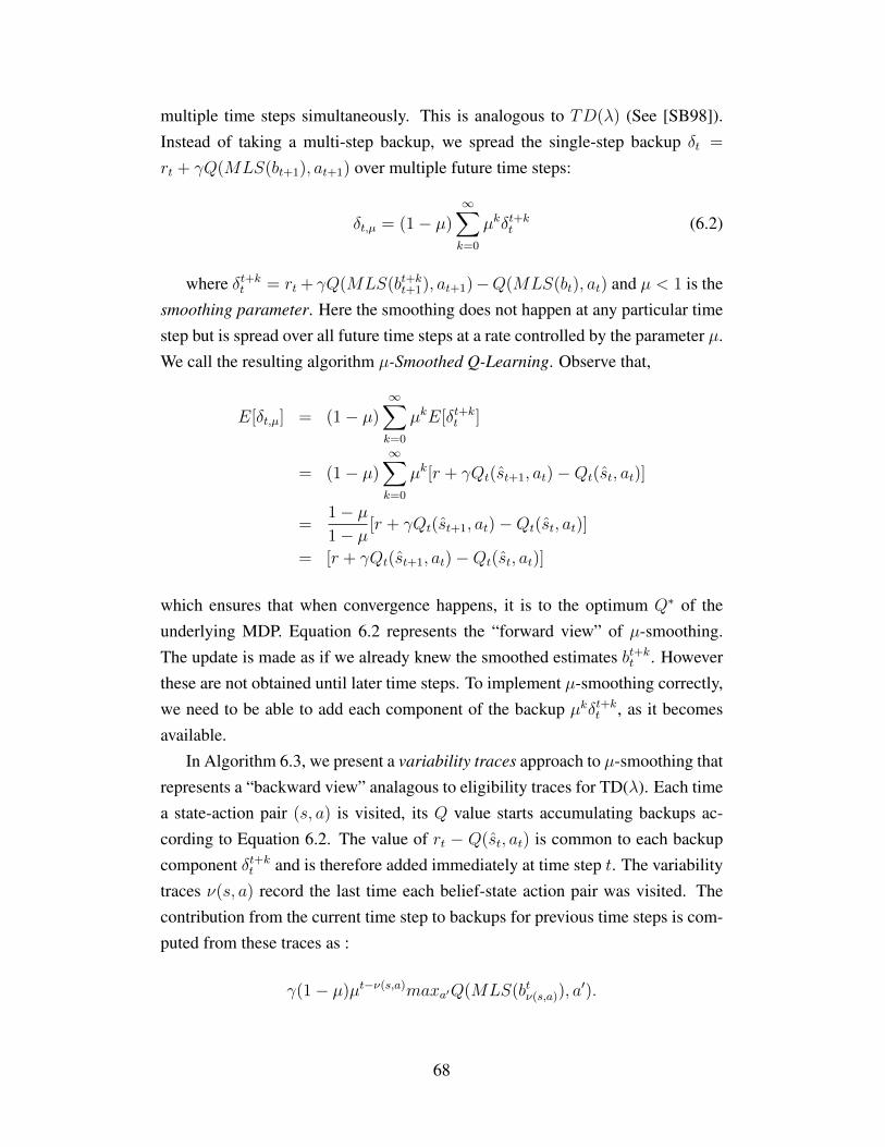
multiple time steps simultaneously. This is analogous to TD(λ) (See [SB98]).Instead of taking a multi-step backup, we spread the single-step backup δt =

rt + γQ(MLS(bt+1), at+1) over multiple future time steps:

δt,µ = (1− µ)∞∑

k=0

µkδt+kt (6.2)

where δt+kt = rt + γQ(MLS(bt+kt+1), at+1)−Q(MLS(bt), at) and µ < 1 is thesmoothing parameter. Here the smoothing does not happen at any particular timestep but is spread over all future time steps at a rate controlled by the parameter µ.We call the resulting algorithm µ-Smoothed Q-Learning. Observe that,

E[δt,µ] = (1− µ)∞∑

k=0

µkE[δt+kt ]

= (1− µ)∞∑

k=0

µk[r + γQt(st+1, at)−Qt(st, at)]

=1− µ1− µ [r + γQt(st+1, at)−Qt(st, at)]

= [r + γQt(st+1, at)−Qt(st, at)]

which ensures that when convergence happens, it is to the optimum Q∗ of theunderlying MDP. Equation 6.2 represents the “forward view” of µ-smoothing.The update is made as if we already knew the smoothed estimates bt+kt . Howeverthese are not obtained until later time steps. To implement µ-smoothing correctly,we need to be able to add each component of the backup µkδt+kt , as it becomesavailable.

In Algorithm 6.3, we present a variability traces approach to µ-smoothing thatrepresents a “backward view” analagous to eligibility traces for TD(λ). Each timea state-action pair (s, a) is visited, its Q value starts accumulating backups ac-cording to Equation 6.2. The value of rt − Q(st, at) is common to each backupcomponent δt+kt and is therefore added immediately at time step t. The variabilitytraces ν(s, a) record the last time each belief-state action pair was visited. Thecontribution from the current time step to backups for previous time steps is com-puted from these traces as :

γ(1− µ)µt−ν(s,a)maxa′Q(MLS(btν(s,a)), a′).

68

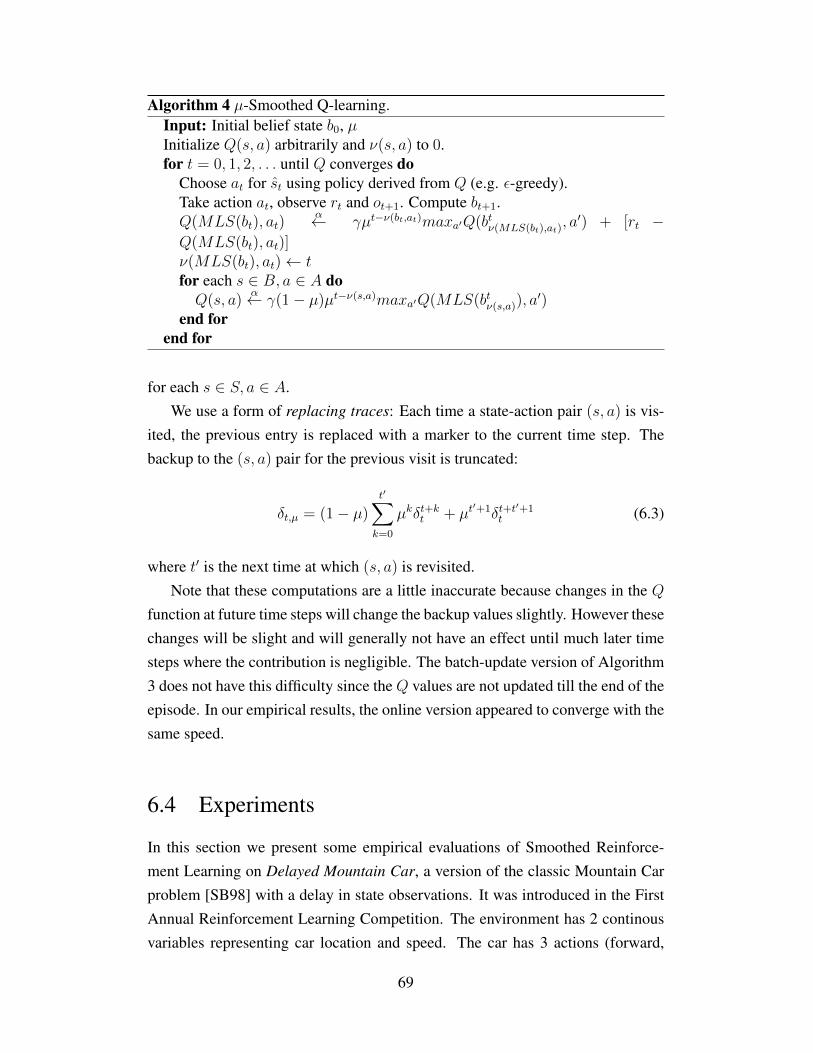
Algorithm 4 µ-Smoothed Q-learning.Input: Initial belief state b0, µInitialize Q(s, a) arbitrarily and ν(s, a) to 0.for t = 0, 1, 2, . . . until Q converges do

Choose at for st using policy derived from Q (e.g. ε-greedy).Take action at, observe rt and ot+1. Compute bt+1.Q(MLS(bt), at)

α← γµt−ν(bt,at)maxa′Q(btν(MLS(bt),at), a′) + [rt −

Q(MLS(bt), at)]ν(MLS(bt), at)← tfor each s ∈ B, a ∈ A doQ(s, a)

α← γ(1− µ)µt−ν(s,a)maxa′Q(MLS(btν(s,a)), a′)

end forend for

for each s ∈ S, a ∈ A.We use a form of replacing traces: Each time a state-action pair (s, a) is vis-

ited, the previous entry is replaced with a marker to the current time step. Thebackup to the (s, a) pair for the previous visit is truncated:

δt,µ = (1− µ)t′∑

k=0

µkδt+kt + µt′+1δt+t

′+1t (6.3)

where t′ is the next time at which (s, a) is revisited.Note that these computations are a little inaccurate because changes in the Q

function at future time steps will change the backup values slightly. However thesechanges will be slight and will generally not have an effect until much later timesteps where the contribution is negligible. The batch-update version of Algorithm3 does not have this difficulty since the Q values are not updated till the end of theepisode. In our empirical results, the online version appeared to converge with thesame speed.

6.4 Experiments

In this section we present some empirical evaluations of Smoothed Reinforce-ment Learning on Delayed Mountain Car, a version of the classic Mountain Carproblem [SB98] with a delay in state observations. It was introduced in the FirstAnnual Reinforcement Learning Competition. The environment has 2 continousvariables representing car location and speed. The car has 3 actions (forward,

69

Figure 6.7: Delayed Mountain Car Results

neutral, reverse) and rewards of −1 for all states except the terminal goal state atthe top of the hill, which has reward 0. A 10 × 10 grid was overlaid and coarsetiling was used to discretize the feature space. We compared the performance ofSarsa(0), Sarsa(0.9), Model Based Simulation + Model Parameter Approximation([WNL07]), and our own 0.5-smoothed Sarsa and 0.9-smoothed Sarsa. The re-sults (Figure 6.7) show that variability traces outperformed eligibility traces as away of accounting for delay in the environment. Since a higher value of µ biasesthe smoothing towards backups from later time steps, 0.9-smoothed Sarsa did bet-ter that 0.5-smoothed Sarsa for higher delay values and vice versa. MBS+MPAuses a model to simulate steps between delayed and actual state. It is speciallydesigned for such tasks and is given the length of the delay as input. Our moregeneral algorithm perform competitively against it over a significant range of de-lays. The data represents averages over 10 runs with 200 episodes per run. In thenext chapter, we show the performance of Smoothed Q-Learning on a POMDPproblem arising from a robot navigation task.

6.5 Contributions

In this chapter, I extended the investigation of Almost MDPs and Almost CD-MDPs to finding Reinforcement Learning algorithms suitable for these problems.

70

I found that using Q-Learning on the MLS state of an AMDP converges to theoptimal policy for the underlying MDP for sufficiently high θ over a range ofproblems. These policies also generalized to changes in observation models betterthan the policy learned on the POMDP. I also demonstrated reinforcement learningin Almost CD-MDPs using smoothing as the key operation. For the case wherethe delay in the CD-MDP is not known, I showed a variability traces frameworkfor Smoothed RL that spreads the smoothed backup step over multiple time steps.

71

CHAPTER 7

AN APPLICATION TO ROBOTICS

The goal in this chapter is to make high level decisions for mobile robots. Inparticular, given a queue of prioritized object delivery tasks, we wish to find asequence of actions in real time to accomplish these tasks efficiently. The solutionuses Smoothed Sarsa (described in chapter 6) to learn a policy for the decisionmaking problem and introduces Region-based Particle Filters, a more efficientquasi-topological representation of the state-space. I demonstrate the success ofthis approach on the PLAYER/Stage robot simulator and on a Pioneer mobilerobot.

7.1 Introduction

Mobile robots have now been deployed in environments with people includingoffices [AV98, MAF+99, MMI+06, Hir07] and hospitals [Eng93, PMP+03]. Arobot assistant can help elderly individuals and nurses in hospitals and long termcare facilities, and provide assistance in home and office environments. Suchrobots need to interact with entities in their environment both verbally (e.g. pro-viding information to people) and physically (e.g. fetching objects). The robotmust plan efficient sequences of actions to accomplish these tasks. This planningneeds to be responsive to new tasks being added dynamically and changes in theenvironment.

In this chapter, we are concerned with dynamically planning efficient actionsequences for multiple delivery tasks of the form “Deliver object X to person Y”.The primitive actions are of the kind “Move to location X”, “Pick Up” and “De-liver”. I assume that there are low-level controllers and navigational algorithmsavailable to perform these actions. (though not always successfully).

At every step, the robot needs to decide what action to take to maximize theexpected total reward, given the distribution of the tasks and the belief state over

72

entity locations. This can be modeled as a POMDP with significant observationaluncertainty caused by noisy sensors. I describe how Smoothed Sarsa can be usedto efficiently learn a policy in simulation then transfered to a real robot for execu-tion.

The second contribution is the use of a quasi-topological representation of thestate-space for decision making. When making decisions about what action totake next, the exact position of an object or person is of little relevance. Whatmatters is the probability that the entity is at some approximate region, such asin front of his desk or on the kitchen table. The entity-tracking algorithm used, aregion-based particle-filter, is specially designed to exploit this property.

POMDP’s have been applied extensively in the past [TK04, KS98, SK95,SV04] to robot navigation and some crude forms of decision-making. The ap-plicability of these approaches are limited by the high dimensional discretizationof space they use, hand tuning of policy, and the excessive time taken to learn agood policy. This is the first work that solves task-level decision making problemsfor robots at this level of generality.

We implemented our approach in simulation and on a Pioneer mobile robotin a 5 room office environment. Smoothed Sarsa managed to learn a good policyin 3 hours, wheras PERSEUS [SV04] took days to return a policy with worseperformance. In simulated trials, the learned policy completed a set of deliverytasks 30% faster on average than a carefully crafted manual policy.

The rest of this chapter is organized as follows. In section 7.2 we describe thestate-space used by the decision making algorithm and the region-based particlefilter. Section 7.3 discusses our observation model for entities and localization.Section 7.4 presents the Region-based Particle Filter. Section 7.5 presents our ex-periments. Sections 7.6 and 7.7 discuss related work and conclusions respectively.

7.2 Belief State Representation

I begin by describing the region-based representation we use for the location ofentities (objects or persons). The basic model is a hierarchical Dynamic BayesianNetwork. In this section, I define its state space and transition model.

73

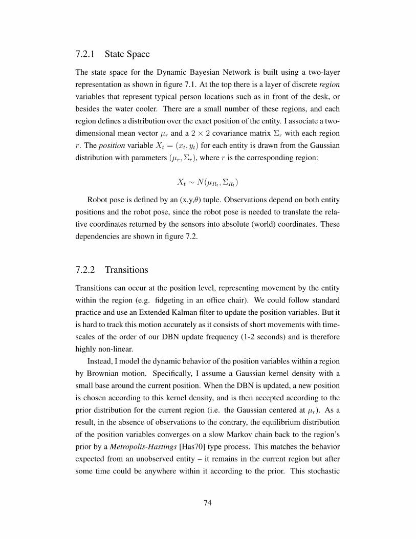
7.2.1 State Space

The state space for the Dynamic Bayesian Network is built using a two-layerrepresentation as shown in figure 7.1. At the top there is a layer of discrete region

variables that represent typical person locations such as in front of the desk, orbesides the water cooler. There are a small number of these regions, and eachregion defines a distribution over the exact position of the entity. I associate a two-dimensional mean vector µr and a 2 × 2 covariance matrix Σr with each regionr. The position variable Xt = (xt, yt) for each entity is drawn from the Gaussiandistribution with parameters (µr,Σr), where r is the corresponding region:

Xt ∼ N(µRt ,ΣRt)

Robot pose is defined by an (x,y,θ) tuple. Observations depend on both entitypositions and the robot pose, since the robot pose is needed to translate the rela-tive coordinates returned by the sensors into absolute (world) coordinates. Thesedependencies are shown in figure 7.2.

7.2.2 Transitions

Transitions can occur at the position level, representing movement by the entitywithin the region (e.g. fidgeting in an office chair). We could follow standardpractice and use an Extended Kalman filter to update the position variables. But itis hard to track this motion accurately as it consists of short movements with time-scales of the order of our DBN update frequency (1-2 seconds) and is thereforehighly non-linear.

Instead, I model the dynamic behavior of the position variables within a regionby Brownian motion. Specifically, I assume a Gaussian kernel density with asmall base around the current position. When the DBN is updated, a new positionis chosen according to this kernel density, and is then accepted according to theprior distribution for the current region (i.e. the Gaussian centered at µr). As aresult, in the absence of observations to the contrary, the equilibrium distributionof the position variables converges on a slow Markov chain back to the region’sprior by a Metropolis-Hastings [Has70] type process. This matches the behaviorexpected from an unobserved entity – it remains in the current region but aftersome time could be anywhere within it according to the prior. This stochastic

74

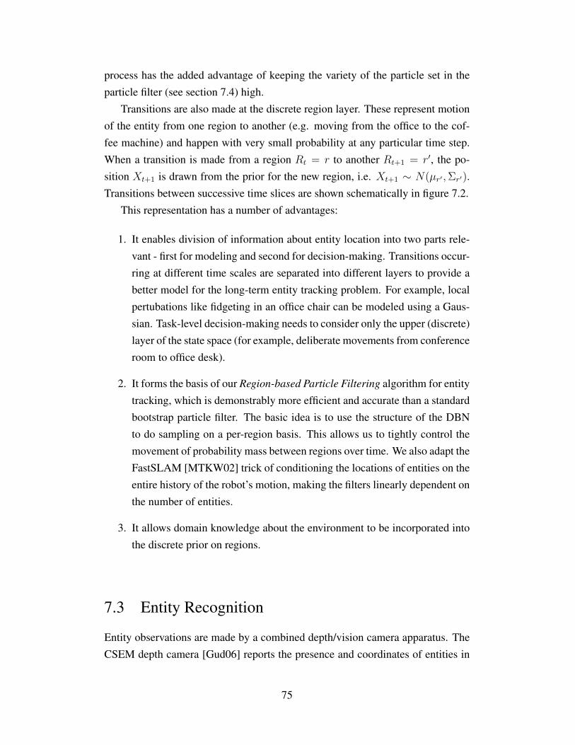
process has the added advantage of keeping the variety of the particle set in theparticle filter (see section 7.4) high.

Transitions are also made at the discrete region layer. These represent motionof the entity from one region to another (e.g. moving from the office to the cof-fee machine) and happen with very small probability at any particular time step.When a transition is made from a region Rt = r to another Rt+1 = r′, the po-sition Xt+1 is drawn from the prior for the new region, i.e. Xt+1 ∼ N(µr′ ,Σr′).Transitions between successive time slices are shown schematically in figure 7.2.

This representation has a number of advantages:

1. It enables division of information about entity location into two parts rele-vant - first for modeling and second for decision-making. Transitions occur-ring at different time scales are separated into different layers to provide abetter model for the long-term entity tracking problem. For example, localpertubations like fidgeting in an office chair can be modeled using a Gaus-sian. Task-level decision-making needs to consider only the upper (discrete)layer of the state space (for example, deliberate movements from conferenceroom to office desk).

2. It forms the basis of our Region-based Particle Filtering algorithm for entitytracking, which is demonstrably more efficient and accurate than a standardbootstrap particle filter. The basic idea is to use the structure of the DBNto do sampling on a per-region basis. This allows us to tightly control themovement of probability mass between regions over time. We also adapt theFastSLAM [MTKW02] trick of conditioning the locations of entities on theentire history of the robot’s motion, making the filters linearly dependent onthe number of entities.

3. It allows domain knowledge about the environment to be incorporated intothe discrete prior on regions.

7.3 Entity Recognition

Entity observations are made by a combined depth/vision camera apparatus. TheCSEM depth camera [Gud06] reports the presence and coordinates of entities in

75

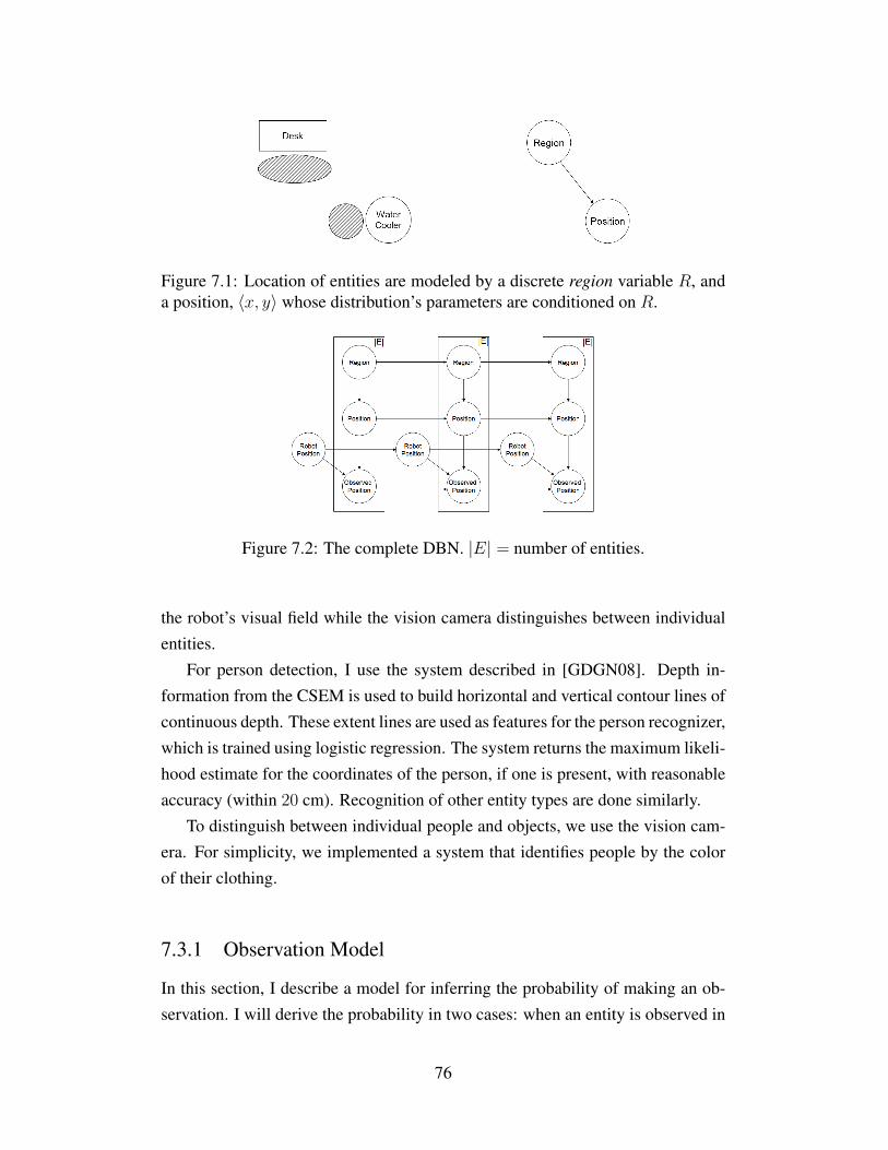
Figure 7.1: Location of entities are modeled by a discrete region variable R, anda position, 〈x, y〉 whose distribution’s parameters are conditioned on R.

Figure 7.2: The complete DBN. |E| = number of entities.

the robot’s visual field while the vision camera distinguishes between individualentities.

For person detection, I use the system described in [GDGN08]. Depth in-formation from the CSEM is used to build horizontal and vertical contour lines ofcontinuous depth. These extent lines are used as features for the person recognizer,which is trained using logistic regression. The system returns the maximum likeli-hood estimate for the coordinates of the person, if one is present, with reasonableaccuracy (within 20 cm). Recognition of other entity types are done similarly.

To distinguish between individual people and objects, we use the vision cam-era. For simplicity, we implemented a system that identifies people by the colorof their clothing.

7.3.1 Observation Model

In this section, I describe a model for inferring the probability of making an ob-servation. I will derive the probability in two cases: when an entity is observed in

76

Figure 7.3: TORO, the Tracking and Observing RObot. At the top are the CSEMdepth and vision cameras. The SICK laser is used for localization.

the current visual field and when it is not.For now, I assume that our observation apparatus (cameras and CSEM) can

make observations of a single person at a time. The lowest layer of our DBN(Figure 7.2) contains an observation variable Ot that takes a structured value(OI

t , OXt ). OI is an indicator variable that is equal to 1 when the entity has been

observed by the observation apparatus, and 0 otherwise. If OI = 1, then the valueof OX is the position (X − Y coordinates) returned by the observation apparatus.

Assume an entity at position Xt = (xt, yt). I assume the observation error hasa Gaussian distribution centered at Xt. The covariance matrix of this distribution,Σobs is rotated such that the principal axes of the Gaussian are along the normaland perpendicular from the robot to the position Xt (see fig 7.4(a)). Thus, theprobability of not making an observation of the entity in the current visual field is:

Pr[Ot = (0,−)|Xt] = 1−∫

A

N(x;Xt,Σobs)dx (7.1)

whereA is the unoccluded region (shown shaded) in the visual field, andN(·;µ,Σ)

is the Gaussian distribution with mean µ and covariance Σ.For the case where an observation is made, as in figure 7.4(b) (i.e. Ot =

(1, (ox, oy))), we cannot assign to this event a probability equal to the pdf at(ox, oy) since this would make it asymmetrical w.r.t. the unobserved case. Instead

77

(a) Observation model when entity ismissing. Xt is the position of the par-ticle. The shaded region is propor-tional to how much the particle is down-weighted

(b) Observation model when entityis in the visual field. Xt is the po-sition of the particle. The shadedregion is proportional to how muchthe particle is re-weighted

Figure 7.4: Updating of particles based on field of view and obstacles (includingwalls) in the environment.

I associate the event of making an observation (1, (ox, oy)) with the hypothesisthat the error in the observation is at least ‖ ox − xt, oy − yt ‖:

Pr(Ot = (1, (ox, oy))|Xt = (xt, yt)) = (7.2)

erf(|x− xt| > |ox − xt|, |y − yt| > |oy − yt|; (xt, yt),Σobs)

where erf is the error function (The cdf of the normal distribution). Thiscorresponds to the area of the shaded region in Figure 7.4(b).

Computing the probability in the observed case presents no problem as it justinvolves finding the cdf of a Gaussian. The integral in the unobserved case ismore tricky since it involves occluding areas. I approximate this value by a onedimensional integration (normalized to 1) of unoccluded points along the majorprincipal axis X ′ that is perpendicular to the robot pose. The depth of the wall isobtained from laser range-finder readings.

7.3.2 Robot Localization

Now I describe the localization algorithm used by the robot for tracking its po-sition over time. This is important, because our entity-tracking algorithm makesuse of certain conditional independencies exhibited by the localizer.

78

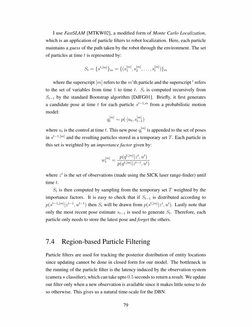
I use FastSLAM [MTKW02], a modified form of Monte Carlo Localization,which is an application of particle filters to robot localization. Here, each particlemaintains a guess of the path taken by the robot through the environment. The setof particles at time t is represented by:

St = {st,[m]}m = {(s[m]1 , s

[m]2 , . . . , s

[m]t )}m

where the superscript [m] refers to them’th particle and the superscript t refersto the set of variables from time 1 to time t. St is computed recursively fromSt−1 by the standard Bootstrap algorithm [DdFG01]. Briefly, it first generatesa candidate pose at time t for each particle st−1,m from a probabilistic motionmodel:

q[m]t ∼ p(·|ut, s[m]

t−1)

where ut is the control at time t. This new pose q[m]t is appended to the set of poses

in st−1,[m] and the resulting particles stored in a temporary set T . Each particle inthis set is weighted by an importance factor given by:

w[m]t =

p(qt,[m]|zt, ut)p(qt,[m]|zt−1, ut)

where zt is the set of observations (made using the SICK laser range-finder) untiltime t.

St is then computed by sampling from the temporary set T weighted by theimportance factors. It is easy to check that if St−1 is distributed according top(st−1,[m]|zt−1, ut−1) then St will be drawn from p(st,[m]|zt, ut). Lastly note thatonly the most recent pose estimate st−1 is used to generate St. Therefore, eachparticle only needs to store the latest pose and forget the others.

7.4 Region-based Particle Filtering

Particle filters are used for tracking the posterior distribution of entity locationssince updating cannot be done in closed form for our model. The bottleneck inthe running of the particle filter is the latency induced by the observation system(camera + classifier), which can take upto 0.5 seconds to return a result. We updateour filter only when a new observation is available since it makes little sense to doso otherwise. This gives us a natural time-scale for the DBN.

79

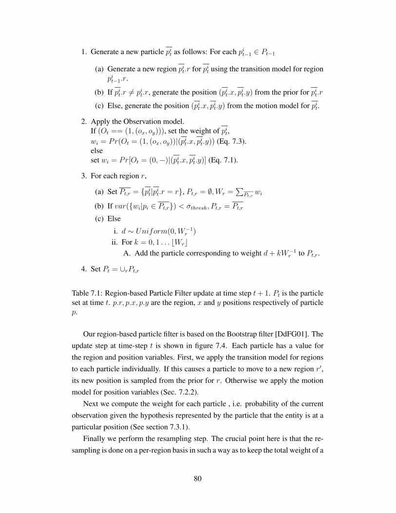
1. Generate a new particle pit as follows: For each pit−1 ∈ Pt−1

(a) Generate a new region pit.r for pit using the transition model for regionpit−1.r.

(b) If pit.r 6= pit.r, generate the position (pit.x, pit.y) from the prior for pit.r

(c) Else, generate the position (pit.x, pit.y) from the motion model for pit.

2. Apply the Observation model.If (Ot == (1, (ox, oy))), set the weight of pit,wi = Pr(Ot = (1, (ox, oy))|(pit.x, pit.y)) (Eq. 7.3).elseset wi = Pr[Ot = (0,−)|(pit.x, pit.y)] (Eq. 7.1).

3. For each region r,

(a) Set Pt,r = {pit|pit.r = r}, Pt,r = ∅,Wr =∑

Pt,rwi

(b) If var({wi|pi ∈ Pt,r}) < σthresh, Pt,r = Pt,r

(c) Else

i. d ∼ Uniform(0,W−1r )

ii. For k = 0, 1 . . . bWrcA. Add the particle corresponding to weight d+ kW−1

r to Pt,r.

4. Set Pt = ∪rPt,r

Table 7.1: Region-based Particle Filter update at time step t+ 1. Pt is the particleset at time t. p.r, p.x, p.y are the region, x and y positions respectively of particlep.

Our region-based particle filter is based on the Bootstrap filter [DdFG01]. Theupdate step at time-step t is shown in figure 7.4. Each particle has a value forthe region and position variables. First, we apply the transition model for regionsto each particle individually. If this causes a particle to move to a new region r′,its new position is sampled from the prior for r. Otherwise we apply the motionmodel for position variables (Sec. 7.2.2).

Next we compute the weight for each particle , i.e. probability of the currentobservation given the hypothesis represented by the particle that the entity is at aparticular position (See section 7.3.1).

Finally we perform the resampling step. The crucial point here is that the re-sampling is done on a per-region basis in such a way as to keep the total weight of a

80

given region equal to the total weight of all the particles in that region. This allowsus to keep the probability mass of each region tightly controlled. Essentially, theonly way for mass to shift from one region to another is through the transitionmodel. Thus the estimates of the discrete probabilities at the region layers willbe highly accurate, even if the distribution of the position variables are not. Thisimproves the performance of planning algorithms that use only the discrete regionvalues for decision-making. It also prevents particles from overlapping regionsbeing confused.

Re-sampling is not done at every step, but only when the empirical varianceof the particle weights for a region is below a fixed threshold. The idea is that itis advantageous to re-sample when the weights are concentrated on a small set ofparticles in the region.

We also use a sequential stochastic process during re-sampling instead of gen-erating each new particle individually. The idea is to first generate a random num-ber t in the range [0,W−1] where W is the total weight. Then the set of samplesreturned correspond to the weights t, t+W−1, t+ 2W−1, . . . . This process whilebeing only slightly less random than the naive one, reduces the complexity ofthe re-sampling from O(M logM) to O(M), where M is the number of particles[TBF05b].

Note that there is some similarity between our region-based algorithm andstratified sampling [TBF05b]. In stratified sampling, the partitions of the parti-cles are chosen arbitrarily, rather than based on the value of one of the sampledvariables, and the purpose there is variance reduction rather than controlling theprobability masses of the partitions. Our method has all the advantages of strati-fied sampling and the ones described above.

It might be useful to combine our work with a KLD-sampling strategy [D.03]that adapts the number of particles on a per-region basis.

7.4.1 Multiple Entities

Tracking multiple entities can be efficiently done by using separate particle fil-ters. Observe that in our model the only correlations between entity locations arethose induced by the robot pose, upon which the observations of all the entitiesdepend (see Figure 7.2). It is easy to see however, that the location of two enti-ties are conditionally independent of each other given the complete history of the

81

robot’s motion (i.e. robot poses at all time steps). As described in section 7.3.2,the localizer represents this information in each particle, and therefore separateparticle filters can be used for tracking the location of each entity. This bringsdown the dependence of the size of the particle filter on the number of entities,from exponential to linear.

7.4.2 Comparison with Rao-Blackwellization

Rao-Blackwellization [DdFG01] is a standard technique, where a portion of thestate space is tracked analytically while the rest is sampled. We experimented withRao-Blackwellizing our model by sampling the region variables and updating thepositions using an Extended Kalman Filter (EKF). However, complications areintroduced by the observation model, which prevent updates from being made inclosed form in the EKF. Essentially, when the camera views part of a region anddoes not find an entity there, then every particle from that region has to be split

into two, representing the observed and unobserved parts of the region respec-tively. The observed part will then be downweighted. In the limiting case, as theregions keep splitting, we end up with a large number of regions, which is practi-cally equivalent to having sampled the position variables directly in the first place.Hence we chose not to use Rao-Blackwellization.

7.5 Experiments

We applied these methods to robot delivery tasks in simulation and on a real robot.We considered n-object n-person delivery scenarios in a 5-room office environ-ment, with varying n. Reinforcement learning was done in the simulation overthe course of thousands of scenarios to learn a good policy for this task, and thentransferred to a real robot. The actions available to the robot were:

1. Move towards region r for t seconds.

2. Pickup object x from region r.

3. Deliver currently held object to person x in region r.

82

The robot gets a reward for completing each task proportional to its priority.The Q function was represented in the following parametrized form:

Q(s, a) un∑

i=1

wiφi(s, a) = w · φ(s, a) (7.3)

where φ = φ1, . . . , φn is a vector of fixed feature functions and w = w1, . . . , wn

is a vector of weights. The feature functions are chosen to encode properties ofthe state and action that are relevant to determining the Q value. The featurevector used to approximate the Q function (Equation 7.3) was composed of rele-vant state variables such as Pr(Entity e in Region r), distance(entity e, region r),IsVisible(region r, region r′) and others. We also used some non-linear functionsof these basic features (such as Pr(Entity e in Region r)

distance(entity e, region r) ) to capture any non-linear de-pendence the Q∗ function has on the state.

Even with just two delivery tasks we can expect very complex behaviour fromthe optimal policy. Suppose for example, the robot was in a position to immedi-ately pick up either of the two objects. It would generally prefer the task for whichits belief about the person’s location was more certain in the current state. But thiscould change if one task had greater priority than the other or if choosing the othertask meant that unexplored regions of the environment could be visited and newobservations made. When choosing its next action, the robot must not only con-sider regions that are likely to have relevant entities, but also the distances to themand the visibility of other regions from there. We shall show that the learnedpolicy exhibits these behaviours, and finds near-optimal tradeoffs between them.

7.5.1 Entity Tracking

We compared the performance of the region-based particle filter against a baselinebootstrap filter without any region representation by running 100 real-time sim-ulations of the multiple entity delivery task described above in PLAYER’s robotsimulator [GVH03a]. The manual policy describe above was used in conjunctionwith both belief-tracking algorithms. We demonstrate the improvement in thestate tracking by measuring the mean-time to completion of all the tasks in bothcases. The results in Figure 7.5 clearly show that the region-based particle filterdominates. Note that this is not the running time of the algorithm, but the simu-lation time taken by the robot to complete the task. More time is wasted by the

83

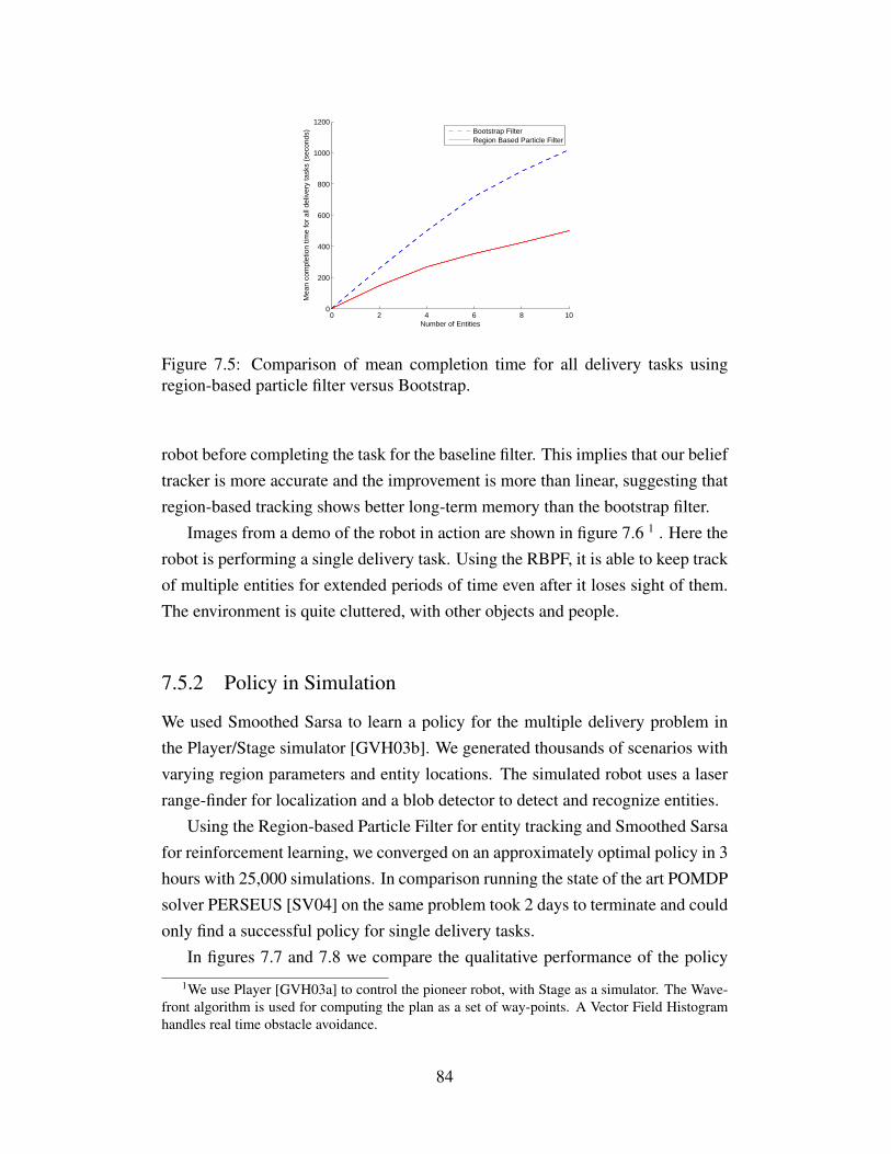
0 2 4 6 8 100

200

400

600

800

1000

1200

Number of Entities

Mea

n co

mpl

etio

n tim

e fo

r al

l del

iver

y ta

sks

(sec

onds

)

Bootstrap FilterRegion Based Particle Filter

Figure 7.5: Comparison of mean completion time for all delivery tasks usingregion-based particle filter versus Bootstrap.

robot before completing the task for the baseline filter. This implies that our belieftracker is more accurate and the improvement is more than linear, suggesting thatregion-based tracking shows better long-term memory than the bootstrap filter.

Images from a demo of the robot in action are shown in figure 7.6 1 . Here therobot is performing a single delivery task. Using the RBPF, it is able to keep trackof multiple entities for extended periods of time even after it loses sight of them.The environment is quite cluttered, with other objects and people.

7.5.2 Policy in Simulation

We used Smoothed Sarsa to learn a policy for the multiple delivery problem inthe Player/Stage simulator [GVH03b]. We generated thousands of scenarios withvarying region parameters and entity locations. The simulated robot uses a laserrange-finder for localization and a blob detector to detect and recognize entities.

Using the Region-based Particle Filter for entity tracking and Smoothed Sarsafor reinforcement learning, we converged on an approximately optimal policy in 3hours with 25,000 simulations. In comparison running the state of the art POMDPsolver PERSEUS [SV04] on the same problem took 2 days to terminate and couldonly find a successful policy for single delivery tasks.

In figures 7.7 and 7.8 we compare the qualitative performance of the policy

1We use Player [GVH03a] to control the pioneer robot, with Stage as a simulator. The Wave-front algorithm is used for computing the plan as a set of way-points. A Vector Field Histogramhandles real time obstacle avoidance.

84

Figure 7.6: Particle filter with beliefs for robot and person position (best viewed incolor). Person particles are shown with black squares. Object particles are shownwith red circles. Robot position is shown as an unfilled circle. Ordered from leftto right, Top row: (i) Prior belief at start (ii) After person is detected (iii) Belief asrobot is leaving the room and person is no longer seen, Second Row: (iv) Beforeentering the room on the right (v) After object is recognized (vi) Robot in corridorbut new position of person is not seen. Third Row: (vii) After person is seenagain (viii) Robot approaching its planned position and does not find the person(ix) Robot replans and find person.

learned by Smoothed Sarsa and a manually crafted basline policy. The manualpolicy does each task in order of priority, and when searching for an entity, itvisits the regions in order of maximum likelihood. The smoothed-sarsa policydemonstrates more intelligent behaviour than the manual one. The manual policystarts out looking for the first object in the leftmost room and keeps looking for itwithout switching tasks after it sees the second object. Consequently it must moveback and forth between the two ends of the office 3 times to complete all the tasks.The smoothed sarsa policy moves to the rightmost room first because it recognizesthat the probability of completing some task is greatest there. It decides to do thesecond delivery task since both the object and the person are in the same room.It then completes the first task, moving across to the left room just once. Thetotal run time was 50 seconds for the sarsa policy and 118 seconds for the manualpolicy.

85

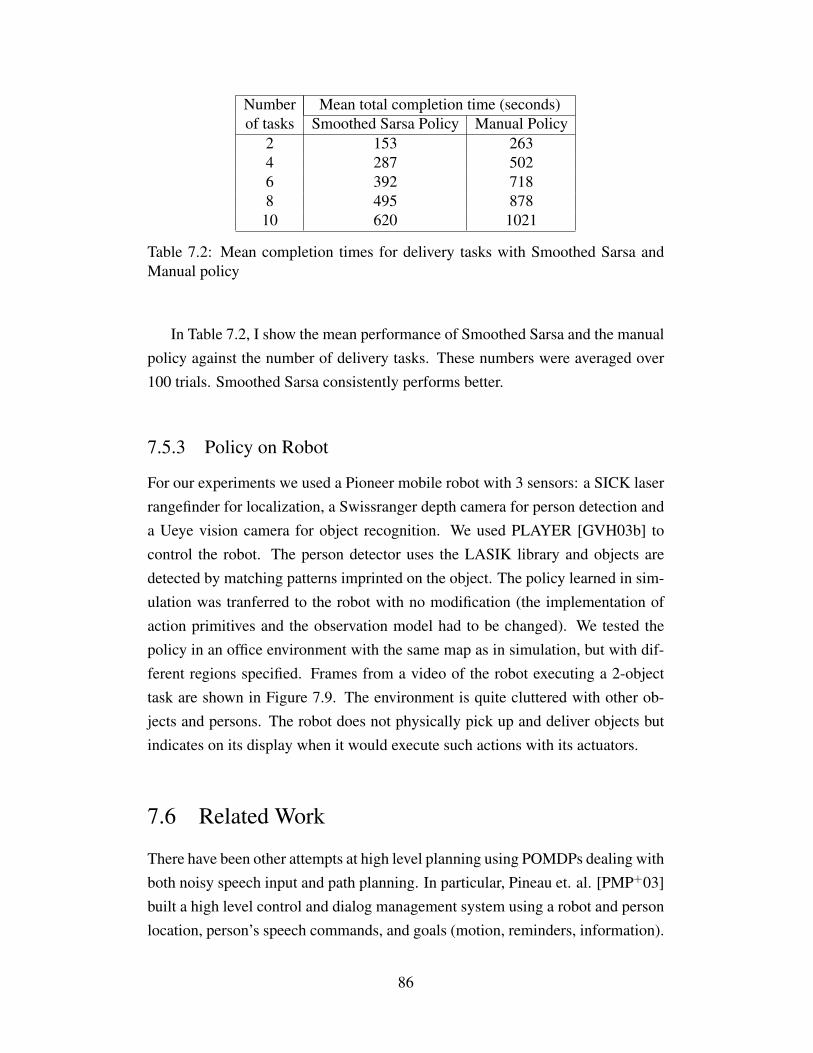
Number Mean total completion time (seconds)of tasks Smoothed Sarsa Policy Manual Policy

2 153 2634 287 5026 392 7188 495 87810 620 1021

Table 7.2: Mean completion times for delivery tasks with Smoothed Sarsa andManual policy

In Table 7.2, I show the mean performance of Smoothed Sarsa and the manualpolicy against the number of delivery tasks. These numbers were averaged over100 trials. Smoothed Sarsa consistently performs better.

7.5.3 Policy on Robot

For our experiments we used a Pioneer mobile robot with 3 sensors: a SICK laserrangefinder for localization, a Swissranger depth camera for person detection anda Ueye vision camera for object recognition. We used PLAYER [GVH03b] tocontrol the robot. The person detector uses the LASIK library and objects aredetected by matching patterns imprinted on the object. The policy learned in sim-ulation was tranferred to the robot with no modification (the implementation ofaction primitives and the observation model had to be changed). We tested thepolicy in an office environment with the same map as in simulation, but with dif-ferent regions specified. Frames from a video of the robot executing a 2-objecttask are shown in Figure 7.9. The environment is quite cluttered with other ob-jects and persons. The robot does not physically pick up and deliver objects butindicates on its display when it would execute such actions with its actuators.

7.6 Related Work

There have been other attempts at high level planning using POMDPs dealing withboth noisy speech input and path planning. In particular, Pineau et. al. [PMP+03]built a high level control and dialog management system using a robot and personlocation, person’s speech commands, and goals (motion, reminders, information).

86

They learnt a policy using a hierarchical decomposition of POMDPs that askedfor confirmations to reduce uncertainty. However they made a strong assumptionthat the domain possesses structure that can be expressed via an action hierarchy.Schmidt-Rohr et. al. [SRKLD08, SRLD08] built a POMDP with 200 states and11 actions for a fetch and delivery task. However, their policy is manual and notlearnt. Spaan et. al. [SV04] perform both localization and path planning usingPOMDPs. They discretize a multiple room environment into a 500 position gridand performs an object delivery task from a group of static pickup grid locationsto a static group of delivery grid locations, with an extra bit for carrying mail.However their policy does not consider the interesting features of decision makingthat we have, and in fact can be thought of as solving multiple path planningproblems.

The closest work in the reinforcement community to our Smoothed Sarsa al-gorithm is that by Walsh et. al. [WNL07] on learning with delayed rewards, asetting where rewards are received by the agent only after some delay.

Past work on entity tracking has concentrated on tracking movement of peo-ple in the immediate neighborhood of the mobile robot over short time periodsusing lasers and RFID sensors [MTW02, SBFC03, BBCT05]. However, these ap-proaches focus on short-term tracking and lose track of the entity within secondsof it going out of the field of view. In addition, lasers cannot recognize peopleexcept as dynamic obstacles in the environment and the wide-scale use of RFIDsis impractical.

7.7 Contributions

In this chapter I propose a framework for learning to do task-level decision mak-ing on robots. The major contribution is the application of Smoothed Sarsa to areal-life reinforcement learning problem i.e. object delivery on robots. I showedthat Smoothed Sarsa leads to faster task completion times and higher values then amanual policy. It can learn a policy orders of magnitude faster than previous pol-icy search algorithms when significant observational uncertainty exists. I demon-strated results on the Player/Stage simulator and have shown successful task com-pletions using the same policy on a Pioneer robot.

Second, I introduced the region-based particle filter for tracking people andobjects in the environment. The algorithm emphasizes the accurate tracking of

87

the discrete region variables, which are more useful for decision making, at theexpense of precise positional estimates.

It is possible to extend this work to tasks other than object delivery, such asrecycling and robot relocalization. The same methods should apply with appro-priate modifications to the Q function representation. For further generality, thelocations of the regions and the transition model could be learned from clusteringreal-world observations of peoples’ behaviour over time.

88

Figure 7.7: Manual policy using Stage simulator. The top image in each frame is asnapshot from the simulator and the bottom is a visualization of the robot’s beliefstate and current action. The line joining the robot to the region shows the regionthat the robot is moving to. Ordering from left to right (best viewed in color). TOPROW (a) Robot initialized with priors (b) Robot looking for the first object in theleft room based on prior (c) first object not found but first person found. MIDDLELOW (d) Robot looking for the first object in right room (e) second object found.Robot next navigates to top part of room. BOTTOM ROW (f) First object foundand picked up. Robot navigating to first person in left room (g) After deliveringfirst object, robot navigating to second object (h) Robot picks up second objectand navigates to second person in the right room (i) Second object delivered.

89

Figure 7.8: Smoothed Sarsa policy using Stage simulator. The top image in eachframe is a snapshot from the simulator and the bottom is a visualization of therobot’s belief state and current action. The line joining the robot to the regionshows the region that the robot is moving to. Ordering from left to right (bestviewed in color). TOP ROW (a) Robot going to left room to look for first object(b) Robot sees second object and picks it up (c) Second object is being deliveredto the second person BOTTOM ROW (d) Robot moving to the first object in thesame right room (e) Robot looking for first person in the left room (f) First objectdelivered.

90

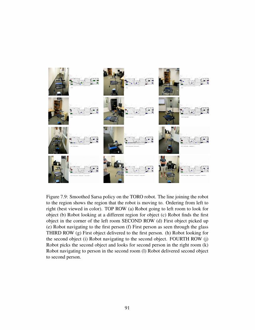
Figure 7.9: Smoothed Sarsa policy on the TORO robot. The line joining the robotto the region shows the region that the robot is moving to. Ordering from left toright (best viewed in color). TOP ROW (a) Robot going to left room to look forobject (b) Robot looking at a different region for object (c) Robot finds the firstobject in the corner of the left room SECOND ROW (d) First object picked up(e) Robot navigating to the first person (f) First person as seen through the glassTHIRD ROW (g) First object delivered to the first person. (h) Robot looking forthe second object (i) Robot navigating to the second object. FOURTH ROW (j)Robot picks the second object and looks for second person in the right room (k)Robot navigating to person in the second room (l) Robot delivered second objectto second person.

91

CHAPTER 8

CONCLUSION

Reinforcement Learning is a complex learning paradigm. The basic algorithmsand techniques have reached a level of maturity and applications have proliferated.However many extensions and variations of the basic formulation can be made andindeed, have practical applications in the real world. In my thesis I focused on theimplications of our knowledge of reward functions and ignorance of observationmodels. I showed that we can gain insight into how decision making can be doneoptimally and intelligently in these situations by analyzing models of decisionmaking in classical RL problems. Of course, I have only skimmed the surface ofwhat can be done by varying the problem parameters. However, from the evidencepresented here, I believe we can conclude that:

Solutions for more general Reinforcement Learning problems can be found by

analyzing models of the decision making process in simpler ones.

92

APPENDIX A

PROOFS FOR CHAPTER 2

Theorem A.1. Given a distribution P (R) over reward functions R for an MDP

(S,A, T, γ), the loss function Lppolicy(R, π) is minimized for all p by π∗M , the opti-

mal policy for the Markov Decision Problem M = (S,A, T, γ, EP [R]).

Proof. From the Bellman equations (1.1) we can derive the following:

V π(R) = (I − γT π)−1R (A.1)

where T π is the |S| × |S| transition matrix for policy π. Thus, for a state s ∈ Sand fixed π, the value function is a linear function of the rewards:

V π(s,R) = w(s, π) ·R

where w(s, π) is the s’th row of the coefficient matrix (I − γT π)−1 in (A.1).Suppose we wish to maximize E[V π(s,R)] alone. Then,

maxπ

E[V π(s,R)] = maxπ

E[w(s, π) ·R] = maxπw(s, π) · E[R]

By definition this is equal to V ∗M(s), the optimum value function for M , andthe maximizing policy π is π∗M , the optimal policy for M . Thus for all statess ∈ S, E[V π(s,R)] is maximum at π = π∗M .

But V ∗(s,R) ≥ V π(s,R) for all s ∈ S, reward functions R, and policies π.Therefore

E[Lppolicy(π)] = E(‖ V ∗(R)− V π(R) ‖p)

is minimized for all p by π = π∗M .

Lemma A.2. Let F (·) be a positive real valued function defined on the cube {x ∈Rn| − d ≤ xi ≤ d} for some positive d, satisfying for all λ ∈ [0, 1] and some α, β

|f(x)− f(y)| ≤ α ‖ x− y ‖∞

93

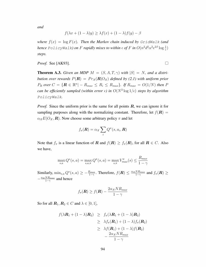
and

f(λx+ (1− λ)y) ≥ λf(x) + (1− λ)f(y)− β

where f(x) = logF (x). Then the Markov chain induced by GridWalk (and

hence PolicyWalk) on F rapidly mixes to within ε of F in O(n2d2α2e2β log 1ε)

steps.

Proof. See [AK93].

Theorem A.3. Given an MDP M = (S,A, T, γ) with |S| = N , and a distri-

bution over rewards P (R) = PrX (R|OX ) defined by (2.1) with uniform prior

PR over C = {R ∈ Rn| − Rmax ≤ Ri ≤ Rmax}. If Rmax = O(1/N) then P

can be efficiently sampled (within error ε) in O(N2 log 1/ε) steps by algorithm

PolicyWalk.

Proof. Since the uniform prior is the same for all points R, we can ignore it forsampling purposes along with the normalizing constant. Therefore, let f(R) =

αXE(OX ,R). Now choose some arbitrary policy π and let

fπ(R) = αX∑

i

Qπ(s, ai,R)

Note that fπ is a linear function of R and f(R) ≥ fπ(R), for all R ∈ C. Alsowe have,

maxs,a

Q∗(s, a) = maxs,a,π

Qπ(s, a) = maxs,π

V πmax(s) ≤

Rmax

1− γ

Similarly, mins,aQ∗(s, a) ≥ −Rmax

1−γ . Therefore, f(R) ≤ αXNRmax1−γ and fπ(R) ≥

−αXNRmax1−γ and hence

fπ(R) ≥ f(R)− 2αXNRmax

1− γ

So for allR1,R2 ∈ C and λ ∈ [0, 1],

f(λR1 + (1− λ)R2) ≥ fπ(λR1 + (1− λ)R2)

≥ λfπ(R1) + (1− λ)fπ(R2)

≥ λf(R1) + (1− λ)f(R2)

− 2αXNRmax

1− γ

94

Therefore, f satisfies the conditions of Lemma 2.2 with β = 2αXNRmax1−γ =

2N · O( 1N)

1−γ = O(1) and

α =|f(R1)− f(R2)|‖ R1 −R2 ‖∞

≤ 2αXNRmax

(1− γ)O( 1N

)= O(N)

Hence the Markov chain induced by the GridWalk algorithm (and the PolicyWalkalgorithm) on P mixes rapidly to within ε of P in a number of steps equal toO(N2 1

N2N2eO(1) log 1/ε) = O(N2 log 1/ε).

95

APPENDIX B

PROOF FOR CHAPTER 4

Theorem B.1. Let M = (S,A, T, γ, R) be an MDP. Let F : S ×A 7→ R be some

shaping function. Then,

1. If F is potential-based, then every optimal policy for M ′ = (S,A, T, γ, R+

F ) will also be an optimal policy for M (and vice versa).

2. If F is not potential-based, then there exists a transition function T and a

reward function R such that no optimal policy for M ′ is optimal for M .

Proof. The optimal Q function for M , Q∗M satisfies the Bellman equations (1.1),

Q∗M(s, a) = R(s, a) + γEs′∼Psa [maxa′∈A

Q∗M(s′, a′)]

Subtracting Φ(s) and rearranging terms on the right hand side:

Q∗M(s, a)− Φ(s) = R(s, a) + γEs′∼Psa [Φ(s′)]− Φ(s)

+γEs′∼Psa [maxa′∈A

Q∗M(s′, a′)− Φ(s′)]

Let QM ′(s, a) , Q∗M(s, a)− Φ(s).

QM ′(s, a) = R′(s, a) + γEs′∼Psa [maxa′∈A

QM ′(s′, a′)]

So QM ′ satisfies the Bellman equation forM ′ and must be the optimalQ function.Therefore the optimal policy for M ′ satisfies:

π∗M ′(s) ∈ argmaxa∈A

Q∗M ′(s, a)

= argmaxa∈A

Q∗M(s, a)− Φ(s)

= argmaxa∈A

Q∗M(s, a)

and so π∗ is also optimal forM . For the other direction, we can simply interchange

96

the roles of M and M ′.

97

APPENDIX C

PROOF FOR CHAPTER 5

Theorem C.1. The expected value of the almost MDP M is less than that of its

underlying MDP MA by at most (1−θ)Rmax1−γ−γθ+γ2θ .

Proof. Let π∗ be the optimal policy of M and b1 be a belief state of MA such thatPr(b1 = s1) > θ for the underlying state s1 of M . We will compare the valueobtained by π∗ on s1 in M and b1 in MA. For the MDP M ,

V π∗M (s1) = r(s1, a1) + E[γr(s2, a2) + γ2r(s3, a3) + . . .]

For the Almost MDP MA, we can seperate out

V πAMDPMA

(b1) = Pr(b1 = s1)E[V π∗MA

(b1)|b1 = s1] + Pr(b1 6= s1)E[V π∗MA

(b1)|b1 6= s1]

Subtracting,

V π∗M (s1)− V πAMDP

MA(b1)

= r(s1, a1) + E[γr(s2, a2) + γ2r(s3, a3) + . . .]

−[Pr(b1 = s1)E[V π∗MA

(b1)|b1 = s1]

+Pr(b1 6= s1)E[V π∗MA

(b1)|b1 6= s1]]

< r(s1, a1) + E[γr(s2, a2) + γ2r(s3, a3) + . . .]

−θE[V π∗MA

(b1)|b1 = s1]

< r(s1, a1) + E[γr(s2, a2) + γ2r(s3, a3) + . . .]

−θ(r(s1, a1) + γE[V π∗MA

(b2)])

< (1− θ)r(s1, a1) + E[γr(s2, a2) + γ2r(s3, a3) + . . .]

98

V π∗M (s1)− V πAMDP

MA(b1)

−γθ2E[V π∗MA

(b2)|b2 = s2]

< (1− θ)r(s1, a1) + E[γ(1− θ2)r(s2, a2)]+E[γ2r(s3, a3) + γ3r(s4, a4) + . . .]

−γ2θ2E[V π∗MA

(b3)]

. . .

< E[(1− θ)r(s1, a1) + γ(1− θ2)r(s2, a2)+γ3(1− θ3)r(s3, a3) + . . .]

<(1− θ)Rmax

1− γ − γθ + γ2θ

Note that we are taking the difference of two infinite series above, which isallowed since they are both absolutely convergent.

Theorem C.2. The expected value of the Almost CD-MDP MA with parameter k

is less than that of the underlying CD-MDP M by at most (1−θ)Rmax1−γ−γθ+γ2θ .

Proof. Consider the MDP MI = 〈S × Ak, A, T, γ, R〉 with expanded state spaceI = S ×Ak. As discussed in section 5.3, the optimal policy πIand value functionV π for MI , is an optimal policy and value function for the CD-MDP M . Now,define a POMDP, PI = 〈I, A, T, γ, R, (O,Ak)〉 with belief space BI = B × Akwhere B is the belief space of MA. We can make a similar connection betweenoptimal policies and value functions for PI and MA. Now, we show that PI is anAMDP for the MDP M . Indeed,

Pr(it+k = i|ot+k, at:t+k) = Pr(bt = s|ot+k, at+1:t+k)Pr(at+1:t+k)

= Pr(bt = s|ot+k)> θ

Therefore, the value of PI at belief state bi = (b, a1:k),

VPI [bi] > Es∼b[VMI((s, a1:k))]− (1− θ)Rmax

1− γ − γθ + γ2θ

99

and therefore,

VMA[b] > Esi∼bi [VM((si, a

1:k))]− (1− θ)Rmax

1− γ − γθ + γ2θ

100

REFERENCES

[ACV08] Nicholas Armstrong-Crews and Manuela M. Veloso. An approxi-mate algorithm for solving oracular pomdps. In ICRA, pages 3346–3352, 2008.

[AD01] L. F. Abbott and Peter Dayan. Theoretical neuroscience: compu-tational and mathematical modeling of neural systems. The M.I.T.Press, Cambridge, Mass., 2001.

[ADNT08] Pieter Abbeel, Dmitri Dolgov, Andrew Y. Ng, and Sebastian Thrun.Apprenticeship learning for motion planning with application toparking lot navigation. In IROS, pages 1083–1090, 2008.

[AK93] D. Applegate and R. Kannan. Sampling and integration of near log-concave functions. In Proceedings of the ACM Symposium on theTheory of Computing’93, 1993.

[AM02] R. Amit and Maja Mataric. Learning movement sequences fromdemonstration. In Proc. ICDL, pages 203–208, 2002.

[Ama98] Shun-Ichi Amari. Natural gradient works efficiently in learning.Neural Comput., 10:251–276, February 1998.

[AN04] Pieter Abbeel and Andrew Y. Ng. Apprenticeship learning via in-verse reinforcement learning. In Proceedings of the Twenty-first In-ternational Conference on Machine Learning, 2004.

[AS97] C. Atkeson and S. Schaal. Robot learning from demonstration. InProceedings of ICML’97, 1997.

[Asi50] Isaac Asimov. I, Robot, chapter Runaround. Doubleday & Com-pany, 1950.

[AV98] K O Arras and S J Vestli. Hybrid, high-precision localization formail distribution mobile system robot mops. In Proceedings ofthe IEEE International Conference on Robotics and Automation(ICRA), May 1998.

101

[BBCT05] Maren Bennewitz, Wolfram Burgard, Grzegorz Cielniak, and Sebas-tian Thrun. Learning motion patterns of people for compliant robotmotion. The International Journal of Robotics Research, 24(1):31–48, 2005.

[Bel57] R. Bellman. Dynamic Programming. Princeton University Press,Princeton, NJ, 1957.

[Ber93] James O. Berger. Statistical Decision Theory and Bayesian Analy-sis. Springer, 2nd edition, 1993.

[BGFB94] S. Boyd, L. E. Ghaoui, E. Feron, and V. Balakrishnan. Linear matrixinequalities in system and control theory. SIAM, 1994.

[BP66] L. E. Baum and T. Petrie. Statistical inference for probabilistic func-tions of finte state markov chains. Annals of Mathematical Statistics,37:1554–1563, 1966.

[BPSS98] Darse Billings, Denis Papp, Jonathan Schaeffer, and Duane Szafron.Opponent modeling in Poker. In Proceedings of the 15th NationalConference on Artificial Intelligence (AAAI-98), pages 493–498,Madison, WI, 1998. AAAI Press.

[BRP01] Craig Boutilier, Raymond Reiter, and Bob Price. Symbolic dynamicprogramming for first-order MDPs. In Proc. Seventeenth Interna-tional Joint Conference on Artificial Intelligence (IJCAI ’01), pages690–700, 2001.

[BT01] Ronen I. Brafman and Moshe Tennenholtz. R-max - a generalpolynomial time algorithm for near-optimal reinforcement learning.Journal of Machine Learning Research, 3:213–231, 2001.

[CAN09] Adam Coates, Pieter Abbeel, and Andrew Y. Ng. Apprentice-ship learning for helicopter control. Communications of the ACM,52(7):97–105, 2009.

[CH94] W. W. Cohen and H. Hirsh, editors. Reward functions for acceler-ated learning, CA, 1994. Morgan Kauffman.

[Cip87] Barry A. Cipra. An introduction to the Ising model. American Math-ematics Monthly, 94(10):937–959, 1987.

[CKO01] Urszula Chajewska, Daphne Koller, and Dirk Ormoneit. Learningan agent’s utility function by observing behavior. In Proc. 18th In-ternational Conf. on Machine Learning, pages 35–42. Morgan Kauf-mann, San Francisco, CA, 2001.

[Cla89] P Clark. Knowledge representation in machine learning. Machineand Human Learning, pages 35–49, 1989.

102

[CV95] Corinna Cortes and V. Vapnik. Support-vector networks. MachineLearning, 20, 1995.

[D.03] Fox D. Adapting the sample size in particle filters through kld-sampling. International Journal of Robotics Research, 22, 2003.

[DdFG01] Arnaud Doucet, Nando de Freitas, and Neil Gordon, editors. Se-quential Monte Carlo Methods in Practice. Springer, 2001.

[DeJ04] Gerald DeJong. Explanation-based learning. In A. Tucker, edi-tor, Computer Science Handbook, pages 68.1 – 68.18. Chapman &Hall/CRC and ACM, 2nd edition, 2004.

[Eng93] J F. Engelberger. Health care robotics goes commercial - the help-mate experience. Robotica, 7:517–523, 1993.

[GDGN08] Goodfellow, Dreyfus, Gould, and Ng. People detection in 3-dimensions on STAIR. Unpublished Manuscript, 2008.

[GKP01] C. Guestrin, D. Koller, and R. Parr. Multiagent planning with fac-tored mdps. In 14th Neural Information Processing Systems (NIPS-14), 2001.

[Gud06] S. A. Gudmundsson. Robot vision applications using the CSEMswissranger camera. Master’s thesis, Informatics and MathematicalModelling, Technical University of Denmark DTU, 2006.

[GVH03a] Brian Gerkey, Richard T. Vaughan, and Andrew Howard. Theplayer/stage project: Tools for multi-robot and distributed sensorsystems. In Proceedings of the 11th International Conference onAdvanced Robotics (ICAR 2003), pages 317–323, 2003.

[GVH03b] Brian P. Gerkey, Richard T. Vaughan, and Andrew Howard. Theplayer/stage project: Tools for multi-robot and distributed sensorsystems. In In Proceedings of the 11th International Conference onAdvanced Robotics, pages 317–323, 2003.

[HA04] Brian Hlubocky and Eyal Amir. Knowledge-gathering agents in ad-venture games. In AAAI-04 workshop on Challenges in Game AI,2004.

[Has70] W. K. Hastings. Monte carlo sampling methods using markov chainsand their applications. Biometrika, 57(1):97–109, 1970.

[HD94] Gillian Hayes and John Demiris. A robot controller using learn-ing by imitation. In Adam Borkowski and James L Crowley, ed-itors, SIRS-94, Proc. of the 2nd Intern. Symposium on IntelligentRobotic Systems, pages 198–204, LIFIA-IMAG, Grenoble, France,July 1994.

103

[Hir07] Hirohisa Hirukawa. Walking biped humanoids that performmanual labour. Philosophical Transactions of the RoyalSociety A:Meathematical, Physical and Engineering Sciences,365(1850):65–77, January 2007.

[How60] Ronald A. Howard. Dynamic Programming and Markov Processes.The M.I.T. Press, 1960.

[Jay57] E.T. Jaynes. Information theory and statistical mechanics. PhysicsReviews, 106:620–630, 1957.

[JEI87] Jr. Jonathan E. Ingersoll. Theory of Financial Decision Making.Rowman and Littlefield, 1987.

[JUA+07] Yoshiaki Jitsukawa, Ryuichi Ueda, Tamio Arai, Kazutaka Takeshita,Yuji Hasegawa, Shota Kase, Takashi Okuzumi, Kazunori Umeda,and Hisashi Osumi. Fast decision making of autonomous robotunder dynamic environment by sampling real-time q-mdp valuemethod. In IROS, pages 1644–1650, 2007.

[Kal60] Rudolph Emil Kalman. A new approach to linear filtering and pre-diction problems. Transactions of the ASME–Journal of Basic En-gineering, 82(Series D):35–45, 1960.

[KAN07] J. Zico Kolter, Pieter Abbeel, and Andrew Y. Ng. Hierarchical ap-prenticeship learning with application to quadruped locomotion. InNIPS, 2007.

[KD01] J. Kvarnstrom and P. Doherty. Talplanner: A temporal logic basedforward chaining planner. Annals of Mathematics and Artificial In-telligence (AMAI), Volume 30:pages 119–169, 2001.

[KE03] K.V. Katsikopoulos and S.E. Engelbrecht. Markov decision pro-cesses with delays and asynchronous cost collection. In IEEE trans.on Automatic Control, 2003.

[KLC98] Leslie Pack Kaelbling, M. Littman, and A Cassandra. Planning andacting in partially observable stochastic domains. Artificial Intelli-gence, 101:99–134, 1998.

[KS98] Sven Koenig and Reid Simmons. Xavier: A robot navigation archi-tecture based on partially observable markov decision process mod-els. In D. Kortenkamp, R. Bonasso, and R. Murphy, editors, Artifi-cial Intelligence Based Mobile Robotics: Case Studies of SuccessfulRobot Systems, pages 91 – 122. MIT Press, 1998.

[KS02] Michael Kearns and Satinder Singh. Near-optimal reinforcementlearning in polynomial time. Mach. Learn., 49:209–232, November2002.

104

[Lav66] R E Lave. A markov decision process for economic quality con-trol. In IEEE Transactions on Systems Science and Cybernetics,volume 2, pages 45–54, 1966.

[LD02] Adam Laud and Gerald DeJong. Reinforcement learning and shap-ing: Encouraging intended behaviors. In Proceedings of the 19thInternational Conference on Machine Learning (ICML-02), pages355–362, 2002.

[Lit94] Michael L. Littman. Memoryless policies: theoretical limitationsand practical results. In Proceedings of the third international con-ference on Simulation of adaptive behavior : from animals to an-imats 3: from animals to animats 3, pages 238–245, Cambridge,MA, USA, 1994. MIT Press.

[Lit96] Michael Lederman Littman. Algorithms for sequential decisionmaking. PhD thesis, Brown University, 1996.

[LMM08] Manuel C. Lopes, Francisco S. Melo, and Luis Montesano.Affordance-based imitation learning in robots. Proceedings of the2008 IEEE/RSJ International Conference on Intelligent Robots andSystems, pages 1015–1021, 2008.

[LS98] John Loch and Satinder P. Singh. Using eligibility traces to findthe best memoryless policy in partially observable markov decisionprocesses. In ICML, pages 323–331, 1998.

[LS04] Hugo Liu and Push Singh. Conceptnet: A practical commonsensereasoning toolkit. BT Technology Journal, 22, 2004.

[MAF+99] Toshihiro Matsui, Hideki Asoh, John Fry, Youichi Motomura, Fu-toshi Asano, Takio Kurita, Isao Hara, and Nobuyuki Otsu. Inte-grated natural spoken dialogue system of Jijo-2 mobile robot foroffice services. In Proceedings of American Association of ArtificialIntelligence Conference (AAAI), pages 621–627, Orlando, FL, July18-22 1999.

[Mar07] Bhaskara Marthi. Automatic shaping and decomposition of rewardfunctions. In Proceedings of the 24th international conference onMachine learning, ICML ’07, pages 601–608, New York, NY, USA,2007. ACM.

[MD03] A N Meltzoff and J. Decety. What imitation tells us about so-cial cognition: a rapprochement between developmental psychol-ogy and cognitive neuroscience. Philos Trans R Soc Lond B BiolSci, 358(1431):491–500, March 2003.

105

[MMI+06] Noriaki Mitsunaga, Takahiro Miyashita, Hiroshi Ishiguro, KiyoshiKogure, and Norihiro Hagita. Robovie-IV: A communication robotinteracting with people daily in an office. In The 2006 IEEE/RSJInternational Conference on Intelligent Robots and Systems (IROS),pages 5066–5072, October 2006.

[MRB+99] Iacoboni M., Woods R.P., M. Brass, H. Bekkering, J.C. Mazziotta, ,and Rizzolatti G. Cortical mechanisms of human imitation. Science,286:2526–8, 1999.

[MTKW02] M. Montemerlo, S. Thrun, D. Koller, and B. Wegbreit. FastSLAM:A factored solution to the simultaneous localization and mappingproblem. In Proceedings of the AAAI National Conference on Arti-ficial Intelligence, 2002.

[MTW02] Michael Montemerlo, Sebastian Thrun, and William Whittaker.Conditional particle filters for simultaneous mobile robot localiza-tion and people-tracking. In Proceedings of IEEE InternationalConference on Robotics and Automation (ICRA), volume 1, pages695– 701, Washington D.C., May 2002.

[MW03] Mausam and Daniel S. Weld. Solving relational MDPs with first-order machine learning. In Proc. ICAPS Workshop on Planning un-der Uncertainty and Incomplete Information, 2003.

[NHR99] Andrew Y. Ng, Daishi Harada, and Stuart Russell. Policy invari-ance under reward transformations: theory and application to rewardshaping. In Proc. 16th International Conf. on Machine Learning,pages 278–287. Morgan Kaufmann, San Francisco, CA, 1999.

[NPB95] Illah Nourbakhsh, Rob Powers, and Stan Birchfield. Dervish: Anoffice-navigating robot. AI Magazine, 16(1), 1995.

[NR00] Andrew Y. Ng and Stuart Russell. Algorithms for inverse reinforce-ment learning. In Proc. 17th International Conf. on Machine Learn-ing, pages 663–670. Morgan Kaufmann, San Francisco, CA, 2000.

[NS07] Gergely Neu and Csaba Szepesvari. Apprenticeship learning usinginverse reinforcement learning and gradient methods. In Proc. UAI,2007.

[PB03] Bob Price and Craig Boutilier. A Bayesian approach to imitation inreinforcement learning. In Proc. IJCAI, 2003.

[Pin04] J. Pineau. Tractable Planning Under Uncertainty: Exploiting Struc-ture. PhD thesis, Carnegie Mellon University, 2004.

106

[PMP+03] J. Pineau, M. Montemerlo, M. Pollack, N. Roy, and S. Thrun.Towards robotic assistants in nursing homes: Challenges and re-sults. Special issue on Socially Interactive Robots, Robotics andAutonomous Systems, 42(3-4):271–281, 2003.

[Pro93] Gregory M. Provan. Tradeoffs in constructing and evaluating tem-poral influence diagrams. In UAI’93, pages 40–47, 1993.

[PT87] Christos Papadimitriou and John N. Tsitsiklis. The complexity ofmarkov decision processes. Math. Oper. Res., 12:441–450, August1987.

[Put94] M L Puterman. Markov decision processes: discrete stochastic dy-namic programming. John Wiley & Sons, Inc., New York, NY, USA,1994.

[PVS05] J. Peters, S. Vijayakumar, and S. Schaal. natural actor-critic. Inproceedings of the 16th european conference on machine learning(ecml 2005), pages 280–291. springer, 2005.

[RA98] Jette Randløv and Preben Alstrøm. Learning to drive a bicycle usingreinforcement learning and shaping. In Proceedings of the FifteenthInternational Conference on Machine Learning, ICML ’98, pages463–471, San Francisco, CA, USA, 1998. Morgan Kaufmann Pub-lishers Inc.

[RA07] Deepak Ramachandran and Eyal Amir. Bayesian inverse reinforce-ment learning. In IJCAI, pages 2586–2591, 2007.

[RN94] G. A. Rummery and M. Niranjan. On-line Q-learning using con-nectionist systems. Technical Report CUED/F-INFENG/TR 166,Cambridge University Engineering Dept., 1994.

[RRG05] Deepak Ramachandran, P. Reagan, and K. Goolsbey. First-orderizedResearchCyc: Expressivity and efficiency in a common-sense ontol-ogy. In Papers from the AAAI Workshop on Contexts and Ontolo-gies: Theory, Practice and Applications, Pittsburgh, Pennsylvania,July 2005.

[Rus98] Stuart Russell. Learning agents for uncertain environments (ex-tended abstract). In Proceedings of the Eleventh Annual Conferenceon Learning Theory. ACM Press, 1998.

[RZP+09] Nathan Ratliff, Brian Ziebart, Kevin Peterson, J. Andrew Bagnell,Martial Hebert, Anind K. Dey, and Siddhartha Srinivasa. Inverseoptimal heuristic control for imitation learning. In Proc. AISTATS,pages 424–431, 2009.

107

[Sar94] T J Sargent. Do people behave according to Bellman’s principle ofoptimality? Journal of Economic Perspectives, 1994.

[SB98] R.S. Sutton and A.G. Barto. Reinforcement Learning. MIT Press,1998.

[SBFC03] Dirk Schulz, Wolfram Burgard, Dieter Fox, and Armin B. Cremers.People tracking with mobile robots using sample-based joint proba-bilistic data association filters. The International Journal of RoboticsResearch, 22(2):99–226, 2003.

[SHKM92] Claude Sammut, Scott Hurst, Dana Kedzier, and Donald Michie.Learning to fly. In In Proceedings of the Ninth International Con-ference on Machine Learning, pages 385–393. Morgan Kaufmann,1992.

[SJJ94] Satinder P. Singh, Tommi Jaakkola, and Michael I. Jordan. Learningwithout state-estimation in partially observable markovian decisionprocesses. In In Proceedings of the Eleventh International Con-ference on Machine Learning, pages 284–292. Morgan Kaufmann,1994.

[SK95] Reid Simmons and Sven Koenig. Probabilistic robot navigationin partially observable environments. In Proceedings of the Inter-national Joint Conference on Artificial Intelligence (IJCAI), pages1080–1087, 1995.

[Son78] E J Sondik. The optimal control of partially observable markovprocesses over the infinite horizon: discounted cost. OperationsResearch, 26:282–304, 1978.

[SRKLD08] Sven R. Schmidt-Rohr, Steffen Knoop, Martin Lsch, and RdigerDillmann. Reasoning for a multi-modal service robot consideringuncertainty in human-robot interaction. In Proceedings of the 3rdACM/IEEE international conference on Human robot interaction,pages 249–254, 2008.

[SRLD08] Sven R. Schmidt-Rohr, Martin Losch, and Rudiger Dillmann. Hu-man and robot behavior modeling for probabilistic cognition of anautonomous service robot. In The 17th IEEE International Sympo-sium on Robot and Human Interactive Communication (RO-MAN),pages 635–640, August 2008.

[SSL10] Jonathan Sorg, Satinder Singh, and Richard L. Lewis. Internal re-wards mitigate agent boundedness. In Proceedings of the 27th In-ternational Conference on Machine Learning (ICML), 2010.

108

[SV04] Matthijs T. J. Spaan and Nikos Vlassis. A point-based POMDP algo-rithm for robot planning. In Proceedings of the IEEE InternationalConference on Robotics and Automation (ICRA), April 2004.

[Sze10] Cs. Szepesvari. Algorithms for Reinforcement Learning. Morganand Claypool, July 2010.

[Tar05] Albert Tarantola. Inverse Problem Theory and Methods for ModelParameter Estimation. SIAM, 2nd edition, 2005.

[TBF05a] Sebastian Thrun, Wolfram Burgard, and Dieter Fox. ProbabilisticRobotics. The MIT Press, 2005.

[TBF05b] Sebastian Thrun, Wolfram Burgard, and Dieter Fox. ProbabilisticRobotics. MIT Press, September 2005.

[TK04] Georgios Theocharous and Leslie Pack Kaelbling. Approximateplanning in POMDPs with macro-actions. In Advances in NeuralInformation Processing Systems 16 (NIPS), 2004.

[Vem05] Santhosh Vempala. Geometric random walks: A survey. MSRIvolume on Combinatorial and Computational Geometry, 2005.

[Wat89] J.C.H. Watkins. Learning from Delayed Rewards. PhD thesis, Cam-bridge University, Cambridge, England, 1989.

[WNL07] Thomas J. Walsh, Ali Nouri, and Lihong Li. Planning and learningin environments with delayed feedback. In In ECML-07, pages 442–453, 2007.

[WNLL09] Thomas J. Walsh, Ali Nouri, Lihong Li, and Michael L. Littman.Learning and planning in environments with delayed feedback. Au-tonomous Agents and Multi-Agent Systems, 18:83–105, February2009.

[ZBD10] Brian Ziebart, J. Andrew Bagnell, and Anind K. Dey. Modelinginteraction via the principle of maximum causal entropy. In ICML,pages 1255–1262, 2010.

[ZCMG01] Bo Zhang, Qingsheng Cai, Jianfeng Mao, and Baining Guo. Plan-ning and acting under uncertainty: A new model for spoken dia-logue system. In Proceedings of the 17th Conference in Uncertaintyin Artificial Intelligence, UAI ’01, pages 572–579, San Francisco,CA, USA, 2001. Morgan Kaufmann Publishers Inc.

[ZMBD08] Brian Ziebart, Andrew L. Maas, J. Andrew Bagnell, and Anind K.Dey. Maximum entropy inverse reinforcement learning. In AAAI,pages 1433–1438, 2008.

109