F INITE E LEMENT VIBRATION MODELLING AND E XPERIMENTAL V ALIDATION FOR AN AIRCRAFT E NGINE C ASING by Christopher Rabbitt A thesis submitted in conformity with the requirements for the degree of Master of Applied Science Department of Mechanical and Industrial Engineering University of Toronto © Copyright 2017 by Christopher Rabbitt

Welcome message from author
This document is posted to help you gain knowledge. Please leave a comment to let me know what you think about it! Share it to your friends and learn new things together.
Transcript
FINITE ELEMENT VIBRATION MODELLING AND EXPERIMENTAL
VALIDATION FOR AN AIRCRAFT ENGINE CASING
by
Christopher Rabbitt
A thesis submitted in conformity with the requirementsfor the degree of Master of Applied Science
Department of Mechanical and Industrial EngineeringUniversity of Toronto
© Copyright 2017 by Christopher Rabbitt

Abstract
Finite Element Vibration Modelling and Experimental Validation for an Aircraft Engine
Casing
Christopher Rabbitt
Master of Applied Science
Department of Mechanical and Industrial Engineering
University of Toronto
2017
This thesis presents a procedure for the development and validation of a theoretical vibration
model, applies this procedure to a pair of aircraft engine casings, and compares select
parameters from experimental testing of those casings to those from a theoretical model using
the Modal Assurance Criterion (MAC) and linear regression coefficients. A novel method of
determining the optimal MAC between axisymmetric results is developed and employed.
It is concluded that the dynamic finite element models developed as part of this
research are fully capable of modelling the modal parameters within the frequency range of
interest. Confidence intervals calculated in this research for correlation coefficients provide
important information regarding the reliability of predictions, and it is recommended that
these intervals be calculated for all comparable coefficients. The procedure outlined for
aligning mode shapes around an axis of symmetry proved useful, and the results are
promising for the development of further optimization techniques.
ii

To Navishta,
Never far from my thoughts, forever in my heart, and inspiring me always.
Acknowledgements
I would like to thank my supervisor, Professor Kamran Behdinan, for his guidance and
support in composing this thesis and throughout my Masters program. I have benefited
immensely from his expertise. I would also like to thank Professor Jean Zu, who brought me
to the University of Toronto and co-supervised me for the majority of my time here. Her
guidance, support, and encouragement was invaluable in getting me to where I am today.
This research could not have happened without the support this project received
from Pratt & Whitney Canada and NSERC. I am also grateful for the support of the BC Public
Service and the Ministry of Transportation and Infrastructure, whose support through a
leave-of-absence and the Pacific Leaders Scholarships for Public Servants program allowed
me to pursue this degree.
I am very thankful for my colleagues in both the Vibration, Design, & Mechatronics
Laboratory and the Advanced Research Laboratory for Multifunctional Lightweight
Structures for the help and friendship they extended to me during my time here. I would like
to especially acknowledge the assistance of Dr. Vincent Iacobellis, whose help in navigating
the department bureaucracy and operating the lab’s equipment has been invaluable.
My friends and family have been there for me throughout my studies, and their good
wishes and companionship have kept me going though even the most difficult times.
Lastly, none of this would have happened without the love and support of my
fiancee, Akanksha. Her patience and understanding throughout this long process has been
incredible, and I will be forever grateful.
iii
Contents
1 Introduction 1
1.1 Background . . . . . . . . . . . . . . . . . . . . . . . . . . . . . . . . . . . . 1
1.2 Motivation . . . . . . . . . . . . . . . . . . . . . . . . . . . . . . . . . . . . . 2
1.3 Challenges . . . . . . . . . . . . . . . . . . . . . . . . . . . . . . . . . . . . . 3
1.4 Applications . . . . . . . . . . . . . . . . . . . . . . . . . . . . . . . . . . . . 4
1.5 Thesis Organization . . . . . . . . . . . . . . . . . . . . . . . . . . . . . . . . 4
2 Literature Review 5
2.1 Theoretical Analysis of Vibration . . . . . . . . . . . . . . . . . . . . . . . . . 5
2.1.1 Main Analysis Types . . . . . . . . . . . . . . . . . . . . . . . . . . . 6
2.1.2 Finite Element Types . . . . . . . . . . . . . . . . . . . . . . . . . . . 6
2.2 Experimental Modal Analysis . . . . . . . . . . . . . . . . . . . . . . . . . . 7
2.2.1 Measurement Techniques . . . . . . . . . . . . . . . . . . . . . . . . . 7
2.2.2 Boundary Conditions . . . . . . . . . . . . . . . . . . . . . . . . . . . 8
2.3 Correlation Efforts . . . . . . . . . . . . . . . . . . . . . . . . . . . . . . . . 9
2.3.1 Orthogonality Check . . . . . . . . . . . . . . . . . . . . . . . . . . . 9
2.3.2 Modal Assurance Criterion . . . . . . . . . . . . . . . . . . . . . . . . 10
iv

2.3.3 Reduction Methods . . . . . . . . . . . . . . . . . . . . . . . . . . . . 12
2.3.4 Approaches to Axisymmetric Structures . . . . . . . . . . . . . . . . . 13
2.4 Reliability Estimation . . . . . . . . . . . . . . . . . . . . . . . . . . . . . . . 14
3 Modal Parameters 16
3.1 Frequency Response Functions . . . . . . . . . . . . . . . . . . . . . . . . . . 16
3.1.1 Modelling Considerations . . . . . . . . . . . . . . . . . . . . . . . . 17
3.1.2 Correlation Methods . . . . . . . . . . . . . . . . . . . . . . . . . . . 18
3.2 Natural Frequencies . . . . . . . . . . . . . . . . . . . . . . . . . . . . . . . . 18
3.2.1 Modelling Considerations . . . . . . . . . . . . . . . . . . . . . . . . 18
3.2.2 Correlation Methods . . . . . . . . . . . . . . . . . . . . . . . . . . . 19
3.3 Mode Shapes . . . . . . . . . . . . . . . . . . . . . . . . . . . . . . . . . . . 20
3.3.1 Modelling Considerations . . . . . . . . . . . . . . . . . . . . . . . . 20
3.3.2 Correlation Methods . . . . . . . . . . . . . . . . . . . . . . . . . . . 21
4 Aircraft Engine Casing Case Study 23
4.1 Finite Element Modelling . . . . . . . . . . . . . . . . . . . . . . . . . . . . . 24
4.2 Experimental Setup . . . . . . . . . . . . . . . . . . . . . . . . . . . . . . . . 25
5 Results 27
5.1 MAC Optimization . . . . . . . . . . . . . . . . . . . . . . . . . . . . . . . . 27
5.1.1 Front Compressor Casing . . . . . . . . . . . . . . . . . . . . . . . . 29
5.1.2 Rear Compressor Casing . . . . . . . . . . . . . . . . . . . . . . . . . 29
5.2 Correlation of Natural Frequencies and Mode Shapes . . . . . . . . . . . . . . 30
v

5.2.1 Front Engine Casing . . . . . . . . . . . . . . . . . . . . . . . . . . . 31
5.2.2 Rear Engine Casing . . . . . . . . . . . . . . . . . . . . . . . . . . . . 33
6 Conclusions 36
6.1 Contribution . . . . . . . . . . . . . . . . . . . . . . . . . . . . . . . . . . . . 37
6.2 Recommendations for Future Research . . . . . . . . . . . . . . . . . . . . . . 37
References 38
A Modelling 48
A.1 Finite Element . . . . . . . . . . . . . . . . . . . . . . . . . . . . . . . . . . . 48
A.2 Experimental . . . . . . . . . . . . . . . . . . . . . . . . . . . . . . . . . . . 49
A.3 Additional Software . . . . . . . . . . . . . . . . . . . . . . . . . . . . . . . . 51
B Coding for MAC Optimization in Axisymmetric Structures 52
vi

List of Tables
5.1 Natural Frequencies & MAC for Front Compressor Meshes . . . . . . . . . . . 32
5.2 Natural Frequencies & MAC for Rear Compressor Meshes . . . . . . . . . . . 35
A.1 Front Compressor Casing Mesh Statistics . . . . . . . . . . . . . . . . . . . . 48
A.2 Rear Compressor Casing Mesh Statistics . . . . . . . . . . . . . . . . . . . . . 49
A.3 Additional Analysis Software . . . . . . . . . . . . . . . . . . . . . . . . . . . 51
vii

List of Figures
2.1 Two Element Types . . . . . . . . . . . . . . . . . . . . . . . . . . . . . . . . 6
2.2 Experimental Modal Analysis Example . . . . . . . . . . . . . . . . . . . . . 8
3.1 A Frequency Response Function . . . . . . . . . . . . . . . . . . . . . . . . . 17
3.2 MAC Optimization Procedure Flowchart . . . . . . . . . . . . . . . . . . . . . 22
4.1 PW300 Engine Components . . . . . . . . . . . . . . . . . . . . . . . . . . . 23
4.2 Meshes for Front Compressor Casing . . . . . . . . . . . . . . . . . . . . . . 24
4.3 Meshes for Rear Compressor Casing . . . . . . . . . . . . . . . . . . . . . . . 25
4.4 Experimental Setup . . . . . . . . . . . . . . . . . . . . . . . . . . . . . . . . 26
5.1 MAC Value Response to Computational Remodelling for Front Compressor
Casing . . . . . . . . . . . . . . . . . . . . . . . . . . . . . . . . . . . . . . . 28
5.2 Mode 1 Response to Computational Remodelling for Front Compressor Casing 28
5.3 MAC Value Response to Computational Remodelling for Rear Compressor
Casing . . . . . . . . . . . . . . . . . . . . . . . . . . . . . . . . . . . . . . . 30
5.4 Mode 1 Response to Computational Remodelling for Rear Compressor Casing 31
5.5 Natural Frequencies & MAC for Front Compressor Meshes . . . . . . . . . . . 32
5.6 Natural Frequency Error for Front Compressor Casing . . . . . . . . . . . . . 33
5.7 Natural Frequencies & MAC for Rear Compressor Meshes . . . . . . . . . . . 34
5.8 Natural Frequency Error for Rear Compressor Casing . . . . . . . . . . . . . . 34
A.1 Sample FRFs From Each Component . . . . . . . . . . . . . . . . . . . . . . 50
A.2 Experimental Models . . . . . . . . . . . . . . . . . . . . . . . . . . . . . . . 50
viii

List of Symbols
α Type I Error Rate
X Mean of Observed Predictor Variables
β0 Regression Line Intercept
β1 Regression Line Slope
Yi Predicted Response Variable
Yh Point Estimator for Response Variable
Ψ Eigenvector
b0 Least Squares Estimate of β0
b1 Least Squares Estimate of β1
I Identity Matrix
M Mass Matrix
n Number of observed values
tα/2;n−2 Percentile of the t-distribution
Xh Given Value of Predictor Variable
Xi Observed Predictor Variable
Yi Observed Response Variable
ix

Chapter 1
Introduction
This thesis seeks to develop models for vibration in aircraft engine structures, and validate
those models experimentally. These models must be accurate and computationally efficient,
and must be shown capable of accurately reflecting the dynamic properties of interest. To that
end, methods and strategies for modelling components, experimentally measuring dynamic
properties, and correlating theoretical models with experimental data are all explored.
1.1 Background
Modal analysis is the study of vibration in structures. Vibration can occur in a variety of
structures, from large buildings and industrial equipment, to motor vehicles and small
mechanical components, and it can be either beneficial or detrimental. For example, it is
beneficial when induced to mix chemicals or remove surface contaminants in industrial
processes, but is detrimental when created by the operation of an unbalanced engine or the
buffeting of a bridge by wind.
In either case, a thorough understanding of the occurrence of vibration in the
structure is necessary either to exploit its effects or effect its reduction. Typically, modal
analysis is concerned with the determination of two sets of parameters. The first are the
natural frequencies; i.e., the frequencies at which a structure will oscillate in the absence of
1

CHAPTER 1. INTRODUCTION 2
any applied force. The second are the mode shapes, which refer to the parts of a structure that
move with the same phase at a specific frequency of vibration. These parameters indicate the
frequencies at which a structure will vibrate most efficiently and can therefore be exploited or
avoided, depending on the application. They also indicate at which part of the structure an
applied force is both most and least likely to create the largest vibrations. With this
knowledge, engineers can choose a design that optimizes the vibrational response of the
structure and predict what mitigation measures may be necessary.
1.2 Motivation
In the study of vibrations in structures, mathematical models are often employed to assist in
design and analysis prior to the implementation. Numerous models have been developed, with
Finite Element (FE) models the most widely used. Besides being much less expensive to
construct and modify than physical prototypes, they can provide important information about
parts of the structure which are difficult or impossible to measure using experimental
techniques. In addition, analysis can be carried out much more quickly through computer
modelling than physical testing. However, while these techniques have been successfully used
for the analysis of many structures, the extent of variation between structures demands that
newly developed models be validated against either experimental results or previously
validated models for similar structures. While it is beneficial to compare as many parameters
as is practical during validation, it is critical that they cover the full range of expected
applications. Therefore, correlation criteria must be developed and applied in a systematic
way across all the parameters of interest. Only then can the model be used with confidence as
an adequate representation of the real structure.
The objective of this research is to implement a robust FE model validation
procedure capable of validating a wide range of linear vibration models. These procedures
must include specific provisions for determining the correlation of axisymmetric structures,

CHAPTER 1. INTRODUCTION 3
and should be applied to a real-world case study to validate their feasibility. Where possible,
the reliability of any results should be assessed, and this research should be conducted in such
a way to maximise and simplify reproducibility by future researchers.
1.3 Challenges
Modal analysis can be carried out theoretically or experimentally, with theoretical modal
analysis further divided into analytical and numerical models. Analytical models have
closed-form mathematical solutions, but they exist for a few relatively simple structures. By
contrast, numerical models, predominantly falling within the class of techniques known as
Finite Element Methods (FEM), are iterative techniques approximating the behaviour of a
structure, and they can be applied to a wide range of structures having arbitrary geometry. In
addition, experimental modal analysis can be carried out using a variety of techniques, all
involving the induction and measurement of the vibrational response of a structure. It is
frequently important to correlate modal parameters from two sources, such as using
experimental results to validate a theoretical model, or comparing experimental results
obtained over time to detect the degradation of a structure. A challenge in establishing
correlations between modal analyses is determining which features to compare and when
differences are significant for the intended application of the data. As real-world structures are
continuous and have an effectively infinite number of possible measurements, it is impossible
to compare every possible set of measurements. However, it is important that the correlation
method accurately illustrate the degree of similarity between the two sources within the
measurement range of interest.
Axisymmetric structures present special challenges. While the structure is
axisymmetric, the vibrational response may not be. Difficulties can then arise as the
orientation of the structure about the axis of symmetry does not assist in determining the
orientation of the results.

CHAPTER 1. INTRODUCTION 4
1.4 Applications
Modal analysis has been applied to a wide variety of structures that are expected to undergo
vibration, from large civil structures [1]–[6] to tiny piezoelectric sensors [7]–[10]. Many of
these structures are commonly largely axisymmetric, such as turbines, rotor housings,
pressure vessels, rotational bearings, missiles, and piping. The methods presented in this
paper hold promise for advancing analysis of all these structures.
1.5 Thesis Organization
This thesis will present the background and theoretical basis for this work, followed by a case
study and specific results. Chapter 2 presents a review of literature relevant to the topics
under consideration, with Section 2.1 focusing on theoretical vibration models, Section 2.2
discussing past efforts in experimental modal analysis, and Section 2.3 contrasting the various
methods employed to validate and correlate linear vibration models. Chapter 3 discusses the
most common parameters considered in modal analysis, with sections devoted to each of the
main classes of parameter and their respective modelling and correlation considerations.
Chapter 4 presents details of the aircraft engine casing examined in this research as a case
study, with sections devoted to the development of both the theoretical and experimental
models. Chapter 5 comprises a presentation, analysis, and discussion of the results of the
correlation methods presented in Chapter 3 to the case study presented in Chapter 4. Chapter
6 sums up the conclusions drawn from this research, highlights the contributions this work
makes to the broader research field, and gives recommendations for how this research may be
further extended. The Appendices contain additional details of this research to supplement
those in the main body of this work.

Chapter 2
Literature Review
Vibration in structures has been studied by humans for thousands of years [11], first
experimentally, and later theoretically. Both experimental and theoretical techniques started
simply with what could be learned through direct observation, becoming ever more
sophisticated as understanding of mathematics and physics advanced, and technology allowed
for more detailed observations. In this chapter, the literature to date in the areas of theoretical
and experimental analysis of vibration will be examined. In any scientific endeavour,
determining the degree of correlation between results and ensuring repeatability are important
considerations, and the literature related to these areas as they apply to the study of vibration
is also reviewed.
2.1 Theoretical Analysis of Vibration
Modern vibration theory is often traced back to Galileo Galilei [11] and his work on stretched
strings [12]. Similar analytical solutions were later developed for beams [13] and plates [14].
While exact analytical solutions to vibration problems continue to be developed [15], with the
rapid increase in computing power in recent decades, Finite Element (FE) analysis has
emerged as a widely used technique due to its ability to model structures of greater
complexity than is currently possible through analytical techniques [11].
5

CHAPTER 2. LITERATURE REVIEW 6
2.1.1 Main Analysis Types
For linear structures, three main types of analysis are commonly used: real eigenvalue
analysis, linear frequency response analysis, and linear transient response analysis [16]. Even
for applications where modelling requirements exceed the limits of these analysis methods, it
is common practice for analysts to begin with a real eigenvalue analysis [16]–[18] as a
relatively quick and efficient way of validating the basic behaviour of the model prior to
moving on to more complex analysis. Most commonly used commercial FE packages include
this capability [16], [19]–[21], presumably for this reason.
2.1.2 Finite Element Types
The main solid element types used in FE analysis of structural vibration are tetrahedral (tet)
hexagonal (hex) elements [22]. Both are commonly used, and each offers advantages and
disadvantages. Tet meshes are more amenable for use with a variety of robust algorithms [23],
while hex meshes are considerably more time-consuming to formulate. While Cifuentes et al
[24] found no appreciable advantage to using hex elements over second order tet elements in
terms of solution accuracy, other studies [23], [25]–[27] have cited the superior stability of
hex elements as a reason to continue their use.
G4
G10
G3
G6
G9
G8
G1
G5G2
G7
(a) TET Element
G18
G6
G17
G4 G12
G1
G11
G8
G19
G7
G2
G9
G5
G20
G10G3
G15
G16
G13
G14
(b) HEX Element
Figure 2.1: Two Solid Element Types[28]

CHAPTER 2. LITERATURE REVIEW 7
2.2 Experimental Modal Analysis
2.2.1 Measurement Techniques
Modal testing has existed for decades [29], advancing quickly as more sophisticated
computing and signal processing technology has developed. Measurement of the vibrational
response has traditionally been done through a sensor in contact with the structure, though
Marudachalam et al. [30] found that even relatively small sensor masses can impact the modal
response in some situations. To avoid this, efforts started in the 1970’s to measure vibration
without contact [31]–[33], with the most successful efforts focusing on the use of lasers.
Another advantage sought by those developing laser vibrometers was the ability to measure
rotational degrees of freedom, which most traditional contact sensors are unable to measure
[34]. While laser vibrometry has continued to advance and find new applications in recent
decades [35], traditional contact-based sensors have continued to find use due to their lower
cost, smaller footprint, and ability to measure surfaces to which a clear line of sight is not
available. Some techniques have been developed to minimize the effect of sensor masses,
though these are primarily aimed at small structures where the sensor mass is significant in
proportion to the structure mass [36]–[38]. Additionally, the ability of a laser vibrometer to
detect vibration is strongly dependent on the surface properties of the structure. For example,
non-retroreflective surfaces may not return a strong signal to the accelerometer, although in
some situations this can be mitigated by surface treatments.
A third technique which has seen some activity is digital image correlation [39].
This technique relies on high speed cameras to record vibration, and digital signal processing
to extract the modal parameters. In some ways, this method uses the same techniques used in
direct observation of vibration for centuries, using computer technology to capture the image
in more detail than the human eye can see. This method shares with laser vibrometry the
advantage of non-contact with the vibrating structure, as well as the ability to record the
response of a large area of the part. Further, digital image correlation offers the potential to do
CHAPTER 2. LITERATURE REVIEW 8
Structure
Force Transducer
Exciter (shaker)
Signal Conditioner
(power amplifier)
Computer (acquires data and
stores frequency-response
functions)
Spectrum
(FFT) analyser
Accelerometer
Elastic cord
(to simulate free-free condition)
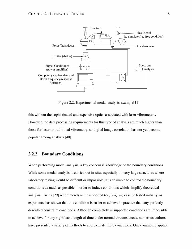
Figure 2.2: Experimental modal analysis example[11]
this without the sophisticated and expensive optics associated with laser vibrometers.
However, the data processing requirements for this type of analysis are much higher than
those for laser or traditional vibrometry, so digital image correlation has not yet become
popular among analysts [40].
2.2.2 Boundary Conditions
When performing modal analysis, a key concern is knowledge of the boundary conditions.
While some modal analysis is carried out in-situ, especially on very large structures where
laboratory testing would be difficult or impossible, it is desirable to control the boundary
conditions as much as possible in order to induce conditions which simplify theoretical
analysis. Ewins [29] recommends an unsupported (or free-free) case be tested initially, as
experience has shown that this condition is easier to achieve in practice than any perfectly
described constraint conditions. Although completely unsupported conditions are impossible
to achieve for any significant length of time under normal circumstances, numerous authors
have presented a variety of methods to approximate these conditions. One commonly applied

CHAPTER 2. LITERATURE REVIEW 9
method is to suspend the structure from above in such a manner that the structure can freely
oscillate in all directions, both linear and rotational, at a frequency an order of magnitude
lower than the lowest natural frequency of the unsupported structure. In [29], it is
recommended that the analyst attach such supports as close to the nodal points as possible in
order to minimize their influence, although as Avitabile points out in [41], it is rare that the
analyst knows the exact location of all nodal points with certainty a priori.
2.3 Correlation Efforts
From the first theoretical vibration models, it has been necessary to correlate these models
with other results for validation purposes. Galileo [12] validated his work on what would later
be termed lumped mass models by comparing the predominant natural frequency predicted by
his model to that observed in experiments. The simplicity and effectiveness of this technique
means it is still in use today. Correlation of mode shapes has also been an important goal.
While the mode shapes for some simple lumped mass models such as pendulums can be
correlated through direct observation and measurement with simple tools, most structures
require indirect measurement and correlation methods. Early mode shape visualization
techniques were pioneered by Chladni [42] and Hooke [43] and relied on visually comparing
mode shapes in a qualitative way. Visual comparison is still done today, as it is a quick check
not relying on any sophisticated mathematics but which can immediately detect large
discrepancies. Nevertheless, as modal analysis became more sophisticated, quantitative
methods for mode shape correlation were sought.
2.3.1 Orthogonality Check
An early example, arising directly from theory, was the orthogonality check [44]. As normal
modes are orthogonal to each other, it was thought that the eigenvectors from one source
would be orthogonal to the eigenvectors from another source except for those representing the

CHAPTER 2. LITERATURE REVIEW 10
same mode which would be identical. Targoff [44] represented this with the following
equation:
ΨT1MΨ2 = I (2.1)
When normalized, this approach would ideally return an identity vector, with values
approaching unity along the diagonal showing strong correlation between mode pairs and
values approaching zero everywhere else. While this approach is theoretically sound, it has
several weaknesses. The first is that it requires a mass matrix, which is of course theoretical
and subject to error. This means that if one wanted to correlate two experimental results, for
example to test for changes in the boundary conditions or autocorrelation, an theoretical
model would need to be developed in order to perform this check. Also, the addition of a
theoretical mass matrix causes errors in the mass matrix to propagate through the system as
the degrees-of-freedom (dofs) best able to represent the mode shape may not correspond to
those most representative of the structure’s mass distribution.
2.3.2 Modal Assurance Criterion
An alternative metric is the Modal Assurance Criterion (MAC) [29], [45], [46], given by the
following equation:
MAC =
∣∣ΨT1 Ψ2
∣∣2ΨT
1 Ψ1ΨT2 Ψ2
(2.2)
This metric works the same way as the orthogonality check, in that values near unity indicate
strong correlation between those pairs of modes, while values near zero indicate poor
correlation. Unlike the orthogonality check, it can be performed on experimental results
without reference to a mass matrix. It has proven very popular, and the original paper [45]
continues to be cited frequently in the peer-reviewed literature. The MAC and orthogonality
check, together with their variants, are the most popular quantitative correlation metrics for
mode shapes in use today, although they are not without their drawbacks. Both are indicators
of global correlation, and do not give any information about correlation at a particular location

CHAPTER 2. LITERATURE REVIEW 11
on the structure which may be of greater importance in practice. They also both struggle with
axisymmetric structures; the matrix algebra assumes a common coordinate system, whereas in
axisymmetric structures any arbitrary rotation about the axis of symmetry could be described
by the same mass matrix but yields different eigenvectors. There has been some research
suggesting approaches to resolve this issue [47]–[49], but no clear consensus has emerged as
to the best approach.
It is also important to note that neither the orthogonality check nor the MAC are
linear metrics, and are simply trigonometric functions of the angle between the eigenvectors.
This means that a MAC value of 0.8 is not necessarily “10%” closer in any absolute sense to
perfect correlation than a MAC value of 0.7. This is not intuitive, and some authors such as
[48] continue to cite MAC values as percentages. In [50], Morales discussed a variety of
methods for linearizing the MAC value. On the basis that simply linearizing the MAC yields a
profile insufficiently sensitive to changes as the value approaches 1, he proposes linearizing
the Normalized MAC (NCO) presented in [29]. This would yield the following equation:
LNCO = 1 − π
2acos
( ∣∣ΨT1MΨ2
∣∣2(ΨT
1MΨ1)(ΨT2MΨ2)
)(2.3)
One can see from this that the mass matrix has been reintroduced, bringing with it the
problems observed for the orthogonality check. Indeed, this metric could be referred to as a
linearized cross orthogonality check. While the advantages of the LNCO cited in [50] are real,
a high degree of confidence in the mass matrix would be required for this to be a useful
metric. If an accurate mass matrix is available, the LNCO would be most valuable in model
updating and optimization applications, where small differences between correlation
coefficients are most important.
A further extension of the MAC is the FMAC[51]. This method plots the MAC
values on a graph, and a linear regression line along the matched mode pairs. Presenting the
data this way provides information regarding correlation of both the mode shapes and the

CHAPTER 2. LITERATURE REVIEW 12
natural frequencies on the same plot. The autocorrelation values of the mode shapes from one
set of results (the AutoMAC) can also be included in the plot to convey further information.
2.3.3 Reduction Methods
The mode shape correlation metrics identified above rely on the eigenvectors under
comparison being the same length. In many applications this is impractical, the most severe
being when comparing experimental results against FE models which may have thousands or
even millions of dofs. Therefore, a method must be used to either represent the larger model
with fewer dofs, or extrapolate the smaller model to additional dofs. Wang and Luo [52]
present a good overview of the methods in use.
Static reduction, also called Guyan reduction after its author [53], is performed by
creating a transformation matrix from the stiffness matrices and neglecting any inertia effects.
This method provides good results at lower frequencies, but degrades as the frequency
increases and inertia effects become more significant. It is also very sensitive to the choice of
location for the reduced dofs, as the process of creating an equivalent mass and stiffness
matrix can become problematic in locations where the replaced dofs are highly
non-homogeneous. Nevertheless, it is the simplest of the commonly used methods and the
original paper continues to be cited frequently. An extension of this method is dynamic
reduction, first presented in [54]. It works the same way, but creates the transformation matrix
based on the mass matrix, stiffness matrix, and an arbitrary frequency, thereby incorporating
some inertial effects. This can provide good results near a frequency of interest, but results
again degrade away from the selected frequency. Therefore, the advantage offered over Guyan
reduction is limited, and dynamic reduction is less frequently cited.
The next important improvement attempt for model reduction was the Improved
Reduction System (IRS) presented in [55]. This method introduces a procedure to refine the
Guyan technique to approximate the inertial effects over wide range of frequencies. This
method relies on minimization of both the stain and potential energies to approximate the

CHAPTER 2. LITERATURE REVIEW 13
inertial forces within the system, and renders the reduction relatively less sensitive to the
location of the reduced degrees of freedom. An iterative technique was presented in [56],
which showed an improvement over Guyan reduction over a wide range of frequencies.
System Equivalent Reduction Expansion Process (SEREP) [57] works in reverse, by
first reducing the results of the larger model, then using the resulting transformation matrix to
extrapolate the results of the smaller model to the larger dofs. Consequently, the quality of the
reduced model is much less influenced by the choice of dof location, although the number and
placement of dof must still be sufficient to fully describe the mode shapes. Several
comparative studies [52], [58], [59] have found it to be the most accurate of the reduction
techniques, though it is also the most complicated. However, as Ewins notes [29], this
technique creates a situation where the results of an experimental model are transformed
using results from a theoretical model. This can be seen as a biased process, as it attempts to
fit the experimental results to the theoretical results. Unlike the previous techniques, SEREP
preserves eigenvalues and eigenvector values for both models at the original measurement
points in the comparison, without suffering data loss or corruption in the transformation
process.
2.3.4 Approaches to Axisymmetric Structures
As was noted in the discussion of correlation metrics, the existing quantitative methods suffer
from complications when applied to axisymmetric structures. Several approaches have been
investigated to solve this problem. In [47], Chen et al. present methods for simply rotating the
mode shapes about the axis of symmetry, using an analytical solution to the angle that
maximizes MAC value for a given mode, then averages angle based on a weighting formula to
produce an optimal angle for the modes under measurement. Schedlinski et al. [48] present a
similar but iterative rather than analytical approach. Neither paper presented a comparison of
their approach to a proven global optimum, or investigated the sensitivity of the MAC value to
the angle parameter.
CHAPTER 2. LITERATURE REVIEW 14
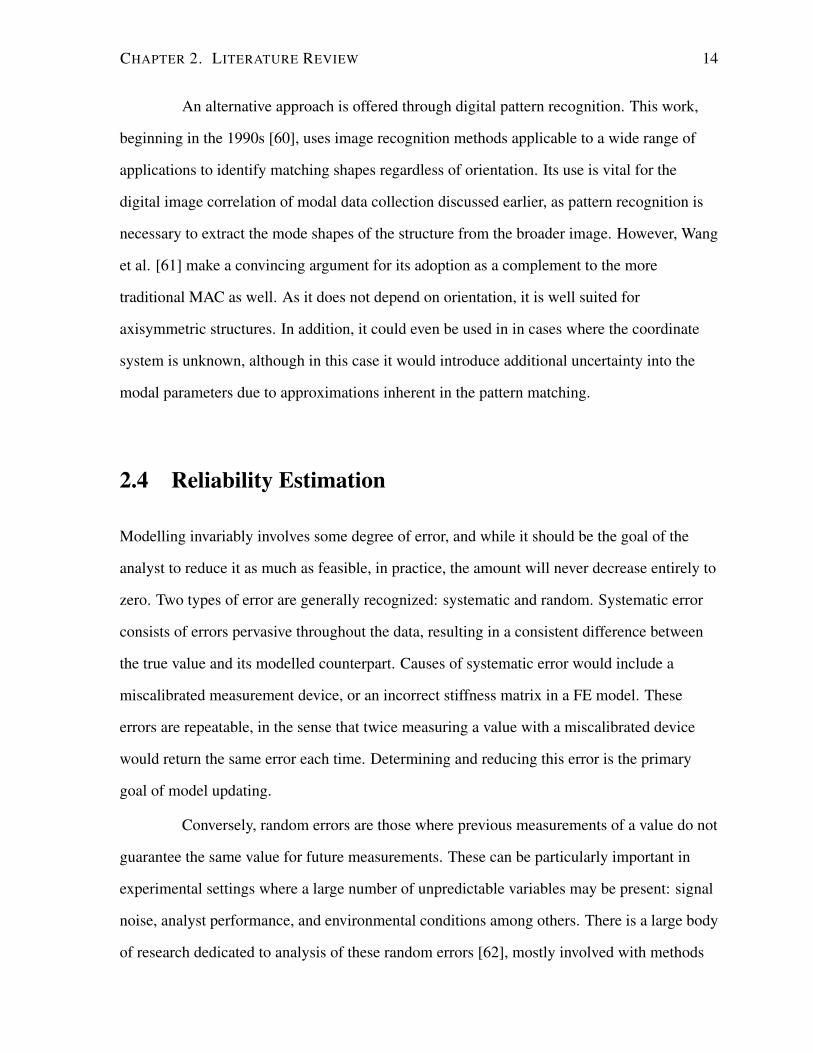
An alternative approach is offered through digital pattern recognition. This work,
beginning in the 1990s [60], uses image recognition methods applicable to a wide range of
applications to identify matching shapes regardless of orientation. Its use is vital for the
digital image correlation of modal data collection discussed earlier, as pattern recognition is
necessary to extract the mode shapes of the structure from the broader image. However, Wang
et al. [61] make a convincing argument for its adoption as a complement to the more
traditional MAC as well. As it does not depend on orientation, it is well suited for
axisymmetric structures. In addition, it could even be used in in cases where the coordinate
system is unknown, although in this case it would introduce additional uncertainty into the
modal parameters due to approximations inherent in the pattern matching.
2.4 Reliability Estimation
Modelling invariably involves some degree of error, and while it should be the goal of the
analyst to reduce it as much as feasible, in practice, the amount will never decrease entirely to
zero. Two types of error are generally recognized: systematic and random. Systematic error
consists of errors pervasive throughout the data, resulting in a consistent difference between
the true value and its modelled counterpart. Causes of systematic error would include a
miscalibrated measurement device, or an incorrect stiffness matrix in a FE model. These
errors are repeatable, in the sense that twice measuring a value with a miscalibrated device
would return the same error each time. Determining and reducing this error is the primary
goal of model updating.
Conversely, random errors are those where previous measurements of a value do not
guarantee the same value for future measurements. These can be particularly important in
experimental settings where a large number of unpredictable variables may be present: signal
noise, analyst performance, and environmental conditions among others. There is a large body
of research dedicated to analysis of these random errors [62], mostly involved with methods

CHAPTER 2. LITERATURE REVIEW 15
of quantifying the uncertainty.
With respect to modal analysis, reliability of the parameter estimations is rarely
considered, and few of the references cited so far make any reference to it. A notable
exception is digital image correlation, where the heuristic nature of the analysis necessitates a
calculated degree of confidence in the solution [63]. For more traditional experimental modal
analysis approaches, this is often not done. However, there has been some research in this
area. Any analysis of random error involves some degree of repeated measurement, to
establish the amount of random variation present. [64] used the bootstrap, a simulated
sampling technique, to estimate the error distribution of experimental measurements and
calculate confidence intervals for the modal parameters. As the bootstrap depends on
independent measurements, all individual responses must be recorded as opposed to the
averaged responses more commonly collected by software. To see if this requirement could be
relaxed, [65] conducted a comparison study on the bootstrap and the Monte Carlo technique
which can be used with averaged data. Unfortunately, they were unable to conclude that the
two techniques yielded equivalent results.
Other approaches have been attempted, including the use of fuzzy numbers [66], but
variations of the traditional least-squares technique [67], [68] appear to have gained the most
acceptance. These techniques work by assuming a model, and positing that the best
parameters for that model are those which minimize the sum of the squared residuals, and
assume that the error follows some known distribution. If the distribution is known, the
confidence interval can then be calculated based on the existing sample measurements.

Chapter 3
Modal Parameters
Modal analysis consists of the study of vibration in structures through the measurement of a
few well-defined parameters. These are the frequency response functions, the natural
frequencies, and mode shapes, which together provide a fairly complete description of the
vibrational response of the structure, at least within the frequency domain. Analysis of
behaviour in the time domain, such as the transient response analysis referenced in the
literature review, is would not normally be referred to as modal analysis and falls outside of
the scope of this thesis.
3.1 Frequency Response Functions
As the name implies, frequency response functions (FRFs) are functions describing the
frequency-domain response of a structure. An example of a FRF plot is provided in Figure
3.1. They more completely describe the vibrational response of a structure than the other
parameters, as they provide information at regarding the response at all frequencies, and can
be transformed through a Fourier transform to show the time-domain response as well.
Natural frequencies and mode shapes can both be extracted from FRFs, with natural
frequencies being represented as peaks on an FRF graph, and mode shapes being the
represented by a vector of the values of the FRFs at the natural frequencies at different points
16

CHAPTER 3. MODAL PARAMETERS 17
Frequency
Am
plitu
de
Figure 3.1: A Frequency Response Function
on the structure.
FRFs are particularly important in the study of non-linear response, as
non-linearities will appear as distortions of the natural frequency peaks within the FRF. As the
models being developed for this thesis are linear, non-linear FRFs will not be discussed
further at this time, though their use may be necessary if this work is extended to more
advanced useage cases at a later time.
3.1.1 Modelling Considerations
In spite of their advantages, FE modelling of the frequency response function is often avoided
when possible. As the full FRF is a continuous infinite function, full numerical computation is
impossible, and some amount of truncation is required. This inherently produces error, and
cannot be avoided. Additionally, this degree of detail is often not required. Resonant
frequencies will dominate any response, and the range of frequencies at which a structure will
typically be excited is likewise limited. Therefore, modelling techniques which focus on these
parameters to the exclusion of others are often used in place of full FRF modelling.
Nevertheless, FRF modelling remains in use for applications where more complete modelling
is required, such when non-linearities are present.

CHAPTER 3. MODAL PARAMETERS 18
3.1.2 Correlation Methods
Due to the inherent errors present in FRF modelling techniques, successful correlation has
often been found to present difficulties[69]. Nevertheless, it is important to visually inspect
the FRFs from experimental testing to get a sense of if the modelling assumptions are correct;
primarily the presence or absence of non-linearity. As the FE models developed assume a
linear response, the FRFs from experimental testing should be consistent with this and show
straight vertical peaks with roughly symmetrical responses surrounding them. Aside from
this, for the reasons discussed in the preceding section, the FE models developed through the
research discussed here have not been used to generate FRFs; therefore, no direct correlation
procedure has been presented.
3.2 Natural Frequencies
Natural frequencies are commonly measured parameters, as they are scalar values, easily
compared. They can be defined as the frequencies at which a system vibrates when subjected
to an impulse from rest[70], and are sometimes referred to as the eigenvalues. The number of
possible natural frequencies is equal to the number of dofs for the structure. While there are
theoretically an infinite number of these for any continuous system, only a limited number
will be relevant for a given usage case.
3.2.1 Modelling Considerations
Calculating natural frequencies within a given range from a FE model is comparatively quick.
As with any FE simulation, mesh density and quality can have a significant impact on the
results. For natural frequency calculations, the finite element model tends to exhibit higher
natural frequencies than the physical object and increasing the mesh density can reduce this
error. This effect can be reversed in poor quality meshes or with geometries prone to
phenomena such a shear-locking; in these cases, the use of higher-order elements can help

CHAPTER 3. MODAL PARAMETERS 19
eliminate these effects [71]. A number of solution methods exist, but MSC Nastran
recommends the use of the Lanczos method for most problems due to its efficency and
reliability[16].
3.2.2 Correlation Methods
Two primary methods exist for correlating natural frequencies [29], and both were used in this
research. The first is simply comparing the percent difference between two sets of results,
often in tabular or bar graph form. The second is to use simple linear regression to model the
relationship between the two sets of values. This is the practice of formulating an equation
that describes a linear relationship between the experimental and theoretical frequencies. The
method used in this work is the method of least squares; a procedure that seeks to minimize
the difference between the experimental value predicted from the equation, and that found in
practice. This requires the minimization of the following equation [72]:
Q =n∑i=1
(Yi − β0 − β1Xi) (3.1)
The regression equation then takes the form [72]:
Yi = b0 + b1Xi (3.2)
The ideal case for model validation would be the experimental and theoretical results having
a 1-to-1 relationship, resulting in slope of 1 when plotted in a graph. This second method has
the advantage of accounting for all the natural frequencies within the range of interest, thereby
revealing systematic errors in the model. Points showing little scatter but resulting in a line
with a slope other than 1 or an intercept other than zero can indicate an error in the material
properties of the model. The significance of these deviations can be assessed using standard

CHAPTER 3. MODAL PARAMETERS 20
statistical techniques, such as the regression confidence interval[72], [73]:
Yh ± tα/2;n−2
√MSE
(1
n+
(Xh − X)2∑(Xi − X)2
)(3.3)
This equation calculates the upper and lower bounds of a predicted value based on the
assumption that either the error or the estimator follow a normal (Gaussian) distribution. The
requirement for the theoretical models used in this research is that the frequency deviations
fall within ± 10% of the experimental value for the natural frequencies of interest.
3.3 Mode Shapes
Mode shapes are critical parameters in the study of vibration, as they provide information as
to which parts of a structure are most excited at a given frequency. In addition, they also
provide a metric for validating the overall vibration model. In the context of the equations of
motion, mode shapes are represented by (and sometimes referred to as) the eigenvectors.
3.3.1 Modelling Considerations
The typical limitations of FE modelling apply to the extraction of mode shapes as well.
However, the experimental measurement of mode shapes involves additional considerations
not present in the measurement of natural frequencies or FRFs. While natural frequencies and
FRFs can be measured and evaluated at discrete points, mode shapes require measurement at
a range of locations. Points must be of sufficient number and placement to capture all points
of inflection on the mode shape. The number and location of these points can be predicted
through use of a pre-test FE simulation; however, additional points should be included to
account for possible errors in the FE model [41]. It must be noted that the number of
additional points should be kept to a minimum, as collecting data for additional sampling
points is a time-consuming procedure. It is also important to consider the eventual model

CHAPTER 3. MODAL PARAMETERS 21
reduction when choosing sampling locations, as the points should be chosen such that a dof at
that location can be assigned properties that adaquately account for the larger number of
nearby dofs replaced in the reduction procedure.
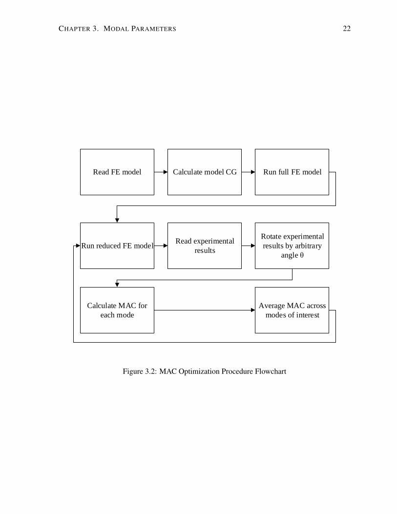
3.3.2 Correlation Methods
MSC.ProCOR is used to calculate the MAC between the experimental and theoretical results,
using Guyan reduction to equivalence the dofs. In addition, a new procedure has been
developed to maximize its effectiveness for axisymmetric structures. As noted in the literature
review, for an axisymmetric structure, any arbitrary rotation of the results about the axis of
symmetry results in an equally valid solution. However, the MAC treats the angle of rotation
as significant; experimental and theoretical mode shapes with poorly matched rotations will
result a poor MAC value, as seen in [47] . It is important to note, that although the rotation of
the results can be arbitrary, the rotation of individual mode shapes is not independent but
connected to that of the other shapes. This is apparent when one considers the response of a
single point on a structure; it can be a node for one mode, and antinode for another, and
somewhere in-between for a third. By the principle of superposition, the response is the sum
of all these modes, meaning that while the overall rotation may be arbitrary, each mode shape
must maintain its rotation relative to the other modes. To account for this, this work sought to
maximize the average MAC across the modes of interest as opposed to maximising any
individual MAC number. To accomplish this, a script was written in the Patran Command
Language (PCL) which automatically calculated the MAC between experimental and
theoretical results. This script can be used to either obtain the results for the rotation angle
that optimizes the averaged MAC or generate a table for the MAC values for a set of
iterations. The requirement for models used in this research is that the MAC be >0.9 for all
correlated modes of interest, and <0.1 for all uncorrelated modes.
CHAPTER 3. MODAL PARAMETERS 22
Read FE model Calculate model CG Run full FE model
Run reduced FE modelRead experimental
results
Rotate experimental
results by arbitrary
angle θ
Calculate MAC for
each mode
Average MAC across
modes of interest
Figure 3.2: MAC Optimization Procedure Flowchart

Chapter 4
Aircraft Engine Casing Case Study
To demonstrate and validate the procedures discussed in the proceeding chapter, front and rear
engine casing components from the Pratt & Whitney PW300 turbofan engine were subjected
to modelling and testing. The components in question and their associated 3D CAD files were
provided by Pratt & Whitney Canada (PWC) and are depicted in Figure 4.1. These models
were made as part of a larger project to model and analyse the vibration throughout the entire
engine. This case study serves as a validation for the modelling techniques used for this part
of the project.
(a) Front Compressor Casing
(b) Rear Compressor Casing
Figure 4.1: PW300 Engine Components
23
CHAPTER 4. AIRCRAFT ENGINE CASING CASE STUDY 24
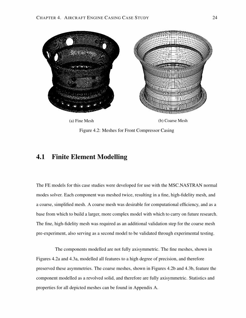
(a) Fine Mesh (b) Coarse Mesh
Figure 4.2: Meshes for Front Compressor Casing
4.1 Finite Element Modelling
The FE models for this case studies were developed for use with the MSC.NASTRAN normal
modes solver. Each component was meshed twice, resulting in a fine, high-fidelity mesh, and
a coarse, simplified mesh. A coarse mesh was desirable for computational efficiency, and as a
base from which to build a larger, more complex model with which to carry on future research.
The fine, high-fidelity mesh was required as an additional validation step for the coarse mesh
pre-experiment, also serving as a second model to be validated through experimental testing.
The components modelled are not fully axisymmetric. The fine meshes, shown in
Figures 4.2a and 4.3a, modelled all features to a high degree of precision, and therefore
preserved these asymmetries. The coarse meshes, shown in Figures 4.2b and 4.3b, feature the
component modelled as a revolved solid, and therefore are fully axisymmetric. Statistics and
properties for all depicted meshes can be found in Appendix A.

CHAPTER 4. AIRCRAFT ENGINE CASING CASE STUDY 25
(a) Fine Mesh (b) Coarse Mesh
Figure 4.3: Meshes for Rear Compressor Casing
4.2 Experimental Setup
For this case study, experimental modal analysis was carried out using the test setup shown in
Figure 4.4. A test piece of high stiffness is placed on a softly sprung support. As the stiffness
of the support is orders of magnitude lower than the stiffness of the test piece, the vibrational
response approximates that of an unsupported (free-floating) piece. A piezoelectric triaxle
accelerometer is attached to the piece by a thin layer of wax, and both it and an impact
hammer containing an integral accelerometer are attached to a signal analyser. The signal
analyser digitizes the signal received from both pieces of equipment and sends them to the
computer for further processing and analysis. The accelerometer measures the acceleration
along three orthogonal axes at a point. When the impact hammer strikes the test piece, it
sends a signal to the computer through the signal analyser, which allows measurements from
the accelerometer to be linked to that specific strike. Sophisticated signal processing by the
computer then extracts modal properties, such as the frequency transfer function, natural
frequencies, and mode shapes for the test piece.
To collect the experimental data used in this case study, the shapes of the engine
casing components were entered into the analysis software (LMS Test.Lab), along with the
strike and measurement points. The engine casing components were then placed on a thick
soft foam pad. Since the components are composed of steel or titanium alloys, their stiffness
far exceeds that of the foam, so the vibrational response should approximate that of an
unsupported object. The software was then turned to data acquisition mode, and the test piece

CHAPTER 4. AIRCRAFT ENGINE CASING CASE STUDY 26
Test Piece
Signal Conditioner
Soft
Spring
Support
Triaxle
Accelerometer
Figure 4.4: Experimental Setup
struck at the selected point with the hammer. Upon impact, the software registered the strike
and the resulting response from the accelerometer. The newly generated data was analysed,
after which the software prompted the experimenter to strike the object again. The process
was repeated until adequate data had been collected at the measurement point, at which time
the accelerometer was moved to the next point. This procedure is known as a roving
accelerometer test. The adequacy of the data was determined by the absence of high signal
noise and by compatibility between repeated strikes according to predetermined limits set in
the software. Generally, this required 3-5 strikes at each measurement point, but additional
strikes were required in cases of missed strikes, loss of accelerometer signal, or other signal
errors. Once adequate data was collected, the software was switched to data analysis mode,
the frequency transfer function examined, and the natural frequencies and corresponding
mode shapes extracted. Sampling points were determined based on those sufficient to detect
and discriminate between those predicted by the corresponding theoretical model.
Potential sources of error in this test setup include those resulting from the
approximations used in formulating the boundary conditions, calibration error of the
instruments, signal noise, and manufacturing discrepancies in the test pieces. Attempts were
made to minimse these errors to the extent possible. All sensors used were professionally
calibrated.
Chapter 5
Results
The FRF depicted in Figure 3.1 is representative of those found experimentally from this case
study. It exhibits two natural frequency peaks, and appears to be linear due to its smooth and
symmetric shape.The two closely spaced natural frequencies are characteristic of
axisymmetric structures, and this pattern can be seen in the tables below as well for both FE
and experimental results. Sample FRFs for each component can be found in Appendix A. The
frequencies presented have been normalized between zero and the largest measured natural
frequency to preserve the proprietory nature of the underlying data.
5.1 MAC Optimization
The PCL algorithm presented in Section 3.3.2 was used to optimze the MAC values between
the axisymmetric FE models and the experimental results. A large number of values were
calculated for each component, increasing the probability of the maximum values closely
approximating the global optimum.
27

CHAPTER 5. RESULTS 28
●
●
●
●
●
●
●
●●
●
●●
●
●
●
●
●
●●
●
●
●
●
●●
●
●
●
●
●
●
●
●
●
●
●
●
●
●●
●
●●
●
●
●
●
●
●
●
●
●
●
●
●
●●●
●
●
●
●
●
●
●
●
●
●
●
●
●
●
●
●
●
●
●
●
●
●
●
●
●●
●
●●
●
●
●
●
●
●
●
●●
●
●
●
●
●
●
●●
●
●
●
●
●
●
●
●
●
●
●
●
●
●
●
●
●
●
●
●
●
●
●
●
●
●
●
●
●
●
●
●
●
●
●
●
●
●●
●
●●
●
●
●
●
●
●
●●
●
●
●
●
●
●
●
●
●
●
●
●●
●●
●
●
●
●
●
●
●
●
●
●
●
●
●
●
●
●
●
●
●
●
●
●
●
●
●
●
●
●
●
●
●
●
●
●
●
●
●
●
●●
●
●
●
●
●
●
●
●
●●
●
●●
●
●
●●
●
●
●
●
●
●
●
●
●
●
●
●
●
●
●
●
●
●
●
●
●●
●
●
●
●
●●
●
●
●
●
●
●
●
●
●
●
●
●
●
●
●●
●
●
●
●
●
●
●
●
●
●
●
●
●
●
●
●
●
●
●
●
●
●
●
●●
●
●●
●
●●
●
●
●
●●
●
●
●
●
●
●
●
●
●
●
●
●
●
●
●
●
●
●
●
●
●
●
●
●
●
●
●●
●
●
●
●
●
●●
●
●●
●
●
●
●
●
●
●
●
●
●
●
●
●
●
●
●
●
●
●
●
●
●
●
●●
●
●●
●●
●
●
●●●
●
●
●
●
●●
●
●
●
●
●
●
●
●
●
●
●
●
●
●●
●
●●
●
●
●
●
●
●
●
●
●
●
●
●
●
●●
●
●
●
●
●
●
●
●
●
●
●
●
●
●
●
●
●
●
●
●
●
●
●
●
●
●
●
●●
●
●
●
●
●
●
●
●●
●
●
●
●
●
●
●●
●
●
●
●
●
●
●
●
●
●
●
●
●
●
●
●
●
●
●
●
●
●
●
●
●
●
●
●
●
●
●
●
●
●
●
●
●
●●
●
●
●
●
●
●
●
●
●
●●
●
●
●
●
●
●
●
●
●
●
●
●●
●
●
●
●●
●
●
●
●
●
●
●
●
●
●
●
●
●
●
●
●
●
●
●
●
●●
●
●
●
●
●
●
●
●
●
●
●
●●
●●
●
●
●
●
●
●
●
●
●
●
●
●●
●
●
●●
●
●
●
●
●
●
●
●
●
●
●
●
●
●
●
●
●
●
●
●
●●
●
●
●
●
●●
●
●
●
●
●
●
●
●
●
●
●
●
●
●
●●
●
●
●
●
●
●
●
●
●
●
●
●
●●
●
●
●
●
●
●
●
●
●
●●
●
●●
●
●●
●
●
●
●
●
●
●
●
●
●
●
●
●
●
●
●
●
●
●
●
●
●
●
●
●
●
●
●
●
●
●
●●
●
●
●
●
●
●●
●
●●
●
●
●
●
●
●
●
●
●
●
●
●
●
●
●
●
●
●
●
●
●
●
●
●●
●
●
●●
●
●
●●
●
●
●
●
●
●
●
●
●
●
●
●
●
●
●
●
●
●
●
●
●
●
●
●
●
●●
●
●
●
●
●
●
●
●
●
●●
●
●
●
●
●
●
●
●
●
●
●
●
●
●
●
●
●
●
●
●●
●
●
●
●
●
●
●
●
●
●
●
●
●
●
●
●
●
●
●
●
●
●●
●
●
●
●
●
●
●
●●
●
●
●
●
●
●
●
●
●
●
●
●
●
●
●
●
●
●
●
●
●
●
●
●
●
●
●
●
●
●●
●
●
●
●
●
●
●
●
●
●
●
●
●
●
●
●
●
●
●
●
●
●
●
●
●
●
●
●
●
●●
●
●●
●
●
●
●
●
●
●
●
●
●
●
●
●
●
●●
●
●
●
●
●
●
●
●
●
●
●
●
●
●●
●
●
●
●
●
●
●
●
●
●
●
●
●
●
●
●
●
●
●
●
●
●
●
●
●
●
●●
●
●●
●
●
●
●
●
●
●
●
●
●
●
●
●
●
●
●●
●
●
●●
●
●
●
●
●
●
●
●
●
●
●
●
●
●
●
●
●
●
●
●
●
●
●
●
●
●
●
●
●
●
●
●
●
●
●
●
●
●
●
●
●
●
●
●
●
●
●
●
●
●
●
●
●
●
●
●
●
●
●
●
●
●
●
●
●
●
●
●
●
●
●
●
●
●
●
●
●
●●
●
●
●
●
●
●
●
●●
●
●
●
●
●●
●
●
●
●
●
●
●
●
●
●
●
●
●
●
●
●
●
●
●
●
●
●
●
●
●
●
●
●
●
●
●
●
●
●
●
●
●
●
●
●
●
●
●
●
●
●
●
●
●
●
●
●
●
●
●
●
●
●
●
●
●
●
●
●
●
●
●●
●
●
●
●
●
●
●
●
●
●
●
●
●
●
●
●●
●●
●
●
●
●
●●
●
●
●
●
●●
●
●
●
●
●
●
●
●
●●●
●
●
●
●
●
●
●●
●
●
●
●
●●
●
●
●
●
●
●
●
●
●●
●
●
●
●
●
●
●
●
●
●
●
●
●
●●
●
●
●
●
●
●
●
●
●
●
●
●
●
●
●
●
●
●
●
●
●
●
●
●
●●●
●
●
●●
●
●●
●
●●
●
●
●
●
●
●
●
●
●
●
●
●
●
●
●
●
●
●
●
●
●
●
●
●
●
●
●●
●
●
●
●
●
●
●
●
●
●
●
●
●
●
●
●
●
●
●
●
●
●
●
●
●
●
●●
●
●●
●
●●
●
●
●
●
●
●
●
●
●
●
●
●
●
●
●
●
●●
●
●
●
●
●
●
●
●
●
●
●
●
●
●
●
●
●
●
●
●
●
●
●
●
●
●
●
●
●
●
●
●
●
●
●
●
●●
●
●
●
●
●
●
●
●
●
●
●
●
●
●
●
●
●
●
●●
●
●
●
●
●
●
●
●
●
●
●
●
●●
●
●
●
●
●
●
●
●
●
●
●
●
●●
●●
●
●
●
●
●●
●
●
●
●
●
●
●
●
●
●
●
●
●
●
●
●
●●●●
●
●●
●
●●
●
●
●●●
●
●
●
●
●
●
●●
●
●●
●●●
●
●
●
●●●
●●
●
●
●●
●
●
●
●
●●●
●
●
●
●
●
●
●
●
●●
●
●●
●
●●
●●
●
●●
●
●
●●
●●
●●
●
●
●
●●
●
●
●
●
●
●
●
●●
●
●
●●
●
●
●
●●
●
●
●
●
●●
●●●
●
●
●
●
●●
●
●●
●
●
●
●
●
●
●
●
●
●
●●
●
●
●
●
●
●
●
●
●
●
●
●
●
●
●
●
●
●
●
●
●
●●
●
●
●●●●
●
●●●
●
●●
●
●
●●
●
●
●
●
●
●
●
●●
●
●
●
●●
●
●●
●
●
●●
●
●
●
●
●
●
●
●●●
●
●
●
●
●
●
●
●
●
●
●
●
●
●
●
●
●
●●
●
●
●●
●
●
●
●●
●
●
●
●
●
●
●
●
●
●
●
●●●●●●●
●
●
●
●
●
●●
●
●
●
●●
●
●
●
●
●
●
●
●
●●●
●
●
●
●
●
●
●
●
●
●
●
●
●
●
●
●
●
●
●
●
●
●
●
●
●
●
●
●
●
●
●●●
●●
●
●●
●
●
●●
●
●
●
●
●
●
●
●
●●
●
●
●
●
●●
●
●
●
●
●●
●
●
●
●
●
●
●
●
●●●
●
●
●
●
●
●
●
●●
●●●
●●●
●
●
●●
●
●
●
●
●●
●●
●
●
●●
●●
●
●●
●
●
●
●
●●
●●
●●
●
●
●●
●
●
●
●
●
●
●●
●
●
●
●
●●
●
●
●
●
●●●●
●
●
●
●●
●
●
●
●
●
●
●
●
●
●
●
●●
●
●
●
●
●
●
●
●
●
●●●
●
●●
●
●
●
●
●
●
●
●
●●
●●
●
●
●●
●●
●
●●
●
●
●
●
●●
●
●
●●
●●
●●
●
●
●
●
●
●
●●
●
●
●
●
●●
●
●
●
●
●●
●●
●
●
●
●●
●
●
●
●
●
●
●
●
●
●
●
●●
●
●
●
●
●
●
●
●
●
●●●
●●●
●
●
●●
●
●
●
●
●●
●●
●
●●●
●●
●
●●
●
●
●●●●
●
●
●●
●●
●●
●
●
●
●
●
●
●●
●
●●●
●●
●
●
●
●
●●
●●
●
●
●
●●
●
●
●
●
●
●
●
●
●
●
●
●●
●
●
●
●
●
●
●
●
●
●●●
●●●
●
●
●
●●
●
●
●
●●
●●
●
●●●
●●
●
●●
●
●
●●●●
●
●
●●
●
●
●●
●
●
●
●
●●
●●
●
●
●
●
●●
●
●
●
●
●●
●●
●
●
●
●●
●
●
●
●
●
●
●
●
●
●
●
●●
●●
●
●
●
●
●
●
●
●●●●
●●
●●●●●●●●●●
●●●●●●
●
●
●
●●
●●●
●●●●●
●
●
●●●●●●
●●
●●●
●
●
●
●
●●●●
●
●●
●
●●
●●
●●
●
●●●●●
●
●●●
●●●
●●●●
●
●
●●
●
●
●
●●●●●
●●●
●
●●
●
●
●
●●●
●
●
●●●●
●●●●
●
●●
●●
●
●
●●●
●●●●●●●
●
●
●
●
●
●
●
●
●●
●
●
●
●
●
●●
●●●●
●
●●●
●
●●●●●●
●
●
●●●●●
●
●●●●●●
●●●
●●
●
●●●●●●●
●
●
●
●
●●
●●●
●
●●●●
●
●
●
●●●●
●●
●●
●
●●●
●●
●
●
●●●●●●
●●
●
●●
●●●●
●
●●
●
●
●
●
●●●●●●●
●
●
●
●
●●●
●●●
●
●
●
●
●
●●
●●●●●
●
●
●●
●●
●●
●
●●●●
●●●
●
●●
●
●
●
●
●●
●
●
●
●
●●●●●●●●
●●●
●●
●●
●
●●
●
●
●
●
●
●
●●●
●●●
●●
●
●
●●
●●
●
●
●
●●●
●●●
●
●
●
●
●
●●
●
●
●
●
●
●
●
●
●
●
●
●
●
●
●
●
●
●
●
●
●
●
●
●
●●
●
●
●
●
●
●
●
●
●
●●●
●
●●
●●
●
●
●
●
●
●●
●
●
●
●●
●
●
●
●
●
●
●
●
●
●
●●
●●
●
●●
●●
●
●
●
●●
●●
●
●●●
●
●●
●
●●
●
●
●
●
●
●
●
●●
●
●
●
●
●
●
●
●
●
●
●
●
●
●
●●
●
●●
●
●
●
●●
●
●
●
●
●
●●
●●
●
●
●
●
●
●
●
●
●
●
●
●
●●
●
●
●
●●
●
●●
●
●
●
●
●
●●
●
●
●
●
●
●●
●
●
●
●
●
●
●
●●
●
●●
●
●
●
●
●●
●
●●
●
●
●
●
●
●
●
●
●
●
●
●
●
●
●
●
●
●
●
●●
●
●
●
●
●
●●
●
●●
●
●
●
●
●
●
●
●
●
●
●●
●●
●
●
●
●
●
●●
●
●
●
●
●
●●
●
●●
●
●
●
●
●
●●
●●
●
●●
●
●
●
●
●
●
●
●●
●
●
●●
●
●
●
●
●
●
●
●
●
●
●
●●
●
●
●
●
●
●
●
●
●
●●
●
●
●
●
●●
●
●
●
●
●
●
●
●
●
●
●
●
●
●
●
●
●●
●●
●
●
●
●
●
●
●
●
●
●●
●
●
●
●
●●
●
●
●
●●
●
●
●
●●
●
●
●
●
●
●●
●
●
●
●●
●
●●
●
●
●●
●
●
●
●
●
●●
●
●●
●
●●●
●
●●
●●
●
●
●
●●
●●
●
●
●●
●
●
●
●
●
●
●
●
●
●●
●●
●●
●
●
●
●
●
●
●
●
●
●
●●
●
●
●●
●
●
●
●
●
●
●●
●
●●
●
●
●
●
●
●
●
●
●
●
●
●
●
●
●
●
●●
●
●
●
●
●
●●
●
●●
●
●
●
●
●
●
●
●
●
●
●
●
●●
●
●
●
●
●●
●
●
●
●
●
●
●●
●
●
●
●
●
●
●
●
●
●
●
●
●
●
●
●
●
●●
●
●
●
●
●
●
●
●
●
●
●
●
●
●
●
●
●
●
●
●
●
●●
●
●
●
●●
●
●●
●
●
●
●
●
●
●
●
●
●
●
●
●●
●●
●
●
●●
●
●●
●
●●
●●
●
●
●
●●
●
●
●
●
●
●●
●
●●
●
●
●●
●
●●●
●
●
●
●
●
●
●●
●
●
●
●
●
●
●
●●
●
●●
●
●●●
●
●●
●
●
●●
●
●
●
●
●
●
●
●
●●
●
●
●
●
●
●●
●
●●
●
●
●
●
●
●
●●
●
●
●
●
●●
●
●
●
●
●
●
●
●
●
●
●
●
●●
●
●●
●
●
●●
●
●
●●
●
●
●
●
●●
●
●
●
●
●
●
●
●
●
●●
●
●
●
●
●●●
●
●●
●
●●●●●●●●●●●
●●●●●●●●●●●●●●●●●
●●●●●●●●●●●●●●●●●●
●●●●●●●●●●
●●●●●●●
●●●●●●●●●●●●●●●●●
●●●●●●●●●●●●●●●●●●●●●●●●●●●●●●●
●●●●●●●●●●●
●●●●●●●●●●●●●●●●●
●●●●●●●●●●●●●●●●●●●●●●●●●
●●●●●●●●●●●●●
●●●●●●●●●●●●●●●●●●●●●
●●●●●●●●●●●●●●●●●●●●●●●●●●●●●●●
●●●●●●●●●●●●●●●●●●●●●
●●●●●●●●●●
●●●●●●●●●●●●●●●●●●
●●●●●●●●●●●●●●●●●●●●●●●●●●●●●●●●●●●●●●●●●
●●●●●●●●●●●●●●
●●●●●●●●●●●●●●●●●●●●●●●●●●●
0.00
0.25
0.50
0.75
1.00
0 45 90 135 180 225 270 315 360Iteration #
MA
C V
alue
Mode #●
●
●
●
●
●
●
●
●
●
12345678910
Figure 5.1: MAC Value Response to Computational Remodelling for Front Compressor Casing
●
●
●
●
●
●
●
●●
●
●
●
●
●
●
●
●
●
●
●
●
●
●
●●
●
●
●
●
●
●
●
●
●
●
●
●
●
●
●
●
●
●
●
●
●
●
●
●
●
●
●
●
●
●
●
●●
●
●
●
●
●
●
●
●
●
●
●
●
●
●
●
●
●
●
●
●
●
●
●
●
●
●
●
●
●
●
●
●
●
●
●
●
●
●
●
●
●
●
●
●
●
●
●
●
●
●
●
●
●
●
●
●
●
●
●
●
●
●
●
●
●
●
●
●
●
●
●
●
●
●
●
●
●
●
●
●
●
●
●
●
●
●
●
●
●
●
●
●
●
●
●
●
●
●
●
●
●
●
●
●
●
●
●
●●
●
●
●
●
●
●
●
●
●
●
●
●
●
●
●
●
●
●
●
●
●
●
●
●
●
●
●
●
●
●
●
●
●
●
●
●
●
●
●
●
●●
●
●
●
●
●
●
●
●
●
●
●
●
●
●
●
●●
●
●
●
●
●
●
●
●
●
●
●
●
●
●
●
●
●
●
●
●
●
●
●
●
●
●
●●
●
●
●
●
●
●
●
●
●
●
●
●
●
●
●●
●
●
●
●
●
●
●
●
●
●
●
●
●
●
●
●
●
●
●
●
●
●
●
●
●
●
●
●
●
●
●
●
●
●
●
●
●
●
●
●
●
●
●
●
●
●
●
●
●
●
●
●
●
●
●
●
●
●
●
●
●
●
●
●
●
●
●
●
●
●
●
●
●●
●
●
●
●
●
●
●
●
●
●
●
●
●
●
●
●
●
0.5
0.6
0.7
0.8
0.9
0 45 90 135 180 225 270 315 360Iteration #
MA
C V
alue
(a) MAC Value with Rotation
0
1
2
3
0.5 0.6 0.7 0.8 0.9MAC Value
Den
sity
(b) MAC Value Density
Figure 5.2: Mode 1 Response to Computational Remodelling for Front Compressor Casing

CHAPTER 5. RESULTS 29
5.1.1 Front Compressor Casing
Figure 5.1 presents the response of the MAC value of the front compressor casing to
computational remodelling as a result of rotating the experimental results about the axis of
symmetry. A large amount of scatter is present, with the largest amount of scatter
accompanying the best-correlated modes. Figure 5.2 isolates the response of the mode shape
to computational remodelling for the first mode. This is one of the most widely dispersed
modes, with peak values of >0.9 and low values of <0.5. No clear pattern is apparent from
these plots, limiting the potential for development of an optimization algorithm to determine
optimal rotation angles.This is likely the result of the multiple reductions of the FE model
resulting in unpredictable mode shape orientation about the axis of symmetry. However,
Figure 5.2b shows a strong concentration of values at the upper end of the range, indicating
that a close approximation of the optimal MAC value has likely been achieved. Therefore,
these results are sufficient for determination of an approximate optimal MAC for each pair of
mode shapes; in this case, those values are found at iteration numbers 185, 267, 189, 272, and
241. With this information, the experimental results were rotated to produce Figure 5.5a and
Table 5.1a.
5.1.2 Rear Compressor Casing
Figure 5.3 presents the response of the MAC value of the rear compressor casing to
computational remodelling as a result of rotating the experimental results about the axis of
symmetry. The amount and pattern of scatter is similar to that observed for the front
compressor casing. This further supports the hypothesis that the repeated calculation of the
reduced FE model by the algorithm is leading to unpredictable changes in the mode shape
orientation about the axis of symmetry. In this case, the bias of MAC value concentration
shown in Figure 5.4b is even more pronouced than previously, increasing confidence that an
approximate optimal MAC value can be obtained; in this case, at iteration numbers 49, 162,
68, 310, and 196. As with the front compressor casing, the experimental results for the rear

CHAPTER 5. RESULTS 30
●
●
●
●
●
●
●
●
●
●
●
●
●
●
●
●
●
●
●
●
●
●
●
●
●
●
●
●
●
●
●
●
●
●
●
●
●
●
●
●
●
●
●●
●
●
●
●
●
●
●
●
●
●
●
●
●
●
●
●
●
●
●
●
●
●
●
●
●
●
●●●
●
●
●
●
●
●
●
●
●
●
●
●
●
●
●
●
●
●
●
●
●
●
●
●
●
●
●
●
●
●
●
●
●
●
●
●
●
●
●
●
●
●
●
●
●
●
●
●
●
●
●
●●●
●●
●
●●
●●●●
●
●
●
●
●
●
●
●
●
●
●
●●
●
●
●
●
●
●
●
●
●
●
●
●
●
●
●
●
●
●
●
●
●
●
●
●
●
●
●
●
●●●●
●●
●
●
●
●
●
●
●●
●
●
●
●
●
●
●
●
●
●
●
●
●
●●
●
●
●●
●
●
●●●●
●
●
●
●
●
●
●
●
●
●
●
●●●●
●●●●
●●
●
●●●
●●●
●
●
●
●
●
●
●
●
●●
●
●●
●
●
●
●
●
●
●
●
●
●
●
●
●
●
●
●
●
●
●
●
●
●
●
●
●
●
●
●
●
●
●
●
●
●
●
●●●
●
●
●
●
●
●
●
●
●
●
●
●●●
●
●
●
●
●
●
●
●
●●
●●
●
●●●
●
●
●
●
●
●
●
●
●
●
●
●
●
●
●
●
●
●
●
●
●●●
●●
●
●
●
●
●
●
●
●
●
●
●●
●
●
●
●
●
●●●
●
●
●
●
●
●
●
●
●
●
●
●
●
●
●
●
●
●
●
●
●
●
●
●
●
●
●
●
●
●
●
●●●
●
●
●
●
●
●
●
●
●
●
●
●
●
●
●
●
●
●●
●
●
●
●
●
●
●
●
●
●
●
●
●
●
●
●
●
●
●
●
●
●
●
●
●
●
●
●●●
●
●
●●
●
●
●
●
●
●
●
●
●
●
●
●
●
●
●
●
●
●
●
●
●
●
●
●
●
●
●
●
●●
●●
●
●●●
●
●
●
●
●
●
●
●
●
●
●●
●
●
●
●
●●
●
●
●
●
●
●
●
●
●
●
●
●
●
●
●
●
●
●
●
●
●
●
●
●
●
●
●●●●
●●
●
●
●
●
●
●
●
●
●●
●
●
●
●
●
●
●
●
●
●
●
●●
●
●
●●
●
●
●●●●
●
●
●●
●
●
●
●
●
●
●
●
●
●
●
●
●
●
●●●●●●●
●●●
●
●
●
●
●
●
●
●
●●
●
●●
●
●●
●
●
●
●
●
●
●●
●
●
●
●
●
●
●
●
●
●
●
●
●
●
●
●
●
●
●
●
●
●
●
●●●●
●
●
●
●
●
●
●
●
●
●●
●●●
●
●●
●●
●
●
●
●
●●●
●
●
●●●●
●
●
●
●
●●
●
●
●
●
●
●
●
●
●
●
●
●
●●●
●●
●
●
●
●
●
●
●
●
●
●
●
●
●
●●
●
●
●
●
●
●
●
●
●
●
●
●
●
●
●
●
●
●
●
●
●
●
●●
●
●
●
●●●
●
●
●
●
●
●
●
●
●
●
●
●
●
●●
●
●
●
●
●
●
●
●
●
●●●●●
●
●
●
●
●
●
●
●
●
●
●●
●
●
●
●
●
●
●
●
●
●
●
●
●
●
●
●
●
●
●
●
●
●
●
●
●
●
●
●
●
●
●
●
●
●
●
●
●
●
●
●
●
●●●●●●●●●
●
●
●
●
●
●
●
●
●
●●●
●
●
●
●
●
●●
●
●●
●●●●●●
●
●
●
●
●
●
●
●
●
●
●
●
●
●
●●
●
●
●
●
●
●
●
●
●
●
●
●
●
●●●●
●
●
●
●
●
●
●
●
●
●
●
●●●●
●
●●●●●●●●
●
●
●
●
●
●●
●●●●●
●
●
●
●
●
●
●
●●●●●●
●
●●●
●●●●●●●●
●
●●●●
●
●
●
●
●
●
●●
●●
●
●
●
●
●
●
●●●●●●●●
●
●
●
●
●
●
●
●
●
●
●
●
●
●
●
●
●●●
●●
●
●●●●●●
●●
●
●
●
●
●
●
●
●
●
●
●
●
●
●
●
●
●●
●
●
●
●
●●
●●●
●
●
●
●
●
●
●
●
●
●
●
●
●
●●
●
●
●
●
●●●
●
●
●
●
●●●
●●
●
●
●
●
●
●
●
●
●
●
●
●
●
●
●
●
●
●
●
●
●
●
●
●
●
●
●
●●●
●
●
●
●
●
●
●
●
●
●
●
●
●●●
●
●
●
●
●
●
●
●
●
●●●●●
●
●
●
●
●
●
●
●
●
●
●●
●
●
●
●
●
●
●
●
●
●
●
●
●
●
●
●
●
●
●
●
●
●
●
●
●
●
●
●
●
●
●
●
●
●
●
●
●
●
●
●
●
●●●●●●●●●
●
●
●
●
●
●
●
●
●
●●●
●
●
●
●
●
●●
●
●●
●●●●●●
●
●
●
●
●
●
●
●
●
●
●
●
●
●
●●
●
●
●
●
●
●
●
●
●●
●●
●
●●●●
●
●
●
●
●
●
●
●
●
●
●
●●
●●
●●●●●●
●●●
●
●
●
●
●
●●
●●●●●
●
●
●
●
●
●
●
●●●●●●
●
●●●
●●●●●●●●
●
●●●●
●
●
●
●
●
●
●●
●●
●
●
●
●
●
●
●●●●●●●●
●
●
●
●
●
●
●
●
●
●
●
●
●
●
●
●
●●●
●
●
●
●●
●●●●●●
●
●
●
●
●
●
●
●
●
●
●
●
●
●
●
●
●
●
●
●
●
●
●●●●●
●
●
●
●
●
●
●
●
●
●
●
●
●
●●
●
●
●
●
●
●
●
●
●
●
●
●
●
●
●
●
●
●
●
●
●
●
●
●●
●
●
●
●●
●●
●
●
●
●
●
●
●
●
●
●
●●
●
●
●
●
●
●
●
●
●
●
●
●
●
●
●
●●
●●
●
●
●●
●
●●
●
●
●
●
●
●
●
●
●
●
●
●
●
●
●●
●
●
●
●
●●
●
●
●
●
●
●
●
●
●
●
●
●
●
●
●
●
●
●
●
●
●
●
●
●
●●
●
●
●
●
●
●
●
●●
●
●
●
●
●
●
●
●
●
●
●
●
●
●
●
●
●●
●
●
●
●
●
●●
●
●●●●●
●
●
●
●
●
●
●
●
●
●
●
●
●●●●
●
●●●●
●
●
●
●
●●
●
●
●
●
●
●
●
●●●
●
●●●
●
●
●
●
●
●
●
●
●
●
●
●
●
●
●
●
●
●
●
●
●
●●
●
●
●
●
●
●
●
●
●
●
●
●●
●
●
●
●
●
●●●●
●
●
●
●●●●
●●●●●●
●
●
●
●
●
●
●
●
●
●
●
●
●●●●
●
●
●
●
●
●
●
●
●
●
●
●
●
●
●
●
●
●
●
●
●●
●
●
●●●
●
●
●
●
●
●
●
●
●
●
●
●
●
●
●
●
●
●
●
●
●
●
●
●
●
●
●
●
●
●
●
●
●
●
●
●
●
●
●
●
●
●
●
●
●
●
●
●
●
●●●
●
●●
●
●
●
●
●
●
●
●
●
●
●
●
●
●
●
●
●
●
●
●
●
●
●
●
●
●
●
●
●
●
●
●
●
●
●
●
●
●
●
●
●
●
●
●
●
●
●
●
●
●
●
●
●
●
●
●
●
●
●
●
●
●
●
●
●
●
●
●●
●
●
●
●
●
●
●
●
●
●●
●
●
●
●
●
●
●
●
●
●
●
●
●
●
●
●
●
●
●
●
●
●
●
●
●
●
●●●
●
●
●
●
●
●
●
●
●
●
●
●
●
●
●
●
●
●
●
●
●
●
●
●
●
●
●
●
●
●
●
●
●
●
●
●
●
●
●
●
●
●
●
●
●
●
●
●
●
●
●
●
●
●
●
●
●
●
●
●
●
●
●
●
●
●
●
●
●
●
●
●
●
●
●
●
●
●●
●
●●●
●
●
●
●
●
●
●●●
●
●
●
●
●
●
●
●
●
●
●
●
●
●
●
●
●
●
●
●
●
●
●
●
●
●
●
●
●
●●
●
●
●
●
●
●
●
●
●
●
●
●
●
●
●
●
●
●
●
●
●
●
●
●
●
●
●
●
●
●
●
●
●
●
●
●
●
●
●
●
●
●
●
●
●
●
●
●
●
●
●
●
●
●
●
●
●
●
●
●
●
●
●
●
●
●
●
●
●
●
●
●●
●
●
●
●
●
●
●
●
●
●
●
●
●
●
●
●●
●
●
●
●
●
●
●
●
●●
●
●
●
●
●
●
●
●
●
●
●
●
●
●●
●
●
●
●
●
●
●
●
●
●
●
●
●
●
●
●
●
●
●
●
●
●
●
●
●
●
●
●
●
●
●
●
●
●
●
●
●
●
●
●
●
●
●
●
●
●
●
●
●
●
●
●
●
●
●
●
●
●
●
●
●
●
●
●
●
●
●
●
●
●
●
●
●
●
●
●
●
●
●
●
●●
●
●
●
●
●
●
●
●
●
●
●
●
●
●
●
●
●
●
●
●
●
●
●
●
●
●
●
●
●
●
●
●
●
●
●
●
●
●●●
●
●●
●
●
●
●
●
●
●
●
●
●
●
●●
●
●
●
●
●●
●
●
●
●
●
●●●
●
●
●
●
●
●
●
●
●
●
●
●
●
●
●
●
●
●
●
●
●●
●
●
●
●
●●
●
●
●
●
●
●
●
●
●
●
●
●
●
●
●
●
●
●
●
●
●
●
●
●
●
●●
●●
●
●
●●●
●
●
●
●
●
●
●
●
●●●
●
●
●
●
●
●
●●
●
●
●
●
●
●
●
●
●
●
●●
●
●
●●
●
●●●
●
●
●
●
●
●
●
●
●
●
●
●
●
●
●
●
●
●
●
●
●
●
●
●
●
●
●
●
●
●
●
●
●
●
●
●
●
●
●
●
●
●●
●
●
●
●●
●
●
●
●
●
●
●
●
●
●
●
●
●
●
●
●
●
●
●
●
●
●
●
●
●
●
●
●
●
●
●
●
●
●
●
●
●
●
●
●
●
●●●
●
●
●
●
●
●
●
●
●
●
●
●
●
●●
●
●
●
●
●
●
●
●●●
●
●
●
●
●
●
●
●
●
●
●
●
●
●
●●
●
●
●
●
●
●
●
●
●
●
●
●
●
●
●
●
●
●
●
●
●
●
●
●
●
●
●
●
●●●
●
●
●
●
●
●
●
●●●
●
●
●
●
●
●
●
●
●
●
●
●
●
●
●
●
●
●
●
●
●
●
●
●
●
●
●
●
●
●
●●●●●
●
●
●
●
●
●
●
●
●
●
●
●
●
●
●
●
●
●
●
●
●
●
●
●
●
●
●
●
●
●
●
●
●
●●
●
●
●
●
●
●
●
●
●
●
●
●
●
●
●
●
●
●●
●
●
●●
●
●
●
●
●
●
●
●●●
●
●
●
●
●
●
●
●
●
●
●
●
●
●
●
●
●
●●
●●
●
●
●●
●
●
●
●●●
●
●
●
●
●
●
●
●
●●
●●
●
●
●
●
●
●
●
●
●
●
●
●
●
●
●
●
●
●
●
●
●●●●●●●
●
●●●
●●
●
●
●
●
●
●
●
●
●
●
●
●
●
●
●
●●
●
●
●
●●
●
●●
●
●
●
●
●
●
●
●●●●●●
●
●
●
●
●
●
●
●
●
●
●●
●●
●
●
●
●
●
●
●●
●
●
●
●
●
●
●
●
●
●
●
●●●
●
●
●●
●
●
●
●
●
●●
●●●
●●●●●
●●
●
●
●
●
●
●
●
●
●
●
●
●
●
●
●
●
●
●
●
●
●
●
●
●
●
●
●
●
●
●
●
●
●
●
●
●
●
●
●
●
●
●
●
●
●
●
●
●
●
●
●
●
●
●
●
●
●
●
●
●
●
●
●
●
●
●
●
●
●
●
●
●
●
●
●
●
●
●
●
●
●
●
●
●●●
●
●
●
●
●
●
●
●
●
●
●
●
●
●
●
●
●
●
●
●
●
●
●
●
●
●
●
●
●
●
●●●●●
●
●
●
●
●
●
●
●
●
●
●
●
●
●
●
●
●
●
●
●
●
●
●
●●
●
●
●
●
●
●
●
●
●●
●
●
●
●●●
●●
●
●●●
●
●
●
●
●
●●
●
●
●●
●
●
●
●
●
●
●
●●
●
●
●
●
●
●
●
●
●
●
●
●
●
●
●
●
●
●
●
●●
●●
●
●●
●
●●●●●
●
●
●
●
●
●
●
●
●●
●●
●
●
●
●
●
●
●
●
●
●
●
●
●
●
●
●
●
●●●
●
●●●●
●●
●
●●●
●
●
●
●
●
●
●
●
●
●
●
●
●
●
●
●
●
●●
●
●
●
●
●
●
●●
●
●
●
●
●
●
●
●●●●
●
●
●
●
●
●
●
●
●
●
●
●
●
●
●
●
●
●
●
●
●●
●
●
●
●
●
●
●
●
●
●
●
●
●
●●●●
●●●
●
●
●
●
●
●
●
●●●●●●●●
●●
●
●
●
●
●
●
●
●
●
●
●●
●
●
●
●
●
●
●
●
●
●
●
●
●
●
●
●
●
●
●
●
●
●
●
●
●
●
●
●
●
●
●
●
●
●
●
●
0.4
0.6
0.8
1.0
0 45 90 135 180 225 270 315 360Iteration #
MA
C V
alue
Mode #●
●
●
●
●
●
●
●
●
123456789
Figure 5.3: MAC Value Response to Computational Remodelling for Rear Compressor Casing
compressor casing were rotated by the specified angles to produce Figure 5.7a and Table 5.2a.
5.2 Correlation of Natural Frequencies and Mode Shapes
The results of the described experiments are shown in Figures 5.5 and 5.7, as well as Tables
5.1 and 5.2. These figures follow a modified form of the FMAC introduced by Fotsch and
Ewins [51]. The diameter of the green circles represents the AutoMAC value for each
experimental frequency, while the diameter of the hollow blue circles represents the MAC
values for each paring of experimental and theoretical modes. The red line represents the
simple linear regression line between correlated mode pairs. 1-to-1 correlation is desired,
therefore slopes other than 1 are considered representative of error within the model. The
dashed lines represent ±10% error limits on the regression line, and the linear regression
equation is displayed on the plot. Grey shading around the regression line indicates the 95%
confidence band for that line, and can indicate the probability that the results of further
experimentation will show acceptable correlation.

CHAPTER 5. RESULTS 31
●
●
●
●
●
●
●
●
●
●
●
●
●
●
●
●
●
●
●
●
●
●
●
●
●
●
●
●
●
●
●
●
●
●
●
●
●
●
●
●
●
●
●
●
●
●
●
●
●
●
●
●
●
●
●
●
●
●
●
●
●
●
●
●
●
●
●
●
●
●
●
●
●
●
●
●
●
●
●
●
●
●
●
●
●
●
●
●
●
●
●
●
●
●
●
●
●
●
●
●
●
●
●
●
●
●
●
●
●
●
●
●
●
●
●
●
●
●
●
●
●
●
●
●
●
●●
●●
●
●●
●
●
●●
●
●
●
●
●
●
●
●
●
●
●
●
●
●
●
●
●
●
●
●
●
●
●
●
●
●
●
●
●
●
●
●
●
●
●
●
●
●
●
●
●
●
●
●
●
●
●
●
●
●
●
●
●
●
●
●
●
●
●
●
●
●
●
●
●
●
●
●
●●
●
●
●●
●
●
●
●●●
●
●
●
●
●
●
●
●
●
●
●
●●
●●
●
●
●
●
●
●
●
●●
●
●
●
●
●
●
●
●
●
●
●
●
●
●
●
●●
●
●
●
●
●
●
●
●
●
●
●
●
●
●
●
●
●
●
●
●
●
●
●
●
●
●
●
●
●
●
●
●
●
●
●
●●●
●
●
●
●
●
●
●
●
●
●
●
●
●
●
●
●
●
●
●
●
●
●
●●
●●
●
●
●●
●
●
●
●
●
●
●
●
●
●
●
●
●
●
●
●
●
●
●
●
●
●
●
●
●
●
●
●
●
●
●
●
●
●
●
●
0.5
0.6
0.7
0.8
0.9
1.0
0 45 90 135 180 225 270 315 360Iteration #
MA
C V
alue
(a) MAC Value with Rotation
0
1
2
3
4
5
0.5 0.6 0.7 0.8 0.9 1.0MAC Value
Den
sity
(b) MAC Value Density
Figure 5.4: Mode 1 Response to Computational Remodelling for Rear Compressor Casing
5.2.1 Front Engine Casing
From 5.5, it is apparent that the relationship between correlated mode pairs for the front
compressor casing appears to be linear and no consistent bias is apparent for error relative to
the regression line. Both MAC and AutoMAC values which fall on the regression line are
significantly larger than those off it, with no significant MAC values appearing off the
diagonal for either mesh. Due to discretization error, the intercept of the regression line for
the coarse mesh is higher than that for the fine mesh. This indicates consistently higher
natural frequencies resulting from the coarse mesh as predicted by theory [74], and is
therefore expected. Of note is the fact that the regression line for the coarse mesh falls outside
the 10% deviation limit. While this can indicate a problem with the mesh properties [29], the
fact that the regression line for the fine mesh, which uses the same mesh properties as the
coarse mesh, falls well within acceptable limits would appear to indicate an issue with the
geometric fidelity of the coarse mesh instead.
Table 5.1 presents the numerical MAC values for the front compressor casing. The
cells are colour-coded on a gradient scale, with high MAC values having green shading and
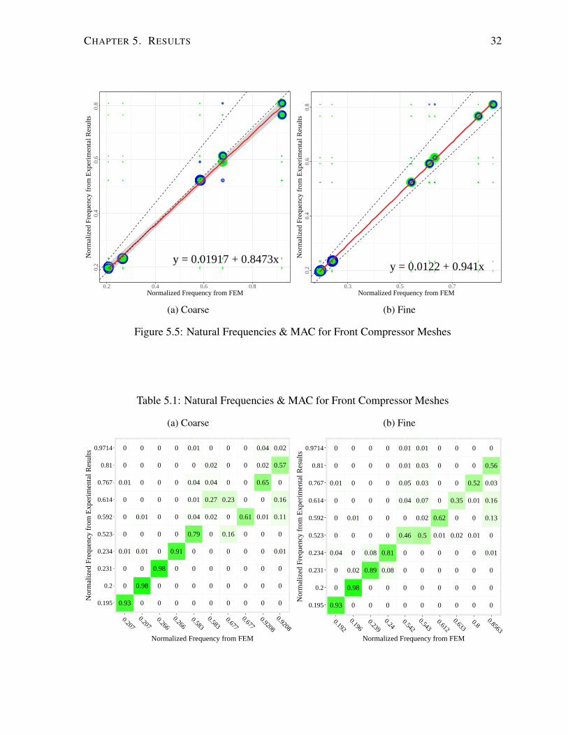
CHAPTER 5. RESULTS 32
● ●● ●● ●● ●●
● ●● ●● ●● ●●
●● ● ●● ●● ●●
●● ● ●● ●● ●●
●● ●● ● ●● ●●●● ●● ● ●● ●●
●● ●● ●● ● ●●
●● ●● ●● ● ●●
●● ●● ●● ●● ●
●● ●● ●● ●● ●
●● ●●
● ● ●●
●● ● ●
● ●● ●● ●
● ● ●● ●●● ● ●● ●●
● ●● ●● ●●
●● ●● ●●
●● ●● ●●
● ●● ●●
y = 0.01917 + 0.8473x
0.2
0.4
0.6
0.8
0.2 0.4 0.6 0.8Normalized Frequency from FEM
Nor
mal
ized
Fre
quen
cy fr
om E
xper
imen
tal R
esul
ts
(a) Coarse
● ●● ●● ● ● ● ●
● ●● ●● ● ● ● ●
● ● ● ●● ● ● ● ●
● ● ● ●● ● ● ● ●
● ● ●● ● ● ● ● ●● ● ●● ● ● ● ● ●
● ● ●● ●● ● ● ●
● ● ●● ●● ● ● ●
● ● ●● ●● ● ● ●
● ● ●● ●● ● ● ●
● ● ● ● ●
● ● ● ● ●
● ● ●
● ● ●● ● ● ● ● ●
● ●● ● ● ●● ● ● ●● ● ● ● ●
● ● ● ● ● ●
● ● ● ● ●
● ● ● ● ● ● ● ●
● ● ● ● ● ● ●
y = 0.0122 + 0.941x
0.2
0.4
0.6
0.8
0.3 0.5 0.7Normalized Frequency from FEM
Nor
mal
ized
Fre
quen
cy fr
om E
xper
imen
tal R
esul
ts
(b) Fine
Figure 5.5: Natural Frequencies & MAC for Front Compressor Meshes
Table 5.1: Natural Frequencies & MAC for Front Compressor Meshes
(a) Coarse
0.93
0
0
0.01
0
0
0
0.01
0
0
0
0.98
0
0.01
0
0.01
0
0
0
0
0
0
0.98
0
0
0
0
0
0
0
0
0
0
0.91
0
0
0
0
0
0
0
0
0
0
0.79
0.04
0.01
0.04
0
0.01
0
0
0
0
0
0.02
0.27
0.04
0.02
0
0
0
0
0
0.16
0
0.23
0
0
0
0
0
0
0
0
0.61
0
0
0
0
0
0
0
0
0
0.01
0
0.65
0.02
0.04
0
0
0
0.01
0
0.11
0.16
0
0.57
0.02
0.195
0.2
0.231
0.234
0.523
0.592
0.614
0.767
0.81
0.9714
0.207
0.207
0.266
0.266
0.583
0.583
0.677
0.677
0.9208
0.9208
Normalized Frequency from FEM
Nor
mal
ized
Fre
quen
cy fr
om E
xper
imen
tal R
esul
ts
(b) Fine
0.93
0
0
0.04
0
0
0
0.01
0
0
0
0.98
0.02
0
0
0.01
0
0
0
0
0
0
0.89
0.08
0
0
0
0
0
0
0
0
0.08
0.81
0
0
0
0
0
0
0
0
0
0
0.46
0
0.04
0.05
0.01
0.01
0
0
0
0
0.5
0.02
0.07
0.03
0.03
0.01
0
0
0
0
0.01
0.62
0
0
0
0
0
0
0
0
0.02
0
0.35
0
0
0
0
0
0
0
0.01
0
0.01
0.52
0
0
0
0
0
0.01
0
0.13
0.16
0.03
0.56
0
0.195
0.2
0.231
0.234
0.523
0.592
0.614
0.767
0.81
0.9714
0.192
0.196
0.239
0.24 0.542
0.543
0.612
0.633 0.8
0.8563Normalized Frequency from FEM
Nor
mal
ized
Fre
quen
cy fr
om E
xper
imen
tal R
esul
ts

CHAPTER 5. RESULTS 33
987654321
0 1 2 3 4 5 6 7 8 9 10 11 12 13 14 15 16 17 18 19 20% Difference between FE and Experimental
Exp
erim
enta
l Mod
e #
(a) Coarse
10987654321
0 1 2 3 4 5 6% Difference between FE and Experimental
Exp
erim
enta
l Mod
e #
(b) Fine
Figure 5.6: Natural Frequency Error for Front Compressor Casing
low MAC values having no shading. A clear diagonal line of high MAC values is apparent in
both Table 5.1a and Table 5.1b, indicating that the MAC has proven effective in selecting
correlated mode pairs. Of particular interest is the 5th experimental frequency; the tables
clearly indicate that a second natural frequency is predicted nearby which was not detected by
the experiment. Additional signal processing of the experimental data may be able to yield the
missing mode. Also of note is the poor MAC values for the higher frequency modes in Table
5.1. While these values are higher than the surrounding values, they are well below optimal.
Since this issue arises in both the fine and coarse meshes, it may indicate a more fundamental
problem with the model parameters rather than an issue with the meshing strategy.
5.2.2 Rear Engine Casing
As for the previous part, the intercept of the regression line is higher for the coarse mesh than
for the fine. Again, this is expected. Both regression lines fall well within the acceptable
bounds, indicating a high degree of correlation between both models and experimental results.
In Figure 5.7a, the scatter of high MAC and AutoMAC is small, indicating a strong linear
relationship between the model and experimental results. In particular, there are no large
MAC or AutoMAC values off the diagonal, indicating a low degree of autocorrelation
between results and a high degree of certainty in selecting correlated mode pairs. Figure 5.7b
shows a near ideal result for a plot of this type: it is readily apparent that no significant MAC
or AutoMAC values appear off the regression line, the MAC values for correlated mode pairs
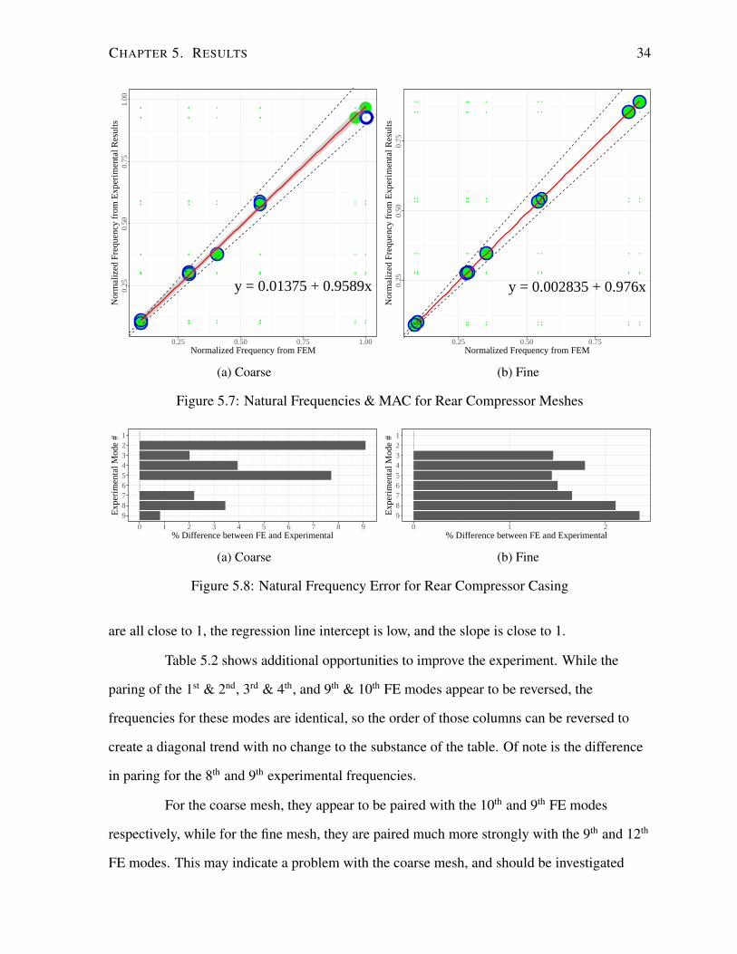
CHAPTER 5. RESULTS 34
● ●● ● ●● ● ●
● ●● ● ●● ● ●
●● ● ● ●● ● ●
●● ● ● ●● ● ●
●● ●● ●● ● ●
●● ●● ● ● ● ●
●● ●● ● ● ● ●
●● ●● ● ●● ●
●● ●● ● ●● ●
● ●
● ● ● ● ●
● ● ●●
● ●
● ●
● ● ● ●
● ●● ●
●● ● ●● ● ● ●
y = 0.01375 + 0.9589x0.25
0.50
0.75
1.00
0.25 0.50 0.75 1.00Normalized Frequency from FEM
Nor
mal
ized
Fre
quen
cy fr
om E
xper
imen
tal R
esul
ts
(a) Coarse
● ● ● ● ● ● ● ●
● ● ● ● ● ● ● ●
● ● ● ● ● ● ● ●
● ● ● ● ● ● ● ●
● ● ● ● ● ● ● ●
● ● ● ● ● ● ● ●
● ● ● ● ● ● ● ●
● ● ● ● ● ● ● ●
● ● ● ● ● ● ● ●
● ● ● ●
●
● ● ●
● ● ●
●
●
●
y = 0.002835 + 0.976x0.25
0.50
0.75
0.25 0.50 0.75Normalized Frequency from FEM
Nor
mal
ized
Fre
quen
cy fr
om E
xper
imen
tal R
esul
ts
(b) Fine
Figure 5.7: Natural Frequencies & MAC for Rear Compressor Meshes
987654321
0 1 2 3 4 5 6 7 8 9% Difference between FE and Experimental
Exp
erim
enta
l Mod
e #
(a) Coarse
987654321
0 1 2% Difference between FE and Experimental
Exp
erim
enta
l Mod
e #
(b) Fine
Figure 5.8: Natural Frequency Error for Rear Compressor Casing
are all close to 1, the regression line intercept is low, and the slope is close to 1.
Table 5.2 shows additional opportunities to improve the experiment. While the
paring of the 1st & 2nd, 3rd & 4th, and 9th & 10th FE modes appear to be reversed, the
frequencies for these modes are identical, so the order of those columns can be reversed to
create a diagonal trend with no change to the substance of the table. Of note is the difference
in paring for the 8th and 9th experimental frequencies.
For the coarse mesh, they appear to be paired with the 10th and 9th FE modes
respectively, while for the fine mesh, they are paired much more strongly with the 9th and 12th
FE modes. This may indicate a problem with the coarse mesh, and should be investigated

CHAPTER 5. RESULTS 35
Table 5.2: Natural Frequencies & MAC for Rear Compressor Meshes
(a) Coarse
0
0.97
0
0
0
0
0
0
0
0.99
0
0
0
0
0
0
0
0
0
0
0
0.97
0
0
0
0
0
0
0
0.97
0
0
0
0
0
0
0
0
0
0
0.98
0
0
0
0
0
0
0
0
0
0
0
0
0
0
0
0
0
0
0.96
0.02
0
0
0
0
0
0
0
0.01
0.89
0
0
0
0
0
0
0
0
0
0
0.82
0
0
0
0
0
0
0
0.72
0
0
0
0
0
0
0
0
0.2
0.07
0
0
0
0
0
0
0
0.04
0.06
0.1
0.11
0.298
0.304
0.376
0.578
0.591
0.927
0.967
0.1 0.1
0.292
0.292
0.405
0.405
0.578
0.578
0.959
0.959 1 1
Normalized Frequency from FEM
Nor
mal
ized
Fre
quen
cy fr
om E
xper
imen
tal R
esul
ts(b) Fine
0.98
0.03
0
0
0
0
0
0
0
0.01
0.95
0
0
0
0
0
0
0
0
0
0.98
0
0
0
0
0
0
0
0
0
0.97
0
0
0
0
0
0
0
0
0
0.98
0
0
0
0
0
0
0
0
0
0
0
0
0
0
0
0
0
0
0.98
0.06
0
0
0
0
0
0
0
0
0.85
0
0
0
0
0
0
0
0
0
0.96
0
0
0
0
0
0
0
0
0
0
0
0
0
0
0
0
0
0.02
0
0
0
0
0
0
0
0
0
0.96
0.09
0.1
0.275
0.28
0.347
0.533
0.545
0.855
0.892
0.09
0.1 0.279
0.285
0.352
0.359
0.541
0.554
0.873
0.887
0.903
0.913
Normalized Frequency from FEM
Nor
mal
ized
Fre
quen
cy fr
om E
xper
imen
tal R
esul
ts
further if those higher mode shapes are of importance. Table 5.2b also shows 3 possible
missing modes from the experimental results corresponding to FE modes 6, 10, and 11.
Further signal analysis of the experimental data may be able to extract those missing modes if
they exist.

Chapter 6
Conclusions
This work has presented a comprehensive procedure for the development and validation of a
finite element vibration model, culminating in a demonstration of this procedure to validate a
pair of aircraft engine casing components. The MAC and FMAC show good correlation
between the models and the parts tested, and highlight issues and avenues of further
investigation not apparent through more basic correlation methods. For the rear compressor
casing, Table 5.2b indicates the likely absence of three modes from the experimental results.
For the front compressor casing, Table 5.1 indicates a missing mode near the 5th experimental
mode. These absences are not apparent from the FMAC alone, which show strong correlation
between the matched modes and frequencies. The use of both MAC tables and the FMAC in
concert is therefore shown to be an efficient and effective method of correlating normal modes
in structures.
The PCL algorithm was able to successfully determine a reduced model resulting in
high MAC values for two axisymmetric structures. In both cases, a high degree of scatter in
the MAC values was observed. However, the scatter appears biased, showing a distinct
distribution, leaving open the possibility that a near optimal results may be possible with a
smaller number of iterations.
36

CHAPTER 6. CONCLUSIONS 37
6.1 Contribution
The algorithm described in this work was able to locate the optimal MAC values for each set
of mode pairs in two axisymmetric structures. In addition, the FMAC has been extended to
show the confidence interval for the regression line, providing further information to the
analyst as to the reliability of their results. Coding for the PCL algorithm is provided in
Appendix B. This document was written in LATEX with knitr[75], the code for which is
available upon request for easy reproduction of Figures 5.1 to 5.8, Tables 5.1 and 5.2, and
associated analysis. An experimental setup and testing procedure were developed which
proved capable of measuring the natural frequencies and mode shapes of interest.
6.2 Recommendations for Future Research
Plotting of the MAC value for an axisymmetric part against the iteration number revealed a
large amount of scatter in the values. While some amount of scatter is unavoidable due to the
discretized nature of both the experimental sampling points and the FE model, more precise
modal expansion methods such as SEREP may have some beneficial impact. Their effect on
the scatter should be explored. Additionally, for many applications, obtaining the optimal
interation while minimizing the computation time may be of interest; the datasets presented
here should serve as a good basis from which to test various optimization techniques requiring
a smaller number of computations. Approaches for evaluating and limiting the effects of
heteroscedasticity in the fitted models should be considered.

References
[1] Y. Zhou, Y. Zhou, W. Yi, T. Chen, D. Tan, and S. Mi, “Operational modal analysis and
rational finite-element model selection for ten high-rise buildings based on on-site
ambient vibration measurements”, Journal of Performance of Constructed Facilities,
vol. 31, no. 5, 2017. DOI: 10.1061/(ASCE)CF.1943-5509.0001019.
[2] S.-G. Gwon and D.-H. Choi, “Improved continuum model for free vibration analysis of
suspension bridges”, Journal of Engineering Mechanics, vol. 143, no. 7, 2017. DOI:
10.1061/(ASCE)EM.1943-7889.0001244.
[3] A. Malekjafarian and E. OBrien, “On the use of a passing vehicle for the estimation of
bridge mode shapes”, Journal of Sound and Vibration, vol. 397, pp. 77–91, 2017. DOI:
10.1016/j.jsv.2017.02.051.
[4] C. Hessek, Y. Kim, and Y. Ji, “Various FRP-bracing configurations for multistory
buildings under seismic loading: Conceptual modeling and comparative assessment”,
Journal of Composites for Construction, vol. 21, no. 3, 2017. DOI:
10.1061/(ASCE)CC.1943-5614.0000761.
[5] A. Darvishpour, A. Ghanbari, S. Hosseini, and M. Nekooei, “A 3d analytical approach
for determining natural frequency of retaining walls”, International Journal of Civil
Engineering, vol. 15, no. 3, pp. 363–375, 2017. DOI: 10.1007/s40999-017-0192-9.
38
REFERENCES 39
[6] X. Wu, H. Deng, and D. Zhu, “Mode shape expansions for the dynamic testing of cable
domes considering random pretension deviations”, Journal of Sound and Vibration,
vol. 394, pp. 155–170, 2017. DOI: 10.1016/j.jsv.2017.01.036.
[7] M. I. Ramli, M. Z. Nuawi, S. Abdullah, M. R. M. Rasani, K. K. Seng, and
M. A. F. Ahmad, “Development on simulation of small structure modal analysis
method using piezoelectric film sensor”, in 23rd International Congress on Sound and
Vibration, ICSV 2016, International Institute of Acoustics and Vibrations, 2016.
[8] X. Ma, A. Wilson, C. Rahn, and S. Trolier-McKinstry, “Efficient energy harvesting
using piezoelectric compliant mechanisms: Theory and experiment”, Journal of
Vibration and Acoustics, Transactions of the ASME, vol. 138, no. 2, 2016. DOI:
10.1115/1.4032178.
[9] J. Yang, M. Morita, and Z. Jiang, “Design of a novel scissoring micro-stirrer for blood
clot dissolution”, Sensors and Actuators, A: Physical, vol. 248, pp. 130–137, 2016.
DOI: 10.1016/j.sna.2016.05.001.
[10] G. Piana, E. Lofrano, A. Carpinteri, A. Paolone, and G. Ruta, “Experimental modal
analysis of straight and curved slender beams by piezoelectric transducers”, Meccanica,
vol. 51, no. 11, pp. 2797–2811, 2016. DOI: 10.1007/s11012-016-0487-y.
[11] S. Rao, Mechanical Vibrations. PRENTICE HALL, 2016, ISBN: 9780134361307.
[12] G. Galilei, Discorsi e dimostrazioni matematiche intorno a due nuove scienze attenenti
alla mecanica ed i movimenti locali. Gli Elsevirii, 1638.
[13] D. Bernoulli, “De vibrationibus et sono laminarum elasticarum commentationes
physico-geometricae”, Commentari Academiae Scientiarum Imperialis Petropolitanae,
vol. 13, p. 105, 1741.
[14] A. E. H. Love, “The small free vibrations and deformation of a thin elastic shell”,
Philosophical Transactions of the Royal Society of London. A, vol. 179, pp. 491–546,
1888.
REFERENCES 40
[15] D. Ebenezer, K. Ravichandran, and C. Padmanabhan, “Free and forced vibrations of
hollow elastic cylinders of finite length a”, The Journal of the Acoustical Society of
America, vol. 137, no. 5, pp. 2927–2938, 2015.
[16] MSC Nastran 2016 Dynamic Analysis User’s Guide. Newport Beach, CA: MSC
Software Corporation, Apr. 2016. [Online]. Available: https://simcompanion.
mscsoftware.com/infocenter/index?page=content&id=DOC10960&actp=LIST.
[17] G. Kerschen, M. Peeters, J. C. Golinval, and C. Stephan, “Nonlinear modal analysis of
a full-scale aircraft”, English, Journal of Aircraft, vol. 50, no. 5, pp. 1409–1419, Sep.
2013. DOI: 10.2514/1.C031918. [Online]. Available:
http://arc.aiaa.org/doi/full/10.2514/1.C031918.
[18] E. Petrov and D. Ewins, “State-of-the-art dynamic analysis for non-linear gas turbine
structures”, Proceedings of the Institution of Mechanical Engineers, Part G: Journal of
Aerospace Engineering, vol. 218, no. 3, pp. 199–211, 2004.
[19] COMSOL Multiphysics: Version 3.5a. User’s guide, v. 1. Comsol, 2008. [Online].
Available: https://books.google.ca/books?id=Mr9McgAACAAJ.
[20] M. Hatch, Vibration Simulation Using MATLAB and ANSYS, ser. Mechanical
engineering / Applied mathematics v. 10. Taylor & Francis, 2000, ISBN:
9781584882053.
[21] LS-DYNA Theory Manual. Lovermore Software Technology Corporation, 2006, ISBN:
0-9778540-0-0.
[22] L. Komzsik, What Every Engineer Should Know about Computational Techniques of
Finite Element Analysis, Second Edition. CRC Press, 2016, ISBN: 9781439802953.
[23] C. Nielsen, W. Zhang, L. Alves, N. Bay, and P. Martins, Modeling of
Thermo-Electro-Mechanical Manufacturing Processes: Applications in Metal Forming
and Resistance Welding, ser. SpringerBriefs in Applied Sciences and Technology.
Springer London, 2012, ISBN: 9781447146421.
REFERENCES 41
[24] A. Cifuentes and A. Kalbag, “A performance study of tetrahedral and hexahedral
elements in 3-d finite element structural analysis”, Finite Elements in Analysis and
Design, vol. 12, no. 3, pp. 313–318, 1992, ISSN: 0168-874X. DOI:
http://dx.doi.org/10.1016/0168-874X(92)90040-J.
[25] “Comparison of hexahedral and tetrahedral elements in finite element analysis of the
foot and footwear”, Journal of Biomechanics, vol. 44, no. 12, pp. 2337–2343, 2011,
ISSN: 0021-9290. DOI: http://dx.doi.org/10.1016/j.jbiomech.2011.05.006.
[26] J. F. Shepherd and C. R. Johnson, “Hexahedral mesh generation constraints”,
Engineering with Computers, vol. 24, no. 3, pp. 195–213, 2008.
[27] Y. Li, Y. Liu, W. Xu, W. Wang, and B. Guo, “All-hex meshing using
singularity-restricted field”, ACM Transactions on Graphics (TOG), vol. 31, no. 6,
p. 177, 2012.
[28] MSC Nastran 2016 Reference Guide. Newport Beach, CA: MSC Software Corporation,
Apr. 2016. [Online]. Available:
https://simcompanion.mscsoftware.com/infocenter/index?page=content&
id=DOC10967&cat=MSC_NASTRAN_DOCUMENTATION_2016&actp=LIST.
[29] D. J. Ewins, Modal Testing : Theory, Practice, and Application, eng, 2nd ed. New
York: Wiley, 2000, ID: 1779510 (UTL catalogue ckey), ISBN: 0863802184.
[30] K. Marudachalam and A. L. Wicks, “An attempt to quantify the errors in the
experimental modal analysis process”, in 9th Conference International Modal Analysis
Conference (IMAC), vol. 1, 1991, pp. 1522–1527.
[31] Y. Korolev and O. Balandin, “Vibration-proof device for a laser vibrometer”,
Measurement Techniques, vol. 17, no. 12, pp. 1900–1901, 1974. DOI:
10.1007/BF00819158.
REFERENCES 42
[32] R. Il’yasov, Y. Malinin, and Y. Pol’skii, “Laser vibrometer with increased accuracy and
interference immunity”, Measurement Techniques, vol. 20, no. 10, pp. 1470–1472,
1977. DOI: 10.1007/BF00824271.
[33] J. L. Lesne and B. Lacrampe, “Development of laser vibration meters. [developpements
en vibrometrie par laser.]”, RGE, Revue Generale de l’Electricite, no. 5, pp. 365–369,
1981.
[34] N. Halliwell, C. Pickering, and P. Eastwood, “The laser torsional vibrometer: A new
instrument”, Journal of Sound and Vibration, vol. 93, no. 4, pp. 588–592, 1984. DOI:
10.1016/0022-460X(84)90427-9.
[35] S. Rothberg, M. Allen, P. Castellini, D. Di Maio, J. Dirckx, D. Ewins, B. J. Halkon,
P. Muyshondt, N. Paone, T. Ryan, et al., “An international review of laser doppler
vibrometry: Making light work of vibration measurement”, Optics and Lasers in
Engineering, 2016.
[36] D. Rovscek, J. Slavic, and M. Boltezar, “Operational mode-shape normalisation with a
structural modification for small and light structures”, Mechanical Systems and Signal
Processing, vol. 42, no. 1-2, pp. 1–13, 2014. DOI: 10.1016/j.ymssp.2013.08.019.
[37] M. Khatibi, M. Ashory, and A. Malekjafarian, “Scaling of operational mode shapes
using mass-cancellation methods”, in 4th International Operational Modal Analysis
Conference, IOMAC 2011, 2011, pp. 41–48.
[38] M. Ashory, “Correction of mass-loading effects of transducers and suspension effects
in modal testing”, in Proceedings of the International Modal Analysis Conference -
IMAC, vol. 2, 1998, pp. 815–828.
[39] M. Sutton, J. Orteu, and H. Schreier, Image Correlation for Shape, Motion and
Deformation Measurements: Basic Concepts,Theory and Applications. Springer US,
2009, ISBN: 9780387787473.

REFERENCES 43
[40] R. Hunady and M. Hagara, “A new procedure of modal parameter estimation for
high-speed digital image correlation”, Mechanical Systems and Signal Processing,
vol. 93, pp. 66–79, 2017, ISSN: 0888-3270. DOI:
https://doi.org/10.1016/j.ymssp.2017.02.010.
[41] P. Avitabile, “Back to basics”, Experimental Techniques, vol. 26, no. 6, pp. 17–19,
2002. DOI: 10.1111/j.1747-1567.2002.tb00085.x. [Online]. Available:
http://dx.doi.org/10.1111/j.1747-1567.2002.tb00085.x.
[42] E. F. F. Chladni, Entdeckungen uber die Theorie des Klanges. Zentralantiquariat der
DDR, 1787.
[43] R. Hooke, The Posthumous Works of Robert Hooke, ... Containing His Cutlerian
Lectures, and Other Discourses, Read at the Meetings of the Illustrious Royal Society.
... Illustrated with Sculptures. To These Discourses is Prefixt the Author’s Life, ...
Publish’d by Richard Waller. Sam. Smith and Benj. Walford, 1705.
[44] W. P. Targoff, “Orthogonality Check and Correction of Measured Modes”, AIAA
Journal, vol. 14, no. 2, pp. 164–167, 1976, doi: 10.2514/3.61351; 08. DOI:
10.2514/3.61351. [Online]. Available: http://dx.doi.org/10.2514/3.61351.
[45] R. J. Allemang and D. L. Brown, “Correlation coefficient for modal vector analysis”,
English, in Proceedings of the International Modal Analysis Conference and Exhibit,
1982, pp. 110–116.
[46] R. J. Allemang, “The modal assurance criterion–twenty years of use and abuse”,
English, Sound and Vibration, vol. 37, no. 8, pp. 14–21, 2003.
[47] G. Chen, D. Fotsch, N. Imamovic, and D. Ewins, “Correlation methods for
axisymmetric structures”, Proceedings of the International Modal Analysis Conference
- IMAC, vol. 2, pp. 1006–1012, 2000.

REFERENCES 44
[48] C. Schedlinski and B. Staples, “Computational model updating of axis symmetric
systems”, in Proc. of the International Conference on Noise and Vibration Engineering
ISMA, 2004.
[49] A. Skafte, M. Aenlle, and R. Brincker, “Cross orthogonality check for structures with
closely spaced modes”, in Conference Proceedings of the Society for Experimental
Mechanics Series, vol. 3, 2015, pp. 321–328. DOI:
10.1007/978-3-319-15224-0_34.
[50] C. Morales, “Comments on the MAC and the NCO, and a linear modal correlation
coefficient”, Journal of Sound and Vibration, vol. 282, no. 1, pp. 529–537, 2005, ISSN:
0022-460X. DOI: http://dx.doi.org/10.1016/j.jsv.2004.04.011.
[51] D. Fotsch and D. Ewins, “Application of MAC in the frequency domain”, Proceedings
of the International Modal Analysis Conference - IMAC, vol. 2, pp. 1225–1231, 2000.
[52] F. Wang and G. Luo, “A comparison study on application of model reduction methods
in rotor dynamics”, in Vibroengineering Procedia, vol. 5, 2015, pp. 59–64.
[53] R. Guyan, “Reduction of stiffness and mass matrices”, AIAA Journal, vol. 3, no. 2,
pp. 380–386, 1965.
[54] M. Paz, “Dynamic condensation”, AIAA Journal, vol. 22, no. 5, pp. 724–727, 1984.
[55] J. O’Callahan, “A procedure for an improved reduced system (irs) model”, Proceedings
of the 7th International Modal Analysis Conference, pp. 17–21, 1989.
[56] M. Friswell, S. Garvey, and J. Penny, “Model reduction using dynamic and iterated irs
techniques”, Journal of sound and vibration, vol. 186, no. 2, pp. 311–323, 1995.
[57] R. R. John O’Callahan Peter Avitabile, “System Equivalent Reduction Expansion
Process (SEREP)”, in Proceedings of the 7th International Modal Analysis Conference.
Union College and Society for Experimental Mechanics, 1989, pp. 29–37.
REFERENCES 45
[58] P. Koutsovasilis and M. Beitelschmidt, “Comparison of model reduction techniques for
large mechanical systems”, Multibody System Dynamics, vol. 20, no. 2, pp. 111–128,
2008.
[59] C. Sastry, D. Mahapatra, S. Gopalakrishnan, and T. Ramamurthy, “An iterative system
equivalent reduction expansion process for extraction of high frequency response from
reduced order finite element model”, Computer Methods in Applied Mechanics and
Engineering, vol. 192, no. 15, pp. 1821–1840, 2003. DOI:
10.1016/S0045-7825(03)00204-4.
[60] S. Sclaroff and A. P. Pentland, “Modal matching for correspondence and recognition”,
IEEE Transactions on Pattern Analysis and Machine Intelligence, vol. 17, no. 6,
pp. 545–561, 1995.
[61] W. Wang, J. E. Mottershead, and C. Mares, “Vibration mode shape recognition using
image processing”, English, Journal of Sound and Vibration, vol. 326, no. 3-5,
pp. 909–938, 2009. DOI: 10.1016/j.jsv.2009.05.024.
[62] J. Bendat and A. Piersol, Random Data: Analysis and Measurement Procedures,
ser. Wiley Series in Probability and Statistics. Wiley, 2011, ISBN: 9781118210826.
[63] C. Sebastian, E. Lopez-Alba, and E. Patterson, “A comparison methodology for
measured and predicted displacement fields in modal analysis”, Journal of Sound and
Vibration, vol. 400, pp. 354–368, 2017.
[64] T. Peaz and N. F. Hunter, “Statistical analysis of modal parameters using the
bootstrap”, in Proceedings of 14 th International Modal Analysis Conference, 1996.
[65] C. R. Farrar, S. W. Doebling, and P. J. Cornwell, “A comparison study of modal
parameter confidence intervals computed using the monte carlo and bootstrap
techniques”, in PROCEEDINGS-SPIE THE INTERNATIONAL SOCIETY FOR
OPTICAL ENGINEERING, SPIE INTERNATIONAL SOCIETY FOR OPTICAL,
vol. 2, 1998, pp. 936–944.

REFERENCES 46
[66] G. Plessis, B. Lallemand, T. Tison, and P. Level, “Fuzzy modal parameters”, Journal of
Sound and Vibration, vol. 233, no. 5, pp. 797–812, 2000. DOI:
10.1006/jsvi.1999.2851.
[67] B. Peeters, H. Van der Auweraer, P. Guillaume, and J. Leuridan, “The polymax
frequency-domain method: A new standard for modal parameter estimation?”, Shock
and Vibration, vol. 11, no. 3-4, pp. 395–409, 2004.
[68] P. Guillaume, P. Verboven, and S. Vanlanduit, “Frequency-domain maximum likelihood
identification of modal parameters with confidence intervals”, in Proceedings of the
international seminar on modal analysis, Katholieke Universiteit Leuven, vol. 1, 1998,
pp. 359–366.
[69] T. Marinone and A. Moya, “Comparison of FRF Correlation Techniques”, in Model
Validation and Uncertainty Quantification, Volume 3: Proceedings of the 33rd IMAC, A
Conference and Exposition on Structural Dynamics, 2015, H. S. Atamturktur,
B. Moaveni, C. Papadimitriou, and T. Schoenherr, Eds. Cham: Springer International
Publishing, 2015, pp. 299–309, ISBN: 978-3-319-15224-0. DOI:
10.1007/978-3-319-15224-0_32. [Online]. Available:
http://dx.doi.org/10.1007/978-3-319-15224-0_32.
[70] W. Vorus and J. Paulling, Vibration, ser. The Principles of Naval Architecture Series.
Society of Naval Architects and Marine Engineers, 2010, ISBN: 9780939773756.
[71] E. Q. Sun, “Shear locking and hourglassing in MSC Nastran, ABAQUS, and ANSYS”,
in MSC Software Users Meeting, 2006.
[72] M. Kutner, Applied Linear Statistical Models, ser. McGraw-Hill International Edition.
McGraw-Hill Irwin, 2005, ISBN: 9780071122214.
[73] D. C. Montgomery and G. C. Runger, Applied statistics and probability for engineers.
John Wiley & Sons, 2010.

REFERENCES 47
[74] K.-J. Bathe, “Finite element procedures”, in, 1. print. Englewood Cliffs, NJ: Prentice
Hall, 1996, ch. Formulation of the Finite Element Method, ISBN: 0133014584.
[75] Y. Xie, Dynamic Documents with R and Knitr, Second Edition, 2nd. Chapman &
Hall/CRC, 2015, ISBN: 1498716962, 9781498716963. [Online]. Available:
http://CRAN.Rproject.org/package=knitr.

Appendix A
Modelling
A.1 Finite Element
The FE modelling for this project required the meshing of 15 components, two of which are
referenced in this thesis. The geometry was determined from solid models provided by Pratt
& Whitney Canada. The actual material properties were not provided, as they were
considered proprietary, so the properties of similar generic materials were used instead. The
2016.1 version was used for all MSC products referenced in this thesis (MSC Nastran, MSC
Patran, MSC ProCOR).
Tables A.1 and A.2 provide the properties and number of elements used for the two
parts examined in this thesis. The two parts were also weighed, and their weights compared
against those predicted by their respective solid models; the percent discrepancy is also
Table A.1: Front Compressor Casing Mesh Statistics
Front Compressor CasingYoung’s Modulus 113.8 GPaPoisson’s Ratio 0.342Density 4.43 g/ccWeight Discrepancy from CAD 11.3%
Fine Mesh Coarse Mesh1220644 2ndorder TET 12760 1storder HEX
48

APPENDIX A. MODELLING 49
Table A.2: Rear Compressor Casing Mesh Statistics
Rear Compressor CasingYoung’s Modulus 204.8 GPaPoisson’s Ratio 0.291Density 8.22 g/ccWeight Discrepancy from CAD 3.12%
Fine Mesh Coarse Mesh1020642 2ndorder TET 45588 1storder HEX
348 1storder PENTA
provided in these tables.
The fine meshes were created using the Altair Hypermesh v13.0 solid automesher,
creating 2ndorder tet elements which closely followed the supplied CAD geometry. These
meshes included all the asymmetries of the actual part. The coarse meshes were created by
sweeping an approximate cross-section of the component about the central axis, resulting in a
fully axi-symmetric part. The coarse meshes are made using 1storder hex elements for
increased efficiency.
A.2 Experimental
Figure A.2 shows the sampling grid used to collect the experimental data used in this thesis.
The front compressor casing was modelled with 90 dofs, and the rear compressor casing was
modelled with 140 dofs. LMS Test Lab R16A was used for all analysis, processing data from
a LMS SCADAS Mobile 02 Mainframe. A PCB Piezotronics Model 356A31 triaxial
accelerometer and Model 086C03 general purpose modal analysis impact hammer with a
nylon tip were used for data collection. Figure A.1 shows sample FRFs from the components
tested in as part of this work.

APPENDIX A. MODELLING 50
Frequency
Am
plitu
de
(a) Front Compressor Casing
FrequencyA
mpl
itude
(b) Rear Compressor Casing
Figure A.1: Sample FRFs From Each Component
(a) Front Compressor Casing(b) Rear Compressor Casing
Figure A.2: Experimental Models

APPENDIX A. MODELLING 51
A.3 Additional Software
In addition to the modelling software discussed above, Table A.3 presents software used for
the analysis presented in this thesis. All listed software is open source, and available on
multiple platforms.
Table A.3: Additional Analysis Software
Software VersionR 3.3.2ggplot2 2.1.0ggExtra 0.5reshape2 1.4.1knitr 1.14
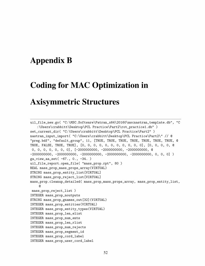
Appendix B
Coding for MAC Optimization in
Axisymmetric Structures
uil_file_new.go( "C:\MSC.Software\Patran_x64\20160\mscnastran_template.db", "C
:\Users\crabbitt\Desktop\PCL Practice\Part2\rot_practice1.db" )
set_current_dir( "C:\Users\crabbitt\Desktop\PCL Practice\Part2" )
nastran_input_import( "C:\Users\crabbitt\Desktop\PCL Practice\Part2\" // @
"preg.bdf", "default_group", 11, [TRUE, TRUE, TRUE, TRUE, TRUE, TRUE, TRUE, @
TRUE, FALSE, TRUE, TRUE], [0, 0, 0, 0, 0, 0, 0, 0, 0, 0, 0], [0, 0, 0, 0, @
0, 0, 0, 0, 0, 0, 0], [-2000000000, -2000000000, -2000000000, @
-2000000000, -2000000000, -2000000000, -2000000000, -2000000000, 0, 0, 0] )
ga_view_aa_set( -67., 0., -34. )
uil_file_report.open_file( "mass_prop.rpt", 80 )
REAL mass_prop_mass_props_array(VIRTUAL)
STRING mass_prop_entity_list[VIRTUAL]
STRING mass_prop_reject_list[VIRTUAL]
mass_prop.cleanup_detailed( mass_prop_mass_props_array, mass_prop_entity_list,
@
mass_prop_reject_list )
INTEGER mass_prop_noutputs
STRING mass_prop_gnames_out[32](VIRTUAL)
INTEGER mass_prop_entities(VIRTUAL)
INTEGER mass_prop_entity_types(VIRTUAL)
INTEGER mass_prop_len_elist
INTEGER mass_prop_num_ents
INTEGER mass_prop_len_rlist
INTEGER mass_prop_num_rejects
INTEGER mass_prop_segment_id
INTEGER mass_prop_cord_label
INTEGER mass_prop_user_cord_label
52

APPENDIX B. CODING FOR MAC OPTIMIZATION IN AXISYMMETRIC STRUCTURES 53
mass_prop_create_detailed( "3D", "Group", "FEM", "Summary", 1, [ @
"default_group"], "", "Coord 0", "Use Element Properties", @
"Use Element Properties", "Coord 0", 3, 1, FALSE, FALSE, mass_prop_noutputs, @
mass_prop_gnames_out, mass_prop_entities, mass_prop_entity_types, @
mass_prop_mass_props_array, mass_prop_entity_list, mass_prop_len_elist, @
mass_prop_num_ents, mass_prop_reject_list, mass_prop_len_rlist, @
mass_prop_num_rejects, mass_prop_segment_id, mass_prop_cord_label, @
mass_prop_user_cord_label )
mass_prop.gen_report_detailed( 80, mass_prop_noutputs, "Summary", "FEM", @
mass_prop_gnames_out, mass_prop_entities, mass_prop_entity_types, @
mass_prop_mass_props_array, "Use Element Properties", @
mass_prop_user_cord_label, mass_prop_entity_list, mass_prop_num_ents, @
mass_prop_len_elist, mass_prop_reject_list, mass_prop_num_rejects, @
mass_prop_len_rlist )
ui_exec_function( "mesh_seed_display_mgr", "init" )
mesh_seed_display_mgr.erase( )
INTEGER chan1, integer_holder(8)
REAL real_holder(8)
STRING string_holder[80](8)
text_open("mass_prop.rpt", "OR", 0, 0, chan1)
While( text_read(chan1, "%OF%%A%%F15%", integer_holder(1), real_holder(1),
string_holder(1)) != -1)
IF(string_holder(1) == "X") THEN real_holder(2)=real_holder(1)
IF(string_holder(1) == "Y") THEN real_holder(3)=real_holder(1)
IF(string_holder(1) == "Z") THEN real_holder(4)=real_holder(1)
END While
STRING fem_create_nodes__nodes_created[VIRTUAL]
fem_create_nodes_1( "Coord 0", "Coord 0", 2, "999999", @
" [" // str_from_real(real_holder(2)) // " " // str_from_real(real_holder(3))
// @
" " // str_from_real(real_holder(4)) // "]", fem_create_nodes__nodes_created
)
$? NO 1
$? YES 6022095
mesh_seed_display_mgr.erase( )
$? NO 1
sys_free_string(fem_create_nodes__nodes_created)
jobfile.open( "pre-g", "ANALYZE NO JOBFILE" )
$? YES 6016027
msc_delete_old_files( "pre-g", ".bdf", ".op2" )
jobfile.write_spl( "/* Jobfile for PATNAS created %A% at %A% */", ["25-Apr-17"
@
, "17:33:19"] )
jobfile.writec( "", "TRANSLATOR = pat3nas" )
jobfile.writec( "DATABASE", "C:\Users\crabbitt\Desktop\PCL Practice\Part2\" //
@
"rot_practice1.db" )

APPENDIX B. CODING FOR MAC OPTIMIZATION IN AXISYMMETRIC STRUCTURES 54
jobfile.writec( "JOBNAME", "pre-g" )
jobfile.writec( "ANALYSIS TITLE", "" )
jobfile.writec( "ANALYSIS SUBTITLE", "" )
jobfile.writec( "ANALYSIS LABEL", "" )
jobfile.writec( "", "" )
jobfile.writec( "OBJECT", "Entire Model" )
jobfile.writec( "METHOD", "Full Run" )
jobfile.writec( "", "" )
jobfile.writec( "MODEL SUFFIX", ".bdf" )
jobfile.writec( "RESULTS SUFFIX", ".op2" )
jobfile.writec( "", "" )
jobfile.writec( "", "/*" )
jobfile.writec( "", " * File Search Path Declaration" )
jobfile.writec( "", " */" )
jobfile.writec( "", "" )
jobfile.writec( "File Search Path", "C:\Users\crabbitt" )
jobfile.writec( "File Search Path", "C:\MSC.Software\Patran_x64\20160" )
jobfile.writec( "File Search Path", "C:\MSC.Software\Patran_x64\20160\help" //
@
"files" )
jobfile.writec( "File Search Path", "C:\MSC.Software\Patran_x64\20160\alters"
)
jobfile.writec( "File Search Path", "C:\MSC.Software\Patran_x64\20160\icons" )
jobfile.writec( "File Search Path", "C:\MSC.Software\Patran_x64\20160\icon" //
@
"s\RibbonIcons" )
jobfile.writec( "File Search Path", "C:\MSC.Software\Patran_x64\20160\bin" )
jobfile.writec( "File Search Path", "C:\MSC.Software\Patran_x64\20160\bin\exe"
)
jobfile.writec( "File Search Path", "C:\MSC.Software\Patran_x64\20160\msce" //
@
"xplore_files\" )
jobfile.writec( "File Search Path", "C:\MSC.Software\Patran_x64\20160\mscp" //
@
"rocor_files\dmap" )
jobfile.writec( "File Search Path", "C:\MSC.Software\Patran_x64\20160\mscp" //
@
"rocor_files\plb" )
jobfile.writec( "File Search Path", "C:\MSC.Software\Patran_x64\20160\mscp" //
@
"rocor_files\lib" )
jobfile.writec( "File Search Path", "C:\MSC.Software\Patran_x64\20160\mscp" //
@
"rocor_files\icons" )
jobfile.writec( "File Search Path", "C:\MSC.Software\Patran_x64\20160\shar" //
@
"eware\msc\unsupported\utilities\icons" )

APPENDIX B. CODING FOR MAC OPTIMIZATION IN AXISYMMETRIC STRUCTURES 55
jobfile.writec( "File Search Path", "C:\MSC.Software\Patran_x64\20160\shar" //
@
"eware\msc\unsupported\utilities\plb" )
jobfile.writec( "File Search Path", "C:\MSC.Software\Patran_x64\20160\shar" //
@
"eware\msc\unsupported\utilities\extra_files" )
jobfile.writec( "", "" )
jobfile.writec( "", "/*" )
jobfile.writec( "", " * Translation Parameters" )
jobfile.writec( "", " */" )
jobfile.writec( "", "" )
jobfile.writec( "DATA OUTPUT", "OP2" )
jobfile.writec( "OUTPUT2 REQUESTS", "P3 Built In" )
jobfile.writec( "OUTPUT2 FORMAT", "Binary" )
jobfile.writec( "DIVISION TOLERANCE", "1.0e-08" )
jobfile.writec( "NUMERICAL TOLERANCE", "1.0e-04" )
jobfile.writec( "WRITING TOLERANCE", "1.0e-20" )
jobfile.writec( "GEOM CHECK", "INFORM" )
jobfile.writec( "SORTED BULK", "NO" )
jobfile.writec( "CARD FORMAT", "small" )
jobfile.writec( "NODE COORDINATES", "reference frame" )
jobfile.writec( "COORD COORDINATES", "global" )
jobfile.writec( "MSC.Nastran VERSION", "2016." )
jobfile.writec( "WRITE STORED PRECISION", "TRUE" )
jobfile.writec( "PROPS ON ELEM ENTRY", "FALSE" )
jobfile.writec( "CONTINUATION ENTRY", "FALSE" )
jobfile.writec( "PCOMPG ENTRY", "FALSE" )
jobfile.writec( "CONVERT CBAR CBEAM", "FALSE" )
jobfile.writec( "ITERATIVE SOLVER", "FALSE" )
jobfile.writei( "SUPER ELEMENT 0", 0 )
jobfile.writec( "SEALL WRITE", "FALSE" )
jobfile.writec( "PART SUPERELEMENT CREATE", "TRUE" )
jobfile.writec( "AUTOQSET", "FALSE" )
jobfile.writec( "FIXEDB", "FALSE" )
jobfile.writei( "SUPER TREE COUNT", 0 )
jobfile.writec( "MODEL TOLERANCE", "0.0049999999" )
jobfile.writec( "ELEMENT PROPERTY OFFSET", "0" )
jobfile.writec( "MATERIAL PROPERTY OFFSET", "0" )
jobfile.writec( "TABLE OFFSET", "0" )
jobfile.writec( "LOAD SET OFFSET", "0" )
jobfile.writec( "LOAD CASE OFFSET", "1" )
jobfile.writec( "CONTROL SET OFFSET", "0" )
jobfile.writec( "RIGID ELEMENT OFFSET", "0" )
jobfile.writec( "SCALAR POINT OFFSET", "0" )
jobfile.writec( "BEGINNING CONTINUATION MARKER", "+ A" )
jobfile.writec( "NUMBER ONLY", "ON" )
jobfile.writec( "BEGINNING NUMBER", "OFF" )

APPENDIX B. CODING FOR MAC OPTIMIZATION IN AXISYMMETRIC STRUCTURES 56
jobfile.writec( "TRAILING NUMBER", "OFF" )
jobfile.writec( "SYNTAX NUMBER", "ON" )
jobfile.writec( "SYNTAX MARKER", "." )
jobfile.writec( "EXTERNAL SUPERELEMENT METHOD", "NONE" )
jobfile.writec( "", "" )
jobfile.writec( "", "/*" )
jobfile.writec( "", " * Solution Parameters" )
jobfile.writec( "", " */" )
jobfile.writec( "", "" )
jobfile.writec( "SOLUTION TYPE", "NORMAL MODES" )
jobfile.writei( "SOLUTION SEQUENCE", 103 )
jobfile.writec( "DATABASE RUN", "ON" )
jobfile.writec( "INTERACTIVE MODES", "OFF" )
jobfile.writec( "CYCLIC SYMMETRY", "OFF" )
jobfile.writec( "AUTOMATIC CONSTRAINTS", "ON" )
jobfile.writec( "SHELL NORMAL TOLERANCE", "" )
jobfile.writec( "MASS CALCULATION", "Lumped" )
jobfile.writec( "DATA DECK ECHO", "None" )
jobfile.writec( "PLATE RZ STIFFNESS FACTOR", "0.0" )
jobfile.writec( "MAXIMUM PRINTED LINES", "999999999" )
jobfile.writec( "MAXIMUM RUN TIME", "600" )
jobfile.writec( "WT-MASS CONVERSION", "1.0" )
jobfile.writec( "NODE ID FOR WT-GENER", "999999" )
jobfile.writec( "RIGID ELEMENT TYPE", "LINEAR" )
jobfile.writec( "USE SOL600", "OFF" )
jobfile.writec( "RESIDUAL VECTOR", "Nastran Default" )
jobfile.writec( "NEF STRESS UNITS", "MPA" )
jobfile.writec( "NEF STRESS COMBINATION", "ABSMAXPR" )
jobfile.writec( "NEF RESULT LOCATION", "NODA" )
jobfile.writec( "NEF RECOVERY LOCATION", "CORNER" )
jobfile.writec( "NEF LAYER LOCATION", "WORST" )
jobfile.writec( "NEF INTERPOLATION LIMIT", "0" )
jobfile.writec( "NEF LEVEL OF MESSAGE", "0" )
jobfile.writec( "NEF NUMBER OF THREADS", "1" )
jobfile.writer( "NEF CERTAINTY OF SURVIVAL", 50. )
jobfile.writer( "NEF OVERALL SCALE FACTOR", 1. )
jobfile.writer( "NEF TOP STRESS PERCENTAGE FILTER", 100. )
jobfile.writer( "NEF TOP DAMAGE PERCENTAGE FILTER", 100. )
jobfile.writec( "NEF TIME HISTORY DIRECTORY", "C:\Users\crabbitt" )
jobfile.writei( "NEF MAX LOAD PER EVENT", 1 )
jobfile.writec( "NEF EVENT DATA", "0" )
jobfile.writec( "NEF LOAD SEQUENCE DATA", "0" )
jobfile.writec( "USE CONTACT TABLE", "OFF" )
jobfile.writec( "INITIAL CONTACTPAIR LOADCASE NAME", "" )
jobfile.writei( "MDOF DATA", 0 )
jobfile.writec( "CELL WRITE", "ON" )
jobfile.writei( "CELL INPUT 0", 1 )
APPENDIX B. CODING FOR MAC OPTIMIZATION IN AXISYMMETRIC STRUCTURES 57
jobfile.writec( "CELL INPUT 1", "NASTRAN PARALLEL=20" )
jobfile.writec( "FMS WRITE", "ON" )
jobfile.writei( "FMS INPUT 0", 7 )
jobfile.writec( "FMS INPUT 1", "init master(s) $ do not save database" )
jobfile.writec( "FMS INPUT 2", "ASSIGN OUTPUT2='pregke.op2' ,UNIT=23,DELETE" )
jobfile.writec( "FMS INPUT 3", "ASSIGN OUTPUT2='pregdpr.op2',UNIT=41,DELETE" )
jobfile.writec( "FMS INPUT 4", "ASSIGN OUTPUT4='pre_grun.op4'," )
jobfile.writec( "FMS INPUT 5", " UNIT=31," )
jobfile.writec( "FMS INPUT 6", " FORM='FORMATTED', DELETE" )
jobfile.writec( "FMS INPUT 7", "$ Modes output to .pch file" )
jobfile.writec( "EXEC WRITE", "ON" )
jobfile.writei( "EXEC INPUT 0", 2 )
jobfile.writec( "EXEC INPUT 1", "INCLUDE 'C:\MSC.Software\Patran_x64\20160" //
@
"/mscprocor_files/dmap\p" )
jobfile.writec( "EXEC INPUT 2", "rocor.v2016'" )
jobfile.writec( "CASE WRITE", "ON" )
jobfile.writei( "CASE INPUT 0", 3 )
jobfile.writec( "CASE INPUT 1", "PARAM,RUNTYPE,GSET" )
jobfile.writec( "CASE INPUT 2", "PARAM,DMIGPHI,YES" )
jobfile.writec( "CASE INPUT 3", "PARAM,KEFILT,1.000E-8" )
jobfile.writec( "BULK WRITE", "ON" )
jobfile.writei( "BULK INPUT 0", 12 )
jobfile.writec( "BULK INPUT 1", "$ change gset disp, spcf, and ese patran " //
@
"output" )
jobfile.writec( "BULK INPUT 2", "DTI,PREGLAB,1,CR,1,DW,83,84,2" )
jobfile.writec( "BULK INPUT 3", ",PRE-G" )
jobfile.writec( "BULK INPUT 4", "DTI,PREGLAB,2,ER,ENDREC" )
jobfile.writec( "BULK INPUT 5", "$ change gset computed mode ke % label fo" //
@
"r patran output" )
jobfile.writec( "BULK INPUT 6", "DTI,PREGKE,1,CR,1,DW,83,89,7" )
jobfile.writec( "BULK INPUT 7", ",PREGKE,1,KINETIC,ENERGY" )
jobfile.writec( "BULK INPUT 8", "DTI,PREGKE,2,ER,ENDREC" )
jobfile.writec( "BULK INPUT 9", "$ change gset computed mode DPR label for" //
@
" patran output" )
jobfile.writec( "BULK INPUT 10", "DTI,PREGDPR,1,CR,1,DW,83,89,7" )
jobfile.writec( "BULK INPUT 11", ",PREGDPR,1,DPR--RA,W" )
jobfile.writec( "BULK INPUT 12", "DTI,PREGDPR,2,ER,ENDREC" )
jobfile.writec( "CELL DTI POSITION", "START" )
jobfile.writec( "FMS DTI POSITION", "START" )
jobfile.writec( "EXEC DTI POSITION", "END" )
jobfile.writec( "CASE DTI POSITION", "START" )
jobfile.writec( "BULK DTI POSITION", "START" )
jobfile.writec( "", "END" )

APPENDIX B. CODING FOR MAC OPTIMIZATION IN AXISYMMETRIC STRUCTURES 58
jobfile.close( )
$# Create "pre-g" loadcase
loadcase_create2( "pre-g", "Static", "", 1., [""], [0], [0.], "", 0., TRUE )
$# Create "pre-g" subcase
mscnastran_subcase.create( "103", "pre-g", "" )
mscnastran_subcase.create_char_param( "LOAD CASE", "pre-g" )
mscnastran_subcase.create_char_param( "SUBCASE TITLE", "" )
mscnastran_subcase.create_char_param( "SUBCASE SUBTITLE", "pre-g" )
mscnastran_subcase.create_char_param( "SUBCASE LABEL", "" )
mscnastran_subcase.create_char_param( "SUBCASE TITLE FLAG", "OFF" )
mscnastran_subcase.create_char_param( "SUBCASE SUBTITLE FLAG", "ON" )
mscnastran_subcase.create_char_param( "SUBCASE LABEL FLAG", "OFF" )
mscnastran_subcase.create_char_param( "pre-g", "STRUCTURAL" )
mscnastran_subcase.create_char_param( "CONSTRAINT FORCES", "1" )
mscnastran_subcase.create_char_param( "CONSTRAINT FORCES 1", @
"SPCFORCES=0" )
mscnastran_subcase.create_char_param( "ELEMENT STRAIN ENERGIES", "1" )
mscnastran_subcase.create_char_param( "ELEMENT STRAIN ENERGIES 1", "ESE=0" )
mscnastran_subcase.create_char_param( "EIGENVECTORS", "1" )
mscnastran_subcase.create_char_param( "EIGENVECTORS 1", "VECTOR=0" )
mscnastran_subcase.create_char_param( "SUBCASE WRITE", "ON" )
mscnastran_subcase.create_char_param( "SUBCASE DIRECT TEXT POS", "ON" )
mscnastran_subcase.create_int_param( "SUBCASE INPUT 0", 0 )
mscnastran_subcase.create_char_param( "REAL EIGENVALUE EXTRACTION METHOD", @
"Lanczos" )
mscnastran_subcase.create_char_param( "LOWER FREQUENCY RANGE", "10" )
mscnastran_subcase.create_char_param( "UPPER FREQUENCY RANGE", "1200" )
mscnastran_subcase.create_char_param( "REAL EIGNVALUE NUMBER OF DESIRED ROOTS"
@
, "44" )
mscnastran_subcase.create_char_param( "DIAGNOSTIC OUTPUT LEVEL", "0" )
mscnastran_subcase.create_char_param( "REAL EIGENVALUE NORMALIZATION METHOD",
@
"Mass" )
mscnastran_subcase.create_char_param( "ALL EXPLICIT MPCS", "ON" )
$# Start "pre-g" Run
mscnastran_job.associate_subcases( "103", "pre-g", 1, ["pre-g"] )
analysis_submit( "MSC.Nastran", "pre-g", TRUE)
sys_free_array(mass_prop_entities)
sys_free_array(mass_prop_entity_types)
sys_free_array(mass_prop_gnames_out)
sys_free_array(mass_prop_mass_props_array)
sys_free_string(mass_prop_entity_list)
sys_free_string(mass_prop_reject_list)
sys_free_string(fem_create_nodes__nodes_created)
$# Start reading in ASET Nodes & create map
Integer chan1, count, integer_holder(9), lrecl, nodecount, uff_trace(VIRTUAL)

APPENDIX B. CODING FOR MAC OPTIMIZATION IN AXISYMMETRIC STRUCTURES 59
Integer count3, count2
real real_holder(8), uff_coords(VIRTUAL)
string string_holder[80](8), record[1]
sys_allocate_array(uff_coords, 1,300, 1,3)
sys_allocate_array(uff_trace, 1, 900)
text_open("Experiment2_rot.unv", "OR", 0, 0, chan1)
real_holder(1) = 1
integer_holder(1) = 1
count = 0
nodecount = 0
count2 = 0
count3 = 0
while( text_read(chan1, "%OF%%I8%", integer_holder(1), real_holder(1),
string_holder(1)) != -1)
count += 1
IF(integer_holder(1)==15) THEN
text_read(chan1, "%OF%%I8%%33W%%3F13%", integer_holder(1:3), real_holder
(1:3), string_holder(1:3))
while(integer_holder(1) != -1)
count += 1
nodecount +=1
uff_coords(nodecount,1:3) = real_holder(1:3)
IF(count > 422000) THEN BREAK
text_read(chan1, "%OF%%I8%%33W%%3F13%", integer_holder(1:3),
real_holder(1:3), string_holder(1:3))
end while
end IF
IF(integer_holder(1)==82) THEN
Integer i
text_read(chan1, "%OF%%8I10%", integer_holder(1:8), real_holder(1:8),
string_holder(1:8))
text_read(chan1, "%OF%%8I10%", integer_holder(1:8), real_holder(1:8),
string_holder(1:8))
text_read(chan1, "%OF%%8I10%", integer_holder(1:8), real_holder(1:8),
string_holder(1:8))
while(integer_holder(1) != -1)
count2 += 1
For(i=1 to 8)
uff_trace(count3*8 + i) = integer_holder(i)
End For
count3 += 1
count += 1
IF(count > 422000) THEN BREAK
text_read(chan1, "%OF%%8I10%", integer_holder(1:8), real_holder(1:8),
string_holder(1:8))
end while
end IF

APPENDIX B. CODING FOR MAC OPTIMIZATION IN AXISYMMETRIC STRUCTURES 60
IF(count > 422000) THEN BREAK
end while
text_close(chan1, "")
sys_reallocate_array(uff_trace, 1, count2*8)
count = 0
$# Variables for nodematch
String match_out[VIRTUAL], string1[1], groupnodes[14], string2[14], string3[
VIRTUAL]
String node_coord[40], str_max[12], deleted_nodes[VIRTUAL], not_found_nodes[
VIRTUAL]
Real distance_out(VIRTUAL), real1
Integer length_out, entity_count, node1
Integer node_map(VIRTUAL), max_node, int1(1)
ga_group_create("UFF_nodes")
ga_group_current_set("UFF_nodes")
db_count_nodes_in_group(1,node1)
sys_allocate_array(node_map, 1, node1-1)
groupnodes = "Node 1:" // str_from_integer(node1-1)
while(count < nodecount)
count += 1
string_write("[%3E%]", int1 , uff_coords(count,1:3), string1, node_coord)
fem_create_nodes_1( "Coord 0", "Coord 0", 2, "#", node_coord, string3 )
db_get_max_node_id(max_node)
str_max = "Node "// str_from_integer(max_node)
fem_geom_match_closest(str_max, groupnodes, @
entity_count, match_out, distance_out, length_out)
node_map(count) = str_to_integer(str_substr(match_out, 5, 6))
sys_free_string(match_out)
sys_free_array(distance_out)
String match_out[VIRTUAL]
Real distance_out(VIRTUAL)
fem_delete_free_node(str_max, deleted_nodes, not_found_nodes )
End while
$# Clear variables from nodematch
sys_free_string(match_out)
sys_free_string(deleted_nodes)
sys_free_string(not_found_nodes)
sys_free_array(distance_out)
$# Populate ASET elements
Integer uff_trace2(VIRTUAL)
sys_allocate_array(uff_trace2, 1, 2, 1, count2*8)
count3 = 0
for(i=1 to count2*8)
IF(uff_trace(i) == 0) THEN CONTINUE
IF(uff_trace(i+1) == 0) THEN CONTINUE
count3 += 1
uff_trace2(1, count3) = node_map(uff_trace(i))

APPENDIX B. CODING FOR MAC OPTIMIZATION IN AXISYMMETRIC STRUCTURES 61
uff_trace2(2, count3) = node_map(uff_trace(i+1))
End for
String string_holder2[VIRTUAL](2), traceformat[12]
sys_allocate_string(string_holder2, 2000)
traceformat = "Node %" // str_from_integer(count3) // "I%"
string_write(traceformat, uff_trace2(1,1:300), real_holder, string_holder,
string_holder2(1))
string_write(traceformat, uff_trace2(2,1:300), real_holder, string_holder,
string_holder2(2))
fem_create_elems( "Bar ", "Bar2", "#", "Standard", TRUE, string_holder2(1),
string_holder2(2), "", "", "", "", "", "", "" )
$# sys_free_array(uff_trace)
sys_free_array(uff_trace2)
sys_free_string(string3)
sys_free_string(string_holder2)
Integer max_elem, min_elem
db_get_max_elem_id(max_elem)
min_elem = max_elem - count3 + 1
elementprops_create( "uff_traceline", 67, 25, 20, 28, 2, 34, [40], [4], [ @
"DUMMY"], "Element " // str_from_integer(min_elem) // ":" // str_from_integer(
max_elem) )
$# Start Pre-Test ASET Analysis
msc_delete_old_files( "pre-a", ".bdf", ".op2" )
jobfile.open( "pre-a", "ANALYZE NO JOBFILE" )
jobfile.write_spl( "/* Jobfile for PATNAS created %A% at %A% */", ["25-Apr-17"
@
, "17:37:19"] )
jobfile.writec( "", "TRANSLATOR = pat3nas" )
jobfile.writec( "DATABASE", "C:\Users\crabbitt\Desktop\PCL Practice\Part2\" //
@
"rot_practice1.db" )
jobfile.writec( "JOBNAME", "pre-a" )
jobfile.writec( "ANALYSIS TITLE", "" )
jobfile.writec( "ANALYSIS SUBTITLE", "" )
jobfile.writec( "ANALYSIS LABEL", "" )
jobfile.writec( "", "" )
jobfile.writec( "OBJECT", "Entire Model" )
jobfile.writec( "METHOD", "Full Run" )
jobfile.writec( "", "" )
jobfile.writec( "MODEL SUFFIX", ".bdf" )
jobfile.writec( "RESULTS SUFFIX", ".op2" )
jobfile.writec( "", "" )
jobfile.writec( "", "/*" )
jobfile.writec( "", " * File Search Path Declaration" )
jobfile.writec( "", " */" )
jobfile.writec( "", "" )

APPENDIX B. CODING FOR MAC OPTIMIZATION IN AXISYMMETRIC STRUCTURES 62
jobfile.writec( "File Search Path", "C:\MSC.Software\Patran_x64\20160\msce" //
@
"xplore_files\" )
jobfile.writec( "File Search Path", "C:\MSC.Software\Patran_x64\20160\bin\exe"
)
jobfile.writec( "File Search Path", "C:\MSC.Software\Patran_x64\20160\bin" )
jobfile.writec( "File Search Path", "C:\MSC.Software\Patran_x64\20160\icon" //
@
"s\RibbonIcons" )
jobfile.writec( "File Search Path", "C:\MSC.Software\Patran_x64\20160\icons" )
jobfile.writec( "File Search Path", "C:\MSC.Software\Patran_x64\20160\alters"
)
jobfile.writec( "File Search Path", "C:\MSC.Software\Patran_x64\20160\help" //
@
"files" )
jobfile.writec( "File Search Path", "C:\MSC.Software\Patran_x64\20160" )
jobfile.writec( "File Search Path", "C:\MSC.Software\Patran_x64\20160\shar" //
@
"eware\msc\unsupported\utilities\extra_files" )
jobfile.writec( "File Search Path", "C:\MSC.Software\Patran_x64\20160\shar" //
@
"eware\msc\unsupported\utilities\plb" )
jobfile.writec( "File Search Path", "C:\MSC.Software\Patran_x64\20160\shar" //
@
"eware\msc\unsupported\utilities\icons" )
jobfile.writec( "File Search Path", "C:\MSC.Software\Patran_x64\20160\mscp" //
@
"rocor_files\icons" )
jobfile.writec( "File Search Path", "C:\MSC.Software\Patran_x64\20160\mscp" //
@
"rocor_files\lib" )
jobfile.writec( "File Search Path", "C:\MSC.Software\Patran_x64\20160\mscp" //
@
"rocor_files\plb" )
jobfile.writec( "File Search Path", "C:\MSC.Software\Patran_x64\20160\mscp" //
@
"rocor_files\dmap" )
jobfile.writec( "File Search Path", "C:\Users\crabbitt" )
jobfile.writec( "", "" )
jobfile.writec( "", "/*" )
jobfile.writec( "", " * Translation Parameters" )
jobfile.writec( "", " */" )
jobfile.writec( "", "" )
jobfile.writec( "DATA OUTPUT", "OP2" )
jobfile.writec( "OUTPUT2 REQUESTS", "P3 Built In" )
jobfile.writec( "OUTPUT2 FORMAT", "Binary" )
jobfile.writec( "DIVISION TOLERANCE", "1.0e-08" )

APPENDIX B. CODING FOR MAC OPTIMIZATION IN AXISYMMETRIC STRUCTURES 63
jobfile.writec( "NUMERICAL TOLERANCE", "1.0e-04" )
jobfile.writec( "WRITING TOLERANCE", "1.0e-20" )
jobfile.writec( "GEOM CHECK", "INFORM" )
jobfile.writec( "SORTED BULK", "NO" )
jobfile.writec( "CARD FORMAT", "small" )
jobfile.writec( "NODE COORDINATES", "reference frame" )
jobfile.writec( "COORD COORDINATES", "global" )
jobfile.writec( "MSC.Nastran VERSION", "2016." )
jobfile.writec( "WRITE STORED PRECISION", "TRUE" )
jobfile.writec( "PROPS ON ELEM ENTRY", "FALSE" )
jobfile.writec( "CONTINUATION ENTRY", "FALSE" )
jobfile.writec( "PCOMPG ENTRY", "FALSE" )
jobfile.writec( "CONVERT CBAR CBEAM", "FALSE" )
jobfile.writec( "ITERATIVE SOLVER", "FALSE" )
jobfile.writei( "SUPER ELEMENT 0", 0 )
jobfile.writec( "SEALL WRITE", "FALSE" )
jobfile.writec( "PART SUPERELEMENT CREATE", "TRUE" )
jobfile.writec( "AUTOQSET", "FALSE" )
jobfile.writec( "FIXEDB", "FALSE" )
jobfile.writei( "SUPER TREE COUNT", 0 )
jobfile.writec( "MODEL TOLERANCE", "0.0049999999" )
jobfile.writec( "ELEMENT PROPERTY OFFSET", "0" )
jobfile.writec( "MATERIAL PROPERTY OFFSET", "0" )
jobfile.writec( "TABLE OFFSET", "0" )
jobfile.writec( "LOAD SET OFFSET", "0" )
jobfile.writec( "LOAD CASE OFFSET", "1" )
jobfile.writec( "CONTROL SET OFFSET", "0" )
jobfile.writec( "RIGID ELEMENT OFFSET", "0" )
jobfile.writec( "SCALAR POINT OFFSET", "0" )
jobfile.writec( "BEGINNING CONTINUATION MARKER", "+ A" )
jobfile.writec( "NUMBER ONLY", "ON" )
jobfile.writec( "BEGINNING NUMBER", "OFF" )
jobfile.writec( "TRAILING NUMBER", "OFF" )
jobfile.writec( "SYNTAX NUMBER", "ON" )
jobfile.writec( "SYNTAX MARKER", "." )
jobfile.writec( "EXTERNAL SUPERELEMENT METHOD", "NONE" )
jobfile.writec( "", "" )
jobfile.writec( "", "/*" )
jobfile.writec( "", " * Solution Parameters" )
jobfile.writec( "", " */" )
jobfile.writec( "", "" )
jobfile.writec( "SOLUTION TYPE", "NORMAL MODES" )
jobfile.writei( "SOLUTION SEQUENCE", 103 )
jobfile.writec( "DATABASE RUN", "ON" )
jobfile.writec( "INTERACTIVE MODES", "OFF" )
jobfile.writec( "CYCLIC SYMMETRY", "OFF" )
jobfile.writec( "AUTOMATIC CONSTRAINTS", "ON" )

APPENDIX B. CODING FOR MAC OPTIMIZATION IN AXISYMMETRIC STRUCTURES 64
jobfile.writec( "SHELL NORMAL TOLERANCE", "" )
jobfile.writec( "MASS CALCULATION", "Lumped" )
jobfile.writec( "DATA DECK ECHO", "None" )
jobfile.writec( "PLATE RZ STIFFNESS FACTOR", "0.0" )
jobfile.writec( "MAXIMUM PRINTED LINES", "999999999" )
jobfile.writec( "MAXIMUM RUN TIME", "600" )
jobfile.writec( "WT-MASS CONVERSION", "1.0" )
jobfile.writec( "NODE ID FOR WT-GENER", "999999" )
jobfile.writec( "RIGID ELEMENT TYPE", "LINEAR" )
jobfile.writec( "USE SOL600", "OFF" )
jobfile.writec( "RESIDUAL VECTOR", "Nastran Default" )
jobfile.writec( "NEF STRESS UNITS", "MPA" )
jobfile.writec( "NEF STRESS COMBINATION", "ABSMAXPR" )
jobfile.writec( "NEF RESULT LOCATION", "NODA" )
jobfile.writec( "NEF RECOVERY LOCATION", "CORNER" )
jobfile.writec( "NEF LAYER LOCATION", "WORST" )
jobfile.writec( "NEF INTERPOLATION LIMIT", "0" )
jobfile.writec( "NEF LEVEL OF MESSAGE", "0" )
jobfile.writec( "NEF NUMBER OF THREADS", "1" )
jobfile.writer( "NEF CERTAINTY OF SURVIVAL", 50. )
jobfile.writer( "NEF OVERALL SCALE FACTOR", 1. )
jobfile.writer( "NEF TOP STRESS PERCENTAGE FILTER", 100. )
jobfile.writer( "NEF TOP DAMAGE PERCENTAGE FILTER", 100. )
jobfile.writec( "NEF TIME HISTORY DIRECTORY", "C:\Users\crabbitt" )
jobfile.writei( "NEF MAX LOAD PER EVENT", 1 )
jobfile.writec( "NEF EVENT DATA", "0" )
jobfile.writec( "NEF LOAD SEQUENCE DATA", "0" )
jobfile.writec( "USE CONTACT TABLE", "OFF" )
jobfile.writec( "INITIAL CONTACTPAIR LOADCASE NAME", "" )
jobfile.writei( "MDOF DATA", 0 )
jobfile.writec( "CELL WRITE", "ON" )
jobfile.writei( "CELL INPUT 0", 1 )
jobfile.writec( "CELL INPUT 1", "NASTRAN PARALLEL=20" )
jobfile.writec( "FMS WRITE", "ON" )
jobfile.writei( "FMS INPUT 0", 9 )
jobfile.writec( "FMS INPUT 1", "init master(s) $ do not save database" )
jobfile.writec( "FMS INPUT 2", "ASSIGN OUTPUT2='preake.op2' ,UNIT=24,DELETE" )
jobfile.writec( "FMS INPUT 3", "ASSIGN OUTPUT2='preadpr.op2',UNIT=42,DELETE" )
jobfile.writec( "FMS INPUT 4", "$" )
jobfile.writec( "FMS INPUT 5", "$ Mode input included in bulk data (.dmig " //
@
"or .pch)" )
jobfile.writec( "FMS INPUT 6", "$" )
jobfile.writec( "FMS INPUT 7", "ASSIGN OUTPUT4='pre_arun.op4'," )
jobfile.writec( "FMS INPUT 8", " UNIT=33," )
jobfile.writec( "FMS INPUT 9", " FORM='FORMATTED', DELETE" )
jobfile.writec( "EXEC WRITE", "ON" )

APPENDIX B. CODING FOR MAC OPTIMIZATION IN AXISYMMETRIC STRUCTURES 65
jobfile.writei( "EXEC INPUT 0", 2 )
jobfile.writec( "EXEC INPUT 1", "INCLUDE 'C:\MSC.Software\Patran_x64\20160" //
@
"/mscprocor_files/dmap\p" )
jobfile.writec( "EXEC INPUT 2", "rocor.v2016'" )
jobfile.writec( "CASE WRITE", "ON" )
jobfile.writei( "CASE INPUT 0", 5 )
jobfile.writec( "CASE INPUT 1", "PARAM,RUNTYPE,ASET" )
jobfile.writec( "CASE INPUT 2", "PARAM,UT1UT2,NO" )
jobfile.writec( "CASE INPUT 3", "$" )
jobfile.writec( "CASE INPUT 4", "PARAM,DMIGPHI,YES" )
jobfile.writec( "CASE INPUT 5", "PARAM,KEFILT,1.000E-8" )
jobfile.writec( "BULK WRITE", "ON" )
jobfile.writei( "BULK INPUT 0", 153 )
jobfile.writec( "BULK INPUT 1", "INCLUDE 'pre-g.pch'" )
jobfile.writec( "BULK INPUT 2", "$ change aset disp, spcf, and ese patran " //
@
"output" )
jobfile.writec( "BULK INPUT 3", "DTI,PREALAB,1,CR,1,DW,83,84,2" )
jobfile.writec( "BULK INPUT 4", ",PRE-A" )
jobfile.writec( "BULK INPUT 5", "DTI,PREALAB,2,ER,ENDREC" )
jobfile.writec( "BULK INPUT 6", "$ change aset computed mode ke % label fo" //
@
"r patran output" )
jobfile.writec( "BULK INPUT 7", "DTI,PREAKE,1,CR,1,DW,83,89,7" )
jobfile.writec( "BULK INPUT 8", ",PREAKE,1,KINETIC,ENERGY" )
jobfile.writec( "BULK INPUT 9", "DTI,PREAKE,2,ER,ENDREC" )
jobfile.writec( "BULK INPUT 10", "$ change aset computed mode DPR label fo" //
@
"r patran output" )
jobfile.writec( "BULK INPUT 11", "DTI,PREADPR,1,CR,1,DW,83,89,7" )
jobfile.writec( "BULK INPUT 12", ",PREADPR,1,DPR--RA,W" )
jobfile.writec( "BULK INPUT 13", "DTI,PREADPR,2,ER,ENDREC" )
STRING BULK_LINE[14]
STRING ASET_NODE[VIRTUAL]
SYS_ALLOCATE_STRING(ASET_NODE, 22)
FOR(i=1 to count3)
BULK_LINE = "BULK INPUT " // str_from_integer(13+i)
ASET_NODE = "ASET1 123 " // str_from_integer(node_map(i))
jobfile.writec( BULK_LINE, ASET_NODE)
END FOR
jobfile.writec( "CELL DTI POSITION", "START" )
jobfile.writec( "FMS DTI POSITION", "START" )
jobfile.writec( "EXEC DTI POSITION", "END" )
jobfile.writec( "CASE DTI POSITION", "START" )
jobfile.writec( "BULK DTI POSITION", "START" )
jobfile.writec( "", "END" )

APPENDIX B. CODING FOR MAC OPTIMIZATION IN AXISYMMETRIC STRUCTURES 66
jobfile.close( )
$# Create "pre-a" loadcase
loadcase_create2( "pre-a", "Static", "", 1., [""], [0], [0.], "", 0., TRUE )
$# Create "pre-a" subcase
mscnastran_subcase.create( "103", "pre-a", "" )
mscnastran_subcase.create_char_param( "LOAD CASE", "pre-a" )
mscnastran_subcase.create_char_param( "SUBCASE TITLE", "" )
mscnastran_subcase.create_char_param( "SUBCASE SUBTITLE", "pre-a" )
mscnastran_subcase.create_char_param( "SUBCASE LABEL", "" )
mscnastran_subcase.create_char_param( "SUBCASE TITLE FLAG", "OFF" )
mscnastran_subcase.create_char_param( "SUBCASE SUBTITLE FLAG", "ON" )
mscnastran_subcase.create_char_param( "SUBCASE LABEL FLAG", "OFF" )
mscnastran_subcase.create_char_param( "pre-a", "STRUCTURAL" )
mscnastran_subcase.create_char_param( "CONSTRAINT FORCES", "1" )
mscnastran_subcase.create_char_param( "CONSTRAINT FORCES 1", @
"SPCFORCES=0" )
mscnastran_subcase.create_char_param( "ELEMENT STRAIN ENERGIES", "1" )
mscnastran_subcase.create_char_param( "ELEMENT STRAIN ENERGIES 1", "ESE=0" )
mscnastran_subcase.create_char_param( "EIGENVECTORS", "1" )
mscnastran_subcase.create_char_param( "EIGENVECTORS 1", "VECTOR=0" )
mscnastran_subcase.create_char_param( "SUBCASE WRITE", "ON" )
mscnastran_subcase.create_char_param( "SUBCASE DIRECT TEXT POS", "ON" )
mscnastran_subcase.create_int_param( "SUBCASE INPUT 0", 0 )
mscnastran_subcase.create_char_param( "REAL EIGENVALUE EXTRACTION METHOD", @
"Lanczos" )
mscnastran_subcase.create_char_param( "LOWER FREQUENCY RANGE", "10" )
mscnastran_subcase.create_char_param( "UPPER FREQUENCY RANGE", "1200" )
mscnastran_subcase.create_char_param( "REAL EIGNVALUE NUMBER OF DESIRED ROOTS"
@
, "44" )
mscnastran_subcase.create_char_param( "DIAGNOSTIC OUTPUT LEVEL", "0" )
mscnastran_subcase.create_char_param( "REAL EIGENVALUE NORMALIZATION METHOD",
@
"Mass" )
mscnastran_subcase.create_char_param( "ALL EXPLICIT MPCS", "ON" )
$# Start "pre-a" Run
mscnastran_job.associate_subcases( "103", "pre-a", 1, ["pre-a"] )
analysis_submit( "MSC.Nastran", "pre-a", TRUE )
$# Import Test Frequencies and Mode Shapes
Integer chan2
text_open("test_shapes_original.pch", "OR", 0, 0, chan1)
text_open("test_shapes.pch", "NORW", 0, 0, chan2)
while(text_read(chan1, "%OF%%A15%%I9%%I8%%I8%%A16%%I16%", integer_holder(1),
real_holder(1), string_holder(1)) != -1)
If(integer_holder(1) == 0) THEN
IF(integer_holder(2) != 0) THEN

APPENDIX B. CODING FOR MAC OPTIMIZATION IN AXISYMMETRIC STRUCTURES 67
text_write(chan2, "%A15%%I9%%I8%%I8%%A16%%I16%", integer_holder(1),
real_holder(1), string_holder(1))
CONTINUE
End If
integer_holder(1) = integer_holder(3)
integer_holder(2) = 0
text_write(chan2, "%A15%%W9%%I16%%I16%", integer_holder(1), real_holder
(1), string_holder(1))
CONTINUE
End If
If(integer_holder(1) != 0) THEN
integer_holder(1) = node_map(integer_holder(1))
integer_holder(2) = integer_holder(3)
text_write(chan2, "%A15%%I9%%I16%%A16%", integer_holder(1), real_holder
(1), string_holder(1))
CONTINUE
End If
End while
text_close(chan1, "")
text_close(chan2, "")
$# Run post-test ASET analysis
msc_delete_old_files( "post-a", ".bdf", ".op2" )
jobfile.open( "post-a", "ANALYZE NO JOBFILE" )
jobfile.write_spl( "/* Jobfile for PATNAS created %A% at %A% */", ["25-Apr-17"
@
, "17:39:10"] )
jobfile.writec( "", "TRANSLATOR = pat3nas" )
jobfile.writec( "DATABASE", "C:\Users\crabbitt\Desktop\PCL Practice\Part2\" //
@
"rot_practice1.db" )
jobfile.writec( "JOBNAME", "post-a" )
jobfile.writec( "ANALYSIS TITLE", "" )
jobfile.writec( "ANALYSIS SUBTITLE", "" )
jobfile.writec( "ANALYSIS LABEL", "" )
jobfile.writec( "", "" )
jobfile.writec( "OBJECT", "Entire Model" )
jobfile.writec( "METHOD", "Full Run" )
jobfile.writec( "", "" )
jobfile.writec( "MODEL SUFFIX", ".bdf" )
jobfile.writec( "RESULTS SUFFIX", ".op2" )
jobfile.writec( "", "" )
jobfile.writec( "", "/*" )
jobfile.writec( "", " * File Search Path Declaration" )
jobfile.writec( "", " */" )
jobfile.writec( "", "" )
jobfile.writec( "File Search Path", "C:\MSC.Software\Patran_x64\20160\shar" //
@
APPENDIX B. CODING FOR MAC OPTIMIZATION IN AXISYMMETRIC STRUCTURES 68
"eware\msc\unsupported\utilities\extra_files" )
jobfile.writec( "File Search Path", "C:\MSC.Software\Patran_x64\20160" )
jobfile.writec( "File Search Path", "C:\MSC.Software\Patran_x64\20160\help" //
@
"files" )
jobfile.writec( "File Search Path", "C:\MSC.Software\Patran_x64\20160\alters"
)
jobfile.writec( "File Search Path", "C:\MSC.Software\Patran_x64\20160\icons" )
jobfile.writec( "File Search Path", "C:\MSC.Software\Patran_x64\20160\icon" //
@
"s\RibbonIcons" )
jobfile.writec( "File Search Path", "C:\MSC.Software\Patran_x64\20160\bin" )
jobfile.writec( "File Search Path", "C:\MSC.Software\Patran_x64\20160\bin\exe"
)
jobfile.writec( "File Search Path", "C:\Users\crabbitt" )
jobfile.writec( "File Search Path", "C:\MSC.Software\Patran_x64\20160\mscp" //
@
"rocor_files\dmap" )
jobfile.writec( "File Search Path", "C:\MSC.Software\Patran_x64\20160\mscp" //
@
"rocor_files\plb" )
jobfile.writec( "File Search Path", "C:\MSC.Software\Patran_x64\20160\mscp" //
@
"rocor_files\lib" )
jobfile.writec( "File Search Path", "C:\MSC.Software\Patran_x64\20160\mscp" //
@
"rocor_files\icons" )
jobfile.writec( "File Search Path", "C:\MSC.Software\Patran_x64\20160\shar" //
@
"eware\msc\unsupported\utilities\icons" )
jobfile.writec( "File Search Path", "C:\MSC.Software\Patran_x64\20160\shar" //
@
"eware\msc\unsupported\utilities\plb" )
jobfile.writec( "File Search Path", "C:\MSC.Software\Patran_x64\20160\msce" //
@
"xplore_files\" )
jobfile.writec( "", "" )
jobfile.writec( "", "/*" )
jobfile.writec( "", " * Translation Parameters" )
jobfile.writec( "", " */" )
jobfile.writec( "", "" )
jobfile.writec( "DATA OUTPUT", "OP2" )
jobfile.writec( "OUTPUT2 REQUESTS", "P3 Built In" )
jobfile.writec( "OUTPUT2 FORMAT", "Binary" )
jobfile.writec( "DIVISION TOLERANCE", "1.0e-08" )
jobfile.writec( "NUMERICAL TOLERANCE", "1.0e-04" )
jobfile.writec( "WRITING TOLERANCE", "1.0e-20" )

APPENDIX B. CODING FOR MAC OPTIMIZATION IN AXISYMMETRIC STRUCTURES 69
jobfile.writec( "GEOM CHECK", "INFORM" )
jobfile.writec( "SORTED BULK", "NO" )
jobfile.writec( "CARD FORMAT", "small" )
jobfile.writec( "NODE COORDINATES", "reference frame" )
jobfile.writec( "COORD COORDINATES", "global" )
jobfile.writec( "MSC.Nastran VERSION", "2016." )
jobfile.writec( "WRITE STORED PRECISION", "TRUE" )
jobfile.writec( "PROPS ON ELEM ENTRY", "FALSE" )
jobfile.writec( "CONTINUATION ENTRY", "FALSE" )
jobfile.writec( "PCOMPG ENTRY", "FALSE" )
jobfile.writec( "CONVERT CBAR CBEAM", "FALSE" )
jobfile.writec( "ITERATIVE SOLVER", "FALSE" )
jobfile.writei( "SUPER ELEMENT 0", 0 )
jobfile.writec( "SEALL WRITE", "FALSE" )
jobfile.writec( "PART SUPERELEMENT CREATE", "TRUE" )
jobfile.writec( "AUTOQSET", "FALSE" )
jobfile.writec( "FIXEDB", "FALSE" )
jobfile.writei( "SUPER TREE COUNT", 0 )
jobfile.writec( "MODEL TOLERANCE", "0.0049999999" )
jobfile.writec( "ELEMENT PROPERTY OFFSET", "0" )
jobfile.writec( "MATERIAL PROPERTY OFFSET", "0" )
jobfile.writec( "TABLE OFFSET", "0" )
jobfile.writec( "LOAD SET OFFSET", "0" )
jobfile.writec( "LOAD CASE OFFSET", "1" )
jobfile.writec( "CONTROL SET OFFSET", "0" )
jobfile.writec( "RIGID ELEMENT OFFSET", "0" )
jobfile.writec( "SCALAR POINT OFFSET", "0" )
jobfile.writec( "BEGINNING CONTINUATION MARKER", "+ A" )
jobfile.writec( "NUMBER ONLY", "ON" )
jobfile.writec( "BEGINNING NUMBER", "OFF" )
jobfile.writec( "TRAILING NUMBER", "OFF" )
jobfile.writec( "SYNTAX NUMBER", "ON" )
jobfile.writec( "SYNTAX MARKER", "." )
jobfile.writec( "EXTERNAL SUPERELEMENT METHOD", "NONE" )
jobfile.writec( "", "" )
jobfile.writec( "", "/*" )
jobfile.writec( "", " * Solution Parameters" )
jobfile.writec( "", " */" )
jobfile.writec( "", "" )
jobfile.writec( "SOLUTION TYPE", "NORMAL MODES" )
jobfile.writei( "SOLUTION SEQUENCE", 103 )
jobfile.writec( "DATABASE RUN", "ON" )
jobfile.writec( "INTERACTIVE MODES", "OFF" )
jobfile.writec( "CYCLIC SYMMETRY", "OFF" )
jobfile.writec( "AUTOMATIC CONSTRAINTS", "ON" )
jobfile.writec( "SHELL NORMAL TOLERANCE", "" )
jobfile.writec( "MASS CALCULATION", "Lumped" )

APPENDIX B. CODING FOR MAC OPTIMIZATION IN AXISYMMETRIC STRUCTURES 70
jobfile.writec( "DATA DECK ECHO", "None" )
jobfile.writec( "PLATE RZ STIFFNESS FACTOR", "0.0" )
jobfile.writec( "MAXIMUM PRINTED LINES", "999999999" )
jobfile.writec( "MAXIMUM RUN TIME", "600" )
jobfile.writec( "WT-MASS CONVERSION", "1.0" )
jobfile.writec( "NODE ID FOR WT-GENER", "999999" )
jobfile.writec( "RIGID ELEMENT TYPE", "LINEAR" )
jobfile.writec( "USE SOL600", "OFF" )
jobfile.writec( "RESIDUAL VECTOR", "Nastran Default" )
jobfile.writec( "NEF STRESS UNITS", "MPA" )
jobfile.writec( "NEF STRESS COMBINATION", "ABSMAXPR" )
jobfile.writec( "NEF RESULT LOCATION", "NODA" )
jobfile.writec( "NEF RECOVERY LOCATION", "CORNER" )
jobfile.writec( "NEF LAYER LOCATION", "WORST" )
jobfile.writec( "NEF INTERPOLATION LIMIT", "0" )
jobfile.writec( "NEF LEVEL OF MESSAGE", "0" )
jobfile.writec( "NEF NUMBER OF THREADS", "1" )
jobfile.writer( "NEF CERTAINTY OF SURVIVAL", 50. )
jobfile.writer( "NEF OVERALL SCALE FACTOR", 1. )
jobfile.writer( "NEF TOP STRESS PERCENTAGE FILTER", 100. )
jobfile.writer( "NEF TOP DAMAGE PERCENTAGE FILTER", 100. )
jobfile.writec( "NEF TIME HISTORY DIRECTORY", "C:\Users\crabbitt" )
jobfile.writei( "NEF MAX LOAD PER EVENT", 1 )
jobfile.writec( "NEF EVENT DATA", "0" )
jobfile.writec( "NEF LOAD SEQUENCE DATA", "0" )
jobfile.writec( "USE CONTACT TABLE", "OFF" )
jobfile.writec( "INITIAL CONTACTPAIR LOADCASE NAME", "" )
jobfile.writei( "MDOF DATA", 0 )
jobfile.writec( "CELL WRITE", "ON" )
jobfile.writei( "CELL INPUT 0", 1 )
jobfile.writec( "CELL INPUT 1", "NASTRAN PARALLEL=20" )
jobfile.writec( "FMS WRITE", "ON" )
jobfile.writei( "FMS INPUT 0", 7 )
jobfile.writec( "FMS INPUT 1", "init master(s) $ do not save database" )
jobfile.writec( "FMS INPUT 2", "ASSIGN OUTPUT4='post_arun.op4',UNIT=34,FOR" //
@
"M='FORMATTED' DELETE" )
jobfile.writec( "FMS INPUT 3", "ASSIGN OUTPUT2='posttphi.op2',UNIT=26,DELETE"
)
jobfile.writec( "FMS INPUT 4", "ASSIGN OUTPUT2='postake.op2' ,UNIT=27,DELETE"
)
jobfile.writec( "FMS INPUT 5", "ASSIGN OUTPUT2='posttke.op2' ,UNIT=28,DELETE"
)
jobfile.writec( "FMS INPUT 6", "ASSIGN OUTPUT2='postadpr.op2',UNIT=43,DELETE"
)
jobfile.writec( "FMS INPUT 7", "ASSIGN OUTPUT2='posttdpr.op2',UNIT=44,DELETE"
)

APPENDIX B. CODING FOR MAC OPTIMIZATION IN AXISYMMETRIC STRUCTURES 71
jobfile.writec( "EXEC WRITE", "ON" )
jobfile.writei( "EXEC INPUT 0", 2 )
jobfile.writec( "EXEC INPUT 1", "INCLUDE 'C:\MSC.Software\Patran_x64\20160" //
@
"/mscprocor_files/dmap\p" )
jobfile.writec( "EXEC INPUT 2", "rocor.v2016'" )
jobfile.writec( "CASE WRITE", "ON" )
jobfile.writei( "CASE INPUT 0", 6 )
jobfile.writec( "CASE INPUT 1", "PARAM,RUNTYPE,TCOR" )
jobfile.writec( "CASE INPUT 2", "PARAM,KEFILT,1.000E-8" )
jobfile.writec( "CASE INPUT 3", "PARAM,GRAM,NONE" )
jobfile.writec( "CASE INPUT 4", "PARAM,DMIGPHI,NO" )
jobfile.writec( "CASE INPUT 5", "PARAM,BKEXPTST,YES" )
jobfile.writec( "CASE INPUT 6", "PARAM,GCOMP,NO" )
jobfile.writec( "BULK WRITE", "ON" )
jobfile.writei( "BULK INPUT 0", 166 )
jobfile.writec( "BULK INPUT 1", "$ change gset disp, spcf, and ese patran " //
@
"output" )
jobfile.writec( "BULK INPUT 2", "DTI,POSTLAB,1,CR,1,DW,83,84,2" )
jobfile.writec( "BULK INPUT 3", ",POST-A" )
jobfile.writec( "BULK INPUT 4", "DTI,POSTLAB,2,ER,ENDREC" )
jobfile.writec( "BULK INPUT 5", "$ change test mode shape label for patran" //
@
" output" )
jobfile.writec( "BULK INPUT 6", "DTI,POSTTPHI,1,CR,1,DW,83,89,7" )
jobfile.writec( "BULK INPUT 7", ",POSTTPHI,1,DISPLACE,MENT" )
jobfile.writec( "BULK INPUT 8", "DTI,POSTTPHI,2,ER,ENDREC" )
jobfile.writec( "BULK INPUT 9", "$ change aset computed mode ke % label fo" //
@
"r patran output" )
jobfile.writec( "BULK INPUT 10", "DTI,POSTAKE,1,CR,1,DW,83,89,7" )
jobfile.writec( "BULK INPUT 11", ",POSTAKE,1,KINETIC,ENERGY" )
jobfile.writec( "BULK INPUT 12", "DTI,POSTAKE,2,ER,ENDREC" )
jobfile.writec( "BULK INPUT 13", "$ change test mode ke % label for patran" //
@
" output" )
jobfile.writec( "BULK INPUT 14", "DTI,POSTTKE,1,CR,1,DW,83,89,7" )
jobfile.writec( "BULK INPUT 15", ",POSTTKE,1,KINETIC,ENERGY" )
jobfile.writec( "BULK INPUT 16", "DTI,POSTTKE,2,ER,ENDREC" )
jobfile.writec( "BULK INPUT 17", "$ change aset computed mode DPR label fo" //
@
"r patran output" )
jobfile.writec( "BULK INPUT 18", "DTI,POSTADPR,1,CR,1,DW,83,89,7" )
jobfile.writec( "BULK INPUT 19", ",POSTADPR,1,DPRA-RA,W" )
jobfile.writec( "BULK INPUT 20", "DTI,POSTADPR,2,ER,ENDREC" )

APPENDIX B. CODING FOR MAC OPTIMIZATION IN AXISYMMETRIC STRUCTURES 72
jobfile.writec( "BULK INPUT 21", "$ change test computed mode DPR label fo" //
@
"r patran output" )
jobfile.writec( "BULK INPUT 22", "DTI,POSTTDPR,1,CR,1,DW,83,89,7" )
jobfile.writec( "BULK INPUT 23", ",POSTTDPR,1,DPRT-RA,W" )
jobfile.writec( "BULK INPUT 24", "DTI,POSTTDPR,2,ER,ENDREC" )
jobfile.writec( "BULK INPUT 25", "INCLUDE 'test_freqs.dmi'" )
jobfile.writec( "BULK INPUT 26", "INCLUDE 'test_shapes.pch'" )
FOR(i=1 to count3)
BULK_LINE = "BULK INPUT " // str_from_integer(26+i)
ASET_NODE = "ASET1 123 " // str_from_integer(node_map(i))
jobfile.writec( BULK_LINE, ASET_NODE)
END FOR
jobfile.writec( "CELL DTI POSITION", "START" )
jobfile.writec( "FMS DTI POSITION", "START" )
jobfile.writec( "EXEC DTI POSITION", "END" )
jobfile.writec( "CASE DTI POSITION", "START" )
jobfile.writec( "BULK DTI POSITION", "START" )
jobfile.writec( "", "END" )
jobfile.close( )
$# Create "post-a" loadcase
loadcase_create2( "post-a", "Static", "", 1., [""], [0], [0.], "", 0., TRUE )
$# Create "post-a" subcase
mscnastran_subcase.create( "103", "post-a", "" )
mscnastran_subcase.create_char_param( "LOAD CASE", "post-a" )
mscnastran_subcase.create_char_param( "SUBCASE TITLE", "" )
mscnastran_subcase.create_char_param( "SUBCASE SUBTITLE", "post-a" )
mscnastran_subcase.create_char_param( "SUBCASE LABEL", "" )
mscnastran_subcase.create_char_param( "SUBCASE TITLE FLAG", "OFF" )
mscnastran_subcase.create_char_param( "SUBCASE SUBTITLE FLAG", "ON" )
mscnastran_subcase.create_char_param( "SUBCASE LABEL FLAG", "OFF" )
mscnastran_subcase.create_char_param( "post-a", "STRUCTURAL" )
mscnastran_subcase.create_char_param( "CONSTRAINT FORCES", "1" )
mscnastran_subcase.create_char_param( "CONSTRAINT FORCES 1", @
"SPCFORCES=0" )
mscnastran_subcase.create_char_param( "ELEMENT STRAIN ENERGIES", "1" )
mscnastran_subcase.create_char_param( "ELEMENT STRAIN ENERGIES 1", "ESE=0" )
mscnastran_subcase.create_char_param( "EIGENVECTORS", "1" )
mscnastran_subcase.create_char_param( "EIGENVECTORS 1", "VECTOR=0" )
mscnastran_subcase.create_char_param( "SUBCASE WRITE", "ON" )
mscnastran_subcase.create_char_param( "SUBCASE DIRECT TEXT POS", "ON" )
mscnastran_subcase.create_int_param( "SUBCASE INPUT 0", 0 )
mscnastran_subcase.create_char_param( "REAL EIGENVALUE EXTRACTION METHOD", @
"Lanczos" )
mscnastran_subcase.create_char_param( "LOWER FREQUENCY RANGE", "10" )
mscnastran_subcase.create_char_param( "UPPER FREQUENCY RANGE", "1200" )
APPENDIX B. CODING FOR MAC OPTIMIZATION IN AXISYMMETRIC STRUCTURES 73
mscnastran_subcase.create_char_param( "REAL EIGNVALUE NUMBER OF DESIRED ROOTS"
@
, "44" )
mscnastran_subcase.create_char_param( "DIAGNOSTIC OUTPUT LEVEL", "0" )
mscnastran_subcase.create_char_param( "REAL EIGENVALUE NORMALIZATION METHOD",
@
"Mass" )
mscnastran_subcase.create_char_param( "ALL EXPLICIT MPCS", "ON" )
$# Start "post-a" Run
mscnastran_job.associate_subcases( "103", "post-a", 1, ["post-a"] )
analysis_submit( "MSC.Nastran", "post-a" , TRUE)
$# Extract and average MAC values
text_open("post_arun.op4", "OR", 0, 0, chan1)
Real MAC_line(VIRTUAL), MAC1
Integer i, i2
sys_allocate_array(MAC_line, 1, 15, 1, 15)
count = 0
while( text_read(chan1, "%OF%%3I%%A%", integer_holder(3:5), real_holder(1),
string_holder(1)) != -1)
IF(string_holder(1) == "1MACTA") THEN
i = integer_holder(4)
i2 = integer_holder(3)
For(count = 1 to i2)
text_read(chan1, "%3I%", integer_holder(1), real_holder(1),
string_holder(1))
text_read(chan1, "%" // str_from_integer(i) // "F%", integer_holder(1)
, MAC_line(count, 1:15), string_holder(1))
End For
End IF
End While
INTEGER count4
Real MAC_Avg(15)
For(count4 = 1 to i)
MAC1 = 0
For(count = 1 to i2)
IF(MAC_line(count, count4) > MAC1) THEN MAC1 = MAC_line(count, count4)
End For
MAC_Avg(count4) = MAC1
End For
$# sys_free_array(MAC_line)
text_close(chan1, "")
REAL theta, MAC_vec(VIRTUAL)
sys_allocate_array(MAC_vec, 1, 361, 1, 15)
MAC_vec(1,1:15) = MAC_Avg(1:15)
file_delete("test_shapes.pch")
file_delete("pre-a.f06")
file_delete("post-a.f06")

APPENDIX B. CODING FOR MAC OPTIMIZATION IN AXISYMMETRIC STRUCTURES 74
file_delete("pre-a.f04")
file_delete("post-a.f04")
file_delete("pre-a.bdf")
file_delete("post-a.bdf")
file_delete("post-a.op2")
file_delete("postadpr.op2")
file_delete("postake.op2")
file_delete("posttdpr.op2")
file_delete("posttke.op2")
file_delete("posttphi.op2")
file_delete("pre-a.op2")
file_delete("preadpr.op2")
file_delete("preake.op2")
file_delete("post-a.log")
file_delete("pre-a.log")
analysis_main_tasks.delete_job( "MSC.Nastran", "pre-a" )
analysis_main_tasks.delete_job( "MSC.Nastran", "post-a" )
ga_group_members_delete("")
text_open("Mode_vector.txt", "NORW", 0, 0, chan2)
text_write(chan2,"%11G%", integer_holder, MAC_vec(1,1:(count4-1)),
string_holder)
text_close(chan2, "")
theta = 0
$# Looping for optimization
theta = 30
FOR(theta=121 to 360 by 1)
$# Variables for nodematch
String match_out[VIRTUAL], string3[VIRTUAL]
String deleted_nodes[VIRTUAL], not_found_nodes[VIRTUAL]
Real distance_out(VIRTUAL), uff_coords2(VIRTUAL)
sys_allocate_array(uff_coords2, 1, nodecount, 1, 3)
count = 0
while(count < nodecount)
count += 1
uff_coords2(count,1) = uff_coords(count,1)*mth_cosd(theta) - uff_coords(
count,2)*mth_sind(theta)
uff_coords2(count,2) = uff_coords(count,1)*mth_sind(theta) + uff_coords(
count,2)*mth_cosd(theta)
uff_coords2(count,3) = uff_coords(count,3)
End While
count = 0
while(count < nodecount)
count += 1
string_write("[%3E%]", int1 , uff_coords2(count,1:3), string1, node_coord
)
fem_create_nodes_1( "Coord 0", "Coord 0", 2, "#", node_coord, string3 )
db_get_max_node_id(max_node)

APPENDIX B. CODING FOR MAC OPTIMIZATION IN AXISYMMETRIC STRUCTURES 75
str_max = "Node "// str_from_integer(max_node)
fem_geom_match_closest(str_max, groupnodes, @
entity_count, match_out, distance_out, length_out)
node_map(count) = str_to_integer(str_substr(match_out, 5, 6))
sys_free_string(match_out)
sys_free_array(distance_out)
String match_out[VIRTUAL]
Real distance_out(VIRTUAL)
fem_delete_free_node(str_max, deleted_nodes, not_found_nodes )
End while
$# Clear variables from nodematch
sys_free_string(match_out)
sys_free_string(deleted_nodes)
sys_free_string(not_found_nodes)
sys_free_array(distance_out)
sys_free_array(uff_coords2)
$# Populate ASET elements
Integer uff_trace2(VIRTUAL)
sys_allocate_array(uff_trace2, 1, 2, 1, count2*8)
count3 = 0
for(i=1 to count2*8)
IF(uff_trace(i) == 0) THEN CONTINUE
IF(uff_trace(i+1) == 0) THEN CONTINUE
count3 += 1
uff_trace2(1, count3) = node_map(uff_trace(i))
uff_trace2(2, count3) = node_map(uff_trace(i+1))
End for
String string_holder2[VIRTUAL](2), traceformat[12]
sys_allocate_string(string_holder2, 2000)
traceformat = "Node %" // str_from_integer(count3) // "I%"
string_write(traceformat, uff_trace2(1,1:300), real_holder, string_holder,
string_holder2(1))
string_write(traceformat, uff_trace2(2,1:300), real_holder, string_holder,
string_holder2(2))
fem_create_elems( "Bar ", "Bar2", "#", "Standard", TRUE, string_holder2(1),
string_holder2(2), "", "", "", "", "", "", "" )
elementprops_delete( ["uff_traceline"] )
sandia_utils.delete_n_metadata( 1, ["uff_traceline"] )
elementprops_create( "uff_traceline", 67, 25, 20, 28, 2, 34, [40], [4], [ @
"DUMMY"], "Element " // str_from_integer(min_elem) // ":" //
str_from_integer(max_elem) )
sys_free_array(uff_trace2)
sys_free_string(string3)
sys_free_string(string_holder2)
$# Start Pre-Test ASET Analysis
msc_delete_old_files( "pre-a", ".bdf", ".op2" )
jobfile.open( "pre-a", "ANALYZE NO JOBFILE" )

APPENDIX B. CODING FOR MAC OPTIMIZATION IN AXISYMMETRIC STRUCTURES 76
jobfile.write_spl( "/* Jobfile for PATNAS created %A% at %A% */", ["25-Apr
-17" @
, "17:37:19"] )
jobfile.writec( "", "TRANSLATOR = pat3nas" )
jobfile.writec( "DATABASE", "C:\Users\crabbitt\Desktop\PCL Practice\Part2\"
// @
"rot_practice1.db" )
jobfile.writec( "JOBNAME", "pre-a" )
jobfile.writec( "ANALYSIS TITLE", "" )
jobfile.writec( "ANALYSIS SUBTITLE", "" )
jobfile.writec( "ANALYSIS LABEL", "" )
jobfile.writec( "", "" )
jobfile.writec( "OBJECT", "Entire Model" )
jobfile.writec( "METHOD", "Full Run" )
jobfile.writec( "", "" )
jobfile.writec( "MODEL SUFFIX", ".bdf" )
jobfile.writec( "RESULTS SUFFIX", ".op2" )
jobfile.writec( "", "" )
jobfile.writec( "", "/*" )
jobfile.writec( "", " * File Search Path Declaration" )
jobfile.writec( "", " */" )
jobfile.writec( "", "" )
jobfile.writec( "File Search Path", "C:\MSC.Software\Patran_x64\20160\msce"
// @
"xplore_files\" )
jobfile.writec( "File Search Path", "C:\MSC.Software\Patran_x64\20160\bin\
exe" )
jobfile.writec( "File Search Path", "C:\MSC.Software\Patran_x64\20160\bin"
)
jobfile.writec( "File Search Path", "C:\MSC.Software\Patran_x64\20160\icon"
// @
"s\RibbonIcons" )
jobfile.writec( "File Search Path", "C:\MSC.Software\Patran_x64\20160\icons
" )
jobfile.writec( "File Search Path", "C:\MSC.Software\Patran_x64\20160\
alters" )
jobfile.writec( "File Search Path", "C:\MSC.Software\Patran_x64\20160\help"
// @
"files" )
jobfile.writec( "File Search Path", "C:\MSC.Software\Patran_x64\20160" )
jobfile.writec( "File Search Path", "C:\MSC.Software\Patran_x64\20160\shar"
// @
"eware\msc\unsupported\utilities\extra_files" )
jobfile.writec( "File Search Path", "C:\MSC.Software\Patran_x64\20160\shar"
// @
"eware\msc\unsupported\utilities\plb" )

APPENDIX B. CODING FOR MAC OPTIMIZATION IN AXISYMMETRIC STRUCTURES 77
jobfile.writec( "File Search Path", "C:\MSC.Software\Patran_x64\20160\shar"
// @
"eware\msc\unsupported\utilities\icons" )
jobfile.writec( "File Search Path", "C:\MSC.Software\Patran_x64\20160\mscp"
// @
"rocor_files\icons" )
jobfile.writec( "File Search Path", "C:\MSC.Software\Patran_x64\20160\mscp"
// @
"rocor_files\lib" )
jobfile.writec( "File Search Path", "C:\MSC.Software\Patran_x64\20160\mscp"
// @
"rocor_files\plb" )
jobfile.writec( "File Search Path", "C:\MSC.Software\Patran_x64\20160\mscp"
// @
"rocor_files\dmap" )
jobfile.writec( "File Search Path", "C:\Users\crabbitt" )
jobfile.writec( "", "" )
jobfile.writec( "", "/*" )
jobfile.writec( "", " * Translation Parameters" )
jobfile.writec( "", " */" )
jobfile.writec( "", "" )
jobfile.writec( "DATA OUTPUT", "OP2" )
jobfile.writec( "OUTPUT2 REQUESTS", "P3 Built In" )
jobfile.writec( "OUTPUT2 FORMAT", "Binary" )
jobfile.writec( "DIVISION TOLERANCE", "1.0e-08" )
jobfile.writec( "NUMERICAL TOLERANCE", "1.0e-04" )
jobfile.writec( "WRITING TOLERANCE", "1.0e-20" )
jobfile.writec( "GEOM CHECK", "INFORM" )
jobfile.writec( "SORTED BULK", "NO" )
jobfile.writec( "CARD FORMAT", "small" )
jobfile.writec( "NODE COORDINATES", "reference frame" )
jobfile.writec( "COORD COORDINATES", "global" )
jobfile.writec( "MSC.Nastran VERSION", "2016." )
jobfile.writec( "WRITE STORED PRECISION", "TRUE" )
jobfile.writec( "PROPS ON ELEM ENTRY", "FALSE" )
jobfile.writec( "CONTINUATION ENTRY", "FALSE" )
jobfile.writec( "PCOMPG ENTRY", "FALSE" )
jobfile.writec( "CONVERT CBAR CBEAM", "FALSE" )
jobfile.writec( "ITERATIVE SOLVER", "FALSE" )
jobfile.writei( "SUPER ELEMENT 0", 0 )
jobfile.writec( "SEALL WRITE", "FALSE" )
jobfile.writec( "PART SUPERELEMENT CREATE", "TRUE" )
jobfile.writec( "AUTOQSET", "FALSE" )
jobfile.writec( "FIXEDB", "FALSE" )
jobfile.writei( "SUPER TREE COUNT", 0 )
jobfile.writec( "MODEL TOLERANCE", "0.0049999999" )
jobfile.writec( "ELEMENT PROPERTY OFFSET", "0" )

APPENDIX B. CODING FOR MAC OPTIMIZATION IN AXISYMMETRIC STRUCTURES 78
jobfile.writec( "MATERIAL PROPERTY OFFSET", "0" )
jobfile.writec( "TABLE OFFSET", "0" )
jobfile.writec( "LOAD SET OFFSET", "0" )
jobfile.writec( "LOAD CASE OFFSET", "1" )
jobfile.writec( "CONTROL SET OFFSET", "0" )
jobfile.writec( "RIGID ELEMENT OFFSET", "0" )
jobfile.writec( "SCALAR POINT OFFSET", "0" )
jobfile.writec( "BEGINNING CONTINUATION MARKER", "+ A" )
jobfile.writec( "NUMBER ONLY", "ON" )
jobfile.writec( "BEGINNING NUMBER", "OFF" )
jobfile.writec( "TRAILING NUMBER", "OFF" )
jobfile.writec( "SYNTAX NUMBER", "ON" )
jobfile.writec( "SYNTAX MARKER", "." )
jobfile.writec( "EXTERNAL SUPERELEMENT METHOD", "NONE" )
jobfile.writec( "", "" )
jobfile.writec( "", "/*" )
jobfile.writec( "", " * Solution Parameters" )
jobfile.writec( "", " */" )
jobfile.writec( "", "" )
jobfile.writec( "SOLUTION TYPE", "NORMAL MODES" )
jobfile.writei( "SOLUTION SEQUENCE", 103 )
jobfile.writec( "DATABASE RUN", "ON" )
jobfile.writec( "INTERACTIVE MODES", "OFF" )
jobfile.writec( "CYCLIC SYMMETRY", "OFF" )
jobfile.writec( "AUTOMATIC CONSTRAINTS", "ON" )
jobfile.writec( "SHELL NORMAL TOLERANCE", "" )
jobfile.writec( "MASS CALCULATION", "Lumped" )
jobfile.writec( "DATA DECK ECHO", "None" )
jobfile.writec( "PLATE RZ STIFFNESS FACTOR", "0.0" )
jobfile.writec( "MAXIMUM PRINTED LINES", "999999999" )
jobfile.writec( "MAXIMUM RUN TIME", "600" )
jobfile.writec( "WT-MASS CONVERSION", "1.0" )
jobfile.writec( "NODE ID FOR WT-GENER", "999999" )
jobfile.writec( "RIGID ELEMENT TYPE", "LINEAR" )
jobfile.writec( "USE SOL600", "OFF" )
jobfile.writec( "RESIDUAL VECTOR", "Nastran Default" )
jobfile.writec( "NEF STRESS UNITS", "MPA" )
jobfile.writec( "NEF STRESS COMBINATION", "ABSMAXPR" )
jobfile.writec( "NEF RESULT LOCATION", "NODA" )
jobfile.writec( "NEF RECOVERY LOCATION", "CORNER" )
jobfile.writec( "NEF LAYER LOCATION", "WORST" )
jobfile.writec( "NEF INTERPOLATION LIMIT", "0" )
jobfile.writec( "NEF LEVEL OF MESSAGE", "0" )
jobfile.writec( "NEF NUMBER OF THREADS", "1" )
jobfile.writer( "NEF CERTAINTY OF SURVIVAL", 50. )
jobfile.writer( "NEF OVERALL SCALE FACTOR", 1. )
jobfile.writer( "NEF TOP STRESS PERCENTAGE FILTER", 100. )

APPENDIX B. CODING FOR MAC OPTIMIZATION IN AXISYMMETRIC STRUCTURES 79
jobfile.writer( "NEF TOP DAMAGE PERCENTAGE FILTER", 100. )
jobfile.writec( "NEF TIME HISTORY DIRECTORY", "C:\Users\crabbitt" )
jobfile.writei( "NEF MAX LOAD PER EVENT", 1 )
jobfile.writec( "NEF EVENT DATA", "0" )
jobfile.writec( "NEF LOAD SEQUENCE DATA", "0" )
jobfile.writec( "USE CONTACT TABLE", "OFF" )
jobfile.writec( "INITIAL CONTACTPAIR LOADCASE NAME", "" )
jobfile.writei( "MDOF DATA", 0 )
jobfile.writec( "CELL WRITE", "ON" )
jobfile.writei( "CELL INPUT 0", 1 )
jobfile.writec( "CELL INPUT 1", "NASTRAN PARALLEL=20" )
jobfile.writec( "FMS WRITE", "ON" )
jobfile.writei( "FMS INPUT 0", 9 )
jobfile.writec( "FMS INPUT 1", "init master(s) $ do not save database" )
jobfile.writec( "FMS INPUT 2", "ASSIGN OUTPUT2='preake.op2' ,UNIT=24,DELETE
" )
jobfile.writec( "FMS INPUT 3", "ASSIGN OUTPUT2='preadpr.op2',UNIT=42,DELETE
" )
jobfile.writec( "FMS INPUT 4", "$" )
jobfile.writec( "FMS INPUT 5", "$ Mode input included in bulk data (.dmig "
// @
"or .pch)" )
jobfile.writec( "FMS INPUT 6", "$" )
jobfile.writec( "FMS INPUT 7", "ASSIGN OUTPUT4='pre_arun.op4'," )
jobfile.writec( "FMS INPUT 8", " UNIT=33," )
jobfile.writec( "FMS INPUT 9", " FORM='FORMATTED', DELETE" )
jobfile.writec( "EXEC WRITE", "ON" )
jobfile.writei( "EXEC INPUT 0", 2 )
jobfile.writec( "EXEC INPUT 1", "INCLUDE 'C:\MSC.Software\Patran_x64\20160"
// @
"/mscprocor_files/dmap\p" )
jobfile.writec( "EXEC INPUT 2", "rocor.v2016'" )
jobfile.writec( "CASE WRITE", "ON" )
jobfile.writei( "CASE INPUT 0", 5 )
jobfile.writec( "CASE INPUT 1", "PARAM,RUNTYPE,ASET" )
jobfile.writec( "CASE INPUT 2", "PARAM,UT1UT2,NO" )
jobfile.writec( "CASE INPUT 3", "$" )
jobfile.writec( "CASE INPUT 4", "PARAM,DMIGPHI,YES" )
jobfile.writec( "CASE INPUT 5", "PARAM,KEFILT,1.000E-8" )
jobfile.writec( "BULK WRITE", "ON" )
jobfile.writei( "BULK INPUT 0", 153 )
jobfile.writec( "BULK INPUT 1", "INCLUDE 'pre-g.pch'" )
jobfile.writec( "BULK INPUT 2", "$ change aset disp, spcf, and ese patran "
// @
"output" )
jobfile.writec( "BULK INPUT 3", "DTI,PREALAB,1,CR,1,DW,83,84,2" )
jobfile.writec( "BULK INPUT 4", ",PRE-A" )

APPENDIX B. CODING FOR MAC OPTIMIZATION IN AXISYMMETRIC STRUCTURES 80
jobfile.writec( "BULK INPUT 5", "DTI,PREALAB,2,ER,ENDREC" )
jobfile.writec( "BULK INPUT 6", "$ change aset computed mode ke % label fo"
// @
"r patran output" )
jobfile.writec( "BULK INPUT 7", "DTI,PREAKE,1,CR,1,DW,83,89,7" )
jobfile.writec( "BULK INPUT 8", ",PREAKE,1,KINETIC,ENERGY" )
jobfile.writec( "BULK INPUT 9", "DTI,PREAKE,2,ER,ENDREC" )
jobfile.writec( "BULK INPUT 10", "$ change aset computed mode DPR label fo"
// @
"r patran output" )
jobfile.writec( "BULK INPUT 11", "DTI,PREADPR,1,CR,1,DW,83,89,7" )
jobfile.writec( "BULK INPUT 12", ",PREADPR,1,DPR--RA,W" )
jobfile.writec( "BULK INPUT 13", "DTI,PREADPR,2,ER,ENDREC" )
STRING BULK_LINE[14]
FOR(i=1 to count3)
BULK_LINE = "BULK INPUT " // str_from_integer(13+i)
ASET_NODE = "ASET1 123 " // str_from_integer(node_map(i))
jobfile.writec( BULK_LINE, ASET_NODE)
END FOR
jobfile.writec( "CELL DTI POSITION", "START" )
jobfile.writec( "FMS DTI POSITION", "START" )
jobfile.writec( "EXEC DTI POSITION", "END" )
jobfile.writec( "CASE DTI POSITION", "START" )
jobfile.writec( "BULK DTI POSITION", "START" )
jobfile.writec( "", "END" )
jobfile.close( )
$# Start "pre-a" Run
mscnastran_job.associate_subcases( "103", "pre-a", 1, ["pre-a"] )
analysis_submit( "MSC.Nastran", "pre-a", TRUE )
$# Import Test Frequencies and Mode Shapes
text_open("test_shapes_original.pch", "OR", 0, 0, chan1)
text_open("test_shapes2.pch", "NORW", 0, 0, chan2)
REAL temp1234(3)
while(text_read(chan1, "%OF%%A15%%I9%%I8%%I8%%A16%%I16%", integer_holder(1)
, real_holder(1), string_holder(1)) != -1)
If(integer_holder(1) == 0) THEN
IF(integer_holder(2) != 0) THEN
text_write(chan2, "%A15%%I9%%I8%%I8%%A16%%I16%", integer_holder(1),
real_holder(1), string_holder(1))
CONTINUE
End If
integer_holder(1) = integer_holder(3)
integer_holder(2) = 0
text_write(chan2, "%A15%%W9%%I16%%I16%", integer_holder(1),
real_holder(1), string_holder(1))
CONTINUE
End If
APPENDIX B. CODING FOR MAC OPTIMIZATION IN AXISYMMETRIC STRUCTURES 81
If(integer_holder(1) != 0) THEN
If(integer_holder(3) == 1) THEN
temp1234(1) = str_to_real(string_holder(2))/1100
integer_holder(5) = node_map(integer_holder(1))
integer_holder(6) = integer_holder(3)
CONTINUE
End If
If(integer_holder(3) == 2) THEN
temp1234(2) = str_to_real(string_holder(2))/1100
integer_holder(7) = node_map(integer_holder(1))
integer_holder(8) = integer_holder(3)
CONTINUE
End If
If(integer_holder(3) == 3) THEN
integer_holder(9) = node_map(integer_holder(1))
real_holder(1) = temp1234(1)*mth_cosd(theta) - temp1234(2)*mth_sind
(theta)
integer_holder(1) = integer_holder(5)
integer_holder(2) = integer_holder(6)
text_write(chan2, "%A15%%I9%%I16%%E16.5%", integer_holder,
real_holder, string_holder)
real_holder(1) = temp1234(1)*mth_sind(theta) + temp1234(2)*mth_cosd
(theta)
integer_holder(1) = integer_holder(7)
integer_holder(2) = integer_holder(8)
text_write(chan2, "%A15%%I9%%I16%%E16.5%", integer_holder,
real_holder, string_holder)
real_holder(1) = str_to_real(string_holder(2))/1100
integer_holder(2) = integer_holder(3)
integer_holder(1) = integer_holder(9)
text_write(chan2, "%A15%%I9%%I16%%E16.5%", integer_holder,
real_holder, string_holder)
CONTINUE
End If
CONTINUE
End If
End while
text_close(chan1, "")
text_close(chan2, "")
text_open("test_shapes2.pch", "OR", 0, 0, chan1)
text_open("test_shapes.pch", "NORW", 0, 0, chan2)
while(text_read(chan1, "%OF%%A15%%I9%%I8%%I8%%A16%%I16%", integer_holder(1)
, real_holder(1), string_holder(1)) != -1)
If(integer_holder(1) == 0) THEN
IF(integer_holder(2) != 0) THEN
text_write(chan2, "%A15%%I9%%I8%%I8%%A16%%I16%", integer_holder(1),
real_holder(1), string_holder(1))

APPENDIX B. CODING FOR MAC OPTIMIZATION IN AXISYMMETRIC STRUCTURES 82
CONTINUE
End If
integer_holder(1) = integer_holder(3)
integer_holder(2) = 0
text_write(chan2, "%A15%%W9%%I16%%I16%", integer_holder(1),
real_holder(1), string_holder(1))
CONTINUE
End If
If(integer_holder(1) != 0) THEN
integer_holder(2) = integer_holder(3)
str_assign(string_holder(2), 14, 2, "D-")
text_write(chan2, "%A15%%I9%%I16%%A16%", integer_holder(1),
real_holder(1), string_holder(1))
CONTINUE
End If
End while
text_close(chan1, "")
text_close(chan2, "")
$# Run post-test ASET analysis
msc_delete_old_files( "post-a", ".bdf", ".op2" )
jobfile.open( "post-a", "ANALYZE NO JOBFILE" )
jobfile.write_spl( "/* Jobfile for PATNAS created %A% at %A% */", ["25-Apr
-17" @
, "17:39:10"] )
jobfile.writec( "", "TRANSLATOR = pat3nas" )
jobfile.writec( "DATABASE", "C:\Users\crabbitt\Desktop\PCL Practice\Part2\"
// @
"rot_practice1.db" )
jobfile.writec( "JOBNAME", "post-a" )
jobfile.writec( "ANALYSIS TITLE", "" )
jobfile.writec( "ANALYSIS SUBTITLE", "" )
jobfile.writec( "ANALYSIS LABEL", "" )
jobfile.writec( "", "" )
jobfile.writec( "OBJECT", "Entire Model" )
jobfile.writec( "METHOD", "Full Run" )
jobfile.writec( "", "" )
jobfile.writec( "MODEL SUFFIX", ".bdf" )
jobfile.writec( "RESULTS SUFFIX", ".op2" )
jobfile.writec( "", "" )
jobfile.writec( "", "/*" )
jobfile.writec( "", " * File Search Path Declaration" )
jobfile.writec( "", " */" )
jobfile.writec( "", "" )
jobfile.writec( "File Search Path", "C:\MSC.Software\Patran_x64\20160\shar"
// @
"eware\msc\unsupported\utilities\extra_files" )
jobfile.writec( "File Search Path", "C:\MSC.Software\Patran_x64\20160" )
APPENDIX B. CODING FOR MAC OPTIMIZATION IN AXISYMMETRIC STRUCTURES 83
jobfile.writec( "File Search Path", "C:\MSC.Software\Patran_x64\20160\help"
// @
"files" )
jobfile.writec( "File Search Path", "C:\MSC.Software\Patran_x64\20160\
alters" )
jobfile.writec( "File Search Path", "C:\MSC.Software\Patran_x64\20160\icons
" )
jobfile.writec( "File Search Path", "C:\MSC.Software\Patran_x64\20160\icon"
// @
"s\RibbonIcons" )
jobfile.writec( "File Search Path", "C:\MSC.Software\Patran_x64\20160\bin"
)
jobfile.writec( "File Search Path", "C:\MSC.Software\Patran_x64\20160\bin\
exe" )
jobfile.writec( "File Search Path", "C:\Users\crabbitt" )
jobfile.writec( "File Search Path", "C:\MSC.Software\Patran_x64\20160\mscp"
// @
"rocor_files\dmap" )
jobfile.writec( "File Search Path", "C:\MSC.Software\Patran_x64\20160\mscp"
// @
"rocor_files\plb" )
jobfile.writec( "File Search Path", "C:\MSC.Software\Patran_x64\20160\mscp"
// @
"rocor_files\lib" )
jobfile.writec( "File Search Path", "C:\MSC.Software\Patran_x64\20160\mscp"
// @
"rocor_files\icons" )
jobfile.writec( "File Search Path", "C:\MSC.Software\Patran_x64\20160\shar"
// @
"eware\msc\unsupported\utilities\icons" )
jobfile.writec( "File Search Path", "C:\MSC.Software\Patran_x64\20160\shar"
// @
"eware\msc\unsupported\utilities\plb" )
jobfile.writec( "File Search Path", "C:\MSC.Software\Patran_x64\20160\msce"
// @
"xplore_files\" )
jobfile.writec( "", "" )
jobfile.writec( "", "/*" )
jobfile.writec( "", " * Translation Parameters" )
jobfile.writec( "", " */" )
jobfile.writec( "", "" )
jobfile.writec( "DATA OUTPUT", "OP2" )
jobfile.writec( "OUTPUT2 REQUESTS", "P3 Built In" )
jobfile.writec( "OUTPUT2 FORMAT", "Binary" )
jobfile.writec( "DIVISION TOLERANCE", "1.0e-08" )
jobfile.writec( "NUMERICAL TOLERANCE", "1.0e-04" )
jobfile.writec( "WRITING TOLERANCE", "1.0e-20" )
APPENDIX B. CODING FOR MAC OPTIMIZATION IN AXISYMMETRIC STRUCTURES 84
jobfile.writec( "GEOM CHECK", "INFORM" )
jobfile.writec( "SORTED BULK", "NO" )
jobfile.writec( "CARD FORMAT", "small" )
jobfile.writec( "NODE COORDINATES", "reference frame" )
jobfile.writec( "COORD COORDINATES", "global" )
jobfile.writec( "MSC.Nastran VERSION", "2016." )
jobfile.writec( "WRITE STORED PRECISION", "TRUE" )
jobfile.writec( "PROPS ON ELEM ENTRY", "FALSE" )
jobfile.writec( "CONTINUATION ENTRY", "FALSE" )
jobfile.writec( "PCOMPG ENTRY", "FALSE" )
jobfile.writec( "CONVERT CBAR CBEAM", "FALSE" )
jobfile.writec( "ITERATIVE SOLVER", "FALSE" )
jobfile.writei( "SUPER ELEMENT 0", 0 )
jobfile.writec( "SEALL WRITE", "FALSE" )
jobfile.writec( "PART SUPERELEMENT CREATE", "TRUE" )
jobfile.writec( "AUTOQSET", "FALSE" )
jobfile.writec( "FIXEDB", "FALSE" )
jobfile.writei( "SUPER TREE COUNT", 0 )
jobfile.writec( "MODEL TOLERANCE", "0.0049999999" )
jobfile.writec( "ELEMENT PROPERTY OFFSET", "0" )
jobfile.writec( "MATERIAL PROPERTY OFFSET", "0" )
jobfile.writec( "TABLE OFFSET", "0" )
jobfile.writec( "LOAD SET OFFSET", "0" )
jobfile.writec( "LOAD CASE OFFSET", "1" )
jobfile.writec( "CONTROL SET OFFSET", "0" )
jobfile.writec( "RIGID ELEMENT OFFSET", "0" )
jobfile.writec( "SCALAR POINT OFFSET", "0" )
jobfile.writec( "BEGINNING CONTINUATION MARKER", "+ A" )
jobfile.writec( "NUMBER ONLY", "ON" )
jobfile.writec( "BEGINNING NUMBER", "OFF" )
jobfile.writec( "TRAILING NUMBER", "OFF" )
jobfile.writec( "SYNTAX NUMBER", "ON" )
jobfile.writec( "SYNTAX MARKER", "." )
jobfile.writec( "EXTERNAL SUPERELEMENT METHOD", "NONE" )
jobfile.writec( "", "" )
jobfile.writec( "", "/*" )
jobfile.writec( "", " * Solution Parameters" )
jobfile.writec( "", " */" )
jobfile.writec( "", "" )
jobfile.writec( "SOLUTION TYPE", "NORMAL MODES" )
jobfile.writei( "SOLUTION SEQUENCE", 103 )
jobfile.writec( "DATABASE RUN", "ON" )
jobfile.writec( "INTERACTIVE MODES", "OFF" )
jobfile.writec( "CYCLIC SYMMETRY", "OFF" )
jobfile.writec( "AUTOMATIC CONSTRAINTS", "ON" )
jobfile.writec( "SHELL NORMAL TOLERANCE", "" )
jobfile.writec( "MASS CALCULATION", "Lumped" )

APPENDIX B. CODING FOR MAC OPTIMIZATION IN AXISYMMETRIC STRUCTURES 85
jobfile.writec( "DATA DECK ECHO", "None" )
jobfile.writec( "PLATE RZ STIFFNESS FACTOR", "0.0" )
jobfile.writec( "MAXIMUM PRINTED LINES", "999999999" )
jobfile.writec( "MAXIMUM RUN TIME", "600" )
jobfile.writec( "WT-MASS CONVERSION", "1.0" )
jobfile.writec( "NODE ID FOR WT-GENER", "999999" )
jobfile.writec( "RIGID ELEMENT TYPE", "LINEAR" )
jobfile.writec( "USE SOL600", "OFF" )
jobfile.writec( "RESIDUAL VECTOR", "Nastran Default" )
jobfile.writec( "NEF STRESS UNITS", "MPA" )
jobfile.writec( "NEF STRESS COMBINATION", "ABSMAXPR" )
jobfile.writec( "NEF RESULT LOCATION", "NODA" )
jobfile.writec( "NEF RECOVERY LOCATION", "CORNER" )
jobfile.writec( "NEF LAYER LOCATION", "WORST" )
jobfile.writec( "NEF INTERPOLATION LIMIT", "0" )
jobfile.writec( "NEF LEVEL OF MESSAGE", "0" )
jobfile.writec( "NEF NUMBER OF THREADS", "1" )
jobfile.writer( "NEF CERTAINTY OF SURVIVAL", 50. )
jobfile.writer( "NEF OVERALL SCALE FACTOR", 1. )
jobfile.writer( "NEF TOP STRESS PERCENTAGE FILTER", 100. )
jobfile.writer( "NEF TOP DAMAGE PERCENTAGE FILTER", 100. )
jobfile.writec( "NEF TIME HISTORY DIRECTORY", "C:\Users\crabbitt" )
jobfile.writei( "NEF MAX LOAD PER EVENT", 1 )
jobfile.writec( "NEF EVENT DATA", "0" )
jobfile.writec( "NEF LOAD SEQUENCE DATA", "0" )
jobfile.writec( "USE CONTACT TABLE", "OFF" )
jobfile.writec( "INITIAL CONTACTPAIR LOADCASE NAME", "" )
jobfile.writei( "MDOF DATA", 0 )
jobfile.writec( "CELL WRITE", "ON" )
jobfile.writei( "CELL INPUT 0", 1 )
jobfile.writec( "CELL INPUT 1", "NASTRAN PARALLEL=20" )
jobfile.writec( "FMS WRITE", "ON" )
jobfile.writei( "FMS INPUT 0", 7 )
jobfile.writec( "FMS INPUT 1", "init master(s) $ do not save database" )
jobfile.writec( "FMS INPUT 2", "ASSIGN OUTPUT4='post_arun.op4',UNIT=34,FOR"
// @
"M='FORMATTED' DELETE" )
jobfile.writec( "FMS INPUT 3", "ASSIGN OUTPUT2='posttphi.op2',UNIT=26,
DELETE" )
jobfile.writec( "FMS INPUT 4", "ASSIGN OUTPUT2='postake.op2' ,UNIT=27,
DELETE" )
jobfile.writec( "FMS INPUT 5", "ASSIGN OUTPUT2='posttke.op2' ,UNIT=28,
DELETE" )
jobfile.writec( "FMS INPUT 6", "ASSIGN OUTPUT2='postadpr.op2',UNIT=43,
DELETE" )
jobfile.writec( "FMS INPUT 7", "ASSIGN OUTPUT2='posttdpr.op2',UNIT=44,
DELETE" )

APPENDIX B. CODING FOR MAC OPTIMIZATION IN AXISYMMETRIC STRUCTURES 86
jobfile.writec( "EXEC WRITE", "ON" )
jobfile.writei( "EXEC INPUT 0", 2 )
jobfile.writec( "EXEC INPUT 1", "INCLUDE 'C:\MSC.Software\Patran_x64\20160"
// @
"/mscprocor_files/dmap\p" )
jobfile.writec( "EXEC INPUT 2", "rocor.v2016'" )
jobfile.writec( "CASE WRITE", "ON" )
jobfile.writei( "CASE INPUT 0", 6 )
jobfile.writec( "CASE INPUT 1", "PARAM,RUNTYPE,TCOR" )
jobfile.writec( "CASE INPUT 2", "PARAM,KEFILT,1.000E-8" )
jobfile.writec( "CASE INPUT 3", "PARAM,GRAM,NONE" )
jobfile.writec( "CASE INPUT 4", "PARAM,DMIGPHI,NO" )
jobfile.writec( "CASE INPUT 5", "PARAM,BKEXPTST,YES" )
jobfile.writec( "CASE INPUT 6", "PARAM,GCOMP,NO" )
jobfile.writec( "BULK WRITE", "ON" )
jobfile.writei( "BULK INPUT 0", 166 )
jobfile.writec( "BULK INPUT 1", "$ change gset disp, spcf, and ese patran "
// @
"output" )
jobfile.writec( "BULK INPUT 2", "DTI,POSTLAB,1,CR,1,DW,83,84,2" )
jobfile.writec( "BULK INPUT 3", ",POST-A" )
jobfile.writec( "BULK INPUT 4", "DTI,POSTLAB,2,ER,ENDREC" )
jobfile.writec( "BULK INPUT 5", "$ change test mode shape label for patran"
// @
" output" )
jobfile.writec( "BULK INPUT 6", "DTI,POSTTPHI,1,CR,1,DW,83,89,7" )
jobfile.writec( "BULK INPUT 7", ",POSTTPHI,1,DISPLACE,MENT" )
jobfile.writec( "BULK INPUT 8", "DTI,POSTTPHI,2,ER,ENDREC" )
jobfile.writec( "BULK INPUT 9", "$ change aset computed mode ke % label fo"
// @
"r patran output" )
jobfile.writec( "BULK INPUT 10", "DTI,POSTAKE,1,CR,1,DW,83,89,7" )
jobfile.writec( "BULK INPUT 11", ",POSTAKE,1,KINETIC,ENERGY" )
jobfile.writec( "BULK INPUT 12", "DTI,POSTAKE,2,ER,ENDREC" )
jobfile.writec( "BULK INPUT 13", "$ change test mode ke % label for patran"
// @
" output" )
jobfile.writec( "BULK INPUT 14", "DTI,POSTTKE,1,CR,1,DW,83,89,7" )
jobfile.writec( "BULK INPUT 15", ",POSTTKE,1,KINETIC,ENERGY" )
jobfile.writec( "BULK INPUT 16", "DTI,POSTTKE,2,ER,ENDREC" )
jobfile.writec( "BULK INPUT 17", "$ change aset computed mode DPR label fo"
// @
"r patran output" )
jobfile.writec( "BULK INPUT 18", "DTI,POSTADPR,1,CR,1,DW,83,89,7" )
jobfile.writec( "BULK INPUT 19", ",POSTADPR,1,DPRA-RA,W" )
jobfile.writec( "BULK INPUT 20", "DTI,POSTADPR,2,ER,ENDREC" )

APPENDIX B. CODING FOR MAC OPTIMIZATION IN AXISYMMETRIC STRUCTURES 87
jobfile.writec( "BULK INPUT 21", "$ change test computed mode DPR label fo"
// @
"r patran output" )
jobfile.writec( "BULK INPUT 22", "DTI,POSTTDPR,1,CR,1,DW,83,89,7" )
jobfile.writec( "BULK INPUT 23", ",POSTTDPR,1,DPRT-RA,W" )
jobfile.writec( "BULK INPUT 24", "DTI,POSTTDPR,2,ER,ENDREC" )
jobfile.writec( "BULK INPUT 25", "INCLUDE 'test_freqs.dmi'" )
jobfile.writec( "BULK INPUT 26", "INCLUDE 'test_shapes.pch'" )
FOR(i=1 to count3)
BULK_LINE = "BULK INPUT " // str_from_integer(26+i)
ASET_NODE = "ASET1 123 " // str_from_integer(node_map(i))
jobfile.writec( BULK_LINE, ASET_NODE)
END FOR
jobfile.writec( "CELL DTI POSITION", "START" )
jobfile.writec( "FMS DTI POSITION", "START" )
jobfile.writec( "EXEC DTI POSITION", "END" )
jobfile.writec( "CASE DTI POSITION", "START" )
jobfile.writec( "BULK DTI POSITION", "START" )
jobfile.writec( "", "END" )
jobfile.close( )
$# Start "post-a" Run
mscnastran_job.associate_subcases( "103", "post-a", 1, ["post-a"] )
analysis_submit( "MSC.Nastran", "post-a" , TRUE)
$# Extract and average MAC values
text_open("post_arun.op4", "OR", 0, 0, chan1)
Real MAC_line(VIRTUAL), MAC1
Integer i, i2
sys_allocate_array(MAC_line, 1, 20, 1, 20)
count = 0
while( text_read(chan1, "%OF%%3I%%A%", integer_holder(3:5), real_holder(1),
string_holder(1)) != -1)
IF(string_holder(1) == "1MACTA") THEN
i = integer_holder(4)
i2 = integer_holder(3)
For(count = 1 to i2)
text_read(chan1, "%3I%", integer_holder(1), real_holder(1),
string_holder(1))
text_read(chan1, "%" // str_from_integer(i) // "F%", integer_holder
(1), MAC_line(count, 1:15), string_holder(1))
End For
End IF
End While
INTEGER count4
Real MAC_Avg(15)
For(count4 = 1 to i)
MAC1 = 0
For(count = 1 to i2)

APPENDIX B. CODING FOR MAC OPTIMIZATION IN AXISYMMETRIC STRUCTURES 88
IF(MAC_line(count, count4) > MAC1) THEN MAC1 = MAC_line(count, count4)
End For
MAC_Avg(count4) = MAC1
End For
$# sys_free_array(MAC_line)
text_close(chan1, "")
MAC_vec(theta+1,1:15) = MAC_Avg(1:15)
file_delete("test_shapes.pch")
file_delete("pre-a.f06")
file_delete("post-a.f06")
file_delete("pre-a.f04")
file_delete("post-a.f04")
file_delete("pre-a.bdf")
file_delete("post-a.bdf")
file_delete("post-a.op2")
file_delete("postadpr.op2")
file_delete("postake.op2")
file_delete("posttdpr.op2")
file_delete("posttke.op2")
file_delete("posttphi.op2")
file_delete("pre-a.op2")
file_delete("preadpr.op2")
file_delete("preake.op2")
file_delete("post-a.log")
file_delete("pre-a.log")
analysis_main_tasks.delete_job( "MSC.Nastran", "pre-a" )
analysis_main_tasks.delete_job( "MSC.Nastran", "post-a" )
ga_group_members_delete("")
End FOR
sys_free_array(uff_coords)
sys_free_array(node_map)
sys_free_string(ASET_NODE)
sys_free_array(MAC_line)
sys_free_array(uff_trace)
text_open("Mode_vector.txt", "NORW", 0, 0, chan2)
For(i=1 to 361)
text_write(chan2,"%11G%", integer_holder, MAC_vec(i,1:(count4-1)),
string_holder)
End FOR
text_close(chan2, "")
Related Documents