FINANCIAL INTERMEDIATION COSTS: EFFECTS ON BUSINESS CYCLES, DELAYED RECOVERIES AND RELATIVE CONSUMPTION VOLATILITY By Ayse Sapci Dissertation Submitted to the Faculty of the Graduate School of Vanderbilt University in partial fulllment of the requirements for the degree of DOCTOR OF PHILOSOPHY in Economics August, 2013 Nashville, Tennessee Approved: Professor Kevin X. D. Huang Professor Mario J. Crucini Professor Robert Driskill Professor Gregory W. Hu/man Professor David Parsley

Welcome message from author
This document is posted to help you gain knowledge. Please leave a comment to let me know what you think about it! Share it to your friends and learn new things together.
Transcript

FINANCIAL INTERMEDIATION COSTS: EFFECTS ON BUSINESS CYCLES,
DELAYED RECOVERIES AND RELATIVE CONSUMPTION VOLATILITY
By
Ayse Sapci
Dissertation
Submitted to the Faculty of the
Graduate School of Vanderbilt University
in partial ful�llment of the requirements
for the degree of
DOCTOR OF PHILOSOPHY
in
Economics
August, 2013
Nashville, Tennessee
Approved:
Professor Kevin X. D. Huang
Professor Mario J. Crucini
Professor Robert Driskill
Professor Gregory W. Hu¤man
Professor David Parsley

Copyright © 2013 by Ayse Sapci
All Rights Reserved

iii
To my family... Ülkü, Nurettin and Onur Şapçı

iv
ACKNOWLEDGEMENTS
I would like to thank my family for its endless support and love. My parents
encouraged me from thousands of miles away and made me feel like they are always
right beside me. It is priceless to have such a wonderful brother and a best friend who
understands the PhD process from his own experience. I am very lucky to have them in
my life and proud to dedicate this dissertation to them.
I am deeply indebted to my mentor and advisor, Kevin Huang, who provided constant
feedback on my research. His patience and support has been exceptional. Most
importantly, I would like to thank him for teaching me how to be a researcher. I am also
thankful to my committee members Gregory Huffman, Mario Crucini, Robert Driskill
and David Parsley for their invaluable comments.
I am especially grateful to Matthew Jaremski and Yan Ma for their encouragement and
help throughout this process. I learnt so much from them that I will take with me in the
rest of my life. I also would like to thank all of my friends who brought color to my life.
Lastly, I would like to express my gratitude to my undergraduate professors and mentors
Saadet Kasman, Adnan Kasman and Ahmet Koltuksuz for initiating this long journey.

v
TABLE OF CONTENTS
Page
ACKNOWLEDGEMENTS................................................................................................iv
LIST OF TABLES...............................................................................................................v
LIST OF FIGURES............................................................................................................vi
CHAPTERS
I. INTRODUCTION............................................................................................................1
II. FINANCIAL INTERMEDIATION COSTS..................................................................5
Cyclicality of Financial Intermediation Costs ................................................. 7
Asymmetry in Financial Intermediation Costs............................................... 11
Comparison of Financial Intermediation Costs across Countries ..................12
Relationship between Financial Intermediation Costs and Lending Rates ... 13
Impacts of Financial Intermediation Costs on Business Cycles: A Time Series
Analysis...........................................................................................................15
Financial Intermediation Costs in a Theoretical Framework: Enhanced Fi-
nancial Accelerator Mechanism ..................................................................... 20
The Model .......................................................................................... 23
Households ........................................................................... 23
Capital Builders.................................................................... 24
Entrepreneurs........................................................................ 25
Financial Intermediaries ....................................................... 26
Entrepreneur.s Problem......................................................... 27
Production .............................................................................29
Resource Constraint and Labor Market Clearing Condition.30
Results.…........................................................................................... 30
Calibration ........................................................................... 30
Simulations........................................................................... 31
Conclusion...........................................................................................35
III. FINANCIAL INTERMEDIATION COSTS AND BUSINESS CYCLE ASYMME-
TRIES................................................................................................................................38
The Model ......................................................................................... 42
Results.…........................................................................................... 44
Calibration ........................................................................... 44
Simulations........................................................................... 45
Conclusion...........................................................................................51
vi
IV. FINANCIAL INTERMEDIATION COSTS AND RELATIVE CONSUMPTION
VOLATILITY....................................................................................................................53
Relative Consumption Volatility to Output.................................................... 56
The Model ...................................................................................................... 58
Households ........................................................................................ 58
Patient Households .............................................. 58
Impatient Households........................................... 59
Firms…................................................................................ 61
Banks ………....................................................................... 62
Resource Constraint and Market Clearing Conditions…….63
Model Parameterization………………………….....………..………64
Results.…............................................................................................ 65
Model’s Fit .......................................................................... 65
Simulation............................................................................ 66
Conclusion…………………………………………………………...71
V. CONCLUSION…………………………….................................................................73
BIBLIOGRAPHY……………………………..................................................................75
vii
LIST OF TABLES
Table Page
CHAPTER II
1. Table 2-1 Intermediation Costs of Fifth Third Bank……………….................6
2. Table 2-2: Intermediation Costs / Total Assets for Different Income
Groups…………………………………………………………………….….13
3. Table 2-3: The Relationship between Lending Rates and Financial
Intermediation Costs for Different Country Groups: Descriptive Statistics
..........................................................................................................................14
4. Table 2-4: Augmented Dickey-Fuller and Phillips Perron Test Statistics......17
5. Table 2-5: F-statistics for Granger-Causality in VARs with GDP and
Investment…………………………………………………………………....19
6. Table 2-6: Calibration of Parameters...............................................................32
CHAPTER III
7. Table 3-1: Calibration of Parameters...............................................................45
CHAPTER IV
8. Table 4-1: Volatility of Macroeconomic Variables.........................................57
9. Table 4-2: Calibration of Parameters...............................................................65
10. Table 4-3: Model’s fit......................................................................................66
viii
LIST OF FIGURES
Table Page
CHAPTER II
1. Figure 2-1: Total Intermediation Cost: Largest Three Banks and the
Aggregate……………………………………………………………………...8
2. Figure 2-2: Comparison of Total Costs with Total Assets….……………….10
3. Figure 2-3: Financial Intermediation Costs / Total Assets for an Excerpt of
Banks and for the US….……………………………………….…………….10
4. Figure 2-4: Financial Intermediation Costs / Total Assets for the US and
Emerging Countries……………………………….……………...………….12
5. Figure 2-5: Lending Rates and Financial Intermediation Costs: All Countries
in the Sample……………………………….……………...……………....…15
6. Figure 2-6: Selected Impulse Responses to One Standard Deviation Shock...21
7. Figure 2-7: One Standard Deviation Shock to Total Factor Productivity…...33
8. Figure 2-8: One Standard Deviation Shock to Investment Efficiency………34
9. Figure 2-8: One Standard Deviation Shock to the Financial Intermediation
Cost………………………………………………………………………..…35
CHAPTER III
10. Figure 3-1: One Standard Deviation Shock to TFP.........................................47
11. Figure 3-2: One Standard Deviation Shock to the Efficiency of Investment..49
12. Figure 3-3: One Standard Deviation Shock to the Cost of Financial
Intermediation.................................................................................................50
CHAPTER IV
13. Figure 4-1: Responses to the TFP shock..........................................................67
14. Figure 4-2: Responses to Intermediation Cost Shock……………………......68
15. Figure 4-3: Responses to TFP shock for the US and Turkey..........................70
16. Figure 4-4: Intermediation Cost Shock for the US and Turkey.......................71
CHAPTER I
INTRODUCTION
Banks have an indispensable role in the US economy. According to the FDIC�s
National Survey in 2011, only 8:2% of all US households are unbanked. Five commercial
banks made the top 25 of Fortune 500�s most pro�table companies in 2011. In pro�tability,
the number of commercial banks in the top 25 surpassed even the petroleum re�ning indus-
try, which had four companies. Moreover, two of the most catastrophic economic crises in
the US history, the Great Depression and the Great Recession, were initiated and magni�ed
by disruptions in the �nancial sector.
Although the impact of banks on the US economy is critical, scholarly atten-
tion has been lacking. Macroeconomic theory has generally treated them as empty buildings
in which lenders and borrows come together and exchange funds costlessly. Only recently
banks have been thought of as pro�t maximizers just like other non-�nancial �rms in dy-
namic general equilibrium models (see Gertler and Karadi (2011) and Gertler and Kiyotaki
(2010)).
Even though the literature have recognized the importance of banks, they
still maintained the costless intermediation assumption. However, like non-�nancial �rms,
banks incur real costs such as wages, litigation expenses, professional service fees, etc. and
expend great e¤orts to keep them under control. For instance, in March 2009 the president
and the CEO of Bank of America, Kenneth D. Lewis, began his �Letter to Shareholders�
by highlighting the adverse e¤ects of the 2008 recession on company�s pro�ts. Notably, the
�rst factor Lewis identi�ed with respect to declining pro�ts was increasing intermediation
1

cost: "Credit costs, which had been rising steadily all year, escalated as unemployment
and underemployment rose sharply. We expect credit costs to continue to rise this year."
Lewis�s letter tells us what economists have often ignored: Intermediation costs are vital.
Several studies have incorporated intermediation costs into general equilib-
rium models. For instance, Cook (1999) and Antunes et al. (2008 and 2013) use the idea of
costly intermediation to generate a wedge between deposit and lending rates. While Cook
(1999) �nds that intermediation cost magni�es the monetary shocks, Antunes et al. (2008)
show that these costs account for part of the di¤erences in international income levels. Ad-
ditionally, Antunes et al. (2013) show that a one percent reduction in intermediation costs
leads to a 1:9 percent increase in the US consumption.
Despite a step forward, these studies had limitations because they did not
have a micro level, high frequency data which is important to capture the characteristics
of intermediation costs and their e¤ects on business cycles. They use an annual dataset
covering the period 1993-2009 across countries. Because of this data limitation, they only
use the intermediation cost as a static mechanism (more like a ratio that does not change
over time) that creates a spread between deposits and lending rates.
This dissertation �lls the gap in the literature by constructing a micro level
dataset containing intermediation cost breakdowns for large and mid-sized banks in a quar-
terly frequency. This dataset allows me to focus on the characteristics of intermediation
costs in great detail and to study their e¤ects on business cycles more accurately. Using
this new dataset and combining it with the previously annualized international data, this
dissertation also highlights the role of intermediation costs in extending recoveries from
recessions and increasing consumption volatility across countries.
The second chapter of this dissertation analyzes �nancial intermediation costs
2

in detail using this unique quarterly dataset. These costs entail four characteristics. First,
intermediation costs are strongly countercyclical. Second, the probability of having a large
increase in intermediation costs is much greater than the probability of having a same
magnitude decrease. Third, an international comparison shows that developed countries
generally have lower intermediation cost per asset than their less developed counterparts
which can suggest an e¢ ciency measure for �nancial intermediaries. Finally, intermediation
costs co-move with bank lending rates very closely across countries.
After presenting the characteristics of intermediation costs, this chapter then
estimates the size and nature of the dynamic relationship between business cycles and �nan-
cial intermediation costs using a VAR framework. This chapter also constructs a theoretical
model targeting the VAR estimates to understand how these e¤ects take place in an econ-
omy. This model is based on the �nancial accelerator mechanism (Bernanke et al. (1999))
and relies on the feedback e¤ect between this mechanism and �nancial intermediation costs.
Simulated results of the model �t the data very well and show that �nancial intermedia-
tion costs create and magnify recessions signi�cantly by triggering the �nancial accelerator
mechanism.
The third chapter turns to the role of intermediation costs in extending re-
coveries from recessions. Using the model developed in the �rst chapter, I explore three
questions: (1) Why do recessions take place suddenly, whereas recoveries are gradual? (2)
Why do banks tend to increase their lending rates in recessions immediately, but they are
reluctant to decrease them even after recoveries take place? and (3) Why are the �rst two
empirical facts more pronounced in �nancially less developed countries? By incorporating
the costly intermediation, the model proposed in the second chapter can answer all three
questions. In this chapter, I show the accuracy of the mechanism by conducting simulations
3

of the model and comparing them across countries.
The fourth chapter highlights the role of intermediation costs on preventing
consumption smoothing. The model proposed in this chapter introduces housing market
interactions to explain relative consumption volatility di¤erences between developed and
emerging countries using the costly intermediation framework. In the �nal chapter I sum-
marize my �ndings.
4
CHAPTER II
FINANCIAL INTERMEDIATION COSTS
Financial intermediation costs consist of all non-interest costs that a bank under-
takes to operate. These costs range from personnel, marketing, litigation to data processing
expenses and are sometimes called overhead costs. Table 2-1 presents intermediation costs
of Fifth Third Bank to provide a breakdown of the types of expenses that a bank could
incur.1
The unique dataset of this chapter contains all �nancial intermediation cost
breakdowns and assets of individual banks. They are obtained from Mergent Online�s
collection of bank income statements and balance sheets. This micro level data covers most
of the commercial banks with asset sizes larger than 50 billion dollars (large banks) and
between 5 and 10 billion dollars (mid-sized banks) for the period of 1992:1-2011:4.2 With
over 3200 observations, this dataset represents all commercial banks well by capturing a large
share of total assets in the sector. For instance, total assets of banks in this sample account
for 55 percent of all commercial banks in the US.3 Additionally, the heterogeneity created
by mid-sized banks causes the dataset to represent the real world better. While quarterly
frequency of the data allows the study of the relationship between intermediation costs and
business cycles, cost breakdowns helps to introduce a non-trivial banking sector. To the
1Fifth Third Bank is chosen for its detailed cost decomposition. Most of the other banks report theiraggregate costs without providing much detail except the large items such as salaries, litigation and occu-pancy.
2To maintain the consistency across time and banks, some banks are deducted from the analysis.3Data for total assets of all commercial banks is obtained from FRED, Federal Reserve Economic Data
of St. Louis.
5
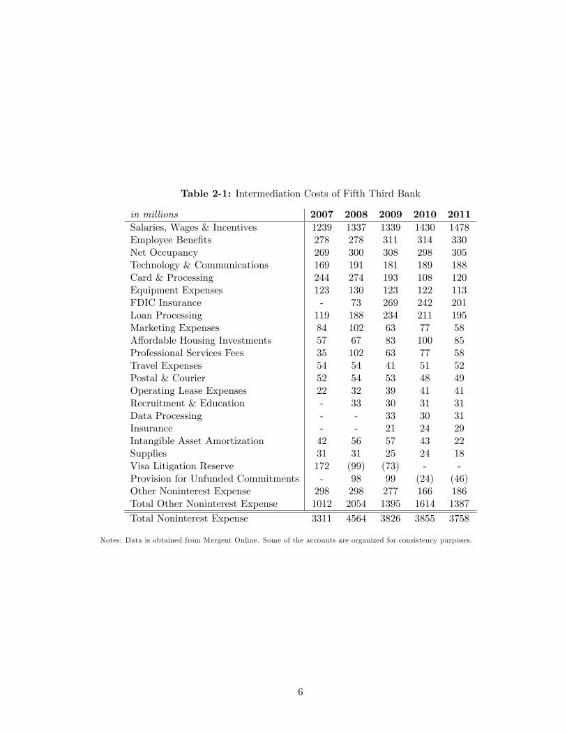
Table 2-1: Intermediation Costs of Fifth Third Bank
in millions 2007 2008 2009 2010 2011Salaries, Wages & Incentives 1239 1337 1339 1430 1478Employee Bene�ts 278 278 311 314 330Net Occupancy 269 300 308 298 305Technology & Communications 169 191 181 189 188Card & Processing 244 274 193 108 120Equipment Expenses 123 130 123 122 113FDIC Insurance - 73 269 242 201Loan Processing 119 188 234 211 195Marketing Expenses 84 102 63 77 58A¤ordable Housing Investments 57 67 83 100 85Professional Services Fees 35 102 63 77 58Travel Expenses 54 54 41 51 52Postal & Courier 52 54 53 48 49Operating Lease Expenses 22 32 39 41 41Recruitment & Education - 33 30 31 31Data Processing - - 33 30 31Insurance - - 21 24 29Intangible Asset Amortization 42 56 57 43 22Supplies 31 31 25 24 18Visa Litigation Reserve 172 (99) (73) - -Provision for Unfunded Commitments - 98 99 (24) (46)Other Noninterest Expense 298 298 277 166 186Total Other Noninterest Expense 1012 2054 1395 1614 1387
Total Noninterest Expense 3311 4564 3826 3855 3758
Notes: Data is obtained from Mergent Online. Some of the accounts are organized for consistency purposes.
6

best of my knowledge, this is the �rst study that examines the business cycle properties of
�nancial intermediation costs using high frequency data.
This dataset uncovers four empirical facts about �nancial intermediation costs.
First, �nancial intermediation costs increase sharply during recessions. Second, costs are
fairly sticky. They increase easily during recessions however it takes a very long time to
return their previous level, creating an asymmetry. Third, an analysis of these costs across
countries support the �rst fact for not only the US but also for other countries. More-
over, as one country becomes more developed, its banks operate at lower cost to asset ratio
than the ones in less developed countries. Finally, bank lending rates and intermediation
costs co-move closely for all countries in the sample. In other words, when intermediation
becomes costly, banks re�ect this increase in their lending rates.
The next four sections introduce these characteristics of �nancial intermedi-
ation costs. The cyclicality of costs are examined in the �rst section, whereas the sticky
behavior of costs are studied in the next. While the third section compares intermediation
costs across countries, the fourth section covers the relationship between lending rates and
costs. The �fth section introduces a time series analysis focusing on VAR estimations to
compute the magnitude of the e¤ects of costs on business cycles. The last section introduces
a theoretical model capturing the e¤ects of �nancial intermediation costs on the economy
that is motivated in the �fth section.
Cyclicality of Financial Intermediation Costs
Figure 2-1 demonstrates the cyclical behavior of �nancial intermediation cost.
It plots the total costs of three largest commercial banks with respect to asset sizes on the
7

Figure 2-1: Total Intermediation Cost: Largest Three Banks and the Aggregate
left panel and the aggregation of all banks on the right panel. Costs tend to increase beyond
the trend during recessions which are denoted with gray shades. They return to their normal
trend with a delay after recoveries peak up.
Although almost all cost items increase during recessions, some of them cause
a major spike in total intermediation costs. These are loan processing expenses, profes-
sional service fees, litigation expenses, and marketing expenses. During recessions, banks
usually have increasing di¢ culties in collecting accurate information about borrowers due
to the uncertainty in the economy, and therefore incur higher loan processing expenses. To
overcome these di¢ culties, banks hire analysts, consultants, attorneys and accountants that
in�ate their professional service expenses. For instance, the professional service fees, which
are normally stable, increased more than three times for International Bank of Commerce
during the recent recession. Additionally, as more and more borrowers declare bankruptcy
8

due to unfavorable economic conditions, bank litigation expenses increase dramatically as
well. Only First Bank had more than four times increase in its legal costs from 2007 to
2009. During recessions, banks also try to regain their lost reputation by investing more on
marketing. For instance, Old National Bank�s marketing expenses tripled during the recent
recession.
However, a cost increase is not necessarily bad for the economy. In particular,
an increase in costs can be a result of an enhancement in assets. For instance, as assets
increase (e.g., as banks provide more loans or open new branches) it is natural to expect
a proportional increase in intermediation costs as well. Figure 2-2 plots the real aggregate
intermediation cost and real total assets for the sample. Both series are detrended with
Hodrick-Prescott �lter. Grey shaded areas again indicate the 2001:1-2001:4 and 2007:4-
2009:3 recessions, respectively. The Figure shows that the �nancial intermediation cost and
total assets move very closely. In fact, the correlation between the intermediation cost and
assets is above 90 percent. Therefore, it is not easy to understand whether a cost increase
is due to growing assets or due to the uncertainty created by the recession.
The ratio of intermediation cost to total assets solves the problem addressed
above and provides an e¢ ciency interpretation by showing how much a bank has to pay in
order to raise one dollar worth of assets. The left panel of Figure 2-3 shows this ratio for
the biggest and smallest banks in both large and mid-sized bank groups. The right panel
shows the same measure for the aggregated sample. As Figure 2-3 indicates, individual
banks and the entire banking sector in the US become less cost e¢ cient during recessions.
Cost e¢ ciency generally increases during recoveries.
9

Figure 2-2: Comparison of Total Costs with Total Assets:
Figure 2-3: Intermediation Costs / Total Assets for Some Banks and for the US
10

Asymmetry in Financial Intermediation Costs
The second empirical fact related to the �nancial intermediation cost is its
sticky behavior during recoveries. As Figure 2-1 shows, the total intermediation cost in-
creases sharply during recessions, however it takes quite long time to return to its trend.
Figure 2-3 demonstrates that the intermediation cost per asset also shows the same asym-
metry with the aggregate measure. Cost per asset increases quickly as a recession hits the
economy, however its recovery is very gradual over time which creates an asymmetry in the
�nancial sector.
As commonly used in the business cycle asymmetry literature, I compute the
skewness of the growth rate of costs to assets ratio to account for the asymmetry. In this
analysis, I detrended the data with Hodrick Prescott �lter and computed the growth rate
of detrended series. I used the adjusted Fisher-Pearson standardized moment coe¢ cient
according to the following formula. In this formula, T corresponds to number of quarters
in the sample; xt is the growth rate of the detrended aggregate cost to assets ratio; and �x
denotes the sample mean of the series.
Skewness =T
(T � 1)(T � 2)
TPt=1(xt � �x)3�
TPt=1(xt � �x)2
� 32
If this ratio is more likely to experience larger jumps than reductions of the
same magnitude, the skewness of its growth rate must be positive. In fact, the skewness
of the cost per asset is found to be 3:95 which is outside of the 90 percent interval of
[�0:539; 0:539]: This strongly positive skewness suggest that the �nancial intermediation
cost to total asset ratio is more likely to increase than to decrease. Moreover, this fact holds
if the individual bank level data is examined rather than the aggregate data.
11
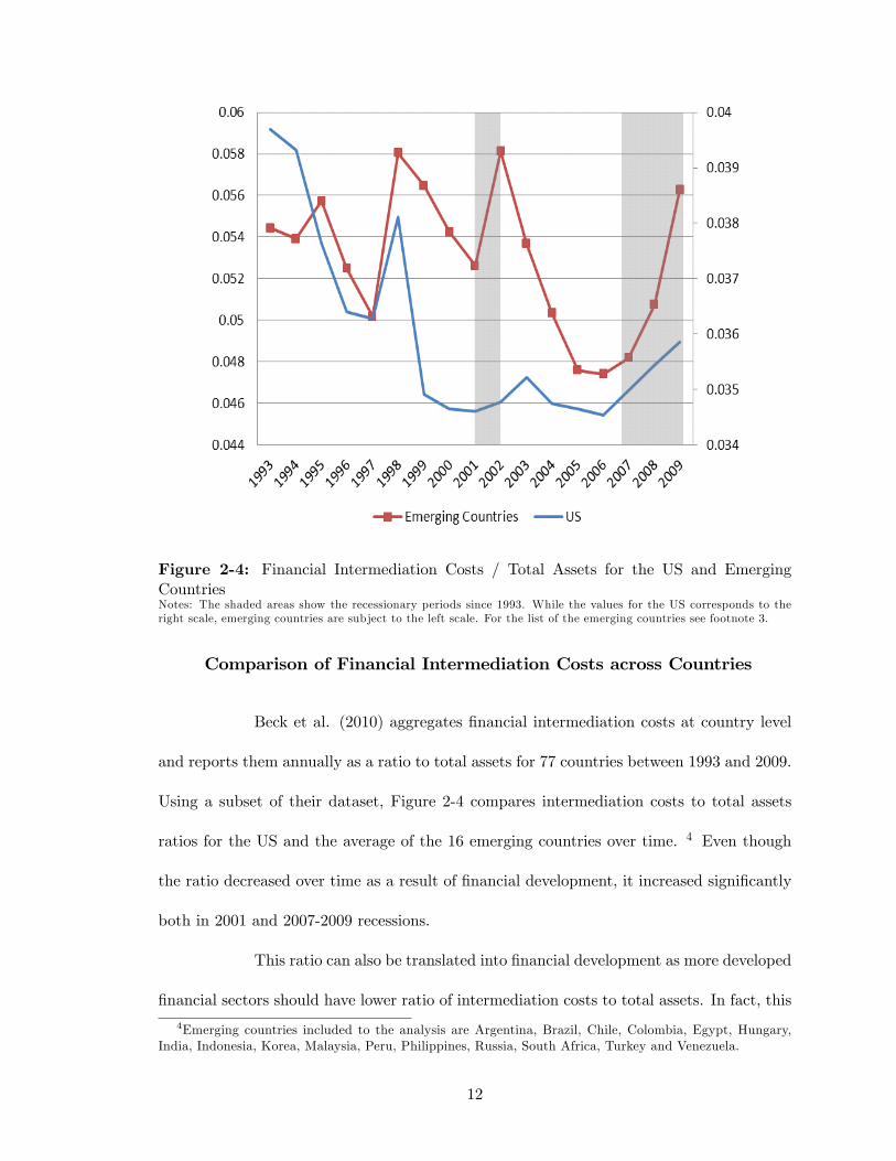
Figure 2-4: Financial Intermediation Costs / Total Assets for the US and EmergingCountriesNotes: The shaded areas show the recessionary periods since 1993. While the values for the US corresponds to theright scale, emerging countries are subject to the left scale. For the list of the emerging countries see footnote 3.
Comparison of Financial Intermediation Costs across Countries
Beck et al. (2010) aggregates �nancial intermediation costs at country level
and reports them annually as a ratio to total assets for 77 countries between 1993 and 2009.
Using a subset of their dataset, Figure 2-4 compares intermediation costs to total assets
ratios for the US and the average of the 16 emerging countries over time. 4 Even though
the ratio decreased over time as a result of �nancial development, it increased signi�cantly
both in 2001 and 2007-2009 recessions.
This ratio can also be translated into �nancial development as more developed
�nancial sectors should have lower ratio of intermediation costs to total assets. In fact, this
4Emerging countries included to the analysis are Argentina, Brazil, Chile, Colombia, Egypt, Hungary,India, Indonesia, Korea, Malaysia, Peru, Philippines, Russia, South Africa, Turkey and Venezuela.
12

Table 2-2: Intermediation Costs / Total Assets for Di¤erent Income Groups
Costs / AssetsG-7 3.3 Emerging 5.3
Germany 4.3 Argentina 8.4UK 3.1 Brazil 8.7US 3.5 Turkey 6.3
Notes: Data is obtained from Beck et al. (2010). Values represent simple averages across countries in percentages.
ratio is around 3:5 percent in the US, but is above 8 percent in some emerging countries, such
as Argentina and Brazil. Table 2-2 provides more information on �nancial intermediation
costs per assets across country groups. According to this Table, developed countries have
much lower cost to asset ratios (about 3 percent) than emerging countries (around 5 percent)
on average. In other words, an average bank in a developed country pays 3 cents to raise
one dollar worth of assets, whereas an average bank in an emerging country pays around 5
cents. Improving upon existing models, the comparison of intermediation costs allows me
to forecast the impact of a �nancial crisis on countries with di¤erent development levels.
Relationship between Financial Intermediation Costs and Lending Rates
When it becomes more costly for banks to intermediate, they either raise
their lending rates and/or cut their loans, both of which create distortions in an economy.
Therefore, an increase in intermediation costs can have a direct impact on lending rates.
While Table 2-3 demonstrates the relationship between lending rates (prime rates) and costs
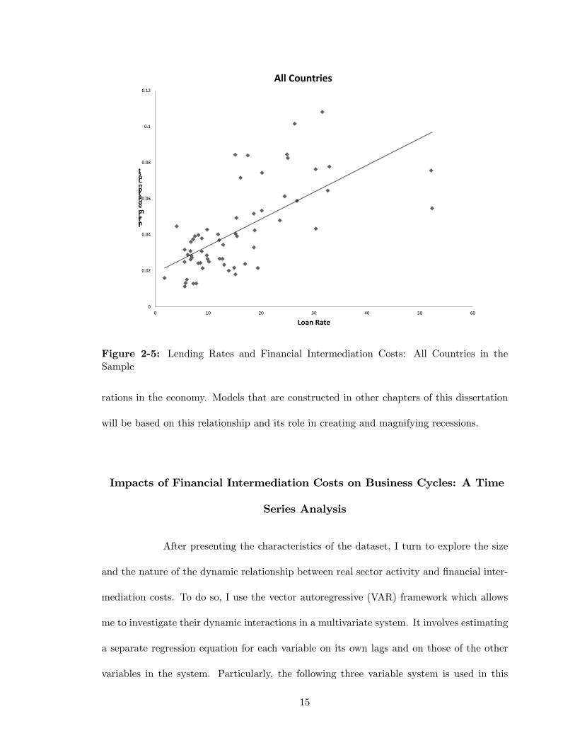
using the descriptive statistics of country groups, Figure 2-5 shows this relationship for all
countries in the sample.5 Table 2-3 displays the strong positive correlation between lending
rates and intermediation costs. Their correlation ranges from 50 percent for least developed
countries to 98 percent for most developed countries. The relatively low cross correlation
5The data for prime rates is obtained from Economists Intelligence Units, Country Data.
13

Table 2-3: The Relationship between Lending Rates and Financial Intermediation Costsfor Di¤erent Country Groups: Descriptive Statistics
Lending Rate Intermediation Cost
AllCorr 0.666
Average 15.403 0.042
Stn Dev 10.449 0.023
DevelopedCorr 0.544
Average 6.466 0.031
Stn Dev 1.919 0.009
G7Corr 0.979
Average 6.463 0.033
Stn Dev 2.722 0.009
NondevelopedCorr 0.579
Average 20.223 0.049
Stn Dev 10.525 0.026
EmergingCorr 0.742
Average 17.048 0.046
Stn Dev 8.390 0.025
Developing Corr 0.492
Average 22.794 0.052
Stn Dev 11.537 0.027
for least developed countries is a result of the heterogeneity among this group. Because
of the data availability for lending rates, 52 countries are used in this analysis. The data
consist of 15 developed, 16 emerging, and 21 developing countries. Table 2-3 also gives
more detail about intermediation costs for a broader sample of countries. It particularly
demonstrates intermediation costs di¤erences in magnitudes between developed and less
developed countries.
Figure 2-5 also shows the positive correlation between lending rates and �-
nancial intermediation costs for the entire sample of 52 countries. Countries with higher
intermediation costs experience higher lending rates as well. Any increase in intermediation
costs, therefore, should trigger less favorable interest rates for borrowers, causing deterio-
14
0
0.02
0.04
0.06
0.08
0.1
0.12
0 10 20 30 40 50 60
IntermediationCost
Loan Rate
All Countries
Figure 2-5: Lending Rates and Financial Intermediation Costs: All Countries in theSample
rations in the economy. Models that are constructed in other chapters of this dissertation
will be based on this relationship and its role in creating and magnifying recessions.
Impacts of Financial Intermediation Costs on Business Cycles: A Time
Series Analysis
After presenting the characteristics of the dataset, I turn to explore the size
and the nature of the dynamic relationship between real sector activity and �nancial inter-
mediation costs. To do so, I use the vector autoregressive (VAR) framework which allows
me to investigate their dynamic interactions in a multivariate system. It involves estimating
a separate regression equation for each variable on its own lags and on those of the other
variables in the system. Particularly, the following three variable system is used in this
15

analysis.
x1;t = a1 +kXi=1
b1;ix1;t�i +kXi=1
c1;ix2;t�i +kXi=1
d1;ix3;t�i + u1;t
x2;t = a2 +kXi=1
b2;ix1;t�i +kXi=1
c2;ix2;t�i +kXi=1
d2;ix3;t�i + u2;t
x3;t = a3 +
kXi=1
b3;ix1;t�i +kXi=1
c3;ix2;t�i +kXi=1
d3;ix3;t�i + u3;t
Here x1, x2; and x3 represent the real GDP, the real money stock, and the
�nancial intermediation cost to total asset ratio, respectively. k denotes the number of lags
used in the system. The lag is chosen optimally according to Akaike Information Criteria
and Nested Likelihood Ratio tests. As a second set of analysis, GDP is replaced with
the gross private investment to retrieve the direct e¤ect of intermediation costs on external
�nance opportunities of borrowers. Money stock controls �nancial development levels across
time.
Because stationarity is very important to have a stable VAR system, unit root
tests were applied on each time series. Table 2-4.a summarizes the �ndings for Augmented
Dickey Fuller tests (ADF) and Philips Perron tests. The lag used in the ADF test is chosen
according to the Akaike information criterion. For Phillips-Perron test statistic, Bartlett
kernel spectral estimation method is used and bandwidth is selected by Newey- West. The
hypothesis of no unit root cannot be rejected in levels for at least one of the tests for all of
the variables used in the system. However, the system is �rst di¤erence stationary.
Sims, Stock, and Watson (1990) show that as long as there exist a single
cointegrating relationship among variables, the error terms of the system are stationary in
tri-variate VARs even in the presence of unit roots. Cointegration implies that there is a
16
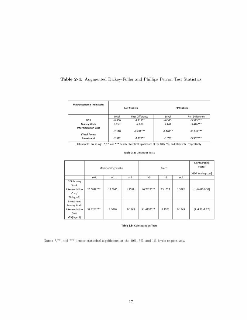
Table 2-4: Augmented Dickey-Fuller and Phillips Perron Test Statistics
Macroeconomic Indicators:ADF Statistic PP Statistic
Level First Difference Level First DifferenceGDP 0.850 3.817** 0.585 5.515***
Money Stock 0.053 2.608 2.441 3.446***Intermediation Cost
/Total Assets2.110 7.491*** 4.167** 13.067***
Investment 2.512 3.277** 1.757 5.367***
All variables are in logs. *,**, and *** denote statistical significance at the 10%, 5%, and 1% levels, respectively.
Table 3.a: Unit Root Tests
Maximum Eigenvalue Trace
CointegratingVector
[GDP lending cost]r=0 r<1 r<2 r=0 r<1 r<2
GDP MoneyStock
IntermediationCost/
TA(lags=3)
25.5898*** 13.5945 1.5582 40.7425*** 15.1527 1.5582 [1 0.413 0.55]
InvestmentMoney Stock
IntermediationCost
/TA(lags=2)
32.9267*** 8.3076 0.1849 41.4192*** 8.4925 0.1849 [1 4.39 1.97]
Table 3.b: Cointegration Tests
Notes: *,**, and *** denote statistical signi�cance at the 10%, 5%, and 1% levels respectively.
17

linear combination of non-stationary variables that makes the series stationary. To test the
existence of one cointegration vector in the system, I used the Johansen test. Table 2-3.b
summarizes the results of this test. Rejection of the null hypothesis of no cointegration
(r=0) and a failure to reject the null of at most one cointegrating vector (r=1) provides
evidence of a single cointegrating relationship among variables. According to the Johansen
test statistics, the null of no cointegration is rejected at 5 percent in both systems and the
null of one cointegration cannot be rejected for any. Thus, the stationarity of error terms
has been maintained with this cointegration result.
Next, I proceed to Granger Causality test to see the joint evaluation of both
short- and long-term e¤ects of movements in one variable upon the others which creates
each system. Indeed, as the �nancial intermediation cost per asset increases, or in other
words, as banks get more ine¢ cient over time the loans will be distributed inadequately as
well. This will cause distortions on the real activity since the loan distribution departs from
the optimal distribution.
Table 2-5 shows the results of this test. When intermediation costs per assets
increases, it causes a strong decline in GDP as the representative of economic real activities.
The causality works in the opposite direction as well. Although the e¤ect is not strong, an
increase in GDP leads to a decrease in costs per assets. However, when GDP is replaced
with the investment results are not statistically signi�cant. The notion of causality must
be interpreted cautiously here as it does not denote the economic causality. In the VAR
system, the Granger causality assumes full information sets which most likely would be
violated in any case. It, however, shows a strong linkage among the variables, particularly
from cost per asset to GDP.
After characterizing a causal ordering, orthogonalized impulse responses of
18

Table 2-5: F-statistics for Granger-Causality in VARs with GDP and Investment
Levels VAR Granger tests
GDP Money Stock Intermediation Cost/ Total Assets R^2
lags 1 1a
(GDP)
0.897
(0.000)
0.03
(0.0075)
0.051
(0.001)
0.99
1b
(Money Stock)
0.105
(0.0192)
1.099
(0.000)
0.1197
(0.021)
0.98
1c
(Cost)
0.57
(0.0006)
0.0313
(0.7408)
0.346
(0.009)
0.70
Levels VAR Granger tests
Investment Money Stock Intermediation Cost/ Total Assets R^2
lags 4 1a
(Investment)
0.994
(0.000)
0.263
(0.0872)
0.153
(0.2695)
0.94
1b
(Money Stock)
0.042
(0.1829)
1.049
(0.000)
0.015
(0.0977)
0.99
1c
(Cost)
0.133
(0.3124)
0.203
(0.000)
0.742
(0.000)
0.82
19

each variable in the system to one time shocks in others would give an idea about the
magnitude of nonlinear dynamic e¤ects. Figure 2-6 presents impulse responses to one
standard deviation shocks in the system. In this analysis, the identi�cation assumption
is that the cost per asset determines the �nancial development level which is controlled
by the money stock. Consequently, �nancial sector development a¤ects the real activity
represented by GDP. This assumption is consistent with the Granger causality results above.
As a robustness check, I also reversed the ordering from GDP to �nancial development and
�nally to the ratio of intermediation costs per total assets. Results are robust to this reverse
ordering as well.
According to the Figure 2-6, when the intermediation cost increases one stan-
dard deviation, GDP decreases by half of a percentage. Given that the change in the cost
ratio is a very small one, this result is very strong. As expected from the causality results,
a change in GDP has a less signi�cant negative e¤ect on cost per asset. An increase in cost
also decreases investment, whereas a rise in investment has negative e¤ects after a delay.
These results demonstrate that the �nancial intermediation shock has a signi�cant negative
e¤ect on GDP.
Financial Intermediation Costs in a Theoretical Framework: EnhancedFinancial Accelerator Mechanism
In this section, I examine the role of intermediation costs in a �nancial accel-
erator framework (Bernanke et al. (1999), BGG thereafter) targeting the impulse responses
generated by the VAR analysis above. To do this, I use a modi�ed model based on �nancial
accelerator mechanism with �nancial frictions. Financial frictions are added to economic
models through an agency problem, as lenders cannot always trust borrowers to pay their
20

.005
0
.005
.01
.015
0 5 10 15
Effect of Cost on GDP
.006
.004
.002
0
0 5 10 15
Effect of GDP on Cost
.02
0
.02
.04
0 5 10 15
Effect of Investment on Cost
.05
0
.05
.1
0 5 10 15
Effect of Cost on Investment
Figure 2-6: Selected Impulse Responses to One Standard Deviation Shock
21
loans back. This problem creates ine¢ ciencies in the �nancial market which in turn am-
pli�es the e¤ect of negative shocks in the economy. This ampli�cation mechanism is called
��nancial accelerator�. Financial accelerator mechanism suggests that a negative shock in
the economy decreases the total income and causes the demand for capital to decline. Lower
demand pushes capital prices down and consequently assets are worth less. This intensi�es
the agency problem between banks and �rms causing the external �nance premium to rise.
Growing pressure on �rms�borrowing eventually leads to bankruptcies. These bankruptcies
increase the external premium even more, creating an accelerator e¤ect that ampli�es reces-
sions. Among many others, Christiano, Motto and Rostagno (2009) found that the �nancial
accelerator mechanism accounts for a greater proportion of aggregate output �uctuations
in the US and the Euro Area (27 percent and 50 percent, respectively) than the commonly
used technological shock in standard models (22 percent).6
Despite being an important step forward, most of the �nancial accelerator
literature does not model banks and thus cannot account the spillover of �nancial shocks
to the economy. This model with �nancial intermediation costs thus provides two unique
improvements in order to study the real world behavior. First, I add a realistic bank sector
with their own balance sheet e¤ects into the �nancial accelerator framework. This allows
me to model �nancial intermediation between borrowers and lenders. Second, the costly
intermediation allows me to introduce a new and tangible way to form �nancial shocks that
directly a¤ect the �nancial sector instead of simply amplifying the impact of other shocks.
Particularly, when there is a �nancial shock, i.e. an increase in intermediation cost, banks
either raise their lending rates and/or cut their loans, both of which create di¢ culties in
borrowing. As borrowing becomes more costly, �rms demand less capital and the price of
6See Christensen and Dib (2008), Gertler, Gilchrist and Natalucci (2007), and Christiano, Trabandt andWalentin (2011).
22
capital decreases. Net worth of �rms loses value due to low asset prices and subsequently
the �nancial accelerator mechanism emerges. Therefore, intermediation cost triggers the
�nancial accelerator mechanism and ampli�es the e¤ects of ordinary recessions.
The Model
The dynamic stochastic general equilibrium (DSGE) model in this chapter
consists of a representative household, capital builders, ex-ante similar entrepreneurs and
�nancial intermediaries. It also introduces costly intermediation between borrowers and
savers.
Households
There is a continuum of households of length unity. The total endowment of
time is normalized to one. Each household works, consumes, and saves. The representative
household maximizes utility over consumption, Ct; and leisure, 1�Lt according the following
objective function.
maxCt;Dt+1;Lt
Et
( 1Xk=0
�k [ln(Ct+k) + � ln(1� Lt+k)])
(1)
The household chooses Ct; Lt and Dt+1 using the objective function (1) and
the budget constraint (2):
Ct =WtLt +RtDt �Dt+1 (2)
Here Dt denotes the deposits that households hold at time t which pay the
riskless rate of return, Rt; and Wt is the wage rate that they get from working at non-
�nancial �rms.
23

The �rst order conditions that characterize the Euler equations for consumption
and labor supply of household�s problem are given in equation (3) and (4); respectively.
EfCt+1g = Rt+1�Ct (3)
Wt
Ct= �
1
1� Lt(4)
Capital Builders
Capital builders rent the capital stock, Kt; from entrepreneurs and use it to
produce new capital. Since this takes place within the period, the rental rate is zero. Capital
producers maximize their pro�t, �t using the objective function below.
maxIt�t = maxEtfQt�tIt � It �
�
2
�ItKt
� ��2Ktg (5)
While It represents the gross investment, � and � denote the depreciation rate
and the adjustment cost of capital, respectively. �t is a shock to the marginal e¢ ciency of
investment as in Greenwood, Hercovitz Hu¤man (1988) which has the following AR(1)
process.
log �t = �� log �t�1 + "
�t (6)
with "�t � iid N(0; �2):
The solution to capital builders�pro�t maximization problem yields the fol-
lowing rule for capital price setting.
EfQt�t � 1� ��It
Kt� ��g = 0 (7)
24

The evolution of capital satis�es:
Kt+1 = �tIt + (1� �)Kt (8)
Entrepreneurs
Entrepreneurs acquire physical capital, K; from capital producers at the price
of Q in each period. Entrepreneurs �nance the new investment either by using their net
worth, Nt; or by issuing �nancial securities, St+1. The following equation summarizes this
balance sheet condition for the entrepreneur j:
QjtKjt+1 = Sjt+1 +Njt (9)
As in BGG, an idiosyncratic shock, !jt; a¤ects the gross return on capital
averaged across �rms. ! is iid across time and across �rms with a lognormal cumulative
distribution function, F (!): BGG shows that there is a cuto¤value of the idiosyncratic shock
, �!jt; which makes the return to capital just equal to the total amount of entrepreneur j0s
debt.
�!jt+1Rkt+1QtKjt+1 = Zjt+1Sjt+1 (10)
Here Rkt+1 and Zjt+1 denote the gross return on capital and the gross non
default rate, respectively. When the entrepreneur cannot pay his debt, in other words, if the
realization of !jt is lower than the threshold value, he defaults. The �nancial intermediary
overtakes all the remaining assets of the �rm and tries to �re sale them. A fraction, �; of the
bankrupt �rm�s total assets is lost during �re sales. Notice that � has a di¤erent meaning
than in BGG. This fraction is used to denote the costly state veri�cation in BGG, and
25
decreases in recessions as it is multiplied with total assets. However, costs tend to increase
during recessions as can be captured in this model. � is not contained in the intermediation
costs used in the model or data.
Given that �rms are ex-ante same the aggregate net worth evolves according
to the equation (11).
Nt+1 = hRkt+1QtKt+1 �Rst+1(QtKt+1 �Nt)
i+ (1� )gt (11)
where Rst+1denotes the external �nance premium as follows.
Rst+1 =
0BBB@Rt+1(1 + ct) +��!R0
!f(!)d!Rkt+1QtKt+1
QtKt+1 �Nt
1CCCA (12)
symbolizes the constant survival probability of �rms to the next period. The
constant survival probability introduces dynamics to the life of entrepreneurs by implying an
expected lifetime equal to 11� . It also guarantees that an entrepreneur cannot accumulate
enough wealth to self �nance his projects. gt is the start up money transfer from exiting
to new entrepreneurs. As Equation (12) shows the intermediation cost increases the gap
between the external premium and the risk free rate. ct;the �nancial intermediation cost,
follows the AR(1) process shown in equation (13).
ln ct = (1� �c) ln �c+ �c ln ct�1+"ct (13)
Notice that the intermediation cost does not become zero in the steady state.
Instead it is equal to its long run average �c; because in reality costs never diminish entirely.
26

Financial Intermediaries
There are many identical �nancial intermediaries that operate in a perfectly
competitive environment. They can purchase securities by using their own net worth and
deposits collected from households. The balance sheet equation for intermediaries can be
expressed as:
(1 + ct)St+1 = Nbt +Dt+1 (14)
Here ct represents the intermediation cost of �nancial intermediaries. A por-
tion equal to ct of total intermediary assets are lost to create the optimal contract which
satis�es the following condition.
24(1� F (�!t))�!t + (1� �) �!tZ0
!f(!)d!
35Rkt+1QtKt+1 = Rt+1(1 + ct)St+1 (15)
According to (15), the optimal contract must satisfy a condition that guaran-
tees the equality of the expected return of providing funds to �rms given by the left hand
side to its opportunity cost represented by the right hand side.
The net worth of intermediaries is given by:
N bt+1 = R
st+1St+1 �Rt+1Dt+1 (16)
The �rst term in the right hand side of (16) shows the expected return form
�nancial intermediation, whereas the second term denotes the repayment of debt to house-
holds.
27

Entrepreneur�s Problem
Entrepreneurs maximize their expected return subject to the credit constraint
from optimal contract condition in Equation (15).
maxKt+1;�!
n�Rkt+1QtKt+1
o(17)
Pro�t maximization problem of entrepreneurs yields equation (18) and (19):
While the former shows the role of the intermediation cost on the external premium, as
Equation (12); the latter shows the �nancial accelerator mechanism and the ampli�cation
e¤ect of the cost.
st =Rkt+1Rt+1
=�(1 + ct)
(��� �) (18)
where
� =1R�!!f(!)d! � �!
1R�!f(!)d!; � = (1 � �)
�!R0
!f(!)d! + �!(1 � F (�!)); and � =
1�F (�!)(1�F (�!)���!f(�!))
� represents the expected gross share of pro�ts for the entrepreneur, and �
denotes the �nancial intermediaries�net share of pro�ts (net of monitoring costs).
QtKt+1Nt
= (st; ct) (19)
or equivalently Equation (18) and (19) can merge into the following form.
Et
�Rkt+1
�= s
�Nt
QtKt+1;1
ct
�Rt+1 (20)
where 0 () > 0 and s0 () < 0
28

Intermediation cost has direct positive e¤ects on the external �nance pre-
mium. Moreover, as in BGG, when net worth decreases the external �nance premium
increases as well, creating a �nancial accelerator mechanism by a¤ecting the borrowing
capacity of �rms.
Production
Entrepreneurs use their accumulated capital and labor in the production of a
homogenous good, Yt; in competitive markets. The aggregate production can be expressed
as:
Yt = AtK�t L
1��t (21)
where � � 0 is the capital share in production and At is total factor productivity
(TFP) that follows the AR (1) process in (22).
logAt = �A logAt�1 + "At (22)
where �A is the persistency of shock, and E("At ) = 0:
Solving the pro�t maximization problem for entrepreneurs yields Equations
(23) and (24): They represent the demand of labor and expected gross return on holding
one unit of capital, respectively.
Wt =Yt(1� �)
Lt(23)
and
EfRkt+1g = E( �Yt+1
Kt+1+Qt+1(1� �)Qt
)(24)
29

Resource Constraint and Labor Market Clearing Condition
The economy-wide resource constraint shows that the total output is equal to
the sum of total consumption, investment and deadweight loss due to �re sales.
Yt = Ct + It + �
�!Z0
!f(!)d!RktQt�1Kt (25)
The labor market clearing condition imposes an equality to the demand for
and supply of labor as follows.
Yt(1� �)LtCt
= �1
1� Lt(26)
Results
Calibration
I choose standard values for the taste and technology parameters. I set the
capital share in production to 0:35, the quarterly depreciation rate to 2:5 % and the discount
factor to 0:99 which pins down the risk-free rate in the steady state. Persistence of TFP and
investment e¢ ciency shock are set to 0:95 and 0:66 with standard deviations equal to 0:009
and 0:0331, respectively. The parameters for investment e¢ ciency shock and the capital
adjustment cost are estimated by Christensen and Dib (2008) using Bayesian methodology.
These values are similar to the estimates of Ireland (2003). As in Christensen and Dib, I
choose capital adjustment cost to be around 0:59; which is close to the estimates of Meier
and Muller (2006). The capital adjustment cost has a signi�cant role on the �nancial
accelerator mechanism. For instance, high values of capital adjustment costs cause stronger
30
capital price responses, and therefore a¤ects the net worth of �rms and the external �nance
premium. Furthermore, high adjustment costs make the investment more expensive and
less responsive to shocks. Therefore, it is important to choose a realistic estimate for the
adjustment cost. The weight of leisure in the utility function is chosen so that households
devote one third of their entire time to work.
The death rate of �rms is chosen to be 3 percent, which is consistent with
the data obtained from US Small Business Administration (SBA). The fraction of �re sales
losses is 0:10. The standard deviation of the iid shock is chosen to make the capital net worth
ratio equal to 2 in the steady state. What is unique about this chapter is the estimation of
the �nancial intermediation cost. Using the AR(1) process in Equation (13); the persistence
and standard deviation of the cost is computed. The intermediation cost equals to its long-
run average in the steady state. This long-run average is 3 times smaller in my sample as
I am only looking at the largest banks. In fact, if the entire banking sector is used in this
analysis than the long run average would have been more than 3 times higher. Therefore
the results in this model is signi�cantly underestimated. Nonetheless, it gives an idea about
how strong the e¤ect of cost is on key macroeconomic variables. Table 2-6 summarizes all
the calibrated values of the parameters.
Simulations
Figure 2-7 shows the e¤ects of one standard deviation decrease in total factor
productivity (TFP) on the economy simulated for the US. A decrease in TFP brings the
�nancial accelerator mechanism into work. In particular, it leads to lower output and
consumption in the economy. This causes �rms to demand more capital. High demand
pushes up the capital prices and consequently assets are worth more. This leads to a
31

Table 2-6: Calibration of ParametersDescriptioncapital share in production � = 0:35discount factor � = 0:99depreciation rate � = 0:025weight of leisure in utility function � = 1:64loss in �re sales � = 0:10survival probability = 0:97capital adjustment cost � = 0:59standard deviation of iid shock � = 0:30persistence of TFP �A = 0:95standard deviation of TFP �A = 0:009persistence of investment shock �� = 0:66standard deviation of investment shock �� = 0:033average intermediation cost/total assets c = 0:013persistence of intermediation cost �c = 0:026standard deviation of intermediation cost ��US = 0:01
Notes: One period in the model corresponds to one year. Thus, the values in the table match the annual frequency.
decrease in net worth of �rms and an increase in the agency problem between �rms and
banks. As a result, the external �nance premium increases that tightens the borrowing
constraint of entrepreneurs. As borrowing goes down they cannot �nd a room to expand
their business and their net worth declines further which creates a negative feedback loop,
or in other words, a �nancial accelerator. This feedback between the external premium
and the net worth of �rms causes more �rms to bankrupt. As the number of bankruptcies
increases, intermediation costs increase as well. High costs in�ate lending rates making
borrowing even more di¢ cult for entrepreneurs. Therefore, there is also a feedback between
the intermediation cost and the �nancial accelerator mechanism. This relationship makes
the e¤ects of intermediation cost more signi�cant on business cycles.
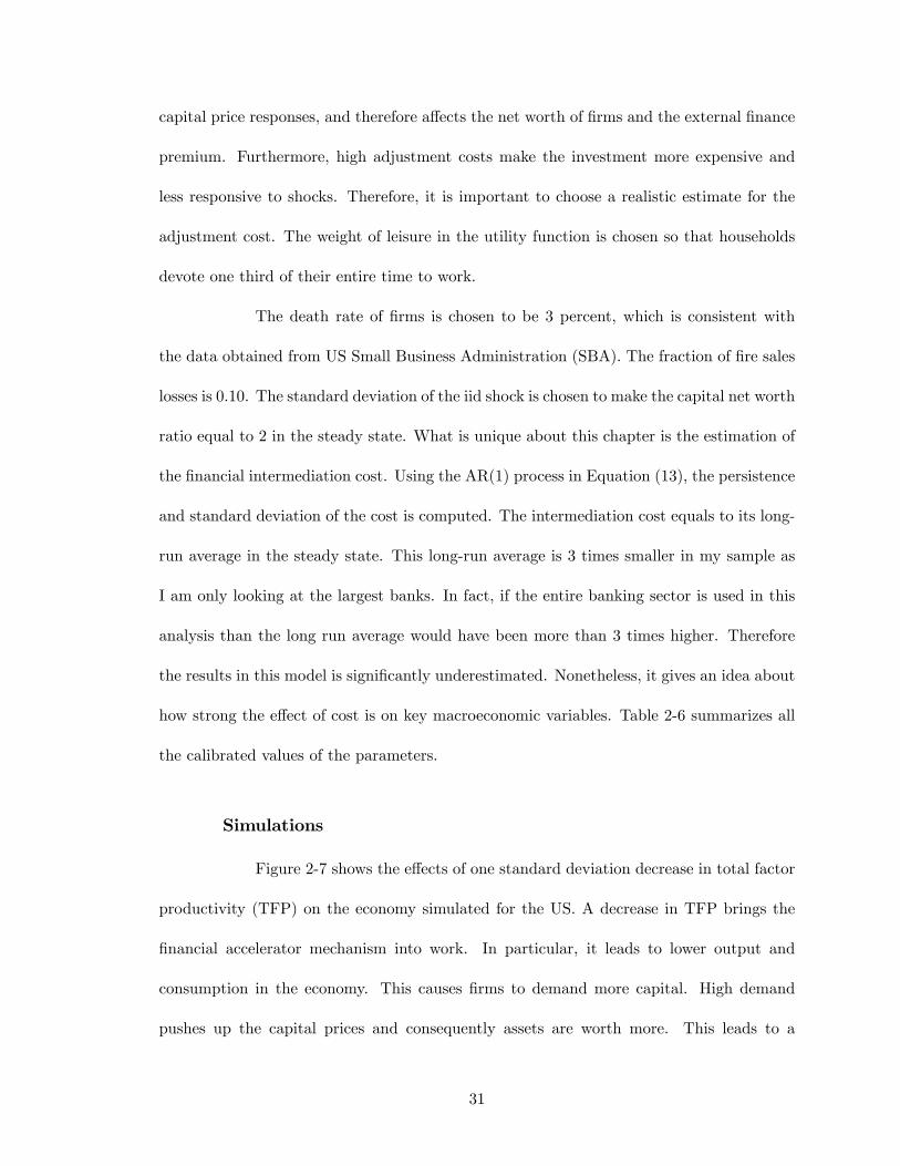
Figure 2-8 demonstrates the responses of key macroeconomic variables to a
standard deviation decrease in investment e¢ ciency. In particular, when the e¢ ciency de-
creases the output and investment immediately decreases. This decreases the amount bor-
rowed leading to lower interest rates. The decrease in interest rates pushes the households
32

Figure 2-7: One Standard Deviation Shock to Total Factor Productivity
33
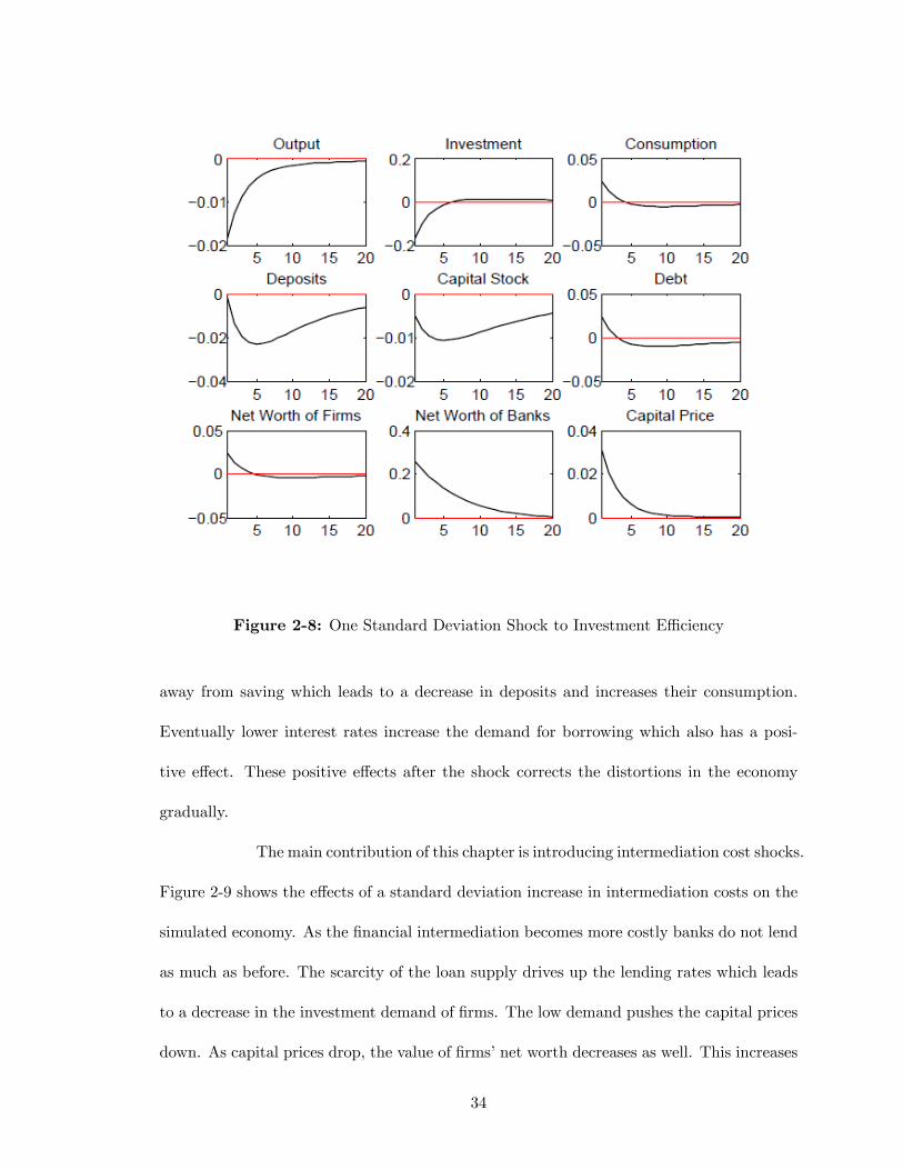
Figure 2-8: One Standard Deviation Shock to Investment E¢ ciency
away from saving which leads to a decrease in deposits and increases their consumption.
Eventually lower interest rates increase the demand for borrowing which also has a posi-
tive e¤ect. These positive e¤ects after the shock corrects the distortions in the economy
gradually.
The main contribution of this chapter is introducing intermediation cost shocks.
Figure 2-9 shows the e¤ects of a standard deviation increase in intermediation costs on the
simulated economy. As the �nancial intermediation becomes more costly banks do not lend
as much as before. The scarcity of the loan supply drives up the lending rates which leads
to a decrease in the investment demand of �rms. The low demand pushes the capital prices
down. As capital prices drop, the value of �rms�net worth decreases as well. This increases
34
Figure 2-9: One Standard Deviation Shock to the Financial Intermediation Cost
the agency problem between entrepreneurs and intermediaries leading to a �nancial accel-
erator mechanism which results in stronger credit crunches and lower output levels. Once
again, the impulse responses here is underestimated as the data only has larger and more
e¢ cient banks in the sample. This sample has three times lower cost to asset ratio than
the entire �nancial sector in the US. Keeping this downward bias in mind, the simulation
results are very similar to the VAR results.
Conclusion
This section of the dissertation analyzes �nancial intermediation costs in great
detail using a unique quarterly dataset. This dataset consists of large and mid-sized banks�
35

cost breakdowns and their total assets. The micro level, high frequency data allows the
study of the intermediation cost characteristics and its e¤ects on the business cycles. The
cost entails four characteristics. First, as a largely ignored phenomenon, �nancial intermedi-
ation costs is strongly countercyclical. Second, it tends to have large increases rather than
decreases. Third, an international comparison shows that developed countries generally
have lower intermediation cost per asset than their less developed counterparts which can
suggest an e¢ ciency measure for �nancial intermediaries. Lastly, �nancial intermediation
costs and lending rates co-move very closely.
According to the US data, a one standard deviation increase in cost causes a
50 percentage points decrease in GDP. By introducing a nontrivial banking sector and costly
intermediation, this model can estimate the e¤ects very closely to the data. Moreover, GDP
also a¤ects intermediation costs however this e¤ect is relatively weak.
The second main contribution of this chapter besides costly intermediation
is giving a realistic role to banks. In particular, their balance sheets have as signi�cant
role as any other �rm in the economy. The model in this chapter enhances the �nancial
accelerator mechanism by adding costly intermediation and a non-trivial banking sector.
In particular, when there is a recession in the economy, generated from �nancial sector or
not, causes the intermediation costs go up. As intermediation becomes costly banks either
provide less loans or increase their lending rates. In fact, the �nancial intermediation cost
and lending rates co-move very closely in the data as well. Both of these actions of banks
borrowing becomes increasingly more di¢ cult. Less borrowing causes lower investments
and output. Low investment, in other words, low demand for capital, decreases the asset
prices leading to smaller net worth. This increases the agency problem between banks and
�rms which in�ates the external premium and consequently borrowing becomes even more
36

di¢ cult creating a �nancial accelerator mechanism. Therefore, intermediation cost and
�nancial accelerator mechanism triggers each other.
37

CHAPTER III
FINANCIAL INTERMEDIATION COSTS AND BUSINESS CYCLE ASYMMETRIES
The recent �nancial crisis that began in late 2007 has subsequently turned into
the worst recession of the post-war period with its exceedingly long recovery. A sudden and
deep crisis followed by a slow recovery -an asymmetry in business cycles- is true for almost
every recession in US history. For instance, the Great Depression bottomed out after less
than three years but took eight more years until the economy returned to its previous level.
As Keynes (1936) stated; "the substitution of a downward for an upward tendency often
takes place suddenly and violently, whereas there is, as a rule, no such sharp turning point
when a[n] upward is substituted for a downward tendency" (p. 314). Moreover, the �nancial
sector experiences a similar asymmetry in bank lending rates during economic downturns.
Many researchers have documented that lending rates increase sharply during crises but
decrease gradually during recoveries.1 This chapter connects the two asymmetries observed
in business cycles and the �nancial sector by accounting for costly intermediation in a
"�nancial accelerator" (Bernanke et al. (1999), BGG thereafter) framework. In particular,
when intermediation cost per asset increases, �nancial intermediaries become less e¢ cient
and struggle to absorb the distortions in the sector. This leads to greater credit crunches
followed by economy-wide recessions with slow recoveries.
As the recovery of an economy takes longer, more people su¤er from the con-
sequences of the recession.2 For instance, in the �rst year of the recent recession around four
1See Veldkamp (2005), Thompson (2006), Magud (2008), Gambacorta and Ianotti (2008) , Ordonez(2010).
2Federal Reserve chairman Ben Bernanke commented on the long recovery of recent �nancial crisis as:
38
hundred thousand workers left the labor force; by 2011 the number of discouraged workers
exceeded one million.3 Because of the negative impacts of slow recoveries, many economists
have attempted to understand the causes of business cycle asymmetries. In the literature,
this asymmetry is associated with skill requirement mismatches of new technologies (Ace-
moglu and Scott (1997)); with di¢ culties in extending �rm capacity limits (Hansen and
Prescott (2005)); with delays in production and hiring decisions due to unclear predictions
of the future (Veldkamp (2005)); and with disproportionalities of monetary policy e¤ective-
ness during recoveries (DeLong and Summers (1988), Cover (1992), Macklem et al. (1996),
Ravn and Sola (2004), and Lo and Piger (2005)).
However, these explanations of the business cycle asymmetry do not address
three important points: (1) The asymmetry is stronger for recessions associated with �nan-
cial crises. Reinhart and Rogo¤ (2008 and 2009), Bordo and Haubrich (2010), and many
others have found that an economic downturn accompanied by a �nancial crisis is more
severe and protracted than an ordinary recession.4 (2) The �nancial sector shows a similar
asymmetry in lending rates. Many studies have documented that the lending rates of banks
(i.e., the interest rates that banks charge their most favorable costumers) increase sharply
during crises but decrease gradually during recoveries (See Veldkamp (2005), Thompson
(2006), Magud (2008), Gambacorta and Ianotti (2008), and Ordonez (2009)). For instance,
in 1994, Mexican lending rates took 4 months to rise 70 percentage points but more than
30 months to return to their pre-crisis levels.5 (3) The business cycle and the lending rates
�The �nancial crisis of 2008 and 2009, together with the associated deep recession, was a historic event�historic in the sense that its severity and economic consequences were enormous, but also in the sense thatthe crisis seems certain to have profound and long-lasting e¤ects on our economy, our society, and ourpolitics�(October 18, 2011).
3Data are obtained from Bureau of Labor Statistics.4For instance, Reinhart and Reinhart (2010) Cecchetti, Kohler, and Upper (2009).5Ordonez (2010), �Larger Crises, Slower Recoveries: The Asymmetric E¤ects of Financial Frictions on
Lending Rates�
39

asymmetries are greater in less developed countries. Claessens et al. (2012) show that
recoveries in emerging countries take almost two times longer than recessions, whereas it
takes on average 1.3 times longer for their developed counterparts. Moreover, Ordonez
(2009) �nds that while lending rates in developed countries take twice as long to return to
pre-recession levels, it takes 3 to 15 times longer for the less developed countries depending
on their development levels. Incorporating a nontrivial banking sector and costly interme-
diation into the �nancial accelerator framework, this chapter �lls the gap in the literature
by explaining all three points above.
Although the recent recession highlighted the role of the �nancial sector, the
literature largely ignored bank balance sheets. Furthermore, banks have been treated as
places in which borrowers and lenders can costlessly exchange funds. However, in reality,
banks maximize their net worth like other non-�nancial �rms and accrue many costs as-
sociated with wages, marketing, litigation and data processing among others. These costs
increase signi�cantly during recessions and vary substantially across countries. For instance,
banks in developed countries operate at 75 percent lower cost to asset ratio than those in
emerging countries.6
In this chapter, the interaction between intermediation costs and the �nancial
accelerator mechanism delays recoveries from economic downturns. The �nancial acceler-
ator mechanism suggests that a negative shock in the economy decreases the total income
and causes the demand for capital to decline. Lower demand pushes capital prices down
and consequently assets are worth less. This intensi�es the agency problem between banks
and �rms causing the external �nance premium to rise. Growing pressure on �rms�bor-
rowing eventually leads to bankruptcies. These bankruptcies increase the external premium
6Beck et al. (2010) "A new database on �nancial development and structure."
40
even more, creating an accelerator e¤ect that ampli�es recessions. However, the �nancial
accelerator mechanism alone cannot account for the three points addressed above. By in-
corporating a nontrivial �nancial sector, this model �lls the gap in the literature. When
there is a �nancial shock, i.e. an increase in intermediation cost, banks either raise their
lending rates and/or cut their loans, both of which create di¢ culties in borrowing. As bor-
rowing becomes more costly, �rms demand less capital and the price of capital decreases.
Net worth of �rms loses value due to low asset prices and subsequently the �nancial accel-
erator mechanism emerges. Therefore, intermediation cost triggers the �nancial accelerator
mechanism and delays the recovery more than an ordinary recession that is not originated
from the �nancial sector. This feedback loop between intermediation cost and �nancial ac-
celerator prevents banks from charging more favorable rates to borrowers. Although banks
can increase their lending rates as a response to an increase in the intermediation cost fairly
quickly, they cannot decrease them as fast because of the delay in recovery which creates an
asymmetry in lending rates as well. Moreover, if the �nancial sector of a country operates
with higher intermediation costs, the feedback loop would be stronger. Therefore, countries
with high �nancial intermediation costs experience larger asymmetries than countries with
lower costs.
Incorporating a banking sector and costly intermediation into the �nancial
accelerator framework, this model shows that a �nancial shock causes output and bank
lending rates to take 10 and 5 quarters to fully recover, respectively. In line with the
data, the model indicates that recessions are around 3 times deeper for �nancially less
developed countries and their recovery last 67 percent longer compared to their developed
counterparts.
The chapter is organized as follows. In the next section, I describe highlights
41

of the model, while following sections the calibration and simulation results, respectively. I
provide concluding comments in the closing section.
The Model:
The model of this chapter is identical with the model introduced in the second
chapter. I will only highlight its important aspects in this section. For the full layout of
the model, please refer to "Financial Intermediation Costs in a Theoretical Framework:
Enhanced Financial Accelerator Mechanism" section in the second chapter.
The model builds upon the idea that entrepreneurs acquire physical capital,
K; by using their net worth, Nt; or by issuing �nancial securities, St+1. The following
equation summarizes this balance sheet condition for the entrepreneur j:
QjtKjt+1 = Sjt+1 +Njt (1)
An idiosyncratic shock, !jt; which is iid across time and �rms, a¤ects the
gross return on capital. The cuto¤ value, �!jt;equates the gross return to capital to the total
amount of entrepreneur j0s debt as in Equation (2). A realization of !jt that is lower than
this threshold value causes the entrepreneur to default as his capital return is lower than
his debt repayment.
�!jt+1Rkt+1QtKjt+1 = Zjt+1Sjt+1 (2)
Here Rkt+1 and Zjt+1 denote the gross return on capital and the gross non
default rate, respectively. Given that �rms are ex-ante same the aggregate net worth evolves
according to the equation (3).
42

Nt+1 = hRkt+1QtKt+1 �Rst+1(QtKt+1 �Nt)
i+ (1� )gt (3)
where Rst+1denotes the external �nance premium as follows.
Rst+1 =
0BBB@Rt+1(1 + ct) +��!R0
!f(!)d!Rkt+1QtKt+1
QtKt+1 �Nt
1CCCA (4)
symbolizes the constant survival probability of �rms to the next period. As
Equation (4) shows the intermediation cost increases the gap between the external premium
and the risk free rate. Here ct represents the intermediation cost of �nancial intermediaries
with the following AR(1) process.
ln ct = (1� �c) ln �c+ �c ln ct�1+"ct (5)
Financial intermediaries can purchase securities issued by entrepreneurs by
using their own net worth and deposits collected from households. The balance sheet
equation for intermediaries can be expressed as:
(1 + ct)St+1 = Nbt +Dt+1 (6)
A portion equal to ct of total intermediary assets are lost to create the optimal
contract which satis�es the following condition:
24(1� F (�!t))�!t + (1� �) �!tZ0
!f(!)d!
35Rkt+1QtKt+1 = Rt+1(1 + ct)St+1 (7)
According to (7), the optimal contract must satisfy a condition that guarantees
the equality of the expected return of providing funds to �rms given by the left hand side
43

to its opportunity cost represented by the right hand side. Entrepreneurs maximize their
expected return subject to the credit constraint from optimal contract condition above.
Pro�t maximization problem of entrepreneurs yields:
QtKt+1Nt
= (st; ct) (8)
or equivalently;
Et
�Rkt+1
�= s
�Nt
QtKt+1;1
ct
�Rt+1 (9)
where 0 () > 0 and s0 () < 0
Intermediation cost has direct positive e¤ects on the external �nance pre-
mium. Moreover, as in BGG, when net worth decreases the external �nance premium
increases as well, creating a �nancial accelerator mechanism by a¤ecting the borrowing
capacity of �rms.
Results
Calibration
I choose standard values for the taste and technology parameters. I set the
capital share in production to 0:35, the annual depreciation rate to 10% and the discount
factor to 0:96 which pins down the risk-free rate in the steady state. Persistence of TFP and
investment e¢ ciency shock are set to 0:95 and 0:66 with standard deviations equal to 0:009
and 0:0331, respectively. The parameters for investment e¢ ciency shock and the capital
adjustment cost are estimated by Christensen and Dib (2008) using Bayesian methodology.
44

Table 3-1: Calibration of ParametersDescriptioncapital share in production � = 0:35discount factor � = 0:96depreciation rate � = 0:1weight of leisure in utility function � = 1:66loss in �re sales � = 0:12capital adjustment cost � = 0:59elasticity of external �nance premium � = 0:89persistence of TFP �A = 0:95standard deviation of TFP �A = 0:009persistence of investment shock �� = 0:66standard deviation of investment shock �� = 0:033average intermediation cost/total assets cUS = 0:0356persistence of intermediation cost �cUS = 0:99standard deviation of intermediation cost ��US = 0:072
Notes: One period in the model corresponds to one year. Thus, the values in the table match the annual frequency.
These values are similar to the estimates of Ireland (2003). As in Christensen and Dib, I
choose capital adjustment cost to be around 0:59; which is close to the estimates of Meier
and Muller (2006). The capital adjustment cost has a signi�cant role on the �nancial
accelerator mechanism. For instance, high values of capital adjustment costs cause stronger
capital price responses, and therefore a¤ects the net worth of �rms and the external �nance
premium. Furthermore, high adjustment costs make the investment more expensive and
less responsive to shocks. Therefore, it is important to choose a realistic estimate for the
adjustment cost. The weight of leisure in the utility function is chosen so that households
devote one third of their entire time to work.
The death rate of �rms is chosen to be around 4 percent, which is consistent
with the data obtained from US Small Business Administration (SBA). The fraction of �re
sales losses is 0:12; which is within the range of empirical estimation of [0:1; 0:15]. The
standard deviation of the iid shock is chosen to make the capital net worth ratio equal to 2
in the steady state. Table 3-1 summarizes all the calibrated values of the parameters.
45

Simulations
Claessens et al. (2012) show that less developed countries need longer time
to recover from recessions. In particular, they �nd that a single one month 10% jump in
lending rates recovers in two months for most developed countries, whereas it takes 3 to 15
months for less developed countries. In other words, we observe stronger �nancial sector
asymmetries in less developed countries.
Many problems can trigger long recoveries in less developed countries such
as lack of institutional quality and management skills, etc. However, this chapter focuses
on the role of �nancial intermediation costs in creating recovery length di¤erences across
countries. To pin down the e¤ects of intermediation cost, both countries are assumed to
have same economic conditions except their �nancial sector. In the rest of the chapter I
ask the following question. How would the e¤ects change if the US had the same �nancial
intermediation structure with the median emerging country. In the analysis below, the US
is called "the North" and the median emerging country is called "the South".
Figure 3-1 shows the e¤ects of a standard deviation increase in total factor
productivity. An increase in TFP brings the �nancial accelerator mechanism into work.
Particularly, when TFP goes up output increases as well, causing �rms to demand more
capital. High demand pushes up the capital prices and consequently assets are worth more.
This leads to an increase in net worth of �rms and a decline in the agency problem between
�rms and banks. As a result, the external �nance premium decreases that creates more room
for �rms to borrow. As �rms borrow more, their net worth grow further which creates a
positive feedback loop, or in other words, a �nancial accelerator.
According to Figure 3-1, the asymmetry in recovery length only comes from
the �nancial accelerator e¤ect. Because the intermediation cost is assumed to be exoge-
46

Figure 3-1: One Standard Deviation Shock to TFP
47

nous, a TFP increase does not have real e¤ects on the intermediation cost. Moreover, the
North and the South are assumed to have identical economic conditions except their cost
structures. Therefore, responses of the North and the South to a positive TFP shock are
identical.
Financial accelerator mechanism also has a signi�cant role in amplifying the
recession when there is an investment speci�c shock. Figure 3-2 shows a standard deviation
increase in the e¢ ciency of investment. Variables such as output, investment, and lending
rates have stronger initial responses to investment speci�c shock in countries with high in-
termediation costs. Because the positive investment shock directly expands the borrowing
capacity of �rms, the South can bene�t from a positive shock more due to less tight bor-
rowing constraints. This shows that high intermediation cost magni�es the initial e¤ects of
recessions.
In addition to the ampli�cation mechanism created by intermediation costs,
Figure 3-2 also shows the asymmetry in line with the data. The investment speci�c shock
creates a large and sudden response in key macroeconomic variables such as output, invest-
ment, capital price, risk premium, etc. Moreover, the responses capture the asymmetry in
lending rates and also account for the di¤erences between the North and the South. From
the �gure, it takes 4 quarters longer for the lending rates to recover in the South.
However, when a shock to �nancial sector, i.e. an increase in intermediation
costs, leads the Souther economy to have stronger asymmetries as observed in the data.
Figure 3-3 shows the impulse responses to a standard deviation increase in the cost of
intermediation.
In Figure 3-3, as the �nancial intermediation becomes more costly banks do not
lend as much as before. The scarcity of the loan supply drives up the lending rates which
48

Figure 3-2: One Standard Deviation Shock to the E¢ ciency of Investment
49
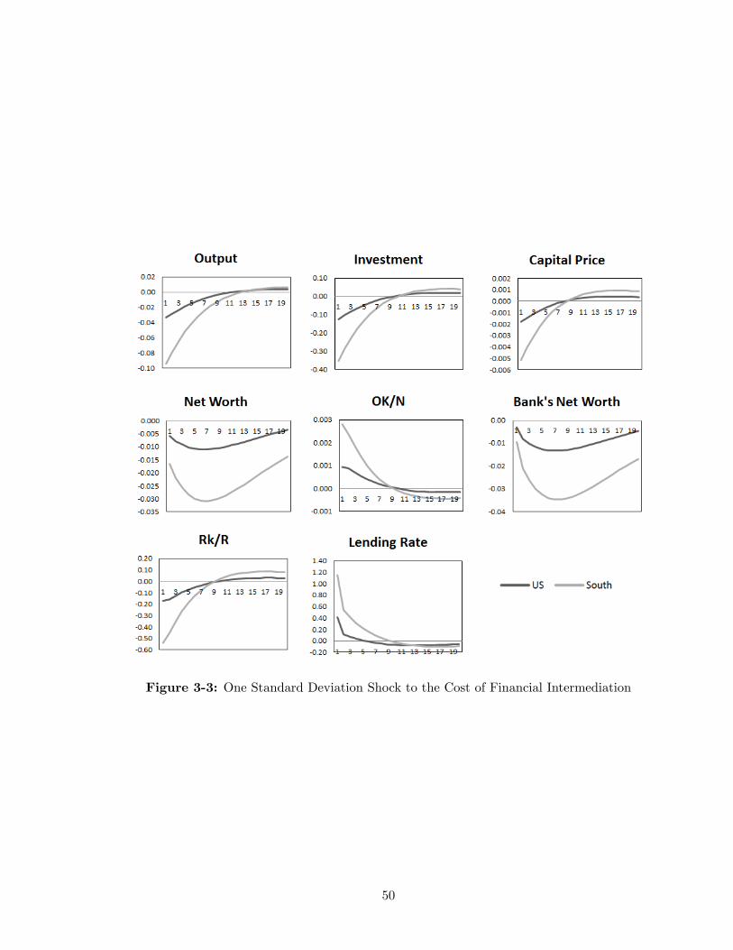
Figure 3-3: One Standard Deviation Shock to the Cost of Financial Intermediation
50

leads to a decrease in the investment demand of �rms. The low demand pushes the capital
prices down. As capital prices drop, the value of �rms�net worth decreases. This increases
the agency problem between entrepreneurs and intermediaries leading to a �nancial ac-
celerator mechanism which results in stronger credit crunches. This negative loop in the
economy prevents banks from lowering their lending rates and causes asymmetries in both
the �nancial sector and business cycle asymmetries.
Conclusion
Incorporating a nontrivial banking sector and costly intermediation, this chap-
ter focuses on the business cycle and �nancial sector asymmetries particularly when the
recessions are originated from �nancial crisis. These asymmetries refer to sudden and deep
crisis followed by slow recoveries in business cycles and lending rates. The chapter �lls
the gap in the literature by explaining the following empirical facts: (1) The asymmetry is
stronger for recessions associated with �nancial crises. (2) The �nancial sector shows a sim-
ilar asymmetry in lending rates. (3) The business cycle and the lending rates asymmetries
are greater in less developed countries.
As an uncovered phenomenon in the literature, intermediation cost generates
strong business cycle asymmetries when recessions are originated from a �nancial shock.
Asymmetries generated from the intermediation cost is stronger than a regular recession
originated with a neutral technology shock. The reason of this is that when a TFP shock
hits the economy only �nancial accelerator mechanism causes delays in recoveries. Whereas,
when a �nancial shock hits the economy, the recovery delays occur because of the feedback
e¤ect of intermediation cost on the �nancial accelerator mechanism. Particularly, when cost
51

increases banks either increase their lending rates or cut their loans both of which create
di¢ culties in �rms�borrowing. This leads to a decrease in capital demand and in capital
prices. Lower capital prices reduce the value of �rms�net worth and eventually the �nancial
accelerator mechanism emerges.
An increase in intermediation costs does not create an asymmetry only for
business cycles, but also for lending rates. As a response to an increase in intermediation
cost, banks immediately increase their lending rates. However, the �nancial accelerator
mechanism prevents the economic conditions from becoming favorable; therefore banks
cannot decrease their lending rates to relieve the stress in the economy. Therefore, lending
rates decrease gradually causing the asymmetry in �nancial sector.
Furthermore, the business cycle and �nancial sector asymmetries are stronger
for �nancially less developed countries. For instance, recessions are around 3 times deeper
for them and their recovery last 67 percent longer than their developed counterparts. Be-
cause less developed countries also have less e¢ cient �nancial sectors in terms of cost to asset
ratios, banks cannot insure against risk in recessions well compared to developed countries.
52

CHAPTER IV
FINANCIAL INTERMEDIATION COSTS AND RELATIVE CONSUMPTION
VOLATILITY
The volatility of macroeconomic variables, particularly that of consumption,
has a detrimental nature on the economy through creating uncertainty and risk. Among
others, Ramey and Ramey (1995) and Laursen and Mahajan (2005) show that it leads to
lower economic growth and social welfare.1 These negative e¤ects are more pronounced
in emerging economies than their developed counterparts even after controlling for crises
by normalizing consumption with output.2 Using a sample of 75 countries, Crucini (1997)
�nds that the standard deviation of consumption relative to output is 3:5 times higher
in less developed countries. This chapter explains the disparity in relative consumption
volatilities between developed and emerging countries by accounting for di¤erences in their
�nancial intermediation costs. Because banks in emerging countries have higher intermedi-
ation costs, their economy experience greater credit crunches which leads to more dramatic
macroeconomic �uctuations.
The literature typically attributes the consumption volatility of a country to
either the degree of the international �nancial integration or the development of the do-
mestic �nancial sector. Baxter and Crucini (1995), Sutherland (1996), and Agenor (2003)
suggest that �nancial integration decreases the consumption volatility by enhancing a na-
tion�s ability to transfer domestic risk to world markets. Studies considering the relationship1Behrman (1988), Rose (1994), and Foster (1995) show that the lack of consumption smoothing cause
signi�cantly negative e¤ects on the life expectancy, nutrition intake and education of households.2Pallage and Robe (2003) �nd that the median welfare cost of aggregate �uctuations in poor countries is
at least 10 times what it is in the United States.
53

between consumption volatility and �nancial development �nd that a developed domestic
�nancial sector can decrease economic volatility through better risk insurance (see Aghion
et al. (1999, 2004); Easterly et al. (2001); Denizer et al. (2002); Ferreira da Silva (2002)
and Fanelli (2008)). Speci�cally, if credit markets are complete, income shocks should be
smoothed away by borrowing and saving, and they should not a¤ect the consumption pat-
tern. Therefore, more �nancially developed and integrated countries should have lower
consumption volatility.
Consumption volatility in emerging countries, however, should naturally be
higher than their developed counterparts because of frequent crises experienced in the for-
mer group. Therefore, the consumption volatility does not provide a clear comparison
between countries unless the e¤ects of crises are eliminated. To overcome this problem,
Kose, Prasad and Terrones (2003) study the relative consumption volatility to output and
�nd that countries who experienced greater �nancial integration during the 1990s also had
an increase in their relative consumption volatility.3 They show, however, that development
of domestic �nancial sector reduces the relative consumption volatility signi�cantly. This
chapter focuses on explaining relative consumption volatility di¤erences between countries
by letting costly �nancial intermediation determine the level of �nancial development of a
country in a DSGE setting with a housing sector. Real estate market interactions have an
important role in the model to connect household consumption decisions with loan market
conditions.
This chapter improves upon existing models by including a nontrivial �nan-
cial sector with costly intermediation. In the literature, �nancial intermediaries (i.e. banks)
have been treated as places in which borrowers and lenders can costlessly exchange funds.3Davis and Kahn (2008) reviewed evidence on the Great Moderation in conjunction with evidence about
volatility trends at the micro level. Their results suggest that the volatility of consumption did not decreaseeven though the economic environment become stable during this time.
54

However, in reality, banks accrue many costs such as wages, marketing expenses, litigation
expenses and data processing expenses. These costs a¤ect consumption because households
take out loans to purchase real estate. Therefore, any change in �nancial intermediation
costs alters the borrowing contract between households and banks. For instance, as inter-
mediation becomes more costly, banks would either cut their loans or increase the lending
rates causing households to adjust their consumption decisions accordingly. Antunes et
al. (2013) show that a one percent reduction in �nancial intermediation cost leads to a
1:9 percent increase in the US consumption. Moreover, these costs increase signi�cantly
during recessions and vary substantially across countries. For instance, banks in developed
countries operate at 75 percent lower cost to asset ratio than those in emerging countries.4
In this way, the �nancial intermediation costs seem to be a reasonable proxy of �nancial
sector development.
Models that include the housing market interactions but not the intermedi-
ation costs, such as Campbell and Hercowitz (2005) and Iacoviello and Pavan (2011) tend
to overshoot the consumption volatility.5 However, the model in this chapter explains the
volatility di¤erences between developed and emerging countries better by incorporating
costly �nancial intermediation. The model suggests that as intermediation cost decreases
households �nd better consumption smoothing possibilities. Thus, countries with lower
intermediation cost, or equivalently more developed �nancial sector, should have lower ag-
gregate and relative consumption volatilities.
The remainder of the chapter is organized as follows. The next section lays out
the empirical motivation by introducing relative consumption volatility. The next section
4Beck et al. (2010) "A new database on �nancial development and structure."5Among those models, Iacoviello (2011) emphasizes the importance of the �nancial sector as well. In
his model, banks have losses when borrowers default on their debt. Yet, these defaults take the form of apositive wealth shock for borrowers. In other words, households can increase their consumption and housingwhile going bankrupt, which is not necessarily what one may expect from a crisis.
55
outlines the model, while following sections discuss the calibration and simulation results.
The last section of the chapter concludes.
Relative Consumption Volatility to Output
After the puzzling results of Kose, Prasad and Terrones (2003), who �nds
positive correlation between the relative consumption volatility and the degree of �nancial
integration, the recent literature has paid greater attention to relative consumption volatil-
ities. Because of the severe and frequent crises that emerging countries experience, their
consumption and output are more volatile than that of developed countries. However, the
relative consumption volatility (i.e. the standard deviation of the consumption to output
ratio, ��C
Y
�) eliminates the e¤ects of economic crises as a shock to a country should de-
crease both consumption and output. In this way, the relative consumption volatility can
be thought of as excess consumption volatility compared to output.
Using the consumption data from the Central Bank of the Republic of Turkey
and the U. S. Bureau of Economic Analysis (BEA), and output and GDP de�ator data
from the OECD, Table 4-1 compares the volatility of macroeconomic variables in the US
and Turkey from 1998:1 to 2012:1. Turkey and the US are the median countries in terms
of �nancial intermediation costs in their respective groups which is why they have been
chosen in this analysis. I chose to represent each group with one country as opposed to
aggregating developed and emerging country groups because aggregation can lead to losses
of some characteristics in the data.6 I use X-12 ARIMA method to seasonally adjust the
6Emerging countries included to the analysis are Argentina, Brazil, Chile, Colombia, Egypt, Hungary,India, Indonesia, Korea, Malaysia, Peru, Philippines, Russia, South Africa, Turkey and Venezuela. Some ofthe other countries that could have been classi�ed as emerging markets are not included because of dataavailability.
56

Table 4-1. Volatility of Macroeconomic Variables
in percent with housing no housingUS TURKEY US TURKEY
�(C) 1:24 4:35 1:52 3:55
�(Y ) 1:34 3:83 1:34 3:83
�
�C
Y
�0:43 2:19 0:52 2:13
Notes: Values are in percent. The consumption data is obtained from Central Bank of the Republic of Turkey andBEA. The GDP and GDP de�ator data are obtained from the OECD. The values are de�ated with GDP de�ators ofthe corresponding country and detrended with HP �lter.
Turkish consumption data for maintaining the consistency with BEA and OECD.
Traditionally, housing consumption, i.e. housing services and utilities, are
included in aggregate consumption. To di¤erentiate the sources of volatility and make the
data consistent with the model, I deduct housing consumption from aggregate consumption
for both countries and report them separately on the "no housing" part of the table.
According to Table 4-1, the consumption and output volatility in the US is
around 2:5 (3:5) times lower than those in Turkey when housing consumption is separated
from (included to) aggregate consumption. On the other hand, the relative volatility of
consumption share is 2:1 percent for Turkey, whereas it is only 0:52 for the US. This stark
di¤erence between the two countries creates the main empirical target of this model.
The housing consumption of Turkey and the US share di¤erent characteris-
tics. First and third columns of Table 4-1 indicate that housing services and utilities are
fairly stable for the US because when the housing sector is deducted from the aggregate
consumption, the consumption volatility increases from 1:24 to 1:52. Conversely, Turkey�s
consumption volatility decreases from 4:35 to 3:55 when housing consumption is not in-
cluded in the aggregate measure. This suggests that housing consumption is much more
volatile in Turkey compared to the US. Because of these di¤erences in housing market char-
acteristics of the two countries, the model in this chapter separates aggregate consumption
57

from housing consumption.
The Model
The model is a version of Iacoviello (2005). In this model, there are patient
and impatient households, a representative �rm, and a bank. The bank intermediates
between borrowers and savers at a cost and requires some of borrower�s real estate to be
collateralized. To simplify the model and focus on relative consumption volatility, only
impatient households can get loans from banks to engage in housing market activities, and
therefore they are the only agents who face collateral constraints. If other agents, such
as �rms, were also constrained in borrowing with their accumulated real estate, then any
housing shock would have a direct e¤ect on the production. However this assumption helps
prevent the model from overestimating the role of the housing sector.
Households
There are two fundamental di¤erences between the households in the model.
First, patient households give greater value to the future than impatient households. Specif-
ically, I assume that the discount factor of patient households is larger than that of impatient
households.7 This assumption guarantees an equilibrium in which the borrowing constraint
of impatient households always binds. Second, only impatient households can engage in
housing market activities. This assumption helps accounting for individuals who do not
want to buy (or not capable of buying) real estate.
7I assume that �p > �(1+ ct) where ct denotes the �nancial intermediation cost as a ratio to total assets.Since this ratio is very small, the assumption holds for any reasonable value used in the literature.
58

Patient Households
Denoted with superscript p; patient households make their consumption, Cpt ;
and leisure, 1� Lpt ; decisions at time t and their total endowment of time is normalized to
one. They also decide how much to save, Dt+1; at the bank for a return of the gross deposit
rate, Rt+1: The patient households use the following objective function to maximize their
lifetime utility from consumption and leisure.
maxCp;t;Lp;t;Dt+1
Et
( 1Xk=0
�kp�ln(Cpt+k) + � ln(1� L
pt+k)
�)(1)
The maximization is subject to the following Walrasian budget constraint that
equates households�spending to their income.
Cpt +Dt+1 = RtDt +WtLpt (2)
First order conditions to the problem of patient households are given by the
following standard consumption Euler equation and the labor supply decision, respectively.
1 = Et
��pC
pt
Cpt+1
�Rt+1 (3)
�
1� Lpt=Wt
Cpt(4)
Impatient Households
Impatient households engage in housing market activities by making a mort-
gage contract with the bank. They buy real estate, Ht+1 for the price, Qht ; at time t:
However, the bank requires some of the assets to be collateralized which restrains the avail-
able credit to borrowers.
59

Impatient households maximize their utility from consumption and leisure as
well as the utility that they get from housing services. They use the following objective
function subject to their �ow of funds constraint in equation (6) and the collateral constraint
in equation (7).
maxCt;Ht+1;Bt+1
Et
( 1Xk=0
�ki�ln(Cit+k) + � ln(Ht+k) + � ln(1� Lit+k)
�)(5)
Represented with the subscript i; impatient households can use the amount
borrowed from banks, Bt+1; their labor income, WtLt; and the return from previous in-
vestment, QhtHjt; to �nance their consumption, new housing investment, and repayment of
their debt. In equation (6), while � shows the adjustment cost of housing, Zt denotes the
gross lending rates. In the model, the housing depreciation rate is assumed to be zero.
Cit +QhtHt+1 +
�
2(Ht+1 �Ht
Ht)2QhtHt = Q
htHjt � ZtBt +Bt+1 +WtL
it (6)
Banks require some of the real estate assets to be used as collateral. With
this collateral constraint households can borrow up to a limit. Speci�cally:
Zt+1Bt+1 � EnQht+1Ht+1
o(7)
First order conditions to the problem of impatient households are given by
equations (8), (9) and (10) that show labor supply, consumption and housing demand
decisions, respectively.
�
1� Lit=Wt
Cit(8)
1
Cit= Et
�Zt+1
��t +
�iCit+1
��(9)
60

�iEt
"(�
Ht+1+Qht+1Cit+1
�1 +
��gt+1(1 +
1
2gt+1)
��)+ �tQ
ht+1
#=QhtCit(1 + �gt) (10)
where �t is the Lagrangian multiplier and
gt =Ht+1 �Ht
Ht(11)
Finally, the equation (12) gives the rule for house price setting. It can
be thought that there are house producers that maximize their pro�ts, �t; where �t =
Qht�Ht � �Ht � �2
��HtHt
�2Ht: Here �Ht = Ht+1 � Ht denotes the housing investment.
The �rst order condition to this problem gives Qht = 1+���HtHt
�which is equivalent to the
equation (12).
Qht = (1 + �gt) (12)
Firms
Firms produce a homogenous good, Yt; using capital and labor in the following
aggregate Cobb-Douglas production function.
Yt = AtK�t L
1��t (13)
� � 0 denotes the capital share in production andAt is the total factor productivity
(TFP) that follows the AR (1) process in equation (14).
logAt = �A logAt�1 + "At (14)
61
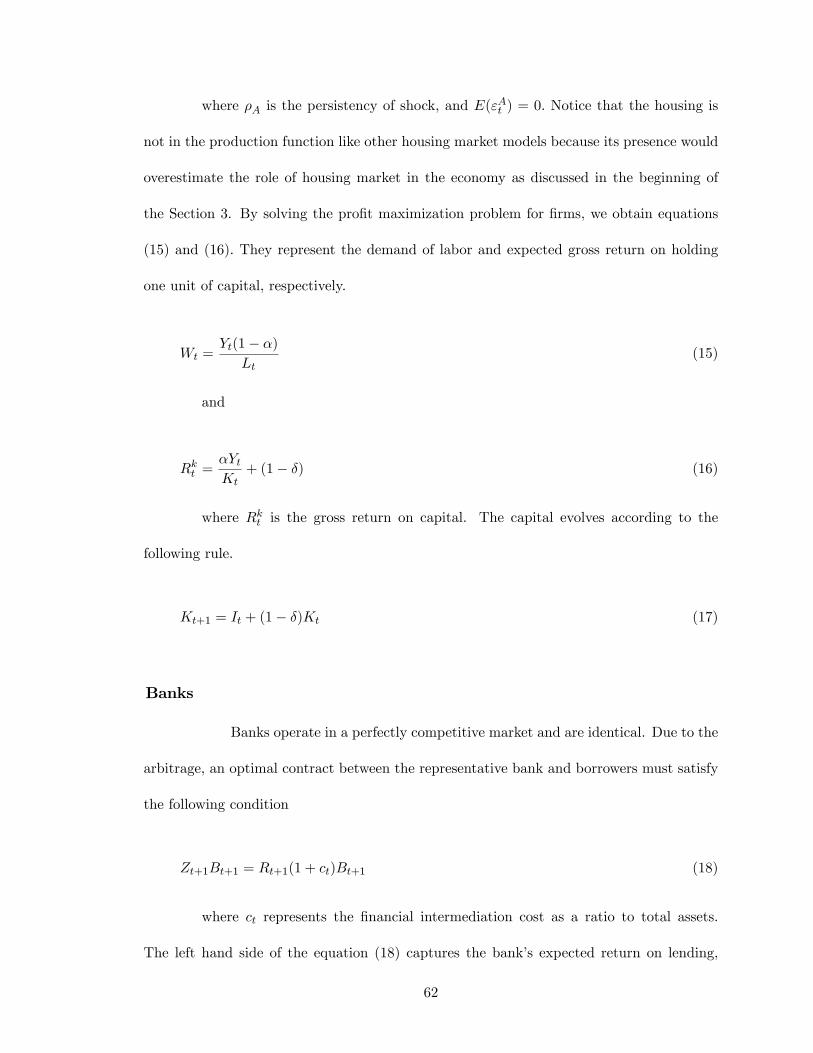
where �A is the persistency of shock, and E("At ) = 0: Notice that the housing is
not in the production function like other housing market models because its presence would
overestimate the role of housing market in the economy as discussed in the beginning of
the Section 3. By solving the pro�t maximization problem for �rms, we obtain equations
(15) and (16): They represent the demand of labor and expected gross return on holding
one unit of capital, respectively.
Wt =Yt(1� �)
Lt(15)
and
Rkt =�YtKt
+ (1� �) (16)
where Rkt is the gross return on capital. The capital evolves according to the
following rule.
Kt+1 = It + (1� �)Kt (17)
Banks
Banks operate in a perfectly competitive market and are identical. Due to the
arbitrage, an optimal contract between the representative bank and borrowers must satisfy
the following condition
Zt+1Bt+1 = Rt+1(1 + ct)Bt+1 (18)
where ct represents the �nancial intermediation cost as a ratio to total assets.
The left hand side of the equation (18) captures the bank�s expected return on lending,
62

whereas the right hand side represents how much could the bank have gained if it accepted
the riskless rate instead of lending. Therefore, equation (18) suggests that arbitrage would
equate the bank�s expected return from lending to its opportunity cost. Notice that the
bank has to pay 1+ct to provide a dollar worth of loans to borrowers. ct is multiplicative to
Bt+1 because the cost itself is observed as a ratio to total assets in the data. From equation
(18), higher cost of intermediation increases the opportunity cost of lending.
Finally, ct follows the AR(1) process shown in equation (19).
ln ct = (1� �c) ln �c+ �c ln ct�1+"ct (19)
Notice that the intermediation cost does not become zero in the steady state.
Instead it is equal to its long run average �c; because in reality costs never diminish entirely.
Resource Constraint and Market Clearing Conditions
The economy-wide resource constraint is shown below where It denotes the
gross investment.
Yt = Ct + It (20)
where aggregate consumption is a sum of patient and impatient household
consumptions as shown in Equation (21).
Ct = Cpt + C
it (21)
The following labor market clearing condition guarantees that the demand
for and supply of labor would be equal.
63
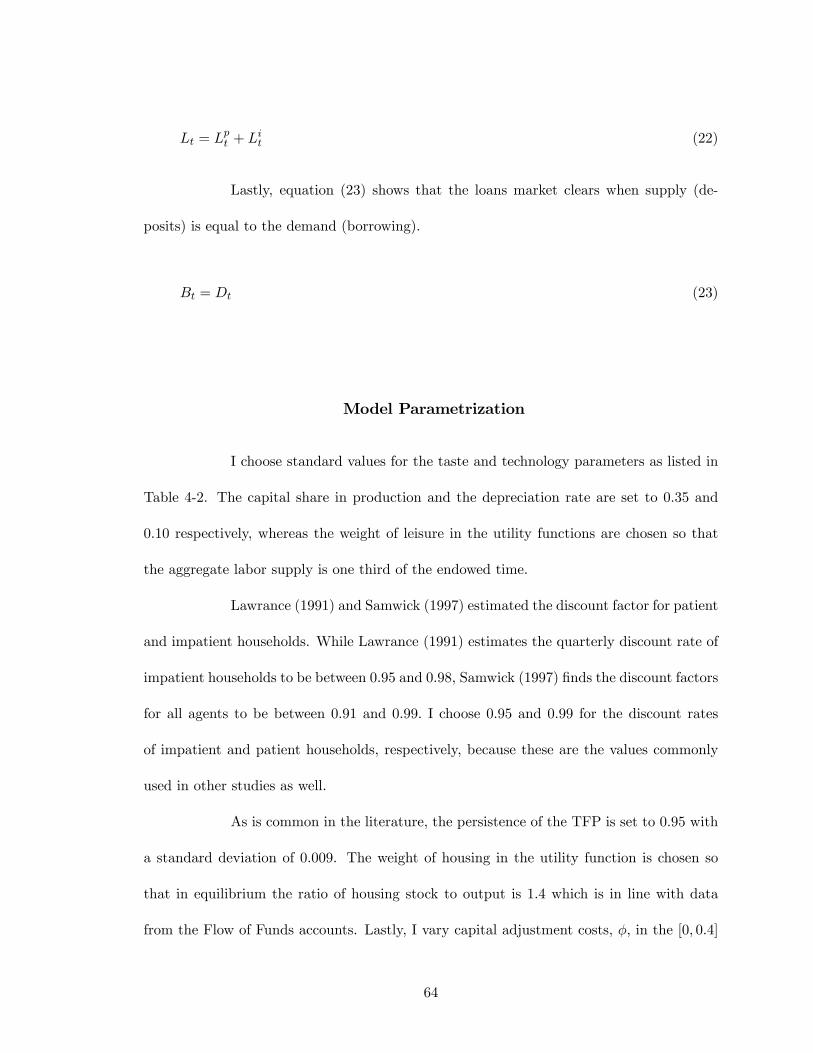
Lt = Lpt + L
it (22)
Lastly, equation (23) shows that the loans market clears when supply (de-
posits) is equal to the demand (borrowing).
Bt = Dt (23)
Model Parametrization
I choose standard values for the taste and technology parameters as listed in
Table 4-2. The capital share in production and the depreciation rate are set to 0:35 and
0:10 respectively, whereas the weight of leisure in the utility functions are chosen so that
the aggregate labor supply is one third of the endowed time.
Lawrance (1991) and Samwick (1997) estimated the discount factor for patient
and impatient households. While Lawrance (1991) estimates the quarterly discount rate of
impatient households to be between 0:95 and 0:98, Samwick (1997) �nds the discount factors
for all agents to be between 0:91 and 0:99: I choose 0:95 and 0:99 for the discount rates
of impatient and patient households, respectively, because these are the values commonly
used in other studies as well.
As is common in the literature, the persistence of the TFP is set to 0:95 with
a standard deviation of 0:009. The weight of housing in the utility function is chosen so
that in equilibrium the ratio of housing stock to output is 1:4 which is in line with data
from the Flow of Funds accounts. Lastly, I vary capital adjustment costs, �; in the [0; 0:4]
64

Table 4-2: Calibration of ParametersDescriptioncapital share in production � = 0:35discount factor for impatient households �i = 0:83discount factor for patient households �p = 0:96
depreciation rate � = 0:1housing adjustment cost � = [0; 0:4]persistence of TFP �A = 0:95standard deviation of TFP �A = 0:009average intermediation cost/total assets cUS = 0:0356
cTR = 0:0634persistence of intermediation cost �cUS = �
cTR = 0:99
standard deviation of intermediation cost ��US = 0:072��TR = 0:24
Notes: One period in the model corresponds to one year. Thus, the values in the table match the annual frequency.
range.
Results
Model�s Fit
Table 4-3 shows that the model �ts the data for the US and Turkey even
when the economic conditions in both countries are assumed to be identical except for
their �nancial intermediation costs. If TFP was also calibrated to the Turkish case, results
reported would be even larger for Turkey; however, then in this case it would not be possible
to pin down the e¤ects of intermediation costs.
The model captures the di¤erences between the US and Turkey particularly
well. Intermediation costs alone account for the higher macroeconomic volatility in Turkey.
Moreover, the relative consumption volatility �ndings are also in line with the data. Specif-
ically, the relative volatility of consumption is observed to be 0:73 and 3:6 for the US and
Turkey, respectively, while the model predicts them to be 0:6 and 2:51. These predictions
65
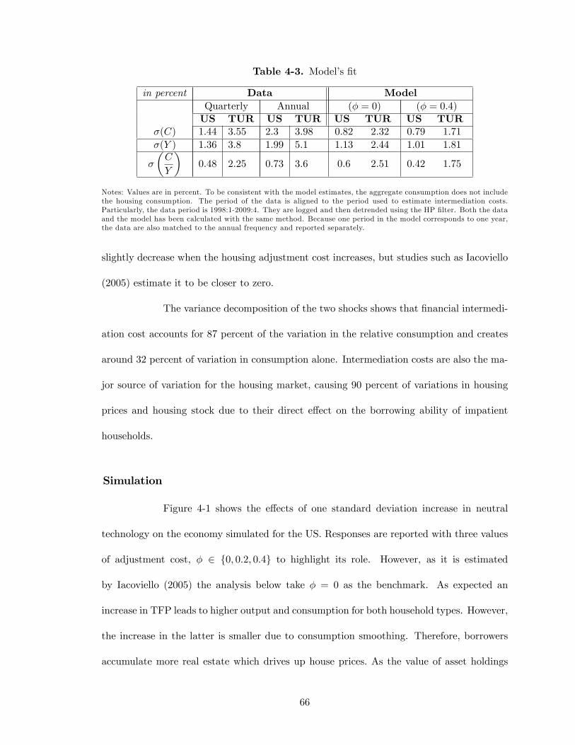
Table 4-3. Model�s �t
in percent Data ModelQuarterly Annual (� = 0) (� = 0:4)US TUR US TUR US TUR US TUR
�(C) 1:44 3:55 2:3 3:98 0:82 2:32 0:79 1:71
�(Y ) 1:36 3:8 1:99 5:1 1:13 2:44 1:01 1:81
�
�C
Y
�0:48 2:25 0:73 3:6 0:6 2:51 0:42 1:75
Notes: Values are in percent. To be consistent with the model estimates, the aggregate consumption does not includethe housing consumption. The period of the data is aligned to the period used to estimate intermediation costs.Particularly, the data period is 1998:1-2009:4. They are logged and then detrended using the HP �lter. Both the dataand the model has been calculated with the same method. Because one period in the model corresponds to one year,the data are also matched to the annual frequency and reported separately.
slightly decrease when the housing adjustment cost increases, but studies such as Iacoviello
(2005) estimate it to be closer to zero.
The variance decomposition of the two shocks shows that �nancial intermedi-
ation cost accounts for 87 percent of the variation in the relative consumption and creates
around 32 percent of variation in consumption alone. Intermediation costs are also the ma-
jor source of variation for the housing market, causing 90 percent of variations in housing
prices and housing stock due to their direct e¤ect on the borrowing ability of impatient
households.
Simulation
Figure 4-1 shows the e¤ects of one standard deviation increase in neutral
technology on the economy simulated for the US. Responses are reported with three values
of adjustment cost, � 2 f0; 0:2; 0:4g to highlight its role. However, as it is estimated
by Iacoviello (2005) the analysis below take � = 0 as the benchmark. As expected an
increase in TFP leads to higher output and consumption for both household types. However,
the increase in the latter is smaller due to consumption smoothing. Therefore, borrowers
accumulate more real estate which drives up house prices. As the value of asset holdings
66

Figure 4-1: Responses to the TFP shock
Notes: The �gures show the responses of key macroeconomic variables to a one standard deviation shock to the TFPfor the US under di¤erent parametrization of the housing adjustment cost.
increases, the borrowing constraint becomes less tight, and households can borrow more and
buy even more real estate. This creates an ampli�cation e¤ect in the economy. The income
increase also causes a substitution and income e¤ect for patient and impatient households,
respectively. Because the substitution e¤ect dominates the income e¤ect, the total labor
supply increases in the economy.
As the housing adjustment become more costly, responses of house prices turn
out to be larger in magnitude. Because of the large change in housing prices, impatient
households have to take more aggressive measures for their labor supply decisions. Apart
from this, the housing adjustment cost does not seem to have a signi�cant impact on the
67
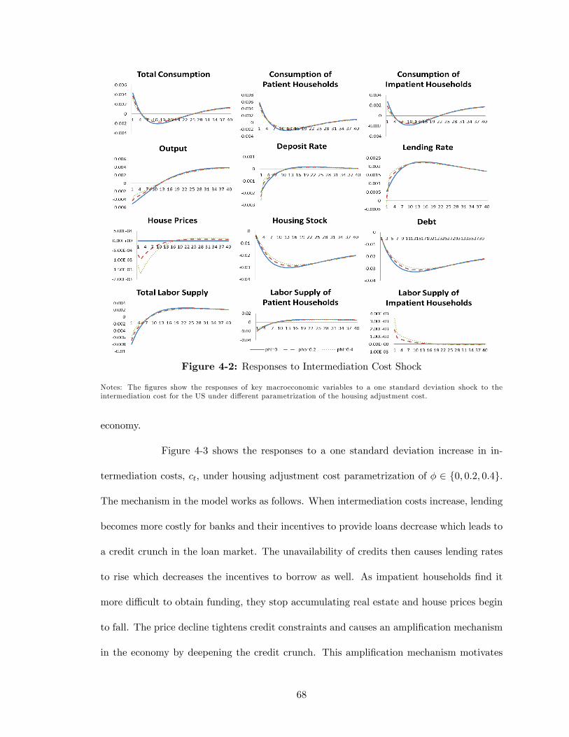
Figure 4-2: Responses to Intermediation Cost Shock
Notes: The �gures show the responses of key macroeconomic variables to a one standard deviation shock to theintermediation cost for the US under di¤erent parametrization of the housing adjustment cost.
economy.
Figure 4-3 shows the responses to a one standard deviation increase in in-
termediation costs, ct; under housing adjustment cost parametrization of � 2 f0; 0:2; 0:4g.
The mechanism in the model works as follows. When intermediation costs increase, lending
becomes more costly for banks and their incentives to provide loans decrease which leads to
a credit crunch in the loan market. The unavailability of credits then causes lending rates
to rise which decreases the incentives to borrow as well. As impatient households �nd it
more di¢ cult to obtain funding, they stop accumulating real estate and house prices begin
to fall. The price decline tightens credit constraints and causes an ampli�cation mechanism
in the economy by deepening the credit crunch. This ampli�cation mechanism motivates
68

impatient households to work more as they need to raise more income. Because they accu-
mulate less housing stock, they begin using a larger portion of their income for consumption.
Additionally, lower deposit rates discourage patient households from saving. Both of these
factors cause an initial rise in total consumption however as the credit crunch becomes
more severe consumption declines as well. On the other hand, the increase in labor supply
decreases real wages and causes patient households to work less. The substitution e¤ect
dominates the income e¤ect, and total labor supply decreases which reduces the output as
well.
Increasing the housing adjustment cost magni�es the response of housing
prices. As adjustment becomes more costly impatient households work harder. Otherwise
there is no di¤erence in the responses of macroeconomic variables under various housing
adjustment cost parametrization.
Figure 4-3 and 4-4 compare the responses for the US and Turkey under a TFP
and �nancial intermediation cost shock, respectively. Figure 4 shows that the responses
from both countries are very similar when there is a neutral technology shock. This is
expected because countries are assumed to be identical except their intermediation costs.
In other words, I used the same values for TFP shock, taste and preference parameters
in simulations for both countries. The di¤erence in their intermediation costs is the only
source that separates the US from Turkey. However, if the TFP was also calibrated to
the Turkish economy, the responses would be stronger than those in the US. Furthermore,
the simplifying assumption of having frictions only on households but not on �rms also
contributes to this result.
A shock to the intermediation cost creates signi�cant di¤erences in Turkey by
amplifying the e¤ects dramatically relative to the US. Consumption and output responses
69
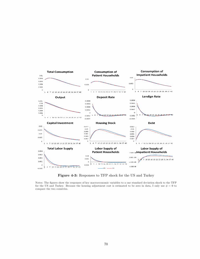
Figure 4-3: Responses to TFP shock for the US and Turkey
Notes: The �gures show the responses of key macroeconomic variables to a one standard deviation shock to the TFPfor the US and Turkey. Because the housing adjustment cost is estimated to be zero in data, I only use � = 0 tocompare the two countries.
70
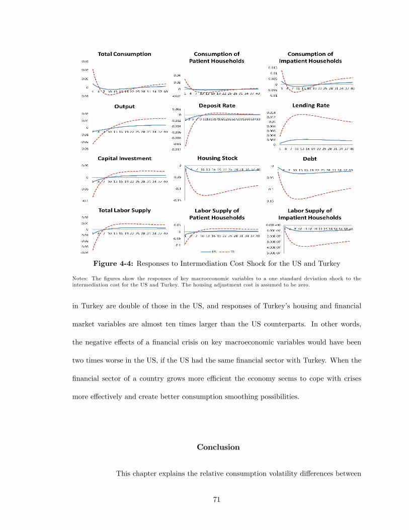
Figure 4-4: Responses to Intermediation Cost Shock for the US and Turkey
Notes: The �gures show the responses of key macroeconomic variables to a one standard deviation shock to theintermediation cost for the US and Turkey. The housing adjustment cost is assumed to be zero.
in Turkey are double of those in the US, and responses of Turkey�s housing and �nancial
market variables are almost ten times larger than the US counterparts. In other words,
the negative e¤ects of a �nancial crisis on key macroeconomic variables would have been
two times worse in the US, if the US had the same �nancial sector with Turkey. When the
�nancial sector of a country grows more e¢ cient the economy seems to cope with crises
more e¤ectively and create better consumption smoothing possibilities.
Conclusion
This chapter explains the relative consumption volatility di¤erences between
71

developed and emerging countries using their �nancial development levels. The relative
consumption volatility is on average 3 times larger in less developed countries which shows
a signi�cantly excessive volatility of consumption for these countries. To understand why
consumption �uctuates more relative to output in less developed countries, I construct a
DSGE model with housing market and collateral constraints. The �nancial intermediation
cost is introduced to the model as a proxy for �nancial development levels. While the cost
per asset is around 3 percent for developed countries, it is closer to 5 percent for emerging
markets. This shows that a bank in an emerging market, such as Turkey, pays two times
more than a bank in the US to raise the same amount of assets. This provides a stark
di¤erence between �nancial development levels of countries.
The model successfully replicates the volatility di¤erences observed in the
data. The results shows that the median country of emerging countries, Turkey, is four
times more volatile than the US in terms of relative consumption to output. The mechanism
of the model works as follows. A negative �nancial shock (high intermediation cost) makes
the lending-borrowing process more costly for the agents in the economy and causes bank
lending rates to increase. The credit crunch creates an ampli�cation mechanism for all the
macroeconomic variables. The model suggests that if the US had the same �nancial sector
with Turkey, a shock to the �nancial intermediation cost would cause double sized negative
e¤ects for consumption and output. Moreover, the negative e¤ects on housing and �nancial
sectors would be almost ten times larger by the time the trough occurs in the recession. In
this way, �nancial intermediation costs have a very signi�cant role in creating frictions and
amplifying the negative e¤ects of �nancial crisis in an economy and should not be ignored
in future studies.
72

CHAPTER V
CONCLUSION
The banking sector, although has a very important role in the US economy,
did only recently gain its deserved attention from macroeconomists. However, banks still
have been thought of as intermediaries that operate at no cost. However, in reality banks
incur many costs ranging from wages to data processing expenses like any other �rm and
they extend great attention in controlling these costs in order to maximize their pro�ts.
This dissertation �lls the gap in the literature by presenting the �rst high
frequency, micro level data of cost breakdowns for large and mid-sized banks in the US.
Covering the period of 1992:1-2011:4, this dataset enlightens four empirical facts. First,
intermediation costs increase dramatically in recessions. Second, they tend to have large
increases rather than same magnitude decreases. Third, developed countries generally have
lower intermediation cost per asset than their less developed counterparts which can suggest
an e¢ ciency measure for �nancial intermediaries. Finally, intermediation costs co-move with
bank lending rates very closely across countries.
Building upon these empirical facts, the dissertation�s �rst lesson is that these
�nancial intermediation costs are highly countercyclical which creates a mechanism that am-
pli�es the adverse e¤ects of recessions. In particular, when intermediation costs increase,
banks re�ect them in their lending rates. Less favorable terms creates di¢ culties for bor-
rowers (�rms or households) and therefore the amount borrowed in the economy decreases.
Due to shortages in external �nancing, borrowers demand less assets causing capital prices
to go down which subsequently reduces their net worth. Knowing that borrowers have lower
73
net worth, banks charge even higher lending rates which creates a negative feedback loop
in the economy. This mechanism creates new recessions and ampli�es existing ones. In the
data, a small increase in these costs can generate a 50 percentage point decrease in output.
A theoretical model that incorporates costly intermediation using the mechanism above
can generate realistic estimates of the data in capturing the relationship between �nancial
intermediation costs and business cycles.
This dissertation also suggests that by triggering a negative feedback loop in
the economy, intermediation costs can also cause delays in recoveries from recessions. The
data shows that costs stay high even after recoveries take place. This does not only delay
recoveries of an economy, but also causes banks to keep their lending rates high even after
recoveries take place. Moreover, the di¤erence in intermediation costs between developed
and less developed countries leads to more pronounced e¤ects in the latter group.
The �nal lesson of this dissertation is that intermediation costs a¤ect house-
holds� consumption decisions as well. Speci�cally, when households purchase mortgage
agreements from banks to buy real estate, they become prone to changes in intermediation
costs. An increase in �nancial intermediation costs would alter their decisions about con-
sumption and saving which causes uncertainty to take place in an economy. This would
cause a lack in consumption smoothing which would lead to higher relative consumption
volatility in the country. A model incorporating both �nancial intermediation costs and
housing market interactions captures this result very closely to the data. Furthermore, in
line with the data, this model �nds that the volatility is higher for less developed countries.
74

BIBLIOGRAPHY
[1] Acemoglu, D., and A. Scott. 1997. Asymmetric business cycles: Theory and time-seriesevidence. Journal of Monetary Economics 97 (40): 501�533.
[2] Agenor, P. 2003. Bene�ts and costs of international �nancial integration: theory andfacts. World Economy 26: 1089-118.
[3] Aghion, P., A. Banerjee, and T. Piketty. 1999. Dualism and macroeconomic volatility.Quarterly Journal of Economics 114: 1359�97.
[4] Aghion,P., P. Bacchetta, and A. Banerjee. 2004. Financial development and the insta-bility of open economies. Journal of Monetary Economics 51: 1077�1106.
[5] Antunes, A., T. Cavalcanti, and A. Villamil. 2008. The e¤ect of �nancial repression andenforcement on entrepreneurship and economic development. Journal of MonetaryEconomics 55 (2): 278-297.
[6] _____ 2013. Costly intermediation and consumption smoothing. Economic Inquiry51 (Jan): 459�472.
[7] Baxter, M., and M. Crucini. 1995. Business cycles and the asset structure of foreigntrade. International Economic Review 36: 821�54.
[8] Beck, T., A. Demirgüc-Kunt, and R. Levine. 2010. A new database on �nancial devel-opment and structure. World Bank dataset October 2010 update.
[9] Behrman, J. 1988. Intrahousehold allocation of nutrients in rural India: are boys fa-vored? Do parents exhibit inequality aversion?. Oxford Economic Papers 40: 32-54.
[10] Bernanke, B., M. Gertler, and S. Gilchrist. 1999. The �nancial accelerator in a quan-titative business cycle framework," in J. Taylor and M. Woodford, eds., Handbookof macroeconomics. Amsterdam: North- Holland, pp. 1341-93.
[11] Bordo, M. D., J.G. Haubrich. 2010. Creditcrises, money and contractions: An historicalview�, Journal of Monetary Economics 57, 1.18.
[12] Bureau of Labor Statistics. 2012. Unemployment rate and discouraged workers data.Retrieved from http://www.bls.gov/data/#unemployment
[13] Campbell, J R., and Z. Hercowitz. 2005. The role of collateralized household debt inmacroeconomic stabilization. NBER Working Papers 11330, National Bureau ofEconomic Research, Inc, May.
[14] Cecchetti, S. D., M. Kohler, C. Upper. 2009. Financial crises and economic activity�,NBER Working Paper No. 15379.
75
[15] Central Bank of the Republic of Turkey. 2013. Final consumption expenditure of resi-dent and non-resident households in current and �xed prices, Ankara.
[16] Christiano, L. J., M. Trabandt, and K. Walentin. Introducing �nancial frictions andunemployment into a small open economy model. Journal of Economic Dynamicsand Control 35.12: 1999-2041.
[17] Christensen, I., and A. Dib. 2008. The �nancial accelerator in an estimated New Key-nesian model�, Review of Economic Dynamics, 11 (1), pp. 155�178.
[18] Claessens, Stijn, M. A. Kose, and M. E. Terrones. 2012. How do business and �nancialcycles interact?. Journal of International economics 87.1: 178-190.
[19] Cook, D. 1999. The liquidity e¤ect and money demand. Journal of Monetary Economics43.2: 377-390.
[20] Cover, J. 1992. Asymmetric e¤ects of positive and negative money-supply shocks. Quar-terly Journal of Economics 107, 1261�82.
[21] Crucini, M. 1997. Country size and economic �uctuations. Review of InternationalEconomics 5, No. 2: 204�20.
[22] Davis, S. J., and J. A. Kahn. 2008. Interpreting the great moderation: changes in thevolatility of economic activity at the macro and micro levels. Journal of EconomicPerspectives 22(4): 155�80.
[23] DeLong, B.J., and L. H. Summers. 1998. How does macroeconomic policy a¤ect out-put?�Brookings Papers on Economic Activity, (2), pp. 433-94.
[24] Denizer, C.A., M.F. Iyigun, and A. Owen. 2002. Finance and macroeconomic volatility.Contributions to Macroeconomics 2: 1�30.
[25] Easterly,W., R. Islam, and J. E. Stiglitz. 2001. Shaken and stirred: explaining growthvolatility. Annual World Bank Conference on Development Economics, ed. by B.Pleskovic and N. Stern.
[26] Fanelli, J. M. 2008. Macro volatility and �nancial institutions. Macroeconomic Volatil-ity, Institutions and Financial Architectures: The Developing World Experience,1-24.
[27] Ferreira da Silva, G. 2002. The impact of �nancial system development on businesscycles volatility: cross-country evidence. Journal of Macroeconomics 24: 233-53,ed. by J.M. Fanelli.
[28] Foster, A. 1995. Prices, credit markets and child growth in low-income rural areas.Economic Journal 105: 551-70.
[29] Gambacorta L., and S. Iannotti. 2008. Are there asymmetries in the response of bankinterest rates to monetary shocks. Applied Economics, 39 (19).
76
[30] Gertler, M., and Peter Karadi. "A model of unconventional monetary policy." Journalof Monetary Economics 58.1 (2011): 17-34.
[31] Gertler, M�S. Gilchrist, and F. M. Natalucci. 2007. External constraints on monetarypolicy and the �nancial accelerator. Journal of Money, Credit and Banking 39.2-3:295-330.
[32] Gertler, Mark, and Nobuhiro Kiyotaki. "Financial intermediation and credit policy inbusiness cycle analysis." Handbook of Monetary Economics 3 (2010): 547.
[33] Greenwood, J., Z. Hercowitz, and G. W. Hu¤man. 1988. Investment, capacity utiliza-tion, and the real business cycle. The American Economic Review: 402-417.
[34] Hansen, G.D., and E. C. Prescott. 2005. Capacity constraints, asymmetries, and thebusiness cycle. Review of Economic Dynamics, 8 (4) (2005), pp. 850�865
[35] Iacoviello, M. 2005. House prices, borrowing constraints and monetary policy in thebusiness cycle. American Economic Review (June): 739-64.
[36] ______ 2011. Financial business cycles. Working Paper, Federal Reserve Board.
[37] Iacoviello, M., and M. Pavan. 2011. Housing and debt over the life cycle and over thebusiness cycle. Boston College Working Papers in Economics 723, Boston CollegeDepartment of Economics.
[38] Ireland, P.N., 2003. Endogenous money or sticky prices? Journal of Monetary Eco-nomics 50, 1623�1648
[39] Keynes, J.M. 1936. The general theory of employment, interest and money. Macmillan,London.
[40] Kose, M. A., E. S. Prasad, and M. E. Terrones. 2003. Financial integration and macro-economic volatility. IMF Sta¤ Papers , Vol. 50. No. 1.
[41] Laursen, T., and S. Mahajan. 2005. Volatility, income distribution, and poverty. in J.Aizenman and B. Pinto, Managing Volatility and Crisis: A Practitioner�s Guide,Cambridge University Press: 101-36.
[42] Lawrence, E. 1991. Poverty and the rate of time preference: evidence from panel data.Journal of Political Economy, 119, 54�77.
[43] Lo, M., and J. Piger. 2005. Is the response of output to monetary policy asymmet-ric?Evidence from a regime-switching coe¢ cients mode. Journal of Money, Creditand Banking, 37, 868�86.
[44] Macklem, T., A. Paquet, L. Phaneuf. Asymmetric e¤ects of monetary policy: Evidencefrom the yield curve. CREFE Working Paper 42.
[45] Magud, N. E. 2008. On asymmetric business cycles and the e¤ectiveness of counter-cyclical �scal policies. Journal of Macroeconomics�, Vol. 30, Issue 3, pp. 885- 905.
77

[46] Meier, A., Müller, G.J., 2006. Fleshing out the monetary transmission mechanism:output composition and the role of �nancial frictions. Journal of Money, Credit,Banking 38, 1999�2133.
[47] Mergent, Inc. Fifth Thrid Bank Income Statements. Retrieved May 2012, from MergentOnline database.
[48] OECD, 2010. Main economic indicators - complete database. Main Economic Indicators(database), http://dx.doi.org/10.1787/data-00052-en (Accessed on January 2013)
[49] Ordonez, G. L. 2009. Larger crises, slower recoveries: The asymmetric e¤ects of �-nancial frictions. Federal Reserve Bank of Minneapolis Research Department Sta¤Report 429.
[50] Pallage, S.,and M. Robe. 2003. On the welfare cost of economic �uctuations in devel-oping countries. International Economic Review 44: 668�77.
[51] Ramey, G, and V.A. Ramey. 1995. Cross-country evidence on the link between volatilityand growth. American Economic Review 85: 1138-51.
[52] Ravn, M.O., and M. Sola. 2004. Asymmetric e¤ects of monetary policy in the UnitedStates. Federal Reserve Bank of St. Louis Review, 86(5), 41-60.
[53] Reinhart, C. M., and V. R. Reinhart. 2010. After the fall. NBER Working Paper No.16334.
[54] Reinhart, C. M., and K. S. Rogo¤. 2008. Banking crises: An equal opportunity menace.NBER Working Paper No. 14587.
[55] _____2009. The aftermath of �nancial crises. NBER Working Paper No. 14656.
[56] Rose, E. 1994. Consumption smoothing and excess female mortality in rural India.draft, University of Washington.
[57] Samwick, A. A. 1998. Discount rate heterogeneity and social security reform. Journalof Development Economics 57: 117�46.
[58] Sims, C. A., J. H. Stock, and M. W. Watson. 1990. Inference in linear time seriesmodels with some unit roots. Econometrica: Journal of the Econometric Society,113-144.
[59] Sutherland, A. 1996. Financial market integration and macroeconomic volatility. Scan-dinavian Journal of Economics 98: 521�39.
[60] Thompson M.A. 2006. Asymmetric adjustment in the prime lending�deposit ratespread. Review of Financial Economics 15, 323�329.
[61] U.S. Bureau of Economic Analysis. Table 2.4.5U, personal consumption expendituresby type of product. (Accessed on January 2013).
78

[62] Veldkamp, L. 2005. Slow boom, sudden crash. Journal of Economic Theory. 124 (2),230�257.
79
Related Documents


