i Computational Studies of Interactions Between Vanadyl, Uranyl, and Thorium Aqua Ions with Bidentate Eudistomin Ligands of Ascidian-origin by Ashutosh Parimi Thesis submitted to the Faculty of Graduate Studies Of the University of Manitoba In partial fulfilment as per the requirements for the MASTER OF SCIENCE Department of Chemistry University of Manitoba Winnipeg Copyright © 2021 by Ashutosh Parimi

Welcome message from author
This document is posted to help you gain knowledge. Please leave a comment to let me know what you think about it! Share it to your friends and learn new things together.
Transcript
i
Computational Studies of Interactions Between Vanadyl, Uranyl,
and Thorium Aqua Ions with Bidentate Eudistomin Ligands of
Ascidian-origin
by
Ashutosh Parimi
Thesis submitted to the Faculty of Graduate Studies
Of the University of Manitoba
In partial fulfilment as per the requirements for the
MASTER OF SCIENCE
Department of Chemistry
University of Manitoba
Winnipeg
Copyright © 2021 by Ashutosh Parimi
ii
ABSTRACT
The nuclear waste generated in nuclear power plants is reprocessed to extract useful actinide
elements, especially uranium and plutonium. In recent times, interest has been growing towards
N-containing ligands to facilitate extraction. More often than not, these ligands have
similarities to biogenic compounds such as eudistomins, which are found in marine animals
called Ascidians.
Ascidians are tunicates which adopt unusual techniques to deter predation, the three main
methods are sequestration of unusual metals, high concentrations of sulphuric acid/sulphate
ions in tunicate-cells, and the presence of eudistomins. Studies have shown the presence of
sulphate ion/sulfuric acid plays a key role in deterring predation. In a separate study,
researchers have found that eudistomins can form metal-complexes with Iron outside of the
ascidian’s body. Whether eudistomins play any role in the presence of sulfuric acid/sulphate
ion, and/or the sequestration of the metals was never studied.
In this study, we have explored the possible interactions of eudistomins as ligands with metal-
aqua ions viz., vanadyl, uranyl, and thorium ions. We have designed five model reactions and
have calculated the formation energies. The model reactions were designed to resemble what
might happen in the body of an ascidian, based on the information obtained from the literature.
We have adopted density function theory (DFT) using PBE-D3, BLYP, and B3LYP functionals
with the ADF (PBE-D3 and BLYP) and ORCA (BLYP and B3LYP) software packages for our
calculations. The formation energies of the complexes were calculated in gas phase and in
solvation phase. COSMO (in ADF) and CPCM (in ORCA) were used for solvation effects.
ZORA was the relativistic method adopted in this work.
From our study, based on the results, we can confirm that with respect to model reactions 1, 4,
and 5, the anionic form of the ligand is capable of forming decent interactions with the metal
aqua ions. The closeness of the ΔG values obtained with respect to all three aqua ions suggest
that ascidians may not have a preference to a specific metal. The adoption of different
methodology has resulted in similar results. To conclude this work, we are confident that
eudistomins may be used as biogenic N-based ligands in the nuclear reprocessing facilities.
i
Table of Contents
List of Figures iii
List of Tables v
List of Abbreviations vii
Acknowledgements viii
Chapter 1 Introduction 1
1.1 General Introduction 1
1.2 Nuclear Reprocessing 2
1.3 Eudistomins 5
1.4 Metal complexation in Ascidians 8
1.5 Objective and Approach 10
1.6 Organization of the thesis 12
Chapter 2 Computational Methods 14
2.1 Schrödinger’s Equation 15
2.2 Born-Oppenheimer Approximation 16
2.3 Variational Method 17
2.4 Perturbation Theory 17
2.5 Basis Sets 18
2.6 Hartree-Fock Method 19
2.7 Density Functional Theory 22
2.7.1 Kohn-Sham Theory 22
2.7.2 Local Density Approximation (LDA) 24
2.7.3 Generalized Gradient Approximation (GGA) 24
2.7.4 Meta-GGA 25
2.7.5 Hybrid Functionals 25
2.7.6 Generalized Random Phase Approximation 25
2.8 Relativistic Effects 26
2.9 Solvation Effects 28
2.10 Charge Analysis 30
2.11 Computational methods in this work 31
ii
Chapter 3 Computational studies of the Eudistomin-Metal aqua
ion interactions
32
3.1 Introduction 32
3.1.1 Eudistomins 32
3.1.2 Metal Aqua Ions 37
3.2 Vanadyl-Eudistomin Complexes 43
3.3 Uranyl-Eudistomin Complexes 51
3.4 Thorium-Eudistomin Complexes 57
3.5 Discussion 66
Chapter 4 Conclusions and Future Work 69
4.1 Conclusions 69
4.2 Future Work 70
References 72
iii
List of Figures
Figure 1.1 Percentage of Uranium Reserves across the globe 2
Figure 1.2 Composition of spent nuclear fuel 3
Figure 1.3 2,6-bis(1,2,4-triazine-3-yl)pyridine (BTP) 4
Figure 1.4 2,4,6-tripyridil-1,3,5-triazine (TPTZ) 5
Figure 1.5 2,2’:6’,2”-terpyridine (Terpy) 5
Figure 1.6 Ascidians 6
Figure 1.7 Eudistoma reginum, a species in the genus Eudistoma 8
Figure 1.8 ß-carboline backbone structure 8
Figure 1.9 Tryptophan 8
Figure 1.10 Eudistomins G, H, & I 9
Figure 1.11 Vanabin2 from Ascisia sydneiensis var. samea 10
Figure 1.12 Molecular structures of the simple bi-dentate eudistomins 11
Figure 2.1 Schematic comparison of STOs and GTOs to 1s atomic orbital 19
Figure 2.2 Jacob’s ladder classification of DFT functionals 26
Figure 3.1 Eudistoma sp. from Polycitoridae family 33
Figure 3.2 Molecular structure of Eudistomin-W 33
Figure 3.3 Optimized geometry of Eudistomin-W 33
Figure 3.4 Ascidians of the genus Ritterella 34
Figure 3.5 Molecular structure of Debromoeudistomin-K 35
Figure 3.6 Optimized geometry of Debromoeudistomin-K 35
Figure 3.7 Eudistoma glaucus 36
Figure 3.8 Molecular structures of Eudistomidin-C and Eudistomidin-B 36
Figure 3.9 Optimized geometries of Eudistomidin-C and Eudistomidin-B 37
Figure 3.10 Optimized geometries of vanadyl aqua ion 39
Figure 3.11 Optimized geometry of [UO2(H2O)5]2+ 41
Figure 3.12 Th4+ ion with nine coordinated aqua sphere 42
Figure 3.13 Optimized geometries of Vanadyl Sulphate 44
Figure 3.14 Optimized geometries of [VO(H2O)2]-eudistomin ligand complexes 45
Figure 3.15 Optimized geometries of [VO(H2O)3]- eudistomin ligand complexes 46
Figure 3.16 Optimized geometry of uranyl sulphate 52
Figure 3.17 Optimized geometries of uranyl eudistomin ligand aqua complexes 53

iv
Figure 3.18 Orbital contributions from uranium towards uranyl complexes 57
Figure 3.19 Optimized geometries of 1:2 (Th:L) thorium-eudistomin ligand
complexes
59
Figure 3.20 Optimized geometries of 1:1 (Th:L) thorium-eudistomin ligand +2
charged complexes
60
Figure 3.21 Optimized geometries of 1:1 (Th:L) thorium-eudistomin ligand neutral
complexes
60
Figure 4.1 Future work axes 70
v
List of Tables
Table 3.1 Comparison of V=O bond lengths 40
Table 3.2 Comparison of U=O bond lengths 41
Table 3.3 Bond lengths between the metal-eudistomin binding atoms in V(n)
complexes
45
Table 3.4 Bond lengths between the metal-eudistomin binding atoms in V(n)*
complexes
46
Table 3.5 Comparison of V=O bond lengths in V(n)* complexes 47
Table 3.6 ΔG values of model reaction 1 [for Vanadyl complexes with L(n)] 48
Table 3.7 ΔG values of model reaction 2 [for Vanadyl complexes with L(n)] 48
Table 3.8 ΔG values of model reaction 3 [for Vanadyl complexes with L(n)] 48
Table 3.9 ΔG values of model reaction 4 [for Vanadyl complexes with L(n)] 49
Table 3.10 ΔG values of model reaction 5 [for Vanadyl complexes with L(n)] 49
Table 3.11 ΔG values of model reaction 1 [for Vanadyl*-complexes with L(n)] 50
Table 3.12 ΔG values of model reaction 2 [for Vanadyl*-complexes with L(n)] 50
Table 3.13 ΔG values of model reaction 3 [for Vanadyl*-complexes with L(n)] 50
Table 3.14 ΔG values of model reaction 4 [for Vanadyl*-complexes with L(n)] 51
Table 3.15 ΔG values of model reaction 5 [for Vanadyl*-complexes with L(n)] 51
Table 3.16 Bond lengths between the metal-eudistomin binding atoms in U(n)
complexes
53
Table 3.17 Comparison of U=O bond lengths and angles in U(n) complexes 54
Table 3.18 ΔG values of model reaction 1 [for Uranyl complexes with L(n)] 54
Table 3.19 ΔG values of model reaction 2 [for Uranyl complexes with L(n)] 55
Table 3.20 ΔG values of model reaction 3 [for Uranyl complexes with L(n)] 55
Table 3.21 ΔG values of model reaction 4 [for Uranyl complexes with L(n)] 55
Table 3.22 ΔG values of model reaction 5 [for Uranyl complexes with L(n)] 55
Table 3.23 Bond lengths between the metal-eudistomin binding atoms in T(n)a
complexes
59
Table 3.24 Bond lengths between the metal-eudistomin binding atoms in T(n)b and
T(n)s complexes
61
Tabl2 3.25 Bond lengths between the Thorium-Oxygen in T(n)s complexes 61
vi
Table 3.26 ΔG values of model reaction 1 [for Thorium 1:2 (Th:L) complexes with
L(n)]
62
Table 3.27 ΔG values of model reaction 2 [for Thorium 1:2 (Th:L) complexes with
L(n)]
62
Table 3.28 ΔG values of model reaction 3 [for Thorium 1:2 (Th:L) complexes with
L(n)]
63
Table 3.29 ΔG values of model reaction 4 [for Thorium 1:2 (Th:L) complexes with
L(n)]
63
Table 3.30 ΔG values of model reaction 5 [for Thorium 1:2 (Th:L) complexes with
L(n)]
63
Table 3.31 ΔG values of model reaction 1 [for Thorium 1:1 (Th:L) complexes with
L(n)]
64
Table 3.32 ΔG values of model reaction 2 [for Thorium 1:1 (Th:L) complexes with
L(n)]
64
Table 3.33 ΔG values of model reaction 3 [for Thorium 1:1 (Th:L) complexes with
L(n)]
65
Table 3.34 ΔG values of model reaction 4 [for Thorium 1:1 (Th:L) complexes with
L(n)]
65
Table 3.35 ΔG values of model reaction 5 [for Thorium 1:1 (Th:L) complexes with
L(n)]
65
Table 3.36 ΔG values Vanadyl, Uranyl, and Thorium complexes with Eudistomin-
W (L1)
67
Table 4.1 ΔG values for model reaction 6 for uranyl complexes 71
vii
List of Abbreviations
V Vanadium
U Uranium
Th Thorium
N Nitrogen
L Ligand
PUREX Plutonium and Uranium Reduction Extraction
UREX Uranium Reduction Extraction
TRUEX Trans-uranium Reduction Extraction
DIAMEX Diamide Extraction
SANEX Selective Actinide Extraction
UNEX Universal Extraction
CEA Commissariat à L'Énergie Atomique et aux énergies
CHNO Carbon Hydrogen Nitrogen Oxygen
ADF Amsterdam Density Functional
DFT Density Functional Theory
PBE Perdew-Burke-Ernzherof
BLYP Becke-Lee-Yang-Par
B3LYP Becke 3- Lee-Yang-Par
LDA Local Density Approximation
GGA Generalized Gradient Approximation
STO Slater Type Orbital
GTO Gaussian Type Orbital
ZORA Zeroth Order Relativistic Approximation
viii
ACKNOWLEDGEMENTS
I would like to express my sincerest possible gratitude to Dr. Georg Schreckenbach for his
constant support, trust, and supervision. I cannot think of enough adjectives or words of
gratitude to express how valuable the conversations are. I unquestionably thank him from the
bottom of my heart.
The advisory committee, Dr. Rebecca Davis and Dr. Mazdak Khajehpour, have consistently
supported me via their respective criticism and valuable suggestions. I am absolutely grateful
for that.
Dr. Ali Kerrache and Dr. Grigory Shamov are the two people without whom I would not have
been able to complete my work. Their prompt response to every technical trouble I had was
incredible and I am very much thankful to them.
I cannot forget the fruitful discussions I had with Dr. Marcel Jaspers, Dr. Mario Bieringer, Dr.
Sean McKenna, and Dr. Joe O’Neil. Their suggestions and discussions have helped me very
much and I would like to acknowledge it as well.
The group members, Xiaobin Zhang, Yang ‘Rico’ Gao, Cen Li, and Varathan Elumalai have
been ever present during the course of this project and have consistently aided me with their
criticism and suggestions. The newer group members and other ‘computational group’
members have also provided me with their words of advice during the ‘group meetings’. I am
very much grateful to each and everyone.
Dr. James Xidos has consistently helped me with his thoughts, regardless of the ‘odd’ timings.
I respect his words and I am grateful to him.

ix
“Dedicated to the frontline workers, families, and the dead
who have been affected by the COVID-19 pandemic around
the world”
1
CHAPTER-1
INTRODUCTION
1.1. General Introduction
Nuclear power-based applications use nuclear fuel to generate electricity, via uranium (and
plutonium resources as well in few countries) in nuclear power plants. Fissile isotopes are
subjected to nuclear fission, and the generated thermal energy is harnessed to produce
electricity. A neutron, when made to hit the nucleus of a fissile material, would split the nucleus
into two daughter nuclei in a nuclear fission event. This process generates heat, which is used
to run steam-turbines, which in turn convert thermal output to electrical energy via mechanical
work. It is estimated that currently around 10% of global electricity generation is done via
nuclear power.1 Nuclear power is considered as one of the most efficient and non-carbon-
emitting sources of energy, ergo, one for the modern-day world.
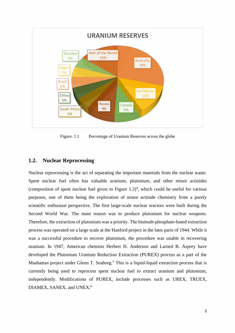
Uranium is one of the main sources for nuclear power as it is one of the reasonably abundant
materials. Canada has the joint 3rd largest uranium reserves along with Russia, only less than
those of Australia and Kazakhstan (Figure 1.1).2 It is estimated that uranium is also present in
sea water at a concentration of 3µg/l, which amounts to 4.4 billion tons of uranium.3 Nuclear
fuel that is being used often generates waste. This is called nuclear waste and is radioactive,
and its disposal requires high level safety measures. Nuclear waste contains unused fuel, and
some important transuranic elements like Americium which are of scientific interest in order
to explore the physical and chemical properties of the heavy elements.4 Separation of actinides
from nuclear waste has been a priority to recover the potentially useful metals, mainly uranium
and other actinides.
2
Figure. 1.1 Percentage of Uranium Reserves across the globe
1.2. Nuclear Reprocessing
Nuclear reprocessing is the act of separating the important materials from the nuclear waste.
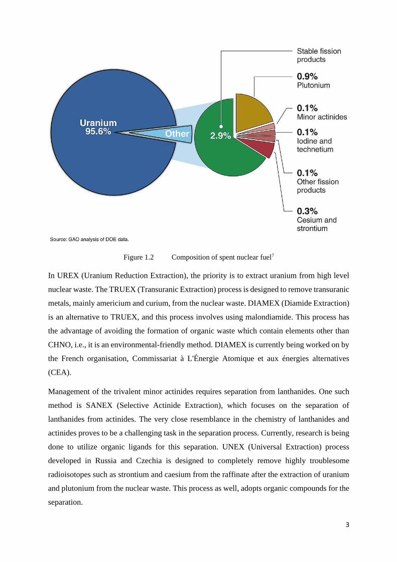
Spent nuclear fuel often has valuable uranium, plutonium, and other minor actinides
(composition of spent nuclear fuel given in Figure 1.2)4, which could be useful for various
purposes, one of them being the exploration of minor actinide chemistry from a purely
scientific enthusiast perspective. The first large-scale nuclear reactors were built during the
Second World War. The main reason was to produce plutonium for nuclear weapons.
Therefore, the extraction of plutonium was a priority. The bismuth-phosphate-based extraction
process was operated on a large scale at the Hanford project in the later parts of 1944. While it
was a successful procedure to recover plutonium, the procedure was unable in recovering
uranium. In 1947, American chemists Herbert H. Anderson and Larned B. Asprey have
developed the Plutonium Uranium Reduction Extraction (PUREX) process as a part of the
Manhattan project under Glenn T. Seaborg.5 This is a liquid-liquid extraction process that is
currently being used to reprocess spent nuclear fuel to extract uranium and plutonium,
independently. Modifications of PUREX, include processes such as UREX, TRUEX,
DIAMEX, SANEX, and UNEX.6
Australia29%
Kazhakstan13%
Canada9%
Russia9%South Africa
5%
China5%
Brazil5%
Niger5%
Namibia5%
Rest of the World15%
URANIUM RESERVES
3
Figure 1.2 Composition of spent nuclear fuel7
In UREX (Uranium Reduction Extraction), the priority is to extract uranium from high level
nuclear waste. The TRUEX (Transuranic Extraction) process is designed to remove transuranic
metals, mainly americium and curium, from the nuclear waste. DIAMEX (Diamide Extraction)
is an alternative to TRUEX, and this process involves using malondiamide. This process has
the advantage of avoiding the formation of organic waste which contain elements other than
CHNO, i.e., it is an environmental-friendly method. DIAMEX is currently being worked on by
the French organisation, Commissariat à L'Énergie Atomique et aux énergies alternatives
(CEA).
Management of the trivalent minor actinides requires separation from lanthanides. One such
method is SANEX (Selective Actinide Extraction), which focuses on the separation of
lanthanides from actinides. The very close resemblance in the chemistry of lanthanides and
actinides proves to be a challenging task in the separation process. Currently, research is being
done to utilize organic ligands for this separation. UNEX (Universal Extraction) process
developed in Russia and Czechia is designed to completely remove highly troublesome
radioisotopes such as strontium and caesium from the raffinate after the extraction of uranium
and plutonium from the nuclear waste. This process as well, adopts organic compounds for the
separation.
4
Separation of trivalent actinides from lanthanides in a very problematic challenge in nuclear
reprocessing. Trivalent lanthanides and actinides exhibit similar chemical behaviour such as
the exhibition of +3 oxidation state, ability to form complexes with similar types of ligands,
comparable ionic radii, etc. Regardless of this, many soft donor ligands have shown preference
to actinides over lanthanides when binding, possibly due to the greater availability of 5f orbitals
in comparison to the 4f orbitals of lanthanides.8,9 This a crucial and critical factor, as the
bonding differences in actinide complexes and lanthanide complexes could help us in
understanding the chemistry of actinides, as well as help in nuclear reprocessing. Recent studies
have suggested the potential of N-donor and/or N-O donor ligands, and their role in the
separation of such useful metals from the waste.9–14 N-donor ligands are currently being
investigated by various research groups in the actinide community to explore their potential in
the separation of actinides. The nitrogen atom’s lone pair provides an opportunity for the 5f
orbitals in the actinides to bind, thereby, helping with the extraction of the actinides.
Terpy (2,2’:6’,2”-terpyridine), first synthesised in the 1930s, has been introduced in the
extraction process for the separation of lanthanides and actinides in 1970s. Its heterocyclic
trident N-donor structure has proven to be the basis for many extraction ligands including BTP
(2,6-bis(1,2,4-triazine-3-yl)pyridine) and BTBP (6,6’-bis(1,2,4-triazine-3-yl)-
[2,2’]bipyridinyl). In acidic conditions, i.e., when the pH is low, extraction ligands need to have
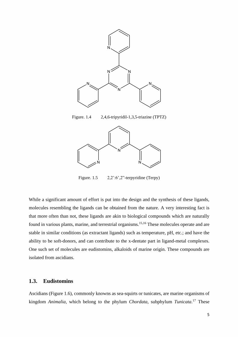
lower proton affinity. TPTZ (2,4,6-tripyridil-1,3,5-triazine) is one such molecule which is used
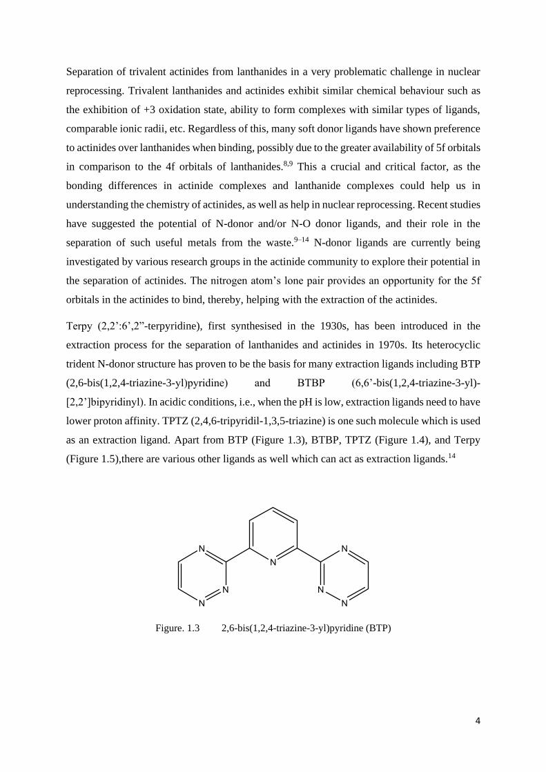
as an extraction ligand. Apart from BTP (Figure 1.3), BTBP, TPTZ (Figure 1.4), and Terpy
(Figure 1.5),there are various other ligands as well which can act as extraction ligands.14
Figure. 1.3 2,6-bis(1,2,4-triazine-3-yl)pyridine (BTP)
5
Figure. 1.4 2,4,6-tripyridil-1,3,5-triazine (TPTZ)
Figure. 1.5 2,2’:6’,2”-terpyridine (Terpy)
While a significant amount of effort is put into the design and the synthesis of these ligands,
molecules resembling the ligands can be obtained from the nature. A very interesting fact is
that more often than not, these ligands are akin to biological compounds which are naturally
found in various plants, marine, and terrestrial organisms.15,16 These molecules operate and are
stable in similar conditions (as extractant ligands) such as temperature, pH, etc.; and have the
ability to be soft-donors, and can contribute to the x-dentate part in ligand-metal complexes.
One such set of molecules are eudistomins, alkaloids of marine origin. These compounds are
isolated from ascidians.
1.3. Eudistomins
Ascidians (Figure 1.6), commonly knowns as sea-squirts or tunicates, are marine organisms of
kingdom Animalia, which belong to the phylum Chordata, subphylum Tunicata.17 These
6
animals supposedly have been on earth since the Ediacaran period (635 to 541 million years
ago), with studies strongly suggesting their presence since the Jurassic times (201.3 to 145
million years ago).18–22 These animals are found all around the world in marine environment.
Despite their evolution and presence in the modern-day world, which emphasizes on their
‘adaption to change’, there is a lack of proper fossil evidence as these animals are soft and
sessile after their larval phase. For this reason, as a part of their ‘adaption to change’, it is
believed that they have adopted various techniques to void predation.
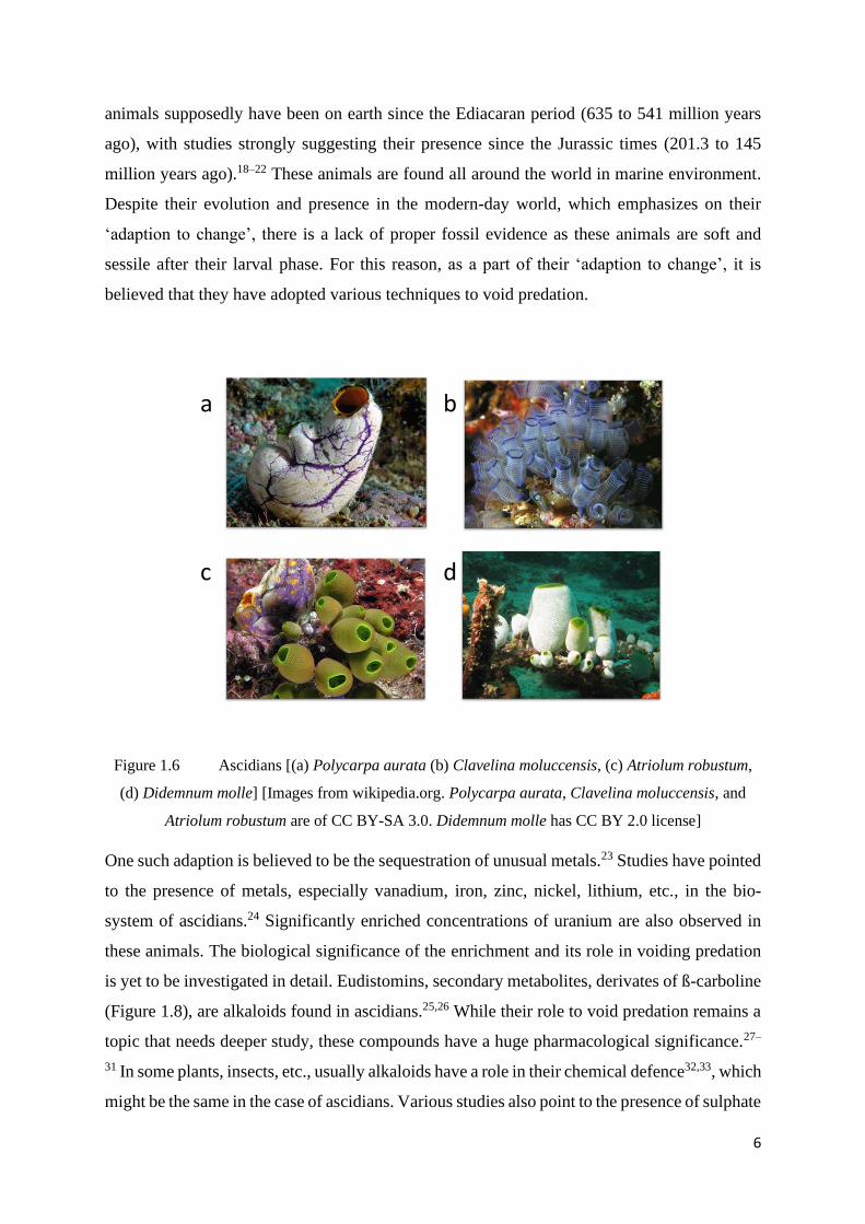
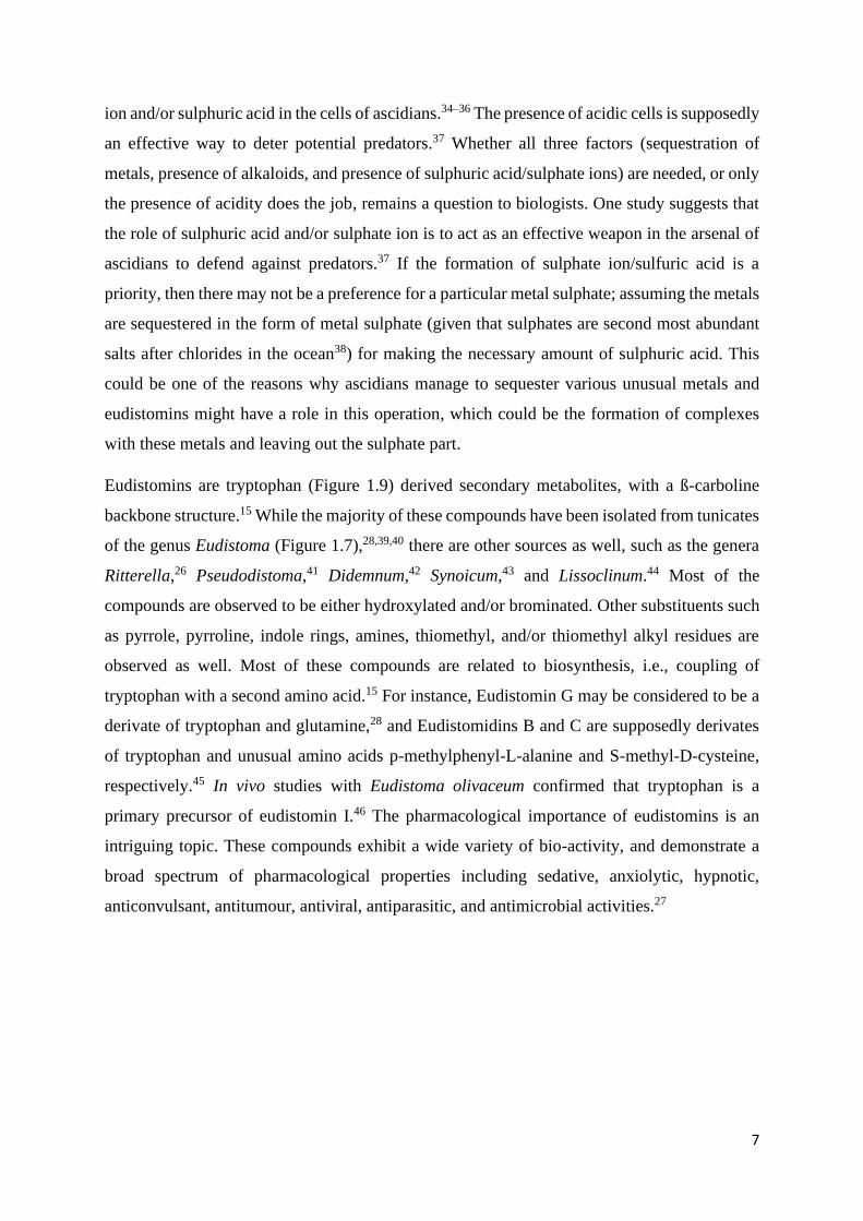
Figure 1.6 Ascidians [(a) Polycarpa aurata (b) Clavelina moluccensis, (c) Atriolum robustum,
(d) Didemnum molle] [Images from wikipedia.org. Polycarpa aurata, Clavelina moluccensis, and
Atriolum robustum are of CC BY-SA 3.0. Didemnum molle has CC BY 2.0 license]
One such adaption is believed to be the sequestration of unusual metals.23 Studies have pointed
to the presence of metals, especially vanadium, iron, zinc, nickel, lithium, etc., in the bio-
system of ascidians.24 Significantly enriched concentrations of uranium are also observed in
these animals. The biological significance of the enrichment and its role in voiding predation
is yet to be investigated in detail. Eudistomins, secondary metabolites, derivates of ß-carboline
(Figure 1.8), are alkaloids found in ascidians.25,26 While their role to void predation remains a
topic that needs deeper study, these compounds have a huge pharmacological significance.27–
31 In some plants, insects, etc., usually alkaloids have a role in their chemical defence32,33, which
might be the same in the case of ascidians. Various studies also point to the presence of sulphate
a b
c d
7
ion and/or sulphuric acid in the cells of ascidians.34–36 The presence of acidic cells is supposedly
an effective way to deter potential predators.37 Whether all three factors (sequestration of
metals, presence of alkaloids, and presence of sulphuric acid/sulphate ions) are needed, or only
the presence of acidity does the job, remains a question to biologists. One study suggests that
the role of sulphuric acid and/or sulphate ion is to act as an effective weapon in the arsenal of
ascidians to defend against predators.37 If the formation of sulphate ion/sulfuric acid is a
priority, then there may not be a preference for a particular metal sulphate; assuming the metals
are sequestered in the form of metal sulphate (given that sulphates are second most abundant
salts after chlorides in the ocean38) for making the necessary amount of sulphuric acid. This
could be one of the reasons why ascidians manage to sequester various unusual metals and
eudistomins might have a role in this operation, which could be the formation of complexes
with these metals and leaving out the sulphate part.
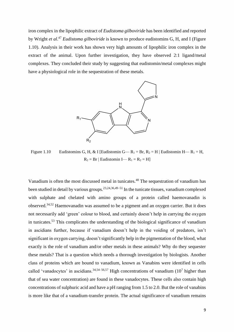
Eudistomins are tryptophan (Figure 1.9) derived secondary metabolites, with a ß-carboline
backbone structure.15 While the majority of these compounds have been isolated from tunicates
of the genus Eudistoma (Figure 1.7),28,39,40 there are other sources as well, such as the genera
Ritterella,26 Pseudodistoma,41 Didemnum,42 Synoicum,43 and Lissoclinum.44 Most of the
compounds are observed to be either hydroxylated and/or brominated. Other substituents such
as pyrrole, pyrroline, indole rings, amines, thiomethyl, and/or thiomethyl alkyl residues are
observed as well. Most of these compounds are related to biosynthesis, i.e., coupling of
tryptophan with a second amino acid.15 For instance, Eudistomin G may be considered to be a
derivate of tryptophan and glutamine,28 and Eudistomidins B and C are supposedly derivates
of tryptophan and unusual amino acids p-methylphenyl-L-alanine and S-methyl-D-cysteine,
respectively.45 In vivo studies with Eudistoma olivaceum confirmed that tryptophan is a
primary precursor of eudistomin I.46 The pharmacological importance of eudistomins is an
intriguing topic. These compounds exhibit a wide variety of bio-activity, and demonstrate a
broad spectrum of pharmacological properties including sedative, anxiolytic, hypnotic,
anticonvulsant, antitumour, antiviral, antiparasitic, and antimicrobial activities.27
8
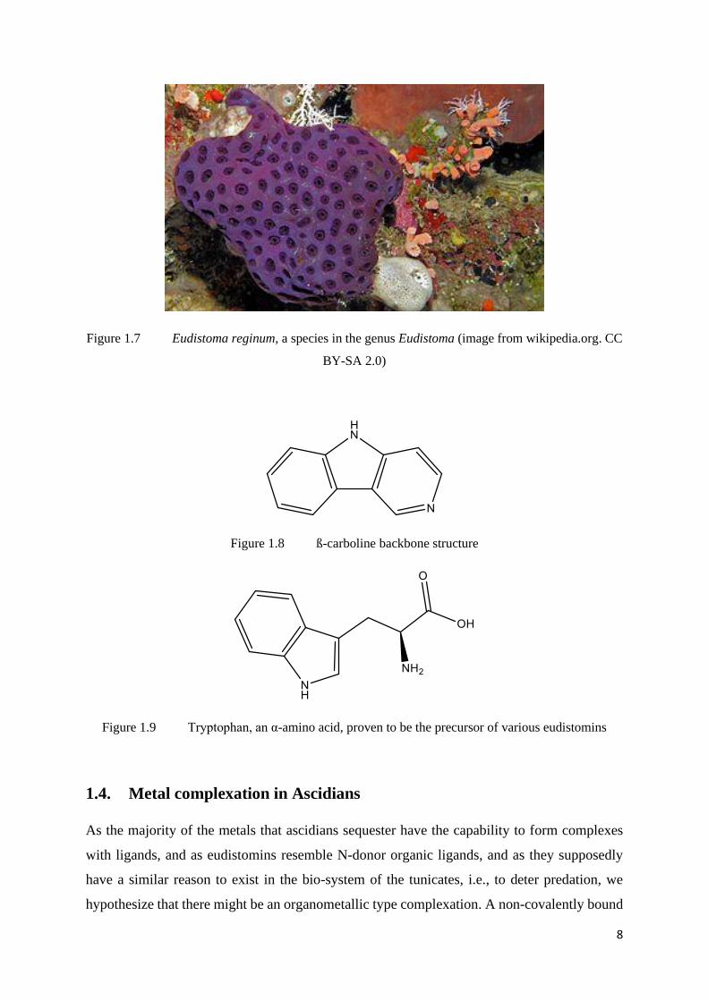
Figure 1.7 Eudistoma reginum, a species in the genus Eudistoma (image from wikipedia.org. CC
BY-SA 2.0)
Figure 1.8 ß-carboline backbone structure
Figure 1.9 Tryptophan, an α-amino acid, proven to be the precursor of various eudistomins
1.4. Metal complexation in Ascidians
As the majority of the metals that ascidians sequester have the capability to form complexes
with ligands, and as eudistomins resemble N-donor organic ligands, and as they supposedly
have a similar reason to exist in the bio-system of the tunicates, i.e., to deter predation, we
hypothesize that there might be an organometallic type complexation. A non-covalently bound
9
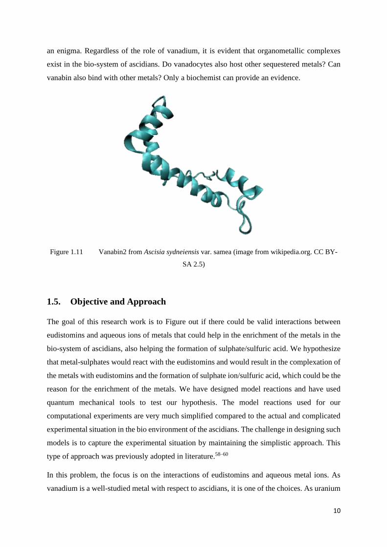
iron complex in the lipophilic extract of Eudistoma gilboviride has been identified and reported
by Wright et al.47 Eudistoma gilboviride is known to produce eudistomins G, H, and I (Figure
1.10). Analysis in their work has shown very high amounts of lipophilic iron complex in the
extract of the animal. Upon further investigation, they have observed 2:1 ligand/metal
complexes. They concluded their study by suggesting that eudistomin/metal complexes might
have a physiological role in the sequestration of these metals.
Figure 1.10 Eudistomins G, H, & I [Eudistomin G— R1 = Br, R2 = H | Eudistomin H— R1 = H,
R2 = Br | Eudistomin I— R1 = R2 = H]
Vanadium is often the most discussed metal in tunicates.48 The sequestration of vanadium has
been studied in detail by various groups.23,24,36,49–51 In the tunicate tissues, vanadium complexed
with sulphate and chelated with amino groups of a protein called haemovanadin is
observed.34,52 Haemovanadin was assumed to be a pigment and an oxygen carrier. But it does
not necessarily add ‘green’ colour to blood, and certainly doesn’t help in carrying the oxygen
in tunicates.53 This complicates the understanding of the biological significance of vanadium
in ascidians further, because if vanadium doesn’t help in the voiding of predators, isn’t
significant in oxygen carrying, doesn’t significantly help in the pigmentation of the blood, what
exactly is the role of vanadium and/or other metals in these animals? Why do they sequester
these metals? That is a question which needs a thorough investigation by biologists. Another
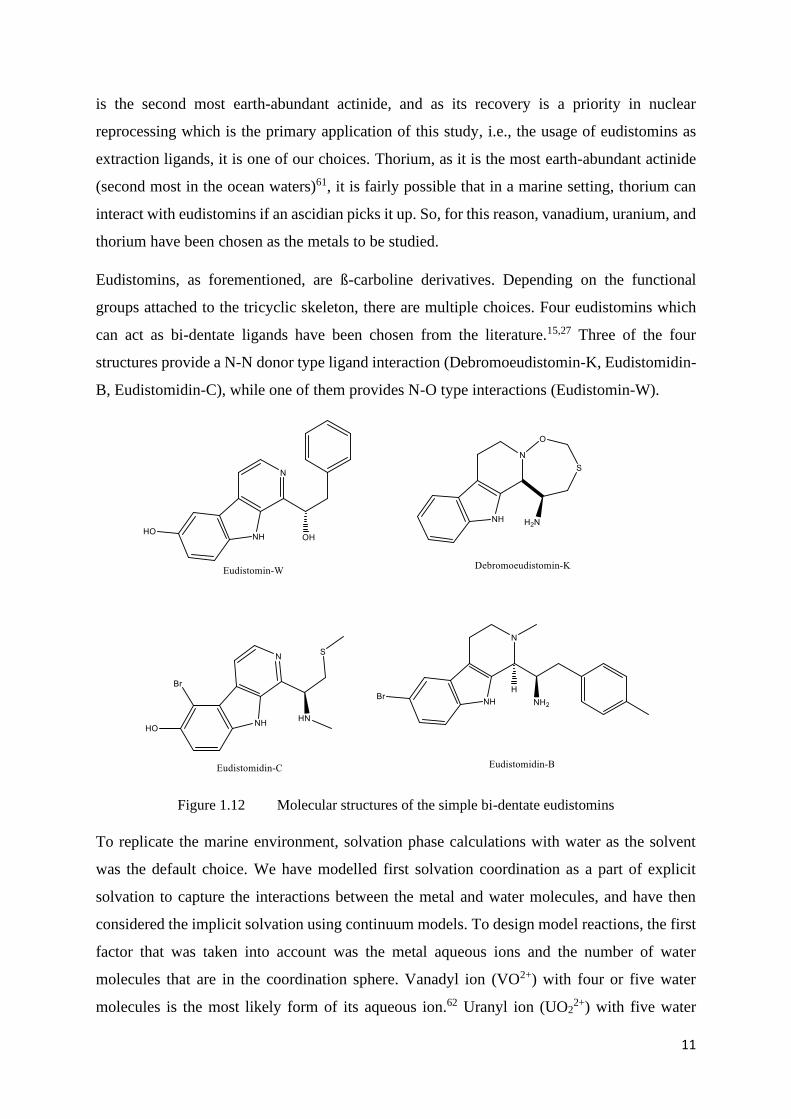
class of proteins which are bound to vanadium, known as Vanabins were identified in cells
called ‘vanadocytes’ in ascidians.34,54–56,57 High concentrations of vanadium (107 higher than
that of sea water concentration) are found in these vanadocytes. These cells also contain high
concentrations of sulphuric acid and have a pH ranging from 1.5 to 2.0. But the role of vanabins
is more like that of a vanadium-transfer protein. The actual significance of vanadium remains
10
an enigma. Regardless of the role of vanadium, it is evident that organometallic complexes
exist in the bio-system of ascidians. Do vanadocytes also host other sequestered metals? Can
vanabin also bind with other metals? Only a biochemist can provide an evidence.
Figure 1.11 Vanabin2 from Ascisia sydneiensis var. samea (image from wikipedia.org. CC BY-
SA 2.5)
1.5. Objective and Approach
The goal of this research work is to Figure out if there could be valid interactions between
eudistomins and aqueous ions of metals that could help in the enrichment of the metals in the
bio-system of ascidians, also helping the formation of sulphate/sulfuric acid. We hypothesize
that metal-sulphates would react with the eudistomins and would result in the complexation of
the metals with eudistomins and the formation of sulphate ion/sulfuric acid, which could be the
reason for the enrichment of the metals. We have designed model reactions and have used
quantum mechanical tools to test our hypothesis. The model reactions used for our
computational experiments are very much simplified compared to the actual and complicated
experimental situation in the bio environment of the ascidians. The challenge in designing such
models is to capture the experimental situation by maintaining the simplistic approach. This
type of approach was previously adopted in literature.58–60
In this problem, the focus is on the interactions of eudistomins and aqueous metal ions. As
vanadium is a well-studied metal with respect to ascidians, it is one of the choices. As uranium
11
is the second most earth-abundant actinide, and as its recovery is a priority in nuclear
reprocessing which is the primary application of this study, i.e., the usage of eudistomins as
extraction ligands, it is one of our choices. Thorium, as it is the most earth-abundant actinide
(second most in the ocean waters)61, it is fairly possible that in a marine setting, thorium can
interact with eudistomins if an ascidian picks it up. So, for this reason, vanadium, uranium, and
thorium have been chosen as the metals to be studied.
Eudistomins, as forementioned, are ß-carboline derivatives. Depending on the functional
groups attached to the tricyclic skeleton, there are multiple choices. Four eudistomins which
can act as bi-dentate ligands have been chosen from the literature.15,27 Three of the four
structures provide a N-N donor type ligand interaction (Debromoeudistomin-K, Eudistomidin-
B, Eudistomidin-C), while one of them provides N-O type interactions (Eudistomin-W).
Figure 1.12 Molecular structures of the simple bi-dentate eudistomins
To replicate the marine environment, solvation phase calculations with water as the solvent
was the default choice. We have modelled first solvation coordination as a part of explicit
solvation to capture the interactions between the metal and water molecules, and have then
considered the implicit solvation using continuum models. To design model reactions, the first
factor that was taken into account was the metal aqueous ions and the number of water
molecules that are in the coordination sphere. Vanadyl ion (VO2+) with four or five water
molecules is the most likely form of its aqueous ion.62 Uranyl ion (UO22+) with five water
12
molecules in the equatorial plane is the aqueous ion that has been chosen for this work.63
Thorium tetra-positive ion (Th4+) with nine water molecules is the aqueous ion that has been
adopted for the calculations.64 As forementioned, typically ascidians’ cells are highly acidic
with a pH at around 1.8-2.0.35,65 Also, the presence of sulphuric acid and/or sulphate ions is
reported in multiple studies. At pH ranging from 1.5 to 2.0, sulphuric acid mainly exists as
HSO4- ion. However, as sulphate ion (SO4
2-) was also mentioned in the literature34. This ion
was also taken into account. This means, on the product side of the reaction, there needs to be
a HSO4-/SO4
2- ion(s) or sulphuric acid.
With the details mentioned above, five model reactions are designed as follows. (The equations
here are given only as introduction, detailed equations will be discussed in the subsequent
chapters.) In reaction 1, the cation and anion combine to form the complex and water, akin to
a salt-type reaction. In the reaction 2, cation reacts with the neutral ligand, and forms the
complex. The charge in this reaction is transferred to the hydronium ions. In reaction 3, the
metal-sulphate reacts with the neutral eudistomin ligand to form complex and sulphuric acid.
In reaction 4, the metal-sulphate reacts with the ligand anion, forming the complex. The charge
in this reaction is transferred to the sulphate anion. In reaction 5, the metal-sulphate reacts with
the ligand anion in the presence of sulfuric acid, forming the complex and transferring the
charge to HSO4- ions.
1. Aqueous cation + Eudistomin ligand anion => Complex + n. Water
2. Aqueous cation + Neutral eudistomin ligand => Complex + n. Hydronium ion(s)
3. Sulphate + Neutral eudistomin ligand => Complex + n. Sulphuric acid
4. Sulphate + Eudistomin ligand anion => Complex + n. SO42-
5. Sulphate + Sulphuric acid + Eudistomin ligand anion => Complex + n. HSO4-
With the above model reactions, the formation energies of the complexes are calculated to
validate the interactions between the metals and the eudistomins.
1.6. Organization of the thesis
The aim of this thesis is to understand if valid interactions are possible between naturally
occurring actinide metal aqua ions and eudistomins found in ascidians. Based on this study, we
aim at determining if eudistomins can be employed as extractant ligands in nuclear
reprocessing.
13
Chapter 1 and 2 serve as introductory chapters, the former providing a generic introduction and
the latter providing an introduction to the computational methodology adopted in this work.
Chapter 3 provides details about the research work done. Vanadyl, uranyl, and thorium aqua
ion interactions with Eudistomin-W, Debromoeudistomin-K, Eudistomidin-C, and
Eudistomidin-B were calculated using Density Functional Theory (DFT) methods PBE-D3,
BLYP, and B3LYP using Amsterdam Density Functional (ADF) and ORCA software
applications with the usage of relativistic and solvation effects, and the related data are
presented and discussed.
Chapter 4 provides the concluding remarks and future direction of this study.
14
CHAPTER-2
COMPUTATIONAL METHODS
Theoretical chemistry is a branch of chemistry that focuses on developing mathematically
constructed equations which are built on the laws of physics to study chemical properties.
Computational chemistry is the branch where the focus is on the application of theoretical
methods to simulate, study, and solve various types of chemical problems. The first attempts
to solve chemical problems using theoretical methods date back to 1927, using Valence Bond
Theory. With the development of sufficient computer technologies in 1940s, in the early 1950s,
the first semi empirical atomic orbital calculations were performed. By the mid 1970s, Hartree-
Fock and ab initio methods were well established to solve poly atomic molecular chemical
problems.66–69 Density Functional Theory (DFT) was popular among solid state physicists by
the 1970s, and its use among chemists has become popular by the 1990s chiefly due to the
development of better functionals. Today, DFT methods can be surmised as the ‘heart’ of
modern-day computational chemistry. Computational chemists have been recipients of the
Nobel Prize, conspicuously in 1998 and 2013. Walter Kohn and John Pople have been awarded
the Nobel Prize for their works “Development of the Density-Functional-Theory” and
“Development of computational methods in quantum chemistry” in 1998.70 Martin Karplus,
Michael Levitt, and Arieh Warshel have been awarded the Nobel Prize in 2013 for
“Development of multiscale models for complex chemical systems”.71
More often than not, computational chemistry serves as the “theoretical lab” for various
chemical problems. Where experiments are either difficult to perform, need to find a ‘starting
point’, need a ‘double-check’, simply cannot explain certain results, or need a ‘design’ for a
novel molecule; computational chemistry is the go-to-tool. How accurate are the results
obtained from the computational chemistry tools? This depends on the level of theory used,
conditions assumed, and approximations made. The best computational choice is always
computationally expensive, i.e., it requires a large amount of computational ‘power’. The
‘cheapest’ computational method is, more often than not, not so accurate, ergo, gives dross.
The cliché ‘one needs to find balance’ fits perfectly for the computational problems as well.
As atoms have nuclei and electrons, most computational methods are built on the basis of
quantum mechanics, and they attempt to solve the non-relativistic Schrödinger equation, with
15
relativistic corrections added (where applicable). Solving the fully relativistic Dirac equation
is an ongoing and active area of research in computational chemistry. There are a number of
approximate methods which give the ‘right balance’ betwixt accuracy and computational cost.
2.1. Schrödinger’s Equation
The contents in the section are adopted from the works of Schrödinger, Cramer, and Jensen.72–
74
Schrödinger’s equation is arguably one of the greatest modern-day scientific discoveries.
Dissimilar to classical mechanics, quantum mechanical problems are not deterministic, but are
probabilistic. Quantum mechanical calculations would allow us to ‘know’ the probability of a
quantum particle at a certain place, at a certain time. The probability function P(r,t) [where r =
position, t = time] is given as the square of the wave function, Ψ (r,t) (see eq. 2.1.1).
P(r,t) = |Ψ|2(r,t) (eq. 2.1.1)
The wave function can be obtained by solving the Schrödinger wave equation, which can be
given in a simple form (eq. 2.1.2). [This shows the time independent Schrödinger wave
equation]
�̂�𝛹(𝑟, 𝑡) = 𝐸𝛹(𝑟, 𝑡) (eq. 2.1.2)
Where, �̂� is the Hamiltonian operator
E is the energy of the system.
In linear algebraic terms, the wavefunction is an eigenfunction of the Hamiltonian operator
with the corresponding eigenvalue(s) E.
In its general form, the time-dependant Schrödinger equation can be given as follows (eq.
2.1.3).
�̂� |𝛹(𝑟, 𝑡)› = 𝑖ħ𝑑
𝑑𝑡| 𝛹(𝑟, 𝑡)› (eq. 2.1.3)
Where, i is the imaginary unit, and ħ is the reduced Planck’s constant.
For a molecular system, the Hamiltonian has five contributors (eq. 2.14).
16
�̂� = − ∑ħ2
2𝑚𝑒∇𝑖
2𝑖 − ∑
ħ2
2𝑚𝑘∇𝑘
2𝑘 − ∑ ∑
𝑒2𝑍𝑘
𝑟𝑖𝑘𝑘𝑖 + ∑
𝑒2
𝑟𝑖𝑗𝑖<𝑗 + ∑
𝑒2𝑍𝑘𝑍𝑙
𝑟𝑘𝑙𝑘<𝑙 (eq. 2.1.4)
Where i and j correspond to electrons, k and l to nuclei, me is the mass of an electron, mk is the
mass of the nucleus, e is the charge on the electron, Z is the atomic number, and r is the distance
between the respective particles [the units are atomic units (a.u)].
The equation (eq. 2.1.4) has five terms. The first term is the kinetic energy term for each
electron in the molecular system. The second term corresponds to the kinetic energy of each
nucleus in the system. The third term relates to the total electron-nucleus Coulomb attraction
in the molecule. The fourth term is the potential energy from the electron-electron repulsions.
The fifth term is the potential energy from nucleus-nucleus repulsions.
2.2. Born-Oppenheimer Approximation
In a many-body system like that of a molecule, it is always arduous to obtain proper wave
functions, mainly because of the complexity in the Hamiltonian operator. For this reason, to
simplify the problem, one can take the aid of the Born-Oppenheimer approximation.75,76 In this
approximation, the nuclei and the electrons are treated separately, mainly because the nuclei
are massive, move much slower in comparison to the electrons, and are nearly fixed with
respect to the electron-motion. This can mean that one can compute electronic energies for
fixed nuclear positions. The kinetic energy term of the nucleus can be eliminated and the
nucleus-nucleus potential energy term is constant for a fixed geometry. Therefore, the
Schrödinger equation can be given as (eq. 2.2).
(�̂�𝑒𝑙 + 𝑉𝑁)𝛹𝑒𝑙(𝑞𝑖; 𝑞𝑘) = 𝐸𝑒𝑙𝛹𝑒𝑙(𝑞𝑖; 𝑞𝑘) (eq. 2.2)
The subscript ‘el’ emphasizes that the Born-Oppenheimer approximation is considered for
the equation. VN is the nucleus-nucleus potential energy term. qi and qk are independent
variables (electron and nucleus coordinates respectively)
Born-Oppenheimer approximation is fairly accurate for most of the cases, with exceptions. The
Schrödinger equation cannot be solved except for hydrogen atom and H2+ molecule. The
detailed discussion of this topic is beyond the scope of this study.
The contents in the section are adopted from the works of Cramer, Jensen, and Born &
Oppenheimer.73,74,77
17
2.3. Variational Method
The contents in the section are adopted from the works of Cramer, and Jensen.73,74
Variational method is one of the ways to find approximations to the least energy eigen state,
i.e., the ground state, to evaluate the wavefunctions, that of molecular orbitals in a molecular
system.78 A trial function is chosen, that obeys the boundary conditions of the molecular
system, which depends on adjustable variational parameters. By adjusting the variational
parameters, one can find the least energy trial function. The energy and the wavefunction of
the resulting trial function are variational approximations to the exact wavefunction and energy.
The ground state energy of the exact function is always lower than that of the trial function, as
given by the variational principle (eq. 2.3)
𝐸(𝛹) = <𝛹|�̂�|𝛹>
<𝛹|𝛹>≥ 𝐸0 (eq. 2.3)
Where E(Ψ) is the trial function and E0 is the exact ground state energy.
2.4. Perturbation Theory
The contents in the section are adopted from the works of Cramer, and Jensen.73,74
Perturbation theory, as the word suggests, adds perturbation to the existing Schrödinger’s
equation (eq. 2.4.1).
(�̂�0 + �̂�1)(𝛹0 + 𝛹1) = (𝐸0 + 𝐸1)(𝛹0 + 𝛹1) (eq. 2.4.1)
Where the superscript ‘0’ denotes existing states, and ‘1’ denotes the perturbation.
One can eliminate �̂�0𝛹0 and 𝐸0𝛹0 terms as they are zero-order terms. Similarly, �̂�1𝛹1 and
𝐸1𝛹1 terms correspond to second order terms. The first order perturbation can be given as (eq.
2.4.2).
�̂�0𝛹1 + �̂�1𝛹0 = 𝐸0𝛹1 + 𝐸1𝛹0 (eq. 2.4.2)
To obtain the first order correction to the energy, the above equation can be multiplied by Ψ0*
and integrated on both sides. This leaves us with (eq. 2.4.3).
𝐸1 = ∫ 𝛹0∗ �̂�1𝛹0𝑑𝜏 (eq. 2.4.3)
18
This way, the perturbation allows us to improve an existing zeroth order energy. The higher
order terms can be obtained via similar method.
2.5. Basis Sets
A basis set is a collection of mathematical functions that are used to construct a wave function.
The expansion of an unknown function such as a molecular orbital in a set of known functions
would not be an approximation if the basis set is complete. However, this requires an infinite
number of functions in most of the cases, which is an impossible task. A small number of basis
functions leads to a poor representation of the orbitals, while a larger basis set would test the
computational cost. The ‘balance’ plays a key role while selecting the basis sets. Modern day
computational chemistry offers mainly two flavours of basis sets, one with Slater Type Orbitals
(STOs)79, and the other being Gaussian Type Orbitals (GTOs).80
Slater type orbitals, named after John. C. Slater, who introduced them in 1930, have the
functional form shown in (eq. 2.5.1).
𝜒𝜁,𝑛,𝑙,𝑚 (𝑟, 𝜃, 𝜑) = 𝑁𝑌𝑙,𝑚(𝜃, 𝜑)𝑟𝑛−1𝑒−𝜁𝑟 (eq. 2.5.1)
Where, n is the principle quantum number of the valence orbitals, ζ is the exponent which
depends on the atomic number and can be chosen based on the rules developed by Slater, N is
the normalization constant, Yl,m (θ,φ) are spherical harmonic functions, where l and m are
angular quantum numbers , and the spherical coordinates are given by (r,θ,φ).
The shape of the atomic orbitals is well-defined by STOs. The accuracy that can be achieved
via STOs is of high level, as they are exhibiting exponential decay at a long range. The
modelling of the density, especially around the nucleus is accurate, ergo, less functions are
required to obtain a good fit. Despite this, STOs are not computation friendly, and cost a good
amount of computational time.
GTOs, the other flavour of basis sets, are fairly quick in comparison to STOs. This is because
they have 𝑒−𝑟2 dependence, unlike STOs, as shown in (eq. 2.5.2). As a consequence, the
relevant integrals can be evaluated analytically.
𝜒𝜁,𝑛,𝑙,𝑚 (𝑟, 𝜃, 𝜑) = 𝑁𝑌𝑙,𝑚(𝜃, 𝜑)𝑟2𝑛−2−𝑙𝑒−𝜁𝑟2
(eq.2.5.2)
19
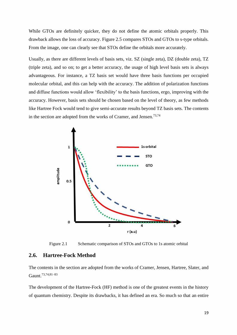
While GTOs are definitely quicker, they do not define the atomic orbitals properly. This
drawback allows the loss of accuracy. Figure 2.5 compares STOs and GTOs to s-type orbitals.
From the image, one can clearly see that STOs define the orbitals more accurately.
Usually, as there are different levels of basis sets, viz. SZ (single zeta), DZ (double zeta), TZ
(triple zeta), and so on; to get a better accuracy, the usage of high level basis sets is always
advantageous. For instance, a TZ basis set would have three basis functions per occupied
molecular orbital, and this can help with the accuracy. The addition of polarization functions
and diffuse functions would allow ‘flexibility’ to the basis functions, ergo, improving with the
accuracy. However, basis sets should be chosen based on the level of theory, as few methods
like Hartree Fock would tend to give semi-accurate results beyond TZ basis sets. The contents
in the section are adopted from the works of Cramer, and Jensen.73,74
Figure 2.1 Schematic comparison of STOs and GTOs to 1s atomic orbital
2.6. Hartree-Fock Method
The contents in the section are adopted from the works of Cramer, Jensen, Hartree, Slater, and
Gaunt.73,74,81–83
The development of the Hartree-Fock (HF) method is one of the greatest events in the history
of quantum chemistry. Despite its drawbacks, it has defined an era. So much so that an entire
20
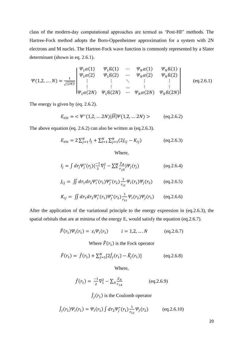
class of the modern-day computational approaches are termed as ‘Post-HF’ methods. The
Hartree-Fock method adopts the Born-Oppenheimer approximation for a system with 2N
electrons and M nuclei. The Hartree-Fock wave function is commonly represented by a Slater
determinant (shown in eq. 2.6.1).
𝛹(1,2, … . 𝑁) =1
√(2𝑁)! ||
𝛹1𝛼(1) 𝛹1ß(1) ⋯ 𝛹𝑁𝛼(1) 𝛹𝑁ß(1)
𝛹1𝛼(2) 𝛹1ß(2) ⋯ 𝛹𝑁𝛼(2) 𝛹𝑁ß(2)⋮ ⋮ ⋱ ⋮ ⋮⋮ ⋮ … ⋮ ⋮
𝛹1𝛼(2𝑁) 𝛹1ß(2𝑁) ⋯ 𝛹𝑁𝛼(2𝑁) 𝛹𝑁ß(2𝑁)
|| (eq.2.6.1)
The energy is given by (eq. 2.6.2).
𝐸𝑒𝑙𝑒 = < 𝛹∗(1,2, … .2𝑁)|𝐻|̂𝛹(1,2, … .2𝑁) > (eq.2.6.2)
The above equation (eq. 2.6.2) can also be written as (eq.2.6.3).
𝐸𝑒𝑙𝑒 = 2 ∑ 𝐼𝑗𝑁𝑗=1 + ∑ ∑ (2𝐽𝑖𝑗 − 𝐾𝑖𝑗)𝑁
𝑗=1𝑁𝑖=1 (eq.2.6.3)
Where,
𝐼𝑗 = ∫ 𝑑𝑟𝑗𝛹𝑗∗(𝑟𝑗)(
−1
2∇𝑗
2 − ∑𝑍𝐴
𝑟𝑗𝐴)𝛹𝑗(𝑟𝑗)𝑀
𝑁 (eq.2.6.4)
𝐽𝑖𝑗 = ∬ 𝑑𝑟1𝑑𝑟2𝛹𝑖∗(𝑟1)𝛹𝑗
∗(𝑟2)1
𝑟12𝛹𝑖(𝑟1)𝛹𝑗(𝑟2) (eq.2.6.5)
𝐾𝑖𝑗 = ∬ 𝑑𝑟1𝑑𝑟2𝛹𝑖∗(𝑟1)𝛹𝑗
∗(𝑟2)1
𝑟12𝛹𝑖(𝑟2)𝛹𝑗(𝑟1) (eq.2.6.6)
After the application of the variational principle to the energy expression in (eq.2.6.3), the
spatial orbitals that are at minima of the energy E, would satisfy the equation (eq.2.6.7).
�̂�(𝑟1)𝛹𝑖(𝑟1) = 𝜀𝑖𝛹𝑖(𝑟1) 𝑖 = 1,2, … . 𝑁 (eq.2.6.7)
Where �̂�(𝑟1) is the Fock operator
�̂�(𝑟1) = 𝑓(𝑟1) + ∑ [2𝐽𝑗(𝑟1) − �̂�𝑗(𝑟1)]𝑁𝑗=1 (eq.2.6.8)
Where,
𝑓(𝑟1) = −1
2∇1
2 − ∑𝑍𝐴
𝑟1𝐴𝐴 (eq.2.6.9)
𝐽𝑗(𝑟1) is the Coulomb operator
𝐽𝑗(𝑟1)𝛹𝑖(𝑟1) = 𝛹𝑖(𝑟1) ∫ 𝑑𝑟2𝛹𝑗∗(𝑟1)
1
𝑟12𝛹𝑗(𝑟2) (eq.2.6.10)
21
�̂�𝑗(𝑟1) is the exchange operator
�̂�𝑗(𝑟1)𝛹𝑖(𝑟1) = 𝛹𝑗(𝑟1) ∫ 𝑑𝑟2𝛹𝑗∗(𝑟2)
1
𝑟12𝛹𝑖(𝑟2) (eq.2.6.11)
An expression for the energy of the ith molecular orbital can be obtained by multiplying
(eq.2.6.7) from the left by 𝛹𝑖∗(𝑟1) and integrating with 𝑟1
𝜀𝑖 = ∫ 𝑑𝑟1𝛹𝑖∗(𝑟1)�̂�(𝑟1)𝛹𝑖(𝑟1) (eq.2.6.12)
Using the Fock operator, (eq.2.6.12) becomes,
𝜀𝑖 = 𝐼𝑗 ∑ [2𝐽𝑖𝑗 − 𝐾𝑖𝑗]𝑁𝑗=1 (eq.2.6.13)
Comparing (eq.2.6.13) and (2.6.3) would give,
𝐸 = ∑ [𝐼𝑖 + 𝜀𝑗]𝑁𝑖=1 (eq. 2.6.14)
Molecular orbitals could be concocted as the linear combinations of basis functions, as
developed by Clemens Roothaan.73,74,84,85
𝛹 = ∑ [𝑐𝜈𝜙𝜈]𝐾𝜈=1 (eq.2.6.15)
The Hartree-Fock-Roothaan equations are given by
∑ [𝐹𝜇𝜈𝑐𝜈]𝜐 = 𝜀 ∑ [𝑆𝜇𝜈𝑐𝜈]𝜐 𝜇 = 1,2,3, … … 𝐾 (eq.2.6.16)
Where, 𝐹𝜇𝜈 accounts for the Fock matrix elements and 𝑆𝜇𝜈 for the overlap matrix elements.
𝐹𝜇𝜈 = ∫ 𝑑𝑟1𝜙𝜇∗ (𝑟1)�̂�(𝑟1)𝜙𝜈(𝑟1) (eq.2.6.17)
𝑆𝜇𝜈 = ∫ 𝑑𝑟1𝜙𝜇∗ (𝑟1)𝜙𝜈(𝑟1) (eq.2.6.18)
The equation (eq.2.6.16) can be given in matrix notion as,
Fc = 𝜀Sc (eq.2.6.19)
Where, F and S are (K x K) matrices and, c is a (K x 1) column vector.
The equation (eq.2.6.19) could be solved via self-consistent procedure called Self-Consistent-
Field method (SCF method).73,74,82,86 Despite its greatness, HF method, as forementioned has
its drawbacks, and is prone to inconsistencies in delivering proper results that can be validated
by experimental results. These hindrances are addressed in most of the post-HF methods.
22
2.7. Density Functional Theory
The contents in the section are adopted from the works of Cramer, and Jensen.73,74
Often regarded as the best way of addressing quantum chemical problems, Density Functional
Theory (DFT) is one of the extensively used ways to solve the electronic structure of many-
body system problems pertaining to atoms, molecules, condensed phase systems, etc. Most
computational works often have DFT as their go-to method, such is the accuracy as well as
popularity.73,74,87–92
The basis or the theoretical foundation of DFT was developed by Walter Kohn and Pierre
Hohenberg by two theorems known as Hohenberg-Kohn theorems, or HK theorems.93 The first
theorem points that the external potential [V(r)] is a unique functional of the electron density
[ρ(r)], as shown in equation (eq.2.7.1). This means that the ground state density of a system is
determined uniquely by the potential and therefore the other properties of the same system can
be determined as well. The second theorem states that if the input density is the true ground
state density of a system, then the functional that delivers the ground state energy of the system
gives the lowest energy of the same system, which means that the ground state energy E0 can
be obtained variationally (eq.2.7.2).
𝐸[𝜌(𝑟)] = ∫ 𝜌(𝑟)𝑉(𝑟) ⅆ𝑟 + 𝐹[𝜌(𝑟)] (eq.2.7.1)
where 𝐹[𝜌(𝑟)] is the universal functional of the electron density 𝜌(𝑟)
𝐸[𝜌(𝑟)] = ∫ 𝜌(𝑟)𝑉(𝑟) ⅆ𝑟 + 𝐹[𝜌(𝑟)] ≥ E0 (eq.2.7.2)
2.7.1. Kohn-Sham Theory
The contents in the section are adopted from the works of Jensen, and Kohn & Sham.74,94
While there have been orbital-free DFT models, most of them have resulted in a poor
representation of the kinetic energy. Kohn-Sham (KS) theory was developed in a way, where
it splits the kinetic energy into two parts, the first term can be calculated exactly and the second
term is a correction term. In the first term, the kinetic energy of a fictious system made of non-
interacting electrons is calculated exactly, while in the second term the corrections to the kinetic
energy and the electron-electron repulsion energy are taken into account. The Kohn-Sham
model resembles the Hartree-Fock model by sharing identical formulations.
23
If λ=0 represents a fictious system, and λ=1 represents a real system, with 0 ≤ 𝜆 ≤ 1, the
Hamiltonian can assume the form as shown in (eq.2.7.3)
Hλ = T + Vext (λ) + λVext (eq.2.7.3)
For λ=0, the electrons are non-interacting, and the exact solution to the Schrödinger equation
is given as a Slater determinant composed of MOs ϕi, and the kinetic energy is given as
(eq.2.7.4)
𝑇𝑆 = ∑ ⟨𝜙𝑖|−1
2∇2|𝜑𝑖⟩
𝑁𝑒𝑙𝑒𝑖=1 (eq.2.7.4)
The λ=1 case is of the interacting electrons, and could be only approximated to the real kinetic
energy.
Another possible way to obtain justification to the use of (eq.2.7.4) to calculate the kinetic
energy is by referring to the natural orbitals, i.e., the eigenvectors of the density matrix. The
exact kinetic energy can be obtained from the natural orbitals (NO) arising from the exact
density matrix.
𝑇[𝜌𝑒𝑥𝑎𝑐𝑡] = ∑ 𝑛𝑖 ⟨𝜙𝑖𝑁𝑂|
−1
2∇2|𝜙𝑖
𝑁𝑂⟩∞𝑖=1 (eq.2.7.5)
[𝜌𝑒𝑥𝑎𝑐𝑡] = ∑ 𝑛𝑖|𝜙𝑗𝑁𝑂|2∞
𝑖=1 (eq.2.7.6)
𝑁𝑒𝑙𝑒𝑐 = ∑ 𝑛𝑖∞𝑖=1 (eq.2.7.7)
As the occupancy number of a natural orbital ni will be between 0 and 1, corresponding to the
number of electrons in the orbital, representation of the exact density would require an infinite
number of natural orbitals. Since the exact density is not known, an approximate density can
be given as a set of auxiliary one-electron functions, i.e., orbitals.
[𝜌𝑎𝑝𝑝𝑟𝑜𝑥] = ∑ |𝜙𝑖|2𝑁𝑒𝑙𝑒𝑐
𝑖=1 (eq.2.7.8)
Kohn-Sham theory calculates the kinetic energy under the assumption of non-interacting
electrons, similar to HF orbitals in wave mechanics. The difference between the exact kinetic
energy and that which is calculated by the assumption of non-interacting orbitals is small. The
remaining kinetic energy is adsorbed into an exchange-correlation term, and a generic DFT
energy expression can be given by (eq.2.7.9).
EDFT [ρ] = TS [ρ] + V[ρ] + EXC [ρ] (eq.2.7.9)
Where ρ is the electron density
24
TS is the kinetic energy obtained from the Slater determinant of the hypothetical system,
V is the classical potential energy term,
and EXC is the exchange-correlation term.
The exchange-correlation term is the element which makes various approximate DFT methods
to be different from each other. The complete solution to the Schrödinger equation can be
obtained if one can obtain the exact value to the exchange-correlation problem. Few techniques
to tackle this problem are Local Density Approximation (LDA), Generalized Gradient
Approximation (GGA), Meta-GGA, Hyper-GGA or Hybrid functionals, and Generalized
Random Phase Approximation (GRPA) methods. The addition of dispersion corrections to the
existing DFT methods would result in the betterment of the results.95–97 One such popular
correction is D3 as given by Grimme et al98. It is known to provide improved results and is
widely used among the computational chemists.
EDFT-dispersion corrected = EDFT + Edispersion correction (eq.2.7.10)
2.7.2. Local Density Approximation (LDA)
The contents in the section are adopted from the work of Jensen.74
In LDA, it is assumed that the density can be treated as a uniform electron gas locally, or
equivalently that the density is a slowly varying function. The exchange correlation term for
spin-unpolarized system by LDA is given by,
𝐸𝑋𝐶𝐿𝐷𝐴[𝜌(𝑟)] = ∫ 𝜌(𝑟) 𝜀𝑋𝐶(𝜌(𝑟)) 𝑑𝑟 (eq.2.7.11)
Where ρ(r) is the local value of the electron density at any position r
εXC is the exchange correlation energy per particle of the homogenous electron gas (HEG) of
charge density ρ
2.7.3. Generalized Gradient Approximation (GGA)
The contents in the section are adopted from the work of Jensen.74
An improvement to the LDA approach, GGA also accounts for the electron density gradient.
𝐸𝑋𝐶𝐺𝐺𝐴[𝜌(𝑟)] = 𝐸𝑋𝐶
𝐿𝐷𝐴[𝜌(𝑟)] + ∆𝐸𝑋𝐶 [|∇𝜌(𝑟)
𝜌43𝑟
] (eq.2.7.12)
25
2.7.4. Meta-GGA
The contents in the section are adopted from the work of Jensen.74
In Meta-GGA, the exchange correlation functional depends on second order terms, with the
Laplacian being the second order term. The calculation of orbital kinetic energy density is
numerically more stable than the calculation of the Laplacian of the density. The functional can
be taken to depend on the orbital kinetic energy density τ.
𝜏(𝑟) = 1
2∑ |∇𝜙𝑖(𝑟)|2𝑜𝑐𝑐𝑢𝑝𝑖𝑒𝑑
𝑖 (eq.2.7.13)
2.7.5. Hybrid functionals
The contents in the section are adopted from the work of Jensen.74
Hybrid theory, as the name suggests, is about linking two different levels of theory to make a
hybrid. Also known as Hyper-GGA method, this method focuses on linking exchange
correlation energy and the corresponding potential connecting the non-interacting reference
and the actual system. The equation, known as Adiabatic Connection Formula (ACF), helps in
integrating over the parameter λ, which “turns on” the electron-electron interaction. Usually,
the hybrid functionals have x% of HF exchange energy, y% of GGA functional exchange
energy along with the correlation energy. An example, PBE099 is given in the (eq.2.7.15)
𝐸𝑋𝐶 = ∫ ⟨𝛹(𝜆)|𝑉𝑋𝐶(𝜆)|𝛹(𝜆)⟩ 𝑑𝜆1
0 (eq.2.7.14)
Exchange-Correlation energy of PBE0 = 25% HF exchange energy + 75% PBE exchange
energy + 100% PBE correlation energy (eq.2.7.15)
2.7.6. Generalized Random Phase Approximation
The contents in the section are adopted from the work of Jensen.74
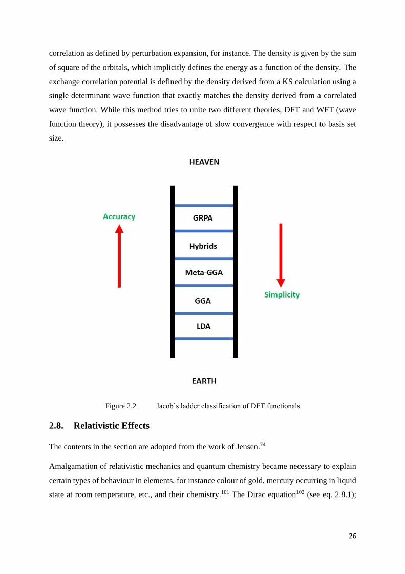
At the top of the Jacob’s ladder classification100 (shown in Figure 2.7), where the full
information of the Kohn-Sham orbitals, both virtual and occupied orbitals, is considered, the
formalism is identical to the methods adopted in the Generalized Random Phase
Approximation (GRPA). While the inclusion of the virtual orbitals certainly improves a few
aspects like van der Waals interactions, etc., very little work is done on these methods. One
such development is the class of Optimized Effective Potential (OEP) methods, where mainly
the exchange-correlation energy is treated as a functional of the unknown density, but the
energy as a function of the orbitals given by the wave function theory to a given order in the
26
correlation as defined by perturbation expansion, for instance. The density is given by the sum
of square of the orbitals, which implicitly defines the energy as a function of the density. The
exchange correlation potential is defined by the density derived from a KS calculation using a
single determinant wave function that exactly matches the density derived from a correlated
wave function. While this method tries to unite two different theories, DFT and WFT (wave
function theory), it possesses the disadvantage of slow convergence with respect to basis set
size.
Figure 2.2 Jacob’s ladder classification of DFT functionals
2.8. Relativistic Effects
The contents in the section are adopted from the work of Jensen.74
Amalgamation of relativistic mechanics and quantum chemistry became necessary to explain
certain types of behaviour in elements, for instance colour of gold, mercury occurring in liquid
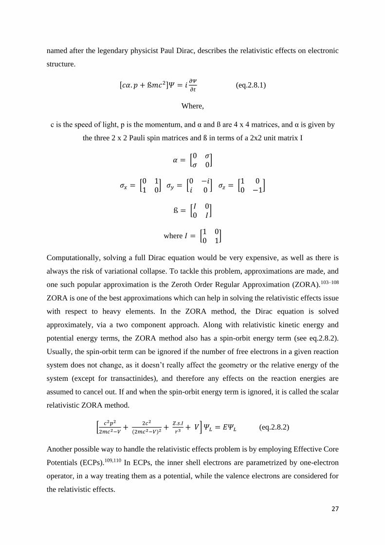
state at room temperature, etc., and their chemistry.101 The Dirac equation102 (see eq. 2.8.1);
27
named after the legendary physicist Paul Dirac, describes the relativistic effects on electronic
structure.
[𝑐𝛼. 𝑝 + ß𝑚𝑐2]𝛹 = 𝑖𝜕𝛹
𝜕𝑡 (eq.2.8.1)
Where,
c is the speed of light, p is the momentum, and α and ß are 4 x 4 matrices, and α is given by
the three 2 x 2 Pauli spin matrices and ß in terms of a 2x2 unit matrix I
𝛼 = [0 𝜎𝜎 0
]
𝜎𝑥 = [0 11 0
] 𝜎𝑦 = [0 −𝑖𝑖 0
] 𝜎𝑧 = [1 00 −1
]
ß = [𝐼 00 𝐼
]
where 𝐼 = [1 00 1
]
Computationally, solving a full Dirac equation would be very expensive, as well as there is
always the risk of variational collapse. To tackle this problem, approximations are made, and
one such popular approximation is the Zeroth Order Regular Approximation (ZORA).103–108
ZORA is one of the best approximations which can help in solving the relativistic effects issue
with respect to heavy elements. In the ZORA method, the Dirac equation is solved
approximately, via a two component approach. Along with relativistic kinetic energy and
potential energy terms, the ZORA method also has a spin-orbit energy term (see eq.2.8.2).
Usually, the spin-orbit term can be ignored if the number of free electrons in a given reaction
system does not change, as it doesn’t really affect the geometry or the relative energy of the
system (except for transactinides), and therefore any effects on the reaction energies are
assumed to cancel out. If and when the spin-orbit energy term is ignored, it is called the scalar
relativistic ZORA method.
[𝑐2𝑝2
2𝑚𝑐2−𝑉+
2𝑐2
(2𝑚𝑐2−𝑉)2 + 𝑍.𝑠.𝐼
𝑟3 + 𝑉] 𝛹𝐿 = 𝐸𝛹𝐿 (eq.2.8.2)
Another possible way to handle the relativistic effects problem is by employing Effective Core
Potentials (ECPs).109,110 In ECPs, the inner shell electrons are parametrized by one-electron
operator, in a way treating them as a potential, while the valence electrons are considered for
the relativistic effects.
28
The advantage of using ZORA is that it is an all-electron calculation, while ECP is not.
Adopting ZORA with small/large frozen core would reduce the computational cost, as the core
electrons are calculated only once for to obtain their states, and then it remains that way
throughout the rest of the calculation. The frozen core ZORA approach gives us the right
balance between the computational cost and the accuracy.
2.9. Solvation Effects
The contents in the section are adopted from the work of Cramer.73
It is only logical to adopt solvation effects for calculations that involve the marine world.
Solvation effects show a very significant difference in comparison to their gaseous counter
parts. For instance, cation and anion interactions in gas phase result in extremely high
formation energies, while in aqueous phase, not so.
Solvation effects can be calculated via explicit and implicit/continuum solvation models.
Explicit solvation adds a number of solvent molecules around the solute molecule. As the size
of the molecule becomes large, computational cost increases due to the addition of solvent
molecules, and this addition of solvent molecules makes the search for global minima much
more difficult. A continuum model can be defined as a model with a number of the degrees of
freedom of the constituent particles that are described in a continuous way, usually by a
distribution function. Of the widely used solvation models, two implicit models are Polarized
Continuum Model (PCM)111–114 and Conductor like Screening Model (COSMO)115,116. PCM
model comes mainly in two flavours, dielectric PCM (D-PCM), where it adopts polarizable
continuum, and the second type is conductor like PCM (CPCM), which is basically COSMO
in PCM. In COSMO, the surrounding medium is well modelled as a conductor, but lacks the
proper modelling of the specific interactions between solute and solvent molecules. This
problem can be tackled by modelling the first solvation shell which can contain a number of
explicit solvent molecules.117
In the implicit solvation models, the interactions between the solute and the solvent are given
by the free energy of the solvation ΔG0S. For a molecule X, the free energy of the solvation
refers to the change in the free energy of the molecule X leaving the gas phase and entering the
solvation phase, and it can be determined from the equilibrium constant describing the change
in phase from gas to solvation, as shown in the equation 2.9.1.
29
𝛥𝐺𝑆0 = 𝑙𝑖𝑚[𝑋]𝑠𝑜𝑙→0 {−𝑅𝑇 ln
[𝑋]𝑠𝑜𝑙
[𝑋]𝑔𝑎𝑠|
𝑒𝑞
} (eq. 2.9.1)
For a solute molecule X, the Hamiltonian is given as a perturbation to the X’s Hamiltonian in
implicit solvent models, as shown in equation 2.9.2.
�̂�(𝑋𝑡𝑜𝑡𝑎𝑙) = �̂�(𝑋𝑚𝑜𝑙𝑒𝑐𝑢𝑙𝑒) + �̂�(𝑋𝑚𝑜𝑙𝑒𝑐𝑢𝑙𝑒+𝑠𝑜𝑙𝑣𝑒𝑛𝑡) (eq. 2.9.2)
The contributing terms to the Gibbs free energy can be given as shown in equation 2.9.3.
G = Gcavity + Gelectrostatic + Gdispersion + Grepulsion + Gthermal motion (eq. 2.9.3)
Equilibrium electrostatic interactions between solvent and solute are always non-positive. They
are zero if the solute has no electrical moments (like in case of a noble gas), or negative
(meaning an attraction). In continuum models, the solute in a cavity is ‘immersed’ in a
continuous electric field, also called as ‘reaction field’ because it derives from the reaction of
the solvent to the presence of solute. The electric field at a given point in space is the gradient
of the electrostatic potential Φ at that point and the required work to create the charge
distribution can be derived from the interaction of solute charge density ρ with the electrostatic
potential, that which can be obtained from Poisson equation. The polarization energy is given
in the equation 2.9.4.
G = -1
2∫ 𝜌(𝑟)𝛷(𝑟) 𝑑𝑟 (eq. 2.9.4)
Where G is the polarization energy
The total entropy of a molecule in solvation has been explained in the literature73,118,119, and
can be given as shown in equation 2.9.5.
Stotal = Svibration + Stranslation + Srotation + Scavity
Where the Scavity can be given as
Scavity = (𝜕𝐺𝑐𝑎𝑣𝑖𝑡𝑦
𝜕𝑇)
In explicit solvation models, the solvent molecules are modelled around the solute to capture
the realistic picture. However, these models are computationally expensive because of the size
of super-molecule. Besides the computational cost with the size of the super-molecule, one of
the major issues of explicit solvation models is the fact that one has to deal with so many
potential conformers of the solvation shell, which can be done with the aid of molecular
30
dynamic studies. But they do pose an advantage over the implicit models as they are capable
of capturing the interactions between the solvent and solute molecules.
In our work, we have employed a hybrid model, where the metal is coordinated with water
molecules, and then as a whole we have used COSMO and CPCM solvation models. This way
we were able to capture the interactions between the solute and solvent.
2.10. Charge Analysis
The contents in the section are adopted from the work of Jensen.74
Atomic charge is not a physical observable. But it helps in understanding and analysing the
electron density in a molecule. There are various tools to analyse the atomic charges, some
popular ones being Mulliken,120 Mayer Bond analysis,121 Hirshfeld,122 Natural Bonding
Orbitals (NBO)123 and Voronoi Deformation Density (VDD)124.
Mulliken population analysis method assigns an electronic charge to an atom as the sum of
overall orbitals belonging to that atom and then the charge is defined as the difference with the
number of electrons on the isolated free atom. Mayer bond analysis adopts a technique along
the similar lines, by summing up all electron density contribution to the bonds. As both
Mulliken and Mayer Bond analytical tools depend on the coefficients of basis functions, ergo,
have a basis set dependency, usage of larger basis set would ‘ill define’ the populations and the
charges obtained may tend to give different set of results for different basis sets.
In VDD, the technique is built on the partitioning of space into non-overlapping atomic areas
modelled as Voronoi cells and then calculating the deformation density in the interior of those
cells. In Hirshfeld charges, the partial charge is defined relative to the deformation density, i.e.,
difference between the molecular and unrelaxed atomic charge densities. The benefit of
adopting Hirshfeld charges is when the molecular deformation density converges to the true
solution, the computed net charges will necessarily converge. The NBO analysis adopts a
method where the electronic wave functions are interpreted in terms of Lewis-like chemical
bonds. The NBO method considers a quantitative interpretation of the electronic structure of a
molecular system akin to that of a Lewis structure. NBO analysis, as it is not dependent on the
basis set, is a reliable tool.
31
2.11. Computational methods in this work
Amsterdam Density Functional (ADF)125–127 software (version 2017.114) with GGA functional
BLYP128,129 and GGA functional with dispersion correction PBE-D3130,131 with TZ2P105 basis
set, scalar ZORA103,104,106,107 relativistic approach (with small frozen core), and COSMO (with
water) for solvation effects was adopted for two sets of calculations. ORCA132,133 software
(version 4.2.1) with GGA functional BLYP and hybrid functional B3LYP129,134 with basis set
def2-TZVPP (SARC-ZORA-TZVPP for Uranium and Thorium), scalar ZORA relativistic
approach, and CPCM (with water) for solvation effects was adopted for two other sets of
calculations. Both COSMO115,116 (in ADF) and CPCM135 (in ORCA) solvation effects have
been used with the respective default settings as given in the respective software applications.
Gas phase and solvation phase calculations are performed, where the solvation effects were
ignored for the former.
The different levels of theories using two different software applications gives us a validation
to the model reactions adopted in this study, as the data suggests (discussed in the following
chapter).
32
CHAPTER-3
Computational studies of the Eudistomin-Metal aqua ion
interactions
3.1. Introduction
In an ideal world, tunicates are probably one of the least important things to humans with no
use to the hominal community, except for maybe the Chilean, Korean, and Japanese chefs and
cooks. But ‘reality’ often likes to go to a novelty shop, buy a great gift, wrap it in a cheap paper,
and deliver it to us on a least expected day. The ‘unimportant’ tunicates contain compounds of
a greater ‘importance’. The identification of eudistomins in their biosystem has made them
relevant and important to the pharmacological researchers.27,29–31,45 The identification of the
complexation of Eudistomins G, H, and I with iron47, has sparked interest and made them a
prospect in the actinide community. The interactions between [UO2]2+, [UO2(H2O)5]
2+, and
[UO2(CO3)3]4- with the same eudistomins G, H, and I have been explored in a preliminary
study.136 The main goal of this study is to understand if valid interactions are possible between
eudistomin ligands and metal aqua ions.
Reiterating the statements from the previous chapters, four simple bidentate eudistomin ligands
have been identified from the literature for this study15,27, viz., Eudistomin-W,
Debromoeudistomin-K, Eudistomidin-C, and Eudistomidin-B. Eudistomin-W offers a O-N
bidentate structure, while the latter three eudistomins offer a N-N bidentate structure.
Debromoeudistomin-K has at least one stereoisomer, while there are no mentioned
stereoisomers for the other compounds.137 Regardless of the isomerism, the structures of the
compounds are carefully optimized to avoid any conflict with the structures obtained from the
literature.
3.1.1 Eudistomins
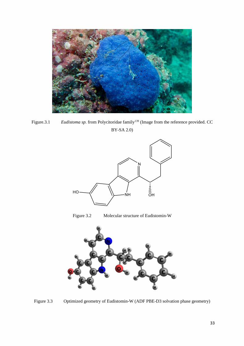
Eudistomin-W is found in a group of undescribed colonial ascidians of the family
Polycitoridae138 (Figure 3.1)139, which are native to Chuuk state of the Federated States of
Micronesia. This compound was isolated, and its anti-bacterial and anti-fungal activity was
studied in detail.40 The molecular structure of the compound is given in Figure 3.2 and the
computationally optimized geometry is shown in Figure 3.3 (geometry shown is of ADF PBE-
D3 level in solvation phase).
33
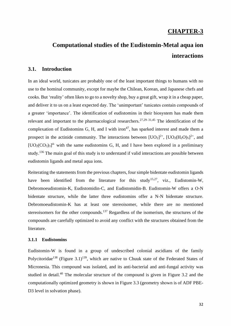
Figure.3.1 Eudistoma sp. from Polycitoridae family139 (Image from the reference provided. CC
BY-SA 2.0)
Figure 3.2 Molecular structure of Eudistomin-W
Figure 3.3 Optimized geometry of Eudistomin-W (ADF PBE-D3 solvation phase geometry)
34
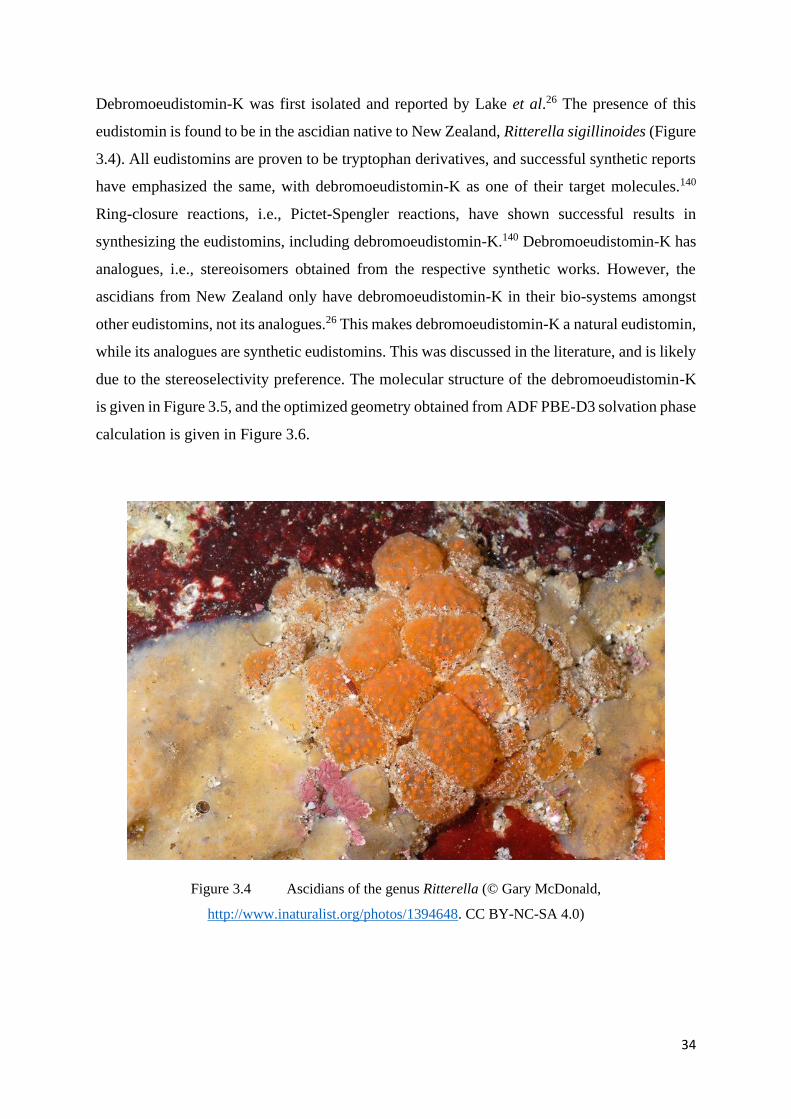
Debromoeudistomin-K was first isolated and reported by Lake et al.26 The presence of this
eudistomin is found to be in the ascidian native to New Zealand, Ritterella sigillinoides (Figure
3.4). All eudistomins are proven to be tryptophan derivatives, and successful synthetic reports
have emphasized the same, with debromoeudistomin-K as one of their target molecules.140
Ring-closure reactions, i.e., Pictet-Spengler reactions, have shown successful results in
synthesizing the eudistomins, including debromoeudistomin-K.140 Debromoeudistomin-K has
analogues, i.e., stereoisomers obtained from the respective synthetic works. However, the
ascidians from New Zealand only have debromoeudistomin-K in their bio-systems amongst
other eudistomins, not its analogues.26 This makes debromoeudistomin-K a natural eudistomin,
while its analogues are synthetic eudistomins. This was discussed in the literature, and is likely
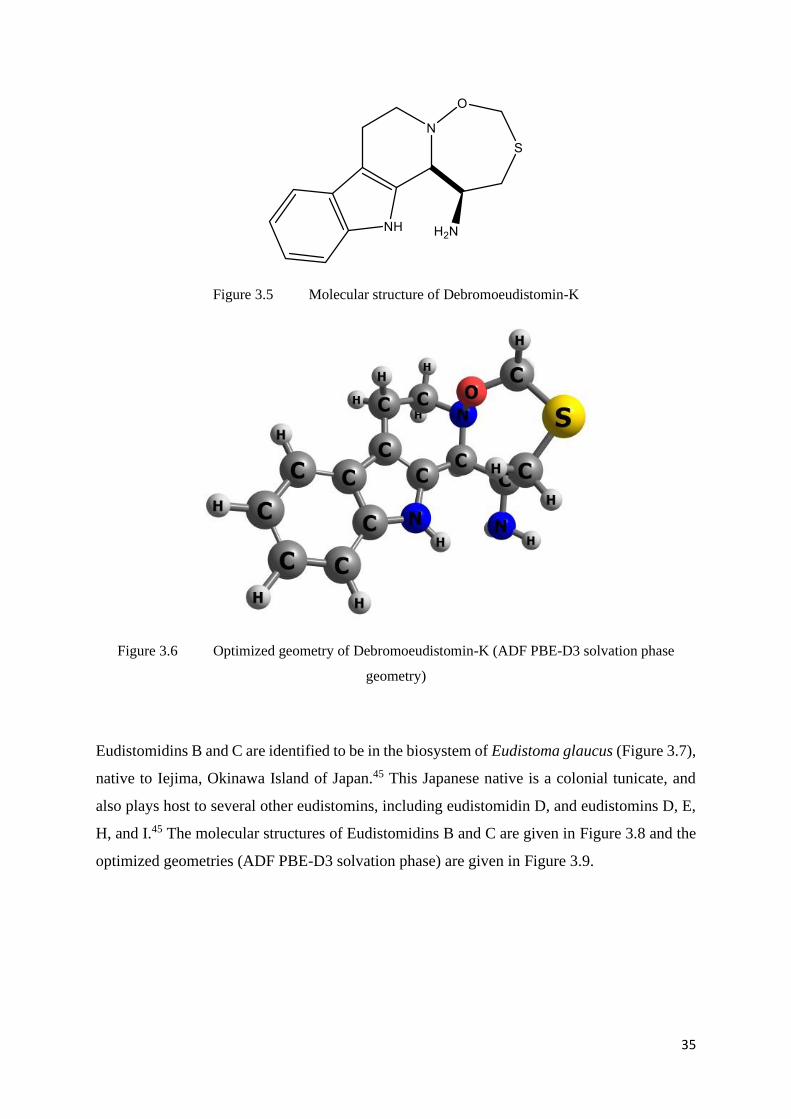
due to the stereoselectivity preference. The molecular structure of the debromoeudistomin-K
is given in Figure 3.5, and the optimized geometry obtained from ADF PBE-D3 solvation phase
calculation is given in Figure 3.6.
Figure 3.4 Ascidians of the genus Ritterella (© Gary McDonald,
http://www.inaturalist.org/photos/1394648. CC BY-NC-SA 4.0)
35
Figure 3.5 Molecular structure of Debromoeudistomin-K
Figure 3.6 Optimized geometry of Debromoeudistomin-K (ADF PBE-D3 solvation phase
geometry)
Eudistomidins B and C are identified to be in the biosystem of Eudistoma glaucus (Figure 3.7),
native to Iejima, Okinawa Island of Japan.45 This Japanese native is a colonial tunicate, and
also plays host to several other eudistomins, including eudistomidin D, and eudistomins D, E,
H, and I.45 The molecular structures of Eudistomidins B and C are given in Figure 3.8 and the
optimized geometries (ADF PBE-D3 solvation phase) are given in Figure 3.9.
36
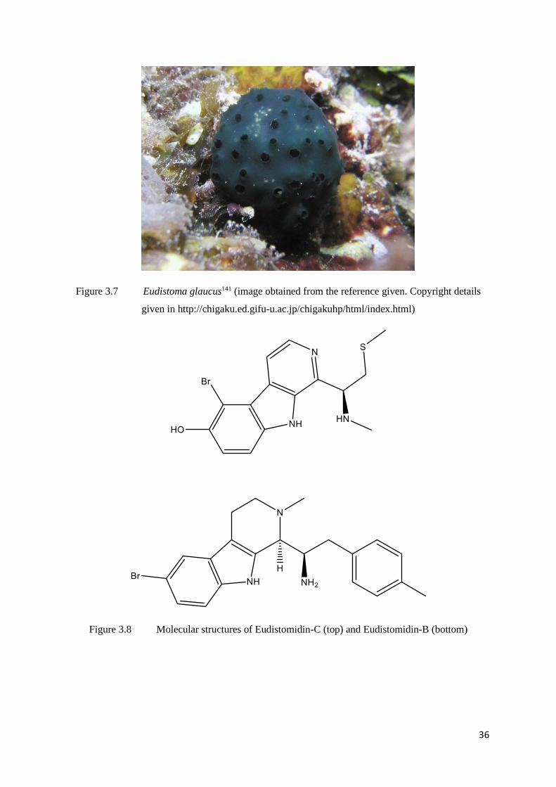
Figure 3.7 Eudistoma glaucus141 (image obtained from the reference given. Copyright details
given in http://chigaku.ed.gifu-u.ac.jp/chigakuhp/html/index.html)
Figure 3.8 Molecular structures of Eudistomidin-C (top) and Eudistomidin-B (bottom)
37
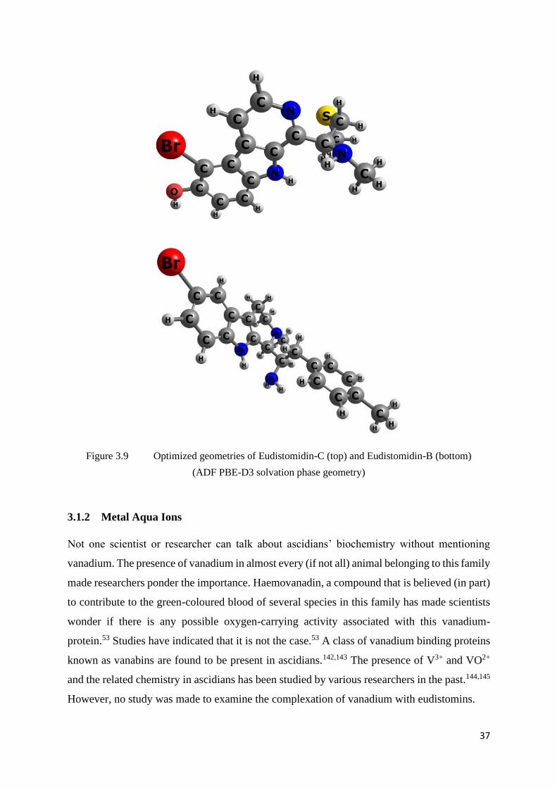
Figure 3.9 Optimized geometries of Eudistomidin-C (top) and Eudistomidin-B (bottom)
(ADF PBE-D3 solvation phase geometry)
3.1.2 Metal Aqua Ions
Not one scientist or researcher can talk about ascidians’ biochemistry without mentioning
vanadium. The presence of vanadium in almost every (if not all) animal belonging to this family
made researchers ponder the importance. Haemovanadin, a compound that is believed (in part)
to contribute to the green-coloured blood of several species in this family has made scientists
wonder if there is any possible oxygen-carrying activity associated with this vanadium-
protein.53 Studies have indicated that it is not the case.53 A class of vanadium binding proteins
known as vanabins are found to be present in ascidians.142,143 The presence of V3+ and VO2+
and the related chemistry in ascidians has been studied by various researchers in the past.144,145
However, no study was made to examine the complexation of vanadium with eudistomins.
38
In this work, due to the importance of vanadium in the biochemistry of ascidians, VO2+
(vanadyl ion) surrounded by four and five water molecules, is one of the subjects. The
optimized geometries of the respective ions are given in the Figure 3.10. The six-coordinated
vanadyl aqua ion has optimized to a distorted octahedral structure, and the five-coordinated
vanadyl aqua ion has optimized to a distorted square pyramid structure. Figure 3.10 (a) and (b)
show a five-coordinated vanadium and 3.10 (c) and (d) show a six-coordinated vanadium. The
vanadyl ion is usually surrounded by five water molecules in its aqua ion. Tetrahydrate and
hexahydrate aqua ions are also possible.61 In most of the crystal structures, vanadyl ion occurs
as a (vanadium-centred) distorted octahedral structure with four water molecules, and the sixth
coordination to the ligand (mostly bound as monodentate ligands).89,146 But di-anionic
bidentate ligands can distort the structure to a (vanadium-centred) distorted square pyramidal
structure or trigonal bipyramidal structure. For this reason, calculations are performed with
vanadyl tetrahydrate ion and vanadyl pentahydrate ion. While there is a noticeable structural
difference in the cations, the optimized geometries of the complexes show that in all of the
cases, the structures of the complexes have not resulted in (vanadium-centred) distorted
octahedral structures. This is discussed in detail in the further parts.
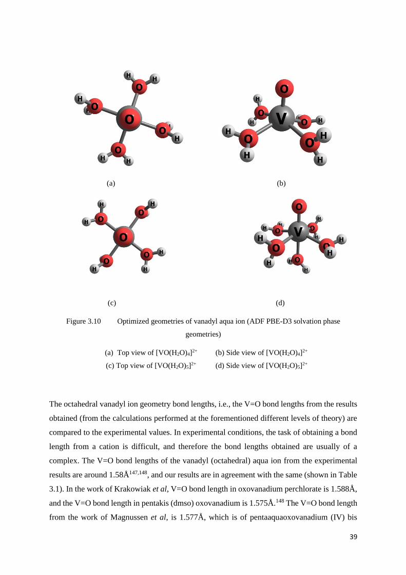
39
(a) (b)
(c) (d)
Figure 3.10 Optimized geometries of vanadyl aqua ion (ADF PBE-D3 solvation phase
geometries)
(a) Top view of [VO(H2O)4]2+ (b) Side view of [VO(H2O)4]2+
(c) Top view of [VO(H2O)5]2+ (d) Side view of [VO(H2O)5]2+
The octahedral vanadyl ion geometry bond lengths, i.e., the V=O bond lengths from the results
obtained (from the calculations performed at the forementioned different levels of theory) are
compared to the experimental values. In experimental conditions, the task of obtaining a bond
length from a cation is difficult, and therefore the bond lengths obtained are usually of a
complex. The V=O bond lengths of the vanadyl (octahedral) aqua ion from the experimental
results are around 1.58Å147,148, and our results are in agreement with the same (shown in Table
3.1). In the work of Krakowiak et al, V=O bond length in oxovanadium perchlorate is 1.588Å,
and the V=O bond length in pentakis (dmso) oxovanadium is 1.575Å.148 The V=O bond length
from the work of Magnussen et al, is 1.577Å, which is of pentaaquaoxovanadium (IV) bis
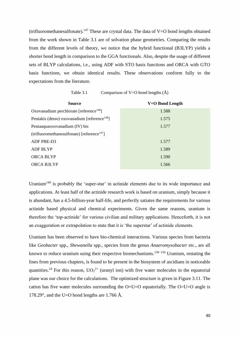
40
(trifluoromethanesulfonate).147 These are crystal data. The data of V=O bond lengths obtained
from the work shown in Table 3.1 are of solvation phase geometries. Comparing the results
from the different levels of theory, we notice that the hybrid functional (B3LYP) yields a
shorter bond length in comparison to the GGA functionals. Also, despite the usage of different
sets of BLYP calculations, i.e., using ADF with STO basis functions and ORCA with GTO
basis functions, we obtain identical results. These observations conform fully to the
expectations from the literature.
Table 3.1 Comparison of V=O bond lengths (Å)
Source V=O Bond Length
Oxovanadium perchlorate [reference148] 1.588
Pentakis (dmso) oxovanadium [reference148] 1.575
Pentaaquaoxovanadium (IV) bis
(trifluoromethanesulfonate) [reference147]
1.577
ADF PBE-D3 1.577
ADF BLYP 1.589
ORCA BLYP 1.590
ORCA B3LYP 1.566
Uranium149 is probably the ‘super-star’ in actinide elements due to its wide importance and
applications. At least half of the actinide research work is based on uranium, simply because it
is abundant, has a 4.5-billion-year half-life, and perfectly satiates the requirements for various
actinide based physical and chemical experiments. Given the same reasons, uranium is
therefore the ‘top-actinide’ for various civilian and military applications. Henceforth, it is not
an exaggeration or extrapolation to state that it is ‘the superstar’ of actinide elements.
Uranium has been observed to have bio-chemical interactions. Various species from bacteria
like Geobacter spp., Shewanella spp., species from the genus Anaeromyxobacter etc., are all
known to reduce uranium using their respective biomechanisms.150–156 Uranium, restating the
lines from previous chapters, is found to be present in the biosystem of ascidians in noticeable
quantities.24 For this reason, UO22+ (uranyl ion) with five water molecules in the equatorial
plane was our choice for the calculations. The optimized structure is given in Figure 3.11. The
cation has five water molecules surrounding the O=U=O equatorially. The O=U=O angle is
178.29°, and the U=O bond lengths are 1.766 Å.
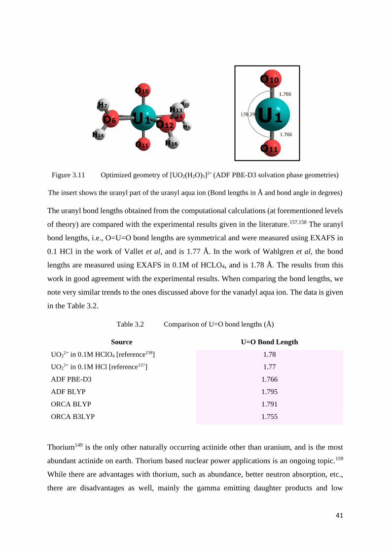
41
Figure 3.11 Optimized geometry of [UO2(H2O)5]2+ (ADF PBE-D3 solvation phase geometries)
The insert shows the uranyl part of the uranyl aqua ion (Bond lengths in Å and bond angle in degrees)
The uranyl bond lengths obtained from the computational calculations (at forementioned levels
of theory) are compared with the experimental results given in the literature.157,158 The uranyl
bond lengths, i.e., O=U=O bond lengths are symmetrical and were measured using EXAFS in
0.1 HCl in the work of Vallet et al, and is 1.77 Å. In the work of Wahlgren et al, the bond
lengths are measured using EXAFS in 0.1M of HCLO4, and is 1.78 Å. The results from this
work in good agreement with the experimental results. When comparing the bond lengths, we
note very similar trends to the ones discussed above for the vanadyl aqua ion. The data is given
in the Table 3.2.
Table 3.2 Comparison of U=O bond lengths (Å)
Source U=O Bond Length
UO22+ in 0.1M HClO4 [reference158] 1.78
UO22+ in 0.1M HCl [reference157] 1.77
ADF PBE-D3 1.766
ADF BLYP 1.795
ORCA BLYP 1.791
ORCA B3LYP 1.755
Thorium149 is the only other naturally occurring actinide other than uranium, and is the most
abundant actinide on earth. Thorium based nuclear power applications is an ongoing topic.159
While there are advantages with thorium, such as abundance, better neutron absorption, etc.,
there are disadvantages as well, mainly the gamma emitting daughter products and low
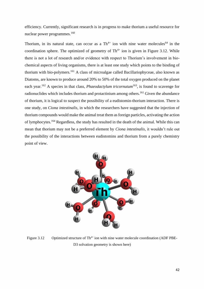
42
efficiency. Currently, significant research is in progress to make thorium a useful resource for
nuclear power programmes.160
Thorium, in its natural state, can occur as a Th4+ ion with nine water molecules64 in the
coordination sphere. The optimized of geometry of Th4+ ion is given in Figure 3.12. While
there is not a lot of research and/or evidence with respect to Thorium’s involvement in bio-
chemical aspects of living organisms, there is at least one study which points to the binding of
thorium with bio-polymers.161 A class of microalgae called Bacillariophyceae, also known as
Diatoms, are known to produce around 20% to 50% of the total oxygen produced on the planet
each year.162 A species in that class, Phaeodactylum tricornutum163, is found to scavenge for
radionuclides which includes thorium and protactinium among others.161 Given the abundance
of thorium, it is logical to suspect the possibility of a eudistomin-thorium interaction. There is
one study, on Ciona intestinalis, in which the researchers have suggested that the injection of
thorium compounds would make the animal treat them as foreign particles, activating the action
of lymphocytes.164 Regardless, the study has resulted in the death of the animal. While this can
mean that thorium may not be a preferred element by Ciona intestinalis, it wouldn’t rule out
the possibility of the interactions between eudistomins and thorium from a purely chemistry
point of view.
Figure 3.12 Optimized structure of Th4+ ion with nine water molecule coordination (ADF PBE-
D3 solvation geometry is shown here)
43
In the subsequent sections, the metal complexes with Eudistomin-W (L1) are given as M1,
with Debromoeudistomin-K (L2) are given as M2, with Eudistomidin-C (L3) are given as M3,
and with Eudistomidin-B are given as M4; where M=V/U/T.
3.2. Vanadyl-Eudistomin Complexes
Vanadyl-eudistomin complexes were optimized in gas phase and solvation phase with water as
solvent using the forementioned software packages (ADF and ORCA) with the level of theory
mentioned earlier. The gas phase geometries have served as the input geometries for the
solvation phase geometries. The four complexes, when calculated with different forementioned
levels of theory, have resulted in identical geometries with insignificant variations in the
respective cases.
NOTE: Vanadyl complexes with L(n) are denoted as V(n) for complexes with two water
molecules and as V(n)* for complexes with three water molecules. [n=1,2,3,4]
None of the *-complexes (complexes with three water molecules) exhibit a vanadium centric
distorted octahedral structure, despite the input geometries being vanadium centric distorted
octahedral structures. The ‘extra’ water molecule has moved away from the vanadium atom to
the second coordination sphere during the geometry optimization, and is held by the
neighbouring water molecules via hydrogen bonds (the differences can be noticed in Figures
3.14 and Figure 3.15). This confirms that the preferred coordination for vanadium is five
(including the oxygen atom on the apex of the square pyramid). This phenomenon was also
observed in the vanadyl sulphate molecules (Figure 3.13) [ADF PBE-D3 solvation phase
geometries are shown here].
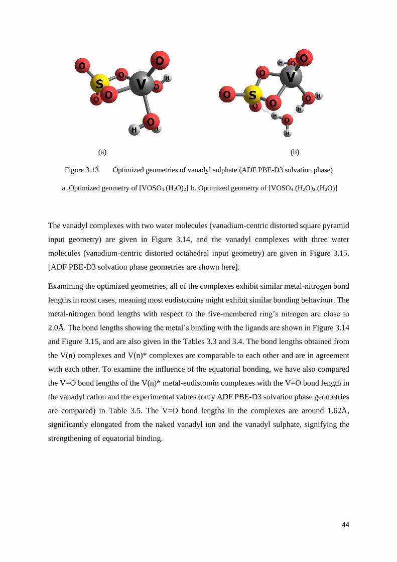
44
(a) (b)
Figure 3.13 Optimized geometries of vanadyl sulphate (ADF PBE-D3 solvation phase)
a. Optimized geometry of [VOSO4.(H2O)2] b. Optimized geometry of [VOSO4.(H2O)2.(H2O)]
The vanadyl complexes with two water molecules (vanadium-centric distorted square pyramid
input geometry) are given in Figure 3.14, and the vanadyl complexes with three water
molecules (vanadium-centric distorted octahedral input geometry) are given in Figure 3.15.
[ADF PBE-D3 solvation phase geometries are shown here].
Examining the optimized geometries, all of the complexes exhibit similar metal-nitrogen bond
lengths in most cases, meaning most eudistomins might exhibit similar bonding behaviour. The
metal-nitrogen bond lengths with respect to the five-membered ring’s nitrogen are close to
2.0Å. The bond lengths showing the metal’s binding with the ligands are shown in Figure 3.14
and Figure 3.15, and are also given in the Tables 3.3 and 3.4. The bond lengths obtained from
the V(n) complexes and V(n)* complexes are comparable to each other and are in agreement
with each other. To examine the influence of the equatorial bonding, we have also compared
the V=O bond lengths of the V(n)* metal-eudistomin complexes with the V=O bond length in
the vanadyl cation and the experimental values (only ADF PBE-D3 solvation phase geometries
are compared) in Table 3.5. The V=O bond lengths in the complexes are around 1.62Å,
significantly elongated from the naked vanadyl ion and the vanadyl sulphate, signifying the
strengthening of equatorial binding.
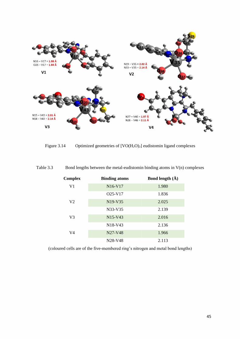
45
Figure 3.14 Optimized geometries of [VO(H2O)2] eudistomin ligand complexes
Table 3.3 Bond lengths between the metal-eudistomin binding atoms in V(n) complexes
Complex Binding atoms Bond length (Å)
V1 N16-V17 1.980
O25-V17 1.836
V2 N19-V35 2.025
N33-V35 2.139
V3 N15-V43 2.016
N18-V43 2.136
V4 N27-V48 1.966
N28-V48 2.113
(coloured cells are of the five-membered ring’s nitrogen and metal bond lengths)
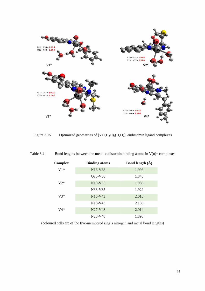
46
Figure 3.15 Optimized geometries of [VO(H2O)2(H2O)] eudistomin ligand complexes
Table 3.4 Bond lengths between the metal-eudistomin binding atoms in V(n)* complexes
Complex Binding atoms Bond length (Å)
V1* N16-V38 1.993
O25-V38 1.845
V2* N19-V35 1.986
N33-V35 1.929
V3* N15-V43 2.010
N18-V43 2.136
V4* N27-V48 2.014
N28-V48 1.898
(coloured cells are of the five-membered ring’s nitrogen and metal bond lengths)
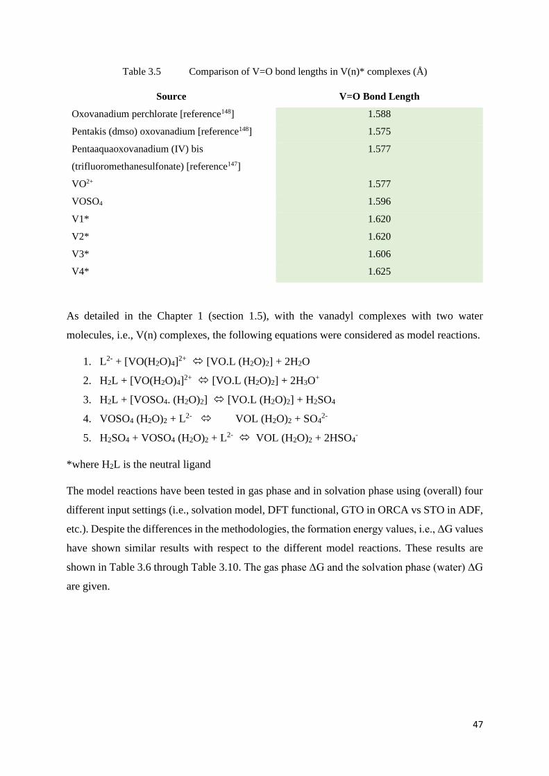
47
Table 3.5 Comparison of V=O bond lengths in V(n)* complexes (Å)
Source V=O Bond Length
Oxovanadium perchlorate [reference148] 1.588
Pentakis (dmso) oxovanadium [reference148] 1.575
Pentaaquaoxovanadium (IV) bis
(trifluoromethanesulfonate) [reference147]
1.577
VO2+ 1.577
VOSO4 1.596
V1* 1.620
V2* 1.620
V3* 1.606
V4* 1.625
As detailed in the Chapter 1 (section 1.5), with the vanadyl complexes with two water
molecules, i.e., V(n) complexes, the following equations were considered as model reactions.
1. L2- + [VO(H2O)4]2+ [VO.L (H2O)2] + 2H2O
2. H2L + [VO(H2O)4]2+ [VO.L (H2O)2] + 2H3O
+
3. H2L + [VOSO4. (H2O)2] [VO.L (H2O)2] + H2SO4
4. VOSO4 (H2O)2 + L2- VOL (H2O)2 + SO42-
5. H2SO4 + VOSO4 (H2O)2 + L2- VOL (H2O)2 + 2HSO4-
*where H2L is the neutral ligand
The model reactions have been tested in gas phase and in solvation phase using (overall) four
different input settings (i.e., solvation model, DFT functional, GTO in ORCA vs STO in ADF,
etc.). Despite the differences in the methodologies, the formation energy values, i.e., ΔG values
have shown similar results with respect to the different model reactions. These results are
shown in Table 3.6 through Table 3.10. The gas phase ΔG and the solvation phase (water) ΔG
are given.
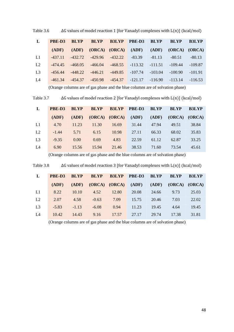
48
Table 3.6 ΔG values of model reaction 1 [for Vanadyl complexes with L(n)] (kcal/mol)
L PBE-D3
(ADF)
BLYP
(ADF)
BLYP
(ORCA)
B3LYP
(ORCA)
PBE-D3
(ADF)
BLYP
(ADF)
BLYP
(ORCA)
B3LYP
(ORCA)
L1 -437.11 -432.72 -429.96 -432.22 -83.39 -81.13 -80.51 -80.13
L2 -474.45 -468.05 -466.04 -468.55 -113.32 -111.51 -109.44 -109.87
L3 -456.44 -448.22 -446.21 -449.85 -107.74 -103.04 -100.90 -101.91
L4 -461.34 -454.37 -450.98 -454.37 -121.17 -116.90 -113.14 -116.53
(Orange columns are of gas phase and the blue columns are of solvation phase)
Table 3.7 ΔG values of model reaction 2 [for Vanadyl complexes with L(n)] (kcal/mol)
L PBE-D3
(ADF)
BLYP
(ADF)
BLYP
(ORCA)
B3LYP
(ORCA)
PBE-D3
(ADF)
BLYP
(ADF)
BLYP
(ORCA)
B3LYP
(ORCA)
L1 4.70 11.23 11.30 16.69 31.44 47.94 49.51 38.84
L2 -1.44 5.71 6.15 10.98 27.11 66.33 68.02 35.83
L3 -9.35 0.00 0.69 4.83 22.59 61.12 62.87 33.25
L4 6.90 15.56 15.94 21.46 38.53 71.60 73.54 45.61
(Orange columns are of gas phase and the blue columns are of solvation phase)
Table 3.8 ΔG values of model reaction 3 [for Vanadyl complexes with L(n)] (kcal/mol)
L PBE-D3
(ADF)
BLYP
(ADF)
BLYP
(ORCA)
B3LYP
(ORCA)
PBE-D3
(ADF)
BLYP
(ADF)
BLYP
(ORCA)
B3LYP
(ORCA)
L1 8.22 10.10 4.52 12.80 20.08 24.66 9.73 25.03
L2 2.07 4.58 -0.63 7.09 15.75 20.46 7.03 22.02
L3 -5.83 -1.13 -6.08 0.94 11.23 19.45 4.64 19.45
L4 10.42 14.43 9.16 17.57 27.17 29.74 17.38 31.81
(Orange columns are of gas phase and the blue columns are of solvation phase)
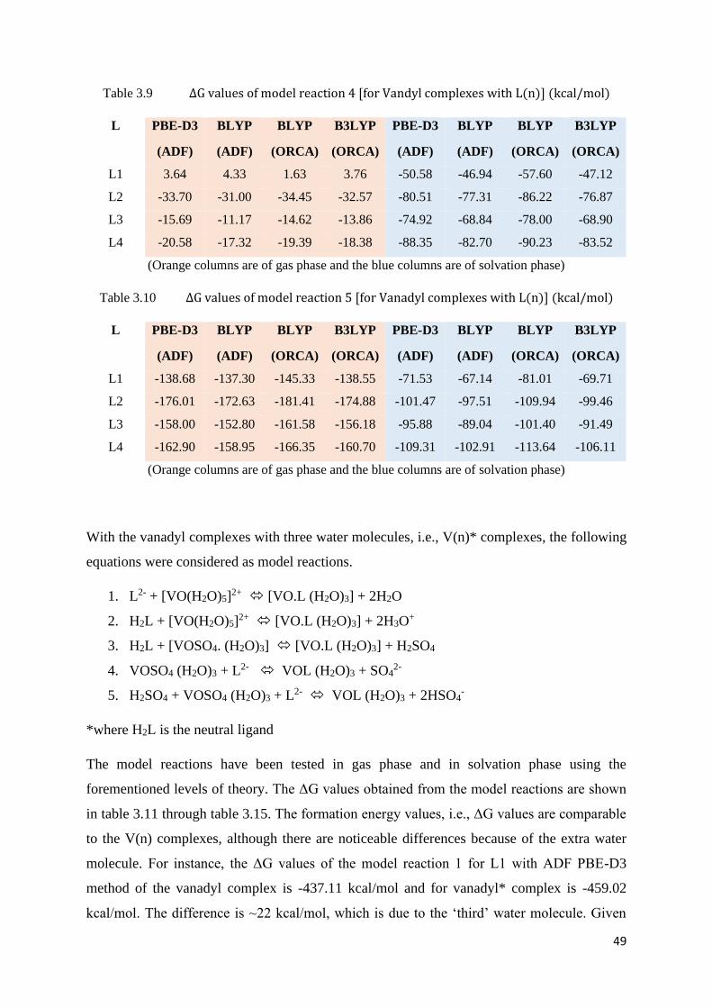
49
Table 3.9 ΔG values of model reaction 4 [for Vandyl complexes with L(n)] (kcal/mol)
L PBE-D3
(ADF)
BLYP
(ADF)
BLYP
(ORCA)
B3LYP
(ORCA)
PBE-D3
(ADF)
BLYP
(ADF)
BLYP
(ORCA)
B3LYP
(ORCA)
L1 3.64 4.33 1.63 3.76 -50.58 -46.94 -57.60 -47.12
L2 -33.70 -31.00 -34.45 -32.57 -80.51 -77.31 -86.22 -76.87
L3 -15.69 -11.17 -14.62 -13.86 -74.92 -68.84 -78.00 -68.90
L4 -20.58 -17.32 -19.39 -18.38 -88.35 -82.70 -90.23 -83.52
(Orange columns are of gas phase and the blue columns are of solvation phase)
Table 3.10 ΔG values of model reaction 5 [for Vanadyl complexes with L(n)] (kcal/mol)
L PBE-D3
(ADF)
BLYP
(ADF)
BLYP
(ORCA)
B3LYP
(ORCA)
PBE-D3
(ADF)
BLYP
(ADF)
BLYP
(ORCA)
B3LYP
(ORCA)
L1 -138.68 -137.30 -145.33 -138.55 -71.53 -67.14 -81.01 -69.71
L2 -176.01 -172.63 -181.41 -174.88 -101.47 -97.51 -109.94 -99.46
L3 -158.00 -152.80 -161.58 -156.18 -95.88 -89.04 -101.40 -91.49
L4 -162.90 -158.95 -166.35 -160.70 -109.31 -102.91 -113.64 -106.11
(Orange columns are of gas phase and the blue columns are of solvation phase)
With the vanadyl complexes with three water molecules, i.e., V(n)* complexes, the following
equations were considered as model reactions.
1. L2- + [VO(H2O)5]2+ [VO.L (H2O)3] + 2H2O
2. H2L + [VO(H2O)5]2+ [VO.L (H2O)3] + 2H3O
+
3. H2L + [VOSO4. (H2O)3] [VO.L (H2O)3] + H2SO4
4. VOSO4 (H2O)3 + L2- VOL (H2O)3 + SO42-
5. H2SO4 + VOSO4 (H2O)3 + L2- VOL (H2O)3 + 2HSO4-
*where H2L is the neutral ligand
The model reactions have been tested in gas phase and in solvation phase using the
forementioned levels of theory. The ΔG values obtained from the model reactions are shown
in table 3.11 through table 3.15. The formation energy values, i.e., ΔG values are comparable
to the V(n) complexes, although there are noticeable differences because of the extra water
molecule. For instance, the ΔG values of the model reaction 1 for L1 with ADF PBE-D3
method of the vanadyl complex is -437.11 kcal/mol and for vanadyl* complex is -459.02
kcal/mol. The difference is ~22 kcal/mol, which is due to the ‘third’ water molecule. Given
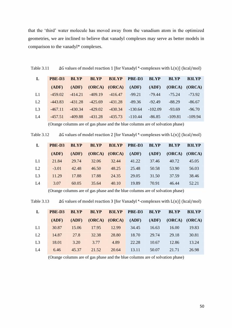
50
that the ‘third’ water molecule has moved away from the vanadium atom in the optimized
geometries, we are inclined to believe that vanadyl complexes may serve as better models in
comparison to the vanadyl* complexes.
Table 3.11 ΔG values of model reaction 1 [for Vanadyl *-complexes with L(n)] (kcal/mol)
L PBE-D3
(ADF)
BLYP
(ADF)
BLYP
(ORCA)
B3LYP
(ORCA)
PBE-D3
(ADF)
BLYP
(ADF)
BLYP
(ORCA)
B3LYP
(ORCA)
L1 -459.02 -414.21 -409.19 -416.47 -99.21 -79.44 -75.24 -73.92
L2 -443.83 -431.28 -425.69 -431.28 -89.36 -92.49 -88.29 -86.67
L3 -467.11 -430.34 -429.02 -430.34 -130.64 -102.09 -93.69 -96.70
L4 -457.51 -409.88 -431.28 -435.73 -110.44 -86.85 -109.81 -109.94
(Orange columns are of gas phase and the blue columns are of solvation phase)
Table 3.12 ΔG values of model reaction 2 [for Vanadyl *-complexes with L(n)] (kcal/mol)
L PBE-D3
(ADF)
BLYP
(ADF)
BLYP
(ORCA)
B3LYP
(ORCA)
PBE-D3
(ADF)
BLYP
(ADF)
BLYP
(ORCA)
B3LYP
(ORCA)
L1 21.84 29.74 32.06 32.44 41.22 37.46 40.72 45.05
L2 -3.01 42.48 46.50 48.25 25.48 50.58 53.90 56.03
L3 11.29 17.88 17.88 24.35 29.05 31.50 37.59 38.46
L4 3.07 60.05 35.64 40.10 19.89 70.91 46.44 52.21
(Orange columns are of gas phase and the blue columns are of solvation phase)
Table 3.13 ΔG values of model reaction 3 [for Vanadyl *-complexes with L(n)] (kcal/mol)
L PBE-D3
(ADF)
BLYP
(ADF)
BLYP
(ORCA)
B3LYP
(ORCA)
PBE-D3
(ADF)
BLYP
(ADF)
BLYP
(ORCA)
B3LYP
(ORCA)
L1 30.87 15.06 17.95 12.99 34.45 16.63 16.00 19.83
L2 14.87 27.8 32.38 28.80 18.70 29.74 29.18 30.81
L3 18.01 3.20 3.77 4.89 22.28 10.67 12.86 13.24
L4 6.46 45.37 21.52 20.64 13.11 50.07 21.71 26.98
(Orange columns are of gas phase and the blue columns are of solvation phase)
51
Table 3.14 ΔG values of model reaction 4 [for Vanadyl *-complexes with L(n)] (kcal/mol)
L PBE-D3
(ADF)
BLYP
(ADF)
BLYP
(ORCA)
B3LYP
(ORCA)
PBE-D3
(ADF)
BLYP
(ADF)
BLYP
(ORCA)
B3LYP
(ORCA)
L1 12.17 9.29 15.06 3.95 -53.46 -54.97 -51.33 -52.33
L2 -3.01 -7.79 -1.44 -10.85 -63.31 -68.02 -64.38 -68.08
L3 -1.51 -6.84 -4.77 -9.91 -74.55 -77.62 -69.78 -75.11
L4 -12.30 13.62 -7.03 -15.31 -63.88 -62.37 -85.90 -88.35
(Orange columns are of gas phase and the blue columns are of solvation phase)
Table 3.15 ΔG values of model reaction 5 [for Vanadyl *-complexes with L(n)] (kcal/mol)
L PBE-D3
(ADF)
BLYP
(ADF)
BLYP
(ORCA)
B3LYP
(ORCA)
PBE-D3
(ADF)
BLYP
(ADF)
BLYP
(ORCA)
B3LYP
(ORCA)
L1 -130.14 -132.34 -131.9 -138.36 -74.42 -75.17 -74.73 -74.92
L2 -145.33 -149.41 -148.40 -153.17 -84.27 -88.23 -87.79 -90.67
L3 -143.82 -148.47 -151.73 -152.23 -95.51 -97.83 -93.18 -97.70
L4 -154.55 -128.01 -154.00 -157.63 -84.84 -82.58 -109.31 -110.94
(Orange columns are of gas phase and the blue columns are of solvation phase)
From the formation energy values, for vanadyl complexes in solvation phase, model 1, 4, and
5 show positive interactions, i.e., negative ΔG. As model 4 and 5 are designed to resemble what
might be the realistic scenario, and given the similarity of the values despite different levels of
theory, i.e., the basis sets, solvation model, etc., this would suggest the vanadium binding with
eudistomins. Both two-water complexes and three-water complexes exhibit similar results, the
differences in the numbers being due to the one extra-water molecule. We are inclined to think
that the two-water complexes may be the better model, as the third water molecule in the three-
water complexes was observed to settle in the second solvation sphere, leading to a potentially
unbalanced description of the solvation of these complexes.
3.3. Uranyl-Eudistomin Complexes
Uranyl-eudistomin complexes were optimized using the forementioned software packages
(ADF and ORCA) with the levels of theory mentioned earlier, in gas phase and solvation phase
with water as solvent. In all of the cases the gas phase geometries have served as the input
geometries for the solvation phase geometries. The complexes have resulted in similar
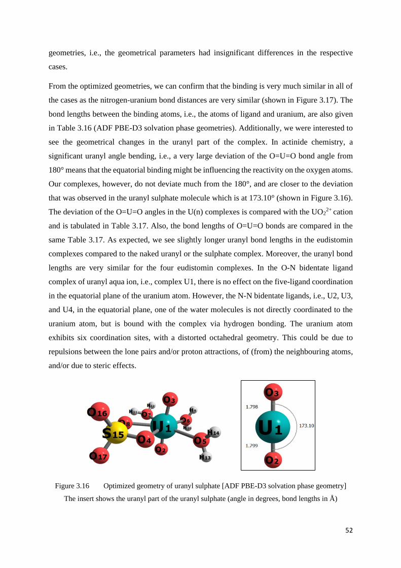
52
geometries, i.e., the geometrical parameters had insignificant differences in the respective
cases.
From the optimized geometries, we can confirm that the binding is very much similar in all of
the cases as the nitrogen-uranium bond distances are very similar (shown in Figure 3.17). The
bond lengths between the binding atoms, i.e., the atoms of ligand and uranium, are also given
in Table 3.16 (ADF PBE-D3 solvation phase geometries). Additionally, we were interested to
see the geometrical changes in the uranyl part of the complex. In actinide chemistry, a
significant uranyl angle bending, i.e., a very large deviation of the O=U=O bond angle from
180° means that the equatorial binding might be influencing the reactivity on the oxygen atoms.
Our complexes, however, do not deviate much from the 180°, and are closer to the deviation
that was observed in the uranyl sulphate molecule which is at 173.10° (shown in Figure 3.16).
The deviation of the O=U=O angles in the U(n) complexes is compared with the UO22+ cation
and is tabulated in Table 3.17. Also, the bond lengths of O=U=O bonds are compared in the
same Table 3.17. As expected, we see slightly longer uranyl bond lengths in the eudistomin
complexes compared to the naked uranyl or the sulphate complex. Moreover, the uranyl bond
lengths are very similar for the four eudistomin complexes. In the O-N bidentate ligand
complex of uranyl aqua ion, i.e., complex U1, there is no effect on the five-ligand coordination
in the equatorial plane of the uranium atom. However, the N-N bidentate ligands, i.e., U2, U3,
and U4, in the equatorial plane, one of the water molecules is not directly coordinated to the
uranium atom, but is bound with the complex via hydrogen bonding. The uranium atom
exhibits six coordination sites, with a distorted octahedral geometry. This could be due to
repulsions between the lone pairs and/or proton attractions, of (from) the neighbouring atoms,
and/or due to steric effects.
Figure 3.16 Optimized geometry of uranyl sulphate [ADF PBE-D3 solvation phase geometry]
The insert shows the uranyl part of the uranyl sulphate (angle in degrees, bond lengths in Å)
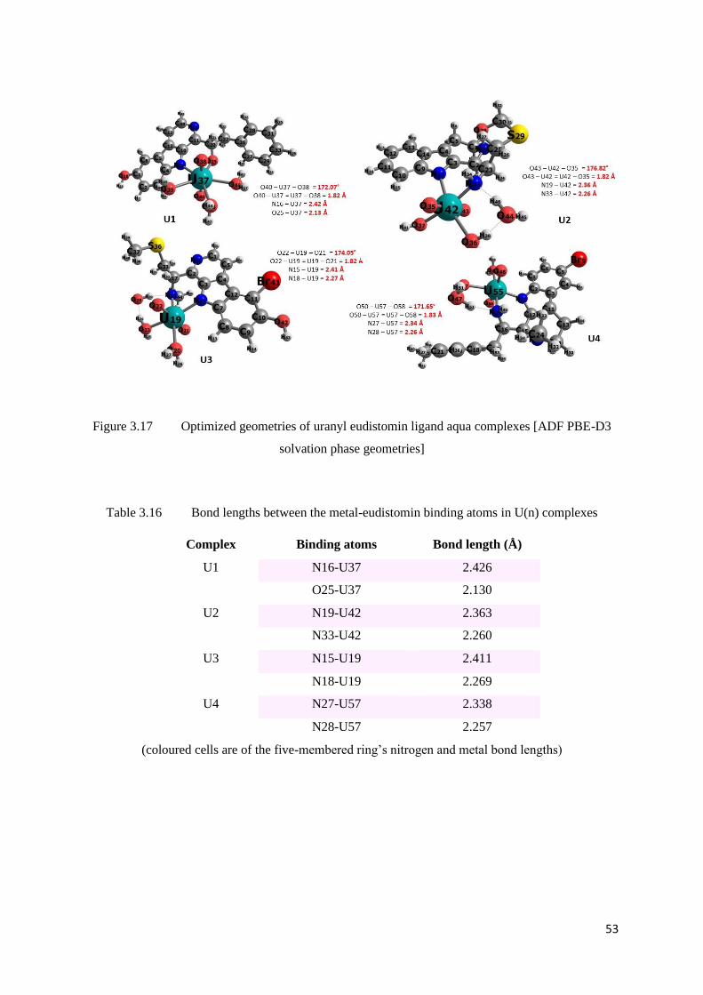
53
Figure 3.17 Optimized geometries of uranyl eudistomin ligand aqua complexes [ADF PBE-D3
solvation phase geometries]
Table 3.16 Bond lengths between the metal-eudistomin binding atoms in U(n) complexes
Complex Binding atoms Bond length (Å)
U1 N16-U37 2.426
O25-U37 2.130
U2 N19-U42 2.363
N33-U42 2.260
U3 N15-U19 2.411
N18-U19 2.269
U4 N27-U57 2.338
N28-U57 2.257
(coloured cells are of the five-membered ring’s nitrogen and metal bond lengths)
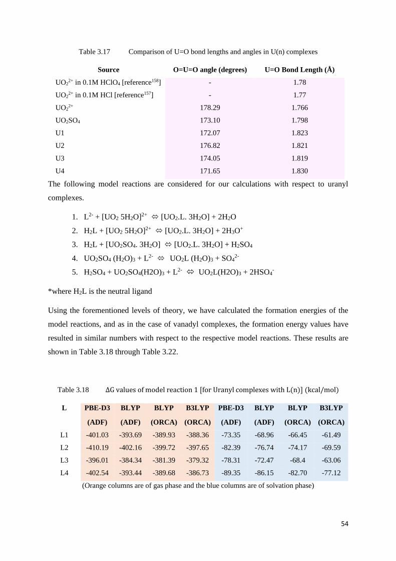
54
Table 3.17 Comparison of U=O bond lengths and angles in U(n) complexes
Source O=U=O angle (degrees) U=O Bond Length (Å)
UO22+ in 0.1M HClO4 [reference158] - 1.78
UO22+ in 0.1M HCl [reference157] - 1.77
UO22+ 178.29 1.766
UO2SO4 173.10 1.798
U1 172.07 1.823
U2 176.82 1.821
U3 174.05 1.819
U4 171.65 1.830
The following model reactions are considered for our calculations with respect to uranyl
complexes.
1. L2- + [UO2 5H2O]2+ [UO2.L. 3H2O] + 2H2O
2. H2L + [UO2 5H2O]2+ [UO2.L. 3H2O] + 2H3O+
3. H2L + [UO2SO4. 3H2O] [UO2.L. 3H2O] + H2SO4
4. UO2SO4 (H2O)3 + L2- UO2L (H2O)3 + SO42-
5. H2SO4 + UO2SO4(H2O)3 + L2- UO2L(H2O)3 + 2HSO4-
*where H2L is the neutral ligand
Using the forementioned levels of theory, we have calculated the formation energies of the
model reactions, and as in the case of vanadyl complexes, the formation energy values have
resulted in similar numbers with respect to the respective model reactions. These results are
shown in Table 3.18 through Table 3.22.
Table 3.18 ΔG values of model reaction 1 [for Uranyl complexes with L(n)] (kcal/mol)
L PBE-D3
(ADF)
BLYP
(ADF)
BLYP
(ORCA)
B3LYP
(ORCA)
PBE-D3
(ADF)
BLYP
(ADF)
BLYP
(ORCA)
B3LYP
(ORCA)
L1 -401.03 -393.69 -389.93 -388.36 -73.35 -68.96 -66.45 -61.49
L2 -410.19 -402.16 -399.72 -397.65 -82.39 -76.74 -74.17 -69.59
L3 -396.01 -384.34 -381.39 -379.32 -78.31 -72.47 -68.4 -63.06
L4 -402.54 -393.44 -389.68 -386.73 -89.35 -86.15 -82.70 -77.12
(Orange columns are of gas phase and the blue columns are of solvation phase)
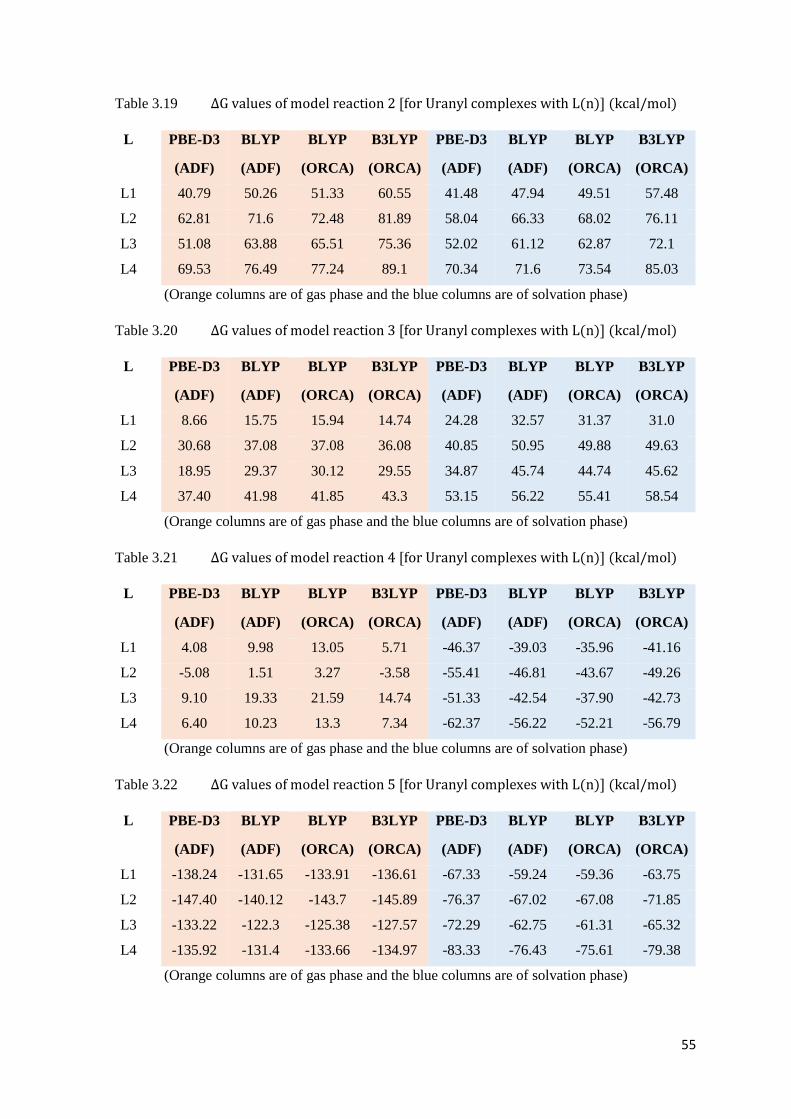
55
Table 3.19 ΔG values of model reaction 2 [for Uranyl complexes with L(n)] (kcal/mol)
L PBE-D3
(ADF)
BLYP
(ADF)
BLYP
(ORCA)
B3LYP
(ORCA)
PBE-D3
(ADF)
BLYP
(ADF)
BLYP
(ORCA)
B3LYP
(ORCA)
L1 40.79 50.26 51.33 60.55 41.48 47.94 49.51 57.48
L2 62.81 71.6 72.48 81.89 58.04 66.33 68.02 76.11
L3 51.08 63.88 65.51 75.36 52.02 61.12 62.87 72.1
L4 69.53 76.49 77.24 89.1 70.34 71.6 73.54 85.03
(Orange columns are of gas phase and the blue columns are of solvation phase)
Table 3.20 ΔG values of model reaction 3 [for Uranyl complexes with L(n)] (kcal/mol)
L PBE-D3
(ADF)
BLYP
(ADF)
BLYP
(ORCA)
B3LYP
(ORCA)
PBE-D3
(ADF)
BLYP
(ADF)
BLYP
(ORCA)
B3LYP
(ORCA)
L1 8.66 15.75 15.94 14.74 24.28 32.57 31.37 31.0
L2 30.68 37.08 37.08 36.08 40.85 50.95 49.88 49.63
L3 18.95 29.37 30.12 29.55 34.87 45.74 44.74 45.62
L4 37.40 41.98 41.85 43.3 53.15 56.22 55.41 58.54
(Orange columns are of gas phase and the blue columns are of solvation phase)
Table 3.21 ΔG values of model reaction 4 [for Uranyl complexes with L(n)] (kcal/mol)
L PBE-D3
(ADF)
BLYP
(ADF)
BLYP
(ORCA)
B3LYP
(ORCA)
PBE-D3
(ADF)
BLYP
(ADF)
BLYP
(ORCA)
B3LYP
(ORCA)
L1 4.08 9.98 13.05 5.71 -46.37 -39.03 -35.96 -41.16
L2 -5.08 1.51 3.27 -3.58 -55.41 -46.81 -43.67 -49.26
L3 9.10 19.33 21.59 14.74 -51.33 -42.54 -37.90 -42.73
L4 6.40 10.23 13.3 7.34 -62.37 -56.22 -52.21 -56.79
(Orange columns are of gas phase and the blue columns are of solvation phase)
Table 3.22 ΔG values of model reaction 5 [for Uranyl complexes with L(n)] (kcal/mol)
L PBE-D3
(ADF)
BLYP
(ADF)
BLYP
(ORCA)
B3LYP
(ORCA)
PBE-D3
(ADF)
BLYP
(ADF)
BLYP
(ORCA)
B3LYP
(ORCA)
L1 -138.24 -131.65 -133.91 -136.61 -67.33 -59.24 -59.36 -63.75
L2 -147.40 -140.12 -143.7 -145.89 -76.37 -67.02 -67.08 -71.85
L3 -133.22 -122.3 -125.38 -127.57 -72.29 -62.75 -61.31 -65.32
L4 -135.92 -131.4 -133.66 -134.97 -83.33 -76.43 -75.61 -79.38
(Orange columns are of gas phase and the blue columns are of solvation phase)
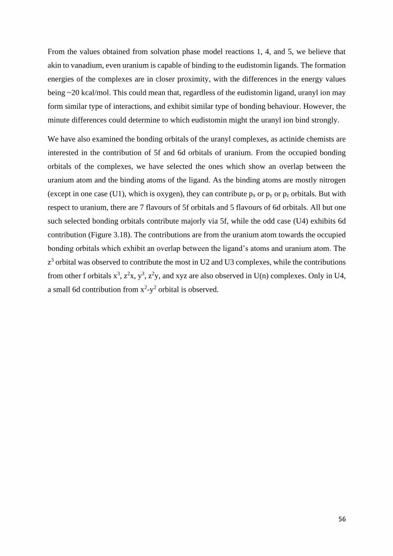
56
From the values obtained from solvation phase model reactions 1, 4, and 5, we believe that
akin to vanadium, even uranium is capable of binding to the eudistomin ligands. The formation
energies of the complexes are in closer proximity, with the differences in the energy values
being ~20 kcal/mol. This could mean that, regardless of the eudistomin ligand, uranyl ion may
form similar type of interactions, and exhibit similar type of bonding behaviour. However, the
minute differences could determine to which eudistomin might the uranyl ion bind strongly.
We have also examined the bonding orbitals of the uranyl complexes, as actinide chemists are
interested in the contribution of 5f and 6d orbitals of uranium. From the occupied bonding
orbitals of the complexes, we have selected the ones which show an overlap between the
uranium atom and the binding atoms of the ligand. As the binding atoms are mostly nitrogen
(except in one case (U1), which is oxygen), they can contribute px or py or pz orbitals. But with
respect to uranium, there are 7 flavours of 5f orbitals and 5 flavours of 6d orbitals. All but one
such selected bonding orbitals contribute majorly via 5f, while the odd case (U4) exhibits 6d
contribution (Figure 3.18). The contributions are from the uranium atom towards the occupied
bonding orbitals which exhibit an overlap between the ligand’s atoms and uranium atom. The
z3 orbital was observed to contribute the most in U2 and U3 complexes, while the contributions
from other f orbitals x3, z2x, y3, z2y, and xyz are also observed in U(n) complexes. Only in U4,
a small 6d contribution from x2-y2 orbital is observed.
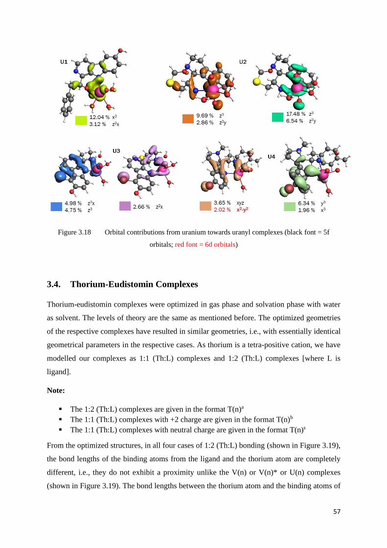
57
Figure 3.18 Orbital contributions from uranium towards uranyl complexes (black font = 5f
orbitals; red font = 6d orbitals)
3.4. Thorium-Eudistomin Complexes
Thorium-eudistomin complexes were optimized in gas phase and solvation phase with water
as solvent. The levels of theory are the same as mentioned before. The optimized geometries
of the respective complexes have resulted in similar geometries, i.e., with essentially identical
geometrical parameters in the respective cases. As thorium is a tetra-positive cation, we have
modelled our complexes as 1:1 (Th:L) complexes and 1:2 (Th:L) complexes [where L is
ligand].
Note:
▪ The 1:2 (Th:L) complexes are given in the format T(n)a
▪ The 1:1 (Th:L) complexes with +2 charge are given in the format T(n)b
▪ The 1:1 (Th:L) complexes with neutral charge are given in the format T(n)s
From the optimized structures, in all four cases of 1:2 (Th:L) bonding (shown in Figure 3.19),
the bond lengths of the binding atoms from the ligand and the thorium atom are completely
different, i.e., they do not exhibit a proximity unlike the V(n) or V(n)* or U(n) complexes
(shown in Figure 3.19). The bond lengths between the thorium atom and the binding atoms of
58
the ligands are given in Table 3.23. In case of 1:1 (Th:L) complexes, one set of the complexes
were +2 charged (shown in Figure 3.20), and the other set of the complexes were neutral with
the sulphate anion countering the charge (shown in Figure 3.21). In all of the complexes,
thorium exhibits a 7-coordination. The bond lengths between the binding atoms of the ligand
and the thorium atom of the 1:1 (Th:L) complexes, i.e., the T(n)b and T(n)s complexes are given
in Table 3.24. Comparing the bond lengths in T(n)b complexes to T(n)s complexes, the bond
lengths in the +2 charged complexes, i.e., the T(n)b complexes are slightly shorter than the
T(n)s complexes. As the bonding is mainly ionic in these cases, smaller charge could have led
to slightly weaker bonds, henceforth the slight differences in the bond lengths.
In case of the sulphate-ligand-metal complexes, the sulphate ion seems to show a mono-dentate
structure in the Figure 3.21, because the O-Th bonds are uneven. The unevenness is simply
because of the heavy crowding of atoms around the Th atom. There actually exists a bonding
between Th and the oxygen atoms from the sulphate, but in the Figure 3.21, the complexes
seem to appear as mono-dentate because of this reason. Also, the Figure 3.21 depicts the
hydrogen bonding between the oxygen atom of the sulphate ion with the neighbouring water
molecules. This could mean that the sulphate ion is stabilized via hydrogen bonding. The Th-
O bonds pertaining to the sulphate ion are given in Table 3.25.
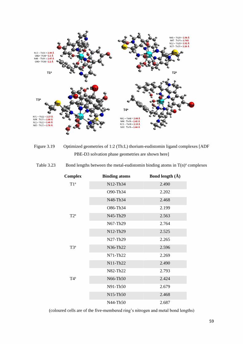
59
Figure 3.19 Optimized geometries of 1:2 (Th:L) thorium-eudistomin ligand complexes [ADF
PBE-D3 solvation phase geometries are shown here]
Table 3.23 Bond lengths between the metal-eudistomin binding atoms in T(n)a complexes
Complex Binding atoms Bond length (Å)
T1a N12-Th34 2.490
O90-Th34 2.202
N48-Th34 2.468
O86-Th34 2.199
T2a N45-Th29 2.563
N67-Th29 2.764
N12-Th29 2.525
N27-Th29 2.265
T3a N36-Th22 2.596
N71-Th22 2.269
N11-Th22 2.490
N82-Th22 2.793
T4a N66-Th50 2.424
N91-Th50 2.679
N15-Th50 2.468
N44-Th50 2.687
(coloured cells are of the five-membered ring’s nitrogen and metal bond lengths)
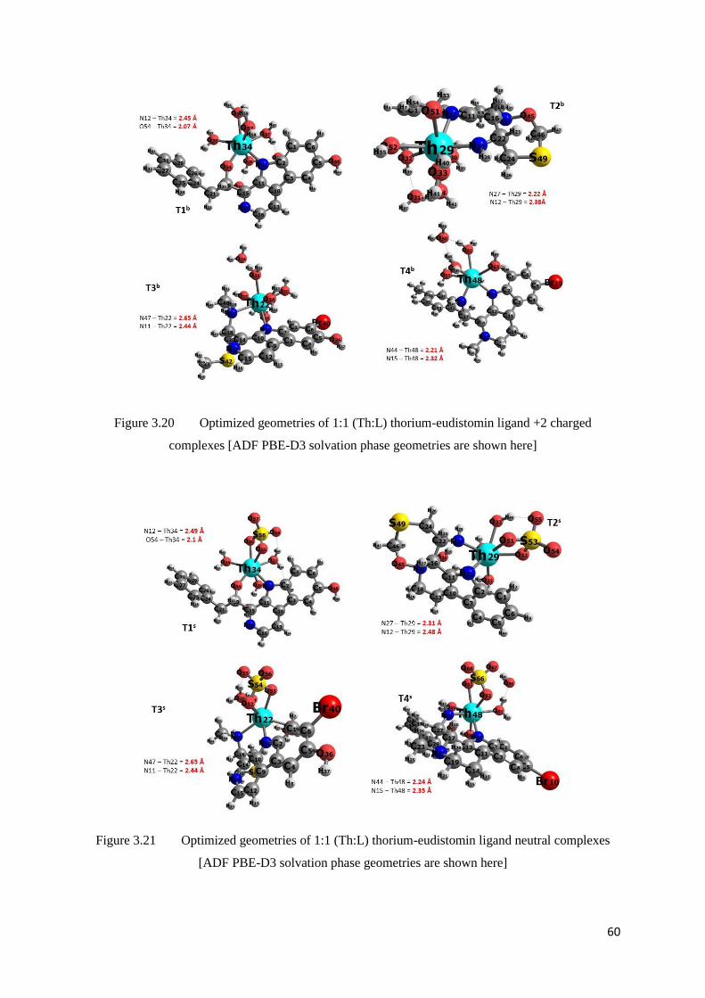
60
Figure 3.20 Optimized geometries of 1:1 (Th:L) thorium-eudistomin ligand +2 charged
complexes [ADF PBE-D3 solvation phase geometries are shown here]
Figure 3.21 Optimized geometries of 1:1 (Th:L) thorium-eudistomin ligand neutral complexes
[ADF PBE-D3 solvation phase geometries are shown here]
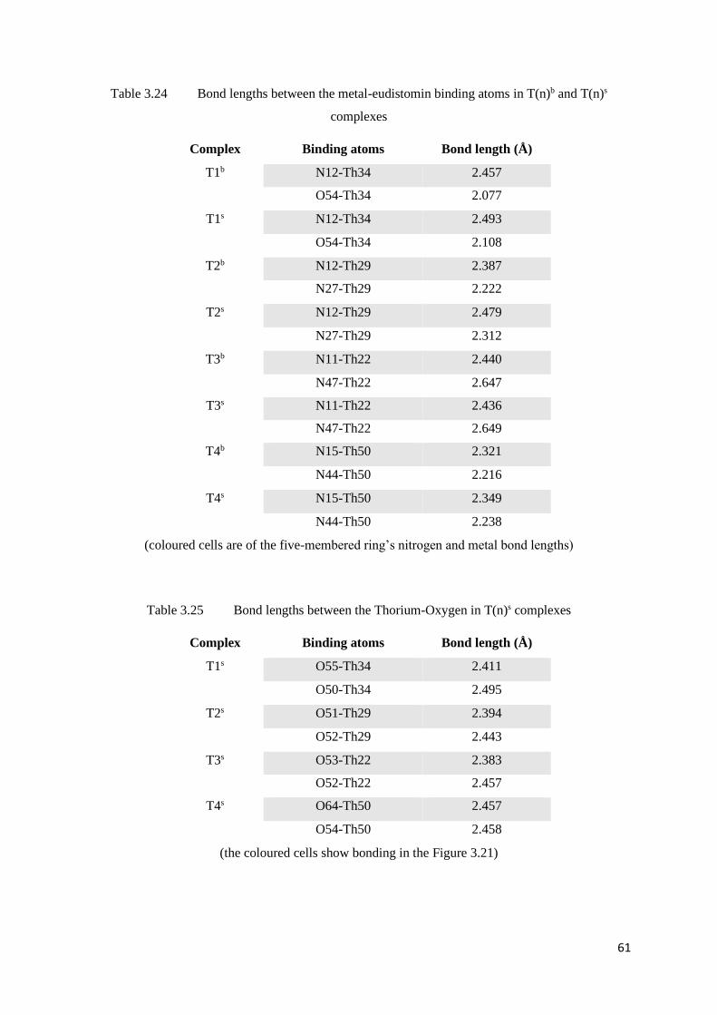
61
Table 3.24 Bond lengths between the metal-eudistomin binding atoms in T(n)b and T(n)s
complexes
Complex Binding atoms Bond length (Å)
T1b N12-Th34 2.457
O54-Th34 2.077
T1s N12-Th34 2.493
O54-Th34 2.108
T2b N12-Th29 2.387
N27-Th29 2.222
T2s N12-Th29 2.479
N27-Th29 2.312
T3b N11-Th22 2.440
N47-Th22 2.647
T3s N11-Th22 2.436
N47-Th22 2.649
T4b N15-Th50 2.321
N44-Th50 2.216
T4s N15-Th50 2.349
N44-Th50 2.238
(coloured cells are of the five-membered ring’s nitrogen and metal bond lengths)
Table 3.25 Bond lengths between the Thorium-Oxygen in T(n)s complexes
Complex Binding atoms Bond length (Å)
T1s O55-Th34 2.411
O50-Th34 2.495
T2s O51-Th29 2.394
O52-Th29 2.443
T3s O53-Th22 2.383
O52-Th22 2.457
T4s O64-Th50 2.457
O54-Th50 2.458
(the coloured cells show bonding in the Figure 3.21)
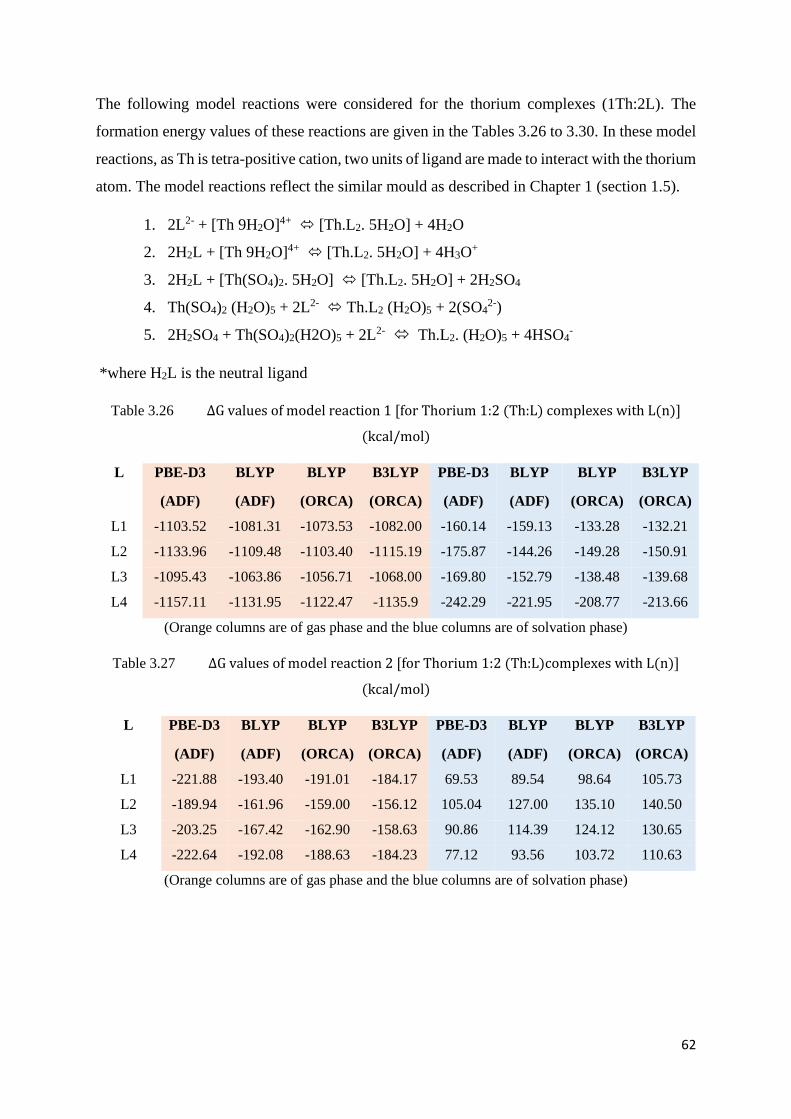
62
The following model reactions were considered for the thorium complexes (1Th:2L). The
formation energy values of these reactions are given in the Tables 3.26 to 3.30. In these model
reactions, as Th is tetra-positive cation, two units of ligand are made to interact with the thorium
atom. The model reactions reflect the similar mould as described in Chapter 1 (section 1.5).
1. 2L2- + [Th 9H2O]4+ [Th.L2. 5H2O] + 4H2O
2. 2H2L + [Th 9H2O]4+ [Th.L2. 5H2O] + 4H3O+
3. 2H2L + [Th(SO4)2. 5H2O] [Th.L2. 5H2O] + 2H2SO4
4. Th(SO4)2 (H2O)5 + 2L2- Th.L2 (H2O)5 + 2(SO42-)
5. 2H2SO4 + Th(SO4)2(H2O)5 + 2L2- Th.L2. (H2O)5 + 4HSO4-
*where H2L is the neutral ligand
Table 3.26 ΔG values of model reaction 1 [for Thorium 1:2 (Th:L) complexes with L(n)]
(kcal/mol)
L PBE-D3
(ADF)
BLYP
(ADF)
BLYP
(ORCA)
B3LYP
(ORCA)
PBE-D3
(ADF)
BLYP
(ADF)
BLYP
(ORCA)
B3LYP
(ORCA)
L1 -1103.52 -1081.31 -1073.53 -1082.00 -160.14 -159.13 -133.28 -132.21
L2 -1133.96 -1109.48 -1103.40 -1115.19 -175.87 -144.26 -149.28 -150.91
L3 -1095.43 -1063.86 -1056.71 -1068.00 -169.80 -152.79 -138.48 -139.68
L4 -1157.11 -1131.95 -1122.47 -1135.9 -242.29 -221.95 -208.77 -213.66
(Orange columns are of gas phase and the blue columns are of solvation phase)
Table 3.27 ΔG values of model reaction 2 [for Thorium 1:2 (Th:L)complexes with L(n)]
(kcal/mol)
L PBE-D3
(ADF)
BLYP
(ADF)
BLYP
(ORCA)
B3LYP
(ORCA)
PBE-D3
(ADF)
BLYP
(ADF)
BLYP
(ORCA)
B3LYP
(ORCA)
L1 -221.88 -193.40 -191.01 -184.17 69.53 89.54 98.64 105.73
L2 -189.94 -161.96 -159.00 -156.12 105.04 127.00 135.10 140.50
L3 -203.25 -167.42 -162.90 -158.63 90.86 114.39 124.12 130.65
L4 -222.64 -192.08 -188.63 -184.23 77.12 93.56 103.72 110.63
(Orange columns are of gas phase and the blue columns are of solvation phase)
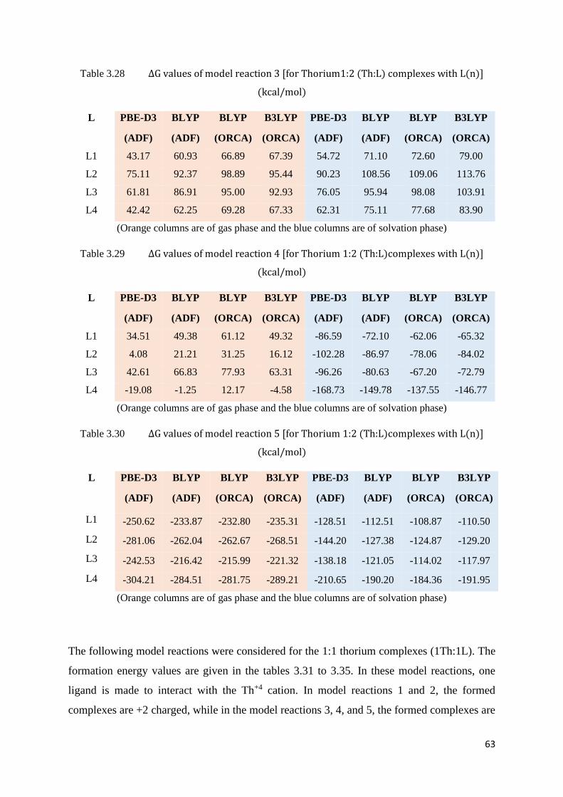
63
Table 3.28 ΔG values of model reaction 3 [for Thorium1:2 (Th:L) complexes with L(n)]
(kcal/mol)
L PBE-D3
(ADF)
BLYP
(ADF)
BLYP
(ORCA)
B3LYP
(ORCA)
PBE-D3
(ADF)
BLYP
(ADF)
BLYP
(ORCA)
B3LYP
(ORCA)
L1 43.17 60.93 66.89 67.39 54.72 71.10 72.60 79.00
L2 75.11 92.37 98.89 95.44 90.23 108.56 109.06 113.76
L3 61.81 86.91 95.00 92.93 76.05 95.94 98.08 103.91
L4 42.42 62.25 69.28 67.33 62.31 75.11 77.68 83.90
(Orange columns are of gas phase and the blue columns are of solvation phase)
Table 3.29 ΔG values of model reaction 4 [for Thorium 1:2 (Th:L)complexes with L(n)]
(kcal/mol)
L PBE-D3
(ADF)
BLYP
(ADF)
BLYP
(ORCA)
B3LYP
(ORCA)
PBE-D3
(ADF)
BLYP
(ADF)
BLYP
(ORCA)
B3LYP
(ORCA)
L1 34.51 49.38 61.12 49.32 -86.59 -72.10 -62.06 -65.32
L2 4.08 21.21 31.25 16.12 -102.28 -86.97 -78.06 -84.02
L3 42.61 66.83 77.93 63.31 -96.26 -80.63 -67.20 -72.79
L4 -19.08 -1.25 12.17 -4.58 -168.73 -149.78 -137.55 -146.77
(Orange columns are of gas phase and the blue columns are of solvation phase)
Table 3.30 ΔG values of model reaction 5 [for Thorium 1:2 (Th:L)complexes with L(n)]
(kcal/mol)
L PBE-D3
(ADF)
BLYP
(ADF)
BLYP
(ORCA)
B3LYP
(ORCA)
PBE-D3
(ADF)
BLYP
(ADF)
BLYP
(ORCA)
B3LYP
(ORCA)
L1 -250.62 -233.87 -232.80 -235.31 -128.51 -112.51 -108.87 -110.50
L2 -281.06 -262.04 -262.67 -268.51 -144.20 -127.38 -124.87 -129.20
L3 -242.53 -216.42 -215.99 -221.32 -138.18 -121.05 -114.02 -117.97
L4 -304.21 -284.51 -281.75 -289.21 -210.65 -190.20 -184.36 -191.95
(Orange columns are of gas phase and the blue columns are of solvation phase)
The following model reactions were considered for the 1:1 thorium complexes (1Th:1L). The
formation energy values are given in the tables 3.31 to 3.35. In these model reactions, one
ligand is made to interact with the Th+4 cation. In model reactions 1 and 2, the formed
complexes are +2 charged, while in the model reactions 3, 4, and 5, the formed complexes are
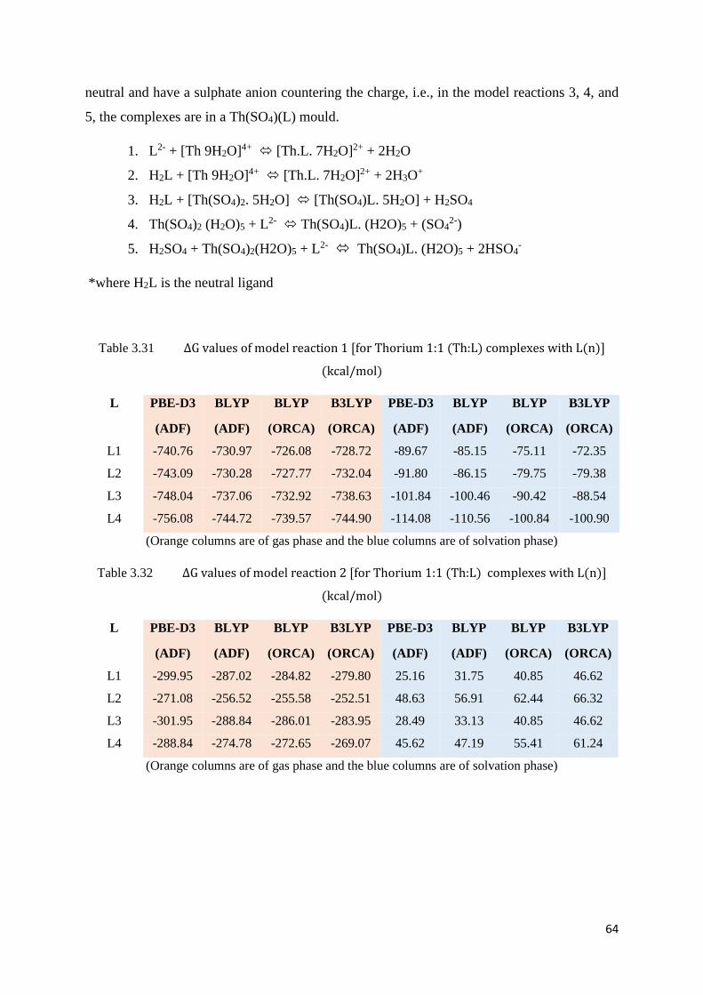
64
neutral and have a sulphate anion countering the charge, i.e., in the model reactions 3, 4, and
5, the complexes are in a Th(SO4)(L) mould.
1. L2- + [Th 9H2O]4+ [Th.L. 7H2O]2+ + 2H2O
2. H2L + [Th 9H2O]4+ [Th.L. 7H2O]2+ + 2H3O+
3. H2L + [Th(SO4)2. 5H2O] [Th(SO4)L. 5H2O] + H2SO4
4. Th(SO4)2 (H2O)5 + L2- Th(SO4)L. (H2O)5 + (SO42-)
5. H2SO4 + Th(SO4)2(H2O)5 + L2- Th(SO4)L. (H2O)5 + 2HSO4-
*where H2L is the neutral ligand
Table 3.31 ΔG values of model reaction 1 [for Thorium 1:1 (Th:L) complexes with L(n)]
(kcal/mol)
L PBE-D3
(ADF)
BLYP
(ADF)
BLYP
(ORCA)
B3LYP
(ORCA)
PBE-D3
(ADF)
BLYP
(ADF)
BLYP
(ORCA)
B3LYP
(ORCA)
L1 -740.76 -730.97 -726.08 -728.72 -89.67 -85.15 -75.11 -72.35
L2 -743.09 -730.28 -727.77 -732.04 -91.80 -86.15 -79.75 -79.38
L3 -748.04 -737.06 -732.92 -738.63 -101.84 -100.46 -90.42 -88.54
L4 -756.08 -744.72 -739.57 -744.90 -114.08 -110.56 -100.84 -100.90
(Orange columns are of gas phase and the blue columns are of solvation phase)
Table 3.32 ΔG values of model reaction 2 [for Thorium 1:1 (Th:L) complexes with L(n)]
(kcal/mol)
L PBE-D3
(ADF)
BLYP
(ADF)
BLYP
(ORCA)
B3LYP
(ORCA)
PBE-D3
(ADF)
BLYP
(ADF)
BLYP
(ORCA)
B3LYP
(ORCA)
L1 -299.95 -287.02 -284.82 -279.80 25.16 31.75 40.85 46.62
L2 -271.08 -256.52 -255.58 -252.51 48.63 56.91 62.44 66.32
L3 -301.95 -288.84 -286.01 -283.95 28.49 33.13 40.85 46.62
L4 -288.84 -274.78 -272.65 -269.07 45.62 47.19 55.41 61.24
(Orange columns are of gas phase and the blue columns are of solvation phase)
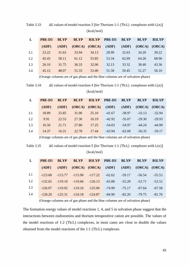
65
Table 3.33 ΔG values of model reaction 3 [for Thorium 1:1 (Th:L) complexes with L(n)]
(kcal/mol)
L PBE-D3
(ADF)
BLYP
(ADF)
BLYP
(ORCA)
B3LYP
(ORCA)
PBE-D3
(ADF)
BLYP
(ADF)
BLYP
(ORCA)
B3LYP
(ORCA)
L1 23.22 31.63 33.94 34.13 28.99 32.63 34.20 39.22
L2 45.43 58.11 61.12 55.85 53.34 62.69 64.26 68.96
L3 26.10 31.75 36.33 32.06 32.13 33.32 38.40 43.36
L4 45.12 48.07 51.33 53.40 51.58 50.45 51.27 56.16
(Orange columns are of gas phase and the blue columns are of solvation phase)
Table 3.34 ΔG values of model reaction 4 [for Thorium 1:1 (Th:L) complexes with L(n)]
(kcal/mol)
L PBE-D3
(ADF)
BLYP
(ADF)
BLYP
(ORCA)
B3LYP
(ORCA)
PBE-D3
(ADF)
BLYP
(ADF)
BLYP
(ORCA)
B3LYP
(ORCA)
L1 18.89 25.85 31.06 25.10 -41.67 -38.97 -33.13 -32.94
L2 9.91 22.53 27.30 16.19 -42.92 -35.07 -29.30 -29.93
L3 16.50 21.71 27.80 17.25 -54.03 -54.97 -44.24 -44.99
L4 14.37 16.31 22.78 17.44 -63.94 -62.00 -56.35 -59.17
(Orange columns are of gas phase and the blue columns are of solvation phase)
Table 3.35 ΔG values of model reaction 5 [for Thorium 1:1 (Th:L) complexes with L(n)]
(kcal/mol)
L PBE-D3
(ADF)
BLYP
(ADF)
BLYP
(ORCA)
B3LYP
(ORCA)
PBE-D3
(ADF)
BLYP
(ADF)
BLYP
(ORCA)
B3LYP
(ORCA)
L1 -123.68 -115.77 -115.90 -117.22 -62.62 -59.17 -56.54 -55.53
L2 -132.65 -119.10 -119.66 -126.13 -63.88 -55.28 -52.71 -52.52
L3 -126.07 -119.92 -119.16 -125.06 -74.99 -75.17 -67.64 -67.58
L4 -128.20 -125.31 -124.18 -124.87 -84.90 -82.20 -79.75 -81.76
(Orange columns are of gas phase and the blue columns are of solvation phase)
The formation energy values of model reactions 1, 4, and 5 in solvation phase suggest that the
interactions between eudistomins and thorium tetrapositive cation are possible. The values of
the model reactions of 1:2 (Th:L) complexes, in most cases are close to double the values
obtained from the model reactions of the 1:1 (Th:L) complexes.
66
3.5. Discussion
The results show that there are possible interactions between eudistomin ligands and metal
aqua ions. The model reactions 1, 4, and 5, where the ligand anion is made to interact with the
metal aqua ion/metal sulphate, have resulted in exothermic formation energies. The model
reactions 2 and 3, which involve a H-N bond breaking (deprotonation), have resulted in
endothermic formation energies, owing to the broken bonds. We are inclined to think that
model reactions 4 and 5 may provide a better result as they are modelled to resemble the, what
could be, real-time scenario. The fact that both these models have resulted in exothermic
formation energies makes us believe that the metal aqua ions may form decent interactions
with the eudistomin ligands.
The vanadyl complexes with three water molecules (i.e., the vanadium-centric distorted
octahedral input geometry), i.e., V(n)* complexes have all resulted in geometrical structures
with the third water molecule pushed away into the second solvation sphere (the water
molecule opposite to the oxygen atom in the V=O bond). The size of ligands may have
influenced this and could have allowed the extra-water molecule to get away from the
vanadium atom.
Uranium has a ground state electronic configuration of [Rn] 7s2 6d1 5f3.61 The near-
degeneracy of 5f and 6d orbitals is an interesting aspect for physicists and chemists as well.
The degeneracy driven covalency is a very interesting region for the “explorers”. 165 Actinide-
ligand bonding might exhibit covalency due to the near-degeneracy, especially in the middle
actinides like americium. However, these types of systems may not be as stable as their “ionic-
bond” counter-parts, i.e., when the stability of the molecules with covalent behaviour and ionic
behaviour are compared, ionic compounds have shown a better stability than the covalent
molecules.166 We, as actinide chemists, were interested to take a note of which orbital binds to
our ligands, and see if there was any such phenomenon. Unsurprisingly, our complexes are
“electrostatics-driven”, and in all but one case there was a 5f-domination the exception being
the 6d contribution (in case of U4 complex, as shown in Figure 3.18).
With thorium tetrapositive cation we have explored two possible flavours of complexes, i.e.,
1:2 (Th:L) and 1:1 (Th:L) complexes. The 1:2 (Th:L) complexes, in most of the cases, have
formation energy values close to two times the values obtained from the 1:1 (Th:L) complexes.
The formation of 1:1 (Th:L) complexes or 1:2 (Th:L) complexes would be a question of the
concentrations and we are inclined to think that they are low enough to result in 1:1 (Th:L)
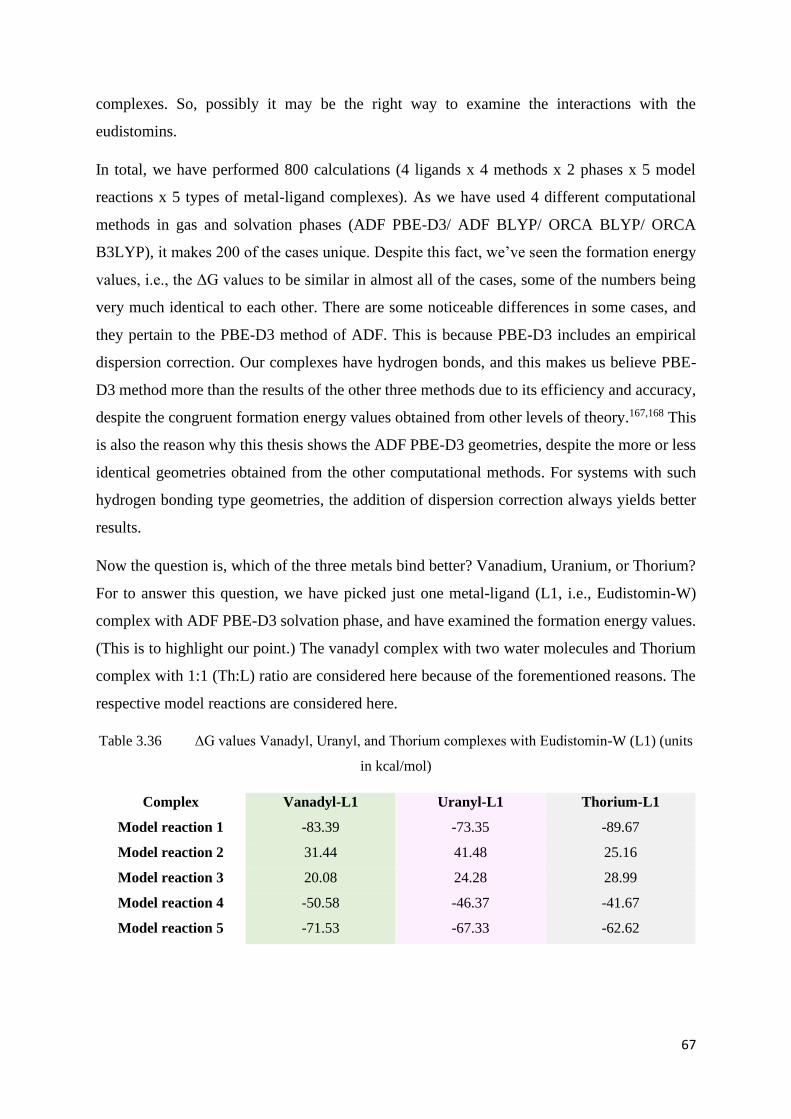
67
complexes. So, possibly it may be the right way to examine the interactions with the
eudistomins.
In total, we have performed 800 calculations (4 ligands x 4 methods x 2 phases x 5 model
reactions x 5 types of metal-ligand complexes). As we have used 4 different computational
methods in gas and solvation phases (ADF PBE-D3/ ADF BLYP/ ORCA BLYP/ ORCA
B3LYP), it makes 200 of the cases unique. Despite this fact, we’ve seen the formation energy
values, i.e., the ΔG values to be similar in almost all of the cases, some of the numbers being
very much identical to each other. There are some noticeable differences in some cases, and
they pertain to the PBE-D3 method of ADF. This is because PBE-D3 includes an empirical
dispersion correction. Our complexes have hydrogen bonds, and this makes us believe PBE-
D3 method more than the results of the other three methods due to its efficiency and accuracy,
despite the congruent formation energy values obtained from other levels of theory.167,168 This
is also the reason why this thesis shows the ADF PBE-D3 geometries, despite the more or less
identical geometries obtained from the other computational methods. For systems with such
hydrogen bonding type geometries, the addition of dispersion correction always yields better
results.
Now the question is, which of the three metals bind better? Vanadium, Uranium, or Thorium?
For to answer this question, we have picked just one metal-ligand (L1, i.e., Eudistomin-W)
complex with ADF PBE-D3 solvation phase, and have examined the formation energy values.
(This is to highlight our point.) The vanadyl complex with two water molecules and Thorium
complex with 1:1 (Th:L) ratio are considered here because of the forementioned reasons. The
respective model reactions are considered here.
Table 3.36 ΔG values Vanadyl, Uranyl, and Thorium complexes with Eudistomin-W (L1) (units
in kcal/mol)
Complex Vanadyl-L1 Uranyl-L1 Thorium-L1
Model reaction 1 -83.39 -73.35 -89.67
Model reaction 2 31.44 41.48 25.16
Model reaction 3 20.08 24.28 28.99
Model reaction 4 -50.58 -46.37 -41.67
Model reaction 5 -71.53 -67.33 -62.62
68
From Table 3.36, we can see that the formation energy values are distinguishable, but are within
the range of ~20kcal/mol in most cases, especially the model reactions involving sulphuric
acid, sulphate ion, and bisulphate ion. This takes us back to the question, do ascidians need
metals, or do they need the sulphate part of the metal-sulphate? From these results we are
inclined to assume that the metal-sulphate is what ascidians tend to sequester, not the metals
alone. Also, the closeness of the values in all of the cases adds to our assumption that the over-
presence of vanadium in ascidians in comparison to uranium or thorium might have a relation
with the abundance of vanadium in sea-waters, not with the preference of ascidians. Vanadium
is the second most-abundant d-block element in the ocean waters, and VO2+ is the most stable
oxy-cation. On the other hand, uranium and thorium (also other metals which are observed to
be sequestered by ascidians) are not that abundant in comparison to vanadium. Whether this
could have a role to play? It is debatable.
In conclusion to this chapter, it can be stated that our study has confirmed the possible
interactions between the eudistomin ligands and metals as per the respective model reactions
1, 4, and 5. There is not a lot to distinguish as all three metals have formation energy close to
each other (~10 kcal/mol) when compared, which prompts the idea that any metal can bind to
eudistomins. However, the minor differences might play a role when we apply this philosophy
to nuclear reprocessing.
69
CHAPTER-4
Conclusions and Future work
4.1. Conclusions
Nuclear reprocessing is an essential procedure to recovering useful uranium and other
actinides.169 This procedure requires ligands which can bind with the actinides. Ascidians are
marine animals which contain eudistomins, compounds of pharmacological importance. In this
work, we have started with an agenda to identify the potential of eudistomins as possible
biogenic ligands for nuclear reprocessing. In that process, we have investigated the possible
interactions between metal aqua ions and eudistomins. Five model reactions were designed to
explore the possible interactions and calculations were done in accordance. The simplest
possible eudistomins which could provide a bidentate structure were selected from the
literature. Three metal aqua ions, viz., vanadyl, uranyl, and thorium ions were adopted for our
study. Our study suggests that eudistomins are capable of forming exothermic interactions with
metals while in anionic form, as per the designed respective model reactions 1, 4, and 5. The
cells which contain the vanadium also contain sulphate ion/sulphuric acid, and have a pH range
of 1.8 to 2.0. At this range, sulphuric acid can occur as HSO4- ion. Model reactions 4 and 5
were designed to resemble the possible conditions in the ascidians, i.e., have a SO42- ion (in
model reaction 4) and HSO4- ion (in model reaction 5) on the product side, along with the
eudistomin-metal complex. We conclude this study by stating that model reactions 4 and 5 may
provide a better picture in comparison to the rest. The conclusions derived from this study can
be given as follows.
1. Eudistomins, when in anionic form as in (respective) model reactions 1, 4, and 5 show
exothermic interactions with the metal ions/sulphates. All of the interactions in these
respective model reactions are electrostatic in nature.
2. We are inclined to think that ascidians may not have preference to a specific metal, but
could be more interested towards the ‘sulphate’ part of the metal-sulphates.
3. Vanadium, when bound to a bidentate structure, is likely to prefer five coordination
over six coordination (including the oxygen in V=O).
4. Uranium in the uranyl complexes of our study has shown interactions dominated by 5f-
orbitals.
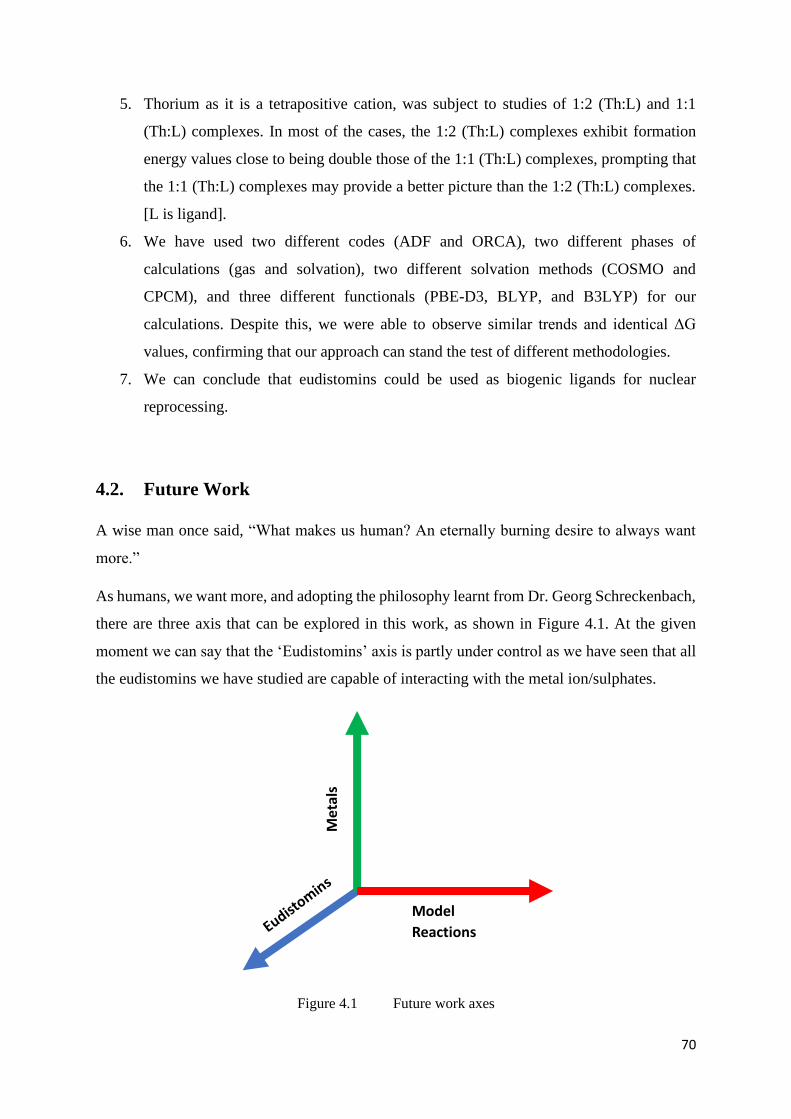
70
5. Thorium as it is a tetrapositive cation, was subject to studies of 1:2 (Th:L) and 1:1
(Th:L) complexes. In most of the cases, the 1:2 (Th:L) complexes exhibit formation
energy values close to being double those of the 1:1 (Th:L) complexes, prompting that
the 1:1 (Th:L) complexes may provide a better picture than the 1:2 (Th:L) complexes.
[L is ligand].
6. We have used two different codes (ADF and ORCA), two different phases of
calculations (gas and solvation), two different solvation methods (COSMO and
CPCM), and three different functionals (PBE-D3, BLYP, and B3LYP) for our
calculations. Despite this, we were able to observe similar trends and identical ΔG
values, confirming that our approach can stand the test of different methodologies.
7. We can conclude that eudistomins could be used as biogenic ligands for nuclear
reprocessing.
4.2. Future Work
A wise man once said, “What makes us human? An eternally burning desire to always want
more.”
As humans, we want more, and adopting the philosophy learnt from Dr. Georg Schreckenbach,
there are three axis that can be explored in this work, as shown in Figure 4.1. At the given
moment we can say that the ‘Eudistomins’ axis is partly under control as we have seen that all
the eudistomins we have studied are capable of interacting with the metal ion/sulphates.
Figure 4.1 Future work axes
Model
Reactions
Met
als
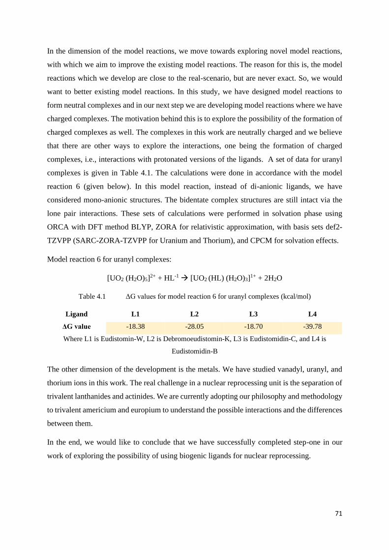
71
In the dimension of the model reactions, we move towards exploring novel model reactions,
with which we aim to improve the existing model reactions. The reason for this is, the model
reactions which we develop are close to the real-scenario, but are never exact. So, we would
want to better existing model reactions. In this study, we have designed model reactions to
form neutral complexes and in our next step we are developing model reactions where we have
charged complexes. The motivation behind this is to explore the possibility of the formation of
charged complexes as well. The complexes in this work are neutrally charged and we believe
that there are other ways to explore the interactions, one being the formation of charged
complexes, i.e., interactions with protonated versions of the ligands. A set of data for uranyl
complexes is given in Table 4.1. The calculations were done in accordance with the model
reaction 6 (given below). In this model reaction, instead of di-anionic ligands, we have
considered mono-anionic structures. The bidentate complex structures are still intact via the
lone pair interactions. These sets of calculations were performed in solvation phase using
ORCA with DFT method BLYP, ZORA for relativistic approximation, with basis sets def2-
TZVPP (SARC-ZORA-TZVPP for Uranium and Thorium), and CPCM for solvation effects.
Model reaction 6 for uranyl complexes:
[UO2 (H2O)5]2+ + HL-1 → [UO2 (HL) (H2O)3]
1+ + 2H2O
Table 4.1 ΔG values for model reaction 6 for uranyl complexes (kcal/mol)
Ligand L1 L2 L3 L4
ΔG value -18.38 -28.05 -18.70 -39.78
Where L1 is Eudistomin-W, L2 is Debromoeudistomin-K, L3 is Eudistomidin-C, and L4 is
Eudistomidin-B
The other dimension of the development is the metals. We have studied vanadyl, uranyl, and
thorium ions in this work. The real challenge in a nuclear reprocessing unit is the separation of
trivalent lanthanides and actinides. We are currently adopting our philosophy and methodology
to trivalent americium and europium to understand the possible interactions and the differences
between them.
In the end, we would like to conclude that we have successfully completed step-one in our
work of exploring the possibility of using biogenic ligands for nuclear reprocessing.
72
REFERENCES
1. Nuclear Power in the World Today. https://www.world-nuclear.org/information-
library/current-and-future-generation/nuclear-power-in-the-world-today.aspx.
2. Ağbulut, Ü. Turkey’s electricity generation problem and nuclear energy policy. Energy
Sources, Part A Recover. Util. Environ. Eff. 41, 2281–2298 (2019).
3. Emsley, J. Nature’s building blocks : an A-Z guide to the elements. (Oxford University
Press, 2003).
4. Ewing, R. C. Nuclear waste forms for actinides. Proc. Natl. Acad. Sci. 96, 3432–3439
(1999).
5. Anderson, H. H. & Asprey, L. B. Solvent Extraction Process for Plutonium. (1960).
6. Nuclear Reprocessing. https://en.wikipedia.org/wiki/Nuclear_reprocessing.
7. United States Government Accountability Office. Nuclear Fuel Cycle Options (Report
to Congressional Requesters). (2011).
8. Panak, P. J. & Geist, A. Complexation and Extraction of Trivalent Actinides and
Lanthanides by Triazinylpyridine N -Donor Ligands. Chem. Rev. 113, 1199–1236
(2013).
9. Geist, A. & Panak, P. J. Recent Progress in Trivalent Actinide and Lanthanide Solvent
Extraction and Coordination Chemistry with Triazinylpyridine N Donor Ligands.
Solvent Extr. Ion Exch. 39, 128–151 (2021).
10. Afsar, A., Distler, P., Harwood, L. M., John, J. & Westwood, J. Synthesis and
Screening of Modified 6,6′-Bis(5,5,8,8-tetramethyl-5,6,7,8-tetrahydrobenzo[ e
][1,2,4]triazin-3-yl)-2,2′-bipyridine Ligands for Actinide and Lanthanide Separation in
Nuclear Waste Treatment. J. Org. Chem. 81, 10517–10520 (2016).
11. Sittel, T., Trumm, M., Adam, C., Geist, A. & Panak, P. J. Impact of Solvent Polarity
on the Ligand Configuration in Tetravalent Thorium N-Donor Complexes. Inorg.
Chem. 60, 1092–1098 (2021).
12. Lewis, F. W. et al. Synthesis and Evaluation of Lipophilic BTBP Ligands for An/Ln
Separation in Nuclear Waste Treatment: The Effect of Alkyl Substitution on
Extraction Properties and Implications for Ligand Design. European J. Org. Chem.
73
2012, 1509–1519 (2012).
13. Xia, M., Yang, X., Chai, Z. & Wang, D. Stronger Hydration of Eu(III) Impedes Its
Competition against Am(III) in Binding with N-donor Extractants. Inorg. Chem. 59,
6267–6278 (2020).
14. Ekberg, C. et al. An overview and historical look back at the solvent extraction using
nitrogen donor ligands to extract and separate An(III) from Ln(III). Radiochim. Acta
96, (2008).
15. Menna, M., Fattorusso, E. & Imperatore, C. Alkaloids from Marine Ascidians.
Molecules 16, 8694–8732 (2011).
16. Aniszewski, T. Alkaloids — Secrets of Life. (Elsevier, 2007).
17. Shenkar, N. & Swalla, B. J. Global Diversity of Ascidiacea. PLoS One 6, e20657
(2011).
18. Chen, J.-Y. et al. The first tunicate from the Early Cambrian of South China. Proc.
Natl. Acad. Sci. 100, 8314–8318 (2003).
19. Porter, S. M. Calcite and aragonite seas and the de novo acquisition of carbonate
skeletons. Geobiology 8, 256–277 (2010).
20. Varol, O. & Houghton, S. D. A review and classification of fossil didemnid ascidian
spicules. J. Micropalaeontology 15, 135–149 (1996).
21. Buge, E. & Monniot, F. Nouveaux Spicules D’Ascidiesde L’Ypresien du Bassin de
Paris et du Toarcien des Deux-Sevres. Geobios 5, 83–90 (1972).
22. Fedonkin, M. A., Vickers-Rich, P., Swalla, B. J., Trusler, P. & Hall, M. A new
metazoan from the Vendian of the White Sea, Russia, with possible affinities to the
ascidians. Paleontol. J. 46, 1–11 (2012).
23. Odate, S. & Pawlik, J. R. The Role of Vanadium in the Chemical Defense of the
Solitary Tunicate, Phallusia nigra. J. Chem. Ecol. 33, 643–654 (2007).
24. Bromley, L. C. The Chemistry of Aloga Bay Ascidians. (Rhodes University, SA,
2015).
25. Davis, A. R. Alkaloids and ascidian chemical defense: Evidence for the ecological role
of natural products fromEudistoma olivaceum. Mar. Biol. 111, 375–379 (1991).
74
26. Lake, R., Blunt, J. & Munro, M. Eudistomins From the New Zealand Ascidian
Ritterella sigillinoides. Aust. J. Chem. 42, 1201 (1989).
27. Cao, R., Peng, W., Wang, Z. & Xu, A. ß-Carboline Alkaloids: Biochemical and
Pharmacological Functions. Curr. Med. Chem. 14, 479–500 (2007).
28. Kobayashi, J., Harbour, G. C., Gilmore, J. & Rinehart, K. L. Eudistomins A, D, G, H,
I, J, M, N, O, P, and Q, bromo, hydroxy, pyrrolyl and iminoazepino .beta.-carbolines
from the antiviral Caribbean tunicate Eudistoma olivaceum. J. Am. Chem. Soc. 106,
1526–1528 (1984).
29. Buaban, K., Phutdhawong, W., Taechowisan, T. & Phutdhawong, W. S. Synthesis and
Investigation of Tetrahydro-β-carboline Derivatives as Inhibitors of Plant Pathogenic
Fungi. Molecules 26, 207 (2021).
30. Bracegirdle, J. & Keyzers, R. A. Marine-derived Polyaromatic Butenolides - Isolation,
Synthesis and Biological Evaluations. Curr. Pharm. Des. 26, 4351–4361 (2020).
31. Casertano, M., Menna, M. & Imperatore, C. The Ascidian-Derived Metabolites with
Antimicrobial Properties. Antibiotics 9, 510 (2020).
32. Silva, K. L. & Trigo, J. R. Structure–Activity Relationships of Pyrrolizidine Alkaloids
in Insect Chemical Defense Against the Orb-Weaving Spider Nephila clavipes. J.
Chem. Ecol. 28, 657–688 (2002).
33. Bennet, R. N. & Wallsgrove, R. M. Secondary metabolites in plant defence
mechanisms. New Phytol. 127, 617–633 (1994).
34. Bell, M. V. et al. Contents of Vanadium and Sulphur in the Blood Cells of Ascidia
Mentula and Ascidiella Aspersa. J. Mar. Biol. Assoc. United Kingdom 62, 709–716
(1982).
35. Michibata, H., Iwata, Y. & Hirata, J. Isolation of highly acidic and vanadium-
containing blood cells from among several types of blood cell from ascidiidae species
by density-gradient centrifugation. J. Exp. Zool. 257, 306–313 (1991).
36. Frank, P., Hedman, B. & Hodgson, K. O. Sulfur Allocation and Vanadium−Sulfate
Interactions in Whole Blood Cells from the Tunicate Ascidia ceratodes , Investigated
Using X-ray Absorption Spectroscopy. Inorg. Chem. 38, 260–270 (1999).
75
37. Pisut, D. P. & Pawlik, J. R. Anti-predatory chemical defenses of ascidians: secondary
metabolites or inorganic acids? J. Exp. Mar. Bio. Ecol. 270, 203–214 (2002).
38. Mackenzie, F. T., Byrne, Howard, R., Duxbury & Alyn, C. Seawater. Encylopedia
Britannica. https://www.britannica.com/science/seawater (2020).
39. Kinzer, K. F. & Cardellina, J. H. Three new β-carbolines from the bermudian tunicate
Eudistoma olivaceum. Tetrahedron Lett. 28, 925–926 (1987).
40. Schupp, P. et al. Eudistomins W and X, Two New β-Carbolines from the Micronesian
Tunicate Eudistoma sp. J. Nat. Prod. 66, 272–275 (2003).
41. Davis, R. A., Carroll, A. R. & Quinn, R. J. Eudistomin V, a New β-Carboline from the
Australian Ascidian Pseudodistoma aureum. J. Nat. Prod. 61, 959–960 (1998).
42. Schumacher, R. W. & Davidson, B. S. Didemnolines A-D, new N9-substituted β-
carbolines from the marine ascidian Didemnum sp. Tetrahedron 51, 10125–10130
(1995).
43. Ravinder, K. et al. Isolation and synthesis of a novel β-carboline guanidine derivative
tiruchanduramine from the Indian ascidian Synoicum macroglossum. Tetrahedron
Lett. 46, 5475–5478 (2005).
44. Badre, A. et al. Eudistomin U and Isoeudistomin U, New Alkaloids from the Carribean
Ascidian Lissoclinum fragile. J. Nat. Prod. 57, 528–533 (1994).
45. Kobayashi, J. et al. Eudistomidins B, C, and D: novel antileukemic alkaloids from the
Okinawan marine tunicate Eudistoma glaucus. J. Org. Chem. 55, 3666–3670 (1990).
46. Shen, G. Q. & Baker, B. J. Biosynthetic studies of the eudistomins in the tunicate
eudistoma olivaceum. Tetrahedron Lett. 35, 1141–1144 (1994).
47. Wright, S. H. et al. Marine metabolites and metal ion chelation: Intact recovery and
identification of an iron(II) complex in the extract of the ascidian Eudistoma
gilboviride. Angew. Chemie - Int. Ed. 47, 8090–8092 (2008).
48. Kalk, M. Absorption of vanadium by tunicates. Nature 198, 1010–1011 (1963).
49. Macara, I. G., Mcleod, G. . & Kustin, K. Vanadium in tunicates: Oxygen-binding
studies. Comp. Biochem. Physiol. Part A Physiol. 62, 821–826 (1979).
50. Swinehart, J. H., Biggs, W. R., Halko, D. J. & Schroeder, N. C. The vanadium and
76
selected metal contents of some ascidians. BIOL.BULL. 146, 302–312 (1974).
51. Frank, P., Carlson, E. J., Carlson, R. M. K., Hedman, B. & Hodgson, K. O. The uptake
and fate of vanadyl ion in ascidian blood cells and a detailed hypothesis for the
mechanism and location of biological vanadium reduction. A visible and X-ray
absorption spectroscopic study. J. Inorg. Biochem. 102, 809–823 (2008).
52. Fox, D. L. Biochromy: Natural Coloration of Living Things. (University of California
Press, 1979).
53. Boeri, E. The determination of hemovanadin and its oxidation potential. Arch.
Biochem. Biophys. 37, 449–456 (1952).
54. Henze, M. Untersuchungen über das Blut der Ascidien. I. Mitteilung. Die
Vanadiumverbindung der Blutkörperchen. Hoppe-Seyler´s Zeitschrift für Physiol.
Chemie 72, 494–501 (1911).
55. Michibata, H., Uyama, T., Ueki, T. & Kanamori, K. Vanadocytes, cells hold the key to
resolving the highly selective accumulation and reduction of vanadium in ascidians.
Microsc. Res. Tech. 56, 421–434 (2002).
56. Ueki, T., Yamaguchi, N. & Michibata, H. Chloride channel in vanadocytes of a
vanadium-rich ascidian Ascidia sydneiensis samea. Comp. Biochem. Physiol. Part B
Biochem. Mol. Biol. 136, 91–98 (2003).
57. Hamada, T. et al. Solution structure of vanabin2, a vanadium(IV)-binding protein from
the vanadium-rich ascidian Ascidia sydneiensis samea. J. Am. Chem. Soc. 127, 4216–
4222 (2005).
58. Schreckenbach, G. & Shamov, G. A. Theoretical Actinide Molecular Science. Acc.
Chem. Res. 43, 19–29 (2010).
59. Hay, P. J., Martin, R. L. & Schreckenbach, G. Theoretical Studies of the Properties
and Solution Chemistry of AnO 2 2+ and AnO 2 + Aquo Complexes for An = U, Np,
and Pu. J. Phys. Chem. A 104, 6259–6270 (2000).
60. Mason, M. M., Smith, C., Vasiliu, M., Carrick, J. D. & Dixon, D. A. Prediction of
An(III)/Ln(III) Separation by 1,2,4-Triazinylpyridine Derivatives. J. Phys. Chem. A
125, 6529–6542 (2021).
77
61. Greenwood. Chemistry of the Elements. (Elsevier Science & Technology Books,
1996).
62. Ballhausen, C. J. & Gray, H. B. The Electronic Structure of the Vanadyl Ion. Inorg.
Chem. 1, 111–122 (1962).
63. Evans, H. T. Uranyl Ion Coordination. Science (80-. ). 141, 154–158 (1963).
64. Tutson, C. D. & Gorden, A. E. V. Thorium coordination: A comprehensive review
based on coordination number. Coord. Chem. Rev. 333, 27–43 (2017).
65. Frank, P., Carlson, R. M. K., Carlson, E. J., Hedman, B. & Hodgson, K. O. Biological
sulfur in the blood cells of Ascidia ceratodes: XAS spectroscopy and a cellular-
enzymatic hypothesis for vanadium reduction in the ascidians. J. Inorg. Biochem. 205,
110991 (2020).
66. Boys, S. F., Cook, G. B., Reeves, C. M. & Shavitt, I. Automatic Fundamental
Calculations of Molecular Structure. Nature 178, 1207–1209 (1956).
67. Preuss, H. DasSCF-MO-P(LCGO)-Verfahren und seine Varianten. Int. J. Quantum
Chem. 2, 651–662 (1968).
68. Allinger, N. L. Conformational analysis. 130. MM2. A hydrocarbon force field
utilizing V1 and V2 torsional terms. J. Am. Chem. Soc. 99, 8127–8134 (1977).
69. Buenker, R. J. & Peyerimhoff, S. D. Ab initio SCF calculations for azulene and
naphthalene. Chem. Phys. Lett. 3, 37–42 (1969).
70. Nobel Prize in Chemistry, 1998.
https://www.nobelprize.org/prizes/chemistry/1998/summary/.
71. Nobel Prize in Chemistry, 2013.
https://www.nobelprize.org/prizes/chemistry/2013/press-release/.
72. Schrödinger, E. An Undulatory Theory of the Mechanics of Atoms and Molecules.
Phys. Rev. 28, 1049–1070 (1926).
73. Cramer, C. J. Essentials of Computational Chemistry: Theories and Models. (Wiley,
2004).
74. Jensen, F. Introduction to Computational Chemistry. (John Wiley & Sons, Ltd, 2007).
78
75. Gordon, A. & Avron, J. E. Born-Oppenheimer Approximation near Level Crossing.
Phys. Rev. Lett. 85, 34–37 (2000).
76. Waschewsky, G. C. G., Kash, P. W., Myers, T. L., Kitchen, D. C. & Butler, L. J. What
Woodward and Hoffmann didn’t tell us: the failure of the Born–Oppenheimer
approximation in competing reaction pathways. J. Chem. Soc., Faraday Trans. 90,
1581–1598 (1994).
77. Born, M. & Oppenheimer, R. Zur Quantentheorie der Molekeln. Ann. Phys. 389, 457–
484 (1927).
78. Sommerfeld, T. Lorentz Trial Function for the Hydrogen Atom: A Simple, Elegant
Exercise. J. Chem. Educ. 88, 1521–1524 (2011).
79. Slater, J. C. Atomic Shielding Constants. Phys. Rev. 36, 57–64 (1930).
80. Boys, S. F. Electronic wave functions - I. A general method of calculation for the
stationary states of any molecular system. Proc. R. Soc. London. Ser. A. Math. Phys.
Sci. 200, 542–554 (1950).
81. Hartree, D. R. The Wave Mechanics of an Atom with a Non-Coulomb Central Field.
Part II. Some Results and Discussion. Math. Proc. Cambridge Philos. Soc. 24, 111–
132 (1928).
82. Slater, J. C. The Self Consistent Field and the Structure of Atoms. Phys. Rev. 32, 339–
348 (1928).
83. Gaunt, J. A. A Theory of Hartree’s Atomic Fields. Math. Proc. Cambridge Philos.
Soc. 24, 328–342 (1928).
84. Roothaan, C. C. J. New Developments in Molecular Orbital Theory. Rev. Mod. Phys.
23, 69–89 (1951).
85. Hall, G. . The molecular orbital theory of chemical valency VIII. A method of
calculating ionization potentials. Proc. R. Soc. London. Ser. A. Math. Phys. Sci. 205,
541–552 (1951).
86. Fock, V. Näherungsmethode zur Lösung des quantenmechanischen
Mehrkörperproblems. Zeitschrift für Phys. 61, 126–148 (1930).
87. Koch, W. & Holthausen, M. C. A Chemist’s Guide to Density Functional Theory.
79
(Wiley-VCH, 2000).
88. Brás, N. F., Perez, M. A. S., Fernandes, P. A., Silva, P. J. & Ramos, M. J. Accuracy of
Density Functionals in the Prediction of Electronic Proton Affinities of Amino Acid
Side Chains. J. Chem. Theory Comput. 7, 3898–3908 (2011).
89. Holthausen, M. C. Benchmarking approximate density functional theory. I.s/d
excitation energies in 3d transition metal cations. J. Comput. Chem. 26, 1505–1518
(2005).
90. Neumann, R., Nobes, R. H. & Handy, N. C. Exchange functionals and potentials. Mol.
Phys. 87, 1–36 (1996).
91. Wellendorff, J. et al. A benchmark database for adsorption bond energies to transition
metal surfaces and comparison to selected DFT functionals. Surf. Sci. 640, 36–44
(2015).
92. Quintal, M. M., Karton, A., Iron, M. A., Boese, A. D. & Martin, J. M. L. Benchmark
Study of DFT Functionals for Late-Transition-Metal Reactions †. J. Phys. Chem. A
110, 709–716 (2006).
93. Hohenberg, P. & Kohn, W. Inhomogeneous Electron Gas. Phys. Rev. 136, B864–B871
(1964).
94. Kohn, W. & Sham, L. J. Self-Consistent Equations Including Exchange and
Correlation Effects. Phys. Rev. 140, A1133–A1138 (1965).
95. Jaoul, A., Nocton, G. & Clavaguéra, C. Assessment of Density Functionals for
Computing Thermodynamic Properties of Lanthanide Complexes. ChemPhysChem 18,
2688–2696 (2017).
96. Nazarian, D., Ganesh, P. & Sholl, D. S. Benchmarking density functional theory
predictions of framework structures and properties in a chemically diverse test set of
metal–organic frameworks. J. Mater. Chem. A 3, 22432–22440 (2015).
97. Fan, J.-Y., Zheng, Z.-Y., Su, Y. & Zhao, J.-J. Assessment of dispersion correction
methods within density functional theory for energetic materials. Mol. Simul. 43, 568–
574 (2017).
98. Grimme, S., Antony, J., Ehrlich, S. & Krieg, H. A consistent and accurate ab initio
80
parametrization of density functional dispersion correction (DFT-D) for the 94
elements H-Pu. J. Chem. Phys. 132, 154104 (2010).
99. Perdew, J. P. et al. Rationale for mixing exact exchange with density functional
approximations Rationale for mixing exact exchange with density functional
approximations. 9982, 9982–9985 (2010).
100. Perdew, J. P. & Schmidt, K. Jacob’s ladder of density functional approximations for
the exchange-correlation energy. in AIP Conference Proceedings vol. 577 1–20 (AIP,
2001).
101. Pyykkö, P. Relativistic Effects in Chemistry: More Common Than You Thought.
Annu. Rev. Phys. Chem. 63, 45–64 (2012).
102. Dirac, P. A. M. The quantum theory of the electron. Proc. R. Soc. London. Ser. A,
Contain. Pap. a Math. Phys. Character 117, 610–624 (1928).
103. Van Lenthe, E., Baerends, E. J. & Snijders, J. G. Relativistic total energy using regular
approximations. J. Chem. Phys. 101, 9783–9792 (1994).
104. Van Lenthe, E. Geometry optimizations in the zero order regular approximation for
relativistic effects. J. Chem. Phys. 110, 8943–8953 (1999).
105. Van Lenthe, E. & Baerends, E. J. Optimized Slater-type basis sets for the elements 1-
118. J. Comput. Chem. 24, 1142–1156 (2003).
106. Visscher, L. & Van Lenthe, E. On the distinction between scalar and spin-orbit
relativistic effects. Chem. Phys. Lett. 306, 357–365 (1999).
107. Van Lenthe, E., Snijders, J. G. & Baerends, E. J. The zero-order regular approximation
for relativistic effects: The effect of spin-orbit coupling in closed shell molecules. J.
Chem. Phys. 105, 6505–6516 (1996).
108. Van Lenthe, E., Baerends, E. J. & Snijders, J. G. Relativistic regular two-component
Hamiltonians. J. Chem. Phys. 99, 4597–4610 (1993).
109. Yin, M. T. & Cohen, M. L. Theory of ab initio pseudopotential calculations. Phys.
Rev. B 25, 7403–7412 (1982).
110. Vanderbilt, D. Soft self-consistent pseudopotentials in a generalized eigenvalue
formalism. Phys. Rev. B 41, 7892–7895 (1990).
81
111. Tomasi, J. & Persico, M. Molecular Interactions in Solution: An Overview of Methods
Based on Continuous Distributions of the Solvent. Chem. Rev. 94, 2027–2094 (1994).
112. Miertuš, S., Scrocco, E. & Tomasi, J. Electrostatic interaction of a solute with a
continuum. A direct utilizaion of AB initio molecular potentials for the prevision of
solvent effects. Chem. Phys. 55, 117–129 (1981).
113. Cammi, R. & Tomasi, J. Remarks on the use of the apparent surface charges (ASC)
methods in solvation problems: Iterative versus matrix-inversion procedures and the
renormalization of the apparent charges. J. Comput. Chem. 16, 1449–1458 (1995).
114. Cossi, M., Barone, V., Cammi, R. & Tomasi, J. Ab initio study of solvated molecules:
a new implementation of the polarizable continuum model. Chem. Phys. Lett. 255,
327–335 (1996).
115. Klamt, A., Moya, C. & Palomar, J. A Comprehensive Comparison of the IEFPCM and
SS(V)PE Continuum Solvation Methods with the COSMO Approach. J. Chem. Theory
Comput. 11, 4220–4225 (2015).
116. Klamt, A. Conductor-like Screening Model for Real Solvents: A New Approach to the
Quantitative Calculation of Solvation Phenomena. J. Phys. Chem. 99, 2224–2235
(1995).
117. Cramer, C. J. & Truhlar, D. G. Implicit Solvation Models: Equilibria, Structure,
Spectra, and Dynamics. Chem. Rev. 99, 2161–2200 (1999).
118. Leung, B. O., Reid, D. L., Armstrong, D. A. & Rauk, A. Entropies in Solution from
Entropies in the Gas Phase. J. Phys. Chem. A 108, 2720–2725 (2004).
119. Garza, A. J. Solvation Entropy Made Simple. J. Chem. Theory Comput. 15, 3204–3214
(2019).
120. Mulliken, R. S. Electronic Population Analysis on LCAO–MO Molecular Wave
Functions. I. J. Chem. Phys. 23, 1833–1840 (1955).
121. Mayer, I. Bond order and valence indices: A personal account. J. Comput. Chem. 28,
204–221 (2007).
122. Hirshfeld, F. L. Bonded-atom fragments for describing molecular charge densities.
Theor. Chim. Acta 44, 129–138 (1977).
82
123. Reed, A. E., Weinstock, R. B. & Weinhold, F. Natural population analysis. J. Chem.
Phys. 83, 735–746 (1985).
124. Fonseca Guerra, C., Handgraaf, J.-W., Baerends, E. J. & Bickelhaupt, F. M. Voronoi
deformation density (VDD) charges: Assessment of the Mulliken, Bader, Hirshfeld,
Weinhold, and VDD methods for charge analysis. J. Comput. Chem. 25, 189–210
(2004).
125. te Velde, G. et al. Chemistry with ADF. J. Comput. Chem. 22, 931–967 (2001).
126. Fonseca Guerra, C., Snijders, J. G., te Velde, G. & Baerends, E. J. Towards an order-
N DFT method. Theor. Chem. Accounts Theory, Comput. Model. (Theoretica Chim.
Acta) 99, 391–403 (1998).
127. ADF, SCM, Theoretical Chemistry, Vrije Universiteit, . ADF. (2017).
128. Becke, A. D. Density-functional exchange-energy approximation with correct
asymptotic behavior. Phys. Rev. A 38, 3098–3100 (1988).
129. Lee, C., Yang, W. & Parr, R. G. Development of the Colle-Salvetti correlation-energy
formula into a functional of the electron density. Phys. Rev. B 37, 785–789 (1988).
130. Perdew, J. P., Burke, K. & Ernzerhof, M. Generalized Gradient Approximation Made
Simple. Phys. Rev. Lett. 77, 3865–3868 (1996).
131. Burke, K., Ernzerhof, M. & Perdew, J. P. The adiabatic connection method: a non-
empirical hybrid. Chem. Phys. Lett. 265, 115–120 (1997).
132. Neese, F. The ORCA program system. WIREs Comput. Mol. Sci. 2, 73–78 (2012).
133. Neese, F. Software update: the ORCA program system, version 4.0. WIREs Comput.
Mol. Sci. 8, (2018).
134. Becke, A. D. A new mixing of Hartree–Fock and local density‐functional theories. J.
Chem. Phys. 98, 1372–1377 (1993).
135. Barone, V. & Cossi, M. Quantum Calculation of Molecular Energies and Energy
Gradients in Solution by a Conductor Solvent Model. J. Phys. Chem. A 102, 1995–
2001 (1998).
136. Santos, R. Application of Density Functional Theory to the Interaction of Uranium
with Eudistomins. (University of Manitoba, 2019).
83
137. SpectraBase. John Wiley & Sons, Inc. SpectraBase https://spectrabase.com/.
138. Polycitoridae. https://www.gbif.org/species/7349.
139. Dupont, B. Colonial Ascidian Eudistoma sp.
https://www.flickr.com/photos/berniedup/8502008103/.
140. Nakagawa, M., Liu, J. J. & Hino, T. Total synthesis of (-)-eudistomin L and (-)-
debromoeudistomin L. J. Am. Chem. Soc. 111, 2721–2722 (1989).
141. Toru. Midori Kaimen Boya.
http://www.ha.shotoku.ac.jp/~kawa/KYO/SEIBUTSU/DOUBUTSU/sango/okinawa/se
kisakudoubutsumon/midorikaimen/01.html.
142. Hamada, T. et al. Solution Structure of Vanabin2, a Vanadium(IV)-Binding Protein
from the Vanadium-Rich Ascidian Ascidia s ydneiensis samea. J. Am. Chem. Soc. 127,
4216–4222 (2005).
143. Kawakami, N., Ueki, T., Matsuo, K., Gekko, K. & Michibata, H. Selective metal
binding by Vanabin2 from the vanadium-rich ascidian, Ascidia sydneiensis samea.
Biochim. Biophys. Acta - Gen. Subj. 1760, 1096–1101 (2006).
144. Frank, P., Carlson, E. J., Carlson, R. M. K., Hedman, B. & Hodgson, K. O. The uptake
and fate of vanadyl ion in ascidian blood cells and a detailed hypothesis for the
mechanism and location of biological vanadium reduction. A visible and X-ray
absorption spectroscopic study. J. Inorg. Biochem. 102, 809–823 (2008).
145. Frank, P., Robinson, W. E., Kustin, K. & Hodgson, K. O. Unprecedented forms of
vanadium observed within the blood cells of Phallusia nigra using K-edge X-ray
absorption spectroscopy. J. Inorg. Biochem. 86, 635–648 (2001).
146. Tachez, M. & Théobald, F. Structure du sulfate de vanadyle pentahydraté VO(H 2 O)
5 SO 4 β (variété orthorhombique). Acta Crystallogr. Sect. B Struct. Crystallogr.
Cryst. Chem. 36, 1757–1761 (1980).
147. Magnussen, M., Brock-Nannestad, T. & Bendix, J. Pentaaquaoxovanadium(IV)
bis(trifluoromethanesulfonate). Acta Crystallogr. Sect. C Cryst. Struct. Commun. 63,
m51–m53 (2007).
148. Krakowiak, J., Lundberg, D. & Persson, I. A Coordination Chemistry Study of
84
Hydrated and Solvated Cationic Vanadium Ions in Oxidation States +III, +IV, and +V
in Solution and Solid State. Inorg. Chem. 51, 9598–9609 (2012).
149. The Chemistry of the Actinide and Transactinide Elements. (Springer Netherlands,
2006). doi:10.1007/1-4020-3598-5.
150. Rui, X. et al. Bioreduction of hydrogen uranyl phosphate: Mechanisms and U(IV)
products. Environ. Sci. Technol. 47, 5668–5678 (2013).
151. Koribanics, N. M. et al. Spatial distribution of an uranium-respiring
betaproteobacterium at the Rifle, CO field research site. PLoS One 10, (2015).
152. Vettese, G. F. et al. Multiple Lines of Evidence Identify U(V) as a Key Intermediate
during U(VI) Reduction by Shewanella oneidensis MR1. Environ. Sci. Technol. 54,
2268–2276 (2020).
153. Wu, Q., Sanford, R. A. & Löffler, F. E. Uranium(VI) reduction by Anaeromyxobacter
dehalogenans strain 2CP-C. Appl. Environ. Microbiol. 72, 3608–3614 (2006).
154. Khijniak, T. V. et al. Reduction of uranium(VI) phosphate during growth of the
thermophilic bacterium Thermoterrabacterium ferrireducens. Appl. Environ.
Microbiol. 71, 6423–6426 (2005).
155. Lovley, D. R., Phillips, E. J. P., Gorby, Y. A. & Landa, E. R. Microbial reduction of
uranium. Nature 350, 413–416 (1991).
156. Lovley, D. R. & Phillips, E. J. P. Reduction of uranium by Desulfovibrio
desulfuricans. Appl. Environ. Microbiol. 58, 850–856 (1992).
157. Vallet, V. et al. Solvent Effects on Uranium(VI) Fluoride and Hydroxide Complexes
Studied by EXAFS and Quantum Chemistry. Inorg. Chem. 40, 3516–3525 (2001).
158. Wahlgren, U. et al. Structure of Uranium(VI) in Strong Alkaline Solutions. A
Combined Theoretical and Experimental Investigation. J. Phys. Chem. A 103, 8257–
8264 (1999).
159. Cooper, N., Minakata, D., Begovic, M. & Crittenden, J. Should We Consider Using
Liquid Fluoride Thorium Reactors for Power Generation? Environ. Sci. Technol. 45,
6237–6238 (2011).
160. World Nuclear Association ‘Thorium’. https://www.world-nuclear.org/information-
85
library/current-and-future-generation/thorium.aspx#References (2020).
161. Chuang, C.-Y. et al. Important role of biomolecules from diatoms in the scavenging of
particle-reactive radionuclides of thorium, protactinium, lead, polonium, and beryllium
in the ocean: A case study with Phaeodactylum tricornutum. Limnol. Oceanogr. 59,
1256–1266 (2014).
162. Alverson, A. The Air You’re Breathing? A Diatom Made That.
https://www.livescience.com/46250-teasing-apart-the-diatom-genome.html (2014).
163. Martino, A. De, Meichenin, A., Shi, J., Pan, K. & Bowler, C. Genetic and phenotypic
characterization of Phaeodactylum tricornutum (Bacillariophyceae) accessions 1. J.
Phycol. 43, 992–1009 (2007).
164. Brown, A. C. & Davies, A. B. The fate of thorium dioxide introduced into the body
cavity of Ciona intestinalis (Tunicata). J. Invertebr. Pathol. 18, 276–279 (1971).
165. Cooper, S. & Kaltsoyannis, N. Covalency in AnCl 3 (An = Th–No). Dalt. Trans. 50,
1478–1485 (2021).
166. Sadhu, B. & Dolg, M. Enhancing Actinide(III) over Lanthanide(III) Selectivity
through Hard-by-Soft Donor Substitution: Exploitation and Implication of Near-
Degeneracy-Driven Covalency. Inorg. Chem. 58, 9738–9748 (2019).
167. Grimme, S., Huenerbein, R. & Ehrlich, S. On the Importance of the Dispersion Energy
for the Thermodynamic Stability of Molecules. ChemPhysChem 12, 1258–1261
(2011).
168. Grimme, S., Hansen, A., Brandenburg, J. G. & Bannwarth, C. Dispersion-Corrected
Mean-Field Electronic Structure Methods. Chem. Rev. 116, 5105–5154 (2016).
169. Taylor, R. Reprocessing and Recycling of Spent Nuclear Fuel 1st Edition. (Woodhead
Publishing, Elsevier Ltd., 2015).
Related Documents