DESIGN, MODELING, AND EXPERIMENTAL VALIDATION OF A STIRLING ENGINE WITH A CONTROLLED DISPLACER PISTON By Anna Winkelmann Thesis Submitted to the Faculty of the Graduate School of Vanderbilt University in partial fulfillment of the requirements for the degree of MASTER OF SCIENCE in Mechanical Engineering May, 2015 Nashville, Tennessee Approved: Dr. Eric J. Barth Dr. Michael Goldfarb Dr. Alvin Strauss

Welcome message from author
This document is posted to help you gain knowledge. Please leave a comment to let me know what you think about it! Share it to your friends and learn new things together.
Transcript

DESIGN, MODELING, AND EXPERIMENTAL VALIDATION OF A STIRLING ENGINE WITH A
CONTROLLED DISPLACER PISTON
By
Anna Winkelmann
Thesis
Submitted to the Faculty of the
Graduate School of Vanderbilt University
in partial fulfillment of the requirements
for the degree of
MASTER OF SCIENCE
in
Mechanical Engineering
May, 2015
Nashville, Tennessee
Approved:
Dr. Eric J. Barth
Dr. Michael Goldfarb
Dr. Alvin Strauss

ii
ACKNOWLEDGEMENTS
First and foremost I would like to express my gratitude and appreciation to my advisor, Dr. Eric J.
Barth, for giving me the opportunity to work and do research in the Laboratory for the Design and Control
of Energetic Systems. I would like to thank him for his guidance throughout this work. My gratitude also
extends to the rest of my colleagues, Bryn Pitt, David Comber, and Alex Pedchenko, each of whom I
learned from. I would also express my appreciation to the members of my thesis committee: Dr. Michael
Goldfarb and Dr. Alvin Strauss.
I would like to thank Red River machine for machining all my parts, for being very responsive and
very helpful. I appreciate all the work they have done for me.
I thank my parents and my brother for their constant support and encouragement during my studies
despite being so far away from home. Without them I would have not made it so far. At this point I would
like to especially thank my dad for all the technical advice, mental support, and for being there whenever I
was in need to talk to someone.
Finally, I would like to thank the Center for Compact and Efficient Fluid Power (CCEFP) grant EEC-
0540834 for funding this work.

iii
TABLE OF CONTENTS
Page
Acknowledgements ii
List of Figures iv
List of Tables vii
Chapter
I. Overview 1
Introduction and Motivation 1 Literature Survey 3 Organization of the Document 4 References 5
II. Manuscript 1: System Dynamic Model and Design of a Stirling Pump 7
Abstract 7 Introduction 7 Design of Stirling Pump 9 Multi-Stage to Single-Stage Design Change 10 Working Fluid and Pumping Fluid 11 Other Design Changes 13 Dynamic Model 14 Results 17 Conclusion 19 Acknowledgement 20 References 20
III. Manuscript 2: Design, model, and experimental testing of a stirling Pressurizer 21
Abstract 21 Introduction 21 Design 23 Dynamic Model 25
A. Pressure Dynamics 26 B. Mass Flow 27 C. Heat transfer 28 D. Regenerative Channel 30
Experimental Validation of the Model 31 A. Experimental Setup 31 B. Engine Parameters 35 C. Tuned Model Parameters 36 D. Sinusoidal Displacer Motion 37 E. Non-sinusoidal Displacer Motion 39
Conclusion 41 Acknowledgment 41 References 41
IV. Future Directions and Discussion 43
Appendix 45
A. Simulink Diagrams 45 B. Matlab Code 53 C. Technical drawings for prototype 58

iv
LIST OF FIGURES
Page
Figure 1-1: Comparison of the energy transduction of a typical electric system with a Stirling
pressurizer combined with a hydraulic pump ............................................................................ 2
Figure 1-2: Energy density vs. actuation power density of different devices. 2
Figure 2-1: Generation-1 multistage thermocompressor device concept ..................................................... 9
Figure 2-2: Design for a single stage of the generation-1 thermocompressor device. A reciprocating
lead screw driven by a DC motor moves a loose-fit displacer piston between the hot side
and the cold side. In response to this, the pressure in the device changes as the working
fluid moves between the hot side (high pressure) and the cold side (low pressure). As the
pressure fluctuates, the thermocompressor outputs high pressure fluid to a reservoir and
intakes low pressure fluid from the environment (or from a previous stage). ......................... 10
Figure 2-3: Design of the generation 2 device ............................................................................................ 11
Figure 2-4: Pumping Section....................................................................................................................... 12
Figure 2-5: Linear DC Servomotor .............................................................................................................. 13
Figure 2-6: Driving (blue) and average (green) pressure vs. time .............................................................. 18
Figure 2-7: Displacement of the pumping piston with respect to time ........................................................ 18
Figure 2-8: Pressure dynamics in the pumping chamber compared to the supply pressure (7 MPa) and
atmospheric pressure (101kPa) .............................................................................................. 19
Figure 3-1: Design of the Stirling pressurizer .............................................................................................. 24
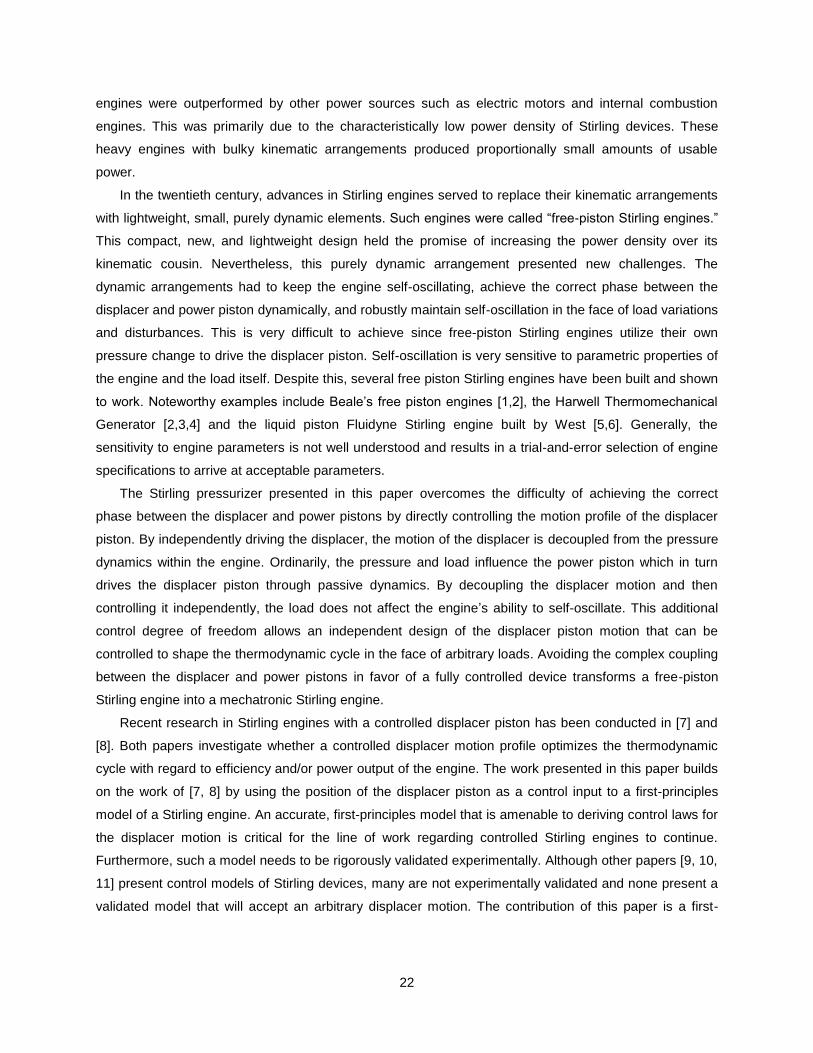
Figure 3-2: A System overview of all the dynamics taking place within the pressurizer. This diagram
illustrates dynamic interactions within the system ................................................................... 27
Figure 3-3: Diagram explaining the shuttle heat transfer ............................................................................ 30
Figure 3-4: Experimental setup ................................................................................................................... 33
Figure 3- 5: Thermographic image of the engine section ........................................................................... 34
Figure 3-6: Orifice area was adjusted such that modeled and measured pressure inside the return
chamber would be the same. .................................................................................................. 36
Figure 3-7: Measured and modeled pressure Pk inside the engine section at low heater head
temperature (250°C), low pressure (10 bar), and at a frequency of 1 Hz. The modeled
pressure ratio is about 7% lower than measured pressure ratio. ............................................ 37
Figure 3-8: Measured and modeled pressure Pk inside the engine section at 450°C heater head
temperature, high pressure (20 bar), and at a frequency of 2 Hz. The modeled pressure
ratio is about 3% higher than measured pressure ratio. ......................................................... 38

v
Figure 3-9: Measured and modeled pressure Pk inside the engine section at high heater head
temperature (500°C), high pressure (20 bar), and at a frequency of 2 Hz. The modeled
pressure ratio is about 4.6% higher than measured pressure ratio. ....................................... 38
Figure 3-10: Filtered square wave motion profile of the displacer piston at 450°C, 20bar and 2Hz .......... 40
Figure 3-11: Measured and modeled pressure Pk inside the engine section at 450°C heater head
temperature, high pressure (20 bar), and at a frequency of 2 Hz. The modeled pressure
ratio is 8% higher than measured pressure ratio..................................................................... 40
Figure 4-1: Stirling device using additive manufacturing capabilities ......................................................... 44
Figure A-1: Overall system .......................................................................................................................... 45
Figure A-2: Volumes ................................................................................................................................... 45
Figure A-3: Engine dynamics ...................................................................................................................... 46
Figure A-4: Pressure dynamics on hot side ................................................................................................ 47
Figure A-5: Heat transfer losses ................................................................................................................. 48
Figure A-6: Regenerative system ............................................................................................................... 48
Figure A-7: Mass flow rate in engine section .............................................................................................. 49
Figure A-8: Mass flow rate in engine section times Tflow ............................................................................. 49
Figure A-9: Pressure dynamics on cold side .............................................................................................. 50
Figure A-10: Direction switch ...................................................................................................................... 51
Figure A-11: Mass flow rate between cold side and return chamber ......................................................... 51
Figure A-12: Mass flow rate between cold side and return chamber ......................................................... 52
Figure C-1: Engine weld assembly ............................................................................................................. 58
Figure C-2: Heater head ............................................................................................................................. 59
Figure C-3: Inconel cylinder ........................................................................................................................ 60
Figure C-4: Cooling fins .............................................................................................................................. 61
Figure C-5: Cooler head .............................................................................................................................. 62
Figure C-7: Top part of Hugger1 ................................................................................................................. 64
Figure C-8: Shaft part of hugger1 ............................................................................................................... 65
Figure C-9: Return part of hugger1 ............................................................................................................. 66
Figure C-10: Hugger2 of return chamber .................................................................................................... 67
Figure C-11: Top part of hugger2 ............................................................................................................... 68
Figure C-13: Displacer weld assembly ....................................................................................................... 70
Figure C-14: Top part of displacer piston .................................................................................................... 71
Figure C-15: Displacer cylinder ................................................................................................................... 72
Figure C-16: Bottom of displacer ................................................................................................................ 73

vi
Figure C-17: Extension rod ......................................................................................................................... 74
Figure C-18: Clamp assembly .................................................................................................................... 75
Figure C-21: Connection between coupling and linear motor ..................................................................... 78
vii
LIST OF TABLES
Page
Table 2-1: Values of significant parameters ................................................................................................ 15
Table 2-2: Values of significant parameters ................................................................................................ 16
Table 2-3: Conditions for Pu and Pd ............................................................................................................ 16
Table 2-4: Parameters used in simulation .................................................................................................. 17
Table 3-1: Engine Parameters .................................................................................................................... 35
Table 3-2: Pressure ratio of experimental and ............................................................................................ 39
Table 3-3: Pressure ratio of experimental and modeled data at 2 Hz ....................................................... 39

1
CHAPTER I
OVERVIEW
Introduction and Motivation
An un-tethered, portable, and effective power supply for human-scale robots has progressively
become more important in robotics research. This is because today’s mobile robots must be energetically
autonomous to be truly effective. Typical electric power supply and actuation systems using batteries and
motor drives are not capable of powering human-scale robots like the Honda P3 robot or Honda ASIMO
for more than 25 min. More recent progress includes systems like Big Dog which use hydrocarbon fueled
IC engines and hydraulic actuators. Although superior in energy and power density to electric systems, IC
engine based systems are very noisy.
The motivation of this research is to develop a more adequate power supply and actuation system
that provides an order of magnitude greater power and energy density than the state-of-the-art batteries
and motor drives while also avoiding the drawbacks of IC-based systems. It should also be noted that this
challenge is very scale-dependent. Miniaturizing IC engines results in very poor efficiencies whereas the
downscaling of Stirling devices actually enhances their power density [1]. The key to a more effective,
portable power supply and actuation system is a combined measure of 1) a high energy density fuel
source, 2) an efficient energy conversion to mechanical work, 3) a low converter mass, and 4) high power
density actuators. The reason why an electric power supply and actuation system cannot power human-
scale robots for more than 25 min is simply because of the low energy density of batteries and the low
power density of electric motors compared to the high overall converter mass of the system. This work
proposes a Stirling pressurizer combined with a power unit to be used as the power supply. The power
unit could be anything that can be driven by a pressure swing such as a hydraulic pump, a linear electric
generator, a reciprocating piston compressor, or a high pressure water filtration system, among others.
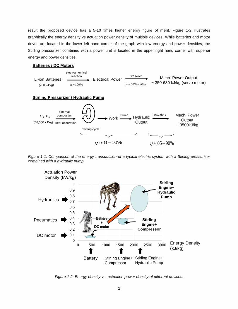
Figure 1-1 compares the energy transduction of a typical electric power supply and actuation system
with the energy transduction of a Stirling pressurizer combined with a hydraulic pump. The power supply
and actuation proposed here yields an increased energetic merit on the overall system level. This is
because the pressurizer uses a much more energy dense fuel source than electric systems. The Stirling
pressurizer can operate using a variety of heat sources such as high energy density hydrocarbon fuels
(propane, butane, etc.), natural gas, solar concentrators, geothermal or radioisotope sources or others.
The energy density of hydrocarbon fuels for example is more than 65 times higher than the energy
density of Li-ion batteries (46,000 kJ/kg vs 700 kJ/kg). This implies that a fairly poor energy conversion
from the heat absorption to the pressurizer’s power output (about 10% efficient) will result in a higher
mechanical work output per unit mass of the overall system compared to electric systems. The Stirling
pressurizer combined with a hydraulic pump will output about 3500 kJ per unit mass of energy source,
while a typical battery and DC Motor drive outputs about 350-630kJ per unit mass of energy source. As a
2
result the proposed device has a 5-10 times higher energy figure of merit. Figure 1-2 illustrates
graphically the energy density vs actuation power density of multiple devices. While batteries and motor
drives are located in the lower left hand corner of the graph with low energy and power densities, the
Stirling pressurizer combined with a power unit is located in the upper right hand corner with superior
energy and power densities.
Figure 1-1: Comparison of the energy transduction of a typical electric system with a Stirling pressurizer combined with a hydraulic pump
Figure 1-2: Energy density vs. actuation power density of different devices.
Li-ion Batteries
electrochemical
reactionElectrical Power
DC servoMech. Power Output
~ 350-630 kJ/kg (servo motor)(700 kJ/kg) %100 %90%50
Batteries / DC Motors
104 HC
(46,500 kJ/kg)
external
combustionWork Hydraulic
Output
Pump Mech. Power
Output
~ 3500kJ/kgHeat absorption
Stirling cycle
actuators
Stirling Pressurizer / Hydraulic Pump
%108 %9085
Energy Density
(kJ/kg)
Actuation Power
Density (kW/kg)Stirling
Engine+
Hydraulic
Pump
Stirling
Engine+
Compressor
Battery
DC motor
Pneumatics
Hydraulics
Stirling Engine+
Compressor
Stirling Engine+
Hydraulic Pump
3
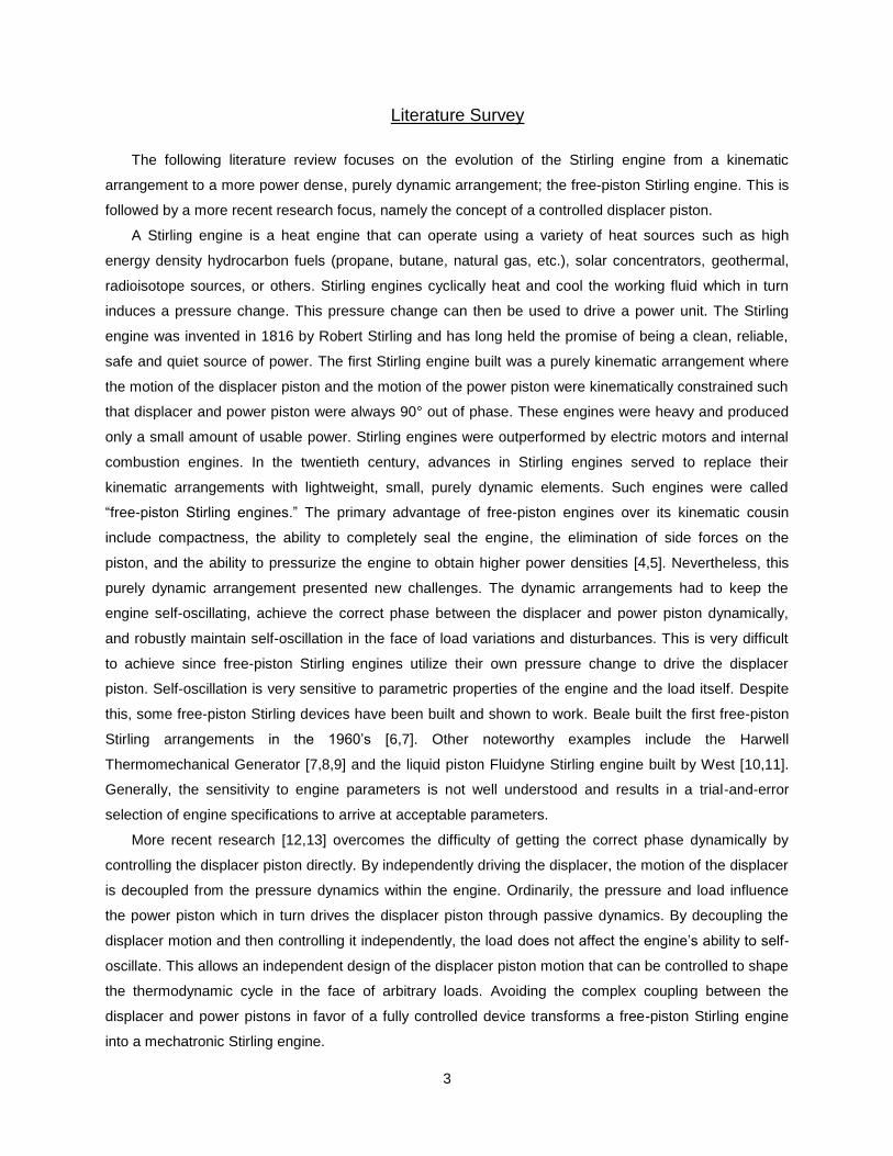
Literature Survey
The following literature review focuses on the evolution of the Stirling engine from a kinematic
arrangement to a more power dense, purely dynamic arrangement; the free-piston Stirling engine. This is
followed by a more recent research focus, namely the concept of a controlled displacer piston.
A Stirling engine is a heat engine that can operate using a variety of heat sources such as high
energy density hydrocarbon fuels (propane, butane, natural gas, etc.), solar concentrators, geothermal,
radioisotope sources, or others. Stirling engines cyclically heat and cool the working fluid which in turn
induces a pressure change. This pressure change can then be used to drive a power unit. The Stirling
engine was invented in 1816 by Robert Stirling and has long held the promise of being a clean, reliable,
safe and quiet source of power. The first Stirling engine built was a purely kinematic arrangement where
the motion of the displacer piston and the motion of the power piston were kinematically constrained such
that displacer and power piston were always 90° out of phase. These engines were heavy and produced
only a small amount of usable power. Stirling engines were outperformed by electric motors and internal
combustion engines. In the twentieth century, advances in Stirling engines served to replace their
kinematic arrangements with lightweight, small, purely dynamic elements. Such engines were called
“free-piston Stirling engines.” The primary advantage of free-piston engines over its kinematic cousin
include compactness, the ability to completely seal the engine, the elimination of side forces on the
piston, and the ability to pressurize the engine to obtain higher power densities [4,5]. Nevertheless, this
purely dynamic arrangement presented new challenges. The dynamic arrangements had to keep the
engine self-oscillating, achieve the correct phase between the displacer and power piston dynamically,
and robustly maintain self-oscillation in the face of load variations and disturbances. This is very difficult
to achieve since free-piston Stirling engines utilize their own pressure change to drive the displacer
piston. Self-oscillation is very sensitive to parametric properties of the engine and the load itself. Despite
this, some free-piston Stirling devices have been built and shown to work. Beale built the first free-piston
Stirling arrangements in the 1960’s [6,7]. Other noteworthy examples include the Harwell
Thermomechanical Generator [7,8,9] and the liquid piston Fluidyne Stirling engine built by West [10,11].
Generally, the sensitivity to engine parameters is not well understood and results in a trial-and-error
selection of engine specifications to arrive at acceptable parameters.
More recent research [12,13] overcomes the difficulty of getting the correct phase dynamically by
controlling the displacer piston directly. By independently driving the displacer, the motion of the displacer
is decoupled from the pressure dynamics within the engine. Ordinarily, the pressure and load influence
the power piston which in turn drives the displacer piston through passive dynamics. By decoupling the
displacer motion and then controlling it independently, the load does not affect the engine’s ability to self-
oscillate. This allows an independent design of the displacer piston motion that can be controlled to shape
the thermodynamic cycle in the face of arbitrary loads. Avoiding the complex coupling between the
displacer and power pistons in favor of a fully controlled device transforms a free-piston Stirling engine
into a mechatronic Stirling engine.
4
The work presented in this document builds on the work of [12,13] by using the position of the
displacer piston as a control input to a first-principles model of a Stirling engine. An accurate, first-
principles model that is amenable to deriving control laws for the displacer motion is critical for the line of
work regarding controlled Stirling engines to continue. Furthermore, such a model needs to be rigorously
validated experimentally. Although other papers [14, 15, 16] present control models of Stirling devices,
many are not experimentally validated and none present a validated model that will accept an arbitrary
displacer motion. The contribution of this paper is a first-principles model, amenable to the direct control
of the displacer piston, that is validated experimentally for a wide range operating conditions.
Described herein is a Stirling device that uses the position of a displacer piston as a control input to a
first-principles model. The design, first-principles model, and experimental setup of such a Stirling device
are described. The first-principles model is experimentally validated for two different motion profiles of the
displacer piston, a variety of heater head temperatures, and a variety of different average engine
pressures. Additionally, a system dynamic model of a Stirling pressurizer combined with a hydraulic pump
is presented.
Organization of the Document
The thesis is organized in four chapters. Chapter I presents the introduction, motivation, and the
literature survey of the work. Chapter II and III are comprised of the manuscripts that encompass the
body of the work completed during the author’s two years at Vanderbilt University. Chapter II contains a
Conference paper on the system dynamic model and design of a Stirling pressurizer combined with a
hydraulic pump. Chapter III builds on the work of Chapter II by experimentally validating the model of a
Stirling pressurizer. Chapter IV concludes with a discussion and future directions of the work.
Manuscript 1: System Dynamic Model and Design of a Stirling Pump
This paper presents the system dynamic model and design of a Stirling engine combined with a hydraulic
pump. The Stirling pump is intended to fill the technological gap of a compact high energy density power
supply for untethered fluid power applications in the 50W to 500W range. The Stirling device uses pre-
pressurized helium as its working fluid for maximum power and efficiency. A directly controlled, loose-fit
displacer piston moves the pre-pressurized working fluid between the hot and cold side of the sealed
engine section; therefore inducing a pressure swing. The hydraulic pump uses this pressure swing to
pump hydraulic fluid to a desired output pressure of 70bar. Manuscript 1 is based on the following
conference paper:
A. Winkelmann, and E. J. Barth, “System Dynamic Model and Design of a Stirling Pump,” 2014
Proceeding of the 27th Symposium on Fluid Power and Motion Control, ASME/Bath, FPMC2014-7839,
September 10-12, 2014, Bath, England
5
Manuscript 2: Design, Modeling and Experimental Validation of a Stirling Pressurizer with a
Controlled Displacer Piston
This paper presents the design, first-principles model, and experimental setup of a Stirling Pressurizer.
The first-principles model is validated with experimental results. This paper builds on the work of
manuscript 1. More complexity has been added to the first-principle model by incorporating regenerative
effects and heat transfer losses (shuttle losses and conduction losses) within the engine section.
Experimental data for two directly controlled motion profiles of the displacer piston, a variety of heater
head temperatures, and a variety of different average engine pressures validate the first-principle model.
Experimental results show that the first-principles model can not only be used for the optimization of the
pressurizer’s efficiency and/or power output through an optimized displacer piston motion profile but the
model also informs about the design and sizing of Stirling devices in general. Manuscript 2 is based on
the following paper:
A. Winkelmann, and E. J. Barth,”Design, Modeling and Experimental Validation of a Stirling
Pressurizer with a Controlled Displacer Piston,” Submitted to: IEEE/ASME Transactions on Mechatronics,
2015.
References
[1] F. Formosa, L.G. Frechette, “Scaling laws for free piston Stirling engine design: Benefits and
chellenges of miniaturization” Energy, vol 57, pp. 796-808, 2013.
doi:10.1016/j.energy.2013.05.009
[2] C.Ronneau, “Energie, pollution de l’air et developpement durable”, Presses universitaires de
Louvain, 2004. Print
[3] M. Raibert et al., “BigDog, the Rough-Terrain Quadruped Robot”, Proceedings of the 17th IFAC
World Congress, 2008:17-1:10822-10825.
[4] G. Walker, “Large Free-Piston Stirling Engines,” Lecture Notes in Engineering, Springer-Verlag,
pp.216-221, 1985.
[5] A. J. Organ, “The Regenerator and the Stirling Engine,” Mechanical Engineering Publications
Limited, London, 1997.
[6] G. Walker, Stirling Engines, Oxford University Press, 1980.
[7] G. Walker and J. R. Senft, Lecture Notes in Engineering: Free Piston Stirling Engines, Springer-
Verlag, New York, 1985.
[8] E. H. Cooke-Yarborough, E. Franklin, T. Gesow, R. Howlett, C. D. West, “Thermomechanical
generator: an efficient means of converting heat to electricity at low power levels,” Proceedings
IEE, no. 121, p. 749-751, 1974.
[9] C. D. West, Principles and Applications of Stirling Engines, Van Nostrand Reinhold Company,
New York, 1986.
[10] C. D. West, Liquid Piston Stirling Engines, Van Nostrand Reinhold Company, New York, 1983.

6
[11] F. T. Reader and M. A. Clarke, “Liquid Piston Stirling Air Engines,” 2nd International Conference
of on Stirling Engines, 14 p, 1984
[12] Gopal, V. K., Duke, R., and Clucas, D., 2009. “Active Stirling Engine”. In TENCON 2009-2009
IEEE Region 10 Conference, IEEE, pp. 1–6.
[13] M. Craun, B. Bamieh, “Optimal Periodic Control of an Ideal Stirling Engine Model,” ASME
Journal of Dynamic Systems, Measurement and Control, Jan 2nd 2015. doi:10.1115/1.4029682
[14] Chin-Hsiang Cheng, and Ying-Ju Yu, “Numerical model for predicting thermodynamic cycle and
thermal efficiency of a beta-type Stirling engine with rhombic-drive mechanism”, Renewable
Energy, vol. 35, pp. 2590-2601, 2010. doi:10.1016/j.renene.2010.04.002
[15] F. Formosa and G. Despesse, “Analytical model for Stirling cycle machine design”, Energy
Conversion and Management, vol. 51, pp. 1855-1863, 2010.
doi:10.1016/j.enconman.2010.02.010
[16] H. Karabulut, “Dynamic analysis of a free piston Stirling engine working with closed and open
thermodynamic cycles”, Renewable Energy, vol. 36, pp. 1704-1709, 2011.
doi:10.1016/j.renene.2010.12.006

7
CHAPTER II.
MANUSCRIPT 1: SYSTEM DYNAMIC MODEL AND DESIGN OF A STIRLING PUMP
Anna Winkelmann and Eric J. Barth
Vanderbilt University
Nashville, TN
Accepted as a Conference Paper at the
Proceedings of the 27th Symposium on Fluid Power & Motion Control
ASME/Bath 2014
Abstract
This paper presents the design and dynamic modeling of a second generation prototype combined
Stirling engine pump. The Stirling pump is intended to fill the technological gap of a compact high energy
density power supply for untethered fluid power applications in the 50W to 500W range. Specifically, this
prototype is intended as a compact and quiet, untethered, hydraulic power supply for an ankle foot
orthosis testbed associated with the Center for Compact and Efficient Fluid Power. The energy source for
the unit is flexible and can include propane, butane, methane, natural gas, or other high energy density
hydrocarbon source of heat. The target output pressure of 7 MPa (1000 psig) is obtained from a pumping
stage that is driven by a sealed engine stage that utilizes high pressure helium as the working fluid. The
separate pumping stage utilizes the differential pressure swing inside the engine section to pump
hydraulic fluid to the desired output pressure. This paper presents the system dynamic model of the
Stirling pump, and includes (1) heat transfer from the heat source to the working fluid in the hot space of
the engine, (2) heat transfer from the working fluid in the cold space of the engine to the heat sink, (3)
energetically derived pressure dynamics in the hot and cold spaces, (4) mass flow around the displacer
piston in between the hot and cold sides, (5) work output to the pump driving section, (6) pumping piston
inertial dynamics, (7) flow losses through the pump’s check valves, and (8) hydraulic power output. This
dynamic model allows components of the Stirling pump to be sized. The paper includes results from the
dynamic model.
Introduction
More than 6 million individuals in the US are affected by an impaired ankle function. Commercially
available passive Ankle Foot Orthoses (AFO) are compact and durable but lack functionality since they
8
cannot provide active motion control or generate net power. Active AFOs lack utility because they require
tethered power supplies. One of the goals of the Center for Compact and Efficient Fluid Power (CCEFP)
is to develop a fluid powered untethered device that operates in the 10 to 100 W power range to address
the shortcomings of both passive and active AFOs. The Stirling pump is intended to serve as a silent, low
vibration, compact, efficient, untethered, and high energy-density hydraulic power supply for an AFO, or
similar application.
Stirling engines have been a research curiosity for more than a century. They have the appeal of
offering power from any heat source including fuels, solar concentration, biomass, geothermal, or
radioisotope decay. They also have the theoretical appeal of offering high thermodynamic efficiency due
to the Stirling cycle. In the limited number of applications they have found, Stirling engines have been
shown to be reliable and requiring little to zero maintenance. Despite their appealing properties, it is also
fair to say that Stirling engines have fallen far short of their expectations primarily due to their low power
density.
The historical progression of Stirling machines has offered some improvement in power density as
their configurations have progressed from purely kinematic to free-piston varieties. Purely kinematic
configurations rely on bulky linkages to enforce the correct phasing between the power piston and the
displacer piston. Free-piston Stirling engines rely upon dynamic forces developed in the engine and the
dynamic responses of the displacer and power pistons to enforce the necessary relationship between the
two. If the engine is designed with these dynamics in mind, it can be shown that kinematic linkages are
not necessary [1]. The first purely dynamic (non-kinematic) Stirling engine was Beale’s free-piston Stirling
engine [1]. The free-piston arrangement was not only lighter, but was able to be hermetically sealed and
eliminated side forces on the pistons due to a connecting rod. Moreover, the ability to pressurize a sealed
engine allows for higher power densities [2,3].
The challenge with free-piston configurations is to get the phase of the displacer and power piston
correct in order to approximate the Stirling cycle. Designing the dynamics to do this correctly and robustly
in the face of varying loads and heat input remains a technological barrier. Some success in the design of
working free-piston Stirling engines is represented by many of Beale’s arrangements [4, 5], the Harwell
Thermomechanical Generator [6, 5, 7], and the liquid piston Fluidyne Stirling engine by West [8, 9]. The
analysis of even these working Stirling machines demonstrates a knowledge gap with respect to
designing their parameters for robust operation [5].
The Stirling pump presented in this paper overcomes this knowledge gap by decoupling the sensitive
interacting dynamics of the displacer and power pistons. This is done by directly controlling the motion of
the displacer piston. This allows more design degrees of freedom and ensures that the device is
insensitive to load or internal dynamics variations. This paper describes the design and dynamic model of
the combined Stirling engine pump. The Stirling pump is pre-pressurized and has a separate pump
section that uses the pressure swing of the engine to pump hydraulic fluid.

9
Design of Stirling Pump
The rationale for the design of the proposed device result in large part from results and observations
from a previous Stirling Thermocompressor device that was designed, fabricated, and experimentally
tested by our research group [10]. The previous (generation 1) device was a multi-stage, true
thermocompressor (Fig.2-1). A true thermocompressor uses the working fluid as the output fluid (air in
this case). As discussed below, results from this previous device motivated: 1) a change in architecture
from a multistage device to a single stage device, and 2) a change in functionality and architecture from a
thermocompressor to a hydraulic pump. A single stage of this previous multistage device is shown in Fig.
2-2.
The generation 1 device used a brushless DC motor to drive a continuous linear reciprocating lead
screw onto which the displacer piston was attached. The displacer piston was chosen to be made from
Macor machinable ceramic due to its low thermal conductivity (1.46 W/m/K at 25°C) and its high service
temperature. A quartz glass cylinder was chosen to seal the working fluid in between the heater head and
the heat sink due to the same characteristics - low thermal conductivity and high service temperature.
Figure 2-1: Generation-1 multistage thermocompressor device concept

10
Figure 2-2: Design for a single stage of the generation-1 thermocompressor device. A reciprocating lead screw driven by a DC motor moves a loose-fit displacer piston between the hot side and the cold side. In response to this, the pressure in the device changes as the working fluid moves between the hot side (high pressure) and the cold side (low pressure). As the pressure fluctuates, the thermocompressor outputs high pressure fluid to a reservoir and intakes low pressure fluid from the environment (or from a previous stage).
Multi-Stage to Single-Stage Design Change
A dynamic simulation of the multi-stage thermocompressor [10] showed that more than four
compression stages would be needed to reach the target output pressure. With respect to the multi-stage
architecture, the prospect of having at least four compression stages to reach a target output pressure of
80 psig (for pneumatics reservoir) becomes untenable in the face of the mechanical complexity
encountered in our single stage prototype. A multi-stage device requires that each stage become smaller
with increasing pressure and the realities of dead-volume in such stages would make them far less than
ideal as they become smaller. It was clear that a different approach was needed for the next generation of
the device.
The generation 2 device will be of single-stage architecture with a sealed pre-pressurized engine
section and separate pumping stage that pumps hydraulic fluid. Although the prospect of a true
thermocompressor is appealing, the fundamental work density per stroke [J/(m3stroke)] increases by
more than two orders of magnitude by increasing the pre-pressurization (pressure when cold) to 500 psig.
This agrees with the observation that almost every Stirling device (actual experimental platform) in the
literature operates at a high pressure and agrees with the observations of authors such as G. Walker, G.
T. Reader, O.R. Fauvel, I. Urieli, N. Isshiki, D. Gedeon, M. B. Ibrahim, M. Carlini, L. Bauwens, and others.

11
Pursuing this pre-pressurized architecture, as opposed to a true thermocompressor, requires a separate
pump section that utilizes the differential pressure swing inside the engine section. Based on the
experimentally measured heat transfer and pressure ratio of the generation-1 device, an output pressure
of greater than 1000 psig (7000 kPa) can be obtained by utilizing a separate pumping stage and a single
pre-pressurized sealed engine section with a similar size as the generation-1 device.
Working Fluid and Pumping Fluid
As discussed above, better compactness and power density can be achieved by using a single-stage,
pre-pressurized engine section. This design change allows a consideration of a different working fluid
than air. For maximum efficiency and power, helium was selected as the working fluid in the sealed
engine section. The advantage of helium over air is that helium has a higher heat transfer coefficient than
air. For our conditions, the use of helium over air would result in a 20 times higher heat transfer coefficient
(14800 W/m2/K for helium vs. 715 W/m
2/K for air).
Figure 2-3: Design of the generation 2 device
The design change to a sealed single-stage also allows for a consideration of the fluid being pumped
to be something other than air. Hydraulic pumping is inherently more efficient than compressing and
Pump section

12
pumping air. This is due to the fact that when air is compressed, appreciable energy is stored as pressure
potential energy that can be lost in the form of heat once pumped to its destination. Driving an air
compressor also presents the possibility of pressurizing the gas to an inadequate level to pump, and then
losing the work that was needed for that pressurization. This occurs even in the case where some of the
air is pumped and may leave a remainder that is not pumped due to dead volume in the compressor
section. This remainder is then susceptible to heat loss. Due to hydraulic oil’s much higher stiffness as
compared to a gas, much less energy is stored in the compression of the fluid thereby reducing thermal
effects during the pumping phase. Finally, since hydraulic fluid is nearly incompressible, it eliminates the
dead volume in the pumping section.
The design of the separate pump stage can be seen in Fig. 2-4. The pump section utilizes the
differential pressure swing inside the engine section to pump hydraulic fluid at a desired output pressure.
The pump section is composed of three types of chambers; the driving chamber, the pumping chamber,
and the return chamber. The driving chamber will be connected to the cold side of the engine section
such both are always at the same pressure. The bottom chamber represents a self-balancing return
chamber. This is achieved by staying near an average pressure via a flow restriction implemented with a
simple needle valve (see Fig. 2-3). The pressure difference in the driving and return chamber will cause
the piston in the pumping chamber to move. When the pressure in the driver chamber is higher than in
the return chamber, the piston moves down and pumps the hydraulic fluid in the lower pumping chamber
through a check valve when the pressure is greater than the supply pressure. Simultaneously, the fluid in
the upper pumping chamber decompresses and ultimately draws in more fluid through a check valve from
the low pressure side of the hydraulic system. Conversely, when the piston moves up, fluid is pumped out
of the upper pumping chamber and drawn in to the lower pumping chamber.
Figure 2-4: Pumping Section

13
Other Design Changes
Other design changes that need to be made to the generation-1 device include a different driver
mechanism for the displacer piston and a different sealing mechanism at the hot end. For the generation
1 device, the position and velocity of the displacer was controlled by driving a reciprocating lead screw
with a brushless DC motor. The reciprocating lead screw had “criss-crossed’ left-handed and right-
handed threads which enabled the motor to be driven in one direction while achieving a reciprocating
motion of the displacer piston. This was intended to reduce the power consumption of the motor since it
does not need to accelerate and decelerate the motor shaft. Nevertheless, the power consumption was
still found to be much higher than expected due to excessive friction in the lead screw mechanism. As a
result, the displacer of the generation 1 device could only be driven at a frequency of 2.8 Hz. Dead
volume around the lead screw mechanism was also a downside of the mechanism and limited the
pressure swing in the engine. At 800°C and 2.8 Hz, the generation-1 device showed a pressure ratio of
1.6. While favorably comparable to devices in the literature, it was lower than expected.
The dead-volume and the higher than expected motor power necessitated a better solution for the
linear drive mechanism of the displacer piston. The generation 2 device replaces the DC motor and the
reciprocating lead-screw with a compact COTS linear actuator (Faulhaber) (see Fig. 2-5). The linear DC-
Servomotor is light weight and has linear Hall sensors for position sensing. The positioning of the rod can
be controlled very accurately such that dead volume at the cylinder ends can be held to a minimum. The
smooth shaft of the linear motor also reduces the dead volume seen in the reciprocating lead screw
design. A linear spring located in between the displacer piston and the linear motor will act as a
conservative restoring force to minimize actuation energy, and effectively replaces the energetically
motivated unidirectional operation of the reciprocating lead screw.
Figure 2-5: Linear DC Servomotor
Finally, experimental results of the generation-1 device revealed a slow leak resulting from the high
temperature seal between the fused quartz glass and the heater head. To avoid a leak, the generation 2

14
device will have an engine cylinder made of Inconel 625 as opposed to fused quartz. This will be tougher
and able to be welded, thus solving the sealing problem at the hot end.
Dynamic Model
The entire Stirling Pump can be dynamically modeled as having two sections, namely, the engine
section and the pump section. The only input to the pump section is the pressure swing on the cold side
of the engine section. The displacer piston in the engine section is driven by a linear DC servomotor with
a sinusoidal velocity of
t)f(flV HzHzStroke 2sin
(1)
where fHz is the frequency the displacer motion, and lStroke is the stroke length of the displacer piston in the
engine section of the Stirling pump. The position of the displacer is given accordingly by:
)2cos(
22ft
llx strokestroke
displacer (2)
The engine section of the Stirling pump is modeled as two control volumes of variable size. The
control volumes represent the volume of the medium in the hot and the cold side of the engine section.
The two control volumes are separated by the displacer piston which represents a flow restriction. The
size of the control volume and the rate at which these are changing are governed by the position and
velocity of the displacer piston above. The walls in the hot control volume (Vh) transfer thermal energy
from heat source to the medium, and the walls in the cold control volume (Vk) transfer thermal energy from
the medium out of the engine section of the Stirling pump. The wall temperatures on the hot and cold side
of the engine section are set to a constant temperature of Th and Tk, respectively. The dead volume
around the displacer piston is equally divided into the model of Vh and Vk. Since the displacer never hits
the ends of the cylinder, additional dead volume is added to both sides.
The pressure dynamics in the cylinder were derived from a fundamental power balance of the stored
energy, enthalpy, heat flow and work:
WQHU heat
(3)
Rearranging the terms and solving for the pressure dynamics inside the control volume yields:
V
TTAhVPRTmP
khwallHekhHeHeflowHe
,,, )1(
(4)
An estimate of the heat transfer coefficient hHe was done by using fully developed pipe flow analysis as
similar to [11]. In order to determine whether the flow is laminar or turbulent, the Reynolds number was
calculated:
mxRe
(5)

15
where �̇�𝑚 is the mean velocity of helium, δ is the characteristic length, and ν is the kinematic viscosity of
helium. The hydraulic diameter was used for the characteristic length given by:
C
Ac4
(6)
where Ac is the area of the gap in between the engine cylinder and the displacer piston and C is the
wetted perimeter given by:
)( displacercylinder ddC
(7)
where dcylinder is the inside diameter of the Inconel housing and ddisplacer is the diameter of the displacer
piston.
The heat transfer coefficient is determined by calculating the Nusselt number and solving for the heat
transfer coefficient h by using the following equation:
nma
k
hNu PrRe
(8)
where k is the thermal conductivity, Pr is the Prandtl number and a, m, n are constants that depend on
the flow regime. For a frequency of 20 Hz, turbulent flow (Re>2300), and a smooth pipe, the constants
used in the implementation of equations 5-8 are shown in the Table 2-1 below. Solving for the heat
transfer coefficient yields 14800 W/m2/K. Since the calculation of this parameter depends on the mean
pressure and the mean temperature in determining the kinematic viscosity, conservative values were
used such that the h calculated is a lower bound for the conditions in the engine.
Table 2-1: Values of significant parameters
mx 125 m/s
δ 0.00099 m
ν 5.643e-6 m2/s
k 0.245 W/m/K
a 0.023
Pr 0.656
m 0.8
n 0.3
h 14800 W/m2/K
The mass flow restriction between the displacer piston and the Inconel cylinder that separates the two
control volumes was modeled using Grinnel’s model of compressible fluid flow [12] in a thin passage,
which is given by:
22
3
12du
pistonflowhelium
pistonPP
LRT
srm
(9)
16
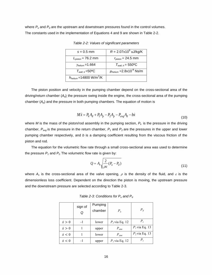
where Pu and Pd are the upstream and downstream pressures found in the control volumes.
The constants used in the implementation of Equations 4 and 9 are shown in Table 2-2.
Table 2-2: Values of significant parameters
s = 0.5 mm R = 2.07x10⁹ uJ/kg/K
Lpiston = 76.2 mm rpiston = 24.5 mm
helium =1.664 Twall, h = 550ºC
Twall, k =50ºC µhelium =2.8x10⁻⁸
Ns/m
hhelium =14800 W/m2/K
The piston position and velocity in the pumping chamber depend on the cross-sectional area of the
driving/return chamber (Ad), the pressure swing inside the engine, the cross-sectional area of the pumping
chamber (Ap) and the pressure in both pumping chambers. The equation of motion is
xbAPAPAPAPxM davgppdk 21 (10)
where M is the mass of the piston/rod assembly in the pumping section, Pk is the pressure in the driving
chamber, Pavg is the pressure in the return chamber, P1 and P2 are the pressures in the upper and lower
pumping chamber respectively, and b is a damping coefficient resulting from the viscous friction of the
piston and rod.
The equation for the volumetric flow rate through a small cross-sectional area was used to determine
the pressure P1 and P2. The volumetric flow rate is given by:
)(
2duv PPAQ
(11)
where Av is the cross-sectional area of the valve opening, is the density of the fluid, and is the
dimensionless loss coefficient. Dependent on the direction the piston is moving, the upstream pressure
and the downstream pressure are selected according to Table 2-3.
Table 2-3: Conditions for Pu and Pd
sign of
Q
Pumping
chamber Pu Pd
�̇� > 0 -1 lower P2 via Eq. 12 Ps
�̇� > 0 1 upper Patm P1 via Eq. 13
�̇� < 0 1 lower Patm P2 via Eq. 13
�̇� < 0 -1 upper P1 via Eq. 12 Ps

17
The negative sign for the volumetric flow rate indicates that fluid is being pumped out of the pumping
section while a positive sign indicates that fluid is pumped into the pumping section. By calculating the
flow rate Q with the equation pAxQ and then setting Pu and Pd to the boundary conditions indicated in
Table 2-3, the pressures in the upper and lower pumping chambers P1 and P2 can be found.
d
v
pu P
A
AxP
2
2
(12)
2
2
v
pud
A
AxPP
(13)
These dynamics fully describe the engine and pump section of the Stirling device. To further
characterize the device, average output power is calculated by filtering the instantaneous power with a
slow, unity-gain first order filter. The instantaneous power output instantP is calculated by:
soutPQinstantP (14)
where xAQ pout is the volumetric flow rate out of the two pumping chambers and Ps is the desired supply
pressure.
Results
Results of the dynamic simulation show that the device can pump 1000 psig (7000 kPa) when the
engine runs at 20 Hz (controlled sinusoidal motion of the displacer as given by Eqn. 2), is initially
pressurized to 500 psig (3.55 MPa) with cold helium and is then held at a constant temperature Th of
550°C on the hot side. The parameters for the Stirling pump as designed are given in Table 2-4.
Table 2-4: Parameters used in simulation
lcyl 200 mm ldrive 22 mm
borecyl 50 mm boredrive/return 60 mm
lpiston 76 mm borepump 10 mm
dpiston 49 mm dvalve 2.5 mm
M 0.2 kg
b 500 Ns/m
The pressure difference in the driving and return chamber (Fig.2-6) caused by the pressure swing
inside the engine results in a displacement of the pumping piston as seen Fig. 2-7.

18
Figure 2-6: Driving (blue) and average (green) pressure vs. time
Figure 2-7: Displacement of the pumping piston with respect to time
2 2.05 2.1 2.15 2.2 2.25 2.3 2.35 2.4 2.45 2.56600
6700
6800
6900
7000
7100
7200
7300
Pre
ssure
in k
Pa
time in sec
3 3.05 3.1 3.15 3.2 3.25 3.3 3.35 3.4 3.45 3.5
0
1
2
3
4
5
6
7
8
9
10
dis
tance in m
m
time in sec
19
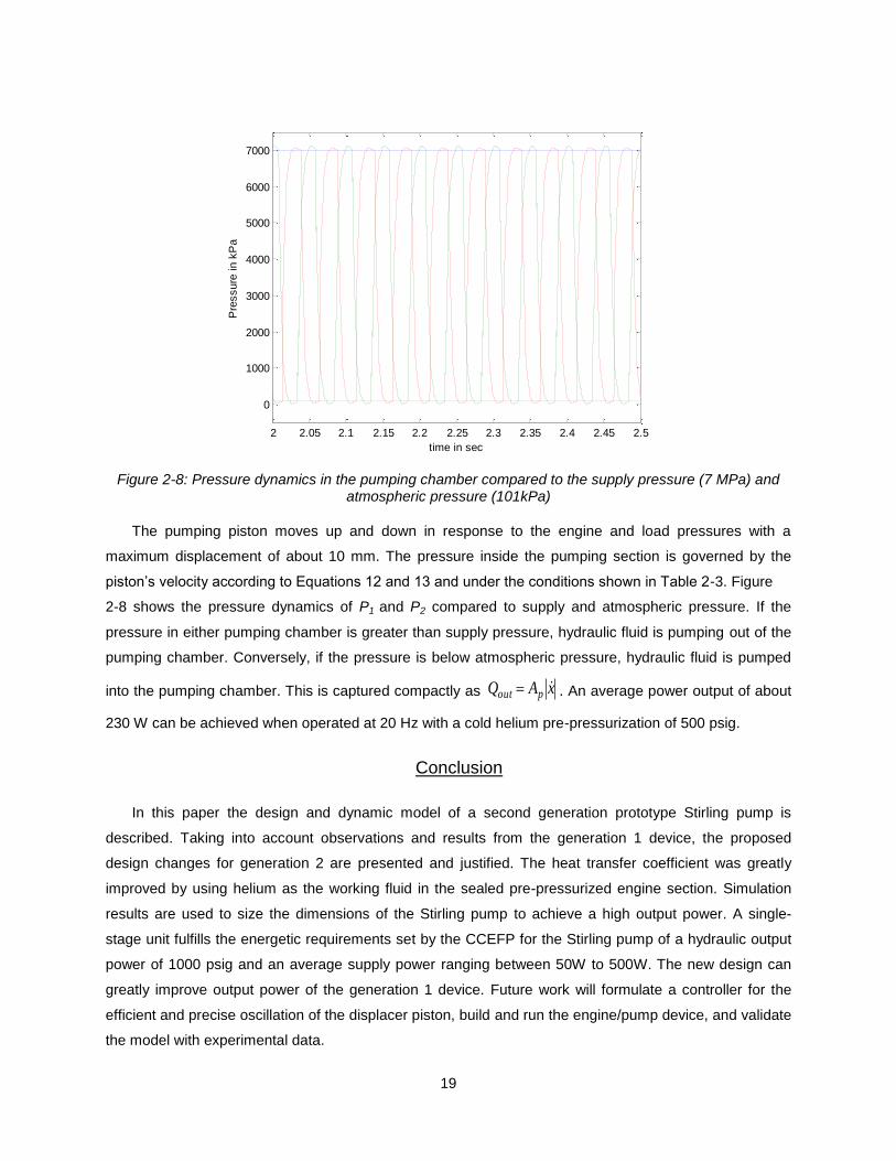
Figure 2-8: Pressure dynamics in the pumping chamber compared to the supply pressure (7 MPa) and atmospheric pressure (101kPa)
The pumping piston moves up and down in response to the engine and load pressures with a
maximum displacement of about 10 mm. The pressure inside the pumping section is governed by the
piston’s velocity according to Equations 12 and 13 and under the conditions shown in Table 2-3. Figure
2-8 shows the pressure dynamics of P1 and P2 compared to supply and atmospheric pressure. If the
pressure in either pumping chamber is greater than supply pressure, hydraulic fluid is pumping out of the
pumping chamber. Conversely, if the pressure is below atmospheric pressure, hydraulic fluid is pumped
into the pumping chamber. This is captured compactly as xAQ pout . An average power output of about
230 W can be achieved when operated at 20 Hz with a cold helium pre-pressurization of 500 psig.
Conclusion
In this paper the design and dynamic model of a second generation prototype Stirling pump is
described. Taking into account observations and results from the generation 1 device, the proposed
design changes for generation 2 are presented and justified. The heat transfer coefficient was greatly
improved by using helium as the working fluid in the sealed pre-pressurized engine section. Simulation
results are used to size the dimensions of the Stirling pump to achieve a high output power. A single-
stage unit fulfills the energetic requirements set by the CCEFP for the Stirling pump of a hydraulic output
power of 1000 psig and an average supply power ranging between 50W to 500W. The new design can
greatly improve output power of the generation 1 device. Future work will formulate a controller for the
efficient and precise oscillation of the displacer piston, build and run the engine/pump device, and validate
the model with experimental data.
2 2.05 2.1 2.15 2.2 2.25 2.3 2.35 2.4 2.45 2.5
0
1000
2000
3000
4000
5000
6000
7000
Pre
ssure
in k
Pa
time in sec

20
Acknowledgement
This work was supported by the Center for Compact and Efficient Fluid Power, an NSF Engineering
Research Center, grant EEC-0540834.
References
[1] G. Walker, G. Reader, O. R. Fauvel, E. R. Bingham, The Stirling Alternative: Power Systems,
Refrigerants and Heat Pumps, Gordon and Breach Science Publishers, 1994.
[2] G. Walker, “Large Free-Piston Stirling Engines,” Lecture Notes in Engineering, Springer-Verlag,
pp.216-221, 1985.
[3] A. J. Organ, The Regenerator and the Stirling Engine, Mechanical Engineering Publications
Limited, London, 1997.
[4] G. Walker, Stirling Engines, Oxford University Press, 1980.
[5] G. Walker and J. R. Senft, Lecture Notes in Engineering: Free Piston Stirling Engines, Springer-
Verlag, New York, 1985.
[6] E. H. Cooke-Yarborough, E. Franklin, T. Gesow, R. Howlett, C. D. West, “Thermomechanical
generator – an Efficient Means of Converting Heat to Electricity at Low Power Levels,”
Proceedings of the IEE, no. 121, p. 749-751.
[7] C. D. West, Principles and Applications of Stirling Engines, Van Nostrand Reinhold Company,
New York, 1986.
[8] C. D. West, Liquid Piston Stirling Engines, Van Nostrand Reinhold Company, New York, 1983.
[9] G. T. Reader and M. A. Clarke, “Liquid Piston Stirling Air Engines,” 2nd International Conference
on Stirling Engines, 14p, 1984.
[10] M. E. Hofacker, N. Kumar, E. J. Barth. “Dynamic Simulation and Experimental Validation of a
Single Stage Thermocompressor for a Pneumatic Anke-Foot Orthosis”. 2013 Proceedings of the
25th Symposium on Fluid Power and Motion Control, ASME/Bath, FPMC2013-4483, October 6-
9, 2013, Sarasota, FL.
[11] J. Van de Ven, P. Gaffuri, B. Mies, and G. Cole, “Developments Towards a Liquid Piston Stirling
Engine,” International Energy Conversion Engineering Conference, Cleveland, Ohio, 2008.
[12] S. K. Grinnell, “Flow of a Compressible Fluid in a Thin Passage”. ASME, 16 pages, 1954.
21
CHAPTER III.
MANUSCRIPT 2: DESIGN, MODEL, AND EXPERIMENTAL TESTING OF A
STIRLING PRESSURIZER WITH A CONTROLLED DISPLACER PISTON
Anna Winkelmann, Eric J. Barth
Vanderbilt University
Nashville, TN
Submitted as a Regular Paper to the
IEEE/ASME Transactions on Mechatronics
(In Review)
Abstract
This paper presents the design, first-principles model, and experimental setup of a Stirling
pressurizer. The Stirling pressurizer is a Stirling engine with an independently controlled displacer piston.
The directly controlled, loose-fit displacer is actuated with a small linear motor and moves the pre-
pressurized working fluid (helium) between the hot and cold side of the sealed engine section; therefore
inducing a pressure change. The position of the displacer is the only control input to the first-principles
model. The first-principles model is validated with experimental results for different controlled displacer
piston motion profiles. Modeled and experimentally measured pressures are compared for average
pressures ranging from 10 – 20 bar, and heater head temperatures ranging from 250°C – 500°C. The
first-principles model is intended for: 1) the design and sizing of the pressurizer and power piston / power
extraction, 2) specification of a displacer piston motion profile to optimize the efficiency and/or power
output, and 3) the general design of Stirling devices, beyond the design of the experimental prototype
investigated here, through the use of a lumped parameter model with well-defined and measurable
parameters.
Introduction
A Stirling engine is a heat engine that can operate using a variety of heat sources such as high
energy density hydrocarbon fuels (propane, butane, natural gas, etc.), solar concentrators, geothermal,
radioisotope sources, or others. Stirling engines cyclically heat and cool a working fluid, inducing a
pressure change which in turn drives a power unit. The Stirling engine was invented in 1816 by Robert
Stirling and has long held the promise of being a clean, reliable, safe and quiet source of power. Stirling
22
engines were outperformed by other power sources such as electric motors and internal combustion
engines. This was primarily due to the characteristically low power density of Stirling devices. These
heavy engines with bulky kinematic arrangements produced proportionally small amounts of usable
power.
In the twentieth century, advances in Stirling engines served to replace their kinematic arrangements
with lightweight, small, purely dynamic elements. Such engines were called “free-piston Stirling engines.”
This compact, new, and lightweight design held the promise of increasing the power density over its
kinematic cousin. Nevertheless, this purely dynamic arrangement presented new challenges. The
dynamic arrangements had to keep the engine self-oscillating, achieve the correct phase between the
displacer and power piston dynamically, and robustly maintain self-oscillation in the face of load variations
and disturbances. This is very difficult to achieve since free-piston Stirling engines utilize their own
pressure change to drive the displacer piston. Self-oscillation is very sensitive to parametric properties of
the engine and the load itself. Despite this, several free piston Stirling engines have been built and shown
to work. Noteworthy examples include Beale’s free piston engines [1,2], the Harwell Thermomechanical
Generator [2,3,4] and the liquid piston Fluidyne Stirling engine built by West [5,6]. Generally, the
sensitivity to engine parameters is not well understood and results in a trial-and-error selection of engine
specifications to arrive at acceptable parameters.
The Stirling pressurizer presented in this paper overcomes the difficulty of achieving the correct
phase between the displacer and power pistons by directly controlling the motion profile of the displacer
piston. By independently driving the displacer, the motion of the displacer is decoupled from the pressure
dynamics within the engine. Ordinarily, the pressure and load influence the power piston which in turn
drives the displacer piston through passive dynamics. By decoupling the displacer motion and then
controlling it independently, the load does not affect the engine’s ability to self-oscillate. This additional
control degree of freedom allows an independent design of the displacer piston motion that can be
controlled to shape the thermodynamic cycle in the face of arbitrary loads. Avoiding the complex coupling
between the displacer and power pistons in favor of a fully controlled device transforms a free-piston
Stirling engine into a mechatronic Stirling engine.
Recent research in Stirling engines with a controlled displacer piston has been conducted in [7] and
[8]. Both papers investigate whether a controlled displacer motion profile optimizes the thermodynamic
cycle with regard to efficiency and/or power output of the engine. The work presented in this paper builds
on the work of [7, 8] by using the position of the displacer piston as a control input to a first-principles
model of a Stirling engine. An accurate, first-principles model that is amenable to deriving control laws for
the displacer motion is critical for the line of work regarding controlled Stirling engines to continue.
Furthermore, such a model needs to be rigorously validated experimentally. Although other papers [9, 10,
11] present control models of Stirling devices, many are not experimentally validated and none present a
validated model that will accept an arbitrary displacer motion. The contribution of this paper is a first-

23
principles model, amenable to the direct control of the displacer piston, that is validated experimentally for
a wide range operating conditions.
This paper presents and describes the design, dynamic model, and experimental setup of a Stirling
pressurizer with a controlled displacer. The Stirling pressurizer presented in this paper has no power
piston attached, which allows isolation and experimental validation of the complex pressure dynamics of
the engine. The dynamic model is validated with experimental data for two directly controlled motion
profiles of the displacer piston, a variety of heater head temperatures, and a variety of different average
engine pressures.
Design
The device has two chambers, namely a sealed engine section that uses pre-pressurized helium as
its working fluid for enhanced efficiency and power density, and a return chamber. A cross-section of the
engine design is shown in Fig. 3-1. This engine section is referred to as a Stirling pressurizer since it is
intended as the portion of a Stirling engine responsible for generating large pressure oscillations that can
subsequently be used by a power piston connected at the “power connection ports” to output work. The
sealed engine section contains a loose-fit displacer piston (radial clearance of 0.4 mm). The displacer is
connected to the linear motor via an extension rod and a shaft coupling which offsets small angular and
lateral misalignment. The linear motor moves the displacer piston between the hot side (toward the heater
head) and cold side (toward the cooling fins) and in turn shuttles the helium gas. The resulting
temperature change of the helium gas produces a pressure change inside the engine section.
The return chamber is kept at an average pressure. This is achieved through a flow restriction
induced by a needle valve which connects the cold side of the engine section with the return chamber
(needle valve not shown in Fig. 3-1). Two ports, one on the cold side of the engine section and one on the
return chamber, are installed to connect a power unit with a power piston to the pressurizer. This power
unit could be anything that can be driven by a pressure change such as a hydraulic pump, a linear electric
generator, a reciprocating piston compressor, or a high pressure water filtration system, among others.
The selection of the working fluid inside the engine section is of importance in order to achieve good
performance and high efficiency. Gases of significant interest for the working fluid inside the engine
section are air, helium and hydrogen. Air is of significant interest since it is readily available and easier to
seal within the engine than helium or hydrogen. Nevertheless, the heat transfer properties of air don’t
allow an air operated engine to compete with internal combustion engines [1]. Therefore, gases with
superior heat transfer properties and low viscosities, such as helium or hydrogen, need to be used. Even
though hydrogen has better heat transfer properties, it is highly combustible in the presence of air.
Therefore, helium was selected due to its good thermophysical characteristics such as its high heat
transfer coefficient and its relatively low viscous flow losses. The heat transfer coefficient of helium is
about 11 times higher than that of air in the pressure and temperature range the engine is operating.

24
The heater head of the engine section is made from stainless steel. For this prototype, electric
cartridge heaters were chosen such that accurate temperature control of the heater head is provided.
Eight tight fit holes for the insertion of cartridge heaters guarantee good conduction between the heaters
and the heater head such that the working fluid on the hot side can be heated up to a maximum of 600°C.
The hot and cold sides of the engine section are connected via an Inconel cylinder. Inconel was selected
due to its high melting point, and its low thermal conductivity. Low thermal conductivity is important since
the heat flow from the hot to the cold side along the engine section needs to be as small as possible.
Another advantage of Inconel among other materials is that it can be welded to the heater head; therefore
providing sealing of helium at high temperatures. To keep helium sealed within the device, static and
dynamic O-rings were carefully selected. Two static seals are used on the cold side, one on the bottom
cap that bolts to the cooling fins (Parker part no. OR2-228-V9975), and one at the flange on the return
chamber (Parker part no. OR2-230-V1475). One dynamic seal is used to seal around the extension rod
(Parker part no. O2-006-V9975).
Figure 3-1: Design of the Stirling pressurizer
heater head
(electric heaters)
Internal fins
displacer piston
Inconel engine cylinder
cooling fins
linear motor
shaft coupling
extension rod
power connection ports (not shown)
Seale
d E
ngin
e S
ection
Retu
rn c
ham
be
r

25
Internal fins inside the heater head and external fins on the cold side of the engine section increase
the area for heat transfer in and out of the system, respectively. Thermal conduction along the displacer
piston and the Inconel cylinder are minimized by reducing the wall thicknesses such that it will withstand
the exposed pressure without failing or deforming significantly. For the displacer design, not only the wall
thickness but also the length of the displacer is important for thermal isolation of the cold and the hot
section. A length of three times the diameter was chosen for the displacer piston, since good results on
other Stirling devices have been recorded for that aspect ratio [1]. The annular gap between the displacer
piston and the Inconel cylinder serves as the flow passage of the working fluid and also forms the
regenerator. In most small, low-speed engines it has been found that a formal regenerator as seen in
most larger Stirling engines has proven inadequate due to its large dead volume. Instead, small Stirling
engines often rely on the annular gap connecting the cold and the hot side such as in Beale’s small free-
piston engines [1]. Guidelines say that the gap should be between 0.38 and 0.76 mm to minimize thermal
conduction losses and to maximize the working fluid’s wall contact without increasing the flow restriction
too much [1]. For this prototype a gap of 0.4 mm was selected. The reciprocating motion of the displacer
piston moves the working fluid back and forth between the hot and cold control volumes. When the
working fluid is in the regenerative channel, the fluid liberates or absorbs heat from the displacer and
cylinder walls, depending on the direction the fluid is moving. When the fluid is moving downward from
the hot to the cold side of the engine section, heat is transferred from the fluid to the walls. Consequently,
the fluid leaves the channel at a lower temperature Treg,k. Conversely, when the working fluid moves
upward, the fluid absorbs heat from the walls and leaves the channel at a higher temperature Treg,h.
Dynamic Model
The only exogenous input to the dynamic model is the position of the displacer piston which is
determined by the position f(t) of the linear motor which is rigidly attached to the displacer. This position
function is the result of the linear motor tracking a reference trajectory through any variety of feedback
control. The position input to the model is arbitrary; for experimental validation, the response to a
sinusoidal and a square wave reference input was chosen. The position of the displacer piston is given
by:
)(22
tfll
x strokestroked
where lStroke is the stroke length of the displacer piston in the engine section. The velocity of the displacer
is accordingly given by:
)(2
tfl
v Stroked
With the position and velocity of the displacer piston known, the engine section can be modeled as two
control volumes of variable size, namely the hot control volume (Vh) and the cold control volume (Vk) (Fig.

26
3-2). In each control volume convection between the walls of the engine housing and the working fluid is
present. The walls of the hot control volume (Vh) transfer thermal energy from the heat source to the
working fluid while the working fluid in the cold control volume (Vk) transfers thermal energy to the cylinder
wall and cooling fins out to the surroundings. The dead volume surrounding the displacer piston is equally
added to either control volume Vh and Vk. The dead volume due to the internal fins at the heater head is
also incorporated to the control volume of the hot side.
A. Pressure Dynamics
The pressure dynamics in each control volume were derived from a fundamental power balance
resulting from the first law of thermodynamics, given by
WQHU
Expanding and rearranging terms, the pressure dynamics in each control volume as influenced by heat
flux, enthalpy, and volume changes can be found. The pressure dynamics of each control volume (h: hot
side, k: cold side, r: return chamber) is given by:
h
hHeflowHeHehlossinh
V
VPRTmQQP
)1)(( , (4a)
k
kHeflowHeHeklossink
V
VPRTmQQP
)1)(( , (4b)
r
rrHerflowHerHeout
rV
VPRTmQP
,)1( (4c)
where Tflow is the temperature of the gas that is entering/leaving the control volume, dependent on the
pressure difference between the hot and cold sides and the direction the displacer is moving. The mass
flow rate into or out of the control volume is denoted by m , with a positive sign convention for mass
flowing into the control volume. The heat transfer rate between the heat source and the working fluid (in),
or between the working fluid and the cooling fins (out), is denoted outinQ /
, where the sign convention is
always positive for heat entering the control volume. The conduction and shuttle heat transfer losses are
denoted lossQ , with a positive sign convention for heat entering the control volume.
Figure 3-2 is an overview of the system dynamics. These system dynamics are dependent on the
terms in Eqns. (4a), (4b), and (4c) for each of the three control volumes: hot side, cold side, and return
chamber, respectively. For the experimental validation presented, the rV term in equation (4c) is zero.
More generally, it is included in the model to account for a power piston that would utilize the pressure in
the return chamber. A fourth control volume represents the regenerative channel (to be presented). The
dynamics of each control volume describes their interaction with external conditions as well as with the
other control volumes. The dynamic dependencies of each control volume are described below.
27
Figure 3-2: A System overview of all the dynamics taking place within the pressurizer. This diagram illustrates dynamic interactions within the system
B. Mass Flow
The mass flow rate m is calculated using the Navier-Stokes equation and the volumetric flow rate
equation, as is done in [9]. The Navier-Stokes equation for quasi steady, incompressible, fully developed,
annular flow given by
)(11
r
vr
rrdz
dP z
where μ and ρ are the dynamic viscosity and the density of the fluid, respectively. Integrating equation (5)
and using the following boundary equations 1) v = vd at r = rd , and 2) v = 0 at r = rcyl, the velocity profile vz
is given by
r
r
r
r
tv
r
r
r
r
rrrr
dz
dPv
cyl
d
cyl
d
cyl
d
cyl
dcylcylz ln
ln
)(ln
ln4
122
22
h
hhHeflowHeHehlossin
hV
VPRTmQQP
)1)(( ,
k
kkHeflowHerHeklossout
kV
VPRTmmQQP
)()1)(( ,
Twall,k
Ph, Vh, Th
Pk, Vk, Tk
Twall,h
xd
Tflow,h
Tflow,kTflow,k
Tflow,h
Treg,k for
Tk for
Treg,h for
Th for
Vh, Vk,
xd
Rm
VPT
h
hhh
Rm
VPT
k
kkk
r
rrHerflowHerHeout
rV
VPRTmQP
,)1(Pr, Vr, Tr
Tflow,r
Tk for
Tr for

28
Substituting dP/dz with (Ph-Pk)/lcyl and using the volumetric flow rate equation and the density of the fluid,
the mass flow equation yields:
2
2
12
2
1
ln
ln)(2
)22(4
1ln2ln2
2
1
ln
)(2
ln
222
44
8
dr
cylr
dr
cylr
cylrt
dv
dr
cylr
dr
dr
cylr
cylr
dr
cylr
td
v
dr
cylr
dr
cylr
dr
cylr
cyll
kP
hP
m
The sign convention for the mass flow rate is determined positive when the fluid enters the hot control
volume and leaves the cold control volume such that mmh and mmk
.
The mass flow between the return chamber and the cold side of the engine section is calculated
using Bernoulli’s equation. Assuming steady-state, incompressible, inviscid, laminar flow, the mass flow
rate is given by
)(2
1
14
lowhigh
orificedorifice
PPAcm
where cd is the discharge coefficient, Aorifice is the orifice area and β is the ratio of orifice diameter and
diameter of the pipe. The driving pressures Phigh and Plow are given by:
),min(
),max(
rklow
rkhigh
PPP
PPP
The mass flow rate into and out of the return section is therefore given as:
orificerkr mPPm )(sign
C. Heat transfer
The heat transfer rate due to convection with the engine walls within each control volume is governed
by:

29
rkhrkhwallrkhHeoutin TTAhQ ,,,,,,,/
where Ah,k,r is the surface area for heat transfer in each control volume and hHe is the heat tranfer
coefficient for helium. On the hot side and the cold side of the engine the heat transfer rate is limited by
the rated output power of the electric heaters and the effectivness and thermal resistance of the cooling
fins, respectively. The heat transfer coefficient is estimated by performing a fully developed pipe flow
analysis simular to [12]. The Nusselt number given by
nm
He
He ak
hNu PrRe
is used to solve for the heat transfer coefficient hHe. Pr is the Prandtl number and a, m, n are constants
from the Dittus-Boelter equation for turbulent flow (Table I). The Prandtl number for helium over a wide
range of temperatures is about 0.7. The characteristic length δ is given by
C
Ac4
where Ac and C are the cross-sectional annular area of the gap in between the displacer piston and the
housing cylinder, and the wetted perimeter given by the interior circumference of the housing cylinder,
respectively. The Renolds number Re depends on the frequency of the displacer piston. It is calculated
using
mxRe
where ν is the kinematic viscosity of the working fluid and mx is mean velocity of the working fluid which is
dependent on the frequency and travel of the displacer piston.
The major heat transfer losses within the engine are the shuttle heat transfer losses and the internal
conduction losses along the engine cylinder wall. The heat transfer equation for these losses is given by:
condshuttleloss QQQ
The shuttle heat transfer losses occur due to the reciprocating motion of the displacer piston and the
temperature distribution along the walls of the displacer and housing cylinder. When the displacer piston
is at top dead center, the temperature profile along the displacer and the wall are similar, but when the
displacer piston moves down, the temperature profile of the displacer piston is greater than that of the
engine wall. Consequently heat will be transferred to the cold side of the engine section. This thermal
effect is generally termed “shuttle losses”. The shuttle heat transfer loss is estimated to be [1]:
displacer
kwallhwalldisplacerHestrokeshuttle
lS
TTdklQ
,,24.0

30
where S is the radial gap given by rcyl – rd. Figure 3-3 illustrates this phenomenon. The temperature profile
of the engine housing is a result of the conduction along the cylinder wall between the hot and the cold
side. These conduction losses are given by:
cyl
kwallhwallcylcylInconelcond
l
TTtdkQ
)( ,,
where dcyl and tcyl is the diameter and thickness of the housing cylinder respectively. Given that the total
heat flux of equation (15) is positive with positive values for both terms given by equations (16) and (17),
The sign conventions of the control volumes are given as losshloss QQ , and losskloss QQ , .
Figure 3-3: Diagram explaining the shuttle heat transfer
D. Regenerative Channel
The regenerative channel uses the first law of thermodynamics in the absence of work and internal
energy storage to determine the heat transfer rate between the fluid and the walls of the regenerative
channel. The heat transfer rate is given by:
outinreg hhmQ
where hin and hout are the specific enthalpies at the entry and exit of the regenerative channel,
respectively, and m is given by Equation (7). The specific enthalpies are calculated using:
Tch p
Twall,h
Twall,k
Temperature profile of the engine housing
Temperature profile of the displacer
Difference in the temperature profile resulting in Shuttle heat transfer losses
Q

31
where cp is the specific heat at constant pressure and T is the temperature of the working fluid at the
associated location. The temperature of the inlet or outlet fluid is dependent on the flow direction. The
outlet temperature depends on the effectiveness of the regenerative channel. The effectiveness of the
regenerative channel is stated as:
changeenthalpyaltheroreticmaximum
changeenthalpyactual
The outlet temperature is calculated using an assumed effectiveness. The outlet temperatures depending
on the direction of fluid flow is given by
0, mforTTTT hkhkreg (22a)
and
0, mforTTTT khkhreg (22b)
where Treg,k is the outlet temperature of the regenerative channel on the cold side, Treg,h is the outlet
temperature of the regenerative channel on the hot side, and m is given by Equation (7). These
regenerator fluid temperatures then determine the following flow temperatures used for Equations (4a)
and (4b) applied to the hot and cold sides as follows:
0for
0for
,
,
hhreg
hh
hflow mT
mTT
(23a)
0for
0for
,
,
kkreg
kk
kflow mT
mTT
(23b)
Experimental Validation of the Model
A. Experimental Setup
The Stirling device was tested in a laboratory fume hood surrounded by half inch thick stainless steel
plates. Figure 3-4 shows the Stirling pressurizer instrumented within the fume hood.
For data acquisition, Matlab Simulink was used in conjunction with a Real-Time Windows target
machine. The target machine housing one data acquisition board is located outside of the fume hood.
Eight electric Firerod Cartridge Heaters (Watlow part no. G2J110-N24H) and a temperature controller
(Watlow part no. PM6C1CH) were used to regulate the temperature on the hot side of the engine. The
manufacturers’ recommended hole fit for the insertion of the heaters into the heater head for good
conduction was followed. To gather temperature and pressure dynamics, a type K thermocouple
(Nunmac part no. C2-7) and a pressure sensor (PCB part no. 112A05) were installed on the cold side of
32
the engine section (see. Fig 3-4). The thermocouple is a right-angle ribbon thermocouple especially
suitable to measure temperatures of gasses and liquids at high pressure with a one millisecond response
time. To ensure that the working fluid is totally sealed within the engine section and cannot escape
through the thermocouple port, the thermocouple was welded to the engine housing. An instrumentation
amplifier (AD 595) was used to amplify the signal of the thermocouple. The pressure sensor (PCB
112A05) used on the cold side of the engine section was a high-precision charge mode pressure sensor
that uses the piezoelectric properties of quartz to convert an applied pressure into its analog electric
output. An IN-Line charge converter (PCB part no. 422E53) and a single-channel, line-operated signal
conditioner (PCB part no. 482A21) was used to convert the sensor’s high impedance charge signal to a
low impedance voltage signal and to decouple the signal from the DC bias voltage, respectively. To
minimize sensor noise, the sensor was connected to the charge converter using a coaxial cable (PCB
part no. 003A03).

33
Figure 3-4: Experimental setup
The return chamber is connected to the engine section via a 1/8 inch stainless steel tube and needle
valve (Parker part no. 10V2072) (partially obscured in Fig. 3-4). The return chamber houses another
pressure sensor, a linear motor and a 3-way ball valve. The pressure sensor (Kulite part no. HEM-59-375-
1000A) is used for high temperature, high frequency measurement applications. An instrumentation
operational amplifier (AD 624) was selected to precisely amplify the signal with common-mode noise
rejection. The 3-way ball valve (Swagelok part no. XX-41GXS1) was used to either purge air out of the
engine section, to fill the engine with high purity helium for experimental testing, or to seal the engine
closed.
The linear motor (Faulhaber part no. LM 1247) is a DC-Servomotor. To control the output position of
the motor, the Faulhaber motion controller (MCLM 3003/06) and its Motion Manager software was used.
A Sub-D Type connector (Ceramtec part no. 16800-01-W) hermetically feeds the electric wires of the
Cartridge heaters
Temperature control
PCB Pressure sensor
Thermocouple
Kulite Pressure sensor
Motor leads 3 way ball valve
Needle valve
Helium inlet

34
motor out of the pressurized return chamber to the surroundings. A command input from Matlab Simulink
into the motion controller excites the motor. The actual and the target position of the motor can be
extracted from the motion manager software. The actual position of the motor was used as the input to
the dynamic model.
An infrared picture was taken with a thermographic camera (Fluke part no. 676-FLK-TI40060Hz) to
illustrate the temperature distribution of the engine section (Fig. 3-5). As seen in Fig. 3-5 the temperature
gradually decreases when moving toward to the cold side of the engine section. The cartridge heaters
heat the heater head up to a desired temperature (up to a maximum temperature of 600°C). The cooling
fins and the Inconel cylinder absorb heat from the working fluid and transfer it to the surroundings.
Figure 3-5: Thermographic image of the engine section

35
B. Engine Parameters
The dynamic model was validated by taking data for different displacer motion profiles and
frequencies, different average engine pressures and different heater head temperatures. A sinusoidal
motion profile and a step function motion profile were chosen for the displacer. Table 3-1 shows the
engine parameters for this prototype.
Table 3-1: Engine Parameters
maximum stroke length lstroke 23.5 mm
length of displacer ldisplacer 143.5 mm
length of housing cylinder lcyl 167 mm
thickness of cylinder tcyl 1.245 mm
thickness of displacer
piston td 0.889mm
diameter of displacer ddisplacer 47.5 mm
diameter of cylinder dcyl 48.31 mm
radial gap S 0.405 mm
gas constant for Helium R 2070 J/kg/K
thermal conductivity of He kHe 0.2114 W/m/K
thermal conductivity of
Inconel kInconel 10.1 W/m/K
ratio of specific heats for
He γHe 1.664
constant pressure specific
heat for Helium cp 5196 J/kg/K
Prandtl Number Pr 0.7
from Dittus-Boelter
equation a 0.023
from Dittus-Boelter
equation m 0.8
from Dittus-Boelter
equation n 0.3
Needle valve discharge
coefficient cd 0.7

36
C. Tuned Model Parameters
Given all of the model parameters, the only two that are unknown for the dynamic model are the
effectiveness of the regenerator and the orifice area induced by the needle valve. In order to estimate the
orifice area of the manually adjustable needle valve (that has no demarcations), the modeled pressure
within the return chamber determined by Equation (4c) was adjusted by tuning Aorifice in Equation (8) such
that it fit the measured pressure in the return chamber. Figure 3-6 compares the modeled and actual
measured pressure change inside the return chamber when the heater temperature was set to 500°C and
a displacer frequency of 2 Hz. The orifice diameter was found to be about 0.5 mm. Estimating the orifice
area from Equation (4c) and Equations (8-10) separates much of the dynamics in the upper portion of the
engine from the estimate since Pk is measured and used directly as the driving function. It should also be
noted that Aorifice is a physically meaningful parameter that can be measured directly.
Figure 3-6: Orifice area was adjusted such that modeled and measured pressure inside the return
chamber would be the same.
The effectiveness depends on the annular gap between the displacer piston and the housing cylinder
and the length of the displacer piston. Based on the long displacer piston and the small gap, the
effectiveness of the regenerator was selected similarly to [9] to be 0.8.
0 0.5 1 1.5 2 2.5 3 3.5 4 4.5 52
2.02
2.04
2.06
2.08
2.1
2.12
2.14
2.16
2.18
2.2
time (sec)
Pr (
MP
a)
Pr measured
Pr modeled

37
D. Sinusoidal Displacer Motion
For a sinusoidal displacer motion profile, data was taken at different heater head temperatures of
250°C, 350°C, 450°C, and 500°C. For each of these temperatures the engine was run at three different
average pressures and two different frequencies namely, 10bar, 15bar, and 20bar and, 1Hz and 2Hz. The
actual positon of the motor and therefore the displacer’s position as measured by the linear motor’s
position sensor was used as the input to the model. The engine was allowed to run for a duration
adequate for it to come to steady-state operating condition before the data were taken. The modeled and
measured pressure Pk inside the engine section is compared in Fig. 3-7 and Fig.3-9. Tables 3-2 and
Table 3-3 compare measured and modeled pressure ratios of maximum and minimum Pk for other data
taken that are not shown graphically. The measured and modeled pressures Pk agree within a few
percent over a wide range of different average pressures, heater head temperatures, and displacer
frequencies.
Figure 3-7: Measured and modeled pressure Pk inside the engine section at low heater head temperature (250°C), low pressure (10 bar), and at a frequency of 1 Hz. The modeled pressure ratio is about 7% lower than measured pressure ratio.
0 0.5 1 1.5 2 2.5 3 3.5 4 4.5 50.8
0.9
1
1.1
1.2
1.3
1.4
1.5
time (sec)
Pk (
MP
a)
Pk measured
Pk of model

38
Figure 3-8: Measured and modeled pressure Pk inside the engine section at 450°C heater head temperature, high pressure (20 bar), and at a frequency of 2 Hz. The modeled pressure ratio is about 3% higher than measured pressure ratio.
Figure 3-9: Measured and modeled pressure Pk inside the engine section at high heater head
temperature (500°C), high pressure (20 bar), and at a frequency of 2 Hz. The modeled pressure ratio is
about 4.6% higher than measured pressure ratio.
0 0.5 1 1.5 2 2.5 3 3.5 4 4.5 51.4
1.6
1.8
2
2.2
2.4
2.6
2.8
time (sec)
Pk (
MP
a)
Pk measured
Pk of model
0 0.5 1 1.5 2 2.5 3 3.5 4 4.5 51.4
1.6
1.8
2
2.2
2.4
2.6
2.8
3
time (sec)
Pk (
MP
a)
Pk measured
Pk of model

39
Table 3-2: Pressure ratio of experimental and
modeled data at 1 Hz
1Hz 250°C 350°C 450°C 500°C
10bar 1.53
-7.1
4 1.62
-4.4
8 1.78
3.2
6 1.79
5.0
7
1.42 1.55 1.84 1.88
15bar 1.52
-6.4
3 1.63
-2.4
4 1.76
3.9
2 1.77
4.6
2
1.42 1.59 1.83 1.85
20bar 1.49
-2.4
1 1.56
1.9
3 1.56
6.8
7 1.76
3.4
5
1.45 1.59 1.67 1.82
Key for Tables 3-2 and Table 3-3:
Table 3-3: Pressure ratio of experimental and modeled data at 2 Hz
2Hz 250°C 350°C 450°C 500°C
10bar 1.55
-9.8
4 1.74
-3.4
4 1.89
-3.5
1 1.87
7.7
1
1.40 1.68 1.82 2.01
15bar 1.54
-3.7
6 1.70
-2.1
3 1.86
1.8
2 1.89
6.0
0
1.48 1.66 1.89 2.00
20bar 1.48
0.8
2 1.66
2.7
1 1.86
2.8
2 1.89
4.6
1
1.49 1.70 1.92 1.98
E. Non-sinusoidal Displacer Motion
Part of the motivation for casting a dynamic model of the Stirling pressurizer was to be able to study
various displacer motion profiles. A model that adequately captures differences with regard to different
displacer motion profiles would allow a model-based optimization of the displacer motion for maximum
efficiency, power, or other metrics discernable from the model. This section presents a model validation
for a non-sinusoidal displacer motion. The displacer piston’s linear motor was given a filtered square
wave reference input command to track. Figure 3-10 shows the resulting motion profile. Data were
gathered for a heater head temperature of 450°C and at pressures and frequencies of 15 bar and 20 bar
and 1Hz and 2Hz, respectively; all other conditions were the same as those for the sinusoidal motion
tests. The actual and modeled cold-side pressure was compared. Figure 3-11 can be compared to Fig. 3-
8 and shows that the model captures differences between the two motion profiles.
Experimental
min,max, / kk PP
% E
rror
Modeled
min,max, / kk PP
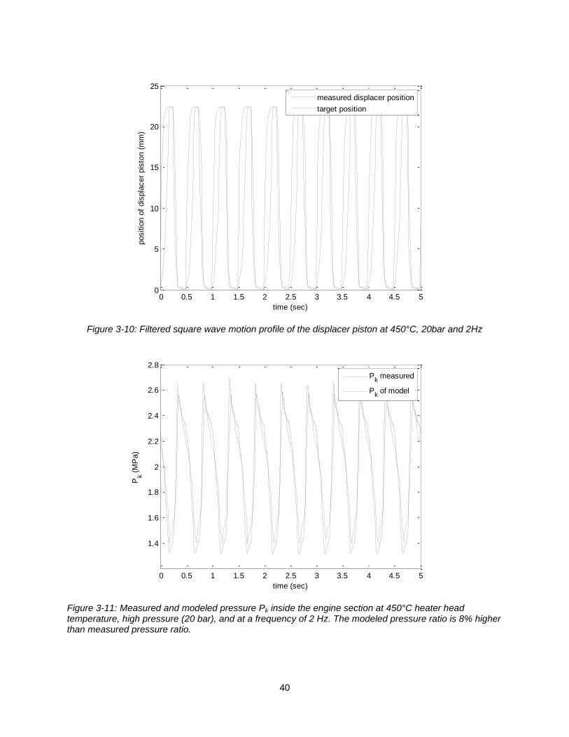
40
Figure 3-10: Filtered square wave motion profile of the displacer piston at 450°C, 20bar and 2Hz
Figure 3-11: Measured and modeled pressure Pk inside the engine section at 450°C heater head temperature, high pressure (20 bar), and at a frequency of 2 Hz. The modeled pressure ratio is 8% higher than measured pressure ratio.
0 0.5 1 1.5 2 2.5 3 3.5 4 4.5 50
5
10
15
20
25
time (sec)
positio
n o
f dis
pla
cer
pis
ton (
mm
)
measured displacer position
target position
0 0.5 1 1.5 2 2.5 3 3.5 4 4.5 5
1.4
1.6
1.8
2
2.2
2.4
2.6
2.8
time (sec)
Pk (
MP
a)
Pk measured
Pk of model

41
Conclusion
The design, first-principles dynamic model and the experimental setup of a Stirling pressurizer has
been described. The dynamic model has been validated with experimental data.
The model matches experimental data for different displacer motion profiles and frequencies, different
average engine pressures, and different heater head temperatures. Experimental and modeled pressure
ratios do not differ by more than 10% (in most cases less than 5%). Furthermore, since the dynamic
model incorporates an arbitrarily specifiable displacer motion, it could be used to optimize such motion
with respect to the pressurizer’s power, efficiency, or other performance metrics. Additionally, the lumped
parameter model could be used in deriving control strategies.
The dynamic model validation presented here does not show the effects of a power piston extracting
energy from the system because the experimental setup has no power-piston attached at the power
connection ports (shown in Fig. 3-1). However, these effects are included in the model as volumes, and
rates of change of volumes, in both the return chamber and the cold-side chamber (rV ,
rV ,kV ,
kV ) that
would be influenced by a power piston driven by the pressure difference between the return chamber and
the dynamic engine pressure. It can be stated with high confidence that such terms in the model would
model the effects well given that such terms are already present for control volume changes in the hot
and cold sides due to the displacer motion (hV ,
hV ,kV ,
kV ).
Finally, it should be emphasized that the model required no tuning of parameters with the exception
of the regenerator effectiveness which was set according to the range in [9]. In conclusion, the model
presented could be used to inform the design and control of not only this engine arrangement, but for
others more generically since the dynamic model is built from first-principles with known or measureable
parameters.
Acknowledgment
This work was supported by the Center for Compact and Efficient Fluid Power, an NSF Engineering
Research Center, grant EEC-0540834.
References
[1] G. Walker, Stirling Engines, Oxford University Press, 1980.
[2] G. Walker and J. R. Senft, Lecture Notes in Engineering: Free Piston Stirling Engines, Springer-
Verlag, New York, 1985.
[3] E. H. Cooke-Yarborough, E. Franklin, T. Gesow, R. Howlett, C. D. West, “Thermomechanical
generator: an efficient means of converting heat to electricity at low power levels,” Proceedings
IEE, no. 121, p. 749-751, 1974.

42
[4] C. D. West, Principles and Applications of Stirling Engines, Van Nostrand Reinhold Company,
New York, 1986.
[5] C. D. West, Liquid Piston Stirling Engines, Van Nostrand Reinhold Company, New York, 1983.
[6] F. T. Reader and M. A. Clarke, “Liquid Piston Stirling Air Engines,” 2nd International Conference
of on Stirling Engines, 14 p, 1984
[7] Gopal, V. K., Duke, R., and Clucas, D., 2009. “Active Stirling Engine”. In TENCON 2009-2009
IEEE Region 10 Conference, IEEE, pp. 1–6.
[8] M. Craun, B. Bamieh, “Optimal Periodic Control of an Ideal Stirling Engine Model,” ASME
Journal of Dynamic Systems, Measurement and Control, Jan 2nd 2015. doi:10.1115/1.4029682
[9] Chin-Hsiang Cheng, and Ying-Ju Yu, “Numerical model for predicting thermodynamic cycle and
thermal efficiency of a beta-type Stirling engine with rhombic-drive mechanism”, Renewable
Energy, vol. 35, pp. 2590-2601, 2010. doi:10.1016/j.renene.2010.04.002
[10] F. Formosa and G. DEspesse, “Analytical model for Stirling cycle machine design”, Energy
Conversion and Management, vol. 51, pp. 1855-1863, 2010.
doi:10.1016/j.enconman.2010.02.010
[11] H. Karabulut, “Dynamic analysis of a free piston Stirling engine working with closed and open
thermodynamic cycles”, Renewable Energy, vol. 36, pp. 1704-1709, 2011.
doi:10.1016/j.renene.2010.12.006
[12] Van de Ven, J., Gaffuri, P., Mies, B., and Cole, G., 2008, "Developments Towards a Liquid
Piston Stirling Engine," International Energy Conversion Engineering Conference, Cleveland,
Ohio

43
CHAPTER IV.
FUTURE DIRECTIONS AND DISCUSSION
The contribution of this work, as presented in Chapter II and Chapter III, is a first principles model of
the Stirling pressurizer that is validated with experimental data for two different displacer motion profiles,
a variety of heater head temperatures and a variety of different average engine pressures. Results show
that the first-principles model can be used to optimize efficiency and/ or power output of the Stirling
device, can also be used to inform the design of control strategies and the design of the Stirling
pressurizer.
The first-principles model can also be used for the design and sizing of an attached power unit. A
power unit that can be driven by the pressure swing of the Stirling pressurizer would be a hydraulic pump,
a compressor, or an electric generator, making the Stirling pressurizer an ideal power source for a variety
of applications.
Oak Ridge National Laboratory for example is interested in building a Stirling device using their
Manufacturing Demonstration Facility (MDF) to enable additive manufactured metal components. Additive
manufacturing enables unprecedented leap-ahead capabilities in Stirling engines due to the ability to
integrate geometries not previously possible with traditional machining. Increasing the surface area for
heat transfer along with a controlled displacer could possibly achieve near-ideal Stirling cycle efficiencies.
Figure 4-1 illustrates how additive manufacturing allows integrating complex geometries to increase the
surface area for heat transfer. A collaboration with Oak Ridge National Laboratory would seek to build a
Stirling device to drive an electric generator which in turn could either power a car or deliver electricity to
the grid when the car is parked.
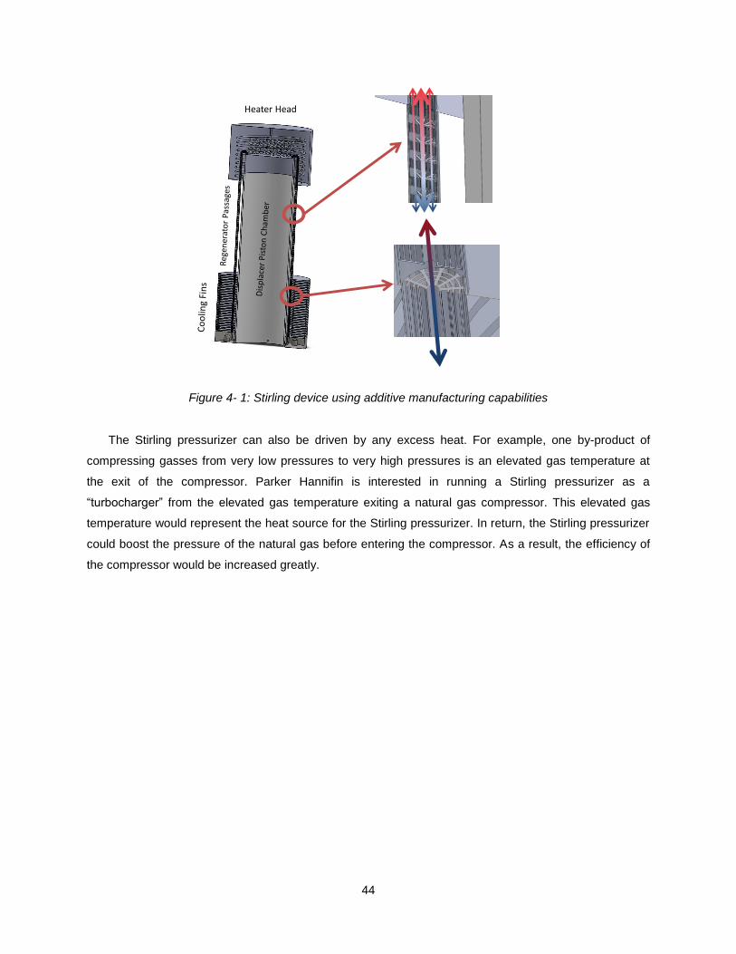
44
Figure 4- 1: Stirling device using additive manufacturing capabilities
The Stirling pressurizer can also be driven by any excess heat. For example, one by-product of
compressing gasses from very low pressures to very high pressures is an elevated gas temperature at
the exit of the compressor. Parker Hannifin is interested in running a Stirling pressurizer as a
“turbocharger” from the elevated gas temperature exiting a natural gas compressor. This elevated gas
temperature would represent the heat source for the Stirling pressurizer. In return, the Stirling pressurizer
could boost the pressure of the natural gas before entering the compressor. As a result, the efficiency of
the compressor would be increased greatly.
Heater Head

45
APPENDIX
A. SIMULINK DIAGRAMS
Figure A-1: Overall system
Figure A-2: Volumes

46
Figure A-3: Engine dynamics

47
Figure A-4: Pressure dynamics on hot side
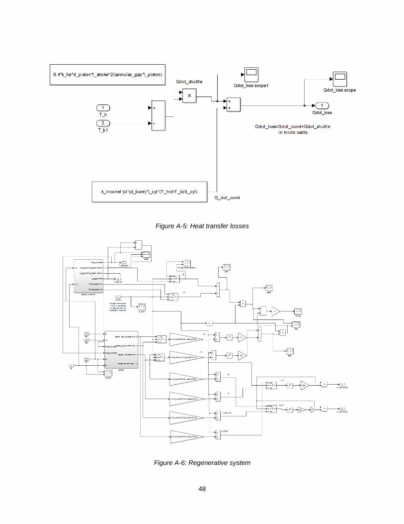
48
Figure A-5: Heat transfer losses
Figure A-6: Regenerative system

49
Figure A-7: Mass flow ate in engine section
Figure A-8: Mass flow rate in engine section times Tflow
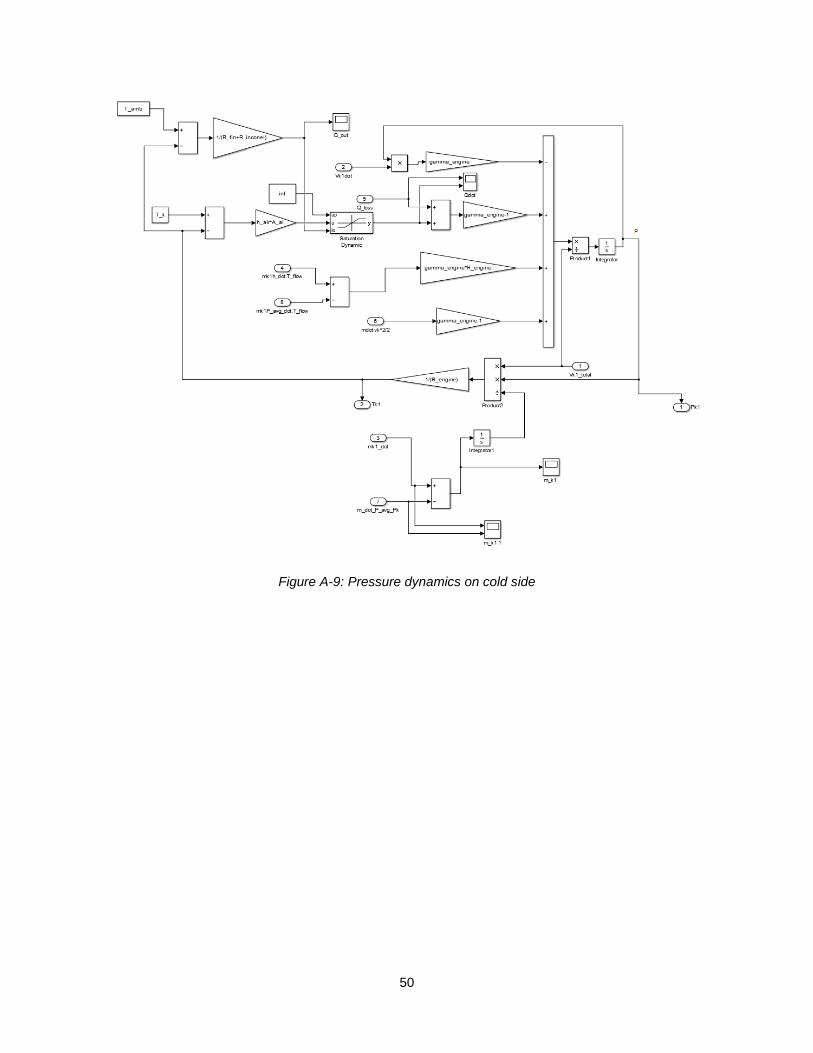
50
Figure A-9: Pressure dynamics on cold side

51
Figure A-10: Direction switch
Figure A-11: Mass flow rate between cold side and return chamber

52
Figure A-12: Mass flow rate between cold side and return chamber

53
B. MATLAB CODE
% Stirling Pressurizer
% Base Units: %mm, kg, s, mN, kPa, microJ (uJ), microW (uW), K
%% % Atmospheric Temperature and Pressure
T_amb=25+273; % Ambient air temperature (K) P_atm=14.65*6.89; % Atmoshperic Pressure (kPa)
%% variables
l_stroke=23.6; %(mm) stroke length
%% working gas constants (helium) in engine section
% data: % cv_helium=12.5 % J/mol/K % cp_helium=20.8 % J/mol/K % molecular weight = 4.002602 g/mol % cp_gas=5193.2*1e6; %constant pressure specific heat (in uJ/kg/K) % cv_gas=3123*1e6; %constant volume specific heat (in uJ/kg/K) % R_univ=8.3145*1e6; %Average gas constant (in uJ/mol/K)
cp_helium=20.8/4.002602*1000*1e6; %constant pressure specific heat (in
uJ/kg/K) cv_helium=12.5/4.002602*1000*1e6; %constant volume specific heat (in uJ/kg/K) R_helium=cp_helium-cv_helium; %gas constant (in uJ/kg/K) gamma_helium=cp_helium/cv_helium; %ratio of specific heats (no dim)
%% working gas constants (krypton) % data: % cp=0.248 J/g/K % cv=12.5 J/mol/K % molecular weight = 83.798 g/mol % cv=0.1492 J/g/K R_univ=8.3145*1e6; %Average gas constant (in uJ/mol/K) cp_krypton=248*1e6; %constant pressure specific heat (in
uJ/kg/K) cv_krypton=149.2*1e6; %constant volume specific heat (in
uJ/kg/K) R_krypton=cp_krypton-cv_krypton; %gas constant (in uJ/kg/K) gamma_krypton=cp_krypton/cv_krypton; %ratio of specific heats (no dim)
%%
cp_engine=cp_helium; % constant pressure specific heat (in uJ/kg/K) cv_engine=cv_helium; % constant volume specific heat (in uJ/kg/K)
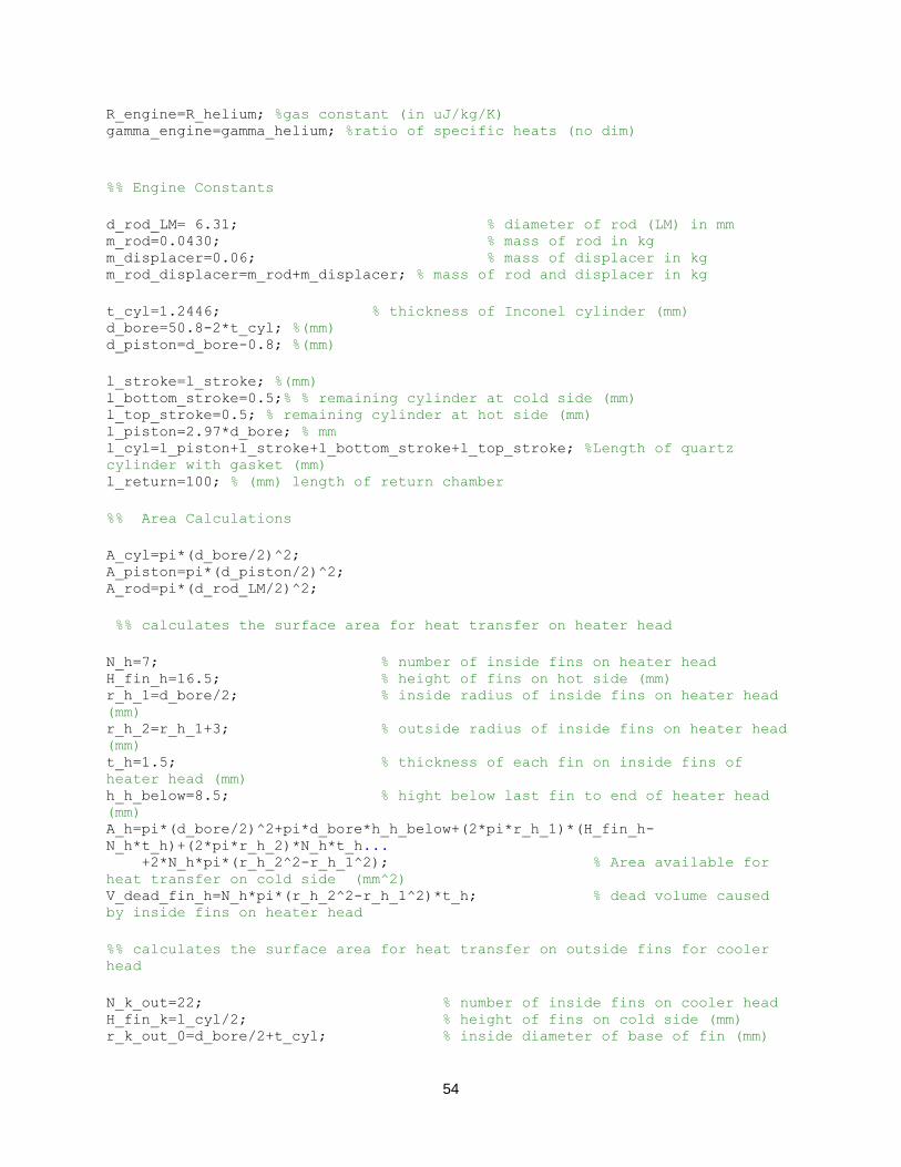
54
R_engine=R_helium; %gas constant (in uJ/kg/K) gamma_engine=gamma_helium; %ratio of specific heats (no dim)
%% Engine Constants
d_rod_LM= 6.31; % diameter of rod (LM) in mm m_rod=0.0430; % mass of rod in kg m_displacer=0.06; % mass of displacer in kg m_rod_displacer=m_rod+m_displacer; % mass of rod and displacer in kg
t_cyl=1.2446; % thickness of Inconel cylinder (mm) d_bore=50.8-2*t_cyl; %(mm) d_piston=d_bore-0.8; %(mm)
l_stroke=l_stroke; %(mm) l_bottom_stroke=0.5;% % remaining cylinder at cold side (mm) l_top_stroke=0.5; % remaining cylinder at hot side (mm) l_piston=2.97*d_bore; % mm l_cyl=l_piston+l_stroke+l_bottom_stroke+l_top_stroke; %Length of quartz
cylinder with gasket (mm) l_return=100; % (mm) length of return chamber
%% Area Calculations
A_cyl=pi*(d_bore/2)^2; A_piston=pi*(d_piston/2)^2; A_rod=pi*(d_rod_LM/2)^2;
%% calculates the surface area for heat transfer on heater head
N_h=7; % number of inside fins on heater head H_fin_h=16.5; % height of fins on hot side (mm) r_h_1=d_bore/2; % inside radius of inside fins on heater head
(mm) r_h_2=r_h_1+3; % outside radius of inside fins on heater head
(mm) t_h=1.5; % thickness of each fin on inside fins of
heater head (mm) h_h_below=8.5; % hight below last fin to end of heater head
(mm) A_h=pi*(d_bore/2)^2+pi*d_bore*h_h_below+(2*pi*r_h_1)*(H_fin_h-
N_h*t_h)+(2*pi*r_h_2)*N_h*t_h... +2*N_h*pi*(r_h_2^2-r_h_1^2); % Area available for
heat transfer on cold side (mm^2) V_dead_fin_h=N_h*pi*(r_h_2^2-r_h_1^2)*t_h; % dead volume caused
by inside fins on heater head
%% calculates the surface area for heat transfer on outside fins for cooler
head
N_k_out=22; % number of inside fins on cooler head H_fin_k=l_cyl/2; % height of fins on cold side (mm) r_k_out_0=d_bore/2+t_cyl; % inside diameter of base of fin (mm)

55
r_k_out_1=d_bore/2+7; % inside radius of inside fins on
cooler head (mm) r_k_out_2=45; % outside radius of inside fins on
cooler head (mm) t_k_out=2; % thickness of each fin on inside fins
of cooler head (mm) A_al=(2*pi*r_k_out_1)*(H_fin_k-N_k_out*t_k_out)+(pi/4)*(d_bore^2-
d_rod_LM^2)... +(2*pi*r_k_out_2)*N_k_out*t_k_out+2*N_k_out*pi*(r_k_out_2^2-
r_k_out_1^2); % Area available for heat transfer on cold side (housing, lead
screw, etc.) (mm^2)
%% fin efficiency
T_amb=T_amb; T_b=333; % Temperature on base of fins (between fins and Inconel
cylinder) k_Al=215000; % thermal conductivity of Aluminium
(uW/mm/K) k_inconel=10.1e3; % thermal conductivity of Inconel
(uW/mm/K) h_air=50; % W/m^2/K or uW/mm^2/K r_k_out_2c=r_k_out_2+(t_k_out/2); % corrected outside fin radius (mm) L=r_k_out_2-r_k_out_1; L_c=L+(t_k_out/2); % corrected length A_f=2*pi*(r_k_out_2c^2-r_k_out_1^2); % from heat transfer book p.171 A_t=N_k_out*A_f+2*pi*r_k_out_1*(H_fin_k-N_k_out*t_k_out); % from heat
transfer book p.171 A_p=L_c*t_k_out; (L_c)^1.5*sqrt(h_air/(k_Al*A_p)); % look up efficiency of annular fin of
rectancular profile n_f=0.95;
run('Z:\Anna\Research\MATLAB\other MATLAB files\calculation_h')
R_He_cyl=(1/(h*2*pi*(d_bore/2)*(H_fin_k))); R_inconel=(log(r_k_out_0/(d_bore/2))/(2*pi*k_inconel*H_fin_k)); R_fin_base=(log(r_k_out_1/r_k_out_0))/(2*pi*k_Al*H_fin_k); R_fin=1/(h_air*A_t*(1-((N_k_out*A_f)/A_t)*(1-n_f)));
q_t=(1/(R_He_cyl+R_inconel+R_fin_base+R_fin))*(T_amb-T_b);
%% Heat transfer
hA_h= h*A_h;
%% Calculate Volumes V_cyl=A_cyl*l_cyl;
V_piston=l_piston*A_piston; % Volume taken up by piston
V_dead_piston=l_piston*(A_cyl-A_piston); %Dead volume surrounding piston V_h_dead=V_dead_piston/2+l_top_stroke*A_cyl+V_dead_fin_h; V_h_max=V_h_dead+l_stroke*A_cyl; % Max volume of air on hot side (m^3) V_h_min=V_h_dead; % Min volume of air on hot side (m^3)

56
V_k_dead=l_bottom_stroke*A_cyl+V_dead_piston/2; V_k_max=V_k_dead+l_stroke*A_cyl; % Max volume of air on cold side (m^3) V_k_min=V_k_dead; % Min volume of gas on cold side (m^3)
%% initial conditions engine hot side
T_h_0=T_hot; P_h_0=P_k_min; V_h_0=V_h_dead; m_h_0=P_h_0*V_h_0/(R_engine*T_h_0);
%% initial conditions engine cold side T_k_0=T_k; P_k_0=P_k_min; V_k_0=V_k_dead + l_stroke*A_cyl; m_k_0=P_k_0*V_k_0/(R_engine*T_k_0);
%% regneration effect
k_he=211.4; % thermal conductivity of helium (uW/mm/K) at 500K k_ss=17e3; % thermal conductivity of stainless steel (uW/mm/K) alpha_ss=4.2; % thermal diffusivity of stainless steel (mm^2/s) k_inconel=k_inconel;
%thermal conductivity of Inconel (uW/mm/K) annular_gap=(d_bore/2)-(d_piston/2); % annular gap (mm) omega=2*pi*f_Hz; C=(k_ss/k_he)*annular_gap*sqrt(omega/(2*alpha_ss)); BET=(2*C^2-C)/(2*C^2-1); Q_shuttle=(pi/8)*k_he*l_stroke*(T_hot-
T_k)*(d_bore/annular_gap)*(l_stroke/l_piston)*BET;
%% constants needed to calculate m_dot
r_bore=d_bore/2; r_piston=d_piston/2;
constant1_mdot=((r_bore)^4-(r_piston)^4-(((r_bore)^2-
(r_piston)^2)^2/log(r_bore/r_piston))); constant2_mdot=0.5*(r_bore^2*log(r_bore)-r_piston^2*log(r_piston))-
0.25*(r_bore^2-r_piston^2); constant3_mdot=0.5*r_bore^2-0.5*r_piston^2;
A_hole_displacer=(pi/4)*0.1^2;

57
Code to calculate the heat transfer coefficient h
% calculation of convection coefficient h
A_gap=(pi/4)*(d_bore^2-d_piston^2); V_cyl=A_cyl*l_cyl; % Volume of cylinder V_piston=A_piston*l_piston; % Volume of piston
V_dead_piston=l_piston*(A_gap); %Dead volume surrounding piston V_h_dead=V_dead_piston/2+l_top_stroke*A_cyl; V_k_dead=l_bottom_stroke*A_cyl+V_dead_piston/2; V_dead=V_k_dead+V_h_dead;
V_max=V_cyl-V_piston-V_dead; % max. Volume thats moved by displacer
per stroke
t=1/(f_Hz*2); % time displacer moves V_max (sec)
V_dot=V_max/t; % in mm^3/sec velocity=V_dot/A_gap/1000; % in m/sec
C=d_bore-d_piston; % characteristic length of a duct in mm charac_length=(C)/1000; % characteristic length of a duct in m R_He=2.077; % kJ/kg/K % T_avg=600; % avg. Temperature in K % P_avg=2000; % avg. Pressure in kPa density_He=P_avg/(R_He*T_avg); % from ideal gas law in kg/m^3 viscosity_He=19e-6*((273+79.4)/(T_avg+79.4))*(T_avg/273)^1.5; % in Pa*s kinem_viscosity_He=viscosity_He/density_He ; % in m^2/s
density_air=0.588; % from ideal gas law in kg/m^3 viscosity_air=3.017e-5; % in Pa*s kinem_viscosity_air=viscosity_air/density_air ; % in m^2/s k_air=0.0485; Re_He=velocity*charac_length/kinem_viscosity_He; Re_air=velocity*charac_length/kinem_viscosity_air; a=0.023; Pr=0.7; m=0.8; n=0.3; k=0.14789*(T_avg/273)^0.6958;
h=a*Re_He^m*Pr^n*k/charac_length h_air=a*Re_air^m*Pr^n*k_air/charac_length
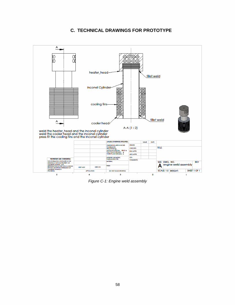
58
C. TECHNICAL DRAWINGS FOR PROTOTYPE
Figure C-1: Engine weld assembly

59
Figure C-2: Heater head
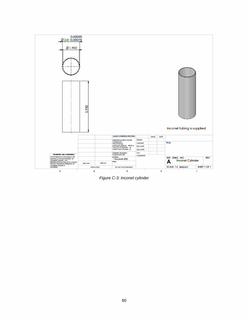
60
Figure C-3: Inconel cylinder

61
Figure C-4: Cooling fins

62
Figure C-5: Cooler head

63
Figure C-6: Hugger1 of return chamber

64
Figure C-7: Top part of hugger1

65
Figure C-8: Shaft part of hugger1

66
Figure C-9: Return part of hugger1

67
Figure C-10: Hugger2 of return chamber
68
Figure C-11: Top part of hugger2

69
Figure C-12: Shaft part of hugger2

70
Figure C-13: Displacer weld assembly
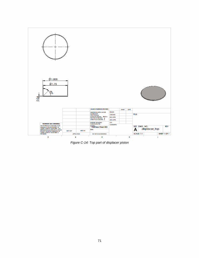
71
Figure C-14: Top part of displacer piston

72
Figure C-15: Displacer cylinder

73
Figure C-16: Bottom of displacer

74
Figure C-17: Extension rod

75
Figure C-18: Clamp assembly
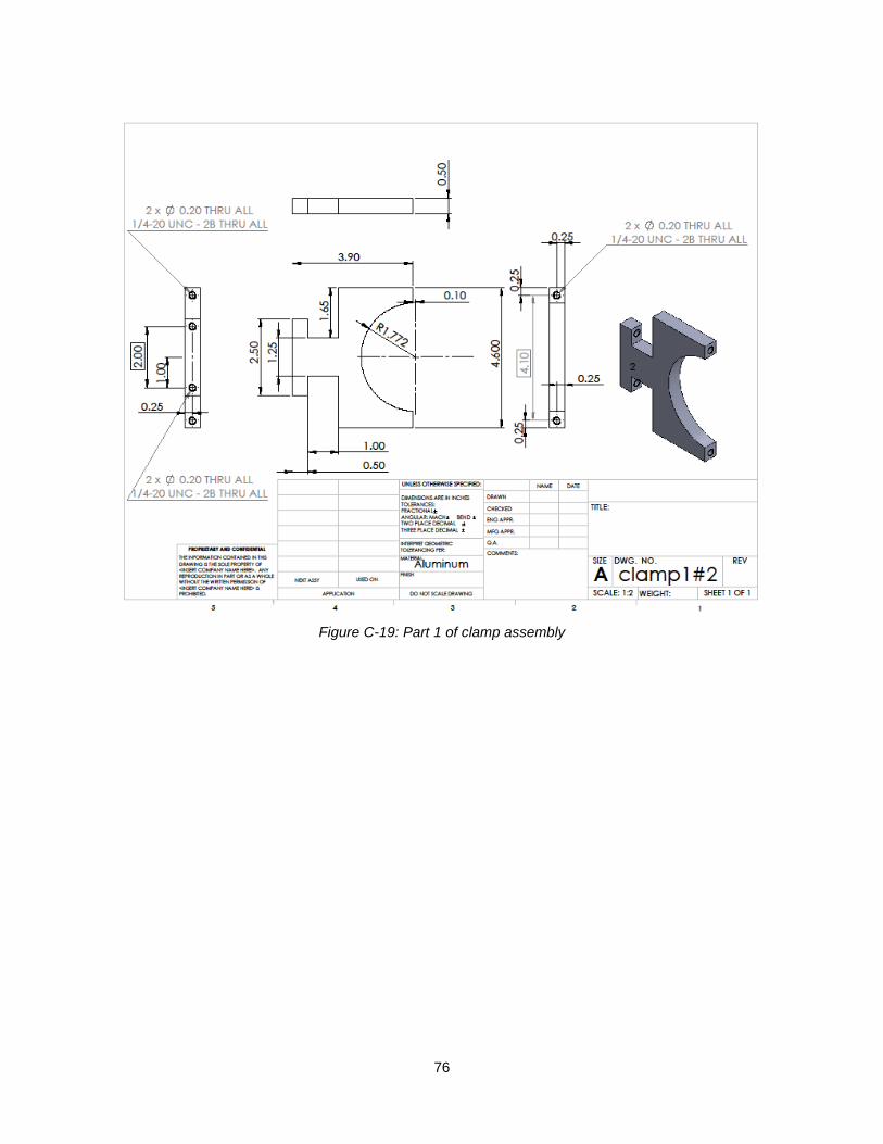
76
Figure C-19: Part 1 of clamp assembly

77
Figure C-20: Part 2 of clamp assembly

78
Figure C-21: Connection between coupling and linear motor
Related Documents