Comparative anatomical and biophysical characterization of a hippocampal-like network in teleost and rodents By Anh-Tuân Trinh Final version: August 2021 Thesis submitted to the University of Ottawa in partial fulfillment of the requirements for the Doctor of Philosophy in Neuroscience Department of Cellular and Molecular Medicine Faculty of Medicine University of Ottawa © Anh-Tuân Trinh, Ottawa, Canada, 2021

Welcome message from author
This document is posted to help you gain knowledge. Please leave a comment to let me know what you think about it! Share it to your friends and learn new things together.
Transcript
Comparative anatomical and biophysical characterization of a hippocampal-like network in teleost and rodents
By
Anh-Tuân Trinh
Final version: August 2021
Thesis submitted to the
University of Ottawa
in partial fulfillment of the requirements for the
Doctor of Philosophy in Neuroscience
Department of Cellular and Molecular Medicine
Faculty of Medicine
University of Ottawa
© Anh-Tuân Trinh, Ottawa, Canada, 2021

II
Abstract
The work presented in this thesis investigates whether primitive pallial brain circuits such as
those found in teleost fish may also encode complex information such as spatial memory despite
its circuitry being “simpler” than those found in species with much larger brains such as primates
and rodents. Previous behavioral studies have already shown that most teleost fish are capable of
spatially orienting themselves and remembering past food locations. Behavioral studies combined
with selective brain lesions and related anatomical studies have identified a hippocampal-like
region in the fish’s pallium; however, it is unknown whether the neurons located in this structure
can also perform cortical-like computations as those found in the mammalian hippocampus.
Consequently, this thesis will first present an anatomical characterization of the intrinsic circuitry
of this hippocampal-like structure, followed by an in vitro electrophysiological characterization of
its constituent neurons. Surprisingly, we have found that this hippocampal-like structure possesses
many features reminiscent of the mammalian cortex, including recurrent local connectivity as well
as a laminar/columnar-like organization. Furthermore, we have also identified many biophysical
properties which would describe these hippocampal-like neurons as sparse coders, including a
prominent after-hyperpolarizing potential and an adapting spike threshold with slow recovery.
Since this particular dynamic spike threshold mechanism has not been thoroughly characterized in
the mammalian hippocampus, we have further investigated the dynamic threshold in the major
rodent hippocampal cell types. We have found that only a subset of excitatory neurons displayed
this dynamic spike threshold on the time scale that was observed in teleost pallial cells, which
allowed us to discuss its potential role in encoding spatial information in both species.
Nevertheless, the fact that this teleost hippocampal homologue possesses characteristics that are
both akin to the cortex and hippocampus suggest that it may perform computations that, in a
mammalian brain, would require both structures and makes this ancestral structure a very
interesting candidate to study the mechanism(s) underlying spatial memory.

III
Résumé
Le travail effectué dans le cadre de cette thèse cherche à démontrer si les circuits neuronaux
primitifs, tels que ceux présents dans le pallium des poissons téléostéens, peuvent aussi encoder
de l’information complexe rattachée à la mémoire spatiale. Ceci, malgré que leurs circuits
neuronaux soient “plus simples” que ceux appartenant aux espèces possédant des cerveaux plus
volumineux, comme les primates ou les rongeurs. Des études comportementales antérieures ont
démontré que la plupart des poissons téléostéens sont capables de s’orienter spatialement et de se
souvenir de l’architecture spatiale de leurs terrains de chasse. Des études comportementales
utilisant des animaux ayant des lésions cérébrales, et les études anatomiques qui y sont reliées ont
permis d’identifier une région similaire à l’hippocampe dans le pallium des poissons. Cependant,
il reste à déterminer si les neurones situés dans cette structure peuvent aussi effectuer des
computations corticales telles que celles répertoriées dans l’hippocampe mammalien. Cette thèse
va d’abord présenter une étude anatomique du circuit intrinsèque à cette structure présumée
homologue à l’hippocampe, puis une étude électrophysiologique in vitro des neurones qui la
constituent. Nous avons trouvé que cette structure possède plusieurs caractéristiques similaires au
cortex mammalien, incluant une connectivité récurrente locale ainsi que des connexions organisées
en colonnes et en strates. De plus, nous avons identifié plusieurs propriétés biophysiques qui
suggèrent que ces neurones sont aptes à effectuer un codage épars (« sparse coding »). Notamment,
ceux-ci démontrent un fort potentiel d’hyperpolarisation (« after-hyperpolarization ») ainsi qu’un
seuil de potentiel d’action ascendant qui se rétablit lentement. Puisque cette modulation du
potentiel de seuil n’a pas encore été caractérisée dans sa totalité dans l’hippocampe mammalien,
nous avons également investigué ce mécanisme dans les cellules principales de l’hippocampe chez
les rongeurs. Nous avons trouvé que seul certains types de neurones excitateurs de l’hippocampe
mammalien démontrent ce délai lors du rétablissement du seuil, tel qu’observé chez les poissons.
Cela nous permet d’explorer le rôle potentiel de ce type de modulation dans l’encodage
d’informations spatiales chez les deux espèces. Ceci dit, que l’homologue fourni par le poisson
téléostéen possède des caractéristiques appartenant à la fois au cortex et à l’hippocampe suggère
qu’il pourrait performer des computations qui, dans le cerveau des mammifères, nécessiteraient
les deux types de structures. Cela ferait de cette structure primitive une candidate très intéressante
à l’étude de la mémoire spatiale.

IV
Acknowledgments
Throughout my graduate studies, I was fortunate to have met and worked with wonderful
colleagues who have all helped me develop into the scientist that I am today. As such, I would like
to give my sincerest thanks for all their dedication and support in helping me achieve my academic
and scientific goals.
Most importantly, I would like to thank my supervisor, Dr. Leonard Maler, who has dedicated
many hours in supporting me over the years. His enthusiasm for science has always been a source
of inspiration for me and through our discussions, I sometime feel like his knowledge of
neuroscience is endless. Hence, I feel very fortunate and grateful to have had him as a mentor.
I would also like to thank the members of my Thesis Advisory Committee, Dr. Jean-Claude
Béïque, Dr. André Longtin and Dr. John Lewis who have all provided me with invaluable feedback
on both my progress and my development as a neuroscientist.
Next, I would also like to take this opportunity to thank my past and current colleagues in the
Maler and Béïque labs who have all supported me and helped me throughout my graduate studies.
Notably, I would like to thank Dr. Érik Harvey-Girard, my friend and colleague, who has helped
me with my numerous questions regarding experimental techniques and technical support.
Of course, this work would also not have been possible without the help and support from my
family and friends which, without a doubt, has positively impacted my productivity. Hence, I
would like to thank everyone who has supported me over the years with a special mention to my
wife Camille LeBlanc-Gagné.
Finally, I would like to thank the University of Ottawa and the provincial government of Ontario
for funding my graduate studies through the Ontario Graduate Scholarship and the provincial
government of Quebec for funding my graduate studies through the Fonds de Recherche Nature et
Technologies doctoral scholarship.

V
Dedication
I dedicate this work to my late father, Dr. Ngoc Chau Trinh, who, since my childhood, has
always inspired me to learn as much as possible and ultimately, has inspired me to become a
scientist.

VI
Contents
ABSTRACT ...........................................................................................................................................................II
RÉSUMÉ ............................................................................................................................................................. III
ACKNOWLEDGEMENTS ................................................................................................................................. IV
DEDICATION ...................................................................................................................................................... V
LIST OF FIGURES ........................................................................................................................................... IX
LIST OF TABLES ............................................................................................................................................ XII
LIST OF ABBREVIATIONS ........................................................................................................................ XIII
CHAPTER 1: GENERAL INTRODUCTION ...................................................................................................... 1
CHAPTER 1.1 REPRESENTATION OF SPACE IN THE MAMMALIAN HIPPOCAMPUS ....................................................... 2
CHAPTER 1.2 SPATIAL MEMORY IN THE MAMMALIAN HIPPOCAMPUS ...................................................................... 4
CHAPTER 1.3 REPRESENTATION OF TIME IN THE MAMMALIAN HIPPOCAMPUS ......................................................... 5
CHAPTER 1.4 RECURRENT NEURAL NETWORKS AND SPIKE FREQUENCY ADAPTATION .............................................. 6
CHAPTER 1.5 WHY STUDY THE TELEOST HIPPOCAMPAL HOMOLOGUE? ................................................................ 10
CHAPTER 1.6 THE HIPPOCAMPAL HOMOLOGUE IN TELEOST FISH ......................................................................... 11
CHAPTER 1.7 THE ANATOMICAL AND BIOCHEMICAL EVIDENCE SUGGESTING THAT DL IS HOMOLOGOUS TO THE
MAMMALIAN HIPPOCAMPUS ....................................................................................................................................... 14
CHAPTER 1.8 BEHAVIORAL EVIDENCE OF SPATIAL MEMORY FORMATION IN THE TELEOST HIPPOCAMPAL
HOMOLOGUE ............................................................................................................................................................ 16
CHAPTER 1.9 OPEN QUESTIONS AND PREFACE FOR CHAPTERS II-IV .................................................................... 19
CHAPTER 2: CHARACTERIZING THE MICRO-CIRCUITRY OF THE TELEOST HIPPOCAMPAL-
LIKE STRUCTURE. (ORIGINAL MANUSCRIPT I) .............................................................................................. 22
ABSTRACT .......................................................................................................................................................... 25
INTRODUCTION .................................................................................................................................................. 26
MATERIALS & METHODS ..................................................................................................................................... 29
Care of Apteronotus leptorhynchus fish .................................................................................................... 29
Stereological counts ................................................................................................................................... 30
Shrinkage estimates of frozen sections ...................................................................................................... 32
DL neuron distribution............................................................................................................................... 32
Circuitry analysis: In vitro ......................................................................................................................... 33
In vivo injections ........................................................................................................................................ 35
Microscopy .................................................................................................................................................. 35
Image analysis and figure preparation ...................................................................................................... 36
Random graph theory analysis................................................................................................................... 38
RESULTS ............................................................................................................................................................ 38
Organization and cell counts of the dorsolateral pallium ......................................................................... 38

VII
DL intrinsic connectivity ............................................................................................................................ 40
Slab slices: Laminar symmetric recurrent connections in DL .................................................................. 41
Transverse slices: Vertical unidirectional connectivity in DL .................................................................. 46
Quantifying connectivity in the tangential plane ...................................................................................... 50
Analyzing DL connectivity with graph theory ........................................................................................... 51
DISCUSSION ....................................................................................................................................................... 55
Comparative aspects of DL laminar and columnar organization ............................................................. 59
Possible homology of DL to either/or hippocampus and cortex of mammals .......................................... 61
Dorsolateral pallium: Recurrent networks, bump attractors, and reverberatory activity ........................ 63
CHAPTER 3: BIOPHYSICAL CHARACTERIZATION OF HIPPOCAMPAL-LIKE NEURONS IN THE
FISH PALLIUM. (ORIGINAL MANUSCRIPT II) .................................................................................................. 66
ABSTRACT .......................................................................................................................................................... 68
INTRODUCTION .................................................................................................................................................. 69
MATERIALS AND METHODS ................................................................................................................................. 71
Slice preparation ......................................................................................................................................... 72
In vitro recordings ...................................................................................................................................... 73
Pharmacology ............................................................................................................................................. 74
RT-PCR ....................................................................................................................................................... 75
Data analysis............................................................................................................................................... 76
Inactivating exponential integrate and fire model (iEIF) ......................................................................... 77
Code accessibility ........................................................................................................................................ 80
RESULTS ............................................................................................................................................................ 81
Noisy versus quiet cells ............................................................................................................................... 82
Noisy cells ................................................................................................................................................... 84
Quiet cells ................................................................................................................................................... 86
Asymmetric input resistance ...................................................................................................................... 89
Voltage-dependent calcium conductance .................................................................................................. 93
AHPs ........................................................................................................................................................... 94
Dynamic AHP and spike threshold ............................................................................................................ 98
DISCUSSION ..................................................................................................................................................... 102
The biophysical properties of DL neurons suggest that they are sparse coders ..................................... 104
Can the DL network transform PG sequential encounter time stamps to a spatial map? ..................... 106
EXTENDED FIGURES ........................................................................................................................................ 113
CHAPTER 4: CHARACTERIZING THE INTRINSIC BIOPHYSICAL PROPERTIES OF THE HILAR
MOSSY CELLS (MANUSCRIPT IN PREPARATION) ......................................................................................... 114
ABSTRACT ........................................................................................................................................................ 116
INTRODUCTION ................................................................................................................................................ 117

VIII
MATERIALS AND METHODS ............................................................................................................................... 122
In vitro slice procedure ............................................................................................................................. 122
In vitro recordings .................................................................................................................................... 123
Pharmacology ........................................................................................................................................... 124
Data analysis............................................................................................................................................. 125
RESULTS .......................................................................................................................................................... 126
Spontaneous Synaptic Transmission ....................................................................................................... 128
Hilar Mossy Cell Intrinsic Properties ...................................................................................................... 130
Dynamic spike threshold in the hippocampal formation ........................................................................ 134
DISCUSSION ..................................................................................................................................................... 137
Potential origin of the synaptic noise ....................................................................................................... 138
Dynamic spike threshold in the hippocampal formation ........................................................................ 139
Dynamic spike threshold in hMC ............................................................................................................ 141
Outlook for future model of hMCs .......................................................................................................... 143
ANNEX: SUPPLEMENTARY FIGURES ................................................................................................................ 144
CHAPTER 5: THESIS DISCUSSION ............................................................................................................. 146
CHAPTER 5.1 COMPARATIVE INTERPRETATION OF THE TELEOST DL................................................................... 147
CHAPTER 5.2 PROPOSED THEORETICAL MODEL FOR MEMORY ENCODING IN THE TELEOST PALLIUM .................... 150
CHAPTER 5.3 THE POTENTIAL ROLES FOR A DYNAMIC SPIKE THRESHOLD ........................................................... 153
CONCLUDING REMARKS ................................................................................................................................... 155
BIBLIOGRAPHY ............................................................................................................................................. 156

IX
List of figures
Chapter 1 Figures
FIGURE I. CIRCUITRY OF THE PARAHIPPOCAMPAL AND HIPPOCAMPAL FORMATIONS ...................... 3
FIGURE II. CIRCUITRY OF THE GYMNOTIFORM FISH PALLIUM ....................................................... 13
FIGURE III. HIPPOCAMPAL HOMOLOGY HYPOTHESIS IN GYMNOTIFORM FISH. ............................... 15
Chapter 2 Figures
FIGURE 1. CRESYL VIOLET-STAINED TRANSVERSE SECTIONS OF THE TELENCEPHALON ................. 28
FIGURE 2. TRACER INJECTIONS IN DL, SLAB SLICE ........................................................................ 42
FIGURE 3. TRACER INJECTIONS IN PROXIMITY TO EACH OTHER, SLAB SLICE .................................. 43
FIGURE 4. IN VIVO INJECTION OF MINIRUBY IN DL ....................................................................... 44
FIGURE 5. INJECTION OF THE MINIRUBY TRACER IN TRANSVERSE DL SLICES ILLUSTRATING
VERTICAL CONNECTIVITY ...................................................................................................... 45
FIGURE 6. ESTIMATING THE WIDTH OF A CRYPTIC DL COLUMN .................................................... 47
FIGURE 7. VERTICAL CONNECTIVITY SEEN BY ROTATION OF A SLAB SLICE ................................... 48
FIGURE 8. MICROSTRUCTURE OF THE VERTICAL CONNECTIVITY IN DL, TRANSVERSE SLICES. THE
SURFACE OF DL IS AT THE TOP OF THE IMAGES ...................................................................... 49
FIGURE 9. CONNECTION PROBABILITY AS A FUNCTION OF TANGENTIAL DISTANCE FROM THE
INJECTION SITE TO RETROGRADELY LABELED NEURONS ......................................................... 51
FIGURE 10. DIRECTED RANDOM GRAPH MODEL OF DL.................................................................. 55
FIGURE 11. SCHEMATIC SUMMARY OF DL CIRCUITRY .................................................................. 58

X
Chapter 3 Figures
FIGURE 1. ANATOMY OF THE A. LEPTORHYNCHUS TELENCEPHALON .............................................. 81
FIGURE 2. RMP OF DL NEURONS .................................................................................................. 83
FIGURE 3. NOISY CELLS ................................................................................................................ 85
FIGURE 4. SPIKING CHARACTERISTICS OF DL NEURONS ................................................................ 87
FIGURE 5. PHARMACOLOGICAL BLOCK OF SODIUM AND OTHER CHANNELS IN DL NEURONS ........ 90
FIGURE 6. SK-MEDIATED POTASSIUM CHANNELS CONTRIBUTE TO THE AHP OF DL NEURONS ..... 95
FIGURE 7. THE EFFECT OF INTRACELLULAR CA2
CHELATION ON DL NEURON RESPONSES TO
DEPOLARIZATION ................................................................................................................... 97
FIGURE 8. DL NEURON SPIKING CAUSES A DECREASE IN AHP AMPLITUDE AND AN INCREASE IN
SPIKE THRESHOLD .................................................................................................................. 99
FIGURE 9. DL NEURON SPIKE THRESHOLD ADAPTATION CAN LAST UP TO HUNDREDS OF
MILLISECONDS ..................................................................................................................... 101
EXTENDED FIGURE 5-1. GIRK CHANNEL MRNA EXPRESSION OBTAINED FROM RT-PCR IN THE
APTERONOTUS BRAIN USING PAN-PCR PRIMER PAIRS IN CONSERVED REGIONS .................... 113
EXTENDED FIGURE 8-1. CURRENT-EVOKED SPIKING DECREASES THE AHP AMPLITUDE OF DL
NEURON ............................................................................................................................... 113
Chapter 4 Figures
FIGURE 1. CIRCUITRY OF THE HILAR NETWORK. .......................................................................... 118

XI
FIGURE 2. STRONG MEMBRANE FLUCTUATIONS ARE PRESENT IN HMC NEURONS ....................... 127
FIGURE 3. SPIKING INDEPENDENT SYNAPTIC NOISE ..................................................................... 129
FIGURE 4. CHARACTERIZING THE SPIKE THRESHOLD IN HMC NEURONS ..................................... 132
FIGURE 5. SPIKE THRESHOLD ADAPTATION TIMESCALE .............................................................. 137
SUPPLEMENTARY FIGURE 1. CHARACTERIZING THE AHP IN HMC NEURONS ............................. 144
SUPPLEMENTARY FIGURE 2. ADDITIONAL CHARACTERIZATION OF THE INTRINSIC PROPERTIES OF
HMCS .................................................................................................................................. 145

XII
List of tables
Chapter 2 Table
TABLE 1. STEREOLOGICAL MEASUREMENTS SHOWING THE NEURON DENSITY, THE TOTAL
VOLUME, THE TOTAL NUMBER OF NEURONS FOR SEVERAL BRAIN AREAS, AND THE RATIOS
OF DL NEURONS OVER THE NUMBER OF NEURONS FROM DIFFERENT BRAIN REGIONS .... 38
Chapter 3 Tables
TABLE 1. I-V SLOPE MEASUREMENTS OBTAINED FROM THE DEPOLARIZING AND
HYPERPOLARIZING RESPONSES OF DL NEURONS IN BOTH TELEOST SPECIES FOR THE TTX
AND QX-314 EXPERIMENTS.................................................................................................. 92
TABLE 2. DIFFERENCE IN SPIKE THRESHOLD AND RESTING MEMBRANE ACROSS MULTIPLE CELL
TYPES .................................................................................................................................. 105
TABLE 3. STATISTICAL TABLE. .................................................................................................. 108

XIII
List of abbreviations
CA1 cornu Ammonis areas 1
CA3 cornu Ammonis areas 3
DG dentate gyrus
EC entorhinal cortex
GC granule cell
hMC hilar mossy cell
AHP after-hyperpolarizing potential
BK large conductance Ca2+-activated K+-channel
SK small conductance Ca2+-activated K+-channel
GABA gamma-aminobutyric acid
PV parvalbumin
SOM somatostatin
DC central division of dorsal telencephalon
DCc core subdivision of centrodorsal telencephalon
DCs shell subdivision of centrodorsal telencephalon
DDi inferior subdivision of dorsodorsal telencephalon
DDmg magnocellular subdivision of dorsodorsal telencephalon
DDs superficial subdivision of dorsodorsal telencephalon
DL laterodorsal telencephalon
DLc caudal subdivision of the laterodorsal telencephalon
DLv ventral subdivision of the dorsolateral telencephalon
DLd dorsal subdivision of the dorsolateral telencephalon
DM mediodorsal telencephalon
DP posterior pallium
ELL electrosensory lateral line lobe
IL inferior lobe
PFC prefrontal cortex
PGl lateral subdivision of preglomerular nucleus
PGm medial subdivision of preglomerular nucleus
PGr rostral subdivision of preglomerular nucleus
RNN recurrent neural network
TeO optic tectum
TS torus semicircularis
Vc central subdivision of the ventral telencephalon
Vd dorsal subdivision of the ventral telencephalon
Vs supracommissural subdivision of the ventral telencephalon
DCN dorsal cochlear nucleus
ACSF artificial cerebrospinal fluid
TTX tetrodotoxin
PTX picrotoxin
RMP resting membrane potential
MP membrane potential
ISI inter-spike interval

1
Chapter 1: General introduction
Whether it is for a trip to the grocery or to your favorite movie theater, a central part of our
daily lives involves travelling from one destination to another. To successfully navigate these 3D
environments, our brain must have the ability to first distinguish the difference between various
olfactory, somatosensory and visual cues, all of which can then be used as reference points or
landmarks. These reference points will then have to be combined in some way in the subject’s
brain which will ultimately allow the subject to chart a course through space before committing to
it. Additionally, this navigation process must be constantly updated with the various changes to
our environment as well as with our past experiences of the environment. In fact, past studies have
provided evidence that mnemonic information is involved in the planning of distinct trajectories
which would allow the subject to avoid dangerous routes as well as retrace previously visited
locations (O'Keefe and Nadel, 1978; Compte et al., 2000; Moser et al., 2008; Pastalkova et al.,
2008; Rolls, 2016). Therefore, to successfully navigate through an environment, certain contextual
information must somehow be stored in the subject’s brain allowing him/her to associate context
and location. In fact, this is true not only for humans but for other mammalian and non-mammalian
species, including reptiles and teleost fish (Rodriguez et al., 2002). The adult human brain is made
up of more than 100 billion neurons (Herculano-Houzel, 2012), while the adult zebrafish (Danio
rerio) brain only has a mere 10 million neurons (Hinsch and Zupanc, 2007), yet both species can
perform spatial navigation tasks. Why is that? What are the main brain circuits that are necessary
for the encoding space and time? Can the neurons involved in these spatial navigation circuits
perform similar computations across species? These will be some of the topics that I will be
exploring in my thesis.

2
Chapter 1.1 Representation of space in the mammalian hippocampus
Ever since it was shown that the medial temporal lobe is implicated in the formation of spatial
memories (Scoville and Milner, 1957), scientists have dedicated their entire career in studying the
hippocampus. To study the fundamental mechanisms of spatial memory, early studies in the 1960s
and 70s have often used a food foraging task where animals must search an arena, or different
types of mazes for a specific food location. Using this type of behavioral paradigm, the
experimenter can then test for the formation of spatial memory by removing the food and then
examining whether the animal still remembers the learned food location. Although there have been
lesions studies in primates (Mahut, 1971) and rodents (Becker et al., 1980; Morris et al., 1982)
showing that the hippocampus is required for the formation of a spatial memory, it was only after
the discovery of “place cells” in the 1970s which provided the necessary breakthrough to propel
the field into what it is today. Subsequently, place cells have been extensively studied and have
been found in all the major areas of the mammalian hippocampus, notably in the cornu Ammonis
areas 1 and 3 (CA1, CA3) and in the dentate gyrus (DG). In brief, these neurons can encode the
animal’s environment by producing a receptor field which is attuned to the animal’s location in
space. In other words, once the animal moves into the physical space encoded by that particular
“place” neuron, it evokes an action potential. By having neighboring cells each encoding a
different place field, the neural network can then theoretically reproduce the animal’s spatial
environment (O'Keefe, 1976; Wilson and McNaughton, 1993). Following this discovery, O'Keefe
and Nadel (1978) then proposed the cognitive map theory in which the combined neural activities
from these neurons will presumably allow the animal to form a “spatial map” of its environment,
thus allowing it to remember important things such as landmarks and borders in an episodic
manner.

3
Figure I. Circuitry of the parahippocampal and hippocampal formations. Information from the neocortex
is first transmitted to the parahippocampal region (PHR) which encompasses the perirhinal cortex (PER)
and the postrhinal cortex (POR) before being sent off to the hippocampal formation (HF). PER than projects
to the lateral entorhinal cortex (LEC) while the POR projects to the medial entorhinal cortex (MEC); both
of which constitute the entorhinal cortex (EC) and both projects primarily to the dentate gyrus (DG) through
the perforant pathway but also to the CA3, CA1 and subiculum (Sub) regions. Furthermore, the
parasubiculum (PaS) and the presubiculum (PrS) also project to the medial entorhinal cortex. Next, the DG
granule cells project to the CA3 via the mossy fibers while the CA3 neurons project to the CA1 via the
Schaffer collaterals. Finally, CA1 neurons project to the entorhinal cortex and to the subiculum proper (Sub)
which then projects back to the entorhinal cortex, completing the loop between the hippocampal formation
and the parahippocampal formation. Adapted from Cappaert et al. (2015).
In the mammalian nervous system, sensory information is first processed in their respective
cortical regions before being sent to the parahippocapmal formation via the entorhinal cortex,
which is considered as the main source of cortical input to the hippocampus (Witter et al., 1989).
DG granule cells first receive inputs from the entorhinal cortex. They then project to the CA3 field
of the hippocampus which, in turn, projects to CA1; the CA1 to entorhinal cortex projection then
completes the loop (Fig. I). A back projection pathway from CA3 to the dentate gyrus via the hilar
mossy cells (hMC) was first shown by Amaral (1978), however, little is known about its function

4
in the overall network (Scharfman, 2016). Although the entorhinal cortex can be further
subdivided into multiple subregions, the subregion which has often been associated with spatial
memory in non-primate species is the medial entorhinal cortex due to the presence of grid cells
(Moser et al., 2008; Witter et al., 2017). Similarly to their hippocampal counterpart, the projection
cells from the medial entorhinal cortex can encode spatial information, but unlike those in the
hippocampus proper, these cells can encode multiple place fields (Fyhn et al., 2004) and these
fields can maintain their spiking features across different environments (Fyhn et al., 2007).
Additionally, when recorded in sufficient numbers, the place fields produced by these cells overlap
each other forming a triangular array, hence the name “grid cells” (Hafting et al., 2005). As such,
it has been suggested that these cells may provide landmark-independent and path integration
related information to the place cells in the hippocampus proper (Hafting et al., 2005). Overall,
these findings provide much support for O’Keefe’s initial theory of a cognitive spatial map being
formed in our brains to help the subject navigate as well as form memories of its environment.
Chapter 1.2 Spatial memory in the mammalian hippocampus
Although place fields have been discovered a long time ago, they are merely considered as the
readout of a spatial memory since these place cells can be reactivated in the absence of behavior
(Nakazawa et al., 2003). Hence, the formation of the spatial memory itself can then be referred to
as a combination of two processes known as pattern separation and pattern completion (Rolls,
2013). Pattern separation, as its name implies, is the classification and separation of different
sensory features of a new memory into multiple subnetworks, a role which has often been
attributed to DG (Marr, 1971; Yassa and Stark, 2011; Rolls, 2016). In practice, however, pattern
separation can be defined as a network capable of producing less correlated outputs when

5
compared to its inputs (Yassa and Stark, 2011). In contrast, pattern completion is the association
of various sensory features used to recreate the memory, a task which is often associated with the
CA3 region due to its highly recurrent connectivity (Miles and Wong, 1986; McNaughton and
Morris, 1987). Direct experimental evidence for these theories are few, however, a significant
example was shown by Neunuebel and Knierim (2014). The authors have shown that by
manipulating the location of spatial cues in a “double-rotation” behavior, the neural representation
encoded by DG granule in rodents becomes decorrelated following each shift in spatial cues,
highlighting its role in pattern separation. In contrast, the shift in spatial cues did not significantly
affect the neural representation encoded by CA3 pyramidal neurons, suggesting that it may have
already “completed” the neural representation following each distortion of the local cues
(Neunuebel and Knierim, 2014). Although this study does not provide many answers as to how
the patterns are separated in DG and then completed in CA3, it does provide us with a hint that
these spatial representation processes are not just theoretical but may also be occurring in vivo.
Chapter 1.3 Representation of time in the mammalian hippocampus
Following the discovery of grid cells, many studies have also found that hippocampal neurons
can encode sequences of events which implies that they may also encode some aspect(s) of the
time to event occurrence. Notably, Manns et al. (2007) revealed that CA1 pyramidal neurons can
encode the temporal order of different odour presentations. Pastalkova et al. (2008) has shown that
CA1 pyramidal neurons in rodents can also encode the sequence of a “running period” along a T-
maze. A follow-up study has also shown that CA1 neurons can encode the duration of the inter-
trial period of a place reversal task (Gill et al., 2011). However, it was only a few years ago when
Kraus et al. (2013) has revealed a direct connection between time and space by recording CA1

6
pyramidal neurons while the animal is running in place on a treadmill before navigating a T-maze.
In brief, the authors have shown that some CA1 neurons preferentially encode the duration of the
behavior while others preferentially encode the distance travelled during the behavior, however,
in both cases, these neurons also have place fields at different locations along the maze. This
suggests that CA1 neurons can encode both time and space (Kraus et al., 2013). Furthermore, it
has been shown that time can also be encoded in grid cells in the entorhinal cortex. Similarly, to
their CA1 counterpart, grid cells have been shown to fire at specific times when the animal is
running at the same place (Kraus et al., 2015). In any case, this temporal specific neural activity
has been suggested to be internally generated in the hippocampal formation and it may allow the
hippocampal network to encode information as “a succession of events” (Buzsaki and Llinas,
2017). Consequently, understanding how these internally generated sequences are formed is still
an open question that requires active research. Since this is a very difficult question to address
experimentally, there have been many theoretical models over the years that have attempted to
address this question (Itskov et al., 2011; Rajan et al., 2016; Rolls and Mills, 2019). In fact, one of
the common features of these models is the necessity of attractor-like dynamics, i.e., a recurrent
neural network, in the generation of sequential neural activity. Whether these neural network
features are also present in more primitive species is a theme that will be explored in this thesis.
Chapter 1.4 Recurrent neural networks and spike frequency adaptation
Nowadays, recurrent neural networks are commonly used in neuroscience research to explore
hypotheses for neural activity (Barak, 2017). In fact, recurrent neural networks were first proposed
by Hopfield (1982) as a theoretical framework in which memories can be stored as discrete stable
states. This type of neural network is also commonly referred to as an attractor network since the
7
activity generated by the network generally reaches a “stable” state, i.e. a local minima of the state
space (Wang, 1999). This “stable” state is often associated with the observation of neurons spiking
persistently in the absence of any sensory stimuli (Wang, 2001). Hence, a refinement of this theory
was proposed by Compte et al. (2000) where they suggested that a group of cells may be able to
encode the animal’s location in real space which can be translated into a “bump” of neural activity
visualized at specific times and locations in the neural network. Consequently, whenever the
animal changes location in real space, the neural activity “bump” will also move across the network
space, i.e., different neural ensembles will activate (and inactivate) depending on the location of
the animal (Wang, 2001; Wimmer et al., 2014). This type of network was also later used to model
the sequential neural activity that was observed in in vivo when the animal was moving across a
2D space (Itskov et al., 2011; Rajan et al., 2016).
Computationally, there are many proposed ways to represent how this “bump” may move
across the neural network space. One of the proposed ways is to modify the synaptic weights of
the neurons within this recurrent network which would ultimately destabilize the neurons that were
previously activated in order to propagate the “bump” to other neurons in the network (Vogels et
al., 2005). Comparably to this paradigm, Rajan et al. (2016) has summed the average fluctuations
generated from the recurrent network in addition to the strong external synaptic inputs in order to
create an asymmetrical population response which would allow the “bump” to move across the
network space. Finally, another way of “moving the activity bump” is to add adaptation into the
network which would allow new neurons to be recruited to the “bump” while old ones will cease
their activity due to the adaptation (Wang, 1999; Vogels et al., 2005). An example of this can be
seen in the model proposed by Itskov et al. (2011) which will be further discussed (see Chapter 3).

8
Speaking of adaptation, neuronal adaptation can occur on the large network scale, which
includes, for example, global inhibition initiated from multiple GABAergic inputs, but also at the
single neuron level which can consists of multiple intrinsic mechanisms related to spike frequency
adaptation. At its core, neural adaptation acts as a high pass filter which would suppress low
frequency stimuli (Benda and Hennig, 2008; Benda, 2021). This filtering should therefore allow
the neuron to better discriminate sudden changes to the environment, often encoded as a high
frequency component of the stimulus (Benda, 2021). Although there are many mechanisms that
contribute to spike frequency adaptation, two of the most common ones are the after-
hyperpolarizing potential (AHP) and the dynamic spike threshold.
The AHP of an action potential has long been shown to be caused by the introduction of K+
ions through the activation of Ca2+-activated K+ channels. More specifically, the AHP can be
decomposed into multiple components including a fast, medium and slow component (Faber,
2009). Previous work has shown that the fast component of the AHP (which occurs immediately
after an action potential decays in less than a hundred millisecond) is mediated by the big
conductance K+-channel (BK) and contributes minimally to the modulation of the neuron’s firing
rate (Lancaster and Nicoll, 1987; Storm, 1987; Faber and Sah, 2002). In contrast, the medium
component (which typically decays after hundreds of milliseconds) was shown to be mediated by
the small conductance K+ channels (SK) which can regulate a neuron’s spiking activity by
increasing the time between action potentials as well as decreasing spiking frequency (Kohler et
al., 1996; Engel et al., 1999; Brenner et al., 2005; Faber, 2009). Finally, the slow component of
the AHP (which decays on the order of multiple seconds) has been more elusive to study, most
likely because there seems to be multiple channels which may contribute to this response (Andrade
9
et al., 2012). As such, for the remaining of this thesis, I will be shifting my focus primarily on
characterizing the medium AHP (mAHP).
Another common spike-frequency adaptation mechanism is the dynamic spike threshold which
is modulated by the inactivation of Na+ channels. The first description of a dynamic spike threshold
was first done in visual cortical neurons (V1) in vivo (Azouz and Gray, 2000). In these
experiments, the authors recorded from the cat visual cortex during a presentation of a visual
stimuli, and they had observed that the spike threshold was inversely correlated with the rate of
membrane depolarization as well as with the maximal rate of depolarizing during the spike
upstroke (Azouz and Gray, 2000). The authors have followed up this previous study by showing
that the dynamic spike threshold increases the neuron’s sensitivity to fast inputs allowing it to
better discriminate coincident inputs (Azouz and Gray, 2003). A similar dynamic spike threshold
was also found in rat hippocampal CA1 pyramidal neurons which was proposed to be caused by
the inactivation of Na+ channels (Henze and Buzsaki, 2001). Although the dynamic spike threshold
was primarily studied in cortical neurons, they can also be found in sensory neurons as well. For
example, while recording from the electrosensory lobe (ELL) in gymnotiform fish, Chacron et al.
(2007) have shown that the dynamic spike threshold present in these neurons can lead to an
increase in spike threshold that adapts over tens of milliseconds. Since ELL neurons are more akin
to sensory neurons, the authors have shown that the accumulative voltage change caused by the
dynamic spike threshold during high frequency spiking can regularize spike trains as well as
decrease the amount of intrinsic noise at certain optimal frequencies which the authors later claim
can optimize information transfer in burst spiking regimes (Chacron et al., 2007).
Although these two intrinsic mechanisms provide a negative feedback onto the neuron’s
spiking capabilities, they actually have different effects on the neuron’s sensitivity to incoming
10
stimulus. More specifically, the AHP acts linearly while the dynamic spike threshold acts supra-
linearly on the neuron’s ability to transmit information (Benda et al., 2010). Given their important
role in information transmission, and by extension, their potential role in modulating the bump
activity in recurrent neural networks, I will be characterizing both of these major spike frequency
adaptation processes in this thesis.
Chapter 1.5 Why study the teleost hippocampal homologue?
Although the most commonly used animal model to study the mechanisms of spatial memory
formation nowadays are the rodent and primate models, progress is often limited by the complexity
of the mammalian brain. As such, it has been difficult to combine the neural activity observed at
the network level with the synaptic activity recorded at the cellular level into a comprehensive
theory of how spatial and temporal information are encoded in the mammalian hippocampus. In
contrast, teleost species, with far smaller and simpler brains, provides a fresh perspective on this
decade old problem as well as easier access to the telencephalon, especially in transparent species
such as the zebrafish. Additionally, it will also provide better insights as to whether the formation
of spatial memory as well as these internally generated sequences are derived from evolutionary
conserved brain circuits. For my thesis, I have chosen to study the hippocampal homologue in the
weakly electric fish, specifically the Apteronotus leptorhynchus since it possesses a unique
advantage over other fish models: it uses an electrosense to sample its environment (Krahe and
Maler, 2014). This unique active sensing mechanism allows the fish to sample its environment
but, for related fish (e.g., Gymnotus sp), it also allows the experimenter to accurately measure
when this sampling occurs just by placing an electrode in the aquarium water. Unlike the rodent

11
model, this therefore allows the experimenter to precisely determine when the fish is paying
attention to novel objects in its environment (Jun et al., 2016; Jung et al., 2019b).
Chapter 1.6 The hippocampal homologue in teleost fish
In the mammalian telencephalon, the hippocampus is part of the medial temporal lobe and
receives inputs from various cortices such as the medial entorhinal cortex, the parietal cortex and
the perirhinal cortex (Rolls, 2013; Cappaert et al., 2015). In contrast, teleost fish do not have an
obvious cortex, nor less an obvious hippocampal structure. Although most of the structure within
the fish’s telencephalon has been identified using histological and immunochemical studies, the
functions associated to these structures have not been thoroughly studied. Yet, there is
accumulating evidence showing that the dorsal lateral pallium (DL) in fish is homologous to the
mammalian hippocampus.
The DL structure can be further partitioned into the smaller dorsal (Dld) and ventral (Dlv)
subdivisions. The main difference between each region is that Dlv receives olfactory inputs from
olfactory bulb while DLd does not (Wullimann and Mueller, 2004; Northcutt, 2006). That being
said, the majority of the olfactory inputs actually terminate in another pallial structure; the posterior
pallium (Dp). There is evidence demonstrating that this pallial region can encode associative
learning (Frank et al., 2019), however, this will not be further discussed in this thesis. Additionally,
since I will be focusing on the study of DL proper, I will now refer to DLd simply as “DL” for the
rest of my thesis except where otherwise stated.
Unlike the amniote vertebrates, teleosts fish which are a part of the actinopterygian fish class
(also called ray-finned) possess a rather different brain structure that can be explained by their
divergent embryonic development. In these non-actinopterygian species, the developing
12
telencephalon undergoes a process called evagination where the neural tissue develops towards
the midline creating two brain hemispheres each containing a hollow space (ventricle). In contrast,
the ray-finned fish species undergo an opposite process called eversion where the neural tissue
“curves” laterally which produces two solid hemispheres separated by a common ventricle (Ito
and Yamamoto, 2009). This divergent embryonic development therefore makes it difficult to
directly compare the mammalian telencephalon to the teleost telencephalon. As such, the
interpretation of the teleost hippocampus has also been highly debated.
To date, there are two major hypotheses as to the function of the DL structure in teleost. The
first one considers DL as homologous to the isocortex, specifically to layer 4, since DL is known
to be the one of major recipients of the preglomerular nucleus, a structure which is believed to be
in part homologous to the mammalian thalamus (Yamamoto and Ito, 2008), however, some studies
have also shown that parts of the preglomerular nucleus may have divergent embryonic origins
which further suggests that it may have subregions which are homologous to a diencephalic
“tuberal” region (Northcutt, 2008). As such, the second hypothesis which states that DL is
homologous to the medial pallial of amphibians, and by extension to the mammalian hippocampus
has gained more acceptance over the years. This hypothesis is based on accumulating evidence
from anatomical studies (Northcutt, 2006; Giassi et al., 2012c; Giassi et al., 2012a),
immunochemical/biochemical studies (Wullimann and Mueller, 2004; Harvey-Girard et al., 2012;
Ganz et al., 2014) as well as multiple behavioral studies (Salas et al., 1996a; Lopez et al., 2000a;
Rodriguez et al., 2002; Harvey-Girard et al., 2010b; Jun et al., 2016).
As for the anatomical composition of DL itself, this teleost pallial structure does not show any
similarities to either the mammalian hippocampus or to the mammalian isocortex. In mammals,
these aforementioned structures can be divided into multiple laminas and additionally, the

13
isocortex possess a columnar structure (Harris and Shepherd, 2015). In contrast, the fish’s DL is
mostly made up of randomly distributed neurons with no visible structural organization (Giassi et
al., 2012b). Furthermore, the gross majority of the DL neurons are glutamatergic, i.e., they are
presumably excitatory cells (Giassi et al., 2012b), however, they do receive massive inhibitory
projections from the GABAergic interneurons in the entopeduncular nucleus (Sas and Maler, 1991;
Giassi et al., 2012c; see discusion in Elliott et al., 2017). Finally, the neurons in DL all seem to
share the same morphological features, i.e. they are small spiny multipolar neurons (Giassi et al.,
2012b) while the neurons in both the mammalian isocortex and the mammalian hippocampus are
quite diverse. Due to these striking anatomical differences, it remains to be seen whether these DL
neurons can also perform the same neural computations as their mammalian counterpart.
Figure II. Circuitry of the gymnotiform fish pallium. The major sensory inputs are first processed by the
preglomerular nucleus (PG) before they are sent to the fish pallium via its projection to DL. DLv which
also receives olfactory inputs as well as Dx (a subregion lying between DL and DC) also projects to DL.

14
DL then projects to DD, more specifically to DD intermediate (DDi) and DD superficial (DDs), but not to
the magnocellular DD (DDmg). However, DDmg which receives inputs from DDi projects back to DL
thereby, closing a trisynaptic loop. Additionally, the subpallium (ventral telencephalon, Vc/Vd/Vi) also
projects to both DL and notably, the GABAergic projections from the entopeduncular nucleus (Er)
terminates in both DL and DD, providing the main source of inhibition to these two areas. Finally, DL
projects to both Dx which then connects to the hypothalamus, and also to DC which serves as the primary
output for the fish’s pallium since it also projects back to the optic tectum and to the PG. FF designates
feedforward connections and FB designates feedback connection. The positive sign (+) indicates an
excitatory projection. Adapted from Giassi et al. (2012a).
Chapter 1.7 The anatomical and biochemical evidence suggesting that DL is
homologous to the mammalian hippocampus
The main anatomical evidence supporting the hippocampal hypothesis can be subdivided into
2 themes: the evidence derived from the developmental studies supporting the eversion theory (as
briefly explained previously) and the evidence derived from connectivity studies (Northcutt,
2008). The eversion theory supports the idea that the outer edge of the fish telencephalon
(specifically Dlv) should be homologous to the medial pallium in amphibians while the upper edge
(Dm, Dl, Dd) would be homologous to the isocortex (Wullimann and Mueller, 2004). In contrast,
the efferent connectivity of DL (both DLd and DLv) are topographically similar to those of the
tetrapod hippocampus, notably Dld projects to the hypothalamic region in teleost fish (Northcutt,
2006). Further complementing this study, previous work done by my host laboratory has also
confirmed that DL receives inputs from PG (Fig. II), but DL also projects massively to DC and it
is the DC neurons that project to the optic tectum (Giassi et al., 2012c). More importantly, the
authors have also identified a recurrent connection in the teleost pallium between DL and the
dorsal-dorsal (DD) region using neurotracer injections and they have also suggested that the entire
DL region may also be recurrent (Giassi et al., 2012a). To follow up on this hypothesis, I have
further examined the micro-circuitry of the DL network in the first part of my thesis (see below).
In parallel to my anatomical characterization of DL, a colleague in my host lab has also examined

15
the intrinsic connectivity of DD, one of the output regions of DL. In brief, this study shows that
some DD neurons form local networks, notably DDs and DDi, but more importantly, the intrinsic
connectivity between DL, DDi and DDmg has allowed the authors to hypothesize that a neural
network homologous to the mammalian hippocampal hilar network may also be present in the
fish’s pallium (Fig. III, Elliott et al., 2017).
Figure III. Hippocampal homology hypothesis in gymnotiform fish. In the gymnotiform fish, DL projects
to DDi which then projects to DDmg, and finally DDmg projects back to DL, completing the loop. This is
hypothesized to be homologous to the projection of DG granule cells to CA3 and CA3 then projects back
to the DG granule cells via the intermediary of the hilar mossy cells (MC). In the mammalian system, hilar
mossy cells and DG granule cells are known to receive GABAergic inputs from hilar interneurons which
are primarily composed of parvalbumin and somatostatin positive interneurons (Scharfman, 2016). In
contrast to their mammalian counterpart, DL and DDmg neurons receives GABAergic inputs from
somatostatin positive interneurons (SS) from the entopeduncular nucleus (Er). “?” denotes an unknown
result while “X” an absent result. Adapted from Elliott et al. (2017).
Their anatomical studies were supplemented by biochemical studies which have shown that
certain genes which are primarily expressed in the mammalian hippocampus were also found to
be highly expressed in DL. Notably, FoxO3, a molecular marker that is strongly expressed in the
mammalian hippocampal formation (Hoekman et al., 2006) was also shown to be highly expressed

16
in the DL and DD regions of the weakly electric fish pallium (Harvey-Girard et al., 2012).
Additionally, Prox1, a molecular marker which is primarily expressed in the mammalian dentate
gyrus was also found to be highly expressed in the rostral sections of DL in zebrafish (Ganz et al.,
2014). Finally, the early growth response 1 protein (EGR-1), an immediate early gene that is often
found to be expressed at the onset of learning and that is often used as a neural activity marker in
rodents (Knapska and Kaczmarek, 2004), was found to be highly expressed during social
habituation studies in the gymnotiform fish (Harvey-Girard et al., 2010b). Although the anatomical
and biochemical evidence presented so far seemed compelling, the hypothesis that DL is
homologous to the mammalian hippocampus could have only taken form because of the spatial
memory behavioral experiments that have started in the 1990s and that has continued to this day.
Chapter 1.8 Behavioral evidence of spatial memory formation in the teleost
hippocampal homologue
Although most of the current knowledge regarding spatial memory was derived from studies
performed in mammals, primarily in humans, non-human primates and rodents, there is also
accumulating evidence illustrating the existence of spatial memory in other vertebrate species as
well. For example, many anatomical studies have shown that the dorsal medial telencephalon in
reptiles and birds may be homologous to the mammalian hippocampus (Rodriguez et al., 2002;
Striedter, 2016; Tosches et al., 2018). Just like their mammalian counterpart, there are reports in
both reptiles, notably turtles, (Lopez et al., 2003) and birds (Patel et al., 1997) that showed a
decrease in behavioral performance during spatial memory tasks once the area suspected to be
homologous to the hippocampus was lesioned.

17
Additionally, the earliest evidence illustrating that teleost fish can also encode spatial memories
dates back to the early goldfish (Carassius auratus) studies done in the late 1990s and early 2000s.
In these studies, goldfishes were trained to perform a spatial memory task (by reaching a
designated location), however, the fish that underwent a lesion to the lateral pallium (DL)
expressed much difficulties in performing this task (Salas et al., 1996b; Salas et al., 1996a; Lopez
et al., 2000b; Portavella et al., 2002; Rodriguez et al., 2002). In contrast, lesions to other pallial
structures, for example DM, was shown to have disrupted emotional learning (Portavella et al.,
2004). Since this type of spatial memory relies fundamentally on visual inputs, it can be
categorized as visual-spatial learning. Unsurprisingly, this type of memory is predominantly found
in species that relied primarily on their visual sense for navigation, for example, the Atlantic
salmon (Braithwaite et al., 1996) the zebrafish (Williams et al., 2002; Sison and Gerlai, 2010;
Yashina et al., 2019) and the Archerfish (Newport et al., 2016).
Since the fish must often rely on visual cues during these tasks, one can then ask whether teleost
fish can properly discriminate between different visual cues. In fact, previous studies have shown
that the Pseudotropheus sp. can discriminate two-dimensional objects such as pictures of another
fish versus pictures of snails (Schluessel et al., 2012) while the more impressive Archerfish which
are capable of shooting down aerial targets, can even discriminate complex objects such as human
faces (Newport et al., 2016). These studies therefore provide multiple evidence that teleost fish
can discriminate visual objects and therefore can encode visual-spatial memory, presumably in the
dorsal lateral pallium.
However, not all teleost fish species rely on their visual inputs for navigation and by extension
to form spatial memories. In fact, the gymnotiform fish, a group of nocturnal weakly electric fish
species, has very poor vision and must therefore rely on its electrosense to navigate the turbid

18
waters of the Amazon River and its tributaries. This process, also known as electrolocation, is
similar to the whisking movements used by rodents, in that it allows the animal to actively sense
their environments. Unlike other fish species, the gymnotiform fish has an electric organ, at the
end of its body, that can generate small changes in voltage, allowing the fish to produce a self-
generated electric field (Salazar et al., 2013). While some species possess an active electrosense
relying on a constant discharge of electric pulses (pulse-type species), others possess a more
passive electrosense which relies on a constant electric field being generated (wave-type species).
Regardless of the type of electrosense, the gymnotiform fish can differentiate between more
conductive elements such as prey as opposed to nonconductive elements such as rocks in the
riverbed by comparing the local perturbations of the self-generated electric field caused by other
aquatic creatures and inanimate objects within the surrounding water. These perturbations are then
detected by multiple cutaneous electroreceptors that cover most of the fish’s body allowing it to
discriminate objects with great accuracy (Krahe and Maler, 2014; Clarke et al., 2015).
Electrolocation is therefore an essential tool that allows the gymonotiform fish to navigate the
murky waters of the South American forests, however, it also provides us with the unique
opportunity to easily measure active sensing during spatial navigation experiments.
In fact, recent experiments in my host laboratory have shown that the gymnotiform fish can
utilize their short-range electrosense to forage for food in complete darkness by utilizing distinct
landmarks that were placed in the arena (Jun et al., 2016). In these experiments, the authors have
shown that the gymnotiform fish can remember past food locations by swimming directly to the
previous location which held the food reward. Additionally, the fish would change its electric
organ discharge frequency over the course of the training period which further demonstrates that
the fish’s behavior was influenced by previous learning. And finally, when no food is present, the

19
fish would increase its sampling and active sensing behavior (in this case, a stereotypical forward
and backward movement, also termed B-scan) at the landmark location which held the food
reward. Given that the fish’s active sensing capabilities are very short-range, the authors have
argued that the fish was utilizing both path integration and landmark-based learning in order to
navigate (Jun et al., 2016). Following up on this study, Fotowat et al. (2019) have used a similar
behavioral paradigm in combination with in vivo tetrode recordings in freely moving fish to show
that there are distinct cells that respond strongly to the landmarks and to the borders of the foraging
arena. Specifically, the authors have shown that dorsal-dorsal (DD) neurons within the fish’s
forebrain, a CA3-like telencephalic region (see below), exclusively spiked when the fish was
sampling a landmark or the border of the aquarium maze (Fotowat et al., 2019). Similar results
were also found in goldfish that were freely exploring. In particular, in vivo recordings in freely
swimming goldfish have revealed that some DL neurons can encode the fish’s head-direction,
while others can encode the fish’s speed and the edges of the aquarium (Vinepinsky et al., 2020).
All these studies therefore support the hypothesis that path integration, primarily driven by active
sensing, in conjunction with landmark encoding may be used by teleost fish to form a cognitive
spatial map of their environment and that the DL and DD regions are somehow related to the
encoding of spatial memories in fish.
Chapter 1.9 Open questions and preface for chapters 2 to 4
As mentioned previously, the general connectivity of the teleost pallium has already been
studied previously (Northcutt, 2006; Giassi et al., 2012c; Giassi et al., 2012a), however, the
intrinsic connectivity of DL is still unknown. Morphological evidence has demonstrated that the
dendrites of DL neurons can extend up to 20 µm which suggest that they may form recurrent local

20
connections, yet this is still unverified (Giassi et al., 2012b). To address this knowledge gap, I first
used micro-injections of neurotracers in vitro (and in vivo) in combination with graph theory
modelling in order to investigate the local connectivity of DL neurons in the gymnotiform fish. By
better understanding the connectivity of DL, we can therefore better interpret the actual function
of DL, i.e., does it act as an auto-associative structure similarly to the hippocampal CA3 area or
does it only act as a gateway to the fish’s pallium similarly to the isocortex layer 4? These questions
will be answered in the second chapter of my thesis which has also resulted in the publication of
Trinh et al. (2016).
Recent studies have shown through in vivo recordings that DL may encode information
regarding spatial navigation (Fotowat et al., 2019; Vinepinsky et al., 2020), however, the actual
electrophysiological properties of these neurons have not yet been explored. Hence to follow up
on my first chapter, I will also investigate the biophysical properties of DL neurons in vitro using
whole-cell patch recordings in the gymnotiform fish, as well as in the goldfish. Since most
mammalian cortical neurons do not spike as frequently when compared to sensory neurons, I
would expect that DL neurons would share some cellular mechanism with their mammalian
counterpart that would limit spiking activity. In fact, these biophysical characterizations were
further detailed in Trinh et al. (2019).
Given that the intrinsic pallial connectivity of the gymnotiform fish was hypothesized to be
homologous to the mammalian hilar network (Elliott et al., 2017), I suspect that some of the
obscure spike frequency mechanism described in DL may also be present in the neurons of the
hilar network. Consequently, in the fourth chapter of my thesis, I have used whole-cell patch
recordings in rodent hippocampal slices to examine whether these previously described spike
frequency adaptation mechanisms are also found in the neurons of the mammalian hippocampal

21
formation. I have narrowed my investigation to the main excitatory neuron subtypes of this
network, which include the DG granule cells, the hilar mossy cells, the CA3 and CA1 pyramidal
neurons as well as to the main hilar interneuron subtypes (parvalbumin and somatostatin positive
interneurons). My investigation of the neurons within the dentate gyrus has been completed and
will be described in the last data chapter (experimental results only); it will subsequently be
combined with a modeling analysis (done by Mauricio Girardi Schappo) in preparation for a
complete manuscript.
In this thesis, I will thus present the work which I have undertaken during my graduate studies
at the University of Ottawa. The next two chapters will be presented as original manuscripts which
have been formatted to their respective journals. The fourth chapter will be presented as a
manuscript in preparation which will also be submitted shortly after the submission of my thesis.
Each of these chapters will be prefaced by a short significance statement followed by a complete
title page which was used during submission (or in future submissions for the fourth chapter).
Finally, a discussion chapter will be included at the end to conclude the thesis.

22
Chapter 2: Characterizing the micro-circuitry of the teleost
hippocampal-like structure (Original manuscript I)
Significance statement
The cortex has been widely studied in mammals and, there are accumulating evidence which
supports the hypothesis that the mammalian cortical and the avian/reptilian pallial structures may
have evolved from a common ancestor (Dugas-Ford et al., 2012). Previous work in teleost fish,
including in the gymnotiform’s fish pallium have also shown that it possesses similar sensory input
and output regions which are usually associated to the mammalian L4 (input) and L5/6 (output)
(Ito and Yamamoto, 2009; Giassi et al., 2012b). Yet, these studies have not shown any evidence
of a laminar structure in the teleost pallium, but instead would support the idea that the fish pallium
is organized into specific nuclei, similarly to avian pallium (Calabrese and Woolley, 2015). To our
knowledge, this is first study to show that a columnar/laminar organization may also be present in
teleost fish. Although the dorsal lateral pallium in teleost is believed to be homologous to the
mammalian hippocampus, here we present evidence highlighting a neuro-architecture which may
be more reminiscent of the mammalian cortex. Notably, we have shown that although the
anatomical distribution of the cells in the dorsal lateral pallium seems random, their connectivity
was locally recurrent and organized into discrete columns and layers. We therefore propose that
the dorsal lateral pallium in teleost may support local network attractor connectivity that would
underlie the encoding of memories through the “bump” attractor hypothesis.

23
Cryptic Laminar and Columnar Organization in the Dorsolateral Pallium of a
Weakly Electric Fish
Anh-Tuan Trinh,1* Erik Harvey-Girard,1 Fellipe Teixeira,1,2 and Leonard Maler1,3
1. Department of Cellular and Molecular Medicine, University of Ottawa, Ottawa, Ontario, Canada
2. Departamento de Biofısica, Universidade Federal do Rio de Janeiro, Rio de Janeiro, Brazil
3. Center for Neural Dynamics, University of Ottawa, Ottawa, Ontario, Canada
ACKNOWLEDGMENTS
We thank William Ellis for assistance with the histology, and Ana Giassi for extensive discussions
on pallial architecture.
CONFLICT OF INTEREST
The authors declare no competing financial interest.
ROLE OF AUTHORS
All authors had full access to all the data in the study and take responsibility for the integrity of
the data and the accuracy of the data analysis. Study concept and design: Anh-Tuan Trinh, Erik
Harvey-Girard, Leonard Maler. Acquisition of data: Anh-Tuan Trinh, Erik Harvey-Girard.
Analysis and interpretation of data: AnhTuan Trinh, Erik Harvey-Girard, Leonard Maler, Fellipe
Teixeira. Drafting of the article: Anh-Tuan Trinh, Erik Harvey-Girard, Leonard Maler. Obtained
funding: Leonard Maler. Study supervision: Leonard Maler.
Grant sponsor: Canadian Institutes for Health Research; Grant numbers: 6027; 49510.
Received March 2, 2015; Revised July 28, 2015; Accepted July 28, 2015.
DOI 10.1002/cne.23874
Published online August 20, 2015 in Wiley Online Library (wileyonlinelibrary.com)
© 2015 Wiley Periodicals, Inc.
INDEXING TERMS: weakly electric fish; telencephalon; columnar organization;
random graph; recurrent synapses; attractor network; pallial homologies; RRID:
SciRes_000114; RRID: SciRes_000137; RRID: rid_000085; RRID: nif0000-00314;
RRID: nlx_153890

24
Excerpt from reprint permission
“This Agreement between Mr. Anh-Tuan Trinh ("You") and John Wiley and Sons ("John
Wiley and Sons") consists of your license details and the terms and conditions provided
by John Wiley and Sons and Copyright Clearance Center.”
License number: 5054370158667
Type of use: Dissertation/Thesis
“The materials you have requested permission to reproduce or reuse (the "Wiley
Materials") are protected by copyright. You are hereby granted a personal, non-exclusive,
non-sub licensable (on a stand-alone basis), non-transferable, worldwide, limited license
to reproduce the Wiley Materials for the purpose specified in the licensing process. This
license, and any CONTENT (PDF or image file) purchased as part of your order, is
for a one-time use only and limited to any maximum distribution number specified in the
license. The first instance of republication or reuse granted by this license must be
completed within two years of the date of the grant of this license (although copies
prepared before the end date may be distributed thereafter). The Wiley Materials shall not
be used in any other manner or for any other purpose, beyond what is granted in the
license. Permission is granted subject to an appropriate acknowledgement given to the
author, title of the material/book/journal and the publisher. You shall also duplicate the
copyright notice that appears in the Wiley publication in your use of the Wiley Material.
Permission is also granted on the understanding that nowhere in the text is a previously
published source acknowledged for all or part of this Wiley Material. Any third party
content is expressly excluded from this permission.”

25
Abstract
In the weakly electric gymnotiform fish, Apteronotus leptorhynchus, the dorsolateral pallium
(DL) receives diencephalic inputs representing electrosensory input utilized for communication
and navigation. Cell counts reveal that, similar to thalamocortical projections, many more cells are
present in DL than in the diencephalic nucleus that provides it with sensory input. DL is implicated
in learning and memory and considered homologous to medial and/or dorsal pallium. The
gymnotiform DL has an apparently simple architecture with a random distribution of simple
multipolar neurons. We used multiple neurotracer injections in order to study the microcircuitry of
DL. Surprisingly, we demonstrated that the intrinsic connectivity of DL is highly organized. It
consists of orthogonal laminar and vertical excitatory synaptic connections. The laminar synaptic
connections are symmetric sparse, random, and drop off exponentially with distance; they
parcellate DL into narrow (60 µm) overlapping cryptic layers. At distances greater than 100 µm,
the laminar connections generate a strongly connected directed graph architecture within DL. The
vertical connectivity suggests that DL is also organized into cryptic columns; these connections
are highly asymmetric, with superficial DL cells preferentially projecting towards deeper cells.
Our experimental analyses suggest that the overlapping cryptic columns have a width of 100 µm,
in agreement with the minimal distance for strong connectivity. The architecture of DL and the
expansive representation of its input, taken together with the strong expression of N-methyl-D-
aspartate (NMDA) receptors by its cells, are consistent with theoretical ideas concerning the
cortical computations of pattern separation and memory storage via bump attractors.

26
Introduction
The dorsal telencephalon (pallium) of amniotes is exceptionally complex, with multiple
intricately connected subregions, each of which has its own distinct pattern of local connectivity.
In mammals, the pallium is organized in a laminar manner with the number of laminae ranging
from three (olfactory cortex and hippocampus) to the classic six-layered cortex with its complex
yet stereotyped intrinsic circuitry (Harris and Mrsic-Flogel, 2013). The avian pallium is also large
and well differentiated but, in contrast, is mostly organized into nuclear masses and not layers.
However, closer examination reveals that at least some regions in the avian pallium do have a
cryptic laminar organization (Wang et al., 2010). Furthermore, the functional flow of information
in this region is entirely parallel to that seen across the lamina of the equivalent region in
mammalian cortex (Calabrese and Woolley, 2015; Harris, 2015), suggesting that gross differences
in cell arrangements can mask equivalent organization apparent at a finer scale. One important
organizational principle that is, however, found across amniotes is the presence of sensory pallial
regions that project to motor regions via pathways independent of the hippocampal formation.
In contrast to the amniote pallium, the pallium of teleost fish is much smaller and less
differentiated; yet it is also essential for some forms of sensory processing, learning, and memory
storage. In particular, the dorsolateral pallium (DL) receives sensory and other input from the
preglomerular nucleus in gymnotiform (Giassi et al., 2012c) and other teleost fish (Ito and
Yamamoto, 2009). As previously described in detail (Giassi et al., 2012b), and based on
cytoarchitectonic and molecular criteria (Giassi et al., 2012b; Harvey-Girard et al., 2013), the
pallium of gymnotiform fish (and teleost fish in general) is composed of dorsolateral (DL),
dorsomedial (DM), dorsodorsal (DD), dorsoposterior (DP), and dorsocentral (DC) divisions (Fig.
1). DL itself contains a distinct caudal region (DLc) not considered in this article. Proper DL

27
appears to be a homogeneous structure containing uniformly distributed multipolar neurons (Giassi
et al., 2012b) despite the considerable molecular differentiation along its rostrocaudal and
dorsoventral axes (Fig.1, see Harvey-Girard et al., 2007; Harvey-Girard et al., 2013).

28
Figure 1. Cresyl violet-stained transverse sections of the telencephalon. A: Schematic diagram of DL inputs
and outputs; the left box indicates descending (desc) inputs from pallium, hypothalamic inputs and other
minor inputs. B–D: Rostral to caudal sequence of sections at levels indicated in the insert above C.
Boundaries of major pallial and subpallial regions are indicated as well as expression of mRNAs that help
differentiate the pallial regions. A: The first division of dorsomedial pallium (DM1) and DL are separated
by a thin fiber bundle (left side), but CB1R mRNA expression extends across this boundary; its expression
is limited to DM1 and rostral DL as indicated. C: Left: The dashed line illustrates the plane of section for a
“slab” slice that contains only DL. The tangential (T) plane is parallel to the surface of DL at its midpoint
and the vertical (V) axis is perpendicular to this plane as illustrated. The box (E) is shown in a high-power
view in E. Right: DL appears to be homogeneous in terms of cell distribution, but its dorsal and ventral
regions can be distinguished on the basis of aptRasGRF-1 versus aptRasGRF-2 expression. A sharp
boundary separates DL from the shell component of dorsocentral pallium (DCs). D: At caudal levels, a
cytoarchitectonically distinct portion of DL is observed, DLc; it forms a near vertical band of densely
packed neurons. E: Higher-magnification view of DL illustrating the uniformity of its cell distribution. The
upper box illustrates the dense accumulation of cells immediately adjacent to the surface of DL. The lower
box illustrates the local distribution of DL neurons within DL, both isolated cells and apparent cell clumps
are observed. Scale bars = 100 µm in A,E; 500 µm in B–D; 10 µm in E. [Color figure can be viewed in the
online issue, which is available at wileyonlinelibrary.com.]
Since gymnotiform fish are nocturnal and known to live in turbid waters, they rely heavily on
their electrosensory system in order to survive. Extensive studies of electrocommunication and
electrolocation (Chacron et al., 2011; Marsat et al., 2012; Krahe and Maler, 2014) have identified
the features extracted via the electrosense up to the level of the midbrain torus semicircularis (TS)
and tectum (TeO). The TS and TeO in turn convey this sensory input to the preglomerular nucleus
(PGm, PGl; Giassi et al., 2012c); additional less well characterized hypothalamic and other inputs
are also represented in PG (Giassi et al., 2012c). In goldfish, the topography of PG to DL
projections is known to maintain segregation of different sensory inputs (Northcutt, 2006;
Yamamoto et al., 2007; Ito and Yamamoto, 2009; Yamamoto et al., 2010). In gymnotiform fish
the PG projections to DL are also topographic (Giassi et al., 2012a), but the functional attributes
of this projection have not been analyzed, e.g., the sites in DL where electrocommunication- versus
electrolocation-related input terminate are not known. DL in turn projects to DC (Giassi et al.,
2012a) but, again, the functional attributes of this projection are not known. DC finally provides

29
efferent projections back to the midbrain areas: TS and TeO (Fig. 1) and, via at least its projection
to TeO, can presumably control movement (Ángeles Luque et al., 2005).
Lesion studies have also directly implicated DL in spatial learning (Rodriguez et al., 2002;
Gómez et al., 2006; Rajan et al., 2011). In gymnotiform fish, indirect evidence (Harvey-Girard et
al., 2010b) suggests that DL may also be important for perceptual discrimination and social
learning. It therefore appears that, unlike the amniote case, there may be no clear separation of
sensory input for motor control versus sensory input for mnemonic function in the dorsolateral
pallium of teleost fish.
Here we analyze the intrinsic connectivity of DL of a gymnotiform fish (Apteronotus
leptorhynchus) and demonstrate that, despite its apparent homogeneous cellular architecture, DL
circuitry contains cryptic but highly spatially organized recurrent circuitry. We discuss our results
from three perspectives: first, we compare the structure of DL to that of various vertebrate brain
regions that have a laminar and/or columnar organization; second, in relation to theories
concerning the possible homology of teleost DL to medial (hippocampus) versus dorsal (cortex)
pallium of mammals; and, lastly, in relation to theories about the functions of recurrent neural
networks.
Materials & methods
Care of Apteronotus leptorhynchus fish
Apteronotus leptorhynchus (either sex) were kept at 28ºC and taken just before tissue
preparation. Telencephalon slice preparation was based on previous protocols (Berman et al., 1997;
Berman and Maler, 1998b, a; Harvey-Girard et al., 2010a; Harvey-Girard and Maler, 2013). All
procedures were approved by the University of Ottawa Animal Care and follow guidelines

30
established by the Society for Neuroscience. For the connectivity studies described below, fish
were deeply anesthetized with 0.2% 3-aminobenzoic ethyl ester (MS222; Sigma, St. Louis, MO)
in water. Anesthetized fish were quickly installed on a dissection rig while respirating with a mouth
tube delivering circulating oxygenated water containing MS-222.
Stereological counts
Stereological quantitative analyses were carried out on 25-µm-thick transverse sections stained
with cresyl violet and previously used in the brain atlas of A. leptorhynchus (Maler et al., 1991).
We performed the stereological optical fractionator using the program Stereo Investigator (MBF
Bioscience, Williston, VT; RRID: SciRes_000114) in order to determine the cell density and the
volume of several pallial areas including DL (Table 1). Neurons were counted after identification
using the criteria (shape and ~10 µm in diameter) and after confirming their location was within
the boundaries of DL as previously established (Giassi et al., 2012b). Frame and grid sizes were
determined empirically by reducing the standard deviation of the neuron counts between sections
(Slomianka and West, 2005). The total number of neurons in an area was determined by
multiplying the cell density and the area volume ratio. We also had to introduce a multiplication
factor of 3 for the area volumes and total neuron counts as in the A. leptorhynchus brain atlas,
because only every third transverse sections were cut and collected (Maler et al., 1991).
The dorsolateral pallium is intricately interconnected with other forebrain regions (Giassi et al.,
2012c; Giassi et al., 2012a): it receives input from the preglomerular nucleus (PGl, m, r,
respectively lateral, medial, and rostral subdivisions; it projects to DC (DCc,s, respectively core
and shell subdivisions); it has reciprocal connections with DD (DDi, mg, s, respectively
intermediate, magnocellular, and superficial subdivisions). In order to facilitate our discussion on

31
the functional implications of our analyses, we therefore also did stereological counts of all these
structures (Table 1).
With the histological sections used for the atlas, it was difficult to determine the limit of rostral
DL with the rostral subdivision of dorsomedial pallium (DM1) and the caudal limit between DL
and its caudal subdivision (DLc) (Maler et al., 1991). The volume of DL was therefore determined
by a 3D DL reconstruction from paraffin sections of the telencephalon (see below). Routine
paraffin embedding, sectioning, and cresyl violet staining procedures were carried out as
previously described (Harvey-Girard et al., 2013). This paraffin embedding method reduced, but
did not eliminate, tissue shrinkage.
To determine the amount of tissue shrinkage during paraffin embedding we deeply anesthetized
one fish, exposed the telencephalon and iontophoresed Alcian Blue (see Krahe et al., 2008, for
details) into a regular grid pattern in telencephalon: six injections spaced 200 µm (two parallel
rows of three injections) apart in the mediolateral and rostrocaudal planes repeated in both
telencephalic hemispheres. This fish was then processed in an identical manner to that described
above (paraffin sections). The distances between the Alcian Blue spots were measured and
compared to the distance during injections: we thus obtained a shrinkage factor of 10%. A
correction factor of 0.729 [=(9/10)3] then was applied to the initial DL volume estimate
(Table 1).
The reconstruction was done in Fiji (ImageJ, http:// fiji.sc/Fiji, RRID:SciRes_000137) using
the plug-in TrakEM2 by stacking together 10 µm transverse sections of a paraffin-embedded brain
stained by cresyl violet. We measured shrinkage of the paraffin sections of 10% in all axes
compared to normal or frozen sections (see below). To compensate for shrinkage, we corrected the

32
DL volume by dividing by the correction factor (0.729[=(9/10)3]). The total number of neurons in
DL was then determined by the cell density and the DL volume ratio (V3D reconstruction/Vstereology, where
V3D reconstruction is the volume obtained using the 3D model in Fiji and Vstereology is the volume of DL
obtained during stereology measurement).
Shrinkage estimates of frozen sections
No estimate of tissue shrinkage was available for the frozen sectioned material. A recent study,
however, has shown that there is minimal shrinkage in the plane of sections (Carlo and Stevens,
2011). In addition, extensive use of the Maler et al. atlas (1991) to guide electrophysiological and
tracer injections also suggests minimal shrinkage. Carlo and Stevens do demonstrate shrinkage in
the z-axis of frozen brain sections. However, our volume estimates used the cutting thickness value
and our cell counts were confined to cells within a plane; the z-axis shrinkage will therefore not
affect our results.
DL neuron distribution
To test if DL neurons occurred in clumps, as previously suggested (Giassi et al., 2012c), we
used the 10-µm paraffin thin brain transverse sections stained by cresyl violet and determined the
spatial probability distribution of DL neurons. To determine the appropriate counting frame area,
we used the smallest 2D frame size that would permit counting at least one cell. Smaller frame
sizes gave too many empty counts and thereby skewed the count distribution. Larger frames
smoothed the counts into a Gaussian distribution, as expected by the law of large numbers. The
frame area used in the count was empirically determined by finding the biggest empty area with
an irregular shape and using a rectangular frame of the same area. The resultant 2D frame size used
was 1,000 µm2. Neurons were counted after identification using the criteria (shape and ~10 µm in
diameter) and lie within the boundaries of DL (Giassi et al., 2012b).

33
Circuitry analysis: In vitro
Tissue preparation
After anesthesia with MS-222 (see above), ice-cold oxygenized artificial cerebrospinal fluid
(aCSF) containing the following (in mM): 130 NaCl, 3 KCl, 0.75 KH2PO4, 2 CaCl2, 1.5 MgSO4,
24 NaHCO3, 10 D-glucose (SigmaAldrich) was dripped on the head and brain during the
dissection. The skin and the rostral skull were removed to expose the telencephalon. The olfactory
nerves were severed and the mesencephalon was transversely cut. The forebrain was quickly
removed and transferred in an ice-cold metal mold to which oxygenized aCSF with 2.5% agarose
(Agarose type IX, ultra-low melting point; Sigma-Aldrich) was quickly added. After gelation, the
agarose/forebrain block was transferred to an ice-cold aCSF bath.
Two types of telencephalon preparations were made. One was a, “DL slab” about 400 µm thick
that was made via an oblique cut that isolated DL (see Fig. 1); this slice was used for analyzing
local tangential connectivity of DL. A telencephalic transverse section of 350 µm was made in the
standard atlas plane (Maler et al., 1991); this was used primarily for examining DL vertical
connectivity (Fig. 1). For the DL slab, the forebrain was maintained in agarose and an initial cut
through the contralateral telencephalon was made by hand (Feather double edge carbon steel blade;
Electron Microscopy Sciences, Hatfield, PA) to generate the correct orientation. A vibratome was
then used to make the final slice. For the transverse sections, the most rostral one-fourth of
telencephalon (containing rostral dorsomedial pallium, DM1) was removed. The remaining was
placed rostral part down in a vibratome, secured with agarose, and sectioned at 350 µm in ice-cold
aCSF. DL slabs and transverse slices were then transferred in a recording chamber perfused with
oxygenated aCSF (95% O2, 5% CO2) at room temperature (see Harvey-Girard et al., 2010a for a
description of the in vitro recording apparatus).

34
Tracer injections
Fluorescent dextran conjugates (Dextran mini-Ruby, Dextran Alexa Fluor-488 and Dextran
Alexa Fluor-647; 10,000MW; Life Technologies, Bethesda, MD) were suspended at 10 mg/mL in
0.1M phosphate-buffered saline (PBS) pH = 7.2. All injections were done in a slice preparation
under visual control using a Leica DM-LFSA fluorescent microscope at 5X for large injections
and 10X for the small ones. This method was inspired by and partly follows previous studies
reporting on local connectivity within the avian pallium (Wang et al., 2006; Wang et al., 2010).
A stimulus isolation unit (model DS2; Digitimer, UK) was driven by a TTL pulse delivered by
a Digidata 1440A controlled by a Multiclamp 700B (Molecular Devices, Palo Alto, CA) and
pClamp 10.3 (Molecular Devices, RRID: rid_000085) under Windows 7. The stimulation unit
generated five to ten 400 msec pulses of – 92.8V via an 11 ± 2 MΩ electrode (I = –8.3 ± 1.2 µA)
to deliver the dextran-conjugated fluorescent dye by iontophoresis. The critical feature of this
method is that we could stop iontophoresis when we could see a small fluorescent sphere <100 µm
in diameter. Although we cannot completely eliminate the possibility that our injections label
fibers of passage, we think that such artifactual staining is relatively minor (or absent) given our
minimal iontophoretic currents and the close connection between directly labeled cells and the
afferent and efferent fibers emanating from them. The slices were incubated overnight in the slice
chamber at room temperature with continuous perfusion of oxygenated aCSF to allow retrograde
and anterograde transport. They were then fixed in 4% paraformaldehyde / 0.1M PBS pH = 7.2
and stored at 4ºC. The brain slices were rendered transparent using the SeeDB procedure (Ke et
al., 2013). In brief, slices were incubated in ascending concentrations of fructose (20, 40, 60,
80%w/v for half a day; and 100 and 115%w/v for a day) in 0.01M PBS pH = 7.2 containing 0.5%
α-thioglycerol. The slices were imaged immediately after the four day tissue clearing procedure.

35
In vivo injections
We were concerned that our in vitro preparations were not healthy or that our survival time was
too short for adequate tracer transport. We therefore also did a small number of in vivo DL
injections of mini-Ruby (n = 3). Three fish were anesthetized and respirated with oxygenated water
(with 0.2% MS-222). We used the methods previously described in Giassi et al. (2012c); Giassi et
al. (2012a). The telencephalon was exposed and the mini-Ruby injection electrode was inserted in
DL with a motorized manipulator. Injections were confined to DL and current parameters were
identical to those used previously. After 1–3 days, the fish were deeply anesthetized and perfused
with 0.9% saline and 4% paraformaldehyde in 0.1M PBS, pH = 7.2. The brains were removed and
further fixed overnight at 4ºC in 4% p-formaldehyde in 0.1M PBS pH = 7.2. Finally, brain slices
were sectioned as DL slabs and made transparent using the SeeDB protocol as previously
described, before being visualized on a Zeiss confocal microscope.
Microscopy
Paraffin sections
Ten-micrometer transverse serial sections used for DL volume measurement and DL neuron
distribution were scanned and digitized under a 40X lens using a mirax MIDI scanner with the
help of the PALM histology Core facility at the University of Ottawa. Sections of interest were
viewed, selected, and photographed using the Panoramic Viewer Software (3DHISTECH,
Budapest, Hungary) and used for further analysis (3D atlas representation and DL volume; DL
neuron distribution) and for the images in Figure 1.

36
Tracer injections
Prior to imaging, the slices were immersed in a solution of 115% SeeDB (Ke et al., 2013) and
fixed on a microscope slide (Fisher Scientific, Pittsburgh, PA). An upright Zeiss LSM
510/AxioImager.M1 Confocal Microscope was used to visualize the brain slices. The slices were
visualized using a 488 nm argon laser, 543 and 633 HeNe lasers depending on the fluorophore
used during the injection. The images were taken using a 10X EC Plan-Neofluar 0.3 Ph1 and 20X
Plan-Apochromat 0.8 objectives (Zeiss; with a working distance of 550 µm). The Zen program
(Zeiss) was used to capture images in z-stacks. These stacks were taken with a total thickness of
100–250 µm and images were taken at every 3 µm.
Image analysis and figure preparation
Raw confocal z stack images were taken using a Zeiss LSM 510/AxioImager.M1 Confocal
Microscope and saved as 8-bit LSM files. The 3D confocal images in stacks were then analyzed
using the software Imaris (v. 7.6.2, Bitplane, Zurich, Switzerland, RRID: nif-000000314). The
distance and direction between each retrogradely labeled cell and the injection site, the distance
between the surface of the slice and the cell bodies, the distance between multiple injections sites,
and the volume of the injection site were all estimated in 3D using Imaris. The gamma was
sometimes adjusted manually in order to visualize very lightly labeled neurons or neurons close to
the fluorescent-saturated injection site. The visualization and processing of the 2D confocal images
were done in Fiji. The 2D images were obtained using Z-projections (standard deviation) on all
the images of a given z-stack.
To find the width of a column in DL, we considered only transverse injection images that had
significant anterograde labeling of axonal projections (n = 26). Using Fiji, we first applied a
Gaussian blur using a sigma radius of 15 µm on the 2D images obtained from the original z-stack
37
file. An intensity plot profile line was then taken along the tangential axis at 60 µm along the
vertical axis below the injection site. The resultant curve was then fitted to a Gaussian curve fit
using MatLab (MathWorks, Natick, MA; RRID: nlx_153890). Lastly, two standard deviations of
the Gaussian fit were estimated and used to approximate the width of a cryptic column in DL. A
vertical intensity plot was also taken at the center of the image in order to show the asymmetric
distribution of labeled cells and fibers. As before, a Gaussian curve fit produced from MatLab was
used to highlight the asymmetry in the vertical axis. This procedure was carried out both for the
raw data and for the Gaussian blurred image.
In order to determine a connectivity probability based on distance, only slab injections were
used for the analysis. We first divided the slab injection images (n = 67) into multiple annuli around
the injection site. The area around the injection site was divided into an initial annulus which had
a radius of 10 µm and subsequent annuli had an increasing radius by steps of 10 µm until all the
labeled cells were incorporated into an annulus. For this analysis, only cells <45º to the DL vertical
axis were considered since they were considered to be part of the tangential connectivity. Using
cell density in DL found previously in our stereological analysis, we calculated the total number
of cells found within the volume of each hollow cylinder formed by the annuli described
previously. The connectivity probability is found by dividing the total amount of labeled cells by
the total number of cells within each annulus.
Final figures were prepared using Adobe Photoshop CS6 and Adobe Illustrator CS6 (Adobe
Systems, San Jose, CA). Only minor corrections of brightness and contrast were made in
Photoshop to enhance the clarity of the figures. For Figure 2, the magnification was increased 2-
fold and the brightness of the close-up squares “c” to “e” are enhanced by 100% in order to show
the small labeled terminals.

38
Random graph theory analysis
Our analyses were based on standard theory of random and directed graphs (see Results and
Discussion). We used primarily Mathematica software for the computations but, whenever
possible, checked the algorithms by also using Maple software.
Results
Organization and cell counts of the dorsolateral pallium
DL is composed of small densely packed neurons (diameter ~10 µm) that have a consistent
apparently clumped distribution (Fig. 1E; Giassi et al., 2012b); in a previous publication (Giassi et
al., 2012b), we referred to cell “clusters” within DL but now reserve this term for its meaning in
graph theory (see below). Cell counts over a section with an area of 1,000 µm2 (n = 390 areas; one
fish) revealed that the cell count mean was 3.28 and its variance was 3.27, implying that the 2D
distribution of cells is a Poisson process. The DL volume is the sum of independent slices and,
since the sum of Poisson processes is also a Poisson distribution, we conclude that the 3D spatial
distribution of DL neurons is completely random and follows a Poisson distribution
(Schabenberger and Gotway, 2004). The apparent clumping of cells is an artifact of visual
perception.
Table 1. Stereological Measurements Showing the Neuron Density, the Total Volume, the Total Number of
Neurons for Several Brain Areas, and the Ratios of DL Neurons Over the Number of Neurons From Different
Brain Regions
Brain region
Neuron density:
(cells/106µm3)
Total volume
(µm3)
Total
number of
neurons
Ratio of #
neurons:
DL/region X
DL 610 1.80E+109 1096000 1
DLc 980 8.21E+107 80210 14

39
DCc 50 2.27E+108 11250 97
DCs 80 4.28E+108 34100 32
DDi 210 2.30E+107 4880 225
DDmg 180 2.44E+107 4320 254
DDs 320 3.36E+107 10830 101
PGl 510 1.24E+108 63200 17
PGm 200 3.96E+108 79350 14
PGr 480 1.40E+108 67330 16
DL,DLc: dorsolateral pallium and its caudal subdivision; DCc,s: dorsocentral pallium core and shell subdivisions; DDi,mg,s:
dorsodorsal pallium intermediate, magnocellular and superficial subdivisions; PGl,m,r: preglomerular nucleus lateral, medial
and rostral subdivisions.
We estimated the neuronal density in DL by the stereology method of the optical fractionator
(West, 2002; Slomianka and West, 2005) using cresyl violet stained sections of the Apteronotus
brain (Figure 1; Maler et al., 1991). We concentrated our stereological cell density measurements
in the middle region of DL (Fig. 1B) to avoid any contamination with the dorsomedial (DM1) on
the rostral side (Fig. 1A) and with DLc at its caudal end (Fig. 1C). We estimate that the cell density
of DL neurons is ~600 cells per 106 µm3, which corresponds to ~600 neurons in a DL tissue cube
with a side of 100 µm (Table 1). The total volume of DL was estimated to 1.80 ×109 µm3 which
gives a total number of 1.10 × 10⁶ DL neurons. A comparison of region volumes, cell densities,
and cell counts for the diencephalic and pallial regions connected to DL and relevant to the
interpretation of our results are given in Table 1.
As mentioned previously, PG is subdivided into multiple regions and these PG subdivisions in
turn project to DL. There are a total of ~79,300 neurons in PGm and ~63,200 in PGl. The ratio of

40
DL to PGm/l neurons is therefore ~14:1 and 17:1, respectively. DL projects to DC (core and shell;
Giassi et al., 2012a; Harvey-Girard et al., 2013) and DC core in turn projects back to TS and TeO
(Giassi et al., 2012c). There are ~11,250 cells in DC core and the ratio of DL to DC core cells is
therefore ~97:1. There are ~20,000 cells in total within DD. DD itself is composed of superficial
(DDs), intermediate (DDi), and magnocellular (DDmg) subdivisions and it is not yet certain which
receive DL input and which project to DL (Giassi et al., 2012a). We can therefore only set a lower
bound on the convergence and divergence ratios of DL to and from DD: >54:1. Even this crude
estimate of convergence may have important implications for the types of memory storage possible
in DL (see Discussion).
DL intrinsic connectivity
Previously, we have qualitatively shown the presence of recurrent circuits in DL but the large
injections used prevented their detailed analysis (Giassi et al., 2012a). By doing our injections of
fluorescent neurotracers under microscopic control, we were able to obtain small precisely located
injections of one, two, or three tracers. For our analysis, 3,971 cells encompassing 140 injections
were utilized. Two types of telencephalon slices were utilized: a “slab” slice which was cut along
the tangential axis of DL and a transverse slice parallel to the DL vertical axis (Fig. 1). The intrinsic
circuitry of DL was described using a 3D coordinate system consisting of a tangential plane parallel
to its surface and a vertical axis perpendicular to this plane (Fig. 1B,D). We note that the vertical
axis will change orientation depending on the location in DL. Since we were able to visually
monitor the tracer spread during the injection, we were able to produce small injections sites
typically less than 35 µm in diameter. We have found that the number of cells labeled increases
according to the size of the injection. For injections less than 20 µm in diameter, there were usually
~4 labeled cells. Injections with a diameter of 35 µm resulted in ~25 labeled cells. Larger injections

41
thus produced, as expected, more retrogradely labeled cells; however, the spatial pattern of the
labeled cells was preserved. The tip to tip dendritic spread of DL cells is ~70 µm and there will be
extensive dendritic overlap for all the cells within these small injection zones. For the quantitative
analyses described below we therefore assume that every neuron within the injection zone receives
input from each of the retrogradely labeled neurons.
Slab slices: Laminar symmetric recurrent connections in DL
We labeled, after ~12 hours in the perfused recording chamber, multiple DL cells via retrograde
transport and extensive axons and terminals via anterograde transport. In the slab slices small
numbers of labeled cells were consistently seen at apparently random distances from the injection
site but predominantly within the tangential plane. The labeled cells spread in a roughly circular
manner with the number of cells dropping rapidly as a function of distance from the injection site
(Fig. 2A). The distance to the farthest cell labeled on the edge of the circular pattern was never
more than 150 µm from the injection site. We used the smaller injection sizes to estimate the
thickness of the connectivity found in the slab slice. By measuring the distance between the farthest
cells in the z-axis, we estimate that the minimal thickness of a tangential connectivity band is ~60
µm. Effectively, its intrinsic connectivity suggests that DL can be decomposed into overlapping
60 µm tangential bands or lamellae.

42
Figure 2. Tracer injections in DL, slab slice. A: The injection of the MiniRuby dextran tracer was done at
a depth of ~150 µm within a 400-µm-thick slice. The retrogradely labeled cells are spread in a roughly
circular manner around the injection site and therefore lie in a plane tangential to the DL surface. The cells
extend ~175 µm from the injection site. Arrow “a” highlights a cell with weak retrograde labeling; arrow
“b” highlights a cell with strong labeling that is further from the injection site, suggesting that amount of
retrograde transport is partly independent of distance. B: The injections of the Alexa647 (left) and MiniRuby
(right) dextran-based dyes were done at a depth of ~100 µm within a 400-µm DL slice. The distance
between the two injection sites was 182 µm. The injections produce a circular spread of labeled cells; there
were no double-labeled cells observed. The axons project further than the labeled cells, as highlighted by
the arrows illustrating distant terminals. Terminals can still be seen at even greater distances up to 300–400
µm in some cases, as illustrated by the arrows “c” to “e.” The magnification has been increased 2-fold and
the intensity has been increased by 100% in order to show these lightly labeled terminals. Scale bars = 50
µm in A,B; 2.5 µm in c–e.
The intensity of retrograde labeling was not constant: there were cells that were more strongly
labeled than others as highlighted by the arrows “a” and “b” in Fig. 2A. The fluorescence intensity
was independent of the cell’s distance from the injection site, since we can find cells far away or
close to the injection sites that were either lightly or intensely labeled. Assuming that the intensity
of fluorescence is proportional to the number of synapses made by a particular cells, our result
suggests that the synaptic weights of tangential connections vary over a wide range and are at least
partially independent of the distance between the connected cells; clearly, functional studies are
required to investigate this possibility.

43
We also found that anterogradely labeled axons and terminals also extended in the same narrow
circular tangential plane as did the retrogradely labeled cells. The anterogradely labeled projections
of the injected cells clearly extended much further and, in some cases, terminals can still be seen
up to 300 µm away from the injection site as demonstrated by the arrows “c” to “e” in Fig. 2B.
The labeled axons and terminals are, however, very sparse and would therefore presumably not
take up sufficient tracer for retrograde transport to be visualized. This result also indicates that our
quantitative connectivity estimates (see below) will be a slight underestimate of their true value.
Figure 3. Tracer injections in proximity to each other, slab slice. Injections of the Alexa488 and MiniRuby
tracers in the DL. Both injections were done at a depth of ~200 µm within a 500-µm-thick slice. The
distance between the two injection sites was 41 µm. A: Merged image. As shown by the arrows “a” and
“b,” there were only two double-labeled cells observed despite the proximity of injection sites. In this figure,
arrow “c” denotes two cells that are 10 µm apart but project to different injection sites. B: Alexa488 channel
only. C: MiniRuby channel only. Scale bars = 50 µm.
Considering that DL cell density is ~600 neurons within a 100-µm-sided cube, the paucity of
labeled cells was surprising. One possibility is that the unlabeled cells are unhealthy or dead and
that their terminals are not capable of tracer uptake. As one test for this possibility, we did two
closely spaced injections of different tracers. As a typical example, we illustrate the transport
resulting from two injections spaced 40 µm apart. With this injection pair, we were able to visualize
many labeled cells of each neurotracer used including two double-labeled cells as denoted by the

44
arrows “a” and “b” in Figure 3. Of the 1,637 counted cells in the slab slices, there were only five
double-labeled cells. From this observation we conclude that each DL cell projects to only a
restricted region within DL, typically less than 40 µm in radius. We also frequently observed that
there are single-labeled cells that are very close to each other, <10 µm apart, but projecting to
different injection sites (Fig. 3, “c” arrow). Both cells are viable and yet, since they project to
different targets, only one of them would have been visible with a single injection. This result
strongly suggests that our slices are healthy and that the probability of tangential connectivity
between DL cells is very low (see below). It also demonstrates that the projections of even adjacent
cells are random and typically confined to small disjoint volumes within <150 µm of their somata.
Figure 4. In vivo injection of MiniRuby in DL. The injection was at a depth of ~100 µm. A slab slice was
prepared; thus this image is the DL tangential plane. The pattern of retrograde transport is similar to what
is seen for in vitro injections. Axons are more strongly labeled near the injection site. The labeled cells are
sparse and randomly distributed in a roughly symmetric manner; there is a steep decrease in the number
labeled neurons with distance from the injection site. The most distant cells are highlighted by the arrows.
Scale bar = 50 µm.
An alternative explanation of our results is that the short survival times we used were not sufficient
to reveal all the retrogradely labeled cells and, especially, might have missed more distant
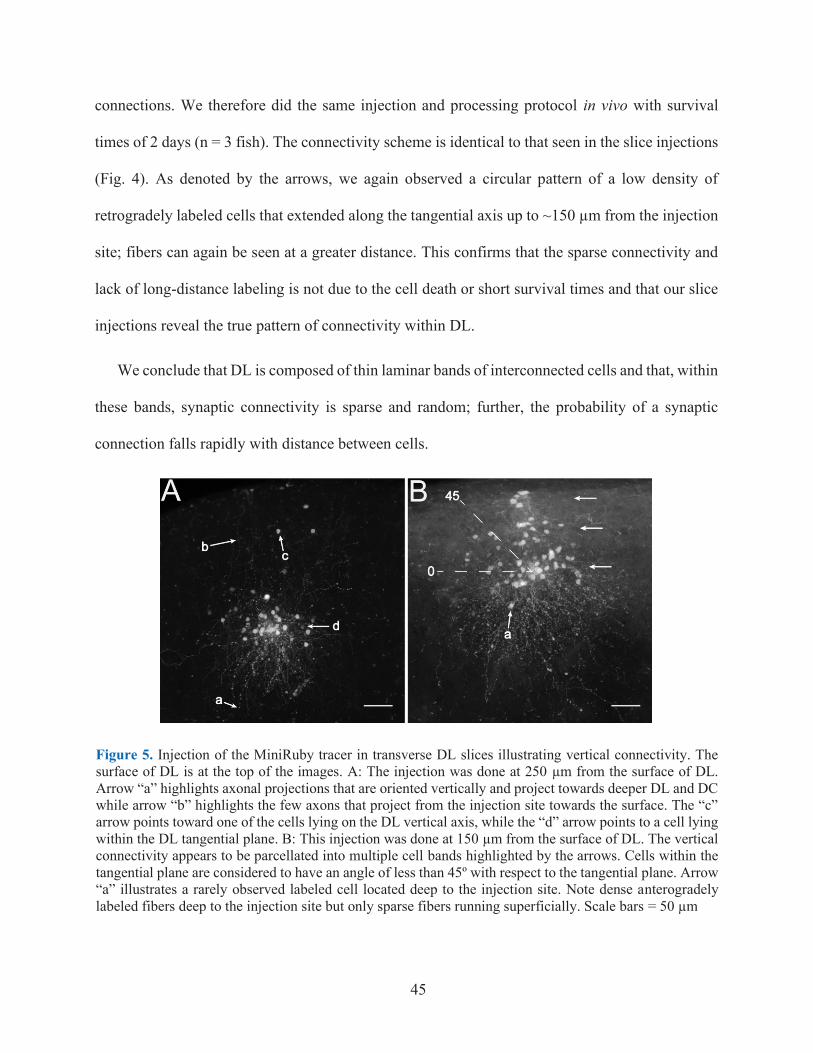
45
connections. We therefore did the same injection and processing protocol in vivo with survival
times of 2 days (n = 3 fish). The connectivity scheme is identical to that seen in the slice injections
(Fig. 4). As denoted by the arrows, we again observed a circular pattern of a low density of
retrogradely labeled cells that extended along the tangential axis up to ~150 µm from the injection
site; fibers can again be seen at a greater distance. This confirms that the sparse connectivity and
lack of long-distance labeling is not due to the cell death or short survival times and that our slice
injections reveal the true pattern of connectivity within DL.
We conclude that DL is composed of thin laminar bands of interconnected cells and that, within
these bands, synaptic connectivity is sparse and random; further, the probability of a synaptic
connection falls rapidly with distance between cells.
Figure 5. Injection of the MiniRuby tracer in transverse DL slices illustrating vertical connectivity. The
surface of DL is at the top of the images. A: The injection was done at 250 µm from the surface of DL.
Arrow “a” highlights axonal projections that are oriented vertically and project towards deeper DL and DC
while arrow “b” highlights the few axons that project from the injection site towards the surface. The “c”
arrow points toward one of the cells lying on the DL vertical axis, while the “d” arrow points to a cell lying
within the DL tangential plane. B: This injection was done at 150 µm from the surface of DL. The vertical
connectivity appears to be parcellated into multiple cell bands highlighted by the arrows. Cells within the
tangential plane are considered to have an angle of less than 45º with respect to the tangential plane. Arrow
“a” illustrates a rarely observed labeled cell located deep to the injection site. Note dense anterogradely
labeled fibers deep to the injection site but only sparse fibers running superficially. Scale bars = 50 µm

46
Transverse slices: Vertical unidirectional connectivity in DL
Injections in transverse slices also revealed retrogradely labeled cells that were spread out in a
tangential disc; the vertical (60 µm) and tangential (<150 µm) distribution of the majority of
labeled cells within this disc was similar to that described above for the slab slices. In addition, we
discovered a surprising pattern of vertical connectivity (Figs. 5–7). The vertical and tangential
connectivity are orthogonal to each other and the vertical connections decompose DL into
overlapping cryptic columns. The most remarkable aspect of the vertical (columnar) connectivity
was its asymmetry. As shown in Figure 5, the tangential connected cells are within a disc. A
separate population of labeled cells are located at greater vertical distances (more than 200 µm)
from the injection site and are mostly superficial to the injection site. In contrast, the majority of
anterogradely labeled axons and terminals project towards the deeper part of DL. While we did
observe a smaller number of retrogradely labeled cells deep to the injection site and a lesser number
of anterogradely labeled fibers running superficially, it was always clear that connectivity in the
vertical axis of DL is asymmetric and this is readily confirmed when quantified by a density map

47
(Fig. 6A,B). Cells receive more input from more
superficially located neurons. In turn, neurons in mid-
DL project predominantly to deeper neurons within
their column. This connectivity pattern was also seen
with z-axis projections in the slab slices (Fig. 7), but
was more readily analyzed in the transverse slices.
Figure 6. Estimating the width of a cryptic DL column. A:
A small (<30 µm diameter) tracer injection (MiniRuby) in
a transverse slice of DL retrogradely labels a tangential
band of cells parallel to the horizontal white dashed line.
Labeling is observed in numerous fibers deep to the
injection, a lesser number of superficial fibers and a few
superficial cells. An intensity plot of along the vertical axis
is illustrated in white on the right side of the figure in order
to show the asymmetric amount of fibers above and below
the injection site. The gray curve to the right represents the
Gaussian fit. The white arrow marks the skew of the
vertical intensity plot towards the bottom half of the figure.
A clear distinction can be seen between the anterogradely
labeled axons with a tangential versus vertical orientation.
B: Application of a Gaussian filter smoothes the deep
fibers. The white dashed line indicates where the intensity
plot was taken. Again, the right side of the image also
shows an intensity plot as well as the Gaussian fit taken
along the vertical axis. C: Gaussian curve fit (black dash
curve) of the intensity values (gray curve) used to obtain
the radial width of a column. This distance corresponds to
four standard deviations of the Gaussian curve as denoted
by the two black dotted lines. Here the standard deviation
is 47.63 µm. Scale bars = 50 µm.
We used the smallest injections to estimate a lower
bound on the diameter of the cryptic columns. We
applied a Gaussian blur (ImageJ) to the vertically
oriented fibers deep to the injection site and below the band of tangent cells and fibers (see Fig. 6).
We then fit a Gaussian to the blurred image and took two standard deviations of this Gaussian as
an estimate of the radius of the column. We estimated that the width of a column is ~104.0 ± 31.2

48
µm (n = 26). This is in accord with the maximum tangential extent of a DL lamella which was
found to extend no farther than ~150 µm from the injection site. The diameter of a column is
substantially greater than the diameter of our small injections (>100 µm versus <30 µm), strongly
implying that it is a real structural attribute of DL connectivity rather than merely the reflection of
the injection site diameter.
In about one-third of our transverse injections, we also observed bands of labeled cells which
were separated by empty gaps (Figs. 5B, 8B). In most cases, however, we observed a continuous
distribution of labeled cells extending superficially from the injection site (Fig. 8A). Even in these
cases there was some order in the retrograde labeling: injections in the deepest aspect of DL did
not yield any superficial labeled cells (i.e., near the surface of DL), e.g., a deep injection (~300
µm) resulted in a band of labeled cells extending only to the mid-DL, ~150 µm from its surface
(Fig. 8C). In contrast, injections in mid-DL did produce labeling of superficial neurons (Fig. 8A,B).
Taken together, our results demonstrate that DL is also organized into columns of ~100 µm
diameter with asymmetric connectivity such that cells project predominantly from superficial to
deep. Our results suggest that there may be additional microstructure within the DL columns;
however, our methods are not adequate to fully characterize this structure.
Figure 7. Vertical connectivity seen by rotation of a slab slice. Injection of the Alexa 488 tracer in the slab
DL slices showing the vertical connectivity. The surface of DL is at the top of the image. The injection was
done at ~200 µm from the surface of DL. Two distinct cell populations can be distinguished: a tangential
and vertical cell population. The brightness and the contrast have been lightly increased in order to show
the labeled cells. Scale bar = 50 µm.

49
It is possible that the vertically projecting cells are part of a distinct cell population different
from the tangentially projecting cells. In order to address this question, we did double injections
that should label both populations. Deep injections were made to label more superficial cells
(vertical population) and a second injection made at the level where these cells were expected to
be located (tangential population). If we saw double-labeled cells then this would imply that the
same population of cells are able to project vertically and tangentially. We did find a spatially
overlapping population of singly labeled cells in the appropriate region: dorsal to the deep injection
and lateral to the superficial injection. However, after many injection attempts (n = 47), we were
unable to see any double-labeled cells (these negative data are not shown). We therefore
hypothesize that there are at least two populations of cells in DL (aside from the small population
of GABAergic neurons; Giassi et al., 2012c): those projecting tangentially and those projecting
vertically. Despite this negative finding, it is still possible that we may have missed double-labeled
cells since the probability of connections between cells is very sparse (see below). This question
therefore remains open for future electrophysiological investigation.
Figure 8. Microstructure of the vertical connectivity in DL, transverse slices. The surface of DL is at the
top of the images. A: Injection of MiniRuby tracer at a depth of 180 µm shows a continuous distribution of
cells up to the surface of DL. B: Injection of tracer at a depth of 250 µm shows bands of labeled cells
(arrows) along the vertical axis separated by empty gaps. C: Injection of tracer at a depth of 305 µm shows

50
labeled cells in the middle of DL. No labeled cells were seen at the surface, unlike the injections illustrated
in A and B. The farthest labeled cell (arrow) was 150 µm from the surface of DL. Scale bars = 50 µm.
Quantifying connectivity in the tangential plane
In order to compute the probability of a synaptic connection between DL neurons as a function
of the distance between them, we first separated the tangential bands and vertical column cells. As
illustrated by Figure 5B, we defined the horizontal cells as those with angles of 0–45º, and the
vertical cells as those with angles of 45–90º. This analysis was done for all the “slab” injections
only (n = 67). We chose to focus our connectivity analysis using injections exclusively from the
slab slices only since the transverse slicing might have damaged fibers important for the tangential
connections. There appear to be two dominant populations of cells in DL: those lying
predominantly within a tangential band and those lying predominantly within a vertical column.
There were only a few “oblique” cells near the 45º line and eliminating these did not appreciably
change the results of our analyses (data not shown). We used only those cells considered to be in
the tangential band for our quantitative analyses. We also assumed that all retrogradely labeled
neurons projected to all the neurons within the injection site; this assumption is at least partially
justified by the facts that 1) there is a high degree of dendritic overlap of the nearby cells within
the injection site (Giassi et al., 2012b) and 2) we got the same results when using only very small
injections (~20 µm diameter). We also note that at least small deviations from this assumption will
not change our qualitative results.
In order to obtain an estimate of connectivity probability based on the raw data, we counted
the labeled cells within an annulus surrounding the injection site and then divided by the number
of cells expected over that region by our cell density estimate. First, we divided the area around
the injection site into multiple annuli. The annuli started with a radius of 10 µm and increased by
steps of 10 µm. These annuli had radii corresponding to the distance bins used to separate the

51
labeled cells. We did not include the retrogradely labeled cells that were less than 30 µm away
from the injection site for our calculations, half the width of the dendritic spread, since they might
be directly filled via their dendritic arbors, which extends 70 µm from tip to tip (Giassi et al.,
2012b). The connection probabilities were found to follow an exponential curve defined by the
following equation: f(x) = 0.057e–0.021x. From this, we extrapolated backwards and estimated that
the highest possible probability of recurrent connectivity between DL cells is ~0.06 at the shortest
distances and that the probability quickly drops as a function of distance (Fig. 9). At distances
greater than 110 µm, the connectivity probability has decreased by a factor of ~10.
Figure 9. Connection probability as a function of tangential distance from the injection site to retrogradely
labeled neurons. The probability is extracted from the tangential connections using cells contained in
annulus around the injection site where the distance bins correspond to the diameter of each annulus used.
Cells that were too close to the injection site (<30 µm) were not taken into account since they may have
been directly filled through their dendritic arborization. The maximum connectivity probability is
extrapolated to be ~0.06 and falls off exponentially with distance.
Analyzing DL connectivity with graph theory
An important question arises from the sparse connectivity seen in DL: does every neuron within
some volume of DL connect to every other neuron, i.e., is DL strongly connected? The alternative
would be that, within some DL volume, there are neurons that are not linked by any chain of
synaptic connections. To answer this question, we turned to graph theory. The unidirectional nature

52
of synaptic connections implies that DL should be considered a directed graph (Bang-Jensen and
Gutin, 2010). The random distribution of retrogradely labeled cells implies that DL should be
considered a random graph (Durrett, 2007). Although there are strong analytic results for both
undirected random graphs and directed deterministic graphs, there are, to our knowledge, no
analytic results appropriate for directed random graphs. A further difficulty is that graph theory
does not explicitly apply a metric to a network, i.e., there is no simple explicit way to model
connection probability as a function of distance (Penrose, 2003). As illustrated in Figure 10A, we
considered small directed random graphs and asked whether they are strongly connected, i.e.,
whether any graph node can connect to any other node. The illustrated graph (n = 10 “neurons”) is
strongly connected. We assume that all cells in this graph receive excitatory input from PG but
that spike threshold is reached in only five of them (as indicated). Every remaining cell (as
indicated) receives input from at least two active cells and might therefore be expected to reach
spike threshold even with weak PG input. Given the appropriate synaptic dynamics (see
Discussion), this might lead to sustained activity of all 10 cells. A full analysis to justify this
speculation would require a complete spatial model of the DL network and its cell and synaptic
dynamics. We lack this information and, instead, used a first-order approximation. We note that in
our illustration, the “neurons” are at different distances from each other and their connection
probabilities would vary accordingly. We assumed that, for this small network, we could
approximate the spatially variable connection probability by the mean connection probability over
the spatial extent of the network up to short distances from the injection center. The question then
became: how does the probability of a DL network being strongly connected vary as a function of
the diameter of a tangential lamina? It should be noted that, for undirected random graphs with N
vertices, Erdos and Renyi (1961) proved the existence of a sharp connection probability threshold

53
(cLog(N)/N, c>1) above which strong connectivity is highly probable (see Durrett, 2007 for
details). As a consequence, graphs with greater numbers of vertices require lower connection
probabilities in order to achieve strong connectivity. Using simulations (Mathematica) we found
similar results for directed random graphs although, for a given N, the probability threshold for
strong connectivity was greater than for undirected random graphs (simulations not shown). The
number of cells in a lamina increases in proportion to the square of its diameter. The mean
probability of connectivity as a function of distance was obtained by averaging over the
exponential curve in Figure 9 over varying distances from the injection site. This probability
declines only slowly with distance. We then used the Mathematica graph theory package to
estimate the likelihood that a small lamina of the DL was strongly connected, i.e., that every cell
is connected directly or indirectly to every other cell in a limited region. For example, consider the
point marked by the asterisk in Figure 10B. For any DL cell, the average probability of it receiving
an input from other neurons within a radius of 103 µm is Pconn = 0.031—this is an average of the
exponential curve (Fig. 9) between 10 µm and 103 µm. The number of cells in the 60 µm by 103
µm annulus is estimated to be 300. From these values, we generated 1,000 random directed graphs
in Mathematica and found that they were strongly connected in ~930 cases; this gave a 0.93
probability of strong laminar connectivity over distances of ~100 µm. The net result (Fig. 10B) is
that strong connectivity is only likely when the diameter of the horizontal band reaches 100 µm.
This implies that, if PG input were to activate neurons over a region with width ≥100 µm, then
those neurons would constitute a strongly connected network; the consequences that follow from
this analysis are discussed below. Interestingly, our graph theory estimate is identical to our
estimate of the diameter of a DL cryptic column (100 µm). Given the assumptions we had to make

54
in our analysis, we do not know whether this is merely coincidence or evidence of a critical feature
of DL network dynamics—a sharp spatial threshold for localized sustained activity.
There is a serious limitation of our analysis. Random graphs can be clustered: that is, if two graph
vertices are connected to a third vertex, they will be more likely to be connected to each other
(Durrett, 2007; Newman, 2010). By construction, our DL random graph model was not clustered
since the probability of neuron connectivity was binomial and independent. It may be that
clustering in the DL network can be induced by plasticity of its recurrent synaptic connections.
Clustering would greatly alter DL functional connectivity and dynamics; examining this possibility
will therefore be essential to a deeper understanding of the computations performed by the DL
recurrent network.

55
Figure 10. Directed random graph model of DL. A: An
example of a strongly connected random directed graph.
There are 10 vertices (neurons) that connect (synapse)
randomly on each other. In this case the neurons are
spread over a small area and with variable physical
distances between them. Afferent inputs from PG are
assumed to evoke EPSPs in all the neurons but it is
additionally assumed that these EPSPs exceed spike
threshold in only five (active cells) neurons. The
remaining neurons (inactive cells) all receive recurrent
excitatory input from at least two of the spiking neurons
and this summates with the PG input. We assume that this
is likely to result in the remainder of the neurons
discharging asynchronously and thereby initiating
sustained reverberatory input that outlasts the duration of
the PG input. B: Probability of strong connectivity (Prob.
St. Connectivity) as a function of the diameter of a 60-
µm-thick circular slab. The number of cells (#cells) in a
circular slab (60 µm in thickness) increases in proportion
to the square of the slab diameter. The mean probability
of connections (Pconn) decreases slowly as we average
the connection probability taken from the exponential
function illustrated in Figure 9 over increasing slab
diameter. The greater the number of cells in the network,
the lower the connection probability required for strong
connectivity (Psc). The probability of the slab network
being strongly connected therefore rises steeply with the
diameter of the slab as indicated. When the estimated
mean diameter of a cryptic column (~105 µm) is reached
(asterisk), there is a high probability (Psc = 0.93) of strong connectivity. For diameters >100 µm, the
probability of strong connectivity rapidly approaches 1. For these networks, neurons are likely to connect
to other neurons with only one (path length = 2 because there are two synaptic connections required) or two
(path length = 3) neurons intervening (mean path length, MPL = 2.6). The local tangential networks with
>300 neurons are therefore likely to be strongly connected. [Color figure can be viewed in the online issue,
which is available at wileyonlinelibrary.com.]
Discussion
Below, we summarize our most important results, discuss the comparative functional aspects
of the laminar/columnar organization of DL, discuss the implications of our results for the
controversial issue of possible homology of teleost DL and mammalian hippocampus/cortex, and,
finally, discuss the implications of our results for mnemonic functions of the pallium.

56
Babadi and Sompolinsky (2014) note that ascending sensory representations are “expansive”;
by this they simply mean that the number of neurons in the higherlevel representation is greater
than in the lower-level representation. As one example, they cite that there are 25 times more axons
leaving cat visual cortex than arriving from the lateral geniculate nucleus. This simple fact was
then used to deduce powerful although highly abstract conclusions about sensory representations.
Although not discussed by those authors, an equal but opposite effect occurs at the stage where
sensory input is transformed to motor output. Although we do not have exact ratios, it is obvious
that the number of neurons in e.g., primate motor cortex hand region, will greatly exceed the
number of motor neurons in the ventral horn (hand region) of the spinal cord. We refer to this as a
“compressive” transformation. Insofar as we know, there have been no theoretical analyses of the
consequences of compressive projections.
In our case, DL contains far more neurons (~1,000,000) than the preglomerular (PG) nuclei
providing its sensory input (PGl: ~63,000; PGm: ~79,000 neurons). The PG to DL projection is
therefore a topographically precise (Giassi et al., 2012c) expansive representation of
electrosensory and other input (Chacron et al., 2011; Giassi et al., 2012a; McGillivray et al.,
2012). In particular, the representation of the TS and TeO sensory input to in DL is expansive,
but this representation is massively compressed in the descending pathway to DC (~45,000
neurons); DC output in turn controls sensory and motor processing in its midbrain targets (Fig.
1A; Giassi et al., 2012c). The implications of this arrangement for neural computations are
further discussed below.
Our core results appear to be self-contradictory: neurons within DL are distributed in a random
fashion and their intrinsic connectivity is sparse and stochastic so that adjacent cells can project to
different separated targets. Despite this micro-scale randomness, DL connectivity is, over a larger

57
scale, well organized along two orthogonal dimensions: tangential connections form ~60 µm thick
laminae, while vertical connections form ~100 µm wide columns (Fig. 11). The tangential
connections which we will now refer to as laminar-like connections are radially symmetric and the
probability of synaptic connections drops off exponentially from an initial value of ~0.06. Our
graph theory analysis shows that strong laminar connectivity—every neuron is connected directly
or indirectly to every other neuron—will likely occur only for diameters of 100 µm or greater. This
suggests that the anatomically defined 100 µm columns may also be functional columns. The
vertical connections are asymmetric with the predominant connections running from superficial to
deep DL. We note that the putative columns are not structurally discrete, i.e., they are not like the
barrel cortex columns of the rat vibrissae sense, but continuously overlapping. Rather, we envisage
them as more similar to the visual cortex orientation columns, where a small shift in bar orientation
results in a correspondingly small shift to an overlapping column.
We can also conclude that both the laminar and vertical connections within DL are
predominantly glutamatergic (Giassi et al., 2012b), excitatory, and associated with AMPA (Maler
and Monaghan, 1991) and N-methylD-aspartate (NMDA) receptors (Maler and Monaghan, 1991;
Bottai et al., 1997; Bottai et al., 1998; Harvey-Girard et al., 2007). There are very few GABAergic
neurons within DL although, it does contain GABAergic terminals (Giassi et al., 2012b); from
Giassi et al. (2012b) we estimate that fewer than 2% of DL neurons are GABAergic. A similar
very low density of GABA/GAD expressing neurons in DL has been shown in zebrafish (Mueller
and Guo, 2009) and goldfish (Martyniuk et al., 2007); this is far lower than the 10–20% estimate
for mammalian cortex (Fitzpatrick et al., 1987; Giassi et al., 2012b; Sahara et al., 2012). It is likely
that many of the numerous GABAergic boutons in DL emanate from a feedback loop with the
subpallial entopeduncular nucleus (Mueller and Guo, 2009; Giassi et al., 2012a). We do not

58
understand the functional implications of the very different patterns of inhibitory regulation of
teleost versus mammalian pallium.
Figure 11. Schematic summary of DL circuitry. Neurons in DL are organized into orthogonal synaptically
connected networks. The L cells have predominantly laminar and symmetric projections and therefore are
contained within narrow bands—two such bands are illustrated. The probability of a synaptic connection
between two neurons in a band is low (only two are therefore illustrated in the upper band) and drop off
rapidly with distance (dashed arrow illustrates a low probability distant connection in the lower band).
There are also vertical connections in DL and we have hypothesized (but not proven) that they emanate
from a different cell type (V cells). These connections are asymmetric in that they are predominantly from
superficial to deeper cells; we assume, but have not proven, that the synaptic plexus generated by the
tangential connected cells also synapse on the vertical cells. The vertical connections define DL columns;
these are not discrete entities but, rather, overlap as illustrated by the overlapping columns (OC) cells.

59
Synaptic input from PG can activate DL neurons; we do not know whether such input has a preferential
horizontal (“a” arrow) or vertical/columnar (“b” arrow) distribution or is dispersed and random (“c” arrow).
In any case, we hypothesize that PG input will cause local reverberatory activity (bump activity) within
some DL columns. [Color figure can be viewed in the online issue, which is available at
wileyonlinelibrary.com.]
We can conclude that the laminar connections are part of a strongly connected recurrent
excitatory network, while the vertical excitatory connectivity organizes superficial to deep laminar
bands into ~100 µm wide columns. The vertically oriented axons appear to extend deep to DL
proper and appear to penetrate into DC. Although further direct physiological confirmation is
lacking, our model is consistent with previous evidence (Giassi et al., 2012a) that DL contains at
least two excitatory cell populations: one is strictly local and forms the laminar recurrent network
while the second consists of neurons that project to DC and also emit local collaterals to mainly
deeper regions of DL. The possible dynamics implied by the connectivity and transmitters/
receptors of DL are discussed below.
Remarkably, the combination of random and structured anatomical organization has recently
been reported for a structure much smaller than DL, the Drosophila mushroom body (Caron et al.,
2013; Aso et al., 2014). Like DL, the mushroom bodies are important for learning and memory
storage in Drosophila and other insects. We suspect that a combination of ordered and disordered
connectivity may be critically important for associating arbitrary but co-occurring environmental
features. However, it will take extensive and detailed experimental and computational analyses to
replace speculation with a deeper understanding of this neural architecture.
Comparative aspects of DL laminar and columnar organization
Laminar and columnar organizations are commonly associated with highly developed regions
in the brains of diverse vertebrates. This type of organization can occur in the rhombencephalon,
e.g., in the electrosensory lobe (ELL) of gymnotiform fish (Krahe and Maler, 2014), in the vagal

60
lobe of the goldfish (Morita and Finger, 1985, 1987), and in the mammalian dorsal cochlear
nucleus (Jones and Casseday, 1979; Leake and Snyder, 1989; Cant, 1992); in the midbrain, e.g.,
in the tectum (Sas and Maler, 1986; Heiligenberg and Rose, 1987; Wang et al., 2006; Feinberg and
Meister, 2014); in the mammalian cortex (Harris and Mrsic-Flogel, 2013), and in hippocampus
(Amaral and Lavenex, 2007). There are numerous common features across many of these
structures that suggest why such organization might be functionally useful. The laminar
organization segregates different cell classes and inputs and outputs to different layers: e.g., in
ELL different layers contain electrosensory afferents, feedback input, and inhibitory and principal
excitatory cells (Krahe and Maler, 2014); in cortex, each layer has its own excitatory/inhibitory
cell types as well as different inputs and outputs (Harris and Mrsic-Flogel, 2013). Some aspects of
sensory or motor functions are often mapped topographically across the layers, e.g., topographic
projection of electroreceptors onto ELL; orientation selectivity across the primary visual cortex of
cats and primates. Cells within a column process the same type of input but do so differently within
each column, e.g., ELL pyramidal cells within a column have the same receptive field input but
superficial cells would only respond to the onset of the stimuli in a nonlinear manner, while the
deeper pyramidal cells process the integrated response of the stimuli (Maler, 2009a, b). Cells in
one column of visual cortex process one orientation but perform different operations related to
movement, ocular dominance, and other parameters of visual input.
There are some important exceptions to the broad patterns described above. In the visual cortex
of rodents, the columnar organization is composed of orientation tuned cells, but these are
randomly distributed without any systematic graduated change in orientation preference (Harris
and Mrsic-Flogel, 2013). A similar situation applies in the hippocampus, where there is no
continuous mapping of spatial location onto place cell position (O’Keefe, 2007). Inferotemporal
61
cortex (primate) (Tanaka, 2003) and the entorhinal cortex (Burgalossi and Brecht, 2014) have
typical cortical characteristics, yet it is difficult to discern any systematic mapping of the features
to which their cells respond. In the case of the avian pallial auditory region (Field L) there is a
tonotopic mapping and vertical columnar connectivity but the cells do not have vertically oriented
dendrites (Wang et al., 2010).
DL appears to lack many of the defining features of other layered/columnar neural structures.
The cells in DL are morphologically homogeneous and, with large tracer injections, there is no
obvious laminar segregation of cell types or inputs/outputs (Giassi et al., 2012c; Giassi et al.,
2012b). As is the case for Field L, DL neurons have short isotropic dendrites without any vertical
orientation (Giassi et al., 2012b). The key questions are therefore whether the other defining
functional characteristics of laminar/columnar structures are also present in DL. At present, we
lack the data to answer these questions. For example, we do not know whether the axon from a
single PG cell terminates in a columnar or laminar manner (or randomly) in DL. At a more
macroscopic level, we have to first ask whether there is any topographic representation of features
across the laminar dimension of DL? And, are the same types of input features processed in some
systematically different way along the DL vertical columns? Given the near universality of laminar
and columnar computational organization, we hypothesize that PG input will respect the columnar
and laminar organization of DL and that the answer is “yes” for both questions.
Possible homology of DL to either/or hippocampus and cortex of mammals
There are two broad and divergent hypotheses on DL homologies: DL is homologous to medial
pallium (hippocampus; Northcutt, 2008; Nieuwenhuys, 2009) versus DL is homologous to dorsal
pallium (cortex; Yamamoto et al., 2007). In addition, there are “mixed” theories in which DL has
subregions that are homologous to medial and dorsal pallium (Wullimann and Mueller, 2004;

62
Yamamoto et al., 2007). We briefly summarize the supporting data for the two contrasting theories
and the implications of our data for these theories.
The hypothesis that DL is medial pallium and therefore homologous to hippocampus is based
on three lines of evidence. First, teleost telencephalon appears to be formed by an eversion or
eversion and rotation process (Yamamoto et al., 2007; Northcutt, 2008), although a more recent
study (Folgueira et al., 2012) has suggested that these ideas may need revision. Based on this
understanding of pallial development, it appeared natural to consider DL to be medial pallium.
This view was supported by a second line of evidence— lesion studies revealed that DL lesions
selectively eliminated spatial learning (Rodriguez et al., 2002); given the importance of
hippocampus to spatial learning, this reinforced the DL to hippocampus homology. On the
molecular level, the abundant expression of FoxO3 in DL, a gene mainly found in the
hippocampus, further supports the homology to the hippocampus theory (Harvey-Girard et al.,
2012). Recently, further support was provided by evidence that Prox1, a highly conserved gene
marker of avian and mammalian dentate gyrus (Gupta et al., 2012), was also highly expressed in
the rostral DL of zebrafish (Ganz et al., 2014).
The hypothesis that DL is, at least in part, homologous to dorsal pallium and therefore
mammalian cortex was first proposed by Ito and Yamamoto (2007; 2009) and based primarily on
its pattern of connectivity. For simplicity, we illustrate their core idea with respect to the visual
system (tectum) only. They noted that the canonical thalamo-cortical connectivity sequence:
tectum (visual input) → thalamus → cortex (superficial layers) → cortex (deep layers) → tectum
was paralleled in the teleost fish by: tectum (visual input) → PG → DL → DC → tectum (major
motor output in teleost fish).

63
Under this hypothesis, DL is a sensory input layer of pallium homologous (at least in part) to
the input layer(s) of cortex. DC is then homologous to the deep, output, layers of cortex.
Subsequent work supported the DC component of this argument. DC contains spiny glutamatergic
(Giassi et al., 2012b) neurons that express two gene markers of neurons in the deep layers of cortex
(FoxP2 and Otx1; Harvey-Girard et al., 2012). In addition, Ischikawa et al. (2007) provided
evidence that PG originates from the alar diencephalic ventricle and argued that, although migrated
to the lateral location, it was homologous to the dorsal thalamus.
Our results are clearly more supportive of the Ito and Yamamoto argument in that DL laminar
and columnar connectivity is clearly more similar to that of cortex than any part of the
hippocampus. But this produces uncomfortable contradictions: rostral DL expresses Prox 1, a
mammalian dentate gyrus marker; but, unlike dentate gyrus neurons, DL cells have recurrent
connections. Another possibility envisaged by Yamamoto et al. (2007) is that medial and dorsal
pallium are not entirely separated in teleost pallium and that both are contained within DL. At
present there is, in our opinion, not enough evidence from embryology and molecular markers to
choose between these alternative interpretations.
Dorsolateral pallium: Recurrent networks, bump attractors, and reverberatory activity
The projections from thalamus to cortex are vastly expansive, leading to an apparent redundant
and overlapping representation of sensory input (Barlow, 2001; Gardner-Medwin and Barlow,
2001; Babadi and Sompolinsky, 2014). These anatomical facts have led to important theoretical
ideas concerning the neural basis of perception and memory. In brief, it is thought that cortical
recurrent networks generate sparse codes for sensory features in a manner that permits similar
inputs to be discriminated (pattern separation, Barlow, 2001; Gardner-Medwin and Barlow, 2001;
Babadi and Sompolinsky, 2014). The recurrent networks can then store specific features as

64
sustained activity that outlasts stimulus presentation (working memory, Wang, 1999; Wei, 2000;
Wang, 2001). Finally, partial or degraded input can activate a complete memory of a perceptual
feature via recurrent connections—pattern completion (Wang, 2001; Rolls, 2013). In effect, this is
a more precise restatement of Hebb’s theory of “cell assemblies” and “phase sequences” (Hebb,
1949).
Recurrent neural networks (RNNs) are found in the hippocampus (CA3) and cortex but their
spatial extent is very different in these structures. In hippocampus (CA3), these networks are
spatially extensive (Amaral and Lavenex, 2007) and hypothesized to act as pattern completing
attractor networks and memory stores (Burgess, 2007). The cortical RNNs act locally and, in
sensory regions are associated with specific sensory transformations, e.g., computations on
oriented edges in local regions of the visual field. A key concept in these analyses is that of a group
of neurons that form an “attractor network”: when a subset of neurons in this group is briefly
synaptically activated (see Fig. 10A), the entire group will asynchronously discharge in a sustained
or “reverberatory” manner that outlasts the stimulating input. Localized attractor networks are
described as “bump” attractors. One essential ingredient of such bump attractors is that the
recurrent excitatory connections utilize slow NMDA receptors (Wang, 1999, 2001); this criteria is
certainly met for DL (Maler and Monaghan, 1991; Harvey-Girard et al., 2007). A second implicit
criterion is that the recurrent network is strongly connected. DL thus meets both criteria and we
propose that it constitutes a bump attractor network.
DL circuitry therefore appears most consistent with theories of pattern separation of sparse
sensory features (Barlow, 2001; Gardner-Medwin and Barlow, 2001; Babadi and Sompolinsky,
2014) and memory storage via bump attractors (Wang, 1999, 2001)— hypothesized functions of
sensory and prefrontal cortices, respectively. Its highly localized intrinsic connectivity is less

65
compatible with the global recurrent connectivity associated with pattern completion — a
hypothesized hippocampal (CA3) function (Bird and Burgess, 2008; Rolls, 2013).
DL processes sensory input from PG (Giassi et al., 2012c), likely acts as a memory store (Harvey-
Girard et al., 2010b), and may be homologous to medial and/ or dorsal pallium (see above). We
hypothesize that the DL has functional features resembling those of sensory cortex, PFC, and
hippocampus. The DL columns act as bump attractors that process sensory input and also store
memories related to that input. Furthermore, following Babadi and Sompolinsky (2014), we
hypothesize that the expansive representation of DL input reduces the overlap between bumps
representing similar types of PG input. Lastly, we hypothesize that the contractive mapping of DL
to DC is the final step (pattern completion) in the recognition and classification of sensory input.
Clearly, detailed experimental and modeling studies will be required to test these hypotheses.

66
Chapter 3: Biophysical characterization of hippocampal-like neurons
in the fish pallium (Original manuscript II)
Significance statement
To our knowledge, this is first study of the intrinsic physiology of teleost pallial (DL) neurons.
Their biophysical properties demonstrate that DL neurons are sparse coders with a dynamic spike
threshold leading us to suggest that they can transform time-stamped input into spatial location
during navigation. The concept of local attractors (bumps) that potentially move “across” local
recurrent networks has been prominent in the neuroscience theory literature. We propose that the
relatively simple and experimentally accessible DL of teleosts may be the best preparation to
examine this idea experimentally and to investigate the properties of local (excitatory) recurrent
networks whose cells are endowed with, e.g., slow spike threshold adaptation dynamics.

67
Cellular and Network Mechanisms May Generate Sparse Coding of Sequential Object Encounters in Hippocampal-Like Circuits
Anh-Tuan Trinh,1 Stephen E. Clarke,3 Erik Harvey-Girard,1 and Leonard Maler1,2
1. Department of Cellular and Molecular Medicine, University of Ottawa, Ottawa, Ontario K1H
8M5, Canada
2. Brain and Mind Institute, Center for Neural Dynamics, University of Ottawa, Ottawa, Ontario
K1H 8M5, Canada
3. Department of Bioengineering, Stanford University, Stanford, CA 94305
Received March 19, 2019; accepted July 12, 2019; First published July 19, 2019
ACKNOWLEDGMENTS
We thank William Ellis for technical support and Maria Lambadaris for her help with the
electrophysiological recordings. We also thank Jean-Claude Béïque, Richard Naud, and Timal
Kannangara for their helpful discussions and suggestions.
CONFLICT OF INTEREST
The authors declare no competing financial interest.
ROLE OF AUTHORS
Author contributions: A.-T.T., S.E.C., E.H.-G., and L.M. designed research; A.-T.T and E.H.-G.
performed research; A.-T.T. analyzed data; A.-T.T., S.E.C., and L.M. wrote the paper; S.E.C.
contributed unpublished reagents/analytic tools.
Grant sponsor: This work was supported by the Canadian Institutes of Health Research Grant
153143 and by the Natural Sciences and Engineering Research Council Grant 04336 (to L.M.).
Key words: hippocampus-like; recurrent network; sparse coding; spike threshold adaptation; time
cell; weakly electric fish
Reprint permission & Copyright
https://doi.org/10.1523/ENEURO.0108-19.2019 Copyright © 2019 Trinh et al.
This is an open-access article distributed under the terms of the Creative Commons Attribution 4.0
International license, which permits unrestricted use, distribution and reproduction in any medium
provided that the original work is properly attributed.

68
Abstract
The localization of distinct landmarks plays a crucial role in encoding new spatial memories.
In mammals, this function is performed by hippocampal neurons that sparsely encode an animal’s
location relative to surrounding objects. Similarly, the dorsolateral pallium (DL) is essential for
spatial learning in teleost fish. The DL of weakly electric gymnotiform fish receives both
electrosensory and visual input from the preglomerular nucleus (PG), which has been hypothesized
to encode the temporal sequence of electrosensory or visual landmark/food encounters. Here, we
show that DL neurons in the Apteronotid fish and in the Carassius auratus (goldfish) have a
hyperpolarized resting membrane potential (RMP) combined with a high and dynamic spike
threshold that increases following each spike. Current-evoked spikes in DL cells are followed by
a strong small-conductance calcium-activated potassium channel (SK)-mediated after-
hyperpolarizing potential (AHP). Together, these properties prevent high frequency and
continuous spiking. The resulting sparseness of discharge and dynamic threshold suggest that DL
neurons meet theoretical requirements for generating spatial memory engrams by decoding the
landmark/food encounter sequences encoded by PG neurons. Thus, DL neurons in teleost fish may
provide a promising, simple system to study the core cell and network mechanisms underlying
spatial memory.
69
Introduction
The mammalian hippocampus is required for the storage and recall of spatial memory that
presumably guides path integration and landmark based navigation (Barry and Burgess, 2014;
Hartley et al., 2014). Conventionally, sparse discharge of dentate gyrus (DG) granule cells and
CA1/CA3 pyramidal cells can encode a rodent’s location with respect to visually identified
landmarks (Barry and Burgess, 2014; Hartley et al., 2014). An emerging alternate view of
hippocampal function emphasizes its role in the encoding of temporal sequences within or across
periods of locomotion (Pastalkova et al., 2008; MacDonald et al., 2011; Kraus et al., 2013;
Eichenbaum, 2014; Modi et al., 2014; Ranganath and Hsieh, 2016). For example, hippocampal
neurons may discharge at specific times after the initiation of running and effectively tile an entire
running episode (Kraus et al., 2013). The encoding of time and location appears to be closely
connected with the responses of a subset of neurons to time spent and distance traveled (Kraus et
al., 2013; Deuker et al., 2016; Eichenbaum, 2017).
Visuospatial memory is also important for teleost fish (Rodriguez et al., 2002), and they can
learn to finely discriminate between visual inputs (Schluessel and Bleckmann, 2005; Siebeck et
al., 2009; Rischawy and Schuster, 2013; Newport et al., 2016). Unlike mammals, fish do not have
an obvious cortex or hippocampus; instead, their dorsal telencephalon (pallium) is divided into
non-layered cell groups that have specific connectivity and function (Rodriguez et al., 2002;
Northcutt, 2008; Giassi et al., 2012c; Giassi et al., 2012b). Visual input to the pallium primarily
arrives from the optic tectum and reaches the dorsolateral pallium (DL) through the thalamus-like
preglomerular nucleus (PG, Yamamoto and Ito, 2008; Giassi et al., 2012c; Wallach et al., 2018).
Lesion studies have shown that DL is essential for visual (landmark) based spatial learning and
memory (Rodriguez et al., 2002).

70
Comparisons of teleost pallium to mammalian dorsal telencephalon has been controversial, and
similarity between DL and either hippocampus or cortex have been stressed. Based on its location
(Yamamoto et al., 2007; Mueller and Wullimann, 2009), extrinsic connections (Elliott et al., 2017),
and molecular markers (Harvey-Girard et al., 2012; Ganz et al., 2014), it has been proposed that
DL is homologous to the hippocampus (in particular to DG, Elliott et al., 2017). However, unlike
the major recipients of sensory information in the hippocampal formation (i.e., DG, CA1), DL
neurons have strong local recurrent connectivity (Trinh et al., 2016). DL’s extrinsic and intrinsic
connectivity also suggests a strong resemblance to the mammalian cortex (Yamamoto et al., 2007;
Giassi et al., 2012c; Trinh et al., 2016; Elliott et al., 2017). However, DL neurons are
morphologically very different from both DG granule cells and the pyramidal cells of the
hippocampus and cortex (Giassi et al., 2012b).
A teleost subgroup, the weakly electric gymnotiform fish, can use their electrosensory system
to finely discriminate temporal (Harvey-Girard et al., 2010b) and spatial (Graff et al., 2004;
Dangelmayer et al., 2016) patterns and use electrosensory-identified landmarks to learn the spatial
location of food (Jun et al., 2016). Electrosensory input is first processed in the hindbrain
electrosensory lobe (ELL) and, via a midbrain relay, then mapped onto the tectum (Krahe and
Maler, 2014). Electrosensory and visual tectal cells then project to PG and their PG target then
projects exclusively to DL (Giassi et al., 2012c). Two recent studies have shown that DL cells can
process visual and electrosensory inputs. In goldfish, Vinepinsky et al. (2018) have described DL
cells responsive to boundaries (visual input) as well as speed and direction of self-motion. In a
gymnotiform fish, neurons within a major target of DL (dorsal pallium, DD) have been shown to
discharge to the electrosensory signals generated when the fish moves near “landmarks” (Fotowat
et al., 2019).

71
Recently, a subset of electrosensory motion PG neurons have been identified that can encode
the time interval between object encounters (Wallach et al., 2018). Wallach et al., hypothesize that
the output of these “time stamp” neurons is used to estimate the distance between the objects
encountered by the fish, thereby supporting the observed electrosense-dependent spatial learning
(Jun et al., 2016). Given the similar anatomic and functional organization of visual and
electrosensory motion pathways, we hypothesize that the transformation of electrosensory motion
signals to a spatial map are processed in DL. Here, we studied the biophysical properties of DL
neurons in vitro to determine if their intrinsic properties are compatible with their putative role in
converting temporal input from PG (i.e., time between object encounters) to a spatial map (Wallach
et al., 2018).
Materials and methods
For the following experiments, we used two closely related Apteronotid fish of either sex
(Apteronotus leptorhynchus and Apteronotus albifrons), a suborder of the gymnotiform family, as
well as Carassius auratus (goldfish) of either sex. The brains of A. leptorhynchus and A. albifrons
cannot be readily distinguished; these species have been used interchangeably in previous anatomic
studies (Carr et al., 1982) and the processing of electrosensory input appears to be nearly identical
in these species (Martinez et al., 2016). Goldfish were included in this study for three reasons.
First, we found that Apteronotus DL cells were challenging to maintain in slice preparation,
whereas goldfish DL cells were more robust, yielding higher success rates on our lengthier
protocols involving pharmacological manipulations. Second, we wanted to check how our results
generalized to non-electrosensory teleosts, given the very general mechanisms of sparse neural
coding proposed in this article. Last, the critical behavioral experiments on the essential role of DL

72
in spatial memory were done in goldfish (Rodriguez et al., 2002), setting a precedent in the
literature; further, the first in vivo DL recordings have also been conducted in goldfish (Vinepinsky
et al., 2018). As demonstrated in the results, our conclusions apply equally well to each of these
species and are therefore directly relevant to spatial learning across a broad range of teleost fish.
Before use, the Apteronotus fish were kept in heated aquariums at 28°C, while goldfish were
kept in aquariums at 22°C (room temperature). All procedures were approved by the University of
Ottawa Animal Care Committee and follow the guidelines issued by the Society for Neuroscience.
Slice preparation
Before the dissection, adult male and female fishes were anesthetized in oxygenated water
containing 0.2% 3-aminobenzoic ethyl ester (tricaine methanesulfonate, Aqua Life, Syndel
Laboratories). As the skull was being removed, ice cold oxygenated (95% O2, 5% CO2) artificial
CSF (ACSF; 130 mM NaCl, 24 mM NaHCO3, 10 mM glucose, 2.5 mM KCl, 1.75 mM KH2HPO4,
1.5 mM CaCl2, 1.5 mM MgSO4, and 295 mOsm, pH 7.4), containing 1 mM of kynurenic acid
(Millipore Sigma), was dripped onto the fish’s brain. The brain was then carefully removed and
submerged in a Petri dish containing ice-cold ACSF with kynurenic acid. Once the brain was
removed, it was placed in an ice-cold cubic mold, to which oxygenated ACSF mixed with 2.5%
low-melting agarose (Millipore Sigma) was added. After the agarose has solidified, an initial cut
was performed to separate the telencephalon from the rest of the brain. Subsequently, 300-µm-
thick transverse brain slices of the telencephalon were obtained using a vibratome. For goldfish
dissections, a slightly different cutting ACSF was used: 108 mM NaCl, 24 mM NaHCO3, 10 mM
glucose, 2.5 mM KCl, 1.25 mM KH2HPO4, 1.5 mM CaCl2, 1.5 mM MgSO4, and 2 mM HEPES,
260 mOsm (adapted from Palmer, 2006). Furthermore, the thick optic nerves underneath the brain
73
had to be severed with micro scissors before the brain was removed and placed in a Petri dish
containing ice-cold ACSF. The rest of the dissection was done in the same manner as in
Apteronotus (see Trinh et al., 2016). Brain slices containing the dorsolateral telencephalon
(DL) were then transferred into a continuously oxygenated slice incubation chamber containing
ACSF where they were left to rest for 30–60 min.
In vitro recordings
After the incubation period, brain slices containing DL were transferred to the recording
chamber where oxygenated ACSF was constantly perfused at a flow rate of 3 ml/min. Recordings
were performed at room temperature (23–24°C). We used fire-polished borosilicate glass
micropipettes (Sutter Instruments) with resistances ranging between 8 and 14 MΩ. The
intracellular solution contained the following: 130 mM K-gluconate, 10 mM KCl, 10 mM HEPES,
4 mM NaCl, 4 mM Mg-ATP, 10 mM phosphocreatine, and 0.3 mM Na-GTP, with an osmolality
of 295 mOsm, and a pH of 7.2 for weakly electric fish recordings. A silver wire plated with silver
chloride was used as a ground. For goldfish experiments, recordings were done in the goldfish
ACSF as described above and a slightly different intracellular solutions was used: 110 mM K-
gluconate, 10 mM KCl, 18 mM HEPES, 4 mM Mg-ATP, 10 mM phosphocreatine, and 0.3 mM
Na-GTP, 265 mOsm, pH 7.2. To visualize the neurons, slices were imaged under differential
interference contrast (DIC) optics using a CMOS infrared camera (Scientifica) directly connected
to the rig computer (Fig. 1). The recording signals were amplified using a Multiclamp 700B
(Molecular Devices), while the signal was filtered at 3 kHz and digitized using a Digidata 1550
(Molecular Devices). The whole-cell recording data were acquired using the PClamp 10.6 software
(Molecular Devices, RRID: SCR_011323). All recordings were performed in current-clamp mode.
Only cells that required a minimal holding current less than –50 pA were included in the study,
74
allowing to stabilize the cell near the average resting membrane potential (RMP; ~ –75 mV; Fig.
2E). The maximal recording time after the dissection was 4–5 h. Once the whole-cell configuration
was obtained, the RMP was recorded for 10 s, and the cells were injected with current steps, which
typically range from 500 to 1000 ms and from –60 to 60 pA, except where otherwise noted. For
our ramp current protocol, we injected two different ramp currents at different inter-stimulus time
intervals ranging from 50 to 1000 ms. Although both ramp stimuli have the same slope, the first
ramp current was always two-fold stronger than the second ramp since the first ramp current had
to evoke multiple action potentials while the second one only had to evoke one action potential.
As such, the magnitude of the second current injection had to be adjusted for each cell since the
rheobase for each cell is different and the magnitude of the first ramp was then adjusted according
to the second ramp. Healthy cells were usually held for 30–60 min.
Pharmacology
A subset of DL cells exhibited membrane “noise.” We bath applied the non-selective
antagonist, kynurenic acid (10 mM; Millipore Sigma), to block ionotropic glutamatergic
transmission to determine if this noise was due to synaptic input to DL cells.
To test for the presence of fast and persistent sodium channels in DL neurons (Berman et al.,
2001), we first patched the cell and injected a standard 500-ms current step before applying 20 M
tetrodotoxin (TTX; Abcam) locally near the recording site by pressure injection. To further
investigate the presence of a persistent sodium channel, we also applied 5 mM lidocaine N-ethyl
bromide (QX-314; Millipore Sigma) via the intracellular recording solution to block sodium
(Salazar et al., 1996) and other channels (e.g., certain K+ channels and Ca2+ channels, see Results;
(Alreja and Aghajanian, 1994; Perkins and Wong, 1995; Talbot and Sayer, 1996).

75
Calcium-activated potassium channels SK1/2 are both expressed in DL (Ellis et al., 2008). We
used our standard current step protocol to evoke spikes in patched DL cells and bath applied an SK
channel blocker 30 µM 6,12,19,20,25,26-hexahydro-5,27:13,18:21,24-trietheno-11,7-metheno-
7H-dibenzo [b,n] [1,5,12,16] tetraazacyclotricosine-5,13-diium dibromide (UCL; Tocris, Bio-
Techne). We also locally applied 1 mM 1-ethyl-2-benzimidazolinone (EBIO; Abcam), a SK
channel agonist near the brain slice by pressure injection. Finally, we patched neurons using a
slightly altered internal solution that contained 10 mM BAPTA (Millipore Sigma) to chelate
intracellular calcium. The osmolarity of this intracellular solution was readjusted to 295 mOsm.
RT-PCR
G-protein-coupled inwardly-rectifying potassium channels (GIRK) 1–4 mRNA sequences
were identified from A. leptorhynchus brain transcriptome data (Salisbury et al., 2015). Two
degenerate PCR primers were designed to bind all GIRK isoform sequences (forward:
CTGGTGGACCTSAAGTGGMG; reverse: TTCTTGGGCTGNGNAGATCTT). Five A.
leptorhynchus fish were anesthetized with tricaine methanesulfonate (Aqua Life, Syndel
Laboratories) and then sacrificed by cervical dislocation while being fed oxygenated water
containing the anesthetic. Different regions of the brain (DL, tectum/torus, subpallium, cerebellum,
ELL, hindbrain) were dissected in ice-cold ACSF, collected and preserved on dry ice. All tissues
were weighed, and homogenized in Trizol to purify total RNA (Millipore Sigma). First-strand
cDNAs were then generated by using the RevertAid H Minus First Strand cDNA Synthesis kit
(Fermentas). Degenerate PCR was performed using the DreamTaq, according to the manufacturer
recommendations (Thermo Fisher Scientific), with the primers mentioned above. On an agarose
gel, the amplicon expected bands were 344 bp.

76
Data analysis
All the recording data were first visualized in Clampfit (Molecular Devices) before being
transferred into MATLAB (MathWorks, RRID: SCR_001622) for subsequent analysis with
custom scripts. To reduce the likelihood of analyzing unhealthy cell responses, only cells which
produced spikes that cross a data-driven threshold of –5 mV were included in the analysis. Cells
that showed significant membrane noise, i.e., a variance 0.5 mV2, were used to construct Figures
2 and 3 but were excluded from any additional analysis. For the analysis of the RMP (Fig. 2), only
cells that did not require a holding current to stabilize were included in this analysis. For the
analysis of the average RMP (and variance) in Figure 3, a total of 2 min of recording (binned into
10-s sweeps) were analyzed for each cell before and after the addition of the synaptic blocker (for
a total of 4 min per cell). If the recording trace contained any spontaneous action potentials, the
action potentials were replaced with the membrane potential recorded in the prior 100 ms. The
membrane time constant was measured by fitting an exponential function to the neuron’s recovery
to equilibrium following injection of a negative step current. The spike amplitude was measured
by two methods: first, as the difference between the spike height and the spike threshold and,
second, from the difference between the spike height and the RMP. To estimate the spike threshold,
we used the method of Azouz and Gray (2000) which defined the spike threshold as the voltage
corresponding to an empirically defined fraction (0.033) of the peak of the first derivative. This
first derivative method was later shown to be slightly better than the second derivative method
(Sekerli et al., 2004) previously used for hindbrain electrosensory neurons (Chacron et al., 2007).
The threshold for the broad Ca2+ spikes were determined visually in Clampfit since the rate of
change of the Ca2+ spike was too slow to be visualize with either the first or second derivative of
the membrane potential. The spike width was calculated by measuring the half-width at half-

77
maximum. The voltage, as a function of injected current (I-V curves), was obtained in Clampfit
using sub-threshold traces and averaged to reduce the variability across cells caused by the holding
current. The input resistance was obtained by calculating the average slope of the I-V curve across
all cells. The after-hyperpolarizing potential (AHP) amplitude was measured as the difference
between the spike threshold and the minimum value of the AHPs. If the recording trace contained
a burst or spike doublet, then the AHP would be measured on the following spike, since a doublet
would typically induce an especially large AHP. The cell’s average firing rate was calculated as
the number of spikes divided by the duration of the stimulus. The δ spike height was calculated as
the difference in spike height between the nth spike and the first spike of an evoked spike train.
The interspike interval (ISI) was measured as the time between the first two spikes of the spike
train induced by a current step injection, while the δ time was calculated as the difference between
the time of the first AHP and the time of the nth AHP. The δ AHP was obtained by subtracting the
first spike’s AHP amplitude from the second spike’s AHP amplitude. The δ threshold was obtained
in a similar fashion. All error bars were determined using the standard error of the mean. Wherever
applicable, the statistical significance was determined using either one-way ANOVA, two-way
ANOVA, one sample t test, two-sample t test or the paired t test, where p < 0.05 is considered
significant.
Inactivating exponential integrate and fire model (iEIF)
To illustrate the putative role of slow sodium channel inactivation on the observed and variable
spike threshold in DL cells, we sought a minimal neuron model that incorporates an abstraction of
sodium channel dynamics. The inactivating exponential integrate and fire neuron (Eq. 1;
Platkiewicz and Brette, 2011) provides a distilled representation of sodium channel activation via
an exponential amplification of the membrane voltage (V), which is attenuated by fast and slow

78
inactivation variables (hf and hs). These sodium channel inactivation terms further affect the
dynamic threshold for spike generation, θ, whose initial value VT reflects no inactivation at the
RMP (Eqs. 2, 3; hf = hs = 1; Platkiewicz and Brette, 2010). Although the exponential approximation
does not realistically capture the full action potential wave form, which spans a large voltage range,
it is valid for voltages near spike initiation. Importantly, this approximation permits the differential
equation for the variable spike threshold, θ, to be simply expressed by sodium channel properties
described in Equations 2, 3 (Platkiewicz and Brette, 2010, 2011).
CdV
dt = g
Lhfhse
V-Vt
ka +gL(EL-V)+I for V < Vt (1)
𝜃 = Vt − 𝑘𝑎 log(hfhs) (2)
Vt = Va − 𝑘𝑎 log(𝑔𝑁𝑎
𝑔𝐿
𝐸𝑁𝑎−𝑉𝑎
𝑘𝑎) (3)
As in the work of Platkiewicz and Brette (2011), the membrane time constant, τ = C/gL = 5 ms,
was introduced for our simulations. Given that the specific membrane capacitance is ∼ 0.9 µF/cm2
for practically all neuron types (Gentet et al., 2000), the leak conductance is constrained to be gL =
0.18 mS/cm2 and the input current, I = 3.8 nA, is scaled by the associated membrane resistance
(5.56 MΩ). The leak current reversal potential was set to EL = –55 (Platkiewicz and Brette, 2011).
When the membrane voltage reaches θ at time t, a spike is generated and V(t +) is reset to the RMP,
Vr = –70 mV. The average threshold for the first spike in DL neurons was –42.96 ± 0.5 mV (N =
42 spikes). To obtain an approximate match between VT and this value, we kept the sodium
activation slope, ka = 4 mV, and reversal potential, Va = –38.6 mV, at the empirically justified
values used by Platkiewicz and Brette (2011). We then set the sodium conductance to gNa = 0.036

79
mS/cm2 to achieve a value of gNa/gL = 0.2, near the range of Platkiewicz and Brette (2011). We
assume this slightly lower value in our model is a reflection of low sodium channel density.
Consistent with this assumption, DL neuron axons are very thin and possibly unmyelinated (Giassi
et al., 2012b) suggesting that they have a low sodium channel density, which may partly explains
the high DL neuron threshold. The sodium channel reversal potential was kept at a standard ENa =
50 mV. When substituted into Equation 3, the above parameter set yielded an initial threshold of
VT = –44.6 mV (see below in the Dynamic AHP and spike threshold section) and gave particularly
close agreement with the Apteronotus data (–45.3 ± 0.2 mV; Fig. 4E).
Drawing on the Hodgkin–Huxley formalism, the inactivation variables, hf and hs, evolve according
to Equations 4, 5, where h∞ is a Boltzmann equation with inactivation parameters Vi = –63 mV and
ki = 6 mV [6]:
𝜏𝑓𝑑ℎ𝑓
𝑑𝑡= ℎ∞(𝑉) − ℎ𝑓 (4)
𝜏𝑓𝑑ℎ𝑠
𝑑𝑡= ℎ∞(𝑉) − ℎ𝑠 (5)
ℎ∞(𝑉) = (1 + e𝑉−𝑉𝑖
𝑘𝑖 )−1 (6)
The parameters τf (fast inactivation timescale) and τs (slow inactivation timescale) are of
particular interest to the model and to our results. To determine τf, the average time between a short
burst of two DL spikes (doublet) was measured at the beginning of the recorded voltage trace,
yielding 15.38 ± 0.6 ms (N = 144 doublets). Selecting τf = 15 ms, we note that the model generates
spikes at a frequency of 64.7 ± 7.8 Hz, consistent with the data mean. We assumed that a slow

80
timescale of inactivation would lead to an increase of spike threshold with a correspondingly long
timescale for recovery (see Discussion). To select τs, we therefore noted that the threshold for DL
cell spiking remains significantly increased for at least 300 ms when stimulated; therefore, τs is
likely on the order of 102 ms. A more direct estimate gave a mean decay time constant (τexp) of
∼640 ms for the slow recovery (see ramp protocol results below). Therefore, we selected τs = 500
ms, which is a conservative value, given slow inactivation is typically >1 s and longer timescales
would only further strengthen our hypotheses (Itskov et al., 2011).
Note that we omitted Ca2+ currents and the resulting SK channel mediated AHP since its
duration is less than the typical ISI of DL neurons. When simulating the model, subthreshold
Gaussian noise, N(0,1), was added to Equation 1 and scaled a factor σ = 0.5. The stochastic forward
Euler method was used as the numerical solver.
Code accessibility
The MATLAB code used in this paper is available as Extended Data 1 and at the University of
Ottawa’s Institutional repository with the corresponding doi number: 10.20381/ruor39306. A
Windows 10 computer was used to simulate the results from the iEIF model.
All panel figures were initially compiled in OriginPro 9.0 (OriginLabs, RRID: SCR_015636)
and the final figureswere assembled in Adobe Illustrator CS6 (Adobe Systems, RRID:
SCR_010279).

81
Figure 1. Anatomy of the A. leptorhynchus telencephalon. A, A transverse section through the Apteronotus
telencephalon indicating the major subdivisions of pallium and subpallium (SP); this section was obtained
from a standard series of cresyl violet-stained sections (Elliott et al., 2017). Midbrain sensory inputs
entering the pallium from PG terminates in the DL. These inputs are processed within the DL recurrent
network (Trinh et al., 2016). DL projects to the core dorsocentral pallium (DCc) which, in turn, projects to
midbrain sensory regions. DL, ventral subdivision (DLv) is located ventral to DL and distinguished by its
olfactory bulb input. The dorsal-dorsal pallium (DD) has reciprocal connections with DL (Elliott et al.,
2017). Scale bar: 500 µm. B, A higher magnification of the cells in DL illustrates an apparent random
distribution and its highly organized intrinsic laminar and columnar circuitry is not evident (Trinh et al.,
2016). The neurons in DL have homogenous morphology and are roughly 10 µm in diameter (Giassi et al.,
2012b). Scale bar: 50 µm. C, An infrared image of a DL neuron undergoing a whole-cell patch recording.
The shadow to the left illustrates the patch pipette, while the white arrow highlights the patched cell. Scale
bar: 20 µm. DCs, dorsocentral pallium, shell; DM, dorsomedial pallium.
Results
We performed whole-cell patch recordings from Apteronotus DL neurons in acute slices from
the rostral- to mid-telencephalon (Fig. 1A). Cells within DL, imaged under infrared illumination
with DIC optics, had a shape and size consistent with those identified in Nissl-stained sections
(Fig. 1B,C). Although we cannot differentiate between excitatory and inhibitory cells, we assume
that the neurons whose biophysical properties we characterize are almost certainly those of
excitatory (glutamatergic) DL neurons since they vastly predominate over the rare inhibitory
(GABAergic) cells (Giassi et al., 2012b). We also recorded neurons from the dorsal portion of C.
auratus (goldfish) DL, while avoiding the ventral DL as it receives olfactory bulb input (Northcutt,

82
2006). The physiology of neurons recorded in the goldfish DL was not distinguishable from those
of Apteronotus (see below).
Noisy versus quiet cells
After attaining the whole-cell patch configuration, we first examined the RMP (no holding
current), and observed two distinct electrophysiological profiles. The majority of the DL cells
(29/35 cells in Apteronotus and 7/11 cells in goldfish) were quiet, that is, they had minimal
spontaneous membrane fluctuations, as shown by the example recording traces from three different
Apteronotus DL cells with different RMPs (Fig. 2A). A smaller number of DL neurons were noisy,
showing considerable spontaneous membrane fluctuations over approximately the same range of
RMPs as the quiet cells (Fig. 2B). A histogram estimating the distribution of RMP variance (Fig.
2C) suggests that, in both Apteronotus and goldfish DL, there were distinct populations of quiet
(variance <0.5 mV2) and noisy cells (variance >0.5 mV2).

83
Figure 2. RMP of DL neurons. A, Three example RMP traces taken from three different quiet neurons
illustrate the membrane potential at which these cells would normally stabilize at naturally (i.e., no holding
current was applied). The RMP at the start of the recording is shown above each trace. B, Three example
RMP traces taken from three different noisy neurons in which no holding current was applied. In contrast
to the quiet cells, these cells exhibited strong membrane fluctuations even when they had stabilized at a
hyperpolarized potential. C, A histogram of the RMP variance for Apteronotus (gray) and goldfish (black)
DL neurons showing that most neurons were of the quiet type where n is the number of individual 10-s
recording traces that were recorded from all cells (Apteronotus, N = 29 cells; goldfish, N = 7 cells; total n
= 85 recordings). D, A histogram of the natural RMPs in both the Apteronotus and in the goldfish
illustrating that the average RMP of DL neurons is around –77 mV in Apteronotus and around –73 mV in
goldfish (Apteronotus, N = 35 cells; goldfish, N = 11 cells; total n = 71 recordings). E, A noisy DL neuron’s
response to the injection of ±37.5-pA current steps in Apteronotus, illustrating that the membrane
fluctuations are invariant to the membrane potential of the cell. F, A scatter plot of the variance and
membrane potential, including all recordings (black dots) that had a variance value above 0.5 mV2
(Apteronotus, N = 6 cells; goldfish; N = 4 cells; total n = 20 recordings).

84
Noisy cells
The noisy electrophysiological feature has previously been observed in pyramidal cells in the
Apteronotus hindbrain ELL and has been attributed to the stochastic opening of voltage-gated ion
channels, an effect which becomes stronger as the membrane potential increases toward threshold
(Marcoux et al., 2016). We therefore wondered whether noisy DL cells shared these features. DL
neurons displayed an in vitro RMPs that were relatively more hyperpolarized (Apteronotus: –70 to
–84 mV; goldfish: –66 to –78 mV; Fig 2D), compared to the ELL pyramidal cells (–67.8 ± 5.7
mV, Berman and Maler, 1998a) and neither subthreshold depolarizing, nor hyperpolarizing current
steps altered the noise fluctuations of Apteronotus DL cells (N = 3 noisy cells; Fig. 2E).
Additionally, we found that a more depolarized RMP of these noisy cells (Apteronotus, N = 6 cells;
goldfish, N = 4 cells) was not associated with an increase in noise variance (Fig. 2F).
In some noisy cells, spontaneous membrane fluctuations could summate to cause a more
sustained depolarization (Fig. 3A). The summating fluctuations were usually between 10 and 20
mV in amplitude and often induced spontaneous action potentials as the membrane potential
crossed the spike threshold. The duration of these spontaneous events was estimated to be 425.5 ±
42.4 ms (N = 4 cells), and could reach as long as 800 ms in instances where spontaneous bursting
occurred (Fig. 3B). We hypothesize that these events are caused by the summation of multiple
postsynaptic potentials, as highlighted by the arrows in Figure 3C.
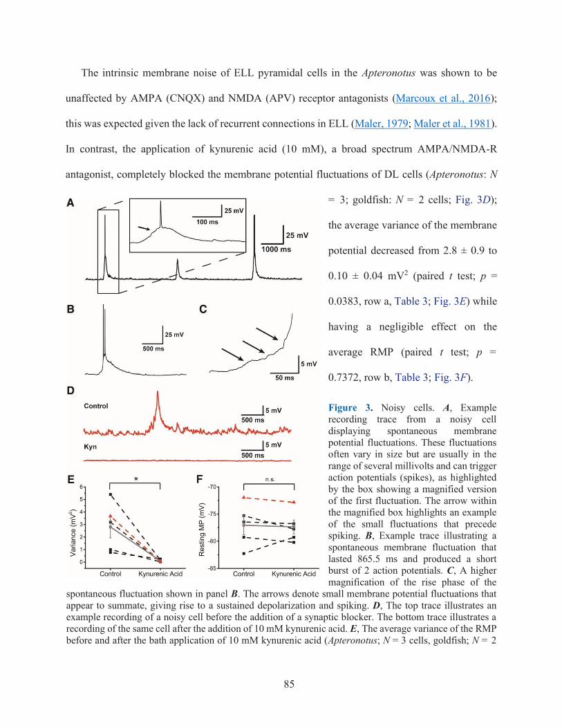
85
The intrinsic membrane noise of ELL pyramidal cells in the Apteronotus was shown to be
unaffected by AMPA (CNQX) and NMDA (APV) receptor antagonists (Marcoux et al., 2016);
this was expected given the lack of recurrent connections in ELL (Maler, 1979; Maler et al., 1981).
In contrast, the application of kynurenic acid (10 mM), a broad spectrum AMPA/NMDA-R
antagonist, completely blocked the membrane potential fluctuations of DL cells (Apteronotus: N
= 3; goldfish: N = 2 cells; Fig. 3D);
the average variance of the membrane
potential decreased from 2.8 ± 0.9 to
0.10 ± 0.04 mV2 (paired t test; p =
0.0383, row a, Table 3; Fig. 3E) while
having a negligible effect on the
average RMP (paired t test; p =
0.7372, row b, Table 3; Fig. 3F).
Figure 3. Noisy cells. A, Example
recording trace from a noisy cell
displaying spontaneous membrane
potential fluctuations. These fluctuations
often vary in size but are usually in the
range of several millivolts and can trigger
action potentials (spikes), as highlighted
by the box showing a magnified version
of the first fluctuation. The arrow within
the magnified box highlights an example
of the small fluctuations that precede
spiking. B, Example trace illustrating a
spontaneous membrane fluctuation that
lasted 865.5 ms and produced a short
burst of 2 action potentials. C, A higher
magnification of the rise phase of the
spontaneous fluctuation shown in panel B. The arrows denote small membrane potential fluctuations that
appear to summate, giving rise to a sustained depolarization and spiking. D, The top trace illustrates an
example recording of a noisy cell before the addition of a synaptic blocker. The bottom trace illustrates a
recording of the same cell after the addition of 10 mM kynurenic acid. E, The average variance of the RMP
before and after the bath application of 10 mM kynurenic acid (Apteronotus; N = 3 cells, goldfish; N = 2

86
cells). Each black square represents a cell from either fish and the gray square represents the mean variance.
The red triangles depict the average variance of the cell shown in D. Of particular note, the wide range of
variances all decreased to a similar value after the application of the synaptic blocker. F, Same as in E
except this graph depicts the RMP instead (Apteronotus; N = 3 cells, goldfish; N = 2 cells). Unlike the
variance, the RMP was unaffected by the bath application of the synaptic blocker. *p < 0.05. n.s, not
significant.
Based on these observations, we suggest that the DL cell membrane noise, are not generated
by intrinsic conductances, but are instead primarily due to synaptic bombardment from neighboring
cells within the DL recurrent network (Trinh et al., 2016). In our slice preparation, DL is
disconnected from all extrinsic input (Giassi et al., 2012c; Giassi et al., 2012a). As such, the
synaptic noise we observed in a subset of DL neurons provides evidence that the activity of the DL
recurrent network alone can drive weak spiking activity. We do not currently know why only some
neurons show pronounced membrane potential fluctuations.
Quiet cells
RMP, spike threshold, and spike discharge patterns
The RMPs of quiet Apteronotus DL cells were approximately Gaussian distributed with a mean
of –76.7 ± 0.3 mV (N = 29 cells; Fig. 2D), similar to that of goldfish (–74.4 ± 0.7 mV, N = 7 cells).
Using the hyperpolarized responses to negative current steps in the Apteronotus, we calculated an
average membrane time constant of 10.28 ± 0.24 ms for these neurons.
We next injected positive current steps to generate spiking. An example recording is shown in
Figure 4Ai, illustrating a typical DL neuron response in Apteronotus. The same response and
spiking pattern was found in all cells regardless of their location within the Apteronotus DL region
and was also observed in the goldfish DL (Fig. 4B). DL neurons exhibited very pronounced
rectification: the membrane potential deflection in response to depolarizing current injections was
far stronger than for hyperpolarizing currents of the same magnitude (Fig. 4Aii). This asymmetry
is quantified below. In addition, we never observed any “sags” in the response of DL neurons to
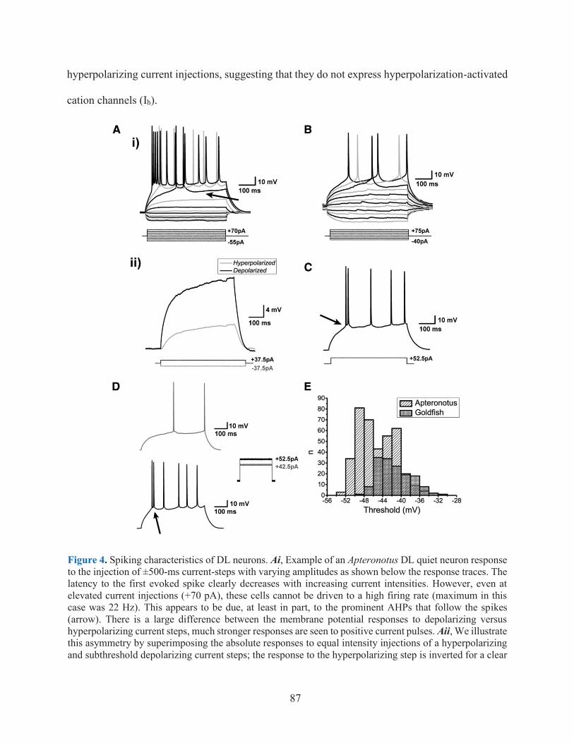
87
hyperpolarizing current injections, suggesting that they do not express hyperpolarization-activated
cation channels (Ih).
Figure 4. Spiking characteristics of DL neurons. Ai, Example of an Apteronotus DL quiet neuron response
to the injection of ±500-ms current-steps with varying amplitudes as shown below the response traces. The
latency to the first evoked spike clearly decreases with increasing current intensities. However, even at
elevated current injections (+70 pA), these cells cannot be driven to a high firing rate (maximum in this
case was 22 Hz). This appears to be due, at least in part, to the prominent AHPs that follow the spikes
(arrow). There is a large difference between the membrane potential responses to depolarizing versus
hyperpolarizing current steps, much stronger responses are seen to positive current pulses. Aii, We illustrate
this asymmetry by superimposing the absolute responses to equal intensity injections of a hyperpolarizing
and subthreshold depolarizing current steps; the response to the hyperpolarizing step is inverted for a clear

88
comparison. DL neuron recordings in goldfish also yielded a similar asymmetry and spiking patterns (data
not shown; but see panel B). B, Example of a goldfish dorsal DL (DLd) neuron response to a standard 500-
ms current step injection; the region chosen for these recordings receive inputs from PG similar to the DL
neurons in Apteronotus. The responses of these cells were very similar to those of Apteronotus DL neurons.
C, Example recording of a DL neuron in response to a single current step injection. The arrow highlights
the location of the threshold for these neurons (panel E). Di, A single spike is evoked for currents near spike
threshold. Dii, After current injections induce depolarizations exceeding the spike threshold, DL neurons
emit a short doublet or triplet burst of spikes at a shorter latency (arrow, Apteronotus recording; similar
behavior was seen in goldfish DL neurons). Note that spike amplitude drops slightly but progressively in
the C, D traces. E, Histogram of the average threshold of the first current-evoked spike in DL neurons. The
spike threshold, which was found using the first derivative of the membrane potential, was ∼ –45 mV in
Apteronotus and ∼ –42 mV in goldfish. The total number of spikes across all cells used for these estimates
was n = 380 in Apteronotus and n = 154 in goldfish.
DL neurons discharge very few action potentials (Fig. 4A,B) and the average injected current
necessary to reach spike threshold (rheobase) was 38.17 ± 2.52 pA (N = 15 cells). Strong current
injections (70 pA) only resulted in average firing rates of 15.3 ± 2.4 Hz (N = 15 cells). We defined
the spike threshold as the voltage corresponding to a pre-determined fraction of the maximal peak
of the first derivative of the membrane potential response to current steps (Azouz and Gray, 2000;
see Materials and Methods). Strong current injection in Apteronotus DL neurons typically results
in an initial high-frequency burst of two or three spikes, followed by an irregular series of spikes
separated by AHPs of varying amplitude and duration (Fig. 4C,D); the same pattern was also
observed in the DL of goldfish (Figs. 4B, 5A). In Apteronotus, the threshold for the first spike is
distributed with a mean of –45.3 ± 0.2 mV (N = 22 cells) and has a high degree of overlap with
the observed spike threshold for goldfish DL cells (mean: –41.5 ± 0.3 mV, N = 14 cells; Fig. 4E).
We measured the mean spike peak amplitude from both the membrane potential at spike threshold
(Apteronotus: 66.2 ± 1.0 mV, N = 22 cells; goldfish: 50.8 ± 1.0 mV, N = 14 cells) and from the
RMP (Apteronotus, 95.9 ± 0.5 mV; goldfish, 90.6 ± 0.5 mV). Lastly, we also measured the spike
half-width at half-maximum (Apteronotus: 2.3 ± 0.1 ms; goldfish: 3.7 ± 0.3 ms).
In summary, the core biophysical properties of DL cells receiving PG input in Apteronotus and
goldfish (dorsal DL, non-olfactory; Northcutt, 2006; Yamamoto and Ito, 2008) were similar, DL

89
neurons have a hyperpolarized RMP and a high spike threshold and spike only sparsely in response
to even strong current injection.
Asymmetric input resistance
A striking property of Apteronotus and goldfish DL cells is an asymmetry in their response to
hyperpolarizing versus depolarizing current steps (Fig. 5Ai). In ELL pyramidal cells, an equivalent,
though far smaller asymmetry is caused by a persistent Na+ channel (Turner et al., 1994) that
amplifies excitatory synaptic input (Berman et al., 2001). We tested this possibility by blocking
the sodium channels of DL neurons with a local application of 20 µM TTX (control: N = 18 cells,
TTX: N = 6 cells). As expected, spike discharge at the previous threshold (~ –45 mV) was
completely blocked by TTX (Fig. 5Aii); the small high threshold spikes evoked with much stronger
current injections will be discussed below (Fig. 5Aii,Cii). On closer inspection of the neurons’
response to positive current injections, we found that application of TTX did not dramatically
change their depolarizing ramp response to peri-threshold current injection (Fig. 5Bi) and, in some
cases, would even slightly increase the neuron’s response to positive current injections (Fig. 5Bii).
These data indicate that low threshold persistent sodium channels are likely not (or only weakly)
expressed in DL neurons.
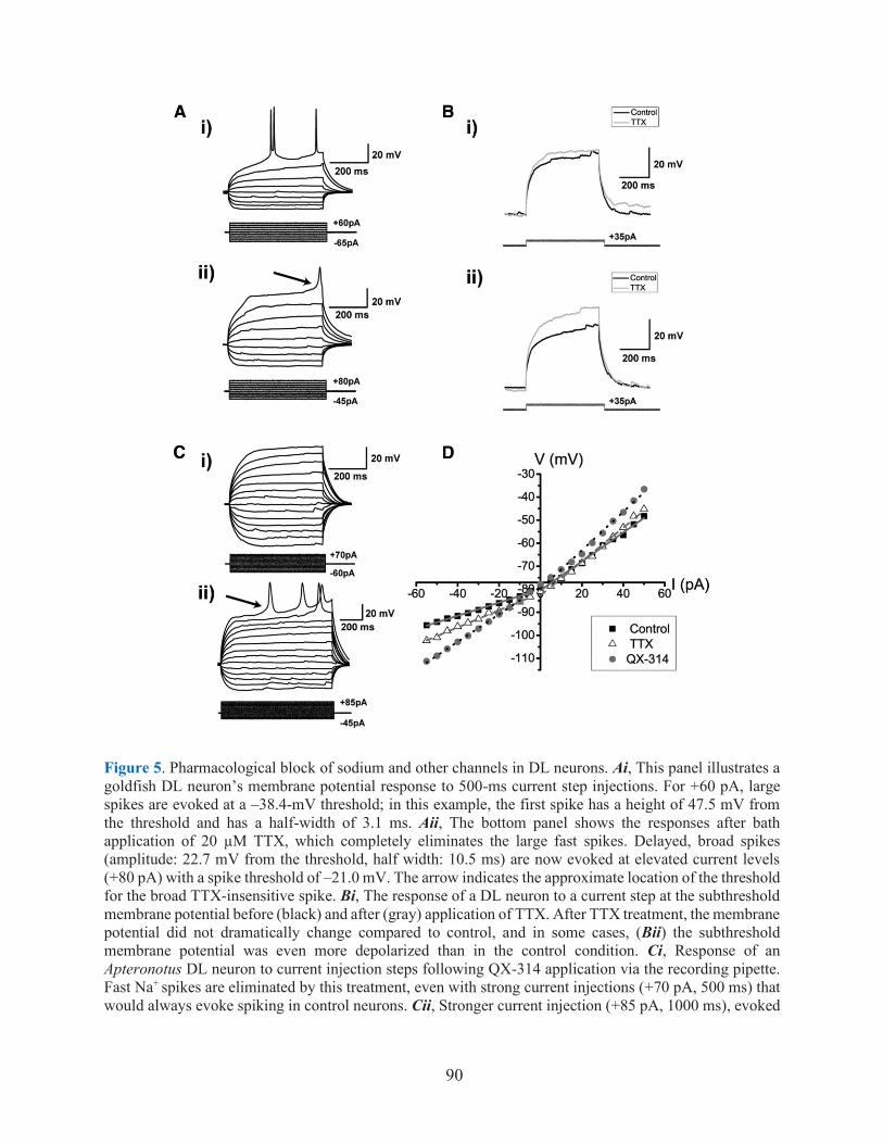
90
Figure 5. Pharmacological block of sodium and other channels in DL neurons. Ai, This panel illustrates a
goldfish DL neuron’s membrane potential response to 500-ms current step injections. For +60 pA, large
spikes are evoked at a –38.4-mV threshold; in this example, the first spike has a height of 47.5 mV from
the threshold and has a half-width of 3.1 ms. Aii, The bottom panel shows the responses after bath
application of 20 µM TTX, which completely eliminates the large fast spikes. Delayed, broad spikes
(amplitude: 22.7 mV from the threshold, half width: 10.5 ms) are now evoked at elevated current levels
(+80 pA) with a spike threshold of –21.0 mV. The arrow indicates the approximate location of the threshold
for the broad TTX-insensitive spike. Bi, The response of a DL neuron to a current step at the subthreshold
membrane potential before (black) and after (gray) application of TTX. After TTX treatment, the membrane
potential did not dramatically change compared to control, and in some cases, (Bii) the subthreshold
membrane potential was even more depolarized than in the control condition. Ci, Response of an
Apteronotus DL neuron to current injection steps following QX-314 application via the recording pipette.
Fast Na+ spikes are eliminated by this treatment, even with strong current injections (+70 pA, 500 ms) that
would always evoke spiking in control neurons. Cii, Stronger current injection (+85 pA, 1000 ms), evoked

91
delayed broad spikes (amplitude from the threshold = 36.9 mV, half-width; 25.9 ms) with a higher threshold
(–8.3 mV) compared to the TTX-insensitive spikes illustrated in panel Ai. Stronger current injections (+85
pA, 1000 ms) evoked several putative Ca2+ spikes with a shorter latency to the first spike. The arrow
highlights the approximate location of the threshold of the broad Ca2+ spike. D, Average I-V relationship
obtained from subthreshold Apteronotus and goldfish DL recordings without the application of any
pharmacological blockers (black squares), after the application of 20 µM TTX (white triangles), and with
the inclusion of QX-314 within the patch pipette solution (gray circles). Both the curves for control and
TTX are piecewise linear with the slope being markedly smaller for hyperpolarizing (control; 0.28 ± 0.02
mV/pA, TTX; 0.32 ± 0.04 mV/pA) compared to depolarizing steps (control; 0.69 ± 0.03 mV/pA, TTX;
0.74 ± 0.03 mV/pA). In contrast, the addition of QX-314 has linearized the I-V curve (hyperpolarizing
slope = 0.60 ± 0.11 mV/pA, depolarizing slope = 0.86 ± 0.12 mV/pA) with its main effect on the response
to hyperpolarizing current injections (Table 1). Extended information illustrating the expression of GIRK
channels in the Apteronotid fish’s brain is available in Extended Data Figure 5-1.
We next plotted the average I-V curves for negative and positive (subthreshold) current
injection (Apteronotus and goldfish; Fig. 5D). The stronger response to positive versus negative
current injection can be clearly seen in the rectification of the I-V curve for the control condition.
These curves can be used to compute separate input resistances for positive and negative current
injections. Typically, the response to hyperpolarizing current injection is assumed to reflect the
passive properties of a neuron and is reported as its input resistance (e.g., ELL pyramidal cells;
Mathieson and Maler, 1988; Berman et al., 1997). In DL cells, the input resistance for depolarizing
current injection is approximately double that for hyperpolarizing current injection when compared
under both control and TTX conditions (Table 1; paired t test; control; p = 3.3 × 10⁻¹², row c, Table
3, TTX; p = 9.9 × 10⁻⁶, row d, Table 3). The addition of TTX had no significant effect on the
hyperpolarizing slope (one-way ANOVA; p = 0.32, row f, Table 3), nor did it have any significant
effect on the input resistance for the depolarizing slope (Table 1; one-way ANOVA; p = 0.42, row
h, Table 3; Fig. 5D). Thus, it appears that there is no contribution of persistent Na+ channels to the
RMP of DL neurons, in accordance with the small effects of TTX observed in Figure 5B.

92
Table 1. I-V slope measurements obtained from the depolarizing and hyperpolarizing responses of DL neurons in
both teleost species for the TTX and QX-314 experiments
Conditions Depolarizing Slope
(GΩ)
Hyperpolarizing Slope
(GΩ)
Control
(N = 18 cells)
0.69 ± 0.03 0.28 ± 0.02
TTX
(N = 6 cells)
0.74 ± 0.03 0.32 ± 0.04
QX-314
(N = 6 cells)
0.86 ± 0.12 0.60 ±0.11
To further investigate the basis of the observed asymmetrical response to current injection, we
have also recorded DL neurons using an intracellular solution containing 5 mM QX-314, a blocker
of Na+ channels, as well as some K+ and Ca2+ channels (Talbot and Sayer, 1996; control, N = 18
cells; QX-314, N = 6 cells; Fig. 5C,D). QX-314 has previously been used to block all Na+ channels
in Apteronotus ELL pyramidal cells (Berman et al., 2001). The I-V graph constructed from the
QX-314 experiments showed a higher depolarizing versus hyperpolarizing input resistance (paired
t test; p = 2.3 × 10⁻⁴, row e, Table 3), similar to control and TTX conditions (above). There was a
small increase in input resistance for the depolarizing current injection that failed to reach
significance (Table 1; one-way ANOVA, p = 0.07, row i, Table 3; Fig. 5D). In contrast, there was
a large and highly significant increase of input resistance in the responses to hyperpolarizing
current injections, it more than doubled over control values (Table 1; one-way ANOVA, p = 5.9 ×
10−5, row g, Table 3). Since we only expect K+ permeating channels to be open at such
hyperpolarized membrane potential, we attribute this effect to the “nonspecific” actions of QX-
314 (Perkins and Wong, 1995; Slesinger, 2001). The results of the TTX and QX-314 experiments
lead to two hypotheses: first, the subthreshold response of DL cells to depolarizing input is mainly
due to their passive membrane properties. Second, the RMP of hyperpolarized DL cells is likely

93
due to a strong rectifying K+ conductance that is blocked by QX-314 and typically prevents the cell
from deviating from the reversal potential of K+ ions (Fig. 5). Given that GIRK channels are
ubiquitous in the mammalian cortex (Luscher and Slesinger, 2010; Lujan and Aguado, 2015) and
can be blocked by QX-314 (Zhou et al., 2001), we suspected them to also be present in the teleost
pallium. To confirm the presence of GIRKs in DL, we used a RT-PCR approach to show the
expression of GIRK channels in different brain regions in the Apteronotid fish (DL, subpallium,
tectum/torus, cerebellum, ELL and hindbrain) using a primer pair hybridizing in conserved
segments of all GIRK paralogs. Unsurprisingly, pan-GIRK amplicons were found in all brain
regions, but were not present in the control (Extended Data Fig. 5-1), suggesting that GIRK
channels are ubiquitously expressed in the Apteronotus brain.
Voltage-dependent calcium conductance
In the presence of TTX, strong current injections (>80 pA) were able to evoke a broad (half-
width: 33.0 ± 3.1 ms) spike with a very high threshold (mean threshold: –21.2 ± 0.5 mV, N = 4 of
6 cells; Fig. 5Aii). Spike amplitude was 18.6 ± 0.7 mV from the threshold potential and 79.1 ± 0.9
mV from the RMP. Similar to the TTX results, QX-314 treated cells did not produce any action
potentials at the threshold for control cells (Fig. 5Ci), but did produce broad spikes at much higher
stimulus intensities (spike half-width, 21.1 ± 1.1 ms; height = 31.3 ± 0.7 mV from threshold and
100.6 ± 0.9 mV from RMP, N = 4 of 6 cells; Fig. 5Cii). The average threshold for these broad
spikes was found to be at –6.8 ± 1.3 mV, which is also consistent with the range of voltages that
has been reported for the activation of HVA Ca2+ channels (Tsien et al., 1988). Therefore, we
hypothesize that DL neurons express HVA Ca2+ channels that will likely be activated by Na+-
mediated action potentials.

94
AHPs
DL neurons exhibit a strong AHP (Figs. 4–6). Previously, it was shown that DL cells express
both SK1 and SK2 channels (Ellis et al., 2008) and that UCL1684 is highly effective at blocking
such channels (Harvey-Girard and Maler, 2013). We therefore bath-applied 30 µM UCL1684,
resulting in a significantly diminished AHP compared to the control conditions (Fig. 6A). To
quantify this AHP reduction, we measured the AHP amplitude (Fig. 6Ci) and the area under the
AHP (Fig. 6Cii) following the first single spike obtained in response to current injection. The
addition of UCL1684 reduced the average amplitude of the first AHP to half its control value
(control: 3.5 ± 0.3 mV, N = 13 cells; UCL1684: 1.4 ± 0.2 mV; N = 7 cells; two-sample t test; p =
0.0003, row j, Table 3; Fig. 6Ci). A similar reduction was also observed when comparing the area
under AHPs: from 1980.3 ± 192.6 to 701.4 ± 128.4 mV/ms (two-sample t test; p = 0.0002, row l,
Table 3; Fig. 6Cii). In contrast, after the addition of the SK channel agonist EBIO (1 mM; Ellis et
al., 2007), current injection evoked very few spikes; thus current steps were increased to 750 and
1000 ms. As expected, the average AHP amplitude increased from 3.5 ± 0.3 mV to 6.7 ± 1.0 mV
(control, N = 13 cells; EBIO, N = 6 cells; two-sample t test; p = 0.001, row k, Table 3), while the
area under the curve also increased from 1980.3 ± 192.6 to 3952.2 ± 277.5 mV/ms (two-sample t
test, p = 0.00002, row m, Table 3).

95
Figure 6. SK-mediated potassium channels contribute to the AHP of DL neurons. A, Apteronotus DL
neuron response to 500-ms step current injection before (black trace) and after the bath application of 30
µM UCL1684 (gray trace). The black arrow shows the minimum membrane potential between two spikes
and is used to estimate the amplitude of the AHP by comparison with the membrane potential immediately
preceding the first action potential. The prominent AHPs seen in the control condition are reduced by this
treatment and the spike rate has also increased (from three to eight spikes). B, DL neuron response to the
injection of 750-ms current steps before (black trace) and after bath application of 1 mM EBIO in the
goldfish (gray trace; a longer pulse was needed to increase the likelihood of evoking more than one spike).
The amplitude of the AHP (arrow) was increased by this treatment and the spike rate has been reduced
(from 4 to 2 Hz). C, Average amplitude (i) and average area under the membrane potential (ii) of the AHP
following the first spike of DL neurons in response to current steps (control, N = 12 cells; UCL1684, N =
7 cells; EBIO, N = 6 cells). Both the amplitude and the area under the AHP are significantly diminished
after the application of UCL1684, while a strong increase was observed after the application of EBIO. D,
Average firing rate plotted as a function of the amount of current injected for the control condition (black
trace), the UCL1684 condition (gray trace), and the EBIO condition (light gray trace) in both Apteronotus
and goldfish (control, N = 28 cells; UCL1684, N = 7 cells; EBIO, N = 6 cells). The firing rate increases for
all current injections after UCL1684 application, while the firing rate decreases after the EBIO application.
**p < 0.01
Blocking SK channels also increased the current evoked firing rate compared to the control
condition (control, N = 28 cells; UCL1684, N = 7 cells; two-way ANOVA; p = 0.0013, row n,
Table 3; Fig. 6D), while EBIO reduced the evoked firing rate since the cell required a longer time
to reach spike threshold after the first spike (N = 6 cells; two-way ANOVA; p = 0.000092, row o,
96
Table 3; Fig. 6B,D). We conclude that the SK1/2 channels of DL neurons act as negative feedback
on the cell’s responsiveness to excitatory input.
Finally, we wanted to confirm whether SK channel activation in DL neurons could be blocked
by preventing Ca2+ activation of the channel. We recorded DL neurons in Apteronotus using an
intracellular solution containing 10 mM BAPTA, a Ca2+ chelator (N = 7 cells; Fig. 7A). In all cases,
the AHP was completely abolished, unlike the partial AHP block obtained with UCL1684. This
suggests that another unidentified Ca2+-activated K+ channel may also be contributing to the AHP.
Further work will be required to investigate this possibility. The firing rate also dramatically
increased compared to the control condition (control, N = 28; UCL1684, N = 7; BAPTA, N = 7
cells; two-way ANOVA; p = 1.5 × 10⁻¹⁵, row p, Table 3; Fig. 7B) and compared to UCL1684
treatment (two-way ANOVA; p = 0.00063, row q, Table 3). Furthermore, this BAPTA induced
increase in firing rate was also accompanied by a significant reduction in spike height compared
to both control (two-way ANOVA; p = 2.1 × 10⁻¹², row r, Table 3; Fig. 7C) and UCL1684
conditions (two-way ANOVA; p = 1.6 × 10⁻⁶, row s, Table 3). In contrast, the difference in spike
height between the UCL1684 and control did not yield a significant difference (two-way ANOVA;
p = 0.14, row t, Table 3). We hypothesize that Na+ channel inactivation may be causing this
reduction (see below in the Dynamic AHP and spike threshold section). Another distinctive feature
of the DL neuron’s spiking response during the BAPTA application was the increase in spike width
occurring along successive spikes and typically becoming most prominent by the 8th spike (Fig.
7A,D). In the control and UCL1684 conditions, there was a slight increase in spike width, however,
in the BAPTA condition, the spike width increased dramatically with successive spikes (Fig. 7A,D)
compared to control (two-way ANOVA; p = 1.3 × 10⁻³¹, row u, Table 3) and UCL1684 conditions
(two-way ANOVA; p = 3.7 × 10⁻¹⁰, row v, Table 3). In contrast, the difference between the control

97
and BAPTA conditions was not significant up until the third spike (two-way ANOVA; p = 0.24,
row w, Table 3), suggesting that the spike width increase is caused by a cumulative process.
Calcium channels typically inactivate via a Ca2+-dependent mechanism (Simms and Zamponi,
2014), leading us to hypothesize that this dramatic change in spike width may be caused by a
decrease in Ca2+-dependent inactivation of the Ca2+ channel leading to an increase of its open time.
Figure 7. The effect of intracellular Ca2 chelation on DL neuron responses to depolarization. A, Example
recording trace (Apteronotus) with 10 mM BAPTA added to the internal solution of the patch pipette. The
AHP appears to be completely eliminated which promotes higher frequency spiking; note that successive
spike heights drop continuously for the first seven spikes. By the 8th spike, very prominent spike
broadening begins and the spike height drops to an even greater degree compared to the UCL1684
application in Figure 6A. B, The average firing rate was plotted as a function of the amount of current
injected for the control (black trace, N = 28 cells), UCL1684 (gray trace, N = 7 cells), and BAPTA
conditions (light gray trace, N = 7 cells). The addition of intracellular BAPTA promotes an even stronger
increase in firing rate compared to the addition of the SK channel blocker UCL1684. C, The average
difference in spike height between the nth spike and the first spike was plotted as function of successive
spikes obtained after a 500-ms current step injection for all three conditions mentioned in B. The addition

98
of UCL1684 did not strongly affect the spike height, unlike the addition of BAPTA, which reduced the
spike height across successive spikes following a step current injection. The arrow highlights the 8th spike,
which marks the beginning of the non-linearity in the BAPTA condition. D, The average spike width was
plotted as a function of successive spikes, similar to panel C. UCL1684 application has only a minimal
effect on spike width. The presence of intracellular BAPTA increased the spike width across successive
spikes during a step current injection when compared to the other conditions. The arrow indicating the 8th
spike marks a strong change in spike width, as denoted by the arrow in A.
Dynamic AHP and spike threshold
Although the presence of the AHP greatly reduces the firing rate, we also observed that after
successive spikes, the AHP itself decreased (Extended Data Fig. 8-1A) and the spike threshold
increased (Fig. 8A). To better quantify the AHP modulation, we measured the difference in AHP
amplitude between the first two spikes of a current-evoked spike train that did not show an initial
burst. We found that there was a significant reduction in AHP amplitude that was invariant to the
time length of the AHP (N = 26 cells; one-sample t test, p = 4.45 × 10⁻²⁷, row x, Table 3; Extended
Data Fig. 8-1B, black squares). For recording traces that showed initial bursts, we examined the
first spike pair following the burst and found a similar reduction in AHP (N = 20 cells; one sample
t test, p = 1.26 × 10⁻¹³, row y, Table 3; Extended Data Fig. 8-1B, gray triangles). This reduction
is presumably caused by Ca2+-induced inactivation of the HVA Ca2+ channels, which will decrease
the total amount of Ca2+ available to the cell and limit the activation of SK channels.

99
Figure 8. DL neuron spiking causes a decrease in AHP amplitude and an increase in spike threshold. A, A
magnified view of the first three spikes in an example trace of a DL neuron’s response to a +60-pA current
injection where the black dashed line is placed to coincide with the minimum of the first spike’s AHP and
the gray dashed line is placed to coincide with the first spike’s threshold. The black arrows highlight the
progressive increase in spike threshold following consecutives spikes. B, The increase in spike threshold
between the second and first spikes was plotted in the same manner as a function of the first ISI. Individual
black squares represent a pair of spikes that were taken from a trace which did not contain an initial burst
(total of 160 non-burst pairs), while individual gray triangles represent a pair of spikes that were taken from
a trace displaying an initial burst of spikes as in Figure 4C (total of 117 burst spike pairs). The majority of
the spike thresholds increased (>300 ms) with no evident recovery. C, The difference in average spike
threshold between the nth spike and the first spike is plotted as a function of the spike number. The
subsequent curve was fit with a double exponential equation (y = 2.72e0.04x –9.0e -0.72x; R2 = 0.987). D, The
increase in spike threshold between the nth spike and the first spike is plotted as a function of the time
interval between them. Each black square represents a spike pair (total of 573 spike pairs). Overall, the
increase in threshold appears to be larger following longer timer intervals. Extended information related to
the modulation of the AHP after prolonged spiking is available in Extended Data Figure 8-1.
Even with the spiking-induced reduction of the AHP, DL neurons could not surpass a sustained
firing rate of 30 Hz (Fig. 7B), which suggests the presence of an additional mechanism(s) that
limits firing rate. In ELL pyramidal neurons, spike threshold fatigue has been shown to limit the
firing rate whenever a burst occurs (Chacron et al., 2007). On closer inspection, we found a
significant increase in spike threshold during long spike trains (Fig. 8A). This dynamic spike

100
threshold was also found to be invariant to the ISI (up to ~300 ms) for both non-burst traces (one-
sample t test, p = 1.24 × 10⁻²², row z, Table 3; Fig. 8B, black squares) and for traces containing
an initial burst (one sample t test, p = 8.30 × 10⁻²⁸, row aa, Table 3; Fig. 8B). Next, we wanted to
confirm whether the threshold fatigue that was observed in DL neurons may be caused by the
history of past spikes, i.e., whether Na+ channel inactivation due to continuous spiking may
influence the spike threshold. We examined the difference in threshold for all non-burst traces to
see whether it varies throughout a spike train. The threshold increases continued to at least 10
spikes and could be fitted by a double exponential function (equation: y = 2.72e0.04x –9.0e −0.72x; R2
= 0.987; Fig. 8C); here we considered only the number of spikes and not the duration of the spike
train. A similar analysis where the difference in threshold was compared to the time between spikes
instead of the spike number also led to the same conclusion: this effect became more prominent
after long periods of depolarization despite the variability in the number of intervening spikes (Fig.
8D). These results suggest that the increase in threshold is caused by an accumulation of slow Na+
channel inactivation.
In mammalian cortical cells, the recovery from inactivation of Na+ channels have both a fast
component (millisecond timescale) and a slow component that can extend to much longer
timescales (seconds to minutes; Fleidervish et al., 1996; Mickus et al., 1999; Ellerkmann et al.,
2001). To quantify the duration of this spike threshold adaptation, we developed a protocol in
which a long ramp current (evoking multiple spikes) was injected followed by a shorter ramp
current (evoking one spike) at various inter-stimulus time intervals (Fig. 9A, upper panel). This
protocol induced spike threshold fatigue during the first current injection, while the second current
injection was used to test for time-dependent changes in spike threshold. We found that the increase
in spike threshold between the first and second current injection was significantly higher at short

101
compared to longer time intervals (Fig. 9A, bottom panel). Using these changes in threshold, we
found that the recovery from this spike threshold fatigue had a highly variable time constant
ranging from 300 to 900 ms with an average time constant τexp = 637.28 ± 85.9 ms (Fig. 9B). This
suggest that the decrease in cell excitability caused by the dynamic threshold can operate on the
timescale of hundreds of milliseconds.
Figure 9. DL neuron spike threshold adaptation can last up to hundreds of milliseconds. Ai, Two ramp
current injections separated at various times t (in this example 50, 500, and 1000 ms) were used to measure
the time constant of the spike threshold adaptation. Although both ramp current injections have the same
slope (slope = 1.3 pA/ms), the objective of the first ramp current was to induce an accumulation of Na+
channel inactivation through the firing of multiple action potentials and therefore was stronger than the
second ramp current which would only produce one action potential. Aii, A magnified view of the example
responses obtained after the first ramp current injection and after the second ramp current injections at times
t = 50 ms, t = 500 ms, and t = 1000 ms, respectively. The black dash line is aligned to the first spike’s
threshold obtained after the first ramp current injection while the gray dotted lines are aligned to the spike
threshold obtained from the second ramp current injection for the various times t mentioned previously. B,
The average difference in spike threshold (for the first spike only) between the first and second ramp current
injections were plotted as a function of the time t between each ramp injection. The resulting curve was
fitted with an exponential equation (y = 2.38*e-0.0017x, R2 = 0.917). C, We used a simplified EIF with fast (τf
= 15 ms) and slow (τs = 500 ms) Na+ channel inactivation in an attempt to connect the apparent Na+ channel

102
inactivation (Fig. 7A) with the increase in spike threshold over multiple spikes (Fig. 8C,D). i, When driven
by a step current, the model produces a small number of spikes at frequencies consistent with the data;
however, the neuron quickly ceases discharge despite continuous application of the strong positive current.
ii, This result can be easily understood in terms of the dynamic spike threshold (θ), which increases because
of cumulative slow inactivation of the Na+ channel (hf and hs not shown). Note that the threshold changes
by ~4 mV (gray shading) over the course of a few spikes, in line with the upper bound for threshold
increases seen between DL cell spikes (Fig. 8C). Our model parameter set gave an initial threshold of -
44.6mV in close agreement with the Aptoronotus data (-45 mV, Fig. 4E).
To further investigate whether Na+ channel inactivation is responsible for the observed increase
in threshold, we employed a model with minimal assumptions: the iEIF (Platkiewicz and Brette,
2011). This model includes a slow inactivation term, as well as the traditional fast inactivation term
associated with Na+ channels; inactivation kinetics for both forms were derived from our data (see
Materials and Methods). Since we were primarily interested in the effect of sodium inactivation on
the spike threshold, the minimal model omits AHP dynamics and Ca2+ currents (see Materials and
Methods). We found that the addition of slowly inactivating Na+ channels, as suggested by the
effects of BAPTA (Fig. 7A), was itself sufficient to qualitatively reproduce the response of DL
neurons to current injection and predict an increase in spike threshold that was similar to that
observed in our whole-cell recordings (Fig. 9C). We therefore conclude that the accumulation of
slow Na+ channel inactivation, caused by spike discharge and simple depolarization, may act as a
source of negative feedback to reduce the cell’s firing rate via an increase in spike threshold.
Discussion
The work presented here is, to our knowledge, the first study of the biophysical properties of
teleost DL neurons. Our previous work mapped the local DL circuitry (Trinh et al., 2016), the
organization of thalamic and other inputs to DL (Giassi et al., 2012c), and the telencephalic
connectivity of DL (Giassi et al., 2012a; Elliott et al., 2017). In gymnotiform fish, we have
previously shown that the electrosensory system contributes to spatial learning (Jun et al., 2016),
103
and that the PG (thalamic) inputs to DL can encode responses to object motion (Wallach et al.,
2018). Although the intrinsic and extrinsic properties of DL synaptic input have yet to be examined,
we believe that the constraints imposed by DL circuitry, behavioral function plus recent theoretical
analyses, are sufficient to generate testable hypotheses of the computations performed by DL
during spatial learning. Below, we first summarize the main conclusions of our work and then
discuss whether the biophysical properties of DL neurons and their connectivity are compatible
with the critical role of DL in spatial learning and memory. In particular, we suggest that DL
neurons possess the minimal requirements to be labeled as sparse coders. Next, we suggest that
spike threshold adaptation is key to the extraction of spatial information in DL from the time
stamped electrosensory input conveyed by PG (Wallach et al., 2018). Our hypothesis relies on a
previous theoretical model of time coding cells (Itskov et al., 2011) that utilizes, as an essential
ingredient, spike threshold adaptation with a long recovery time constant.
Our main results show that DL neurons express a combination of ion channels that have been
reported for many other types of neurons. DL neurons have a hyperpolarized RMP. We hypothesize
that this is due, at least in part, to GIRK channels. GIRKs can hyperpolarize mammalian CA1
hippocampal neurons by at least 8 mV under basal conditions (Luscher and Slesinger, 2010) and
have been shown to set the RMP of dorsal cochlear nucleus (DCN) neurons to a hyperpolarized
level (Ceballos et al., 2016). DL neurons also have a high spike threshold and theoretical analyses
suggest this may attributed to a low density of voltage-gated Na+ channels (Platkiewicz and Brette,
2010). Furthermore, our results also imply the presence of HVA Ca2+ channels, which activate a
strong SK channel mediated AHP that strongly reduces current-evoked spiking. We propose that
the combination of a hyperpolarized RMP, the low input resistance at hyperpolarized potentials
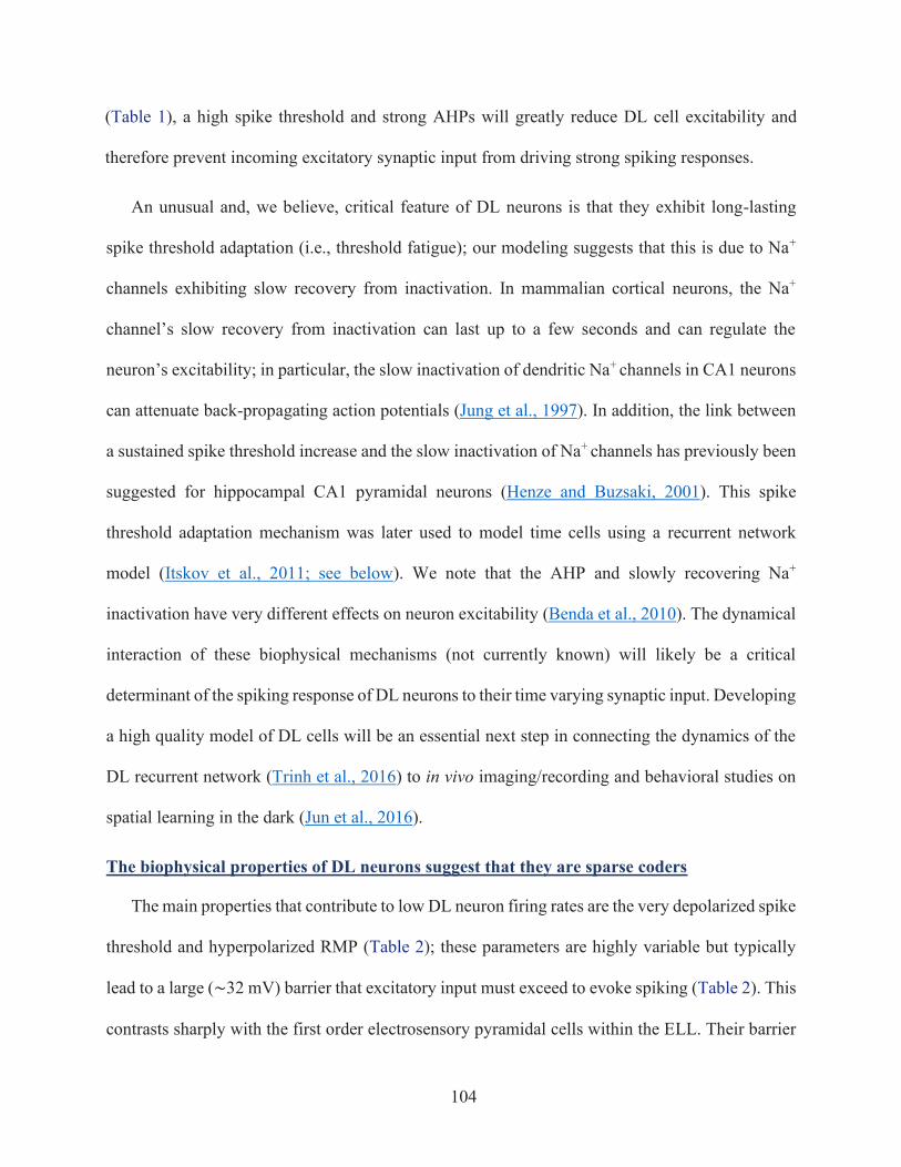
104
(Table 1), a high spike threshold and strong AHPs will greatly reduce DL cell excitability and
therefore prevent incoming excitatory synaptic input from driving strong spiking responses.
An unusual and, we believe, critical feature of DL neurons is that they exhibit long-lasting
spike threshold adaptation (i.e., threshold fatigue); our modeling suggests that this is due to Na+
channels exhibiting slow recovery from inactivation. In mammalian cortical neurons, the Na+
channel’s slow recovery from inactivation can last up to a few seconds and can regulate the
neuron’s excitability; in particular, the slow inactivation of dendritic Na+ channels in CA1 neurons
can attenuate back-propagating action potentials (Jung et al., 1997). In addition, the link between
a sustained spike threshold increase and the slow inactivation of Na+ channels has previously been
suggested for hippocampal CA1 pyramidal neurons (Henze and Buzsaki, 2001). This spike
threshold adaptation mechanism was later used to model time cells using a recurrent network
model (Itskov et al., 2011; see below). We note that the AHP and slowly recovering Na+
inactivation have very different effects on neuron excitability (Benda et al., 2010). The dynamical
interaction of these biophysical mechanisms (not currently known) will likely be a critical
determinant of the spiking response of DL neurons to their time varying synaptic input. Developing
a high quality model of DL cells will be an essential next step in connecting the dynamics of the
DL recurrent network (Trinh et al., 2016) to in vivo imaging/recording and behavioral studies on
spatial learning in the dark (Jun et al., 2016).
The biophysical properties of DL neurons suggest that they are sparse coders
The main properties that contribute to low DL neuron firing rates are the very depolarized spike
threshold and hyperpolarized RMP (Table 2); these parameters are highly variable but typically
lead to a large (∼32 mV) barrier that excitatory input must exceed to evoke spiking (Table 2). This
contrasts sharply with the first order electrosensory pyramidal cells within the ELL. Their barrier

105
from rest to spiking is a mere 4.9 mV (Table 2) and they can even respond to weak signals with
discharge frequencies over 100 Hz. ELL pyramidal neurons also recover rapidly from spike
induced increases in spike threshold, i.e., threshold fatigue (tens of milliseconds; Chacron et al.,
2007). It is hypothesized that these properties are responsible for the ability of pyramidal cells to
densely encode spatial and social electrosensory signals (Vonderschen and Chacron, 2011). The
low barrier from RMP to spike threshold is also seen in primary auditory neurons and in layer 4
cells of the primary visual and somatosensory cortex (Table 2). Although no precise estimates are
available, it appears likely that all these low-level sensory neurons encode sensory input much
more densely than neurons in the hippocampus.
Table 2. Difference in spike threshold and resting membrane across multiple cell types
‘hippocampus’ L4 Sensory cortex Primary Sens. cells
Values in
mV
DL cells DG granule
cellsa
Barrel
Fieldb
Visual
Cortexc
ELL
Pyr
ON
cells
DCN
Pyr
Cellsf
Spike
threshold
-45.3 -40.8 -45.1 ~-63.5 -62.9d -48.1
RMP -76.7 -74.7 -63.0 -72.0 -67.8e -62.7
Threshold –
RMP
31.4 33.9 17.9 8.5 4.9 14.6
a Kowalski et al. (2016), in vivo, threshold: used point of 1st derivative which exceeded 20 V*s-1.
b Yu et al. (2016), in vivo, threshold: used point of 1st derivative which exceeded 3 times the average 1st derivative.
c Wilent and Contreras (2005), in vivo, threshold: used peak of 2nd derivative, values were averaged from the data
for preferred direction and non-preferred direction
d Mehaffey et al. (2008), in vitro, threshold: used point of 1st derivative which was 8 times greater than SD.
e Berman and Maler (1998a), in vitro.
f Li et al. (2013), in vitro, threshold: used point of 1st derivative which exceeded 10 V*s-1.

106
Hippocampal neurons such as DG granule cells are nearly silent at rest, and discharge very
sparsely in response to the animal’s spatial location, i.e., place field (Diamantaki et al., 2016). The
low excitability in mature granule cells was shown to be partly due to the constitutive activity of
GIRK channels (Gonzalez et al., 2018). We hypothesize that a similar mechanism is contributing
to the low RMP of DL neurons in fish, which may partly explain why the difference between RMP
and spike threshold is nearly identical in DL and DG cells (Table 2).
With the above examples in mind, we hypothesize that the key biophysical signatures of sparse
coding is, for all neurons, a large gap between the RMP and the spike threshold. We further
hypothesize that DL neurons will sparsely encode the spatial relations required for memory guided
navigation.
Can the DL network transform PG sequential encounter time stamps to a spatial map?
Previous studies have investigated electrosensory spatial learning in a related gymnotiform fish
(Jun et al., 2016; Fotowat et al., 2019). Jun et al., showed that these fish can locate food relative to
landmarks in the dark because, after learning, they rapidly navigated to the remembered food
location during probe trials (no food). Fotowat et al. (2019) showed that neurons within DD, which
has strong reciprocal connections with DL (Giassi et al., 2012a; Elliott et al., 2017), discharged
when the fish was engaged in active sensing movements near landmarks. Together, these studies
imply that DL is engaged in learning and storing the spatial memories of the relative location of
landmarks and food. The electrosense is very local and, for most of their trajectory, the fish had no
external sensory cues (Jun et al., 2016). This led Jun et al. to argue that, after leaving a landmark,
the fish used the path integration of speed and orientation signals to continuously update its current
location and thus compute the trajectory to the remembered food location. Path integration

107
information was assumed to potentially derive from lateral line receptors, vestibular afferents,
proprioceptors and vestibular afferents. Bastian (1995) has previously reported that there are
brainstem proprioceptive neurons in the gymnotiform fish that are capable of signaling tail
bending. Recently, Wallach et al. (2018) found PG neurons are responsive to continuous lateral
line input, confirming a second potential source of information related to the fish’s speed. A recent
study in the larval zebrafish has demonstrated that vestibular input can evoked strong and
widespread activity in the telencephalon that, from the images presented, likely includes DL
(Favre-Bulle et al., 2018). We now hypothesize that an encounter with a landmark triggers an
autonomous “moving bump” in the DL recurrent network and this is the primary driver for the
fish’s estimation of its changing location during its landmark-to-food trajectories. While
proprioceptive, lateral line and vestibular input are important, we now hypothesize they merely
modulate the essential intrinsic DL network dynamics. We elaborate on this hypothesis below.
In gymnotiform fish, PG cells respond to object motion (electrosensory and visual; Wallach et
al., 2018). Anatomic studies indicate that these responses are driven by tectal input (Giassi et al.,
2011). The gymnotiform tectum maintains a topographic representation of electrosensory input
and tracks continuous object motion (Bastian, 1982). PG neurons generate a major transformation
of their tectal input, the majority of PG motion sensitive cells lose topographic information and
respond over the fish’s entire body but only to object motion start (all cells) and stop (some cells)
and not the intervening continuous motion (Wallach et al., 2018). Wallach et al. proposed that,
during navigation in the dark, these PG cells will respond transiently when any part of the fish’s
body first encounters a landmark (or food), i.e., the response of the cell when the experimenter
moves an object toward the fish is equivalent to its response when the fish moves near a landmark

108
or food. Wallach et al. further proposed that the time interval between encounters could be “read
out” from the change in second versus first encounter firing rates of a subset of DL cells.
In the following discussion, we borrow extensively from work on “time” and “place” cells in
the mammalian hippocampus using, in particular, the very thorough papers of Kraus et al. (2013)
and Pastalkova et al. (2008) as well as the related theoretical papers of Itskov et al. (2011) and
Rajan et al. (2016). Kraus et al. (2013) describe hippocampal neurons that respond at specific times
during a rat’s motion on a treadmill. These experiments carefully dissociated time from place so
that the authors were able to demonstrate the existence of time cells, traditional place cells as well
as cells with information on both the time and distance traveled. Pastalkova et al. (2008) and Itskov
et al. (2011) had previously argued that sequential activation of cell assemblies is internally
generated by hippocampal dynamics and can give rise to time cells independent of sensory input.
Kraus et al. (2013) extended this hypothesis and argued that their time cells were driven by both
internal network dynamics and external cues such as treadmill speed.
Table 3. Statistical Table.
DATA STRUCTURE TYPE OF
STATISTICAL
TEST
POWER
a Difference between the average variances of
the resting membrane potential
Control vs Kynurenic
Acid
Paired-t test p = 0.0383
b Difference between the average resting
membrane potential
Control vs Kynurenic
Acid
Paired-t test n.s. (p =
0.7372)
c Difference between the input resistance
(hyperpolarizing vs depolarizing)
Control Paired-t test p = 3.3×10-
12
d TTX Paired-t test p = 9.9×10⁻⁶
e QX-314 Paired-t test p = 2.3×10⁻⁴
f Difference between the input resistance for
hyperpolarizing current injections
Control vs TTX One-way
ANOVA
n.s. (p =
0.32)
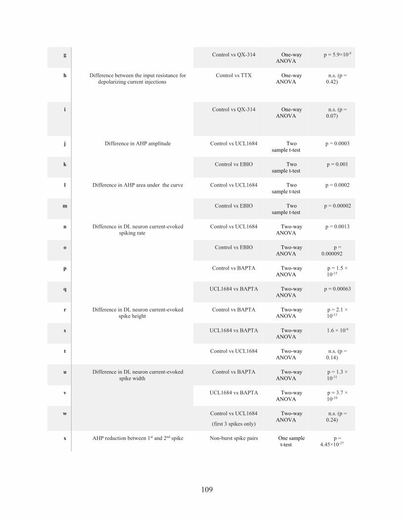
109
g Control vs QX-314 One-way
ANOVA
p = 5.9×10⁻⁵
h Difference between the input resistance for
depolarizing current injections
Control vs TTX One-way
ANOVA
n.s. (p =
0.42)
i Control vs QX-314 One-way
ANOVA
n.s. (p =
0.07)
j Difference in AHP amplitude Control vs UCL1684 Two
sample t-test
p = 0.0003
k Control vs EBIO Two
sample t-test
p = 0.001
l Difference in AHP area under the curve Control vs UCL1684 Two
sample t-test
p = 0.0002
m Control vs EBIO Two
sample t-test
p = 0.00002
n Difference in DL neuron current-evoked
spiking rate
Control vs UCL1684 Two-way
ANOVA
p = 0.0013
o Control vs EBIO Two-way
ANOVA
p =
0.000092
p Control vs BAPTA Two-way
ANOVA
p = 1.5 ×
10-15
q UCL1684 vs BAPTA Two-way
ANOVA
p = 0.00063
r Difference in DL neuron current-evoked
spike height
Control vs BAPTA Two-way
ANOVA
p = 2.1 ×
10-12
s UCL1684 vs BAPTA Two-way
ANOVA
1.6 × 10⁻⁶
t Control vs UCL1684 Two-way
ANOVA
n.s. (p =
0.14)
u Difference in DL neuron current-evoked
spike width
Control vs BAPTA Two-way
ANOVA
p = 1.3 ×
10-31
v UCL1684 vs BAPTA Two-way
ANOVA
p = 3.7 ×
10-10
w Control vs UCL1684
(first 3 spikes only)
Two-way
ANOVA
n.s. (p =
0.24)
x AHP reduction between 1st and 2nd spike Non-burst spike pairs One sample
t-test
p =
4.45×10⁻²⁷

110
y Initial burst spike pairs One sample
t-test
p =
1.26×10⁻¹³
z Spike threshold increase between 1st and 2nd
spike
Non-burst spike pair One sample
t-test
p =
1.24×10⁻²²
aa Initial burst spike pairs One sample
t-test
p =
8.30×10⁻²⁸
n.s. = non-significant.
The theoretical papers of Itskov et al. (2011) and Rajan et al. (2016) asked: how might the
intrinsic activity of a neural network result in the sequential activation of neuron assemblies, e.g.,
time cells? Both papers started with the same core architecture, a local excitatory recurrent network
that, once activated, was capable of sustained discharge. This is the “bump attractor” hypothesis
originally formulated to explain the sustained activity of neurons during a working memory task
(Wang, 1999; Wimmer et al., 2014). The theoretical analysis of Wang (1999) demonstrated that
slow excitatory synapses, i.e., mediated by NMDA receptors, were required for bump dynamics.
Both Itskov et al. (2011) and Rajan et al. (2016) generated “cell assembly sequences” by
destabilizing the bump attractor dynamics. Itskov et al. (2011) accomplished this by introducing
spike threshold adaptation with a long recovery time constant. In contrast, Rajan et al. (2016)
destabilized the bump by introducing asymmetries in synaptic strengths within the attractor so that
the attractor dynamics would generate a sequential activation of the cell assembly; a process which
necessitated both recurrent connections and external input. In both cases, sequential activation of
neurons within the cell assembly are able to produce time cells or other sequential outputs. A recent
paper (Heys and Dombeck, 2018) has also suggested that time cells of the entorhinal cortex might
be generated by moving bumps in entorhinal recurrent attractor network (Zutshi et al., 2018). This
paper did not, however, explicitly discuss the mechanism by which the putative “bumps” would
move.

111
Our earlier work (Trinh et al., 2016) demonstrated that DL contains excitatory local recurrent
networks; our earlier work had already demonstrated that DL is highly enriched in NMDA
receptors (Harvey-Girard et al., 2007). Trinh et al. (2016), therefore, hypothesized that the DL
recurrent network supported bump attractor dynamics capable of memory storage. Our noisy cells
suggest that the recurrent connections within DL are, in fact, capable of supporting autonomous
discharge. We have now demonstrated that DL neurons exhibit the same threshold adaptation used
in the Itskov et al. (2011) model, thus suggesting that the putative DL bumps may not be stable
attractors. We have not yet studied the properties of either PG-derived or intrinsic synapses in DL
and therefore cannot evaluate whether Rajan et al. (2016)’s architecture might apply. In accordance
with the Itskov model, we hypothesize that DL contains unstable bump attractor neural networks
that are capable of supporting autonomous sequential activation and thus DL time cells. We assume
that, when the fish initially encounters a landmark, the resulting electrosensory-evoked transient
discharge in a subset of PG neurons triggers activity in a small region of DL (Giassi et al., 2012c).
This activity will then propagate through a subset of the DL network forming a cell assembly
temporal sequence (time cells). Following Kraus et al. (2013), we further hypothesize that the
sequential activity in this network is modified by ongoing self-motion sensory input, the vestibular,
lateral line and proprioceptive input mentioned above. These inputs provide the path integration
signals that converts the time cell sequence to a location cell sequence. In functional terms, we
propose that the propagation of neural activity in the DL network represents the fish’s estimate of
where it is located along the trajectory between a landmark and food. When the fish reaches the
food (or another landmark), PG neurons would again discharge to signal the total time/distance
traveled (Wallach et al., 2018) and the potential start of a new trajectory. In this model, learning a
trajectory from a particular landmark to food would consist of strengthening the synaptic

112
connections of the moving bump induced by that landmark so as to represent the time/location
sequence leading from the landmark to food. Such strengthening might result in a Rajan et al.
(2016) type mechanism in which directed bump movement was now also a consequence of
asymmetric synaptic strengthening.
Our hypotheses are, at the moment not testable, because testing would require population
recording from or visualizing activity across a large portion of the DL network. What is needed is
a teleost that is transparent when adult, whose neurons express a genetically encoded calcium
indicator (e.g., gCamp6) and whose pallium might be activated by ethologically relevant transient
signals. Fortunately, such a model system has recently become available (Schulze et al., 2018) and
may permit direct tests of our hypotheses.

113
Extended figures
Extended Figure 5-1. GIRK channel mRNA expression obtained from RT-PCR in the Apteronotus brain
using pan-PCR primer pairs in conserved regions. GIRK channels are ubiquitously expressed albeit at
variable levels. In particular they are expressed in DL. SP, subpallium; TT, tectum/torus; Cer, cerebellum;
HB, hindbrain; ch, chicken (negative control); M, molecular marker.
Extended Figure 8-1. Current-evoked spiking decreases the AHP amplitude of DL neuron. A. Example
trace of a DL neuron’s response to a +60 pA current step injection lasting 500 ms. Consecutive spiking
causes the AHP amplitude to decrease when compared to the first AHP as emphasized by the arrow. A
black dashed line is placed to coincide with the minimum of the first spike’s AHP. We hypothesize that the
decrease in AHP amplitude is due to a reduction in Ca2+ influx (i.e., Ca2+-dependent Ca2+ channel
inactivation) and subsequent reduction in SK channel opening. B. The decrease in AHP amplitude between
the second and first spikes is plotted as a function of the time interval between the first two spikes similarly
to Fig. 8B. Each black square represents a spike pair taken from a trace which did not contain a burst (total
of 160 non-burst spike pairs), while each grey triangle represents a spike pair taken from a trace which
contained a burst at the beginning of the trace (total of 117 burst spike pairs). The majority of the AHPs are
reduced throughout the 300 ms test period without any evident recovery trend.

114
Chapter 4: Characterizing the intrinsic biophysical properties of the
hilar mossy cells (Manuscript in preparation)
Significance statement
One of our original goals was to verify whether DG granule cell had a dynamic spike threshold
with slow recovery, given their suspected homology to a subset of fish pallial neurons. Given the
proposed homology between the mammalian hilar network and the hippocampal-like circuit
described in Elliott et al. (2017), we broadened the scope of our investigation by also characterizing
the dynamic spike threshold in all neurons involved in the mammalian hilar network as well as the
core biophysical properties of the hilar mossy cells. Notably, these experiments have shown that
only a subset of excitatory neurons in the hippocampal formation, including the hilar mossy cells,
displayed this slowly adapting dynamic spike threshold. This study will thus provide an overview
of the main spiking characteristics of the hilar mossy cells and will be the basis for the construction
of a computational model of these neurons.

115
Slow dynamic spike threshold recovery contributes to spiking patterns of hilar
mossy cells
Anh-Tuan Trinh1*, Mauricio Girardi Schappo2, Timal Kannangara1, Jean-Claude
Béïque1,3,4, André Longtin2,3,4, Leonard Maler1,3,4
1. Department of Cellular and Molecular Medicine, University of Ottawa, Ottawa, Ontario, Canada
2. Department of Physics, University of Ottawa, Ottawa, Ontario, Canada
3. Brain and Mind Institute, Center for Neural Dynamics, University of Ottawa, Ottawa, Ontario,
Canada
4. Center for Neural Dynamics, University of Ottawa, Ottawa, Ontario, Canada
Author Contributions: A.T., T.K., M.S., J-C.B., A.L. and L.M. designed the research. A.T. and
T.K. performed the research. M.S. and A.L. built the computational model. A.T., M.S., J-C.B.,
A.L. and L.M. analyzed the data. A.T., M.S., A.L. and L.M. wrote the paper.
This chapter presents a manuscript in preparation. Please note that all figures in this chapter with
the exception of figure 3 will be publish in a first manuscript focusing on the intrinsic properties
of the hilar mossy cells. Figure 3 will be used for a subsequent manuscript detailing the possible
origin of the synaptic noise. Additionally, most of the data presented in figure 3 was obtained by
Timal Kannangara while I did the analysis of that data.
Acknowledgements: We would like to thank Dr. Kirk Mulatz for his help with technical support
and Dr. Érik Harvey-Girard with his help in developing a cutting procedure which would has
allowed us to record from the hilar mossy cells in vitro.

116
Abstract
The encoding of spatial temporal information is a hallmark property of the mammalian
hippocampus. Although this subject has been thoroughly studied in the neurons involved in the
famous tri-synaptic pathway (dentate gyrus granule cells, CA3 pyramidal neurons and CA1
pyramidal neurons), the back-projection pathway from CA3 to the dentate gyrus via the hilar
mossy cells has, until recently, been neglected. Hilar mossy cells have been shown to be involved
in the encoding of space and context. Here, we show that the hilar mossy cells are very active in a
slice preparation and that most of this activity is due to spike-evoked and spontaneous synaptic
glutamate release. Moreover, we have shown that hilar mossy cells support two main mechanisms
for spike frequency adaptation including a SK channel-mediated after-hyperpolarizing potential
and a prominent slowly adapting spike threshold driven by the slow inactivation of Na+ channels.
Hence, we suggest that these intrinsic spike frequency adaptation mechanisms in combination with
its known in vivo firing pattern may allow these cells to better discriminate the afferent inputs from
the CA3 and DG. Specifically, this intrinsic mechanism may shape the formation of in vivo spike
bursts which would allow the cell to detect novel changes in the animal’s environment.

117
Introduction
Past research has mainly focused on the feedforward “trisynaptic pathway”: dentate gyrus (DG)
→ CA3 → CA1. Granule cells in DG project to CA3 pyramidal neurons and activate a recurrent
neural network hypothesized to form cell assemblies - networks of neurons that become stronger
through repeated co-activation (Treves and Rolls, 1994; Rolls, 2013; Rebola et al., 2017).
However, these studies have often overlooked the “backprojection pathway” which involves
CA3→ hilar mossy cells (hMC) → DG (Fig. 1). These mossy cells, located in the hilus, are easily
identifiable by the presence of thorny-like excrescences near the cell body which gave them a
“mossy-like” appearance (Amaral, 1978; Scharfman, 2016). Unlike the other subregions of the
hippocampal formation, the hilar mossy cells have not been extensively studied mostly because
they are very susceptible to excitotoxicity (Sloviter, 1987; Scharfman, 2016) which makes them
hard to record from in vitro. In contrast, in vivo recording studies have often mistaken them for
DG granule cells due to them being situated between the two granule cell layers (Senzai and
Buzsaki, 2017; Fig. 4-1). For example, Leutgeb et al. (2007) reported that the DG cells which they
had recorded exhibited multiple place fields, however, recent recordings in DG reported the
granule cells often exhibited one or no place fields while the hilar mossy cells exhibited multiple
place fields (GoodSmith et al., 2017).

118
Figure 1. Circuitry of the hilar network. A. The hilus is the region located between the two granule cell
layers. It is mostly composed of hilar mossy cells and hilar interneurons, of which there are numerous
subtypes including the parvalbumin and somatostatin positive interneurons (H_INT). B. DG granule cells
(GC) projects to CA3 pyramidal neurons via the mossy fibers, however, these mossy fibers also provide
collateral projections to the hilar MC. CA3 pyramidal neurons then projects back to the GC via the
intermediary of the MC. Finally, some hilar interneurons also recurrently connect to the hilar MC while
others project to the GC. GC projections are in gray, CA3 projections are in black, H_INT projections are
in orange and MC projections are in green.
Previous attempts at elucidating the role of the hMC to GC connection has shown that the net
effect of hMC onto GC is inhibitory (Scharfman, 1995). Using paired sharp electrode recordings
in hMC and GC, the author has found that only a small proportion of paired recordings yielded a
depolarized response in GC once an action potential was evoked in hMC, however, in the majority
of cases, a hyperpolarizing response was observed in GC instead (Scharfman, 1995). As such, it
has been long assumed that the role of the hMCs may have been to provide global inhibition to the
DG granule cell population via their connection to the hilar interneurons (Buckmaster and
Schwartzkroin, 1994; Jinde et al., 2012; Scharfman, 2016). However, recent in vivo behavioral

119
experiments have shown that hMCs preferably respond to different locations in space (Danielson
et al., 2017; GoodSmith et al., 2017; Senzai and Buzsaki, 2017). These findings have thus allowed
us to hypothesize that the hMCs may be involved in the encoding of spatial memories.
Pattern separation, the process by which the brain would be able to discriminate between
similar experiences, has often been attributed with the encoding of new memories (Yassa and
Stark, 2011; Rolls, 2013). As such, one of the key predictions is that sparse features of the sensory
stimuli will be encoded in networks involved in pattern separation. Given their large numbers and
unique sparseness of activity observed in vivo (Diamantaki et al., 2016), DG granule cells (GC)
have often been associated with the abstraction of EC inputs (McNaughton and Morris, 1987; Rolls
et al., 1998). In fact, previous in vivo experiments have demonstrated that the DG and proximal
CA3 neurons’ population responses are more decorrelated when compared to the initial EC to DG
input (Neunuebel and Knierim, 2014; Knierim and Neunuebel, 2016). This would suggest that the
entire dentate gyrus network may play an important role in pattern separation. Additionally, most
of these aforementioned studies have yet to consider the hilar mossy cells (hMC) which projects
back to the granule cells (Scharfman, 2016). In fact, previous work has shown that the ablation of
hMCs, using a neurotoxin, produced massive hyperexcitability in the neighboring GCs and also
disrupted the animal’s ability to properly discriminate (Jinde et al., 2012). This finding was further
explored in a recent study which showed that the selective optogenetic inhibition of hMCs during
training would disrupt the animal’s ability to discriminate previous food locations (Bui et al.,
2018). Surprisingly, a more recent study has shown that it was instead the excitation of hMCs
which disrupted the animal’s ability to associate the previous food location (Azevedo et al., 2019).
Regardless of these contradictory results, it seems that the disruption (either excitatory or

120
inhibitory) seems to affect the animal’s ability to properly discriminate spatial information which
would ultimately suggest that hMCs may be involved in pattern separation.
Despite the recent growing interest in the hilus, little is known about the contributions of hilar
mossy cells to the computation(s) performed by hippocampal networks. Previous examination of
the intracellular properties of the hMCs has revealed that they are very noisy and that this noise
was synaptic in nature since it can be abolished using synaptic blockers (Scharfman, 1993). Since
CA3 and DG both project to the hMCs, it would be natural to assume that the noise is generated
by either one of these adjacent networks and given that the CA3 network can sometime produce
spontaneous spiking in hyperexcitable states in vitro (Wong and Prince, 1981) and in vivo
(Kowalski et al., 2016), it was presumed that the synaptic noise observed in hMCs originated from
CA3 (Scharfman, 1994). Furthermore, in vivo recordings of these cells have revealed that hMCs
are typically more active than their adjacent counterparts (GC and CA3 neurons; GoodSmith et
al., 2017; GoodSmith et al., 2019). However, even after physically severing the CA3 to hMC
connection, the spontaneous synaptic noise was still present in hMCs (Hendricks et al., 2017). As
such, the source of the synaptic noise in hMCs is still an open question as well as whether the
synaptic noise has any functional significance.
Recent in vivo recordings of these cells during behavior have revealed that the hMCs often
spike in bursts (GoodSmith et al., 2017; Senzai and Buzsaki, 2017). However, past studies have
yet to characterize the main spike frequency adaptation mechanisms which would regulate the
formation of these bursts in vivo. Although there are many mechanisms that can regulate a cell’s
spiking frequency, the two most commons ones are the activation of hyperpolarizing currents, for
example, the activation of voltage-dependent and Ca2+-activated K+ channels, and the inactivation
of depolarizing channels (Benda and Herz, 2003) which in the case of Na+ inactivation, can be

121
observed as a dynamic spike threshold. I will thus focus my investigation on confirming the
suspected basis of the after-hyperpolarizing potential (AHP) in hMCs - Ca2+-activated K+ channels
- and on characterizing their dynamic spike threshold.
In the previous chapter of my thesis, I have shown that the teleost DL neurons exhibited sparse
spiking features which had prompted us to suggest that they may be homologous to the mammalian
DG granule cells (Trinh et al., 2019). Furthermore, the connectivity of the gymnotiform fish’s
pallium has also added some weight to this hypothesis by further demonstrating that DL connects
DDi, an area believed to homologous the mammalian hippocampal CA3 while also receiving
sparse inputs from DDmg, a fish pallial region which may be homologous the mammalian hilar
mossy cells (Elliott et al., 2017; Figure III). Finally, a recent study has also demonstrated that DL
neurons spike very rarely in vivo (Vinepinsky et al., 2020) similarly to recordings of DG granule
cells in vivo (Diamantaki et al., 2016). Given these similarities, we had predicted that the DG
neurons may share some of the same biophysical mechanisms that were observed in DL neurons,
such as the slowly adapting dynamic spike threshold.
In this chapter, I will follow up on my previous findings in the gymnotiform fish by exploring
whether a slowly adapting spike threshold is also present in the neurons of the mouse hilar network,
including the DG granule cells and the hilar mossy cells. Moreover, I will be characterizing the
biophysical features of these hilar mossy cells with special emphasis on the intrinsic mechanisms
regulating spike frequency adaptation. These features will allow us to create a computational
model of these cells that can be later used to study the hilar network.

122
Materials and methods
For this study, we have used 26-55 day old mice from transgenic mouse lines in our
experiments for accurate cell identification; the PV:Tdtomato mices (obtained from crossing the
PV-cre mouseline with the Rosa:TdTomato mouseline) and the SOM:TdTomato mice were used
to obtain recordings from hilar parvalbumin (PV) and hilar somatostatin (SOMO) interneurons
respectively. As for the hMCs, recordings were obtained from Drd2:TdTomato mice (Drd2-cre
was crossed with the Rosa:TdTomato mouseline). For all other excitatory cell types (DG granule
cells, CA3 pyramidal neurons and CA1 pyramidal neurons), recordings were obtained in wild type
animals (C57BL/6 mice). Animals from both sexes were used interchangeably for these
experiments since no distinguishable sex differences were observed in initial studies.
All procedures were approved by the University of Ottawa Animal Care Committee and follow
the guidelines from the Society for Neuroscience.
In vitro slice procedure
Prior to the dissection, a slightly modified version of the N-methyl-D-glucamine (NMDG)
cutting solution and a recovery ACSF solution were placed in two distinct slice chambers. The
NMDG solution was adapted from Ting et al. (2014), and contained (in mM): 92 NMDG, 2.5 KCl,
1.25 NaH2PO4, 30 NaHCO3, 20 HEPES, 10 MgSO4, 25 Glucose, 0.5 CaCl2.2H2O, 5 Ascorbic
Acid, 2 Thiourea, 10 N-acetyl-L-cysteine, 3 Sodium Pyruvate, and was calibrated to 295 mOsm
while the recovery ACSF solution contained (in mM): 92 NaCl, 2.5 KCl, 1.25 NaH2PO4, 30
NaHCO3, 2 MgSO4, 25 Glucose, 2 CaCl2, 5 Ascorbic Acid, 2 Thiourea, 10 N-acetyl-L-cysteine,
3 Sodium Pyruvate, and was calibrated to 295 mOsm. Both recovery chambers were then
oxygenated (95% O2, 5% CO2) and heated to 37°C.

123
Once the NMDG cutting solution (roughly 350mL) was oxygenated and chilled to 4°C, the
mouse was anesthetized in Isoflurane inhalation (Baxter Corporation, Canada). A transcardial
perfusion (10 mL) was then performed in order to exchange the animal’s blood with a slightly
modified version of NMDG cutting solution before being sacrificed by decapitation in accordance
with the University of Ottawa Animal Care Committee. Once the brain was removed and placed
in the chilled cutting solution, coronal sections (300 um thick) were obtained using a vibratome
(Leica) and the slices were transferred to previously heated (to 37°C) custom-made incubation
chamber containing the NMDG solution for 7-10 mins. Before the slices were transferred, both
incubation chambers were removed from the heating bath and were left to rest at room temperature.
After the 7-10 mins, the coronal slices were then transferred to the slice chamber containing the
recovery ACSF for at least 45 mins until the time of recording.
In vitro recordings
Whole-cell patch clamp recordings were done in the recording ACSF (119 mM NaCl, 26 mM
NaHCO3, 11 mM glucose, 2.5 mM KCl, 1 mM NaH2HPO4-H2O, 2.5 mM CaCl2, 1.35 mM MgSO4,
and 295 mOsm, pH 7.4) in a perfused recording chamber at room temperature (22-25°C).
Borosilicate glass micropipettes (Sutter Instruments) with resistances ranging between 5-12 MΩ,
filled with the K-gluconate solution (135 mM K-gluconate, 7 mM KCl, 10 mM HEPES, 4 mM
Mg-ATP, 10 mM phosphocreatine, and 0.4 mM Na-GTP, with an osmolality of 295 mOsm, pH
7.2), were used for our recordings. Neurons were visualized with a differential interference
contrast (DIC) optics using a CMOS infrared camera (Scientifica). The recordings were first
amplified using a Multiclamp 700B (Axon Instruments), sampled at 10 kHz, filtered at 3 kHz and
then digitized using a Digidata 1550 (Molecular devices) after which the recordings were acquired
with the PClamp 10.6 software (Molecular devices). All recordings were done in current-clamp

124
mode unless specified and were done in the presence of a holding current to keep the cell
hyperpolarized at a value near the cell’s respective resting membrane potential (RMP). After
attaining the whole-cell configuration, the resting membrane potential was recorded for 30-60s
after which square pulse current injections of varying magnitude was injected into the cell for 500
ms. To further characterize the slowly adapting spike threshold, we have injected a ramp current
injection protocol similarly to what was previously described in Trinh et al. (2019). Recorded cells
were held at room temperature for roughly 20-45 mins depending on the health of the cell. A
hyperpolarizing pulse was used to monitor the cell’s access resistance and cells were discarded if
the access resistance changed by 30%.
Pharmacology
To confirm the synaptic nature of the membrane noise, we have bath applied a glutamatergic
receptor antagonist (10 µM CNQX). Next to evaluate the contribution of GABA transmission to
the synaptic noise observed in hMCs, we have bath applied picrotoxin, a GABAA chloride channel
blocker (10 mM PTX) during our recordings of the resting membrane potential (Fig. 4-2). To
quantify the contribution of spiking to the spontaneous noise, we have bath applied 0.5 µM
tetrodotoxin (TTX), a Na+ channel antagonist (Alle and Geiger, 2006). Given that that the hMCs
displayed intense synaptic activity, we henceforth added 10 µM CNQX as well as 10 mM PTX, in
our recording ACSF (from Fig 4-4 and onwards) in order to better study the intrinsic properties of
these cells. According to the Hippocampus RNA-seq database published by Cembrowski et al.
(2016) and the Janelia research campus, Ca2+-activated K+ (SK) channels are known to be
expressed in the hilar region of the dentate gyrus. Hence, to quantify the contribution of SK
channels to the after-hyperpolarizing potential (AHP) observed in hMCs, we have bath applied 30
µM UCL1684, an SK channel antagonist (Ellis et al., 2007; Trinh et al., 2019).

125
Data analysis
Recordings were first visualized in Clampfit (Molecular devices) and then subsequently
analyzed in Matlab (Mathworks) using custom scripts. To identify postsynaptic potential events,
we have developed a threshold-based method where the first derivative of the RMP was first
smoothed with a moving average filter. Afterwards, an arbitrary threshold (0.05 mV*ms) was used
to detect the peak of each event. The amplitude was calculated by subtracting the peak of each
event with the baseline prior to each event. Given that this was a crude method for detecting events,
we did not differentiate between individual events and summed events which may have caused us
to underestimate the true total of postsynaptic events. The spike threshold was defined as the value
corresponding to an arbitrary chosen fraction (0.033) of the peak of the 1st derivative of the
membrane potential (Azouz and Gray, 2000; Trinh et al., 2019). The difference in spike threshold
(or delta spike threshold) was defined as the difference between the first and nth spike threshold.
Similarly, the delta spike height was calculated in a similar manner (difference between the 1st
evoked spike height and the nth evoked spike). The latency to 1st spike was measured as the time
from the onset of the intracellular current injection with the time associated with the peak of the
1st evoked spike. The rheobase was defined as the minimal amount of current needed to produce
an action potential. The AHP amplitude was calculated as the difference between the spike
threshold of the prior spike (spike “n”) and the minimum recorded value during the inter-spike
interval (ISI) between spike “n” and spike “n+1”. Given that the hMC would sometime spike very
early (especially at higher current injections), we opted to study the AHP of the 2nd spike (or 3rd
spike if there was a burst at the beginning). The AHP area was calculated as the area under the
curve associated with the AHP. The medium AHP (mAHP) area was calculated as the area under
the curve between the minimum value recorded during the ISI and the value associated with spike

126
threshold of spike “n” after the refractory period (Suppl. fig. S4-1). All error bars were determined
using the standard error of the mean. Wherever applicable, the statistical significance was
determined using either the two-sample t test, the paired t test, or the Kruskal-Wallis test where p
< 0.05 is considered significant.
Results
Upon reaching the whole-cell configuration, we characterized the resting membrane potential
of these hMCs. We observed large membrane potential fluctuations in the absence of any current
injections (Fig. 2A). Since these fluctuations, were often greater than 10-20 mV, this would often
lead to the cell spiking spontaneously at an average rate of 0.48 ± 0.15 Hz (maximal observed rate
of 1 Hz over 25 s; N = 3 cells, inset Fig. 2A). These spontaneous spikes often occurred following
the onset of large fluctuating events, i.e., >10mV suggesting that it may require multiple
coincident events to evoke spontaneous spiking (Fig. 2B). Previous studies have suggested that
such fluctuations of the membrane potential may be caused by the stochastic opening and closing
of various ion channels along the neuron’s membrane and result in a Gaussian distribution of the
mean subtracted membrane potential (Faisal et al., 2008; Marcoux et al., 2016). The mean-
subtracted membrane potential distribution observed in hMCs was asymmetrical (Fig. 2C.). This
suggests that the membrane noise may not be intrinsic in nature but instead driven by synaptic
input. Next, to compare the amount of membrane fluctuations across different cell types, we have
decided to compare the average variance of the membrane potential as a broad indication of
“noisiness”. The hMCs (N = 13 cells) exhibited by far the strongest fluctuations when compared
to the other excitatory cell types (two-sample t test, GC: p = 0.0004; CA3: p = 0.0008; CA1; p =
0.003; Fig. 2D) as well as to the main hilar interneuron subtypes (two-sample t test, PV; p = 0.0009;

127
SOM p = 0.009; Fig. 2D). When compared among themselves, the excitatory neurons did not show
any significant difference in mean RMP variance (two sample t-test: GC vs CA3; p = 0.574, GC
vs CA1; p = 0.364, CA3 vs CA1; p = 0.124) and this was also the case for the interneurons (two-
sample t-test; p = 0.057)
Figure 2. Strong membrane fluctuations are present in hMC neurons. A. Example of a cell displaying
spontaneous spiking at a rate of 2.2 Hz. Upon closer inspection, multiple spontaneous events can be seen

128
prior to spiking which suggest that multiple coincident events may be driving the cell to spike (inset). B.
Postsynaptic potential amplitude histogram for the example trace shown in A. When the postsynaptic
potential events were analyzed, it seems that most spikes occurred during spontaneous events having greater
than 12mV in amplitude as denoted by the arrows. C. Average membrane fluctuations histogram. Each
recording (N = 13 cells) was normalized by subtracting the membrane potential with its mean. D.
Comparison of membrane potential variance across hippocampal cell types. Most excitatory cells do not
show any significant difference in mean RMP variance (GC; N = 8 cells, CA3; N = 8 cells, CA1; N = 6
cells), however the mean variance between the hMC (N = 11 cells) and the other excitatory neuron subtypes
were significantly different. The mean variance between the two interneuron subtypes (PV: N=8 cells,
SOM: N = 8 cells) were also not significantly different. E. Bath application of synaptic transmission
blockers. Ei) The application of a synaptic blocker, 10 µM CNQX, had completely abolished the generation
of spontaneous events (bottom, red trace). Eii) In contrast, the bath application of a GABAa antagonist, 0.1
mM PTX, did not appear to affect the generation of spontaneous events (control is the black trace and the
red trace illustrates the membrane potential after drug application). F. MP variance after the application
CNQX. The absence of synaptic events was made apparent by a significant drop in MP variance. Each grey
dash line series represents an experiment while each open circle represents the average for a given cell. The
open circle black-red pair indicates the cell used in 2E while the filled black circle represents the average
across all cells. G. MP variance after the application of PTX. The bath application of PTX did not
significantly affect the MP variance. The same color scheme was used as in 2F. n.s. = non-significant, **
p<0.01, *** p<0.001
Spontaneous synaptic transmission
To test whether the observed noise is caused by spontaneous synaptic inputs, we have bath
applied the AMPA/NMDA receptor antagonist CNQX (10 µM) during our recordings (N = 11
cells; Fig. 2Ei). After this addition, the membrane potential variance dropped to negligible levels,
from 10.8 ± 2.1 mV2 to 0.4 ± 0.1 mV2 (paired t-test; p=0.0005; Fig. 2F), suggesting that most of
these fluctuations were synaptically driven which is in accordance with past literature (Buckmaster
et al., 1993; Scharfman, 1993). Additionally, we have sought to quantify the amount of GABA
transmission in the generation of these MP fluctuations by bath applying 0.1 mM picrotoxin
(PTX), a GABA-A antagonist, during our recordings (Fig. 2Eii). The addition of PTX did not
significantly affect the variance of the MP (Control; 12.3 ± 4.8 mV2, PTX; 11.6 ± 5.5 mV2; paired
t-test; p = 0.61; Fig. 2G) which was similar to what was previously shown using bicuculline, a
GABAA receptor antagonist (Scharfman, 1993). This suggest that glutamatergic transmission was
mostly responsible for the massive fluctuations in hMC. Considering the negligible effect of PTX,

129
we have thus decided to include it in all our subsequent experiments in order to rule out the effects
of GABA transmission to the spontaneous synaptic noise.
Given that there are no evidence demonstrating that hMC are recurrently connected
(Buckmaster et al., 1996; Sun et al., 2017), we can then assume that this synaptic noise is driven
onto hMCs from an adjacent region, for example CA3 or DG. However, as shown by Fig. 2D,
these regions have minimal spontaneous synaptic activity. As such, to further examine the
assumption that the synaptic noise originated elsewhere, we have switched to voltage-clamp and
we have applied 0.5 µM of tetrodotoxin (TTX), a Na+ channel antagonist, in order to remove all
spontaneous spiking activity from the brain slice (N = 7 cells; Fig. 3A,B).
Figure 3. Spiking independent synaptic noise. Ai) Example of a voltage-clamp trace of synaptic noise. A
magnified version of the recording trace denoted by the shaded grey area was highlighted in ii). Bi) Example
of a voltage-clamp trace after the application of 0.5 µM TTX. A magnified version of the recording trace
denoted by the shaded grey area was highlighted in ii). C. EPSC amplitude plot. The amplitude of recorded
EPSC events were not significantly reduced after the application of TTX (N = 7 cells). Each grey dash line
series represents an experiment while each open circle represents the average for a given cell. The open
circle black-red pair indicates the cell used in 3A and 3B while the filled black circle represents the average

130
across all cells. D. Average EPSC event frequency plot. In contrast, the frequency of spontaneous events
significantly decreased after the application of TTX (N = 7 cells). The same color scheme was used as in
3C. E. Inter-event serial correlation plot. The serial correlation did not change following the application of
TTX, and it hovered near zero (N = 7 cells). The same color scheme was again used as in 3C. F. Histogram
of inter-event intervals. After the application of TTX, the sum of events had decreased which can also be
visualized as a rightward shift in the cumulative probability plot (inset). n.s. = non-significant, ** p<0.01
The bath application of TTX did not significantly affect the spontaneous EPSC amplitude
(Control; 49.2 ± 4.0 pA; TTX; 42.1 ± 2.8 pA; paired t test; p = 0.06). In contrast, the frequency of
spontaneous events dropped from 10.9 ± 1.9 Hz to 6.1 ± 1.4 Hz after the application of TTX (paired
t-test; p = 0.0008). This suggests that almost half of the spontaneous events are driven by spiking
activity, presumably from adjacent regions within the slice. The serial correlations of spontaneous
events were near zero before and after the administration of TTX (Control; 0.04 ± 0.01; TTX; 0.04
± 0.02; paired t test; p = 0.9) strongly indicating that both the spontaneous and spike driven
fluctuations were generated by renewal processes. Finally, when we plotted the histogram of inter-
event intervals, we have also observed that the number of events was reduced after the addition of
TTX (Fig. 3F) which further supports our findings that roughly half of the spontaneous events
were driven by spiking within the hilar network. The inter-event distribution of membrane
fluctuation events (control and after TTX application) was well fitted by exponential densities
(Control: tau = 78.2 ± 0.9 ms, adjusted R-square: 0.999; TTX: tau = 123.8 ± 2.3 ms, adjusted R-
square: 0.997) suggesting that the events were driven by Poisson processes. Given that large
number of spontaneous events were still present after the application of TTX, we hypothesize that
these events were caused by spontaneous release of synaptic vesicles (see discussion).
Hilar mossy cell intrinsic properties
We will now focus entirely on the intrinsic biophysical properties of these hMCs and
subsequent experiments were carried out after bath application of 0.1mM PTX into our recording
ACSF and bath application of 10 µM CNQX once we have patched hilar cells. To examine the

131
firing properties of these neurons, we have injected square pulse currents at various intensities
after the addition of our synaptic blocker cocktail (PTX and CNQX). After the elimination of all
synaptic inputs, even strong current injections (+180 pA) hMCs could not induce high frequency
spiking (average rate of 7.4 ± 1.2 Hz with current injection, N =13 cells: Fig. 4A, B). We have
thus decided to examine the various mechanisms which would have contribute to this low
frequency firing with emphasis on the after-hyperpolarizing potential (AHP) as well as the spike
threshold.
Past studies have shown that the AHP can be primarily driven by Ca2+-activated K+ channels
including the small conductance K+ (SK) channels (Kohler et al., 1996; Engel et al., 1999). Once
the synaptic noise was removed by CNQX, we were able to visualize a prominent AHP which was
previously masked by the barrage of PSPs (Fig. 4B). According to the Hippocampus RNA-seq
database published by Cembrowski et al. (2016) and the Janelia research campus, SK channels are
known to be expressed in the hilus of the rodent dentate gyrus. To test whether SK channels are
responsible for the mAHP in hMCs (Suppl. fig. S1Ai), we had bath applied 30 µM of UCL1684,
an SK channel antagonist, to visualize its effect on the neuron’s spiking response (N = 6 cells). It
appeared that the UCL1684 has reduced the peak magnitude of the AHP (Suppl. fig. S1Aii), but
this decrease was not statistically significant (mean amplitude for control: 11.1 ± 0.8 mV, for
UCL1684: 7.9 ± 1.3 mV, paired t-test; p = 0.075; Suppl. fig. S1B). However, it seems that the
mAHP area was significantly reduced after the application of the SK channel antagonist (mean
area for control: 223.1 ± 24.9; UCL1684: 111.3 ± 35.2 mV2, paired t-test; p = 0.007; Suppl. fig.
S1C). Therefore, we can conclude that the mAHP was primarily driven by SK channels in hMCs,
however, since the peak AHP amplitude was not significantly affected by the UCL1684, the

132
earliest component of the AHP may be mostly driven by fast conducting Ca2+-dependent K+
channels; future studies will be required to fully characterize such putative channels.
Figure 4. Characterizing the spike threshold in hMC neurons. A. Example neuronal response to +270 pA
square pulse current injections. B. Same as in A, except that 10 µM CNQX has been applied prior to this
recording. Notice that the AHP becomes more distinguishable in the absence of synaptic noise (black
arrow). C. Histogram of the 1st spike threshold in the presence of synaptic noise (black) and in the absence
of synaptic noise (red). D. Mean 1st spike threshold comparison across different cell types (GC; N = 8 cells,
CA3; N = 8 cells, CA1; N = 6 cells, hMC; N = 13 cells, hilar PV; N =8 cells, hilar SOM; N = 9 cells). E.

133
The effects of current injections on the 1st spike threshold and the 1st ISI. The average 1st spike threshold
(black squares) and the 1st ISI (grey triangles) were plotted as function of current injection amplitude. F.
The recorded spiking response displayed a dynamic spike threshold. i) This example response trace to a
+230pA current injection displayed an increasing spike threshold after successive spiking. When comparing
the first spike to the last spike, there is a difference of 9.6mV. ii) This effect can be further illustrated by
the phase plot of the membrane potential during the current injection. The black arrow illustrates the last
spike of the neuron’s response. G. Comparison of the dynamic spike threshold across hippocampal cell
types. The delta spike threshold (see methods) was plotted as a function of the spike number for all major
hippocampal subtypes (red circle; hMC, green square; GC, dark yellow triangle; CA1; magenta open circle;
hilar PV, cyan open square; hilar SOM). CA3 pyramidal neurons were not shown here due to the low
numbers of recorded spikes. H. Spike threshold adaptation and spike height adaptation. The increase in
spike threshold (delta spike threshold) was plotted as function of the delta height (difference in spike height;
see methods). Same color scheme as in 4G. n.s. = non-significant, * p<0.05, ** p<0.01
When examining the first evoked spike from our square-pulse current injections, we have
observed that the distribution of 1st spike thresholds in hMCs was quite similar whether CNQX
was applied or not (N = 13 cells; Fig. 4). Additionally, the spike threshold did not seem to correlate
with the variability of the resting membrane potential (Suppl. fig. S2A). When we compared the
average spike threshold across the major hippocampal cell types, we found that the average spike
threshold of the hMC (mean 1st spike threshold: 42.6 ± 2.0 mV) was comparable to the other major
hippocampal cell types (GC, N= 8 cells: 42.3 ± 2.7 mV;CA3, N = 8 cells: -41.7 ± 2.9 mV; hilar
PV, N = 8 cells: -47.7 ± 2.4 mV; hilar SOM, N = 9 cells: -48.0 ± 2.5 mV; two-sample t-test: hMC
vs GC; p = 0.92; hMC vs CA3; p = 0.79, hMC vs PV; p = 0.12; hMC vs SOM; p = 0.11) with the
exception of CA1 pyramidal neurons (mean 1st spikes threshold: -52.3 ± 1.2 mV; two sample t-
test; hMC vs CA1; p = 0.006; Fig. 4D). Additionally, we also observed that the first spike threshold
increases with stronger current injections, unlike the first ISI which remained independent of the
current injection intensity (Fig. 4E) suggesting that stronger depolarization did not promote
bursting but instead, decreased the cell’s excitability. In fact, only a small proportion of the
recorded hMCs (2 of 13 cells) exhibited bursting behaviors at high current injections which is
further highlighted by the small proportion of spikes having an ISI of less than 20 ms (Suppl. fig.
S2B). In contrast, stronger current injections also produced a shorter latency to first spike (Suppl.

134
fig. S2C) which would ultimately allow the cell to spike earlier when the cell is highly depolarized.
This would suggest that there may be K+ channels that are active at subthreshold potentials,
delaying the onset of the first spike.
Dynamic spike threshold in the hippocampal formation
Considering that the magnitude of the synaptic noise is normally extremely high, this should
in theory, promote spiking by lowering the voltage needed to cross the spike threshold (Azouz and
Gray, 2000). However, this is not the case as shown by the low number of cells that were spiking
spontaneously, suggesting that there must be other intrinsic mechanisms that could limit spiking.
Excluding the AHP which was covered previously, another intrinsic mechanism which could
ultimately affect spiking is the presence of a slowly adapting spike threshold (Trinh et al., 2019).
Once we examined the evoked spiking response, we noticed that the spike threshold increased
after successive spiking (Fig. 4F). This slowly adapting spike threshold was found not only in
hMCs but also in all the other studied hippocampal cell types (Fig. 4G). Despite being present in
multiple cell types, this adaptation mechanism was strongest in the hMCs when compared to the
other hippocampal cell types with the hilar interneurons showing the least amount of adaptation
(Fig. 4G). Previous studies have shown that this dynamic spike threshold adaptation may be caused
by the slow inactivation of Na+ channels which accumulates after successive spiking (Platkiewicz
and Brette, 2011; Trinh et al., 2019). This inactivation of Na+ channels can be measured indirectly
as a reduction of spike height, since it is presumed that the inactivation will cause less Na+ channels
to be open during a depolarizing response (Henze and Buzsaki, 2001). Effectively, this increased
in spike threshold (delta threshold) was shown to be inversely correlated with a decrease in spike
height (delta height) which occurred after successive spiking in all measured cell types, except in

135
the PV interneurons (Fig. 4H). These results suggest that an accumulation of Na+ channel
inactivation may also be responsible for the increased in spike threshold observed in these cells.
To further characterize this dynamic spike threshold adaptation, we have used a ramp current
injection protocol which had been previously used to measure the decay of this adaptation process
in hippocampal-like cells in teleost fish (Trinh et al., 2019). In brief, this protocol aims to generate
spike threshold fatigue with a strong initial current injection which would allow us to characterize
how the dynamic spike threshold adaptation decays over time. By injecting a long ramp current to
evoke spiking and threshold fatigue, followed by a shorter ramp at various time intervals, we could
then measure the change in spike threshold as a function of inter-stimulus interval duration (Fig.
5A). Surprisingly, the recovery from this spike threshold fatigue in hMCs followed a very similar
timescale to the fish hippocampal-like neurons (mean decay time constant = 554.1 ± 66.4 ms; Fig.
5B). In contrast, the DG granule cells showed no significant spike threshold adaptation over long
periods of time, which may suggest that its threshold adaptation recovered rapidly and was not
detectable by our current injection protocol (Fig. 5C, 5D). In comparison to the other excitatory
hippocampal cell types, both the CA3 pyramidal neurons and the hMCs displayed the strongest
increase in spike threshold (CA3 mean: 4.41 ± 1.05 mV, hMC mean: 2.47 ± 0.45 mV) 50 ms
following the first ramp current injection while the CA1 showed the least increase in spike
threshold (mean: 1.07 ± 0.42 mV; Fig. 5Ei). In contrast, the inhibitory cell types only showed a
minor increase in spike threshold following the first ramp current injection similarly to the CA1
pyramidal neurons (Fig 5Eii). All hippocampal cell types, with the exception of the DG granule
cells, were fitted with an exponential curve which allowed us to estimate the average decay time
constant of the spike threshold adaptation. Based on our fitting, the recovery from the spike
threshold fatigue was slowest in the CA3 (mean tau: 462.6 ± 58.4 ms) and hMC (mean tau: 554.1

136
± 66.4 ms; Fig 5F) neurons when compared to the other cell types (mean tau: CA1: 197.9 ± 21.8
ms; hilar SOM: 344.6 ± 78.7 ms; hilar PV: 157.7 ms; Kruskal-Wallis test: hMC vs CA3; p = 0.98;
hMC vs CA1; p = 5.2 x 10⁻¹⁵, hMC vs PV; p = 6.9 x 10⁻¹⁸; hMC vs SOM; p = 1.3 x 10⁻¹¹).
Considering the slow timescale of this dynamic spike threshold adaptation, we can therefore
hypothesize that this process was caused by the slow recovery of Na+ channels inactivation as
previously shown in the hippocampal-like neurons of the weakly electric fish (Trinh et al., 2019).

137
Figure 5. Spike threshold adaptation timescale. A. Example hMC response to the ramp current injection
protocol. i) Two ramp current (0) and (1) were injected after various time t. ii) The first ramp current (0)
was always twice as strong and twice as long in duration as the second ramp current (1), (2), (3), (n), etc.
In this example the first ramp current was +500 pA and lasted 200 ms while the second ramp current was
+250 pA and lasted 100 ms. By injecting the second “probe” ramp current at different pre-selected times t
(in this example, 50, 500, 1000ms), we can then measure the recovery from the spike threshold adaptation.
iii) Example hMC response to the first ramp current injection (0), and various “probe” ramp current
injections after t = 50 ms (1), t = 500 ms (2), t = 1000 ms (3). When the time t between the two ramp current
injections was short, a strong increase in spike threshold was observed (1), while when the time t is long
(3), the increase in spike threshold was negligible. B. Decay of the spike threshold adaptation in hMC. The
difference in spike threshold between the first spike of the first ramp current injection and the spike
threshold produced from the “probe” ramp current injection was plotted as function of time t. The decay
curve was fitted with an exponential (y = 3.208e-0.0018x) C. Example DG granule cell’s response to the ramp
current injection protocol. i) The same protocol described in 5i) was used, except the scale of the current
injection was different (+300 pA instead of +500 pA). ii) Example GC response to the first ramp current
injection (0), and various “probe” ramp current injections after t = 50 ms (1), t = 500 ms (2), t = 1000 ms
(3). Unlike the hMC, the GC did not show any persistent changes in spike threshold that adapts over time.
D. Same as in 5B, except for DG granule cells. Since theses neurons do not show any prolonged spike
threshold increase, a linear fit was used instead of an exponential fit (y = 0.00017x-0.453). E. Comparison
of the spike threshold adaptation in hippocampal neurons. i) Same as in 4B and D, except that all of the
excitatory neuron subtypes are presented (red circles; hMC, green squares; GC). An exponential fit was
also used for the CA3 (blue diamonds; y = 4.031e-0.0022x) and for the CA1 neurons (dark yellow triangles; y
= 1.451e-0.0051x). ii) Same as in 5B and D, except for all interneurons. An exponential fit was also used for
the hilar PV (magenta open circles; y = 1.521e-0.0063x) and for the hilar SOM (cyan open squares; y = 1.326e-
0.0029x) neuron. F. Comparison of the average decay tau of the spike threshold adaptation in hippocampal
neurons. n.s. = non-significant, ** p<0.01
Discussion
Although our initial goal was to examine whether the slowly adapting spike threshold was also
a mechanism in the mammalian hippocampus, we have broadened the scope of this study by further
characterizing the intrinsic properties of the mysterious hMCs. In summary, our results have shown
that hMCs normally receive massive amounts of synaptic inputs. Although we were unable to
pinpoint the origin of these synaptic events, we were able to demonstrate that roughly half of these
events were driven by spontaneous spiking emanating from cells in adjacent regions. We
hypothesize that the other half must be driven by spontaneous release at one of the excitatory
synapses connecting to the hMC. Additionally, we have characterized two main spike-frequency
adaptive mechanisms including an SK-mediated AHP (Fig. S1) and a slowly adapting spike

138
threshold (Fig. 5). Given the intensity of the synaptic noise recorded in these cells, we believe that
these spike-frequency adaptation mechanisms will be important to limit the spiking activity of
these neurons in vivo. These findings will thus allow us to set a framework for a preliminary
working computational model of the hMC which would eventually allow us to examine how these
cells would process the information from two different streams (feedforward from DG vs feedback
from CA3).
Potential origin of the synaptic noise
Previous in vitro recordings of the hMCs have shown that they display a large amount of
spontaneous activity (Scharfman, 1993; Hyde and Strowbridge, 2012; Hendricks et al., 2017).
Surprisingly, we have found that roughly half of this synaptic activity was action-potential
independent (Fig. 3) which prompted us to suggest that these events were driven by the
spontaneous release of synaptic vesicles at the presynaptic terminal. Furthermore, since the
distribution of the inter-event interval in the presence of TTX was shown to follow a Poisson
distribution (Fig. 3F, red curve), we can therefore speculate that the remaining synaptic noise was
driven by multiple independent release sites with a low release probability (Del Castillo and Katz,
1954; Raastad et al., 1992). Similarly, in the absence of TTX, the inter-event interval also displayed
a Poisson-like distribution (Fig. 3F, black curve); this would also allow us to hypothesize that the
spiking activity causing these synaptic events onto the recorded hMC are independent and firing
at a low rate. Lastly, since the amplitude of the synaptic events did not change with the addition
of TTX, this would also suggest that the spike-driven and the spontaneously driven release both
emanated from the same source.
Previous anatomical characterization of the hMCs suggests that they are not connected among
themselves (Buckmaster et al., 1996; Sun et al., 2017). This would suggest that the synaptic noise

139
is originating from either the DG or the CA3 regions. It is well known that hMC receives input
from both DG via “en passant” connections from the mossy fibers which project mainly to their
thorny excrescences and from the CA3 networks that project primarily to the distal dendrites
(Scharfman, 2016). Given that both the CA3 pyramidal neurons and DG granule cells displayed a
very low RMP variance (Fig. 3), we suspect that neither of these cell types discharge
spontaneously. In fact, most granule cells are quite silent in vivo (Jung and McNaughton, 1993;
Diamantaki et al., 2016), so we can therefore speculate that the spiking-dependent component of
the synaptic noise in hMC is possibly caused by the activity of the recurrent CA3 network.
However, in vitro, CA3 pyramidal neurons do not often spike spontaneously, as highlighted by
Fig. 3, which therefore begs the question as to where does this spiking activity originate from?
Mossy fiber synapses are very unique in the hippocampal formation, in that they have multiple
release sites (Chamberland et al., 2014; Evstratova and Toth, 2014) and are known to be able to
spontaneously release glutamate onto CA3 pyramidal neurons (Henze et al., 2002). Since these
mossy fibers also terminate on the thorny excrescences of the hMC which are presumably similar
to those of the CA3 pyramidal neurons and will thus contain mostly AMPA receptors (Jonas et al.,
1993; Evstratova and Toth, 2014), we can therefore hypothesize that most of the action potential-
independent synaptic noise is driven by the DG granule cell synapse. A previous study has shown
that by physically removing CA3, the hMCs were still synaptically noisy (Hendricks et al., 2017)
which adds further credibility to this theory. Regardless, further work will be required to carefully
pinpoint the origin of these massive membrane potential fluctuations in the hMCs.
Dynamic spike threshold in the hippocampal formation
Given the many similarities that are found between the teleost DL network and the mammalian
DG as discussed previously (Fig. III), we have also tested whether the neurons in the mammalian

140
hippocampal formation also displayed this slowly adapting spike threshold. Surprisingly, we found
that although the spiking behavior in DG neurons displayed characteristics reminiscent of an
accumulation of Na+ channel inactivation, the GC did not exhibit a slowly adapting spike threshold
as predicted by the teleost DL data. Despite their absence in DG granule cells, the slowly adapting
spike threshold was shown to be present in both the hMC and CA3 pyramidal neurons (Fig. 5).
Previous recordings in CA1 pyramidal neurons have revealed that the spike threshold recorded
in vivo can vary quite a lot (roughly 5 mV) and the increase in spike threshold was shown to be
dependent on past spiking history (Henze and Buzsaki, 2001). In our in vitro recordings, we have
confirmed these results by showing that the spike threshold in CA1 pyramidal neurons can also
increase to roughly 8 mV in cases of sustained spiking (Fig. 4G). However, Henze and Buzsaki
(2001) have also reported that in some cases, the increase in spike threshold can persist for over 1
second. In our in vitro recordings, we have found that the average decay time for this increase in
spike threshold was only around 200 ms (Fig. 5F). Although the discrepancy between these results
may likely arose from our limited sample size, it could also arise from the fact that the spikes
analyzed in vivo were not triggered by somatic current injections in a controlled manner. As such,
it is possible that their analysis was contaminated by past spiking history which would not have
been the case in our ramp current injection protocol in which a single test spike was produced for
our analysis (Fig. 5A).
Furthermore, a recurrent network model which includes a dynamic spike threshold was
previously used to propose how sequential activity may be encoded in cell assemblies (Itskov et
al., 2011). Although the authors had claimed that this model may be applicable to the sequential
activity which they had observed in CA1 pyramidal neurons, it is well known that the CA1 network
is not recurrently connected (Amaral, 1993). Additionally, the recovery time constant of the

141
dynamic spike threshold used in their model was of a very long timescale (2 s) which does not
agree with the recovery time that we had measured for CA1 pyramidal neurons (197.9 ± 21.8 ms).
However, since the recovery from adaption in CA3 pyramidal neurons was shown to be a lot
slower in our analysis (462.6 ± 58.4 ms), we would argue that the model proposed by Itskov et al.
(2011) may be more adaptable to the CA3 network giving its known recurrent connectivity features
(Miles and Wong, 1986; McNaughton and Morris, 1987; Rolls, 2016). In summary, the presence
of a slowly adapting spike threshold may have important implications in a recurrent neural network
as it may be used to destabilize the “bump” activity generated by the network (see Chapter 3).
Dynamic spike threshold in hMCs
Two of the main features of the hMCs is the massive presence of synaptic noise (as discussed
above) and the presence of a slowly adapting spike threshold. Although not explicitly shown in
this work, this slowly adapting spike threshold is hypothesized to be caused by the slow
inactivation of Na+ channels (Henze and Buzsaki, 2001; Platkiewicz and Brette, 2011; Trinh et al.,
2019). A previous study has shown that rat hilar neurons possess Na+ channels which displayed a
slow recovery from inactivation that could ultimately limit the availability of Na+ channels prior
to depolarization (Ellerkmann et al., 2001). Interestingly, the authors of this paper had shown that
the recovery from inactivation was similar among DG granule cells and hilar neurons, yet our
experiments had shown that only the hMCs displayed a robust slowly adapting spike threshold
(Fig. 5). This discrepancy may be due to the difference in recording protocol; we have been
recording using the whole-cell configuration while Ellerkmann et al. (2001) was patching using
the outside-out configuration which may have underestimated the diversity of Na+ channels
expressed in these mossy cells. It is therefore possible that the hMCs have a different configuration
of Na+ channel expression compared to the DG granule cells as predicted from our data.

142
As outlined in the thesis introduction (Chapter 1), previous in vivo recordings in the visual
cortex have shown that L2/3 visual cortical cells exhibit a dynamic spike threshold (Azouz and
Gray, 2000). The authors have further shown that this dynamic spike threshold was correlated with
the rate of change of the membrane potential prior to a spike which could potentially increase the
neuron’s sensitivity to high frequency and coincident inputs (Azouz and Gray, 2003). Similarly,
to this example, the hMCs are very “noisy” cells as shown by Fig. 2. The presence of this synaptic
noise could therefore potentially promote sub-threshold coincident inputs which, in theory, should
have faster membrane potential slopes. In fact, this is corroborated by my in vitro recordings which
showed that the spontaneous spikes were driven by the summation of multiple EPSPs (Fig. 2A,B)
and by another in vitro recording study which has revealed that hMCs often displayed compound
EPSCs (high frequency bursts of EPSCs) that were driven by the CA3 inputs (Hendricks et al.,
2017). Furthermore, in vivo recordings in hilar mossy cells have shown that hMCs have a high
burst index, i.e., they tend to spike more often in short bursts of high frequency spiking
(GoodSmith et al., 2017; Senzai and Buzsaki, 2017). As such, we could then speculate that the
slow recovery from Na+ channel inactivation present in these cells could then influence the
formation of burst spiking by negatively affecting the spike threshold as well as the membrane
potential slope between spikes. Hence, this slowly adapting spike threshold may be useful for
regulating the bursting behavior of these cells while also allowing them to better detect coincidence
generated from the CA3 input. In other words, the intrinsic mechanism present in these mossy
cells may further enhance their role as a potential comparator between the DG and the CA3 inputs.
Finally, recent studies have suggested that hMCs may act as rapid sensors for environmental
changes (Moretto et al., 2017; Jung et al., 2019a). For example, when a novel cue was added to
the running track of the tested animal, a higher proportion of hMCs would change their spiking

143
patterns to reflect this novel addition when compared to the DG granule cells (Jung et al., 2019a).
As such, it is possible that this slowly adapting spike threshold may be useful for improving the
cell’s ability to discriminate different stimuli related to context and novelty by regulating the
bursting behavior of these cells while also allowing them to detect coincidence inputs from both
the DG and CA3 inputs. Future work will therefore have to evaluate the role of bursting in the
context of novelty detection in hMCs in vivo.
Outlook for a future model of hMCs
Using the results presented in this chapter, we will construct a cellular model of hMCs that will
reproduce the same spiking behavior observed in vitro. For example, the spiking waveforms will
be not fitted directly to the model but will instead be used to estimate the voltage reset value as per
Teeter et al. (2018). As such, the spiking dynamics (AHP and dynamic spike threshold) along with
the Poisson-like synaptic noise distribution will be the main contributors to this custom exponential
integrate and fire model. This model will then complete the last section of my third manuscript
which will, in summary, provide a description of the main intrinsic properties of the hMCs
cumulating in a computational model of these hMCs. Eventually, our goal will be to construct a
hilus network model which includes the inputs from both the DG and CA3 using this hMC cellular
model as a basis. This would allow us to study how can the hilar network combine the information
from two seemingly different information streams, i.e., how can the hMCs differentiate the inputs
from the DG granule cells which are commonly associated with pattern separation and those from
the CA3 pyramidal neurons which are commonly associated with pattern completion.
Additionally, this network model will also allow us to answer more in vivo-like questions such as
why these cells can encode multiple place fields, and whether its intrinsic properties, including the

144
slowly adapting spike threshold, may allow these cells to encode more complex features such as
the distance travelled by the animal.
Annex: Supplementary figures
Supplementary figure 1. Characterizing the AHP in hMC neurons. A.i) Left: Example response trace
following a 500 ms square-pulse current injection in the presence of PTX and CNQX. A magnified view
of the AHP delimited by the dark gray zone is shown in the inset on the right. Inset. Although the AHP can
be divided into multiple components, we only considered the mAHP for our analysis. ii) UCL1684 blocks
SK channels and reduces the mAHP. Upon the bath application of an SK channel blocker, 30 µM UCL1684,
the AHP was reduced when both traces are aligned. (black trace: control, red trace: after the application of
UCL1684). B. AHP amplitude plot. The AHP amplitude was slightly reduced following the application of
UCL1684, however, this was not significant (N =6 cells). Each grey data point represents the average for a
given cell. Each grey dash line series represents an experiment while each open circle represents the average
for a given cell. The open circle black-red pair indicates the cell used in S1Aii) while the filled black circle
represents the average across all cells. C. mAHP area plot. In contrast, after the addition of UCL1684, the
area associated with the mAHP was significantly reduced (N = 6 cells). Same color scheme as in S1B. **
p < 0.01

145
Supplementary figure 2. Additional characterization of the intrinsic properties of hMCs. A. The effects of
MP fluctuations to the spike threshold. By comparing the average 1st spike threshold with the mean MP
variance, we have observed that most cells with high spike threshold had low MP variance prior to the bath
application of CNQX (N = 12 cells). Here, each square represents the mean value for a given cell. B. ISI
histogram for hMC neurons. Overall, the average ISIs varied between 40ms and 80ms, however, there is a
small population of ISIs which were less than 20ms. (N = 13 cells). This suggests that only a few hMCs
would produce burst spiking in vitro. C. The latency to 1st spike as a function of current injection intensities.
With stronger current injection intensities, the latency to 1st spike overall decreased, in other words, the cell
would spike earlier within increasing stimulus intensity (N = 13 cells).

146
Chapter 5: Thesis discussion
After witnessing the complexity of studying the rodent hippocampus prior to my graduate
studies, I was persuaded that by studying a more “simpler” brain circuit, we may be able to
examine the fundamental neural substrates of learning and memory as well as common principles
that can be later translated to the mammalian brain. At the beginning of this thesis, I have first
introduced our current understanding of how space is represented in the mammalian brain followed
by a brief introduction to our general understanding of spatial memory encoding. Afterwards, I
have switched focus towards the teleost pallium in which I have listed a number of studies
summarizing how the dorsal lateral pallium (DL) may be homologous to the mammalian
hippocampus and may support the encoding of spatial memories. Since most of the evidence
regarding spatial memory in teleost were derived from past behavioral studies, I have thus pursued
a thesis that revolved around the systems and cellular aspects of the fish’s pallium. Here, I have
provided novel anatomical (Chapter 2) and electrophysiological (Chapter 3) data that supports the
similarities between the structure and physiology of the fish pallium to those of the mammalian
hippocampus and cortex. Finally, I have also tested in rodents whether some of the intrinsic
properties that were observed in these hippocampal-like neurons were also found in the
mammalian hippocampus (Chapter 4). As such, I hope that the findings presented in my thesis will
convince you that comparative studies of pallial brain circuits may allow us to explore fundamental
and conserved neural mechanisms that have been overlooked in the mammalian hippocampus and
cortex.

147
Chapter 5.1 Comparative interpretation of the teleost DL
The classical definition of the cortex describes a brain region divided into 6 layers which can
be differentiated by the cellular composition as well as by the function of each layer (Harris and
Mrsic-Flogel, 2013). Similar in principle, the notion of cortical columns was also extensively
studied in the visual cortex where each “column” of neurons responds preferentially to a preferred
orientation of an edge or bar (Hubel and Wiesel, 1962). Originally, the laminar organization of the
forebrain was thought to have originated in reptiles due to turtle forebrain having a three-layered
cortex (Striedter, 2016; Tosches et al., 2018). Recently, however, it has also been reported that the
avian auditory cortex may also have a similar columnar and laminar organization even though the
rest of the avian forebrain is divided into nuclear groups instead of layers (Wang et al., 2010). In
the weakly electric fish, however, such a structural organization appears non-existent and the
neurons in the pallium are organized into distinct nuclear groups (Northcutt, 2008; Giassi et al.,
2012b) similarly to the avian pallium (Dugas-Ford et al., 2012). Although their brain architecture
seems quite different, information streams can still be identified in the avian pallium that parallel
those in the mammalian cortex (Calabrese and Woolley, 2015; Briscoe et al., 2018). In the second
chapter of my thesis, I have provided, for the first time, anatomical evidence showing that the
connectivity within DL can be organized into a laminar and columnar organization (Fig. 11; Trinh
et al., 2016). Furthermore, this architecture may be unique to the DL region since a parallel analysis
performed by a fellow colleague did not find any columnar nor laminar connectivity in the adjacent
DD region of the gymnotiform fish’s pallium (Elliott et al., 2017). Since we do not know to which
extent the PG (thalamic) projections innervate the DL neurons (Giassi et al., 2012c), we cannot
fully speculate as to what would be the function of these cryptic layers and columns. Nevertheless,
recent in vivo recordings of DL neurons in freely moving goldfish have revealed that some of them

148
are attuned to head direction, others to swimming speed, while others respond preferentially to
edges of the aquarium (Vinepinsky et al., 2020). In the mammalian system, neurons in the
entorhinal cortex (EC) are known to be capable of encoding head direction (Hafting et al., 2005)
as well as geometric borders (Solstad et al., 2008) and more recently grid cells in EC have also
been shown to encode the animal’s speed (Kropff et al., 2015). These findings in the goldfish
would therefore suggest that DL or at least a portion of it, can encode similar features as the
neurons in the mammalian EC. Furthermore, the EC, similarly to other mammalian cortical areas,
is also subdivided into multiple layers (five total) and it has also been reported that the neurons in
the deep layers of the MEC would project in a columnar arrangement towards the upper layers
(Cappaert et al., 2015). A similar one-way projection pattern was also described in the teleost DL
in the second chapter of my thesis (Figs. 5, 6; Trinh et al., 2016). Knowing these facts, we can then
hypothesize that DL, or parts of it, may be able to perform similar computations as the mammalian
entorhinal cortex.
Furthermore, as outlined in the introduction of my thesis, the DL in teleost is strongly believed
to be homologous to the mammalian hippocampus (Northcutt, 2008; Mueller and Wullimann,
2009; Elliott et al., 2017). Previous biochemical studies in zebrafish have shown that Prox1, a
molecular maker that was previously shown to be important for the maturation of dentate granule
cells (Lavado and Oliver, 2007; Lavado et al., 2010), was highly expressed in the rostral sections
of DL (Ganz et al., 2014). Another defining characteristic that is unique to the dentate gyrus is the
high presence of zinc in the mossy fiber projections from the DG to CA3 which can be visualized
with the Timm’s staining procedure (Zimmer, 1978). In contrast, using fluorescent zinc staining
(Zinpyr-1), DL and DP displayed the highest amount of Zinc in the zebrafish’s telencephalon
(Braga et al., 2013). Furthermore, my electrophysiological characterization of these DL neurons

149
has shown that they display many similar spiking features reminiscent of the mammalian DG
granule cells including a large gap between the spike threshold and resting membrane potential as
well as a low spiking rate (Chapter 3). And finally, based on the projection patterns of DL neurons
and DD neurons, Elliott et al. (2017) have speculated that DL may be homologous to DG due to
its projection to DDi, an area hypothesized to be homologous to CA3 and because DL receives
projections from DDmg, an area which was hypothesized to be homologous to the hilar mossy
cells (Fig. III). The sum of these evidence therefore strongly suggests that DL or at least parts of
it, may be homologous to the mammalian DG.
However, unlike the mammalian EC (and the mammalian DG), DL is one of the main recipients
of thalamic inputs while the EC does not have a layer 4, which is commonly associated with
thalamic-receiving neurons (and DG neurons do not receive direct thalamic inputs). At the present,
we do not know if the teleost DL can be further subdivided into different modules which may each
act as independent cortical-like, EC-like and DG-like modules. Yet, consider the following
example: the lamprey, a species that has evolutionary diverged over 200 million of years before
the teleost fish, has a lateral pallium, the structure believed to be homologous to the mammalian
cortex, that can be subdivided into 3 distinct layers (molecular layer, outer cellular layer and inner
cellular layer). However, the majority of the thalamic-receiving neurons and the pyramidal tract
neurons which project outside of the lateral pallium, were found to be intermingled in the same
outer cellular layer (Suryanarayana et al., 2017). It is therefore possible that a similar architecture
is also in present in the teleost DL, i.e., thalamic receiving neurons, EC-like neurons and DG-like
neurons are all intermingled across DL. In conclusion, I believe that the work presented in my
thesis has further enriched this debate by illustrating that DL is not simply a hippocampal
homologue but is instead a mixture of multiple cortical and hippocampal regions. However, further

150
work will be necessary to fully discern a proper interpretation of the teleost DL. Recently, single-
cell transcriptomics was to identify various mammalian-like hippocampal formations in the medial
cortex of turtles (Tosches et al., 2018). Maybe a similar approach can also be used for the fish’s
pallium to improve our understanding of the teleost telencephalon.
Chapter 5.2 Proposed theoretical model for memory encoding in the teleost
pallium
Although the discussion above suggest that DL may be an amalgam of multiple cortical
structures including the neocortex, the EC and the DG, behavioral studies (Salas et al., 1996a;
Rodriguez et al., 2002; Gomez et al., 2006) as well as developmental data (Nieuwenhuys, 2009)
would instead suggest that it is homologous to the mammalian hippocampus. When examined
more closely, the lesions in the lateral pallium evoked both a deficit in memory recall (significant
drop in performance) as well as a deficit in forming new memories (a decrease in the learning rate;
Rodriguez et al., 2002). This would therefore suggest that both pattern separation (encoding) and
pattern competition (retrieval) were impacted by the lesioning of DL. In my thesis, I have provided
data which demonstrates that DL has a neural architecture which could potentially support both
pattern separation and pattern completion; both of which will be discussed below.
Pattern separation requires a network of neurons that exhibit sparse activity which would allow
multiple independent signals to be discriminated (Yassa and Stark, 2011; Rolls, 2016). As outlined
in the introduction, the mammalian DG possesses many electrophysiological and anatomical
characteristics which would support pattern separation. In the third chapter of my thesis, I have
demonstrated that DL neurons possess many electrophysiological features which would labelled
them as sparse coders including a large difference between the spike threshold and resting

151
membrane potential, a prominent SK channel mediated AHP as well as a slowly adapting dynamic
spike threshold (Trinh et al., 2019). This is also supported by in vivo recordings in the freely
moving goldfish which reported that spiking in DL neurons was sparse, and bursting was
practically non-existent (Vinepinsky et al., 2020). Additionally, this is also supported by
anatomical evidence which illustrates that DL has by far the highest number of neurons in the
fish’s pallium when compared to the other pallial areas (Table 1; Trinh et al., 2016). This would
suggest that sensory information transmitted from the PG afferents are redundant and
overrepresented in DL, which would ultimately decorrelate the incoming inputs to DL in a process
known as expansive recoding (Babadi and Sompolinsky, 2014; Rolls, 2016). As such, DL, just
like the mammalian DG, possesses multiple features which suggest that it may be able to perform
pattern separation.
As briefly discussed in the introduction, pattern completion necessitates a recurrent neural
network which would allow a discrete stimulus to be amplified into a persistent activity state, i.e.,
a self-sustained population activity (Wang, 2008). In the second chapter of my thesis, I have shown
that DL neurons can recurrently connect with each other (Trinh et al., 2016). The presence of
recurrent connections in addition to the high expression of NMDA receptors in DL (Harvey-Girard
et al., 2007) would suggest that it can support bump attractor-like activity according to the
theoretical work of Wang (1999). Furthermore, my in vitro recordings of these cells have also
shown that they exhibit a slowly adapting dynamic spike threshold (Chapter 3; Trinh et al., 2019).
This slow adaptation process was previously hypothesized to allow the bump activity generated
from the attractor model to move to different fixed points in the network space (Itskov et al., 2011).
Consequently, we had hypothesized that the DL network may be able to encode sequences as per
the recurrent network model proposed by Itskov et al. (2011) (see Chapter 3 discussion). In

152
contrast, past work done in the lab has also shown that the neurons of the adjacent DDi region, one
of the major outputs of the DL network, can also form recurrent connections (Elliott et al., 2017).
Recent in vivo recordings of DDi neurons in freely moving gymnotiform fish has revealed that
spiking was sparse in these neurons, but more importantly, they preferentially spiked near
landmarks and when the fish was in motion (Fotowat et al., 2019). This would suggest that DDi
neurons spike preferentially following thalamic inputs from PG via DL in a similar fashion to how
theoretical models would predict that the recurrent CA3 network would activate following direct
inputs from EC to CA3 via the mossy fiber inputs of DG (Yassa and Stark, 2011). Furthermore, in
vivo recordings in immobilized gymnotiform fish have shown that DDi/DDmg neurons are capable
of sustained activity following an induction by a naturalistic electro-sensory stimulus (Elliott and
Maler, 2015) which the authors later speculate that it may be a signature of the recurrent network
activity in DDi (Elliott et al., 2017). These findings therefore suggest that DDi may be able to
compute associations, and by extension, may be able to perform pattern completion in a similar
fashion to the mammalian CA3 network. In summary, it seems that the teleost pallium has two
distinct networks which may be capable of pattern completion (DL and DDi), however, given the
connectivity of DDi which feeds back onto DL via the DDmg neurons (Fig. III), and the sparse
amount of DL neurons that project to DDi, we can speculate that DDi may be more suitable for
pattern completion compared to DL (Elliott et al., 2017). Regardless, further work will be needed
to confirm whether the activity in DDi remains consistent following changes to the behavioral
stimulus when compared to the activity in DL which would provide further support for pattern
completion in DDi.
Based on this discussion, we can then summarize a theoretical framework for the encoding of
spatial memory in teleost fish. As per Jun et al. (2016), when the gymnotiform fish moves in the

153
area near a new food location, sensory information reaches the pallium via the thalamic projections
from PG to DL (Giassi et al., 2012c). The information carried by these afferent inputs are
presumably multi-modal (Wallach et al., 2018) and will sparsely activate a few neurons in DL, for
example, neurons encoding head direction or the aquarium edges, etc. This sparse activation of
neurons will activate both the local recurrent networks in DL as well as those in DDi. The
formation of a memory, i.e., the activation of the recurrent network in DDi could then be translated
as a sustained activity trace which can then be perceived by the DDmg neurons which would then
ultimately feedback to the DL neurons where the memory is presumably stored. Since this is very
speculative, future work will need to focus on correlating the in vivo neural activity in DL with the
activity in DD in order to further deepen our understanding of how memories are formed in the
teleost telencephalon.
Chapter 5.3 The potential roles for a dynamic spike threshold
As described in the introductory chapter, there are many types of spike frequency adaptation
mechanisms and they all regulate neuronal excitability differently (Benda et al., 2010; Benda,
2021). Depending on the cell type (low level sensory vs cortical), and by extension, the spiking
behavior of the cell, the adaptation caused by the dynamic spike threshold may serve different
purposes (Chacron et al., 2007). In this thesis, I have characterized a dynamic spike threshold in
multiple cell types, however, only the fish DL neurons, the rodent hippocampal CA3 pyramidal
neurons and the hilar mossy cells displayed a slow adaptation following an increase in spike
threshold.
Previous studies in cortical neurons have shown that the dynamic spike threshold can affect
the cell’s ability to detect coincident inputs (Azouz and Gray, 2003) as well as regulate oscillatory

154
behaviors in cortical networks (van Vreeswijk and Hansel, 2001). This is equally relevant in the
hippocampus, given that it supports multiple types of oscillatory states including theta oscillations
(rhythmic activity in the 4-12 Hz band) and high frequency oscillations such as sharp wave ripples
(bursts of high frequency oscillations, 100-250 Hz usually occurring in periods of rest and sleep)
(Pignatelli et al., 2012; Colgin, 2016). Although they are believed to have originated from the
medial septum, theta oscillations which are assumed to act as a link between different neural
ensembles during learning (Colgin, 2016) have also been found in the CA3, CA1 (Dragoi and
Buzsaki, 2006; Pignatelli et al., 2012), and hilar mossy cells (Soltesz et al., 1993). Similarly, sharp
wave ripples which are thought to be important for the consolidation of memory, are hypothesized
to originate from the CA3 networks which are then transmitted to the CA1 network (Buzsaki,
1986; Colgin, 2016). Since the CA3 pyramidal neurons also project to the hMCs, it is not surprising
to confirm that the hMCs can also display this type of oscillatory behavior (Swaminathan et al.,
2018). Since these oscillatory states are often associated with precise spike timings, for example
burst spiking are associated with sharp wave ripples (Buzsaki, 1986), I would speculate that
intrinsic mechanisms such as the dynamic spike threshold reported in my thesis can modulate the
cell’s firing patterns during these events.
Furthermore, as outlined in the introduction, recurrent neural networks have been shown to be
necessary for various cortical computations including decision making (Harvey et al., 2012),
working memory formation (Wimmer et al., 2014) as well as pattern completion (Rolls, 2016).
However, regardless of its intended role, these attractor networks have been hypothesized to be
one of main mechanisms of generating persistent activity (Compte et al., 2000; Wang, 2001;
Wimmer et al., 2014). Although persistent activity can also be generated from intrinsic
mechanisms, there has been many reports citing that persistent activity can be visualized in the

155
major excitatory cell types of the hippocampal formation (hMC: Hyde and Strowbridge, 2012;
CA3: Jochems and Yoshida, 2013; CA1: Knauer et al., 2013). Since these persistent activity states
often include prolonged stretches of spiking, we could also speculate that the presence of the
dynamic spike threshold in the excitatory hippocampal cell types, notably the CA3 and hMCs, can
also modulate the number of spikes generated from these sustained activity states. Thus, it seems
that the presence of this intrinsic biophysical mechanism may also affect the reliability of the
information encoded by these persistent activity states. In conclusion, the intrinsic nature of the
dynamic spike threshold implies that it can easily affect the network’s ability to produce
synchronized as well as persistent activity, and by extension, it can regulate the mammalian hilar
network’s ability to encode spatial information.
Concluding remarks
The goal of this thesis was to study how spatial memory may be encoded in a pallial circuit
believed to be homologous to the mammalian hippocampus. By examining the anatomical and
electrophysiological characteristics of the teleost hippocampal-like network, I have identified
several key features suggesting that the dorsal lateral pallium of teleost fish may be able to perform
computations that, in a mammalian brain, would require both the cortex and the hippocampus.
Consequently, I predict that under the right conditions, persistent neural activity reminiscent of
those observed during decision making may also be detectable in the teleost DL in vivo and have
similar dynamics as those observed in mammalian recurrent cortical networks. Thus, I hope that
this thesis has highlighted the merit of comparative neurophysiological studies in allowing us to
elucidate core cortical computations related to the encoding of memory across all species.

156
Bibliography
Alle H, Geiger JR (2006) Combined analog and action potential coding in hippocampal mossy
fibers. Science 311:1290-1293.
Alreja M, Aghajanian GK (1994) QX-314 blocks the potassium but not the sodium-dependent
component of the opiate response in locus coeruleus neurons. Brain Res 639:320-324.
Amaral D, Lavenex P (2007) Hippocampal Neuroanatomy. In: The hippocampus book
(Andersen P, Morris R, Amaral D, Bliss T, O'Keefe J, eds). Oxford, U.K.: Oxford
University Press.
Amaral DG (1978) A Golgi study of cell types in the hilar region of the hippocampus in the rat. J
Comp Neurol 182:851-914.
Amaral DG (1993) Emerging principles of intrinsic hippocampal organization. Curr Opin
Neurobiol 3:225-229.
Andrade R, Foehring RC, Tzingounis AV (2012) The calcium-activated slow AHP: cutting
through the Gordian knot. Front Cell Neurosci 6:47.
Ángeles Luque M, Pilar Pérez-Pérez M, Herrero L, Torres B (2005) Involvement of the optic
tectum and mesencephalic reticular formation in the generation of saccadic eye
movements in goldfish. Brain research reviews 49:388-397.
Aso Y, Hattori D, Yu Y, Johnston RM, Iyer NA, Ngo TT, Dionne H, Abbott LF, Axel R,
Tanimoto H, Rubin GM (2014) The neuronal architecture of the mushroom body
provides a logic for associative learning. Elife 3:e04577.
Azevedo EP, Pomeranz L, Cheng J, Schneeberger M, Vaughan R, Stern SA, Tan B, Doerig K,
Greengard P, Friedman JM (2019) A Role of Drd2 Hippocampal Neurons in Context-
Dependent Food Intake. Neuron 102:873-886 e875.
Azouz R, Gray CM (2000) Dynamic spike threshold reveals a mechanism for synaptic
coincidence detection in cortical neurons in vivo. Proc Natl Acad Sci U S A 97:8110-
8115.

157
Azouz R, Gray CM (2003) Adaptive coincidence detection and dynamic gain control in visual
cortical neurons in vivo. Neuron 37:513-523.
Babadi B, Sompolinsky H (2014) Sparseness and expansion in sensory representations. Neuron
83:1213-1226.
Bang-Jensen J, Gutin GZ (2010) Digraphs: Theory, Algorithms and Applications, 2nd Edition.
London: Springer-Verlag London Limited.
Barak O (2017) Recurrent neural networks as versatile tools of neuroscience research. Curr Opin
Neurobiol 46:1-6.
Barlow H (2001) Redundancy reduction revisited. Network 12:241-253.
Barry C, Burgess N (2014) Neural mechanisms of self-location. Curr Biol 24:R330-339.
Bastian J (1982) Vision and electroreception. Integration of sensory information in the optic
tectum of the weakly electric fish Apteronotus albifrons. Journal of Comparative
Physiology A-Sensory Neural & Behavioral Physiology 147:287-297.
Bastian J (1995) Pyramidal-cell plasticity in weakly electric fish: a mechanism for attenuating
responses to reafferent electrosensory inputs. Journal of Comparative Physiology A-
Sensory Neural & Behavioral Physiology 176:63-73.
Becker JT, Walker JA, Olton DS (1980) Neuroanatomical bases of spatial memory. Brain Res
200:307-320.
Benda J (2021) Neural adaptation. Curr Biol 31:R110-R116.
Benda J, Herz AV (2003) A universal model for spike-frequency adaptation. Neural Comput
15:2523-2564.
Benda J, Hennig RM (2008) Spike-frequency adaptation generates intensity invariance in a
primary auditory interneuron. J Comput Neurosci 24:113-136.
Benda J, Maler L, Longtin A (2010) Linear versus nonlinear signal transmission in neuron
models with adaptation currents or dynamic thresholds. J Neurophysiol 104:2806-2820.

158
Berman N, Dunn RJ, Maler L (2001) Function of NMDA receptors and persistent sodium
channels in a feedback fathway of the electrosensory system. Journal of Neurophysiology
86:1612-1621.
Berman NJ, Maler L (1998a) Inhibition evoked from primary afferents in the electrosensory
lateral line lobe of the weakly electric fish (Apteronotus leptorhynchus). J Neurophysiol
80:3173-3196.
Berman NJ, Maler L (1998b) Distal versus proximal inhibitory shaping of feedback excitation in
the electrosensory lateral line lobe: implications for sensory filtering. J Neurophysiol
80:3214-3232.
Berman NJ, Plant J, Turner RW, Maler L (1997) Excitatory amino acid receptors at a feedback
pathway in the electrosensory system: implications for the searchlight hypothesis. J
Neurophysiol 78:1869-1881.
Bird CM, Burgess N (2008) The hippocampus and memory: insights from spatial processing.
Nat Rev Neurosci 9:182-194.
Bottai D, Maler L, Dunn RJ (1998) Alternative RNA splicing of the NMDA receptor NR1
mRNA in the neurons of the teleost electrosensory system. J Neurosci 18:5191-5202.
Bottai D, Dunn RJ, Ellis W, Maler L (1997) N-methyl-D-aspartate receptor 1 mRNA distribution
in the central nervous system of the weakly electric fish Apteronotus leptorhynchus. J
Comp Neurol 389:65-80.
Braga MM, Rosemberg DB, de Oliveira DL, Loss CM, Cordova SD, Rico EP, Silva ES, Dias
RD, Souza DO, Calcagnotto ME (2013) Topographical analysis of reactive zinc in the
central nervous system of adult zebrafish (Danio rerio). Zebrafish 10:376-388.
Braithwaite V, Armstrong J, McAdam H, Huntingford F (1996) Can juvenile Atlantic salmon
use multiple cue systems in spatial learning? Animal Behaviour 51:1409-1415.
Brenner R, Chen QH, Vilaythong A, Toney GM, Noebels JL, Aldrich RW (2005) BK channel
beta4 subunit reduces dentate gyrus excitability and protects against temporal lobe
seizures. Nat Neurosci 8:1752-1759.
159
Briscoe SD, Albertin CB, Rowell JJ, Ragsdale CW (2018) Neocortical Association Cell Types in
the Forebrain of Birds and Alligators. Curr Biol 28:686-696 e686.
Buckmaster PS, Schwartzkroin PA (1994) Hippocampal mossy cell function: a speculative view.
Hippocampus 4:393-402.
Buckmaster PS, Strowbridge BW, Schwartzkroin PA (1993) A comparison of rat hippocampal
mossy cells and CA3c pyramidal cells. J Neurophysiol 70:1281-1299.
Buckmaster PS, Wenzel HJ, Kunkel DD, Schwartzkroin PA (1996) Axon arbors and synaptic
connections of hippocampal mossy cells in the rat in vivo. J Comp Neurol 366:271-292.
Bui AD, Nguyen TM, Limouse C, Kim HK, Szabo GG, Felong S, Maroso M, Soltesz I (2018)
Dentate gyrus mossy cells control spontaneous convulsive seizures and spatial memory.
Science 359:787-790.
Burgalossi A, Brecht M (2014) Cellular, columnar and modular organization of spatial
representations in medial entorhinal cortex. Curr Opin Neurobiol 24:47-54.
Burgess N (2007) Computational models of the spatial and mnemonic functions of the
hippocampus. In: The hippocampus book. (Andersen P, Morris R, Amaral D, Bliss T,
O'Keefe J, eds). Oxford, U.K: Oxford University Press.
Buzsaki G (1986) Hippocampal sharp waves: their origin and significance. Brain Res 398:242-
252.
Buzsaki G, Llinas R (2017) Space and time in the brain. Science 358:482-485.
Calabrese A, Woolley SM (2015) Coding principles of the canonical cortical microcircuit in the
avian brain. Proc Natl Acad Sci U S A.
Cant NB (1992) The cochlear nucleus: neuronal types and their synaptic organization. In: The
Mammalian Auditory Pathway: Neuroanatomy (Webster AR, Fay RR, eds), pp pp. 66–
116. New York: Springer.
Cappaert NL, Van Strien NM, Witter MP (2015) Hippocampal formation. In: The rat nervous
system, pp 511-573: Elsevier.

160
Carlo CN, Stevens CF (2011) Analysis of differential shrinkage in frozen brain sections and its
implications for the use of guard zones in stereology. J Comp Neurol 519:2803-2810.
Caron SJ, Ruta V, Abbott LF, Axel R (2013) Random convergence of olfactory inputs in the
Drosophila mushroom body. Nature 497:113-117.
Carr CE, Maler L, Sas E (1982) Peripheral organization and central projections of the
electrosensory organs in gymnotiform fish. Journal of Comparative Neurology 211:139-
153.
Ceballos CC, Li S, Roque AC, Tzounopoulos T, Leao RM (2016) Ih Equalizes Membrane Input
Resistance in a Heterogeneous Population of Fusiform Neurons in the Dorsal Cochlear
Nucleus. Front Cell Neurosci 10:249.
Cembrowski MS, Wang L, Sugino K, Shields BC, Spruston N (2016) Hipposeq: a
comprehensive RNA-seq database of gene expression in hippocampal principal neurons.
eLife 5:e14997.
Chacron MJ, Lindner B, Longtin A (2007) Threshold fatigue and information transfer. J Comput
Neurosci 23:301-311.
Chacron MJ, Longtin A, Maler L (2011) Efficient computation via sparse coding in
electrosensory neural networks. Curr Opin Neurobiol 21:1-9.
Chamberland S, Evstratova A, Toth K (2014) Interplay between synchronization of
multivesicular release and recruitment of additional release sites support short-term
facilitation at hippocampal mossy fiber to CA3 pyramidal cells synapses. J Neurosci
34:11032-11047.
Clarke SE, Longtin A, Maler L (2015) Contrast coding in the electrosensory system: parallels
with visual computation. Nat Rev Neurosci 16:733-744.
Colgin LL (2016) Rhythms of the hippocampal network. Nat Rev Neurosci 17:239-249.
Compte A, Brunel N, Goldman-Rakic PS, Wang XJ (2000) Synaptic mechanisms and network
dynamics underlying spatial working memory in a cortical network model. Cereb Cortex
10:910-923.

161
Dangelmayer S, Benda J, Grewe J (2016) Weakly electric fish learn both visual and
electrosensory cues in a multisensory object discrimination task. J Physiol Paris 110:182-
189.
Danielson NB, Turi GF, Ladow M, Chavlis S, Petrantonakis PC, Poirazi P, Losonczy A (2017)
In Vivo Imaging of Dentate Gyrus Mossy Cells in Behaving Mice. Neuron 93:552-559
e554.
Del Castillo J, Katz B (1954) Quantal components of the end-plate potential. J Physiol 124:560-
573.
Deuker L, Bellmund JL, Navarro Schroder T, Doeller CF (2016) An event map of memory space
in the hippocampus. Elife 5.
Diamantaki M, Frey M, Berens P, Preston-Ferrer P, Burgalossi A (2016) Sparse activity of
identified dentate granule cells during spatial exploration. Elife 5.
Dragoi G, Buzsaki G (2006) Temporal encoding of place sequences by hippocampal cell
assemblies. Neuron 50:145-157.
Dugas-Ford J, Rowell JJ, Ragsdale CW (2012) Cell-type homologies and the origins of the
neocortex. Proc Natl Acad Sci U S A 109:16974-16979.
Durrett R (2007) Random Graph Dynamics. New York: Cambridge University Press.
Eichenbaum H (2014) Time cells in the hippocampus: a new dimension for mapping memories.
Nat Rev Neurosci 15:732-744.
Eichenbaum H (2017) On the Integration of Space, Time, and Memory. Neuron 95:1007-1018.
Ellerkmann RK, Riazanski V, Elger CE, Urban BW, Beck H (2001) Slow recovery from
inactivation regulates the availability of voltage-dependent Na(+) channels in
hippocampal granule cells, hilar neurons and basket cells. J Physiol 532:385-397.
Elliott SB, Maler L (2015) Stimulus-induced up states in the dorsal pallium of a weakly electric
fish. J Neurophysiol 114:2071-2076.
162
Elliott SB, Harvey-Girard E, Giassi AC, Maler L (2017) Hippocampal-like circuitry in the
pallium of an electric fish: Possible substrates for recursive pattern separation and
completion. J Comp Neurol 525:8-46.
Ellis LD, Maler L, Dunn RJ (2008) Differential distribution of SK channel subtypes in the brain
of the weakly electric fish Apteronotus leptorhynchus. J Comp Neurol 507:1964-1978.
Ellis LD, Mehaffey WH, Harvey-Girard E, Turner RW, Maler L, Dunn RJ (2007) SK channels
provide a novel mechanism for the control of frequency tuning in electrosensory neurons.
J Neurosci 27:9491-9502.
Engel J, Schultens HA, Schild D (1999) Small conductance potassium channels cause an
activity-dependent spike frequency adaptation and make the transfer function of neurons
logarithmic. Biophys J 76:1310-1319.
Erdős P, Rényi A (1961) On the strength of connectedness of a random graph. Acta Mathematica
Hungarica 12:261-267.
Evstratova A, Toth K (2014) Information processing and synaptic plasticity at hippocampal
mossy fiber terminals. Front Cell Neurosci 8:28.
Faber ES (2009) Functions and modulation of neuronal SK channels. Cell Biochem Biophys
55:127-139.
Faber ES, Sah P (2002) Physiological role of calcium-activated potassium currents in the rat
lateral amygdala. J Neurosci 22:1618-1628.
Faisal AA, Selen LP, Wolpert DM (2008) Noise in the nervous system. Nat Rev Neurosci 9:292-
303.
Favre-Bulle IA, Vanwalleghem G, Taylor MA, Rubinsztein-Dunlop H, Scott EK (2018)
Cellular-Resolution Imaging of Vestibular Processing across the Larval Zebrafish Brain.
Curr Biol 28:3711-3722 e3713.
Feinberg EH, Meister M (2014) Orientation columns in the mouse superior colliculus. Nature
519:229-232.
Fitzpatrick D, Lund JS, Schmechel DE, Towles AC (1987) Distribution of GABAergic neurons
and axon terminals in the macaque striate cortex. J Comp Neurol 264:73-91.

163
Fleidervish IA, Friedman A, Gutnick MJ (1996) Slow inactivation of Na+ current and slow
cumulative spike adaptation in mouse and guinea-pig neocortical neurones in slices. J
Physiol 493 ( Pt 1):83-97.
Folgueira M, Bayley P, Navratilova P, Becker TS, Wilson SW, Clarke JD (2012) Morphogenesis
underlying the development of the everted teleost telencephalon. Neural development
7:32.
Fotowat H, Lee C, Jun JJ, Maler L (2019) Neural activity in a hippocampus-like region of the
teleost pallium is associated with active sensing and navigation. Elife 8.
Frank T, Monig NR, Satou C, Higashijima SI, Friedrich RW (2019) Associative conditioning
remaps odor representations and modifies inhibition in a higher olfactory brain area. Nat
Neurosci 22:1844-1856.
Fyhn M, Molden S, Witter MP, Moser EI, Moser MB (2004) Spatial representation in the
entorhinal cortex. Science 305:1258-1264.
Fyhn M, Hafting T, Treves A, Moser MB, Moser EI (2007) Hippocampal remapping and grid
realignment in entorhinal cortex. Nature 446:190-194.
Ganz J, Kroehne V, Freudenreich D, Machate A, Geffarth M, Braasch I, Kaslin J, Brand M
(2014) Subdivisions of the adult zebrafish pallium based on molecular marker analysis.
F1000Research 3:308.
Gardner-Medwin AR, Barlow HB (2001) The limits of counting accuracy in distributed neural
representations. Neural Comput 13:477-504.
Gentet LJ, Stuart GJ, Clements JD (2000) Direct measurement of specific membrane capacitance
in neurons. Biophys J 79:314-320.
Giassi AC, Ellis W, Maler L (2012a) The Organization of the Gymnotiform Fish Pallium in
Relation to Learning and Memory: III. Intrinsic connections. Journal of Comparative
Neurology 520 3369–3394.
Giassi AC, Maler L, Moreira JE, Hoffmann A (2011) The glomerular nucleus of the weakly
electric fish, Gymnotus sp.: Cytoarchitecture, histochemistry and fiber connections -
164
insights from neuroanatomy to evolution and behavior. The Journal of comparative
neurology 519:1658-1676.
Giassi AC, Harvey-Girard E, Valsamis B, Maler L (2012b) The Organization of the
Gymnotiform Fish Pallium in Relation to Learning and Memory: I. Cytoarchitectonics
and Cellular Structure. Journal of Comparative Neurology 520:3314–3337.
Giassi AC, Duarte TT, Ellis W, Maler L (2012c) The Organization of the Gymnotiform Fish
Pallium in Relation to Learning and Memory: II. Extrinsic connections. Journal of
Comparative Neurology 520:3338–3368.
Gill PR, Mizumori SJ, Smith DM (2011) Hippocampal episode fields develop with learning.
Hippocampus 21:1240-1249.
Gomez Y, Vargas JP, Portavella M, Lopez JC (2006) Spatial learning and goldfish telencephalon
NMDA receptors. Neurobiol Learn Mem 85:252-262.
Gómez Y, Vargas JP, Portavella M, López JC (2006) Spatial learning and goldfish telencephalon
NMDA receptors. Neurobiol Learn Mem 85:252-262.
Gonzalez JC, Epps SA, Markwardt SJ, Wadiche JI, Overstreet-Wadiche L (2018) Constitutive
and Synaptic Activation of GIRK Channels Differentiates Mature and Newborn Dentate
Granule Cells. J Neurosci 38:6513-6526.
GoodSmith D, Lee H, Neunuebel JP, Song H, Knierim JJ (2019) Dentate Gyrus Mossy Cells
Share a Role in Pattern Separation with Dentate Granule Cells and Proximal CA3
Pyramidal Cells. J Neurosci 39:9570-9584.
GoodSmith D, Chen X, Wang C, Kim SH, Song H, Burgalossi A, Christian KM, Knierim JJ
(2017) Spatial Representations of Granule Cells and Mossy Cells of the Dentate Gyrus.
Neuron 93:677-690 e675.
Graff C, Kaminski G, Gresty M, Ohlmann T (2004) Fish perform spatial pattern recognition and
abstraction by exclusive use of active electrolocation. Curr Biol 14:818-823.
Gupta S, Maurya R, Saxena M, Sen J (2012) Defining structural homology between the
mammalian and avian hippocampus through conserved gene expression patterns
observed in the chick embryo. Dev Biol 366:125-141.

165
Hafting T, Fyhn M, Molden S, Moser MB, Moser EI (2005) Microstructure of a spatial map in
the entorhinal cortex. Nature 436:801-806.
Harris KD (2015) Cortical computation in mammals and birds. Proc Natl Acad Sci U S A
112:3184-3185.
Harris KD, Mrsic-Flogel TD (2013) Cortical connectivity and sensory coding. Nature 503:51-58.
Harris KD, Shepherd GM (2015) The neocortical circuit: themes and variations. Nat Neurosci
18:170-181.
Hartley T, Lever C, Burgess N, O'Keefe J (2014) Space in the brain: how the hippocampal
formation supports spatial cognition. Philos Trans R Soc Lond B Biol Sci 369:20120510.
Harvey-Girard E, Maler L (2013) Dendritic SK channels convert NMDA-R-dependent LTD to
burst timing-dependent plasticity. J Neurophysiol 110:2689-2703.
Harvey-Girard E, Dunn RJ, Maler L (2007) Regulated expression of N-methyl-D-aspartate
receptors and associated proteins in teleost electrosensory system and telencephalon. J
Comp Neurol 505:644-668.
Harvey-Girard E, Lewis J, Maler L (2010a) Burst-induced anti-Hebbian depression acts through
short-term synaptic dynamics to cancel redundant sensory signals. J Neurosci 30:6152-
6169.
Harvey-Girard E, Giassi AC, Ellis W, Maler L (2012) The Organization of the Gymnotiform
Fish Pallium in Relation to Learning and Memory: IV. Expression of Conserved
Transcription Factors and Implications for the Evolution of Dorsal Telencephalon.
Journal of Comparative Neurology 520:3395–3413.
Harvey-Girard E, Giassi AC, Ellis W, Maler L (2013) Expression of the cannabinoid CB1
receptor in the gymnotiform fish brain and its implications for the organization of the
teleost pallium. J Comp Neurol 521:949-975.
Harvey-Girard E, Tweedle J, Ironstone J, Cuddy M, Ellis W, Maler L (2010b) Long-term
recognition memory of individual conspecifics is associated with telencephalic
expression of Egr-1 in the electric fish Apteronotus leptorhynchus. J Comp Neurol
518:2666-2692.

166
Harvey CD, Coen P, Tank DW (2012) Choice-specific sequences in parietal cortex during a
virtual-navigation decision task. Nature 484:62-68.
Hebb D (1949) The organisation of behavior: a neuropsychological theory: Editions John Wiley.
Heiligenberg W, Rose GJ (1987) The optic tectum of the gymnotiform electric fish,
Eigenmannia: labeling of physiologically identified cells. Neuroscience 22:331-340.
Hendricks WD, Chen Y, Bensen AL, Westbrook GL, Schnell E (2017) Short-Term Depression
of Sprouted Mossy Fiber Synapses from Adult-Born Granule Cells. J Neurosci 37:5722-
5735.
Henze DA, Buzsaki G (2001) Action potential threshold of hippocampal pyramidal cells in vivo
is increased by recent spiking activity. Neuroscience 105:121-130.
Henze DA, McMahon DB, Harris KM, Barrionuevo G (2002) Giant miniature EPSCs at the
hippocampal mossy fiber to CA3 pyramidal cell synapse are monoquantal. J
Neurophysiol 87:15-29.
Herculano-Houzel S (2012) The remarkable, yet not extraordinary, human brain as a scaled-up
primate brain and its associated cost. Proc Natl Acad Sci U S A 109 Suppl 1:10661-
10668.
Heys JG, Dombeck DA (2018) Evidence for a subcircuit in medial entorhinal cortex representing
elapsed time during immobility. Nat Neurosci 21:1574-1582.
Hinsch K, Zupanc GK (2007) Generation and long-term persistence of new neurons in the adult
zebrafish brain: a quantitative analysis. Neuroscience 146:679-696.
Hoekman MF, Jacobs FM, Smidt MP, Burbach JP (2006) Spatial and temporal expression of
FoxO transcription factors in the developing and adult murine brain. Gene Expr Patterns
6:134-140.
Hopfield JJ (1982) Neural networks and physical systems with emergent collective
computational abilities. Proc Natl Acad Sci U S A 79:2554-2558.
Hubel DH, Wiesel TN (1962) Receptive fields, binocular interaction and functional architecture
in the cat's visual cortex. J Physiol 160:106-154.

167
Hyde RA, Strowbridge BW (2012) Mnemonic representations of transient stimuli and temporal
sequences in the rodent hippocampus in vitro. Nat Neurosci 15:1430-1438.
Ishikawa Y, Yamamoto N, Yoshimoto M, Yasuda T, Maruyama K, Kage T, Takeda H, Ito H
(2007) Developmental origin of diencephalic sensory relay nuclei in teleosts. Brain
Behav Evol 69:87-95.
Ito H, Yamamoto N (2009) Non-laminar cerebral cortex in teleost fishes? Biol Lett 5:117-121.
Itskov V, Curto C, Pastalkova E, Buzsaki G (2011) Cell assembly sequences arising from spike
threshold adaptation keep track of time in the hippocampus. J Neurosci 31:2828-2834.
Jinde S, Zsiros V, Jiang Z, Nakao K, Pickel J, Kohno K, Belforte JE, Nakazawa K (2012) Hilar
mossy cell degeneration causes transient dentate granule cell hyperexcitability and
impaired pattern separation. Neuron 76:1189-1200.
Jochems A, Yoshida M (2013) Persistent firing supported by an intrinsic cellular mechanism in
hippocampal CA3 pyramidal cells. Eur J Neurosci 38:2250-2259.
Jonas P, Major G, Sakmann B (1993) Quantal components of unitary EPSCs at the mossy fibre
synapse on CA3 pyramidal cells of rat hippocampus. J Physiol 472:615-663.
Jones DR, Casseday JH (1979) Projections to laminae in dorsal cochlear nucleus in the tree
shrew, Tupaia glis. Brain Res 160:131-133.
Jun JJ, Longtin A, Maler L (2016) Active sensing associated with spatial learning reveals
memory-based attention in an electric fish. J Neurophysiol 115:2577-2592.
Jung D, Kim S, Sariev A, Sharif F, Kim D, Royer S (2019a) Dentate granule and mossy cells
exhibit distinct spatiotemporal responses to local change in a one-dimensional landscape
of visual-tactile cues. Sci Rep 9:9545.
Jung HY, Mickus T, Spruston N (1997) Prolonged sodium channel inactivation contributes to
dendritic action potential attenuation in hippocampal pyramidal neurons. J Neurosci
17:6639-6646.
Jung MW, McNaughton BL (1993) Spatial selectivity of unit activity in the hippocampal
granular layer. Hippocampus 3:165-182.

168
Jung SN, Künzel S, Engelmann J (2019b) Spatial learning through active electroreception in
Gnathonemus petersii. Animal Behaviour 156:1-10.
Ke MT, Fujimoto S, Imai T (2013) SeeDB: a simple and morphology-preserving optical clearing
agent for neuronal circuit reconstruction. Nat Neurosci 16:1154-1161.
Knapska E, Kaczmarek L (2004) A gene for neuronal plasticity in the mammalian brain:
Zif268/Egr-1/NGFI-A/Krox-24/TIS8/ZENK? Prog Neurobiol 74:183-211.
Knauer B, Jochems A, Valero-Aracama MJ, Yoshida M (2013) Long-lasting intrinsic persistent
firing in rat CA1 pyramidal cells: a possible mechanism for active maintenance of
memory. Hippocampus 23:820-831.
Knierim JJ, Neunuebel JP (2016) Tracking the flow of hippocampal computation: Pattern
separation, pattern completion, and attractor dynamics. Neurobiol Learn Mem 129:38-49.
Kohler M, Hirschberg B, Bond CT, Kinzie JM, Marrion NV, Maylie J, Adelman JP (1996)
Small-conductance, calcium-activated potassium channels from mammalian brain.
Science 273:1709-1714.
Kowalski J, Gan J, Jonas P, Pernia-Andrade AJ (2016) Intrinsic membrane properties determine
hippocampal differential firing pattern in vivo in anesthetized rats. Hippocampus 26:668-
682.
Krahe R, Maler L (2014) Neural maps in the electrosensory system of weakly electric fish. Curr
Opin Neurobiol 24C:13-21.
Krahe R, Bastian JA, Chacron MJ (2008) Temporal processing across multiple topographic maps
in the electrosensory system. Journal of Neurophysiology 100:852-867.
Kraus BJ, Robinson RJ, 2nd, White JA, Eichenbaum H, Hasselmo ME (2013) Hippocampal
"Time Cells": Time versus Path Integration. Neuron 78:1090-1101.
Kraus BJ, Brandon MP, Robinson RJ, 2nd, Connerney MA, Hasselmo ME, Eichenbaum H
(2015) During Running in Place, Grid Cells Integrate Elapsed Time and Distance Run.
Neuron 88:578-589.
Kropff E, Carmichael JE, Moser MB, Moser EI (2015) Speed cells in the medial entorhinal
cortex. Nature 523:419-424.

169
Lancaster B, Nicoll RA (1987) Properties of two calcium-activated hyperpolarizations in rat
hippocampal neurones. J Physiol 389:187-203.
Lavado A, Oliver G (2007) Prox1 expression patterns in the developing and adult murine brain.
Dev Dyn 236:518-524.
Lavado A, Lagutin OV, Chow LM, Baker SJ, Oliver G (2010) Prox1 is required for granule cell
maturation and intermediate progenitor maintenance during brain neurogenesis. PLoS
Biol 8.
Leake PA, Snyder RL (1989) Topographic organization of the central projections of the spiral
ganglion in cats. J Comp Neurol 281:612-629.
Leutgeb JK, Leutgeb S, Moser MB, Moser EI (2007) Pattern separation in the dentate gyrus and
CA3 of the hippocampus. Science 315:961-966.
Li S, Choi V, Tzounopoulos T (2013) Pathogenic plasticity of Kv7.2/3 channel activity is
essential for the induction of tinnitus. Proc Natl Acad Sci U S A 110:9980-9985.
Lopez JC, Vargas JP, Gomez Y, Salas C (2003) Spatial and non-spatial learning in turtles: the
role of medial cortex. Behav Brain Res 143:109-120.
Lopez JC, Broglio C, Rodriguez F, Thinus-Blanc C, Salas C (2000a) Reversal learning deficit in
a spatial task but not in a cued one after telencephalic ablation in goldfish. Behav Brain
Res 109:91-98.
Lopez JC, Bingman VP, Rodriguez F, Gomez Y, Salas C (2000b) Dissociation of place and cue
learning by telencephalic ablation in goldfish. Behav Neurosci 114:687-699.
Lujan R, Aguado C (2015) Localization and Targeting of GIRK Channels in Mammalian Central
Neurons. Int Rev Neurobiol 123:161-200.
Luscher C, Slesinger PA (2010) Emerging roles for G protein-gated inwardly rectifying
potassium (GIRK) channels in health and disease. Nat Rev Neurosci 11:301-315.
MacDonald CJ, Lepage KQ, Eden UT, Eichenbaum H (2011) Hippocampal "time cells" bridge
the gap in memory for discontiguous events. Neuron 71:737-749.

170
Mahut H (1971) Spatial and object reversal learning in monkeys with partial temporal lobe
ablations. Neuropsychologia 9:409-424.
Maler L (1979) The posterior lateral line lobe of certain gymnotiform fish. Quantitative light
microscopy. Journal of Comparative Neurology 183:323-363.
Maler L (2009a) Receptive field organization across multiple electrosensory maps. II.
Computational analysis of the effects of receptive field size on prey localization. J Comp
Neurol 516:394-422.
Maler L (2009b) Receptive field organization across multiple electrosensory maps. I. Columnar
organization and estimation of receptive field size. J Comp Neurol 516:376-393.
Maler L, Monaghan D (1991) The distribution of excitatory amino acid binding sites in the brain
of an electric fish, Apteronotus leptorhynchus. J Chem Neuroanat 4:39-61.
Maler L, Sas EK, Rogers J (1981) The cytology of the posterior lateral line lobe of high
frequency weakly electric fish (Gymnotoidei): Dendritic differentiation and synaptic
specificity in a simple cortex. Journal of Comparative Neurology 195:87-139.
Maler L, Sas E, Johnston S, Ellis W (1991) An atlas of the brain of the electric fish Apteronotus
leptorhynchus. J Chem Neuroanat 4:1-38.
Manns JR, Howard MW, Eichenbaum H (2007) Gradual changes in hippocampal activity
support remembering the order of events. Neuron 56:530-540.
Marcoux CM, Clarke SE, Nesse WH, Longtin A, Maler L (2016) Balanced ionotropic receptor
dynamics support signal estimation via voltage-dependent membrane noise. J
Neurophysiol 115:530-545.
Marr D (1971) Simple memory: a theory for archicortex. Philos Trans R Soc Lond B Biol Sci
262:23-81.
Marsat G, Longtin A, Maler L (2012) Cellular and circuit properties supporting different sensory
coding strategies in electric fish and other systems. Curr Opin Neurobiol 22:686-692.
Martinez D, Metzen MG, Chacron MJ (2016) Electrosensory processing in Apteronotus
albifrons: implications for general and specific neural coding strategies across wave-type
weakly electric fish species. J Neurophysiol 116:2909-2921.

171
Martyniuk CJ, Awad R, Hurley R, Finger TE, Trudeau VL (2007) Glutamic acid decarboxylase
65, 67, and GABA-transaminase mRNA expression and total enzyme activity in the
goldfish (Carassius auratus) brain. Brain Res 1147:154-166.
Mathieson WB, Maler L (1988) Morphological and electrophysiological properties of a novel in
vitro preparation: the electrosensory lateral line lobe brain slice. Journal of Comparative
Physiology A 163:489-506.
McGillivray P, Vonderschen K, Fortune ES, Chacron MJ (2012) Parallel coding of first- and
second-order stimulus attributes by midbrain electrosensory neurons. J Neurosci 32:5510-
5524.
McNaughton BL, Morris RG (1987) Hippocampal synaptic enhancement and information
storage within a distributed memory system. Trends in neurosciences 10:408-415.
Mehaffey WH, Maler L, Turner RW (2008) Intrinsic Frequency Tuning in ELL Pyramidal Cells
Varies Across Electrosensory Maps. J Neurophysiol 99:2641-2655.
Mickus T, Jung H, Spruston N (1999) Properties of slow, cumulative sodium channel
inactivation in rat hippocampal CA1 pyramidal neurons. Biophys J 76:846-860.
Miles R, Wong RK (1986) Excitatory synaptic interactions between CA3 neurones in the guinea-
pig hippocampus. J Physiol 373:397-418.
Modi MN, Dhawale AK, Bhalla US (2014) CA1 cell activity sequences emerge after
reorganization of network correlation structure during associative learning. Elife
3:e01982.
Moretto JN, Duffy AM, Scharfman HE (2017) Acute restraint stress decreases c-fos
immunoreactivity in hilar mossy cells of the adult dentate gyrus. Brain Struct Funct
222:2405-2419.
Morita Y, Finger TE (1985) Topographic and laminar organization of the vagal gustatory system
in the goldfish, Carassius auratus. J Comp Neurol 238:187-201.
Morita Y, Finger TE (1987) Topographic representation of the sensory and motor roots of the
vagus nerve in the medulla of goldfish, Carassius auratus. J Comp Neurol 264:231-249.

172
Morris RG, Garrud P, Rawlins JN, O'Keefe J (1982) Place navigation impaired in rats with
hippocampal lesions. Nature 297:681-683.
Moser EI, Kropff E, Moser MB (2008) Place Cells, Grid Cells, and the Brain's Spatial
Representation System. Annu Rev Neurosci.
Mueller T, Wullimann MF (2009) An evolutionary interpretation of teleostean forebrain
anatomy. Brain Behav Evol 74:30-42.
Mueller T, Guo S (2009) The distribution of GAD67-mRNA in the adult zebrafish (teleost)
forebrain reveals a prosomeric pattern and suggests previously unidentified homologies
to tetrapods. J Comp Neurol 516:553-568.
Nakazawa K, Sun LD, Quirk MC, Rondi-Reig L, Wilson MA, Tonegawa S (2003) Hippocampal
CA3 NMDA receptors are crucial for memory acquisition of one-time experience.
Neuron 38:305-315.
Neunuebel JP, Knierim JJ (2014) CA3 retrieves coherent representations from degraded input:
direct evidence for CA3 pattern completion and dentate gyrus pattern separation. Neuron
81:416-427.
Newman MEJ (2010) Networks: An Introduction. New York, USA: Oxford University Press,
Oxford.
Newport C, Wallis G, Reshitnyk Y, Siebeck UE (2016) Discrimination of human faces by
archerfish (Toxotes chatareus). Sci Rep 6:27523.
Nieuwenhuys R (2009) The forebrain of actinopterygians revisited. Brain Behav Evol 73:229-
252.
Northcutt RG (2006) Connections of the lateral and medial divisions of the goldfish
telencephalic pallium. J Comp Neurol 494:903-943.
Northcutt RG (2008) Forebrain evolution in bony fishes. Brain Res Bull 75:191-205.
O'Keefe J (1976) Place units in the hippocampus of the freely moving rat. Exp Neurol 51:78-
109.

173
O'Keefe J, Nadel L (1978) The Hippocampus as a Cognitive Map. Oxford, U.K.: Oxford
University Press.
O’Keefe J (2007) Hippocampal neurophysiology in the behaving animal. In: The hippocampus
book. (Andersen P, Morris R, Amaral D, Bliss T, O'Keefe J, eds). Oxford, U.K: Oxford
University Press.
Palmer MJ (2006) Modulation of Ca(2+)-activated K+ currents and Ca(2+)-dependent action
potentials by exocytosis in goldfish bipolar cell terminals. J Physiol 572:747-762.
Pastalkova E, Itskov V, Amarasingham A, Buzsaki G (2008) Internally generated cell assembly
sequences in the rat hippocampus. Science 321:1322-1327.
Patel SN, Clayton NS, Krebs JR (1997) Hippocampal tissue transplants reverse lesion-induced
spatial memory deficits in zebra finches (Taeniopygia guttata). J Neurosci 17:3861-3869.
Penrose M (2003) Random Geometric Graphs. New York: Oxford University Press.
Perkins KL, Wong RK (1995) Intracellular QX-314 blocks the hyperpolarization-activated
inward current Iq in hippocampal CA1 pyramidal cells. J Neurophysiol 73:911-915.
Pignatelli M, Beyeler A, Leinekugel X (2012) Neural circuits underlying the generation of theta
oscillations. J Physiol Paris 106:81-92.
Platkiewicz J, Brette R (2010) A threshold equation for action potential initiation. PLoS Comput
Biol 6:e1000850.
Platkiewicz J, Brette R (2011) Impact of fast sodium channel inactivation on spike threshold
dynamics and synaptic integration. PLoS Comput Biol 7:e1001129.
Portavella M, Vargas JP, Torres B, Salas C (2002) The effects of telencephalic pallial lesions on
spatial, temporal, and emotional learning in goldfish. Brain research bulletin 57:397-399.
Portavella M, Torres B, Salas C, Papini MR (2004) Lesions of the medial pallium, but not of the
lateral pallium, disrupt spaced-trial avoidance learning in goldfish (Carassius auratus).
Neurosci Lett 362:75-78.

174
Raastad M, Storm JF, Andersen P (1992) Putative Single Quantum and Single Fibre Excitatory
Postsynaptic Currents Show Similar Amplitude Range and Variability in Rat
Hippocampal Slices. Eur J Neurosci 4:113-117.
Rajan K, Harvey CD, Tank DW (2016) Recurrent Network Models of Sequence Generation and
Memory. Neuron 90:128-142.
Rajan KE, Ganesh A, Dharaneedharan S, Radhakrishnan K (2011) Spatial learning-induced egr-
1 expression in telencephalon of gold fish Carassius auratus. Fish Physiology Biochem
37:153-159.
Ranganath C, Hsieh LT (2016) The hippocampus: a special place for time. Ann N Y Acad Sci
1369:93-110.
Rebola N, Carta M, Mulle C (2017) Operation and plasticity of hippocampal CA3 circuits:
implications for memory encoding. Nat Rev Neurosci 18:208-220.
Rischawy I, Schuster S (2013) Visual search in hunting archerfish shares all hallmarks of human
performance. J Exp Biol 216:3096-3103.
Rodriguez F, Lopez JC, Vargas JP, Gomez Y, Broglio C, Salas C (2002) Conservation of spatial
memory function in the pallial forebrain of reptiles and ray-finned fishes. J Neurosci
22:2894-2903.
Rolls ET (2013) The mechanisms for pattern completion and pattern separation in the
hippocampus. Frontiers in systems neuroscience 7:74.
Rolls ET (2016) Pattern separation, completion, and categorisation in the hippocampus and
neocortex. Neurobiol Learn Mem 129:4-28.
Rolls ET, Mills P (2019) The Generation of Time in the Hippocampal Memory System. Cell Rep
28:1649-1658 e1646.
Rolls ET, Treves A, Rolls ET (1998) Neural networks and brain function: Oxford university
press Oxford.
Sahara S, Yanagawa Y, O'Leary DD, Stevens CF (2012) The fraction of cortical GABAergic
neurons is constant from near the start of cortical neurogenesis to adulthood. J Neurosci
32:4755-4761.

175
Salas C, Rodriguez F, Vargas JP, Duran E, Torres B (1996a) Spatial learning and memory
deficits after telencephalic ablation in goldfish trained in place and turn maze procedures.
Behav Neurosci 110:965-980.
Salas C, Broglio C, Rodriguez F, Lopez JC, Portavella M, Torres B (1996b) Telencephalic
ablation in goldfish impairs performance in a 'spatial constancy' problem but not in a
cued one. Behav Brain Res 79:193-200.
Salazar BC, Castillo C, Diaz ME, Recio-Pinto E (1996) Multiple open channel states revealed by
lidocaine and QX-314 on rat brain voltage-dependent sodium channels. J Gen Physiol
107:743-754.
Salazar VL, Krahe R, Lewis JE (2013) The energetics of electric organ discharge generation in
gymnotiform weakly electric fish. Journal of Experimental Biology 216:2459-2468.
Salisbury JP, Sirbulescu RF, Moran BM, Auclair JR, Zupanc GK, Agar JN (2015) The central
nervous system transcriptome of the weakly electric brown ghost knifefish (Apteronotus
leptorhynchus): de novo assembly, annotation, and proteomics validation. BMC
Genomics 16:166.
Sas E, Maler L (1986) The optic tectum of gymnotiform teleosts Eigenmannia virescens and
Apteronotus leptorhynchus: a Golgi study. Neuroscience 18:215-246.
Sas E, Maler L (1991) Somatostatin-like immunoreactivity in the brain of an electric fish
(Apteronotus leptorhynchus) identified with monoclonal antibodies. In: J Chem
Neuroanat, pp 155-186.
Schabenberger O, Gotway CA (2004) Statistical Methods for Spatial Data Analysis: Chapman
and Hall/CRC.
Scharfman HE (1993) Characteristics of spontaneous and evoked EPSPs recorded from dentate
spiny hilar cells in rat hippocampal slices. J Neurophysiol 70:742-757.
Scharfman HE (1994) Evidence from simultaneous intracellular recordings in rat hippocampal
slices that area CA3 pyramidal cells innervate dentate hilar mossy cells. J Neurophysiol
72:2167-2180.

176
Scharfman HE (1995) Electrophysiological evidence that dentate hilar mossy cells are excitatory
and innervate both granule cells and interneurons. J Neurophysiol 74:179-194.
Scharfman HE (2016) The enigmatic mossy cell of the dentate gyrus. Nat Rev Neurosci 17:562-
575.
Schluessel V, Bleckmann H (2005) Spatial memory and orientation strategies in the
elasmobranch Potamotrygon motoro. J Comp Physiol A Neuroethol Sens Neural Behav
Physiol 191:695-706.
Schluessel V, Fricke G, Bleckmann H (2012) Visual discrimination and object categorization in
the cichlid Pseudotropheus sp. Anim Cogn 15:525-537.
Schulze L, Henninger J, Kadobianskyi M, Chaigne T, Faustino AI, Hakiy N, Albadri S, Schuelke
M, Maler L, Del Bene F, Judkewitz B (2018) Transparent Danionella translucida as a
genetically tractable vertebrate brain model. Nat Methods 15:977-983.
Scoville WB, Milner B (1957) Loss of recent memory after bilateral hippocampal lesions. J
Neurol Neurosurg Psychiatry 20:11-21.
Sekerli M, Del Negro CA, Lee RH, Butera RJ (2004) Estimating action potential thresholds from
neuronal time-series: new metrics and evaluation of methodologies. IEEE Trans Biomed
Eng 51:1665-1672.
Senzai Y, Buzsaki G (2017) Physiological Properties and Behavioral Correlates of Hippocampal
Granule Cells and Mossy Cells. Neuron 93:691-704 e695.
Siebeck UE, Litherland L, Wallis GM (2009) Shape learning and discrimination in reef fish. J
Exp Biol 212:2113-2119.
Simms BA, Zamponi GW (2014) Neuronal voltage-gated calcium channels: structure, function,
and dysfunction. Neuron 82:24-45.
Sison M, Gerlai R (2010) Associative learning in zebrafish (Danio rerio) in the plus maze. Behav
Brain Res 207:99-104.
Slesinger PA (2001) Ion selectivity filter regulates local anesthetic inhibition of G-protein-gated
inwardly rectifying K+ channels. Biophys J 80:707-718.

177
Slomianka L, West MJ (2005) Estimators of the precision of stereological estimates: an example
based on the CA1 pyramidal cell layer of rats. Neuroscience 136:757-767.
Sloviter RS (1987) Decreased hippocampal inhibition and a selective loss of interneurons in
experimental epilepsy. Science 235:73-76.
Solstad T, Boccara CN, Kropff E, Moser MB, Moser EI (2008) Representation of geometric
borders in the entorhinal cortex. Science 322:1865-1868.
Soltesz I, Bourassa J, Deschenes M (1993) The behavior of mossy cells of the rat dentate gyrus
during theta oscillations in vivo. Neuroscience 57:555-564.
Storm JF (1987) Action potential repolarization and a fast after-hyperpolarization in rat
hippocampal pyramidal cells. J Physiol 385:733-759.
Striedter GF (2016) Evolution of the hippocampus in reptiles and birds. The Journal of
Comparative Neurology 524:496-517.
Sun Y, Grieco SF, Holmes TC, Xu X (2017) Local and Long-Range Circuit Connections to Hilar
Mossy Cells in the Dentate Gyrus. eNeuro 4.
Suryanarayana SM, Robertson B, Wallen P, Grillner S (2017) The Lamprey Pallium Provides a
Blueprint of the Mammalian Layered Cortex. Curr Biol 27:3264-3277 e3265.
Swaminathan A, Wichert I, Schmitz D, Maier N (2018) Involvement of Mossy Cells in Sharp
Wave-Ripple Activity In Vitro. Cell Rep 23:2541-2549.
Talbot MJ, Sayer RJ (1996) Intracellular QX-314 inhibits calcium currents in hippocampal CA1
pyramidal neurons. Journal of Neurophysiology 76:2120-2124.
Tanaka K (2003) Columns for complex visual object features in the inferotemporal cortex:
clustering of cells with similar but slightly different stimulus selectivities. Cereb Cortex
13:90-99.
Teeter C, Iyer R, Menon V, Gouwens N, Feng D, Berg J, Szafer A, Cain N, Zeng H, Hawrylycz
M, Koch C, Mihalas S (2018) Generalized leaky integrate-and-fire models classify
multiple neuron types. Nat Commun 9:709.
178
Ting JT, Daigle TL, Chen Q, Feng G (2014) Acute Brain Slice Methods for Adult and Aging
Animals: Application of Targeted Patch Clamp Analysis and Optogenetics. In: Patch-
Clamp Methods and Protocols (Martina M, Taverna S, eds), pp 221-242. New York, NY:
Springer New York.
Tosches MA, Yamawaki TM, Naumann RK, Jacobi AA, Tushev G, Laurent G (2018) Evolution
of pallium, hippocampus, and cortical cell types revealed by single-cell transcriptomics in
reptiles. Science 360:881-888.
Treves A, Rolls ET (1994) Computational analysis of the role of the hippocampus in memory.
Hippocampus 4:374-391.
Trinh A-T, Clarke SE, Harvey-Girard E, Maler L (2019) Cellular and Network Mechanisms May
Generate Sparse Coding of Sequential Object Encounters in Hippocampal-Like Circuits.
eneuro 6:ENEURO.0108-0119.2019.
Trinh AT, Harvey-Girard E, Teixeira F, Maler L (2016) Cryptic laminar and columnar
organization in the dorsolateral pallium of a weakly electric fish. J Comp Neurol
524:408-428.
Tsien RW, Lipscombe D, Madison DV, Bley KR, Fox AP (1988) Multiple types of neuronal
calcium channels and their selective modulation. Trends Neurosci 11:431-438.
Turner RW, Maler L, Deerinck T, Levinson SR, Ellisman MH (1994) TTX-sensitive dendritic
sodium channels underlie oscillatory discharge in a vertebrate sensory neuron. The
Journal of Neuroscience 14:6453-6471.
van Vreeswijk C, Hansel D (2001) Patterns of synchrony in neural networks with spike
adaptation. Neural Comput 13:959-992.
Vinepinsky E, Perchik S, Ben-Shahar O, Donchin O, Segev R (2018) Representation of Border,
Velocity and Speed in the Goldfish Brain. bioRxiv:291013.
Vinepinsky E, Cohen L, Perchik S, Ben-Shahar O, Donchin O, Segev R (2020) Representation
of edges, head direction, and swimming kinematics in the brain of freely-navigating fish.
Sci Rep 10:14762.

179
Vogels TP, Rajan K, Abbott LF (2005) Neural network dynamics. Annu Rev Neurosci 28:357-
376.
Vonderschen K, Chacron MJ (2011) Sparse and dense coding of natural stimuli by distinct
midbrain neuron subpopulations in weakly electric fish. Journal of neurophysiology
106:3102-3118.
Wallach A, Harvey-Girard E, Jun JJ, Longtin A, Maler L (2018) A time-stamp mechanism may
provide temporal information necessary for egocentric to allocentric spatial
transformations. Elife 7.
Wang XJ (1999) Synaptic basis of cortical persistent activity: the importance of NMDA
receptors to working memory. J Neurosci 19:9587-9603.
Wang XJ (2001) Synaptic reverberation underlying mnemonic persistent activity. Trends
Neurosci 24:455-463.
Wang XJ (2008) Decision making in recurrent neuronal circuits. Neuron 60:215-234.
Wang Y, Brzozowska-Prechtl A, Karten HJ (2010) Laminar and columnar auditory cortex in
avian brain. Proc Natl Acad Sci U S A 107:12676-12681.
Wang Y, Luksch H, Brecha NC, Karten HJ (2006) Columnar projections from the cholinergic
nucleus isthmi to the optic tectum in chicks (Gallus gallus): a possible substrate for
synchronizing tectal channels. J Comp Neurol 494:7-35.
Wei Y (2000) Recurrent neural networks for computing weighted Moore–Penrose inverse1. Appl
Math Comput 116:279-287.
West MJ (2002) Design-based stereological methods for counting neurons. Prog Brain Res
135:43-51.
Wilent WB, Contreras D (2005) Dynamics of excitation and inhibition underlying stimulus
selectivity in rat somatosensory cortex. Nat Neurosci 8:1364-1370.
Williams FE, White D, Messer Jr WS (2002) A simple spatial alternation task for assessing
memory function in zebrafish. Behavioural processes 58:125-132.

180
Wilson MA, McNaughton BL (1993) Dynamics of the hippocampal ensemble code for space.
Science 261:1055-1058.
Wimmer K, Nykamp DQ, Constantinidis C, Compte A (2014) Bump attractor dynamics in
prefrontal cortex explains behavioral precision in spatial working memory. Nat Neurosci
17:431-439.
Witter MP, Groenewegen HJ, Lopes da Silva FH, Lohman AH (1989) Functional organization of
the extrinsic and intrinsic circuitry of the parahippocampal region. Prog Neurobiol
33:161-253.
Witter MP, Doan TP, Jacobsen B, Nilssen ES, Ohara S (2017) Architecture of the Entorhinal
Cortex A Review of Entorhinal Anatomy in Rodents with Some Comparative Notes.
Frontiers in systems neuroscience 11:46.
Wong R, Prince D (1981) Afterpotential generation in hippocampal pyramidal cells. Journal of
Neurophysiology 45:86-97.
Wullimann MF, Mueller T (2004) Teleostean and mammalian forebrains contrasted: Evidence
from genes to behavior. J Comp Neurol 475:143-162.
Yamamoto N, Ito H (2008) Visual, lateral line, and auditory ascending pathways to the dorsal
telencephalic area through the rostrolateral region of the lateral preglomerular nucleus in
cyprinids. J Comp Neurol 508:615-647.
Yamamoto N, Kato T, Okada Y, Somiya H (2010) Somatosensory nucleus in the torus
semicircularis of cyprinid teleosts. J Comp Neurol 518:2475-2502.
Yamamoto N, Ishikawa Y, Yoshimoto M, Xue H-G, Bahaxar N, Sawai N, Yang C-Y, Ozawa H,
Ito H (2007) A new interpretation on the homology of the teleostean telencephalon based
on hodology and a new eversion model. Brain Behav Evol 69:96-104.
Yashina K, Tejero-Cantero A, Herz A, Baier H (2019) Zebrafish Exploit Visual Cues and
Geometric Relationships to Form a Spatial Memory. iScience 19:119-134.
Yassa MA, Stark CE (2011) Pattern separation in the hippocampus. Trends Neurosci 34:515-
525.
181
Yu J, Gutnisky DA, Hires SA, Svoboda K (2016) Layer 4 fast-spiking interneurons filter
thalamocortical signals during active somatosensation. Nat Neurosci 19:1647-1657.
Zhou W, Arrabit C, Choe S, Slesinger PA (2001) Mechanism underlying bupivacaine inhibition
of G protein-gated inwardly rectifying K+ channels. Proc Natl Acad Sci U S A 98:6482-
6487.
Zimmer J (1978) Development of the hippocampus and fascia dentata: morphological and
histochemical aspects. Prog Brain Res 48:171-190.
Zutshi I, Fu ML, Lilascharoen V, Leutgeb JK, Lim BK, Leutgeb S (2018) Recurrent circuits
within medial entorhinal cortex superficial layers support grid cell firing. Nat Commun
9:3701.
Related Documents


