BVP Weak Formulation Weak Formulation ( variational formulation) on 0 in u f u ) ( ) ( ) , ( such t ) ( Find 1 0 1 0 H v v F v u a H u where Multiply equation (1) by and then integrate over the domain fvdxdy dxdy u v Green’s theorem gives fvdxdx vdxdy u dxdy n u v ) 1 , 0 ( ) 1 , 0 ( ) ( 1 0 H v fv v u fvdxdx v F vdxdy u v u a ) ( ) , ( ) 1 , 1 (

BVP Weak Formulation Weak Formulation ( variational formulation) where Multiply equation (1) by and then integrate over the domain Green’s theorem gives.
Dec 19, 2015
Welcome message from author
This document is posted to help you gain knowledge. Please leave a comment to let me know what you think about it! Share it to your friends and learn new things together.
Transcript

BVP
Weak Formulation
Weak Formulation ( variational formulation)
on 0 in
ufu
)( )(),(such that )( Find
10
10
HvvFvuaHu
where
Multiply equation (1) by and then integrate over the domain
fvdxdydxdyuv
Green’s theorem gives
fvdxdxvdxdyudxdyn
uv
)1,0()1,0(
)(10 Hv
fvvu
fvdxdxvF
vdxdyuvua
)(
),(
)1,1(

Green’s First identity in R^2 (p285)
Green’s First Identity
dAvuuvdsn
uv
)Ω( Cuv
RΩ
)(
Then .in be and Let
boundary. as curvesmooth piecewise closed, a
haveing in domain bounded a be Let
2
2

Galerkin Methods
Weak Formulation ( variational formulation)
)( )(),(such that )( Find
10
10
HvvFvuaHu
Infinite dimensional space
space)(Hilbert subspace ldimensiona finite a
be )( :Let 10 HX h
h
hXvvFvua
Xu
)(),(
such that Find)(1
0 HhX
)(10 HX h
Is finite dim hn Xfor basis ,,,, 321
} ,,,, { 321 nh spanX
Unique sol?Unique sol?

Galerkin Methods
Discrete Form
hh
hhXvvFvua
Xu
)(),(
such that Find )(10 HX h
Is finite dim hn Xfor basis ,,,, 321
} ,,,, { 321 nh spanX
We can approximate u nnh ccccuu 332211
)(
)(
)(
),(),(),(
),(),(),(
),(),(),(
2
1
2
1
21
22221
11211
nnnnnn
n
n
F
F
F
c
c
c
aaa
aaa
aaa
Galerkin Methods
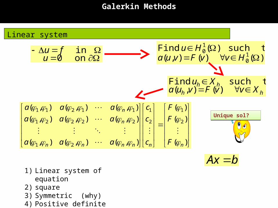
Linear system
hh
hhXvvFvua
Xu
)(),(
such that Find
)(
)(
)(
),(),(),(
),(),(),(
),(),(),(
2
1
2
1
21
22221
11211
nnnnnn
n
n
F
F
F
c
c
c
aaa
aaa
aaa
)( )(),(such that )( Find
10
10
HvvFvuaHu
1) Linear system of equation2) square3) Symmetric (why)4) Positive definite
bAx
Unique sol?Unique sol?
on 0 in
ufu

Finite Element Methods
Finite Element Methods
hh
hhXvvFvua
Xu
)(),(
such that Find
)1,0()1,0(
on 0 with in function linear piecewise all of space
h vvX h
h
)(10 HX h
Example
whywhy
No of elements = 16No of nodes = 13No interior nodes = 5No of boundary nodes = 8
Triangulation

Finite Element Methods
1D Problem
0 10.25 0.5 0.75
)(1 x
0 10.25 0.5 0.75
)(2 x
0 10.25 0.5 0.75
)(3 x
1
1
1

Global basis functions
0 with in
function linear piecewise
all of space
honv
v
X h
} , ,,, { 54321 spanX h
h0S

1
2
3
4
5
6
78
9
1011
12
13
1312111050 ,,,, SpanS h
Element Labeling
14
15
16

Node Labeling (global labeling)
12
3 4
5
6
7
8
9
1011
12 13
1312111050 ,,,, SpanS h

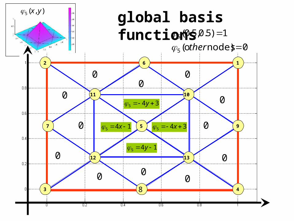
global basis functions
12
3 4
5
6
7
8
9
1011
12 13
1312111050 ,,,, SpanS h
),(5 yx
0)nodes o(
1)5.0,5.0(
5
5
ther

12
3 4
5
6
7
8
9
1011
12 13
1312111050 ,,,, SpanS h
),(10 yx
0)nodes o(
1)75.0,75.0(
10
10
ther
global basis functions

Global basis functions
global basis functions),(5 yx
0)nodes o(
1)5.0,5.0(
5
5
ther
12
3 4
6
7
8
9345 x
0
0
0
0
0
0
0
0
0
0
0 0
145 x
345 y1011
5
145 y1312
1
23
4
56
78
910
1112
13
14
15
16
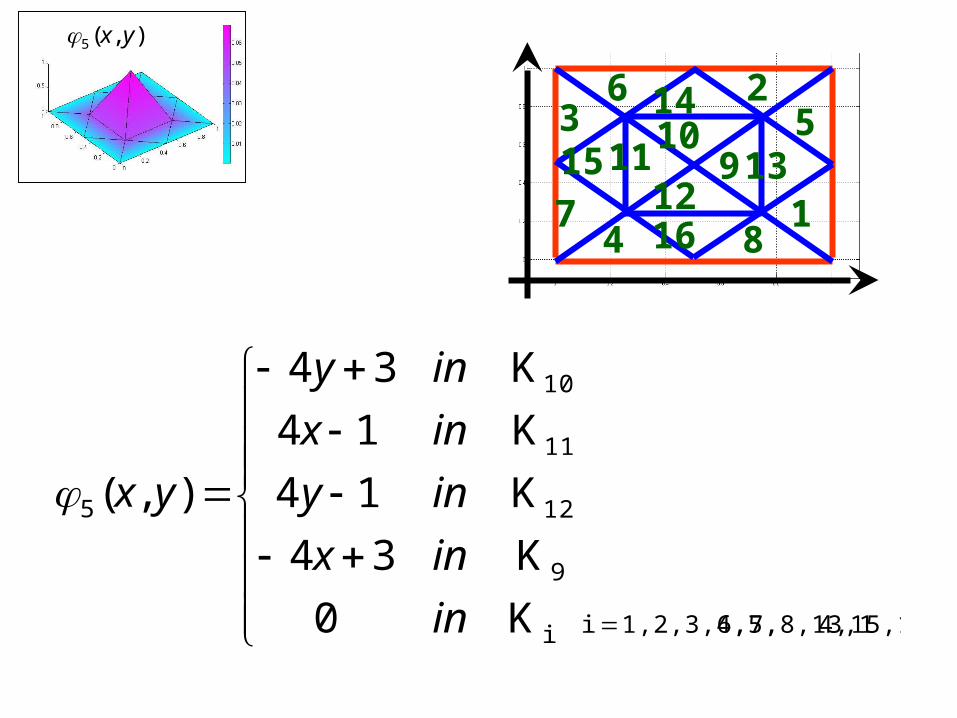
),(5 yx
4,15,166,7,8,13,11,2,3,4,5,ii
9
12
11
10
5
K0
K34
K14
K14
K34
),(
in
inx
iny
inx
iny
yx

global basis functions),(10 yx
0)nodes o(
1)75.0,75.0(
10
10
ther
12
3 4
6
7
8
910
0
0
0
0
0
0
0 0
1011
5
1312
0
0 10
10
10
10
10

)l(
)l(
)l(
)l(
)l(
c13
c12
c11
c10
c5
*****13
*****12
*****11
*****10
*****5
131211105
13
12
11
10
5
1
23
4
56
78
910
1112
13
14
15
16
12
3 4
5
6
7
8
9
1011
12 13
dxdya yyxx ,10,5,10,5105 ),(
109
,10,5,10,5,10,5,10,5
K
yyxx
K
yyxx dxdydxdy
16
1,10,5,10,5
i K
yyxx
i
dxdy
Assemble linear system

)l(
)l(
)l(
)l(
)l(
c13
c12
c11
c10
c5
*****13
*****12
*****11
*****10
*****5
131211105
13
12
11
10
5
dxdya yyxx ,10,5,10,5105 ),(
109
,10,5,10,5,10,5,10,5
K
yyxx
K
yyxx dxdydxdy
Assemble linear system
12
3 4
6
7
8
9345 x
0
0
0
0
0
0
0
0
0
0
0 0
145 x
345 y1011
5
145 y
1312
),(5 yx
12
3 4
6
7
8
9222 yx
0
00
0
00
0 0
1011
5
1312 00 10
10 10
10
),(10 yx
222 yx
999
8)2()4()2()0(KKK
dxdydxdy
101010
8)2()0()2()4(KKK
dxdydxdy
1
1
),( 1210 a

Finite Element Methods
HomeWork:
)(
)(
)(
),(),(),(
),(),(),(
),(),(),(
2
1
2
1
21
22221
11211
nnnnnn
n
n
F
F
F
c
c
c
aaa
aaa
aaa
bAx
Compute the matrix A and the vector b then solve the linear system and write the solution as a linear combination of the basis then approximate the value of the function at (x,y)= (0.3,0.3) and (0.7,0.7) . can you find the analytic solution of the problem?
where f(x)= x(x-1)y(y-1) with pcw-linear
on 0 in
ufu

Approximation of u
10
20
30
40
50.069
60
70
80
90
100.049
110.049
120.049
130.049
u

X-coordinate and y-coordinate
Matrix p(2,#elements)
12345678910111213
x10010.50.500.510.750.250.250.75
y11000.510.500.50.750.750.250.25p
Matlab matrices (computation info)

Boundary node
vector e(#boundary node)
e1e2e3e4e5e6e7e8
start12346789
end67892341e
131211105nodeinterior
Matlab matrices (computation info)

Node Label (local labeling)
1 2
3
Each triangle has 3 nodes. Label them locally inside the triangle
Matlab matrices (computation info)

Node and Element LabelMatlab matrices (computation info)

Local label .vs. global label
Matrix t(3,#elements)
12345678910111213141516
141231234555510111213
29678101112131310111213101112
3131011129678101112139678
t
Matlab matrices (computation info)
Related Documents


