BUSINESS STATISTICS OpenStax University of Oklahoma & De Anza College

Welcome message from author
This document is posted to help you gain knowledge. Please leave a comment to let me know what you think about it! Share it to your friends and learn new things together.
Transcript
BUSINESS STATISTICS
OpenStaxUniversity of Oklahoma & De Anza College
Book: Business Statistics (OpenStax)

This text is disseminated via the Open Education Resource (OER) LibreTexts Project (https://LibreTexts.org) and like thehundreds of other texts available within this powerful platform, it is freely available for reading, printing and"consuming." Most, but not all, pages in the library have licenses that may allow individuals to make changes, save, andprint this book. Carefully consult the applicable license(s) before pursuing such effects.
Instructors can adopt existing LibreTexts texts or Remix them to quickly build course-specific resources to meet the needsof their students. Unlike traditional textbooks, LibreTexts’ web based origins allow powerful integration of advancedfeatures and new technologies to support learning.
The LibreTexts mission is to unite students, faculty and scholars in a cooperative effort to develop an easy-to-use onlineplatform for the construction, customization, and dissemination of OER content to reduce the burdens of unreasonabletextbook costs to our students and society. The LibreTexts project is a multi-institutional collaborative venture to developthe next generation of open-access texts to improve postsecondary education at all levels of higher learning by developingan Open Access Resource environment. The project currently consists of 14 independently operating and interconnectedlibraries that are constantly being optimized by students, faculty, and outside experts to supplant conventional paper-basedbooks. These free textbook alternatives are organized within a central environment that is both vertically (from advance tobasic level) and horizontally (across different fields) integrated.
The LibreTexts libraries are Powered by MindTouch and are supported by the Department of Education Open TextbookPilot Project, the UC Davis Office of the Provost, the UC Davis Library, the California State University AffordableLearning Solutions Program, and Merlot. This material is based upon work supported by the National Science Foundationunder Grant No. 1246120, 1525057, and 1413739. Unless otherwise noted, LibreTexts content is licensed by CC BY-NC-SA 3.0.
Any opinions, findings, and conclusions or recommendations expressed in this material are those of the author(s) and donot necessarily reflect the views of the National Science Foundation nor the US Department of Education.
Have questions or comments? For information about adoptions or adaptions contact [email protected]. Moreinformation on our activities can be found via Facebook (https://facebook.com/Libretexts), Twitter(https://twitter.com/libretexts), or our blog (http://Blog.Libretexts.org).
This text was compiled on 01/07/2022
®
1 1/7/2022
TABLE OF CONTENTSIntroductory Business Statistics is designed to meet the scope and sequence requirements of the one-semester statistics course forbusiness, economics, and related majors. Core statistical concepts and skills have been augmented with practical business examples,scenarios, and exercises. The result is a meaningful understanding of the discipline, which will serve students in their business careersand real-world experiences.
1: SAMPLING AND DATA1.0: INTRODUCTION TO SAMPLING AND DATA1.1: DEFINITIONS OF STATISTICS, PROBABILITY, AND KEY TERMS1.2: DATA, SAMPLING, AND VARIATION IN DATA AND SAMPLING1.3: LEVELS OF MEASUREMENT1.4: EXPERIMENTAL DESIGN AND ETHICS1.5: CHAPTER KEY TERMS1.6: CHAPTER REFERENCES1.H: SAMPLING AND DATA (HOMEWORK)1.R: SAMPLING AND DATA (REVIEW)1.S: SAMPLING AND DATA (SOLUTIONS)
2: DESCRIPTIVE STATISTICS2.0: INTRODUCTION TO DESCRIPTIVE STATISTICS2.1: DISPLAY DATA2.2: MEASURES OF THE LOCATION OF THE DATA2.3: MEASURES OF THE CENTER OF THE DATA2.4: SIGMA NOTATION AND CALCULATING THE ARITHMETIC MEAN2.5: GEOMETRIC MEAN2.6: SKEWNESS AND THE MEAN, MEDIAN, AND MODE2.7: MEASURES OF THE SPREAD OF THE DATA2.8: HOMEWORK2.9: CHAPTER FORMULA REVIEW2.10: CHAPTER HOMEWORK2.11: CHAPTER KEY TERMS2.12: CHAPTER REFERENCES2.13: CHAPTER HOMEWORK SOLUTIONS2.14: CHAPTER PRACTICE2.R: DESCRIPTIVE STATISTICS (REVIEW)
3: PROBABILITY TOPICS3.0: INTRODUCTION TO PROBABILITY3.1: PROBABILITY TERMINOLOGY3.2: INDEPENDENT AND MUTUALLY EXCLUSIVE EVENTS3.3: TWO BASIC RULES OF PROBABILITY3.4: CONTINGENCY TABLES AND PROBABILITY TREES3.5: VENN DIAGRAMS3.6: CHAPTER FORMULA REVIEW3.7: CHAPTER HOMEWORK3.8: CHAPTER KEY TERMS3.9: CHAPTER MORE PRACTICE3.10: CHAPTER PRACTICE3.11: CHAPTER REFERENCE3.12: CHAPTER REVIEW3.13: CHAPTER SOLUTION (PRACTICE + HOMEWORK)
4: DISCRETE RANDOM VARIABLES4.0: INTRODUCTION TO DISCRETE RANDOM VARIABLES4.1: HYPERGEOMETRIC DISTRIBUTION
2 1/7/2022
4.2: BINOMIAL DISTRIBUTION4.3: GEOMETRIC DISTRIBUTION4.4: POISSON DISTRIBUTION4.5: CHAPTER FORMULA REVIEW4.6: CHAPTER HOMEWORK4.7: CHAPTER KEY ITEMS4.8: CHAPTER PRACTICE4.9: CHAPTER REFERENCES4.10: CHAPTER REVIEW4.11: CHAPTER SOLUTION (PRACTICE + HOMEWORK)
5: CONTINUOUS RANDOM VARIABLES5.0: PRELUDE TO CONTINUOUS RANDOM VARIABLES5.1: PROPERTIES OF CONTINUOUS PROBABILITY DENSITY FUNCTIONS5.2: THE UNIFORM DISTRIBUTION5.3: THE EXPONENTIAL DISTRIBUTION5.4: CHAPTER FORMULA REVIEW5.5: CHAPTER HOMEWORK5.6: CHAPTER KEY TERMS5.7: CHAPTER PRACTICE5.8: CHAPTER REFERENCES5.9: CHAPTER REVIEW5.10: CHAPTER SOLUTION (PRACTICE + HOMEWORK)
6: THE NORMAL DISTRIBUTION6.0: INTRODUCTION TO NORMAL DISTRIBUTION6.1: THE STANDARD NORMAL DISTRIBUTION6.2: USING THE NORMAL DISTRIBUTION6.3: ESTIMATING THE BINOMIAL WITH THE NORMAL DISTRIBUTION6.4: CHAPTER FORMULA REVIEW6.5: CHAPTER HOMEWORK6.6: CHAPTER KEY ITEMS6.7: CHAPTER PRACTICE6.8: CHAPTER REFERENCES6.9: CHAPTER REVIEW6.10: CHAPTER SOLUTION (PRACTICE + HOMEWORK)
7: THE CENTRAL LIMIT THEOREM7.0: INTRODUCTION TO THE CENTRAL LIMIT THEOREM7.1: THE CENTRAL LIMIT THEOREM FOR SAMPLE MEANS7.2: USING THE CENTRAL LIMIT THEOREM7.3: THE CENTRAL LIMIT THEOREM FOR PROPORTIONS7.4: FINITE POPULATION CORRECTION FACTOR7.5: CHAPTER FORMULA REVIEW7.6: CHAPTER HOMEWORK7.7: CHAPTER KEY TERMS7.8: CHAPTER PRACTICE7.9: CHAPTER REFERENCES7.10: CHAPTER REVIEW7.11: CHAPTER SOLUTION (PRACTICE + HOMEWORK)
8: CONFIDENCE INTERVALS8.0: INTRODUCTION TO CONFIDENCE INTERVALS8.1: A CONFIDENCE INTERVAL FOR A POPULATION STANDARD DEVIATION, KNOWN OR LARGE SAMPLE SIZE8.2: A CONFIDENCE INTERVAL FOR A POPULATION STANDARD DEVIATION UNKNOWN, SMALL SAMPLE CASE8.3: A CONFIDENCE INTERVAL FOR A POPULATION PROPORTION8.4: CALCULATING THE SAMPLE SIZE N- CONTINUOUS AND BINARY RANDOM VARIABLES8.5: CHAPTER FORMULA REVIEW8.6: CHAPTER HOMEWORK
3 1/7/2022
8.7: CHAPTER KEY TERMS8.8: CHAPTER PRACTICE8.9: CHAPTER REFERENCES8.10: CHAPTER REVIEW8.11: CHAPTER SOLUTION (PRACTICE + HOMEWORK)
9: HYPOTHESIS TESTING WITH ONE SAMPLE9.0: INTRODUCTION TO HYPOTHESIS TESTING9.1: NULL AND ALTERNATIVE HYPOTHESES9.2: OUTCOMES AND THE TYPE I AND TYPE II ERRORS9.3: DISTRIBUTION NEEDED FOR HYPOTHESIS TESTING9.4: FULL HYPOTHESIS TEST EXAMPLES9.5: CHAPTER FORMULA REVIEW9.6: CHAPTER HOMEWORK9.7: CHAPTER KEY TERMS9.8: CHAPTER PRACTICE9.9: CHAPTER REFERENCES9.10: CHAPTER REVIEW9.11: CHAPTER SOLUTION (PRACTICE + HOMEWORK)
10: HYPOTHESIS TESTING WITH TWO SAMPLES10.0: INTRODUCTION10.1: COMPARING TWO INDEPENDENT POPULATION MEANS10.2: COHEN'S STANDARDS FOR SMALL, MEDIUM, AND LARGE EFFECT SIZES10.3: TEST FOR DIFFERENCES IN MEANS- ASSUMING EQUAL POPULATION VARIANCES10.4: COMPARING TWO INDEPENDENT POPULATION PROPORTIONS10.5: TWO POPULATION MEANS WITH KNOWN STANDARD DEVIATIONS10.6: MATCHED OR PAIRED SAMPLES10.7: HOMEWORK10.8: CHAPTER FORMULA REVIEW10.9: CHAPTER HOMEWORK10.10: CHAPTER KEY TERMS10.11: CHAPTER PRACTICE10.12: CHAPTER REFERENCES10.13: CHAPTER REVIEW10.14: CHAPTER SOLUTION (PRACTICE + HOMEWORK)
11: THE CHI-SQUARE DISTRIBUTION11.0: PRELUDE TO THE CHI-SQUARE DISTRIBUTION11.1: FACTS ABOUT THE CHI-SQUARE DISTRIBUTION11.2: TEST OF A SINGLE VARIANCE11.3: GOODNESS-OF-FIT TEST11.4: TEST OF INDEPENDENCE11.5: TEST FOR HOMOGENEITY11.6: COMPARISON OF THE CHI-SQUARE TESTS11.7: HOMEWORK11.8: CHAPTER FORMULA REVIEW11.9: CHAPTER HOMEWORK11.10: CHAPTER KEY TERMS11.11: CHAPTER PRACTICE11.12: CHAPTER REFERENCES11.13: CHAPTER REVIEW11.14: CHAPTER SOLUTION (PRACTICE + HOMEWORK)
12: F DISTRIBUTION AND ONE-WAY ANOVA12.0: INTRODUCTION TO F DISTRIBUTION AND ONE-WAY ANOVA12.1: TEST OF TWO VARIANCES12.2: ONE-WAY ANOVA12.3: THE F DISTRIBUTION AND THE F-RATIO
4 1/7/2022
12.4: FACTS ABOUT THE F DISTRIBUTION12.5: CHAPTER FORMULA REVIEW12.6: CHAPTER HOMEWORK12.7: CHAPTER KEY TERMS12.8: CHAPTER PRACTICE12.9: CHAPTER REFERENCE12.10: CHAPTER REVIEW12.11: CHAPTER SOLUTION (PRACTICE + HOMEWORK)
13: LINEAR REGRESSION AND CORRELATION13.0: INTRODUCTION TO LINEAR REGRESSION AND CORRELATION13.1: THE CORRELATION COEFFICIENT R13.2: TESTING THE SIGNIFICANCE OF THE CORRELATION COEFFICIENT13.3: LINEAR EQUATIONS13.4: THE REGRESSION EQUATION13.5: INTERPRETATION OF REGRESSION COEFFICIENTS- ELASTICITY AND LOGARITHMIC TRANSFORMATION13.6: PREDICTING WITH A REGRESSION EQUATION13.7: CHAPTER KEY TERMS13.8: CHAPTER PRACTICE13.9: CHAPTER REVIEW13.10: CHAPTER SOLUTION13.11: HOW TO USE MICROSOFT EXCEL® FOR REGRESSION ANALYSIS
14: APPPENDICES14.0: B | MATHEMATICAL PHRASES, SYMBOLS, AND FORMULAS14.1: A | STATISTICAL TABLES
BACK MATTERINDEXGLOSSARY

1 1/7/2022
CHAPTER OVERVIEW1: SAMPLING AND DATA
1.0: INTRODUCTION TO SAMPLING AND DATA1.1: DEFINITIONS OF STATISTICS, PROBABILITY, AND KEY TERMS1.2: DATA, SAMPLING, AND VARIATION IN DATA AND SAMPLING1.3: LEVELS OF MEASUREMENT1.4: EXPERIMENTAL DESIGN AND ETHICS1.5: CHAPTER KEY TERMS1.6: CHAPTER REFERENCES1.H: SAMPLING AND DATA (HOMEWORK)1.R: SAMPLING AND DATA (REVIEW)1.S: SAMPLING AND DATA (SOLUTIONS)

Alexander Holms, Barbara Illowsky, & Susan Dean 1.0.1 12/10/2021 https://stats.libretexts.org/@go/page/5472
1.0: Introduction to Sampling and DataYou are probably asking yourself the question, "When and where will I use statistics?" If you read any newspaper, watchtelevision, or use the Internet, you will see statistical information. There are statistics about crime, sports, education,politics, and real estate. Typically, when you read a newspaper article or watch a television news program, you are givensample information. With this information, you may make a decision about the correctness of a statement, claim, or "fact."Statistical methods can help you make the "best educated guess."
Figure We encounter statistics in our daily lives more often than we probably realize and from many differentsources, like the news. (credit: David Sim)
Since you will undoubtedly be given statistical information at some point in your life, you need to know some techniquesfor analyzing the information thoughtfully. Think about buying a house or managing a budget. Think about your chosenprofession. The fields of economics, business, psychology, education, biology, law, computer science, police science, andearly childhood development require at least one course in statistics.
Included in this chapter are the basic ideas and words of probability and statistics. You will soon understand that statisticsand probability work together. You will also learn how data are gathered and what "good" data can be distinguished from"bad."
1.0.1
Alexander Holms, Barbara Illowsky, & Susan Dean 1.1.1 12/31/2021 https://stats.libretexts.org/@go/page/4540
1.1: Definitions of Statistics, Probability, and Key TermsThe science of statistics deals with the collection, analysis, interpretation, and presentation of data. We see and use data inour everyday lives.
In this course, you will learn how to organize and summarize data. Organizing and summarizing data is called descriptivestatistics. Two ways to summarize data are by graphing and by using numbers (for example, finding an average). Afteryou have studied probability and probability distributions, you will use formal methods for drawing conclusions from"good" data. The formal methods are called inferential statistics. Statistical inference uses probability to determine howconfident we can be that our conclusions are correct.
Effective interpretation of data (inference) is based on good procedures for producing data and thoughtful examination ofthe data. You will encounter what will seem to be too many mathematical formulas for interpreting data. The goal ofstatistics is not to perform numerous calculations using the formulas, but to gain an understanding of your data. Thecalculations can be done using a calculator or a computer. The understanding must come from you. If you can thoroughlygrasp the basics of statistics, you can be more confident in the decisions you make in life.
Probability
Probability is a mathematical tool used to study randomness. It deals with the chance (the likelihood) of an eventoccurring. For example, if you toss a fair coin four times, the outcomes may not be two heads and two tails. However, ifyou toss the same coin 4,000 times, the outcomes will be close to half heads and half tails. The expected theoreticalprobability of heads in any one toss is or 0.5. Even though the outcomes of a few repetitions are uncertain, there is aregular pattern of outcomes when there are many repetitions. After reading about the English statistician Karl Pearsonwho tossed a coin 24,000 times with a result of 12,012 heads, one of the authors tossed a coin 2,000 times. The resultswere 996 heads. The fraction is equal to 0.498 which is very close to 0.5, the expected probability.
The theory of probability began with the study of games of chance such as poker. Predictions take the form ofprobabilities. To predict the likelihood of an earthquake, of rain, or whether you will get an A in this course, we useprobabilities. Doctors use probability to determine the chance of a vaccination causing the disease the vaccination issupposed to prevent. A stockbroker uses probability to determine the rate of return on a client's investments. You might useprobability to decide to buy a lottery ticket or not. In your study of statistics, you will use the power of mathematicsthrough probability calculations to analyze and interpret your data.
Key Terms
In statistics, we generally want to study a population. You can think of a population as a collection of persons, things, orobjects under study. To study the population, we select a sample. The idea of sampling is to select a portion (or subset) ofthe larger population and study that portion (the sample) to gain information about the population. Data are the result ofsampling from a population.
Because it takes a lot of time and money to examine an entire population, sampling is a very practical technique. If youwished to compute the overall grade point average at your school, it would make sense to select a sample of students whoattend the school. The data collected from the sample would be the students' grade point averages. In presidential elections,opinion poll samples of 1,000–2,000 people are taken. The opinion poll is supposed to represent the views of the people inthe entire country. Manufacturers of canned carbonated drinks take samples to determine if a 16 ounce can contains 16ounces of carbonated drink.
From the sample data, we can calculate a statistic. A statistic is a number that represents a property of the sample. Forexample, if we consider one math class to be a sample of the population of all math classes, then the average number ofpoints earned by students in that one math class at the end of the term is an example of a statistic. The statistic is anestimate of a population parameter, in this case the mean. A parameter is a numerical characteristic of the wholepopulation that can be estimated by a statistic. Since we considered all math classes to be the population, then the averagenumber of points earned per student over all the math classes is an example of a parameter.
One of the main concerns in the field of statistics is how accurately a statistic estimates a parameter. The accuracy reallydepends on how well the sample represents the population. The sample must contain the characteristics of the population
1
2
996
2000
Alexander Holms, Barbara Illowsky, & Susan Dean 1.1.2 12/31/2021 https://stats.libretexts.org/@go/page/4540
in order to be a representative sample. We are interested in both the sample statistic and the population parameter ininferential statistics. In a later chapter, we will use the sample statistic to test the validity of the established populationparameter.
A variable, or random variable, usually notated by capital letters such as and , is a characteristic or measurement thatcan be determined for each member of a population. Variables may be numerical or categorical. Numerical variablestake on values with equal units such as weight in pounds and time in hours. Categorical variables place the person orthing into a category. If we let equal the number of points earned by one math student at the end of a term, then is anumerical variable. If we let be a person's party affiliation, then some examples of include Republican, Democrat,and Independent. is a categorical variable. We could do some math with values of (calculate the average number ofpoints earned, for example), but it makes no sense to do math with values of (calculating an average party affiliationmakes no sense).
Data are the actual values of the variable. They may be numbers or they may be words. Datum is a single value.
Two words that come up often in statistics are mean and proportion. If you were to take three exams in your math classesand obtain scores of 86, 75, and 92, you would calculate your mean score by adding the three exam scores and dividing bythree (your mean score would be 84.3 to one decimal place). If, in your math class, there are 40 students and 22 are menand 18 are women, then the proportion of men students is and the proportion of women students is . Mean andproportion are discussed in more detail in later chapters.
The words "mean" and "average" are often used interchangeably. The substitution of one word for the other iscommon practice. The technical term is "arithmetic mean," and "average" is technically a center location. However, inpractice among non-statisticians, "average" is commonly accepted for "arithmetic mean."
Determine what the key terms refer to in the following study. We want to know the average (mean) amount of moneyfirst year college students spend at ABC College on school supplies that do not include books. We randomly surveyed100 first year students at the college. Three of those students spent $150, $200, and $225, respectively.
Answer
Solution 1.1
The population is all first year students attending ABC College this term.
The sample could be all students enrolled in one section of a beginning statistics course at ABC College (althoughthis sample may not represent the entire population).
The parameter is the average (mean) amount of money spent (excluding books) by first year college students atABC College this term: the population mean.
The statistic is the average (mean) amount of money spent (excluding books) by first year college students in thesample.
The variable could be the amount of money spent (excluding books) by one first year student. Let = the amountof money spent (excluding books) by one first year student attending ABC College.
The data are the dollar amounts spent by the first year students. Examples of the data are $150, $200, and $225.
Determine what the key terms refer to in the following study. We want to know the average (mean) amount of moneyspent on school uniforms each year by families with children at Knoll Academy. We randomly survey 100 familieswith children in the school. Three of the families spent $65, $75, and $95, respectively.
X Y
X X
Y Y
Y X
Y
22
40
18
40
NOTE
Example 1.1
X
Exercise 1.1
Alexander Holms, Barbara Illowsky, & Susan Dean 1.1.3 12/31/2021 https://stats.libretexts.org/@go/page/4540
Determine what the key terms refer to in the following study.
A study was conducted at a local college to analyze the average cumulative GPA’s of students who graduated last year.Fill in the letter of the phrase that best describes each of the items below.
1. Population ____ 2. Statistic ____ 3. Parameter ____ 4. Sample ____ 5. Variable ____ 6. Data ____
a. all students who attended the college last yearb. the cumulative GPA of one student who graduated from the college last yearc. 3.65, 2.80, 1.50, 3.90d. a group of students who graduated from the college last year, randomly selectede. the average cumulative GPA of students who graduated from the college last yearf. all students who graduated from the college last yearg. the average cumulative GPA of students in the study who graduated from the college last year
Answer
Solution 1.2
1. f; 2. g; 3. e; 4. d; 5. b; 6. c
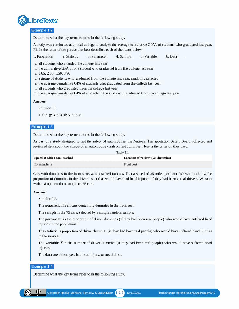
Determine what the key terms refer to in the following study.
As part of a study designed to test the safety of automobiles, the National Transportation Safety Board collected andreviewed data about the effects of an automobile crash on test dummies. Here is the criterion they used:
Speed at which cars crashed Location of “drive” (i.e. dummies)
35 miles/hour Front Seat
Table 1.1
Cars with dummies in the front seats were crashed into a wall at a speed of 35 miles per hour. We want to know theproportion of dummies in the driver’s seat that would have had head injuries, if they had been actual drivers. We startwith a simple random sample of 75 cars.
Answer
Solution 1.3
The population is all cars containing dummies in the front seat.
The sample is the 75 cars, selected by a simple random sample.
The parameter is the proportion of driver dummies (if they had been real people) who would have suffered headinjuries in the population.
The statistic is proportion of driver dummies (if they had been real people) who would have suffered head injuriesin the sample.
The variable = the number of driver dummies (if they had been real people) who would have suffered headinjuries.
The data are either: yes, had head injury, or no, did not.
Determine what the key terms refer to in the following study.
Example 1.2
Example 1.3
X
Example 1.4
Alexander Holms, Barbara Illowsky, & Susan Dean 1.1.4 12/31/2021 https://stats.libretexts.org/@go/page/4540
An insurance company would like to determine the proportion of all medical doctors who have been involved in one ormore malpractice lawsuits. The company selects 500 doctors at random from a professional directory and determinesthe number in the sample who have been involved in a malpractice lawsuit.
Answer
Solution 1.4
The population is all medical doctors listed in the professional directory.
The parameter is the proportion of medical doctors who have been involved in one or more malpractice suits inthe population.
The sample is the 500 doctors selected at random from the professional directory.
The statistic is the proportion of medical doctors who have been involved in one or more malpractice suits in thesample.
The variable = the number of medical doctors who have been involved in one or more malpractice suits.
The data are either: yes, was involved in one or more malpractice lawsuits, or no, was not.
X
Alexander Holms, Barbara Illowsky, & Susan Dean 1.2.1 12/17/2021 https://stats.libretexts.org/@go/page/4541
1.2: Data, Sampling, and Variation in Data and SamplingData may come from a population or from a sample. Lowercase letters like or generally are used to represent datavalues. Most data can be put into the following categories:
QualitativeQuantitative
Qualitative data are the result of categorizing or describing attributes of a population. Qualitative data are also oftencalled categorical data. Hair color, blood type, ethnic group, the car a person drives, and the street a person lives on areexamples of qualitative(categorical) data. Qualitative(categorical) data are generally described by words or letters. Forinstance, hair color might be black, dark brown, light brown, blonde, gray, or red. Blood type might be AB+, O-, or B+.Researchers often prefer to use quantitative data over qualitative(categorical) data because it lends itself more easily tomathematical analysis. For example, it does not make sense to find an average hair color or blood type.
Quantitative data are always numbers. Quantitative data are the result of counting or measuring attributes of apopulation. Amount of money, pulse rate, weight, number of people living in your town, and number of students who takestatistics are examples of quantitative data. Quantitative data may be either discrete or continuous.
All data that are the result of counting are called quantitative discrete data. These data take on only certain numericalvalues. If you count the number of phone calls you receive for each day of the week, you might get values such as zero,one, two, or three.
Data that are not only made up of counting numbers, but that may include fractions, decimals, or irrational numbers, arecalled quantitative continuous data. Continuous data are often the results of measurements like lengths, weights, ortimes. A list of the lengths in minutes for all the phone calls that you make in a week, with numbers like 2.4, 7.5, or 11.0,would be quantitative continuous data.
The data are the number of books students carry in their backpacks. You sample five students. Two students carry threebooks, one student carries four books, one student carries two books, and one student carries one book. The numbersof books (three, four, two, and one) are the quantitative discrete data.
The data are the number of machines in a gym. You sample five gyms. One gym has 12 machines, one gym has 15machines, one gym has ten machines, one gym has 22 machines, and the other gym has 20 machines. What type ofdata is this?
The data are the weights of backpacks with books in them. You sample the same five students. The weights (inpounds) of their backpacks are 6.2, 7, 6.8, 9.1, 4.3. Notice that backpacks carrying three books can have differentweights. Weights are quantitative continuous data.
The data are the areas of lawns in square feet. You sample five houses. The areas of the lawns are 144 sq. feet, 160 sq.feet, 190 sq. feet, 180 sq. feet, and 210 sq. feet. What type of data is this?
You go to the supermarket and purchase three cans of soup (19 ounces) tomato bisque, 14.1 ounces lentil, and 19ounces Italian wedding), two packages of nuts (walnuts and peanuts), four different kinds of vegetable (broccoli,
x y
Example : DATA SAMPLE OF QUANTITATIVE DISCRETE DATA1.2.1
Exercise 1.2.1
Example : DATA SAMPLE OF QUANTITATIVE CONTINUOUS DATA1.2.2
Exercise 1.2.2
Example 1.2.3
Alexander Holms, Barbara Illowsky, & Susan Dean 1.2.2 12/17/2021 https://stats.libretexts.org/@go/page/4541
cauliflower, spinach, and carrots), and two desserts (16 ounces pistachio ice cream and 32 ounces chocolate chipcookies).
Name data sets that are quantitative discrete, quantitative continuous, and qualitative(categorical).
Answer
One Possible Solution:
The three cans of soup, two packages of nuts, four kinds of vegetables and two desserts are quantitative discretedata because you count them.The weights of the soups (19 ounces, 14.1 ounces, 19 ounces) are quantitative continuous data because youmeasure weights as precisely as possible.Types of soups, nuts, vegetables and desserts are qualitative(categorical) data because they are categorical.
Try to identify additional data sets in this example.
The data are the colors of backpacks. Again, you sample the same five students. One student has a red backpack, twostudents have black backpacks, one student has a green backpack, and one student has a gray backpack. The colorsred, black, black, green, and gray are qualitative(categorical) data.
The data are the colors of houses. You sample five houses. The colors of the houses are white, yellow, white, red, andwhite. What type of data is this?
You may collect data as numbers and report it categorically. For example, the quiz scores for each student are recordedthroughout the term. At the end of the term, the quiz scores are reported as A, B, C, D, or F
Work collaboratively to determine the correct data type (quantitative or qualitative). Indicate whether quantitative dataare continuous or discrete. Hint: Data that are discrete often start with the words "the number of."
a. the number of pairs of shoes you ownb. the type of car you drivec. the distance from your home to the nearest grocery stored. the number of classes you take per school yeare. the type of calculator you usef. weights of sumo wrestlersg. number of correct answers on a quizh. IQ scores (This may cause some discussion.)
Answer
Items a, d, and g are quantitative discrete; items c, f, and h are quantitative continuous; items b and e arequalitative, or categorical.
Determine the correct data type (quantitative or qualitative) for the number of cars in a parking lot. Indicate whetherquantitative data are continuous or discrete.
Example 1.2.4
Exercise 1.2.4
Example 1.2.5
Exercise 1.2.5
Alexander Holms, Barbara Illowsky, & Susan Dean 1.2.3 12/17/2021 https://stats.libretexts.org/@go/page/4541
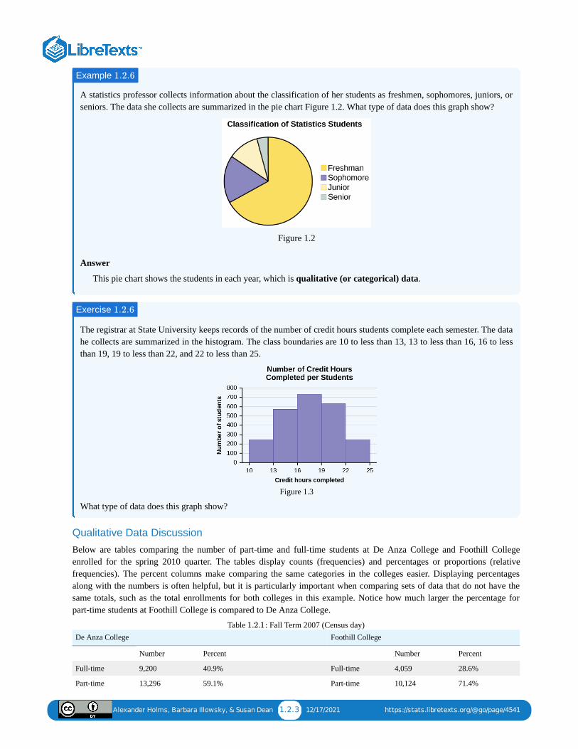
A statistics professor collects information about the classification of her students as freshmen, sophomores, juniors, orseniors. The data she collects are summarized in the pie chart Figure 1.2. What type of data does this graph show?
Figure 1.2
Answer
This pie chart shows the students in each year, which is qualitative (or categorical) data.
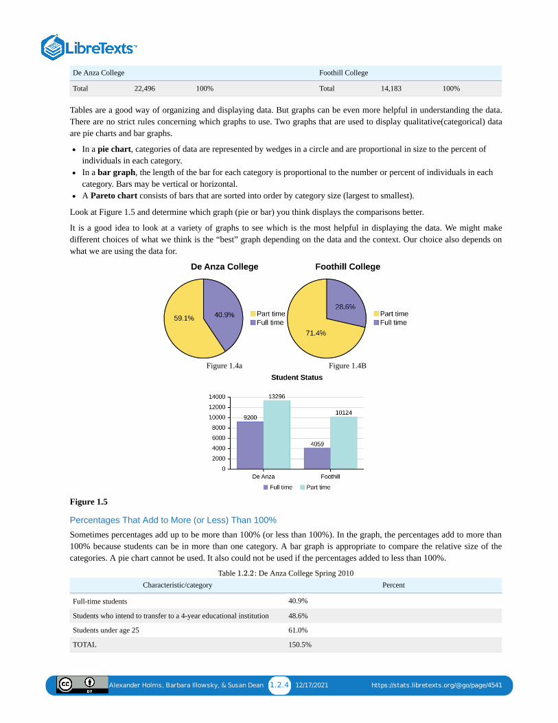
The registrar at State University keeps records of the number of credit hours students complete each semester. The datahe collects are summarized in the histogram. The class boundaries are 10 to less than 13, 13 to less than 16, 16 to lessthan 19, 19 to less than 22, and 22 to less than 25.
Figure 1.3
What type of data does this graph show?
Qualitative Data Discussion
Below are tables comparing the number of part-time and full-time students at De Anza College and Foothill Collegeenrolled for the spring 2010 quarter. The tables display counts (frequencies) and percentages or proportions (relativefrequencies). The percent columns make comparing the same categories in the colleges easier. Displaying percentagesalong with the numbers is often helpful, but it is particularly important when comparing sets of data that do not have thesame totals, such as the total enrollments for both colleges in this example. Notice how much larger the percentage forpart-time students at Foothill College is compared to De Anza College.
Table : Fall Term 2007 (Census day)De Anza College Foothill College
Number Percent Number Percent
Full-time 9,200 40.9% Full-time 4,059 28.6%
Part-time 13,296 59.1% Part-time 10,124 71.4%
Example 1.2.6
Exercise 1.2.6
1.2.1
Alexander Holms, Barbara Illowsky, & Susan Dean 1.2.4 12/17/2021 https://stats.libretexts.org/@go/page/4541
De Anza College Foothill College
Total 22,496 100% Total 14,183 100%
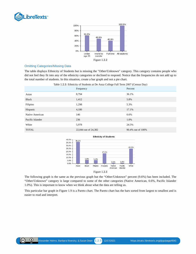
Tables are a good way of organizing and displaying data. But graphs can be even more helpful in understanding the data.There are no strict rules concerning which graphs to use. Two graphs that are used to display qualitative(categorical) dataare pie charts and bar graphs.
In a pie chart, categories of data are represented by wedges in a circle and are proportional in size to the percent ofindividuals in each category.In a bar graph, the length of the bar for each category is proportional to the number or percent of individuals in eachcategory. Bars may be vertical or horizontal.A Pareto chart consists of bars that are sorted into order by category size (largest to smallest).
Look at Figure 1.5 and determine which graph (pie or bar) you think displays the comparisons better.
It is a good idea to look at a variety of graphs to see which is the most helpful in displaying the data. We might makedifferent choices of what we think is the “best” graph depending on the data and the context. Our choice also depends onwhat we are using the data for.
Figure 1.4a Figure 1.4B
Figure 1.5
Percentages That Add to More (or Less) Than 100%
Sometimes percentages add up to be more than 100% (or less than 100%). In the graph, the percentages add to more than100% because students can be in more than one category. A bar graph is appropriate to compare the relative size of thecategories. A pie chart cannot be used. It also could not be used if the percentages added to less than 100%.
Table : De Anza College Spring 2010Characteristic/category Percent
Full-time students 40.9%
Students who intend to transfer to a 4-year educational institution 48.6%
Students under age 25 61.0%
TOTAL 150.5%
1.2.2
Alexander Holms, Barbara Illowsky, & Susan Dean 1.2.5 12/17/2021 https://stats.libretexts.org/@go/page/4541
Figure
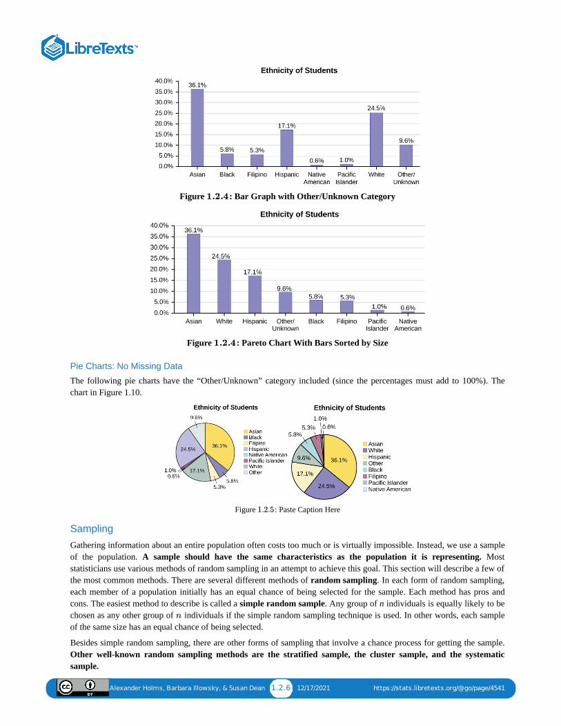
Omitting Categories/Missing Data
The table displays Ethnicity of Students but is missing the "Other/Unknown" category. This category contains people whodid not feel they fit into any of the ethnicity categories or declined to respond. Notice that the frequencies do not add up tothe total number of students. In this situation, create a bar graph and not a pie chart.
Table : Ethnicity of Students at De Anza College Fall Term 2007 (Census Day)Frequency Percent
Asian 8,794 36.1%
Black 1,412 5.8%
Filipino 1,298 5.3%
Hispanic 4,180 17.1%
Native American 146 0.6%
Pacific Islander 236 1.0%
White 5,978 24.5%
TOTAL 22,044 out of 24,382 90.4% out of 100%
Figure
The following graph is the same as the previous graph but the “Other/Unknown” percent (9.6%) has been included. The“Other/Unknown” category is large compared to some of the other categories (Native American, 0.6%, Pacific Islander1.0%). This is important to know when we think about what the data are telling us.
This particular bar graph in Figure 1.9 is a Pareto chart. The Pareto chart has the bars sorted from largest to smallest and iseasier to read and interpret.
1.2.2
1.2.3
1.2.3
Alexander Holms, Barbara Illowsky, & Susan Dean 1.2.6 12/17/2021 https://stats.libretexts.org/@go/page/4541
Figure : Bar Graph with Other/Unknown Category
Figure : Pareto Chart With Bars Sorted by Size
Pie Charts: No Missing Data
The following pie charts have the “Other/Unknown” category included (since the percentages must add to 100%). Thechart in Figure 1.10.
Figure : Paste Caption Here
Sampling
Gathering information about an entire population often costs too much or is virtually impossible. Instead, we use a sampleof the population. A sample should have the same characteristics as the population it is representing. Moststatisticians use various methods of random sampling in an attempt to achieve this goal. This section will describe a few ofthe most common methods. There are several different methods of random sampling. In each form of random sampling,each member of a population initially has an equal chance of being selected for the sample. Each method has pros andcons. The easiest method to describe is called a simple random sample. Any group of n individuals is equally likely to bechosen as any other group of individuals if the simple random sampling technique is used. In other words, each sampleof the same size has an equal chance of being selected.
Besides simple random sampling, there are other forms of sampling that involve a chance process for getting the sample.Other well-known random sampling methods are the stratified sample, the cluster sample, and the systematicsample.
1.2.4
1.2.4
1.2.5
n
Alexander Holms, Barbara Illowsky, & Susan Dean 1.2.7 12/17/2021 https://stats.libretexts.org/@go/page/4541
To choose a stratified sample, divide the population into groups called strata and then take a proportionate number fromeach stratum. For example, you could stratify (group) your college population by department and then choose aproportionate simple random sample from each stratum (each department) to get a stratified random sample. To choose asimple random sample from each department, number each member of the first department, number each member of thesecond department, and do the same for the remaining departments. Then use simple random sampling to chooseproportionate numbers from the first department and do the same for each of the remaining departments. Those numberspicked from the first department, picked from the second department, and so on represent the members who make up thestratified sample.
To choose a cluster sample, divide the population into clusters (groups) and then randomly select some of the clusters. Allthe members from these clusters are in the cluster sample. For example, if you randomly sample four departments fromyour college population, the four departments make up the cluster sample. Divide your college faculty by department. Thedepartments are the clusters. Number each department, and then choose four different numbers using simple randomsampling. All members of the four departments with those numbers are the cluster sample.
To choose a systematic sample, randomly select a starting point and take every piece of data from a listing of thepopulation. For example, suppose you have to do a phone survey. Your phone book contains 20,000 residence listings. Youmust choose 400 names for the sample. Number the population 1–20,000 and then use a simple random sample to pick anumber that represents the first name in the sample. Then choose every fiftieth name thereafter until you have a total of400 names (you might have to go back to the beginning of your phone list). Systematic sampling is frequently chosenbecause it is a simple method.
A type of sampling that is non-random is convenience sampling. Convenience sampling involves using results that arereadily available. For example, a computer software store conducts a marketing study by interviewing potential customerswho happen to be in the store browsing through the available software. The results of convenience sampling may be verygood in some cases and highly biased (favor certain outcomes) in others.
Sampling data should be done very carefully. Collecting data carelessly can have devastating results. Surveys mailed tohouseholds and then returned may be very biased (they may favor a certain group). It is better for the person conductingthe survey to select the sample respondents.
True random sampling is done with replacement. That is, once a member is picked, that member goes back into thepopulation and thus may be chosen more than once. However for practical reasons, in most populations, simple randomsampling is done without replacement. Surveys are typically done without replacement. That is, a member of thepopulation may be chosen only once. Most samples are taken from large populations and the sample tends to be small incomparison to the population. Since this is the case, sampling without replacement is approximately the same as samplingwith replacement because the chance of picking the same individual more than once with replacement is very low.
In a college population of 10,000 people, suppose you want to pick a sample of 1,000 randomly for a survey. For anyparticular sample of 1,000, if you are sampling with replacement,
the chance of picking the first person is 1,000 out of 10,000 (0.1000);the chance of picking a different second person for this sample is 999 out of 10,000 (0.0999);the chance of picking the same person again is 1 out of 10,000 (very low).
If you are sampling without replacement,
the chance of picking the first person for any particular sample is 1000 out of 10,000 (0.1000);the chance of picking a different second person is 999 out of 9,999 (0.0999);you do not replace the first person before picking the next person.
Compare the fractions 999/10,000 and 999/9,999. For accuracy, carry the decimal answers to four decimal places. To fourdecimal places, these numbers are equivalent (0.0999).
Sampling without replacement instead of sampling with replacement becomes a mathematical issue only when thepopulation is small. For example, if the population is 25 people, the sample is ten, and you are sampling with replacementfor any particular sample, then the chance of picking the first person is ten out of 25, and the chance of picking adifferent second person is nine out of 25 (you replace the first person).
nth
Alexander Holms, Barbara Illowsky, & Susan Dean 1.2.8 12/17/2021 https://stats.libretexts.org/@go/page/4541
If you sample without replacement, then the chance of picking the first person is ten out of 25, and then the chance ofpicking the second person (who is different) is nine out of 24 (you do not replace the first person).
Compare the fractions 9/25 and 9/24. To four decimal places, 9/25 = 0.3600 and 9/24 = 0.3750. To four decimal places,these numbers are not equivalent.
When you analyze data, it is important to be aware of sampling errors and nonsampling errors. The actual process ofsampling causes sampling errors. For example, the sample may not be large enough. Factors not related to the samplingprocess cause nonsampling errors. A defective counting device can cause a nonsampling error.
In reality, a sample will never be exactly representative of the population so there will always be some sampling error. As arule, the larger the sample, the smaller the sampling error.
In statistics, a sampling bias is created when a sample is collected from a population and some members of the populationare not as likely to be chosen as others (remember, each member of the population should have an equally likely chance ofbeing chosen). When a sampling bias happens, there can be incorrect conclusions drawn about the population that is beingstudied.
Critical Evaluation
We need to evaluate the statistical studies we read about critically and analyze them before accepting the results of thestudies. Common problems to be aware of include
Problems with samples: A sample must be representative of the population. A sample that is not representative of thepopulation is biased. Biased samples that are not representative of the population give results that are inaccurate andnot valid.Self-selected samples: Responses only by people who choose to respond, such as call-in surveys, are often unreliable.Sample size issues: Samples that are too small may be unreliable. Larger samples are better, if possible. In somesituations, having small samples is unavoidable and can still be used to draw conclusions. Examples: crash testing carsor medical testing for rare conditionsUndue influence: collecting data or asking questions in a way that influences the responseNon-response or refusal of subject to participate: The collected responses may no longer be representative of thepopulation. Often, people with strong positive or negative opinions may answer surveys, which can affect the results.Causality: A relationship between two variables does not mean that one causes the other to occur. They may be related(correlated) because of their relationship through a different variable.Self-funded or self-interest studies: A study performed by a person or organization in order to support their claim. Isthe study impartial? Read the study carefully to evaluate the work. Do not automatically assume that the study is good,but do not automatically assume the study is bad either. Evaluate it on its merits and the work done.Misleading use of data: improperly displayed graphs, incomplete data, or lack of contextConfounding: When the effects of multiple factors on a response cannot be separated. Confounding makes it difficult orimpossible to draw valid conclusions about the effect of each factor.
A study is done to determine the average tuition that San Jose State undergraduate students pay per semester. Eachstudent in the following samples is asked how much tuition he or she paid for the Fall semester. What is the type ofsampling in each case?
a. A sample of 100 undergraduate San Jose State students is taken by organizing the students’ names by classification(freshman, sophomore, junior, or senior), and then selecting 25 students from each.
b. A random number generator is used to select a student from the alphabetical listing of all undergraduate students inthe Fall semester. Starting with that student, every 50th student is chosen until 75 students are included in thesample.
c. A completely random method is used to select 75 students. Each undergraduate student in the fall semester has thesame probability of being chosen at any stage of the sampling process.
d. The freshman, sophomore, junior, and senior years are numbered one, two, three, and four, respectively. A randomnumber generator is used to pick two of those years. All students in those two years are in the sample.
Example 1.2.7
Alexander Holms, Barbara Illowsky, & Susan Dean 1.2.9 12/17/2021 https://stats.libretexts.org/@go/page/4541
e. An administrative assistant is asked to stand in front of the library one Wednesday and to ask the first 100undergraduate students he encounters what they paid for tuition the Fall semester. Those 100 students are thesample.
Answer
a. stratified; b. systematic; c. simple random; d. cluster; e. convenience
Determine the type of sampling used (simple random, stratified, systematic, cluster, or convenience).
a. A soccer coach selects six players from a group of boys aged eight to ten, seven players from a group of boys aged11 to 12, and three players from a group of boys aged 13 to 14 to form a recreational soccer team.
b. A pollster interviews all human resource personnel in five different high tech companies.c. A high school educational researcher interviews 50 high school female teachers and 50 high school male teachers.d. A medical researcher interviews every third cancer patient from a list of cancer patients at a local hospital.e. A high school counselor uses a computer to generate 50 random numbers and then picks students whose names
correspond to the numbers.f. A student interviews classmates in his algebra class to determine how many pairs of jeans a student owns, on the
average.
Answer
a. stratified; b. cluster; c. stratified; d. systematic; e. simple random; f.convenience
If we were to examine two samples representing the same population, even if we used random sampling methodsfor the samples, they would not be exactly the same. Just as there is variation in data, there is variation in samples.As you become accustomed to sampling, the variability will begin to seem natural.
Suppose ABC College has 10,000 part-time students (the population). We are interested in the average amount ofmoney a part-time student spends on books in the fall term. Asking all 10,000 students is an almost impossible task.
Suppose we take two different samples.
First, we use convenience sampling and survey ten students from a first term organic chemistry class. Many of thesestudents are taking first term calculus in addition to the organic chemistry class. The amount of money they spend onbooks is as follows:
$128; $87; $173; $116; $130; $204; $147; $189; $93; $153
The second sample is taken using a list of senior citizens who take P.E. classes and taking every fifth senior citizen onthe list, for a total of ten senior citizens. They spend:
$50; $40; $36; $15; $50; $100; $40; $53; $22; $22
It is unlikely that any student is in both samples.
a. Do you think that either of these samples is representative of (or is characteristic of) the entire 10,000 part-timestudent population?
Answer
a. No. The first sample probably consists of science-oriented students. Besides the chemistry course, some of themare also taking first-term calculus. Books for these classes tend to be expensive. Most of these students are, morethan likely, paying more than the average part-time student for their books. The second sample is a group of seniorcitizens who are, more than likely, taking courses for health and interest. The amount of money they spend on
Example 1.2.8
Example 1.2.8
Alexander Holms, Barbara Illowsky, & Susan
Dean1.2.10 12/17/2021 https://stats.libretexts.org/@go/page/4541
books is probably much less than the average part-time student. Both samples are biased. Also, in both cases, notall students have a chance to be in either sample.
b. Since these samples are not representative of the entire population, is it wise to use the results to describe the entirepopulation?
Answer
Solution 1.13
b. No. For these samples, each member of the population did not have an equally likely chance of being chosen.
Now, suppose we take a third sample. We choose ten different part-time students from the disciplines of chemistry,math, English, psychology, sociology, history, nursing, physical education, art, and early childhood development.(We assume that these are the only disciplines in which part-time students at ABC College are enrolled and that anequal number of part-time students are enrolled in each of the disciplines.) Each student is chosen using simplerandom sampling. Using a calculator, random numbers are generated and a student from a particular discipline isselected if he or she has a corresponding number. The students spend the following amounts:
$180; $50; $150; $85; $260; $75; $180; $200; $200; $150
c. Is the sample biased?
Answer
Solution 1.13
c. The sample is unbiased, but a larger sample would be recommended to increase the likelihood that the samplewill be close to representative of the population. However, for a biased sampling technique, even a large sampleruns the risk of not being representative of the population.
Students often ask if it is "good enough" to take a sample, instead of surveying the entire population. If the surveyis done well, the answer is yes.
A local radio station has a fan base of 20,000 listeners. The station wants to know if its audience would prefer moremusic or more talk shows. Asking all 20,000 listeners is an almost impossible task.
The station uses convenience sampling and surveys the first 200 people they meet at one of the station’s music concertevents. 24 people said they’d prefer more talk shows, and 176 people said they’d prefer more music.
Do you think that this sample is representative of (or is characteristic of) the entire 20,000 listener population?
Variation in DataVariation is present in any set of data. For example, 16-ounce cans of beverage may contain more or less than 16 ouncesof liquid. In one study, eight 16 ounce cans were measured and produced the following amount (in ounces) of beverage:
15.8; 16.1; 15.2; 14.8; 15.8; 15.9; 16.0; 15.5
Measurements of the amount of beverage in a 16-ounce can may vary because different people make the measurements orbecause the exact amount, 16 ounces of liquid, was not put into the cans. Manufacturers regularly run tests to determine ifthe amount of beverage in a 16-ounce can falls within the desired range.
Be aware that as you take data, your data may vary somewhat from the data someone else is taking for the same purpose.This is completely natural. However, if two or more of you are taking the same data and get very different results, it is timefor you and the others to reevaluate your data-taking methods and your accuracy.
Exercise 1.2.8
Alexander Holms, Barbara Illowsky, & Susan
Dean1.2.11 12/17/2021 https://stats.libretexts.org/@go/page/4541
Variation in SamplesIt was mentioned previously that two or more samples from the same population, taken randomly, and having close to thesame characteristics of the population will likely be different from each other. Suppose Doreen and Jung both decide tostudy the average amount of time students at their college sleep each night. Doreen and Jung each take samples of 500students. Doreen uses systematic sampling and Jung uses cluster sampling. Doreen's sample will be different from Jung'ssample. Even if Doreen and Jung used the same sampling method, in all likelihood their samples would be different.Neither would be wrong, however.
Think about what contributes to making Doreen’s and Jung’s samples different.
If Doreen and Jung took larger samples (i.e. the number of data values is increased), their sample results (the averageamount of time a student sleeps) might be closer to the actual population average. But still, their samples would be, in alllikelihood, different from each other. This variability in samples cannot be stressed enough.
Size of a Sample
The size of a sample (often called the number of observations, usually given the symbol n) is important. The examples youhave seen in this book so far have been small. Samples of only a few hundred observations, or even smaller, are sufficientfor many purposes. In polling, samples that are from 1,200 to 1,500 observations are considered large enough and goodenough if the survey is random and is well done. Later we will find that even much smaller sample sizes will give verygood results. You will learn why when you study confidence intervals.
Be aware that many large samples are biased. For example, call-in surveys are invariably biased, because people choose torespond or not.
Alexander Holms, Barbara Illowsky, & Susan Dean 1.3.1 12/3/2021 https://stats.libretexts.org/@go/page/4542
1.3: Levels of MeasurementOnce you have a set of data, you will need to organize it so that you can analyze how frequently each datum occurs in theset. However, when calculating the frequency, you may need to round your answers so that they are as precise as possible.
Levels of MeasurementThe way a set of data is measured is called its level of measurement. Correct statistical procedures depend on a researcherbeing familiar with levels of measurement. Not every statistical operation can be used with every set of data. Data can beclassified into four levels of measurement. They are (from lowest to highest level):
Nominal scale levelOrdinal scale levelInterval scale levelRatio scale level
Data that is measured using a nominal scale is qualitative (categorical). Categories, colors, names, labels and favoritefoods along with yes or no responses are examples of nominal level data. Nominal scale data are not ordered. For example,trying to classify people according to their favorite food does not make any sense. Putting pizza first and sushi second isnot meaningful.
Smartphone companies are another example of nominal scale data. The data are the names of the companies that makesmartphones, but there is no agreed upon order of these brands, even though people may have personal preferences.Nominal scale data cannot be used in calculations.
Data that is measured using an ordinal scale is similar to nominal scale data but there is a big difference. The ordinal scaledata can be ordered. An example of ordinal scale data is a list of the top five national parks in the United States. The topfive national parks in the United States can be ranked from one to five but we cannot measure differences between thedata.
Another example of using the ordinal scale is a cruise survey where the responses to questions about the cruise are“excellent,” “good,” “satisfactory,” and “unsatisfactory.” These responses are ordered from the most desired response tothe least desired. But the differences between two pieces of data cannot be measured. Like the nominal scale data, ordinalscale data cannot be used in calculations.
Data that is measured using the interval scale is similar to ordinal level data because it has a definite ordering but there isa difference between data. The differences between interval scale data can be measured though the data does not have astarting point.
Temperature scales like Celsius (C) and Fahrenheit (F) are measured by using the interval scale. In both temperaturemeasurements, 40° is equal to 100° minus 60°. Differences make sense. But 0 degrees does not because, in both scales, 0 isnot the absolute lowest temperature. Temperatures like -10° F and -15° C exist and are colder than 0.
Interval level data can be used in calculations, but one type of comparison cannot be done. 80° C is not four times as hot as20° C (nor is 80° F four times as hot as 20° F). There is no meaning to the ratio of 80 to 20 (or four to one).
Data that is measured using the ratio scale takes care of the ratio problem and gives you the most information. Ratio scaledata is like interval scale data, but it has a 0 point and ratios can be calculated. For example, four multiple choice statisticsfinal exam scores are 80, 68, 20 and 92 (out of a possible 100 points). The exams are machine-graded.
The data can be put in order from lowest to highest: 20, 68, 80, 92.
The differences between the data have meaning. The score 92 is more than the score 68 by 24 points. Ratios can becalculated. The smallest score is 0. So 80 is four times 20. The score of 80 is four times better than the score of 20.
Frequency
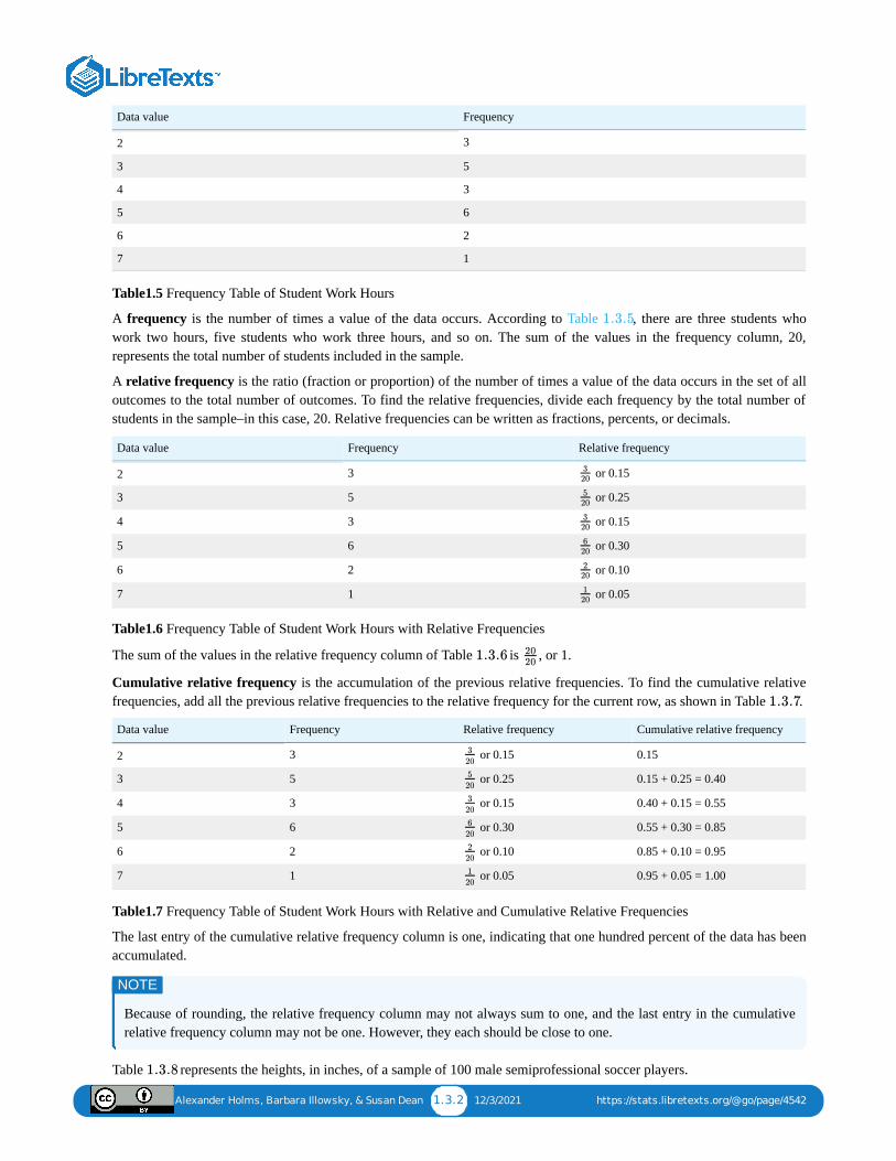
Twenty students were asked how many hours they worked per day. Their responses, in hours, are as follows: 5; 6; 3; 3; 2;4; 7; 5; 2; 3; 5; 6; 5; 4; 4; 3; 5; 2; 5; 3.
Table lists the different data values in ascending order and their frequencies.1.3.5
Alexander Holms, Barbara Illowsky, & Susan Dean 1.3.2 12/3/2021 https://stats.libretexts.org/@go/page/4542
Data value Frequency
2 3
3 5
4 3
5 6
6 2
7 1
Table1.5 Frequency Table of Student Work Hours
A frequency is the number of times a value of the data occurs. According to Table , there are three students whowork two hours, five students who work three hours, and so on. The sum of the values in the frequency column, 20,represents the total number of students included in the sample.
A relative frequency is the ratio (fraction or proportion) of the number of times a value of the data occurs in the set of alloutcomes to the total number of outcomes. To find the relative frequencies, divide each frequency by the total number ofstudents in the sample–in this case, 20. Relative frequencies can be written as fractions, percents, or decimals.
Data value Frequency Relative frequency
2 3 or 0.15
3 5 or 0.25
4 3 or 0.15
5 6 or 0.30
6 2 or 0.10
7 1 or 0.05
Table1.6 Frequency Table of Student Work Hours with Relative Frequencies
The sum of the values in the relative frequency column of Table is , or 1.
Cumulative relative frequency is the accumulation of the previous relative frequencies. To find the cumulative relativefrequencies, add all the previous relative frequencies to the relative frequency for the current row, as shown in Table .
Data value Frequency Relative frequency Cumulative relative frequency
2 3 or 0.15 0.15
3 5 or 0.25 0.15 + 0.25 = 0.40
4 3 or 0.15 0.40 + 0.15 = 0.55
5 6 or 0.30 0.55 + 0.30 = 0.85
6 2 or 0.10 0.85 + 0.10 = 0.95
7 1 or 0.05 0.95 + 0.05 = 1.00
Table1.7 Frequency Table of Student Work Hours with Relative and Cumulative Relative Frequencies
The last entry of the cumulative relative frequency column is one, indicating that one hundred percent of the data has beenaccumulated.
Because of rounding, the relative frequency column may not always sum to one, and the last entry in the cumulativerelative frequency column may not be one. However, they each should be close to one.
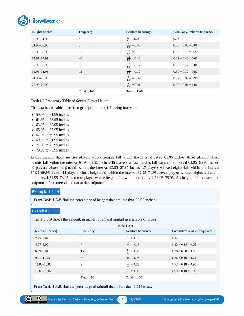
Table represents the heights, in inches, of a sample of 100 male semiprofessional soccer players.
1.3.5
3
20
5
20
3
20
6
20
2
20
1
20
1.3.6 20
20
1.3.7
3
20
5
20
3
20
6
20
2
20
1
20
NOTE
1.3.8
Alexander Holms, Barbara Illowsky, & Susan Dean 1.3.3 12/3/2021 https://stats.libretexts.org/@go/page/4542
Heights (inches) Frequency Relative frequency Cumulative relative frequency
59.95–61.95 5 = 0.05 0.05
61.95–63.95 3 = 0.03 0.05 + 0.03 = 0.08
63.95–65.95 15 = 0.15 0.08 + 0.15 = 0.23
65.95–67.95 40 = 0.40 0.23 + 0.40 = 0.63
67.95–69.95 17 = 0.17 0.63 + 0.17 = 0.80
69.95–71.95 12 = 0.12 0.80 + 0.12 = 0.92
71.95–73.95 7 = 0.07 0.92 + 0.07 = 0.99
73.95–75.95 1 = 0.01 0.99 + 0.01 = 1.00
Total = 100 Total = 1.00
Table1.8 Frequency Table of Soccer Player Height
The data in this table have been grouped into the following intervals:
59.95 to 61.95 inches61.95 to 63.95 inches63.95 to 65.95 inches65.95 to 67.95 inches67.95 to 69.95 inches69.95 to 71.95 inches71.95 to 73.95 inches73.95 to 75.95 inches
In this sample, there are five players whose heights fall within the interval 59.95–61.95 inches, three players whoseheights fall within the interval 61.95–63.95 inches, 15 players whose heights fall within the interval 63.95–65.95 inches,40 players whose heights fall within the interval 65.95–67.95 inches, 17 players whose heights fall within the interval67.95–69.95 inches, 12 players whose heights fall within the interval 69.95–71.95, seven players whose heights fall withinthe interval 71.95–73.95, and one player whose heights fall within the interval 73.95–75.95. All heights fall between theendpoints of an interval and not at the endpoints.
From Table , find the percentage of heights that are less than 65.95 inches.
Table shows the amount, in inches, of annual rainfall in a sample of towns.
Rainfall (inches) Frequency Relative frequency Cumulative relative frequency
2.95–4.97 6 = 0.12 0.12
4.97–6.99 7 = 0.14 0.12 + 0.14 = 0.26
6.99–9.01 15 = 0.30 0.26 + 0.30 = 0.56
9.01–11.03 8 = 0.16 0.56 + 0.16 = 0.72
11.03–13.05 9 = 0.18 0.72 + 0.18 = 0.90
13.05–15.07 5 = 0.10 0.90 + 0.10 = 1.00
Total = 50 Total = 1.00
Table
From Table , find the percentage of rainfall that is less than 9.01 inches.
5
10
3
100
15
100
40
100
17
100
12
100
7
100
1
100
Example 1.3.14
1.3.8
Exercise 1.3.14
1.3.9
6
50
7
50
15
50
8
50
9
50
5
50
1.3.9
1.3.9
Alexander Holms, Barbara Illowsky, & Susan Dean 1.3.4 12/3/2021 https://stats.libretexts.org/@go/page/4542
From Table , find the percentage of heights that fall between 61.95 and 65.95 inches.
Answer
Solution 1.15
Add the relative frequencies in the second and third rows: or 18%.
From Table , find the percentage of rainfall that is between 6.99 and 13.05 inches.
Use the heights of the 100 male semiprofessional soccer players in Table . Fill in the blanks and check youranswers.
1. The percentage of heights that are from 67.95 to 71.95 inches is: ____.2. The percentage of heights that are from 67.95 to 73.95 inches is: ____.3. The percentage of heights that are more than 65.95 inches is: ____.4. The number of players in the sample who are between 61.95 and 71.95 inches tall is: ____.5. What kind of data are the heights?6. Describe how you could gather this data (the heights) so that the data are characteristic of all male semiprofessional
soccer players.
Remember, you count frequencies. To find the relative frequency, divide the frequency by the total number of datavalues. To find the cumulative relative frequency, add all of the previous relative frequencies to the relative frequencyfor the current row.
Answer
Solution 1.16
1. 29%2. 36%3. 77%4. 875. quantitative continuous6. get rosters from each team and choose a simple random sample from each
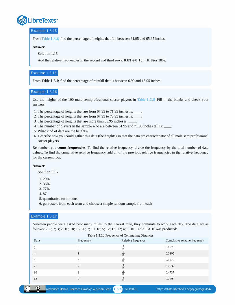
Nineteen people were asked how many miles, to the nearest mile, they commute to work each day. The data are asfollows: 2; 5; 7; 3; 2; 10; 18; 15; 20; 7; 10; 18; 5; 12; 13; 12; 4; 5; 10. Table was produced:
Data Frequency Relative frequency Cumulative relative frequency
3 3 0.1579
4 1 0.2105
5 3 0.1579
7 2 0.2632
10 3 0.4737
12 2 0.7895
Table Frequency of Commuting Distances
Example 1.3.15
1.3.8
0.03+0.15 = 0.18
Exercise 1.3.15
1.3.9
Example 1.3.16
1.3.8
Example 1.3.17
1.3.10
3
19
1
19
3
19
2
19
4
19
2
19
1.3.10
Alexander Holms, Barbara Illowsky, & Susan Dean 1.3.5 12/3/2021 https://stats.libretexts.org/@go/page/4542
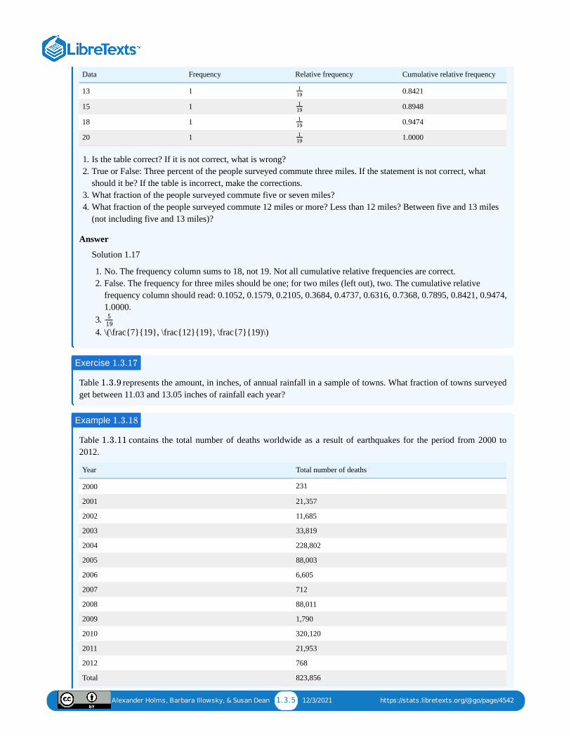
Data Frequency Relative frequency Cumulative relative frequency
13 1 0.8421
15 1 0.8948
18 1 0.9474
20 1 1.0000
1. Is the table correct? If it is not correct, what is wrong?2. True or False: Three percent of the people surveyed commute three miles. If the statement is not correct, what
should it be? If the table is incorrect, make the corrections.3. What fraction of the people surveyed commute five or seven miles?4. What fraction of the people surveyed commute 12 miles or more? Less than 12 miles? Between five and 13 miles
(not including five and 13 miles)?
Answer
Solution 1.17
1. No. The frequency column sums to 18, not 19. Not all cumulative relative frequencies are correct.2. False. The frequency for three miles should be one; for two miles (left out), two. The cumulative relative
frequency column should read: 0.1052, 0.1579, 0.2105, 0.3684, 0.4737, 0.6316, 0.7368, 0.7895, 0.8421, 0.9474,1.0000.
3. 4. \(\frac{7}{19}, \frac{12}{19}, \frac{7}{19)\)
Table represents the amount, in inches, of annual rainfall in a sample of towns. What fraction of towns surveyedget between 11.03 and 13.05 inches of rainfall each year?
Table contains the total number of deaths worldwide as a result of earthquakes for the period from 2000 to2012.
Year Total number of deaths
2000 231
2001 21,357
2002 11,685
2003 33,819
2004 228,802
2005 88,003
2006 6,605
2007 712
2008 88,011
2009 1,790
2010 320,120
2011 21,953
2012 768
Total 823,856
1
19
1
19
1
19
1
19
5
19
Exercise 1.3.17
1.3.9
Example 1.3.18
1.3.11
Alexander Holms, Barbara Illowsky, & Susan Dean 1.3.6 12/3/2021 https://stats.libretexts.org/@go/page/4542
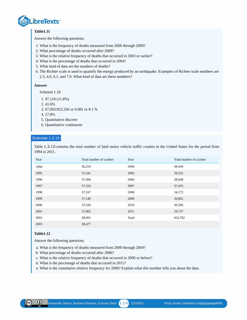
Table1.11
Answer the following questions.
1. What is the frequency of deaths measured from 2006 through 2009?2. What percentage of deaths occurred after 2009?3. What is the relative frequency of deaths that occurred in 2003 or earlier?4. What is the percentage of deaths that occurred in 2004?5. What kind of data are the numbers of deaths?6. The Richter scale is used to quantify the energy produced by an earthquake. Examples of Richter scale numbers are
2.3, 4.0, 6.1, and 7.0. What kind of data are these numbers?
Answer
Solution 1.18
1. 97,118 (11.8%)2. 41.6%3. 67,092/823,356 or 0.081 or 8.1 %4. 27.8%5. Quantitative discrete6. Quantitative continuous
Table contains the total number of fatal motor vehicle traffic crashes in the United States for the period from1994 to 2011.
Year Total number of crashes Year Total number of crashes
1994 36,254 2004 38,444
1995 37,241 2005 39,252
1996 37,494 2006 38,648
1997 37,324 2007 37,435
1998 37,107 2008 34,172
1999 37,140 2009 30,862
2000 37,526 2010 30,296
2001 37,862 2011 29,757
2002 38,491 Total 653,782
2003 38,477
Table1.12
Answer the following questions.
a. What is the frequency of deaths measured from 2000 through 2004?b. What percentage of deaths occurred after 2006?c. What is the relative frequency of deaths that occurred in 2000 or before?d. What is the percentage of deaths that occurred in 2011?e. What is the cumulative relative frequency for 2006? Explain what this number tells you about the data.
Exercise 1.3.18
1.3.12
Alexander Holms, Barbara Illowsky, & Susan Dean 1.4.1 12/17/2021 https://stats.libretexts.org/@go/page/4543
1.4: Experimental Design and EthicsDoes aspirin reduce the risk of heart attacks? Is one brand of fertilizer more effective at growing roses than another? Isfatigue as dangerous to a driver as the influence of alcohol? Questions like these are answered using randomizedexperiments. In this module, you will learn important aspects of experimental design. Proper study design ensures theproduction of reliable, accurate data.
The purpose of an experiment is to investigate the relationship between two variables. When one variable causes change inanother, we call the first variable the independent variable or explanatory variable. The affected variable is called thedependent variable or response variable: stimulus, response. In a randomized experiment, the researcher manipulatesvalues of the explanatory variable and measures the resulting changes in the response variable. The different values of theexplanatory variable are called treatments. An experimental unit is a single object or individual to be measured.
You want to investigate the effectiveness of vitamin E in preventing disease. You recruit a group of subjects and ask themif they regularly take vitamin E. You notice that the subjects who take vitamin E exhibit better health on average than thosewho do not. Does this prove that vitamin E is effective in disease prevention? It does not. There are many differencesbetween the two groups compared in addition to vitamin E consumption. People who take vitamin E regularly often takeother steps to improve their health: exercise, diet, other vitamin supplements, choosing not to smoke. Any one of thesefactors could be influencing health. As described, this study does not prove that vitamin E is the key to disease prevention.
Additional variables that can cloud a study are called lurking variables. In order to prove that the explanatory variable iscausing a change in the response variable, it is necessary to isolate the explanatory variable. The researcher must designher experiment in such a way that there is only one difference between groups being compared: the planned treatments.This is accomplished by the random assignment of experimental units to treatment groups. When subjects are assignedtreatments randomly, all of the potential lurking variables are spread equally among the groups. At this point the onlydifference between groups is the one imposed by the researcher. Different outcomes measured in the response variable,therefore, must be a direct result of the different treatments. In this way, an experiment can prove a cause-and-effectconnection between the explanatory and response variables.
The power of suggestion can have an important influence on the outcome of an experiment. Studies have shown that theexpectation of the study participant can be as important as the actual medication. In one study of performance-enhancingdrugs, researchers noted:
Results showed that believing one had taken the substance resulted in [performance] times almost as fast as thoseassociated with consuming the drug itself. In contrast, taking the drug without knowledge yielded no significantperformance increment. (McClung, M. Collins, D. “Because I know it will!”: placebo effects of an ergogenic aid onathletic performance. Journal of Sport & Exercise Psychology. 2007 Jun. 29(3):382-94. Web. April 30, 2013.)
When participation in a study prompts a physical response from a participant, it is difficult to isolate the effects of theexplanatory variable. To counter the power of suggestion, researchers set aside one treatment group as a control group.This group is given a placebo treatment–a treatment that cannot influence the response variable. The control group helpsresearchers balance the effects of being in an experiment with the effects of the active treatments. Of course, if you areparticipating in a study and you know that you are receiving a pill which contains no actual medication, then the power ofsuggestion is no longer a factor. Blinding in a randomized experiment preserves the power of suggestion. When a personinvolved in a research study is blinded, he does not know who is receiving the active treatment(s) and who is receiving theplacebo treatment. A double-blind experiment is one in which both the subjects and the researchers involved with thesubjects are blinded.
The Smell & Taste Treatment and Research Foundation conducted a study to investigate whether smell can affectlearning. Subjects completed mazes multiple times while wearing masks. They completed the pencil and paper mazesthree times wearing floral-scented masks, and three times with unscented masks. Participants were assigned at randomto wear the floral mask during the first three trials or during the last three trials. For each trial, researchers recorded thetime it took to complete the maze and the subject’s impression of the mask’s scent: positive, negative, or neutral.
a. Describe the explanatory and response variables in this study.
Example 1.4.19
Alexander Holms, Barbara Illowsky, & Susan Dean 1.4.2 12/17/2021 https://stats.libretexts.org/@go/page/4543
b. What are the treatments?c. Identify any lurking variables that could interfere with this study.d. Is it possible to use blinding in this study?
Answer
Solution 1.19
The explanatory variable is scent, and the response variable is the time it takes to complete the maze. There are twotreatments: a floral-scented mask and an unscented mask. All subjects experienced both treatments. The order oftreatments was randomly assigned so there were no differences between the treatment groups. Random assignmenteliminates the problem of lurking variables. Subjects will clearly know whether they can smell flowers or not, sosubjects cannot be blinded in this study. Researchers timing the mazes can be blinded, though. The researcher whois observing a subject will not know which mask is being worn.
Alexander Holms, Barbara Illowsky, & Susan Dean 1.5.1 11/26/2021 https://stats.libretexts.org/@go/page/4544
1.5: Chapter Key Terms
Averagealso called mean or arithmetic mean; a number that describes the central tendency of the data
Blindingnot telling participants which treatment a subject is receiving
Categorical Variablevariables that take on values that are names or labels
Cluster Samplinga method for selecting a random sample and dividing the population into groups (clusters); use simple randomsampling to select a set of clusters. Every individual in the chosen clusters is included in the sample.
Continuous Random Variablea random variable (RV) whose outcomes are measured; the height of trees in the forest is a continuous RV.
Control Groupa group in a randomized experiment that receives an inactive treatment but is otherwise managed exactly as the othergroups
Convenience Samplinga nonrandom method of selecting a sample; this method selects individuals that are easily accessible and may result inbiased data.
Cumulative Relative FrequencyThe term applies to an ordered set of observations from smallest to largest. The cumulative relative frequency is thesum of the relative frequencies for all values that are less than or equal to the given value.
Dataa set of observations (a set of possible outcomes); most data can be put into two groups: qualitative (an attribute whosevalue is indicated by a label) or quantitative (an attribute whose value is indicated by a number). Quantitative data canbe separated into two subgroups: discrete and continuous. Data is discrete if it is the result of counting (such as thenumber of students of a given ethnic group in a class or the number of books on a shelf). Data is continuous if it is theresult of measuring (such as distance traveled or weight of luggage)
Discrete Random Variablea random variable (RV) whose outcomes are counted
Double-blindingthe act of blinding both the subjects of an experiment and the researchers who work with the subjects
Experimental Unitany individual or object to be measured
Explanatory Variablethe independent variable in an experiment; the value controlled by researchers
Frequencythe number of times a value of the data occurs
Informed Consent
Alexander Holms, Barbara Illowsky, & Susan Dean 1.5.2 11/26/2021 https://stats.libretexts.org/@go/page/4544
Any human subject in a research study must be cognizant of any risks or costs associated with the study. The subjecthas the right to know the nature of the treatments included in the study, their potential risks, and their potential benefits.Consent must be given freely by an informed, fit participant.
Institutional Review Boarda committee tasked with oversight of research programs that involve human subjects
Lurking Variablea variable that has an effect on a study even though it is neither an explanatory variable nor a response variable
Mathematical Modelsa description of a phenomenon using mathematical concepts, such as equations, inequalities, distributions, etc.
Nonsampling Erroran issue that affects the reliability of sampling data other than natural variation; it includes a variety of human errorsincluding poor study design, biased sampling methods, inaccurate information provided by study participants, dataentry errors, and poor analysis.
Numerical Variablevariables that take on values that are indicated by numbers
Observational Studya study in which the independent variable is not manipulated by the researcher
Parametera number that is used to represent a population characteristic and that generally cannot be determined easily
Placeboan inactive treatment that has no real effect on the explanatory variable
Populationall individuals, objects, or measurements whose properties are being studied
Probabilitya number between zero and one, inclusive, that gives the likelihood that a specific event will occur
Proportionthe number of successes divided by the total number in the sample
Qualitative DataSee Data.
Quantitative DataSee Data.
Random Assignmentthe act of organizing experimental units into treatment groups using random methods
Random Samplinga method of selecting a sample that gives every member of the population an equal chance of being selected.
Relative Frequencythe ratio of the number of times a value of the data occurs in the set of all outcomes to the number of all outcomes tothe total number of outcomes
Alexander Holms, Barbara Illowsky, & Susan Dean 1.5.3 11/26/2021 https://stats.libretexts.org/@go/page/4544
Representative Samplea subset of the population that has the same characteristics as the population
Response Variablethe dependent variable in an experiment; the value that is measured for change at the end of an experiment
Samplea subset of the population studied
Sampling Biasnot all members of the population are equally likely to be selected
Sampling Errorthe natural variation that results from selecting a sample to represent a larger population; this variation decreases as thesample size increases, so selecting larger samples reduces sampling error.
Sampling with ReplacementOnce a member of the population is selected for inclusion in a sample, that member is returned to the population for theselection of the next individual.
Sampling without ReplacementA member of the population may be chosen for inclusion in a sample only once. If chosen, the member is not returnedto the population before the next selection.
Simple Random Samplinga straightforward method for selecting a random sample; give each member of the population a number. Use a randomnumber generator to select a set of labels. These randomly selected labels identify the members of your sample.
Statistica numerical characteristic of the sample; a statistic estimates the corresponding population parameter.
Statistical Modelsa description of a phenomenon using probability distributions that describe the expected behavior of the phenomenonand the variability in the expected observations.
Stratified Samplinga method for selecting a random sample used to ensure that subgroups of the population are represented adequately;divide the population into groups (strata). Use simple random sampling to identify a proportionate number ofindividuals from each stratum.
Surveya study in which data is collected as reported by individuals.
Systematic Samplinga method for selecting a random sample; list the members of the population. Use simple random sampling to select astarting point in the population. Let k = (number of individuals in the population)/(number of individuals needed in thesample). Choose every kth individual in the list starting with the one that was randomly selected. If necessary, return tothe beginning of the population list to complete your sample.
Treatmentsdifferent values or components of the explanatory variable applied in an experiment
Variablea characteristic of interest for each person or object in a population
Alexander Holms, Barbara Illowsky, & Susan Dean 1.6.1 12/3/2021 https://stats.libretexts.org/@go/page/5150
1.6: Chapter References
Definitions of Statistics, Probability, and Key TermsThe Data and Story Library, lib.stat.cmu.edu/DASL/Stories...stDummies.html (accessed May 1, 2013).
Data, Sampling, and Variation in Data and SamplingGallup-Healthways Well-Being Index. http://www.well-beingindex.com/default.asp (accessed May 1, 2013).Gallup-Healthways Well-Being Index. http://www.well-beingindex.com/methodology.asp (accessed May 1, 2013).Gallup-Healthways Well-Being Index. http://www.gallup.com/poll/146822/ga...questions.aspx (accessed May 1, 2013).Data from www.bookofodds.com/Relationsh...-the-PresidentDominic Lusinchi, “’President’ Landon and the 1936 Literary Digest Poll: Were Automobile and Telephone Owners toBlame?” Social Science History 36, no. 1: 23-54 (2012), ssh.dukejournals.org/content/36/1/23.abstract (accessed May1, 2013).“The Literary Digest Poll,” Virtual Laboratories in Probability and Statisticshttp://www.math.uah.edu/stat/data/LiteraryDigest.html (accessed May 1, 2013).“Gallup Presidential Election Trial-Heat Trends, 1936–2008,” Gallup Politicshttp://www.gallup.com/poll/110548/ga...9362004.aspx#4 (accessed May 1, 2013).The Data and Story Library, lib.stat.cmu.edu/DASL/Datafiles/USCrime.html (accessed May 1, 2013).LBCC Distance Learning (DL) program data in 2010-2011, http://de.lbcc.edu/reports/2010-11/f...hts.html#focus(accessed May 1, 2013).Data from San Jose Mercury News
Levels of Measurement“State & County QuickFacts,” U.S. Census Bureau. quickfacts.census.gov/qfd/download_data.html (accessed May 1,2013).“State & County QuickFacts: Quick, easy access to facts about people, business, and geography,” U.S. Census Bureau.quickfacts.census.gov/qfd/index.html (accessed May 1, 2013).“Table 5: Direct hits by mainland United States Hurricanes (1851-2004),” National Hurricane Center,http://www.nhc.noaa.gov/gifs/table5.gif (accessed May 1, 2013).“Levels of Measurement,” infinity.cos.edu/faculty/wood...ata_Levels.htm (accessed May 1, 2013).Courtney Taylor, “Levels of Measurement,” about.com, http://statistics.about.com/od/Helpa...easurement.htm (accessedMay 1, 2013).David Lane. “Levels of Measurement,” Connexions, http://cnx.org/content/m10809/latest/ (accessed May 1, 2013).
Experimental Design and Ethics“Vitamin E and Health,” Nutrition Source, Harvard School of Public Health,http://www.hsph.harvard.edu/nutritio...rce/vitamin-e/ (accessed May 1, 2013).Stan Reents. “Don’t Underestimate the Power of Suggestion,” athleteinme.com,www.athleteinme.com/ArticleView.aspx?id=1053 (accessed May 1, 2013).Ankita Mehta. “Daily Dose of Aspiring Helps Reduce Heart Attacks: Study,” International Business Times, July 21,2011. Also available online at http://www.ibtimes.com/daily-dose-as...s-study-300443 (accessed May 1, 2013).The Data and Story Library, lib.stat.cmu.edu/DASL/Stories...dLearning.html (accessed May 1, 2013).M.L. Jacskon et al., “Cognitive Components of Simulated Driving Performance: Sleep Loss effect and Predictors,”Accident Analysis and Prevention Journal, Jan no. 50 (2013), http://www.ncbi.nlm.nih.gov/pubmed/22721550(accessed May 1, 2013).“Earthquake Information by Year,” U.S. Geological Survey. http://earthquake.usgs.gov/earthquak...archives/year/(accessed May 1, 2013).“Fatality Analysis Report Systems (FARS) Encyclopedia,” National Highway Traffic and Safety Administration.http://www-fars.nhtsa.dot.gov/Main/index.aspx (accessed May 1, 2013).Data from www.businessweek.com (accessed May 1, 2013).Data from www.forbes.com (accessed May 1, 2013).

Alexander Holms, Barbara Illowsky, & Susan Dean 1.6.2 12/3/2021 https://stats.libretexts.org/@go/page/5150
“America’s Best Small Companies,” http://www.forbes.com/best-small-companies/list/ (accessed May 1, 2013).U.S. Department of Health and Human Services, Code of Federal Regulations Title 45 Public Welfare Department ofHealth and Human Services Part 46 Protection of Human Subjects revised January 15, 2009. Section 46.111:Criteriafor IRB Approval of Research.“April 2013 Air Travel Consumer Report,” U.S. Department of Transportation, April 11 (2013),http://www.dot.gov/airconsumer/april...onsumer-report (accessed May 1, 2013).Lori Alden, “Statistics can be Misleading,” econoclass.com, http://www.econoclass.com/misleadingstats.html (accessedMay 1, 2013).Maria de los A. Medina, “Ethics in Statistics,” Based on “Building an Ethics Module for Business, Science, andEngineering Students” by Jose A. Cruz-Cruz and William Frey, Connexions, http://cnx.org/content/m15555/latest/(accessed May 1, 2013).
Alexander Holms, Barbara Illowsky, & Susan
Dean1.H.1 1/7/2022 https://stats.libretexts.org/@go/page/6175
1.H: Sampling and Data (Homework)
1.1 Definitions of Statistics, Probability, and Key Terms
For each of the following eight exercises, identify: a. the population, b. the sample, c. the parameter, d. the statistic, e. thevariable, and f. the data. Give examples where appropriate.
1.
A fitness center is interested in the mean amount of time a client exercises in the center each week.
2.
Ski resorts are interested in the mean age that children take their first ski and snowboard lessons. They need thisinformation to plan their ski classes optimally.
3.
A cardiologist is interested in the mean recovery period of her patients who have had heart attacks.
4.
Insurance companies are interested in the mean health costs each year of their clients, so that they can determine the costsof health insurance.
5.
A politician is interested in the proportion of voters in his district who think he is doing a good job.
6.
A marriage counselor is interested in the proportion of clients she counsels who stay married.
7.
Political pollsters may be interested in the proportion of people who will vote for a particular cause.
8.
A marketing company is interested in the proportion of people who will buy a particular product.
Use the following information to answer the next three exercises: A Lake Tahoe Community College instructor isinterested in the mean number of days Lake Tahoe Community College math students are absent from class during aquarter.
9.
What is the population she is interested in?
a. all Lake Tahoe Community College studentsb. all Lake Tahoe Community College English studentsc. all Lake Tahoe Community College students in her classesd. all Lake Tahoe Community College math students
10.
Consider the following:
= number of days a Lake Tahoe Community College math student is absent
In this case, is an example of a:
a. variable.b. population.c. statistic.d. data.
11.
The instructor’s sample produces a mean number of days absent of 3.5 days. This value is an example of a:
X
X
Alexander Holms, Barbara Illowsky, & Susan
Dean1.H.2 1/7/2022 https://stats.libretexts.org/@go/page/6175
a. parameter.b. data.c. statistic.d. variable.
1.2 Data, Sampling, and Variation in Data and SamplingFor the following exercises, identify the type of data that would be used to describe a response (quantitative discrete,quantitative continuous, or qualitative), and give an example of the data.
12.
number of tickets sold to a concert
13.
percent of body fat
14.
favorite baseball team
15.
time in line to buy groceries
16.
number of students enrolled at Evergreen Valley College
17.
most-watched television show
18.
brand of toothpaste
19.
distance to the closest movie theatre
20.
age of executives in Fortune 500 companies
21.
number of competing computer spreadsheet software packages
Use the following information to answer the next two exercises: A study was done to determine the age, number of timesper week, and the duration (amount of time) of resident use of a local park in San Jose. The first house in the neighborhoodaround the park was selected randomly and then every 8th house in the neighborhood around the park was interviewed.
22.
“Number of times per week” is what type of data?
a. qualitative (categorical)b. quantitative discretec. quantitative continuous
23.
“Duration (amount of time)” is what type of data?
a. qualitative (categorical)b. quantitative discretec. quantitative continuous
24.
Alexander Holms, Barbara Illowsky, & Susan
Dean1.H.3 1/7/2022 https://stats.libretexts.org/@go/page/6175
Airline companies are interested in the consistency of the number of babies on each flight, so that they have adequatesafety equipment. Suppose an airline conducts a survey. Over Thanksgiving weekend, it surveys six flights from Boston toSalt Lake City to determine the number of babies on the flights. It determines the amount of safety equipment needed bythe result of that study.
a. Using complete sentences, list three things wrong with the way the survey was conducted.b. Using complete sentences, list three ways that you would improve the survey if it were to be repeated.
25.
Suppose you want to determine the mean number of students per statistics class in your state. Describe a possible samplingmethod in three to five complete sentences. Make the description detailed.
26.
Suppose you want to determine the mean number of cans of soda drunk each month by students in their twenties at yourschool. Describe a possible sampling method in three to five complete sentences. Make the description detailed.
27.
List some practical difficulties involved in getting accurate results from a telephone survey.
28.
List some practical difficulties involved in getting accurate results from a mailed survey.
29.
With your classmates, brainstorm some ways you could overcome these problems if you needed to conduct a phone ormail survey.
30.
The instructor takes her sample by gathering data on five randomly selected students from each Lake Tahoe CommunityCollege math class. The type of sampling she used is
a. cluster samplingb. stratified samplingc. simple random samplingd. convenience sampling
31.
A study was done to determine the age, number of times per week, and the duration (amount of time) of residents using alocal park in San Jose. The first house in the neighborhood around the park was selected randomly and then every eighthhouse in the neighborhood around the park was interviewed. The sampling method was:
a. simple randomb. systematicc. stratifiedd. cluster
32.
Name the sampling method used in each of the following situations:
a. A woman in the airport is handing out questionnaires to travelers asking them to evaluate the airport’s service. She doesnot ask travelers who are hurrying through the airport with their hands full of luggage, but instead asks all travelerswho are sitting near gates and not taking naps while they wait.
b. A teacher wants to know if her students are doing homework, so she randomly selects rows two and five and then callson all students in row two and all students in row five to present the solutions to homework problems to the class.
c. The marketing manager for an electronics chain store wants information about the ages of its customers. Over the nexttwo weeks, at each store location, 100 randomly selected customers are given questionnaires to fill out asking forinformation about age, as well as about other variables of interest.
Alexander Holms, Barbara Illowsky, & Susan
Dean1.H.4 1/7/2022 https://stats.libretexts.org/@go/page/6175
d. The librarian at a public library wants to determine what proportion of the library users are children. The librarian has atally sheet on which she marks whether books are checked out by an adult or a child. She records this data for everyfourth patron who checks out books.
e. A political party wants to know the reaction of voters to a debate between the candidates. The day after the debate, theparty’s polling staff calls 1,200 randomly selected phone numbers. If a registered voter answers the phone or isavailable to come to the phone, that registered voter is asked whom he or she intends to vote for and whether the debatechanged his or her opinion of the candidates.
33.
A “random survey” was conducted of 3,274 people of the “microprocessor generation” (people born since 1971, the yearthe microprocessor was invented). It was reported that 48% of those individuals surveyed stated that if they had $2,000 tospend, they would use it for computer equipment. Also, 66% of those surveyed considered themselves relatively savvycomputer users.
a. Do you consider the sample size large enough for a study of this type? Why or why not?b. Based on your “gut feeling,” do you believe the percents accurately reflect the U.S. population for those individuals
born since 1971? If not, do you think the percents of the population are actually higher or lower than the samplestatistics? Why? Additional information: The survey, reported by Intel Corporation, was filled out by individuals who visited the LosAngeles Convention Center to see the Smithsonian Institute's road show called “America’s Smithsonian.”
c. With this additional information, do you feel that all demographic and ethnic groups were equally represented at theevent? Why or why not?
d. With the additional information, comment on how accurately you think the sample statistics reflect the populationparameters.
34.
The Well-Being Index is a survey that follows trends of U.S. residents on a regular basis. There are six areas of health andwellness covered in the survey: Life Evaluation, Emotional Health, Physical Health, Healthy Behavior, WorkEnvironment, and Basic Access. Some of the questions used to measure the Index are listed below.
Identify the type of data obtained from each question used in this survey: qualitative(categorical), quantitative discrete, orquantitative continuous.
a. Do you have any health problems that prevent you from doing any of the things people your age can normally do?b. During the past 30 days, for about how many days did poor health keep you from doing your usual activities?c. In the last seven days, on how many days did you exercise for 30 minutes or more?d. Do you have health insurance coverage?
35.
In advance of the 1936 Presidential Election, a magazine titled Literary Digest released the results of an opinion pollpredicting that the republican candidate Alf Landon would win by a large margin. The magazine sent post cards toapproximately 10,000,000 prospective voters. These prospective voters were selected from the subscription list of themagazine, from automobile registration lists, from phone lists, and from club membership lists. Approximately 2,300,000people returned the postcards.
a. Think about the state of the United States in 1936. Explain why a sample chosen from magazine subscription lists,automobile registration lists, phone books, and club membership lists was not representative of the population of theUnited States at that time.
b. What effect does the low response rate have on the reliability of the sample?c. Are these problems examples of sampling error or nonsampling error?d. During the same year, George Gallup conducted his own poll of 30,000 prospective voters. These researchers used a
method they called "quota sampling" to obtain survey answers from specific subsets of the population. Quota samplingis an example of which sampling method described in this module?
36.
Alexander Holms, Barbara Illowsky, & Susan
Dean1.H.5 1/7/2022 https://stats.libretexts.org/@go/page/6175
Crime-related and demographic statistics for 47 US states in 1960 were collected from government agencies, including theFBI'sUniform Crime Report. One analysis of this data found a strong connection between education and crime indicatingthat higher levels of education in a community correspond to higher crime rates.
Which of the potential problems with samples discussed in Example could explain this connection?
37.
YouPolls is a website that allows anyone to create and respond to polls. One question posted April 15 asks:
“Do you feel happy paying your taxes when members of the Obama administration are allowed to ignore their taxliabilities?” (lastbaldeagle. 2013. On Tax Day, House to Call for Firing Federal Workers Who Owe Back Taxes. Opinionpoll posted online at: http://www.youpolls.com/details.aspx?id=12328 (accessed May 1, 2013).)
As of April 25, 11 people responded to this question. Each participant answered “NO!”
Which of the potential problems with samples discussed in this module could explain this connection?
38.
A scholarly article about response rates begins with the following quote:
“Declining contact and cooperation rates in random digit dial (RDD) national telephone surveys raise serious concernsabout the validity of estimates drawn from such research.” (Scott Keeter et al., “Gauging the Impact of GrowingNonresponse on Estimates from a National RDD Telephone Survey,” Public Opinion Quarterly 70 no. 5 (2006),http://poq.oxfordjournals.org/content/70/5/759.full (accessed May 1, 2013).)
The Pew Research Center for People and the Press admits:
“The percentage of people we interview – out of all we try to interview – has been declining over the past decade ormore.” (Frequently Asked Questions, Pew Research Center for the People & the Press, http://www.people-press.org/methodol...wer-your-polls (accessed May 1, 2013).)
a. What are some reasons for the decline in response rate over the past decade?b. Explain why researchers are concerned with the impact of the declining response rate on public opinion polls.
1.3 Levels of Measurement39.
Fifty part-time students were asked how many courses they were taking this term. The (incomplete) results are shownbelow:
# of courses Frequency Relative frequency Cumulative relative frequency
1 30 0.6
2 15
3
Table1.13 Part-time Student Course Loads
a. Fill in the blanks in Table .b. What percent of students take exactly two courses?c. What percent of students take one or two courses?
40.
Sixty adults with gum disease were asked the number of times per week they used to floss before their diagnosis. The(incomplete) results are shown in Table .
# flossing per week Frequency Relative frequency Cumulative relative frequency
0 27 0.4500
1 18
3 0.9333
1.H. 4
1.H. 13
1.H.14
Alexander Holms, Barbara Illowsky, & Susan
Dean1.H.6 1/7/2022 https://stats.libretexts.org/@go/page/6175
# flossing per week Frequency Relative frequency Cumulative relative frequency
6 3 0.0500
7 1 0.0167
Table1.14 Flossing Frequency for Adults with Gum Disease
a. Fill in the blanks in Table .b. What percent of adults flossed six times per week?c. What percent flossed at most three times per week?
41.
Nineteen immigrants to the U.S were asked how many years, to the nearest year, they have lived in the U.S. The data areas follows: 2;5; 7; 2; 2; 10; 20; 15; 0; 7; 0; 20; 5; 12; 15; 12; 4; 5; 10 .
Table was produced.
Data Frequency Relative frequency Cumulative relative frequency
0 2 219219 0.1053
2 3 319319 0.2632
4 1 119119 0.3158
5 3 319319 0.4737
7 2 219219 0.5789
10 2 219219 0.6842
12 2 219219 0.7895
15 1 119119 0.8421
20 1 119119 1.0000
Table Frequency of Immigrant Survey Responses
a. Fix the errors in Table . Also, explain how someone might have arrived at the incorrect number(s).b. Explain what is wrong with this statement: “47 percent of the people surveyed have lived in the U.S. for 5 years.”c. Fix the statement in b to make it correct.d. What fraction of the people surveyed have lived in the U.S. five or seven years?e. What fraction of the people surveyed have lived in the U.S. at most 12 years?f. What fraction of the people surveyed have lived in the U.S. fewer than 12 years?g. What fraction of the people surveyed have lived in the U.S. from five to 20 years, inclusive?
42.
How much time does it take to travel to work? Table shows the mean commute time by state for workers at least16 years old who are not working at home. Find the mean travel time, and round off the answer properly.
24.0 24.3 25.9 18.9 27.5 17.9 21.8 20.9 16.7 27.3
18.2 24.7 20.0 22.6 23.9 18.0 31.4 22.3 24.0 25.5
24.7 24.6 28.1 24.9 22.6 23.6 23.4 25.7 24.8 25.5
21.2 25.7 23.1 23.0 23.9 26.0 16.3 23.1 21.4 21.5
27.0 27.0 18.6 31.7 23.3 30.1 22.9 23.3 21.7 18.6
Table
43.
Forbes magazine published data on the best small firms in 2012. These were firms which had been publicly traded for atleast a year, have a stock price of at least $5 per share, and have reported annual revenue between $5 million and $1billion. Table shows the ages of the chief executive officers for the first 60 ranked firms.
1.H. 14
1.H. 15
1.H. 15
1.H. 15
1.H.16
1.H. 16
1.H.17
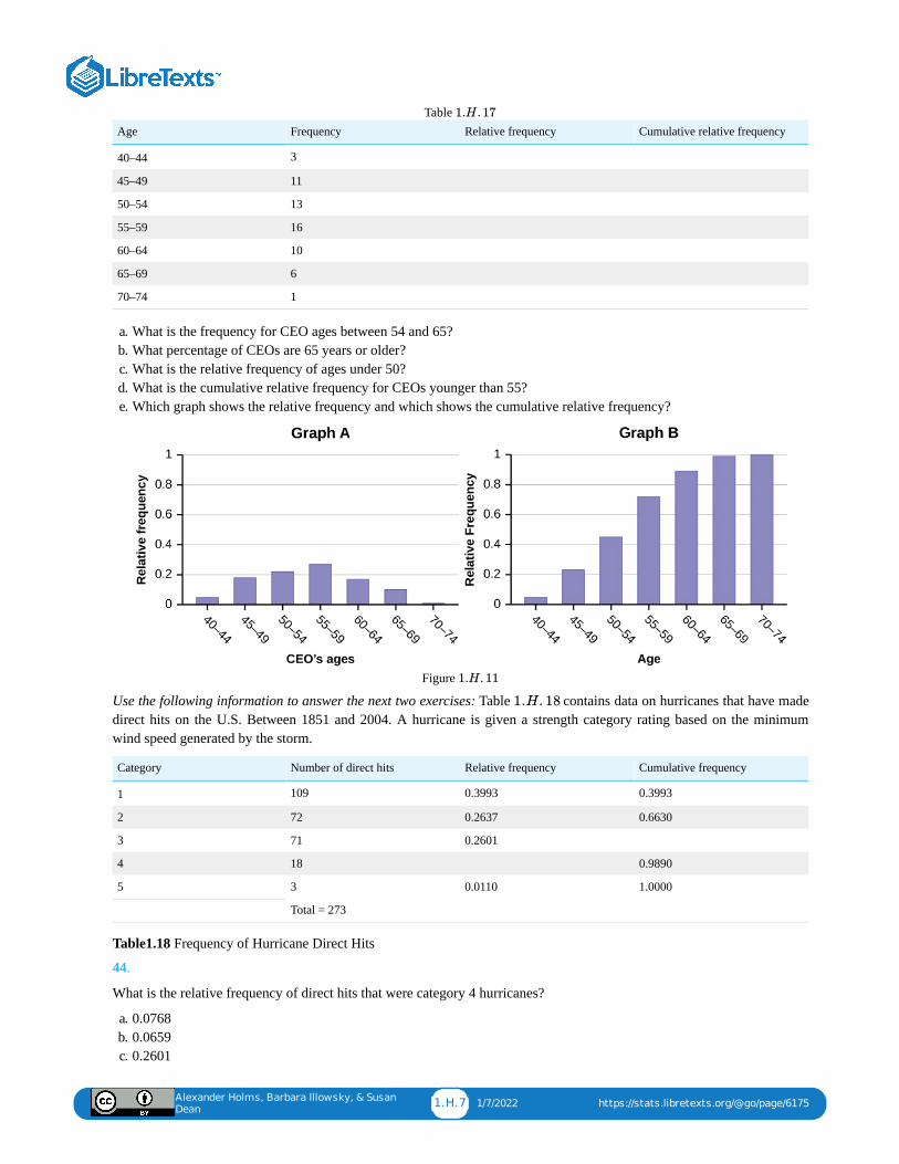
Alexander Holms, Barbara Illowsky, & Susan
Dean1.H.7 1/7/2022 https://stats.libretexts.org/@go/page/6175
Age Frequency Relative frequency Cumulative relative frequency
40–44 3
45–49 11
50–54 13
55–59 16
60–64 10
65–69 6
70–74 1
Table
a. What is the frequency for CEO ages between 54 and 65?b. What percentage of CEOs are 65 years or older?c. What is the relative frequency of ages under 50?d. What is the cumulative relative frequency for CEOs younger than 55?e. Which graph shows the relative frequency and which shows the cumulative relative frequency?
Figure
Use the following information to answer the next two exercises: Table contains data on hurricanes that have madedirect hits on the U.S. Between 1851 and 2004. A hurricane is given a strength category rating based on the minimumwind speed generated by the storm.
Category Number of direct hits Relative frequency Cumulative frequency
Total = 273
1 109 0.3993 0.3993
2 72 0.2637 0.6630
3 71 0.2601
4 18 0.9890
5 3 0.0110 1.0000
Table1.18 Frequency of Hurricane Direct Hits
44.
What is the relative frequency of direct hits that were category 4 hurricanes?
a. 0.0768b. 0.0659c. 0.2601
1.H. 17
1.H. 11
1.H. 18

Alexander Holms, Barbara Illowsky, & Susan
Dean1.H.8 1/7/2022 https://stats.libretexts.org/@go/page/6175
d. Not enough information to calculate
45.
What is the relative frequency of direct hits that were AT MOST a category 3 storm?
a. 0.3480b. 0.9231c. 0.2601d. 0.3370
Alexander Holms, Barbara Illowsky, & Susan
Dean1.R.1 12/24/2021 https://stats.libretexts.org/@go/page/4545
1.R: Sampling and Data (Review)
1.1 Definitions of Statistics, Probability, and Key Terms
The mathematical theory of statistics is easier to learn when you know the language. This module presents important termsthat will be used throughout the text.
1.2 Data, Sampling, and Variation in Data and SamplingData are individual items of information that come from a population or sample. Data may be classified as qualitative(categorical), quantitative continuous, or quantitative discrete.
Because it is not practical to measure the entire population in a study, researchers use samples to represent the population.A random sample is a representative group from the population chosen by using a method that gives each individual in thepopulation an equal chance of being included in the sample. Random sampling methods include simple random sampling,stratified sampling, cluster sampling, and systematic sampling. Convenience sampling is a nonrandom method of choosinga sample that often produces biased data.
Samples that contain different individuals result in different data. This is true even when the samples are well-chosen andrepresentative of the population. When properly selected, larger samples model the population more closely than smallersamples. There are many different potential problems that can affect the reliability of a sample. Statistical data needs to becritically analyzed, not simply accepted.
1.3 Levels of MeasurementSome calculations generate numbers that are artificially precise. It is not necessary to report a value to eight decimal placeswhen the measures that generated that value were only accurate to the nearest tenth. Round off your final answer to onemore decimal place than was present in the original data. This means that if you have data measured to the nearest tenth ofa unit, report the final statistic to the nearest hundredth.
In addition to rounding your answers, you can measure your data using the following four levels of measurement.
Nominal scale level: data that cannot be ordered nor can it be used in calculationsOrdinal scale level: data that can be ordered; the differences cannot be measuredInterval scale level: data with a definite ordering but no starting point; the differences can be measured, but there is nosuch thing as a ratio.Ratio scale level: data with a starting point that can be ordered; the differences have meaning and ratios can becalculated.
When organizing data, it is important to know how many times a value appears. How many statistics students study fivehours or more for an exam? What percent of families on our block own two pets? Frequency, relative frequency, andcumulative relative frequency are measures that answer questions like these.
1.4 Experimental Design and Ethics
A poorly designed study will not produce reliable data. There are certain key components that must be included in everyexperiment. To eliminate lurking variables, subjects must be assigned randomly to different treatment groups. One of thegroups must act as a control group, demonstrating what happens when the active treatment is not applied. Participants inthe control group receive a placebo treatment that looks exactly like the active treatments but cannot influence the responsevariable. To preserve the integrity of the placebo, both researchers and subjects may be blinded. When a study is designedproperly, the only difference between treatment groups is the one imposed by the researcher. Therefore, when groupsrespond differently to different treatments, the difference must be due to the influence of the explanatory variable.
“An ethics problem arises when you are considering an action that benefits you or some cause you support, hurts orreduces benefits to others, and violates some rule.” (Andrew Gelman, “Open Data and Open Methods,” Ethics andStatistics, http://www.stat.columbia.edu/~gelman...nceEthics1.pdf (accessed May 1, 2013).) Ethical violations in statisticsare not always easy to spot. Professional associations and federal agencies post guidelines for proper conduct. It isimportant that you learn basic statistical procedures so that you can recognize proper data analysis.
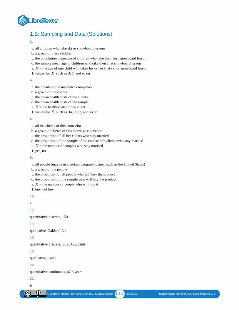
Alexander Holms, Barbara Illowsky, & Susan Dean 1.S.1 1/6/2022 https://stats.libretexts.org/@go/page/6173
1.S: Sampling and Data (Solutions)2.
a. all children who take ski or snowboard lessonsb. a group of these childrenc. the population mean age of children who take their first snowboard lessond. the sample mean age of children who take their first snowboard lessone. = the age of one child who takes his or her first ski or snowboard lessonf. values for , such as 3, 7, and so on
4.
a. the clients of the insurance companiesb. a group of the clientsc. the mean health costs of the clientsd. the mean health costs of the samplee. = the health costs of one clientf. values for , such as 34, 9, 82, and so on
6.
a. all the clients of this counselorb. a group of clients of this marriage counselorc. the proportion of all her clients who stay marriedd. the proportion of the sample of the counselor’s clients who stay marriede. = the number of couples who stay marriedf. yes, no
8.
a. all people (maybe in a certain geographic area, such as the United States)b. a group of the peoplec. the proportion of all people who will buy the productd. the proportion of the sample who will buy the producte. = the number of people who will buy itf. buy, not buy
10.
a
12.
quantitative discrete, 150
14.
qualitative, Oakland A’s
16.
quantitative discrete, 11,234 students
18.
qualitative, Crest
20.
quantitative continuous, 47.3 years
22.
b
X
X
X
X
X
X
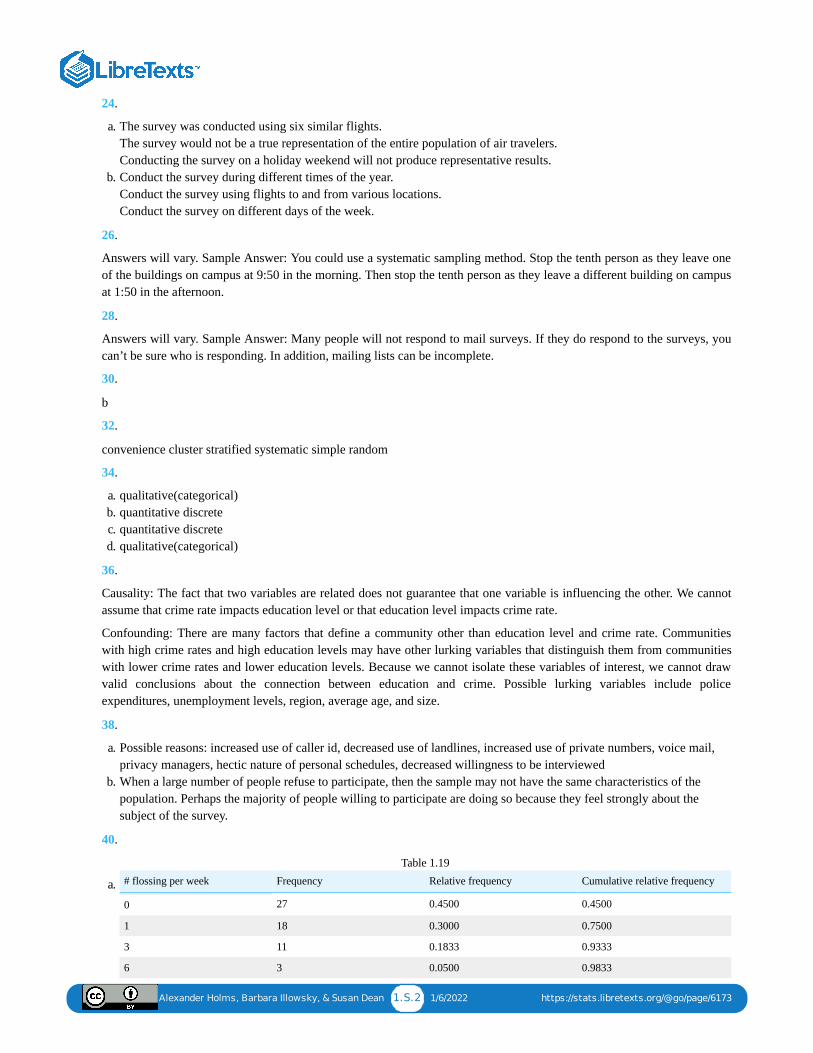
Alexander Holms, Barbara Illowsky, & Susan Dean 1.S.2 1/6/2022 https://stats.libretexts.org/@go/page/6173
24.
a. The survey was conducted using six similar flights. The survey would not be a true representation of the entire population of air travelers. Conducting the survey on a holiday weekend will not produce representative results.
b. Conduct the survey during different times of the year. Conduct the survey using flights to and from various locations. Conduct the survey on different days of the week.
26.
Answers will vary. Sample Answer: You could use a systematic sampling method. Stop the tenth person as they leave oneof the buildings on campus at 9:50 in the morning. Then stop the tenth person as they leave a different building on campusat 1:50 in the afternoon.
28.
Answers will vary. Sample Answer: Many people will not respond to mail surveys. If they do respond to the surveys, youcan’t be sure who is responding. In addition, mailing lists can be incomplete.
30.
b
32.
convenience cluster stratified systematic simple random
34.
a. qualitative(categorical)b. quantitative discretec. quantitative discreted. qualitative(categorical)
36.
Causality: The fact that two variables are related does not guarantee that one variable is influencing the other. We cannotassume that crime rate impacts education level or that education level impacts crime rate.
Confounding: There are many factors that define a community other than education level and crime rate. Communitieswith high crime rates and high education levels may have other lurking variables that distinguish them from communitieswith lower crime rates and lower education levels. Because we cannot isolate these variables of interest, we cannot drawvalid conclusions about the connection between education and crime. Possible lurking variables include policeexpenditures, unemployment levels, region, average age, and size.
38.
a. Possible reasons: increased use of caller id, decreased use of landlines, increased use of private numbers, voice mail,privacy managers, hectic nature of personal schedules, decreased willingness to be interviewed
b. When a large number of people refuse to participate, then the sample may not have the same characteristics of thepopulation. Perhaps the majority of people willing to participate are doing so because they feel strongly about thesubject of the survey.
40.
a. # flossing per week Frequency Relative frequency Cumulative relative frequency
0 27 0.4500 0.4500
1 18 0.3000 0.7500
3 11 0.1833 0.9333
6 3 0.0500 0.9833
Table 1.19
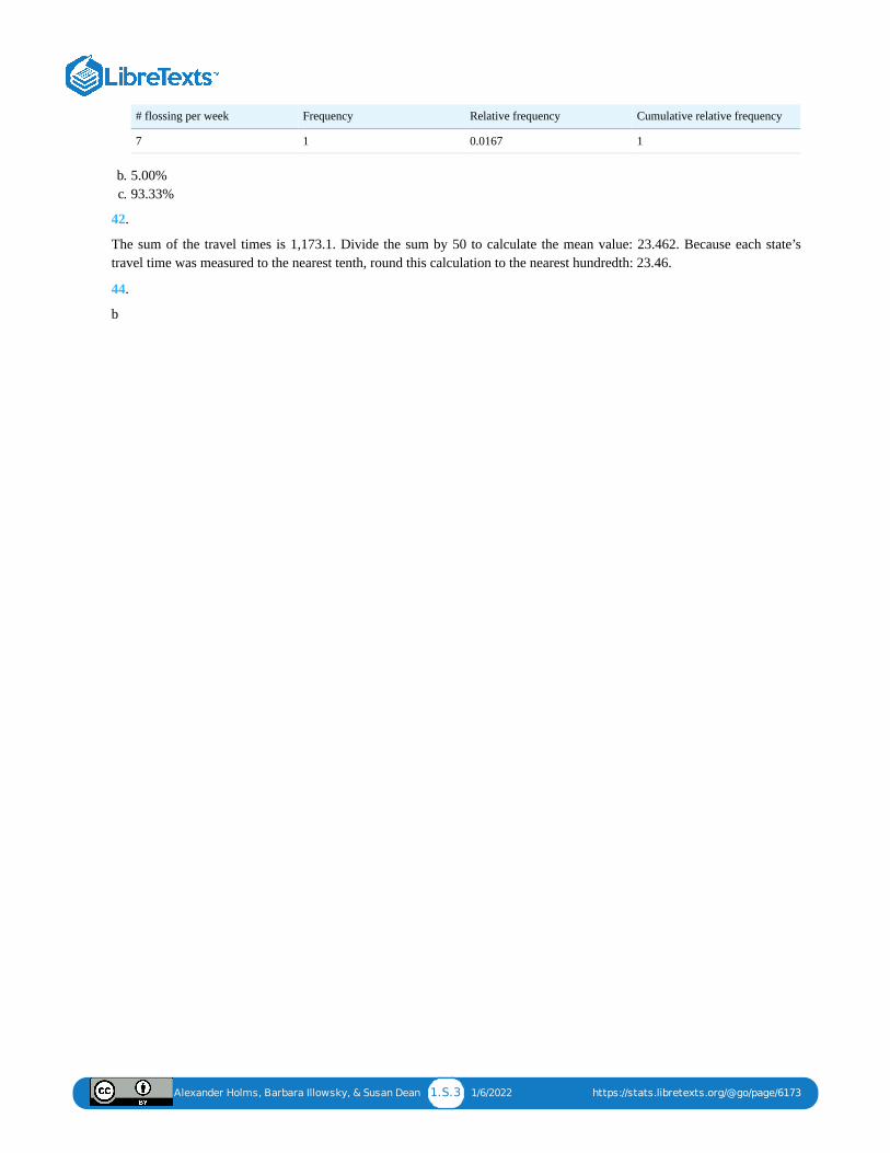
Alexander Holms, Barbara Illowsky, & Susan Dean 1.S.3 1/6/2022 https://stats.libretexts.org/@go/page/6173
# flossing per week Frequency Relative frequency Cumulative relative frequency
7 1 0.0167 1
b. 5.00%c. 93.33%
42.
The sum of the travel times is 1,173.1. Divide the sum by 50 to calculate the mean value: 23.462. Because each state’stravel time was measured to the nearest tenth, round this calculation to the nearest hundredth: 23.46.
44.
b

1 1/7/2022
CHAPTER OVERVIEW2: DESCRIPTIVE STATISTICS
2.0: INTRODUCTION TO DESCRIPTIVE STATISTICS2.1: DISPLAY DATA2.2: MEASURES OF THE LOCATION OF THE DATAThe common measures of location are quartiles and percentiles Quartiles are special percentiles. The first quartile, Q1, is the same asthe 25th percentile, and the third quartile, Q3, is the same as the 75th percentile.
2.3: MEASURES OF THE CENTER OF THE DATAThe "center" of a data set is also a way of describing location. The two most widely used measures of the "center" of the data are themean(average) and the median.
2.4: SIGMA NOTATION AND CALCULATING THE ARITHMETIC MEAN2.5: GEOMETRIC MEAN2.6: SKEWNESS AND THE MEAN, MEDIAN, AND MODE2.7: MEASURES OF THE SPREAD OF THE DATA2.8: HOMEWORK2.9: CHAPTER FORMULA REVIEW2.10: CHAPTER HOMEWORK2.11: CHAPTER KEY TERMS2.12: CHAPTER REFERENCES2.13: CHAPTER HOMEWORK SOLUTIONS2.14: CHAPTER PRACTICE2.R: DESCRIPTIVE STATISTICS (REVIEW)
Alexander Holms, Barbara Illowsky, & Susan Dean 2.0.1 12/31/2021 https://stats.libretexts.org/@go/page/5473
2.0: introduction to Descriptive Statistics
Figure When you have large amounts of data, you will need to organize it in a way that makes sense. These ballotsfrom an election are rolled together with similar ballots to keep them organized. (credit: William Greeson)
Once you have collected data, what will you do with it? Data can be described and presented in many different formats.For example, suppose you are interested in buying a house in a particular area. You may have no clue about the houseprices, so you might ask your real estate agent to give you a sample data set of prices. Looking at all the prices in thesample often is overwhelming. A better way might be to look at the median price and the variation of prices. The medianand variation are just two ways that you will learn to describe data. Your agent might also provide you with a graph of thedata.
In this chapter, you will study numerical and graphical ways to describe and display your data. This area of statistics iscalled "Descriptive Statistics." You will learn how to calculate, and even more importantly, how to interpret thesemeasurements and graphs.
A statistical graph is a tool that helps you learn about the shape or distribution of a sample or a population. A graph can bea more effective way of presenting data than a mass of numbers because we can see where data clusters and where thereare only a few data values. Newspapers and the Internet use graphs to show trends and to enable readers to compare factsand figures quickly. Statisticians often graph data first to get a picture of the data. Then, more formal tools may be applied.
Some of the types of graphs that are used to summarize and organize data are the dot plot, the bar graph, the histogram, thestem-and-leaf plot, the frequency polygon (a type of broken line graph), the pie chart, and the box plot. In this chapter, wewill briefly look at stem-and-leaf plots, line graphs, and bar graphs, as well as frequency polygons, and time series graphs.Our emphasis will be on histograms and box plots.
2.0.1
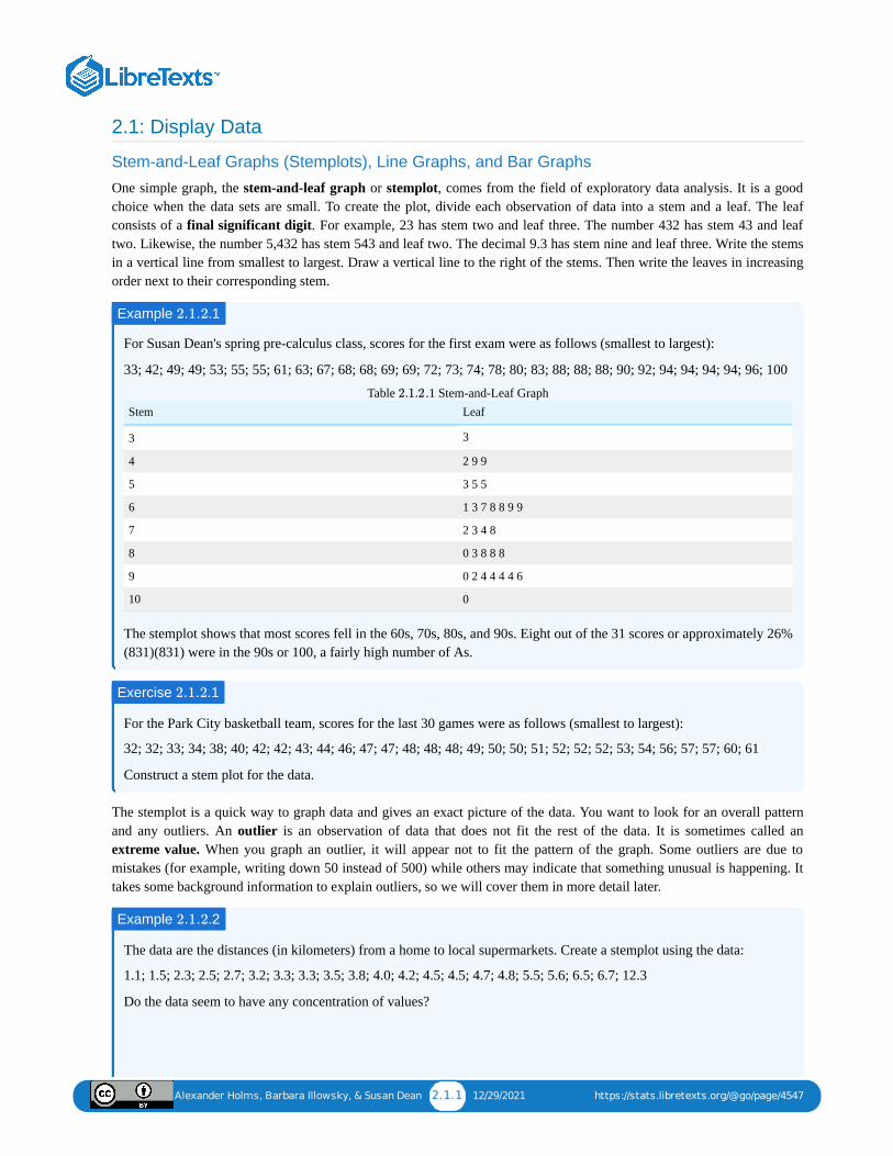
Alexander Holms, Barbara Illowsky, & Susan Dean 2.1.1 12/29/2021 https://stats.libretexts.org/@go/page/4547
2.1: Display Data
Stem-and-Leaf Graphs (Stemplots), Line Graphs, and Bar Graphs
One simple graph, the stem-and-leaf graph or stemplot, comes from the field of exploratory data analysis. It is a goodchoice when the data sets are small. To create the plot, divide each observation of data into a stem and a leaf. The leafconsists of a final significant digit. For example, 23 has stem two and leaf three. The number 432 has stem 43 and leaftwo. Likewise, the number 5,432 has stem 543 and leaf two. The decimal 9.3 has stem nine and leaf three. Write the stemsin a vertical line from smallest to largest. Draw a vertical line to the right of the stems. Then write the leaves in increasingorder next to their corresponding stem.
For Susan Dean's spring pre-calculus class, scores for the first exam were as follows (smallest to largest):
33; 42; 49; 49; 53; 55; 55; 61; 63; 67; 68; 68; 69; 69; 72; 73; 74; 78; 80; 83; 88; 88; 88; 90; 92; 94; 94; 94; 94; 96; 100
Stem Leaf
3 3
4 2 9 9
5 3 5 5
6 1 3 7 8 8 9 9
7 2 3 4 8
8 0 3 8 8 8
9 0 2 4 4 4 4 6
10 0
Table .1 Stem-and-Leaf Graph
The stemplot shows that most scores fell in the 60s, 70s, 80s, and 90s. Eight out of the 31 scores or approximately 26%(831)(831) were in the 90s or 100, a fairly high number of As.
For the Park City basketball team, scores for the last 30 games were as follows (smallest to largest):
32; 32; 33; 34; 38; 40; 42; 42; 43; 44; 46; 47; 47; 48; 48; 48; 49; 50; 50; 51; 52; 52; 52; 53; 54; 56; 57; 57; 60; 61
Construct a stem plot for the data.
The stemplot is a quick way to graph data and gives an exact picture of the data. You want to look for an overall patternand any outliers. An outlier is an observation of data that does not fit the rest of the data. It is sometimes called anextreme value. When you graph an outlier, it will appear not to fit the pattern of the graph. Some outliers are due tomistakes (for example, writing down 50 instead of 500) while others may indicate that something unusual is happening. Ittakes some background information to explain outliers, so we will cover them in more detail later.
The data are the distances (in kilometers) from a home to local supermarkets. Create a stemplot using the data:
1.1; 1.5; 2.3; 2.5; 2.7; 3.2; 3.3; 3.3; 3.5; 3.8; 4.0; 4.2; 4.5; 4.5; 4.7; 4.8; 5.5; 5.6; 6.5; 6.7; 12.3
Do the data seem to have any concentration of values?
Example .12.1.2
2.1.2
Exercise .12.1.2
Example .22.1.2
Alexander Holms, Barbara Illowsky, & Susan Dean 2.1.2 12/29/2021 https://stats.libretexts.org/@go/page/4547
The leaves are to the right of the decimal.
Answer
The value 12.3 may be an outlier. Values appear to concentrate at three and four kilometers.
Stem Leaf
1 1 5
2 3 5 7
3 2 3 3 5 8
4 0 2 5 5 7 8
5 5 6
6 5 7
7
8
9
10
11
12 3
Table .2
The following data show the distances (in miles) from the homes of off-campus statistics students to the college.Create a stem plot using the data and identify any outliers:
0.5; 0.7; 1.1; 1.2; 1.2; 1.3; 1.3; 1.5; 1.5; 1.7; 1.7; 1.8; 1.9; 2.0; 2.2; 2.5; 2.6; 2.8; 2.8; 2.8; 3.5; 3.8; 4.4; 4.8; 4.9; 5.2;5.5; 5.7; 5.8; 8.0
A side-by-side stem-and-leaf plot allows a comparison of the two data sets in two columns. In a side-by-side stem-and-leaf plot, two sets of leaves share the same stem. The leaves are to the left and the right of the stems. Table .4and Table .5 show the ages of presidents at their inauguration and at their death. Construct a side-by-side stem-and-leaf plot using this data.
Answer
Ages at Inauguration Ages at Death
9 9 8 7 7 7 6 3 2 4 6 9
8 7 7 7 7 6 6 6 5 5 5 5 4 4 4 4 4 2 2 1 1 1 11 0
5 3 6 6 7 7 8
9 8 5 4 4 2 1 1 1 0 6 0 0 3 3 4 4 5 6 7 7 7 8
7 0 0 1 1 1 4 7 8 8 9
8 0 1 3 5 8
9 0 0 3 3
Table .3
NOTE
2.1.2
Exercise .22.1.2
Example .32.1.2
2.1.2
2.1.2
2.1.2
Alexander Holms, Barbara Illowsky, & Susan Dean 2.1.3 12/29/2021 https://stats.libretexts.org/@go/page/4547
President Age President Age President Age
Washington 57 Lincoln 52 Hoover 54
J. Adams 61 A. Johnson 56 F. Roosevelt 51
Jefferson 57 Grant 46 Truman 60
Madison 57 Hayes 54 Eisenhower 62
Monroe 58 Garfield 49 Kennedy 43
J. Q. Adams 57 Arthur 51 L. Johnson 55
Jackson 61 Cleveland 47 Nixon 56
Van Buren 54 B. Harrison 55 Ford 61
W. H. Harrison 68 Cleveland 55 Carter 52
Tyler 51 McKinley 54 Reagan 69
Polk 49 T. Roosevelt 42 G.H.W. Bush 64
Taylor 64 Taft 51 Clinton 47
Fillmore 50 Wilson 56 G. W. Bush 54
Pierce 48 Harding 55 Obama 47
Buchanan 65 Coolidge 51 Trump 70
Table .4 Presidential Ages at Inauguration
President Age President Age President Age
Washington 67 Lincoln 56 Hoover 90
J. Adams 90 A. Johnson 66 F. Roosevelt 63
Jefferson 83 Grant 63 Truman 88
Madison 85 Hayes 70 Eisenhower 78
Monroe 73 Garfield 49 Kennedy 46
J. Q. Adams 80 Arthur 56 L. Johnson 64
Jackson 78 Cleveland 71 Nixon 81
Van Buren 79 B. Harrison 67 Ford 93
W. H. Harrison 68 Cleveland 71 Reagan 93
Tyler 71 McKinley 58
Polk 53 T. Roosevelt 60
Taylor 65 Taft 72
Fillmore 74 Wilson 67
Pierce 64 Harding 57
Buchanan 77 Coolidge 60
Table .5 Presidential Age at Death
Another type of graph that is useful for specific data values is a line graph. In the particular line graph shown in Example , the x-axis(horizontal axis) consists of data values and the y-axis (vertical axis) consists of frequency points. The
frequency points are connected using line segments.
In a survey, 40 mothers were asked how many times per week a teenager must be reminded to do his or her chores.The results are shown in Table .6 and in Figure .2.
Number of times teenager is reminded Frequency
2.1.2
2.1.2
2.1.4
Example .42.1.2
2.1.2 2.1.2
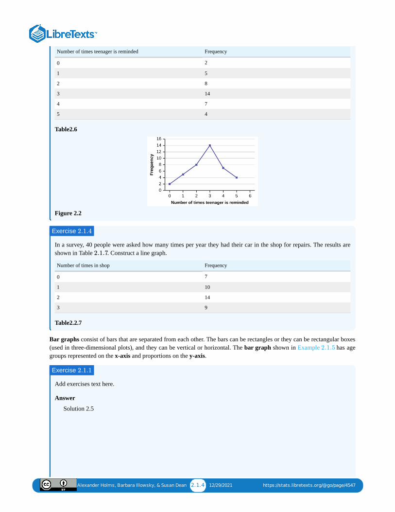
Alexander Holms, Barbara Illowsky, & Susan Dean 2.1.4 12/29/2021 https://stats.libretexts.org/@go/page/4547
Number of times teenager is reminded Frequency
0 2
1 5
2 8
3 14
4 7
5 4
Table2.6
Figure 2.2
In a survey, 40 people were asked how many times per year they had their car in the shop for repairs. The results areshown in Table . Construct a line graph.
Number of times in shop Frequency
0 7
1 10
2 14
3 9
Table2.2.7
Bar graphs consist of bars that are separated from each other. The bars can be rectangles or they can be rectangular boxes(used in three-dimensional plots), and they can be vertical or horizontal. The bar graph shown in Example has agegroups represented on the x-axis and proportions on the y-axis.
Add exercises text here.
Answer
Solution 2.5
Exercise 2.1.4
2.1.7
2.1.5
Exercise 2.1.1
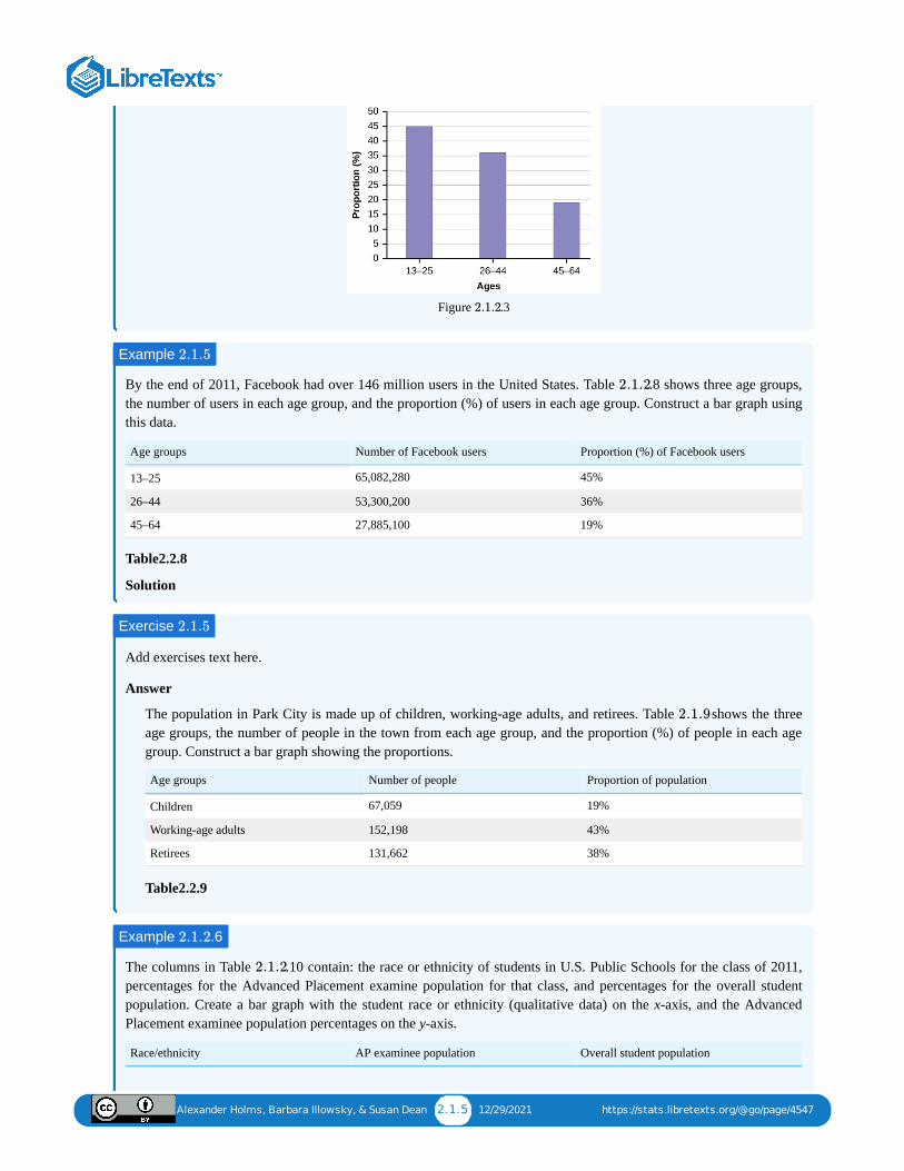
Alexander Holms, Barbara Illowsky, & Susan Dean 2.1.5 12/29/2021 https://stats.libretexts.org/@go/page/4547
Figure .3
By the end of 2011, Facebook had over 146 million users in the United States. Table .8 shows three age groups,the number of users in each age group, and the proportion (%) of users in each age group. Construct a bar graph usingthis data.
Age groups Number of Facebook users Proportion (%) of Facebook users
13–25 65,082,280 45%
26–44 53,300,200 36%
45–64 27,885,100 19%
Table2.2.8
Solution
Add exercises text here.
Answer
The population in Park City is made up of children, working-age adults, and retirees. Table shows the threeage groups, the number of people in the town from each age group, and the proportion (%) of people in each agegroup. Construct a bar graph showing the proportions.
Age groups Number of people Proportion of population
Children 67,059 19%
Working-age adults 152,198 43%
Retirees 131,662 38%
Table2.2.9
The columns in Table .10 contain: the race or ethnicity of students in U.S. Public Schools for the class of 2011,percentages for the Advanced Placement examine population for that class, and percentages for the overall studentpopulation. Create a bar graph with the student race or ethnicity (qualitative data) on the x-axis, and the AdvancedPlacement examinee population percentages on the y-axis.
Race/ethnicity AP examinee population Overall student population
2.1.2
Example 2.1.5
2.1.2
Exercise 2.1.5
2.1.9
Example .62.1.2
2.1.2
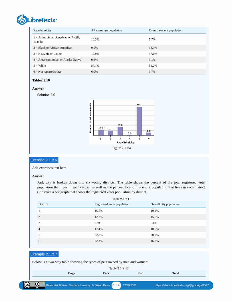
Alexander Holms, Barbara Illowsky, & Susan Dean 2.1.6 12/29/2021 https://stats.libretexts.org/@go/page/4547
Race/ethnicity AP examinee population Overall student population
1 = Asian, Asian American or PacificIslander
10.3% 5.7%
2 = Black or African American 9.0% 14.7%
3 = Hispanic or Latino 17.0% 17.6%
4 = American Indian or Alaska Native 0.6% 1.1%
5 = White 57.1% 59.2%
6 = Not reported/other 6.0% 1.7%
Table2.2.10
Answer
Solution 2.6
Figure .4
Add exercises text here.
Answer
Park city is broken down into six voting districts. The table shows the percent of the total registered voterpopulation that lives in each district as well as the percent total of the entire population that lives in each district.Construct a bar graph that shows the registered voter population by district.
District Registered voter population Overall city population
1 15.5% 19.4%
2 12.2% 15.6%
3 9.8% 9.0%
4 17.4% 18.5%
5 22.8% 20.7%
6 22.3% 16.8%
Table .11
Below is a two-way table showing the types of pets owned by men and women:
Dogs Cats Fish TotalTable .12
2.1.2
Exercise .62.1.2
2.1.2
Example .72.1.2
2.1.2
Alexander Holms, Barbara Illowsky, & Susan Dean 2.1.7 12/29/2021 https://stats.libretexts.org/@go/page/4547
Dogs Cats Fish Total
Men 4 2 2 8
Women 4 6 2 12
Total 8 8 4 20
Given these data, calculate the conditional distributions for the subpopulation of men who own each pet type.
AnswerMen who own dogs = 4/8 = 0.5Men who own cats = 2/8 = 0.25Men who own fish = 2/8 = 0.25
Note: The sum of all of the conditional distributions must equal one. In this case, 0.5 + 0.25 + 0.25 = 1; therefore,the solution "checks".
Histograms, Frequency Polygons, and Time Series Graphs
For most of the work you do in this book, you will use a histogram to display the data. One advantage of a histogram isthat it can readily display large data sets. A rule of thumb is to use a histogram when the data set consists of 100 values ormore.
A histogram consists of contiguous (adjoining) boxes. It has both a horizontal axis and a vertical axis. The horizontal axisis labeled with what the data represents (for instance, distance from your home to school). The vertical axis is labeledeither frequency or relative frequency (or percent frequency or probability). The graph will have the same shape witheither label. The histogram (like the stemplot) can give you the shape of the data, the center, and the spread of the data.
The relative frequency is equal to the frequency for an observed value of the data divided by the total number of datavalues in the sample.(Remember, frequency is defined as the number of times an answer occurs.) If:
= frequency = total number of data values (or the sum of the individual frequencies), and
= relative frequency,
then:
\[\RF=\frac{f}{n}\nonumber]
For example, if three students in Mr. Ahab's English class of 40 students received from 90% to 100%, then, , , and . 7.5% of the students received 90–100%. 90–100% are quantitative measures.
To construct a histogram, first decide how many bars or intervals, also called classes, represent the data. Manyhistograms consist of five to 15 bars or classes for clarity. The number of bars needs to be chosen. Choose a starting pointfor the first interval to be less than the smallest data value. A convenient starting point is a lower value carried out to onemore decimal place than the value with the most decimal places. For example, if the value with the most decimal places is6.1 and this is the smallest value, a convenient starting point is 6.05 (6.1 – 0.05 = 6.05). We say that 6.05 has moreprecision. If the value with the most decimal places is 2.23 and the lowest value is 1.5, a convenient starting point is 1.495(1.5 – 0.005 = 1.495). If the value with the most decimal places is 3.234 and the lowest value is 1.0, a convenient startingpoint is 0.9995 (1.0 – 0.0005 = 0.9995). If all the data happen to be integers and the smallest value is two, then aconvenient starting point is 1.5 (2 – 0.5 = 1.5). Also, when the starting point and other boundaries are carried to oneadditional decimal place, no data value will fall on a boundary. The next two examples go into detail about how toconstruct a histogram using continuous data and how to create a histogram using discrete data.
f
n
RF
f = 3
n = 40 RF = = = 0.075f
n3
40
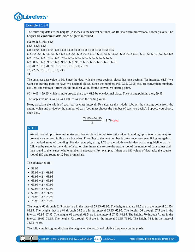
Alexander Holms, Barbara Illowsky, & Susan Dean 2.1.8 12/29/2021 https://stats.libretexts.org/@go/page/4547
The following data are the heights (in inches to the nearest half inch) of 100 male semiprofessional soccer players. Theheights are continuous data, since height is measured.
60; 60.5; 61; 61; 61.5 63.5; 63.5; 63.5 64; 64; 64; 64; 64; 64; 64; 64.5; 64.5; 64.5; 64.5; 64.5; 64.5; 64.5; 64.5 66; 66; 66; 66; 66; 66; 66; 66; 66; 66; 66.5; 66.5; 66.5; 66.5; 66.5; 66.5; 66.5; 66.5; 66.5; 66.5; 66.5; 67; 67; 67; 67;67; 67; 67; 67; 67; 67; 67; 67; 67.5; 67.5; 67.5; 67.5; 67.5; 67.5; 67.5 68; 68; 69; 69; 69; 69; 69; 69; 69; 69; 69; 69; 69.5; 69.5; 69.5; 69.5; 69.5 70; 70; 70; 70; 70; 70; 70.5; 70.5; 70.5; 71; 71; 71 72; 72; 72; 72.5; 72.5; 73; 73.5 74
The smallest data value is 60. Since the data with the most decimal places has one decimal (for instance, 61.5), wewant our starting point to have two decimal places. Since the numbers 0.5, 0.05, 0.005, etc. are convenient numbers,use 0.05 and subtract it from 60, the smallest value, for the convenient starting point.
60 – 0.05 = 59.95 which is more precise than, say, 61.5 by one decimal place. The starting point is, then, 59.95.
The largest value is 74, so 74 + 0.05 = 74.05 is the ending value.
Next, calculate the width of each bar or class interval. To calculate this width, subtract the starting point from theending value and divide by the number of bars (you must choose the number of bars you desire). Suppose you chooseeight bars.
We will round up to two and make each bar or class interval two units wide. Rounding up to two is one way toprevent a value from falling on a boundary. Rounding to the next number is often necessary even if it goes againstthe standard rules of rounding. For this example, using 1.76 as the width would also work. A guideline that isfollowed by some for the width of a bar or class interval is to take the square root of the number of data values andthen round to the nearest whole number, if necessary. For example, if there are 150 values of data, take the squareroot of 150 and round to 12 bars or intervals.
The boundaries are:
59.9559.95 + 2 = 61.9561.95 + 2 = 63.9563.95 + 2 = 65.9565.95 + 2 = 67.9567.95 + 2 = 69.9569.95 + 2 = 71.9571.95 + 2 = 73.9573.95 + 2 = 75.95
The heights 60 through 61.5 inches are in the interval 59.95–61.95. The heights that are 63.5 are in the interval 61.95–63.95. The heights that are 64 through 64.5 are in the interval 63.95–65.95. The heights 66 through 67.5 are in theinterval 65.95–67.95. The heights 68 through 69.5 are in the interval 67.95–69.95. The heights 70 through 71 are in theinterval 69.95–71.95. The heights 72 through 73.5 are in the interval 71.95–73.95. The height 74 is in the interval73.95–75.95.
The following histogram displays the heights on the x-axis and relative frequency on the y-axis.
Example .82.1.2
= 1.76\non74.05 −59.95
8
NOTE
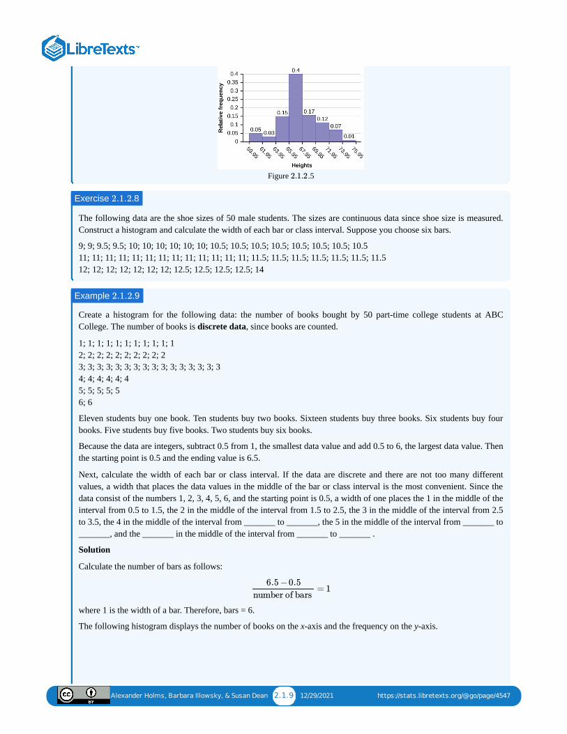
Alexander Holms, Barbara Illowsky, & Susan Dean 2.1.9 12/29/2021 https://stats.libretexts.org/@go/page/4547
Figure .5
The following data are the shoe sizes of 50 male students. The sizes are continuous data since shoe size is measured.Construct a histogram and calculate the width of each bar or class interval. Suppose you choose six bars.
9; 9; 9.5; 9.5; 10; 10; 10; 10; 10; 10; 10.5; 10.5; 10.5; 10.5; 10.5; 10.5; 10.5; 10.5 11; 11; 11; 11; 11; 11; 11; 11; 11; 11; 11; 11; 11; 11.5; 11.5; 11.5; 11.5; 11.5; 11.5; 11.5 12; 12; 12; 12; 12; 12; 12; 12.5; 12.5; 12.5; 12.5; 14
Create a histogram for the following data: the number of books bought by 50 part-time college students at ABCCollege. The number of books is discrete data, since books are counted.
1; 1; 1; 1; 1; 1; 1; 1; 1; 1; 1 2; 2; 2; 2; 2; 2; 2; 2; 2; 2 3; 3; 3; 3; 3; 3; 3; 3; 3; 3; 3; 3; 3; 3; 3; 3 4; 4; 4; 4; 4; 4 5; 5; 5; 5; 56; 6
Eleven students buy one book. Ten students buy two books. Sixteen students buy three books. Six students buy fourbooks. Five students buy five books. Two students buy six books.
Because the data are integers, subtract 0.5 from 1, the smallest data value and add 0.5 to 6, the largest data value. Thenthe starting point is 0.5 and the ending value is 6.5.
Next, calculate the width of each bar or class interval. If the data are discrete and there are not too many differentvalues, a width that places the data values in the middle of the bar or class interval is the most convenient. Since thedata consist of the numbers 1, 2, 3, 4, 5, 6, and the starting point is 0.5, a width of one places the 1 in the middle of theinterval from 0.5 to 1.5, the 2 in the middle of the interval from 1.5 to 2.5, the 3 in the middle of the interval from 2.5to 3.5, the 4 in the middle of the interval from _______ to _______, the 5 in the middle of the interval from _______ to_______, and the _______ in the middle of the interval from _______ to _______ .
Solution
Calculate the number of bars as follows:
where 1 is the width of a bar. Therefore, bars = 6.
The following histogram displays the number of books on the x-axis and the frequency on the y-axis.
2.1.2
Exercise .82.1.2
Example .92.1.2
= 16.5 −0.5
number of bars
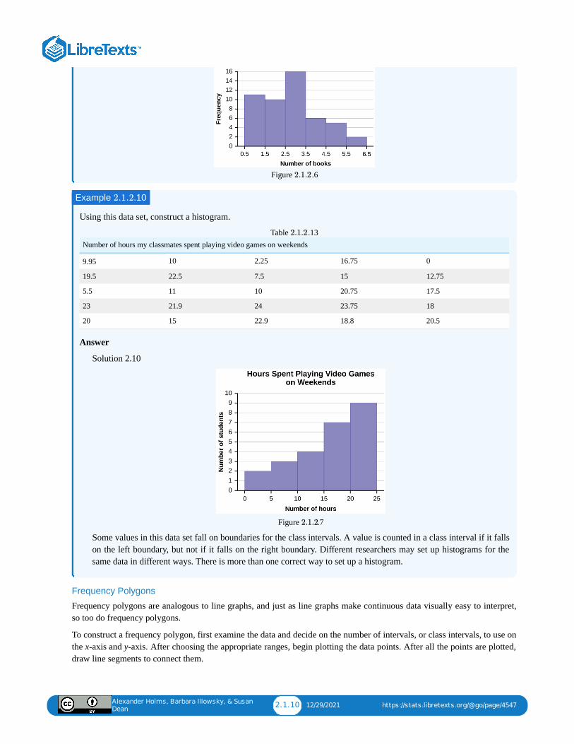
Alexander Holms, Barbara Illowsky, & Susan
Dean2.1.10 12/29/2021 https://stats.libretexts.org/@go/page/4547
Figure .6
Using this data set, construct a histogram.
Number of hours my classmates spent playing video games on weekends
9.95 10 2.25 16.75 0
19.5 22.5 7.5 15 12.75
5.5 11 10 20.75 17.5
23 21.9 24 23.75 18
20 15 22.9 18.8 20.5
Table .13
Answer
Solution 2.10
Figure .7
Some values in this data set fall on boundaries for the class intervals. A value is counted in a class interval if it fallson the left boundary, but not if it falls on the right boundary. Different researchers may set up histograms for thesame data in different ways. There is more than one correct way to set up a histogram.
Frequency Polygons
Frequency polygons are analogous to line graphs, and just as line graphs make continuous data visually easy to interpret,so too do frequency polygons.
To construct a frequency polygon, first examine the data and decide on the number of intervals, or class intervals, to use onthe x-axis and y-axis. After choosing the appropriate ranges, begin plotting the data points. After all the points are plotted,draw line segments to connect them.
2.1.2
Example .102.1.2
2.1.2
2.1.2
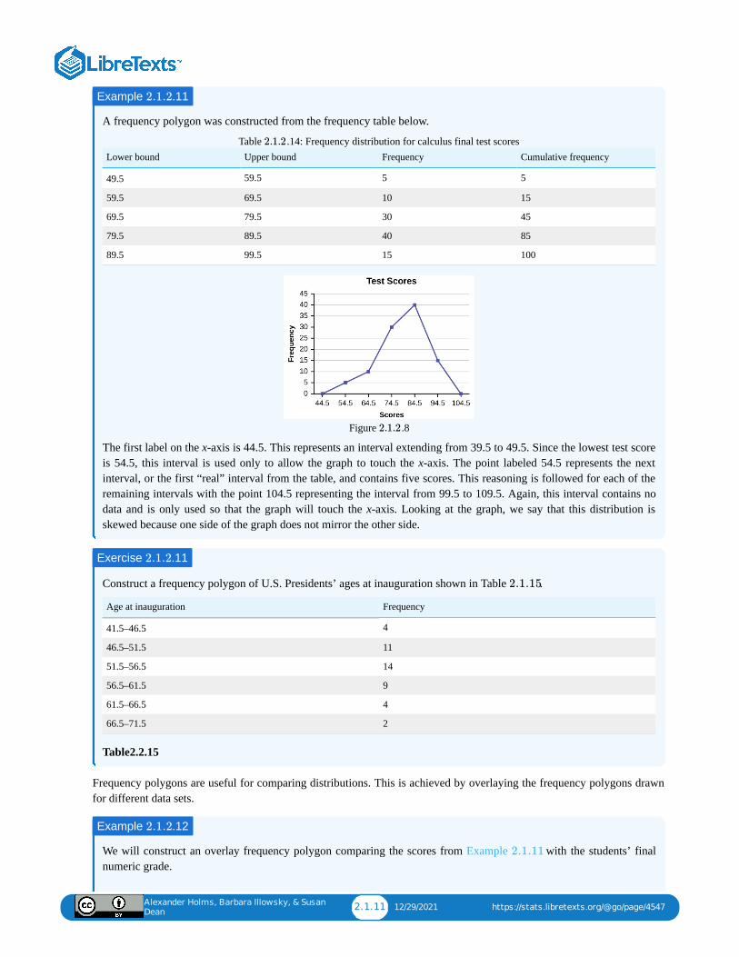
Alexander Holms, Barbara Illowsky, & Susan
Dean2.1.11 12/29/2021 https://stats.libretexts.org/@go/page/4547
A frequency polygon was constructed from the frequency table below.
Lower bound Upper bound Frequency Cumulative frequency
49.5 59.5 5 5
59.5 69.5 10 15
69.5 79.5 30 45
79.5 89.5 40 85
89.5 99.5 15 100
Table .14: Frequency distribution for calculus final test scores
Figure .8
The first label on the x-axis is 44.5. This represents an interval extending from 39.5 to 49.5. Since the lowest test scoreis 54.5, this interval is used only to allow the graph to touch the x-axis. The point labeled 54.5 represents the nextinterval, or the first “real” interval from the table, and contains five scores. This reasoning is followed for each of theremaining intervals with the point 104.5 representing the interval from 99.5 to 109.5. Again, this interval contains nodata and is only used so that the graph will touch the x-axis. Looking at the graph, we say that this distribution isskewed because one side of the graph does not mirror the other side.
Construct a frequency polygon of U.S. Presidents’ ages at inauguration shown in Table .
Age at inauguration Frequency
41.5–46.5 4
46.5–51.5 11
51.5–56.5 14
56.5–61.5 9
61.5–66.5 4
66.5–71.5 2
Table2.2.15
Frequency polygons are useful for comparing distributions. This is achieved by overlaying the frequency polygons drawnfor different data sets.
We will construct an overlay frequency polygon comparing the scores from Example with the students’ finalnumeric grade.
Example .112.1.2
2.1.2
2.1.2
Exercise .112.1.2
2.1.15
Example .122.1.2
2.1.11
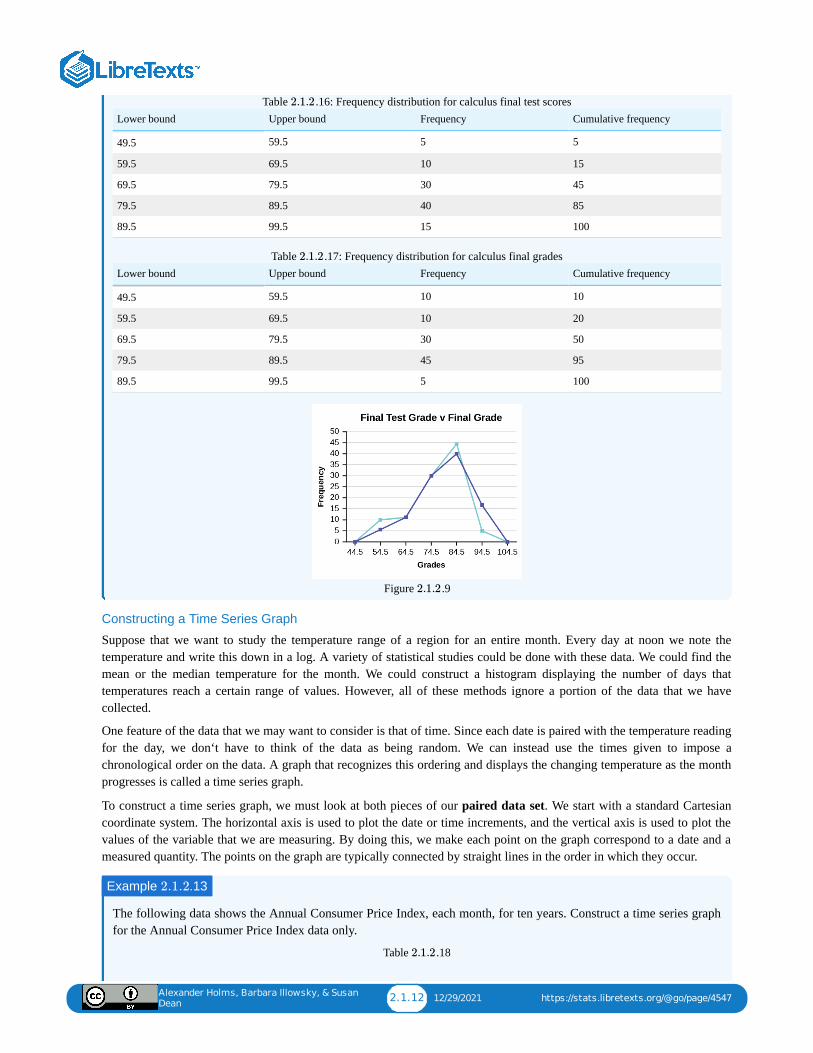
Alexander Holms, Barbara Illowsky, & Susan
Dean2.1.12 12/29/2021 https://stats.libretexts.org/@go/page/4547
Lower bound Upper bound Frequency Cumulative frequency
49.5 59.5 5 5
59.5 69.5 10 15
69.5 79.5 30 45
79.5 89.5 40 85
89.5 99.5 15 100
Table .16: Frequency distribution for calculus final test scores
Lower bound Upper bound Frequency Cumulative frequency
49.5 59.5 10 10
59.5 69.5 10 20
69.5 79.5 30 50
79.5 89.5 45 95
89.5 99.5 5 100
Table .17: Frequency distribution for calculus final grades
Figure .9
Constructing a Time Series Graph
Suppose that we want to study the temperature range of a region for an entire month. Every day at noon we note thetemperature and write this down in a log. A variety of statistical studies could be done with these data. We could find themean or the median temperature for the month. We could construct a histogram displaying the number of days thattemperatures reach a certain range of values. However, all of these methods ignore a portion of the data that we havecollected.
One feature of the data that we may want to consider is that of time. Since each date is paired with the temperature readingfor the day, we don‘t have to think of the data as being random. We can instead use the times given to impose achronological order on the data. A graph that recognizes this ordering and displays the changing temperature as the monthprogresses is called a time series graph.
To construct a time series graph, we must look at both pieces of our paired data set. We start with a standard Cartesiancoordinate system. The horizontal axis is used to plot the date or time increments, and the vertical axis is used to plot thevalues of the variable that we are measuring. By doing this, we make each point on the graph correspond to a date and ameasured quantity. The points on the graph are typically connected by straight lines in the order in which they occur.
The following data shows the Annual Consumer Price Index, each month, for ten years. Construct a time series graphfor the Annual Consumer Price Index data only.
Table .18
2.1.2
2.1.2
2.1.2
Example .132.1.2
2.1.2
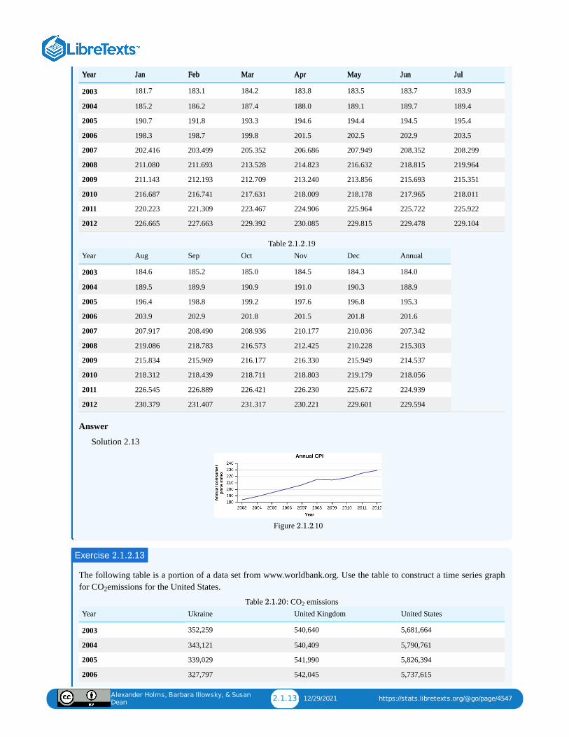
Alexander Holms, Barbara Illowsky, & Susan
Dean2.1.13 12/29/2021 https://stats.libretexts.org/@go/page/4547
Year Jan Feb Mar Apr May Jun JulYear Jan Feb Mar Apr May Jun Jul
2003 181.7 183.1 184.2 183.8 183.5 183.7 183.9
2004 185.2 186.2 187.4 188.0 189.1 189.7 189.4
2005 190.7 191.8 193.3 194.6 194.4 194.5 195.4
2006 198.3 198.7 199.8 201.5 202.5 202.9 203.5
2007 202.416 203.499 205.352 206.686 207.949 208.352 208.299
2008 211.080 211.693 213.528 214.823 216.632 218.815 219.964
2009 211.143 212.193 212.709 213.240 213.856 215.693 215.351
2010 216.687 216.741 217.631 218.009 218.178 217.965 218.011
2011 220.223 221.309 223.467 224.906 225.964 225.722 225.922
2012 226.665 227.663 229.392 230.085 229.815 229.478 229.104
Year Aug Sep Oct Nov Dec Annual
2003 184.6 185.2 185.0 184.5 184.3 184.0
2004 189.5 189.9 190.9 191.0 190.3 188.9
2005 196.4 198.8 199.2 197.6 196.8 195.3
2006 203.9 202.9 201.8 201.5 201.8 201.6
2007 207.917 208.490 208.936 210.177 210.036 207.342
2008 219.086 218.783 216.573 212.425 210.228 215.303
2009 215.834 215.969 216.177 216.330 215.949 214.537
2010 218.312 218.439 218.711 218.803 219.179 218.056
2011 226.545 226.889 226.421 226.230 225.672 224.939
2012 230.379 231.407 231.317 230.221 229.601 229.594
Table .19
Answer
Solution 2.13
Figure .10
The following table is a portion of a data set from www.worldbank.org. Use the table to construct a time series graphfor CO emissions for the United States.
Year Ukraine United Kingdom United States
2003 352,259 540,640 5,681,664
2004 343,121 540,409 5,790,761
2005 339,029 541,990 5,826,394
2006 327,797 542,045 5,737,615
Table : CO emissions
2.1.2
2.1.2
Exercise .132.1.2
2
2.1.20 2
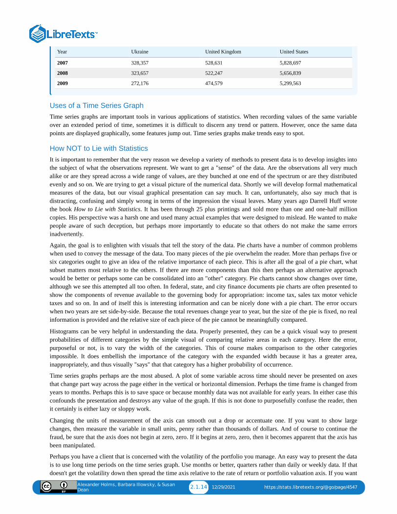
Alexander Holms, Barbara Illowsky, & Susan
Dean2.1.14 12/29/2021 https://stats.libretexts.org/@go/page/4547
Year Ukraine United Kingdom United States
2007 328,357 528,631 5,828,697
2008 323,657 522,247 5,656,839
2009 272,176 474,579 5,299,563
Uses of a Time Series Graph Time series graphs are important tools in various applications of statistics. When recording values of the same variableover an extended period of time, sometimes it is difficult to discern any trend or pattern. However, once the same datapoints are displayed graphically, some features jump out. Time series graphs make trends easy to spot.
How NOT to Lie with Statistics It is important to remember that the very reason we develop a variety of methods to present data is to develop insights intothe subject of what the observations represent. We want to get a "sense" of the data. Are the observations all very muchalike or are they spread across a wide range of values, are they bunched at one end of the spectrum or are they distributedevenly and so on. We are trying to get a visual picture of the numerical data. Shortly we will develop formal mathematicalmeasures of the data, but our visual graphical presentation can say much. It can, unfortunately, also say much that isdistracting, confusing and simply wrong in terms of the impression the visual leaves. Many years ago Darrell Huff wrotethe book How to Lie with Statistics. It has been through 25 plus printings and sold more than one and one-half millioncopies. His perspective was a harsh one and used many actual examples that were designed to mislead. He wanted to makepeople aware of such deception, but perhaps more importantly to educate so that others do not make the same errorsinadvertently.
Again, the goal is to enlighten with visuals that tell the story of the data. Pie charts have a number of common problemswhen used to convey the message of the data. Too many pieces of the pie overwhelm the reader. More than perhaps five orsix categories ought to give an idea of the relative importance of each piece. This is after all the goal of a pie chart, whatsubset matters most relative to the others. If there are more components than this then perhaps an alternative approachwould be better or perhaps some can be consolidated into an "other" category. Pie charts cannot show changes over time,although we see this attempted all too often. In federal, state, and city finance documents pie charts are often presented toshow the components of revenue available to the governing body for appropriation: income tax, sales tax motor vehicletaxes and so on. In and of itself this is interesting information and can be nicely done with a pie chart. The error occurswhen two years are set side-by-side. Because the total revenues change year to year, but the size of the pie is fixed, no realinformation is provided and the relative size of each piece of the pie cannot be meaningfully compared.
Histograms can be very helpful in understanding the data. Properly presented, they can be a quick visual way to presentprobabilities of different categories by the simple visual of comparing relative areas in each category. Here the error,purposeful or not, is to vary the width of the categories. This of course makes comparison to the other categoriesimpossible. It does embellish the importance of the category with the expanded width because it has a greater area,inappropriately, and thus visually "says" that that category has a higher probability of occurrence.
Time series graphs perhaps are the most abused. A plot of some variable across time should never be presented on axesthat change part way across the page either in the vertical or horizontal dimension. Perhaps the time frame is changed fromyears to months. Perhaps this is to save space or because monthly data was not available for early years. In either case thisconfounds the presentation and destroys any value of the graph. If this is not done to purposefully confuse the reader, thenit certainly is either lazy or sloppy work.
Changing the units of measurement of the axis can smooth out a drop or accentuate one. If you want to show largechanges, then measure the variable in small units, penny rather than thousands of dollars. And of course to continue thefraud, be sure that the axis does not begin at zero, zero. If it begins at zero, zero, then it becomes apparent that the axis hasbeen manipulated.
Perhaps you have a client that is concerned with the volatility of the portfolio you manage. An easy way to present the datais to use long time periods on the time series graph. Use months or better, quarters rather than daily or weekly data. If thatdoesn't get the volatility down then spread the time axis relative to the rate of return or portfolio valuation axis. If you want

Alexander Holms, Barbara Illowsky, & Susan
Dean2.1.15 12/29/2021 https://stats.libretexts.org/@go/page/4547
to show "quick" dramatic growth, then shrink the time axis. Any positive growth will show visually "high" growth rates.Do note that if the growth is negative then this trick will show the portfolio is collapsing at a dramatic rate.
Again, the goal of descriptive statistics is to convey meaningful visuals that tell the story of the data. Purposefulmanipulation is fraud and unethical at the worst, but even at its best, making these type of errors will lead to confusion onthe part of the analysis.
Alexander Holms, Barbara Illowsky, & Susan Dean 2.2.1 12/24/2021 https://stats.libretexts.org/@go/page/4548
2.2: Measures of the Location of the DataThe common measures of location are quartiles and percentiles
Quartiles are special percentiles. The first quartile, , is the same as the percentile, and the third quartile, , is the same as the percentile. The median, M, is called both the second quartile and the 50th percentile.
To calculate quartiles and percentiles, the data must be ordered from smallest to largest. Quartiles divide ordered data into quarters. Percentilesdivide ordered data into hundredths. To score in the percentile of an exam does not mean, necessarily, that you received 90% on a test. Itmeans that 90% of test scores are the same or less than your score and 10% of the test scores are the same or greater than your test score.
Percentiles are useful for comparing values. For this reason, universities and colleges use percentiles extensively. One instance in which collegesand universities use percentiles is when SAT results are used to determine a minimum testing score that will be used as an acceptance factor. Forexample, suppose Duke accepts SAT scores at or above the percentile. That translates into a score of at least 1220.
Percentiles are mostly used with very large populations. Therefore, if you were to say that 90% of the test scores are less (and not the same orless) than your score, it would be acceptable because removing one particular data value is not significant.
The median is a number that measures the "center" of the data. You can think of the median as the "middle value," but it does not actually haveto be one of the observed values. It is a number that separates ordered data into halves. Half the values are the same number or smaller than themedian, and half the values are the same number or larger. For example, consider the following data.
Ordered from smallest to largest:
Since there are 14 observations, the median is between the seventh value, 6.8, and the eighth value, 7.2. To find the median, add the two valuestogether and divide by two.
The median is seven. Half of the values are smaller than seven and half of the values are larger than seven.
Quartiles are numbers that separate the data into quarters. Quartiles may or may not be part of the data. To find the quartiles, first find themedian or second quartile. The first quartile, , is the middle value of the lower half of the data, and the third quartile, , is the middle value,or median, of the upper half of the data. To get the idea, consider the same data set: 1; 1; 2; 2; 4; 6; 6.8; 7.2; 8; 8.3; 9; 10; 10; 11.5
The median or second quartile is seven. The lower half of the data are 1, 1, 2, 2, 4, 6, 6.8. The middle value of the lower half is two. 1; 1; 2; 2; 4; 6; 6.8
The number two, which is part of the data, is the first quartile. One-fourth of the entire sets of values are the same as or less than two and three-fourths of the values are more than two.
The upper half of the data is 7.2, 8, 8.3, 9, 10, 10, 11.5. The middle value of the upper half is nine.
The third quartile, , is nine. Three-fourths (75%) of the ordered data set are less than nine. One-fourth (25%) of the ordered data set aregreater than nine. The third quartile is part of the data set in this example.
The interquartile range is a number that indicates the spread of the middle half or the middle 50% of the data. It is the difference between thethird quartile ( ) and the first quartile ( ).
The can help to determine potential outliers. A value is suspected to be a potential outlier if it is less than \(\bf{(1.5)(IQR)\) below thefirst quartile or more than above the third quartile. Potential outliers always require further investigation.
A potential outlier is a data point that is significantly different from the other data points. These special data points may be errors or somekind of abnormality or they may be a key to understanding the data.
For the following 13 real estate prices, calculate the and determine if any prices are potential outliers. Prices are in dollars.
Answer
Solution 2.14
Order the data from smallest to largest.
Q1 25th Q3 75th
90th
75th
1; 11.5; 6; 7.2; 4; 8; 9; 10; 6.8; 8.3; 2; 2; 10; 1
1; 1; 2; 2; 4; 6; 6.8; 7.2; 8; 8.3; 9; 10; 10; 11.5
= 76.8 +7.2
2
Q1 Q3
Q3
Q3 Q1
IQR = –Q3 Q1
IQR
(1.5)(IQR)
potential outlier
Example 2.2.14
IQR
389, 950; 230, 500; 158, 000; 479, 000; 639, 000; 114, 950; 5, 500, 000; 387, 000; 659, 000; 529, 000; 575, 000; 488, 800;
1, 095, 000
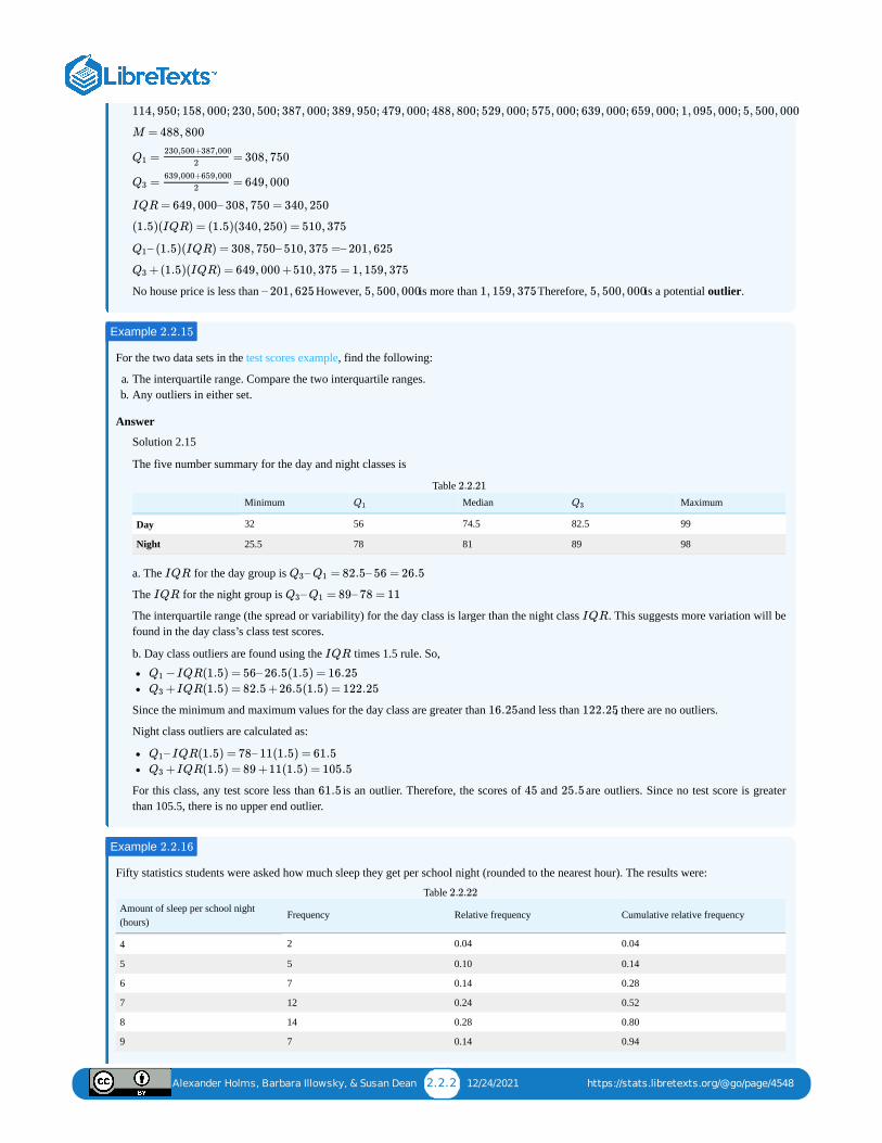
Alexander Holms, Barbara Illowsky, & Susan Dean 2.2.2 12/24/2021 https://stats.libretexts.org/@go/page/4548
No house price is less than . However, is more than . Therefore, is a potential outlier.
For the two data sets in the test scores example, find the following:
a. The interquartile range. Compare the two interquartile ranges.b. Any outliers in either set.
Answer
Solution 2.15
The five number summary for the day and night classes is
Minimum Median Maximum
Day 32 56 74.5 82.5 99
Night 25.5 78 81 89 98
Table
a. The for the day group is
The for the night group is
The interquartile range (the spread or variability) for the day class is larger than the night class . This suggests more variation will befound in the day class’s class test scores.
b. Day class outliers are found using the times 1.5 rule. So,
Since the minimum and maximum values for the day class are greater than and less than , there are no outliers.
Night class outliers are calculated as:
For this class, any test score less than is an outlier. Therefore, the scores of and are outliers. Since no test score is greaterthan 105.5, there is no upper end outlier.
Fifty statistics students were asked how much sleep they get per school night (rounded to the nearest hour). The results were:
Amount of sleep per school night(hours)
Frequency Relative frequency Cumulative relative frequency
4 2 0.04 0.04
5 5 0.10 0.14
6 7 0.14 0.28
7 12 0.24 0.52
8 14 0.28 0.80
9 7 0.14 0.94
Table
114, 950; 158, 000; 230, 500; 387, 000; 389, 950; 479, 000; 488, 800; 529, 000; 575, 000; 639, 000; 659, 000; 1, 095, 000; 5, 500, 000
M = 488, 800
= = 308, 750Q1230,500+387,000
2
= = 649, 000Q3639,000+659,000
2
IQR = 649, 000– 308, 750 = 340, 250
(1.5)(IQR) = (1.5)(340, 250) = 510, 375
– (1.5)(IQR) = 308, 750– 510, 375 =– 201, 625Q1
+(1.5)(IQR) = 649, 000 +510, 375 = 1, 159, 375Q3
– 201, 625 5, 500, 000 1, 159, 375 5, 500, 000
Example 2.2.15
Q1 Q3
2.2.21
IQR – = 82.5– 56 = 26.5Q3 Q1
IQR – = 89– 78 = 11Q3 Q1
IQR
IQR
−IQR(1.5) = 56– 26.5(1.5) = 16.25Q1
+IQR(1.5) = 82.5 +26.5(1.5) = 122.25Q3
16.25 122.25
– IQR(1.5) = 78– 11(1.5) = 61.5Q1
+IQR(1.5) = 89 +11(1.5) = 105.5Q3
61.5 45 25.5
Example 2.2.16
2.2.22
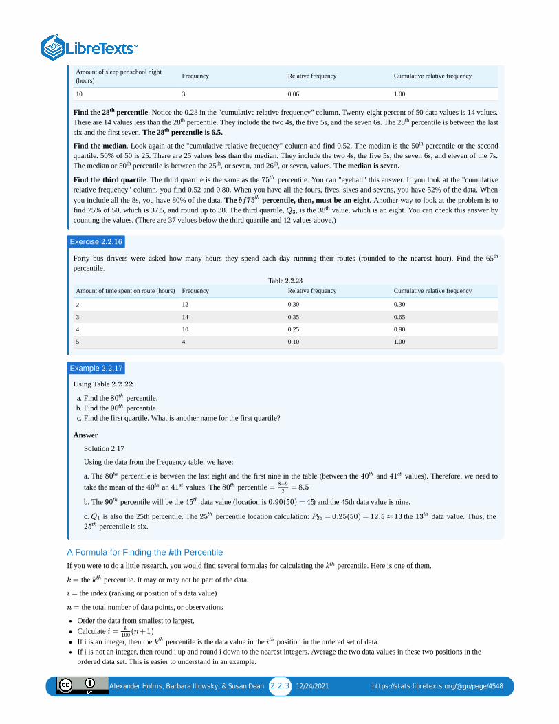
Alexander Holms, Barbara Illowsky, & Susan Dean 2.2.3 12/24/2021 https://stats.libretexts.org/@go/page/4548
Amount of sleep per school night(hours)
Frequency Relative frequency Cumulative relative frequency
10 3 0.06 1.00
Find the 28 percentile. Notice the 0.28 in the "cumulative relative frequency" column. Twenty-eight percent of 50 data values is 14 values.There are 14 values less than the 28 percentile. They include the two 4s, the five 5s, and the seven 6s. The 28 percentile is between the lastsix and the first seven. The 28 percentile is 6.5.
Find the median. Look again at the "cumulative relative frequency" column and find 0.52. The median is the 50 percentile or the secondquartile. 50% of 50 is 25. There are 25 values less than the median. They include the two 4s, the five 5s, the seven 6s, and eleven of the 7s.The median or 50 percentile is between the 25 , or seven, and 26 , or seven, values. The median is seven.
Find the third quartile. The third quartile is the same as the percentile. You can "eyeball" this answer. If you look at the "cumulativerelative frequency" column, you find 0.52 and 0.80. When you have all the fours, fives, sixes and sevens, you have 52% of the data. Whenyou include all the 8s, you have 80% of the data. The percentile, then, must be an eight. Another way to look at the problem is tofind 75% of 50, which is 37.5, and round up to 38. The third quartile, , is the 38 value, which is an eight. You can check this answer bycounting the values. (There are 37 values below the third quartile and 12 values above.)
Forty bus drivers were asked how many hours they spend each day running their routes (rounded to the nearest hour). Find the 65percentile.
Amount of time spent on route (hours) Frequency Relative frequency Cumulative relative frequency
2 12 0.30 0.30
3 14 0.35 0.65
4 10 0.25 0.90
5 4 0.10 1.00
Table
Using Table :
a. Find the percentile.b. Find the percentile.c. Find the first quartile. What is another name for the first quartile?
Answer
Solution 2.17
Using the data from the frequency table, we have:
a. The percentile is between the last eight and the first nine in the table (between the and values). Therefore, we need totake the mean of the an values. The percentile
b. The percentile will be the data value (location is ) and the 45th data value is nine.
c. is also the 25th percentile. The percentile location calculation: the data value. Thus, the percentile is six.
A Formula for Finding the th PercentileIf you were to do a little research, you would find several formulas for calculating the percentile. Here is one of them.
the percentile. It may or may not be part of the data.
the index (ranking or position of a data value)
the total number of data points, or observations
Order the data from smallest to largest.Calculate If i is an integer, then the percentile is the data value in the position in the ordered set of data.If i is not an integer, then round i up and round i down to the nearest integers. Average the two data values in these two positions in theordered data set. This is easier to understand in an example.
th
th th
th
th
th th th
75th
bf75th
Q3th
Exercise 2.2.16
th
2.2.23
Example 2.2.17
2.2.22
80th
90th
80th 40th 41st
40th 41st 80th = = 8.58+9
2
90th 45th 0.90(50) = 45
Q1 25th = 0.25(50) = 12.5 ≈ 13P25 13th
25th
k
kth
k = kth
i =
n =
i = (n+1)k
100
kth ith
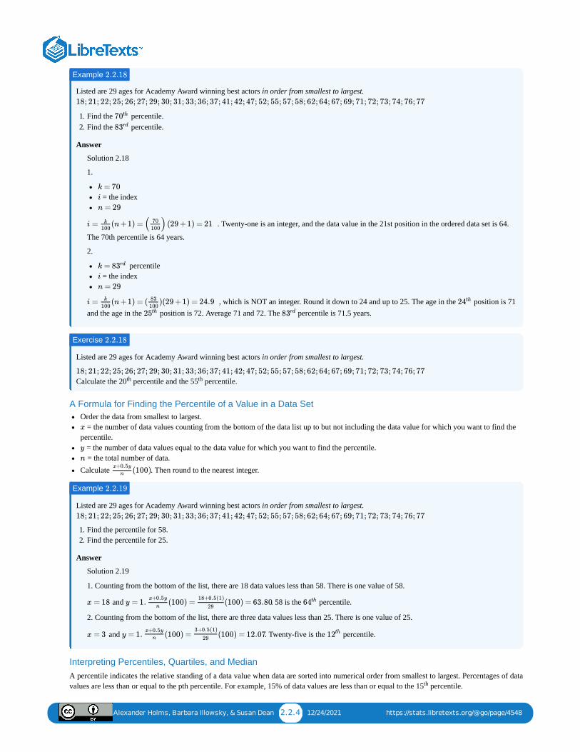
Alexander Holms, Barbara Illowsky, & Susan Dean 2.2.4 12/24/2021 https://stats.libretexts.org/@go/page/4548
Listed are 29 ages for Academy Award winning best actors in order from smallest to largest.
1. Find the percentile.2. Find the percentile.
Answer
Solution 2.18
1.
= the index
. Twenty-one is an integer, and the data value in the 21st position in the ordered data set is 64.
The 70th percentile is 64 years.
2.
percentile = the index
, which is NOT an integer. Round it down to 24 and up to 25. The age in the position is 71and the age in the position is 72. Average 71 and 72. The percentile is 71.5 years.
Listed are 29 ages for Academy Award winning best actors in order from smallest to largest.
Calculate the 20 percentile and the 55 percentile.
A Formula for Finding the Percentile of a Value in a Data SetOrder the data from smallest to largest.
= the number of data values counting from the bottom of the data list up to but not including the data value for which you want to find thepercentile.
= the number of data values equal to the data value for which you want to find the percentile. = the total number of data.
Calculate . Then round to the nearest integer.
Listed are 29 ages for Academy Award winning best actors in order from smallest to largest.
1. Find the percentile for 58.2. Find the percentile for 25.
Answer
Solution 2.19
1. Counting from the bottom of the list, there are 18 data values less than 58. There is one value of 58.
and . 58 is the percentile.
2. Counting from the bottom of the list, there are three data values less than 25. There is one value of 25.
and . Twenty-five is the percentile.
Interpreting Percentiles, Quartiles, and MedianA percentile indicates the relative standing of a data value when data are sorted into numerical order from smallest to largest. Percentages of datavalues are less than or equal to the pth percentile. For example, 15% of data values are less than or equal to the 15 percentile.
Example 2.2.18
18; 21; 22; 25; 26; 27; 29; 30; 31; 33; 36; 37; 41; 42; 47; 52; 55; 57; 58; 62; 64; 67; 69; 71; 72; 73; 74; 76; 77
70th
83rd
k = 70
i
n = 29
i = (n+1) = ( ) (29 +1) = 21k
100
70
100
k = 83rd
i
n = 29
i = (n+1) = ( )(29 +1) = 24.9k
100
83
10024th
25th 83rd
Exercise 2.2.18
18; 21; 22; 25; 26; 27; 29; 30; 31; 33; 36; 37; 41; 42; 47; 52; 55; 57; 58; 62; 64; 67; 69; 71; 72; 73; 74; 76; 77th th
x
y
n
(100)x+0.5y
n
Example 2.2.19
18; 21; 22; 25; 26; 27; 29; 30; 31; 33; 36; 37; 41; 42; 47; 52; 55; 57; 58; 62; 64; 67; 69; 71; 72; 73; 74; 76; 77
x = 18 y = 1. (100) = (100) = 63.80x+0.5y
n
18+0.5(1)
2964th
x = 3 y = 1. (100) = (100) = 12.07x+0.5y
n
3+0.5(1)
2912th
th
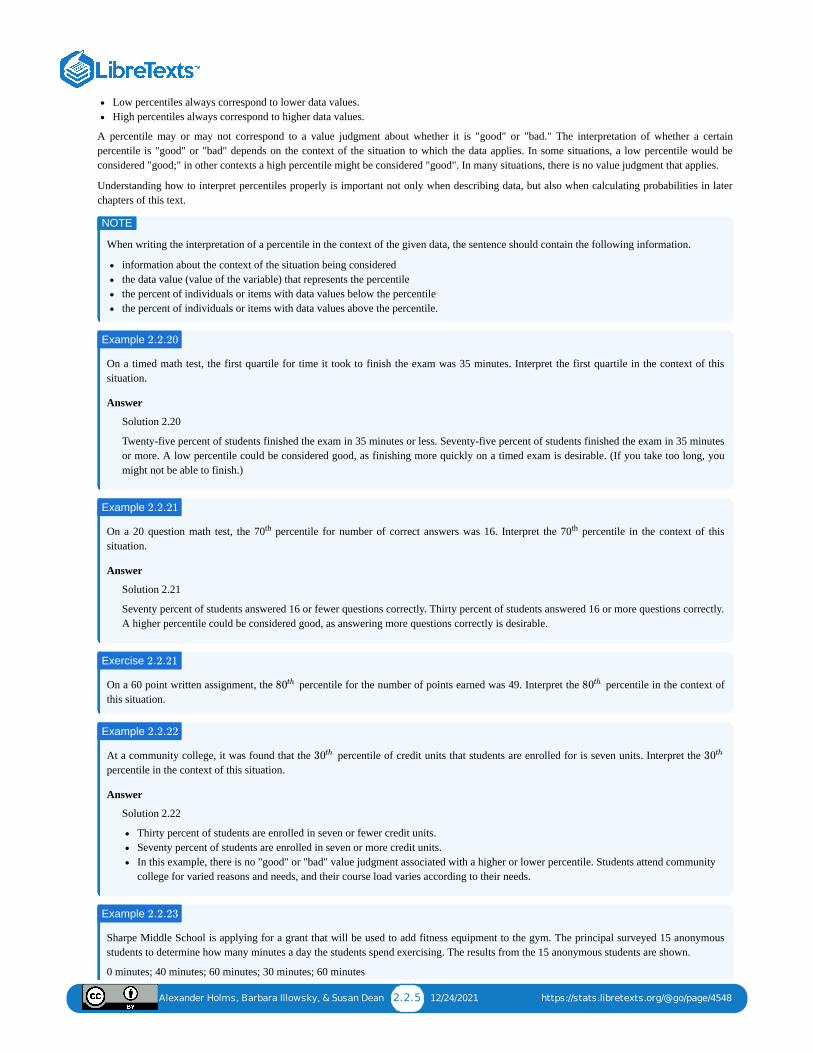
Alexander Holms, Barbara Illowsky, & Susan Dean 2.2.5 12/24/2021 https://stats.libretexts.org/@go/page/4548
Low percentiles always correspond to lower data values.High percentiles always correspond to higher data values.
A percentile may or may not correspond to a value judgment about whether it is "good" or "bad." The interpretation of whether a certainpercentile is "good" or "bad" depends on the context of the situation to which the data applies. In some situations, a low percentile would beconsidered "good;" in other contexts a high percentile might be considered "good". In many situations, there is no value judgment that applies.
Understanding how to interpret percentiles properly is important not only when describing data, but also when calculating probabilities in laterchapters of this text.
When writing the interpretation of a percentile in the context of the given data, the sentence should contain the following information.
information about the context of the situation being consideredthe data value (value of the variable) that represents the percentilethe percent of individuals or items with data values below the percentilethe percent of individuals or items with data values above the percentile.
On a timed math test, the first quartile for time it took to finish the exam was 35 minutes. Interpret the first quartile in the context of thissituation.
Answer
Solution 2.20
Twenty-five percent of students finished the exam in 35 minutes or less. Seventy-five percent of students finished the exam in 35 minutesor more. A low percentile could be considered good, as finishing more quickly on a timed exam is desirable. (If you take too long, youmight not be able to finish.)
On a 20 question math test, the 70 percentile for number of correct answers was 16. Interpret the 70 percentile in the context of thissituation.
Answer
Solution 2.21
Seventy percent of students answered 16 or fewer questions correctly. Thirty percent of students answered 16 or more questions correctly.A higher percentile could be considered good, as answering more questions correctly is desirable.
On a 60 point written assignment, the percentile for the number of points earned was 49. Interpret the percentile in the context ofthis situation.
At a community college, it was found that the percentile of credit units that students are enrolled for is seven units. Interpret the percentile in the context of this situation.
Answer
Solution 2.22
Thirty percent of students are enrolled in seven or fewer credit units.Seventy percent of students are enrolled in seven or more credit units.In this example, there is no "good" or "bad" value judgment associated with a higher or lower percentile. Students attend communitycollege for varied reasons and needs, and their course load varies according to their needs.
Sharpe Middle School is applying for a grant that will be used to add fitness equipment to the gym. The principal surveyed 15 anonymousstudents to determine how many minutes a day the students spend exercising. The results from the 15 anonymous students are shown.
0 minutes; 40 minutes; 60 minutes; 30 minutes; 60 minutes
NOTE
Example 2.2.20
Example 2.2.21
th th
Exercise 2.2.21
80th 80th
Example 2.2.22
30th 30th
Example 2.2.23
Alexander Holms, Barbara Illowsky, & Susan Dean 2.2.6 12/24/2021 https://stats.libretexts.org/@go/page/4548
10 minutes; 45 minutes; 30 minutes; 300 minutes; 90 minutes;
30 minutes; 120 minutes; 60 minutes; 0 minutes; 20 minutes
Determine the following five values.
Min = 0
Med = 40
Max = 300
If you were the principal, would you be justified in purchasing new fitness equipment? Since 75% of the students exercise for 60 minutes orless daily, and since the is 40 minutes , we know that half of the students surveyed exercise between 20 minutes and 60minutes daily. This seems a reasonable amount of time spent exercising, so the principal would be justified in purchasing the new equipment.
However, the principal needs to be careful. The value 300 appears to be a potential outlier.
.
The value 300 is greater than 120 so it is a potential outlier. If we delete it and calculate the five values, we get the following values:
Min = 0
Max = 120
We still have 75% of the students exercising for 60 minutes or less daily and half of the students exercising between 20 and 60
= 20Q1
= 60Q3
IQR (60– 20 = 40)
+1.5(IQR) = 60 +(1.5)(40) = 120Q3
= 20Q1
= 60Q3
Alexander Holms, Barbara Illowsky, & Susan Dean 2.3.1 10/22/2021 https://stats.libretexts.org/@go/page/4549
2.3: Measures of the Center of the DataThe "center" of a data set is also a way of describing location. The two most widely used measures of the "center" of the data are the mean(average) andthe median. To calculate the mean weight of 50 people, add the 50 weights together and divide by 50. Technically this is the arithmetic mean. We willdiscuss the geometric mean later. To find the median weight of the 50 people, order the data and find the number that splits the data into two equal partsmeaning an equal number of observations on each side. The weight of 25 people are below this weight and 25 people are heavier than this weight. Themedian is generally a better measure of the center when there are extreme values or outliers because it is not affected by the precise numerical values of theoutliers. The mean is the most common measure of the center.
The words “mean” and “average” are often used interchangeably. The substitution of one word for the other is common practice. The technical term is“arithmetic mean” and “average” is technically a center location. Formally, the arithmetic mean is called the first moment of the distribution bymathematicians. However, in practice among non-statisticians, “average" is commonly accepted for “arithmetic mean.”
When each value in the data set is not unique, the mean can be calculated by multiplying each distinct value by its frequency and then dividing the sum bythe total number of data values. The letter used to represent the sample mean is an x with a bar over it (pronounced “ bar”): .
The Greek letter (pronounced "mew") represents the population mean. One of the requirements for the sample mean to be a good estimate of thepopulation mean is for the sample taken to be truly random.
To see that both ways of calculating the mean are the same, consider the sample: 1; 1; 1; 2; 2; 3; 4; 4; 4; 4; 4
In the second calculation, the frequencies are 3, 2, 1, and 5.
You can quickly find the location of the median by using the expression .
The letter is the total number of data values in the sample. If is an odd number, the median is the middle value of the ordered data (ordered smallest tolargest). If is an even number, the median is equal to the two middle values added together and divided by two after the data has been ordered. Forexample, if the total number of data values is 97, then . The median is the 49 value in the ordered data. If the total number of datavalues is 100, then . The median occurs midway between the 50 and 51 values. The location of the median and the value of themedian are not the same. The upper case letter is often used to represent the median. The next example illustrates the location of the median and thevalue of the median.
AIDS data indicating the number of months a patient with AIDS lives after taking a new antibody drug are as follows (smallest to largest): 3; 4; 8; 8; 10; 11; 12; 13; 14; 15; 15; 16; 16; 17; 17; 18; 21; 22; 22; 24; 24; 25; 26; 26; 27; 27; 29; 29; 31; 32; 33; 33; 34; 34; 35; 37; 40; 44; 44; 47; Calculate the mean and the median.
Answer
Solution 2.24
The calculation for the mean is:
To find the median, , first use the formula for the location. The location is:
Starting at the smallest value, the median is located between the 20 and 21 values (the two 24s):
Suppose that in a small town of 50 people, one person earns $5,000,000 per year and the other 49 each earn $30,000. Which is the better measure ofthe "center": the mean or the median?
Answer
Solution 2.25
(There are 49 people who earn $30,000 and one person who earns $5,000,000.)
NOTE
x x̄̄̄
μ
= = 2.7x̄̄̄1 +1 +1 +2 +2 +3 +4 +4 +4 +4 +4
11
= = 2.7x̄̄̄3(1) +2(2) +1(3) +5(4)
11
n+12
n n
n
= = 49n+1
2
97+1
2th
= = 50.5n+1
2
100+1
2th st
M
Example 2.24
= = 23.6x̄̄̄[3+4+(8)(2)+10+11+12+13+14+(15)(2)+…+35+37+40+(44)(2)+47]
40
M
= = 20.5n+1
2
40+1
2th st
3; 4; 8; 8; 10; 11; 12; 13; 14; 15; 15; 16; 16; 17; 17; 18; 21; 22; 22; 24; 24; 25; 26; 26; 27; 27; 29; 29; 31; 32; 33; 33; 34; 34; 35; 37; 40; 44; 44; 47;
M = = 2424+24
2
Example 2.25
= = 129, 400x̄̄̄5,000,000+49(30,000)
50
M = 30, 000
☰
Alexander Holms, Barbara Illowsky, & Susan Dean 2.3.2 10/22/2021 https://stats.libretexts.org/@go/page/4549
The median is a better measure of the "center" than the mean because 49 of the values are 30,000 and one is 5,000,000. The 5,000,000 is an outlier.The 30,000 gives us a better sense of the middle of the data.
Another measure of the center is the mode. The mode is the most frequent value. There can be more than one mode in a data set as long as those valueshave the same frequency and that frequency is the highest. A data set with two modes is called bimodal.
Statistics exam scores for 20 students are as follows:
50; 53; 59; 59; 63; 63; 72; 72; 72; 72; 72; 76; 78; 81; 83; 84; 84; 84; 90; 93
Find the mode.
Answer
Solution 2.26
The most frequent score is 72, which occurs five times. Mode = 72.
Five real estate exam scores are 430, 430, 480, 480, 495. The data set is bimodal because the scores 430 and 480 each occur twice.
When is the mode the best measure of the "center"? Consider a weight loss program that advertises a mean weight loss of six pounds the first week ofthe program. The mode might indicate that most people lose two pounds the first week, making the program less appealing.
The mode can be calculated for qualitative data as well as for quantitative data. For example, if the data set is: red, red, red, green, green, yellow,purple, black, blue, the mode is red.
Calculating the Arithmetic Mean of Grouped Frequency Tables
When only grouped data is available, you do not know the individual data values (we only know intervals and interval frequencies); therefore, you cannotcompute an exact mean for the data set. What we must do is estimate the actual mean by calculating the mean of a frequency table. A frequency table is adata representation in which grouped data is displayed along with the corresponding frequencies. To calculate the mean from a grouped frequency table wecan apply the basic definition of mean: mean = We simply need to modify the definition to fit within the restrictions of a frequencytable.
Since we do not know the individual data values we can instead find the midpoint of each interval. The midpoint is . We can
now modify the mean definition to be where f = the frequency of the interval and m = the midpoint of the
interval.
A frequency table displaying professor Blount’s last statistic test is shown. Find the best estimate of the class mean.
Grade interval Number of students
50–56.5 1
56.5–62.5 0
62.5–68.5 4
68.5–74.5 4
74.5–80.5 2
80.5–86.5 3
86.5–92.5 4
92.5–98.5 1
Table 2.24
Answer
Solution 2.28
Find the midpoints for all intervals
Grade interval Midpoint
50–56.5 53.25
56.5–62.5 59.5
62.5–68.5 65.5
Table 2.25
Example 2.26
Example 2.27
NOTE
data sum number of data values
lower boundary+upper boundary
2
Mean of Frequency Table =∑ fm
∑ f
Example 2.28
☰
Alexander Holms, Barbara Illowsky, & Susan Dean 2.3.3 10/22/2021 https://stats.libretexts.org/@go/page/4549
Grade interval Midpoint
68.5–74.5 71.5
74.5–80.5 77.5
80.5–86.5 83.5
86.5–92.5 89.5
92.5–98.5 95.5
Calculate the sum of the product of each interval frequency and midpoint.
Maris conducted a study on the effect that playing video games has on memory recall. As part of her study, she compiled the following data:
Hours teenagers spend on video games Number of teenagers
0–3.5 3
3.5–7.5 7
7.5–11.5 12
11.5–15.5 7
15.5–19.5 9
Table 2.26
What is the best estimate for the mean number of hours spent playing video games?
∑fm
53.25(1) +59.5(0) +65.5(4) +71.5(4) +77.5(2) +83.5(3) +89.5(4) +95.5(1) = 1460.25
μ = = = 76.86∑ fm
∑ f
1460.25
19
Exercise 2.28
☰
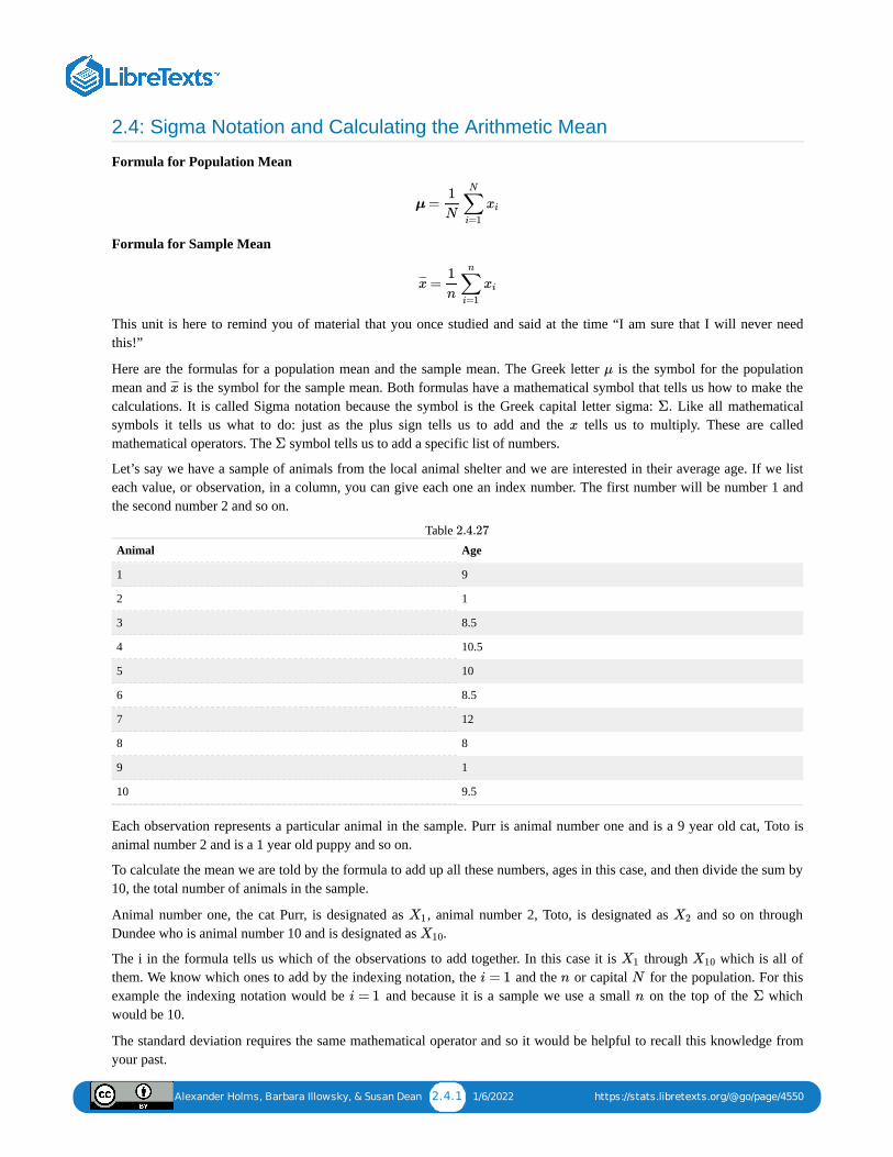
Alexander Holms, Barbara Illowsky, & Susan Dean 2.4.1 1/6/2022 https://stats.libretexts.org/@go/page/4550
2.4: Sigma Notation and Calculating the Arithmetic Mean
Formula for Population Mean
Formula for Sample Mean
This unit is here to remind you of material that you once studied and said at the time “I am sure that I will never needthis!”
Here are the formulas for a population mean and the sample mean. The Greek letter is the symbol for the populationmean and is the symbol for the sample mean. Both formulas have a mathematical symbol that tells us how to make thecalculations. It is called Sigma notation because the symbol is the Greek capital letter sigma: . Like all mathematicalsymbols it tells us what to do: just as the plus sign tells us to add and the tells us to multiply. These are calledmathematical operators. The symbol tells us to add a specific list of numbers.
Let’s say we have a sample of animals from the local animal shelter and we are interested in their average age. If we listeach value, or observation, in a column, you can give each one an index number. The first number will be number 1 andthe second number 2 and so on.
Animal Age
1 9
2 1
3 8.5
4 10.5
5 10
6 8.5
7 12
8 8
9 1
10 9.5
Table
Each observation represents a particular animal in the sample. Purr is animal number one and is a 9 year old cat, Toto isanimal number 2 and is a 1 year old puppy and so on.
To calculate the mean we are told by the formula to add up all these numbers, ages in this case, and then divide the sum by10, the total number of animals in the sample.
Animal number one, the cat Purr, is designated as , animal number 2, Toto, is designated as and so on throughDundee who is animal number 10 and is designated as .
The i in the formula tells us which of the observations to add together. In this case it is through which is all ofthem. We know which ones to add by the indexing notation, the and the or capital for the population. For thisexample the indexing notation would be and because it is a sample we use a small on the top of the whichwould be 10.
The standard deviation requires the same mathematical operator and so it would be helpful to recall this knowledge fromyour past.
μ =1
N∑i=1
N
xi
=x¯̄̄1
n∑i=1
n
xi
μ
x¯̄̄
Σ
x
Σ
2.4.27
X1 X2
X10
X1 X10
i = 1 n N
i = 1 n Σ

Alexander Holms, Barbara Illowsky, & Susan Dean 2.4.2 1/6/2022 https://stats.libretexts.org/@go/page/4550
The sum of the ages is found to be 78 and dividing by 10 gives us the sample mean age as 7.8 years.
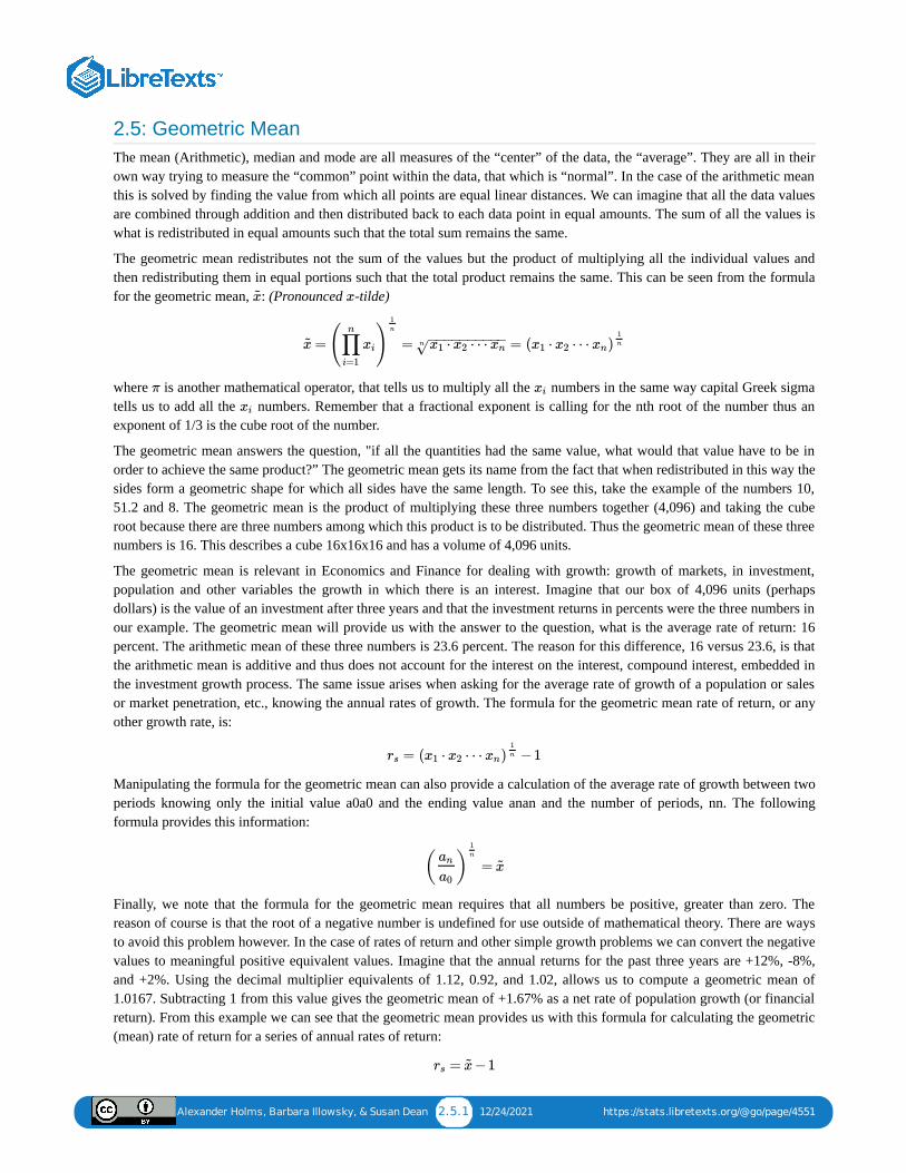
Alexander Holms, Barbara Illowsky, & Susan Dean 2.5.1 12/24/2021 https://stats.libretexts.org/@go/page/4551
2.5: Geometric MeanThe mean (Arithmetic), median and mode are all measures of the “center” of the data, the “average”. They are all in theirown way trying to measure the “common” point within the data, that which is “normal”. In the case of the arithmetic meanthis is solved by finding the value from which all points are equal linear distances. We can imagine that all the data valuesare combined through addition and then distributed back to each data point in equal amounts. The sum of all the values iswhat is redistributed in equal amounts such that the total sum remains the same.
The geometric mean redistributes not the sum of the values but the product of multiplying all the individual values andthen redistributing them in equal portions such that the total product remains the same. This can be seen from the formulafor the geometric mean, : (Pronounced -tilde)
where is another mathematical operator, that tells us to multiply all the numbers in the same way capital Greek sigmatells us to add all the numbers. Remember that a fractional exponent is calling for the nth root of the number thus anexponent of 1/3 is the cube root of the number.
The geometric mean answers the question, "if all the quantities had the same value, what would that value have to be inorder to achieve the same product?” The geometric mean gets its name from the fact that when redistributed in this way thesides form a geometric shape for which all sides have the same length. To see this, take the example of the numbers 10,51.2 and 8. The geometric mean is the product of multiplying these three numbers together (4,096) and taking the cuberoot because there are three numbers among which this product is to be distributed. Thus the geometric mean of these threenumbers is 16. This describes a cube 16x16x16 and has a volume of 4,096 units.
The geometric mean is relevant in Economics and Finance for dealing with growth: growth of markets, in investment,population and other variables the growth in which there is an interest. Imagine that our box of 4,096 units (perhapsdollars) is the value of an investment after three years and that the investment returns in percents were the three numbers inour example. The geometric mean will provide us with the answer to the question, what is the average rate of return: 16percent. The arithmetic mean of these three numbers is 23.6 percent. The reason for this difference, 16 versus 23.6, is thatthe arithmetic mean is additive and thus does not account for the interest on the interest, compound interest, embedded inthe investment growth process. The same issue arises when asking for the average rate of growth of a population or salesor market penetration, etc., knowing the annual rates of growth. The formula for the geometric mean rate of return, or anyother growth rate, is:
Manipulating the formula for the geometric mean can also provide a calculation of the average rate of growth between twoperiods knowing only the initial value a0a0 and the ending value anan and the number of periods, nn. The followingformula provides this information:
Finally, we note that the formula for the geometric mean requires that all numbers be positive, greater than zero. Thereason of course is that the root of a negative number is undefined for use outside of mathematical theory. There are waysto avoid this problem however. In the case of rates of return and other simple growth problems we can convert the negativevalues to meaningful positive equivalent values. Imagine that the annual returns for the past three years are +12%, -8%,and +2%. Using the decimal multiplier equivalents of 1.12, 0.92, and 1.02, allows us to compute a geometric mean of1.0167. Subtracting 1 from this value gives the geometric mean of +1.67% as a net rate of population growth (or financialreturn). From this example we can see that the geometric mean provides us with this formula for calculating the geometric(mean) rate of return for a series of annual rates of return:
x~
x
= = =x~ ( )∏
i=1
n
xi
1n
⋅ ⋯x1 x2 xn− −−−−−−−−−
√n ( ⋅ ⋯ )x1 x2 xn
1n
π xi
xi
= −1rs ( ⋅ ⋯ )x1 x2 xn
1n
=( )an
a0
1n
x~
= −1rs x~

Alexander Holms, Barbara Illowsky, & Susan Dean 2.5.2 12/24/2021 https://stats.libretexts.org/@go/page/4551
where is average rate of return and is the geometric mean of the returns during some number of time periods. Notethat the length of each time period must be the same.
As a general rule one should convert the percent values to its decimal equivalent multiplier. It is important to recognizethat when dealing with percents, the geometric mean of percent values does not equal the geometric mean of the decimalmultiplier equivalents and it is the decimal multiplier equivalent geometric mean that is relevant.
rs x~
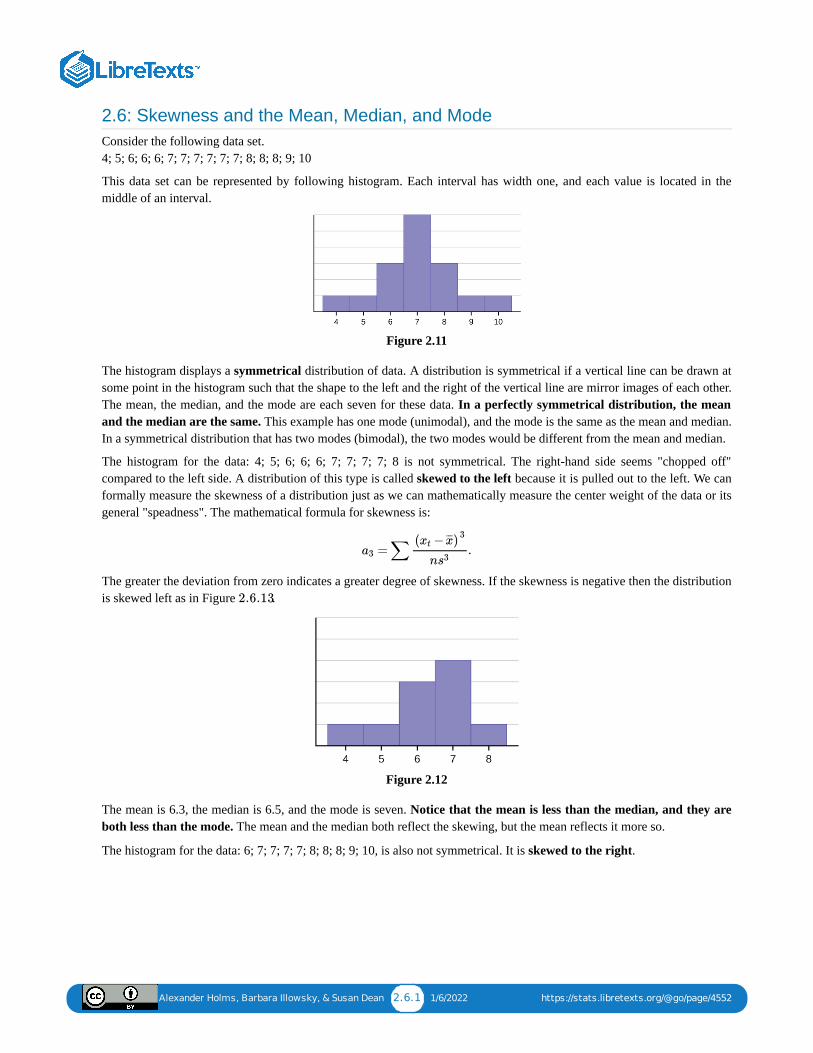
Alexander Holms, Barbara Illowsky, & Susan Dean 2.6.1 1/6/2022 https://stats.libretexts.org/@go/page/4552
2.6: Skewness and the Mean, Median, and ModeConsider the following data set. 4; 5; 6; 6; 6; 7; 7; 7; 7; 7; 7; 8; 8; 8; 9; 10
This data set can be represented by following histogram. Each interval has width one, and each value is located in themiddle of an interval.
Figure 2.11
The histogram displays a symmetrical distribution of data. A distribution is symmetrical if a vertical line can be drawn atsome point in the histogram such that the shape to the left and the right of the vertical line are mirror images of each other.The mean, the median, and the mode are each seven for these data. In a perfectly symmetrical distribution, the meanand the median are the same. This example has one mode (unimodal), and the mode is the same as the mean and median.In a symmetrical distribution that has two modes (bimodal), the two modes would be different from the mean and median.
The histogram for the data: 4; 5; 6; 6; 6; 7; 7; 7; 7; 8 is not symmetrical. The right-hand side seems "chopped off"compared to the left side. A distribution of this type is called skewed to the left because it is pulled out to the left. We canformally measure the skewness of a distribution just as we can mathematically measure the center weight of the data or itsgeneral "speadness". The mathematical formula for skewness is:
The greater the deviation from zero indicates a greater degree of skewness. If the skewness is negative then the distributionis skewed left as in Figure .
Figure 2.12
The mean is 6.3, the median is 6.5, and the mode is seven. Notice that the mean is less than the median, and they areboth less than the mode. The mean and the median both reflect the skewing, but the mean reflects it more so.
The histogram for the data: 6; 7; 7; 7; 7; 8; 8; 8; 9; 10, is also not symmetrical. It is skewed to the right.
=∑ .a3
( − )xt x̄̄̄3
ns3
2.6.13
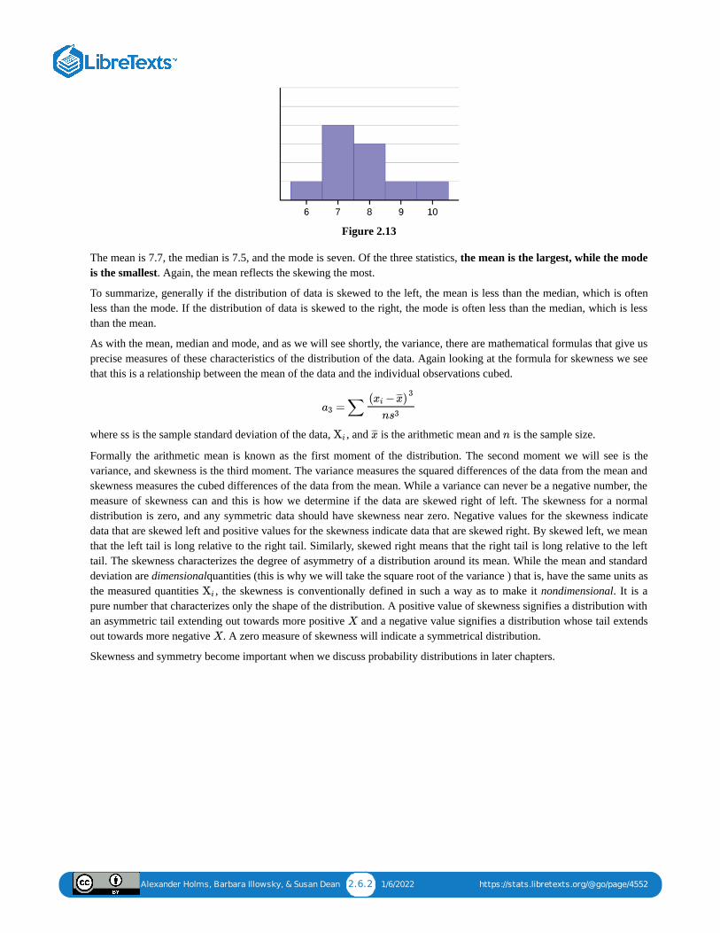
Alexander Holms, Barbara Illowsky, & Susan Dean 2.6.2 1/6/2022 https://stats.libretexts.org/@go/page/4552
Figure 2.13
The mean is 7.7, the median is 7.5, and the mode is seven. Of the three statistics, the mean is the largest, while the modeis the smallest. Again, the mean reflects the skewing the most.
To summarize, generally if the distribution of data is skewed to the left, the mean is less than the median, which is oftenless than the mode. If the distribution of data is skewed to the right, the mode is often less than the median, which is lessthan the mean.
As with the mean, median and mode, and as we will see shortly, the variance, there are mathematical formulas that give usprecise measures of these characteristics of the distribution of the data. Again looking at the formula for skewness we seethat this is a relationship between the mean of the data and the individual observations cubed.
where ss is the sample standard deviation of the data, , and is the arithmetic mean and is the sample size.
Formally the arithmetic mean is known as the first moment of the distribution. The second moment we will see is thevariance, and skewness is the third moment. The variance measures the squared differences of the data from the mean andskewness measures the cubed differences of the data from the mean. While a variance can never be a negative number, themeasure of skewness can and this is how we determine if the data are skewed right of left. The skewness for a normaldistribution is zero, and any symmetric data should have skewness near zero. Negative values for the skewness indicatedata that are skewed left and positive values for the skewness indicate data that are skewed right. By skewed left, we meanthat the left tail is long relative to the right tail. Similarly, skewed right means that the right tail is long relative to the lefttail. The skewness characterizes the degree of asymmetry of a distribution around its mean. While the mean and standarddeviation are dimensionalquantities (this is why we will take the square root of the variance ) that is, have the same units asthe measured quantities , the skewness is conventionally defined in such a way as to make it nondimensional. It is apure number that characterizes only the shape of the distribution. A positive value of skewness signifies a distribution withan asymmetric tail extending out towards more positive and a negative value signifies a distribution whose tail extendsout towards more negative . A zero measure of skewness will indicate a symmetrical distribution.
Skewness and symmetry become important when we discuss probability distributions in later chapters.
=∑a3
( − )xi x̄̄̄3
ns3
Xi x̄̄̄ n
Xi
X
X
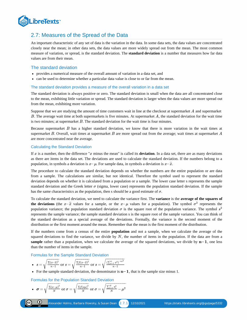
Alexander Holms, Barbara Illowsky, & Susan Dean 2.7.1 12/10/2021 https://stats.libretexts.org/@go/page/5332
2.7: Measures of the Spread of the DataAn important characteristic of any set of data is the variation in the data. In some data sets, the data values are concentratedclosely near the mean; in other data sets, the data values are more widely spread out from the mean. The most commonmeasure of variation, or spread, is the standard deviation. The standard deviation is a number that measures how far datavalues are from their mean.
The standard deviationprovides a numerical measure of the overall amount of variation in a data set, andcan be used to determine whether a particular data value is close to or far from the mean.
The standard deviation provides a measure of the overall variation in a data set
The standard deviation is always positive or zero. The standard deviation is small when the data are all concentrated closeto the mean, exhibiting little variation or spread. The standard deviation is larger when the data values are more spread outfrom the mean, exhibiting more variation.
Suppose that we are studying the amount of time customers wait in line at the checkout at supermarket and supermarket . The average wait time at both supermarkets is five minutes. At supermarket , the standard deviation for the wait time
is two minutes; at supermarket . The standard deviation for the wait time is four minutes.
Because supermarket has a higher standard deviation, we know that there is more variation in the wait times atsupermarket . Overall, wait times at supermarket are more spread out from the average; wait times at supermarket are more concentrated near the average.
Calculating the Standard Deviation
If is a number, then the difference " minus the mean" is called its deviation. In a data set, there are as many deviationsas there are items in the data set. The deviations are used to calculate the standard deviation. If the numbers belong to apopulation, in symbols a deviation is . For sample data, in symbols a deviation is .
The procedure to calculate the standard deviation depends on whether the numbers are the entire population or are datafrom a sample. The calculations are similar, but not identical. Therefore the symbol used to represent the standarddeviation depends on whether it is calculated from a population or a sample. The lower case letter s represents the samplestandard deviation and the Greek letter (sigma, lower case) represents the population standard deviation. If the samplehas the same characteristics as the population, then s should be a good estimate of .
To calculate the standard deviation, we need to calculate the variance first. The variance is the average of the squares ofthe deviations (the values for a sample, or the values for a population). The symbol represents thepopulation variance; the population standard deviation is the square root of the population variance. The symbol represents the sample variance; the sample standard deviation s is the square root of the sample variance. You can think ofthe standard deviation as a special average of the deviations. Formally, the variance is the second moment of thedistribution or the first moment around the mean. Remember that the mean is the first moment of the distribution.
If the numbers come from a census of the entire population and not a sample, when we calculate the average of thesquared deviations to find the variance, we divide by , the number of items in the population. If the data are from asample rather than a population, when we calculate the average of the squared deviations, we divide by , one lessthan the number of items in the sample.
Formulas for the Sample Standard Deviation
For the sample standard deviation, the denominator is , that is the sample size minus 1.
Formulas for the Population Standard Deviation
A
B A
B
B
B B A
x x
x– μ x– x̄̄̄
σ
σ
x– x̄̄̄ x– μ σ2
σ s2
N
n– 1
s = or s = or s =Σ(x−x̄̄̄)2
n−1
− −−−−−√ Σf(x−x̄̄̄)2
n−1
− −−−−−−√ ( )∑
ni=1 x2 −nx2
n−1
− −−−−−−−−√
n– 1
σ = or σ = or σ =Σ(x−μ)
2
N
− −−−−−√ Σf(xμ)
2
N
− −−−−−√ −
∑Ni=1 x2
i
Nμ2
− −−−−−−−−−√
Alexander Holms, Barbara Illowsky, & Susan Dean 2.7.2 12/10/2021 https://stats.libretexts.org/@go/page/5332
For the population standard deviation, the denominator is , the number of items in the population.
In these formulas, represents the frequency with which a value appears. For example, if a value appears once, is one. Ifa value appears three times in the data set or population, is three. Two important observations concerning the varianceand standard deviation: the deviations are measured from the mean and the deviations are squared. In principle, thedeviations could be measured from any point, however, our interest is measurement from the center weight of the data,what is the "normal" or most usual value of the observation. Later we will be trying to measure the "unusualness" of anobservation or a sample mean and thus we need a measure from the mean. The second observation is that the deviationsare squared. This does two things, first it makes the deviations all positive and second it changes the units of measurementfrom that of the mean and the original observations. If the data are weights then the mean is measured in pounds, but thevariance is measured in pounds-squared. One reason to use the standard deviation is to return to the original units ofmeasurement by taking the square root of the variance. Further, when the deviations are squared it explodes their value.For example, a deviation of 10 from the mean when squared is 100, but a deviation of 100 from the mean is 10,000. Whatthis does is place great weight on outliers when calculating the variance.
Types of Variability in Samples
When trying to study a population, a sample is often used, either for convenience or because it is not possible to access theentire population. Variability is the term used to describe the differences that may occur in these outcomes. Common typesof variability include the following:
Observational or measurement variabilityNatural variabilityInduced variabilitySample variability
Here are some examples to describe each type of variability.
Example 1: Measurement variability
Measurement variability occurs when there are differences in the instruments used to measure or in the people using thoseinstruments. If we are gathering data on how long it takes for a ball to drop from a height by having students measure thetime of the drop with a stopwatch, we may experience measurement variability if the two stopwatches used were made bydifferent manufacturers: For example, one stopwatch measures to the nearest second, whereas the other one measures tothe nearest tenth of a second. We also may experience measurement variability because two different people are gatheringthe data. Their reaction times in pressing the button on the stopwatch may differ; thus, the outcomes will vary accordingly.The differences in outcomes may be affected by measurement variability.
Example 2: Natural variability
Natural variability arises from the differences that naturally occur because members of a population differ from each other.For example, if we have two identical corn plants and we expose both plants to the same amount of water and sunlight,they may still grow at different rates simply because they are two different corn plants. The difference in outcomes may beexplained by natural variability.
Example 3: Induced variability
Induced variability is the counterpart to natural variability; this occurs because we have artificially induced an element ofvariation (that, by definition, was not present naturally): For example, we assign people to two different groups to studymemory, and we induce a variable in one group by limiting the amount of sleep they get. The difference in outcomes maybe affected by induced variability.
Example 4: Sample variability
Sample variability occurs when multiple random samples are taken from the same population. For example, if I conductfour surveys of 50 people randomly selected from a given population, the differences in outcomes may be affected bysample variability.
N
f f
f
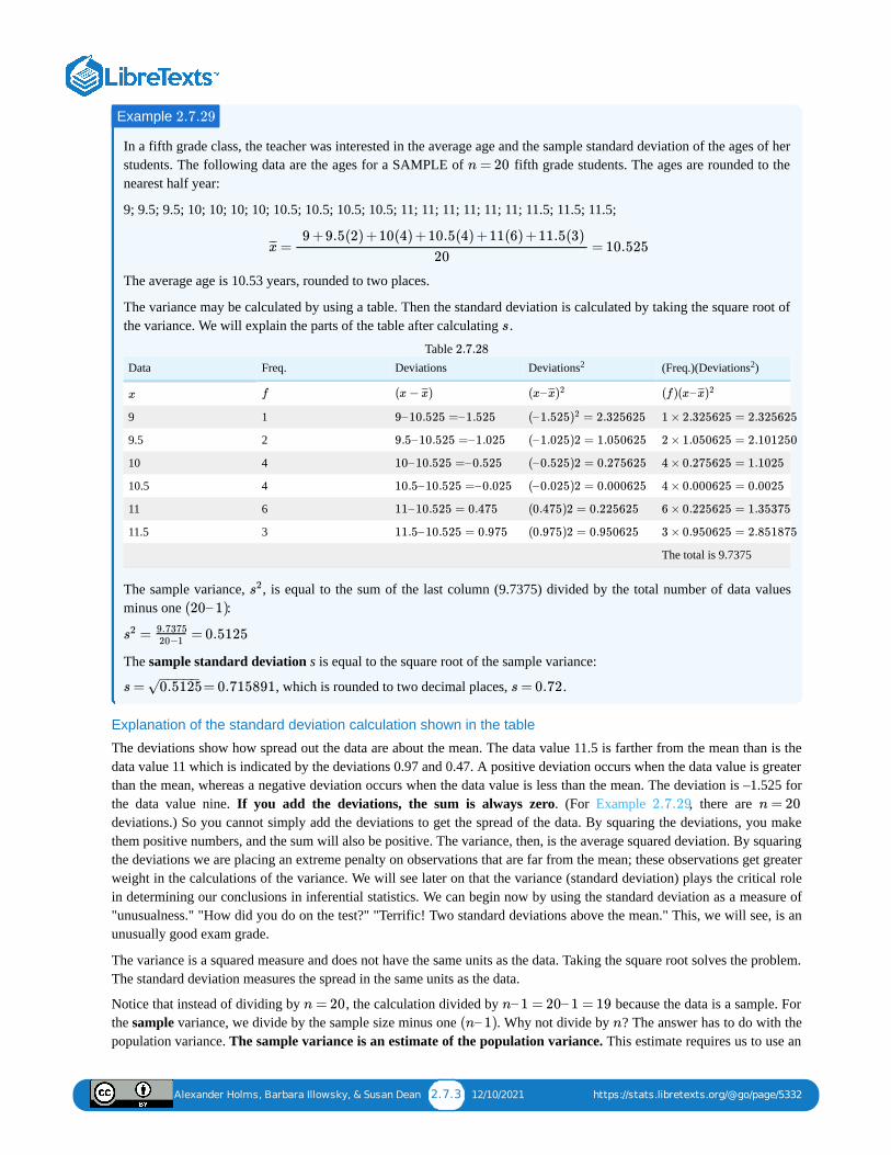
Alexander Holms, Barbara Illowsky, & Susan Dean 2.7.3 12/10/2021 https://stats.libretexts.org/@go/page/5332
In a fifth grade class, the teacher was interested in the average age and the sample standard deviation of the ages of herstudents. The following data are the ages for a SAMPLE of fifth grade students. The ages are rounded to thenearest half year:
9; 9.5; 9.5; 10; 10; 10; 10; 10.5; 10.5; 10.5; 10.5; 11; 11; 11; 11; 11; 11; 11.5; 11.5; 11.5;
The average age is 10.53 years, rounded to two places.
The variance may be calculated by using a table. Then the standard deviation is calculated by taking the square root ofthe variance. We will explain the parts of the table after calculating .
Data Freq. Deviations Deviations (Freq.)(Deviations )
9 1
9.5 2
10 4
10.5 4
11 6
11.5 3
The total is 9.7375
Table
The sample variance, , is equal to the sum of the last column (9.7375) divided by the total number of data valuesminus one :
The sample standard deviation s is equal to the square root of the sample variance:
, which is rounded to two decimal places, .
Explanation of the standard deviation calculation shown in the table
The deviations show how spread out the data are about the mean. The data value 11.5 is farther from the mean than is thedata value 11 which is indicated by the deviations 0.97 and 0.47. A positive deviation occurs when the data value is greaterthan the mean, whereas a negative deviation occurs when the data value is less than the mean. The deviation is –1.525 forthe data value nine. If you add the deviations, the sum is always zero. (For Example , there are deviations.) So you cannot simply add the deviations to get the spread of the data. By squaring the deviations, you makethem positive numbers, and the sum will also be positive. The variance, then, is the average squared deviation. By squaringthe deviations we are placing an extreme penalty on observations that are far from the mean; these observations get greaterweight in the calculations of the variance. We will see later on that the variance (standard deviation) plays the critical rolein determining our conclusions in inferential statistics. We can begin now by using the standard deviation as a measure of"unusualness." "How did you do on the test?" "Terrific! Two standard deviations above the mean." This, we will see, is anunusually good exam grade.
The variance is a squared measure and does not have the same units as the data. Taking the square root solves the problem.The standard deviation measures the spread in the same units as the data.
Notice that instead of dividing by , the calculation divided by because the data is a sample. Forthe sample variance, we divide by the sample size minus one . Why not divide by ? The answer has to do with thepopulation variance. The sample variance is an estimate of the population variance. This estimate requires us to use an
Example 2.7.29
n = 20
= = 10.525x̄̄̄9 +9.5(2) +10(4) +10.5(4) +11(6) +11.5(3)
20
s
2 2
x f (x − )x̄̄̄ (x– x̄̄̄)2 (f)(x– x̄̄̄)2
9–10.525 =–1.525 (–1.525 = 2.325625)2 1 × 2.325625 = 2.325625
9.5–10.525 =–1.025 (–1.025)2 = 1.050625 2 × 1.050625 = 2.101250
10–10.525 =–0.525 (–0.525)2 = 0.275625 4 × 0.275625 = 1.1025
10.5–10.525 =–0.025 (–0.025)2 = 0.000625 4 × 0.000625 = 0.0025
11–10.525 = 0.475 (0.475)2 = 0.225625 6 × 0.225625 = 1.35375
11.5–10.525 = 0.975 (0.975)2 = 0.950625 3 × 0.950625 = 2.851875
2.7.28
s2
(20– 1)
= = 0.5125s2 9.737520−1
s = = 0.7158910.5125− −−−−
√ s = 0.72
2.7.29 n = 20
n = 20 n– 1 = 20– 1 = 19(n– 1) n
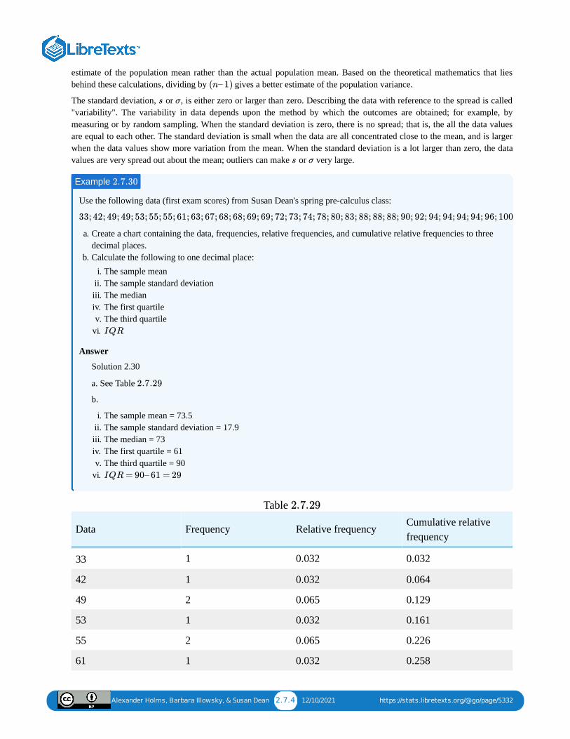
Alexander Holms, Barbara Illowsky, & Susan Dean 2.7.4 12/10/2021 https://stats.libretexts.org/@go/page/5332
estimate of the population mean rather than the actual population mean. Based on the theoretical mathematics that liesbehind these calculations, dividing by gives a better estimate of the population variance.
The standard deviation, or , is either zero or larger than zero. Describing the data with reference to the spread is called"variability". The variability in data depends upon the method by which the outcomes are obtained; for example, bymeasuring or by random sampling. When the standard deviation is zero, there is no spread; that is, the all the data valuesare equal to each other. The standard deviation is small when the data are all concentrated close to the mean, and is largerwhen the data values show more variation from the mean. When the standard deviation is a lot larger than zero, the datavalues are very spread out about the mean; outliers can make or very large.
Use the following data (first exam scores) from Susan Dean's spring pre-calculus class:
a. Create a chart containing the data, frequencies, relative frequencies, and cumulative relative frequencies to threedecimal places.
b. Calculate the following to one decimal place:i. The sample mean
ii. The sample standard deviationiii. The medianiv. The first quartilev. The third quartile
vi.
Answer
Solution 2.30
a. See Table
b.
i. The sample mean = 73.5ii. The sample standard deviation = 17.9iii. The median = 73iv. The first quartile = 61v. The third quartile = 90
vi.
Data Frequency Relative frequencyCumulative relativefrequency
33 1 0.032 0.032
42 1 0.032 0.064
49 2 0.065 0.129
53 1 0.032 0.161
55 2 0.065 0.226
61 1 0.032 0.258
Table
(n– 1)
s σ
s σ
Example 2.7.30
33; 42; 49; 49; 53; 55; 55; 61; 63; 67; 68; 68; 69; 69; 72; 73; 74; 78; 80; 83; 88; 88; 88; 90; 92; 94; 94; 94; 94; 96; 100
IQR
2.7.29
IQR = 90– 61 = 29
2.7.29
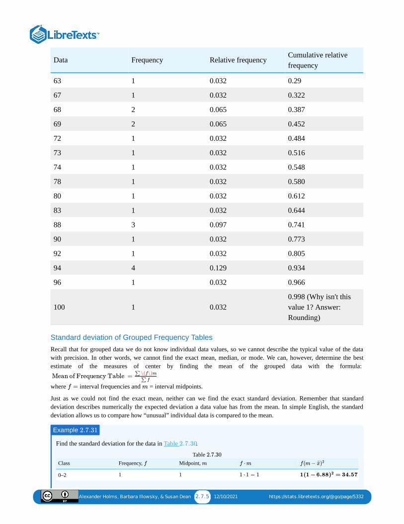
Alexander Holms, Barbara Illowsky, & Susan Dean 2.7.5 12/10/2021 https://stats.libretexts.org/@go/page/5332
Data Frequency Relative frequencyCumulative relativefrequency
63 1 0.032 0.29
67 1 0.032 0.322
68 2 0.065 0.387
69 2 0.065 0.452
72 1 0.032 0.484
73 1 0.032 0.516
74 1 0.032 0.548
78 1 0.032 0.580
80 1 0.032 0.612
83 1 0.032 0.644
88 3 0.097 0.741
90 1 0.032 0.773
92 1 0.032 0.805
94 4 0.129 0.934
96 1 0.032 0.966
100 1 0.0320.998 (Why isn't thisvalue 1? Answer:Rounding)
Standard deviation of Grouped Frequency Tables
Recall that for grouped data we do not know individual data values, so we cannot describe the typical value of the datawith precision. In other words, we cannot find the exact mean, median, or mode. We can, however, determine the bestestimate of the measures of center by finding the mean of the grouped data with the formula:
where interval frequencies and = interval midpoints.
Just as we could not find the exact mean, neither can we find the exact standard deviation. Remember that standarddeviation describes numerically the expected deviation a data value has from the mean. In simple English, the standarddeviation allows us to compare how “unusual” individual data is compared to the mean.
Find the standard deviation for the data in Table .
Class Frequency, Midpoint,
0–2 1 1
Table
Mean of Frequency Table =∑ \(f\)m
∑ f
f = m
Example 2.7.31
2.7.30
f m f ⋅ m f(m − x̄)2
1 ⋅ 1 = 1 1(1 − 6.88 = 34.57)2
2.7.30
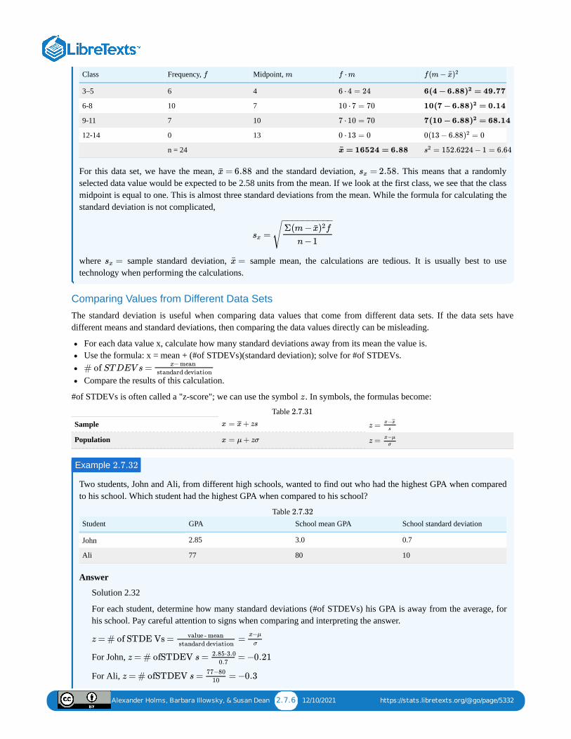
Alexander Holms, Barbara Illowsky, & Susan Dean 2.7.6 12/10/2021 https://stats.libretexts.org/@go/page/5332
Class Frequency, Midpoint,
3–5 6 4
6-8 10 7
9-11 7 10
12-14 0 13
n = 24
For this data set, we have the mean, and the standard deviation, . This means that a randomlyselected data value would be expected to be 2.58 units from the mean. If we look at the first class, we see that the classmidpoint is equal to one. This is almost three standard deviations from the mean. While the formula for calculating thestandard deviation is not complicated,
where sample standard deviation, sample mean, the calculations are tedious. It is usually best to usetechnology when performing the calculations.
Comparing Values from Different Data Sets
The standard deviation is useful when comparing data values that come from different data sets. If the data sets havedifferent means and standard deviations, then comparing the data values directly can be misleading.
For each data value x, calculate how many standard deviations away from its mean the value is.Use the formula: x = mean + (#of STDEVs)(standard deviation); solve for #of STDEVs.
Compare the results of this calculation.
#of STDEVs is often called a "z-score"; we can use the symbol . In symbols, the formulas become:
Sample
Population
Table
Two students, John and Ali, from different high schools, wanted to find out who had the highest GPA when comparedto his school. Which student had the highest GPA when compared to his school?
Student GPA School mean GPA School standard deviation
John 2.85 3.0 0.7
Ali 77 80 10
Table
Answer
Solution 2.32
For each student, determine how many standard deviations (#of STDEVs) his GPA is away from the average, forhis school. Pay careful attention to signs when comparing and interpreting the answer.
For John,
For Ali,
f m f ⋅ m f(m − x̄)2
6 ⋅ 4 = 24 6(4 − 6.88 = 49.77)2
10 ⋅ 7 = 70 10(7 − 6.88 = 0.14)2
7 ⋅ 10 = 70 7(10 − 6.88 = 68.14)2
0 ⋅ 13 = 0 0(13 − 6.88 = 0)2
= 16524 = 6.88x̄ = 152.6224 − 1 = 6.64s2
= 6.88x̄ = 2.58sx
=sx
Σ(m − fx̄)2
n −1
− −−−−−−−−−
√
=sx =x̄
# of ST DEV s =x− mean
standard deviation
z
x = + zsx̄̄̄ z =x−x̄̄̄
s
x = μ + zσ z =x−μ
σ
2.7.31
Example 2.7.32
2.7.32
z = # of STDE Vs = = value - mean standard deviation
x−μ
σ
z = # ofSTDEV s = = −0.212.85⋅3.00.7
z = # ofSTDEV s = = −0.377−80
10
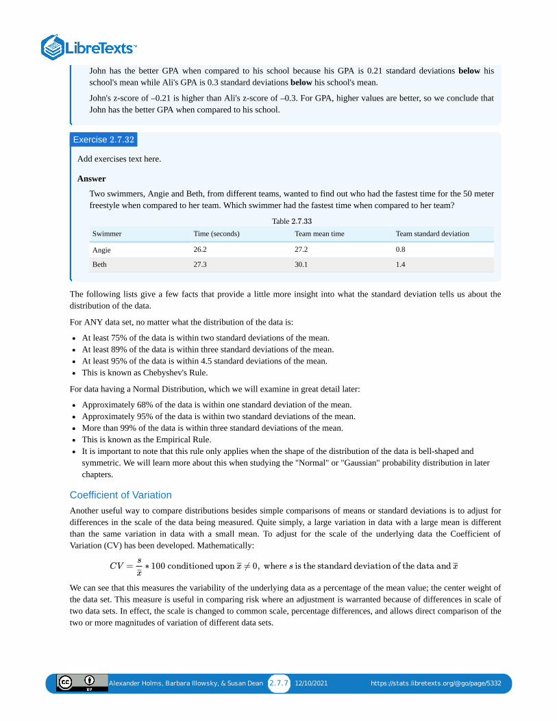
Alexander Holms, Barbara Illowsky, & Susan Dean 2.7.7 12/10/2021 https://stats.libretexts.org/@go/page/5332
John has the better GPA when compared to his school because his GPA is 0.21 standard deviations below hisschool's mean while Ali's GPA is 0.3 standard deviations below his school's mean.
John's z-score of –0.21 is higher than Ali's z-score of –0.3. For GPA, higher values are better, so we conclude thatJohn has the better GPA when compared to his school.
Add exercises text here.
Answer
Two swimmers, Angie and Beth, from different teams, wanted to find out who had the fastest time for the 50 meterfreestyle when compared to her team. Which swimmer had the fastest time when compared to her team?
Swimmer Time (seconds) Team mean time Team standard deviation
Angie 26.2 27.2 0.8
Beth 27.3 30.1 1.4
Table
The following lists give a few facts that provide a little more insight into what the standard deviation tells us about thedistribution of the data.
For ANY data set, no matter what the distribution of the data is:
At least 75% of the data is within two standard deviations of the mean.At least 89% of the data is within three standard deviations of the mean.At least 95% of the data is within 4.5 standard deviations of the mean.This is known as Chebyshev's Rule.
For data having a Normal Distribution, which we will examine in great detail later:
Approximately 68% of the data is within one standard deviation of the mean.Approximately 95% of the data is within two standard deviations of the mean.More than 99% of the data is within three standard deviations of the mean.This is known as the Empirical Rule.It is important to note that this rule only applies when the shape of the distribution of the data is bell-shaped andsymmetric. We will learn more about this when studying the "Normal" or "Gaussian" probability distribution in laterchapters.
Coefficient of VariationAnother useful way to compare distributions besides simple comparisons of means or standard deviations is to adjust fordifferences in the scale of the data being measured. Quite simply, a large variation in data with a large mean is differentthan the same variation in data with a small mean. To adjust for the scale of the underlying data the Coefficient ofVariation (CV) has been developed. Mathematically:
We can see that this measures the variability of the underlying data as a percentage of the mean value; the center weight ofthe data set. This measure is useful in comparing risk where an adjustment is warranted because of differences in scale oftwo data sets. In effect, the scale is changed to common scale, percentage differences, and allows direct comparison of thetwo or more magnitudes of variation of different data sets.
Exercise 2.7.32
2.7.33
CV = ∗ 100 conditioned upon ≠ 0, where s is the standard deviation of the data and s
x̄̄̄x̄̄̄ x̄̄̄
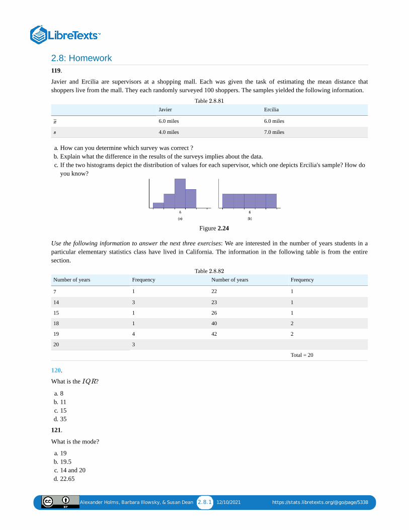
Alexander Holms, Barbara Illowsky, & Susan Dean 2.8.1 12/10/2021 https://stats.libretexts.org/@go/page/5338
2.8: Homework119.
Javier and Ercilia are supervisors at a shopping mall. Each was given the task of estimating the mean distance thatshoppers live from the mall. They each randomly surveyed 100 shoppers. The samples yielded the following information.
Javier Ercilia
6.0 miles 6.0 miles
4.0 miles 7.0 miles
Table
a. How can you determine which survey was correct ?b. Explain what the difference in the results of the surveys implies about the data.c. If the two histograms depict the distribution of values for each supervisor, which one depicts Ercilia's sample? How do
you know?
Figure 2.24
Use the following information to answer the next three exercises: We are interested in the number of years students in aparticular elementary statistics class have lived in California. The information in the following table is from the entiresection.
Number of years Frequency Number of years Frequency
Total = 20
7 1 22 1
14 3 23 1
15 1 26 1
18 1 40 2
19 4 42 2
20 3
Table
120.
What is the ?
a. 8b. 11c. 15d. 35
121.
What is the mode?
a. 19b. 19.5c. 14 and 20d. 22.65
x¯̄̄
s
2.8.81
2.8.82
IQR
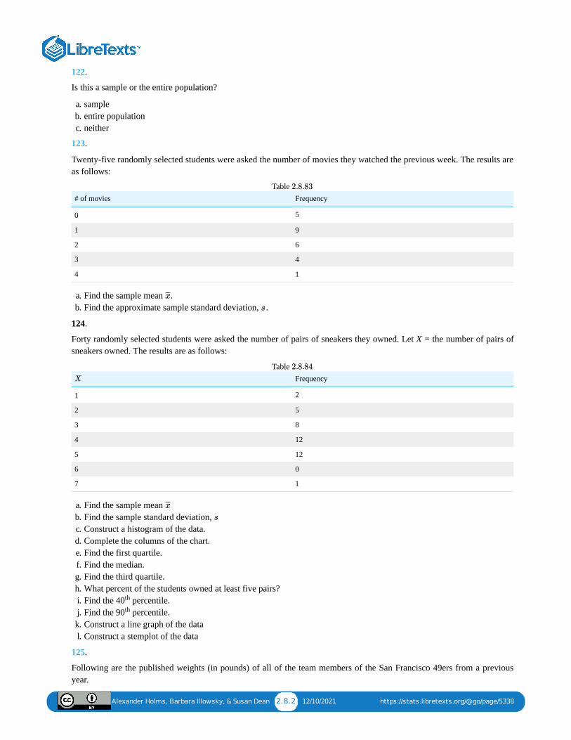
Alexander Holms, Barbara Illowsky, & Susan Dean 2.8.2 12/10/2021 https://stats.libretexts.org/@go/page/5338
122.
Is this a sample or the entire population?
a. sampleb. entire populationc. neither
123.
Twenty-five randomly selected students were asked the number of movies they watched the previous week. The results areas follows:
# of movies Frequency
0 5
1 9
2 6
3 4
4 1
Table
a. Find the sample mean .b. Find the approximate sample standard deviation, .
124.
Forty randomly selected students were asked the number of pairs of sneakers they owned. Let X = the number of pairs ofsneakers owned. The results are as follows:
Frequency
1 2
2 5
3 8
4 12
5 12
6 0
7 1
Table
a. Find the sample mean b. Find the sample standard deviation, c. Construct a histogram of the data.d. Complete the columns of the chart.e. Find the first quartile.f. Find the median.g. Find the third quartile.h. What percent of the students owned at least five pairs?i. Find the 40 percentile.j. Find the 90 percentile.k. Construct a line graph of the datal. Construct a stemplot of the data
125.
Following are the published weights (in pounds) of all of the team members of the San Francisco 49ers from a previousyear.
2.8.83
x̄̄̄
s
X
2.8.84
x̄̄̄
s
th
th
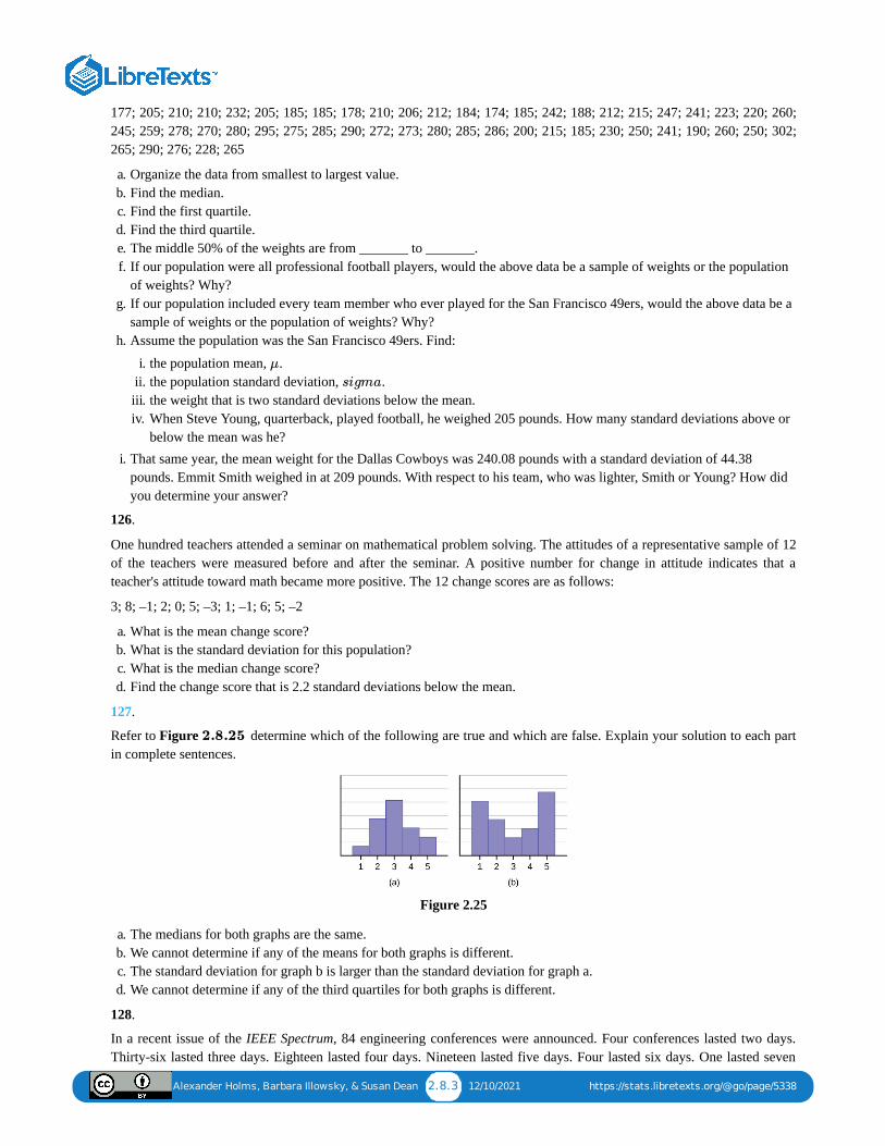
Alexander Holms, Barbara Illowsky, & Susan Dean 2.8.3 12/10/2021 https://stats.libretexts.org/@go/page/5338
177; 205; 210; 210; 232; 205; 185; 185; 178; 210; 206; 212; 184; 174; 185; 242; 188; 212; 215; 247; 241; 223; 220; 260;245; 259; 278; 270; 280; 295; 275; 285; 290; 272; 273; 280; 285; 286; 200; 215; 185; 230; 250; 241; 190; 260; 250; 302;265; 290; 276; 228; 265
a. Organize the data from smallest to largest value.b. Find the median.c. Find the first quartile.d. Find the third quartile.e. The middle 50% of the weights are from _______ to _______.f. If our population were all professional football players, would the above data be a sample of weights or the population
of weights? Why?g. If our population included every team member who ever played for the San Francisco 49ers, would the above data be a
sample of weights or the population of weights? Why?h. Assume the population was the San Francisco 49ers. Find:
i. the population mean, .ii. the population standard deviation, .iii. the weight that is two standard deviations below the mean.iv. When Steve Young, quarterback, played football, he weighed 205 pounds. How many standard deviations above or
below the mean was he?i. That same year, the mean weight for the Dallas Cowboys was 240.08 pounds with a standard deviation of 44.38
pounds. Emmit Smith weighed in at 209 pounds. With respect to his team, who was lighter, Smith or Young? How didyou determine your answer?
126.
One hundred teachers attended a seminar on mathematical problem solving. The attitudes of a representative sample of 12of the teachers were measured before and after the seminar. A positive number for change in attitude indicates that ateacher's attitude toward math became more positive. The 12 change scores are as follows:
3; 8; –1; 2; 0; 5; –3; 1; –1; 6; 5; –2
a. What is the mean change score?b. What is the standard deviation for this population?c. What is the median change score?d. Find the change score that is 2.2 standard deviations below the mean.
127.
Refer to Figure determine which of the following are true and which are false. Explain your solution to each partin complete sentences.
Figure 2.25
a. The medians for both graphs are the same.b. We cannot determine if any of the means for both graphs is different.c. The standard deviation for graph b is larger than the standard deviation for graph a.d. We cannot determine if any of the third quartiles for both graphs is different.
128.
In a recent issue of the IEEE Spectrum, 84 engineering conferences were announced. Four conferences lasted two days.Thirty-six lasted three days. Eighteen lasted four days. Nineteen lasted five days. Four lasted six days. One lasted seven
μ
sigma
2.8.25
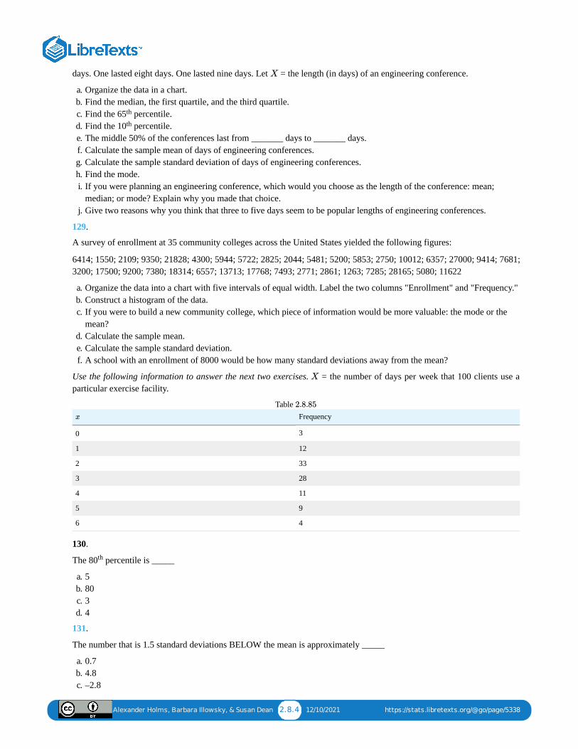
Alexander Holms, Barbara Illowsky, & Susan Dean 2.8.4 12/10/2021 https://stats.libretexts.org/@go/page/5338
days. One lasted eight days. One lasted nine days. Let = the length (in days) of an engineering conference.
a. Organize the data in a chart.b. Find the median, the first quartile, and the third quartile.c. Find the 65 percentile.d. Find the 10 percentile.e. The middle 50% of the conferences last from _______ days to _______ days.f. Calculate the sample mean of days of engineering conferences.g. Calculate the sample standard deviation of days of engineering conferences.h. Find the mode.i. If you were planning an engineering conference, which would you choose as the length of the conference: mean;
median; or mode? Explain why you made that choice.j. Give two reasons why you think that three to five days seem to be popular lengths of engineering conferences.
129.
A survey of enrollment at 35 community colleges across the United States yielded the following figures:
6414; 1550; 2109; 9350; 21828; 4300; 5944; 5722; 2825; 2044; 5481; 5200; 5853; 2750; 10012; 6357; 27000; 9414; 7681;3200; 17500; 9200; 7380; 18314; 6557; 13713; 17768; 7493; 2771; 2861; 1263; 7285; 28165; 5080; 11622
a. Organize the data into a chart with five intervals of equal width. Label the two columns "Enrollment" and "Frequency."b. Construct a histogram of the data.c. If you were to build a new community college, which piece of information would be more valuable: the mode or the
mean?d. Calculate the sample mean.e. Calculate the sample standard deviation.f. A school with an enrollment of 8000 would be how many standard deviations away from the mean?
Use the following information to answer the next two exercises. = the number of days per week that 100 clients use aparticular exercise facility.
Frequency
0 3
1 12
2 33
3 28
4 11
5 9
6 4
Table
130.
The 80 percentile is _____
a. 5b. 80c. 3d. 4
131.
The number that is 1.5 standard deviations BELOW the mean is approximately _____
a. 0.7b. 4.8c. –2.8
X
th
th
X
x
2.8.85
th
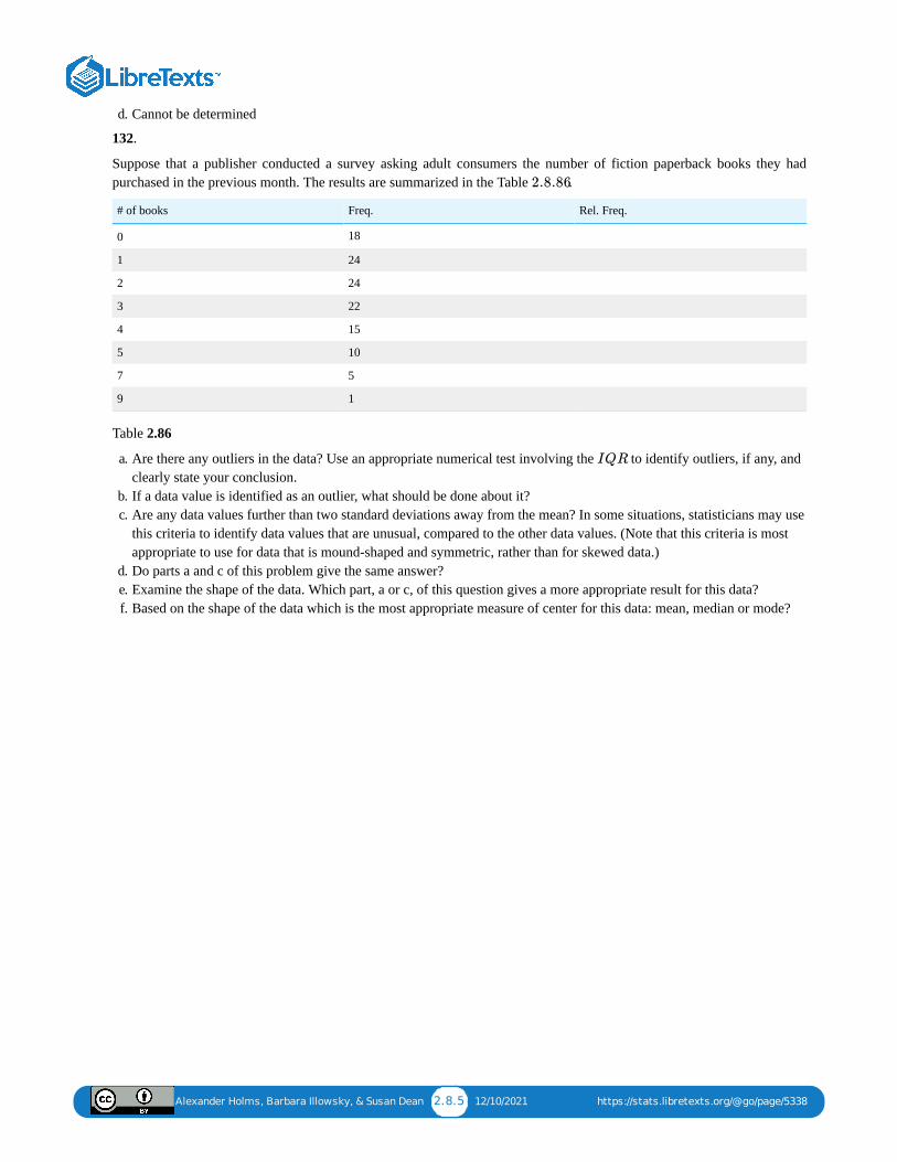
Alexander Holms, Barbara Illowsky, & Susan Dean 2.8.5 12/10/2021 https://stats.libretexts.org/@go/page/5338
d. Cannot be determined
132.
Suppose that a publisher conducted a survey asking adult consumers the number of fiction paperback books they hadpurchased in the previous month. The results are summarized in the Table .
# of books Freq. Rel. Freq.
0 18
1 24
2 24
3 22
4 15
5 10
7 5
9 1
Table 2.86
a. Are there any outliers in the data? Use an appropriate numerical test involving the to identify outliers, if any, andclearly state your conclusion.
b. If a data value is identified as an outlier, what should be done about it?c. Are any data values further than two standard deviations away from the mean? In some situations, statisticians may use
this criteria to identify data values that are unusual, compared to the other data values. (Note that this criteria is mostappropriate to use for data that is mound-shaped and symmetric, rather than for skewed data.)
d. Do parts a and c of this problem give the same answer?e. Examine the shape of the data. Which part, a or c, of this question gives a more appropriate result for this data?f. Based on the shape of the data which is the most appropriate measure of center for this data: mean, median or mode?
2.8.86
IQR
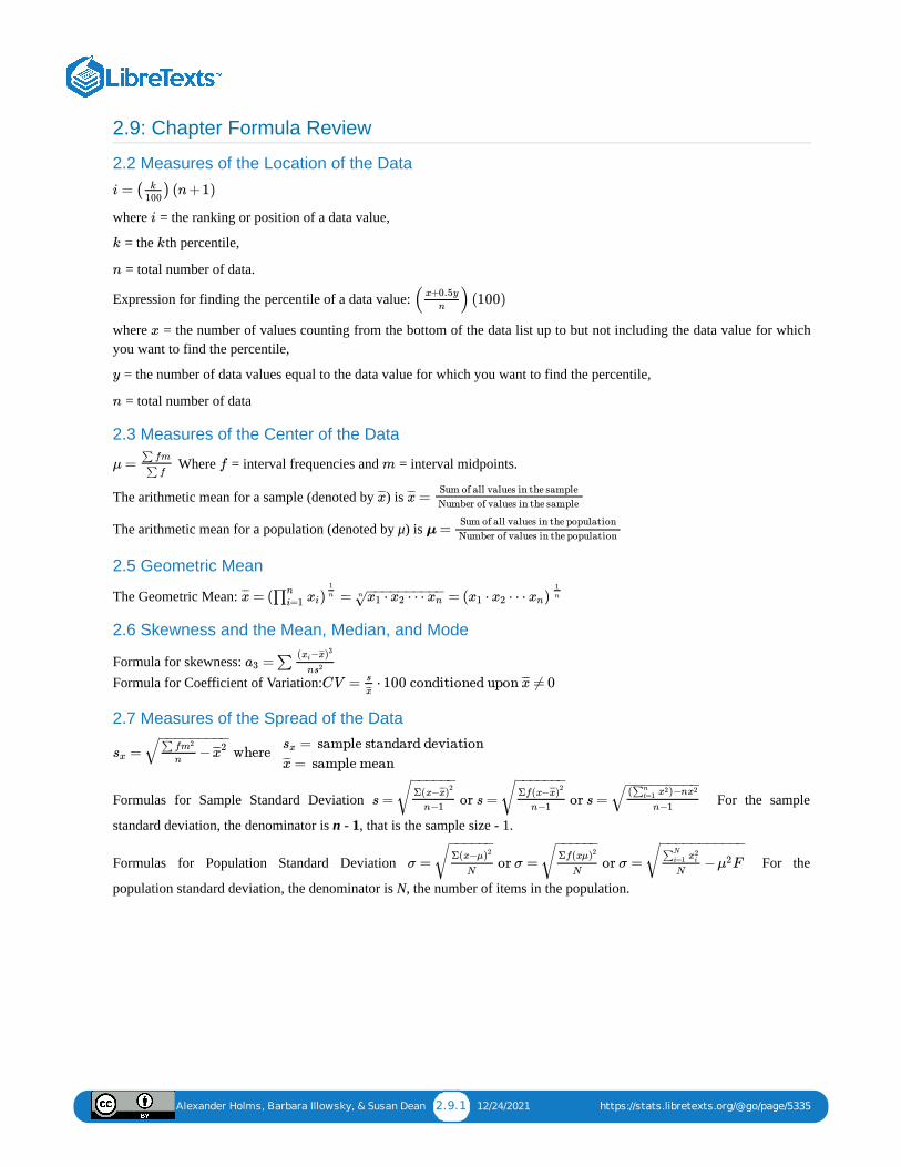
Alexander Holms, Barbara Illowsky, & Susan Dean 2.9.1 12/24/2021 https://stats.libretexts.org/@go/page/5335
2.9: Chapter Formula Review
2.2 Measures of the Location of the Data
where = the ranking or position of a data value,
= the th percentile,
= total number of data.
Expression for finding the percentile of a data value:
where = the number of values counting from the bottom of the data list up to but not including the data value for whichyou want to find the percentile,
= the number of data values equal to the data value for which you want to find the percentile,
= total number of data
2.3 Measures of the Center of the Data
Where = interval frequencies and = interval midpoints.
The arithmetic mean for a sample (denoted by ) is
The arithmetic mean for a population (denoted by μ) is
2.5 Geometric Mean
The Geometric Mean:
2.6 Skewness and the Mean, Median, and Mode
Formula for skewness: Formula for Coefficient of Variation:
2.7 Measures of the Spread of the Data
Formulas for Sample Standard Deviation For the sample
standard deviation, the denominator is n - 1, that is the sample size - 1.
Formulas for Population Standard Deviation For the
population standard deviation, the denominator is N, the number of items in the population.
i = ( ) (n +1)k
100
i
k k
n
( ) (100)x+0.5y
n
x
y
n
μ =∑ fm
∑ ff m
x̄̄̄ =x̄̄̄ Sum of all values in the sample
Number of values in the sample
μ = Sum of all values in the population
Number of values in the population
= = =x̄̄̄ ( )∏n
i=1 xi
1n ⋅ ⋯x1 x2 xn
− −−−−−−−−−√n ( ⋅ ⋯ )x1 x2 xn
1n
=∑a3( − )xi x̄̄̄ 3
ns2
CV = ⋅ 100 conditioned upon ≠ 0s
x̄̄̄x̄̄̄
= where sx −∑ fm2
nx̄̄̄2
− −−−−−−−−√ = sample standard deviation sx
= sample mean x̄̄̄
s = or s = or s =Σ(x−x̄̄̄)
2
n−1
− −−−−−√ Σf(x−x̄̄̄)
2
n−1
− −−−−−−√ ( )−n∑n
t=1 x2 x2
n−1
− −−−−−−−−√
σ = or σ = or σ =Σ(x−μ)2
N
− −−−−−√ Σf(xμ)2
N
− −−−−−√ − F
∑N
i=1 x2i
Nμ2
− −−−−−−−−−−√
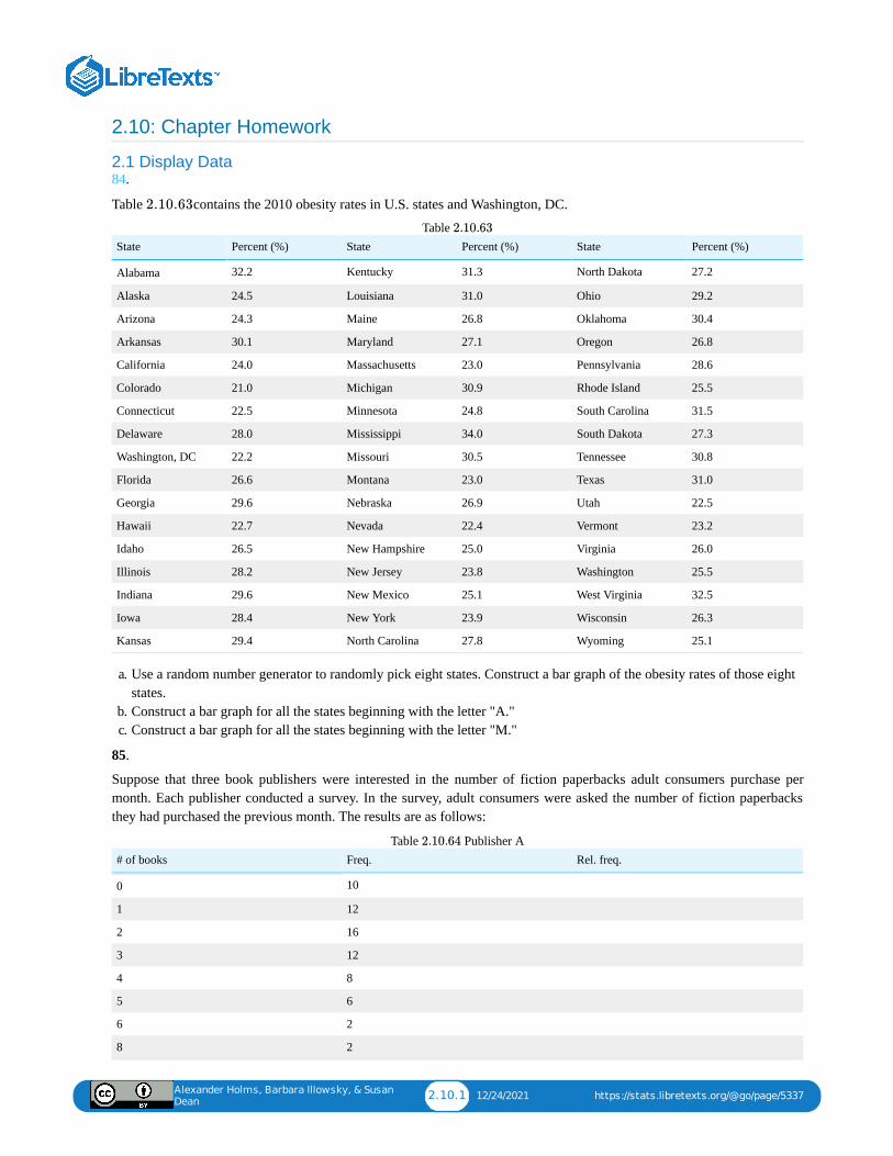
Alexander Holms, Barbara Illowsky, & Susan
Dean2.10.1 12/24/2021 https://stats.libretexts.org/@go/page/5337
2.10: Chapter Homework
2.1 Display Data84.
Table contains the 2010 obesity rates in U.S. states and Washington, DC.
State Percent (%) State Percent (%) State Percent (%)
Alabama 32.2 Kentucky 31.3 North Dakota 27.2
Alaska 24.5 Louisiana 31.0 Ohio 29.2
Arizona 24.3 Maine 26.8 Oklahoma 30.4
Arkansas 30.1 Maryland 27.1 Oregon 26.8
California 24.0 Massachusetts 23.0 Pennsylvania 28.6
Colorado 21.0 Michigan 30.9 Rhode Island 25.5
Connecticut 22.5 Minnesota 24.8 South Carolina 31.5
Delaware 28.0 Mississippi 34.0 South Dakota 27.3
Washington, DC 22.2 Missouri 30.5 Tennessee 30.8
Florida 26.6 Montana 23.0 Texas 31.0
Georgia 29.6 Nebraska 26.9 Utah 22.5
Hawaii 22.7 Nevada 22.4 Vermont 23.2
Idaho 26.5 New Hampshire 25.0 Virginia 26.0
Illinois 28.2 New Jersey 23.8 Washington 25.5
Indiana 29.6 New Mexico 25.1 West Virginia 32.5
Iowa 28.4 New York 23.9 Wisconsin 26.3
Kansas 29.4 North Carolina 27.8 Wyoming 25.1
Table
a. Use a random number generator to randomly pick eight states. Construct a bar graph of the obesity rates of those eightstates.
b. Construct a bar graph for all the states beginning with the letter "A."c. Construct a bar graph for all the states beginning with the letter "M."
85.
Suppose that three book publishers were interested in the number of fiction paperbacks adult consumers purchase permonth. Each publisher conducted a survey. In the survey, adult consumers were asked the number of fiction paperbacksthey had purchased the previous month. The results are as follows:
# of books Freq. Rel. freq.
0 10
1 12
2 16
3 12
4 8
5 6
6 2
8 2
Table Publisher A
2.10.63
2.10.63
2.10.64
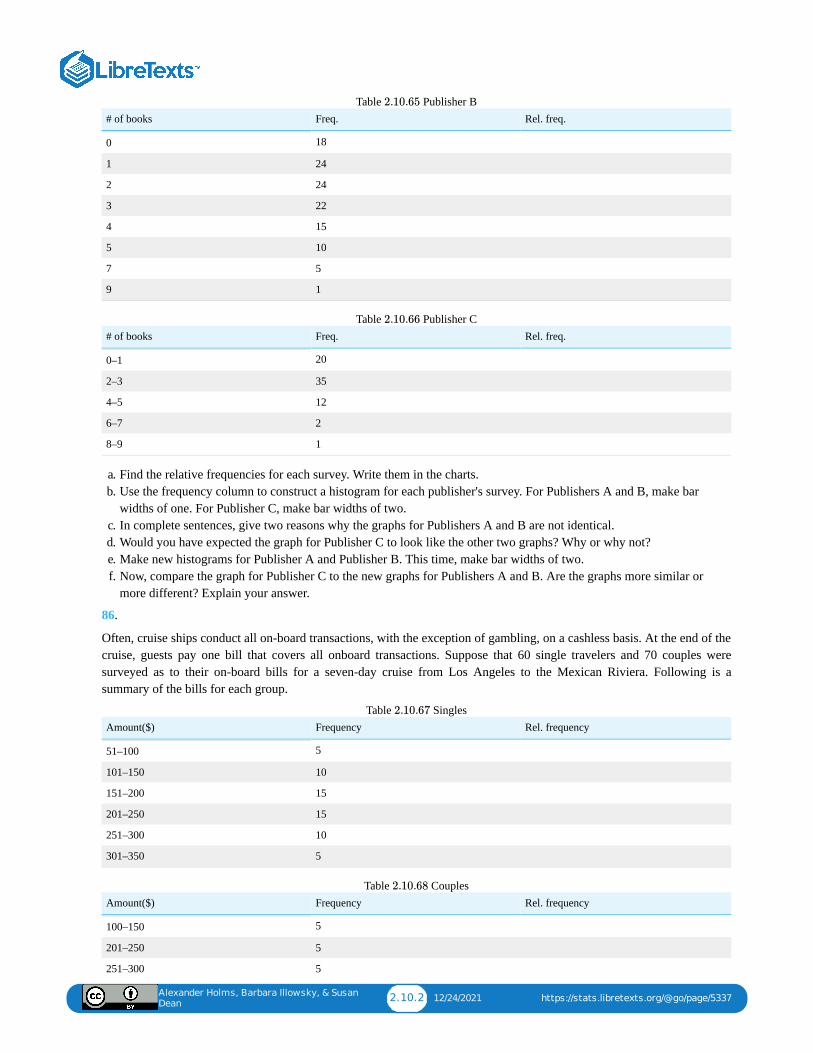
Alexander Holms, Barbara Illowsky, & Susan
Dean2.10.2 12/24/2021 https://stats.libretexts.org/@go/page/5337
# of books Freq. Rel. freq.
0 18
1 24
2 24
3 22
4 15
5 10
7 5
9 1
Table Publisher B
# of books Freq. Rel. freq.
0–1 20
2–3 35
4–5 12
6–7 2
8–9 1
Table Publisher C
a. Find the relative frequencies for each survey. Write them in the charts.b. Use the frequency column to construct a histogram for each publisher's survey. For Publishers A and B, make bar
widths of one. For Publisher C, make bar widths of two.c. In complete sentences, give two reasons why the graphs for Publishers A and B are not identical.d. Would you have expected the graph for Publisher C to look like the other two graphs? Why or why not?e. Make new histograms for Publisher A and Publisher B. This time, make bar widths of two.f. Now, compare the graph for Publisher C to the new graphs for Publishers A and B. Are the graphs more similar or
more different? Explain your answer.
86.
Often, cruise ships conduct all on-board transactions, with the exception of gambling, on a cashless basis. At the end of thecruise, guests pay one bill that covers all onboard transactions. Suppose that 60 single travelers and 70 couples weresurveyed as to their on-board bills for a seven-day cruise from Los Angeles to the Mexican Riviera. Following is asummary of the bills for each group.
Amount($) Frequency Rel. frequency
51–100 5
101–150 10
151–200 15
201–250 15
251–300 10
301–350 5
Table Singles
Amount($) Frequency Rel. frequency
100–150 5
201–250 5
251–300 5
Table Couples
2.10.65
2.10.66
2.10.67
2.10.68
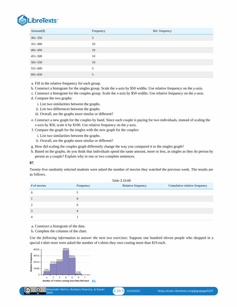
Alexander Holms, Barbara Illowsky, & Susan
Dean2.10.3 12/24/2021 https://stats.libretexts.org/@go/page/5337
Amount($) Frequency Rel. frequency
301–350 5
351–400 10
401–450 10
451–500 10
501–550 10
551–600 5
601–650 5
a. Fill in the relative frequency for each group.b. Construct a histogram for the singles group. Scale the x-axis by $50 widths. Use relative frequency on the y-axis.c. Construct a histogram for the couples group. Scale the x-axis by $50 widths. Use relative frequency on the y-axis.d. Compare the two graphs:
i. List two similarities between the graphs.ii. List two differences between the graphs.iii. Overall, are the graphs more similar or different?
e. Construct a new graph for the couples by hand. Since each couple is paying for two individuals, instead of scaling thex-axis by $50, scale it by $100. Use relative frequency on the y-axis.
f. Compare the graph for the singles with the new graph for the couples:i. List two similarities between the graphs.
ii. Overall, are the graphs more similar or different?g. How did scaling the couples graph differently change the way you compared it to the singles graph?h. Based on the graphs, do you think that individuals spend the same amount, more or less, as singles as they do person by
person as a couple? Explain why in one or two complete sentences.
87.
Twenty-five randomly selected students were asked the number of movies they watched the previous week. The results areas follows.
# of movies Frequency Relative frequency Cumulative relative frequency
0 5
1 9
2 6
3 4
4 1
Table
a. Construct a histogram of the data.b. Complete the columns of the chart.
Use the following information to answer the next two exercises: Suppose one hundred eleven people who shopped in aspecial t-shirt store were asked the number of t-shirts they own costing more than $19 each.
88.
2.10.69
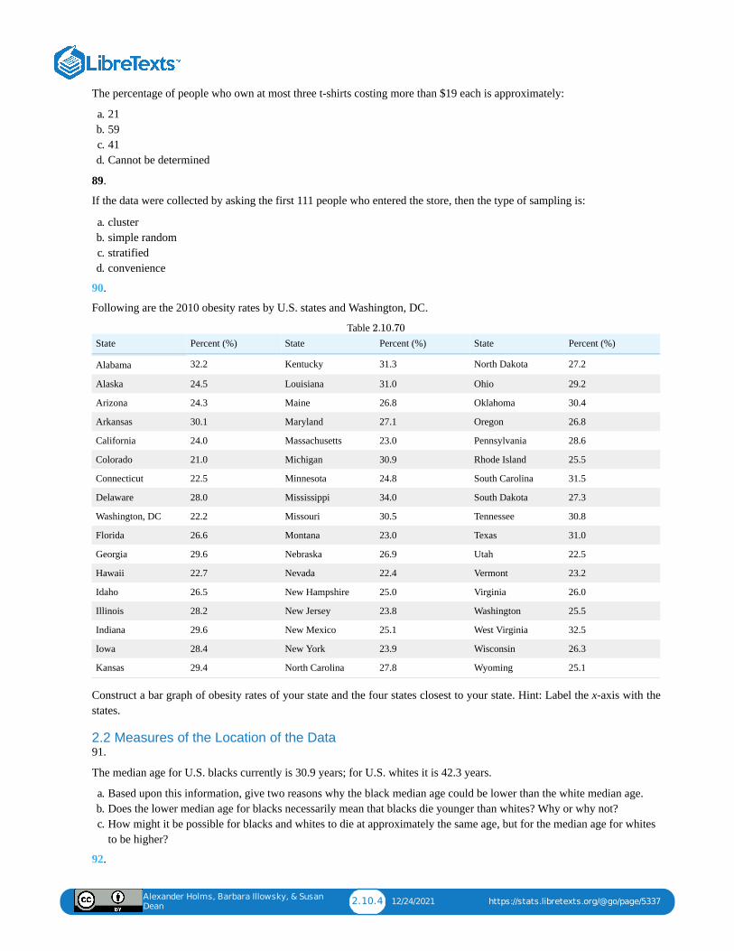
Alexander Holms, Barbara Illowsky, & Susan
Dean2.10.4 12/24/2021 https://stats.libretexts.org/@go/page/5337
The percentage of people who own at most three t-shirts costing more than $19 each is approximately:
a. 21b. 59c. 41d. Cannot be determined
89.
If the data were collected by asking the first 111 people who entered the store, then the type of sampling is:
a. clusterb. simple randomc. stratifiedd. convenience
90.
Following are the 2010 obesity rates by U.S. states and Washington, DC.
State Percent (%) State Percent (%) State Percent (%)
Alabama 32.2 Kentucky 31.3 North Dakota 27.2
Alaska 24.5 Louisiana 31.0 Ohio 29.2
Arizona 24.3 Maine 26.8 Oklahoma 30.4
Arkansas 30.1 Maryland 27.1 Oregon 26.8
California 24.0 Massachusetts 23.0 Pennsylvania 28.6
Colorado 21.0 Michigan 30.9 Rhode Island 25.5
Connecticut 22.5 Minnesota 24.8 South Carolina 31.5
Delaware 28.0 Mississippi 34.0 South Dakota 27.3
Washington, DC 22.2 Missouri 30.5 Tennessee 30.8
Florida 26.6 Montana 23.0 Texas 31.0
Georgia 29.6 Nebraska 26.9 Utah 22.5
Hawaii 22.7 Nevada 22.4 Vermont 23.2
Idaho 26.5 New Hampshire 25.0 Virginia 26.0
Illinois 28.2 New Jersey 23.8 Washington 25.5
Indiana 29.6 New Mexico 25.1 West Virginia 32.5
Iowa 28.4 New York 23.9 Wisconsin 26.3
Kansas 29.4 North Carolina 27.8 Wyoming 25.1
Table
Construct a bar graph of obesity rates of your state and the four states closest to your state. Hint: Label the x-axis with thestates.
2.2 Measures of the Location of the Data91.
The median age for U.S. blacks currently is 30.9 years; for U.S. whites it is 42.3 years.
a. Based upon this information, give two reasons why the black median age could be lower than the white median age.b. Does the lower median age for blacks necessarily mean that blacks die younger than whites? Why or why not?c. How might it be possible for blacks and whites to die at approximately the same age, but for the median age for whites
to be higher?
92.
2.10.70
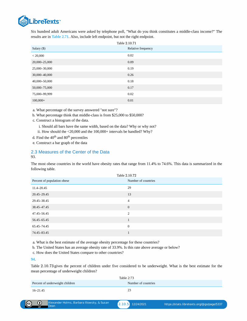
Alexander Holms, Barbara Illowsky, & Susan
Dean2.10.5 12/24/2021 https://stats.libretexts.org/@go/page/5337
Six hundred adult Americans were asked by telephone poll, "What do you think constitutes a middle-class income?" Theresults are in Table 2.71. Also, include left endpoint, but not the right endpoint.
Salary ($) Relative frequency
< 20,000 0.02
20,000–25,000 0.09
25,000–30,000 0.19
30,000–40,000 0.26
40,000–50,000 0.18
50,000–75,000 0.17
75,000–99,999 0.02
100,000+ 0.01
Table
a. What percentage of the survey answered "not sure"?b. What percentage think that middle-class is from $25,000 to $50,000?c. Construct a histogram of the data.
i. Should all bars have the same width, based on the data? Why or why not?ii. How should the <20,000 and the 100,000+ intervals be handled? Why?
d. Find the 40 and 80 percentilese. Construct a bar graph of the data
2.3 Measures of the Center of the Data93.
The most obese countries in the world have obesity rates that range from 11.4% to 74.6%. This data is summarized in thefollowing table.
Percent of population obese Number of countries
11.4–20.45 29
20.45–29.45 13
29.45–38.45 4
38.45–47.45 0
47.45–56.45 2
56.45–65.45 1
65.45–74.45 0
74.45–83.45 1
Table
a. What is the best estimate of the average obesity percentage for these countries?b. The United States has an average obesity rate of 33.9%. Is this rate above average or below?c. How does the United States compare to other countries?
94.
Table gives the percent of children under five considered to be underweight. What is the best estimate for themean percentage of underweight children?
Percent of underweight children Number of countries
16–21.45 23
Table 2:73
2.10.71
th th
2.10.72
2.10.73
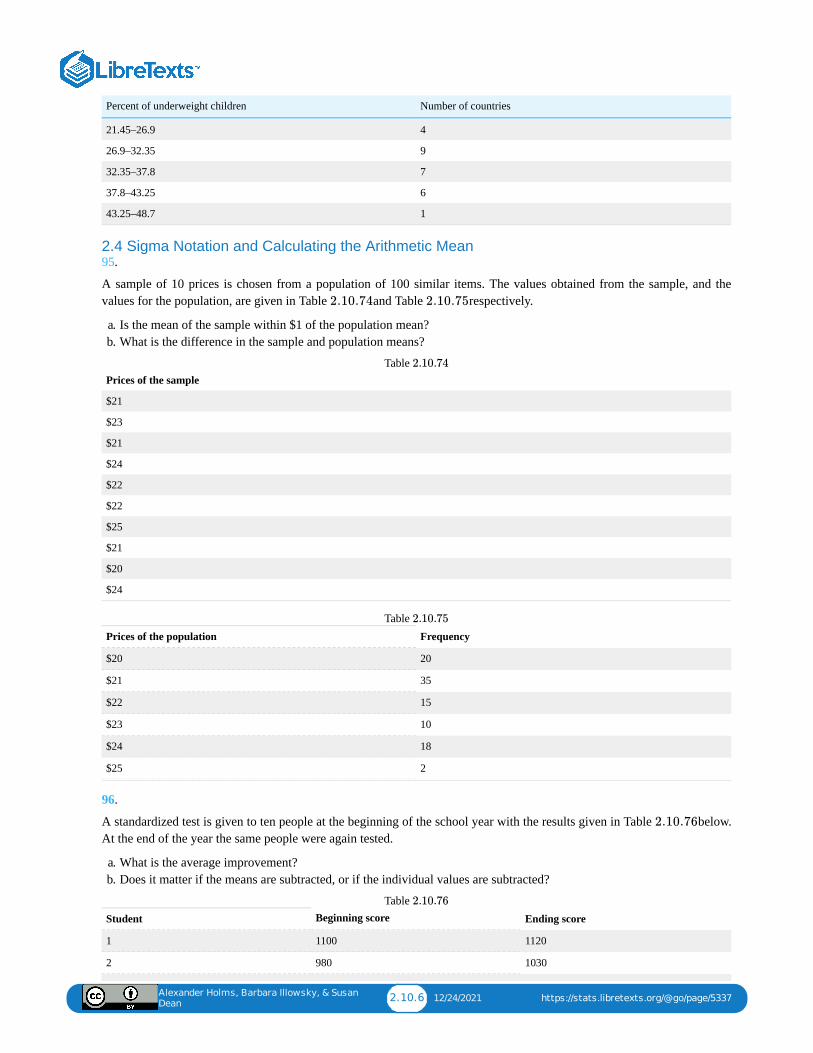
Alexander Holms, Barbara Illowsky, & Susan
Dean2.10.6 12/24/2021 https://stats.libretexts.org/@go/page/5337
Percent of underweight children Number of countries
21.45–26.9 4
26.9–32.35 9
32.35–37.8 7
37.8–43.25 6
43.25–48.7 1
2.4 Sigma Notation and Calculating the Arithmetic Mean95.
A sample of 10 prices is chosen from a population of 100 similar items. The values obtained from the sample, and thevalues for the population, are given in Table and Table respectively.
a. Is the mean of the sample within $1 of the population mean?b. What is the difference in the sample and population means?
Prices of the sample
$21
$23
$21
$24
$22
$22
$25
$21
$20
$24
Table
Prices of the population Frequency
$20 20
$21 35
$22 15
$23 10
$24 18
$25 2
Table
96.
A standardized test is given to ten people at the beginning of the school year with the results given in Table below.At the end of the year the same people were again tested.
a. What is the average improvement?b. Does it matter if the means are subtracted, or if the individual values are subtracted?
Student Beginning score Ending score
1 1100 1120
2 980 1030
Table
2.10.74 2.10.75
2.10.74
2.10.75
2.10.76
2.10.76
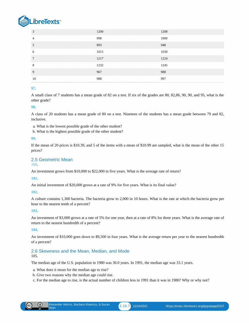
Alexander Holms, Barbara Illowsky, & Susan
Dean2.10.7 12/24/2021 https://stats.libretexts.org/@go/page/5337
3 1200 1208
4 998 1000
5 893 948
6 1015 1030
7 1217 1224
8 1232 1245
9 967 988
10 988 997
97.
A small class of 7 students has a mean grade of 82 on a test. If six of the grades are 80, 82,86, 90, 90, and 95, what is theother grade?
98.
A class of 20 students has a mean grade of 80 on a test. Nineteen of the students has a mean grade between 79 and 82,inclusive.
a. What is the lowest possible grade of the other student?b. What is the highest possible grade of the other student?
99.
If the mean of 20 prices is $10.39, and 5 of the items with a mean of $10.99 are sampled, what is the mean of the other 15prices?
2.5 Geometric Mean100.
An investment grows from $10,000 to $22,000 in five years. What is the average rate of return?
101.
An initial investment of $20,000 grows at a rate of 9% for five years. What is its final value?
102.
A culture contains 1,300 bacteria. The bacteria grow to 2,000 in 10 hours. What is the rate at which the bacteria grow perhour to the nearest tenth of a percent?
103.
An investment of $3,000 grows at a rate of 5% for one year, then at a rate of 8% for three years. What is the average rate ofreturn to the nearest hundredth of a percent?
104.
An investment of $10,000 goes down to $9,500 in four years. What is the average return per year to the nearest hundredthof a percent?
2.6 Skewness and the Mean, Median, and Mode105.
The median age of the U.S. population in 1980 was 30.0 years. In 1991, the median age was 33.1 years.
a. What does it mean for the median age to rise?b. Give two reasons why the median age could rise.c. For the median age to rise, is the actual number of children less in 1991 than it was in 1980? Why or why not?
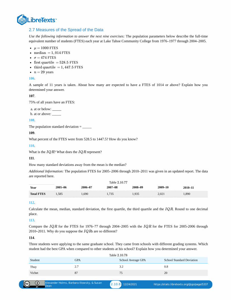
Alexander Holms, Barbara Illowsky, & Susan
Dean2.10.8 12/24/2021 https://stats.libretexts.org/@go/page/5337
2.7 Measures of the Spread of the DataUse the following information to answer the next nine exercises: The population parameters below describe the full-timeequivalent number of students (FTES) each year at Lake Tahoe Community College from 1976–1977 through 2004–2005.
FTES FTES
FTES FTES
FTES years
106.
A sample of 11 years is taken. About how many are expected to have a FTES of 1014 or above? Explain how youdetermined your answer.
107.
75% of all years have an FTES:
a. at or below: _____b. at or above: _____
108.
The population standard deviation = _____
109.
What percent of the FTES were from 528.5 to 1447.5? How do you know?
110.
What is the ? What does the represent?
111.
How many standard deviations away from the mean is the median?
Additional Information: The population FTES for 2005–2006 through 2010–2011 was given in an updated report. The dataare reported here.
Year 2005–06 2006–07 2007–08 2008–09 2009–10 2010–11
Total FTES 1,585 1,690 1,735 1,935 2,021 1,890
Table
112.
Calculate the mean, median, standard deviation, the first quartile, the third quartile and the . Round to one decimalplace.
113.
Compare the for the FTES for 1976–77 through 2004–2005 with the for the FTES for 2005-2006 through2010–2011. Why do you suppose the s are so different?
114.
Three students were applying to the same graduate school. They came from schools with different grading systems. Whichstudent had the best GPA when compared to other students at his school? Explain how you determined your answer.
Student GPA School Average GPA School Standard Deviation
Thuy 2.7 3.2 0.8
Vichet 87 75 20
Table
μ = 1000
median = 1, 014
σ = 474
first quartile = 528.5
third quartile = 1, 447.5
n = 29
IQR IQR
2.10.77
IQR
IQR IQR
IQR
2.10.78
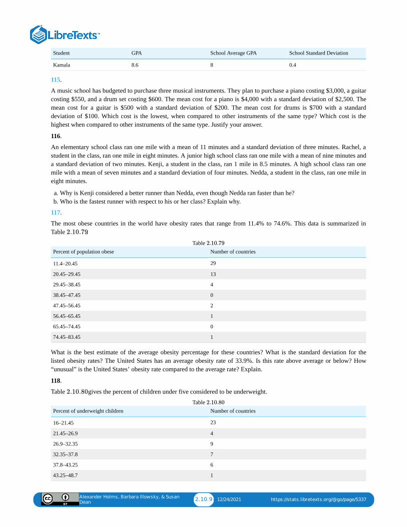
Alexander Holms, Barbara Illowsky, & Susan
Dean2.10.9 12/24/2021 https://stats.libretexts.org/@go/page/5337
Student GPA School Average GPA School Standard Deviation
Kamala 8.6 8 0.4
115.
A music school has budgeted to purchase three musical instruments. They plan to purchase a piano costing $3,000, a guitarcosting $550, and a drum set costing $600. The mean cost for a piano is $4,000 with a standard deviation of $2,500. Themean cost for a guitar is $500 with a standard deviation of $200. The mean cost for drums is $700 with a standarddeviation of $100. Which cost is the lowest, when compared to other instruments of the same type? Which cost is thehighest when compared to other instruments of the same type. Justify your answer.
116.
An elementary school class ran one mile with a mean of 11 minutes and a standard deviation of three minutes. Rachel, astudent in the class, ran one mile in eight minutes. A junior high school class ran one mile with a mean of nine minutes anda standard deviation of two minutes. Kenji, a student in the class, ran 1 mile in 8.5 minutes. A high school class ran onemile with a mean of seven minutes and a standard deviation of four minutes. Nedda, a student in the class, ran one mile ineight minutes.
a. Why is Kenji considered a better runner than Nedda, even though Nedda ran faster than he?b. Who is the fastest runner with respect to his or her class? Explain why.
117.
The most obese countries in the world have obesity rates that range from 11.4% to 74.6%. This data is summarized inTable .
Percent of population obese Number of countries
11.4–20.45 29
20.45–29.45 13
29.45–38.45 4
38.45–47.45 0
47.45–56.45 2
56.45–65.45 1
65.45–74.45 0
74.45–83.45 1
Table
What is the best estimate of the average obesity percentage for these countries? What is the standard deviation for thelisted obesity rates? The United States has an average obesity rate of 33.9%. Is this rate above average or below? How“unusual” is the United States’ obesity rate compared to the average rate? Explain.
118.
Table gives the percent of children under five considered to be underweight.
Percent of underweight children Number of countries
16–21.45 23
21.45–26.9 4
26.9–32.35 9
32.35–37.8 7
37.8–43.25 6
43.25–48.7 1
Table
2.10.79
2.10.79
2.10.80
2.10.80

Alexander Holms, Barbara Illowsky, & Susan
Dean2.10.10 12/24/2021 https://stats.libretexts.org/@go/page/5337
What is the best estimate for the mean percentage of underweight children? What is the standard deviation? Whichinterval(s) could be considered unusual? Explain.
Alexander Holms, Barbara Illowsky, & Susan
Dean2.11.1 12/10/2021 https://stats.libretexts.org/@go/page/5333
2.11: Chapter Key Terms
Frequencythe number of times a value of the data occurs
Frequency Tablea data representation in which grouped data is displayed along with the corresponding frequencies
Histograma graphical representation in x-y form of the distribution of data in a data set; x represents the data and y represents thefrequency, or relative frequency. The graph consists of contiguous rectangles.
Interquartile Rangeor IQR, is the range of the middle 50 percent of the data values; the IQR is found by subtracting the first quartile fromthe third quartile.
Mean (arithmetic)a number that measures the central tendency of the data; a common name for mean is 'average.' The term 'mean' is ashortened form of 'arithmetic mean.' By definition, the mean for a sample (denoted by ) is
, and the mean for a population (denoted by μ) is
Mean (geometric)a measure of central tendency that provides a measure of average geometric growth over multiple time periods.
Mediana number that separates ordered data into halves; half the values are the same number or smaller than the median andhalf the values are the same number or larger than the median. The median may or may not be part of the data.
Midpointthe mean of an interval in a frequency table
Modethe value that appears most frequently in a set of data
Outlieran observation that does not fit the rest of the data
Percentilea number that divides ordered data into hundredths; percentiles may or may not be part of the data. The median of thedata is the second quartile and the 50 percentile. The first and third quartiles are the 25 and the 75 percentiles,respectively.
Quartilesthe numbers that separate the data into quarters; quartiles may or may not be part of the data. The second quartile is themedian of the data.
Relative Frequencythe ratio of the number of times a value of the data occurs in the set of all outcomes to the number of all outcomes
Standard Deviationa number that is equal to the square root of the variance and measures how far data values are from their mean;notation: s for sample standard deviation and σ for population standard deviation.
x̄̄̄
=x̄̄̄ Sum of all values in the sample
Number of values in the sample μ =
Sum of all values in the population
Number of values in the population
th th th

Alexander Holms, Barbara Illowsky, & Susan
Dean2.11.2 12/10/2021 https://stats.libretexts.org/@go/page/5333
Variancemean of the squared deviations from the mean, or the square of the standard deviation; for a set of data, a deviation canbe represented as x – where x is a value of the data and is the sample mean. The sample variance is equal to thesum of the squares of the deviations divided by the difference of the sample size and one.
x̄̄̄ x̄̄̄

Alexander Holms, Barbara Illowsky, & Susan Dean 1 12/31/2021 https://stats.libretexts.org/@go/page/5339
Welcome to the Statistics Library. This Living Library is a principal hub of the LibreTexts project, which is a multi-institutional collaborative venture to develop the next generation of open-access texts to improve postsecondary educationat all levels of higher learning. The LibreTexts approach is highly collaborative where an Open Access textbookenvironment is under constant revision by students, faculty, and outside experts to supplant conventional paper-basedbooks.
Campus Bookshelves Bookshelves
Learning Objects
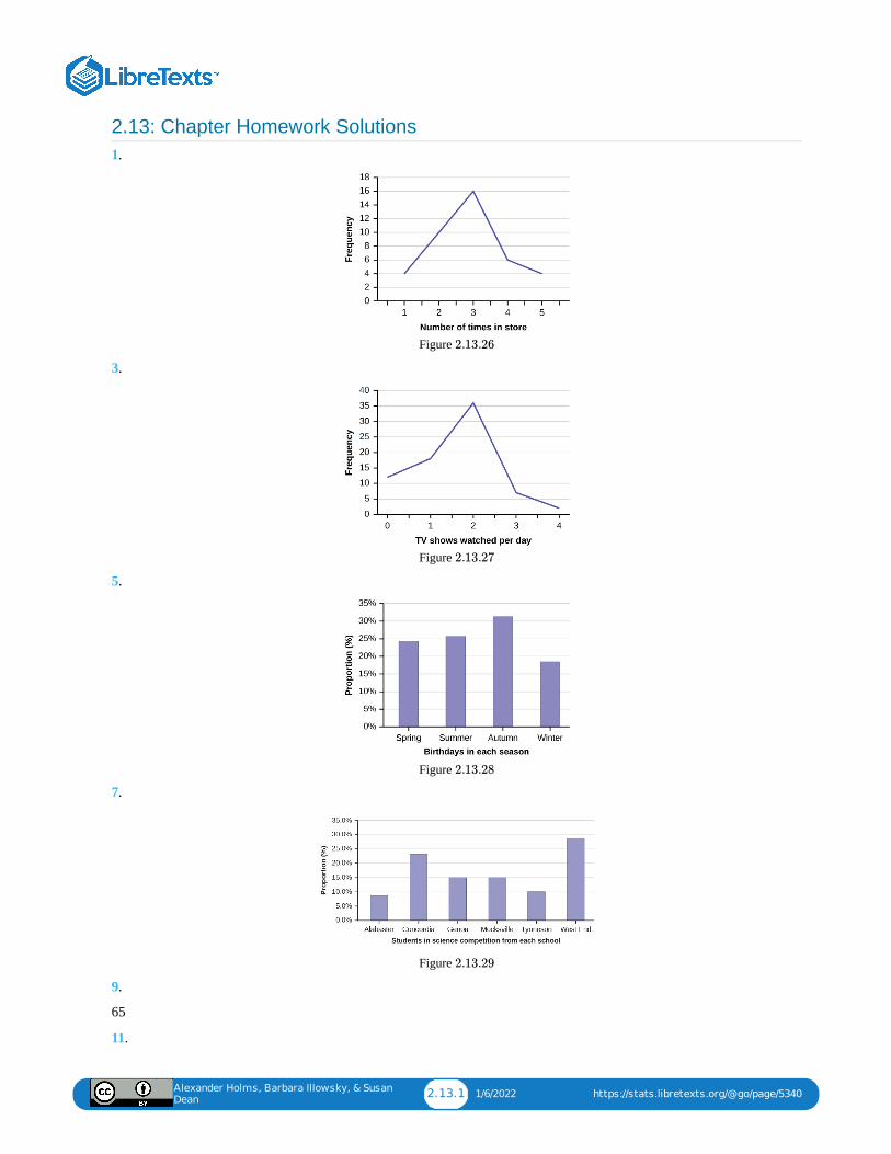
Alexander Holms, Barbara Illowsky, & Susan
Dean2.13.1 1/6/2022 https://stats.libretexts.org/@go/page/5340
2.13: Chapter Homework Solutions1.
Figure
3.
Figure
5.
Figure
7.
Figure
9.
65
11.
2.13.26
2.13.27
2.13.28
2.13.29
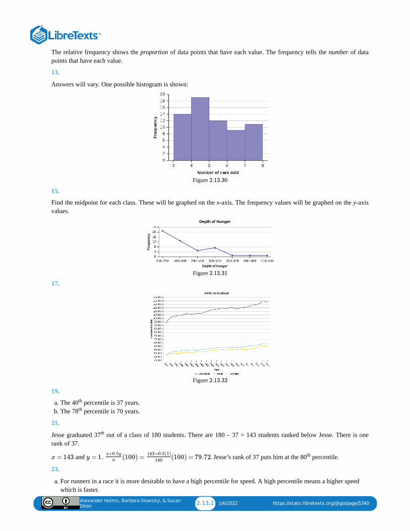
Alexander Holms, Barbara Illowsky, & Susan
Dean2.13.2 1/6/2022 https://stats.libretexts.org/@go/page/5340
The relative frequency shows the proportion of data points that have each value. The frequency tells the number of datapoints that have each value.
13.
Answers will vary. One possible histogram is shown:
Figure
15.
Find the midpoint for each class. These will be graphed on the x-axis. The frequency values will be graphed on the y-axisvalues.
Figure
17.
Figure
19.
a. The 40 percentile is 37 years.b. The 78 percentile is 70 years.
21.
Jesse graduated 37 out of a class of 180 students. There are 180 – 37 = 143 students ranked below Jesse. There is onerank of 37.
and . . Jesse’s rank of 37 puts him at the 80 percentile.
23.
a. For runners in a race it is more desirable to have a high percentile for speed. A high percentile means a higher speedwhich is faster.
2.13.30
2.13.31
2.13.32
th
th
th
x = 143 y = 1 (100) = (100) = 79.72x+0.5y
n
143+0.5(1)
180th
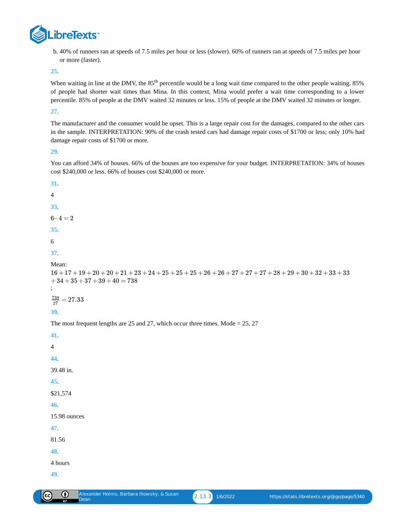
Alexander Holms, Barbara Illowsky, & Susan
Dean2.13.3 1/6/2022 https://stats.libretexts.org/@go/page/5340
b. 40% of runners ran at speeds of 7.5 miles per hour or less (slower). 60% of runners ran at speeds of 7.5 miles per houror more (faster).
25.
When waiting in line at the DMV, the 85 percentile would be a long wait time compared to the other people waiting. 85%of people had shorter wait times than Mina. In this context, Mina would prefer a wait time corresponding to a lowerpercentile. 85% of people at the DMV waited 32 minutes or less. 15% of people at the DMV waited 32 minutes or longer.
27.
The manufacturer and the consumer would be upset. This is a large repair cost for the damages, compared to the other carsin the sample. INTERPRETATION: 90% of the crash tested cars had damage repair costs of $1700 or less; only 10% haddamage repair costs of $1700 or more.
29.
You can afford 34% of houses. 66% of the houses are too expensive for your budget. INTERPRETATION: 34% of housescost $240,000 or less. 66% of houses cost $240,000 or more.
31.
4
33.
35.
6
37.
Mean:
;
39.
The most frequent lengths are 25 and 27, which occur three times. Mode = 25, 27
41.
4
44.
39.48 in.
45.
$21,574
46.
15.98 ounces
47.
81.56
48.
4 hours
49.
th
6– 4 = 2
16 +17 +19 +20 +20 +21 +23 +24 +25 +25 +25 +26 +26 +27 +27 +27 +28 +29 +30 +32 +33 +33+34 +35 +37 +39 +40 = 738
= 27.3373827
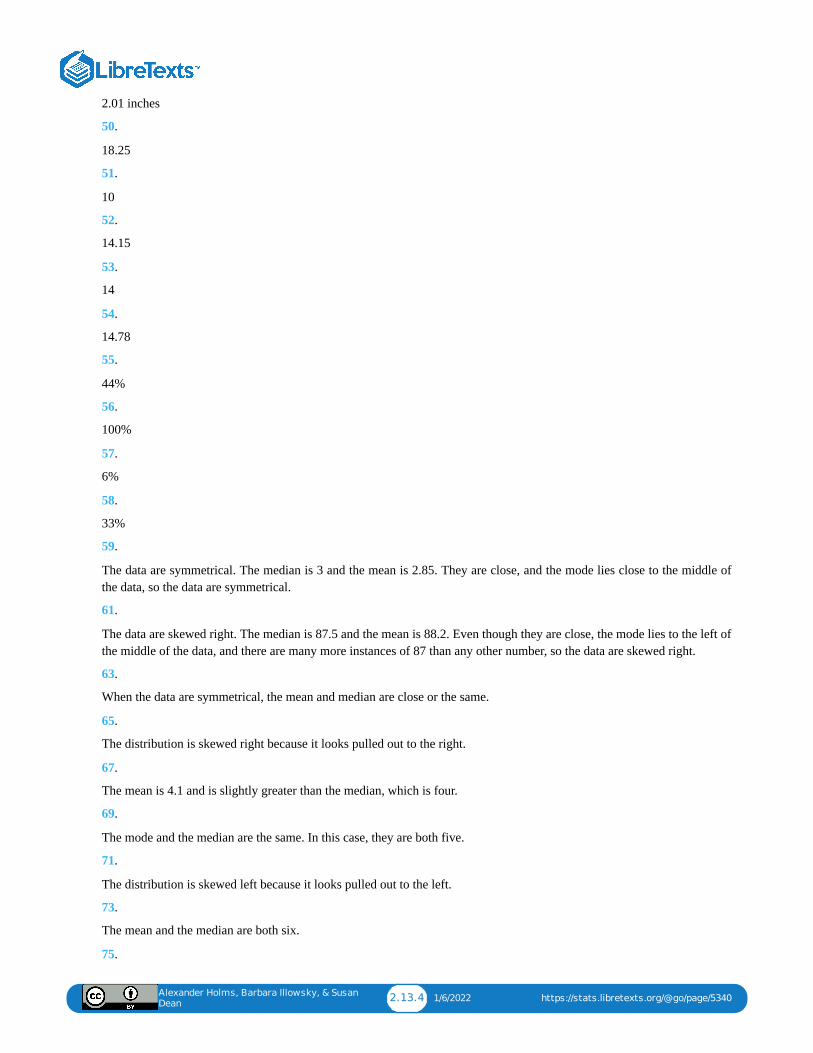
Alexander Holms, Barbara Illowsky, & Susan
Dean2.13.4 1/6/2022 https://stats.libretexts.org/@go/page/5340
2.01 inches
50.
18.25
51.
10
52.
14.15
53.
14
54.
14.78
55.
44%
56.
100%
57.
6%
58.
33%
59.
The data are symmetrical. The median is 3 and the mean is 2.85. They are close, and the mode lies close to the middle ofthe data, so the data are symmetrical.
61.
The data are skewed right. The median is 87.5 and the mean is 88.2. Even though they are close, the mode lies to the left ofthe middle of the data, and there are many more instances of 87 than any other number, so the data are skewed right.
63.
When the data are symmetrical, the mean and median are close or the same.
65.
The distribution is skewed right because it looks pulled out to the right.
67.
The mean is 4.1 and is slightly greater than the median, which is four.
69.
The mode and the median are the same. In this case, they are both five.
71.
The distribution is skewed left because it looks pulled out to the left.
73.
The mean and the median are both six.
75.
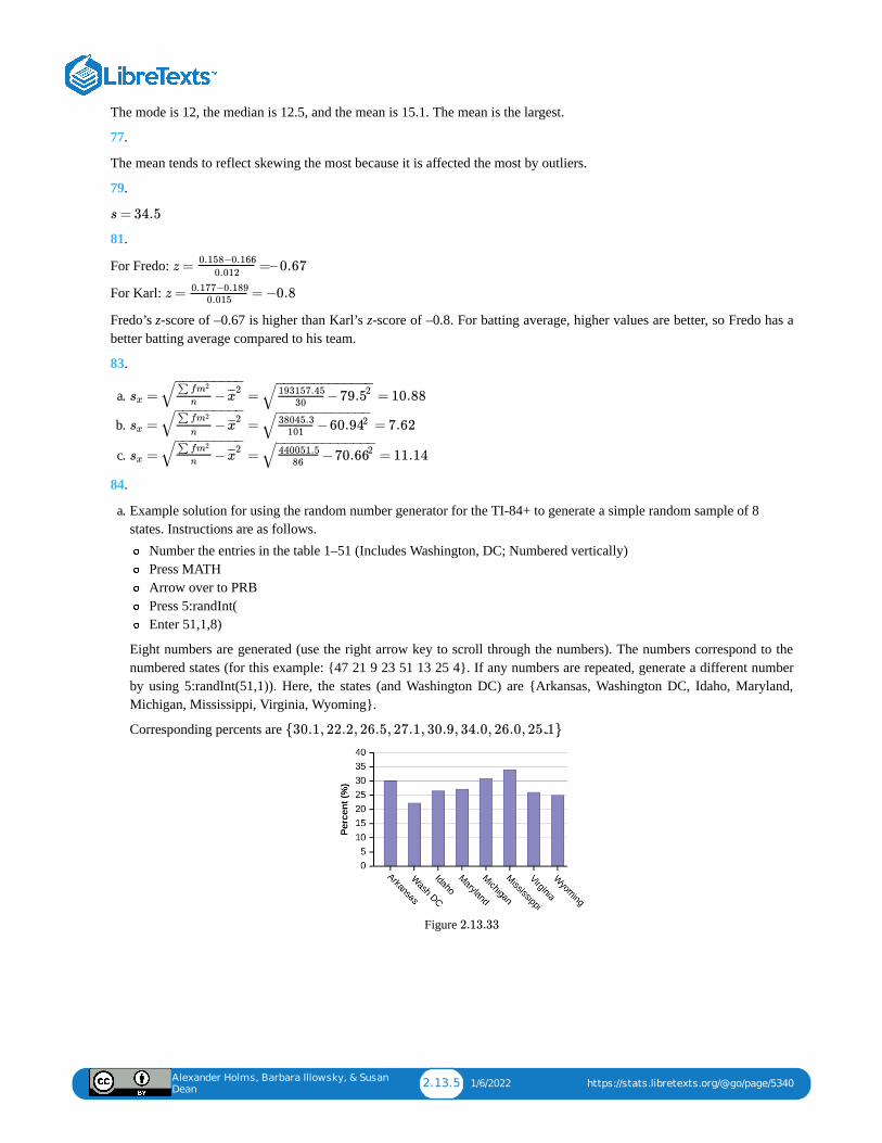
Alexander Holms, Barbara Illowsky, & Susan
Dean2.13.5 1/6/2022 https://stats.libretexts.org/@go/page/5340
The mode is 12, the median is 12.5, and the mean is 15.1. The mean is the largest.
77.
The mean tends to reflect skewing the most because it is affected the most by outliers.
79.
81.
For Fredo:
For Karl:
Fredo’s z-score of –0.67 is higher than Karl’s z-score of –0.8. For batting average, higher values are better, so Fredo has abetter batting average compared to his team.
83.
a.
b.
c.
84.
a. Example solution for using the random number generator for the TI-84+ to generate a simple random sample of 8states. Instructions are as follows.
Number the entries in the table 1–51 (Includes Washington, DC; Numbered vertically)Press MATHArrow over to PRBPress 5:randInt(Enter 51,1,8)
Eight numbers are generated (use the right arrow key to scroll through the numbers). The numbers correspond to thenumbered states (for this example: {47 21 9 23 51 13 25 4}. If any numbers are repeated, generate a different numberby using 5:randInt(51,1)). Here, the states (and Washington DC) are {Arkansas, Washington DC, Idaho, Maryland,Michigan, Mississippi, Virginia, Wyoming}.
Corresponding percents are .
Figure
s = 34.5
z = =– 0.670.158−0.166
0.012
z = = −0.80.177−0.1890.015
= = = 10.88sx −∑ fm2
n x̄̄̄2
− −−−−−−−−√ −193157.45
3079.52
− −−−−−−−−−−−−√
= = = 7.62sx −∑ fm2
nx̄̄̄
2− −−−−−−−−
√ −38045.3101
60.942− −−−−−−−−−−−
√
= = = 11.14sx −∑ fm2
n x̄̄̄2
− −−−−−−−−√ −440051.5
8670.662
− −−−−−−−−−−−−√
{30.1, 22.2, 26.5, 27.1, 30.9, 34.0, 26.0, 25.1}
2.13.33
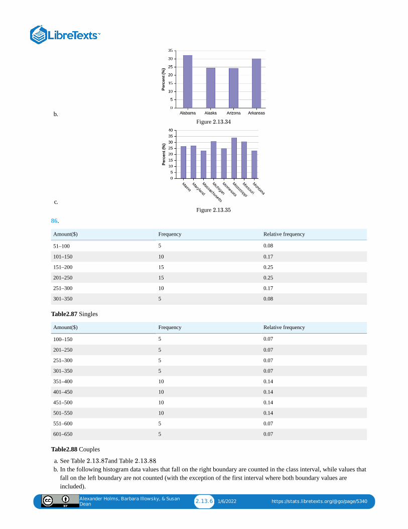
Alexander Holms, Barbara Illowsky, & Susan
Dean2.13.6 1/6/2022 https://stats.libretexts.org/@go/page/5340
b. Figure
c. Figure
86.
Amount($) Frequency Relative frequency
51–100 5 0.08
101–150 10 0.17
151–200 15 0.25
201–250 15 0.25
251–300 10 0.17
301–350 5 0.08
Table2.87 Singles
Amount($) Frequency Relative frequency
100–150 5 0.07
201–250 5 0.07
251–300 5 0.07
301–350 5 0.07
351–400 10 0.14
401–450 10 0.14
451–500 10 0.14
501–550 10 0.14
551–600 5 0.07
601–650 5 0.07
Table2.88 Couples
a. See Table and Table .b. In the following histogram data values that fall on the right boundary are counted in the class interval, while values that
fall on the left boundary are not counted (with the exception of the first interval where both boundary values areincluded).
2.13.34
2.13.35
2.13.87 2.13.88
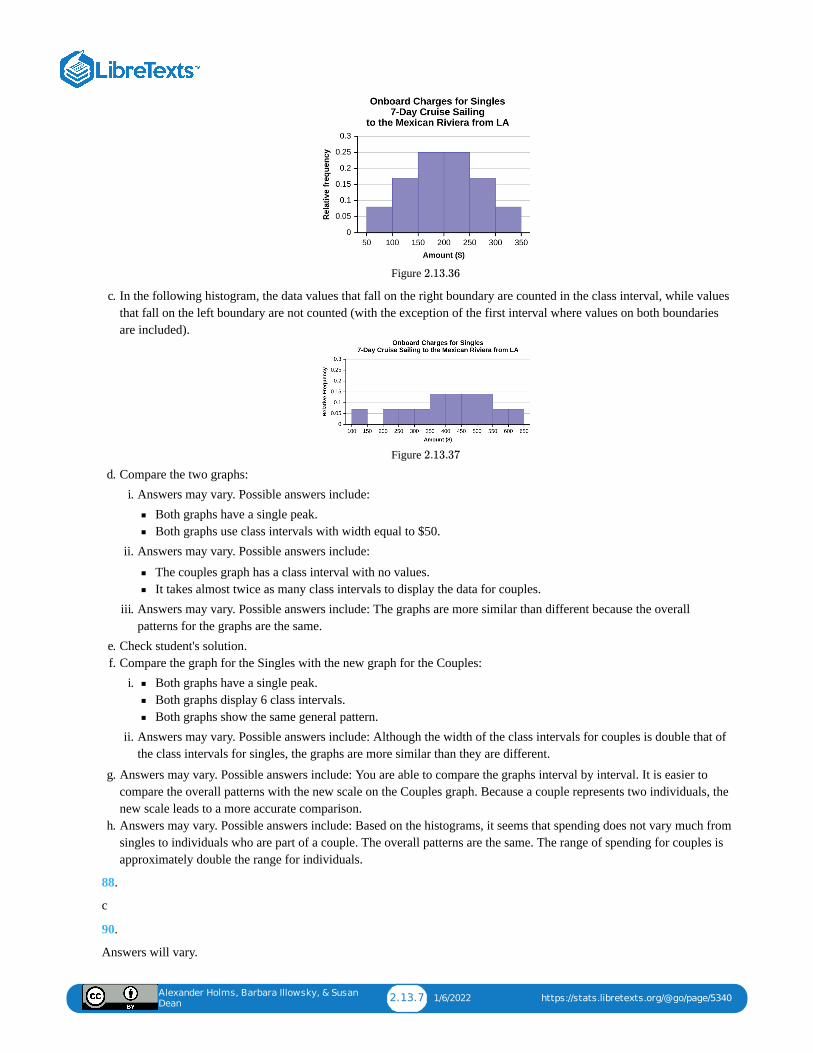
Alexander Holms, Barbara Illowsky, & Susan
Dean2.13.7 1/6/2022 https://stats.libretexts.org/@go/page/5340
Figure
c. In the following histogram, the data values that fall on the right boundary are counted in the class interval, while valuesthat fall on the left boundary are not counted (with the exception of the first interval where values on both boundariesare included).
Figure
d. Compare the two graphs:i. Answers may vary. Possible answers include:
Both graphs have a single peak.Both graphs use class intervals with width equal to $50.
ii. Answers may vary. Possible answers include:
The couples graph has a class interval with no values.It takes almost twice as many class intervals to display the data for couples.
iii. Answers may vary. Possible answers include: The graphs are more similar than different because the overallpatterns for the graphs are the same.
e. Check student's solution.f. Compare the graph for the Singles with the new graph for the Couples:
i. Both graphs have a single peak.Both graphs display 6 class intervals.Both graphs show the same general pattern.
ii. Answers may vary. Possible answers include: Although the width of the class intervals for couples is double that ofthe class intervals for singles, the graphs are more similar than they are different.
g. Answers may vary. Possible answers include: You are able to compare the graphs interval by interval. It is easier tocompare the overall patterns with the new scale on the Couples graph. Because a couple represents two individuals, thenew scale leads to a more accurate comparison.
h. Answers may vary. Possible answers include: Based on the histograms, it seems that spending does not vary much fromsingles to individuals who are part of a couple. The overall patterns are the same. The range of spending for couples isapproximately double the range for individuals.
88.
c
90.
Answers will vary.
2.13.36
2.13.37
Alexander Holms, Barbara Illowsky, & Susan
Dean2.13.8 1/6/2022 https://stats.libretexts.org/@go/page/5340
92.
a. b. c. Check student’s solution.d. 40 percentile will fall between 30,000 and 40,000
80 percentile will fall between 50,000 and 75,000
e. Check student’s solution.
94.
The mean percentage,
95.
a. Yesb. The sample is 0.5 higher.
96.
a. 20b. No
97.
51
98.
a. 42b. 99
99.
$10.19
100.
17%
101.
$30,772.48
102.
4.4%
103.
7.24%
104.
-1.27%
106.
The median value is the middle value in the ordered list of data values. The median value of a set of 11 will be the 6thnumber in order. Six years will have totals at or below the median.
108.
474 FTES
110.
919
112.
1– (0.02 +0.09 +0.19 +0.26 +0.18 +0.17 +0.02 +0.01) = 0.06
0.19 +0.26 +0.18 = 0.63
th
th
= = 26.75x̄̄̄ 1328.6550
Alexander Holms, Barbara Illowsky, & Susan
Dean2.13.9 1/6/2022 https://stats.libretexts.org/@go/page/5340
mean = 1,809.3median = 1,812.5standard deviation = 151.2first quartile = 1,690third quartile = 1,935
113.
Hint: Think about the number of years covered by each time period and what happened to higher education during thoseperiods.
115.
For pianos, the cost of the piano is 0.4 standard deviations BELOW the mean. For guitars, the cost of the guitar is 0.25standard deviations ABOVE the mean. For drums, the cost of the drum set is 1.0 standard deviations BELOW the mean.Of the three, the drums cost the lowest in comparison to the cost of other instruments of the same type. The guitar costs themost in comparison to the cost of other instruments of the same type.
117.
Using the TI 83/84, we obtain a standard deviation of: .The obesity rate of the United States is 10.58% higher than the average obesity rate.Since the standard deviation is 12.95, we see that is the obesity percentage that is one standarddeviation from the mean. The United States obesity rate is slightly less than one standard deviation from the mean.Therefore, we can assume that the United States, while 34% obese, does not hav e an unusually high percentage ofobese people.
120.
a
122.
b
123.
a. 1.48b. 1.12
125.
a. 174; 177; 178; 184; 185; 185; 185; 185; 188; 190; 200; 205; 205; 206; 210; 210; 210; 212; 212; 215; 215; 220; 223;228; 230; 232; 241; 241; 242; 245; 247; 250; 250; 259; 260; 260; 265; 265; 270; 272; 273; 275; 276; 278; 280; 280;285; 285; 286; 290; 290; 295; 302
b. 241c. 205.5d. 272.5e. 205.5, 272.5f. sampleg. population
i. h. 236.34ii. 37.50iii. 161.34iv. 0.84 std. dev. below the mean
i. Young
127.
IQR = 245
= 23.32x̄̄̄
= 12.95sx
23.32 +12.95 = 36.27
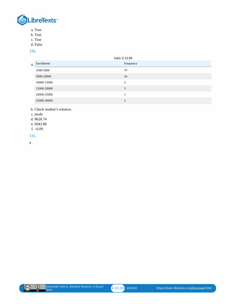
Alexander Holms, Barbara Illowsky, & Susan
Dean2.13.10 1/6/2022 https://stats.libretexts.org/@go/page/5340
a. Trueb. Truec. Trued. False
129.
a. Enrollment Frequency
1000-5000 10
5000-10000 16
10000-15000 3
15000-20000 3
20000-25000 1
25000-30000 2
Table
b. Check student’s solution.c. moded. 8628.74e. 6943.88f. –0.09
131.
a
2.13.89
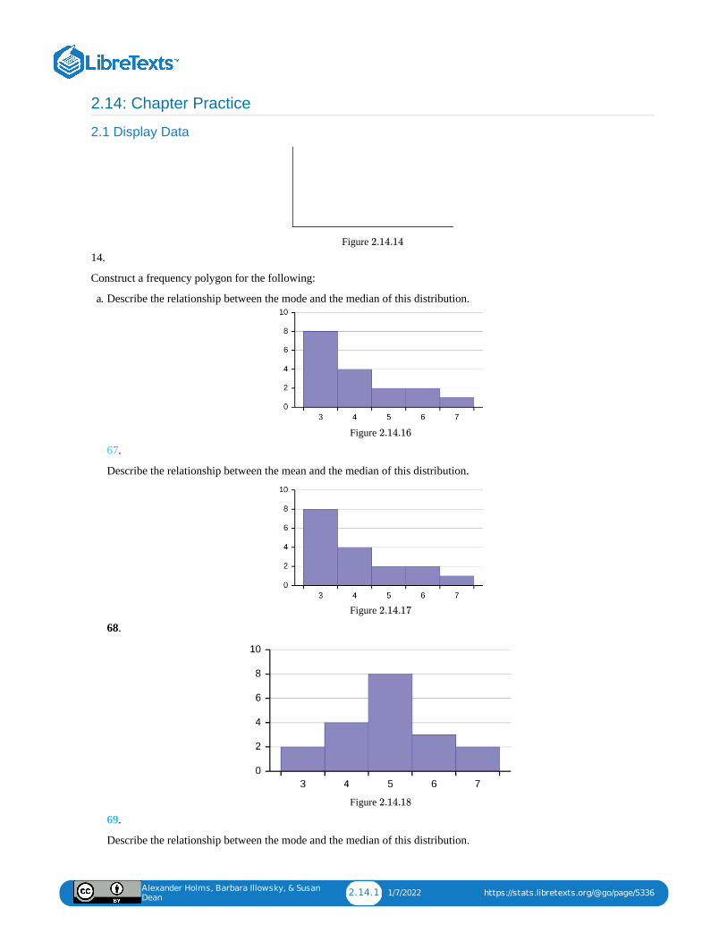
Alexander Holms, Barbara Illowsky, & Susan
Dean2.14.1 1/7/2022 https://stats.libretexts.org/@go/page/5336
2.14: Chapter Practice
2.1 Display Data
Figure 14.
Construct a frequency polygon for the following:
a. Describe the relationship between the mode and the median of this distribution.
Figure
67.
Describe the relationship between the mean and the median of this distribution.
Figure
68.
Figure
69.
Describe the relationship between the mode and the median of this distribution.
2.14.14
2.14.16
2.14.17
2.14.18
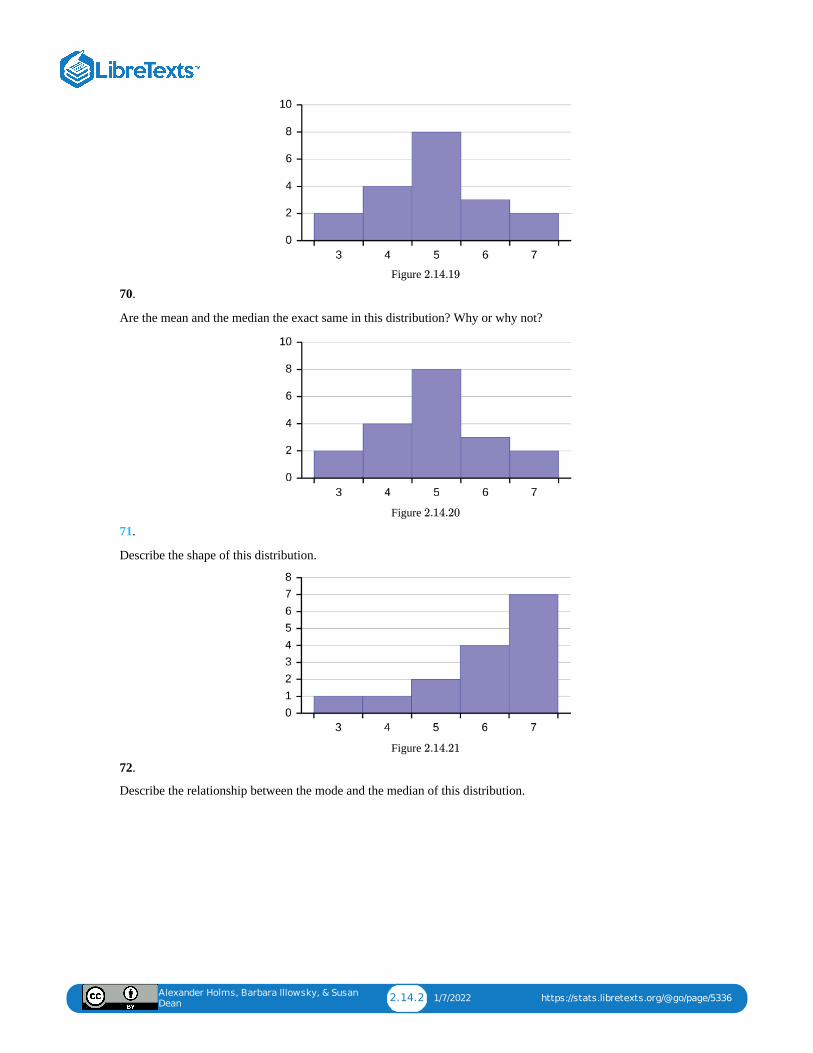
Alexander Holms, Barbara Illowsky, & Susan
Dean2.14.2 1/7/2022 https://stats.libretexts.org/@go/page/5336
Figure
70.
Are the mean and the median the exact same in this distribution? Why or why not?
Figure
71.
Describe the shape of this distribution.
Figure
72.
Describe the relationship between the mode and the median of this distribution.
2.14.19
2.14.20
2.14.21
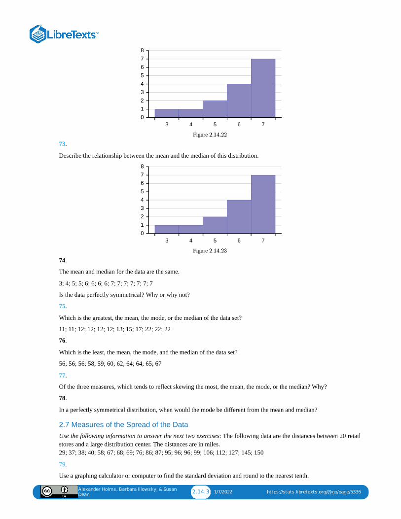
Alexander Holms, Barbara Illowsky, & Susan
Dean2.14.3 1/7/2022 https://stats.libretexts.org/@go/page/5336
Figure
73.
Describe the relationship between the mean and the median of this distribution.
Figure
74.
The mean and median for the data are the same.
3; 4; 5; 5; 6; 6; 6; 6; 7; 7; 7; 7; 7; 7; 7
Is the data perfectly symmetrical? Why or why not?
75.
Which is the greatest, the mean, the mode, or the median of the data set?
11; 11; 12; 12; 12; 12; 13; 15; 17; 22; 22; 22
76.
Which is the least, the mean, the mode, and the median of the data set?
56; 56; 56; 58; 59; 60; 62; 64; 64; 65; 67
77.
Of the three measures, which tends to reflect skewing the most, the mean, the mode, or the median? Why?
78.
In a perfectly symmetrical distribution, when would the mode be different from the mean and median?
2.7 Measures of the Spread of the DataUse the following information to answer the next two exercises: The following data are the distances between 20 retailstores and a large distribution center. The distances are in miles. 29; 37; 38; 40; 58; 67; 68; 69; 76; 86; 87; 95; 96; 96; 99; 106; 112; 127; 145; 150
79.
Use a graphing calculator or computer to find the standard deviation and round to the nearest tenth.
2.14.22
2.14.23
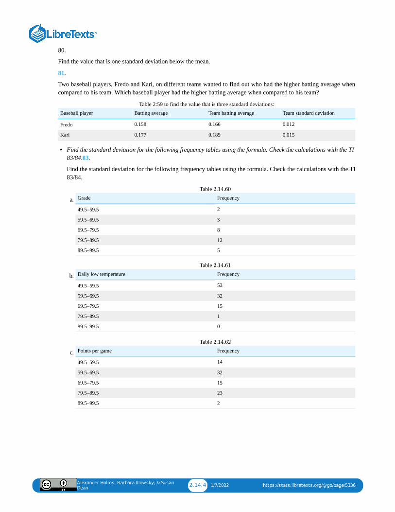
Alexander Holms, Barbara Illowsky, & Susan
Dean2.14.4 1/7/2022 https://stats.libretexts.org/@go/page/5336
80.
Find the value that is one standard deviation below the mean.
81.
Two baseball players, Fredo and Karl, on different teams wanted to find out who had the higher batting average whencompared to his team. Which baseball player had the higher batting average when compared to his team?
Baseball player Batting average Team batting average Team standard deviation
Fredo 0.158 0.166 0.012
Karl 0.177 0.189 0.015
Table 2:59 to find the value that is three standard deviations:
Find the standard deviation for the following frequency tables using the formula. Check the calculations with the TI83/84.83.
Find the standard deviation for the following frequency tables using the formula. Check the calculations with the TI83/84.
a. Grade Frequency
49.5–59.5 2
59.5–69.5 3
69.5–79.5 8
79.5–89.5 12
89.5–99.5 5
Table
b. Daily low temperature Frequency
49.5–59.5 53
59.5–69.5 32
69.5–79.5 15
79.5–89.5 1
89.5–99.5 0
Table
c. Points per game Frequency
49.5–59.5 14
59.5–69.5 32
69.5–79.5 15
79.5–89.5 23
89.5–99.5 2
Table
2.14.60
2.14.61
2.14.62
Alexander Holms, Barbara Illowsky, & Susan
Dean2.R.1 11/26/2021 https://stats.libretexts.org/@go/page/5334
2.R: Descriptive Statistics (Review)
2.1 Display Data
A stem-and-leaf plot is a way to plot data and look at the distribution. In a stem-and-leaf plot, all data values within aclass are visible. The advantage in a stem-and-leaf plot is that all values are listed, unlike a histogram, which gives classesof data values. A line graph is often used to represent a set of data values in which a quantity varies with time. Thesegraphs are useful for finding trends. That is, finding a general pattern in data sets including temperature, sales,employment, company profit or cost over a period of time. A bar graph is a chart that uses either horizontal or verticalbars to show comparisons among categories. One axis of the chart shows the specific categories being compared, and theother axis represents a discrete value. Some bar graphs present bars clustered in groups of more than one (grouped bargraphs), and others show the bars divided into subparts to show cumulative effect (stacked bar graphs). Bar graphs areespecially useful when categorical data is being used.
A histogram is a graphic version of a frequency distribution. The graph consists of bars of equal width drawn adjacent toeach other. The horizontal scale represents classes of quantitative data values and the vertical scale represents frequencies.The heights of the bars correspond to frequency values. Histograms are typically used for large, continuous, quantitativedata sets. A frequency polygon can also be used when graphing large data sets with data points that repeat. The datausually goes on y-axis with the frequency being graphed on the x-axis. Time series graphs can be helpful when looking atlarge amounts of data for one variable over a period of time.
2.2 Measures of the Location of the DataThe values that divide a rank-ordered set of data into 100 equal parts are called percentiles. Percentiles are used to compareand interpret data. For example, an observation at the 50 percentile would be greater than 50 percent of the otherobservations in the set. Quartiles divide data into quarters. The first quartile ( ) is the 25 percentile,the second quartile (
or median) is 50 percentile, and the third quartile ( ) is the the 75 percentile. The interquartile range, or , isthe range of the middle 50 percent of the data values. The is found by subtracting from , and can helpdetermine outliers by using the following two expressions.
2.3 Measures of the Center of the DataThe mean and the median can be calculated to help you find the "center" of a data set. The mean is the best estimate for theactual data set, but the median is the best measurement when a data set contains several outliers or extreme values. Themode will tell you the most frequently occuring datum (or data) in your data set. The mean, median, and mode areextremely helpful when you need to analyze your data, but if your data set consists of ranges which lack specific values,the mean may seem impossible to calculate. However, the mean can be approximated if you add the lower boundary withthe upper boundary and divide by two to find the midpoint of each interval. Multiply each midpoint by the number ofvalues found in the corresponding range. Divide the sum of these values by the total number of data values in the set.
2.6 Skewness and the Mean, Median, and Mode
Looking at the distribution of data can reveal a lot about the relationship between the mean, the median, and the mode.There are three types of distributions. A right (or positive) skewed distribution has a shape like Figure .
2.7 Measures of the Spread of the DataThe standard deviation can help you calculate the spread of data. There are different equations to use if are calculating thestandard deviation of a sample or of a population.
The Standard Deviation allows us to compare individual data or classes to the data set mean numerically.
is the formula for calculating the standard deviation of a sample. To calculate the
standard deviation of a population, we would use the population mean, μ, and the formula
th
Q1th
Q2th Q3
th IQR
IQR Q1 Q3
+IQR(1.5)Q3
– IQR(1.5)Q1
2.R. 11
s = or s =∑(x−x̄̄̄)
2
n−1
− −−−−−√ ∑ f(x−x̄̄̄)
2
n−1
− −−−−−−√

Alexander Holms, Barbara Illowsky, & Susan
Dean2.R.2 11/26/2021 https://stats.libretexts.org/@go/page/5334
.σ = or σ =∑(x−μ)
2
N
− −−−−−√ ∑ f(x−μ)
2
N
− −−−−−−√
1 1/7/2022
CHAPTER OVERVIEW3: PROBABILITY TOPICS
You have, more than likely, used probability. In fact, you probably have an intuitive sense of probability. Probability deals with thechance of an event occurring. Whenever you weigh the odds of whether or not to do your homework or to study for an exam, you areusing probability. In this chapter, you will learn how to solve probability problems using a systematic approach.
3.0: INTRODUCTION TO PROBABILITYIt is often necessary to "guess" about the outcome of an event in order to make a decision. Politicians study polls to guess theirlikelihood of winning an election. Teachers choose a particular course of study based on what they think students can comprehend.Doctors choose the treatments needed for various diseases based on their assessment of likely results. You may have visited a casinowhere people play games chosen because of the belief that the likelihood of winning is good.
3.1: PROBABILITY TERMINOLOGY3.2: INDEPENDENT AND MUTUALLY EXCLUSIVE EVENTS3.3: TWO BASIC RULES OF PROBABILITY3.4: CONTINGENCY TABLES AND PROBABILITY TREESA contingency table provides a way of portraying data that can facilitate calculating probabilities. The table helps in determiningconditional probabilities quite easily. The table displays sample values in relation to two different variables that may be dependent orcontingent on one another.
3.5: VENN DIAGRAMSA Venn diagram is a picture that represents the outcomes of an experiment. It generally consists of a box that represents the samplespace S together with circles or ovals. The circles or ovals represent events. Venn diagrams also help us to convert common Englishwords into mathematical terms that help add precision.
3.6: CHAPTER FORMULA REVIEW3.7: CHAPTER HOMEWORK3.8: CHAPTER KEY TERMS3.9: CHAPTER MORE PRACTICE3.10: CHAPTER PRACTICE3.11: CHAPTER REFERENCE3.12: CHAPTER REVIEW3.13: CHAPTER SOLUTION (PRACTICE + HOMEWORK)
Alexander Holms, Barbara Illowsky, & Susan Dean 3.0.1 12/17/2021 https://stats.libretexts.org/@go/page/4554
3.0: Introduction to ProbabilityIt is often necessary to "guess" about the outcome of an event in order to make a decision. Politicians study polls to guesstheir likelihood of winning an election. Teachers choose a particular course of study based on what they think students cancomprehend. Doctors choose the treatments needed for various diseases based on their assessment of likely results. Youmay have visited a casino where people play games chosen because of the belief that the likelihood of winning is good.You may have chosen your course of study based on the probable availability of jobs.
Figure 3.1 Meteor showers are rare, but the probability of them occurring can be calculated. (credit: Navicore/flickr)
You have, more than likely, used probability. In fact, you probably have an intuitive sense of probability. Probability dealswith the chance of an event occurring. Whenever you weigh the odds of whether or not to do your homework or to studyfor an exam, you are using probability. In this chapter, you will learn how to solve probability problems using a systematicapproach.
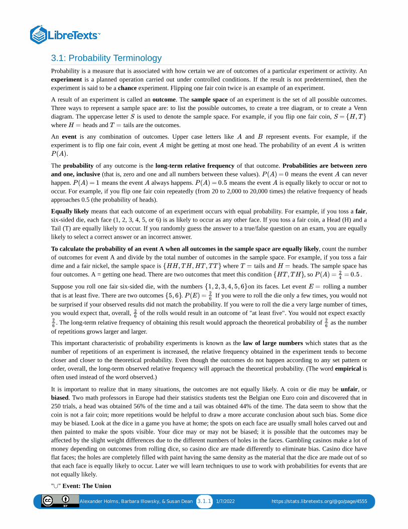
Alexander Holms, Barbara Illowsky, & Susan Dean 3.1.1 1/7/2022 https://stats.libretexts.org/@go/page/4555
3.1: Probability TerminologyProbability is a measure that is associated with how certain we are of outcomes of a particular experiment or activity. Anexperiment is a planned operation carried out under controlled conditions. If the result is not predetermined, then theexperiment is said to be a chance experiment. Flipping one fair coin twice is an example of an experiment.
A result of an experiment is called an outcome. The sample space of an experiment is the set of all possible outcomes.Three ways to represent a sample space are: to list the possible outcomes, to create a tree diagram, or to create a Venndiagram. The uppercase letter is used to denote the sample space. For example, if you flip one fair coin, where heads and tails are the outcomes.
An event is any combination of outcomes. Upper case letters like and represent events. For example, if theexperiment is to flip one fair coin, event might be getting at most one head. The probability of an event is written
.
The probability of any outcome is the long-term relative frequency of that outcome. Probabilities are between zeroand one, inclusive (that is, zero and one and all numbers between these values). means the event can neverhappen. means the event always happens. means the event is equally likely to occur or not tooccur. For example, if you flip one fair coin repeatedly (from 20 to 2,000 to 20,000 times) the relative frequency of headsapproaches 0.5 (the probability of heads).
Equally likely means that each outcome of an experiment occurs with equal probability. For example, if you toss a fair,six-sided die, each face (1, 2, 3, 4, 5, or 6) is as likely to occur as any other face. If you toss a fair coin, a Head (H) and aTail (T) are equally likely to occur. If you randomly guess the answer to a true/false question on an exam, you are equallylikely to select a correct answer or an incorrect answer.
To calculate the probability of an event A when all outcomes in the sample space are equally likely, count the numberof outcomes for event A and divide by the total number of outcomes in the sample space. For example, if you toss a fairdime and a fair nickel, the sample space is where tails and heads. The sample space hasfour outcomes. A = getting one head. There are two outcomes that meet this condition , so .
Suppose you roll one fair six-sided die, with the numbers on its faces. Let event rolling a numberthat is at least five. There are two outcomes . If you were to roll the die only a few times, you would notbe surprised if your observed results did not match the probability. If you were to roll the die a very large number of times,you would expect that, overall, of the rolls would result in an outcome of "at least five". You would not expect exactly
. The long-term relative frequency of obtaining this result would approach the theoretical probability of as the numberof repetitions grows larger and larger.
This important characteristic of probability experiments is known as the law of large numbers which states that as thenumber of repetitions of an experiment is increased, the relative frequency obtained in the experiment tends to becomecloser and closer to the theoretical probability. Even though the outcomes do not happen according to any set pattern ororder, overall, the long-term observed relative frequency will approach the theoretical probability. (The word empirical isoften used instead of the word observed.)
It is important to realize that in many situations, the outcomes are not equally likely. A coin or die may be unfair, orbiased. Two math professors in Europe had their statistics students test the Belgian one Euro coin and discovered that in250 trials, a head was obtained 56% of the time and a tail was obtained 44% of the time. The data seem to show that thecoin is not a fair coin; more repetitions would be helpful to draw a more accurate conclusion about such bias. Some dicemay be biased. Look at the dice in a game you have at home; the spots on each face are usually small holes carved out andthen painted to make the spots visible. Your dice may or may not be biased; it is possible that the outcomes may beaffected by the slight weight differences due to the different numbers of holes in the faces. Gambling casinos make a lot ofmoney depending on outcomes from rolling dice, so casino dice are made differently to eliminate bias. Casino dice haveflat faces; the holes are completely filled with paint having the same density as the material that the dice are made out of sothat each face is equally likely to occur. Later we will learn techniques to use to work with probabilities for events that arenot equally likely.
" " Event: The Union
S S = {H,T}
H = T =
A B
A A
P (A)
P (A) = 0 A
P (A) = 1 A P (A) = 0.5 A
{HH,TH,HT ,TT} T = H =
{HT ,TH} P (A) = = 0.524
{1, 2, 3, 4, 5, 6} E =
{5, 6} P (E) = 26
26
26
26
∪
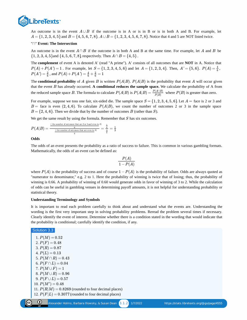
Alexander Holms, Barbara Illowsky, & Susan Dean 3.1.2 1/7/2022 https://stats.libretexts.org/@go/page/4555
An outcome is in the event if the outcome is in A or is in B or is in both A and B. For example, let and . . Notice that 4 and 5 are NOT listed twice.
" " Event: The Intersection
An outcome is in the event if the outcome is in both A and B at the same time. For example, let and be and , respectively. Then .
The complement of event A is denoted A′ (read "A prime"). A′ consists of all outcomes that are NOT in A. Notice that . For example, let and let . Then, . ,
, and
The conditional probability of given is written . is the probability that event will occur giventhat the event has already occurred. A conditional reduces the sample space. We calculate the probability of A fromthe reduced sample space . The formula to calculate is where is greater than zero.
For example, suppose we toss one fair, six-sided die. The sample space . Let face is 2 or 3 and face is even . To calculate , we count the number of outcomes 2 or 3 in the sample space
. Then we divide that by the number of outcomes (rather than ).
We get the same result by using the formula. Remember that has six outcomes.
Odds
The odds of an event presents the probability as a ratio of success to failure. This is common in various gambling formats.Mathematically, the odds of an event can be defined as:
where is the probability of success and of course is the probability of failure. Odds are always quoted as"numerator to denominator," e.g. 2 to 1. Here the probability of winning is twice that of losing; thus, the probability ofwinning is 0.66. A probability of winning of 0.60 would generate odds in favor of winning of 3 to 2. While the calculationof odds can be useful in gambling venues in determining payoff amounts, it is not helpful for understanding probability orstatistical theory.
Understanding Terminology and Symbols
It is important to read each problem carefully to think about and understand what the events are. Understanding thewording is the first very important step in solving probability problems. Reread the problem several times if necessary.Clearly identify the event of interest. Determine whether there is a condition stated in the wording that would indicate thatthe probability is conditional; carefully identify the condition, if any.
1. 2. 3. 4. 5. 6. 7. 8. 9.
10. 11. (rounded to four decimal places)12. (rounded to four decimal places)
A∪B
A= {1, 2, 3, 4, 5} B= {4, 5, 6, 7, 8} A∪B= {1, 2, 3, 4, 5, 6, 7, 8}
∩
A∩B A B
{1, 2, 3, 4, 5} {4, 5, 6, 7, 8} A∩B= {4, 5}
P (A) +P (A') = 1 S = {1, 2, 3, 4, 5, 6} A= {1, 2, 3, 4} A' = {5, 6} P (A) = 46
P (A') = 26
P (A) +P (A') = + = 146
26
A B P (A|B) P (A|B) A
B
B P (A|B) P (A|B) =P(A∩B)
P(B)P (B)
S = {1, 2, 3, 4, 5, 6} A=
B= (2, 4, 6) P (A|B)
B= {2, 4, 6} B S
S
P (A|B) = = =( the number of outcomes that are 2 or 3 and even in S)
6
( the number of outcomes that are even in S)
6
1
6
36
13
P (A)
1 −P (A)
P (A) 1 −P (A)
Solution 3.3
P (M) = 0.52
P (F ) = 0.48
P (R) = 0.87
P (L) = 0.13
P (M ∩R) = 0.43
P (F ∩L) = 0.04
P (M ∪F ) = 1
P (M ∪R) = 0.96
P (F ∪L) = 0.57
P ( ) = 0.48M′
P (R|M) = 0.8269
P (F |L) = 0.3077

Alexander Holms, Barbara Illowsky, & Susan Dean 3.1.3 1/7/2022 https://stats.libretexts.org/@go/page/4555
13. P (L|F ) = 0.0833
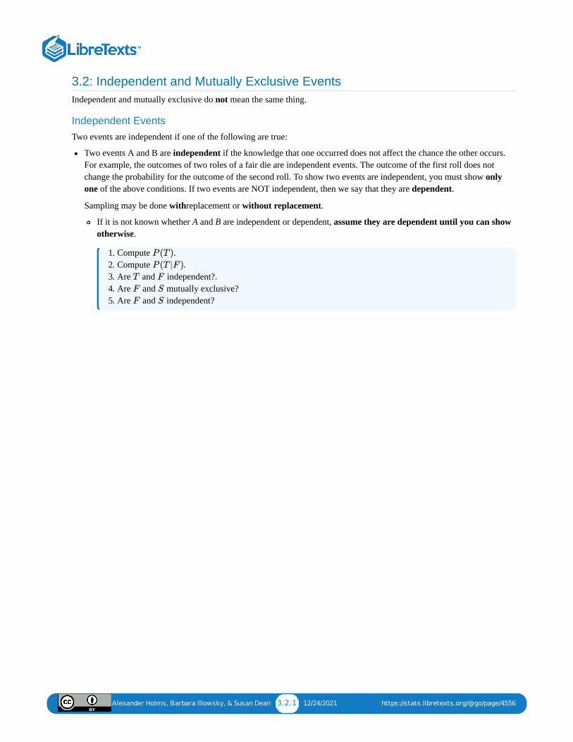
Alexander Holms, Barbara Illowsky, & Susan Dean 3.2.1 12/24/2021 https://stats.libretexts.org/@go/page/4556
3.2: Independent and Mutually Exclusive EventsIndependent and mutually exclusive do not mean the same thing.
Independent EventsTwo events are independent if one of the following are true:
Two events A and B are independent if the knowledge that one occurred does not affect the chance the other occurs.For example, the outcomes of two roles of a fair die are independent events. The outcome of the first roll does notchange the probability for the outcome of the second roll. To show two events are independent, you must show onlyone of the above conditions. If two events are NOT independent, then we say that they are dependent.
Sampling may be done withreplacement or without replacement.
If it is not known whether A and B are independent or dependent, assume they are dependent until you can showotherwise.
1. Compute .2. Compute .3. Are and independent?.4. Are and mutually exclusive?5. Are and independent?
P (T )
P (T |F )
T F
F S
F S
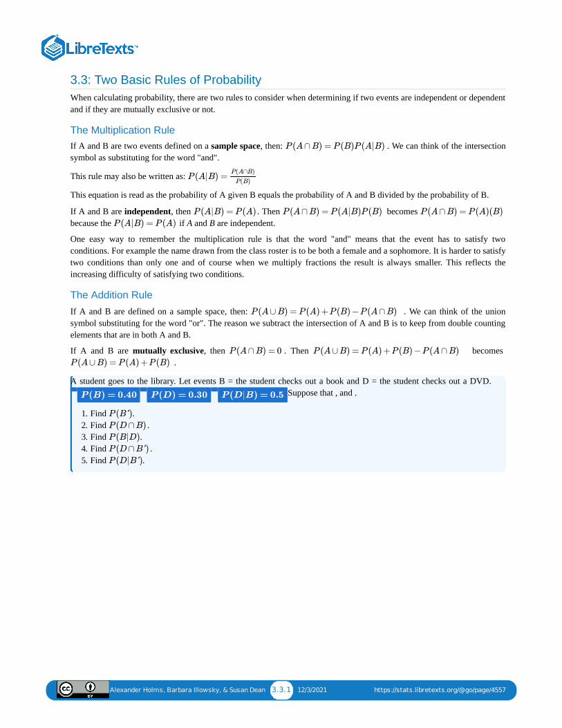
Alexander Holms, Barbara Illowsky, & Susan Dean 3.3.1 12/3/2021 https://stats.libretexts.org/@go/page/4557
3.3: Two Basic Rules of ProbabilityWhen calculating probability, there are two rules to consider when determining if two events are independent or dependentand if they are mutually exclusive or not.
The Multiplication RuleIf A and B are two events defined on a sample space, then: . We can think of the intersectionsymbol as substituting for the word "and".
This rule may also be written as:
This equation is read as the probability of A given B equals the probability of A and B divided by the probability of B.
If A and B are independent, then . Then becomes because the if A and B are independent.
One easy way to remember the multiplication rule is that the word "and" means that the event has to satisfy twoconditions. For example the name drawn from the class roster is to be both a female and a sophomore. It is harder to satisfytwo conditions than only one and of course when we multiply fractions the result is always smaller. This reflects theincreasing difficulty of satisfying two conditions.
The Addition Rule
If A and B are defined on a sample space, then: . We can think of the unionsymbol substituting for the word "or". The reason we subtract the intersection of A and B is to keep from double countingelements that are in both A and B.
If A and B are mutually exclusive, then . Then becomes .
1. Find .2. Find .3. Find .4. Find .5. Find .
P (A∩B) = P (B)P (A|B)
P (A|B) =P(A∩B)
P(B)
P (A|B) = P (A) P (A∩B) = P (A|B)P (B) P (A∩B) = P (A)(B)
P (A|B) = P (A)
P (A∪B) = P (A) +P (B) −P (A∩B)
P (A∩B) = 0 P (A∪B) = P (A) +P (B) −P (A∩B)
P (A∪B) = P (A) +P (B)
A student goes to the library. Let events B = the student checks out a book and D = the student checks out a DVD.Suppose that , and .P (B) = 0.40 P (D) = 0.30 P (D|B) = 0.5
P (B')
P (D∩B)
P (B|D)
P (D∩B')
P (D|B')
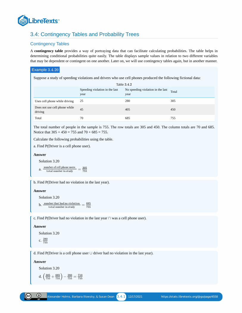
Alexander Holms, Barbara Illowsky, & Susan Dean 3.4.1 12/17/2021 https://stats.libretexts.org/@go/page/4558
3.4: Contingency Tables and Probability Trees
Contingency Tables
A contingency table provides a way of portraying data that can facilitate calculating probabilities. The table helps indetermining conditional probabilities quite easily. The table displays sample values in relation to two different variablesthat may be dependent or contingent on one another. Later on, we will use contingency tables again, but in another manner.
Suppose a study of speeding violations and drivers who use cell phones produced the following fictional data:
Speeding violation in the lastyear
No speeding violation in the lastyear
Total
Uses cell phone while driving 25 280 305
Does not use cell phone whiledriving
45 405 450
Total 70 685 755
Table
The total number of people in the sample is 755. The row totals are 305 and 450. The column totals are 70 and 685.Notice that 305 + 450 = 755 and 70 + 685 = 755.
Calculate the following probabilities using the table.
a. Find P(Driver is a cell phone user).
Answer
Solution 3.20
a.
b. Find P(Driver had no violation in the last year).
Answer
Solution 3.20
b.
c. Find P(Driver had no violation in the last year was a cell phone user).
Answer
Solution 3.20
c.
d. Find P(Driver is a cell phone user driver had no violation in the last year).
Answer
Solution 3.20
d.
Example 3.4.20
3.4.2
= number of cell phone users
total number in study 305755
= number that had no violation
total number in study
685
755
∩
280
755
∪
( + )− =305755
685755
280755
710755
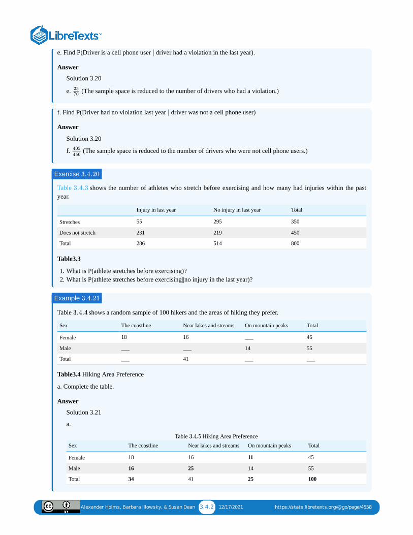
Alexander Holms, Barbara Illowsky, & Susan Dean 3.4.2 12/17/2021 https://stats.libretexts.org/@go/page/4558
e. Find P(Driver is a cell phone user driver had a violation in the last year).
Answer
Solution 3.20
e. (The sample space is reduced to the number of drivers who had a violation.)
f. Find P(Driver had no violation last year driver was not a cell phone user)
Answer
Solution 3.20
f. (The sample space is reduced to the number of drivers who were not cell phone users.)
Table shows the number of athletes who stretch before exercising and how many had injuries within the pastyear.
Injury in last year No injury in last year Total
Stretches 55 295 350
Does not stretch 231 219 450
Total 286 514 800
Table3.3
1. What is P(athlete stretches before exercising)?2. What is P(athlete stretches before exercising||no injury in the last year)?
Table shows a random sample of 100 hikers and the areas of hiking they prefer.
Sex The coastline Near lakes and streams On mountain peaks Total
Female 18 16 ___ 45
Male ___ ___ 14 55
Total ___ 41 ___ ___
Table3.4 Hiking Area Preference
a. Complete the table.
Answer
Solution 3.21
a.
Sex The coastline Near lakes and streams On mountain peaks Total
Female 18 16 11 45
Male 16 25 14 55
Total 34 41 25 100
Table Hiking Area Preference
|
2570
|
405
450
Exercise 3.4.20
3.4.3
Example 3.4.21
3.4.4
3.4.5
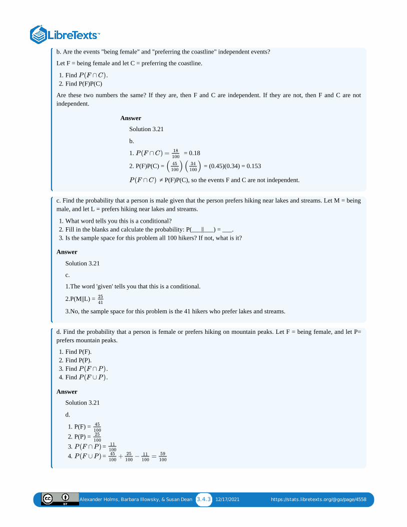
Alexander Holms, Barbara Illowsky, & Susan Dean 3.4.3 12/17/2021 https://stats.libretexts.org/@go/page/4558
b. Are the events "being female" and "preferring the coastline" independent events?
Let F = being female and let C = preferring the coastline.
1. Find .2. Find P(F)P(C)
Are these two numbers the same? If they are, then F and C are independent. If they are not, then F and C are notindependent.
Answer
Solution 3.21
b.
1. = 0.18
2. P(F)P(C) = = (0.45)(0.34) = 0.153
≠ P(F)P(C), so the events F and C are not independent.
c. Find the probability that a person is male given that the person prefers hiking near lakes and streams. Let M = beingmale, and let L = prefers hiking near lakes and streams.
1. What word tells you this is a conditional?2. Fill in the blanks and calculate the probability: P(___||___) = ___.3. Is the sample space for this problem all 100 hikers? If not, what is it?
Answer
Solution 3.21
c.
1.The word 'given' tells you that this is a conditional.
2.P(M||L) =
3.No, the sample space for this problem is the 41 hikers who prefer lakes and streams.
d. Find the probability that a person is female or prefers hiking on mountain peaks. Let F = being female, and let P=prefers mountain peaks.
1. Find P(F).2. Find P(P).3. Find .4. Find .
Answer
Solution 3.21
d.
1. P(F) = 2. P(P) = 3. = 4. =
P (F ∩C)
P (F ∩C) = 18
100
( )( )45
100
34
100
P (F ∩C)
25
41
P (F ∩P )
P (F ∪P )
45
10025
100
P (F ∩P ) 11100
P (F ∪P ) + − =45
100
25
10011100
59
100
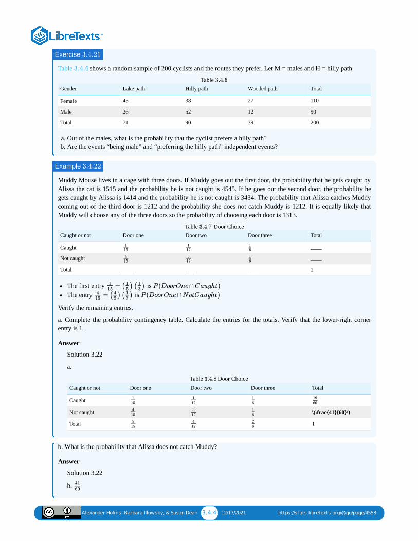
Alexander Holms, Barbara Illowsky, & Susan Dean 3.4.4 12/17/2021 https://stats.libretexts.org/@go/page/4558
Table shows a random sample of 200 cyclists and the routes they prefer. Let M = males and H = hilly path.
Gender Lake path Hilly path Wooded path Total
Female 45 38 27 110
Male 26 52 12 90
Total 71 90 39 200
Table
a. Out of the males, what is the probability that the cyclist prefers a hilly path?b. Are the events “being male” and “preferring the hilly path” independent events?
Muddy Mouse lives in a cage with three doors. If Muddy goes out the first door, the probability that he gets caught byAlissa the cat is 1515 and the probability he is not caught is 4545. If he goes out the second door, the probability hegets caught by Alissa is 1414 and the probability he is not caught is 3434. The probability that Alissa catches Muddycoming out of the third door is 1212 and the probability she does not catch Muddy is 1212. It is equally likely thatMuddy will choose any of the three doors so the probability of choosing each door is 1313.
Caught or not Door one Door two Door three Total
Caught ____
Not caught ____
Total ____ ____ ____ 1
Table Door Choice
The first entry is The entry is
Verify the remaining entries.
a. Complete the probability contingency table. Calculate the entries for the totals. Verify that the lower-right cornerentry is 1.
Answer
Solution 3.22
a.
Caught or not Door one Door two Door three Total
Caught
Not caught \(\frac{41}{60}\)
Total 1
Table Door Choice
b. What is the probability that Alissa does not catch Muddy?
Answer
Solution 3.22
b.
Exercise 3.4.21
3.4.6
3.4.6
Example 3.4.22
115
112
16
415
312
16
3.4.7
= ( ) ( )115
15
13
P (DoorOne∩Caught)
= ( ) ( )415
45
13
P (DoorOne∩NotCaught)
115
112
16
1960
415
312
16
515
412
26
3.4.8
4160
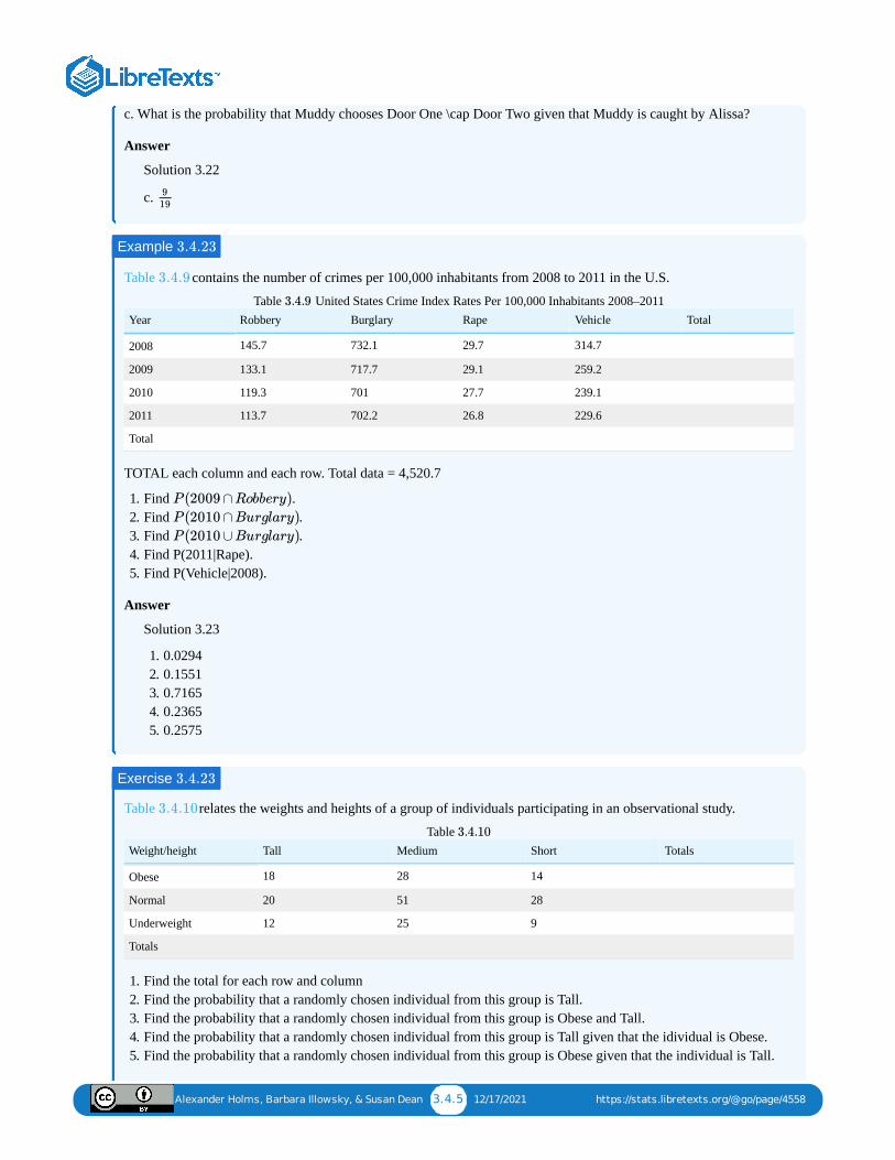
Alexander Holms, Barbara Illowsky, & Susan Dean 3.4.5 12/17/2021 https://stats.libretexts.org/@go/page/4558
c. What is the probability that Muddy chooses Door One \cap Door Two given that Muddy is caught by Alissa?
Answer
Solution 3.22
c.
Table contains the number of crimes per 100,000 inhabitants from 2008 to 2011 in the U.S.
Year Robbery Burglary Rape Vehicle Total
2008 145.7 732.1 29.7 314.7
2009 133.1 717.7 29.1 259.2
2010 119.3 701 27.7 239.1
2011 113.7 702.2 26.8 229.6
Total
Table United States Crime Index Rates Per 100,000 Inhabitants 2008–2011
TOTAL each column and each row. Total data = 4,520.7
1. Find .2. Find .3. Find .4. Find P(2011|Rape).5. Find P(Vehicle|2008).
Answer
Solution 3.23
1. 0.02942. 0.15513. 0.71654. 0.23655. 0.2575
Table relates the weights and heights of a group of individuals participating in an observational study.
Weight/height Tall Medium Short Totals
Obese 18 28 14
Normal 20 51 28
Underweight 12 25 9
Totals
Table
1. Find the total for each row and column2. Find the probability that a randomly chosen individual from this group is Tall.3. Find the probability that a randomly chosen individual from this group is Obese and Tall.4. Find the probability that a randomly chosen individual from this group is Tall given that the idividual is Obese.5. Find the probability that a randomly chosen individual from this group is Obese given that the individual is Tall.
919
Example 3.4.23
3.4.9
3.4.9
P (2009 ∩Robbery)
P (2010 ∩Burglary)
P (2010 ∪Burglary)
Exercise 3.4.23
3.4.10
3.4.10
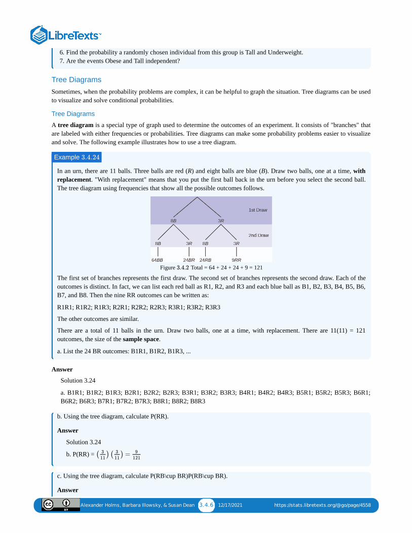
Alexander Holms, Barbara Illowsky, & Susan Dean 3.4.6 12/17/2021 https://stats.libretexts.org/@go/page/4558
6. Find the probability a randomly chosen individual from this group is Tall and Underweight.7. Are the events Obese and Tall independent?
Tree Diagrams
Sometimes, when the probability problems are complex, it can be helpful to graph the situation. Tree diagrams can be usedto visualize and solve conditional probabilities.
Tree Diagrams
A tree diagram is a special type of graph used to determine the outcomes of an experiment. It consists of "branches" thatare labeled with either frequencies or probabilities. Tree diagrams can make some probability problems easier to visualizeand solve. The following example illustrates how to use a tree diagram.
In an urn, there are 11 balls. Three balls are red (R) and eight balls are blue (B). Draw two balls, one at a time, withreplacement. "With replacement" means that you put the first ball back in the urn before you select the second ball.The tree diagram using frequencies that show all the possible outcomes follows.
Figure Total = 64 + 24 + 24 + 9 = 121
The first set of branches represents the first draw. The second set of branches represents the second draw. Each of theoutcomes is distinct. In fact, we can list each red ball as R1, R2, and R3 and each blue ball as B1, B2, B3, B4, B5, B6,B7, and B8. Then the nine RR outcomes can be written as:
R1R1; R1R2; R1R3; R2R1; R2R2; R2R3; R3R1; R3R2; R3R3
The other outcomes are similar.
There are a total of 11 balls in the urn. Draw two balls, one at a time, with replacement. There are 11(11) = 121outcomes, the size of the sample space.
a. List the 24 BR outcomes: B1R1, B1R2, B1R3, ...
Answer
Solution 3.24
a. B1R1; B1R2; B1R3; B2R1; B2R2; B2R3; B3R1; B3R2; B3R3; B4R1; B4R2; B4R3; B5R1; B5R2; B5R3; B6R1;B6R2; B6R3; B7R1; B7R2; B7R3; B8R1; B8R2; B8R3
b. Using the tree diagram, calculate P(RR).
Answer
Solution 3.24
b. P(RR) =
c. Using the tree diagram, calculate P(RB\cup BR)P(RB\cup BR).
Answer
Example 3.4.24
3.4.2
( ) ( ) =3
11
3
11
9
121
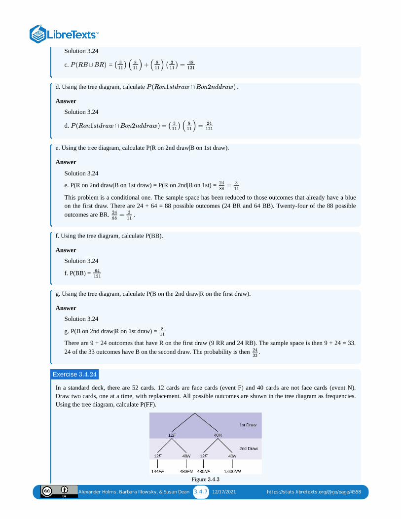
Alexander Holms, Barbara Illowsky, & Susan Dean 3.4.7 12/17/2021 https://stats.libretexts.org/@go/page/4558
Solution 3.24
c. =
d. Using the tree diagram, calculate .
Answer
Solution 3.24
d.
e. Using the tree diagram, calculate P(R on 2nd draw|B on 1st draw).
Answer
Solution 3.24
e. P(R on 2nd draw|B on 1st draw) = P(R on 2nd|B on 1st) =
This problem is a conditional one. The sample space has been reduced to those outcomes that already have a blueon the first draw. There are 24 + 64 = 88 possible outcomes (24 BR and 64 BB). Twenty-four of the 88 possibleoutcomes are BR. .
f. Using the tree diagram, calculate P(BB).
Answer
Solution 3.24
f. P(BB) =
g. Using the tree diagram, calculate P(B on the 2nd draw|R on the first draw).
Answer
Solution 3.24
g. P(B on 2nd draw|R on 1st draw) =
There are 9 + 24 outcomes that have R on the first draw (9 RR and 24 RB). The sample space is then 9 + 24 = 33.24 of the 33 outcomes have B on the second draw. The probability is then .
In a standard deck, there are 52 cards. 12 cards are face cards (event F) and 40 cards are not face cards (event N).Draw two cards, one at a time, with replacement. All possible outcomes are shown in the tree diagram as frequencies.Using the tree diagram, calculate P(FF).
Figure
P (RB∪BR) ( )( )+( ) ( ) =311
811
811
311
48121
P (Ron1stdraw∩Bon2nddraw)
P (Ron1stdraw∩Bon2nddraw) = ( )( ) =311
811
24121
=24
88
3
11
=24
88
3
11
64121
811
2433
Exercise 3.4.24
3.4.3
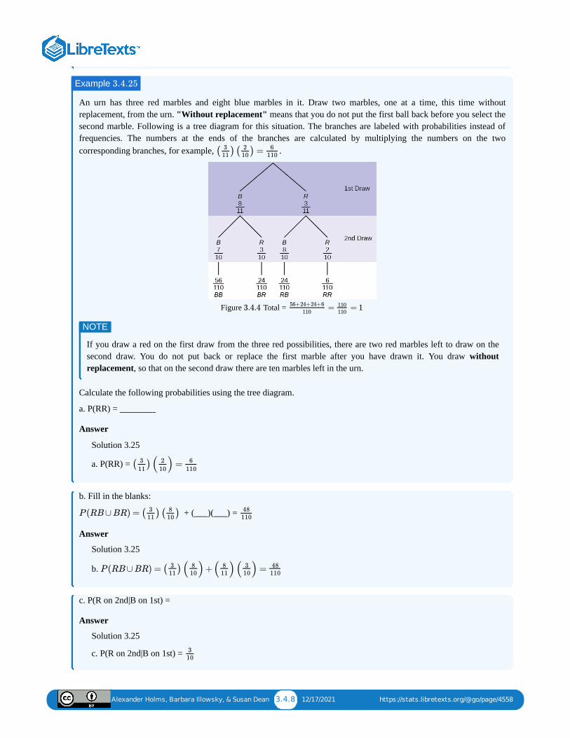
Alexander Holms, Barbara Illowsky, & Susan Dean 3.4.8 12/17/2021 https://stats.libretexts.org/@go/page/4558
An urn has three red marbles and eight blue marbles in it. Draw two marbles, one at a time, this time withoutreplacement, from the urn. "Without replacement" means that you do not put the first ball back before you select thesecond marble. Following is a tree diagram for this situation. The branches are labeled with probabilities instead offrequencies. The numbers at the ends of the branches are calculated by multiplying the numbers on the twocorresponding branches, for example, .
Figure Total =
If you draw a red on the first draw from the three red possibilities, there are two red marbles left to draw on thesecond draw. You do not put back or replace the first marble after you have drawn it. You draw withoutreplacement, so that on the second draw there are ten marbles left in the urn.
Calculate the following probabilities using the tree diagram.
a. P(RR) = ________
Answer
Solution 3.25
a. P(RR) =
b. Fill in the blanks:
+ (___)(___) =
Answer
Solution 3.25
b.
c. P(R on 2nd|B on 1st) =
Answer
Solution 3.25
c. P(R on 2nd|B on 1st) =
Example 3.4.25
( ) ( ) =311
210
6110
3.4.4 = = 156+24+24+6
110110110
NOTE
( )( ) =3
11
2
10
6
110
P (RB∪BR) = ( ) ( )311
810
48110
P (RB∪BR) = ( )( )+( )( ) =311
810
811
310
48110
310
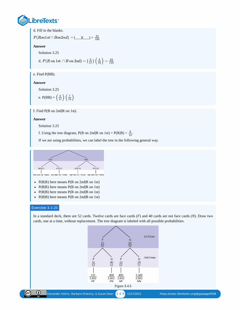
Alexander Holms, Barbara Illowsky, & Susan Dean 3.4.9 12/17/2021 https://stats.libretexts.org/@go/page/4558
d. Fill in the blanks.
= (___)(___) =
Answer
Solution 3.25
d.
e. Find P(BB).
Answer
Solution 3.25
e. P(BB) =
f. Find P(B on 2nd|R on 1st).
Answer
Solution 3.25
f. Using the tree diagram, P(B on 2nd|R on 1st) = P(R|B) = .
If we are using probabilities, we can label the tree in the following general way.
P(R|R) here means P(R on 2nd|R on 1st)P(B|R) here means P(B on 2nd|R on 1st)P(R|B) here means P(R on 2nd|B on 1st)P(B|B) here means P(B on 2nd|B on 1st)
In a standard deck, there are 52 cards. Twelve cards are face cards (F) and 40 cards are not face cards (N). Draw twocards, one at a time, without replacement. The tree diagram is labeled with all possible probabilities.
Figure
P (Ron1st∩Bon2nd) 24100
P (R on 1st ∩B on 2nd) = ( )( ) =311
810
24110
( )( )811
710
8
10
Exercise 3.4.25
3.4.5
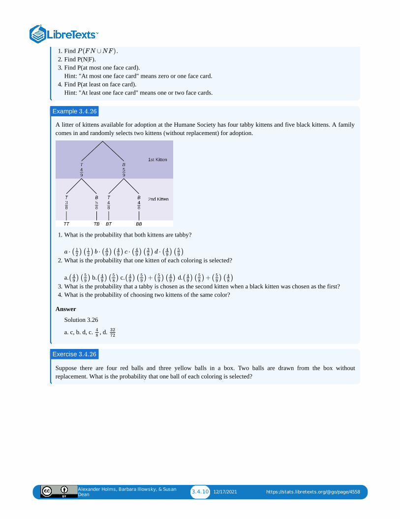
Alexander Holms, Barbara Illowsky, & Susan
Dean3.4.10 12/17/2021 https://stats.libretexts.org/@go/page/4558
1. Find .2. Find P(N|F).3. Find P(at most one face card).
Hint: "At most one face card" means zero or one face card.4. Find P(at least on face card).
Hint: "At least one face card" means one or two face cards.
A litter of kittens available for adoption at the Humane Society has four tabby kittens and five black kittens. A familycomes in and randomly selects two kittens (without replacement) for adoption.
1. What is the probability that both kittens are tabby?
2. What is the probability that one kitten of each coloring is selected? a. b. c. d.
3. What is the probability that a tabby is chosen as the second kitten when a black kitten was chosen as the first?4. What is the probability of choosing two kittens of the same color?
Answer
Solution 3.26
a. c, b. d, c. , d.
Suppose there are four red balls and three yellow balls in a box. Two balls are drawn from the box withoutreplacement. What is the probability that one ball of each coloring is selected?
P (FN ∪NF )
Example 3.4.26
a ⋅ ( ) ( ) b ⋅ ( ) ( ) c ⋅ ( ) ( )d ⋅ ( ) ( )12
12
49
49
49
38
49
59
( ) ( )49
59
( ) ( )49
58
( ) ( )+( ) ( )49
59
59
49
( ) ( )+( ) ( )49
58
59
48
48
3272
Exercise 3.4.26
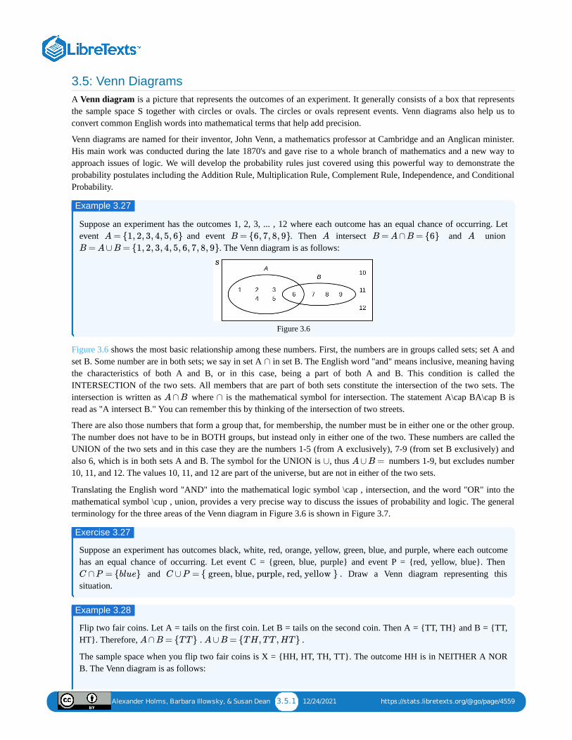
Alexander Holms, Barbara Illowsky, & Susan Dean 3.5.1 12/24/2021 https://stats.libretexts.org/@go/page/4559
3.5: Venn DiagramsA Venn diagram is a picture that represents the outcomes of an experiment. It generally consists of a box that representsthe sample space S together with circles or ovals. The circles or ovals represent events. Venn diagrams also help us toconvert common English words into mathematical terms that help add precision.
Venn diagrams are named for their inventor, John Venn, a mathematics professor at Cambridge and an Anglican minister.His main work was conducted during the late 1870's and gave rise to a whole branch of mathematics and a new way toapproach issues of logic. We will develop the probability rules just covered using this powerful way to demonstrate theprobability postulates including the Addition Rule, Multiplication Rule, Complement Rule, Independence, and ConditionalProbability.
Suppose an experiment has the outcomes 1, 2, 3, ... , 12 where each outcome has an equal chance of occurring. Letevent and event . Then intersect and union
. The Venn diagram is as follows:
Figure 3.6
Figure 3.6 shows the most basic relationship among these numbers. First, the numbers are in groups called sets; set A andset B. Some number are in both sets; we say in set A in set B. The English word "and" means inclusive, meaning havingthe characteristics of both A and B, or in this case, being a part of both A and B. This condition is called theINTERSECTION of the two sets. All members that are part of both sets constitute the intersection of the two sets. Theintersection is written as where is the mathematical symbol for intersection. The statement A\cap BA\cap B isread as "A intersect B." You can remember this by thinking of the intersection of two streets.
There are also those numbers that form a group that, for membership, the number must be in either one or the other group.The number does not have to be in BOTH groups, but instead only in either one of the two. These numbers are called theUNION of the two sets and in this case they are the numbers 1-5 (from A exclusively), 7-9 (from set B exclusively) andalso 6, which is in both sets A and B. The symbol for the UNION is , thus numbers 1-9, but excludes number10, 11, and 12. The values 10, 11, and 12 are part of the universe, but are not in either of the two sets.
Translating the English word "AND" into the mathematical logic symbol \cap , intersection, and the word "OR" into themathematical symbol \cup , union, provides a very precise way to discuss the issues of probability and logic. The generalterminology for the three areas of the Venn diagram in Figure 3.6 is shown in Figure 3.7.
Suppose an experiment has outcomes black, white, red, orange, yellow, green, blue, and purple, where each outcomehas an equal chance of occurring. Let event C = {green, blue, purple} and event P = {red, yellow, blue}. Then
and . Draw a Venn diagram representing thissituation.
Flip two fair coins. Let A = tails on the first coin. Let B = tails on the second coin. Then A = {TT, TH} and B = {TT,HT}. Therefore, . .
The sample space when you flip two fair coins is X = {HH, HT, TH, TT}. The outcome HH is in NEITHER A NORB. The Venn diagram is as follows:
Example 3.27
A = {1, 2, 3, 4, 5, 6} B = {6, 7, 8, 9} A B = A ∩ B = {6} A
B = A ∪ B = {1, 2, 3, 4, 5, 6, 7, 8, 9}
∩
A ∩ B ∩
∪ A ∪ B =
Exercise 3.27
C ∩ P = {blue} C ∪ P = { green, blue, purple, red, yellow }
Example 3.28
A ∩ B = {T T } A ∪ B = {T H, T T , HT }
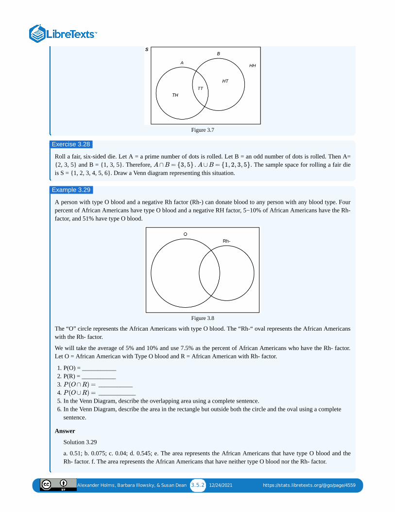
Alexander Holms, Barbara Illowsky, & Susan Dean 3.5.2 12/24/2021 https://stats.libretexts.org/@go/page/4559
Figure 3.7
Roll a fair, six-sided die. Let A = a prime number of dots is rolled. Let B = an odd number of dots is rolled. Then A={2, 3, 5} and B = {1, 3, 5}. Therefore, . . The sample space for rolling a fair dieis S = {1, 2, 3, 4, 5, 6}. Draw a Venn diagram representing this situation.
A person with type O blood and a negative Rh factor (Rh-) can donate blood to any person with any blood type. Fourpercent of African Americans have type O blood and a negative RH factor, 5−10% of African Americans have the Rh-factor, and 51% have type O blood.
Figure 3.8
The “O” circle represents the African Americans with type O blood. The “Rh-“ oval represents the African Americanswith the Rh- factor.
We will take the average of 5% and 10% and use 7.5% as the percent of African Americans who have the Rh- factor.Let O = African American with Type O blood and R = African American with Rh- factor.
1. P(O) = ___________2. P(R) = ___________3. ___________4. ____________5. In the Venn Diagram, describe the overlapping area using a complete sentence.6. In the Venn Diagram, describe the area in the rectangle but outside both the circle and the oval using a complete
sentence.
Answer
Solution 3.29
a. 0.51; b. 0.075; c. 0.04; d. 0.545; e. The area represents the African Americans that have type O blood and theRh- factor. f. The area represents the African Americans that have neither type O blood nor the Rh- factor.
Exercise 3.28
A ∩ B = {3, 5} A ∪ B = {1, 2, 3, 5}
Example 3.29
P (O ∩ R) =
P (O ∪ R) =
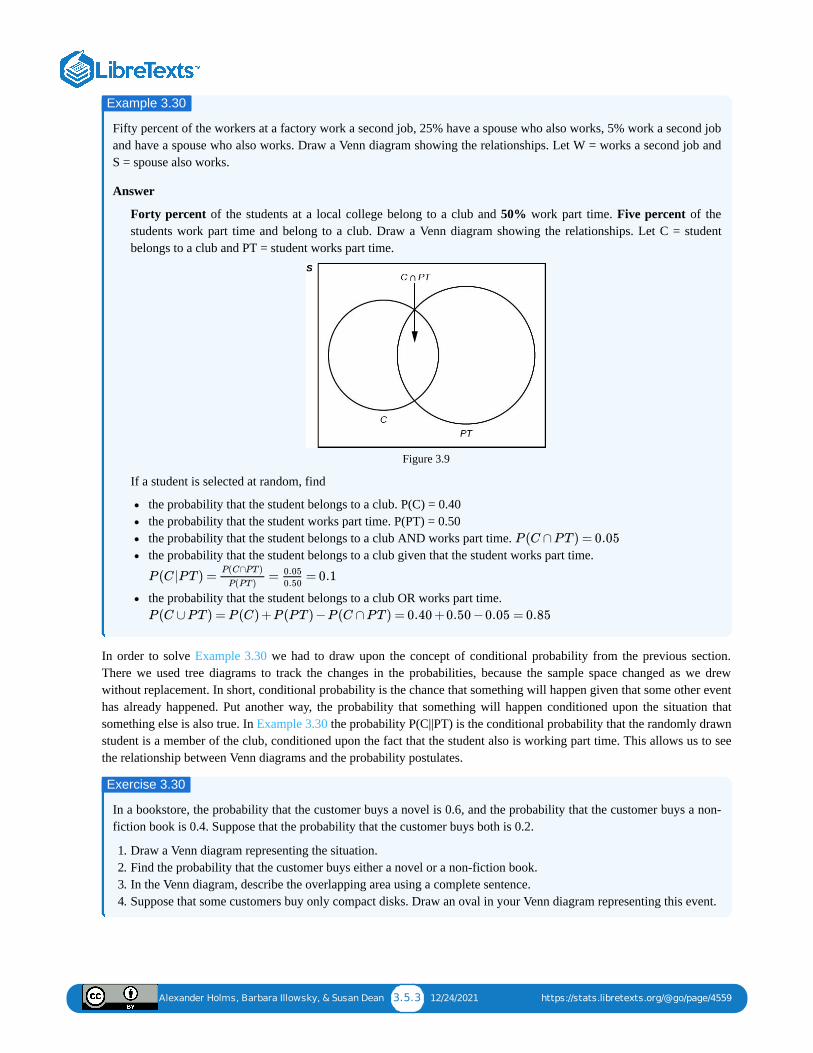
Alexander Holms, Barbara Illowsky, & Susan Dean 3.5.3 12/24/2021 https://stats.libretexts.org/@go/page/4559
Fifty percent of the workers at a factory work a second job, 25% have a spouse who also works, 5% work a second joband have a spouse who also works. Draw a Venn diagram showing the relationships. Let W = works a second job andS = spouse also works.
Answer
Forty percent of the students at a local college belong to a club and 50% work part time. Five percent of thestudents work part time and belong to a club. Draw a Venn diagram showing the relationships. Let C = studentbelongs to a club and PT = student works part time.
Figure 3.9
If a student is selected at random, find
the probability that the student belongs to a club. P(C) = 0.40the probability that the student works part time. P(PT) = 0.50the probability that the student belongs to a club AND works part time. the probability that the student belongs to a club given that the student works part time.
the probability that the student belongs to a club OR works part time.
In order to solve Example 3.30 we had to draw upon the concept of conditional probability from the previous section.There we used tree diagrams to track the changes in the probabilities, because the sample space changed as we drewwithout replacement. In short, conditional probability is the chance that something will happen given that some other eventhas already happened. Put another way, the probability that something will happen conditioned upon the situation thatsomething else is also true. In Example 3.30 the probability P(C||PT) is the conditional probability that the randomly drawnstudent is a member of the club, conditioned upon the fact that the student also is working part time. This allows us to seethe relationship between Venn diagrams and the probability postulates.
In a bookstore, the probability that the customer buys a novel is 0.6, and the probability that the customer buys a non-fiction book is 0.4. Suppose that the probability that the customer buys both is 0.2.
1. Draw a Venn diagram representing the situation.2. Find the probability that the customer buys either a novel or a non-fiction book.3. In the Venn diagram, describe the overlapping area using a complete sentence.4. Suppose that some customers buy only compact disks. Draw an oval in your Venn diagram representing this event.
Example 3.30
P (C ∩ P T ) = 0.05
P (C|P T ) = = = 0.1P(C∩PT )
P(PT )
0.05
0.50
P (C ∪ P T ) = P (C) +P (P T ) −P (C ∩ P T ) = 0.40 +0.50 −0.05 = 0.85
Exercise 3.30
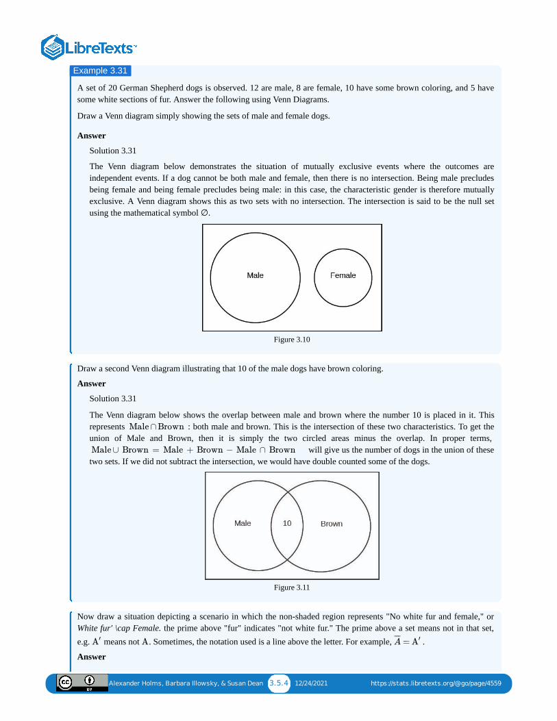
Alexander Holms, Barbara Illowsky, & Susan Dean 3.5.4 12/24/2021 https://stats.libretexts.org/@go/page/4559
A set of 20 German Shepherd dogs is observed. 12 are male, 8 are female, 10 have some brown coloring, and 5 havesome white sections of fur. Answer the following using Venn Diagrams.
Draw a Venn diagram simply showing the sets of male and female dogs.
Answer
Solution 3.31
The Venn diagram below demonstrates the situation of mutually exclusive events where the outcomes areindependent events. If a dog cannot be both male and female, then there is no intersection. Being male precludesbeing female and being female precludes being male: in this case, the characteristic gender is therefore mutuallyexclusive. A Venn diagram shows this as two sets with no intersection. The intersection is said to be the null setusing the mathematical symbol ∅.
Figure 3.10
Draw a second Venn diagram illustrating that 10 of the male dogs have brown coloring.
Answer
Solution 3.31
The Venn diagram below shows the overlap between male and brown where the number 10 is placed in it. Thisrepresents : both male and brown. This is the intersection of these two characteristics. To get theunion of Male and Brown, then it is simply the two circled areas minus the overlap. In proper terms,
will give us the number of dogs in the union of thesetwo sets. If we did not subtract the intersection, we would have double counted some of the dogs.
Figure 3.11
Now draw a situation depicting a scenario in which the non-shaded region represents "No white fur and female," orWhite fur′ \cap Female. the prime above "fur" indicates "not white fur." The prime above a set means not in that set,e.g. means not . Sometimes, the notation used is a line above the letter. For example, .
Answer
Example 3.31
Male ∩ Brown
Male ∪ Brown = Male + Brown − Male ∩ Brown
A′ A =A¯ ¯¯̄
A′
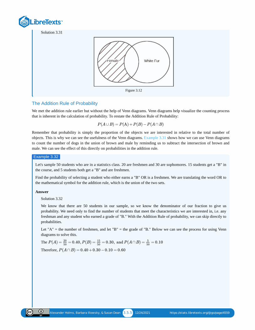
Alexander Holms, Barbara Illowsky, & Susan Dean 3.5.5 12/24/2021 https://stats.libretexts.org/@go/page/4559
Solution 3.31
Figure 3.12
The Addition Rule of Probability
We met the addition rule earlier but without the help of Venn diagrams. Venn diagrams help visualize the counting processthat is inherent in the calculation of probability. To restate the Addition Rule of Probability:
Remember that probability is simply the proportion of the objects we are interested in relative to the total number ofobjects. This is why we can see the usefulness of the Venn diagrams. Example 3.31 shows how we can use Venn diagramsto count the number of dogs in the union of brown and male by reminding us to subtract the intersection of brown andmale. We can see the effect of this directly on probabilities in the addition rule.
Let's sample 50 students who are in a statistics class. 20 are freshmen and 30 are sophomores. 15 students get a "B" inthe course, and 5 students both get a "B" and are freshmen.
Find the probability of selecting a student who either earns a "B" OR is a freshmen. We are translating the word OR tothe mathematical symbol for the addition rule, which is the union of the two sets.
Answer
Solution 3.32
We know that there are 50 students in our sample, so we know the denominator of our fraction to give usprobability. We need only to find the number of students that meet the characteristics we are interested in, i.e. anyfreshman and any student who earned a grade of "B." With the Addition Rule of probability, we can skip directly toprobabilities.
Let "A" = the number of freshmen, and let "B" = the grade of "B." Below we can see the process for using Venndiagrams to solve this.
The
Therefore,
P (A ∪ B) = P (A) +P (B) −P (A ∩ B)
Example 3.32
P (A) = = 0.40, P (B) = = 0.30, and P (A ∩ B) = = 0.1020
50
15
50
5
50
P (A ∩ B) = 0.40 +0.30 −0.10 = 0.60
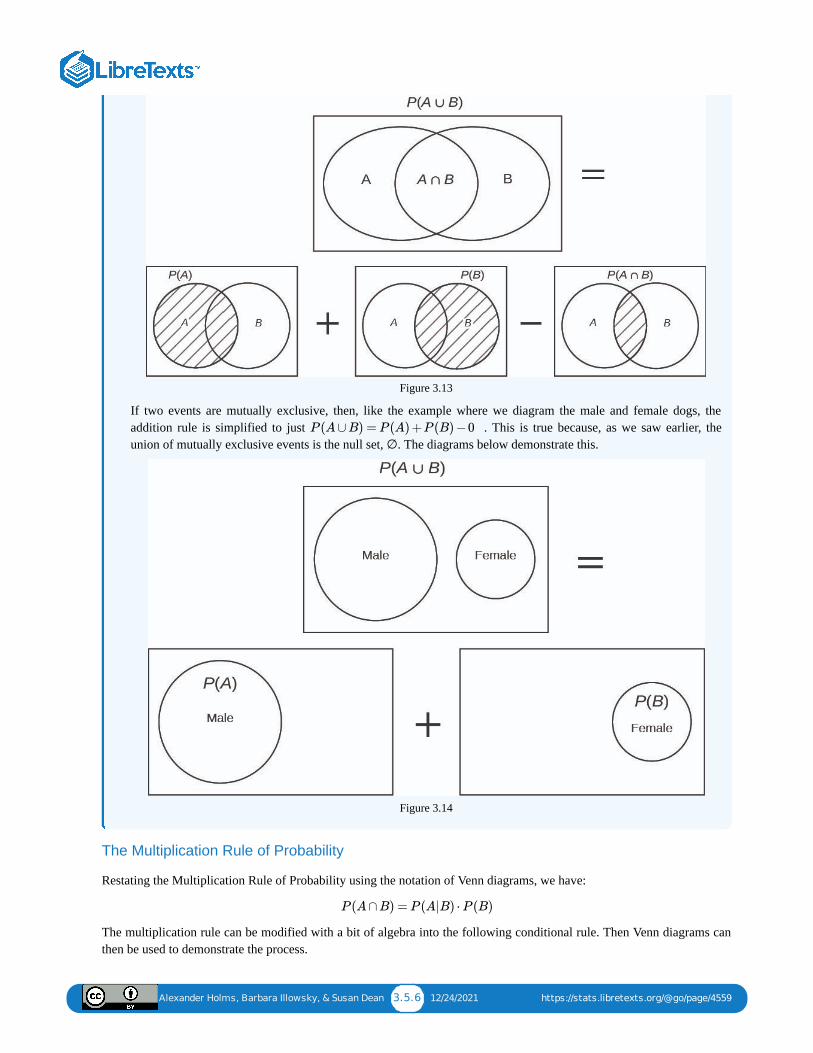
Alexander Holms, Barbara Illowsky, & Susan Dean 3.5.6 12/24/2021 https://stats.libretexts.org/@go/page/4559
Figure 3.13
If two events are mutually exclusive, then, like the example where we diagram the male and female dogs, theaddition rule is simplified to just . This is true because, as we saw earlier, theunion of mutually exclusive events is the null set, ∅. The diagrams below demonstrate this.
Figure 3.14
The Multiplication Rule of Probability
Restating the Multiplication Rule of Probability using the notation of Venn diagrams, we have:
The multiplication rule can be modified with a bit of algebra into the following conditional rule. Then Venn diagrams canthen be used to demonstrate the process.
P (A ∪ B) = P (A) +P (B) −0
P (A ∩ B) = P (A|B) ⋅ P (B)
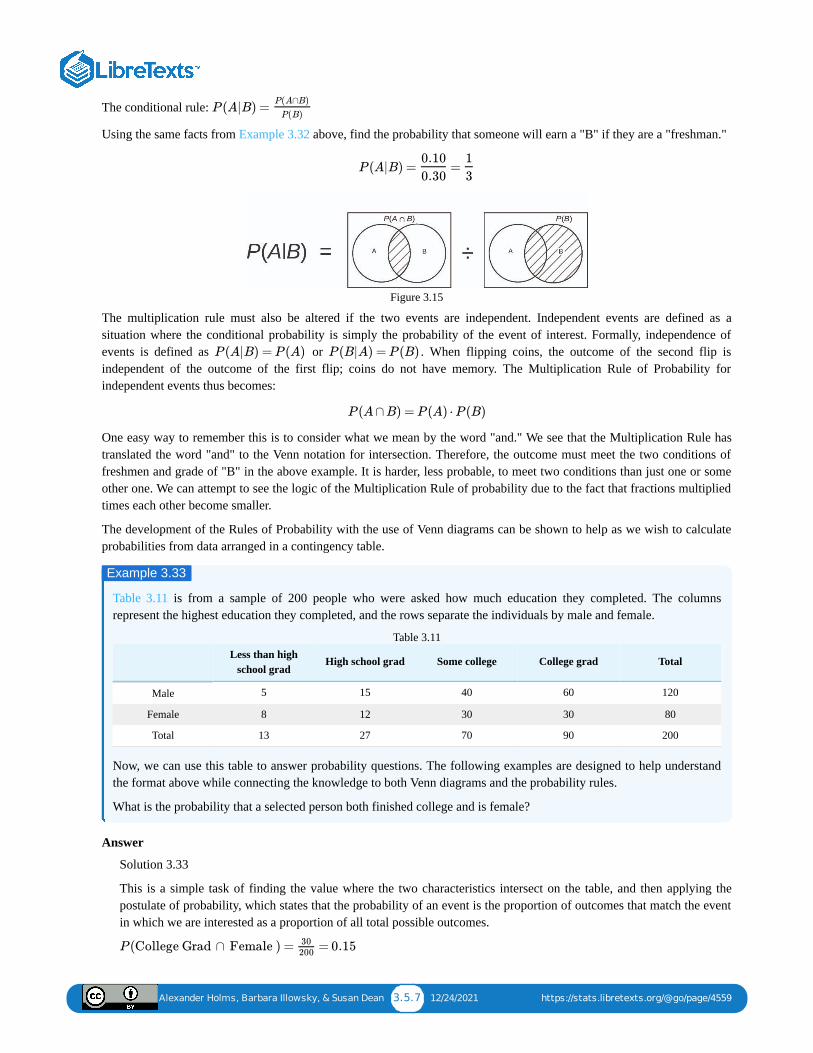
Alexander Holms, Barbara Illowsky, & Susan Dean 3.5.7 12/24/2021 https://stats.libretexts.org/@go/page/4559
The conditional rule:
Using the same facts from Example 3.32 above, find the probability that someone will earn a "B" if they are a "freshman."
Figure 3.15
The multiplication rule must also be altered if the two events are independent. Independent events are defined as asituation where the conditional probability is simply the probability of the event of interest. Formally, independence ofevents is defined as or . When flipping coins, the outcome of the second flip isindependent of the outcome of the first flip; coins do not have memory. The Multiplication Rule of Probability forindependent events thus becomes:
One easy way to remember this is to consider what we mean by the word "and." We see that the Multiplication Rule hastranslated the word "and" to the Venn notation for intersection. Therefore, the outcome must meet the two conditions offreshmen and grade of "B" in the above example. It is harder, less probable, to meet two conditions than just one or someother one. We can attempt to see the logic of the Multiplication Rule of probability due to the fact that fractions multipliedtimes each other become smaller.
The development of the Rules of Probability with the use of Venn diagrams can be shown to help as we wish to calculateprobabilities from data arranged in a contingency table.
Table 3.11 is from a sample of 200 people who were asked how much education they completed. The columnsrepresent the highest education they completed, and the rows separate the individuals by male and female.
Less than highschool grad
High school grad Some college College grad Total
Male 5 15 40 60 120
Female 8 12 30 30 80
Total 13 27 70 90 200
Table 3.11
Now, we can use this table to answer probability questions. The following examples are designed to help understandthe format above while connecting the knowledge to both Venn diagrams and the probability rules.
What is the probability that a selected person both finished college and is female?
Answer
Solution 3.33
This is a simple task of finding the value where the two characteristics intersect on the table, and then applying thepostulate of probability, which states that the probability of an event is the proportion of outcomes that match the eventin which we are interested as a proportion of all total possible outcomes.
P (A|B) =P(A∩B)
P(B)
P (A|B) = =0.10
0.30
1
3
P (A|B) = P (A) P (B|A) = P (B)
P (A ∩ B) = P (A) ⋅ P (B)
Example 3.33
P (College Grad ∩ Female ) = = 0.1530200
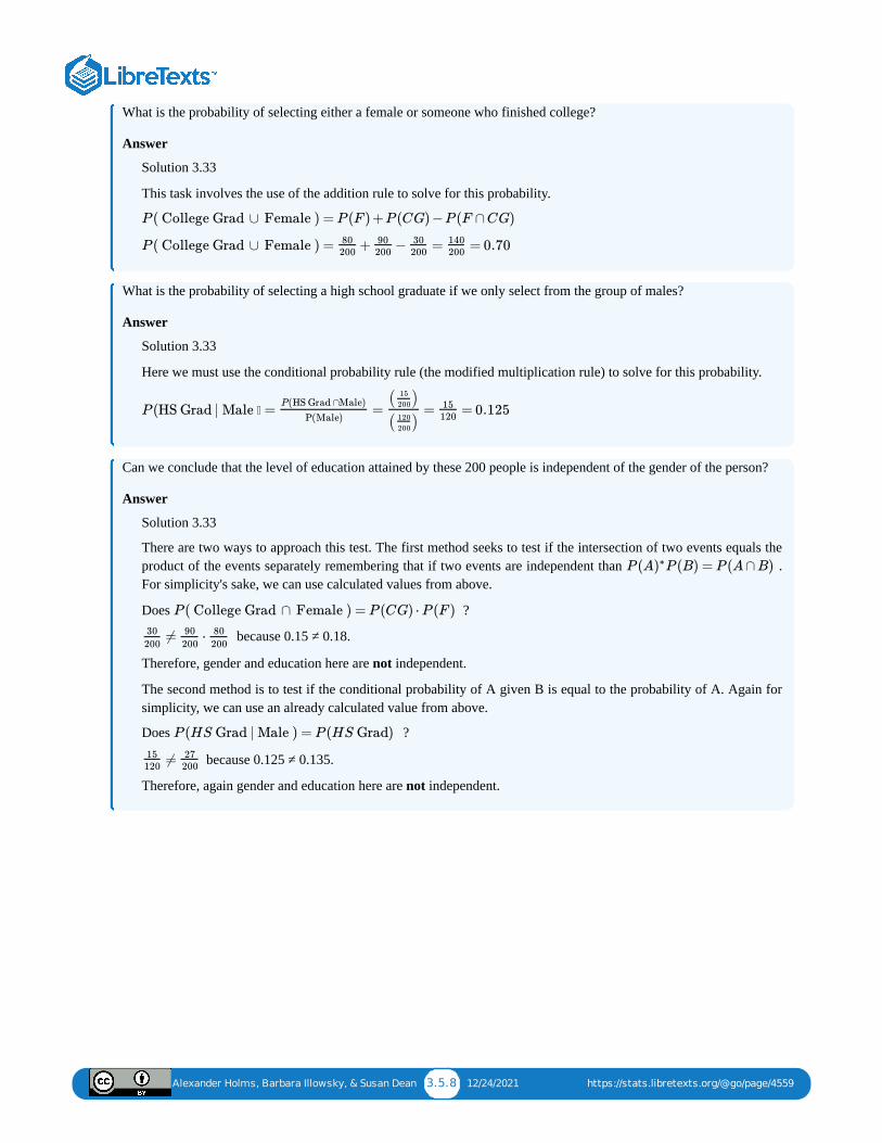
Alexander Holms, Barbara Illowsky, & Susan Dean 3.5.8 12/24/2021 https://stats.libretexts.org/@go/page/4559
What is the probability of selecting either a female or someone who finished college?
Answer
Solution 3.33
This task involves the use of the addition rule to solve for this probability.
What is the probability of selecting a high school graduate if we only select from the group of males?
Answer
Solution 3.33
Here we must use the conditional probability rule (the modified multiplication rule) to solve for this probability.
Can we conclude that the level of education attained by these 200 people is independent of the gender of the person?
Answer
Solution 3.33
There are two ways to approach this test. The first method seeks to test if the intersection of two events equals theproduct of the events separately remembering that if two events are independent than .For simplicity's sake, we can use calculated values from above.
Does ?
because 0.15 ≠ 0.18.
Therefore, gender and education here are not independent.
The second method is to test if the conditional probability of A given B is equal to the probability of A. Again forsimplicity, we can use an already calculated value from above.
Does ?
because 0.125 ≠ 0.135.
Therefore, again gender and education here are not independent.
P ( College Grad ∪ Female ) = P (F ) +P (CG) −P (F ∩ CG)
P ( College Grad ∪ Female ) = + − = = 0.7080200
90200
30200
140200
P (HS Grad | Male = = = = 0.125P(HS Grad ∩Male)
P(Male)
( )15
200
( )120
200
15120
P (A P (B) = P (A ∩ B))∗
P ( College Grad ∩ Female ) = P (CG) ⋅ P (F )
≠ ⋅30
200
90
200
80
200
P (HS Grad | Male ) = P (HS Grad)
≠15120
27200

Alexander Holms, Barbara Illowsky, & Susan Dean 3.6.1 12/31/2021 https://stats.libretexts.org/@go/page/5544
3.6: Chapter Formula Review
3.1 Terminology
A and B are events
where is the sample space
3.2 Independent and Mutually Exclusive Events
3.3 Two Basic Rules of Probability
The multiplication rule:
The addition rule:
P (S) = 1 S
0 ≤ P (A) ≤ 1
P (A|B) =P(A∩B)
P(B)
If A and B are independent, P (A∩B) = P (A)P (B),P (A|B) = P (A) and P (B|A) = P (B)
If A and B are mutually exclusive, P (A∪B) = P (A) +P (B) and P (A∩B) = 0
P (A∩B) = P (A|B)P (B)
P (A∪B) = P (A) +P (B) −P (A∩B)
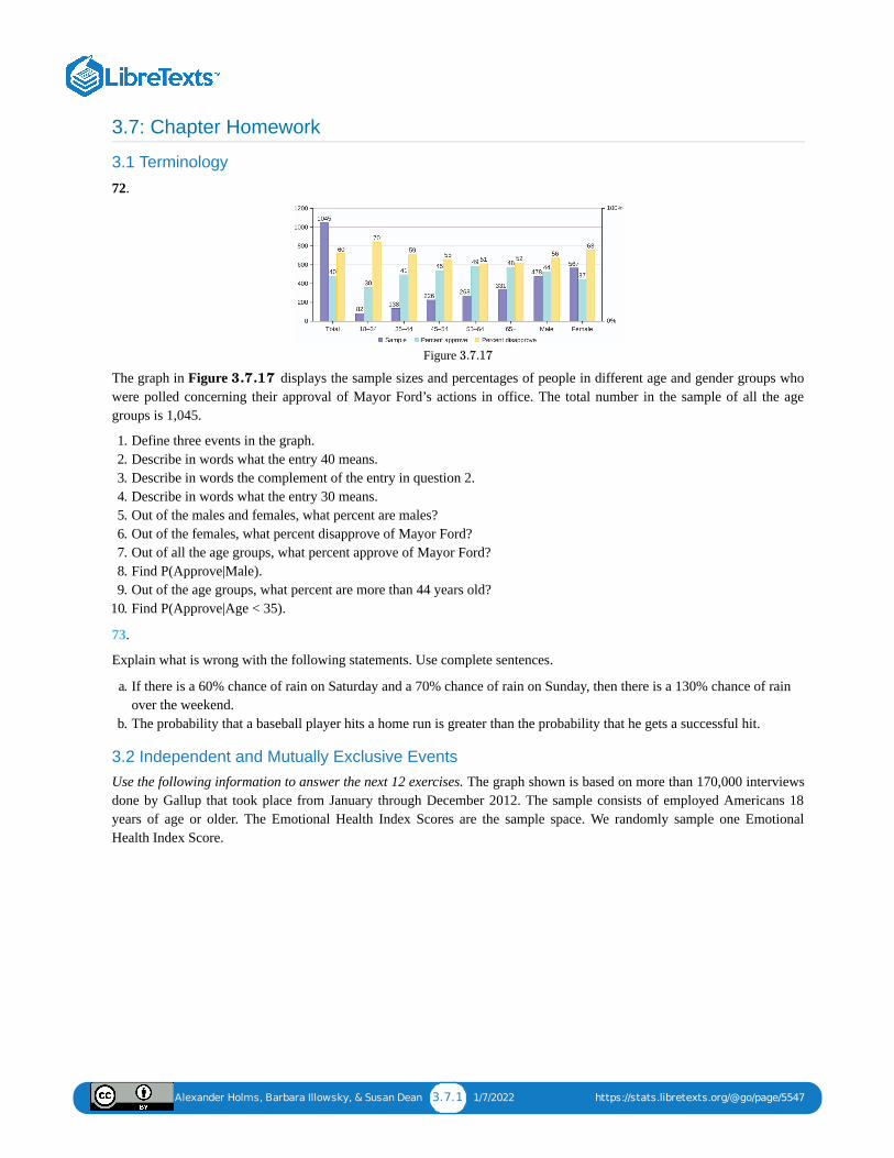
Alexander Holms, Barbara Illowsky, & Susan Dean 3.7.1 1/7/2022 https://stats.libretexts.org/@go/page/5547
3.7: Chapter Homework
3.1 Terminology
72.
Figure
The graph in Figure displays the sample sizes and percentages of people in different age and gender groups whowere polled concerning their approval of Mayor Ford’s actions in office. The total number in the sample of all the agegroups is 1,045.
1. Define three events in the graph.2. Describe in words what the entry 40 means.3. Describe in words the complement of the entry in question 2.4. Describe in words what the entry 30 means.5. Out of the males and females, what percent are males?6. Out of the females, what percent disapprove of Mayor Ford?7. Out of all the age groups, what percent approve of Mayor Ford?8. Find P(Approve|Male).9. Out of the age groups, what percent are more than 44 years old?
10. Find P(Approve|Age < 35).
73.
Explain what is wrong with the following statements. Use complete sentences.
a. If there is a 60% chance of rain on Saturday and a 70% chance of rain on Sunday, then there is a 130% chance of rainover the weekend.
b. The probability that a baseball player hits a home run is greater than the probability that he gets a successful hit.
3.2 Independent and Mutually Exclusive EventsUse the following information to answer the next 12 exercises. The graph shown is based on more than 170,000 interviewsdone by Gallup that took place from January through December 2012. The sample consists of employed Americans 18years of age or older. The Emotional Health Index Scores are the sample space. We randomly sample one EmotionalHealth Index Score.
3.7.17
3.7.17
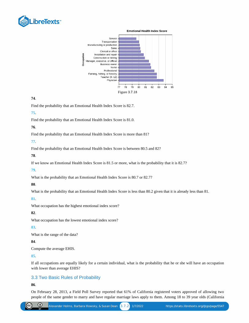
Alexander Holms, Barbara Illowsky, & Susan Dean 3.7.2 1/7/2022 https://stats.libretexts.org/@go/page/5547
Figure
74.
Find the probability that an Emotional Health Index Score is 82.7.
75.
Find the probability that an Emotional Health Index Score is 81.0.
76.
Find the probability that an Emotional Health Index Score is more than 81?
77.
Find the probability that an Emotional Health Index Score is between 80.5 and 82?
78.
If we know an Emotional Health Index Score is 81.5 or more, what is the probability that it is 82.7?
79.
What is the probability that an Emotional Health Index Score is 80.7 or 82.7?
80.
What is the probability that an Emotional Health Index Score is less than 80.2 given that it is already less than 81.
81.
What occupation has the highest emotional index score?
82.
What occupation has the lowest emotional index score?
83.
What is the range of the data?
84.
Compute the average EHIS.
85.
If all occupations are equally likely for a certain individual, what is the probability that he or she will have an occupationwith lower than average EHIS?
3.3 Two Basic Rules of Probability
86.
On February 28, 2013, a Field Poll Survey reported that 61% of California registered voters approved of allowing twopeople of the same gender to marry and have regular marriage laws apply to them. Among 18 to 39 year olds (California
3.7.18
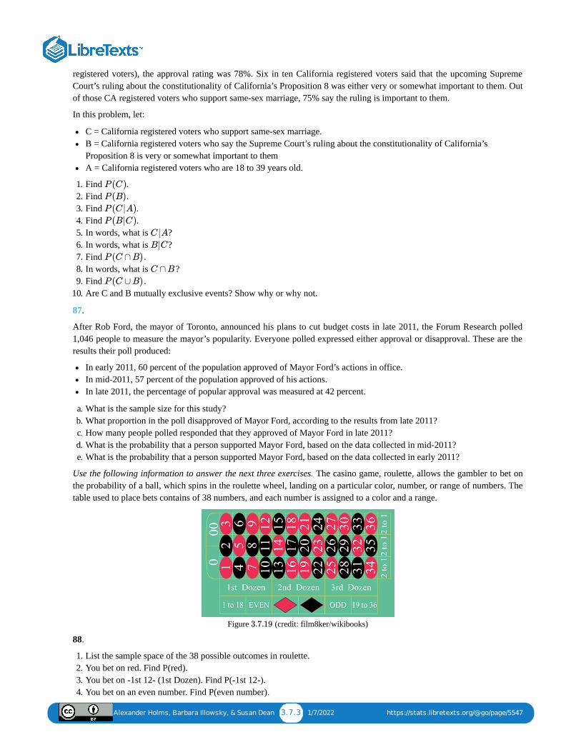
Alexander Holms, Barbara Illowsky, & Susan Dean 3.7.3 1/7/2022 https://stats.libretexts.org/@go/page/5547
registered voters), the approval rating was 78%. Six in ten California registered voters said that the upcoming SupremeCourt’s ruling about the constitutionality of California’s Proposition 8 was either very or somewhat important to them. Outof those CA registered voters who support same-sex marriage, 75% say the ruling is important to them.
In this problem, let:
C = California registered voters who support same-sex marriage.B = California registered voters who say the Supreme Court’s ruling about the constitutionality of California’sProposition 8 is very or somewhat important to themA = California registered voters who are 18 to 39 years old.
1. Find .2. Find .3. Find .4. Find .5. In words, what is ?6. In words, what is ?7. Find .8. In words, what is ?9. Find .
10. Are C and B mutually exclusive events? Show why or why not.
87.
After Rob Ford, the mayor of Toronto, announced his plans to cut budget costs in late 2011, the Forum Research polled1,046 people to measure the mayor’s popularity. Everyone polled expressed either approval or disapproval. These are theresults their poll produced:
In early 2011, 60 percent of the population approved of Mayor Ford’s actions in office.In mid-2011, 57 percent of the population approved of his actions.In late 2011, the percentage of popular approval was measured at 42 percent.
a. What is the sample size for this study?b. What proportion in the poll disapproved of Mayor Ford, according to the results from late 2011?c. How many people polled responded that they approved of Mayor Ford in late 2011?d. What is the probability that a person supported Mayor Ford, based on the data collected in mid-2011?e. What is the probability that a person supported Mayor Ford, based on the data collected in early 2011?
Use the following information to answer the next three exercises. The casino game, roulette, allows the gambler to bet onthe probability of a ball, which spins in the roulette wheel, landing on a particular color, number, or range of numbers. Thetable used to place bets contains of 38 numbers, and each number is assigned to a color and a range.
Figure (credit: film8ker/wikibooks)
88.
1. List the sample space of the 38 possible outcomes in roulette.2. You bet on red. Find P(red).3. You bet on -1st 12- (1st Dozen). Find P(-1st 12-).4. You bet on an even number. Find P(even number).
P (C)
P (B)
P (C|A)
P (B|C)
C|A
B|C
P (C ∩B)
C ∩B
P (C ∪B)
3.7.19
Alexander Holms, Barbara Illowsky, & Susan Dean 3.7.4 1/7/2022 https://stats.libretexts.org/@go/page/5547
5. Is getting an odd number the complement of getting an even number? Why?6. Find two mutually exclusive events.7. Are the events Even and 1st Dozen independent?
89.
Compute the probability of winning the following types of bets:
a. Betting on two lines that touch each other on the table as in 1-2-3-4-5-6b. Betting on three numbers in a line, as in 1-2-3c. Betting on one numberd. Betting on four numbers that touch each other to form a square, as in 10-11-13-14e. Betting on two numbers that touch each other on the table, as in 10-11 or 10-13f. Betting on 0-00-1-2-3g. Betting on 0-1-2; or 0-00-2; or 00-2-3
90.
Compute the probability of winning the following types of bets:
a. Betting on a colorb. Betting on one of the dozen groupsc. Betting on the range of numbers from 1 to 18d. Betting on the range of numbers 19–36e. Betting on one of the columnsf. Betting on an even or odd number (excluding zero)
91.
Suppose that you have eight cards. Five are green and three are yellow. The five green cards are numbered 1, 2, 3, 4, and 5.The three yellow cards are numbered 1, 2, and 3. The cards are well shuffled. You randomly draw one card.
G = card drawn is greenE = card drawn is even-numbered1. List the sample space.2. _____3. _____4. _____5. _____6. Are G and E mutually exclusive? Justify your answer numerically.
92.
Roll two fair dice separately. Each die has six faces.
1. List the sample space.2. Let A be the event that either a three or four is rolled first, followed by an even number. Find .3. Let B be the event that the sum of the two rolls is at most seven. Find .4. In words, explain what “ ” represents. Find .5. Are A and B mutually exclusive events? Explain your answer in one to three complete sentences, including numerical
justification.6. Are A and B independent events? Explain your answer in one to three complete sentences, including numerical
justification.
93.
A special deck of cards has ten cards. Four are green, three are blue, and three are red. When a card is picked, its color of itis recorded. An experiment consists of first picking a card and then tossing a coin.
1. List the sample space.2. Let A be the event that a blue card is picked first, followed by landing a head on the coin toss. Find P(A).
P (G) =
P (G|E) =
P (G∩E) =
P (G∪E) =
P (A)
P (B)
P (A|B) P (A|B)
Alexander Holms, Barbara Illowsky, & Susan Dean 3.7.5 1/7/2022 https://stats.libretexts.org/@go/page/5547
3. Let B be the event that a red or green is picked, followed by landing a head on the coin toss. Are the events A and Bmutually exclusive? Explain your answer in one to three complete sentences, including numerical justification.
4. Let C be the event that a red or blue is picked, followed by landing a head on the coin toss. Are the events A and Cmutually exclusive? Explain your answer in one to three complete sentences, including numerical justification.
94.
An experiment consists of first rolling a die and then tossing a coin.
1. List the sample space.2. Let A be the event that either a three or a four is rolled first, followed by landing a head on the coin toss. Find P(A).3. Let B be the event that the first and second tosses land on heads. Are the events A and B mutually exclusive? Explain
your answer in one to three complete sentences, including numerical justification.
95.
An experiment consists of tossing a nickel, a dime, and a quarter. Of interest is the side the coin lands on.
1. List the sample space.2. Let A be the event that there are at least two tails. Find P(A).3. Let B be the event that the first and second tosses land on heads. Are the events A and B mutually exclusive? Explain
your answer in one to three complete sentences, including justification.
96.
Consider the following scenario: Let . Let . Let .
1. Find .2. Are C and D mutually exclusive? Why or why not?3. Are C and D independent events? Why or why not?4. Find .5. Find .
97.
Y and Z are independent events.
1. Rewrite the basic Addition Rule using the information that Y and Z areindependent events.
2. Use the rewritten rule to find if and .
98.
G and H are mutually exclusive events.
1. Explain why the following statement MUST be false: .2. Find .3. Are G and H independent or dependent events? Explain in a complete sentence.
99.
Approximately 281,000,000 people over age five live in the United States. Of these people, 55,000,000 speak a languageother than English at home. Of those who speak another language at home, 62.3% speak Spanish.
Let: E = speaks English at home; E′ = speaks another language at home; S = speaks Spanish;
Finish each probability statement by matching the correct answer.
Probability Statements Answers
a. i. 0.8043
Table
P (C) = 0.4
P (D) = 0.5
P (C|D) = 0.6
P (C ∩D)
P (C ∪D)
P (D|C)
P (Y ∪Z) = P (Y ) +P (Z) −P (Y ∩Z)
P (Z) P (Y ∪Z) = 0.71 P (Y ) = 0.42
P (G) = 0.5P (H) = 0.3
P (H|G) = 0.4
P (H ∪G)
P(E') =
3.7.14
Alexander Holms, Barbara Illowsky, & Susan Dean 3.7.6 1/7/2022 https://stats.libretexts.org/@go/page/5547
Probability Statements Answers
b. ii. 0.623
c. iii. 0.1957
d. iv. 0.1219
100.
1994, the U.S. government held a lottery to issue 55,000 Green Cards (permits for non-citizens to work legally in theU.S.). Renate Deutsch, from Germany, was one of approximately 6.5 million people who entered this lottery. Let G = wongreen card.
1. What was Renate’s chance of winning a Green Card? Write your answer as a probability statement.2. In the summer of 1994, Renate received a letter stating she was one of 110,000 finalists chosen. Once the finalists were
chosen, assuming that each finalist had an equal chance to win, what was Renate’s chance of winning a Green Card?Write your answer as a conditional probability statement. Let F = was a finalist.
3. Are G and F independent or dependent events? Justify your answer numerically and also explain why.4. Are G and F mutually exclusive events? Justify your answer numerically and explain why.
101.
Three professors at George Washington University did an experiment to determine if economists are more selfish thanother people. They dropped 64 stamped, addressed envelopes with $10 cash in different classrooms on the GeorgeWashington campus. 44% were returned overall. From the economics classes 56% of the envelopes were returned. Fromthe business, psychology, and history classes 31% were returned.
Let: R = money returned; E = economics classes; O = other classes
1. Write a probability statement for the overall percent of money returned.2. Write a probability statement for the percent of money returned out of the economics classes.3. Write a probability statement for the percent of money returned out of the other classes.4. Is money being returned independent of the class? Justify your answer numerically and explain it.5. Based upon this study, do you think that economists are more selfish than other people? Explain why or why not.
Include numbers to justify your answer.
102.
The following table of data obtained from www.baseball-almanac.com shows hit information for four players. Supposethat one hit from the table is randomly selected.
Name Single Double Triple Home run Total hits
Babe Ruth 1,517 506 136 714 2,873
Jackie Robinson 1,054 273 54 137 1,518
Ty Cobb 3,603 174 295 114 4,189
Hank Aaron 2,294 624 98 755 3,771
Total 8,471 1,577 583 1,720 12,351
Table
Are "the hit being made by Hank Aaron" and "the hit being a double" independent events?
1. Yes, because P(hit by Hank Aaron|hit is a double) = P(hit by Hank Aaron)2. No, because P(hit by Hank Aaron|hit is a double) ≠ P(hit is a double)3. No, because P(hit is by Hank Aaron|hit is a double) ≠ P(hit by Hank Aaron)4. Yes, because P(hit is by Hank Aaron|hit is a double) = P(hit is a double)
103.
P(E) =
P(S ∩E') =
P(S|E') =
3.7.15
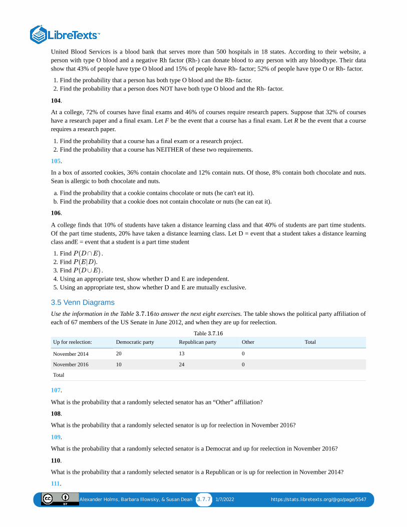
Alexander Holms, Barbara Illowsky, & Susan Dean 3.7.7 1/7/2022 https://stats.libretexts.org/@go/page/5547
United Blood Services is a blood bank that serves more than 500 hospitals in 18 states. According to their website, aperson with type O blood and a negative Rh factor (Rh-) can donate blood to any person with any bloodtype. Their datashow that 43% of people have type O blood and 15% of people have Rh- factor; 52% of people have type O or Rh- factor.
1. Find the probability that a person has both type O blood and the Rh- factor.2. Find the probability that a person does NOT have both type O blood and the Rh- factor.
104.
At a college, 72% of courses have final exams and 46% of courses require research papers. Suppose that 32% of courseshave a research paper and a final exam. Let F be the event that a course has a final exam. Let R be the event that a courserequires a research paper.
1. Find the probability that a course has a final exam or a research project.2. Find the probability that a course has NEITHER of these two requirements.
105.
In a box of assorted cookies, 36% contain chocolate and 12% contain nuts. Of those, 8% contain both chocolate and nuts.Sean is allergic to both chocolate and nuts.
a. Find the probability that a cookie contains chocolate or nuts (he can't eat it).b. Find the probability that a cookie does not contain chocolate or nuts (he can eat it).
106.
A college finds that 10% of students have taken a distance learning class and that 40% of students are part time students.Of the part time students, 20% have taken a distance learning class. Let D = event that a student takes a distance learningclass andE = event that a student is a part time student
1. Find .2. Find .3. Find .4. Using an appropriate test, show whether D and E are independent.5. Using an appropriate test, show whether D and E are mutually exclusive.
3.5 Venn DiagramsUse the information in the Table to answer the next eight exercises. The table shows the political party affiliation ofeach of 67 members of the US Senate in June 2012, and when they are up for reelection.
Up for reelection: Democratic party Republican party Other Total
November 2014 20 13 0
November 2016 10 24 0
Total
Table
107.
What is the probability that a randomly selected senator has an “Other” affiliation?
108.
What is the probability that a randomly selected senator is up for reelection in November 2016?
109.
What is the probability that a randomly selected senator is a Democrat and up for reelection in November 2016?
110.
What is the probability that a randomly selected senator is a Republican or is up for reelection in November 2014?
111.
P (D∩E)
P (E|D)
P (D∪E)
3.7.16
3.7.16
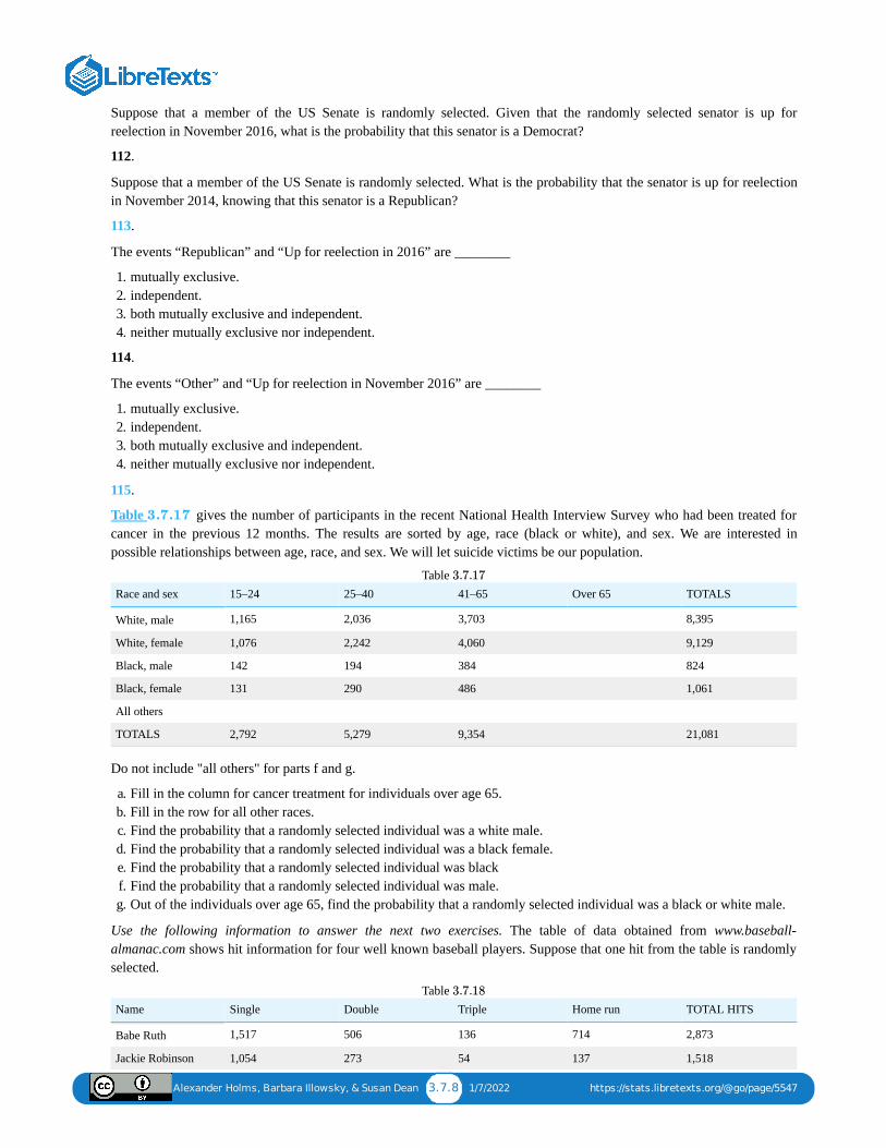
Alexander Holms, Barbara Illowsky, & Susan Dean 3.7.8 1/7/2022 https://stats.libretexts.org/@go/page/5547
Suppose that a member of the US Senate is randomly selected. Given that the randomly selected senator is up forreelection in November 2016, what is the probability that this senator is a Democrat?
112.
Suppose that a member of the US Senate is randomly selected. What is the probability that the senator is up for reelectionin November 2014, knowing that this senator is a Republican?
113.
The events “Republican” and “Up for reelection in 2016” are ________
1. mutually exclusive.2. independent.3. both mutually exclusive and independent.4. neither mutually exclusive nor independent.
114.
The events “Other” and “Up for reelection in November 2016” are ________
1. mutually exclusive.2. independent.3. both mutually exclusive and independent.4. neither mutually exclusive nor independent.
115.
Table gives the number of participants in the recent National Health Interview Survey who had been treated forcancer in the previous 12 months. The results are sorted by age, race (black or white), and sex. We are interested inpossible relationships between age, race, and sex. We will let suicide victims be our population.
Race and sex 15–24 25–40 41–65 Over 65 TOTALS
White, male 1,165 2,036 3,703 8,395
White, female 1,076 2,242 4,060 9,129
Black, male 142 194 384 824
Black, female 131 290 486 1,061
All others
TOTALS 2,792 5,279 9,354 21,081
Table
Do not include "all others" for parts f and g.
a. Fill in the column for cancer treatment for individuals over age 65.b. Fill in the row for all other races.c. Find the probability that a randomly selected individual was a white male.d. Find the probability that a randomly selected individual was a black female.e. Find the probability that a randomly selected individual was blackf. Find the probability that a randomly selected individual was male.g. Out of the individuals over age 65, find the probability that a randomly selected individual was a black or white male.
Use the following information to answer the next two exercises. The table of data obtained from www.baseball-almanac.com shows hit information for four well known baseball players. Suppose that one hit from the table is randomlyselected.
Name Single Double Triple Home run TOTAL HITS
Babe Ruth 1,517 506 136 714 2,873
Jackie Robinson 1,054 273 54 137 1,518
Table
3.7.17
3.7.17
3.7.18
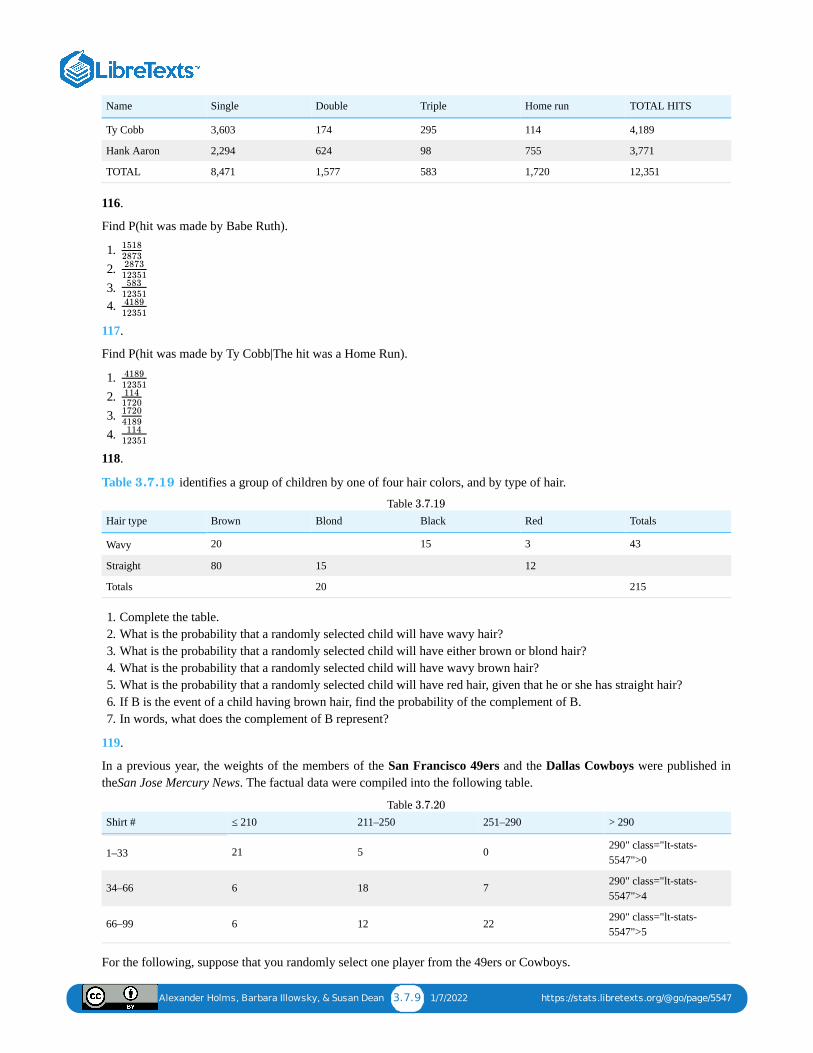
Alexander Holms, Barbara Illowsky, & Susan Dean 3.7.9 1/7/2022 https://stats.libretexts.org/@go/page/5547
Name Single Double Triple Home run TOTAL HITS
Ty Cobb 3,603 174 295 114 4,189
Hank Aaron 2,294 624 98 755 3,771
TOTAL 8,471 1,577 583 1,720 12,351
116.
Find P(hit was made by Babe Ruth).
1. 2. 3. 4.
117.
Find P(hit was made by Ty Cobb|The hit was a Home Run).
1. 2. 3. 4.
118.
Table identifies a group of children by one of four hair colors, and by type of hair.
Hair type Brown Blond Black Red Totals
Wavy 20 15 3 43
Straight 80 15 12
Totals 20 215
Table
1. Complete the table.2. What is the probability that a randomly selected child will have wavy hair?3. What is the probability that a randomly selected child will have either brown or blond hair?4. What is the probability that a randomly selected child will have wavy brown hair?5. What is the probability that a randomly selected child will have red hair, given that he or she has straight hair?6. If B is the event of a child having brown hair, find the probability of the complement of B.7. In words, what does the complement of B represent?
119.
In a previous year, the weights of the members of the San Francisco 49ers and the Dallas Cowboys were published intheSan Jose Mercury News. The factual data were compiled into the following table.
Shirt # ≤ 210 211–250 251–290 > 290
1–33 21 5 0 290" class="lt-stats-5547">0
34–66 6 18 7 290" class="lt-stats-5547">4
66–99 6 12 22 290" class="lt-stats-5547">5
Table
For the following, suppose that you randomly select one player from the 49ers or Cowboys.
151828732873
12351583
123514189
12351
418912351114
172017204189
11412351
3.7.19
3.7.19
3.7.20
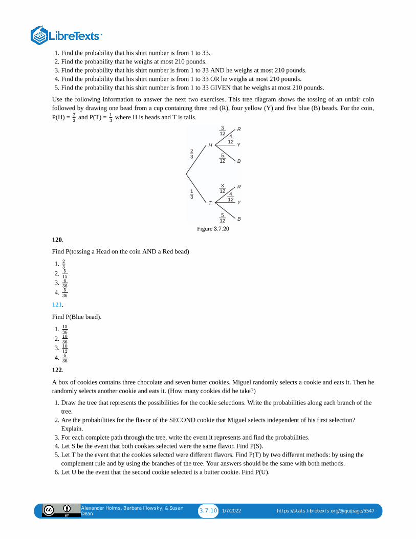
Alexander Holms, Barbara Illowsky, & Susan
Dean3.7.10 1/7/2022 https://stats.libretexts.org/@go/page/5547
1. Find the probability that his shirt number is from 1 to 33.2. Find the probability that he weighs at most 210 pounds.3. Find the probability that his shirt number is from 1 to 33 AND he weighs at most 210 pounds.4. Find the probability that his shirt number is from 1 to 33 OR he weighs at most 210 pounds.5. Find the probability that his shirt number is from 1 to 33 GIVEN that he weighs at most 210 pounds.
Use the following information to answer the next two exercises. This tree diagram shows the tossing of an unfair coinfollowed by drawing one bead from a cup containing three red (R), four yellow (Y) and five blue (B) beads. For the coin,P(H) = and P(T) = where H is heads and T is tails.
Figure
120.
Find P(tossing a Head on the coin AND a Red bead)
1. 2. 3. 4.
121.
Find P(Blue bead).
1. 2. 3. 4.
122.
A box of cookies contains three chocolate and seven butter cookies. Miguel randomly selects a cookie and eats it. Then herandomly selects another cookie and eats it. (How many cookies did he take?)
1. Draw the tree that represents the possibilities for the cookie selections. Write the probabilities along each branch of thetree.
2. Are the probabilities for the flavor of the SECOND cookie that Miguel selects independent of his first selection?Explain.
3. For each complete path through the tree, write the event it represents and find the probabilities.4. Let S be the event that both cookies selected were the same flavor. Find P(S).5. Let T be the event that the cookies selected were different flavors. Find P(T) by two different methods: by using the
complement rule and by using the branches of the tree. Your answers should be the same with both methods.6. Let U be the event that the second cookie selected is a butter cookie. Find P(U).
23
13
3.7.20
235
156
365
36
1536103610126
36
Alexander Holms, Barbara Illowsky, & Susan Dean 3.8.1 12/10/2021 https://stats.libretexts.org/@go/page/5542
3.8: Chapter Key Terms
Conditional Probabilitythe likelihood that an event will occur given that another event has already occurred
Contingency Tablethe method of displaying a frequency distribution as a table with rows and columns to show how two variables may bedependent (contingent) upon each other; the table provides an easy way to calculate conditional probabilities.
Dependent EventsIf two events are NOT independent, then we say that they are dependent.
Equally LikelyEach outcome of an experiment has the same probability.
Eventa subset of the set of all outcomes of an experiment; the set of all outcomes of an experiment is called a sample spaceand is usually denoted by S. An event is an arbitrary subset in S. It can contain one outcome, two outcomes, nooutcomes (empty subset), the entire sample space, and the like. Standard notations for events are capital letters such asA, B, C, and so on.
Experimenta planned activity carried out under controlled conditions
Independent EventsThe occurrence of one event has no effect on the probability of the occurrence of another event. Events A and B areindependent if one of the following is true:
1. 2. 3.
Mutually ExclusiveTwo events are mutually exclusive if the probability that they both happen at the same time is zero. If events A and Bare mutually exclusive, then .
Outcomea particular result of an experiment
Probabilitya number between zero and one, inclusive, that gives the likelihood that a specific event will occur; the foundation ofstatistics is given by the following 3 axioms (by A.N. Kolmogorov, 1930’s): Let S denote the sample space and A andB are two events in S. Then:
If A and B are any two mutually exclusive events, then .
Sample Spacethe set of all possible outcomes of an experiment
Sampling with ReplacementIf each member of a population is replaced after it is picked, then that member has the possibility of being chosen morethan once.
P (A|B) = P (A)
P (B|A) = P (B)
P (A∩B) = P (A)P (B)
P (A∩B) = 0
0 ≤ P (A) ≤ 1
P (A∪B) = P (A) +P (B)
P (S) = 1
Alexander Holms, Barbara Illowsky, & Susan Dean 3.8.2 12/10/2021 https://stats.libretexts.org/@go/page/5542
Sampling without ReplacementWhen sampling is done without replacement, each member of a population may be chosen only once.
The Complement EventThe complement of event A consists of all outcomes that are NOT in A.
The Conditional Probability of P(A||B) is the probability that event A will occur given that the event B has already occurred.
The Intersection: the EventAn outcome is in the event |(A \cap B\) if the outcome is in both at the same time.
The Union: the EventAn outcome is in the event if the outcome is in A or is in B or is in both A and B.
Tree Diagramthe useful visual representation of a sample space and events in the form of a “tree” with branches marked by possibleoutcomes together with associated probabilities (frequencies, relative frequencies)
Venn Diagramthe visual representation of a sample space and events in the form of circles or ovals showing their intersections
A|B
∩
A∩B
∪
A∪B

Alexander Holms, Barbara Illowsky, & Susan Dean 3.9.1 12/10/2021 https://stats.libretexts.org/@go/page/5546
3.9: Chapter More PracticeUse the following information to answer the next seven exercises. An article in the New England Journal of Medicine,reported about a study of smokers in California and Hawaii. In one part of the report, the self-reported ethnicity andsmoking levels per day were given. Of the people smoking at most ten cigarettes per day, there were 9,886 AfricanAmericans, 2,745 Native Hawaiians, 12,831 Latinos, 8,378 Japanese Americans, and 7,650 Whites. Of the people smoking11 to 20 cigarettes per day, there were 6,514 African Americans, 3,062 Native Hawaiians, 4,932 Latinos, 10,680 JapaneseAmericans, and 9,877 Whites. Of the people smoking 21 to 30 cigarettes per day, there were 1,671 African Americans,1,419 Native Hawaiians, 1,406 Latinos, 4,715 Japanese Americans, and 6,062 Whites. Of the people smoking at least 31cigarettes per day, there were 759 African Americans, 788 Native Hawaiians, 800 Latinos, 2,305 Japanese Americans, and3,970 Whites.
59.
Complete the table using the data provided. Suppose that one person from the study is randomly selected. Find theprobability that person smoked 11 to 20 cigarettes per day.
Smoking level African American Native Hawaiian Latino JapaneseAmericans
White TOTALS
1–10
11–20
21–30
31+
TOTALS
Table Smoking Levels by Ethnicity
60.
Suppose that one person from the study is randomly selected. Find the probability that person smoked 11 to 20 cigarettesper day.
61.
Find the probability that the person was Latino.
62.
In words, explain what it means to pick one person from the study who is “Japanese American AND smokes 21 to 30cigarettes per day.” Also, find the probability.
63.
In words, explain what it means to pick one person from the study who is “Japanese American smokes 21 to 30cigarettes per day.” Also, find the probability.
64.
In words, explain what it means to pick one person from the study who is “Japanese American that person smokes 21 to30 cigarettes per day.” Also, find the probability.
65.
Prove that smoking level/day and ethnicity are dependent events.
Use the following information to answer the next two exercises. Suppose that you have eight cards. Five are green andthree are yellow. The cards are well shuffled.
66.
Suppose that you randomly draw two cards, one at a time, with replacement. Let = first card is green Let = second card is green
3.9.13
∪
|
G1
G2
Alexander Holms, Barbara Illowsky, & Susan Dean 3.9.2 12/10/2021 https://stats.libretexts.org/@go/page/5546
1. Use the following information to answer the next two exercises. The percent of licensed U.S. drivers (from a recentyear) that are female is 48.60. Of the females, 5.03% are age 19 and under; 81.36% are age 20–64; 13.61% are age 65or over. Of the licensed U.S. male drivers, 5.04% are age 19 and under; 81.43% are age 20–64; 13.53% are age 65 orover.68.
Complete the following.
1. Construct a table or a tree diagram of the situation.2. Find P(driver is female).3. Find P(driver is age 65 or over driver is female).4. Find P(driver is age 65 or over female).5. In words, explain the difference between the probabilities in part c and part d.6. Find P(driver is age 65 or over).7. Are being age 65 or over and being female mutually exclusive events? How do you know?
69.
Suppose that 10,000 U.S. licensed drivers are randomly selected.
a. How many would you expect to be male?b. Using the table or tree diagram, construct a contingency table of gender versus age group.c. Using the contingency table, find the probability that out of the age 20–64 group, a randomly selected driver is
female.70.
Approximately 86.5% of Americans commute to work by car, truck, or van. Out of that group, 84.6% drive alone and15.4% drive in a carpool. Approximately 3.9% walk to work and approximately 5.3% take public transportation.
1. Construct a table or a tree diagram of the situation. Include a branch for all other modes of transportation to work.2. Assuming that the walkers walk alone, what percent of all commuters travel alone to work?3. Suppose that 1,000 workers are randomly selected. How many would you expect to travel alone to work?4. Suppose that 1,000 workers are randomly selected. How many would you expect to drive in a carpool?
71.
When the Euro coin was introduced in 2002, two math professors had their statistics students test whether the Belgianone Euro coin was a fair coin. They spun the coin rather than tossing it and found that out of 250 spins, 140 showed ahead (event H) while 110 showed a tail (event T). On that basis, they claimed that it is not a fair coin.
1. Based on the given data, find P(H) and P(T).2. Use a tree to find the probabilities of each possible outcome for the experiment of tossing the coin twice.3. Use the tree to find the probability of obtaining exactly one head in two tosses of the coin.4. Use the tree to find the probability of obtaining at least one head.
|
∩
Alexander Holms, Barbara Illowsky, & Susan
Dean3.10.1 12/17/2021 https://stats.libretexts.org/@go/page/5545
3.10: Chapter Practice
3.1 Terminology1.
In a particular college class, there are male and female students. Some students have long hair and some students haveshort hair. Write the symbols for the probabilities of the events for parts a through j. (Note that you cannot find numericalanswers here. You were not given enough information to find any probability values yet; concentrate on understanding thesymbols.)
Use the following information to answer the next four exercises. A box is filled with several party favors. It contains 12hats, 15 noisemakers, ten finger traps, and five bags of confetti. Let H = the event of getting a hat. Let N = the event of getting a noisemaker. Let F = the event of getting a finger trap. Let C = the event of getting a bag of confetti.2.
Find P(H).
3.
Find P(N).
4.
Find P(F).
5.
Find P(C).
6.
Find P(B).
7.
Find P(G).
8.
Find P(P).
9.
Find P(R).
10.
Find P(Y).
11.
Find P(O).
Use the following information to answer the next six exercises. There are 23 countries in North America, 12 countriesin South America, 47 countries in Europe, 44 countries in Asia, 54 countries in Africa, and 14 in Oceania (PacificOcean region). Let A = the event that a country is in Asia. Let E = the event that a country is in Europe. Let F = the event that a country is in Africa. Let N = the event that a country is in North America. Let O = the event that a country is in Oceania. Let S = the event that a country is in South America.
12.
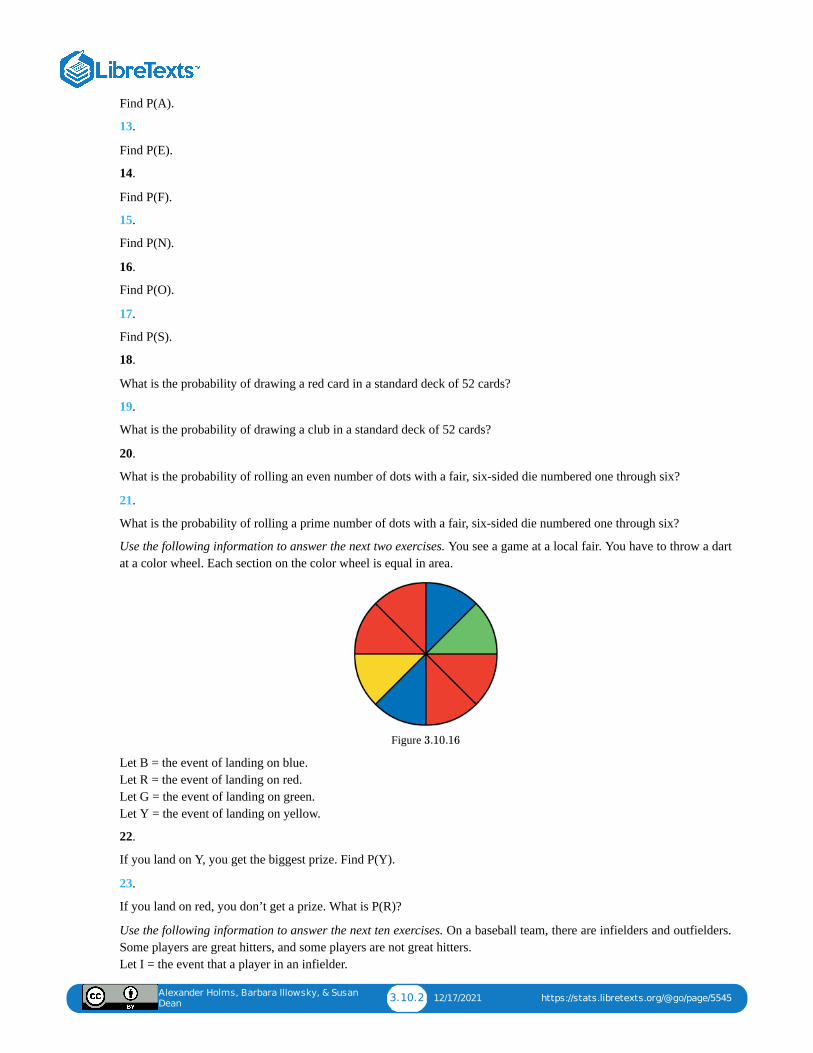
Alexander Holms, Barbara Illowsky, & Susan
Dean3.10.2 12/17/2021 https://stats.libretexts.org/@go/page/5545
Find P(A).
13.
Find P(E).
14.
Find P(F).
15.
Find P(N).
16.
Find P(O).
17.
Find P(S).
18.
What is the probability of drawing a red card in a standard deck of 52 cards?
19.
What is the probability of drawing a club in a standard deck of 52 cards?
20.
What is the probability of rolling an even number of dots with a fair, six-sided die numbered one through six?
21.
What is the probability of rolling a prime number of dots with a fair, six-sided die numbered one through six?
Use the following information to answer the next two exercises. You see a game at a local fair. You have to throw a dartat a color wheel. Each section on the color wheel is equal in area.
Figure
Let B = the event of landing on blue. Let R = the event of landing on red. Let G = the event of landing on green. Let Y = the event of landing on yellow.
22.
If you land on Y, you get the biggest prize. Find P(Y).
23.
If you land on red, you don’t get a prize. What is P(R)?
Use the following information to answer the next ten exercises. On a baseball team, there are infielders and outfielders.Some players are great hitters, and some players are not great hitters. Let I = the event that a player in an infielder.
3.10.16
Alexander Holms, Barbara Illowsky, & Susan
Dean3.10.3 12/17/2021 https://stats.libretexts.org/@go/page/5545
Let O = the event that a player is an outfielder. Let H = the event that a player is a great hitter. Let N = the event that a player is not a great hitter.
24.
Write the symbols for the probability that a player is not an outfielder.
25.
Write the symbols for the probability that a player is an outfielder or is a great hitter.
26.
Write the symbols for the probability that a player is an infielder and is not a great hitter.
27.
Write the symbols for the probability that a player is a great hitter, given that the player is an infielder.
28.
Write the symbols for the probability that a player is an infielder, given that the player is a great hitter.
29.
Write the symbols for the probability that of all the outfielders, a player is not a great hitter.
30.
Write the symbols for the probability that of all the great hitters, a player is an outfielder.
31.
Write the symbols for the probability that a player is an infielder or is not a great hitter.
32.
Write the symbols for the probability that a player is an outfielder and is a great hitter.
33.
Write the symbols for the probability that a player is an infielder.
34.
What is the word for the set of all possible outcomes?
35.
What is conditional probability?
36.
A shelf holds 12 books. Eight are fiction and the rest are nonfiction. Each is a different book with a unique title. Thefiction books are numbered one to eight. The nonfiction books are numbered one to four. Randomly select one book Let F = event that book is fiction Let N = event that book is nonfiction What is the sample space?
37.
What is the sum of the probabilities of an event and its complement?
Use the following information to answer the next two exercises. You are rolling a fair, six-sided number cube. Let E =the event that it lands on an even number. Let M = the event that it lands on a multiple of three.
38.
What does mean in words?
39.
P (E|M)
Alexander Holms, Barbara Illowsky, & Susan
Dean3.10.4 12/17/2021 https://stats.libretexts.org/@go/page/5545
What does mean in words?
3.2 Independent and Mutually Exclusive Events40.
41.
42.
1. Use the following information to answer the next ten exercises. Forty-eight percent of all Californians registeredvoters prefer life in prison without parole over the death penalty for a person convicted of first degree murder.Among Latino California registered voters, 55% prefer life in prison without parole over the death penalty for aperson convicted of first degree murder. 37.6% of all Californians are Latino.
In this problem, let:
Suppose that one Californian is randomly selected.44.
Find P(C).
45.
Find .
46.
Find .
47.
In words, what is ?
48.
Find .
49.
In words, what is ?
50.
Are L and C independent events? Show why or why not.
51.
Find .
52.
In words, what is L ?
53.
Are L and C mutually exclusive events? Show why or why not.
3.5 Venn Diagrams
Gender Self-taught Studied in school Private instruction Total
Female 12 38 22 72
Male 19 24 15 58
Total 31 62 37 130
Table
P (E∪M)
E and F are mutually exclusive events. P (E) = 0.4;P (F ) = 0.5. Find P (E|F )
J and K are independent events. P (J|K) = 0.3. Find P (J)
U and V are mutually exclusive events. P (U) = 0.26;P (V ) = 0.37.Find :
P (L)
P (C|L)
C|L
P (L∩C)
L∩C
P (L∪C)
∪C
3.10.12
Alexander Holms, Barbara Illowsky, & Susan
Dean3.10.5 12/17/2021 https://stats.libretexts.org/@go/page/5545
54.
Find P(musician is a female).
55.
Find P(musician is a male had private instruction).
56.
Find P(musician is a female is self taught).
57.
Are the events “being a female musician” and “learning music in school” mutually exclusive events?
58.
The probability that a man develops some form of cancer in his lifetime is 0.4567. The probability that a manhas at least one false positive test result (meaning the test comes back for cancer when the man does not have it)is 0.51. Let: C = a man develops cancer in his lifetime; P = man has at least one false positive. Construct a treediagram of the situation.
∩
∪
Alexander Holms, Barbara Illowsky, & Susan
Dean3.11.1 12/31/2021 https://stats.libretexts.org/@go/page/5550
3.11: Chapter Reference
3.1 Terminology
“Countries List by Continent.” Worldatlas, 2013. Available online at http://www.worldatlas.com/cntycont.htm (accessedMay 2, 2013).
3.2 Independent and Mutually Exclusive EventsLopez, Shane, Preety Sidhu. “U.S. Teachers Love Their Lives, but Struggle in the Workplace.” Gallup Wellbeing, 2013.http://www.gallup.com/poll/161516/te...workplace.aspx (accessed May 2, 2013).
Data from Gallup. Available online at www.gallup.com/ (accessed May 2, 2013).
3.3 Two Basic Rules of Probability
DiCamillo, Mark, Mervin Field. “The File Poll.” Field Research Corporation. Available online atwww.field.com/fieldpollonline...rs/Rls2443.pdf (accessed May 2, 2013).
Rider, David, “Ford support plummeting, poll suggests,” The Star, September 14, 2011. Available online athttp://www.thestar.com/news/gta/2011..._suggests.html (accessed May 2, 2013).
“Mayor’s Approval Down.” News Release by Forum Research Inc. Available online atwww.forumresearch.com/forms/News Archives/News Releases/74209_TO_Issues_-_Mayoral_Approval_%28Forum_Research%29%2820130320%29.pdf (accessed May 2, 2013).
“Roulette.” Wikipedia. Available online at http://en.Wikipedia.org/wiki/Roulette (accessed May 2, 2013).
Shin, Hyon B., Robert A. Kominski. “Language Use in the United States: 2007.” United States Census Bureau. Availableonline at www.census.gov/hhes/socdemo/l...acs/ACS-12.pdf (accessed May 2, 2013).
Data from the Baseball-Almanac, 2013. Available online at www.baseball-almanac.com (accessed May 2, 2013).
Data from U.S. Census Bureau.
Data from the Wall Street Journal.
Data from The Roper Center: Public Opinion Archives at the University of Connecticut. Available online atwww.ropercenter.uconn.edu/ (accessed May 2, 2013).
Data from Field Research Corporation. Available online at www.field.com/fieldpollonline (accessed May 2,2 013).
3.4 Contingency Tables and Probability Trees
“Blood Types.” American Red Cross, 2013. Available online at http://www.redcrossblood.org/learn-a...od/blood-types(accessed May 3, 2013).
Data from the National Center for Health Statistics, part of the United States Department of Health and Human Services.
Data from United States Senate. Available online at www.senate.gov (accessed May 2, 2013).
“Human Blood Types.” Unite Blood Services, 2011. Available online at https://www.vitalant.org/Donate/Blood-Donation/Donate-Blood-Overview.aspx (accessed May 2, 2013).
Haiman, Christopher A., Daniel O. Stram, Lynn R. Wilkens, Malcom C. Pike, Laurence N. Kolonel, Brien E. Henderson,and Loīc Le Marchand. “Ethnic and Racial Differences in the Smoking-Related Risk of Lung Cancer.” The New EnglandJournal of Medicine, 2013. Available online at http://www.nejm.org/doi/full/10.1056/NEJMoa033250 (accessed May 2,2013).
Samuel, T. M. “Strange Facts about RH Negative Blood.” eHow Health, 2013. Available online athttp://www.ehow.com/facts_5552003_st...ive-blood.html (accessed May 2, 2013).
“United States: Uniform Crime Report – State Statistics from 1960–2011.” The Disaster Center. Available online athttp://www.disastercenter.com/crime/ (accessed May 2, 2013).

Alexander Holms, Barbara Illowsky, & Susan
Dean3.11.2 12/31/2021 https://stats.libretexts.org/@go/page/5550
Data from Clara County Public H.D.
Data from the American Cancer Society.
Data from The Data and Story Library, 1996. Available online at http://lib.stat.cmu.edu/DASL/ (accessed May 2, 2013).
Data from the Federal Highway Administration, part of the United States Department of Transportation.
Data from the United States Census Bureau, part of the United States Department of Commerce.
Data from USA Today.
“Environment.” The World Bank, 2013. Available online at http://data.worldbank.org/topic/environment (accessed May 2,2013).
“Search for Datasets.” Roper Center: Public Opinion Archives, University of Connecticut., 2013. Available online athttps://ropercenter.cornell.edu/?s=S...h+for+Datasets (accessed February 6, 2019).
Alexander Holms, Barbara Illowsky, & Susan
Dean3.12.1 12/24/2021 https://stats.libretexts.org/@go/page/5543
3.12: Chapter Review
3.1 Terminology
In this module we learned the basic terminology of probability. The set of all possible outcomes of an experiment is calledthe sample space. Events are subsets of the sample space, and they are assigned a probability that is a number between zeroand one, inclusive.
3.2 Independent and Mutually Exclusive EventsTwo events A and B are independent if the knowledge that one occurred does not affect the chance the other occurs. If twoevents are not independent, then we say that they are dependent.
In sampling with replacement, each member of a population is replaced after it is picked, so that member has thepossibility of being chosen more than once, and the events are considered to be independent. In sampling withoutreplacement, each member of a population may be chosen only once, and the events are considered not to be independent.When events do not share outcomes, they are mutually exclusive of each other.
3.3 Two Basic Rules of Probability
The multiplication rule and the addition rule are used for computing the probability of A and B, as well as the probabilityof A or B for two given events A, B defined on the sample space. In sampling with replacement each member of apopulation is replaced after it is picked, so that member has the possibility of being chosen more than once, and the eventsare considered to be independent. In sampling without replacement, each member of a population may be chosen onlyonce, and the events are considered to be not independent. The events A and B are mutually exclusive events when they donot have any outcomes in common.
3.4 Contingency Tables and Probability TreesThere are several tools you can use to help organize and sort data when calculating probabilities. Contingency tables helpdisplay data and are particularly useful when calculating probabilities that have multiple dependent variables.
A tree diagram use branches to show the different outcomes of experiments and makes complex probability questions easyto visualize.
3.5 Venn DiagramsA Venn diagram is a picture that represents the outcomes of an experiment. It generally consists of a box that representsthe sample space S or universe of the objects of interest together with circles or ovals. The circles or ovals represent groupsof events called sets. A Venn diagram is especially helpful for visualizing the event, the event, and the complement ofan event and for understanding conditional probabilities. A Venn diagram is especially helpful for visualizing anIntersection of two events, a Union of two events, or a Complement of one event. A system of Venn diagrams can also helpto understand Conditional probabilities. Venn diagrams connect the brain and eyes by matching the literal arithmetic to apicture. It is important to note that more than one Venn diagram is needed to solve the probability rule formulas introducedin Section 3.3.
∪ ∩
Alexander Holms, Barbara Illowsky, & Susan
Dean3.13.1 12/31/2021 https://stats.libretexts.org/@go/page/5549
3.13: Chapter Solution (Practice + Homework)1.
1. 2. 3. 4. 5. 6. 7. 8. 9.
10.
3.
5.
7.
9.
11.
13.
15.
17.
19.
21.
23.
25.
27.
29.
P (L') = P (S)
P (M ∪S)
P (F ∩L)
P (M |L)
P (L|M)
P (S|F )
P (F |L)
P (F ∪L)
P (M ∩S)
P (F )
P (N) = = = 0.361542
514
P (C) = = 0.12542
P (G) = = = 0.1320150
215
P (R) = = = 0.1522150
1175
P (O) = = = = 0.11150−22−38−20−28−26
15016150
875
P (E) = = 0.2447194
P (N) = = 0.1223194
P (S) = = = 0.0612194
697
= = 0.251352
14
= = 0.536
12
P (R) = = 0.548
P (O∪H)
P (H|I)
Alexander Holms, Barbara Illowsky, & Susan
Dean3.13.2 12/31/2021 https://stats.libretexts.org/@go/page/5549
31.
33.
35.
The likelihood that an event will occur given that another event has already occurred.
37.
1
39.
the probability of landing on an even number or a multiple of three
41.
43.
45.
0.376
47.
C|L means, given the person chosen is a Latino Californian, the person is a registered voter who prefers life in prisonwithout parole for a person convicted of first degree murder.
49.
L \cap C is the event that the person chosen is a Latino California registered voter who prefers life without parole over thedeath penalty for a person convicted of first degree murder.
51.
0.6492
53.
No, because P(L \cap C) does not equal 0.
55.
57.
The events are not mutually exclusive. It is possible to be a female musician who learned music in school.
58.
P (N |O)
P (I ∪N)
P (I)
P (J) = 0.3
P (Q∩R) = P (Q)P (R)
0.1 = (0.4)P (R)
P (R) = 0.25
P ( musician is a male ∩ had private instruction) = = = 0.12.15130
326
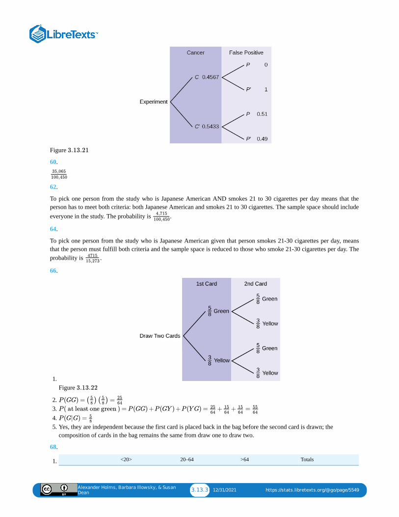
Alexander Holms, Barbara Illowsky, & Susan
Dean3.13.3 12/31/2021 https://stats.libretexts.org/@go/page/5549
Figure
60.
62.
To pick one person from the study who is Japanese American AND smokes 21 to 30 cigarettes per day means that theperson has to meet both criteria: both Japanese American and smokes 21 to 30 cigarettes. The sample space should includeeveryone in the study. The probability is .
64.
To pick one person from the study who is Japanese American given that person smokes 21-30 cigarettes per day, meansthat the person must fulfill both criteria and the sample space is reduced to those who smoke 21-30 cigarettes per day. Theprobability is .
66.
1. Figure
2. 3. 4. 5. Yes, they are independent because the first card is placed back in the bag before the second card is drawn; the
composition of cards in the bag remains the same from draw one to draw two.
68.
1. <20> 20–64 >64 Totals
3.13.21
35,065
100,450
4,715
100,450
471515,273
3.13.22
P (GG) = ( ) ( ) =58
58
2564
P ( at least one green ) = P (GG) +P (GY ) +P (YG) = + + =2564
1564
1564
5564
P (G|G) = 58
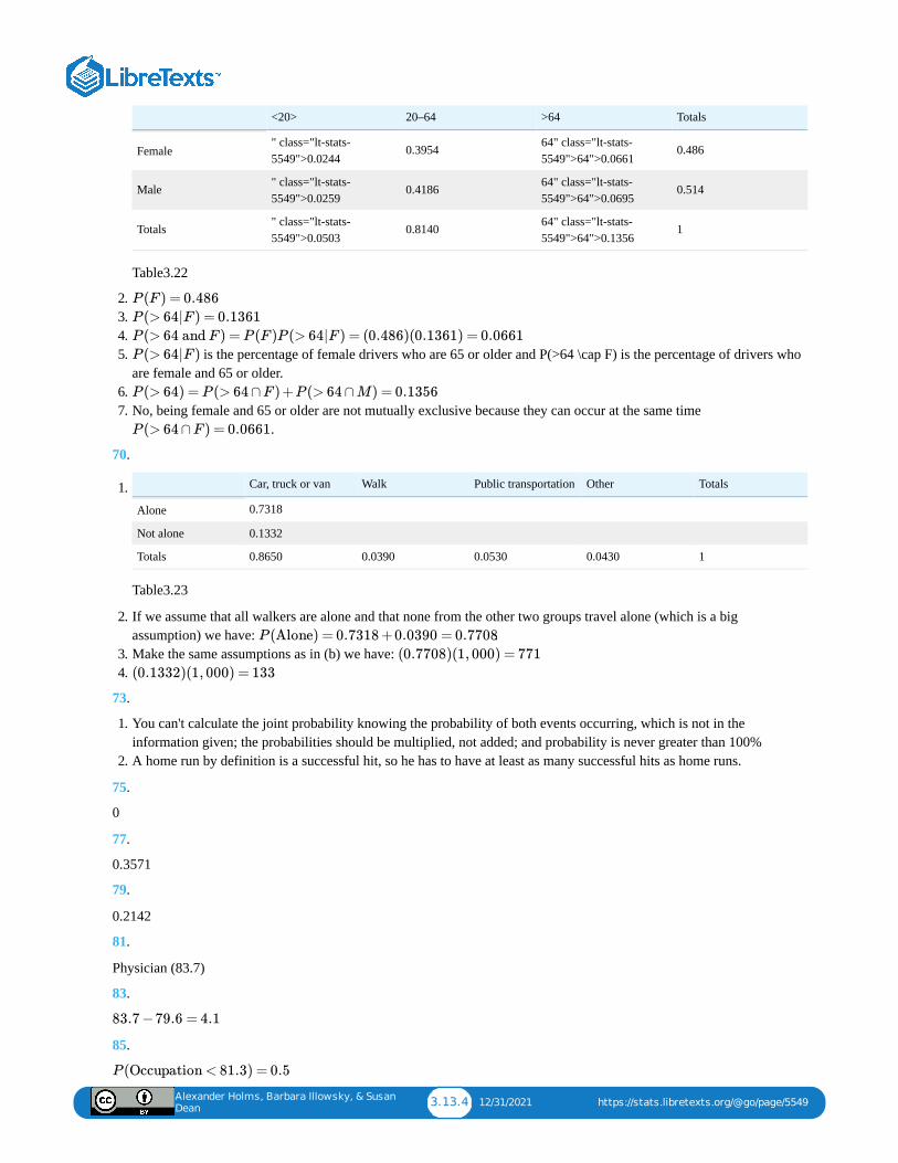
Alexander Holms, Barbara Illowsky, & Susan
Dean3.13.4 12/31/2021 https://stats.libretexts.org/@go/page/5549
<20> 20–64 >64 Totals
Female" class="lt-stats-5549">0.0244
0.3954 64" class="lt-stats-5549">64">0.0661
0.486
Male " class="lt-stats-5549">0.0259
0.4186 64" class="lt-stats-5549">64">0.0695
0.514
Totals " class="lt-stats-5549">0.0503
0.8140 64" class="lt-stats-5549">64">0.1356
1
Table3.22
2. 3. 4. 5. is the percentage of female drivers who are 65 or older and P(>64 \cap F) is the percentage of drivers who
are female and 65 or older.6. 7. No, being female and 65 or older are not mutually exclusive because they can occur at the same time
.
70.
1. Car, truck or van Walk Public transportation Other Totals
Alone 0.7318
Not alone 0.1332
Totals 0.8650 0.0390 0.0530 0.0430 1
Table3.23
2. If we assume that all walkers are alone and that none from the other two groups travel alone (which is a bigassumption) we have: .
3. Make the same assumptions as in (b) we have: 4.
73.
1. You can't calculate the joint probability knowing the probability of both events occurring, which is not in theinformation given; the probabilities should be multiplied, not added; and probability is never greater than 100%
2. A home run by definition is a successful hit, so he has to have at least as many successful hits as home runs.
75.
0
77.
0.3571
79.
0.2142
81.
Physician (83.7)
83.
85.
P (F ) = 0.486
P (> 64|F ) = 0.1361
P (> 64 and F ) = P (F )P (> 64|F ) = (0.486)(0.1361) = 0.0661
P (> 64|F )
P (> 64) = P (> 64 ∩F ) +P (> 64 ∩M) = 0.1356
P (> 64 ∩F ) = 0.0661
P (Alone) = 0.7318 +0.0390 = 0.7708
(0.7708)(1, 000) = 771
(0.1332)(1, 000) = 133
83.7 −79.6 = 4.1
P (Occupation < 81.3) = 0.5
Alexander Holms, Barbara Illowsky, & Susan
Dean3.13.5 12/31/2021 https://stats.libretexts.org/@go/page/5549
87.
1. The Forum Research surveyed 1,046 Torontonians.2. 58%3. 42% of 1,046 = 439 (rounding to the nearest integer)4. 0.575. 0.60.
89.
1. 2. 3. 4. 5. 6. 7.
91.
1. 2. 3. 4. 5. 6. No, because does not equal 0.
93.
NOTE
The coin toss is independent of the card picked first.
1. 2. 3. Yes, A and B are mutually exclusive because they cannot happen at the same time; you cannot pick a card that is both
blue and also (red or green). 4. No, A and C are not mutually exclusive because they can occur at the same time. In fact, C includes all of the outcomes
of A; if the card chosen is blue it is also (red or blue).
95.
1. 2. 3. Yes, because if A has occurred, it is impossible to obtain two tails. In other words, .
97.
1. If Y and Z are independent, then , so .2. 0.5
99.
iii i iv ii
101.
1. 2. 3.
P ( Betting on two line that touch each other on the table) = .638
P ( Betting on three numbers in a line ) = 338
P ( Betting on one number ) = 138
P ( Betting on four number that touch each other to form a square) = .438
P ( Betting on two number that touch each other on the table ) = 238
P ( Betting on 0 −00 −1 −2 −3) = 538
P ( Betting on 0 −1 −2; or 0 −00 −2; or 00 −2 −3) = 338
{G1,G2,G3,G4,G5,Y 1,Y 2,Y 3}58232868
P (G∩E)
{(G,H)(G,T )(B,H)(B,T )(R,H)(R,T )}
P (A) = P ( blue )P ( head ) = ( ) ( ) =310
12
320
P (A∩B) = 0
P (A∩C) = P (A) = 320
S = {(HHH), (HHT ), (HTH), (HTT ), (THH), (THT ), (TTH), (TTT )}48
P (A∩B) = 0
P (Y ∩Z) = P (Y )P (Z) P (Y ∪Z) = P (Y ) +P (Z) −P (Y )P (Z)
P (R) = 0.44
P (R|E) = 0.56
P (R|O) = 0.31
Alexander Holms, Barbara Illowsky, & Susan
Dean3.13.6 12/31/2021 https://stats.libretexts.org/@go/page/5549
4. No, whether the money is returned is not independent of which class the money was placed in. There are several waysto justify this mathematically, but one is that the money placed in economics classes is not returned at the same overallrate; .
5. No, this study definitely does not support that notion; in fact, it suggests the opposite. The money placed in theeconomics classrooms was returned at a higher rate than the money place in all classes collectively; .
103.
1.
; solve to find
6% of people have type O, Rh- blood
2.
94% of people do not have type O, Rh- blood
105.
1. Let C = be the event that the cookie contains chocolate. Let N = the event that the cookie contains nuts.2. 3.
107.
0
109.
111.
113.
d
115.
1. Race and sex 1–14 15–24 25–64 Over 64 TOTALS
White, male 210 3,360 13,610 4,870 22,050
White, female 80 580 3,380 890 4,930
Black, male 10 460 1,060 140 1,670
Black, female 0 40 270 20 330
All others 100
TOTALS 310 4,650 18,780 6,020 29,760
Table3.24
2. Race and sex 1–14 15–24 25–64 Over 64 TOTALS
White, male 210 3,360 13,610 4,870 22,050
White, female 80 580 3,380 890 4,930
Black, male 10 460 1,060 140 1,670
Black, female 0 40 270 20 330
All others 10 210 460 100 780
TOTALS 310 4,650 18,780 6,020 29,760
P (R|E) ≠ P (R)
P (R|E) > P (R)
P ( type O∪ Rh−) = P ( type O) +P (Rh−) −P ( type O∩ Rh−)
0.52 = 0.43 +0.15 −P ( type O∩ Rh−) P ( type O∩ Rh−) = 0.06
P ( NOT (type O ∩ Rh−)) = 1 −P ( type O∩ Rh−) = 1 −0.06 = 0.94
P (C ∪N) = P (C) +P (N) −P (C ∩N) = 0.36 +0.12 −0.08 = 0.40
P ( NElTHER chocolate NOR nuts) = 1 −P (C ∪N) = 1 −0.40 = 0.60
1067
1034
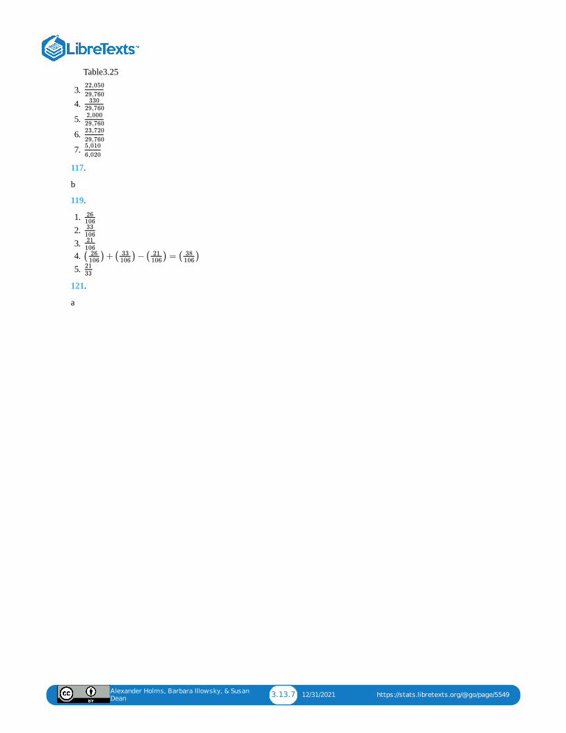
Alexander Holms, Barbara Illowsky, & Susan
Dean3.13.7 12/31/2021 https://stats.libretexts.org/@go/page/5549
Table3.25
3. 4.
5.
6.
7.
117.
b
119.
1. 2. 3. 4. 5.
121.
a
22,050
29,760330
29,7602,000
29,76023,720
29,7605,010
6,020
261063310621106
( )+( )−( ) = ( )26106
33106
21106
38106
2133

1 1/7/2022
CHAPTER OVERVIEW4: DISCRETE RANDOM VARIABLES
4.0: INTRODUCTION TO DISCRETE RANDOM VARIABLES4.1: HYPERGEOMETRIC DISTRIBUTION4.2: BINOMIAL DISTRIBUTION4.3: GEOMETRIC DISTRIBUTIONThe geometric probability density function builds upon what we have learned from the binomial distribution. In this case theexperiment continues until either a success or a failure occurs rather than for a set number of trials.
4.4: POISSON DISTRIBUTION4.5: CHAPTER FORMULA REVIEW4.6: CHAPTER HOMEWORK4.7: CHAPTER KEY ITEMS4.8: CHAPTER PRACTICE4.9: CHAPTER REFERENCES4.10: CHAPTER REVIEW4.11: CHAPTER SOLUTION (PRACTICE + HOMEWORK)

Alexander Holms, Barbara Illowsky, & Susan Dean 4.0.1 12/24/2021 https://stats.libretexts.org/@go/page/4565
4.0: Introduction to Discrete Random Variables
Figure You can use probability and discrete random variables to calculate the likelihood of lightning striking theground five times during a half-hour thunderstorm. (Credit: Leszek Leszczynski)
A student takes a ten-question, true-false quiz. Because the student had such a busy schedule, he or she could not study andguesses randomly at each answer. What is the probability of the student passing the test with at least a 70%?
Small companies might be interested in the number of long-distance phone calls their employees make during the peaktime of the day. Suppose the historical average is 20 calls. What is the probability that the employees make more than 20long-distance phone calls during the peak time?
These two examples illustrate two different types of probability problems involving discrete random variables. Recall thatdiscrete data are data that you can count, that is, the random variable can only take on whole number values. A randomvariable describes the outcomes of a statistical experiment in words. The values of a random variable can vary with eachrepetition of an experiment, often called a trial.
Random Variable Notation
The upper case letter X denotes a random variable. Lower case letters like x or y denote the value of a random variable. IfX is a random variable, then X is written in words, and x is given as a number.
For example, let X = the number of heads you get when you toss three fair coins. The sample space for the toss of three faircoins is TTT; THH; HTH; HHT; HTT; THT; TTH; HHH. Then, x = 0, 1, 2, 3. X is in words and x is a number. Notice thatfor this example, the x values are countable outcomes. Because you can count the possible values as whole numbers that Xcan take on and the outcomes are random (the x values 0, 1, 2, 3), X is a discrete random variable.
Probability Density Functions (PDF) for a Random Variable
A probability density function or probability distribution function has two characteristics:
1. A probability density function is a mathematical formula that calculates probabilities for specific types of events, whatwe have been calling experiments. There is a sort of magic to a probability density function (Pdf) partially because thesame formula often describes very different types of events. For example, the binomial Pdf will calculate probabilitiesfor flipping coins, yes/no questions on an exam, opinions of voters in an up or down opinion poll, indeed any binaryevent. Other probability density functions will provide probabilities for the time until a part will fail, when a customerwill arrive at the turnpike booth, the number of telephone calls arriving at a central switchboard, the growth rate of abacterium, and on and on. There are whole families of probability density functions that are used in a wide variety ofapplications, including medicine, business and finance, physics and engineering, among others.
For our needs here we will concentrate on only a few probability density functions as we develop the tools ofinferential statistics.
Counting Formulas and the Combinational Formula
As an equation this is:
4.0.1
Alexander Holms, Barbara Illowsky, & Susan Dean 4.0.2 12/24/2021 https://stats.libretexts.org/@go/page/4565
When we looked at the sample space for flipping 3 coins we could easily write the full sample space and thus couldeasily count the number of events that met our desired result, e.g. x = 1 , where X is the random variable defined as thenumber of heads.
As we have larger numbers of items in the sample space, such as a full deck of 52 cards, the ability to write out thesample space becomes impossible.
We see that probabilities are nothing more than counting the events in each group we are interested in and dividing bythe number of elements in the universe, or sample space. This is easy enough if we are counting sophomores in a Statclass, but in more complicated cases listing all the possible outcomes may take a life time. There are, for example, 36possible outcomes from throwing just two six-sided dice where the random variable is the sum of the number of spotson the up-facing sides. If there were four dice then the total number of possible outcomes would become 1,296. Thereare more than 2.5 MILLION possible 5 card poker hands in a standard deck of 52 cards. Obviously keeping track of allthese possibilities and counting them to get at a single probability would be tedious at best.
An alternative to listing the complete sample space and counting the number of elements we are interested in, is to skipthe step of listing the sample space, and simply figuring out the number of elements in it and doing the appropriatedivision. If we are after a probability we really do not need to see each and every element in the sample space, we onlyneed to know how many elements are there. Counting formulas were invented to do just this. They tell us the numberof unordered subsets of a certain size that can be created from a set of unique elements. By unordered it is meant that,for example, when dealing cards, it does not matter if you got {ace, ace, ace, ace, king} or {king, ace, ace, ace, ace} or{ace, king, ace, ace, ace} and so on. Each of these subsets are the same because they each have 4 aces and one king.
Combinational Formula
This is the formula that tells the number of unique unordered subsets of size x that can be created from n uniqueelements. The formula is read “n combinatorial x”. Sometimes it is read as “n choose x." The exclamation point "!" iscalled a factorial and tells us to take all the numbers from 1 through the number before the ! and multiply them togetherthus 4! is 1·2·3·4=24. By definition 0! = 1. The formula is called the Combinatorial Formula. It is also called theBinomial Coefficient, for reasons that will be clear shortly. While this mathematical concept was understood longbefore 1653, Blaise Pascal is given major credit for his proof that he published in that year. Further, he developed ageneralized method of calculating the values for combinatorials known to us as the Pascal Triangle. Pascal was one ofthe geniuses of an era of extraordinary intellectual advancement which included the work of Galileo, Rene Descartes,Isaac Newton, William Shakespeare and the refinement of the scientific method, the very rationale for the topic of thistext.
Let’s find the hard way the total number of combinations of the four aces in a deck of cards if we were going to takethem two at a time. The sample space would be:
S={Spade,Heart),(Spade, Diamond),(Spade,Club), (Diamond,Club),(Heart,Diamond),(Heart,Club)}
There are 6 combinations; formally, six unique unordered subsets of size 2 that can be created from 4 unique elements.To use the combinatorial formula we would solve the formula as follows:
If we wanted to know the number of unique 5 card poker hands that could be created from a 52 card deck we simplycompute:
P (A) = number of ways to get A
Total number of possible outcomes (4.0.1)
( ) =n
x=n Cx
n!
x!(n −x)!
( ) = = = 64
2
4!
(4 −2)!2!
4 ⋅ 3 ⋅ 2 ⋅ 1
2 ⋅ 1 ⋅ 2 ⋅ 1
( )52
5

Alexander Holms, Barbara Illowsky, & Susan Dean 4.0.3 12/24/2021 https://stats.libretexts.org/@go/page/4565
where 52 is the total number of unique elements from which we are drawing and 5 is the size group we are puttingthem into.
With the combinatorial formula we can count the number of elements in a sample space without having to write eachone of them down, truly a lifetime's work for just the number of 5 card hands from a deck of 52 cards. We can nowapply this tool to a very important probability density function, the hypergeometric distribution.
Remember, a probability density function computes probabilities for us. We simply put the appropriate numbers in theformula and we get the probability of specific events. However, for these formulas to work they must be applied only tocases for which they were designed.
Alexander Holms, Barbara Illowsky, & Susan Dean 4.1.1 1/6/2022 https://stats.libretexts.org/@go/page/4561
4.1: Hypergeometric DistributionThe simplest probability density function is the hypergeometric. This is the most basic one because it is created bycombining our knowledge of probabilities from Venn diagrams, the addition and multiplication rules, and thecombinatorial counting formula.
To find the number of ways to get 2 aces from the four in the deck we computed:
And if we did not care what else we had in our hand for the other three cards we would compute:
Putting this together, we can compute the probability of getting exactly two aces in a 5 card poker hand as:
This solution is really just the probability distribution known as the Hypergeometric. The generalized formula is:
where = the number we are interested in coming from the group with A objects.
is the probability of successes, in n attempts, when A successes (aces in this case) are in a population that containsN elements. The hypergeometric distribution is an example of a discrete probability distribution because there is nopossibility of partial success, that is, there can be no poker hands with 2 1/2 aces. Said another way, a discrete randomvariable has to be a whole, or counting, number only. This probability distribution works in cases where the probability ofa success changes with each draw. Another way of saying this is that the events are NOT independent. In using a deck ofcards, we are sampling WITHOUT replacement. If we put each card back after it was drawn then the hypergeometricdistribution be an inappropriate Pdf.
For the hypergeometric to work,
1. the population must be dividable into two and only two independent subsets (aces and non-aces in our example). Therandom variable = the number of items from the group of interest.
2. the experiment must have changing probabilities of success with each experiment (the fact that cards are not replacedafter the draw in our example makes this true in this case). Another way to say this is that you sample withoutreplacement and therefore each pick is not independent.
3. the random variable must be discrete, rather than continuous.
A candy dish contains 30 jelly beans and 20 gumdrops. Ten candies are picked at random. What is the probability that5 of the 10 are gumdrops? The two groups are jelly beans and gumdrops. Since the probability question asks for theprobability of picking gumdrops, the group of interest (first group A in the formula) is gumdrops. The size of the groupof interest (first group) is 30. The size of the second group is 20. The size of the sample is 10 (jelly beans orgumdrops). Let = the number of gumdrops in the sample of 10. takes on the values . a. Whatis the probability statement written mathematically? b. What is the hypergeometric probability density function written
( ) = = 64
2
4!
2!(4 −2)!
( ) = = 17, 29648
3
48!
3!45!
= .0399
( )( )4
2
48
3
( )52
5
h(x) =
( )( )A
x
N −A
n −x
( )N
n
x
h(x) x
X
Example 4.1.1
X X x = 0, 1, 2, . . . , 10
Alexander Holms, Barbara Illowsky, & Susan Dean 4.1.2 1/6/2022 https://stats.libretexts.org/@go/page/4561
out to solve this problem? c. What is the answer to the question "What is the probability of drawing 5 gumdrops in 10picks from the dish?"
Answer
a.
b.
c.
A bag contains letter tiles. Forty-four of the tiles are vowels, and 56 are consonants. Seven tiles are picked at random.You want to know the probability that four of the seven tiles are vowels. What is the group of interest, the size of thegroup of interest, and the size of the sample?
P (x = 5)
P (x = 5) =( )( )
30
5
20
5
( )50
10
P (x = 5) = 0.215
Exercise 4.1.1
Alexander Holms, Barbara Illowsky, & Susan Dean 4.2.1 12/9/2021 https://stats.libretexts.org/@go/page/4562
Skip to main content4.2: Binomial DistributionA more valuable probability density function with many applications is the binomial distribution. This distribution willcompute probabilities for any binomial process. A binomial process, often called a Bernoulli process after the first personto fully develop its properties, is any case where there are only two possible outcomes in any one trial, called successesand failures. It gets its name from the binary number system where all numbers are reduced to either 1's or 0's, which isthe basis for computer technology and CD music recordings.
Binomial Formula
where is the probability of successes in trials when the probability of a success in ANY ONE TRIAL is . Andof course and is the probability of a failure in any one trial.
We can see now why the combinatorial formula is also called the binomial coefficient because it reappears here again inthe binomial probability function. For the binomial formula to work, the probability of a success in any one trial must bethe same from trial to trial, or in other words, the outcomes of each trial must be independent. Flipping a coin is abinomial process because the probability of getting a head in one flip does not depend upon what has happened inPREVIOUS flips. (At this time it should be noted that using for the parameter of the binomial distribution is a violationof the rule that population parameters are designated with Greek letters. In many textbooks (pronounced theta) is usedinstead of p and this is how it should be.
Just like a set of data, a probability density function has a mean and a standard deviation that describes the data set. Forthe binomial distribution these are given by the formulas:
Notice that p is the only parameter in these equations. The binomial distribution is thus seen as coming from the one-parameter family of probability distributions. In short, we know all there is to know about the binomial once we know p,the probability of a success in any one trial.
In probability theory, under certain circumstances, one probability distribution can be used to approximate another. Wesay that one is the limiting distribution of the other. If a small number is to be drawn from a large population, even if thereis no replacement, we can still use the binomial even thought this is not a binomial process. If there is no replacement itviolates the independence rule of the binomial. Nevertheless, we can use the binomial to approximate a probability that isreally a hypergeometric distribution if we are drawing fewer than 10 percent of the population, i.e. n is less than 10percent of N in the formula for the hypergeometric function. The rationale for this argument is that when drawing a smallpercentage of the population we do not alter the probability of a success from draw to draw in any meaningful way.Imagine drawing from not one deck of 52 cards but from 6 decks of cards. The probability of say drawing an ace does notchange the conditional probability of what happens on a second draw in the same way it would if there were only 4 acesrather than the 24 aces now to draw from. This ability to use one probability distribution to estimate others will becomevery valuable to us later.
There are three characteristics of a binomial experiment.
1. There are a fixed number of trials. Think of trials as repetitions of an experiment. The letter denotes the numberof trials.
2. The random variable, , number of successes, is discrete.3. There are only two possible outcomes, called "success" and "failure," for each trial. The letter denotes the
probability of a success on any one trial, and denotes the probability of a failure on any one trial. .4. The n trials are independent and are repeated using identical conditions. Think of this as drawing WITH
replacement. Because the n trials are independent, the outcome of one trial does not help in predicting theoutcome of another trial. Another way of saying this is that for each individual trial, the probability, , of a
b(x) =( )n
xpxqn−x
b(x) X n p
q = (1 −p)
p
θ
μ = np
σ = npq−−−√
n
x
p
q p +q = 1
p
Alexander Holms, Barbara Illowsky, & Susan Dean 4.2.2 12/9/2021 https://stats.libretexts.org/@go/page/4562
success and probability, , of a failure remain the same. For example, randomly guessing at a true-false statisticsquestion has only two outcomes. If a success is guessing correctly, then a failure is guessing incorrectly. SupposeJoe always guesses correctly on any statistics true-false question with a probability . Then, . Thismeans that for every true-false statistics question Joe answers, his probability of success ( ) and hisprobability of failure ( ) remain the same.
The outcomes of a binomial experiment fit a binomial probability distribution. The random variable = the number ofsuccesses obtained in the independent trials.
The mean, , and variance, , for the binomial probability distribution are and . The standarddeviation, , is then \sigma = .
Any experiment that has characteristics three and four and where is called a Bernoulli Trial (named after JacobBernoulli who, in the late 1600s, studied them extensively). A binomial experiment takes place when the number ofsuccesses is counted in one or more Bernoulli Trials.
Suppose you play a game that you can only either win or lose. The probability that you win any game is 55%, and theprobability that you lose is 45%. Each game you play is independent. If you play the game 20 times, write thefunction that describes the probability that you win 15 of the 20 times. Here, if you define as the number of wins,then takes on the values 0, 1, 2, 3, ..., 20. The probability of a success is . The probability of a failure is
. The number of trials is . The probability question can be stated mathematically as
A trainer is teaching a dolphin to do tricks. The probability that the dolphin successfully performs the trick is 35%,and the probability that the dolphin does not successfully perform the trick is 65%. Out of 20 attempts, you want tofind the probability that the dolphin succeeds 12 times. Find the using the binomial Pdf
A fair coin is flipped 15 times. Each flip is independent. What is the probability of getting more than ten heads? Let = the number of heads in 15 flips of the fair coin. takes on the values 0, 1, 2, 3, ..., 15. Since the coin is fair,
and . The number of trials is . State the probability question mathematically.
Answer
Approximately 70% of statistics students do their homework in time for it to be collected and graded. Each studentdoes homework independently. In a statistics class of 50 students, what is the probability that at least 40 will do theirhomework on time? Students are selected randomly.
a. This is a binomial problem because there is only a success or a __________, there are a fixed number of trials, andthe probability of a success is 0.70 for each trial.
Answer
a. failure
b. If we are interested in the number of students who do their homework on time, then how do we define ?
Answer
b. = the number of statistics students who do their homework on time
q
p = 0.6 q = 0.4p = 0.6
q = 0.4
X
n
μ σ2 μ = np = npqσ2
σ npq−−−√
n = 1
Example 4.2.2
X
X p = 0.55q = 0.45 n = 20 P (x = 15)
Exercise 4.2.2
P (X = 12)
Example 4.2.3
X X
p = 0.5 q = 0.5 n = 15
P (x > 10)
Example 4.2.4
X
X
Alexander Holms, Barbara Illowsky, & Susan Dean 4.2.3 12/9/2021 https://stats.libretexts.org/@go/page/4562
c. What values does take on?
Answer
c. 0, 1, 2, …, 50
d. What is a "failure," in words?
Answer
d. Failure is defined as a student who does not complete his or her homework on time.
The probability of a success is . The number of trials is .
e. If , then what is ?
Answer
e.
f. The words "at least" translate as what kind of inequality for the probability question ____ 40).
Answer
f. greater than or equal to ( ) The probability question is .
Sixty-five percent of people pass the state driver’s exam on the first try. A group of 50 individuals who have taken thedriver’s exam is randomly selected. Give two reasons why this is a binomial problem
During the 2013 regular NBA season, DeAndre Jordan of the Los Angeles Clippers had the highest field goalcompletion rate in the league. DeAndre scored with 61.3% of his shots. Suppose you choose a random sample of 80shots made by DeAndre during the 2013 season. Let = the number of shots that scored points.
a. What is the probability distribution for ?b. Using the formulas, calculate the (i) mean and (ii) standard deviation of .c. Find the probability that DeAndre scored with 60 of these shots.d. Find the probability that DeAndre scored with more than 50 of these shots.
x
p = 0.70 n = 50
p +q = 1 q
q = 0.30
P (x
≥P (x ≥ 40)
Exercise 4.2.4
Exercise 4.2.4
X
X
X
Alexander Holms, Barbara Illowsky, & Susan Dean 4.3.1 12/17/2021 https://stats.libretexts.org/@go/page/4563
4.3: Geometric DistributionThe geometric probability density function builds upon what we have learned from the binomial distribution. In this casethe experiment continues until either a success or a failure occurs rather than for a set number of trials. There are threemain characteristics of a geometric experiment.
1. There are one or more Bernoulli trials with all failures except the last one, which is a success. In other words, you keeprepeating what you are doing until the first success. Then you stop. For example, you throw a dart at a bullseye untilyou hit the bullseye. The first time you hit the bullseye is a "success" so you stop throwing the dart. It might take sixtries until you hit the bullseye. You can think of the trials as failure, failure, failure, failure, failure, success, STOP.
2. In theory, the number of trials could go on forever.3. The probability, , of a success and the probability, , of a failure is the same for each trial. and .
For example, the probability of rolling a three when you throw one fair die is . This is true no matter how many timesyou roll the die. Suppose you want to know the probability of getting the first three on the fifth roll. On rolls onethrough four, you do not get a face with a three. The probability for each of the rolls is q = , the probability of afailure. The probability of getting a three on the fifth roll is
4. = the number of independent trials until the first success.
You play a game of chance that you can either win or lose (there are no other possibilities) until you lose. Yourprobability of losing is . What is the probability that it takes five games until you lose? Let = the numberof games you play until you lose (includes the losing game). Then X takes on the values 1, 2, 3, ... (could go onindefinitely). The probability question is .
You throw darts at a board until you hit the center area. Your probability of hitting the center area is . Youwant to find the probability that it takes eight throws until you hit the center. What values does take on?
A safety engineer feels that 35% of all industrial accidents in her plant are caused by failure of employees to followinstructions. She decides to look at the accident reports (selected randomly and replaced in the pile after reading) untilshe finds one that shows an accident caused by failure of employees to follow instructions. On average, how manyreports would the safety engineer expect to look at until she finds a report showing an accident caused by employeefailure to follow instructions? What is the probability that the safety engineer will have to examine at least threereports until she finds a report showing an accident caused by employee failure to follow instructions?
Let = the number of accidents the safety engineer must examine until she finds a report showing an accident causedby employee failure to follow instructions. X takes on the values 1, 2, 3, .... The first question asks you to find theexpected value or the mean. The second question asks you to find . ("At least" translates to a "greater thanor equal to" symbol).
An instructor feels that 15% of students get below a C on their final exam. She decides to look at final exams (selectedrandomly and replaced in the pile after reading) until she finds one that shows a grade below a C. We want to know theprobability that the instructor will have to examine at least ten exams until she finds one with a grade below a C. Whatis the probability question stated mathematically?
p q p +q = 1 q = 1 −p16
56
( ) ( ) ( ) ( ) ( ) = 0.080456
56
56
56
16
X
Example 4.3.5
p = 0.57 X
P (x = 5)
Exercise 4.3.5
p = 0.17
X
Example 4.3.6
X
P (x ≥ 3)
Exercise 4.3.6
Alexander Holms, Barbara Illowsky, & Susan Dean 4.3.2 12/17/2021 https://stats.libretexts.org/@go/page/4563
Suppose that you are looking for a student at your college who lives within five miles of you. You know that 55% ofthe 25,000 students do live within five miles of you. You randomly contact students from the college until one says heor she lives within five miles of you. What is the probability that you need to contact four people?
This is a geometric problem because you may have a number of failures before you have the one success you desire.Also, the probability of a success stays approximately the same each time you ask a student if he or she lives withinfive miles of you. There is no definite number of trials (number of times you ask a student).
a. Let = the number of ____________ you must ask ____________ one says yes.
Answer
a. Let = the number of students you must ask until one says yes.
b. What values does take on?
Answer
b. 1, 2, 3, …, (total number of students)
c. What are and ?
Answer
c.
d. The probability question is (_______).
Answer
d.
Notation for the Geometric: G = Geometric Probability Distribution Function
Read this as " is a random variable with a geometric distribution." The parameter is ; = the probability of a successfor each trial.
The Geometric Pdf tells us the probability that the first occurrence of success requires number of independent trials, eachwith success probability p. If the probability of success on each trial is p, then the probability that the th trial (out of trials) is the first success is:
for , .... The expected value of , the mean of this distribution, is . This tells us how many trials we have to expect until we getthe first success including in the count the trial that results in success. The above form of the Geometric distribution is usedfor modeling the number of trials until the first success. The number of trials includes the one that is a success: = alltrials including the one that is a success. This can be seen in the form of the formula. If = number of trials including thesuccess, then we must multiply the probability of failure, , times the number of failures, that is .
By contrast, the following form of the geometric distribution is used for modeling number of failures until the first success:
for , .... In this case the trial that is a success is not counted as a trial in the formula: = number of failures. The expected value,
Example 4.3.7
X
X
X
p q
p = 0.55; q = 0.45
P
P (x = 4)
X ∼ G(p)
X p p
x
x x
P(X = x) = (1 −p p)x−1
x = 1, 2, 3
X 1/p
x
X
(1 −p) X −1
P(X = x) = (1 −p p)x
x = 0, 1, 2, 3
x
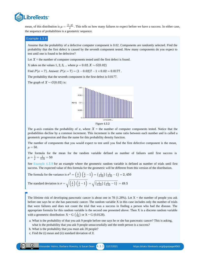
Alexander Holms, Barbara Illowsky, & Susan Dean 4.3.3 12/17/2021 https://stats.libretexts.org/@go/page/4563
mean, of this distribution is . This tells us how many failures to expect before we have a success. In either case,the sequence of probabilities is a geometric sequence.
Assume that the probability of a defective computer component is 0.02. Components are randomly selected. Find theprobability that the first defect is caused by the seventh component tested. How many components do you expect totest until one is found to be defective?
Let = the number of computer components tested until the first defect is found.
X takes on the values , ... where
Find . Answer: .
The probability that the seventh component is the first defect is 0.0177.
The graph of is:
Figure
The -axis contains the probability of , where = the number of computer components tested. Notice that theprobabilities decline by a common increment. This increment is the same ratio between each number and is called ageometric progression and thus the name for this probability density function.
The number of components that you would expect to test until you find the first defective component is the mean, .
The formula for the mean for the random variable defined as number of failures until first success is
See Example for an example where the geometric random variable is defined as number of trials until firstsuccess. The expected value of this formula for the geometric will be different from this version of the distribution.
The formula for the variance is
The standard deviation is
The lifetime risk of developing pancreatic cancer is about one in 78 (1.28%). Let X = the number of people you askbefore one says he or she has pancreatic cancer. The random variable X in this case includes only the number of trialsthat were failures and does not count the trial that was a success in finding a person who had the disease. Theappropriate formula for this random variable is the second one presented above. Then X is a discrete random variablewith a geometric distribution: X ~ G or X ~ G (0.0128).
a. What is the probability of that you ask 9 people before one says he or she has pancreatic cancer? This is asking,what is the probability that you ask 9 people unsuccessfully and the tenth person is a success?
b. What is the probability that you must ask 20 people?c. Find the (i) mean and (ii) standard deviation of X.
μ =(1−p)
p
Example 4.3.8
X
1, 2, 3 p = 0.02.X ∼ G(0.02)
P (x = 7) P (x = 7) = (1 −0.02)7 −1 ×0.02 = 0.0177
X ∼ G(0.02)
4.3.2
y x X
μ = 50
μ = = = 501p
10.02
4.3.9
= ( )( −1) = ( ) ( −1) = 2, 450σ2 1p
1p
10.02
10.02
σ = = = 49.5( )( −1)1p
1p
− −−−−−−−−−−√ ( ) ( −1)1
0.021
0.02
− −−−−−−−−−−−−√
( )178
Alexander Holms, Barbara Illowsky, & Susan Dean 4.3.4 12/17/2021 https://stats.libretexts.org/@go/page/4563
Answer
a.
b.
i. Mean =
ii. Standard Deviation =
The literacy rate for a nation measures the proportion of people age 15 and over who can read and write. The literacyrate for women in The United Colonies of Independence is 12%. Let = the number of women you ask until one saysthat she is literate.
a. What is the probability distribution of ?b. What is the probability that you ask five women before one says she is literate?c. What is the probability that you must ask ten women?
A baseball player has a batting average of 0.320. This is the general probability that he gets a hit each time he is at bat.
What is the probability that he gets his first hit in the third trip to bat?
Answer
In this case the sequence is failure, failure success.
How many trips to bat do you expect the hitter to need before getting a hit?
Answer
This is simply the expected value of successes and therefore the mean of the distribution.
There is an 80% chance that a Dalmatian dog has 13 black spots. You go to a dog show and count the spots onDalmatians. What is the probability that you will review the spots on 3 dogs before you find one that has 13 blackspots?
Answer
Footnotes1 ”Prevalence of HIV, total (% of populations ages 15-49),” The World Bank, 2013. Available online athttp://data.worldbank.org/indicator/...last&sort=desc (accessed May 15, 2013).
P (x = 9) = (1 −0.0128 ⋅ 0.0128 = 0.0114)9
P (x = 20) = (1 −0.0128 ⋅ 0.0128 = 0.01)19
μ = = = 77.12(1−p)
p
(1−0.0128)
0.0128
σ = = ≈ 77.621−p
p2
− −−√ 1−0.0128
0.01282
− −−−−−√
Exercise 4.3.9
X
X
Example 4.3.10
P (x = 3) = (1 −0.32 ×.32 = 0.1480)3−1
μ = = = 3.125 ≈ 31p
10.320
Example 4.3.11
P (x = 3) = (1 −0.80 ×0.80 = 0.0064)3
Alexander Holms, Barbara Illowsky, & Susan Dean 4.4.1 12/3/2021 https://stats.libretexts.org/@go/page/4564
4.4: Poisson DistributionAnother useful probability distribution is the Poisson distribution, or waiting time distribution. This distribution is used todetermine how many checkout clerks are needed to keep the waiting time in line to specified levels, how may telephonelines are needed to keep the system from overloading, and many other practical applications. A modification of thePoisson, the Pascal, invented nearly four centuries ago, is used today by telecommunications companies worldwide forload factors, satellite hookup levels and Internet capacity problems. The distribution gets its name from Simeon Poissonwho presented it in 1837 as an extension of the binomial distribution which we will see can be estimated with the Poisson.
There are two main characteristics of a Poisson experiment.
1. The Poisson probability distribution gives the probability of a number of events occurring in a fixed interval of timeor space if these events happen with a known average rate.
2. The events are independently of the time since the last event. For example, a book editor might be interested in thenumber of words spelled incorrectly in a particular book. It might be that, on the average, there are five words spelledincorrectly in 100 pages. The interval is the 100 pages and it is assumed that there is no relationship between whenmisspellings occur.
3. The random variable = the number of occurrences in the interval of interest.
A bank expects to receive six bad checks per day, on average. What is the probability of the bank getting fewer thanfive bad checks on any given day? Of interest is the number of checks the bank receives in one day, so the timeinterval of interest is one day. Let = the number of bad checks the bank receives in one day. If the bank expects toreceive six bad checks per day then the average is six checks per day. Write a mathematical statement for theprobability question.
Answer
You notice that a news reporter says "uh," on average, two times per broadcast. What is the probability that the newsreporter says "uh" more than two times per broadcast.
This is a Poisson problem because you are interested in knowing the number of times the news reporter says "uh"during a broadcast.
a. What is the interval of interest?
Answer
a. one broadcast measured in minutes
b. What is the average number of times the news reporter says "uh" during one broadcast?
Answer
b. 2
c. Let = ____________. What values does take on?
Answer
c. Let = the number of times the news reporter says "uh" during one broadcast. , ...
X
Example 4.4.12
X
P (x < 5)
Example 4.4.13
X X
X
x = 0, 1, 2, 3
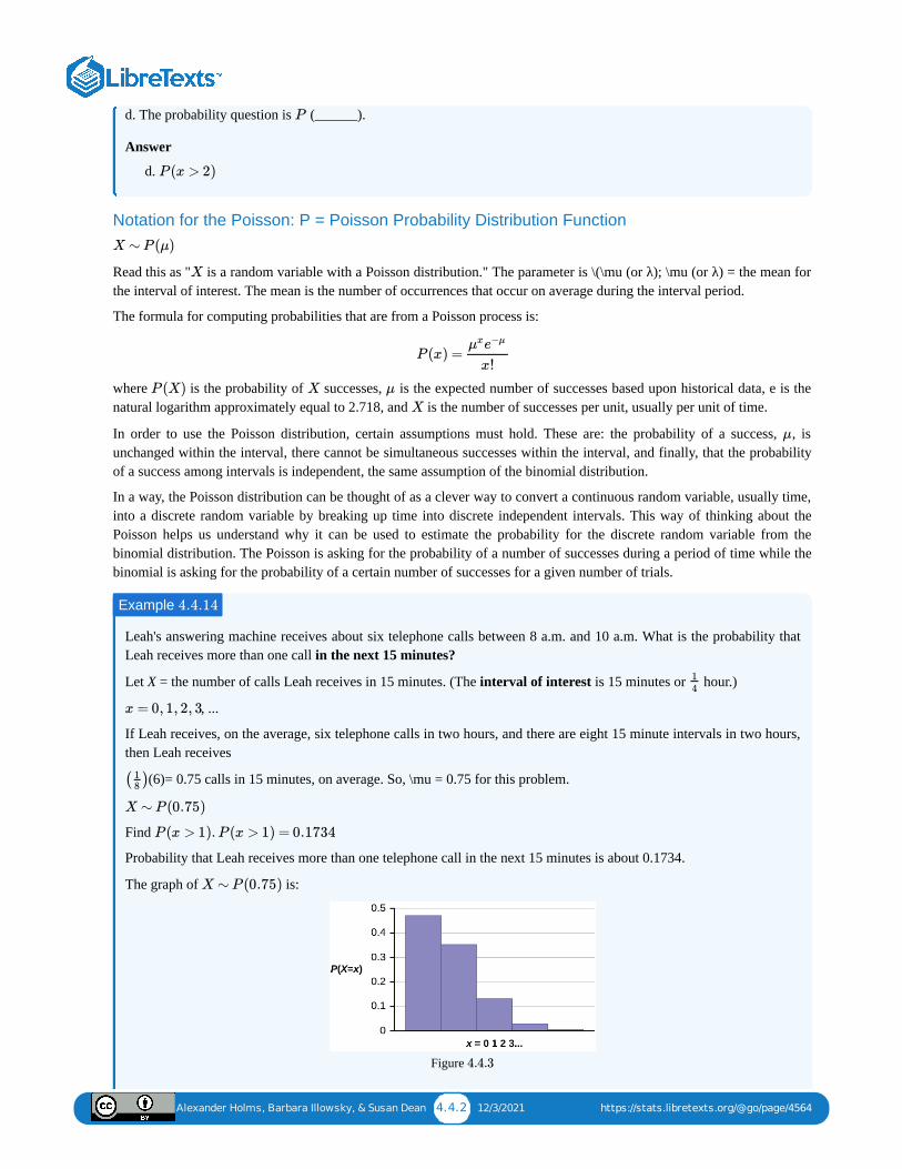
Alexander Holms, Barbara Illowsky, & Susan Dean 4.4.2 12/3/2021 https://stats.libretexts.org/@go/page/4564
d. The probability question is (______).
Answer
d.
Notation for the Poisson: P = Poisson Probability Distribution Function
Read this as " is a random variable with a Poisson distribution." The parameter is \(\mu (or λ); \mu (or λ) = the mean forthe interval of interest. The mean is the number of occurrences that occur on average during the interval period.
The formula for computing probabilities that are from a Poisson process is:
where is the probability of successes, is the expected number of successes based upon historical data, e is thenatural logarithm approximately equal to 2.718, and is the number of successes per unit, usually per unit of time.
In order to use the Poisson distribution, certain assumptions must hold. These are: the probability of a success, , isunchanged within the interval, there cannot be simultaneous successes within the interval, and finally, that the probabilityof a success among intervals is independent, the same assumption of the binomial distribution.
In a way, the Poisson distribution can be thought of as a clever way to convert a continuous random variable, usually time,into a discrete random variable by breaking up time into discrete independent intervals. This way of thinking about thePoisson helps us understand why it can be used to estimate the probability for the discrete random variable from thebinomial distribution. The Poisson is asking for the probability of a number of successes during a period of time while thebinomial is asking for the probability of a certain number of successes for a given number of trials.
Leah's answering machine receives about six telephone calls between 8 a.m. and 10 a.m. What is the probability thatLeah receives more than one call in the next 15 minutes?
Let X = the number of calls Leah receives in 15 minutes. (The interval of interest is 15 minutes or hour.)
, ...
If Leah receives, on the average, six telephone calls in two hours, and there are eight 15 minute intervals in two hours,then Leah receives
(6)= 0.75 calls in 15 minutes, on average. So, \mu = 0.75 for this problem.
Find
Probability that Leah receives more than one telephone call in the next 15 minutes is about 0.1734.
The graph of is:
Figure
P
P (x > 2)
X ∼ P (μ)
X
P (x) =μxe−μ
x!
P (X) X μ
X
μ
Example 4.4.14
14
x = 0, 1, 2, 3
( )18
X ∼ P (0.75)
P (x > 1). P (x > 1) = 0.1734
X ∼ P (0.75)
4.4.3
Alexander Holms, Barbara Illowsky, & Susan Dean 4.4.3 12/3/2021 https://stats.libretexts.org/@go/page/4564
The -axis contains the probability of where = the number of calls in 15 minutes.
According to a survey a university professor gets, on average, 7 emails per day. Let X = the number of emails aprofessor receives per day. The discrete random variable X takes on the values x = 0, 1, 2 …. The random variable Xhas a Poisson distribution: X ~ P (7). The mean is 7 emails.
a. What is the probability that an email user receives exactly 2 emails per day?b. What is the probability that an email user receives at most 2 emails per day?c. What is the standard deviation?
Answer
a.
b.
c. Standard Deviation =
Text message users receive or send an average of 41.5 text messages per day.
a. How many text messages does a text message user receive or send per hour?b. What is the probability that a text message user receives or sends two messages per hour?c. What is the probability that a text message user receives or sends more than two messages per hour?
Answer
a.Let X = the number of texts that a user sends or receives in one hour. The average number of texts received perhour is ≈ 1.7292.
b.
c.
On May 13, 2013, starting at 4:30 PM, the probability of low seismic activity for the next 48 hours in Alaska wasreported as about 1.02%. Use this information for the next 200 days to find the probability that there will be lowseismic activity in ten of the next 200 days. Use both the binomial and Poisson distributions to calculate theprobabilities. Are they close?
Answer
Let X = the number of days with low seismic activity.
Using the binomial distribution:
Using the Poisson distribution:
Calculate
y x X
Example 4.4.15
P (x = 2) = = = 0.022μ −μxe
x!72e−7
2!
P (x ≤ 2) = + + = 0.02970e−7
0!71e−7
1!72e−7
2!
σ = = ≈ 2.65μ−−√ 7–
√
Example 4.4.16
41.524
P (x = 2) = = = 0.265μxe−μ
x!1.7292e−1.729
2!
P (x > 2) = 1 −P (x ≤ 2) = 1 −[ + + ] = 0.25070e−7
0!71e7
1!72e−7
2!
Example 4.4.17
P (x = 10) = × × = 0.000039200!
10!(200 −10)!.010210 .9898190
μ = np = 200(0.0102) ≈ 2.04
P (x = 10) = = = 0.000045μxe−μ
x!
2.0410e−2.04
10!
Alexander Holms, Barbara Illowsky, & Susan Dean 4.4.4 12/3/2021 https://stats.libretexts.org/@go/page/4564
We expect the approximation to be good because is large (greater than 20) and is small (less than 0.05). Theresults are close—both probabilities reported are almost 0.
Estimating the Binomial Distribution with the Poisson DistributionWe found before that the binomial distribution provided an approximation for the hypergeometric distribution. Now wefind that the Poisson distribution can provide an approximation for the binomial. We say that the binomial distributionapproaches the Poisson. The binomial distribution approaches the Poisson distribution is as n gets larger and p is smallsuch that np becomes a constant value. There are several rules of thumb for when one can say they will use a Poisson toestimate a binomial. One suggests that np, the mean of the binomial, should be less than 25. Another author suggests that itshould be less than 7. And another, noting that the mean and variance of the Poisson are both the same, suggests that npand npq, the mean and variance of the binomial, should be greater than 5. There is no one broadly accepted rule of thumbfor when one can use the Poisson to estimate the binomial.
As we move through these probability distributions we are getting to more sophisticated distributions that, in a sense,contain the less sophisticated distributions within them. This proposition has been proven by mathematicians. This gets usto the highest level of sophistication in the next probability distribution which can be used as an approximation to all ofthose that we have discussed so far. This is the normal distribution.
A survey of 500 seniors in the Price Business School yields the following information. 75% go straight to work aftergraduation. 15% go on to work on their MBA. 9% stay to get a minor in another program. 1% go on to get a Master'sin Finance.
What is the probability that more than 2 seniors go to graduate school for their Master's in finance?
Answer
This is clearly a binomial probability distribution problem. The choices are binary when we define the results as"Graduate School in Finance" versus "all other options." The random variable is discrete, and the events are, wecould assume, independent. Solving as a binomial problem, we have:
Binomial Solution
Adding all 3 together = 0.12339
Poisson approximation
n p
Example 4.4.18
n ⋅ p = 500 ⋅ 0.01 = 5 = μ
P (0) = (1 −0.01 = 0.00657500!
0!(500 −0)!0.010 )500−0
P (1) = (1 −0.01 = 0.03318500!
1!(500 −1)!0.011 )500
P (2) = (1 −0.01 = 0.08363500!
2!(500 −2)!0.012 )5002
1 −0.12339 = 0.87661
n ⋅ p = 500 ⋅ 0.01 = 5 = μ
n ⋅ p ⋅ (1 −p) = 500 ⋅ 0.01 ⋅ (0.99) ≈ 5 = = μσ2
P (X) = ={P (0) = }+{P (1) = }+{P (2) = }(npe−np )x
x!
⋅e−5 50
0!
⋅e−5 51
1!
⋅e−5 52
2!
0.0067 +0.0337 +0.0842 = 0.1247

Alexander Holms, Barbara Illowsky, & Susan Dean 4.4.5 12/3/2021 https://stats.libretexts.org/@go/page/4564
An approximation that is off by 1 one thousandth is certainly an acceptable approximation.
1 −0.1247 = 0.8753
Alexander Holms, Barbara Illowsky, & Susan Dean 4.5.1 12/10/2021 https://stats.libretexts.org/@go/page/5555
4.5: Chapter Formula Review
Hypergeometric Distribution
Binomial Distribution means that the discrete random variable has a binomial probability distribution with trials and
probability of success .
the number of successes in n independent trials
the number of independent trials
takes on the values
the probability of a success for any trial
the probability of a failure for any trial
The mean of is . The standard deviation of is .
where is the probability of successes in trials when the probability of a success in ANY ONE TRIAL is .
Geometric Distribution
means that the discrete random variable has a geometric probability distribution with probability of successin a single trial .
the number of independent trials until the first success
takes on the values
the probability of a success for any trial
the probability of a failure for any trial
The mean is .
The standard deviation is .
Poisson Distribution means that has a Poisson probability distribution where the number of occurrences in the interval of
interest.
takes on the values
The mean or is typically given.
The variance is , and the standard deviation is .
h(x) =( )( )
A
x
N−A
n−x
( )N
n
X ∼ B(n, p) X n
p
X =
n =
X x = 0, 1, 2, 3, . . . , n
p =
q =
p +q = 1
q = 1– p
X μ = np X σ = npq−−−√
P (x) = ⋅n!
x!(n −x)!pxq(n−x)
P (X) X n p
P (X = x) = p(1 −p)x−1
X ∼ G(p) X
p
X =
X x = 1, 2, 3, . . .
p =
q = p +q = 1q = 1– p
μ = 1p
σ = =1−p
p2
− −−√ ( −1)1
p1p
− −−−−−−−√
X ∼ P (μ) X X =
X x = 0, 1, 2, 3, . . .
μ λ
= μσ2
σ = μ−−√

Alexander Holms, Barbara Illowsky, & Susan Dean 4.5.2 12/10/2021 https://stats.libretexts.org/@go/page/5555
When is used to approximate a binomial distribution, where n represents the number of independent trialsand represents the probability of success in a single trial.
P (μ) μ = np
p
P (x) =μxe−μ
x!
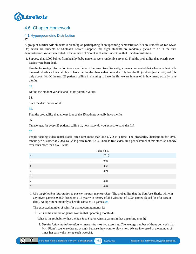
Alexander Holms, Barbara Illowsky, & Susan Dean 4.6.1 12/10/2021 https://stats.libretexts.org/@go/page/5557
4.6: Chapter Homework
4.1 Hypergeometric Distribution47.
A group of Martial Arts students is planning on participating in an upcoming demonstration. Six are students of Tae KwonDo; seven are students of Shotokan Karate. Suppose that eight students are randomly picked to be in the firstdemonstration. We are interested in the number of Shotokan Karate students in that first demonstration.
1. Suppose that 1,000 babies from healthy baby nurseries were randomly surveyed. Find the probability that exactly twobabies were born deaf.
Use the following information to answer the next four exercises. Recently, a nurse commented that when a patient callsthe medical advice line claiming to have the flu, the chance that he or she truly has the flu (and not just a nasty cold) isonly about 4%. Of the next 25 patients calling in claiming to have the flu, we are interested in how many actually havethe flu.
53.
Define the random variable and list its possible values.
54.
State the distribution of .
55.
Find the probability that at least four of the 25 patients actually have the flu.
56.
On average, for every 25 patients calling in, how many do you expect to have the flu?
57.
People visiting video rental stores often rent more than one DVD at a time. The probability distribution for DVDrentals per customer at Video To Go is given Table . There is five-video limit per customer at this store, so nobodyever rents more than five DVDs.
0 0.03
1 0.50
2 0.24
3
4 0.07
5 0.04
Table
1. Use the following information to answer the next two exercises: The probability that the San Jose Sharks will winany given game is 0.3694 based on a 13-year win history of 382 wins out of 1,034 games played (as of a certaindate). An upcoming monthly schedule contains 12 games.59.
The expected number of wins for that upcoming month is:
1. Let X = the number of games won in that upcoming month.60.
What is the probability that the San Jose Sharks win six games in that upcoming month?
1. Use the following information to answer the next two exercises: The average number of times per week thatMrs. Plum’s cats wake her up at night because they want to play is ten. We are interested in the number oftimes her cats wake her up each week.93.
X
4.6.5
x P(x)
4.6.5
Alexander Holms, Barbara Illowsky, & Susan Dean 4.6.2 12/10/2021 https://stats.libretexts.org/@go/page/5557
In words, the random variable _________________
1. the number of times Mrs. Plum’s cats wake her up each week.2. the number of times Mrs. Plum’s cats wake her up each hour.3. the number of times Mrs. Plum’s cats wake her up each night.4. the number of times Mrs. Plum’s cats wake her up.
94.
Find the probability that her cats will wake her up no more than five times next week.
1. 0.50002. 0.93293. 0.03784. 0.0671
X =
Alexander Holms, Barbara Illowsky, & Susan Dean 4.7.1 12/17/2021 https://stats.libretexts.org/@go/page/4566
4.7: Chapter Key Items
Bernoulli Trialsan experiment with the following characteristics:
1. There are only two possible outcomes called “success” and “failure” for each trial.2. The probability of a success is the same for any trial (so the probability of a failure is the same for any
trial).
Binomial Experimenta statistical experiment that satisfies the following three conditions:
1. There are a fixed number of trials, .2. There are only two possible outcomes, called "success" and, "failure," for each trial. The letter denotes the
probability of a success on one trial, and denotes the probability of a failure on one trial.3. The trials are independent and are repeated using identical conditions.
Binomial Probability Distributiona discrete random variable (RV) that arises from Bernoulli trials; there are a fixed number, , of independent trials.“Independent” means that the result of any trial (for example, trial one) does not affect the results of the followingtrials, and all trials are conducted under the same conditions. Under these circumstances the binomial RV is definedas the number of successes in n trials. The mean is and the standard deviation is . The probability of
exactly x successes in trials is .
Geometric Distributiona discrete random variable (RV) that arises from the Bernoulli trials; the trials are repeated until the first success. Thegeometric variable X is defined as the number of trials until the first success. The mean is and the standard
deviation is . The probability of exactly x failures before the first success is given by the formula:
where one wants to know probability for the number of trials until the first success: the thtrail is the first success. An alternative formulation of the geometric distribution asks the question: what is the probability of failures until thefirst success? In this formulation the trial that resulted in the first success is not counted. The formula for thispresentation of the geometric is: The expected value in this form of the geometric distribution is The easiest way to keep these two forms of the geometric distribution straight is to remember that p is the probabilityof success and is the probability of failure. In the formula the exponents simply count the number of successesand number of failures of the desired outcome of the experiment. Of course the sum of these two numbers must add tothe number of trials in the experiment.
Geometric Experimenta statistical experiment with the following properties:1. There are one or more Bernoulli trials with all failures except the last one, which is a success.2. In theory, the number of trials could go on forever. There must be at least one trial.3. The probability, , of a success and the probability, , of a failure do not change from trial to trial.
Hypergeometric Experimenta statistical experiment with the following properties:
1. You take samples from two groups.2. You are concerned with a group of interest, called the first group.3. You sample without replacement from the combined groups.4. Each pick is not independent, since sampling is without replacement.
p q = 1 −p
n
p
q
n
n
X
μ = np σ = npq−−−√
n P (X = x) =( )n
xpxqn−x
μ = 1p
σ = ( −1)1p
1p
− −−−−−−−√
P (X = x) = p(1 −p)x−1 x
x
P (X = x) = p(1 −p)x
μ =1−p
p
(1 −p)
p q
Alexander Holms, Barbara Illowsky, & Susan Dean 4.7.2 12/17/2021 https://stats.libretexts.org/@go/page/4566
Hypergeometric Probabilitya discrete random variable (RV) that is characterized by:
1. A fixed number of trials.2. The probability of success is not the same from trial to trial.
We sample from two groups of items when we are interested in only one group. is defined as the number ofsuccesses out of the total number of items chosen.
Poisson Probability Distributiona discrete random variable (RV) that counts the number of times a certain event will occur in a specific interval;characteristics of the variable:
The probability that the event occurs in a given interval is the same for all intervals.The events occur with a known mean and independently of the time since the last event.
The distribution is defined by the mean of the event in the interval. The mean is . The standard deviation is
. The probability of having exactly successes in trials is . The Poisson distribution is oftenused to approximate the binomial distribution, when is “large” and is “small” (a general rule is that should begreater than or equal to 25 and should be less than or equal to 0.01).
Probability Distribution Function (PDF)a mathematical description of a discrete random variable (RV), given either in the form of an equation (formula) or inthe form of a table listing all the possible outcomes of an experiment and the probability associated with each outcome.
Random Variable (RV)a characteristic of interest in a population being studied; common notation for variables are upper case Latin letters
,...; common notation for a specific value from the domain (set of all possible values of a variable) are lowercase Latin letters , and . For example, if is the number of children in a family, then represents a specificinteger 0, 1, 2, 3,.... Variables in statistics differ from variables in intermediate algebra in the two following ways.
The domain of the random variable (RV) is not necessarily a numerical set; the domain may be expressed in words;for example, if hair color then the domain is {black, blond, gray, green, orange}.We can tell what specific value x the random variable takes only after performing the experiment.
X
μ μ = np
σ = μ−−√ x r P (x) =μxe−μ
x!
n p np
p
X, Y , Z
x, y z X x
X =X
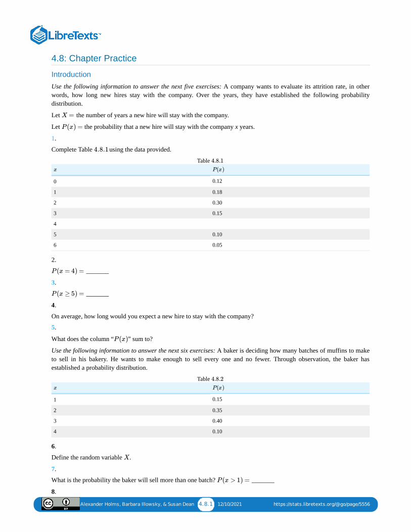
Alexander Holms, Barbara Illowsky, & Susan Dean 4.8.1 12/10/2021 https://stats.libretexts.org/@go/page/5556
4.8: Chapter Practice
Introduction
Use the following information to answer the next five exercises: A company wants to evaluate its attrition rate, in otherwords, how long new hires stay with the company. Over the years, they have established the following probabilitydistribution.
Let the number of years a new hire will stay with the company.
Let the probability that a new hire will stay with the company x years.
1.
Complete Table using the data provided.
0 0.12
1 0.18
2 0.30
3 0.15
4
5 0.10
6 0.05
Table
2.
_______
3.
_______
4.
On average, how long would you expect a new hire to stay with the company?
5.
What does the column “ ” sum to?
Use the following information to answer the next six exercises: A baker is deciding how many batches of muffins to maketo sell in his bakery. He wants to make enough to sell every one and no fewer. Through observation, the baker hasestablished a probability distribution.
1 0.15
2 0.35
3 0.40
4 0.10
Table
6.
Define the random variable .
7.
What is the probability the baker will sell more than one batch? _______
8.
X =
P (x) =
4.8.1
x P(x)
4.8.1
P (x = 4) =
P (x ≥ 5) =
P (x)
x P(x)
4.8.2
X
P (x > 1) =
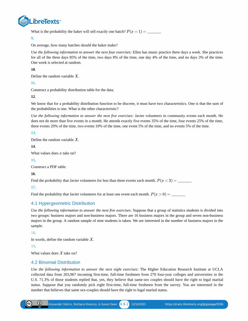
Alexander Holms, Barbara Illowsky, & Susan Dean 4.8.2 12/10/2021 https://stats.libretexts.org/@go/page/5556
What is the probability the baker will sell exactly one batch? _______
9.
On average, how many batches should the baker make?
Use the following information to answer the next four exercises: Ellen has music practice three days a week. She practicesfor all of the three days 85% of the time, two days 8% of the time, one day 4% of the time, and no days 3% of the time.One week is selected at random.
10.
Define the random variable .
11.
Construct a probability distribution table for the data.
12.
We know that for a probability distribution function to be discrete, it must have two characteristics. One is that the sum ofthe probabilities is one. What is the other characteristic?
Use the following information to answer the next five exercises: Javier volunteers in community events each month. Hedoes not do more than five events in a month. He attends exactly five events 35% of the time, four events 25% of the time,three events 20% of the time, two events 10% of the time, one event 5% of the time, and no events 5% of the time.
13.
Define the random variable .
14.
What values does take on?
15.
Construct a PDF table.
16.
Find the probability that Javier volunteers for less than three events each month. _______
17.
Find the probability that Javier volunteers for at least one event each month. _______
4.1 Hypergeometric DistributionUse the following information to answer the next five exercises: Suppose that a group of statistics students is divided intotwo groups: business majors and non-business majors. There are 16 business majors in the group and seven non-businessmajors in the group. A random sample of nine students is taken. We are interested in the number of business majors in thesample.
18.
In words, define the random variable .
19.
What values does take on?
4.2 Binomial DistributionUse the following information to answer the next eight exercises: The Higher Education Research Institute at UCLAcollected data from 203,967 incoming first-time, full-time freshmen from 270 four-year colleges and universities in theU.S. 71.3% of those students replied that, yes, they believe that same-sex couples should have the right to legal maritalstatus. Suppose that you randomly pick eight first-time, full-time freshmen from the survey. You are interested in thenumber that believes that same sex-couples should have the right to legal marital status.
P (x = 1) =
X
X
x
P (x < 3) =
P (x > 0) =
X
X
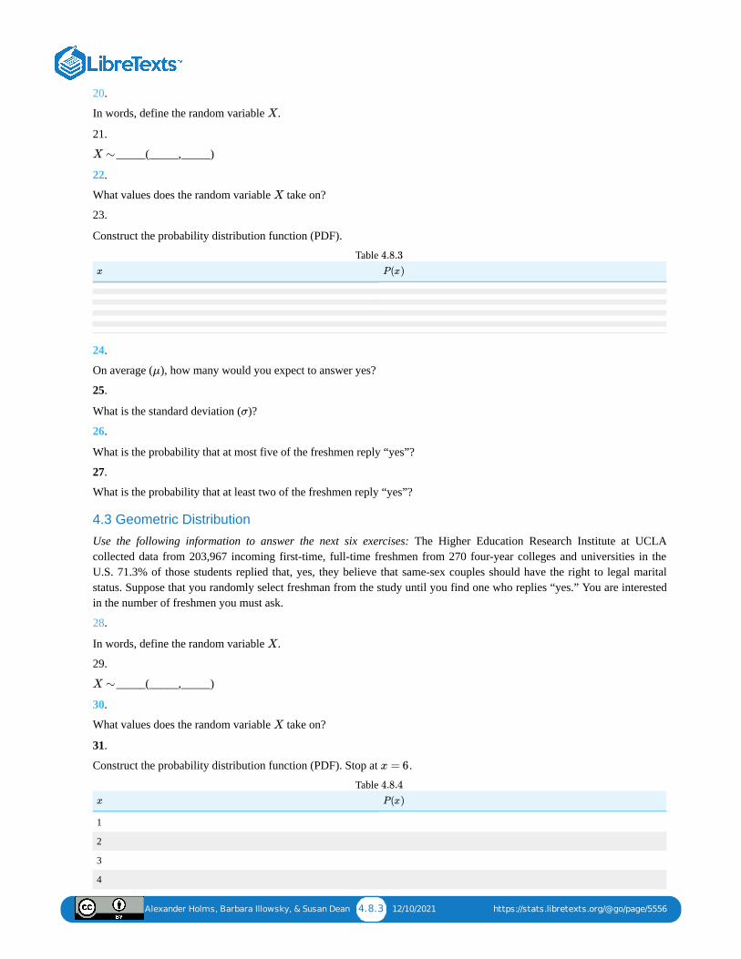
Alexander Holms, Barbara Illowsky, & Susan Dean 4.8.3 12/10/2021 https://stats.libretexts.org/@go/page/5556
20.
In words, define the random variable .
21.
_____(_____,_____)
22.
What values does the random variable take on?
23.
Construct the probability distribution function (PDF).
Table
24.
On average ( ), how many would you expect to answer yes?
25.
What is the standard deviation ( )?
26.
What is the probability that at most five of the freshmen reply “yes”?
27.
What is the probability that at least two of the freshmen reply “yes”?
4.3 Geometric Distribution
Use the following information to answer the next six exercises: The Higher Education Research Institute at UCLAcollected data from 203,967 incoming first-time, full-time freshmen from 270 four-year colleges and universities in theU.S. 71.3% of those students replied that, yes, they believe that same-sex couples should have the right to legal maritalstatus. Suppose that you randomly select freshman from the study until you find one who replies “yes.” You are interestedin the number of freshmen you must ask.
28.
In words, define the random variable .
29.
_____(_____,_____)
30.
What values does the random variable take on?
31.
Construct the probability distribution function (PDF). Stop at .
1
2
3
4
Table
X
X ∼
X
x P(x)
4.8.3
μ
σ
X
X ∼
X
x = 6
x P(x)
4.8.4
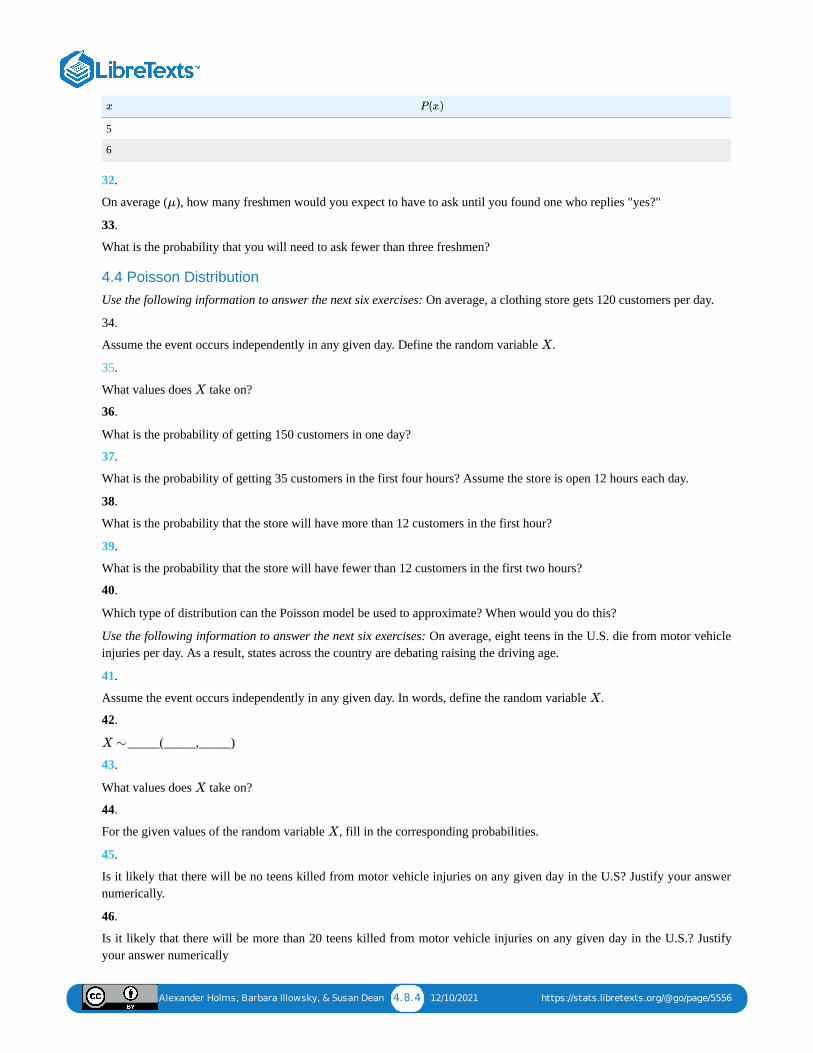
Alexander Holms, Barbara Illowsky, & Susan Dean 4.8.4 12/10/2021 https://stats.libretexts.org/@go/page/5556
5
6
32.
On average ( ), how many freshmen would you expect to have to ask until you found one who replies "yes?"
33.
What is the probability that you will need to ask fewer than three freshmen?
4.4 Poisson DistributionUse the following information to answer the next six exercises: On average, a clothing store gets 120 customers per day.
34.
Assume the event occurs independently in any given day. Define the random variable .
35.
What values does take on?
36.
What is the probability of getting 150 customers in one day?
37.
What is the probability of getting 35 customers in the first four hours? Assume the store is open 12 hours each day.
38.
What is the probability that the store will have more than 12 customers in the first hour?
39.
What is the probability that the store will have fewer than 12 customers in the first two hours?
40.
Which type of distribution can the Poisson model be used to approximate? When would you do this?
Use the following information to answer the next six exercises: On average, eight teens in the U.S. die from motor vehicleinjuries per day. As a result, states across the country are debating raising the driving age.
41.
Assume the event occurs independently in any given day. In words, define the random variable .
42.
_____(_____,_____)
43.
What values does take on?
44.
For the given values of the random variable , fill in the corresponding probabilities.
45.
Is it likely that there will be no teens killed from motor vehicle injuries on any given day in the U.S? Justify your answernumerically.
46.
Is it likely that there will be more than 20 teens killed from motor vehicle injuries on any given day in the U.S.? Justifyyour answer numerically
x P(x)
μ
X
X
X
X ∼
X
X
Alexander Holms, Barbara Illowsky, & Susan Dean 4.9.1 11/5/2021 https://stats.libretexts.org/@go/page/5558
4.9: Chapter References
Binomial Distribution“Access to electricity (% of population),” The World Bank, 2013. Available online athttp://data.worldbank.org/indicator/...first&sort=asc (accessed May 15, 2015).“Distance Education.” Wikipedia. Available online at http://en.Wikipedia.org/wiki/Distance_education (accessed May15, 2013).“NBA Statistics – 2013,” ESPN NBA, 2013. Available online at http://espn.go.com/nba/statistics/_/seasontype/2(accessed May 15, 2013).Newport, Frank. “Americans Still Enjoy Saving Rather than Spending: Few demographic differences seen in theseviews other than by income,” GALLUP® Economy, 2013. Available online athttp://www.gallup.com/poll/162368/am...-spending.aspx (accessed May 15, 2013).Pryor, John H., Linda DeAngelo, Laura Palucki Blake, Sylvia Hurtado, Serge Tran. The American Freshman: NationalNorms Fall 2011. Los Angeles: Cooperative Institutional Research Program at the Higher Education Research Instituteat UCLA, 2011. Also available online at http://heri.ucla.edu/PDFs/pubs/TFS/N...eshman2011.pdf (accessed May 15,2013).“The World FactBook,” Central Intelligence Agency. Available online athttps://www.cia.gov/library/publicat...k/geos/af.html (accessed May 15, 2013).“What are the key statistics about pancreatic cancer?” American Cancer Society, 2013. Available online athttp://www.cancer.org/cancer/pancrea...key-statistics (accessed May 15, 2013).
Geometric Distribution“Millennials: A Portrait of Generation Next,” PewResearchCenter. Available online athttp://www.pewsocialtrends.org/files...-to-change.pdf (accessed May 15, 2013).“Millennials: Confident. Connected. Open to Change.” Executive Summary by PewResearch Social & DemographicTrends, 2013. Available online at http://www.pewsocialtrends.org/2010/...pen-to-change/ (accessed May 15, 2013).“Prevalence of HIV, total (% of populations ages 15-49),” The World Bank, 2013. Available online athttp://data.worldbank.org/indicator/...last&sort=desc (accessed May 15, 2013).Pryor, John H., Linda DeAngelo, Laura Palucki Blake, Sylvia Hurtado, Serge Tran. The American Freshman: NationalNorms Fall 2011.Los Angeles: Cooperative Institutional Research Program at the Higher Education Research Instituteat UCLA, 2011. Also available online at http://heri.ucla.edu/PDFs/pubs/TFS/N...eshman2011.pdf (accessed May 15,2013).“Summary of the National Risk and Vulnerability Assessment 2007/8: A profile of Afghanistan,” The European Unionand ICON-Institute. Available online at ec.europa.eu/europeaid/where/...summary_en.pdf (accessed May 15, 2013).“The World FactBook,” Central Intelligence Agency. Available online athttps://www.cia.gov/library/publicat...k/geos/af.html (accessed May 15, 2013).“UNICEF reports on Female Literacy Centers in Afghanistan established to teach women and girls basic resading [sic]and writing skills,” UNICEF Television. Video available online at http://www.unicefusa.org/assets/vide...y-centers.html(accessed May 15, 2013).
Poisson Distribution“ATL Fact Sheet,” Department of Aviation at the Hartsfield-Jackson Atlanta International Airport, 2013. Availableonline at www.atl.com/about-atl/atl-factsheet/ (accessed February 6, 2019).Center for Disease Control and Prevention. “Teen Drivers: Fact Sheet,” Injury Prevention & Control: Motor VehicleSafety, October 2, 2012. Available online at http://www.cdc.gov/Motorvehiclesafet...factsheet.html (accessed May 15,2013).“Children and Childrearing,” Ministry of Health, Labour, and Welfare. Available online athttp://www.mhlw.go.jp/english/policy...ing/index.html (accessed May 15, 2013).“Eating Disorder Statistics,” South Carolina Department of Mental Health, 2006. Available online athttp://www.state.sc.us/dmh/anorexia/statistics.htm (accessed May 15, 2013).

Alexander Holms, Barbara Illowsky, & Susan Dean 4.9.2 11/5/2021 https://stats.libretexts.org/@go/page/5558
“Giving Birth in Manila: The maternity ward at the Dr Jose Fabella Memorial Hospital in Manila, the busiest in thePhilippines, where there is an average of 60 births a day,” theguardian, 2013. Available online athttp://www.theguardian.com/world/gal...471900&index=2 (accessed May 15, 2013).“How Americans Use Text Messaging,” Pew Internet, 2013. Available online athttp://pewinternet.org/Reports/2011/...in-Report.aspx (accessed May 15, 2013).Lenhart, Amanda. “Teens, Smartphones & Testing: Texting volum is up while the frequency of voice calling is down.About one in four teens say they own smartphones,” Pew Internet, 2012. Available online atwww.pewinternet.org/~/media/F...nd_Texting.pdf (accessed May 15, 2013).“One born every minute: the maternity unit where mothers are THREE to a bed,” MailOnline. Available online athttp://www.dailymail.co.uk/news/arti...thers-bed.html (accessed May 15, 2013).Vanderkam, Laura. “Stop Checking Your Email, Now.” CNNMoney, 2013. Available online atmanagement.fortune.cnn.com/20...our-email-now/ (accessed May 15, 2013).“World Earthquakes: Live Earthquake News and Highlights,” World Earthquakes, 2012. www.world-earthquakes.com/ind...thq_prediction (accessed May 15, 2013).
Alexander Holms, Barbara Illowsky, & Susan
Dean4.10.1 12/31/2021 https://stats.libretexts.org/@go/page/5554
4.10: Chapter Review
Introduction
The characteristics of a probability distribution or density function (PDF) are as follows:
1. Each probability is between zero and one, inclusive (inclusive means to include zero and one).2. The sum of the probabilities is one.
4.1 Hypergeometric DistributionThe combinatorial formula can provide the number of unique subsets of size that can be created from unique objects to
help us calculate probabilities. The combinatorial formula is
A hypergeometric experiment is a statistical experiment with the following properties:
1. You take samples from two groups.2. You are concerned with a group of interest, called the first group.3. You sample without replacement from the combined groups.4. Each pick is not independent, since sampling is without replacement.
The outcomes of a hypergeometric experiment fit a hypergeometric probability distribution. The random variable the
number of items from the group of interest. .
Binomial DistributionA statistical experiment can be classified as a binomial experiment if the following conditions are met:
1. There are a fixed number of trials, .2. There are only two possible outcomes, called "success" and, "failure" for each trial. The letter denotes the probability
of a success on one trial and denotes the probability of a failure on one trial.3. The trials are independent and are repeated using identical conditions.
The outcomes of a binomial experiment fit a binomial probability distribution. The random variable the number ofsuccesses obtained in the independent trials. The mean of can be calculated using the formula , and thestandard deviation is given by the formula .
The formula for the Binomial probability density function is
Geometric Distribution
There are three characteristics of a geometric experiment:
1. There are one or more Bernoulli trials with all failures except the last one, which is a success.2. In theory, the number of trials could go on forever. There must be at least one trial.3. The probability, , of a success and the probability, , of a failure are the same for each trial.
In a geometric experiment, define the discrete random variable as the number of independent trials until the firstsuccess. We say that has a geometric distribution and write where is the probability of success in a singletrial.
The mean of the geometric distribution is where number of trials until first success for theformula where the number of trials is up and including the first success.
An alternative formulation of the geometric distribution asks the question: what is the probability of x failures until thefirst success? In this formulation the trial that resulted in the first success is not counted. The formula for this presentation
x n
( ) =n
x=n Cx
n!x!(n−x)!
X =
h(x) =( )( )
A
x
N−A
n−x
( )N
n
n
p
q
n
X =n X μ = np
σ = npq−−−√
P (x) = ⋅n!
x!(n −x)!pxq(n−x)
p q
X
X X ∼ G(p) p
X ∼ G(p) μ = 1/p x =P (X = x) = (1 −p p)x−1
Alexander Holms, Barbara Illowsky, & Susan
Dean4.10.2 12/31/2021 https://stats.libretexts.org/@go/page/5554
of the geometric is:
The expected value in this form of the geometric distribution is
The easiest way to keep these two forms of the geometric distribution straight is to remember that is the probability ofsuccess and is the probability of failure. In the formula the exponents simply count the number of successes andnumber of failures of the desired outcome of the experiment. Of course the sum of these two numbers must add to thenumber of trials in the experiment.
Poisson DistributionA Poisson probability distribution of a discrete random variable gives the probability of a number of events occurring ina fixed interval of time or space, if these events happen at a known average rate and independently of the time since thelast event. The Poisson distribution may be used to approximate the binomial, if the probability of success is "small" (lessthan or equal to 0.01) and the number of trials is "large" (greater than or equal to 25). Other rules of thumb are alsosuggested by different authors, but all recognize that the Poisson distribution is the limiting distribution of the binomial as
increases and approaches zero.
The formula for computing probabilities that are from a Poisson process is:
where is the probability of successes, (pronounced mu) is the expected number of successes, is the naturallogarithm approximately equal to , and is the number of successes per unit, usually per unit of time.
P (X = x) = p(1 −p)x
μ =1 −p
p
p
(1 −p)
n p
P (x) =μxe−μ
x!
P (X) μ e
2.718 X
Alexander Holms, Barbara Illowsky, & Susan
Dean4.11.1 12/31/2021 https://stats.libretexts.org/@go/page/5559
4.11: Chapter Solution (Practice + Homework)1.
0 0.12
1 0.18
2 0.30
3 0.15
4 0.10
5 0.10
6 0.05
Table
3.
0.10 + 0.05 = 0.15
5.
1
7.
0.35 + 0.40 + 0.10 = 0.85
9.
1(0.15) + 2(0.35) + 3(0.40) + 4(0.10) = 0.15 + 0.70 + 1.20 + 0.40 = 2.45
11.
0 0.03
1 0.04
2 0.08
3 0.85
Table
13.
Let the number of events Javier volunteers for each month.
15.
0 0.05
1 0.05
2 0.10
3 0.20
4 0.25
5 0.35
Table
17.
1 – 0.05 = 0.95
x P(x)
4.11.6
x P(x)
4.11.7
X =
x P(x)
4.11.8
Alexander Holms, Barbara Illowsky, & Susan
Dean4.11.2 12/31/2021 https://stats.libretexts.org/@go/page/5559
18.
the number of business majors in the sample.
19.
2, 3, 4, 5, 6, 7, 8, 9
20.
the number that reply “yes”
22.
0, 1, 2, 3, 4, 5, 6, 7, 8
24.
5.7
26.
0.4151
28.
the number of freshmen selected from the study until one replied "yes" that same-sex couples should have the right tolegal marital status.
30.
1,2,…
32.
1.4
35.
0, 1, 2, 3, 4, …
37.
0.0485
39.
0.0214
41.
the number of U.S. teens who die from motor vehicle injuries per day.
43.
0, 1, 2, 3, 4, ...
45.
No
48.
1. 50.1. 53.
the number of patients calling in claiming to have the flu, who actually have the flu.
55.
0.0165
57.
X =
X =
X =
X =
X =
Alexander Holms, Barbara Illowsky, & Susan
Dean4.11.3 12/31/2021 https://stats.libretexts.org/@go/page/5559
1. 59.
4. 4.43
4
63.
65.1. 67.
1. 69.1. 71.
1. 73.
1. Figure 2. 75.
1. 77.1. 79.
0, 1, 2, and 3
1. 82.1. 84.
Let the number of defective bulbs in a string.
Using the binomial distribution:The Poisson approximation is very good—the difference between theprobabilities is only .
86.
1. 88.1. 90.
1. 92.1. 94.
4
4.11.4
X =
0.0026

1 1/7/2022
CHAPTER OVERVIEW5: CONTINUOUS RANDOM VARIABLES
5.0: PRELUDE TO CONTINUOUS RANDOM VARIABLES5.1: PROPERTIES OF CONTINUOUS PROBABILITY DENSITY FUNCTIONS5.2: THE UNIFORM DISTRIBUTION5.3: THE EXPONENTIAL DISTRIBUTION5.4: CHAPTER FORMULA REVIEW5.5: CHAPTER HOMEWORK5.6: CHAPTER KEY TERMS5.7: CHAPTER PRACTICE5.8: CHAPTER REFERENCES5.9: CHAPTER REVIEW5.10: CHAPTER SOLUTION (PRACTICE + HOMEWORK)

Alexander Holms, Barbara Illowsky, & Susan Dean 5.0.1 12/10/2021 https://stats.libretexts.org/@go/page/4571
5.0: Prelude to Continuous Random VariablesContinuous random variables have many applications. Baseball batting averages, IQ scores, the length of time a longdistance telephone call lasts, the amount of money a person carries, the length of time a computer chip lasts, rates of returnfrom an investment, and SAT scores are just a few. The field of reliability depends on a variety of continuous randomvariables, as do all areas of risk analysis.
Figure The heights of these radish plants are continuous random variables. (Credit: Rev Stan)
The values of discrete and continuous random variables can be ambiguous. For example, if is equal to the numberof miles (to the nearest mile) you drive to work, then is a discrete random variable. You count the miles. If is thedistance you drive to work, then you measure values of and is a continuous random variable. For a secondexample, if is equal to the number of books in a backpack, then is a discrete random variable. If is the weightof a book, then is a continuous random variable because weights are measured. How the random variable is definedis very important.
5.0.1
Note
X
X X
X X
X X X
X
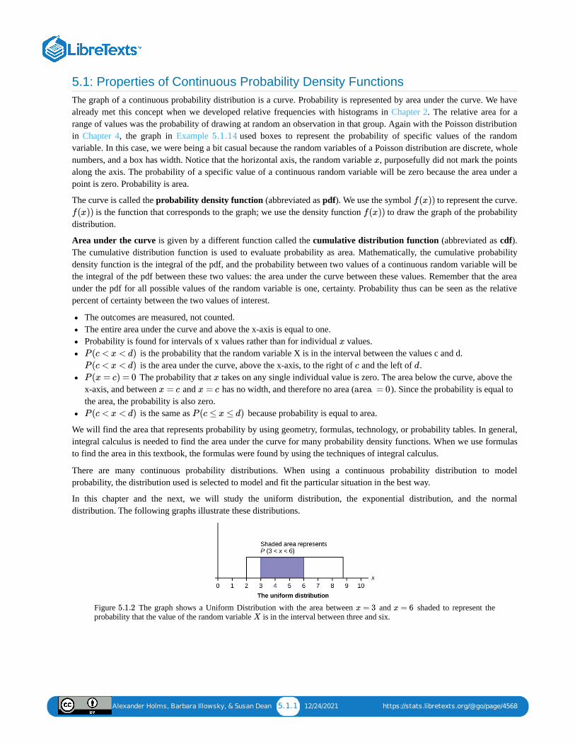
Alexander Holms, Barbara Illowsky, & Susan Dean 5.1.1 12/24/2021 https://stats.libretexts.org/@go/page/4568
5.1: Properties of Continuous Probability Density FunctionsThe graph of a continuous probability distribution is a curve. Probability is represented by area under the curve. We havealready met this concept when we developed relative frequencies with histograms in Chapter 2. The relative area for arange of values was the probability of drawing at random an observation in that group. Again with the Poisson distributionin Chapter 4, the graph in Example used boxes to represent the probability of specific values of the randomvariable. In this case, we were being a bit casual because the random variables of a Poisson distribution are discrete, wholenumbers, and a box has width. Notice that the horizontal axis, the random variable , purposefully did not mark the pointsalong the axis. The probability of a specific value of a continuous random variable will be zero because the area under apoint is zero. Probability is area.
The curve is called the probability density function (abbreviated as pdf). We use the symbol to represent the curve. is the function that corresponds to the graph; we use the density function to draw the graph of the probability
distribution.
Area under the curve is given by a different function called the cumulative distribution function (abbreviated as cdf).The cumulative distribution function is used to evaluate probability as area. Mathematically, the cumulative probabilitydensity function is the integral of the pdf, and the probability between two values of a continuous random variable will bethe integral of the pdf between these two values: the area under the curve between these values. Remember that the areaunder the pdf for all possible values of the random variable is one, certainty. Probability thus can be seen as the relativepercent of certainty between the two values of interest.
The outcomes are measured, not counted.The entire area under the curve and above the x-axis is equal to one.Probability is found for intervals of x values rather than for individual values.
is the probability that the random variable X is in the interval between the values c and d. is the area under the curve, above the x-axis, to the right of and the left of . The probability that takes on any single individual value is zero. The area below the curve, above the
x-axis, and between and has no width, and therefore no area ( ). Since the probability is equal tothe area, the probability is also zero.
is the same as because probability is equal to area.
We will find the area that represents probability by using geometry, formulas, technology, or probability tables. In general,integral calculus is needed to find the area under the curve for many probability density functions. When we use formulasto find the area in this textbook, the formulas were found by using the techniques of integral calculus.
There are many continuous probability distributions. When using a continuous probability distribution to modelprobability, the distribution used is selected to model and fit the particular situation in the best way.
In this chapter and the next, we will study the uniform distribution, the exponential distribution, and the normaldistribution. The following graphs illustrate these distributions.
Figure The graph shows a Uniform Distribution with the area between and shaded to represent theprobability that the value of the random variable is in the interval between three and six.
5.1.14
x
f(x))
f(x)) f(x))
x
P (c < x < d)
P (c < x < d) c d
P (x = c) = 0 x
x = c x = c area = 0
P (c < x < d) P (c ≤ x ≤ d)
5.1.2 x = 3 x = 6X
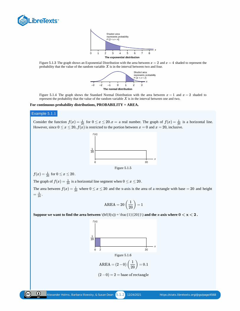
Alexander Holms, Barbara Illowsky, & Susan Dean 5.1.2 12/24/2021 https://stats.libretexts.org/@go/page/4568
Figure The graph shows an Exponential Distribution with the area between and shaded to represent theprobability that the value of the random variable is in the interval between two and four.
Figure The graph shows the Standard Normal Distribution with the area between and shaded torepresent the probability that the value of the random variable is in the interval between one and two.
For continuous probability distributions, PROBABILITY = AREA.
Consider the function for a real number. The graph of is a horizontal line.However, since is restricted to the portion between and , inclusive.
Figure
for .
The graph of is a horizontal line segment when .
The area between where and the x-axis is the area of a rectangle with base and height .
Suppose we want to find the area between \(bf{f(x)) = \frac{1}{20}}\) and the x-axis where .
Figure
5.1.3 x = 2 x = 4X
5.1.4 x = 1 x = 2X
Example 5.1.1
f(x) = 120
0 ≤ x ≤ 20.x = f(x) = 120
0 ≤ x ≤ 20, f(x) x = 0 x = 20
5.1.5
f(x) = 120
0 ≤ x ≤ 20
f(x) = 120
0 ≤ x ≤ 20
f(x) = 120
0 ≤ x ≤ 20 = 20
= 120
AREA = 20( ) = 11
20
0 < x < 2
5.1.6
AREA = (2 −0)( ) = 0.11
20
(2 −0) = 2 = base of rectangle
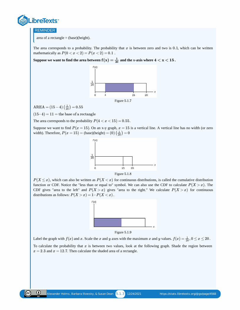
Alexander Holms, Barbara Illowsky, & Susan Dean 5.1.3 12/24/2021 https://stats.libretexts.org/@go/page/4568
area of a rectangle = (base)(height).
The area corresponds to a probability. The probability that is between zero and two is , which can be writtenmathematically as .
Suppose we want to find the area between and the x-axis where .
Figure
The area corresponds to the probability .
Suppose we want to find . On an x-y graph, is a vertical line. A vertical line has no width (or zerowidth). Therefore, (base)(height)
Figure
, which can also be written as for continuous distributions, is called the cumulative distributionfunction or CDF. Notice the "less than or equal to" symbol. We can also use the CDF to calculate . TheCDF gives "area to the left" and gives "area to the right." We calculate for continuousdistributions as follows: .
Figure
Label the graph with and . Scale the and axes with the maximum and values. .
To calculate the probability that is between two values, look at the following graph. Shade the region between and . Then calculate the shaded area of a rectangle.
REMINDER
x 0.1
P (0 < x < 2) = P (x < 2) = 0.1
f (x) = 120
4 < x < 15
5.1.7
AREA = (15 −4)( ) = 0.55120
(15– 4) = 11 = the base of a rectangle
P (4 < x < 15) = 0.55
P (x = 15) x = 15
P (x = 15) = = (0)( ) = 0120
5.1.8
P (X ≤ x) P (X < x)
P (X > x)
P (X > x) P (X > x)
P (X > x) = 1–P (X < x)
5.1.9
f(x) x x y x y f(x) = , 0 ≤ x ≤ 20120
x
x = 2.3 x = 12.7
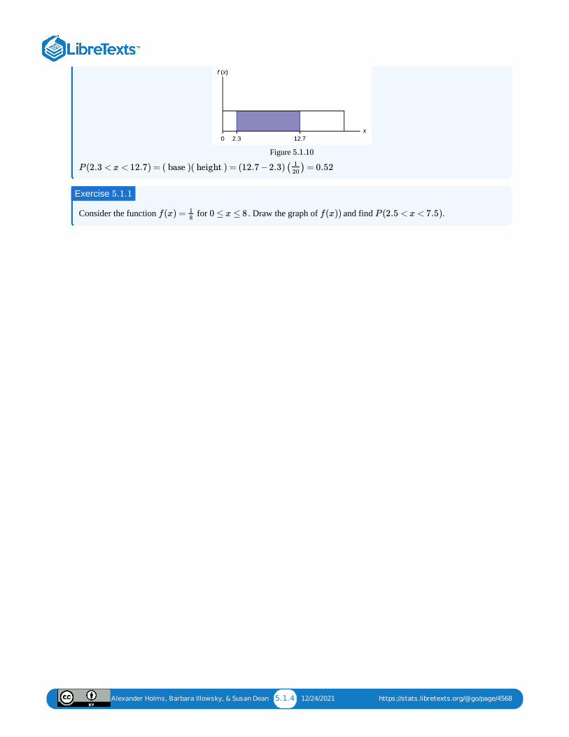
Alexander Holms, Barbara Illowsky, & Susan Dean 5.1.4 12/24/2021 https://stats.libretexts.org/@go/page/4568
Figure
Consider the function for . Draw the graph of and find .
5.1.10
P (2.3 < x < 12.7) = ( base )( height ) = (12.7 −2.3)( ) = 0.52120
Exercise 5.1.1
f(x) = 18
0 ≤ x ≤ 8 f(x)) P (2.5 < x < 7.5)
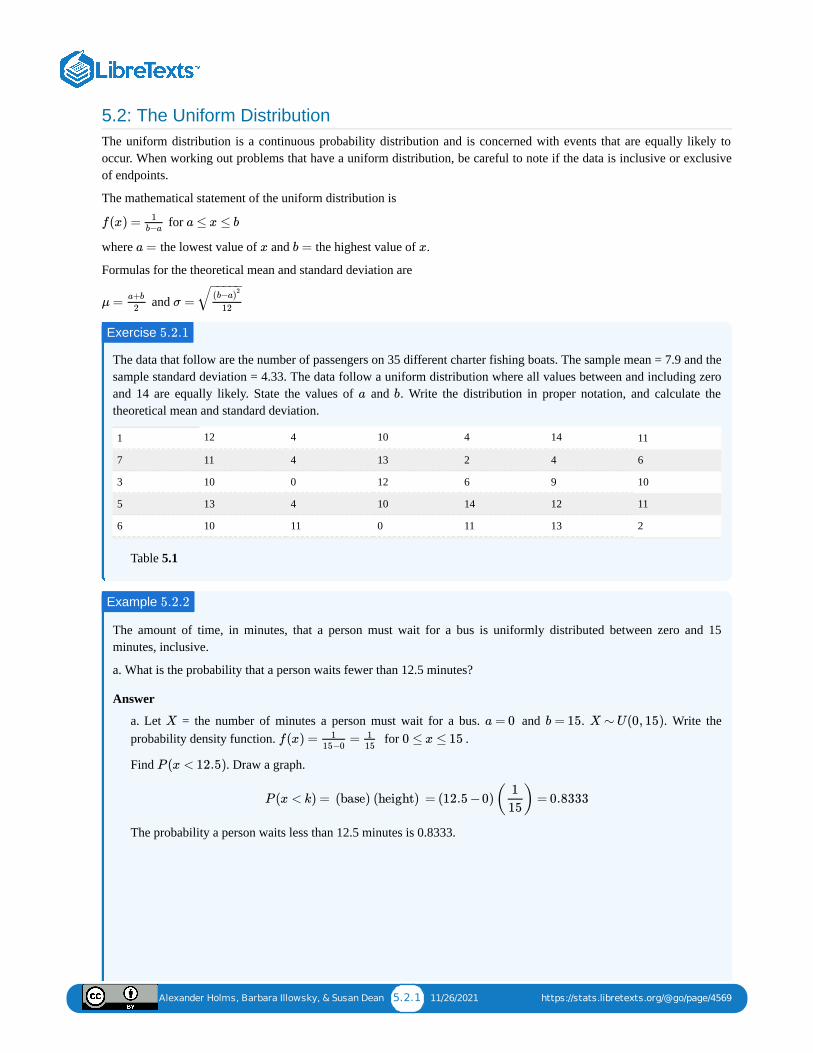
Alexander Holms, Barbara Illowsky, & Susan Dean 5.2.1 11/26/2021 https://stats.libretexts.org/@go/page/4569
5.2: The Uniform DistributionThe uniform distribution is a continuous probability distribution and is concerned with events that are equally likely tooccur. When working out problems that have a uniform distribution, be careful to note if the data is inclusive or exclusiveof endpoints.
The mathematical statement of the uniform distribution is
for
where the lowest value of and the highest value of .
Formulas for the theoretical mean and standard deviation are
and
The data that follow are the number of passengers on 35 different charter fishing boats. The sample mean = 7.9 and thesample standard deviation = 4.33. The data follow a uniform distribution where all values between and including zeroand 14 are equally likely. State the values of and . Write the distribution in proper notation, and calculate thetheoretical mean and standard deviation.
1 12 4 10 4 14 11
7 11 4 13 2 4 6
3 10 0 12 6 9 10
5 13 4 10 14 12 11
6 10 11 0 11 13 2
Table 5.1
The amount of time, in minutes, that a person must wait for a bus is uniformly distributed between zero and 15minutes, inclusive.
a. What is the probability that a person waits fewer than 12.5 minutes?
Answer
a. Let = the number of minutes a person must wait for a bus. and . . Write theprobability density function. for .
Find . Draw a graph.
The probability a person waits less than 12.5 minutes is 0.8333.
f(x) = 1b−a
a ≤ x ≤ b
a = x b = x
μ =a+b
2σ =
(b−a)2
12
− −−−−√
Exercise 5.2.1
a b
Example 5.2.2
X a = 0 b = 15 X ∼ U(0, 15)
f(x) = =115−0
115
0 ≤ x ≤ 15
P (x < 12.5)
P (x < k) = (base) (height) = (12.5 −0)( ) = 0.83331
15
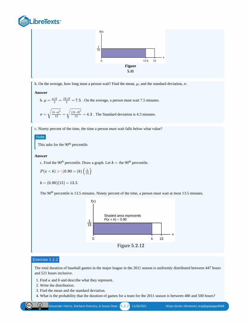
Alexander Holms, Barbara Illowsky, & Susan Dean 5.2.2 11/26/2021 https://stats.libretexts.org/@go/page/4569
Figure5.11
b. On the average, how long must a person wait? Find the mean, , and the standard deviation, .
Answer
b. . On the average, a person must wait 7.5 minutes.
. The Standard deviation is 4.3 minutes.
c. Ninety percent of the time, the time a person must wait falls below what value?
This asks for the 90 percentile.
Answer
c. Find the 90 percentile. Draw a graph. Let the 90 percentile.
The 90 percentile is 13.5 minutes. Ninety percent of the time, a person must wait at most 13.5 minutes.
Figure
The total duration of baseball games in the major league in the 2011 season is uniformly distributed between 447 hoursand 521 hours inclusive.
1. Find and and describe what they represent.2. Write the distribution.3. Find the mean and the standard deviation.4. What is the probability that the duration of games for a team for the 2011 season is between 480 and 500 hours?
μ σ
μ = = = 7.5a+b
2
15+0
2
σ = = = 4.3(b−a)
2
12
− −−−−√ (15−θ)
2
12
− −−−−√
Note
th
th k = th
P (x < k) > \(0.90 = (k)( )115
k = (0.90)(15) = 13.5
th
5.2.12
Exercise 5.2.2
a b
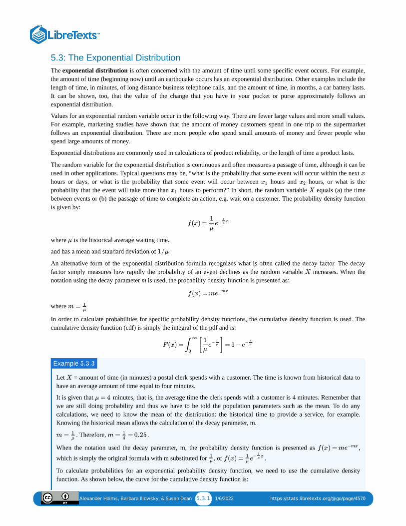
Alexander Holms, Barbara Illowsky, & Susan Dean 5.3.1 1/6/2022 https://stats.libretexts.org/@go/page/4570
5.3: The Exponential DistributionThe exponential distribution is often concerned with the amount of time until some specific event occurs. For example,the amount of time (beginning now) until an earthquake occurs has an exponential distribution. Other examples include thelength of time, in minutes, of long distance business telephone calls, and the amount of time, in months, a car battery lasts.It can be shown, too, that the value of the change that you have in your pocket or purse approximately follows anexponential distribution.
Values for an exponential random variable occur in the following way. There are fewer large values and more small values.For example, marketing studies have shown that the amount of money customers spend in one trip to the supermarketfollows an exponential distribution. There are more people who spend small amounts of money and fewer people whospend large amounts of money.
Exponential distributions are commonly used in calculations of product reliability, or the length of time a product lasts.
The random variable for the exponential distribution is continuous and often measures a passage of time, although it can beused in other applications. Typical questions may be, “what is the probability that some event will occur within the next hours or days, or what is the probability that some event will occur between hours and hours, or what is theprobability that the event will take more than hours to perform?” In short, the random variable equals (a) the timebetween events or (b) the passage of time to complete an action, e.g. wait on a customer. The probability density functionis given by:
where is the historical average waiting time.
and has a mean and standard deviation of .
An alternative form of the exponential distribution formula recognizes what is often called the decay factor. The decayfactor simply measures how rapidly the probability of an event declines as the random variable increases. When thenotation using the decay parameter m is used, the probability density function is presented as:
where
In order to calculate probabilities for specific probability density functions, the cumulative density function is used. Thecumulative density function (cdf) is simply the integral of the pdf and is:
Let = amount of time (in minutes) a postal clerk spends with a customer. The time is known from historical data tohave an average amount of time equal to four minutes.
It is given that minutes, that is, the average time the clerk spends with a customer is 4 minutes. Remember thatwe are still doing probability and thus we have to be told the population parameters such as the mean. To do anycalculations, we need to know the mean of the distribution: the historical time to provide a service, for example.Knowing the historical mean allows the calculation of the decay parameter, m.
. Therefore, .
When the notation used the decay parameter, m, the probability density function is presented as ,
which is simply the original formula with m substituted for , or .
To calculate probabilities for an exponential probability density function, we need to use the cumulative densityfunction. As shown below, the curve for the cumulative density function is:
x
x1 x2
x1 X
f(x) =1
μe− x1
μ
μ
1/μ
X
f(x) = me−mx
m = 1μ
F (x) = [ ] = 1 −∫∞
0
1
μe−
x
μ e−x
μ
Example 5.3.3
X
μ = 4
m = 1μ
m = = 0.2514
f(x) = me−mx
1μ f(x) = 1
μ e− x1μ
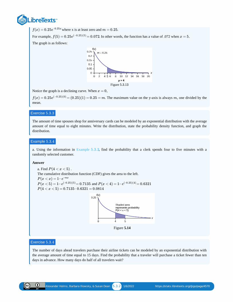
Alexander Holms, Barbara Illowsky, & Susan Dean 5.3.2 1/6/2022 https://stats.libretexts.org/@go/page/4570
where x is at least zero and .
For example, . In other words, the function has a value of .072 when .
The graph is as follows:
Figure
Notice the graph is a declining curve. When ,
. The maximum value on the y-axis is always , one divided by themean.
The amount of time spouses shop for anniversary cards can be modeled by an exponential distribution with the averageamount of time equal to eight minutes. Write the distribution, state the probability density function, and graph thedistribution.
a. Using the information in Example , find the probability that a clerk spends four to five minutes with arandomly selected customer.
Answer
a. Find . The cumulative distribution function (CDF) gives the area to the left.
and
Figure 5.14
The number of days ahead travelers purchase their airline tickets can be modeled by an exponential distribution withthe average amount of time equal to 15 days. Find the probability that a traveler will purchase a ticket fewer than tendays in advance. How many days do half of all travelers wait?
f(x) = 0.25e–0.25x m = 0.25
f(5) = 0.25 = 0.072e(−0.25)(5) x = 5
5.3.13
x = 0
f(x) = 0.25 = (0.25)(1) = 0.25 = me(−0.25)(0) m
Exercise 5.3.3
Example 5.3.4
5.3.3
P (4 < x < 5)
P (x < x) = 1– e–mx
P (x < 5) = 1– = 0.7135e(–0.25)(5) P (x < 4) = 1– = 0.6321e(–0.25)(4)
P (4 < x < 5) = 0.7135– 0.6321 = 0.0814
Exercise 5.3.4
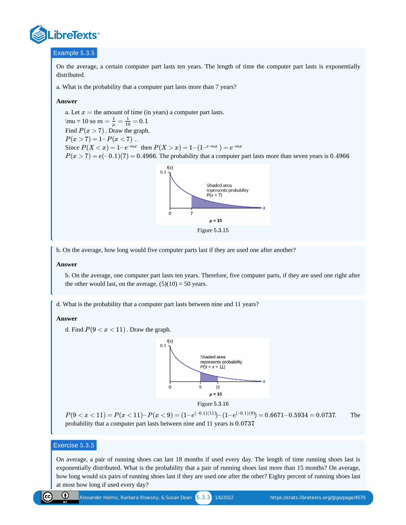
Alexander Holms, Barbara Illowsky, & Susan Dean 5.3.3 1/6/2022 https://stats.libretexts.org/@go/page/4570
On the average, a certain computer part lasts ten years. The length of time the computer part lasts is exponentiallydistributed.
a. What is the probability that a computer part lasts more than 7 years?
Answer
a. Let the amount of time (in years) a computer part lasts. \mu = 10 so Find . Draw the graph.
. Since then
. The probability that a computer part lasts more than seven years is .
Figure
b. On the average, how long would five computer parts last if they are used one after another?
Answer
b. On the average, one computer part lasts ten years. Therefore, five computer parts, if they are used one right afterthe other would last, on the average, (5)(10) = 50 years.
d. What is the probability that a computer part lasts between nine and 11 years?
Answer
d. Find . Draw the graph.
Figure
. Theprobability that a computer part lasts between nine and 11 years is .
On average, a pair of running shoes can last 18 months if used every day. The length of time running shoes last isexponentially distributed. What is the probability that a pair of running shoes last more than 15 months? On average,how long would six pairs of running shoes last if they are used one after the other? Eighty percent of running shoes lastat most how long if used every day?
Example 5.3.5
x =
m = = = 0.11μ
110
P (x > 7)
P (x > 7) = 1– P (x < 7)
P (X < x) = 1– e–mx P (X > x) = 1– (1 ) =–e–mx e–mx
P (x > 7) = e(– 0.1)(7) = 0.4966 0.4966
5.3.15
P (9 < x < 11)
5.3.16
P (9 < x < 11) = P (x < 11)– P (x < 9) = (1– )– (1– ) = 0.6671– 0.5934 = 0.0737e(–0.1)(11) e(–0.1)(9)
0.0737
Exercise 5.3.5
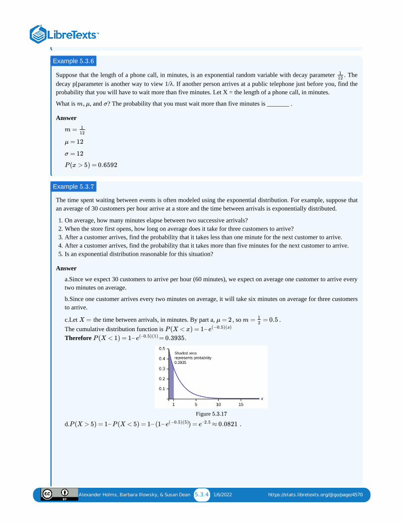
Alexander Holms, Barbara Illowsky, & Susan Dean 5.3.4 1/6/2022 https://stats.libretexts.org/@go/page/4570
Suppose that the length of a phone call, in minutes, is an exponential random variable with decay parameter . Thedecay p[parameter is another way to view 1/λ. If another person arrives at a public telephone just before you, find theprobability that you will have to wait more than five minutes. Let X = the length of a phone call, in minutes.
What is , and ? The probability that you must wait more than five minutes is _______ .
Answer
The time spent waiting between events is often modeled using the exponential distribution. For example, suppose thatan average of 30 customers per hour arrive at a store and the time between arrivals is exponentially distributed.
1. On average, how many minutes elapse between two successive arrivals?2. When the store first opens, how long on average does it take for three customers to arrive?3. After a customer arrives, find the probability that it takes less than one minute for the next customer to arrive.4. After a customer arrives, find the probability that it takes more than five minutes for the next customer to arrive.5. Is an exponential distribution reasonable for this situation?
Answer
a.Since we expect 30 customers to arrive per hour (60 minutes), we expect on average one customer to arrive everytwo minutes on average.
b.Since one customer arrives every two minutes on average, it will take six minutes on average for three customersto arrive.
c.Let the time between arrivals, in minutes. By part a, , so . The cumulative distribution function is Therefore .
Figure
d. .
Example 5.3.6
112
m, μ σ
m = 112
μ = 12
σ = 12
P (x > 5) = 0.6592
Example 5.3.7
X = μ = 2 m = = 0.512
P (X < x) = 1– e(−0.5)(x)
P (X < 1) = 1– = 0.3935e(–0.5)(1)
5.3.17
P (X > 5) = 1– P (X < 5) = 1– (1– ) = ≈ 0.0821e(−0.5)(5) e–2.5
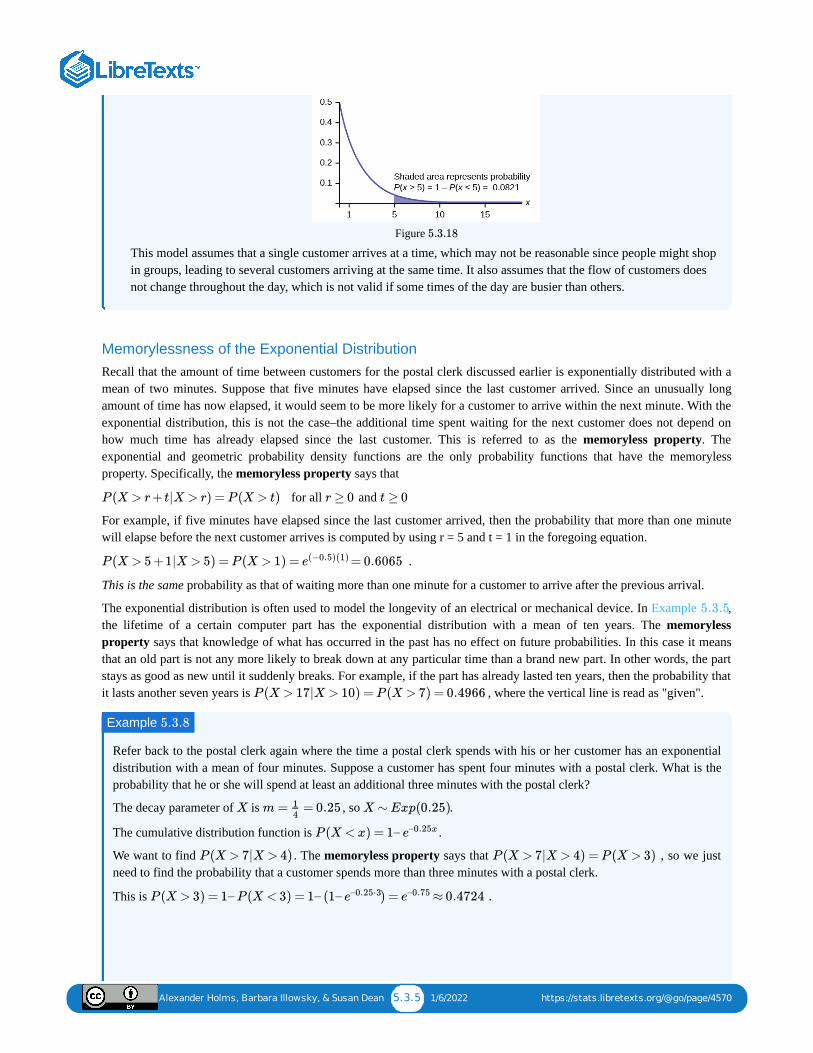
Alexander Holms, Barbara Illowsky, & Susan Dean 5.3.5 1/6/2022 https://stats.libretexts.org/@go/page/4570
Figure
This model assumes that a single customer arrives at a time, which may not be reasonable since people might shopin groups, leading to several customers arriving at the same time. It also assumes that the flow of customers doesnot change throughout the day, which is not valid if some times of the day are busier than others.
Memorylessness of the Exponential DistributionRecall that the amount of time between customers for the postal clerk discussed earlier is exponentially distributed with amean of two minutes. Suppose that five minutes have elapsed since the last customer arrived. Since an unusually longamount of time has now elapsed, it would seem to be more likely for a customer to arrive within the next minute. With theexponential distribution, this is not the case–the additional time spent waiting for the next customer does not depend onhow much time has already elapsed since the last customer. This is referred to as the memoryless property. Theexponential and geometric probability density functions are the only probability functions that have the memorylessproperty. Specifically, the memoryless property says that
for all and
For example, if five minutes have elapsed since the last customer arrived, then the probability that more than one minutewill elapse before the next customer arrives is computed by using r = 5 and t = 1 in the foregoing equation.
.
This is the same probability as that of waiting more than one minute for a customer to arrive after the previous arrival.
The exponential distribution is often used to model the longevity of an electrical or mechanical device. In Example ,the lifetime of a certain computer part has the exponential distribution with a mean of ten years. The memorylessproperty says that knowledge of what has occurred in the past has no effect on future probabilities. In this case it meansthat an old part is not any more likely to break down at any particular time than a brand new part. In other words, the partstays as good as new until it suddenly breaks. For example, if the part has already lasted ten years, then the probability thatit lasts another seven years is , where the vertical line is read as "given".
Refer back to the postal clerk again where the time a postal clerk spends with his or her customer has an exponentialdistribution with a mean of four minutes. Suppose a customer has spent four minutes with a postal clerk. What is theprobability that he or she will spend at least an additional three minutes with the postal clerk?
The decay parameter of is , so .
The cumulative distribution function is .
We want to find . The memoryless property says that , so we justneed to find the probability that a customer spends more than three minutes with a postal clerk.
This is .
5.3.18
P (X > r + t|X > r) = P (X > t) r ≥ 0 t ≥ 0
P (X > 5 +1|X > 5) = P (X > 1) = = 0.6065e(−0.5)(1)
5.3.5
P (X > 17|X > 10) = P (X > 7) = 0.4966
Example 5.3.8
X m = = 0.2514
X ∼ Exp(0.25)
P (X < x) = 1– e–0.25x
P (X > 7|X > 4) P (X > 7|X > 4) = P (X > 3)
P (X > 3) = 1– P (X < 3) = 1– (1– ) = ≈ 0.4724e–0.25⋅3 e–0.75
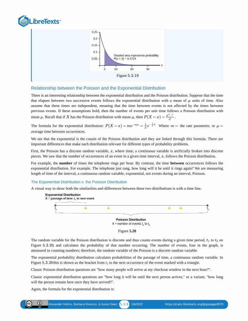
Alexander Holms, Barbara Illowsky, & Susan Dean 5.3.6 1/6/2022 https://stats.libretexts.org/@go/page/4570
Figure
Relationship between the Poisson and the Exponential Distribution
There is an interesting relationship between the exponential distribution and the Poisson distribution. Suppose that the timethat elapses between two successive events follows the exponential distribution with a mean of units of time. Alsoassume that these times are independent, meaning that the time between events is not affected by the times betweenprevious events. If these assumptions hold, then the number of events per unit time follows a Poisson distribution withmean . Recall that if has the Poisson distribution with mean , then .
The formula for the exponential distribution: Where the rate parameter, or average time between occurrences.
We see that the exponential is the cousin of the Poisson distribution and they are linked through this formula. There areimportant differences that make each distribution relevant for different types of probability problems.
First, the Poisson has a discrete random variable, , where time; a continuous variable is artificially broken into discretepieces. We saw that the number of occurrences of an event in a given time interval, , follows the Poisson distribution.
For example, the number of times the telephone rings per hour. By contrast, the time between occurrences follows theexponential distribution. For example. The telephone just rang, how long will it be until it rings again? We are measuringlength of time of the interval, a continuous random variable, exponential, not events during an interval, Poisson.
The Exponential Distribution v. the Poisson Distribution
A visual way to show both the similarities and differences between these two distributions is with a time line.
Figure 5.20
The random variable for the Poisson distribution is discrete and thus counts events during a given time period, to onFigure , and calculates the probability of that number occurring. The number of events, four in the graph, ismeasured in counting numbers; therefore, the random variable of the Poisson is a discrete random variable.
The exponential probability distribution calculates probabilities of the passage of time, a continuous random variable. InFigure this is shown as the bracket from t to the next occurrence of the event marked with a triangle.
Classic Poisson distribution questions are "how many people will arrive at my checkout window in the next hour?".
Classic exponential distribution questions are "how long it will be until the next person arrives," or a variant, "how longwill the person remain here once they have arrived?".
Again, the formula for the exponential distribution is:
5.3.19
μ
μ X μ P (X = x) =μ −μxe
x!
P (X = x) = m =e−mx 1μ e− x
1μ m = μ =
x
x
t1 t2
5.3.20
5.3.20 1
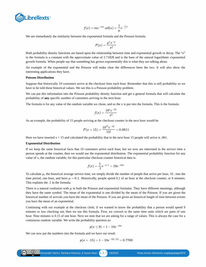
Alexander Holms, Barbara Illowsky, & Susan Dean 5.3.7 1/6/2022 https://stats.libretexts.org/@go/page/4570
We see immediately the similarity between the exponential formula and the Poisson formula.
Both probability density functions are based upon the relationship between time and exponential growth or decay. The “e”in the formula is a constant with the approximate value of 2.71828 and is the base of the natural logarithmic exponentialgrowth formula. When people say that something has grown exponentially this is what they are talking about.
An example of the exponential and the Poisson will make clear the differences been the two. It will also show theinteresting applications they have.
Poisson Distribution
Suppose that historically 10 customers arrive at the checkout lines each hour. Remember that this is still probability so wehave to be told these historical values. We see this is a Poisson probability problem.
We can put this information into the Poisson probability density function and get a general formula that will calculate theprobability of any specific number of customers arriving in the next hour.
The formula is for any value of the random variable we chose, and so the x is put into the formula. This is the formula:
As an example, the probability of 15 people arriving at the checkout counter in the next hour would be
Here we have inserted x = 15 and calculated the probability that in the next hour 15 people will arrive is .061.
Exponential Distribution
If we keep the same historical facts that 10 customers arrive each hour, but we now are interested in the service time aperson spends at the counter, then we would use the exponential distribution. The exponential probability function for anyvalue of x, the random variable, for this particular checkout counter historical data is:
To calculate , the historical average service time, we simply divide the number of people that arrive per hour, 10 , into thetime period, one hour, and have . Historically, people spend 0.1 of an hour at the checkout counter, or 6 minutes.This explains the .1 in the formula.
There is a natural confusion with in both the Poisson and exponential formulas. They have different meanings, althoughthey have the same symbol. The mean of the exponential is one divided by the mean of the Poisson. If you are given thehistorical number of arrivals you have the mean of the Poisson. If you are given an historical length of time between eventsyou have the mean of an exponential.
Continuing with our example at the checkout clerk; if we wanted to know the probability that a person would spend 9minutes or less checking out, then we use this formula. First, we convert to the same time units which are parts of onehour. Nine minutes is 0.15 of one hour. Next we note that we are asking for a range of values. This is always the case for acontinuous random variable. We write the probability question as:
We can now put the numbers into the formula and we have our result.
f(x) = m orf(x) =e−mx 1
μe
− x1μ
P (x) =μxe−μ
x!
f(x) =10xe−10
x!
P (x = 15) = = 0.06111015e−10
15!
f(x) = = 101
.1e−x/1 e−10x
μ
μ = 0.1
μ
p(x ≤ 9) = 1 −10e−10x
p(x = .15) = 1 −10 = 0.7769e−10(.15)

Alexander Holms, Barbara Illowsky, & Susan Dean 5.3.8 1/6/2022 https://stats.libretexts.org/@go/page/4570
The probability that a customer will spend 9 minutes or less checking out is .
We see that we have a high probability of getting out in less than nine minutes and a tiny probability of having 15customers arriving in the next hour.
0.7769
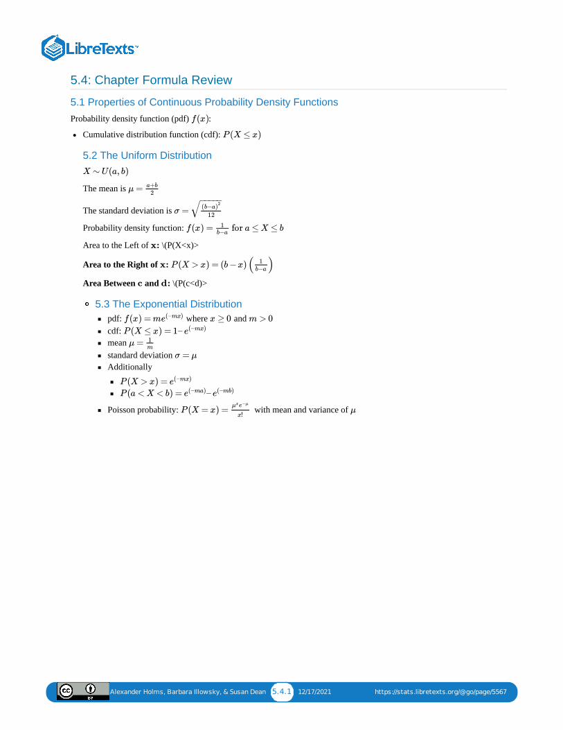
Alexander Holms, Barbara Illowsky, & Susan Dean 5.4.1 12/17/2021 https://stats.libretexts.org/@go/page/5567
5.4: Chapter Formula Review
5.1 Properties of Continuous Probability Density Functions
Probability density function (pdf) :
Cumulative distribution function (cdf):
5.2 The Uniform Distribution
The mean is
The standard deviation is
Probability density function:
Area to the Left of : \(P(X<x)>
Area to the Right of :
Area Between and : \(P(c<d)>
5.3 The Exponential Distributionpdf: where and cdf: mean standard deviation Additionally
Poisson probability: with mean and variance of
f(x)
P (X ≤ x)
X ∼ U(a, b)
μ = a+b
2
σ =(b−a)
2
12
− −−−−√
f(x) = for a ≤ X ≤ b1b−a
x
x P (X > x) = (b −x)( )1b−a
c d
f(x) = me(–mx) x ≥ 0 m > 0
P (X ≤ x) = 1– e(–mx)
μ = 1m
σ = μ
P (X > x) = e(–mx)
P (a < X < b) = –e(–ma) e(–mb)
P (X = x) =μxe−μ
x!μ
Alexander Holms, Barbara Illowsky, & Susan Dean 5.5.1 1/6/2022 https://stats.libretexts.org/@go/page/5569
5.5: Chapter Homework
5.1 Properties of Continuous Probability Density Functions
For each probability and percentile problem, draw the picture.
70.
Consider the following experiment. You are one of 100 people enlisted to take part in a study to determine the percent ofnurses in America with an R.N. (registered nurse) degree. You ask nurses if they have an R.N. degree. The nurses answer“yes” or “no.” You then calculate the percentage of nurses with an R.N. degree. You give that percentage to yoursupervisor.
1. For each probability and percentile problem, draw the picture.72.
Births are approximately uniformly distributed between the 52 weeks of the year. They can be said to follow a uniformdistribution from one to 53 (spread of 52 weeks).
1. Use the following information to answer the next three exercises. The Sky Train from the terminal to the rental–carand long–term parking center is supposed to arrive every eight minutes. The waiting times for the train are knownto follow a uniform distribution.77.
What is the average waiting time (in minutes)?
a. Use the following information to answer the next three exercises. The average lifetime of a certain new cellphone is three years. The manufacturer will replace any cell phone failing within two years of the date ofpurchase. The lifetime of these cell phones is known to follow an exponential distribution.88.
The decay rate is:
a. 0.3333b. 0.5000c. 2d. 3
89.
What is the probability that a phone will fail within two years of the date of purchase?
a. 0.8647b. 0.4866c. 0.2212d. 0.9997
90.
What is the median lifetime of these phones (in years)?
a. 0.1941b. 1.3863c. 2.0794d. 5.5452
91.
At a 911 call center, calls come in at an average rate of one call every two minutes. Assume that the time thatelapses from one call to the next has the exponential distribution.
1. On average, how much time occurs between five consecutive calls?2. Find the probability that after a call is received, it takes more than three minutes for the next call to occur.3. Ninety-percent of all calls occur within how many minutes of the previous call?4. Suppose that two minutes have elapsed since the last call. Find the probability that the next call will occur
within the next minute.5. Find the probability that less than 20 calls occur within an hour.
Alexander Holms, Barbara Illowsky, & Susan Dean 5.5.2 1/6/2022 https://stats.libretexts.org/@go/page/5569
92.
In major league baseball, a no-hitter is a game in which a pitcher, or pitchers, doesn't give up any hits throughoutthe game. No-hitters occur at a rate of about three per season. Assume that the duration of time between no-hitters is exponential.
1. What is the probability that an entire season elapses with a single no-hitter?2. If an entire season elapses without any no-hitters, what is the probability that there are no no-hitters in the
following season?3. What is the probability that there are more than 3 no-hitters in a single season?
93.
During the years 1998–2012, a total of 29 earthquakes of magnitude greater than 6.5 have occurred in PapuaNew Guinea. Assume that the time spent waiting between earthquakes is exponential.
1. What is the probability that the next earthquake occurs within the next three months?2. Given that six months has passed without an earthquake in Papua New Guinea, what is the probability that
the next three months will be free of earthquakes?3. What is the probability of zero earthquakes occurring in 2014?4. What is the probability that at least two earthquakes will occur in 2014?
94.
According to the American Red Cross, about one out of nine people in the U.S. have Type B blood. Suppose theblood types of people arriving at a blood drive are independent. In this case, the number of Type B blood typesthat arrive roughly follows the Poisson distribution.
1. If 100 people arrive, how many on average would be expected to have Type B blood?2. What is the probability that over 10 people out of these 100 have type B blood?3. What is the probability that more than 20 people arrive before a person with type B blood is found?
95.
A web site experiences traffic during normal working hours at a rate of 12 visits per hour. Assume that theduration between visits has the exponential distribution.
1. Find the probability that the duration between two successive visits to the web site is more than ten minutes.2. The top 25% of durations between visits are at least how long?3. Suppose that 20 minutes have passed since the last visit to the web site. What is the probability that the next
visit will occur within the next 5 minutes?4. Find the probability that less than 7 visits occur within a one-hour period.
96.
At an urgent care facility, patients arrive at an average rate of one patient every seven minutes. Assume that theduration between arrivals is exponentially distributed.
1. Find the probability that the time between two successive visits to the urgent care facility is less than 2minutes.
2. Find the probability that the time between two successive visits to the urgent care facility is more than 15minutes.
3. If 10 minutes have passed since the last arrival, what is the probability that the next person will arrive withinthe next five minutes?
4. Find the probability that more than eight patients arrive during a half-hour period.
Alexander Holms, Barbara Illowsky, & Susan Dean 5.6.1 11/12/2021 https://stats.libretexts.org/@go/page/4572
5.6: Chapter Key Terms
Conditional Probabilitythe likelihood that an event will occur given that another event has already occurred.
decay parameterThe decay parameter describes the rate at which probabilities decay to zero for increasing values of . It is the value min the probability density function of an exponential random variable. It is also equal to ,where is the mean of the random variable.
Exponential Distributiona continuous random variable (RV) that appears when we are interested in the intervals of time between some randomevents, for example, the length of time between emergency arrivals at a hospital. The mean is and the standard
deviation is . The probability density function is and the cumulative
distribution function is .
memoryless propertyFor an exponential random variable , the memoryless property is the statement that knowledge of what has occurredin the past has no effect on future probabilities. This means that the probability that exceeds , given that it hasexceeded , is the same as the probability that would exceed t if we had no knowledge about it. In symbols we saythat .
Poisson distributionIf there is a known average of \mu events occurring per unit time, and these events are independent of each other, thenthe number of events X occurring in one unit of time has the Poisson distribution. The probability of x events occurring
in one unit time is equal to .
Uniform Distributiona continuous random variable (RV) that has equally likely outcomes over the domain, ; it is often referred asthe rectangular distribution because the graph of the pdf has the form of a rectangle. The mean is and the
standard deviation is . The probability density function is \(f(x)=\frac{1}{b-a} \text { for } a
x
f(x) = me(−mx) m = 1μ
μ
μ = 1m
σ = 1m f(x) = m or f(x) = , x ≥ 0e−mx 1
μ e− x1μ
P (X ≤ x) = 1 − or P (X ≤ x) = 1 −e−mx e− x1μ
X
X x + t
x X
P (X > x + t|X > x) = P (X > t)
P (X = x) =μxe−μ
x!
a < x < b
μ =a+b
2
σ =(b−a)2
12
− −−−−√
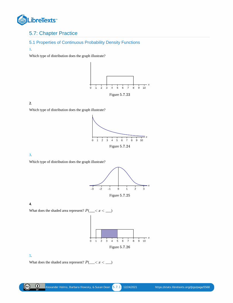
Alexander Holms, Barbara Illowsky, & Susan Dean 5.7.1 12/24/2021 https://stats.libretexts.org/@go/page/5568
5.7: Chapter Practice
5.1 Properties of Continuous Probability Density Functions
1.
Which type of distribution does the graph illustrate?
Figure
2.
Which type of distribution does the graph illustrate?
Figure
3.
Which type of distribution does the graph illustrate?
Figure
4.
What does the shaded area represent? (___ ___)
Figure
5.
What does the shaded area represent? (___ ___)
5.7.23
5.7.24
5.7.25
P < x <
5.7.26
P < x <
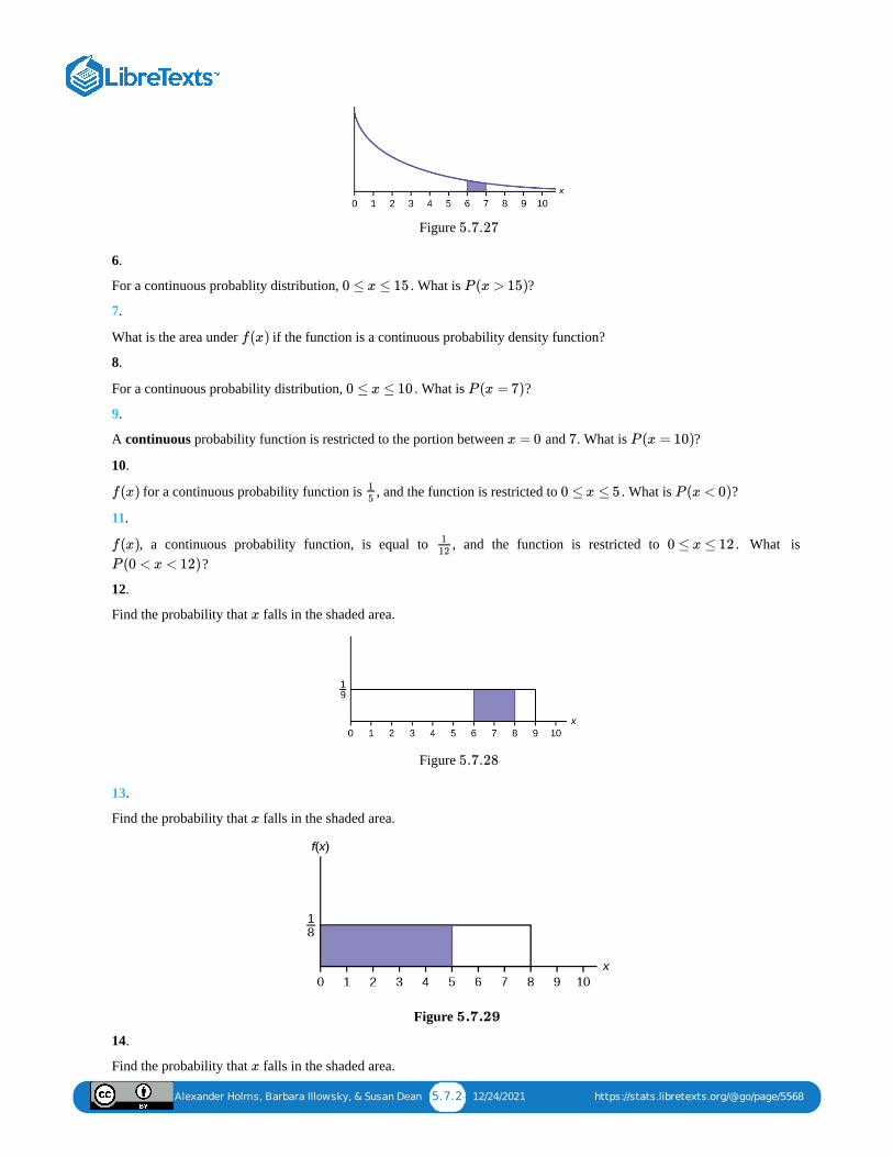
Alexander Holms, Barbara Illowsky, & Susan Dean 5.7.2 12/24/2021 https://stats.libretexts.org/@go/page/5568
Figure
6.
For a continuous probablity distribution, . What is ?
7.
What is the area under if the function is a continuous probability density function?
8.
For a continuous probability distribution, . What is ?
9.
A continuous probability function is restricted to the portion between and . What is ?
10.
for a continuous probability function is , and the function is restricted to . What is ?
11.
, a continuous probability function, is equal to , and the function is restricted to . What is ?
12.
Find the probability that falls in the shaded area.
Figure
13.
Find the probability that falls in the shaded area.
Figure
14.
Find the probability that falls in the shaded area.
5.7.27
0 ≤ x ≤ 15 P (x > 15)
f(x)
0 ≤ x ≤ 10 P (x = 7)
x = 0 7 P (x = 10)
f(x) 15
0 ≤ x ≤ 5 P (x < 0)
f(x) 112
0 ≤ x ≤ 12
P (0 < x < 12)
x
5.7.28
x
5.7.29
x
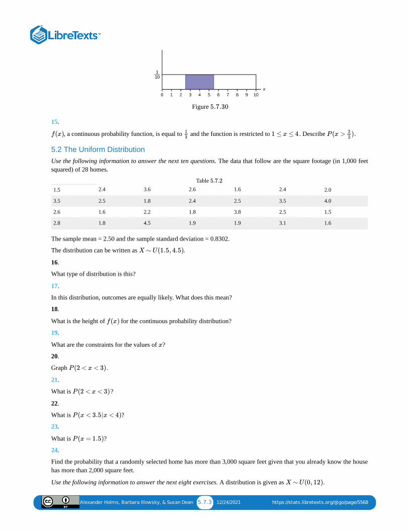
Alexander Holms, Barbara Illowsky, & Susan Dean 5.7.3 12/24/2021 https://stats.libretexts.org/@go/page/5568
Figure
15.
, a continuous probability function, is equal to and the function is restricted to . Describe .
5.2 The Uniform DistributionUse the following information to answer the next ten questions. The data that follow are the square footage (in 1,000 feetsquared) of 28 homes.
1.5 2.4 3.6 2.6 1.6 2.4 2.0
3.5 2.5 1.8 2.4 2.5 3.5 4.0
2.6 1.6 2.2 1.8 3.8 2.5 1.5
2.8 1.8 4.5 1.9 1.9 3.1 1.6
Table
The sample mean = 2.50 and the sample standard deviation = 0.8302.
The distribution can be written as .
16.
What type of distribution is this?
17.
In this distribution, outcomes are equally likely. What does this mean?
18.
What is the height of for the continuous probability distribution?
19.
What are the constraints for the values of ?
20.
Graph .
21.
What is ?
22.
What is ?
23.
What is ?
24.
Find the probability that a randomly selected home has more than 3,000 square feet given that you already know the househas more than 2,000 square feet.
Use the following information to answer the next eight exercises. A distribution is given as .
5.7.30
f(x) 13
1 ≤ x ≤ 4 P (x > )32
5.7.2
X ∼ U(1.5, 4.5)
f(x)
x
P (2 < x < 3)
P (2 < x < 3)
P (x < 3.5|x < 4)
P (x = 1.5)
X ∼ U(0, 12)
Alexander Holms, Barbara Illowsky, & Susan Dean 5.7.4 12/24/2021 https://stats.libretexts.org/@go/page/5568
25.
What is ? What does it represent?
26.
What is ? What does it represent?
27.
What is the probability density function?
28.
What is the theoretical mean?
29.
What is the theoretical standard deviation?
30.
Draw the graph of the distribution for .
31.
Find .
Use the following information to answer the next eleven exercises. The age of cars in the staff parking lot of a suburbancollege is uniformly distributed from six months (0.5 years) to 9.5 years.
32.
What is being measured here?
33.
In words, define the random variable .
34.
Are the data discrete or continuous?
35.
The interval of values for is ______.
36.
The distribution for is ______.
37.
Write the probability density function.
38.
Graph the probability distribution.
1. Sketch the graph of the probability distribution.
a
b
P (x > 9)
P (x > 9)
X
x
X
Alexander Holms, Barbara Illowsky, & Susan Dean 5.7.5 12/24/2021 https://stats.libretexts.org/@go/page/5568
Figure
2. Identify the following values:Lowest value for : _______Highest value for : _______Height of the rectangle: _______Label for x-axis (words): _______Label for y-axis (words): _______
39.
Find the average age of the cars in the lot.
40.
Find the probability that a randomly chosen car in the lot was less than four years old.
a. Sketch the graph, and shade the area of interest.
Figure
b. Find the probability. = _______
41.
Considering only the cars less than 7.5 years old, find the probability that a randomly chosen car in the lot was less thanfour years old.
1. Sketch the graph, shade the area of interest.
Figure
5.7.31
x̄̄̄
x̄̄̄
5.7.32
P (x < 4)
5.7.33
Alexander Holms, Barbara Illowsky, & Susan Dean 5.7.6 12/24/2021 https://stats.libretexts.org/@go/page/5568
2. Find the probability. _______
42.
What has changed in the previous two problems that made the solutions different?
43.
Find the third quartile of ages of cars in the lot. This means you will have to find the value such that , or 75%, of the carsare at most (less than or equal to) that age.
1. Sketch the graph, and shade the area of interest.
Figure
2. Find the value such that .3. The third quartile is _______
5.3 The Exponential Distribution
Use the following information to answer the next ten exercises. A customer service representative must spend differentamounts of time with each customer to resolve various concerns. The amount of time spent with each customer can bemodeled by the following distribution:
44.
What type of distribution is this?
45.
Are outcomes equally likely in this distribution? Why or why not?
46.
What is ? What does it represent?
47.
What is the mean?
48.
What is the standard deviation?
49.
State the probability density function.
50.
Graph the distribution.
51.
Find .
52.
P (x < 4|x < 7.5) =
34
5.7.34
k P (x < k) = 0.75
X ∼ Exp(0.2)
m
P (2 < x < 10)
Alexander Holms, Barbara Illowsky, & Susan Dean 5.7.7 12/24/2021 https://stats.libretexts.org/@go/page/5568
Find .
53.
Find the 70 percentile.
Use the following information to answer the next seven exercises. A distribution is given as .
54.
What is m?
55.
What is the probability density function?
56.
What is the cumulative distribution function?
57.
Draw the distribution.
58.
Find .
59.
Find the 30 percentile.
60.
Find the median.
61.
Which is larger, the mean or the median?
Use the following information to answer the next 16 exercises. Carbon-14 is a radioactive element with a half-life of about5,730 years. Carbon-14 is said to decay exponentially. The decay rate is 0.000121. We start with one gram of carbon-14.We are interested in the time (years) it takes to decay carbon-14.
62.
What is being measured here?
63.
Are the data discrete or continuous?
64.
In words, define the random variable .
65.
What is the decay rate ( )?
66.
The distribution for is ______.
67.
Find the amount (percent of one gram) of carbon-14 lasting less than 5,730 years. This means, find .
1. Sketch the graph, and shade the area of interest.
P (x > 6)
th
X ∼ Exp(0.75)
P (x < 4)
th
X
m
X
P (x < 5, 730)
Alexander Holms, Barbara Illowsky, & Susan Dean 5.7.8 12/24/2021 https://stats.libretexts.org/@go/page/5568
Figure
2. Find the probability. __________
68.
Find the percentage of carbon-14 lasting longer than 10,000 years.
1. Sketch the graph, and shade the area of interest.
Figure
2. Find the probability. ________
69.
Thirty percent (30%) of carbon-14 will decay within how many years?
1. Sketch the graph, and shade the area of interest.
Figure
Find the value such that .
5.7.35
P (x < 5, 730) =
5.7.36
P (x > 10, 000) =
5.7.37
k P (x < k) = 0.30
Alexander Holms, Barbara Illowsky, & Susan Dean 5.8.1 12/31/2021 https://stats.libretexts.org/@go/page/5571
5.8: Chapter References
5.2 The Uniform Distribution
McDougall, John A. The McDougall Program for Maximum Weight Loss. Plume, 1995.
5.3 The Exponential DistributionData from the United States Census Bureau.
Data from World Earthquakes, 2013. Available online at http://www.world-earthquakes.com/ (accessed June 11, 2013).
“No-hitter.” Baseball-Reference.com, 2013. Available online at http://www.baseball-reference.com/bullpen/No-hitter(accessed June 11, 2013).
Zhou, Rick. “Exponential Distribution lecture slides.” Available online atwww.public.iastate.edu/~riczw/stat330s11/lecture/lec13.pdf (accessed June 11, 2013).
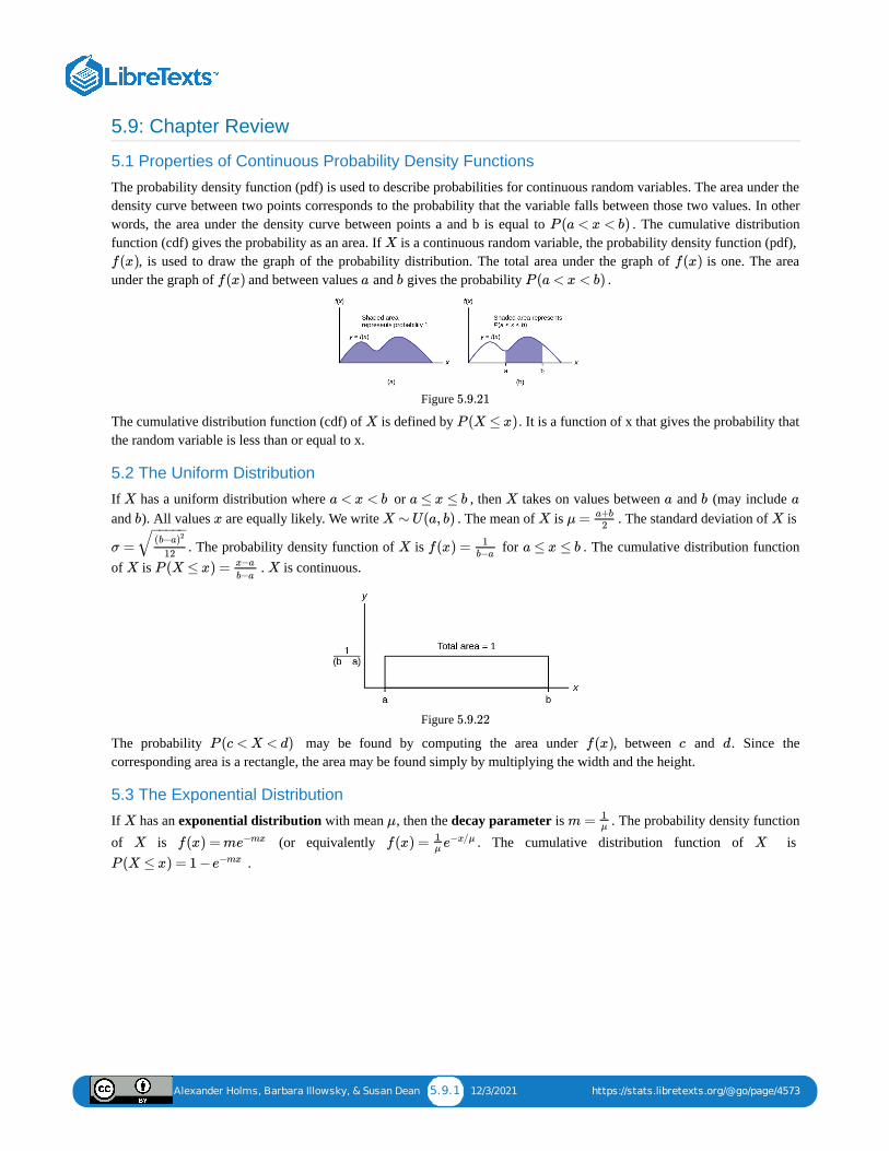
Alexander Holms, Barbara Illowsky, & Susan Dean 5.9.1 12/3/2021 https://stats.libretexts.org/@go/page/4573
5.9: Chapter Review
5.1 Properties of Continuous Probability Density Functions
The probability density function (pdf) is used to describe probabilities for continuous random variables. The area under thedensity curve between two points corresponds to the probability that the variable falls between those two values. In otherwords, the area under the density curve between points a and b is equal to . The cumulative distributionfunction (cdf) gives the probability as an area. If is a continuous random variable, the probability density function (pdf),
, is used to draw the graph of the probability distribution. The total area under the graph of is one. The areaunder the graph of and between values and gives the probability .
Figure
The cumulative distribution function (cdf) of is defined by . It is a function of x that gives the probability thatthe random variable is less than or equal to x.
5.2 The Uniform Distribution
If has a uniform distribution where or , then takes on values between and (may include and ). All values are equally likely. We write . The mean of is . The standard deviation of is
. The probability density function of is for . The cumulative distribution functionof is . is continuous.
Figure
The probability may be found by computing the area under , between and . Since thecorresponding area is a rectangle, the area may be found simply by multiplying the width and the height.
5.3 The Exponential Distribution
If has an exponential distribution with mean , then the decay parameter is . The probability density functionof is (or equivalently . The cumulative distribution function of is
.
P (a < x < b)
X
f(x) f(x)
f(x) a b P (a < x < b)
5.9.21
X P (X ≤ x)
X a < x < b a ≤ x ≤ b X a b a
b x X ∼ U(a, b) X μ = a+b
2X
σ =(b−a)2
12
− −−−−√ X f(x) = 1
b−aa ≤ x ≤ b
X P (X ≤ x) = x−a
b−aX
5.9.22
P (c < X < d) f(x) c d
X μ m = 1μ
X f(x) = me−mx f(x) = 1μ e
−x/μ X
P (X ≤ x) = 1 −e−mx
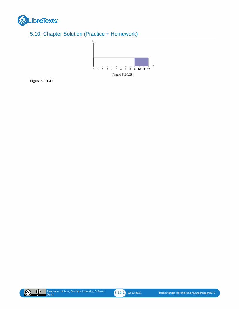
Alexander Holms, Barbara Illowsky, & Susan
Dean5.10.1 12/10/2021 https://stats.libretexts.org/@go/page/5570
5.10: Chapter Solution (Practice + Homework)
Figure
Figure
5.10.38
5.10.41

1 1/7/2022
CHAPTER OVERVIEW6: THE NORMAL DISTRIBUTION
6.0: INTRODUCTION TO NORMAL DISTRIBUTION6.1: THE STANDARD NORMAL DISTRIBUTION6.2: USING THE NORMAL DISTRIBUTION6.3: ESTIMATING THE BINOMIAL WITH THE NORMAL DISTRIBUTION6.4: CHAPTER FORMULA REVIEW6.5: CHAPTER HOMEWORK6.6: CHAPTER KEY ITEMS6.7: CHAPTER PRACTICE6.8: CHAPTER REFERENCES6.9: CHAPTER REVIEW6.10: CHAPTER SOLUTION (PRACTICE + HOMEWORK)
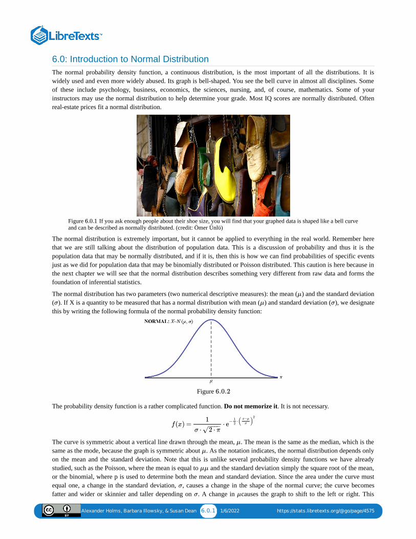
Alexander Holms, Barbara Illowsky, & Susan Dean 6.0.1 1/6/2022 https://stats.libretexts.org/@go/page/4575
6.0: Introduction to Normal DistributionThe normal probability density function, a continuous distribution, is the most important of all the distributions. It iswidely used and even more widely abused. Its graph is bell-shaped. You see the bell curve in almost all disciplines. Someof these include psychology, business, economics, the sciences, nursing, and, of course, mathematics. Some of yourinstructors may use the normal distribution to help determine your grade. Most IQ scores are normally distributed. Oftenreal-estate prices fit a normal distribution.
Figure If you ask enough people about their shoe size, you will find that your graphed data is shaped like a bell curveand can be described as normally distributed. (credit: Ömer Ünlϋ)
The normal distribution is extremely important, but it cannot be applied to everything in the real world. Remember herethat we are still talking about the distribution of population data. This is a discussion of probability and thus it is thepopulation data that may be normally distributed, and if it is, then this is how we can find probabilities of specific eventsjust as we did for population data that may be binomially distributed or Poisson distributed. This caution is here because inthe next chapter we will see that the normal distribution describes something very different from raw data and forms thefoundation of inferential statistics.
The normal distribution has two parameters (two numerical descriptive measures): the mean ( ) and the standard deviation( ). If X is a quantity to be measured that has a normal distribution with mean ( ) and standard deviation ( ), we designatethis by writing the following formula of the normal probability density function:
Figure
The probability density function is a rather complicated function. Do not memorize it. It is not necessary.
The curve is symmetric about a vertical line drawn through the mean, . The mean is the same as the median, which is thesame as the mode, because the graph is symmetric about . As the notation indicates, the normal distribution depends onlyon the mean and the standard deviation. Note that this is unlike several probability density functions we have alreadystudied, such as the Poisson, where the mean is equal to and the standard deviation simply the square root of the mean,or the binomial, where p is used to determine both the mean and standard deviation. Since the area under the curve mustequal one, a change in the standard deviation, , causes a change in the shape of the normal curve; the curve becomesfatter and wider or skinnier and taller depending on . A change in causes the graph to shift to the left or right. This
6.0.1
μ
σ μ σ
6.0.2
f(x) = ⋅1
σ ⋅ 2 ⋅ π− −−−
√e
− ⋅1
2( )
x−μ
σ
2
μ
μ
μμ
σ
σ μ

Alexander Holms, Barbara Illowsky, & Susan Dean 6.0.2 1/6/2022 https://stats.libretexts.org/@go/page/4575
means there are an infinite number of normal probability distributions. One of special interest is called the standardnormal distribution.
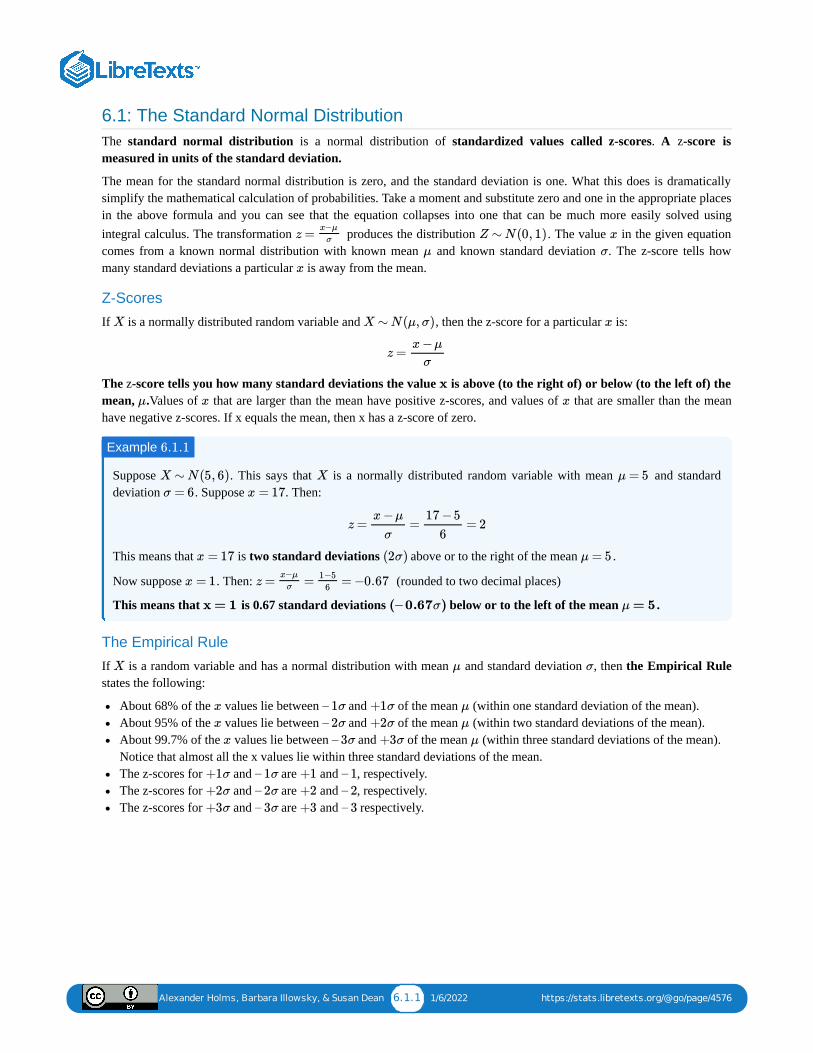
Alexander Holms, Barbara Illowsky, & Susan Dean 6.1.1 1/6/2022 https://stats.libretexts.org/@go/page/4576
6.1: The Standard Normal DistributionThe standard normal distribution is a normal distribution of standardized values called z-scores. A z-score ismeasured in units of the standard deviation.
The mean for the standard normal distribution is zero, and the standard deviation is one. What this does is dramaticallysimplify the mathematical calculation of probabilities. Take a moment and substitute zero and one in the appropriate placesin the above formula and you can see that the equation collapses into one that can be much more easily solved usingintegral calculus. The transformation produces the distribution . The value in the given equationcomes from a known normal distribution with known mean and known standard deviation . The z-score tells howmany standard deviations a particular is away from the mean.
Z-Scores
If is a normally distributed random variable and , then the z-score for a particular is:
The z-score tells you how many standard deviations the value is above (to the right of) or below (to the left of) themean, .Values of that are larger than the mean have positive z-scores, and values of that are smaller than the meanhave negative z-scores. If x equals the mean, then x has a z-score of zero.
Suppose . This says that is a normally distributed random variable with mean and standarddeviation . Suppose . Then:
This means that is two standard deviations above or to the right of the mean .
Now suppose . Then: (rounded to two decimal places)
This means that is 0.67 standard deviations below or to the left of the mean .
The Empirical Rule
If is a random variable and has a normal distribution with mean and standard deviation , then the Empirical Rulestates the following:
About 68% of the values lie between and of the mean (within one standard deviation of the mean).About 95% of the values lie between and of the mean (within two standard deviations of the mean).About 99.7% of the values lie between and of the mean (within three standard deviations of the mean).Notice that almost all the x values lie within three standard deviations of the mean.The z-scores for and are and , respectively.The z-scores for and are and , respectively.The z-scores for and are and respectively.
z =x−μ
σ Z ∼ N(0, 1) x
μ σ
x
X X ∼ N(μ, σ) x
z =x −μ
σ
x
μ x x
Example 6.1.1
X ∼ N(5, 6) X μ = 5
σ = 6 x = 17
z = = = 2x −μ
σ
17 −5
6
x = 17 (2σ) μ = 5
x = 1 z = = = −0.67x−μ
σ
1−5
6
x = 1 (– 0.67σ) μ = 5
X μ σ
x – 1σ +1σ μ
x – 2σ +2σ μ
x – 3σ +3σ μ
+1σ – 1σ +1 – 1
+2σ – 2σ +2 – 2
+3σ – 3σ +3 – 3
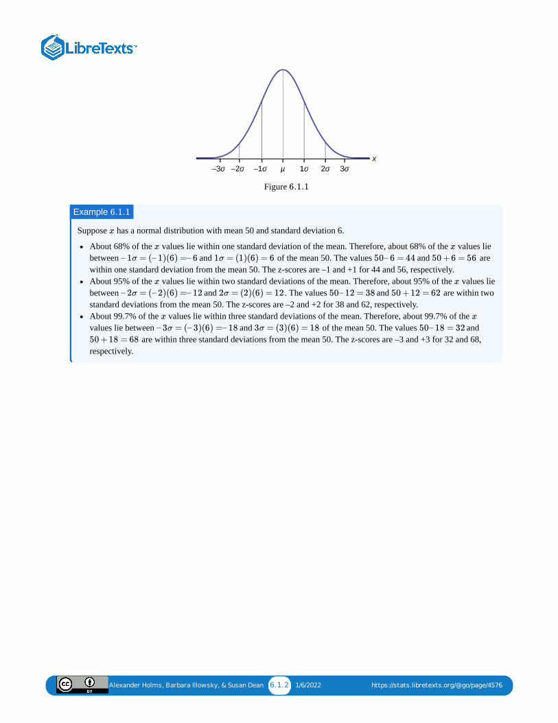
Alexander Holms, Barbara Illowsky, & Susan Dean 6.1.2 1/6/2022 https://stats.libretexts.org/@go/page/4576
Figure
Suppose has a normal distribution with mean 50 and standard deviation 6.
About 68% of the values lie within one standard deviation of the mean. Therefore, about 68% of the values liebetween and of the mean 50. The values and arewithin one standard deviation from the mean 50. The z-scores are –1 and +1 for 44 and 56, respectively.About 95% of the values lie within two standard deviations of the mean. Therefore, about 95% of the values liebetween and . The values and are within twostandard deviations from the mean 50. The z-scores are –2 and +2 for 38 and 62, respectively.About 99.7% of the values lie within three standard deviations of the mean. Therefore, about 99.7% of the values lie between and of the mean 50. The values and
are within three standard deviations from the mean 50. The z-scores are –3 and +3 for 32 and 68,respectively.
6.1.1
Example 6.1.1
x
x x
– 1σ = (– 1)(6) =– 6 1σ = (1)(6) = 6 50– 6 = 44 50 +6 = 56
x x
– 2σ = (– 2)(6) =– 12 2σ = (2)(6) = 12 50– 12 = 38 50 +12 = 62
x x
– 3σ = (– 3)(6) =– 18 3σ = (3)(6) = 18 50– 18 = 32
50 +18 = 68
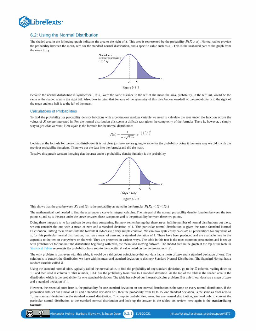
Alexander Holms, Barbara Illowsky, & Susan Dean 6.2.1 11/19/2021 https://stats.libretexts.org/@go/page/4577
6.2: Using the Normal DistributionThe shaded area in the following graph indicates the area to the right of . This area is represented by the probability . Normal tables providethe probability between the mean, zero for the standard normal distribution, and a specific value such as . This is the unshaded part of the graph fromthe mean to .
Figure
Because the normal distribution is symmetrical , if were the same distance to the left of the mean the area, probability, in the left tail, would be thesame as the shaded area in the right tail. Also, bear in mind that because of the symmetry of this distribution, one-half of the probability is to the right ofthe mean and one-half is to the left of the mean.
Calculations of Probabilities
To find the probability for probability density functions with a continuous random variable we need to calculate the area under the function across thevalues of we are interested in. For the normal distribution this seems a difficult task given the complexity of the formula. There is, however, a simplyway to get what we want. Here again is the formula for the normal distribution:
Looking at the formula for the normal distribution it is not clear just how we are going to solve for the probability doing it the same way we did it with theprevious probability functions. There we put the data into the formula and did the math.
To solve this puzzle we start knowing that the area under a probability density function is the probability.
Figure
This shows that the area between and is the probability as stated in the formula:
The mathematical tool needed to find the area under a curve is integral calculus. The integral of the normal probability density function between the twopoints x and x is the area under the curve between these two points and is the probability between these two points.
Doing these integrals is no fun and can be very time consuming. But now, remembering that there are an infinite number of normal distributions out there,we can consider the one with a mean of zero and a standard deviation of 1. This particular normal distribution is given the name Standard NormalDistribution. Putting these values into the formula it reduces to a very simple equation. We can now quite easily calculate all probabilities for any value ofx, for this particular normal distribution, that has a mean of zero and a standard deviation of 1. These have been produced and are available here in theappendix to the text or everywhere on the web. They are presented in various ways. The table in this text is the most common presentation and is set upwith probabilities for one-half the distribution beginning with zero, the mean, and moving outward. The shaded area in the graph at the top of the table inStatistical Tables represents the probability from zero to the specific value noted on the horizontal axis, .
The only problem is that even with this table, it would be a ridiculous coincidence that our data had a mean of zero and a standard deviation of one. Thesolution is to convert the distribution we have with its mean and standard deviation to this new Standard Normal Distribution. The Standard Normal has arandom variable called .
Using the standard normal table, typically called the normal table, to find the probability of one standard deviation, go to the column, reading down to1.0 and then read at column 0. That number, is the probability from zero to 1 standard deviation. At the top of the table is the shaded area in thedistribution which is the probability for one standard deviation. The table has solved our integral calculus problem. But only if our data has a mean of zeroand a standard deviation of 1.
However, the essential point here is, the probability for one standard deviation on one normal distribution is the same on every normal distribution. If thepopulation data set has a mean of 10 and a standard deviation of 5 then the probability from 10 to 15, one standard deviation, is the same as from zero to1, one standard deviation on the standard normal distribution. To compute probabilities, areas, for any normal distribution, we need only to convert theparticular normal distribution to the standard normal distribution and look up the answer in the tables. As review, here again is the standardizingformula:
x P (X > x)x1
x1
6.2.1
x1
X
f(x) = ⋅1
σ ⋅ 2 ⋅ π− −−−
√e
− ⋅1
2( )
x−μ
σ
2
6.2.2
X1 X2 P ( ≤ X ≤ )X1 X2
1 2
Z Z
Z
Z
0.3413
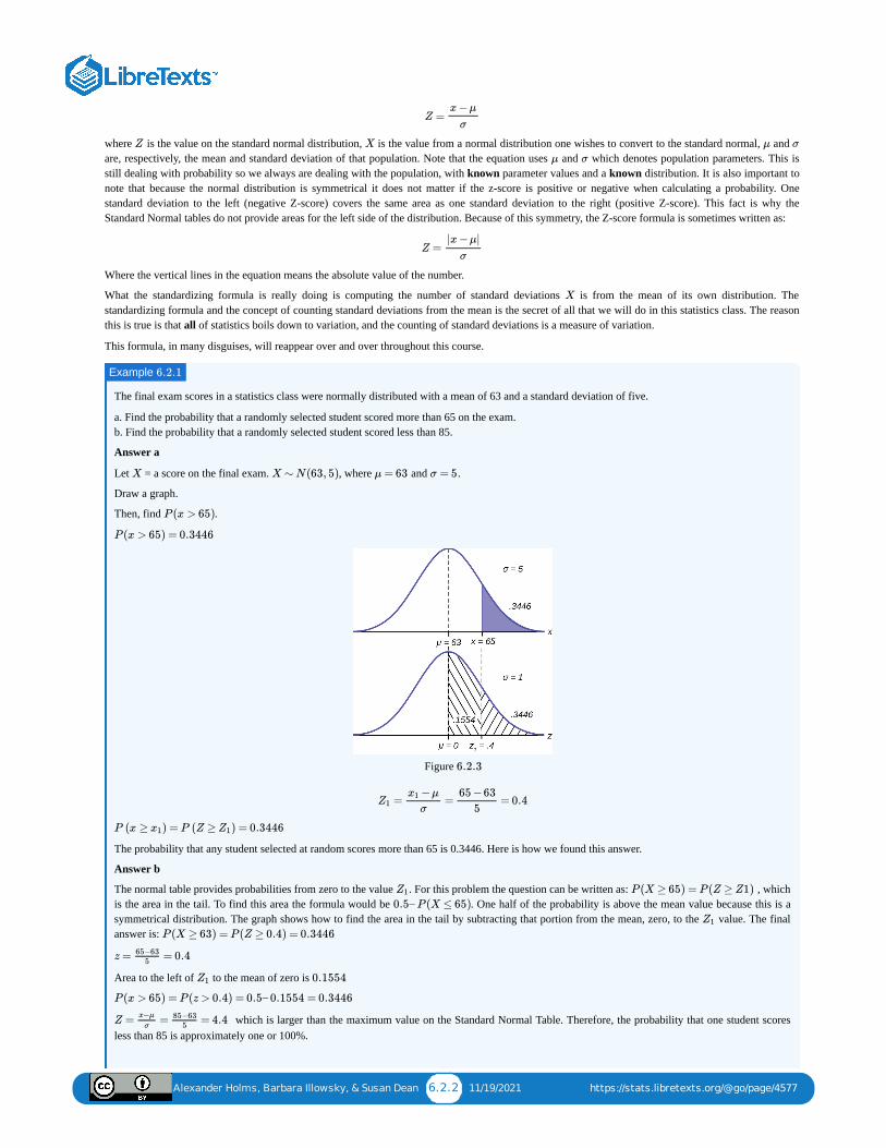
Alexander Holms, Barbara Illowsky, & Susan Dean 6.2.2 11/19/2021 https://stats.libretexts.org/@go/page/4577
where is the value on the standard normal distribution, is the value from a normal distribution one wishes to convert to the standard normal, and are, respectively, the mean and standard deviation of that population. Note that the equation uses and which denotes population parameters. This isstill dealing with probability so we always are dealing with the population, with known parameter values and a known distribution. It is also important tonote that because the normal distribution is symmetrical it does not matter if the z-score is positive or negative when calculating a probability. Onestandard deviation to the left (negative Z-score) covers the same area as one standard deviation to the right (positive Z-score). This fact is why theStandard Normal tables do not provide areas for the left side of the distribution. Because of this symmetry, the Z-score formula is sometimes written as:
Where the vertical lines in the equation means the absolute value of the number.
What the standardizing formula is really doing is computing the number of standard deviations is from the mean of its own distribution. Thestandardizing formula and the concept of counting standard deviations from the mean is the secret of all that we will do in this statistics class. The reasonthis is true is that all of statistics boils down to variation, and the counting of standard deviations is a measure of variation.
This formula, in many disguises, will reappear over and over throughout this course.
The final exam scores in a statistics class were normally distributed with a mean of 63 and a standard deviation of five.
a. Find the probability that a randomly selected student scored more than 65 on the exam. b. Find the probability that a randomly selected student scored less than 85.
Answer a
Let = a score on the final exam. , where and .
Draw a graph.
Then, find .
Figure
The probability that any student selected at random scores more than 65 is 0.3446. Here is how we found this answer.
Answer b
The normal table provides probabilities from zero to the value . For this problem the question can be written as: , whichis the area in the tail. To find this area the formula would be . One half of the probability is above the mean value because this is asymmetrical distribution. The graph shows how to find the area in the tail by subtracting that portion from the mean, zero, to the value. The finalanswer is:
Area to the left of to the mean of zero is
which is larger than the maximum value on the Standard Normal Table. Therefore, the probability that one student scoresless than 85 is approximately one or 100%.
Z =x −μ
σ
Z X μ σ
μ σ
Z =|x −μ|
σ
X
Example 6.2.1
X X ∼ N(63, 5) μ = 63 σ = 5
P (x > 65)
P (x > 65) = 0.3446
6.2.3
= = = 0.4Z1−μx1
σ
65 −63
5
P (x ≥ ) = P (Z ≥ ) = 0.3446x1 Z1
Z1 P (X ≥ 65) = P (Z ≥ Z1)0.5– P (X ≤ 65)
Z1
P (X ≥ 63) = P (Z ≥ 0.4) = 0.3446
z = = 0.465−635
Z1 0.1554
P (x > 65) = P (z > 0.4) = 0.5– 0.1554 = 0.3446
Z = = = 4.4x−μ
σ
85−635
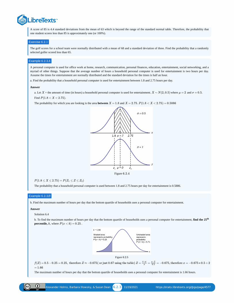
Alexander Holms, Barbara Illowsky, & Susan Dean 6.2.3 11/19/2021 https://stats.libretexts.org/@go/page/4577
A score of 85 is 4.4 standard deviations from the mean of 63 which is beyond the range of the standard normal table. Therefore, the probability thatone student scores less than 85 is approximately one (or 100%).
The golf scores for a school team were normally distributed with a mean of 68 and a standard deviation of three. Find the probability that a randomlyselected golfer scored less than 65.
A personal computer is used for office work at home, research, communication, personal finances, education, entertainment, social networking, and amyriad of other things. Suppose that the average number of hours a household personal computer is used for entertainment is two hours per day.Assume the times for entertainment are normally distributed and the standard deviation for the times is half an hour.
a. Find the probability that a household personal computer is used for entertainment between 1.8 and 2.75 hours per day.
Answer
a. Let = the amount of time (in hours) a household personal computer is used for entertainment. where and .
Find .
The probability for which you are looking is the area between and .
Figure
The probability that a household personal computer is used between 1.8 and 2.75 hours per day for entertainment is 0.5886.
b. Find the maximum number of hours per day that the bottom quartile of households uses a personal computer for entertainment.
Answer
Solution 6.4
b. To find the maximum number of hours per day that the bottom quartile of households uses a personal computer for entertainment, find the 25percentile, , where .
Figure
The maximum number of hours per day that the bottom quartile of households uses a personal computer for entertainment is 1.66 hours.
Exercise 6.2.1
Example 6.2.2A
X X ∼ N(2, 0.5) μ = 2 σ = 0.5
P (1.8 < X < 2.75)
X = 1.8 X = 2.75 P (1.8 < X < 2.75) = 0.5886
6.2.4
P (1.8 ≤ X ≤ 2.75) = P ( ≤ Z ≤ )Z1 Z2
Example 6.2.2B
th
k P (x < k) = 0.25
6.2.5
f(Z) = 0.5 −0.25 = 0.25, therefore Z ≈ −0.675( or just 0.67 using the table) Z = = = −0.675, therefore x = −0.675 ∗ 0.5 +2x−μ
σ
x−20.5
= 1.66
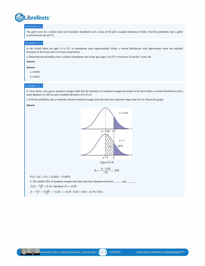
Alexander Holms, Barbara Illowsky, & Susan Dean 6.2.4 11/19/2021 https://stats.libretexts.org/@go/page/4577
The golf scores for a school team were normally distributed with a mean of 68 and a standard deviation of three. Find the probability that a golferscored between 66 and 70.
In the United States the ages 13 to 55+ of smartphone users approximately follow a normal distribution with approximate mean and standarddeviation of 36.9 years and 13.9 years, respectively.
a. Determine the probability that a random smartphone user in the age range 13 to 55+ is between 23 and 64.7 years old.
Answer
Answer
a. 0.8186
b. 0.8413
A citrus farmer who grows mandarin oranges finds that the diameters of mandarin oranges harvested on his farm follow a normal distribution with amean diameter of 5.85 cm and a standard deviation of 0.24 cm.
a. Find the probability that a randomly selected mandarin orange from this farm has a diameter larger than 6.0 cm. Sketch the graph.
Answer
Figure
b. The middle 20% of mandarin oranges from this farm have diameters between ______ and ______.
Exercise 6.2.2
Example 6.2.3
Example 6.2.4
6.2.6
= = .625Z16 −5.85
.24
P (x ≥ 6) = P (z ≥ 0.625) = 0.2670
f(Z) = = 0.10, therefore Z ≈ ±0.250.202
Z = = = ±0.25 → ±0.25 ⋅ 0.24 +5.85 = (5.79, 5.91)x−μ
σ
x−5.850.24
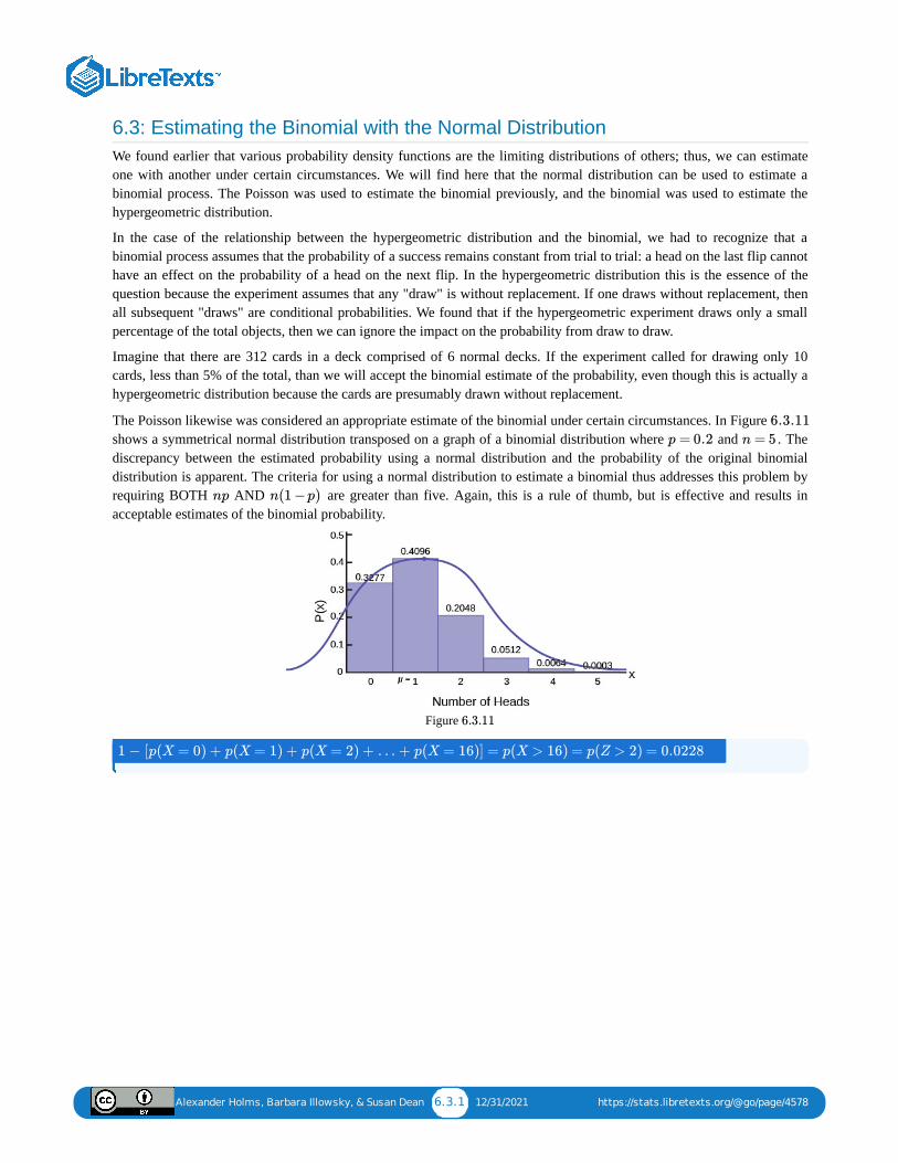
Alexander Holms, Barbara Illowsky, & Susan Dean 6.3.1 12/31/2021 https://stats.libretexts.org/@go/page/4578
6.3: Estimating the Binomial with the Normal DistributionWe found earlier that various probability density functions are the limiting distributions of others; thus, we can estimateone with another under certain circumstances. We will find here that the normal distribution can be used to estimate abinomial process. The Poisson was used to estimate the binomial previously, and the binomial was used to estimate thehypergeometric distribution.
In the case of the relationship between the hypergeometric distribution and the binomial, we had to recognize that abinomial process assumes that the probability of a success remains constant from trial to trial: a head on the last flip cannothave an effect on the probability of a head on the next flip. In the hypergeometric distribution this is the essence of thequestion because the experiment assumes that any "draw" is without replacement. If one draws without replacement, thenall subsequent "draws" are conditional probabilities. We found that if the hypergeometric experiment draws only a smallpercentage of the total objects, then we can ignore the impact on the probability from draw to draw.
Imagine that there are 312 cards in a deck comprised of 6 normal decks. If the experiment called for drawing only 10cards, less than 5% of the total, than we will accept the binomial estimate of the probability, even though this is actually ahypergeometric distribution because the cards are presumably drawn without replacement.
The Poisson likewise was considered an appropriate estimate of the binomial under certain circumstances. In Figure shows a symmetrical normal distribution transposed on a graph of a binomial distribution where and . Thediscrepancy between the estimated probability using a normal distribution and the probability of the original binomialdistribution is apparent. The criteria for using a normal distribution to estimate a binomial thus addresses this problem byrequiring BOTH AND are greater than five. Again, this is a rule of thumb, but is effective and results inacceptable estimates of the binomial probability.
Figure
6.3.11
p = 0.2 n = 5
np n(1 −p)
6.3.11
1 − [p(X = 0) + p(X = 1) + p(X = 2) + … + p(X = 16)] = p(X > 16) = p(Z > 2) = 0.0228
Alexander Holms, Barbara Illowsky, & Susan Dean 6.4.1 1/7/2022 https://stats.libretexts.org/@go/page/5817
6.4: Chapter Formula Review
Introduction
the mean; the standard deviation
The Standard Normal Distribution
standardized value (z-score)
mean = 0; standard deviation = 1
To find the percentile of when the z-scores is known:
z-score: or
the random variable for z-scores
Estimating the Binomial with the Normal DistributionNormal Distribution: where is the mean and is the standard deviation.
Standard Normal Distribution: .
X ∼ N(μ, σ)
μ = σ =
Z ∼ N(0, 1)
z = a
kth X
k = μ +(z)σ
z =x−μ
σ z =|x−μ|
σ
Z =
Z ∼ N(0, 1)
X ∼ N(μ, σ) μ σ
Z ∼ N(0, 1)
Alexander Holms, Barbara Illowsky, & Susan Dean 6.5.1 11/26/2021 https://stats.libretexts.org/@go/page/5822
6.5: Chapter Homework
6.1 The Standard Normal Distribution
Use the following information to answer the next two exercises: The patient recovery time from a particular surgicalprocedure is normally distributed with a mean of 5.3 days and a standard deviation of 2.1 days.
65.
What is the median recovery time?
a. 2.7b. 5.3c. 7.4d. 2.1
66.
What is the z-score for a patient who takes ten days to recover?
a. 1.5b. 0.2c. 2.2d. 7.3
67.
The length of time to find a parking space at 9 A.M. follows a normal distribution with a mean of five minutes and astandard deviation of two minutes. If the mean is significantly greater than the standard deviation, which of the followingstatements is true?
I. The data cannot follow the uniform distribution.II. The data cannot follow the exponential distribution..
III. The data cannot follow the normal distribution.
a. I onlyb. II onlyc. III onlyd. I, II, and III
68.
The heights of the 430 National Basketball Association players were listed on team rosters at the start of the 2005–2006season. The heights of basketball players have an approximate normal distribution with mean, inches and astandard deviation, inches. For each of the following heights, calculate the z-score and interpret it usingcomplete sentences.
1. 77 inches2. 85 inches3. If an NBA player reported his height had a z-score of 3.5, would you believe him? Explain your answer.
69.
The systolic blood pressure (given in millimeters) of males has an approximately normal distribution with mean and standard deviation . Systolic blood pressure for males follows a normal distribution.
1. Calculate the z-scores for the male systolic blood pressures 100 and 150 millimeters.2. If a male friend of yours said he thought his systolic blood pressure was 2.5 standard deviations below the mean, but
that he believed his blood pressure was between 100 and 150 millimeters, what would you say to him?
70.
μ = 79
σ = 3.89
μ = 125
σ = 14
Alexander Holms, Barbara Illowsky, & Susan Dean 6.5.2 11/26/2021 https://stats.libretexts.org/@go/page/5822
Kyle’s doctor told him that the z-score for his systolic blood pressure is 1.75. Which of the following is the bestinterpretation of this standardized score? The systolic blood pressure (given in millimeters) of males has an approximatelynormal distribution with mean and standard deviation . If a systolic blood pressure score then N (125, 14).
1. Which answer(s) is/are correct?
Kyle’s systolic blood pressure is 175.Kyle’s systolic blood pressure is 1.75 times the average blood pressure of men his age.Kyle’s systolic blood pressure is 1.75 above the average systolic blood pressure of men his age.Kyles’s systolic blood pressure is 1.75 standard deviations above the average systolic blood pressure for men.
2. Calculate Kyle’s blood pressure.
71.
Height and weight are two measurements used to track a child’s development. The World Health Organization measureschild development by comparing the weights of children who are the same height and the same gender. In 2009, weightsfor all 80 cm girls in the reference population had a mean kg and standard deviation kg. Weights arenormally distributed. N(10.2, 0.8). Calculate the z-scores that correspond to the following weights and interpret them.
1. 11 kg2. 7.9 kg3. 12.2 kg
72.
In 2005, 1,475,623 students heading to college took the SAT. The distribution of scores in the math section of the SATfollows a normal distribution with mean and standard deviation .
1. Calculate the z-score for an SAT score of 720. Interpret it using a complete sentence.2. What math SAT score is 1.5 standard deviations above the mean? What can you say about this SAT score?3. For 2012, the SAT math test had a mean of 514 and standard deviation 117. The ACT math test is an alternate to the
SAT and is approximately normally distributed with mean 21 and standard deviation 5.3. If one person took the SATmath test and scored 700 and a second person took the ACT math test and scored 30, who did better with respect to thetest they took?
6.3 Estimating the Binomial with the Normal Distribution
Use the following information to answer the next two exercises: The patient recovery time from a particular surgicalprocedure is normally distributed with a mean of 5.3 days and a standard deviation of 2.1 days.
73.
What is the probability of spending more than two days in recovery?
a. 0.0580b. 0.8447c. 0.0553d. 0.9420
Use the following information to answer the next three exercises: The length of time it takes to find a parking space at 9A.M. follows a normal distribution with a mean of five minutes and a standard deviation of two minutes.
74.
Based upon the given information and numerically justified, would you be surprised if it took less than one minute to finda parking space?
a. Yesb. Noc. Unable to determine
75.
μ = 125 σ = 14 X = X ∼
μ = 10.2 σ = 0.8
X ∼
μ = 520 σ = 115
Alexander Holms, Barbara Illowsky, & Susan Dean 6.5.3 11/26/2021 https://stats.libretexts.org/@go/page/5822
Find the probability that it takes at least eight minutes to find a parking space.
a. 0.0001b. 0.9270c. 0.1862d. 0.0668
76.
Seventy percent of the time, it takes more than how many minutes to find a parking space?
a. 1.24b. 2.41c. 3.95d. 6.05
77.
According to a study done by De Anza students, the height for Asian adult males is normally distributed with an averageof 66 inches and a standard deviation of 2.5 inches. Suppose one Asian adult male is randomly chosen. Let height ofthe individual.
1. _____(_____,_____)2. Find the probability that the person is between 65 and 69 inches. Include a sketch of the graph, and write a probability
statement.3. Would you expect to meet many Asian adult males over 72 inches? Explain why or why not, and justify your answer
numerically.4. The middle 40% of heights fall between what two values? Sketch the graph, and write the probability statement.
78.
IQ is normally distributed with a mean of 100 and a standard deviation of 15. Suppose one individual is randomly chosen.Let X= IQ of an individual.
1. _____(_____,_____)2. Find the probability that the person has an IQ greater than 120. Include a sketch of the graph, and write a probability
statement.3. MENSA is an organization whose members have the top 2% of all IQs. Find the minimum IQ needed to qualify for the
MENSA organization. Sketch the graph, and write the probability statement.
79.
The percent of fat calories that a person in America consumes each day is normally distributed with a mean of about 36and a standard deviation of 10. Suppose that one individual is randomly chosen. Let percent of fat calories.
1. _____(_____,_____)2. Find the probability that the percent of fat calories a person consumes is more than 40. Graph the situation. Shade in
the area to be determined.3. Find the maximum number for the lower quarter of percent of fat calories. Sketch the graph and write the probability
statement.
80.
Suppose that the distance of fly balls hit to the outfield (in baseball) is normally distributed with a mean of 250 feet and astandard deviation of 50 feet.
1. If distance in feet for a fly ball, then _____(_____,_____)2. If one fly ball is randomly chosen from this distribution, what is the probability that this ball traveled fewer than 220
feet? Sketch the graph. Scale the horizontal axis . Shade the region corresponding to the probability. Find theprobability.
81.
X =
X ∼
X ∼
X =
X ∼
X = X ∼
X
Alexander Holms, Barbara Illowsky, & Susan Dean 6.5.4 11/26/2021 https://stats.libretexts.org/@go/page/5822
In China, four-year-olds average three hours a day unsupervised. Most of the unsupervised children live in rural areas,considered safe. Suppose that the standard deviation is 1.5 hours and the amount of time spent alone is normallydistributed. We randomly select one Chinese four-year-old living in a rural area. We are interested in the amount of timethe child spends alone per day.
1. In words, define the random variable .2. _____(_____,_____)3. Find the probability that the child spends less than one hour per day unsupervised. Sketch the graph, and write the
probability statement.4. What percent of the children spend over ten hours per day unsupervised?5. Seventy percent of the children spend at least how long per day unsupervised?
82.
In the 1992 presidential election, Alaska’s 40 election districts averaged 1,956.8 votes per district for President Clinton.The standard deviation was 572.3. (There are only 40 election districts in Alaska.) The distribution of the votes per districtfor President Clinton was bell-shaped. Let number of votes for President Clinton for an election district.
1. State the approximate distribution of .2. Is 1,956.8 a population mean or a sample mean? How do you know?3. Find the probability that a randomly selected district had fewer than 1,600 votes for President Clinton. Sketch the graph
and write the probability statement.4. Find the probability that a randomly selected district had between 1,800 and 2,000 votes for President Clinton.5. Find the third quartile for votes for President Clinton.
83.
Suppose that the duration of a particular type of criminal trial is known to be normally distributed with a mean of 21 daysand a standard deviation of seven days.
1. In words, define the random variable .2. _____(_____,_____)3. If one of the trials is randomly chosen, find the probability that it lasted at least 24 days. Sketch the graph and write the
probability statement.4. Sixty percent of all trials of this type are completed within how many days?
84.
Terri Vogel, an amateur motorcycle racer, averages 129.71 seconds per 2.5 mile lap (in a seven-lap race) with a standarddeviation of 2.28 seconds. The distribution of her race times is normally distributed. We are interested in one of herrandomly selected laps.
1. In words, define the random variable 2. _____(_____,_____)3. Find the percent of her laps that are completed in less than 130 seconds.4. The fastest 3% of her laps are under _____.5. The middle 80% of her laps are from _______ seconds to _______ seconds.
85.
Thuy Dau, Ngoc Bui, Sam Su, and Lan Voung conducted a survey as to how long customers at Lucky claimed to wait inthe checkout line until their turn. Let time in line. Table displays the ordered real data (in minutes):
0.50 4.25 5 6 7.25
1.75 4.25 5.25 6 7.25
2 4.25 5.25 6.25 7.25
2.25 4.25 5.5 6.25 7.75
2.25 4.5 5.5 6.5 8
Table
X
X ∼
X =
X
X
X ∼
X.
X ∼
X = 6.5.1
6.5.1
Alexander Holms, Barbara Illowsky, & Susan Dean 6.5.5 11/26/2021 https://stats.libretexts.org/@go/page/5822
2.5 4.75 5.5 6.5 8.25
2.75 4.75 5.75 6.5 9.5
3.25 4.75 5.75 6.75 9.5
3.75 5 6 6.75 9.75
3.75 5 6 6.75 10.75
1. Calculate the sample mean and the sample standard deviation.2. Construct a histogram.3. Draw a smooth curve through the midpoints of the tops of the bars.4. In words, describe the shape of your histogram and smooth curve.5. Let the sample mean approximate μ and the sample standard deviation approximate \sigma. The distribution of X can
then be approximated by _____(_____,_____)6. Use the distribution in part e to calculate the probability that a person will wait fewer than 6.1 minutes.7. Determine the cumulative relative frequency for waiting less than 6.1 minutes.8. Why aren’t the answers to part 6 and part 7 exactly the same?9. Why are the answers to part 6 and part 7 as close as they are?
10. If only ten customers has been surveyed rather than 50, do you think the answers to part f and part g would have beencloser together or farther apart? Explain your conclusion.
86.
Suppose that Ricardo and Anita attend different colleges. Ricardo’s GPA is the same as the average GPA at his school.Anita’s GPA is 0.70 standard deviations above her school average. In complete sentences, explain why each of thefollowing statements may be false.
1. Ricardo’s actual GPA is lower than Anita’s actual GPA.2. Ricardo is not passing because his z-score is zero.3. Anita is in the percentile of students at her college.
87.
An expert witness for a paternity lawsuit testifies that the length of a pregnancy is normally distributed with a mean of 280days and a standard deviation of 13 days. An alleged father was out of the country from 240 to 306 days before the birth ofthe child, so the pregnancy would have been less than 240 days or more than 306 days long if he was the father. The birthwas uncomplicated, and the child needed no medical intervention. What is the probability that he was NOT the father?What is the probability that he could be the father? Calculate the z-scores first, and then use those to calculate theprobability.
88.
A NUMMI assembly line, which has been operating since 1984, has built an average of 6,000 cars and trucks a week.Generally, 10% of the cars were defective coming off the assembly line. Suppose we draw a random sample of cars. Let represent the number of defective cars in the sample. What can we say about in regard to the 68-95-99.7empirical rule (one standard deviation, two standard deviations and three standard deviations from the mean are beingreferred to)? Assume a normal distribution for the defective cars in the sample.
89.
We flip a coin 100 times ( ) and note that it only comes up heads 20% ( ) of the time. The mean andstandard deviation for the number of times the coin lands on heads is and (verify the mean and standarddeviation). Solve the following:
1. There is about a 68% chance that the number of heads will be somewhere between ___ and ___.2. There is about a ____chance that the number of heads will be somewhere between 12 and 28.3. There is about a ____ chance that the number of heads will be somewhere between eight and 32.
90.
X ∼
70th
n = 100
X X
n = 100 p = 0.20
μ = 20 σ = 4
Alexander Holms, Barbara Illowsky, & Susan Dean 6.5.6 11/26/2021 https://stats.libretexts.org/@go/page/5822
A $1 scratch off lotto ticket will be a winner one out of five times. Out of a shipment of lotto tickets, find theprobability for the lotto tickets that there are
1. somewhere between 34 and 54 prizes.2. somewhere between 54 and 64 prizes.3. more than 64 prizes.
91.
Facebook provides a variety of statistics on its Web site that detail the growth and popularity of the site.
On average, 28 percent of 18 to 34 year olds check their Facebook profiles before getting out of bed in the morning.Suppose this percentage follows a normal distribution with a standard deviation of five percent.
92.
A hospital has 49 births in a year. It is considered equally likely that a birth be a boy as it is the birth be a girl.
1. What is the mean?2. What is the standard deviation?3. Can this binomial distribution be approximated with a normal distribution?4. If so, use the normal distribution to find the probability that at least 23 of the 49 births were boys.
93.
Historically, a final exam in a course is passed with a probability of 0.9. The exam is given to a group of 70 students.
1. What is the mean of the binomial distribution?2. What is the standard deviation?3. Can this binomial distribution be approximate with a normal distribution?4. If so, use the normal distribution to find the probability that at least 60 of the students pass the exam?
94.
A tree in an orchard has 200 oranges. Of the oranges, 40 are not ripe. Use the normal distribution to approximate thebinomial distribution, and determine the probability a box containing 35 oranges has at most two oranges that are not ripe.
95.
In a large city one in ten fire hydrants are in need of repair. If a crew examines 100 fire hydrants in a week, what is theprobability they will find nine of fewer fire hydrants that need repair? Use the normal distribution to approximate thebinomial distribution.
96.
On an assembly line it is determined 85% of the assembled products have no defects. If one day 50 items are assembled,what is the probability at least 4 and no more than 8 are defective. Use the normal distribution to approximate the binomialdistribution.
n = 190
Alexander Holms, Barbara Illowsky, & Susan Dean 6.6.1 12/31/2021 https://stats.libretexts.org/@go/page/4579
6.6: Chapter Key Items
Normal Distributiona continuous random variable with pdf
, where is the mean of the distribution and is the standard deviation; notation: . If and ,the , , is called the standard normal distribution.
Standard Normal Distributiona continuous random variable ; when follows the standard normal distribution, it is often noted as
.
z-score
the linear transformation of the form or written as ; if this transformation is applied to any normaldistribution the result is the standard normal distribution . If this transformation is appliedto any specific value of the with mean and standard deviation , the result is called the z-score of . The z-score allows us to compare data that are normally distributed but scaled differently. A z-score is the number of standarddeviations a particular is away from its mean value.
(RV ) f(x) =
1
σ 2π−−
√e
−(x−μ)2
2σ2
μ σ X ∼ N(μ, σ) μ = 0 σ = 1RV Z
(RV )X ∼ N(0, 1) X
Z ∼ N(0, 1)
z =x−μ
σ z =|x−μ|
σ
X ∼ N(μ, σ) Z ∼ N(0, 1)x RV μ σ x
x
Alexander Holms, Barbara Illowsky, & Susan Dean 6.7.1 12/31/2021 https://stats.libretexts.org/@go/page/5821
6.7: Chapter Practice
6.1 The Standard Normal Distribution1.
A bottle of water contains 12.05 fluid ounces with a standard deviation of 0.01 ounces. Define the random variable inwords. ____________.
2.
A normal distribution has a mean of 61 and a standard deviation of 15. What is the median?
3.
_______
4.
A company manufactures rubber balls. The mean diameter of a ball is 12 cm with a standard deviation of 0.2 cm. Definethe random variable in words. ______________.
5.
What is the median?
6.
_______
7.
_______
8.
What does a z-score measure?
9.
What does standardizing a normal distribution do to the mean?
10.
Is a standardized normal distribution? Why or why not?
11.
What is the z-score of , if it is two standard deviations to the right of the mean?
12.
What is the z-score of , if it is 1.5 standard deviations to the left of the mean?
13.
What is the z-score of , if it is 2.78 standard deviations to the right of the mean?
14.
What is the z-score of , if it is 0.133 standard deviations to the left of the mean?
15.
Suppose . What value of has a z-score of three?
16.
X
X =
X ∼ N(1, 2)
σ =
X X =
X ∼ N(– 4, 1)
X ∼ N(3, 5)
σ =
X ∼ N(– 2, 1)
μ =
X ∼ N(0, 1)
x = 12
x = 9
x =– 2
x = 7
X ∼ N(2, 6) x
Alexander Holms, Barbara Illowsky, & Susan Dean 6.7.2 12/31/2021 https://stats.libretexts.org/@go/page/5821
Suppose . What value of has a z-score of –2.25?
17.
Suppose . What value of has a z-score of –0.5?
18.
Suppose . What value of has a z-score of –0.67?
19.
Suppose . What value of is 1.5 standard deviations to the left of the mean?
20.
Suppose . What value of is two standard deviations to the right of the mean?
21.
Suppose . What value of is 0.67 standard deviations to the left of the mean?
22.
Suppose . What is the z-score of ?
23.
Suppose . What is the z-score of ?
24.
Suppose . What is the z-score of ?
25.
Suppose a normal distribution has a mean of six and a standard deviation of 1.5. What is the z-score of ?
26.
In a normal distribution, and . This tells you that is ____ standard deviations to the ____ (right orleft) of the mean.
27.
In a normal distribution, and . This tells you that is ____ standard deviations to the ____ (right orleft) of the mean.
28.
In a normal distribution, and . This tells you that is ____ standard deviations to the ____ (right or left)of the mean.
29.
In a normal distribution, and . This tells you that is ____ standard deviations to the ____ (right orleft) of the mean.
30.
In a normal distribution, and . This tells you that is ____ standard deviations to the ____ (right orleft) of the mean.
31.
About what percent of values from a normal distribution lie within one standard deviation (left and right) of the mean ofthat distribution?
32.
About what percent of the values from a normal distribution lie within two standard deviations (left and right) of themean of that distribution?
33.
X ∼ N(8, 1) x
X ∼ N(9, 5) x
X ∼ N(2, 3) x
X ∼ N(4, 2) x
X ∼ N(4, 2) x
X ∼ N(8, 9) x
X ∼ N(– 1, 2) x = 2
X ∼ N(12, 6) x = 2
X ∼ N(9, 3) x = 9
x = 5.5
x = 5 z =– 1.25 x = 5
x = 3 z = 0.67 x = 3
x =– 2 z = 6 x =– 2
x =– 5 z =– 3.14 x =– 5
x = 6 z =– 1.7 x = 6
x
x
Alexander Holms, Barbara Illowsky, & Susan Dean 6.7.3 12/31/2021 https://stats.libretexts.org/@go/page/5821
About what percent of values lie between the second and third standard deviations (both sides)?
34.
Suppose . Between what values does 68.27% of the data lie? The range of values is centered at themean of the distribution (i.e., 15).
35.
Suppose . Between what values does 95.45% of the data lie? The range of values is centered at themean of the distribution(i.e., –3).
36.
Suppose . Between what values does 34.14% of the data lie?
37.
About what percent of values lie between the mean and three standard deviations?
38.
About what percent of values lie between the mean and one standard deviation?
39.
About what percent of values lie between the first and second standard deviations from the mean (both sides)?
40.
About what percent of values lie betwween the first and third standard deviations(both sides)?
Use the following information to answer the next two exercises: The life of Sunshine CD players is normally distributedwith mean of 4.1 years and a standard deviation of 1.3 years. A CD player is guaranteed for three years. We are interestedin the length of time a CD player lasts.
41.
Define the random variable in words. _______________.
42.
_____(_____,_____)
6.3 Estimating the Binomial with the Normal Distribution43.
How would you represent the area to the left of one in a probability statement?
Figure 44.
What is the area to the right of one?
x
X ∼ N(15, 3) x x
X ∼ N(– 3, 1) x x
X ∼ N(– 3, 1) x
x
x
x
x
X X =
X ∼
6.7.13
Alexander Holms, Barbara Illowsky, & Susan Dean 6.7.4 12/31/2021 https://stats.libretexts.org/@go/page/5821
Figure 45.
Is equal to ? Why?
46.
How would you represent the area to the left of three in a probability statement?
Figure 47.
What is the area to the right of three?
Figure 48.
If the area to the left of in a normal distribution is , what is the area to the right of ?
49.
If the area to the right of in a normal distribution is , what is the area to the left of ?
Use the following information to answer the next four exercises:
50.
Find the probability that .
51.
Find the probability that .
52.
Find the probability that is between three and nine.
6.7.14
P (x < 1) P (x ≤ 1)
6.7.15
6.7.16
x 0.123 x
x 0.543 x
X ∼ N(54, 8)
x > 56
x < 30
X ∼ N(6, 2)
x
Alexander Holms, Barbara Illowsky, & Susan Dean 6.7.5 12/31/2021 https://stats.libretexts.org/@go/page/5821
53.
Find the probability that is between one and four.
54.
Find the maximum of in the bottom quartile.
55.
Use the following information to answer the next three exercise: The life of Sunshine CD players is normally distributedwith a mean of 4.1 years and a standard deviation of 1.3 years. A CD player is guaranteed for three years. We areinterested in the length of time a CD player lasts. Find the probability that a CD player will break down during theguarantee period.
1. Sketch the situation. Label and scale the axes. Shade the region corresponding to the probability.
Figure
2. ____________) = ___________ (Use zero for the minimum value of .)
56.
Find the probability that a CD player will last between 2.8 and six years.
1. Sketch the situation. Label and scale the axes. Shade the region corresponding to the probability.
Figure
2. (__________ __________) = __________
57.
An experiment with a probability of success given as 0.40 is repeated 100 times. Use the normal distribution toapproximate the binomial distribution, and find the probability the experiment will have at least 45 successes.
58.
An experiment with a probability of success given as 0.30 is repeated 90 times. Use the normal distribution to approximatethe binomial distribution, and find the probability the experiment will have at least 22 successes.
59.
An experiment with a probability of success given as 0.40 is repeated 100 times. Use the normal distribution toapproximate the binomial distribution, and find the probability the experiment will have from 35 to 45 successes.
X ∼ N(– 3, 4)
x
X ∼ N(4, 5)
x
6.7.17
P (0 < x < x
6.7.18
P < x <
Alexander Holms, Barbara Illowsky, & Susan Dean 6.7.6 12/31/2021 https://stats.libretexts.org/@go/page/5821
60.
An experiment with a probability of success given as 0.30 is repeated 90 times. Use the normal distribution to approximatethe binomial distribution, and find the probability the experiment will have from 26 to 30 successes.
61.
An experiment with a probability of success given as 0.40 is repeated 100 times. Use the normal distribution toapproximate the binomial distribution, and find the probability the experiment will have at most 34 successes.
62.
An experiment with a probability of success given as 0.30 is repeated 90 times. Use the normal distribution to approximatethe binomial distribution, and find the probability the experiment will have at most 34 successes.
63.
A multiple choice test has a probability any question will be guesses correctly of 0.25. There are 100 questions, and astudent guesses at all of them. Use the normal distribution to approximate the binomial distribution, and determine theprobability at least 30, but no more than 32, questions will be guessed correctly.
64.
A multiple choice test has a probability any question will be guesses correctly of 0.25. There are 100 questions, and astudent guesses at all of them. Use the normal distribution to approximate the binomial distribution, and determine theprobability at least 24, but no more than 28, questions will be guessed correctly.
Alexander Holms, Barbara Illowsky, & Susan Dean 6.8.1 12/24/2021 https://stats.libretexts.org/@go/page/5828
6.8: Chapter References
The Standard Normal Distribution“Blood Pressure of Males and Females.” StatCruch, 2013. Available online athttp://www.statcrunch.com/5.0/viewre...reportid=11960 (accessed May 14, 2013).“The Use of Epidemiological Tools in Conflict-affected populations: Open-access educational resources for policy-makers: Calculation of z-scores.” London School of Hygiene and Tropical Medicine, 2009. Available online athttp://conflict.lshtm.ac.uk/page_125.htm (accessed May 14, 2013).“2012 College-Bound Seniors Total Group Profile Report.” CollegeBoard, 2012. Available online athttp://media.collegeboard.com/digita...Group-2012.pdf (accessed May 14, 2013).“Digest of Education Statistics: ACT score average and standard deviations by sex and race/ethnicity and percentage ofACT test takers, by selected composite score ranges and planned fields of study: Selected years, 1995 through 2009.”National Center for Education Statistics. Available online at http://nces.ed.gov/programs/digest/d...s/dt09_147.asp(accessed May 14, 2013).Data from the San Jose Mercury News.Data from The World Almanac and Book of Facts.“List of stadiums by capacity.” Wikipedia. Available online at https://en.Wikipedia.org/wiki/List_o...ms_by_capacity(accessed May 14, 2013).Data from the National Basketball Association. Available online at www.nba.com (accessed May 14, 2013).
Using the Normal Distribution“Naegele’s rule.” Wikipedia. Available online at http://en.Wikipedia.org/wiki/Naegele's_rule (accessed May 14, 2013).“403: NUMMI.” Chicago Public Media & Ira Glass, 2013. Available online athttp://www.thisamericanlife.org/radi...sode/403/nummi (accessed May 14, 2013).“Scratch-Off Lottery Ticket Playing Tips.” WinAtTheLottery.com, 2013. Available online atwww.winatthelottery.com/publi...partment40.cfm (accessed May 14, 2013).“Smart Phone Users, By The Numbers.” Visual.ly, 2013. Available online at http://visual.ly/smart-phone-users-numbers (accessed May 14, 2013).“Facebook Statistics.” Statistics Brain. Available online at http://www.statisticbrain.com/facebo...tics/(accessed May14, 2013).
Alexander Holms, Barbara Illowsky, & Susan Dean 6.9.1 12/17/2021 https://stats.libretexts.org/@go/page/4580
6.9: Chapter Review
6.1 The Standard Normal Distribution
A z-score is a standardized value. Its distribution is the standard normal, . The mean of the z-scores is zeroand the standard deviation is one. If is the z-score for a value from the normal distribution then tells youhow many standard deviations is above (greater than) or below (less than) .
6.3 Estimating the Binomial with the Normal DistributionThe normal distribution, which is continuous, is the most important of all the probability distributions. Its graph is bell-shaped. This bell-shaped curve is used in almost all disciplines. Since it is a continuous distribution, the total area underthe curve is one. The parameters of the normal are the mean and the standard deviation . A special normal distribution,called the standard normal distribution is the distribution of z-scores. Its mean is zero, and its standard deviation is one.
Z ∼ N(0, 1)
z x N(μ, σ) z
x μ
μ σ
Alexander Holms, Barbara Illowsky, & Susan
Dean6.10.1 11/5/2021 https://stats.libretexts.org/@go/page/5829
6.10: Chapter Solution (Practice + Homework)1.
ounces of water in a bottle
3.
2
5.
–4
7.
–2
9.
The mean becomes zero.
11.
13.
15.
17.
19.
21.
23.
25.
27.
0.67, right
29.
3.14, left
31.
about 68%
33.
about 4%
35.
between –5 and –1
z = 2
z = 2.78
x = 20
x = 6.5
x = 1
x = 1.97
z =– 1.67
z ≈– 0.33
Alexander Holms, Barbara Illowsky, & Susan
Dean6.10.2 11/5/2021 https://stats.libretexts.org/@go/page/5829
37.
about 50%
39.
about 27%
41.
The lifetime of a Sunshine CD player measured in years.
43.
45.
Yes, because they are the same in a continuous distribution:
47.
or
49.
51.
0.0013
53.
0.1186
55.
1. 57.
0.154
0.874
59.
0.693
60.
0.346
61.
0.110
62.
0.946
63.
0.071
64.
0.347
66.
c
68.
1. 70.
P (x < 1)
P (x = 1) = 0
1– P (x < 3) P (x > 3)
1– 0.543 = 0.457
Alexander Holms, Barbara Illowsky, & Susan
Dean6.10.3 11/5/2021 https://stats.libretexts.org/@go/page/5829
1. 72.
Let an SAT math score and an ACT math score.
1. 75.
d
1. 79.1. 81.
1. 83.1. 85.
1. 88.
90.92.1. 93.
1. 94.
0.02
0.37
96.
0.50
X = Y =
1 1/7/2022
CHAPTER OVERVIEW7: THE CENTRAL LIMIT THEOREM
7.0: INTRODUCTION TO THE CENTRAL LIMIT THEOREMWhy are we so concerned with means? Two reasons are: they give us a middle ground for comparison, and they are easy to calculate.In this chapter, you will study means and the Central Limit Theorem.
7.1: THE CENTRAL LIMIT THEOREM FOR SAMPLE MEANSThe Central Limit Theorem answers the question: from what distribution did a sample mean come? If this is discovered, then we cantreat a sample mean just like any other observation and calculate probabilities about what values it might take on. We have effectivelymoved from the world of statistics where we know only what we have from the sample, to the world of probability where we knowthe distribution from which the sample mean came and the parameters of that distribution.
7.2: USING THE CENTRAL LIMIT THEOREM7.3: THE CENTRAL LIMIT THEOREM FOR PROPORTIONS7.4: FINITE POPULATION CORRECTION FACTOR7.5: CHAPTER FORMULA REVIEW7.6: CHAPTER HOMEWORK7.7: CHAPTER KEY TERMS7.8: CHAPTER PRACTICE7.9: CHAPTER REFERENCES7.10: CHAPTER REVIEW7.11: CHAPTER SOLUTION (PRACTICE + HOMEWORK)
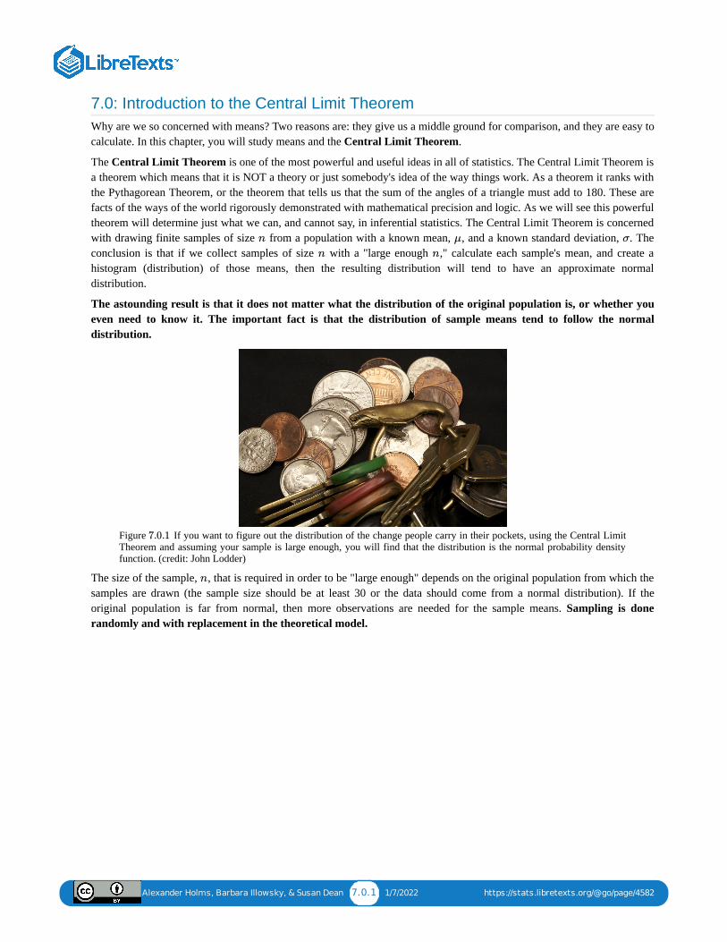
Alexander Holms, Barbara Illowsky, & Susan Dean 7.0.1 1/7/2022 https://stats.libretexts.org/@go/page/4582
7.0: Introduction to the Central Limit TheoremWhy are we so concerned with means? Two reasons are: they give us a middle ground for comparison, and they are easy tocalculate. In this chapter, you will study means and the Central Limit Theorem.
The Central Limit Theorem is one of the most powerful and useful ideas in all of statistics. The Central Limit Theorem isa theorem which means that it is NOT a theory or just somebody's idea of the way things work. As a theorem it ranks withthe Pythagorean Theorem, or the theorem that tells us that the sum of the angles of a triangle must add to 180. These arefacts of the ways of the world rigorously demonstrated with mathematical precision and logic. As we will see this powerfultheorem will determine just what we can, and cannot say, in inferential statistics. The Central Limit Theorem is concernedwith drawing finite samples of size from a population with a known mean, , and a known standard deviation, . Theconclusion is that if we collect samples of size with a "large enough ," calculate each sample's mean, and create ahistogram (distribution) of those means, then the resulting distribution will tend to have an approximate normaldistribution.
The astounding result is that it does not matter what the distribution of the original population is, or whether youeven need to know it. The important fact is that the distribution of sample means tend to follow the normaldistribution.
Figure If you want to figure out the distribution of the change people carry in their pockets, using the Central LimitTheorem and assuming your sample is large enough, you will find that the distribution is the normal probability densityfunction. (credit: John Lodder)
The size of the sample, , that is required in order to be "large enough" depends on the original population from which thesamples are drawn (the sample size should be at least 30 or the data should come from a normal distribution). If theoriginal population is far from normal, then more observations are needed for the sample means. Sampling is donerandomly and with replacement in the theoretical model.
n μ σ
n n
7.0.1
n
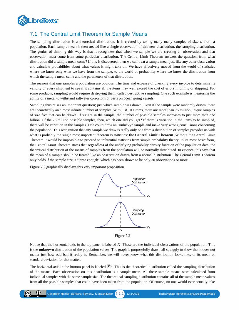
Alexander Holms, Barbara Illowsky, & Susan Dean 7.1.1 12/3/2021 https://stats.libretexts.org/@go/page/4583
7.1: The Central Limit Theorem for Sample MeansThe sampling distribution is a theoretical distribution. It is created by taking many many samples of size from apopulation. Each sample mean is then treated like a single observation of this new distribution, the sampling distribution.The genius of thinking this way is that it recognizes that when we sample we are creating an observation and thatobservation must come from some particular distribution. The Central Limit Theorem answers the question: from whatdistribution did a sample mean come? If this is discovered, then we can treat a sample mean just like any other observationand calculate probabilities about what values it might take on. We have effectively moved from the world of statisticswhere we know only what we have from the sample, to the world of probability where we know the distribution fromwhich the sample mean came and the parameters of that distribution.
The reasons that one samples a population are obvious. The time and expense of checking every invoice to determine itsvalidity or every shipment to see if it contains all the items may well exceed the cost of errors in billing or shipping. Forsome products, sampling would require destroying them, called destructive sampling. One such example is measuring theability of a metal to withstand saltwater corrosion for parts on ocean going vessels.
Sampling thus raises an important question; just which sample was drawn. Even if the sample were randomly drawn, thereare theoretically an almost infinite number of samples. With just 100 items, there are more than 75 million unique samplesof size five that can be drawn. If six are in the sample, the number of possible samples increases to just more than onebillion. Of the 75 million possible samples, then, which one did you get? If there is variation in the items to be sampled,there will be variation in the samples. One could draw an "unlucky" sample and make very wrong conclusions concerningthe population. This recognition that any sample we draw is really only one from a distribution of samples provides us withwhat is probably the single most important theorem is statistics: the Central Limit Theorem. Without the Central LimitTheorem it would be impossible to proceed to inferential statistics from simple probability theory. In its most basic form,the Central Limit Theorem states that regardless of the underlying probability density function of the population data, thetheoretical distribution of the means of samples from the population will be normally distributed. In essence, this says thatthe mean of a sample should be treated like an observation drawn from a normal distribution. The Central Limit Theoremonly holds if the sample size is "large enough" which has been shown to be only 30 observations or more.
Figure 7.2 graphically displays this very important proposition.
Figure 7.2
Notice that the horizontal axis in the top panel is labeled . These are the individual observations of the population. Thisis the unknown distribution of the population values. The graph is purposefully drawn all squiggly to show that it does notmatter just how odd ball it really is. Remember, we will never know what this distribution looks like, or its mean orstandard deviation for that matter.
The horizontal axis in the bottom panel is labeled 's. This is the theoretical distribution called the sampling distributionof the means. Each observation on this distribution is a sample mean. All these sample means were calculated fromindividual samples with the same sample size. The theoretical sampling distribution contains all of the sample mean valuesfrom all the possible samples that could have been taken from the population. Of course, no one would ever actually take
n
X
X¯ ¯¯̄
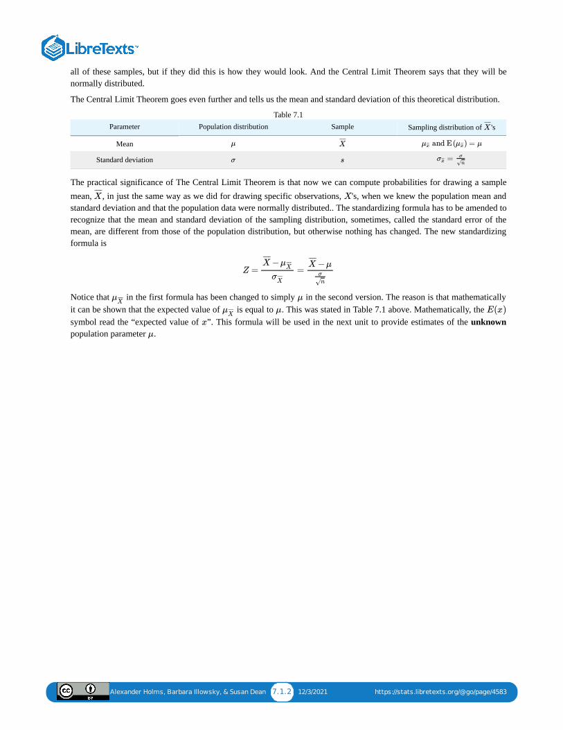
Alexander Holms, Barbara Illowsky, & Susan Dean 7.1.2 12/3/2021 https://stats.libretexts.org/@go/page/4583
all of these samples, but if they did this is how they would look. And the Central Limit Theorem says that they will benormally distributed.
The Central Limit Theorem goes even further and tells us the mean and standard deviation of this theoretical distribution.
Table 7.1Parameter Population distribution Sample Sampling distribution of 's
Mean
Standard deviation
The practical significance of The Central Limit Theorem is that now we can compute probabilities for drawing a samplemean, , in just the same way as we did for drawing specific observations, 's, when we knew the population mean andstandard deviation and that the population data were normally distributed.. The standardizing formula has to be amended torecognize that the mean and standard deviation of the sampling distribution, sometimes, called the standard error of themean, are different from those of the population distribution, but otherwise nothing has changed. The new standardizingformula is
Notice that in the first formula has been changed to simply in the second version. The reason is that mathematicallyit can be shown that the expected value of is equal to . This was stated in Table 7.1 above. Mathematically, the symbol read the “expected value of ”. This formula will be used in the next unit to provide estimates of the unknownpopulation parameter .
X¯ ¯¯̄
μ X¯ ¯¯̄ and E( ) = μμx̄̄̄ μx̄̄̄
σ s =σx̄̄̄σ
n√
X¯ ¯¯̄
X
Z = =−X
¯ ¯¯̄μ
X¯ ¯¯̄¯
σX¯ ¯¯̄¯
−μX¯ ¯¯̄
σ
n√
μX¯ ¯¯̄¯ μ
μX¯ ¯¯̄¯ μ E(x)
x
μ
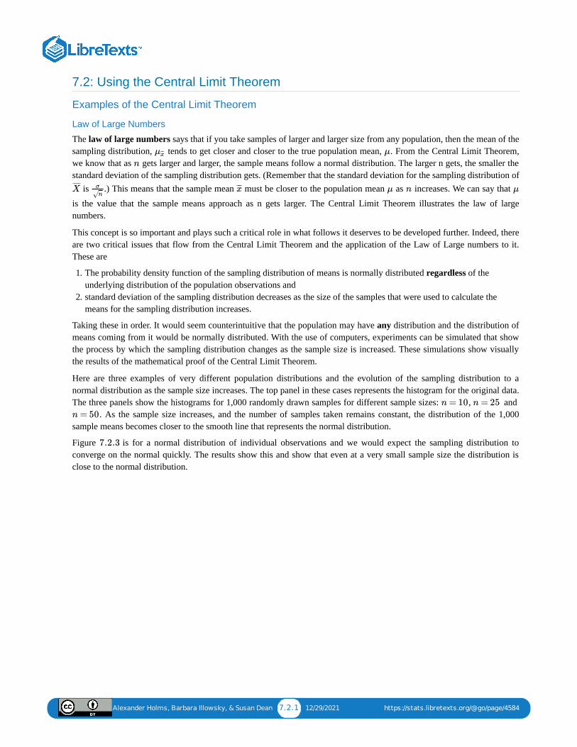
Alexander Holms, Barbara Illowsky, & Susan Dean 7.2.1 12/29/2021 https://stats.libretexts.org/@go/page/4584
7.2: Using the Central Limit Theorem
Examples of the Central Limit Theorem
Law of Large Numbers
The law of large numbers says that if you take samples of larger and larger size from any population, then the mean of thesampling distribution, tends to get closer and closer to the true population mean, . From the Central Limit Theorem,we know that as gets larger and larger, the sample means follow a normal distribution. The larger n gets, the smaller thestandard deviation of the sampling distribution gets. (Remember that the standard deviation for the sampling distribution of
is .) This means that the sample mean must be closer to the population mean as increases. We can say that
is the value that the sample means approach as n gets larger. The Central Limit Theorem illustrates the law of largenumbers.
This concept is so important and plays such a critical role in what follows it deserves to be developed further. Indeed, thereare two critical issues that flow from the Central Limit Theorem and the application of the Law of Large numbers to it.These are
1. The probability density function of the sampling distribution of means is normally distributed regardless of theunderlying distribution of the population observations and
2. standard deviation of the sampling distribution decreases as the size of the samples that were used to calculate themeans for the sampling distribution increases.
Taking these in order. It would seem counterintuitive that the population may have any distribution and the distribution ofmeans coming from it would be normally distributed. With the use of computers, experiments can be simulated that showthe process by which the sampling distribution changes as the sample size is increased. These simulations show visuallythe results of the mathematical proof of the Central Limit Theorem.
Here are three examples of very different population distributions and the evolution of the sampling distribution to anormal distribution as the sample size increases. The top panel in these cases represents the histogram for the original data.The three panels show the histograms for 1,000 randomly drawn samples for different sample sizes: , and
. As the sample size increases, and the number of samples taken remains constant, the distribution of the 1,000sample means becomes closer to the smooth line that represents the normal distribution.
Figure is for a normal distribution of individual observations and we would expect the sampling distribution toconverge on the normal quickly. The results show this and show that even at a very small sample size the distribution isclose to the normal distribution.
μx̄̄̄ μ
n
X¯ ¯¯̄ σ
n√x̄̄̄ μ n μ
n = 10 n = 25
n = 50
7.2.3
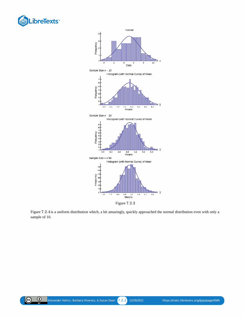
Alexander Holms, Barbara Illowsky, & Susan Dean 7.2.2 12/29/2021 https://stats.libretexts.org/@go/page/4584
Figure
Figure is a uniform distribution which, a bit amazingly, quickly approached the normal distribution even with only asample of 10.
7.2.3
7.2.4
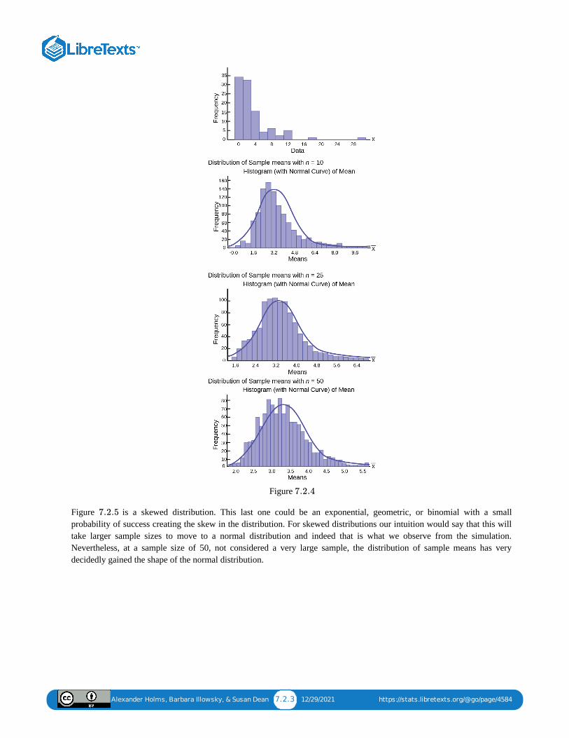
Alexander Holms, Barbara Illowsky, & Susan Dean 7.2.3 12/29/2021 https://stats.libretexts.org/@go/page/4584
Figure
Figure is a skewed distribution. This last one could be an exponential, geometric, or binomial with a smallprobability of success creating the skew in the distribution. For skewed distributions our intuition would say that this willtake larger sample sizes to move to a normal distribution and indeed that is what we observe from the simulation.Nevertheless, at a sample size of 50, not considered a very large sample, the distribution of sample means has verydecidedly gained the shape of the normal distribution.
7.2.4
7.2.5
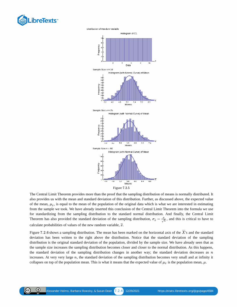
Alexander Holms, Barbara Illowsky, & Susan Dean 7.2.4 12/29/2021 https://stats.libretexts.org/@go/page/4584
Figure
The Central Limit Theorem provides more than the proof that the sampling distribution of means is normally distributed. Italso provides us with the mean and standard deviation of this distribution. Further, as discussed above, the expected valueof the mean, , is equal to the mean of the population of the original data which is what we are interested in estimatingfrom the sample we took. We have already inserted this conclusion of the Central Limit Theorem into the formula we usefor standardizing from the sampling distribution to the standard normal distribution. And finally, the Central LimitTheorem has also provided the standard deviation of the sampling distribution, , and this is critical to have to
calculate probabilities of values of the new random variable, .
Figure shows a sampling distribution. The mean has been marked on the horizontal axis of the 's and the standarddeviation has been written to the right above the distribution. Notice that the standard deviation of the samplingdistribution is the original standard deviation of the population, divided by the sample size. We have already seen that asthe sample size increases the sampling distribution becomes closer and closer to the normal distribution. As this happens,the standard deviation of the sampling distribution changes in another way; the standard deviation decreases as increases. At very very large , the standard deviation of the sampling distribution becomes very small and at infinity itcollapses on top of the population mean. This is what it means that the expected value of is the population mean, .
7.2.5
μx̄̄̄
=σx̄̄̄σ
n√
x̄̄̄
7.2.6 X¯ ¯¯̄
n
n
μx̄̄̄ μ
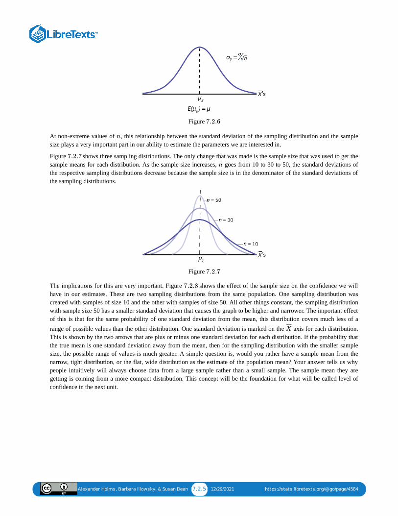
Alexander Holms, Barbara Illowsky, & Susan Dean 7.2.5 12/29/2021 https://stats.libretexts.org/@go/page/4584
Figure
At non-extreme values of , this relationship between the standard deviation of the sampling distribution and the samplesize plays a very important part in our ability to estimate the parameters we are interested in.
Figure shows three sampling distributions. The only change that was made is the sample size that was used to get thesample means for each distribution. As the sample size increases, goes from 10 to 30 to 50, the standard deviations ofthe respective sampling distributions decrease because the sample size is in the denominator of the standard deviations ofthe sampling distributions.
Figure
The implications for this are very important. Figure shows the effect of the sample size on the confidence we willhave in our estimates. These are two sampling distributions from the same population. One sampling distribution wascreated with samples of size 10 and the other with samples of size 50. All other things constant, the sampling distributionwith sample size 50 has a smaller standard deviation that causes the graph to be higher and narrower. The important effectof this is that for the same probability of one standard deviation from the mean, this distribution covers much less of arange of possible values than the other distribution. One standard deviation is marked on the axis for each distribution.This is shown by the two arrows that are plus or minus one standard deviation for each distribution. If the probability thatthe true mean is one standard deviation away from the mean, then for the sampling distribution with the smaller samplesize, the possible range of values is much greater. A simple question is, would you rather have a sample mean from thenarrow, tight distribution, or the flat, wide distribution as the estimate of the population mean? Your answer tells us whypeople intuitively will always choose data from a large sample rather than a small sample. The sample mean they aregetting is coming from a more compact distribution. This concept will be the foundation for what will be called level ofconfidence in the next unit.
7.2.6
n
7.2.7
n
7.2.7
7.2.8
X¯ ¯¯̄
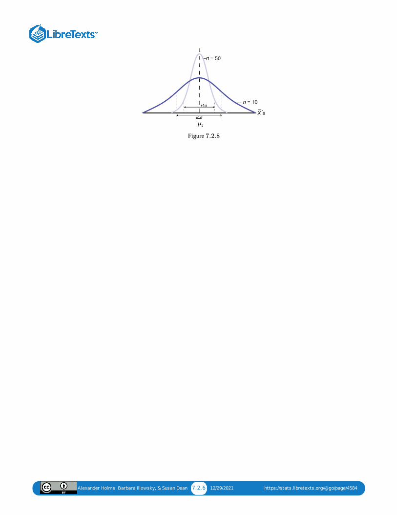
Alexander Holms, Barbara Illowsky, & Susan Dean 7.2.6 12/29/2021 https://stats.libretexts.org/@go/page/4584
Figure 7.2.8
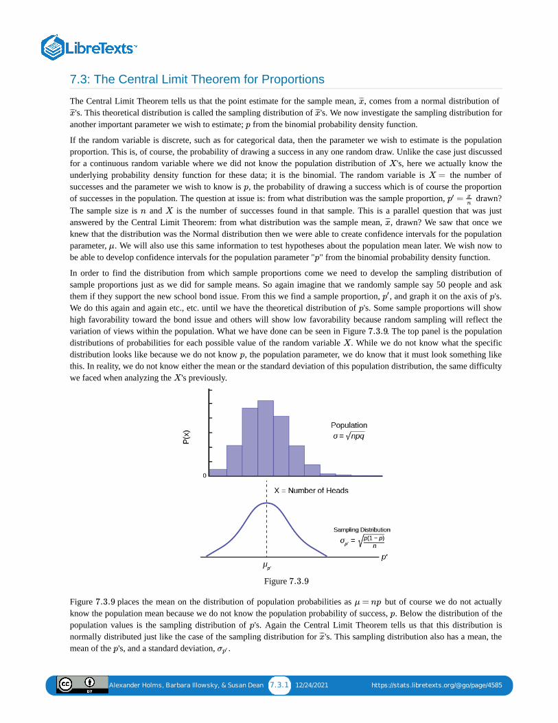
Alexander Holms, Barbara Illowsky, & Susan Dean 7.3.1 12/24/2021 https://stats.libretexts.org/@go/page/4585
7.3: The Central Limit Theorem for Proportions
The Central Limit Theorem tells us that the point estimate for the sample mean, , comes from a normal distribution of 's. This theoretical distribution is called the sampling distribution of 's. We now investigate the sampling distribution for
another important parameter we wish to estimate; from the binomial probability density function.
If the random variable is discrete, such as for categorical data, then the parameter we wish to estimate is the populationproportion. This is, of course, the probability of drawing a success in any one random draw. Unlike the case just discussedfor a continuous random variable where we did not know the population distribution of 's, here we actually know theunderlying probability density function for these data; it is the binomial. The random variable is the number ofsuccesses and the parameter we wish to know is , the probability of drawing a success which is of course the proportionof successes in the population. The question at issue is: from what distribution was the sample proportion, drawn?The sample size is and is the number of successes found in that sample. This is a parallel question that was justanswered by the Central Limit Theorem: from what distribution was the sample mean, , drawn? We saw that once weknew that the distribution was the Normal distribution then we were able to create confidence intervals for the populationparameter, . We will also use this same information to test hypotheses about the population mean later. We wish now tobe able to develop confidence intervals for the population parameter " " from the binomial probability density function.
In order to find the distribution from which sample proportions come we need to develop the sampling distribution ofsample proportions just as we did for sample means. So again imagine that we randomly sample say 50 people and askthem if they support the new school bond issue. From this we find a sample proportion, , and graph it on the axis of 's.We do this again and again etc., etc. until we have the theoretical distribution of 's. Some sample proportions will showhigh favorability toward the bond issue and others will show low favorability because random sampling will reflect thevariation of views within the population. What we have done can be seen in Figure . The top panel is the populationdistributions of probabilities for each possible value of the random variable . While we do not know what the specificdistribution looks like because we do not know , the population parameter, we do know that it must look something likethis. In reality, we do not know either the mean or the standard deviation of this population distribution, the same difficultywe faced when analyzing the 's previously.
Figure
Figure places the mean on the distribution of population probabilities as but of course we do not actuallyknow the population mean because we do not know the population probability of success, . Below the distribution of thepopulation values is the sampling distribution of 's. Again the Central Limit Theorem tells us that this distribution isnormally distributed just like the case of the sampling distribution for 's. This sampling distribution also has a mean, themean of the 's, and a standard deviation, .
x̄̄̄
x̄̄̄ x̄̄̄
p
X
X =p
=p′ xn
n X
x̄̄̄
μ
p
p′ p
p
7.3.9X
p
X
7.3.9
7.3.9 μ = np
p
p
x̄̄̄
p σp′
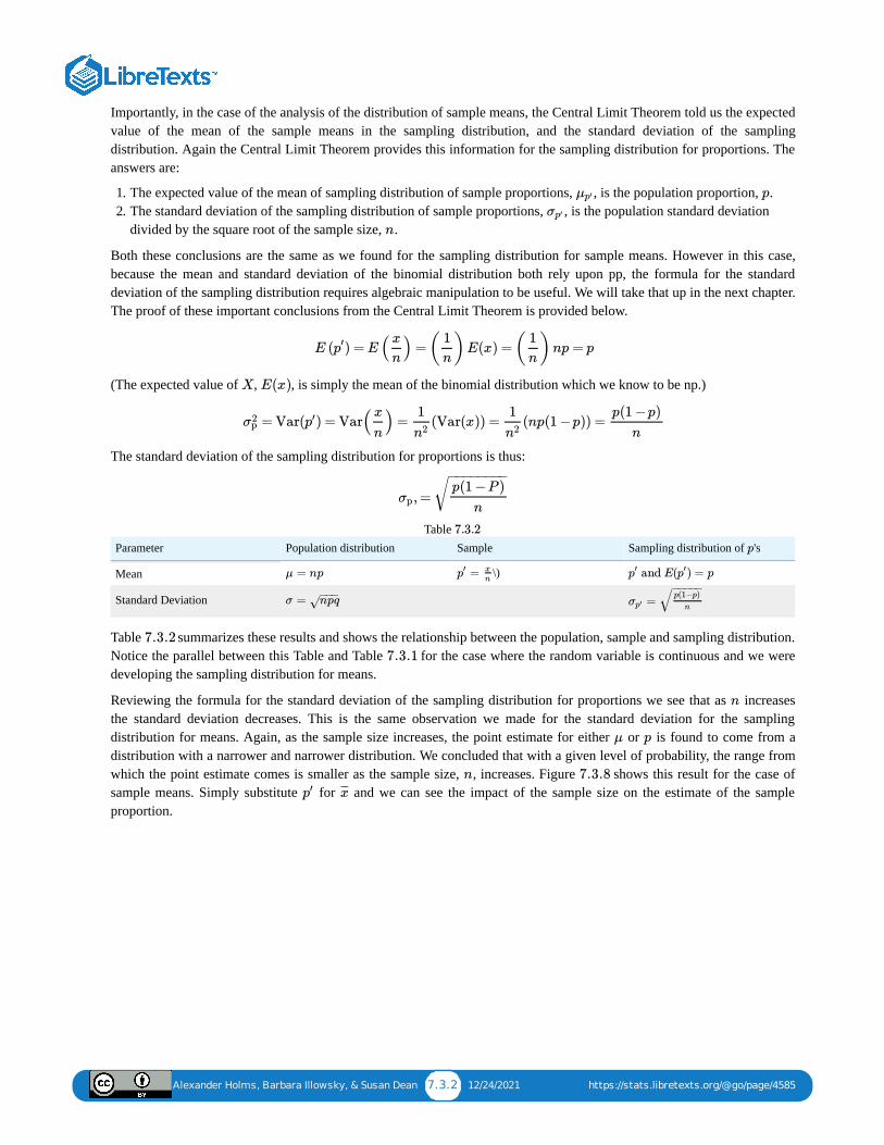
Alexander Holms, Barbara Illowsky, & Susan Dean 7.3.2 12/24/2021 https://stats.libretexts.org/@go/page/4585
Importantly, in the case of the analysis of the distribution of sample means, the Central Limit Theorem told us the expectedvalue of the mean of the sample means in the sampling distribution, and the standard deviation of the samplingdistribution. Again the Central Limit Theorem provides this information for the sampling distribution for proportions. Theanswers are:
1. The expected value of the mean of sampling distribution of sample proportions, , is the population proportion, .2. The standard deviation of the sampling distribution of sample proportions, , is the population standard deviation
divided by the square root of the sample size, .
Both these conclusions are the same as we found for the sampling distribution for sample means. However in this case,because the mean and standard deviation of the binomial distribution both rely upon pp, the formula for the standarddeviation of the sampling distribution requires algebraic manipulation to be useful. We will take that up in the next chapter.The proof of these important conclusions from the Central Limit Theorem is provided below.
(The expected value of , , is simply the mean of the binomial distribution which we know to be np.)
The standard deviation of the sampling distribution for proportions is thus:
Parameter Population distribution Sample Sampling distribution of 's
Mean \)
Standard Deviation
Table
Table summarizes these results and shows the relationship between the population, sample and sampling distribution.Notice the parallel between this Table and Table for the case where the random variable is continuous and we weredeveloping the sampling distribution for means.
Reviewing the formula for the standard deviation of the sampling distribution for proportions we see that as increasesthe standard deviation decreases. This is the same observation we made for the standard deviation for the samplingdistribution for means. Again, as the sample size increases, the point estimate for either or is found to come from adistribution with a narrower and narrower distribution. We concluded that with a given level of probability, the range fromwhich the point estimate comes is smaller as the sample size, , increases. Figure shows this result for the case ofsample means. Simply substitute for and we can see the impact of the sample size on the estimate of the sampleproportion.
μp′ p
σp′
n
E ( ) = E ( ) =( )E(x) =( )np = pp′ x
n
1
n
1
n
X E(x)
= Var( ) = Var( ) = (Var(x)) = (np(1 −p)) =σ2p p′ x
n
1
n2
1
n2
p(1 −p)
n
, =σpp(1 −P )
n
− −−−−−−−√
p
μ = np =p′ xn
and E( ) = pp′ p′
σ = npq−−−√ =σp′
p(1−p)
n
− −−−−√
7.3.2
7.3.27.3.1
n
μ p
n 7.3.8p′ x̄̄̄
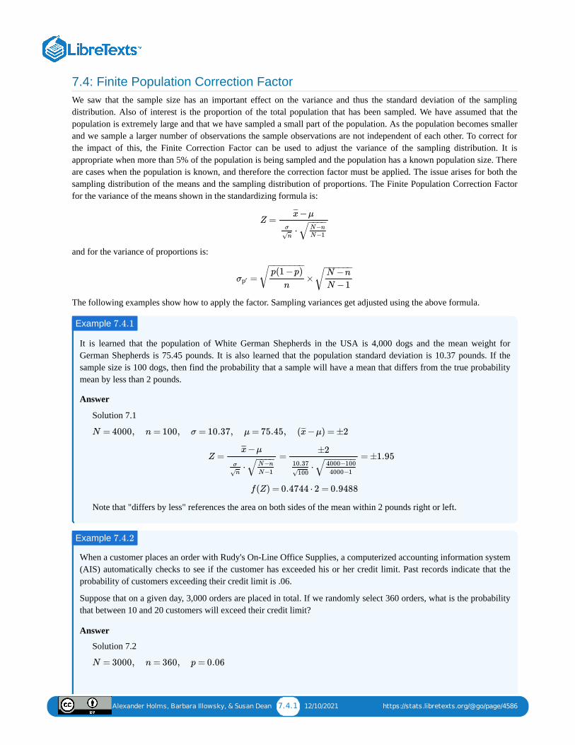
Alexander Holms, Barbara Illowsky, & Susan Dean 7.4.1 12/10/2021 https://stats.libretexts.org/@go/page/4586
7.4: Finite Population Correction FactorWe saw that the sample size has an important effect on the variance and thus the standard deviation of the samplingdistribution. Also of interest is the proportion of the total population that has been sampled. We have assumed that thepopulation is extremely large and that we have sampled a small part of the population. As the population becomes smallerand we sample a larger number of observations the sample observations are not independent of each other. To correct forthe impact of this, the Finite Correction Factor can be used to adjust the variance of the sampling distribution. It isappropriate when more than 5% of the population is being sampled and the population has a known population size. Thereare cases when the population is known, and therefore the correction factor must be applied. The issue arises for both thesampling distribution of the means and the sampling distribution of proportions. The Finite Population Correction Factorfor the variance of the means shown in the standardizing formula is:
and for the variance of proportions is:
The following examples show how to apply the factor. Sampling variances get adjusted using the above formula.
It is learned that the population of White German Shepherds in the USA is 4,000 dogs and the mean weight forGerman Shepherds is 75.45 pounds. It is also learned that the population standard deviation is 10.37 pounds. If thesample size is 100 dogs, then find the probability that a sample will have a mean that differs from the true probabilitymean by less than 2 pounds.
Answer
Solution 7.1
Note that "differs by less" references the area on both sides of the mean within 2 pounds right or left.
When a customer places an order with Rudy's On-Line Office Supplies, a computerized accounting information system(AIS) automatically checks to see if the customer has exceeded his or her credit limit. Past records indicate that theprobability of customers exceeding their credit limit is .06.
Suppose that on a given day, 3,000 orders are placed in total. If we randomly select 360 orders, what is the probabilitythat between 10 and 20 customers will exceed their credit limit?
Answer
Solution 7.2
Z =−μx̄̄̄
⋅σ
n√N−n
N−1
− −−−√
= ×σp′
p(1 −p)
n
− −−−−−−√ N −n
N −1
− −−−−−√
Example 7.4.1
N = 4000, n = 100, σ = 10.37, μ = 75.45, ( −μ) = ±2x̄̄̄
Z = = = ±1.95−μx̄̄̄
⋅σ
n√
N−n
N−1
− −−−√
±2
⋅10.37
100√
4000−1004000−1
− −−−−−√
f(Z) = 0.4744 ⋅ 2 = 0.9488
Example 7.4.2
N = 3000, n = 360, p = 0.06
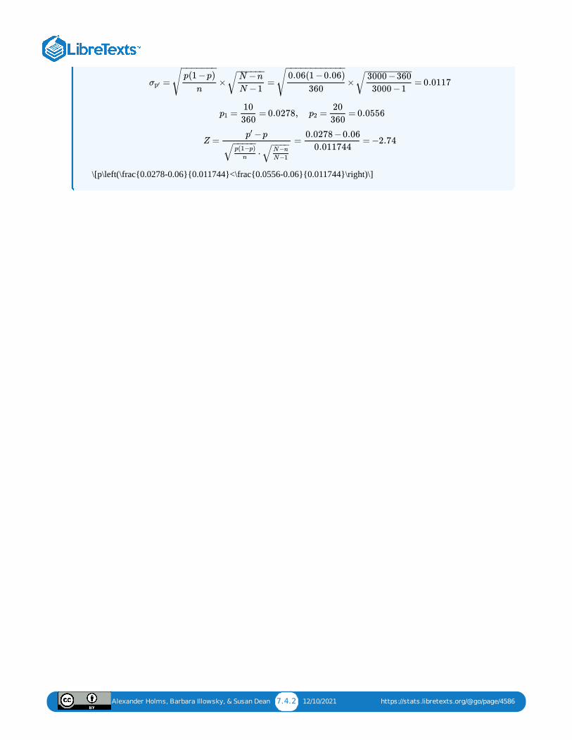
Alexander Holms, Barbara Illowsky, & Susan Dean 7.4.2 12/10/2021 https://stats.libretexts.org/@go/page/4586
\[p\left(\frac{0.0278-0.06}{0.011744}<\frac{0.0556-0.06}{0.011744}\right)\]
= × = × = 0.0117σp′
p(1 −p)
n
− −−−−−−
√ N −n
N −1
− −−−−−√
0.06(1 −0.06)
360
− −−−−−−−−−−−
√3000 −360
3000 −1
− −−−−−−−−√
= = 0.0278, = = 0.0556p110
360p2
20
360
Z = = = −2.74−pp′
⋅p(1−p)
n
− −−−−√ N−n
N−1
− −−−√
0.0278 −0.06
0.011744
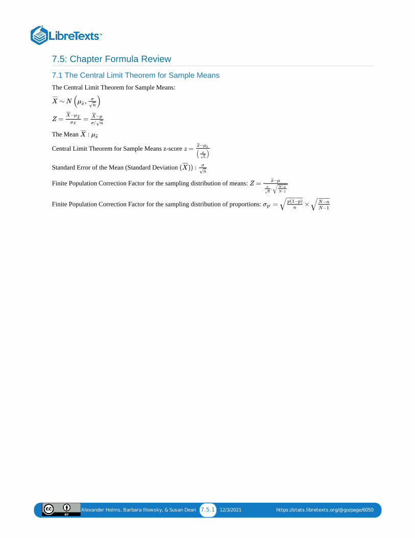
Alexander Holms, Barbara Illowsky, & Susan Dean 7.5.1 12/3/2021 https://stats.libretexts.org/@go/page/6050
7.5: Chapter Formula Review
7.1 The Central Limit Theorem for Sample Means
The Central Limit Theorem for Sample Means:
The Mean
Central Limit Theorem for Sample Means z-score
Standard Error of the Mean (Standard Deviation
Finite Population Correction Factor for the sampling distribution of means:
Finite Population Correction Factor for the sampling distribution of proportions:
∼ N ( , )X¯ ¯¯̄
μx̄̄̄σ
n√
Z = =−X
¯ ¯¯̄¯μ
X̄̄̄
σX
−μX¯ ¯¯̄¯
σ/ n√
:X¯ ¯¯̄
μx̄̄̄
z =−x̄̄̄ μx̄
( )σ
n√
( )) :X¯ ¯¯̄ σ
n√
Z =−μx̄̄̄
⋅σ
n√
N−n
N−1√
= ×σp′p(1−p)
n
− −−−−√ N−n
N−1
− −−−√
Alexander Holms, Barbara Illowsky, & Susan Dean 7.6.1 1/7/2022 https://stats.libretexts.org/@go/page/6056
7.6: Chapter Homework
The Central Limit Theorem for Sample Means
49
Previously, De Anza statistics students estimated that the amount of change daytime statistics students carry isexponentially distributed with a mean of $0.88. Suppose that we randomly pick 25 daytime statistics students.
1. In words, = ____________2. _____(_____,_____)3. In words, = ____________4. ______ (______, ______)5. Find the probability that an individual had between $0.80 and $1.00. Graph the situation, and shade in the area to be
determined.6. Find the probability that the average of the 25 students was between $0.80 and $1.00. Graph the situation, and shade in
the area to be determined.7. Explain why there is a difference in part e and part f.
Answer1. = amount of change students carry2. 3. = average amount of change carried by a sample of 25 students.4. 5. 6. 7. The distributions are different. Part 1 is exponential and part 2 is normal.
50.
Suppose that the distance of fly balls hit to the outfield (in baseball) is normally distributed with a mean of 250 feet and astandard deviation of 50 feet. We randomly sample 49 fly balls.
1. If = average distance in feet for 49 fly balls, then _______(_______,_______)2. What is the probability that the 49 balls traveled an average of less than 240 feet? Sketch the graph. Scale the
horizontal axis for . Shade the region corresponding to the probability. Find the probability.3. Find the 80th percentile of the distribution of the average of 49 fly balls.
51.
According to the Internal Revenue Service, the average length of time for an individual to complete (keep records for,learn, prepare, copy, assemble, and send) IRS Form 1040 is 10.53 hours (without any attached schedules). The distributionis unknown. Let us assume that the standard deviation is two hours. Suppose we randomly sample 36 taxpayers.
1. In words, _____________2. In words, = _____________3. _____(_____,_____)4. Would you be surprised if the 36 taxpayers finished their Form 1040s in an average of more than 12 hours? Explain
why or why not in complete sentences.5. Would you be surprised if one taxpayer finished his or her Form 1040 in more than 12 hours? In a complete sentence,
explain why.
52.
Suppose that a category of world-class runners are known to run a marathon (26 miles) in an average of 145 minutes witha standard deviation of 14 minutes. Consider 49 of the races. Let the average of the 49 races.
XX ∼
X¯ ¯¯̄
∼X¯ ¯¯̄
XX ∼ E(0.88, 0.88)
X¯ ¯¯̄
∼ N(0.88, 0.176)X¯ ¯¯̄
0.08190.1882
X¯ ¯¯̄
∼X¯ ¯¯̄
X¯ ¯¯̄
X =
X¯ ¯¯̄
∼X¯ ¯¯̄
X¯ ¯¯̄
Alexander Holms, Barbara Illowsky, & Susan Dean 7.6.2 1/7/2022 https://stats.libretexts.org/@go/page/6056
1. _____(_____,_____)2. Find the probability that the runner will average between 142 and 146 minutes in these 49 marathons.3. Find the percentile for the average of these 49 marathons.4. Find the median of the average running times.
53.
The length of songs in a collector’s iTunes album collection is uniformly distributed from two to 3.5 minutes. Suppose werandomly pick five albums from the collection. There are a total of 43 songs on the five albums.
1. In words, = _________2. _____________3. In words, = _____________4. _____(_____,_____)5. Find the first quartile for the average song length.6. The (interquartile range) for the average song length is from _______–_______.
54.
In 1940 the average size of a U.S. farm was 174 acres. Let’s say that the standard deviation was 55 acres. Suppose werandomly survey 38 farmers from 1940.
1. In words, = _____________2. In words, = _____________3. _____(_____,_____)4. The for is from _______ acres to _______ acres.
55.
Determine which of the following are true and which are false. Then, in complete sentences, justify your answers.
1. When the sample size is large, the mean of is approximately equal to the mean of .2. When the sample size is large, is approximately normally distributed.3. When the sample size is large, the standard deviation of is approximately the same as the standard deviation of .
56.
The percent of fat calories that a person in America consumes each day is normally distributed with a mean of about 36and a standard deviation of about ten. Suppose that 16 individuals are randomly chosen. Let = average percent of fatcalories.
a. ______(______, ______)b. For the group of 16, find the probability that the average percent of fat calories consumed is more than five. Graph the
situation and shade in the area to be determined.c. Find the first quartile for the average percent of fat calories.
57.
The distribution of income in some Third World countries is considered wedge shaped (many very poor people, very fewmiddle income people, and even fewer wealthy people). Suppose we pick a country with a wedge shaped distribution. Letthe average salary be $2,000 per year with a standard deviation of $8,000. We randomly survey 1,000 residents of thatcountry.
1. In words, = _____________2. In words, = _____________3. _____(_____,_____)4. How is it possible for the standard deviation to be greater than the average?5. Why is it more likely that the average of the 1,000 residents will be from $2,000 to $2,100 than from $2,100 to $2,200?
58.
∼X¯ ¯¯̄
80th
XX ∼
X¯ ¯¯̄
∼X¯ ¯¯̄
IQR
X
X¯ ¯¯̄
∼X¯ ¯¯̄
IQR X¯ ¯¯̄
X¯ ¯¯̄
X
X¯ ¯¯̄
X¯ ¯¯̄ X
X¯ ¯¯̄
∼X¯ ¯¯̄
X
X¯ ¯¯̄
∼X¯ ¯¯̄
Alexander Holms, Barbara Illowsky, & Susan Dean 7.6.3 1/7/2022 https://stats.libretexts.org/@go/page/6056
Which of the following is NOT TRUE about the distribution for averages?
1. The mean, median, and mode are equal.2. The area under the curve is one.3. The curve never touches the x-axis.4. The curve is skewed to the right.
59.
The cost of unleaded gasoline in the Bay Area once followed an unknown distribution with a mean of $4.59 and a standarddeviation of $0.10. Sixteen gas stations from the Bay Area are randomly chosen. We are interested in the average cost ofgasoline for the 16 gas stations. The distribution to use for the average cost of gasoline for the 16 gas stations is:
a.
b.
c.
d.
Using the Central Limit Theorem60.
A large population of 5,000 students take a practice test to prepare for a standardized test. The population mean is 140questions correct, and the standard deviation is 80. What size samples should a researcher take to get a distribution ofmeans of the samples with a standard deviation of 10?
61.
A large population has skewed data with a mean of 70 and a standard deviation of 6. Samples of size 100 are taken, and thedistribution of the means of these samples is analyzed.
1. Will the distribution of the means be closer to a normal distribution than the distribution of the population?2. Will the mean of the means of the samples remain close to 70?3. Will the distribution of the means have a smaller standard deviation?4. What is that standard deviation?
62.
A researcher is looking at data from a large population with a standard deviation that is much too large. In order toconcentrate the information, the researcher decides to repeatedly sample the data and use the distribution of the means ofthe samples? The first effort used sample sized of 100. But the standard deviation was about double the value theresearcher wanted. What is the smallest size samples the researcher can use to remedy the problem?
63.
A researcher looks at a large set of data, and concludes the population has a standard deviation of 40. Using sample sizesof 64, the researcher is able to focus the mean of the means of the sample to a narrower distribution where the standarddeviation is 5. Then, the researcher realizes there was an error in the original calculations, and the initial standard deviationis really 20. Since the standard deviation of the means of the samples was obtained using the original standard deviation,this value is also impacted by the discovery of the error. What is the correct value of the standard deviation of the means ofthe samples?
64.
A population has a standard deviation of 50. It is sampled with samples of size 100. What is the variance of the means ofthe samples?
∼ N(4.59, 0.10)X¯ ¯¯̄
∼ N (4.59, )X¯ ¯¯̄ 0.10
16√
∼ N (4.59, )X¯ ¯¯̄ 16
0.10
∼ N (4.59, )X¯ ¯¯̄ 16√
0.10
Alexander Holms, Barbara Illowsky, & Susan Dean 7.6.4 1/7/2022 https://stats.libretexts.org/@go/page/6056
The Central Limit Theorem for Proportions65.
A farmer picks pumpkins from a large field. The farmer makes samples of 260 pumpkins and inspects them. If one in fiftypumpkins are not fit to market and will be saved for seeds, what is the standard deviation of the mean of the samplingdistribution of sample proportions?
66.
A store surveys customers to see if they are satisfied with the service they received. Samples of 25 surveys are taken. Onein five people are unsatisfied. What is the variance of the mean of the sampling distribution of sample proportions for thenumber of unsatisfied customers? What is the variance for satisfied customers?
67.
A company gives an anonymous survey to its employees to see what percent of its employees are happy. The company istoo large to check each response, so samples of 50 are taken, and the tendency is that three-fourths of the employees arehappy. For the mean of the sampling distribution of sample proportions, answer the following questions, if the sample sizeis doubled.
1. How does this affect the mean?2. How does this affect the standard deviation?3. How does this affect the variance?
68.
A pollster asks a single question with only yes and no as answer possibilities. The poll is conducted nationwide, sosamples of 100 responses are taken. There are four yes answers for each no answer overall. For the mean of the samplingdistribution of sample proportions, find the following for yes answers.
a. The expected value.b. The standard deviation.c. The variance.
69.
The mean of the sampling distribution of sample proportions has a value of of 0.3, and sample size of 40.
1. Is there a difference in the expected value if and reverse roles?2. Is there a difference in the calculation of the standard deviation with the same reversal?
Finite Population Correction Factor70.
A company has 1,000 employees. The average number of workdays between absence for illness is 80 with a standarddeviation of 11 days. Samples of 80 employees are examined. What is the probability a sample has a mean of workdayswith no absence for illness of at least 78 days and at most 84 days?
71.
Trucks pass an automatic scale that monitors 2,000 trucks. This population of trucks has an average weight of 20 tons witha standard deviation of 2 tons. If a sample of 50 trucks is taken, what is the probability the sample will have an averageweight within one-half ton of the population mean?
72.
A town keeps weather records. From these records it has been determined that it rains on an average of 12% of the dayseach year. If 30 days are selected at random from one year, what is the probability that at most 3 days had rain?
73.
A maker of greeting cards has an ink problem that causes the ink to smear on 7% of the cards. The daily production run is500 cards. What is the probability that if a sample of 35 cards is checked, there will be ink smeared on at most 5 cards?
p
p q

Alexander Holms, Barbara Illowsky, & Susan Dean 7.6.5 1/7/2022 https://stats.libretexts.org/@go/page/6056
74.
A school has 500 students. Usually, there are an average of 20 students who are absent. If a sample of 30 students is takenon a certain day, what is the probability that at least 2 students in the sample will be absent?
Alexander Holms, Barbara Illowsky, & Susan Dean 7.7.1 10/29/2021 https://stats.libretexts.org/@go/page/4587
7.7: Chapter Key Terms
Averagea number that describes the central tendency of the data; there are a number of specialized averages, including thearithmetic mean, weighted mean, median, mode, and geometric mean.
Central Limit TheoremGiven a random variable with known mean μ and known standard deviation, σ, we are sampling with size n, and we areinterested in two new RVs: the sample mean, . If the size ( ) of the sample is sufficiently large, then
. If the size ( ) of the sample is sufficiently large, then the distribution of the sample means will
approximate a normal distributions regardless of the shape of the population. The mean of the sample means will equalthe population mean. The standard deviation of the distribution of the sample means, , is called the standard error of
the mean.
Finite Population Correction Factoradjusts the variance of the sampling distribution if the population is known and more than 5% of the population isbeing sampled.
Meana number that measures the central tendency; a common name for mean is "average." The term "mean" is a shortenedform of "arithmetic mean." By definition, the mean for a sample (denoted by ) is
, and the mean for a population (denoted by ) is
.
Normal Distribution
a continuous random variable with pdf , where is the mean of the distribution and is the
standard deviation.; notation: . If and , the random variable, , is called the standardnormal distribution.
Sampling DistributionGiven simple random samples of size from a given population with a measured characteristic such as mean,proportion, or standard deviation for each sample, the probability distribution of all the measured characteristics iscalled a sampling distribution.
Standard Error of the Meanthe standard deviation of the distribution of the sample means, or .
Standard Error of the Proportionthe standard deviation of the sampling distribution of proportions
X¯ ¯¯̄
n
∼ N (μ, )X¯ ¯¯̄ σ
n√n
σ
n√
x̄̄̄
= =x̄̄̄ x̄̄̄ Sum of all values in the sample
Number of values in the sample μ
μ = Sum of all values in the population
Number of values in the population
f(x) = 1
σ 2π√e
−(x−μ)2
2σ2 μ σ
X ∼ N(μ, σ) μ = 0 σ = 1 Z
n
σ
n√
Alexander Holms, Barbara Illowsky, & Susan Dean 7.8.1 12/17/2021 https://stats.libretexts.org/@go/page/6055
7.8: Chapter Practice
Using the Central Limit Theorem
Use the following information to answer the next ten exercises: A manufacturer produces 25-pound lifting weights. Thelowest actual weight is 24 pounds, and the highest is 26 pounds. Each weight is equally likely so the distribution ofweights is uniform. A sample of 100 weights is taken.
1.
1. What is the distribution for the weights of one 25-pound lifting weight? What is the mean and standard deivation?2. What is the distribution for the mean weight of 100 25-pound lifting weights?3. Find the probability that the mean actual weight for the 100 weights is less than 24.9.
2.
Draw the graph from Exercise
3.
Find the probability that the mean actual weight for the 100 weights is greater than 25.2.
4.
Draw the graph from Exercise
5.
Find the 90 percentile for the mean weight for the 100 weights.
6.
Draw the graph from Exercise
7.
1. What is the distribution for the sum of the weights of 100 25-pound lifting weights?2. Find .
8.
Draw the graph from Exercise
9.
Find the 90 percentile for the total weight of the 100 weights.
10.
Draw the graph from Exercise
Use the following information to answer the next five exercises: The length of time a particular smartphone's battery lastsfollows an exponential distribution with a mean of ten months. A sample of 64 of these smartphones is taken.
11.
1. What is the standard deviation?2. What is the parameter ?
12.
What is the distribution for the length of time one battery lasts?
13.
What is the distribution for the mean length of time 64 batteries last?
14.
What is the distribution for the total length of time 64 batteries last?
7.8.1
7.8.3
th
7.8.5
P (Σx < 2, 450)
7.8.7
th
7.8.9
m
Alexander Holms, Barbara Illowsky, & Susan Dean 7.8.2 12/17/2021 https://stats.libretexts.org/@go/page/6055
15.
Find the probability that the sample mean is between seven and 11.
16.
Find the 80 percentile for the total length of time 64 batteries last.
17.
Find the for the mean amount of time 64 batteries last.
18.
Find the middle 80% for the total amount of time 64 batteries last.
Use the following information to answer the next eight exercises: A uniform distribution has a minimum of six and amaximum of ten. A sample of 50 is taken.
19.
Find .
20.
Find the 90 percentile for the sums.
21.
Find the 15 percentile for the sums.
22.
Find the first quartile for the sums.
23.
Find the third quartile for the sums.
24.
Find the 80 percentile for the sums.
25.
A population has a mean of 25 and a standard deviation of 2. If it is sampled repeatedly with samples of size 49, what isthe mean and standard deviation of the sample means?
26.
A population has a mean of 48 and a standard deviation of 5. If it is sampled repeatedly with samples of size 36, what isthe mean and standard deviation of the sample means?
27.
A population has a mean of 90 and a standard deviation of 6. If it is sampled repeatedly with samples of size 64, what isthe mean and standard deviation of the sample means?
28.
A population has a mean of 120 and a standard deviation of 2.4. If it is sampled repeatedly with samples of size 40, what isthe mean and standard deviation of the sample means?
29.
A population has a mean of 17 and a standard deviation of 1.2. If it is sampled repeatedly with samples of size 50, what isthe mean and standard deviation of the sample means?
30.
A population has a mean of 17 and a standard deviation of 0.2. If it is sampled repeatedly with samples of size 16, what isthe expected value and standard deviation of the sample means?
th
IQR
P (Σx > 420)
th
th
th
Alexander Holms, Barbara Illowsky, & Susan Dean 7.8.3 12/17/2021 https://stats.libretexts.org/@go/page/6055
31.
A population has a mean of 38 and a standard deviation of 3. If it is sampled repeatedly with samples of size 48, what isthe expected value and standard deviation of the sample means?
32.
A population has a mean of 14 and a standard deviation of 5. If it is sampled repeatedly with samples of size 60, what isthe expected value and standard deviation of the sample means?
The Central Limit Theorem for Proportions
33.
A question is asked of a class of 200 freshmen, and 23% of the students know the correct answer. If a sample of 50students is taken repeatedly, what is the expected value of the mean of the sampling distribution of sample proportions?
34.
A question is asked of a class of 200 freshmen, and 23% of the students know the correct answer. If a sample of 50students is taken repeatedly, what is the standard deviation of the mean of the sampling distribution of sample proportions?
35.
A game is played repeatedly. A player wins one-fifth of the time. If samples of 40 times the game is played are takenrepeatedly, what is the expected value of the mean of the sampling distribution of sample proportions?
36.
A game is played repeatedly. A player wins one-fifth of the time. If samples of 40 times the game is played are takenrepeatedly, what is the standard deviation of the mean of the sampling distribution of sample proportions?
37.
A virus attacks one in three of the people exposed to it. An entire large city is exposed. If samples of 70 people are taken,what is the expected value of the mean of the sampling distribution of sample proportions?
38.
A virus attacks one in three of the people exposed to it. An entire large city is exposed. If samples of 70 people are taken,what is the standard deviation of the mean of the sampling distribution of sample proportions?
39.
A company inspects products coming through its production process, and rejects detected products. One-tenth of the itemsare rejected. If samples of 50 items are taken, what is the expected value of the mean of the sampling distribution ofsample proportions?
40.
A company inspects products coming through its production process, and rejects detected products. One-tenth of the itemsare rejected. If samples of 50 items are taken, what is the standard deviation of the mean of the sampling distribution ofsample proportions?
Finite Population Correction Factor
41.
A fishing boat has 1,000 fish on board, with an average weight of 120 pounds and a standard deviation of 6.0 pounds. Ifsample sizes of 50 fish are checked, what is the probability the fish in a sample will have mean weight within 2.8 poundsthe true mean of the population?
42.
An experimental garden has 500 sunflowers plants. The plants are being treated so they grow to unusual heights. Theaverage height is 9.3 feet with a standard deviation of 0.5 foot. If sample sizes of 60 plants are taken, what is theprobability the plants in a given sample will have an average height within 0.1 foot of the true mean of the population?
Alexander Holms, Barbara Illowsky, & Susan Dean 7.8.4 12/17/2021 https://stats.libretexts.org/@go/page/6055
43.
A company has 800 employees. The average number of workdays between absence for illness is 123 with a standarddeviation of 14 days. Samples of 50 employees are examined. What is the probability a sample has a mean of workdayswith no absence for illness of at least 124 days?
44.
Cars pass an automatic speed check device that monitors 2,000 cars on a given day. This population of cars has an averagespeed of 67 miles per hour with a standard deviation of 2 miles per hour. If samples of 30 cars are taken, what is theprobability a given sample will have an average speed within 0.50 mile per hour of the population mean?
45.
A town keeps weather records. From these records it has been determined that it rains on an average of 37% of the dayseach year. If 30 days are selected at random from one year, what is the probability that at least 5 and at most 11 days hadrain?
46.
A maker of yardsticks has an ink problem that causes the markings to smear on 4% of the yardsticks. The daily productionrun is 2,000 yardsticks. What is the probability if a sample of 100 yardsticks is checked, there will be ink smeared on atmost 4 yardsticks?
47.
A school has 300 students. Usually, there are an average of 21 students who are absent. If a sample of 30 students is takenon a certain day, what is the probability that at most 2 students in the sample will be absent?
48.
A college gives a placement test to 5,000 incoming students each year. On the average 1,213 place in one or moredevelopmental courses. If a sample of 50 is taken from the 5,000, what is the probability at most 12 of those sampled willhave to take at least one developmental course?

Alexander Holms, Barbara Illowsky, & Susan Dean 7.9.1 12/10/2021 https://stats.libretexts.org/@go/page/6057
7.9: Chapter References
7.1 The Central Limit Theorem for Sample Means
Baran, Daya. “20 Percent of Americans Have Never Used Email.”WebGuild, 2010. Available online athttp://www.webguild.org/20080519/20-...ver-used-email (accessed May 17, 2013).
Data from The Flurry Blog, 2013. Available online at blog.flurry.com (accessed May 17, 2013).
Data from the United States Department of Agriculture.
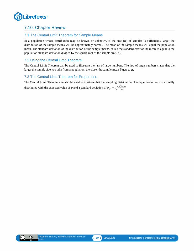
Alexander Holms, Barbara Illowsky, & Susan
Dean7.10.1 11/26/2021 https://stats.libretexts.org/@go/page/6049
7.10: Chapter Review
7.1 The Central Limit Theorem for Sample Means
In a population whose distribution may be known or unknown, if the size ( ) of samples is sufficiently large, thedistribution of the sample means will be approximately normal. The mean of the sample means will equal the populationmean. The standard deviation of the distribution of the sample means, called the standard error of the mean, is equal to thepopulation standard deviation divided by the square root of the sample size ( ).
7.2 Using the Central Limit TheoremThe Central Limit Theorem can be used to illustrate the law of large numbers. The law of large numbers states that thelarger the sample size you take from a population, the closer the sample mean gets to .
7.3 The Central Limit Theorem for ProportionsThe Central Limit Theorem can also be used to illustrate that the sampling distribution of sample proportions is normally
distributed with the expected value of and a standard deviation of
n
n
x̄̄̄ μ
p =σp′p(1−p)
n
− −−−−√

Alexander Holms, Barbara Illowsky, & Susan
Dean7.11.1 12/24/2021 https://stats.libretexts.org/@go/page/6058
7.11: Chapter Solution (Practice + Homework)1.
1. 3.
0.0003
25.07
7.
1. 9.
2,507.40
1. 13.
0.7799
17.
1.69
19.
0.0072
21.
391.54
23.
405.51
25.
Mean = 25, standard deviation = 2/7
26.
Mean = 48, standard deviation = 5/6
27.
Mean = 90, standard deviation = 3/4
28.
Mean = 120, standard deviation = 0.38
29.
Mean = 17, standard deviation = 0.17
30.
Expected value = 17, standard deviation = 0.05
31.
Expected value = 38, standard deviation = 0.43
32.
Expected value = 14, standard deviation = 0.65
33.
0.23
N(10, ))108
Alexander Holms, Barbara Illowsky, & Susan
Dean7.11.2 12/24/2021 https://stats.libretexts.org/@go/page/6058
34.
0.060
35.
1/5
36.
0.063
37.
1/3
38.
0.056
39.
1/10
40.
0.042
41.
0.999
42.
0.901
43.
0.301
44.
0.832
45.
0.483
46.
0.500
47.
0.502
48.
0.519
49.
1. 51.1. 53.
1. 55.
1. 57.1. 59.
b
64
Alexander Holms, Barbara Illowsky, & Susan
Dean7.11.3 12/24/2021 https://stats.libretexts.org/@go/page/6058
61.
1. 62.
400
2.5
64.
25
65.
0.0087
66.
0.0064, 0.0064
67.
1. 68.1. 69.
a. 70.
0.955
0.927
72.
0.648
73.
0.101
74.
0.273

1 1/7/2022
CHAPTER OVERVIEW8: CONFIDENCE INTERVALS
8.0: INTRODUCTION TO CONFIDENCE INTERVALS8.1: A CONFIDENCE INTERVAL FOR A POPULATION STANDARD DEVIATION, KNOWN OR LARGE SAMPLE SIZEA confidence interval for a population mean with a known population standard deviation is based on the conclusion of the CentralLimit Theorem that the sampling distribution of the sample means follow an approximately normal distribution.
8.2: A CONFIDENCE INTERVAL FOR A POPULATION STANDARD DEVIATION UNKNOWN, SMALL SAMPLE CASE8.3: A CONFIDENCE INTERVAL FOR A POPULATION PROPORTION8.4: CALCULATING THE SAMPLE SIZE N- CONTINUOUS AND BINARY RANDOM VARIABLES8.5: CHAPTER FORMULA REVIEW8.6: CHAPTER HOMEWORK8.7: CHAPTER KEY TERMS8.8: CHAPTER PRACTICE8.9: CHAPTER REFERENCES8.10: CHAPTER REVIEW8.11: CHAPTER SOLUTION (PRACTICE + HOMEWORK)
Alexander Holms, Barbara Illowsky, & Susan Dean 8.0.1 12/17/2021 https://stats.libretexts.org/@go/page/4589
8.0: Introduction to Confidence IntervalsSuppose you were trying to determine the mean rent of a two-bedroom apartment in your town. You might look in theclassified section of the newspaper, write down several rents listed, and average them together. You would have obtained apoint estimate of the true mean. If you are trying to determine the percentage of times you make a basket when shooting abasketball, you might count the number of shots you make and divide that by the number of shots you attempted. In thiscase, you would have obtained a point estimate for the true proportion the parameter in the binomial probability densityfunction.
Figure Have you ever wondered what the average number of M&Ms in a bag at the grocery store is? You can useconfidence intervals to answer this question. (credit: comedy_nose/flickr)
We use sample data to make generalizations about an unknown population. This part of statistics is called inferentialstatistics. The sample data help us to make an estimate of a population parameter. We realize that the point estimateis most likely not the exact value of the population parameter, but close to it. After calculating point estimates, weconstruct interval estimates, called confidence intervals. What statistics provides us beyond a simple average, or pointestimate, is an estimate to which we can attach a probability of accuracy, what we will call a confidence level. We makeinferences with a known level of probability.
In this chapter, you will learn to construct and interpret confidence intervals. You will also learn a new distribution, theStudent's-t, and how it is used with these intervals. Throughout the chapter, it is important to keep in mind that theconfidence interval is a random variable. It is the population parameter that is fixed.
If you worked in the marketing department of an entertainment company, you might be interested in the mean number ofsongs a consumer downloads a month from iTunes. If so, you could conduct a survey and calculate the sample mean, ,and the sample standard deviation, . You would use to estimate the population mean and to estimate the populationstandard deviation. The sample mean, , is the point estimate for the population mean, . The sample standard deviation,
, is the point estimate for the population standard deviation, .
and are each called a statistic.
A confidence interval is another type of estimate but, instead of being just one number, it is an interval of numbers. Theinterval of numbers is a range of values calculated from a given set of sample data. The confidence interval is likely toinclude the unknown population parameter.
Suppose, for the iTunes example, we do not know the population mean , but we do know that the population standarddeviation is and our sample size is 100. Then, by the central limit theorem, the standard deviation of the samplingdistribution of the sample means is
The empirical rule, which applies to the normal distribution, says that in approximately 95% of the samples, the samplemean, , will be within two standard deviations of the population mean \mu. For our iTunes example, two standarddeviations is . The sample mean is likely to be within 0.2 units of .
p
8.0.1
x̄̄̄
s x̄̄̄ s
x̄̄̄ μ
s σ
x̄̄̄ s
μ
σ = 1
= = 0.1.σ
n−−
√
1
100−−−
√
x̄̄̄
(2)(0.1) = 0.2 x̄̄̄ μ
Alexander Holms, Barbara Illowsky, & Susan Dean 8.0.2 12/17/2021 https://stats.libretexts.org/@go/page/4589
Because is within 0.2 units of , which is unknown, then is likely to be within 0.2 units of with 95% probability.The population mean is contained in an interval whose lower number is calculated by taking the sample mean andsubtracting two standard deviations and whose upper number is calculated by taking the sample mean and addingtwo standard deviations. In other words, is between and in 95% of all the samples.
For the iTunes example, suppose that a sample produced a sample mean . Then with 95% probability the unknownpopulation mean is between
We say that we are 95% confident that the unknown population mean number of songs downloaded from iTunes permonth is between 1.8 and 2.2. The 95% confidence interval is (1.8, 2.2). Please note that we talked in terms of 95%confidence using the empirical rule. The empirical rule for two standard deviations is only approximately 95% of theprobability under the normal distribution. To be precise, two standard deviations under a normal distribution is actually95.44% of the probability. To calculate the exact 95% confidence level we would use 1.96 standard deviations.
The 95% confidence interval implies two possibilities. Either the interval (1.8, 2.2) contains the true mean , or oursample produced an that is not within 0.2 units of the true mean . The second possibility happens for only 5% of all thesamples (95% minus 100% = 5%).
Remember that a confidence interval is created for an unknown population parameter like the population mean, .
For the confidence interval for a mean the formula would be:
Or written another way as:
Where is the sample mean. is determined by the level of confidence desired by the analyst, and is the standarddeviation of the sampling distribution for means given to us by the Central Limit Theorem.
x̄̄̄ μ μ x̄̄̄
μ
(2)(0.1)μ −0.2x̄̄̄ +0.2x̄̄̄
= 2x̄̄̄
μ
−0.2 = 2 −0.2 = 1.8 and +0.2 = 2 +0.2 = 2.2x̄̄̄ x̄̄̄
μ
x̄̄̄ μ
μ
μ = ± σ/X¯ ¯¯̄
Zα n−−
√
− σ ≤ μ ≤ + σ/X¯ ¯¯̄
Zα / n√X¯ ¯¯̄
Zα n−−
√
x̄̄̄ Zα σ/ n−−
√
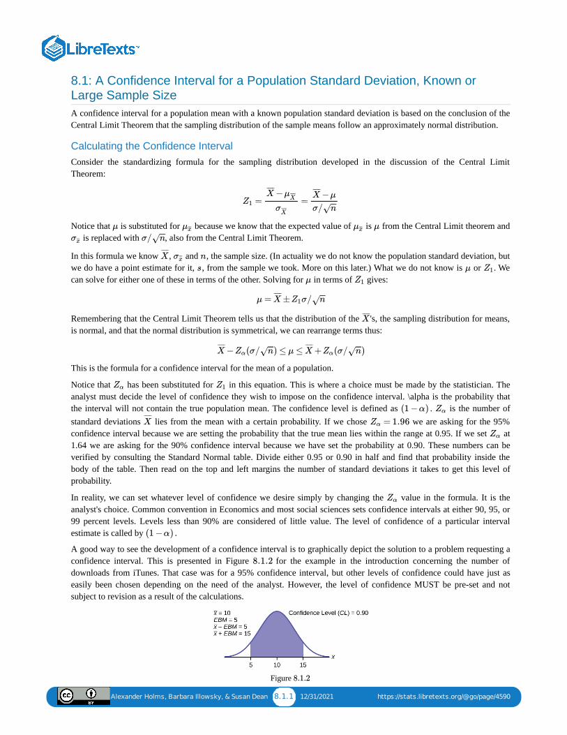
Alexander Holms, Barbara Illowsky, & Susan Dean 8.1.1 12/31/2021 https://stats.libretexts.org/@go/page/4590
8.1: A Confidence Interval for a Population Standard Deviation, Known orLarge Sample SizeA confidence interval for a population mean with a known population standard deviation is based on the conclusion of theCentral Limit Theorem that the sampling distribution of the sample means follow an approximately normal distribution.
Calculating the Confidence IntervalConsider the standardizing formula for the sampling distribution developed in the discussion of the Central LimitTheorem:
Notice that is substituted for because we know that the expected value of is from the Central Limit theorem and is replaced with , also from the Central Limit Theorem.
In this formula we know , and , the sample size. (In actuality we do not know the population standard deviation, butwe do have a point estimate for it, , from the sample we took. More on this later.) What we do not know is or . Wecan solve for either one of these in terms of the other. Solving for in terms of gives:
Remembering that the Central Limit Theorem tells us that the distribution of the 's, the sampling distribution for means,is normal, and that the normal distribution is symmetrical, we can rearrange terms thus:
This is the formula for a confidence interval for the mean of a population.
Notice that has been substituted for in this equation. This is where a choice must be made by the statistician. Theanalyst must decide the level of confidence they wish to impose on the confidence interval. \alpha is the probability thatthe interval will not contain the true population mean. The confidence level is defined as . is the number ofstandard deviations lies from the mean with a certain probability. If we chose we are asking for the 95%confidence interval because we are setting the probability that the true mean lies within the range at 0.95. If we set at1.64 we are asking for the 90% confidence interval because we have set the probability at 0.90. These numbers can beverified by consulting the Standard Normal table. Divide either 0.95 or 0.90 in half and find that probability inside thebody of the table. Then read on the top and left margins the number of standard deviations it takes to get this level ofprobability.
In reality, we can set whatever level of confidence we desire simply by changing the value in the formula. It is theanalyst's choice. Common convention in Economics and most social sciences sets confidence intervals at either 90, 95, or99 percent levels. Levels less than 90% are considered of little value. The level of confidence of a particular intervalestimate is called by .
A good way to see the development of a confidence interval is to graphically depict the solution to a problem requesting aconfidence interval. This is presented in Figure for the example in the introduction concerning the number ofdownloads from iTunes. That case was for a 95% confidence interval, but other levels of confidence could have just aseasily been chosen depending on the need of the analyst. However, the level of confidence MUST be pre-set and notsubject to revision as a result of the calculations.
Figure
= =Z1
−X¯ ¯¯̄ μX¯ ¯¯̄¯
σX¯ ¯¯̄¯
−μX¯ ¯¯̄
σ/ n−−√
μ μx̄̄̄ μx̄̄̄ μ
σx̄̄̄ σ/ n−−√
X¯ ¯¯̄
σx̄̄̄ n
s μ Z1
μ Z1
μ = ± σ/X¯ ¯¯̄
Z1 n−−√
X¯ ¯¯̄
− (σ/ ) ≤ μ ≤ + (σ/ )X¯ ¯¯̄
Zα n−−√ X¯ ¯¯̄
Zα n−−√
Zα Z1
(1 −α) Zα
X¯ ¯¯̄
= 1.96Zα
Zα
Zα
(1 −α)
8.1.2
8.1.2
Alexander Holms, Barbara Illowsky, & Susan Dean 8.1.2 12/31/2021 https://stats.libretexts.org/@go/page/4590
For this example, let's say we know that the actual population mean number of iTunes downloads is 2.1. The truepopulation mean falls within the range of the 95% confidence interval. There is absolutely nothing to guarantee that thiswill happen. Further, if the true mean falls outside of the interval we will never know it. We must always rememberthat we will never ever know the true mean.Statistics simply allows us, with a given level of probability (confidence), tosay that the true mean is within the range calculated. This is what was called in the introduction, the "level of ignoranceadmitted".
Changing the Confidence Level or Sample SizeHere again is the formula for a confidence interval for an unknown population mean assuming we know the populationstandard deviation:
It is clear that the confidence interval is driven by two things, the chosen level of confidence, , and the standarddeviation of the sampling distribution. The Standard deviation of the sampling distribution is further affected by twothings, the standard deviation of the population and the sample size we chose for our data. Here we wish to examine theeffects of each of the choices we have made on the calculated confidence interval, the confidence level and the samplesize.
For a moment we should ask just what we desire in a confidence interval. Our goal was to estimate the population meanfrom a sample. We have forsaken the hope that we will ever find the true population mean, and population standarddeviation for that matter, for any case except where we have an extremely small population and the cost of gathering thedata of interest is very small. In all other cases we must rely on samples. With the Central Limit Theorem we have thetools to provide a meaningful confidence interval with a given level of confidence, meaning a known probability of beingwrong. By meaningful confidence interval we mean one that is useful. Imagine that you are asked for a confidence intervalfor the ages of your classmates. You have taken a sample and find a mean of 19.8 years. You wish to be very confident soyou report an interval between 9.8 years and 29.8 years. This interval would certainly contain the true population mean andhave a very high confidence level. However, it hardly qualifies as meaningful. The very best confidence interval is narrowwhile having high confidence. There is a natural tension between these two goals. The higher the level of confidence thewider the confidence interval as the case of the students' ages above. We can see this tension in the equation for theconfidence interval.
The confidence interval will increase in width as increases, increases as the level of confidence increases. There isa tradeoff between the level of confidence and the width of the interval. Now let's look at the formula again and we see thatthe sample size also plays an important role in the width of the confidence interval. The sample sized, nn, shows up in thedenominator of the standard deviation of the sampling distribution. As the sample size increases, the standard deviation ofthe sampling distribution decreases and thus the width of the confidence interval, while holding constant the level ofconfidence. This relationship was demonstrated in Figure . Again we see the importance of having large samples forour analysis although we then face a second constraint, the cost of gathering data.
Calculating the Confidence Interval: An Alternative ApproachAnother way to approach confidence intervals is through the use of something called the Error Bound. The Error Boundgets its name from the recognition that it provides the boundary of the interval derived from the standard error of thesampling distribution. In the equations above it is seen that the interval is simply the estimated mean, sample mean, plus orminus something. That something is the Error Bound and is driven by the probability we desire to maintain in our estimate,
, times the standard deviation of the sampling distribution. The Error Bound for a mean is given the name, ErrorBound Mean, or .
To construct a confidence interval for a single unknown population mean , where the population standard deviation isknown, we need as an estimate for and we need the margin of error. Here, the margin of error is called the
− (σ/ ) ≤ μ ≤ + (σ/ )X¯ ¯¯̄
Zα n−−√ X¯ ¯¯̄
Zα n−−√
Zα
μ = ± ( )x̄̄̄ Zα
σ
n−−√
Zα Zα
8.1.8
Zα
EBM
μ
x̄̄̄ μ (EBM)
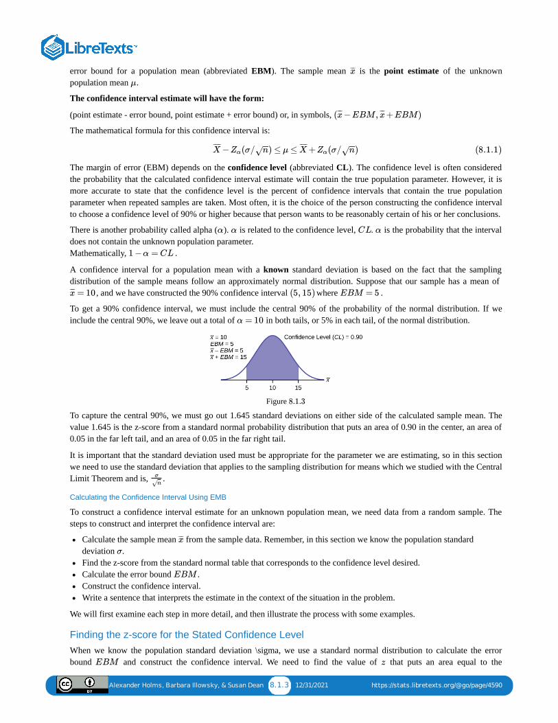
Alexander Holms, Barbara Illowsky, & Susan Dean 8.1.3 12/31/2021 https://stats.libretexts.org/@go/page/4590
error bound for a population mean (abbreviated EBM). The sample mean is the point estimate of the unknownpopulation mean .
The confidence interval estimate will have the form:
(point estimate - error bound, point estimate + error bound) or, in symbols,
The mathematical formula for this confidence interval is:
The margin of error (EBM) depends on the confidence level (abbreviated CL). The confidence level is often consideredthe probability that the calculated confidence interval estimate will contain the true population parameter. However, it ismore accurate to state that the confidence level is the percent of confidence intervals that contain the true populationparameter when repeated samples are taken. Most often, it is the choice of the person constructing the confidence intervalto choose a confidence level of 90% or higher because that person wants to be reasonably certain of his or her conclusions.
There is another probability called alpha ( ). is related to the confidence level, . is the probability that the intervaldoes not contain the unknown population parameter. Mathematically, .
A confidence interval for a population mean with a known standard deviation is based on the fact that the samplingdistribution of the sample means follow an approximately normal distribution. Suppose that our sample has a mean of
, and we have constructed the 90% confidence interval where .
To get a 90% confidence interval, we must include the central 90% of the probability of the normal distribution. If weinclude the central 90%, we leave out a total of in both tails, or 5% in each tail, of the normal distribution.
Figure
To capture the central 90%, we must go out 1.645 standard deviations on either side of the calculated sample mean. Thevalue 1.645 is the z-score from a standard normal probability distribution that puts an area of 0.90 in the center, an area of0.05 in the far left tail, and an area of 0.05 in the far right tail.
It is important that the standard deviation used must be appropriate for the parameter we are estimating, so in this sectionwe need to use the standard deviation that applies to the sampling distribution for means which we studied with the CentralLimit Theorem and is, .
Calculating the Confidence Interval Using EMB
To construct a confidence interval estimate for an unknown population mean, we need data from a random sample. Thesteps to construct and interpret the confidence interval are:
Calculate the sample mean from the sample data. Remember, in this section we know the population standarddeviation .Find the z-score from the standard normal table that corresponds to the confidence level desired.Calculate the error bound .Construct the confidence interval.Write a sentence that interprets the estimate in the context of the situation in the problem.
We will first examine each step in more detail, and then illustrate the process with some examples.
Finding the z-score for the Stated Confidence LevelWhen we know the population standard deviation \sigma, we use a standard normal distribution to calculate the errorbound and construct the confidence interval. We need to find the value of that puts an area equal to the
x̄̄̄
μ
( −EBM , +EBM)x̄̄̄ x̄̄̄
− (σ/ ) ≤ μ ≤ + (σ/ )X¯ ¯¯̄ Zα n−−√ X¯ ¯¯̄ Zα n−−√ (8.1.1)
α α CL α
1 −α = CL
= 10x̄̄̄ (5, 15) EBM = 5
α = 10
8.1.3
σ
n√
x̄̄̄
σ
EBM
EBM z
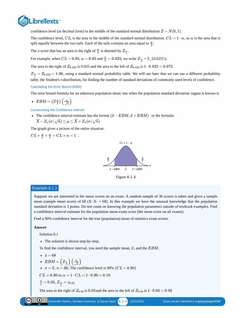
Alexander Holms, Barbara Illowsky, & Susan Dean 8.1.4 12/31/2021 https://stats.libretexts.org/@go/page/4590
confidence level (in decimal form) in the middle of the standard normal distribution .
The confidence level, , is the area in the middle of the standard normal distribution. , so is the area that issplit equally between the two tails. Each of the tails contains an area equal to .
The z-score that has an area to the right of is denoted by .
For example, when , and ; we write = Z_{0.025}\).
The area to the right of is 0.025 and the area to the left of is .
, using a standard normal probability table. We will see later that we can use a different probabilitytable, the Student's t-distribution, for finding the number of standard deviations of commonly used levels of confidence.
Calculating the Error Bound (EBM)
The error bound formula for an unknown population mean \mu when the population standard deviation \sigma is known is
Constructing the Confidence Interval
The confidence interval estimate has the format or the formula:
The graph gives a picture of the entire situation.
.
Figure
Suppose we are interested in the mean scores on an exam. A random sample of 36 scores is taken and gives a samplemean (sample mean score) of 68 (X−X- = 68). In this example we have the unusual knowledge that the populationstandard deviation is 3 points. Do not count on knowing the population parameters outside of textbook examples. Finda confidence interval estimate for the population mean exam score (the mean score on all exams).
Find a 90% confidence interval for the true (population) mean of statistics exam scores.
Answer
Solution 8.1
The solution is shown step-by-step.
To find the confidence interval, you need the sample mean, , and the .
; ; The confidence level is 90%
so
The area to the right of is and the area to the left of is .
Z ∼ N(0, 1)
CL CL = 1– α αα2
α
2Z α
2
CL = 0.95 α = 0.05 = 0.025α
2Z α
2
Z0.025 Z0.025 1– 0.025 = 0.975
= = 1.96Z α
2Z0.025
EBM = (Z )( )α2
σ
n√
( −EBM , +EBM)x̄̄̄ x̄̄̄
− (σ/ ) ≤ μ ≤ + (σ/ )X¯ ¯¯̄ Zα n−−√ X¯ ¯¯̄ Zα n−−√
CL + + = CL +α = 1α2
α2
8.1.4
Example 8.1.1
x̄̄̄ EBM
= 68x̄̄̄
EBM = ( )( )Z α
2
σ
n√
σ = 3 n = 36 (CL = 0.90)
CL = 0.90 α = 1– CL = 1– 0.90 = 0.10
= 0.05, =α
2Z α
2z0.05
Z0.05 0.05 Z0.05 1– 0.05 = 0.95
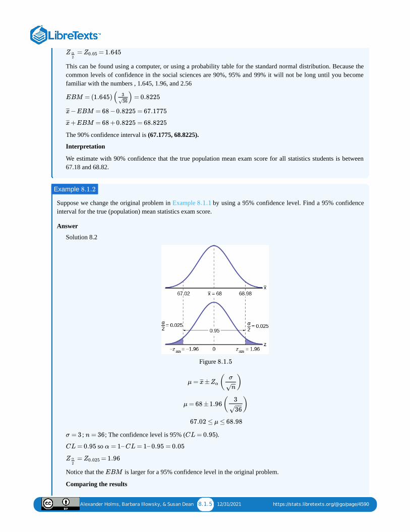
Alexander Holms, Barbara Illowsky, & Susan Dean 8.1.5 12/31/2021 https://stats.libretexts.org/@go/page/4590
This can be found using a computer, or using a probability table for the standard normal distribution. Because thecommon levels of confidence in the social sciences are 90%, 95% and 99% it will not be long until you becomefamiliar with the numbers , 1.645, 1.96, and 2.56
The 90% confidence interval is (67.1775, 68.8225).
Interpretation
We estimate with 90% confidence that the true population mean exam score for all statistics students is between67.18 and 68.82.
Suppose we change the original problem in Example by using a 95% confidence level. Find a 95% confidenceinterval for the true (population) mean statistics exam score.
Answer
Solution 8.2
Figure
; ; The confidence level is 95% ( ).
so
Notice that the is larger for a 95% confidence level in the original problem.
Comparing the results
= = 1.645Z α
2Z0.05
EBM = (1.645)( ) = 0.82253
36√
−EBM = 68 −0.8225 = 67.1775x̄̄̄
+EBM = 68 +0.8225 = 68.8225x̄̄̄
Example 8.1.2
8.1.1
8.1.5
μ = ± ( )x̄̄̄ Zα
σ
n−−√
μ = 68 ±1.96( )3
36−−
√
67.02 ≤ μ ≤ 68.98
σ = 3 n = 36 CL = 0.95
CL = 0.95 α = 1– CL = 1– 0.95 = 0.05
= = 1.96Z α
2Z0.025
EBM
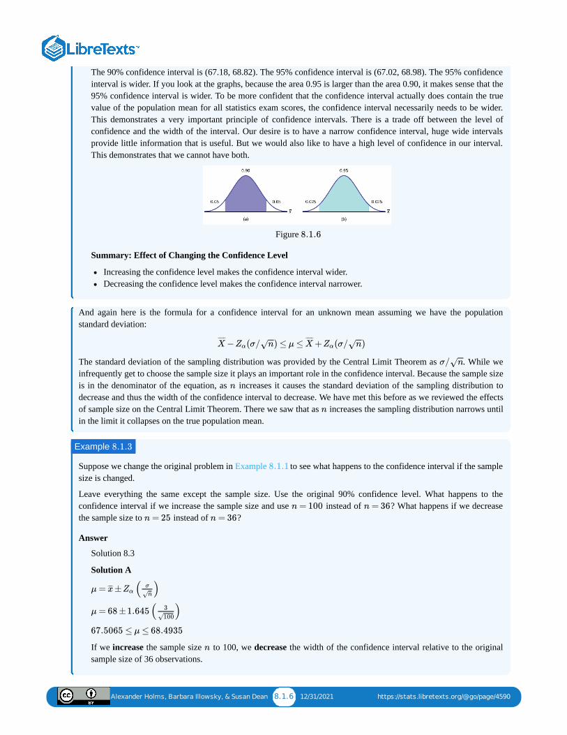
Alexander Holms, Barbara Illowsky, & Susan Dean 8.1.6 12/31/2021 https://stats.libretexts.org/@go/page/4590
The 90% confidence interval is (67.18, 68.82). The 95% confidence interval is (67.02, 68.98). The 95% confidenceinterval is wider. If you look at the graphs, because the area 0.95 is larger than the area 0.90, it makes sense that the95% confidence interval is wider. To be more confident that the confidence interval actually does contain the truevalue of the population mean for all statistics exam scores, the confidence interval necessarily needs to be wider.This demonstrates a very important principle of confidence intervals. There is a trade off between the level ofconfidence and the width of the interval. Our desire is to have a narrow confidence interval, huge wide intervalsprovide little information that is useful. But we would also like to have a high level of confidence in our interval.This demonstrates that we cannot have both.
Figure
Summary: Effect of Changing the Confidence Level
Increasing the confidence level makes the confidence interval wider.Decreasing the confidence level makes the confidence interval narrower.
And again here is the formula for a confidence interval for an unknown mean assuming we have the populationstandard deviation:
The standard deviation of the sampling distribution was provided by the Central Limit Theorem as . While weinfrequently get to choose the sample size it plays an important role in the confidence interval. Because the sample sizeis in the denominator of the equation, as increases it causes the standard deviation of the sampling distribution todecrease and thus the width of the confidence interval to decrease. We have met this before as we reviewed the effectsof sample size on the Central Limit Theorem. There we saw that as increases the sampling distribution narrows untilin the limit it collapses on the true population mean.
Suppose we change the original problem in Example to see what happens to the confidence interval if the samplesize is changed.
Leave everything the same except the sample size. Use the original 90% confidence level. What happens to theconfidence interval if we increase the sample size and use instead of ? What happens if we decreasethe sample size to instead of ?
Answer
Solution 8.3
Solution A
If we increase the sample size to 100, we decrease the width of the confidence interval relative to the originalsample size of 36 observations.
8.1.6
− (σ/ ) ≤ μ ≤ + (σ/ )X¯ ¯¯̄
Zα n−−√ X¯ ¯¯̄
Zα n−−√
σ/ n−−√
n
n
Example 8.1.3
8.1.1
n = 100 n = 36n = 25 n = 36
μ = ± ( )x̄̄̄ Zασ
n√
μ = 68 ±1.645( )3
100√
67.5065 ≤ μ ≤ 68.4935
n
Alexander Holms, Barbara Illowsky, & Susan Dean 8.1.7 12/31/2021 https://stats.libretexts.org/@go/page/4590
Answer
Solution 8.3
Solution B
If we decrease the sample size to 25, we increase the width of the confidence interval by comparison to theoriginal sample size of 36 observations.
Summary: Effect of Changing the Sample Size
Increasing the sample size makes the confidence interval narrower.Decreasing the sample size makes the confidence interval wider.
We have already seen this effect when we reviewed the effects of changing the size of the sample, n, on the Central LimitTheorem. See Figure to see this effect. Before we saw that as the sample size increased the standard deviation of thesampling distribution decreases. This was why we choose the sample mean from a large sample as compared to a smallsample, all other things held constant.
Thus far we assumed that we knew the population standard deviation. This will virtually never be the case. We will havethe sample standard deviation, s, however. This is a point estimate for the population standard deviation and can besubstituted into the formula for confidence intervals for a mean under certain circumstances. We just saw the effect thesample size has on the width of confidence interval and the impact on the sampling distribution for our discussion of theCentral Limit Theorem. We can invoke this to substitute the point estimate for the standard deviation if the sample size islarge "enough". Simulation studies indicate that 30 observations or more will be sufficient to eliminate any meaningfulbias in the estimated confidence interval.
Spring break can be a very expensive holiday. A sample of 80 students is surveyed, and the average amount spent bystudents on travel and beverages is $593.84. The sample standard deviation is approximately $369.34.
Construct a 92% confidence interval for the population mean amount of money spent by spring breakers.
Answer
Solution 8.4
We begin with the confidence interval for a mean. We use the formula for a mean because the random variable isdollars spent and this is a continuous random variable. The point estimate for the population standard deviation, s,has been substituted for the true population standard deviation because with 80 observations there is no concern forbias in the estimate of the confidence interval.
Substituting the values into the formula, we have:
is found on the standard normal table by looking up 0.46 in the body of the table and finding the number ofstandard deviations on the side and top of the table; 1.75. The solution for the interval is thus:
μ = ± ( )x̄̄̄ Zασ
n√
μ = 68 ±1.645( )3
25√
67.013 ≤ μ ≤ 68.987
n
8.1.7
Example 8.1.4
μ = ±[ ]x̄̄̄ Z(a/2)s
n−−√
μ = 593.84 ±[1.75 ]369.34
80−−
√
Z(a/2)
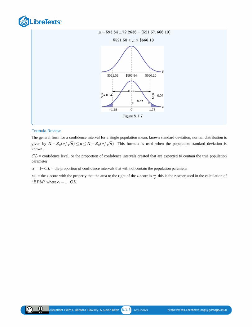
Alexander Holms, Barbara Illowsky, & Susan Dean 8.1.8 12/31/2021 https://stats.libretexts.org/@go/page/4590
Figure
Formula Review
The general form for a confidence interval for a single population mean, known standard deviation, normal distribution isgiven by This formula is used when the population standard deviation isknown.
= confidence level, or the proportion of confidence intervals created that are expected to contain the true populationparameter
= the proportion of confidence intervals that will not contain the population parameter
= the z-score with the property that the area to the right of the z-score is this is the z-score used in the calculation of" " where .
μ = 593.84 ±72.2636 = (521.57, 666.10)
$521.58 ≤ μ ≤ $666.10
8.1.7
− (σ/ ) ≤ μ ≤ + (σ/ )X¯ ¯¯̄
Zα n−−
√ X¯ ¯¯̄
Zα n−−
√
CL
α = 1– CL
z α
2
∝2
EBM α = 1– CL
Alexander Holms, Barbara Illowsky, & Susan Dean 8.2.1 12/3/2021 https://stats.libretexts.org/@go/page/4591
8.2: A Confidence Interval for a Population Standard Deviation Unknown, SmallSample CaseIn practice, we rarely know the population standard deviation. In the past, when the sample size was large, this did notpresent a problem to statisticians. They used the sample standard deviation s as an estimate for and proceeded as beforeto calculate a confidence interval with close enough results. This is what we did in Example above. The pointestimate for the standard deviation, , was substituted in the formula for the confidence interval for the population standarddeviation. In this case there 80 observation well above the suggested 30 observations to eliminate any bias from a smallsample. However, statisticians ran into problems when the sample size was small. A small sample size caused inaccuraciesin the confidence interval.
William S. Goset (1876–1937) of the Guinness brewery in Dublin, Ireland ran into this problem. His experiments withhops and barley produced very few samples. Just replacing with did not produce accurate results when he tried tocalculate a confidence interval. He realized that he could not use a normal distribution for the calculation; he found that theactual distribution depends on the sample size. This problem led him to "discover" what is called the Student's t-distribution. The name comes from the fact that Gosset wrote under the pen name "A Student."
Up until the mid-1970s, some statisticians used the normal distribution approximation for large sample sizes and used theStudent's t-distribution only for sample sizes of at most 30 observations.
If you draw a simple random sample of size from a population with mean and unknown population standard deviation and calculate the t-score
then the t-scores follow a Student's t-distribution with degrees of freedom. The t-score has the same interpretationas the z-score. It measures how far in standard deviation units is from its mean \mu. For each sample size , there is adifferent Student's t-distribution.
The degrees of freedom, , come from the calculation of the sample standard deviation . Remember when we firstcalculated a sample standard deviation we divided the sum of the squared deviations by , but we used deviations (values) to calculate . Because the sum of the deviations is zero, we can find the last deviation once we know the other
deviations. The other deviations can change or vary freely. We call the number the degrees of freedom( ) in recognition that one is lost in the calculations. The effect of losing a degree of freedom is that the t-value increasesand the confidence interval increases in width.
Properties of the Student's t-DistributionThe graph for the Student's t-distribution is similar to the standard normal curve and at infinite degrees of freedom it isthe normal distribution. You can confirm this by reading the bottom line at infinite degrees of freedom for a familiarlevel of confidence, e.g. at column 0.05, 95% level of confidence, we find the t-value of 1.96 at infinite degrees offreedom.The mean for the Student's t-distribution is zero and the distribution is symmetric about zero, again like the standardnormal distribution.The Student's t-distribution has more probability in its tails than the standard normal distribution because the spread ofthe t-distribution is greater than the spread of the standard normal. So the graph of the Student's t-distribution will bethicker in the tails and shorter in the center than the graph of the standard normal distribution.The exact shape of the Student's t-distribution depends on the degrees of freedom. As the degrees of freedom increases,the graph of Student's t-distribution becomes more like the graph of the standard normal distribution.The underlying population of individual observations is assumed to be normally distributed with unknown populationmean \ and unknown population standard deviation . This assumption comes from the Central Limit theorembecause the individual observations in this case are the s of the sampling distribution. The size of the underlyingpopulation is generally not relevant unless it is very small. If it is normal then the assumption is met and doesn't needdiscussion.
σ
8.2.4s
σ s
n μ
σ
t =−μx̄̄̄
( )s
n√
(8.2.1)
n– 1
x̄̄̄ n
n– 1 s
n– 1 n x̄̄̄
s
n– 1 n– 1 n– 1
df
mu σ
x̄̄̄
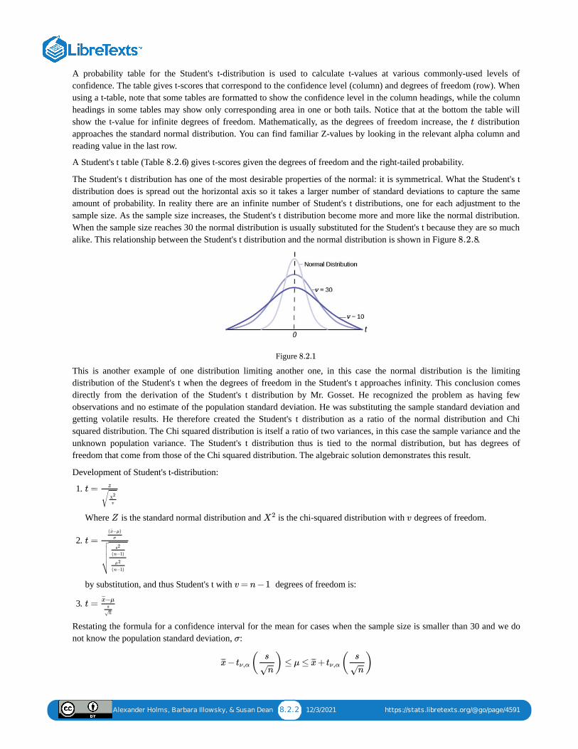
Alexander Holms, Barbara Illowsky, & Susan Dean 8.2.2 12/3/2021 https://stats.libretexts.org/@go/page/4591
A probability table for the Student's t-distribution is used to calculate t-values at various commonly-used levels ofconfidence. The table gives t-scores that correspond to the confidence level (column) and degrees of freedom (row). Whenusing a t-table, note that some tables are formatted to show the confidence level in the column headings, while the columnheadings in some tables may show only corresponding area in one or both tails. Notice that at the bottom the table willshow the t-value for infinite degrees of freedom. Mathematically, as the degrees of freedom increase, the distributionapproaches the standard normal distribution. You can find familiar Z-values by looking in the relevant alpha column andreading value in the last row.
A Student's t table (Table ) gives t-scores given the degrees of freedom and the right-tailed probability.
The Student's t distribution has one of the most desirable properties of the normal: it is symmetrical. What the Student's tdistribution does is spread out the horizontal axis so it takes a larger number of standard deviations to capture the sameamount of probability. In reality there are an infinite number of Student's t distributions, one for each adjustment to thesample size. As the sample size increases, the Student's t distribution become more and more like the normal distribution.When the sample size reaches 30 the normal distribution is usually substituted for the Student's t because they are so muchalike. This relationship between the Student's t distribution and the normal distribution is shown in Figure .
Figure
This is another example of one distribution limiting another one, in this case the normal distribution is the limitingdistribution of the Student's t when the degrees of freedom in the Student's t approaches infinity. This conclusion comesdirectly from the derivation of the Student's t distribution by Mr. Gosset. He recognized the problem as having fewobservations and no estimate of the population standard deviation. He was substituting the sample standard deviation andgetting volatile results. He therefore created the Student's t distribution as a ratio of the normal distribution and Chisquared distribution. The Chi squared distribution is itself a ratio of two variances, in this case the sample variance and theunknown population variance. The Student's t distribution thus is tied to the normal distribution, but has degrees offreedom that come from those of the Chi squared distribution. The algebraic solution demonstrates this result.
Development of Student's t-distribution:
1.
Where is the standard normal distribution and is the chi-squared distribution with degrees of freedom.
2.
by substitution, and thus Student's t with degrees of freedom is:
3.
Restating the formula for a confidence interval for the mean for cases when the sample size is smaller than 30 and we donot know the population standard deviation, :
t
8.2.6
8.2.8
8.2.1
t = z
χ2
v√
Z X2 v
t =( −μ)x̄
σ
s2
(n−1)
σ2
(n−1)
⎷
v = n −1
t =−μx̄̄̄s
n√
σ
− ( ) ≤ μ ≤ + ( )x̄̄̄ tν,αs
n−−√x̄̄̄ tν,α
s
n−−√
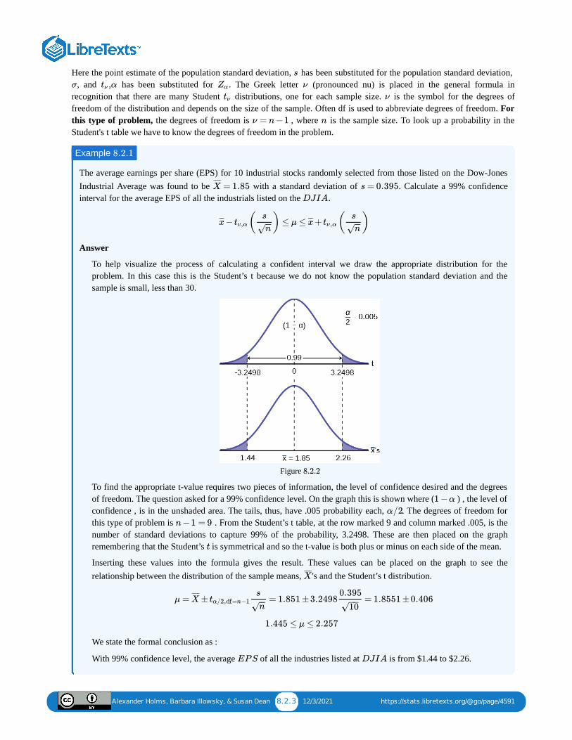
Alexander Holms, Barbara Illowsky, & Susan Dean 8.2.3 12/3/2021 https://stats.libretexts.org/@go/page/4591
Here the point estimate of the population standard deviation, has been substituted for the population standard deviation, , and , has been substituted for . The Greek letter (pronounced nu) is placed in the general formula in
recognition that there are many Student distributions, one for each sample size. is the symbol for the degrees offreedom of the distribution and depends on the size of the sample. Often df is used to abbreviate degrees of freedom. Forthis type of problem, the degrees of freedom is , where is the sample size. To look up a probability in theStudent's t table we have to know the degrees of freedom in the problem.
The average earnings per share (EPS) for 10 industrial stocks randomly selected from those listed on the Dow-JonesIndustrial Average was found to be with a standard deviation of . Calculate a 99% confidenceinterval for the average EPS of all the industrials listed on the .
Answer
To help visualize the process of calculating a confident interval we draw the appropriate distribution for theproblem. In this case this is the Student’s t because we do not know the population standard deviation and thesample is small, less than 30.
Figure
To find the appropriate t-value requires two pieces of information, the level of confidence desired and the degreesof freedom. The question asked for a 99% confidence level. On the graph this is shown where ( ) , the level ofconfidence , is in the unshaded area. The tails, thus, have .005 probability each, . The degrees of freedom forthis type of problem is . From the Student’s t table, at the row marked 9 and column marked .005, is thenumber of standard deviations to capture 99% of the probability, 3.2498. These are then placed on the graphremembering that the Student’s is symmetrical and so the t-value is both plus or minus on each side of the mean.
Inserting these values into the formula gives the result. These values can be placed on the graph to see therelationship between the distribution of the sample means, 's and the Student’s t distribution.
We state the formal conclusion as :
With 99% confidence level, the average of all the industries listed at is from $1.44 to $2.26.
s
σ tν α Zα ν
tν ν
ν = n −1 n
Example 8.2.1
= 1.85X¯ ¯¯̄
s = 0.395DJIA
− ( ) ≤ μ ≤ + ( )x̄̄̄ tv,αs
n−−√x̄̄̄ tν,α
s
n−−√
8.2.2
1 −α
α/2n −1 = 9
t
X¯ ¯¯̄
μ = ± = 1.851 ±3.2498 = 1.8551 ±0.406X¯ ¯¯̄
tα/2,df=n−1s
n−−√
0.395
10−−
√
1.445 ≤ μ ≤ 2.257
EP S DJIA

Alexander Holms, Barbara Illowsky, & Susan Dean 8.2.4 12/3/2021 https://stats.libretexts.org/@go/page/4591
You do a study of hypnotherapy to determine how effective it is in increasing the number of hours of sleep subjects geteach night. You measure hours of sleep for 12 subjects with the following results. Construct a 95% confidence intervalfor the mean number of hours slept for the population (assumed normal) from which you took the data.
8.2; 9.1; 7.7; 8.6; 6.9; 11.2; 10.1; 9.9; 8.9; 9.2; 7.5; 10.5
Exercise 8.2.2
Alexander Holms, Barbara Illowsky, & Susan Dean 8.3.1 12/3/2021 https://stats.libretexts.org/@go/page/4592
8.3: A Confidence Interval for A Population ProportionDuring an election year, we see articles in the newspaper that state confidence intervals in terms of proportions orpercentages. For example, a poll for a particular candidate running for president might show that the candidate has 40% ofthe vote within three percentage points (if the sample is large enough). Often, election polls are calculated with 95%confidence, so, the pollsters would be 95% confident that the true proportion of voters who favored the candidate would bebetween 0.37 and 0.43.
Investors in the stock market are interested in the true proportion of stocks that go up and down each week. Businesses thatsell personal computers are interested in the proportion of households in the United States that own personal computers.Confidence intervals can be calculated for the true proportion of stocks that go up or down each week and for the trueproportion of households in the United States that own personal computers.
The procedure to find the confidence interval for a population proportion is similar to that for the population mean, but theformulas are a bit different although conceptually identical. While the formulas are different, they are based upon the samemathematical foundation given to us by the Central Limit Theorem. Because of this we will see the same basic formatusing the same three pieces of information: the sample value of the parameter in question, the standard deviation of therelevant sampling distribution, and the number of standard deviations we need to have the confidence in our estimate thatwe desire.
How do you know you are dealing with a proportion problem? First, the underlying distribution has a binaryrandom variable and therefore is a binomial distribution. (There is no mention of a mean or average.) If is abinomial random variable, then where is the number of trials and is the probability of a success. To forma sample proportion, take , the random variable for the number of successes and divide it by , the number of trials (orthe sample size). The random variable (read "P prime") is the sample proportion,
(Sometimes the random variable is denoted as , read "P hat".)
= the estimated proportion of successes or sample proportion of successes ( is a point estimate for , the truepopulation proportion, and thus is the probability of a failure in any one trial.)
= the number of successes in the sample = the size of the sample
The formula for the confidence interval for a population proportion follows the same format as that for an estimate of apopulation mean. Remembering the sampling distribution for the proportion from Chapter 7, the standard deviation wasfound to be:
The confidence interval for a population proportion, therefore, becomes:
is set according to our desired degree of confidence and is the standard deviation of the sampling
distribution.
The sample proportions and are estimates of the unknown population proportions and . The estimatedproportions and are used because and are not known.
Remember that as moves further from 0.5 the binomial distribution becomes less symmetrical. Because we areestimating the binomial with the symmetrical normal distribution the further away from symmetrical the binomial becomesthe less confidence we have in the estimate.
X
X ∼ B(n, p) n p
X n
P ′
=P ′ X
n
P̂
P ′ P ′ p
q
x
n
=σp′
p(1 −p)
n
− −−−−−−√
p = ±[ ]p′ Z( )a
2
(1 − )p′ p′
n
− −−−−−−−−√
Z( )a
2
(1− )p′ p′
n
− −−−−−√
p′ q′ p q
p′ q ′ p q
p
Alexander Holms, Barbara Illowsky, & Susan Dean 8.3.2 12/3/2021 https://stats.libretexts.org/@go/page/4592
This conclusion can be demonstrated through the following analysis. Proportions are based upon the binomial probabilitydistribution. The possible outcomes are binary, either “success” or “failure”. This gives rise to a proportion, meaning thepercentage of the outcomes that are “successes”. It was shown that the binomial distribution could be fully understood ifwe knew only the probability of a success in any one trial, called . The mean and the standard deviation of the binomialwere found to be:
It was also shown that the binomial could be estimated by the normal distribution if BOTH AND were greater than5. From the discussion above, it was found that the standardizing formula for the binomial distribution is:
which is nothing more than a restatement of the general standardizing formula with appropriate substitutions for and from the binomial. We can use the standard normal distribution, the reason is in the equation, because the normaldistribution is the limiting distribution of the binomial. This is another example of the Central Limit Theorem. We havealready seen that the sampling distribution of means is normally distributed. Recall the extended discussion in Chapter 7concerning the sampling distribution of proportions and the conclusions of the Central Limit Theorem.
We can now manipulate this formula in just the same way we did for finding the confidence intervals for a mean, but tofind the confidence interval for the binomial population parameter, .
Where , the point estimate of taken from the sample. Notice that has replaced in the formula. This isbecause we do not know , indeed, this is just what we are trying to estimate.
Unfortunately, there is no correction factor for cases where the sample size is small so and must always be greaterthan 5 to develop an interval estimate for .
Suppose that a market research firm is hired to estimate the percent of adults living in a large city who have cellphones. Five hundred randomly selected adult residents in this city are surveyed to determine whether they have cellphones. Of the 500 people sampled, 421 responded yes - they own cell phones. Using a 95% confidence level,compute a confidence interval estimate for the true proportion of adult residents of this city who have cell phones.
AnswerThe solution step-by-step.
Let = the number of people in the sample who have cell phones. is binomial: the random variable is binary,people either have a cell phone or they do not.
To calculate the confidence interval, we must find .
is the sample proportion; this is the point estimate of the population proportion.
Since the requested confidence level is , then .
Then
p
μ = np
σ = npq−−−√
np nq
Z =−pp′
( )pq
n
− −−−√
μ σ
Z
p
− ≤ p ≤ +p′ Zα
p′q ′
n
− −−−√ p′ Zα
p′q ′
n
− −−−√
= x/np′ p p′ p
p
np′ nq ′
p
Example 8.3.1
X X
,p′ q ′
n = 500
x = the number of successes in the sample = 421
= = = 0.842p′ x
n
421500
= 0.842p′
= 1 − = 1 −0.842 = 0.158q ′ p′
CL = 0.95 α = 1 −CL = 1 −0.95 = 0.05 ( ) = 0.025α
2
= = 1.96z α
2z0.025
Alexander Holms, Barbara Illowsky, & Susan Dean 8.3.3 12/3/2021 https://stats.libretexts.org/@go/page/4592
This can be found using the Standard Normal probability table in Table . This can also be found in thestudents t table at the 0.025 column and infinity degrees of freedom because at infinite degrees of freedom thestudents t distribution becomes the standard normal distribution, .
The confidence interval for the true binomial population proportion is
Interpretation
We estimate with 95% confidence that between 81% and 87.4% of all adult residents of this city have cell phones.
Explanation of 95% Confidence Level
Ninety-five percent of the confidence intervals constructed in this way would contain the true value for thepopulation proportion of all adult residents of this city who have cell phones.
Suppose 250 randomly selected people are surveyed to determine if they own a tablet. Of the 250 surveyed, 98reported owning a tablet. Using a 95% confidence level, compute a confidence interval estimate for the true proportionof people who own tablets.
The Dundee Dog Training School has a larger than average proportion of clients who compete in competitiveprofessional events. A confidence interval for the population proportion of dogs that compete in professional eventsfrom 150 different training schools is constructed. The lower limit is determined to be 0.08 and the upper limit isdetermined to be 0.16. Determine the level of confidence used to construct the interval of the population proportion ofdogs that compete in professional events.
Answer
We begin with the formula for a confidence interval for a proportion because the random variable is binary; eitherthe client competes in professional competitive dog events or they don't.
Next we find the sample proportion:
The that makes up the confidence interval is thus and , theboundaries of the confidence interval. Finally, we solve for .
And then look up the probability for 1.51 standard deviations on the standard normal table.
.
8.3.6
Z
− ≤ p ≤ +p′ Zα
p′q ′
n
− −−−√ p′ Zα
p′q ′
n
− −−−√
Substituting in the values from above we find the confidence interval is : 0.810 ≤ p ≤ 0.874
Exercise 8.3.1
Example 8.3.2
p = ±[ ]p′ Z( )a
2
(1 − )p′ p′
n
− −−−−−−−−
√
= = 0.12p′ 0.08 +0.16
2
± 0.04; 0.12 +0.04 = 0.16 0.12 −0.04 = 0.08Z
[Z ⋅ ] = 0.04, therefore z = 1.510.12(1−0.12)
150
− −−−−−−−√
p(Z = 1.51) = 0.4345, p(Z) ⋅ 2 = 0.8690 or 86.90%
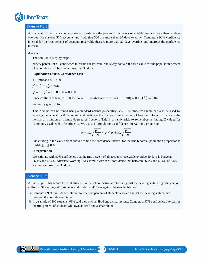
Alexander Holms, Barbara Illowsky, & Susan Dean 8.3.4 12/3/2021 https://stats.libretexts.org/@go/page/4592
A financial officer for a company wants to estimate the percent of accounts receivable that are more than 30 daysoverdue. He surveys 500 accounts and finds that 300 are more than 30 days overdue. Compute a 90% confidenceinterval for the true percent of accounts receivable that are more than 30 days overdue, and interpret the confidenceinterval.
AnswerThe solution is step-by-step:
Ninety percent of all confidence intervals constructed in this way contain the true value for the population percentof accounts receivable that are overdue 30 days.
Explanation of 90% Confidence Level
and
Since confidence level = , then
This Z-value can be found using a standard normal probability table. The student's t-table can also be used byentering the table at the 0.05 column and reading at the line for infinite degrees of freedom. The t-distribution is thenormal distribution at infinite degrees of freedom. This is a handy trick to remember in finding Z-values forcommonly used levels of confidence. We use this formula for a confidence interval for a proportion:
Substituting in the values from above we find the confidence interval for the true binomial population proportion is
Interpretation
We estimate with 90% confidence that the true percent of all accounts receivable overdue 30 days is between56.4% and 63.6%. Alternate Wording: We estimate with 90% confidence that between 56.4% and 63.6% of ALLaccounts are overdue 30 days.
A student polls his school to see if students in the school district are for or against the new legislation regarding schooluniforms. She surveys 600 students and finds that 480 are against the new legislation.
a. Compute a 90% confidence interval for the true percent of students who are against the new legislation, andinterpret the confidence interval.
b. In a sample of 300 students, 68% said they own an iPod and a smart phone. Compute a 97% confidence interval forthe true percent of students who own an iPod and a smartphone.
Example 8.3.3
x = 300 n = 500
= = = 0.600p′ x
n
300500
= 1 − = 1 −0.600 = 0.400q ′ p′
0.90 a = 1 − confidence level = (1 −0.90) = 0.10 ( ) = 0.05α
2
= = 1.645Z α
2Z0.05
− ≤ p ≤ +p′ Zα
p′q ′
n
− −−−√ p′ Zα
p′q ′
n
− −−−√
0.564 ≤ p ≤ 0.636
Exercise 8.3.2
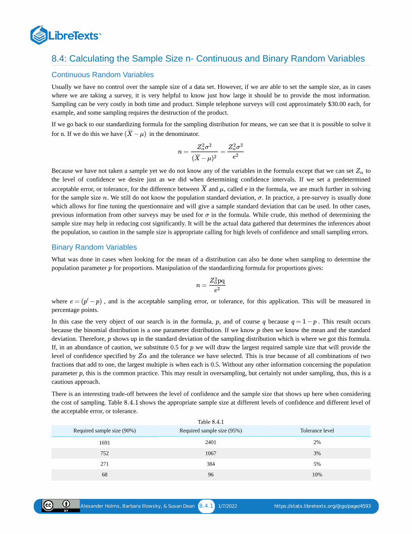
Alexander Holms, Barbara Illowsky, & Susan Dean 8.4.1 1/7/2022 https://stats.libretexts.org/@go/page/4593
8.4: Calculating the Sample Size n- Continuous and Binary Random Variables
Continuous Random Variables
Usually we have no control over the sample size of a data set. However, if we are able to set the sample size, as in caseswhere we are taking a survey, it is very helpful to know just how large it should be to provide the most information.Sampling can be very costly in both time and product. Simple telephone surveys will cost approximately $30.00 each, forexample, and some sampling requires the destruction of the product.
If we go back to our standardizing formula for the sampling distribution for means, we can see that it is possible to solve itfor n. If we do this we have in the denominator.
Because we have not taken a sample yet we do not know any of the variables in the formula except that we can set tothe level of confidence we desire just as we did when determining confidence intervals. If we set a predeterminedacceptable error, or tolerance, for the difference between and , called e in the formula, we are much further in solvingfor the sample size . We still do not know the population standard deviation, . In practice, a pre-survey is usually donewhich allows for fine tuning the questionnaire and will give a sample standard deviation that can be used. In other cases,previous information from other surveys may be used for in the formula. While crude, this method of determining thesample size may help in reducing cost significantly. It will be the actual data gathered that determines the inferences aboutthe population, so caution in the sample size is appropriate calling for high levels of confidence and small sampling errors.
Binary Random Variables
What was done in cases when looking for the mean of a distribution can also be done when sampling to determine thepopulation parameter for proportions. Manipulation of the standardizing formula for proportions gives:
where , and is the acceptable sampling error, or tolerance, for this application. This will be measured inpercentage points.
In this case the very object of our search is in the formula, , and of course because . This result occursbecause the binomial distribution is a one parameter distribution. If we know then we know the mean and the standarddeviation. Therefore, shows up in the standard deviation of the sampling distribution which is where we got this formula.If, in an abundance of caution, we substitute 0.5 for we will draw the largest required sample size that will provide thelevel of confidence specified by and the tolerance we have selected. This is true because of all combinations of twofractions that add to one, the largest multiple is when each is 0.5. Without any other information concerning the populationparameter , this is the common practice. This may result in oversampling, but certainly not under sampling, thus, this is acautious approach.
There is an interesting trade-off between the level of confidence and the sample size that shows up here when consideringthe cost of sampling. Table shows the appropriate sample size at different levels of confidence and different level ofthe acceptable error, or tolerance.
Required sample size (90%) Required sample size (95%) Tolerance level
1691 2401 2%
752 1067 3%
271 384 5%
68 96 10%
Table
( −μ)X¯ ¯¯̄
n = =Z2
ασ2
( −μX¯ ¯¯̄ )2
Z2ασ2
e2
Zα
X¯ ¯¯̄
μ
n σ
σ
p
n =pqZ2
α
e2
e = ( −p)p′
p q q = 1 −p
p
p
p
Zα
p
8.4.1
8.4.1
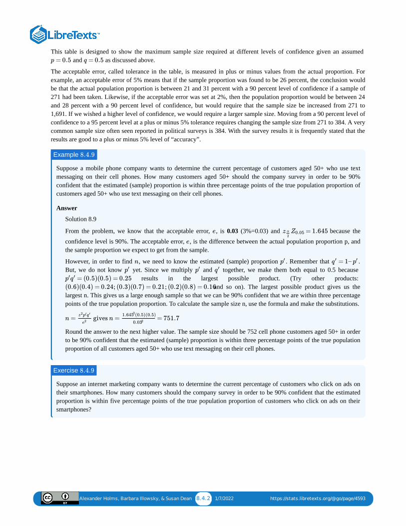
Alexander Holms, Barbara Illowsky, & Susan Dean 8.4.2 1/7/2022 https://stats.libretexts.org/@go/page/4593
This table is designed to show the maximum sample size required at different levels of confidence given an assumed and as discussed above.
The acceptable error, called tolerance in the table, is measured in plus or minus values from the actual proportion. Forexample, an acceptable error of 5% means that if the sample proportion was found to be 26 percent, the conclusion wouldbe that the actual population proportion is between 21 and 31 percent with a 90 percent level of confidence if a sample of271 had been taken. Likewise, if the acceptable error was set at 2%, then the population proportion would be between 24and 28 percent with a 90 percent level of confidence, but would require that the sample size be increased from 271 to1,691. If we wished a higher level of confidence, we would require a larger sample size. Moving from a 90 percent level ofconfidence to a 95 percent level at a plus or minus 5% tolerance requires changing the sample size from 271 to 384. A verycommon sample size often seen reported in political surveys is 384. With the survey results it is frequently stated that theresults are good to a plus or minus 5% level of “accuracy”.
Suppose a mobile phone company wants to determine the current percentage of customers aged 50+ who use textmessaging on their cell phones. How many customers aged 50+ should the company survey in order to be 90%confident that the estimated (sample) proportion is within three percentage points of the true population proportion ofcustomers aged 50+ who use text messaging on their cell phones.
Answer
Solution 8.9
From the problem, we know that the acceptable error, , is 0.03 (3%=0.03) and because the
confidence level is 90%. The acceptable error, , is the difference between the actual population proportion p, andthe sample proportion we expect to get from the sample.
However, in order to find , we need to know the estimated (sample) proportion . Remember that .But, we do not know yet. Since we multiply and together, we make them both equal to 0.5 because
results in the largest possible product. (Try other products: and so on). The largest possible product gives us the
largest n. This gives us a large enough sample so that we can be 90% confident that we are within three percentagepoints of the true population proportion. To calculate the sample size n, use the formula and make the substitutions.
Round the answer to the next higher value. The sample size should be 752 cell phone customers aged 50+ in orderto be 90% confident that the estimated (sample) proportion is within three percentage points of the true populationproportion of all customers aged 50+ who use text messaging on their cell phones.
Suppose an internet marketing company wants to determine the current percentage of customers who click on ads ontheir smartphones. How many customers should the company survey in order to be 90% confident that the estimatedproportion is within five percentage points of the true population proportion of customers who click on ads on theirsmartphones?
p = 0.5 q = 0.5
Example 8.4.9
e = 1.645z α
2Z0.05
e
n p′ = 1–q ′ p′
p′ p′ q ′
= (0.5)(0.5) = 0.25p′q ′
(0.6)(0.4) = 0.24; (0.3)(0.7) = 0.21; (0.2)(0.8) = 0.16
n = gives n = = 751.7z2p′q ′
e2
(0.5)(0.5)1.6452
0.032
Exercise 8.4.9
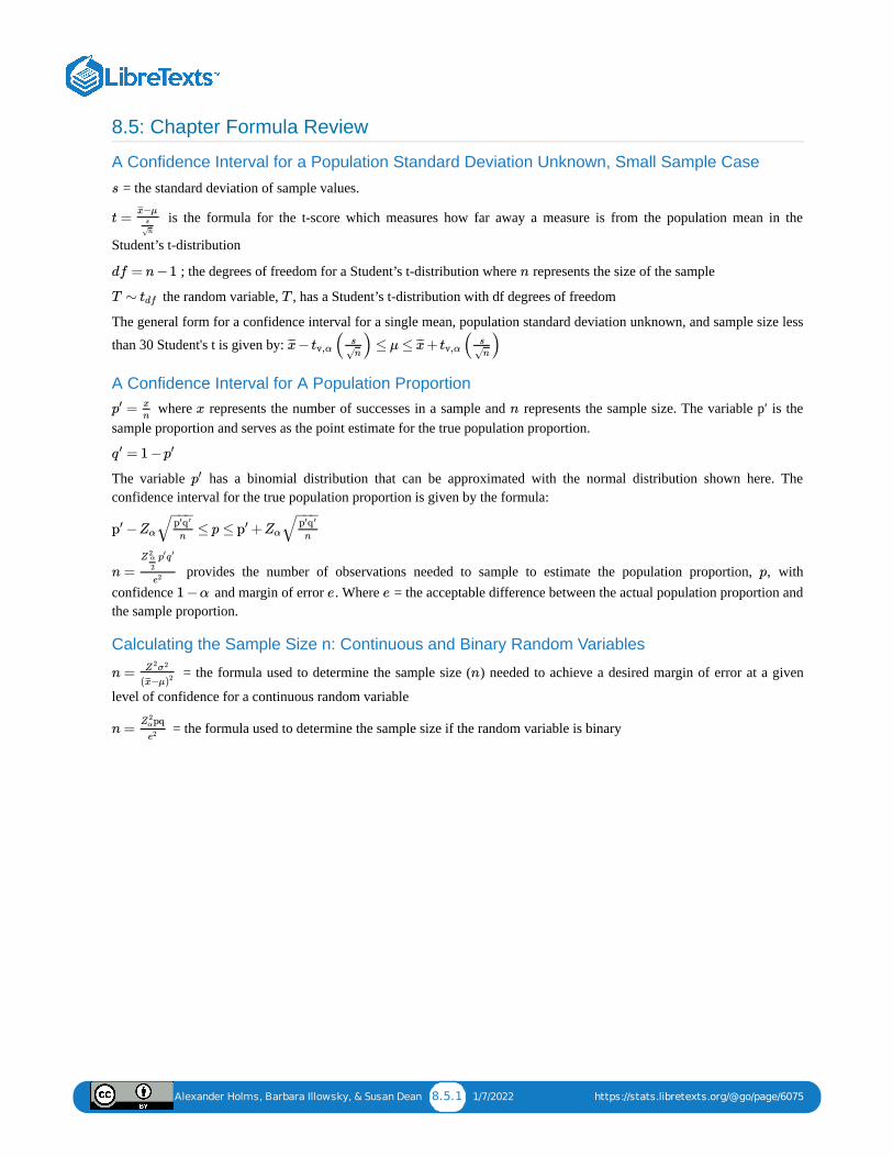
Alexander Holms, Barbara Illowsky, & Susan Dean 8.5.1 1/7/2022 https://stats.libretexts.org/@go/page/6075
8.5: Chapter Formula Review
A Confidence Interval for a Population Standard Deviation Unknown, Small Sample Case
= the standard deviation of sample values.
is the formula for the t-score which measures how far away a measure is from the population mean in the
Student’s t-distribution
; the degrees of freedom for a Student’s t-distribution where represents the size of the sample
the random variable, , has a Student’s t-distribution with df degrees of freedom
The general form for a confidence interval for a single mean, population standard deviation unknown, and sample size less
than 30 Student's t is given by:
A Confidence Interval for A Population Proportion where represents the number of successes in a sample and represents the sample size. The variable p′ is the
sample proportion and serves as the point estimate for the true population proportion.
The variable has a binomial distribution that can be approximated with the normal distribution shown here. Theconfidence interval for the true population proportion is given by the formula:
provides the number of observations needed to sample to estimate the population proportion, , withconfidence and margin of error . Where = the acceptable difference between the actual population proportion andthe sample proportion.
Calculating the Sample Size n: Continuous and Binary Random Variables
= the formula used to determine the sample size ( ) needed to achieve a desired margin of error at a given
level of confidence for a continuous random variable
= the formula used to determine the sample size if the random variable is binary
s
t =−μx̄̄̄s
n√
df = n−1 n
T ∼ tdf T
− ( ) ≤ μ ≤ + ( )x̄̄̄ tv,αs
n√x̄̄̄ tv,α
s
n√
=p′ x
nx n
= 1 −q ′ p′
p′
− ≤ p ≤ +p′ Zαp′q ′
n
−−−√ p′ Zα
p′q ′
n
−−−√
n =Z 2
α
2
p′q ′
e2 p
1 −α e e
n = Z 2σ2
( −μx̄̄̄ )2 n
n =pqZ 2
α
e2
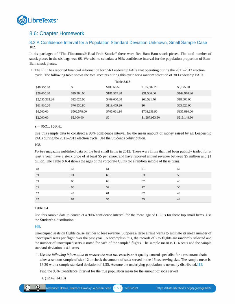
Alexander Holms, Barbara Illowsky, & Susan Dean 8.6.1 12/10/2021 https://stats.libretexts.org/@go/page/6077
8.6: Chapter Homework
8.2 A Confidence Interval for a Population Standard Deviation Unknown, Small Sample Case102.
In six packages of “The Flintstones® Real Fruit Snacks” there were five Bam-Bam snack pieces. The total number ofsnack pieces in the six bags was 68. We wish to calculate a 96% confidence interval for the population proportion of Bam-Bam snack pieces.
1. The FEC has reported financial information for 556 Leadership PACs that operating during the 2011–2012 electioncycle. The following table shows the total receipts during this cycle for a random selection of 30 Leadership PACs.
$46,500.00 $0 $40,966.50 $105,887.20 $5,175.00
$29,050.00 $19,500.00 $181,557.20 $31,500.00 $149,970.80
$2,555,363.20 $12,025.00 $409,000.00 $60,521.70 $18,000.00
$61,810.20 $76,530.80 $119,459.20 $0 $63,520.00
$6,500.00 $502,578.00 $705,061.10 $708,258.90 $135,810.00
$2,000.00 $2,000.00 $0 $1,287,933.80 $219,148.30
Table
Use this sample data to construct a 95% confidence interval for the mean amount of money raised by all LeadershipPACs during the 2011–2012 election cycle. Use the Student's t-distribution.
108.
Forbes magazine published data on the best small firms in 2012. These were firms that had been publicly traded for atleast a year, have a stock price of at least $5 per share, and have reported annual revenue between $5 million and $1billion. The Table shows the ages of the corporate CEOs for a random sample of these firms.
48 58 51 61 56
59 74 63 53 50
59 60 60 57 46
55 63 57 47 55
57 43 61 62 49
67 67 55 55 49
Table 8.4
Use this sample data to construct a 90% confidence interval for the mean age of CEO’s for these top small firms. Usethe Student's t-distribution.
109.
Unoccupied seats on flights cause airlines to lose revenue. Suppose a large airline wants to estimate its mean number ofunoccupied seats per flight over the past year. To accomplish this, the records of 225 flights are randomly selected andthe number of unoccupied seats is noted for each of the sampled flights. The sample mean is 11.6 seats and the samplestandard deviation is 4.1 seats.
1. Use the following information to answer the next two exercises: A quality control specialist for a restaurant chaintakes a random sample of size 12 to check the amount of soda served in the 16 oz. serving size. The sample mean is13.30 with a sample standard deviation of 1.55. Assume the underlying population is normally distributed.113.
Find the 95% Confidence Interval for the true population mean for the amount of soda served.
a. (12.42, 14.18)
8.6.3
s = $521, 130.41
8.6.4
Alexander Holms, Barbara Illowsky, & Susan Dean 8.6.2 12/10/2021 https://stats.libretexts.org/@go/page/6077
b. (12.32, 14.29)c. (12.50, 14.10)d. Impossible to determine
8.3 A Confidence Interval for A Population Proportion114.
Insurance companies are interested in knowing the population percent of drivers who always buckle up beforeriding in a car.
1. When designing a study to determine this population proportion, what is the minimum number you would needto survey to be 95% confident that the population proportion is estimated to within 0.03?
2. If it were later determined that it was important to be more than 95% confident and a new survey wascommissioned, how would that affect the minimum number you would need to survey? Why?
115.
Suppose that the insurance companies did do a survey. They randomly surveyed 400 drivers and found that 320claimed they always buckle up. We are interested in the population proportion of drivers who claim they alwaysbuckle up.
1. = __________ = __________ = __________
2. Define the random variables and , in words.3. Which distribution should you use for this problem? Explain your choice.4. Construct a 95% confidence interval for the population proportion who claim they always buckle up.
State the confidence interval.Sketch the graph.
5. If this survey were done by telephone, list three difficulties the companies might have in obtaining randomresults.
116.
According to a recent survey of 1,200 people, 61% feel that the president is doing an acceptable job. We areinterested in the population proportion of people who feel the president is doing an acceptable job.
1. Define the random variables and in words.2. Which distribution should you use for this problem? Explain your choice.3. Construct a 90% confidence interval for the population proportion of people who feel the president is doing an
acceptable job.State the confidence interval.Sketch the graph.
117.
An article regarding interracial dating and marriage recently appeared in the Washington Post. Of the 1,709randomly selected adults, 315 identified themselves as Latinos, 323 identified themselves as blacks, 254 identifiedthemselves as Asians, and 779 identified themselves as whites. In this survey, 86% of blacks said that they wouldwelcome a white person into their families. Among Asians, 77% would welcome a white person into their families,71% would welcome a Latino, and 66% would welcome a black person.
1. We are interested in finding the 95% confidence interval for the percent of all black adults who would welcomea white person into their families. Define the random variables and , in words.
2. Which distribution should you use for this problem? Explain your choice.3. Construct a 95% confidence interval.
State the confidence interval.Sketch the graph.
x
n
p′
X P ′
X P ′
X P ′
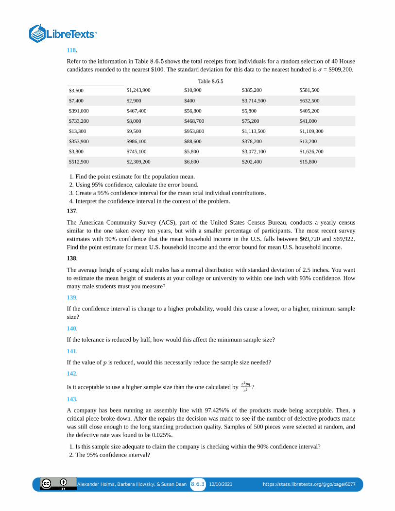
Alexander Holms, Barbara Illowsky, & Susan Dean 8.6.3 12/10/2021 https://stats.libretexts.org/@go/page/6077
118.
Refer to the information in Table shows the total receipts from individuals for a random selection of 40 Housecandidates rounded to the nearest $100. The standard deviation for this data to the nearest hundred is = $909,200.
$3,600 $1,243,900 $10,900 $385,200 $581,500
$7,400 $2,900 $400 $3,714,500 $632,500
$391,000 $467,400 $56,800 $5,800 $405,200
$733,200 $8,000 $468,700 $75,200 $41,000
$13,300 $9,500 $953,800 $1,113,500 $1,109,300
$353,900 $986,100 $88,600 $378,200 $13,200
$3,800 $745,100 $5,800 $3,072,100 $1,626,700
$512,900 $2,309,200 $6,600 $202,400 $15,800
Table
1. Find the point estimate for the population mean.2. Using 95% confidence, calculate the error bound.3. Create a 95% confidence interval for the mean total individual contributions.4. Interpret the confidence interval in the context of the problem.
137.
The American Community Survey (ACS), part of the United States Census Bureau, conducts a yearly censussimilar to the one taken every ten years, but with a smaller percentage of participants. The most recent surveyestimates with 90% confidence that the mean household income in the U.S. falls between $69,720 and $69,922.Find the point estimate for mean U.S. household income and the error bound for mean U.S. household income.
138.
The average height of young adult males has a normal distribution with standard deviation of 2.5 inches. You wantto estimate the mean height of students at your college or university to within one inch with 93% confidence. Howmany male students must you measure?
139.
If the confidence interval is change to a higher probability, would this cause a lower, or a higher, minimum samplesize?
140.
If the tolerance is reduced by half, how would this affect the minimum sample size?
141.
If the value of is reduced, would this necessarily reduce the sample size needed?
142.
Is it acceptable to use a higher sample size than the one calculated by ?
143.
A company has been running an assembly line with 97.42%% of the products made being acceptable. Then, acritical piece broke down. After the repairs the decision was made to see if the number of defective products madewas still close enough to the long standing production quality. Samples of 500 pieces were selected at random, andthe defective rate was found to be 0.025%.
1. Is this sample size adequate to claim the company is checking within the 90% confidence interval?2. The 95% confidence interval?
8.6.5
σ
8.6.5
p
pqz2
e2
Alexander Holms, Barbara Illowsky, & Susan Dean 8.7.1 12/24/2021 https://stats.libretexts.org/@go/page/4594
8.7: Chapter Key Terms
Binomial Distributiona discrete random variable (RV) which arises from Bernoulli trials; there are a fixed number, , of independent trials.“Independent” means that the result of any trial (for example, trial 1) does not affect the results of the following trials,and all trials are conducted under the same conditions. Under these circumstances the binomial is defined as thenumber of successes in n trials. The notation is: . The mean is and the standard deviation is
. The probability of exactly successes in trials is .
Confidence Interval (CI)an interval estimate for an unknown population parameter. This depends on:
the desired confidence level,information that is known about the distribution (for example, known standard deviation),the sample and its size.
Confidence Level (CL)the percent expression for the probability that the confidence interval contains the true population parameter; forexample, if the CL = 90%, then in 90 out of 100 samples the interval estimate will enclose the true populationparameter.
Degrees of Freedom (df)the number of objects in a sample that are free to vary
Error Bound for a Population Mean (EBM)the margin of error; depends on the confidence level, sample size, and known or estimated population standarddeviation.
Error Bound for a Population Proportion (EBP)the margin of error; depends on the confidence level, the sample size, and the estimated (from the sample) proportionof successes.
Inferential Statisticsalso called statistical inference or inductive statistics; this facet of statistics deals with estimating a populationparameter based on a sample statistic. For example, if four out of the 100 calculators sampled are defective we mightinfer that four percent of the production is defective.
Normal Distribution
a continuous random variable (RV) with pdf , where is the mean of the distribution and
is the standard deviation, notation: . If and , the RV is called the standard normaldistribution.
Parametera numerical characteristic of a population
Point Estimatea single number computed from a sample and used to estimate a population parameter
Standard Deviationa number that is equal to the square root of the variance and measures how far data values are from their mean;notation: for sample standard deviation and \sigma for population standard deviation
Student's t-Distribution
n
RV X
X ∼ B(n, p) μ = np
σ = npq−−−√ x n P (X = x) =( )
n
xpxqn−x
f(x) = 1σ 2π√
e−(x−μ /2)2
σ2μ σ
X ∼ N(μ, σ) μ = 0 σ = 1
s

Alexander Holms, Barbara Illowsky, & Susan Dean 8.7.2 12/24/2021 https://stats.libretexts.org/@go/page/4594
investigated and reported by William S. Gossett in 1908 and published under the pseudonym Student; the majorcharacteristics of this random variable ( ) are:
It is continuous and assumes any real values.The pdf is symmetrical about its mean of zero.It approaches the standard normal distribution as get larger.There is a "family" of t–distributions: each representative of the family is completely defined by the number ofdegrees of freedom, which depends upon the application for which the t is being used.
RV
n
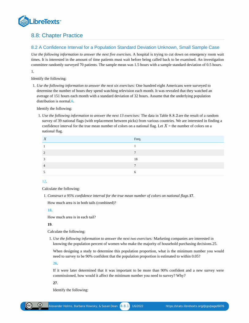
Alexander Holms, Barbara Illowsky, & Susan Dean 8.8.1 1/6/2022 https://stats.libretexts.org/@go/page/6076
8.8: Chapter Practice
8.2 A Confidence Interval for a Population Standard Deviation Unknown, Small Sample CaseUse the following information to answer the next five exercises. A hospital is trying to cut down on emergency room waittimes. It is interested in the amount of time patients must wait before being called back to be examined. An investigationcommittee randomly surveyed 70 patients. The sample mean was 1.5 hours with a sample standard deviation of 0.5 hours.
1.
Identify the following:
1. Use the following information to answer the next six exercises: One hundred eight Americans were surveyed todetermine the number of hours they spend watching television each month. It was revealed that they watched anaverage of 151 hours each month with a standard deviation of 32 hours. Assume that the underlying populationdistribution is normal.6.
Identify the following:
1. Use the following information to answer the next 13 exercises: The data in Table are the result of a randomsurvey of 39 national flags (with replacement between picks) from various countries. We are interested in finding aconfidence interval for the true mean number of colors on a national flag. Let = the number of colors on anational flag.
Freq.
1 1
2 7
3 18
4 7
5 6
12.
Calculate the following:
1. Construct a 95% confidence interval for the true mean number of colors on national flags.17.
How much area is in both tails (combined)?
18.
How much area is in each tail?
19.
Calculate the following:
1. Use the following information to answer the next two exercises: Marketing companies are interested inknowing the population percent of women who make the majority of household purchasing decisions.25.
When designing a study to determine this population proportion, what is the minimum number you wouldneed to survey to be 90% confident that the population proportion is estimated to within 0.05?
26.
If it were later determined that it was important to be more than 90% confident and a new survey werecommissioned, how would it affect the minimum number you need to survey? Why?
27.
Identify the following:
8.8.2
X
X
Alexander Holms, Barbara Illowsky, & Susan Dean 8.8.2 1/6/2022 https://stats.libretexts.org/@go/page/6076
1. Use the following information to answer the next five exercises: Of 1,050 randomly selected adults, 360identified themselves as manual laborers, 280 identified themselves as non-manual wage earners, 250identified themselves as mid-level managers, and 160 identified themselves as executives. In the survey,82% of manual laborers preferred trucks, 62% of non-manual wage earners preferred trucks, 54% of mid-level managers preferred trucks, and 26% of executives preferred trucks.32.
We are interested in finding the 95% confidence interval for the percent of executives who prefer trucks.Define random variables and in words.
33.
Which distribution should you use for this problem?
34.
Construct a 95% confidence interval. State the confidence interval, sketch the graph, and calculate theerror bound.
35.
Suppose we want to lower the sampling error. What is one way to accomplish that?
36.
The sampling error given in the survey is ±2%. Explain what the ±2% means.
37.
Define the random variable in words.
38.
Define the random variable in words.
39.
Which distribution should you use for this problem?
40.
Construct a 90% confidence interval, and state the confidence interval and the error bound.
41.
What would happen to the confidence interval if the level of confidence were 95%?
Use the following information to answer the next 16 exercises: The Ice Chalet offers dozens of differentbeginning ice-skating classes. All of the class names are put into a bucket. The 5 P.M., Monday night,ages 8 to 12, beginning ice-skating class was picked. In that class were 64 girls and 16 boys. Suppose thatwe are interested in the true proportion of girls, ages 8 to 12, in all beginning ice-skating classes at the IceChalet. Assume that the children in the selected class are a random sample of the population.
42.
What is being counted?
43.
In words, define the random variable .
44.
Calculate the following:
1. Use the following information to answer the next five exercises: The standard deviation of the weightsof elephants is known to be approximately 15 pounds. We wish to construct a 95% confidenceinterval for the mean weight of newborn elephant calves. Fifty newborn elephants are weighed. Thesample mean is 244 pounds. The sample standard deviation is 11 pounds.58.
X p′
X
p′
X
Alexander Holms, Barbara Illowsky, & Susan Dean 8.8.3 1/6/2022 https://stats.libretexts.org/@go/page/6076
Identify the following:
1. Use the following information to answer the next seven exercises: The U.S. Census Bureauconducts a study to determine the time needed to complete the short form. The Bureau surveys200 people. The sample mean is 8.2 minutes. There is a known standard deviation of 2.2 minutes.The population distribution is assumed to be normal.63.
Identify the following:
1. Use the following information to answer the next ten exercises: A sample of 20 heads oflettuce was selected. Assume that the population distribution of head weight is normal. Theweight of each head of lettuce was then recorded. The mean weight was 2.2 pounds with astandard deviation of 0.1 pounds. The population standard deviation is known to be 0.2pounds.70.
Identify the following:
1. Use the following information to answer the next 14 exercises: The mean age for allFoothill College students for a recent Fall term was 33.2. The population standard deviationhas been pretty consistent at 15. Suppose that twenty-five Winter students were randomlyselected. The mean age for the sample was 30.4. We are interested in the true mean age forWinter Foothill College students. Let = the age of a Winter Foothill College student.80.
= _____
81.
= _____
82.
________ = 15
83.
In words, define the random variable .
84.
What is estimating?
85.
Is known?
86.
As a result of your answer to Exercise , state the exact distribution to use whencalculating the confidence interval.
87.
How much area is in both tails (combined)? =________
88.
How much area is in each tail? =________
89.
Identify the following specifications:
1. lower limit2. upper limit3. error bound
90.
The 95% confidence interval is:__________________.
X
x̄̄̄
n
X¯ ¯¯̄
x¯̄̄
σx
8.8.83
α
α
2
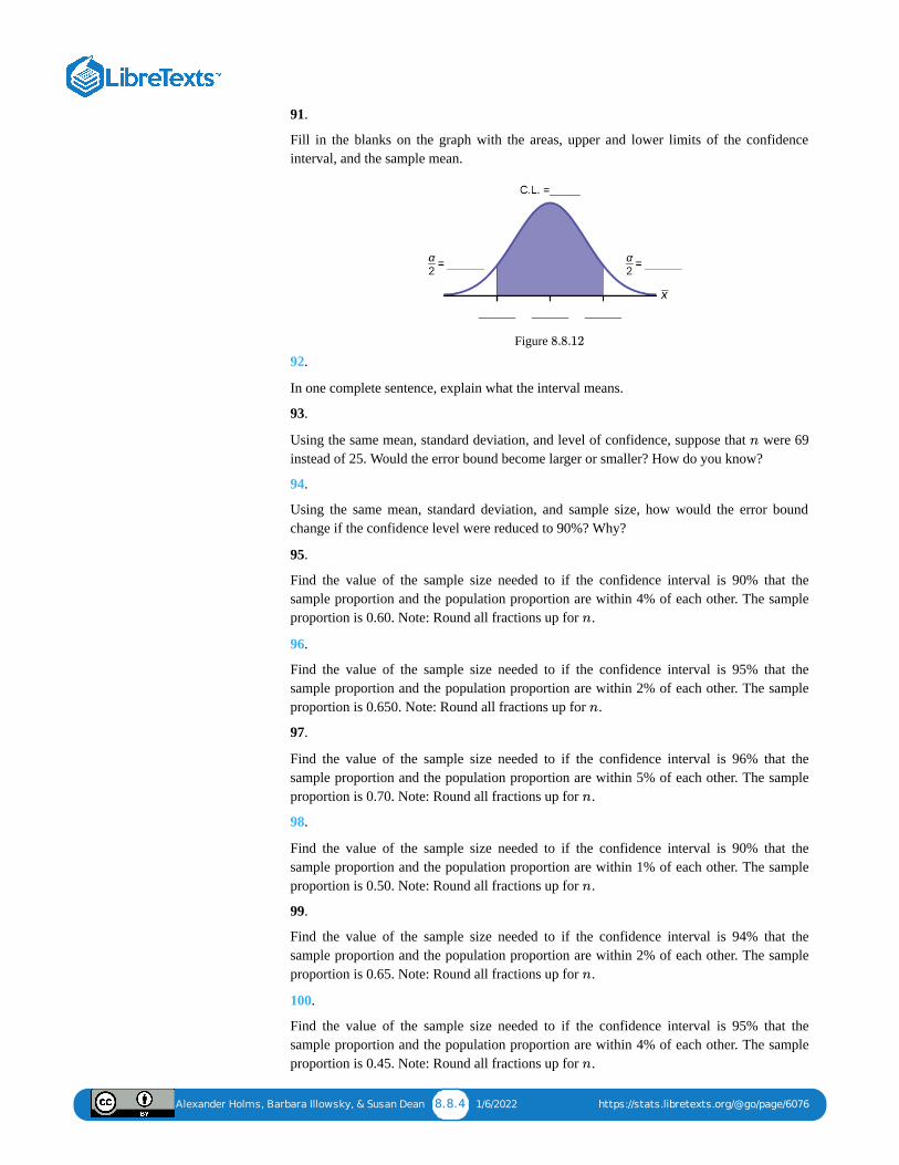
Alexander Holms, Barbara Illowsky, & Susan Dean 8.8.4 1/6/2022 https://stats.libretexts.org/@go/page/6076
91.
Fill in the blanks on the graph with the areas, upper and lower limits of the confidenceinterval, and the sample mean.
Figure
92.
In one complete sentence, explain what the interval means.
93.
Using the same mean, standard deviation, and level of confidence, suppose that were 69instead of 25. Would the error bound become larger or smaller? How do you know?
94.
Using the same mean, standard deviation, and sample size, how would the error boundchange if the confidence level were reduced to 90%? Why?
95.
Find the value of the sample size needed to if the confidence interval is 90% that thesample proportion and the population proportion are within 4% of each other. The sampleproportion is 0.60. Note: Round all fractions up for .
96.
Find the value of the sample size needed to if the confidence interval is 95% that thesample proportion and the population proportion are within 2% of each other. The sampleproportion is 0.650. Note: Round all fractions up for .
97.
Find the value of the sample size needed to if the confidence interval is 96% that thesample proportion and the population proportion are within 5% of each other. The sampleproportion is 0.70. Note: Round all fractions up for .
98.
Find the value of the sample size needed to if the confidence interval is 90% that thesample proportion and the population proportion are within 1% of each other. The sampleproportion is 0.50. Note: Round all fractions up for .
99.
Find the value of the sample size needed to if the confidence interval is 94% that thesample proportion and the population proportion are within 2% of each other. The sampleproportion is 0.65. Note: Round all fractions up for .
100.
Find the value of the sample size needed to if the confidence interval is 95% that thesample proportion and the population proportion are within 4% of each other. The sampleproportion is 0.45. Note: Round all fractions up for .
8.8.12
n
n
n
n
n
n
n

Alexander Holms, Barbara Illowsky, & Susan Dean 8.8.5 1/6/2022 https://stats.libretexts.org/@go/page/6076
101.
Find the value of the sample size needed to if the confidence interval is 90% that thesample proportion and the population proportion are within 2% of each other. The sampleproportion is 0.3. Note: Round all fractions up for .n
Alexander Holms, Barbara Illowsky, & Susan Dean 8.9.1 12/10/2021 https://stats.libretexts.org/@go/page/6078
8.9: Chapter References
A Confidence Interval for a Population Standard Deviation, Known or Large Sample Size“American Fact Finder.” U.S. Census Bureau. Available online at http://factfinder2.census.gov/faces/...html?refresh=t(accessed July 2, 2013).“Disclosure Data Catalog: Candidate Summary Report 2012.” U.S. Federal Election Commission. Available online atwww.fec.gov/data/index.jsp (accessed July 2, 2013).“Headcount Enrollment Trends by Student Demographics Ten-Year Fall Trends to Most Recently Completed Fall.”Foothill De Anza Community College District. Available online at research.fhda.edu/factbook/FH...phicTrends.htm(accessed September 30,2013).Kuczmarski, Robert J., Cynthia L. Ogden, Shumei S. Guo, Laurence M. Grummer-Strawn, Katherine M. Flegal, ZuguoMei, Rong Wei, Lester R. Curtin, Alex F. Roche, Clifford L. Johnson. “2000 CDC Growth Charts for the United States:Methods and Development.” Centers for Disease Control and Prevention. Available online athttp://www.cdc.gov/growthcharts/2000...thchart-us.pdf (accessed July 2, 2013).La, Lynn, Kent German. "Cell Phone Radiation Levels." c|net part of CBX Interactive Inc. Available online athttp://reviews.cnet.com/cell-phone-radiation-levels/ (accessed July 2, 2013).“Mean Income in the Past 12 Months (in 2011 Inflaction-Adjusted Dollars): 2011 American Community Survey 1-YearEstimates.” American Fact Finder, U.S. Census Bureau. Available online athttp://factfinder2.census.gov/faces/...prodType=table (accessed July 2, 2013).“Metadata Description of Candidate Summary File.” U.S. Federal Election Commission. Available online atwww.fec.gov/finance/disclosur...esummary.shtml (accessed July 2, 2013).“National Health and Nutrition Examination Survey.” Centers for Disease Control and Prevention. Available online athttp://www.cdc.gov/nchs/nhanes.htm (accessed July 2, 2013).
A Confidence Interval for a Population Standard Deviation Unknown, Small Sample Case“America’s Best Small Companies.” Forbes, 2013. Available online at http://www.forbes.com/best-small-companies/list/ (accessed July 2, 2013).Data from Microsoft Bookshelf.Data from http://www.businessweek.com/.Data from http://www.forbes.com/.“Disclosure Data Catalog: Leadership PAC and Sponsors Report, 2012.” Federal Election Commission. Availableonline at www.fec.gov/data/index.jsp (accessed July 2,2013).“Human Toxome Project: Mapping the Pollution in People.” Environmental Working Group. Available online atwww.ewg.org/sites/humantoxome...tero%2Fnewborn (accessed July 2, 2013).“Metadata Description of Leadership PAC List.” Federal Election Commission. Available online atwww.fec.gov/finance/disclosur...pPacList.shtml (accessed July 2, 2013).
A Confidence Interval for A Population ProportionJensen, Tom. “Democrats, Republicans Divided on Opinion of Music Icons.” Public Policy Polling. Available online atwww.publicpolicypolling.com/Day2MusicPoll.pdf (accessed July 2, 2013).Madden, Mary, Amanda Lenhart, Sandra Coresi, Urs Gasser, Maeve Duggan, Aaron Smith, and Meredith Beaton.“Teens, Social Media, and Privacy.” PewInternet, 2013. Available online at www.pewinternet.org/Reports/2...d-Privacy.aspx (accessed July 2, 2013).Prince Survey Research Associates International. “2013 Teen and Privacy Management Survey.” Pew Research Center:Internet and American Life Project. Available online at www.pewinternet.org/~/media//...al%20Media.pdf (accessedJuly 2, 2013).Saad, Lydia. “Three in Four U.S. Workers Plan to Work Pas Retirement Age: Slightly more say they will do this bychoice rather than necessity.” Gallup® Economy, 2013. Available online athttp://www.gallup.com/poll/162758/th...ement-age.aspx (accessed July 2, 2013).The Field Poll. Available online at field.com/fieldpollonline/subscribers/ (accessed July 2, 2013).

Alexander Holms, Barbara Illowsky, & Susan Dean 8.9.2 12/10/2021 https://stats.libretexts.org/@go/page/6078
Zogby. “New SUNYIT/Zogby Analytics Poll: Few Americans Worry about Emergency Situations Occurring in TheirCommunity; Only one in three have an Emergency Plan; 70% Support Infrastructure ‘Investment’ for NationalSecurity.” Zogby Analytics, 2013. Available online at http://www.zogbyanalytics.com/news/2...analytics-poll (accessedJuly 2, 2013).“52% Say Big-Time College Athletics Corrupt Education Process.” Rasmussen Reports, 2013. Available online athttp://www.rasmussenreports.com/publ...cation_process (accessed July 2, 2013).
Alexander Holms, Barbara Illowsky, & Susan
Dean8.10.1 12/24/2021 https://stats.libretexts.org/@go/page/6074
8.10: Chapter Review
8.2 A Confidence Interval for a Population Standard Deviation Unknown, Small Sample Case
In many cases, the researcher does not know the population standard deviation, , of the measure being studied. In thesecases, it is common to use the sample standard deviation, s, as an estimate of \sigma. The normal distribution createsaccurate confidence intervals when is known, but it is not as accurate when s is used as an estimate. In this case, theStudent’s t-distribution is much better. Define a t-score using the following formula:
The t-score follows the Student’s t-distribution with degrees of freedom. The confidence interval under this
distribution is calculated with where is the t-score with area to the right equal to , is the sample
standard deviation, and is the sample size. Use a table, calculator, or computer to find for a given .
8.3 A Confidence Interval for A Population ProportionSome statistical measures, like many survey questions, measure qualitative rather than quantitative data. In this case, thepopulation parameter being estimated is a proportion. It is possible to create a confidence interval for the true populationproportion following procedures similar to those used in creating confidence intervals for population means. The formulasare slightly different, but they follow the same reasoning.
Let represent the sample proportion, , where represents the number of successes and represents the sample size.Let . Then the confidence interval for a population proportion is given by the following formula:
8.4 Calculating the Sample Size n: Continuous and Binary Random Variables
Sometimes researchers know in advance that they want to estimate a population mean within a specific margin of error fora given level of confidence. In that case, solve the relevant confidence interval formula for n to discover the size of thesample that is needed to achieve this goal:
If the random variable is binary then the formula for the appropriate sample size to maintain a particular level ofconfidence with a specific tolerance level is given by
σ
σ
t =−μx̄̄̄
s/ n√
n– 1
±( )x̄̄̄ t α
2
s
n√t α
2
α2
s
n t α
2α
p′ x/n x n
= 1 −q ′ p′
− ≤ p ≤ +p′ Zαp′q ′
n
−−−√ p′ Zα
p′q ′
n
−−−√
n =Z 2
ασ2
( −μx̄̄̄ )2
n =pqZ 2
α
e2

Alexander Holms, Barbara Illowsky, & Susan
Dean8.11.1 12/10/2021 https://stats.libretexts.org/@go/page/6079
8.11: Chapter Solution (Practice + Homework)
Figure 8.11.23

1 1/7/2022
CHAPTER OVERVIEW9: HYPOTHESIS TESTING WITH ONE SAMPLE
9.0: INTRODUCTION TO HYPOTHESIS TESTING9.1: NULL AND ALTERNATIVE HYPOTHESESThe actual test begins by considering two hypotheses. They are called the null hypothesis and the alternative hypothesis. Thesehypotheses contain opposing viewpoints.
9.2: OUTCOMES AND THE TYPE I AND TYPE II ERRORS9.3: DISTRIBUTION NEEDED FOR HYPOTHESIS TESTING9.4: FULL HYPOTHESIS TEST EXAMPLES9.5: CHAPTER FORMULA REVIEW9.6: CHAPTER HOMEWORK9.7: CHAPTER KEY TERMS9.8: CHAPTER PRACTICE9.9: CHAPTER REFERENCES9.10: CHAPTER REVIEW9.11: CHAPTER SOLUTION (PRACTICE + HOMEWORK)
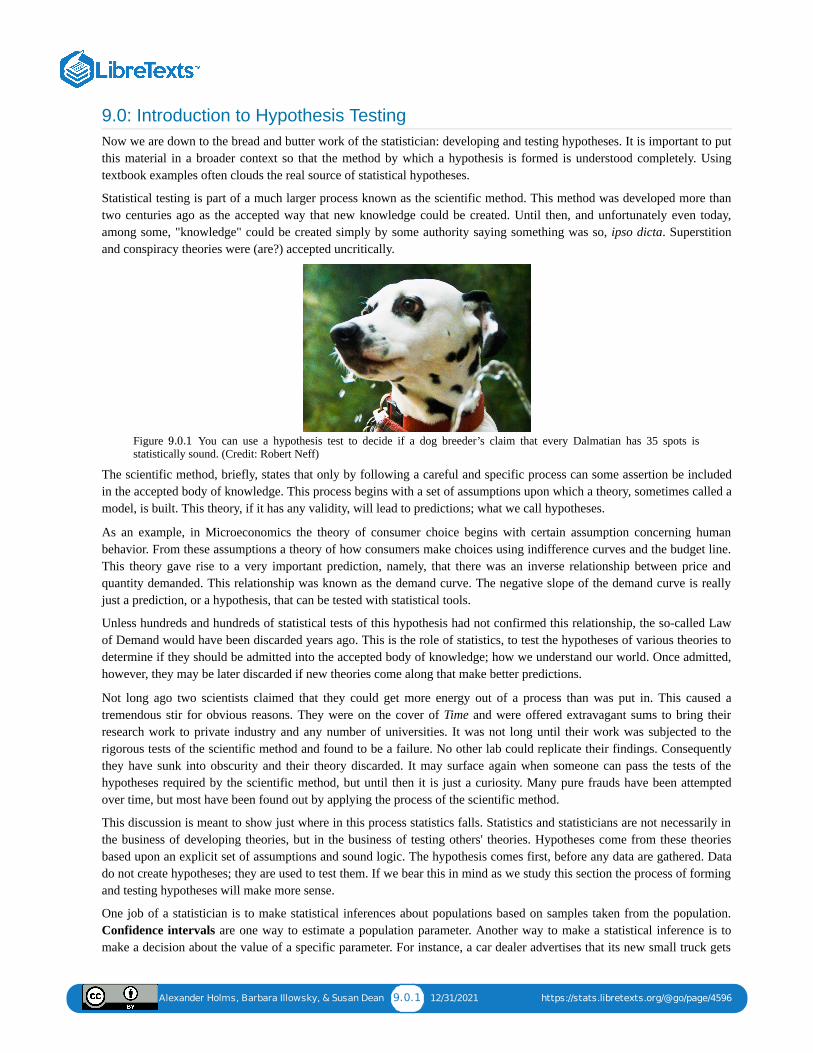
Alexander Holms, Barbara Illowsky, & Susan Dean 9.0.1 12/31/2021 https://stats.libretexts.org/@go/page/4596
9.0: Introduction to Hypothesis TestingNow we are down to the bread and butter work of the statistician: developing and testing hypotheses. It is important to putthis material in a broader context so that the method by which a hypothesis is formed is understood completely. Usingtextbook examples often clouds the real source of statistical hypotheses.
Statistical testing is part of a much larger process known as the scientific method. This method was developed more thantwo centuries ago as the accepted way that new knowledge could be created. Until then, and unfortunately even today,among some, "knowledge" could be created simply by some authority saying something was so, ipso dicta. Superstitionand conspiracy theories were (are?) accepted uncritically.
Figure You can use a hypothesis test to decide if a dog breeder’s claim that every Dalmatian has 35 spots isstatistically sound. (Credit: Robert Neff)
The scientific method, briefly, states that only by following a careful and specific process can some assertion be includedin the accepted body of knowledge. This process begins with a set of assumptions upon which a theory, sometimes called amodel, is built. This theory, if it has any validity, will lead to predictions; what we call hypotheses.
As an example, in Microeconomics the theory of consumer choice begins with certain assumption concerning humanbehavior. From these assumptions a theory of how consumers make choices using indifference curves and the budget line.This theory gave rise to a very important prediction, namely, that there was an inverse relationship between price andquantity demanded. This relationship was known as the demand curve. The negative slope of the demand curve is reallyjust a prediction, or a hypothesis, that can be tested with statistical tools.
Unless hundreds and hundreds of statistical tests of this hypothesis had not confirmed this relationship, the so-called Lawof Demand would have been discarded years ago. This is the role of statistics, to test the hypotheses of various theories todetermine if they should be admitted into the accepted body of knowledge; how we understand our world. Once admitted,however, they may be later discarded if new theories come along that make better predictions.
Not long ago two scientists claimed that they could get more energy out of a process than was put in. This caused atremendous stir for obvious reasons. They were on the cover of Time and were offered extravagant sums to bring theirresearch work to private industry and any number of universities. It was not long until their work was subjected to therigorous tests of the scientific method and found to be a failure. No other lab could replicate their findings. Consequentlythey have sunk into obscurity and their theory discarded. It may surface again when someone can pass the tests of thehypotheses required by the scientific method, but until then it is just a curiosity. Many pure frauds have been attemptedover time, but most have been found out by applying the process of the scientific method.
This discussion is meant to show just where in this process statistics falls. Statistics and statisticians are not necessarily inthe business of developing theories, but in the business of testing others' theories. Hypotheses come from these theoriesbased upon an explicit set of assumptions and sound logic. The hypothesis comes first, before any data are gathered. Datado not create hypotheses; they are used to test them. If we bear this in mind as we study this section the process of formingand testing hypotheses will make more sense.
One job of a statistician is to make statistical inferences about populations based on samples taken from the population.Confidence intervals are one way to estimate a population parameter. Another way to make a statistical inference is tomake a decision about the value of a specific parameter. For instance, a car dealer advertises that its new small truck gets
9.0.1

Alexander Holms, Barbara Illowsky, & Susan Dean 9.0.2 12/31/2021 https://stats.libretexts.org/@go/page/4596
35 miles per gallon, on average. A tutoring service claims that its method of tutoring helps 90% of its students get an A ora B. A company says that women managers in their company earn an average of $60,000 per year.
A statistician will make a decision about these claims. This process is called "hypothesis testing." A hypothesis testinvolves collecting data from a sample and evaluating the data. Then, the statistician makes a decision as to whether or notthere is sufficient evidence, based upon analyses of the data, to reject the null hypothesis.
In this chapter, you will conduct hypothesis tests on single means and single proportions. You will also learn about theerrors associated with these tests.
Alexander Holms, Barbara Illowsky, & Susan Dean 9.1.1 1/6/2022 https://stats.libretexts.org/@go/page/4597
9.1: Null and Alternative HypothesesThe actual test begins by considering two hypotheses. They are called the null hypothesis and the alternative hypothesis.These hypotheses contain opposing viewpoints.
: The null hypothesis: It is a statement of no difference between a sample mean or proportion and a populationmean or proportion. In other words, the difference equals 0. This can often be considered the status quo and as a resultif you cannot accept the null it requires some action.
: The alternative hypothesis: It is a claim about the population that is contradictory to and what we concludewhen we cannot accept . The alternative hypothesis is the contender and must win with significant evidence tooverthrow the status quo. This concept is sometimes referred to the tyranny of the status quo because as we will seelater, to overthrow the null hypothesis takes usually 90 or greater confidence that this is the proper decision.
Since the null and alternative hypotheses are contradictory, you must examine evidence to decide if you have enoughevidence to reject the null hypothesis or not. The evidence is in the form of sample data.
After you have determined which hypothesis the sample supports, you make a decision. There are two options for adecision. They are "cannot accept " if the sample information favors the alternative hypothesis or "do not reject " or"decline to reject " if the sample information is insufficient to reject the null hypothesis. These conclusions are all basedupon a level of probability, a significance level, that is set my the analyst.
Table 9.1 presents the various hypotheses in the relevant pairs. For example, if the null hypothesis is equal to some value,the alternative has to be not equal to that value.
Table 9.1
equal (=) not equal ( )
greater than or equal to ( ) less than (<)
less than or equal to ( ) more than (>)
As a mathematical convention always has a symbol with an equal in it. Ha never has a symbol with an equal in it.The choice of symbol depends on the wording of the hypothesis test.
: No more than 30% of the registered voters in Santa Clara County voted in the primary election. : More than 30% of the registered voters in Santa Clara County voted in the primary election.
We want to test whether the mean GPA of students in American colleges is different from 2.0 (out of 4.0). The null andalternative hypotheses are:
We want to test if college students take less than five years to graduate from college, on the average. The null andalternative hypotheses are:
H0
Ha H0
H0
H0 H0
H0
H0 Ha
≠
≥
≤
Note
H0
Example 9.1
H0 p ≤ 30
Ha p > 30
Example 9.2
: μ = 2.0H0
: μ ≠ 2.0Ha
Example 9.3
: μ ≥ 5H0
: μ < 5Ha
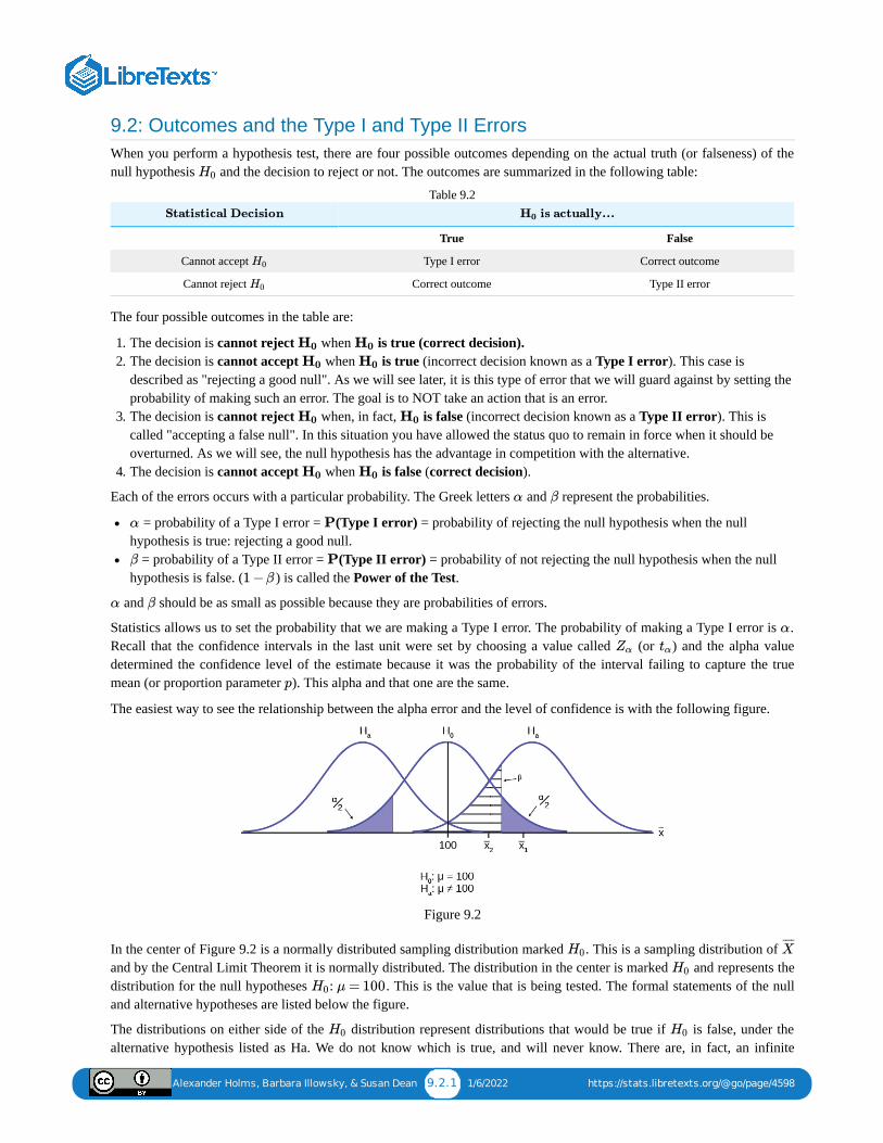
Alexander Holms, Barbara Illowsky, & Susan Dean 9.2.1 1/6/2022 https://stats.libretexts.org/@go/page/4598
9.2: Outcomes and the Type I and Type II ErrorsWhen you perform a hypothesis test, there are four possible outcomes depending on the actual truth (or falseness) of thenull hypothesis and the decision to reject or not. The outcomes are summarized in the following table:
Table 9.2
True False
Cannot accept Type I error Correct outcome
Cannot reject Correct outcome Type II error
The four possible outcomes in the table are:
1. The decision is cannot reject when is true (correct decision).2. The decision is cannot accept when is true (incorrect decision known as a Type I error). This case is
described as "rejecting a good null". As we will see later, it is this type of error that we will guard against by setting theprobability of making such an error. The goal is to NOT take an action that is an error.
3. The decision is cannot reject when, in fact, is false (incorrect decision known as a Type II error). This iscalled "accepting a false null". In this situation you have allowed the status quo to remain in force when it should beoverturned. As we will see, the null hypothesis has the advantage in competition with the alternative.
4. The decision is cannot accept when is false (correct decision).
Each of the errors occurs with a particular probability. The Greek letters and represent the probabilities.
= probability of a Type I error = (Type I error) = probability of rejecting the null hypothesis when the nullhypothesis is true: rejecting a good null.
= probability of a Type II error = (Type II error) = probability of not rejecting the null hypothesis when the nullhypothesis is false. ( ) is called the Power of the Test.
and should be as small as possible because they are probabilities of errors.
Statistics allows us to set the probability that we are making a Type I error. The probability of making a Type I error is .Recall that the confidence intervals in the last unit were set by choosing a value called (or ) and the alpha valuedetermined the confidence level of the estimate because it was the probability of the interval failing to capture the truemean (or proportion parameter ). This alpha and that one are the same.
The easiest way to see the relationship between the alpha error and the level of confidence is with the following figure.
Figure 9.2
In the center of Figure 9.2 is a normally distributed sampling distribution marked . This is a sampling distribution of and by the Central Limit Theorem it is normally distributed. The distribution in the center is marked and represents thedistribution for the null hypotheses : . This is the value that is being tested. The formal statements of the nulland alternative hypotheses are listed below the figure.
The distributions on either side of the distribution represent distributions that would be true if is false, under thealternative hypothesis listed as Ha. We do not know which is true, and will never know. There are, in fact, an infinite
H0
Statistical Decision is actually...H0
H0
H0
H0 H0
H0 H0
H0 H0
H0 H0
α β
α P
β P
1 −β
α β
α
Zα tα
p
H0 X¯ ¯¯̄
H0
H0 μ = 100
H0 H0
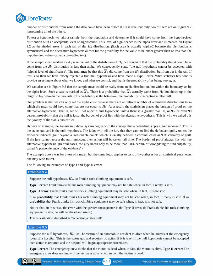
Alexander Holms, Barbara Illowsky, & Susan Dean 9.2.2 1/6/2022 https://stats.libretexts.org/@go/page/4598
number of distributions from which the data could have been drawn if Ha is true, but only two of them are on Figure 9.2representing all of the others.
To test a hypothesis we take a sample from the population and determine if it could have come from the hypothesizeddistribution with an acceptable level of significance. This level of significance is the alpha error and is marked on Figure9.2 as the shaded areas in each tail of the distribution. (Each area is actually \alpha/2 because the distribution issymmetrical and the alternative hypothesis allows for the possibility for the value to be either greater than or less than thehypothesized value--called a two-tailed test).
If the sample mean marked as is in the tail of the distribution of , we conclude that the probability that it could havecome from the distribution is less than alpha. We consequently state, "the null hypothesis cannot be accepted with(\alpha) level of significance". The truth may be that this did come from the distribution, but from out in the tail. Ifthis is so then we have falsely rejected a true null hypothesis and have made a Type I error. What statistics has done isprovide an estimate about what we know, and what we control, and that is the probability of us being wrong, .
We can also see in Figure 9.2 that the sample mean could be really from an Ha distribution, but within the boundary set bythe alpha level. Such a case is marked as . There is a probability that actually came from Ha but shows up in therange of between the two tails. This probability is the beta error, the probability of accepting a false null.
Our problem is that we can only set the alpha error because there are an infinite number of alternative distributions fromwhich the mean could have come that are not equal to . As a result, the statistician places the burden of proof on thealternative hypothesis. That is, we will not reject a null hypothesis unless there is a greater than 90, or 95, or even 99percent probability that the null is false: the burden of proof lies with the alternative hypothesis. This is why we called thisthe tyranny of the status quo earlier.
By way of example, the American judicial system begins with the concept that a defendant is "presumed innocent". This isthe status quo and is the null hypothesis. The judge will tell the jury that they can not find the defendant guilty unless theevidence indicates guilt beyond a "reasonable doubt" which is usually defined in criminal cases as 95% certainty of guilt.If the jury cannot accept the null, innocent, then action will be taken, jail time. The burden of proof always lies with thealternative hypothesis. (In civil cases, the jury needs only to be more than 50% certain of wrongdoing to find culpability,called "a preponderance of the evidence").
The example above was for a test of a mean, but the same logic applies to tests of hypotheses for all statistical parametersone may wish to test.
The following are examples of Type I and Type II errors.
Suppose the null hypothesis, , is: Frank's rock climbing equipment is safe.
Type I error: Frank thinks that his rock climbing equipment may not be safe when, in fact, it really is safe.
Type II error: Frank thinks that his rock climbing equipment may be safe when, in fact, it is not safe.
probability that Frank thinks his rock climbing equipment may not be safe when, in fact, it really is safe. probability that Frank thinks his rock climbing equipment may be safe when, in fact, it is not safe.
Notice that, in this case, the error with the greater consequence is the Type II error. (If Frank thinks his rock climbingequipment is safe, he will go ahead and use it.)
This is a situation described as "accepting a false null".
Suppose the null hypothesis, , is: The victim of an automobile accident is alive when he arrives at the emergencyroom of a hospital. This is the status quo and requires no action if it is true. If the null hypothesis cannot be acceptedthen action is required and the hospital will begin appropriate procedures.
Type I error: The emergency crew thinks that the victim is dead when, in fact, the victim is alive. Type II error: Theemergency crew does not know if the victim is alive when, in fact, the victim is dead.
H0
X¯ ¯¯̄
1 H0
H0
X¯ ¯¯̄1 H0
α
X¯ ¯¯̄
2 X¯ ¯¯̄
2
H0
H0
Example 9.4
H0
α = β =
Example 9.5
H0
Alexander Holms, Barbara Illowsky, & Susan Dean 9.2.3 1/6/2022 https://stats.libretexts.org/@go/page/4598
probability that the emergency crew thinks the victim is dead when, in fact, he is really alive = P(Type I error). probability that the emergency crew does not know if the victim is alive when, in fact, the victim is dead =
P(Type II error).
The error with the greater consequence is the Type I error. (If the emergency crew thinks the victim is dead, they willnot treat him.)
Suppose the null hypothesis, , is: a patient is not sick. Which type of error has the greater consequence, Type I orType II?
It’s a Boy Genetic Labs claim to be able to increase the likelihood that a pregnancy will result in a boy being born.Statisticians want to test the claim. Suppose that the null hypothesis, , is: It’s a Boy Genetic Labs has no effect ongender outcome. The status quo is that the claim is false. The burden of proof always falls to the person making theclaim, in this case the Genetics Lab.
Type I error: This results when a true null hypothesis is rejected. In the context of this scenario, we would state thatwe believe that It’s a Boy Genetic Labs influences the gender outcome, when in fact it has no effect. The probability ofthis error occurring is denoted by the Greek letter alpha, \alpha.
Type II error: This results when we fail to reject a false null hypothesis. In context, we would state that It’s a BoyGenetic Labs does not influence the gender outcome of a pregnancy when, in fact, it does. The probability of this erroroccurring is denoted by the Greek letter beta, \beta.
The error of greater consequence would be the Type I error since couples would use the It’s a Boy Genetic Labsproduct in hopes of increasing the chances of having a boy.
“Red tide” is a bloom of poison-producing algae–a few different species of a class of plankton called dinoflagellates.When the weather and water conditions cause these blooms, shellfish such as clams living in the area developdangerous levels of a paralysis-inducing toxin. In Massachusetts, the Division of Marine Fisheries (DMF) monitorslevels of the toxin in shellfish by regular sampling of shellfish along the coastline. If the mean level of toxin in clamsexceeds 800 μg (micrograms) of toxin per kg of clam meat in any area, clam harvesting is banned there until the bloomis over and levels of toxin in clams subside. Describe both a Type I and a Type II error in this context, and state whicherror has the greater consequence.
A certain experimental drug claims a cure rate of at least 75% for males with prostate cancer. Describe both the Type Iand Type II errors in context. Which error is the more serious?
Type I: A cancer patient believes the cure rate for the drug is less than 75% when it actually is at least 75%.
Type II: A cancer patient believes the experimental drug has at least a 75% cure rate when it has a cure rate that is lessthan 75%.
In this scenario, the Type II error contains the more severe consequence. If a patient believes the drug works at least75% of the time, this most likely will influence the patient’s (and doctor’s) choice about whether to use the drug as atreatment option.
α =
β =
Exercise 9.5
H0
Example 9.6
H0
Exercise 9.6
Example 9.7
Alexander Holms, Barbara Illowsky, & Susan Dean 9.3.1 12/10/2021 https://stats.libretexts.org/@go/page/4599
9.3: Distribution Needed for Hypothesis TestingEarlier, we discussed sampling distributions. Particular distributions are associated with hypothesis testing.We willperform hypotheses tests of a population mean using a normal distribution or a Student's -distribution. (Remember, use aStudent's -distribution when the population standard deviation is unknown and the sample size is small, where small isconsidered to be less than 30 observations.) We perform tests of a population proportion using a normal distribution whenwe can assume that the distribution is normally distributed. We consider this to be true if the sample proportion, , timesthe sample size is greater than 5 and times the sample size is also greater then 5. This is the same rule of thumb weused when developing the formula for the confidence interval for a population proportion.
Hypothesis Test for the MeanGoing back to the standardizing formula we can derive the test statistic for testing hypotheses concerning means.
The standardizing formula can not be solved as it is because we do not have , the population mean. However, if wesubstitute in the hypothesized value of the mean, in the formula as above, we can compute a value. This is the teststatistic for a test of hypothesis for a mean and is presented in Figure 9.3. We interpret this value as the associatedprobability that a sample with a sample mean of could have come from a distribution with a population mean of andwe call this value for “calculated”. Figure 9.3 and Figure 9.4 show this process.
Figure 9.3
In Figure 9.3 two of the three possible outcomes are presented. and are in the tails of the hypothesized distributionof . Notice that the horizontal axis in the top panel is labeled 's. This is the same theoretical distribution of 's, thesampling distribution, that the Central Limit Theorem tells us is normally distributed. This is why we can draw it with thisshape. The horizontal axis of the bottom panel is labeled and is the standard normal distribution. and , calledthe critical values, are marked on the bottom panel as the values associated with the probability the analyst has set asthe level of significance in the test, ( ). The probabilities in the tails of both panels are, therefore, the same.
Notice that for each there is an associated , called the calculated , that comes from solving the equation above. Thiscalculated is nothing more than the number of standard deviations that the hypothesized mean is from the sample mean.If the sample mean falls "too many" standard deviations from the hypothesized mean we conclude that the sample meancould not have come from the distribution with the hypothesized mean, given our pre-set required level of significance. Itcould have come from , but it is deemed just too unlikely. In Figure 9.3 both and are in the tails of thedistribution. They are deemed "too far" from the hypothesized value of the mean given the chosen level of alpha. If in fact
t
t
p′
1 −p′
=Zc
−x̄̄̄ μ0
σ/ n−−√
μ
μ0 Z
Z
X¯ ¯¯̄ H0
Z Zc
X¯ ¯¯̄1 X¯ ¯¯̄
3
H0 X¯ ¯¯̄
X¯ ¯¯̄
Z Z α
2−Z α
2
Z
α
X¯ ¯¯̄ Zc Z
Z
H0 X¯ ¯¯̄
1 X¯ ¯¯̄
3
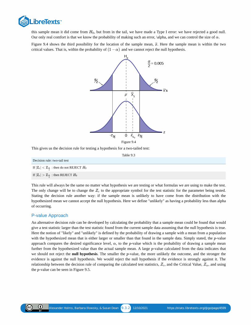
Alexander Holms, Barbara Illowsky, & Susan Dean 9.3.2 12/10/2021 https://stats.libretexts.org/@go/page/4599
this sample mean it did come from , but from in the tail, we have made a Type I error: we have rejected a good null.Our only real comfort is that we know the probability of making such an error, \alpha, and we can control the size of .
Figure 9.4 shows the third possibility for the location of the sample mean, . Here the sample mean is within the twocritical values. That is, within the probability of and we cannot reject the null hypothesis.
Figure 9.4
This gives us the decision rule for testing a hypothesis for a two-tailed test:
Decision rule: two-tail test
If : then do not REJECT
If : then REJECT
Table 9.3
This rule will always be the same no matter what hypothesis we are testing or what formulas we are using to make the test.The only change will be to change the to the appropriate symbol for the test statistic for the parameter being tested.Stating the decision rule another way: if the sample mean is unlikely to have come from the distribution with thehypothesized mean we cannot accept the null hypothesis. Here we define "unlikely" as having a probability less than alphaof occurring.
P-value ApproachAn alternative decision rule can be developed by calculating the probability that a sample mean could be found that wouldgive a test statistic larger than the test statistic found from the current sample data assuming that the null hypothesis is true.Here the notion of "likely" and "unlikely" is defined by the probability of drawing a sample with a mean from a populationwith the hypothesized mean that is either larger or smaller than that found in the sample data. Simply stated, the -valueapproach compares the desired significance level, , to the -value which is the probability of drawing a sample meanfurther from the hypothesized value than the actual sample mean. A large -value calculated from the data indicates thatwe should not reject the null hypothesis. The smaller the -value, the more unlikely the outcome, and the stronger theevidence is against the null hypothesis. We would reject the null hypothesis if the evidence is strongly against it. Therelationship between the decision rule of comparing the calculated test statistics, , and the Critical Value, , and usingthe -value can be seen in Figure 9.5.
H0
α
x̄̄̄
(1 −α)
| | <Zc Z α
2H0
| | >Zc Z α
2H0
Zc
p
α p
p
p
Zc Zα
p
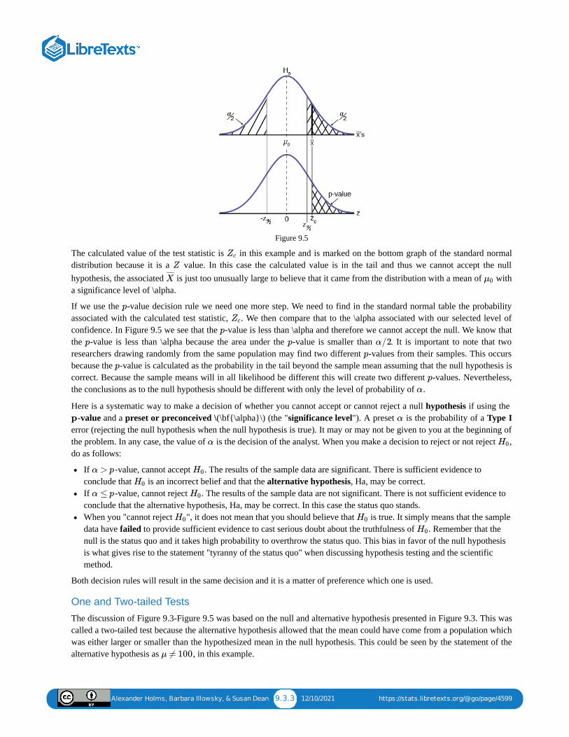
Alexander Holms, Barbara Illowsky, & Susan Dean 9.3.3 12/10/2021 https://stats.libretexts.org/@go/page/4599
Figure 9.5
The calculated value of the test statistic is in this example and is marked on the bottom graph of the standard normaldistribution because it is a value. In this case the calculated value is in the tail and thus we cannot accept the nullhypothesis, the associated is just too unusually large to believe that it came from the distribution with a mean of witha significance level of \alpha.
If we use the -value decision rule we need one more step. We need to find in the standard normal table the probabilityassociated with the calculated test statistic, . We then compare that to the \alpha associated with our selected level ofconfidence. In Figure 9.5 we see that the -value is less than \alpha and therefore we cannot accept the null. We know thatthe -value is less than \alpha because the area under the -value is smaller than . It is important to note that tworesearchers drawing randomly from the same population may find two different -values from their samples. This occursbecause the -value is calculated as the probability in the tail beyond the sample mean assuming that the null hypothesis iscorrect. Because the sample means will in all likelihood be different this will create two different -values. Nevertheless,the conclusions as to the null hypothesis should be different with only the level of probability of .
Here is a systematic way to make a decision of whether you cannot accept or cannot reject a null hypothesis if using the -value and a preset or preconceived \(\bf{\alpha}\) (the "significance level"). A preset is the probability of a Type I
error (rejecting the null hypothesis when the null hypothesis is true). It may or may not be given to you at the beginning ofthe problem. In any case, the value of is the decision of the analyst. When you make a decision to reject or not reject ,do as follows:
If -value, cannot accept . The results of the sample data are significant. There is sufficient evidence toconclude that is an incorrect belief and that the alternative hypothesis, Ha, may be correct.If -value, cannot reject . The results of the sample data are not significant. There is not sufficient evidence toconclude that the alternative hypothesis, Ha, may be correct. In this case the status quo stands.When you "cannot reject ", it does not mean that you should believe that is true. It simply means that the sampledata have failed to provide sufficient evidence to cast serious doubt about the truthfulness of . Remember that thenull is the status quo and it takes high probability to overthrow the status quo. This bias in favor of the null hypothesisis what gives rise to the statement "tyranny of the status quo" when discussing hypothesis testing and the scientificmethod.
Both decision rules will result in the same decision and it is a matter of preference which one is used.
One and Two-tailed Tests
The discussion of Figure 9.3-Figure 9.5 was based on the null and alternative hypothesis presented in Figure 9.3. This wascalled a two-tailed test because the alternative hypothesis allowed that the mean could have come from a population whichwas either larger or smaller than the hypothesized mean in the null hypothesis. This could be seen by the statement of thealternative hypothesis as , in this example.
Zc
Z
X¯ ¯¯̄
μ0
p
Zc
p
p p α/2p
p
p
α
p α
α H0
α > p H0
H0
α ≤ p H0
H0 H0
H0
μ ≠ 100
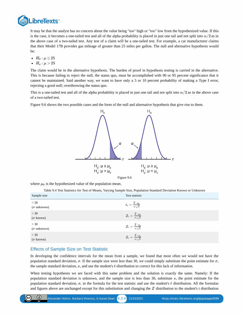
Alexander Holms, Barbara Illowsky, & Susan Dean 9.3.4 12/10/2021 https://stats.libretexts.org/@go/page/4599
It may be that the analyst has no concern about the value being "too" high or "too" low from the hypothesized value. If thisis the case, it becomes a one-tailed test and all of the alpha probability is placed in just one tail and not split into as inthe above case of a two-tailed test. Any test of a claim will be a one-tailed test. For example, a car manufacturer claimsthat their Model 17B provides gas mileage of greater than 25 miles per gallon. The null and alternative hypothesis wouldbe:
The claim would be in the alternative hypothesis. The burden of proof in hypothesis testing is carried in the alternative.This is because failing to reject the null, the status quo, must be accomplished with 90 or 95 percent significance that itcannot be maintained. Said another way, we want to have only a 5 or 10 percent probability of making a Type I error,rejecting a good null; overthrowing the status quo.
This is a one-tailed test and all of the alpha probability is placed in just one tail and not split into as in the above caseof a two-tailed test.
Figure 9.6 shows the two possible cases and the form of the null and alternative hypothesis that give rise to them.
Figure 9.6
where is the hypothesized value of the population mean.
Sample size Test statistic
< 30 ( unknown)
< 30 ( known)
> 30 ( unknown)
> 30 ( known)
Table 9.4 Test Statistics for Test of Means, Varying Sample Size, Population Standard Deviation Known or Unknown
Effects of Sample Size on Test StatisticIn developing the confidence intervals for the mean from a sample, we found that most often we would not have thepopulation standard deviation, . If the sample size were less than 30, we could simply substitute the point estimate for ,the sample standard deviation, , and use the student's -distribution to correct for this lack of information.
When testing hypotheses we are faced with this same problem and the solution is exactly the same. Namely: If thepopulation standard deviation is unknown, and the sample size is less than 30, substitute , the point estimate for thepopulation standard deviation, , in the formula for the test statistic and use the student's distribution. All the formulasand figures above are unchanged except for this substitution and changing the distribution to the student's t distribution
α/2
: μ ≤ 25H0
: μ > 25Ha
α/2
μ0
σ=tc
−X¯ ¯¯̄¯
μ0
s/ n√
σ=Zc
−X¯ ¯¯̄¯
μ0
σ/ n√
σ=Zc
−X¯ ¯¯̄¯
μ0
s/ n√
σ=Zc
−X¯ ¯¯̄¯
μ0
σ/ n√
σ σ
s t
s
σ t
Z
Alexander Holms, Barbara Illowsky, & Susan Dean 9.3.5 12/10/2021 https://stats.libretexts.org/@go/page/4599
on the graph. Remember that the student's t distribution can only be computed knowing the proper degrees of freedom forthe problem. In this case, the degrees of freedom is computed as before with confidence intervals: . Thecalculated t-value is compared to the t-value associated with the pre-set level of confidence required in the test, foundin the student's t tables. If we do not know , but the sample size is 30 or more, we simply substitute for and use thenormal distribution.
Table 9.4 summarizes these rules.
A Systematic Approach for Testing A Hypothesis
A systematic approach to hypothesis testing follows the following steps and in this order. This template will work for allhypotheses that you will ever test.
Set up the null and alternative hypothesis. This is typically the hardest part of the process. Here the question beingasked is reviewed. What parameter is being tested, a mean, a proportion, differences in means, etc. Is this a one-tailedtest or two-tailed test? Remember, if someone is making a claim it will always be a one-tailed test.Decide the level of significance required for this particular case and determine the critical value. These can be found inthe appropriate statistical table. The levels of confidence typical for businesses are 80, 90, 95, 98, and 99. However, thelevel of significance is a policy decision and should be based upon the risk of making a Type I error, rejecting a goodnull. Consider the consequences of making a Type I error.
Next, on the basis of the hypotheses and sample size, select the appropriate test statistic and find the relevant criticalvalue: , , etc. Drawing the relevant probability distribution and marking the critical value is always big help. Besure to match the graph with the hypothesis, especially if it is a one-tailed test.
Take a sample(s) and calculate the relevant parameters: sample mean, standard deviation, or proportion. Using theformula for the test statistic from above in step 2, now calculate the test statistic for this particular case using theparameters you have just calculated.Compare the calculated test statistic and the critical value. Marking these on the graph will give a good visual picture ofthe situation. There are now only two situations:1. The test statistic is in the tail: Cannot Accept the null, the probability that this sample mean (proportion) came from
the hypothesized distribution is too small to believe that it is the real home of these sample data.2. The test statistic is not in the tail: Cannot Reject the null, the sample data are compatible with the hypothesized
population parameter.Reach a conclusion. It is best to articulate the conclusion two different ways. First a formal statistical conclusion suchas “With a 5 % level of significance we cannot accept the null hypotheses that the population mean is equal to XX(units of measurement)”. The second statement of the conclusion is less formal and states the action, or lack of action,required. If the formal conclusion was that above, then the informal one might be, “The machine is broken and we needto shut it down and call for repairs”.
All hypotheses tested will go through this same process. The only changes are the relevant formulas and those aredetermined by the hypothesis required to answer the original question.
df = (n−1)tα,df
σ s σ
Zα tα
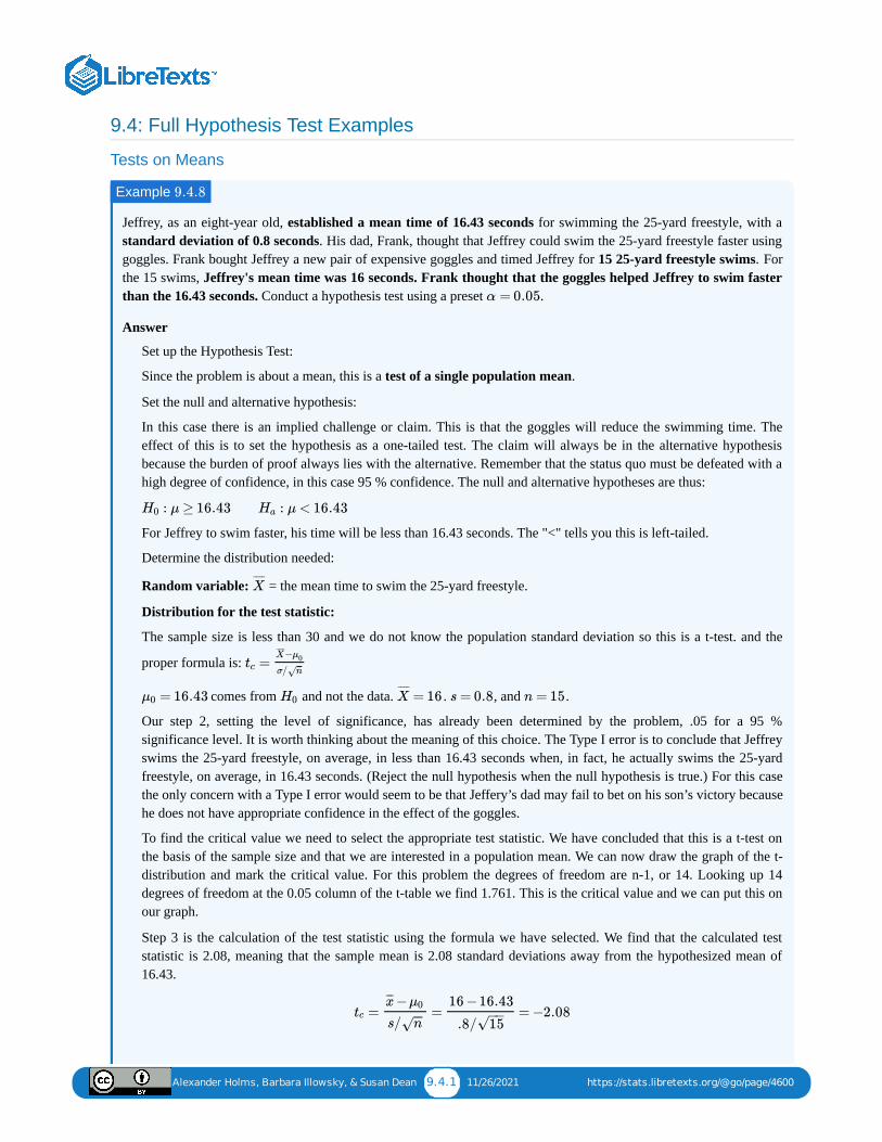
Alexander Holms, Barbara Illowsky, & Susan Dean 9.4.1 11/26/2021 https://stats.libretexts.org/@go/page/4600
9.4: Full Hypothesis Test Examples
Tests on Means
Jeffrey, as an eight-year old, established a mean time of 16.43 seconds for swimming the 25-yard freestyle, with astandard deviation of 0.8 seconds. His dad, Frank, thought that Jeffrey could swim the 25-yard freestyle faster usinggoggles. Frank bought Jeffrey a new pair of expensive goggles and timed Jeffrey for 15 25-yard freestyle swims. Forthe 15 swims, Jeffrey's mean time was 16 seconds. Frank thought that the goggles helped Jeffrey to swim fasterthan the 16.43 seconds. Conduct a hypothesis test using a preset .
Answer
Set up the Hypothesis Test:
Since the problem is about a mean, this is a test of a single population mean.
Set the null and alternative hypothesis:
In this case there is an implied challenge or claim. This is that the goggles will reduce the swimming time. Theeffect of this is to set the hypothesis as a one-tailed test. The claim will always be in the alternative hypothesisbecause the burden of proof always lies with the alternative. Remember that the status quo must be defeated with ahigh degree of confidence, in this case 95 % confidence. The null and alternative hypotheses are thus:
For Jeffrey to swim faster, his time will be less than 16.43 seconds. The "<" tells you this is left-tailed.
Determine the distribution needed:
Random variable: = the mean time to swim the 25-yard freestyle.
Distribution for the test statistic:
The sample size is less than 30 and we do not know the population standard deviation so this is a t-test. and the
proper formula is:
comes from and not the data. . , and .
Our step 2, setting the level of significance, has already been determined by the problem, .05 for a 95 %significance level. It is worth thinking about the meaning of this choice. The Type I error is to conclude that Jeffreyswims the 25-yard freestyle, on average, in less than 16.43 seconds when, in fact, he actually swims the 25-yardfreestyle, on average, in 16.43 seconds. (Reject the null hypothesis when the null hypothesis is true.) For this casethe only concern with a Type I error would seem to be that Jeffery’s dad may fail to bet on his son’s victory becausehe does not have appropriate confidence in the effect of the goggles.
To find the critical value we need to select the appropriate test statistic. We have concluded that this is a t-test onthe basis of the sample size and that we are interested in a population mean. We can now draw the graph of the t-distribution and mark the critical value. For this problem the degrees of freedom are n-1, or 14. Looking up 14degrees of freedom at the 0.05 column of the t-table we find 1.761. This is the critical value and we can put this onour graph.
Step 3 is the calculation of the test statistic using the formula we have selected. We find that the calculated teststatistic is 2.08, meaning that the sample mean is 2.08 standard deviations away from the hypothesized mean of16.43.
Example 9.4.8
α = 0.05
: μ ≥ 16.43H0 : μ < 16.43Ha
X¯ ¯¯̄
=tc
−X¯ ¯¯̄ μ0
σ/ n√
= 16.43μ0 H0 = 16X¯ ¯¯̄
s = 0.8 n = 15
= = = −2.08tc
−x̄̄̄ μ0
s/ n−−
√
16 −16.43
.8/ 15−−
√
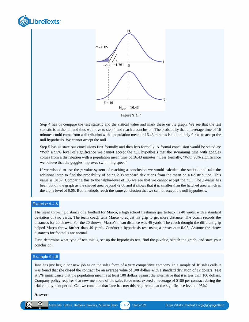
Alexander Holms, Barbara Illowsky, & Susan Dean 9.4.2 11/26/2021 https://stats.libretexts.org/@go/page/4600
Figure
Step 4 has us compare the test statistic and the critical value and mark these on the graph. We see that the teststatistic is in the tail and thus we move to step 4 and reach a conclusion. The probability that an average time of 16minutes could come from a distribution with a population mean of 16.43 minutes is too unlikely for us to accept thenull hypothesis. We cannot accept the null.
Step 5 has us state our conclusions first formally and then less formally. A formal conclusion would be stated as:“With a 95% level of significance we cannot accept the null hypothesis that the swimming time with gogglescomes from a distribution with a population mean time of 16.43 minutes.” Less formally, “With 95% significancewe believe that the goggles improves swimming speed”
If we wished to use the -value system of reaching a conclusion we would calculate the statistic and take theadditional step to find the probability of being 2.08 standard deviations from the mean on a t-distribution. Thisvalue is .0187. Comparing this to the \alpha-level of .05 we see that we cannot accept the null. The -value hasbeen put on the graph as the shaded area beyond -2.08 and it shows that it is smaller than the hatched area which isthe alpha level of 0.05. Both methods reach the same conclusion that we cannot accept the null hypothesis.
The mean throwing distance of a football for Marco, a high school freshman quarterback, is 40 yards, with a standarddeviation of two yards. The team coach tells Marco to adjust his grip to get more distance. The coach records thedistances for 20 throws. For the 20 throws, Marco’s mean distance was 45 yards. The coach thought the different griphelped Marco throw farther than 40 yards. Conduct a hypothesis test using a preset . Assume the throwdistances for footballs are normal.
First, determine what type of test this is, set up the hypothesis test, find the -value, sketch the graph, and state yourconclusion.
Jane has just begun her new job as on the sales force of a very competitive company. In a sample of 16 sales calls itwas found that she closed the contract for an average value of 108 dollars with a standard deviation of 12 dollars. Testat 5% significance that the population mean is at least 100 dollars against the alternative that it is less than 100 dollars.Company policy requires that new members of the sales force must exceed an average of $100 per contract during thetrial employment period. Can we conclude that Jane has met this requirement at the significance level of 95%?
Answer
9.4.7
p
p
Exercise 9.4.8
α = 0.05
p
Example 9.4.9
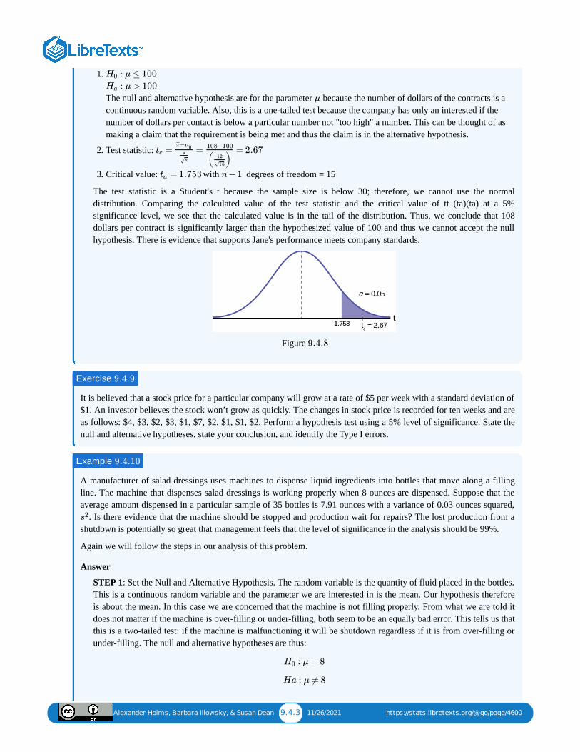
Alexander Holms, Barbara Illowsky, & Susan Dean 9.4.3 11/26/2021 https://stats.libretexts.org/@go/page/4600
1.
The null and alternative hypothesis are for the parameter because the number of dollars of the contracts is acontinuous random variable. Also, this is a one-tailed test because the company has only an interested if thenumber of dollars per contact is below a particular number not "too high" a number. This can be thought of asmaking a claim that the requirement is being met and thus the claim is in the alternative hypothesis.
2. Test statistic:
3. Critical value: with degrees of freedom = 15
The test statistic is a Student's t because the sample size is below 30; therefore, we cannot use the normaldistribution. Comparing the calculated value of the test statistic and the critical value of tt (ta)(ta) at a 5%significance level, we see that the calculated value is in the tail of the distribution. Thus, we conclude that 108dollars per contract is significantly larger than the hypothesized value of 100 and thus we cannot accept the nullhypothesis. There is evidence that supports Jane's performance meets company standards.
Figure
It is believed that a stock price for a particular company will grow at a rate of $5 per week with a standard deviation of$1. An investor believes the stock won’t grow as quickly. The changes in stock price is recorded for ten weeks and areas follows: $4, $3, $2, $3, $1, $7, $2, $1, $1, $2. Perform a hypothesis test using a 5% level of significance. State thenull and alternative hypotheses, state your conclusion, and identify the Type I errors.
A manufacturer of salad dressings uses machines to dispense liquid ingredients into bottles that move along a fillingline. The machine that dispenses salad dressings is working properly when 8 ounces are dispensed. Suppose that theaverage amount dispensed in a particular sample of 35 bottles is 7.91 ounces with a variance of 0.03 ounces squared,
. Is there evidence that the machine should be stopped and production wait for repairs? The lost production from ashutdown is potentially so great that management feels that the level of significance in the analysis should be 99%.
Again we will follow the steps in our analysis of this problem.
Answer
STEP 1: Set the Null and Alternative Hypothesis. The random variable is the quantity of fluid placed in the bottles.This is a continuous random variable and the parameter we are interested in is the mean. Our hypothesis thereforeis about the mean. In this case we are concerned that the machine is not filling properly. From what we are told itdoes not matter if the machine is over-filling or under-filling, both seem to be an equally bad error. This tells us thatthis is a two-tailed test: if the machine is malfunctioning it will be shutdown regardless if it is from over-filling orunder-filling. The null and alternative hypotheses are thus:
: μ ≤ 100H0
: μ > 100Ha
μ
= = = 2.67tc
−x̄̄̄ μ0s
n√
108−100
( )12
16√
= 1.753ta n −1
9.4.8
Exercise 9.4.9
Example 9.4.10
s2
: μ = 8H0
Ha : μ ≠ 8
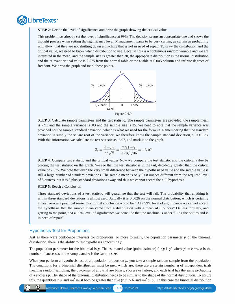
Alexander Holms, Barbara Illowsky, & Susan Dean 9.4.4 11/26/2021 https://stats.libretexts.org/@go/page/4600
STEP 2: Decide the level of significance and draw the graph showing the critical value.
This problem has already set the level of significance at 99%. The decision seems an appropriate one and shows thethought process when setting the significance level. Management wants to be very certain, as certain as probabilitywill allow, that they are not shutting down a machine that is not in need of repair. To draw the distribution and thecritical value, we need to know which distribution to use. Because this is a continuous random variable and we areinterested in the mean, and the sample size is greater than 30, the appropriate distribution is the normal distributionand the relevant critical value is 2.575 from the normal table or the t-table at 0.005 column and infinite degrees offreedom. We draw the graph and mark these points.
Figure
STEP 3: Calculate sample parameters and the test statistic. The sample parameters are provided, the sample meanis 7.91 and the sample variance is .03 and the sample size is 35. We need to note that the sample variance wasprovided not the sample standard deviation, which is what we need for the formula. Remembering that the standarddeviation is simply the square root of the variance, we therefore know the sample standard deviation, s, is 0.173.With this information we calculate the test statistic as -3.07, and mark it on the graph.
STEP 4: Compare test statistic and the critical values Now we compare the test statistic and the critical value byplacing the test statistic on the graph. We see that the test statistic is in the tail, decidedly greater than the criticalvalue of 2.575. We note that even the very small difference between the hypothesized value and the sample value isstill a large number of standard deviations. The sample mean is only 0.08 ounces different from the required levelof 8 ounces, but it is 3 plus standard deviations away and thus we cannot accept the null hypothesis.
STEP 5: Reach a Conclusion
Three standard deviations of a test statistic will guarantee that the test will fail. The probability that anything iswithin three standard deviations is almost zero. Actually it is 0.0026 on the normal distribution, which is certainlyalmost zero in a practical sense. Our formal conclusion would be “ At a 99% level of significance we cannot acceptthe hypothesis that the sample mean came from a distribution with a mean of 8 ounces” Or less formally, andgetting to the point, “At a 99% level of significance we conclude that the machine is under filling the bottles and isin need of repair”.
Hypothesis Test for ProportionsJust as there were confidence intervals for proportions, or more formally, the population parameter of the binomialdistribution, there is the ability to test hypotheses concerning .
The population parameter for the binomial is . The estimated value (point estimate) for is where , is thenumber of successes in the sample and is the sample size.
When you perform a hypothesis test of a population proportion , you take a simple random sample from the population.The conditions for a binomial distribution must be met, which are: there are a certain number n of independent trialsmeaning random sampling, the outcomes of any trial are binary, success or failure, and each trial has the same probabilityof a success . The shape of the binomial distribution needs to be similar to the shape of the normal distribution. To ensurethis, the quantities and must both be greater than five ( and ). In this case the binomial distribution
9.4.9
= = = −3.07Zc
−x̄̄̄ μ0
s/ n−−
√
7.91 −8
⋅173/ 35−−
√
p
p
p p p′ = x/np′ x
n
p
p
np′ nq ′ n > 5p′ n > 5q ′
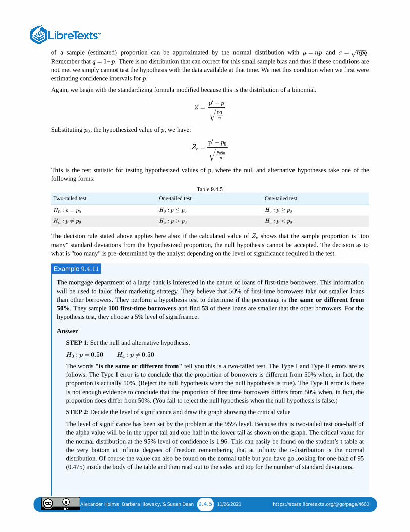
Alexander Holms, Barbara Illowsky, & Susan Dean 9.4.5 11/26/2021 https://stats.libretexts.org/@go/page/4600
of a sample (estimated) proportion can be approximated by the normal distribution with and .Remember that . There is no distribution that can correct for this small sample bias and thus if these conditions arenot met we simply cannot test the hypothesis with the data available at that time. We met this condition when we first wereestimating confidence intervals for .
Again, we begin with the standardizing formula modified because this is the distribution of a binomial.
Substituting , the hypothesized value of , we have:
This is the test statistic for testing hypothesized values of p, where the null and alternative hypotheses take one of thefollowing forms:
Two-tailed test One-tailed test One-tailed testTable
The decision rule stated above applies here also: if the calculated value of shows that the sample proportion is "toomany" standard deviations from the hypothesized proportion, the null hypothesis cannot be accepted. The decision as towhat is "too many" is pre-determined by the analyst depending on the level of significance required in the test.
The mortgage department of a large bank is interested in the nature of loans of first-time borrowers. This informationwill be used to tailor their marketing strategy. They believe that 50% of first-time borrowers take out smaller loansthan other borrowers. They perform a hypothesis test to determine if the percentage is the same or different from50%. They sample 100 first-time borrowers and find 53 of these loans are smaller that the other borrowers. For thehypothesis test, they choose a 5% level of significance.
Answer
STEP 1: Set the null and alternative hypothesis.
The words "is the same or different from" tell you this is a two-tailed test. The Type I and Type II errors are asfollows: The Type I error is to conclude that the proportion of borrowers is different from 50% when, in fact, theproportion is actually 50%. (Reject the null hypothesis when the null hypothesis is true). The Type II error is thereis not enough evidence to conclude that the proportion of first time borrowers differs from 50% when, in fact, theproportion does differ from 50%. (You fail to reject the null hypothesis when the null hypothesis is false.)
STEP 2: Decide the level of significance and draw the graph showing the critical value
The level of significance has been set by the problem at the 95% level. Because this is two-tailed test one-half ofthe alpha value will be in the upper tail and one-half in the lower tail as shown on the graph. The critical value forthe normal distribution at the 95% level of confidence is 1.96. This can easily be found on the student’s t-table atthe very bottom at infinite degrees of freedom remembering that at infinity the t-distribution is the normaldistribution. Of course the value can also be found on the normal table but you have go looking for one-half of 95(0.475) inside the body of the table and then read out to the sides and top for the number of standard deviations.
μ = np σ = npq−−−√
q = 1– p
p
Z =−pp′
pqn
−−√
p0 p
=Zc
−p′ p0
p0q0
n
− −−√
: p =H0 p0 : p ≤H0 p0 : p ≥H0 p0
: p ≠Ha p0 : p >Ha p0 : p <Ha p0
9.4.5
Zc
Example 9.4.11
: p = 0.50H0 : p ≠ 0.50Ha
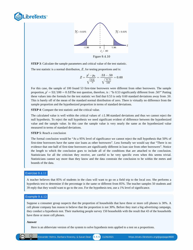
Alexander Holms, Barbara Illowsky, & Susan Dean 9.4.6 11/26/2021 https://stats.libretexts.org/@go/page/4600
Figure
STEP 3: Calculate the sample parameters and critical value of the test statistic.
The test statistic is a normal distribution, , for testing proportions and is:
For this case, the sample of 100 found 53 first-time borrowers were different from other borrowers. The sampleproportion, The test question, therefore, is : “Is 0.53 significantly different from .50?” Puttingthese values into the formula for the test statistic we find that 0.53 is only 0.60 standard deviations away from .50.This is barely off of the mean of the standard normal distribution of zero. There is virtually no difference from thesample proportion and the hypothesized proportion in terms of standard deviations.
STEP 4: Compare the test statistic and the critical value.
The calculated value is well within the critical values of standard deviations and thus we cannot reject thenull hypothesis. To reject the null hypothesis we need significant evident of difference between the hypothesizedvalue and the sample value. In this case the sample value is very nearly the same as the hypothesized valuemeasured in terms of standard deviations.
STEP 5: Reach a conclusion
The formal conclusion would be “At a 95% level of significance we cannot reject the null hypothesis that 50% offirst-time borrowers have the same size loans as other borrowers”. Less formally we would say that “There is noevidence that one-half of first-time borrowers are significantly different in loan size from other borrowers”. Noticethe length to which the conclusion goes to include all of the conditions that are attached to the conclusion.Statisticians for all the criticism they receive, are careful to be very specific even when this seems trivial.Statisticians cannot say more than they know and the data constrain the conclusion to be within the metes andbounds of the data.
A teacher believes that 85% of students in the class will want to go on a field trip to the local zoo. She performs ahypothesis test to determine if the percentage is the same or different from 85%. The teacher samples 50 students and39 reply that they would want to go to the zoo. For the hypothesis test, use a 1% level of significance.
Suppose a consumer group suspects that the proportion of households that have three or more cell phones is 30%. Acell phone company has reason to believe that the proportion is not 30%. Before they start a big advertising campaign,they conduct a hypothesis test. Their marketing people survey 150 households with the result that 43 of the householdshave three or more cell phones.
Answer
Here is an abbreviate version of the system to solve hypothesis tests applied to a test on a proportions.
9.4.10
Z
Z = = = 0.60−p′ p0
p0q0
n
− −−√
.53 −.50
.5(.5)
100
− −−−√
= 53/100 = 0.53p′
±1.96
Exercise 9.4.11
Example 9.4.12
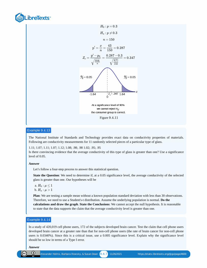
Alexander Holms, Barbara Illowsky, & Susan Dean 9.4.7 11/26/2021 https://stats.libretexts.org/@go/page/4600
Figure
The National Institute of Standards and Technology provides exact data on conductivity properties of materials.Following are conductivity measurements for 11 randomly selected pieces of a particular type of glass.
1.11; 1.07; 1.11; 1.07; 1.12; 1.08; .98; .98 1.02; .95; .95 Is there convincing evidence that the average conductivity of this type of glass is greater than one? Use a significancelevel of 0.05.
Answer
Let’s follow a four-step process to answer this statistical question.
State the Question: We need to determine if, at a 0.05 significance level, the average conductivity of the selectedglass is greater than one. Our hypotheses will be
a. b.
Plan: We are testing a sample mean without a known population standard deviation with less than 30 observations.Therefore, we need to use a Student's-t distribution. Assume the underlying population is normal. Do thecalculations and draw the graph. State the Conclusions: We cannot accept the null hypothesis. It is reasonableto state that the data supports the claim that the average conductivity level is greater than one.
In a study of 420,019 cell phone users, 172 of the subjects developed brain cancer. Test the claim that cell phone usersdeveloped brain cancer at a greater rate than that for non-cell phone users (the rate of brain cancer for non-cell phoneusers is 0.0340%). Since this is a critical issue, use a 0.005 significance level. Explain why the significance levelshould be so low in terms of a Type I error.
Answer
: p = 0.3H0
: p ≠ 0.3Ha
n = 150
= = = 0.287p′ x
n
43
150
= = = 0.347Zc
−p′ p0
p0q0
n
− −−√
0.287 −0.3
3(7)
150
− −−√
9.4.11
Example 9.4.13
: μ ≤ 1H0
: μ > 1Ha
Example 9.4.14
Alexander Holms, Barbara Illowsky, & Susan Dean 9.4.8 11/26/2021 https://stats.libretexts.org/@go/page/4600
1. We need to conduct a hypothesis test on the claimed cancer rate. Our hypotheses will bea. b.
If we commit a Type I error, we are essentially accepting a false claim. Since the claim describes cancer-causingenvironments, we want to minimize the chances of incorrectly identifying causes of cancer.
2. We will be testing a sample proportion with and . The sample is sufficiently largebecause we have , , two independentoutcomes, and a fixed probability of success . Thus we will be able to generalize our results to thepopulation.
: p ≤ 0.00034H0
: p > 0.00034Ha
x = 172 n = 420, 019n = 420, 019(0.00034) = 142.8p′ n = 420, 019(0.99966) = 419, 876.2q ′
= 0.00034p′
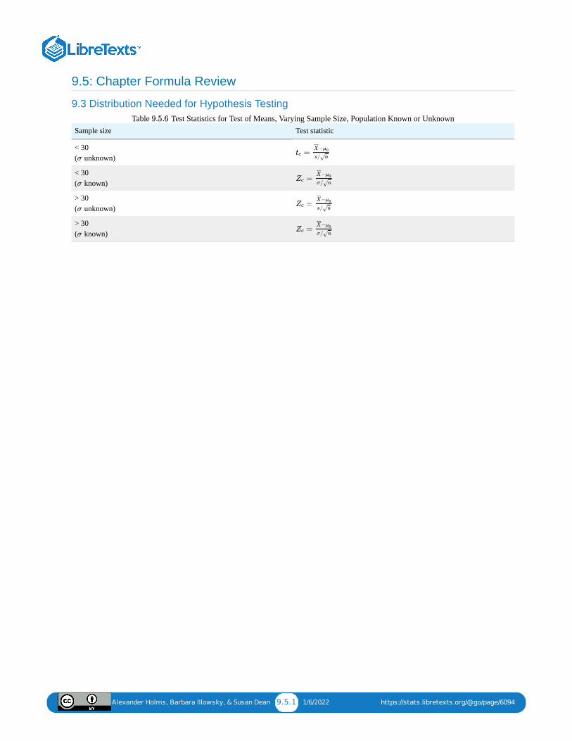
Alexander Holms, Barbara Illowsky, & Susan Dean 9.5.1 1/6/2022 https://stats.libretexts.org/@go/page/6094
9.5: Chapter Formula Review
9.3 Distribution Needed for Hypothesis Testing
Sample size Test statistic
< 30 ( unknown)
< 30 ( known)
> 30 ( unknown)
> 30 ( known)
Table Test Statistics for Test of Means, Varying Sample Size, Population Known or Unknown
σ=tc
−X¯ ¯¯̄¯
μ0
s/ n√
σ=Zc
−X¯ ¯¯̄¯
μ0
σ/ n√
σ=Zc
−X¯ ¯¯̄¯
μ0
s/ n√
σ=Zc
−X¯ ¯¯̄¯
μ0
σ/ n√
9.5.6

Alexander Holms, Barbara Illowsky, & Susan Dean 9.6.1 12/17/2021 https://stats.libretexts.org/@go/page/6096
9.6: Chapter Homework
Alexander Holms, Barbara Illowsky, & Susan Dean 9.6.2 12/17/2021 https://stats.libretexts.org/@go/page/6096
Exercise . Conduct a hypothesis test to see if your decision and conclusion wouldchange if your belief were that the brown trout’s mean I.Q. is not four.65.
According to an article in Newsweek, the natural ratio of girls to boys is 100:105. In China, the birth ratiois 100: 114 (46.7% girls). Suppose you don’t believe the reported figures of the percent of girls born inChina. You conduct a study. In this study, you count the number of girls and boys born in 150 randomlychosen recent births. There are 60 girls and 90 boys born of the 150. Based on your study, do you believethat the percent of girls born in China is 46.7?
66.
A poll done for Newsweek found that 13% of Americans have seen or sensed the presence of an angel. Acontingent doubts that the percent is really that high. It conducts its own survey. Out of 76 Americanssurveyed, only two had seen or sensed the presence of an angel. As a result of the contingent’s survey,would you agree with the Newsweek poll? In complete sentences, also give three reasons why the twopolls might give different results.
67.
The mean work week for engineers in a start-up company is believed to be about 60 hours. A newlyhired engineer hopes that it’s shorter. She asks ten engineering friends in start-ups for the lengths of theirmean work weeks. Based on the results that follow, should she count on the mean work week to beshorter than 60 hours?
Data (length of mean work week): 70; 45; 55; 60; 65; 55; 55; 60; 50; 55.
68.
Sixty-eight percent of online courses taught at community colleges nationwide were taught by full-timefaculty. To test if 68% also represents California’s percent for full-time faculty teaching the onlineclasses, Long Beach City College (LBCC) in California, was randomly selected for comparison. In thesame year, 34 of the 44 online courses LBCC offered were taught by full-time faculty. Conduct ahypothesis test to determine if 68% represents California. NOTE: For more accurate results, use moreCalifornia community colleges and this past year's data.
69.
According to an article in Bloomberg Businessweek, New York City's most recent adult smoking rate is14%. Suppose that a survey is conducted to determine this year’s rate. Nine out of 70 randomly chosenN.Y. City residents reply that they smoke. Conduct a hypothesis test to determine if the rate is still 14%or if it has decreased.
70.
The mean age of De Anza College students in a previous term was 26.6 years old. An instructor thinksthe mean age for online students is older than 26.6. She randomly surveys 56 online students and findsthat the sample mean is 29.4 with a standard deviation of 2.1. Conduct a hypothesis test.
71.
Registered nurses earned an average annual salary of $69,110. For that same year, a survey wasconducted of 41 California registered nurses to determine if the annual salary is higher than $69,110 for
9.6.63
Alexander Holms, Barbara Illowsky, & Susan Dean 9.6.3 12/17/2021 https://stats.libretexts.org/@go/page/6096
California nurses. The sample average was $71,121 with a sample standard deviation of $7,489. Conducta hypothesis test.
72.
La Leche League International reports that the mean age of weaning a child from breastfeeding is agefour to five worldwide. In America, most nursing mothers wean their children much earlier. Suppose arandom survey is conducted of 21 U.S. mothers who recently weaned their children. The mean weaningage was nine months (3/4 year) with a standard deviation of 4 months. Conduct a hypothesis test todetermine if the mean weaning age in the U.S. is less than four years old.
73.
Over the past few decades, public health officials have examined the link between weight concerns andteen girls' smoking. Researchers surveyed a group of 273 randomly selected teen girls living inMassachusetts (between 12 and 15 years old). After four years the girls were surveyed again. Sixty-threesaid they smoked to stay thin. Is there good evidence that more than thirty percent of the teen girlssmoke to stay thin? After conducting the test, your decision and conclusion are
a. Instructions: For the following ten exercises, Hypothesis testing: For the following ten exercises, answer each question.1. 3; 2; 1; 3; 7; 2; 9; 4; 6; 6; 8; 0; 5; 6; 4; 2; 1; 3; 4; 1
At the level can it be concluded that the sample mean is higher than 5.8 visits peryear?
84.
According to the N.Y. Times Almanac the mean family size in the U.S. is 3.18. A sample of acollege math class resulted in the following family sizes: 5; 4; 5; 4; 4; 3; 6; 4; 3; 3; 5; 5; 6; 3; 3; 2; 7; 4; 5; 2; 2; 2; 3; 2 At level, is the class’ mean family size greater than the national average? Does theAlmanac result remain valid? Why?
85.
The student academic group on a college campus claims that freshman students study at least 2.5hours per day, on average. One Introduction to Statistics class was skeptical. The class took arandom sample of 30 freshman students and found a mean study time of 137 minutes with astandard deviation of 45 minutes. At level, is the student academic group’s claimcorrect?
α = 0.05
α = 0.05
α = 0.01
Alexander Holms, Barbara Illowsky, & Susan Dean 9.7.1 12/24/2021 https://stats.libretexts.org/@go/page/4601
9.7: Chapter Key Terms
Binomial Distributiona discrete random variable (RV) that arises from Bernoulli trials. There are a fixed number, n, of independent trials.“Independent” means that the result of any trial (for example, trial 1) does not affect the results of the following trials,and all trials are conducted under the same conditions. Under these circumstances the binomial RV Χ is defined as thenumber of successes in trials. The notation is: and the standard deviation is . The
probability of exactly successes in trials is .
Central Limit TheoremGiven a random variable (RV) with known mean and known standard deviation . We are sampling with size n andwe are interested in two new RVs - the sample mean, . If the size n of the sample is sufficiently large, then
. If the size n of the sample is sufficiently large, then the distribution of the sample means will
approximate a normal distribution regardless of the shape of the population. The expected value of the mean of thesample means will equal the population mean. The standard deviation of the distribution of the sample means, , is
called the standard error of the mean.
Confidence Interval (CI)an interval estimate for an unknown population parameter. This depends on:
The desired confidence level.Information that is known about the distribution (for example, known standard deviation).The sample and its size.
Critical ValueThe or value set by the researcher that measures the probability of a Type I error, .
Hypothesisa statement about the value of a population parameter, in case of two hypotheses, the statement assumed to be true iscalled the null hypothesis (notation ) and the contradictory statement is called the alternative hypothesis (notation
).
Hypothesis TestingBased on sample evidence, a procedure for determining whether the hypothesis stated is a reasonable statement andshould not be rejected, or is unreasonable and should be rejected.
Normal Distribution
a continuous random variable (RV) with pdf , where is the mean of the distribution, and is
the standard deviation, notation: . If and , the RV is called the standard normaldistribution.
Standard Deviationa number that is equal to the square root of the variance and measures how far data values are from their mean;notation: s for sample standard deviation and σ for population standard deviation.
Student's t-Distributioninvestigated and reported by William S. Gossett in 1908 and published under the pseudonym Student. The majorcharacteristics of the random variable (RV) are:
It is continuous and assumes any real values.
n X ∼ B(n, p)μ = np σ = npq−−−√
x n P (X = x) =( )n
xpxqn−x
μ σ
X¯ ¯¯̄
∼ N (μ, )X¯ ¯¯̄ σ
n√
σ
n√
t Z σ
H0
Ha
f(x) = 1σ 2π√
e−(x−μ)2
2σ2 μ σ
X ∼ N(μ, σ) μ = 0 σ = 1
Alexander Holms, Barbara Illowsky, & Susan Dean 9.7.2 12/24/2021 https://stats.libretexts.org/@go/page/4601
The pdf is symmetrical about its mean of zero. However, it is more spread out and flatter at the apex than thenormal distribution.It approaches the standard normal distribution as n gets larger.There is a "family" of t distributions: every representative of the family is completely defined by the number ofdegrees of freedom which is one less than the number of data items.
Test StatisticThe formula that counts the number of standard deviations on the relevant distribution that estimated parameter is awayfrom the hypothesized value.
Type I ErrorThe decision is to reject the null hypothesis when, in fact, the null hypothesis is true.
Type II ErrorThe decision is not to reject the null hypothesis when, in fact, the null hypothesis is false.
Alexander Holms, Barbara Illowsky, & Susan Dean 9.8.1 12/31/2021 https://stats.libretexts.org/@go/page/6095
9.8: Chapter Practice
Exercise .15.
A group of doctors is deciding whether or not to perform an operation. Suppose the null hypothesis, ,is: the surgical procedure will go well. State the Type I and Type II errors in complete sentences.
16.
A group of doctors is deciding whether or not to perform an operation. Suppose the null hypothesis, ,is: the surgical procedure will go well. Which is the error with the greater consequence?
17.
The power of a test is 0.981. What is the probability of a Type II error?
18.
A group of divers is exploring an old sunken ship. Suppose the null hypothesis, , is: the sunken shipdoes not contain buried treasure. State the Type I and Type II errors in complete sentences.
19.
A microbiologist is testing a water sample for E-coli. Suppose the null hypothesis, , is: the sampledoes not contain E-coli. The probability that the sample does not contain E-coli, but the microbiologistthinks it does is 0.012. The probability that the sample does contain E-coli, but the microbiologist thinksit does not is 0.002. What is the power of this test?
20.
A microbiologist is testing a water sample for E-coli. Suppose the null hypothesis, , is: the samplecontains E-coli. Which is the error with the greater consequence?
9.3 Distribution Needed for Hypothesis Testing21.
Which two distributions can you use for hypothesis testing for this chapter?
22.
Which distribution do you use when you are testing a population mean and the population standard deviation is known?Assume sample size is large. Assume a normal distribution with .
23.
Which distribution do you use when the standard deviation is not known and you are testing one population mean?Assume a normal distribution, with .
24.
A population mean is 13. The sample mean is 12.8, and the sample standard deviation is two. The sample size is 20. Whatdistribution should you use to perform a hypothesis test? Assume the underlying population is normal.
25.
A population has a mean is 25 and a standard deviation of five. The sample mean is 24, and the sample size is 108. Whatdistribution should you use to perform a hypothesis test?
26.
9.8.12
H0
H0
H0
H0
H0
n ≥ 30
n ≥ 30
Alexander Holms, Barbara Illowsky, & Susan Dean 9.8.2 12/31/2021 https://stats.libretexts.org/@go/page/6095
It is thought that 42% of respondents in a taste test would prefer Brand . In a particular test of 100 people, 39% preferredBrand . What distribution should you use to perform a hypothesis test?
27.
You are performing a hypothesis test of a single population mean using a Student’s t-distribution. What must you assumeabout the distribution of the data?
28.
You are performing a hypothesis test of a single population mean using a Student’s t-distribution. The data are not from asimple random sample. Can you accurately perform the hypothesis test?
29.
You are performing a hypothesis test of a single population proportion. What must be true about the quantities of and ?
30.
You are performing a hypothesis test of a single population proportion. You find out that is less than five. What mustyou do to be able to perform a valid hypothesis test?
31.
You are performing a hypothesis test of a single population proportion. The data come from which distribution?
9.4 Full Hypothesis Test Examples32.
Assume and . Is this a left-tailed, right-tailed, or two-tailed test?
33.
Assume and \(H_a: \mu > 6). Is this a left-tailed, right-tailed, or two-tailed test?
34.
Assume and . Is this a left-tailed, right-tailed, or two-tailed test?
35.
Draw the general graph of a left-tailed test.
36.
Draw the graph of a two-tailed test.
37.
A bottle of water is labeled as containing 16 fluid ounces of water. You believe it is less than that. What type of test wouldyou use?
38.
Your friend claims that his mean golf score is 63. You want to show that it is higher than that. What type of test would youuse?
39.
A bathroom scale claims to be able to identify correctly any weight within a pound. You think that it cannot be thataccurate. What type of test would you use?
40.
You flip a coin and record whether it shows heads or tails. You know the probability of getting heads is 50%, but you thinkit is less for this particular coin. What type of test would you use?
41.
If the alternative hypothesis has a not equals ( ) symbol, you know to use which type of test?
42.
A
A
np
nq
np
: μ = 9H0 : μ < 9Ha
: μ ≤ 6H0
: p = 0.25H0 : p ≠ 0.25Ha
≠

Alexander Holms, Barbara Illowsky, & Susan Dean 9.8.3 12/31/2021 https://stats.libretexts.org/@go/page/6095
Assume the null hypothesis states that the mean is at least 18. Is this a left-tailed, right-tailed, or two-tailed test?
43.
Assume the null hypothesis states that the mean is at most 12. Is this a left-tailed, right-tailed, or two-tailed test?
44.
Assume the null hypothesis states that the mean is equal to 88. The alternative hypothesis states that the mean is not equalto 88. Is this a left-tailed, right-tailed, or two-tailed test?
Alexander Holms, Barbara Illowsky, & Susan Dean 9.9.1 12/24/2021 https://stats.libretexts.org/@go/page/6097
9.9: Chapter References
9.1 Null and Alternative Hypotheses
Data from the National Institute of Mental Health. Available online at http://www.nimh.nih.gov/publicat/depression.cfm.
9.4 Full Hypothesis Test ExamplesData from Amit Schitai. Director of Instructional Technology and Distance Learning. LBCC.
Data from Bloomberg Businessweek. Available online at http://www.businessweek.com/news/2011- 09-15/nyc-smoking-rate-falls-to-record-low-of-14-bloomberg-says.html.
Data from energy.gov. Available online at http://energy.gov (accessed June 27. 2013).
Data from Gallup®. Available online at www.gallup.com (accessed June 27, 2013).
Data from Growing by Degrees by Allen and Seaman.
Data from La Leche League International. Available online at www.lalecheleague.org/Law/BAFeb01.html.
Data from the American Automobile Association. Available online at www.aaa.com (accessed June 27, 2013).
Data from the American Library Association. Available online at www.ala.org (accessed June 27, 2013).
Data from the Bureau of Labor Statistics. Available online at http://www.bls.gov/oes/current/oes291111.htm.
Data from the Centers for Disease Control and Prevention. Available online at www.cdc.gov (accessed June 27, 2013)
Data from the U.S. Census Bureau, available online at quickfacts.census.gov/qfd/states/00000.html (accessed June 27,2013).
Data from the United States Census Bureau. Available online at www.census.gov/hhes/socdemo/language/.
Data from Toastmasters International. Available online at toastmasters.org/artisan/deta...eID=429&Page=1.
Data from Weather Underground. Available online at www.wunderground.com (accessed June 27, 2013).
Federal Bureau of Investigations. “Uniform Crime Reports and Index of Crime in Daviess in the State of Kentuckyenforced by Daviess County from 1985 to 2005.” Available online athttp://www.disastercenter.com/kentucky/crime/3868.htm (accessed June 27, 2013).
“Foothill-De Anza Community College District.” De Anza College, Winter 2006. Available online atresearch.fhda.edu/factbook/DA...t_da_2006w.pdf.
Johansen, C., J. Boice, Jr., J. McLaughlin, J. Olsen. “Cellular Telephones and Cancer—a Nationwide Cohort Study inDenmark.” Institute of Cancer Epidemiology and the Danish Cancer Society, 93(3):203-7. Available online athttp://www.ncbi.nlm.nih.gov/pubmed/11158188 (accessed June 27, 2013).
Rape, Abuse & Incest National Network. “How often does sexual assault occur?” RAINN, 2009. Available online athttp://www.rainn.org/get-information...sexual-assault (accessed June 27, 2013).
Alexander Holms, Barbara Illowsky, & Susan
Dean9.10.1 12/31/2021 https://stats.libretexts.org/@go/page/6092
9.10: Chapter Review
9.1 Null and Alternative Hypotheses
In a hypothesis test, sample data is evaluated in order to arrive at a decision about some type of claim. If certainconditions about the sample are satisfied, then the claim can be evaluated for a population. In a hypothesis test, we:
1. Evaluate the null hypothesis, typically denoted with H0. The null is not rejected unless the hypothesis test showsotherwise. The null statement must always contain some form of equality (=, ≤ or ≥)
2. Always write the alternative hypothesis, typically denoted with or , using not equal, less than or greater thansymbols, i.e., ( , <, or > ).
3. If we reject the null hypothesis, then we can assume there is enough evidence to support the alternative hypothesis.4. Never state that a claim is proven true or false. Keep in mind the underlying fact that hypothesis testing is based on
probability laws; therefore, we can talk only in terms of non-absolute certainties.
9.2 Outcomes and the Type I and Type II ErrorsIn every hypothesis test, the outcomes are dependent on a correct interpretation of the data. Incorrect calculations ormisunderstood summary statistics can yield errors that affect the results. A Type I error occurs when a true null hypothesisis rejected. A Type II error occurs when a false null hypothesis is not rejected.
The probabilities of these errors are denoted by the Greek letters and , for a Type I and a Type II error respectively. Thepower of the test, , quantifies the likelihood that a test will yield the correct result of a true alternative hypothesisbeing accepted. A high power is desirable.
9.3 Distribution Needed for Hypothesis TestingIn order for a hypothesis test’s results to be generalized to a population, certain requirements must be satisfied.
When testing for a single population mean:
1. A Student's -test should be used if the data come from a simple, random sample and the population is approximatelynormally distributed, or the sample size is large, with an unknown standard deviation.
2. The normal test will work if the data come from a simple, random sample and the population is approximatelynormally distributed, or the sample size is large.
When testing a single population proportion use a normal test for a single population proportion if the data comes from asimple, random sample, fill the requirements for a binomial distribution, and the mean number of successes and the meannumber of failures satisfy the conditions: and where is the sample size, is the probability of a success,and is the probability of a failure.
9.4 Full Hypothesis Test Examples
The hypothesis test itself has an established process. This can be summarized as follows:
1. Determine and . Remember, they are contradictory.2. Determine the random variable.3. Determine the distribution for the test.4. Draw a graph and calculate the test statistic.5. Compare the calculated test statistic with the critical value determined by the level of significance required by the
test and make a decision (cannot reject or cannot accept ), and write a clear conclusion using English sentences.
Ha H1
neq
α β
1– β
t
np > 5 nq > 5 n p
q
H0 Ha
Z
H0 H0
Alexander Holms, Barbara Illowsky, & Susan
Dean9.11.1 1/7/2022 https://stats.libretexts.org/@go/page/6098
9.11: Chapter Solution (Practice + Homework)Figure
38.
a right-tailed test
40.
a left-tailed test
42.
This is a left-tailed test.
44.
This is a two-tailed test.
45.
1. 47.
c
1. 51.
b
d
55.
d
56.
1. 58.1. 60.
1. 62.1. 64.
1. 66.
1. 69.1. 71.
1. 73.
c
c
77.
1. 79.
1. 81.1. 83.
1. 85.1. 2. -value = 0.06223. alpha = 0.014. Do not reject the null hypothesis.5. At the 1% significance level, there is not enough evidence to conclude
that freshmen students study less than 2.5 hours per day, on average.
9.11.12
: μ ≥ 150 : μ < 150H0 Ha
p

Alexander Holms, Barbara Illowsky, & Susan
Dean9.11.2 1/7/2022 https://stats.libretexts.org/@go/page/6098
6. The student academic group’s claim appears to be correct.
1 1/7/2022
CHAPTER OVERVIEW10: HYPOTHESIS TESTING WITH TWO SAMPLES
10.0: INTRODUCTION10.1: COMPARING TWO INDEPENDENT POPULATION MEANS10.2: COHEN'S STANDARDS FOR SMALL, MEDIUM, AND LARGE EFFECT SIZES10.3: TEST FOR DIFFERENCES IN MEANS- ASSUMING EQUAL POPULATION VARIANCES10.4: COMPARING TWO INDEPENDENT POPULATION PROPORTIONS10.5: TWO POPULATION MEANS WITH KNOWN STANDARD DEVIATIONS10.6: MATCHED OR PAIRED SAMPLES10.7: HOMEWORK10.8: CHAPTER FORMULA REVIEW10.9: CHAPTER HOMEWORK10.10: CHAPTER KEY TERMS10.11: CHAPTER PRACTICE10.12: CHAPTER REFERENCES10.13: CHAPTER REVIEW10.14: CHAPTER SOLUTION (PRACTICE + HOMEWORK)
Alexander Holms, Barbara Illowsky, & Susan
Dean10.0.1 11/26/2021 https://stats.libretexts.org/@go/page/4603
10.0: Introduction
Figure If you want to test a claim that involves two groups (the types of breakfasts eaten east and west of theMississippi River) you can use a slightly different technique when conducting a hypothesis test. (credit: Chloe Lim)
Studies often compare two groups. For example, researchers are interested in the effect aspirin has in preventing heartattacks. Over the last few years, newspapers and magazines have reported various aspirin studies involving two groups.Typically, one group is given aspirin and the other group is given a placebo. Then, the heart attack rate is studied overseveral years.
There are other situations that deal with the comparison of two groups. For example, studies compare various diet andexercise programs. Politicians compare the proportion of individuals from different income brackets who might vote forthem. Students are interested in whether SAT or GRE preparatory courses really help raise their scores. Many businessapplications require comparing two groups. It may be the investment returns of two different investment strategies, or thedifferences in production efficiency of different management styles.
To compare two means or two proportions, you work with two groups. The groups are classified either as independent ormatched pairs. Independent groups consist of two samples that are independent, that is, sample values selected from onepopulation are not related in any way to sample values selected from the other population. Matched pairs consist of twosamples that are dependent. The parameter tested using matched pairs is the population mean. The parameters tested usingindependent groups are either population means or population proportions of each group.
10.0.1
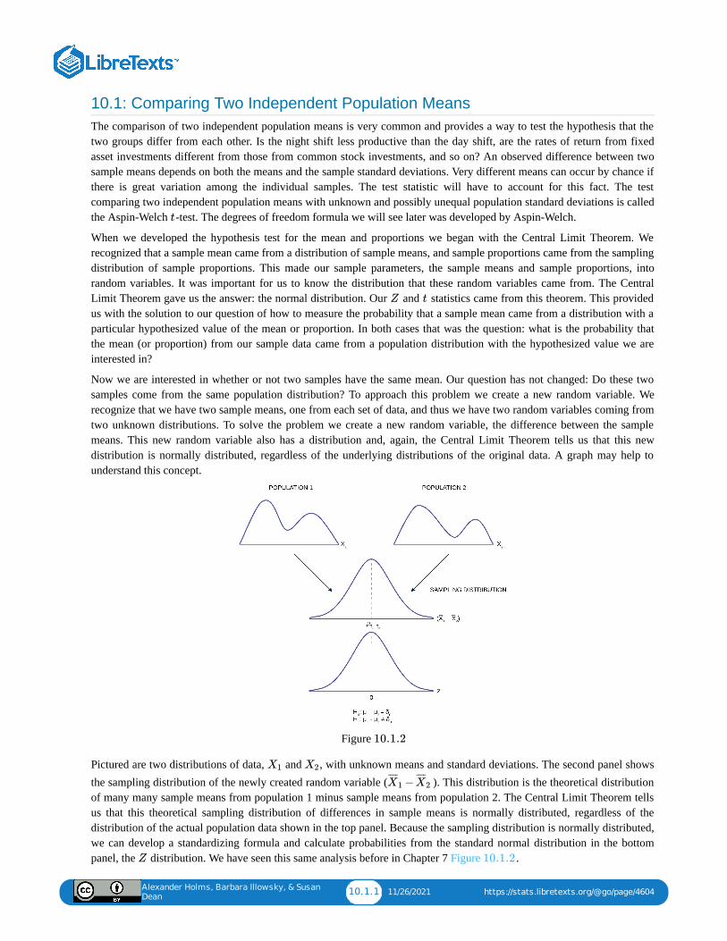
Alexander Holms, Barbara Illowsky, & Susan
Dean10.1.1 11/26/2021 https://stats.libretexts.org/@go/page/4604
10.1: Comparing Two Independent Population MeansThe comparison of two independent population means is very common and provides a way to test the hypothesis that thetwo groups differ from each other. Is the night shift less productive than the day shift, are the rates of return from fixedasset investments different from those from common stock investments, and so on? An observed difference between twosample means depends on both the means and the sample standard deviations. Very different means can occur by chance ifthere is great variation among the individual samples. The test statistic will have to account for this fact. The testcomparing two independent population means with unknown and possibly unequal population standard deviations is calledthe Aspin-Welch -test. The degrees of freedom formula we will see later was developed by Aspin-Welch.
When we developed the hypothesis test for the mean and proportions we began with the Central Limit Theorem. Werecognized that a sample mean came from a distribution of sample means, and sample proportions came from the samplingdistribution of sample proportions. This made our sample parameters, the sample means and sample proportions, intorandom variables. It was important for us to know the distribution that these random variables came from. The CentralLimit Theorem gave us the answer: the normal distribution. Our and statistics came from this theorem. This providedus with the solution to our question of how to measure the probability that a sample mean came from a distribution with aparticular hypothesized value of the mean or proportion. In both cases that was the question: what is the probability thatthe mean (or proportion) from our sample data came from a population distribution with the hypothesized value we areinterested in?
Now we are interested in whether or not two samples have the same mean. Our question has not changed: Do these twosamples come from the same population distribution? To approach this problem we create a new random variable. Werecognize that we have two sample means, one from each set of data, and thus we have two random variables coming fromtwo unknown distributions. To solve the problem we create a new random variable, the difference between the samplemeans. This new random variable also has a distribution and, again, the Central Limit Theorem tells us that this newdistribution is normally distributed, regardless of the underlying distributions of the original data. A graph may help tounderstand this concept.
Figure
Pictured are two distributions of data, and , with unknown means and standard deviations. The second panel showsthe sampling distribution of the newly created random variable ( ). This distribution is the theoretical distributionof many many sample means from population 1 minus sample means from population 2. The Central Limit Theorem tellsus that this theoretical sampling distribution of differences in sample means is normally distributed, regardless of thedistribution of the actual population data shown in the top panel. Because the sampling distribution is normally distributed,we can develop a standardizing formula and calculate probabilities from the standard normal distribution in the bottompanel, the distribution. We have seen this same analysis before in Chapter 7 Figure .
t
Z t
10.1.2
X1 X2
−X¯ ¯¯̄
1 X¯ ¯¯̄
2
Z 10.1.2
Alexander Holms, Barbara Illowsky, & Susan
Dean10.1.2 11/26/2021 https://stats.libretexts.org/@go/page/4604
The Central Limit Theorem, as before, provides us with the standard deviation of the sampling distribution, and further,that the expected value of the mean of the distribution of differences in sample means is equal to the differences in thepopulation means. Mathematically this can be stated:
Because we do not know the population standard deviations, we estimate them using the two sample standard deviationsfrom our independent samples. For the hypothesis test, we calculate the estimated standard deviation, or standard error,of the difference in sample means, .
We remember that substituting the sample variance for the population variance when we did not have the populationvariance was the technique we used when building the confidence interval and the test statistic for the test of hypothesisfor a single mean back in Confidence Intervals and Hypothesis Testing with One Sample. The test statistic (t-score) iscalculated as follows:
where:
and , the sample standard deviations, are estimates of and , respectively and and are the unknown population standard deviations. and are the sample means. and are the unknown population means.
The number of degrees of freedom (df) requires a somewhat complicated calculation. The are not always a wholenumber. The test statistic above is approximated by the Student's -distribution with as follows:
Degrees of freedom
When both sample sizes and are 30 or larger, the Student's t approximation is very good. If each sample has morethan 30 observations then the degrees of freedom can be calculated as .
The format of the sampling distribution, differences in sample means, specifies that the format of the null and alternativehypothesis is:
where is the hypothesized difference between the two means. If the question is simply “is there any difference betweenthe means?” then and the null and alternative hypotheses becomes:
An example of when might not be zero is when the comparison of the two groups requires a specific difference for thedecision to be meaningful. Imagine that you are making a capital investment. You are considering changing from yourcurrent model machine to another. You measure the productivity of your machines by the speed they produce the product.
E ( − ) = −μx̄̄̄1μx̄̄̄2
μ1 μ2
−X¯ ¯¯̄1 X¯ ¯¯̄
2
The standard error is:
+( )s1
2
n1
( )s22
n2
− −−−−−−−−−−
√
=tc( − ) −x̄̄̄1 x̄̄̄2 δ0
+( )s1
2
n1
( )s22
n2
− −−−−−−−−√
s1 s2 σ1 σ2
σ1 σ2
x̄̄̄1 x̄̄̄2 μ1 μ2
df
t df
df =
( + )( )s1
2
n1
( )s22
n2
2
( ) +( )1−1n1
( )( )s1
2
n1
21−1n2
( )( )s2
2
n2
2
n1 n2
+ −2n1 n2
: − =H0 μ1 μ2 δ0
: − ≠Ha μ1 μ2 δ0
δ0
= 0δ0
: =H0 μ1 μ2
: ≠Ha μ1 μ2
δ0
Alexander Holms, Barbara Illowsky, & Susan
Dean10.1.3 11/26/2021 https://stats.libretexts.org/@go/page/4604
It may be that a contender to replace the old model is faster in terms of product throughput, but is also more expensive.The second machine may also have more maintenance costs, setup costs, etc. The null hypothesis would be set up so thatthe new machine would have to be better than the old one by enough to cover these extra costs in terms of speed and costof production. This form of the null and alternative hypothesis shows how valuable this particular hypothesis test can be.For most of our work we will be testing simple hypotheses asking if there is any difference between the two distributionmeans.
The Kona Iki Corporation produces coconut milk. They take coconuts and extract the milk inside by drilling a hole andpouring the milk into a vat for processing. They have both a day shift (called the B shift) and a night shift (called the Gshift) to do this part of the process. They would like to know if the day shift and the night shift are equally efficient inprocessing the coconuts. A study is done sampling 9 shifts of the G shift and 16 shifts of the B shift. The results of thenumber of hours required to process 100 pounds of coconuts is presented in Table . A study is done and data arecollected, resulting in the data in Table .
Sample Size Average Number of Hours toProcess 100 Pounds of Coconuts
Sample Standard Deviation
G Shift 9 2 0.8660.866
B Shift 16 3.2 1.00
Table
Is there a difference in the mean amount of time for each shift to process 100 pounds of coconuts? Test at the 5% levelof significance.
Answer
Solution 10.1
The population standard deviations are not known and cannot be assumed to equal each other. Let be thesubscript for the G Shift and be the subscript for the B Shift. Then, is the population mean for G Shift and is the population mean for B Shift. This is a test of two independent groups, two population means.
Random variable: = difference in the sample mean amount of time between the G Shift and the B Shifttakes to process the coconuts.
The words "the same" tell you has an "=". Since there are no other words to indicate , is either faster orslower. This is a two tailed test.
Distribution for the test: Use where is calculated using the formula for independent groups, twopopulation means above. Using a calculator, is approximately 18.8462.
Graph:
Example INDEPENDENT GROUPS10.1.1
10.1.1
10.1.1
10.1.1
g
b μg μb
−X¯ ¯¯̄
g X¯ ¯¯̄
b
: =\H0 μg μb : – = 0\H0 μg μb
: ≠Ha μg μb : – ≠ 0Ha μg μb
\H0 Ha
tdf df df
df
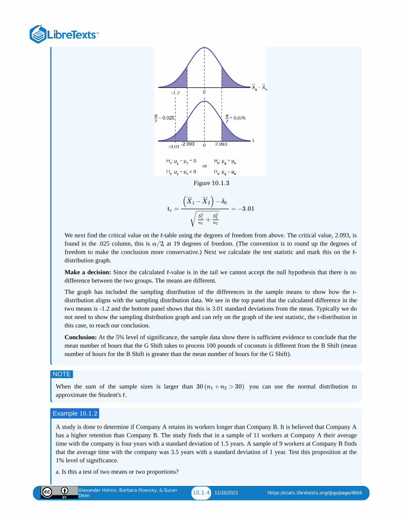
Alexander Holms, Barbara Illowsky, & Susan
Dean10.1.4 11/26/2021 https://stats.libretexts.org/@go/page/4604
Figure
We next find the critical value on the -table using the degrees of freedom from above. The critical value, 2.093, isfound in the .025 column, this is , at 19 degrees of freedom. (The convention is to round up the degrees offreedom to make the conclusion more conservative.) Next we calculate the test statistic and mark this on the -distribution graph.
Make a decision: Since the calculated -value is in the tail we cannot accept the null hypothesis that there is nodifference between the two groups. The means are different.
The graph has included the sampling distribution of the differences in the sample means to show how the t-distribution aligns with the sampling distribution data. We see in the top panel that the calculated difference in thetwo means is -1.2 and the bottom panel shows that this is 3.01 standard deviations from the mean. Typically we donot need to show the sampling distribution graph and can rely on the graph of the test statistic, the t-distribution inthis case, to reach our conclusion.
Conclusion: At the 5% level of significance, the sample data show there is sufficient evidence to conclude that themean number of hours that the G Shift takes to process 100 pounds of coconuts is different from the B Shift (meannumber of hours for the B Shift is greater than the mean number of hours for the G Shift).
When the sum of the sample sizes is larger than you can use the normal distribution toapproximate the Student's .
A study is done to determine if Company A retains its workers longer than Company B. It is believed that Company Ahas a higher retention than Company B. The study finds that in a sample of 11 workers at Company A their averagetime with the company is four years with a standard deviation of 1.5 years. A sample of 9 workers at Company B findsthat the average time with the company was 3.5 years with a standard deviation of 1 year. Test this proposition at the1% level of significance.
a. Is this a test of two means or two proportions?
10.1.3
= = −3.01tc
( − )−X¯ ¯¯̄
1 X¯ ¯¯̄
2 δ0
+S2
1
n1
S22
n2
− −−−−−−√
t
α/2
t
t
NOTE
30 ( + > 30)n1 n2
t
Example 10.1.2
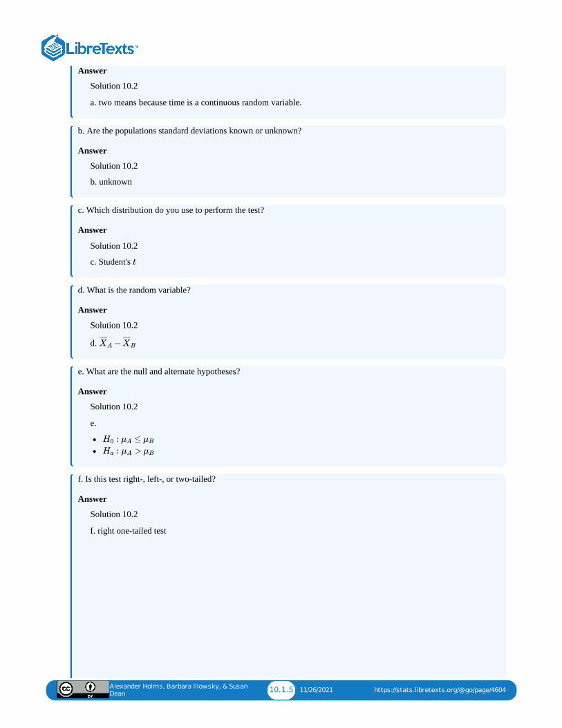
Alexander Holms, Barbara Illowsky, & Susan
Dean10.1.5 11/26/2021 https://stats.libretexts.org/@go/page/4604
Answer
Solution 10.2
a. two means because time is a continuous random variable.
b. Are the populations standard deviations known or unknown?
Answer
Solution 10.2
b. unknown
c. Which distribution do you use to perform the test?
Answer
Solution 10.2
c. Student's
d. What is the random variable?
Answer
Solution 10.2
d.
e. What are the null and alternate hypotheses?
Answer
Solution 10.2
e.
f. Is this test right-, left-, or two-tailed?
Answer
Solution 10.2
f. right one-tailed test
t
−X¯ ¯¯̄
A X¯ ¯¯̄
B
: ≤H0 μA μB
: >Ha μA μB
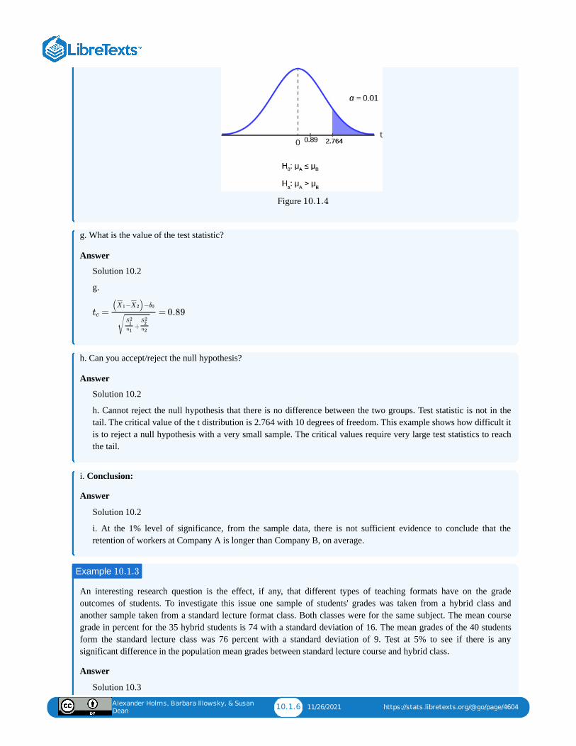
Alexander Holms, Barbara Illowsky, & Susan
Dean10.1.6 11/26/2021 https://stats.libretexts.org/@go/page/4604
Figure
g. What is the value of the test statistic?
Answer
Solution 10.2
g.
h. Can you accept/reject the null hypothesis?
Answer
Solution 10.2
h. Cannot reject the null hypothesis that there is no difference between the two groups. Test statistic is not in thetail. The critical value of the t distribution is 2.764 with 10 degrees of freedom. This example shows how difficult itis to reject a null hypothesis with a very small sample. The critical values require very large test statistics to reachthe tail.
i. Conclusion:
Answer
Solution 10.2
i. At the 1% level of significance, from the sample data, there is not sufficient evidence to conclude that theretention of workers at Company A is longer than Company B, on average.
An interesting research question is the effect, if any, that different types of teaching formats have on the gradeoutcomes of students. To investigate this issue one sample of students' grades was taken from a hybrid class andanother sample taken from a standard lecture format class. Both classes were for the same subject. The mean coursegrade in percent for the 35 hybrid students is 74 with a standard deviation of 16. The mean grades of the 40 studentsform the standard lecture class was 76 percent with a standard deviation of 9. Test at 5% to see if there is anysignificant difference in the population mean grades between standard lecture course and hybrid class.
Answer
Solution 10.3
10.1.4
= = 0.89tc( − )−X
¯ ¯¯̄1 X
¯ ¯¯̄2 δ0
+S2
1n1
S22
n2√
Example 10.1.3
Alexander Holms, Barbara Illowsky, & Susan
Dean10.1.7 11/26/2021 https://stats.libretexts.org/@go/page/4604
We begin by noting that we have two groups, students from a hybrid class and students from a standard lectureformat class. We also note that the random variable, what we are interested in, is students' grades, a continuousrandom variable. We could have asked the research question in a different way and had a binary random variable.For example, we could have studied the percentage of students with a failing grade, or with an A grade. Both ofthese would be binary and thus a test of proportions and not a test of means as is the case here. Finally, there is nopresumption as to which format might lead to higher grades so the hypothesis is stated as a two-tailed test.
As would virtually always be the case, we do not know the population variances of the two distributions and thusour test statistic is:
To determine the critical value of the Student's t we need the degrees of freedom. For this case we use: . This is large enough to consider it the normal distribution thus
. Again as always we determine if the calculated value is in the tail determined by the critical value. Inthis case we do not even need to look up the critical value: the calculated value of the difference in these twoaverage grades is not even one standard deviation apart. Certainly not in the tail.
Conclusion: Cannot reject the null at . Therefore, evidence does not exist to prove that the grades inhybrid and standard classes differ.
: =H0 μ1 μ2
: ≠Ha μ1 μ2
= = = −0.65tc( − ) −x̄̄̄1 x̄̄̄2 δ0
+s2
n1
s2
n2
− −−−−−−√
(74 −76) −0
+162
35
92
40
− −−−−−−√
df = + −2 = 35 +40 −2 = 73n1 n2
= 1.96tα/2
α = 5%
Alexander Holms, Barbara Illowsky, & Susan
Dean10.2.1 1/6/2022 https://stats.libretexts.org/@go/page/4605
10.2: Cohen's Standards for Small, Medium, and Large Effect SizesCohen's is a measure of "effect size" based on the differences between two means. Cohen’s , named for United Statesstatistician Jacob Cohen, measures the relative strength of the differences between the means of two populations based onsample data. The calculated value of effect size is then compared to Cohen’s standards of small, medium, and large effectsizes.
Size of effect
Small 0.2
Medium 0.5
Large 0.8
Table 10.2 Cohen's Standard Effect Sizes
Cohen's is the measure of the difference between two means divided by the pooled standard deviation: where
It is important to note that Cohen's does not provide a level of confidence as to the magnitude of the size of the effectcomparable to the other tests of hypothesis we have studied. The sizes of the effects are simply indicative.
d d
d
d d = −x̄̄̄1 x̄̄̄2
s pooled
=spooled( −1) +( −1)n1 s2
1 n2 s22
+ −2n1 n2
− −−−−−−−−−−−√
d
The effect is small because 0.384 is between Cohen’s value of 0.2 for small effect size and 0.5 formedium effect size. The size of the differences of the means for the two companies is small indicatingthat there is not a significant difference between them.
Alexander Holms, Barbara Illowsky, & Susan
Dean10.3.1 12/24/2021 https://stats.libretexts.org/@go/page/4606
10.3: Test for Differences in Means- Assuming Equal Population VariancesTypically we can never expect to know any of the population parameters, mean, proportion, or standard deviation. Whentesting hypotheses concerning differences in means we are faced with the difficulty of two unknown variances that play acritical role in the test statistic. We have been substituting the sample variances just as we did when testing hypotheses fora single mean. And as we did before, we used a Student's t to compensate for this lack of information on the populationvariance. There may be situations, however, when we do not know the population variances, but we can assume that thetwo populations have the same variance. If this is true then the pooled sample variance will be smaller than the individualsample variances. This will give more precise estimates and reduce the probability of discarding a good null. The null andalternative hypotheses remain the same, but the test statistic changes to:
where is the pooled variance given by the formula:
=tc
( − ) −x̄̄̄1 x̄̄̄2 δ0
p( + )S2 1n1
1n2
− −−−−−−−−−−−√
S2p
=S2p
( −1) +( −1)n1 s12 n2 s2
2
+ −2n1 n2
The test statistic is clearly in the tail, 2.31 is larger than the critical value of 1.703, and therefore wecannot maintain the null hypothesis. Thus, we conclude that there is significant evidence at the 95%level of confidence that the new medicine produces the effect desired.
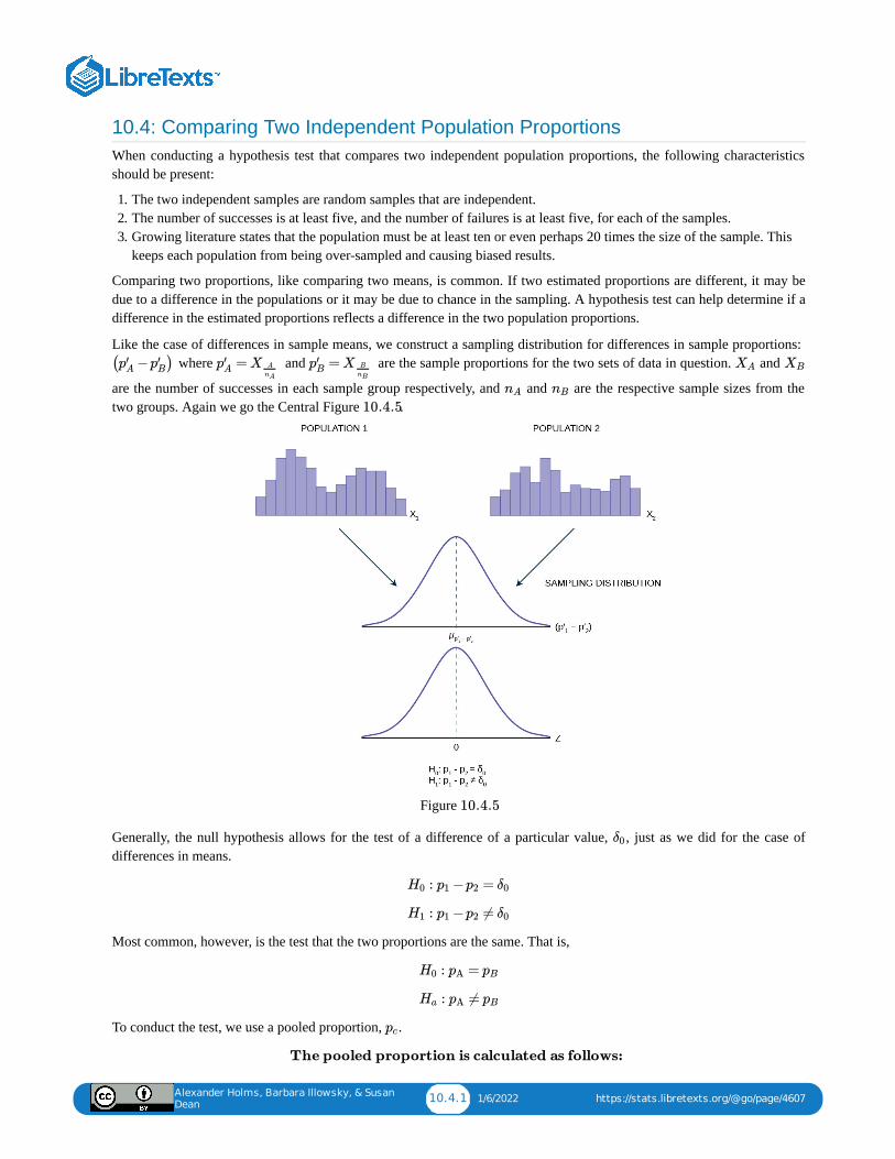
Alexander Holms, Barbara Illowsky, & Susan
Dean10.4.1 1/6/2022 https://stats.libretexts.org/@go/page/4607
10.4: Comparing Two Independent Population ProportionsWhen conducting a hypothesis test that compares two independent population proportions, the following characteristicsshould be present:
1. The two independent samples are random samples that are independent.2. The number of successes is at least five, and the number of failures is at least five, for each of the samples.3. Growing literature states that the population must be at least ten or even perhaps 20 times the size of the sample. This
keeps each population from being over-sampled and causing biased results.
Comparing two proportions, like comparing two means, is common. If two estimated proportions are different, it may bedue to a difference in the populations or it may be due to chance in the sampling. A hypothesis test can help determine if adifference in the estimated proportions reflects a difference in the two population proportions.
Like the case of differences in sample means, we construct a sampling distribution for differences in sample proportions: where and are the sample proportions for the two sets of data in question. and
are the number of successes in each sample group respectively, and and are the respective sample sizes from thetwo groups. Again we go the Central Figure .
Figure
Generally, the null hypothesis allows for the test of a difference of a particular value, , just as we did for the case ofdifferences in means.
Most common, however, is the test that the two proportions are the same. That is,
To conduct the test, we use a pooled proportion, .
( − )p′A p′
B =p′A X A
nA
=p′B X B
nB
XA XB
nA nB
10.4.5
10.4.5
δ0
: − =H0 p1 p2 δ0
: − ≠H1 p1 p2 δ0
: =H0 pA pB
: ≠Ha pA pB
pc
The pooled proportion is calculated as follows:
Alexander Holms, Barbara Illowsky, & Susan
Dean10.4.2 1/6/2022 https://stats.libretexts.org/@go/page/4607
where is the hypothesized differences between the two proportions and p is the pooled variance from the formulaabove.
A bank has recently acquired a new branch and thus has customers in this new territory. They are interested in thedefault rate in their new territory. They wish to test the hypothesis that the default rate is different from their currentcustomer base. They sample 200 files in area A, their current customers, and find that 20 have defaulted. In area B, thenew customers, another sample of 200 files shows 12 have defaulted on their loans. At a 10% level of significance canwe say that the default rates are the same or different?
Answer
Solution 10.6
This is a test of proportions. We know this because the underlying random variable is binary, default or not default.Further, we know it is a test of differences in proportions because we have two sample groups, the current customerbase and the newly acquired customer base. Let A and B be the subscripts for the two customer groups. Thenp and p are the two population proportions we wish to test.
Random Variable:
= difference in the proportions of customers who defaulted in the two groups.
The words "is a difference" tell you the test is two-tailed.
Distribution for the test: Since this is a test of two binomial population proportions, the distribution is normal:
follows an approximate normal distribution.
Estimated proportion for group A:
Estimated proportion for group B:
The estimated difference between the two groups is : .
=pc
+xA xB
+nA nB
The test statistic (z-score) is:
=Zc
( − )−p′A
p′B
δ0
(1 − )( + )pc pc1
nA
1nB
− −−−−−−−−−−−−−−−−√
δ0 c
Example 10.4.6
A B
−P ′A P ′
B
: =H0 pA pB
: ≠Ha pA pB
= = = 0.08pc+xA xB
+nA nB
20+12
200+2001 − = 0.92pc
( A − B) = 0.04p′ p′
= = = 0.1p′A
xA
nA
20200
= = = 0.06p′B
xB
nB
12200
− = 0.1 −0.06 = 0.04p′A p′
B
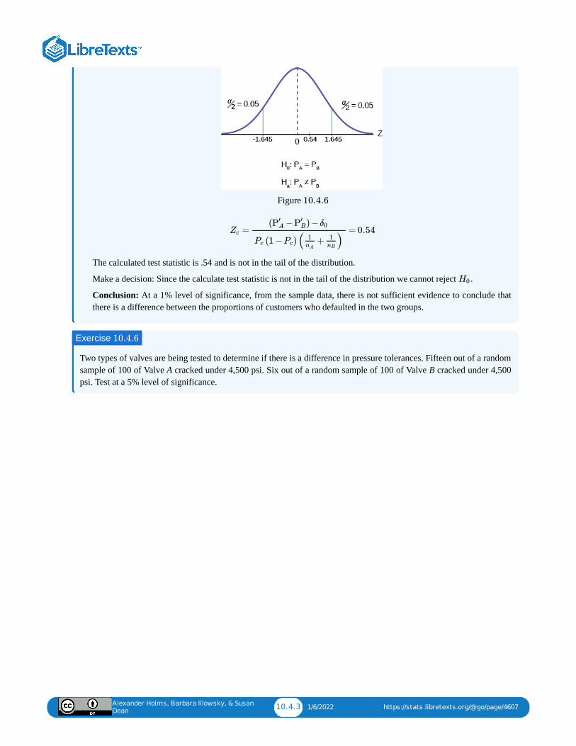
Alexander Holms, Barbara Illowsky, & Susan
Dean10.4.3 1/6/2022 https://stats.libretexts.org/@go/page/4607
Figure
The calculated test statistic is .54 and is not in the tail of the distribution.
Make a decision: Since the calculate test statistic is not in the tail of the distribution we cannot reject .
Conclusion: At a 1% level of significance, from the sample data, there is not sufficient evidence to conclude thatthere is a difference between the proportions of customers who defaulted in the two groups.
Two types of valves are being tested to determine if there is a difference in pressure tolerances. Fifteen out of a randomsample of 100 of Valve A cracked under 4,500 psi. Six out of a random sample of 100 of Valve B cracked under 4,500psi. Test at a 5% level of significance.
10.4.6
= = 0.54Zc
( − ) −P′A P′
B δ0
(1 − )( + )Pc Pc1
nA
1nB
H0
Exercise 10.4.6
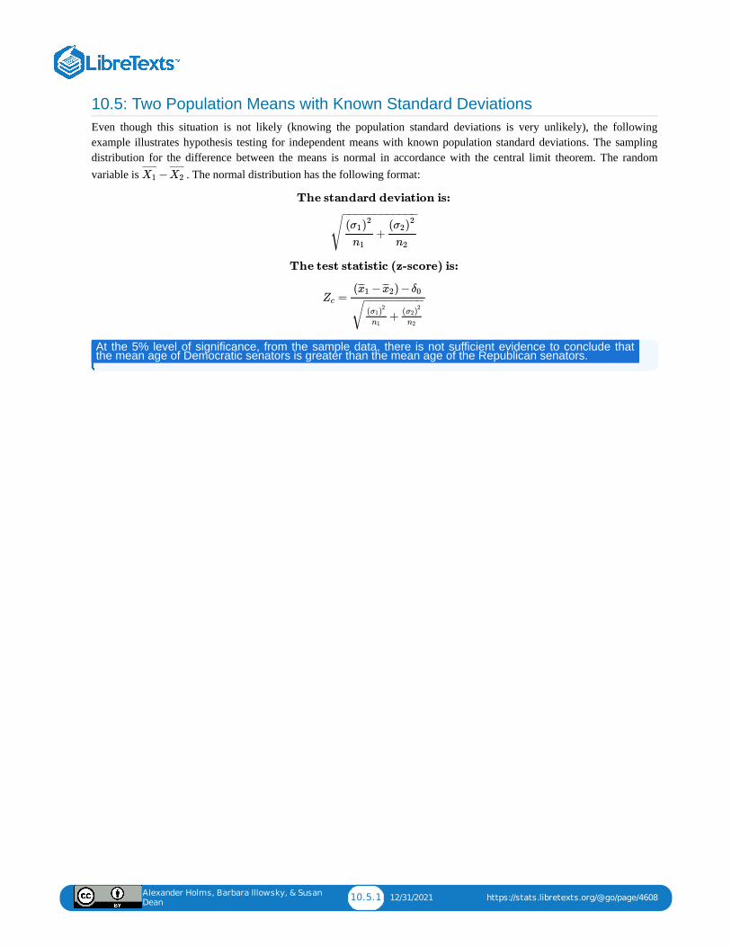
Alexander Holms, Barbara Illowsky, & Susan
Dean10.5.1 12/31/2021 https://stats.libretexts.org/@go/page/4608
10.5: Two Population Means with Known Standard DeviationsEven though this situation is not likely (knowing the population standard deviations is very unlikely), the followingexample illustrates hypothesis testing for independent means with known population standard deviations. The samplingdistribution for the difference between the means is normal in accordance with the central limit theorem. The randomvariable is . The normal distribution has the following format:−X1
¯ ¯¯̄ ¯̄X2¯ ¯¯̄ ¯̄
The standard deviation is:
+( )σ1
2
n1
( )σ22
n2
− −−−−−−−−−−−
√
The test statistic (z-score) is:
=Zc
( − ) −x̄̄̄1 x̄̄̄2 δ0
+( )σ1
2
n1
( )σ22
n2
− −−−−−−−−√
At the 5% level of significance, from the sample data, there is not sufficient evidence to conclude thatthe mean age of Democratic senators is greater than the mean age of the Republican senators.
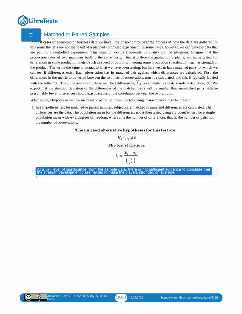
Alexander Holms, Barbara Illowsky, & Susan
Dean10.6.1 10/22/2021 https://stats.libretexts.org/@go/page/6115
10.6: Matched or Paired SamplesIn most cases of economic or business data we have little or no control over the process of how the data are gathered. Inthis sense the data are not the result of a planned controlled experiment. In some cases, however, we can develop data thatare part of a controlled experiment. This situation occurs frequently in quality control situations. Imagine that theproduction rates of two machines built to the same design, but at different manufacturing plants, are being tested fordifferences in some production metric such as speed of output or meeting some production specification such as strength ofthe product. The test is the same in format to what we have been testing, but here we can have matched pairs for which wecan test if differences exist. Each observation has its matched pair against which differences are calculated. First, thedifferences in the metric to be tested between the two lists of observations must be calculated, and this is typically labeledwith the letter "d." Then, the average of these matched differences, is calculated as is its standard deviation, . Weexpect that the standard deviation of the differences of the matched pairs will be smaller than unmatched pairs becausepresumably fewer differences should exist because of the correlation between the two groups.
When using a hypothesis test for matched or paired samples, the following characteristics may be present:
1. In a hypothesis test for matched or paired samples, subjects are matched in pairs and differences are calculated. Thedifferences are the data. The population mean for the differences, , is then tested using a Student's-t test for a singlepopulation mean with degrees of freedom, where is the number of differences, that is, the number of pairs notthe number of observations.
X¯ ¯¯̄
d Sd
μd
n– 1 n
The null and alternative hypotheses for this test are:
: ≠ 0Ha μd
The test statistic is:
=tc−x̄̄̄d μd
( )sd
n√
At a 5% level of significance, from the sample data, there is not sufficient evidence to conclude thatthe strength development class helped to make the players stronger, on average.
☰
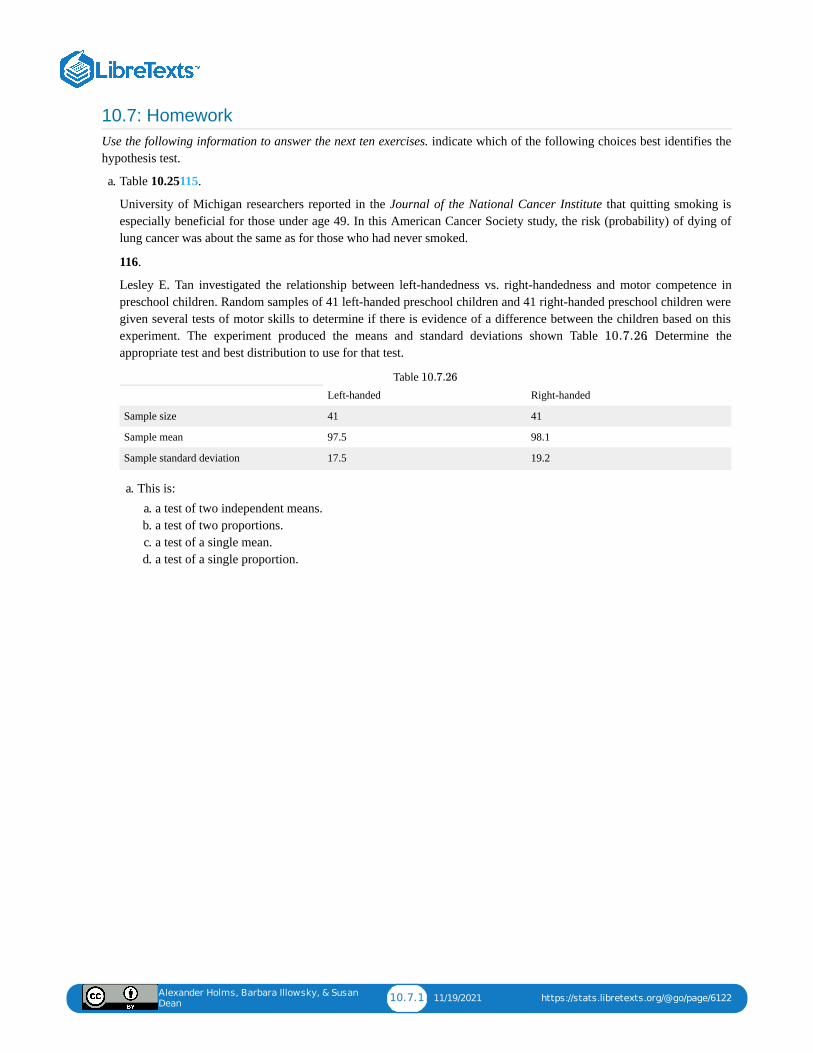
Alexander Holms, Barbara Illowsky, & Susan
Dean10.7.1 11/19/2021 https://stats.libretexts.org/@go/page/6122
10.7: HomeworkUse the following information to answer the next ten exercises. indicate which of the following choices best identifies thehypothesis test.
a. Table 10.25115.
University of Michigan researchers reported in the Journal of the National Cancer Institute that quitting smoking isespecially beneficial for those under age 49. In this American Cancer Society study, the risk (probability) of dying oflung cancer was about the same as for those who had never smoked.
116.
Lesley E. Tan investigated the relationship between left-handedness vs. right-handedness and motor competence inpreschool children. Random samples of 41 left-handed preschool children and 41 right-handed preschool children weregiven several tests of motor skills to determine if there is evidence of a difference between the children based on thisexperiment. The experiment produced the means and standard deviations shown Table . Determine theappropriate test and best distribution to use for that test.
Left-handed Right-handed
Sample size 41 41
Sample mean 97.5 98.1
Sample standard deviation 17.5 19.2
Table
a. This is:a. a test of two independent means.b. a test of two proportions.c. a test of a single mean.d. a test of a single proportion.
10.7.26
10.7.26
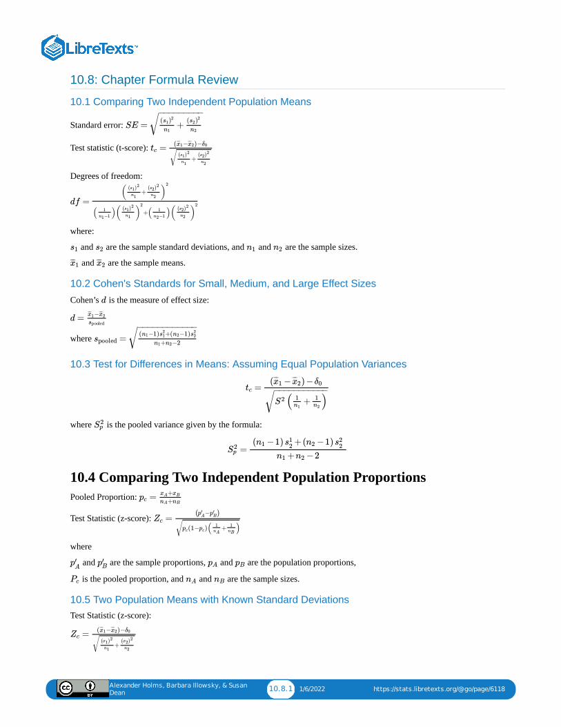
Alexander Holms, Barbara Illowsky, & Susan
Dean10.8.1 1/6/2022 https://stats.libretexts.org/@go/page/6118
10.8: Chapter Formula Review
10.1 Comparing Two Independent Population Means
Standard error:
Test statistic (t-score):
Degrees of freedom:
where:
and are the sample standard deviations, and and are the sample sizes.
and are the sample means.
10.2 Cohen's Standards for Small, Medium, and Large Effect Sizes
Cohen’s is the measure of effect size:
where
10.3 Test for Differences in Means: Assuming Equal Population Variances
where is the pooled variance given by the formula:
10.4 Comparing Two Independent Population ProportionsPooled Proportion:
Test Statistic (z-score):
where
and are the sample proportions, and are the population proportions,
is the pooled proportion, and and are the sample sizes.
10.5 Two Population Means with Known Standard DeviationsTest Statistic (z-score):
SE = +( )s1
2
n1
( )s22
n2
− −−−−−−−−√
=tc( − )−x̄̄̄1 x̄̄̄2 δ0
+( )s1
2
n1
( )s22
n2√
df =( + )
( )s12
n1
( )s22
n2
2
( ) +( )1
−1n1( )
( )s12
n1
21
−1n2( )
( )s22
n2
2
s1 s2 n1 n2
x̄̄̄1 x̄̄̄2
d
d =−x̄̄̄1 x̄̄̄2
spooled
=spooled( −1) +( −1)n1 s2
1 n2 s22
+ −2n1 n2
− −−−−−−−−−−−√
=tc( − ) −x̄̄̄1 x̄̄̄2 δ0
( + )S2 1n1
1n2
− −−−−−−−−−−√
S2p
=S2p
( −1) +( −1)n1 s12
n2 s22
+ −2n1 n2
=pc+xA xB+nA nB
=Zc
( − )p′A p′
B
(1− )( + )pc pc1nA
1nB
√
p′A
p′B pA pB
Pc nA nB
=Zc( − )−x̄̄̄1 x̄̄̄2 δ0
+( )σ1
2
n1
( )σ22
n2√
Alexander Holms, Barbara Illowsky, & Susan
Dean10.8.2 1/6/2022 https://stats.libretexts.org/@go/page/6118
where: and are the known population standard deviations. and are the sample sizes. and are the sample means. and are the population means.
10.6 Matched or Paired Samples
Test Statistic (t-score):
where:
is the mean of the sample differences. is the mean of the population differences. is the sample standard deviationof the differences. is the sample size.
σ1 σ2 n1 n2 x̄̄̄1 x̄̄̄2
μ1 μ2
=tc−x̄̄̄d μd
( )sd
n√
x̄̄̄d μd sdn
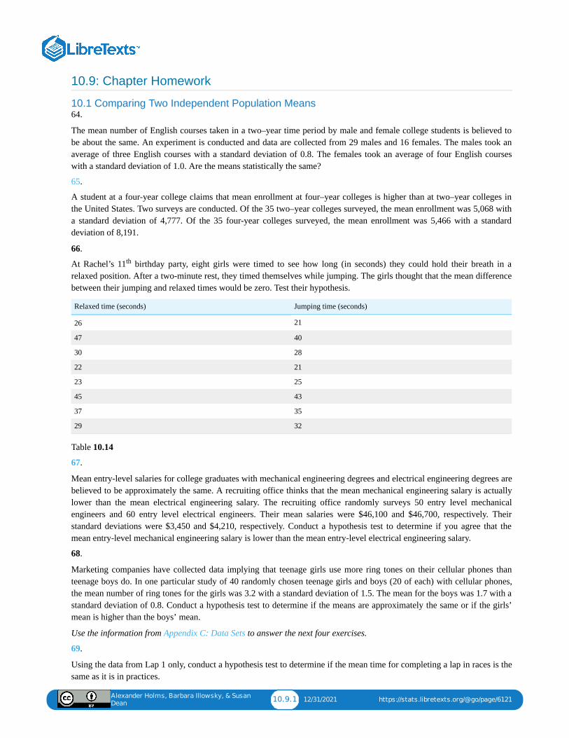
Alexander Holms, Barbara Illowsky, & Susan
Dean10.9.1 12/31/2021 https://stats.libretexts.org/@go/page/6121
10.9: Chapter Homework
10.1 Comparing Two Independent Population Means64.
The mean number of English courses taken in a two–year time period by male and female college students is believed tobe about the same. An experiment is conducted and data are collected from 29 males and 16 females. The males took anaverage of three English courses with a standard deviation of 0.8. The females took an average of four English courseswith a standard deviation of 1.0. Are the means statistically the same?
65.
A student at a four-year college claims that mean enrollment at four–year colleges is higher than at two–year colleges inthe United States. Two surveys are conducted. Of the 35 two–year colleges surveyed, the mean enrollment was 5,068 witha standard deviation of 4,777. Of the 35 four-year colleges surveyed, the mean enrollment was 5,466 with a standarddeviation of 8,191.
66.
At Rachel’s 11 birthday party, eight girls were timed to see how long (in seconds) they could hold their breath in arelaxed position. After a two-minute rest, they timed themselves while jumping. The girls thought that the mean differencebetween their jumping and relaxed times would be zero. Test their hypothesis.
Relaxed time (seconds) Jumping time (seconds)
26 21
47 40
30 28
22 21
23 25
45 43
37 35
29 32
Table 10.14
67.
Mean entry-level salaries for college graduates with mechanical engineering degrees and electrical engineering degrees arebelieved to be approximately the same. A recruiting office thinks that the mean mechanical engineering salary is actuallylower than the mean electrical engineering salary. The recruiting office randomly surveys 50 entry level mechanicalengineers and 60 entry level electrical engineers. Their mean salaries were $46,100 and $46,700, respectively. Theirstandard deviations were $3,450 and $4,210, respectively. Conduct a hypothesis test to determine if you agree that themean entry-level mechanical engineering salary is lower than the mean entry-level electrical engineering salary.
68.
Marketing companies have collected data implying that teenage girls use more ring tones on their cellular phones thanteenage boys do. In one particular study of 40 randomly chosen teenage girls and boys (20 of each) with cellular phones,the mean number of ring tones for the girls was 3.2 with a standard deviation of 1.5. The mean for the boys was 1.7 with astandard deviation of 0.8. Conduct a hypothesis test to determine if the means are approximately the same or if the girls’mean is higher than the boys’ mean.
Use the information from Appendix C: Data Sets to answer the next four exercises.
69.
Using the data from Lap 1 only, conduct a hypothesis test to determine if the mean time for completing a lap in races is thesame as it is in practices.
th
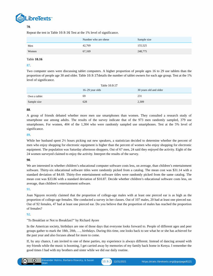
Alexander Holms, Barbara Illowsky, & Susan
Dean10.9.2 12/31/2021 https://stats.libretexts.org/@go/page/6121
70.
Repeat the test in Table . Test at the 1% level of significance.
Number who are obese Sample size
Men 42,769 155,525
Women 67,169 248,775
Table 10.16
87.
Two computer users were discussing tablet computers. A higher proportion of people ages 16 to 29 use tablets than theproportion of people age 30 and older. Table details the number of tablet owners for each age group. Test at the 1%level of significance.
16–29 year olds 30 years old and older
Own a tablet 69 231
Sample size 628 2,309
Table
88.
A group of friends debated whether more men use smartphones than women. They consulted a research study ofsmartphone use among adults. The results of the survey indicate that of the 973 men randomly sampled, 379 usesmartphones. For women, 404 of the 1,304 who were randomly sampled use smartphones. Test at the 5% level ofsignificance.
89.
While her husband spent 2½ hours picking out new speakers, a statistician decided to determine whether the percent ofmen who enjoy shopping for electronic equipment is higher than the percent of women who enjoy shopping for electronicequipment. The population was Saturday afternoon shoppers. Out of 67 men, 24 said they enjoyed the activity. Eight of the24 women surveyed claimed to enjoy the activity. Interpret the results of the survey.
90.
We are interested in whether children’s educational computer software costs less, on average, than children’s entertainmentsoftware. Thirty-six educational software titles were randomly picked from a catalog. The mean cost was $31.14 with astandard deviation of $4.69. Thirty-five entertainment software titles were randomly picked from the same catalog. Themean cost was $33.86 with a standard deviation of $10.87. Decide whether children’s educational software costs less, onaverage, than children’s entertainment software.
91.
Joan Nguyen recently claimed that the proportion of college-age males with at least one pierced ear is as high as theproportion of college-age females. She conducted a survey in her classes. Out of 107 males, 20 had at least one pierced ear.Out of 92 females, 47 had at least one pierced ear. Do you believe that the proportion of males has reached the proportionof females?
92.
"To Breakfast or Not to Breakfast?" by Richard Ayore
In the American society, birthdays are one of those days that everyone looks forward to. People of different ages and peergroups gather to mark the 18th, 20th, …, birthdays. During this time, one looks back to see what he or she has achieved forthe past year and also focuses ahead for more to come.
If, by any chance, I am invited to one of these parties, my experience is always different. Instead of dancing around withmy friends while the music is booming, I get carried away by memories of my family back home in Kenya. I remember thegood times I had with my brothers and sister while we did our daily routine.
10.9.16
10.9.17
10.9.17
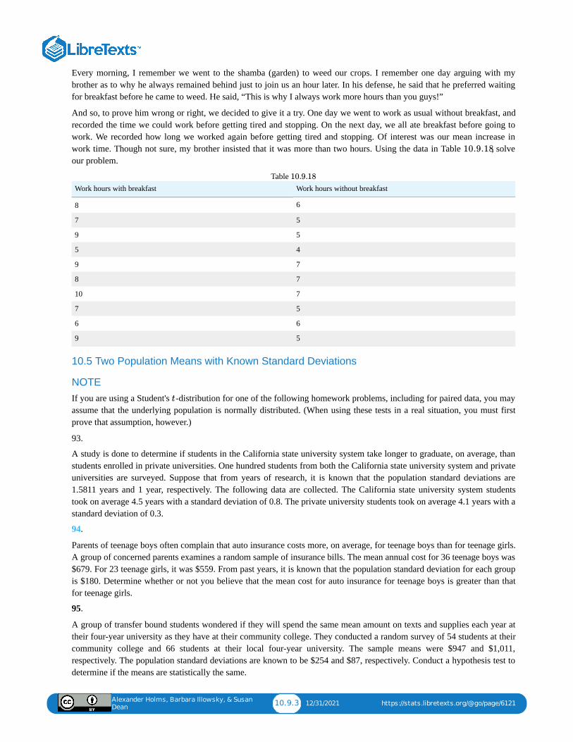
Alexander Holms, Barbara Illowsky, & Susan
Dean10.9.3 12/31/2021 https://stats.libretexts.org/@go/page/6121
Every morning, I remember we went to the shamba (garden) to weed our crops. I remember one day arguing with mybrother as to why he always remained behind just to join us an hour later. In his defense, he said that he preferred waitingfor breakfast before he came to weed. He said, “This is why I always work more hours than you guys!”
And so, to prove him wrong or right, we decided to give it a try. One day we went to work as usual without breakfast, andrecorded the time we could work before getting tired and stopping. On the next day, we all ate breakfast before going towork. We recorded how long we worked again before getting tired and stopping. Of interest was our mean increase inwork time. Though not sure, my brother insisted that it was more than two hours. Using the data in Table , solveour problem.
Work hours with breakfast Work hours without breakfast
8 6
7 5
9 5
5 4
9 7
8 7
10 7
7 5
6 6
9 5
Table
10.5 Two Population Means with Known Standard Deviations
NOTEIf you are using a Student's -distribution for one of the following homework problems, including for paired data, you mayassume that the underlying population is normally distributed. (When using these tests in a real situation, you must firstprove that assumption, however.)
93.
A study is done to determine if students in the California state university system take longer to graduate, on average, thanstudents enrolled in private universities. One hundred students from both the California state university system and privateuniversities are surveyed. Suppose that from years of research, it is known that the population standard deviations are1.5811 years and 1 year, respectively. The following data are collected. The California state university system studentstook on average 4.5 years with a standard deviation of 0.8. The private university students took on average 4.1 years with astandard deviation of 0.3.
94.
Parents of teenage boys often complain that auto insurance costs more, on average, for teenage boys than for teenage girls.A group of concerned parents examines a random sample of insurance bills. The mean annual cost for 36 teenage boys was$679. For 23 teenage girls, it was $559. From past years, it is known that the population standard deviation for each groupis $180. Determine whether or not you believe that the mean cost for auto insurance for teenage boys is greater than thatfor teenage girls.
95.
A group of transfer bound students wondered if they will spend the same mean amount on texts and supplies each year attheir four-year university as they have at their community college. They conducted a random survey of 54 students at theircommunity college and 66 students at their local four-year university. The sample means were $947 and $1,011,respectively. The population standard deviations are known to be $254 and $87, respectively. Conduct a hypothesis test todetermine if the means are statistically the same.
10.9.18
10.9.18
t
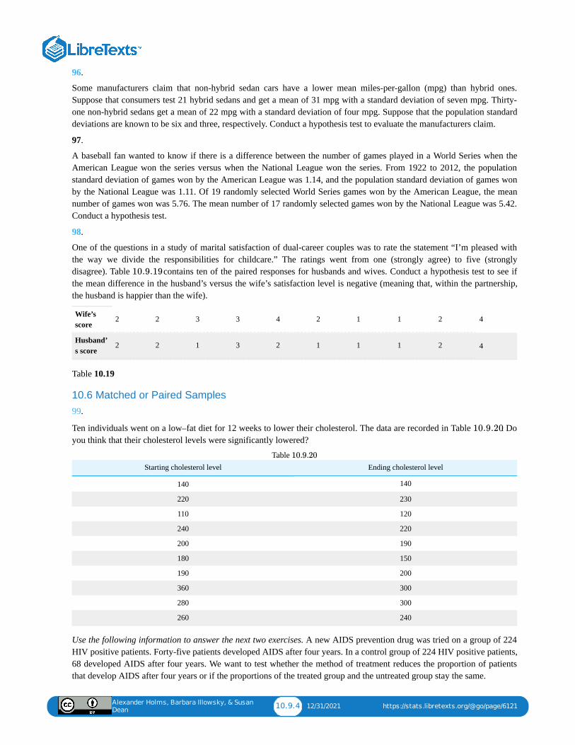
Alexander Holms, Barbara Illowsky, & Susan
Dean10.9.4 12/31/2021 https://stats.libretexts.org/@go/page/6121
96.
Some manufacturers claim that non-hybrid sedan cars have a lower mean miles-per-gallon (mpg) than hybrid ones.Suppose that consumers test 21 hybrid sedans and get a mean of 31 mpg with a standard deviation of seven mpg. Thirty-one non-hybrid sedans get a mean of 22 mpg with a standard deviation of four mpg. Suppose that the population standarddeviations are known to be six and three, respectively. Conduct a hypothesis test to evaluate the manufacturers claim.
97.
A baseball fan wanted to know if there is a difference between the number of games played in a World Series when theAmerican League won the series versus when the National League won the series. From 1922 to 2012, the populationstandard deviation of games won by the American League was 1.14, and the population standard deviation of games wonby the National League was 1.11. Of 19 randomly selected World Series games won by the American League, the meannumber of games won was 5.76. The mean number of 17 randomly selected games won by the National League was 5.42.Conduct a hypothesis test.
98.
One of the questions in a study of marital satisfaction of dual-career couples was to rate the statement “I’m pleased withthe way we divide the responsibilities for childcare.” The ratings went from one (strongly agree) to five (stronglydisagree). Table contains ten of the paired responses for husbands and wives. Conduct a hypothesis test to see ifthe mean difference in the husband’s versus the wife’s satisfaction level is negative (meaning that, within the partnership,the husband is happier than the wife).
Wife’sscore
2 2 3 3 4 2 1 1 2 4
Husband’s score
2 2 1 3 2 1 1 1 2 4
Table 10.19
10.6 Matched or Paired Samples99.
Ten individuals went on a low–fat diet for 12 weeks to lower their cholesterol. The data are recorded in Table . Doyou think that their cholesterol levels were significantly lowered?
Starting cholesterol level Ending cholesterol level
140 140
220 230
110 120
240 220
200 190
180 150
190 200
360 300
280 300
260 240
Table
Use the following information to answer the next two exercises. A new AIDS prevention drug was tried on a group of 224HIV positive patients. Forty-five patients developed AIDS after four years. In a control group of 224 HIV positive patients,68 developed AIDS after four years. We want to test whether the method of treatment reduces the proportion of patientsthat develop AIDS after four years or if the proportions of the treated group and the untreated group stay the same.
10.9.19
10.9.20
10.9.20
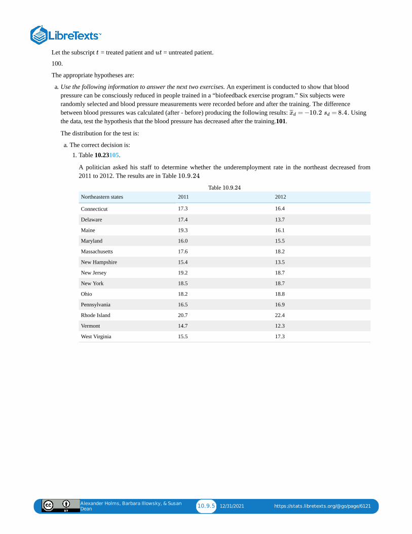
Alexander Holms, Barbara Illowsky, & Susan
Dean10.9.5 12/31/2021 https://stats.libretexts.org/@go/page/6121
Let the subscript = treated patient and = untreated patient.
100.
The appropriate hypotheses are:
a. Use the following information to answer the next two exercises. An experiment is conducted to show that bloodpressure can be consciously reduced in people trained in a “biofeedback exercise program.” Six subjects wererandomly selected and blood pressure measurements were recorded before and after the training. The differencebetween blood pressures was calculated (after - before) producing the following results: . Usingthe data, test the hypothesis that the blood pressure has decreased after the training.101.
The distribution for the test is:
a. The correct decision is:1. Table 10.23105.
A politician asked his staff to determine whether the underemployment rate in the northeast decreased from2011 to 2012. The results are in Table .
Northeastern states 2011 2012
Connecticut 17.3 16.4
Delaware 17.4 13.7
Maine 19.3 16.1
Maryland 16.0 15.5
Massachusetts 17.6 18.2
New Hampshire 15.4 13.5
New Jersey 19.2 18.7
New York 18.5 18.7
Ohio 18.2 18.8
Pennsylvania 16.5 16.9
Rhode Island 20.7 22.4
Vermont 14.7 12.3
West Virginia 15.5 17.3
Table
t ut
= −10.2x̄̄̄d = 8.4sd
10.9.24
10.9.24
Alexander Holms, Barbara Illowsky, & Susan
Dean10.10.1 12/24/2021 https://stats.libretexts.org/@go/page/6116
10.10: Chapter Key Terms
Cohen’s da measure of effect size based on the differences between two means. If is between 0 and 0.2 then the effect is small.If approaches is 0.5, then the effect is medium, and if approaches 0.8, then it is a large effect.
Independent Groupstwo samples that are selected from two populations, and the values from one population are not related in any way tothe values from the other population.
Matched Pairstwo samples that are dependent. Differences between a before and after scenario are tested by testing one populationmean of differences.
Pooled Variancea weighted average of two variances that can then be used when calculating standard error.
d
d d
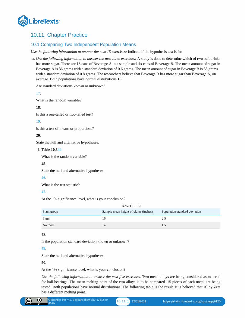
Alexander Holms, Barbara Illowsky, & Susan
Dean10.11.1 12/31/2021 https://stats.libretexts.org/@go/page/6120
10.11: Chapter Practice
10.1 Comparing Two Independent Population Means
Use the following information to answer the next 15 exercises: Indicate if the hypothesis test is for
a. Use the following information to answer the next three exercises: A study is done to determine which of two soft drinkshas more sugar. There are 13 cans of Beverage A in a sample and six cans of Beverage B. The mean amount of sugar inBeverage A is 36 grams with a standard deviation of 0.6 grams. The mean amount of sugar in Beverage B is 38 gramswith a standard deviation of 0.8 grams. The researchers believe that Beverage B has more sugar than Beverage A, onaverage. Both populations have normal distributions.16.
Are standard deviations known or unknown?
17.
What is the random variable?
18.
Is this a one-tailed or two-tailed test?
19.
Is this a test of means or proportions?
20.
State the null and alternative hypotheses.
1. Table 10.844.
What is the random variable?
45.
State the null and alternative hypotheses.
46.
What is the test statistic?
47.
At the 1% significance level, what is your conclusion?
Plant group Sample mean height of plants (inches) Population standard deviation
Food 16 2.5
No food 14 1.5
Table
48.
Is the population standard deviation known or unknown?
49.
State the null and alternative hypotheses.
50.
At the 1% significance level, what is your conclusion?
Use the following information to answer the next five exercises. Two metal alloys are being considered as materialfor ball bearings. The mean melting point of the two alloys is to be compared. 15 pieces of each metal are beingtested. Both populations have normal distributions. The following table is the result. It is believed that Alloy Zetahas a different melting point.
10.11.9
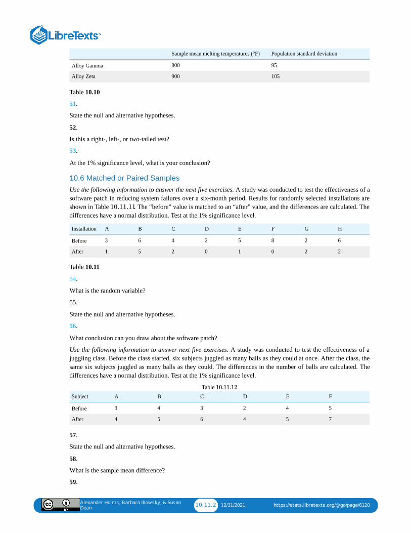
Alexander Holms, Barbara Illowsky, & Susan
Dean10.11.2 12/31/2021 https://stats.libretexts.org/@go/page/6120
Sample mean melting temperatures (°F) Population standard deviation
Alloy Gamma 800 95
Alloy Zeta 900 105
Table 10.10
51.
State the null and alternative hypotheses.
52.
Is this a right-, left-, or two-tailed test?
53.
At the 1% significance level, what is your conclusion?
10.6 Matched or Paired SamplesUse the following information to answer the next five exercises. A study was conducted to test the effectiveness of asoftware patch in reducing system failures over a six-month period. Results for randomly selected installations areshown in Table . The “before” value is matched to an “after” value, and the differences are calculated. Thedifferences have a normal distribution. Test at the 1% significance level.
Installation A B C D E F G H
Before 3 6 4 2 5 8 2 6
After 1 5 2 0 1 0 2 2
Table 10.11
54.
What is the random variable?
55.
State the null and alternative hypotheses.
56.
What conclusion can you draw about the software patch?
Use the following information to answer next five exercises. A study was conducted to test the effectiveness of ajuggling class. Before the class started, six subjects juggled as many balls as they could at once. After the class, thesame six subjects juggled as many balls as they could. The differences in the number of balls are calculated. Thedifferences have a normal distribution. Test at the 1% significance level.
Subject A B C D E F
Before 3 4 3 2 4 5
After 4 5 6 4 5 7
Table
57.
State the null and alternative hypotheses.
58.
What is the sample mean difference?
59.
10.11.11
10.11.12
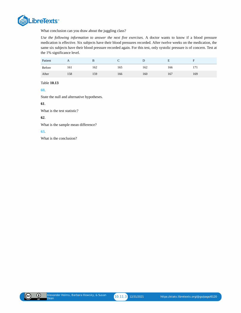
Alexander Holms, Barbara Illowsky, & Susan
Dean10.11.3 12/31/2021 https://stats.libretexts.org/@go/page/6120
What conclusion can you draw about the juggling class?
Use the following information to answer the next five exercises. A doctor wants to know if a blood pressuremedication is effective. Six subjects have their blood pressures recorded. After twelve weeks on the medication, thesame six subjects have their blood pressure recorded again. For this test, only systolic pressure is of concern. Test atthe 1% significance level.
Patient A B C D E F
Before 161 162 165 162 166 171
After 158 159 166 160 167 169
Table 10.13
60.
State the null and alternative hypotheses.
61.
What is the test statistic?
62.
What is the sample mean difference?
63.
What is the conclusion?
Alexander Holms, Barbara Illowsky, & Susan
Dean10.12.1 12/17/2021 https://stats.libretexts.org/@go/page/6119
10.12: Chapter References
10.1 Comparing Two Independent Population Means
Data from Graduating Engineer + Computer Careers. Available online at www.graduatingengineer.com
Data from Microsoft Bookshelf.
Data from the United States Senate website, available online at www.Senate.gov (accessed June 17, 2013).
“List of current United States Senators by Age.” Wikipedia. Available online aten.Wikipedia.org/wiki/List_of...enators_by_age (accessed June 17, 2013).
“Sectoring by Industry Groups.” Nasdaq. Available online at www.nasdaq.com/markets/barcha...&base=industry (accessedJune 17, 2013).
“Strip Clubs: Where Prostitution and Trafficking Happen.” Prostitution Research and Education, 2013. Available online atwww.prostitutionresearch.com/ProsViolPosttrauStress.html (accessed June 17, 2013).
“World Series History.” Baseball-Almanac, 2013. Available online at http://www.baseball-almanac.com/ws/wsmenu.shtml(accessed June 17, 2013).
10.4 Comparing Two Independent Population ProportionsData from Educational Resources, December catalog.
Data from Hilton Hotels. Available online at http://www.hilton.com (accessed June 17, 2013).
Data from Hyatt Hotels. Available online at hyatt.com (accessed June 17, 2013).
Data from Statistics, United States Department of Health and Human Services.
Data from Whitney Exhibit on loan to San Jose Museum of Art.
Data from the American Cancer Society. Available online at http://www.cancer.org/index (accessed June 17, 2013).
Data from the Chancellor’s Office, California Community Colleges, November 1994.
“State of the States.” Gallup, 2013. Available online at http://www.gallup.com/poll/125066/St...ef=interactive (accessedJune 17, 2013).
“West Nile Virus.” Centers for Disease Control and Prevention. Available online athttp://www.cdc.gov/ncidod/dvbid/westnile/index.htm (accessed June 17, 2013).
10.5 Two Population Means with Known Standard Deviations
Data from the United States Census Bureau. Available online at www.census.gov/prod/cen2010/b...c2010br-02.pdf
Hinduja, Sameer. “Sexting Research and Gender Differences.” Cyberbulling Research Center, 2013. Available online athttp://cyberbullying.us/blog/sexting...r-differences/ (accessed June 17, 2013).
“Smart Phone Users, By the Numbers.” Visually, 2013. Available online at http://visual.ly/smart-phone-users-numbers(accessed June 17, 2013).
Smith, Aaron. “35% of American adults own a Smartphone.” Pew Internet, 2013. Available online atwww.pewinternet.org/~/media/F...martphones.pdf (accessed June 17, 2013).
“State-Specific Prevalence of Obesity AmongAduls—Unites States, 2007.” MMWR, CDC. Available online athttp://www.cdc.gov/mmwr/preview/mmwrhtml/mm5728a1.htm (accessed June 17, 2013).
“Texas Crime Rates 1960–1012.” FBI, Uniform Crime Reports, 2013. Available online at:http://www.disastercenter.com/crime/txcrime.htm (accessed June 17, 2013).
Alexander Holms, Barbara Illowsky, & Susan
Dean10.13.1 12/17/2021 https://stats.libretexts.org/@go/page/6117
10.13: Chapter Review
10.1 Comparing Two Independent Population Means
Two population means from independent samples where the population standard deviations are not known
Random Variable: = the difference of the sampling meansDistribution: Student's t-distribution with degrees of freedom (variances not pooled)
10.2 Cohen's Standards for Small, Medium, and Large Effect Sizes
Cohen's d is a measure of “effect size” based on the differences between two means.
It is important to note that Cohen's does not provide a level of confidence as to the magnitude of the size of the effectcomparable to the other tests of hypothesis we have studied. The sizes of the effects are simply indicative.
10.3 Test for Differences in Means: Assuming Equal Population VariancesIn situations when we do not know the population variances but assume the variances are the same, the pooled samplevariance will be smaller than the individual sample variances.
This will give more precise estimates and reduce the probability of discarding a good null.
10.4 Comparing Two Independent Population ProportionsTest of two population proportions from independent samples.
Random variable: = difference between the two estimated proportionsDistribution: normal distribution
10.5 Two Population Means with Known Standard DeviationsA hypothesis test of two population means from independent samples where the population standard deviations are known(typically approximated with the sample standard deviations), will have these characteristics:
Random variable: = the difference of the meansDistribution: normal distribution
10.6 Matched or Paired SamplesA hypothesis test for matched or paired samples (t-test) has these characteristics:
Test the differences by subtracting one measurement from the other measurementRandom Variable: = mean of the differencesDistribution: Student’s t-distribution with degrees of freedomIf the number of differences is small (less than 30), the differences must follow a normal distribution.Two samples are drawn from the same set of objects.Samples are dependent.
−X¯ ¯¯̄
1 X¯ ¯¯̄
2
d
−p′
Ap
′
B
−X¯ ¯¯̄
1 X¯ ¯¯̄
2
x¯̄̄ d
n– 1
Alexander Holms, Barbara Illowsky, & Susan
Dean10.14.1 11/26/2021 https://stats.libretexts.org/@go/page/6123
10.14: Chapter Solution (Practice + Homework)1.
two proportions
3.
matched or paired samples
5.
single mean
7.
independent group means, population standard deviations and/or variances unknown
9.
two proportions
11.
independent group means, population standard deviations and/or variances unknown
13.
independent group means, population standard deviations and/or variances unknown
15.
two proportions
17.
The random variable is the difference between the mean amounts of sugar in the two soft drinks.
19.
means
21.
two-tailed
23.
the difference between the mean life spans of whites and nonwhites
25.
This is a comparison of two population means with unknown population standard deviations.
27.
Check student’s solution.
28.
1. 31.
= difference in the proportions of phones that had system failures within the first eight hours of operationwith and .
proportions
36.
right-tailed
38.
−P ′OS1
P ′OS2
OS1 OS2
Alexander Holms, Barbara Illowsky, & Susan
Dean10.14.2 11/26/2021 https://stats.libretexts.org/@go/page/6123
The random variable is the difference in proportions (percents) of the populations that are of two or more races inNevada and North Dakota.
40.
Our sample sizes are much greater than five each, so we use the normal for two proportions distribution for thishypothesis test.
42.
1. 44.
The difference in mean speeds of the fastball pitches of the two pitchers
–2.46
47.
At the 1% significance level, we can reject the null hypothesis. There is sufficient data to conclude that the meanspeed of Rodriguez’s fastball is faster than Wesley’s.
49.
Subscripts: 1 = Food, 2 = No Food
51.
Subscripts: 1 = Gamma, 2 = Zeta
53.
There is sufficient evidence so we cannot accept the null hypothesis. The data support that the melting point forAlloy Zeta is different from the melting point of Alloy Gamma.
54.
the mean difference of the system failures
56.
With a -value 0.0067, we can cannot accept the null hypothesis. There is enough evidence to support that thesoftware patch is effective in reducing the number of system failures.
60.
63.
We decline to reject the null hypothesis. There is not sufficient evidence to support that the medication is effective.
65.
Subscripts: 1: two-year colleges; 2: four-year colleges
1. 67.
Subscripts: 1: mechanical engineering; 2: electrical engineering
1. 69.1. 71.
: ≤H0 μ1 μ2
: >Ha μ1 μ2
: =H0 μ1 μ2
: ≠Ha μ1 μ2
p
: ≥ 0H0 μd
: < 0Ha μd
Alexander Holms, Barbara Illowsky, & Susan
Dean10.14.3 11/26/2021 https://stats.libretexts.org/@go/page/6123
1. 74.
c
Test: two independent sample means, population standard deviations unknown. Random variable:
Distribution: . The mean age of entering prostitution in Canada is lowerthan the mean age in the United States.
Graph: left-tailed -value : 0.0151
Decision: Cannot reject .
Conclusion: At the 1% level of significance, from the sample data, there is not sufficient evidence toconclude that the mean age of entering prostitution in Canada is lower than the mean age in theUnited States.
78.
d
80.
1. 82.
Subscripts: 1 = Cabrillo College, 2 = Lake Tahoe College
1. 84.
a
Test: two independent sample proportions.
Random variable:
Distribution: . The proportion of eReader users is different for the16- to 29-year-old users from that of the 30 and older users.
Graph: two-tailed
87.
Test: two independent sample proportions
Random variable:
Distribution: . A higher proportion of tablet owners are aged 16 to29 years old than are 30 years old and older.
Graph: right-tailed
Do not reject the .
Conclusion: At the 1% level of significance, from the sample data, there is not sufficientevidence to conclude that a higher proportion of tablet owners are aged 16 to 29 years old thanare 30 years old and older.
89.
Subscripts: 1: men; 2: women
1. 91.
1. 92.1. 94.
Subscripts: 1 = boys, 2 = girls
1. 96.
−X¯ ¯¯̄
1 X¯ ¯¯̄
2
: =H0 μ1 μ2 : <Ha μ1 μ2
p
H0
−p′1 p′
2
: =H0 p1 p2 : ≠Ha p1 p2
−p′1 p′
2
: =H0 p1 p2 : >Ha p1 p2
H0
Alexander Holms, Barbara Illowsky, & Susan
Dean10.14.4 11/26/2021 https://stats.libretexts.org/@go/page/6123
Subscripts: 1 = non-hybrid sedans, 2 = hybrid sedans
1. 98.
1. 99.
-value = 0.1494
103.
Test: two matched pairs or paired samples ( -test)
Random variable:
Distribution:
The mean of the differences of new female breast cancer cases in thesouth between 2013 and 2012 is greater than zero. The estimate for newfemale breast cancer cases in the south is higher in 2013 than in 2012.
Graph: right-tailed
-value: 0.0004
Decision: Cannot accept
Conclusion: At the 5% level of significance, from the sample data, thereis sufficient evidence to conclude that there was a higher estimate of newfemale breast cancer cases in 2013 than in 2012.
105.
Test: matched or paired samples ( -test)
Difference data:
Random Variable:
Distribution:
The mean of the differences of the rate of underemployment in thenortheastern states between 2012 and 2011 is less than zero. Theunderemployment rate went down from 2011 to 2012.
Graph: left-tailed.
Decision: Cannot reject .
Conclusion: At the 5% level of significance, from the sample data, thereis not sufficient evidence to conclude that there was a decrease in theunderemployment rates of the northeastern states from 2011 to 2012.
107.
e
109.
d
111.
f
113.
e
p
t
X¯ ¯¯̄d
t12
: = 0H0 μd : > 0Ha μd
p
H0
t
{– 0.9, – 3.7, – 3.2, – 0.5, 0.6, – 1.9, – 0.5, 0.2, 0.6, 0.4, 1.7, – 2.4, 1.8}
X¯ ¯¯̄
d
: = 0 : < 0H0 μd Ha μd
H0

Alexander Holms, Barbara Illowsky, & Susan
Dean10.14.5 11/26/2021 https://stats.libretexts.org/@go/page/6123
115.
f
117.
a

1 1/7/2022
CHAPTER OVERVIEW11: THE CHI-SQUARE DISTRIBUTION
11.0: PRELUDE TO THE CHI-SQUARE DISTRIBUTION11.1: FACTS ABOUT THE CHI-SQUARE DISTRIBUTION11.2: TEST OF A SINGLE VARIANCE11.3: GOODNESS-OF-FIT TESTThe Goodness-of-Fit hypothesis test, you determine whether the data "fit" a particular distribution or not. For example, you maysuspect your unknown data fit a binomial distribution. You use a chi-square test (meaning the distribution for the hypothesis test ischi-square) to determine if there is a fit or not. The null and the alternative hypotheses for this test may be written in sentences or maybe stated as equations or inequalities.
11.4: TEST OF INDEPENDENCE11.5: TEST FOR HOMOGENEITY11.6: COMPARISON OF THE CHI-SQUARE TESTS11.7: HOMEWORK11.8: CHAPTER FORMULA REVIEW11.9: CHAPTER HOMEWORK11.10: CHAPTER KEY TERMS11.11: CHAPTER PRACTICE11.12: CHAPTER REFERENCES11.13: CHAPTER REVIEW11.14: CHAPTER SOLUTION (PRACTICE + HOMEWORK)
Alexander Holms, Barbara Illowsky, & Susan
Dean11.0.1 1/7/2022 https://stats.libretexts.org/@go/page/4610
11.0: Prelude to the Chi-Square DistributionHave you ever wondered if lottery winning numbers were evenly distributed or if some numbers occurred with a greaterfrequency? How about if the types of movies people preferred were different across different age groups? What about if acoffee machine was dispensing approximately the same amount of coffee each time? You could answer these questions byconducting a hypothesis test.
Figure : The chi-square distribution can be used to find relationships between two things, like grocery prices atdifferent stores. (credit: Pete/flickr)
You will now study a new distribution, one that is used to determine the answers to such questions. This distribution iscalled the chi-square distribution. In this chapter, you will learn the three major applications of the chi-square distribution:
1. the goodness-of-fit test, which determines if data fit a particular distribution, such as in the lottery example2. the test of independence, which determines if events are independent, such as in the movie example3. the test of a single variance, which tests variability, such as in the coffee example
11.0.1
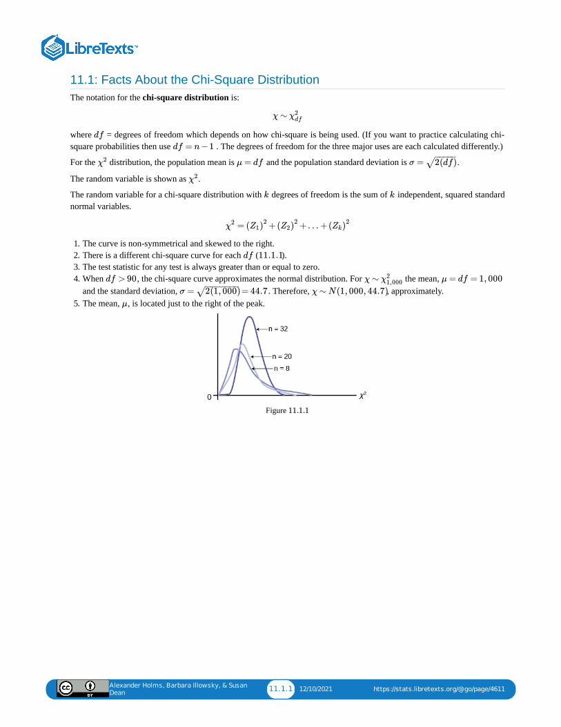
Alexander Holms, Barbara Illowsky, & Susan
Dean11.1.1 12/10/2021 https://stats.libretexts.org/@go/page/4611
11.1: Facts About the Chi-Square DistributionThe notation for the chi-square distribution is:
where = degrees of freedom which depends on how chi-square is being used. (If you want to practice calculating chi-square probabilities then use . The degrees of freedom for the three major uses are each calculated differently.)
For the distribution, the population mean is and the population standard deviation is .
The random variable is shown as .
The random variable for a chi-square distribution with degrees of freedom is the sum of independent, squared standardnormal variables.
1. The curve is non-symmetrical and skewed to the right.2. There is a different chi-square curve for each ( ).3. The test statistic for any test is always greater than or equal to zero.4. When , the chi-square curve approximates the normal distribution. For the mean,
and the standard deviation, . Therefore, , approximately.5. The mean, , is located just to the right of the peak.
Figure
χ ∼ χ2df
df
df = n−1
χ2 μ = df σ = 2(df)− −−−−
√
χ2
k k
= + +… +χ2 ( )Z12
( )Z22
( )Zk2
df 11.1.1
df > 90 χ ∼ χ21,000 μ = df = 1, 000
σ = = 44.72(1, 000)− −−−−−−√ χ ∼ N(1, 000, 44.7)
μ
11.1.1
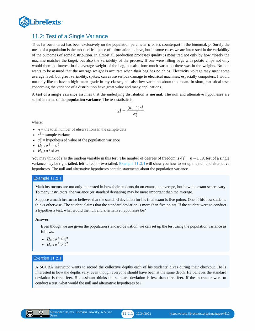
Alexander Holms, Barbara Illowsky, & Susan
Dean11.2.1 12/24/2021 https://stats.libretexts.org/@go/page/4612
11.2: Test of a Single VarianceThus far our interest has been exclusively on the population parameter or it's counterpart in the binomial, . Surely themean of a population is the most critical piece of information to have, but in some cases we are interested in the variabilityof the outcomes of some distribution. In almost all production processes quality is measured not only by how closely themachine matches the target, but also the variability of the process. If one were filling bags with potato chips not onlywould there be interest in the average weight of the bag, but also how much variation there was in the weights. No onewants to be assured that the average weight is accurate when their bag has no chips. Electricity voltage may meet someaverage level, but great variability, spikes, can cause serious damage to electrical machines, especially computers. I wouldnot only like to have a high mean grade in my classes, but also low variation about this mean. In short, statistical testsconcerning the variance of a distribution have great value and many applications.
A test of a single variance assumes that the underlying distribution is normal. The null and alternative hypotheses arestated in terms of the population variance. The test statistic is:
where:
= the total number of observations in the sample data = sample variance = hypothesized value of the population variance
You may think of s as the random variable in this test. The number of degrees of freedom is . A test of a singlevariance may be right-tailed, left-tailed, or two-tailed. Example will show you how to set up the null and alternativehypotheses. The null and alternative hypotheses contain statements about the population variance.
Math instructors are not only interested in how their students do on exams, on average, but how the exam scores vary.To many instructors, the variance (or standard deviation) may be more important than the average.
Suppose a math instructor believes that the standard deviation for his final exam is five points. One of his best studentsthinks otherwise. The student claims that the standard deviation is more than five points. If the student were to conducta hypothesis test, what would the null and alternative hypotheses be?
Answer
Even though we are given the population standard deviation, we can set up the test using the population variance asfollows.
A SCUBA instructor wants to record the collective depths each of his students' dives during their checkout. He isinterested in how the depths vary, even though everyone should have been at the same depth. He believes the standarddeviation is three feet. His assistant thinks the standard deviation is less than three feet. If the instructor were toconduct a test, what would the null and alternative hypotheses be?
μ p
=χ2c
(n−1)s2
σ20
n
s2
σ20
: =H0 σ2 σ20
: ≠Ha σ2 σ20
df = n−1
11.2.1
Example 11.2.1
: ≤H0 σ2 52
: >Ha σ2 52
Exercise 11.2.1
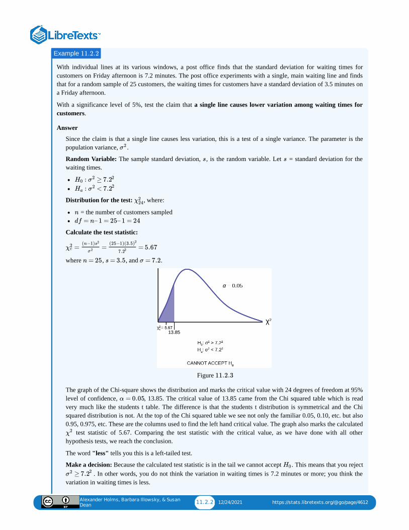
Alexander Holms, Barbara Illowsky, & Susan
Dean11.2.2 12/24/2021 https://stats.libretexts.org/@go/page/4612
With individual lines at its various windows, a post office finds that the standard deviation for waiting times forcustomers on Friday afternoon is 7.2 minutes. The post office experiments with a single, main waiting line and findsthat for a random sample of 25 customers, the waiting times for customers have a standard deviation of 3.5 minutes ona Friday afternoon.
With a significance level of 5%, test the claim that a single line causes lower variation among waiting times forcustomers.
Answer
Since the claim is that a single line causes less variation, this is a test of a single variance. The parameter is thepopulation variance, .
Random Variable: The sample standard deviation, , is the random variable. Let = standard deviation for thewaiting times.
Distribution for the test: , where:
= the number of customers sampled
Calculate the test statistic:
where , , and .
Figure
The graph of the Chi-square shows the distribution and marks the critical value with 24 degrees of freedom at 95%level of confidence, , 13.85. The critical value of 13.85 came from the Chi squared table which is readvery much like the students t table. The difference is that the students t distribution is symmetrical and the Chisquared distribution is not. At the top of the Chi squared table we see not only the familiar 0.05, 0.10, etc. but also0.95, 0.975, etc. These are the columns used to find the left hand critical value. The graph also marks the calculated
test statistic of 5.67. Comparing the test statistic with the critical value, as we have done with all otherhypothesis tests, we reach the conclusion.
The word "less" tells you this is a left-tailed test.
Make a decision: Because the calculated test statistic is in the tail we cannot accept . This means that you reject. In other words, you do not think the variation in waiting times is 7.2 minutes or more; you think the
variation in waiting times is less.
Example 11.2.2
σ2
s s
: ≥H0 σ2 7.22
: <Ha σ2 7.22
χ224
n
df = n– 1 = 25– 1 = 24
= = = 5.67χ2c
(n−1)s2
σ2
(25−1)(3.5)2
7.22
n = 25 s = 3.5 σ = 7.2
11.2.3
α = 0.05
χ2
H0
≥σ2 7.22
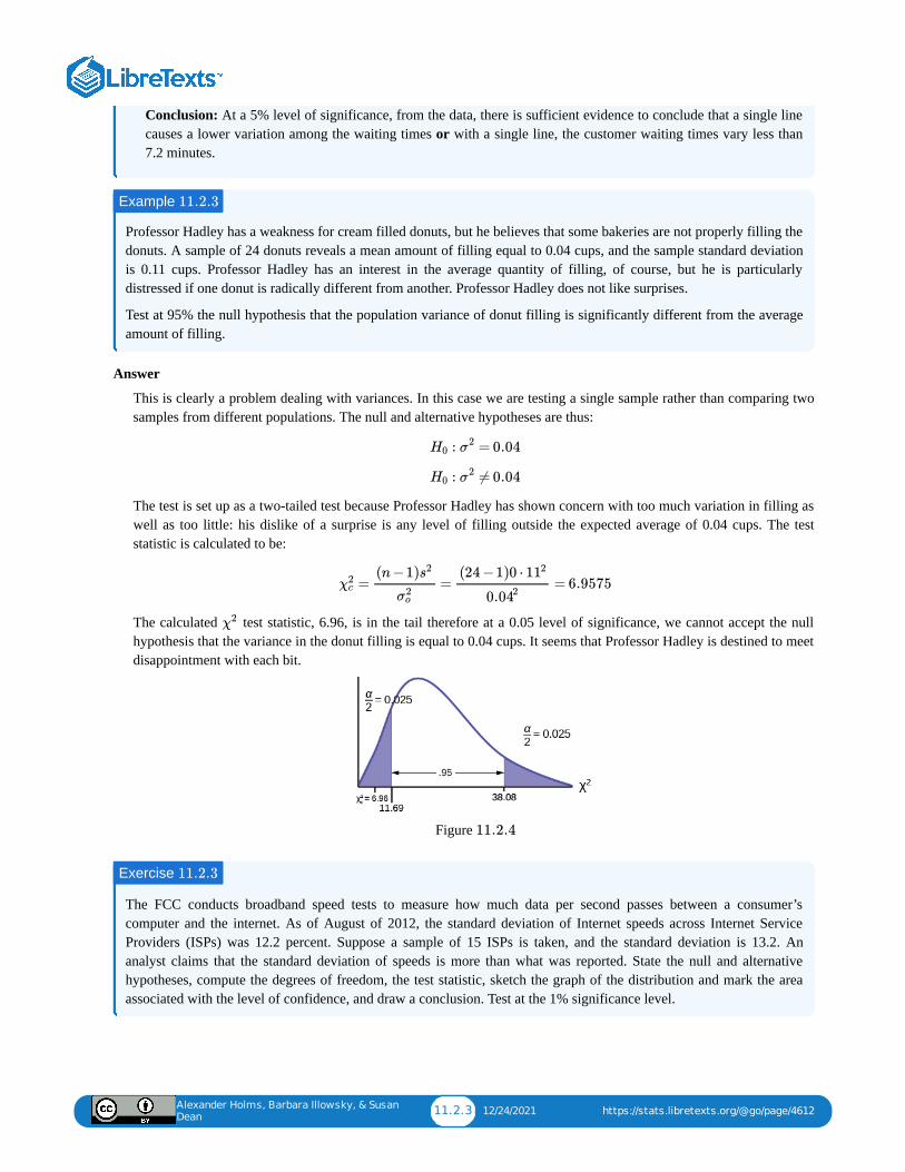
Alexander Holms, Barbara Illowsky, & Susan
Dean11.2.3 12/24/2021 https://stats.libretexts.org/@go/page/4612
Conclusion: At a 5% level of significance, from the data, there is sufficient evidence to conclude that a single linecauses a lower variation among the waiting times or with a single line, the customer waiting times vary less than7.2 minutes.
Professor Hadley has a weakness for cream filled donuts, but he believes that some bakeries are not properly filling thedonuts. A sample of 24 donuts reveals a mean amount of filling equal to 0.04 cups, and the sample standard deviationis 0.11 cups. Professor Hadley has an interest in the average quantity of filling, of course, but he is particularlydistressed if one donut is radically different from another. Professor Hadley does not like surprises.
Test at 95% the null hypothesis that the population variance of donut filling is significantly different from the averageamount of filling.
Answer
This is clearly a problem dealing with variances. In this case we are testing a single sample rather than comparing twosamples from different populations. The null and alternative hypotheses are thus:
The test is set up as a two-tailed test because Professor Hadley has shown concern with too much variation in filling aswell as too little: his dislike of a surprise is any level of filling outside the expected average of 0.04 cups. The teststatistic is calculated to be:
The calculated test statistic, 6.96, is in the tail therefore at a 0.05 level of significance, we cannot accept the nullhypothesis that the variance in the donut filling is equal to 0.04 cups. It seems that Professor Hadley is destined to meetdisappointment with each bit.
Figure
The FCC conducts broadband speed tests to measure how much data per second passes between a consumer’scomputer and the internet. As of August of 2012, the standard deviation of Internet speeds across Internet ServiceProviders (ISPs) was 12.2 percent. Suppose a sample of 15 ISPs is taken, and the standard deviation is 13.2. Ananalyst claims that the standard deviation of speeds is more than what was reported. State the null and alternativehypotheses, compute the degrees of freedom, the test statistic, sketch the graph of the distribution and mark the areaassociated with the level of confidence, and draw a conclusion. Test at the 1% significance level.
Example 11.2.3
: = 0.04H0 σ2
: ≠ 0.04H0 σ2
= = = 6.9575χ2c
(n−1)s2
σ2o
(24 −1)0 ⋅ 112
0.042
χ2
11.2.4
Exercise 11.2.3
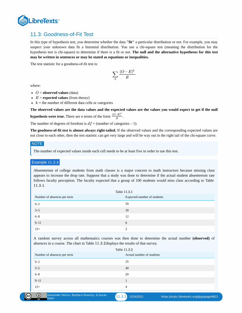
Alexander Holms, Barbara Illowsky, & Susan
Dean11.3.1 12/24/2021 https://stats.libretexts.org/@go/page/4613
11.3: Goodness-of-Fit TestIn this type of hypothesis test, you determine whether the data "fit" a particular distribution or not. For example, you maysuspect your unknown data fit a binomial distribution. You use a chi-square test (meaning the distribution for thehypothesis test is chi-square) to determine if there is a fit or not. The null and the alternative hypotheses for this testmay be written in sentences or may be stated as equations or inequalities.
The test statistic for a goodness-of-fit test is:
where:
= observed values (data) = expected values (from theory) = the number of different data cells or categories
The observed values are the data values and the expected values are the values you would expect to get if the null
hypothesis were true. There are n terms of the form .
The number of degrees of freedom is = (number of categories – 1).
The goodness-of-fit test is almost always right-tailed. If the observed values and the corresponding expected values arenot close to each other, then the test statistic can get very large and will be way out in the right tail of the chi-square curve.
The number of expected values inside each cell needs to be at least five in order to use this test.
Absenteeism of college students from math classes is a major concern to math instructors because missing classappears to increase the drop rate. Suppose that a study was done to determine if the actual student absenteeism ratefollows faculty perception. The faculty expected that a group of 100 students would miss class according to Table
.
Number of absences per term Expected number of students
0–2 50
3–5 30
6–8 12
9–11 6
12+ 2
Table
A random survey across all mathematics courses was then done to determine the actual number (observed) ofabsences in a course. The chart in Table displays the results of that survey.
Number of absences per term Actual number of students
0–2 35
3–5 40
6–8 20
9–11 1
12+ 4
Table
∑k
(O−E)2
E
O
E
k
(O−E)2
E
df
NOTE
Example 11.3.4
11.3.1
11.3.1
11.3.2
11.3.2
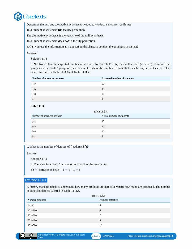
Alexander Holms, Barbara Illowsky, & Susan
Dean11.3.2 12/24/2021 https://stats.libretexts.org/@go/page/4613
Determine the null and alternative hypotheses needed to conduct a goodness-of-fit test.
: Student absenteeism fits faculty perception.
The alternative hypothesis is the opposite of the null hypothesis.
: Student absenteeism does not fit faculty perception.
a. Can you use the information as it appears in the charts to conduct the goodness-of-fit test?
Answer
Solution 11.4
a. No. Notice that the expected number of absences for the "12+" entry is less than five (it is two). Combine thatgroup with the "9–11" group to create new tables where the number of students for each entry are at least five. Thenew results are in Table and Table .
Number of absences per term Expected number of students
0–2 50
3–5 30
6–8 12
9+ 8
Table 11.3
Number of absences per term Actual number of students
0–2 35
3–5 40
6–8 20
9+ 5
Table
b. What is the number of degrees of freedom ( )?
Answer
Solution 11.4
b. There are four "cells" or categories in each of the new tables.
A factory manager needs to understand how many products are defective versus how many are produced. The numberof expected defects is listed in Table .
Number produced Number defective
0–100 5
101–200 6
201–300 7
301–400 8
401–500 10
Table
Ha
Ha
11.3.3 11.3.4
11.3.4
df
df = number of cells −1 = 4 −1 = 3
Exercise 11.3.4
11.3.5
11.3.5
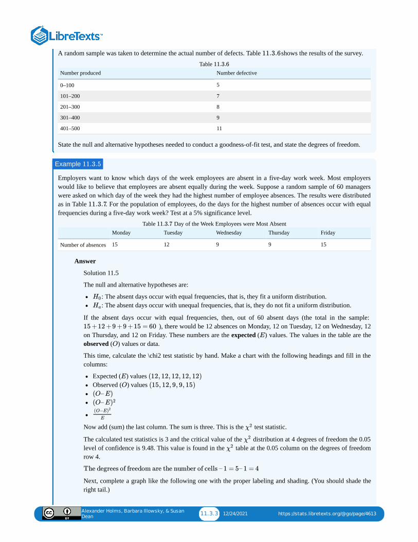
Alexander Holms, Barbara Illowsky, & Susan
Dean11.3.3 12/24/2021 https://stats.libretexts.org/@go/page/4613
A random sample was taken to determine the actual number of defects. Table shows the results of the survey.
Number produced Number defective
0–100 5
101–200 7
201–300 8
301–400 9
401–500 11
Table
State the null and alternative hypotheses needed to conduct a goodness-of-fit test, and state the degrees of freedom.
Employers want to know which days of the week employees are absent in a five-day work week. Most employerswould like to believe that employees are absent equally during the week. Suppose a random sample of 60 managerswere asked on which day of the week they had the highest number of employee absences. The results were distributedas in Table . For the population of employees, do the days for the highest number of absences occur with equalfrequencies during a five-day work week? Test at a 5% significance level.
Monday Tuesday Wednesday Thursday Friday
Number of absences 15 12 9 9 15
Table Day of the Week Employees were Most Absent
Answer
Solution 11.5
The null and alternative hypotheses are:
: The absent days occur with equal frequencies, that is, they fit a uniform distribution.: The absent days occur with unequal frequencies, that is, they do not fit a uniform distribution.
If the absent days occur with equal frequencies, then, out of 60 absent days (the total in the sample: ), there would be 12 absences on Monday, 12 on Tuesday, 12 on Wednesday, 12
on Thursday, and 12 on Friday. These numbers are the expected ( ) values. The values in the table are theobserved ( ) values or data.
This time, calculate the \chi2 test statistic by hand. Make a chart with the following headings and fill in thecolumns:
Expected ( ) values Observed ( ) values
Now add (sum) the last column. The sum is three. This is the test statistic.
The calculated test statistics is 3 and the critical value of the distribution at 4 degrees of freedom the 0.05level of confidence is 9.48. This value is found in the table at the 0.05 column on the degrees of freedomrow 4.
Next, complete a graph like the following one with the proper labeling and shading. (You should shade theright tail.)
11.3.6
11.3.6
Example 11.3.5
11.3.7
11.3.7
H0
Ha
15 +12 +9 +9 +15 = 60
E
O
E (12, 12, 12, 12, 12)
O (15, 12, 9, 9, 15)
(O–E)
(O–E)2
(O−E)2
E
χ2
χ2
χ2
The degrees of freedom are the number of cells – 1 = 5– 1 = 4
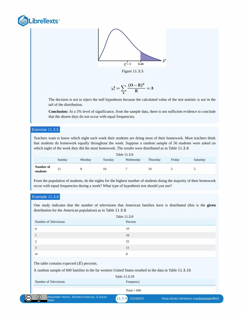
Alexander Holms, Barbara Illowsky, & Susan
Dean11.3.4 12/24/2021 https://stats.libretexts.org/@go/page/4613
Figure
The decision is not to reject the null hypothesis because the calculated value of the test statistic is not in thetail of the distribution.
Conclusion: At a 5% level of significance, from the sample data, there is not sufficient evidence to concludethat the absent days do not occur with equal frequencies.
Teachers want to know which night each week their students are doing most of their homework. Most teachers thinkthat students do homework equally throughout the week. Suppose a random sample of 56 students were asked onwhich night of the week they did the most homework. The results were distributed as in Table .
Sunday Monday Tuesday Wednesday Thursday Friday Saturday
Number ofstudents
11 8 10 7 10 5 5
Table
From the population of students, do the nights for the highest number of students doing the majority of their homeworkoccur with equal frequencies during a week? What type of hypothesis test should you use?
One study indicates that the number of televisions that American families have is distributed (this is the givendistribution for the American population) as in Table .
Number of Televisions Percent
0 10
1 16
2 55
3 11
4+ 8
Table
The table contains expected ( ) percents.
A random sample of 600 families in the far western United States resulted in the data in Table .
Number of Televisions Frequency
Total = 600
Table
11.3.5
= = 3χ2c ∑
k
(O− E)2
E
Exercise 11.3.5
11.3.8
11.3.8
Example 11.3.6
11.3.9
11.3.9
E
11.3.10
11.3.10
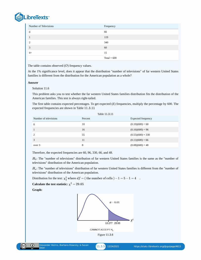
Alexander Holms, Barbara Illowsky, & Susan
Dean11.3.5 12/24/2021 https://stats.libretexts.org/@go/page/4613
Number of Televisions Frequency
Total = 600
0 66
1 119
2 340
3 60
4+ 15
The table contains observed ( ) frequency values.
At the 1% significance level, does it appear that the distribution "number of televisions" of far western United Statesfamilies is different from the distribution for the American population as a whole?
Answer
Solution 11.6
This problem asks you to test whether the far western United States families distribution fits the distribution of theAmerican families. This test is always right-tailed.
The first table contains expected percentages. To get expected (E) frequencies, multiply the percentage by 600. Theexpected frequencies are shown in Table .
Number of televisions Percent Expected frequency
0 10 (0.10)(600) = 60
1 16 (0.16)(600) = 96
2 55 (0.55)(600) = 330
3 11 (0.11)(600) = 66
over 3 8 (0.08)(600) = 48
Table
Therefore, the expected frequencies are 60, 96, 330, 66, and 48.
: The "number of televisions" distribution of far western United States families is the same as the "number oftelevisions" distribution of the American population.
: The "number of televisions" distribution of far western United States families is different from the "number oftelevisions" distribution of the American population.
Distribution for the test: .
Calculate the test statistic:
Graph:
Figure
O
11.3.11
11.3.11
H0
Ha
where df = ( the number of cells ) −1 = 5 −1 = 4χ24
= 29.65χ2
11.3.6
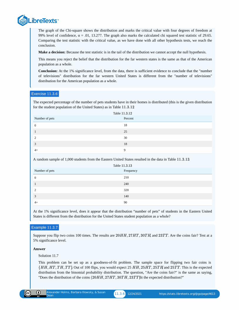
Alexander Holms, Barbara Illowsky, & Susan
Dean11.3.6 12/24/2021 https://stats.libretexts.org/@go/page/4613
The graph of the Chi-square shows the distribution and marks the critical value with four degrees of freedom at99% level of confidence, α = .01, 13.277. The graph also marks the calculated chi squared test statistic of 29.65.Comparing the test statistic with the critical value, as we have done with all other hypothesis tests, we reach theconclusion.
Make a decision: Because the test statistic is in the tail of the distribution we cannot accept the null hypothesis.
This means you reject the belief that the distribution for the far western states is the same as that of the Americanpopulation as a whole.
Conclusion: At the 1% significance level, from the data, there is sufficient evidence to conclude that the "numberof televisions" distribution for the far western United States is different from the "number of televisions"distribution for the American population as a whole.
The expected percentage of the number of pets students have in their homes is distributed (this is the given distributionfor the student population of the United States) as in Table .
Number of pets Percent
0 18
1 25
2 30
3 18
4+ 9
Table
A random sample of 1,000 students from the Eastern United States resulted in the data in Table .
Number of pets Frequency
0 210
1 240
2 320
3 140
4+ 90
Table
At the 1% significance level, does it appear that the distribution “number of pets” of students in the Eastern UnitedStates is different from the distribution for the United States student population as a whole?
Suppose you flip two coins 100 times. The results are , and . Are the coins fair? Test at a5% significance level.
Answer
Solution 11.7
This problem can be set up as a goodness-of-fit problem. The sample space for flipping two fair coins is . Out of 100 flips, you would expect 25 , and . This is the expected
distribution from the binomial probability distribution. The question, "Are the coins fair?" is the same as saying,"Does the distribution of the coins fit the expected distribution?"
Exercise 11.3.6
11.3.12
11.3.12
11.3.13
11.3.13
Example 11.3.7
20HH, 27HT , 30TH 23TT
{HH,HT ,TH,TT} HH, 25HT , 25TH 25TT
(20HH, 27HT , 30TH, 23TT )
Alexander Holms, Barbara Illowsky, & Susan
Dean11.3.7 12/24/2021 https://stats.libretexts.org/@go/page/4613
Random Variable: Let = the number of heads in one flip of the two coins. X takes on the values 0, 1, 2. (Thereare 0, 1, or 2 heads in the flip of two coins.) Therefore, the number of cells is three. Since = the number ofheads, the observed frequencies are 20 (for two heads), 57 (for one head), and 23 (for zero heads or both tails). Theexpected frequencies are 25 (for two heads), 50 (for one head), and 25 (for zero heads or both tails). This test isright-tailed.
: The coins are fair.
: The coins are not fair.
Distribution for the test: where .
Calculate the test statistic: .
Graph:
Figure
The graph of the Chi-square shows the distribution and marks the critical value with two degrees of freedom at95% level of confidence, , 5.991. The graph also marks the calculated test statistic of 2.14. Comparingthe test statistic with the critical value, as we have done with all other hypothesis tests, we reach the conclusion.
Conclusion: There is insufficient evidence to conclude that the coins are not fair: we cannot reject the nullhypothesis that the coins are fair.
X
X
H0
Ha
χ22 df = 3– 1 = 2
= 2.14χ2
11.3.7
α = 0.05 χ2
Alexander Holms, Barbara Illowsky, & Susan
Dean11.4.1 12/31/2021 https://stats.libretexts.org/@go/page/4614
11.4: Test of IndependenceTests of independence involve using a contingency table of observed (data) values. The test statistic for a test ofindependence is similar to that of a goodness-of-fit test:
where:
= observed values = expected values
= the number of rows in the table = the number of columns in the table
There are terms of the form .
A test of independence determines whether two factors are independent or not. You first encountered the termindependence in Table 3.1 earlier. As a review, consider the following example.
The expected value inside each cell needs to be at least five in order for you to use this test.
Suppose = a speeding violation in the last year and = a cell phone user while driving. If and are independentthen is the event that a driver received a speeding violation last year and also used acell phone while driving. Suppose, in a study of drivers who received speeding violations in the last year, and whoused cell phone while driving, that 755 people were surveyed. Out of the 755, 70 had a speeding violation and 685 didnot; 305 used cell phones while driving and 450 did not.
Let y = expected number of drivers who used a cell phone while driving and received speeding violations.
If and are independent, then . By substitution,
Solve for :
About 28 people from the sample are expected to use cell phones while driving and to receive speeding violations.
In a test of independence, we state the null and alternative hypotheses in words. Since the contingency table consists oftwo factors, the null hypothesis states that the factors are independent and the alternative hypothesis states that theyare not independent (dependent). If we do a test of independence using the example, then the null hypothesis is:
: Being a cell phone user while driving and receiving a speeding violation are independent events; in other words,they have no effect on each other.
If the null hypothesis were true, we would expect about 28 people to use cell phones while driving and to receive aspeeding violation.
The test of independence is always right-tailed because of the calculation of the test statistic. If the expected andobserved values are not close together, then the test statistic is very large and way out in the right tail of the chi-squarecurve, as it is in a goodness-of-fit.
The number of degrees of freedom for the test of independence is:
The following formula calculates the expected number (E):
∑(i⋅j)
(O−E)2
E
O
E
i
j
i ⋅ j(O−E)2
E
Note
Example 11.8
A B A B
P (A∩B) = P (A)P (B).A∩B
A B P (A∩B) = P (A)P (B)
=( )( )y
755
70
755
305
755
y y = = 28.3(70)(305)
755
H0
df = ( number of columns −1)( number of rows −1)
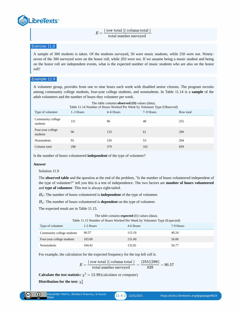
Alexander Holms, Barbara Illowsky, & Susan
Dean11.4.2 12/31/2021 https://stats.libretexts.org/@go/page/4614
A sample of 300 students is taken. Of the students surveyed, 50 were music students, while 250 were not. Ninety-seven of the 300 surveyed were on the honor roll, while 203 were not. If we assume being a music student and beingon the honor roll are independent events, what is the expected number of music students who are also on the honorroll?
A volunteer group, provides from one to nine hours each week with disabled senior citizens. The program recruitsamong community college students, four-year college students, and nonstudents. In Table 11.14 is a sample of theadult volunteers and the number of hours they volunteer per week.
The table contains observed (O) values (data).
Type of volunteer 1–3 Hours 4–6 Hours 7–9 Hours Row total
Community collegestudents
111 96 48 255
Four-year collegestudents
96 133 61 290
Nonstudents 91 150 53 294
Column total 298 379 162 839
Table 11.14 Number of Hours Worked Per Week by Volunteer Type (Observed)
Is the number of hours volunteered independent of the type of volunteer?
Answer
Solution 11.9
The observed table and the question at the end of the problem, "Is the number of hours volunteered independent ofthe type of volunteer?" tell you this is a test of independence. The two factors are number of hours volunteeredand type of volunteer. This test is always right-tailed.
: The number of hours volunteered is independent of the type of volunteer.
: The number of hours volunteered is dependent on the type of volunteer.
The expected result are in Table 11.15.
The table contains expected (E) values (data).
Type of volunteer 1-3 Hours 4-6 Hours 7-9 Hours
Community college students 90.57 115.19 49.24
Four-year college students 103.00 131.00 56.00
Nonstudents 104.42 132.81 56.77
Table 11.15 Number of Hours Worked Per Week by Volunteer Type (Expected)
For example, the calculation for the expected frequency for the top left cell is
Calculate the test statistic: (calculator or computer)
Distribution for the test:
E =( row total )( column total )
total number surveyed
Exercise 11.8
Example 11.9
H0
Ha
E = = = 90.57( row total )( column total )
total number surveyed
(255)(298)
839
= 12.99χ2
χ24
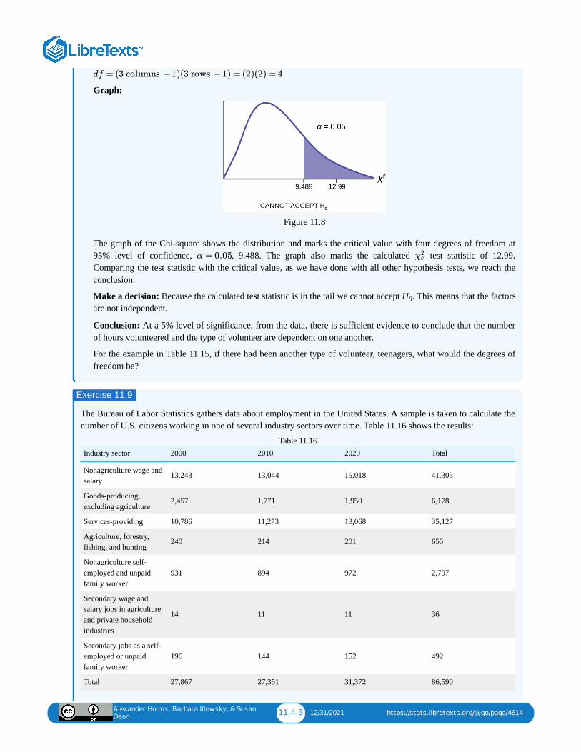
Alexander Holms, Barbara Illowsky, & Susan
Dean11.4.3 12/31/2021 https://stats.libretexts.org/@go/page/4614
Graph:
Figure 11.8
The graph of the Chi-square shows the distribution and marks the critical value with four degrees of freedom at95% level of confidence, , 9.488. The graph also marks the calculated test statistic of 12.99.Comparing the test statistic with the critical value, as we have done with all other hypothesis tests, we reach theconclusion.
Make a decision: Because the calculated test statistic is in the tail we cannot accept H . This means that the factorsare not independent.
Conclusion: At a 5% level of significance, from the data, there is sufficient evidence to conclude that the numberof hours volunteered and the type of volunteer are dependent on one another.
For the example in Table 11.15, if there had been another type of volunteer, teenagers, what would the degrees offreedom be?
The Bureau of Labor Statistics gathers data about employment in the United States. A sample is taken to calculate thenumber of U.S. citizens working in one of several industry sectors over time. Table 11.16 shows the results:
Industry sector 2000 2010 2020 Total
Nonagriculture wage andsalary
13,243 13,044 15,018 41,305
Goods-producing,excluding agriculture
2,457 1,771 1,950 6,178
Services-providing 10,786 11,273 13,068 35,127
Agriculture, forestry,fishing, and hunting
240 214 201 655
Nonagriculture self-employed and unpaidfamily worker
931 894 972 2,797
Secondary wage andsalary jobs in agricultureand private householdindustries
14 11 11 36
Secondary jobs as a self-employed or unpaidfamily worker
196 144 152 492
Total 27,867 27,351 31,372 86,590
Table 11.16
df = (3 columns −1)(3 rows −1) = (2)(2) = 4
α = 0.05 χ2c
0
Exercise 11.9
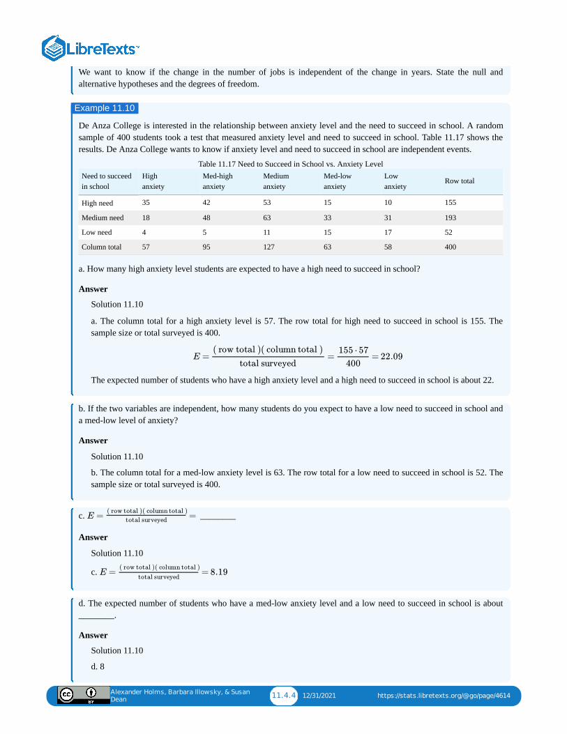
Alexander Holms, Barbara Illowsky, & Susan
Dean11.4.4 12/31/2021 https://stats.libretexts.org/@go/page/4614
We want to know if the change in the number of jobs is independent of the change in years. State the null andalternative hypotheses and the degrees of freedom.
De Anza College is interested in the relationship between anxiety level and the need to succeed in school. A randomsample of 400 students took a test that measured anxiety level and need to succeed in school. Table 11.17 shows theresults. De Anza College wants to know if anxiety level and need to succeed in school are independent events.
Need to succeedin school
High anxiety
Med-high anxiety
Medium anxiety
Med-low anxiety
Low anxiety
Row total
High need 35 42 53 15 10 155
Medium need 18 48 63 33 31 193
Low need 4 5 11 15 17 52
Column total 57 95 127 63 58 400
Table 11.17 Need to Succeed in School vs. Anxiety Level
a. How many high anxiety level students are expected to have a high need to succeed in school?
Answer
Solution 11.10
a. The column total for a high anxiety level is 57. The row total for high need to succeed in school is 155. Thesample size or total surveyed is 400.
The expected number of students who have a high anxiety level and a high need to succeed in school is about 22.
b. If the two variables are independent, how many students do you expect to have a low need to succeed in school anda med-low level of anxiety?
Answer
Solution 11.10
b. The column total for a med-low anxiety level is 63. The row total for a low need to succeed in school is 52. Thesample size or total surveyed is 400.
c. ________
Answer
Solution 11.10
c.
d. The expected number of students who have a med-low anxiety level and a low need to succeed in school is about________.
Answer
Solution 11.10
d. 8
Example 11.10
E = = = 22.09( row total )( column total )
total surveyed
155 ⋅ 57
400
E = =( row total )( column total )
total surveyed
E = = 8.19( row total )( column total )
total surveyed
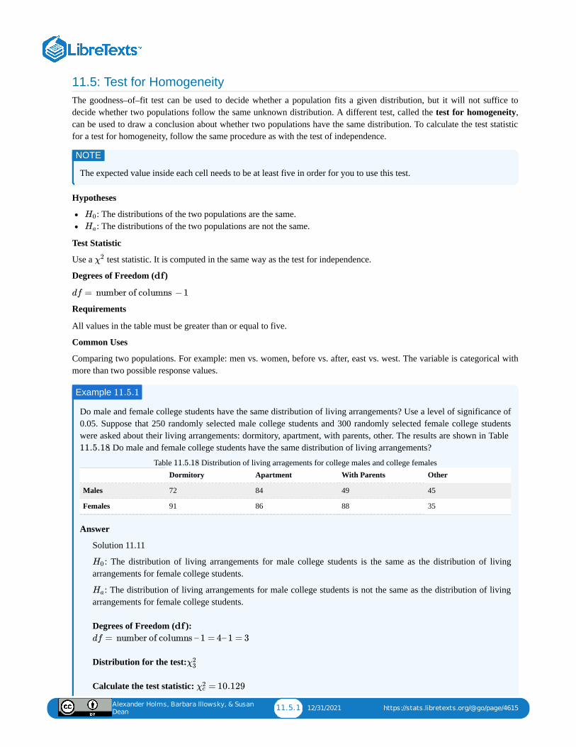
Alexander Holms, Barbara Illowsky, & Susan
Dean11.5.1 12/31/2021 https://stats.libretexts.org/@go/page/4615
11.5: Test for HomogeneityThe goodness–of–fit test can be used to decide whether a population fits a given distribution, but it will not suffice todecide whether two populations follow the same unknown distribution. A different test, called the test for homogeneity,can be used to draw a conclusion about whether two populations have the same distribution. To calculate the test statisticfor a test for homogeneity, follow the same procedure as with the test of independence.
The expected value inside each cell needs to be at least five in order for you to use this test.
Hypotheses
: The distributions of the two populations are the same.: The distributions of the two populations are not the same.
Test Statistic
Use a test statistic. It is computed in the same way as the test for independence.
Degrees of Freedom ( )
Requirements
All values in the table must be greater than or equal to five.
Common Uses
Comparing two populations. For example: men vs. women, before vs. after, east vs. west. The variable is categorical withmore than two possible response values.
Do male and female college students have the same distribution of living arrangements? Use a level of significance of0.05. Suppose that 250 randomly selected male college students and 300 randomly selected female college studentswere asked about their living arrangements: dormitory, apartment, with parents, other. The results are shown in Table
. Do male and female college students have the same distribution of living arrangements?
Dormitory Apartment With Parents Other
Males 72 84 49 45
Females 91 86 88 35
Table Distribution of living arragements for college males and college females
Answer
Solution 11.11
: The distribution of living arrangements for male college students is the same as the distribution of livingarrangements for female college students.
: The distribution of living arrangements for male college students is not the same as the distribution of livingarrangements for female college students. Degrees of Freedom ( ):
Distribution for the test: Calculate the test statistic:
NOTE
H0
Ha
χ2
df
df = number of columns −1
Example 11.5.1
11.5.18
11.5.18
H0
Ha
df
df = number of columns – 1 = 4– 1 = 3
χ23
= 10.129χ2c
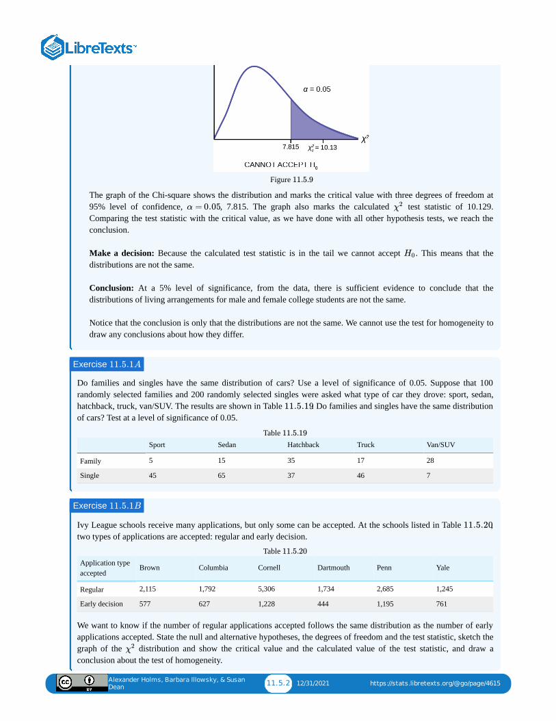
Alexander Holms, Barbara Illowsky, & Susan
Dean11.5.2 12/31/2021 https://stats.libretexts.org/@go/page/4615
Figure
The graph of the Chi-square shows the distribution and marks the critical value with three degrees of freedom at95% level of confidence, , 7.815. The graph also marks the calculated test statistic of 10.129.Comparing the test statistic with the critical value, as we have done with all other hypothesis tests, we reach theconclusion. Make a decision: Because the calculated test statistic is in the tail we cannot accept . This means that thedistributions are not the same. Conclusion: At a 5% level of significance, from the data, there is sufficient evidence to conclude that thedistributions of living arrangements for male and female college students are not the same. Notice that the conclusion is only that the distributions are not the same. We cannot use the test for homogeneity todraw any conclusions about how they differ.
Do families and singles have the same distribution of cars? Use a level of significance of 0.05. Suppose that 100randomly selected families and 200 randomly selected singles were asked what type of car they drove: sport, sedan,hatchback, truck, van/SUV. The results are shown in Table . Do families and singles have the same distributionof cars? Test at a level of significance of 0.05.
Sport Sedan Hatchback Truck Van/SUV
Family 5 15 35 17 28
Single 45 65 37 46 7
Table
Ivy League schools receive many applications, but only some can be accepted. At the schools listed in Table ,two types of applications are accepted: regular and early decision.
Application typeaccepted
Brown Columbia Cornell Dartmouth Penn Yale
Regular 2,115 1,792 5,306 1,734 2,685 1,245
Early decision 577 627 1,228 444 1,195 761
Table
We want to know if the number of regular applications accepted follows the same distribution as the number of earlyapplications accepted. State the null and alternative hypotheses, the degrees of freedom and the test statistic, sketch thegraph of the distribution and show the critical value and the calculated value of the test statistic, and draw aconclusion about the test of homogeneity.
11.5.9
α = 0.05 χ2
H0
Exercise 11.5.1A
11.5.19
11.5.19
Exercise 11.5.1B
11.5.20
11.5.20
χ2
Alexander Holms, Barbara Illowsky, & Susan
Dean11.6.1 1/7/2022 https://stats.libretexts.org/@go/page/6131
11.6: Comparison of the Chi-Square TestsAbove the test statistic was used in three different circumstances. The following list is a summary of which test isthe appropriate one to use in different circumstances.
Test for Goodness-of-FitUse the goodness-of-fit test to decide whether a population with an unknown distribution "fits" a known distribution. Inthis case there will be a single qualitative survey question or a single outcome of an experiment from a single population.Goodness-of-Fit is typically used to see if the population is uniform (all outcomes occur with equal frequency), thepopulation is normal, or the population is the same as another population with a known distribution. The null andalternative hypotheses are:
: The population fits the given distribution.: The population does not fit the given distribution.
Test for Independence
Use the test for independence to decide whether two variables (factors) are independent or dependent. In this case therewill be two qualitative survey questions or experiments and a contingency table will be constructed. The goal is to see ifthe two variables are unrelated (independent) or related (dependent). The null and alternative hypotheses are:
: The two variables (factors) are independent.: The two variables (factors) are dependent.
Test for Homogeneity
Use the test for homogeneity to decide if two populations with unknown distributions have the same distribution as eachother. In this case there will be a single qualitative survey question or experiment given to two different populations. Thenull and alternative hypotheses are:
: The two populations follow the same distribution.: The two populations have different distributions.
χ2 χ2
H0
Ha
H0
Ha
H0
Ha

Alexander Holms, Barbara Illowsky, & Susan
Dean11.7.1 12/24/2021 https://stats.libretexts.org/@go/page/6138
11.7: Homework122.
1. Explain why a goodness-of-fit test and a test of independence are generally right-tailed tests.2. If you did a left-tailed test, what would you be testing?
Alexander Holms, Barbara Illowsky, & Susan
Dean11.8.1 12/10/2021 https://stats.libretexts.org/@go/page/6135
11.8: Chapter Formula Review
Facts About the Chi-Square Distribution
chi-square distribution random variable
chi-square distribution population mean
Chi-Square distribution population standard deviation
Test of a Single Variance
Test of a single variance statistic where:
: sample size : sample standard deviation : hypothesized value of the population standard deviation
Degrees of freedom
Test of a Single Variance
Use the test to determine variation.The degrees of freedom is the number of samples – 1.
The test statistic is , where = sample size, = sample variance, and = population variance.
The test may be left-, right-, or two-tailed.
Goodness-of-Fit Test
goodness-of-fit test statistic where:
: observed values : expected values
: number of different data cells or categories
degrees of freedom
Test of Independence
Test of Independence
The number of degrees of freedom is equal to (number of columns - 1)(number of rows - 1).
The test statistic is where = observed values, = expected values, = the number of rows in the table,and = the number of columns in the table.
If the null hypothesis is true, the expected number .
Test for Homogeneity
Homogeneity test statistic where: = observed values = expected values
= number of rows in data contingency table = number of columns in data contingency table
Degrees of freedom
= + +…x2 ( )Z12 ( )Z2
2 ( )Zdf2
= dfμ2χ
=σχ2 2(df)− −−−−
√
=χ2 (n−1)s2
σ20
n
s
σ0
df = n– 1
(n−1)s2
σ20
n s2 σ2
∑k
(O−E)2
E
O
E
k
df = k−1
∑i⋅j(O−E)
2
EO E i
j
E =( row total )( column total )
total surveyed
∑i.j(O−E)
2
EO
E
i
j
df = (i−1)(j−1)
Alexander Holms, Barbara Illowsky, & Susan
Dean11.9.1 12/17/2021 https://stats.libretexts.org/@go/page/6137
11.9: Chapter Homework
Facts About the Chi-Square Distribution
Decide whether the following statements are true or false.
63.
As the number of degrees of freedom increases, the graph of the chi-square distribution looks more and more symmetrical.
64.
The standard deviation of the chi-square distribution is twice the mean.
65.
The mean and the median of the chi-square distribution are the same if = 24.
Test of a Single VarianceUse the following information to answer the next twelve exercises: Suppose an airline claims that its flights are consistentlyon time with an average delay of at most 15 minutes. It claims that the average delay is so consistent that the variance is nomore than 150 minutes. Doubting the consistency part of the claim, a disgruntled traveler calculates the delays for his next25 flights. The average delay for those 25 flights is 22 minutes with a standard deviation of 15 minutes.
66.
Is the traveler disputing the claim about the average or about the variance?
67.
A sample standard deviation of 15 minutes is the same as a sample variance of __________ minutes.
68.
Is this a right-tailed, left-tailed, or two-tailed test?
69.
: __________
70.
= ________
71.
chi-square test statistic = ________
72.
Graph the situation. Label and scale the horizontal axis. Mark the mean and test statistic. Shade the area associated withthe level of confidence.
73.
Let Decision: ________ Conclusion (write out in a complete sentence.): ________
74.
How did you know to test the variance instead of the mean?
75.
If an additional test were done on the claim of the average delay, which distribution would you use?
76.
df
H0
df
α = 0.05
Alexander Holms, Barbara Illowsky, & Susan
Dean11.9.2 12/17/2021 https://stats.libretexts.org/@go/page/6137
If an additional test were done on the claim of the average delay, but 45 flights were surveyed, which distribution wouldyou use?
77.
A plant manager is concerned her equipment may need recalibrating. It seems that the actual weight of the 15 oz. cerealboxes it fills has been fluctuating. The standard deviation should be at most 0.5 oz. In order to determine if the machineneeds to be recalibrated, 84 randomly selected boxes of cereal from the next day’s production were weighed. The standarddeviation of the 84 boxes was 0.54. Does the machine need to be recalibrated?
78.
Consumers may be interested in whether the cost of a particular calculator varies from store to store. Based on surveying43 stores, which yielded a sample mean of $84 and a sample standard deviation of $12, test the claim that the standarddeviation is greater than $15.
79.
Isabella, an accomplished Bay to Breakers runner, claims that the standard deviation for her time to run the 7.5 mile raceis at most three minutes. To test her claim, Rupinder looks up five of her race times. They are 55 minutes, 61 minutes, 58minutes, 63 minutes, and 57 minutes.
80.
Airline companies are interested in the consistency of the number of babies on each flight, so that they have adequatesafety equipment. They are also interested in the variation of the number of babies. Suppose that an airline executivebelieves the average number of babies on flights is six with a variance of nine at most. The airline conducts a survey. Theresults of the 18 flights surveyed give a sample average of 6.4 with a sample standard deviation of 3.9. Conduct ahypothesis test of the airline executive’s belief.
81.
The number of births per woman in China is 1.6 down from 5.91 in 1966. This fertility rate has been attributed to the lawpassed in 1979 restricting births to one per woman. Suppose that a group of students studied whether or not the standarddeviation of births per woman was greater than 0.75. They asked 50 women across China the number of births they hadhad. The results are shown in Table . Does the students’ survey indicate that the standard deviation is greater than0.75?
Table # of births Frequency
0 5
1 30
2 10
3 5
82.
According to an avid aquarist, the average number of fish in a 20-gallon tank is 10, with a standard deviation of two. Hisfriend, also an aquarist, does not believe that the standard deviation is two. She counts the number of fish in 15 other 20-gallon tanks. Based on the results that follow, do you think that the standard deviation is different from two? Data: 11; 10;9; 10; 10; 11; 11; 10; 12; 9; 7; 9; 11; 10; 11
83.
The manager of "Frenchies" is concerned that patrons are not consistently receiving the same amount of French fries witheach order. The chef claims that the standard deviation for a ten-ounce order of fries is at most 1.5 oz., but the managerthinks that it may be higher. He randomly weighs 49 orders of fries, which yields a mean of 11 oz. and a standard deviationof two oz.
84.
11.9.28
11.9.28
Alexander Holms, Barbara Illowsky, & Susan
Dean11.9.3 12/17/2021 https://stats.libretexts.org/@go/page/6137
You want to buy a specific computer. A sales representative of the manufacturer claims that retail stores sell this computerat an average price of $1,249 with a very narrow standard deviation of $25. You find a website that has a price comparisonfor the same computer at a series of stores as follows: $1,299; $1,229.99; $1,193.08; $1,279; $1,224.95; $1,229.99;$1,269.95; $1,249. Can you argue that pricing has a larger standard deviation than claimed by the manufacturer? Use the5% significance level. As a potential buyer, what would be the practical conclusion from your analysis?
85.
A company packages apples by weight. One of the weight grades is Class A apples. Class A apples have a mean weight of150 g, and there is a maximum allowed weight tolerance of 5% above or below the mean for apples in the same consumerpackage. A batch of apples is selected to be included in a Class A apple package. Given the following apple weights of thebatch, does the fruit comply with the Class A grade weight tolerance requirements. Conduct an appropriate hypothesis test.
a. at the 5% significance levelb. at the 1% significance level
Weights in selected apple batch (in grams): 158; 167; 149; 169; 164; 139; 154; 150; 157; 171; 152; 161; 141; 166; 172;
11.3 Goodness-of-Fit Test
86.A six-sided die is rolled 120 times. Fill in the expected frequency column. Then, conduct a hypothesis test to determine ifthe die is fair. The data in Table are the result of the 120 rolls.
Table Face value Frequency Expected frequency
1 15
2 29
3 16
4 15
5 30
6 15
87.
The marital status distribution of the U.S. male population, ages 15 and older, is as shown in Table .
Marital status Percent Expected frequency
Never married 31.3
Married 56.1
Widowed 2.5
Divorced/Separated 10.1
Table
Suppose that a random sample of 400 U.S. young adult males, 18 to 24 years old, yielded the following frequencydistribution. We are interested in whether this age group of males fits the distribution of the U.S. adult population.Calculate the frequency one would expect when surveying 400 people. Fill in Table , rounding to two decimalplaces.
Marital status Frequency
Never married 140
Married 238
Widowed 2
Table
11.9.29
11.9.29
11.9.30
11.9.30
11.9.30
11.9.31
Alexander Holms, Barbara Illowsky, & Susan
Dean11.9.4 12/17/2021 https://stats.libretexts.org/@go/page/6137
Marital status Frequency
Divorced/Separated 20
Use the following information to answer the next two exercises: The columns in Table contain the Race/Ethnicityof U.S. Public Schools for a recent year, the percentages for the Advanced Placement Examinee Population for that class,and the Overall Student Population. Suppose the right column contains the result of a survey of 1,000 local students fromthat year who took an AP Exam.
Race/Ethnicity AP examinee population Overall student population Survey frequency
Asian, Asian American, orPacific Islander
10.2% 5.4% 113
Black or African-American 8.2% 14.5% 94
Hispanic or Latino 15.5% 15.9% 136
American Indian or AlaskaNative
0.6% 1.2% 10
White 59.4% 61.6% 604
Not reported/other 6.1% 1.4% 43
Table
88.
Perform a goodness-of-fit test to determine whether the local results follow the distribution of the U.S. overall studentpopulation based on ethnicity.
89.
Perform a goodness-of-fit test to determine whether the local results follow the distribution of U.S. AP examineepopulation, based on ethnicity.
90.
The City of South Lake Tahoe, CA, has an Asian population of 1,419 people, out of a total population of 23,609. Supposethat a survey of 1,419 self-reported Asians in the Manhattan, NY, area yielded the data in Table . Conduct agoodness-of-fit test to determine if the self-reported sub-groups of Asians in the Manhattan area fit that of the Lake Tahoearea.
Race Lake Tahoe frequency Manhattan frequency
Asian Indian 131 174
Chinese 118 557
Filipino 1,045 518
Japanese 80 54
Korean 12 29
Vietnamese 9 21
Other 24 66
Table
Use the following information to answer the next two exercises: UCLA conducted a survey of more than 263,000 collegefreshmen from 385 colleges in fall 2005. The results of students' expected majors by gender were reported in TheChronicle of Higher Education (2/2/2006). Suppose a survey of 5,000 graduating females and 5,000 graduating males wasdone as a follow-up last year to determine what their actual majors were. The results are shown in the tables for Table
shows the business categories in the survey, the sample size of each category, and the number of businesses ineach category that recycle one commodity. Based on the study, on average half of the businesses were expected to berecycling one commodity. As a result, the last column shows the expected number of businesses in each category that
11.9.32
11.9.32
11.9.33
11.9.33
11.9.36
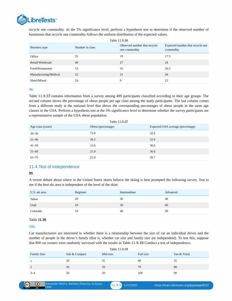
Alexander Holms, Barbara Illowsky, & Susan
Dean11.9.5 12/17/2021 https://stats.libretexts.org/@go/page/6137
recycle one commodity. At the 5% significance level, perform a hypothesis test to determine if the observed number ofbusinesses that recycle one commodity follows the uniform distribution of the expected values.
Business type Number in class Observed number that recycleone commodity
Expected number that recycle onecommodity
Office 35 19 17.5
Retail/Wholesale 48 27 24
Food/Restaurants 53 35 26.5
Manufacturing/Medical 52 21 26
Hotel/Mixed 24 9 12
Table
98.
Table contains information from a survey among 499 participants classified according to their age groups. Thesecond column shows the percentage of obese people per age class among the study participants. The last column comesfrom a different study at the national level that shows the corresponding percentages of obese people in the same ageclasses in the USA. Perform a hypothesis test at the 5% significance level to determine whether the survey participants area representative sample of the USA obese population.
Age class (years) Obese (percentage) Expected USA average (percentage)
20–30 75.0 32.6
31–40 26.5 32.6
41–50 13.6 36.6
51–60 21.9 36.6
61–70 21.0 39.7
Table
11.4 Test of Independence99.
A recent debate about where in the United States skiers believe the skiing is best prompted the following survey. Test tosee if the best ski area is independent of the level of the skier.
U.S. ski area Beginner Intermediate Advanced
Tahoe 20 30 40
Utah 10 30 60
Colorado 10 40 50
Table 11.38
100.
Car manufacturers are interested in whether there is a relationship between the size of car an individual drives and thenumber of people in the driver’s family (that is, whether car size and family size are independent). To test this, supposethat 800 car owners were randomly surveyed with the results in Table . Conduct a test of independence.
Family Size Sub & Compact Mid-size Full-size Van & Truck
1 20 35 40 35
2 20 50 70 80
3–4 20 50 100 90
Table
11.9.36
11.9.37
11.9.37
11.9.39
11.9.39
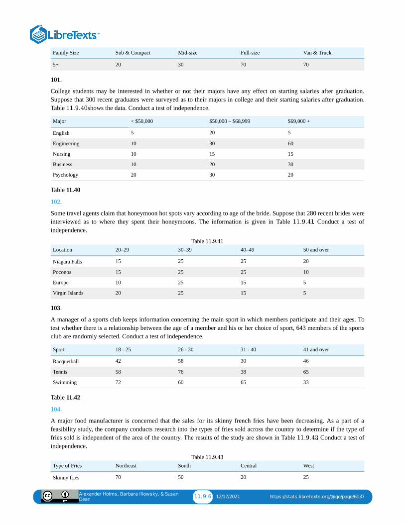
Alexander Holms, Barbara Illowsky, & Susan
Dean11.9.6 12/17/2021 https://stats.libretexts.org/@go/page/6137
Family Size Sub & Compact Mid-size Full-size Van & Truck
5+ 20 30 70 70
101.
College students may be interested in whether or not their majors have any effect on starting salaries after graduation.Suppose that 300 recent graduates were surveyed as to their majors in college and their starting salaries after graduation.Table shows the data. Conduct a test of independence.
Major < $50,000 $50,000 – $68,999 $69,000 +
English 5 20 5
Engineering 10 30 60
Nursing 10 15 15
Business 10 20 30
Psychology 20 30 20
Table 11.40
102.
Some travel agents claim that honeymoon hot spots vary according to age of the bride. Suppose that 280 recent brides wereinterviewed as to where they spent their honeymoons. The information is given in Table . Conduct a test ofindependence.
Location 20–29 30–39 40–49 50 and over
Niagara Falls 15 25 25 20
Poconos 15 25 25 10
Europe 10 25 15 5
Virgin Islands 20 25 15 5
Table
103.
A manager of a sports club keeps information concerning the main sport in which members participate and their ages. Totest whether there is a relationship between the age of a member and his or her choice of sport, 643 members of the sportsclub are randomly selected. Conduct a test of independence.
Sport 18 - 25 26 - 30 31 - 40 41 and over
Racquetball 42 58 30 46
Tennis 58 76 38 65
Swimming 72 60 65 33
Table 11.42
104.
A major food manufacturer is concerned that the sales for its skinny french fries have been decreasing. As a part of afeasibility study, the company conducts research into the types of fries sold across the country to determine if the type offries sold is independent of the area of the country. The results of the study are shown in Table . Conduct a test ofindependence.
Type of Fries Northeast South Central West
Skinny fries 70 50 20 25
Table
11.9.40
11.9.41
11.9.41
11.9.43
11.9.43
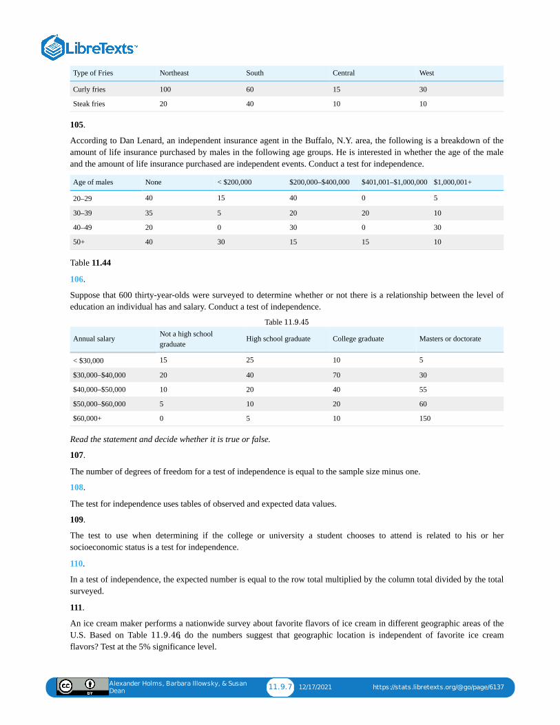
Alexander Holms, Barbara Illowsky, & Susan
Dean11.9.7 12/17/2021 https://stats.libretexts.org/@go/page/6137
Type of Fries Northeast South Central West
Curly fries 100 60 15 30
Steak fries 20 40 10 10
105.
According to Dan Lenard, an independent insurance agent in the Buffalo, N.Y. area, the following is a breakdown of theamount of life insurance purchased by males in the following age groups. He is interested in whether the age of the maleand the amount of life insurance purchased are independent events. Conduct a test for independence.
Age of males None < $200,000 $200,000–$400,000 $401,001–$1,000,000 $1,000,001+
20–29 40 15 40 0 5
30–39 35 5 20 20 10
40–49 20 0 30 0 30
50+ 40 30 15 15 10
Table 11.44
106.
Suppose that 600 thirty-year-olds were surveyed to determine whether or not there is a relationship between the level ofeducation an individual has and salary. Conduct a test of independence.
Annual salary Not a high schoolgraduate
High school graduate College graduate Masters or doctorate
< $30,000 15 25 10 5
$30,000–$40,000 20 40 70 30
$40,000–$50,000 10 20 40 55
$50,000–$60,000 5 10 20 60
$60,000+ 0 5 10 150
Table
Read the statement and decide whether it is true or false.
107.
The number of degrees of freedom for a test of independence is equal to the sample size minus one.
108.
The test for independence uses tables of observed and expected data values.
109.
The test to use when determining if the college or university a student chooses to attend is related to his or hersocioeconomic status is a test for independence.
110.
In a test of independence, the expected number is equal to the row total multiplied by the column total divided by the totalsurveyed.
111.
An ice cream maker performs a nationwide survey about favorite flavors of ice cream in different geographic areas of theU.S. Based on Table , do the numbers suggest that geographic location is independent of favorite ice creamflavors? Test at the 5% significance level.
11.9.45
11.9.46
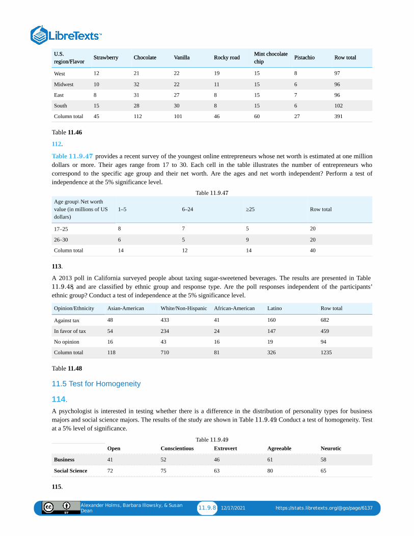
Alexander Holms, Barbara Illowsky, & Susan
Dean11.9.8 12/17/2021 https://stats.libretexts.org/@go/page/6137
U.S.region/Flavor
Strawberry Chocolate Vanilla Rocky road Mint chocolatechip
Pistachio Row totalU.S.region/Flavor
Strawberry Chocolate Vanilla Rocky road Mint chocolatechip
Pistachio Row total
West 12 21 22 19 15 8 97
Midwest 10 32 22 11 15 6 96
East 8 31 27 8 15 7 96
South 15 28 30 8 15 6 102
Column total 45 112 101 46 60 27 391
Table 11.46
112.
Table provides a recent survey of the youngest online entrepreneurs whose net worth is estimated at one milliondollars or more. Their ages range from 17 to 30. Each cell in the table illustrates the number of entrepreneurs whocorrespond to the specific age group and their net worth. Are the ages and net worth independent? Perform a test ofindependence at the 5% significance level.
Age group\ Net worthvalue (in millions of USdollars)
1–5 6–24 ≥25 Row total
17–25 8 7 5 20
26–30 6 5 9 20
Column total 14 12 14 40
Table
113.
A 2013 poll in California surveyed people about taxing sugar-sweetened beverages. The results are presented in Table , and are classified by ethnic group and response type. Are the poll responses independent of the participants’
ethnic group? Conduct a test of independence at the 5% significance level.
Opinion/Ethnicity Asian-American White/Non-Hispanic African-American Latino Row total
Against tax 48 433 41 160 682
In favor of tax 54 234 24 147 459
No opinion 16 43 16 19 94
Column total 118 710 81 326 1235
Table 11.48
11.5 Test for Homogeneity
114.A psychologist is interested in testing whether there is a difference in the distribution of personality types for businessmajors and social science majors. The results of the study are shown in Table . Conduct a test of homogeneity. Testat a 5% level of significance.
Open Conscientious Extrovert Agreeable Neurotic
Business 41 52 46 61 58
Social Science 72 75 63 80 65
Table
115.
11.9.47
11.9.47
11.9.48
11.9.49
11.9.49
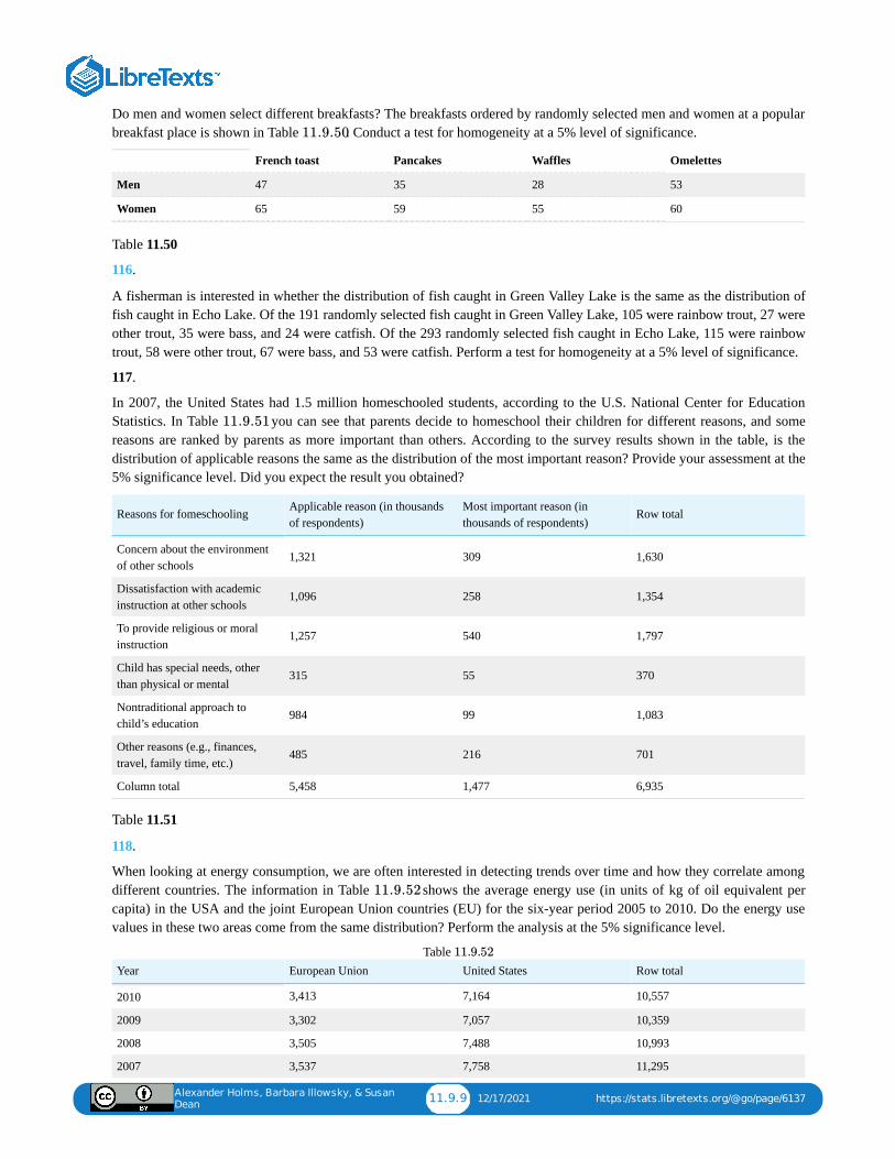
Alexander Holms, Barbara Illowsky, & Susan
Dean11.9.9 12/17/2021 https://stats.libretexts.org/@go/page/6137
Do men and women select different breakfasts? The breakfasts ordered by randomly selected men and women at a popularbreakfast place is shown in Table . Conduct a test for homogeneity at a 5% level of significance.
French toast Pancakes Waffles Omelettes
Men 47 35 28 53
Women 65 59 55 60
Table 11.50
116.
A fisherman is interested in whether the distribution of fish caught in Green Valley Lake is the same as the distribution offish caught in Echo Lake. Of the 191 randomly selected fish caught in Green Valley Lake, 105 were rainbow trout, 27 wereother trout, 35 were bass, and 24 were catfish. Of the 293 randomly selected fish caught in Echo Lake, 115 were rainbowtrout, 58 were other trout, 67 were bass, and 53 were catfish. Perform a test for homogeneity at a 5% level of significance.
117.
In 2007, the United States had 1.5 million homeschooled students, according to the U.S. National Center for EducationStatistics. In Table you can see that parents decide to homeschool their children for different reasons, and somereasons are ranked by parents as more important than others. According to the survey results shown in the table, is thedistribution of applicable reasons the same as the distribution of the most important reason? Provide your assessment at the5% significance level. Did you expect the result you obtained?
Reasons for fomeschooling Applicable reason (in thousandsof respondents)
Most important reason (inthousands of respondents)
Row total
Concern about the environmentof other schools
1,321 309 1,630
Dissatisfaction with academicinstruction at other schools
1,096 258 1,354
To provide religious or moralinstruction
1,257 540 1,797
Child has special needs, otherthan physical or mental
315 55 370
Nontraditional approach tochild’s education
984 99 1,083
Other reasons (e.g., finances,travel, family time, etc.)
485 216 701
Column total 5,458 1,477 6,935
Table 11.51
118.
When looking at energy consumption, we are often interested in detecting trends over time and how they correlate amongdifferent countries. The information in Table shows the average energy use (in units of kg of oil equivalent percapita) in the USA and the joint European Union countries (EU) for the six-year period 2005 to 2010. Do the energy usevalues in these two areas come from the same distribution? Perform the analysis at the 5% significance level.
Year European Union United States Row total
2010 3,413 7,164 10,557
2009 3,302 7,057 10,359
2008 3,505 7,488 10,993
2007 3,537 7,758 11,295
Table
11.9.50
11.9.51
11.9.52
11.9.52
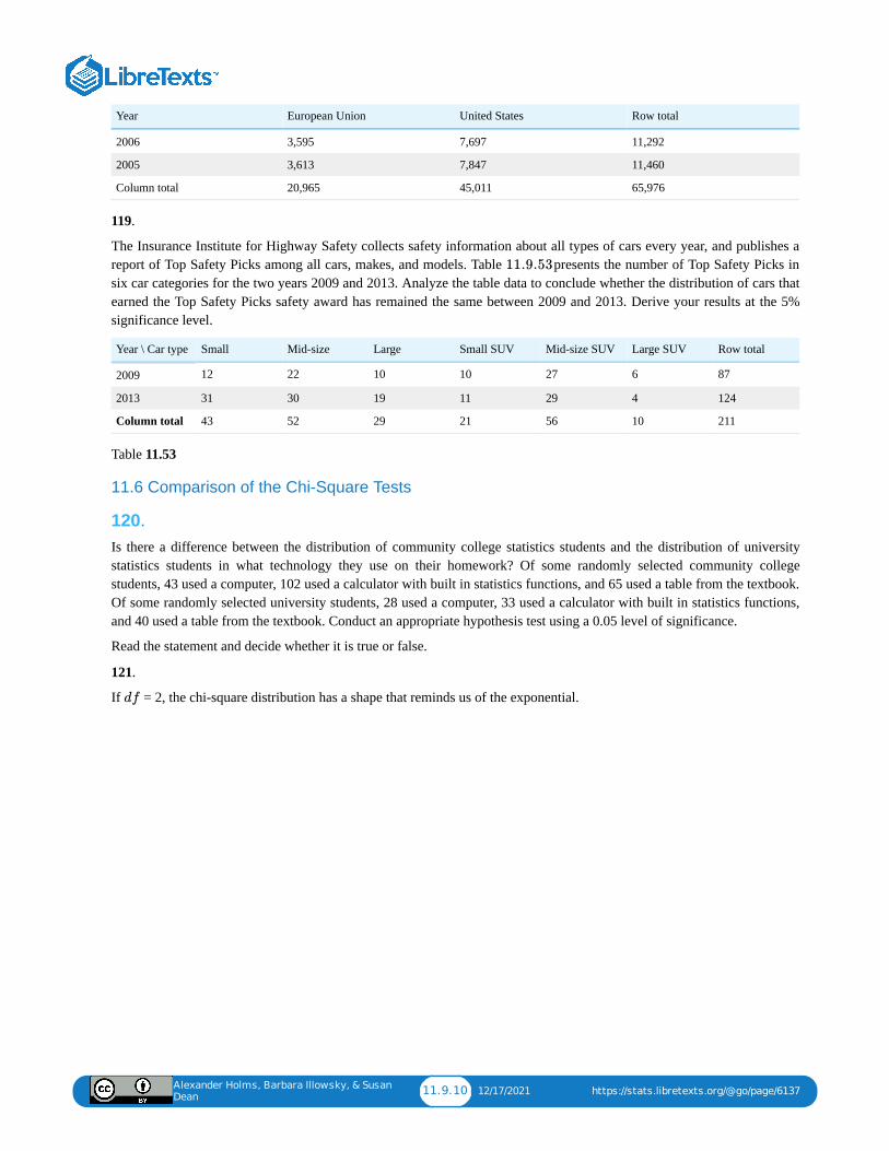
Alexander Holms, Barbara Illowsky, & Susan
Dean11.9.10 12/17/2021 https://stats.libretexts.org/@go/page/6137
Year European Union United States Row total
2006 3,595 7,697 11,292
2005 3,613 7,847 11,460
Column total 20,965 45,011 65,976
119.
The Insurance Institute for Highway Safety collects safety information about all types of cars every year, and publishes areport of Top Safety Picks among all cars, makes, and models. Table presents the number of Top Safety Picks insix car categories for the two years 2009 and 2013. Analyze the table data to conclude whether the distribution of cars thatearned the Top Safety Picks safety award has remained the same between 2009 and 2013. Derive your results at the 5%significance level.
Year \ Car type Small Mid-size Large Small SUV Mid-size SUV Large SUV Row total
2009 12 22 10 10 27 6 87
2013 31 30 19 11 29 4 124
Column total 43 52 29 21 56 10 211
Table 11.53
11.6 Comparison of the Chi-Square Tests
120.Is there a difference between the distribution of community college statistics students and the distribution of universitystatistics students in what technology they use on their homework? Of some randomly selected community collegestudents, 43 used a computer, 102 used a calculator with built in statistics functions, and 65 used a table from the textbook.Of some randomly selected university students, 28 used a computer, 33 used a calculator with built in statistics functions,and 40 used a table from the textbook. Conduct an appropriate hypothesis test using a 0.05 level of significance.
Read the statement and decide whether it is true or false.
121.
If = 2, the chi-square distribution has a shape that reminds us of the exponential.
11.9.53
df
Alexander Holms, Barbara Illowsky, & Susan
Dean11.10.1 1/6/2022 https://stats.libretexts.org/@go/page/6132
11.10: Chapter Key Terms
Contingency Tablea table that displays sample values for two different factors that may be dependent or contingent on one another; itfacilitates determining conditional probabilities.
Goodness-of-Fita hypothesis test that compares expected and observed values in order to look for significant differences within onenon-parametric variable. The degrees of freedom used equals the (number of categories – 1).
Test for Homogeneitya test used to draw a conclusion about whether two populations have the same distribution. The degrees of freedomused equals the (number of columns – 1).
Test of Independencea hypothesis test that compares expected and observed values for contingency tables in order to test for independencebetween two variables. The degrees of freedom used equals the (number of columns – 1) multiplied by the (number ofrows – 1).
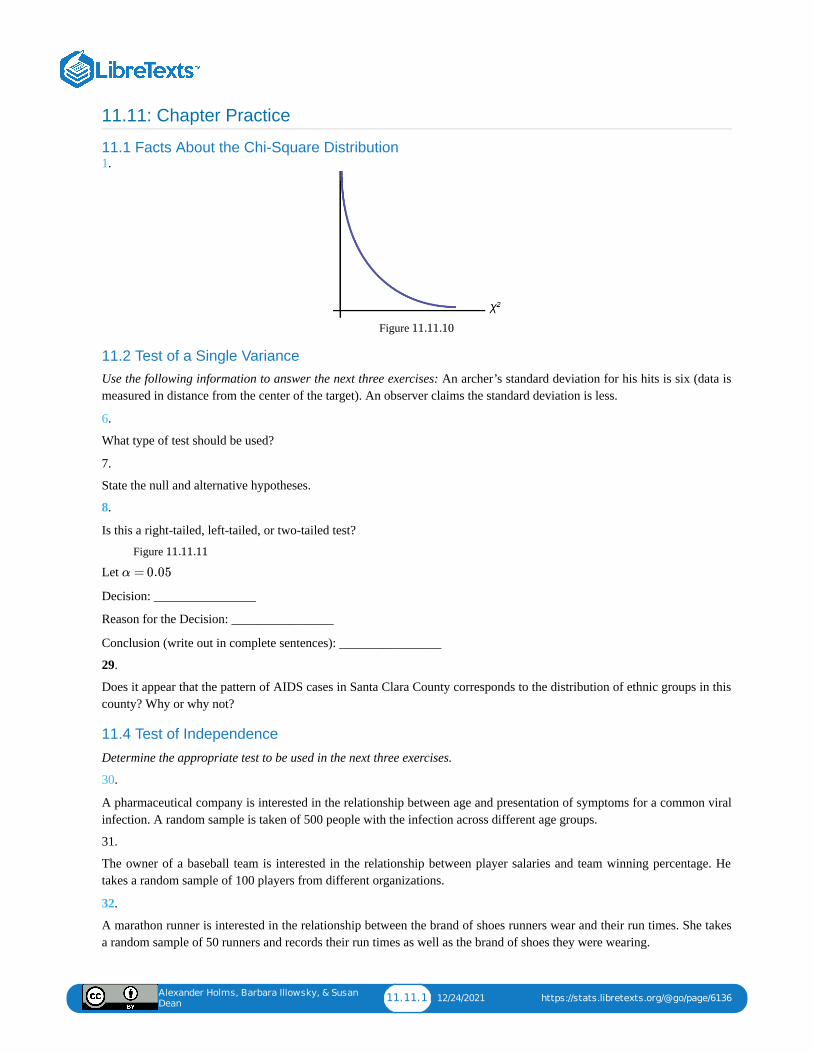
Alexander Holms, Barbara Illowsky, & Susan
Dean11.11.1 12/24/2021 https://stats.libretexts.org/@go/page/6136
11.11: Chapter Practice
11.1 Facts About the Chi-Square Distribution1.
Figure
11.2 Test of a Single VarianceUse the following information to answer the next three exercises: An archer’s standard deviation for his hits is six (data ismeasured in distance from the center of the target). An observer claims the standard deviation is less.
6.
What type of test should be used?
7.
State the null and alternative hypotheses.
8.
Is this a right-tailed, left-tailed, or two-tailed test?
Figure
Let
Decision: ________________
Reason for the Decision: ________________
Conclusion (write out in complete sentences): ________________
29.
Does it appear that the pattern of AIDS cases in Santa Clara County corresponds to the distribution of ethnic groups in thiscounty? Why or why not?
11.4 Test of Independence
Determine the appropriate test to be used in the next three exercises.
30.
A pharmaceutical company is interested in the relationship between age and presentation of symptoms for a common viralinfection. A random sample is taken of 500 people with the infection across different age groups.
31.
The owner of a baseball team is interested in the relationship between player salaries and team winning percentage. Hetakes a random sample of 100 players from different organizations.
32.
A marathon runner is interested in the relationship between the brand of shoes runners wear and their run times. She takesa random sample of 50 runners and records their run times as well as the brand of shoes they were wearing.
11.11.10
11.11.11
α = 0.05
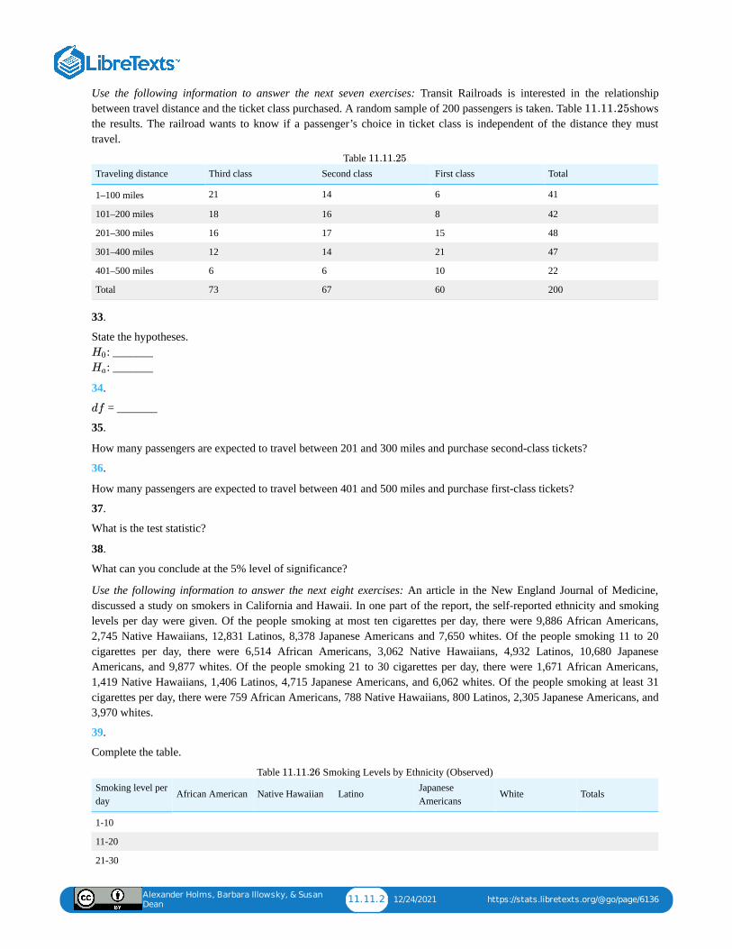
Alexander Holms, Barbara Illowsky, & Susan
Dean11.11.2 12/24/2021 https://stats.libretexts.org/@go/page/6136
Use the following information to answer the next seven exercises: Transit Railroads is interested in the relationshipbetween travel distance and the ticket class purchased. A random sample of 200 passengers is taken. Table showsthe results. The railroad wants to know if a passenger’s choice in ticket class is independent of the distance they musttravel.
Traveling distance Third class Second class First class Total
1–100 miles 21 14 6 41
101–200 miles 18 16 8 42
201–300 miles 16 17 15 48
301–400 miles 12 14 21 47
401–500 miles 6 6 10 22
Total 73 67 60 200
Table
33.
State the hypotheses. : _______ : _______
34.
= _______
35.
How many passengers are expected to travel between 201 and 300 miles and purchase second-class tickets?
36.
How many passengers are expected to travel between 401 and 500 miles and purchase first-class tickets?
37.
What is the test statistic?
38.
What can you conclude at the 5% level of significance?
Use the following information to answer the next eight exercises: An article in the New England Journal of Medicine,discussed a study on smokers in California and Hawaii. In one part of the report, the self-reported ethnicity and smokinglevels per day were given. Of the people smoking at most ten cigarettes per day, there were 9,886 African Americans,2,745 Native Hawaiians, 12,831 Latinos, 8,378 Japanese Americans and 7,650 whites. Of the people smoking 11 to 20cigarettes per day, there were 6,514 African Americans, 3,062 Native Hawaiians, 4,932 Latinos, 10,680 JapaneseAmericans, and 9,877 whites. Of the people smoking 21 to 30 cigarettes per day, there were 1,671 African Americans,1,419 Native Hawaiians, 1,406 Latinos, 4,715 Japanese Americans, and 6,062 whites. Of the people smoking at least 31cigarettes per day, there were 759 African Americans, 788 Native Hawaiians, 800 Latinos, 2,305 Japanese Americans, and3,970 whites.
39.
Complete the table.
Smoking level perday
African American Native Hawaiian Latino JapaneseAmericans
White Totals
1-10
11-20
21-30
Table Smoking Levels by Ethnicity (Observed)
11.11.25
11.11.25
H0
Ha
df
11.11.26
Alexander Holms, Barbara Illowsky, & Susan
Dean11.11.3 12/24/2021 https://stats.libretexts.org/@go/page/6136
Smoking level perday
African American Native Hawaiian Latino JapaneseAmericans
White Totals
31+
Totals
40.
State the hypotheses. : _______ : _______
41.
Enter expected values in Table . Round to two decimal places.
Calculate the following values:
42.
= _______
43.
test statistic = ______
44.
Is this a right-tailed, left-tailed, or two-tailed test? Explain why.
45.
Graph the situation. Label and scale the horizontal axis. Mark the mean and test statistic. Shade in the regioncorresponding to the confidence level.
Figure
State the decision and conclusion (in a complete sentence) for the following preconceived levels of \alpha.
46.
1. A math teacher wants to see if two of her classes have the same distribution of test scores. What test should she use?49.
What are the null and alternative hypotheses for Table .
20–30 30–40 40–50 50–60
Private practice 16 40 38 6
Hospital 8 44 59 39
Table
H0
Ha
11.11.26
df
χ2
11.11.12
α = 0.05
11.11.27
11.11.27
Alexander Holms, Barbara Illowsky, & Susan
Dean11.11.4 12/24/2021 https://stats.libretexts.org/@go/page/6136
53.
State the null and alternative hypotheses.
54.
= _______
55.
What is the test statistic?
56.
What can you conclude at the 5% significance level?
11.6 Comparison of the Chi-Square Tests
57.58.
What is the null hypothesis for the type of test from Exercise ?
59.
Which test would you use to decide whether two factors have a relationship?
60.
Which test would you use to decide if two populations have the same distribution?
61.
How are tests of independence similar to tests for homogeneity?
62.
How are tests of independence different from tests for homogeneity?
df
11.11.57
Alexander Holms, Barbara Illowsky, & Susan
Dean11.12.1 1/6/2022 https://stats.libretexts.org/@go/page/6139
11.12: Chapter References
11.1 Facts About the Chi-Square Distribution
Data from Parade Magazine.
“HIV/AIDS Epidemiology Santa Clara County.”Santa Clara County Public Health Department, May 2011.
11.2 Test of a Single Variance“AppleInsider Price Guides.” Apple Insider, 2013. Available online at http://appleinsider.com/mac_price_guide (accessedMay 14, 2013).
Data from the World Bank, June 5, 2012.
11.3 Goodness-of-Fit TestData from the U.S. Census Bureau
Data from the College Board. Available online at http://www.collegeboard.com.
Data from the U.S. Census Bureau, Current Population Reports.
Ma, Y., E.R. Bertone, E.J. Stanek III, G.W. Reed, J.R. Hebert, N.L. Cohen, P.A. Merriam, I.S. Ockene, “Associationbetween Eating Patterns and Obesity in a Free-living US Adult Population.” American Journal of Epidemiology volume158, no. 1, pages 85-92.
Ogden, Cynthia L., Margaret D. Carroll, Brian K. Kit, Katherine M. Flegal, “Prevalence of Obesity in the United States,2009–2010.” NCHS Data Brief no. 82, January 2012. Available online athttp://www.cdc.gov/nchs/data/databriefs/db82.pdf (accessed May 24, 2013).
Stevens, Barbara J., “Multi-family and Commercial Solid Waste and Recycling Survey.” Arlington Count, VA. Availableonline at www.arlingtonva.us/department.../file84429.pdf (accessed May 24,2013).
11.4 Test of IndependenceDiCamilo, Mark, Mervin Field, “Most Californians See a Direct Linkage between Obesity and Sugary Sodas. Two inThree Voters Support Taxing Sugar-Sweetened Beverages If Proceeds are Tied to Improving School Nutrition and PhysicalActivity Programs.” The Field Poll, released Feb. 14, 2013. Available online atfield.com/fieldpollonline/sub...rs/Rls2436.pdf (accessed May 24, 2013).
Harris Interactive, “Favorite Flavor of Ice Cream.” Available online at http://www.statisticbrain.com/favori...r-of-ice-cream(accessed May 24, 2013)
“Youngest Online Entrepreneurs List.” Available online at http://www.statisticbrain.com/younge...repreneur-list (accessedMay 24, 2013).
11.5 Test for Homogeneity
Data from the Insurance Institute for Highway Safety, 2013. Available online at www.iihs.org/iihs/ratings (accessed May24, 2013).
“Energy use (kg of oil equivalent per capita).” The World Bank, 2013. Available online athttp://data.worldbank.org/indicator/...G.OE/countries (accessed May 24, 2013).
“Parent and Family Involvement Survey of 2007 National Household Education Survey Program (NHES),” U.S.Department of Education, National Center for Education Statistics. Available online athttp://nces.ed.gov/pubsearch/pubsinf...?pubid=2009030 (accessed May 24, 2013).
“Parent and Family Involvement Survey of 2007 National Household Education Survey Program (NHES),” U.S.Department of Education, National Center for Education Statistics. Available online athttp://nces.ed.gov/pubs2009/2009030_sup.pdf (accessed May 24, 2013).
Alexander Holms, Barbara Illowsky, & Susan
Dean11.13.1 12/31/2021 https://stats.libretexts.org/@go/page/6133
11.13: Chapter Review
11.1 Facts About the Chi-Square Distribution
The chi-square distribution is a useful tool for assessment in a series of problem categories. These problem categoriesinclude primarily (i) whether a data set fits a particular distribution, (ii) whether the distributions of two populations are thesame, (iii) whether two events might be independent, and (iv) whether there is a different variability than expected within apopulation.
An important parameter in a chi-square distribution is the degrees of freedom in a given problem. The random variablein the chi-square distribution is the sum of squares of standard normal variables, which must be independent. The keycharacteristics of the chi-square distribution also depend directly on the degrees of freedom.
The chi-square distribution curve is skewed to the right, and its shape depends on the degrees of freedom . For ,the curve approximates the normal distribution. Test statistics based on the chi-square distribution are always greater thanor equal to zero. Such application tests are almost always right-tailed tests.
11.2 Test of a Single Variance
To test variability, use the chi-square test of a single variance. The test may be left-, right-, or two-tailed, and its hypothesesare always expressed in terms of the variance (or standard deviation).
11.3 Goodness-of-Fit TestTo assess whether a data set fits a specific distribution, you can apply the goodness-of-fit hypothesis test that uses the chi-square distribution. The null hypothesis for this test states that the data come from the assumed distribution. The testcompares observed values against the values you would expect to have if your data followed the assumed distribution. Thetest is almost always right-tailed. Each observation or cell category must have an expected value of at least five.
11.4 Test of Independence
To assess whether two factors are independent or not, you can apply the test of independence that uses the chi-squaredistribution. The null hypothesis for this test states that the two factors are independent. The test compares observed valuesto expected values. The test is right-tailed. Each observation or cell category must have an expected value of at least 5.
11.5 Test for HomogeneityTo assess whether two data sets are derived from the same distribution—which need not be known, you can apply the testfor homogeneity that uses the chi-square distribution. The null hypothesis for this test states that the populations of the twodata sets come from the same distribution. The test compares the observed values against the expected values if the twopopulations followed the same distribution. The test is right-tailed. Each observation or cell category must have anexpected value of at least five.
11.6 Comparison of the Chi-Square TestsThe goodness-of-fit test is typically used to determine if data fits a particular distribution. The test of independence makesuse of a contingency table to determine the independence of two factors. The test for homogeneity determines whether twopopulations come from the same distribution, even if this distribution is unknown.
df
df
df df > 90
Alexander Holms, Barbara Illowsky, & Susan
Dean11.14.1 12/17/2021 https://stats.libretexts.org/@go/page/6140
11.14: Chapter Solution (Practice + Homework)1.
mean = 25 and standard deviation = 7.0711
3.
when the number of degrees of freedom is greater than 90
5.
6.
a test of a single variance
8.
a left-tailed test
10.
;
.
12.
a test of a single variance
16.
a goodness-of-fit test
18.
3
20.
2.04
21.
We decline to reject the null hypothesis. There is not enough evidence to suggest that the observed test scores aresignificantly different from the expected test scores.
23.
: the distribution of AIDS cases follows the ethnicities of the general population of Santa Clara County.
25.
right-tailed
27.
2016.136
28.
30.
a test of independence
a test of independence
34.
8
df = 2
: = 0.812H0 σ2
: > 0.812Ha σ2
H0
Alexander Holms, Barbara Illowsky, & Susan
Dean11.14.2 12/17/2021 https://stats.libretexts.org/@go/page/6140
36.
6.6
39.
Smoking levelper day
AfricanAmerican
Native Hawaiian Latino JapaneseAmericans
White Totals
1-10 9,886 2,745 12,831 8,378 7,650 41,490
11-20 6,514 3,062 4,932 10,680 9,877 35,065
21-30 1,671 1,419 1,406 4,715 6,062 15,273
31+ 759 788 800 2,305 3,970 8,622
Totals 18,830 8,014 19,969 26,078 27,559 10,0450
Table
41.
Smoking level perday
African American Native Hawaiian Latino Japanese Americans White
1-10 7777.57 3310.11 8248.02 10771.29 11383.01
11-20 6573.16 2797.52 6970.76 9103.29 9620.27
21-30 2863.02 1218.49 3036.20 3965.05 4190.23
31+ 1616.25 687.87 1714.01 2238.37 2365.49
Table
43.
10,301.8
44.
right
46.
1. 48.
test for homogeneity
test for homogeneity
52.
All values in the table must be greater than or equal to five.
54.
3
57.
a goodness-of-fit test
59.
a test for independence
61.
Answers will vary. Sample answer: Tests of independence and tests for homogeneity both calculate the test statistic
the same way . In addition, all values must be greater than or equal to five.
63.
11.14.54
11.14.55
∑(ij)
(O−E)2
E
Alexander Holms, Barbara Illowsky, & Susan
Dean11.14.3 12/17/2021 https://stats.libretexts.org/@go/page/6140
true
65.
false
67.
225
69.
71.
36
72.
Check student’s solution.
74.
The claim is that the variance is no more than 150 minutes.
76.
a Student's - or normal distribution
78.
1. 80.1. 82.
1. 84.1. 87.
Marital status Percent Expected frequency
Never married 31.3 125.2
Married 56.1 224.4
Widowed 2.5 10
Divorced/Separated 10.1 40.4
Table
1. 89.1. 91.
1. 94.
true
false
98.
1. 100.1. 102.
1. 104.
1. 106.1. 108.
true
true
: ≤ 150H0 σ2
t
11.14.56
Alexander Holms, Barbara Illowsky, & Susan
Dean11.14.4 12/17/2021 https://stats.libretexts.org/@go/page/6140
112.
1. 114.
1. 116.1. 118.
1. 120.1. 122.
1. The test statistic is always positive and if theexpected and observed values are not close together,the test statistic is large and the null hypothesis willbe rejected.
2. Testing to see if the data fits the distribution “toowell” or is too perfect.

1 1/7/2022
CHAPTER OVERVIEW12: F DISTRIBUTION AND ONE-WAY ANOVA
12.0: INTRODUCTION TO F DISTRIBUTION AND ONE-WAY ANOVA12.1: TEST OF TWO VARIANCES12.2: ONE-WAY ANOVA12.3: THE F DISTRIBUTION AND THE F-RATIO12.4: FACTS ABOUT THE F DISTRIBUTION12.5: CHAPTER FORMULA REVIEW12.6: CHAPTER HOMEWORK12.7: CHAPTER KEY TERMS12.8: CHAPTER PRACTICE12.9: CHAPTER REFERENCE12.10: CHAPTER REVIEW12.11: CHAPTER SOLUTION (PRACTICE + HOMEWORK)

Alexander Holms, Barbara Illowsky, & Susan
Dean12.0.1 1/7/2022 https://stats.libretexts.org/@go/page/4617
12.0: Introduction to F Distribution and One-Way ANOVA
Figure One-way ANOVA is used to measure information from several groups.
Many statistical applications in psychology, social science, business administration, and the natural sciences involveseveral groups. For example, an environmentalist is interested in knowing if the average amount of pollution varies inseveral bodies of water. A sociologist is interested in knowing if the amount of income a person earns varies according tohis or her upbringing. A consumer looking for a new car might compare the average gas mileage of several models.
For hypothesis tests comparing averages among more than two groups, statisticians have developed a method called"Analysis of Variance" (abbreviated ANOVA). In this chapter, you will study the simplest form of ANOVA called singlefactor or one-way ANOVA. You will also study the distribution, used for one-way ANOVA, and the test for differencesbetween two variances. This is just a very brief overview of one-way ANOVA. One-Way ANOVA, as it is presented here,relies heavily on a calculator or computer.
12.0.1
F
Alexander Holms, Barbara Illowsky, & Susan
Dean12.1.1 1/6/2022 https://stats.libretexts.org/@go/page/4618
12.1: Test of Two VariancesThis chapter introduces a new probability density function, the distribution. This distribution is used for manyapplications including ANOVA and for testing equality across multiple means. We begin with the distribution and thetest of hypothesis of differences in variances. It is often desirable to compare two variances rather than two averages. Forinstance, college administrators would like two college professors grading exams to have the same variation in theirgrading. In order for a lid to fit a container, the variation in the lid and the container should be approximately the same. Asupermarket might be interested in the variability of check-out times for two checkers. In finance, the variance is ameasure of risk and thus an interesting question would be to test the hypothesis that two different investment portfolioshave the same variance, the volatility.
In order to perform a test of two variances, it is important that the following are true:
1. The populations from which the two samples are drawn are approximately normally distributed.2. The two populations are independent of each other.
Unlike most other hypothesis tests in this book, the test for equality of two variances is very sensitive to deviations fromnormality. If the two distributions are not normal, or close, the test can give a biased result for the test statistic.
Suppose we sample randomly from two independent normal populations. Let and be the unknown populationvariances and and be the sample variances. Let the sample sizes be and . Since we are interested in comparingthe two sample variances, we use the ratio:
has the distribution
where are the degrees of freedom for the numerator and are the degrees of freedom for the denominator.
If the null hypothesis is , then the Ratio, test statistic, becomes
The various forms of the hypotheses tested are:
Two-Tailed Test One-Tailed Test One-Tailed TestTable 12.1
A more general form of the null and alternative hypothesis for a two tailed test would be :
Where if it is a simple test of the hypothesis that the two variances are equal. This form of the hypothesis does havethe benefit of allowing for tests that are more than for simple differences and can accommodate tests for specificdifferences as we did for differences in means and differences in proportions. This form of the hypothesis also shows therelationship between the distribution and the : the is a ratio of two chi squared distributions a distribution we sawin the last chapter. This is helpful in determining the degrees of freedom of the resultant distribution.
If the two populations have equal variances, then and are close in value and the test statistic, is close to one.
But if the two population variances are very different, and tend to be very different, too. Choosing as the larger
F
F
F
F
σ21 σ2
2
s21 s2
2 n1 n2
F
F =[ ]
s21
σ21
[ ]s22
σ22
F F ∼ F ( −1, −1)n1 n2
– 1n1 – 1n2
=σ21 σ2
2 F = =Fc
[ ]s21
σ21
[ ]s22
σ22
s21
s22
: =H0 σ21 σ2
2 : ≤H0 σ21 σ2
2 : ≥H0 σ21 σ2
2
: ≠H1 σ21 σ2
2 : >H1 σ21 σ2
2 : <H1 σ21 σ2
2
: =H0
σ21
σ22
δ0
: ≠Ha
σ21
σ22
δ0
= 1δ0
F χ2 F
F
s21 s2
2 =Fcs2
1
s22
s21 s2
2 s21
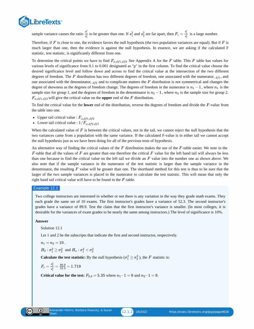
Alexander Holms, Barbara Illowsky, & Susan
Dean12.1.2 1/6/2022 https://stats.libretexts.org/@go/page/4618
sample variance causes the ratio to be greater than one. If and are far apart, then is a large number.
Therefore, if is close to one, the evidence favors the null hypothesis (the two population variances are equal). But if ismuch larger than one, then the evidence is against the null hypothesis. In essence, we are asking if the calculated Fstatistic, test statistic, is significantly different from one.
To determine the critical points we have to find . See Appendix A for the table. This table has values forvarious levels of significance from 0.1 to 0.001 designated as "p" in the first column. To find the critical value choose thedesired significance level and follow down and across to find the critical value at the intersection of the two differentdegrees of freedom. The distribution has two different degrees of freedom, one associated with the numerator, , andone associated with the denominator, and to complicate matters the distribution is not symmetrical and changes thedegree of skewness as the degrees of freedom change. The degrees of freedom in the numerator is , where is thesample size for group 1, and the degrees of freedom in the denominator is , where is the sample size for group 2.
will give the critical value on the upper end of the distribution.
To find the critical value for the lower end of the distribution, reverse the degrees of freedom and divide the -value fromthe table into one.
Upper tail critical value : Lower tail critical value :
When the calculated value of is between the critical values, not in the tail, we cannot reject the null hypothesis that thetwo variances came from a population with the same variance. If the calculated F-value is in either tail we cannot acceptthe null hypothesis just as we have been doing for all of the previous tests of hypothesis.
An alternative way of finding the critical values of the distribution makes the use of the -table easier. We note in the -table that all the values of are greater than one therefore the critical value for the left hand tail will always be less
than one because to find the critical value on the left tail we divide an value into the number one as shown above. Wealso note that if the sample variance in the numerator of the test statistic is larger than the sample variance in thedenominator, the resulting value will be greater than one. The shorthand method for this test is thus to be sure that thelarger of the two sample variances is placed in the numerator to calculate the test statistic. This will mean that only theright hand tail critical value will have to be found in the -table.
Two college instructors are interested in whether or not there is any variation in the way they grade math exams. Theyeach grade the same set of 10 exams. The first instructor's grades have a variance of 52.3. The second instructor'sgrades have a variance of 89.9. Test the claim that the first instructor's variance is smaller. (In most colleges, it isdesirable for the variances of exam grades to be nearly the same among instructors.) The level of significance is 10%.
Answer
Solution 12.1
Let 1 and 2 be the subscripts that indicate the first and second instructor, respectively.
.
and
Calculate the test statistic: By the null hypothesis ( ), the statistic is:
Critical value for the test: where and .
s21
s22
s21 s2
2 =Fc
s21
s22
F F
Fα,df1,df2 F F
F df1
df2 F
−1n1 n1
−1n2 n2
Fα,df1,df2 F
F
Fα,df1,df2
1/Fα,df2,df1
F
F F
F F F
F
F
F
Example 12.1
= = 10n1 n2
: ≥H0 σ21 σ2
2 : <Ha σ21 σ2
2
≥σ21 σ2
2 F
= = = 1.719Fc
s22
s21
89.952.3
= 5.35F9,9 – 1 = 9n1 – 1 = 9n2
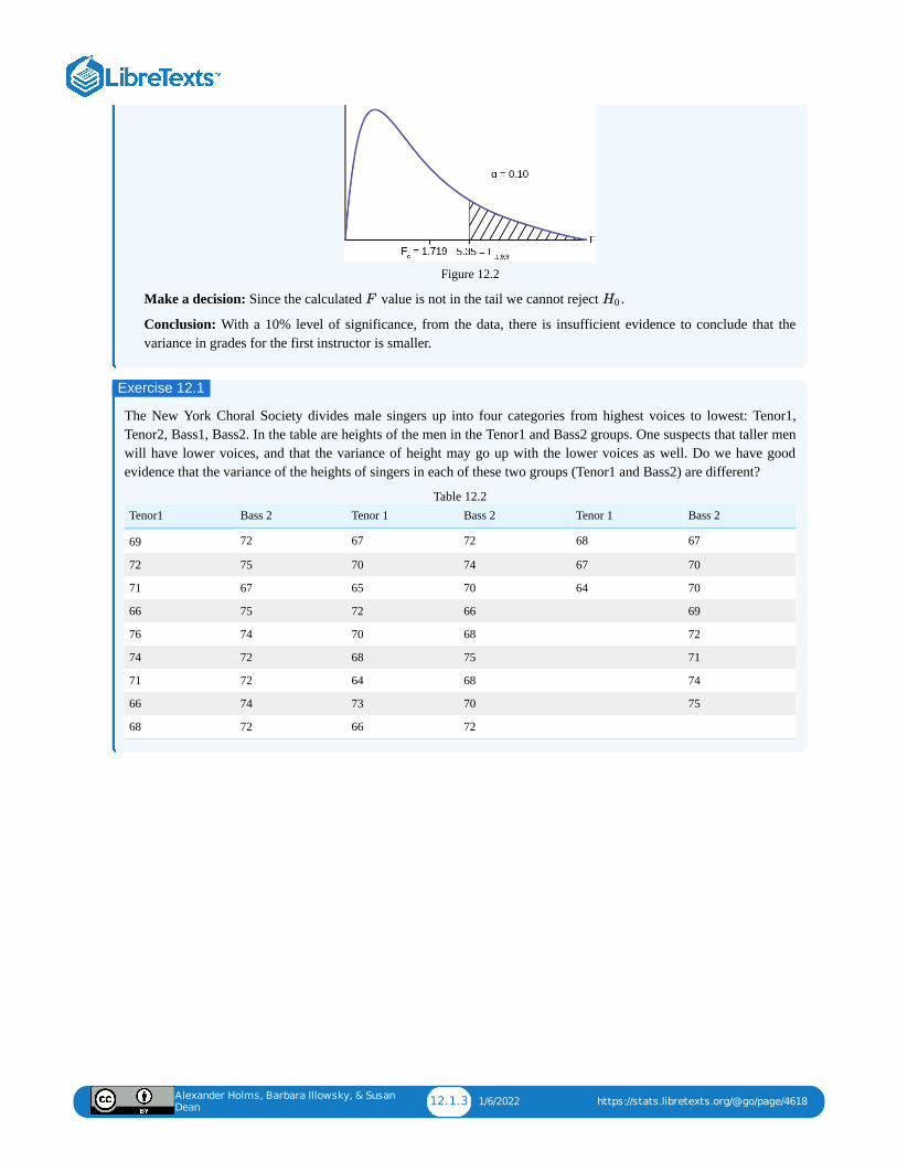
Alexander Holms, Barbara Illowsky, & Susan
Dean12.1.3 1/6/2022 https://stats.libretexts.org/@go/page/4618
Figure 12.2
Make a decision: Since the calculated value is not in the tail we cannot reject .
Conclusion: With a 10% level of significance, from the data, there is insufficient evidence to conclude that thevariance in grades for the first instructor is smaller.
The New York Choral Society divides male singers up into four categories from highest voices to lowest: Tenor1,Tenor2, Bass1, Bass2. In the table are heights of the men in the Tenor1 and Bass2 groups. One suspects that taller menwill have lower voices, and that the variance of height may go up with the lower voices as well. Do we have goodevidence that the variance of the heights of singers in each of these two groups (Tenor1 and Bass2) are different?
Tenor1 Bass 2 Tenor 1 Bass 2 Tenor 1 Bass 2
69 72 67 72 68 67
72 75 70 74 67 70
71 67 65 70 64 70
66 75 72 66 69
76 74 70 68 72
74 72 68 75 71
71 72 64 68 74
66 74 73 70 75
68 72 66 72
Table 12.2
F H0
Exercise 12.1
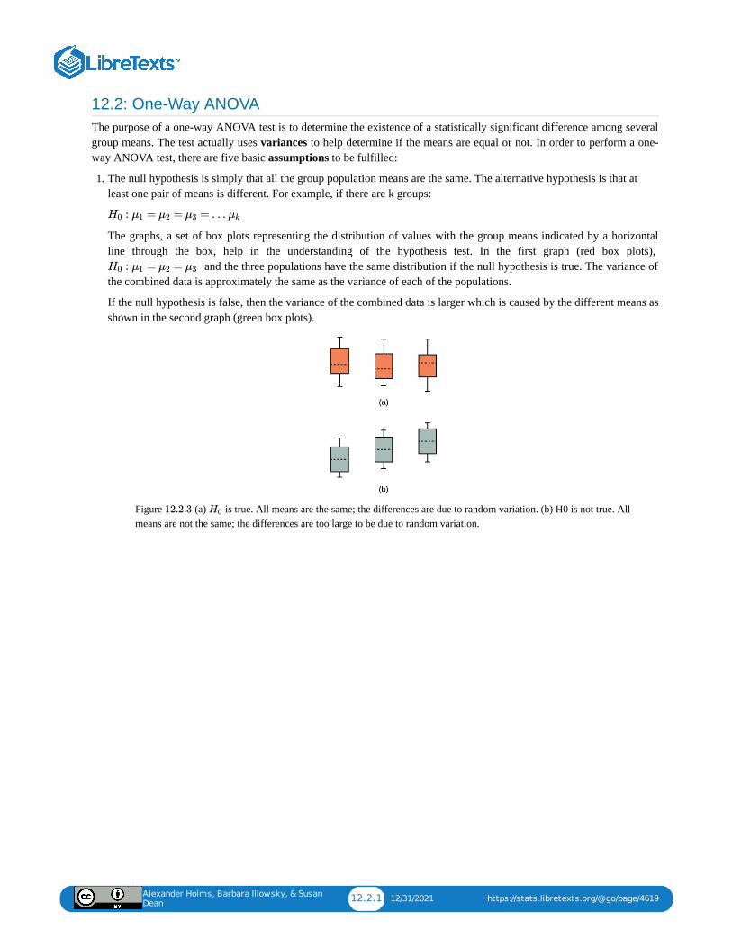
Alexander Holms, Barbara Illowsky, & Susan
Dean12.2.1 12/31/2021 https://stats.libretexts.org/@go/page/4619
12.2: One-Way ANOVAThe purpose of a one-way ANOVA test is to determine the existence of a statistically significant difference among severalgroup means. The test actually uses variances to help determine if the means are equal or not. In order to perform a one-way ANOVA test, there are five basic assumptions to be fulfilled:
1. The null hypothesis is simply that all the group population means are the same. The alternative hypothesis is that atleast one pair of means is different. For example, if there are k groups:
The graphs, a set of box plots representing the distribution of values with the group means indicated by a horizontalline through the box, help in the understanding of the hypothesis test. In the first graph (red box plots),
and the three populations have the same distribution if the null hypothesis is true. The variance ofthe combined data is approximately the same as the variance of each of the populations.
If the null hypothesis is false, then the variance of the combined data is larger which is caused by the different means asshown in the second graph (green box plots).
Figure (a) is true. All means are the same; the differences are due to random variation. (b) H0 is not true. Allmeans are not the same; the differences are too large to be due to random variation.
: = = = …H0 μ1 μ2 μ3 μk
: = =H0 μ1 μ2 μ3
12.2.3 H0
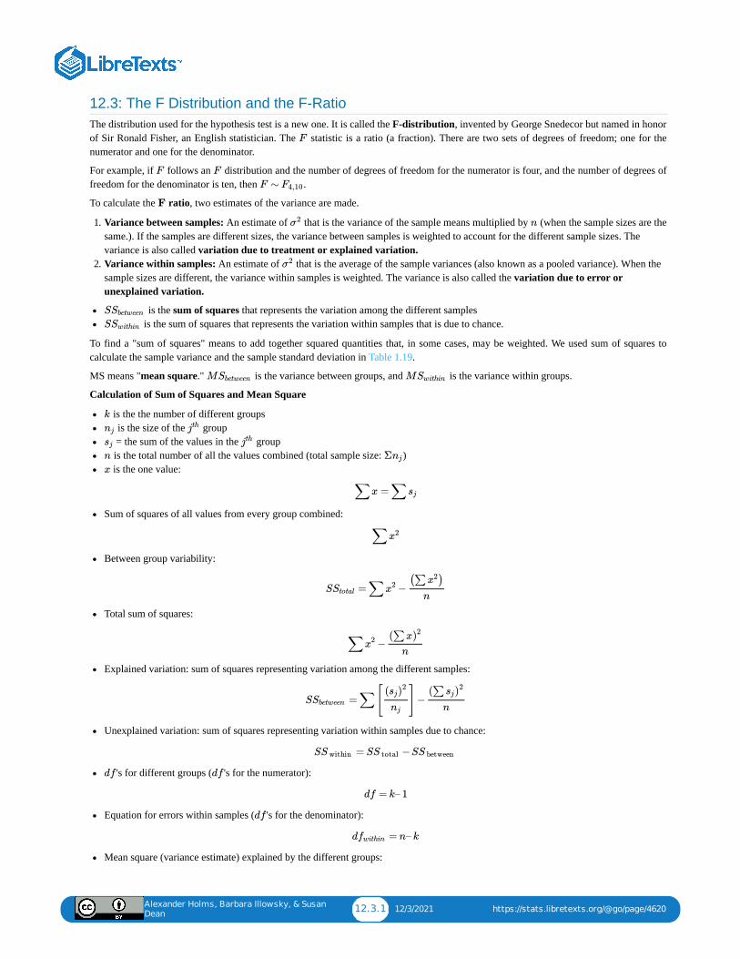
Alexander Holms, Barbara Illowsky, & Susan
Dean12.3.1 12/3/2021 https://stats.libretexts.org/@go/page/4620
12.3: The F Distribution and the F-RatioThe distribution used for the hypothesis test is a new one. It is called the F-distribution, invented by George Snedecor but named in honorof Sir Ronald Fisher, an English statistician. The statistic is a ratio (a fraction). There are two sets of degrees of freedom; one for thenumerator and one for the denominator.
For example, if follows an distribution and the number of degrees of freedom for the numerator is four, and the number of degrees offreedom for the denominator is ten, then .
To calculate the ratio, two estimates of the variance are made.
1. Variance between samples: An estimate of that is the variance of the sample means multiplied by (when the sample sizes are thesame.). If the samples are different sizes, the variance between samples is weighted to account for the different sample sizes. Thevariance is also called variation due to treatment or explained variation.
2. Variance within samples: An estimate of that is the average of the sample variances (also known as a pooled variance). When thesample sizes are different, the variance within samples is weighted. The variance is also called the variation due to error orunexplained variation.
is the sum of squares that represents the variation among the different samples is the sum of squares that represents the variation within samples that is due to chance.
To find a "sum of squares" means to add together squared quantities that, in some cases, may be weighted. We used sum of squares tocalculate the sample variance and the sample standard deviation in Table 1.19.
MS means "mean square." is the variance between groups, and is the variance within groups.
Calculation of Sum of Squares and Mean Square
is the the number of different groups is the size of the group = the sum of the values in the group is the total number of all the values combined (total sample size: ) is the one value:
Sum of squares of all values from every group combined:
Between group variability:
Total sum of squares:
Explained variation: sum of squares representing variation among the different samples:
Unexplained variation: sum of squares representing variation within samples due to chance:
's for different groups ( 's for the numerator):
Equation for errors within samples ( 's for the denominator):
Mean square (variance estimate) explained by the different groups:
F
F F
F ∼ F4,10
F
σ2 n
σ2
SSbetween
SSwithin
MSbetween MSwithin
k
nj jth
sj jth
n Σnj
x
∑x =∑sj
∑x2
S =∑ −Stotal x2(∑ )x2
n
∑ −x2 (∑x)2
n
S =∑[ ]−Sbetween
( )sj2
nj
(∑ )sj2
n
S = S −SS within S total S between
df df
df = k– 1
df
d = n– kfwithin
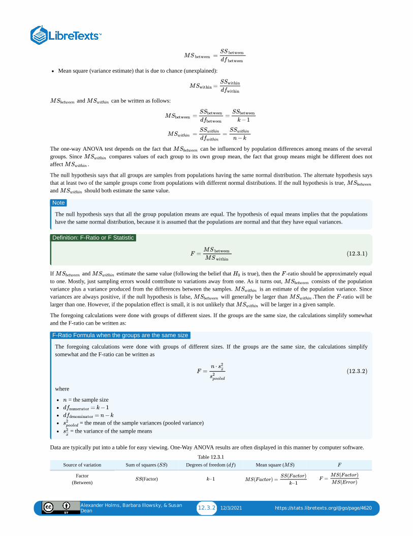
Alexander Holms, Barbara Illowsky, & Susan
Dean12.3.2 12/3/2021 https://stats.libretexts.org/@go/page/4620
Mean square (variance estimate) that is due to chance (unexplained):
and can be written as follows:
The one-way ANOVA test depends on the fact that can be influenced by population differences among means of the severalgroups. Since compares values of each group to its own group mean, the fact that group means might be different does notaffect .
The null hypothesis says that all groups are samples from populations having the same normal distribution. The alternate hypothesis saysthat at least two of the sample groups come from populations with different normal distributions. If the null hypothesis is true, and should both estimate the same value.
The null hypothesis says that all the group population means are equal. The hypothesis of equal means implies that the populationshave the same normal distribution, because it is assumed that the populations are normal and that they have equal variances.
If and estimate the same value (following the belief that is true), then the -ratio should be approximately equalto one. Mostly, just sampling errors would contribute to variations away from one. As it turns out, consists of the populationvariance plus a variance produced from the differences between the samples. is an estimate of the population variance. Sincevariances are always positive, if the null hypothesis is false, will generally be larger than .Then the -ratio will belarger than one. However, if the population effect is small, it is not unlikely that will be larger in a given sample.
The foregoing calculations were done with groups of different sizes. If the groups are the same size, the calculations simplify somewhatand the F-ratio can be written as:
The foregoing calculations were done with groups of different sizes. If the groups are the same size, the calculations simplifysomewhat and the F-ratio can be written as
where
= the sample size
= the mean of the sample variances (pooled variance) = the variance of the sample means
Data are typically put into a table for easy viewing. One-Way ANOVA results are often displayed in this manner by computer software.
Table Source of variation Sum of squares ( ) Degrees of freedom ( ) Mean square ( )
Factor (Between)
(Factor)
M =S between SS between
df between
M =SwithinSSwithin
dfwithin
MSbetween MSwithin
MSbetween
MSwithin
= =SSbetween
dfbetween
SSbetween
k−1
= =SSwithin
dfwithin
SSwithin
n−k
MSbetween
MSwithin
MSwithin
MSbetween
MSwithin
Note
Definition: F-Ratio or F Statistic
F =MS between
MS within (12.3.1)
MSbetween MSwithin H0 F
MSbetween
MSwithin
MSbetween MSwithin F
MSwithin
F-Ratio Formula when the groups are the same size
F =n ⋅ s2
x̄̄̄
s2pooled
(12.3.2)
n
d = k−1fnumerator
d = n−kfdenominator
s2pooled
s2x̄̄̄
12.3.1
SS df MS F
SS k–1 MS(Factor) =SS(Factor)
k–1F =
MS(Factor)
MS(Error)
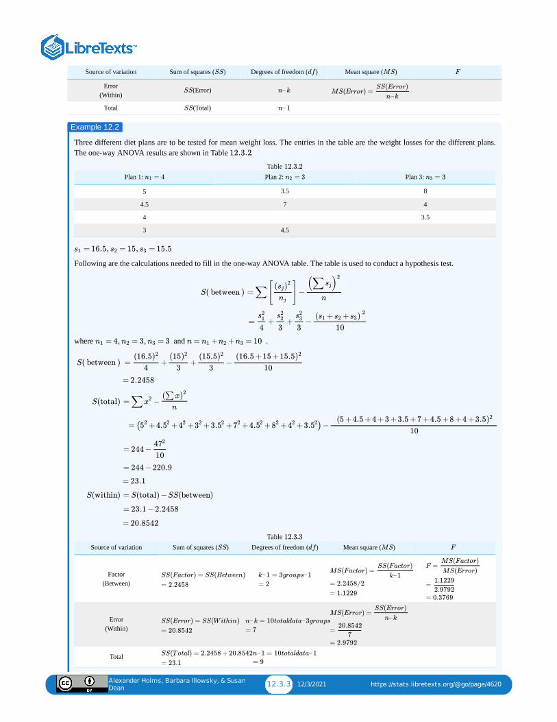
Alexander Holms, Barbara Illowsky, & Susan
Dean12.3.3 12/3/2021 https://stats.libretexts.org/@go/page/4620
Source of variation Sum of squares ( ) Degrees of freedom ( ) Mean square ( )
Error (Within)
(Error)
Total (Total)
Three different diet plans are to be tested for mean weight loss. The entries in the table are the weight losses for the different plans.The one-way ANOVA results are shown in Table .
Table Plan 1: Plan 2: Plan 3:
5 3.5 8
4.5 7 4
4 3.5
3 4.5
Following are the calculations needed to fill in the one-way ANOVA table. The table is used to conduct a hypothesis test.
where and .
Table Source of variation Sum of squares ( ) Degrees of freedom ( ) Mean square ( )
Factor (Between)
Error (Within)
Total
SS df MS F
SS n–k MS(Error) =SS(Error)
n–k
SS n–1
Example 12.2
12.3.2
12.3.2
= 4n1 = 3n2 = 3n3
= 16.5, = 15, = 15.5s1 s2 s3
S( between ) =∑[ ]−( )sj
2
nj
(∑ )sj2
n
= + + −s2
1
4
s22
3
s23
3
( + + )s1 s2 s32
10
= 4, = 3, = 3n1 n2 n3 n = + + = 10n1 n2 n3
S( between )
S(total)
S(within)
= + + −(16.5)2
4
(15)2
3
(15.5)2
3
(16.5 +15 +15.5)2
10
= 2.2458
=∑ −x2 (∑x)2
n
= ( + + + + + + + + + )−52 4.52 42 32 3.52 72 4.52 82 42 3.52 (5 +4.5 +4 +3 +3.5 +7 +4.5 +8 +4 +3.5)2
10
= 244 −472
10
= 244 −220.9
= 23.1
= S(total) −SS(between)
= 23.1 −2.2458
= 20.8542
12.3.3
SS df MS F
SS(Factor) = SS(Between)
= 2.2458
k–1 = 3groups–1
= 2
MS(Factor) =SS(Factor)
k–1= 2.2458/2
= 1.1229
F =MS(Factor)
MS(Error)
=1.1229
2.9792= 0.3769
SS(Error) = SS(Within)
= 20.8542
n–k = 10totaldata–3groups
= 7
MS(Error) =SS(Error)
n–k
=20.8542
7= 2.9792
SS(Total) = 2.2458 + 20.8542
= 23.1
n–1 = 10totaldata–1= 9
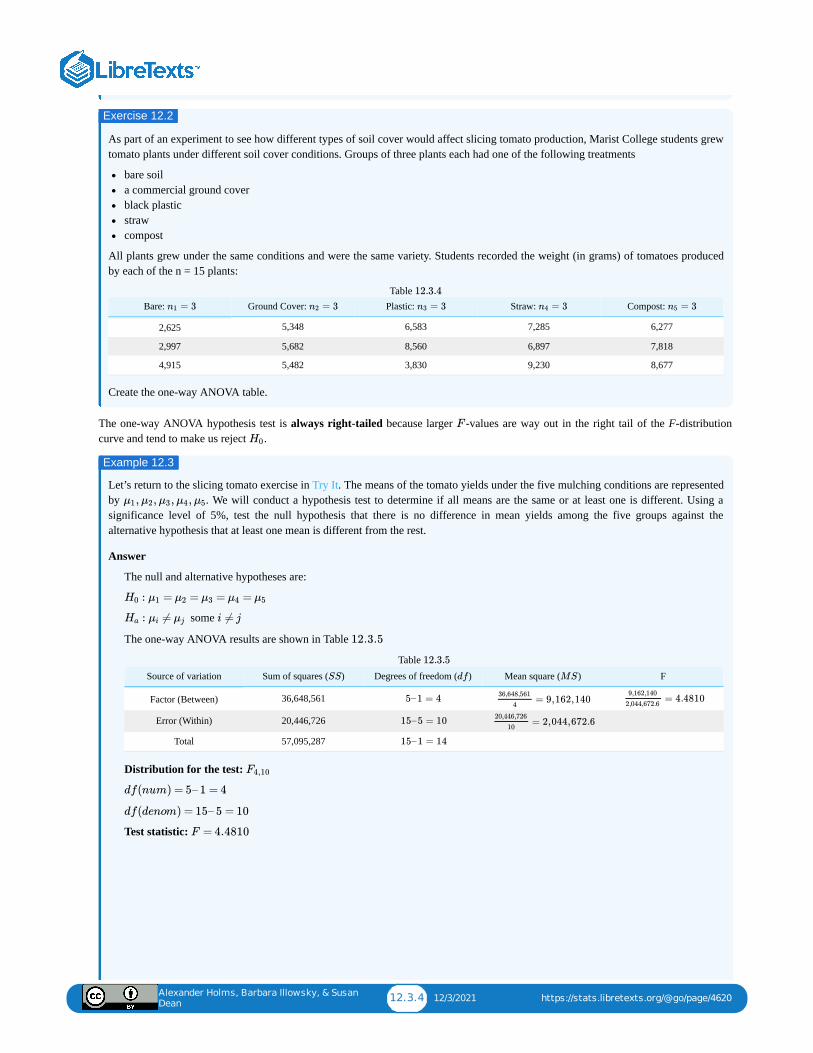
Alexander Holms, Barbara Illowsky, & Susan
Dean12.3.4 12/3/2021 https://stats.libretexts.org/@go/page/4620
As part of an experiment to see how different types of soil cover would affect slicing tomato production, Marist College students grewtomato plants under different soil cover conditions. Groups of three plants each had one of the following treatments
bare soila commercial ground coverblack plasticstrawcompost
All plants grew under the same conditions and were the same variety. Students recorded the weight (in grams) of tomatoes producedby each of the n = 15 plants:
Bare: Ground Cover: Plastic: Straw: Compost:
2,625 5,348 6,583 7,285 6,277
2,997 5,682 8,560 6,897 7,818
4,915 5,482 3,830 9,230 8,677
Table
Create the one-way ANOVA table.
The one-way ANOVA hypothesis test is always right-tailed because larger -values are way out in the right tail of the F-distributioncurve and tend to make us reject .
Let’s return to the slicing tomato exercise in Try It. The means of the tomato yields under the five mulching conditions are representedby . We will conduct a hypothesis test to determine if all means are the same or at least one is different. Using asignificance level of 5%, test the null hypothesis that there is no difference in mean yields among the five groups against thealternative hypothesis that at least one mean is different from the rest.
Answer
The null and alternative hypotheses are:
some
The one-way ANOVA results are shown in Table
Table Source of variation Sum of squares ( ) Degrees of freedom ( ) Mean square ( ) F
Factor (Between) 36,648,561
Error (Within) 20,446,726
Total 57,095,287
Distribution for the test:
Test statistic:
Exercise 12.2
= 3n1 = 3n2 = 3n3 = 3n4 = 3n5
12.3.4
F
H0
Example 12.3
, , , ,μ1 μ2 μ3 μ4 μ5
: = = = =H0 μ1 μ2 μ3 μ4 μ5
: ≠Ha μi μj i ≠ j
12.3.5
12.3.5
SS df MS
5–1 = 4 = 9,162,14036,648,561
4= 4.4810
9,162,140
2,044,672.6
15–5 = 10 = 2,044,672.620,446,726
10
15–1 = 14
F4,10
df(num) = 5– 1 = 4
df(denom) = 15– 5 = 10
F = 4.4810
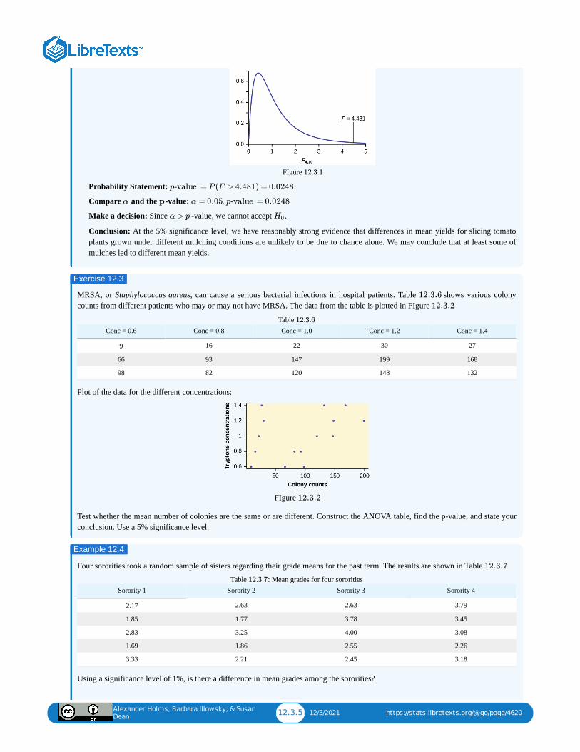
Alexander Holms, Barbara Illowsky, & Susan
Dean12.3.5 12/3/2021 https://stats.libretexts.org/@go/page/4620
FIgure
Probability Statement:
Compare and the -value: ,
Make a decision: Since -value, we cannot accept .
Conclusion: At the 5% significance level, we have reasonably strong evidence that differences in mean yields for slicing tomatoplants grown under different mulching conditions are unlikely to be due to chance alone. We may conclude that at least some ofmulches led to different mean yields.
MRSA, or Staphylococcus aureus, can cause a serious bacterial infections in hospital patients. Table shows various colonycounts from different patients who may or may not have MRSA. The data from the table is plotted in FIgure .
Table Conc = 0.6 Conc = 0.8 Conc = 1.0 Conc = 1.2 Conc = 1.4
9 16 22 30 27
66 93 147 199 168
98 82 120 148 132
Plot of the data for the different concentrations:
FIgure
Test whether the mean number of colonies are the same or are different. Construct the ANOVA table, find the p-value, and state yourconclusion. Use a 5% significance level.
Four sororities took a random sample of sisters regarding their grade means for the past term. The results are shown in Table .
Table : Mean grades for four sororitiesSorority 1 Sorority 2 Sorority 3 Sorority 4
2.17 2.63 2.63 3.79
1.85 1.77 3.78 3.45
2.83 3.25 4.00 3.08
1.69 1.86 2.55 2.26
3.33 2.21 2.45 3.18
Using a significance level of 1%, is there a difference in mean grades among the sororities?
12.3.1
p-value = P (F > 4.481) = 0.0248.
α p α = 0.05 p-value = 0.0248
α > p H0
Exercise 12.3
12.3.6
12.3.2
12.3.6
12.3.2
Example 12.4
12.3.7
12.3.7
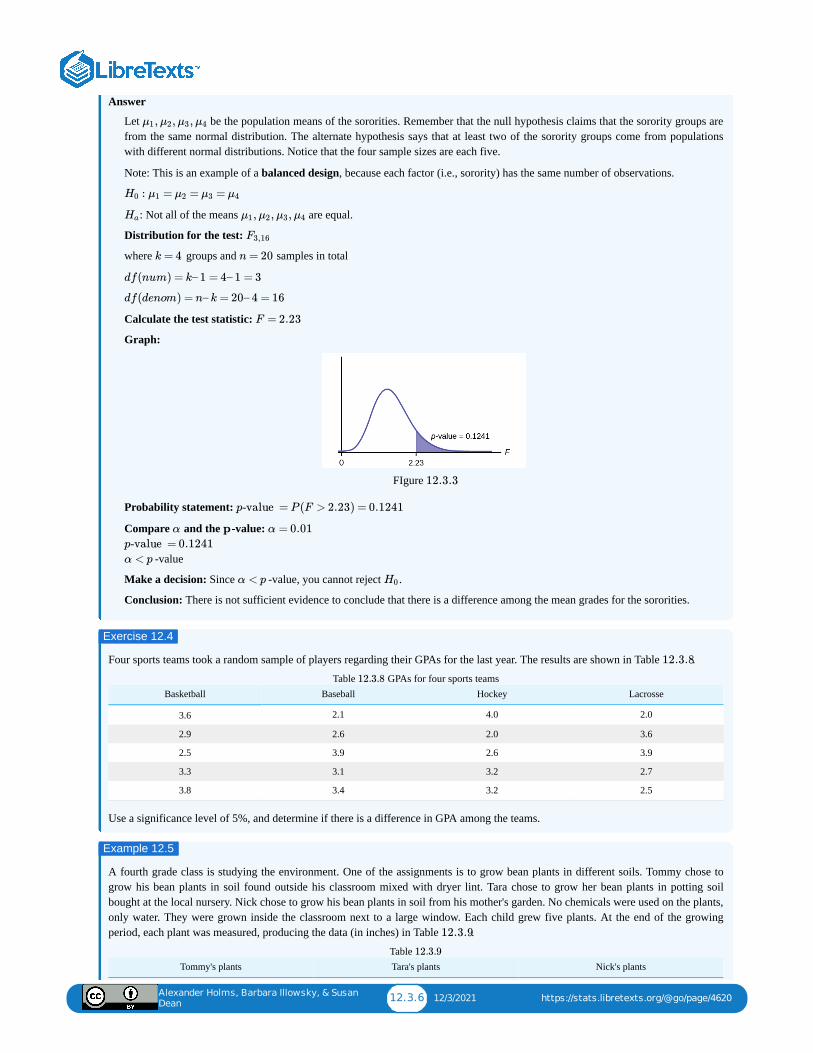
Alexander Holms, Barbara Illowsky, & Susan
Dean12.3.6 12/3/2021 https://stats.libretexts.org/@go/page/4620
Answer
Let be the population means of the sororities. Remember that the null hypothesis claims that the sorority groups arefrom the same normal distribution. The alternate hypothesis says that at least two of the sorority groups come from populationswith different normal distributions. Notice that the four sample sizes are each five.
Note: This is an example of a balanced design, because each factor (i.e., sorority) has the same number of observations.
: Not all of the means are equal.
Distribution for the test:
where groups and samples in total
Calculate the test statistic:
Graph:
FIgure
Probability statement:
Compare and the -value:
-value
Make a decision: Since -value, you cannot reject .
Conclusion: There is not sufficient evidence to conclude that there is a difference among the mean grades for the sororities.
Four sports teams took a random sample of players regarding their GPAs for the last year. The results are shown in Table .
Table GPAs for four sports teamsBasketball Baseball Hockey Lacrosse
3.6 2.1 4.0 2.0
2.9 2.6 2.0 3.6
2.5 3.9 2.6 3.9
3.3 3.1 3.2 2.7
3.8 3.4 3.2 2.5
Use a significance level of 5%, and determine if there is a difference in GPA among the teams.
A fourth grade class is studying the environment. One of the assignments is to grow bean plants in different soils. Tommy chose togrow his bean plants in soil found outside his classroom mixed with dryer lint. Tara chose to grow her bean plants in potting soilbought at the local nursery. Nick chose to grow his bean plants in soil from his mother's garden. No chemicals were used on the plants,only water. They were grown inside the classroom next to a large window. Each child grew five plants. At the end of the growingperiod, each plant was measured, producing the data (in inches) in Table .
Tommy's plants Tara's plants Nick's plantsTable
, , ,μ1 μ2 μ3 μ4
: = = =H0 μ1 μ2 μ3 μ4
Ha , , ,μ1 μ2 μ3 μ4
F3,16
k = 4 n = 20
df(num) = k– 1 = 4– 1 = 3
df(denom) = n– k = 20– 4 = 16
F = 2.23
12.3.3
p-value = P (F > 2.23) = 0.1241
α p α = 0.01
p-value = 0.1241
α < p
α < p H0
Exercise 12.4
12.3.8
12.3.8
Example 12.5
12.3.9
12.3.9
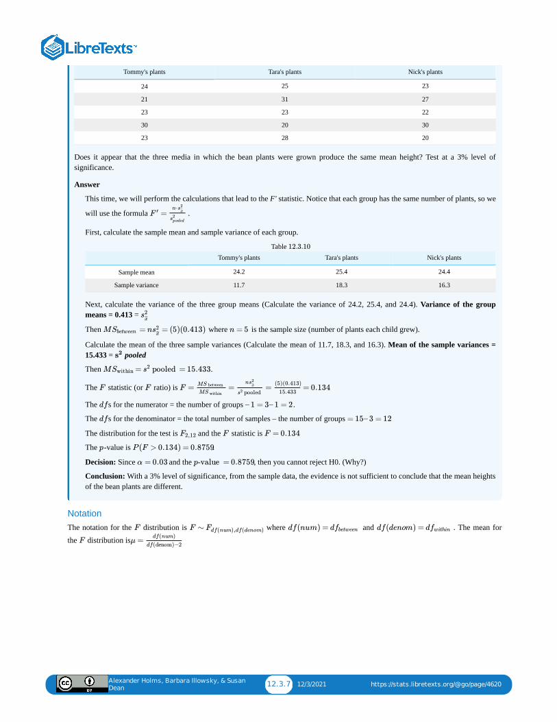
Alexander Holms, Barbara Illowsky, & Susan
Dean12.3.7 12/3/2021 https://stats.libretexts.org/@go/page/4620
Tommy's plants Tara's plants Nick's plants
24 25 23
21 31 27
23 23 22
30 20 30
23 28 20
Does it appear that the three media in which the bean plants were grown produce the same mean height? Test at a 3% level ofsignificance.
Answer
This time, we will perform the calculations that lead to the F' statistic. Notice that each group has the same number of plants, so we
will use the formula .
First, calculate the sample mean and sample variance of each group.
Tommy's plants Tara's plants Nick's plants
Sample mean 24.2 25.4 24.4
Sample variance 11.7 18.3 16.3
Table
Next, calculate the variance of the three group means (Calculate the variance of 24.2, 25.4, and 24.4). Variance of the groupmeans = 0.413 =
Then where is the sample size (number of plants each child grew).
Calculate the mean of the three sample variances (Calculate the mean of 11.7, 18.3, and 16.3). Mean of the sample variances =15.433 = pooled
Then .
The statistic (or ratio) is
The s for the numerator = the number of groups .
The s for the denominator = the total number of samples – the number of groups
The distribution for the test is and the statistic is
The -value is .
Decision: Since and the , then you cannot reject H0. (Why?)
Conclusion: With a 3% level of significance, from the sample data, the evidence is not sufficient to conclude that the mean heightsof the bean plants are different.
NotationThe notation for the distribution is where and . The mean for
the distribution is
=F ′n⋅s2
x̄
s2pooled
12.3.10
s2x̄̄̄
M = n = (5)(0.413)Sbetween s2x̄̄̄
n = 5
s2
M = pooled = 15.433Swithin s2
F F F = = = = 0.134MS between
MS within
ns2x̄
pooled s2
(5)(0.413)
15.433
df – 1 = 3– 1 = 2
df = 15– 3 = 12
F2,12 F F = 0.134
p P (F > 0.134) = 0.8759
α = 0.03 p-value = 0.8759
F F ∼ Fdf(num),df(denom) df(num) = dfbetween df(denom) = dfwithin
F μ =df(num)
df(denom)−2
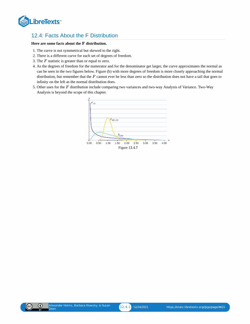
Alexander Holms, Barbara Illowsky, & Susan
Dean12.4.1 12/24/2021 https://stats.libretexts.org/@go/page/4621
12.4: Facts About the F DistributionHere are some facts about the distribution.
1. The curve is not symmetrical but skewed to the right.2. There is a different curve for each set of degrees of freedom.3. The statistic is greater than or equal to zero.4. As the degrees of freedom for the numerator and for the denominator get larger, the curve approximates the normal as
can be seen in the two figures below. Figure (b) with more degrees of freedom is more closely approaching the normaldistribution, but remember that the cannot ever be less than zero so the distribution does not have a tail that goes toinfinity on the left as the normal distribution does.
5. Other uses for the distribution include comparing two variances and two-way Analysis of Variance. Two-WayAnalysis is beyond the scope of this chapter.
Figure
F
F
F
F
12.4.7
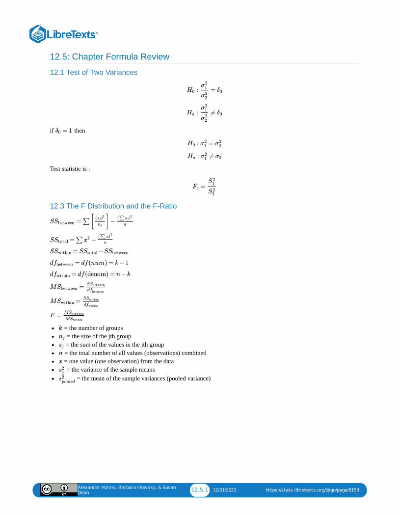
Alexander Holms, Barbara Illowsky, & Susan
Dean12.5.1 12/31/2021 https://stats.libretexts.org/@go/page/6153
12.5: Chapter Formula Review
12.1 Test of Two Variances
if then
Test statistic is :
12.3 The F Distribution and the F-Ratio
= the number of groups = the size of the jth group = the sum of the values in the jth group = the total number of all values (observations) combined = one value (one observation) from the data = the variance of the sample means
= the mean of the sample variances (pooled variance)
: =H0
σ21
σ22
δ0
: ≠Ha
σ21
σ22
δ0
= 1δ0
: =H0 σ21 σ2
2
: ≠Ha σ21 σ2
=Fc
S21
S22
S =∑[ ]−Sbetween( )sj
2
nj
(∑ )sj2
n
S =∑ −Stotal x2 (∑ x)2
n
S = S −SSwithin Stotal Sbetween
d = df(num) = k−1fbetween
d = df(denom) = n−kfwithin
M =SbetweenSSbetween
dfbetween
M =SwithinSSwithin
dfwithin
F =MSbetween
MSwithin
k
nj
sjn
x
s2x̄̄̄
s2pooled
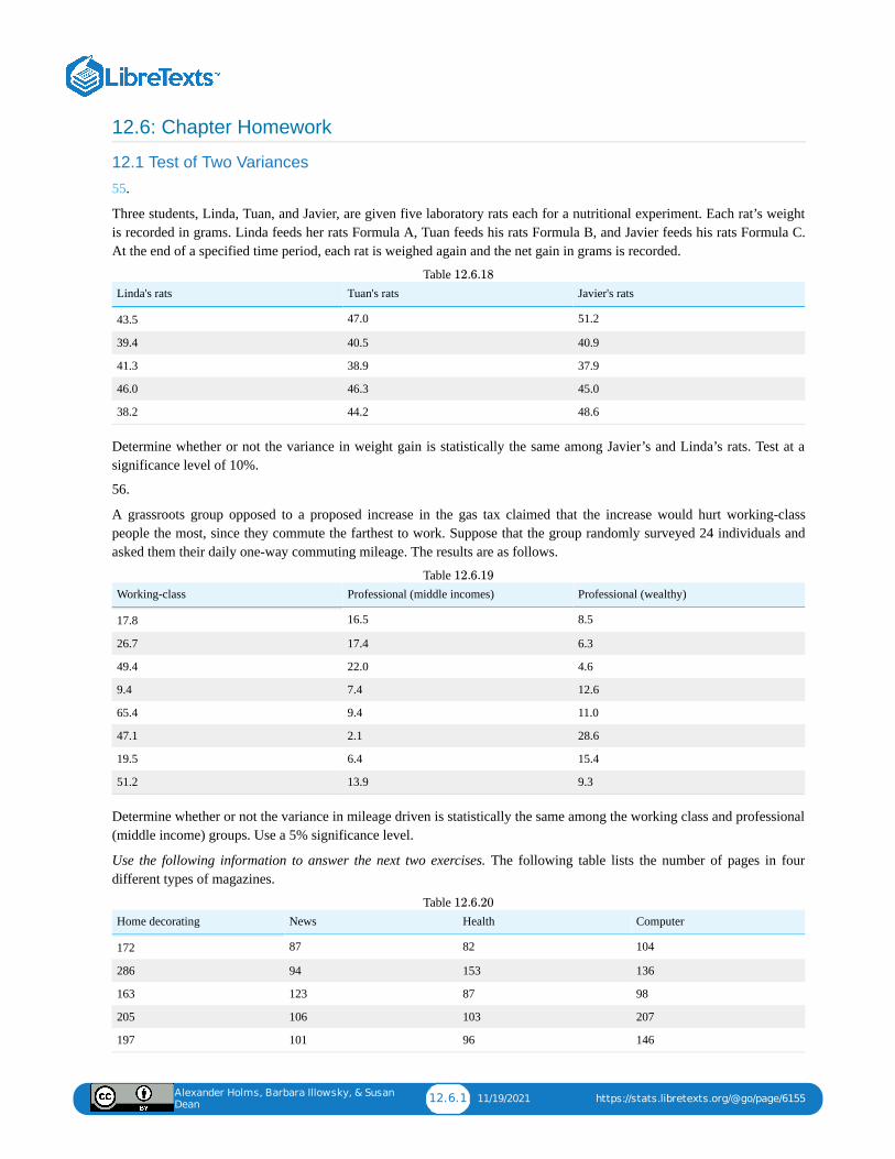
Alexander Holms, Barbara Illowsky, & Susan
Dean12.6.1 11/19/2021 https://stats.libretexts.org/@go/page/6155
12.6: Chapter Homework
12.1 Test of Two Variances
55.
Three students, Linda, Tuan, and Javier, are given five laboratory rats each for a nutritional experiment. Each rat’s weightis recorded in grams. Linda feeds her rats Formula A, Tuan feeds his rats Formula B, and Javier feeds his rats Formula C.At the end of a specified time period, each rat is weighed again and the net gain in grams is recorded.
Linda's rats Tuan's rats Javier's rats
43.5 47.0 51.2
39.4 40.5 40.9
41.3 38.9 37.9
46.0 46.3 45.0
38.2 44.2 48.6
Table
Determine whether or not the variance in weight gain is statistically the same among Javier’s and Linda’s rats. Test at asignificance level of 10%.
56.
A grassroots group opposed to a proposed increase in the gas tax claimed that the increase would hurt working-classpeople the most, since they commute the farthest to work. Suppose that the group randomly surveyed 24 individuals andasked them their daily one-way commuting mileage. The results are as follows.
Working-class Professional (middle incomes) Professional (wealthy)
17.8 16.5 8.5
26.7 17.4 6.3
49.4 22.0 4.6
9.4 7.4 12.6
65.4 9.4 11.0
47.1 2.1 28.6
19.5 6.4 15.4
51.2 13.9 9.3
Table
Determine whether or not the variance in mileage driven is statistically the same among the working class and professional(middle income) groups. Use a 5% significance level.
Use the following information to answer the next two exercises. The following table lists the number of pages in fourdifferent types of magazines.
Home decorating News Health Computer
172 87 82 104
286 94 153 136
163 123 87 98
205 106 103 207
197 101 96 146
Table
12.6.18
12.6.19
12.6.20
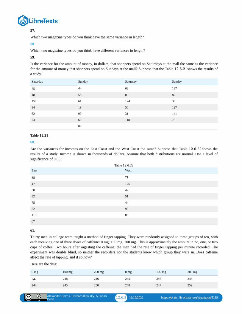
Alexander Holms, Barbara Illowsky, & Susan
Dean12.6.2 11/19/2021 https://stats.libretexts.org/@go/page/6155
57.
Which two magazine types do you think have the same variance in length?
58.
Which two magazine types do you think have different variances in length?
59.
Is the variance for the amount of money, in dollars, that shoppers spend on Saturdays at the mall the same as the variancefor the amount of money that shoppers spend on Sundays at the mall? Suppose that the Table shows the results ofa study.
Saturday Sunday Saturday Sunday
75 44 62 137
18 58 0 82
150 61 124 39
94 19 50 127
62 99 31 141
73 60 118 73
89
Table 12.21
60.
Are the variances for incomes on the East Coast and the West Coast the same? Suppose that Table shows theresults of a study. Income is shown in thousands of dollars. Assume that both distributions are normal. Use a level ofsignificance of 0.05.
East West
38 71
47 126
30 42
82 51
75 44
52 90
115 88
67
Table
61.
Thirty men in college were taught a method of finger tapping. They were randomly assigned to three groups of ten, witheach receiving one of three doses of caffeine: 0 mg, 100 mg, 200 mg. This is approximately the amount in no, one, or twocups of coffee. Two hours after ingesting the caffeine, the men had the rate of finger tapping per minute recorded. Theexperiment was double blind, so neither the recorders nor the students knew which group they were in. Does caffeineaffect the rate of tapping, and if so how?
Here are the data:
0 mg 100 mg 200 mg 0 mg 100 mg 200 mg
242 248 246 245 246 248
244 245 250 248 247 252
12.6.21
12.6.22
12.6.22
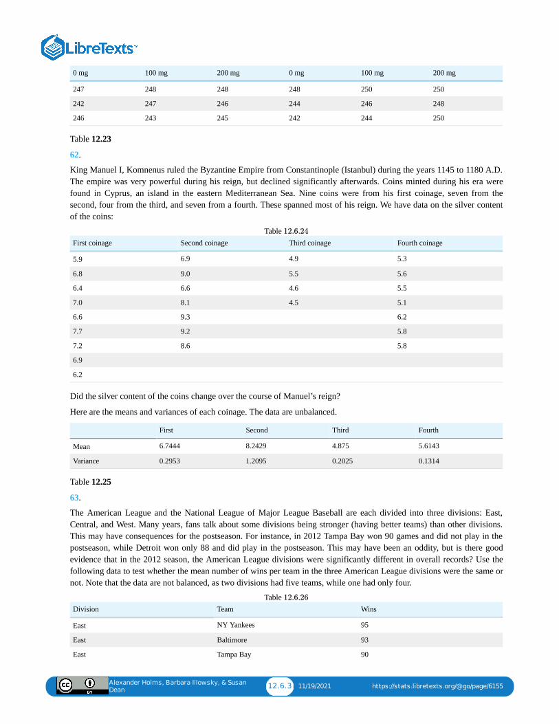
Alexander Holms, Barbara Illowsky, & Susan
Dean12.6.3 11/19/2021 https://stats.libretexts.org/@go/page/6155
0 mg 100 mg 200 mg 0 mg 100 mg 200 mg
247 248 248 248 250 250
242 247 246 244 246 248
246 243 245 242 244 250
Table 12.23
62.
King Manuel I, Komnenus ruled the Byzantine Empire from Constantinople (Istanbul) during the years 1145 to 1180 A.D.The empire was very powerful during his reign, but declined significantly afterwards. Coins minted during his era werefound in Cyprus, an island in the eastern Mediterranean Sea. Nine coins were from his first coinage, seven from thesecond, four from the third, and seven from a fourth. These spanned most of his reign. We have data on the silver contentof the coins:
First coinage Second coinage Third coinage Fourth coinage
5.9 6.9 4.9 5.3
6.8 9.0 5.5 5.6
6.4 6.6 4.6 5.5
7.0 8.1 4.5 5.1
6.6 9.3 6.2
7.7 9.2 5.8
7.2 8.6 5.8
6.9
6.2
Table
Did the silver content of the coins change over the course of Manuel’s reign?
Here are the means and variances of each coinage. The data are unbalanced.
First Second Third Fourth
Mean 6.7444 8.2429 4.875 5.6143
Variance 0.2953 1.2095 0.2025 0.1314
Table 12.25
63.
The American League and the National League of Major League Baseball are each divided into three divisions: East,Central, and West. Many years, fans talk about some divisions being stronger (having better teams) than other divisions.This may have consequences for the postseason. For instance, in 2012 Tampa Bay won 90 games and did not play in thepostseason, while Detroit won only 88 and did play in the postseason. This may have been an oddity, but is there goodevidence that in the 2012 season, the American League divisions were significantly different in overall records? Use thefollowing data to test whether the mean number of wins per team in the three American League divisions were the same ornot. Note that the data are not balanced, as two divisions had five teams, while one had only four.
Division Team Wins
East NY Yankees 95
East Baltimore 93
East Tampa Bay 90
Table
12.6.24
12.6.26
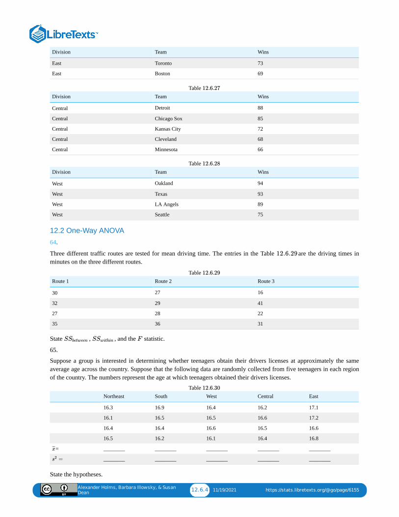
Alexander Holms, Barbara Illowsky, & Susan
Dean12.6.4 11/19/2021 https://stats.libretexts.org/@go/page/6155
Division Team Wins
East Toronto 73
East Boston 69
Division Team Wins
Central Detroit 88
Central Chicago Sox 85
Central Kansas City 72
Central Cleveland 68
Central Minnesota 66
Table
Division Team Wins
West Oakland 94
West Texas 93
West LA Angels 89
West Seattle 75
Table
12.2 One-Way ANOVA
64.
Three different traffic routes are tested for mean driving time. The entries in the Table are the driving times inminutes on the three different routes.
Route 1 Route 2 Route 3
30 27 16
32 29 41
27 28 22
35 36 31
Table
State , , and the statistic.
65.
Suppose a group is interested in determining whether teenagers obtain their drivers licenses at approximately the sameaverage age across the country. Suppose that the following data are randomly collected from five teenagers in each regionof the country. The numbers represent the age at which teenagers obtained their drivers licenses.
Northeast South West Central East
16.3 16.9 16.4 16.2 17.1
16.1 16.5 16.5 16.6 17.2
16.4 16.4 16.6 16.5 16.6
16.5 16.2 16.1 16.4 16.8
= ________ ________ ________ ________ ________
________ ________ ________ ________ ________
Table
State the hypotheses.
12.6.27
12.6.28
12.6.29
12.6.29
SSbetween SSwithin F
x̄̄̄
=s2
12.6.30
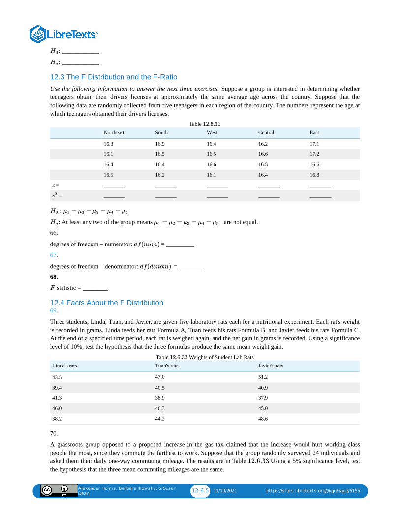
Alexander Holms, Barbara Illowsky, & Susan
Dean12.6.5 11/19/2021 https://stats.libretexts.org/@go/page/6155
: ____________
: ____________
12.3 The F Distribution and the F-Ratio
Use the following information to answer the next three exercises. Suppose a group is interested in determining whetherteenagers obtain their drivers licenses at approximately the same average age across the country. Suppose that thefollowing data are randomly collected from five teenagers in each region of the country. The numbers represent the age atwhich teenagers obtained their drivers licenses.
Northeast South West Central East
16.3 16.9 16.4 16.2 17.1
16.1 16.5 16.5 16.6 17.2
16.4 16.4 16.6 16.5 16.6
16.5 16.2 16.1 16.4 16.8
= ________ ________ ________ ________ ________
________ ________ ________ ________ ________
Table
: At least any two of the group means are not equal.
66.
degrees of freedom – numerator: = _________
67.
degrees of freedom – denominator: = ________
68.
statistic = ________
12.4 Facts About the F Distribution69.
Three students, Linda, Tuan, and Javier, are given five laboratory rats each for a nutritional experiment. Each rat's weightis recorded in grams. Linda feeds her rats Formula A, Tuan feeds his rats Formula B, and Javier feeds his rats Formula C.At the end of a specified time period, each rat is weighed again, and the net gain in grams is recorded. Using a significancelevel of 10%, test the hypothesis that the three formulas produce the same mean weight gain.
Linda's rats Tuan's rats Javier's rats
43.5 47.0 51.2
39.4 40.5 40.9
41.3 38.9 37.9
46.0 46.3 45.0
38.2 44.2 48.6
Table Weights of Student Lab Rats
70.
A grassroots group opposed to a proposed increase in the gas tax claimed that the increase would hurt working-classpeople the most, since they commute the farthest to work. Suppose that the group randomly surveyed 24 individuals andasked them their daily one-way commuting mileage. The results are in Table . Using a 5% significance level, testthe hypothesis that the three mean commuting mileages are the same.
H0
Ha
x̄̄̄
=s2
12.6.31
: = = = =H0 μ1 μ2 μ3 μ4 μ5
Ha = = = =μ1 μ2 μ3 μ4 μ5
df(num)
df(denom)
F
12.6.32
12.6.33
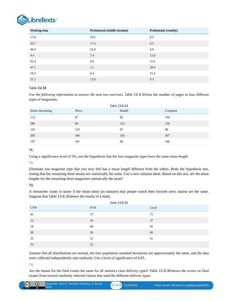
Alexander Holms, Barbara Illowsky, & Susan
Dean12.6.6 11/19/2021 https://stats.libretexts.org/@go/page/6155
Working-class Professional (middle incomes) Professional (wealthy)Working-class Professional (middle incomes) Professional (wealthy)
17.8 16.5 8.5
26.7 17.4 6.3
49.4 22.0 4.6
9.4 7.4 12.6
65.4 9.4 11.0
47.1 2.1 28.6
19.5 6.4 15.4
51.2 13.9 9.3
Table 12.33
Use the following information to answer the next two exercises. Table lists the number of pages in four differenttypes of magazines.
Home decorating News Health Computer
172 87 82 104
286 94 153 136
163 123 87 98
205 106 103 207
197 101 96 146
Table
71.
Using a significance level of 5%, test the hypothesis that the four magazine types have the same mean length.
72.
Eliminate one magazine type that you now feel has a mean length different from the others. Redo the hypothesis test,testing that the remaining three means are statistically the same. Use a new solution sheet. Based on this test, are the meanlengths for the remaining three magazines statistically the same?
73.
A researcher wants to know if the mean times (in minutes) that people watch their favorite news station are the same.Suppose that Table shows the results of a study.
CNN FOX Local
45 15 72
12 43 37
18 68 56
38 50 60
23 31 51
35 22
Table
Assume that all distributions are normal, the four population standard deviations are approximately the same, and the datawere collected independently and randomly. Use a level of significance of 0.05.
74.
Are the means for the final exams the same for all statistics class delivery types? Table shows the scores on finalexams from several randomly selected classes that used the different delivery types.
12.6.34
12.6.34
12.6.35
12.6.35
12.6.36
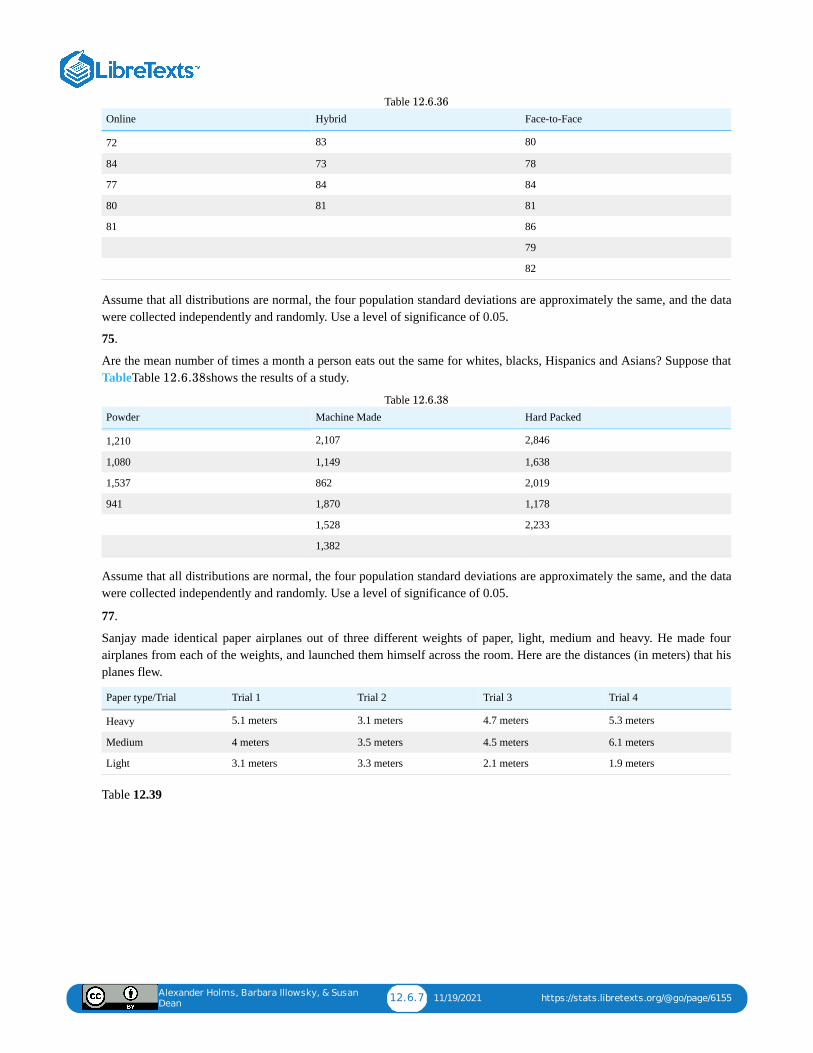
Alexander Holms, Barbara Illowsky, & Susan
Dean12.6.7 11/19/2021 https://stats.libretexts.org/@go/page/6155
Online Hybrid Face-to-Face
72 83 80
84 73 78
77 84 84
80 81 81
81 86
79
82
Table
Assume that all distributions are normal, the four population standard deviations are approximately the same, and the datawere collected independently and randomly. Use a level of significance of 0.05.
75.
Are the mean number of times a month a person eats out the same for whites, blacks, Hispanics and Asians? Suppose thatTableTable shows the results of a study.
Powder Machine Made Hard Packed
1,210 2,107 2,846
1,080 1,149 1,638
1,537 862 2,019
941 1,870 1,178
1,528 2,233
1,382
Table
Assume that all distributions are normal, the four population standard deviations are approximately the same, and the datawere collected independently and randomly. Use a level of significance of 0.05.
77.
Sanjay made identical paper airplanes out of three different weights of paper, light, medium and heavy. He made fourairplanes from each of the weights, and launched them himself across the room. Here are the distances (in meters) that hisplanes flew.
Paper type/Trial Trial 1 Trial 2 Trial 3 Trial 4
Heavy 5.1 meters 3.1 meters 4.7 meters 5.3 meters
Medium 4 meters 3.5 meters 4.5 meters 6.1 meters
Light 3.1 meters 3.3 meters 2.1 meters 1.9 meters
Table 12.39
12.6.36
12.6.38
12.6.38
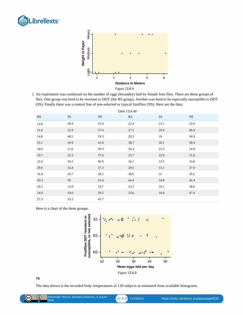
Alexander Holms, Barbara Illowsky, & Susan
Dean12.6.8 11/19/2021 https://stats.libretexts.org/@go/page/6155
Figure
1. An experiment was conducted on the number of eggs (fecundity) laid by female fruit flies. There are three groups offlies. One group was bred to be resistant to DDT (the RS group). Another was bred to be especially susceptible to DDT(SS). Finally there was a control line of non-selected or typical fruitflies (NS). Here are the data:
RS SS NS RS SS NS
12.8 38.4 35.4 22.4 23.1 22.6
21.6 32.9 27.4 27.5 29.4 40.4
14.8 48.5 19.3 20.3 16 34.4
23.1 20.9 41.8 38.7 20.1 30.4
34.6 11.6 20.3 26.4 23.3 14.9
19.7 22.3 37.6 23.7 22.9 51.8
22.6 30.2 36.9 26.1 22.5 33.8
29.6 33.4 37.3 29.5 15.1 37.9
16.4 26.7 28.2 38.6 31 29.5
20.3 39 23.4 44.4 16.9 42.4
29.3 12.8 33.7 23.2 16.1 36.6
14.9 14.6 29.2 23.6 10.8 47.4
27.3 12.2 41.7
Table
Here is a chart of the three groups:
Figure
79.
The data shown is the recorded body temperatures of 130 subjects as estimated from available histograms.
12.6.8
12.6.40
12.6.9
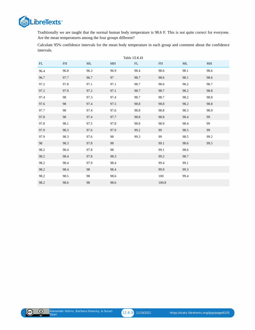
Alexander Holms, Barbara Illowsky, & Susan
Dean12.6.9 11/19/2021 https://stats.libretexts.org/@go/page/6155
Traditionally we are taught that the normal human body temperature is 98.6 F. This is not quite correct for everyone.Are the mean temperatures among the four groups different?
Calculate 95% confidence intervals for the mean body temperature in each group and comment about the confidenceintervals.
FL FH ML MH FL FH ML MH
96.4 96.8 96.3 96.9 98.4 98.6 98.1 98.6
96.7 97.7 96.7 97 98.7 98.6 98.1 98.6
97.2 97.8 97.1 97.1 98.7 98.6 98.2 98.7
97.2 97.9 97.2 97.1 98.7 98.7 98.2 98.8
97.4 98 97.3 97.4 98.7 98.7 98.2 98.8
97.6 98 97.4 97.5 98.8 98.8 98.2 98.8
97.7 98 97.4 97.6 98.8 98.8 98.3 98.9
97.8 98 97.4 97.7 98.8 98.8 98.4 99
97.8 98.1 97.5 97.8 98.8 98.9 98.4 99
97.9 98.3 97.6 97.9 99.2 99 98.5 99
97.9 98.3 97.6 98 99.3 99 98.5 99.2
98 98.3 97.8 98 99.1 98.6 99.5
98.2 98.4 97.8 98 99.1 98.6
98.2 98.4 97.8 98.3 99.2 98.7
98.2 98.4 97.9 98.4 99.4 99.1
98.2 98.4 98 98.4 99.9 99.3
98.2 98.5 98 98.6 100 99.4
98.2 98.6 98 98.6 100.8
Table
12.6.41
Alexander Holms, Barbara Illowsky, & Susan
Dean12.7.1 1/7/2022 https://stats.libretexts.org/@go/page/4622
12.7: Chapter Key Terms
Analysis of Variancealso referred to as ANOVA, is a method of testing whether or not the means of three or more populations are equal. Themethod is applicable if:
The test statistic for analysis of variance is the -ratio.
One-Way ANOVAa method of testing whether or not the means of three or more populations are equal; the method is applicable if:
The test statistic for analysis of variance is the -ratio.
Variancemean of the squared deviations from the mean; the square of the standard deviation. For a set of data, a deviation canbe represented as where is a value of the data and is the sample mean. The sample variance is equal to thesum of the squares of the deviations divided by the difference of the sample size and one.
F
F
x– x¯̄̄ x x¯̄̄
Alexander Holms, Barbara Illowsky, & Susan
Dean12.8.1 12/3/2021 https://stats.libretexts.org/@go/page/6154
12.8: Chapter Practice
12.1 Test of Two Variances
Use the following information to answer the next two exercises. There are two assumptions that must be true in order toperform an test of two variances.
1.
Name one assumption that must be true.
2.
What is the other assumption that must be true?
Use the following information to answer the next five exercises. Two coworkers commute from the same building. Theyare interested in whether or not there is any variation in the time it takes them to drive to work. They each record theirtimes for 20 commutes. The first worker’s times have a variance of 12.1. The second worker’s times have a variance of16.9. The first worker thinks that he is more consistent with his commute times. Test the claim at the 10% level. Assumethat commute times are normally distributed.
3.
State the null and alternative hypotheses.
4.
What is in this problem?
5.
What is in this problem?
6.
What is ?
7.
What is the statistic?
8.
What is the critical value?
9.
Is the claim accurate?
Use the following information to answer the next four exercises. Two students are interested in whether or not there isvariation in their test scores for math class. There are 15 total math tests they have taken so far. The first student’s gradeshave a standard deviation of 38.1. The second student’s grades have a standard deviation of 22.5. The second studentthinks his scores are more consistent.
10.
State the null and alternative hypotheses.
11.
What is the Statistic?
12.
What is the critical value?
13.
At the 5% significance level, do we reject the null hypothesis?
F
s1
s2
n
F
F
Alexander Holms, Barbara Illowsky, & Susan
Dean12.8.2 12/3/2021 https://stats.libretexts.org/@go/page/6154
Use the following information to answer the next three exercises. Two cyclists are comparing the variances of their overallpaces going uphill. Each cyclist records his or her speeds going up 35 hills. The first cyclist has a variance of 23.8 and thesecond cyclist has a variance of 32.1. The cyclists want to see if their variances are the same or different. Assume thatcommute times are normally distributed.
14.
State the null and alternative hypotheses.
15.
What is the Statistic?
16.
At the 5% significance level, what can we say about the cyclists’ variances?
12.2 One-Way ANOVA
Use the following information to answer the next five exercises. There are five basic assumptions that must be fulfilled inorder to perform a one-way ANOVA test. What are they?
17.
Write one assumption.
18.
Write another assumption.
19.
Write a third assumption.
20.
Write a fourth assumption.
12.3 The F Distribution and the F-RatioUse the following information to answer the next eight exercises. Groups of men from three different areas of the countryare to be tested for mean weight. The entries in Table are the weights for the different groups.
Group 1 Group 2 Group 3
216 202 170
198 213 165
240 284 182
187 228 197
176 210 201
Table 12.13
21.
What is the Sum of Squares Factor?
22.
What is the Sum of Squares Error?
23.
What is the for the numerator?
24.
What is the for the denominator?
25.
F
12.8.13
df
df
Alexander Holms, Barbara Illowsky, & Susan
Dean12.8.3 12/3/2021 https://stats.libretexts.org/@go/page/6154
What is the Mean Square Factor?
26.
What is the Mean Square Error?
27.
What is the statistic?
Use the following information to answer the next eight exercises. Girls from four different soccer teams are to be tested formean goals scored per game. The entries in Table are the goals per game for the different teams.
Team 1 Team 2 Team 3 Team 4
1 2 0 3
2 3 1 4
0 2 1 4
3 4 0 3
2 4 0 2
Table
28.
What is ?
29.
What is the for the numerator?
30.
What is ?
31.
What is ?
32.
What is the for the denominator?
33.
What is ?
34.
What is the statistic?
35.
Judging by the statistic, do you think it is likely or unlikely that you will reject the null hypothesis?
12.4 Facts About the F Distribution36.
An statistic can have what values?
37.
What happens to the curves as the degrees of freedom for the numerator and the denominator get larger?
Use the following information to answer the next seven exercise. Four basketball teams took a random sample of playersregarding how high each player can jump (in inches). The results are shown in Table .
Team 1 Team 2 Team 3 Team 4 Team 5
36 32 48 38 41
Table
F
12.8.14
12.8.14
SSbetween
df
MSbetween
SSwithin
df
MSwithin
F
F
F
12.8.15
12.8.15
Alexander Holms, Barbara Illowsky, & Susan
Dean12.8.4 12/3/2021 https://stats.libretexts.org/@go/page/6154
Team 1 Team 2 Team 3 Team 4 Team 5
42 35 50 44 39
51 38 39 46 40
38.
What is the ?
39.
What is the ?
40.
What are the Sum of Squares and Mean Squares Factors?
41.
What are the Sum of Squares and Mean Squares Errors?
42.
What is the statistic?
43.
What is the -value?
44.
At the 5% significance level, is there a difference in the mean jump heights among the teams?
Use the following information to answer the next seven exercises. A video game developer is testing a new game on threedifferent groups. Each group represents a different target market for the game. The developer collects scores from arandom sample from each group. The results are shown in Table
Group A Group B Group C
101 151 101
108 149 109
98 160 198
107 112 186
111 126 160
Table 12.16
45.
What is the ?
46.
What is the ?
47.
What are the and ?
48.
What are the and ?
49.
What is the Statistic?
50.
What is the p-value?
df(num)
df(denom)
F
p
12.8.16
df(num)
df(denom)
SSbetween MSbetween
SSwithin MSwithin
F
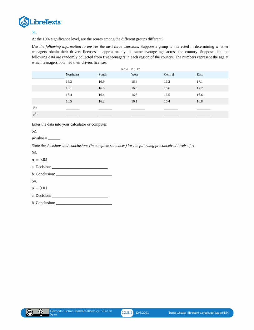
Alexander Holms, Barbara Illowsky, & Susan
Dean12.8.5 12/3/2021 https://stats.libretexts.org/@go/page/6154
51.
At the 10% significance level, are the scores among the different groups different?
Use the following information to answer the next three exercises. Suppose a group is interested in determining whetherteenagers obtain their drivers licenses at approximately the same average age across the country. Suppose that thefollowing data are randomly collected from five teenagers in each region of the country. The numbers represent the age atwhich teenagers obtained their drivers licenses.
Northeast South West Central East
16.3 16.9 16.4 16.2 17.1
16.1 16.5 16.5 16.6 17.2
16.4 16.4 16.6 16.5 16.6
16.5 16.2 16.1 16.4 16.8
= ________ ________ ________ ________ ________
= ________ ________ ________ ________ ________
Table
Enter the data into your calculator or computer.
52.
-value = ______
State the decisions and conclusions (in complete sentences) for the following preconceived levels of .
53.
a. Decision: ____________________________
b. Conclusion: ____________________________
54.
a. Decision: ____________________________
b. Conclusion: ____________________________
x̄̄̄
s2
12.8.17
p
α
α = 0.05
α = 0.01
Alexander Holms, Barbara Illowsky, & Susan
Dean12.9.1 12/10/2021 https://stats.libretexts.org/@go/page/6156
12.9: Chapter Reference
12.1 Test of Two Variances
“MLB Vs. Division Standings – 2012.” Available online at http://espn.go.com/mlb/standings/_/y...ion/order/true.
12.3 The F Distribution and the F-RatioTomato Data, Marist College School of Science (unpublished student research)
12.4 Facts About the F DistributionData from a fourth grade classroom in 1994 in a private K – 12 school in San Jose, CA.
Hand, D.J., F. Daly, A.D. Lunn, K.J. McConway, and E. Ostrowski. A Handbook of Small Datasets: Data for FruitflyFecundity. London: Chapman & Hall, 1994.
Hand, D.J., F. Daly, A.D. Lunn, K.J. McConway, and E. Ostrowski. A Handbook of Small Datasets. London: Chapman &Hall, 1994, pg. 50.
Hand, D.J., F. Daly, A.D. Lunn, K.J. McConway, and E. Ostrowski. A Handbook of Small Datasets. London: Chapman &Hall, 1994, pg. 118.
“MLB Standings – 2012.” Available online at http://espn.go.com/mlb/standings/_/year/2012.
Mackowiak, P. A., Wasserman, S. S., and Levine, M. M. (1992), "A Critical Appraisal of 98.6 Degrees F, the Upper Limitof the Normal Body Temperature, and Other Legacies of Carl Reinhold August Wunderlich," Journal of the AmericanMedical Association, 268, 1578-1580.
Alexander Holms, Barbara Illowsky, & Susan
Dean12.10.1 12/24/2021 https://stats.libretexts.org/@go/page/6152
12.10: Chapter Review
12.1 Test of Two Variances
The test for the equality of two variances rests heavily on the assumption of normal distributions. The test is unreliableif this assumption is not met. If both distributions are normal, then the ratio of the two sample variances is distributed as an
statistic, with numerator and denominator degrees of freedom that are one less than the samples sizes of thecorresponding two groups. A test of two variances hypothesis test determines if two variances are the same. Thedistribution for the hypothesis test is the distribution with two different degrees of freedom.
Assumptions:
1. Analysis of variance extends the comparison of two groups to several, each a level of a categorical variable (factor).Samples from each group are independent, and must be randomly selected from normal populations with equalvariances. We test the null hypothesis of equal means of the response in every group versus the alternative hypothesisof one or more group means being different from the others. A one-way ANOVA hypothesis test determines if severalpopulation means are equal. The distribution for the test is the Fdistribution with two different degrees of freedom.
Assumptions:
1. Analysis of variance compares the means of a response variable for several groups. ANOVA compares the variationwithin each group to the variation of the mean of each group. The ratio of these two is the statistic from an distribution with (number of groups – 1) as the numerator degrees of freedom and (number of observations –number of groups) as the denominator degrees of freedom. These statistics are summarized in the ANOVA table.
12.4 Facts About the DistributionWhen the data have unequal group sizes (unbalanced data), then techniques from Figure need to be used forhand calculations. In the case of balanced data (the groups are the same size) however, simplified calculations basedon group means and variances may be used. In practice, of course, software is usually employed in the analysis. Asin any analysis, graphs of various sorts should be used in conjunction with numerical techniques. Always look atyour data!
F
F
F
F F
F
12.10.3
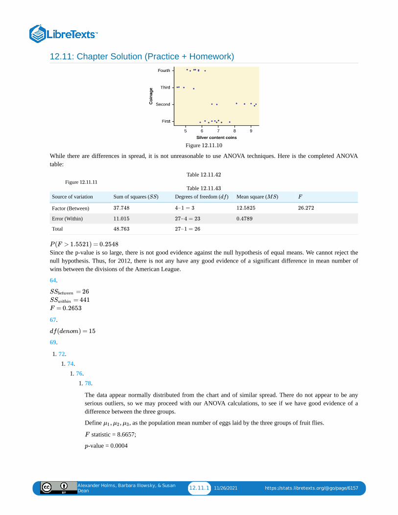
Alexander Holms, Barbara Illowsky, & Susan
Dean12.11.1 11/26/2021 https://stats.libretexts.org/@go/page/6157
12.11: Chapter Solution (Practice + Homework)
Figure
While there are differences in spread, it is not unreasonable to use ANOVA techniques. Here is the completed ANOVAtable:
Source of variation Sum of squares ( ) Degrees of freedom ( ) Mean square ( )
Factor (Between)
Error (Within)
Total
Table Figure
Table
Since the p-value is so large, there is not good evidence against the null hypothesis of equal means. We cannot reject thenull hypothesis. Thus, for 2012, there is not any have any good evidence of a significant difference in mean number ofwins between the divisions of the American League.
64.
67.
69.
1. 72.1. 74.
1. 76.1. 78.
The data appear normally distributed from the chart and of similar spread. There do not appear to be anyserious outliers, so we may proceed with our ANOVA calculations, to see if we have good evidence of adifference between the three groups.
Define , as the population mean number of eggs laid by the three groups of fruit flies.
statistic = 8.6657;
-value = 0.0004
12.11.10
SS df MS F
37.748 4–1 = 3 12.5825 26.272
11.015 27–4 = 23 0.4789
48.763 27–1 = 26
12.11.42
12.11.1112.11.43
P (F > 1.5521) = 0.2548
S = 26Sbetween
S = 441Swithin
F = 0.2653
df(denom) = 15
, ,μ1 μ2 μ3
F
p
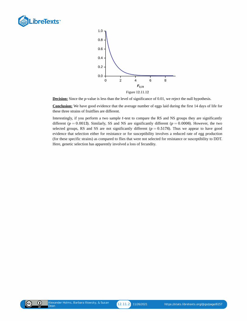
Alexander Holms, Barbara Illowsky, & Susan
Dean12.11.2 11/26/2021 https://stats.libretexts.org/@go/page/6157
Figure
Decision: Since the -value is less than the level of significance of 0.01, we reject the null hypothesis.
Conclusion: We have good evidence that the average number of eggs laid during the first 14 days of life forthese three strains of fruitflies are different.
Interestingly, if you perform a two sample -test to compare the RS and NS groups they are significantlydifferent ( ). Similarly, SS and NS are significantly different ( ). However, the twoselected groups, RS and SS are not significantly different ( ). Thus we appear to have goodevidence that selection either for resistance or for susceptibility involves a reduced rate of egg production(for these specific strains) as compared to flies that were not selected for resistance or susceptibility to DDT.Here, genetic selection has apparently involved a loss of fecundity.
12.11.12
p
t
p = 0.0013 p = 0.0006
p = 0.5176
1 1/7/2022
CHAPTER OVERVIEW13: LINEAR REGRESSION AND CORRELATION
13.0: INTRODUCTION TO LINEAR REGRESSION AND CORRELATION13.1: THE CORRELATION COEFFICIENT R13.2: TESTING THE SIGNIFICANCE OF THE CORRELATION COEFFICIENT13.3: LINEAR EQUATIONS13.4: THE REGRESSION EQUATION13.5: INTERPRETATION OF REGRESSION COEFFICIENTS- ELASTICITY AND LOGARITHMIC TRANSFORMATION13.6: PREDICTING WITH A REGRESSION EQUATION13.7: CHAPTER KEY TERMS13.8: CHAPTER PRACTICE13.9: CHAPTER REVIEW13.10: CHAPTER SOLUTION13.11: HOW TO USE MICROSOFT EXCEL® FOR REGRESSION ANALYSIS
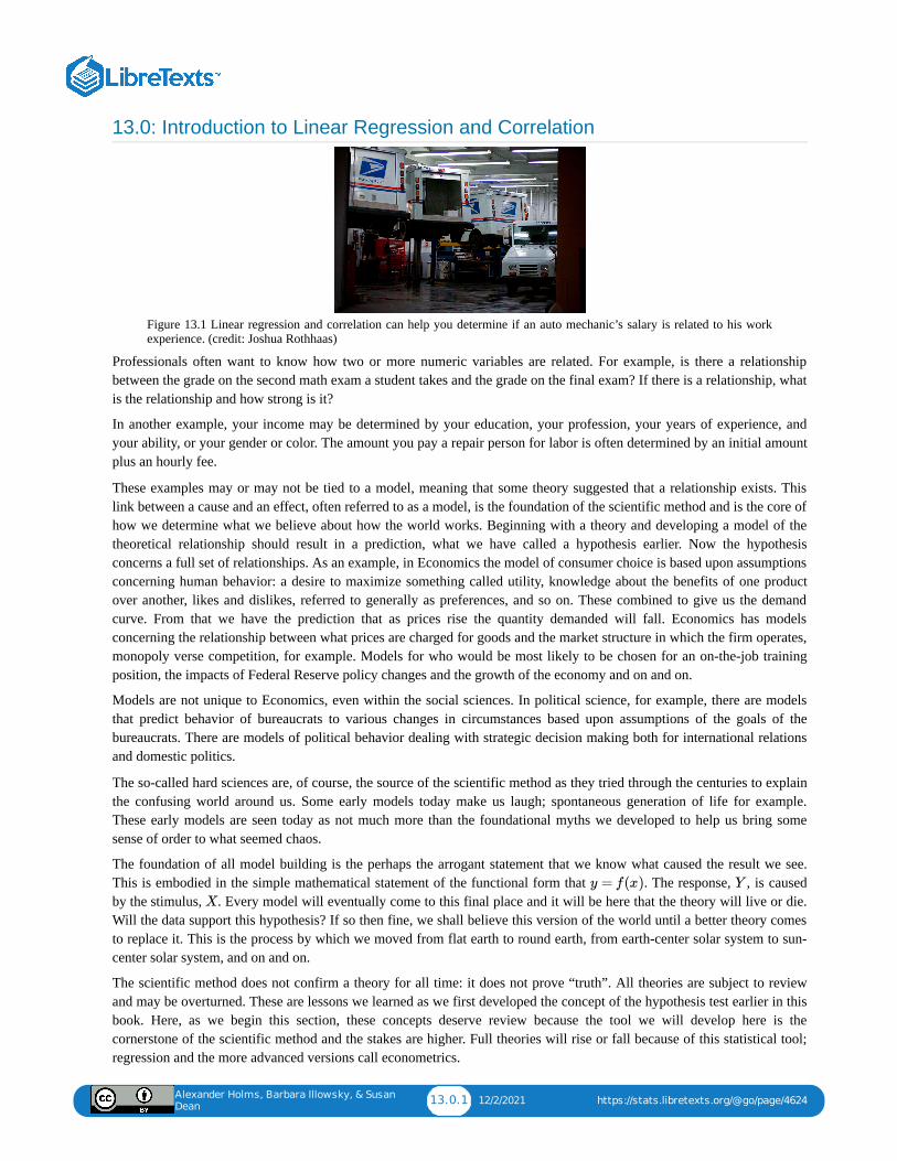
Alexander Holms, Barbara Illowsky, & Susan
Dean13.0.1 12/2/2021 https://stats.libretexts.org/@go/page/4624
13.0: Introduction to Linear Regression and Correlation
Figure 13.1 Linear regression and correlation can help you determine if an auto mechanic’s salary is related to his workexperience. (credit: Joshua Rothhaas)
Professionals often want to know how two or more numeric variables are related. For example, is there a relationshipbetween the grade on the second math exam a student takes and the grade on the final exam? If there is a relationship, whatis the relationship and how strong is it?
In another example, your income may be determined by your education, your profession, your years of experience, andyour ability, or your gender or color. The amount you pay a repair person for labor is often determined by an initial amountplus an hourly fee.
These examples may or may not be tied to a model, meaning that some theory suggested that a relationship exists. Thislink between a cause and an effect, often referred to as a model, is the foundation of the scientific method and is the core ofhow we determine what we believe about how the world works. Beginning with a theory and developing a model of thetheoretical relationship should result in a prediction, what we have called a hypothesis earlier. Now the hypothesisconcerns a full set of relationships. As an example, in Economics the model of consumer choice is based upon assumptionsconcerning human behavior: a desire to maximize something called utility, knowledge about the benefits of one productover another, likes and dislikes, referred to generally as preferences, and so on. These combined to give us the demandcurve. From that we have the prediction that as prices rise the quantity demanded will fall. Economics has modelsconcerning the relationship between what prices are charged for goods and the market structure in which the firm operates,monopoly verse competition, for example. Models for who would be most likely to be chosen for an on-the-job trainingposition, the impacts of Federal Reserve policy changes and the growth of the economy and on and on.
Models are not unique to Economics, even within the social sciences. In political science, for example, there are modelsthat predict behavior of bureaucrats to various changes in circumstances based upon assumptions of the goals of thebureaucrats. There are models of political behavior dealing with strategic decision making both for international relationsand domestic politics.
The so-called hard sciences are, of course, the source of the scientific method as they tried through the centuries to explainthe confusing world around us. Some early models today make us laugh; spontaneous generation of life for example.These early models are seen today as not much more than the foundational myths we developed to help us bring somesense of order to what seemed chaos.
The foundation of all model building is the perhaps the arrogant statement that we know what caused the result we see.This is embodied in the simple mathematical statement of the functional form that . The response, , is causedby the stimulus, . Every model will eventually come to this final place and it will be here that the theory will live or die.Will the data support this hypothesis? If so then fine, we shall believe this version of the world until a better theory comesto replace it. This is the process by which we moved from flat earth to round earth, from earth-center solar system to sun-center solar system, and on and on.
The scientific method does not confirm a theory for all time: it does not prove “truth”. All theories are subject to reviewand may be overturned. These are lessons we learned as we first developed the concept of the hypothesis test earlier in thisbook. Here, as we begin this section, these concepts deserve review because the tool we will develop here is thecornerstone of the scientific method and the stakes are higher. Full theories will rise or fall because of this statistical tool;regression and the more advanced versions call econometrics.
y = f(x) Y
X

Alexander Holms, Barbara Illowsky, & Susan
Dean13.0.2 12/2/2021 https://stats.libretexts.org/@go/page/4624
In this chapter we will begin with correlation, the investigation of relationships among variables that may or may not befounded on a cause and effect model. The variables simply move in the same, or opposite, direction. That is to say, they donot move randomly. Correlation provides a measure of the degree to which this is true. From there we develop a tool tomeasure cause and effect relationships; regression analysis. We will be able to formulate models and tests to determine ifthey are statistically sound. If they are found to be so, then we can use them to make predictions: if as a matter of policywe changed the value of this variable what would happen to this other variable? If we imposed a gasoline tax of 50 centsper gallon how would that effect the carbon emissions, sales of Hummers/Hybrids, use of mass transit, etc.? The ability toprovide answers to these types of questions is the value of regression as both a tool to help us understand our world and tomake thoughtful policy decisions.
Alexander Holms, Barbara Illowsky, & Susan
Dean13.1.1 1/6/2022 https://stats.libretexts.org/@go/page/4625
13.1: The Correlation Coefficient rAs we begin this section we note that the type of data we will be working with has changed. Perhaps unnoticed, all the datawe have been using is for a single variable. It may be from two samples, but it is still a univariate variable. The type ofdata described in the examples above and for any model of cause and effect is bivariate data — "bi" for two variables. Inreality, statisticians use multivariate data, meaning many variables.
For our work we can classify data into three broad categories, time series data, cross-section data, and panel data. We metthe first two very early on. Time series data measures a single unit of observation; say a person, or a company or a country,as time passes. What are measured will be at least two characteristics, say the person’s income, the quantity of a particulargood they buy and the price they paid. This would be three pieces of information in one time period, say 1985. If wefollowed that person across time we would have those same pieces of information for 1985,1986, 1987, etc. This wouldconstitute a times series data set. If we did this for 10 years we would have 30 pieces of information concerning thisperson’s consumption habits of this good for the past decade and we would know their income and the price they paid.
A second type of data set is for cross-section data. Here the variation is not across time for a single unit of observation, butacross units of observation during one point in time. For a particular period of time we would gather the price paid, amountpurchased, and income of many individual people.
A third type of data set is panel data. Here a panel of units of observation is followed across time. If we take our examplefrom above we might follow 500 people, the unit of observation, through time, ten years, and observe their income, pricepaid and quantity of the good purchased. If we had 500 people and data for ten years for price, income and quantitypurchased we would have 15,000 pieces of information. These types of data sets are very expensive to construct andmaintain. They do, however, provide a tremendous amount of information that can be used to answer very importantquestions. As an example, what is the effect on the labor force participation rate of women as their family of origin, motherand father, age? Or are there differential effects on health outcomes depending upon the age at which a person startedsmoking? Only panel data can give answers to these and related questions because we must follow multiple people acrosstime. The work we do here however will not be fully appropriate for data sets such as these.
Beginning with a set of data with two independent variables we ask the question: are these related? One way to visuallyanswer this question is to create a scatter plot of the data. We could not do that before when we were doing descriptivestatistics because those data were univariate. Now we have bivariate data so we can plot in two dimensions. Threedimensions are possible on a flat piece of paper, but become very hard to fully conceptualize. Of course, more than threedimensions cannot be graphed although the relationships can be measured mathematically.
To provide mathematical precision to the measurement of what we see we use the correlation coefficient. The correlationtells us something about the co-movement of two variables, but nothing about why this movement occurred. Formally,correlation analysis assumes that both variables being analyzed are independent variables. This means that neither onecauses the movement in the other. Further, it means that neither variable is dependent on the other, or for that matter, onany other variable. Even with these limitations, correlation analysis can yield some interesting results.
The correlation coefficient, ρ (pronounced rho), is the mathematical statistic for a population that provides us with ameasurement of the strength of a linear relationship between the two variables. For a sample of data, the statistic, r,developed by Karl Pearson in the early 1900s, is an estimate of the population correlation and is defined mathematicallyas:
OR
r =
Σ ( − )( − )1
n−1X1i X
¯ ¯¯̄
1 X2i X¯ ¯¯̄
2
sx1sx2
r =∑ −n −X1iX2i X
¯ ¯¯̄1 X
¯ ¯¯̄2
(Σ −n )(Σ −n )X2
1iX¯ ¯¯̄ 2
1 X2
2iX¯ ¯¯̄ 2
2
− −−−−−−−−−−−−−−−−−−−−−−−
√
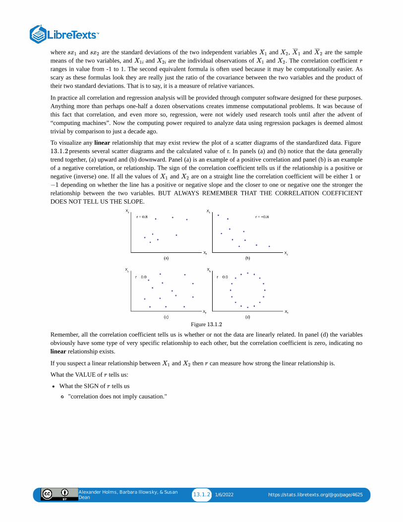
Alexander Holms, Barbara Illowsky, & Susan
Dean13.1.2 1/6/2022 https://stats.libretexts.org/@go/page/4625
where and are the standard deviations of the two independent variables and , and are the samplemeans of the two variables, and and are the individual observations of and . The correlation coefficient ranges in value from -1 to 1. The second equivalent formula is often used because it may be computationally easier. Asscary as these formulas look they are really just the ratio of the covariance between the two variables and the product oftheir two standard deviations. That is to say, it is a measure of relative variances.
In practice all correlation and regression analysis will be provided through computer software designed for these purposes.Anything more than perhaps one-half a dozen observations creates immense computational problems. It was because ofthis fact that correlation, and even more so, regression, were not widely used research tools until after the advent of“computing machines”. Now the computing power required to analyze data using regression packages is deemed almosttrivial by comparison to just a decade ago.
To visualize any linear relationship that may exist review the plot of a scatter diagrams of the standardized data. Figure presents several scatter diagrams and the calculated value of r. In panels (a) and (b) notice that the data generally
trend together, (a) upward and (b) downward. Panel (a) is an example of a positive correlation and panel (b) is an exampleof a negative correlation, or relationship. The sign of the correlation coefficient tells us if the relationship is a positive ornegative (inverse) one. If all the values of and are on a straight line the correlation coefficient will be either or
depending on whether the line has a positive or negative slope and the closer to one or negative one the stronger therelationship between the two variables. BUT ALWAYS REMEMBER THAT THE CORRELATION COEFFICIENTDOES NOT TELL US THE SLOPE.
Figure
Remember, all the correlation coefficient tells us is whether or not the data are linearly related. In panel (d) the variablesobviously have some type of very specific relationship to each other, but the correlation coefficient is zero, indicating nolinear relationship exists.
If you suspect a linear relationship between and then can measure how strong the linear relationship is.
What the VALUE of tells us:
What the SIGN of tells us
"correlation does not imply causation."
sx1 sx2 X1 X2 X¯ ¯¯̄
1 X¯ ¯¯̄
2
X1i X2i X1 X2 r
13.1.2
X1 X2 1
−1
13.1.2
X1 X2 r
r
r
Alexander Holms, Barbara Illowsky, & Susan
Dean13.2.1 12/3/2021 https://stats.libretexts.org/@go/page/4626
13.2: Testing the Significance of the Correlation CoefficientThe correlation coefficient, , tells us about the strength and direction of the linear relationship between and .
The sample data are used to compute , the correlation coefficient for the sample. If we had data for the entire population,we could find the population correlation coefficient. But because we have only sample data, we cannot calculate thepopulation correlation coefficient. The sample correlation coefficient, r, is our estimate of the unknown populationcorrelation coefficient.
The hypothesis test lets us decide whether the value of the population correlation coefficient \rho is "close to zero" or"significantly different from zero". We decide this based on the sample correlation coefficient and the sample size .
If the test concludes that the correlation coefficient is significantly different from zero, we say that thecorrelation coefficient is "significant."
What the Hypotheses Mean in WordsDrawing a Conclusion There are two methods of making the decision concerning the hypothesis. The teststatistic to test this hypothesis is:
Where the second formula is an equivalent form of the test statistic, is the sample size and the degrees offreedom are . This is a -statistic and operates in the same way as other tests. Calculate the -value andcompare that with the critical value from the -table at the appropriate degrees of freedom and the level ofconfidence you wish to maintain. If the calculated value is in the tail then cannot accept the null hypothesis thatthere is no linear relationship between these two independent random variables. If the calculated -value is NOTin the tailed then cannot reject the null hypothesis that there is no linear relationship between the two variables.
A quick shorthand way to test correlations is the relationship between the sample size and the correlation. If:
then this implies that the correlation between the two variables demonstrates that a linear relationship exists andis statistically significant at approximately the 0.05 level of significance. As the formula indicates, there is aninverse relationship between the sample size and the required correlation for significance of a linear relationship.With only 10 observations, the required correlation for significance is 0.6325, for 30 observations the requiredcorrelation for significance decreases to 0.3651 and at 100 observations the required level is only 0.2000.
Correlations may be helpful in visualizing the data, but are not appropriately used to "explain" a relationshipbetween two variables. Perhaps no single statistic is more misused than the correlation coefficient. Citingcorrelations between health conditions and everything from place of residence to eye color have the effect ofimplying a cause and effect relationship. This simply cannot be accomplished with a correlation coefficient. Thecorrelation coefficient is, of course, innocent of this misinterpretation. It is the duty of the analyst to use astatistic that is designed to test for cause and effect relationships and report only those results if they areintending to make such a claim. The problem is that passing this more rigorous test is difficult so lazy and/orunscrupulous "researchers" fall back on correlations when they cannot make their case legitimately.
r X1 X2
r
r n
=tc
r
(1 − ) /(n −2)r2− −−−−−−−−−−−−√
=tc
r n −2− −−−−
√
1 −r2− −−−−
√
n
n −2 t t t
t
t
|r| ≥2
n−−
√
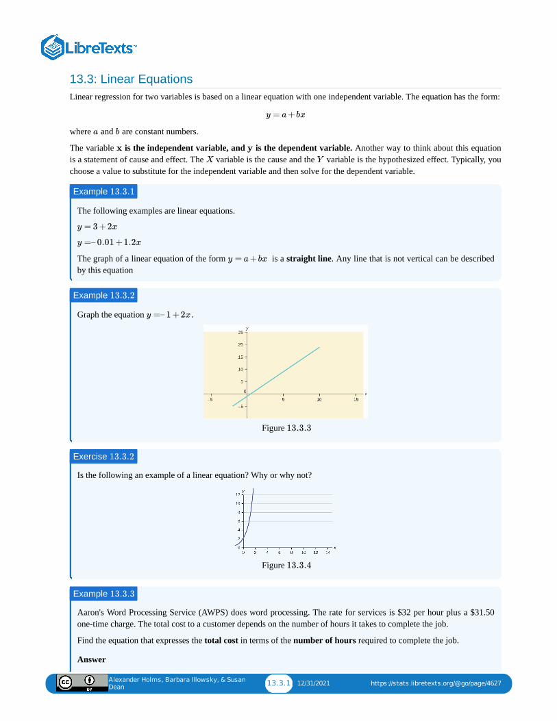
Alexander Holms, Barbara Illowsky, & Susan
Dean13.3.1 12/31/2021 https://stats.libretexts.org/@go/page/4627
13.3: Linear EquationsLinear regression for two variables is based on a linear equation with one independent variable. The equation has the form:
where and are constant numbers.
The variable is the independent variable, and is the dependent variable. Another way to think about this equationis a statement of cause and effect. The variable is the cause and the variable is the hypothesized effect. Typically, youchoose a value to substitute for the independent variable and then solve for the dependent variable.
The following examples are linear equations.
The graph of a linear equation of the form is a straight line. Any line that is not vertical can be describedby this equation
Graph the equation .
Figure
Is the following an example of a linear equation? Why or why not?
Figure
Aaron's Word Processing Service (AWPS) does word processing. The rate for services is $32 per hour plus a $31.50one-time charge. The total cost to a customer depends on the number of hours it takes to complete the job.
Find the equation that expresses the total cost in terms of the number of hours required to complete the job.
Answer
y = a+bx
a b
x y
X Y
Example 13.3.1
y = 3 +2x
y =– 0.01 +1.2x
y = a+bx
Example 13.3.2
y =– 1 +2x
13.3.3
Exercise 13.3.2
13.3.4
Example 13.3.3
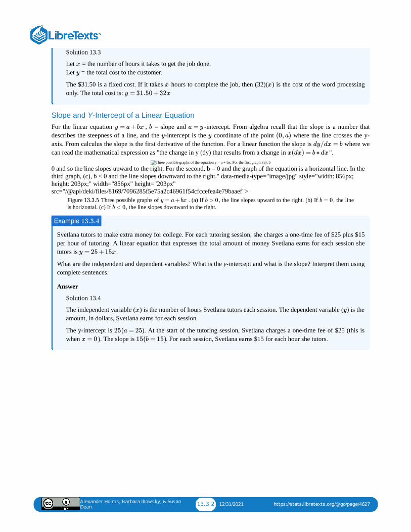
Alexander Holms, Barbara Illowsky, & Susan
Dean13.3.2 12/31/2021 https://stats.libretexts.org/@go/page/4627
Solution 13.3
Let = the number of hours it takes to get the job done. Let = the total cost to the customer.
The $31.50 is a fixed cost. If it takes hours to complete the job, then (32)( ) is the cost of the word processingonly. The total cost is:
Slope and Y-Intercept of a Linear EquationFor the linear equation , = slope and -intercept. From algebra recall that the slope is a number thatdescribes the steepness of a line, and the -intercept is the coordinate of the point where the line crosses the y-axis. From calculus the slope is the first derivative of the function. For a linear function the slope is where wecan read the mathematical expression as "the change in y (dy) that results from a change in ".
Three possible graphs of the equation y = a + bx. For the first graph, (a), b
0 and so the line slopes upward to the right. For the second, b = 0 and the graph of the equation is a horizontal line. In thethird graph, (c), b < 0 and the line slopes downward to the right." data-media-type="image/jpg" style="width: 856px;height: 203px;" width="856px" height="203px"src="/@api/deki/files/8169/7096285f5e75a2c46961f54cfccefea4e79baaef">
Figure Three possible graphs of . (a) If , the line slopes upward to the right. (b) If , the lineis horizontal. (c) If , the line slopes downward to the right.
Svetlana tutors to make extra money for college. For each tutoring session, she charges a one-time fee of $25 plus $15per hour of tutoring. A linear equation that expresses the total amount of money Svetlana earns for each session shetutors is .
What are the independent and dependent variables? What is the y-intercept and what is the slope? Interpret them usingcomplete sentences.
Answer
Solution 13.4
The independent variable ( ) is the number of hours Svetlana tutors each session. The dependent variable ( ) is theamount, in dollars, Svetlana earns for each session.
The y-intercept is ). At the start of the tutoring session, Svetlana charges a one-time fee of $25 (this iswhen ). The slope is . For each session, Svetlana earns $15 for each hour she tutors.
x
y
x x
y = 31.50 +32x
y = a+bx b a = y
y y (0, a)
dy/dx = b
x(dx) = b ∗ dx
13.3.5 y = a+ bx b > 0 b = 0b < 0
Example 13.3.4
y = 25 +15x
x y
25(a = 25
x = 0 15(b = 15)
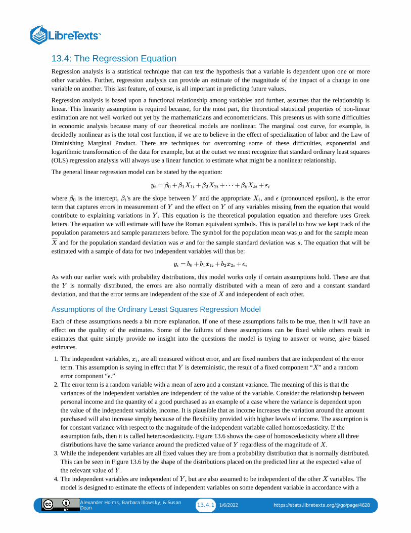
Alexander Holms, Barbara Illowsky, & Susan
Dean13.4.1 1/6/2022 https://stats.libretexts.org/@go/page/4628
13.4: The Regression EquationRegression analysis is a statistical technique that can test the hypothesis that a variable is dependent upon one or moreother variables. Further, regression analysis can provide an estimate of the magnitude of the impact of a change in onevariable on another. This last feature, of course, is all important in predicting future values.
Regression analysis is based upon a functional relationship among variables and further, assumes that the relationship islinear. This linearity assumption is required because, for the most part, the theoretical statistical properties of non-linearestimation are not well worked out yet by the mathematicians and econometricians. This presents us with some difficultiesin economic analysis because many of our theoretical models are nonlinear. The marginal cost curve, for example, isdecidedly nonlinear as is the total cost function, if we are to believe in the effect of specialization of labor and the Law ofDiminishing Marginal Product. There are techniques for overcoming some of these difficulties, exponential andlogarithmic transformation of the data for example, but at the outset we must recognize that standard ordinary least squares(OLS) regression analysis will always use a linear function to estimate what might be a nonlinear relationship.
The general linear regression model can be stated by the equation:
where is the intercept, 's are the slope between and the appropriate , and (pronounced epsilon), is the errorterm that captures errors in measurement of and the effect on of any variables missing from the equation that wouldcontribute to explaining variations in . This equation is the theoretical population equation and therefore uses Greekletters. The equation we will estimate will have the Roman equivalent symbols. This is parallel to how we kept track of thepopulation parameters and sample parameters before. The symbol for the population mean was and for the sample mean
and for the population standard deviation was and for the sample standard deviation was . The equation that will beestimated with a sample of data for two independent variables will thus be:
As with our earlier work with probability distributions, this model works only if certain assumptions hold. These are thatthe is normally distributed, the errors are also normally distributed with a mean of zero and a constant standarddeviation, and that the error terms are independent of the size of and independent of each other.
Assumptions of the Ordinary Least Squares Regression Model
Each of these assumptions needs a bit more explanation. If one of these assumptions fails to be true, then it will have aneffect on the quality of the estimates. Some of the failures of these assumptions can be fixed while others result inestimates that quite simply provide no insight into the questions the model is trying to answer or worse, give biasedestimates.
1. The independent variables, , are all measured without error, and are fixed numbers that are independent of the errorterm. This assumption is saying in effect that is deterministic, the result of a fixed component “ ” and a randomerror component “ .”
2. The error term is a random variable with a mean of zero and a constant variance. The meaning of this is that thevariances of the independent variables are independent of the value of the variable. Consider the relationship betweenpersonal income and the quantity of a good purchased as an example of a case where the variance is dependent uponthe value of the independent variable, income. It is plausible that as income increases the variation around the amountpurchased will also increase simply because of the flexibility provided with higher levels of income. The assumption isfor constant variance with respect to the magnitude of the independent variable called homoscedasticity. If theassumption fails, then it is called heteroscedasticity. Figure 13.6 shows the case of homoscedasticity where all threedistributions have the same variance around the predicted value of regardless of the magnitude of .
3. While the independent variables are all fixed values they are from a probability distribution that is normally distributed.This can be seen in Figure 13.6 by the shape of the distributions placed on the predicted line at the expected value ofthe relevant value of .
4. The independent variables are independent of , but are also assumed to be independent of the other variables. Themodel is designed to estimate the effects of independent variables on some dependent variable in accordance with a
= + + +⋯ + +yi β0 β1X1i β2X2i βkXki εi
β0 βi Y Xi ϵ
Y Y
Y
μ
X¯ ¯¯̄
σ s
= + + +yi b0 b1x1i b2x2i ei
Y
X
xi
Y X
ϵ
Y X
Y
Y X
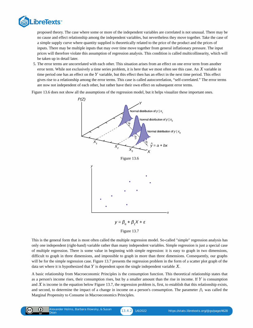
Alexander Holms, Barbara Illowsky, & Susan
Dean13.4.2 1/6/2022 https://stats.libretexts.org/@go/page/4628
proposed theory. The case where some or more of the independent variables are correlated is not unusual. There may beno cause and effect relationship among the independent variables, but nevertheless they move together. Take the case ofa simple supply curve where quantity supplied is theoretically related to the price of the product and the prices ofinputs. There may be multiple inputs that may over time move together from general inflationary pressure. The inputprices will therefore violate this assumption of regression analysis. This condition is called multicollinearity, which willbe taken up in detail later.
5. The error terms are uncorrelated with each other. This situation arises from an effect on one error term from anothererror term. While not exclusively a time series problem, it is here that we most often see this case. An variable intime period one has an effect on the variable, but this effect then has an effect in the next time period. This effectgives rise to a relationship among the error terms. This case is called autocorrelation, “self-correlated.” The error termsare now not independent of each other, but rather have their own effect on subsequent error terms.
Figure 13.6 does not show all the assumptions of the regression model, but it helps visualize these important ones.
Figure 13.6
Figure 13.7
This is the general form that is most often called the multiple regression model. So-called "simple" regression analysis hasonly one independent (right-hand) variable rather than many independent variables. Simple regression is just a special caseof multiple regression. There is some value in beginning with simple regression: it is easy to graph in two dimensions,difficult to graph in three dimensions, and impossible to graph in more than three dimensions. Consequently, our graphswill be for the simple regression case. Figure 13.7 presents the regression problem in the form of a scatter plot graph of thedata set where it is hypothesized that is dependent upon the single independent variable .
A basic relationship from Macroeconomic Principles is the consumption function. This theoretical relationship states thatas a person's income rises, their consumption rises, but by a smaller amount than the rise in income. If is consumptionand is income in the equation below Figure 13.7, the regression problem is, first, to establish that this relationship exists,and second, to determine the impact of a change in income on a person's consumption. The parameter was called theMarginal Propensity to Consume in Macroeconomics Principles.
X
Y
Y X
Y
X
β1
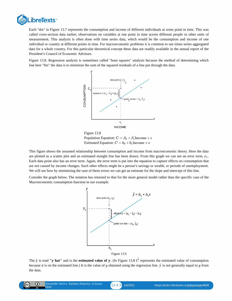
Alexander Holms, Barbara Illowsky, & Susan
Dean13.4.3 1/6/2022 https://stats.libretexts.org/@go/page/4628
Each "dot" in Figure 13.7 represents the consumption and income of different individuals at some point in time. This wascalled cross-section data earlier; observations on variables at one point in time across different people or other units ofmeasurement. This analysis is often done with time series data, which would be the consumption and income of oneindividual or country at different points in time. For macroeconomic problems it is common to use times series aggregateddata for a whole country. For this particular theoretical concept these data are readily available in the annual report of thePresident’s Council of Economic Advisors.
Figure 13.8. Regression analysis is sometimes called "least squares" analysis because the method of determining whichline best "fits" the data is to minimize the sum of the squared residuals of a line put through the data.
Figure 13.8 Population Equation: Estimated Equation:
This figure shows the assumed relationship between consumption and income from macroeconomic theory. Here the dataare plotted as a scatter plot and an estimated straight line has been drawn. From this graph we can see an error term, .Each data point also has an error term. Again, the error term is put into the equation to capture effects on consumption thatare not caused by income changes. Such other effects might be a person’s savings or wealth, or periods of unemployment.We will see how by minimizing the sum of these errors we can get an estimate for the slope and intercept of this line.
Consider the graph below. The notation has returned to that for the more general model rather than the specific case of theMacroeconomic consumption function in our example.
Figure 13.9
The is read " hat" and is the estimated value of . (In Figure 13.8 represents the estimated value of consumptionbecause it is on the estimated line.) It is the value of obtained using the regression line. is not generally equal to fromthe data.
C = + lncome +εβ0 β1
C = + lncome +eb0 b1
e1
ŷ y y Ĉ
y ŷ y
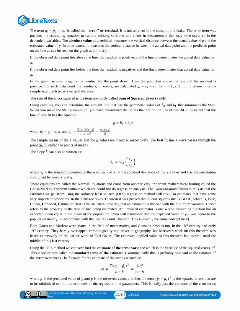
Alexander Holms, Barbara Illowsky, & Susan
Dean13.4.4 1/6/2022 https://stats.libretexts.org/@go/page/4628
The term is called the "error" or residual. It is not an error in the sense of a mistake. The error term wasput into the estimating equation to capture missing variables and errors in measurement that may have occurred in thedependent variables. The absolute value of a residual measures the vertical distance between the actual value of and theestimated value of . In other words, it measures the vertical distance between the actual data point and the predicted pointon the line as can be seen on the graph at point .
If the observed data point lies above the line, the residual is positive, and the line underestimates the actual data value for .
If the observed data point lies below the line, the residual is negative, and the line overestimates that actual data value for .
In the graph, is the residual for the point shown. Here the point lies above the line and the residual ispositive. For each data point the residuals, or errors, are calculated for where is thesample size. Each is a vertical distance.
The sum of the errors squared is the term obviously called Sum of Squared Errors (SSE).
Using calculus, you can determine the straight line that has the parameter values of and that minimizes the SSE.When you make the SSE a minimum, you have determined the points that are on the line of best fit. It turns out that theline of best fit has the equation:
where and
The sample means of the values and the values are and , respectively. The best fit line always passes through thepoint ( , ) called the points of means.
The slope can also be written as:
where = the standard deviation of the values and = the standard deviation of the values and is the correlationcoefficient between and .
These equations are called the Normal Equations and come from another very important mathematical finding called theGauss-Markov Theorem without which we could not do regression analysis. The Gauss-Markov Theorem tells us that theestimates we get from using the ordinary least squares (OLS) regression method will result in estimates that have somevery important properties. In the Gauss-Markov Theorem it was proved that a least squares line is BLUE, which is, Best,Linear, Unbiased, Estimator. Best is the statistical property that an estimator is the one with the minimum variance. Linearrefers to the property of the type of line being estimated. An unbiased estimator is one whose estimating function has anexpected mean equal to the mean of the population. (You will remember that the expected value of was equal to thepopulation mean in accordance with the Central Limit Theorem. This is exactly the same concept here).
Both Gauss and Markov were giants in the field of mathematics, and Gauss in physics too, in the 18 century and early19 century. They barely overlapped chronologically and never in geography, but Markov’s work on this theorem wasbased extensively on the earlier work of Carl Gauss. The extensive applied value of this theorem had to wait until themiddle of this last century.
Using the OLS method we can now find the estimate of the error variance which is the variance of the squared errors, e .This is sometimes called the standard error of the estimate. (Grammatically this is probably best said as the estimate ofthe error’svariance) The formula for the estimate of the error variance is:
where is the predicted value of and is the observed value, and thus the term is the squared errors that areto be minimized to find the estimates of the regression line parameters. This is really just the variance of the error terms
− =y0 ŷ0 e0
y
y
X0
y
y
− =y0 ŷ0 e0
− =yi ŷ i ei i = 1, 2, 3, . . . , n n
|e|
b0 b1
= + xŷ b0 b1
= −b0 ȳ̄̄ b1 x̄̄̄ = =b1Σ(x− )(y− )x̄̄̄ ȳ̄̄
Σ(x−x̄̄̄)2
cov(x,y)
s2x
x y x̄̄̄ ȳ̄̄
ȳ̄̄ x̄̄̄
b
= ( )b1 ry,x
sy
sx
sy y sx x r
x y
μx̄̄̄
μ
th
th
2
= =s2e
Σ( − )yi ŷ i2
n −k
Σe2i
n −k
ŷ y y ( − )yi ŷ i2
Alexander Holms, Barbara Illowsky, & Susan
Dean13.4.5 1/6/2022 https://stats.libretexts.org/@go/page/4628
and follows our regular variance formula. One important note is that here we are dividing by , which is the degreesof freedom. The degrees of freedom of a regression equation will be the number of observations, , reduced by the numberof estimated parameters, which includes the intercept as a parameter.
The variance of the errors is fundamental in testing hypotheses for a regression. It tells us just how “tight” the dispersion isabout the line. As we will see shortly, the greater the dispersion about the line, meaning the larger the variance of theerrors, the less probable that the hypothesized independent variable will be found to have a significant effect on thedependent variable. In short, the theory being tested will more likely fail if the variance of the error term is high. Uponreflection this should not be a surprise. As we tested hypotheses about a mean we observed that large variances reduced thecalculated test statistic and thus it failed to reach the tail of the distribution. In those cases, the null hypotheses could not berejected. If we cannot reject the null hypothesis in a regression problem, we must conclude that the hypothesizedindependent variable has no effect on the dependent variable.
A way to visualize this concept is to draw two scatter plots of and data along a predetermined line. The first will havelittle variance of the errors, meaning that all the data points will move close to the line. Now do the same except the datapoints will have a large estimate of the error variance, meaning that the data points are scattered widely along the line.Clearly the confidence about a relationship between and is effected by this difference between the estimate of the errorvariance.
Testing the Parameters of the LineThe whole goal of the regression analysis was to test the hypothesis that the dependent variable, , was in fact dependentupon the values of the independent variables as asserted by some foundation theory, such as the consumption functionexample. Looking at the estimated equation under Figure 13.8, we see that this amounts to determining the values of and . Notice that again we are using the convention of Greek letters for the population parameters and Roman letters fortheir estimates.
The regression analysis output provided by the computer software will produce an estimate of and , and any other 'sfor other independent variables that were included in the estimated equation. The issue is how good are these estimates? Inorder to test a hypothesis concerning any estimate, we have found that we need to know the underlying samplingdistribution. It should come as no surprise at his stage in the course that the answer is going to be the normal distribution.This can be seen by remembering the assumption that the error term in the population, , is normally distributed. If theerror term is normally distributed and the variance of the estimates of the equation parameters, and , are determinedby the variance of the error term, it follows that the variances of the parameter estimates are also normally distributed. Andindeed this is just the case.
We can see this by the creation of the test statistic for the test of hypothesis for the slope parameter, in our consumptionfunction equation. To test whether or not does indeed depend upon , or in our example, that consumption dependsupon income, we need only test the hypothesis that equals zero. This hypothesis would be stated formally as:
If we cannot reject the null hypothesis, we must conclude that our theory has no validity. If we cannot reject the nullhypothesis that then , the coefficient of Income, is zero and zero times anything is zero. Therefore the effect ofIncome on Consumption is zero. There is no relationship as our theory had suggested.
Notice that we have set up the presumption, the null hypothesis, as "no relationship". This puts the burden of proof on thealternative hypothesis. In other words, if we are to validate our claim of finding a relationship, we must do so with a levelof significance greater than 90, 95, or 99 percent. The status quo is ignorance, no relationship exists, and to be able tomake the claim that we have actually added to our body of knowledge we must do so with significant probability of beingcorrect. John Maynard Keynes got it right and thus was born Keynesian economics starting with this basic concept in1936.
The test statistic for this test comes directly from our old friend the standardizing formula:
(n −k)
n
x y
x y
Y
b0
b1
b0 b1 b
ϵ
b0 b1
β1
Y X
β1
: = 0H0 β1
: ≠ 0Ha β1
= 0β1 b1
Alexander Holms, Barbara Illowsky, & Susan
Dean13.4.6 1/6/2022 https://stats.libretexts.org/@go/page/4628
where is the estimated value of the slope of the regression line, is the hypothesized value of beta, in this case zero,and is the standard deviation of the estimate of . In this case we are asking how many standard deviations is theestimated slope away from the hypothesized slope. This is exactly the same question we asked before with respect to ahypothesis about a mean: how many standard deviations is the estimated mean, the sample mean, from the hypothesizedmean?
The test statistic is written as a student's t distribution, but if the sample size is larger enough so that the degrees offreedom are greater than 30 we may again use the normal distribution. To see why we can use the student's t or normaldistribution we have only to look at ,the formula for the standard deviation of the estimate of :
Where is the estimate of the error variance and is the variance of values of the coefficient of the independentvariable being tested.
We see that , the estimate of the error variance, is part of the computation. Because the estimate of the error varianceis based on the assumption of normality of the error terms, we can conclude that the sampling distribution of the 's, thecoefficients of our hypothesized regression line, are also normally distributed.
One last note concerns the degrees of freedom of the test statistic, . Previously we subtracted 1 from the samplesize to determine the degrees of freedom in a student's t problem. Here we must subtract one degree of freedom for eachparameter estimated in the equation. For the example of the consumption function we lose 2 degrees of freedom, one for
, the intercept, and one for , the slope of the consumption function. The degrees of freedom would be ,where k is the number of independent variables and the extra one is lost because of the intercept. If we were estimating anequation with three independent variables, we would lose 4 degrees of freedom: three for the independent variables, , andone more for the intercept.
The decision rule for acceptance or rejection of the null hypothesis follows exactly the same form as in all our previous testof hypothesis. Namely, if the calculated value of (or ) falls into the tails of the distribution, where the tails are definedby , the required significance level in the test, we cannot accept the null hypothesis. If on the other hand, the calculatedvalue of the test statistic is within the critical region, we cannot reject the null hypothesis.
If we conclude that we cannot accept the null hypothesis, we are able to state with level of confidence that theslope of the line is given by . This is an extremely important conclusion. Regression analysis not only allows us to test ifa cause and effect relationship exists, we can also determine the magnitude of that relationship, if one is found to exist. It isthis feature of regression analysis that makes it so valuable. If models can be developed that have statistical validity, we arethen able to simulate the effects of changes in variables that may be under our control with some degree of probability , ofcourse. For example, if advertising is demonstrated to effect sales, we can determine the effects of changing the advertisingbudget and decide if the increased sales are worth the added expense.
Multicollinearity
Our discussion earlier indicated that like all statistical models, the OLS regression model has important assumptionsattached. Each assumption, if violated, has an effect on the ability of the model to provide useful and meaningful estimates.The Gauss-Markov Theorem has assured us that the OLS estimates are unbiased and minimum variance, but this is trueonly under the assumptions of the model. Here we will look at the effects on OLS estimates if the independent variablesare correlated. The other assumptions and the methods to mitigate the difficulties they pose if they are found to be violated
=tc
−b1 β1
Sb1
b1 β1
Sb1b1
Sb1 b1
=Sb1
S2e
( − )xi x̄̄̄2
− −−−−−−√
or
=Sb1
S2e
(n −1)S2x
Se S2x x
Se
b
ν = n −k
b0 b1 n −k −1
k
t Z
α
(1 −α)
b1
Alexander Holms, Barbara Illowsky, & Susan
Dean13.4.7 1/6/2022 https://stats.libretexts.org/@go/page/4628
are examined in Econometrics courses. We take up multicollinearity because it is so often prevalent in Economic modelsand it often leads to frustrating results.
The OLS model assumes that all the independent variables are independent of each other. This assumption is easy to testfor a particular sample of data with simple correlation coefficients. Correlation, like much in statistics, is a matter ofdegree: a little is not good, and a lot is terrible.
The goal of the regression technique is to tease out the independent impacts of each of a set of independent variables onsome hypothesized dependent variable. If two 2 independent variables are interrelated, that is, correlated, then we cannotisolate the effects on of one from the other. In an extreme case where is a linear combination of , correlation equalto one, both variables move in identical ways with . In this case it is impossible to determine the variable that is the truecause of the effect on . (If the two variables were actually perfectly correlated, then mathematically no regression resultscould actually be calculated.)
The normal equations for the coefficients show the effects of multicollinearity on the coefficients.
The correlation between and , , appears in the denominator of both the estimating formula for and . If theassumption of independence holds, then this term is zero. This indicates that there is no effect of the correlation on thecoefficient. On the other hand, as the correlation between the two independent variables increases the denominatordecreases, and thus the estimate of the coefficient increases. The correlation has the same effect on both of the coefficientsof these two variables. In essence, each variable is “taking” part of the effect on Y that should be attributed to the collinearvariable. This results in biased estimates.
Multicollinearity has a further deleterious impact on the OLS estimates. The correlation between the two independentvariables also shows up in the formulas for the estimate of the variance for the coefficients.
Here again we see the correlation between and in the denominator of the estimates of the variance for thecoefficients for both variables. If the correlation is zero as assumed in the regression model, then the formula collapses tothe familiar ratio of the variance of the errors to the variance of the relevant independent variable. If however the twoindependent variables are correlated, then the variance of the estimate of the coefficient increases. This results in a smaller -value for the test of hypothesis of the coefficient. In short, multicollinearity results in failing to reject the null hypothesis
that the variable has no impact on when in fact does have a statistically significant impact on . Said another way,the large standard errors of the estimated coefficient created by multicollinearity suggest statistical insignificance evenwhen the hypothesized relationship is strong.
How Good is the Equation?In the last section we concerned ourselves with testing the hypothesis that the dependent variable did indeed depend uponthe hypothesized independent variable or variables. It may be that we find an independent variable that has some effect onthe dependent variable, but it may not be the only one, and it may not even be the most important one. Remember that theerror term was placed in the model to capture the effects of any missing independent variables. It follows that the errorterm may be used to give a measure of the "goodness of fit" of the equation taken as a whole in explaining the variation ofthe dependent variable, .
Y x1 x2
Y
Y
=b1
( − )sy r yx1 rx1x2 r yx2
(1 − )sx1r2
x1x2
=b2
( − )sy rx2yrx1x2
r yx1
(1 − )sx2 r2x1x2
= − −b0 ȳ̄̄ b1 x̄̄̄1 b2 x̄̄̄2
x1 x2 r2x1x2 b1 b2
=s2b1
s2e
(n −1) (1 − )s2x1 r2
x1x2
=s2b2
s2e
(n −1) (1 − )s2x2 r2
x1x2
x1 x2
t
X Y X Y
Y
Alexander Holms, Barbara Illowsky, & Susan
Dean13.4.8 1/6/2022 https://stats.libretexts.org/@go/page/4628
The multiple correlation coefficient, also called the coefficient of multiple determination or the coefficient ofdetermination, is given by the formula:
where SSR is the regression sum of squares, the squared deviation of the predicted value of from the mean value of , and SST is the total sum Figure 13.10 shows how the total deviation of the dependent variable, y, is partitioned
into these two pieces.
Figure 13.10
Figure 13.10 shows the estimated regression line and a single observation, . Regression analysis tries to explain thevariation of the data about the mean value of the dependent variable, . The question is, why do the observations of y varyfrom the average level of ? The value of y at observation varies from the mean of by the difference . Thesum of these differences squared is SST, the sum of squares total. The actual value of at deviates from the estimatedvalue, , by the difference between the estimated value and the actual value, . We recall that this is the error term,e, and the sum of these errors is SSE, sum of squared errors. The deviation of the predicted value of , , from the meanvalue of is and is the SSR, sum of squares regression. It is called “regression” because it is the deviationexplained by the regression. (Sometimes the SSR is called SSM for sum of squares mean because it measures the deviationfrom the mean value of the dependent variable, y, as shown on the graph.).
Because the SST = SSR + SSE we see that the multiple correlation coefficient is the percent of the variance, or deviation in from its mean value, that is explained by the equation when taken as a whole. will vary between zero and 1, with
zero indicating that none of the variation in was explained by the equation and a value of 1 indicating that 100% of thevariation in was explained by the equation. For time series studies expect a high and for cross-section data expectlow .
While a high is desirable, remember that it is the tests of the hypothesis concerning the existence of a relationshipbetween a set of independent variables and a particular dependent variable that was the motivating factor in using theregression model. It is validating a cause and effect relationship developed by some theory that is the true reason that wechose the regression analysis. Increasing the number of independent variables will have the effect of increasing . To
account for this effect the proper measure of the coefficient of determination is the , adjusted for degrees of freedom, tokeep down mindless addition of independent variables.
There is no statistical test for the and thus little can be said about the model using with our characteristicconfidence level. Two models that have the same size of SSE, that is sum of squared errors, may have very different ifthe competing models have different SST, total sum of squared deviations. The goodness of fit of the two models is thesame; they both have the same sum of squares unexplained, errors squared, but because of the larger total sum of squareson one of the models the differs. Again, the real value of regression as a tool is to examine hypotheses developed froma model that predicts certain relationships among the variables. These are tests of hypotheses on the coefficients of themodel and not a game of maximizing .
=R2 SSR
SST
y
y( − )ŷ ȳ̄̄
x1
y
y x1 y ( − )yi ȳ̄̄
y x1
ŷ ( − )yi ŷ
y ŷ
y ( − )ŷ ȳ̄̄
y R2
y
y R2
R2
R2
R2
R¯ ¯¯̄ 2
R2 R2
R2
R2
R2
Alexander Holms, Barbara Illowsky, & Susan
Dean13.4.9 1/6/2022 https://stats.libretexts.org/@go/page/4628
Another way to test the general quality of the overall model is to test the coefficients as a group rather than independently.Because this is multiple regression (more than one X), we use the F-test to determine if our coefficients collectively affectY. The hypothesis is:
: "at least one of the is not equal to 0"
If the null hypothesis cannot be rejected, then we conclude that none of the independent variables contribute to explainingthe variation in . Reviewing Figure 13.10 we see that SSR, the explained sum of squares, is a measure of just how muchof the variation in is explained by all the variables in the model. SSE, the sum of the errors squared, measures just howmuch is unexplained. It follows that the ratio of these two can provide us with a statistical test of the model as a whole.Remembering that the distribution is a ratio of Chi squared distributions and that variances are distributed according toChi Squared, and the sum of squared errors and the sum of squares are both variances, we have the test statistic for thishypothesis as:
where is the number of observations and is the number of independent variables. It can be shown that this is equivalentto:
Figure 13.10 where is the coefficient of determination which is also a measure of the “goodness” of the model.
As with all our tests of hypothesis, we reach a conclusion by comparing the calculated statistic with the critical valuegiven our desired level of confidence. If the calculated test statistic, an statistic in this case, is in the tail of thedistribution, then we cannot accept the null hypothesis. By not being able to accept the null hypotheses we conclude thatthis specification of this model has validity, because at least one of the estimated coefficients is significantly different fromzero.
An alternative way to reach this conclusion is to use the p-value comparison rule. The -value is the area in the tail, giventhe calculated statistic. In essence, the computer is finding the value in the table for us. The computer regressionoutput for the calculated statistic is typically found in the ANOVA table section labeled “significance F". How to readthe output of an Excel regression is presented below. This is the probability of NOT accepting a false null hypothesis. Ifthis probability is less than our pre-determined alpha error, then the conclusion is that we cannot accept the nullhypothesis.
Dummy VariablesThus far the analysis of the OLS regression technique assumed that the independent variables in the models tested werecontinuous random variables. There are, however, no restrictions in the regression model against independent variablesthat are binary. This opens the regression model for testing hypotheses concerning categorical variables such as gender,race, region of the country, before a certain data, after a certain date and innumerable others. These categorical variablestake on only two values, 1 and 0, success or failure, from the binomial probability distribution. The form of the equationbecomes:
: = = … = = 0Ho β1 β2 βi
Ha βi
Y
Y
F
=Fc
( )SSR
k
( )SSE
n−k−1
n k
= ⋅Fc
n −k −1
k
R2
1 −R2
R2
F
F
p
F F
F
= + +ŷ b0 b2x2 b1x1
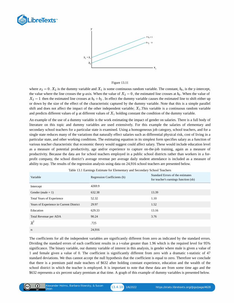
Alexander Holms, Barbara Illowsky, & Susan
Dean13.4.10 1/6/2022 https://stats.libretexts.org/@go/page/4628
Figure 13.11
where . is the dummy variable and is some continuous random variable. The constant, , is the y-intercept,the value where the line crosses the -axis. When the value of , the estimated line crosses at . When the value of
then the estimated line crosses at . In effect the dummy variable causes the estimated line to shift either upor down by the size of the effect of the characteristic captured by the dummy variable. Note that this is a simple parallelshift and does not affect the impact of the other independent variable; .This variable is a continuous random variableand predicts different values of at different values of holding constant the condition of the dummy variable.
An example of the use of a dummy variable is the work estimating the impact of gender on salaries. There is a full body ofliterature on this topic and dummy variables are used extensively. For this example the salaries of elementary andsecondary school teachers for a particular state is examined. Using a homogeneous job category, school teachers, and for asingle state reduces many of the variations that naturally effect salaries such as differential physical risk, cost of living in aparticular state, and other working conditions. The estimating equation in its simplest form specifies salary as a function ofvarious teacher characteristic that economic theory would suggest could affect salary. These would include education levelas a measure of potential productivity, age and/or experience to capture on-the-job training, again as a measure ofproductivity. Because the data are for school teachers employed in a public school districts rather than workers in a for-profit company, the school district’s average revenue per average daily student attendance is included as a measure ofability to pay. The results of the regression analysis using data on 24,916 school teachers are presented below.
Variable Regression Coefficients (b) Standard Errors of the estimates for teacher's earnings function (sb)
Intercept 4269.9
Gender (male = 1) 632.38 13.39
Total Years of Experience 52.32 1.10
Years of Experience in Current District 29.97 1.52
Education 629.33 13.16
Total Revenue per ADA 90.24 3.76
.725
24,916
Table 13.1 Earnings Estimate for Elementary and Secondary School Teachers
The coefficients for all the independent variables are significantly different from zero as indicated by the standard errors.Dividing the standard errors of each coefficient results in a t-value greater than 1.96 which is the required level for 95%significance. The binary variable, our dummy variable of interest in this analysis, is gender where male is given a value of1 and female given a value of 0. The coefficient is significantly different from zero with a dramatic t-statistic of 47standard deviations. We thus cannot accept the null hypothesis that the coefficient is equal to zero. Therefore we concludethat there is a premium paid male teachers of $632 after holding constant experience, education and the wealth of theschool district in which the teacher is employed. It is important to note that these data are from some time ago and the$632 represents a six percent salary premium at that time. A graph of this example of dummy variables is presented below.
= 0x2 X2 X1 b0
y = 0X2 b0
= 1X2 +b0 b2
X1
y X1
R¯ ¯¯̄ 2
n
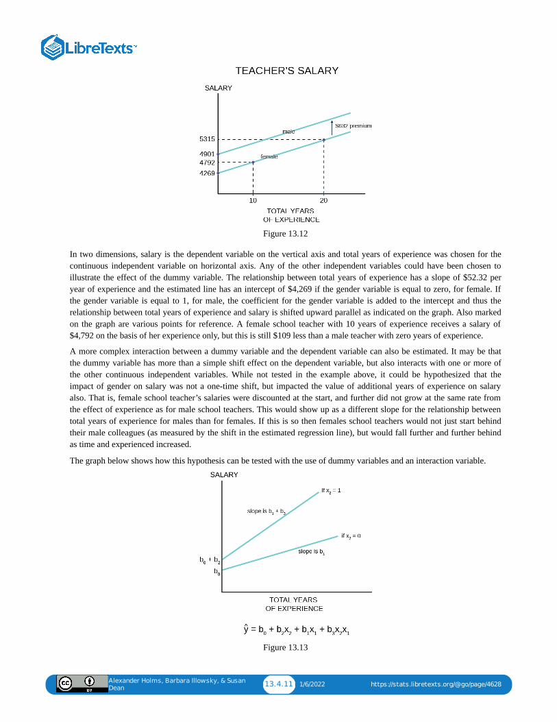
Alexander Holms, Barbara Illowsky, & Susan
Dean13.4.11 1/6/2022 https://stats.libretexts.org/@go/page/4628
Figure 13.12
In two dimensions, salary is the dependent variable on the vertical axis and total years of experience was chosen for thecontinuous independent variable on horizontal axis. Any of the other independent variables could have been chosen toillustrate the effect of the dummy variable. The relationship between total years of experience has a slope of $52.32 peryear of experience and the estimated line has an intercept of $4,269 if the gender variable is equal to zero, for female. Ifthe gender variable is equal to 1, for male, the coefficient for the gender variable is added to the intercept and thus therelationship between total years of experience and salary is shifted upward parallel as indicated on the graph. Also markedon the graph are various points for reference. A female school teacher with 10 years of experience receives a salary of$4,792 on the basis of her experience only, but this is still $109 less than a male teacher with zero years of experience.
A more complex interaction between a dummy variable and the dependent variable can also be estimated. It may be thatthe dummy variable has more than a simple shift effect on the dependent variable, but also interacts with one or more ofthe other continuous independent variables. While not tested in the example above, it could be hypothesized that theimpact of gender on salary was not a one-time shift, but impacted the value of additional years of experience on salaryalso. That is, female school teacher’s salaries were discounted at the start, and further did not grow at the same rate fromthe effect of experience as for male school teachers. This would show up as a different slope for the relationship betweentotal years of experience for males than for females. If this is so then females school teachers would not just start behindtheir male colleagues (as measured by the shift in the estimated regression line), but would fall further and further behindas time and experienced increased.
The graph below shows how this hypothesis can be tested with the use of dummy variables and an interaction variable.
Figure 13.13
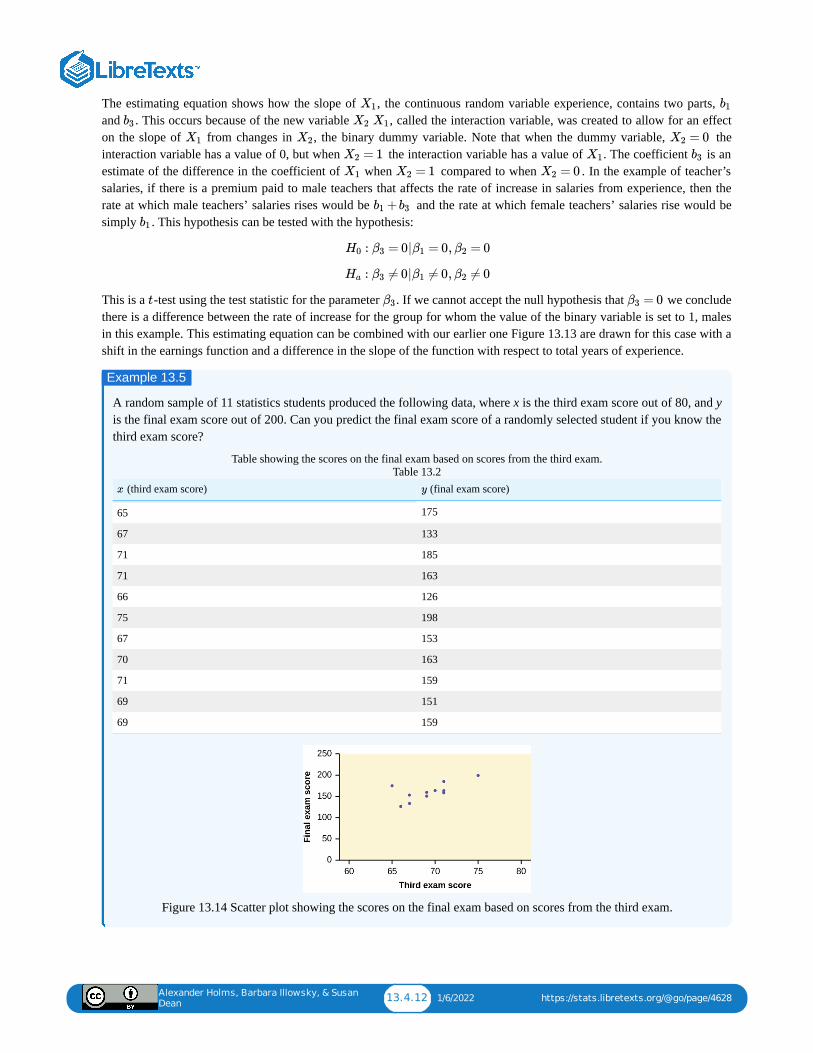
Alexander Holms, Barbara Illowsky, & Susan
Dean13.4.12 1/6/2022 https://stats.libretexts.org/@go/page/4628
The estimating equation shows how the slope of , the continuous random variable experience, contains two parts, and . This occurs because of the new variable , called the interaction variable, was created to allow for an effecton the slope of from changes in , the binary dummy variable. Note that when the dummy variable, theinteraction variable has a value of 0, but when the interaction variable has a value of . The coefficient is anestimate of the difference in the coefficient of when compared to when . In the example of teacher’ssalaries, if there is a premium paid to male teachers that affects the rate of increase in salaries from experience, then therate at which male teachers’ salaries rises would be and the rate at which female teachers’ salaries rise would besimply . This hypothesis can be tested with the hypothesis:
This is a -test using the test statistic for the parameter . If we cannot accept the null hypothesis that we concludethere is a difference between the rate of increase for the group for whom the value of the binary variable is set to 1, malesin this example. This estimating equation can be combined with our earlier one Figure 13.13 are drawn for this case with ashift in the earnings function and a difference in the slope of the function with respect to total years of experience.
A random sample of 11 statistics students produced the following data, where x is the third exam score out of 80, and yis the final exam score out of 200. Can you predict the final exam score of a randomly selected student if you know thethird exam score?
Table showing the scores on the final exam based on scores from the third exam.
(third exam score) (final exam score)
65 175
67 133
71 185
71 163
66 126
75 198
67 153
70 163
71 159
69 151
69 159
Table 13.2
Figure 13.14 Scatter plot showing the scores on the final exam based on scores from the third exam.
X1 b1
b3 X2 X1
X1 X2 = 0X2
= 1X2 X1 b3
X1 = 1X2 = 0X2
+b1 b3
b1
: = 0| = 0, = 0H0 β3 β1 β2
: ≠ 0| ≠ 0, ≠ 0Ha β3 β1 β2
t β3 = 0β3
Example 13.5
x y
Alexander Holms, Barbara Illowsky, & Susan
Dean13.5.1 12/10/2021 https://stats.libretexts.org/@go/page/4629
13.5: Interpretation of Regression Coefficients- Elasticity and LogarithmicTransformationAs we have seen, the coefficient of an equation estimated using OLS regression analysis provides an estimate of the slopeof a straight line that is assumed be the relationship between the dependent variable and at least one independent variable.From the calculus, the slope of the line is the first derivative and tells us the magnitude of the impact of a one unit changein the variable upon the value of the variable measured in the units of the variable. As we saw in the case ofdummy variables, this can show up as a parallel shift in the estimated line or even a change in the slope of the line throughan interactive variable. Here we wish to explore the concept of elasticity and how we can use a regression analysis toestimate the various elasticities in which economists have an interest.
The concept of elasticity is borrowed from engineering and physics where it is used to measure a material’s responsivenessto a force, typically a physical force such as a stretching/pulling force. It is from here that we get the term an “elastic”band. In economics, the force in question is some market force such as a change in price or income. Elasticity is measuredas a percentage change/response in both engineering applications and in economics. The value of measuring in percentageterms is that the units of measurement do not play a role in the value of the measurement and thus allows directcomparison between elasticities. As an example, if the price of gasoline increased say 50 cents from an initial price of$3.00 and generated a decline in monthly consumption for a consumer from 50 gallons to 48 gallons we calculate theelasticity to be 0.25. The price elasticity is the percentage change in quantity resulting from some percentage change inprice. A 16 percent increase in price has generated only a 4 percent decrease in demand: 16% price change 4% quantitychange or . This is called an inelastic demand meaning a small response to the price change. This comesabout because there are few if any real substitutes for gasoline; perhaps public transportation, a bicycle or walking.Technically, of course, the percentage change in demand from a price increase is a decline in demand thus price elasticityis a negative number. The common convention, however, is to talk about elasticity as the absolute value of the number.Some goods have many substitutes: pears for apples for plums, for grapes, etc. etc. The elasticity for such goods is largerthan one and are called elastic in demand. Here a small percentage change in price will induce a large percentage change inquantity demanded. The consumer will easily shift the demand to the close substitute.
While this discussion has been about price changes, any of the independent variables in a demand equation will have anassociated elasticity. Thus, there is an income elasticity that measures the sensitivity of demand to changes in income: notmuch for the demand for food, but very sensitive for yachts. If the demand equation contains a term for substitute goods,say candy bars in a demand equation for cookies, then the responsiveness of demand for cookies from changes in prices ofcandy bars can be measured. This is called the cross-price elasticity of demand and to an extent can be thought of as brandloyalty from a marketing view. How responsive is the demand for Coca-Cola to changes in the price of Pepsi?
Now imagine the demand for a product that is very expensive. Again, the measure of elasticity is in percentage terms thusthe elasticity can be directly compared to that for gasoline: an elasticity of 0.25 for gasoline conveys the same informationas an elasticity of 0.25 for $25,000 car. Both goods are considered by the consumer to have few substitutes and thus haveinelastic demand curves, elasticities less than one.
The mathematical formulae for various elasticities are:
Where is the Greek small case letter eta used to designate elasticity. ∆ is read as “change”.
Where is used as the symbol for income.
Where P2 is the price of the substitute good.
X Y Y
→
.04/.16 = .25
Price elasticity: =ηp(%ΔQ)
(%ΔP)
η
Income elasticity: =ηY
(%ΔQ)
(%ΔY)
Y
Cross-Price elasticity: =ηp1
(%Δ )Q1
(%Δ )P2
Alexander Holms, Barbara Illowsky, & Susan
Dean13.5.2 12/10/2021 https://stats.libretexts.org/@go/page/4629
Examining closer the price elasticity we can write the formula as:
Where is the estimated coefficient for price in the OLS regression.
The first form of the equation demonstrates the principle that elasticities are measured in percentage terms. Of course, theordinary least squares coefficients provide an estimate of the impact of a unit change in the independent variable, , on thedependent variable measured in units of . These coefficients are not elasticities, however, and are shown in the second
way of writing the formula for elasticity as , the derivative of the estimated demand function which is simply the
slope of the regression line. Multiplying the slope times provides an elasticity measured in percentage terms.
Along a straight-line demand curve the percentage change, thus elasticity, changes continuously as the scale changes,while the slope, the estimated regression coefficient, remains constant. Going back to the demand for gasoline. A change inprice from $3.00 to $3.50 was a 16 percent increase in price. If the beginning price were $5.00 then the same 50¢ increasewould be only a 10 percent increase generating a different elasticity. Every straight-line demand curve has a range ofelasticities starting at the top left, high prices, with large elasticity numbers, elastic demand, and decreasing as one goesdown the demand curve, inelastic demand.
In order to provide a meaningful estimate of the elasticity of demand the convention is to estimate the elasticity at the pointof means. Remember that all OLS regression lines will go through the point of means. At this point is the greatest weightof the data used to estimate the coefficient. The formula to estimate an elasticity when an OLS demand curve has beenestimated becomes:
Where and are the mean values of these data used to estimate , the price coefficient.
The same method can be used to estimate the other elasticities for the demand function by using the appropriate meanvalues of the other variables; income and price of substitute goods for example.
Logarithmic Transformation of the Data
Ordinary least squares estimates typically assume that the population relationship among the variables is linear thus of theform presented in The Regression Equation. In this form the interpretation of the coefficients is as discussed above; quitesimply the coefficient provides an estimate of the impact of a one unit change in on measured in units of . It doesnot matter just where along the line one wishes to make the measurement because it is a straight line with a constant slopethus constant estimated level of impact per unit change. It may be, however, that the analyst wishes to estimate not thesimple unit measured impact on the variable, but the magnitude of the percentage impact on of a one unit change inthe variable. Such a case might be how a unit change in experience, say one year, effects not the absolute amount of aworker’s wage, but the percentage impact on the worker’s wage. Alternatively, it may be that the question asked is theunit measured impact on of a specific percentage increase in X. An example may be “by how many dollars will salesincrease if the firm spends percent more on advertising?” The third possibility is the case of elasticity discussed above.Here we are interested in the percentage impact on quantity demanded for a given percentage change in price, or income orperhaps the price of a substitute good. All three of these cases can be estimated by transforming the data to logarithmsbefore running the regression. The resulting coefficients will then provide a percentage change measurement of therelevant variable.
To summarize, there are four cases:
1. (Standard OLS case)2. 3. 4. (elasticity case)
Case 1: The ordinary least squares case begins with the linear model developed above:
= = ( ) = b( )ηp(%ΔQ)
(%ΔP)
dQ
dP
P
Q
P
Q
b
X
Y
( )dQ
dPP
Q
= b( )ηpP¯¯̄̄
Q
P¯¯̄̄
Q¯ ¯¯̄
b
X Y Y
Y Y
X
Y
X
Unit ΔX → Unit ΔY
Unit ΔX → %ΔY
%ΔX → Unit ΔY
%ΔX → %ΔY
Alexander Holms, Barbara Illowsky, & Susan
Dean13.5.3 12/10/2021 https://stats.libretexts.org/@go/page/4629
where the coefficient of the independent variable is the slope of a straight line and thus measures the impact of aunit change in on measured in units of .
Case 2: The underlying estimated equation is:
The equation is estimated by converting the values to logarithms and using OLS techniques to estimate the coefficientof the variable, . This is called a semi-log estimation. Again, differentiating both sides of the equation allows us todevelop the interpretation of the coefficient :
Multiply by 100 to covert to percentages and rearranging terms gives:
is thus the percentage change in resulting from a unit change in .
Case 3: In this case the question is “what is the unit change in resulting from a percentage change in ?” What is thedollar loss in revenues of a five percent increase in price or what is the total dollar cost impact of a five percent increase inlabor costs? The estimated equation for this case would be:
Here the calculus differential of the estimated equation is:
Divide by 100 to get percentage and rearranging terms gives:
Therefore, is the increase in measured in units from a one percent increase in .
Case 4: This is the elasticity case where both the dependent and independent variables are converted to logs before theOLS estimation. This is known as the log-log case or double log case, and provides us with direct estimates of theelasticities of the independent variables. The estimated equation is:
Differentiating we have:
thus:
and our definition of elasticity. We conclude that we can directly estimate the elasticity of a variable throughdouble log transformation of the data. The estimated coefficient is the elasticity. It is common to use double log
Y = a+bX
b = dY
dX
X Y Y
log(Y) = a+bX
Y
X b
X b
d( ) = bdXlogY
= bdXdY
Y
100b =%ΔY
Unit ΔX
100b Y X
Y X
Y = a+B log(X)
dY = bd(logX)
dY = bdX
X
= =b
100
dY
100 dXX
Unit ΔY
%ΔX
b
100Y X
logY = a+blogX
d(logY ) = bd(logX)
d(logX) = b dX1
X
dY = b dX OR = b OR b = ( )1
Y
1
X
dY
Y
dX
X
dY
dX
X
Y
b = %ΔY
%ΔX

Alexander Holms, Barbara Illowsky, & Susan
Dean13.5.4 12/10/2021 https://stats.libretexts.org/@go/page/4629
transformation of all variables in the estimation of demand functions to get estimates of all the various elasticities of thedemand curve.
Alexander Holms, Barbara Illowsky, & Susan
Dean13.6.1 12/17/2021 https://stats.libretexts.org/@go/page/6166
13.6: Predicting with a Regression EquationOne important value of an estimated regression equation is its ability to predict the effects on of a change in one or morevalues of the independent variables. The value of this is obvious. Careful policy cannot be made without estimates of theeffects that may result. Indeed, it is the desire for particular results that drive the formation of most policy. Regressionmodels can be, and have been, invaluable aids in forming such policies.
The Gauss-Markov theorem assures us that the point estimate of the impact on the dependent variable derived by putting inthe equation the hypothetical values of the independent variables one wishes to simulate will result in an estimate of thedependent variable which is minimum variance and unbiased. That is to say that from this equation comes the bestunbiased point estimate of y given the values of .
Remember that point estimates do not carry a particular level of probability, or level of confidence, because points have no“width” above which there is an area to measure. This was why we developed confidence intervals for the mean andproportion earlier. The same concern arises here also. There are actually two different approaches to the issue ofdeveloping estimates of changes in the independent variable, or variables, on the dependent variable. The first approachwishes to measure the expected mean value of y from a specific change in the value of : this specific value implies theexpected value. Here the question is: what is the mean impact on that would result from multiple hypotheticalexperiments on at this specific value of . Remember that there is a variance around the estimated parameter of andthus each experiment will result in a bit of a different estimate of the predicted value of .
The second approach to estimate the effect of a specific value of x on y treats the event as a single experiment: you choosex and multiply it times the coefficient and that provides a single estimate of y. Because this approach acts as if there were asingle experiment the variance that exists in the parameter estimate is larger than the variance associated with the expectedvalue approach.
The conclusion is that we have two different ways to predict the effect of values of the independent variable(s) on thedependent variable and thus we have two different intervals. Both are correct answers to the question being asked, butthere are two different questions. To avoid confusion, the first case where we are asking for the expected value of themean of the estimated , is called a confidence interval as we have named this concept before. The second case, where weare asking for the estimate of the impact on the dependent variable y of a single experiment using a value of , is called theprediction interval. The test statistics for these two interval measures within which the estimated value of will fall are:
Where is the standard deviation of the error term and is the standard deviation of the variable.
The mathematical computations of these two test statistics are complex. Various computer regression software packagesprovide programs within the regression functions to Figure .
Y
x
= +b, +⋯ +ŷ b0 X1i bkXki
x
y
y x x
y
y
x
y
Confidence Interval for Expected Value of Mean Value of y for x = xp
= ±ŷ tα/2se
⎛
⎝+
1
n
( − )xp x̄̄̄2
sx
− −−−−−−−−−−−
√⎞
⎠
Prediction Interval for an Individual y for x = xp
= ±ŷ tα/2se
⎛
⎝1 + +
1
n
( − )xp x̄̄̄2
sx
− −−−−−−−−−−−−−−
√⎞
⎠
se sx x
13.6.15
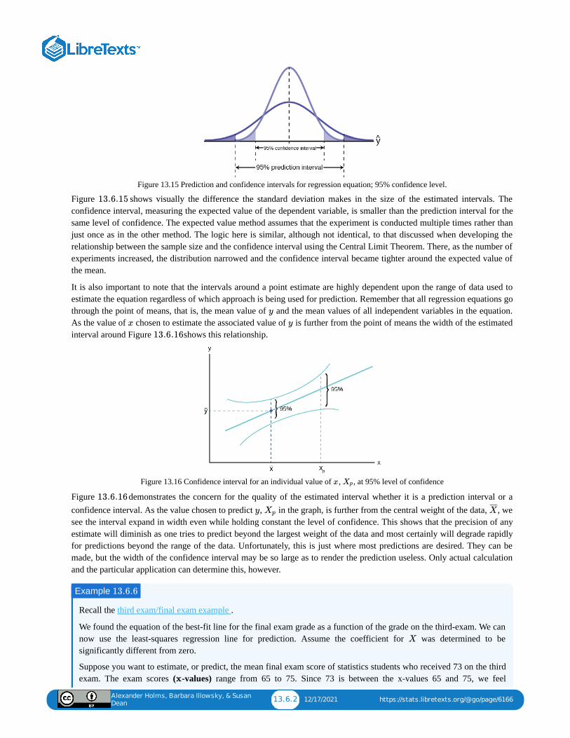
Alexander Holms, Barbara Illowsky, & Susan
Dean13.6.2 12/17/2021 https://stats.libretexts.org/@go/page/6166
Figure 13.15 Prediction and confidence intervals for regression equation; 95% confidence level.
Figure shows visually the difference the standard deviation makes in the size of the estimated intervals. Theconfidence interval, measuring the expected value of the dependent variable, is smaller than the prediction interval for thesame level of confidence. The expected value method assumes that the experiment is conducted multiple times rather thanjust once as in the other method. The logic here is similar, although not identical, to that discussed when developing therelationship between the sample size and the confidence interval using the Central Limit Theorem. There, as the number ofexperiments increased, the distribution narrowed and the confidence interval became tighter around the expected value ofthe mean.
It is also important to note that the intervals around a point estimate are highly dependent upon the range of data used toestimate the equation regardless of which approach is being used for prediction. Remember that all regression equations gothrough the point of means, that is, the mean value of and the mean values of all independent variables in the equation.As the value of chosen to estimate the associated value of is further from the point of means the width of the estimatedinterval around Figure shows this relationship.
Figure 13.16 Confidence interval for an individual value of , , at 95% level of confidence
Figure demonstrates the concern for the quality of the estimated interval whether it is a prediction interval or aconfidence interval. As the value chosen to predict , in the graph, is further from the central weight of the data, , wesee the interval expand in width even while holding constant the level of confidence. This shows that the precision of anyestimate will diminish as one tries to predict beyond the largest weight of the data and most certainly will degrade rapidlyfor predictions beyond the range of the data. Unfortunately, this is just where most predictions are desired. They can bemade, but the width of the confidence interval may be so large as to render the prediction useless. Only actual calculationand the particular application can determine this, however.
Recall the third exam/final exam example .
We found the equation of the best-fit line for the final exam grade as a function of the grade on the third-exam. We cannow use the least-squares regression line for prediction. Assume the coefficient for was determined to besignificantly different from zero.
Suppose you want to estimate, or predict, the mean final exam score of statistics students who received 73 on the thirdexam. The exam scores ( -values) range from 65 to 75. Since 73 is between the x-values 65 and 75, we feel
13.6.15
y
x y
13.6.16
x Xp
13.6.16
y Xp X¯ ¯¯̄
Example 13.6.6
X
x
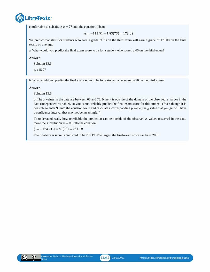
Alexander Holms, Barbara Illowsky, & Susan
Dean13.6.3 12/17/2021 https://stats.libretexts.org/@go/page/6166
comfortable to substitute into the equation. Then:
We predict that statistics students who earn a grade of 73 on the third exam will earn a grade of 179.08 on the finalexam, on average.
a. What would you predict the final exam score to be for a student who scored a 66 on the third exam?
Answer
Solution 13.6
a. 145.27
b. What would you predict the final exam score to be for a student who scored a 90 on the third exam?
Answer
Solution 13.6
b. The values in the data are between 65 and 75. Ninety is outside of the domain of the observed values in thedata (independent variable), so you cannot reliably predict the final exam score for this student. (Even though it ispossible to enter 90 into the equation for and calculate a corresponding value, the value that you get will havea confidence interval that may not be meaningful.)
To understand really how unreliable the prediction can be outside of the observed values observed in the data,make the substitution into the equation.
The final-exam score is predicted to be 261.19. The largest the final-exam score can be is 200.
x = 73
= −173.51 +4.83(73) = 179.08ŷ
x x
x y y
x
x = 90
= −173.51 +4.83(90) = 261.19ŷ
Alexander Holms, Barbara Illowsky, & Susan
Dean13.7.1 12/24/2021 https://stats.libretexts.org/@go/page/6168
13.7: Chapter Key Terms
a is the symbol for the Y-InterceptSometimes written as , because when writing the theoretical linear model is used to represent a coefficient for apopulation.
b is the symbol for SlopeThe word coefficient will be used regularly for the slope, because it is a number that will always be next to the letter “
.” It will be written as when a sample is used, and will be used with a population or when writing the theoreticallinear model.
Bivariatetwo variables are present in the model where one is the “cause” or independent variable and the other is the “effect” ofdependent variable.
Lineara model that takes data and regresses it into a straight line equation.
Multivariatea system or model where more than one independent variable is being used to predict an outcome. There can only everbe one dependent variable, but there is no limit to the number of independent variables.
R2R2 – Coefficient of DeterminationThis is a number between 0 and 1 that represents the percentage variation of the dependent variable that can beexplained by the variation in the independent variable. Sometimes calculated by the equation where isthe “Sum of Squares Regression” and is the “Sum of Squares Total.” The appropriate coefficient of determinationto be reported should always be adjusted for degrees of freedom first.
Residual or “error”the value calculated from subtracting . The absolute value of a residual measures the vertical distancebetween the actual value of y and the estimated value of y that appears on the best-fit line.
RR – Correlation CoefficientA number between −1 and 1 that represents the strength and direction of the relationship between “ ” and “ .” Thevalue for “ ” will equal 1 or −1 only if all the plotted points form a perfectly straight line.
Sum of Squared Errors (SSE)the calculated value from adding up all the squared residual terms. The hope is that this value is very small whencreating a model.
X – the independent variableThis will sometimes be referred to as the “predictor” variable, because these values were measured in order todetermine what possible outcomes could be predicted.
Y – the dependent variableAlso, using the letter “ ” represents actual values while represents predicted or estimated values. Predicted valueswill come from plugging in observed “ ” values into a linear model.
b0 β0
x b1 β1
=R2 SSR
SSTSSR
SST
− =y0 ŷ0
e0
X Y
r
y ŷ
x
Alexander Holms, Barbara Illowsky, & Susan
Dean13.8.1 1/7/2022 https://stats.libretexts.org/@go/page/6170
13.8: Chapter Practice
13.1 The Correlation Coefficient r
1.
In order to have a correlation coefficient between traits and , it is necessary to have:
a. one group of subjects, some of whom possess characteristics of trait , the remainder possessing those of trait b. measures of trait on one group of subjects and of trait on another groupc. two groups of subjects, one which could be classified as or not , the other as or not d. two groups of subjects, one which could be classified as or not , the other as or not
2.
Define the Correlation Coefficient and give a unique example of its use.
3.
If the correlation between age of an auto and money spent for repairs is +.90
a. 81% of the variation in the money spent for repairs is explained by the age of the autob. 81% of money spent for repairs is unexplained by the age of the autoc. 90% of the money spent for repairs is explained by the age of the autod. none of the above
4.
Suppose that college grade-point average and verbal portion of an IQ test had a correlation of .40. What percentage of thevariance do these two have in common?
a. 20b. 16c. 40d. 80
5.
True or false? If false, explain why: The coefficient of determination can have values between -1 and +1.
6.
True or False: Whenever r is calculated on the basis of a sample, the value which we obtain for r is only an estimate of thetrue correlation coefficient which we would obtain if we calculated it for the entire population.
7.
Under a "scatter diagram" there is a notation that the coefficient of correlation is .10. What does this mean?
a. plus and minus 10% from the means includes about 68% of the casesb. one-tenth of the variance of one variable is shared with the other variablec. one-tenth of one variable is caused by the other variabled. on a scale from -1 to +1, the degree of linear relationship between the two variables is +.10
8.
The correlation coefficient for and is known to be zero. We then can conclude that:
a. X and have standard distributionsb. the variances of and are equalc. there exists no relationship between and Yd. there exists no linear relationship between and Ye. none of these
9.
A B
A B
A B
A A B B
A A B B
X Y
Y
X Y
X
X
Alexander Holms, Barbara Illowsky, & Susan
Dean13.8.2 1/7/2022 https://stats.libretexts.org/@go/page/6170
What would you guess the value of the correlation coefficient to be for the pair of variables: "number of man-hoursworked" and "number of units of work completed"?
a. Approximately 0.9b. Approximately 0.4c. Approximately 0.0d. Approximately -0.4e. Approximately -0.9
10.
In a given group, the correlation between height measured in feet and weight measured in pounds is +.68. Which of thefollowing would alter the value of r?
a. height is expressed centimeters.b. weight is expressed in Kilograms.c. both of the above will affect r.d. neither of the above changes will affect r.
13.2 Testing the Significance of the Correlation Coefficient11.
Define a Test of a Regression Coefficient, and give a unique example of its use.
12.
The correlation between scores on a neuroticism test and scores on an anxiety test is high and positive; therefore
a. anxiety causes neuroticismb. those who score low on one test tend to score high on the other.c. those who score low on one test tend to score low on the other.d. no prediction from one test to the other can be meaningfully made.
13.3 Linear Equations13.
True or False? If False, correct it: Suppose a 95% confidence interval for the slope of the straight line regression of on is given by . Then a two-sided test of the hypothesis would result in rejection of at
the 1% level of significance.
14.
True or False: It is safer to interpret correlation coefficients as measures of association rather than causation because of thepossibility of spurious correlation.
15.
We are interested in finding the linear relation between the number of widgets purchased at one time and the cost perwidget. The following data has been obtained:
: Number of widgets purchased – 1, 3, 6, 10, 15
: Cost per widget(in dollars) – 55, 52, 46, 32, 25
Suppose the regression line is . We compute the average price per widget if 30 are purchased and observewhich of the following?
a. ; obviously, we are mistaken; the prediction is actually +15 dollars.b. , which seems reasonable judging by the data.c. \(\hat{y}=-15 \text { dollars }\, which is obvious nonsense. The regression line must be incorrect.d. , which is obvious nonsense. This reminds us that predicting outside the range of values in our
data is a very poor practice.
t
β Y
X −3.5 < β < −0.5 : β = −1H0 H0
X
Y
= −2.5x +60ŷ
= 15 dollars ŷ ŷ
= 15 dollars ŷ
= −15 dollars ŷ Y X
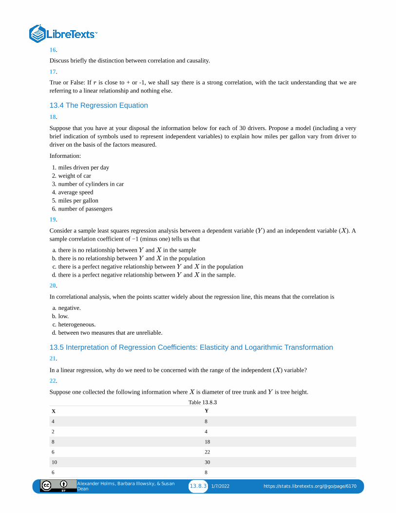
Alexander Holms, Barbara Illowsky, & Susan
Dean13.8.3 1/7/2022 https://stats.libretexts.org/@go/page/6170
16.
Discuss briefly the distinction between correlation and causality.
17.
True or False: If is close to + or -1, we shall say there is a strong correlation, with the tacit understanding that we arereferring to a linear relationship and nothing else.
13.4 The Regression Equation
18.
Suppose that you have at your disposal the information below for each of 30 drivers. Propose a model (including a verybrief indication of symbols used to represent independent variables) to explain how miles per gallon vary from driver todriver on the basis of the factors measured.
Information:
1. miles driven per day2. weight of car3. number of cylinders in car4. average speed5. miles per gallon6. number of passengers
19.
Consider a sample least squares regression analysis between a dependent variable ( ) and an independent variable ( ). Asample correlation coefficient of −1 (minus one) tells us that
a. there is no relationship between and in the sampleb. there is no relationship between and in the populationc. there is a perfect negative relationship between and in the populationd. there is a perfect negative relationship between and in the sample.
20.
In correlational analysis, when the points scatter widely about the regression line, this means that the correlation is
a. negative.b. low.c. heterogeneous.d. between two measures that are unreliable.
13.5 Interpretation of Regression Coefficients: Elasticity and Logarithmic Transformation21.
In a linear regression, why do we need to be concerned with the range of the independent ( ) variable?
22.
Suppose one collected the following information where is diameter of tree trunk and is tree height.
X Y
4 8
2 4
8 18
6 22
10 30
6 8
Table
r
Y X
Y X
Y X
Y X
Y X
X
X Y
13.8.3
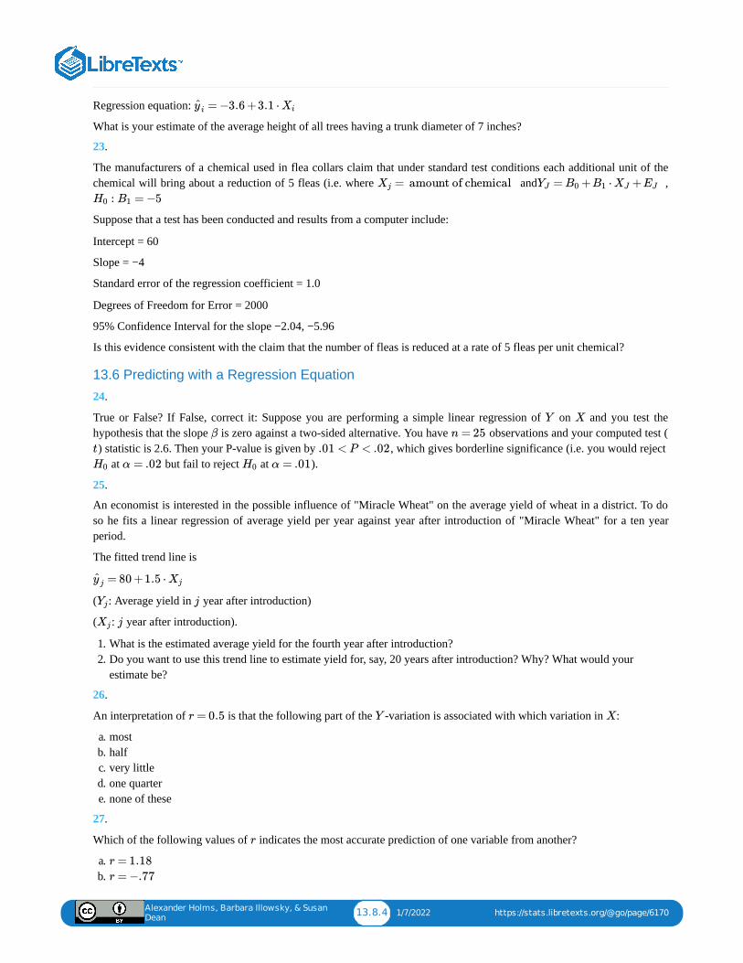
Alexander Holms, Barbara Illowsky, & Susan
Dean13.8.4 1/7/2022 https://stats.libretexts.org/@go/page/6170
Regression equation:
What is your estimate of the average height of all trees having a trunk diameter of 7 inches?
23.
The manufacturers of a chemical used in flea collars claim that under standard test conditions each additional unit of thechemical will bring about a reduction of 5 fleas (i.e. where and ,
Suppose that a test has been conducted and results from a computer include:
Intercept = 60
Slope = −4
Standard error of the regression coefficient = 1.0
Degrees of Freedom for Error = 2000
95% Confidence Interval for the slope −2.04, −5.96
Is this evidence consistent with the claim that the number of fleas is reduced at a rate of 5 fleas per unit chemical?
13.6 Predicting with a Regression Equation
24.
True or False? If False, correct it: Suppose you are performing a simple linear regression of on and you test thehypothesis that the slope is zero against a two-sided alternative. You have observations and your computed test () statistic is 2.6. Then your P-value is given by , which gives borderline significance (i.e. you would reject
at but fail to reject at ).
25.
An economist is interested in the possible influence of "Miracle Wheat" on the average yield of wheat in a district. To doso he fits a linear regression of average yield per year against year after introduction of "Miracle Wheat" for a ten yearperiod.
The fitted trend line is
( : Average yield in year after introduction)
( : year after introduction).
1. What is the estimated average yield for the fourth year after introduction?2. Do you want to use this trend line to estimate yield for, say, 20 years after introduction? Why? What would your
estimate be?
26.
An interpretation of is that the following part of the -variation is associated with which variation in :
a. mostb. halfc. very littled. one quartere. none of these
27.
Which of the following values of indicates the most accurate prediction of one variable from another?
a. b.
= −3.6 +3.1 ⋅ŷ i Xi
= amount of chemical Xj = + ⋅ +YJ B0 B1 XJ EJ
: = −5H0 B1
Y X
β n = 25
t .01 < P < .02
H0 α = .02 H0 α = .01
= 80 +1.5 ⋅ŷ j Xj
Yj j
Xj j
r = 0.5 Y X
r
r = 1.18
r = −.77
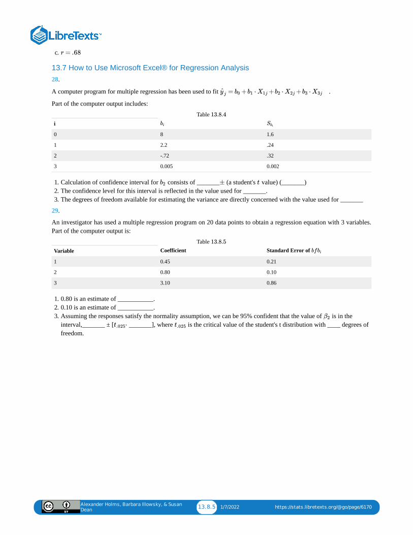
Alexander Holms, Barbara Illowsky, & Susan
Dean13.8.5 1/7/2022 https://stats.libretexts.org/@go/page/6170
c.
13.7 How to Use Microsoft Excel® for Regression Analysis28.
A computer program for multiple regression has been used to fit .
Part of the computer output includes:
i
0 8 1.6
1 2.2 .24
2 -.72 .32
3 0.005 0.002
Table
1. Calculation of confidence interval for consists of _______ (a student's value) (_______)2. The confidence level for this interval is reflected in the value used for _______.3. The degrees of freedom available for estimating the variance are directly concerned with the value used for _______
29.
An investigator has used a multiple regression program on 20 data points to obtain a regression equation with 3 variables.Part of the computer output is:
Variable Coefficient Standard Error of
1 0.45 0.21
2 0.80 0.10
3 3.10 0.86
Table
1. 0.80 is an estimate of ___________.2. 0.10 is an estimate of ___________.3. Assuming the responses satisfy the normality assumption, we can be 95% confident that the value of is in the
interval,_______ ± [ _______], where is the critical value of the student's t distribution with ____ degrees offreedom.
r = .68
= + ⋅ + ⋅ + ⋅ŷ j b0 b1 X1j b2 X2j b3 X3j
bi Sbi
13.8.4
b2 ± t
bfbi
13.8.5
β2
⋅t.025 t.025
Alexander Holms, Barbara Illowsky, & Susan
Dean13.9.1 12/10/2021 https://stats.libretexts.org/@go/page/6169
13.9: Chapter Review
13.3 Linear Equations
The most basic type of association is a linear association. This type of relationship can be defined algebraically by theequations used, numerically with actual or predicted data values, or graphically from a plotted curve. (Lines are classifiedas straight curves.) Algebraically, a linear equation typically takes the form , where and are constants,
is the independent variable, is the dependent variable. In a statistical context, a linear equation is written in the form , where and are the constants. This form is used to help readers distinguish the statistical context from the
algebraic context. In the equation , the constant that multiplies the variable ( is called a coefficient) iscalled the slope. The slope describes the rate of change between the independent and dependent variables; in other words,the slope describes the change that occurs in the dependent variable as the independent variable is changed. In the equation
, the constant a is called the y-intercept.
The slope of a line is a value that describes the rate of change between the independent and dependent variables. The slopetells us how the dependent variable ( ) changes for every one unit increase in the independent ( ) variable, on average.The -intercept is used to describe the dependent variable when the independent variable equals zero. Graphically, theslope is represented by three line types in elementary statistics.
13.4 The Regression EquationIt is hoped that this discussion of regression analysis has demonstrated the tremendous potential value it has as a tool fortesting models and helping to better understand the world around us. The regression model has its limitations, especiallythe requirement that the underlying relationship be approximately linear. To the extent that the true relationship isnonlinear it may be approximated with a linear relationship or nonlinear forms of transformations that can be estimatedwith linear techniques. Double logarithmic transformation of the data will provide an easy way to test this particular shapeof the relationship. A reasonably good quadratic form (the shape of the total cost curve from Microeconomics Principles)can be generated by the equation:
where the values of are simply squared and put into the equation as a separate variable.
There is much more in the way of econometric "tricks" that can bypass some of the more troublesome assumptions of thegeneral regression model. This statistical technique is so valuable that further study would provide any student significant,statistically significant, dividends.
y = mx + b m b
x y
y = a+ bx a b
y = a+bx b x b
y = a+bx
y x
y
Y = a+ X+b1 b2X2
X
Alexander Holms, Barbara Illowsky, & Susan
Dean13.10.1 12/17/2021 https://stats.libretexts.org/@go/page/6171
13.10: Chapter Solution1.
d
2.
A measure of the degree to which variation of one variable is related to variation in one or more other variables. The mostcommonly used correlation coefficient indicates the degree to which variation in one variable is described by a straight linerelation with another variable.
Suppose that sample information is available on family income and Years of schooling of the head of the household. Acorrelation coefficient = 0 would indicate no linear association at all between these two variables. A correlation of 1 wouldindicate perfect linear association (where all variation in family income could be associated with schooling and vice versa).
3.
a. 81% of the variation in the money spent for repairs is explained by the age of the auto
4.
b. 16
5.
The coefficient of determination is with , since .
6.
True
7.
d. on a scale from -1 to +1, the degree of linear relationship between the two variables is +.10
8.
d. there exists no linear relationship between X and Y
9.
Approximately 0.9
10.
d. neither of the above changes will affect .
11.
Definition: A test is obtained by dividing a regression coefficient by its standard error and then comparing the result tocritical values for Students' t with Error . It provides a test of the claim that when all other variables have beenincluded in the relevant regression model.
Example: Suppose that 4 variables are suspected of influencing some response. Suppose that the results of fitting include:
Variable Regression coefficient Standard error of regular coefficient
.5 1 -3
.4 2 +2
.02 3 +1
.6 4 -.5
Table
calculated for variables 1, 2, and 3 would be 5 or larger in absolute value while that for variable 4 would be less than 1.For most significance levels, the hypothesis would be rejected. But, notice that this is for the case when , ,
r ⋅ ⋅2 0 ≤ r ⋅ ⋅2 ≤ 1 −1 ≤ r ≤ 1
r
t
df = 0βi
= + + + + +Yi β0 β1X1i β2X2i β3X3i β4X4i ei
13.10.6
t
= 0β1 X2 X3
Alexander Holms, Barbara Illowsky, & Susan
Dean13.10.2 12/17/2021 https://stats.libretexts.org/@go/page/6171
and have been included in the regression. For most significance levels, the hypothesis would be continued(retained) for the case where , , and are in the regression. Often this pattern of results will result in computinganother regression involving only , , , and examination of the t ratios produced for that case.
12.
c. those who score low on one test tend to score low on the other.
13.
False. Since would not be rejected at , it would not be rejected at .
14.
True
15.
d
16.
Some variables seem to be related, so that knowing one variable's status allows us to predict the status of the other. Thisrelationship can be measured and is called correlation. However, a high correlation between two variables in no wayproves that a cause-and-effect relation exists between them. It is entirely possible that a third factor causes both variablesto vary together.
17.
True
18.
19.
d. there is a perfect negative relationship between and in the sample.
20.
b. low
21.
The precision of the estimate of the variable depends on the range of the independent ( ) variable explored. If weexplore a very small range of the variable, we won't be able to make much use of the regression. Also, extrapolation isnot recommended.
22.
23.
Most simply, since −5 is included in the confidence interval for the slope, we can conclude that the evidence is consistentwith the claim at the 95% confidence level.
Using a t test: .
Since we retain the null hypothesis that .
24.
True.
25.
X4 = 0β4
X1 X2 X3
X1 X2 X3
: β = −1H0 α = 0.05 α = 0.01
= + ⋅ + ⋅ + ⋅ + ⋅ + ⋅ +Yj b0 b1 X1 b2 X2 b3 X3 b4 X4 b5 X6 ej
Y X
Y X
X
= −3.6 +(3.1 ⋅ 7) = 18.1ŷ
: = −5H0 B1 : ≠ −5HA B1 = = −1t calculated −5−(−4)
1= −1.96t critical
<tcalc tcrit = −5B1
= ±2.5t (critical, ,df=23, two-tailed, α=.02)
= ±2.8t critical ,df=23, two-tailed, α=.01
Alexander Holms, Barbara Illowsky, & Susan
Dean13.10.3 12/17/2021 https://stats.libretexts.org/@go/page/6171
1. 2. No. Most business statisticians would not want to extrapolate that far. If someone did, the estimate would be 110, but
some other factors probably come into play with 20 years.
26.
d. one quarter
27.
b.
28.
1. 2. the value3. the value
29.
1. The population value for , the change that occurs in with a unit change in , when the other variables are heldconstant.
2. The population value for the standard error of the distribution of estimates of .3. .
80 +1.5 ⋅ 4 = 86
r = −.77
−.72, .32
t
t
β2 Y X2
β2
.8, .1, 16 = 20 −4

Alexander Holms, Barbara Illowsky, & Susan
Dean13.11.1 12/3/2021 https://stats.libretexts.org/@go/page/6167
13.11: How to Use Microsoft Excel® for Regression AnalysisThis section of this chapter is here in recognition that what we are now asking requires much more than a quick calculationof a ratio or a square root. Indeed, the use of regression analysis was almost non- existent before the middle of the lastcentury and did not really become a widely used tool until perhaps the late 1960’s and early 1970’s. Even then thecomputational ability of even the largest IBM machines is laughable by today’s standards. In the early days programs weredeveloped by the researchers and shared. There was no market for something called “software” and certainly nothingcalled “apps”, an entrant into the market only a few years old.
With the advent of the personal computer and the explosion of a vital software market we have a number of regression andstatistical analysis packages to choose from. Each has their merits. We have chosen Microsoft Excel because of the wide-spread availability both on college campuses and in the post-college market place. Stata is an alternative and has featuresthat will be important for more advanced econometrics study if you choose to follow this path. Even more advancedpackages exist, but typically require the analyst to do some significant amount of programing to conduct their analysis.The goal of this section is to demonstrate how to use Excel to run a regression and then to do so with an example of asimple version of a demand curve.
The first step to doing a regression using Excel is to load the program into your computer. If you have Excel you have theAnalysis ToolPak although you may not have it activated. The program calls upon a significant amount of space so is notloaded automatically.
To activate the Analysis ToolPak follow these steps:
Click “File” > “Options” > “Add-ins” to bring up a menu of the add-in “ToolPaks”. Select “Analysis ToolPak” and click“GO” next to “Manage: excel add-ins” near the bottom of the window. This will open a new window where you click“Analysis ToolPak” (make sure there is a green check mark in the box) and then click “OK”. Now there should be anAnalysis tab under the data menu. These steps are presented in the following screen shots.
Figure 13.11.17
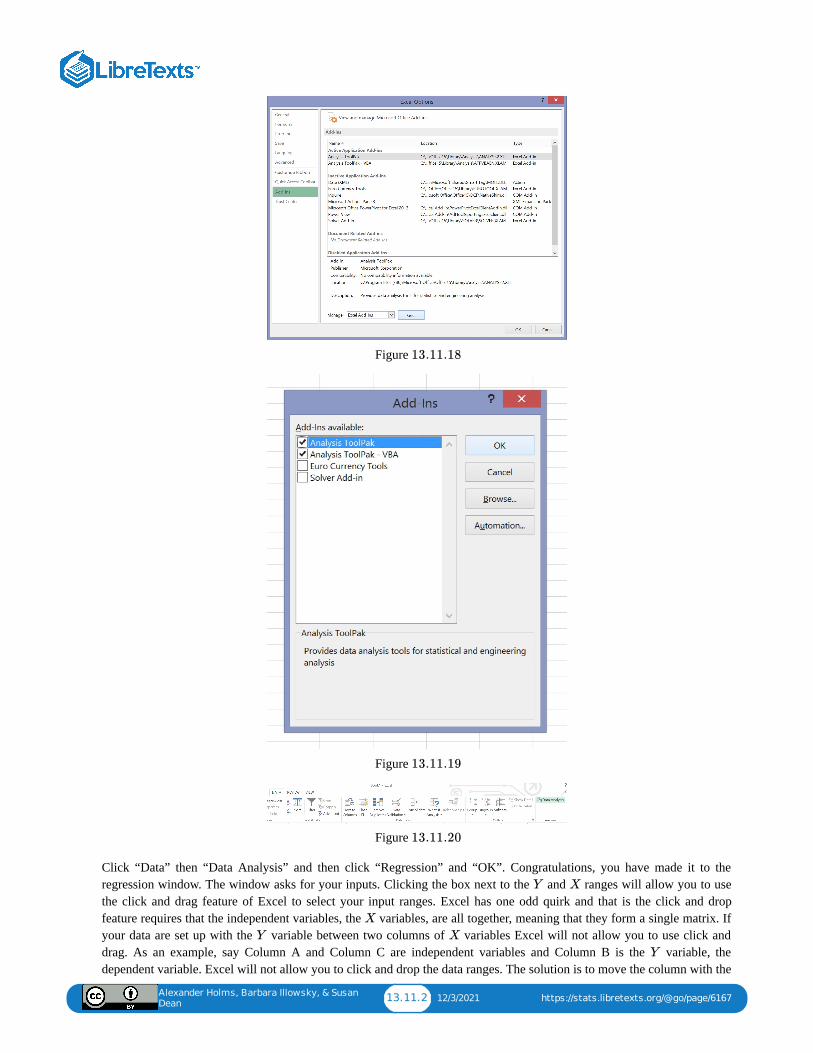
Alexander Holms, Barbara Illowsky, & Susan
Dean13.11.2 12/3/2021 https://stats.libretexts.org/@go/page/6167
Figure
Figure
Figure
Click “Data” then “Data Analysis” and then click “Regression” and “OK”. Congratulations, you have made it to theregression window. The window asks for your inputs. Clicking the box next to the and ranges will allow you to usethe click and drag feature of Excel to select your input ranges. Excel has one odd quirk and that is the click and dropfeature requires that the independent variables, the variables, are all together, meaning that they form a single matrix. Ifyour data are set up with the variable between two columns of variables Excel will not allow you to use click anddrag. As an example, say Column A and Column C are independent variables and Column B is the variable, thedependent variable. Excel will not allow you to click and drop the data ranges. The solution is to move the column with the
13.11.18
13.11.19
13.11.20
Y X
X
Y X
Y
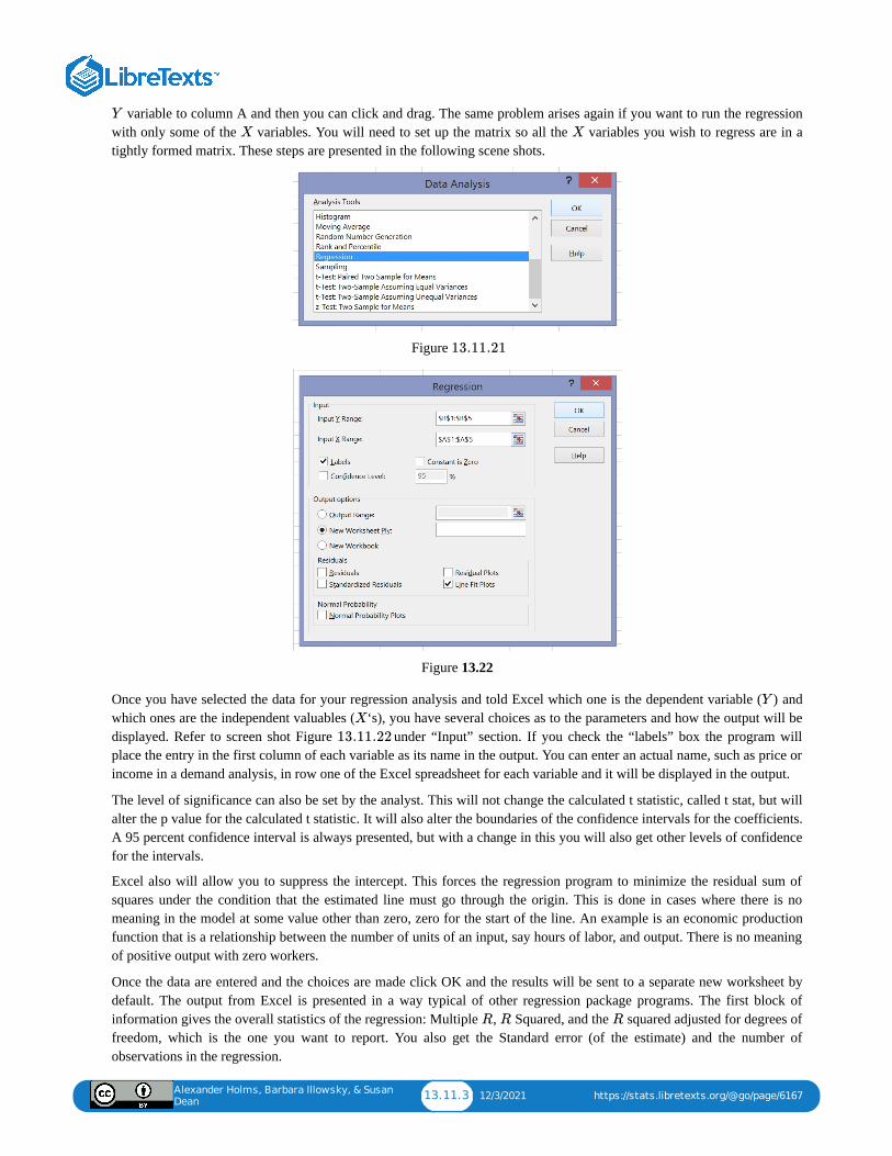
Alexander Holms, Barbara Illowsky, & Susan
Dean13.11.3 12/3/2021 https://stats.libretexts.org/@go/page/6167
variable to column A and then you can click and drag. The same problem arises again if you want to run the regressionwith only some of the variables. You will need to set up the matrix so all the variables you wish to regress are in atightly formed matrix. These steps are presented in the following scene shots.
Figure
Figure 13.22
Once you have selected the data for your regression analysis and told Excel which one is the dependent variable ( ) andwhich ones are the independent valuables ( ‘s), you have several choices as to the parameters and how the output will bedisplayed. Refer to screen shot Figure under “Input” section. If you check the “labels” box the program willplace the entry in the first column of each variable as its name in the output. You can enter an actual name, such as price orincome in a demand analysis, in row one of the Excel spreadsheet for each variable and it will be displayed in the output.
The level of significance can also be set by the analyst. This will not change the calculated t statistic, called t stat, but willalter the p value for the calculated t statistic. It will also alter the boundaries of the confidence intervals for the coefficients.A 95 percent confidence interval is always presented, but with a change in this you will also get other levels of confidencefor the intervals.
Excel also will allow you to suppress the intercept. This forces the regression program to minimize the residual sum ofsquares under the condition that the estimated line must go through the origin. This is done in cases where there is nomeaning in the model at some value other than zero, zero for the start of the line. An example is an economic productionfunction that is a relationship between the number of units of an input, say hours of labor, and output. There is no meaningof positive output with zero workers.
Once the data are entered and the choices are made click OK and the results will be sent to a separate new worksheet bydefault. The output from Excel is presented in a way typical of other regression package programs. The first block ofinformation gives the overall statistics of the regression: Multiple , Squared, and the squared adjusted for degrees offreedom, which is the one you want to report. You also get the Standard error (of the estimate) and the number ofobservations in the regression.
Y
X X
13.11.21
Y
X
13.11.22
R R R
Alexander Holms, Barbara Illowsky, & Susan
Dean13.11.4 12/3/2021 https://stats.libretexts.org/@go/page/6167
The second block of information is titled ANOVA which stands for Analysis of Variance. Our interest in this section is thecolumn marked . This is the calculated statistics for the null hypothesis that all of the coefficients are equal to zeroverse the alternative that at least one of the coefficients are not equal to zero. This hypothesis test was presented in 13.4under “How Good is the Equation?” The next column gives the p value for this test under the title “Significance F”. If thep value is less than say 0.05 (the calculated statistic is in the tail) we can say with 90 % confidence that we cannotaccept the null hypotheses that all the coefficients are equal to zero. This is a good thing: it means that at least one of thecoefficients is significantly different from zero thus do have an effect on the value of .
The last block of information contains the hypothesis tests for the individual coefficient. The estimated coefficients, theintercept and the slopes, are first listed and then each standard error (of the estimated coefficient) followed by the t stat(calculated student’s t statistic for the null hypothesis that the coefficient is equal to zero). We compare the t stat and thecritical value of the student’s t, dependent on the degrees of freedom, and determine if we have enough evidence to rejectthe null that the variable has no effect on . Remember that we have set up the null hypothesis as the status quo and ourclaim that we know what caused the to change is in the alternative hypothesis. We want to reject the status quo andsubstitute our version of the world, the alternative hypothesis. The next column contains the p values for this hypothesistest followed by the estimated upper and lower bound of the confidence interval of the estimated slope parameter forvarious levels of confidence set by us at the beginning.
Estimating the Demand for Roses
Here is an example of using the Excel program to run a regression for a particular specific case: estimating the demand forroses. We are trying to estimate a demand curve, which from economic theory we expect certain variables affect how muchof a good we buy. The relationship between the price of a good and the quantity demanded is the demand curve. Beyondthat we have the demand function that includes other relevant variables: a person’s income, the price of substitute goods,and perhaps other variables such as season of the year or the price of complimentary goods. Quantity demanded will be our
variable, and Price of roses, Price of carnations and Income will be our independent variables, the variables.
For all of these variables theory tells us the expected relationship. For the price of the good in question, roses, theorypredicts an inverse relationship, the negatively sloped demand curve. Theory also predicts the relationship between thequantity demanded of one good, here roses, and the price of a substitute, carnations in this example. Theory predicts thatthis should be a positive or direct relationship; as the price of the substitute falls we substitute away from roses to thecheaper substitute, carnations. A reduction in the price of the substitute generates a reduction in demand for the good beinganalyzed, roses here. Reduction generates reduction is a positive relationship. For normal goods, theory also predicts apositive relationship; as our incomes rise we buy more of the good, roses. We expect these results because that is what ispredicted by a hundred years of economic theory and research. Essentially we are testing these century-old hypotheses.The data gathered was determined by the model that is being tested. This should always be the case. One is not doinginferential statistics by throwing a mountain of data into a computer and asking the machine for a theory. Theory first, testfollows.
These data here are national average prices and income is the nation’s per capita personal income. Quantity demanded istotal national annual sales of roses. These are annual time series data; we are tracking the rose market for the United Statesfrom 1984-2017, 33 observations.
Because of the quirky way Excel requires how the data are entered into the regression package it is best to have theindependent variables, price of roses, price of carnations and income next to each other on the spreadsheet. Once your dataare entered into the spreadsheet it is always good to look at the data. Examine the range, the means and the standarddeviations. Use your understanding of descriptive statistics from the very first part of this course. In large data sets you willnot be able to “scan” the data. The Analysis ToolPac makes it easy to get the range, mean, standard deviations and otherparameters of the distributions. You can also quickly get the correlations among the variables. Examine for outliers.Review the history. Did something happen? Was here a labor strike, change in import fees, something that makes theseobservations unusual? Do not take the data without question. There may have been a typo somewhere, who knows withoutreview.
Go to the regression window, enter the data and select 95% confidence level and click “OK”. You can include the labels inthe input range if you have put a title at the top of each column, but be sure to click the “labels” box on the main regressionpage if you do.
F F
F
Y
Y
Y
Y X
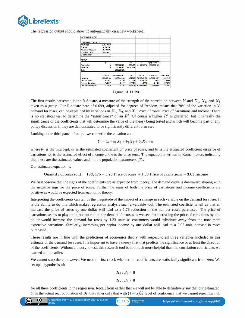
Alexander Holms, Barbara Illowsky, & Susan
Dean13.11.5 12/3/2021 https://stats.libretexts.org/@go/page/6167
The regression output should show up automatically on a new worksheet.
Figure
The first results presented is the R-Square, a measure of the strength of the correlation between and , , and taken as a group. Our R-square here of 0.699, adjusted for degrees of freedom, means that 70% of the variation in Y,demand for roses, can be explained by variations in , , and , Price of roses, Price of carnations and Income. Thereis no statistical test to determine the “significance” of an . Of course a higher is preferred, but it is really thesignificance of the coefficients that will determine the value of the theory being tested and which will become part of anypolicy discussion if they are demonstrated to be significantly different form zero.
Looking at the third panel of output we can write the equation as:
where is the intercept, is the estimated coefficient on price of roses, and b is the estimated coefficient on price ofcarnations, is the estimated effect of income and e is the error term. The equation is written in Roman letters indicatingthat these are the estimated values and not the population parameters, ’s.
Our estimated equation is:
We first observe that the signs of the coefficients are as expected from theory. The demand curve is downward sloping withthe negative sign for the price of roses. Further the signs of both the price of carnations and income coefficients arepositive as would be expected from economic theory.
Interpreting the coefficients can tell us the magnitude of the impact of a change in each variable on the demand for roses. Itis the ability to do this which makes regression analysis such a valuable tool. The estimated coefficients tell us that anincrease the price of roses by one dollar will lead to a 1.76 reduction in the number roses purchased. The price ofcarnations seems to play an important role in the demand for roses as we see that increasing the price of carnations by onedollar would increase the demand for roses by 1.33 units as consumers would substitute away from the now moreexpensive carnations. Similarly, increasing per capita income by one dollar will lead to a 3.03 unit increase in rosespurchased.
These results are in line with the predictions of economics theory with respect to all three variables included in thisestimate of the demand for roses. It is important to have a theory first that predicts the significance or at least the directionof the coefficients. Without a theory to test, this research tool is not much more helpful than the correlation coefficients welearned about earlier.
We cannot stop there, however. We need to first check whether our coefficients are statistically significant from zero. Weset up a hypothesis of:
for all three coefficients in the regression. Recall from earlier that we will not be able to definitively say that our estimated is the actual real population of , but rather only that with level of confidence that we cannot reject the null
13.11.23
Y X1 X2 X3
X1 X2 X3
R2 R2
Y = + + + +eb0 b1X1 b2X2 b3X3
b0 b1 2b3
β
Quantity of roses sold = 183, 475 −1.76 Price of roses +1.33 Price of carnations +3.03 Income
: = 0H0 β1
: ≠ 0Ha β1
b1 β1 (1 −α)%
Alexander Holms, Barbara Illowsky, & Susan
Dean13.11.6 12/3/2021 https://stats.libretexts.org/@go/page/6167
hypothesis that our estimated is significantly different from zero. The analyst is making a claim that the price of rosescauses an impact on quantity demanded. Indeed, that each of the included variables has an impact on the quantity of rosesdemanded. The claim is therefore in the alternative hypotheses. It will take a very large probability, 0.95 in this case, tooverthrow the null hypothesis, the status quo, that . In all regression hypothesis tests the claim is in the alternativeand the claim is that the theory has found a variable that has a significant impact on the variable.
The test statistic for this hypothesis follows the familiar standardizing formula which counts the number of standarddeviations, , that the estimated value of the parameter, , is away from the hypothesized value, , which is zero in thiscase:
The computer calculates this test statistic and presents it as “t stat”. You can find this value to the right of the standard errorof the coefficient estimate. The standard error of the coefficient for is in the formula. To reach a conclusion wecompare this test statistic with the critical value of the student’s at degrees of freedom , and alpha =0.025 (5% significance level for a two-tailed test). Our stat for is approximately 5.90 which is greater than 1.96 (thecritical value we looked up in the t-table), so we cannot accept our null hypotheses of no effect. We conclude that Price hasa significant effect because the calculated t value is in the tail. We conduct the same test for b2 and b3. For each variable,we find that we cannot accept the null hypothesis of no relationship because the calculated t-statistics are in the tail foreach case, that is, greater than the critical value. All variables in this regression have been determined to have a significanteffect on the demand for roses.
These tests tell us whether or not an individual coefficient is significantly different from zero, but does not address theoverall quality of the model. We have seen that the R squared adjusted for degrees of freedom indicates this model withthese three variables explains 70% of the variation in quantity of roses demanded. We can also conduct a second test of themodel taken as a whole. This is the test presented in section 13.4 of this chapter. Because this is a multiple regression(more than one X), we use the -test to determine if our coefficients collectively affect . The hypothesis is:
Under the ANOVA section of the output we find the calculated statistic for this hypotheses. For this example the statistic is 21.9. Again, comparing the calculated statistic with the critical value given our desired level of significanceand the degrees of freedom will allow us to reach a conclusion.
The best way to reach a conclusion for this statistical test is to use the p-value comparison rule. The p-value is the area inthe tail, given the calculated statistic. In essence the computer is finding the value in the table for us and calculatingthe p-value. In the Summary Output under “significance F” is this probability. For this example, it is calculated to be 2.6 10-5, or 2.6 then moving the decimal five places to the left. (.000026) This is an almost infinitesimal level of probabilityand is certainly less than our alpha level of .05 for a 5 percent level of significance.
By not being able to accept the null hypotheses we conclude that this specification of this model has validity because atleast one of the estimated coefficients is significantly different from zero. Since -calculated is greater than -critical, wecannot accept H0, meaning that , and together has a significant effect on .
The development of computing machinery and the software useful for academic and business research has made it possibleto answer questions that just a few years ago we could not even formulate. Data is available in electronic format and can bemoved into place for analysis in ways and at speeds that were unimaginable a decade ago. The sheer magnitude of datasets that can today be used for research and analysis gives us a higher quality of results than in days past. Even with onlyan Excel spreadsheet we can conduct very high level research. This section gives you the tools to conduct some of thisvery interesting research with the only limit being your imagination.
β1
β = 0
Y
t b1 β0
=tc
−b1 β0
Sb1
b1 Sb1
t n −3 −1 = 29
t b1
F
F Y
: = = … = βi = 0H0 β1 β2
:" at least one of the is not equal to 0 "Ha βi
F F
F
F F
X
F F
X1 X2 X3 Y

1 1/7/2022
CHAPTER OVERVIEW14: APPPENDICES
14.0: B | MATHEMATICAL PHRASES, SYMBOLS, AND FORMULAS14.1: A | STATISTICAL TABLES
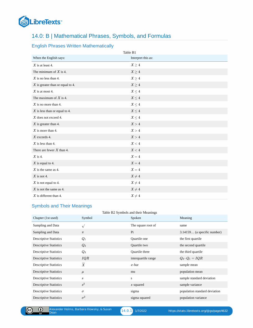
Alexander Holms, Barbara Illowsky, & Susan
Dean14.0.1 1/7/2022 https://stats.libretexts.org/@go/page/4632
14.0: B | Mathematical Phrases, Symbols, and Formulas
English Phrases Written Mathematically
When the English says: Interpret this as:
is at least 4.
The minimum of is 4.
is no less than 4.
is greater than or equal to 4.
is at most 4.
The maximum of is 4.
is no more than 4.
is less than or equal to 4.
does not exceed 4.
is greater than 4.
is more than 4.
exceeds 4.
is less than 4.
There are fewer than 4.
is 4.
is equal to 4.
is the same as 4.
is not 4.
is not equal to 4.
is not the same as 4.
is different than 4.
Table B1
Symbols and Their Meanings
Chapter (1st used) Symbol Spoken Meaning
Sampling and Data The square root of same
Sampling and Data Pi 3.14159… (a specific number)
Descriptive Statistics Quartile one the first quartile
Descriptive Statistics Quartile two the second quartile
Descriptive Statistics Quartile three the third quartile
Descriptive Statistics interquartile range
Descriptive Statistics -bar sample mean
Descriptive Statistics mu population mean
Descriptive Statistics s sample standard deviation
Descriptive Statistics squared sample variance
Descriptive Statistics sigma population standard deviation
Descriptive Statistics sigma squared population variance
Table B2 Symbols and their Meanings
X X ≥ 4
X X ≥ 4
X X ≥ 4
X X ≥ 4
X X ≤ 4
X X ≤ 4
X X ≤ 4
X X ≤ 4
X X ≤ 4
X X > 4
X X > 4
X X > 4
X X < 4
X X < 4
X X = 4
X X = 4
X X = 4
X X ≠ 4
X X ≠ 4
X X ≠ 4
X X ≠ 4
√
π
Q1
Q2
Q3
IQR – = IQRQ3 Q1
X¯ ¯¯̄ x
μ
s
s2 s
σ
σ2
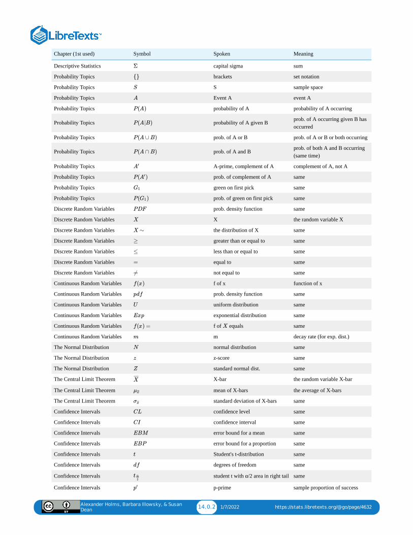
Alexander Holms, Barbara Illowsky, & Susan
Dean14.0.2 1/7/2022 https://stats.libretexts.org/@go/page/4632
Chapter (1st used) Symbol Spoken Meaning
Descriptive Statistics capital sigma sum
Probability Topics brackets set notation
Probability Topics S sample space
Probability Topics Event A event A
Probability Topics probability of A probability of A occurring
Probability Topics probability of A given B prob. of A occurring given B hasoccurred
Probability Topics prob. of A or B prob. of A or B or both occurring
Probability Topics prob. of A and B prob. of both A and B occurring(same time)
Probability Topics A-prime, complement of A complement of A, not A
Probability Topics prob. of complement of A same
Probability Topics green on first pick same
Probability Topics prob. of green on first pick same
Discrete Random Variables prob. density function same
Discrete Random Variables X the random variable X
Discrete Random Variables the distribution of X same
Discrete Random Variables greater than or equal to same
Discrete Random Variables less than or equal to same
Discrete Random Variables equal to same
Discrete Random Variables not equal to same
Continuous Random Variables f of x function of x
Continuous Random Variables prob. density function same
Continuous Random Variables uniform distribution same
Continuous Random Variables exponential distribution same
Continuous Random Variables f of equals same
Continuous Random Variables m decay rate (for exp. dist.)
The Normal Distribution normal distribution same
The Normal Distribution z-score same
The Normal Distribution standard normal dist. same
The Central Limit Theorem X-bar the random variable X-bar
The Central Limit Theorem mean of X-bars the average of X-bars
The Central Limit Theorem standard deviation of X-bars same
Confidence Intervals confidence level same
Confidence Intervals confidence interval same
Confidence Intervals error bound for a mean same
Confidence Intervals error bound for a proportion same
Confidence Intervals Student's t-distribution same
Confidence Intervals degrees of freedom same
Confidence Intervals student t with α/2 area in right tail same
Confidence Intervals p-prime sample proportion of success
Σ
{}
S
A
P(A)
P(A|B)
P(A ∪ B)
P(A ∩ B)
A′
P( )A′
G1
P( )G1
X
X ∼
≥
≤
=
≠
f(x)
U
Exp
f(x) = X
m
N
z
Z
X¯ ¯¯̄
μx̄̄̄
σx̄̄̄
CL
CI
EBM
EBP
t
df
t α
2
p′
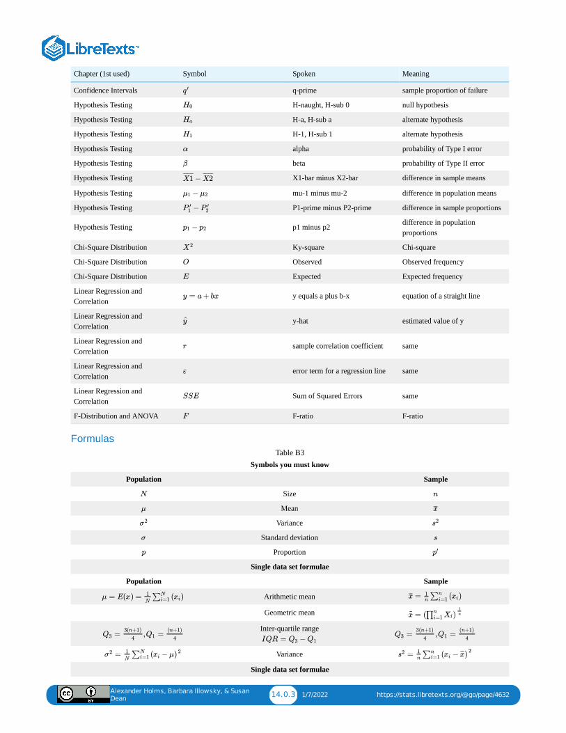
Alexander Holms, Barbara Illowsky, & Susan
Dean14.0.3 1/7/2022 https://stats.libretexts.org/@go/page/4632
Chapter (1st used) Symbol Spoken Meaning
Confidence Intervals q-prime sample proportion of failure
Hypothesis Testing H-naught, H-sub 0 null hypothesis
Hypothesis Testing H-a, H-sub a alternate hypothesis
Hypothesis Testing H-1, H-sub 1 alternate hypothesis
Hypothesis Testing alpha probability of Type I error
Hypothesis Testing beta probability of Type II error
Hypothesis Testing X1-bar minus X2-bar difference in sample means
Hypothesis Testing mu-1 minus mu-2 difference in population means
Hypothesis Testing P1-prime minus P2-prime difference in sample proportions
Hypothesis Testing p1 minus p2 difference in populationproportions
Chi-Square Distribution Ky-square Chi-square
Chi-Square Distribution Observed Observed frequency
Chi-Square Distribution Expected Expected frequency
Linear Regression andCorrelation
y equals a plus b-x equation of a straight line
Linear Regression andCorrelation
y-hat estimated value of y
Linear Regression andCorrelation
sample correlation coefficient same
Linear Regression andCorrelation
error term for a regression line same
Linear Regression andCorrelation
Sum of Squared Errors same
F-Distribution and ANOVA F-ratio F-ratio
Formulas
Symbols you must know
Population Sample
Size
Mean
Variance
Standard deviation
Proportion
Single data set formulae
Population Sample
Arithmetic mean
Geometric mean
Inter-quartile range
Variance
Single data set formulae
Table B3
q ′
H0
Ha
H1
α
β
−X1¯ ¯¯̄¯̄¯
X2¯ ¯¯̄¯̄¯
−μ1 μ2
−P ′1 P ′
2
−p1 p2
X2
O
E
y = a+ bx
ŷ
r
ε
SSE
F
N n
μ x̄̄̄
σ2 s2
σ s
p p′
μ = E(x) = ( )1N∑N
i=1 xi = ( )x̄̄̄ 1n∑n
i=1 xi
=x~ ( )∏ni=1Xi
1n
= , =Q33(n+1)
4Q1
(n+1)
4 IQR = −Q3 Q1= , =Q3
3(n+1)
4Q1
(n+1)
4
=σ2 1N∑N
i=1 ( − μ)xi2 =s2 1
n∑n
i=1 ( − )xi x̄̄̄2
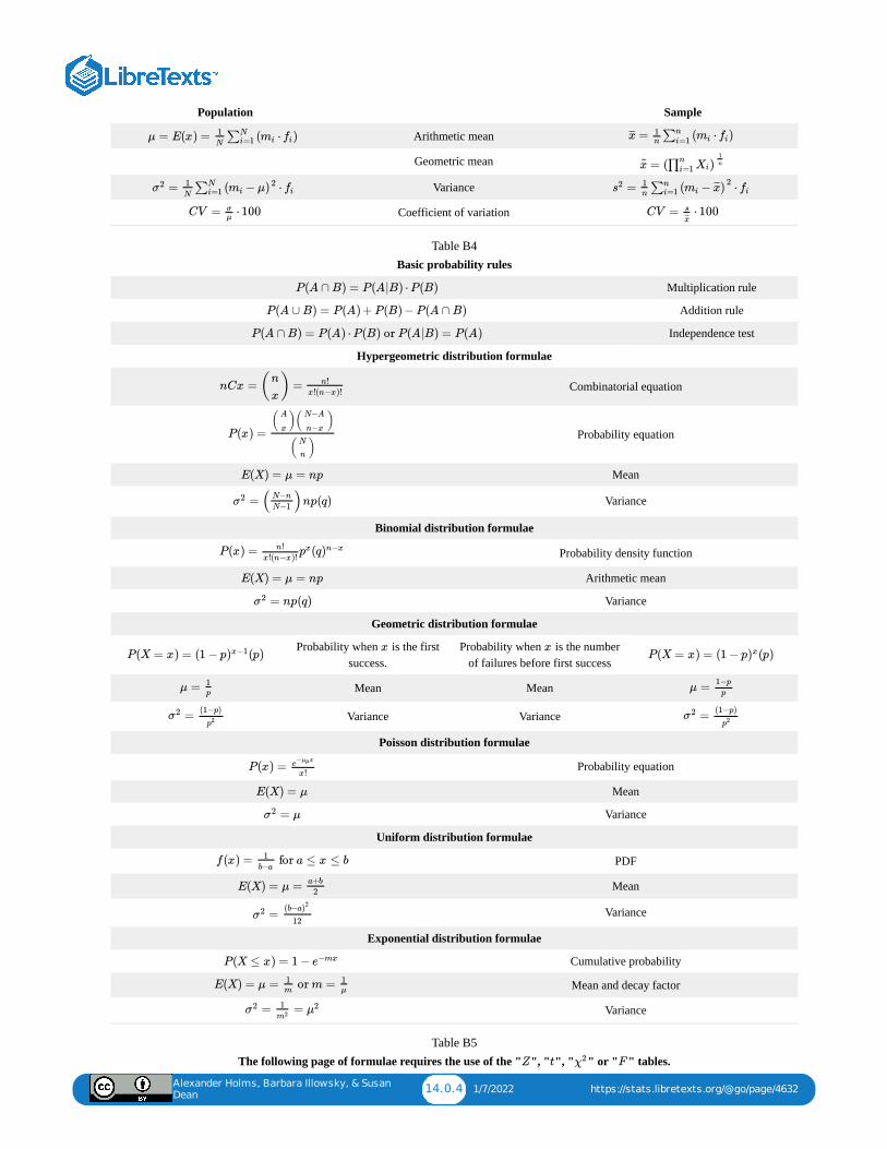
Alexander Holms, Barbara Illowsky, & Susan
Dean14.0.4 1/7/2022 https://stats.libretexts.org/@go/page/4632
Population Sample
Arithmetic mean
Geometric mean
Variance
Coefficient of variation
Basic probability rules
Multiplication rule
Addition rule
Independence test
Hypergeometric distribution formulae
Combinatorial equation
Probability equation
Mean
Variance
Binomial distribution formulae
Probability density function
Arithmetic mean
Variance
Geometric distribution formulae
Probability when is the firstsuccess.
Probability when is the numberof failures before first success
Mean Mean
Variance Variance
Poisson distribution formulae
Probability equation
Mean
Variance
Uniform distribution formulae
Mean
Variance
Exponential distribution formulae
Cumulative probability
Mean and decay factor
Variance
Table B4
The following page of formulae requires the use of the " ", " ", " " or " " tables.Table B5
μ = E(x) = ( ⋅ )1N∑N
i=1 mi fi = ( ⋅ )x̄̄̄ 1n∑n
i=1 mi fi
=x~ ( )∏ni=1Xi
1n
= ⋅σ2 1N∑N
i=1 ( − μ)mi2 fi = ⋅s2 1
n∑n
i=1 ( − )mi x̄̄̄2
fi
CV = ⋅ 100σμ
CV = ⋅ 100s
x̄̄̄
P(A ∩ B) = P(A|B) ⋅P(B)
P(A ∪ B) = P(A) +P(B) −P(A ∩ B)
P(A ∩ B) = P(A) ⋅P(B) or P(A|B) = P(A)
nCx = ( ) =n
x
n!x!(n−x)!
P(x) =( )( )A
x
N−A
n−x
( )N
n
E(X) = μ = np
= ( )np(q)σ2 N−n
N−1
P(x) = (qn!x!(n−x)!
px )n−x
E(X) = μ = np
= np(q)σ2
P(X = x) = (1 − p (p))x−1 x xP(X = x) = (1 − p (p))x
μ = 1p
μ =1−p
p
=σ2 (1−p)
p2 =σ2 (1−p)
p2
P(x) = e− xμμ
x!
E(X) = μ
= μσ2
f(x) = for a ≤ x ≤ b1b−a
E(X) = μ =a+b
2
=σ2 (b−a)2
12
P(X ≤ x) = 1 − e−mx
E(X) = μ = or m =1m
1μ
= =σ2 1m2 μ2
Z t χ2 F
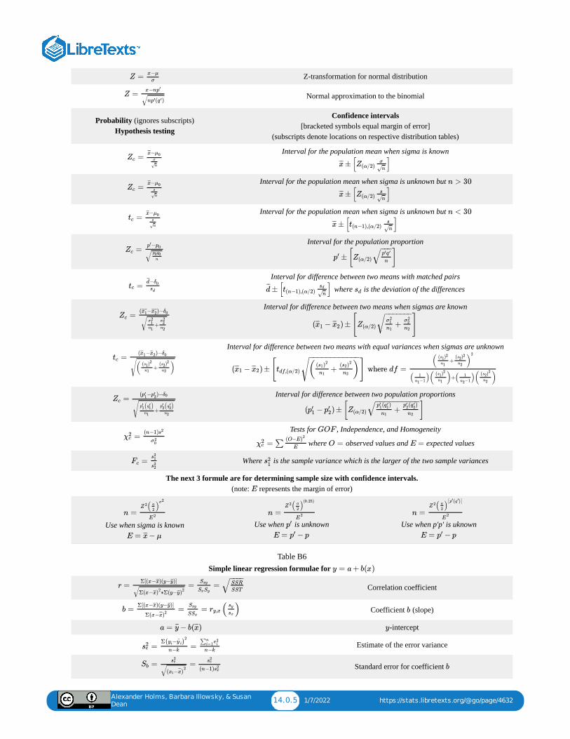
Alexander Holms, Barbara Illowsky, & Susan
Dean14.0.5 1/7/2022 https://stats.libretexts.org/@go/page/4632
Z-transformation for normal distribution
Normal approximation to the binomial
Probability (ignores subscripts) Hypothesis testing
Confidence intervals [bracketed symbols equal margin of error]
(subscripts denote locations on respective distribution tables)
Interval for the population mean when sigma is known
Interval for the population mean when sigma is unknown but
Interval for the population mean when sigma is unknown but
Interval for the population proportion
Interval for difference between two means with matched pairs
where is the deviation of the differences
Interval for difference between two means when sigmas are known
Interval for difference between two means with equal variances when sigmas are unknown
Interval for difference between two population proportions
Tests for , Independence, and Homogeneity
where observed values and expected values
Where is the sample variance which is the larger of the two sample variances
The next 3 formule are for determining sample size with confidence intervals. (note: represents the margin of error)
Use when sigma is known
Use when is unknown
Use when p'p′ is uknown
Simple linear regression formulae for
Correlation coefficient
Coefficient (slope)
-intercept
Estimate of the error variance
Standard error for coefficient
Table B6
Z =x−μ
σ
Z =x−np′
n ( )p′ q ′√
=Zc−x̄̄̄ μ0σ
n√ ± [ ]x̄̄̄ Z(α/2)σ
n√
=Zc−x̄̄̄ μ0s
n√
n > 30
± [ ]x̄̄̄ Z(α/2)s
n√
=tc−x̄̄̄ μ0s
n√
n < 30
± [ ]x̄̄̄ t(n−1),(α/2)s
n√
=Zc−p′ p0
p0q0n
√ ± [ ]p′ Z(α/2)p′q ′
n
−−−√
=tc−d¯̄̄ δ0
sd ± [ ]d¯̄̄
t(n−1),(α/2)sd
n√sd
=Zc( − )−x1¯ ¯¯̄¯̄ x2
¯ ¯¯̄¯̄ δ0
+σ2
1n1
σ22n2
√ ( − ) ± [ ]x̄̄̄1 x̄̄̄2 Z(α/2) +σ2
1
n1
σ22
n2
− −−−−−−√
=tc( − )−x̄̄̄1 x̄̄̄2 δ0
( + )( )s1
2
n1
( )s22
n2√ ( − ) ± [ ] where df =x̄̄̄1 x̄̄̄2 tdf,(α/2) ( + )
( )s12
n1
( )s22
n2
− −−−−−−−−−−−
√( + )
( )s12
n1
( )s22
n2
2
( )( )+( )( )1
−1n1
( )s12
n1
1
−1n2
( )s22
n2
=Zc( − )−p′
1 p′2 δ0
+( )p′
1 q ′1
n1
( )p′2 q ′
2n2
√ ( − ) ± [ ]p′1 p′
2 Z(α/2) +( )p′
1 q ′1
n1
( )p′2 q ′
2
n2
− −−−−−−−−−√
=χ2c
(n−1)s2
σ20
GOF
= ∑χ2c
(O−E)2
EO = E =
=Fcs2
1
s22
s21
E
n =Z 2( )a
2
σ2
E2
E = − μx̄̄̄
n =Z 2( )a
2
(0.25)
E2
p′
E = − pp′
n =Z 2( )a
2
[ ( )]p′ q ′
E2
E = − pp′
y = a+ b(x)
r = = =Σ[(x− )(y− )]x̄̄̄ ȳ̄̄
Σ(x− ∗Σ(y−x̄̄̄)2ȳ̄̄)2√
Sxy
SxSy
SSR
SST
− −−−√
b = = = ( )Σ[(x− )(y− )]x̄̄̄ ȳ̄̄
Σ(x−x̄̄̄)2
Sxy
SSxry,x
sy
sxb
a = − b( )ȳ̄̄ x̄̄̄ y
= =s2e
Σ( − )yi ŷ i
2
n−k
∑ni=1e
2i
n−k
= =Sbs2e
( − )xi x̄̄̄2√
s2e
(n−1)s2x
b
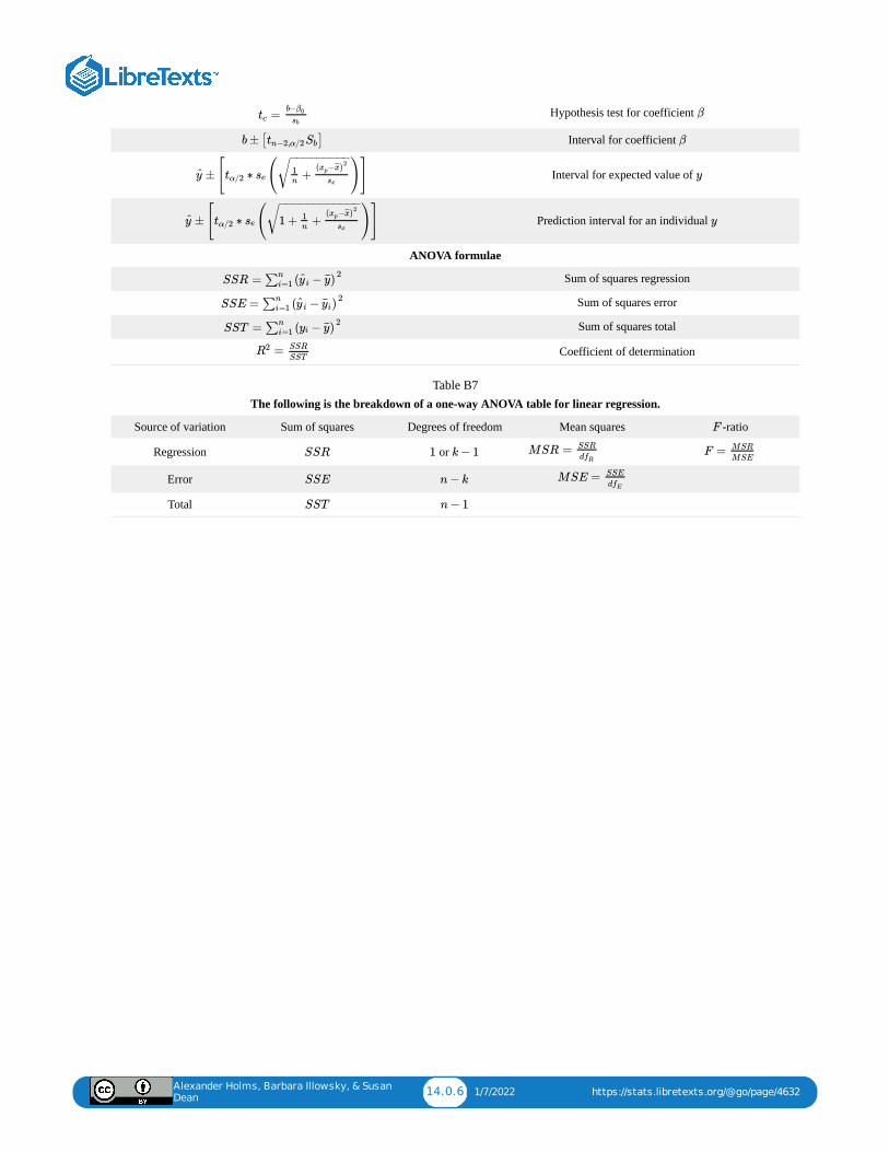
Alexander Holms, Barbara Illowsky, & Susan
Dean14.0.6 1/7/2022 https://stats.libretexts.org/@go/page/4632
Hypothesis test for coefficient
Interval for coefficient
Interval for expected value of
Prediction interval for an individual
ANOVA formulae
Sum of squares regression
Sum of squares error
Sum of squares total
Coefficient of determination
The following is the breakdown of a one-way ANOVA table for linear regression.
Source of variation Sum of squares Degrees of freedom Mean squares -ratio
Regression or
Error
Total
Table B7
=tcb−β0
sbβ
b± [ ]tn−2,α/2Sb β
± [ ∗ ( )]ŷ tα/2 se +1n
( − )xp x̄̄̄2
sx
− −−−−−−−−√ y
± [ ∗ ( )]ŷ tα/2 se 1 + +1n
( − )xp x̄̄̄2
sx
− −−−−−−−−−−−√ y
SSR = ∑ni=1 ( − )ŷ i ȳ̄̄
2
SSE = ∑ni=1 ( − )ŷ i ȳ̄̄i
2
SST = ∑ni=1 ( − )yi ȳ̄̄
2
=R2 SSR
SST
F
SSR 1 k− 1 MSR = SSR
dfRF = MSR
MSE
SSE n− k MSE = SSE
dfE
SST n− 1
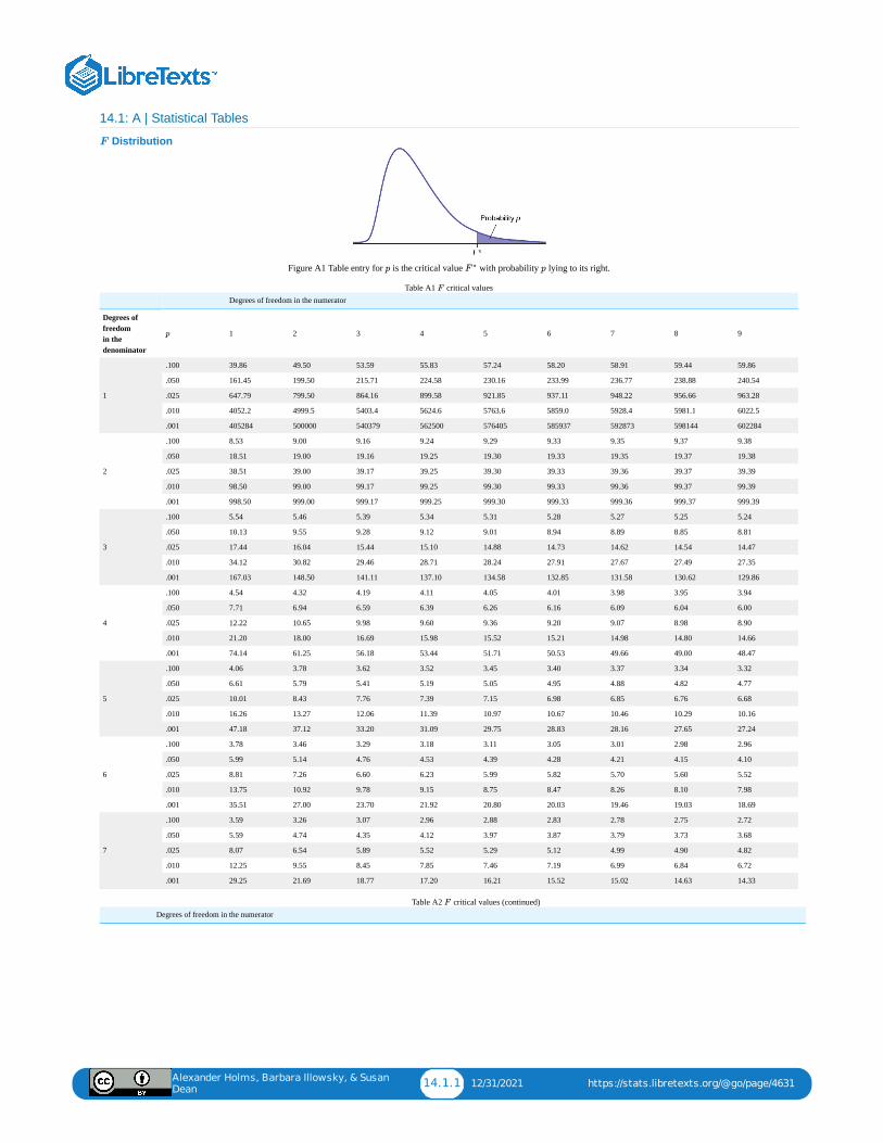
Alexander Holms, Barbara Illowsky, & Susan
Dean14.1.1 12/31/2021 https://stats.libretexts.org/@go/page/4631
14.1: A | Statistical Tables
Distribution
Figure A1 Table entry for is the critical value with probability lying to its right.
Degrees of freedom in the numerator
Degrees offreedom in thedenominator
1 2 3 4 5 6 7 8 9
1
.100 39.86 49.50 53.59 55.83 57.24 58.20 58.91 59.44 59.86
.050 161.45 199.50 215.71 224.58 230.16 233.99 236.77 238.88 240.54
.025 647.79 799.50 864.16 899.58 921.85 937.11 948.22 956.66 963.28
.010 4052.2 4999.5 5403.4 5624.6 5763.6 5859.0 5928.4 5981.1 6022.5
.001 405284 500000 540379 562500 576405 585937 592873 598144 602284
2
.100 8.53 9.00 9.16 9.24 9.29 9.33 9.35 9.37 9.38
.050 18.51 19.00 19.16 19.25 19.30 19.33 19.35 19.37 19.38
.025 38.51 39.00 39.17 39.25 39.30 39.33 39.36 39.37 39.39
.010 98.50 99.00 99.17 99.25 99.30 99.33 99.36 99.37 99.39
.001 998.50 999.00 999.17 999.25 999.30 999.33 999.36 999.37 999.39
3
.100 5.54 5.46 5.39 5.34 5.31 5.28 5.27 5.25 5.24
.050 10.13 9.55 9.28 9.12 9.01 8.94 8.89 8.85 8.81
.025 17.44 16.04 15.44 15.10 14.88 14.73 14.62 14.54 14.47
.010 34.12 30.82 29.46 28.71 28.24 27.91 27.67 27.49 27.35
.001 167.03 148.50 141.11 137.10 134.58 132.85 131.58 130.62 129.86
4
.100 4.54 4.32 4.19 4.11 4.05 4.01 3.98 3.95 3.94
.050 7.71 6.94 6.59 6.39 6.26 6.16 6.09 6.04 6.00
.025 12.22 10.65 9.98 9.60 9.36 9.20 9.07 8.98 8.90
.010 21.20 18.00 16.69 15.98 15.52 15.21 14.98 14.80 14.66
.001 74.14 61.25 56.18 53.44 51.71 50.53 49.66 49.00 48.47
5
.100 4.06 3.78 3.62 3.52 3.45 3.40 3.37 3.34 3.32
.050 6.61 5.79 5.41 5.19 5.05 4.95 4.88 4.82 4.77
.025 10.01 8.43 7.76 7.39 7.15 6.98 6.85 6.76 6.68
.010 16.26 13.27 12.06 11.39 10.97 10.67 10.46 10.29 10.16
.001 47.18 37.12 33.20 31.09 29.75 28.83 28.16 27.65 27.24
6
.100 3.78 3.46 3.29 3.18 3.11 3.05 3.01 2.98 2.96
.050 5.99 5.14 4.76 4.53 4.39 4.28 4.21 4.15 4.10
.025 8.81 7.26 6.60 6.23 5.99 5.82 5.70 5.60 5.52
.010 13.75 10.92 9.78 9.15 8.75 8.47 8.26 8.10 7.98
.001 35.51 27.00 23.70 21.92 20.80 20.03 19.46 19.03 18.69
7
.100 3.59 3.26 3.07 2.96 2.88 2.83 2.78 2.75 2.72
.050 5.59 4.74 4.35 4.12 3.97 3.87 3.79 3.73 3.68
.025 8.07 6.54 5.89 5.52 5.29 5.12 4.99 4.90 4.82
.010 12.25 9.55 8.45 7.85 7.46 7.19 6.99 6.84 6.72
.001 29.25 21.69 18.77 17.20 16.21 15.52 15.02 14.63 14.33
Table A1 critical values
Degrees of freedom in the numeratorTable A2 critical values (continued)
F
p F ∗ p
p
F
F
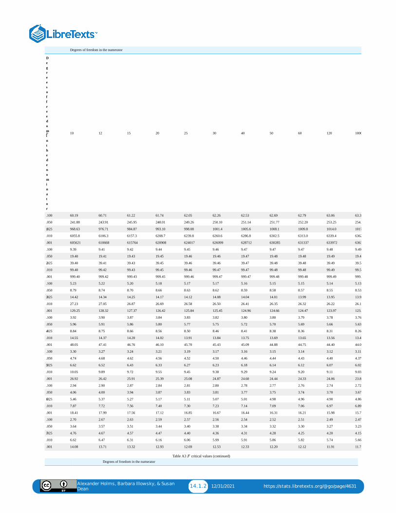
Alexander Holms, Barbara Illowsky, & Susan
Dean14.1.2 12/31/2021 https://stats.libretexts.org/@go/page/4631
Degrees of freedom in the numerator
Degreesoffreedominthedenominator
10 12 15 20 25 30 40 50 60 120 1000
1
.100 60.19 60.71 61.22 61.74 62.05 62.26 62.53 62.69 62.79 63.06 63.30
.050 241.88 243.91 245.95 248.01 249.26 250.10 251.14 251.77 252.20 253.25 254.
.025 968.63 976.71 984.87 993.10 998.08 1001.4 1005.6 1008.1 1009.8 1014.0 1017
.010 6055.8 6106.3 6157.3 6208.7 6239.8 6260.6 6286.8 6302.5 6313.0 6339.4 6362
.001 605621 610668 615764 620908 624017 626099 628712 630285 631337 633972 6363
2
.100 9.39 9.41 9.42 9.44 9.45 9.46 9.47 9.47 9.47 9.48 9.49
.050 19.40 19.41 19.43 19.45 19.46 19.46 19.47 19.48 19.48 19.49 19.49
.025 39.40 39.41 39.43 39.45 39.46 39.46 39.47 39.48 39.48 39.49 39.50
.010 99.40 99.42 99.43 99.45 99.46 99.47 99.47 99.48 99.48 99.49 99.50
.001 999.40 999.42 999.43 999.45 999.46 999.47 999.47 999.48 999.48 999.49 999.
3
.100 5.23 5.22 5.20 5.18 5.17 5.17 5.16 5.15 5.15 5.14 5.13
.050 8.79 8.74 8.70 8.66 8.63 8.62 8.59 8.58 8.57 8.55 8.53
.025 14.42 14.34 14.25 14.17 14.12 14.08 14.04 14.01 13.99 13.95 13.9
.010 27.23 27.05 26.87 26.69 26.58 26.50 26.41 26.35 26.32 26.22 26.14
.001 129.25 128.32 127.37 126.42 125.84 125.45 124.96 124.66 124.47 123.97 123.
4
.100 3.92 3.90 3.87 3.84 3.83 3.82 3.80 3.80 3.79 3.78 3.76
.050 5.96 5.91 5.86 5.80 5.77 5.75 5.72 5.70 5.69 5.66 5.63
.025 8.84 8.75 8.66 8.56 8.50 8.46 8.41 8.38 8.36 8.31 8.26
.010 14.55 14.37 14.20 14.02 13.91 13.84 13.75 13.69 13.65 13.56 13.4
.001 48.05 47.41 46.76 46.10 45.70 45.43 45.09 44.88 44.75 44.40 44.09
5
.100 3.30 3.27 3.24 3.21 3.19 3.17 3.16 3.15 3.14 3.12 3.11
.050 4.74 4.68 4.62 4.56 4.52 4.50 4.46 4.44 4.43 4.40 4.37
.025 6.62 6.52 6.43 6.33 6.27 6.23 6.18 6.14 6.12 6.07 6.02
.010 10.05 9.89 9.72 9.55 9.45 9.38 9.29 9.24 9.20 9.11 9.03
.001 26.92 26.42 25.91 25.39 25.08 24.87 24.60 24.44 24.33 24.06 23.82
6
.100 2.94 2.90 2.87 2.84 2.81 2.80 2.78 2.77 2.76 2.74 2.72
.050 4.06 4.00 3.94 3.87 3.83 3.81 3.77 3.75 3.74 3.70 3.67
.025 5.46 5.37 5.27 5.17 5.11 5.07 5.01 4.98 4.96 4.90 4.86
.010 7.87 7.72 7.56 7.40 7.30 7.23 7.14 7.09 7.06 6.97 6.89
.001 18.41 17.99 17.56 17.12 16.85 16.67 16.44 16.31 16.21 15.98 15.7
7
.100 2.70 2.67 2.63 2.59 2.57 2.56 2.54 2.52 2.51 2.49 2.47
.050 3.64 3.57 3.51 3.44 3.40 3.38 3.34 3.32 3.30 3.27 3.23
.025 4.76 4.67 4.57 4.47 4.40 4.36 4.31 4.28 4.25 4.20 4.15
.010 6.62 6.47 6.31 6.16 6.06 5.99 5.91 5.86 5.82 5.74 5.66
.001 14.08 13.71 13.32 12.93 12.69 12.53 12.33 12.20 12.12 11.91 11.72
Degrees of freedom in the numeratorTable A3 critical values (continued)
p
F
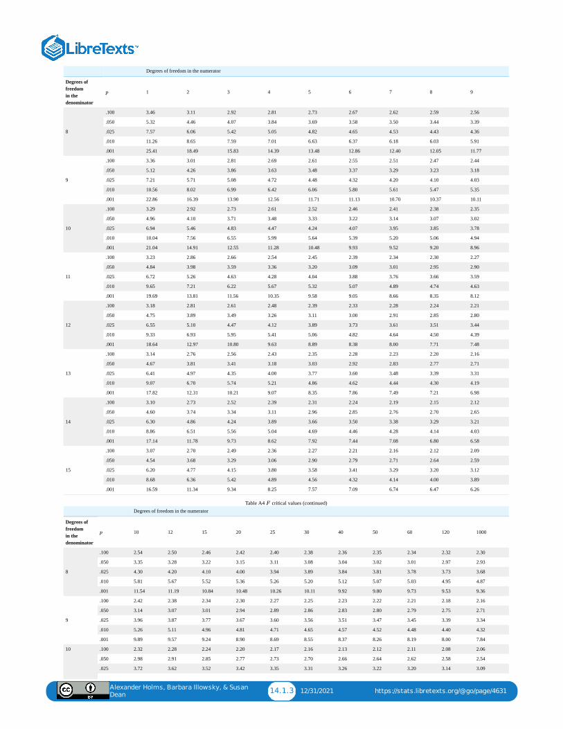
Alexander Holms, Barbara Illowsky, & Susan
Dean14.1.3 12/31/2021 https://stats.libretexts.org/@go/page/4631
Degrees of freedom in the numerator
Degrees offreedom in thedenominator
1 2 3 4 5 6 7 8 9
8
.100 3.46 3.11 2.92 2.81 2.73 2.67 2.62 2.59 2.56
.050 5.32 4.46 4.07 3.84 3.69 3.58 3.50 3.44 3.39
.025 7.57 6.06 5.42 5.05 4.82 4.65 4.53 4.43 4.36
.010 11.26 8.65 7.59 7.01 6.63 6.37 6.18 6.03 5.91
.001 25.41 18.49 15.83 14.39 13.48 12.86 12.40 12.05 11.77
9
.100 3.36 3.01 2.81 2.69 2.61 2.55 2.51 2.47 2.44
.050 5.12 4.26 3.86 3.63 3.48 3.37 3.29 3.23 3.18
.025 7.21 5.71 5.08 4.72 4.48 4.32 4.20 4.10 4.03
.010 10.56 8.02 6.99 6.42 6.06 5.80 5.61 5.47 5.35
.001 22.86 16.39 13.90 12.56 11.71 11.13 10.70 10.37 10.11
10
.100 3.29 2.92 2.73 2.61 2.52 2.46 2.41 2.38 2.35
.050 4.96 4.10 3.71 3.48 3.33 3.22 3.14 3.07 3.02
.025 6.94 5.46 4.83 4.47 4.24 4.07 3.95 3.85 3.78
.010 10.04 7.56 6.55 5.99 5.64 5.39 5.20 5.06 4.94
.001 21.04 14.91 12.55 11.28 10.48 9.93 9.52 9.20 8.96
11
.100 3.23 2.86 2.66 2.54 2.45 2.39 2.34 2.30 2.27
.050 4.84 3.98 3.59 3.36 3.20 3.09 3.01 2.95 2.90
.025 6.72 5.26 4.63 4.28 4.04 3.88 3.76 3.66 3.59
.010 9.65 7.21 6.22 5.67 5.32 5.07 4.89 4.74 4.63
.001 19.69 13.81 11.56 10.35 9.58 9.05 8.66 8.35 8.12
12
.100 3.18 2.81 2.61 2.48 2.39 2.33 2.28 2.24 2.21
.050 4.75 3.89 3.49 3.26 3.11 3.00 2.91 2.85 2.80
.025 6.55 5.10 4.47 4.12 3.89 3.73 3.61 3.51 3.44
.010 9.33 6.93 5.95 5.41 5.06 4.82 4.64 4.50 4.39
.001 18.64 12.97 10.80 9.63 8.89 8.38 8.00 7.71 7.48
13
.100 3.14 2.76 2.56 2.43 2.35 2.28 2.23 2.20 2.16
.050 4.67 3.81 3.41 3.18 3.03 2.92 2.83 2.77 2.71
.025 6.41 4.97 4.35 4.00 3.77 3.60 3.48 3.39 3.31
.010 9.07 6.70 5.74 5.21 4.86 4.62 4.44 4.30 4.19
.001 17.82 12.31 10.21 9.07 8.35 7.86 7.49 7.21 6.98
14
.100 3.10 2.73 2.52 2.39 2.31 2.24 2.19 2.15 2.12
.050 4.60 3.74 3.34 3.11 2.96 2.85 2.76 2.70 2.65
.025 6.30 4.86 4.24 3.89 3.66 3.50 3.38 3.29 3.21
.010 8.86 6.51 5.56 5.04 4.69 4.46 4.28 4.14 4.03
.001 17.14 11.78 9.73 8.62 7.92 7.44 7.08 6.80 6.58
15
.100 3.07 2.70 2.49 2.36 2.27 2.21 2.16 2.12 2.09
.050 4.54 3.68 3.29 3.06 2.90 2.79 2.71 2.64 2.59
.025 6.20 4.77 4.15 3.80 3.58 3.41 3.29 3.20 3.12
.010 8.68 6.36 5.42 4.89 4.56 4.32 4.14 4.00 3.89
.001 16.59 11.34 9.34 8.25 7.57 7.09 6.74 6.47 6.26
Degrees of freedom in the numerator
Degrees offreedom in thedenominator
10 12 15 20 25 30 40 50 60 120 1000
8
.100 2.54 2.50 2.46 2.42 2.40 2.38 2.36 2.35 2.34 2.32 2.30
.050 3.35 3.28 3.22 3.15 3.11 3.08 3.04 3.02 3.01 2.97 2.93
.025 4.30 4.20 4.10 4.00 3.94 3.89 3.84 3.81 3.78 3.73 3.68
.010 5.81 5.67 5.52 5.36 5.26 5.20 5.12 5.07 5.03 4.95 4.87
.001 11.54 11.19 10.84 10.48 10.26 10.11 9.92 9.80 9.73 9.53 9.36
9
.100 2.42 2.38 2.34 2.30 2.27 2.25 2.23 2.22 2.21 2.18 2.16
.050 3.14 3.07 3.01 2.94 2.89 2.86 2.83 2.80 2.79 2.75 2.71
.025 3.96 3.87 3.77 3.67 3.60 3.56 3.51 3.47 3.45 3.39 3.34
.010 5.26 5.11 4.96 4.81 4.71 4.65 4.57 4.52 4.48 4.40 4.32
.001 9.89 9.57 9.24 8.90 8.69 8.55 8.37 8.26 8.19 8.00 7.84
10 .100 2.32 2.28 2.24 2.20 2.17 2.16 2.13 2.12 2.11 2.08 2.06
.050 2.98 2.91 2.85 2.77 2.73 2.70 2.66 2.64 2.62 2.58 2.54
.025 3.72 3.62 3.52 3.42 3.35 3.31 3.26 3.22 3.20 3.14 3.09
Table A4 critical values (continued)
p
p
F
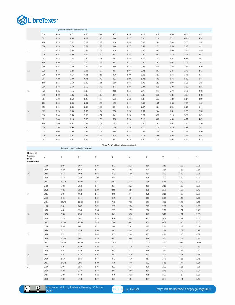
Alexander Holms, Barbara Illowsky, & Susan
Dean14.1.4 12/31/2021 https://stats.libretexts.org/@go/page/4631
Degrees of freedom in the numerator
.010 4.85 4.71 4.56 4.41 4.31 4.25 4.17 4.12 4.08 4.00 3.92
.001 8.75 8.45 8.13 7.80 7.60 7.47 7.30 7.19 7.12 6.94 6.78
11
.100 2.25 2.21 2.17 2.12 2.10 2.08 2.05 2.04 2.03 2.00 1.98
.050 2.85 2.79 2.72 2.65 2.60 2.57 2.53 2.51 2.49 2.45 2.41
.025 3.53 3.43 3.33 3.23 3.16 3.12 3.06 3.03 3.00 2.94 2.89
.010 4.54 4.40 4.25 4.10 4.01 3.94 3.86 3.81 3.78 3.69 3.61
.001 7.92 7.63 7.32 7.01 6.81 6.68 6.52 6.42 6.35 6.18 6.02
12
.100 2.19 2.15 2.10 2.06 2.03 2.01 1.99 1.97 1.96 1.93 1.91
.050 2.75 2.69 2.62 2.54 2.50 2.47 2.43 2.40 2.38 2.34 2.30
.025 3.37 3.28 3.18 3.07 3.01 2.96 2.91 2.87 2.85 2.79 2.73
.010 4.30 4.16 4.01 3.86 3.76 3.70 3.62 3.57 3.54 3.45 3.37
.001 7.29 7.00 6.71 6.40 6.22 6.09 5.93 5.83 5.76 5.59 5.44
13
.100 2.14 2.10 2.05 2.01 1.98 1.96 1.93 1.92 1.90 1.88 1.85
.050 2.67 2.60 2.53 2.46 2.41 2.38 2.34 2.31 2.30 2.25 2.21
.025 3.25 3.15 3.05 2.95 2.88 2.84 2.78 2.74 2.72 2.66 2.60
.010 4.10 3.96 3.82 3.66 3.57 3.51 3.43 3.38 3.34 3.25 3.18
.001 6.80 6.52 6.23 5.93 5.75 5.63 5.47 5.37 5.30 5.14 4.99
14
.100 2.10 2.05 2.01 1.96 1.93 1.91 1.89 1.87 1.86 1.83 1.80
.050 2.60 2.53 2.46 2.39 2.34 2.31 2.27 2.24 2.22 2.18 2.14
.025 3.15 3.05 2.95 2.84 2.78 2.73 2.67 2.64 2.61 2.55 2.50
.010 3.94 3.80 3.66 3.51 3.41 3.35 3.27 3.22 3.18 3.09 3.02
.001 6.40 6.13 5.85 5.56 5.38 5.25 5.10 5.00 4.94 4.77 4.62
15
.100 2.06 2.02 1.97 1.92 1.89 1.87 1.85 1.83 1.82 1.79 1.76
.050 2.54 2.48 2.40 2.33 2.28 2.25 2.20 2.18 2.16 2.11 2.07
.025 3.06 2.96 2.86 2.76 2.69 2.64 2.59 2.55 2.52 2.46 2.40
.010 3.80 3.67 3.52 3.37 3.28 3.21 3.13 3.08 3.05 2.96 2.88
.001 6.08 5.81 5.54 5.25 5.07 4.95 4.80 4.70 4.64 4.47 4.33
Degrees of freedom in the numerator
Degrees offreedom in thedenominator
1 2 3 4 5 6 7 8 9
16
.100 3.05 2.67 2.46 2.33 2.24 2.18 2.13 2.09 2.06
.050 4.49 3.63 3.24 3.01 2.85 2.74 2.66 2.59 2.54
.025 6.12 4.69 4.08 3.73 3.50 3.34 3.22 3.12 3.05
.010 8.53 6.23 5.29 4.77 4.44 4.20 4.03 3.89 3.78
.001 16.12 10.97 9.01 7.94 7.27 6.80 6.46 6.19 5.98
17
.100 3.03 2.64 2.44 2.31 2.22 2.15 2.10 2.06 2.03
.050 4.45 3.59 3.20 2.96 2.81 2.70 2.61 2.55 2.49
.025 6.04 4.62 4.01 3.66 3.44 3.28 3.16 3.06 2.98
.010 8.40 6.11 5.19 4.67 4.34 4.10 3.93 3.79 3.68
.001 15.72 10.66 8.73 7.68 7.02 6.56 6.22 5.96 5.75
18
.100 3.01 2.62 2.42 2.29 2.20 2.13 2.08 2.04 2.00
.050 4.41 3.55 3.16 2.93 2.77 2.66 2.58 2.51 2.46
.025 5.98 4.56 3.95 3.61 3.38 3.22 3.10 3.01 2.93
.010 8.29 6.01 5.09 4.58 4.25 4.01 3.84 3.71 3.60
.001 15.38 10.39 8.49 7.46 6.81 6.35 6.02 5.76 5.56
19
.100 3.36 3.01 2.81 2.69 2.61 2.55 2.51 2.47 2.44
.050 5.12 4.26 3.86 3.63 3.48 3.37 3.29 3.23 3.18
.025 7.21 5.71 5.08 4.72 4.48 4.32 4.20 4.10 4.03
.010 10.56 8.02 6.99 6.42 6.06 5.80 5.61 5.47 5.35
.001 22.86 16.39 13.90 12.56 11.71 11.13 10.70 10.37 10.11
20
.100 2.97 2.59 2.38 2.25 2.16 2.09 2.04 2.00 1.96
.050 4.35 3.49 3.10 2.87 2.71 2.60 2.51 2.45 2.39
.025 5.87 4.46 3.86 3.51 3.29 3.13 3.01 2.91 2.84
.010 8.10 5.85 4.94 4.43 4.10 3.87 3.70 3.56 3.46
.001 14.82 9.95 8.10 7.10 6.46 6.02 5.69 5.44 5.24
21 .100 2.96 2.57 2.36 2.23 2.14 2.08 2.02 1.98 1.95
.050 4.32 3.47 3.07 2.84 2.68 2.57 2.49 2.42 2.37
.025 5.83 4.42 3.82 3.48 3.25 3.09 2.97 2.87 2.80
.010 8.02 5.78 4.87 4.37 4.04 3.81 3.64 3.51 3.40
Table A5 critical values (continued)
p
F
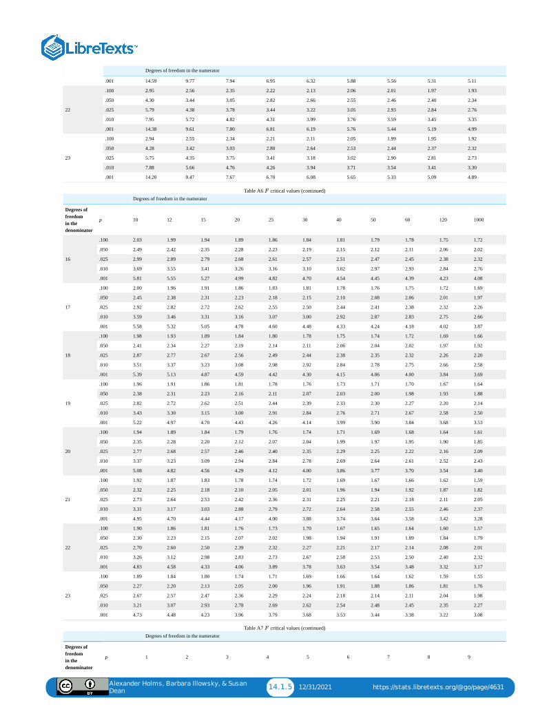
Alexander Holms, Barbara Illowsky, & Susan
Dean14.1.5 12/31/2021 https://stats.libretexts.org/@go/page/4631
Degrees of freedom in the numerator
.001 14.59 9.77 7.94 6.95 6.32 5.88 5.56 5.31 5.11
22
.100 2.95 2.56 2.35 2.22 2.13 2.06 2.01 1.97 1.93
.050 4.30 3.44 3.05 2.82 2.66 2.55 2.46 2.40 2.34
.025 5.79 4.38 3.78 3.44 3.22 3.05 2.93 2.84 2.76
.010 7.95 5.72 4.82 4.31 3.99 3.76 3.59 3.45 3.35
.001 14.38 9.61 7.80 6.81 6.19 5.76 5.44 5.19 4.99
23
.100 2.94 2.55 2.34 2.21 2.11 2.05 1.99 1.95 1.92
.050 4.28 3.42 3.03 2.80 2.64 2.53 2.44 2.37 2.32
.025 5.75 4.35 3.75 3.41 3.18 3.02 2.90 2.81 2.73
.010 7.88 5.66 4.76 4.26 3.94 3.71 3.54 3.41 3.30
.001 14.20 9.47 7.67 6.70 6.08 5.65 5.33 5.09 4.89
Degrees of freedom in the numerator
Degrees offreedom in thedenominator
10 12 15 20 25 30 40 50 60 120 1000
16
.100 2.03 1.99 1.94 1.89 1.86 1.84 1.81 1.79 1.78 1.75 1.72
.050 2.49 2.42 2.35 2.28 2.23 2.19 2.15 2.12 2.11 2.06 2.02
.025 2.99 2.89 2.79 2.68 2.61 2.57 2.51 2.47 2.45 2.38 2.32
.010 3.69 3.55 3.41 3.26 3.16 3.10 3.02 2.97 2.93 2.84 2.76
.001 5.81 5.55 5.27 4.99 4.82 4.70 4.54 4.45 4.39 4.23 4.08
17
.100 2.00 1.96 1.91 1.86 1.83 1.81 1.78 1.76 1.75 1.72 1.69
.050 2.45 2.38 2.31 2.23 2.18 2.15 2.10 2.08 2.06 2.01 1.97
.025 2.92 2.82 2.72 2.62 2.55 2.50 2.44 2.41 2.38 2.32 2.26
.010 3.59 3.46 3.31 3.16 3.07 3.00 2.92 2.87 2.83 2.75 2.66
.001 5.58 5.32 5.05 4.78 4.60 4.48 4.33 4.24 4.18 4.02 3.87
18
.100 1.98 1.93 1.89 1.84 1.80 1.78 1.75 1.74 1.72 1.69 1.66
.050 2.41 2.34 2.27 2.19 2.14 2.11 2.06 2.04 2.02 1.97 1.92
.025 2.87 2.77 2.67 2.56 2.49 2.44 2.38 2.35 2.32 2.26 2.20
.010 3.51 3.37 3.23 3.08 2.98 2.92 2.84 2.78 2.75 2.66 2.58
.001 5.39 5.13 4.87 4.59 4.42 4.30 4.15 4.06 4.00 3.84 3.69
19
.100 1.96 1.91 1.86 1.81 1.78 1.76 1.73 1.71 1.70 1.67 1.64
.050 2.38 2.31 2.23 2.16 2.11 2.07 2.03 2.00 1.98 1.93 1.88
.025 2.82 2.72 2.62 2.51 2.44 2.39 2.33 2.30 2.27 2.20 2.14
.010 3.43 3.30 3.15 3.00 2.91 2.84 2.76 2.71 2.67 2.58 2.50
.001 5.22 4.97 4.70 4.43 4.26 4.14 3.99 3.90 3.84 3.68 3.53
20
.100 1.94 1.89 1.84 1.79 1.76 1.74 1.71 1.69 1.68 1.64 1.61
.050 2.35 2.28 2.20 2.12 2.07 2.04 1.99 1.97 1.95 1.90 1.85
.025 2.77 2.68 2.57 2.46 2.40 2.35 2.29 2.25 2.22 2.16 2.09
.010 3.37 3.23 3.09 2.94 2.84 2.78 2.69 2.64 2.61 2.52 2.43
.001 5.08 4.82 4.56 4.29 4.12 4.00 3.86 3.77 3.70 3.54 3.40
21
.100 1.92 1.87 1.83 1.78 1.74 1.72 1.69 1.67 1.66 1.62 1.59
.050 2.32 2.25 2.18 2.10 2.05 2.01 1.96 1.94 1.92 1.87 1.82
.025 2.73 2.64 2.53 2.42 2.36 2.31 2.25 2.21 2.18 2.11 2.05
.010 3.31 3.17 3.03 2.88 2.79 2.72 2.64 2.58 2.55 2.46 2.37
.001 4.95 4.70 4.44 4.17 4.00 3.88 3.74 3.64 3.58 3.42 3.28
22
.100 1.90 1.86 1.81 1.76 1.73 1.70 1.67 1.65 1.64 1.60 1.57
.050 2.30 2.23 2.15 2.07 2.02 1.98 1.94 1.91 1.89 1.84 1.79
.025 2.70 2.60 2.50 2.39 2.32 2.27 2.21 2.17 2.14 2.08 2.01
.010 3.26 3.12 2.98 2.83 2.73 2.67 2.58 2.53 2.50 2.40 2.32
.001 4.83 4.58 4.33 4.06 3.89 3.78 3.63 3.54 3.48 3.32 3.17
23
.100 1.89 1.84 1.80 1.74 1.71 1.69 1.66 1.64 1.62 1.59 1.55
.050 2.27 2.20 2.13 2.05 2.00 1.96 1.91 1.88 1.86 1.81 1.76
.025 2.67 2.57 2.47 2.36 2.29 2.24 2.18 2.14 2.11 2.04 1.98
.010 3.21 3.07 2.93 2.78 2.69 2.62 2.54 2.48 2.45 2.35 2.27
.001 4.73 4.48 4.23 3.96 3.79 3.68 3.53 3.44 3.38 3.22 3.08
Table A6 critical values (continued)
Degrees of freedom in the numerator
Degrees offreedom in thedenominator
1 2 3 4 5 6 7 8 9
Table A7 critical values (continued)
p
F
p
F
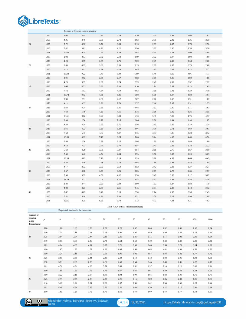
Alexander Holms, Barbara Illowsky, & Susan
Dean14.1.6 12/31/2021 https://stats.libretexts.org/@go/page/4631
Degrees of freedom in the numerator
24
.100 2.93 2.54 2.33 2.19 2.10 2.04 1.98 1.94 1.91
.050 4.26 3.40 3.01 2.78 2.62 2.51 2.42 2.36 2.30
.025 5.72 4.32 3.72 3.38 3.15 2.99 2.87 2.78 2.70
.010 7.82 5.61 4.72 4.22 3.90 3.67 3.50 3.36 3.26
.001 14.03 9.34 7.55 6.59 5.98 5.55 5.23 4.99 4.80
25
.100 2.92 2.53 2.32 2.18 2.09 2.02 1.97 1.93 1.89
.050 4.24 3.39 2.99 2.76 2.60 2.49 2.40 2.34 2.28
.025 5.69 4.29 3.69 3.35 3.13 2.97 2.85 2.75 2.68
.010 7.77 5.57 4.68 4.18 3.85 3.63 3.46 3.32 3.22
.001 13.88 9.22 7.45 6.49 5.89 5.46 5.15 4.91 4.71
26
.100 2.91 2.52 2.31 2.17 2.08 2.01 1.96 1.92 1.88
.050 4.23 3.37 2.98 2.74 2.59 2.47 2.39 2.32 2.27
.025 5.66 4.27 3.67 3.33 3.10 2.94 2.82 2.73 2.65
.010 7.72 5.53 4.64 4.14 3.82 3.59 3.42 3.29 3.18
.001 13.74 9.12 7.36 6.41 5.80 5.38 5.07 4.83 4.64
27
.100 2.90 2.51 2.30 2.17 2.07 2.00 1.95 1.91 1.87
.050 4.21 3.35 2.96 2.73 2.57 2.46 2.37 2.31 2.25
.025 5.63 4.24 3.65 3.31 3.08 2.92 2.80 2.71 2.63
.010 7.68 5.49 4.60 4.11 3.78 3.56 3.39 3.26 3.15
.001 13.61 9.02 7.27 6.33 5.73 5.31 5.00 4.76 4.57
28
.100 2.89 2.50 2.29 2.16 2.06 2.00 1.94 1.90 1.87
.050 4.20 3.34 2.95 2.71 2.56 2.45 2.36 2.29 2.24
.025 5.61 4.22 3.63 3.29 3.06 2.90 2.78 2.69 2.61
.010 7.64 5.45 4.57 4.07 3.75 3.53 3.36 3.23 3.12
.001 13.50 8.93 7.19 6.25 5.66 5.24 4.93 4.69 4.50
29
.100 2.89 2.50 2.28 2.15 2.06 1.99 1.93 1.89 1.86
.050 4.18 3.33 2.93 2.70 2.55 2.43 2.35 2.28 2.22
.025 5.59 4.20 3.61 3.27 3.04 2.88 2.76 2.67 2.59
.010 7.60 5.42 4.54 4.04 3.73 3.50 3.33 3.20 3.09
.001 13.39 8.85 7.12 6.19 5.59 5.18 4.87 4.64 4.45
30
.100 2.88 2.49 2.28 2.14 2.05 1.98 1.93 1.88 1.85
.050 4.17 3.32 2.92 2.69 2.53 2.42 2.33 2.27 2.21
.025 5.57 4.18 3.59 3.25 3.03 2.87 2.75 2.65 2.57
.010 7.56 5.39 4.51 4.02 3.70 3.47 3.30 3.17 3.07
.001 13.29 8.77 7.05 6.12 5.53 5.12 4.82 4.58 4.39
40
.100 2.84 2.44 2.23 2.09 2.00 1.93 1.87 1.83 1.79
.050 4.08 3.23 2.84 2.61 2.45 2.34 2.25 2.18 2.12
.025 5.42 4.05 3.46 3.13 2.90 2.74 2.62 2.53 2.45
.010 7.31 5.18 4.31 3.83 3.51 3.29 3.12 2.99 2.89
.001 12.61 8.25 6.59 5.70 5.13 4.73 4.44 4.21 4.02
Degrees of freedom in the numerator
Degrees offreedom in thedenominator
10 12 15 20 25 30 40 50 60 120 1000
24
.100 1.88 1.83 1.78 1.73 1.70 1.67 1.64 1.62 1.61 1.57 1.54
.050 2.25 2.18 2.11 2.03 1.97 1.94 1.89 1.86 1.84 1.79 1.74
.025 2.64 2.54 2.44 2.33 2.26 2.21 2.15 2.11 2.08 2.01 1.94
.010 3.17 3.03 2.89 2.74 2.64 2.58 2.49 2.44 2.40 2.31 2.22
.001 4.64 4.39 4.14 3.87 3.71 3.59 3.45 3.36 3.29 3.14 2.99
25
.100 1.87 1.82 1.77 1.72 1.68 1.66 1.63 1.61 1.59 1.56 1.52
.050 2.24 2.16 2.09 2.01 1.96 1.92 1.87 1.84 1.82 1.77 1.72
.025 2.61 2.51 2.41 2.30 2.23 2.18 2.12 2.08 2.05 1.98 1.91
.010 3.13 2.99 2.85 2.70 2.60 2.54 2.45 2.40 2.36 2.27 2.18
.001 4.56 4.31 4.06 3.79 3.63 3.52 3.37 3.28 3.22 3.06 2.91
26
.100 1.86 1.81 1.76 1.71 1.67 1.65 1.61 1.59 1.58 1.54 1.51
.050 2.22 2.15 2.07 1.99 1.94 1.90 1.85 1.82 1.80 1.75 1.70
.025 2.59 2.49 2.39 2.28 2.21 2.16 2.09 2.05 2.03 1.95 1.89
.010 3.09 2.96 2.81 2.66 2.57 2.50 2.42 2.36 2.33 2.23 2.14
.001 4.48 4.24 3.99 3.72 3.56 3.44 3.30 3.21 3.15 2.99 2.84
27 .100 1.85 1.80 1.75 1.70 1.66 1.64 1.60 1.58 1.57 1.53 1.50
Table A8 critical values (continued)
p
F
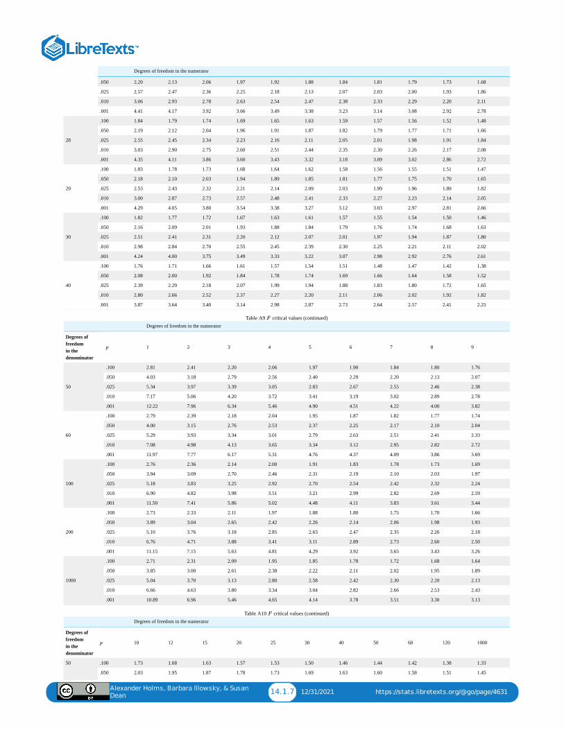
Alexander Holms, Barbara Illowsky, & Susan
Dean14.1.7 12/31/2021 https://stats.libretexts.org/@go/page/4631
Degrees of freedom in the numerator
.050 2.20 2.13 2.06 1.97 1.92 1.88 1.84 1.81 1.79 1.73 1.68
.025 2.57 2.47 2.36 2.25 2.18 2.13 2.07 2.03 2.00 1.93 1.86
.010 3.06 2.93 2.78 2.63 2.54 2.47 2.38 2.33 2.29 2.20 2.11
.001 4.41 4.17 3.92 3.66 3.49 3.38 3.23 3.14 3.08 2.92 2.78
28
.100 1.84 1.79 1.74 1.69 1.65 1.63 1.59 1.57 1.56 1.52 1.48
.050 2.19 2.12 2.04 1.96 1.91 1.87 1.82 1.79 1.77 1.71 1.66
.025 2.55 2.45 2.34 2.23 2.16 2.11 2.05 2.01 1.98 1.91 1.84
.010 3.03 2.90 2.75 2.60 2.51 2.44 2.35 2.30 2.26 2.17 2.08
.001 4.35 4.11 3.86 3.60 3.43 3.32 3.18 3.09 3.02 2.86 2.72
29
.100 1.83 1.78 1.73 1.68 1.64 1.62 1.58 1.56 1.55 1.51 1.47
.050 2.18 2.10 2.03 1.94 1.89 1.85 1.81 1.77 1.75 1.70 1.65
.025 2.53 2.43 2.32 2.21 2.14 2.09 2.03 1.99 1.96 1.89 1.82
.010 3.00 2.87 2.73 2.57 2.48 2.41 2.33 2.27 2.23 2.14 2.05
.001 4.29 4.05 3.80 3.54 3.38 3.27 3.12 3.03 2.97 2.81 2.66
30
.100 1.82 1.77 1.72 1.67 1.63 1.61 1.57 1.55 1.54 1.50 1.46
.050 2.16 2.09 2.01 1.93 1.88 1.84 1.79 1.76 1.74 1.68 1.63
.025 2.51 2.41 2.31 2.20 2.12 2.07 2.01 1.97 1.94 1.87 1.80
.010 2.98 2.84 2.70 2.55 2.45 2.39 2.30 2.25 2.21 2.11 2.02
.001 4.24 4.00 3.75 3.49 3.33 3.22 3.07 2.98 2.92 2.76 2.61
40
.100 1.76 1.71 1.66 1.61 1.57 1.54 1.51 1.48 1.47 1.42 1.38
.050 2.08 2.00 1.92 1.84 1.78 1.74 1.69 1.66 1.64 1.58 1.52
.025 2.39 2.29 2.18 2.07 1.99 1.94 1.88 1.83 1.80 1.72 1.65
.010 2.80 2.66 2.52 2.37 2.27 2.20 2.11 2.06 2.02 1.92 1.82
.001 3.87 3.64 3.40 3.14 2.98 2.87 2.73 2.64 2.57 2.41 2.25
Degrees of freedom in the numerator
Degrees offreedom in thedenominator
1 2 3 4 5 6 7 8 9
50
.100 2.81 2.41 2.20 2.06 1.97 1.90 1.84 1.80 1.76
.050 4.03 3.18 2.79 2.56 2.40 2.29 2.20 2.13 2.07
.025 5.34 3.97 3.39 3.05 2.83 2.67 2.55 2.46 2.38
.010 7.17 5.06 4.20 3.72 3.41 3.19 3.02 2.89 2.78
.001 12.22 7.96 6.34 5.46 4.90 4.51 4.22 4.00 3.82
60
.100 2.79 2.39 2.18 2.04 1.95 1.87 1.82 1.77 1.74
.050 4.00 3.15 2.76 2.53 2.37 2.25 2.17 2.10 2.04
.025 5.29 3.93 3.34 3.01 2.79 2.63 2.51 2.41 2.33
.010 7.08 4.98 4.13 3.65 3.34 3.12 2.95 2.82 2.72
.001 11.97 7.77 6.17 5.31 4.76 4.37 4.09 3.86 3.69
100
.100 2.76 2.36 2.14 2.00 1.91 1.83 1.78 1.73 1.69
.050 3.94 3.09 2.70 2.46 2.31 2.19 2.10 2.03 1.97
.025 5.18 3.83 3.25 2.92 2.70 2.54 2.42 2.32 2.24
.010 6.90 4.82 3.98 3.51 3.21 2.99 2.82 2.69 2.59
.001 11.50 7.41 5.86 5.02 4.48 4.11 3.83 3.61 3.44
200
.100 2.73 2.33 2.11 1.97 1.88 1.80 1.75 1.70 1.66
.050 3.89 3.04 2.65 2.42 2.26 2.14 2.06 1.98 1.93
.025 5.10 3.76 3.18 2.85 2.63 2.47 2.35 2.26 2.18
.010 6.76 4.71 3.88 3.41 3.11 2.89 2.73 2.60 2.50
.001 11.15 7.15 5.63 4.81 4.29 3.92 3.65 3.43 3.26
1000
.100 2.71 2.31 2.09 1.95 1.85 1.78 1.72 1.68 1.64
.050 3.85 3.00 2.61 2.38 2.22 2.11 2.02 1.95 1.89
.025 5.04 3.70 3.13 2.80 2.58 2.42 2.30 2.20 2.13
.010 6.66 4.63 3.80 3.34 3.04 2.82 2.66 2.53 2.43
.001 10.89 6.96 5.46 4.65 4.14 3.78 3.51 3.30 3.13
Table A9 critical values (continued)
Degrees of freedom in the numerator
Degrees offreedom in thedenominator
10 12 15 20 25 30 40 50 60 120 1000
50 .100 1.73 1.68 1.63 1.57 1.53 1.50 1.46 1.44 1.42 1.38 1.33
.050 2.03 1.95 1.87 1.78 1.73 1.69 1.63 1.60 1.58 1.51 1.45
Table A10 critical values (continued)
p
F
p
F
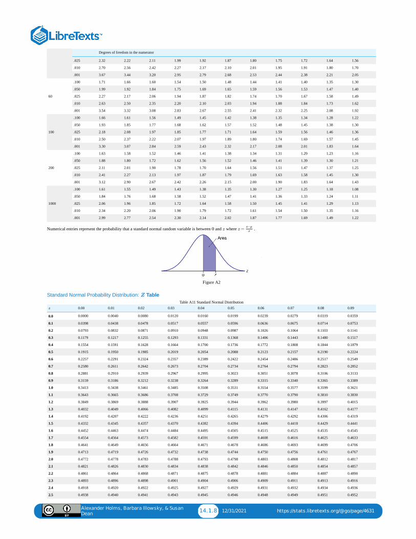
Alexander Holms, Barbara Illowsky, & Susan
Dean14.1.8 12/31/2021 https://stats.libretexts.org/@go/page/4631
Degrees of freedom in the numerator
.025 2.32 2.22 2.11 1.99 1.92 1.87 1.80 1.75 1.72 1.64 1.56
.010 2.70 2.56 2.42 2.27 2.17 2.10 2.01 1.95 1.91 1.80 1.70
.001 3.67 3.44 3.20 2.95 2.79 2.68 2.53 2.44 2.38 2.21 2.05
60
.100 1.71 1.66 1.60 1.54 1.50 1.48 1.44 1.41 1.40 1.35 1.30
.050 1.99 1.92 1.84 1.75 1.69 1.65 1.59 1.56 1.53 1.47 1.40
.025 2.27 2.17 2.06 1.94 1.87 1.82 1.74 1.70 1.67 1.58 1.49
.010 2.63 2.50 2.35 2.20 2.10 2.03 1.94 1.88 1.84 1.73 1.62
.001 3.54 3.32 3.08 2.83 2.67 2.55 2.41 2.32 2.25 2.08 1.92
100
.100 1.66 1.61 1.56 1.49 1.45 1.42 1.38 1.35 1.34 1.28 1.22
.050 1.93 1.85 1.77 1.68 1.62 1.57 1.52 1.48 1.45 1.38 1.30
.025 2.18 2.08 1.97 1.85 1.77 1.71 1.64 1.59 1.56 1.46 1.36
.010 2.50 2.37 2.22 2.07 1.97 1.89 1.80 1.74 1.69 1.57 1.45
.001 3.30 3.07 2.84 2.59 2.43 2.32 2.17 2.08 2.01 1.83 1.64
200
.100 1.63 1.58 1.52 1.46 1.41 1.38 1.34 1.31 1.29 1.23 1.16
.050 1.88 1.80 1.72 1.62 1.56 1.52 1.46 1.41 1.39 1.30 1.21
.025 2.11 2.01 1.90 1.78 1.70 1.64 1.56 1.51 1.47 1.37 1.25
.010 2.41 2.27 2.13 1.97 1.87 1.79 1.69 1.63 1.58 1.45 1.30
.001 3.12 2.90 2.67 2.42 2.26 2.15 2.00 1.90 1.83 1.64 1.43
1000
.100 1.61 1.55 1.49 1.43 1.38 1.35 1.30 1.27 1.25 1.18 1.08
.050 1.84 1.76 1.68 1.58 1.52 1.47 1.41 1.36 1.33 1.24 1.11
.025 2.06 1.96 1.85 1.72 1.64 1.58 1.50 1.45 1.41 1.29 1.13
.010 2.34 2.20 2.06 1.90 1.79 1.72 1.61 1.54 1.50 1.35 1.16
.001 2.99 2.77 2.54 2.30 2.14 2.02 1.87 1.77 1.69 1.49 1.22
Numerical entries represent the probability that a standard normal random variable is between and where .
Figure A2
Standard Normal Probability Distribution: Table
0.00 0.01 0.02 0.03 0.04 0.05 0.06 0.07 0.08 0.09
0.0 0.0000 0.0040 0.0080 0.0120 0.0160 0.0199 0.0239 0.0279 0.0319 0.0359
0.1 0.0398 0.0438 0.0478 0.0517 0.0557 0.0596 0.0636 0.0675 0.0714 0.0753
0.2 0.0793 0.0832 0.0871 0.0910 0.0948 0.0987 0.1026 0.1064 0.1103 0.1141
0.3 0.1179 0.1217 0.1255 0.1293 0.1331 0.1368 0.1406 0.1443 0.1480 0.1517
0.4 0.1554 0.1591 0.1628 0.1664 0.1700 0.1736 0.1772 0.1808 0.1844 0.1879
0.5 0.1915 0.1950 0.1985 0.2019 0.2054 0.2088 0.2123 0.2157 0.2190 0.2224
0.6 0.2257 0.2291 0.2324 0.2357 0.2389 0.2422 0.2454 0.2486 0.2517 0.2549
0.7 0.2580 0.2611 0.2642 0.2673 0.2704 0.2734 0.2764 0.2794 0.2823 0.2852
0.8 0.2881 0.2910 0.2939 0.2967 0.2995 0.3023 0.3051 0.3078 0.3106 0.3133
0.9 0.3159 0.3186 0.3212 0.3238 0.3264 0.3289 0.3315 0.3340 0.3365 0.3389
1.0 0.3413 0.3438 0.3461 0.3485 0.3508 0.3531 0.3554 0.3577 0.3599 0.3621
1.1 0.3643 0.3665 0.3686 0.3708 0.3729 0.3749 0.3770 0.3790 0.3810 0.3830
1.2 0.3849 0.3869 0.3888 0.3907 0.3925 0.3944 0.3962 0.3980 0.3997 0.4015
1.3 0.4032 0.4049 0.4066 0.4082 0.4099 0.4115 0.4131 0.4147 0.4162 0.4177
1.4 0.4192 0.4207 0.4222 0.4236 0.4251 0.4265 0.4279 0.4292 0.4306 0.4319
1.5 0.4332 0.4345 0.4357 0.4370 0.4382 0.4394 0.4406 0.4418 0.4429 0.4441
1.6 0.4452 0.4463 0.4474 0.4484 0.4495 0.4505 0.4515 0.4525 0.4535 0.4545
1.7 0.4554 0.4564 0.4573 0.4582 0.4591 0.4599 0.4608 0.4616 0.4625 0.4633
1.8 0.4641 0.4649 0.4656 0.4664 0.4671 0.4678 0.4686 0.4693 0.4699 0.4706
1.9 0.4713 0.4719 0.4726 0.4732 0.4738 0.4744 0.4750 0.4756 0.4761 0.4767
2.0 0.4772 0.4778 0.4783 0.4788 0.4793 0.4798 0.4803 0.4808 0.4812 0.4817
2.1 0.4821 0.4826 0.4830 0.4834 0.4838 0.4842 0.4846 0.4850 0.4854 0.4857
2.2 0.4861 0.4864 0.4868 0.4871 0.4875 0.4878 0.4881 0.4884 0.4887 0.4890
2.3 0.4893 0.4896 0.4898 0.4901 0.4904 0.4906 0.4909 0.4911 0.4913 0.4916
2.4 0.4918 0.4920 0.4922 0.4925 0.4927 0.4929 0.4931 0.4932 0.4934 0.4936
2.5 0.4938 0.4940 0.4941 0.4943 0.4945 0.4946 0.4948 0.4949 0.4951 0.4952
Table A11 Standard Normal Distribution
0 z z =x−μ
σ
Z
z
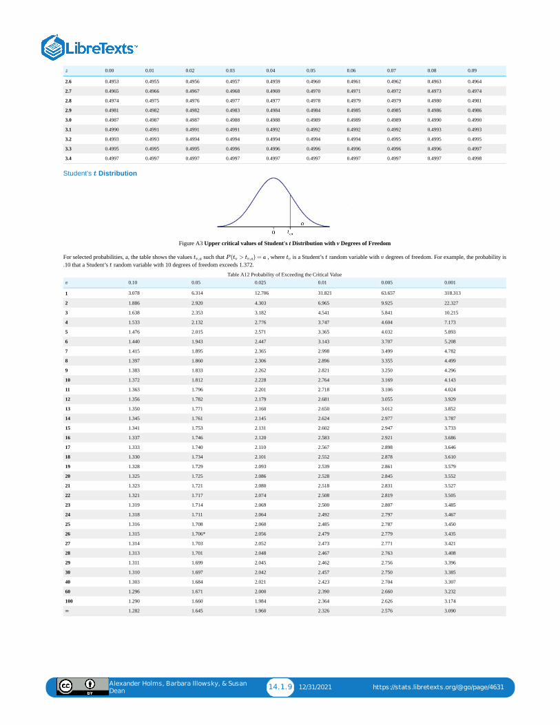
Alexander Holms, Barbara Illowsky, & Susan
Dean14.1.9 12/31/2021 https://stats.libretexts.org/@go/page/4631
0.00 0.01 0.02 0.03 0.04 0.05 0.06 0.07 0.08 0.09
2.6 0.4953 0.4955 0.4956 0.4957 0.4959 0.4960 0.4961 0.4962 0.4963 0.4964
2.7 0.4965 0.4966 0.4967 0.4968 0.4969 0.4970 0.4971 0.4972 0.4973 0.4974
2.8 0.4974 0.4975 0.4976 0.4977 0.4977 0.4978 0.4979 0.4979 0.4980 0.4981
2.9 0.4981 0.4982 0.4982 0.4983 0.4984 0.4984 0.4985 0.4985 0.4986 0.4986
3.0 0.4987 0.4987 0.4987 0.4988 0.4988 0.4989 0.4989 0.4989 0.4990 0.4990
3.1 0.4990 0.4991 0.4991 0.4991 0.4992 0.4992 0.4992 0.4992 0.4993 0.4993
3.2 0.4993 0.4993 0.4994 0.4994 0.4994 0.4994 0.4994 0.4995 0.4995 0.4995
3.3 0.4995 0.4995 0.4995 0.4996 0.4996 0.4996 0.4996 0.4996 0.4996 0.4997
3.4 0.4997 0.4997 0.4997 0.4997 0.4997 0.4997 0.4997 0.4997 0.4997 0.4998
Student's Distribution
Figure A3 Upper critical values of Student's t Distribution with v Degrees of Freedom
For selected probabilities, a, the table shows the values such that , where is a Student’s random variable with degrees of freedom. For example, the probability is.10 that a Student’s random variable with 10 degrees of freedom exceeds 1.372.
0.10 0.05 0.025 0.01 0.005 0.001
1 3.078 6.314 12.706 31.821 63.657 318.313
2 1.886 2.920 4.303 6.965 9.925 22.327
3 1.638 2.353 3.182 4.541 5.841 10.215
4 1.533 2.132 2.776 3.747 4.604 7.173
5 1.476 2.015 2.571 3.365 4.032 5.893
6 1.440 1.943 2.447 3.143 3.707 5.208
7 1.415 1.895 2.365 2.998 3.499 4.782
8 1.397 1.860 2.306 2.896 3.355 4.499
9 1.383 1.833 2.262 2.821 3.250 4.296
10 1.372 1.812 2.228 2.764 3.169 4.143
11 1.363 1.796 2.201 2.718 3.106 4.024
12 1.356 1.782 2.179 2.681 3.055 3.929
13 1.350 1.771 2.160 2.650 3.012 3.852
14 1.345 1.761 2.145 2.624 2.977 3.787
15 1.341 1.753 2.131 2.602 2.947 3.733
16 1.337 1.746 2.120 2.583 2.921 3.686
17 1.333 1.740 2.110 2.567 2.898 3.646
18 1.330 1.734 2.101 2.552 2.878 3.610
19 1.328 1.729 2.093 2.539 2.861 3.579
20 1.325 1.725 2.086 2.528 2.845 3.552
21 1.323 1.721 2.080 2.518 2.831 3.527
22 1.321 1.717 2.074 2.508 2.819 3.505
23 1.319 1.714 2.069 2.500 2.807 3.485
24 1.318 1.711 2.064 2.492 2.797 3.467
25 1.316 1.708 2.060 2.485 2.787 3.450
26 1.315 1.706* 2.056 2.479 2.779 3.435
27 1.314 1.703 2.052 2.473 2.771 3.421
28 1.313 1.701 2.048 2.467 2.763 3.408
29 1.311 1.699 2.045 2.462 2.756 3.396
30 1.310 1.697 2.042 2.457 2.750 3.385
40 1.303 1.684 2.021 2.423 2.704 3.307
60 1.296 1.671 2.000 2.390 2.660 3.232
100 1.290 1.660 1.984 2.364 2.626 3.174
∞ 1.282 1.645 1.960 2.326 2.576 3.090
Table A12 Probability of Exceeding the Critical Value
z
t
tv,a P ( > ) = atv tv,a tv t v
t
v
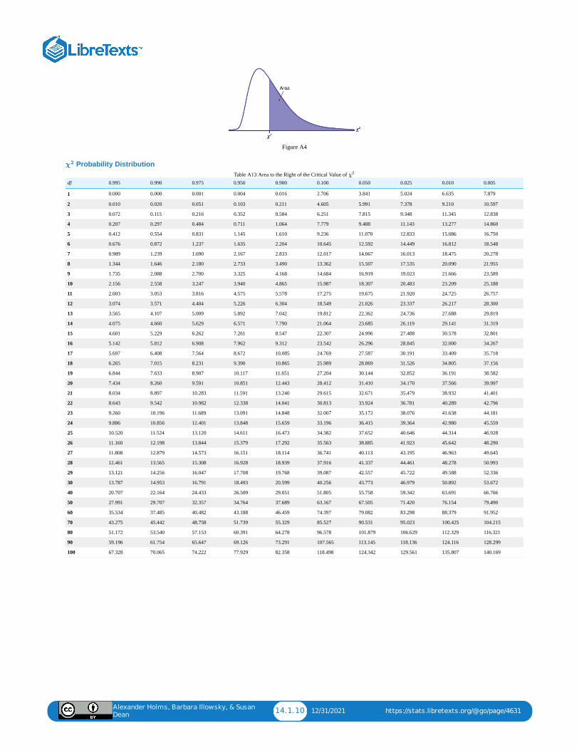
Alexander Holms, Barbara Illowsky, & Susan
Dean14.1.10 12/31/2021 https://stats.libretexts.org/@go/page/4631
Figure A4
Probability Distribution
df 0.995 0.990 0.975 0.950 0.900 0.100 0.050 0.025 0.010 0.005
1 0.000 0.000 0.001 0.004 0.016 2.706 3.841 5.024 6.635 7.879
2 0.010 0.020 0.051 0.103 0.211 4.605 5.991 7.378 9.210 10.597
3 0.072 0.115 0.216 0.352 0.584 6.251 7.815 9.348 11.345 12.838
4 0.207 0.297 0.484 0.711 1.064 7.779 9.488 11.143 13.277 14.860
5 0.412 0.554 0.831 1.145 1.610 9.236 11.070 12.833 15.086 16.750
6 0.676 0.872 1.237 1.635 2.204 10.645 12.592 14.449 16.812 18.548
7 0.989 1.239 1.690 2.167 2.833 12.017 14.067 16.013 18.475 20.278
8 1.344 1.646 2.180 2.733 3.490 13.362 15.507 17.535 20.090 21.955
9 1.735 2.088 2.700 3.325 4.168 14.684 16.919 19.023 21.666 23.589
10 2.156 2.558 3.247 3.940 4.865 15.987 18.307 20.483 23.209 25.188
11 2.603 3.053 3.816 4.575 5.578 17.275 19.675 21.920 24.725 26.757
12 3.074 3.571 4.404 5.226 6.304 18.549 21.026 23.337 26.217 28.300
13 3.565 4.107 5.009 5.892 7.042 19.812 22.362 24.736 27.688 29.819
14 4.075 4.660 5.629 6.571 7.790 21.064 23.685 26.119 29.141 31.319
15 4.601 5.229 6.262 7.261 8.547 22.307 24.996 27.488 30.578 32.801
16 5.142 5.812 6.908 7.962 9.312 23.542 26.296 28.845 32.000 34.267
17 5.697 6.408 7.564 8.672 10.085 24.769 27.587 30.191 33.409 35.718
18 6.265 7.015 8.231 9.390 10.865 25.989 28.869 31.526 34.805 37.156
19 6.844 7.633 8.907 10.117 11.651 27.204 30.144 32.852 36.191 38.582
20 7.434 8.260 9.591 10.851 12.443 28.412 31.410 34.170 37.566 39.997
21 8.034 8.897 10.283 11.591 13.240 29.615 32.671 35.479 38.932 41.401
22 8.643 9.542 10.982 12.338 14.041 30.813 33.924 36.781 40.289 42.796
23 9.260 10.196 11.689 13.091 14.848 32.007 35.172 38.076 41.638 44.181
24 9.886 10.856 12.401 13.848 15.659 33.196 36.415 39.364 42.980 45.559
25 10.520 11.524 13.120 14.611 16.473 34.382 37.652 40.646 44.314 46.928
26 11.160 12.198 13.844 15.379 17.292 35.563 38.885 41.923 45.642 48.290
27 11.808 12.879 14.573 16.151 18.114 36.741 40.113 43.195 46.963 49.645
28 12.461 13.565 15.308 16.928 18.939 37.916 41.337 44.461 48.278 50.993
29 13.121 14.256 16.047 17.708 19.768 39.087 42.557 45.722 49.588 52.336
30 13.787 14.953 16.791 18.493 20.599 40.256 43.773 46.979 50.892 53.672
40 20.707 22.164 24.433 26.509 29.051 51.805 55.758 59.342 63.691 66.766
50 27.991 29.707 32.357 34.764 37.689 63.167 67.505 71.420 76.154 79.490
60 35.534 37.485 40.482 43.188 46.459 74.397 79.082 83.298 88.379 91.952
70 43.275 45.442 48.758 51.739 55.329 85.527 90.531 95.023 100.425 104.215
80 51.172 53.540 57.153 60.391 64.278 96.578 101.879 106.629 112.329 116.321
90 59.196 61.754 65.647 69.126 73.291 107.565 113.145 118.136 124.116 128.299
100 67.328 70.065 74.222 77.929 82.358 118.498 124.342 129.561 135.807 140.169
Table A13 Area to the Right of the Critical Value of
χ2
χ2
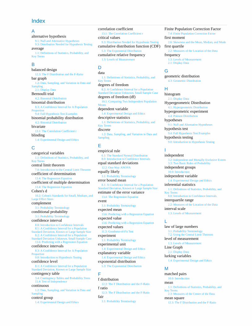
Index
Aalternative hypothesis
9.1: Null and Alternative Hypotheses 9.3: Distribution Needed for Hypothesis Testing
average1.1: Definitions of Statistics, Probability, and
Key Terms
Bbalanced design
12.3: The F Distribution and the F-Ratio bar graph
1.2: Data, Sampling, and Variation in Data andSampling
2.1: Display Data Bernoulli trial
4.2: Binomial Distribution binomial distribution
8.3: A Confidence Interval for A PopulationProportion
9.4: Full Hypothesis Test Examples binomial probability distribution
4.2: Binomial Distribution bivariate
13.1: The Correlation Coefficient r blinding
1.4: Experimental Design and Ethics
Ccategorical variables
1.1: Definitions of Statistics, Probability, andKey Terms central limit theorem
7.0: Introduction to the Central Limit Theorem coefficient of determination
13.4: The Regression Equation coefficient of multiple determination
13.4: The Regression Equation Cohen's d
10.2: Cohen's Standards for Small, Medium, andLarge Effect Sizes complement
3.1: Probability Terminology conditional probability
3.1: Probability Terminology confidence interval
8.0: Introduction to Confidence Intervals 8.1: A Confidence Interval for a Population
Standard Deviation, Known or Large Sample Size 8.2: A Confidence Interval for a Population
Standard Deviation Unknown, Small Sample Case 13.6: Predicting with a Regression Equation
confidence intervals8.3: A Confidence Interval for A Population
Proportion 9.0: Introduction to Hypothesis Testing
confidence level8.1: A Confidence Interval for a Population
Standard Deviation, Known or Large Sample Size contingency table
3.4: Contingency Tables and Probability Trees 11.4: Test of Independence
continuous1.2: Data, Sampling, and Variation in Data and
Sampling control group
1.4: Experimental Design and Ethics
correlation coefficient13.1: The Correlation Coefficient r
critical values9.3: Distribution Needed for Hypothesis Testing
cumulative distribution function (CDF)5.3: The Exponential Distribution
cumulative relative frequency1.3: Levels of Measurement
Ddata
1.1: Definitions of Statistics, Probability, andKey Terms degrees of freedom
8.2: A Confidence Interval for a PopulationStandard Deviation Unknown, Small Sample Case degrees of freedom (df)
10.1: Comparing Two Independent PopulationMeans dependent variable
1.4: Experimental Design and Ethics descriptive statistics
1.1: Definitions of Statistics, Probability, andKey Terms discrete
1.2: Data, Sampling, and Variation in Data andSampling
Eempirical rule
6.1: The Standard Normal Distribution 8.0: Introduction to Confidence Intervals
equal standard deviations12.2: One-Way ANOVA
equally likely3.1: Probability Terminology
error bound mean8.1: A Confidence Interval for a Population
Standard Deviation, Known or Large Sample Size estimate of the error variance
13.4: The Regression Equation event
3.1: Probability Terminology expected mean
13.6: Predicting with a Regression Equation expected value
13.6: Predicting with a Regression Equation expected values
11.3: Goodness-of-Fit Test experiment
3.1: Probability Terminology experimental unit
1.4: Experimental Design and Ethics explanatory variable
1.4: Experimental Design and Ethics exponential distribution
5.3: The Exponential Distribution
Ff distribution
12.3: The F Distribution and the F-Ratio f ratio
12.3: The F Distribution and the F-Ratio fair
3.1: Probability Terminology
Finite Population Correction Factor7.4: Finite Population Correction Factor
first moment2.6: Skewness and the Mean, Median, and Mode
first quartile2.2: Measures of the Location of the Data
frequency1.3: Levels of Measurement 2.1: Display Data
Ggeometric distribution
4.3: Geometric Distribution
Hhistogram
2.1: Display Data Hypergeometric Distribution
4.1: Hypergeometric Distribution hypergeometric experiment
4.4: Poisson Distribution hypotheses
9.1: Null and Alternative Hypotheses hypothesis test
9.4: Full Hypothesis Test Examples hypothesis testing
9.0: Introduction to Hypothesis Testing
Iindependent
3.2: Independent and Mutually Exclusive Events 3.3: Two Basic Rules of Probability
independent groups10.0: Introduction
independent variable1.4: Experimental Design and Ethics
inferential statistics1.1: Definitions of Statistics, Probability, and
Key Terms 8.0: Introduction to Confidence Intervals
interquartile range2.2: Measures of the Location of the Data
interval scale1.3: Levels of Measurement
Llaw of large numbers
3.1: Probability Terminology 7.2: Using the Central Limit Theorem
level of measurement1.3: Levels of Measurement
Line Graph2.1: Display Data
lurking variables1.4: Experimental Design and Ethics
Mmatched pairs
10.0: Introduction mean
1.1: Definitions of Statistics, Probability, andKey Terms
2.3: Measures of the Center of the Data mean square
12.3: The F Distribution and the F-Ratio
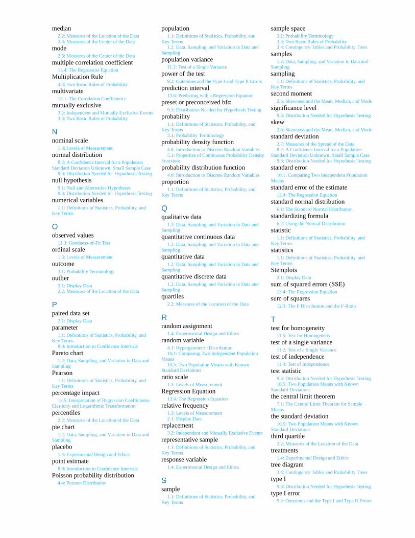
median2.2: Measures of the Location of the Data 2.3: Measures of the Center of the Data
mode2.3: Measures of the Center of the Data
multiple correlation coefficient13.4: The Regression Equation
Multiplication Rule3.3: Two Basic Rules of Probability
multivariate13.1: The Correlation Coefficient r
mutually exclusive3.2: Independent and Mutually Exclusive Events 3.3: Two Basic Rules of Probability
Nnominal scale
1.3: Levels of Measurement normal distribution
8.2: A Confidence Interval for a PopulationStandard Deviation Unknown, Small Sample Case
9.3: Distribution Needed for Hypothesis Testing null hypothesis
9.1: Null and Alternative Hypotheses 9.3: Distribution Needed for Hypothesis Testing
numerical variables1.1: Definitions of Statistics, Probability, and
Key Terms
Oobserved values
11.3: Goodness-of-Fit Test ordinal scale
1.3: Levels of Measurement outcome
3.1: Probability Terminology outlier
2.1: Display Data 2.2: Measures of the Location of the Data
Ppaired data set
2.1: Display Data parameter
1.1: Definitions of Statistics, Probability, andKey Terms
8.0: Introduction to Confidence Intervals Pareto chart
1.2: Data, Sampling, and Variation in Data andSampling Pearson
1.1: Definitions of Statistics, Probability, andKey Terms percentage impact
13.5: Interpretation of Regression Coefficients-Elasticity and Logarithmic Transformation percentiles
2.2: Measures of the Location of the Data pie chart
1.2: Data, Sampling, and Variation in Data andSampling placebo
1.4: Experimental Design and Ethics point estimate
8.0: Introduction to Confidence Intervals Poisson probability distribution
4.4: Poisson Distribution
population1.1: Definitions of Statistics, Probability, and
Key Terms 1.2: Data, Sampling, and Variation in Data and
Sampling population variance
11.2: Test of a Single Variance power of the test
9.2: Outcomes and the Type I and Type II Errors prediction interval
13.6: Predicting with a Regression Equation preset or preconceived bfα
9.3: Distribution Needed for Hypothesis Testing probability
1.1: Definitions of Statistics, Probability, andKey Terms
3.1: Probability Terminology probability density function
4.0: Introduction to Discrete Random Variables 5.1: Properties of Continuous Probability Density
Functions probability distribution function
4.0: Introduction to Discrete Random Variables proportion
1.1: Definitions of Statistics, Probability, andKey Terms
Qqualitative data
1.2: Data, Sampling, and Variation in Data andSampling quantitative continuous data
1.2: Data, Sampling, and Variation in Data andSampling quantitative data
1.2: Data, Sampling, and Variation in Data andSampling quantitative discrete data
1.2: Data, Sampling, and Variation in Data andSampling quartiles
2.2: Measures of the Location of the Data
Rrandom assignment
1.4: Experimental Design and Ethics random variable
4.1: Hypergeometric Distribution 10.1: Comparing Two Independent Population
Means 10.5: Two Population Means with Known
Standard Deviations ratio scale
1.3: Levels of Measurement Regression Equation
13.4: The Regression Equation relative frequency
1.3: Levels of Measurement 2.1: Display Data
replacement3.2: Independent and Mutually Exclusive Events
representative sample1.1: Definitions of Statistics, Probability, and
Key Terms response variable
1.4: Experimental Design and Ethics
Ssample
1.1: Definitions of Statistics, Probability, andKey Terms
sample space3.1: Probability Terminology 3.3: Two Basic Rules of Probability 3.4: Contingency Tables and Probability Trees
samples1.2: Data, Sampling, and Variation in Data and
Sampling sampling
1.1: Definitions of Statistics, Probability, andKey Terms second moment
2.6: Skewness and the Mean, Median, and Mode significance level
9.3: Distribution Needed for Hypothesis Testing skew
2.6: Skewness and the Mean, Median, and Mode standard deviation
2.7: Measures of the Spread of the Data 8.2: A Confidence Interval for a Population
Standard Deviation Unknown, Small Sample Case 9.3: Distribution Needed for Hypothesis Testing
standard error10.1: Comparing Two Independent Population
Means standard error of the estimate
13.4: The Regression Equation standard normal distribution
6.1: The Standard Normal Distribution standardizing formula
6.2: Using the Normal Distribution statistic
1.1: Definitions of Statistics, Probability, andKey Terms statistics
1.1: Definitions of Statistics, Probability, andKey Terms Stemplots
2.1: Display Data sum of squared errors (SSE)
13.4: The Regression Equation sum of squares
12.3: The F Distribution and the F-Ratio
Ttest for homogeneity
11.5: Test for Homogeneity test of a single variance
11.2: Test of a Single Variance test of independence
11.4: Test of Independence test statistic
9.3: Distribution Needed for Hypothesis Testing 10.5: Two Population Means with Known
Standard Deviations the central limit theorem
7.1: The Central Limit Theorem for SampleMeans the standard deviation
10.5: Two Population Means with KnownStandard Deviations third quartile
2.2: Measures of the Location of the Data treatments
1.4: Experimental Design and Ethics tree diagram
3.4: Contingency Tables and Probability Trees type I
9.3: Distribution Needed for Hypothesis Testing type I error
9.2: Outcomes and the Type I and Type II Errors

type II error9.2: Outcomes and the Type I and Type II Errors
Uunfair
3.1: Probability Terminology unit
13.5: Interpretation of Regression Coefficients-Elasticity and Logarithmic Transformation unit change
13.5: Interpretation of Regression Coefficients-Elasticity and Logarithmic Transformation
units13.5: Interpretation of Regression Coefficients-
Elasticity and Logarithmic Transformation
Vvariable
1.1: Definitions of Statistics, Probability, andKey Terms variance
2.7: Measures of the Spread of the Data variance between samples
12.3: The F Distribution and the F-Ratio
variance within samples12.3: The F Distribution and the F-Ratio
variances12.2: One-Way ANOVA
variation1.2: Data, Sampling, and Variation in Data and
Sampling Venn diagram
3.5: Venn Diagrams
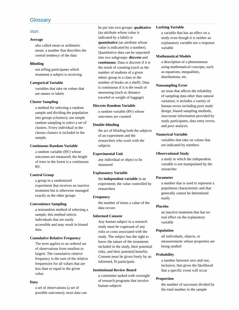
Glossary
start
Averagealso called mean or arithmeticmean; a number that describes thecentral tendency of the data
Blindingnot telling participants whichtreatment a subject is receiving
Categorical Variablevariables that take on values thatare names or labels
Cluster Samplinga method for selecting a randomsample and dividing the populationinto groups (clusters); use simplerandom sampling to select a set ofclusters. Every individual in thechosen clusters is included in thesample.
Continuous Random Variablea random variable (RV) whoseoutcomes are measured; the heightof trees in the forest is a continuousRV.
Control Groupa group in a randomizedexperiment that receives an inactivetreatment but is otherwise managedexactly as the other groups
Convenience Samplinga nonrandom method of selecting asample; this method selectsindividuals that are easilyaccessible and may result in biaseddata.
Cumulative Relative FrequencyThe term applies to an ordered setof observations from smallest tolargest. The cumulative relativefrequency is the sum of the relativefrequencies for all values that areless than or equal to the givenvalue.
Dataa set of observations (a set ofpossible outcomes); most data can
be put into two groups: qualitative(an attribute whose value isindicated by a label) orquantitative (an attribute whosevalue is indicated by a number).Quantitative data can be separatedinto two subgroups: discrete andcontinuous. Data is discrete if it isthe result of counting (such as thenumber of students of a givenethnic group in a class or thenumber of books on a shelf). Datais continuous if it is the result ofmeasuring (such as distancetraveled or weight of luggage)
Discrete Random Variablea random variable (RV) whoseoutcomes are counted
Double-blindingthe act of blinding both the subjectsof an experiment and theresearchers who work with thesubjects
Experimental Unitany individual or object to bemeasured
Explanatory Variablethe independent variable in anexperiment; the value controlled byresearchers
Frequencythe number of times a value of thedata occurs
Informed ConsentAny human subject in a researchstudy must be cognizant of anyrisks or costs associated with thestudy. The subject has the right toknow the nature of the treatmentsincluded in the study, their potentialrisks, and their potential benefits.Consent must be given freely by aninformed, fit participant.
Institutional Review Boarda committee tasked with oversightof research programs that involvehuman subjects
Lurking Variablea variable that has an effect on astudy even though it is neither anexplanatory variable nor a responsevariable
Mathematical Modelsa description of a phenomenonusing mathematical concepts, suchas equations, inequalities,distributions, etc.
Nonsampling Erroran issue that affects the reliabilityof sampling data other than naturalvariation; it includes a variety ofhuman errors including poor studydesign, biased sampling methods,inaccurate information provided bystudy participants, data entry errors,and poor analysis.
Numerical Variablevariables that take on values thatare indicated by numbers
Observational Studya study in which the independentvariable is not manipulated by theresearcher
Parametera number that is used to represent apopulation characteristic and thatgenerally cannot be determinedeasily
Placeboan inactive treatment that has noreal effect on the explanatoryvariable
Populationall individuals, objects, ormeasurements whose properties arebeing studied
Probabilitya number between zero and one,inclusive, that gives the likelihoodthat a specific event will occur
Proportionthe number of successes divided bythe total number in the sample
Qualitative DataSee Data.
Quantitative DataSee Data.
Random Assignmentthe act of organizing experimentalunits into treatment groups usingrandom methods
Random Samplinga method of selecting a sample thatgives every member of thepopulation an equal chance ofbeing selected.
Relative Frequencythe ratio of the number of times avalue of the data occurs in the setof all outcomes to the number of alloutcomes to the total number ofoutcomes
Representative Samplea subset of the population that hasthe same characteristics as thepopulation
Response Variablethe dependent variable in anexperiment; the value that ismeasured for change at the end ofan experiment
Samplea subset of the population studied
Sampling Biasnot all members of the populationare equally likely to be selected
Sampling Errorthe natural variation that resultsfrom selecting a sample torepresent a larger population; thisvariation decreases as the samplesize increases, so selecting largersamples reduces sampling error.
Sampling with ReplacementOnce a member of the population isselected for inclusion in a sample,that member is returned to thepopulation for the selection of thenext individual.
Sampling without Replacement
A member of the population maybe chosen for inclusion in a sampleonly once. If chosen, the member isnot returned to the populationbefore the next selection.
Simple Random Samplinga straightforward method forselecting a random sample; giveeach member of the population anumber. Use a random numbergenerator to select a set of labels.These randomly selected labelsidentify the members of yoursample.
Statistica numerical characteristic of thesample; a statistic estimates thecorresponding populationparameter.
Statistical Modelsa description of a phenomenonusing probability distributions thatdescribe the expected behavior ofthe phenomenon and the variabilityin the expected observations.
Stratified Samplinga method for selecting a randomsample used to ensure thatsubgroups of the population arerepresented adequately; divide thepopulation into groups (strata). Usesimple random sampling to identifya proportionate number ofindividuals from each stratum.
Conditional Probabilitythe likelihood that an event willoccur given that another event hasalready occurred
Contingency Tablethe method of displaying afrequency distribution as a tablewith rows and columns to showhow two variables may bedependent (contingent) upon eachother; the table provides an easyway to calculate conditionalprobabilities.
Dependent EventsIf two events are NOT independent,then we say that they are
dependent.
Equally LikelyEach outcome of an experiment hasthe same probability.
Eventa subset of the set of all outcomesof an experiment; the set of alloutcomes of an experiment iscalled a sample space and is usuallydenoted by S. An event is anarbitrary subset in S. It can containone outcome, two outcomes, nooutcomes (empty subset), the entiresample space, and the like.Standard notations for events arecapital letters such as A, B, C, andso on.
Experimenta planned activity carried out undercontrolled conditions
Independent EventsThe occurrence of one event has noeffect on the probability of theoccurrence of another event. EventsA and B are independent if one ofthe following is true:
Mutually ExclusiveTwo events are mutually exclusiveif the probability that they bothhappen at the same time is zero. Ifevents A and B are mutuallyexclusive, then .
Outcomea particular result of an experiment
If A and B are any two mutuallyexclusive events, then
.
Probabilitya number between zero and one,inclusive, that gives the likelihoodthat a specific event will occur; thefoundation of statistics is given bythe following 3 axioms (by A.N.Kolmogorov, 1930’s): Let S denotethe sample space and A and B are
P (A|B) = P (A)P (B|A) = P (B)P (A∩B) = P (A)P (B)
P (A∩B) = 0
0 ≤ P (A) ≤ 1
P (A∪B) = P (A) +P (B)P (S) = 1
two events in S. Then: (1)There areonly two possible outcomes called“success” and “failure” for eachtrial and (2) The probability of asuccess is the same for any trial (sothe probability of afailure is the same for any trial).
Bernoulli Trialsan experiment with the followingcharacteristics: There are a fixednumber of trials, . There are onlytwo possible outcomes, called"success" and, "failure," for eachtrial. The letter denotes theprobability of a success on onetrial, and denotes the probabilityof a failure on one trial. The trials are independent and arerepeated using identical conditions.
Binomial Experimenta statistical experiment thatsatisfies the following threeconditions:
Binomial Probability Distributiona discrete random variable (RV)that arises from Bernoulli trials;there are a fixed number, , ofindependent trials. “Independent”means that the result of any trial(for example, trial one) does notaffect the results of the followingtrials, and all trials are conductedunder the same conditions. Underthese circumstances the binomialRV is defined as the number ofsuccesses in n trials. The mean is
and the standard deviationis . The probability ofexactly x successes in trials is
.
Geometric Distributiona discrete random variable (RV)that arises from the Bernoulli trials;the trials are repeated until the firstsuccess. The geometric variable Xis defined as the number of trialsuntil the first success. The mean is
and the standard deviation
is . The
probability of exactly x failuresbefore the first success is given bythe formula:
whereone wants to know probability forthe number of trials until the firstsuccess: the th trail is the firstsuccess. An alternative formulationof the geometric distribution asksthe question: what is the probabilityof failures until the first success?In this formulation the trial thatresulted in the first success is notcounted. The formula for thispresentation of the geometric is:
. Theexpected value in this form of thegeometric distribution is .The easiest way to keep these twoforms of the geometric distributionstraight is to remember that p is theprobability of success and is the probability of failure. In theformula the exponents simply countthe number of successes andnumber of failures of the desiredoutcome of the experiment. Ofcourse the sum of these twonumbers must add to the number oftrials in the experiment.There are one or more Bernoullitrials with all failures except thelast one, which is a success.In theory, the number of trialscould go on forever. There must beat least one trial.
The probability, , of a success andthe probability, , of a failure donot change from trial to trial.
Geometric Experimenta statistical experiment with thefollowing properties:
Hypergeometric Experimenta statistical experiment with thefollowing properties:
1. You take samples from twogroups.
2. You are concerned with a groupof interest, called the firstgroup.
3. You sample withoutreplacement from the combinedgroups.
4. Each pick is not independent,since sampling is withoutreplacement.
Normal Distribution
a continuous random variable with pdf
, where is the mean of thedistribution and is the standarddeviation; notation: .If and , the , , iscalled the standard normaldistribution. Standard NormalDistribution a continuous randomvariable ; when
follows the standard normaldistribution, it is often noted as
. z-score the lineartransformation of the form
or written as ;if this transformation is applied toany normal distribution
the result is thestandard normal distribution
. If this transformationis applied to any specific value ofthe with mean and standarddeviation , the result is called thez-score of . The z-score allows usto compare data that are normallydistributed but scaled differently. Az-score is the number of standarddeviations a particular is awayfrom its mean value.
Binomial Distributiona discrete random variable (RV)which arises from Bernoulli trials;there are a fixed number, , ofindependent trials. “Independent”means that the result of any trial(for example, trial 1) does notaffect the results of the followingtrials, and all trials are conductedunder the same conditions. Underthese circumstances the binomial
is defined as the number ofsuccesses in n trials. The notationis: . The mean is
and the standard deviationis . The probability ofexactly successes in trials is
.
Confidence Interval (CI)an interval estimate for anunknown population parameter.
p
q = 1 −p
n
p
q
n
n
X
μ = np
σ = npq−−−√
n
P (X = x) =( )n
xpxqn−x
μ = 1p
σ = ( −1)1p
1p
− −−−−−−−√
P (X = x) = p(1 −p)x−1
x
x
P (X = x) = p(1 −p)x
μ =1−p
p
(1 −p)
p
q
(RV ) f(x) =
1
σ 2π−−
√e
−(x−μ)2
2σ2
μ
σ
X ∼ N(μ, σ)μ = 0 σ = 1 RV Z
(RV )X ∼ N(0, 1)X
Z ∼ N(0, 1)
z =x−μ
σ z =|x−μ|
σ
X ∼ N(μ, σ)
Z ∼ N(0, 1)x
RV μ
σ
x
x
n
RV X
X ∼ B(n, p)
μ = np
σ = npq−−−√x n
P (X = x) =( )n
xpxqn−x
This depends on:
the desired confidence level,information that is known aboutthe distribution (for example,known standard deviation),the sample and its size.
Confidence Level (CL)the percent expression for theprobability that the confidenceinterval contains the truepopulation parameter; for example,if the CL = 90%, then in 90 out of100 samples the interval estimatewill enclose the true populationparameter.
Degrees of Freedom (df)the number of objects in a samplethat are free to vary
Error Bound for a Population Mean(EBM)
the margin of error; depends on theconfidence level, sample size, andknown or estimated populationstandard deviation.
Error Bound for a PopulationProportion (EBP)
the margin of error; depends on theconfidence level, the sample size,and the estimated (from thesample) proportion of successes.
Inferential Statisticsalso called statistical inference orinductive statistics; this facet ofstatistics deals with estimating apopulation parameter based on asample statistic. For example, iffour out of the 100 calculatorssampled are defective we mightinfer that four percent of theproduction is defective.
Normal Distributiona continuous random variable (RV)with pdf
, where
is the mean of the distributionand is the standard deviation,notation: . If and , the RV is called thestandard normal distribution.
Binomial Distribution
a discrete random variable (RV)that arises from Bernoulli trials.There are a fixed number, n, ofindependent trials. “Independent”means that the result of any trial(for example, trial 1) does notaffect the results of the followingtrials, and all trials are conductedunder the same conditions. Underthese circumstances the binomialRV Χ is defined as the number ofsuccesses in trials. The notationis: and thestandard deviation is .The probability of exactly successes in trials is
.
Central Limit TheoremGiven a random variable (RV) withknown mean and known standarddeviation . We are sampling withsize n and we are interested in twonew RVs - the sample mean, . Ifthe size n of the sample issufficiently large, then
. If the size n of
the sample is sufficiently large,then the distribution of the samplemeans will approximate a normaldistribution regardless of the shapeof the population. The expectedvalue of the mean of the samplemeans will equal the populationmean. The standard deviation of thedistribution of the sample means,
, is called the standard error of
the mean.The desired confidence level.
Information that is known about thedistribution (for example, knownstandard deviation).The sample and its size.
Confidence Interval (CI)an interval estimate for anunknown population parameter.This depends on:
Critical ValueThe or value set by theresearcher that measures theprobability of a Type I error, .
Hypothesis
a statement about the value of apopulation parameter, in case oftwo hypotheses, the statementassumed to be true is called the nullhypothesis (notation ) and thecontradictory statement is calledthe alternative hypothesis (notation
).
Hypothesis TestingBased on sample evidence, aprocedure for determining whetherthe hypothesis stated is areasonable statement and shouldnot be rejected, or is unreasonableand should be rejected.
Cohen’s da measure of effect size based onthe differences between two means.If is between 0 and 0.2 then theeffect is small. If approaches is0.5, then the effect is medium, andif approaches 0.8, then it is alarge effect.
a is the symbol for the Y-InterceptSometimes written as , becausewhen writing the theoretical linearmodel is used to represent acoefficient for a population.
b is the symbol for SlopeThe word coefficient will be usedregularly for the slope, because it isa number that will always be nextto the letter “ .” It will be writtenas when a sample is used, and
will be used with a populationor when writing the theoreticallinear model.
Bivariatetwo variables are present in themodel where one is the “cause” orindependent variable and the otheris the “effect” of dependentvariable.
Lineara model that takes data andregresses it into a straight lineequation.
Multivariatea system or model where more thanone independent variable is being
f(x) = 1σ 2π√
e−(x−μ /2)2
σ2
μ
σ
X ∼ N(μ, σ) μ = 0σ = 1
n
X ∼ B(n, p)μ = np
σ = npq−−−√x
n
P (X = x) =( )n
xpxqn−x
μ
σ
X¯ ¯¯̄
∼ N (μ, )X¯ ¯¯̄ σ
n√
σ
n√
t Z
σ
H0
Ha
d
d
d
b0
β0
x
b1
β1
used to predict an outcome. Therecan only ever be one dependentvariable, but there is no limit to thenumber of independent variables.
R2R2 – Coefficient of DeterminationThis is a number between 0 and 1that represents the percentagevariation of the dependent variablethat can be explained by thevariation in the independentvariable. Sometimes calculated bythe equation where
is the “Sum of SquaresRegression” and is the “Sumof Squares Total.” The appropriatecoefficient of determination to bereported should always be adjustedfor degrees of freedom first.
Residual or “error”the value calculated fromsubtracting . Theabsolute value of a residualmeasures the vertical distancebetween the actual value of y andthe estimated value of y thatappears on the best-fit line.
RR – Correlation CoefficientA number between −1 and 1 thatrepresents the strength anddirection of the relationshipbetween “ ” and “ .” The valuefor “ ” will equal 1 or −1 only if allthe plotted points form a perfectlystraight line.
Sum of Squared Errors (SSE)the calculated value from adding upall the squared residual terms. Thehope is that this value is very smallwhen creating a model.
X – the independent variableThis will sometimes be referred toas the “predictor” variable, becausethese values were measured inorder to determine what possibleoutcomes could be predicted.
Y – the dependent variableAlso, using the letter “ ” representsactual values while representspredicted or estimated values.Predicted values will come from
plugging in observed “ ” valuesinto a linear model.all populations of interest arenormally distributed.the populations have equal standarddeviations.
samples (not necessarily of thesame size) are randomly andindependently selected from eachpopulation.there is one independent variableand one dependent variable.
The test statistic for analysis ofvariance is the -ratio.
Analysis of Variancealso referred to as ANOVA, is amethod of testing whether or notthe means of three or morepopulations are equal. The methodis applicable if:
One-Way ANOVAa method of testing whether or notthe means of three or morepopulations are equal; the methodis applicable if:all populations of interest arenormally distributed.the populations have equal standarddeviations.samples (not necessarily of thesame size) are randomly andindependently selected from eachpopulation.
The test statistic for analysis ofvariance is the -ratio.
Variancemean of the squared deviationsfrom the mean; the square of thestandard deviation. For a set ofdata, a deviation can be representedas where is a value of thedata and is the sample mean. Thesample variance is equal to the sumof the squares of the deviationsdivided by the difference of thesample size and one.
Contingency Tablea table that displays sample valuesfor two different factors that maybe dependent or contingent on one
another; it facilitates determiningconditional probabilities.
Goodness-of-Fita hypothesis test that comparesexpected and observed values inorder to look for significantdifferences within one non-parametric variable. The degrees offreedom used equals the (numberof categories – 1).
Test for Homogeneitya test used to draw a conclusionabout whether two populationshave the same distribution. Thedegrees of freedom used equals the(number of columns – 1).
Test of Independencea hypothesis test that comparesexpected and observed values forcontingency tables in order to testfor independence between twovariables. The degrees of freedomused equals the (number ofcolumns – 1) multiplied by the(number of rows – 1).
Independent Groupstwo samples that are selected fromtwo populations, and the valuesfrom one population are not relatedin any way to the values from theother population.
Matched Pairstwo samples that are dependent.Differences between a before andafter scenario are tested by testingone population mean ofdifferences.
Pooled Variancea weighted average of twovariances that can then be usedwhen calculating standard error.
Normal Distributiona continuous random variable (RV)
with pdf ,
where is the mean of thedistribution, and is the standarddeviation, notation: .If and , the RV is
=R2 SSR
SST
SSR
SST
− =y0 ŷ0 e0
X Y
r
y
ŷ
x
F
F
x– x̄̄̄ x
x̄̄̄
f(x) = 1
σ 2π√e
−(x−μ)2
2σ2
μ
σ
X ∼ N(μ, σ)μ = 0 σ = 1
called the standard normaldistribution.
Standard Deviationa number that is equal to the squareroot of the variance and measureshow far data values are from theirmean; notation: s for samplestandard deviation and σ forpopulation standard deviation.
Student's t-Distributioninvestigated and reported byWilliam S. Gossett in 1908 andpublished under the pseudonymStudent. The major characteristicsof the random variable (RV) are:It is continuous and assumes anyreal values.The pdf is symmetrical about itsmean of zero. However, it is morespread out and flatter at the apexthan the normal distribution.
It approaches the standard normaldistribution as n gets larger.There is a "family" of tdistributions: every representativeof the family is completely definedby the number of degrees offreedom which is one less than thenumber of data items.
Test StatisticThe formula that counts the numberof standard deviations on therelevant distribution that estimatedparameter is away from thehypothesized value.
Type I ErrorThe decision is to reject the nullhypothesis when, in fact, the nullhypothesis is true.
Type II ErrorThe decision is not to reject the nullhypothesis when, in fact, the nullhypothesis is false.
Parametera numerical characteristic of apopulation
Point Estimatea single number computed from asample and used to estimate apopulation parameter
Standard Deviationa number that is equal to the squareroot of the variance and measureshow far data values are from theirmean; notation: for samplestandard deviation and \sigma forpopulation standard deviation
Student's t-Distributioninvestigated and reported byWilliam S. Gossett in 1908 andpublished under the pseudonymStudent; the major characteristicsof this random variable ( ) are:
It is continuous and assumesany real values.The pdf is symmetrical about itsmean of zero.It approaches the standardnormal distribution as getlarger.There is a "family" of t–distributions: eachrepresentative of the family iscompletely defined by thenumber of degrees of freedom,which depends upon theapplication for which the t isbeing used.
Averagea number that describes the centraltendency of the data; there are anumber of specialized averages,including the arithmetic mean,weighted mean, median, mode, andgeometric mean.
Central Limit TheoremGiven a random variable withknown mean μ and known standarddeviation, σ, we are sampling withsize n, and we are interested in twonew RVs: the sample mean, . Ifthe size ( ) of the sample issufficiently large, then
. If the size ( ) of
the sample is sufficiently large,then the distribution of the samplemeans will approximate a normaldistributions regardless of the shapeof the population. The mean of thesample means will equal thepopulation mean. The standarddeviation of the distribution of the
sample means, , is called the
standard error of the mean.
Finite Population Correction Factoradjusts the variance of the samplingdistribution if the population isknown and more than 5% of thepopulation is being sampled.
Meana number that measures the centraltendency; a common name formean is "average." The term"mean" is a shortened form of"arithmetic mean." By definition,the mean for a sample (denoted by
) is
, and the mean for a population(denoted by ) is
.
Normal Distributiona continuous random variable with
pdf , where
is the mean of the distribution and is the standard deviation.;
notation: . If and , the random variable, ,is called the standard normaldistribution.
Sampling DistributionGiven simple random samples ofsize from a given populationwith a measured characteristic suchas mean, proportion, or standarddeviation for each sample, theprobability distribution of all themeasured characteristics is called asampling distribution.
Standard Error of the Meanthe standard deviation of thedistribution of the sample means, or
.
Standard Error of the Proportionthe standard deviation of thesampling distribution ofproportions
Conditional Probabilitythe likelihood that an event willoccur given that another event has
s
RV
n
X¯ ¯¯̄
n
∼ N (μ, )X¯ ¯¯̄ σ
n√n
σ
n√
x̄̄̄
= =x̄̄̄ x̄̄̄ Sum of all values in the sample
Number of values in the sample
μ
μ = Sum of all values in the population
Number of values in the population
f(x) = 1
σ 2π√e
−(x−μ)2
2σ2 μ
σ
X ∼ N(μ, σ) μ = 0σ = 1 Z
n
σ
n√
already occurred.
decay parameterThe decay parameter describes therate at which probabilities decay tozero for increasing values of . It isthe value m in the probabilitydensity function of an exponential random variable.It is also equal to , where is the mean of the random variable.
Exponential Distributiona continuous random variable (RV)that appears when we are interestedin the intervals of time betweensome random events, for example,the length of time betweenemergency arrivals at a hospital.The mean is and thestandard deviation is . Theprobability density function is
and the cumulative distributionfunction is
.
memoryless propertyFor an exponential random variable
, the memoryless property is thestatement that knowledge of whathas occurred in the past has noeffect on future probabilities. Thismeans that the probability that exceeds , given that it hasexceeded , is the same as theprobability that would exceed tif we had no knowledge about it. Insymbols we say that
.
Poisson distributionIf there is a known average of \muevents occurring per unit time, andthese events are independent ofeach other, then the number ofevents X occurring in one unit oftime has the Poisson distribution.The probability of x eventsoccurring in one unit time is equal
to .
Uniform Distribution
a continuous random variable (RV)that has equally likely outcomesover the domain, ; it isoften referred as the rectangulardistribution because the graph ofthe pdf has the form of a rectangle.The mean is and thestandard deviation is
. The probability
density function is \(f(x)=\frac{1}{b-a} \text { for } a
Hypergeometric Probabilitya discrete random variable (RV)that is characterized by:
1. A fixed number of trials.2. The probability of success is not
the same from trial to trial.
We sample from two groups ofitems when we are interested inonly one group. is defined as thenumber of successes out of the totalnumber of items chosen.
Poisson Probability Distributiona discrete random variable (RV)that counts the number of times acertain event will occur in aspecific interval; characteristics ofthe variable:
The probability that the eventoccurs in a given interval is thesame for all intervals.The events occur with a knownmean and independently of thetime since the last event.
The distribution is defined by themean of the event in the interval.The mean is . The standarddeviation is . Theprobability of having exactly successes in trials is
. The Poissondistribution is often used toapproximate the binomialdistribution, when is “large” and
is “small” (a general rule is that should be greater than or equal
to 25 and should be less than orequal to 0.01).
Probability Distribution Function(PDF)
a mathematical description of adiscrete random variable (RV),given either in the form of anequation (formula) or in the form ofa table listing all the possibleoutcomes of an experiment and theprobability associated with eachoutcome.
Random Variable (RV)a characteristic of interest in apopulation being studied; commonnotation for variables are uppercase Latin letters ,...;common notation for a specificvalue from the domain (set of allpossible values of a variable) arelower case Latin letters , and .For example, if is the number ofchildren in a family, then represents a specific integer 0, 1, 2,3,.... Variables in statistics differfrom variables in intermediatealgebra in the two following ways.
The domain of the randomvariable (RV) is not necessarilya numerical set; the domainmay be expressed in words; forexample, if hair color thenthe domain is {black, blond,gray, green, orange}.We can tell what specific valuex the random variable takesonly after performing theexperiment.
Sample Spacethe set of all possible outcomes ofan experiment
Sampling with ReplacementIf each member of a population isreplaced after it is picked, then thatmember has the possibility of beingchosen more than once.
Sampling without ReplacementWhen sampling is done withoutreplacement, each member of apopulation may be chosen onlyonce.
The Complement EventThe complement of event Aconsists of all outcomes that areNOT in A.
x
f(x) = me(−mx)
m = 1μ μ
μ = 1m
σ = 1m
f(x) = m or f(x) = , x ≥ 0e−mx 1μe− x
1μ
P (X ≤ x) = 1 − or P (X ≤ x) = 1 −e−mx e− x1μ
X
X
x+ t
x
X
P (X > x+ t|X > x) = P (X > t)
P (X = x) =μxe−μ
x!
a < x < b
μ =a+b
2
σ =(b−a)2
12
− −−−−√
X
μ
μ = np
σ = μ−−√x
r
P (x) =μxe−μ
x!
n
p
np
p
X,Y ,Z
x, y z
X
x
X =
X
The Conditional Probability of P(A||B) is the probability that eventA will occur given that the event Bhas already occurred.
The Intersection: the EventAn outcome is in the event |(A \capB\) if the outcome is in both at the same time.
The Union: the EventAn outcome is in the event if the outcome is in A or is in B oris in both A and B.
Tree Diagramthe useful visual representation of asample space and events in theform of a “tree” with branchesmarked by possible outcomestogether with associatedprobabilities (frequencies, relativefrequencies)
Venn Diagramthe visual representation of asample space and events in theform of circles or ovals showingtheir intersections
Surveya study in which data is collected asreported by individuals.
Systematic Samplinga method for selecting a randomsample; list the members of thepopulation. Use simple randomsampling to select a starting pointin the population. Let k = (numberof individuals in thepopulation)/(number of individualsneeded in the sample). Chooseevery kth individual in the liststarting with the one that wasrandomly selected. If necessary,return to the beginning of thepopulation list to complete yoursample.
Treatmentsdifferent values or components ofthe explanatory variable applied inan experiment
Variable
a characteristic of interest for eachperson or object in a population
Frequencythe number of times a value of thedata occurs
Frequency Tablea data representation in whichgrouped data is displayed alongwith the corresponding frequencies
Histograma graphical representation in x-yform of the distribution of data in adata set; x represents the data and yrepresents the frequency, or relativefrequency. The graph consists ofcontiguous rectangles.
Interquartile Rangeor IQR, is the range of the middle50 percent of the data values; theIQR is found by subtracting thefirst quartile from the third quartile.
Mean (arithmetic)a number that measures the centraltendency of the data; a commonname for mean is 'average.' Theterm 'mean' is a shortened form of'arithmetic mean.' By definition, themean for a sample (denoted by )is ,
and the mean for a population(denoted by μ) is
Mean (geometric)a measure of central tendency thatprovides a measure of averagegeometric growth over multipletime periods.
Mediana number that separates ordereddata into halves; half the values arethe same number or smaller thanthe median and half the values arethe same number or larger than themedian. The median may or maynot be part of the data.
Midpoint
the mean of an interval in afrequency table
Modethe value that appears mostfrequently in a set of data
Outlieran observation that does not fit therest of the data
Percentilea number that divides ordered datainto hundredths; percentiles may ormay not be part of the data. Themedian of the data is the secondquartile and the 50 percentile. Thefirst and third quartiles are the 25and the 75 percentiles,respectively.
Quartilesthe numbers that separate the datainto quarters; quartiles may or maynot be part of the data. The secondquartile is the median of the data.
Relative Frequencythe ratio of the number of times avalue of the data occurs in the setof all outcomes to the number of alloutcomes
Standard Deviationa number that is equal to the squareroot of the variance and measureshow far data values are from theirmean; notation: s for samplestandard deviation and σ forpopulation standard deviation.
Variancemean of the squared deviationsfrom the mean, or the square of thestandard deviation; for a set of data,a deviation can be represented as x– where x is a value of the dataand is the sample mean. Thesample variance is equal to the sumof the squares of the deviationsdivided by the difference of thesample size and one.
end
A|B
∩
A∩B
∪
A∪B
x̄̄̄
=x̄̄̄ Sum of all values in the sample
Number of values in the sample
μ = Sum of all values in the population
Number of values in the population
th
th
th
x̄̄̄
x̄̄̄
Related Documents