GLOBAL EDITION A First Course SEVENTH EDITION David M. Levine • Kathryn A. Szabat • David F. Stephan Business Statistics

Welcome message from author
This document is posted to help you gain knowledge. Please leave a comment to let me know what you think about it! Share it to your friends and learn new things together.
Transcript
GlobAl edITIon
A First CourseSeVenTH edITIon
David M. Levine • Kathryn A. Szabat • David F. Stephan
business Statistics
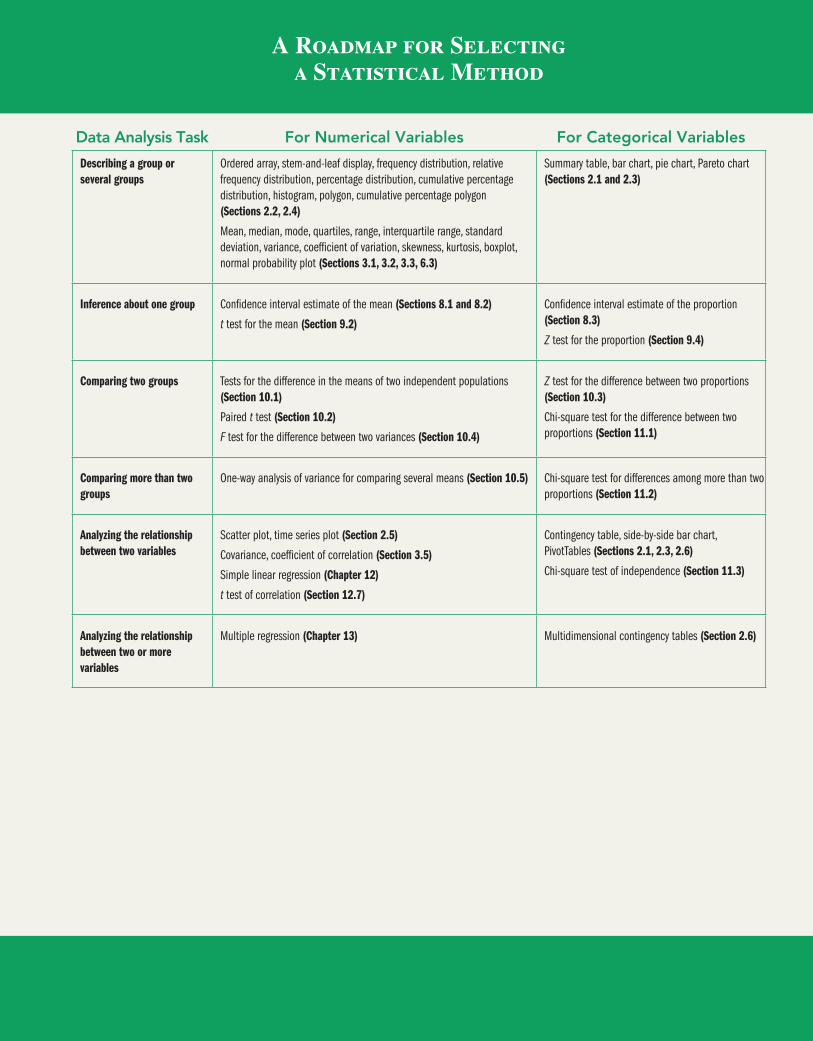
A Roadmap for Selecting a Statistical Method
Data Analysis Task For Numerical Variables For Categorical Variables
Describing a group or several groups
Ordered array, stem-and-leaf display, frequency distribution, relative frequency distribution, percentage distribution, cumulative percentage distribution, histogram, polygon, cumulative percentage polygon (Sections 2.2, 2.4)
Mean, median, mode, quartiles, range, interquartile range, standard deviation, variance, coefficient of variation, skewness, kurtosis, boxplot, normal probability plot (Sections 3.1, 3.2, 3.3, 6.3)
Summary table, bar chart, pie chart, Pareto chart (Sections 2.1 and 2.3)
Inference about one group Confidence interval estimate of the mean (Sections 8.1 and 8.2)
t test for the mean (Section 9.2)
Confidence interval estimate of the proportion (Section 8.3)
Z test for the proportion (Section 9.4)
Comparing two groups Tests for the difference in the means of two independent populations (Section 10.1)
Paired t test (Section 10.2)
F test for the difference between two variances (Section 10.4)
Z test for the difference between two proportions (Section 10.3)
Chi-square test for the difference between two proportions (Section 11.1)
Comparing more than two groups
One-way analysis of variance for comparing several means (Section 10.5) Chi-square test for differences among more than two proportions (Section 11.2)
Analyzing the relationship between two variables
Scatter plot, time series plot (Section 2.5)
Covariance, coefficient of correlation (Section 3.5)
Simple linear regression (Chapter 12)
t test of correlation (Section 12.7)
Contingency table, side-by-side bar chart, PivotTables (Sections 2.1, 2.3, 2.6)
Chi-square test of independence (Section 11.3)
Analyzing the relationship between two or more variables
Multiple regression (Chapter 13) Multidimensional contingency tables (Section 2.6)

This page is intentionally left blank.
David M. LevineDepartment of Statistics and Computer Information Systems
Zicklin School of Business, Baruch College, City University of New York
Kathryn A. SzabatDepartment of Business Systems and Analytics
School of Business, La Salle University
David F. StephanTwo Bridges Instructional Technology
Business Statistics A First Course
Seventh eDition
gLobAL eDition
Boston Columbus Hoboken Indianapolis New York San Francisco Amsterdam Cape Town Dubai London Madrid Milan Munich Paris Montreal Toronto
Delhi Mexico City S~ao Paulo Sydney Hong Kong Seoul Singapore Taipei Tokyo

MICROSOFT® AND WINDOWS® ARE REGISTERED TRADEMARKS OF THE MICROSOFT CORPORATION IN THE U.S.A. AND OTHER COUNTRIES. THIS BOOK IS NOT SPONSORED OR ENDORSED BY OR AFFILIATED WITH THE MICROSOFT CORPORATION. ILLUSTRATIONS OF MICROSOFT ExCEL IN THIS BOOK HAvE BEEN TAKEN FROM MICROSOFT ExCEL 2013, UNLESS OTHERWISE INDICATED.
MICROSOFT AND/OR ITS RESPECTIvE SUPPLIERS MAKE NO REPRESENTATIONS ABOUT THE SUITABILITY OF THE INFORMATION CONTAINED IN THE DOCUMENTS AND RELATED GRAPHICS PUBLISHED AS PART OF THE SERvICES FOR ANY PURPOSE. ALL SUCH DOCUMENTS AND RELATED GRAPHICS ARE PROvIDED “AS IS” WITHOUT WARRANTY OF ANY KIND. MICROSOFT AND/OR ITS RESPECTIvE SUPPLIERS HEREBY DISCLAIM ALL WARRANTIES AND CONDITIONS WITH REGARD TO THIS INFORMATION, INCLUDING ALL WARRANTIES AND CONDITIONS OF MERCHANTABILITY, WHETHER ExPRESS, IMPLIED OR STATUTORY, FITNESS FOR A PARTICULAR PURPOSE, TITLE AND NON-INFRINGEMENT. IN NO EvENT SHALL MICROSOFT AND/OR ITS RESPECTIvE SUPPLIERS BE LIABLE FOR ANY SPECIAL, INDIRECT OR CONSEQUENTIAL DAMAGES OR ANY DAMAGES WHATSOEvER RESULTING FROM LOSS OF USE, DATA OR PROFITS, WHETHER IN AN ACTION OF CONTRACT, NEGLIGENCE OR OTHER TORTIOUS ACTION, ARISING OUT OF OR IN CONNECTION WITH THE USE OR PERFORMANCE OF INFORMATION AvAILABLE FROM THE SERvICES. THE DOCUMENTS AND RELATED GRAPHICS CONTAINED HEREIN COULD INCLUDE TECHNICAL INACCURACIES OR TYPOGRAPHICAL ERRORS. CHANGES ARE PERIODICALLY ADDED TO THE INFORMATION HEREIN. MICROSOFT AND/OR ITS RESPECTIvE SUPPLIERS MAY MAKE IMPROvEMENTS AND/OR CHANGES IN THE PRODUCT(S) AND/OR THE PROGRAM(S) DESCRIBED HEREIN AT ANY TIME. PARTIAL SCREEN SHOTS MAY BE vIEWED IN FULL WITHIN THE SOFTWARE vERSION SPECIFIED.
Minitab © 2013. Portions of information contained in this publication/book are printed with permission of Minitab Inc. All such material remains the exclusive property and copyright of Minitab Inc. All rights reserved.
Pearson Education Limited Edinburgh Gate Harlow Essex CM20 2JE England and Associated Companies throughout the world Visit us on the World Wide Web at: www.pearsonglobaleditions.com © Pearson Education Limited 2016
The rights of David M. Levine, Kathryn A. Szabat, and David F. Stephan to be identified as the authors of this work have been asserted by them in accordance with the Copyright, Designs and Patents Act 1988.
Authorized adaptation from the United States edition, entitled Business Statistics: A First Course, 7th Edition, ISBN 978-0-321-97901-8 by David M. Levine, Kathryn A. Szabat, and David F. Stephan, published by Pearson Education © 2016.
All rights reserved. No part of this publication may be reproduced, stored in a retrieval system, or transmitted in any form or by any means, electronic, mechanical, photocopying, recording or otherwise, without either the prior written permission of the publisher or a license permitting restricted copying in the United Kingdom issued by the Copyright Licensing Agency Ltd, Saffron House, 6–10 Kirby Street, London EC1N 8TS.
All trademarks used herein are the property of their respective owners. The use of any trademark in this text does not vest in the author or publisher any trademark ownership rights in such trademarks, nor does the use of such trademarks imply any affiliation with or endorsement of this book by such owners.
ISBN 10: 1-29-209593-8 ISBN 13: 978-1-292-09593-6 (Print)
British Library Cataloguing-in-Publication Data A catalogue record for this book is available from the British Library
10 9 8 7 6 5 4 3 2 1
Typeset in 10.5, Berkley Std by Lumina Datamatics Printed and bound by vivar in Malaysia
Editorial Director: Chris HoagEditor in Chief: Deirdre LynchAcquisitions Editor: Suzanna BainbridgeEditorial Assistant: Justin BillingAcquisitions Editor, Global Editions: Debapriya MukherjeeAssociate Editor, Global Editions: Paromita BanerjeeProgram Manager: Chere BemelmansProject Manager: Sherry BergProgram Management Team Lead: Marianne StepanianProject Management Team Lead: Peter SilviaSenior Manufacturing Controller, Global Editions: Trudy KimberMedia Producer: Jean ChoeTestGen Content Manager: John Flanagan
MathXL Content Developer: Bob CarrollMedia Production Manager, Global Editions: vikram Kumar Marketing Manager: Erin Kelly Marketing Assistant: Emma SarconiSenior Author Support/Technology Specialist: Joe vetere Rights and Permissions Project Manager: Diahanne Lucas DowridgeSenior Procurement Specialist: Carol Melville Associate Director of Design: Andrea NixProgram Design Lead and Cover Design: Barbara AtkinsonText Design, Production Coordination, Composition, and Illustrations:
Lumina DatamaticsCover Image: © Olga Khomyakova / 123RF
ISBN 13: 978-1-292-09602-5 (PDF)

To our spouses and children, Marilyn, Sharyn, Mary, and Mark
and to our parents, in loving memory, Lee, Reuben, Mary, William, Ruth, and Francis
6
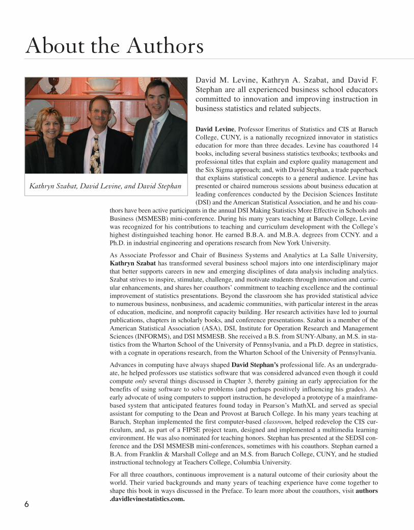
Kathryn Szabat, David Levine, and David Stephan
About the AuthorsDavid M. Levine, Kathryn A. Szabat, and David F. Stephan are all experienced business school educators committed to innovation and improving instruction in business statistics and related subjects.
David Levine, Professor Emeritus of Statistics and CIS at Baruch College, CUNY, is a nationally recognized innovator in statistics education for more than three decades. Levine has coauthored 14 books, including several business statistics textbooks; textbooks and professional titles that explain and explore quality management and the Six Sigma approach; and, with David Stephan, a trade paperback that explains statistical concepts to a general audience. Levine has presented or chaired numerous sessions about business education at leading conferences conducted by the Decision Sciences Institute (DSI) and the American Statistical Association, and he and his coau-
thors have been active participants in the annual DSI Making Statistics More Effective in Schools and Business (MSMESB) mini-conference. During his many years teaching at Baruch College, Levine was recognized for his contributions to teaching and curriculum development with the College’s highest distinguished teaching honor. He earned B.B.A. and M.B.A. degrees from CCNY. and a Ph.D. in industrial engineering and operations research from New York University.
As Associate Professor and Chair of Business Systems and Analytics at La Salle University, Kathryn Szabat has transformed several business school majors into one interdisciplinary major that better supports careers in new and emerging disciplines of data analysis including analytics. Szabat strives to inspire, stimulate, challenge, and motivate students through innovation and curric-ular enhancements, and shares her coauthors’ commitment to teaching excellence and the continual improvement of statistics presentations. Beyond the classroom she has provided statistical advice to numerous business, nonbusiness, and academic communities, with particular interest in the areas of education, medicine, and nonprofit capacity building. Her research activities have led to journal publications, chapters in scholarly books, and conference presentations. Szabat is a member of the American Statistical Association (ASA), DSI, Institute for Operation Research and Management Sciences (INFORMS), and DSI MSMESB. She received a B.S. from SUNY-Albany, an M.S. in sta-tistics from the Wharton School of the University of Pennsylvania, and a Ph.D. degree in statistics, with a cognate in operations research, from the Wharton School of the University of Pennsylvania.
Advances in computing have always shaped David Stephan’s professional life. As an undergradu-ate, he helped professors use statistics software that was considered advanced even though it could compute only several things discussed in Chapter 3, thereby gaining an early appreciation for the benefits of using software to solve problems (and perhaps positively influencing his grades). An early advocate of using computers to support instruction, he developed a prototype of a mainframe-based system that anticipated features found today in Pearson’s MathxL and served as special assistant for computing to the Dean and Provost at Baruch College. In his many years teaching at Baruch, Stephan implemented the first computer-based classroom, helped redevelop the CIS cur-riculum, and, as part of a FIPSE project team, designed and implemented a multimedia learning environment. He was also nominated for teaching honors. Stephan has presented at the SEDSI con-ference and the DSI MSMESB mini-conferences, sometimes with his coauthors. Stephan earned a B.A. from Franklin & Marshall College and an M.S. from Baruch College, CUNY, and he studied instructional technology at Teachers College, Columbia University.
For all three coauthors, continuous improvement is a natural outcome of their curiosity about the world. Their varied backgrounds and many years of teaching experience have come together to shape this book in ways discussed in the Preface. To learn more about the coauthors, visit authors .davidlevinestatistics.com.
Brief ContentsPreface 15Getting Started: Important Things to Learn First 23
1 Defining and Collecting Data 32
2 Organizing and Visualizing Variables 53
3 Numerical Descriptive Measures 119
4 Basic Probability 164
5 Discrete Probability Distributions 198
6 The Normal Distribution 222
7 Sampling Distributions 248
8 Confidence Interval Estimation 270
9 Fundamentals of Hypothesis Testing: One-Sample Tests 306
10 Two-Sample Tests and One-Way ANOVA 345
11 Chi-Square Tests 409
12 Simple Linear Regression 436
13 Multiple Regression 486
14 Statistical Applications in Quality Management (online) 14-1
Appendices A–G 518
Self-Test Solutions and Answers to Selected Even-Numbered Problems 564
Index 589
7
8
Contents
Preface 15
Getting Started: Important Things to Learn First 23UsiNg sTATisTiCs: “You Cannot Escape from Data” 23
GS.1 Statistics: A Way of Thinking 24
GS.2 Data: What Is It? 24Statistics 25
GS.3 The Changing Face of Statistics 26Business Analytics 26“Big Data” 26Integral Role of Software in Statistics 27
GS.4 Statistics: An Important Part of Your Business Education 27
Making Best Use of This Book 27Making Best Use of the Software Guides 28
ReFeRenceS 29
Key teRMS 29
exceL guiDe 30 EG1. Getting Started with Microsoft Excel 30 EG2. Entering Data 30
MinitAb guiDe 31 MG.1 Getting Started with Minitab 31 MG.2 Entering Data 31
1 Defining and Collecting Data 32
UsiNg sTATisTiCs: Beginning of the End … Or the End of the Beginning? 32
1.1 Defining variables 33Classifying variables by Type 33
1.2 Collecting Data 35Data Sources 35Populations and Samples 36Structured versus Unstructured Data 36Electronic Formats and Encodings 37Data Cleaning 37Recoding variables 37
1.3 Types of Sampling Methods 38Simple Random Sample 39Systematic Sample 40Stratified Sample 40Cluster Sample 40
1.4 Types of Survey Errors 41Coverage Error 42
Nonresponse Error 42Sampling Error 42Measurement Error 42Ethical Issues About Surveys 43
ThiNk AboUT This: New Media Surveys/Old Sampling Problems 43
UsiNg sTATisTiCs: Beginning of the End … Revisited 44SuMMARy 45
ReFeRenceS 45
Key teRMS 45
checKing youR unDeRStAnDing 46
chApteR Review pRobLeMS 46
CAses For ChApTer 1 47 Managing Ashland MultiComm Services 47 CardioGood Fitness 47 Clear Mountain State Student Surveys 48 Learning with the Digital Cases 48chApteR 1 exceL guiDe 50 EG1.1 Defining variables 50 EG1.2 Collecting Data 50 EG1.3 Types of Sampling Methods 50
chApteR 1 MinitAb guiDe 51 MG1.1 Defining variables 51 MG1.2 Collecting Data 51 MG1.3 Types of Sampling Methods 52
2 Organizing and Visualizing Variables 53
UsiNg sTATisTiCs: The Choice Is Yours 53
2.1 Organizing Categorical variables 55The Summary Table 55The Contingency Table 55
2.2 Organizing Numerical variables 59The Ordered Array 59The Frequency Distribution 60Classes and Excel Bins 62The Relative Frequency Distribution and the Percentage Distribution 62The Cumulative Distribution 64Stacked and Unstacked Data 66
2.3 visualizing Categorical variables 68The Bar Chart 68The Pie Chart 69The Pareto Chart 70The Side-by-Side Bar Chart 72
2.4 visualizing Numerical variables 74The Stem-and-Leaf Display 74The Histogram 76The Percentage Polygon 77The Cumulative Percentage Polygon (Ogive) 78
2.5 visualizing Two Numerical variables 82The Scatter Plot 82The Time-Series Plot 83
2.6 Organizing and visualizing a Set of variables 85Multidimensional Contingency Tables 86Data Discovery 87
2.7 The Challenge in Organizing and visualizing variables 89
Obscuring Data 89Creating False Impressions 90Chartjunk 90Best Practices for Constructing visualizations 92
UsiNg sTATisTiCs: The Choice Is Yours, Revisited 93SuMMARy 94
ReFeRenceS 94
Key equAtionS 95
Key teRMS 95
checKing youR unDeRStAnDing 95
chApteR Review pRobLeMS 96
CAses For ChApTer 2 100 Managing Ashland MultiComm Services 100 Digital Case 101 CardioGood Fitness 101 The Choice Is Yours Follow-Up 101 Clear Mountain State Student Surveys 101
chApteR 2 exceL guiDe 102 EG2.1 Organizing Categorical variables 102 EG2.2 Organizing Numerical variables 104 EG2.3 visualizing Categorical variables 106 EG2.4 visualizing Numerical variables 108 EG2.5 visualizing Two Numerical variables 111 EG2.6 Organizing and visualizing a Set of variables 111
chApteR 2 MinitAb guiDe 113 MG2.1 Organizing Categorical variables 113 MG2.2 Organizing Numerical variables 113 MG2.3 visualizing Categorical variables 114 MG2.4 visualizing Numerical variables 115 MG2.5 visualizing Two Numerical variables 117 MG2.6 Organizing and visualizing a Set of variables 118
3 Numerical Descriptive Measures 119
UsiNg sTATisTiCs: More Descriptive Choices 119
3.1 Central Tendency 120The Mean 120The Median 122The Mode 123
3.2 variation and Shape 124The Range 124The variance and the Standard Deviation 125The Coefficient of variation 129Z Scores 130Shape: Skewness 131Shape: Kurtosis 132
3.3 Exploring Numerical Data 135Quartiles 135The Interquartile Range 137The Five-Number Summary 138The Boxplot 139
3.4 Numerical Descriptive Measures for a Population 142The Population Mean 142The Population variance and Standard Deviation 143The Empirical Rule 144The Chebyshev Rule 145
3.5 The Covariance and the Coefficient of Correlation 146The Covariance 147The Coefficient of Correlation 148
3.6 Descriptive Statistics: Pitfalls and Ethical Issues 152
UsiNg sTATisTiCs: More Descriptive Choices, Revisited 152SuMMARy 153
ReFeRenceS 153
Key equAtionS 153
Key teRMS 154
checKing youR unDeRStAnDing 154
chApteR Review pRobLeMS 155
CAses For ChApTer 3 158 Managing Ashland MultiComm Services 158 Digital Case 158 CardioGood Fitness 158 More Descriptive Choices Follow-up 158 Clear Mountain State Student Surveys 158
chApteR 3 exceL guiDe 159 EG3.1 Central Tendency 159 EG3.2 variation and Shape 159 EG3.3 Exploring Numerical Data 160 EG3.4 Numerical Descriptive Measures for a Population 161 EG3.5 The Covariance and the Coefficient of Correlation 161
chApteR 3 MinitAb guiDe 162 MG3.1 Central Tendency 162 MG3.2 variation and Shape 162 MG3.3 Exploring Numerical Data 162 MG3.4 Numerical Descriptive Measures for a Population 163 MG3.5 The Covariance and the Coefficient of Correlation 163
4 Basic Probability 164UsiNg sTATisTiCs: Possibilities at M&R Electronics
World 164
4.1 Basic Probability Concepts 165Events and Sample Spaces 166Contingency Tables and venn Diagrams 168Simple Probability 168Joint Probability 169Marginal Probability 170General Addition Rule 171
4.2 Conditional Probability 174Computing Conditional Probabilities 174Decision Trees 176Independence 178Multiplication Rules 179Marginal Probability Using the General Multiplication Rule 180
CONTENTS 9
10 CONTENTS
4.3 Bayes’ Theorem 182
ThiNk AboUT This Divine Providence and Spam 185
4.4 Counting Rules 187
4.5 Ethical Issues and Probability 190
UsiNg sTATisTiCs: Possibilities at M&R Electronics World, Revisited 191
SuMMARy 191
ReFeRenceS 191
Key equAtionS 192
Key teRMS 192
checKing youR unDeRStAnDing 193
chApteR Review pRobLeMS 193
CAses For ChApTer 4 195 Digital Case 195 CardioGood Fitness 195 The Choice Is Yours Follow-Up 195 Clear Mountain State Student Surveys 195
chApteR 4 exceL guiDe 196 EG4.1 Basic Probability Concepts 196 EG4.2 Conditional Probability 196 EG4.3 Bayes’ Theorem 196 EG4.4 Counting Rules 196
chApteR 4 MinitAb guiDe 197 MG4.1 Basic Probability Concepts 197 MG4.2 Conditional Probability 197 MG4.3 Bayes’ Theorem 197 MG4.4 Counting Rules 197
5 Discrete Probability Distributions 198
UsiNg sTATisTiCs: Events of Interest at Ricknel Home Centers 198
5.1 The Probability Distribution for a Discrete variable 199Expected value of a Discrete variable 199variance and Standard Deviation of a Discrete variable 200
5.2 Binomial Distribution 203
5.3 Poisson Distribution 210
UsiNg sTATisTiCs: Events of Interest at Ricknel Home Centers, Revisited 214
SuMMARy 214
ReFeRenceS 214
Key equAtionS 214
Key teRMS 215
checKing youR unDeRStAnDing 215
chApteR Review pRobLeMS 215
CAses For ChApTer 5 217 Managing Ashland MultiComm Services 217
Digital Case 218
chApteR 5 exceL guiDe 219 EG5.1 The Probability Distribution for a Discrete variable 219 EG5.2 Binomial Distribution 219 EG5.3 Poisson Distribution 219
chApteR 5 MinitAb guiDe 220 MG5.1 The Probability Distribution for a Discrete variable 220 MG5.2 Binomial Distribution 220 MG5.3 Poisson Distribution 220
6 The Normal Distribution 222UsiNg sTATisTiCs: Normal Downloading at MyTVLab 222
6.1 Continuous Probability Distributions 223
6.2 The Normal Distribution 223Computing Normal Probabilities 225Finding X values 230
VisUAl explorATioNs: Exploring the Normal Distribution 234
ThiNk AboUT This: What Is Normal? 234
6.3 Evaluating Normality 236Comparing Data Characteristics to Theoretical Properties 236Constructing the Normal Probability Plot 238
UsiNg sTATisTiCs: Normal Downloading at MyTVLab, Revisited 240
SuMMARy 241
ReFeRenceS 241
Key equAtionS 241
Key teRMS 241
checKing youR unDeRStAnDing 242
chApteR Review pRobLeMS 242
CAses For ChApTer 6 243 Managing Ashland MultiComm Services 243 Digital Case 244 CardioGood Fitness 244 More Descriptive Choices Follow-up 244 Clear Mountain State Student Surveys 244
chApteR 6 exceL guiDe 245 EG6.1 Continuous Probability Distributions 245 EG6.2 The Normal Distribution 245 EG6.3 Evaluating Normality 245
chApteR 6 MinitAb guiDe 246 MG6.1 Continuous Probability Distributions 246 MG6.2 The Normal Distribution 246 MG6.3 Evaluating Normality 246
7 Sampling Distributions 248UsiNg sTATisTiCs: Sampling Oxford Cereals 248
7.1 Sampling Distributions 249
7.2 Sampling Distribution of the Mean 249The Unbiased Property of the Sample Mean 249Standard Error of the Mean 251Sampling from Normally Distributed Populations 252Sampling from Non-normally Distributed Populations— The Central Limit Theorem 255
VisUAl explorATioNs: Exploring Sampling Distributions 259
7.3 Sampling Distribution of the Proportion 260

CONTENTS 11
UsiNg sTATisTiCs: Sampling Oxford Cereals, Revisited 264SuMMARy 264
ReFeRenceS 264
Key equAtionS 264
Key teRMS 265
checKing youR unDeRStAnDing 265
chApteR Review pRobLeMS 265
CAses For ChApTer 7 267 Managing Ashland MultiComm Services 267 Digital Case 267chApteR 7 exceL guiDe 268 EG7.1 Sampling Distributions 268 EG7.2 Sampling Distribution of the Mean 268 EG7.3 Sampling Distribution of the Proportion 268chApteR 7 MinitAb guiDe 269 MG7.1 Sampling Distributions 269 MG7.2 Sampling Distribution of the Mean 269 MG7.3 Sampling Distribution of the Proportion 269
8 Confidence Interval Estimation 270
UsiNg sTATisTiCs: Getting Estimates at Ricknel Home Centers 270
8.1 Confidence Interval Estimate for the Mean (s Known) 271Can You Ever Know the Population Standard Deviation? 276
8.2 Confidence Interval Estimate for the Mean (s Unknown) 277
Student’s t Distribution 277Properties of the t Distribution 278The Concept of Degrees of Freedom 279The Confidence Interval Statement 280
8.3 Confidence Interval Estimate for the Proportion 285
8.4 Determining Sample Size 288Sample Size Determination for the Mean 288Sample Size Determination for the Proportion 290
8.5 Confidence Interval Estimation and Ethical Issues 293
8.6 Bootstrapping (online) 294UsiNg sTATisTiCs: Getting Estimates at Ricknel Home
Centers, Revisited 294SuMMARy 294
ReFeRenceS 295
Key equAtionS 295
Key teRMS 295
checKing youR unDeRStAnDing 295
chApteR Review pRobLeMS 296
CAses For ChApTer 8 299 Managing Ashland MultiComm Services 299 Digital Case 300 Sure value Convenience Stores 300 CardioGood Fitness 301 More Descriptive Choices Follow-Up 301 Clear Mountain State Student Surveys 301chApteR 8 exceL guiDe 302 EG8.1 Confidence Interval Estimate for the Mean (s Known) 302 EG8.2 Confidence Interval Estimate for the Mean (s Unknown) 302
EG8.3 Confidence Interval Estimate for the Proportion 303 EG8.4 Determining Sample Size 303
chApteR 8 MinitAb guiDe 304 MG8.1 Confidence Interval Estimate for the Mean (s Known) 304 MG8.2 Confidence Interval Estimate for the Mean
(s Unknown) 304 MG8.3 Confidence Interval Estimate for the Proportion 304 MG8.4 Determining Sample Size 305
9 Fundamentals of Hypothesis Testing: One-Sample Tests 306
UsiNg sTATisTiCs: Significant Testing at Oxford Cereals 306
9.1 Fundamentals of Hypothesis-Testing Methodology 307The Null and Alternative Hypotheses 307The Critical value of the Test Statistic 308Regions of Rejection and Nonrejection 309Risks in Decision Making Using Hypothesis Testing 309Z Test for the Mean (s Known) 312Hypothesis Testing Using the Critical value Approach 312Hypothesis Testing Using the p-value Approach 315A Connection Between Confidence Interval Estimation and Hypothesis Testing 317Can You Ever Know the Population Standard Deviation? 318
9.2 t Test of Hypothesis for the Mean (s Unknown) 319The Critical value Approach 320The p-value Approach 322Checking the Normality Assumption 322
9.3 One-Tail Tests 326The Critical value Approach 326The p-value Approach 327
9.4 Z Test of Hypothesis for the Proportion 330The Critical value Approach 331The p-value Approach 332
9.5 Potential Hypothesis-Testing Pitfalls and Ethical Issues 334
Statistical Significance versus Practical Significance 334Statistical Insignificance versus Importance 335Reporting of Findings 335Ethical Issues 335
UsiNg sTATisTiCs: Significant Testing at Oxford Cereals, Revisited 336
SuMMARy 336
ReFeRenceS 336
Key equAtionS 337
Key teRMS 337
checKing youR unDeRStAnDing 337
chApteR Review pRobLeMS 337
CAses For ChApTer 9 339 Managing Ashland MultiComm Services 339
Digital Case 340 Sure value Convenience Stores 340chApteR 9 exceL guiDe 341 EG9.1 Fundamentals of Hypothesis-Testing Methodology 341 EG9.2 t Test of Hypothesis for the Mean (s Unknown) 341
12 CONTENTS
EG9.3 One-Tail Tests 342 EG9.4 Z Test of Hypothesis for the Proportion 342
chApteR 9 MinitAb guiDe 343 MG9.1 Fundamentals of Hypothesis-Testing Methodology 343 MG9.2 t Test of Hypothesis for the Mean (s Unknown) 343 MG9.3 One-Tail Tests 343 MG9.4 Z Test of Hypothesis for the Proportion 344
10 Two-Sample Tests and One-Way ANOVA 345
UsiNg sTATisTiCs: For North Fork, Are There Different Means to the Ends? 345
10.1 Comparing the Means of Two Independent Populations 346
Pooled-variance t Test for the Difference Between Two Means 346Confidence Interval Estimate for the Difference Between Two Means 351t Test for the Difference Between Two Means, Assuming Unequal variances 352Do People Really Do This? 352
10.2 Comparing the Means of Two Related Populations 355Paired t Test 356Confidence Interval Estimate for the Mean Difference 361
10.3 Comparing the Proportions of Two Independent Populations 363
Z Test for the Difference Between Two Proportions 363Confidence Interval Estimate for the Difference Between Two Proportions 367
10.4 F Test for the Ratio of Two variances 369
10.5 One-Way ANOvA 374F Test for Differences Among More Than Two Means 377One-Way ANOvA F Test Assumptions 381Levene Test for Homogeneity of variance 382Multiple Comparisons: The Tukey-Kramer Procedure 383
10.6 Effect Size (online) 388
UsiNg sTATisTiCs: For North Fork, Are There Different Means to the Ends? Revisited 389
SuMMARy 389
ReFeRenceS 390
Key equAtionS 390
Key teRMS 391
checKing youR unDeRStAnDing 392
chApteR Review pRobLeMS 392
CAses For ChApTer 10 394 Managing Ashland MultiComm Services 394 Digital Case 395 Sure value Convenience Stores 395 CardioGood Fitness 396 More Descriptive Choices Follow-Up 396 Clear Mountain State Student Surveys 396
chApteR 10 exceL guiDe 398 EG10.1 Comparing the Means of Two Independent Populations 398 EG10.2 Comparing the Means of Two Related Populations 400 EG10.3 Comparing the Proportions of Two Independent
Populations 401
EG10.4 F Test for the Ratio of Two variances 401 EG10.5 One-Way ANOvA 402
chApteR 10 MinitAb guiDe 405 MG10.1 Comparing the Means of Two Independent Populations 405 MG10.2 Comparing the Means of Two Related Populations 405 MG10.3 Comparing the Proportions of Two Independent
Populations 406 MG10.4 F Test for the Ratio of Two variances 406 MG10.5 One-Way ANOvA 407
11 Chi-Square Tests 409UsiNg sTATisTiCs: Avoiding Guesswork About Resort
Guests 409
11.1 Chi-Square Test for the Difference Between Two Proportions 410
11.2 Chi-Square Test for Differences Among More Than Two Proportions 417
11.3 Chi-Square Test of Independence 422
UsiNg sTATisTiCs: Avoiding Guesswork About Resort Guests, Revisited 427
SuMMARy 428
ReFeRenceS 428
Key equAtionS 429
Key teRMS 429
checKing youR unDeRStAnDing 429
chApteR Review pRobLeMS 429
CAses For ChApTer 11 431 Managing Ashland MultiComm Services 431 Digital Case 432 CardioGood Fitness 432 Clear Mountain State Student Surveys 433
chApteR 11 exceL guiDe 434 EG11.1 Chi-Square Test for the Difference Between Two
Proportions 434 EG11.2 Chi-Square Test for Differences Among More Than
Two Proportions 434 EG11.3 Chi-Square Test of Independence 434
chApteR 11 MinitAb guiDe 435 MG11.1 Chi-Square Test for the Difference Between Two
Proportions 435 MG11.2 Chi-Square Test for Differences Among More Than
Two Proportions 435 MG11.3 Chi-Square Test of Independence 435
12 Simple Linear Regression 436
UsiNg sTATisTiCs: Knowing Customers at Sunflowers Apparel 436
12.1 Types of Regression Models 437Simple Linear Regression Models 438
12.2 Determining the Simple Linear Regression Equation 439The Least-Squares Method 439Predictions in Regression Analysis: Interpolation versus Extrapolation 442
CONTENTS 13
Computing the Y Intercept, b0, and the Slope, b1 442
VisUAl explorATioNs: Exploring Simple Linear Regression Coefficients 445
12.3 Measures of variation 447Computing the Sum of Squares 447The Coefficient of Determination 448Standard Error of the Estimate 450
12.4 Assumptions of Regression 452
12.5 Residual Analysis 452Evaluating the Assumptions 452
12.6 Measuring Autocorrelation: The Durbin-Watson Statistic 456
Residual Plots to Detect Autocorrelation 456The Durbin-Watson Statistic 457
12.7 Inferences About the Slope and Correlation Coefficient 460
t Test for the Slope 460F Test for the Slope 462Confidence Interval Estimate for the Slope 463t Test for the Correlation Coefficient 464
12.8 Estimation of Mean values and Prediction of Individual values 467
The Confidence Interval Estimate for the Mean Response 467The Prediction Interval for an Individual Response 468
12.9 Potential Pitfalls in Regression 471Six Steps for Avoiding the Potential Pitfalls 473
UsiNg sTATisTiCs: Knowing Customers at Sunflowers Apparel, Revisited 473
SuMMARy 473
ReFeRenceS 474
Key equAtionS 475
Key teRMS 476
checKing youR unDeRStAnDing 476
chApteR Review pRobLeMS 476
CAses For ChApTer 12 480
Managing Ashland MultiComm Services 480
Digital Case 480
Brynne Packaging 480
chApteR 12 exceL guiDe 482 EG12.1 Types of Regression Models 482 EG12.2 Determining the Simple Linear Regression Equation 482 EG12.3 Measures of variation 483 EG12.4 Assumptions of Regression 483 EG12.5 Residual Analysis 483 EG12.6 Measuring Autocorrelation: The Durbin-Watson Statistic 484 EG12.7 Inferences About the Slope and Correlation Coefficient 484 EG12.8 Estimation of Mean values and Prediction of Individual
values 484
chApteR 12 MinitAb guiDe 484 MG12.1 Types of Regression Models 484 MG12.2 Determining the Simple Linear Regression Equation 484 MG12.3 Measures of variation 485 MG12.4 Assumptions 485 MG12.5 Residual Analysis 485 MG12.6 Measuring Autocorrelation: The Durbin-Watson Statistic 485 MG12.7 Inferences About the Slope and Correlation Coefficient 485 MG12.8 Estimation of Mean values and Prediction of Individual
values 485
13 Multiple Regression 486UsiNg sTATisTiCs: The Multiple Effects of OmniPower Bars 486
13.1 Developing a Multiple Regression Model 487Interpreting the Regression Coefficients 488Predicting the Dependent variable Y 490
13.2 r2, Adjusted r2, and the Overall F Test 492Coefficient of Multiple Determination 492Adjusted r 2 493Test for the Significance of the Overall Multiple Regression Model 494
13.3 Residual Analysis for the Multiple Regression Model 496
13.4 Inferences Concerning the Population Regression Coefficients 497
Tests of Hypothesis 497Confidence Interval Estimation 499
13.5 Using Dummy variables and Interaction Terms in Regression Models 501
Dummy variables 501Interactions 503
UsiNg sTATisTiCs: The Multiple Effects of Omnipower Bars, Revisited 507
SuMMARy 507
ReFeRenceS 507
Key equAtionS 509
Key teRMS 509
checKing youR unDeRStAnDing 509
chApteR Review pRobLeMS 509
CAses For ChApTer 13 512
Managing Ashland MultiComm Services 512 Digital Case 512
chApteR 13 exceL guiDe 513 EG13.1 Developing a Multiple Regression Model 513 EG13.2 r 2, Adjusted r 2, and the Overall F Test 514 EG13.3 Residual Analysis for the Multiple Regression Model 514 EG13.4 Inferences Concerning the Population Regression
Coefficients 515 EG13.5 Using Dummy variables and Interaction Terms in
Regression Models 515
chApteR 13 MinitAb guiDe 515 MG13.1 Developing a Multiple Regression Model 515 MG13.2 r 2, Adjusted r 2, and the Overall F Test 516 MG13.3 Residual Analysis for the Multiple Regression Model 516 MG13.4 Inferences Concerning the Population Regression
Coefficients 516 MG13.5 Using Dummy variables and Interaction Terms
in Regression Models 517
14 Statistical Applications in Quality Management (online) 14-1
UsiNg sTATisTiCs: Finding Quality at the Beachcomber 14-1
14.1 The Theory of Control Charts 14-2
14.2 Control Chart for the Proportion: The p Chart 14-4
14.3 The Red Bead Experiment: Understanding Process variability 14-10
14.4 Control Chart for an Area of Opportunity: The c Chart 14-12
14.5 Control Charts for the Range and the Mean 14-15The R Chart 14-16The X Chart 14-18
14.6 Process Capability 14-21Customer Satisfaction and Specification Limits 14-21Capability Indices 14-23CPL, CPU, and Cpk 14-24
14.7 Total Quality Management 14-26
14.8 Six Sigma 14-28The DMAIC Model 14-29Roles in a Six Sigma Organization 14-30Lean Six Sigma 14-30
UsiNg sTATisTiCs: Finding Quality at the Beachcomber, Revisited 14-31
SuMMARy 14-31
ReFeRenceS 14-32
Key equAtionS 14-32
Key teRMS 14-33
chApteR Review pRobLeMS 14-34
The Harnswell Sewing Machine Company Case 14-36 Managing Ashland Multicomm Services 14-38
chApteR 14 exceL guiDe 14-39 EG14.1 The Theory of Control Charts 14-39 EG14.2 Control Chart for the Proportion: The p Chart 14-39 EG14.3 The Red Bead Experiment: Understanding Process
variability 14-40 EG14.4 Control Chart for an Area of Opportunity: The c Chart 14-40 EG14.5 Control Charts for the Range and the Mean 14-41 EG14.6 Process Capability 14-42
chApteR 14 MinitAb guiDe 14-42 MG14.1 The Theory of Control Charts 14-42 MG14.2 Control Chart for the Proportion: The p Chart 14-42 MG14.3 The Red Bead Experiment: Understanding Process
variability 14-42 MG14.4 Control Chart for an Area of Opportunity: The c Chart 14-42 MG14.5 Control Charts for the Range and the Mean 14-43 MG14.6 Process Capability 14-44
Appendices 518A. Basic Math Concepts and Symbols 519
A.1 Rules for Arithmetic Operations 519
A.2 Rules for Algebra: Exponents and Square Roots 519
A.3 Rules for Logarithms 520
A.4 Summation Notation 521
A.5 Statistical Symbols 524
A.6 Greek Alphabet 524
B. Important Excel and Minitab Skills 525
B.1 Basic Excel Operations 525
B.2 Formulas and Cell References 525
B.3 Entering Formulas into Worksheets 526
B.4 Pasting with Paste Special 527
B.5 Basic Worksheet Cell Formatting 527
B.6 Chart Formatting 529
B.7 Selecting Cell Ranges for Charts 530
B.8 Deleting the “Extra” Histogram Bar 530
B.9 Creating Histograms for Discrete Probability Distributions 530
B.10 Basic Minitab Operations 531
C. Online Resources 532
C.1 About the Online Resources for This Book 532
C.2 Accessing the Online Resources 532
C.3 Details of Downloadable Files 532
C.4 PHStat 537
D. Configuring Microsoft Excel 538
D.1 Getting Microsoft Excel Ready for Use (ALL) 538
D.2 Getting PHStat Ready for Use (ALL) 539
D.3 Configuring Excel Security for Add-In Usage (WIN) 539
D.4 Opening PHStat (ALL) 540
D.5 Using a visual Explorations Add-in Workbook (ALL) 540
D.6 Checking for the Presence of the Analysis ToolPak (ALL) 540
E. Tables 541
E.1 Table of Random Numbers 541
E.2 The Cumulative Standardized Normal Distribution 543
E.3 Critical values of t 545
E.4 Critical values of x2 547
E.5 Critical values of F 548
E.6 Critical values of the Studentized Range, Q 552
E.7 Critical values, dL and dU, of the Durbin–Watson Statistic, D (Critical values Are One-Sided) 554
E.8 Control Chart Factors 555
E.9 The Standardized Normal Distribution 556
F. Useful Excel Knowledge 557
F.1 Useful Keyboard Shortcuts 557
F.2 verifying Formulas and Worksheets 557
F.3 New Function Names 558
F.4 Understanding the Nonstatistical Functions 559
G. Software FAQs 561
G.1 PHStat FAQs 561
G.2 Microsoft Excel FAQs 562
G.3 FAQs for New Users of Microsoft Excel 2013 562
G.4 Minitab FAQs 563
Self-Test Solutions and Answers to Selected Even-Numbered Problems 564
Index 589
14 CONTENTS

15
PrefaceThe world of business statistics has grown larger, expanding into and combining with other disci-plines. And, in a reprise of something that occurred a generation ago, new fields of study, this time with names such as informatics, data analytics, and decision science, have emerged.
This time of change makes what is taught in business statistics and how it is taught all the more critical. We, the coauthors, think about these changes as we seek ways to continuously improve the teaching of business statistics. We actively participate in Decision Sciences Institute (DSI), American Statistical Association (ASA), and Making Statistics More Effective in Schools and Business (MSMESB) conferences. We use the ASA’s Guidelines for Assessment and Instruction (GAISE) reports and combine them with our experiences teaching business statistics to a diverse student body at several universities. We also benefit from the interests and efforts of our past coau-thors, Mark Berenson and Timothy Krehbiel.
Our Educational PhilosophyWhen writing for introductory business statistics students, we are guided by these principles:
Help students see the relevance of statistics to their own careers by providing examples drawn from the functional areas in which they may be specializing. Students need to learn sta-tistics in the context of the functional areas of business. We present each statistics topic in the con-text of areas such as accounting, finance, management, and marketing and explain the application of specific methods to business activities.
Emphasize interpretation and analysis of statistical results over calculation. We emphasize the interpretation of results, the evaluation of the assumptions, and the discussion of what should be done if the assumptions are violated. We believe that these activities are more important and will serve students better in the future than focusing on tedious hand calculations.
Give students ample practice in understanding how to apply statistics to business. We believe that both classroom examples and homework exercises should involve actual or realistic data, using small and large sets of data, to the extent possible.
Familiarize students with the use of spreadsheet and statistical software. We integrate spreadsheet and statistical software into all statistics topics to illustrate how this software assists business decision making. (Using software in this way also supports our second point about empha-sizing interpretation over calculation).
Provide clear instructions to students for using spreadsheet and statistical software. We believe that providing such instructions facilitates learning and helps prevent minimizes the chance that learning software to the level necessary will distract from the learning of statistical concepts.
What’s New and Innovative in This Edition?This seventh edition of Business Statistics: A First Course contains these new and innovative features.
Getting Started: Important Things to Learn First Created to help students get a jumpstart on the course, lessen any fear about learning statistics, and provide coverage of those things that would be helpful to know even before the first class of the term. “Getting Started” has been developed to be posted online or otherwise distributed before the first class section begins and is available for download as explained in Appendix C. Instructors teaching online or hybrid course sections may find this to be a particularly valuable tool to help organize the students in their section.
Student Tips In-margin notes that reinforce hard-to-master concepts and provide quick study tips for mastering important details.
Discussion of Business Analytics “Getting Started: Important Things to Learn First” quickly defines business analytics and big data and notes how these things are changing the face of statistics.
PHStat version 4 For Microsoft Excel users, this successor to the PHStat2 statistics add-in contains several new and enhanced procedures, is simpler to set up and run, and is compat-ible with both Microsoft Windows and (Mac) OS x Excel versions.
Additional Chapter Short Takes Online PDF documents (available for download as explained in Appendix C) that supply additional insights or explanations to important statisti-cal concepts or details about the results presented in this book.
revised and enhanced ContentThis seventh edition, Global Edition, of Business Statistics: A First Course contains the following
revised and enhanced content.
New Continuing End-of-Chapter Cases This edition features several new end-of-chapter cases. New and recurring throughout the book is a case that concerns the analysis of sales and marketing data for home fitness equipment (CardioGood Fitness), a case that concerns pric-ing decisions made by a retailer (Sure value Convenience Stores), and the More Descriptive Choices Follow-Up case, which extends the use of the retirement funds sample first introduced in Chapter 2. Also recurring is the Clear Mountain State Student Surveys case, which uses data collected from surveys of undergraduate and graduate students to practice and reinforce statisti-cal methods learned in various chapters. This case replaces end-of-chapter questions related to the student survey database in the previous edition. In addition, there is a new case in simple linear regression (Brynne Packaging).
Many New Applied Examples and Problems Many of the applied examples throughout this book use new problems or revised data. Approximately 43% of the problems are new to this edition. The end-of-section and end-of-chapter problem sets contain many new problems that use data from The Wall Street Journal, USA Today, and other sources.
Revised Using Statistics Scenarios Five chapters have new or revised Using Statistics scenarios.
Revised Making Best Use of This Book section Included as part of Section GS.4 of “Getting Started: Important Things to Learn First,” this section presents an overview of this book and checklist that helps students prepare for using Microsoft Excel or Minitab with this book.
Revised Software Appendices These appendices review the foundational skills for using Microsoft Excel and Minitab, review the latest technical information, and, for Excel users, cover optional but useful skills for working with Excel.
Distinctive FeaturesThis seventh edition, Global Edition, of Business Statistics: A First Course continues the use of the following distinctive features.
Using Statistics Business Scenarios Each chapter begins with a Using Statistics example that shows how statistics is used in the functional areas of business—accounting, finance, informa-tion systems, management, and marketing. Each scenario is used throughout the chapter to pro-vide an applied context for the concepts. The chapter concludes with a Using Statistics, Revisited section that reinforces the statistical methods and applications discussed in each chapter.
Emphasis on Data Analysis and Interpretation of Excel and Minitab Results Our focus emphasizes analyzing data by interpreting results while reducing emphasis on doing calcula-tions. For example, in the coverage of tables and charts in Chapter 2, we help students inter-pret various charts and explain when to use each chart discussed. Our coverage of hypoth-esis testing in Chapters 9 through 11 and regression and multiple regression in Chapters 12 and 13 include extensive software results so that the p-value approach can be emphasized.
Pedagogical Aids We use an active writing style, boxed numbered equations, set-off examples that reinforce learning concepts, student tips, problems divided into “Learning the Basics” and “Applying the Concepts,” key equations, and key terms.
Digital Cases In the Digital Cases, available for download as explained in Appendix C, learn-ers must examine interactive PDF documents to sift through various claims and informa-tion to discover the data most relevant to a business case scenario. Learners then determine whether the conclusions and claims are supported by the data. In doing so, learners discover and learn how to identify common misuses of statistical information. (Instructional tips for using the Digital Cases and solutions to the Digital Cases are included in the Instructor’s Solutions Manual.)
16 PREFACE
PREFACE 17
Answers Most answers to the even-numbered exercises are included at the end of the book.
Flexibility Using Excel For almost every statistical method discussed, students can use In-Depth Excel instructions to directly work with worksheet solution details or they can use either the PHStat instructions or the Analysis ToolPak instructions to automate the creation of those worksheet solutions.
PHStat PHStat is the Pearson Education statistics add-in that includes more than 60 proce-dures that create Excel worksheets and charts. Unlike other add-ins, PHStat results are real worksheets that contain real Excel calculations (called formulas in Excel). You can examine the contents of worksheet solutions to learn the appropriate functions and calculations neces-sary to apply a particular statistical method. With most of these worksheet solutions, you can change worksheet data and immediately see how those changes affect the results.
Descriptive Statistics: boxplot, descriptive summary, dot scale diagram, frequency distribu-tion, histogram and polygons, Pareto diagram, scatter plot, stem-and-leaf display, one-way tables and charts, and two-way tables and charts
Probability and probability distributions: simple and joint probabilities, normal probability plot, and binomial, and Poisson probability distributions
Sampling: sampling distributions simulation
Confidence interval estimation: for the mean, sigma unknown; for the mean, sigma known; and for the proportion
Sample size determination: for the mean and the proportion
One-sample tests: Z test for the mean, sigma known; t test for the mean, sigma unknown; and Z test for the proportion
Two-sample tests (unsummarized data): pooled-variance t test, separate-variance t test, paired t test, and F test for differences in two variances
Two-sample tests (summarized data): pooled-variance t test, separate-variance t test, paired t test, Z test for the differences in two means, F test for differences in two variances, chi-square test for differences in two proportions, and Z test for the difference in two propor-tions
Multiple-sample tests: chi-square test, Levene test, one-way ANOvA, and Tukey-Kramer procedure
Regression: simple linear regression, and multiple regression
Data preparation: stack and unstack data
Control charts: p chart, c chart, and R and Xbar charts.
To learn more about PHStat, see Appendix C.
Visual Explorations The series of Excel workbooks that allow students to interactively explore important statistical concepts in the normal distribution, sampling distributions, and regression analysis. For the normal distribution, students see the effect of changes in the mean and standard deviation on the areas under the normal curve. For sampling distributions, students use simulation to explore the effect of sample size on a sampling distribution. For regression analysis, students fit a line of regression and observe how changes in the slope and intercept affect the goodness of fit. To learn more about visual Explorations, see Appendix C.
Chapter-by-Chapter Changes Made for This EditionBesides the new and innovative content described in “What’s New and Innovative in This Edition?” the seventh edition, Global Edition, of Business Statistics: A First Course contains the following specific changes to each chapter.
Getting Started: Important Things to Learn First This all-new chapter includes new material on business analytics and introduces the DCOvA framework and a basic vocabulary of statis-tics, both of which were introduced in Chapter 1 of the sixth edition.

Chapter 1 Collecting data has been relocated to this chapter from Section 2.1. Sampling meth-ods and types of survey errors have been relocated from Sections 7.1 and 7.2. There is a new subsection on data cleaning. The CardioGood Fitness and Clear Mountain State Surveys cases are included.
Chapter 2 Section 2.1, “Data Collection,” has been moved to Chapter 1. The chapter uses a new data set that contains a sample of 316 mutual funds and a new set of restaurant cost data. The CardioGood Fitness, The Choice Is Yours Follow-up, and Clear Mountain State Surveys cases are included.
Chapter 3 For many examples, this chapter uses the new mutual funds data set that is intro-duced in Chapter 2. There is increased coverage of skewness and kurtosis. There is a new example on computing descriptive measures from a population using “Dogs of the Dow.” The CardioGood Fitness, More Descriptive Choices Follow-up, and Clear Mountain State Surveys cases are included.
Chapter 4 The chapter example has been updated. There are new problems throughout the chapter. The CardioGood Fitness, The Choice Is Yours Follow-up, and Clear Mountain State Surveys cases are included.
Chapter 5 There are many new problems throughout the chapter. The notation used has been made more consistent.
Chapter 6 This chapter has an updated Using Statistics scenario and some new problems. The CardioGood Fitness, More Descriptive Choices Follow-up, and Clear Mountain State Surveys cases are included.
Chapter 7 Sections 7.1 and 7.2 have been moved to Chapter 1. An additional example of sampling distributions from a larger population has been included.
Chapter 8 This chapter includes an updated Using Statistics scenario and new examples and exercises throughout the chapter. The Sure value Convenience Stores, CardioGood Fitness, More Descriptive Choices Follow-up, and Clear Mountain State Surveys cases are included. There is an online section on bootstrapping.
Chapter 9 This chapter includes additional coverage of the pitfalls of hypothesis testing. The Sure value Convenience Stores case is included.
Chapter 10 This chapter has an updated Using Statistics scenario, a new example on the paired t-test on textbook prices, a new example on the Z-test for the difference between two proportions, and a new one-way ANOvA example on mobile electronics sales at a general merchandiser. The Sure value Convenience Stores, CardioGood Fitness, More Descriptive Choices Follow-up, and Clear Mountain State Surveys cases are included. There is a new online section on Effect Size.
Chapter 11 The chapter includes many new problems. This chapter includes the Sure value Convenience Stores, CardioGood Fitness, More Descriptive Choices Follow-up, and Clear Mountain State Surveys cases.
Chapter 12 The Using Statistics scenario has been updated and changed, with new data used throughout the chapter. This chapter includes the Brynne Packaging case.
Chapter 13 The chapter includes many new and revised problems.
Chapter 14 The “Statistical Applications in Quality Management” chapter has been renum-bered as Chapter 14 and is available for download as explained in Appendix C.
Student and Instructor ResourcesStudent Solutions Manual, by Professor Pin Tian Ng of Northern Arizona University and accu-
racy checked by Annie Puciloski, provides detailed solutions to virtually all the even-numbered exercises and worked-out solutions to the self-test problems.
Online resources The complete set of online resources are discussed fully in Appendix C
18 PREFACE
MyStatLab™
PREFACE 19
For adopting instructors, the following resources are among those available at the Instructor’s Resource Center, located at www.pearsonglobaleditions.com/Levine.
Instructor’s Solutions Manual, by Professor Pin Tian Ng of Northern Arizona University and accuracy checked by Annie Puciloski, includes solutions for end-of-section and end-of-chapter problems, answers to case questions where applicable, and teaching tips for each chapter.
Lecture PowerPoint Presentations, by Professor Patrick Schur of Miami University and accuracy checked by David Levine and Kathryn Szabat, are available for each chapter. The PowerPoint slides provide an instructor with individual lecture outlines to accompany the text. The slides include many of the figures and tables from the text. Instructors can use these lecture notes as is or can easily modify the notes to reflect specific presentation needs.
Test Bank, by Professor Pin Tian Ng of Northern Arizona University, contains true/false, mul-tiple-choice, fill-in, and problem-solving questions based on the definitions, concepts, and ideas developed in each chapter of the text.
TestGen® (www.pearsoned.com/testgen) enables instructors to build, edit, print, and admin-ister tests using a computerized bank of questions developed to cover all the objectives of the text. TestGen is algorithmically based, allowing instructors to create multiple but equivalent versions of the same question or test with the click of a button. Instructors can also modify test bank questions or add new questions. The software and test bank are available for down-load from Pearson Education’s online catalog.
MathXL® for Statistics Online Course (access code required) MathxL® is the homework and assessment engine that runs MyStatLab. (MyStatLab is MathxL plus a learning management system.)
With MathXL for Statistics, instructors can:
• Create, edit, and assign online homework and tests using algorithmically generated exercises correlated at the objective level to the textbook.
• Create and assign their own online exercises and import TestGen tests for added flexibility.• Maintain records of all student work, tracked in MathxL’s online gradebook.
With MathXL for Statistics, students can:
• Take chapter tests in MathxL and receive personalized study plans and/or personalized homework assignments based on their test results.
• Use the study plan and/or the homework to link directly to tutorial exercises for the objec-tives they need to study.
• Access supplemental animations directly from selected exercises.• Knowing that students often use external statistical software, we make it easy to copy our
data sets, both from the eText and the MyStatLab questions, into StatCrunch™, Microsoft Excel, Minitab, and a variety of other software packages.
MathxL for Statistics is available to qualified adopters. For more information, visit www.mathxl .com or contact your Pearson representative.
MyStatLab™ Online Course (access code required) MyStatLab from Pearson is the world’s leading online resource for teaching and learning statistics; integrating interactive homework, assessment, and media in a flexible, easy-to-use format. MyStatLab is a course management system that delivers proven results in helping individual students succeed.
• MyStatLab can be implemented successfully in any environment—lab-based, hybrid, fully online, traditional—and demonstrates the quantifiable difference that integrated usage has on student retention, subsequent success, and overall achievement.
• MyStatLab’s comprehensive online gradebook automatically tracks students’ results on tests, quizzes, homework, and in the study plan. Instructors can use the gradebook to provide posi-tive feedback or intervene if students have trouble. Gradebook data can be easily exported to a variety of spreadsheet programs, such as Microsoft Excel.
MyStatLab provides engaging experiences that personalize, stimulate, and measure learning for each student. In addition to the resources below, each course includes a full interactive online ver-sion of the accompanying textbook.
• Tutorial Exercises with Multimedia Learning Aids: The homework and practice exercises in MyStatLab align with the exercises in the textbook, and most regenerate algorithmically to give students unlimited opportunity for practice and mastery. Exercises offer immediate helpful feedback, guided solutions, sample problems, animations, videos, statistical software tutorial videos and eText clips for extra help at point-of-use.
• MyStatLab Accessibility: MyStatLab is compatible with the JAWS screen reader, and ena-bles multiple-choice and free-response problem-types to be read, and interacted with via key-board controls and math notation input. MyStatLab also works with screen enlargers, includ-ing ZoomText, MAGic, and SuperNova. And all MyStatLab videos accompanying texts with copyright 2009 and later have closed captioning. More information on this functionality is available at http://mymathlab.com/accessibility.
• StatTalk Videos: Fun-loving statistician Andrew vickers takes to the streets of Brooklyn, NY, to demonstrate important statistical concepts through interesting stories and real-life events. This series of 24 fun and engaging videos will help students actually understand sta-tistical concepts. Available with an instructor’s user guide and assessment questions.
• Business Insight Videos: 10 engaging videos show managers at top companies using statis-tics in their everyday work. Assignable question encourage discussion.
• Additional Question Libraries: In addition to algorithmically regenerated questions that are aligned with your textbook, MyStatLab courses come with two additional question libraries:• 450 exercises in Getting Ready for Statistics cover the developmental math topics
stu dents need for the course. These can be assigned as a prerequisite to other assign-ments, if desired.
• 1000 exercises in the Conceptual Question Library require students to apply their statisti-cal understanding.
• StatCrunch™: MyStatLab integrates the web-based statistical software, StatCrunch, within the online assessment platform so that students can easily analyze data sets from exercises and the text. In addition, MyStatLab includes access to www.StatCrunch.com, a vibrant online community where users can access tens of thousands of shared data sets, create and conduct online surveys, perform complex analyses using the powerful statistical software, and generate compelling reports.
• Statistical Software Support and Integration: We make it easy to copy our data sets, both from the eText and the MyStatLab questions, into software such as StatCrunch, Minitab, Excel, and more. Students have access to a variety of support tools—Technology Tutorial videos, Technology Study Cards, and Technology Manuals for select titles—to learn how to effectively use statistical software.
And, MyStatLab comes from an experienced partner with educational expertise and an eye on the future.
• Knowing that you are using a Pearson product means knowing that you are using quality content. That means that our eTexts are accurate and our assessment tools work. It means we are committed to making MyMathLab as accessible as possible.
• Whether you are just getting started with MyStatLab, or have a question along the way, we’re here to help you learn about our technologies and how to incorporate them into your course.
To learn more about how MyStatLab combines proven learning applications with powerful assess-ment, visit www.mystatlab.com or contact your Pearson representative.
StatCrunch™ StatCrunch is powerful web-based statistical software that allows users to perform complex analyses, share data sets, and generate compelling reports of their data. The vibrant online community offers tens of thousands of shared data sets for students to analyze.
Full access to StatCrunch is available with a MyStatLab kit, and StatCrunch is available by itself to qualified adopters. StatCrunch Mobile now available; just visit www.statcrunch.com/mobile from the browser on your smart phone or tablet. For more information, visit our website at www .statcrunch.com, or contact your Pearson representative.
20 PREFACE

PREFACE 21
We thank the RAND Corporation and the American Society for Testing and Materials for their kind permission to publish various tables in Appendix E, and to the American Statistical Association for its permission to publish diagrams from the American Statistician.
A Note of ThanksCreating a new edition of a textbook is a team effort, and we would like to thank our Pearson Education editorial, marketing, and production teammates: Suzanna Bainbridge, Chere Bemelmans, Sherry Berg, Erin Kelly, Deirdre Lynch, Christine Stavrou, Jean Choe, Marianne Stepanian, and Joe vetere. We also thank our statistical reader and accuracy checker Annie Puciloski for her diligence in checking our work and Nancy Kincade of Lumina Datamatics. Finally, we would like to thank our families for their patience, understanding, love, and assistance in making this book a reality.
Pearson would like to thank and acknowledge Farah Shaikh for her contributions to this Global Edition. We would also like to thank Gunjan Malhotra, Institute of Management Technology; Patrick Chu, University of Macau; and Ruben Garcia, Jakarta International College, for reviewing the content and sharing their valuable feedback that helped improve this Global Edition.
Contact Us!We invite you to email us at [email protected] if you have a question or require clarification about the contents this book or if you have a suggestion for a future edition of this book. Please include “BSAFC7” in the subject line of your message. While we have strived to make this book as error-free as possible, we encourage you to also email us if you discover an error or have concern about the content in this book.
You can also visit us at davidlevinestatistics.com, where you will find additional information about us, this book, and our other textbooks and publications by the coauthors.
David M. Levine, Kathryn A. Szabat, and David F. Stephan

This page is intentionally left blank.
23
U s i n g s tat i s t i c s
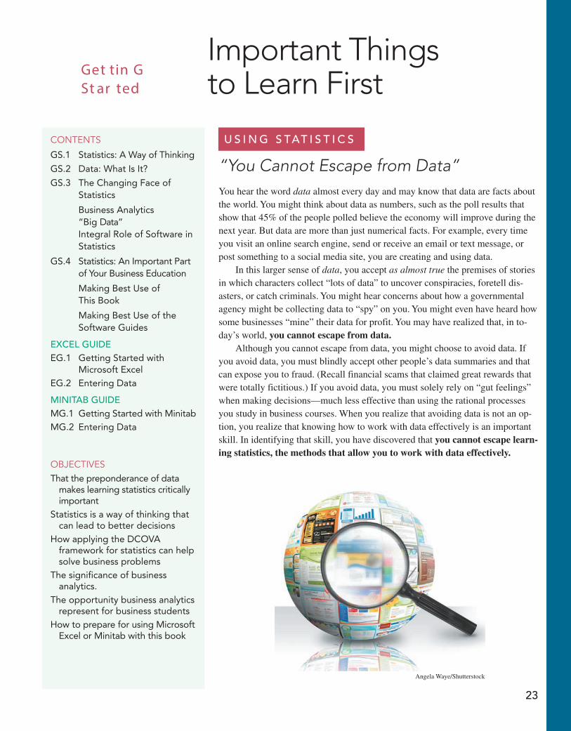
“You Cannot Escape from Data”You hear the word data almost every day and may know that data are facts about the world. You might think about data as numbers, such as the poll results that show that 45% of the people polled believe the economy will improve during the next year. But data are more than just numerical facts. For example, every time you visit an online search engine, send or receive an email or text message, or post something to a social media site, you are creating and using data.
In this larger sense of data, you accept as almost true the premises of stories in which characters collect “lots of data” to uncover conspiracies, foretell dis-asters, or catch criminals. You might hear concerns about how a governmental agency might be collecting data to “spy” on you. You might even have heard how some businesses “mine” their data for profit. You may have realized that, in to-day’s world, you cannot escape from data.
Although you cannot escape from data, you might choose to avoid data. If you avoid data, you must blindly accept other people’s data summaries and that can expose you to fraud. (Recall financial scams that claimed great rewards that were totally fictitious.) If you avoid data, you must solely rely on “gut feelings” when making decisions—much less effective than using the rational processes you study in business courses. When you realize that avoiding data is not an op-tion, you realize that knowing how to work with data effectively is an important skill. In identifying that skill, you have discovered that you cannot escape learn-ing statistics, the methods that allow you to work with data effectively.
contents
GS.1 Statistics: A Way of Thinking
GS.2 Data: What Is It?
GS.3 The Changing Face of Statistics
Business Analytics “Big Data” Integral Role of Software in
Statistics
GS.4 Statistics: An Important Part of Your Business Education
Making Best Use of This Book
Making Best Use of the Software Guides
ExcEl gUidEEG.1 Getting Started with
Microsoft ExcelEG.2 Entering Data
Minitab gUidEMG.1 Getting Started with MinitabMG.2 Entering Data
objectivesThat the preponderance of data
makes learning statistics critically important
Statistics is a way of thinking that can lead to better decisions
How applying the DCOVA framework for statistics can help solve business problems
The significance of business analytics.
The opportunity business analytics represent for business students
How to prepare for using Microsoft Excel or Minitab with this book
Important Things to Learn First
Get tin G St ar ted
Angela Waye/Shutterstock
24 GettInG StARted Important things to Learn First
GS.1 Statistics: A Way of ThinkingStatistics are the methods that allow you to work with data effectively. these methods repre-sent a way of thinking that can help you make better decisions. If you ever created a chart to summarize data or calculated values such as averages to summarize data, you have used sta-tistics. But there’s even more to statistics than these commonly taught techniques, as a quick review of the detailed table of contents shows.
the statistics that you have learned at a lower grade level most likely required you to perform mathematical calculations. In contrast, businesses today rely on software to perform those calculations faster and more accurately than you could do by hand. In any case, compu-tation by software forms only part of one task of many when applying statistics. to best under-stand that statistics is a way of thinking, you need a framework that organizes the set of tasks that form statistics. One such framework is the DCOVA framework.
THE DCOVA FRAMEWORk
the tasks of dCOVA framework are:• Define the data that you want to study to solve a problem or meet an objective.• Collect the data from appropriate sources.• Organize the data collected by developing tables.• Visualize the data collected by developing charts.• Analyze the data collected to reach conclusions and present those results.
the tasks Define, Collect, Organize, Visualize, and Analyze help you to apply statistics to business decision making. You must always do the first two tasks first to have meaningful results, but, in practice, the order of the other three can vary and sometimes are done concur-rently. For example, certain ways of visualizing data help you to organize your data while per-forming preliminary analysis as well.
Using the dCOVA framework helps you to apply statistical methods to these four broad categories of business activities:
• Summarize and visualize business data • Reach conclusions from those data • Make reliable predictions about business activities • Improve business processes
throughout this book, and especially in the Using Statistics scenarios that begin the chapters, you will discover specific examples of how dCOVA helps you apply statistics. For example, in one chapter, you will learn how to demonstrate whether a marketing campaign has increased sales of a product, while in another you will learn how a television station can reduce unneces-sary labor expenses.
GS.2 Data: What Is It?defining data as just “facts about the world,” to quote the opening essay, can prove confus-ing as such facts could be singular, a value associated with something, or collective, a list of values associated with something. For example, “david Levine” is a singular fact, a coauthor of this book, whereas “david, Kathy, and david” is the collective list of authors of this book. Furthermore, if everything is data, how do you distinguish “david Levine” from “Business Statistics: A First Course,” two very different facts (coauthor and title) about this book. Stat-isticians avoid this confusion by using a more specific definition of data and by defining a second word, variable.
GS.2 data: What Is It? 25
Student TipBusiness convention places the data, or set of values, for a variable in a worksheet column. Because of this conven-tion, people sometimes use the word column as a substitute for variable.
VARIABlE
A characteristic of an item or individual.
DATA
the set of individual values associated with a variable.
think about characteristics that distinguish individuals in a human population. name, height, weight, eye color, marital status, adjusted gross income, and place of residence are all characteristics of an individual. All of these traits are possible variables that describe people.
defining a variable called author-name to be the first and last names of the authors of this text makes it clear that valid values would be “david Levine,” “Kathryn Szabat,” and “david Stephan” and not “Levine,” “Szabat,” and “Stephan.” Be careful of cultural or other assumptions in definitions—for example, is “last name” a family name, as is common usage in north America, or an individual’s own unique name, as is common usage in many Asian countries?
StatisticsHaving defined data, you can define the subject of this book, statistics as the methods that help transform data into useful information for decision makers. Statistics allows you to deter-mine whether your data represent information that could be used in making better decisions. therefore, statistics helps you determine whether differences in the numbers are meaningful in a significant way or are due to chance. to illustrate, consider the following news reports about various data findings:
• “Acceptable Online Ad Length Before Seeing Free Content” (USA Today, February 16, 2012, p. 1B) A survey of 1,179 adults 18 and over reported that 54% thought that 15 seconds was an acceptable online ad length before seeing free content.
• “6 New Facts About Facebook.” (Pew Research Center, bit.ly/lkENZcA, February 3, 2014) A survey reported that women were more likely than men to cite seeing photos or videos, sharing with many people at once, seeing entertaining or funny posts, learning about ways to help others, and receiving support from people in your network as reasons to use Facebook.
• “Follow the Tweets” (H. Rui, A. Whinston, and e. Winkler, The Wall Street Journal, november 30, 2009, p. R4) In this study, the authors found that the number of times a specific product was mentioned in comments in the twitter social messaging service could be used to make accurate predictions of sales trends for that product.
Without statistics, you cannot determine whether the “numbers” in these stories represent use-ful information. Without statistics, you cannot validate claims such as the claim that the num-ber of tweets can be used to predict the sales of certain products. And without statistics, you cannot see patterns that large amounts of data sometimes reveal.
In statistics, data are “the values associated with a trait or property that help distinguish the occurrences of something.” For example, the names “david Levine” and “Kathryn Szabat” are data because they are both values that help distinguish one of the authors of this book from another. In this book, data is always plural to remind you that data are a collection, or set, of values. While one could say that a single value, such as “david Levine,” is a datum, the phrases data point, observation, response, and single data value are more typically encountered.
A trait or property of something with which values (data) are associated is called a vari-able. For example, you might define the variables “coauthor” and “title” if you were defining data about a set of textbooks.
Substituting the word characteristic for the phrase “trait or property” and using the phrase “an item or individual” instead of the vague “something” produces the definitions of variable and data that this book uses.
26 GettInG StARted Important things to Learn First
When talking about statistics, you use the term descriptive statistics to refer to methods that primarily help summarize and present data. Counting physical objects in a kindergarten class may have been the first time you used a descriptive method. You use the term inferential statistics to refer to methods that use data collected from a small group to reach conclusions about a larger group. If you had formal statistics instruction in a lower grade, you were prob-ably mostly taught descriptive methods, the focus of the early chapters of this book, and you may be unfamiliar with many of the inferential methods discussed in later chapters.
GS.3 The Changing Face of Statisticsthe data from which the Using Statistics scenario notes you cannot “escape” has encouraged the increasing use of statistical methods that either did not exist, were not practical to do, or were not widely known in the past. these methods and changes in information and commu-nications technologies that you may have studied in another course have helped to extend the application of statistics in business and make statistical knowledge more critical to business success. this is the changing face of statistics.
Business AnalyticsOf all the recent changes that have made statistics more prominent and more important, the set of methods collectively known as business analytics best reflects this changing face of statistics. Business analytics combine traditional statistical methods with methods from man-agement science and information systems to form an interdisciplinary tool that supports fact-based management decision making. Business analytics enables you to:
• Use statistical methods to analyze and explore data to uncover unforeseen relationships. • Use management science methods to develop optimization models that support all levels
of management, from strategic planning to daily operations. • Use information systems methods to collect and process data sets of all sizes, including
very large data sets that would otherwise be hard to examine efficiently.
even if you have never heard of the term business analytics, you may be familiar with the application of these methods. Headlines about governmental agencies mining personal data to combat crime or terrorism, stories about how companies learn your secrets, including the example memorably summarized as “How target Knows You’re Pregnant” (a bit of an over-statement), or even discussions about how social media or streaming media companies recom-mend choices to their users or sell advertisements to display to particular users, all reflect this changing face of statistics.
“Big Data”the data from which you cannot “escape” has taken new forms in recent years, including the form known as big data. Big data are the collections of data that cannot be easily browsed or analyzed using traditional methods.
Big data lacks a more precise operational definition, but using the term implies data that are being collected in huge volumes and at very fast rates (typically in near real-time) as well as data that takes a variety of forms other than the traditional structured forms such as data processing records, files, and tables. these attributes of “volume, velocity, and variety” (see reference 4) help distinguish “big data” from a set of data that happens to be “large” but that can be placed into a file that contains repeating records or rows that share the same arrange-ment or structure.
Big data presents opportunities to gain new management insights or extract value from the data resources of a business (see reference 7). Businesses gain these new insights or value through statistics, especially through the application of the newer methods of business analytics.
GS.4 Statistics: An Important Part of Your Business education 27
Integral Role of Software in StatisticsSection GS.1 notes that businesses rely on software to perform statistical calculations faster and more accurately than you could do by hand. Consistent to this observation, this book em-phasizes the interpretation of statistical results generated by software over the hand calculation of those results. the book uses both Microsoft excel and Minitab to generate those results and show in a larger way how software is integral to applying statistical methods to business deci-sion making.
Both excel and Minitab use worksheets to store data for analysis. Worksheets are tabular arrangements of data, in which the intersections of rows and columns form cells, boxes into which you make entries. In Minitab and excel, you use columns of cells to enter the data for variables, using one column for each variable. typically to use a statistical method in either program, you select one or more columns of data (one or more variables) and then apply the appropriate program function. this means the examples and problems found in this book use traditional structured data and not collections of data that could be considered big data. not to worry, learning with structured data will allow you to master statistical principles that you can apply later when using big data.
GS.4 Statistics: An Important Part of Your Business Education
the changing face of statistics means that statistics has become a very important part of your business education. In the current data-driven environment of business, you need general ana-lytical skills that allow you to manipulate data, interpret analytical results, and incorporate results in a variety of decision-making applications, such as accounting, finance, HR manage-ment, marketing, strategy and planning, and supply chain management.
the decisions you make will be increasingly based on data and not on gut or intuition sup-ported by personal experience. data-guided practice is proving to be successful; studies have shown an increase in productivity, innovation, and competition for organizations that embrace business analytics. the use of data and data analysis to drive business decisions cannot be ignored. Having a well-balanced mix of technical skills—such as statistics, modeling, and ba-sic information technology skills—and managerial skills—such as business acumen, problem-solving skills, and communication skills—will best prepare you for today’s, and tomorrow’s, workplace (see reference 1).
Business students once considered statistics to be merely a required course that contained content unrelated to their own majors. If you opened this book and had similar thoughts, you were overlooking the changing face of statistics. Use this book to better understand the impli-cations of this change as you learn to use the dCOVA framework to apply statistical methods to the four categories of business activities listed in Section GS.1.
Making Best Use of This Bookthis book uses the dCOVA framework to organize and present its statistical content. to make best use of this book, first make sure you understand the dCOVA framework (see page 24). With that knowledge, you can group the chapters of this book as follows:
• Chapter 1: the Define and Collect tasks, the mandatory starting tasks for applying a sta-tistical method.
• Chapters 2 and 3: the Organize and Visualize tasks that help summarize and visualize business data (the first activity listed on page 24).
• Chapter 3 (again) and Chapters 4 through 11: the Analyze task methods that use sample data to help reach conclusions about populations (the second activity listed on page 24).
• Chapters 12 and 13: the Analyze task methods that help make reliable predictions (the third activity).
• Online Chapter 14: the Analyze task methods that help you improve business processes (the fourth activity).
Student TipThe names of Excel and Minitab files that contain the data for examples and problems appear in this distinctive type face Retirement Funds throughout this book.
Student TipDon’t worry if your course does not cover every section of every chapter. Introductory business statistics courses vary in terms of scope, length, and number of college credits earned. Your functional area of study or major may also affect what you learn.
28 GettInG StARted Important things to Learn First
to get the most from every chapter, first read the opening Using Statistics scenarios. each chapter’s scenario always describes a business situation in which the methods about to be dis-cussed in the chapter could be used to help resolve issues or problems that the scenario de-scribed. Scenarios are the source of many of the in-chapter examples used to discuss statistical methods. At the end of each chapter, a “revisited” section reviews how the chapter’s statistical methods would help solve the issues and problems raised initially in the opening scenario.
each chapter fully integrates Microsoft excel and Minitab illustrations with its examples, reflecting the integral role that software plays in applying statistical methods to business deci-sion making. each chapter concludes with software guides (discussed separately below) that contain how-to instructions for using excel or Minitab for the statistical topic the chapter dis-cusses.
each chapter also ends with a summary and a list of key equations and key terms that help you review what you have learned. “Checking Your Understanding” questions test your understanding of basic concepts and “Chapter Review Problems” allow you to practice what you have learned.
As you read through a chapter you will find pointers to supplemental material available online, end-of-section questions and problems as well as these recurring features:
• Student Tips that help clarify and reinforce significant details about particular statistical concepts (such as the tip that occurs on this page).
• Visual Explorations that allow you to interactively explore statistical concepts in Microsoft excel.
• “Think About This” essays that further explore statistical concepts.
You can enhance your analytic and communication skills by making best use of the many case studies found in this book. the continuing case Managing Ashland MultiComm Services appears in most chapters and asks you to use your analytic skills to help solve problems man-agers of a residential telecommunications provider face. Cases unique to a chapter or a subset of chapters provide report-writing practice and additional problem-solving opportunities. the unique “digital Cases” additionally challenge you to use statistical principles to sort through claims found in various documents to uncover which claims are well supported and which ones are dubious, at best.
Making Best Use of the Software Guidesto make best use of software guides, read the getting started information that appears later in this chapter for the program you will be using and complete the table GS.1 checklist. the software how-to guides presume you already have awareness of basic computing concepts and skills such as mouse operations and interacting with windows and dialog boxes. Software guides use the following conventions in their instructions:
• things to type and where to type them appear in boldface. (enter 450 in cell B5.) • names of special keys are capitalized and in boldface. (Press Enter.) • targets of click or select operations appear in boldface. (Click OK. Select the first 2-D
Bar gallery item.) • When instructions require you to press more than one key at the same time, all keys are
shown capitalized and in boldface and are joined together with the “+” symbol. (Press Ctrl+C. Press Ctrl+Shift+Enter. Press Command+Enter.)
• Consecutive menu or ribbon selections are shown capitalized, mixed case, and in bold-face, joined together with the ➔ symbol. (Select File ➔ New. Select Stat ➔ Tables ➔ Tally Individual Variables.)
• Specific names of excel and Minitab functions, worksheets, or files are shown capital-ized, mixed case, and in boldface. (Open to the DATA worksheet of the Retirement Funds workbook.)
• Placeholder objects that express the general case of an instruction appear in italics and in boldface. example: Use AVERAGE(cell range of variable) to compute the mean of a numerical variable.
Student TipIf you need to review these skills, read Basic Computing Skills, a PDF file that you can download using instruc-tions found in Appendix C.
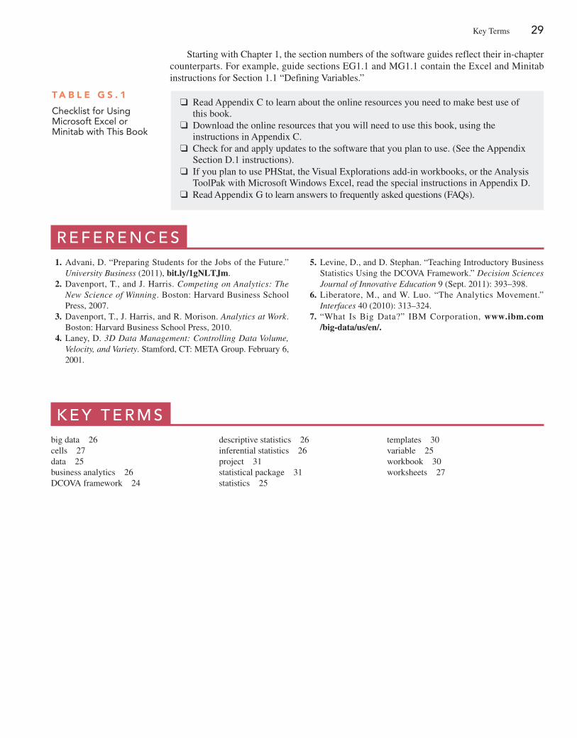
Key terms 29
T A B l e G S . 1
Checklist for Using Microsoft Excel or Minitab with This Book
❑ Read Appendix C to learn about the online resources you need to make best use of this book.
❑ download the online resources that you will need to use this book, using the instructions in Appendix C.
❑ Check for and apply updates to the software that you plan to use. (See the Appendix Section d.1 instructions).
❑ If you plan to use PHStat, the Visual explorations add-in workbooks, or the Analysis toolPak with Microsoft Windows excel, read the special instructions in Appendix d.
❑ Read Appendix G to learn answers to frequently asked questions (FAQs).
r E f E r E n c E s 1. Advani, d. “Preparing Students for the Jobs of the Future.”
University Business (2011), bit.ly/1gNLTJm. 2. davenport, t., and J. Harris. Competing on Analytics: The
New Science of Winning. Boston: Harvard Business School Press, 2007.
3. davenport, t., J. Harris, and R. Morison. Analytics at Work. Boston: Harvard Business School Press, 2010.
4. Laney, d. 3D Data Management: Controlling Data Volume, Velocity, and Variety. Stamford, Ct: MetA Group. February 6, 2001.
5. Levine, d., and d. Stephan. “teaching Introductory Business Statistics Using the dCOVA Framework.” Decision Sciences Journal of Innovative Education 9 (Sept. 2011): 393–398.
6. Liberatore, M., and W. Luo. “the Analytics Movement.” Interfaces 40 (2010): 313–324.
7. “What Is Big data?” IBM Corporation, www.ibm.com /big-data/us/en/.
K E y t E r M sbig data 26cells 27data 25business analytics 26dCOVA framework 24
descriptive statistics 26inferential statistics 26project 31statistical package 31statistics 25
templates 30variable 25workbook 30worksheets 27
Starting with Chapter 1, the section numbers of the software guides reflect their in-chapter counterparts. For example, guide sections eG1.1 and MG1.1 contain the excel and Minitab instructions for Section 1.1 “defining Variables.”
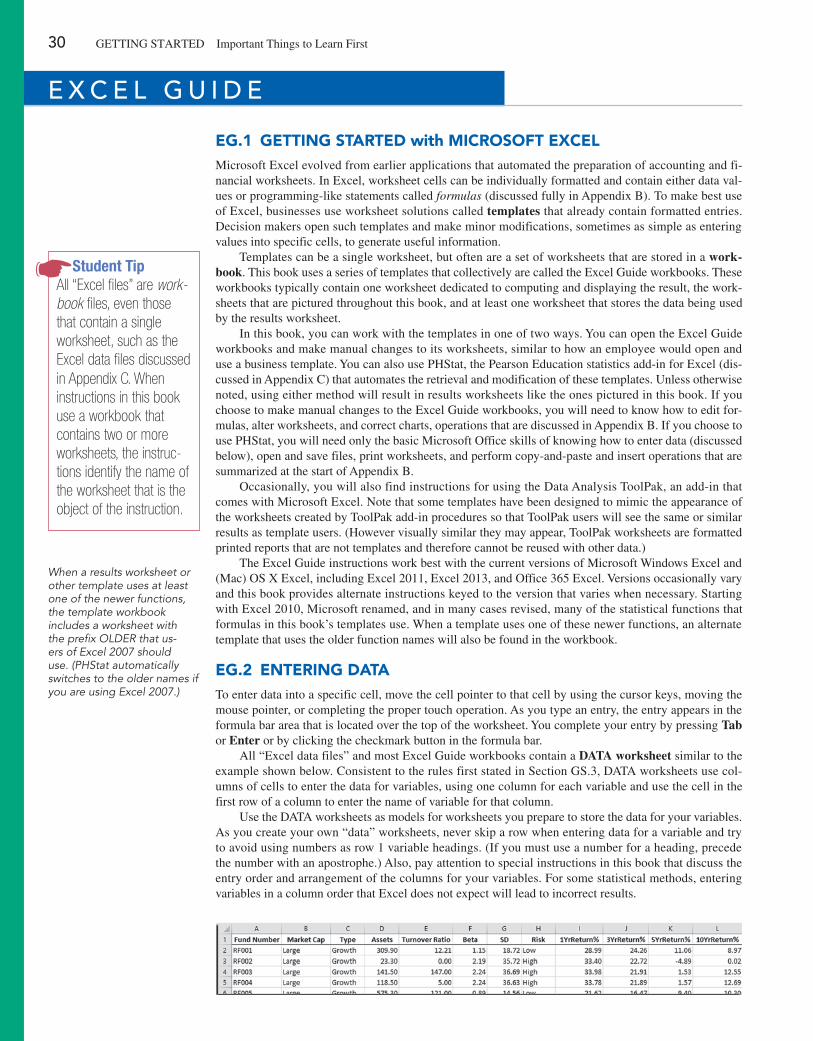
30 GettInG StARted Important things to Learn First
E x c E l g U i d E
eG.1 GeTTInG STARTeD with MIcRoSoFT excelMicrosoft excel evolved from earlier applications that automated the preparation of accounting and fi-nancial worksheets. In excel, worksheet cells can be individually formatted and contain either data val-ues or programming-like statements called formulas (discussed fully in Appendix B). to make best use of excel, businesses use worksheet solutions called templates that already contain formatted entries. decision makers open such templates and make minor modifications, sometimes as simple as entering values into specific cells, to generate useful information.
templates can be a single worksheet, but often are a set of worksheets that are stored in a work-book. this book uses a series of templates that collectively are called the excel Guide workbooks. these workbooks typically contain one worksheet dedicated to computing and displaying the result, the work-sheets that are pictured throughout this book, and at least one worksheet that stores the data being used by the results worksheet.
In this book, you can work with the templates in one of two ways. You can open the excel Guide workbooks and make manual changes to its worksheets, similar to how an employee would open and use a business template. You can also use PHStat, the Pearson education statistics add-in for excel (dis-cussed in Appendix C) that automates the retrieval and modification of these templates. Unless otherwise noted, using either method will result in results worksheets like the ones pictured in this book. If you choose to make manual changes to the excel Guide workbooks, you will need to know how to edit for-mulas, alter worksheets, and correct charts, operations that are discussed in Appendix B. If you choose to use PHStat, you will need only the basic Microsoft Office skills of knowing how to enter data (discussed below), open and save files, print worksheets, and perform copy-and-paste and insert operations that are summarized at the start of Appendix B.
Occasionally, you will also find instructions for using the data Analysis toolPak, an add-in that comes with Microsoft excel. note that some templates have been designed to mimic the appearance of the worksheets created by toolPak add-in procedures so that toolPak users will see the same or similar results as template users. (However visually similar they may appear, toolPak worksheets are formatted printed reports that are not templates and therefore cannot be reused with other data.)
the excel Guide instructions work best with the current versions of Microsoft Windows excel and (Mac) OS X excel, including excel 2011, excel 2013, and Office 365 excel. Versions occasionally vary and this book provides alternate instructions keyed to the version that varies when necessary. Starting with excel 2010, Microsoft renamed, and in many cases revised, many of the statistical functions that formulas in this book’s templates use. When a template uses one of these newer functions, an alternate template that uses the older function names will also be found in the workbook.
eG.2 enTeRInG DATAto enter data into a specific cell, move the cell pointer to that cell by using the cursor keys, moving the mouse pointer, or completing the proper touch operation. As you type an entry, the entry appears in the formula bar area that is located over the top of the worksheet. You complete your entry by pressing Tab or Enter or by clicking the checkmark button in the formula bar.
All “excel data files” and most excel Guide workbooks contain a DATA worksheet similar to the example shown below. Consistent to the rules first stated in Section GS.3, dAtA worksheets use col-umns of cells to enter the data for variables, using one column for each variable and use the cell in the first row of a column to enter the name of variable for that column.
Use the dAtA worksheets as models for worksheets you prepare to store the data for your variables. As you create your own “data” worksheets, never skip a row when entering data for a variable and try to avoid using numbers as row 1 variable headings. (If you must use a number for a heading, precede the number with an apostrophe.) Also, pay attention to special instructions in this book that discuss the entry order and arrangement of the columns for your variables. For some statistical methods, entering variables in a column order that excel does not expect will lead to incorrect results.
Student TipAll “Excel files” are work-book files, even those that contain a single worksheet, such as the Excel data files discussed in Appendix C. When instructions in this book use a workbook that contains two or more worksheets, the instruc-tions identify the name of the worksheet that is the object of the instruction.
When a results worksheet or other template uses at least one of the newer functions, the template workbook includes a worksheet with the prefix OLDER that us-ers of Excel 2007 should use. (PHStat automatically switches to the older names if you are using Excel 2007.)
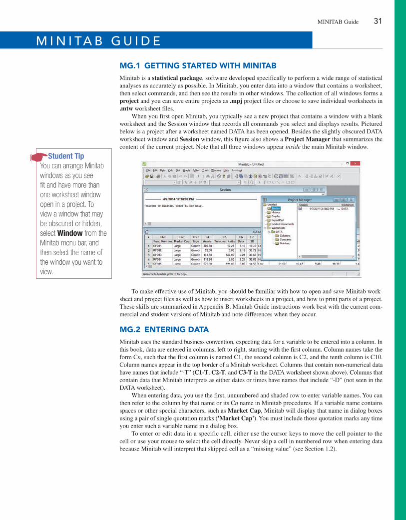
MInItAB Guide 31
Student TipYou can arrange Minitab windows as you see fit and have more than one worksheet window open in a project. To view a window that may be obscured or hidden, select Window from the Minitab menu bar, and then select the name of the window you want to view.
M i n i ta b g U i d E
MG.1 GeTTInG STARTeD wITh MInITABMinitab is a statistical package, software developed specifically to perform a wide range of statistical analyses as accurately as possible. In Minitab, you enter data into a window that contains a worksheet, then select commands, and then see the results in other windows. the collection of all windows forms a project and you can save entire projects as .mpj project files or choose to save individual worksheets in .mtw worksheet files.
When you first open Minitab, you typically see a new project that contains a window with a blank worksheet and the Session window that records all commands you select and displays results. Pictured below is a project after a worksheet named dAtA has been opened. Besides the slightly obscured dAtA worksheet window and Session window, this figure also shows a Project Manager that summarizes the content of the current project. note that all three windows appear inside the main Minitab window.
to make effective use of Minitab, you should be familiar with how to open and save Minitab work-sheet and project files as well as how to insert worksheets in a project, and how to print parts of a project. these skills are summarized in Appendix B. Minitab Guide instructions work best with the current com-mercial and student versions of Minitab and note differences when they occur.
MG.2 enTeRInG DATAMinitab uses the standard business convention, expecting data for a variable to be entered into a column. In this book, data are entered in columns, left to right, starting with the first column. Column names take the form Cn, such that the first column is named C1, the second column is C2, and the tenth column is C10. Column names appear in the top border of a Minitab worksheet. Columns that contain non-numerical data have names that include “-t” (C1-T, C2-T, and C3-T in the dAtA worksheet shown above). Columns that contain data that Minitab interprets as either dates or times have names that include “-d” (not seen in the dAtA worksheet).
When entering data, you use the first, unnumbered and shaded row to enter variable names. You can then refer to the column by that name or its Cn name in Minitab procedures. If a variable name contains spaces or other special characters, such as Market Cap, Minitab will display that name in dialog boxes using a pair of single quotation marks ('Market Cap'). You must include those quotation marks any time you enter such a variable name in a dialog box.
to enter or edit data in a specific cell, either use the cursor keys to move the cell pointer to the cell or use your mouse to select the cell directly. never skip a cell in numbered row when entering data because Minitab will interpret that skipped cell as a “missing value” (see Section 1.2).
32
U s i n g s tat i s t i c s
Beginning of the End … Or the End of the Beginning?The past few years have been challenging for Good Tunes & More (GT&M), a business that traces its roots to Good Tunes, a store that exclusively sold music CDs and vinyl records.
GT&M first broadened its merchandise to include home entertainment and computer systems (the “More”), and then undertook an expansion to take advantage of prime locations left empty by bankrupt former competitors. Today, GT&M finds itself at a crossroads. Hoped-for increases in revenues that have failed to occur and declining profit margins due to the competitive pressures of online sellers have led management to reconsider the future of the business.
While some investors in the business have argued for an orderly retreat, closing stores and limiting the variety of merchandise, GT&M CEO Emma Levia has decided to “double down” and expand the business by purchasing Whitney Wireless, a successful three-store chain that sells smartphones and other mobile devices.
Levia foresees creating a brand new “A-to-Z” electronics retailer but first must establish a fair and reasonable price for the privately held Whitney Wireless. To do so, she has asked a group of analysts to identify the data that would be helpful in setting a price for the wireless business. As part of that group, you quickly realize that you need the data that would help to verify the contents of the wireless company’s basic financial statements.
You focus on data associated with the company’s profit and loss statement and quickly realize the need for sales and expense- related variables. You begin to
think about what the data for such variables would look like and how to collect those data. You realize that you are starting to apply the DCOVA framework to the objective of helping Levia acquire Whitney Wireless.
Chapter Defining and Collecting Data1
Tyler Olson/Shutterstock
contents
1.1 Defining Variables
1.2 Collecting Data
1.3 Types of Sampling Methods
1.4 Types of Survey Errors
think aboUt this: New Media Surveys/Old Sampling Problems
Using statistics: Beginning of the End … Revisited
chapter 1 excel gUide
chapter 1 Minitab gUide
objectivesUnderstand issues that arise
when defining variables
How to define variables
How to collect data
Identify the different ways to collect a sample
Understand the types of survey errors
1.1 Defining Variables 33
W hen Emma Levia decides to purchase Whitney Wireless, she has defined a new goal or business objective for GT&M. Business objectives can arise from any level of management and can be as varied as the following:
• A marketing analyst needs to assess the effectiveness of a new online advertising cam-paign.
• A pharmaceutical company needs to determine whether a new drug is more effective than those currently in use.
• An operations manager wants to improve a manufacturing or service process. • An auditor needs to review a company’s financial transactions to determine whether the
company is in compliance with generally accepted accounting principles.
Establishing an objective marks the end of a problem definition process. This end triggers the new process of identifying the correct data to support the objective. In the GT&M scenario, having decided to buy Whitney Wireless, Levia needs to identify the data that would be helpful in setting a price for the wireless business. This process of identifying the correct data triggers the start of applying the tasks of the DCOVA framework. In other words, the end of problem definition marks the beginning of applying statistics to business decision making.
Identifying the correct data to support a business objective is a two-part job that requires defining variables and collecting the data for those variables. These tasks are the first two tasks of the DCOVA framework first defined in Section GS.1 and which can be restated here as:
• Define the variables that you want to study to solve a problem or meet an objective. • Collect the data for those variables from appropriate sources.
This chapter discusses these two tasks which must always be done before the Organize, Visu-alize, and Analyze tasks.
Defining variables at first may seem to be the simple process of making the list of things one needs to help solve a problem or meet an objective. However, consider the GT&M scenario. Most would quickly agree that yearly sales of Whitney Wireless would be part of the data needed to meet Levia’s objective, but just placing “yearly sales” on a list could lead to confu-sion and miscommunication: Does this variable refer to sales per year for the entire chain or for individual stores? Does the variable refer to net or gross sales? Are the yearly sales values expressed in number of units or as currency amounts such as U.S. dollar sales?
These questions illustrate that for each variable of interest that you identify you must sup-ply an operational definition, a universally accepted meaning that is clear to all associated with an analysis. Operational definitions should also classify the variable, as explained in the next section, and may include additional facts such as units of measures, allowed range of values, and definitions of specific variable values, depending on how the variable is classified.
Classifying Variables by TypeWhen you operationally define a variable, you must classify the variable as being either cate-gorical or numerical. Categorical variables (also known as qualitative variables) take catego-ries as their values. Numerical variables (also known as quantitative variables) have values that represent a counted or measured quantity. Classification also affects a variable’s operational definition and getting the classification correct is important because certain statistical methods can be applied correctly to one type or the other, while other methods may need a specific mix of variable types.
Categorical variables can take the form of yes-and-no questions such as “Do you have a Twitter account?” (in which yes and no form the variable’s two categories) or describe a trait or characteristic that has many categories such as undergraduate class standing (which might have the defined categories freshman, sophomore, junior, and senior). When defining a cat-egorical variable, the list of permissible category values must be included and each category
1.1 Defining VariablesStudent Tip
Providing operational definitions for concepts is important, too, when writing a textbook! The end-of-chapter Key Terms gives you an index of operational definitions and the most funda-mental definitions are presented in boxes such as the page 25 box that defines variable and data.
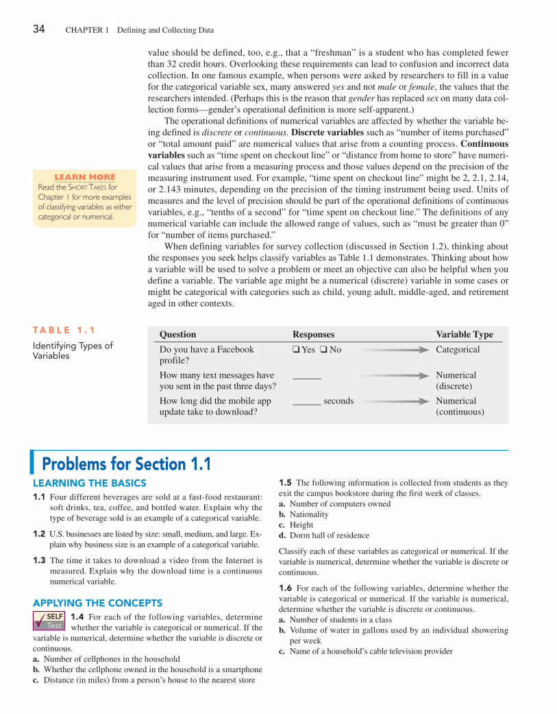
34 CHApTEr 1 Defining and Collecting Data
value should be defined, too, e.g., that a “freshman” is a student who has completed fewer than 32 credit hours. Overlooking these requirements can lead to confusion and incorrect data collection. In one famous example, when persons were asked by researchers to fill in a value for the categorical variable sex, many answered yes and not male or female, the values that the researchers intended. (perhaps this is the reason that gender has replaced sex on many data col-lection forms—gender’s operational definition is more self-apparent.)
The operational definitions of numerical variables are affected by whether the variable be-ing defined is discrete or continuous. Discrete variables such as “number of items purchased” or “total amount paid” are numerical values that arise from a counting process. Continuous variables such as “time spent on checkout line” or “distance from home to store” have numeri-cal values that arise from a measuring process and those values depend on the precision of the measuring instrument used. For example, “time spent on checkout line” might be 2, 2.1, 2.14, or 2.143 minutes, depending on the precision of the timing instrument being used. Units of measures and the level of precision should be part of the operational definitions of continuous variables, e.g., “tenths of a second” for “time spent on checkout line.” The definitions of any numerical variable can include the allowed range of values, such as “must be greater than 0” for “number of items purchased.”
When defining variables for survey collection (discussed in Section 1.2), thinking about the responses you seek helps classify variables as Table 1.1 demonstrates. Thinking about how a variable will be used to solve a problem or meet an objective can also be helpful when you define a variable. The variable age might be a numerical (discrete) variable in some cases or might be categorical with categories such as child, young adult, middle-aged, and retirement aged in other contexts.
Problems for Section 1.1Learning The BaSiCS1.1 Four different beverages are sold at a fast-food restaurant:
soft drinks, tea, coffee, and bottled water. Explain why the type of beverage sold is an example of a categorical variable.
1.2 U.S. businesses are listed by size: small, medium, and large. Ex-plain why business size is an example of a categorical variable.
1.3 The time it takes to download a video from the Internet is measured. Explain why the download time is a continuous numerical variable.
aPPLying The ConCePTSSELF Test
1.4 For each of the following variables, determine whether the variable is categorical or numerical. If the
variable is numerical, determine whether the variable is discrete or continuous.a. Number of cellphones in the householdb. Whether the cellphone owned in the household is a smartphonec. Distance (in miles) from a person’s house to the nearest store
1.5 The following information is collected from students as they exit the campus bookstore during the first week of classes.a. Number of computers ownedb. Nationalityc. Heightd. Dorm hall of residence
Classify each of these variables as categorical or numerical. If the variable is numerical, determine whether the variable is discrete or continuous.
1.6 For each of the following variables, determine whether the variable is categorical or numerical. If the variable is numerical, determine whether the variable is discrete or continuous.a. Number of students in a classb. Volume of water in gallons used by an individual showering
per weekc. Name of a household’s cable television provider
Learn MoreRead the Short takeS for Chapter 1 for more examples of classifying variables as either categorical or numerical.
T a B L e 1 . 1
Identifying Types of Variables
Question Responses Variable Type
Do you have a Facebook profile?
❑ Yes ❑ No Categorical
How many text messages have you sent in the past three days?
______ Numerical (discrete)
How long did the mobile app update take to download?
______ seconds Numerical (continuous)
1.2 Collecting Data 35
1.2 Collecting DataAfter defining the variables that you want to study, you can proceed with the data collection task. Collecting data is a critical task because if you collect data that are flawed by biases, ambiguities, or other types of errors, the results you will get from using such data with even the most sophisticated statistical methods will be suspect or in error. (For a famous example of flawed data collection leading to incorrect results, read the Think About This essay on page 43.)
Data collection consists of identifying data sources, deciding whether the data you collect will be from a population or a sample, cleaning your data, and sometimes recoding variables. The rest of this section explains these aspects of data collection.
Data SourcesYou collect data from either primary or secondary data sources. You are using a primary data source if you collect your own data for analysis. You are using a secondary data source if the data for your analysis have been collected by someone else.
You collect data by using any of the following:
• Data distributed by an organization or individual • The outcomes of a designed experiment • The responses from a survey • The results of conducting an observational study • Data collected by ongoing business activities
Market research companies and trade associations distribute data pertaining to specific in-dustries or markets. Investment services provide business and financial data on publicly listed companies. Syndicated services such as The Nielsen Company provide consumer research data to telecom and mobile media companies. print and online media companies also distribute data that they may have collected themselves or may be republishing from other sources.
The outcomes of a designed experiment are a second data source. For example, a con-sumer electronics company might conduct an experiment that compares the sales of mobile electronics merchandise for different store locations. Note that developing a proper experi-mental design is mostly beyond the scope of this book, but Chapter 10 discusses some of the fundamental experimental design concepts.
Survey responses represent a third type of data source. people being surveyed are asked questions about their beliefs, attitudes, behaviors, and other characteristics. For example, people could be asked which store location for mobile electronics merchandise is preferable. (Such a survey could lead to data that differ from the data collected from the outcomes of the
1.7 For each of the following variables, determine whether the variable is categorical or numerical. If the variable is numerical, determine whether the variable is discrete or continuous.a. Number of shopping trips a person made in the past month b. A person’s preferred brand of coffeec. Time a person spent on exercising in the past month
1.8 Suppose the following information is collected from Simon Walter on his application for a home mortgage loan.a. Annual personal income: $216,370b. Number of times married: 1c. Ever convicted of a felony: Nod. Own a second car: No
Classify each of the responses by type of data.
1.9 One of the variables most often included in surveys is in-come. Sometimes the question is phrased “What is your income (in thousands of dollars)?” In other surveys, the respondent is
asked to “Select the circle corresponding to your income level” and is given a number of income ranges to choose from.a. In the first format, explain why income might be considered
either discrete or continuous.b. Which of these two formats would you prefer to use if you
were conducting a survey? Why?
1.10 If two students score a 90 on the same examination, what arguments could be used to show that the underlying variable—test score—is continuous?
1.11 The director of market research at a large department store chain wanted to conduct a survey throughout a metropolitan area to determine the amount of time working women spend shopping for clothing in a typical month.a. Indicate the type of data the director might want to collect.b. Develop a first draft of the questionnaire needed in (a) by writ-
ing three categorical questions and three numerical questions that you feel would be appropriate for this survey.
36 CHApTEr 1 Defining and Collecting Data
designed experiment of the previous paragraph.) Surveys can be affected by any of the four types of errors that are discussed in Section 1.4.
Observational study results are a fourth data source. A researcher collects data by directly observing a behavior, usually in a natural or neutral setting. Observational studies are a com-mon tool for data collection in business. For example, market researchers use focus groups to elicit unstructured responses to open-ended questions posed by a moderator to a target au-dience. Observational studies are also commonly used to enhance teamwork or improve the quality of products and services.
Data collected by ongoing business activities are a fifth data source. Such data can be collected from operational and transactional systems that exist in both physical “bricks-and-mortar” and online settings but can also be gathered from secondary sources such as third-party social media networks and online apps and website services that collect tracking and usage data. For example, a bank might analyze a decade’s worth of financial transaction data to identify patterns of fraud, and a marketer might use tracking data to determine the effectiveness of a website.
Sources for big data (see Section GS.3) tend to be a mix of primary and secondary sources of this last type. For example, a retailer interested in increasing sales might mine Facebook and Twitter accounts to identify sentiment about certain products or to pinpoint top influencers and then match those data to its own data collected during customer transactions.
Populations and SamplesYou collect your data from either a population or a sample. A population consists of all the items or individuals about which you want to reach conclusions. All the GT&M sales transac-tions for a specific year, all the full-time students enrolled in a college, and all the registered voters in Ohio are examples of populations. In Chapter 3, you will learn that when you analyze data from a population you compute parameters.
A sample is a portion of a population selected for analysis. The results of analyzing a sample are used to estimate characteristics of the entire population. From the three examples of populations just given, you could select a sample of 200 GT&M sales transactions randomly selected by an auditor for study, a sample of 50 full-time students selected for a marketing study, and a sample of 500 registered voters in Ohio contacted via telephone for a political poll. In each of these examples, the transactions or people in the sample represent a portion of the items or individuals that make up the population. In Chapter 3, you will learn that when you analyze data from a sample you compute statistics.
You collect data from a sample when any of the following applies:
• Selecting a sample is less time consuming than selecting every item in the population. • Selecting a sample is less costly than selecting every item in the population. • Analyzing a sample is less cumbersome and more practical than analyzing the entire
population.
Structured Versus Unstructured DataThe data you collect may be formatted in a variety of ways, some of which add to the data collection task. For example, suppose that you wanted to collect electronic financial data about a sample of companies. That data might exist as tables of data, the contents of stan-dardized documents such as fill-in-the-blank surveys, a continuous stream of data such as a stock ticker, or text messages or emails delivered from email systems or social media web-sites. Some of these forms, such as a set of text messages have very little or no repeating structure, are examples of unstructured data. Although unstructured data forms can form a part of a big data collection, collecting data in unstructured forms for the statistical methods discussed in this book requires conversion of the data to a structured form. For example, after collecting text messages, you could convert their contents to a structured form by de-fining a set of variables that might include a numerical variable that counts the number of words in the message and various categorical variables that help classify the content of the message.
Learn MoreRead the Short takeS for Chapter 1 for a further discussion about data sources.
Student TipTo help remember the difference between a sample and a popula-tion, think of a pie. The entire p ie represents the population, and the pie s lice that you select is the sample.
1.2 Collecting Data 37
electronic Formats and encodingsThe same form of data can exist in more than one electronic format, with some formats more immediately usable than others. For example, a table of data might exist as a scanned image or as data in a worksheet file. The worksheet data could be immediately used in a statistical analysis, but the scanned image would need to be first converted to worksheet data using a character-scanning program that can recognize numbers in an image.
Data can also be encoded in more than one way, as you may have learned in an infor-mation systems course. Different encodings may affect the recorded precision of values for continuous variables and lead to values more imprecise or values that convey a false sense of precision, such as a time measurement that gets encoded in ten-thousandths of a second when the original measurement was only in tenths of a second. This changed precision can violate the operational definition of a continuous variable and sometimes affect results calculated.
Data CleaningWhatever ways you choose to collect data, you may find irregularities in the values you collect such as undefined or impossible values. For a categorical variable, an undefined value would be a value that does not represent one of the categories defined for the variable. For a numeri-cal variable, an impossible value would be a value that falls outside a defined range of possible values for the variable. For a numerical variable without a defined range of possible values, you might also find outliers, values that seem excessively different from most of the rest of the values. Such values may or may not be errors, but they demand a second review.
Values that are missing are another type of irregularity. A missing value is a value that was not able to be collected (and therefore not available to be analyzed). For example, you would record a nonresponse to a survey question as a missing value. You can represent missing values in Minitab by using an asterisk value for a numerical variable or by using a blank value for a categorical variable, and such values will be properly excluded from analysis. The more lim-ited Excel has no special values that represent a missing value. When using Excel, you must find and then exclude missing values manually.
When you spot an irregularity in the data you have collected, you may have to “clean” the data. Although a full discussion of data cleaning is beyond the scope of this book (see refer-ence 8), you can learn more about the ways you can use Excel or Minitab for data cleaning in the Short Takes for Chapter 1.
recoding VariablesAfter you have collected data, you may discover that you need to reconsider the categories that you have defined for a categorical variable or that you need to transform a numerical variable into a categorical variable by assigning the individual numeric data values to one of several groups. In either case, you can define a recoded variable that supplements or replaces the original variable in your analysis.
For example, having already defined the variable undergraduate class standing with the catego-ries freshmen, sophomore, junior, and senior, you realize that you are more interested in investigat-ing the differences between lowerclassmen (defined as freshman or sophomore) and upperclassmen (junior or senior). You can create a new variable UpperLower and assign the value Upper if a student is a junior or senior and assign the value Lower if the student is a freshman or sophomore.
When recoding variables, be sure that the category definitions cause each data value to be placed in one and only one category, a property known as being mutually exclusive. Also ensure that the set of categories you create for the new, recoded variables include all the data values being recoded, a property known as being collectively exhaustive. If you are recoding a categorical variable, you can preserve one or more of the original categories, as long as your recodings are both mutually exclusive and collectively exhaustive.
When recoding numerical variables, pay particular attention to the operational definitions of the categories you create for the recoded variable, especially if the categories are not self-defining ranges. For example, while the recoded categories Under 12, 12–20, 21–34, 35–54, and 55 and Over are self-defining for age, the categories Child, Youth, Young Adult, Middle Aged, and Senior need their own operational definitions.
Student TipWhile encoding issues go beyond the scope of this book, the Short Takes for Chapter 1 includes an experiment that you can perform in either Microsoft Excel or Minitab that illustrates how data encoding can affect the precision of values.
Data cleaning will not be necessary when you use the (previously cleaned) data for the examples and problems in this book.
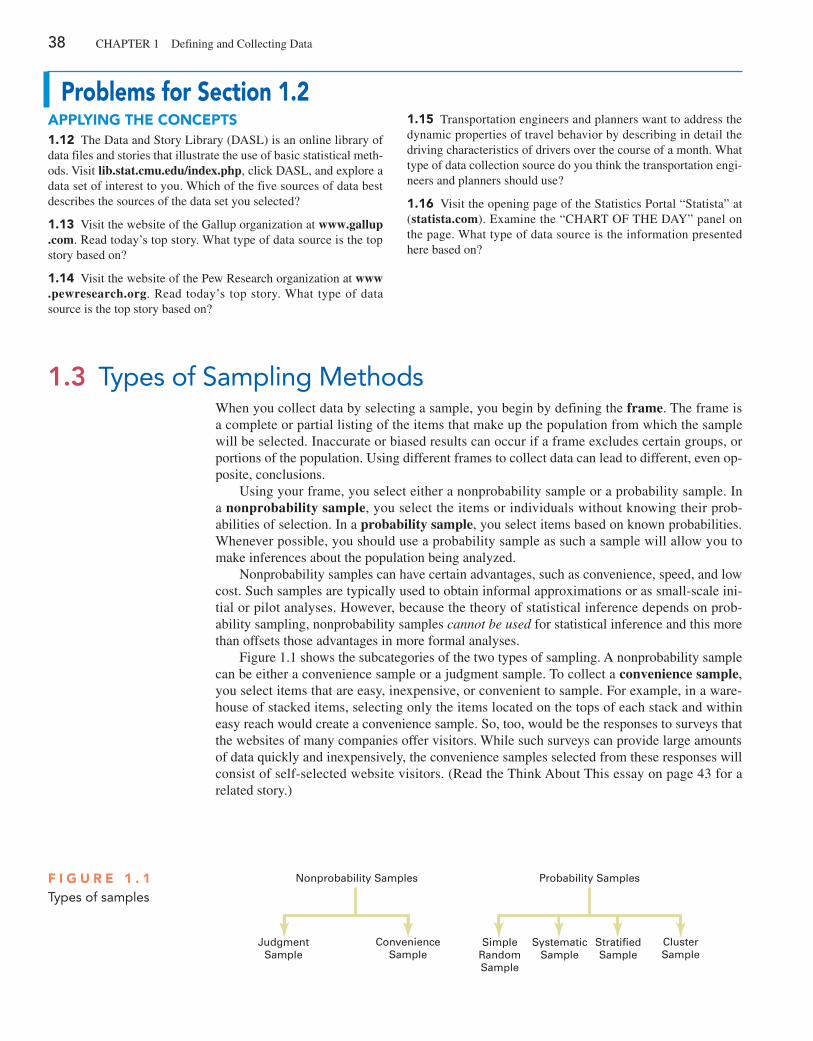
38 CHApTEr 1 Defining and Collecting Data
Problems for Section 1.2aPPLying The ConCePTS1.12 The Data and Story Library (DASL) is an online library of data files and stories that illustrate the use of basic statistical meth-ods. Visit lib.stat.cmu.edu/index.php, click DASL, and explore a data set of interest to you. Which of the five sources of data best describes the sources of the data set you selected?
1.13 Visit the website of the Gallup organization at www.gallup .com. read today’s top story. What type of data source is the top story based on?
1.14 Visit the website of the pew research organization at www .pewresearch.org. read today’s top story. What type of data source is the top story based on?
1.15 Transportation engineers and planners want to address the dynamic properties of travel behavior by describing in detail the driving characteristics of drivers over the course of a month. What type of data collection source do you think the transportation engi-neers and planners should use?
1.16 Visit the opening page of the Statistics portal “Statista” at (statista.com). Examine the “CHArT OF THE DAY” panel on the page. What type of data source is the information presented here based on?
When you collect data by selecting a sample, you begin by defining the frame. The frame is a complete or partial listing of the items that make up the population from which the sample will be selected. Inaccurate or biased results can occur if a frame excludes certain groups, or portions of the population. Using different frames to collect data can lead to different, even op-posite, conclusions.
Using your frame, you select either a nonprobability sample or a probability sample. In a nonprobability sample, you select the items or individuals without knowing their prob-abilities of selection. In a probability sample, you select items based on known probabilities. Whenever possible, you should use a probability sample as such a sample will allow you to make inferences about the population being analyzed.
Nonprobability samples can have certain advantages, such as convenience, speed, and low cost. Such samples are typically used to obtain informal approximations or as small-scale ini-tial or pilot analyses. However, because the theory of statistical inference depends on prob-ability sampling, nonprobability samples cannot be used for statistical inference and this more than offsets those advantages in more formal analyses.
Figure 1.1 shows the subcategories of the two types of sampling. A nonprobability sample can be either a convenience sample or a judgment sample. To collect a convenience sample, you select items that are easy, inexpensive, or convenient to sample. For example, in a ware-house of stacked items, selecting only the items located on the tops of each stack and within easy reach would create a convenience sample. So, too, would be the responses to surveys that the websites of many companies offer visitors. While such surveys can provide large amounts of data quickly and inexpensively, the convenience samples selected from these responses will consist of self-selected website visitors. (read the Think About This essay on page 43 for a related story.)
1.3 Types of Sampling Methods
F i g U r e 1 . 1Types of samples
Nonprobability Samples
JudgmentSample
SystematicSample
StratiedSample
SimpleRandomSample
ClusterSample
Probability Samples
ConvenienceSample
1.3 Types of Sampling Methods 39
To collect a judgment sample, you collect the opinions of preselected experts in the sub-ject matter. Although the experts may be well informed, you cannot generalize their results to the population.
The types of probability samples most commonly used include simple random, system-atic, stratified, and cluster samples. These four types of probability samples vary in terms of cost, accuracy, and complexity, and they are the subject of the rest of this section.
Simple random SampleIn a simple random sample, every item from a frame has the same chance of selection as ev-ery other item, and every sample of a fixed size has the same chance of selection as every other sample of that size. Simple random sampling is the most elementary random sampling tech-nique. It forms the basis for the other random sampling techniques. However, simple random sampling has its disadvantages. Its results are often subject to more variation than other sam-pling methods. In addition, when the frame used is very large, carrying out a simple random sample may be time consuming and expensive.
With simple random sampling, you use n to represent the sample size and N to represent the frame size. You number every item in the frame from 1 to N. The chance that you will se-lect any particular member of the frame on the first selection is 1>N.
You select samples with replacement or without replacement. Sampling with replace-ment means that after you select an item, you return it to the frame, where it has the same probability of being selected again. Imagine that you have a fishbowl containing N business cards, one card for each person. On the first selection, you select the card for Grace Kim. You record pertinent information and replace the business card in the bowl. You then mix up the cards in the bowl and select a second card. On the second selection, Grace Kim has the same probability of being selected again, 1>N. You repeat this process until you have selected the desired sample size, n.
Typically, you do not want the same item or individual to be selected again in a sam-ple. Sampling without replacement means that once you select an item, you cannot select it again. The chance that you will select any particular item in the frame—for example, the business card for Grace Kim—on the first selection is 1>N. The chance that you will select any card not previously chosen on the second selection is now 1 out of N - 1. This process contin-ues until you have selected the desired sample of size n.
When creating a simple random sample, you should avoid the “fishbowl” method of se-lecting a sample because this method lacks the ability to thoroughly mix the cards and, there-fore, randomly select a sample. You should use a more rigorous selection method.
One such method is to use a table of random numbers, such as Table E.1 in Appendix E, for selecting the sample. A table of random numbers consists of a series of digits listed in a randomly generated sequence. To use a random number table for selecting a sample, you first need to assign code numbers to the individual items of the frame. Then you generate the random sample by reading the table of random numbers and selecting those individuals from the frame whose assigned code numbers match the digits found in the table. Because the num-ber system uses 10 digits 10, 1, 2, c , 92 , the chance that you will randomly generate any particular digit is equal to the probability of generating any other digit. This probability is 1 out of 10. Hence, if you generate a sequence of 800 digits, you would expect about 80 to be the digit 0, 80 to be the digit 1, and so on. Because every digit or sequence of digits in the table is random, the table can be read either horizontally or vertically. The margins of the table desig-nate row numbers and column numbers. The digits themselves are grouped into sequences of five in order to make reading the table easier.
Learn MoreLearn to use a table of random numbers to select a simple random sample in a Chapter 1 online section.
40 CHApTEr 1 Defining and Collecting Data
Systematic SampleIn a systematic sample, you partition the N items in the frame into n groups of k items, where
k =Nn
You round k to the nearest integer. To select a systematic sample, you choose the first item to be selected at random from the first k items in the frame. Then, you select the remaining n - 1 items by taking every kth item thereafter from the entire frame.
If the frame consists of a list of prenumbered checks, sales receipts, or invoices, taking a systematic sample is faster and easier than taking a simple random sample. A systematic sam-ple is also a convenient mechanism for collecting data from membership directories, electoral registers, class rosters, and consecutive items coming off an assembly line.
To take a systematic sample of n = 40 from the population of N = 800 full-time employ-ees, you partition the frame of 800 into 40 groups, each of which contains 20 employees. You then select a random number from the first 20 individuals and include every twentieth indi-vidual after the first selection in the sample. For example, if the first random number you select is 008, your subsequent selections are 028, 048, 068, 088, 108, c , 768, and 788.
Simple random sampling and systematic sampling are simpler than other, more sophisti-cated, probability sampling methods, but they generally require a larger sample size. In addi-tion, systematic sampling is prone to selection bias that can occur when there is a pattern in the frame. To overcome the inefficiency of simple random sampling and the potential selec-tion bias involved with systematic sampling, you can use either stratified sampling methods or cluster sampling methods.
Stratified SampleIn a stratified sample, you first subdivide the N items in the frame into separate subpopula-tions, or strata. A stratum is defined by some common characteristic, such as gender or year in school. You select a simple random sample within each of the strata and combine the results from the separate simple random samples. Stratified sampling is more efficient than either simple random sampling or systematic sampling because you are ensured of the representation of items across the entire population. The homogeneity of items within each stratum provides greater precision in the estimates of underlying population parameters. In addition, stratified sampling enables you to reach conclusions about each strata in the frame. However, using a stratified sample requires that you can determine the variable(s) on which to base the stratifica-tion and can also be expensive to implement.
Cluster SampleIn a cluster sample, you divide the N items in the frame into clusters that contain several items. Clusters are often naturally occurring groups, such as counties, election districts, city blocks, households, or sales territories. You then take a random sample of one or more clusters and study all items in each selected cluster.
Cluster sampling is often more cost-effective than simple random sampling, particularly if the population is spread over a wide geographic region. However, cluster sampling often re-quires a larger sample size to produce results as precise as those from simple random sampling or stratified sampling. A detailed discussion of systematic sampling, stratified sampling, and cluster sampling procedures can be found in references 2, 4, and 5.
Learn MoreLearn how to select a stratified sample in a Chapter 1 online section.
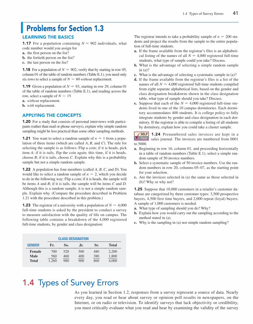
1.4 Types of Survey Errors 41
Problems for Section 1.3Learning The BaSiCS1.17 For a population containing N = 902 individuals, what code number would you assign fora. the first person on the list?b. the fortieth person on the list?c. the last person on the list?
1.18 For a population of N = 902, verify that by starting in row 05, column 01 of the table of random numbers (Table E.1), you need only six rows to select a sample of N = 60 without replacement.
1.19 Given a population of N = 93, starting in row 29, column 01 of the table of random numbers (Table E.1), and reading across the row, select a sample of N = 15a. without replacement.b. with replacement.
aPPLying The ConCePTS1.20 For a study that consists of personal interviews with partici-pants (rather than mail or phone surveys), explain why simple random sampling might be less practical than some other sampling methods.
1.21 You want to select a random sample of n = 1 from a popu-lation of three items (which are called A, B, and C). The rule for selecting the sample is as follows: Flip a coin; if it is heads, pick item A; if it is tails, flip the coin again; this time, if it is heads, choose B; if it is tails, choose C. Explain why this is a probability sample but not a simple random sample.
1.22 A population has four members (called A, B, C, and D). You would like to select a random sample of n = 2, which you decide to do in the following way: Flip a coin; if it is heads, the sample will be items A and B; if it is tails, the sample will be items C and D. Although this is a random sample, it is not a simple random sam-ple. Explain why. (Compare the procedure described in problem 1.21 with the procedure described in this problem.)
1.23 The registrar of a university with a population of N = 4,000 full-time students is asked by the president to conduct a survey to measure satisfaction with the quality of life on campus. The following table contains a breakdown of the 4,000 registered full-time students, by gender and class designation:
The registrar intends to take a probability sample of n = 200 stu-dents and project the results from the sample to the entire popula-tion of full-time students.a. If the frame available from the registrar’s files is an alphabeti-
cal listing of the names of all N = 4,000 registered full-time students, what type of sample could you take? Discuss.
b. What is the advantage of selecting a simple random sample in (a)?
c. What is the advantage of selecting a systematic sample in (a)?d. If the frame available from the registrar’s files is a list of the
names of all N = 4,000 registered full-time students compiled from eight separate alphabetical lists, based on the gender and class designation breakdowns shown in the class designation table, what type of sample should you take? Discuss.
e. Suppose that each of the N = 4,000 registered full-time stu-dents lived in one of the 10 campus dormitories. Each dormi-tory accommodates 400 students. It is college policy to fully integrate students by gender and class designation in each dor-mitory. If the registrar is able to compile a listing of all students by dormitory, explain how you could take a cluster sample.
SELF Test
1.24 prenumbered sales invoices are kept in a sales journal. The invoices are numbered from 0001
to 5000.a. Beginning in row 16, column 01, and proceeding horizontally
in a table of random numbers (Table E.1), select a simple ran-dom sample of 50 invoice numbers.
b. Select a systematic sample of 50 invoice numbers. Use the ran-dom numbers in row 20, columns 05–07, as the starting point for your selection.
c. Are the invoices selected in (a) the same as those selected in (b)? Why or why not?
1.25 Suppose that 10,000 customers in a retailer’s customer da-tabase are categorized by three customer types: 3,500 prospective buyers, 4,500 first time buyers, and 2,000 repeat (loyal) buyers. A sample of 1,000 customers is needed.a. What type of sampling should you do? Why?b. Explain how you would carry out the sampling according to the
method stated in (a).c. Why is the sampling in (a) not simple random sampling?
ClaSS DeSignaTion
genDer Fr. So. Jr. Sr. Total
Female 700 520 500 480 2,200Male 560 460 400 380 1,800Total 1,260 980 900 860 4,000
1.4 Types of Survey ErrorsAs you learned in Section 1.2, responses from a survey represent a source of data. Nearly every day, you read or hear about survey or opinion poll results in newspapers, on the Internet, or on radio or television. To identify surveys that lack objectivity or credibility, you must critically evaluate what you read and hear by examining the validity of the survey
42 CHApTEr 1 Defining and Collecting Data
results. First, you must evaluate the purpose of the survey, why it was conducted, and for whom it was conducted.
The second step in evaluating the validity of a survey is to determine whether it was based on a probability or nonprobability sample (as discussed in Section 1.3). You need to remember that the only way to make valid statistical inferences from a sample to a population is by using a probability sample. Surveys that use nonprobability sampling methods are subject to serious biases that may make the results meaningless.
Even when surveys use probability sampling methods, they are subject to four types of potential survey errors:
• Coverage error • Nonresponse error • Sampling error • Measurement error
Well-designed surveys reduce or minimize these four types of errors, often at considerable cost.
Coverage errorThe key to proper sample selection is having an adequate frame. Coverage error occurs if certain groups of items are excluded from the frame so that they have no chance of being se-lected in the sample or if items are included from outside the frame. Coverage error results in a selection bias. If the frame is inadequate because certain groups of items in the population were not properly included, any probability sample selected will provide only an estimate of the characteristics of the frame, not the actual population.
nonresponse errorNot everyone is willing to respond to a survey. Nonresponse error arises from failure to col-lect data on all items in the sample and results in a nonresponse bias. Because you cannot al-ways assume that persons who do not respond to surveys are similar to those who do, you need to follow up on the nonresponses after a specified period of time. You should make several attempts to convince such individuals to complete the survey and possibly offer an incentive to participate. The follow-up responses are then compared to the initial responses in order to make valid inferences from the survey (see references 2, 4, and 5). The mode of response you use, such as face-to-face interview, telephone interview, paper questionnaire, or computerized questionnaire, affects the rate of response. personal interviews and telephone interviews usu-ally produce a higher response rate than do mail surveys—but at a higher cost.
Sampling errorWhen conducting a probability sample, chance dictates which individuals or items will or will not be included in the sample. Sampling error reflects the variation, or “chance differences,” from sample to sample, based on the probability of particular individuals or items being se-lected in the particular samples.
When you read about the results of surveys or polls in newspapers or on the Internet, there is often a statement regarding a margin of error, such as “the results of this poll are expected to be within {4 percentage points of the actual value.” This margin of error is the sampling error. You can reduce sampling error by using larger sample sizes. Of course, doing so in-creases the cost of conducting the survey.
Measurement errorIn the practice of good survey research, you design surveys with the intention of gathering meaningful and accurate information. Unfortunately, the survey results you get are often only a proxy for the ones you really desire. Unlike height or weight, certain information about behav-iors and psychological states is impossible or impractical to obtain directly.
When surveys rely on self-reported information, the mode of data collection, the respon-dent to the survey, and or the survey itself can be possible sources of measurement error.
1.4 Types of Survey Errors 43
Satisficing, social desirability, reading ability, and/or interviewer effects can be dependent on the mode of data collection. The social desirability bias or cognitive/memory limita-tions of a respondent can affect the results. And vague questions, double-barreled ques-tions that ask about multiple issues but require a single response, or questions that ask the respondent to report something that occurs over time but fail to clearly define the extent of time about which the question asks (the reference period) are some of the survey flaws that can cause errors.
To minimize measurement error, you need to standardize survey administration and re-spondent understanding of questions, but there are many barriers to this (see references 1, 3, and 10).
ethical issues about SurveysEthical considerations arise with respect to the four types of survey error. Coverage error can result in selection bias and becomes an ethical issue if particular groups or individuals are purposely excluded from the frame so that the survey results are more favorable to the survey’s sponsor. Nonresponse error can lead to nonresponse bias and becomes an ethical issue if the sponsor knowingly designs the survey so that particular groups or individuals are less likely than others to respond. Sampling error becomes an ethical issue if the find-ings are purposely presented without reference to sample size and margin of error so that
t h i n k a b o U t t h i s New Media Surveys/Old Sampling ProblemsA software company executive decided to create a “customer experience improvement program” to record how customers use its products, with the goal of using the collected data to make product enhancements. An editor of a news website de-cides to create an instant poll to ask website visi-tors about important political issues. A marketer of products aimed at a specific demographic decides to use a social networking site to collect consumer feedback. What do these decisions have in com-mon with a dead-tree publication that went out of business over 70 years ago?
By 1932, long before the Internet, “straw polls” conducted by the magazine Literary Digest had successfully predicted five U.S. presidential elections in a row. For the 1936 election, the magazine promised its largest poll ever and sent about 10 million ballots to people all across the country. After receiving and tabulating more than 2.3 million ballots, the Digest confidently pro-claimed that Alf Landon would be an easy win-ner over Franklin D. Roosevelt. As things turned out, FDR won in a landslide, with Landon receiv-ing the fewest electoral votes in U.S. history. The reputation of Literary Digest was ruined; the magazine would cease publication less than two years later.
The failure of the Literary Digest poll was a watershed event in the history of sample surveys
and polls. This failure refuted the notion that the larger the sample is, the better. (Remember this the next time someone complains about a political survey’s “small” sample size.) The failure opened the door to new and more modern methods of sampling discussed in this chapter. Using the pre-decessors of those methods, George Gallup, the “Gallup” of the famous poll, and Elmo Roper, of the eponymous reports, both first gained widespread public notice for their correct “scientific” predic-tions of the 1936 election.
The failed Literary Digest poll became fod-der for several postmortems, and the reason for the failure became almost an urban legend. Typically, the explanation is coverage error: The ballots were sent mostly to “rich people,” and this created a frame that excluded poorer citi-zens (presumably more inclined to vote for the Democrat Roosevelt than the Republican Landon). However, later analyses suggest that this was not true; instead, low rates of response (2.3 million ballots represented less than 25% of the ballots distributed) and/or nonresponse error (Roosevelt voters were less likely to mail in a ballot than Landon voters) were significant reasons for the failure (see reference 9).
When Microsoft first revealed its Office Ribbon interface, a manager explained how Micro-soft had applied data collected from its “Customer
Experience Improvement Program” to the user in-terface redesign. This led others to speculate that the data were biased toward beginners—who might be less likely to decline participation in the program—and that, in turn, had led Microsoft to create a user interface that ended up perplexing more experienced users. This was another case of nonresponse error!
The editor’s instant poll mentioned earlier is targeted to the visitors of the news website, and the social network–based survey is aimed at “friends” of a product; such polls can also suffer from nonresponse errors. Often, marketers extol how much they “know” about survey respondents, thanks to data that can be collected from a social network community. But no amount of information about the respondents can tell marketers who the nonrespondents are. There-fore, new media surveys fall prey to the same old type of error that proved fatal to Literary Digest way back when.
Today, companies establish formal surveys based on probability sampling and go to great lengths—and spend large sums—to deal with coverage error, nonresponse error, sampling error, and measurement error. Instant polling and tell-a-friend surveys can be interesting and fun, but they are not replacements for the methods discussed in this chapter.
44 CHApTEr 1 Defining and Collecting Data
Problems for Section 1.4aPPLying The ConCePTS1.26 A survey indicates that the vast majority of college students own their own personal computers. What information would you want to know before you accepted the results of this survey?
1.27 A simple random sample of n = 300 full-time employ-ees is selected from a company list containing the names of all N = 5,000 full-time employees in order to evaluate job satisfaction.a. Give an example of possible coverage error.b. Give an example of possible nonresponse error.c. Give an example of possible sampling error.d. Give an example of possible measurement error.
SELF Test
1.28 The results of a 2013 Adobe Systems study on retail apps and buying habits reveal insights on percep-
tions and attitudes toward mobile shopping using retail apps and browsers, providing new direction for retailers to develop their digital publishing strategies (adobe.ly/11gt8Rq). Increased con-sumer interest in using shopping applications means retailers must adapt to meet the rising expectations for specialized mobile shopping experiences. The results indicate that tablet users (55%) are almost twice as likely as smartphone users (28%) to use their device to purchase products and services. The findings also reveal that retail and catalog apps are rapidly catching up to mobile
browsers as a viable shopping channel: nearly half of all mobile shoppers are interested in using apps instead of a mobile browser (45% of tablet shoppers and 49% of smartphone shoppers). The research is based on an online survey with a sample of 1,003 con-sumers. Identify potential concerns with coverage, nonresponse, sampling, and measurement errors.
1.29 A recent pwC Supply Global Chain survey indicated that companies that acknowledge the supply chain as a strategic asset achieve 70% higher performance (pwc.to/VaFpGz). The “Leaders” in the survey point to next-generation supply chains, which are fast, flexible, and responsive. They are more concerned with skills that separate a company from the crowd: 51% say dif-ferentiating capabilities is the real key to success. What additional information would you want to know about the survey before you accepted the results of the study?
1.30 A recent survey points to a next generation of consum-ers seeking a more mobile TV experience. The 2013 KpMG International Consumer Media Behavior study found that while TV is still the most popular media activity with 88% of U.S. consumers watching TV, a relatively high proportion of U.S. con-sumers, 14%, now prefer to watch TV via their mobile device or tablet for greater flexibility (bit.ly/Wb8Jv9). What additional information would you want to know about the survey before you accepted the results of the study?
The analysts charged by GT&M CEO Emma Levia to identify, define, and collect the data that would be help-
ful in setting a price for Whitney Wireless have completed their task. The group has identified a number of variables to analyze. In the course of doing this work, the group real-ized that most of the variables to study would be discrete numerical variables based on data that (ac)counts the finan-cials of the business. These data would mostly be from the
primary source of the business itself, but some supple-menta l var iab les about economic conditions and other factors that might affect the long-term prospects of the business might come from a secondary data source, such as an economic agency.
U s i n g s tat i s t i c s
Beginning of the End… Revisited
Tyler Olson/Shutterstock
the sponsor can promote a viewpoint that might otherwise be inappropriate. Measurement error can become an ethical issue in one of three ways: (1) a survey sponsor chooses lead-ing questions that guide the respondent in a particular direction; (2) an interviewer, through mannerisms and tone, purposely makes a respondent obligated to please the interviewer or otherwise guides the respondent in a particular direction; or (3) a respondent willfully provides false information.
Ethical issues also arise when the results of nonprobability samples are used to form con-clusions about the entire population. When you use a nonprobability sampling method, you need to explain the sampling procedures and state that the results cannot be generalized be-yond the sample.
s U M M a r yIn this chapter, you learned about the various types of variables used in business. In addition, you learned about different methods of collecting data, several statistical sampling methods, and issues involved in taking samples.
In the next two chapters, you will study a variety of tables and charts and descriptive measures that are used to pres-ent and analyze data.
r e f e r e n c e s 1. Biemer, p. B., r. M. Graves, L. E. Lyberg, A. Mathiowetz, and
S. Sudman. Measurement Errors in Surveys. New York: Wiley Interscience, 2004.
2. Cochran, W. G. Sampling Techniques, 3rd ed. New York: Wiley, 1977.
3. Fowler, F. J. Improving Survey Questions: Design and Evalu-ation, Applied Special Research Methods Series, Vol. 38, Thousand Oaks, CA: Sage publications, 1995.
4. Groves r. M., F. J. Fowler, M. p. Couper, J. M. Lepkowski, E. Singer, and r. Tourangeau. Survey Methodology, 2nd ed. New York: John Wiley, 2009.
5. Lohr, S. L. Sampling Design and Analysis, 2nd ed. Boston, MA: Brooks/Cole Cengage Learning, 2010.
6. Microsoft Excel 2013. redmond, WA: Microsoft Corporation, 2012.
7. Minitab Release 16. State College, pA: Minitab, Inc., 2010. 8. Osbourne, J. Best Practices in Data Cleaning. Thousand Oaks,
CA: Sage publications, 2012. 9. Squire, p. “Why the 1936 Literary Digest poll Failed.” Public
Opinion Quarterly 52 (1988): 125–133. 10. Sudman, S., N. M. Bradburn, and N. Schwarz. Thinking About
Answers: The Application of Cognitive Processes to Survey Methodology. San Francisco, CA: Jossey-Bass, 1993.
k e y t e r M scategorical variable 33cluster 40cluster sample 40collect 33collectively exhaustive 37continuous variable 34convenience sample 38coverage error 42define 33discrete variable 34frame 38judgment sample 39margin of error 42measurement error 42missing value 37
mutually exclusive 37nonprobability sample 38nonresponse bias 42nonresponse error 42numerical variable 33operational definition 33outlier 37parameter 36population 36primary data source 35probability sample 38qualitative variable 33quantitative variable 33recoded variable 37sample 36
sampling error 42sampling with replacement 39sampling without replacement 39secondary data source 35selection bias 42simple random sample 39statistics 36strata 40stratified sample 40systematic sample 40table of random numbers 39unstructured data 36
The group foresaw that examining several categorical vari-ables related to the customers of both GT&M and Whitney Wireless would be necessary. The group discovered that the af-finity (“shopper’s card”) programs of both firms had already collected demographic data of interest when customers en-rolled in those programs. That primary source, when combined
with secondary data gleaned from the social media networks to which the business belongs, might prove useful in getting a rough approximation of the profile of a typical customer that might be interested in doing business with an “A-to-Z” elec-tronics retailer.
Key Terms 45
46 CHApTEr 1 Defining and Collecting Data
c h e c k i n g y o U r U n d e r s ta n d i n g1.31 What is the difference between a sample and a population?
1.32 What is the difference between a statistic and a parameter?
1.33 What is the difference between a categorical variable and a numerical variable?
1.34 What is the difference between a discrete numerical variable and a continuous numerical variable?
1.35 What is the difference between probability sampling and non-probability sampling?
c h a p t e r r e v i e w p r o b l e M s1.36 Visit the official website for either Excel (www.office .microsoft.com/excel) or Minitab (www.minitab.com/products /minitab). read about the program you chose and then think about the ways the program could be useful in statistical analysis.
1.37 results of a 2013 Adobe Systems study on retail apps and buying habits reveals insights on perceptions and attitudes toward mobile shopping using retail apps and browsers, providing new di-rection for retailers to develop their digital publishing strategies. Increased consumer interest in using shopping applications means retailers must adapt to meet the rising expectations for specialized mobile shopping experiences. The results indicate that tablet us-ers (55%) are almost twice as likely as smartphone users (28%) to use their device to purchase products and services. The findings also reveal that retail and catalog apps are rapidly catching up to mobile browsers as a viable shopping channel: Nearly half of all mobile shoppers are interested in using apps instead of a mobile browser (45% of tablet shoppers and 49% of smartphone shop-pers). The research is based on an online survey with a sample of 1,003 18–54 year olds who currently own a smartphone and/or tablet; it includes consumers who use and do not use these devices to shop (adobe.ly/11gt8Rq).a. Describe the population of interest.b. Describe the sample that was collected.c. Describe a parameter of interest.d. Describe the statistic used to estimate the parameter in (c).
1.38 The Gallup organization releases the results of recent polls at its website, www.gallup.com. Visit this site and read an article of interest.a. Describe the population of interest.b. Describe the sample that was collected.c. Describe a parameter of interest.d. Describe the statistic used to estimate the parameter in (c).
1.39 A recent pwC Supply Global Chain survey indicated that com-panies that acknowledge the supply chain as a strategic asset achieve 70% higher performance. The “Leaders” in the survey point to next-generation supply chains, which are fast, flexible, and responsive. They are more concerned with skills that separate a company from the crowd: 51% say differentiating capabilities is the real key to success (pwc.to /VaFpGz). The results are based on a survey of 503 supply chain executives in a wide range of industries representing a mix of com-pany sizes from across three global regions: Asia, Europe, and the Americas.
a. Describe the population of interest.b. Describe the sample that was collected.c. Describe a parameter of interest.d. Describe the statistic used to estimate the parameter in (c).
1.40 The Data and Story Library (DASL) is an online library of data files and stories that illustrate the use of basic statistical meth-ods. Visit lib.stat.cmu.edu/index.php, click DASL, and explore a data set of interest to you.a. Describe a variable in the data set you selected.b. Is the variable categorical or numerical?c. If the variable is numerical, is it discrete or continuous?
1.41 Download and examine the U.S. Census Bureau’s “Business and professional Classification Survey (SQ-CLASS),” available through the Get Help with Your Form link at www.census.gov/econ/.a. Give an example of a categorical variable included in the survey.b. Give an example of a numerical variable included in the survey.
1.42 Three professors examined awareness of four widely dissemi-nated retirement rules among employees at the University of Utah. These rules provide simple answers to questions about retirement plan-ning (r. N. Mayer, C. D. Zick, and M. Glaittle, “public Awareness of retirement planning rules of Thumb,” Journal of Personal Finance, 2011 10(1), 12–35). At the time of the investigation, there were ap-proximately 10,000 benefited employees, and 3,095 participated in the study. Demographic data collected on these 3,095 employees included gender, age (years), education level (years completed), marital status, household income ($), and employment category.a. Describe the population of interest.b. Describe the sample that was collected.c. Indicate whether each of the demographic variables mentioned
is categorical or numerical.
1.43 A manufacturer of cat food is planning to survey households in the United States to determine purchasing habits of cat owners. Among the variables to be collected are the following: i. The primary place of purchase for cat food ii. Whether dry or moist cat food is purchased iii. The number of cats living in the household iv. Whether any cat living in the household is pedigreeda. For each of the four items listed, indicate whether the variable
is categorical or numerical. If it is numerical, is it discrete or continuous?
b. Develop five categorical questions for the survey.c. Develop five numerical questions for the survey.
Cases for Chapter 1 47
c a s e s f o r c h a p t e r 1
Managing ashland Multicomm servicesAshland MultiComm Services (AMS) provides high- quality communications networks in the Greater Ashland area. AMS traces its roots to Ashland Community Access Television (ACATV), a small company that redistributed the broadcast television signals from nearby major metropoli-tan areas but has evolved into a provider of a wide range of broadband services for residential customers.
AMS offers subscription-based services for digital ca-ble video programming, local and long-distance telephone services, and high-speed Internet access. recently, AMS has faced competition from other network providers that have expanded into the Ashland area. AMS has also seen de-creases in the number of new digital cable installations and the rate of digital cable renewals.
AMS management believes that a combination of in-creased promotional expenditures, adjustment in subscrip-tion fees, and improved customer service will allow AMS to successfully face the competition from other network providers. However, AMS management worries about the possible effects that new Internet-based methods of program delivery may have had on their digital cable business. They decide that they need to conduct some research and organize
a team of research specialists to examine the current status of the business and the marketplace in which it competes.
The managers suggest that the research team examine the company’s own historical data for number of subscrib-ers, revenues, and subscription renewal rates for the past few years. They direct the team to examine year-to-date data as well, as the managers suspect that some of the changes they have seen have been a relatively recent phenomena.
1. What type of data source would the company’s own historical data be? Identify other possible data sources that the research team might use to examine the current marketplace for residential broadband services in a city such as Ashland.
2. What type of data collection techniques might the team employ?
3. In their suggestions and directions, the AMS managers have named a number of possible variables to study, but offered no operational definitions for those variables. What types of possible misunderstandings could arise if the team and managers do not first properly define each variable cited?
cardiogood fitness
CardioGood Fitness is a developer of high-quality cardio-vascular exercise equipment. Its products include treadmills, fitness bikes, elliptical machines, and e-glides. CardioGood Fitness looks to increase the sales of its treadmill products and has hired The Adright Agency, a small advertising firm, to create and implement an advertising program. The Adright Agency plans to identify particular market seg-ments that are most likely to buy their clients’ goods and services and then locates advertising outlets that will reach that market group. This activity includes collecting data on clients’ actual sales and on the customers who make the purchases, with the goal of determining whether there is a distinct profile of the typical customer for a particular prod-uct or service. If a distinct profile emerges, efforts are made to match that profile to advertising outlets known to reflect the particular profile, thus targeting advertising directly to high-potential customers.
CardioGood Fitness sells three different lines of tread-mills. The TM195 is an entry-level treadmill. It is as de-pendable as other models offered by CardioGood Fitness, but with fewer programs and features. It is suitable for indi-viduals who thrive on minimal programming and the desire
for simplicity to initiate their walk or hike. The TM195 sells for $1,500.
The middle-line TM498 adds to the features of the entry-level model two user programs and up to 15% eleva-tion upgrade. The TM498 is suitable for individuals who are walkers at a transitional stage from walking to running or midlevel runners. The TM498 sells for $1,750.
The top-of-the-line TM798 is structurally larger and heavier and has more features than the other models. Its unique features include a bright blue backlit LCD console, quick speed and incline keys, a wireless heart rate monitor with a telemetric chest strap, remote speed and incline con-trols, and an anatomical figure that specifies which muscles are minimally and maximally activated. This model features a nonfolding platform base that is designed to handle rig-orous, frequent running; the TM798 is therefore appealing to someone who is a power walker or a runner. The selling price is $2,500.
As a first step, the market research team at Adright is assigned the task of identifying the profile of the typical customer for each treadmill product offered by CardioGood Fitness. The market research team decides to investigate
48 CHApTEr 1 Defining and Collecting Data
clear Mountain state student surveys
1. The Student News Service at Clear Mountain State University (CMSU) has decided to gather data about the undergraduate students who attend CMSU. They create and distribute a survey of 14 questions and receive responses from 62 undergraduates (stored in UndergradSurvey ). Download (see Appendix C) and review the survey document CMUndergradSurvey .pdf. For each question asked in the survey, determine whether the variable is categorical or numerical. If you determine that the variable is numerical, identify whether it is discrete or continuous.
2. The dean of students at CMSU has learned about the undergraduate survey and has decided to undertake a simi-lar survey for graduate students at CMSU. She creates and distributes a survey of 14 questions and receives responses from 44 graduate students (stored in gradSurvey ). Down-load (see Appendix C) and review the survey document CMGradSurvey.pdf. For each question asked in the sur-vey, determine whether the variable is categorical or nu-merical. If you determine that the variable is numerical, identify whether it is discrete or continuous.
whether there are differences across the product lines with respect to customer characteristics. The team decides to col-lect data on individuals who purchased a treadmill at a Car-dioGood Fitness retail store during the prior three months.
The team decides to use both business transactional data and the results of a personal profile survey that every purchaser completes as their sources of data. The team identifies the following customer variables to study: prod-uct purchased—TM195, TM498, or TM798; gender; age, in years; education, in years; relationship status, single or partnered; annual household income ($); mean number
of times the customer plans to use the treadmill each week; mean number of miles the customer expects to walk/run each week; and self-rated fitness on an 1-to-5 scale, where 1 is poor shape and 5 is excellent shape. For this set of variables:
1. Which variables in the survey are categorical?
2. Which variables in the survey are numerical?
3. Which variables are discrete numerical variables?
learning with the digital casesAs you have already learned in this book, decision makers use statistical methods to help analyze data and communi-cate results. Every day, somewhere, someone misuses these techniques either by accident or intentional choice. Identify-ing and preventing such misuses of statistics is an important responsibility for all managers. The Digital Cases give you the practice you need to help develop the skills necessary for this important task.
Each chapter’s Digital Case tests your understanding of how to apply an important statistical concept taught in the chapter. As in many business situations, not all of the infor-mation you encounter will be relevant to your task, and you may occasionally discover conflicting information that you have to resolve in order to complete the case.
To assist your learning, each Digital Case begins with a learning objective and a summary of the problem or is-sue at hand. Each case directs you to the information neces-sary to reach your own conclusions and to answer the case questions. Many cases, such as the sample case worked out next, extend a chapter’s Using Statistics scenario. You can download digital case files for later use or retrieve them on-line from a MyStatLab course for this book, as explained in Appendix C.
To illustrate learning with a Digital Case, open the Digital Case file WhitneyWireless.pdf that contains sum-mary information about the Whitney Wireless business. recall from the Using Statistics scenario for this chapter that Good Tunes & More (GT&M) is a retailer seeking to expand by purchasing Whitney Wireless, a small chain that sells mobile media devices. Apparently, from the claim on the title page, this business is celebrating its “best sales year ever.”
review the Who We Are, What We Do, and What We Plan to Do sections on the second page. Do these sections contain any useful information? What questions does this passage raise? Did you notice that while many facts are pre-sented, no data that would support the claim of “best sales year ever” are presented? And were those mobile “mobile-mobiles” used solely for promotion? Or did they generate any sales? Do you think that a talk-with-your-mouth-full event, however novel, would be a success?
Continue to the third page and the Our Best Sales Year Ever! section. How would you support such a claim? With a table of numbers? remarks attributed to a knowledge-able source? Whitney Wireless has used a chart to present “two years ago” and “latest twelve months” sales data by

category. Are there any problems with what the company has done? Absolutely!
First, note that there are no scales for the symbols used, so you cannot know what the actual sales volumes are. In fact, as you will learn in Section 2.7, charts that in-corporate icons as shown on the third page are considered examples of chartjunk and would never be used by people seeking to properly visualize data. The use of chartjunk symbols creates the impression that unit sales data are be-ing presented. If the data are unit sales, does such data best support the claim being made, or would something else, such as dollar volumes, be a better indicator of sales at the retailer?
For the moment, let’s assume that unit sales are be-ing visualized. What are you to make of the second row, in which the three icons on the right side are much wider than the three on the left? Does that row represent a newer (wider) model being sold or a greater sales volume? Exam-ine the fourth row. Does that row represent a decline in sales or an increase? (Do two partial icons represent more than one whole icon?) As for the fifth row, what are we to think? Is a black icon worth more than a red icon or vice versa?
At least the third row seems to tell some sort of tale of increased sales, and the sixth row tells a tale of constant sales. But what is the “story” about the seventh row? There, the partial icon is so small that we have no idea what prod-uct category the icon represents.
perhaps a more serious issue is those curious chart la-bels. “Latest twelve months” is ambiguous; it could include months from the current year as well as months from one year ago and therefore may not be an equivalent time period to “two years ago.” But the business was established in 2001, and the claim being made is “best sales year ever,” so why hasn’t management included sales figures for every year?
Are the Whitney Wireless managers hiding something, or are they just unaware of the proper use of statistics? Ei-ther way, they have failed to properly organize and visualize their data and therefore have failed to communicate a vital aspect of their story.
In subsequent Digital Cases, you will be asked to pro-vide this type of analysis, using the open-ended case ques-tions as your guide. Not all the cases are as straightforward as this example, and some cases include perfectly appropri-ate applications of statistical methods.
Cases for Chapter 1 49
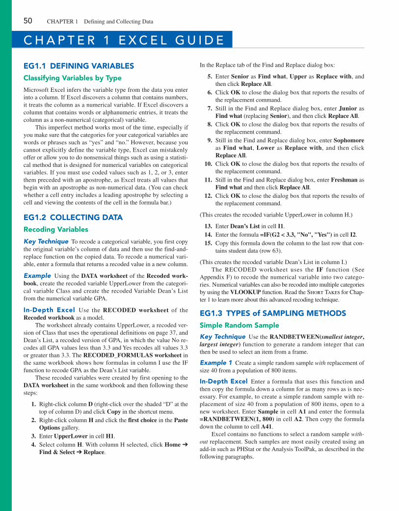
50 CHApTEr 1 Defining and Collecting Data
c h a p t e r 1 e x c e l g U i d e
eg1.1 DeFining VariaBLeSClassifying Variables by Type
Microsoft Excel infers the variable type from the data you enter into a column. If Excel discovers a column that contains numbers, it treats the column as a numerical variable. If Excel discovers a column that contains words or alphanumeric entries, it treats the column as a non-numerical (categorical) variable.
This imperfect method works most of the time, especially if you make sure that the categories for your categorical variables are words or phrases such as “yes” and “no.” However, because you cannot explicitly define the variable type, Excel can mistakenly offer or allow you to do nonsensical things such as using a statisti-cal method that is designed for numerical variables on categorical variables. If you must use coded values such as 1, 2, or 3, enter them preceded with an apostrophe, as Excel treats all values that begin with an apostrophe as non-numerical data. (You can check whether a cell entry includes a leading apostrophe by selecting a cell and viewing the contents of the cell in the formula bar.)
eg1.2 CoLLeCTing DaTarecoding Variables
Key Technique To recode a categorical variable, you first copy the original variable’s column of data and then use the find-and-replace function on the copied data. To recode a numerical vari-able, enter a formula that returns a recoded value in a new column.
Example Using the DATA worksheet of the Recoded work-book, create the recoded variable UpperLower from the categori-cal variable Class and create the recoded Variable Dean’s List from the numerical variable GpA.
in-Depth excel Use the RECODED worksheet of the Recoded workbook as a model.
The worksheet already contains UpperLower, a recoded ver-sion of Class that uses the operational definitions on page 37, and Dean’s List, a recoded version of GpA, in which the value No re-codes all GpA values less than 3.3 and Yes recodes all values 3.3 or greater than 3.3. The RECODED_FORMULAS worksheet in the same workbook shows how formulas in column I use the IF function to recode GpA as the Dean’s List variable.
These recoded variables were created by first opening to the DATA worksheet in the same workbook and then following these steps:
1. right-click column D (right-click over the shaded “D” at the top of column D) and click Copy in the shortcut menu.
2. right-click column H and click the first choice in the Paste Options gallery.
3. Enter UpperLower in cell H1. 4. Select column H. With column H selected, click Home ➔
Find & Select ➔ Replace.
In the replace tab of the Find and replace dialog box:
5. Enter Senior as Find what, Upper as Replace with, and then click Replace All.
6. Click OK to close the dialog box that reports the results of the replacement command.
7. Still in the Find and replace dialog box, enter Junior as Find what (replacing Senior), and then click Replace All.
8. Click OK to close the dialog box that reports the results of the replacement command.
9. Still in the Find and replace dialog box, enter Sophomore as Find what, Lower as Replace with, and then click Replace All.
10. Click OK to close the dialog box that reports the results of the replacement command.
11. Still in the Find and replace dialog box, enter Freshman as Find what and then click Replace All.
12. Click OK to close the dialog box that reports the results of the replacement command.
(This creates the recoded variable UpperLower in column H.)
13. Enter Dean’s List in cell I1. 14. Enter the formula =IF(G2 < 3.3, "No", "Yes") in cell I2. 15. Copy this formula down the column to the last row that con-
tains student data (row 63).
(This creates the recoded variable Dean’s List in column I.)The rECODED worksheet uses the IF function (See
Appendix F) to recode the numerical variable into two catego-ries. Numerical variables can also be recoded into multiple categories by using the VLOOKUP function. read the Short Takes for Chap-ter 1 to learn more about this advanced recoding technique.
eg1.3 TyPeS of SaMPLing MeThoDSSimple random Sample
Key Technique Use the RANDBETWEEN(smallest integer, largest integer) function to generate a random integer that can then be used to select an item from a frame.
Example 1 Create a simple random sample with replacement of size 40 from a population of 800 items.
in-Depth excel Enter a formula that uses this function and then copy the formula down a column for as many rows as is nec-essary. For example, to create a simple random sample with re-placement of size 40 from a population of 800 items, open to a new worksheet. Enter Sample in cell A1 and enter the formula =RANDBETWEEN(1, 800) in cell A2. Then copy the formula down the column to cell A41.
Excel contains no functions to select a random sample with-out replacement. Such samples are most easily created using an add-in such as pHStat or the Analysis Toolpak, as described in the following paragraphs.
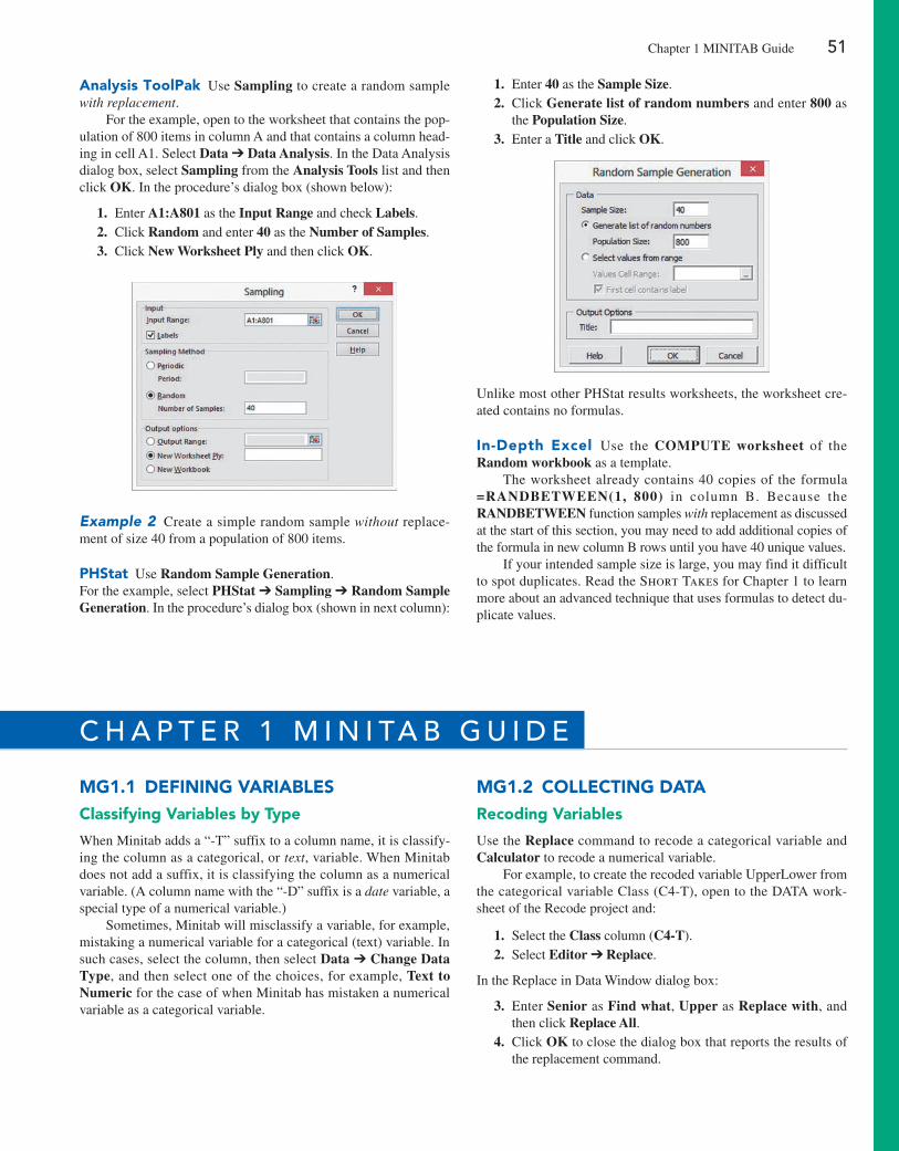
Chapter 1 MINITAB Guide 51
analysis ToolPak Use Sampling to create a random sample with replacement.
For the example, open to the worksheet that contains the pop-ulation of 800 items in column A and that contains a column head-ing in cell A1. Select Data ➔ Data Analysis. In the Data Analysis dialog box, select Sampling from the Analysis Tools list and then click OK. In the procedure’s dialog box (shown below):
1. Enter A1:A801 as the Input Range and check Labels. 2. Click Random and enter 40 as the Number of Samples. 3. Click New Worksheet Ply and then click OK.
Example 2 Create a simple random sample without replace-ment of size 40 from a population of 800 items.
PhStat Use Random Sample Generation.For the example, select PHStat ➔ Sampling ➔ Random Sample Generation. In the procedure’s dialog box (shown in next column):
1. Enter 40 as the Sample Size. 2. Click Generate list of random numbers and enter 800 as
the Population Size. 3. Enter a Title and click OK.
Unlike most other pHStat results worksheets, the worksheet cre-ated contains no formulas.
in-Depth excel Use the COMPUTE worksheet of the Random workbook as a template.
The worksheet already contains 40 copies of the formula =RANDBETWEEN(1, 800) in column B. Because the RANDBETWEEN function samples with replacement as discussed at the start of this section, you may need to add additional copies of the formula in new column B rows until you have 40 unique values.
If your intended sample size is large, you may find it difficult to spot duplicates. read the Short Takes for Chapter 1 to learn more about an advanced technique that uses formulas to detect du-plicate values.
Mg1.1 DeFining VariaBLeSClassifying Variables by Type
When Minitab adds a “-T” suffix to a column name, it is classify-ing the column as a categorical, or text, variable. When Minitab does not add a suffix, it is classifying the column as a numerical variable. (A column name with the “-D” suffix is a date variable, a special type of a numerical variable.)
Sometimes, Minitab will misclassify a variable, for example, mistaking a numerical variable for a categorical (text) variable. In such cases, select the column, then select Data ➔ Change Data Type, and then select one of the choices, for example, Text to Numeric for the case of when Minitab has mistaken a numerical variable as a categorical variable.
Mg1.2 CoLLeCTing DaTarecoding Variables
Use the Replace command to recode a categorical variable and Calculator to recode a numerical variable.
For example, to create the recoded variable UpperLower from the categorical variable Class (C4-T), open to the DATA work-sheet of the recode project and:
1. Select the Class column (C4-T). 2. Select Editor ➔ Replace.
In the replace in Data Window dialog box:
3. Enter Senior as Find what, Upper as Replace with, and then click Replace All.
4. Click OK to close the dialog box that reports the results of the replacement command.
c h a p t e r 1 M i n i ta b g U i d e
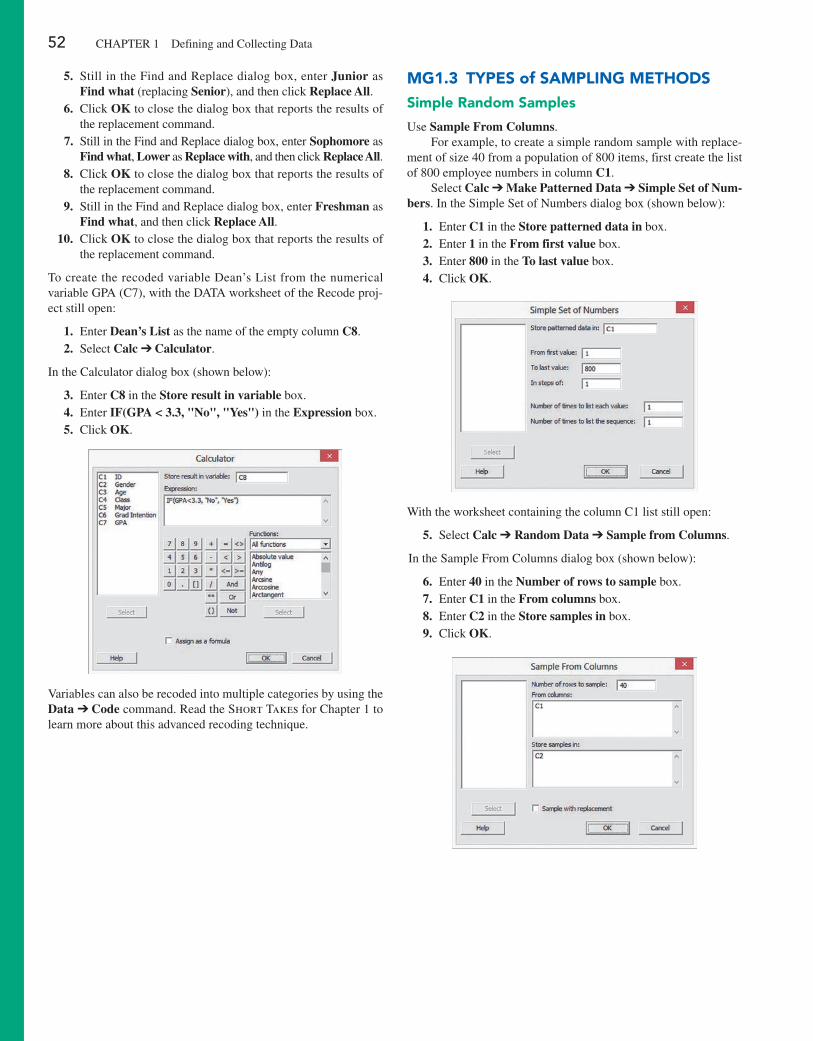
52 CHApTEr 1 Defining and Collecting Data
5. Still in the Find and replace dialog box, enter Junior as Find what (replacing Senior), and then click Replace All.
6. Click OK to close the dialog box that reports the results of the replacement command.
7. Still in the Find and replace dialog box, enter Sophomore as Find what, Lower as Replace with, and then click Replace All.
8. Click OK to close the dialog box that reports the results of the replacement command.
9. Still in the Find and replace dialog box, enter Freshman as Find what, and then click Replace All.
10. Click OK to close the dialog box that reports the results of the replacement command.
To create the recoded variable Dean’s List from the numerical variable GpA (C7), with the DATA worksheet of the recode proj-ect still open:
1. Enter Dean’s List as the name of the empty column C8. 2. Select Calc ➔ Calculator.
In the Calculator dialog box (shown below):
3. Enter C8 in the Store result in variable box. 4. Enter IF(GPA < 3.3, "No", "Yes") in the Expression box. 5. Click OK.
Variables can also be recoded into multiple categories by using the Data ➔ Code command. read the Short Takes for Chapter 1 to learn more about this advanced recoding technique.
Mg1.3 TyPeS of SaMPLing MeThoDSSimple random Samples
Use Sample From Columns.For example, to create a simple random sample with replace-
ment of size 40 from a population of 800 items, first create the list of 800 employee numbers in column C1.
Select Calc ➔ Make Patterned Data ➔ Simple Set of Num-bers. In the Simple Set of Numbers dialog box (shown below):
1. Enter C1 in the Store patterned data in box. 2. Enter 1 in the From first value box. 3. Enter 800 in the To last value box. 4. Click OK.
With the worksheet containing the column C1 list still open:
5. Select Calc ➔ Random Data ➔ Sample from Columns.
In the Sample From Columns dialog box (shown below):
6. Enter 40 in the Number of rows to sample box. 7. Enter C1 in the From columns box. 8. Enter C2 in the Store samples in box. 9. Click OK.
53
U s i n g s tat i s t i c s
The Choice Is YoursEven though he is still in his 20s, Tom Sanchez realizes that you can never start too early to save for retirement. Based on research he has already done, Sanchez seeks to contribute to his 401(k) retirement plan by investing in one or more retirement funds.
Meanwhile, the Choice Is Yours investment service has been thinking about being better prepared to counsel younger investors such as Sanchez about retire-ment funds. To pursue this business objective, a company task force has already selected 316 retirement funds that may prove appropriate for younger investors. You have been asked to define, collect, organize, and visualize data about these funds in ways that could assist prospective clients making decisions about the funds in which they will invest. As a starting point, you think about the facts about each fund that would help customers compare and contrast funds.
You decide to begin by defining the variables for key characteristics of each fund, such as each fund’s past performance. You also decide to define variables such as the amount of assets that a fund manages and whether the goal of a fund is to invest in companies whose earnings are expected to substantially increase in future years (a “growth” fund) or invest in companies whose stock price is undervalued, priced low relative to their earnings potential (a “value” fund).
You collect data from appropriate sources and organize the data as a work-sheet, placing each variable in its own column. As you think more about your task, you realize that 316 rows of data, one for each fund in the sample, would be hard for prospective clients to review easily.
Is there something else you can do? Can you organize and present these data to prospective clients in a more helpful and comprehensible manner?
Contents
2.1 Organizing Categorical Variables
2.2 Organizing Numerical Variables
classes and Excel Bins
stacked and Unstacked Data
2.3 Visualizing Categorical Variables
2.4 Visualizing Numerical Variables
2.5 Visualizing Two Numerical Variables
2.6 Organizing and Visualizing a Set of Variables
2.7 The Challenge in Organizing and Visualizing Variables
Best Practices for constructing Visualizations
Using statistics: the choice Is Yours, Revisited
chaPtER 2 ExcEl gUiDE
chaPtER 2 MinitaB gUiDE
objeCtivesMethods to organize variables
Methods to visualize variables
Methods to organize or visualize more than one variable at the same time
Principles of proper visualizations
Chapter Organizing and Visualizing Variables2
Ryan R Fox/Shutterstock
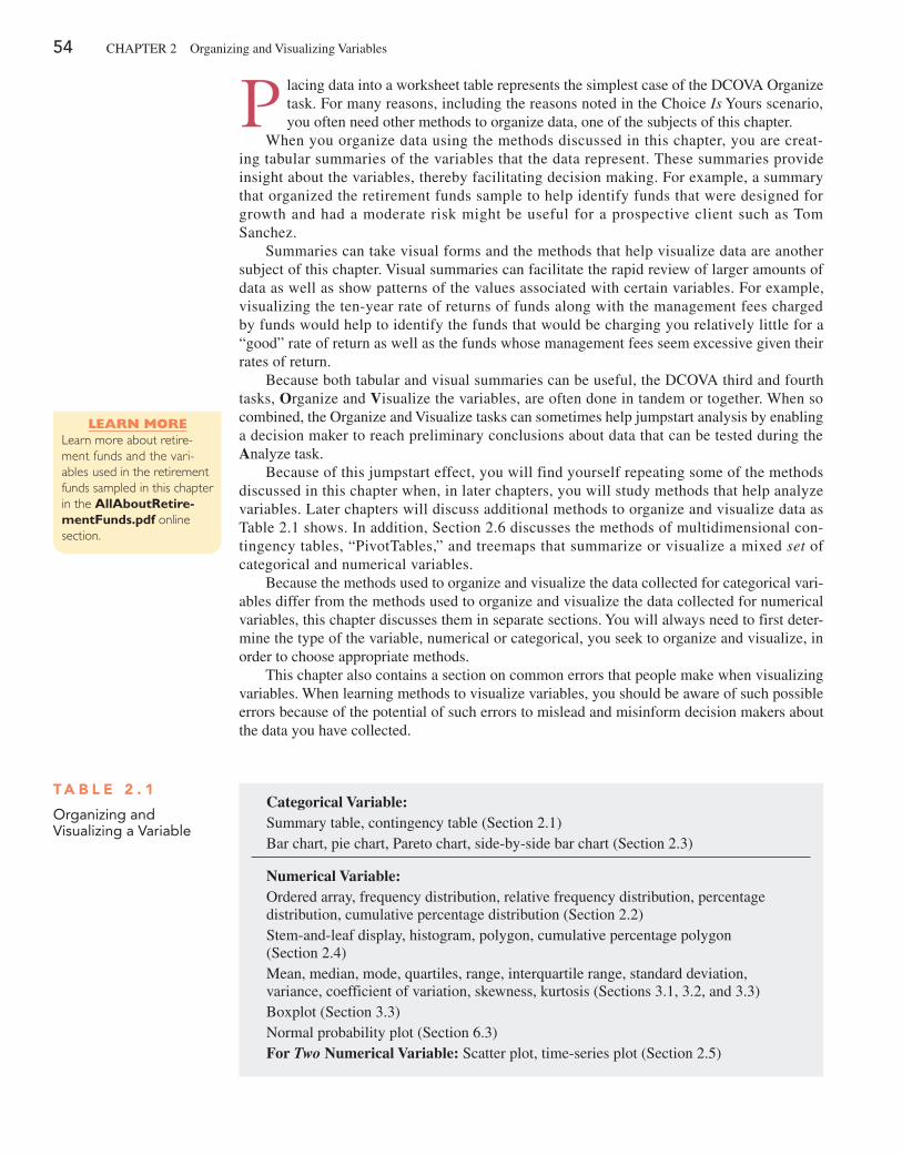
54 ChApTER 2 Organizing and Visualizing Variables
P lacing data into a worksheet table represents the simplest case of the DCOVA Organize task. For many reasons, including the reasons noted in the Choice Is Yours scenario, you often need other methods to organize data, one of the subjects of this chapter.
When you organize data using the methods discussed in this chapter, you are creat-ing tabular summaries of the variables that the data represent. These summaries provide insight about the variables, thereby facilitating decision making. For example, a summary that organized the retirement funds sample to help identify funds that were designed for growth and had a moderate risk might be useful for a prospective client such as Tom Sanchez.
Summaries can take visual forms and the methods that help visualize data are another subject of this chapter. Visual summaries can facilitate the rapid review of larger amounts of data as well as show patterns of the values associated with certain variables. For example, visualizing the ten-year rate of returns of funds along with the management fees charged by funds would help to identify the funds that would be charging you relatively little for a “good” rate of return as well as the funds whose management fees seem excessive given their rates of return.
Because both tabular and visual summaries can be useful, the DCOVA third and fourth tasks, Organize and Visualize the variables, are often done in tandem or together. When so combined, the Organize and Visualize tasks can sometimes help jumpstart analysis by enabling a decision maker to reach preliminary conclusions about data that can be tested during the Analyze task.
Because of this jumpstart effect, you will find yourself repeating some of the methods discussed in this chapter when, in later chapters, you will study methods that help analyze variables. Later chapters will discuss additional methods to organize and visualize data as Table 2.1 shows. In addition, Section 2.6 discusses the methods of multidimensional con-tingency tables, “pivotTables,” and treemaps that summarize or visualize a mixed set of categorical and numerical variables.
Because the methods used to organize and visualize the data collected for categorical vari-ables differ from the methods used to organize and visualize the data collected for numerical variables, this chapter discusses them in separate sections. You will always need to first deter-mine the type of the variable, numerical or categorical, you seek to organize and visualize, in order to choose appropriate methods.
This chapter also contains a section on common errors that people make when visualizing variables. When learning methods to visualize variables, you should be aware of such possible errors because of the potential of such errors to mislead and misinform decision makers about the data you have collected.
T a b l e 2 . 1
Organizing and Visualizing a Variable
Categorical Variable:Summary table, contingency table (Section 2.1)Bar chart, pie chart, pareto chart, side-by-side bar chart (Section 2.3)
Numerical Variable:Ordered array, frequency distribution, relative frequency distribution, percentage distribution, cumulative percentage distribution (Section 2.2)Stem-and-leaf display, histogram, polygon, cumulative percentage polygon (Section 2.4)Mean, median, mode, quartiles, range, interquartile range, standard deviation, variance, coefficient of variation, skewness, kurtosis (Sections 3.1, 3.2, and 3.3)Boxplot (Section 3.3)Normal probability plot (Section 6.3)For Two Numerical Variable: Scatter plot, time-series plot (Section 2.5)
Learn MoreLearn more about retire-ment funds and the vari-ables used in the retirement funds sampled in this chapter in the AllAboutRetire-mentFunds.pdf online section.
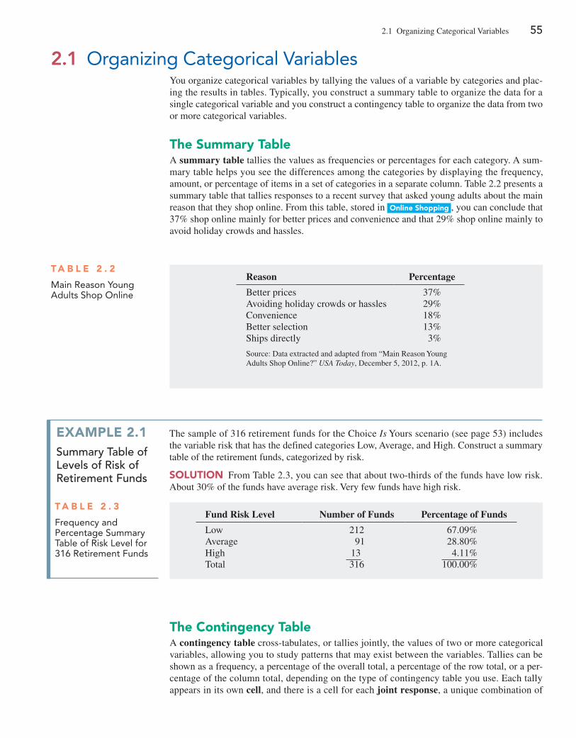
2.1 Organizing Categorical Variables 55
2.1 Organizing Categorical VariablesYou organize categorical variables by tallying the values of a variable by categories and plac-ing the results in tables. Typically, you construct a summary table to organize the data for a single categorical variable and you construct a contingency table to organize the data from two or more categorical variables.
The Summary TableA summary table tallies the values as frequencies or percentages for each category. A sum-mary table helps you see the differences among the categories by displaying the frequency, amount, or percentage of items in a set of categories in a separate column. Table 2.2 presents a summary table that tallies responses to a recent survey that asked young adults about the main reason that they shop online. From this table, stored in Online Shopping , you can conclude that 37% shop online mainly for better prices and convenience and that 29% shop online mainly to avoid holiday crowds and hassles.
T a b l e 2 . 2
Main Reason Young Adults Shop Online
Reason Percentage
Better prices 37%Avoiding holiday crowds or hassles 29%Convenience 18%Better selection 13%Ships directly 3%
Source: Data extracted and adapted from “Main Reason Young Adults Shop Online?” USA Today, December 5, 2012, p. 1A.
example 2.1summary table of levels of Risk of Retirement Funds
The sample of 316 retirement funds for the Choice Is Yours scenario (see page 53) includes the variable risk that has the defined categories Low, Average, and high. Construct a summary table of the retirement funds, categorized by risk.
SOluTiOn From Table 2.3, you can see that about two-thirds of the funds have low risk. About 30% of the funds have average risk. Very few funds have high risk.
T a b l e 2 . 3
Frequency and Percentage Summary Table of Risk Level for 316 Retirement Funds
Fund Risk Level Number of Funds Percentage of Funds
Low 212 67.09%Average 91 28.80%high 13 4.11%Total 316 100.00%
The Contingency TableA contingency table cross-tabulates, or tallies jointly, the values of two or more categorical variables, allowing you to study patterns that may exist between the variables. Tallies can be shown as a frequency, a percentage of the overall total, a percentage of the row total, or a per-centage of the column total, depending on the type of contingency table you use. Each tally appears in its own cell, and there is a cell for each joint response, a unique combination of
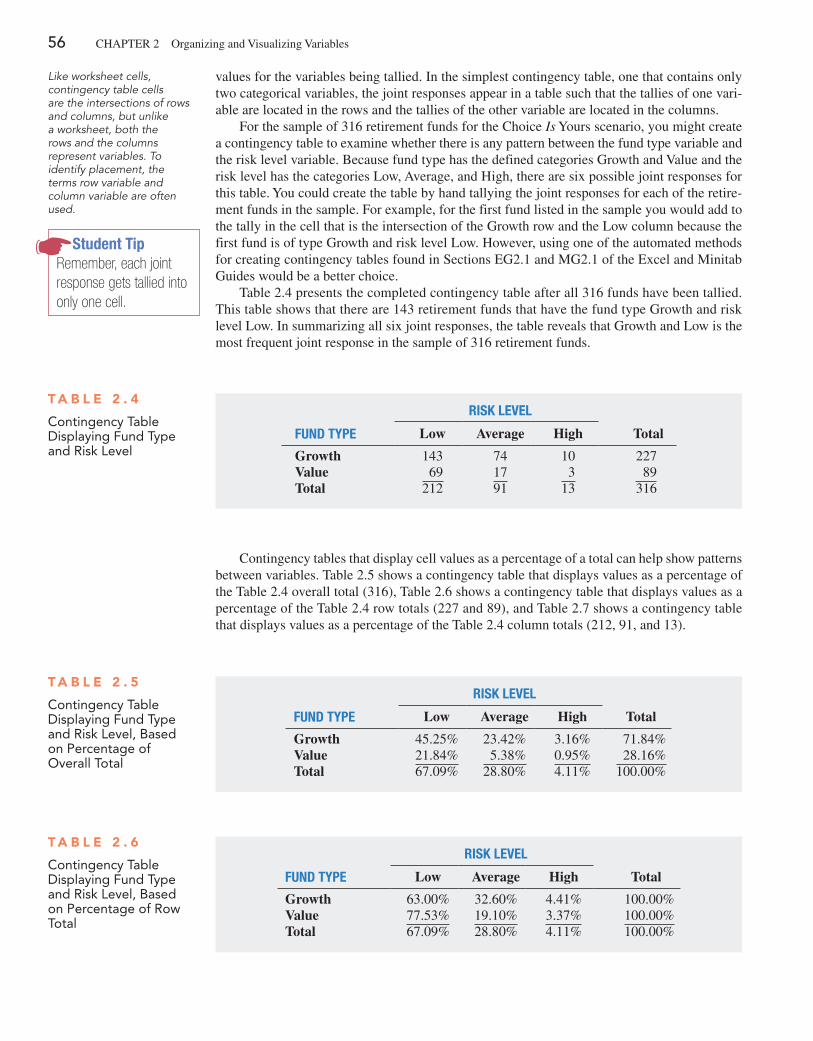
56 ChApTER 2 Organizing and Visualizing Variables
values for the variables being tallied. In the simplest contingency table, one that contains only two categorical variables, the joint responses appear in a table such that the tallies of one vari-able are located in the rows and the tallies of the other variable are located in the columns.
For the sample of 316 retirement funds for the Choice Is Yours scenario, you might create a contingency table to examine whether there is any pattern between the fund type variable and the risk level variable. Because fund type has the defined categories Growth and Value and the risk level has the categories Low, Average, and high, there are six possible joint responses for this table. You could create the table by hand tallying the joint responses for each of the retire-ment funds in the sample. For example, for the first fund listed in the sample you would add to the tally in the cell that is the intersection of the Growth row and the Low column because the first fund is of type Growth and risk level Low. however, using one of the automated methods for creating contingency tables found in Sections EG2.1 and MG2.1 of the Excel and Minitab Guides would be a better choice.
Table 2.4 presents the completed contingency table after all 316 funds have been tallied. This table shows that there are 143 retirement funds that have the fund type Growth and risk level Low. In summarizing all six joint responses, the table reveals that Growth and Low is the most frequent joint response in the sample of 316 retirement funds.
Contingency tables that display cell values as a percentage of a total can help show patterns between variables. Table 2.5 shows a contingency table that displays values as a percentage of the Table 2.4 overall total (316), Table 2.6 shows a contingency table that displays values as a percentage of the Table 2.4 row totals (227 and 89), and Table 2.7 shows a contingency table that displays values as a percentage of the Table 2.4 column totals (212, 91, and 13).
T a b l e 2 . 4
Contingency Table Displaying Fund Type and Risk Level
RISK LEVEL
FUND TYPE Low Average High Total
Growth 143 74 10 227Value 69 17 3 89Total 212 91 13 316
T a b l e 2 . 5
Contingency Table Displaying Fund Type and Risk Level, Based on Percentage of Overall Total
RISK LEVEL
FUND TYPE Low Average High Total
Growth 45.25% 23.42% 3.16% 71.84%Value 21.84% 5.38% 0.95% 28.16%Total 67.09% 28.80% 4.11% 100.00%
T a b l e 2 . 6
Contingency Table Displaying Fund Type and Risk Level, Based on Percentage of Row Total
RISK LEVEL
FUND TYPE Low Average High Total
Growth 63.00% 32.60% 4.41% 100.00%Value 77.53% 19.10% 3.37% 100.00%Total 67.09% 28.80% 4.11% 100.00%
Student TipRemember, each joint response gets tallied into only one cell.
Like worksheet cells, contingency table cells are the intersections of rows and columns, but unlike a worksheet, both the rows and the columns represent variables. To identify placement, the terms row variable and column variable are often used.
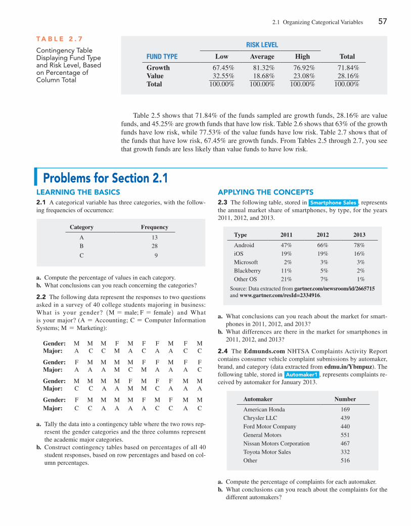
2.1 Organizing Categorical Variables 57
Table 2.5 shows that 71.84% of the funds sampled are growth funds, 28.16% are value funds, and 45.25% are growth funds that have low risk. Table 2.6 shows that 63% of the growth funds have low risk, while 77.53% of the value funds have low risk. Table 2.7 shows that of the funds that have low risk, 67.45% are growth funds. From Tables 2.5 through 2.7, you see that growth funds are less likely than value funds to have low risk.
problems for Section 2.1learning The baSiCS2.1 A categorical variable has three categories, with the follow-ing frequencies of occurrence:
Category Frequency
A 13
B 28
C 9
a. Compute the percentage of values in each category.b. What conclusions can you reach concerning the categories?
2.2 The following data represent the responses to two questions asked in a survey of 40 college students majoring in business: What is your gender? 1M = male; F = female2 and What is your major? (A = Accounting; C = Computer Information Systems; M = Marketing):
Gender: M M M F M F F M F M Major: A C C M A C A A C C
Gender: F M M M M F F M F F Major: A A A M C M A A A C
Gender: M M M M F M F F M M Major: C C A A M M C A A A
Gender: F M M M M F M F M M Major: C C A A A A C C A C
a. Tally the data into a contingency table where the two rows rep-resent the gender categories and the three columns represent the academic major categories.
b. Construct contingency tables based on percentages of all 40 student responses, based on row percentages and based on col-umn percentages.
applying The COnCepTS2.3 The following table, stored in Smartphone Sales , represents the annual market share of smartphones, by type, for the years 2011, 2012, and 2013.
Type 2011 2012 2013
Android 47% 66% 78%
iOS 19% 19% 16%
Microsoft 2% 3% 3%
Blackberry 11% 5% 2%
Other OS 21% 7% 1%
Source: Data extracted from gartner.com/newsroom/id/2665715 and www.gartner.com/resId=2334916.
a. What conclusions can you reach about the market for smart-phones in 2011, 2012, and 2013?
b. What differences are there in the market for smartphones in 2011, 2012, and 2013?
2.4 The Edmunds.com NhTSA Complaints Activity Report contains consumer vehicle complaint submissions by automaker, brand, and category (data extracted from edmu.in/Ybmpuz). The following table, stored in automaker1 , represents complaints re-ceived by automaker for January 2013.
Automaker Number
American honda 169
Chrysler LLC 439
Ford Motor Company 440
General Motors 551
Nissan Motors Corporation 467
Toyota Motor Sales 332
Other 516
a. Compute the percentage of complaints for each automaker.b. What conclusions can you reach about the complaints for the
different automakers?
RISK LEVEL
FUND TYPE Low Average High Total
Growth 67.45% 81.32% 76.92% 71.84%Value 32.55% 18.68% 23.08% 28.16%Total 100.00% 100.00% 100.00% 100.00%
T a b l e 2 . 7
Contingency Table Displaying Fund Type and Risk Level, Based on Percentage of Column Total
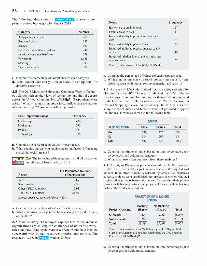
58 ChApTER 2 Organizing and Visualizing Variables
The following table, stored in automaker2 , represents com-plaints received by category for January 2013.
Category Number
Airbags and seatbelts 201
Body and glass 182
Brakes 163
Fuel/emission/exhaust system 240
Interior electronics/hardware 279
powertrain 1,148
Steering 397
Tires and wheels 71
c. Compute the percentage of complaints for each category.d. What conclusions can you reach about the complaints for
different categories?
2.5 The 2013 Mortimer Spinks and Computer Weekly Technol-ogy Survey reflects the views of technology and digital experts across the United Kingdom (bit.ly/WS4jg3). Respondents were asked, “What is the most important factor influencing the success of a tech start-up?” Assume the following results:
Most Important Factor Frequency
Leadership 400
Marketing 346
product 464
Technology 86
a. Compute the percentage of values for each factor.b. What conclusions can you reach concerning factors influencing
successful tech start-ups?
2.6 The following table represents world oil production in millions of barrels a day in 2013:
RegionOil Production (millions
of barrels a day)
Iran 2.69
Saudi Arabia 9.58
Other OpEC countries 17.93
Non-OpEC countries 51.99
Source: opec.org, accessed February 2014.
a. Compute the percentage of values in each category.b. What conclusions can you reach concerning the production of
oil in 2013?
2.7 Visier’s Survey of Employers explores how North American organizations are solving the challenges of delivering work-force analytics. Employers were asked what would help them be successful with human resources metrics and reports. The responses (stored in needs ) were as follows:
SELF Test
Needs Frequency
Easier-to-use analytic tools 127
Faster access to data 41
Improved ability to present and interpret data
123
Improved ability to plan actions 33
Improved ability to predict impacts of my actions 49
Improved relationships to the business line organizations 37
Source: Data extracted from bit.ly/1fmPZrQ.
a. Compute the percentage of values for each response need.b. What conclusions can you reach concerning needs for em-
ployer success with human resources metrics and reports?
2.8 A survey of 1,085 adults asked “Do you enjoy shopping for clothing for yourself?” The results indicated that 51% of the fe-males enjoyed shopping for clothing for themselves as compared to 44% of the males. (Data extracted from “Split Decision on Clothes Shopping,” USA Today, January 28, 2011, p. 1B.) The sample sizes of males and females were not provided. Suppose that the results were as shown in the following table:
GENDER
ENJOY SHOPPING Male Female Total
Yes 238 276 514
No 304 267 571
Total 542 543 1,085
a. Construct contingency tables based on total percentages, row percentages, and column percentages.
b. What conclusions can you reach from these analyses?
2.9 A study of Kickstarter projects showed that 54.2% were suc-cessful, that is, achieved its goal and raised at least the targeted goal amount. In an effort to identify network dynamics that influences success, projects were subdivided into projects of owners who had backed other projects before, during or after creating their project (owners with backing history) and projects of owners without backing history. The results are as follows:
PROJEcT OwNER’S BacKING HISTORY
Project OutcomeBacking History
No Backing History Total
Successful 17,667 19,202 36,869
Not successful 10,921 20,267 31,188
Total 28,588 39,469 68,057
Source: Data extracted from Zvilichovsky et al., “playing Both Sides of the Market: Success and Reciprocity on Crowdfunding platforms,” bit.ly/OoyhqZ.
a. Construct contingency tables based on total percentages, row percentages, and column percentages.
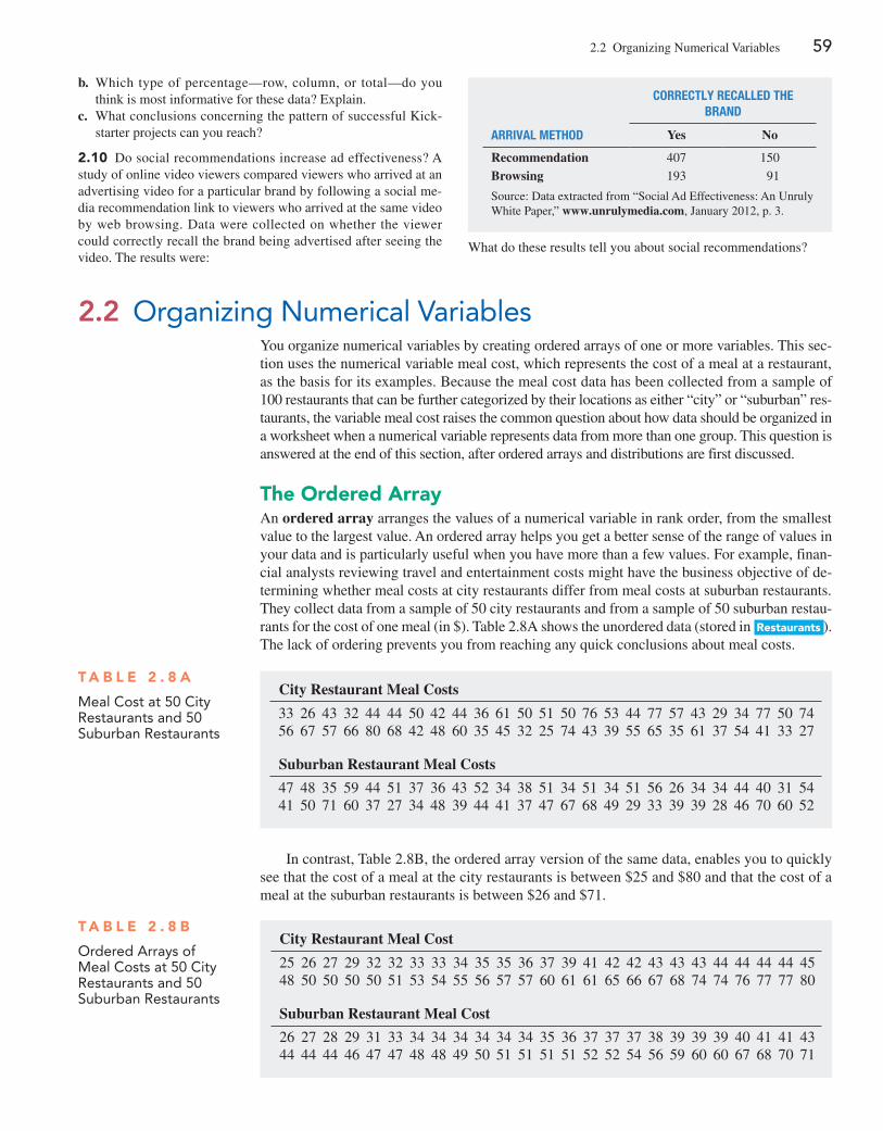
2.2 Organizing Numerical Variables 59
b. Which type of percentage—row, column, or total—do you think is most informative for these data? Explain.
c. What conclusions concerning the pattern of successful Kick-starter projects can you reach?
2.10 Do social recommendations increase ad effectiveness? A study of online video viewers compared viewers who arrived at an advertising video for a particular brand by following a social me-dia recommendation link to viewers who arrived at the same video by web browsing. Data were collected on whether the viewer could correctly recall the brand being advertised after seeing the video. The results were:
cORREcTLY REcaLLED THE BRaND
aRRIVaL METHOD Yes No
Recommendation 407 150
Browsing 193 91
Source: Data extracted from “Social Ad Effectiveness: An Unruly White paper,” www.unrulymedia.com, January 2012, p. 3.
What do these results tell you about social recommendations?
You organize numerical variables by creating ordered arrays of one or more variables. This sec-tion uses the numerical variable meal cost, which represents the cost of a meal at a restaurant, as the basis for its examples. Because the meal cost data has been collected from a sample of 100 restaurants that can be further categorized by their locations as either “city” or “suburban” res-taurants, the variable meal cost raises the common question about how data should be organized in a worksheet when a numerical variable represents data from more than one group. This question is answered at the end of this section, after ordered arrays and distributions are first discussed.
The Ordered arrayAn ordered array arranges the values of a numerical variable in rank order, from the smallest value to the largest value. An ordered array helps you get a better sense of the range of values in your data and is particularly useful when you have more than a few values. For example, finan-cial analysts reviewing travel and entertainment costs might have the business objective of de-termining whether meal costs at city restaurants differ from meal costs at suburban restaurants. They collect data from a sample of 50 city restaurants and from a sample of 50 suburban restau-rants for the cost of one meal (in $). Table 2.8A shows the unordered data (stored in restaurants ). The lack of ordering prevents you from reaching any quick conclusions about meal costs.
2.2 Organizing Numerical Variables
T a b l e 2 . 8 a
Meal Cost at 50 City Restaurants and 50 Suburban Restaurants
City Restaurant Meal Costs
33 26 43 32 44 44 50 42 44 36 61 50 51 50 76 53 44 77 57 43 29 34 77 50 7456 67 57 66 80 68 42 48 60 35 45 32 25 74 43 39 55 65 35 61 37 54 41 33 27
Suburban Restaurant Meal Costs
47 48 35 59 44 51 37 36 43 52 34 38 51 34 51 34 51 56 26 34 34 44 40 31 5441 50 71 60 37 27 34 48 39 44 41 37 47 67 68 49 29 33 39 39 28 46 70 60 52
In contrast, Table 2.8B, the ordered array version of the same data, enables you to quickly see that the cost of a meal at the city restaurants is between $25 and $80 and that the cost of a meal at the suburban restaurants is between $26 and $71.
T a b l e 2 . 8 b
Ordered Arrays of Meal Costs at 50 City Restaurants and 50 Suburban Restaurants
City Restaurant Meal Cost
25 26 27 29 32 32 33 33 34 35 35 36 37 39 41 42 42 43 43 43 44 44 44 44 4548 50 50 50 50 51 53 54 55 56 57 57 60 61 61 65 66 67 68 74 74 76 77 77 80
Suburban Restaurant Meal Cost
26 27 28 29 31 33 34 34 34 34 34 34 35 36 37 37 37 38 39 39 39 40 41 41 4344 44 44 46 47 47 48 48 49 50 51 51 51 51 52 52 54 56 59 60 60 67 68 70 71
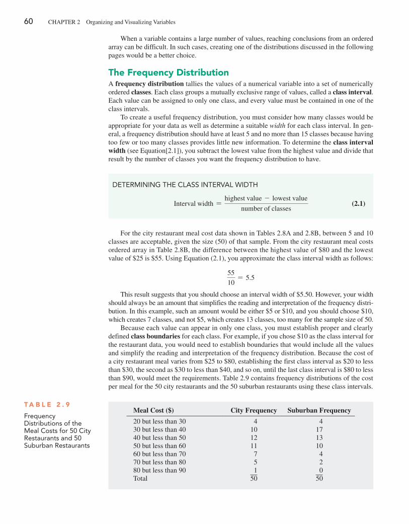
60 ChApTER 2 Organizing and Visualizing Variables
When a variable contains a large number of values, reaching conclusions from an ordered array can be difficult. In such cases, creating one of the distributions discussed in the following pages would be a better choice.
The Frequency DistributionA frequency distribution tallies the values of a numerical variable into a set of numerically ordered classes. Each class groups a mutually exclusive range of values, called a class interval. Each value can be assigned to only one class, and every value must be contained in one of the class intervals.
To create a useful frequency distribution, you must consider how many classes would be appropriate for your data as well as determine a suitable width for each class interval. In gen-eral, a frequency distribution should have at least 5 and no more than 15 classes because having too few or too many classes provides little new information. To determine the class interval width (see Equation[2.1]), you subtract the lowest value from the highest value and divide that result by the number of classes you want the frequency distribution to have.
DeTeRMiNiNg The CLASS iNTeRVAL WiDTh
Interval width =highest value - lowest value
number of classes (2.1)
For the city restaurant meal cost data shown in Tables 2.8A and 2.8B, between 5 and 10 classes are acceptable, given the size (50) of that sample. From the city restaurant meal costs ordered array in Table 2.8B, the difference between the highest value of $80 and the lowest value of $25 is $55. Using Equation (2.1), you approximate the class interval width as follows:
55
10= 5.5
This result suggests that you should choose an interval width of $5.50. however, your width should always be an amount that simplifies the reading and interpretation of the frequency distri-bution. In this example, such an amount would be either $5 or $10, and you should choose $10, which creates 7 classes, and not $5, which creates 13 classes, too many for the sample size of 50.
Because each value can appear in only one class, you must establish proper and clearly defined class boundaries for each class. For example, if you chose $10 as the class interval for the restaurant data, you would need to establish boundaries that would include all the values and simplify the reading and interpretation of the frequency distribution. Because the cost of a city restaurant meal varies from $25 to $80, establishing the first class interval as $20 to less than $30, the second as $30 to less than $40, and so on, until the last class interval is $80 to less than $90, would meet the requirements. Table 2.9 contains frequency distributions of the cost per meal for the 50 city restaurants and the 50 suburban restaurants using these class intervals.
T a b l e 2 . 9
Frequency Distributions of the Meal Costs for 50 City Restaurants and 50 Suburban Restaurants
Meal Cost ($) City Frequency Suburban Frequency
20 but less than 30 4 430 but less than 40 10 1740 but less than 50 12 1350 but less than 60 11 1060 but less than 70 7 470 but less than 80 5 280 but less than 90 1 0Total 50 50
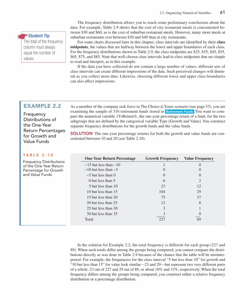
2.2 Organizing Numerical Variables 61
The frequency distribution allows you to reach some preliminary conclusions about the data. For example, Table 2.9 shows that the cost of city restaurant meals is concentrated be-tween $30 and $60, as is the cost of suburban restaurant meals. however, many more meals at suburban restaurants cost between $30 and $40 than at city restaurants.
For some charts discussed later in this chapter, class intervals are identified by their class midpoints, the values that are halfway between the lower and upper boundaries of each class. For the frequency distributions shown in Table 2.9, the class midpoints are $25, $35, $45, $55, $65, $75, and $85. Note that well-chosen class intervals lead to class midpoints that are simple to read and interpret, as in this example.
If the data you have collected do not contain a large number of values, different sets of class intervals can create different impressions of the data. Such perceived changes will dimin-ish as you collect more data. Likewise, choosing different lower and upper class boundaries can also affect impressions.
Student TipThe total of the frequency column must always equal the number of values.
In the solution for Example 2.2, the total frequency is different for each group (227 and 89). When such totals differ among the groups being compared, you cannot compare the distri-butions directly as was done in Table 2.9 because of the chance that the table will be misinter-preted. For example, the frequencies for the class interval “5 but less than 10” for growth and “10 but less than 15” for value look similar—23 and 29—but represent two very different parts of a whole: 23 out of 227 and 29 out of 89, or about 10% and 33%, respectively. When the total frequency differs among the groups being compared, you construct either a relative frequency distribution or a percentage distribution.
T a b l e 2 . 1 0
Frequency Distributions of the One-Year Return Percentage for growth and Value Funds
example 2.2Frequency Distributions of the One-Year Return Percentages for growth and Value Funds
As a member of the company task force in The Choice Is Yours scenario (see page 53), you are examining the sample of 316 retirement funds stored in retirement Funds .You want to com-pare the numerical variable 1YrReturn%, the one-year percentage return of a fund, for the two subgroups that are defined by the categorical variable Type (Growth and Value). You construct separate frequency distributions for the growth funds and the value funds.
SOluTiOn The one-year percentage returns for both the growth and value funds are con-centrated between 10 and 20 (see Table 2.10).
One-Year Return Percentage Growth Frequency Value Frequency
−15 but less than −10 1 0−10 but less than −5 0 0−5 but less than 0 0 0 0 but less than 5 6 2 5 but less than 10 23 1210 but less than 15 104 2915 but less than 20 75 3720 but less than 25 12 825 but less than 30 3 130 but less than 35 3 0
Total 227 89
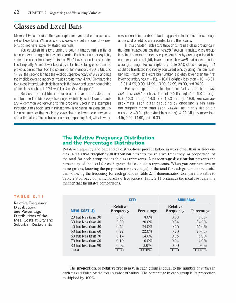
62 ChApTER 2 Organizing and Visualizing Variables
The proportion, or relative frequency, in each group is equal to the number of values in each class divided by the total number of values. The percentage in each group is its proportion multiplied by 100%.
The relative Frequency Distribution and the percentage DistributionRelative frequency and percentage distributions present tallies in ways other than as frequen-cies. A relative frequency distribution presents the relative frequency, or proportion, of the total for each group that each class represents. A percentage distribution presents the percentage of the total for each group that each class represents. When you compare two or more groups, knowing the proportion (or percentage) of the total for each group is more useful than knowing the frequency for each group, as Table 2.11 demonstrates. Compare this table to Table 2.9 on page 60, which displays frequencies. Table 2.11 organizes the meal cost data in a manner that facilitates comparisons.
Classes and Excel BinsMicrosoft Excel requires that you implement your set of classes as a set of Excel bins. While bins and classes are both ranges of values, bins do not have explicitly stated intervals.
You establish bins by creating a column that contains a list of bin numbers arranged in ascending order. Each bin number explicitly states the upper boundary of its bin. Bins’ lower boundaries are de-fined implicitly: A bin’s lower boundary is the first value greater than the previous bin number. For the column of bin numbers 4.99, 9.99, and 14.99, the second bin has the explicit upper boundary of 9.99 and has the implicit lower boundary of “values greater than 4.99.” Compare this to a class interval, which defines both the lower and upper boundaries of the class, such as in “0 (lower) but less than 5 (upper).”
Because the first bin number does not have a “previous” bin number, the first bin always has negative infinity as its lower bound-ary. A common workaround to this problem, used in the examples throughout this book (and in PHStat, too), is to define an extra bin, us-ing a bin number that is slightly lower than the lower boundary value of the first class. This extra bin number, appearing first, will allow the
now-second bin number to better approximate the first class, though at the cost of adding an unwanted bin to the results.
In this chapter, Tables 2.9 through 2.13 use class groupings in the form “valueA but less than valueB.” You can translate class group-ings in this form into nearly equivalent bins by creating a list of bin numbers that are slightly lower than each valueB that appears in the class groupings. For example, the Table 2.10 classes on page 61 could be translated into nearly equivalent bins by using this bin num-ber list: −15.01 (the extra bin number is slightly lower than the first lower boundary value −15), −10.01 (slightly less than −10, −5.01, −0.01, 4.99, 9.99, 14.99, 19.99, 24.99, 29.99, and 34.99.
For class groupings in the form “all values from val-ueA to valueB,” such as the set 0.0 through 4.9, 5.0 through 9.9, 10.0 through 14.9, and 15.0 through 19.9, you can ap-proximate each class grouping by choosing a bin num-ber slightly more than each valueB , as in this list of bin numbers: −0.01 (the extra bin number), 4.99 (slightly more than 4.9), 9.99, 14.99, and 19.99.
T a b l e 2 . 1 1
Relative Frequency Distributions and Percentage Distributions of the Meal Costs at City and Suburban Restaurants
cITY SUBURBaN
MEaL cOST ($)Relative
Frequency Percentage Relative
Frequency Percentage
20 but less than 30 0.08 8.0% 0.08 8.0%30 but less than 40 0.20 20.0% 0.34 34.0%40 but less than 50 0.24 24.0% 0.26 26.0%50 but less than 60 0.22 22.0% 0.20 20.0%60 but less than 70 0.14 14.0% 0.08 8.0%70 but less than 80 0.10 10.0% 0.04 4.0%80 but less than 90 0.02 2.0% 0.00 0.0%Total 1.00 100.0% 1.00 100.0%
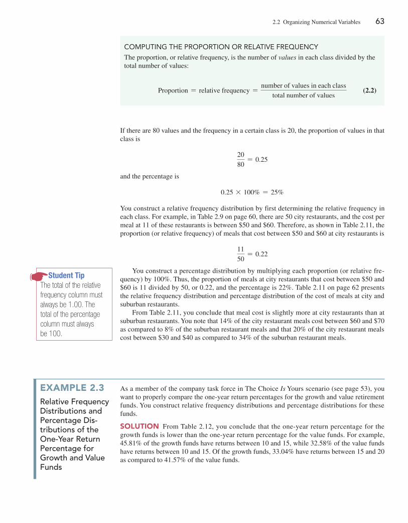
2.2 Organizing Numerical Variables 63
If there are 80 values and the frequency in a certain class is 20, the proportion of values in that class is
20
80= 0.25
and the percentage is
0.25 * 100% = 25%
You construct a relative frequency distribution by first determining the relative frequency in each class. For example, in Table 2.9 on page 60, there are 50 city restaurants, and the cost per meal at 11 of these restaurants is between $50 and $60. Therefore, as shown in Table 2.11, the proportion (or relative frequency) of meals that cost between $50 and $60 at city restaurants is
11
50= 0.22
You construct a percentage distribution by multiplying each proportion (or relative fre-quency) by 100%. Thus, the proportion of meals at city restaurants that cost between $50 and $60 is 11 divided by 50, or 0.22, and the percentage is 22%. Table 2.11 on page 62 presents the relative frequency distribution and percentage distribution of the cost of meals at city and suburban restaurants.
From Table 2.11, you conclude that meal cost is slightly more at city restaurants than at suburban restaurants. You note that 14% of the city restaurant meals cost between $60 and $70 as compared to 8% of the suburban restaurant meals and that 20% of the city restaurant meals cost between $30 and $40 as compared to 34% of the suburban restaurant meals.
COMPuTiNg The PROPORTiON OR ReLATiVe FRequeNCY
The proportion, or relative frequency, is the number of values in each class divided by the total number of values:
proportion = relative frequency =number of values in each class
total number of values (2.2)
Student TipThe total of the relative frequency column must always be 1.00. The total of the percentage column must always be 100.
example 2.3Relative Frequency Distributions and Percentage Dis-tributions of the One-Year Return Percentage for growth and Value Funds
As a member of the company task force in The Choice Is Yours scenario (see page 53), you want to properly compare the one-year return percentages for the growth and value retirement funds. You construct relative frequency distributions and percentage distributions for these funds.
SOluTiOn From Table 2.12, you conclude that the one-year return percentage for the growth funds is lower than the one-year return percentage for the value funds. For example, 45.81% of the growth funds have returns between 10 and 15, while 32.58% of the value funds have returns between 10 and 15. Of the growth funds, 33.04% have returns between 15 and 20 as compared to 41.57% of the value funds.
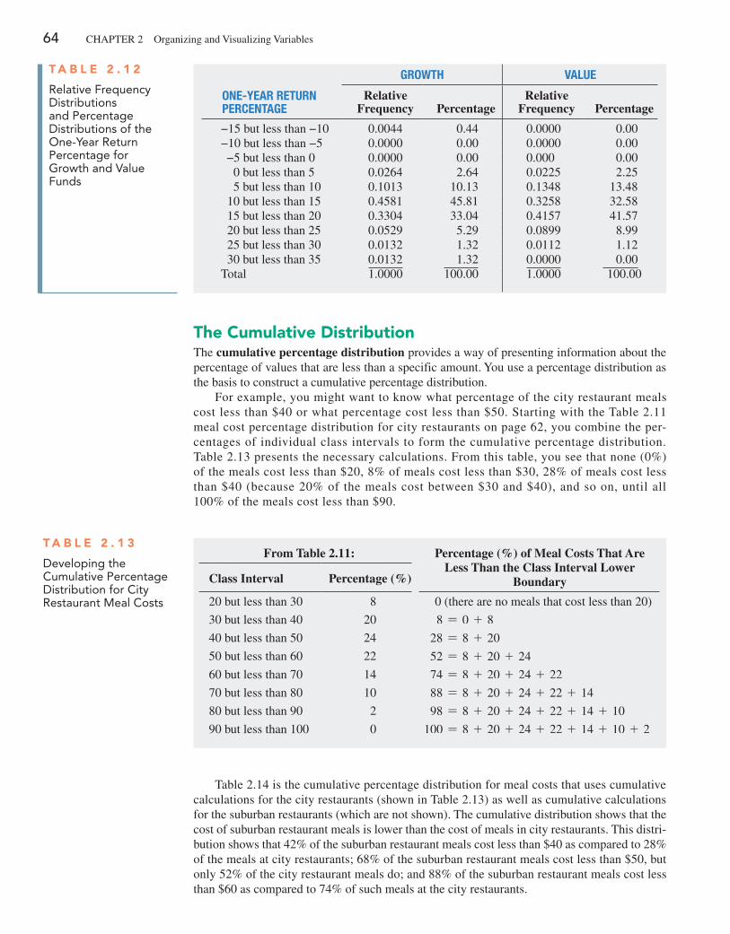
64 ChApTER 2 Organizing and Visualizing Variables
The Cumulative DistributionThe cumulative percentage distribution provides a way of presenting information about the percentage of values that are less than a specific amount. You use a percentage distribution as the basis to construct a cumulative percentage distribution.
For example, you might want to know what percentage of the city restaurant meals cost less than $40 or what percentage cost less than $50. Starting with the Table 2.11 meal cost percentage distribution for city restaurants on page 62, you combine the per-centages of individual class intervals to form the cumulative percentage distribution. Table 2.13 presents the necessary calculations. From this table, you see that none (0%) of the meals cost less than $20, 8% of meals cost less than $30, 28% of meals cost less than $40 (because 20% of the meals cost between $30 and $40), and so on, until all 100% of the meals cost less than $90.
T a b l e 2 . 1 3
Developing the Cumulative Percentage Distribution for City Restaurant Meal Costs
From Table 2.11: Percentage (%) of Meal Costs That Are Less Than the Class Interval Lower
BoundaryClass Interval Percentage (%)
20 but less than 30 8 0 (there are no meals that cost less than 20)
30 but less than 40 20 8 = 0 + 8
40 but less than 50 24 28 = 8 + 20
50 but less than 60 22 52 = 8 + 20 + 24
60 but less than 70 14 74 = 8 + 20 + 24 + 22
70 but less than 80 10 88 = 8 + 20 + 24 + 22 + 14
80 but less than 90 2 98 = 8 + 20 + 24 + 22 + 14 + 10
90 but less than 100 0 100 = 8 + 20 + 24 + 22 + 14 + 10 + 2
Table 2.14 is the cumulative percentage distribution for meal costs that uses cumulative calculations for the city restaurants (shown in Table 2.13) as well as cumulative calculations for the suburban restaurants (which are not shown). The cumulative distribution shows that the cost of suburban restaurant meals is lower than the cost of meals in city restaurants. This distri-bution shows that 42% of the suburban restaurant meals cost less than $40 as compared to 28% of the meals at city restaurants; 68% of the suburban restaurant meals cost less than $50, but only 52% of the city restaurant meals do; and 88% of the suburban restaurant meals cost less than $60 as compared to 74% of such meals at the city restaurants.
GROwTH VaLUE
ONE-YEaR RETURN PERcENTaGE
Relative Frequency
Percentage
Relative Frequency
Percentage
−15 but less than −10 0.0044 0.44 0.0000 0.00−10 but less than −5 0.0000 0.00 0.0000 0.00−5 but less than 0 0.0000 0.00 0.000 0.00 0 but less than 5 0.0264 2.64 0.0225 2.25 5 but less than 10 0.1013 10.13 0.1348 13.4810 but less than 15 0.4581 45.81 0.3258 32.5815 but less than 20 0.3304 33.04 0.4157 41.5720 but less than 25 0.0529 5.29 0.0899 8.9925 but less than 30 0.0132 1.32 0.0112 1.1230 but less than 35 0.0132 1.32 0.0000 0.00
Total 1.0000 100.00 1.0000 100.00
T a b l e 2 . 1 2
Relative Frequency Distributions and Percentage Distributions of the One-Year Return Percentage for growth and Value Funds
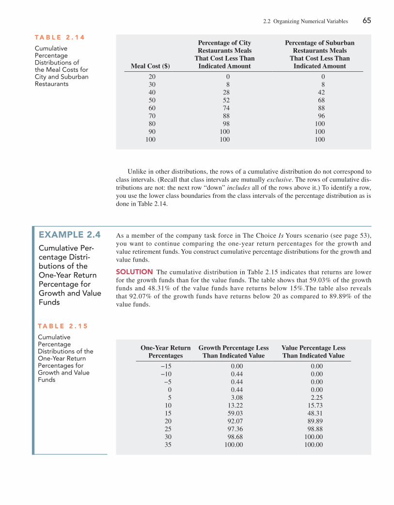
2.2 Organizing Numerical Variables 65
Unlike in other distributions, the rows of a cumulative distribution do not correspond to class intervals. (Recall that class intervals are mutually exclusive. The rows of cumulative dis-tributions are not: the next row “down” includes all of the rows above it.) To identify a row, you use the lower class boundaries from the class intervals of the percentage distribution as is done in Table 2.14.
T a b l e 2 . 1 4
Cumulative Percentage Distributions of the Meal Costs for City and Suburban Restaurants
Meal Cost ($)
Percentage of City Restaurants Meals
That Cost Less Than Indicated Amount
Percentage of Suburban Restaurants Meals
That Cost Less Than Indicated Amount
20 0 0 30 8 8 40 28 42 50 52 68 60 74 88 70 88 96 80 98 100 90 100 100100 100 100
example 2.4cumulative Per-centage Distri-butions of the One-Year Return Percentage for growth and Value Funds
As a member of the company task force in The Choice Is Yours scenario (see page 53), you want to continue comparing the one-year return percentages for the growth and value retirement funds. You construct cumulative percentage distributions for the growth and value funds.
SOluTiOn The cumulative distribution in Table 2.15 indicates that returns are lower for the growth funds than for the value funds. The table shows that 59.03% of the growth funds and 48.31% of the value funds have returns below 15%.The table also reveals that 92.07% of the growth funds have returns below 20 as compared to 89.89% of the value funds.
T a b l e 2 . 1 5
Cumulative Percentage Distributions of the One-Year Return Percentages for growth and Value Funds
One-Year Return Percentages
Growth Percentage Less Than Indicated Value
Value Percentage Less Than Indicated Value
−15 0.00 0.00−10 0.44 0.00−5 0.44 0.00
0 0.44 0.005 3.08 2.25
10 13.22 15.7315 59.03 48.3120 92.07 89.8925 97.36 98.8830 98.68 100.0035 100.00 100.00
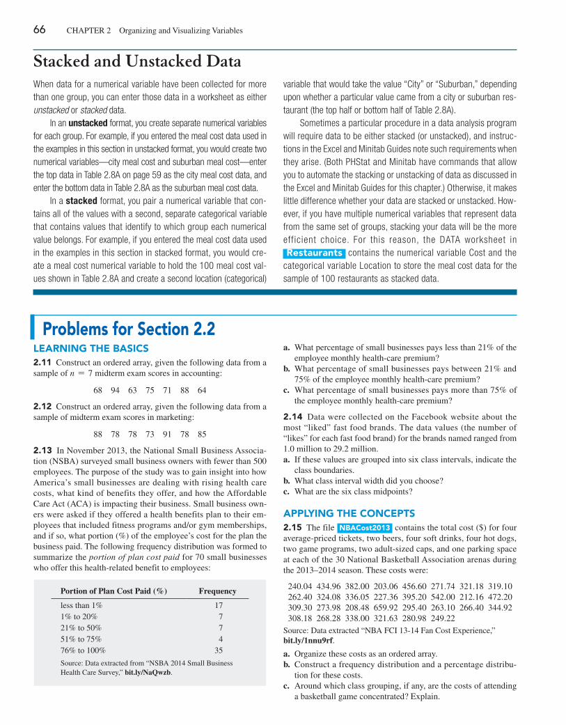
66 ChApTER 2 Organizing and Visualizing Variables
Stacked and Unstacked DataWhen data for a numerical variable have been collected for more than one group, you can enter those data in a worksheet as either unstacked or stacked data.
In an unstacked format, you create separate numerical variables for each group. For example, if you entered the meal cost data used in the examples in this section in unstacked format, you would create two numerical variables—city meal cost and suburban meal cost—enter the top data in Table 2.8A on page 59 as the city meal cost data, and enter the bottom data in Table 2.8A as the suburban meal cost data.
In a stacked format, you pair a numerical variable that con-tains all of the values with a second, separate categorical variable that contains values that identify to which group each numerical value belongs. For example, if you entered the meal cost data used in the examples in this section in stacked format, you would cre-ate a meal cost numerical variable to hold the 100 meal cost val-ues shown in Table 2.8A and create a second location (categorical)
variable that would take the value “City” or “Suburban,” depending upon whether a particular value came from a city or suburban res-taurant (the top half or bottom half of Table 2.8A).
Sometimes a particular procedure in a data analysis program will require data to be either stacked (or unstacked), and instruc-tions in the Excel and Minitab Guides note such requirements when they arise. (Both PHStat and Minitab have commands that allow you to automate the stacking or unstacking of data as discussed in the Excel and Minitab Guides for this chapter.) Otherwise, it makes little difference whether your data are stacked or unstacked. How-ever, if you have multiple numerical variables that represent data from the same set of groups, stacking your data will be the more eff icient choice. For this reason, the DATA worksheet in restaurants contains the numerical variable Cost and the categorical variable Location to store the meal cost data for the sample of 100 restaurants as stacked data.
problems for Section 2.2learning The baSiCS2.11 Construct an ordered array, given the following data from a sample of n = 7 midterm exam scores in accounting:
68 94 63 75 71 88 64
2.12 Construct an ordered array, given the following data from a sample of midterm exam scores in marketing:
88 78 78 73 91 78 85
2.13 In November 2013, the National Small Business Associa-tion (NSBA) surveyed small business owners with fewer than 500 employees. The purpose of the study was to gain insight into how America’s small businesses are dealing with rising health care costs, what kind of benefits they offer, and how the Affordable Care Act (ACA) is impacting their business. Small business own-ers were asked if they offered a health benefits plan to their em-ployees that included fitness programs and/or gym memberships, and if so, what portion (%) of the employee’s cost for the plan the business paid. The following frequency distribution was formed to summarize the portion of plan cost paid for 70 small businesses who offer this health-related benefit to employees:
Portion of Plan Cost Paid (%) Frequency
less than 1% 171% to 20% 721% to 50% 751% to 75% 476% to 100% 35
Source: Data extracted from “NSBA 2014 Small Business health Care Survey,” bit.ly/NaQwzb.
a. What percentage of small businesses pays less than 21% of the employee monthly health-care premium?
b. What percentage of small businesses pays between 21% and 75% of the employee monthly health-care premium?
c. What percentage of small businesses pays more than 75% of the employee monthly health-care premium?
2.14 Data were collected on the Facebook website about the most “liked” fast food brands. The data values (the number of “likes” for each fast food brand) for the brands named ranged from 1.0 million to 29.2 million.a. If these values are grouped into six class intervals, indicate the
class boundaries.b. What class interval width did you choose?c. What are the six class midpoints?
applying The COnCepTS2.15 The file nbaCost2013 contains the total cost ($) for four average-priced tickets, two beers, four soft drinks, four hot dogs, two game programs, two adult-sized caps, and one parking space at each of the 30 National Basketball Association arenas during the 2013–2014 season. These costs were:
240.04 434.96 382.00 203.06 456.60 271.74 321.18 319.10 262.40 324.08 336.05 227.36 395.20 542.00 212.16 472.20 309.30 273.98 208.48 659.92 295.40 263.10 266.40 344.92 308.18 268.28 338.00 321.63 280.98 249.22
Source: Data extracted “NBA FCI 13-14 Fan Cost Experience,” bit.ly/1nnu9rf.
a. Organize these costs as an ordered array.b. Construct a frequency distribution and a percentage distribu-
tion for these costs.c. Around which class grouping, if any, are the costs of attending
a basketball game concentrated? Explain.
2.2 Organizing Numerical Variables 67
SELF Test
2.16 The file utility contains the following data about the cost of electricity (in $) during July 2014 for a random
sample of 50 one-bedroom apartments in a large city.
96 171 202 178 147 102 153 197 127 82157 185 90 116 172 111 148 213 130 165141 149 206 175 123 128 144 168 109 16795 163 150 154 130 143 187 166 139 149
108 119 183 151 114 135 191 137 129 158
a. Construct a frequency distribution and a percentage distribu-tion that have class intervals with the upper class boundaries $99, $119, and so on.
b. Construct a cumulative percentage distribution.c. Around what amount does the monthly electricity cost seem to
be concentrated?
2.17 how much time do commuters living in or near cities spend waiting in traffic, and how much does this waiting cost them per year? The file Congestion contains the time spent waiting in traf-fic and the yearly cost associated with that waiting for commuters in 31 U.S. cities. (Source: Data extracted from “The high Cost of Con-gestion,” Time, October 17, 2011, p. 18.) For both the time spent waiting in traffic and the yearly cost associated with that waiting data,a. Construct a frequency distribution and a percentage distribution.b. Construct a cumulative percentage distribution.c. What conclusions can you reach concerning the time Americans
living in or near cities spend sitting in traffic?d. What conclusions can you reach concerning the time and cost
of waiting in traffic per year?
2.18 how do the average credit scores of people living in differ-ent American cities differ? The data in Credit Scores is an ordered array of the average credit scores of 143 American cities. (Data extracted from usat.ly/109hZAR.)a. Construct a frequency distribution and a percentage distribution.b. Construct a cumulative percentage distribution.c. What conclusions can you reach concerning the average credit
scores of people living in different American cities?
2.19 One operation of a mill is to cut pieces of steel into parts that will later be used as the frame for front seats in an automo-bile. The steel is cut with a diamond saw and requires the result-ing parts to be within {0.005 inch of the length specified by the automobile company. Data are collected from a sample of 100 steel parts and stored in Steel . The measurement reported is the difference in inches between the actual length of the steel part, as measured by a laser measurement device, and the speci-fied length of the steel part. For example, the first value, -0.002, represents a steel part that is 0.002 inch shorter than the specified length.a. Construct a frequency distribution and a percentage distribu-
tion.b. Construct a cumulative percentage distribution.c. Is the steel mill doing a good job meeting the requirements set
by the automobile company? Explain.
2.20 A manufacturing company produces steel housings for electrical equipment. The main component part of the housing
is a steel trough that is made out of a 14-gauge steel coil. It is produced using a 250-ton progressive punch press with a wipe-down operation that puts two 90-degree forms in the flat steel to make the trough. The distance from one side of the form to the other is critical because of weatherproofing in outdoor ap-plications. The company requires that the width of the trough be between 8.31 inches and 8.61 inches. The widths of the troughs, in inches, collected from a sample of 49 troughs and stored in Trough , are:
8.312 8.343 8.317 8.383 8.348 8.410 8.351 8.3738.481 8.422 8.476 8.382 8.484 8.403 8.414 8.4198.385 8.465 8.498 8.447 8.436 8.413 8.489 8.4148.481 8.415 8.479 8.429 8.458 8.462 8.460 8.4448.429 8.460 8.412 8.420 8.410 8.405 8.323 8.4208.396 8.447 8.405 8.439 8.411 8.427 8.420 8.4988.409
a. Construct a frequency distribution and a percentage distribution.b. Construct a cumulative percentage distribution.c. What can you conclude about the number of troughs that will
meet the company’s requirements of troughs being between 8.31 and 8.61 inches wide?
2.21 The manufacturing company in problem 2.20 also produces electric insulators. If the insulators break when in use, a short circuit is likely to occur. To test the strength of the insulators, destructive testing in high-powered labs is carried out to determine how much force is required to break the insulators. Force is mea-sured by observing how many pounds must be applied to the insu-lator before it breaks. The force measurements, collected from a sample of 30 insulators and stored in Force , are:
1,870 1,728 1,656 1,610 1,634 1,784 1,522 1,6961,592 1,662 1,866 1,764 1,734 1,662 1,734 1,7741,550 1,756 1,762 1,866 1,820 1,744 1,788 1,6881,810 1,752 1,680 1,810 1,652 1,736
a. Construct a frequency distribution and a percentage distribution.b. Construct a cumulative percentage distribution.c. What can you conclude about the strength of the insulators if
the company requires a force measurement of at least 1,500 pounds before the insulator breaks?
2.22 The file bulbs contains the life (in hours) of a sample of forty 20-watt compact fluorescent light bulbs produced by Manu-facturer A and a sample of forty 20-watt compact fluorescent light bulbs produced by Manufacturer B.a. Construct a frequency distribution and a percentage distribu-
tion for each manufacturer, using the following class interval widths for each distribution:
Manufacturer A: 6,500 but less than 7,500, 7,500 but less than 8,500, and so on.Manufacturer B: 7,500 but less than 8,500, 8,500 but less than 9,500, and so on.
b. Construct cumulative percentage distributions.c. Which bulbs have a longer life—those from Manufacturer A or
Manufacturer B? Explain.
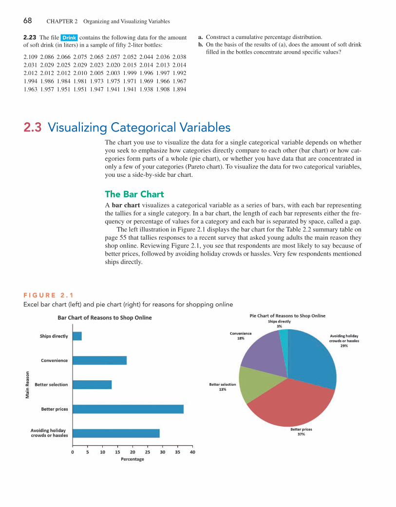
68 ChApTER 2 Organizing and Visualizing Variables
2.23 The file Drink contains the following data for the amount of soft drink (in liters) in a sample of fifty 2-liter bottles:
2.109 2.086 2.066 2.075 2.065 2.057 2.052 2.044 2.036 2.0382.031 2.029 2.025 2.029 2.023 2.020 2.015 2.014 2.013 2.0142.012 2.012 2.012 2.010 2.005 2.003 1.999 1.996 1.997 1.9921.994 1.986 1.984 1.981 1.973 1.975 1.971 1.969 1.966 1.9671.963 1.957 1.951 1.951 1.947 1.941 1.941 1.938 1.908 1.894
a. Construct a cumulative percentage distribution.b. On the basis of the results of (a), does the amount of soft drink
filled in the bottles concentrate around specific values?
2.3 Visualizing Categorical VariablesThe chart you use to visualize the data for a single categorical variable depends on whether you seek to emphasize how categories directly compare to each other (bar chart) or how cat-egories form parts of a whole (pie chart), or whether you have data that are concentrated in only a few of your categories (pareto chart). To visualize the data for two categorical variables, you use a side-by-side bar chart.
The bar ChartA bar chart visualizes a categorical variable as a series of bars, with each bar representing the tallies for a single category. In a bar chart, the length of each bar represents either the fre-quency or percentage of values for a category and each bar is separated by space, called a gap.
The left illustration in Figure 2.1 displays the bar chart for the Table 2.2 summary table on page 55 that tallies responses to a recent survey that asked young adults the main reason they shop online. Reviewing Figure 2.1, you see that respondents are most likely to say because of better prices, followed by avoiding holiday crowds or hassles. Very few respondents mentioned ships directly.
F i g u r e 2 . 1excel bar chart (left) and pie chart (right) for reasons for shopping online
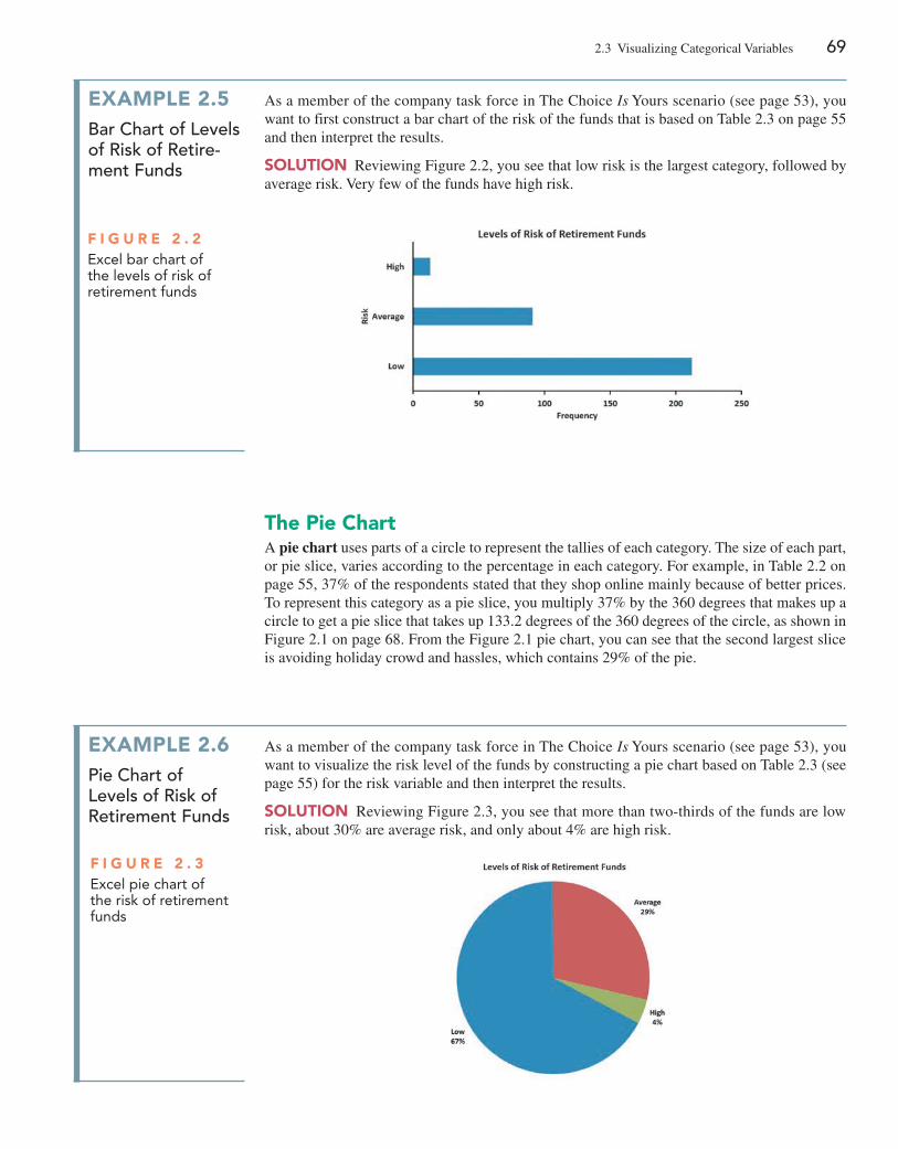
2.3 Visualizing Categorical Variables 69
The pie ChartA pie chart uses parts of a circle to represent the tallies of each category. The size of each part, or pie slice, varies according to the percentage in each category. For example, in Table 2.2 on page 55, 37% of the respondents stated that they shop online mainly because of better prices. To represent this category as a pie slice, you multiply 37% by the 360 degrees that makes up a circle to get a pie slice that takes up 133.2 degrees of the 360 degrees of the circle, as shown in Figure 2.1 on page 68. From the Figure 2.1 pie chart, you can see that the second largest slice is avoiding holiday crowd and hassles, which contains 29% of the pie.
example 2.5Bar chart of levels of Risk of Retire-ment Funds
As a member of the company task force in The Choice Is Yours scenario (see page 53), you want to first construct a bar chart of the risk of the funds that is based on Table 2.3 on page 55 and then interpret the results.
SOluTiOn Reviewing Figure 2.2, you see that low risk is the largest category, followed by average risk. Very few of the funds have high risk.
F i g u r e 2 . 2excel bar chart of the levels of risk of retirement funds
example 2.6Pie chart of levels of Risk of Retirement Funds
As a member of the company task force in The Choice Is Yours scenario (see page 53), you want to visualize the risk level of the funds by constructing a pie chart based on Table 2.3 (see page 55) for the risk variable and then interpret the results.
SOluTiOn Reviewing Figure 2.3, you see that more than two-thirds of the funds are low risk, about 30% are average risk, and only about 4% are high risk.
F i g u r e 2 . 3excel pie chart of the risk of retirement funds
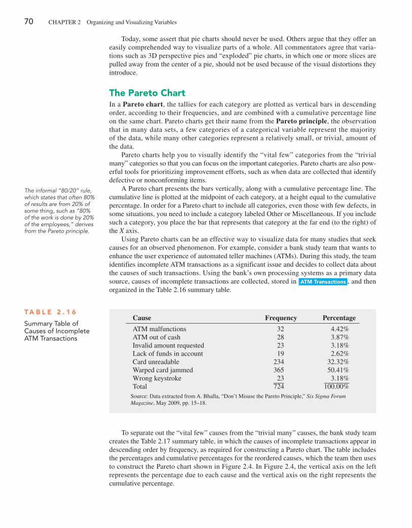
70 ChApTER 2 Organizing and Visualizing Variables
Today, some assert that pie charts should never be used. Others argue that they offer an easily comprehended way to visualize parts of a whole. All commentators agree that varia-tions such as 3D perspective pies and “exploded” pie charts, in which one or more slices are pulled away from the center of a pie, should not be used because of the visual distortions they introduce.
The pareto ChartIn a Pareto chart, the tallies for each category are plotted as vertical bars in descending order, according to their frequencies, and are combined with a cumulative percentage line on the same chart. pareto charts get their name from the Pareto principle, the observation that in many data sets, a few categories of a categorical variable represent the majority of the data, while many other categories represent a relatively small, or trivial, amount of the data.
pareto charts help you to visually identify the “vital few” categories from the “trivial many” categories so that you can focus on the important categories. pareto charts are also pow-erful tools for prioritizing improvement efforts, such as when data are collected that identify defective or nonconforming items.
A pareto chart presents the bars vertically, along with a cumulative percentage line. The cumulative line is plotted at the midpoint of each category, at a height equal to the cumulative percentage. In order for a pareto chart to include all categories, even those with few defects, in some situations, you need to include a category labeled Other or Miscellaneous. If you include such a category, you place the bar that represents that category at the far end (to the right) of the X axis.
Using pareto charts can be an effective way to visualize data for many studies that seek causes for an observed phenomenon. For example, consider a bank study team that wants to enhance the user experience of automated teller machines (ATMs). During this study, the team identifies incomplete ATM transactions as a significant issue and decides to collect data about the causes of such transactions. Using the bank’s own processing systems as a primary data source, causes of incomplete transactions are collected, stored in aTm Transactions , and then organized in the Table 2.16 summary table.
The informal “80/20” rule, which states that often 80% of results are from 20% of some thing, such as “80% of the work is done by 20% of the employees,” derives from the Pareto principle.
Cause Frequency Percentage
ATM malfunctions 32 4.42%ATM out of cash 28 3.87%Invalid amount requested 23 3.18%Lack of funds in account 19 2.62%Card unreadable 234 32.32%Warped card jammed 365 50.41%Wrong keystroke 23 3.18%Total 724 100.00%
Source: Data extracted from A. Bhalla, “Don’t Misuse the pareto principle,” Six Sigma Forum Magazine, May 2009, pp. 15–18.
T a b l e 2 . 1 6
Summary Table of Causes of incomplete ATM Transactions
To separate out the “vital few” causes from the “trivial many” causes, the bank study team creates the Table 2.17 summary table, in which the causes of incomplete transactions appear in descending order by frequency, as required for constructing a pareto chart. The table includes the percentages and cumulative percentages for the reordered causes, which the team then uses to construct the pareto chart shown in Figure 2.4. In Figure 2.4, the vertical axis on the left represents the percentage due to each cause and the vertical axis on the right represents the cumulative percentage.
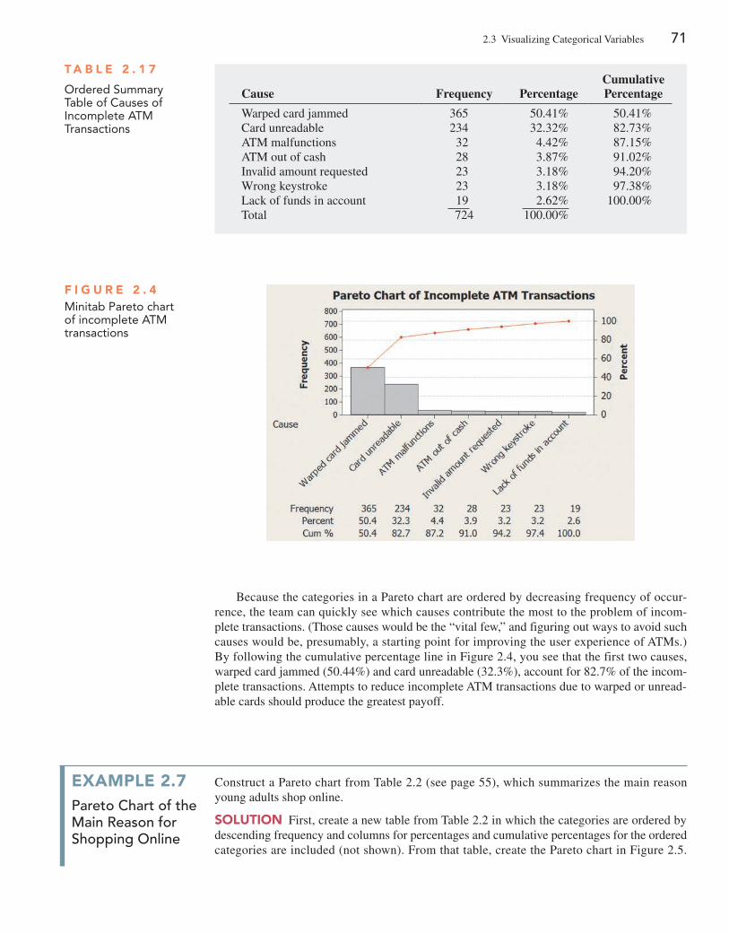
2.3 Visualizing Categorical Variables 71
Because the categories in a pareto chart are ordered by decreasing frequency of occur-rence, the team can quickly see which causes contribute the most to the problem of incom-plete transactions. (Those causes would be the “vital few,” and figuring out ways to avoid such causes would be, presumably, a starting point for improving the user experience of ATMs.) By following the cumulative percentage line in Figure 2.4, you see that the first two causes, warped card jammed (50.44%) and card unreadable (32.3%), account for 82.7% of the incom-plete transactions. Attempts to reduce incomplete ATM transactions due to warped or unread-able cards should produce the greatest payoff.
T a b l e 2 . 1 7
Ordered Summary Table of Causes of incomplete ATM Transactions
Cause
Frequency
Percentage
Cumulative Percentage
Warped card jammed 365 50.41% 50.41%Card unreadable 234 32.32% 82.73%ATM malfunctions 32 4.42% 87.15%ATM out of cash 28 3.87% 91.02%Invalid amount requested 23 3.18% 94.20%Wrong keystroke 23 3.18% 97.38%Lack of funds in account 19 2.62% 100.00%Total 724 100.00%
F i g u r e 2 . 4Minitab Pareto chart of incomplete ATM transactions
example 2.7Pareto chart of the Main Reason for shopping Online
Construct a pareto chart from Table 2.2 (see page 55), which summarizes the main reason young adults shop online.
SOluTiOn First, create a new table from Table 2.2 in which the categories are ordered by descending frequency and columns for percentages and cumulative percentages for the ordered categories are included (not shown). From that table, create the pareto chart in Figure 2.5.
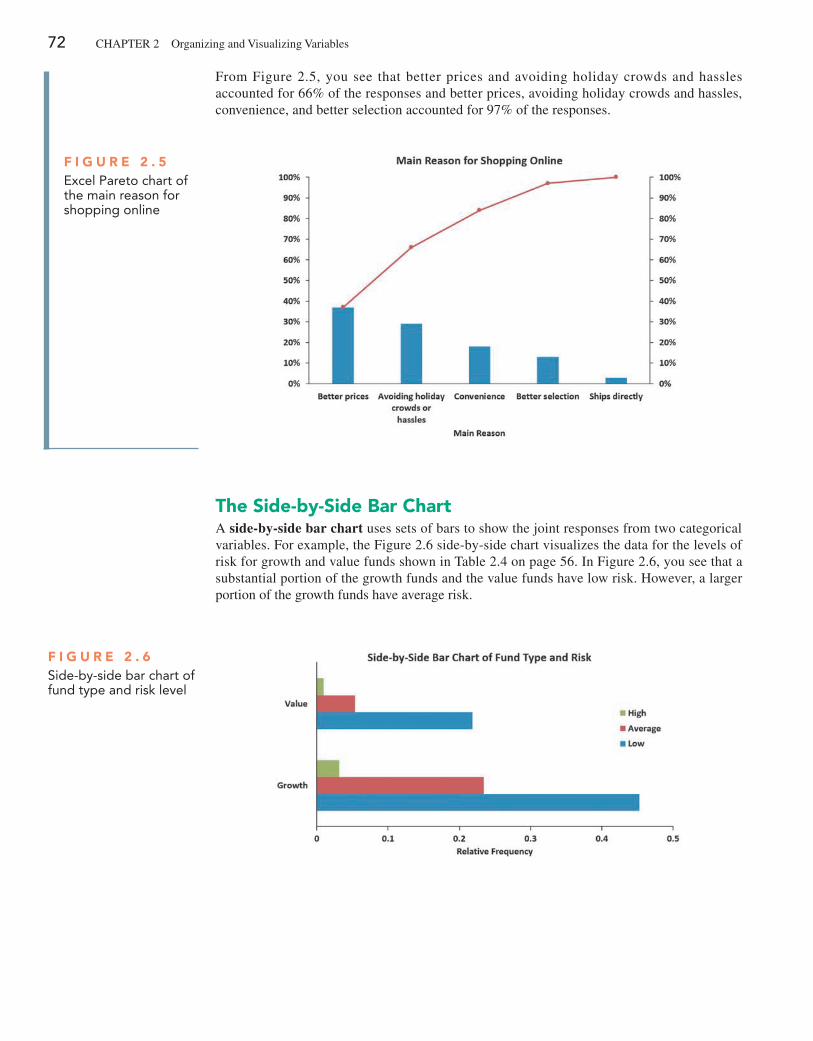
72 ChApTER 2 Organizing and Visualizing Variables
The Side-by-Side bar ChartA side-by-side bar chart uses sets of bars to show the joint responses from two categorical variables. For example, the Figure 2.6 side-by-side chart visualizes the data for the levels of risk for growth and value funds shown in Table 2.4 on page 56. In Figure 2.6, you see that a substantial portion of the growth funds and the value funds have low risk. however, a larger portion of the growth funds have average risk.
F i g u r e 2 . 5excel Pareto chart of the main reason for shopping online
F i g u r e 2 . 6Side-by-side bar chart of fund type and risk level
From Figure 2.5, you see that better prices and avoiding holiday crowds and hassles accounted for 66% of the responses and better prices, avoiding holiday crowds and hassles, convenience, and better selection accounted for 97% of the responses.
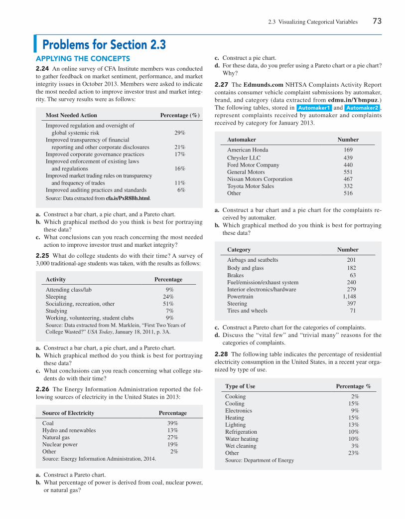
2.3 Visualizing Categorical Variables 73
problems for Section 2.3applying The COnCepTS2.24 An online survey of CFA Institute members was conducted to gather feedback on market sentiment, performance, and market integrity issues in October 2013. Members were asked to indicate the most needed action to improve investor trust and market integ-rity. The survey results were as follows:
Most Needed Action Percentage (%)
Improved regulation and oversight of global systemic risk
29%
Improved transparency of financial reporting and other corporate disclosures
21%
Improved corporate governance practices 17%Improved enforcement of existing laws and regulations
16%
Improved market trading rules on transparency and frequency of trades
11%
Improved auditing practices and standards 6%Source: Data extracted from cfa.is/PxR8Bh.html.
a. Construct a bar chart, a pie chart, and a pareto chart.b. Which graphical method do you think is best for portraying
these data?c. What conclusions can you reach concerning the most needed
action to improve investor trust and market integrity?
2.25 What do college students do with their time? A survey of 3,000 traditional-age students was taken, with the results as follows:
Activity Percentage
Attending class/lab 9%Sleeping 24%Socializing, recreation, other 51%Studying 7%Working, volunteering, student clubs 9%Source: Data extracted from M. Marklein, “First Two Years of College Wasted?” USA Today, January 18, 2011, p. 3A.
a. Construct a bar chart, a pie chart, and a pareto chart.b. Which graphical method do you think is best for portraying
these data?c. What conclusions can you reach concerning what college stu-
dents do with their time?
2.26 The Energy Information Administration reported the fol-lowing sources of electricity in the United States in 2013:
Source of Electricity Percentage
Coal 39%hydro and renewables 13%Natural gas 27%Nuclear power 19%Other 2%Source: Energy Information Administration, 2014.
a. Construct a pareto chart.b. What percentage of power is derived from coal, nuclear power,
or natural gas?
c. Construct a pie chart.d. For these data, do you prefer using a pareto chart or a pie chart?
Why?
2.27 The Edmunds.com NhTSA Complaints Activity Report contains consumer vehicle complaint submissions by automaker, brand, and category (data extracted from edmu.in/Ybmpuz.) The following tables, stored in automaker1 and automaker2 , represent complaints received by automaker and complaints received by category for January 2013.
Automaker Number
American honda 169Chrysler LLC 439Ford Motor Company 440General Motors 551Nissan Motors Corporation 467Toyota Motor Sales 332Other 516
a. Construct a bar chart and a pie chart for the complaints re-ceived by automaker.
b. Which graphical method do you think is best for portraying these data?
Category Number
Airbags and seatbelts 201Body and glass 182Brakes 63Fuel/emission/exhaust system 240Interior electronics/hardware 279powertrain 1,148Steering 397Tires and wheels 71
c. Construct a pareto chart for the categories of complaints.d. Discuss the “vital few” and “trivial many” reasons for the
categories of complaints.
2.28 The following table indicates the percentage of residential electricity consumption in the United States, in a recent year orga-nized by type of use.
Type of Use Percentage %
Cooking 2%Cooling 15%Electronics 9%heating 15%Lighting 13%Refrigeration 10%Water heating 10%Wet cleaning 3%Other 23%Source: Department of Energy
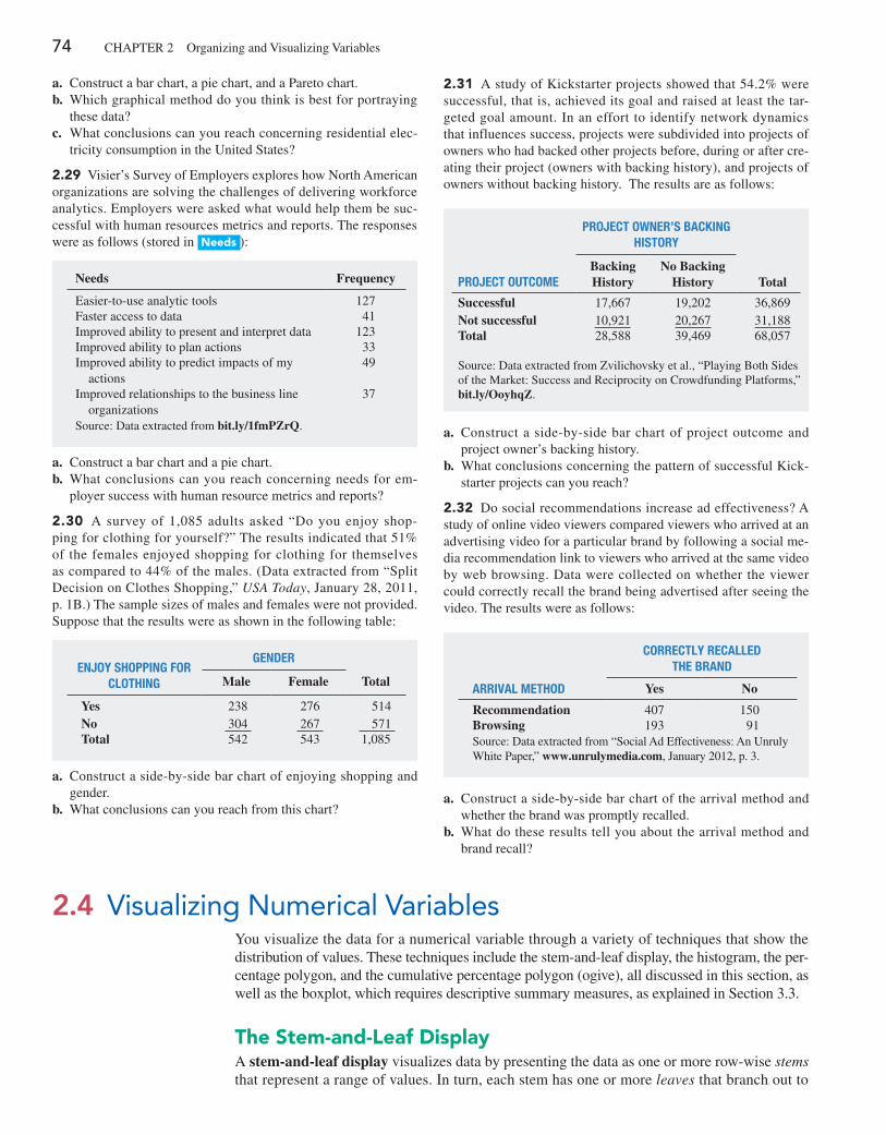
74 ChApTER 2 Organizing and Visualizing Variables
a. Construct a bar chart, a pie chart, and a pareto chart.b. Which graphical method do you think is best for portraying
these data?c. What conclusions can you reach concerning residential elec-
tricity consumption in the United States?
2.29 Visier’s Survey of Employers explores how North American organizations are solving the challenges of delivering workforce analytics. Employers were asked what would help them be suc-cessful with human resources metrics and reports. The responses were as follows (stored in needs ):
Needs Frequency
Easier-to-use analytic tools 127Faster access to data 41Improved ability to present and interpret data 123Improved ability to plan actions 33Improved ability to predict impacts of my actions
49
Improved relationships to the business line organizations
37
Source: Data extracted from bit.ly/1fmPZrQ.
a. Construct a bar chart and a pie chart.b. What conclusions can you reach concerning needs for em-
ployer success with human resource metrics and reports?
2.30 A survey of 1,085 adults asked “Do you enjoy shop-ping for clothing for yourself?” The results indicated that 51% of the females enjoyed shopping for clothing for themselves as compared to 44% of the males. (Data extracted from “Split Decision on Clothes Shopping,” USA Today, January 28, 2011, p. 1B.) The sample sizes of males and females were not provided. Suppose that the results were as shown in the following table:
ENJOY SHOPPING FOR
cLOTHING
GENDER
Male Female Total
Yes 238 276 514 No 304 267 571 Total 542 543 1,085
a. Construct a side-by-side bar chart of enjoying shopping and gender.
b. What conclusions can you reach from this chart?
2.31 A study of Kickstarter projects showed that 54.2% were successful, that is, achieved its goal and raised at least the tar-geted goal amount. In an effort to identify network dynamics that influences success, projects were subdivided into projects of owners who had backed other projects before, during or after cre-ating their project (owners with backing history), and projects of owners without backing history. The results are as follows:
PROJEcT OwNER’S BacKING HISTORY
PROJEcT OUTcOMEBacking History
No Backing History
Total
Successful 17,667 19,202 36,869Not successful 10,921 20,267 31,188Total 28,588 39,469 68,057
Source: Data extracted from Zvilichovsky et al., “playing Both Sides of the Market: Success and Reciprocity on Crowdfunding platforms,” bit.ly/OoyhqZ.
a. Construct a side-by-side bar chart of project outcome and project owner’s backing history.
b. What conclusions concerning the pattern of successful Kick-starter projects can you reach?
2.32 Do social recommendations increase ad effectiveness? A study of online video viewers compared viewers who arrived at an advertising video for a particular brand by following a social me-dia recommendation link to viewers who arrived at the same video by web browsing. Data were collected on whether the viewer could correctly recall the brand being advertised after seeing the video. The results were as follows:
cORREcTLY REcaLLED THE BRaND
aRRIVaL METHOD Yes No
Recommendation 407 150Browsing 193 91Source: Data extracted from “Social Ad Effectiveness: An Unruly White paper,” www.unrulymedia.com, January 2012, p. 3.
a. Construct a side-by-side bar chart of the arrival method and whether the brand was promptly recalled.
b. What do these results tell you about the arrival method and brand recall?
2.4 Visualizing Numerical VariablesYou visualize the data for a numerical variable through a variety of techniques that show the distribution of values. These techniques include the stem-and-leaf display, the histogram, the per-centage polygon, and the cumulative percentage polygon (ogive), all discussed in this section, as well as the boxplot, which requires descriptive summary measures, as explained in Section 3.3.
The Stem-and-leaf DisplayA stem-and-leaf display visualizes data by presenting the data as one or more row-wise stems that represent a range of values. In turn, each stem has one or more leaves that branch out to
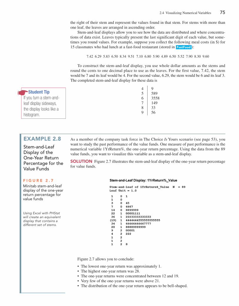
2.4 Visualizing Numerical Variables 75
Student TipIf you turn a stem-and-leaf display sideways, the display looks like a histogram.
example 2.8stem-and-leaf Display of the One-Year Return Percentage for the Value Funds
As a member of the company task force in The Choice Is Yours scenario (see page 53), you want to study the past performance of the value funds. One measure of past performance is the numerical variable 1YrReturn%, the one-year return percentage. Using the data from the 89 value funds, you want to visualize this variable as a stem-and-leaf display.
SOluTiOn Figure 2.7 illustrates the stem-and-leaf display of the one-year return percentage for value funds.
Using Excel with PHStat will create an equivalent display that contains a different set of stems.
F i g u r e 2 . 7Minitab stem-and-leaf display of the one-year return percentage for value funds
Figure 2.7 allows you to conclude:
• The lowest one-year return was approximately 1. • The highest one-year return was 28. • The one-year returns were concentrated between 12 and 19. • Very few of the one-year returns were above 21. • The distribution of the one-year return appears to be bell-shaped.
the right of their stem and represent the values found in that stem. For stems with more than one leaf, the leaves are arranged in ascending order.
Stem-and-leaf displays allow you to see how the data are distributed and where concentra-tions of data exist. Leaves typically present the last significant digit of each value, but some-times you round values. For example, suppose you collect the following meal costs (in $) for 15 classmates who had lunch at a fast-food restaurant (stored in FastFood ):
7.42 6.29 5.83 6.50 8.34 9.51 7.10 6.80 5.90 4.89 6.50 5.52 7.90 8.30 9.60
To construct the stem-and-leaf display, you use whole dollar amounts as the stems and round the cents to one decimal place to use as the leaves. For the first value, 7.42, the stem would be 7 and its leaf would be 4. For the second value, 6.29, the stem would be 6 and its leaf 3. The completed stem-and-leaf display for these data is
4 95 5896 35587 1498 339 56
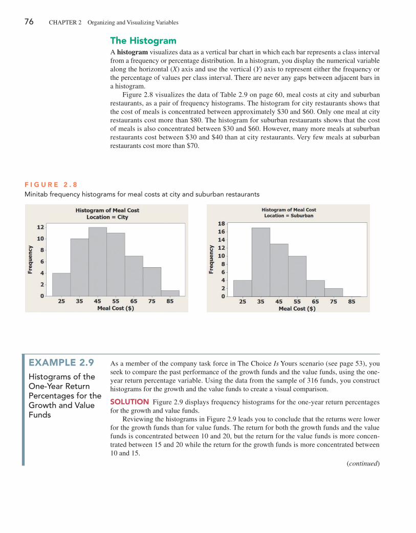
76 ChApTER 2 Organizing and Visualizing Variables
The histogramA histogram visualizes data as a vertical bar chart in which each bar represents a class interval from a frequency or percentage distribution. In a histogram, you display the numerical variable along the horizontal (X) axis and use the vertical (Y) axis to represent either the frequency or the percentage of values per class interval. There are never any gaps between adjacent bars in a histogram.
Figure 2.8 visualizes the data of Table 2.9 on page 60, meal costs at city and suburban restaurants, as a pair of frequency histograms. The histogram for city restaurants shows that the cost of meals is concentrated between approximately $30 and $60. Only one meal at city restaurants cost more than $80. The histogram for suburban restaurants shows that the cost of meals is also concentrated between $30 and $60. however, many more meals at suburban restaurants cost between $30 and $40 than at city restaurants. Very few meals at suburban restaurants cost more than $70.
F i g u r e 2 . 8Minitab frequency histograms for meal costs at city and suburban restaurants
example 2.9histograms of the One-Year Return Percentages for the growth and Value Funds
As a member of the company task force in The Choice Is Yours scenario (see page 53), you seek to compare the past performance of the growth funds and the value funds, using the one-year return percentage variable. Using the data from the sample of 316 funds, you construct histograms for the growth and the value funds to create a visual comparison.
SOluTiOn Figure 2.9 displays frequency histograms for the one-year return percentages for the growth and value funds.
Reviewing the histograms in Figure 2.9 leads you to conclude that the returns were lower for the growth funds than for value funds. The return for both the growth funds and the value funds is concentrated between 10 and 20, but the return for the value funds is more concen-trated between 15 and 20 while the return for the growth funds is more concentrated between 10 and 15.
(continued)
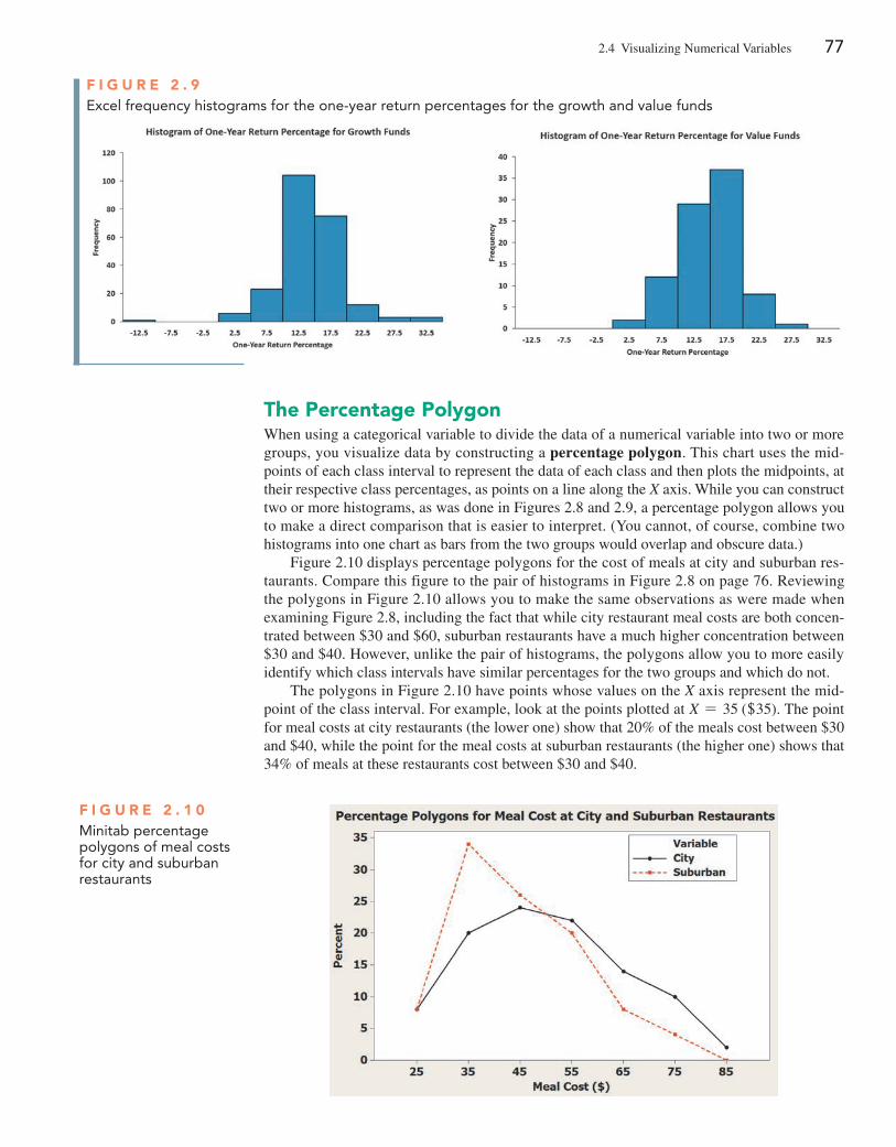
2.4 Visualizing Numerical Variables 77
The percentage polygonWhen using a categorical variable to divide the data of a numerical variable into two or more groups, you visualize data by constructing a percentage polygon. This chart uses the mid-points of each class interval to represent the data of each class and then plots the midpoints, at their respective class percentages, as points on a line along the X axis. While you can construct two or more histograms, as was done in Figures 2.8 and 2.9, a percentage polygon allows you to make a direct comparison that is easier to interpret. (You cannot, of course, combine two histograms into one chart as bars from the two groups would overlap and obscure data.)
Figure 2.10 displays percentage polygons for the cost of meals at city and suburban res-taurants. Compare this figure to the pair of histograms in Figure 2.8 on page 76. Reviewing the polygons in Figure 2.10 allows you to make the same observations as were made when examining Figure 2.8, including the fact that while city restaurant meal costs are both concen-trated between $30 and $60, suburban restaurants have a much higher concentration between $30 and $40. however, unlike the pair of histograms, the polygons allow you to more easily identify which class intervals have similar percentages for the two groups and which do not.
The polygons in Figure 2.10 have points whose values on the X axis represent the mid-point of the class interval. For example, look at the points plotted at X = 35 (+35). The point for meal costs at city restaurants (the lower one) show that 20% of the meals cost between $30 and $40, while the point for the meal costs at suburban restaurants (the higher one) shows that 34% of meals at these restaurants cost between $30 and $40.
F i g u r e 2 . 9excel frequency histograms for the one-year return percentages for the growth and value funds
F i g u r e 2 . 1 0Minitab percentage polygons of meal costs for city and suburban restaurants
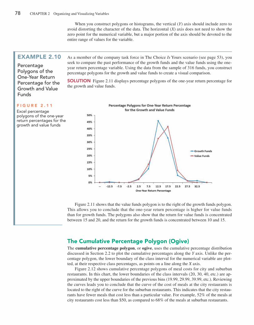
78 ChApTER 2 Organizing and Visualizing Variables
When you construct polygons or histograms, the vertical (Y) axis should include zero to avoid distorting the character of the data. The horizontal (X) axis does not need to show the zero point for the numerical variable, but a major portion of the axis should be devoted to the entire range of values for the variable.
The Cumulative percentage polygon (Ogive)The cumulative percentage polygon, or ogive, uses the cumulative percentage distribution discussed in Section 2.2 to plot the cumulative percentages along the Y axis. Unlike the per-centage polygon, the lower boundary of the class interval for the numerical variable are plot-ted, at their respective class percentages, as points on a line along the X axis.
Figure 2.12 shows cumulative percentage polygons of meal costs for city and suburban restaurants. In this chart, the lower boundaries of the class intervals (20, 30, 40, etc.) are ap-proximated by the upper boundaries of the previous bins (19.99, 29.99, 39.99, etc.). Reviewing the curves leads you to conclude that the curve of the cost of meals at the city restaurants is located to the right of the curve for the suburban restaurants. This indicates that the city restau-rants have fewer meals that cost less than a particular value. For example, 52% of the meals at city restaurants cost less than $50, as compared to 68% of the meals at suburban restaurants.
example 2.10Percentage Polygons of the One-Year Return Percentage for the growth and Value Funds
As a member of the company task force in The Choice Is Yours scenario (see page 53), you seek to compare the past performance of the growth funds and the value funds using the one-year return percentage variable. Using the data from the sample of 316 funds, you construct percentage polygons for the growth and value funds to create a visual comparison.
SOluTiOn Figure 2.11 displays percentage polygons of the one-year return percentage for the growth and value funds.
Figure 2.11 shows that the value funds polygon is to the right of the growth funds polygon. This allows you to conclude that the one-year return percentage is higher for value funds than for growth funds. The polygons also show that the return for value funds is concentrated between 15 and 20, and the return for the growth funds is concentrated between 10 and 15.
F i g u r e 2 . 1 1excel percentage polygons of the one-year return percentages for the growth and value funds
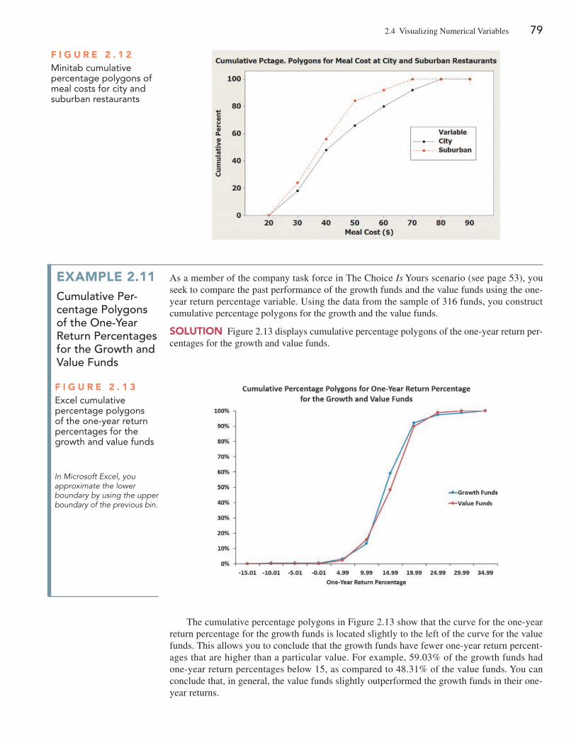
2.4 Visualizing Numerical Variables 79
The cumulative percentage polygons in Figure 2.13 show that the curve for the one-year return percentage for the growth funds is located slightly to the left of the curve for the value funds. This allows you to conclude that the growth funds have fewer one-year return percent-ages that are higher than a particular value. For example, 59.03% of the growth funds had one-year return percentages below 15, as compared to 48.31% of the value funds. You can conclude that, in general, the value funds slightly outperformed the growth funds in their one-year returns.
F i g u r e 2 . 1 2Minitab cumulative percentage polygons of meal costs for city and suburban restaurants
example 2.11cumulative Per-centage Polygons of the One-Year Return Percentages for the growth and Value Funds
As a member of the company task force in The Choice Is Yours scenario (see page 53), you seek to compare the past performance of the growth funds and the value funds using the one-year return percentage variable. Using the data from the sample of 316 funds, you construct cumulative percentage polygons for the growth and the value funds.
SOluTiOn Figure 2.13 displays cumulative percentage polygons of the one-year return per-centages for the growth and value funds.
In Microsoft Excel, you approximate the lower boundary by using the upper boundary of the previous bin.
F i g u r e 2 . 1 3excel cumulative percentage polygons of the one-year return percentages for the growth and value funds
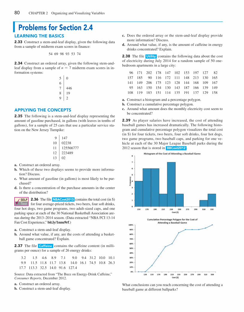
80 ChApTER 2 Organizing and Visualizing Variables
problems for Section 2.4learning The baSiCS2.33 Construct a stem-and-leaf display, given the following data from a sample of midterm exam scores in finance:
54 69 98 93 53 74
2.34 Construct an ordered array, given the following stem-and-leaf display from a sample of n = 7 midterm exam scores in in-formation systems:
5 067 4468 199 2
applying The COnCepTS2.35 The following is a stem-and-leaf display representing the amount of gasoline purchased, in gallons (with leaves in tenths of gallons), for a sample of 25 cars that use a particular service sta-tion on the New Jersey Turnpike:
9 14710 0223811 12556677712 22348913 02
a. Construct an ordered array.b. Which of these two displays seems to provide more informa-
tion? Discuss.c. What amount of gasoline (in gallons) is most likely to be pur-
chased?d. Is there a concentration of the purchase amounts in the center
of the distribution?
SELF Test
2.36 The file nbaCost2013 contains the total cost (in $) for four average-priced tickets, two beers, four soft drinks,
four hot dogs, two game programs, two adult-sized caps, and one parking space at each of the 30 National Basketball Association are-nas during the 2013–2014 season. (Data extracted “NBA FCI 13-14 Fan Cost Experience,” bit.ly/1nnu9rf.)
a. Construct a stem-and-leaf display.b. Around what value, if any, are the costs of attending a basket-
ball game concentrated? Explain.
2.37 The file Caffeine contains the caffeine content (in milli-grams per ounce) for a sample of 26 energy drinks:
3.2 1.5 4.6 8.9 7.1 9.0 9.4 31.2 10.0 10.1 9.9 11.5 11.8 11.7 13.8 14.0 16.1 74.5 10.8 26.3 17.7 113.3 32.5 14.0 91.6 127.4
Source: Data extracted from “The Buzz on Energy-Drink Caffeine,” Consumer Reports, December 2012.
a. Construct an ordered array.b. Construct a stem-and-leaf display.
c. Does the ordered array or the stem-and-leaf display provide more information? Discuss.
d. Around what value, if any, is the amount of caffeine in energy drinks concentrated? Explain.
2.38 The file utility contains the following data about the cost of electricity during July 2014 for a random sample of 50 one-bedroom apartments in a large city:
96 171 202 178 147 102 153 197 127 82157 185 90 116 172 111 148 213 130 165141 149 206 175 123 128 144 168 109 16795 163 150 154 130 143 187 166 139 149
108 119 183 151 114 135 191 137 129 158
a. Construct a histogram and a percentage polygon.b. Construct a cumulative percentage polygon.c. Around what amount does the monthly electricity cost seem to
be concentrated?
2.39 As player salaries have increased, the cost of attending baseball games has increased dramatically. The following histo-gram and cumulative percentage polygon visualizes the total cost (in $) for four tickets, two beers, four soft drinks, four hot dogs, two game programs, two baseball caps, and parking for one ve-hicle at each of the 30 Major League Baseball parks during the 2012 season that is stored in bbCost2012 .
What conclusions can you reach concerning the cost of attending a baseball game at different ballparks?
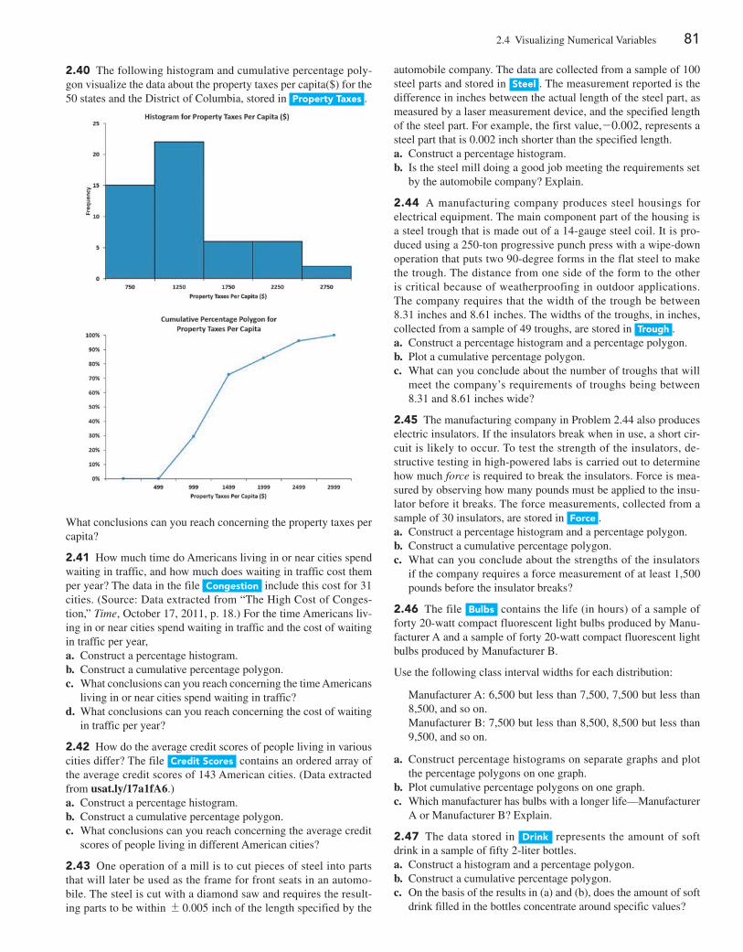
2.4 Visualizing Numerical Variables 81
2.40 The following histogram and cumulative percentage poly-gon visualize the data about the property taxes per capita($) for the 50 states and the District of Columbia, stored in property Taxes .
What conclusions can you reach concerning the property taxes per capita?
2.41 how much time do Americans living in or near cities spend waiting in traffic, and how much does waiting in traffic cost them per year? The data in the file Congestion include this cost for 31 cities. (Source: Data extracted from “The high Cost of Conges-tion,” Time, October 17, 2011, p. 18.) For the time Americans liv-ing in or near cities spend waiting in traffic and the cost of waiting in traffic per year,a. Construct a percentage histogram.b. Construct a cumulative percentage polygon.c. What conclusions can you reach concerning the time Americans
living in or near cities spend waiting in traffic?d. What conclusions can you reach concerning the cost of waiting
in traffic per year?
2.42 how do the average credit scores of people living in various cities differ? The file Credit Scores contains an ordered array of the average credit scores of 143 American cities. (Data extracted from usat.ly/17a1fA6.)a. Construct a percentage histogram.b. Construct a cumulative percentage polygon.c. What conclusions can you reach concerning the average credit
scores of people living in different American cities?
2.43 One operation of a mill is to cut pieces of steel into parts that will later be used as the frame for front seats in an automo-bile. The steel is cut with a diamond saw and requires the result-ing parts to be within { 0.005 inch of the length specified by the
automobile company. The data are collected from a sample of 100 steel parts and stored in Steel . The measurement reported is the difference in inches between the actual length of the steel part, as measured by a laser measurement device, and the specified length of the steel part. For example, the first value, -0.002, represents a steel part that is 0.002 inch shorter than the specified length.a. Construct a percentage histogram.b. Is the steel mill doing a good job meeting the requirements set
by the automobile company? Explain.
2.44 A manufacturing company produces steel housings for electrical equipment. The main component part of the housing is a steel trough that is made out of a 14-gauge steel coil. It is pro-duced using a 250-ton progressive punch press with a wipe-down operation that puts two 90-degree forms in the flat steel to make the trough. The distance from one side of the form to the other is critical because of weatherproofing in outdoor applications. The company requires that the width of the trough be between 8.31 inches and 8.61 inches. The widths of the troughs, in inches, collected from a sample of 49 troughs, are stored in Trough .a. Construct a percentage histogram and a percentage polygon.b. plot a cumulative percentage polygon.c. What can you conclude about the number of troughs that will
meet the company’s requirements of troughs being between 8.31 and 8.61 inches wide?
2.45 The manufacturing company in problem 2.44 also produces electric insulators. If the insulators break when in use, a short cir-cuit is likely to occur. To test the strength of the insulators, de-structive testing in high-powered labs is carried out to determine how much force is required to break the insulators. Force is mea-sured by observing how many pounds must be applied to the insu-lator before it breaks. The force measurements, collected from a sample of 30 insulators, are stored in Force .a. Construct a percentage histogram and a percentage polygon.b. Construct a cumulative percentage polygon.c. What can you conclude about the strengths of the insulators
if the company requires a force measurement of at least 1,500 pounds before the insulator breaks?
2.46 The file bulbs contains the life (in hours) of a sample of forty 20-watt compact fluorescent light bulbs produced by Manu-facturer A and a sample of forty 20-watt compact fluorescent light bulbs produced by Manufacturer B.
Use the following class interval widths for each distribution:
Manufacturer A: 6,500 but less than 7,500, 7,500 but less than 8,500, and so on.Manufacturer B: 7,500 but less than 8,500, 8,500 but less than 9,500, and so on.
a. Construct percentage histograms on separate graphs and plot the percentage polygons on one graph.
b. plot cumulative percentage polygons on one graph.c. Which manufacturer has bulbs with a longer life—Manufacturer
A or Manufacturer B? Explain.
2.47 The data stored in Drink represents the amount of soft drink in a sample of fifty 2-liter bottles.a. Construct a histogram and a percentage polygon.b. Construct a cumulative percentage polygon.c. On the basis of the results in (a) and (b), does the amount of soft
drink filled in the bottles concentrate around specific values?
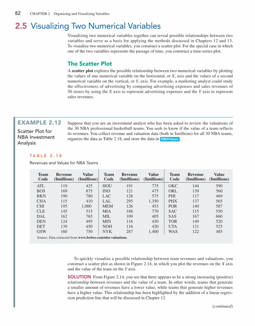
82 ChApTER 2 Organizing and Visualizing Variables
2.5 Visualizing Two Numerical VariablesVisualizing two numerical variables together can reveal possible relationships between two variables and serve as a basis for applying the methods discussed in Chapters 12 and 13. To visualize two numerical variables, you construct a scatter plot. For the special case in which one of the two variables represents the passage of time, you construct a time-series plot.
The Scatter plotA scatter plot explores the possible relationship between two numerical variables by plotting the values of one numerical variable on the horizontal, or X, axis and the values of a second numerical variable on the vertical, or Y, axis. For example, a marketing analyst could study the effectiveness of advertising by comparing advertising expenses and sales revenues of 50 stores by using the X axis to represent advertising expenses and the Y axis to represent sales revenues.
example 2.12scatter Plot for nBa investment analysis
Suppose that you are an investment analyst who has been asked to review the valuations of the 30 NBA professional basketball teams. You seek to know if the value of a team reflects its revenues. You collect revenue and valuation data (both in $millions) for all 30 NBA teams, organize the data as Table 2.18, and store the data in nbaValues .
To quickly visualize a possible relationship between team revenues and valuations, you construct a scatter plot as shown in Figure 2.14, in which you plot the revenues on the X axis and the value of the team on the Y axis.
SOluTiOn From Figure 2.14, you see that there appears to be a strong increasing (positive) relationship between revenues and the value of a team. In other words, teams that generate a smaller amount of revenues have a lower value, while teams that generate higher revenues have a higher value. This relationship has been highlighted by the addition of a linear regres-sion prediction line that will be discussed in Chapter 12.
(continued)
Team Code
Revenue ($millions)
Value ($millions)
Team Code
Revenue ($millions)
Value ($millions)
Team Code
Revenue ($millions)
Value ($millions)
ATL 119 425 hOU 191 775 OKC 144 590BOS 169 875 IND 121 475 ORL 139 560BKN 190 780 LAC 128 575 phI 117 469ChA 115 410 LAL 295 1,350 phX 137 565ChI 195 1,000 MEM 126 453 pOR 140 587CLE 145 515 MIA 188 770 SAC 115 550DAL 162 765 MIL 109 405 SAS 167 660DEN 124 495 MIN 116 430 TOR 149 520DET 139 450 NOh 116 420 UTA 131 525GSW 160 750 NYK 287 1,400 WAS 122 485Source: Data extracted from www.forbes.com/nba-valuations.
T a b l e 2 . 1 8
Revenues and Values for NBA Teams
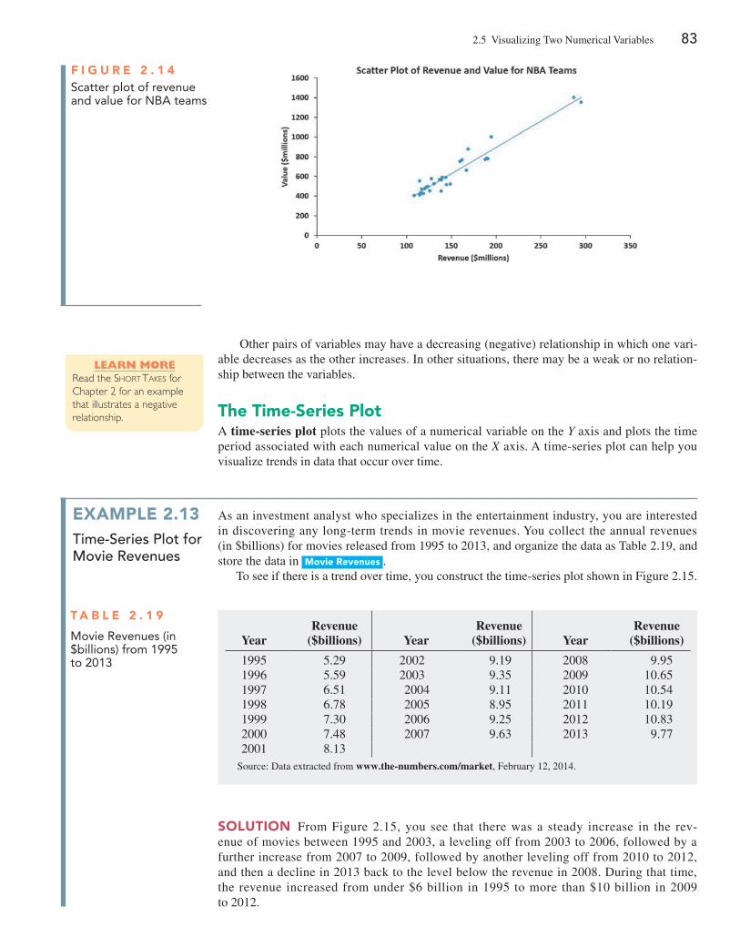
2.5 Visualizing Two Numerical Variables 83
F i g u r e 2 . 1 4Scatter plot of revenue and value for NBA teams
Other pairs of variables may have a decreasing (negative) relationship in which one vari-able decreases as the other increases. In other situations, there may be a weak or no relation-ship between the variables.
The Time-Series plotA time-series plot plots the values of a numerical variable on the Y axis and plots the time period associated with each numerical value on the X axis. A time-series plot can help you visualize trends in data that occur over time.
Learn MoreRead the Short takeS for Chapter 2 for an example that illustrates a negative relationship.
example 2.13time-series Plot for Movie Revenues
As an investment analyst who specializes in the entertainment industry, you are interested in discovering any long-term trends in movie revenues. You collect the annual revenues (in $billions) for movies released from 1995 to 2013, and organize the data as Table 2.19, and store the data in movie revenues .
To see if there is a trend over time, you construct the time-series plot shown in Figure 2.15.
SOluTiOn From Figure 2.15, you see that there was a steady increase in the rev-enue of movies between 1995 and 2003, a leveling off from 2003 to 2006, followed by a further increase from 2007 to 2009, followed by another leveling off from 2010 to 2012, and then a decline in 2013 back to the level below the revenue in 2008. During that time, the revenue increased from under $6 billion in 1995 to more than $10 billion in 2009 to 2012.
Year
Revenue ($billions)
Year
Revenue ($billions)
Year
Revenue ($billions)
1995 5.29 2002 9.19 2008 9.951996 5.59 2003 9.35 2009 10.651997 6.51 2004 9.11 2010 10.541998 6.78 2005 8.95 2011 10.191999 7.30 2006 9.25 2012 10.832000 7.48 2007 9.63 2013 9.772001 8.13
Source: Data extracted from www.the-numbers.com/market, February 12, 2014.
T a b l e 2 . 1 9
Movie Revenues (in $billions) from 1995 to 2013
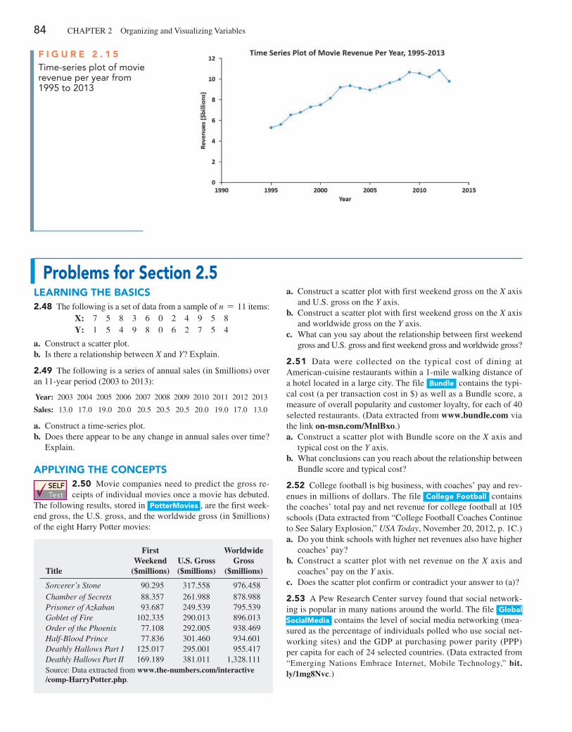
84 ChApTER 2 Organizing and Visualizing Variables
F i g u r e 2 . 1 5Time-series plot of movie revenue per year from 1995 to 2013
problems for Section 2.5learning The baSiCS2.48 The following is a set of data from a sample of n = 11 items:
X: 7 5 8 3 6 0 2 4 9 5 8Y: 1 5 4 9 8 0 6 2 7 5 4
a. Construct a scatter plot.b. Is there a relationship between X and Y? Explain.
2.49 The following is a series of annual sales (in $millions) over an 11-year period (2003 to 2013):
Year: 2003 2004 2005 2006 2007 2008 2009 2010 2011 2012 2013
Sales: 13.0 17.0 19.0 20.0 20.5 20.5 20.5 20.0 19.0 17.0 13.0
a. Construct a time-series plot.b. Does there appear to be any change in annual sales over time?
Explain.
applying The COnCepTS2.50 Movie companies need to predict the gross re-ceipts of individual movies once a movie has debuted.
The following results, stored in pottermovies , are the first week-end gross, the U.S. gross, and the worldwide gross (in $millions) of the eight harry potter movies:
Title
First Weekend
($millions)U.S. Gross ($millions)
Worldwide Gross
($millions)
Sorcerer’s Stone 90.295 317.558 976.458Chamber of Secrets 88.357 261.988 878.988Prisoner of Azkaban 93.687 249.539 795.539Goblet of Fire 102.335 290.013 896.013Order of the Phoenix 77.108 292.005 938.469Half-Blood Prince 77.836 301.460 934.601Deathly Hallows Part I 125.017 295.001 955.417Deathly Hallows Part II 169.189 381.011 1,328.111Source: Data extracted from www.the-numbers.com/interactive /comp-HarryPotter.php.
a. Construct a scatter plot with first weekend gross on the X axis and U.S. gross on the Y axis.
b. Construct a scatter plot with first weekend gross on the X axis and worldwide gross on the Y axis.
c. What can you say about the relationship between first weekend gross and U.S. gross and first weekend gross and worldwide gross?
2.51 Data were collected on the typical cost of dining at American-cuisine restaurants within a 1-mile walking distance of a hotel located in a large city. The file bundle contains the typi-cal cost (a per transaction cost in $) as well as a Bundle score, a measure of overall popularity and customer loyalty, for each of 40 selected restaurants. (Data extracted from www.bundle.com via the link on-msn.com/MnlBxo.)a. Construct a scatter plot with Bundle score on the X axis and
typical cost on the Y axis.b. What conclusions can you reach about the relationship between
Bundle score and typical cost?
2.52 College football is big business, with coaches’ pay and rev-enues in millions of dollars. The file College Football contains the coaches’ total pay and net revenue for college football at 105 schools (Data extracted from “College Football Coaches Continue to See Salary Explosion,” USA Today, November 20, 2012, p. 1C.)a. Do you think schools with higher net revenues also have higher
coaches’ pay?b. Construct a scatter plot with net revenue on the X axis and
coaches’ pay on the Y axis.c. Does the scatter plot confirm or contradict your answer to (a)?
2.53 A pew Research Center survey found that social network-ing is popular in many nations around the world. The file global Socialmedia contains the level of social media networking (mea-sured as the percentage of individuals polled who use social net-working sites) and the GDp at purchasing power parity (ppp) per capita for each of 24 selected countries. (Data extracted from “Emerging Nations Embrace Internet, Mobile Technology,” bit.ly/1mg8Nvc.)
SELF Test
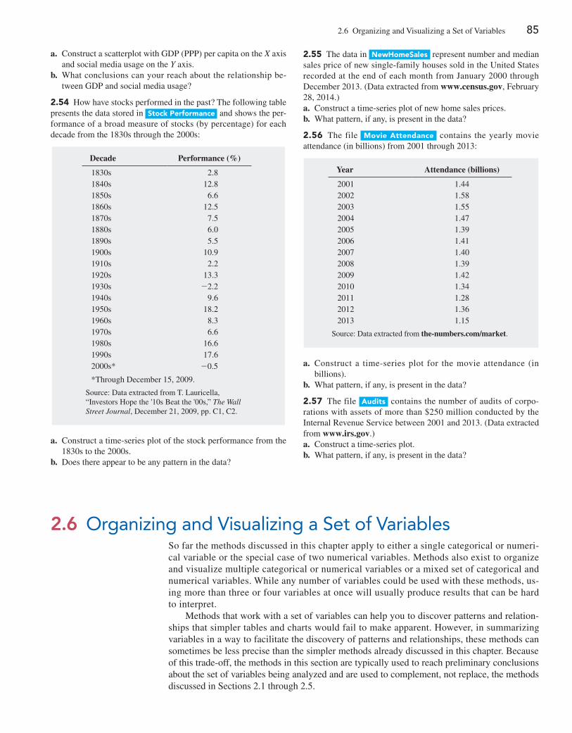
2.6 Organizing and Visualizing a Set of Variables 85
a. Construct a scatterplot with GDp (ppp) per capita on the X axis and social media usage on the Y axis.
b. What conclusions can your reach about the relationship be-tween GDp and social media usage?
2.54 how have stocks performed in the past? The following table presents the data stored in Stock performance and shows the per-formance of a broad measure of stocks (by percentage) for each decade from the 1830s through the 2000s:
Decade Performance (%)
1830s 2.81840s 12.81850s 6.61860s 12.51870s 7.51880s 6.01890s 5.51900s 10.91910s 2.21920s 13.31930s -2.21940s 9.61950s 18.21960s 8.31970s 6.61980s 16.61990s 17.62000s* -0.5
*Through December 15, 2009.
Source: Data extracted from T. Lauricella, “Investors hope the '10s Beat the '00s,” The Wall Street Journal, December 21, 2009, pp. C1, C2.
a. Construct a time-series plot of the stock performance from the 1830s to the 2000s.
b. Does there appear to be any pattern in the data?
2.55 The data in newhomeSales represent number and median sales price of new single-family houses sold in the United States recorded at the end of each month from January 2000 through December 2013. (Data extracted from www.census.gov, February 28, 2014.)a. Construct a time-series plot of new home sales prices.b. What pattern, if any, is present in the data?
2.56 The file movie attendance contains the yearly movie attendance (in billions) from 2001 through 2013:
Year Attendance (billions)
2001 1.442002 1.582003 1.552004 1.472005 1.392006 1.412007 1.402008 1.392009 1.422010 1.342011 1.282012 1.362013 1.15
Source: Data extracted from the-numbers.com/market.
a. Construct a time-series plot for the movie attendance (in billions).
b. What pattern, if any, is present in the data?
2.57 The file audits contains the number of audits of corpo-rations with assets of more than $250 million conducted by the Internal Revenue Service between 2001 and 2013. (Data extracted from www.irs.gov.)a. Construct a time-series plot.b. What pattern, if any, is present in the data?
2.6 Organizing and Visualizing a Set of VariablesSo far the methods discussed in this chapter apply to either a single categorical or numeri-cal variable or the special case of two numerical variables. Methods also exist to organize and visualize multiple categorical or numerical variables or a mixed set of categorical and numerical variables. While any number of variables could be used with these methods, us-ing more than three or four variables at once will usually produce results that can be hard to interpret.
Methods that work with a set of variables can help you to discover patterns and relation-ships that simpler tables and charts would fail to make apparent. however, in summarizing variables in a way to facilitate the discovery of patterns and relationships, these methods can sometimes be less precise than the simpler methods already discussed in this chapter. Because of this trade-off, the methods in this section are typically used to reach preliminary conclusions about the set of variables being analyzed and are used to complement, not replace, the methods discussed in Sections 2.1 through 2.5.
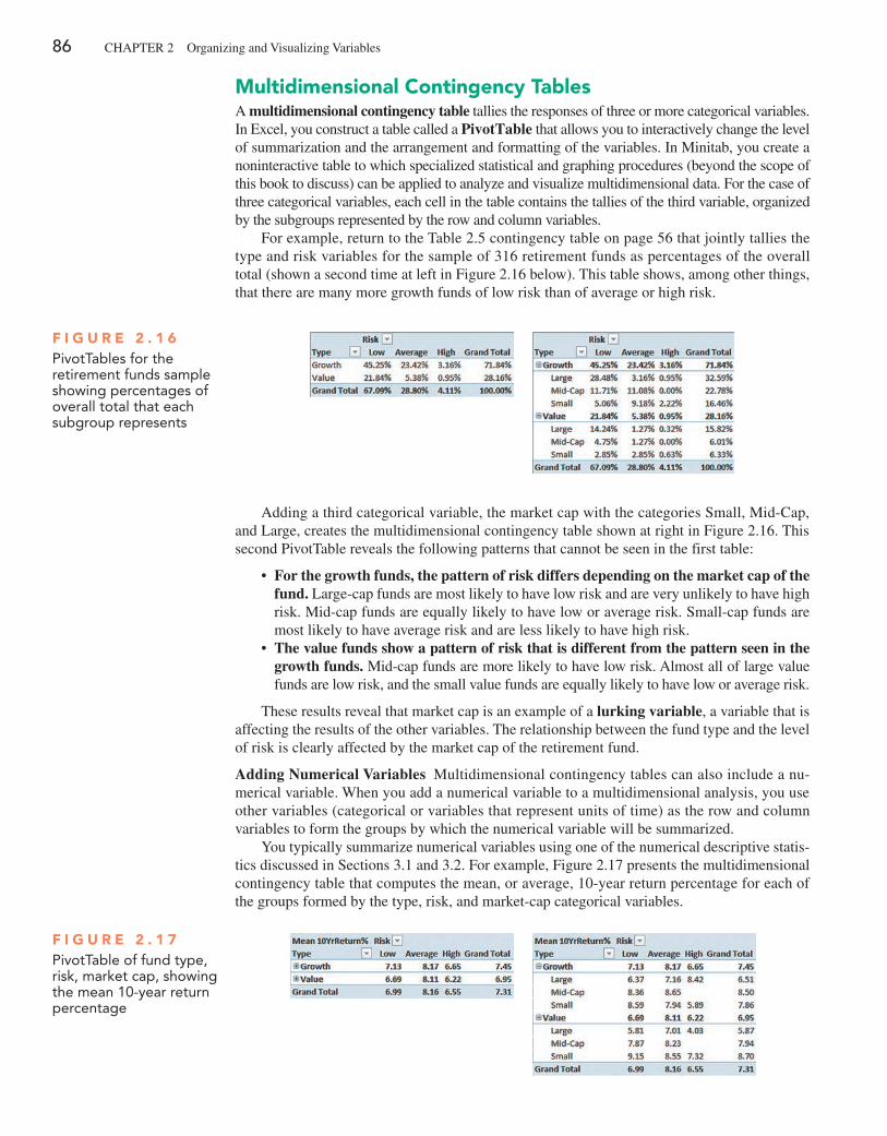
86 ChApTER 2 Organizing and Visualizing Variables
multidimensional Contingency TablesA multidimensional contingency table tallies the responses of three or more categorical variables. In Excel, you construct a table called a PivotTable that allows you to interactively change the level of summarization and the arrangement and formatting of the variables. In Minitab, you create a noninteractive table to which specialized statistical and graphing procedures (beyond the scope of this book to discuss) can be applied to analyze and visualize multidimensional data. For the case of three categorical variables, each cell in the table contains the tallies of the third variable, organized by the subgroups represented by the row and column variables.
For example, return to the Table 2.5 contingency table on page 56 that jointly tallies the type and risk variables for the sample of 316 retirement funds as percentages of the overall total (shown a second time at left in Figure 2.16 below). This table shows, among other things, that there are many more growth funds of low risk than of average or high risk.
F i g u r e 2 . 1 6PivotTables for the retirement funds sample showing percentages of overall total that each subgroup represents
Adding a third categorical variable, the market cap with the categories Small, Mid-Cap, and Large, creates the multidimensional contingency table shown at right in Figure 2.16. This second pivotTable reveals the following patterns that cannot be seen in the first table:
• For the growth funds, the pattern of risk differs depending on the market cap of the fund. Large-cap funds are most likely to have low risk and are very unlikely to have high risk. Mid-cap funds are equally likely to have low or average risk. Small-cap funds are most likely to have average risk and are less likely to have high risk.
• The value funds show a pattern of risk that is different from the pattern seen in the growth funds. Mid-cap funds are more likely to have low risk. Almost all of large value funds are low risk, and the small value funds are equally likely to have low or average risk.
These results reveal that market cap is an example of a lurking variable, a variable that is affecting the results of the other variables. The relationship between the fund type and the level of risk is clearly affected by the market cap of the retirement fund.
Adding Numerical Variables Multidimensional contingency tables can also include a nu-merical variable. When you add a numerical variable to a multidimensional analysis, you use other variables (categorical or variables that represent units of time) as the row and column variables to form the groups by which the numerical variable will be summarized.
You typically summarize numerical variables using one of the numerical descriptive statis-tics discussed in Sections 3.1 and 3.2. For example, Figure 2.17 presents the multidimensional contingency table that computes the mean, or average, 10-year return percentage for each of the groups formed by the type, risk, and market-cap categorical variables.
F i g u r e 2 . 1 7PivotTable of fund type, risk, market cap, showing the mean 10-year return percentage
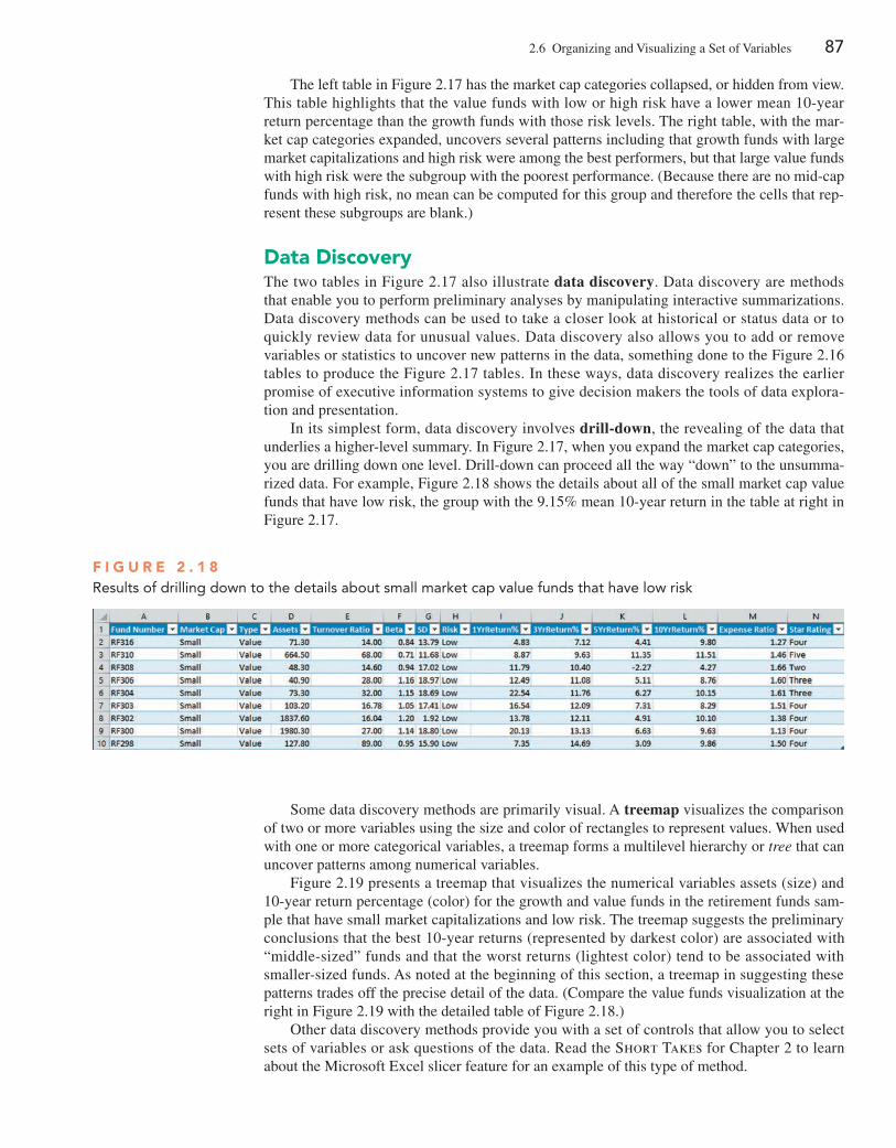
2.6 Organizing and Visualizing a Set of Variables 87
The left table in Figure 2.17 has the market cap categories collapsed, or hidden from view. This table highlights that the value funds with low or high risk have a lower mean 10-year return percentage than the growth funds with those risk levels. The right table, with the mar-ket cap categories expanded, uncovers several patterns including that growth funds with large market capitalizations and high risk were among the best performers, but that large value funds with high risk were the subgroup with the poorest performance. (Because there are no mid-cap funds with high risk, no mean can be computed for this group and therefore the cells that rep-resent these subgroups are blank.)
Data DiscoveryThe two tables in Figure 2.17 also illustrate data discovery. Data discovery are methods that enable you to perform preliminary analyses by manipulating interactive summarizations. Data discovery methods can be used to take a closer look at historical or status data or to quickly review data for unusual values. Data discovery also allows you to add or remove variables or statistics to uncover new patterns in the data, something done to the Figure 2.16 tables to produce the Figure 2.17 tables. In these ways, data discovery realizes the earlier promise of executive information systems to give decision makers the tools of data explora-tion and presentation.
In its simplest form, data discovery involves drill-down, the revealing of the data that underlies a higher-level summary. In Figure 2.17, when you expand the market cap categories, you are drilling down one level. Drill-down can proceed all the way “down” to the unsumma-rized data. For example, Figure 2.18 shows the details about all of the small market cap value funds that have low risk, the group with the 9.15% mean 10-year return in the table at right in Figure 2.17.
F i g u r e 2 . 1 8Results of drilling down to the details about small market cap value funds that have low risk
Some data discovery methods are primarily visual. A treemap visualizes the comparison of two or more variables using the size and color of rectangles to represent values. When used with one or more categorical variables, a treemap forms a multilevel hierarchy or tree that can uncover patterns among numerical variables.
Figure 2.19 presents a treemap that visualizes the numerical variables assets (size) and 10-year return percentage (color) for the growth and value funds in the retirement funds sam-ple that have small market capitalizations and low risk. The treemap suggests the preliminary conclusions that the best 10-year returns (represented by darkest color) are associated with “middle-sized” funds and that the worst returns (lightest color) tend to be associated with smaller-sized funds. As noted at the beginning of this section, a treemap in suggesting these patterns trades off the precise detail of the data. (Compare the value funds visualization at the right in Figure 2.19 with the detailed table of Figure 2.18.)
Other data discovery methods provide you with a set of controls that allow you to select sets of variables or ask questions of the data. Read the Short Takes for Chapter 2 to learn about the Microsoft Excel slicer feature for an example of this type of method.
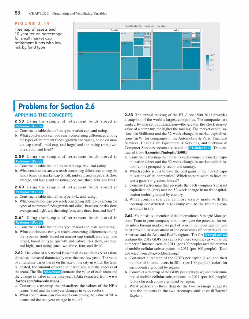
88 ChApTER 2 Organizing and Visualizing Variables
F i g u r e 2 . 1 9Treemap of assets and 10-year return percentage for small market cap retirement funds with low risk by fund type
problems for Section 2.6applying The COnCepTS2.58 Using the sample of retirement funds stored in retirementFunds :a. Construct a table that tallies type, market cap, and rating.b. What conclusions can you reach concerning differences among
the types of retirement funds (growth and value), based on mar-ket cap (small, mid-cap, and large) and the rating (one, two, three, four, and five)?
2.59 Using the sample of retirement funds stored in retirementFunds :a. Construct a table that tallies market cap, risk, and rating.b. What conclusions can you reach concerning differences among the
funds based on market cap (small, mid-cap, and large), risk (low, average, and high), and the rating (one, two, three, four, and five)?
2.60 Using the sample of retirement funds stored in retirementFunds :a. Construct a table that tallies type, risk, and rating.b. What conclusions can you reach concerning differences among the
types of retirement funds (growth and value), based on the risk (low, average, and high), and the rating (one, two, three, four, and five)?
2.61 Using the sample of retirement funds stored in retirementFunds :a. Construct a table that tallies type, market cap, risk, and rating.b. What conclusions can you reach concerning differences among
the types of funds based on market cap (small, mid-cap, and large), based on type (growth and value), risk (low, average, and high), and rating (one, two, three, four, and five)?
2.62 The value of a National Basketball Association (NBA) fran-chise has increased dramatically over the past few years. The value of a franchise varies based on the size of the city in which the team is located, the amount of revenue it receives, and the success of the team. The file nbaValues contains the value of each team and the change in value in the past year. (Data extracted from www .forbes.com/nba-valuations.):a. Construct a treemap that visualizes the values of the NBA
teams (size) and the one year changes in value (color).b. What conclusions can you reach concerning the value of NBA
teams and the one year change in value?
2.63 The annual ranking of the FT Global 500 2013 provides a snapshot of the world’s largest companies. The companies are ranked by market capitalization—the greater the stock market value of a company, the higher the ranking. The market capitaliza-tions (in $billions) and the 52-week change in market capitaliza-tions (in %) for companies in the Automobile & parts, Financial Services, health Care Equipment & Services, and Software & Computer Services sectors are stored in FTglobal500 . (Data ex-tracted from ft.com/intl/indepth/ft500.)a. Construct a treemap that presents each company’s market capi-
talization (size) and the 52-week change in market capitaliza-tion (color) grouped by sector and country.
b. Which sector seems to have the best gains in the market capi-talizations of its companies? Which sectors seem to have the worst gains (or greatest losses)?
c. Construct a treemap that presents the each company’s market capitalization (size) and the 52-week change in market capital-ization (color) grouped by country.
d. What comparison can be more easily made with the treemap constructed in (c) compared to the treemap con-structed in (a).
2.64 Your task as a member of the International Strategic Manage-ment Team in your company is to investigate the potential for en-try into a foreign market. As part of your initial investigation, you must provide an assessment of the economies of countries in the Americas and the Asia and pacific regions. The file Doingbusiness contains the 2012 GDps per capita for these countries as well as the number of Internet users in 2011 (per 100 people) and the number of mobile cellular subscriptions in 2011 (per 100 people). (Data extracted from data.worldbank.org.)a. Construct a treemap of the GDps per capita (size) and their
number of Internet users in 2011 (per 100 people) (color) for each country grouped by region.
b. Construct a treemap of the GDps per capita (size) and their num-ber of mobile cellular subscriptions in 2011 (per 100 people) (color) for each country grouped by region.
c. What patterns to these data do the two treemaps suggest? Are the patterns in the two treemaps similar or different? Explain.
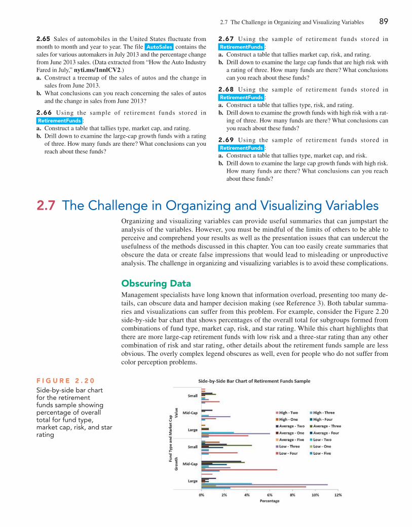
2.7 The Challenge in Organizing and Visualizing Variables 89
2.65 Sales of automobiles in the United States fluctuate from month to month and year to year. The file autoSales contains the sales for various automakers in July 2013 and the percentage change from June 2013 sales. (Data extracted from “how the Auto Industry Fared in July,” nyti.ms/1nnlCV2.)a. Construct a treemap of the sales of autos and the change in
sales from June 2013. b. What conclusions can you reach concerning the sales of autos
and the change in sales from June 2013?
2.66 Using the sample of retirement funds stored in retirementFunds :a. Construct a table that tallies type, market cap, and rating.b. Drill down to examine the large-cap growth funds with a rating
of three. how many funds are there? What conclusions can you reach about these funds?
2.67 Using the sample of retirement funds stored in retirementFunds :a. Construct a table that tallies market cap, risk, and rating. b. Drill down to examine the large cap funds that are high risk with
a rating of three. how many funds are there? What conclusions can you reach about these funds?
2.68 Using the sample of retirement funds stored in retirementFunds :a. Construct a table that tallies type, risk, and rating.b. Drill down to examine the growth funds with high risk with a rat-
ing of three. how many funds are there? What conclusions can you reach about these funds?
2.69 Using the sample of retirement funds stored in retirementFunds :a. Construct a table that tallies type, market cap, and risk.b. Drill down to examine the large cap growth funds with high risk.
how many funds are there? What conclusions can you reach about these funds?
2.7 The Challenge in Organizing and Visualizing VariablesOrganizing and visualizing variables can provide useful summaries that can jumpstart the analysis of the variables. however, you must be mindful of the limits of others to be able to perceive and comprehend your results as well as the presentation issues that can undercut the usefulness of the methods discussed in this chapter. You can too easily create summaries that obscure the data or create false impressions that would lead to misleading or unproductive analysis. The challenge in organizing and visualizing variables is to avoid these complications.
Obscuring DataManagement specialists have long known that information overload, presenting too many de-tails, can obscure data and hamper decision making (see Reference 3). Both tabular summa-ries and visualizations can suffer from this problem. For example, consider the Figure 2.20 side-by-side bar chart that shows percentages of the overall total for subgroups formed from combinations of fund type, market cap, risk, and star rating. While this chart highlights that there are more large-cap retirement funds with low risk and a three-star rating than any other combination of risk and star rating, other details about the retirement funds sample are less obvious. The overly complex legend obscures as well, even for people who do not suffer from color perception problems.
F i g u r e 2 . 2 0Side-by-side bar chart for the retirement funds sample showing percentage of overall total for fund type, market cap, risk, and star rating
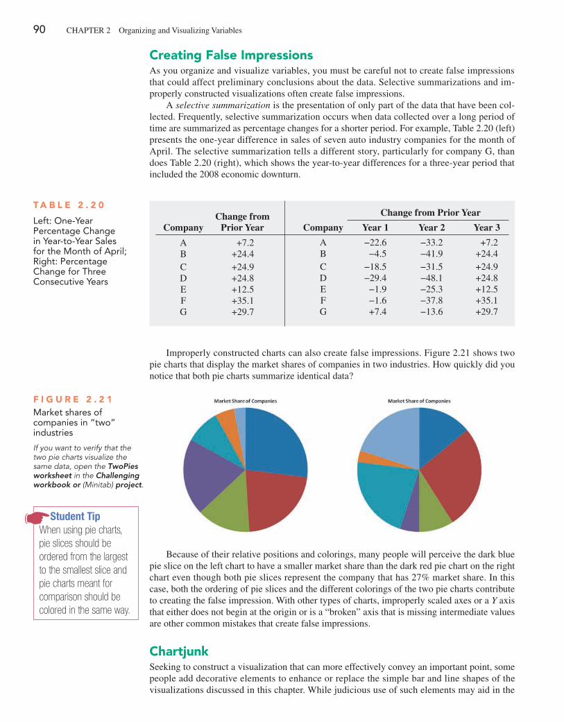
90 ChApTER 2 Organizing and Visualizing Variables
Creating False impressionsAs you organize and visualize variables, you must be careful not to create false impressions that could affect preliminary conclusions about the data. Selective summarizations and im-properly constructed visualizations often create false impressions.
A selective summarization is the presentation of only part of the data that have been col-lected. Frequently, selective summarization occurs when data collected over a long period of time are summarized as percentage changes for a shorter period. For example, Table 2.20 (left) presents the one-year difference in sales of seven auto industry companies for the month of April. The selective summarization tells a different story, particularly for company G, than does Table 2.20 (right), which shows the year-to-year differences for a three-year period that included the 2008 economic downturn.
Improperly constructed charts can also create false impressions. Figure 2.21 shows two pie charts that display the market shares of companies in two industries. how quickly did you notice that both pie charts summarize identical data?
F i g u r e 2 . 2 1Market shares of companies in “two” industries
If you want to verify that the two pie charts visualize the same data, open the TwoPies worksheet in the Challenging workbook or (Minitab) project.
Because of their relative positions and colorings, many people will perceive the dark blue pie slice on the left chart to have a smaller market share than the dark red pie chart on the right chart even though both pie slices represent the company that has 27% market share. In this case, both the ordering of pie slices and the different colorings of the two pie charts contribute to creating the false impression. With other types of charts, improperly scaled axes or a Y axis that either does not begin at the origin or is a “broken” axis that is missing intermediate values are other common mistakes that create false impressions.
ChartjunkSeeking to construct a visualization that can more effectively convey an important point, some people add decorative elements to enhance or replace the simple bar and line shapes of the visualizations discussed in this chapter. While judicious use of such elements may aid in the
Student TipWhen using pie charts, pie slices should be ordered from the largest to the smallest slice and pie charts meant for comparison should be colored in the same way.
T a b l e 2 . 2 0
Left: One-Year Percentage Change in Year-to-Year Sales for the Month of April; Right: Percentage Change for Three Consecutive Years
Change from Prior YearCompany
A +7.2B +24.4C +24.9D +24.8E +12.5F +35.1G +29.7
Change from Prior Year
Company Year 1 Year 2 Year 3
A −22.6 −33.2 +7.2B −4.5 −41.9 +24.4C −18.5 −31.5 +24.9D −29.4 −48.1 +24.8E −1.9 −25.3 +12.5F −1.6 −37.8 +35.1G +7.4 −13.6 +29.7

2.7 The Challenge in Organizing and Visualizing Variables 91
memorability of a chart (see Reference 1), most often such elements either obscure the data or, worse, create a false impression of the data. Such elements are called chartjunk.
Figure 2.22 visualizes the market share for selected soft drink brands. The chartjunk ver-sion fails to convey any more information than a simple bar or pie chart would, and the soft drink bottle tops included on the chart obscure and distort the data. The side-by-side bar chart at right shows how the market shares as represented by the height of the “fizzy” elements over-state the actual market shares of the five lesser brands, using the height of the first bottle and fizz to represent 20%.
Figure 2.23 visualizes Australian wine exports to the United States for four years. The chartjunk version on the left uses wine glasses in a histogram-like display in lieu of a proper time-series plot, such as the one shown on the right. Because the years between measurements are not equally spaced, the four wine glasses create a false impression about the ever-increasing trend in wine exports. The wine glasses also distort the data by using an object with a three-dimensional volume. (While the height of wine in the 1997 glass is a bit more than six times the height of the 1989 glass, the volume of that filled 1997 wine glass would be much more than the almost empty 1989 glass.)
F i g u r e 2 . 2 3Two visualizations of Australian wine exports to the united States, in millions of gallons
Left illustration adapted from S. Watterson, “Liquid Gold—Australians Are Changing the World of Wine. Even the French Seem Grateful,” Time, November 22, 1999, p. 68.
Coke still has most fizzCarbonated soft drinks with the biggest share of the $58 billion market last year:
Coke Classic20%
Pepsi-Cola14%
MountainDew7%
DietCoke9% Sprite
7%Dr Pepper
6%
F i g u r e 2 . 2 2Two visualizations of market share of soft drinks
Source: Left illustration adapted from Anne B. Carey and Sam Ward, “Coke Still has Most Fizz,” USA Today, May 10, 2000, p. 1B.
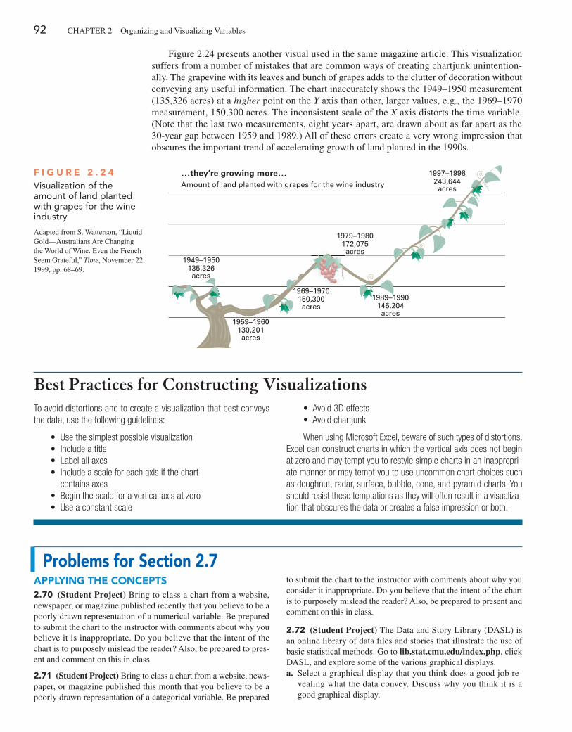
92 ChApTER 2 Organizing and Visualizing Variables
problems for Section 2.7applying The COnCepTS2.70 (Student Project) Bring to class a chart from a website, newspaper, or magazine published recently that you believe to be a poorly drawn representation of a numerical variable. Be prepared to submit the chart to the instructor with comments about why you believe it is inappropriate. Do you believe that the intent of the chart is to purposely mislead the reader? Also, be prepared to pres-ent and comment on this in class.
2.71 (Student Project) Bring to class a chart from a website, news-paper, or magazine published this month that you believe to be a poorly drawn representation of a categorical variable. Be prepared
to submit the chart to the instructor with comments about why you consider it inappropriate. Do you believe that the intent of the chart is to purposely mislead the reader? Also, be prepared to present and comment on this in class.
2.72 (Student Project) The Data and Story Library (DASL) is an online library of data files and stories that illustrate the use of basic statistical methods. Go to lib.stat.cmu.edu/index.php, click DASL, and explore some of the various graphical displays.a. Select a graphical display that you think does a good job re-
vealing what the data convey. Discuss why you think it is a good graphical display.
Figure 2.24 presents another visual used in the same magazine article. This visualization suffers from a number of mistakes that are common ways of creating chartjunk unintention-ally. The grapevine with its leaves and bunch of grapes adds to the clutter of decoration without conveying any useful information. The chart inaccurately shows the 1949–1950 measurement (135,326 acres) at a higher point on the Y axis than other, larger values, e.g., the 1969–1970 measurement, 150,300 acres. The inconsistent scale of the X axis distorts the time variable. (Note that the last two measurements, eight years apart, are drawn about as far apart as the 30-year gap between 1959 and 1989.) All of these errors create a very wrong impression that obscures the important trend of accelerating growth of land planted in the 1990s.
…they’re growing more…Amount of land planted with grapes for the wine industry
1949–1950135,326acres
1959–1960130,201acres
1969–1970150,300acres
1979–1980172,075acres
1989–1990146,204acres
1997–1998243,644
acres
F i g u r e 2 . 2 4Visualization of the amount of land planted with grapes for the wine industry
Adapted from S. Watterson, “Liquid Gold—Australians Are Changing the World of Wine. Even the French Seem Grateful,” Time, November 22, 1999, pp. 68–69.
Best Practices for Constructing VisualizationsTo avoid distortions and to create a visualization that best conveys the data, use the following guidelines:
• Use the simplest possible visualization• Include a title• Label all axes• Include a scale for each axis if the chart
contains axes• Begin the scale for a vertical axis at zero• Use a constant scale
• Avoid 3D effects• Avoid chartjunk
When using Microsoft Excel, beware of such types of distortions. Excel can construct charts in which the vertical axis does not begin at zero and may tempt you to restyle simple charts in an inappropri-ate manner or may tempt you to use uncommon chart choices such as doughnut, radar, surface, bubble, cone, and pyramid charts. You should resist these temptations as they will often result in a visualiza-tion that obscures the data or creates a false impression or both.
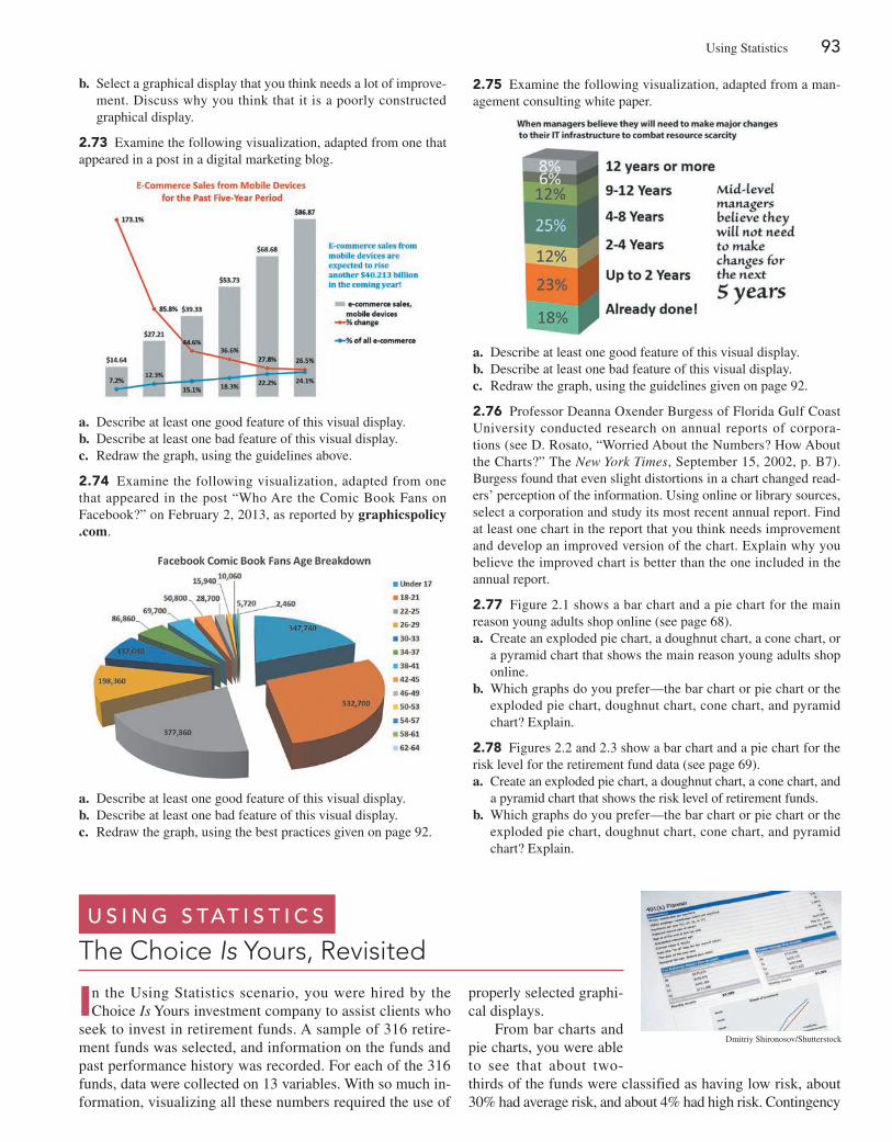
Using Statistics 93
b. Select a graphical display that you think needs a lot of improve-ment. Discuss why you think that it is a poorly constructed graphical display.
2.73 Examine the following visualization, adapted from one that appeared in a post in a digital marketing blog.
a. Describe at least one good feature of this visual display.b. Describe at least one bad feature of this visual display.c. Redraw the graph, using the guidelines above.
2.74 Examine the following visualization, adapted from one that appeared in the post “Who Are the Comic Book Fans on Facebook?” on February 2, 2013, as reported by graphicspolicy .com.
a. Describe at least one good feature of this visual display.b. Describe at least one bad feature of this visual display.c. Redraw the graph, using the best practices given on page 92.
2.75 Examine the following visualization, adapted from a man-agement consulting white paper.
a. Describe at least one good feature of this visual display.b. Describe at least one bad feature of this visual display.c. Redraw the graph, using the guidelines given on page 92.
2.76 professor Deanna Oxender Burgess of Florida Gulf Coast University conducted research on annual reports of corpora-tions (see D. Rosato, “Worried About the Numbers? how About the Charts?” The New York Times, September 15, 2002, p. B7). Burgess found that even slight distortions in a chart changed read-ers’ perception of the information. Using online or library sources, select a corporation and study its most recent annual report. Find at least one chart in the report that you think needs improvement and develop an improved version of the chart. Explain why you believe the improved chart is better than the one included in the annual report.
2.77 Figure 2.1 shows a bar chart and a pie chart for the main reason young adults shop online (see page 68).a. Create an exploded pie chart, a doughnut chart, a cone chart, or
a pyramid chart that shows the main reason young adults shop online.
b. Which graphs do you prefer—the bar chart or pie chart or the exploded pie chart, doughnut chart, cone chart, and pyramid chart? Explain.
2.78 Figures 2.2 and 2.3 show a bar chart and a pie chart for the risk level for the retirement fund data (see page 69).a. Create an exploded pie chart, a doughnut chart, a cone chart, and
a pyramid chart that shows the risk level of retirement funds.b. Which graphs do you prefer—the bar chart or pie chart or the
exploded pie chart, doughnut chart, cone chart, and pyramid chart? Explain.
In the Using Statistics scenario, you were hired by the Choice Is Yours investment company to assist clients who
seek to invest in retirement funds. A sample of 316 retire-ment funds was selected, and information on the funds and past performance history was recorded. For each of the 316 funds, data were collected on 13 variables. With so much in-formation, visualizing all these numbers required the use of
properly selected graphi-cal displays.
From bar charts and pie charts, you were able to see that about two-thirds of the funds were classified as having low risk, about 30% had average risk, and about 4% had high risk. Contingency
U s i n g s tat i s t i c s
The Choice Is Yours, Revisited
Dmitriy Shironosov/Shutterstock
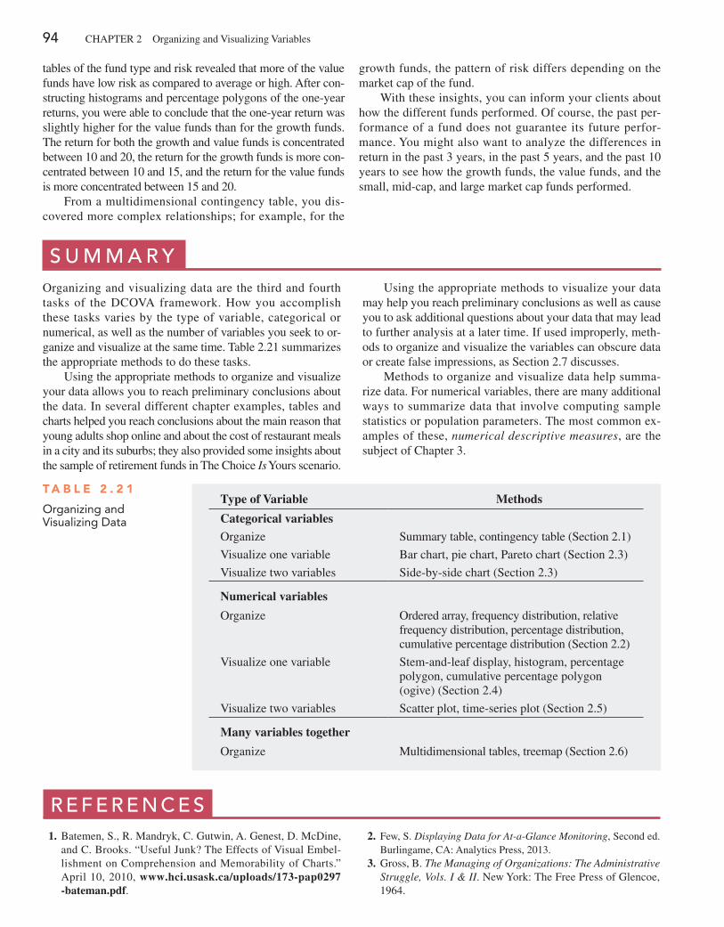
94 ChApTER 2 Organizing and Visualizing Variables
s U M M a R YOrganizing and visualizing data are the third and fourth tasks of the DCOVA framework. how you accomplish these tasks varies by the type of variable, categorical or numerical, as well as the number of variables you seek to or-ganize and visualize at the same time. Table 2.21 summarizes the appropriate methods to do these tasks.
Using the appropriate methods to organize and visualize your data allows you to reach preliminary conclusions about the data. In several different chapter examples, tables and charts helped you reach conclusions about the main reason that young adults shop online and about the cost of restaurant meals in a city and its suburbs; they also provided some insights about the sample of retirement funds in The Choice Is Yours scenario.
Using the appropriate methods to visualize your data may help you reach preliminary conclusions as well as cause you to ask additional questions about your data that may lead to further analysis at a later time. If used improperly, meth-ods to organize and visualize the variables can obscure data or create false impressions, as Section 2.7 discusses.
Methods to organize and visualize data help summa-rize data. For numerical variables, there are many additional ways to summarize data that involve computing sample statistics or population parameters. The most common ex-amples of these, numerical descriptive measures, are the subject of Chapter 3.
Type of Variable Methods
Categorical variables
Organize Summary table, contingency table (Section 2.1)
Visualize one variable Bar chart, pie chart, pareto chart (Section 2.3)
Visualize two variables Side-by-side chart (Section 2.3)
Numerical variables
Organize Ordered array, frequency distribution, relative frequency distribution, percentage distribution, cumulative percentage distribution (Section 2.2)
Visualize one variable Stem-and-leaf display, histogram, percentage polygon, cumulative percentage polygon (ogive) (Section 2.4)
Visualize two variables Scatter plot, time-series plot (Section 2.5)
Many variables together
Organize Multidimensional tables, treemap (Section 2.6)
T a b l e 2 . 2 1
Organizing and Visualizing Data
R E F E R E n c E s 1. Batemen, S., R. Mandryk, C. Gutwin, A. Genest, D. McDine,
and C. Brooks. “Useful Junk? The Effects of Visual Embel-lishment on Comprehension and Memorability of Charts.” April 10, 2010, www.hci.usask.ca/uploads/173-pap0297 -bateman.pdf.
2. Few, S. Displaying Data for At-a-Glance Monitoring, Second ed. Burlingame, CA: Analytics press, 2013.
3. Gross, B. The Managing of Organizations: The Administrative Struggle, Vols. I & II. New York: The Free press of Glencoe, 1964.
tables of the fund type and risk revealed that more of the value funds have low risk as compared to average or high. After con-structing histograms and percentage polygons of the one-year returns, you were able to conclude that the one-year return was slightly higher for the value funds than for the growth funds. The return for both the growth and value funds is concentrated between 10 and 20, the return for the growth funds is more con-centrated between 10 and 15, and the return for the value funds is more concentrated between 15 and 20.
From a multidimensional contingency table, you dis-covered more complex relationships; for example, for the
growth funds, the pattern of risk differs depending on the market cap of the fund.
With these insights, you can inform your clients about how the different funds performed. Of course, the past per-formance of a fund does not guarantee its future perfor-mance. You might also want to analyze the differences in return in the past 3 years, in the past 5 years, and the past 10 years to see how the growth funds, the value funds, and the small, mid-cap, and large market cap funds performed.
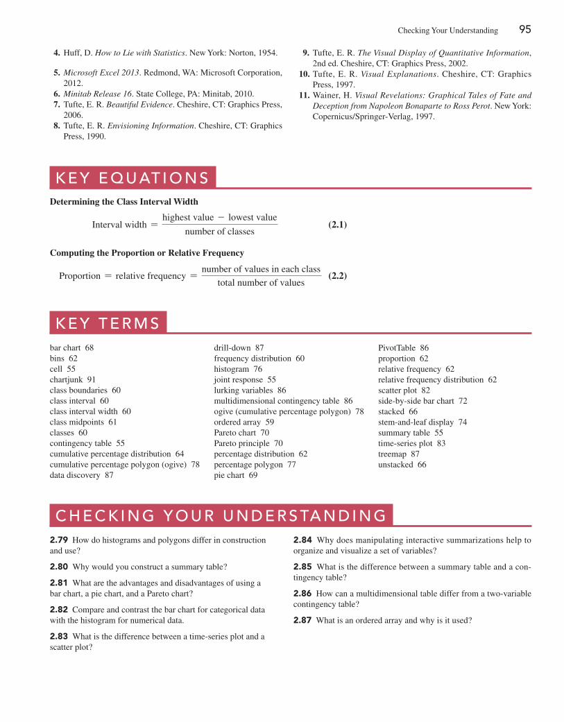
Checking Your Understanding 95
4. huff, D. How to Lie with Statistics. New York: Norton, 1954.
5. Microsoft Excel 2013. Redmond, WA: Microsoft Corporation, 2012.
6. Minitab Release 16. State College, pA: Minitab, 2010. 7. Tufte, E. R. Beautiful Evidence. Cheshire, CT: Graphics press,
2006. 8. Tufte, E. R. Envisioning Information. Cheshire, CT: Graphics
press, 1990.
9. Tufte, E. R. The Visual Display of Quantitative Information, 2nd ed. Cheshire, CT: Graphics press, 2002.
10. Tufte, E. R. Visual Explanations. Cheshire, CT: Graphics press, 1997.
11. Wainer, h. Visual Revelations: Graphical Tales of Fate and Deception from Napoleon Bonaparte to Ross Perot. New York: Copernicus/Springer-Verlag, 1997.
K E Y E q U at i O n sDetermining the Class Interval Width
Interval width =highest value - lowest value
number of classes (2.1)
Computing the Proportion or Relative Frequency
proportion = relative frequency =number of values in each class
total number of values (2.2)
K E Y t E R M sbar chart 68bins 62cell 55chartjunk 91class boundaries 60class interval 60class interval width 60class midpoints 61classes 60contingency table 55cumulative percentage distribution 64cumulative percentage polygon (ogive) 78data discovery 87
drill-down 87frequency distribution 60histogram 76joint response 55lurking variables 86multidimensional contingency table 86ogive (cumulative percentage polygon) 78ordered array 59pareto chart 70pareto principle 70percentage distribution 62percentage polygon 77pie chart 69
pivotTable 86proportion 62relative frequency 62relative frequency distribution 62scatter plot 82side-by-side bar chart 72stacked 66stem-and-leaf display 74summary table 55time-series plot 83treemap 87unstacked 66
c h E c K i n g Y O U R U n D E R s ta n D i n g2.79 how do histograms and polygons differ in construction and use?
2.80 Why would you construct a summary table?
2.81 What are the advantages and disadvantages of using a bar chart, a pie chart, and a pareto chart?
2.82 Compare and contrast the bar chart for categorical data with the histogram for numerical data.
2.83 What is the difference between a time-series plot and a scatter plot?
2.84 Why does manipulating interactive summarizations help to organize and visualize a set of variables?
2.85 What is the difference between a summary table and a con-tingency table?
2.86 how can a multidimensional table differ from a two-variable contingency table?
2.87 What is an ordered array and why is it used?
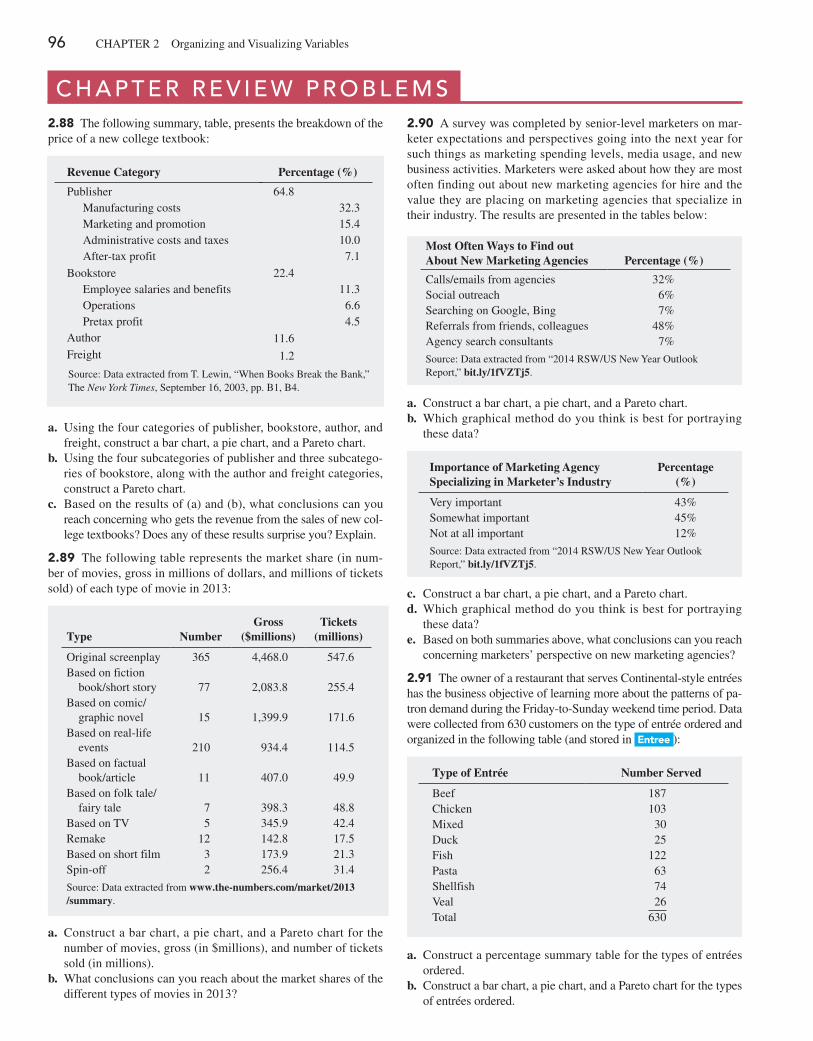
96 ChApTER 2 Organizing and Visualizing Variables
c h a P t E R R E V i E w P R O B l E M s2.88 The following summary, table, presents the breakdown of the price of a new college textbook:
Revenue Category Percentage (%)
publisher 64.8Manufacturing costs 32.3Marketing and promotion 15.4Administrative costs and taxes 10.0After-tax profit 7.1
Bookstore 22.4Employee salaries and benefits 11.3Operations 6.6pretax profit 4.5
Author 11.6Freight 1.2
Source: Data extracted from T. Lewin, “When Books Break the Bank,” The New York Times, September 16, 2003, pp. B1, B4.
a. Using the four categories of publisher, bookstore, author, and freight, construct a bar chart, a pie chart, and a pareto chart.
b. Using the four subcategories of publisher and three subcatego-ries of bookstore, along with the author and freight categories, construct a pareto chart.
c. Based on the results of (a) and (b), what conclusions can you reach concerning who gets the revenue from the sales of new col-lege textbooks? Does any of these results surprise you? Explain.
2.89 The following table represents the market share (in num-ber of movies, gross in millions of dollars, and millions of tickets sold) of each type of movie in 2013:
Type NumberGross
($millions)Tickets
(millions)
Original screenplay 365 4,468.0 547.6Based on fiction book/short story
77
2,083.8
255.4
Based on comic/ graphic novel
15
1,399.9
171.6
Based on real-life events 210 934.4 114.5Based on factual book/article
11
407.0
49.9
Based on folk tale/ fairy tale 7 398.3 48.8Based on TV 5 345.9 42.4Remake 12 142.8 17.5Based on short film 3 173.9 21.3Spin-off 2 256.4 31.4
Source: Data extracted from www.the-numbers.com/market/2013 /summary.
a. Construct a bar chart, a pie chart, and a pareto chart for the number of movies, gross (in $millions), and number of tickets sold (in millions).
b. What conclusions can you reach about the market shares of the different types of movies in 2013?
2.90 A survey was completed by senior-level marketers on mar-keter expectations and perspectives going into the next year for such things as marketing spending levels, media usage, and new business activities. Marketers were asked about how they are most often finding out about new marketing agencies for hire and the value they are placing on marketing agencies that specialize in their industry. The results are presented in the tables below:
Most Often Ways to Find out About New Marketing Agencies
Percentage (%)
Calls/emails from agencies 32%
Social outreach 6%
Searching on Google, Bing 7%
Referrals from friends, colleagues 48%Agency search consultants 7%
Source: Data extracted from “2014 RSW/US New Year Outlook Report,” bit.ly/1fVZTj5.
a. Construct a bar chart, a pie chart, and a pareto chart.b. Which graphical method do you think is best for portraying
these data?
Importance of Marketing Agency Specializing in Marketer’s Industry
Percentage (%)
Very important 43% Somewhat important 45% Not at all important 12%
Source: Data extracted from “2014 RSW/US New Year Outlook Report,” bit.ly/1fVZTj5.
c. Construct a bar chart, a pie chart, and a pareto chart.d. Which graphical method do you think is best for portraying
these data?e. Based on both summaries above, what conclusions can you reach
concerning marketers’ perspective on new marketing agencies?
2.91 The owner of a restaurant that serves Continental-style entrées has the business objective of learning more about the patterns of pa-tron demand during the Friday-to-Sunday weekend time period. Data were collected from 630 customers on the type of entrée ordered and organized in the following table (and stored in entree ):
Type of Entrée Number Served
Beef 187Chicken 103Mixed 30Duck 25Fish 122pasta 63Shellfish 74Veal 26Total 630
a. Construct a percentage summary table for the types of entrées ordered.
b. Construct a bar chart, a pie chart, and a pareto chart for the types of entrées ordered.
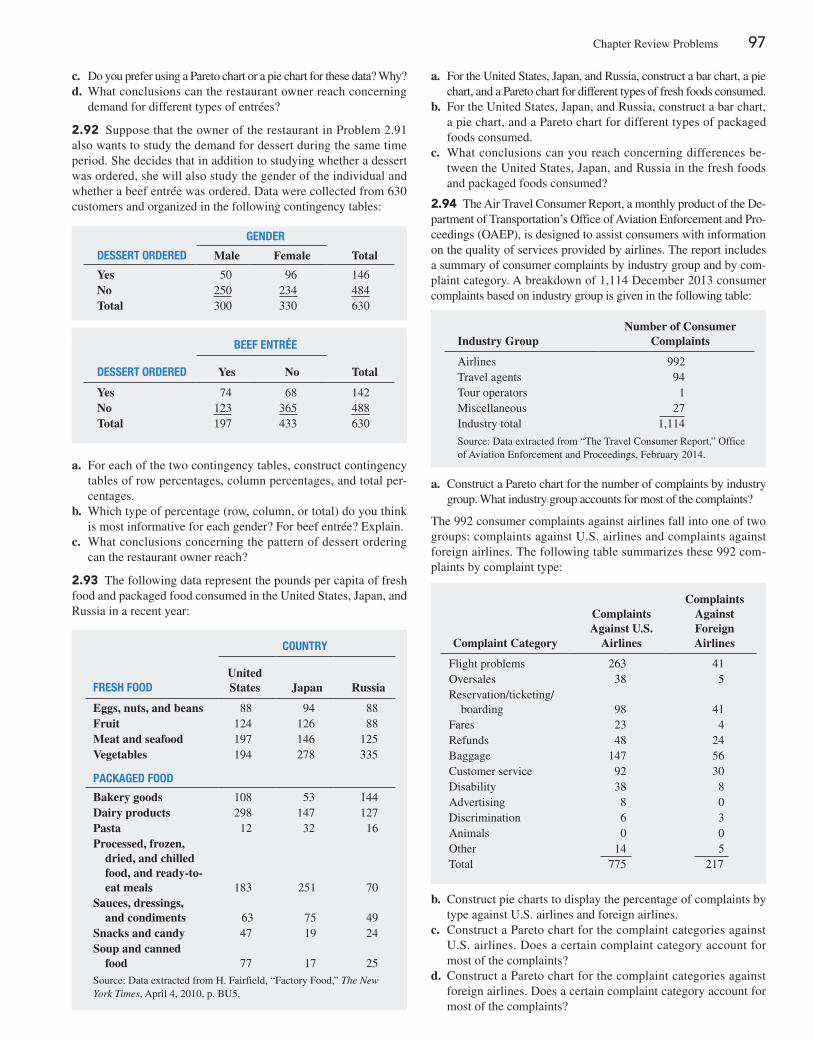
Chapter Review problems 97
c. Do you prefer using a pareto chart or a pie chart for these data? Why?d. What conclusions can the restaurant owner reach concerning
demand for different types of entrées?
2.92 Suppose that the owner of the restaurant in problem 2.91 also wants to study the demand for dessert during the same time period. She decides that in addition to studying whether a dessert was ordered, she will also study the gender of the individual and whether a beef entrée was ordered. Data were collected from 630 customers and organized in the following contingency tables:
GENDER
DESSERT ORDERED Male Female Total
Yes 50 96 146No 250 234 484Total 300 330 630
BEEF ENTRÉE
DESSERT ORDERED Yes No Total
Yes 74 68 142No 123 365 488Total 197 433 630
a. For each of the two contingency tables, construct contingency tables of row percentages, column percentages, and total per-centages.
b. Which type of percentage (row, column, or total) do you think is most informative for each gender? For beef entrée? Explain.
c. What conclusions concerning the pattern of dessert ordering can the restaurant owner reach?
2.93 The following data represent the pounds per capita of fresh food and packaged food consumed in the United States, Japan, and Russia in a recent year:
cOUNTRY
FRESH FOODUnited States Japan Russia
Eggs, nuts, and beans 88 94 88Fruit 124 126 88Meat and seafood 197 146 125Vegetables 194 278 335
PacKaGED FOOD
Bakery goods 108 53 144Dairy products 298 147 127Pasta 12 32 16Processed, frozen, dried, and chilled food, and ready-to- eat meals
183
251
70Sauces, dressings, and condiments
63
75
49
Snacks and candy 47 19 24Soup and canned food
77
17
25
Source: Data extracted from h. Fairfield, “Factory Food,” The New York Times, April 4, 2010, p. BU5.
a. For the United States, Japan, and Russia, construct a bar chart, a pie chart, and a pareto chart for different types of fresh foods consumed.
b. For the United States, Japan, and Russia, construct a bar chart, a pie chart, and a pareto chart for different types of packaged foods consumed.
c. What conclusions can you reach concerning differences be-tween the United States, Japan, and Russia in the fresh foods and packaged foods consumed?
2.94 The Air Travel Consumer Report, a monthly product of the De-partment of Transportation’s Office of Aviation Enforcement and pro-ceedings (OAEp), is designed to assist consumers with information on the quality of services provided by airlines. The report includes a summary of consumer complaints by industry group and by com-plaint category. A breakdown of 1,114 December 2013 consumer complaints based on industry group is given in the following table:
Industry GroupNumber of Consumer
Complaints
Airlines 992Travel agents 94Tour operators 1Miscellaneous 27Industry total 1,114
Source: Data extracted from “The Travel Consumer Report,” Office of Aviation Enforcement and proceedings, February 2014.
a. Construct a pareto chart for the number of complaints by industry group. What industry group accounts for most of the complaints?
The 992 consumer complaints against airlines fall into one of two groups: complaints against U.S. airlines and complaints against foreign airlines. The following table summarizes these 992 com-plaints by complaint type:
Complaint Category
Complaints Against U.S.
Airlines
Complaints Against Foreign Airlines
Flight problems 263 41Oversales 38 5Reservation/ticketing/ boarding
98
41
Fares 23 4Refunds 48 24Baggage 147 56Customer service 92 30Disability 38 8Advertising 8 0Discrimination 6 3Animals 0 0Other 14 5Total 775 217
b. Construct pie charts to display the percentage of complaints by type against U.S. airlines and foreign airlines.
c. Construct a pareto chart for the complaint categories against U.S. airlines. Does a certain complaint category account for most of the complaints?
d. Construct a pareto chart for the complaint categories against foreign airlines. Does a certain complaint category account for most of the complaints?
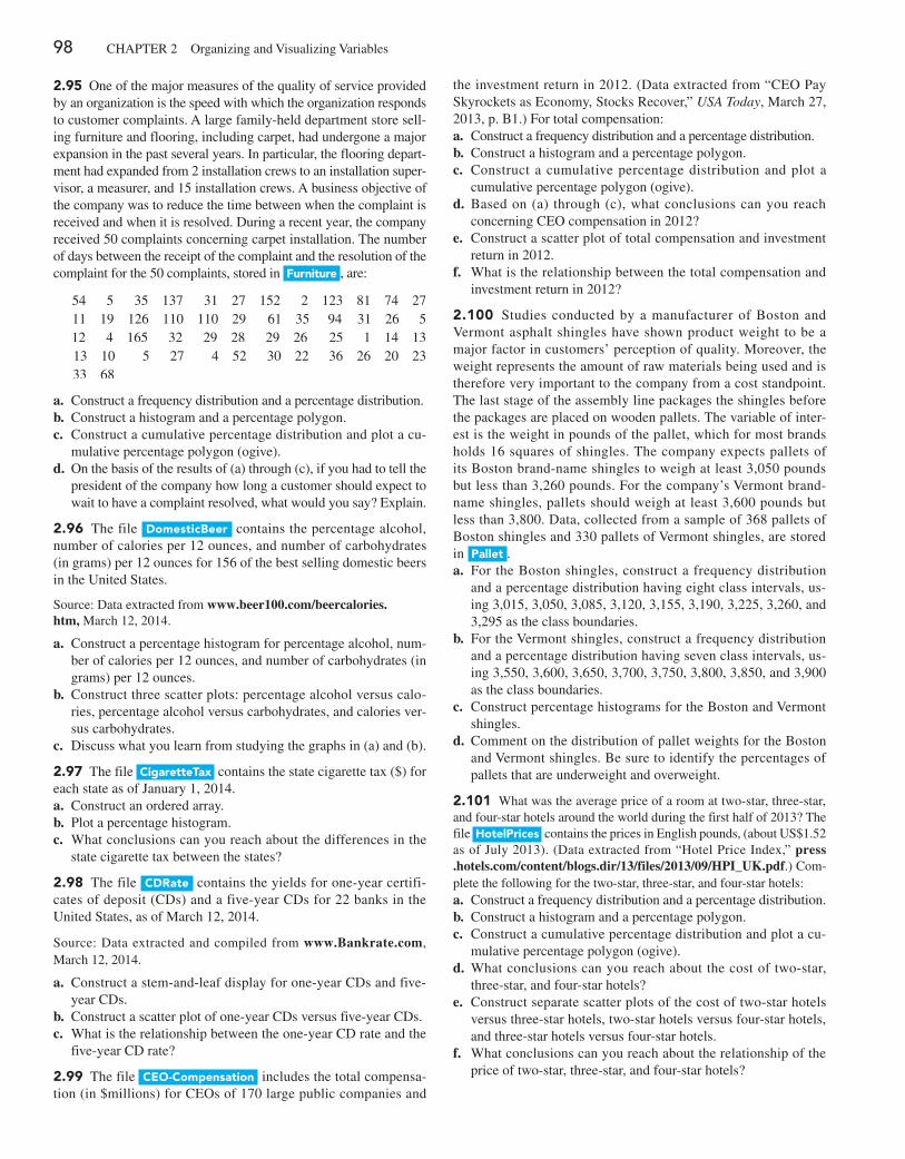
98 ChApTER 2 Organizing and Visualizing Variables
2.95 One of the major measures of the quality of service provided by an organization is the speed with which the organization responds to customer complaints. A large family-held department store sell-ing furniture and flooring, including carpet, had undergone a major expansion in the past several years. In particular, the flooring depart-ment had expanded from 2 installation crews to an installation super-visor, a measurer, and 15 installation crews. A business objective of the company was to reduce the time between when the complaint is received and when it is resolved. During a recent year, the company received 50 complaints concerning carpet installation. The number of days between the receipt of the complaint and the resolution of the complaint for the 50 complaints, stored in Furniture , are:
54 5 35 137 31 27 152 2 123 81 74 2711 19 126 110 110 29 61 35 94 31 26 512 4 165 32 29 28 29 26 25 1 14 1313 10 5 27 4 52 30 22 36 26 20 2333 68
a. Construct a frequency distribution and a percentage distribution.b. Construct a histogram and a percentage polygon.c. Construct a cumulative percentage distribution and plot a cu-
mulative percentage polygon (ogive).d. On the basis of the results of (a) through (c), if you had to tell the
president of the company how long a customer should expect to wait to have a complaint resolved, what would you say? Explain.
2.96 The file Domesticbeer contains the percentage alcohol, number of calories per 12 ounces, and number of carbohydrates (in grams) per 12 ounces for 156 of the best selling domestic beers in the United States.
Source: Data extracted from www.beer100.com/beercalories.htm, March 12, 2014.
a. Construct a percentage histogram for percentage alcohol, num-ber of calories per 12 ounces, and number of carbohydrates (in grams) per 12 ounces.
b. Construct three scatter plots: percentage alcohol versus calo-ries, percentage alcohol versus carbohydrates, and calories ver-sus carbohydrates.
c. Discuss what you learn from studying the graphs in (a) and (b).
2.97 The file CigaretteTax contains the state cigarette tax ($) for each state as of January 1, 2014.a. Construct an ordered array.b. plot a percentage histogram.c. What conclusions can you reach about the differences in the
state cigarette tax between the states?
2.98 The file CDrate contains the yields for one-year certifi-cates of deposit (CDs) and a five-year CDs for 22 banks in the United States, as of March 12, 2014.
Source: Data extracted and compiled from www.Bankrate.com, March 12, 2014.
a. Construct a stem-and-leaf display for one-year CDs and five-year CDs.
b. Construct a scatter plot of one-year CDs versus five-year CDs.c. What is the relationship between the one-year CD rate and the
five-year CD rate?
2.99 The file CeO-Compensation includes the total compensa-tion (in $millions) for CEOs of 170 large public companies and
the investment return in 2012. (Data extracted from “CEO pay Skyrockets as Economy, Stocks Recover,” USA Today, March 27, 2013, p. B1.) For total compensation:a. Construct a frequency distribution and a percentage distribution.b. Construct a histogram and a percentage polygon.c. Construct a cumulative percentage distribution and plot a
cumulative percentage polygon (ogive).d. Based on (a) through (c), what conclusions can you reach
concerning CEO compensation in 2012?e. Construct a scatter plot of total compensation and investment
return in 2012.f. What is the relationship between the total compensation and
investment return in 2012?
2.100 Studies conducted by a manufacturer of Boston and Vermont asphalt shingles have shown product weight to be a major factor in customers’ perception of quality. Moreover, the weight represents the amount of raw materials being used and is therefore very important to the company from a cost standpoint. The last stage of the assembly line packages the shingles before the packages are placed on wooden pallets. The variable of inter-est is the weight in pounds of the pallet, which for most brands holds 16 squares of shingles. The company expects pallets of its Boston brand-name shingles to weigh at least 3,050 pounds but less than 3,260 pounds. For the company’s Vermont brand-name shingles, pallets should weigh at least 3,600 pounds but less than 3,800. Data, collected from a sample of 368 pallets of Boston shingles and 330 pallets of Vermont shingles, are stored in pallet .a. For the Boston shingles, construct a frequency distribution
and a percentage distribution having eight class intervals, us-ing 3,015, 3,050, 3,085, 3,120, 3,155, 3,190, 3,225, 3,260, and 3,295 as the class boundaries.
b. For the Vermont shingles, construct a frequency distribution and a percentage distribution having seven class intervals, us-ing 3,550, 3,600, 3,650, 3,700, 3,750, 3,800, 3,850, and 3,900 as the class boundaries.
c. Construct percentage histograms for the Boston and Vermont shingles.
d. Comment on the distribution of pallet weights for the Boston and Vermont shingles. Be sure to identify the percentages of pallets that are underweight and overweight.
2.101 What was the average price of a room at two-star, three-star, and four-star hotels around the world during the first half of 2013? The file hotelprices contains the prices in English pounds, (about US$1.52 as of July 2013). (Data extracted from “hotel price Index,” press .hotels.com/content/blogs.dir/13/files/2013/09/HPI_UK.pdf.) Com-plete the following for the two-star, three-star, and four-star hotels:a. Construct a frequency distribution and a percentage distribution.b. Construct a histogram and a percentage polygon.c. Construct a cumulative percentage distribution and plot a cu-
mulative percentage polygon (ogive).d. What conclusions can you reach about the cost of two-star,
three-star, and four-star hotels?e. Construct separate scatter plots of the cost of two-star hotels
versus three-star hotels, two-star hotels versus four-star hotels, and three-star hotels versus four-star hotels.
f. What conclusions can you reach about the relationship of the price of two-star, three-star, and four-star hotels?
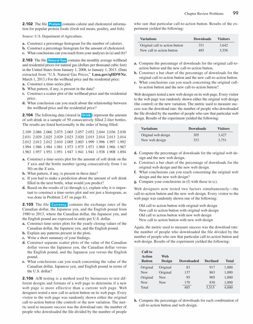
Chapter Review problems 99
2.102 The file protein contains calorie and cholesterol informa-tion for popular protein foods (fresh red meats, poultry, and fish).
Source: U.S. Department of Agriculture.
a. Construct a percentage histogram for the number of calories.b. Construct a percentage histogram for the amount of cholesterol.c. What conclusions can you reach from your analyses in (a) and (b)?
2.103 The file natural gas contains the monthly average wellhead and residential prices for natural gas (dollars per thousand cubic feet) in the United States from January 1, 2008, to January 1, 2013. (Data extracted from “U.S. Natural Gas prices,” 1.usa.gov/qHDWNz, March 1, 2013.) For the wellhead price and the residential price:a. Construct a time-series plot.b. What pattern, if any, is present in the data?c. Construct a scatter plot of the wellhead price and the residential
price.d. What conclusion can you reach about the relationship between
the wellhead price and the residential price?
2.104 The following data (stored in Drink ) represent the amount of soft drink in a sample of 50 consecutively filled 2-liter bottles. The results are listed horizontally in the order of being filled:
2.109 2.086 2.066 2.075 2.065 2.057 2.052 2.044 2.036 2.0382.031 2.029 2.025 2.029 2.023 2.020 2.015 2.014 2.013 2.0142.012 2.012 2.012 2.010 2.005 2.003 1.999 1.996 1.997 1.9921.994 1.986 1.984 1.981 1.973 1.975 1.971 1.969 1.966 1.9671.963 1.957 1.951 1.951 1.947 1.941 1.941 1.938 1.908 1.894
a. Construct a time-series plot for the amount of soft drink on the Y axis and the bottle number (going consecutively from 1 to 50) on the X axis.
b. What pattern, if any, is present in these data?c. If you had to make a prediction about the amount of soft drink
filled in the next bottle, what would you predict?d. Based on the results of (a) through (c), explain why it is impor-
tant to construct a time-series plot and not just a histogram, as was done in problem 2.47 on page 81.
2.105 The file Currency contains the exchange rates of the Canadian dollar, the Japanese yen, and the English pound from 1980 to 2013, where the Canadian dollar, the Japanese yen, and the English pound are expressed in units per U.S. dollar.a. Construct time-series plots for the yearly closing values of the
Canadian dollar, the Japanese yen, and the English pound.b. Explain any patterns present in the plots.c. Write a short summary of your findings.d. Construct separate scatter plots of the value of the Canadian
dollar versus the Japanese yen, the Canadian dollar versus the English pound, and the Japanese yen versus the English pound.
e. What conclusions can you reach concerning the value of the Canadian dollar, Japanese yen, and English pound in terms of the U.S. dollar?
2.106 A/B testing is a method used by businesses to test dif-ferent designs and formats of a web page to determine if a new web page is more effective than a current web page. Web designers tested a new call to action button on its web page. Every visitor to the web page was randomly shown either the original call-to-action button (the control) or the new variation. The met-ric used to measure success was the download rate: the number of people who downloaded the file divided by the number of people
who saw that particular call-to-action button. Results of the ex-periment yielded the following:
Variations Downloads Visitors
Original call to action button 351 3,642New call to action button 485 3,556
a. Compute the percentage of downloads for the original call-to-action button and the new call-to-action button.
b. Construct a bar chart of the percentage of downloads for the original call-to-action button and the new call-to-action button.
c. What conclusions can you reach concerning the original call-to-action button and the new call-to-action button?
Web designers tested a new web design on its web page. Every visitor to the web page was randomly shown either the original web design (the control) or the new variation. The metric used to measure suc-cess was the download rate: the number of people who downloaded the file divided by the number of people who saw that particular web design. Results of the experiment yielded the following:
Variations Downloads Visitors
Original web design 305 3,427New web design 353 3,751
d. Compute the percentage of downloads for the original web de-sign and the new web design.
e. Construct a bar chart of the percentage of downloads for the original web design and the new web design.
f. What conclusions can you reach concerning the original web design and the new web design?
g. Compare your conclusions in (f) with those in (c).
Web designers now tested two factors simultaneously—the call-to-action button and the new web design. Every visitor to the web page was randomly shown one of the following:
Old call to action button with original web design New call to action button with original web design Old call to action button with new web design New call to action button with new web design
Again, the metric used to measure success was the download rate: the number of people who downloaded the file divided by the number of people who saw that particular call-to-action button and web design. Results of the experiment yielded the following:
Call to Action Button
Web Design Downloaded Declined Total
Original Original 83 917 1,000New Original 137 863 1,000Original New 95 905 1,000New New 170 830 1,000Total 485 3,515 4,000
h. Compute the percentage of downloads for each combination of call-to-action button and web design.

100 ChApTER 2 Organizing and Visualizing Variables
c a s E s F O R c h a P t E R 2
Managing ashland Multicomm servicesRecently, Ashland MultiComm Services has been criticized for its inadequate customer service in responding to ques-tions and problems about its telephone, cable television, and Internet services. Senior management has established a task force charged with the business objective of improving cus-tomer service. In response to this charge, the task force col-lected data about the types of customer service errors, the cost of customer service errors, and the cost of wrong bill-ing errors. It found the following data:
Types of Customer Service ErrorsType of Errors Frequency
Incorrect accessory 27Incorrect address 42Incorrect contact phone 31Invalid wiring 9On-demand programming error 14Subscription not ordered 8Suspension error 15Termination error 22Website access error 30Wrong billing 137Wrong end date 17Wrong number of connections 19Wrong price quoted 20Wrong start date 24Wrong subscription type 33Total 448
Cost of Customer Service Errors in the Past YearType of Errors Cost ($ thousands)
Incorrect accessory 17.3Incorrect address 62.4Incorrect contact phone 21.3Invalid wiring 40.8On-demand programming errors 38.8Subscription not ordered 20.3Suspension error 46.8Termination error 50.9Website access errors 60.7Wrong billing 121.7Wrong end date 40.9Wrong number of connections 28.1Wrong price quoted 50.3Wrong start date 40.8Wrong subscription type 60.1Total 701.2
Type and Cost of Wrong Billing ErrorsType of Wrong Billing Errors Cost ($ thousands)
Declined or held transactions 7.6
Incorrect account number 104.3Invalid verification 9.8Total 121.7
i. What conclusions can you reach concerning the original call to action button and the new call to action button and the original web design and the new web design?
j. Compare your conclusions in (i) with those in (c) and (g).
2.107 (Class Project) have each student in the class respond to the question “Which carbonated soft drink do you most prefer?” so that the instructor can tally the results into a summary table.a. Convert the data to percentages and construct a pareto chart.b. Analyze the findings.
2.108 (Class Project) Cross-classify each student in the class by gender (male, female) and current employment status (yes, no), so that the instructor can tally the results.
a. Construct a table with either row or column percentages, de-pending on which you think is more informative.
b. What would you conclude from this study?c. What other variables would you want to know regarding em-
ployment in order to enhance your findings?
repOrT WriTing exerCiSeS2.109 Referring to the results from problem 2.100 on page 98 concerning the weights of Boston and Vermont shingles, write a report that evaluates whether the weights of the pallets of the two types of shingles are what the company expects. Be sure to incor-porate tables and charts into the report.
1. Review these data (stored in amS2-1 ). Identify the vari-ables that are important in describing the customer ser-vice problems. For each variable you identify, construct the graphical representation you think is most appropri-ate and explain your choice. Also, suggest what other in-formation concerning the different types of errors would be useful to examine. Offer possible courses of action for
either the task force or management to take that would support the goal of improving customer service.
2. As a follow-up activity, the task force decides to collect data to study the pattern of calls to the help desk (stored in amS2-2 ). Analyze these data and present your conclu-sions in a report.
Cases for Chapter 2 101
Digital caseIn the Using Statistics scenario, you were asked to gather information to help make wise investment choices. Sources for such information include brokerage firms, investment counselors, and other financial services firms. Apply your knowledge about the proper use of tables and charts in this Digital Case about the claims of foresight and excellence by an Ashland-area financial services firm.
Open EndRunGuide.pdf, which contains the EndRun Financial Services “Guide to Investing.” Review the guide, paying close attention to the company’s investment claims and supporting data and then answer the following.
1. how does the presentation of the general information about EndRun in this guide affect your perception of the business?
2. Is EndRun’s claim about having more winners than losers a fair and accurate reflection of the quality of its invest-ment service? If you do not think that the claim is a fair and accurate one, provide an alternate presentation that you think is fair and accurate.
3. Review the discussion about EndRun’s “Big Eight Differ-ence” and then open and examine the attached sample of mutual funds. Are there any other relevant data from that file that could have been included in the Big Eight table? how would the new data alter your perception of End-Run’s claims?
4. EndRun is proud that all Big Eight funds have gained in value over the past five years. Do you agree that EndRun should be proud of its selections? Why or why not?
cardiogood Fitness
The market research team at AdRight is assigned the task to identify the profile of the typical customer for each tread-mill product offered by CardioGood Fitness. The market research team decides to investigate whether there are dif-ferences across the product lines with respect to customer characteristics. The team decides to collect data on indi-viduals who purchased a treadmill at a CardioGood Fit-ness retail store during the prior three months. The data are stored in the Cardiogood Fitness file. The team identifies the following customer variables to study: product purchased, TM195, TM498, or TM798; gender; age, in years; educa-tion, in years; relationship status, single or partnered; annual
household income ($); average number of times the cus-tomer plans to use the treadmill each week; average number of miles the customer expects to walk/run each week; and self-rated fitness on an 1-to-5 ordinal scale, where 1 is poor shape and 5 is excellent shape.
1. Create a customer profile for each CardioGood Fitness treadmill product line by developing appropriate tables and charts.
2. Write a report to be presented to the management of Car-dioGood Fitness detailing your findings.
the choice Is Yours Follow-UpFollow up the Using Statistics Revisited section on page 93 by analyzing the differences in 3-year return per-centages, 5-year return percentages, and 10-year return per-centages for the sample of 316 retirement funds stored in
retirement Funds . In your analysis, examine differences be-tween the growth and value funds as well as the differences among the small, mid-cap, and large market cap funds.
clear Mountain state student surveys1. The student news service at Clear Mountain State Uni-
versity (CMSU) has decided to gather data about the undergraduate students that attend CMSU. They cre-ate and distribute a survey of 14 questions and re-ceive responses from 62 undergraduates (stored in undergradSurvey ). For each question asked in the survey, construct all the appropriate tables and charts and write a report summarizing your conclusions.
2. The dean of students at CMSU has learned about the undergraduate survey and has decided to undertake a similar survey for graduate students at CMSU. She creates and distributes a survey of 14 questions and re-ceives responses from 44 graduate students (stored in gradSurvey ). For each question asked in the survey, con-struct all the appropriate tables and charts and write a report summarizing your conclusions.
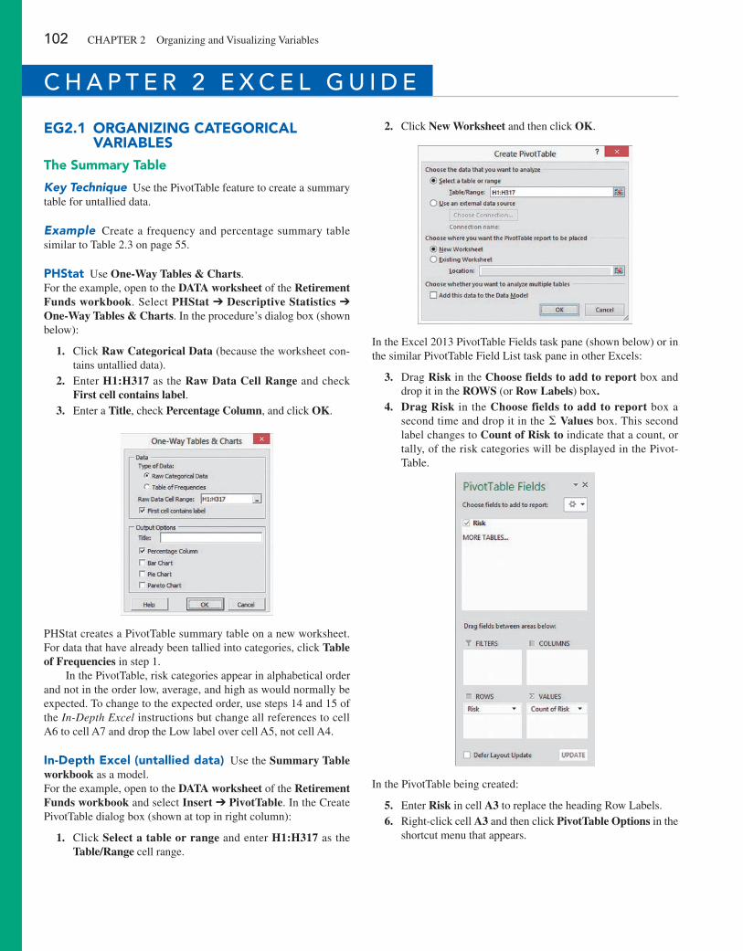
102 ChApTER 2 Organizing and Visualizing Variables
eg2.1 Organizing CaTegOriCal VariableS
The Summary Table
Key Technique Use the pivotTable feature to create a summary table for untallied data.
Example Create a frequency and percentage summary table similar to Table 2.3 on page 55.
phStat Use One-Way Tables & Charts.For the example, open to the DATA worksheet of the Retirement Funds workbook. Select PHStat ➔ Descriptive Statistics ➔ One-Way Tables & Charts. In the procedure’s dialog box (shown below):
1. Click Raw Categorical Data (because the worksheet con-tains untallied data).
2. Enter H1:H317 as the Raw Data Cell Range and check First cell contains label.
3. Enter a Title, check Percentage Column, and click OK.
phStat creates a pivotTable summary table on a new worksheet. For data that have already been tallied into categories, click Table of Frequencies in step 1.
In the pivotTable, risk categories appear in alphabetical order and not in the order low, average, and high as would normally be expected. To change to the expected order, use steps 14 and 15 of the In-Depth Excel instructions but change all references to cell A6 to cell A7 and drop the Low label over cell A5, not cell A4.
in-Depth excel (untallied data) Use the Summary Table workbook as a model.For the example, open to the DATA worksheet of the Retirement Funds workbook and select Insert ➔ PivotTable. In the Create pivotTable dialog box (shown at top in right column):
1. Click Select a table or range and enter H1:H317 as the Table/Range cell range.
2. Click New Worksheet and then click OK.
In the Excel 2013 pivotTable Fields task pane (shown below) or in the similar pivotTable Field List task pane in other Excels:
3. Drag Risk in the Choose fields to add to report box and drop it in the ROWS (or Row Labels) box.
4. Drag Risk in the Choose fields to add to report box a second time and drop it in the Σ Values box. This second label changes to Count of Risk to indicate that a count, or tally, of the risk categories will be displayed in the pivot-Table.
In the pivotTable being created:
5. Enter Risk in cell A3 to replace the heading Row Labels. 6. Right-click cell A3 and then click PivotTable Options in the
shortcut menu that appears.
c h a P t E R 2 E x c E l g U i D E
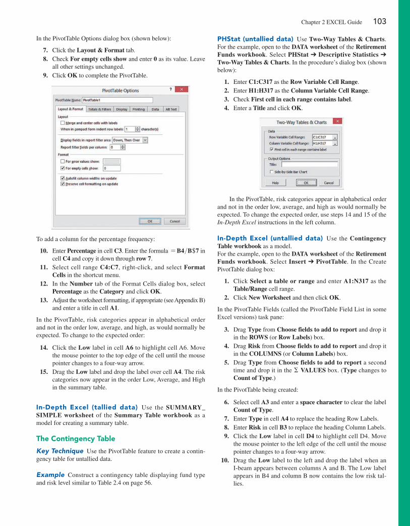
Chapter 2 EXCEL Guide 103
In the pivotTable Options dialog box (shown below):
7. Click the Layout & Format tab. 8. Check For empty cells show and enter 0 as its value. Leave
all other settings unchanged. 9. Click OK to complete the pivotTable.
To add a column for the percentage frequency:
10. Enter Percentage in cell C3. Enter the formula = B4>B+7 in cell C4 and copy it down through row 7.
11. Select cell range C4:C7, right-click, and select Format Cells in the shortcut menu.
12. In the Number tab of the Format Cells dialog box, select Percentage as the Category and click OK.
13. Adjust the worksheet formatting, if appropriate (see Appendix B) and enter a title in cell A1.
In the pivotTable, risk categories appear in alphabetical order and not in the order low, average, and high, as would normally be expected. To change to the expected order:
14. Click the Low label in cell A6 to highlight cell A6. Move the mouse pointer to the top edge of the cell until the mouse pointer changes to a four-way arrow.
15. Drag the Low label and drop the label over cell A4. The risk categories now appear in the order Low, Average, and high in the summary table.
in-Depth excel (tallied data) Use the SUMMARY_ SIMPLE worksheet of the Summary Table workbook as a model for creating a summary table.
The Contingency Table
Key Technique Use the pivotTable feature to create a contin-gency table for untallied data.
Example Construct a contingency table displaying fund type and risk level similar to Table 2.4 on page 56.
phStat (untallied data) Use Two-Way Tables & Charts. For the example, open to the DATA worksheet of the Retirement Funds workbook. Select PHStat ➔ Descriptive Statistics ➔ Two-Way Tables & Charts. In the procedure’s dialog box (shown below):
1. Enter C1:C317 as the Row Variable Cell Range. 2. Enter H1:H317 as the Column Variable Cell Range. 3. Check First cell in each range contains label. 4. Enter a Title and click OK.
In the pivotTable, risk categories appear in alphabetical order and not in the order low, average, and high as would normally be expected. To change the expected order, use steps 14 and 15 of the In-Depth Excel instructions in the left column.
in-Depth excel (untallied data) Use the Contingency Table workbook as a model.For the example, open to the DATA worksheet of the Retirement Funds workbook. Select Insert ➔ PivotTable. In the Create pivotTable dialog box:
1. Click Select a table or range and enter A1:N317 as the Table/Range cell range.
2. Click New Worksheet and then click OK.
In the pivotTable Fields (called the pivotTable Field List in some Excel versions) task pane:
3. Drag Type from Choose fields to add to report and drop it in the ROWS (or Row Labels) box.
4. Drag Risk from Choose fields to add to report and drop it in the COLUMNS (or Column Labels) box.
5. Drag Type from Choose fields to add to report a second time and drop it in the Σ VALUES box. (Type changes to Count of Type.)
In the pivotTable being created:
6. Select cell A3 and enter a space character to clear the label Count of Type.
7. Enter Type in cell A4 to replace the heading Row Labels. 8. Enter Risk in cell B3 to replace the heading Column Labels. 9. Click the Low label in cell D4 to highlight cell D4. Move
the mouse pointer to the left edge of the cell until the mouse pointer changes to a four-way arrow.
10. Drag the Low label to the left and drop the label when an I-beam appears between columns A and B. The Low label appears in B4 and column B now contains the low risk tal-lies.
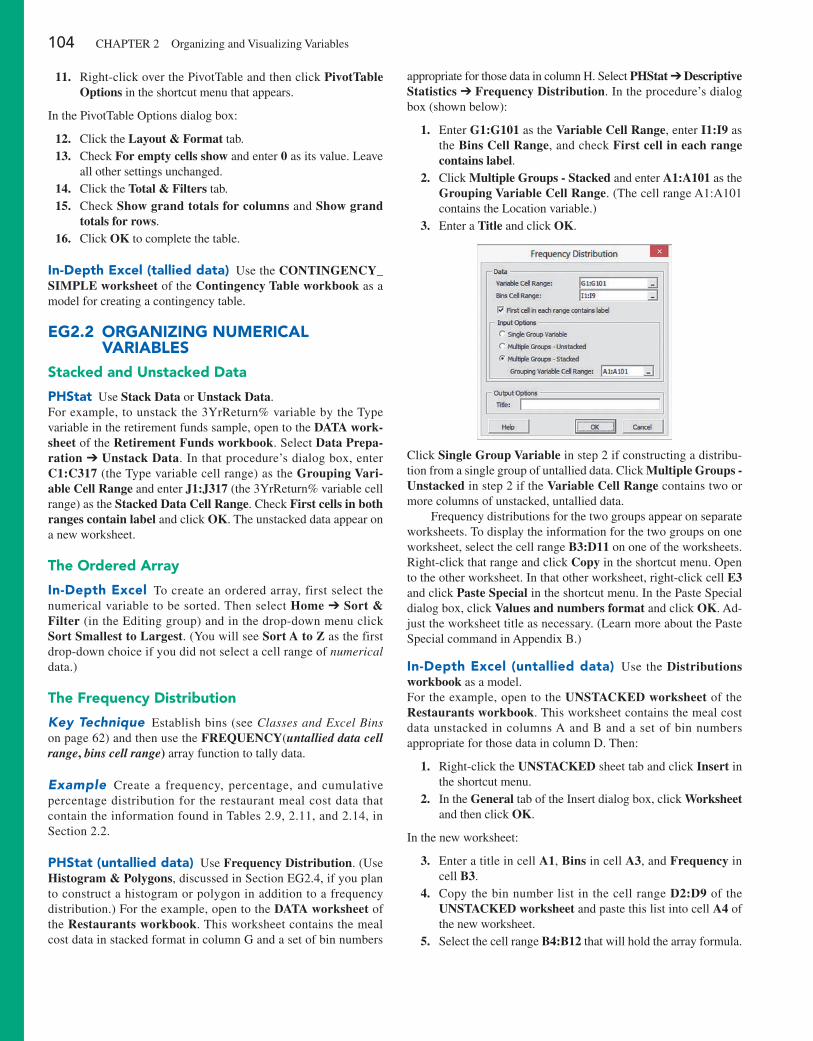
104 ChApTER 2 Organizing and Visualizing Variables
11. Right-click over the pivotTable and then click PivotTable Options in the shortcut menu that appears.
In the pivotTable Options dialog box:
12. Click the Layout & Format tab. 13. Check For empty cells show and enter 0 as its value. Leave
all other settings unchanged. 14. Click the Total & Filters tab. 15. Check Show grand totals for columns and Show grand
totals for rows. 16. Click OK to complete the table.
in-Depth excel (tallied data) Use the CONTINGENCY_SIMPLE worksheet of the Contingency Table workbook as a model for creating a contingency table.
eg2.2 Organizing numeriCal VariableS
Stacked and unstacked Data
phStat Use Stack Data or Unstack Data.For example, to unstack the 3YrReturn% variable by the Type variable in the retirement funds sample, open to the DATA work-sheet of the Retirement Funds workbook. Select Data Prepa-ration ➔ Unstack Data. In that procedure’s dialog box, enter C1:C317 (the Type variable cell range) as the Grouping Vari-able Cell Range and enter J1:J317 (the 3YrReturn% variable cell range) as the Stacked Data Cell Range. Check First cells in both ranges contain label and click OK. The unstacked data appear on a new worksheet.
The Ordered array
in-Depth excel To create an ordered array, first select the numerical variable to be sorted. Then select Home ➔ Sort & Filter (in the Editing group) and in the drop-down menu click Sort Smallest to Largest. (You will see Sort A to Z as the first drop-down choice if you did not select a cell range of numerical data.)
The Frequency Distribution
Key Technique Establish bins (see Classes and Excel Bins on page 62) and then use the FREQUENCY(untallied data cell range, bins cell range) array function to tally data.
Example Create a frequency, percentage, and cumulative percentage distribution for the restaurant meal cost data that contain the information found in Tables 2.9, 2.11, and 2.14, in Section 2.2.
phStat (untallied data) Use Frequency Distribution. (Use Histogram & Polygons, discussed in Section EG2.4, if you plan to construct a histogram or polygon in addition to a frequency distribution.) For the example, open to the DATA worksheet of the Restaurants workbook. This worksheet contains the meal cost data in stacked format in column G and a set of bin numbers
appropriate for those data in column h. Select PHStat ➔ Descriptive Statistics ➔ Frequency Distribution. In the procedure’s dialog box (shown below):
1. Enter G1:G101 as the Variable Cell Range, enter I1:I9 as the Bins Cell Range, and check First cell in each range contains label.
2. Click Multiple Groups - Stacked and enter A1:A101 as the Grouping Variable Cell Range. (The cell range A1:A101 contains the Location variable.)
3. Enter a Title and click OK.
Click Single Group Variable in step 2 if constructing a distribu-tion from a single group of untallied data. Click Multiple Groups - Unstacked in step 2 if the Variable Cell Range contains two or more columns of unstacked, untallied data.
Frequency distributions for the two groups appear on separate worksheets. To display the information for the two groups on one worksheet, select the cell range B3:D11 on one of the worksheets. Right-click that range and click Copy in the shortcut menu. Open to the other worksheet. In that other worksheet, right-click cell E3 and click Paste Special in the shortcut menu. In the paste Special dialog box, click Values and numbers format and click OK. Ad-just the worksheet title as necessary. (Learn more about the paste Special command in Appendix B.)
in-Depth excel (untallied data) Use the Distributions workbook as a model.For the example, open to the UNSTACKED worksheet of the Restaurants workbook. This worksheet contains the meal cost data unstacked in columns A and B and a set of bin numbers appropriate for those data in column D. Then:
1. Right-click the UNSTACKED sheet tab and click Insert in the shortcut menu.
2. In the General tab of the Insert dialog box, click Worksheet and then click OK.
In the new worksheet:
3. Enter a title in cell A1, Bins in cell A3, and Frequency in cell B3.
4. Copy the bin number list in the cell range D2:D9 of the UNSTACKED worksheet and paste this list into cell A4 of the new worksheet.
5. Select the cell range B4:B12 that will hold the array formula.
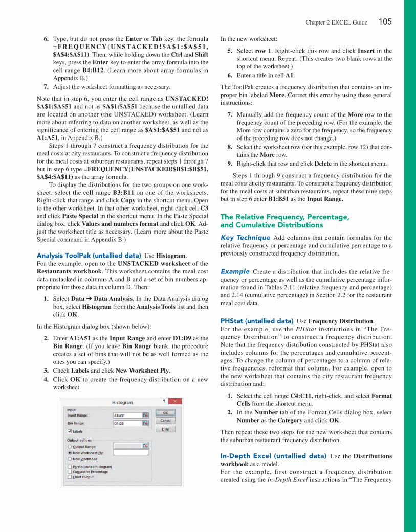
Chapter 2 EXCEL Guide 105
6. Type, but do not press the Enter or Tab key, the formula = F R E Q U E N C Y ( U N S TAC K E D ! $ A $ 1 : $ A $ 5 1 , $A$4:$A$11). Then, while holding down the Ctrl and Shift keys, press the Enter key to enter the array formula into the cell range B4:B12. (Learn more about array formulas in Appendix B.)
7. Adjust the worksheet formatting as necessary.
Note that in step 6, you enter the cell range as UNSTACKED! $A$1:$A$51 and not as $A$1:$A$51 because the untallied data are located on another (the UNSTACKED) worksheet. (Learn more about referring to data on another worksheet, as well as the significance of entering the cell range as $A$1:$A$51 and not as A1:A51, in Appendix B.)
Steps 1 through 7 construct a frequency distribution for the meal costs at city restaurants. To construct a frequency distribution for the meal costs at suburban restaurants, repeat steps 1 through 7 but in step 6 type =FREQUENCY(UNSTACKED!$B$1:$B$51, $A$4:$A$11) as the array formula.
To display the distributions for the two groups on one work-sheet, select the cell range B3:B11 on one of the worksheets. Right-click that range and click Copy in the shortcut menu. Open to the other worksheet. In that other worksheet, right-click cell C3 and click Paste Special in the shortcut menu. In the paste Special dialog box, click Values and numbers format and click OK. Ad-just the worksheet title as necessary. (Learn more about the paste Special command in Appendix B.)
analysis Toolpak (untallied data) Use Histogram.For the example, open to the UNSTACKED worksheet of the Restaurants workbook. This worksheet contains the meal cost data unstacked in columns A and B and a set of bin numbers ap-propriate for those data in column D. Then:
1. Select Data ➔ Data Analysis. In the Data Analysis dialog box, select Histogram from the Analysis Tools list and then click OK.
In the histogram dialog box (shown below):
2. Enter A1:A51 as the Input Range and enter D1:D9 as the Bin Range. (If you leave Bin Range blank, the procedure creates a set of bins that will not be as well formed as the ones you can specify.)
3. Check Labels and click New Worksheet Ply. 4. Click OK to create the frequency distribution on a new
worksheet.
In the new worksheet:
5. Select row 1. Right-click this row and click Insert in the shortcut menu. Repeat. (This creates two blank rows at the top of the worksheet.)
6. Enter a title in cell A1.
The Toolpak creates a frequency distribution that contains an im-proper bin labeled More. Correct this error by using these general instructions:
7. Manually add the frequency count of the More row to the frequency count of the preceding row. (For the example, the More row contains a zero for the frequency, so the frequency of the preceding row does not change.)
8. Select the worksheet row (for this example, row 12) that con-tains the More row.
9. Right-click that row and click Delete in the shortcut menu.
Steps 1 through 9 construct a frequency distribution for the meal costs at city restaurants. To construct a frequency distribution for the meal costs at suburban restaurants, repeat these nine steps but in step 6 enter B1:B51 as the Input Range.
The relative Frequency, percentage, and Cumulative Distributions
Key Technique Add columns that contain formulas for the relative frequency or percentage and cumulative percentage to a previously constructed frequency distribution.
Example Create a distribution that includes the relative fre-quency or percentage as well as the cumulative percentage infor-mation found in Tables 2.11 (relative frequency and percentage) and 2.14 (cumulative percentage) in Section 2.2 for the restaurant meal cost data.
phStat (untallied data) Use Frequency Distribution.For the example, use the PHStat instructions in “The Fre-quency Distribution” to construct a frequency distribution. Note that the frequency distribution constructed by phStat also includes columns for the percentages and cumulative percent-ages. To change the column of percentages to a column of rela-tive frequencies, reformat that column. For example, open to the new worksheet that contains the city restaurant frequency distribution and:
1. Select the cell range C4:C11, right-click, and select Format Cells from the shortcut menu.
2. In the Number tab of the Format Cells dialog box, select Number as the Category and click OK.
Then repeat these two steps for the new worksheet that contains the suburban restaurant frequency distribution.
in-Depth excel (untallied data) Use the Distributions workbook as a model.For the example, first construct a frequency distribution created using the In-Depth Excel instructions in “The Frequency

106 ChApTER 2 Organizing and Visualizing Variables
Distribution.” Open to the new worksheet that contains the frequency distribution for the city restaurants and:
1. Enter Percentage in cell C3 and Cumulative Pctage in cell D3.
2. Enter =B4 ,SUM(+B+4:+B+11) in cell C4 and copy this formula down through row 11.
3. Enter =C4 in cell D4. 4. Enter =C5 + D4 in cell D5 and copy this formula down
through row 11. 5. Select the cell range C4:D11, right-click, and click Format
Cells in the shortcut menu. 6. In the Number tab of the Format Cells dialog box, click Per-
centage in the Category list and click OK.
Then open to the worksheet that contains the frequency distribu-tion for the suburban restaurants and repeat steps 1 through 6.
If you want column C to display relative frequencies instead of percentages, enter Rel. Frequencies in cell C3. Select the cell range C4:C12, right-click, and click Format Cells in the shortcut menu. In the Number tab of the Format Cells dialog box, click Number in the Category list and click OK.
analysis Toolpak Use Histogram and then modify the work-sheet created.
For the example, first construct the frequency distributions using the Analysis ToolPak instructions in “The Frequency Distri-bution.” Then use the In-Depth Excel instructions to modify those distributions.
eg2.3 ViSualizing CaTegOriCal VariableS
Many of the In-Depth Excel instructions in the rest of this Excel Guide refer to the following labeled Charts group illustration.
The bar Chart and the pie Chart
Key Technique Use the Excel bar or pie chart feature. If the variable to be visualized is untallied, first construct a summary table (see the Section EG2.1 “The Summary Table” instructions).
Example Construct a bar or pie chart from a summary table sim-ilar to Table 2.3 on page 55.
phStat Use One-Way Tables & Charts.For the example, use the Section EG2.1 “The Summary Table” PHStat instructions, but in step 3, check either Bar Chart or Pie Chart (or both) in addition to entering a Title, checking Percent-age Column, and clicking OK.
in-Depth excel Use the Summary Table workbook as a model.For the example, open to the OneWayTable worksheet of the Summary Table workbook. (The pivotTable in this worksheet
was constructed using the Section EG2.1 “The Summary Table” instructions.) To construct a bar chart:
1. Select cell range A4:B6. (Begin your selection at cell B6 and not at cell A4, as you would normally do.)
2. In Excel 2013, select Insert, then the Bar icon in the Charts group (#2 in the Charts group illustration), and then select the first 2-D Bar gallery item (Clustered Bar). In other Ex-cels, select Insert ➔ Bar and then select the first 2-D Bar gallery item (Clustered Bar).
3. Right-click the Risk drop-down button in the chart and click Hide All Field Buttons on Chart.
4. (Excel 2013) Select Design ➔ Add Chart Element ➔ Axis Titles ➔ Primary Horizontal.
(Other Excels) Select Layout ➔ Axis Titles ➔ Primary Horizontal Axis Title ➔ Title Below Axis. Select the words “Axis Title” in the chart and enter the title Frequency.
5. Relocate the chart to a chart sheet and turn off the chart legend and gridlines by using the instructions in Appendix Section B.6.
Although not the case with the example, sometimes the horizontal-axis scale of a bar chart will not begin at 0. If this occurs, right-click the horizontal (value) axis in the bar chart and click For-mat Axis in the shortcut menu. In the Excel 2013 Format Axis task pane, click Axis Options. In the Axis Options, enter 0 in the Mini-mum box and then close the pane. In other Excels, in the Format Axis dialog box, click Axis Options in the left pane. In the Axis Options right pane, click the first Fixed option button (for Minimum), enter 0 in its box, and then click Close.
To construct a pie chart, replace steps 2, 4, and 5 with these steps:
2. In Excel 2013, select Insert, then the Pie icon (#4 in the Step 4 illustration), and then select the first 2-D Pie gallery item (Pie). In other Excels, select Insert ➔ Pie and then select the first 2-D Pie gallery item (Pie).
4. (Excel 2013) Select Design ➔ Add Chart Element ➔ Data Labels ➔ More Data Label Options. In the Format Data Labels task pane, click Label Options. In the Label Options, check Category Name and Percentage, clear the other Label Contains check boxes, and click Outside End. (To see the Label Options, you may have to first click the chart [fourth] icon near the top of the task pane.) Then, close the task pane.
(Other Excels) Select Layout ➔ Data Labels ➔ More Data Label Options. In the Format Data Labels dialog box, click Label Options in the left pane. In the Label Options right pane, check Category Name and Percentage and clear the other Label Contains check boxes. Click Outside End and then click Close.
5. Relocate the chart to a chart sheet and turn off the chart legend and gridlines by using the instructions in Appendix Section B.6.
The pareto Chart
Key Technique Use the Excel chart feature with a modified summary table.
Example Construct a pareto chart of the incomplete ATM trans-actions equivalent to Figure 2.4 on page 71.
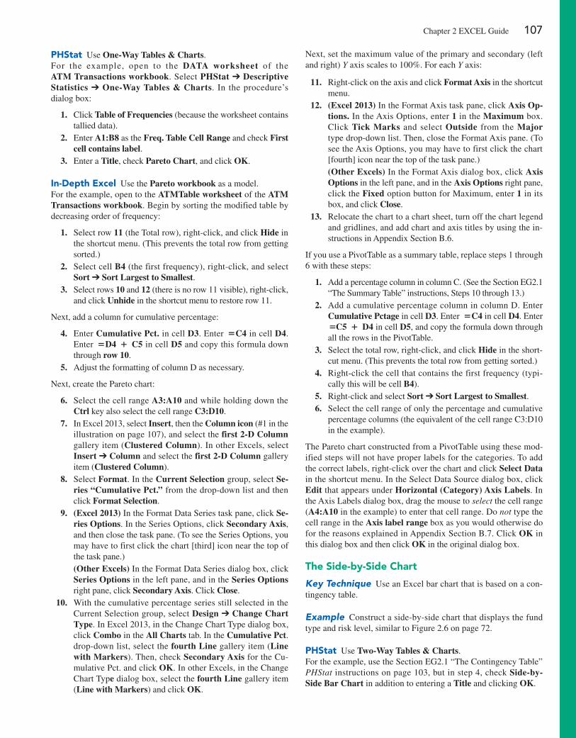
Chapter 2 EXCEL Guide 107
phStat Use One-Way Tables & Charts.For the example, open to the DATA worksheet of the ATM Transactions workbook. Select PHStat ➔ Descriptive Statistics ➔ One-Way Tables & Charts. In the procedure’s dialog box:
1. Click Table of Frequencies (because the worksheet contains tallied data).
2. Enter A1:B8 as the Freq. Table Cell Range and check First cell contains label.
3. Enter a Title, check Pareto Chart, and click OK.
in-Depth excel Use the Pareto workbook as a model.For the example, open to the ATMTable worksheet of the ATM Transactions workbook. Begin by sorting the modified table by decreasing order of frequency:
1. Select row 11 (the Total row), right-click, and click Hide in the shortcut menu. (This prevents the total row from getting sorted.)
2. Select cell B4 (the first frequency), right-click, and select Sort ➔ Sort Largest to Smallest.
3. Select rows 10 and 12 (there is no row 11 visible), right-click, and click Unhide in the shortcut menu to restore row 11.
Next, add a column for cumulative percentage:
4. Enter Cumulative Pct. in cell D3. Enter =C4 in cell D4. Enter =D4 + C5 in cell D5 and copy this formula down through row 10.
5. Adjust the formatting of column D as necessary.
Next, create the pareto chart:
6. Select the cell range A3:A10 and while holding down the Ctrl key also select the cell range C3:D10.
7. In Excel 2013, select Insert, then the Column icon (#1 in the illustration on page 107), and select the first 2-D Column gallery item (Clustered Column). In other Excels, select Insert ➔ Column and select the first 2-D Column gallery item (Clustered Column).
8. Select Format. In the Current Selection group, select Se-ries “Cumulative Pct.” from the drop-down list and then click Format Selection.
9. (Excel 2013) In the Format Data Series task pane, click Se-ries Options. In the Series Options, click Secondary Axis, and then close the task pane. (To see the Series Options, you may have to first click the chart [third] icon near the top of the task pane.)
(Other Excels) In the Format Data Series dialog box, click Series Options in the left pane, and in the Series Options right pane, click Secondary Axis. Click Close.
10. With the cumulative percentage series still selected in the Current Selection group, select Design ➔ Change Chart Type. In Excel 2013, in the Change Chart Type dialog box, click Combo in the All Charts tab. In the Cumulative Pct. drop-down list, select the fourth Line gallery item (Line with Markers). Then, check Secondary Axis for the Cu-mulative pct. and click OK. In other Excels, in the Change Chart Type dialog box, select the fourth Line gallery item (Line with Markers) and click OK.
Next, set the maximum value of the primary and secondary (left and right) Y axis scales to 100%. For each Y axis:
11. Right-click on the axis and click Format Axis in the shortcut menu.
12. (Excel 2013) In the Format Axis task pane, click Axis Op-tions. In the Axis Options, enter 1 in the Maximum box. Click Tick Marks and select Outside from the Major type drop-down list. Then, close the Format Axis pane. (To see the Axis Options, you may have to first click the chart [fourth] icon near the top of the task pane.)
(Other Excels) In the Format Axis dialog box, click Axis Options in the left pane, and in the Axis Options right pane, click the Fixed option button for Maximum, enter 1 in its box, and click Close.
13. Relocate the chart to a chart sheet, turn off the chart legend and gridlines, and add chart and axis titles by using the in-structions in Appendix Section B.6.
If you use a pivotTable as a summary table, replace steps 1 through 6 with these steps:
1. Add a percentage column in column C. (See the Section EG2.1 “The Summary Table” instructions, Steps 10 through 13.)
2. Add a cumulative percentage column in column D. Enter Cumulative Pctage in cell D3. Enter =C4 in cell D4. Enter =C5 + D4 in cell D5, and copy the formula down through all the rows in the pivotTable.
3. Select the total row, right-click, and click Hide in the short-cut menu. (This prevents the total row from getting sorted.)
4. Right-click the cell that contains the first frequency (typi-cally this will be cell B4).
5. Right-click and select Sort ➔ Sort Largest to Smallest. 6. Select the cell range of only the percentage and cumulative
percentage columns (the equivalent of the cell range C3:D10 in the example).
The pareto chart constructed from a pivotTable using these mod-ified steps will not have proper labels for the categories. To add the correct labels, right-click over the chart and click Select Data in the shortcut menu. In the Select Data Source dialog box, click Edit that appears under Horizontal (Category) Axis Labels. In the Axis Labels dialog box, drag the mouse to select the cell range (A4:A10 in the example) to enter that cell range. Do not type the cell range in the Axis label range box as you would otherwise do for the reasons explained in Appendix Section B.7. Click OK in this dialog box and then click OK in the original dialog box.
The Side-by-Side Chart
Key Technique Use an Excel bar chart that is based on a con-tingency table.
Example Construct a side-by-side chart that displays the fund type and risk level, similar to Figure 2.6 on page 72.
phStat Use Two-Way Tables & Charts.For the example, use the Section EG2.1 “The Contingency Table” PHStat instructions on page 103, but in step 4, check Side-by-Side Bar Chart in addition to entering a Title and clicking OK.
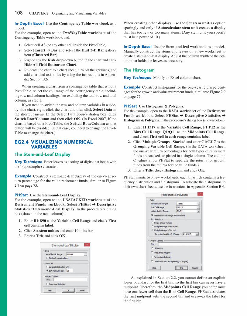
108 ChApTER 2 Organizing and Visualizing Variables
in-Depth excel Use the Contingency Table workbook as a model.For the example, open to the TwoWayTable worksheet of the Contingency Table workbook and:
1. Select cell A3 (or any other cell inside the pivotTable). 2. Select Insert ➔ Bar and select the first 2-D Bar gallery
item (Clustered Bar). 3. Right-click the Risk drop-down button in the chart and click
Hide All Field Buttons on Chart. 4. Relocate the chart to a chart sheet, turn off the gridlines, and
add chart and axis titles by using the instructions in Appen-dix Section B.6.
When creating a chart from a contingency table that is not a pivotTable, select the cell range of the contingency table, includ-ing row and column headings, but excluding the total row and total column, as step 1.
If you need to switch the row and column variables in a side-by-side chart, right-click the chart and then click Select Data in the shortcut menu. In the Select Data Source dialog box, click Switch Row/Column and then click OK. (In Excel 2007, if the chart is based on a pivotTable, the Switch Row/Column as that button will be disabled. In that case, you need to change the pivot-Table to change the chart.)
eg2.4 ViSualizing numeriCal VariableS
The Stem-and-leaf Display
Key Technique Enter leaves as a string of digits that begin with the ’ (apostrophe) character.
Example Construct a stem-and-leaf display of the one-year re-turn percentage for the value retirement funds, similar to Figure 2.7 on page 75.
phStat Use the Stem-and-Leaf Display.For the example, open to the UNSTACKED worksheet of the Retirement Funds workbook. Select PHStat ➔ Descriptive Statistics ➔ Stem-and-Leaf Display. In the procedure’s dialog box (shown in the next column):
1. Enter B1:B90 as the Variable Cell Range and check First cell contains label.
2. Click Set stem unit as and enter 10 in its box. 3. Enter a Title and click OK.
When creating other displays, use the Set stem unit as option sparingly and only if Autocalculate stem unit creates a display that has too few or too many stems. (Any stem unit you specify must be a power of 10.)
in-Depth excel Use the Stem-and-leaf workbook as a model.Manually construct the stems and leaves on a new worksheet to create a stem-and-leaf display. Adjust the column width of the col-umn that holds the leaves as necessary.
The histogram
Key Technique Modify an Excel column chart.
Example Construct histograms for the one-year return percent-ages for the growth and value retirement funds, similar to Figure 2.9 on page 77.
phStat Use Histogram & Polygons.For the example, open to the DATA worksheet of the Retirement Funds workbook. Select PHStat ➔ Descriptive Statistics ➔ Histogram & Polygons. In the procedure’s dialog box (shown below):
1. Enter I1:I317 as the Variable Cell Range, P1:P12 as the Bins Cell Range, Q1:Q11 as the Midpoints Cell Range, and check First cell in each range contains label.
2. Click Multiple Groups - Stacked and enter C1:C317 as the Grouping Variable Cell Range. (In the DATA worksheet, the one-year return percentages for both types of retirement funds are stacked, or placed in a single column. The column C values allow phStat to separate the returns for growth funds from the returns for the value funds.)
3. Enter a Title, check Histogram, and click OK.
phStat inserts two new worksheets, each of which contains a fre-quency distribution and a histogram. To relocate the histograms to their own chart sheets, use the instructions in Appendix Section B.6.
As explained in Section 2.2, you cannot define an explicit lower boundary for the first bin, so the first bin can never have a midpoint. Therefore, the Midpoints Cell Range you enter must have one fewer cell than the Bins Cell Range. phStat associates the first midpoint with the second bin and uses—as the label for the first bin.
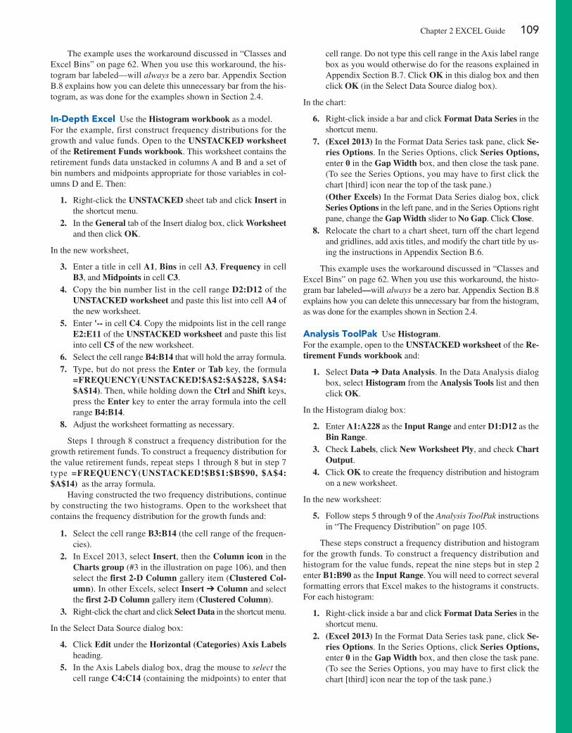
Chapter 2 EXCEL Guide 109
The example uses the workaround discussed in “Classes and Excel Bins” on page 62. When you use this workaround, the his-togram bar labeled—will always be a zero bar. Appendix Section B.8 explains how you can delete this unnecessary bar from the his-togram, as was done for the examples shown in Section 2.4.
in-Depth excel Use the Histogram workbook as a model.For the example, first construct frequency distributions for the growth and value funds. Open to the UNSTACKED worksheet of the Retirement Funds workbook. This worksheet contains the retirement funds data unstacked in columns A and B and a set of bin numbers and midpoints appropriate for those variables in col-umns D and E. Then:
1. Right-click the UNSTACKED sheet tab and click Insert in the shortcut menu.
2. In the General tab of the Insert dialog box, click Worksheet and then click OK.
In the new worksheet,
3. Enter a title in cell A1, Bins in cell A3, Frequency in cell B3, and Midpoints in cell C3.
4. Copy the bin number list in the cell range D2:D12 of the UNSTACKED worksheet and paste this list into cell A4 of the new worksheet.
5. Enter '-- in cell C4. Copy the midpoints list in the cell range E2:E11 of the UNSTACKED worksheet and paste this list into cell C5 of the new worksheet.
6. Select the cell range B4:B14 that will hold the array formula. 7. Type, but do not press the Enter or Tab key, the formula
=FREQUENCY(UNSTACKED!$A$2:$A$228, $A$4: $A$14). Then, while holding down the Ctrl and Shift keys, press the Enter key to enter the array formula into the cell range B4:B14.
8. Adjust the worksheet formatting as necessary.
Steps 1 through 8 construct a frequency distribution for the growth retirement funds. To construct a frequency distribution for the value retirement funds, repeat steps 1 through 8 but in step 7 type =FREQUENCY(UNSTACKED!$B$1:$B$90, $A$4: $A$14) as the array formula.
having constructed the two frequency distributions, continue by constructing the two histograms. Open to the worksheet that contains the frequency distribution for the growth funds and:
1. Select the cell range B3:B14 (the cell range of the frequen-cies).
2. In Excel 2013, select Insert, then the Column icon in the Charts group (#3 in the illustration on page 106), and then select the first 2-D Column gallery item (Clustered Col-umn). In other Excels, select Insert ➔ Column and select the first 2-D Column gallery item (Clustered Column).
3. Right-click the chart and click Select Data in the shortcut menu.
In the Select Data Source dialog box:
4. Click Edit under the Horizontal (Categories) Axis Labels heading.
5. In the Axis Labels dialog box, drag the mouse to select the cell range C4:C14 (containing the midpoints) to enter that
cell range. Do not type this cell range in the Axis label range box as you would otherwise do for the reasons explained in Appendix Section B.7. Click OK in this dialog box and then click OK (in the Select Data Source dialog box).
In the chart:
6. Right-click inside a bar and click Format Data Series in the shortcut menu.
7. (Excel 2013) In the Format Data Series task pane, click Se-ries Options. In the Series Options, click Series Options, enter 0 in the Gap Width box, and then close the task pane. (To see the Series Options, you may have to first click the chart [third] icon near the top of the task pane.)
(Other Excels) In the Format Data Series dialog box, click Series Options in the left pane, and in the Series Options right pane, change the Gap Width slider to No Gap. Click Close.
8. Relocate the chart to a chart sheet, turn off the chart legend and gridlines, add axis titles, and modify the chart title by us-ing the instructions in Appendix Section B.6.
This example uses the workaround discussed in “Classes and Excel Bins” on page 62. When you use this workaround, the histo-gram bar labeled—will always be a zero bar. Appendix Section B.8 explains how you can delete this unnecessary bar from the histogram, as was done for the examples shown in Section 2.4.
analysis Toolpak Use Histogram.For the example, open to the UNSTACKED worksheet of the Re-tirement Funds workbook and:
1. Select Data ➔ Data Analysis. In the Data Analysis dialog box, select Histogram from the Analysis Tools list and then click OK.
In the histogram dialog box:
2. Enter A1:A228 as the Input Range and enter D1:D12 as the Bin Range.
3. Check Labels, click New Worksheet Ply, and check Chart Output.
4. Click OK to create the frequency distribution and histogram on a new worksheet.
In the new worksheet:
5. Follow steps 5 through 9 of the Analysis ToolPak instructions in “The Frequency Distribution” on page 105.
These steps construct a frequency distribution and histogram for the growth funds. To construct a frequency distribution and histogram for the value funds, repeat the nine steps but in step 2 enter B1:B90 as the Input Range. You will need to correct several formatting errors that Excel makes to the histograms it constructs. For each histogram:
1. Right-click inside a bar and click Format Data Series in the shortcut menu.
2. (Excel 2013) In the Format Data Series task pane, click Se-ries Options. In the Series Options, click Series Options, enter 0 in the Gap Width box, and then close the task pane. (To see the Series Options, you may have to first click the chart [third] icon near the top of the task pane.)

110 ChApTER 2 Organizing and Visualizing Variables
(Other Excels) In the Format Data Series dialog box, click Series Options in the left pane, and in the Series Op-tions right pane, change the Gap Width slider to No Gap. Click Close.
histogram bars are labeled by bin numbers. To change the labeling to midpoints, open to each of the new worksheets and:
3. Enter Midpoints in cell C1 and '-- in cell C2. Copy the cell range E2:E11 of the UNSTACKED worksheet and paste this list into cell C5 of the new worksheet.
4. Right-click the histogram and click Select Data. 5. In the Select Data Source dialog box, click Edit under the
Horizontal (Categories) Axis Labels heading. 6. In the Axis Labels dialog box, drag the mouse to select the
cell range C2:C12 to enter that cell range. Do not type this cell range in the Axis label range box as you would other-wise do for the reasons explained in Appendix Section B.7. Click OK in this dialog box and then click OK (in the Se-lect Data Source dialog box).
7. Relocate the chart to a chart sheet, turn off the chart legend, and modify the chart title by using the instructions in Appen-dix Section B.6.
This example uses the workaround discussed on page 62, “Classes and Excel Bins.” Appendix Section B.8 explains how you can delete this unnecessary bar from the histogram, as was done for the examples shown in Section 2.4.
The percentage polygon and the Cumulative percentage polygon (Ogive)
Key Technique Modify an Excel line chart that is based on a frequency distribution.
Example Construct percentage polygons and cumulative per-centage polygons for the one-year return percentages for the growth and value retirement funds, similar to Figure 2.11 on page 78 and equivalent to Figure 2.12 on page 79.
phStat Use Histogram & Polygons.For the example, use the PHStat instructions for creating a histo-gram on page 108 but in step 3 of those instructions, also check Percentage Polygon and Cumulative Percentage Polygon (Ogive) before clicking OK.
in-Depth excel Use the Polygons workbook as a model.For the example, open to the UNSTACKED worksheet of the Retirement Funds workbook and follow steps 1 through 8 to construct a frequency distribution for the growth retirement funds. Repeat steps 1 through 8 but in step 7 type the array formula =FREQUENCY(UNSTACKED!$B$1:$B$90, $A$4: $A$14) to construct a frequency distribution for the value funds. Open to the worksheet that contains the growth funds frequency dis-tribution and:
1. Select column C. Right-click and click Insert in the shortcut menu. Right-click and click Insert in the shortcut menu a sec-ond time. (The worksheet contains new, blank columns C and D and the midpoints column is now column E.)
2. Enter Percentage in cell C3 and Cumulative Pctage. in cell D3.
3. Enter = B4/SUM(+B+4:+B+14) in cell C4 and copy this formula down through row 14.
4. Enter = C4 in cell D4. 5. Enter = C5 + D4 in cell D5 and copy this formula down
through row 14. 6. Select the cell range C4:D14, right-click, and click Format
Cells in the shortcut menu. 7. In the Number tab of the Format Cells dialog box, click Per-
centage in the Category list and click OK.
Open to the worksheet that contains the value funds frequency dis-tribution and repeat steps 1 through 7. To construct the percentage polygons, open to the worksheet that contains the growth funds distribution and:
1. Select cell range C4:C14. 2. In Excel 2013, select Insert, then select the Line icon in the
Charts group (#4 in the illustration on page 106), and then select the fourth 2-D Line gallery item (Line with Mark-ers). In other Excels, select Insert ➔ Line and select the fourth 2-D Line gallery item (Line with Markers).
3. Right-click the chart and click Select Data in the shortcut menu.
In the Select Data Source dialog box:
4. Click Edit under the Legend Entries (Series) heading. In the Edit Series dialog box, enter the formula ="Growth Funds" as the Series name and click OK.
5. Click Edit under the Horizontal (Categories) Axis Labels heading. In the Axis Labels dialog box, drag the mouse to se-lect the cell range E4:E14 to enter that cell range. Do not type this cell range in the Axis label range box as you would other-wise do for the reasons explained in Appendix Section B.7.
6. Click OK in this dialog box and then click OK (in the Select Data Source dialog box).
Back in the chart:
7. Relocate the chart to a chart sheet, turn off the chart grid-lines, add axis titles, and modify the chart title by using the instructions in Appendix Section B.6.
In the new chart sheet:
8. Right-click the chart and click Select Data in the shortcut menu.
9. In the Select Data Source dialog box, click Add.
In the Edit Series dialog box:
10. Enter the formula ="Value Funds" as the Series name and press Tab.
11. With the current value in Series values highlighted, click the worksheet tab for the worksheet that contains the value funds distribution.
12. Drag the mouse to select the cell range C4:C14 to enter that cell range as the Series values. Do not type this cell range in the Series values box as you would otherwise do, for the reasons explained in Appendix Section B.7.
13. Click OK. Back in the Select Data Source dialog box, click OK.
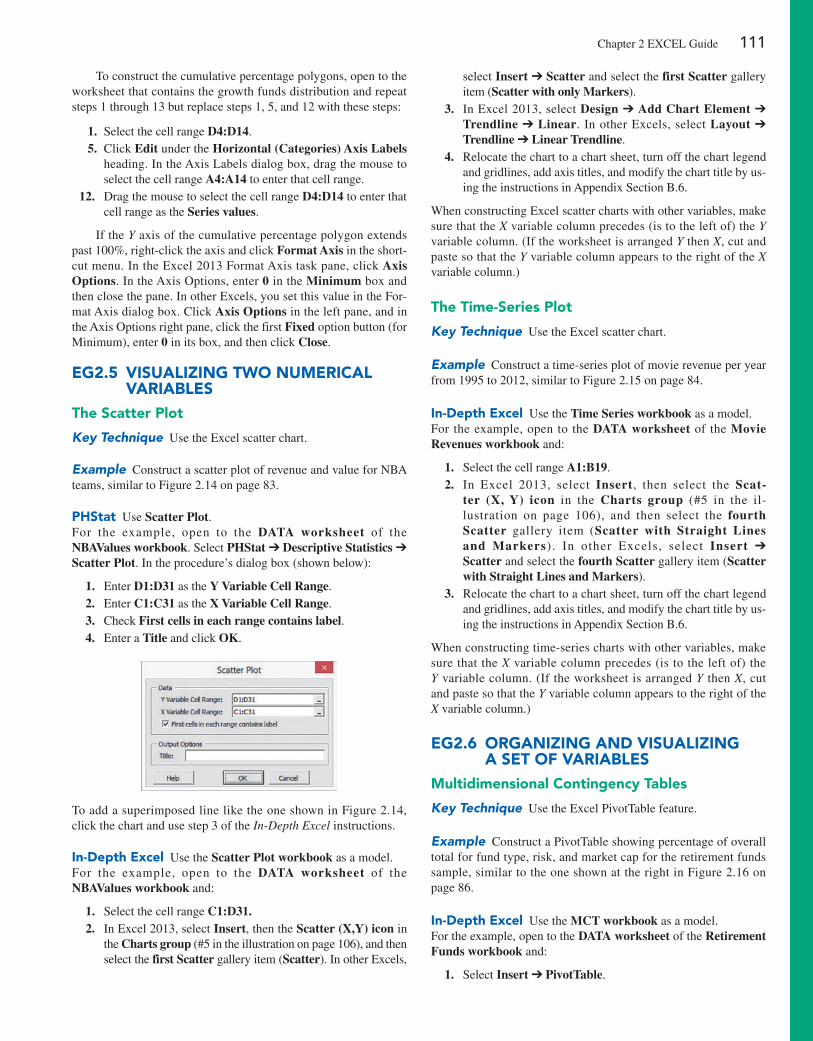
Chapter 2 EXCEL Guide 111
To construct the cumulative percentage polygons, open to the worksheet that contains the growth funds distribution and repeat steps 1 through 13 but replace steps 1, 5, and 12 with these steps:
1. Select the cell range D4:D14. 5. Click Edit under the Horizontal (Categories) Axis Labels
heading. In the Axis Labels dialog box, drag the mouse to select the cell range A4:A14 to enter that cell range.
12. Drag the mouse to select the cell range D4:D14 to enter that cell range as the Series values.
If the Y axis of the cumulative percentage polygon extends past 100%, right-click the axis and click Format Axis in the short-cut menu. In the Excel 2013 Format Axis task pane, click Axis Options. In the Axis Options, enter 0 in the Minimum box and then close the pane. In other Excels, you set this value in the For-mat Axis dialog box. Click Axis Options in the left pane, and in the Axis Options right pane, click the first Fixed option button (for Minimum), enter 0 in its box, and then click Close.
eg2.5 ViSualizing TWO numeriCal VariableS
The Scatter plot
Key Technique Use the Excel scatter chart.
Example Construct a scatter plot of revenue and value for NBA teams, similar to Figure 2.14 on page 83.
phStat Use Scatter Plot.For the example, open to the DATA worksheet of the NBAValues workbook. Select PHStat ➔ Descriptive Statistics ➔ Scatter Plot. In the procedure’s dialog box (shown below):
1. Enter D1:D31 as the Y Variable Cell Range. 2. Enter C1:C31 as the X Variable Cell Range. 3. Check First cells in each range contains label. 4. Enter a Title and click OK.
To add a superimposed line like the one shown in Figure 2.14, click the chart and use step 3 of the In-Depth Excel instructions.
in-Depth excel Use the Scatter Plot workbook as a model.For the example, open to the DATA worksheet of the NBAValues workbook and:
1. Select the cell range C1:D31. 2. In Excel 2013, select Insert, then the Scatter (X,Y) icon in
the Charts group (#5 in the illustration on page 106), and then select the first Scatter gallery item (Scatter). In other Excels,
select Insert ➔ Scatter and select the first Scatter gallery item (Scatter with only Markers).
3. In Excel 2013, select Design ➔ Add Chart Element ➔ Trendline ➔ Linear. In other Excels, select Layout ➔ Trendline ➔ Linear Trendline.
4. Relocate the chart to a chart sheet, turn off the chart legend and gridlines, add axis titles, and modify the chart title by us-ing the instructions in Appendix Section B.6.
When constructing Excel scatter charts with other variables, make sure that the X variable column precedes (is to the left of) the Y variable column. (If the worksheet is arranged Y then X, cut and paste so that the Y variable column appears to the right of the X variable column.)
The Time-Series plot
Key Technique Use the Excel scatter chart.
Example Construct a time-series plot of movie revenue per year from 1995 to 2012, similar to Figure 2.15 on page 84.
in-Depth excel Use the Time Series workbook as a model.For the example, open to the DATA worksheet of the Movie Revenues workbook and:
1. Select the cell range A1:B19. 2. In Excel 2013, select Insert, then select the Scat-
ter (X, Y) icon in the Charts group (#5 in the il-lustration on page 106), and then select the fourth Scatter gallery item (Scatter with Straight Lines and Markers). In other Excels, select Insert ➔ Scatter and select the fourth Scatter gallery item (Scatter with Straight Lines and Markers).
3. Relocate the chart to a chart sheet, turn off the chart legend and gridlines, add axis titles, and modify the chart title by us-ing the instructions in Appendix Section B.6.
When constructing time-series charts with other variables, make sure that the X variable column precedes (is to the left of) the Y variable column. (If the worksheet is arranged Y then X, cut and paste so that the Y variable column appears to the right of the X variable column.)
eg2.6 Organizing anD ViSualizing a SeT OF VariableS
multidimensional Contingency Tables
Key Technique Use the Excel pivotTable feature.
Example Construct a pivotTable showing percentage of overall total for fund type, risk, and market cap for the retirement funds sample, similar to the one shown at the right in Figure 2.16 on page 86.
in-Depth excel Use the MCT workbook as a model.For the example, open to the DATA worksheet of the Retirement Funds workbook and:
1. Select Insert ➔ PivotTable.
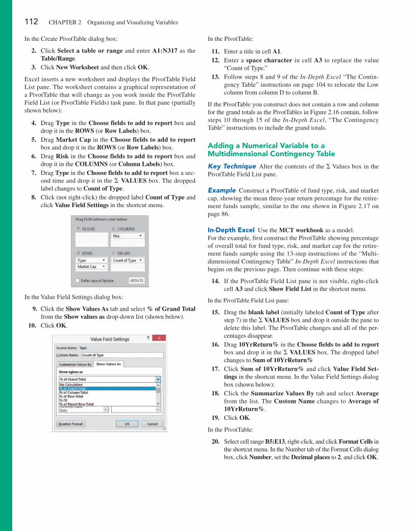
112 ChApTER 2 Organizing and Visualizing Variables
In the Create pivotTable dialog box:
2. Click Select a table or range and enter A1:N317 as the Table/Range.
3. Click New Worksheet and then click OK.
Excel inserts a new worksheet and displays the pivotTable Field List pane. The worksheet contains a graphical representation of a pivotTable that will change as you work inside the pivotTable Field List (or pivotTable Fields) task pane. In that pane (partially shown below):
4. Drag Type in the Choose fields to add to report box and drop it in the ROWS (or Row Labels) box.
5. Drag Market Cap in the Choose fields to add to report box and drop it in the ROWS (or Row Labels) box.
6. Drag Risk in the Choose fields to add to report box and drop it in the COLUMNS (or Column Labels) box.
7. Drag Type in the Choose fields to add to report box a sec-ond time and drop it in the Σ VALUES box. The dropped label changes to Count of Type.
8. Click (not right-click) the dropped label Count of Type and click Value Field Settings in the shortcut menu.
In the Value Field Settings dialog box:
9. Click the Show Values As tab and select % of Grand Total from the Show values as drop-down list (shown below).
10. Click OK.
In the pivotTable:
11. Enter a title in cell A1. 12. Enter a space character in cell A3 to replace the value
“Count of Type.” 13. Follow steps 8 and 9 of the In-Depth Excel “The Contin-
gency Table” instructions on page 104 to relocate the Low column from column D to column B.
If the pivotTable you construct does not contain a row and column for the grand totals as the pivotTables in Figure 2.16 contain, follow steps 10 through 15 of the In-Depth Excel, “The Contingency Table” instructions to include the grand totals.
adding a numerical Variable to a multidimensional Contingency Table
Key Technique Alter the contents of the Σ Values box in the pivotTable Field List pane.
Example Construct a pivotTable of fund type, risk, and market cap, showing the mean three-year return percentage for the retire-ment funds sample, similar to the one shown in Figure 2.17 on page 86.
in-Depth excel Use the MCT workbook as a model.For the example, first construct the pivotTable showing percentage of overall total for fund type, risk, and market cap for the retire-ment funds sample using the 13-step instructions of the “Multi-dimensional Contingency Table” In-Depth Excel instructions that begins on the previous page. Then continue with these steps:
14. If the pivotTable Field List pane is not visible, right-click cell A3 and click Show Field List in the shortcut menu.
In the pivotTable Field List pane:
15. Drag the blank label (initially labeled Count of Type after step 7) in the Σ VALUES box and drop it outside the pane to delete this label. The pivotTable changes and all of the per-centages disappear.
16. Drag 10YrReturn% in the Choose fields to add to report box and drop it in the Σ VALUES box. The dropped label changes to Sum of 10YrReturn%
17. Click Sum of 10YrReturn% and click Value Field Set-tings in the shortcut menu. In the Value Field Settings dialog box (shown below):
18. Click the Summarize Values By tab and select Average from the list. The Custom Name changes to Average of 10YrReturn%.
19. Click OK.
In the pivotTable:
20. Select cell range B5:E13, right-click, and click Format Cells in the shortcut menu. In the Number tab of the Format Cells dialog box, click Number, set the Decimal places to 2, and click OK.
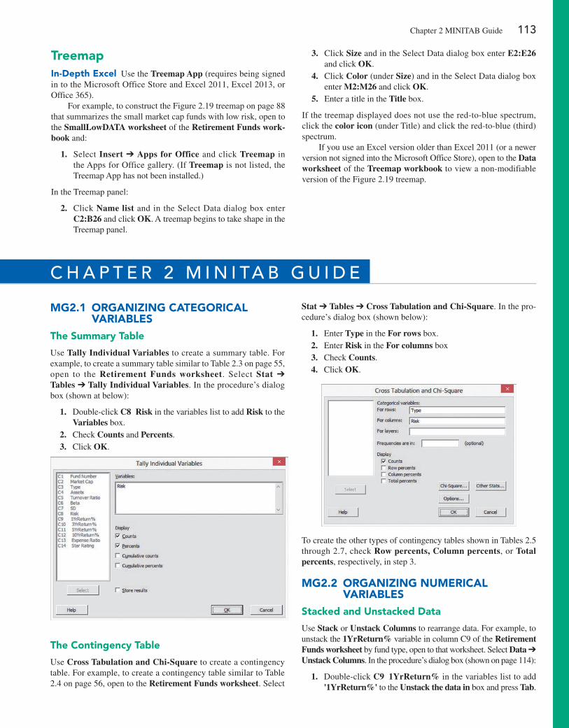
Chapter 2 MINITAB Guide 113
Treemapin-Depth excel Use the Treemap App (requires being signed in to the Microsoft Office Store and Excel 2011, Excel 2013, or Office 365).
For example, to construct the Figure 2.19 treemap on page 88 that summarizes the small market cap funds with low risk, open to the SmallLowDATA worksheet of the Retirement Funds work-book and:
1. Select Insert ➔ Apps for Office and click Treemap in the Apps for Office gallery. (If Treemap is not listed, the Treemap App has not been installed.)
In the Treemap panel:
2. Click Name list and in the Select Data dialog box enter C2:B26 and click OK. A treemap begins to take shape in the Treemap panel.
3. Click Size and in the Select Data dialog box enter E2:E26 and click OK.
4. Click Color (under Size) and in the Select Data dialog box enter M2:M26 and click OK.
5. Enter a title in the Title box.
If the treemap displayed does not use the red-to-blue spectrum, click the color icon (under Title) and click the red-to-blue (third) spectrum.
If you use an Excel version older than Excel 2011 (or a newer version not signed into the Microsoft Office Store), open to the Data worksheet of the Treemap workbook to view a non-modifiable version of the Figure 2.19 treemap.
c h a P t E R 2 M i n i ta B g U i D E
mg2.1 Organizing CaTegOriCal VariableS
The Summary Table
Use Tally Individual Variables to create a summary table. For example, to create a summary table similar to Table 2.3 on page 55, open to the Retirement Funds worksheet. Select Stat ➔ Tables ➔ Tally Individual Variables. In the procedure’s dialog box (shown at below):
1. Double-click C8 Risk in the variables list to add Risk to the Variables box.
2. Check Counts and Percents. 3. Click OK.
The Contingency Table
Use Cross Tabulation and Chi-Square to create a contingency table. For example, to create a contingency table similar to Table 2.4 on page 56, open to the Retirement Funds worksheet. Select
Stat ➔ Tables ➔ Cross Tabulation and Chi-Square. In the pro-cedure’s dialog box (shown below):
1. Enter Type in the For rows box. 2. Enter Risk in the For columns box 3. Check Counts. 4. Click OK.
To create the other types of contingency tables shown in Tables 2.5 through 2.7, check Row percents, Column percents, or Total percents, respectively, in step 3.
mg2.2 Organizing numeriCal VariableS
Stacked and unstacked Data
Use Stack or Unstack Columns to rearrange data. For example, to unstack the 1YrReturn% variable in column C9 of the Retirement Funds worksheet by fund type, open to that worksheet. Select Data ➔ Unstack Columns. In the procedure’s dialog box (shown on page 114):
1. Double-click C9 1YrReturn% in the variables list to add '1YrReturn%' to the Unstack the data in box and press Tab.
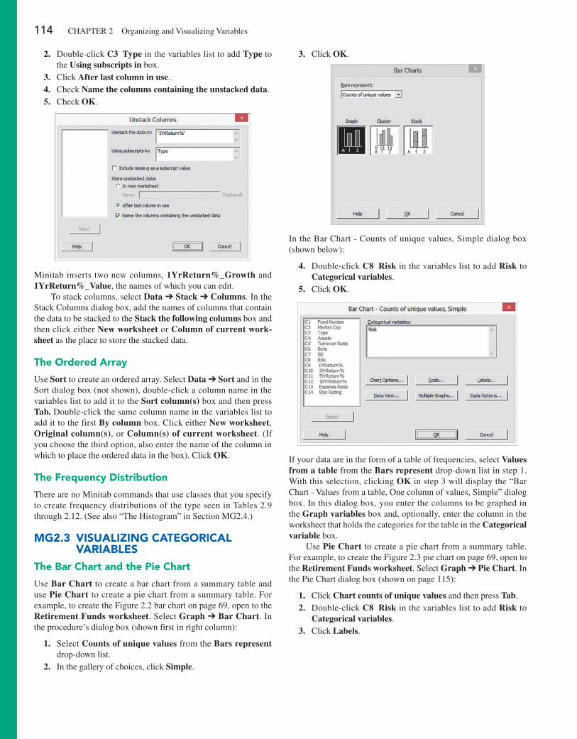
114 ChApTER 2 Organizing and Visualizing Variables
2. Double-click C3 Type in the variables list to add Type to the Using subscripts in box.
3. Click After last column in use. 4. Check Name the columns containing the unstacked data. 5. Check OK.
Minitab inserts two new columns, 1YrReturn%_Growth and 1YrReturn%_Value, the names of which you can edit.
To stack columns, select Data ➔ Stack ➔ Columns. In the Stack Columns dialog box, add the names of columns that contain the data to be stacked to the Stack the following columns box and then click either New worksheet or Column of current work-sheet as the place to store the stacked data.
The Ordered array
Use Sort to create an ordered array. Select Data ➔ Sort and in the Sort dialog box (not shown), double-click a column name in the variables list to add it to the Sort column(s) box and then press Tab. Double-click the same column name in the variables list to add it to the first By column box. Click either New worksheet, Original column(s), or Column(s) of current worksheet. (If you choose the third option, also enter the name of the column in which to place the ordered data in the box). Click OK.
The Frequency Distribution
There are no Minitab commands that use classes that you specify to create frequency distributions of the type seen in Tables 2.9 through 2.12. (See also “The histogram” in Section MG2.4.)
mg2.3 ViSualizing CaTegOriCal VariableS
The bar Chart and the pie Chart
Use Bar Chart to create a bar chart from a summary table and use Pie Chart to create a pie chart from a summary table. For example, to create the Figure 2.2 bar chart on page 69, open to the Retirement Funds worksheet. Select Graph ➔ Bar Chart. In the procedure’s dialog box (shown first in right column):
1. Select Counts of unique values from the Bars represent drop-down list.
2. In the gallery of choices, click Simple.
3. Click OK.
In the Bar Chart - Counts of unique values, Simple dialog box (shown below):
4. Double-click C8 Risk in the variables list to add Risk to Categorical variables.
5. Click OK.
If your data are in the form of a table of frequencies, select Values from a table from the Bars represent drop-down list in step 1. With this selection, clicking OK in step 3 will display the “Bar Chart - Values from a table, One column of values, Simple” dialog box. In this dialog box, you enter the columns to be graphed in the Graph variables box and, optionally, enter the column in the worksheet that holds the categories for the table in the Categorical variable box.
Use Pie Chart to create a pie chart from a summary table. For example, to create the Figure 2.3 pie chart on page 69, open to the Retirement Funds worksheet. Select Graph ➔ Pie Chart. In the pie Chart dialog box (shown on page 115):
1. Click Chart counts of unique values and then press Tab. 2. Double-click C8 Risk in the variables list to add Risk to
Categorical variables. 3. Click Labels.
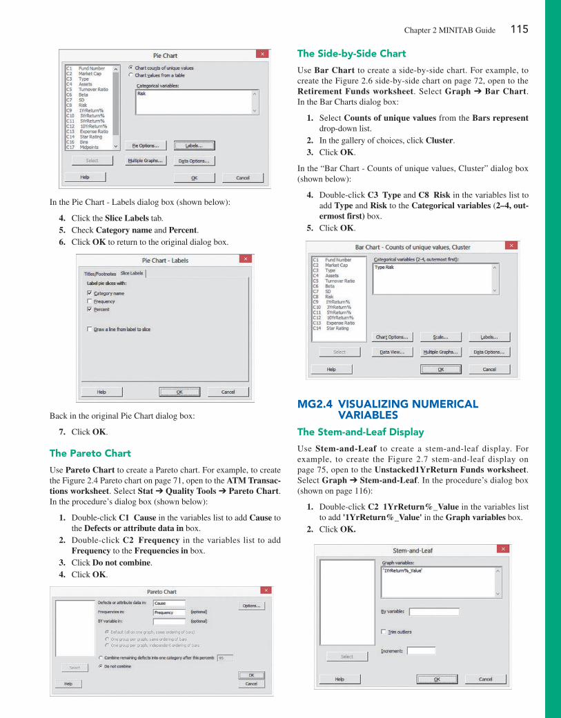
Chapter 2 MINITAB Guide 115
In the pie Chart - Labels dialog box (shown below):
4. Click the Slice Labels tab. 5. Check Category name and Percent. 6. Click OK to return to the original dialog box.
Back in the original pie Chart dialog box:
7. Click OK.
The pareto Chart
Use Pareto Chart to create a pareto chart. For example, to create the Figure 2.4 pareto chart on page 71, open to the ATM Transac-tions worksheet. Select Stat ➔ Quality Tools ➔ Pareto Chart. In the procedure’s dialog box (shown below):
1. Double-click C1 Cause in the variables list to add Cause to the Defects or attribute data in box.
2. Double-click C2 Frequency in the variables list to add Frequency to the Frequencies in box.
3. Click Do not combine. 4. Click OK.
The Side-by-Side Chart
Use Bar Chart to create a side-by-side chart. For example, to create the Figure 2.6 side-by-side chart on page 72, open to the Retirement Funds worksheet. Select Graph ➔ Bar Chart. In the Bar Charts dialog box:
1. Select Counts of unique values from the Bars represent drop-down list.
2. In the gallery of choices, click Cluster. 3. Click OK.
In the “Bar Chart - Counts of unique values, Cluster” dialog box (shown below):
4. Double-click C3 Type and C8 Risk in the variables list to add Type and Risk to the Categorical variables (2–4, out-ermost first) box.
5. Click OK.
mg2.4 ViSualizing numeriCal VariableS
The Stem-and-leaf Display
Use Stem-and-Leaf to create a stem-and-leaf display. For example, to create the Figure 2.7 stem-and-leaf display on page 75, open to the Unstacked1YrReturn Funds worksheet. Select Graph ➔ Stem-and-Leaf. In the procedure’s dialog box (shown on page 116):
1. Double-click C2 1YrReturn%_Value in the variables list to add '1YrReturn%_Value' in the Graph variables box.
2. Click OK.
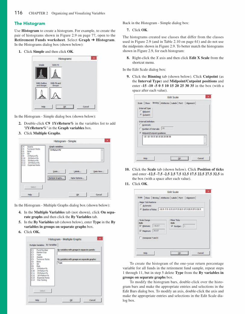
116 ChApTER 2 Organizing and Visualizing Variables
The histogram
Use Histogram to create a histogram. For example, to create the pair of histograms shown in Figure 2.9 on page 77, open to the Retirement Funds worksheet. Select Graph ➔ Histogram. In the histograms dialog box (shown below):
1. Click Simple and then click OK.
In the histogram - Simple dialog box (shown below):
2. Double-click C9 1YrReturn% in the variables list to add '1YrReturn%' in the Graph variables box.
3. Click Multiple Graphs.
In the histogram - Multiple Graphs dialog box (shown below):
4. In the Multiple Variables tab (not shown), click On sepa-rate graphs and then click the By Variables tab.
5. In the By Variables tab (shown below), enter Type in the By variables in groups on separate graphs box.
6. Click OK.
Back in the histogram - Simple dialog box:
7. Click OK.
The histograms created use classes that differ from the classes used in Figure 2.9 (and in Table 2.10 on page 61) and do not use the midpoints shown in Figure 2.9. To better match the histograms shown in Figure 2.9, for each histogram:
8. Right-click the X axis and then click Edit X Scale from the shortcut menu.
In the Edit Scale dialog box:
9. Click the Binning tab (shown below). Click Cutpoint (as the Interval Type) and Midpoint/Cutpoint positions and enter -15 -10 -5 0 5 10 15 20 25 30 35 in the box (with a space after each value).
10. Click the Scale tab (shown below). Click Position of ticks and enter -12.5 -7.5 -2.5 2.5 7.5 12.5 17.5 22.5 27.5 32.5 in the box (with a space after each value).
11. Click OK.
To create the histogram of the one-year return percentage variable for all funds in the retirement fund sample, repeat steps 1 through 11, but in step 5 delete Type from the By variables in groups on separate graphs box.
To modify the histogram bars, double-click over the histo-gram bars and make the appropriate entries and selections in the Edit Bars dialog box. To modify an axis, double-click the axis and make the appropriate entries and selections in the Edit Scale dia-log box.
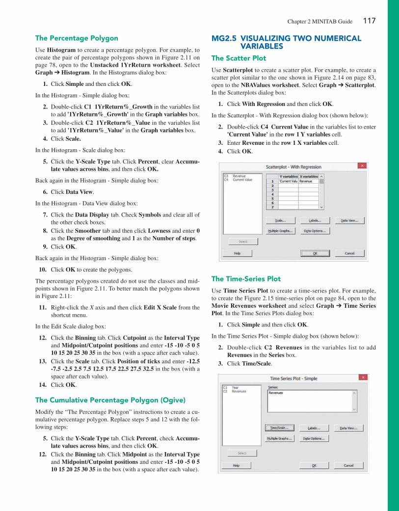
Chapter 2 MINITAB Guide 117
The percentage polygon
Use Histogram to create a percentage polygon. For example, to create the pair of percentage polygons shown in Figure 2.11 on page 78, open to the Unstacked 1YrReturn worksheet. Select Graph ➔ Histogram. In the histograms dialog box:
1. Click Simple and then click OK.
In the histogram - Simple dialog box:
2. Double-click C1 1YrReturn%_Growth in the variables list to add '1YrReturn%_Growth' in the Graph variables box.
3. Double-click C2 1YrReturn%_Value in the variables list to add '1YrReturn%_Value' in the Graph variables box.
4. Click Scale.
In the histogram - Scale dialog box:
5. Click the Y-Scale Type tab. Click Percent, clear Accumu-late values across bins, and then click OK.
Back again in the histogram - Simple dialog box:
6. Click Data View.
In the histogram - Data View dialog box:
7. Click the Data Display tab. Check Symbols and clear all of the other check boxes.
8. Click the Smoother tab and then click Lowness and enter 0 as the Degree of smoothing and 1 as the Number of steps.
9. Click OK.
Back again in the histogram - Simple dialog box:
10. Click OK to create the polygons.
The percentage polygons created do not use the classes and mid-points shown in Figure 2.11. To better match the polygons shown in Figure 2.11:
11. Right-click the X axis and then click Edit X Scale from the shortcut menu.
In the Edit Scale dialog box:
12. Click the Binning tab. Click Cutpoint as the Interval Type and Midpoint/Cutpoint positions and enter -15 -10 -5 0 5 10 15 20 25 30 35 in the box (with a space after each value).
13. Click the Scale tab. Click Position of ticks and enter -12.5 -7.5 -2.5 2.5 7.5 12.5 17.5 22.5 27.5 32.5 in the box (with a space after each value).
14. Click OK.
The Cumulative percentage polygon (Ogive)
Modify the “The percentage polygon” instructions to create a cu-mulative percentage polygon. Replace steps 5 and 12 with the fol-lowing steps:
5. Click the Y-Scale Type tab. Click Percent, check Accumu-late values across bins, and then click OK.
12. Click the Binning tab. Click Midpoint as the Interval Type and Midpoint/Cutpoint positions and enter -15 -10 -5 0 5 10 15 20 25 30 35 in the box (with a space after each value).
mg2.5 ViSualizing TWO numeriCal VariableS
The Scatter plot
Use Scatterplot to create a scatter plot. For example, to create a scatter plot similar to the one shown in Figure 2.14 on page 83, open to the NBAValues worksheet. Select Graph ➔ Scatterplot. In the Scatterplots dialog box:
1. Click With Regression and then click OK.
In the Scatterplot - With Regression dialog box (shown below):
2. Double-click C4 Current Value in the variables list to enter 'Current Value' in the row 1 Y variables cell.
3. Enter Revenue in the row 1 X variables cell. 4. Click OK.
The Time-Series plot
Use Time Series Plot to create a time-series plot. For example, to create the Figure 2.15 time-series plot on page 84, open to the Movie Revenues worksheet and select Graph ➔ Time Series Plot. In the Time Series plots dialog box:
1. Click Simple and then click OK.
In the Time Series plot - Simple dialog box (shown below):
2. Double-click C2 Revenues in the variables list to add Revenues in the Series box.
3. Click Time/Scale.
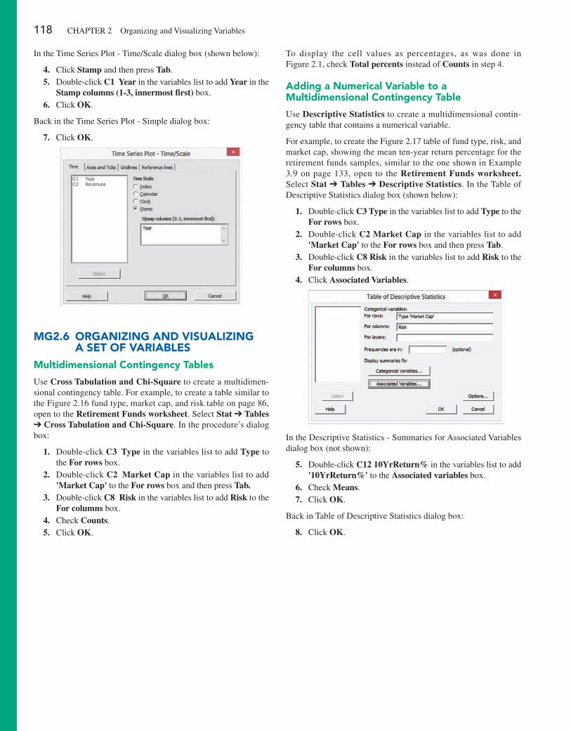
118 ChApTER 2 Organizing and Visualizing Variables
In the Time Series plot - Time/Scale dialog box (shown below):
4. Click Stamp and then press Tab. 5. Double-click C1 Year in the variables list to add Year in the
Stamp columns (1-3, innermost first) box. 6. Click OK.
Back in the Time Series plot - Simple dialog box:
7. Click OK.
mg2.6 Organizing anD ViSualizing a SeT OF VariableS
multidimensional Contingency Tables
Use Cross Tabulation and Chi-Square to create a multidimen-sional contingency table. For example, to create a table similar to the Figure 2.16 fund type, market cap, and risk table on page 86, open to the Retirement Funds worksheet. Select Stat ➔ Tables ➔ Cross Tabulation and Chi-Square. In the procedure’s dialog box:
1. Double-click C3 Type in the variables list to add Type to the For rows box.
2. Double-click C2 Market Cap in the variables list to add 'Market Cap' to the For rows box and then press Tab.
3. Double-click C8 Risk in the variables list to add Risk to the For columns box.
4. Check Counts. 5. Click OK.
To display the cell values as percentages, as was done in Figure 2.1, check Total percents instead of Counts in step 4.
adding a numerical Variable to a multidimensional Contingency Table
Use Descriptive Statistics to create a multidimensional contin-gency table that contains a numerical variable.
For example, to create the Figure 2.17 table of fund type, risk, and market cap, showing the mean ten-year return percentage for the retirement funds samples, similar to the one shown in Example 3.9 on page 133, open to the Retirement Funds worksheet. Select Stat ➔ Tables ➔ Descriptive Statistics. In the Table of Descriptive Statistics dialog box (shown below):
1. Double-click C3 Type in the variables list to add Type to the For rows box.
2. Double-click C2 Market Cap in the variables list to add 'Market Cap' to the For rows box and then press Tab.
3. Double-click C8 Risk in the variables list to add Risk to the For columns box.
4. Click Associated Variables.
In the Descriptive Statistics - Summaries for Associated Variables dialog box (not shown):
5. Double-click C12 10YrReturn% in the variables list to add '10YrReturn%' to the Associated variables box.
6. Check Means. 7. Click OK.
Back in Table of Descriptive Statistics dialog box:
8. Click OK.
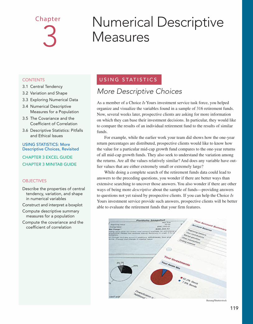
119
Chapter
3Numerical Descriptive Measures
contents
3.1 Central Tendency
3.2 Variation and Shape
3.3 Exploring Numerical Data
3.4 Numerical Descriptive Measures for a Population
3.5 The Covariance and the Coefficient of Correlation
3.6 Descriptive Statistics: Pitfalls and Ethical Issues
Using statistics: More Descriptive choices, Revisited
chapteR 3 excel gUiDe
chapteR 3 Minitab gUiDe
objectives
Describe the properties of central tendency, variation, and shape in numerical variables
Construct and interpret a boxplot
Compute descriptive summary measures for a population
Compute the covariance and the coefficient of correlation
U s i n g s tat i s t i c s
More Descriptive ChoicesAs a member of a Choice Is Yours investment service task force, you helped organize and visualize the variables found in a sample of 316 retirement funds. Now, several weeks later, prospective clients are asking for more information on which they can base their investment decisions. In particular, they would like to compare the results of an individual retirement fund to the results of similar funds.
For example, while the earlier work your team did shows how the one-year return percentages are distributed, prospective clients would like to know how the value for a particular mid-cap growth fund compares to the one-year returns of all mid-cap growth funds. They also seek to understand the variation among the returns. Are all the values relatively similar? And does any variable have out-lier values that are either extremely small or extremely large?
While doing a complete search of the retirement funds data could lead to answers to the preceding questions, you wonder if there are better ways than extensive searching to uncover those answers. You also wonder if there are other ways of being more descriptive about the sample of funds—providing answers to questions not yet raised by prospective clients. If you can help the Choice Is Yours investment service provide such answers, prospective clients will be better able to evaluate the retirement funds that your firm features.
Baranq/Shutterstock
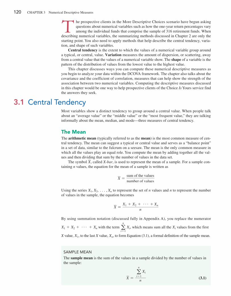
120 ChApTer 3 Numerical Descriptive Measures
T he prospective clients in the More Descriptive Choices scenario have begun asking questions about numerical variables such as how the one-year return percentages vary among the individual funds that comprise the sample of 316 retirement funds. When
describing numerical variables, the summarizing methods discussed in Chapter 2 are only the starting point. You also need to apply methods that help describe the central tendency, varia-tion, and shape of such variables.
Central tendency is the extent to which the values of a numerical variable group around a typical, or central, value. Variation measures the amount of dispersion, or scattering, away from a central value that the values of a numerical variable show. The shape of a variable is the pattern of the distribution of values from the lowest value to the highest value.
This chapter discusses ways you can compute these numerical descriptive measures as you begin to analyze your data within the DCOVA framework. The chapter also talks about the covariance and the coefficient of correlation, measures that can help show the strength of the association between two numerical variables. Computing the descriptive measures discussed in this chapter would be one way to help prospective clients of the Choice Is Yours service find the answers they seek.
Most variables show a distinct tendency to group around a central value. When people talk about an “average value” or the “middle value” or the “most frequent value,” they are talking informally about the mean, median, and mode—three measures of central tendency.
The MeanThe arithmetic mean (typically referred to as the mean) is the most common measure of cen-tral tendency. The mean can suggest a typical or central value and serves as a “balance point” in a set of data, similar to the fulcrum on a seesaw. The mean is the only common measure in which all the values play an equal role. You compute the mean by adding together all the val-ues and then dividing that sum by the number of values in the data set.
The symbol X, called X-bar, is used to represent the mean of a sample. For a sample con-taining n values, the equation for the mean of a sample is written as
X =sum of the values
number of values
Using the series X1, X2, c, Xn to represent the set of n values and n to represent the number of values in the sample, the equation becomes
X =X1 + X2 + g + Xn
n
By using summation notation (discussed fully in Appendix A), you replace the numerator
X1 + X2 + g + Xn with the term an
i= 1 Xi, which means sum all the Xi values from the first
X value, X1, to the last X value, Xn, to form equation (3.1), a formal definition of the sample mean.
3.1 Central Tendency
SaMPlE MEaN
The sample mean is the sum of the values in a sample divided by the number of values in the sample:
X =a
n
i= 1
Xi
n (3.1)
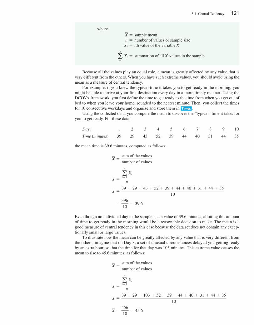
3.1 Central Tendency 121
Because all the values play an equal role, a mean is greatly affected by any value that is very different from the others. When you have such extreme values, you should avoid using the mean as a measure of central tendency.
For example, if you knew the typical time it takes you to get ready in the morning, you might be able to arrive at your first destination every day in a more timely manner. Using the DCOVA framework, you first define the time to get ready as the time from when you get out of bed to when you leave your home, rounded to the nearest minute. Then, you collect the times for 10 consecutive workdays and organize and store them in Times .
Using the collected data, you compute the mean to discover the “typical” time it takes for you to get ready. For these data:
Day: 1 2 3 4 5 6 7 8 9 10
Time (minutes): 39 29 43 52 39 44 40 31 44 35
the mean time is 39.6 minutes, computed as follows:
X =sum of the values
number of values
X =a
n
i= 1 Xi
n
X =39 + 29 + 43 + 52 + 39 + 44 + 40 + 31 + 44 + 35
10
=396
10= 39.6
even though no individual day in the sample had a value of 39.6 minutes, allotting this amount of time to get ready in the morning would be a reasonable decision to make. The mean is a good measure of central tendency in this case because the data set does not contain any excep-tionally small or large values.
To illustrate how the mean can be greatly affected by any value that is very different from the others, imagine that on Day 3, a set of unusual circumstances delayed you getting ready by an extra hour, so that the time for that day was 103 minutes. This extreme value causes the mean to rise to 45.6 minutes, as follows:
X =sum of the values
number of values
X =a
n
i= 1 Xi
n
X =39 + 29 + 103 + 52 + 39 + 44 + 40 + 31 + 44 + 35
10
X =456
10= 45.6
where X = sample mean n = number of values or sample size Xi = ith value of the variable X
an
i=1 Xi = summation of all Xi values in the sample
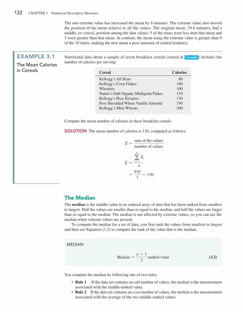
122 ChApTer 3 Numerical Descriptive Measures
The one extreme value has increased the mean by 6 minutes. The extreme value also moved the position of the mean relative to all the values. The original mean, 39.6 minutes, had a middle, or central, position among the data values: 5 of the times were less than that mean and 5 were greater than that mean. In contrast, the mean using the extreme value is greater than 9 of the 10 times, making the new mean a poor measure of central tendency.
The MedianThe median is the middle value in an ordered array of data that has been ranked from smallest to largest. half the values are smaller than or equal to the median, and half the values are larger than or equal to the median. The median is not affected by extreme values, so you can use the median when extreme values are present.
To compute the median for a set of data, you first rank the values from smallest to largest and then use equation (3.2) to compute the rank of the value that is the median.
MEDIaN
Median =n + 1
2 ranked value (3.2)
You compute the median by following one of two rules:
• Rule 1 If the data set contains an odd number of values, the median is the measurement associated with the middle-ranked value.
• Rule 2 If the data set contains an even number of values, the median is the measurement associated with the average of the two middle-ranked values.
ExaMplE 3.1the Mean calories in cereals
Nutritional data about a sample of seven breakfast cereals (stored in Cereals ) includes the number of calories per serving:
Cereal Calories
Kellogg’s All Bran 80Kellogg’s Corn Flakes 100Wheaties 100Nature’s path Organic Multigrain Flakes 110Kellogg’s rice Krispies 130post Shredded Wheat Vanilla Almond 190Kellogg’s Mini Wheats 200
Compute the mean number of calories in these breakfast cereals.
SoluTion The mean number of calories is 130, computed as follows:
X =sum of the values
number of values
X =a
n
i= 1 Xi
n
=910
7= 130
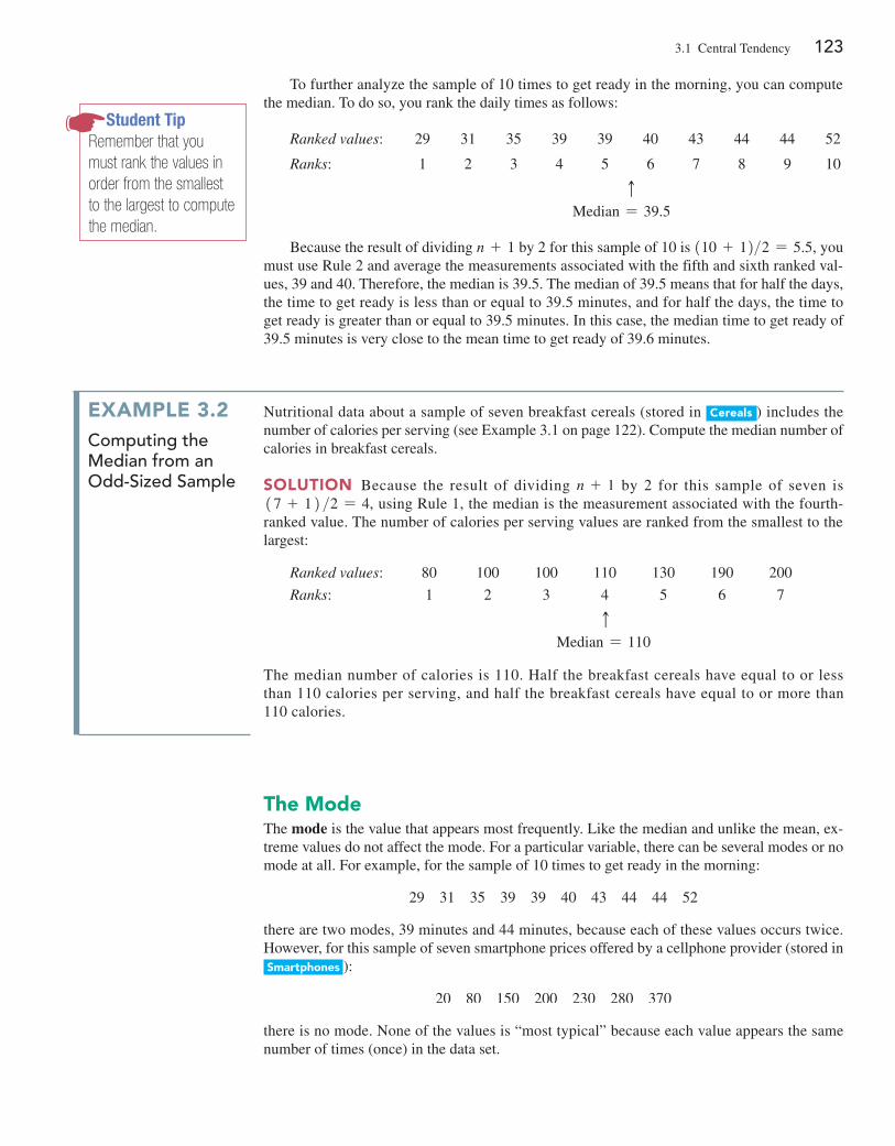
3.1 Central Tendency 123
To further analyze the sample of 10 times to get ready in the morning, you can compute the median. To do so, you rank the daily times as follows:
Ranked values: 29 31 35 39 39 40 43 44 44 52
Ranks: 1 2 3 4 5 6 7 8 9 10
cMedian = 39.5
Because the result of dividing n + 1 by 2 for this sample of 10 is 110 + 12>2 = 5.5, you must use rule 2 and average the measurements associated with the fifth and sixth ranked val-ues, 39 and 40. Therefore, the median is 39.5. The median of 39.5 means that for half the days, the time to get ready is less than or equal to 39.5 minutes, and for half the days, the time to get ready is greater than or equal to 39.5 minutes. In this case, the median time to get ready of 39.5 minutes is very close to the mean time to get ready of 39.6 minutes.
Student TipRemember that you must rank the values in order from the smallest to the largest to compute the median.
The ModeThe mode is the value that appears most frequently. Like the median and unlike the mean, ex-treme values do not affect the mode. For a particular variable, there can be several modes or no mode at all. For example, for the sample of 10 times to get ready in the morning:
29 31 35 39 39 40 43 44 44 52
there are two modes, 39 minutes and 44 minutes, because each of these values occurs twice. however, for this sample of seven smartphone prices offered by a cellphone provider (stored in Smartphones ):
20 80 150 200 230 280 370
there is no mode. None of the values is “most typical” because each value appears the same number of times (once) in the data set.
ExaMplE 3.2computing the Median from an Odd-sized sample
Nutritional data about a sample of seven breakfast cereals (stored in Cereals ) includes the number of calories per serving (see example 3.1 on page 122). Compute the median number of calories in breakfast cereals.
SoluTion Because the result of dividing n + 1 by 2 for this sample of seven is 17 + 12 >2 = 4, using rule 1, the median is the measurement associated with the fourth-ranked value. The number of calories per serving values are ranked from the smallest to the largest:
Ranked values: 80 100 100 110 130 190 200
Ranks: 1 2 3 4 5 6 7
cMedian = 110
The median number of calories is 110. half the breakfast cereals have equal to or less than 110 calories per serving, and half the breakfast cereals have equal to or more than 110 calories.
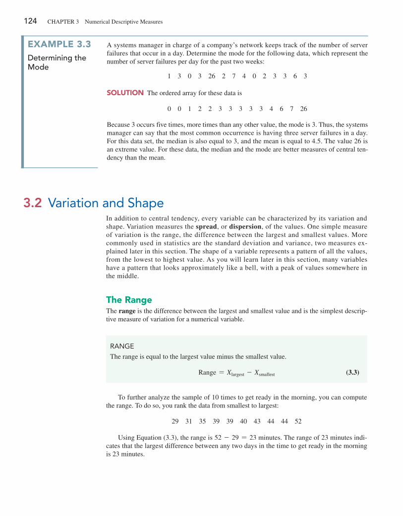
124 ChApTer 3 Numerical Descriptive Measures
3.2 Variation and ShapeIn addition to central tendency, every variable can be characterized by its variation and shape. Variation measures the spread, or dispersion, of the values. One simple measure of variation is the range, the difference between the largest and smallest values. More commonly used in statistics are the standard deviation and variance, two measures ex-plained later in this section. The shape of a variable represents a pattern of all the values, from the lowest to highest value. As you will learn later in this section, many variables have a pattern that looks approximately like a bell, with a peak of values somewhere in the middle.
The RangeThe range is the difference between the largest and smallest value and is the simplest descrip-tive measure of variation for a numerical variable.
RaNgE
The range is equal to the largest value minus the smallest value.
range = Xlargest - Xsmallest (3.3)
To further analyze the sample of 10 times to get ready in the morning, you can compute the range. To do so, you rank the data from smallest to largest:
29 31 35 39 39 40 43 44 44 52
Using equation (3.3), the range is 52 - 29 = 23 minutes. The range of 23 minutes indi-cates that the largest difference between any two days in the time to get ready in the morning is 23 minutes.
SoluTion The ordered array for these data is
0 0 1 2 2 3 3 3 3 3 4 6 7 26
Because 3 occurs five times, more times than any other value, the mode is 3. Thus, the systems manager can say that the most common occurrence is having three server failures in a day. For this data set, the median is also equal to 3, and the mean is equal to 4.5. The value 26 is an extreme value. For these data, the median and the mode are better measures of central ten-dency than the mean.
ExaMplE 3.3Determining the Mode
A systems manager in charge of a company’s network keeps track of the number of server failures that occur in a day. Determine the mode for the following data, which represent the number of server failures per day for the past two weeks:
1 3 0 3 26 2 7 4 0 2 3 3 6 3
3.2 Variation and Shape 125
ExaMplE 3.4computing the Range in the calories in cereals
Nutritional data about a sample of seven breakfast cereals (stored in Cereals ) includes the number of calories per serving (see example 3.1 on page 122). Compute the range of the num-ber of calories for the cereals.
SoluTion ranked from smallest to largest, the calories for the seven cereals are
80 100 100 110 130 190 200
Therefore, using equation (3.3), the range = 200 - 80 = 120. The largest difference in the number of calories between any two cereals is 120.
The range measures the total spread in the set of data. Although the range is a simple measure of the total variation of the variable, it does not take into account how the values are distributed between the smallest and largest values. In other words, the range does not indicate whether the values are evenly distributed, clustered near the middle, or clustered near one or both extremes. Thus, using the range as a measure of variation when at least one value is an extreme value is misleading.
The Variance and the Standard DeviationBeing a simple measure of variation, the range does not consider how the values distribute or cluster between the extremes. Two commonly used measures of variation that account for how all the values are distributed are the variance and the standard deviation. These statistics measure the “average” scatter around the mean—how larger values fluctuate above it and how smaller values fluctuate below it.
A simple measure of variation around the mean might take the difference between each value and the mean and then sum these differences. however, if you did that, you would find that these differences sum to zero because the mean is the balance point for every numerical variable. A measure of variation that differs from one data set to another squares the difference between each value and the mean and then sums these squared differences. The sum of these squared differences, known as the sum of squares (SS), is then used to compute the sample variance 1S22 and the sample standard deviation (S ).
The sample variance (S2 ) is the sum of squares divided by the sample size minus 1. The sample standard deviation (S) is the square root of the sample variance. Because this sum of squares will always be nonnegative according to the rules of algebra, nei-ther the variance nor the standard deviation can ever be negative. For virtually all vari-ables, the variance and standard deviation will be a positive value. Both of these statistics will be zero only if every value in the sample is the same value (i.e., the values show no variation).
For a sample containing n values, X1, X2, X3, c, Xn, the sample variance 1S22 is
S2 =1X1 - X22 + 1X2 - X22 + g + 1Xn - X22
n - 1
equations (3.4) and (3.5) define the sample variance and sample standard deviation using
summation notation. The term an
i= 11Xi - X22 represents the sum of squares.
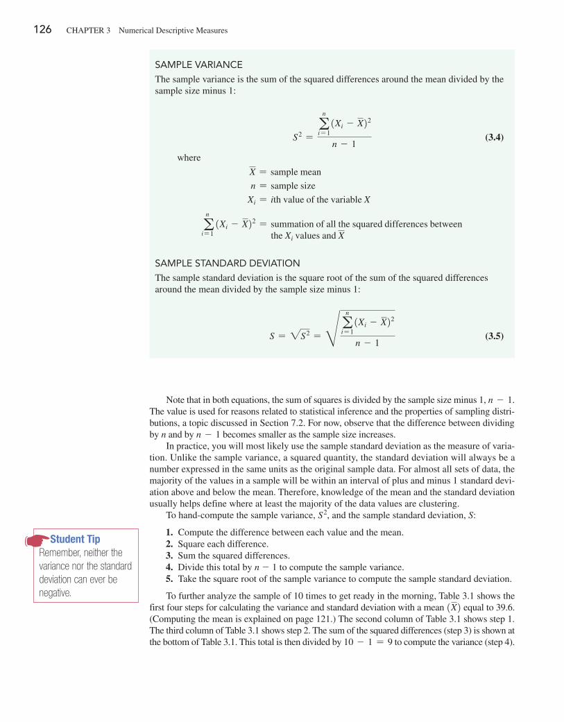
126 ChApTer 3 Numerical Descriptive Measures
Note that in both equations, the sum of squares is divided by the sample size minus 1, n - 1. The value is used for reasons related to statistical inference and the properties of sampling distri-butions, a topic discussed in Section 7.2. For now, observe that the difference between dividing by n and by n - 1 becomes smaller as the sample size increases.
In practice, you will most likely use the sample standard deviation as the measure of varia-tion. Unlike the sample variance, a squared quantity, the standard deviation will always be a number expressed in the same units as the original sample data. For almost all sets of data, the majority of the values in a sample will be within an interval of plus and minus 1 standard devi-ation above and below the mean. Therefore, knowledge of the mean and the standard deviation usually helps define where at least the majority of the data values are clustering.
To hand-compute the sample variance, S2, and the sample standard deviation, S:
1. Compute the difference between each value and the mean. 2. Square each difference. 3. Sum the squared differences. 4. Divide this total by n - 1 to compute the sample variance. 5. Take the square root of the sample variance to compute the sample standard deviation.
To further analyze the sample of 10 times to get ready in the morning, Table 3.1 shows the first four steps for calculating the variance and standard deviation with a mean 1X2 equal to 39.6. (Computing the mean is explained on page 121.) The second column of Table 3.1 shows step 1. The third column of Table 3.1 shows step 2. The sum of the squared differences (step 3) is shown at the bottom of Table 3.1. This total is then divided by 10 - 1 = 9 to compute the variance (step 4).
SaMPlE VaRIaNCE
The sample variance is the sum of the squared differences around the mean divided by the sample size minus 1:
S2 =a
n
i= 11Xi - X22
n - 1 (3.4)
where
X = sample mean
n = sample size
Xi = ith value of the variable X
an
i= 11Xi - X22 = summation of all the squared differences between
the Xi values and X
SaMPlE STaNDaRD DEVIaTIoN
The sample standard deviation is the square root of the sum of the squared differences around the mean divided by the sample size minus 1:
S = 2S2 = H an
i= 11Xi - X22
n - 1 (3.5)
Student TipRemember, neither the variance nor the standard deviation can ever be negative.
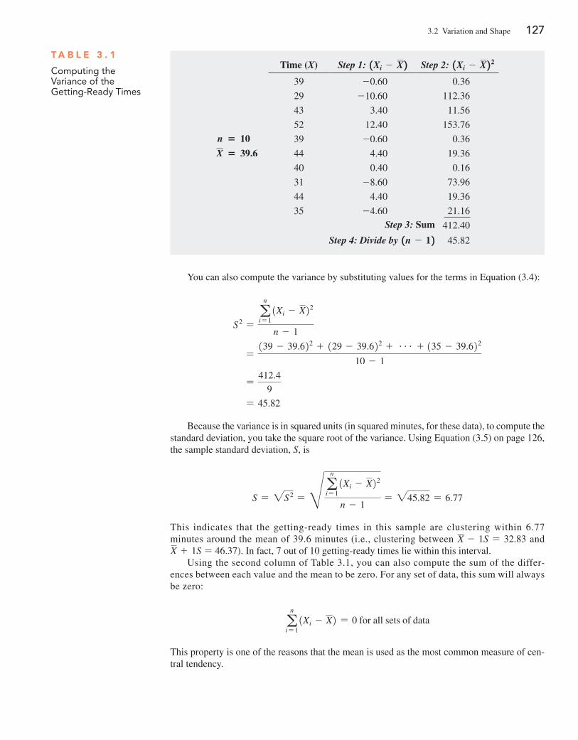
3.2 Variation and Shape 127
You can also compute the variance by substituting values for the terms in equation (3.4):
S2 =a
n
i= 11Xi - X22
n - 1
=139 - 39.622 + 129 - 39.622 + g + 135 - 39.622
10 - 1
=412.4
9
= 45.82
Because the variance is in squared units (in squared minutes, for these data), to compute the standard deviation, you take the square root of the variance. Using equation (3.5) on page 126, the sample standard deviation, S, is
S = 2S2 = H an
i= 11Xi - X22
n - 1= 245.82 = 6.77
This indicates that the getting-ready times in this sample are clustering within 6.77 minutes around the mean of 39.6 minutes (i.e., clustering between X - 1S = 32.83 and X + 1S = 46.37). In fact, 7 out of 10 getting-ready times lie within this interval.
Using the second column of Table 3.1, you can also compute the sum of the differ-ences between each value and the mean to be zero. For any set of data, this sum will always be zero:
an
i= 11Xi - X2 = 0 for all sets of data
This property is one of the reasons that the mean is used as the most common measure of cen-tral tendency.
T a b l E 3 . 1
Computing the Variance of the getting-Ready Times
Time (X) Step 1: 1Xi - X 2 Step 2: 1Xi - X 22
n = 10
X = 39.6
39 -0.60 0.36
29 -10.60 112.36
43 3.40 11.56
52 12.40 153.76
39 -0.60 0.36
44 4.40 19.36
40 0.40 0.16
31 -8.60 73.96
44 4.40 19.36
35 -4.60 21.16
412.40
45.82
Step 3: Sum
Step 4: Divide by 1n - 1 2
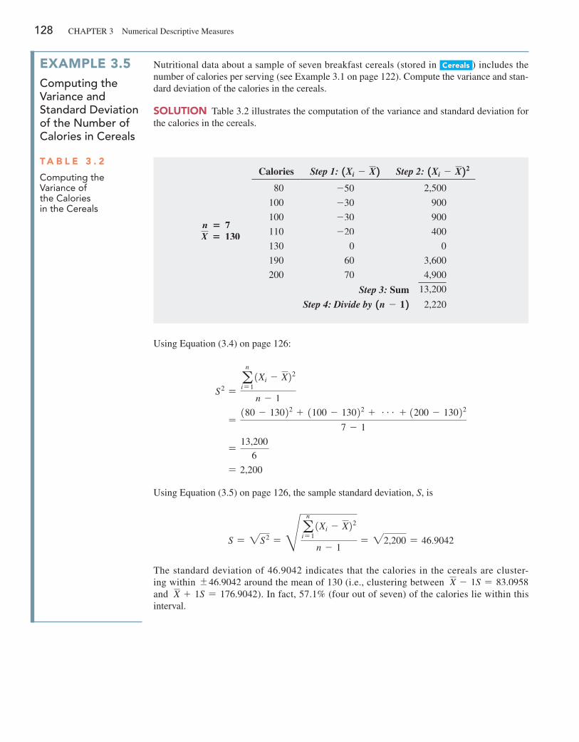
128 ChApTer 3 Numerical Descriptive Measures
ExaMplE 3.5computing the Variance and standard Deviation of the number of calories in cereals
Nutritional data about a sample of seven breakfast cereals (stored in Cereals ) includes the number of calories per serving (see example 3.1 on page 122). Compute the variance and stan-dard deviation of the calories in the cereals.
SoluTion Table 3.2 illustrates the computation of the variance and standard deviation for the calories in the cereals.
T a b l E 3 . 2
Computing the Variance of the Calories in the Cereals
Calories Step 1: 1Xi - X 2 Step 2: 1Xi - X 22
n = 7X = 130
80 -50 2,500
100 -30 900
100 -30 900
110 -20 400
130 0 0
190 60 3,600
200 70 4,900
13,200
2,220
Using equation (3.4) on page 126:
S2 =a
n
i= 11Xi - X22
n - 1
=180 - 13022 + 1100 - 13022 + g + 1200 - 13022
7 - 1
=13,200
6
= 2,200
Using equation (3.5) on page 126, the sample standard deviation, S, is
S = 2S2 = H an
i= 11Xi - X22
n - 1= 22,200 = 46.9042
The standard deviation of 46.9042 indicates that the calories in the cereals are cluster-ing within {46.9042 around the mean of 130 (i.e., clustering between X - 1S = 83.0958 and X + 1S = 176.9042). In fact, 57.1% (four out of seven) of the calories lie within this interval.
Step 4: Divide by 1n - 1 2Step 3: Sum
3.2 Variation and Shape 129
The Coefficient of VariationThe coefficient of variation is equal to the standard deviation divided by the mean, multiplied by 100%. Unlike the measures of variation presented previously, the coefficient of variation (CV ) measures the scatter in the data relative to the mean. The coefficient of variation is a relative measure of variation that is always expressed as a percentage rather than in terms of the units of the particular data. equation (3.6) defines the coefficient of variation.
Student TipThe coefficient of varia-tion is always expressed as a percentage, not in the units of the variables.
CoEffICIENT of VaRIaTIoN
The coefficient of variation is equal to the standard deviation divided by the mean, multiplied by 100%.
CV = a S
Xb100% (3.6)
where
S = sample standard deviation
X = sample mean
For the sample of 10 getting-ready times, because X = 39.6 and S = 6.77, the coefficient of variation is
CV = a S
Xb100% = a 6.77
39.6b100% = 17.10%
For the getting-ready times, the standard deviation is 17.1% of the size of the mean.The coefficient of variation is especially useful when comparing two or more sets of data
that are measured in different units, as example 3.6 illustrates.
Learn MoreThe Sharpe ratio, another relative measure of variation, is often used in financial analysis. Read the Short Takes for Chapter 3 to learn more about this ratio.
ExaMplE 3.6comparing two coefficients of Variation When the two Variables have Different Units of Measurement
Which varies more from cereal to cereal—the number of calories or the amount of sugar (in grams)?
SoluTion Because calories and the amount of sugar have different units of measurement, you need to compare the relative variability in the two measurements.
For calories, using the mean and variance computed in examples 3.1 and 3.5 on pages 122 and 128, the coefficient of variation is
CVCalories = a46.9042
130b100% = 36.08%
For the amount of sugar in grams, the values for the seven cereals are
6 2 4 4 4 11 10
For these data, X = 5.8571 and S = 3.3877. Therefore, the coefficient of variation is
CVSugar = a3.3877
5.8571b100% = 57.84%
You conclude that relative to the mean, the amount of sugar is much more variable than the calories.
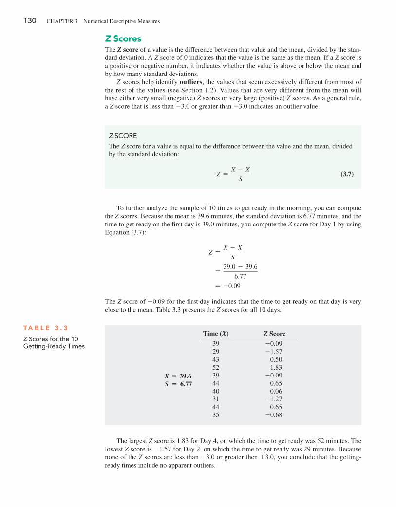
130 ChApTer 3 Numerical Descriptive Measures
Z ScoresThe Z score of a value is the difference between that value and the mean, divided by the stan-dard deviation. A Z score of 0 indicates that the value is the same as the mean. If a Z score is a positive or negative number, it indicates whether the value is above or below the mean and by how many standard deviations.
Z scores help identify outliers, the values that seem excessively different from most of the rest of the values (see Section 1.2). Values that are very different from the mean will have either very small (negative) Z scores or very large (positive) Z scores. As a general rule, a Z score that is less than -3.0 or greater than +3.0 indicates an outlier value.
Z SCoRE
The Z score for a value is equal to the difference between the value and the mean, divided by the standard deviation:
Z =X - X
S (3.7)
To further analyze the sample of 10 times to get ready in the morning, you can compute the Z scores. Because the mean is 39.6 minutes, the standard deviation is 6.77 minutes, and the time to get ready on the first day is 39.0 minutes, you compute the Z score for Day 1 by using equation (3.7):
Z =X - X
S
=39.0 - 39.6
6.77
= -0.09
The Z score of -0.09 for the first day indicates that the time to get ready on that day is very close to the mean. Table 3.3 presents the Z scores for all 10 days.
The largest Z score is 1.83 for Day 4, on which the time to get ready was 52 minutes. The lowest Z score is -1.57 for Day 2, on which the time to get ready was 29 minutes. Because none of the Z scores are less than -3.0 or greater then +3.0, you conclude that the getting-ready times include no apparent outliers.
T a b l E 3 . 3
Z Scores for the 10 getting-Ready Times
Time (X) Z Score
X = 39.6 S = 6.77
39 -0.0929 -1.5743 0.5052 1.8339 -0.0944 0.6540 0.0631 -1.2744 0.6535 -0.68
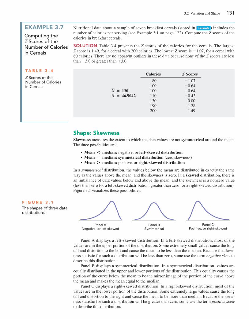
3.2 Variation and Shape 131
Shape: SkewnessSkewness measures the extent to which the data values are not symmetrical around the mean.The three possibilities are:
• Mean * median: negative, or left-skewed distribution • Mean = median: symmetrical distribution (zero skewness) • Mean + median: positive, or right-skewed distribution
In a symmetrical distribution, the values below the mean are distributed in exactly the same way as the values above the mean, and the skewness is zero. In a skewed distribution, there is an imbalance of data values below and above the mean, and the skewness is a nonzero value (less than zero for a left-skewed distribution, greater than zero for a right-skewed distribution). Figure 3.1 visualizes these possibilities.
ExaMplE 3.7computing the Z scores of the number of calories in cereals
Nutritional data about a sample of seven breakfast cereals (stored in Cereals ) includes the number of calories per serving (see example 3.1 on page 122). Compute the Z scores of the calories in breakfast cereals.
SoluTion Table 3.4 presents the Z scores of the calories for the cereals. The largest Z score is 1.49, for a cereal with 200 calories. The lowest Z score is -1.07, for a cereal with 80 calories. There are no apparent outliers in these data because none of the Z scores are less than -3.0 or greater than +3.0.
T a b l E 3 . 4
Z Scores of the Number of Calories in Cereals
Calories Z Scores
X = 130S = 46.9042
80 -1.07100 -0.64100 -0.64110 -0.43130 0.00190 1.28200 1.49
Panel ANegative, or left-skewed
Panel BSymmetrical
Panel CPositive, or right-skewed
F i g u R E 3 . 1The shapes of three data distributions
panel A displays a left-skewed distribution. In a left-skewed distribution, most of the values are in the upper portion of the distribution. Some extremely small values cause the long tail and distortion to the left and cause the mean to be less than the median. Because the skew-ness statistic for such a distribution will be less than zero, some use the term negative skew to describe this distribution.
panel B displays a symmetrical distribution. In a symmetrical distribution, values are equally distributed in the upper and lower portions of the distribution. This equality causes the portion of the curve below the mean to be the mirror image of the portion of the curve above the mean and makes the mean equal to the median.
panel C displays a right-skewed distribution. In a right-skewed distribution, most of the values are in the lower portion of the distribution. Some extremely large values cause the long tail and distortion to the right and cause the mean to be more than median. Because the skew-ness statistic for such a distribution will be greater than zero, some use the term positive skew to describe this distribution.
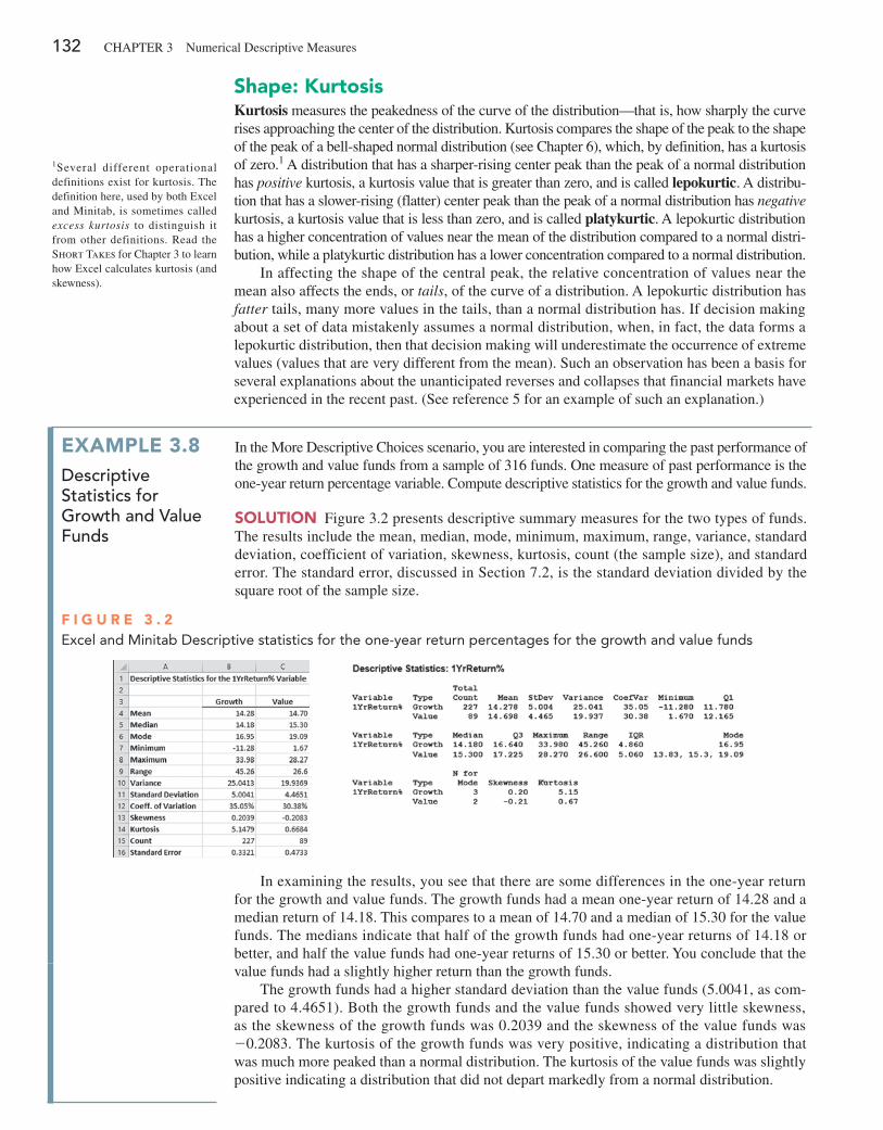
132 ChApTer 3 Numerical Descriptive Measures
1Several different operational definitions exist for kurtosis. The definition here, used by both excel and Minitab, is sometimes called excess kurtosis to distinguish it from other definitions. read the Short Takes for Chapter 3 to learn how excel calculates kurtosis (and skewness).
Shape: KurtosisKurtosis measures the peakedness of the curve of the distribution—that is, how sharply the curve rises approaching the center of the distribution. Kurtosis compares the shape of the peak to the shape of the peak of a bell-shaped normal distribution (see Chapter 6), which, by definition, has a kurtosis of zero.1 A distribution that has a sharper-rising center peak than the peak of a normal distribution has positive kurtosis, a kurtosis value that is greater than zero, and is called lepokurtic. A distribu-tion that has a slower-rising (flatter) center peak than the peak of a normal distribution has negative kurtosis, a kurtosis value that is less than zero, and is called platykurtic. A lepokurtic distribution has a higher concentration of values near the mean of the distribution compared to a normal distri-bution, while a platykurtic distribution has a lower concentration compared to a normal distribution.
In affecting the shape of the central peak, the relative concentration of values near the mean also affects the ends, or tails, of the curve of a distribution. A lepokurtic distribution has fatter tails, many more values in the tails, than a normal distribution has. If decision making about a set of data mistakenly assumes a normal distribution, when, in fact, the data forms a lepokurtic distribution, then that decision making will underestimate the occurrence of extreme values (values that are very different from the mean). Such an observation has been a basis for several explanations about the unanticipated reverses and collapses that financial markets have experienced in the recent past. (See reference 5 for an example of such an explanation.)
ExaMplE 3.8Descriptive statistics for growth and Value Funds
In the More Descriptive Choices scenario, you are interested in comparing the past performance of the growth and value funds from a sample of 316 funds. One measure of past performance is the one-year return percentage variable. Compute descriptive statistics for the growth and value funds.
SoluTion Figure 3.2 presents descriptive summary measures for the two types of funds. The results include the mean, median, mode, minimum, maximum, range, variance, standard deviation, coefficient of variation, skewness, kurtosis, count (the sample size), and standard error. The standard error, discussed in Section 7.2, is the standard deviation divided by the square root of the sample size.
F i g u R E 3 . 2Excel and Minitab Descriptive statistics for the one-year return percentages for the growth and value funds
In examining the results, you see that there are some differences in the one-year return for the growth and value funds. The growth funds had a mean one-year return of 14.28 and a median return of 14.18. This compares to a mean of 14.70 and a median of 15.30 for the value funds. The medians indicate that half of the growth funds had one-year returns of 14.18 or better, and half the value funds had one-year returns of 15.30 or better. You conclude that the value funds had a slightly higher return than the growth funds.
The growth funds had a higher standard deviation than the value funds (5.0041, as com-pared to 4.4651). Both the growth funds and the value funds showed very little skewness, as the skewness of the growth funds was 0.2039 and the skewness of the value funds was -0.2083. The kurtosis of the growth funds was very positive, indicating a distribution that was much more peaked than a normal distribution. The kurtosis of the value funds was slightly positive indicating a distribution that did not depart markedly from a normal distribution.
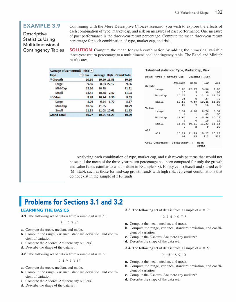
3.2 Variation and Shape 133
ExaMplE 3.9Descriptive statistics Using Multidimensional contingency tables
Continuing with the More Descriptive Choices scenario, you wish to explore the effects of each combination of type, market cap, and risk on measures of past performance. One measure of past performance is the three-year return percentage. Compute the mean three-year return percentage for each combination of type, market cap, and risk.
SoluTion Compute the mean for each combination by adding the numerical variable three-year return percentage to a multidimensional contingency table. The excel and Minitab results are:
Analyzing each combination of type, market cap, and risk reveals patterns that would not be seen if the mean of the three-year return percentage had been computed for only the growth and value funds (similar to what is done in example 3.8). empty cells (excel) and starred cells (Minitab), such as those for mid-cap growth funds with high risk, represent combinations that do not exist in the sample of 316 funds.
problems for Sections 3.1 and 3.2lEaRning ThE baSiCS3.1 The following set of data is from a sample of n = 5:
3 1 2 7 10
a. Compute the mean, median, and mode.b. Compute the range, variance, standard deviation, and coeffi-
cient of variation.c. Compute the Z scores. Are there any outliers?d. Describe the shape of the data set.
3.2 The following set of data is from a sample of n = 6:
7 4 9 7 3 12
a. Compute the mean, median, and mode.b. Compute the range, variance, standard deviation, and coeffi-
cient of variation.c. Compute the Z scores. Are there any outliers?d. Describe the shape of the data set.
3.3 The following set of data is from a sample of n = 7:
12 7 4 9 0 7 3
a. Compute the mean, median, and mode.b. Compute the range, variance, standard deviation, and coeffi-
cient of variation.c. Compute the Z scores. Are there any outliers?d. Describe the shape of the data set.
3.4 The following set of data is from a sample of n = 5:
9 -5 -8 9 10
a. Compute the mean, median, and mode.b. Compute the range, variance, standard deviation, and coeffi-
cient of variation.c. Compute the Z scores. Are there any outliers?d. Describe the shape of the data set.
134 ChApTer 3 Numerical Descriptive Measures
applying ThE ConCEpTS3.5 The results of a survey report on the salaries of professors teaching statistics in research universities with four or five years in the rank of associate professor and professor are shown in the following table.
Title Median
Associate professor $82,400professor $108,600
Interpret the median salary for the associate professors and professors.
3.6 The operations manager of a plant that manufactures tires wants to compare the actual inner diameters of two grades of tires, each of which is expected to be 575 millimeters. A sample of five tires of each grade was selected, and the results representing the inner diam-eters of the tires, ranked from smallest to largest, are as follows:
Grade X Grade Y
568 570 575 578 584 573 574 575 577 578
a. For each of the two grades of tires, compute the mean, median, and standard deviation.
b. Which grade of tire is providing better quality? explain.c. What would be the effect on your answers in (a) and (b) if the
last value for grade Y was 588 instead of 578? explain.
3.7 According to the U.S. Census Bureau (census.gov), in 2013, the median sales price of new houses was $265,900 and the mean sales price was $322,100.a. Interpret the median sales price.b. Interpret the mean sales price.c. Discuss the shape of the distribution of the price of new houses.
SELF Test
3.8 The file Mobileloyalty contains spending on products ($) during a three-month period by a sample
of 15 customers receiving incentives through a mobile loyalty program.
55.35 22.90 67.50 46.10 57.45 108.25 50.75 35.2078.30 50.65 63.00 59.70 41.55 56.65 52.60
a. Compute the mean and median.b. Compute the variance, standard deviation, range, and coeffi-
cient of variation.c. Are the data skewed? If so, how?d. Based on the results of (a) through (c), what conclusions can you
reach concerning spending on products by customers receiving incentives through a mobile loyalty program?
3.9 The file Sedans contains the overall miles per gallon (MpG) of 2014 midsized sedans:
38 26 30 26 25 27 24 22 27 32 3926 24 24 23 24 25 31 26 37 22 33
Source: Data extracted from “Which Car Is right for You,” Consumer Reports, April 2014, pp. 40–41.
a. Compute the mean, median, and mode.b. Compute the variance, standard deviation, range, coefficient of
variation, and Z scores.c. Are the data skewed? If so, how?d. Compare the results of (a) through (c) to those of problem 3.10
(a) through (c) that refer to the miles per gallon of small SUVs.
3.10 The file SuV contains the overall miles per gallon (MpG) of 2014 small SUVs:
26 22 23 21 25 24 22 26 25 2221 21 22 22 23 24 23 22 21 22
Source: Data extracted from “Which Car Is right for You,” Consumer Reports, April 2014, pp. 60–61.
a. Compute the mean, median, and mode.b. Compute the variance, standard deviation, range, coefficient of
variation, and Z scores.c. Are the data skewed? If so, how?d. Compare the results of (a) through (c) to those of problem 3.9
(a) through (c) that refer to the MpG of midsized sedans.
3.11 The file accountingpartners contains the number of partners in a cohort of rising accounting firms that have been tagged as “firms to watch.” The firms have the following numbers of partners:
17 23 19 23 18 17 23 16 34 10 14 30 14 33 26 17 19 2220 27 33 25 12 26 13 30 13 13 33 21 17 12 10 14 12
Source: Data extracted from bit.ly/ODuzd3.
a. Compute the mean, median, and mode.b. Compute the variance, standard deviation, range, coefficient of
variation, and Z scores. Are there any outliers? explain.c. Are the data skewed? If so, how?d. Based on the results of (a) through (c), what conclusions can
you reach concerning the number of partners in rising account-ing firms?
3.12 The file Marketpenetration contains Facebook penetration values (the percentage of the country population who are Face-book users) for 22 of the world’s largest economies:
56 57 43 55 42 35 7 25 42 17 43 6 31 28 59 20 27 36 45 80 57 56
Source: Data extracted from slidesha.re/ODv6vG.
a. Compute the mean, median, and mode.b. Compute the variance, standard deviation, range, coefficient of
variation, and Z scores. Are there any outliers? explain.c. Are the data skewed? If so, how?d. Based on the results of (a) through (c), what conclusions can
you reach concerning Facebook’s market penetration?
3.13 Is there a difference in the variation of the yields of differ-ent types of investments? The file CD Rate contains the yields for one-year certificates of deposit (CDs) and five-year CDs for 22 banks in the United States, as of March 12, 2014.
Source: Data extracted from www.Bankrate.com, March 12, 2014.
a. For one-year and five-year CDs, separately compute the vari-ance, standard deviation, range, and coefficient of variation.
b. Based on the results of (a), do one-year CDs or five-year CDs have more variation in the yields offered? explain.
3.3 exploring Numerical Data 135
3.14 The file hotelaway contains the average room price (in US$) paid by various nationalities while traveling abroad (away from their home country) in 2013:
179 173 175 173 164 143 153 155
Source: Data extracted from http://bit.ly/1pdFkOG.
a. Compute the mean, median, and mode.b. Compute the range, variance, and standard deviation.c. Based on the results of (a) and (b), what conclusions can you
reach concerning the room price (in US$) in 2013?
3.15 A bank branch located in a commercial district of a city has the business objective of developing an improved process for serving customers during the noon-to-1:00 p.m. lunch period. The waiting time, in minutes, is defined as the time the customer enters the line to when he or she reaches the teller window. Data collected from a sample of 15 customers during this hour are stored in bank1 :
4.21 5.55 3.02 5.13 4.77 2.34 3.54 3.204.50 6.10 0.38 5.12 6.46 6.19 3.79
a. Compute the mean and median.b. Compute the variance, standard deviation, range, coefficient of
variation, and Z scores. Are there any outliers? explain.c. Are the data skewed? If so, how?d. As a customer walks into the branch office during the lunch
hour, she asks the branch manager how long she can expect to wait. The branch manager replies, “Almost certainly less than five minutes.” On the basis of the results of (a) through (c), evaluate the accuracy of this statement.
3.16 Suppose that another bank branch, located in a residential area, is also concerned with the noon-to-1:00 p.m. lunch hour. The waiting time, in minutes, collected from a sample of 15 customers during this hour, are stored in bank2 :
9.66 5.90 8.02 5.79 8.73 3.82 8.01 8.3510.49 6.68 5.64 4.08 6.17 9.91 5.47
a. Compute the mean and median.b. Compute the variance, standard deviation, range, coefficient of
variation, and Z scores. Are there any outliers? explain.c. Are the data skewed? If so, how?d. As a customer walks into the branch office during the lunch
hour, he asks the branch manager how long he can expect to
wait. The branch manager replies, “Almost certainly less than five minutes.” On the basis of the results of (a) through (c), evaluate the accuracy of this statement.
3.17 Using the one-year return percentage variable in Retirement Funds :a. Construct a table that computes the mean for each combination
of type, market cap, and risk.b. Construct a table that computes the standard deviation for each
combination of type, market cap, and risk.c. What conclusions can you reach concerning differences among
the types of retirement funds (growth and value), based on mar-ket cap (small, mid-cap, and large) and the risk (low, average, and high)?
3.18 Using the one-year return percentage variable in Retirement Funds :a. Construct a table that computes the mean for each combination
of type, market cap, and rating.b. Construct a table that computes the standard deviation for each
combination of type, market cap, and rating.c. What conclusions can you reach concerning differences among
the types of retirement funds (growth and value), based on mar-ket cap (small, mid-cap, and large) and the rating (one, two, three, four, and five)?
3.19 Using the one-year return percentage variable in Retirement Funds :a. Construct a table that computes the mean for each combination
of market cap, risk, and rating.b. Construct a table that computes the standard deviation for each
combination of market cap, risk, and rating.c. What conclusions can you reach concerning differences based
on the market cap (small, mid-cap, and large), risk (low, aver-age, and high), and rating (one, two, three, four, and five)?
3.20 Using the one-year return percentage variable in Retirement Funds :a. Construct a table that computes the mean for each combination
of type, risk, and rating.b. Construct a table that computes the standard deviation for each
combination of type, risk, and rating.c. What conclusions can you reach concerning differences among
the types of retirement funds (growth and value), based on the risk (low, average, and high) and the rating (one, two, three, four, and five)?
3.3 Exploring Numerical DataSections 3.1 and 3.2 discuss measures of central tendency, variation, and shape. You can also visualize the distribution of the values for a numerical variable by computing the quartiles and the five-number summary and constructing a boxplot.
QuartilesQuartiles split the values into four equal parts—the first quartile 1Q1 2 divides the smallest 25.0% of the values from the other 75.0% that are larger. The second quartile 1Q2 2 is the median; 50.0% of the values are smaller than or equal to the median, and 50.0% are larger than or equal to the median. The third quartile 1Q3 2 divides the smallest 75.0% of the values from the largest 25.0%. equations (3.8) and (3.9) define the first and third quartiles.
136 ChApTer 3 Numerical Descriptive Measures
fIRST QuaRTIlE, Q1
25.0% of the values are smaller than or equal to Q1, the first quartile, and 75.0% are larger than or equal to the first quartile, Q1:
Q1 =n + 1
4 ranked value (3.8)
ThIRD QuaRTIlE, Q3
75.0% of the values are smaller than or equal to the third quartile, Q3, and 25.0% are larger than or equal to the third quartile, Q3:
Q3 =31n + 12
4 ranked value (3.9)
Student TipThe methods of this sec-tion are commonly used in exploratory data analysis.
Student TipAs is the case when you compute the median, you must rank the values in order from smallest to largest before computing the quartiles.
Use the following rules to compute the quartiles from a set of ranked values:
• Rule 1 If the ranked value is a whole number, the quartile is equal to the measure-ment that corresponds to that ranked value. For example, if the sample size n = 7, the first quartile, Q1, is equal to the measurement associated with the 17 + 12>4 = second ranked value.
• Rule 2 If the ranked value is a fractional half (2.5, 4.5, etc.), the quartile is equal to the measurement that corresponds to the average of the measurements corresponding to the two ranked values involved. For example, if the sample size n = 9, the first quartile, Q1, is equal to the 19 + 12>4 = 2.5 ranked value, halfway between the sec-ond ranked value and the third ranked value.
• Rule 3 If the ranked value is neither a whole number nor a fractional half, you round the result to the nearest integer and select the measurement corresponding to that ranked value. For example, if the sample size n = 10, the first quartile, Q1, is equal to the 110 + 12>4 = 2.75 ranked value. round 2.75 to 3 and use the third ranked value.
To further analyze the sample of 10 times to get ready in the morning, you can compute the quartiles. To do so, you rank the data from smallest to largest:
Ranked values: 29 31 35 39 39 40 43 44 44 52
Ranks: 1 2 3 4 5 6 7 8 9 10
The first quartile is the 1n + 12>4 = 110 + 12>4 = 2.75 ranked value. Using rule 3, you round up to the third ranked value. The third ranked value for the getting-ready data is 35 minutes. You interpret the first quartile of 35 to mean that on 25% of the days, the time to get ready is less than or equal to 35 minutes, and on 75% of the days, the time to get ready is greater than or equal to 35 minutes.
The third quartile is the 31n + 12>4 = 3110 + 12>4 = 8.25 ranked value. Using rule 3 for quartiles, you round this down to the eighth ranked value. The eighth ranked value is 44 minutes. Thus, on 75% of the days, the time to get ready is less than or equal to 44 minutes, and on 25% of the days, the time to get ready is greater than or equal to 44 minutes.
percentiles related to quartiles are percentiles that split a variable into 100 equal parts. By this definition, the first quartile is equivalent to the 25th percentile, the second quartile to the 50th percentile, and the third quartile to the 75th percentile. Learn more about percentiles in the Short Takes for Chapter 3.
3.3 exploring Numerical Data 137
ExaMplE 3.10computing the Quartiles
Nutritional data about a sample of seven breakfast cereals (stored in Cereals ) includes the number of calories per serving (see example 3.1 on page 122). Compute the first quartile 1Q12 and third quartile 1Q32 of the number of calories for the cereals.
SoluTion ranked from smallest to largest, the numbers of calories for the seven cereals are as follows:
Ranked values: 80 100 100 110 130 190 200
Ranks: 1 2 3 4 5 6 7
For these data
Q1 =1n + 12
4 ranked value
=7 + 1
4 ranked value = 2nd ranked value
Therefore, using rule 1, Q1 is the second ranked value. Because the second ranked value is 100, the first quartile, Q1, is 100.
To compute the third quartile, Q3,
Q3 =31n + 12
4 ranked value
=317 + 12
4 ranked value = 6th ranked value
Therefore, using rule 1, Q3 is the sixth ranked value. Because the sixth ranked value is 190, Q3 is 190.
The first quartile of 100 indicates that 25% of the cereals contain 100 calories or fewer per serving and 75% contain 100 or more calories. The third quartile of 190 indicates that 75% of the cereals contain 190 calories or fewer per serving and 25% contain 190 or more calories.
The interquartile RangeThe interquartile range (also called the midspread) measures the difference in the center of a distribution between the third and first quartiles.
INTERQuaRTIlE RaNgE
The interquartile range is the difference between the third quartile and the first quartile:
Interquartile range = Q3 - Q1 (3.10)
The interquartile range measures the spread in the middle 50% of the values. Therefore, it is not influenced by extreme values. To further analyze the sample of 10 times to get ready in the morning, you can compute the interquartile range. You first order the data as follows:
29 31 35 39 39 40 43 44 44 52
You use equation (3.10) and the earlier results on page 136, Q1 = 35 and Q3 = 44:
Interquartile range = 44 - 35 = 9 minutes
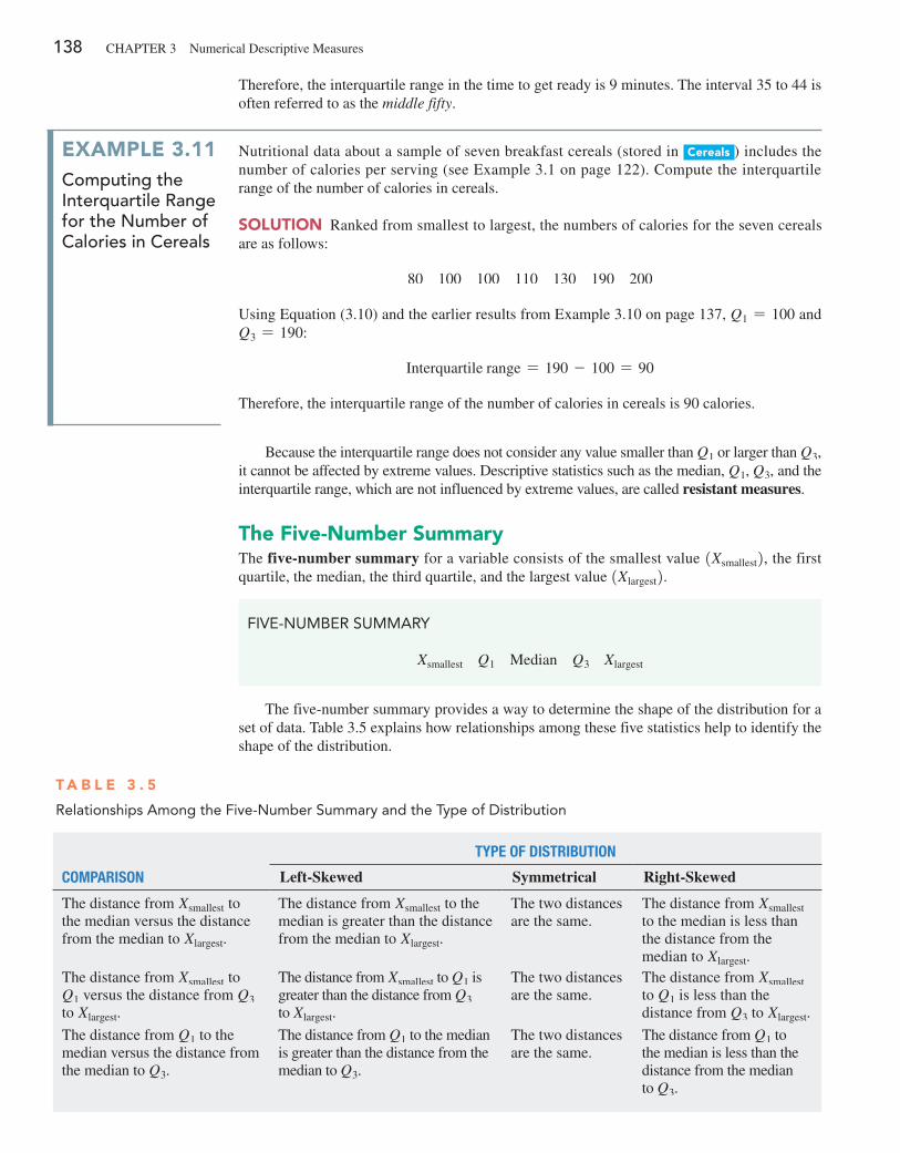
138 ChApTer 3 Numerical Descriptive Measures
ExaMplE 3.11computing the interquartile Range for the number of calories in cereals
Nutritional data about a sample of seven breakfast cereals (stored in Cereals ) includes the number of calories per serving (see example 3.1 on page 122). Compute the interquartile range of the number of calories in cereals.
SoluTion ranked from smallest to largest, the numbers of calories for the seven cereals are as follows:
80 100 100 110 130 190 200
Using equation (3.10) and the earlier results from example 3.10 on page 137, Q1 = 100 and Q3 = 190:
Interquartile range = 190 - 100 = 90
Therefore, the interquartile range of the number of calories in cereals is 90 calories.
Because the interquartile range does not consider any value smaller than Q1 or larger than Q3, it cannot be affected by extreme values. Descriptive statistics such as the median, Q1, Q3, and the interquartile range, which are not influenced by extreme values, are called resistant measures.
The Five-number SummaryThe five-number summary for a variable consists of the smallest value 1Xsmallest2, the first quartile, the median, the third quartile, and the largest value 1Xlargest2.
fIVE-NuMbER SuMMaRy
Xsmallest Q1 Median Q3 Xlargest
The five-number summary provides a way to determine the shape of the distribution for a set of data. Table 3.5 explains how relationships among these five statistics help to identify the shape of the distribution.
Therefore, the interquartile range in the time to get ready is 9 minutes. The interval 35 to 44 is often referred to as the middle fifty.
T a b l E 3 . 5
Relationships among the five-Number Summary and the Type of Distribution
Type of DiSTribuTion
CompariSon Left-Skewed Symmetrical Right-Skewed
The distance from Xsmallest to the median versus the distance from the median to Xlargest.
The distance from Xsmallest to the median is greater than the distance from the median to Xlargest.
The two distances are the same.
The distance from Xsmallest to the median is less than the distance from the median to Xlargest.
The distance from Xsmallest to Q1 versus the distance from Q3 to Xlargest.
The distance from Xsmallest to Q1 is greater than the distance from Q3 to Xlargest.
The two distances are the same.
The distance from Xsmallest to Q1 is less than the distance from Q3 to Xlargest.
The distance from Q1 to the median versus the distance from the median to Q3.
The distance from Q1 to the median is greater than the distance from the median to Q3.
The two distances are the same.
The distance from Q1 to the median is less than the distance from the median to Q3.
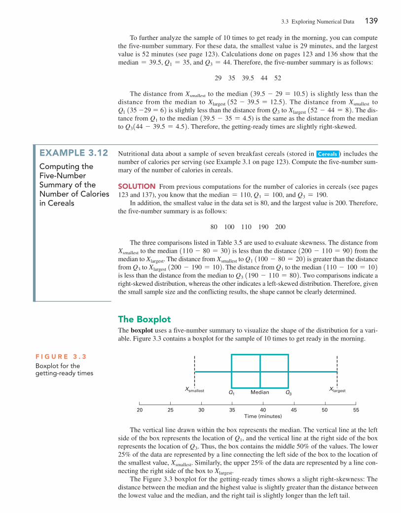
3.3 exploring Numerical Data 139
To further analyze the sample of 10 times to get ready in the morning, you can compute the five-number summary. For these data, the smallest value is 29 minutes, and the largest value is 52 minutes (see page 123). Calculations done on pages 123 and 136 show that the median = 39.5, Q1 = 35, and Q3 = 44. Therefore, the five-number summary is as follows:
29 35 39.5 44 52
The distance from Xsmallest to the median 139.5 - 29 = 10.52 is slightly less than the distance from the median to Xlargest 152 - 39.5 = 12.52. The distance from Xsmallest to Q1 135 -29 = 62 is slightly less than the distance from Q3 to Xlargest 152 - 44 = 82. The dis-tance from Q1 to the median 139.5 - 35 = 4.5) is the same as the distance from the median to Q3144 - 39.5 = 4.52. Therefore, the getting-ready times are slightly right-skewed.
ExaMplE 3.12computing the Five-number summary of the number of calories in cereals
Nutritional data about a sample of seven breakfast cereals (stored in Cereals ) includes the number of calories per serving (see example 3.1 on page 123). Compute the five-number sum-mary of the number of calories in cereals.
SoluTion From previous computations for the number of calories in cereals (see pages 123 and 137), you know that the median = 110, Q1 = 100, and Q3 = 190.
In addition, the smallest value in the data set is 80, and the largest value is 200. Therefore, the five-number summary is as follows:
80 100 110 190 200
The three comparisons listed in Table 3.5 are used to evaluate skewness. The distance from Xsmallest to the median 1110 - 80 = 302 is less than the distance 1200 - 110 = 902 from the median to Xlargest. The distance from Xsmallest to Q1 1100 - 80 = 202 is greater than the distance from Q3 to Xlargest 1200 - 190 = 102. The distance from Q1 to the median 1110 - 100 = 102 is less than the distance from the median to Q3 1190 - 110 = 802. Two comparisons indicate a right-skewed distribution, whereas the other indicates a left-skewed distribution. Therefore, given the small sample size and the conflicting results, the shape cannot be clearly determined.
The boxplotThe boxplot uses a five-number summary to visualize the shape of the distribution for a vari-able. Figure 3.3 contains a boxplot for the sample of 10 times to get ready in the morning.
F i g u R E 3 . 3boxplot for the getting-ready times
Xsmallest XlargestQ1 Median Q3
20 25 30 35 40Time (minutes)
45 50 55
The vertical line drawn within the box represents the median. The vertical line at the left side of the box represents the location of Q1, and the vertical line at the right side of the box represents the location of Q3. Thus, the box contains the middle 50% of the values. The lower 25% of the data are represented by a line connecting the left side of the box to the location of the smallest value, Xsmallest. Similarly, the upper 25% of the data are represented by a line con-necting the right side of the box to Xlargest.
The Figure 3.3 boxplot for the getting-ready times shows a slight right-skewness: The distance between the median and the highest value is slightly greater than the distance between the lowest value and the median, and the right tail is slightly longer than the left tail.
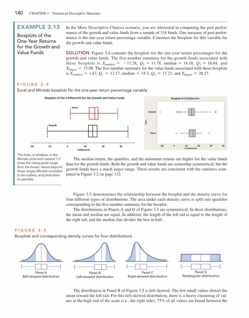
140 ChApTer 3 Numerical Descriptive Measures
Figure 3.5 demonstrates the relationship between the boxplot and the density curve for four different types of distributions. The area under each density curve is split into quartiles corresponding to the five-number summary for the boxplot.
The distributions in panels A and D of Figure 3.5 are symmetrical. In these distributions, the mean and median are equal. In addition, the length of the left tail is equal to the length of the right tail, and the median line divides the box in half.
ExaMplE 3.13boxplots of the One-Year Returns for the growth and Value Funds
In the More Descriptive Choices scenario, you are interested in comparing the past perfor-mance of the growth and value funds from a sample of 316 funds. One measure of past perfor-mance is the one-year return percentage variable. Construct the boxplots for this variable for the growth and value funds.
SoluTion Figure 3.4 contains the boxplots for the one-year return percentages for the growth and value funds. The five-number summary for the growth funds associated with these boxplots is Xsmallest = - 11.28, Q1 = 11.78, median = 14.18, Q3 = 16.64, and Xlargest = 33.98. The five-number summary for the value funds associated with these boxplots is Xsmallest = 1.67, Q1 = 12.17, median = 15.3, Q3 = 17.23, and Xlargest = 28.27.
F i g u R E 3 . 4Excel and Minitab boxplots for the one-year return percentage variable
The lines, or whiskers, in the Minitab plots each extend 1.5 times the interquartile range from the boxes. Values beyond these ranges Minitab considers to be outliers, and plots them as asterisks.
The median return, the quartiles, and the minimum returns are higher for the value funds than for the growth funds. Both the growth and value funds are somewhat symmetrical, but the growth funds have a much larger range. These results are consistent with the statistics com-puted in Figure 3.2 on page 132.
F i g u R E 3 . 5boxplots and corresponding density curves for four distributions
Panel ABell-shaped distribution
Panel BLeft-skewed distribution
Panel CRight-skewed distribution
Panel DRectangular distribution
The distribution in panel B of Figure 3.5 is left-skewed. The few small values distort the mean toward the left tail. For this left-skewed distribution, there is a heavy clustering of val-ues at the high end of the scale (i.e., the right side); 75% of all values are found between the
3.3 exploring Numerical Data 141
Student TipA long tail on the left side of the boxplot indicates a left-skewed distribution. A long tail on the right side of the boxplot indicates a right-skewed distribution.
left edge of the box 1Q12 and the end of the right tail 1Xlargest2. There is a long left tail that contains the smallest 25% of the values, demonstrating the lack of symmetry in this data set.
The distribution in panel C of Figure 3.5 is right-skewed. The concentration of values is on the low end of the scale (i.e., the left side of the boxplot). here, 75% of all values are found between the beginning of the left tail and the right edge of the box 1Q32. There is a long right tail that contains the largest 25% of the values, demonstrating the lack of symmetry in this data set.
problems for Section 3.3lEaRning ThE baSiCS3.21 The data below describe the fat content, in grams per serv-ing, for a sample of 20 chicken sandwiches from fast-food chains.
6 10 4 9 19 22 22 20 20 2721 31 27 17 28 28 29 31 38 58
a. Compute the first quartile 1Q12, the third quartile 1Q32, and the interquartile range.
b. List the five-number summary.c. Construct a boxplot and describe the shape.
3.22 The following is a set of data from a sample of n = 6:
7 4 9 7 3 12
a. Compute the first quartile 1Q12, the third quartile 1Q32, and the interquartile range.
b. List the five-number summary.c. Construct a boxplot and describe its shape.d. Compare your answer in (c) with that from problem 3.2 (d) on
page 133. Discuss.
3.23 The following is a set of data from a sample of n = 5:
7 4 9 8 2
a. Compute the first quartile 1Q12, the third quartile 1Q32, and the interquartile range.
b. List the five-number summary.c. Construct a boxplot and describe its shape.d. Compare your answer in (c) with that from problem 3.1 (d) on
page 133. Discuss.
3.24 The data set below shows the overall miles per gallon (MpG) of a new model of small SUVs.
21 25 24 25 21 23 22 21 2221 23 24 27 17 19 22 26 1721 18 23 24 24 15 17
a. Compute the first quartile 1Q12, the third quartile 1Q32, and the interquartile range.
b. List the five-number summary.c. Construct a boxplot and describe its shape.
applying ThE ConCEpTS3.25 The file accountingpartners contains the number of part-ners in a cohort of rising accounting firms that have been tagged as “firms to watch.” The firms have the following numbers of partners:
17 23 19 23 18 17 23 16 34 10 14 30 14 33 26 17 19 2220 27 33 25 12 26 13 30 13 13 33 21 17 12 10 14 12
Source: Data extracted from bit.ly/ODuzd3.
a. Compute the first quartile 1Q12, the third quartile 1Q32, and the interquartile range.
b. List the five-number summary.c. Construct a boxplot and describe its shape.
3.26 The file Marketpenetration contains Facebook penetration values (the percentage of the country population that are Facebook users) for 22 of the world’s largest economies:
56 57 43 55 42 35 7 25 42 17 43 6 31 28 59 20 27 36 45 80 57 56
Source: Data extracted from slidesha.re/ODv6vG.
a. Compute the first quartile 1Q12, the third quartile 1Q32, and the interquartile range.
b. List the five-number summary.c. Construct a boxplot and describe its shape.
3.27 The file hotelaway contains the average room price (in US$) paid by various nationalities while traveling abroad (away from their home country) in 2013:
179 173 175 173 164 143 153 155
Source: Data extracted from http://bit.ly/1pdFkOG.
a. Compute the first quartile 1Q12, the third quartile 1Q32, and the interquartile range.
b. List the five-number summary.c. Construct a boxplot and describe its shape.
3.28 The file SuV contains the overall MpG of 2014 small SUVs:
26 22 23 21 25 24 22 26 25 2221 21 22 22 23 24 23 22 21 22
Source: Data extracted from “Which Car Is right for You,” Consumer Reports, April 2014, pp. 60–61.
a. Compute the first quartile 1Q12, the third quartile 1Q32, and the interquartile range.
b. List the five-number summary.c. Construct a boxplot and describe its shape.
3.29 The file CD Rate contains the yields for one-year CDs and five-year CDs, for 22 banks in the United States, as of March 12, 2014.
Source: Data extracted from www.Bankrate.com, March 12, 2014.
For each type of account:a. Compute the first quartile 1Q12, the third quartile 1Q32, and the
interquartile range.b. List the five-number summary.c. Construct a boxplot and describe its shape.
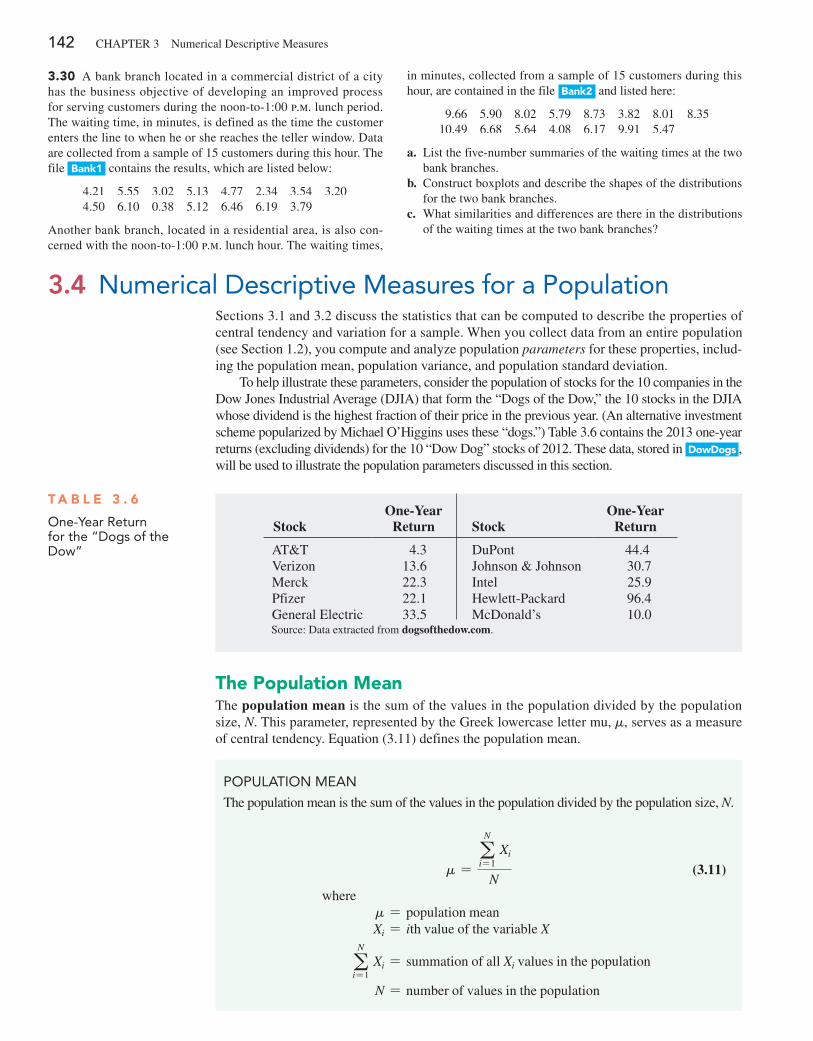
142 ChApTer 3 Numerical Descriptive Measures
3.30 A bank branch located in a commercial district of a city has the business objective of developing an improved process for serving customers during the noon-to-1:00 p.m. lunch period. The waiting time, in minutes, is defined as the time the customer enters the line to when he or she reaches the teller window. Data are collected from a sample of 15 customers during this hour. The file bank1 contains the results, which are listed below:
4.21 5.55 3.02 5.13 4.77 2.34 3.54 3.204.50 6.10 0.38 5.12 6.46 6.19 3.79
Another bank branch, located in a residential area, is also con-cerned with the noon-to-1:00 p.m. lunch hour. The waiting times,
in minutes, collected from a sample of 15 customers during this hour, are contained in the file bank2 and listed here:
9.66 5.90 8.02 5.79 8.73 3.82 8.01 8.3510.49 6.68 5.64 4.08 6.17 9.91 5.47
a. List the five-number summaries of the waiting times at the two bank branches.
b. Construct boxplots and describe the shapes of the distributions for the two bank branches.
c. What similarities and differences are there in the distributions of the waiting times at the two bank branches?
PoPulaTIoN MEaN
The population mean is the sum of the values in the population divided by the population size, N.
m =aN
i=1 Xi
N (3.11)
where m = population mean Xi = ith value of the variable X
aN
i=1 Xi = summation of all Xi values in the population
N = number of values in the population
3.4 Numerical Descriptive Measures for a PopulationSections 3.1 and 3.2 discuss the statistics that can be computed to describe the properties of central tendency and variation for a sample. When you collect data from an entire population (see Section 1.2), you compute and analyze population parameters for these properties, includ-ing the population mean, population variance, and population standard deviation.
To help illustrate these parameters, consider the population of stocks for the 10 companies in the Dow Jones Industrial Average (DJIA) that form the “Dogs of the Dow,” the 10 stocks in the DJIA whose dividend is the highest fraction of their price in the previous year. (An alternative investment scheme popularized by Michael O’higgins uses these “dogs.”) Table 3.6 contains the 2013 one-year returns (excluding dividends) for the 10 “Dow Dog” stocks of 2012. These data, stored in DowDogs , will be used to illustrate the population parameters discussed in this section.
The population MeanThe population mean is the sum of the values in the population divided by the population size, N. This parameter, represented by the Greek lowercase letter mu, m, serves as a measure of central tendency. equation (3.11) defines the population mean.
T a b l E 3 . 6
one-year Return for the “Dogs of the Dow”
StockOne-Year
Return StockOne-Year
Return
AT&T 4.3 Dupont 44.4Verizon 13.6 Johnson & Johnson 30.7Merck 22.3 Intel 25.9pfizer 22.1 hewlett-packard 96.4General electric 33.5 McDonald’s 10.0Source: Data extracted from dogsofthedow.com.
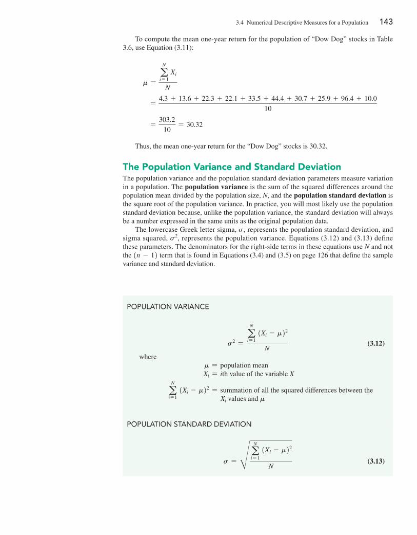
3.4 Numerical Descriptive Measures for a population 143
To compute the mean one-year return for the population of “Dow Dog” stocks in Table 3.6, use equation (3.11):
m =aN
i= 1 Xi
N
=4.3 + 13.6 + 22.3 + 22.1 + 33.5 + 44.4 + 30.7 + 25.9 + 96.4 + 10.0
10
=303.2
10= 30.32
Thus, the mean one-year return for the “Dow Dog” stocks is 30.32.
The population Variance and Standard DeviationThe population variance and the population standard deviation parameters measure variation in a population. The population variance is the sum of the squared differences around the population mean divided by the population size, N, and the population standard deviation is the square root of the population variance. In practice, you will most likely use the population standard deviation because, unlike the population variance, the standard deviation will always be a number expressed in the same units as the original population data.
The lowercase Greek letter sigma, s, represents the population standard deviation, and sigma squared, s2, represents the population variance. equations (3.12) and (3.13) define these parameters. The denominators for the right-side terms in these equations use N and not the 1n - 12 term that is found in equations (3.4) and (3.5) on page 126 that define the sample variance and standard deviation.
PoPulaTIoN VaRIaNCE
s2 =aN
i=1 1Xi - m22
N (3.12)
where m = population mean Xi = ith value of the variable X
aN
i=1 1Xi - m22 = summation of all the squared differences between the
Xi values and m
PoPulaTIoN STaNDaRD DEVIaTIoN
s = R aNi= 1
1Xi - m22
N (3.13)
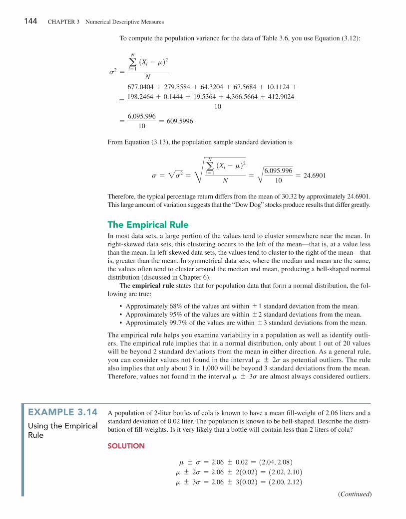
144 ChApTer 3 Numerical Descriptive Measures
To compute the population variance for the data of Table 3.6, you use equation (3.12):
s2 =aN
i=1 1Xi - m22
N
=
677.0404 + 279.5584 + 64.3204 + 67.5684 + 10.1124 +198.2464 + 0.1444 + 19.5364 + 4,366.5664 + 412.9024
10
=6,095.996
10= 609.5996
From equation (3.13), the population sample standard deviation is
s = 2s2 = H aNi= 1
1Xi - m22
N= A6,095.996
10= 24.6901
Therefore, the typical percentage return differs from the mean of 30.32 by approximately 24.6901. This large amount of variation suggests that the “Dow Dog” stocks produce results that differ greatly.
The Empirical RuleIn most data sets, a large portion of the values tend to cluster somewhere near the mean. In right-skewed data sets, this clustering occurs to the left of the mean—that is, at a value less than the mean. In left-skewed data sets, the values tend to cluster to the right of the mean—that is, greater than the mean. In symmetrical data sets, where the median and mean are the same, the values often tend to cluster around the median and mean, producing a bell-shaped normal distribution (discussed in Chapter 6).
The empirical rule states that for population data that form a normal distribution, the fol-lowing are true:
• Approximately 68% of the values are within {1 standard deviation from the mean. • Approximately 95% of the values are within {2 standard deviations from the mean. • Approximately 99.7% of the values are within {3 standard deviations from the mean.
The empirical rule helps you examine variability in a population as well as identify outli-ers. The empirical rule implies that in a normal distribution, only about 1 out of 20 values will be beyond 2 standard deviations from the mean in either direction. As a general rule, you can consider values not found in the interval m { 2s as potential outliers. The rule also implies that only about 3 in 1,000 will be beyond 3 standard deviations from the mean. Therefore, values not found in the interval m { 3s are almost always considered outliers.
ExaMplE 3.14Using the empirical Rule
A population of 2-liter bottles of cola is known to have a mean fill-weight of 2.06 liters and a standard deviation of 0.02 liter. The population is known to be bell-shaped. Describe the distri-bution of fill-weights. Is it very likely that a bottle will contain less than 2 liters of cola?
SoluTion
m { s = 2.06 { 0.02 = 12.04, 2.082 m { 2s = 2.06 { 210.022 = 12.02, 2.102 m { 3s = 2.06 { 310.022 = 12.00, 2.122
(Continued)
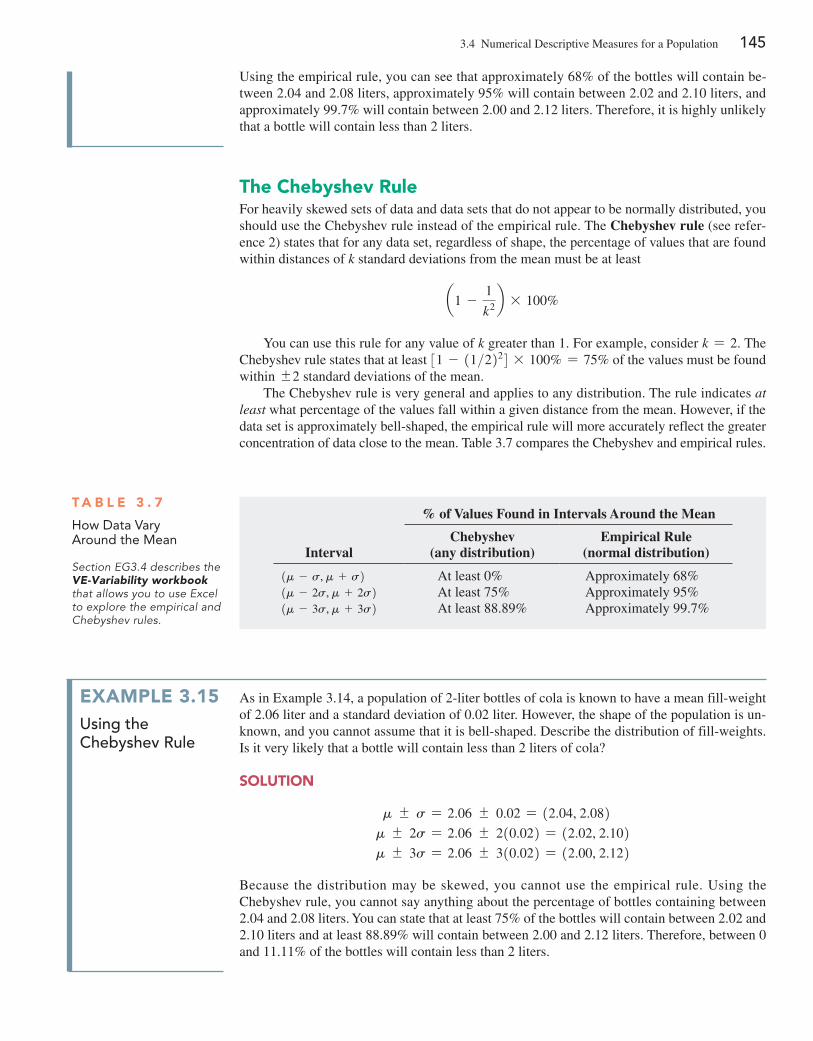
3.4 Numerical Descriptive Measures for a population 145
The Chebyshev RuleFor heavily skewed sets of data and data sets that do not appear to be normally distributed, you should use the Chebyshev rule instead of the empirical rule. The Chebyshev rule (see refer-ence 2) states that for any data set, regardless of shape, the percentage of values that are found within distances of k standard deviations from the mean must be at least
a1 -1
k2b * 100%
You can use this rule for any value of k greater than 1. For example, consider k = 2. The Chebyshev rule states that at least 31 - 11>2224 * 100% = 75% of the values must be found within {2 standard deviations of the mean.
The Chebyshev rule is very general and applies to any distribution. The rule indicates at least what percentage of the values fall within a given distance from the mean. however, if the data set is approximately bell-shaped, the empirical rule will more accurately reflect the greater concentration of data close to the mean. Table 3.7 compares the Chebyshev and empirical rules.
Using the empirical rule, you can see that approximately 68% of the bottles will contain be-tween 2.04 and 2.08 liters, approximately 95% will contain between 2.02 and 2.10 liters, and approximately 99.7% will contain between 2.00 and 2.12 liters. Therefore, it is highly unlikely that a bottle will contain less than 2 liters.
ExaMplE 3.15Using the chebyshev Rule
As in example 3.14, a population of 2-liter bottles of cola is known to have a mean fill-weight of 2.06 liter and a standard deviation of 0.02 liter. however, the shape of the population is un-known, and you cannot assume that it is bell-shaped. Describe the distribution of fill-weights. Is it very likely that a bottle will contain less than 2 liters of cola?
SoluTion
m { s = 2.06 { 0.02 = 12.04, 2.082 m { 2s = 2.06 { 210.022 = 12.02, 2.102 m { 3s = 2.06 { 310.022 = 12.00, 2.122
Because the distribution may be skewed, you cannot use the empirical rule. Using the Chebyshev rule, you cannot say anything about the percentage of bottles containing between 2.04 and 2.08 liters. You can state that at least 75% of the bottles will contain between 2.02 and 2.10 liters and at least 88.89% will contain between 2.00 and 2.12 liters. Therefore, between 0 and 11.11% of the bottles will contain less than 2 liters.
% of Values Found in Intervals Around the Mean
IntervalChebyshev
(any distribution)Empirical Rule
(normal distribution)
1m - s, m + s2 At least 0% Approximately 68%1m - 2s, m + 2s2 At least 75% Approximately 95%1m - 3s, m + 3s2 At least 88.89% Approximately 99.7%
T a b l E 3 . 7
how Data Vary around the Mean
Section EG3.4 describes the VE-Variability workbook that allows you to use Excel to explore the empirical and Chebyshev rules.
146 ChApTer 3 Numerical Descriptive Measures
You can use these two rules to understand how data are distributed around the mean when you have sample data. With each rule, you use the value you computed for X in place of m and the value you computed for S in place of s. The results you compute using the sample statistics are approximations because you used sample statistics 1X, S2 and not population parameters 1m, s2.
problems for Section 3.4lEaRning ThE baSiCS3.31 The following is a set of data for a population with N = 10:
9 8 11 15 14 11 3 7 9 7
a. Compute the population mean.b. Compute the population standard deviation.
3.32 The following is a set of data for a population with N = 10:
7 5 6 6 6 4 8 6 9 3
a. Compute the population mean.b. Compute the population standard deviation.
applying ThE ConCEpTS3.33 The file RadioShack contains the number of radioShack stores located in each of the 50 U.S. states and the District of Columbia, as of December 31, 2013:
65 20 76 53 565 82 68 18 12 309 127
24 28 197 122 68 56 75 81 33 99 115
155 81 47 97 28 33 40 36 156 41 342
139 9 203 59 70 232 20 69 22 88 408
41 16 144 111 36 101 19
Source: Data extracted from “radioShack closing up to 1,100 stores,” USA Today, March 6, 2014, p. 1B.
a. Compute the mean, variance, and standard deviation for this population.
b. What percentage of the 50 states have radioShack stores within {1, {2, or {3 standard deviations of the mean?
c. Compare your findings with what would be expected on the ba-sis of the empirical rule. Are you surprised at the results in (b)?
3.34 Consider a population of 1,024 mutual funds that primarily invest in large companies. You have determined that m, the mean one-year total percentage return achieved by all the funds, is 8.20 and that s, the standard deviation, is 2.75.a. According to the empirical rule, what percentage of these funds
is expected to be within {1 standard deviation of the mean?
b. According to the empirical rule, what percentage of these funds is expected to be within {2 standard deviations of the mean?
c. According to the Chebyshev rule, what percentage of these funds is expected to be within {1, {2, or {3 standard devia-tions of the mean?
d. According to the Chebyshev rule, at least 93.75% of these funds are expected to have one-year total returns between what two amounts?
3.35 The file CigaretteTax contains the state cigarette tax (in $) for each of the 50 states as of January 1, 2014.a. Compute the population mean and population standard devia-
tion for the state cigarette tax.b. Interpret the parameters in (a).
SELF Test
3.36 The file Energy contains the per capita energy consumption, in kilowatt-hours, for each of the 50 states and the District of Columbia during a recent year.a. Compute the mean, variance, and standard deviation for the
population.b. What proportion of these states has per capita energy con-
sumption within {1 standard deviation of the mean, within {2 standard deviations of the mean, and within {3 standard deviations of the mean?
c. Compare your findings with what would be expected based on the empirical rule. Are you surprised at the results in (b)?
d. repeat (a) through (c) with the District of Columbia removed. how have the results changed?
3.37 Thirty companies comprise the DJIA. Just how big are these companies? One common method for measuring the size of a company is to use its market capitalization, which is computed by multiplying the number of stock shares by the price of a share of stock. On March 14, 2014, the market capitalization of these companies ranged from Traveler’s $29.1 billion to exxonMobil’s $403.9 billion. The entire population of market capitalization val-ues is stored in DowMarketCap .
Source: Data extracted from money.cnn.com, March 14, 2014.
a. Compute the mean and standard deviation of the market capitalization for this population of 30 companies.
b. Interpret the parameters computed in (a).
3.5 The Covariance and the Coefficient of CorrelationIn Section 2.5, you used scatter plots to visually examine the relationship between two numeri-cal variables. This section presents two measures of the relationship between two numerical variables: the covariance and the coefficient of correlation.
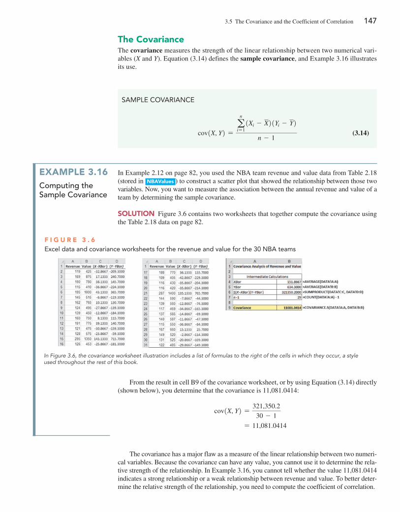
3.5 The Covariance and the Coefficient of Correlation 147
SaMPlE CoVaRIaNCE
cov1X, Y2 =a
n
i=1 1Xi - X2 1Yi - Y2
n - 1 (3.14)
The CovarianceThe covariance measures the strength of the linear relationship between two numerical vari-ables (X and Y). equation (3.14) defines the sample covariance, and example 3.16 illustrates its use.
ExaMplE 3.16computing the sample covariance
In example 2.12 on page 82, you used the NBA team revenue and value data from Table 2.18 (stored in nbaValues ) to construct a scatter plot that showed the relationship between those two variables. Now, you want to measure the association between the annual revenue and value of a team by determining the sample covariance.
SoluTion Figure 3.6 contains two worksheets that together compute the covariance using the Table 2.18 data on page 82.
From the result in cell B9 of the covariance worksheet, or by using equation (3.14) directly (shown below), you determine that the covariance is 11,081.0414:
cov1X, Y2 =321,350.2
30 - 1
= 11,081.0414
F i g u R E 3 . 6Excel data and covariance worksheets for the revenue and value for the 30 Nba teams
In Figure 3.6, the covariance worksheet illustration includes a list of formulas to the right of the cells in which they occur, a style used throughout the rest of this book.
The covariance has a major flaw as a measure of the linear relationship between two numeri-cal variables. Because the covariance can have any value, you cannot use it to determine the rela-tive strength of the relationship. In example 3.16, you cannot tell whether the value 11,081.0414 indicates a strong relationship or a weak relationship between revenue and value. To better deter-mine the relative strength of the relationship, you need to compute the coefficient of correlation.
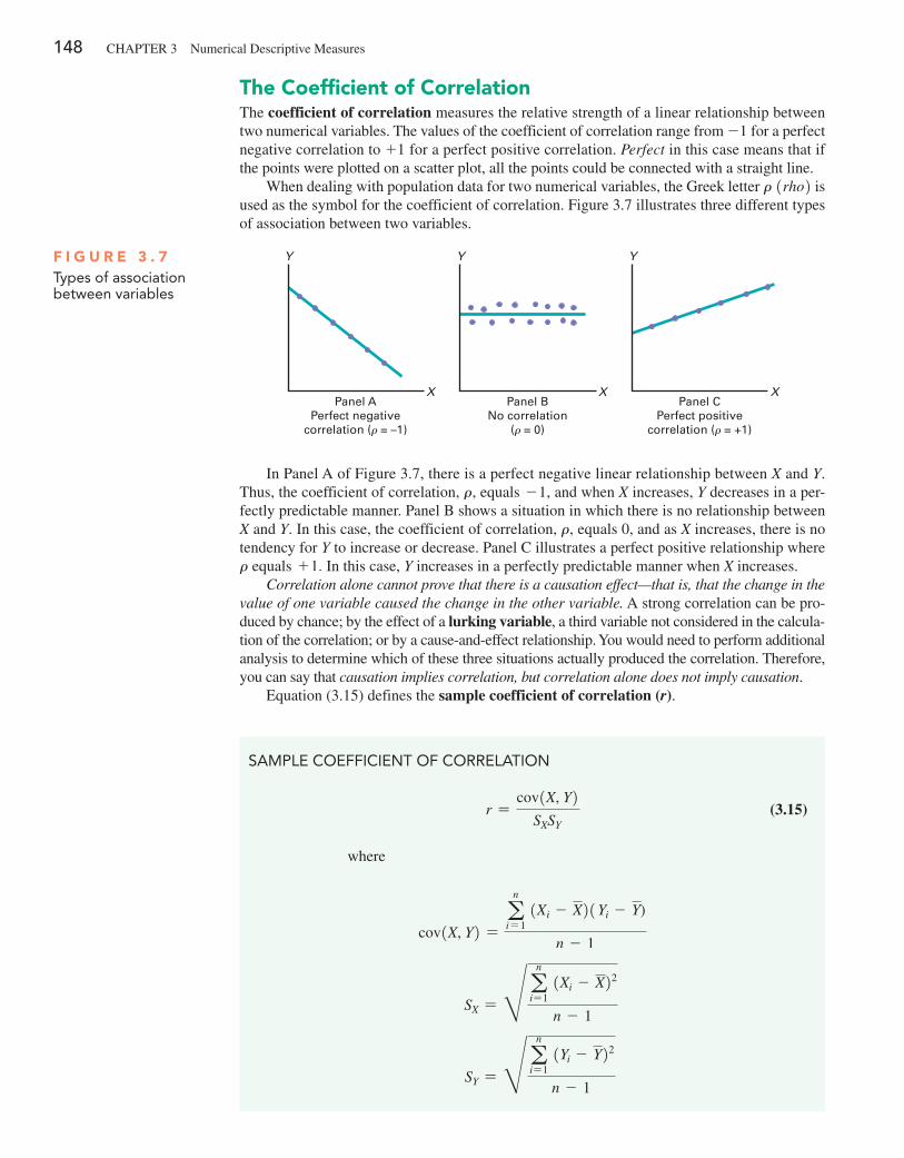
148 ChApTer 3 Numerical Descriptive Measures
The Coefficient of CorrelationThe coefficient of correlation measures the relative strength of a linear relationship between two numerical variables. The values of the coefficient of correlation range from -1 for a perfect negative correlation to +1 for a perfect positive correlation. Perfect in this case means that if the points were plotted on a scatter plot, all the points could be connected with a straight line.
When dealing with population data for two numerical variables, the Greek letter r 1rho2 is used as the symbol for the coefficient of correlation. Figure 3.7 illustrates three different types of association between two variables.
F i g u R E 3 . 7Types of association between variables
Y
Panel APerfect negative
correlation (� = –1)
X
Y
Panel BNo correlation
(� = 0)
X
Y
Panel CPerfect positive
correlation (� = +1)
X
In panel A of Figure 3.7, there is a perfect negative linear relationship between X and Y. Thus, the coefficient of correlation, r, equals - 1, and when X increases, Y decreases in a per-fectly predictable manner. panel B shows a situation in which there is no relationship between X and Y. In this case, the coefficient of correlation, r, equals 0, and as X increases, there is no tendency for Y to increase or decrease. panel C illustrates a perfect positive relationship where r equals + 1. In this case, Y increases in a perfectly predictable manner when X increases.
Correlation alone cannot prove that there is a causation effect—that is, that the change in the value of one variable caused the change in the other variable. A strong correlation can be pro-duced by chance; by the effect of a lurking variable, a third variable not considered in the calcula-tion of the correlation; or by a cause-and-effect relationship. You would need to perform additional analysis to determine which of these three situations actually produced the correlation. Therefore, you can say that causation implies correlation, but correlation alone does not imply causation.
equation (3.15) defines the sample coefficient of correlation (r).
SaMPlE CoEffICIENT of CoRRElaTIoN
r =cov1X, Y2
SXSY (3.15)
where
cov1X, Y2 =a
n
i= 1 1Xi - X21Yi - Y)
n - 1
SX = H an
i=1 1Xi - X22
n - 1
SY = H an
i=1 1Yi - Y22
n - 1
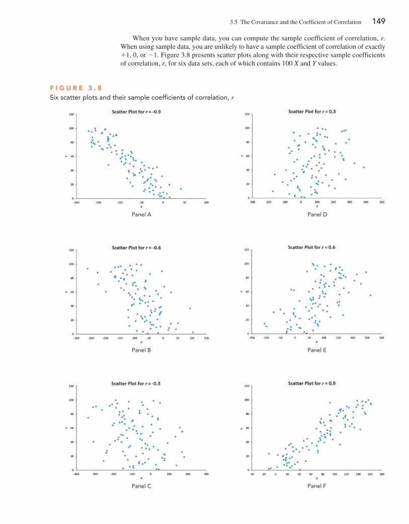
3.5 The Covariance and the Coefficient of Correlation 149
When you have sample data, you can compute the sample coefficient of correlation, r. When using sample data, you are unlikely to have a sample coefficient of correlation of exactly +1, 0, or -1. Figure 3.8 presents scatter plots along with their respective sample coefficients of correlation, r, for six data sets, each of which contains 100 X and Y values.
F i g u R E 3 . 8Six scatter plots and their sample coefficients of correlation, r
Panel a Panel D
Panel b Panel E
Panel C Panel f
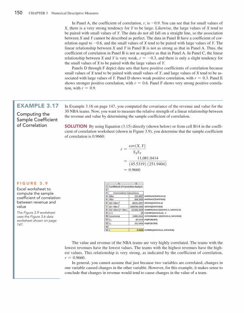
150 ChApTer 3 Numerical Descriptive Measures
In panel A, the coefficient of correlation, r, is -0.9. You can see that for small values of X, there is a very strong tendency for Y to be large. Likewise, the large values of X tend to be paired with small values of Y. The data do not all fall on a straight line, so the association between X and Y cannot be described as perfect. The data in panel B have a coefficient of cor-relation equal to -0.6, and the small values of X tend to be paired with large values of Y. The linear relationship between X and Y in panel B is not as strong as that in panel A. Thus, the coefficient of correlation in panel B is not as negative as that in panel A. In panel C, the linear relationship between X and Y is very weak, r = -0.3, and there is only a slight tendency for the small values of X to be paired with the large values of Y.
panels D through F depict data sets that have positive coefficients of correlation because small values of X tend to be paired with small values of Y, and large values of X tend to be as-sociated with large values of Y. panel D shows weak positive correlation, with r = 0.3. panel e shows stronger positive correlation, with r = 0.6. panel F shows very strong positive correla-tion, with r = 0.9.
ExaMplE 3.17computing the sample coefficient of correlation
In example 3.16 on page 147, you computed the covariance of the revenue and value for the 30 NBA teams. Now, you want to measure the relative strength of a linear relationship between the revenue and value by determining the sample coefficient of correlation.
SoluTion By using equation (3.15) directly (shown below) or from cell B14 in the coeffi-cient of correlation worksheet (shown in Figure 3.9), you determine that the sample coefficient of correlation is 0.9660:
r =cov1X, Y2
SXSY
=11,081.0414
145.53192 1251.94042 = 0.9660
The value and revenue of the NBA teams are very highly correlated. The teams with the lowest revenues have the lowest values. The teams with the highest revenues have the high-est values. This relationship is very strong, as indicated by the coefficient of correlation, r = 0.9660.
In general, you cannot assume that just because two variables are correlated, changes in one variable caused changes in the other variable. however, for this example, it makes sense to conclude that changes in revenue would tend to cause changes in the value of a team.
F i g u R E 3 . 9Excel worksheet to compute the sample coefficient of correlation between revenue and valueThe Figure 3.9 worksheet uses the Figure 3.6 data worksheet shown on page 147.
3.5 The Covariance and the Coefficient of Correlation 151
In summary, the coefficient of correlation indicates the linear relationship, or association, between two numerical variables. When the coefficient of correlation gets closer to + 1 or - 1, the linear relationship between the two variables is stronger. When the coefficient of correla-tion is near 0, little or no linear relationship exists. The sign of the coefficient of correlation indicates whether the data are positively correlated (i.e., the larger values of X are typically paired with the larger values of Y) or negatively correlated (i.e., the larger values of X are typi-cally paired with the smaller values of Y). The existence of a strong correlation does not imply a causation effect. It only indicates the tendencies present in the data.
problems for Section 3.5lEaRning ThE baSiCS3.38 The following is a set of data from a sample of n = 11 items:
X 7 5 8 3 6 10 12 4 9 15 18
Y 21 15 24 9 18 30 36 12 27 45 54
a. Compute the covariance.b. Compute the coefficient of correlation.c. how strong is the relationship between X and Y? explain.
applying ThE ConCEpTS3.39 A study of 483 first-year college women suggests a link be-tween media usage such as texting, chatting on cell phones, and posting status updates on Facebook, and grade point average. Stu-dents reporting a higher use of media had lower grade point aver-ages than students reporting a lower use of media. (Source: Walsh et al., “Female College Students’ Media Use and Academic Out-comes,” Emerging Adulthood, 2013.)a. Does the study suggest that use of media and grade point aver-
age are positively correlated or negatively correlated?b. Do you think that there might be a cause-and-effect relation-
ship between use of media and grade point average? explain.
SELF Test
3.40 The file Cereals lists the calories and sugar, in grams, in one serving of seven breakfast cereals:
a. Compute the covariance.b. Compute the coefficient of correlation.c. Which do you think is more valuable in expressing the relation-
ship between calories and sugar—the covariance or the coef-ficient of correlation? explain.
d. Based on (a) and (b), what conclusions can you reach about the relationship between calories and sugar?
3.41 Movie companies need to predict the gross receipts of indi-vidual movies once a movie has debuted. The data, shown in the next column and stored in potterMovies , are the first weekend gross, the U.S. gross, and the worldwide gross (in $ millions) of the eight harry potter movies:a. Compute the covariance between first weekend gross and U.S.
gross, first weekend gross and worldwide gross, and U.S. gross and worldwide gross.
b. Compute the coefficient of correlation between first weekend gross and U.S. gross, first weekend gross and worldwide gross, and U.S. gross and worldwide gross.
c. Which do you think is more valuable in expressing the rela-tionship between first weekend gross, U.S. gross, and world-wide gross—the covariance or the coefficient of correlation? explain.
d. Based on (a) and (b), what conclusions can you reach about the relationship between first weekend gross, U.S. gross, and worldwide gross?
3.42 College football is big business, with coaches’ total pay and revenues, in millions of dollars. The file College Football con-tains the coaches’ pay and revenues for college football at 105 of the 124 schools that are part of the Division I Football Bowl Subdivision.Source: Data extracted from “College Football Coaches Continue to See Salary explosion,” USA Today, November 20, 2012.
a. Compute the covariance.b. Compute the coefficient of correlation.c. Based on (a) and (b), what conclusions can you reach about the
relationship between coaches’ total pay and revenues?
Cereal Calories Sugar
Kellogg’s All Bran 80 6Kellogg’s Corn Flakes 100 2Wheaties 100 4Nature’s path Organic
Multigrain Flakes110 4
Kellogg’s rice Krispies 130 4post Shredded Wheat Vanilla
Almond190 11
Kellogg’s Mini Wheats 200 10
TitleFirst
WeekendU.S.
GrossWorldwide
Gross
Sorcerer’s Stone 90.295 317.558 976.458Chamber of Secrets 88.357 261.988 878.988Prisoner of Azkaban 93.687 249.539 795.539Goblet of Fire 102.335 290.013 896.013Order of the Phoenix 77.108 292.005 938.469Half-Blood Prince 77.836 301.460 934.601Deathly Hallows Part 1 125.017 295.001 955.417Deathly Hallows Part 2 169.189 381.011 1,328.111Source: Data extracted from www.the-numbers.com/interactive/comp-HarryPotter.php.
152 ChApTer 3 Numerical Descriptive Measures
3.43 A pew research Center survey found that social net-working is popular in many nations around the world. The file globalSocialMedia contains the level of social media network-ing (measured as the percentage of individuals polled who use social networking sites) and the GDp at purchasing power parity (ppp) per capita for each of 24 emerging and developing coun-
tries. (Data extracted from pew research Center, “emerging Na-tions embrace Internet, Mobile Technology,” bit.ly/1mg8Nvc.)a. Compute the covariance.b. Compute the coefficient of correlation.c. Based on (a) and (b), what conclusions can you reach about the
relationship between the GDp and social media use?
3.6 Descriptive Statistics: Pitfalls and Ethical IssuesThis chapter describes how a set of numerical data can be characterized by the statistics that measure the properties of central tendency, variation, and shape. In business, descriptive statis-tics such as the ones discussed in this chapter are frequently included in summary reports that are prepared periodically.
The volume of information available from online, broadcast, or print media has produced much skepticism in the minds of many about the objectivity of data. When you are reading in-formation that contains descriptive statistics, you should keep in mind the quip often attributed to the famous nineteenth-century British statesman Benjamin Disraeli: “There are three kinds of lies: lies, damned lies, and statistics.”
For example, in examining statistics, you need to compare the mean and the median. Are they similar, or are they very different? Or is only the mean provided? The answers to these questions will help you determine whether the data are skewed or symmetrical and whether the median might be a better measure of central tendency than the mean. In addition, you should look to see whether the standard deviation or interquartile range for a very skewed set of data has been included in the statistics provided. Without this, it is impossible to determine the amount of variation that exists in the data.
ethical considerations arise when you are deciding what results to include in a report. You should document both good and bad results. In addition, in all presentations, you need to report results in a fair, objective, and neutral manner. Unethical behavior occurs when you selectively fail to report pertinent findings that are detrimental to the support of a particular position.
In the More Descriptive Choices scenario, you were hired by the Choice Is Yours investment company to assist inves-
tors interested in stock mutual funds. A sample of 316 stock mutual funds included 227 growth funds and 89 value funds. By comparing these two categories, you were able to provide investors with valuable insights.
The one-year returns for both the growth funds and the value funds were symmetrical, as indicated by the box-plots (see Figure 3.4 on page 140). The descriptive statistics (see Figure 3.2 on page 132) allowed you to compare the central tendency, variability, and shape of the returns of the growth funds and the value funds. The mean indicated that the growth funds returned a mean of 14.28, and the median indicated that half of the growth funds had returns of 14.18 or more. The value funds’ central tendencies were slightly higher than those of the growth funds—they had a mean of
14.70, and half the funds had one-year returns above 15.30. T h e g r o w t h funds showed slightly more variability than the value funds, with a standard deviation of 5.0041 as compared to 4.4651. The kurtosis of growth funds was very positive, indicating a distribution that was much more peaked than a normal distribution. Although past performance is no assurance of future performance, the value funds slightly outperformed the growth funds in 2012. (You can examine other variables in Retirement Funds to see if the value funds outperformed the growth funds for the 3-year period 2010–2012, for the 5-year period 2008–2012 and for the 10-year period 2003–2012.)
U s i n g s tat i s t i c s
More Descriptive Choices, Revisited
Baranq/Shutterstock
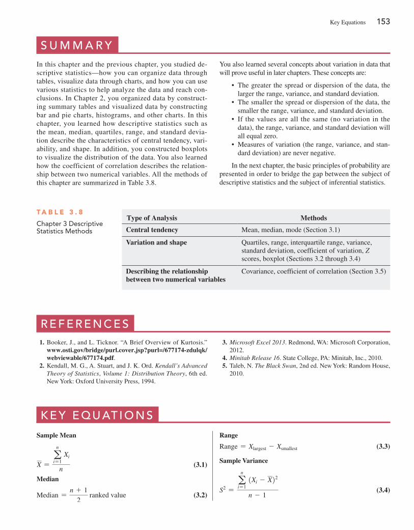
s U M M a R YIn this chapter and the previous chapter, you studied de-scriptive statistics—how you can organize data through tables, visualize data through charts, and how you can use various statistics to help analyze the data and reach con-clusions. In Chapter 2, you organized data by construct-ing summary tables and visualized data by constructing bar and pie charts, histograms, and other charts. In this chapter, you learned how descriptive statistics such as the mean, median, quartiles, range, and standard devia-tion describe the characteristics of central tendency, vari-ability, and shape. In addition, you constructed boxplots to visualize the distribution of the data. You also learned how the coefficient of correlation describes the relation-ship between two numerical variables. All the methods of this chapter are summarized in Table 3.8.
You also learned several concepts about variation in data that will prove useful in later chapters. These concepts are:
• The greater the spread or dispersion of the data, the larger the range, variance, and standard deviation.
• The smaller the spread or dispersion of the data, the smaller the range, variance, and standard deviation.
• If the values are all the same (no variation in the data), the range, variance, and standard deviation will all equal zero.
• Measures of variation (the range, variance, and stan-dard deviation) are never negative.
In the next chapter, the basic principles of probability are presented in order to bridge the gap between the subject of descriptive statistics and the subject of inferential statistics.
T a b l E 3 . 8
Chapter 3 Descriptive Statistics Methods
Type of Analysis Methods
Central tendency Mean, median, mode (Section 3.1)
Variation and shape Quartiles, range, interquartile range, variance, standard deviation, coefficient of variation, Z scores, boxplot (Sections 3.2 through 3.4)
Describing the relationship between two numerical variables
Covariance, coefficient of correlation (Section 3.5)
R e F e R e n c e s 1. Booker, J., and L. Ticknor. “A Brief Overview of Kurtosis.”
www.osti.gov/bridge/purl.cover.jsp?purl=/677174-zdulqk/webviewable/677174.pdf.
2. Kendall, M. G., A. Stuart, and J. K. Ord. Kendall’s Advanced Theory of Statistics, Volume 1: Distribution Theory, 6th ed. New York: Oxford University press, 1994.
3. Microsoft Excel 2013. redmond, WA: Microsoft Corporation, 2012.
4. Minitab Release 16. State College, pA: Minitab, Inc., 2010. 5. Taleb, N. The Black Swan, 2nd ed. New York: random house,
2010.
K e Y e Q U at i O n s
Sample Mean
X =a
n
i=1 Xi
n (3.1)
Median
Median =n + 1
2 ranked value (3.2)
Range
range = Xlargest - Xsmallest (3.3)
Sample Variance
S2 =a
n
i=1 1Xi - X22
n - 1 (3.4)
Key equations 153
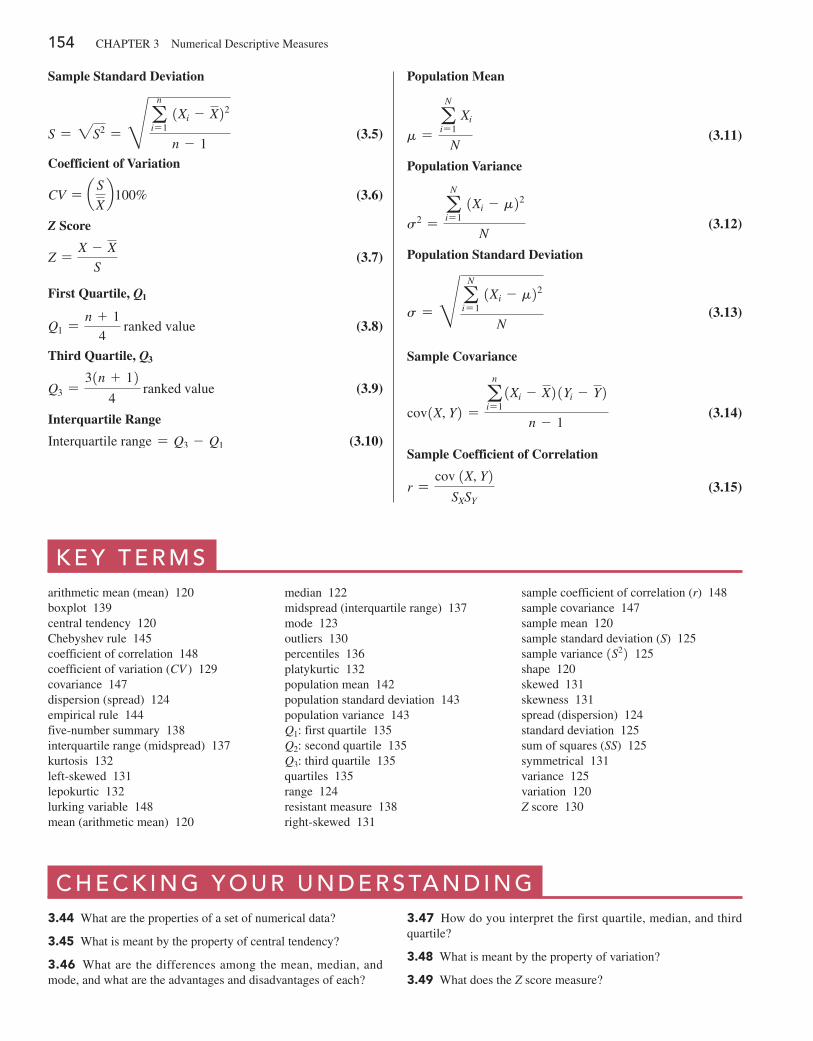
154 ChApTer 3 Numerical Descriptive Measures
Sample Standard Deviation
S = 2S2 = H an
i=1 1Xi - X22
n - 1 (3.5)
Coefficient of Variation
CV = a S
Xb100% (3.6)
Z Score
Z =X - X
S (3.7)
First Quartile, Q1
Q1 =n + 1
4 ranked value (3.8)
Third Quartile, Q3
Q3 =31n + 12
4 ranked value (3.9)
Interquartile Range
Interquartile range = Q3 - Q1 (3.10)
Population Mean
m =aN
i=1 Xi
N (3.11)
Population Variance
s2 =aN
i=1 1Xi - m22
N (3.12)
Population Standard Deviation
s = H aNi= 1
1Xi - m22
N (3.13)
Sample Covariance
cov1X, Y2 =a
n
i=1 1Xi - X2 1Yi - Y2
n - 1 (3.14)
Sample Coefficient of Correlation
r =cov 1X, Y2
SXSY (3.15)
K e Y t e R M sarithmetic mean (mean) 120boxplot 139central tendency 120Chebyshev rule 145coefficient of correlation 148coefficient of variation (CV ) 129covariance 147dispersion (spread) 124empirical rule 144five-number summary 138interquartile range (midspread) 137kurtosis 132left-skewed 131lepokurtic 132lurking variable 148mean (arithmetic mean) 120
median 122midspread (interquartile range) 137mode 123outliers 130percentiles 136platykurtic 132population mean 142population standard deviation 143population variance 143Q1: first quartile 135Q2: second quartile 135Q3: third quartile 135quartiles 135range 124resistant measure 138right-skewed 131
sample coefficient of correlation (r) 148sample covariance 147sample mean 120sample standard deviation (S) 125sample variance 1S22 125shape 120skewed 131skewness 131spread (dispersion) 124standard deviation 125sum of squares (SS) 125symmetrical 131variance 125variation 120Z score 130
c h e c K i n g Y O U R U n D e R s ta n D i n g3.44 What are the properties of a set of numerical data?
3.45 What is meant by the property of central tendency?
3.46 What are the differences among the mean, median, and mode, and what are the advantages and disadvantages of each?
3.47 how do you interpret the first quartile, median, and third quartile?
3.48 What is meant by the property of variation?
3.49 What does the Z score measure?
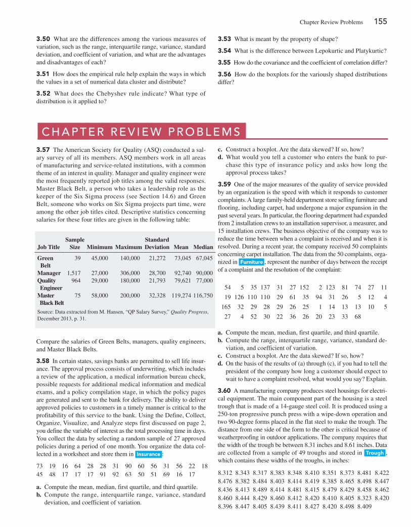
3.50 What are the differences among the various measures of variation, such as the range, interquartile range, variance, standard deviation, and coefficient of variation, and what are the advantages and disadvantages of each?
3.51 how does the empirical rule help explain the ways in which the values in a set of numerical data cluster and distribute?
3.52 What does the Chebyshev rule indicate? What type of distribution is it applied to?
3.53 What is meant by the property of shape?
3.54 What is the difference between Lepokurtic and platykurtic?
3.55 how do the covariance and the coefficient of correlation differ?
3.56 how do the boxplots for the variously shaped distributions differ?
c h a p t e R R e V i e W p R O b l e M s3.57 The American Society for Quality (ASQ) conducted a sal-ary survey of all its members. ASQ members work in all areas of manufacturing and service-related institutions, with a common theme of an interest in quality. Manager and quality engineer were the most frequently reported job titles among the valid responses. Master Black Belt, a person who takes a leadership role as the keeper of the Six Sigma process (see Section 14.6) and Green Belt, someone who works on Six Sigma projects part time, were among the other job titles cited. Descriptive statistics concerning salaries for these four titles are given in the following table:
c. Construct a boxplot. Are the data skewed? If so, how?d. What would you tell a customer who enters the bank to pur-
chase this type of insurance policy and asks how long the approval process takes?
3.59 One of the major measures of the quality of service provided by an organization is the speed with which it responds to customer complaints. A large family-held department store selling furniture and flooring, including carpet, had undergone a major expansion in the past several years. In particular, the flooring department had expanded from 2 installation crews to an installation supervisor, a measurer, and 15 installation crews. The business objective of the company was to reduce the time between when a complaint is received and when it is resolved. During a recent year, the company received 50 complaints concerning carpet installation. The data from the 50 complaints, orga-nized in Furniture , represent the number of days between the receipt of a complaint and the resolution of the complaint:
54 5 35 137 31 27 152 2 123 81 74 27 11
19 126 110 110 29 61 35 94 31 26 5 12 4
165 32 29 28 29 26 25 1 14 13 13 10 5
27 4 52 30 22 36 26 20 23 33 68
a. Compute the mean, median, first quartile, and third quartile.b. Compute the range, interquartile range, variance, standard de-
viation, and coefficient of variation.c. Construct a boxplot. Are the data skewed? If so, how?d. On the basis of the results of (a) through (c), if you had to tell the
president of the company how long a customer should expect to wait to have a complaint resolved, what would you say? explain.
3.60 A manufacturing company produces steel housings for electri-cal equipment. The main component part of the housing is a steel trough that is made of a 14-gauge steel coil. It is produced using a 250-ton progressive punch press with a wipe-down operation and two 90-degree forms placed in the flat steel to make the trough. The distance from one side of the form to the other is critical because of weatherproofing in outdoor applications. The company requires that the width of the trough be between 8.31 inches and 8.61 inches. Data are collected from a sample of 49 troughs and stored in Trough , which contains these widths of the troughs, in inches:
8.312 8.343 8.317 8.383 8.348 8.410 8.351 8.373 8.481 8.4228.476 8.382 8.484 8.403 8.414 8.419 8.385 8.465 8.498 8.4478.436 8.413 8.489 8.414 8.481 8.415 8.479 8.429 8.458 8.4628.460 8.444 8.429 8.460 8.412 8.420 8.410 8.405 8.323 8.4208.396 8.447 8.405 8.439 8.411 8.427 8.420 8.498 8.409
Job TitleSample
Size Minimum MaximumStandard Deviation Mean Median
Green Belt
39 45,000 140,000 21,272 73,045 67,045
Manager 1,517 27,000 306,000 28,700 92,740 90,000Quality Engineer
964 29,000 180,000 21,793 79,621 77,000
Master Black Belt
75 58,000 200,000 32,328 119,274 116,750
Source: Data extracted from M. hansen, “Qp Salary Survey,” Quality Progress, December 2013, p. 31.
Compare the salaries of Green Belts, managers, quality engineers, and Master Black Belts.
3.58 In certain states, savings banks are permitted to sell life insur-ance. The approval process consists of underwriting, which includes a review of the application, a medical information bureau check, possible requests for additional medical information and medical exams, and a policy compilation stage, in which the policy pages are generated and sent to the bank for delivery. The ability to deliver approved policies to customers in a timely manner is critical to the profitability of this service to the bank. Using the Define, Collect, Organize, Visualize, and Analyze steps first discussed on page 2, you define the variable of interest as the total processing time in days. You collect the data by selecting a random sample of 27 approved policies during a period of one month. You organize the data col-lected in a worksheet and store them in insurance :
73 19 16 64 28 28 31 90 60 56 31 56 22 1845 48 17 17 17 91 92 63 50 51 69 16 17
a. Compute the mean, median, first quartile, and third quartile.b. Compute the range, interquartile range, variance, standard
deviation, and coefficient of variation.
Chapter review problems 155
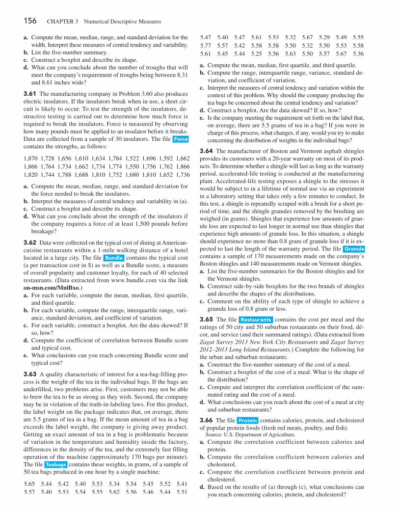
156 ChApTer 3 Numerical Descriptive Measures
a. Compute the mean, median, range, and standard deviation for the width. Interpret these measures of central tendency and variability.
b. List the five-number summary.c. Construct a boxplot and describe its shape.d. What can you conclude about the number of troughs that will
meet the company’s requirement of troughs being between 8.31 and 8.61 inches wide?
3.61 The manufacturing company in problem 3.60 also produces electric insulators. If the insulators break when in use, a short cir-cuit is likely to occur. To test the strength of the insulators, de-structive testing is carried out to determine how much force is required to break the insulators. Force is measured by observing how many pounds must be applied to an insulator before it breaks. Data are collected from a sample of 30 insulators. The file Force contains the strengths, as follows:
1,870 1,728 1,656 1,610 1,634 1,784 1,522 1,696 1,592 1,6621,866 1,764 1,734 1,662 1,734 1,774 1,550 1,756 1,762 1,8661,820 1,744 1,788 1,688 1,810 1,752 1,680 1,810 1,652 1,736
a. Compute the mean, median, range, and standard deviation for the force needed to break the insulators.
b. Interpret the measures of central tendency and variability in (a).c. Construct a boxplot and describe its shape.d. What can you conclude about the strength of the insulators if
the company requires a force of at least 1,500 pounds before breakage?
3.62 Data were collected on the typical cost of dining at American- cuisine restaurants within a 1-mile walking distance of a hotel located in a large city. The file bundle contains the typical cost (a per transaction cost in $) as well as a Bundle score, a measure of overall popularity and customer loyalty, for each of 40 selected restaurants. (Data extracted from www.bundle.com via the link on-msn.com/MnlBxo.)a. For each variable, compute the mean, median, first quartile,
and third quartile.b. For each variable, compute the range, interquartile range, vari-
ance, standard deviation, and coefficient of variation.c. For each variable, construct a boxplot. Are the data skewed? If
so, how?d. Compute the coefficient of correlation between Bundle score
and typical cost.e. What conclusions can you reach concerning Bundle score and
typical cost?
3.63 A quality characteristic of interest for a tea-bag-filling pro-cess is the weight of the tea in the individual bags. If the bags are underfilled, two problems arise. First, customers may not be able to brew the tea to be as strong as they wish. Second, the company may be in violation of the truth-in-labeling laws. For this product, the label weight on the package indicates that, on average, there are 5.5 grams of tea in a bag. If the mean amount of tea in a bag exceeds the label weight, the company is giving away product. Getting an exact amount of tea in a bag is problematic because of variation in the temperature and humidity inside the factory, differences in the density of the tea, and the extremely fast filling operation of the machine (approximately 170 bags per minute). The file Teabags contains these weights, in grams, of a sample of 50 tea bags produced in one hour by a single machine:
5.65 5.44 5.42 5.40 5.53 5.34 5.54 5.45 5.52 5.415.57 5.40 5.53 5.54 5.55 5.62 5.56 5.46 5.44 5.51
5.47 5.40 5.47 5.61 5.53 5.32 5.67 5.29 5.49 5.555.77 5.57 5.42 5.58 5.58 5.50 5.32 5.50 5.53 5.585.61 5.45 5.44 5.25 5.56 5.63 5.50 5.57 5.67 5.36
a. Compute the mean, median, first quartile, and third quartile.b. Compute the range, interquartile range, variance, standard de-
viation, and coefficient of variation.c. Interpret the measures of central tendency and variation within the
context of this problem. Why should the company producing the tea bags be concerned about the central tendency and variation?
d. Construct a boxplot. Are the data skewed? If so, how?e. Is the company meeting the requirement set forth on the label that,
on average, there are 5.5 grams of tea in a bag? If you were in charge of this process, what changes, if any, would you try to make concerning the distribution of weights in the individual bags?
3.64 The manufacturer of Boston and Vermont asphalt shingles provides its customers with a 20-year warranty on most of its prod-ucts. To determine whether a shingle will last as long as the warranty period, accelerated-life testing is conducted at the manufacturing plant. Accelerated-life testing exposes a shingle to the stresses it would be subject to in a lifetime of normal use via an experiment in a laboratory setting that takes only a few minutes to conduct. In this test, a shingle is repeatedly scraped with a brush for a short pe-riod of time, and the shingle granules removed by the brushing are weighed (in grams). Shingles that experience low amounts of gran-ule loss are expected to last longer in normal use than shingles that experience high amounts of granule loss. In this situation, a shingle should experience no more than 0.8 gram of granule loss if it is ex-pected to last the length of the warranty period. The file granule contains a sample of 170 measurements made on the company’s Boston shingles and 140 measurements made on Vermont shingles.a. List the five-number summaries for the Boston shingles and for
the Vermont shingles.b. Construct side-by-side boxplots for the two brands of shingles
and describe the shapes of the distributions.c. Comment on the ability of each type of shingle to achieve a
granule loss of 0.8 gram or less.
3.65 The file Restaurants contains the cost per meal and the ratings of 50 city and 50 suburban restaurants on their food, dé-cor, and service (and their summated ratings). (Data extracted from Zagat Survey 2013 New York City Restaurants and Zagat Survey 2012–2013 Long Island Restaurants.) Complete the following for the urban and suburban restaurants:a. Construct the five-number summary of the cost of a meal.b. Construct a boxplot of the cost of a meal. What is the shape of
the distribution?c. Compute and interpret the correlation coefficient of the sum-
mated rating and the cost of a meal.d. What conclusions can you reach about the cost of a meal at city
and suburban restaurants?
3.66 The file protein contains calories, protein, and cholesterol of popular protein foods (fresh red meats, poultry, and fish).
Source: U.S. Department of Agriculture.a. Compute the correlation coefficient between calories and
protein.b. Compute the correlation coefficient between calories and
cholesterol.c. Compute the correlation coefficient between protein and
cholesterol.d. Based on the results of (a) through (c), what conclusions can
you reach concerning calories, protein, and cholesterol?
3.67 The file hotelprices contains the prices in British pounds (about US$1.52 as of July 2013) of a room at two-star, three-star, and four-star hotels in cities around the world in 2013. (Data extracted from press.hotels.com/content/blogs.dir/13 /files/2013/09/HPI_UK.pdf.) Complete the following for two-star, three-star, and four-star hotels:a. Compute the mean, median, first quartile, and third quartile.b. Compute the range, interquartile range, variance, standard de-
viation, and coefficient of variation.c. Interpret the measures of central tendency and variation within
the context of this problem.d. Construct a boxplot. Are the data skewed? If so, how?e. Compute the covariance between the average price at two-star
and three-star hotels, between two-star and four-star hotels, and between three-star and four-star hotels.
f. Compute the coefficient of correlation between the average price at two-star and three-star hotels, between two-star and four-star hotels, and between three-star and four-star hotels.
g. Which do you think is more valuable in expressing the relation-ship between the average price of a room at two-star, three-star, and four-star hotels—the covariance or the coefficient of cor-relation? explain.
h. Based on (f), what conclusions can you reach about the rela-tionship between the average price of a room at two-star, three-star, and four-star hotels?
3.68 The file propertyTaxes contains the property taxes per cap-ita for the 50 states and the District of Columbia.a. Compute the mean, median, first quartile, and third quartile.b. Compute the range, interquartile range, variance, standard de-
viation, and coefficient of variation.c. Construct a boxplot. Are the data skewed? If so, how?d. Based on the results of (a) through (c), what conclusions can
you reach concerning property taxes per capita for each state and the District of Columbia?
3.69 have you wondered how Internet download speed varies around the globe? The file DownloadSpeed contains the mean download speed Mbps for various countries. (Data extracted from www.netindex.com/download/allcountries/.)a. Compute the mean, median, first quartile, and third quartile.b. Compute the range, interquartile range, variance, standard de-
viation, and coefficient of variation.c. Construct a boxplot. Are the data skewed? If so, how?d. Based on the results of (a) through (c), what conclusions can you
reach concerning the download speed around the globe?
3.70 311 is Chicago’s web and phone portal for government in-formation and nonemergency services. 311 serves as a compre-hensive one-stop shop for residents, visitors, and business owners; therefore, it is critical that 311 representatives answer calls and respond to requests in a timely and accurate fashion. The target response time for answering 311 calls is 45 seconds. Agent aban-donment rate is one of several call center metrics tracked by 311 officials. This metric tracks the percentage of callers who hang up after the target response time of 45 seconds has elapsed. The file 311CallCenter contains the agent abandonment rate for 22 weeks of call center operation during the 7:00 a.m.–3:00 p.m. shift.a. Compute the mean, median, first quartile, and third quartile.b. Compute the range, interquartile range, variance, standard de-
viation, and coefficient of variation.
c. Construct a boxplot. Are the data skewed? If so, how?d. Compute the correlation coefficient between day and agent
abandonment rate.e. Based on the results of (a) through (c), what conclusions might
you reach concerning 311 call center performance operation?
3.71 how much time do Americans living in or near cities spend waiting in traffic, and how much does waiting in traffic cost them per year? The file Congestion includes this cost for 31 cities. (Source: Data extracted from “The high Cost of Congestion,” Time, October 17, 2011, p. 18.) For the time Americans living in or near cities spend waiting in traffic and the cost of waiting in traffic per year:a. Compute the mean, median, first quartile, and third quartile.b. Compute the range, interquartile range, variance, standard
deviation, and coefficient of variation.c. Construct a boxplot. Are the data skewed? If so, how?d. Compute the correlation coefficient between the time spent sit-
ting in traffic and the cost of sitting in traffic.e. Based on the results of (a) through (c), what conclusions might
you reach concerning the time spent waiting in traffic and the cost of waiting in traffic.
3.72 how do the average credit scores of people living in various American cities differ? The file Credit Scores is an ordered array of the average credit scores of people living in 143 American cities. (Data extracted from usat.ly/17a1fA6)a. Compute the mean, median, first quartile, and third quartile.b. Compute the range, interquartile range, variance, standard
deviation, and coefficient of variation.c. Construct a boxplot. Are the data skewed? If so, how?d. Based on the results of (a) through (c), what conclusions might
you reach concerning the average credit scores of people living in various American cities?
3.73 You are planning to study for your statistics examination with a group of classmates, one of whom you particularly want to impress. This individual has volunteered to use Microsoft excel to generate the needed summary information, tables, and charts for a data set that contains several numerical and categorical variables as-signed by the instructor for study purposes. This person comes over to you with the printout and exclaims, “I’ve got it all—the means, the medians, the standard deviations, the boxplots, the pie charts—for all our variables. The problem is, some of the output looks weird—like the boxplots for gender and for major and the pie charts for grade point average and for height. Also, I can’t understand why professor Szabat said we can’t get the descriptive stats for some of the variables; I got them for everything! See, the mean for height is 68.23, the mean for grade point average is 2.76, the mean for gender is 1.50, the mean for major is 4.33.” What is your reply?
REpoRT WRiTing ExERCiSES3.74 The file Domesticbeer contains the percentage alcohol, number of calories per 12 ounces, and number of carbohydrates (in grams) per 12 ounces for 156 of the best-selling domestic beers in the United States. (Data extracted from bit.ly/17H3Ct, March 12, 2014.) Write a report that includes a complete descriptive evaluation of each of the numerical variables—percentage of alcohol, number of calories per 12 ounces, and number of carbohydrates (in grams) per 12 ounces. Append to your report all appropriate tables, charts, and numerical descriptive measures.
Chapter review problems 157
158 ChApTer 3 Numerical Descriptive Measures
c a s e s F O R c h a p t e R 3
Managing ashland Multicomm servicesFor what variable in the Chapter 2 “Managing Ashland MultiComm Services” case (see page 100) are numerical descriptive measures needed?
1. For the variable you identify, compute the appropriate numerical descriptive measures and construct a boxplot.
2. For the variable you identify, construct a graphical dis-play. What conclusions can you reach from this other plot that cannot be made from the boxplot?
3. Summarize your findings in a report that can be included with the task force’s study.
Digital caseApply your knowledge about the proper use of numerical descriptive measures in this continuing Digital Case from Chapter 2.
Open EndRunGuide.pdf, the endrun Financial Services “Guide to Investing.” reexamine endrun’s supporting data for the “More Winners Than Losers” and “The Big eight Difference” and then answer the following:
1. Can descriptive measures be computed for any variables? how would such summary statistics support endrun’s
claims? how would those summary statistics affect your perception of endrun’s record?
2. evaluate the methods endrun used to summarize the re-sults presented on the “Customer Survey results” page. Is there anything you would do differently to summarize these results?
3. Note that the last question of the survey has fewer responses than the other questions. What factors may have limited the number of responses to that question?
cardiogood Fitness
return to the CardioGood Fitness case first presented on page 100. Using the data stored in CardiogoodFitness :
1. Compute descriptive statistics to create a customer profile for each CardioGood Fitness treadmill product line.
2. Write a report to be presented to the management of CardioGood Fitness, detailing your findings.
More Descriptive choices Follow-up
Follow up the Using Statistics revisited section on page 152 by computing descriptive statistics to analyze the differences in 3-year return percentages, 5-year return percentages, and 10-year return percentages for the sample of 316 retirement
funds stored in Retirement Funds . In your analysis, examine differences between the growth and value funds as well as the differences among the small, mid-cap, and large market cap funds.
clear Mountain state student surveys
1. The student news service at Clear Mountain State University (CMSU) has decided to gather data about the undergraduate students who attend CMSU. They create and distribute a survey of 14 questions and receive responses from 62 undergraduates (stored in undergradSurvey ). For each numerical variable included in the survey, compute all the appropriate descriptive statistics and write a report summarizing your conclusions.
2. The dean of students at CMSU has learned about the undergraduate survey and has decided to undertake a similar survey for graduate students at CMSU. She creates and distributes a survey of 14 questions and re-ceives responses from 44 graduate students (stored in gradSurvey ). For each numerical variable included in the survey, compute all the appropriate descriptive sta-tistic and write a report summarizing your conclusions.
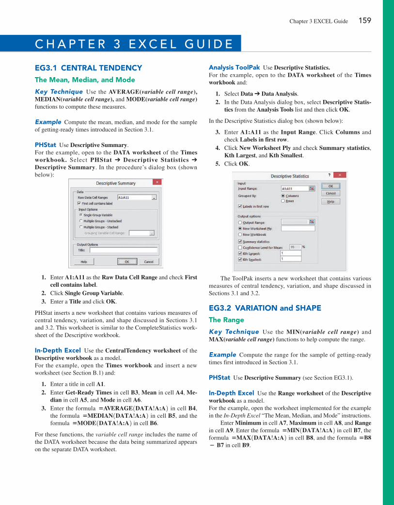
Eg3.1 CEnTRal TEnDEnCyThe Mean, Median, and Mode
Key Technique Use the AVERAGE(variable cell range), MEDIAN(variable cell range), and MODE(variable cell range) functions to compute these measures.
Example Compute the mean, median, and mode for the sample of getting-ready times introduced in Section 3.1.
phStat Use Descriptive Summary.For the example, open to the DATA worksheet of the Times workbook. Select PHStat ➔ Descriptive Statistics ➔ Descriptive Summary. In the procedure’s dialog box (shown below):
1. enter A1:A11 as the Raw Data Cell Range and check First cell contains label.
2. Click Single Group Variable. 3. enter a Title and click OK.
phStat inserts a new worksheet that contains various measures of central tendency, variation, and shape discussed in Sections 3.1 and 3.2. This worksheet is similar to the CompleteStatistics work-sheet of the Descriptive workbook.
in-Depth Excel Use the CentralTendency worksheet of the Descriptive workbook as a model.For the example, open the Times workbook and insert a new worksheet (see Section B.1) and:
1. enter a title in cell A1. 2. enter Get-Ready Times in cell B3, Mean in cell A4, Me-
dian in cell A5, and Mode in cell A6. 3. enter the formula =AVERAGE1DATA!A:A2 in cell B4,
the formula =MEDIAN1DATA!A:A2 in cell B5, and the formula =MODE1DATA!A:A2 in cell B6.
For these functions, the variable cell range includes the name of the DATA worksheet because the data being summarized appears on the separate DATA worksheet.
analysis Toolpak Use Descriptive Statistics.For the example, open to the DATA worksheet of the Times workbook and:
1. Select Data ➔ Data Analysis. 2. In the Data Analysis dialog box, select Descriptive Statis-
tics from the Analysis Tools list and then click OK.
In the Descriptive Statistics dialog box (shown below):
3. enter A1:A11 as the Input Range. Click Columns and check Labels in first row.
4. Click New Worksheet Ply and check Summary statistics, Kth Largest, and Kth Smallest.
5. Click OK.
The Toolpak inserts a new worksheet that contains various measures of central tendency, variation, and shape discussed in Sections 3.1 and 3.2.
Eg3.2 VaRiaTion and ShapEThe Range
Key Technique Use the MIN(variable cell range) and MAX(variable cell range) functions to help compute the range.
Example Compute the range for the sample of getting-ready times first introduced in Section 3.1.
phStat Use Descriptive Summary (see Section eG3.1).
in-Depth Excel Use the Range worksheet of the Descriptive workbook as a model.For the example, open the worksheet implemented for the example in the In-Depth Excel “The Mean, Median, and Mode” instructions.
enter Minimum in cell A7, Maximum in cell A8, and Range in cell A9. enter the formula =MIN1DATA!A:A2 in cell B7, the formula =MAX1DATA!A:A2 in cell B8, and the formula =B8− B7 in cell B9.
c h a p t e R 3 e x c e l g U i D e
Chapter 3 exCeL Guide 159
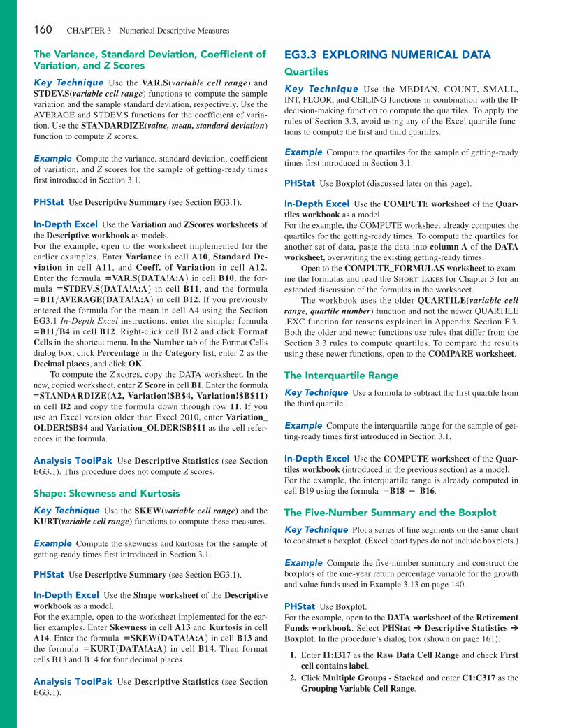
160 ChApTer 3 Numerical Descriptive Measures
The Variance, Standard Deviation, Coefficient of Variation, and Z Scores
Key Technique Use the VAR.S(variable cell range) and STDEV.S(variable cell range) functions to compute the sample variation and the sample standard deviation, respectively. Use the AVerAGe and STDeV.S functions for the coefficient of varia-tion. Use the STANDARDIZE(value, mean, standard deviation) function to compute Z scores.
Example Compute the variance, standard deviation, coefficient of variation, and Z scores for the sample of getting-ready times first introduced in Section 3.1.
phStat Use Descriptive Summary (see Section eG3.1).
in-Depth Excel Use the Variation and ZScores worksheets of the Descriptive workbook as models.For the example, open to the worksheet implemented for the earlier examples. enter Variance in cell A10, Standard De-viation in cell A11, and Coeff. of Variation in cell A12. enter the formula =VAR.S1DATA!A:A2 in cell B10, the for-mula =STDEV.S1DATA!A:A2 in cell B11, and the formula =B11>AVERAGE1DATA!A:A2 in cell B12. If you previously entered the formula for the mean in cell A4 using the Section eG3.1 In-Depth Excel instructions, enter the simpler formula =B11>B4 in cell B12. right-click cell B12 and click Format Cells in the shortcut menu. In the Number tab of the Format Cells dialog box, click Percentage in the Category list, enter 2 as the Decimal places, and click OK.
To compute the Z scores, copy the DATA worksheet. In the new, copied worksheet, enter Z Score in cell B1. enter the formula =STANDARDIZE(A2, Variation!$B$4, Variation!$B$11) in cell B2 and copy the formula down through row 11. If you use an excel version older than excel 2010, enter Variation_OLDER!$B$4 and Variation_OLDER!$B$11 as the cell refer-ences in the formula.
analysis Toolpak Use Descriptive Statistics (see Section eG3.1). This procedure does not compute Z scores.
Shape: Skewness and Kurtosis
Key Technique Use the SKEW(variable cell range) and the KURT(variable cell range) functions to compute these measures.
Example Compute the skewness and kurtosis for the sample of getting-ready times first introduced in Section 3.1.
phStat Use Descriptive Summary (see Section eG3.1).
in-Depth Excel Use the Shape worksheet of the Descriptive workbook as a model.For the example, open to the worksheet implemented for the ear-lier examples. enter Skewness in cell A13 and Kurtosis in cell A14. enter the formula =SKEW1DATA!A:A2 in cell B13 and the formula =KURT1DATA!A:A2 in cell B14. Then format cells B13 and B14 for four decimal places.
analysis Toolpak Use Descriptive Statistics (see Section eG3.1).
Eg3.3 ExploRing nuMERiCal DaTaQuartiles
Key Technique Use the MeDIAN, COUNT, SMALL, INT, FLOOr, and CeILING functions in combination with the IF decision-making function to compute the quartiles. To apply the rules of Section 3.3, avoid using any of the excel quartile func-tions to compute the first and third quartiles.
Example Compute the quartiles for the sample of getting-ready times first introduced in Section 3.1.
phStat Use Boxplot (discussed later on this page).
in-Depth Excel Use the COMPUTE worksheet of the Quar-tiles workbook as a model.For the example, the COMpUTe worksheet already computes the quartiles for the getting-ready times. To compute the quartiles for another set of data, paste the data into column A of the DATA worksheet, overwriting the existing getting-ready times.
Open to the COMPUTE_FORMULAS worksheet to exam-ine the formulas and read the Short Takes for Chapter 3 for an extended discussion of the formulas in the worksheet.
The workbook uses the older QUARTILE(variable cell range, quartile number) function and not the newer QUArTILe .exC function for reasons explained in Appendix Section F.3. Both the older and newer functions use rules that differ from the Section 3.3 rules to compute quartiles. To compare the results using these newer functions, open to the COMPARE worksheet.
The interquartile Range
Key Technique Use a formula to subtract the first quartile from the third quartile.
Example Compute the interquartile range for the sample of get-ting-ready times first introduced in Section 3.1.
in-Depth Excel Use the COMPUTE worksheet of the Quar-tiles workbook (introduced in the previous section) as a model.For the example, the interquartile range is already computed in cell B19 using the formula =B18 − B16.
The Five-number Summary and the boxplot
Key Technique plot a series of line segments on the same chart to construct a boxplot. (excel chart types do not include boxplots.)
Example Compute the five-number summary and construct the boxplots of the one-year return percentage variable for the growth and value funds used in example 3.13 on page 140.
phStat Use Boxplot.For the example, open to the DATA worksheet of the Retirement Funds workbook. Select PHStat ➔ Descriptive Statistics ➔ Boxplot. In the procedure’s dialog box (shown on page 161):
1. enter I1:I317 as the Raw Data Cell Range and check First cell contains label.
2. Click Multiple Groups - Stacked and enter C1:C317 as the Grouping Variable Cell Range.
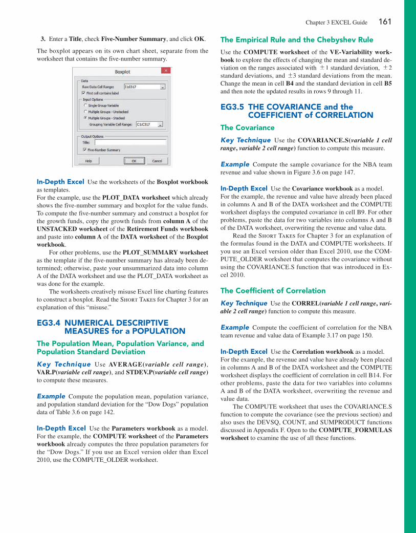
3. enter a Title, check Five-Number Summary, and click OK.
The boxplot appears on its own chart sheet, separate from the worksheet that contains the five-number summary.
in-Depth Excel Use the worksheets of the Boxplot workbook as templates.For the example, use the PLOT_DATA worksheet which already shows the five-number summary and boxplot for the value funds. To compute the five-number summary and construct a boxplot for the growth funds, copy the growth funds from column A of the UNSTACKED worksheet of the Retirement Funds workbook and paste into column A of the DATA worksheet of the Boxplot workbook.
For other problems, use the PLOT_SUMMARY worksheet as the template if the five-number summary has already been de-termined; otherwise, paste your unsummarized data into column A of the DATA worksheet and use the pLOT_DATA worksheet as was done for the example.
The worksheets creatively misuse excel line charting features to construct a boxplot. read the Short Takes for Chapter 3 for an explanation of this “misuse.”
Eg3.4 nuMERiCal DESCRipTiVE MEaSuRES for a populaTion
The population Mean, population Variance, and population Standard Deviation
Key Technique Use AVERAGE(variable cell range) , VAR.P(variable cell range), and STDEV.P(variable cell range) to compute these measures.
Example Compute the population mean, population variance, and population standard deviation for the “Dow Dogs” population data of Table 3.6 on page 142.
in-Depth Excel Use the Parameters workbook as a model. For the example, the COMPUTE worksheet of the Parameters workbook already computes the three population parameters for the “Dow Dogs.” If you use an excel version older than excel 2010, use the COMpUTe_OLDer worksheet.
The Empirical Rule and the Chebyshev Rule
Use the COMPUTE worksheet of the VE-Variability work-book to explore the effects of changing the mean and standard de-viation on the ranges associated with {1 standard deviation, {2 standard deviations, and {3 standard deviations from the mean. Change the mean in cell B4 and the standard deviation in cell B5 and then note the updated results in rows 9 through 11.
Eg3.5 ThE CoVaRianCE and the CoEFFiCiEnT of CoRRElaTion
The Covariance
Key Technique Use the COVARIANCE.S(variable 1 cell range, variable 2 cell range) function to compute this measure.
Example Compute the sample covariance for the NBA team revenue and value shown in Figure 3.6 on page 147.
in-Depth Excel Use the Covariance workbook as a model.For the example, the revenue and value have already been placed in columns A and B of the DATA worksheet and the COMpUTe worksheet displays the computed covariance in cell B9. For other problems, paste the data for two variables into columns A and B of the DATA worksheet, overwriting the revenue and value data.
read the Short Takes for Chapter 3 for an explanation of the formulas found in the DATA and COMpUTe worksheets. If you use an excel version older than excel 2010, use the COM-pUTe_OLDer worksheet that computes the covariance without using the COVArIANCe.S function that was introduced in ex-cel 2010.
The Coefficient of Correlation
Key Technique Use the CORREL(variable 1 cell range, vari-able 2 cell range) function to compute this measure.
Example Compute the coefficient of correlation for the NBA team revenue and value data of example 3.17 on page 150.
in-Depth Excel Use the Correlation workbook as a model.For the example, the revenue and value have already been placed in columns A and B of the DATA worksheet and the COMpUTe worksheet displays the coefficient of correlation in cell B14. For other problems, paste the data for two variables into columns A and B of the DATA worksheet, overwriting the revenue and value data.
The COMpUTe worksheet that uses the COVArIANCe.S function to compute the covariance (see the previous section) and also uses the DeVSQ, COUNT, and SUMprODUCT functions discussed in Appendix F. Open to the COMPUTE_FORMULAS worksheet to examine the use of all these functions.
Chapter 3 exCeL Guide 161
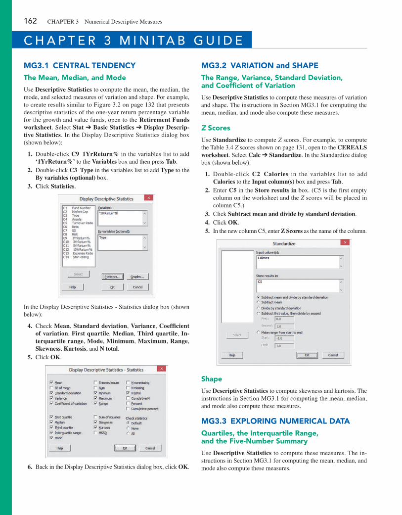
162 ChApTer 3 Numerical Descriptive Measures
Mg3.1 CEnTRal TEnDEnCyThe Mean, Median, and Mode
Use Descriptive Statistics to compute the mean, the median, the mode, and selected measures of variation and shape. For example, to create results similar to Figure 3.2 on page 132 that presents descriptive statistics of the one-year return percentage variable for the growth and value funds, open to the Retirement Funds worksheet. Select Stat ➔ Basic Statistics ➔ Display Descrip-tive Statistics. In the Display Descriptive Statistics dialog box (shown below):
1. Double-click C9 1YrReturn% in the variables list to add ‘1YrReturn%’ to the Variables box and then press Tab.
2. Double-click C3 Type in the variables list to add Type to the By variables (optional) box.
3. Click Statistics.
In the Display Descriptive Statistics - Statistics dialog box (shown below):
4. Check Mean, Standard deviation, Variance, Coefficient of variation, First quartile, Median, Third quartile, In-terquartile range, Mode, Minimum, Maximum, Range, Skewness, Kurtosis, and N total.
5. Click OK.
6. Back in the Display Descriptive Statistics dialog box, click OK.
Mg3.2 VaRiaTion and ShapEThe Range, Variance, Standard Deviation, and Coefficient of Variation
Use Descriptive Statistics to compute these measures of variation and shape. The instructions in Section MG3.1 for computing the mean, median, and mode also compute these measures.
Z Scores
Use Standardize to compute Z scores. For example, to compute the Table 3.4 Z scores shown on page 131, open to the CEREALS worksheet. Select Calc ➔ Standardize. In the Standardize dialog box (shown below):
1. Double-click C2 Calories in the variables list to add Calories to the Input column(s) box and press Tab.
2. enter C5 in the Store results in box. (C5 is the first empty column on the worksheet and the Z scores will be placed in column C5.)
3. Click Subtract mean and divide by standard deviation. 4. Click OK. 5. In the new column C5, enter Z Scores as the name of the column.
Shape
Use Descriptive Statistics to compute skewness and kurtosis. The instructions in Section MG3.1 for computing the mean, median, and mode also compute these measures.
Mg3.3 ExploRing nuMERiCal DaTaQuartiles, the interquartile Range, and the Five-number Summary
Use Descriptive Statistics to compute these measures. The in-structions in Section MG3.1 for computing the mean, median, and mode also compute these measures.
c h a p t e R 3 M i n i ta b g U i D e
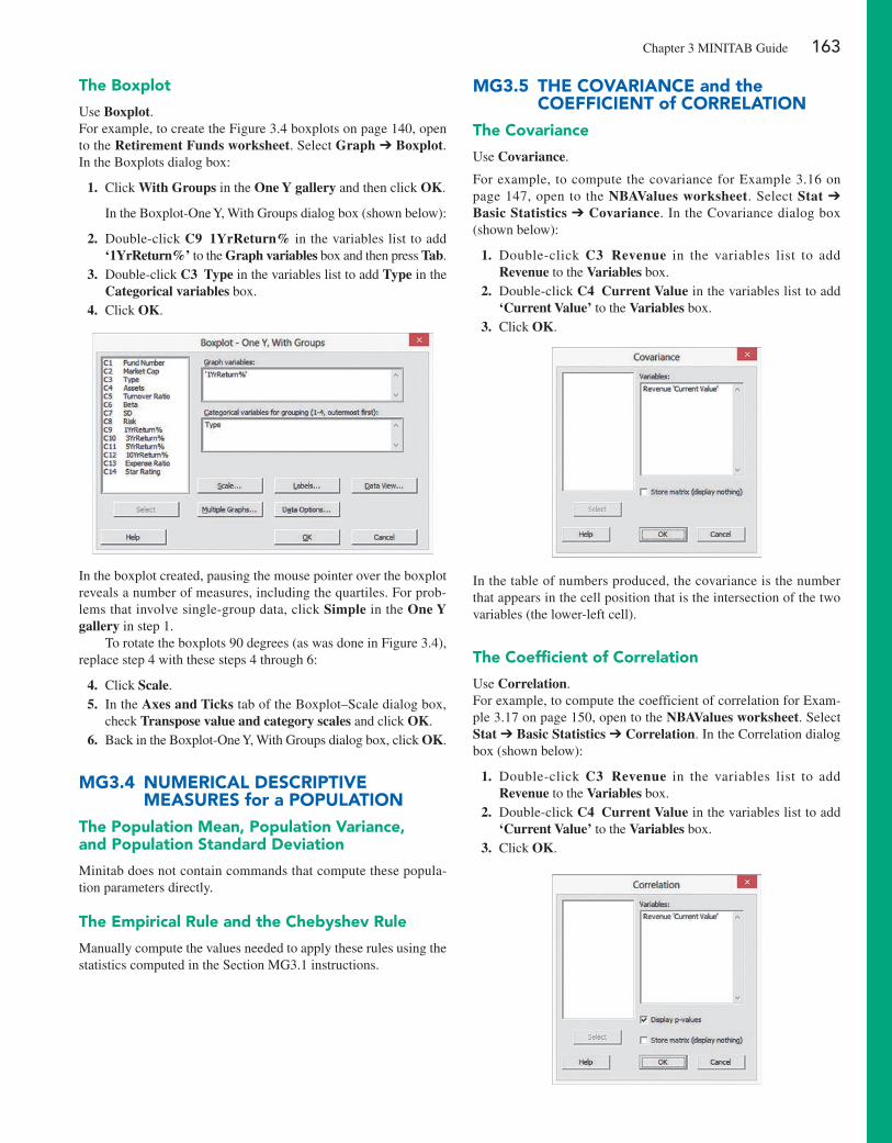
The boxplot
Use Boxplot. For example, to create the Figure 3.4 boxplots on page 140, open to the Retirement Funds worksheet. Select Graph ➔ Boxplot. In the Boxplots dialog box:
1. Click With Groups in the One Y gallery and then click OK.
In the Boxplot-One Y, With Groups dialog box (shown below):
2. Double-click C9 1YrReturn% in the variables list to add ‘1YrReturn%’ to the Graph variables box and then press Tab.
3. Double-click C3 Type in the variables list to add Type in the Categorical variables box.
4. Click OK.
In the boxplot created, pausing the mouse pointer over the boxplot reveals a number of measures, including the quartiles. For prob-lems that involve single-group data, click Simple in the One Y gallery in step 1.
To rotate the boxplots 90 degrees (as was done in Figure 3.4), replace step 4 with these steps 4 through 6:
4. Click Scale. 5. In the Axes and Ticks tab of the Boxplot–Scale dialog box,
check Transpose value and category scales and click OK. 6. Back in the Boxplot-One Y, With Groups dialog box, click OK.
Mg3.4 nuMERiCal DESCRipTiVE MEaSuRES for a populaTion
The population Mean, population Variance, and population Standard Deviation
Minitab does not contain commands that compute these popula-tion parameters directly.
The Empirical Rule and the Chebyshev Rule
Manually compute the values needed to apply these rules using the statistics computed in the Section MG3.1 instructions.
Mg3.5 ThE CoVaRianCE and the CoEFFiCiEnT of CoRRElaTion
The Covariance
Use Covariance.
For example, to compute the covariance for example 3.16 on page 147, open to the NBAValues worksheet. Select Stat ➔ Basic Statistics ➔ Covariance. In the Covariance dialog box (shown below):
1. Double-click C3 Revenue in the variables list to add Revenue to the Variables box.
2. Double-click C4 Current Value in the variables list to add ‘Current Value’ to the Variables box.
3. Click OK.
In the table of numbers produced, the covariance is the number that appears in the cell position that is the intersection of the two variables (the lower-left cell).
The Coefficient of Correlation
Use Correlation.For example, to compute the coefficient of correlation for exam-ple 3.17 on page 150, open to the NBAValues worksheet. Select Stat ➔ Basic Statistics ➔ Correlation. In the Correlation dialog box (shown below):
1. Double-click C3 Revenue in the variables list to add Revenue to the Variables box.
2. Double-click C4 Current Value in the variables list to add ‘Current Value’ to the Variables box.
3. Click OK.
Chapter 3 MINITAB Guide 163

164
U s i n g s tat i s t i c s
Possibilities at M&R Electronics WorldAs the marketing manager for M&R Electronics World, you are analyzing the results of an intent-to-purchase study. The heads of 1,000 households were asked about their intentions to purchase a large-screen HDTV (one that has a screen size of at least 50 inches) sometime during the next 12 months. As a follow-up, you plan to survey the same people 12 months later to see whether they pur-chased a television. For households that did purchase a large-screen HDTV, you would like to know whether the television they purchased had a faster refresh rate (240 Hz or higher) or a standard refresh rate (60 or 120 Hz), whether they also purchased a streaming media box in the past 12 months, and whether they were satisfied with their purchase of the large-screen HDTV.
You plan to use the results of this survey to form a new marketing strategy that will enhance sales and better target those households likely to purchase multiple or more expensive products. What questions can you ask in this survey? How can you express the relationships among the various intent-to-purchase responses of individual households?
contents
4.1 Basic Probability Concepts
4.2 Conditional Probability
4.3 Bayes’ Theorem
think aboUt this: Divine Providence and spam
4.4 Counting Rules
4.5 Ethical Issues and Probability
Using statistics: Possibilities at M&R Electronics World, Revisited
chaPtER 4 ExcEl gUiDE
chaPtER 4 Minitab gUiDE
objectives
Understand basic probability concepts
Understand conditional probability
Use Bayes’ theorem to revise probabilities
Learn various counting rules
Chapter Basic Probability
4
Shock/Fotolia
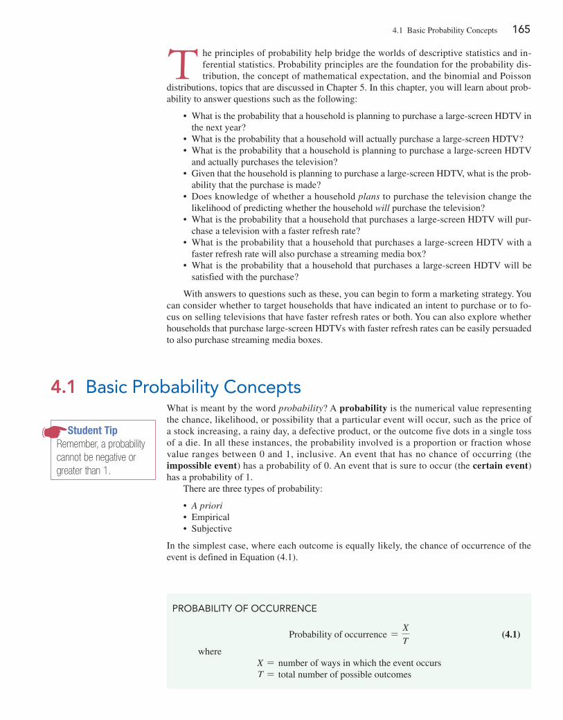
4.1 Basic Probability Concepts 165
T he principles of probability help bridge the worlds of descriptive statistics and in-ferential statistics. Probability principles are the foundation for the probability dis-tribution, the concept of mathematical expectation, and the binomial and Poisson
distributions, topics that are discussed in Chapter 5. In this chapter, you will learn about prob-ability to answer questions such as the following:
• What is the probability that a household is planning to purchase a large-screen HDTV in the next year?
• What is the probability that a household will actually purchase a large-screen HDTV? • What is the probability that a household is planning to purchase a large-screen HDTV
and actually purchases the television? • Given that the household is planning to purchase a large-screen HDTV, what is the prob-
ability that the purchase is made? • Does knowledge of whether a household plans to purchase the television change the
likelihood of predicting whether the household will purchase the television? • What is the probability that a household that purchases a large-screen HDTV will pur-
chase a television with a faster refresh rate? • What is the probability that a household that purchases a large-screen HDTV with a
faster refresh rate will also purchase a streaming media box? • What is the probability that a household that purchases a large-screen HDTV will be
satisfied with the purchase?
With answers to questions such as these, you can begin to form a marketing strategy. You can consider whether to target households that have indicated an intent to purchase or to fo-cus on selling televisions that have faster refresh rates or both. You can also explore whether households that purchase large-screen HDTVs with faster refresh rates can be easily persuaded to also purchase streaming media boxes.
4.1 Basic Probability ConceptsWhat is meant by the word probability? A probability is the numerical value representing the chance, likelihood, or possibility that a particular event will occur, such as the price of a stock increasing, a rainy day, a defective product, or the outcome five dots in a single toss of a die. In all these instances, the probability involved is a proportion or fraction whose value ranges between 0 and 1, inclusive. An event that has no chance of occurring (the impossible event) has a probability of 0. An event that is sure to occur (the certain event) has a probability of 1.
There are three types of probability:
• A priori • Empirical • Subjective
In the simplest case, where each outcome is equally likely, the chance of occurrence of the event is defined in Equation (4.1).
PRoBaBILITy of oCCURREnCE
Probability of occurrence =X
T (4.1)
whereX = number of ways in which the event occursT = total number of possible outcomes
Student TipRemember, a probability cannot be negative or greater than 1.
166 CHAPTER 4 Basic Probability
In a priori probability, the probability of an occurrence is based on prior knowledge of the process involved. Consider a standard deck of cards that has 26 red cards and 26 black cards. The probability of selecting a black card is 26>52 = 0.50 because there are X = 26 black cards and T = 52 total cards. What does this probability mean? If each card is replaced after it is selected, does it mean that 1 out of the next 2 cards selected will be black? No, be-cause you cannot say for certain what will happen on the next several selections. However, you can say that in the long run, if this selection process is continually repeated, the proportion of black cards selected will approach 0.50. Example 4.1 shows another example of computing an a priori probability.
ExamplE 4.1Finding A Priori Probabilities
A standard six-sided die has six faces. Each face of the die contains either one, two, three, four, five, or six dots. If you roll a die, what is the probability that you will get a face with five dots?
Solution Each face is equally likely to occur. Because there are six faces, the probability of getting a face with five dots is 1/6.
The preceding examples use the a priori probability approach because the number of ways the event occurs and the total number of possible outcomes are known from the composition of the deck of cards or the faces of the die.
In the empirical probability approach, the probabilities are based on observed data, not on prior knowledge of a process. Surveys are often used to generate empirical probabilities. Examples of this type of probability are the proportion of individuals in the Using Statistics scenario who actually purchase large-screen HDTVs, the proportion of registered voters who prefer a certain political candidate, and the proportion of students who have part-time jobs. For example, if you take a survey of students, and 60% state that they have part-time jobs, then there is a 0.60 probability that an individual student has a part-time job.
The third approach to probability, subjective probability, differs from the other two ap-proaches because subjective probability differs from person to person. For example, the devel-opment team for a new product may assign a probability of 0.60 to the chance of success for the product, while the president of the company may be less optimistic and assign a probability of 0.30. The assignment of subjective probabilities to various outcomes is usually based on a combination of an individual’s past experience, personal opinion, and analysis of a particular situation. Subjective probability is especially useful in making decisions in situations in which you cannot use a priori probability or empirical probability.
Events and Sample SpacesThe basic elements of probability theory are the individual outcomes of a variable under study. You need the following definitions to understand probabilities.
Student TipEvents are represented by letters of the alphabet.
EvEnT
Each possible outcome of a variable is referred to as an event.A simple event is described by a single characteristic.
For example, when you toss a coin, the two possible outcomes are heads and tails. Each of these represents a simple event. When you roll a standard six-sided die in which the six faces of the die contain either one, two, three, four, five, or six dots, there are six possible simple events. An event can be any one of these simple events, a set of them, or a subset of all of them. For example, the event of an even number of dots consists of three simple events (i.e., two, four, or six dots).
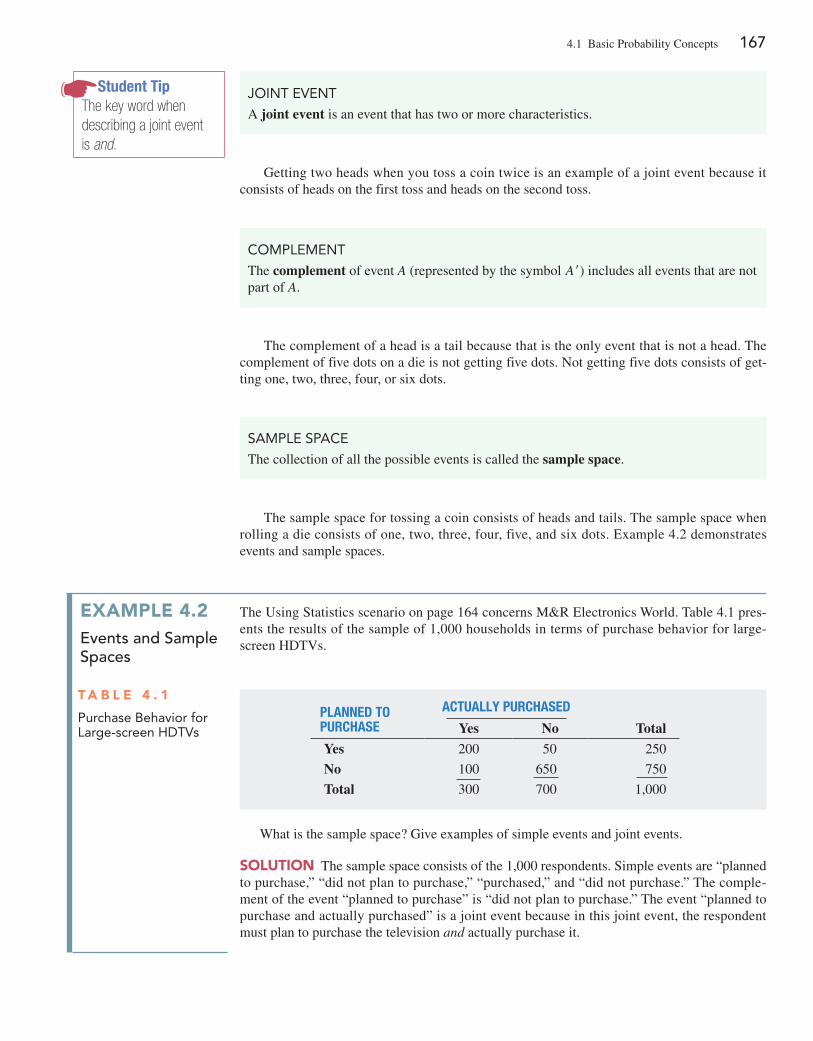
4.1 Basic Probability Concepts 167
Getting two heads when you toss a coin twice is an example of a joint event because it consists of heads on the first toss and heads on the second toss.
JoInT EvEnT
A joint event is an event that has two or more characteristics.
ComPLEmEnT
The complement of event A (represented by the symbol A′) includes all events that are not part of A.
SamPLE SPaCE
The collection of all the possible events is called the sample space.
The complement of a head is a tail because that is the only event that is not a head. The complement of five dots on a die is not getting five dots. Not getting five dots consists of get-ting one, two, three, four, or six dots.
The sample space for tossing a coin consists of heads and tails. The sample space when rolling a die consists of one, two, three, four, five, and six dots. Example 4.2 demonstrates events and sample spaces.
ExamplE 4.2Events and sample spaces
The Using Statistics scenario on page 164 concerns M&R Electronics World. Table 4.1 pres-ents the results of the sample of 1,000 households in terms of purchase behavior for large-screen HDTVs.
t a b l E 4 . 1
Purchase Behavior for Large-screen HDTvs
What is the sample space? Give examples of simple events and joint events.
Solution The sample space consists of the 1,000 respondents. Simple events are “planned to purchase,” “did not plan to purchase,” “purchased,” and “did not purchase.” The comple-ment of the event “planned to purchase” is “did not plan to purchase.” The event “planned to purchase and actually purchased” is a joint event because in this joint event, the respondent must plan to purchase the television and actually purchase it.
Planned To PurchaSe
acTually PurchaSed
Yes No Total
Yes 200 50 250
No 100 650 750
Total 300 700 1,000
Student TipThe key word when describing a joint event is and.
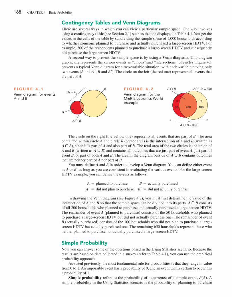
168 CHAPTER 4 Basic Probability
Contingency tables and Venn DiagramsThere are several ways in which you can view a particular sample space. One way involves using a contingency table (see Section 2.1) such as the one displayed in Table 4.1. You get the values in the cells of the table by subdividing the sample space of 1,000 households according to whether someone planned to purchase and actually purchased a large-screen HDTV. For example, 200 of the respondents planned to purchase a large-screen HDTV and subsequently did purchase the large-screen HDTV.
A second way to present the sample space is by using a Venn diagram. This diagram graphically represents the various events as “unions” and “intersections” of circles. Figure 4.1 presents a typical Venn diagram for a two-variable situation, with each variable having only two events (A and A′, B and B′). The circle on the left (the red one) represents all events that are part of A.
A
A
B
A B
BF i g u r E 4 . 1venn diagram for events a and B
A
A B A′ B ′ = 650
A B = 350
B
50 200 100
F i g u r E 4 . 2venn diagram for the m&R Electronics World example
The circle on the right (the yellow one) represents all events that are part of B. The area contained within circle A and circle B (center area) is the intersection of A and B (written as A ¨ B), since it is part of A and also part of B. The total area of the two circles is the union of A and B (written as A ∪ B) and contains all outcomes that are just part of event A, just part of event B, or part of both A and B. The area in the diagram outside of A ∪ B contains outcomes that are neither part of A nor part of B.
You must define A and B in order to develop a Venn diagram. You can define either event as A or B, as long as you are consistent in evaluating the various events. For the large-screen HDTV example, you can define the events as follows:
A = planned to purchase B = actually purchased
A′ = did not plan to purchase B′ = did not actually purchase
In drawing the Venn diagram (see Figure 4.2), you must first determine the value of the intersection of A and B so that the sample space can be divided into its parts. A ¨ B consists of all 200 households who planned to purchase and actually purchased a large-screen HDTV. The remainder of event A (planned to purchase) consists of the 50 households who planned to purchase a large-screen HDTV but did not actually purchase one. The remainder of event B (actually purchased) consists of the 100 households who did not plan to purchase a large-screen HDTV but actually purchased one. The remaining 650 households represent those who neither planned to purchase nor actually purchased a large-screen HDTV.
Simple probabilityNow you can answer some of the questions posed in the Using Statistics scenario. Because the results are based on data collected in a survey (refer to Table 4.1), you can use the empirical probability approach.
As stated previously, the most fundamental rule for probabilities is that they range in value from 0 to 1. An impossible event has a probability of 0, and an event that is certain to occur has a probability of 1.
Simple probability refers to the probability of occurrence of a simple event, P(A). A simple probability in the Using Statistics scenario is the probability of planning to purchase
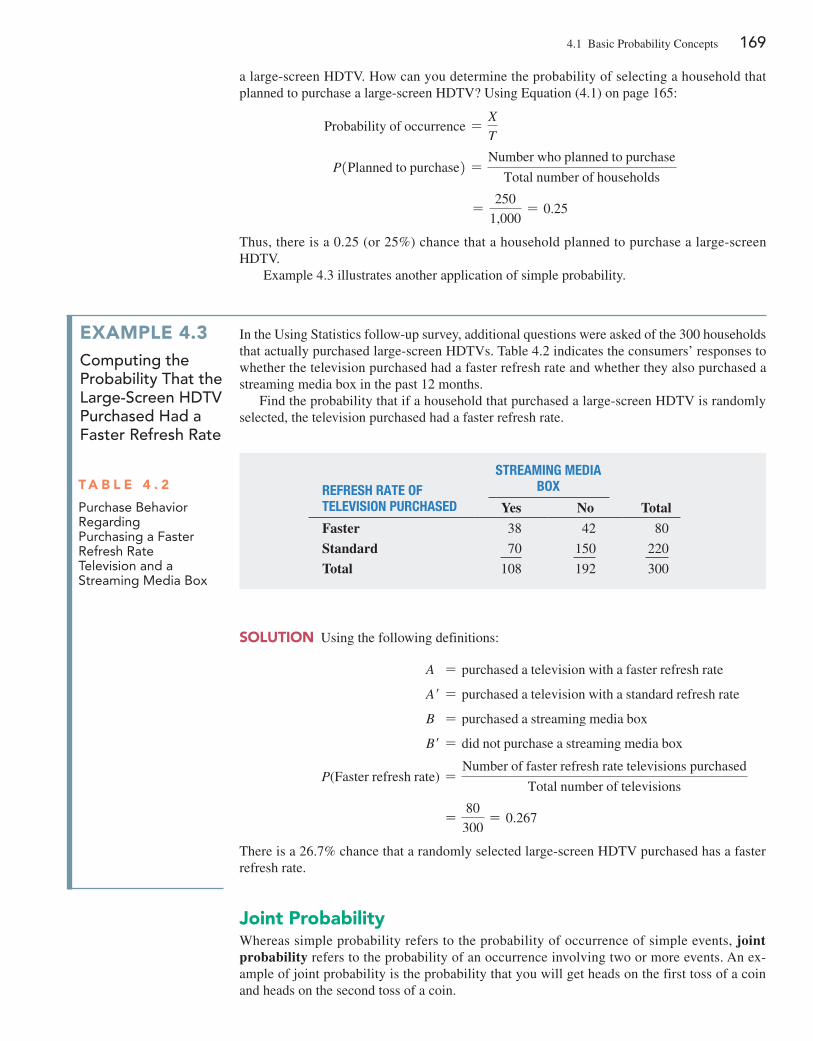
4.1 Basic Probability Concepts 169
a large-screen HDTV. How can you determine the probability of selecting a household that planned to purchase a large-screen HDTV? Using Equation (4.1) on page 165:
Probability of occurrence =X
T
P1Planned to purchase2 =Number who planned to purchase
Total number of households
=250
1,000= 0.25
Thus, there is a 0.25 (or 25%) chance that a household planned to purchase a large-screen HDTV.
Example 4.3 illustrates another application of simple probability.
ExamplE 4.3computing the Probability that the large-screen hDtV Purchased had a Faster Refresh Rate
In the Using Statistics follow-up survey, additional questions were asked of the 300 households that actually purchased large-screen HDTVs. Table 4.2 indicates the consumers’ responses to whether the television purchased had a faster refresh rate and whether they also purchased a streaming media box in the past 12 months.
Find the probability that if a household that purchased a large-screen HDTV is randomly selected, the television purchased had a faster refresh rate.
t a b l E 4 . 2
Purchase Behavior Regarding Purchasing a faster Refresh Rate Television and a Streaming media Box
Solution Using the following definitions:
A = purchased a television with a faster refresh rate
A′ = purchased a television with a standard refresh rate
B = purchased a streaming media box
B′ = did not purchase a streaming media box
P(Faster refresh rate) =Number of faster refresh rate televisions purchased
Total number of televisions
=80
300= 0.267
There is a 26.7% chance that a randomly selected large-screen HDTV purchased has a faster refresh rate.
refreSh raTe of TeleviSion PurchaSed
STreaming media Box
Yes No Total
Faster 38 42 80
Standard 70 150 220
Total 108 192 300
Joint probabilityWhereas simple probability refers to the probability of occurrence of simple events, joint probability refers to the probability of an occurrence involving two or more events. An ex-ample of joint probability is the probability that you will get heads on the first toss of a coin and heads on the second toss of a coin.
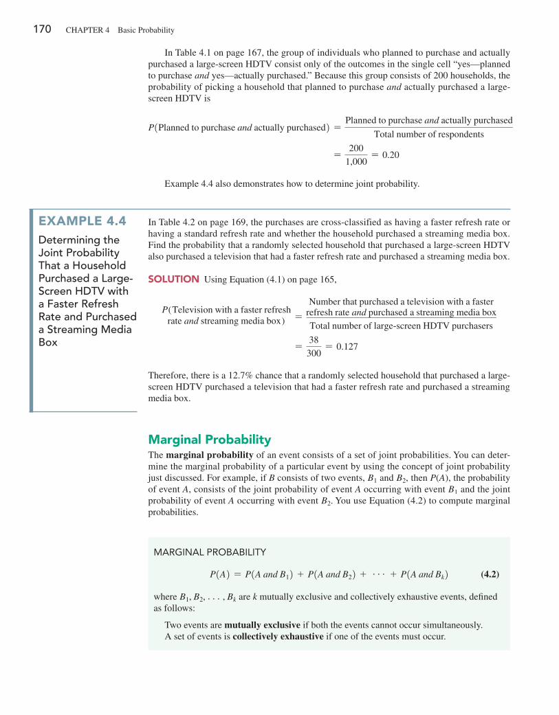
170 CHAPTER 4 Basic Probability
In Table 4.1 on page 167, the group of individuals who planned to purchase and actually purchased a large-screen HDTV consist only of the outcomes in the single cell “yes—planned to purchase and yes—actually purchased.” Because this group consists of 200 households, the probability of picking a household that planned to purchase and actually purchased a large-screen HDTV is
P1Planned to purchase and actually purchased2 =Planned to purchase and actually purchased
Total number of respondents
=200
1,000= 0.20
Example 4.4 also demonstrates how to determine joint probability.
ExamplE 4.4Determining the Joint Probability that a household Purchased a large-screen hDtV with a Faster Refresh Rate and Purchased a streaming Media box
In Table 4.2 on page 169, the purchases are cross-classified as having a faster refresh rate or having a standard refresh rate and whether the household purchased a streaming media box. Find the probability that a randomly selected household that purchased a large-screen HDTV also purchased a television that had a faster refresh rate and purchased a streaming media box.
Solution Using Equation (4.1) on page 165,
P(Television with a faster refreshrate and streaming media box)
=Number that purchased a television with a faster
refresh rate and purchased a streaming media box
Total number of large@screen HDTV purchasers
=38
300= 0.127
Therefore, there is a 12.7% chance that a randomly selected household that purchased a large-screen HDTV purchased a television that had a faster refresh rate and purchased a streaming media box.
marginal probabilityThe marginal probability of an event consists of a set of joint probabilities. You can deter-mine the marginal probability of a particular event by using the concept of joint probability just discussed. For example, if B consists of two events, B1 and B2, then P(A), the probability of event A, consists of the joint probability of event A occurring with event B1 and the joint probability of event A occurring with event B2. You use Equation (4.2) to compute marginal probabilities.
maRgInaL PRoBaBILITy
P1A2 = P1A and B12 + P1A and B22 + g + P1A and Bk2 (4.2)
where B1, B2, g, Bk are k mutually exclusive and collectively exhaustive events, defined as follows:
Two events are mutually exclusive if both the events cannot occur simultaneously.A set of events is collectively exhaustive if one of the events must occur.
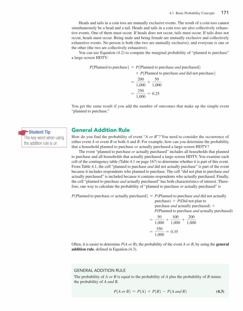
4.1 Basic Probability Concepts 171
Heads and tails in a coin toss are mutually exclusive events. The result of a coin toss cannot simultaneously be a head and a tail. Heads and tails in a coin toss are also collectively exhaus-tive events. One of them must occur. If heads does not occur, tails must occur. If tails does not occur, heads must occur. Being male and being female are mutually exclusive and collectively exhaustive events. No person is both (the two are mutually exclusive), and everyone is one or the other (the two are collectively exhaustive).
You can use Equation (4.2) to compute the marginal probability of “planned to purchase” a large-screen HDTV:
P1Planned to purchase2 = P1Planned to purchase and purchased2 + P1Planned to purchase and did not purchase2
=200
1,000+
50
1,000
=250
1,000= 0.25
You get the same result if you add the number of outcomes that make up the simple event “planned to purchase.”
general addition ruleHow do you find the probability of event “A or B”? You need to consider the occurrence of either event A or event B or both A and B. For example, how can you determine the probability that a household planned to purchase or actually purchased a large-screen HDTV?
The event “planned to purchase or actually purchased” includes all households that planned to purchase and all households that actually purchased a large-screen HDTV. You examine each cell of the contingency table (Table 4.1 on page 167) to determine whether it is part of this event. From Table 4.1, the cell “planned to purchase and did not actually purchase” is part of the event because it includes respondents who planned to purchase. The cell “did not plan to purchase and actually purchased” is included because it contains respondents who actually purchased. Finally, the cell “planned to purchase and actually purchased” has both characteristics of interest. There-fore, one way to calculate the probability of “planned to purchase or actually purchased” is
P1Planned to purchase or actually purchased2 = P (Planned to purchase and did not actually purchase) + P(Did not plan to purchase and actually purchased) + P(Planned to purchase and actually purchased)
=50
1,000+
100
1,000+
200
1,000
=350
1,000= 0.35
Often, it is easier to determine P(A or B), the probability of the event A or B, by using the general addition rule, defined in Equation (4.3).
Student TipThe key word when using the addition rule is or.
gEnERaL aDDITIon RULE
The probability of A or B is equal to the probability of A plus the probability of B minus the probability of A and B.
P1A or B2 = P1A2 + P1B2 - P1A and B2 (4.3)
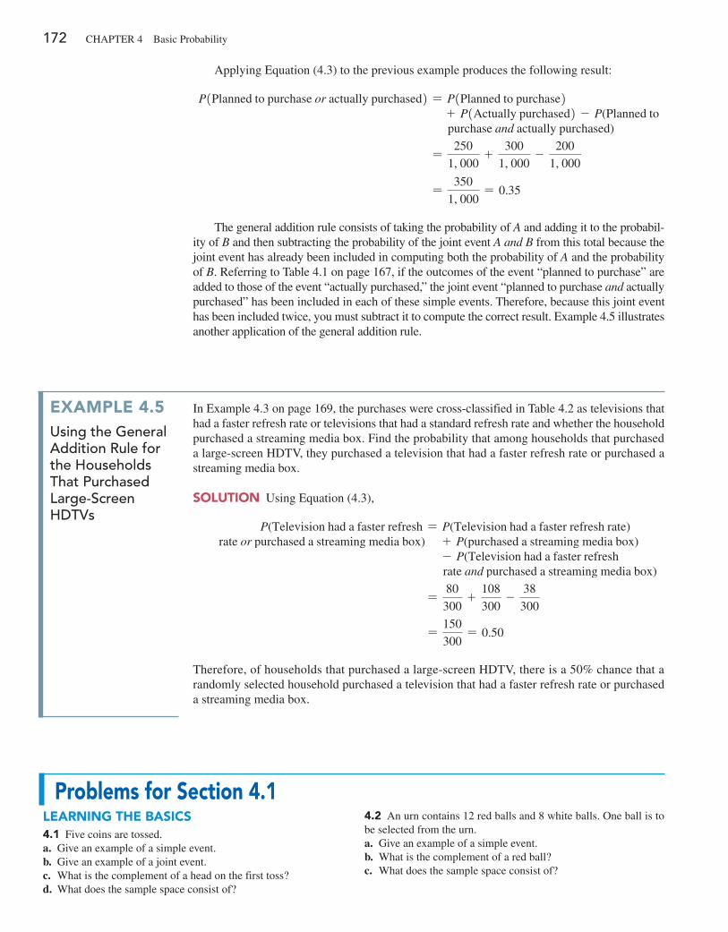
172 CHAPTER 4 Basic Probability
Applying Equation (4.3) to the previous example produces the following result:
P1Planned to purchase or actually purchased2 = P1Planned to purchase2 + P1Actually purchased2 - P(Planned to purchase and actually purchased)
=250
1, 000+
300
1, 000-
200
1, 000
=350
1, 000= 0.35
The general addition rule consists of taking the probability of A and adding it to the probabil-ity of B and then subtracting the probability of the joint event A and B from this total because the joint event has already been included in computing both the probability of A and the probability of B. Referring to Table 4.1 on page 167, if the outcomes of the event “planned to purchase” are added to those of the event “actually purchased,” the joint event “planned to purchase and actually purchased” has been included in each of these simple events. Therefore, because this joint event has been included twice, you must subtract it to compute the correct result. Example 4.5 illustrates another application of the general addition rule.
ExamplE 4.5Using the general addition Rule for the households that Purchased large-screen hDtVs
In Example 4.3 on page 169, the purchases were cross-classified in Table 4.2 as televisions that had a faster refresh rate or televisions that had a standard refresh rate and whether the household purchased a streaming media box. Find the probability that among households that purchased a large-screen HDTV, they purchased a television that had a faster refresh rate or purchased a streaming media box.
Solution Using Equation (4.3),
P(Television had a faster refresh = P(Television had a faster refresh rate) rate or purchased a streaming media box) + P(purchased a streaming media box)
- P(Television had a faster refresh rate and purchased a streaming media box)
=80
300+
108
300-
38
300
=150
300= 0.50
Therefore, of households that purchased a large-screen HDTV, there is a 50% chance that a randomly selected household purchased a television that had a faster refresh rate or purchased a streaming media box.
problems for Section 4.1lEarning thE baSiCS4.1 Five coins are tossed.a. Give an example of a simple event.b. Give an example of a joint event.c. What is the complement of a head on the first toss?d. What does the sample space consist of?
4.2 An urn contains 12 red balls and 8 white balls. One ball is to be selected from the urn.a. Give an example of a simple event.b. What is the complement of a red ball?c. What does the sample space consist of?
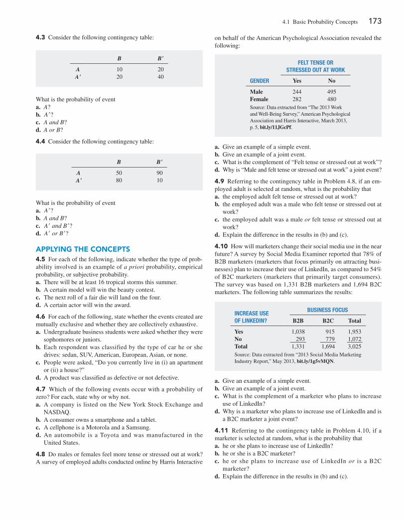
4.1 Basic Probability Concepts 173
4.3 Consider the following contingency table:
B B′
A 10 20A′ 20 40
What is the probability of eventa. A?b. A′?c. A and B?d. A or B?
4.4 Consider the following contingency table:
B B′
A 50 90A′ 80 10
What is the probability of eventa. A′?b. A and B?c. A′ and B′?d. A′ or B′?
applying thE ConCEptS4.5 For each of the following, indicate whether the type of prob-ability involved is an example of a priori probability, empirical probability, or subjective probability.a. There will be at least 16 tropical storms this summer.b. A certain model will win the beauty contest.c. The next roll of a fair die will land on the four.d. A certain actor will win the award.
4.6 For each of the following, state whether the events created are mutually exclusive and whether they are collectively exhaustive.a. Undergraduate business students were asked whether they were
sophomores or juniors.b. Each respondent was classified by the type of car he or she
drives: sedan, SUV, American, European, Asian, or none.c. People were asked, “Do you currently live in (i) an apartment
or (ii) a house?”d. A product was classified as defective or not defective.
4.7 Which of the following events occur with a probability of zero? For each, state why or why not.a. A company is listed on the New York Stock Exchange and
NASDAQ.b. A consumer owns a smartphone and a tablet.c. A cellphone is a Motorola and a Samsung.d. An automobile is a Toyota and was manufactured in the
United States.
4.8 Do males or females feel more tense or stressed out at work? A survey of employed adults conducted online by Harris Interactive
felT TenSe or STreSSed ouT aT Work
gender Yes No
Male 244 495Female 282 480Source: Data extracted from “The 2013 Work and Well-Being Survey,” American Psychological Association and Harris Interactive, March 2013, p. 5, bit.ly/11JGcPf.
a. Give an example of a simple event.b. Give an example of a joint event.c. What is the complement of “Felt tense or stressed out at work”?d. Why is “Male and felt tense or stressed out at work” a joint event?
4.9 Referring to the contingency table in Problem 4.8, if an em-ployed adult is selected at random, what is the probability thata. the employed adult felt tense or stressed out at work?b. the employed adult was a male who felt tense or stressed out at
work?c. the employed adult was a male or felt tense or stressed out at
work?d. Explain the difference in the results in (b) and (c).
4.10 How will marketers change their social media use in the near future? A survey by Social Media Examiner reported that 78% of B2B marketers (marketers that focus primarily on attracting busi-nesses) plan to increase their use of LinkedIn, as compared to 54% of B2C marketers (marketers that primarily target consumers). The survey was based on 1,331 B2B marketers and 1,694 B2C marketers. The following table summarizes the results:
increaSe uSe of linkedin?
BuSineSS focuS
B2B B2C Total
Yes 1,038 915 1,953No 293 779 1,072Total 1,331 1,694 3,025Source: Data extracted from “2013 Social Media Marketing Industry Report,” May 2013, bit.ly/1g5vMQN.
a. Give an example of a simple event.b. Give an example of a joint event.c. What is the complement of a marketer who plans to increase
use of LinkedIn?d. Why is a marketer who plans to increase use of LinkedIn and is
a B2C marketer a joint event?
4.11 Referring to the contingency table in Problem 4.10, if a marketer is selected at random, what is the probability thata. he or she plans to increase use of LinkedIn?b. he or she is a B2C marketer?c. he or she plans to increase use of LinkedIn or is a B2C
marketer?d. Explain the difference in the results in (b) and (c).
on behalf of the American Psychological Association revealed the following:
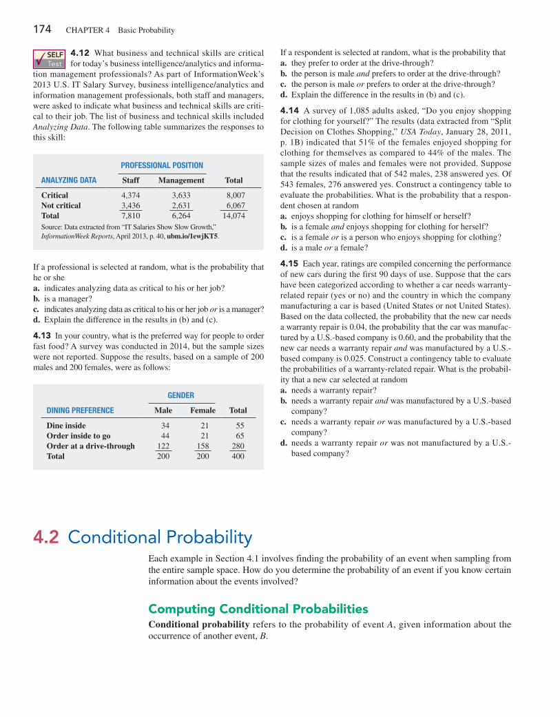
174 CHAPTER 4 Basic Probability
SELF Test
4.12 What business and technical skills are critical for today’s business intelligence/analytics and informa-
tion management professionals? As part of InformationWeek’s 2013 U.S. IT Salary Survey, business intelligence/analytics and information management professionals, both staff and managers, were asked to indicate what business and technical skills are criti-cal to their job. The list of business and technical skills included Analyzing Data. The following table summarizes the responses to this skill:
If a respondent is selected at random, what is the probability that a. they prefer to order at the drive-through?b. the person is male and prefers to order at the drive-through?c. the person is male or prefers to order at the drive-through?d. Explain the difference in the results in (b) and (c).
4.14 A survey of 1,085 adults asked, “Do you enjoy shopping for clothing for yourself?” The results (data extracted from “Split Decision on Clothes Shopping,” USA Today, January 28, 2011, p. 1B) indicated that 51% of the females enjoyed shopping for clothing for themselves as compared to 44% of the males. The sample sizes of males and females were not provided. Suppose that the results indicated that of 542 males, 238 answered yes. Of 543 females, 276 answered yes. Construct a contingency table to evaluate the probabilities. What is the probability that a respon-dent chosen at randoma. enjoys shopping for clothing for himself or herself?b. is a female and enjoys shopping for clothing for herself?c. is a female or is a person who enjoys shopping for clothing?d. is a male or a female?
4.15 Each year, ratings are compiled concerning the performance of new cars during the first 90 days of use. Suppose that the cars have been categorized according to whether a car needs warranty-related repair (yes or no) and the country in which the company manufacturing a car is based (United States or not United States). Based on the data collected, the probability that the new car needs a warranty repair is 0.04, the probability that the car was manufac-tured by a U.S.-based company is 0.60, and the probability that the new car needs a warranty repair and was manufactured by a U.S.-based company is 0.025. Construct a contingency table to evaluate the probabilities of a warranty-related repair. What is the probabil-ity that a new car selected at randoma. needs a warranty repair?b. needs a warranty repair and was manufactured by a U.S.-based
company?c. needs a warranty repair or was manufactured by a U.S.-based
company?d. needs a warranty repair or was not manufactured by a U.S.-
based company?
analyzing daTa
ProfeSSional PoSiTion
Staff Management Total
Critical 4,374 3,633 8,007Not critical 3,436 2,631 6,067Total 7,810 6,264 14,074Source: Data extracted from “IT Salaries Show Slow Growth,” InformationWeek Reports, April 2013, p. 40, ubm.io/1ewjKT5.
If a professional is selected at random, what is the probability that he or shea. indicates analyzing data as critical to his or her job?b. is a manager?c. indicates analyzing data as critical to his or her job or is a manager?d. Explain the difference in the results in (b) and (c).
4.13 In your country, what is the preferred way for people to order fast food? A survey was conducted in 2014, but the sample sizes were not reported. Suppose the results, based on a sample of 200 males and 200 females, were as follows:
gender
dining Preference Male Female Total
Dine inside 34 21 55Order inside to go 44 21 65Order at a drive-through 122 158 280Total 200 200 400
4.2 Conditional ProbabilityEach example in Section 4.1 involves finding the probability of an event when sampling from the entire sample space. How do you determine the probability of an event if you know certain information about the events involved?
Computing Conditional probabilitiesConditional probability refers to the probability of event A, given information about the occurrence of another event, B.
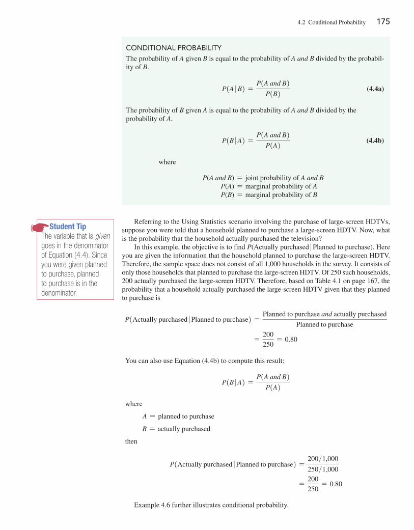
4.2 Conditional Probability 175
Referring to the Using Statistics scenario involving the purchase of large-screen HDTVs, suppose you were told that a household planned to purchase a large-screen HDTV. Now, what is the probability that the household actually purchased the television?
In this example, the objective is to find P(Actually purchased � Planned to purchase). Here you are given the information that the household planned to purchase the large-screen HDTV. Therefore, the sample space does not consist of all 1,000 households in the survey. It consists of only those households that planned to purchase the large-screen HDTV. Of 250 such households, 200 actually purchased the large-screen HDTV. Therefore, based on Table 4.1 on page 167, the probability that a household actually purchased the large-screen HDTV given that they planned to purchase is
P1Actually purchased � Planned to purchase2 =Planned to purchase and actually purchased
Planned to purchase
=200
250= 0.80
You can also use Equation (4.4b) to compute this result:
P1B � A2 =P1A and B2
P1A2
where
A = planned to purchase
B = actually purchased
then
P1Actually purchased � Planned to purchase2 =200>1,000
250>1,000
=200
250= 0.80
Example 4.6 further illustrates conditional probability.
Student TipThe variable that is given goes in the denominator of Equation (4.4). Since you were given planned to purchase, planned to purchase is in the denominator.
ConDITIonaL PRoBaBILITy
The probability of A given B is equal to the probability of A and B divided by the probabil-ity of B.
P1A � B2 =P1A and B2
P1B2 (4.4a)
The probability of B given A is equal to the probability of A and B divided by the probability of A.
P1B � A2 =P1A and B2
P1A2 (4.4b)
where
P(A and B) = joint probability of A and B P(A) = marginal probability of A P(B) = marginal probability of B
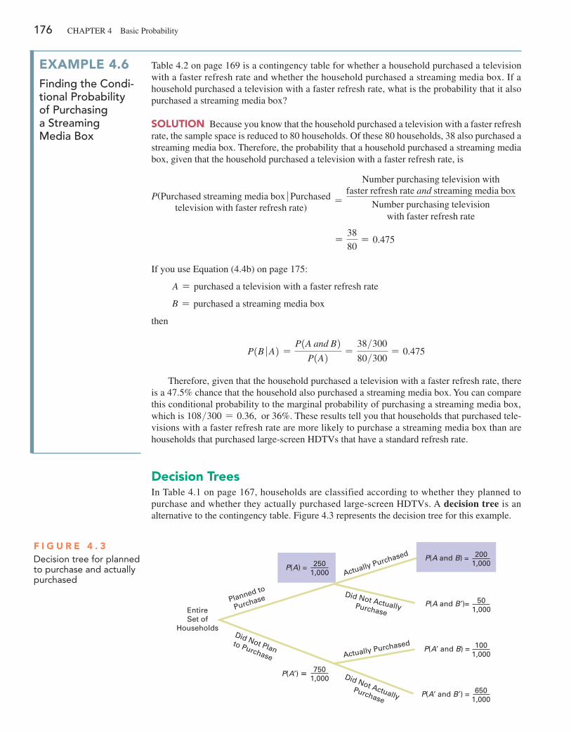
176 CHAPTER 4 Basic Probability
Decision treesIn Table 4.1 on page 167, households are classified according to whether they planned to purchase and whether they actually purchased large-screen HDTVs. A decision tree is an alternative to the contingency table. Figure 4.3 represents the decision tree for this example.
ExamplE 4.6Finding the condi-tional Probability of Purchasing a streaming Media box
Table 4.2 on page 169 is a contingency table for whether a household purchased a television with a faster refresh rate and whether the household purchased a streaming media box. If a household purchased a television with a faster refresh rate, what is the probability that it also purchased a streaming media box?
Solution Because you know that the household purchased a television with a faster refresh rate, the sample space is reduced to 80 households. Of these 80 households, 38 also purchased a streaming media box. Therefore, the probability that a household purchased a streaming media box, given that the household purchased a television with a faster refresh rate, is
P(Purchased streaming media box � Purchasedtelevision with faster refresh rate)
=
Number purchasing television withfaster refresh rate and streaming media box
Number purchasing televisionwith faster refresh rate
=38
80= 0.475
If you use Equation (4.4b) on page 175:
A = purchased a television with a faster refresh rate
B = purchased a streaming media box
then
P1B � A2 =P1A and B2
P1A2 =38>300
80>300= 0.475
Therefore, given that the household purchased a television with a faster refresh rate, there is a 47.5% chance that the household also purchased a streaming media box. You can compare this conditional probability to the marginal probability of purchasing a streaming media box, which is 108>300 = 0.36, or 36%. These results tell you that households that purchased tele-visions with a faster refresh rate are more likely to purchase a streaming media box than are households that purchased large-screen HDTVs that have a standard refresh rate.
F i g u r E 4 . 3Decision tree for planned to purchase and actually purchased
EntireSet of
Households
Planned to
Purchase
Did Not Planto Purchase
Actually Purchased
Actually Purchased
Did Not ActuallyPurchase
Did Not ActuallyPurchase
P(A′) 5 750 1,000
P(A and B ′)= 501,000
P(A′ and B) = 1001,000
P(A′ and B ′) = 6501,000
P(A) = 250 1,000
P(A and B) = 2001,000
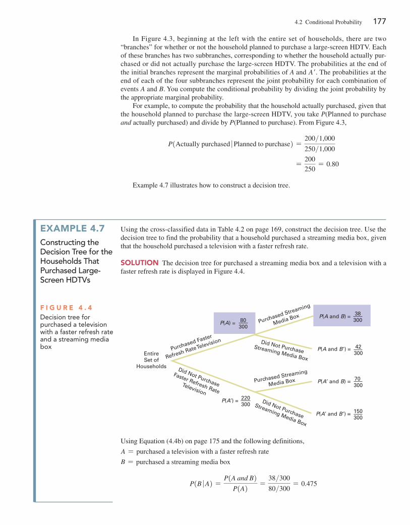
4.2 Conditional Probability 177
In Figure 4.3, beginning at the left with the entire set of households, there are two “branches” for whether or not the household planned to purchase a large-screen HDTV. Each of these branches has two subbranches, corresponding to whether the household actually pur-chased or did not actually purchase the large-screen HDTV. The probabilities at the end of the initial branches represent the marginal probabilities of A and A′. The probabilities at the end of each of the four subbranches represent the joint probability for each combination of events A and B. You compute the conditional probability by dividing the joint probability by the appropriate marginal probability.
For example, to compute the probability that the household actually purchased, given that the household planned to purchase the large-screen HDTV, you take P(Planned to purchase and actually purchased) and divide by P(Planned to purchase). From Figure 4.3,
P1Actually purchased � Planned to purchase2 =200>1,000
250>1,000
=200
250= 0.80
Example 4.7 illustrates how to construct a decision tree.
ExamplE 4.7constructing the Decision tree for the households that Purchased large-screen hDtVs
Using the cross-classified data in Table 4.2 on page 169, construct the decision tree. Use the decision tree to find the probability that a household purchased a streaming media box, given that the household purchased a television with a faster refresh rate.
Solution The decision tree for purchased a streaming media box and a television with a faster refresh rate is displayed in Figure 4.4.
F i g u r E 4 . 4Decision tree for purchased a television with a faster refresh rate and a streaming media box
EntireSet of
Households
Purchased Faster
Refresh Rate Television
Did Not Purchase
Faster Refresh RateTelevision
Purchased Streaming
Media Box
Purchased Streaming
Media Box
Did Not PurchaseStreaming Media Box
Did Not Purchase
Streaming Media Box
P(A′) = 220300
P(A and B ′) = 42 300
P(A′ and B) = 70 300
P(A′ and B ′) = 150 300
P(A) = 80300
P(A and B) = 38 300
Using Equation (4.4b) on page 175 and the following definitions,
A = purchased a television with a faster refresh rate
B = purchased a streaming media box
P1B � A2 =P1A and B2
P1A2 =38>300
80>300= 0.475
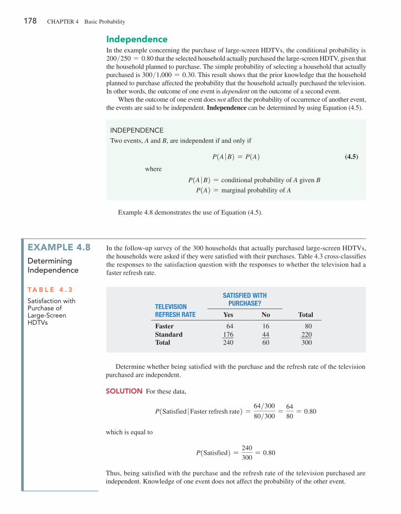
178 CHAPTER 4 Basic Probability
independenceIn the example concerning the purchase of large-screen HDTVs, the conditional probability is 200>250 = 0.80 that the selected household actually purchased the large-screen HDTV, given that the household planned to purchase. The simple probability of selecting a household that actually purchased is 300>1,000 = 0.30. This result shows that the prior knowledge that the household planned to purchase affected the probability that the household actually purchased the television. In other words, the outcome of one event is dependent on the outcome of a second event.
When the outcome of one event does not affect the probability of occurrence of another event, the events are said to be independent. Independence can be determined by using Equation (4.5).
InDEPEnDEnCE
Two events, A and B, are independent if and only if
P1A � B2 = P1A2 (4.5)
where
P1A � B2 = conditional probability of A given B
P1A2 = marginal probability of A
Example 4.8 demonstrates the use of Equation (4.5).
ExamplE 4.8Determining independence
In the follow-up survey of the 300 households that actually purchased large-screen HDTVs, the households were asked if they were satisfied with their purchases. Table 4.3 cross-classifies the responses to the satisfaction question with the responses to whether the television had a faster refresh rate.
t a b l E 4 . 3
Satisfaction with Purchase of Large-Screen HDTvs
TeleviSion refreSh raTe
SaTiSfied WiTh PurchaSe?
Yes No Total
Faster 64 16 80Standard 176 44 220Total 240 60 300
Determine whether being satisfied with the purchase and the refresh rate of the television purchased are independent.
Solution For these data,
P1Satisfied � Faster refresh rate2 =64>300
80>300=
64
80= 0.80
which is equal to
P1Satisfied2 =240
300= 0.80
Thus, being satisfied with the purchase and the refresh rate of the television purchased are independent. Knowledge of one event does not affect the probability of the other event.
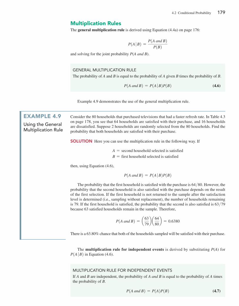
4.2 Conditional Probability 179
multiplication rulesThe general multiplication rule is derived using Equation (4.4a) on page 176:
P1A � B2 =P1A and B2
P1B2and solving for the joint probability P(A and B).
gEnERaL mULTIPLICaTIon RULE
The probability of A and B is equal to the probability of A given B times the probability of B.
P1A and B2 = P1A � B2P1B2 (4.6)
mULTIPLICaTIon RULE foR InDEPEnDEnT EvEnTS
If A and B are independent, the probability of A and B is equal to the probability of A times the probability of B.
P1A and B2 = P1A2P1B2 (4.7)
ExamplE 4.9Using the general Multiplication Rule
Consider the 80 households that purchased televisions that had a faster refresh rate. In Table 4.3 on page 178, you see that 64 households are satisfied with their purchase, and 16 households are dissatisfied. Suppose 2 households are randomly selected from the 80 households. Find the probability that both households are satisfied with their purchase.
Solution Here you can use the multiplication rule in the following way. If
A = second household selected is satisfied
B = first household selected is satisfied
then, using Equation (4.6),
P1A and B2 = P1A � B2P1B2
The probability that the first household is satisfied with the purchase is 64>80. However, the probability that the second household is also satisfied with the purchase depends on the result of the first selection. If the first household is not returned to the sample after the satisfaction level is determined (i.e., sampling without replacement), the number of households remaining is 79. If the first household is satisfied, the probability that the second is also satisfied is 63>79 because 63 satisfied households remain in the sample. Therefore,
P1A and B2 = a 63
79b a 64
80b = 0.6380
There is a 63.80% chance that both of the households sampled will be satisfied with their purchase.
Example 4.9 demonstrates the use of the general multiplication rule.
The multiplication rule for independent events is derived by substituting P(A) for P1A � B2 in Equation (4.6).
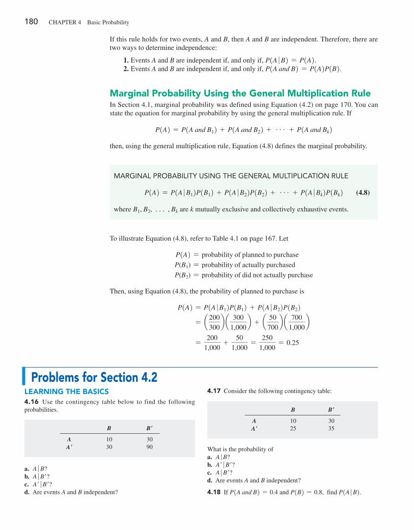
180 CHAPTER 4 Basic Probability
If this rule holds for two events, A and B, then A and B are independent. Therefore, there are two ways to determine independence:
1. Events A and B are independent if, and only if, P1A � B2 = P1A2. 2. Events A and B are independent if, and only if, P1A and B2 = P1A2P1B2.
marginal probability using the general multiplication ruleIn Section 4.1, marginal probability was defined using Equation (4.2) on page 170. You can state the equation for marginal probability by using the general multiplication rule. If
P1A2 = P1A and B12 + P1A and B22 + g + P1A and Bk2
then, using the general multiplication rule, Equation (4.8) defines the marginal probability.
maRgInaL PRoBaBILITy USIng THE gEnERaL mULTIPLICaTIon RULE
P1A2 = P1A � B12P1B12 + P1A � B22P1B22 + g + P1A � Bk2P1Bk2 (4.8)
where B1, B2, c , Bk are k mutually exclusive and collectively exhaustive events.
To illustrate Equation (4.8), refer to Table 4.1 on page 167. Let
P1A2 = probability of planned to purchase
P(B1) = probability of actually purchased
P(B2) = probability of did not actually purchase
Then, using Equation (4.8), the probability of planned to purchase is
P1A2 = P1A � B12P1B12 + P1A � B22P1B22 = a 200
300b a 300
1,000b + a 50
700b a 700
1,000b
=200
1,000+
50
1,000=
250
1,000= 0.25
problems for Section 4.2lEarning thE baSiCS4.16 Use the contingency table below to find the following probabilities.
4.17 Consider the following contingency table:
B B′
A 10 30A′ 30 90
a. A � B?b. A � B′?c. A′ � B′?d. Are events A and B independent?
B B′
A 10 30A′ 25 35
What is the probability ofa. A � B?b. A′ � B′?c. A � B′?d. Are events A and B independent?
4.18 If P1A and B2 = 0.4 and P1B2 = 0.8, find P1A � B2.
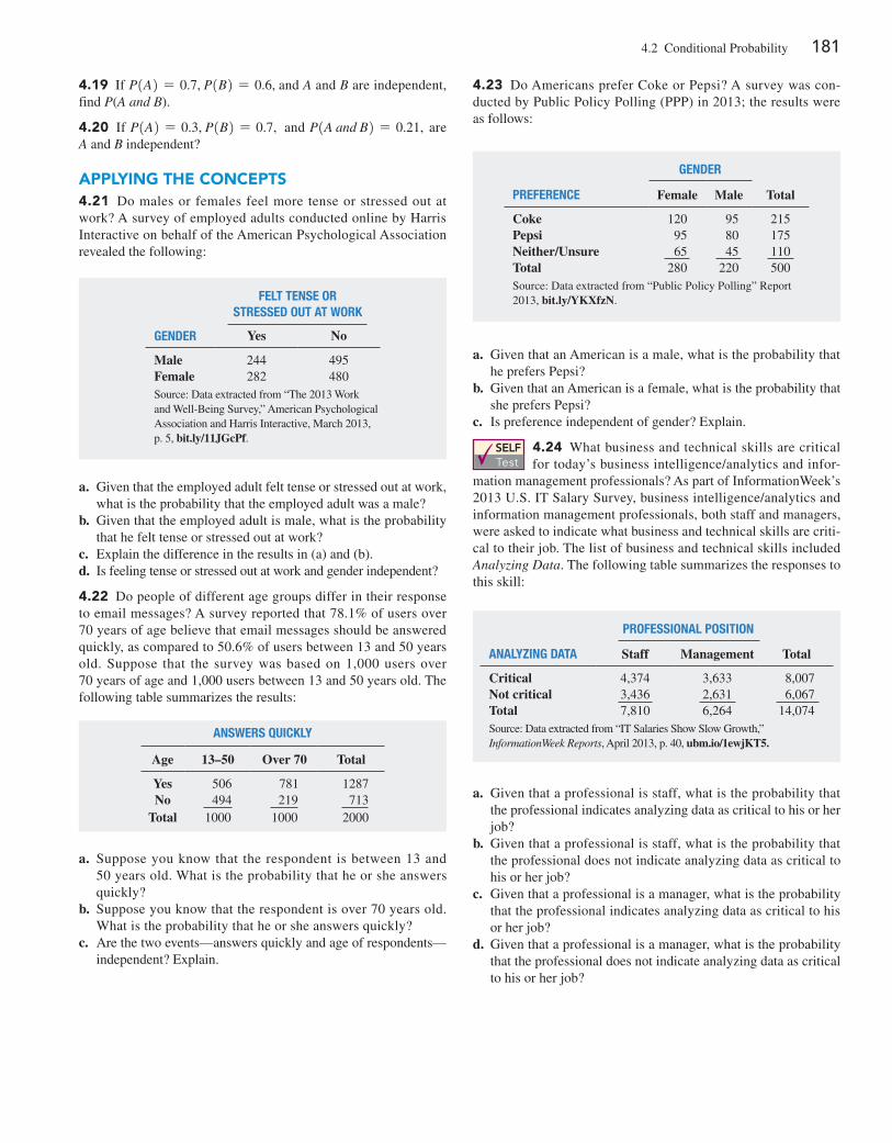
4.2 Conditional Probability 181
4.19 If P1A2 = 0.7, P1B2 = 0.6, and A and B are independent, find P(A and B).
4.20 If P1A2 = 0.3, P1B2 = 0.7, and P1A and B2 = 0.21, are A and B independent?
applying thE ConCEptS4.21 Do males or females feel more tense or stressed out at work? A survey of employed adults conducted online by Harris Interactive on behalf of the American Psychological Association revealed the following:
4.23 Do Americans prefer Coke or Pepsi? A survey was con-ducted by Public Policy Polling (PPP) in 2013; the results were as follows:
felT TenSe or STreSSed ouT aT Work
gender Yes No
Male 244 495Female 282 480Source: Data extracted from “The 2013 Work and Well-Being Survey,” American Psychological Association and Harris Interactive, March 2013, p. 5, bit.ly/11JGcPf.
a. Given that the employed adult felt tense or stressed out at work, what is the probability that the employed adult was a male?
b. Given that the employed adult is male, what is the probability that he felt tense or stressed out at work?
c. Explain the difference in the results in (a) and (b).d. Is feeling tense or stressed out at work and gender independent?
4.22 Do people of different age groups differ in their response to email messages? A survey reported that 78.1% of users over 70 years of age believe that email messages should be answered quickly, as compared to 50.6% of users between 13 and 50 years old. Suppose that the survey was based on 1,000 users over 70 years of age and 1,000 users between 13 and 50 years old. The following table summarizes the results:
anSWerS Quickly
Age 13–50 Over 70 Total
Yes 506 781 1287No 494 219 713
Total 1000 1000 2000
a. Suppose you know that the respondent is between 13 and 50 years old. What is the probability that he or she answers quickly?
b. Suppose you know that the respondent is over 70 years old. What is the probability that he or she answers quickly?
c. Are the two events—answers quickly and age of respondents—independent? Explain.
gender
Preference Female Male Total
Coke 120 95 215Pepsi 95 80 175Neither/Unsure 65 45 110Total 280 220 500Source: Data extracted from “Public Policy Polling” Report 2013, bit.ly/YKXfzN.
a. Given that an American is a male, what is the probability that he prefers Pepsi?
b. Given that an American is a female, what is the probability that she prefers Pepsi?
c. Is preference independent of gender? Explain.
SELF Test
4.24 What business and technical skills are critical for today’s business intelligence/analytics and infor-
mation management professionals? As part of InformationWeek’s 2013 U.S. IT Salary Survey, business intelligence/analytics and information management professionals, both staff and managers, were asked to indicate what business and technical skills are criti-cal to their job. The list of business and technical skills included Analyzing Data. The following table summarizes the responses to this skill:
analyzing daTa
ProfeSSional PoSiTion
Staff Management Total
Critical 4,374 3,633 8,007Not critical 3,436 2,631 6,067Total 7,810 6,264 14,074Source: Data extracted from “IT Salaries Show Slow Growth,” InformationWeek Reports, April 2013, p. 40, ubm.io/1ewjKT5.
a. Given that a professional is staff, what is the probability that the professional indicates analyzing data as critical to his or her job?
b. Given that a professional is staff, what is the probability that the professional does not indicate analyzing data as critical to his or her job?
c. Given that a professional is a manager, what is the probability that the professional indicates analyzing data as critical to his or her job?
d. Given that a professional is a manager, what is the probability that the professional does not indicate analyzing data as critical to his or her job?
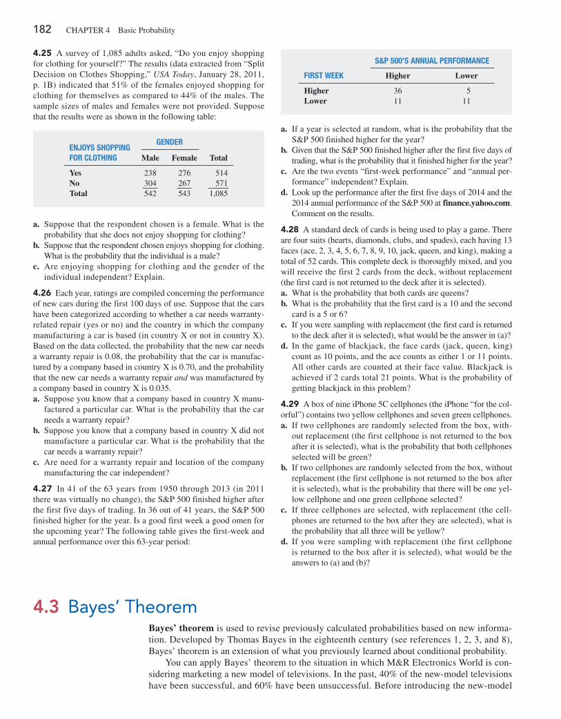
182 CHAPTER 4 Basic Probability
4.25 A survey of 1,085 adults asked, “Do you enjoy shopping for clothing for yourself?” The results (data extracted from “Split Decision on Clothes Shopping,” USA Today, January 28, 2011, p. 1B) indicated that 51% of the females enjoyed shopping for clothing for themselves as compared to 44% of the males. The sample sizes of males and females were not provided. Suppose that the results were as shown in the following table:
a. If a year is selected at random, what is the probability that the S&P 500 finished higher for the year?
b. Given that the S&P 500 finished higher after the first five days of trading, what is the probability that it finished higher for the year?
c. Are the two events “first-week performance” and “annual per-formance” independent? Explain.
d. Look up the performance after the first five days of 2014 and the 2014 annual performance of the S&P 500 at finance.yahoo.com. Comment on the results.
4.28 A standard deck of cards is being used to play a game. There are four suits (hearts, diamonds, clubs, and spades), each having 13 faces (ace, 2, 3, 4, 5, 6, 7, 8, 9, 10, jack, queen, and king), making a total of 52 cards. This complete deck is thoroughly mixed, and you will receive the first 2 cards from the deck, without replacement (the first card is not returned to the deck after it is selected).a. What is the probability that both cards are queens?b. What is the probability that the first card is a 10 and the second
card is a 5 or 6?c. If you were sampling with replacement (the first card is returned
to the deck after it is selected), what would be the answer in (a)?d. In the game of blackjack, the face cards (jack, queen, king)
count as 10 points, and the ace counts as either 1 or 11 points. All other cards are counted at their face value. Blackjack is achieved if 2 cards total 21 points. What is the probability of getting blackjack in this problem?
4.29 A box of nine iPhone 5C cellphones (the iPhone “for the col-orful”) contains two yellow cellphones and seven green cellphones.a. If two cellphones are randomly selected from the box, with-
out replacement (the first cellphone is not returned to the box after it is selected), what is the probability that both cellphones selected will be green?
b. If two cellphones are randomly selected from the box, without replacement (the first cellphone is not returned to the box after it is selected), what is the probability that there will be one yel-low cellphone and one green cellphone selected?
c. If three cellphones are selected, with replacement (the cell-phones are returned to the box after they are selected), what is the probability that all three will be yellow?
d. If you were sampling with replacement (the first cellphone is returned to the box after it is selected), what would be the answers to (a) and (b)?
enjoyS ShoPPing for cloThing
gender
Male Female Total
Yes 238 276 514No 304 267 571Total 542 543 1,085
a. Suppose that the respondent chosen is a female. What is the probability that she does not enjoy shopping for clothing?
b. Suppose that the respondent chosen enjoys shopping for clothing. What is the probability that the individual is a male?
c. Are enjoying shopping for clothing and the gender of the individual independent? Explain.
4.26 Each year, ratings are compiled concerning the performance of new cars during the first 100 days of use. Suppose that the cars have been categorized according to whether a car needs warranty-related repair (yes or no) and the country in which the company manufacturing a car is based (in country X or not in country X). Based on the data collected, the probability that the new car needs a warranty repair is 0.08, the probability that the car is manufac-tured by a company based in country X is 0.70, and the probability that the new car needs a warranty repair and was manufactured by a company based in country X is 0.035.a. Suppose you know that a company based in country X manu-
factured a particular car. What is the probability that the car needs a warranty repair?
b. Suppose you know that a company based in country X did not manufacture a particular car. What is the probability that the car needs a warranty repair?
c. Are need for a warranty repair and location of the company manufacturing the car independent?
4.27 In 41 of the 63 years from 1950 through 2013 (in 2011 there was virtually no change), the S&P 500 finished higher after the first five days of trading. In 36 out of 41 years, the S&P 500 finished higher for the year. Is a good first week a good omen for the upcoming year? The following table gives the first-week and annual performance over this 63-year period:
firST Week
S&P 500’S annual Performance
Higher Lower
Higher 36 5Lower 11 11
4.3 Bayes’ TheoremBayes’ theorem is used to revise previously calculated probabilities based on new informa-tion. Developed by Thomas Bayes in the eighteenth century (see references 1, 2, 3, and 8), Bayes’ theorem is an extension of what you previously learned about conditional probability.
You can apply Bayes’ theorem to the situation in which M&R Electronics World is con-sidering marketing a new model of televisions. In the past, 40% of the new-model televisions have been successful, and 60% have been unsuccessful. Before introducing the new-model
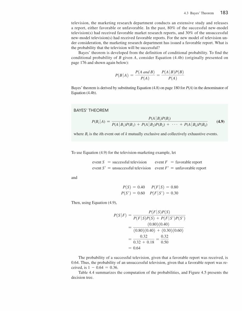
4.3 Bayes’ Theorem 183
television, the marketing research department conducts an extensive study and releases a report, either favorable or unfavorable. In the past, 80% of the successful new-model television(s) had received favorable market research reports, and 30% of the unsuccessful new-model television(s) had received favorable reports. For the new model of television un-der consideration, the marketing research department has issued a favorable report. What is the probability that the television will be successful?
Bayes’ theorem is developed from the definition of conditional probability. To find the conditional probability of B given A, consider Equation (4.4b) (originally presented on page 176 and shown again below):
P1B � A2 =P1A and B2
P1A2 =P1A � B2P1B2
P1A2
Bayes’ theorem is derived by substituting Equation (4.8) on page 180 for P(A) in the denominator of Equation (4.4b).
BayES’ THEoREm
P(Bi � A) =P(A � Bi)P(Bi)
P(A � B1)P(B1) + P(A � B2)P(B2) + g + P(A � Bk)P(Bk) (4.9)
where Bi is the ith event out of k mutually exclusive and collectively exhaustive events.
To use Equation (4.9) for the television-marketing example, let
event S = successful television event F = favorable report
event S′ = unsuccessful television event F′ = unfavorable report
and
P1S2 = 0.40 P1F � S2 = 0.80
P1S′2 = 0.60 P1F � S′2 = 0.30
Then, using Equation (4.9),
P1S � F2 =P1F � S2P1S2
P1F � S2P1S2 + P1F � S′2P1S′2 =
10.80210.40210.80210.402 + 10.30210.602
=0.32
0.32 + 0.18=
0.32
0.50
= 0.64
The probability of a successful television, given that a favorable report was received, is 0.64. Thus, the probability of an unsuccessful television, given that a favorable report was re-ceived, is 1 - 0.64 = 0.36.
Table 4.4 summarizes the computation of the probabilities, and Figure 4.5 presents the decision tree.
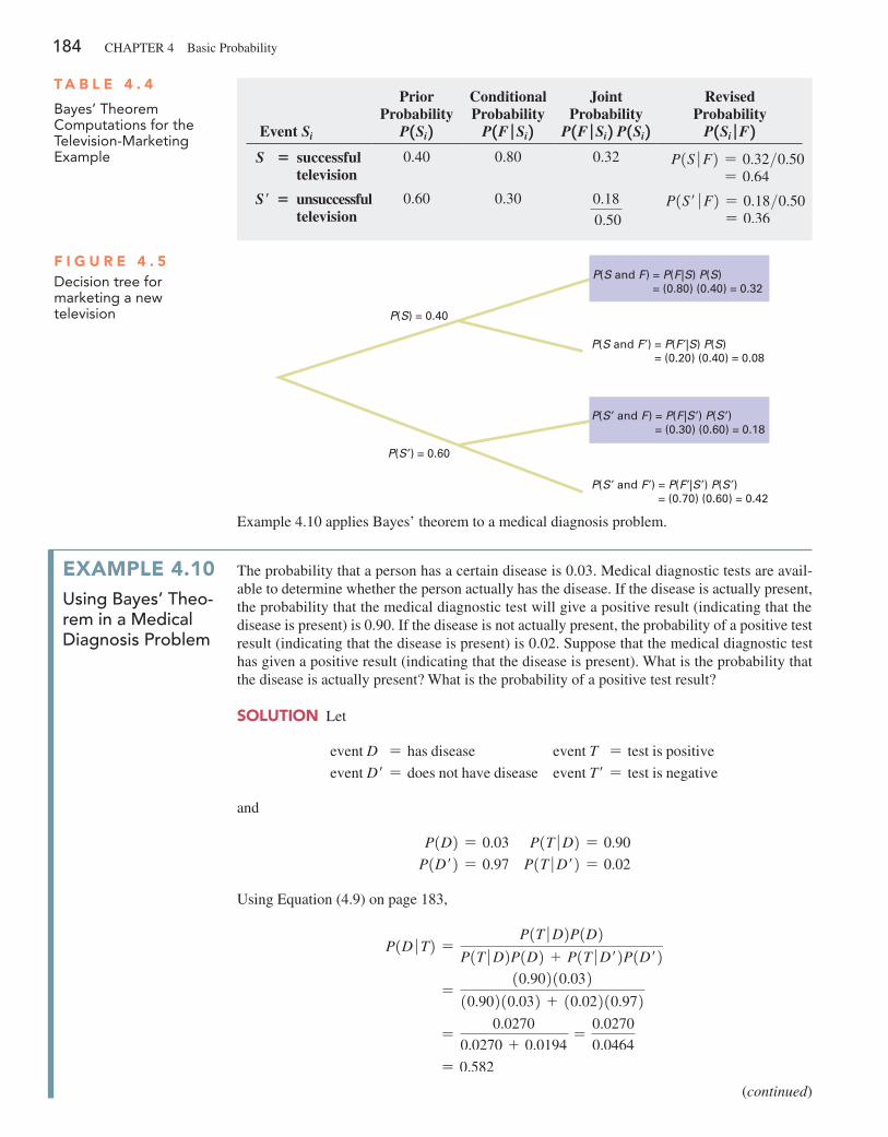
184 CHAPTER 4 Basic Probability
t a b l E 4 . 4
Bayes’ Theorem Computations for the Television-marketing Example
Event Si
Prior Probability
P 1Si 2Conditional Probability
P 1F ∣ Si 2Joint
Probability P 1F ∣ Si 2 P 1Si 2
Revised Probability
P 1Si ∣ F 2S = successful
television0.40 0.80 0.32 P1S � F2 = 0.32>0.50
= 0.64
S′ = unsuccessful television
0.60 0.30 0.18
0.50 P1S′ � F2 = 0.18>0.50
= 0.36
F i g u r E 4 . 5Decision tree for marketing a new television P(S) = 0.40
P(S ′) = 0.60
P(S ′ and F ′) = P(F ′|S ′) P(S ′) = (0.70) (0.60) = 0.42
P(S and F ′) = P(F ′|S) P(S) = (0.20) (0.40) = 0.08
P(S ′ and F) = P(F|S ′) P(S ′) = (0.30) (0.60) = 0.18
P(S and F) = P(F|S) P(S) = (0.80) (0.40) = 0.32
ExamplE 4.10Using bayes’ theo-rem in a Medical Diagnosis Problem
The probability that a person has a certain disease is 0.03. Medical diagnostic tests are avail-able to determine whether the person actually has the disease. If the disease is actually present, the probability that the medical diagnostic test will give a positive result (indicating that the disease is present) is 0.90. If the disease is not actually present, the probability of a positive test result (indicating that the disease is present) is 0.02. Suppose that the medical diagnostic test has given a positive result (indicating that the disease is present). What is the probability that the disease is actually present? What is the probability of a positive test result?
Solution Let
event D = has disease event T = test is positive
event D′ = does not have disease event T′ = test is negative
and
P1D2 = 0.03 P1T � D2 = 0.90
P1D′2 = 0.97 P1T � D′2 = 0.02
Using Equation (4.9) on page 183,
P1D � T2 =P1T � D2P1D2
P1T � D2P1D2 + P1T � D′2P1D′2 =
10.90210.03210.90210.032 + 10.02210.972
=0.0270
0.0270 + 0.0194=
0.0270
0.0464
= 0.582
Example 4.10 applies Bayes’ theorem to a medical diagnosis problem.
(continued)
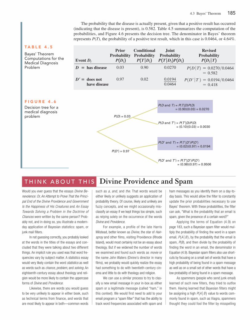
4.3 Bayes’ Theorem 185
The probability that the disease is actually present, given that a positive result has occurred (indicating that the disease is present), is 0.582. Table 4.5 summarizes the computation of the probabilities, and Figure 4.6 presents the decision tree. The denominator in Bayes’ theorem represents P(T), the probability of a positive test result, which in this case is 0.0464, or 4.64%.
t a b l E 4 . 5
Bayes’ Theorem Computations for the medical Diagnosis Problem
Event Di
Prior Probability
P 1Di 2Conditional Probability
P 1T ∣ Di 2Joint
Probability P 1T ∣ Di 2P 1Di 2
Revised Probability
P 1Di ∣ T 2D = has disease 0.03 0.90 0.0270 P1D � T2 = 0.0270>0.0464
= 0.582
D′ = does not have disease
0.97 0.02 0.01940.0464
P1D′ � T 2 = 0.0194>0.0464 = 0.418
F i g u r E 4 . 6Decision tree for a medical diagnosis problem P(D) = 0.03
P(D ′) = 0.97
P(D and T ′) = P(T ′|D)P(D)= (0.10)(0.03) = 0.0030
P(D ′ and T ) = P(T |D ′)P(D ′)= (0.02)(0.97) = 0.0194
P(D ′ and T ′) = P(T ′|D ′)P(D ′)= (0.98)(0.97) = 0.9506
P(D and T ) = P(T |D)P(D)= (0.90)(0.03) = 0.0270
t h i n k a b o U t t h i s Divine Providence and SpamWould you ever guess that the essays Divine Be-nevolence: Or, An Attempt to Prove That the Princi-pal End of the Divine Providence and Government Is the Happiness of His Creatures and An Essay Towards Solving a Problem in the Doctrine of Chances were written by the same person? Prob-ably not, and in doing so, you illustrate a modern-day application of Bayesian statistics: spam, or junk mail filters.
In not guessing correctly, you probably looked at the words in the titles of the essays and con-cluded that they were talking about two different things. An implicit rule you used was that word fre-quencies vary by subject matter. A statistics essay would very likely contain the word statistics as well as words such as chance, problem, and solving. An eighteenth-century essay about theology and reli-gion would be more likely to contain the uppercase forms of Divine and Providence.
Likewise, there are words you would guess to be very unlikely to appear in either book, such as technical terms from finance, and words that are most likely to appear in both—common words
such as a, and, and the. That words would be either likely or unlikely suggests an application of probability theory. Of course, likely and unlikely are fuzzy concepts, and we might occasionally mis-classify an essay if we kept things too simple, such as relying solely on the occurrence of the words Divine and Providence.
For example, a profile of the late Harris Milstead, better known as Divine, the star of Hair-spray and other films, visiting Providence (Rhode Island), would most certainly not be an essay about theology. But if we widened the number of words we examined and found such words as movie or the name John Waters (Divine’s director in many films), we probably would quickly realize the essay had something to do with twentieth-century cin-ema and little to do with theology and religion.
We can use a similar process to try to clas-sify a new email message in your in-box as either spam or a legitimate message (called “ham,” in this context). We would first need to add to your email program a “spam filter” that has the ability to track word frequencies associated with spam and
ham messages as you identify them on a day-to-day basis. This would allow the filter to constantly update the prior probabilities necessary to use Bayes’ theorem. With these probabilities, the filter can ask, “What is the probability that an email is spam, given the presence of a certain word?”
Applying the terms of Equation (4.9) on page 183, such a Bayesian spam filter would mul-tiply the probability of finding the word in a spam email, P1A � B2, by the probability that the email is spam, P(B ), and then divide by the probability of finding the word in an email, the denominator in Equation (4.9). Bayesian spam filters also use short-cuts by focusing on a small set of words that have a high probability of being found in a spam message as well as on a small set of other words that have a low probability of being found in a spam message.
As spammers (people who send junk email) learned of such new filters, they tried to outfox them. Having learned that Bayesian filters might be assigning a high P1A � B2 value to words com-monly found in spam, such as Viagra, spammers thought they could fool the filter by misspelling
186 CHAPTER 4 Basic Probability
the word as Vi@gr@ or V1agra. What they over-looked was that the misspelled variants were even more likely to be found in a spam message than the original word. Thus, the misspelled vari-ants made the job of spotting spam easier for the Bayesian filters.
Other spammers tried to fool the filters by adding “good” words, words that would have a low probability of being found in a spam message, or “rare” words, words not frequently encountered in any message. But these spammers overlooked the fact that the conditional probabilities are con-stantly updated and that words once considered “good” would be soon discarded from the good list by the filter as their P1A � B2, value increased. Likewise, as “rare” words grew more common in spam and yet stayed rare in ham, such words
acted like the misspelled variants that others had tried earlier.
Even then, and perhaps after reading about Bayesian statistics, spammers thought that they could “break” Bayesian filters by inserting random words in their messages. Those random words would affect the filter by causing it to see many words whose P1A � B2, value would be low. The Bayesian filter would begin to label many spam messages as ham and end up being of no practical use. Spammers again overlooked that conditional probabilities are constantly updated.
Other spammers decided to eliminate all or most of the words in their messages and replace them with graphics so that Bayesian filters would have very few words with which to form condi-tional probabilities. But this approach failed, too, as
Bayesian filters were rewritten to consider things other than words in a message. After all, Bayes’ theorem concerns events, and “graphics present with no text” is as valid an event as “some word, X, present in a message.” Other future tricks will ultimately fail for the same reason. (By the way, spam filters use non-Bayesian techniques as well, which makes spammers’ lives even more difficult.)
Bayesian spam filters are an example of the unexpected way that applications of statistics can show up in your daily life. You will discover more examples as you read the rest of this book. By the way, the author of the two essays mentioned earlier was Thomas Bayes, who is a lot more famous for the second essay than the first essay, a failed at-tempt to use mathematics and logic to prove the existence of God.
problems for Section 4.3lEarning thE baSiCS4.30 If P1B2 = 0.15, P1A � B2 = 0.50, P1B′2 = 0.85, andP1A � B′2 = 0.60, find P1B � A2.
4.31 If P1B2 = 0.30, P1A � B2 = 0.60, P1B′2 = 0.70, and and P1A � B′2 = 0.50, find P1B � A2.
applying thE ConCEptS4.32 In Example 4.10 on page 185, suppose that the probability that a medical diagnostic test will give a positive result if the dis-ease is not present is reduced from 0.02 to 0.01.a. If the medical diagnostic test has given a positive result (indi-
cating that the disease is present), what is the probability that the disease is actually present?
b. If the medical diagnostic test has given a negative result (indi-cating that the disease is not present), what is the probability that the disease is not present?
4.33 A banking executive is studying the role of trust in creat-ing customer advocates, and how valuable trust is to the overall banking relationship. Based on study results, the executive has de-termined that 44% of banking customers have complete trust in their primary financial institution, 49% of banking customers have moderate trust in their primary financial institution, and 7% have minimal or no trust in their primary financial institution. Of the banking customers that have complete trust in their primary finan-cial institution, 68% are very likely to recommend their primary financial institution; of the banking customers that have moderate trust in their primary financial institution, 20% are very likely to recommend their primary financial institution; and of the banking customers that have minimal or no trust in their primary financial institution, 3% are very likely to recommend their primary finan-cial institution. (Data extracted from “Global Consumer Banking Survey-2014,” bit.ly/1gwJJuT.)a. Compute the probability that if the banking customer indicates
he or she is very likely to recommend his or her primary finan-cial institution, the banking customer also has complete trust in his or her primary financial institution.
b. Compute the probability that the banking customer is very likely to recommend his or her primary financial institution.
SELF Test
4.34 Olive Construction Company is determining whether it should submit a bid for a new shopping center.
In the past, Olive’s main competitor, Base Construction Company, has submitted bids 70% of the time. If Base Construction Company does not bid on a job, the probability that Olive Construction Company will get the job is 0.50. If Base Construction Company bids on a job, the probability that Olive Construction Company will get the job is 0.25.a. If Olive Construction Company gets the job, what is the prob-
ability that Base Construction Company did not bid?b. What is the probability that Olive Construction Company will
get the job?
4.35 Laid-off workers who become entrepreneurs because they cannot find meaningful employment with another company are known as entrepreneurs by necessity. A major national newspaper reports that these entrepreneurs by necessity are less likely to grow into large businesses than are entrepreneurs by choice. This article states that 88% of entrepreneurs in a certain area are entrepreneurs by choice and 12% are entrepreneurs by necessity. Only 5% of entrepreneurs by necessity expect their new business to employ 20 or more people within five years, whereas 17% of entrepreneurs by choice expect to employ at least 20 people within five years.
If an entrepreneur is selected at random and that individual ex-pects that his or her new business will employ 20 or more people within five years, what is the probability that this individual is an entrepreneur by choice?
4.36 The editor of a textbook publishing company is trying to de-cide whether to publish a proposed business statistics textbook. In-formation on previous textbooks published indicates that 10% are huge successes, 20% are modest successes, 40% break-even, and 30% are losers. However, before a publishing decision is made, the book will be reviewed. In the past, 99% of the huge successes re-ceived favorable reviews, 70% of the moderate successes received favorable reviews, 40% of the break-even books received favorable reviews, and 20% of the losers received favorable reviews.
4.4 Counting Rules 187
a. If the proposed textbook receives a favorable review, how should the editor revise the probabilities of the various out-comes to take this information into account?
b. What proportion of textbooks receive favorable reviews?
4.37 A municipal bond service has three rating categories (A, B, and C). Suppose that in the past year, of the municipal bonds issued throughout the United States, 70% were rated A, 20% were rated B, and 10% were rated C. Of the municipal bonds rated A, 50%
were issued by cities, 40% by suburbs, and 10% by rural areas. Of the municipal bonds rated B, 60% were issued by cities, 20% by suburbs, and 20% by rural areas. Of the municipal bonds rated C, 90% were issued by cities, 5% by suburbs, and 5% by rural areas.a. If a new municipal bond is to be issued by a city, what is the
probability that it will receive an A rating?b. What proportion of municipal bonds are issued by cities?c. What proportion of municipal bonds are issued by suburbs?
4.4 Counting RulesIn Equation (4.1) on page 165, the probability of occurrence of an outcome was defined as the number of ways the outcome occurs, divided by the total number of possible outcomes. Often, there are a large number of possible outcomes, and determining the exact number can be dif-ficult. In such circumstances, rules have been developed for counting the number of possible outcomes. This section presents five different counting rules.
Counting rule 1 Counting rule 1 determines the number of possible outcomes for a set of mutually exclusive and collectively exhaustive events.
CoUnTIng RULE 1
If any one of k different mutually exclusive and collectively exhaustive events can occur on each of n trials, the number of possible outcomes is equal to
kn (4.10)
For example, using Equation (4.10), the number of different possible outcomes from toss-ing a two-sided coin five times is 25 = 2 * 2 * 2 * 2 * 2 = 32.
ExamplE 4.11Rolling a Die twice
Suppose you roll a die twice. How many different possible outcomes can occur?
Solution If a six-sided die is rolled twice, using Equation (4.10), the number of different outcomes is 62 = 36.
Counting rule 2 The second counting rule is a more general version of the first counting rule and allows the number of possible events to differ from trial to trial.
CoUnTIng RULE 2
If there are k1 events on the first trial, k2 events on the second trial, . . . , and kn events on the nth trial, then the number of possible outcomes is
1k121k22 c1kn2 (4.11)
For example, a state motor vehicle department would like to know how many license plate numbers are available if a license plate number consists of three letters followed by three numbers (0 through 9). Using Equation (4.11), if a license plate number con-sists of three letters followed by three numbers, the total number of possible outcomes is 126212621262110211021102 = 17,576,000.
188 CHAPTER 4 Basic Probability
ExamplE 4.12Determining the number of Different Dinners
A restaurant menu has a price-fixed complete dinner that consists of an appetizer, an entrée, a beverage, and a dessert. You have a choice of 5 appetizers, 10 entrées, 3 beverages, and 6 des-serts. Determine the total number of possible dinners.
Solution Using Equation (4.11), the total number of possible dinners is 1521102132162 = 900.
Counting rule 3 The third counting rule involves computing the number of ways that a set of items can be arranged in order.
CoUnTIng RULE 3
The number of ways that all n items can be arranged in order is
n! = 1n21n - 12 c 112 (4.12)
where n! is called n factorial, and 0! is defined as 1.
ExamplE 4.13Using counting Rule 3
If a set of six books is to be placed on a shelf, in how many ways can the six books be arranged?
Solution To begin, you must realize that any of the six books could occupy the first posi-tion on the shelf. Once the first position is filled, there are five books to choose from in filling the second position. You continue this assignment procedure until all the positions are occupied. The number of ways that you can arrange six books is
n! = 6! = 162152142132122112 = 720
Counting rule 4 In many instances you need to know the number of ways in which a subset of an entire group of items can be arranged in order. Each possible arrangement is called a permutation.
CoUnTIng RULE 4: PERmUTaTIonS
The number of ways of arranging x objects selected from n objects in order is
nPx =n!
1n - x2! (4.13)
where
n = total number of objects x = number of objects to be arranged
n! = n factorial = n1n - 12 c112 P = symbol for permutations1
1On many scientific calculators, there is a button labeled nPr that al-lows you to compute permutations. The symbol r is used instead of x.
Student TipBoth permutations and combinations assume that you are sampling without replacement.
4.4 Counting Rules 189
Counting rule 5 In many situations, you are not interested in the order of the outcomes but only in the number of ways that x items can be selected from n items, irrespective of or-der. Each possible selection is called a combination.
ExamplE 4.14Using counting Rule 4
Modifying Example 4.13, if you have six books, but there is room for only four books on the shelf, in how many ways can you arrange these books on the shelf?
Solution Using Equation (4.13), the number of ordered arrangements of four books se-lected from six books is equal to
nPx =n!
1n - x2! =6!
16 - 42! =162152142132122112
122112 = 360
2On many scientific calculators, there is a button labeled nCr that al-lows you to compute combinations. The symbol r is used instead of x.
CoUnTIng RULE 5: ComBInaTIonS
The number of ways of selecting x objects from n objects, irrespective of order, is equal to
nCx =n!
x!1n - x2! (4.14)
wheren = total number of objectsx = number of objects to be arranged
n! = n factorial = n1n - 12 c 112C = symbol for combinations2
If you compare this rule to counting rule 4, you see that it differs only in the inclusion of a term x! in the denominator. When permutations were used, all of the arrangements of the x objects are distinguishable. With combinations, the x! possible arrangements of objects are irrelevant.
ExamplE 4.15Using counting Rule 5
Modifying Example 4.14, if the order of the books on the shelf is irrelevant, in how many ways can you arrange these books on the shelf?
Solution Using Equation (4.14), the number of combinations of four books selected from six books is equal to
nCx =n!
x!1n - x2! =6!
4!16 - 42! =162152142132122112142132122112122112 = 15
problems for Section 4.4applying thE ConCEptS
SELF Test
4.38 If there are 10 multiple-choice questions on an exam, each having three possible answers, how many
different sequences of answers are there?
4.39 A lock on a bank vault consists of three dials, each with 30 positions. In order for the vault to open, each of the three dials must be in the correct position.a. How many different possible dial combinations are there for
this lock?
190 CHAPTER 4 Basic Probability
b. What is the probability that if you randomly select a position on each dial, you will be able to open the bank vault?
c. Explain why “dial combinations” are not mathematical combi-nations expressed by Equation (4.14).
4.40 a. If a coin is tossed seven times, how many different out-comes are possible?
b. If a die is tossed seven times, how many different outcomes are possible?
c. Discuss the differences in your answers to (a) and (b).
4.41 A particular brand of women’s jeans is available in seven different sizes, three different colors, and three different styles. How many different women’s jeans does the store manager need to order to have one pair of each type?
4.42 You would like to “build-your-own-burger” at a fast-food restaurant. There are five different breads, seven different cheeses, four different cold toppings, and five different sauces on the menu. If you want to include one choice from each of these ingredient categories, how many different burgers can you build?
4.43 A team that includes eight different people is being formed. There are eight different positions on the team. How many different ways are there to assign the eight people to the eight positions?
4.44 In Major League Baseball, there are five teams in the Eastern Division of the National League: Atlanta, Florida, New York, Philadelphia, and Washington. How many different orders
of finish are there for these five teams? (Assume that there are no ties in the standings.) Do you believe that all these orders are equally likely? Discuss.
4.45 Referring to Problem 4.44, how many different orders of finish are possible for the first four positions?
4.46 A gardener has ten rows available in his vegetable garden to place ten different vegetables. Each vegetable will be allowed one and only one row. How many ways are there to position these vegetables in his garden?
4.47 How many different ways can a senior project manager and an associate project manager be selected for an analytics project if there are eight data scientists available?
4.48 Four members of a group of 10 people are to be selected to a team. How many ways are there to select these four members?
4.49 A student has 20 books that he would like to place in his backpack. However, there is only room for 18 books. Regardless of the arrangement, how many ways are there of placing 18 books into his backpack?
4.50 A daily lottery is conducted in which 2 winning numbers are selected out of 100 numbers. How many different combina-tions of winning numbers are possible?
4.51 A reading list for a course contains 19 articles. How many ways are there to choose four articles from this list?
Ethical issues can arise when any statements related to probability are presented to the public, particularly when these statements are part of an advertising campaign for a product or service. Unfortunately, many people are not comfortable with numerical concepts (see reference 7) and tend to misinterpret the meaning of the probability. In some instances, the misinterpretation is not intentional, but in other cases, advertisements may unethically try to mislead potential customers.
One example of a potentially unethical application of probability relates to advertisements for state lotteries. When purchasing a lottery ticket, the customer selects a set of numbers (such as 6) from a larger list of numbers (such as 54). Although virtually all participants know that they are unlikely to win the lottery, they also have very little idea of how unlikely it is for them to select all 6 winning numbers from the list of 54 numbers. They have even less of an idea of the probability of not selecting any winning numbers.
Given this background, you might consider a recent commercial for a state lottery that stated, “We won’t stop until we have made everyone a millionaire” to be deceptive and pos-sibly unethical. Do you think the state has any intention of ever stopping the lottery, given the fact that the state relies on it to bring millions of dollars into its treasury? Is it possible that the lottery can make everyone a millionaire? Is it ethical to suggest that the purpose of the lottery is to make everyone a millionaire?
Another example of a potentially unethical application of probability relates to an invest-ment newsletter promising a 90% probability of a 20% annual return on investment. To make the claim in the newsletter an ethical one, the investment service needs to (a) explain the basis on which this probability estimate rests, (b) provide the probability statement in another for-mat, such as 9 chances in 10, and (c) explain what happens to the investment in the 10% of the cases in which a 20% return is not achieved (e.g., is the entire investment lost?).
These are serious ethical issues. If you were going to write an advertisement for the state lottery that ethically describes the probability of winning a certain prize, what would you say? If you were going to write an advertisement for the investment newsletter that ethically states the probability of a 20% return on an investment, what would you say?
4.5 Ethical Issues and Probability
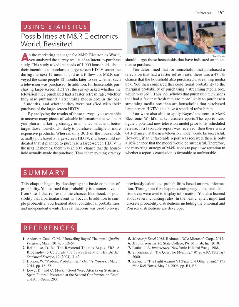
References 191
s U M M a R yThis chapter began by developing the basic concepts of probability. You learned that probability is a numeric value from 0 to 1 that represents the chance, likelihood, or pos-sibility that a particular event will occur. In addition to sim-ple probability, you learned about conditional probabilities and independent events. Bayes’ theorem was used to revise
previously calculated probabilities based on new informa-tion. Throughout the chapter, contingency tables and deci-sion trees were used to display information. You also learned about several counting rules. In the next chapter, important discrete probability distributions including the binomial and Poisson distributions are developed.
R E F E R E n c E s 1. Anderson-Cook, C. M. “Unraveling Bayes’ Theorem.” Quality
Progress, March 2014, p. 52–54. 2. Bellhouse, D. R. “The Reverend Thomas Bayes, FRS: A
Biography to Celebrate the Tercentenary of His Birth.” Statistical Science, 19 (2004), 3–43.
3. Hooper, W. “Probing Probabilities.” Quality Progress, March 2014, pp. 18–22.
4. Lowd, D., and C. Meek. “Good Word Attacks on Statistical Spam Filters.” Presented at the Second Conference on Email and Anti-Spam, 2005.
5. Microsoft Excel 2013. Redmond, WA: Microsoft Corp., 2012. 6. Minitab Release 16. State College, PA: Minitab, Inc, 2010. 7. Paulos, J. A. Innumeracy. New York: Hill and Wang, 1988. 8. Silberman, S. “The Quest for Meaning,” Wired 8.02, February
2000. 9. Zeller, T. “The Fight Against V1@gra (and Other Spam).” The
New York Times, May 21, 2006, pp. B1, B6.
As the marketing manager for M&R Electronics World, you analyzed the survey results of an intent-to-purchase
study. This study asked the heads of 1,000 households about their intentions to purchase a large-screen HDTV sometime during the next 12 months, and as a follow-up, M&R sur-veyed the same people 12 months later to see whether such a television was purchased. In addition, for households pur-chasing large-screen HDTVs, the survey asked whether the television they purchased had a faster refresh rate, whether they also purchased a streaming media box in the past 12 months, and whether they were satisfied with their purchase of the large-screen HDTV.
By analyzing the results of these surveys, you were able to uncover many pieces of valuable information that will help you plan a marketing strategy to enhance sales and better target those households likely to purchase multiple or more expensive products. Whereas only 30% of the households actually purchased a large-screen HDTV, if a household in-dicated that it planned to purchase a large-screen HDTV in the next 12 months, there was an 80% chance that the house-hold actually made the purchase. Thus the marketing strategy
should target those households that have indicated an inten-tion to purchase.
You determined that for households that purchased a television that had a faster refresh rate, there was a 47.5% chance that the household also purchased a streaming media box. You then compared this conditional probability to the marginal probability of purchasing a streaming media box, which was 36%. Thus, households that purchased televisions that had a faster refresh rate are more likely to purchase a streaming media box than are households that purchased large-screen HDTVs that have a standard refresh rate.
You were also able to apply Bayes’ theorem to M&R Electronics World’s market research reports. The reports inves-tigate a potential new television model prior to its scheduled release. If a favorable report was received, then there was a 64% chance that the new television model would be successful. However, if an unfavorable report was received, there is only a 16% chance that the model would be successful. Therefore, the marketing strategy of M&R needs to pay close attention to whether a report’s conclusion is favorable or unfavorable.
U s i n g s tat i s t i c s
Possibilities at M&R Electronics World, Revisited
Shock/Fotolia
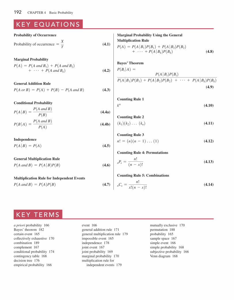
192 CHAPTER 4 Basic Probability
k E y E q U at i o n sProbability of Occurrence
Probability of occurrence =X
T (4.1)
Marginal Probability
P1A2 = P1A and B12 + P1A and B22 + g + P1A and Bk2 (4.2)
General Addition Rule
P1A or B2 = P1A2 + P1B2 - P1A and B2 (4.3)
Conditional Probability
P1A � B2 =P1A and B2
P1B2 (4.4a)
P1B � A2 =P1A and B2
P1A2 (4.4b)
Independence
P1A � B2 = P1A2 (4.5)
General Multiplication Rule
P1A and B2 = P1A � B2P1B2 (4.6)
Multiplication Rule for Independent Events
P1A and B2 = P1A2P1B2 (4.7)
Marginal Probability Using the General Multiplication Rule
P1A2 = P1A � B12P1B12 + P1A � B22P1B22 + g + P1A � Bk2P1Bk2 (4.8)
Bayes’ Theorem
P1Bi � A2 =P1A � Bi2P1Bi2
P1A � B12P1B12 + P1A � B22P1B22 + g + P1A � Bk2P1Bk2 (4.9)
Counting Rule 1
kn (4.10)
Counting Rule 2
1k121k22 c 1kn2 (4.11)
Counting Rule 3
n! = 1n21n - 12 c112 (4.12)
Counting Rule 4: Permutations
nPx =n!
1n - x2! (4.13)
Counting Rule 5: Combinations
nCx =n!
x!1n - x2! (4.14)
k E y t E R M sa priori probability 166Bayes’ theorem 182certain event 165collectively exhaustive 170combination 189complement 167conditional probability 174contingency table 168decision tree 176empirical probability 166
event 166general addition rule 171general multiplication rule 179impossible event 165independence 178joint event 167joint probability 169marginal probability 170multiplication rule for
independent events 179
mutually exclusive 170permutation 188probability 165sample space 167simple event 166simple probability 168subjective probability 166Venn diagram 168
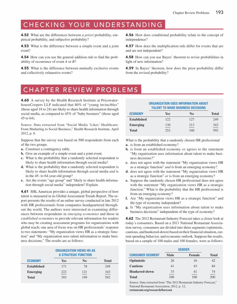
Chapter Review Problems 193
c h E c k i n g y o U R U n D E R s ta n D i n g4.52 What are the differences between a priori probability, em-pirical probability, and subjective probability?
4.53 What is the difference between a simple event and a joint event?
4.54 How can you use the general addition rule to find the prob-ability of occurrence of event A or B?
4.55 What is the difference between mutually exclusive events and collectively exhaustive events?
4.56 How does conditional probability relate to the concept of independence?
4.57 How does the multiplication rule differ for events that are and are not independent?
4.58 How can you use Bayes’ theorem to revise probabilities in light of new information?
4.59 In Bayes’ theorem, how does the prior probability differ from the revised probability?
c h a P t E R R E V i E W P R o b l E M s4.60 A survey by the Health Research Institute at Pricewater-houseCoopers LLP indicated that 80% of “young invincibles” (those aged 18 to 24) are likely to share health information through social media, as compared to 45% of “baby boomers” (those aged 45 to 64).
Source: Data extracted from “Social Media ‘Likes’ Healthcare: From Marketing to Social Business,” Health Research Institute, April 2012, p. 8.
Suppose that the survey was based on 500 respondents from each of the two groups.a. Construct a contingency table.b. Give an example of a simple event and a joint event.c. What is the probability that a randomly selected respondent is
likely to share health information through social media?d. What is the probability that a randomly selected respondent is
likely to share health information through social media and is in the 45- to 64-year-old group?
e. Are the events “age group” and “likely to share health informa-tion through social media” independent? Explain.
4.61 SHL Americas provides a unique, global perspective of how talent is measured in its Global Assessment Trends Report. The re-port presents the results of an online survey conducted in late 2012 with HR professionals from companies headquartered through-out the world. The authors were interested in examining differ-ences between respondents in emerging economies and those in established economies to provide relevant information for readers who may be creating assessment programs for organizations with global reach; one area of focus was on HR professionals’ response to two statements: “My organization views HR as a strategic func-tion” and “My organization uses talent information to make busi-ness decisions.” The results are as follows:
organizaTion vieWS hr aS a STraTegic funcTion
economy Yes No Total
Established 171 78 249
Emerging 222 121 343
Total 393 199 592
organizaTion uSeS informaTion aBouT TalenT To make BuSineSS deciSionS
economy Yes No Total
Established 122 127 249
Emerging 130 213 343
Total 252 340 592
What is the probability that a randomly chosen HR professionala. is from an established economy?b. is from an established economy or agrees to the statement
“My organization uses information about talent to make busi-ness decisions?”
c. does not agree with the statement “My organization views HR as a strategic function” and is from an emerging economy?
d. does not agree with the statement “My organization views HR as a strategic function” or is from an emerging economy?
e. Suppose the randomly chosen HR professional does not agree with the statement “My organization views HR as a strategic function.” What is the probability that the HR professional is from an emerging economy?
f. Are “My organization views HR as a strategic function” and the type of economy independent?
g. Is “My organization uses information about talent to make business decisions” independent of the type of economy?
4.62 The 2012 Restaurant Industry Forecast takes a closer look at today’s consumers. Based on a 2011 National Restaurant Associa-tion survey, consumers are divided into three segments (optimistic, cautious, and hunkered-down) based on their financial situation, cur-rent spending behavior, and economic outlook. Suppose the results, based on a sample of 100 males and 100 females, were as follows:
conSumer SegmenT
gender
Male Female Total
Optimistic 26 16 42
Cautious 41 43 84
Hunkered-down 33 41 74
Total 100 100 200
Source: Data extracted from “The 2012 Restaurant Industry Forecast,” National Restaurant Association, 2012, p. 12,restaurant.org/research/forecast.
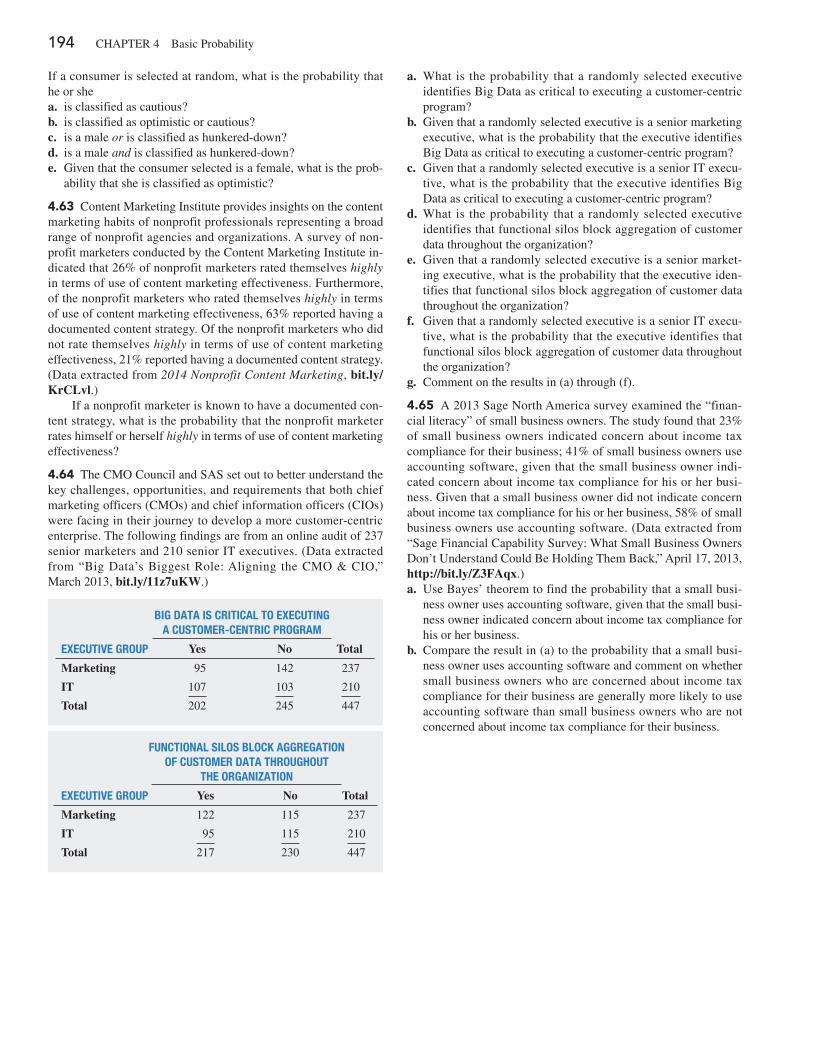
194 CHAPTER 4 Basic Probability
If a consumer is selected at random, what is the probability that he or shea. is classified as cautious?b. is classified as optimistic or cautious?c. is a male or is classified as hunkered-down?d. is a male and is classified as hunkered-down?e. Given that the consumer selected is a female, what is the prob-
ability that she is classified as optimistic?
4.63 Content Marketing Institute provides insights on the content marketing habits of nonprofit professionals representing a broad range of nonprofit agencies and organizations. A survey of non-profit marketers conducted by the Content Marketing Institute in-dicated that 26% of nonprofit marketers rated themselves highly in terms of use of content marketing effectiveness. Furthermore, of the nonprofit marketers who rated themselves highly in terms of use of content marketing effectiveness, 63% reported having a documented content strategy. Of the nonprofit marketers who did not rate themselves highly in terms of use of content marketing effectiveness, 21% reported having a documented content strategy. (Data extracted from 2014 Nonprofit Content Marketing, bit.ly/KrCLvl.)
If a nonprofit marketer is known to have a documented con-tent strategy, what is the probability that the nonprofit marketer rates himself or herself highly in terms of use of content marketing effectiveness?
4.64 The CMO Council and SAS set out to better understand the key challenges, opportunities, and requirements that both chief marketing officers (CMOs) and chief information officers (CIOs) were facing in their journey to develop a more customer-centric enterprise. The following findings are from an online audit of 237 senior marketers and 210 senior IT executives. (Data extracted from “Big Data’s Biggest Role: Aligning the CMO & CIO,” March 2013, bit.ly/11z7uKW.)
Big daTa iS criTical To execuTing a cuSTomer-cenTric Program
execuTive grouP Yes No Total
Marketing 95 142 237
IT 107 103 210
Total 202 245 447
funcTional SiloS Block aggregaTion of cuSTomer daTa ThroughouT
The organizaTion
execuTive grouP Yes No Total
Marketing 122 115 237
IT 95 115 210
Total 217 230 447
a. What is the probability that a randomly selected executive identifies Big Data as critical to executing a customer-centric program?
b. Given that a randomly selected executive is a senior marketing executive, what is the probability that the executive identifies Big Data as critical to executing a customer-centric program?
c. Given that a randomly selected executive is a senior IT execu-tive, what is the probability that the executive identifies Big Data as critical to executing a customer-centric program?
d. What is the probability that a randomly selected executive identifies that functional silos block aggregation of customer data throughout the organization?
e. Given that a randomly selected executive is a senior market-ing executive, what is the probability that the executive iden-tifies that functional silos block aggregation of customer data throughout the organization?
f. Given that a randomly selected executive is a senior IT execu-tive, what is the probability that the executive identifies that functional silos block aggregation of customer data throughout the organization?
g. Comment on the results in (a) through (f).
4.65 A 2013 Sage North America survey examined the “finan-cial literacy” of small business owners. The study found that 23% of small business owners indicated concern about income tax compliance for their business; 41% of small business owners use accounting software, given that the small business owner indi-cated concern about income tax compliance for his or her busi-ness. Given that a small business owner did not indicate concern about income tax compliance for his or her business, 58% of small business owners use accounting software. (Data extracted from “Sage Financial Capability Survey: What Small Business Owners Don’t Understand Could Be Holding Them Back,” April 17, 2013, http://bit.ly/Z3FAqx.)a. Use Bayes’ theorem to find the probability that a small busi-
ness owner uses accounting software, given that the small busi-ness owner indicated concern about income tax compliance for his or her business.
b. Compare the result in (a) to the probability that a small busi-ness owner uses accounting software and comment on whether small business owners who are concerned about income tax compliance for their business are generally more likely to use accounting software than small business owners who are not concerned about income tax compliance for their business.
Cases for Chapter 4 195
c a s E s F o R c h a P t E R 4
Digital caseApply your knowledge about contingency tables and the proper application of simple and joint probabilities in this continuing Digital Case from Chapter 3.
Open EndRunGuide.pdf, the EndRun Financial Services “Guide to Investing,” and read the information about the Guaranteed Investment Package (GIP). Read the claims and examine the supporting data. Then answer the following questions:
1. How accurate is the claim of the probability of suc-cess for EndRun’s GIP? In what ways is the claim
misleading? How would you calculate and state the prob-ability of having an annual rate of return not less than 15%?
2. Using the table found under the “Show Me the Winning Probabilities” subhead, compute the proper probabilities for the group of investors. What mistake was made in re-porting the 7% probability claim?
3. Are there any probability calculations that would be appropriate for rating an investment service? Why or why not?
cardiogood Fitness1. For each CardioGood Fitness treadmill product line (see
the CardiogoodFitness file), construct two-way contin-gency tables of gender, education in years, relationship status, and self-rated fitness. (There will be a total of six tables for each treadmill product.)
2. For each table you construct, compute all conditional and marginal probabilities.
3. Write a report detailing your findings to be presented to the management of CardioGood Fitness.
the choice Is yours Follow-Up1. Follow up the “Using Statistics: The Choice Is Yours,
Revisited” on page 93 by constructing contingency tables of market cap and type, market cap and risk, market cap and rating, type and risk, type and rating, and risk and rating for the sample of 316 retirement funds stored in retirement Funds .
2. For each table you construct, compute all conditional and marginal probabilities.
3. Write a report summarizing your conclusions.
clear Mountain state student surveysThe Student News Service at Clear Mountain State Univer-sity (CMSU) has decided to gather data about the under-graduate students that attend CMSU. CMSU creates and distributes a survey of 14 questions and receive responses from 62 undergraduates (stored in undergradSurvey ).
1. For these data, construct contingency tables of gender and major, gender and graduate school intention, gender and employment status, gender and computer preference, class and graduate school intention, class and employ-ment status, major and graduate school intention, major and employment status, and major and computer prefer-ence.
a. For each of these contingency tables, compute all the conditional and marginal probabilities.
b. Write a report summarizing your conclusions.
2. The CMSU Dean of Students has learned about the un-dergraduate survey and has decided to undertake a simi-lar survey for graduate students at Clear Mountain State. She creates and distributes a survey of 14 questions and receives responses from 44 graduate students (stored in gradSurvey ). Construct contingency tables of gender and graduate major, gender and undergraduate major, gender and employment status, gender and computer preference, graduate major and undergraduate major, graduate ma-jor and employment status, and graduate major and com-puter preference.
a. For each of these contingency tables, compute all the conditional and marginal probabilities.
b. Write a report summarizing your conclusions.
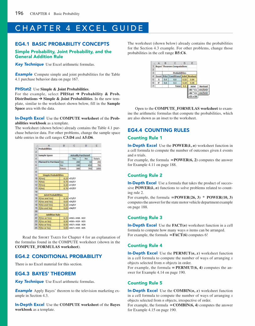
196 CHAPTER 4 Basic Probability
Eg4.1 baSiC probability ConCEptSSimple probability, Joint probability, and the general addition rule
Key Technique Use Excel arithmetic formulas.
Example Compute simple and joint probabilities for the Table 4.1 purchase behavior data on page 167.
phStat2 Use Simple & Joint Probabilities.For the example, select PHStat ➔ Probability & Prob. Distributions ➔ Simple & Joint Probabilities. In the new tem-plate, similar to the worksheet shown below, fill in the Sample Space area with the data.
in-Depth Excel Use the COMPUTE worksheet of the Prob-abilities workbook as a template.The worksheet (shown below) already contains the Table 4.1 pur-chase behavior data. For other problems, change the sample space table entries in the cell ranges C3:D4 and A5:D6.
Read the Short Takes for Chapter 4 for an explanation of the formulas found in the COMPUTE worksheet (shown in the COMPUTE_FORMULAS worksheet).
Eg4.2 ConDitional probabilityThere is no Excel material for this section.
Eg4.3 bayES’ thEorEmKey Technique Use Excel arithmetic formulas.
Example Apply Bayes’ theorem to the television marketing ex-ample in Section 4.3.
in-Depth Excel Use the COMPUTE worksheet of the Bayes workbook as a template.
The worksheet (shown below) already contains the probabilities for the Section 4.3 example. For other problems, change those probabilities in the cell range B5:C6.
Open to the COMPUTE_FORMULAS worksheet to exam-ine the arithmetic formulas that compute the probabilities, which are also shown as an inset to the worksheet.
Eg4.4 Counting rulESCounting rule 1
in-Depth Excel Use the POWER(k, n) worksheet function in a cell formula to compute the number of outcomes given k events and n trials. For example, the formula =POWER(6, 2) computes the answer for Example 4.11 on page 188.
Counting rule 2
in-Depth Excel Use a formula that takes the product of succes-sive POWER(k, n) functions to solve problems related to count-ing rule 2. For example, the formula =POWER(26, 3) * POWER(10, 3) computes the answer for the state motor vehicle department example on page 188.
Counting rule 3
in-Depth Excel Use the FACT(n) worksheet function in a cell formula to compute how many ways n items can be arranged. For example, the formula =FACT(6) computes 6!
Counting rule 4
in-Depth Excel Use the PERMUT(n, x) worksheet function in a cell formula to compute the number of ways of arranging x objects selected from n objects in order. For example, the formula = PERMUT(6, 4) computes the an-swer for Example 4.14 on page 190.
Counting rule 5
in-Depth Excel Use the COMBIN(n, x) worksheet function in a cell formula to compute the number of ways of arranging x objects selected from n objects, irrespective of order. For example, the formula =COMBIN(6, 4) computes the answer for Example 4.15 on page 190.
c h a P t E R 4 E x c E l g U i D E
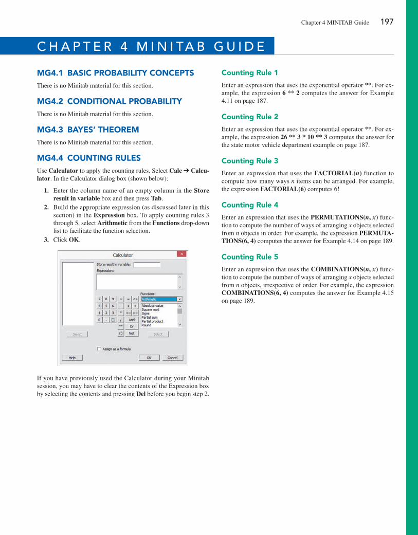
Chapter 4 MINITAB Guide 197
mg4.1 baSiC probability ConCEptSThere is no Minitab material for this section.
mg4.2 ConDitional probabilityThere is no Minitab material for this section.
mg4.3 bayES’ thEorEmThere is no Minitab material for this section.
mg4.4 Counting rulESUse Calculator to apply the counting rules. Select Calc ➔ Calcu-lator. In the Calculator dialog box (shown below):
1. Enter the column name of an empty column in the Store result in variable box and then press Tab.
2. Build the appropriate expression (as discussed later in this section) in the Expression box. To apply counting rules 3 through 5, select Arithmetic from the Functions drop-down list to facilitate the function selection.
3. Click OK.
If you have previously used the Calculator during your Minitab session, you may have to clear the contents of the Expression box by selecting the contents and pressing Del before you begin step 2.
Counting rule 1
Enter an expression that uses the exponential operator **. For ex-ample, the expression 6 ** 2 computes the answer for Example 4.11 on page 187.
Counting rule 2
Enter an expression that uses the exponential operator **. For ex-ample, the expression 26 ** 3 * 10 ** 3 computes the answer for the state motor vehicle department example on page 187.
Counting rule 3
Enter an expression that uses the FACTORIAL(n) function to compute how many ways n items can be arranged. For example, the expression FACTORIAL(6) computes 6!
Counting rule 4
Enter an expression that uses the PERMUTATIONS(n, x) func-tion to compute the number of ways of arranging x objects selected from n objects in order. For example, the expression PERMUTA-TIONS(6, 4) computes the answer for Example 4.14 on page 189.
Counting rule 5
Enter an expression that uses the COMBINATIONS(n, x) func-tion to compute the number of ways of arranging x objects selected from n objects, irrespective of order. For example, the expression COMBINATIONS(6, 4) computes the answer for Example 4.15 on page 189.
c h a P t E R 4 M i n i ta b g U i D E
198
U s i n g s tat i s t i c s
Events of Interest at Ricknel Home CentersLike most other large businesses, Ricknel Home Centers, LLC, a regional home improvement chain, uses an accounting information system (AIS) to manage its accounting and financial data. The Ricknel AIS collects, organizes, stores, ana-lyzes, and distributes financial information to decision makers both inside and outside the firm.
One important function of the Ricknel AIS is to continuously audit account-ing information, looking for errors or incomplete or improbable information. For example, when customers submit orders online, the Ricknel AIS reviews the orders for possible mistakes. Any questionable invoices are tagged and included in a daily exceptions report. Recent data collected by the company show that the likelihood is 0.10 that an order form will be tagged.
As a member of the AIS team, you have been asked by Ricknel manage-ment to determine the likelihood of finding a certain number of tagged forms in a sample of a specific size. For example, what would be the likelihood that none of the order forms are tagged in a sample of four forms? That one of the order forms is tagged?
How could you determine the solution to this type of probability problem?
contents
5.1 The Probability Distribution for a Discrete Variable
5.2 Binomial Distribution
5.3 Poisson Distribution
Using statistics: Events of interest at Ricknel Home centers, Revisited
cHaptER 5 ExcEl gUidE
cHaptER 5 Minitab gUidE
objectives
Learn the properties of a probability distribution
Compute the expected value and variance of a probability distribution
Compute probabilities from the binomial and Poisson, distributions
Use the binomial and Poisson, distributions to solve business problems
Chapter Discrete Probability Distributions5
Sebastian Kaulitzki/Shutterstock
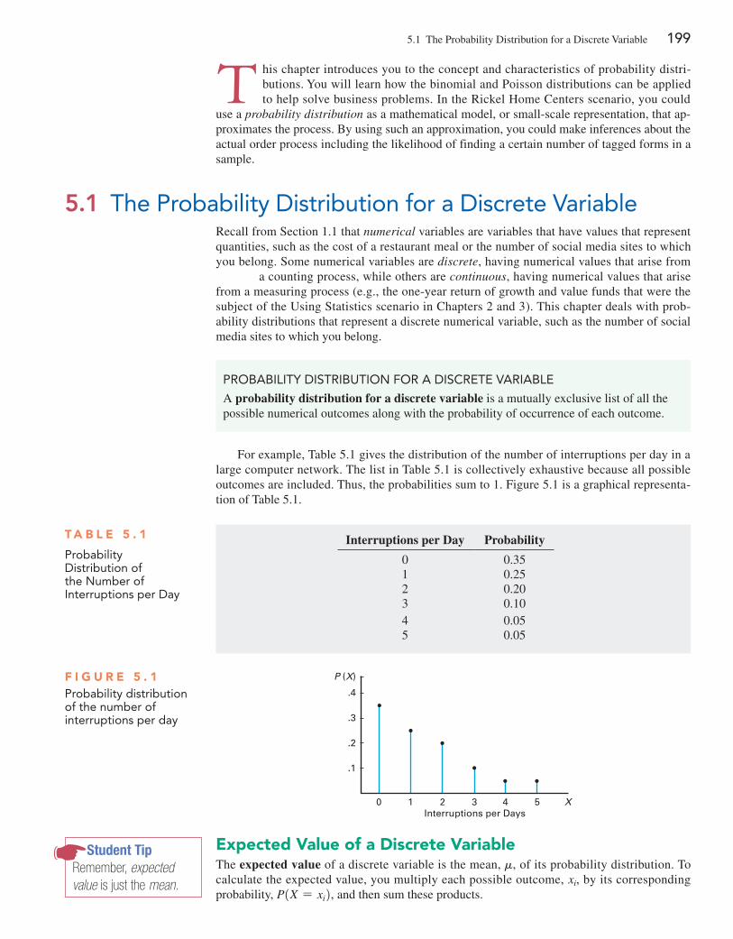
5.1 The Probability Distribution for a Discrete Variable 199
T his chapter introduces you to the concept and characteristics of probability distri-butions. You will learn how the binomial and Poisson distributions can be applied to help solve business problems. In the Rickel Home Centers scenario, you could
use a probability distribution as a mathematical model, or small-scale representation, that ap-proximates the process. By using such an approximation, you could make inferences about the actual order process including the likelihood of finding a certain number of tagged forms in a sample.
Recall from Section 1.1 that numerical variables are variables that have values that represent quantities, such as the cost of a restaurant meal or the number of social media sites to which you belong. Some numerical variables are discrete, having numerical values that arise from a counting process, while others are continuous, having numerical values that arise from a measuring process (e.g., the one-year return of growth and value funds that were the subject of the Using Statistics scenario in Chapters 2 and 3). This chapter deals with prob-ability distributions that represent a discrete numerical variable, such as the number of social media sites to which you belong.
5.1 The Probability Distribution for a Discrete Variable
ProBaBiLiTy DisTriBUTion for a DisCreTe VariaBLe
A probability distribution for a discrete variable is a mutually exclusive list of all the possible numerical outcomes along with the probability of occurrence of each outcome.
For example, Table 5.1 gives the distribution of the number of interruptions per day in a large computer network. The list in Table 5.1 is collectively exhaustive because all possible outcomes are included. Thus, the probabilities sum to 1. Figure 5.1 is a graphical representa-tion of Table 5.1.
T a b l e 5 . 1
Probability Distribution of the number of interruptions per Day
Interruptions per Day Probability
0 0.351 0.252 0.203 0.104 0.055 0.05
F i g u r e 5 . 1Probability distribution of the number of interruptions per day
0 2 3 4 5 X
P (X)
.3
.2
Interruptions per Days
.1
.4
1
expected Value of a Discrete VariableThe expected value of a discrete variable is the mean, m, of its probability distribution. To calculate the expected value, you multiply each possible outcome, xi, by its corresponding probability, P1X = xi2, and then sum these products.
Student TipRemember, expected value is just the mean.
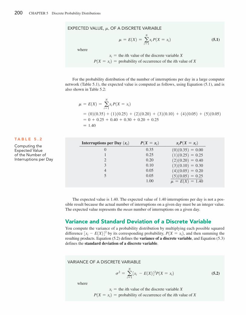
200 CHAPTeR 5 Discrete Probability Distributions
For the probability distribution of the number of interruptions per day in a large computer network (Table 5.1), the expected value is computed as follows, using equation (5.1), and is also shown in Table 5.2:
m = E1X2 = aN
i= 1xi P1X = xi2
= 10210.352 + 11210.252 + 12210.202 + 13210.102 + 14210.052 + 15210.052 = 0 + 0.25 + 0.40 + 0.30 + 0.20 + 0.25 = 1.40
exPeCTeD VaLUe, m, of a DisCreTe VariaBLe
m = E1X2 = aN
i= 1xi P1X = xi2 (5.1)
wherexi = the ith value of the discrete variable X
P1X = xi2 = probability of occurrence of the ith value of X
The expected value is 1.40. The expected value of 1.40 interruptions per day is not a pos-sible result because the actual number of interruptions on a given day must be an integer value. The expected value represents the mean number of interruptions on a given day.
Variance and Standard Deviation of a Discrete VariableYou compute the variance of a probability distribution by multiplying each possible squared difference 3xi - E1X242 by its corresponding probability, P1X = xi2, and then summing the resulting products. equation (5.2) defines the variance of a discrete variable, and equation (5.3) defines the standard deviation of a discrete variable.
VarianCe of a DisCreTe VariaBLe
s2 = aN
i= 13xi - E1X242P1X = xi2 (5.2)
wherexi = the ith value of the discrete variable X
P1X = xi2 = probability of occurrence of the ith value of X
T a b l e 5 . 2
Computing the expected Value of the number of interruptions per Day
Interruptions per Day 1xi2 P1X = xi2 xi P1X = xi20 0.35 10210.352 = 0.001 0.25 11210.252 = 0.252 0.20 12210.202 = 0.403 0.10 13210.102 = 0.304 0.05 14210.052 = 0.205 0.05 15210.052 = 0.25
1.00 m = E1X2 = 1.40
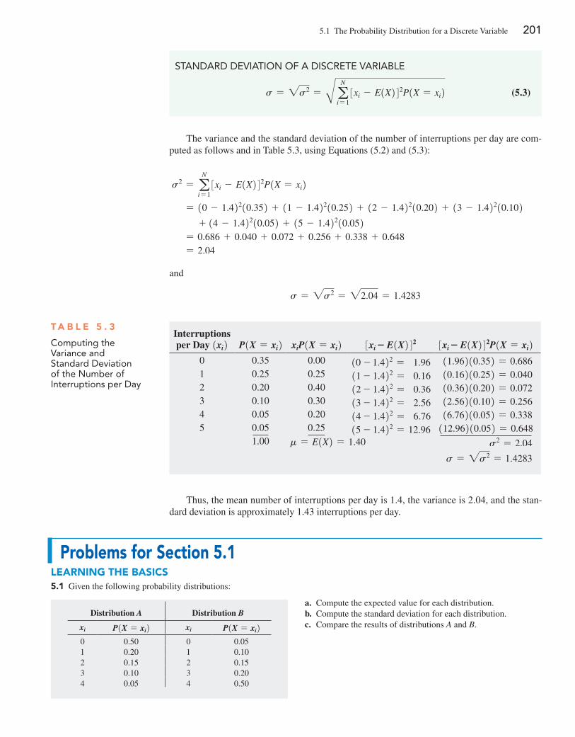
5.1 The Probability Distribution for a Discrete Variable 201
The variance and the standard deviation of the number of interruptions per day are com-puted as follows and in Table 5.3, using equations (5.2) and (5.3):
s2 = aN
i= 13xi - E1X242P1X = xi2
= 10 - 1.42210.352 + 11 - 1.42210.252 + 12 - 1.42210.202 + 13 - 1.42210.102+ 14 - 1.42210.052 + 15 - 1.42210.052
= 0.686 + 0.040 + 0.072 + 0.256 + 0.338 + 0.648 = 2.04
and
s = 2s2 = 22.04 = 1.4283
sTanDarD DeViaTion of a DisCreTe VariaBLe
s = 2s2 = BaN
i= 13xi - E1X242P1X = xi2 (5.3)
T a b l e 5 . 3
Computing the Variance and standard Deviation of the number of interruptions per Day
Interruptions per Day 1xi2 P1X = xi2 xiP1X = xi2 3xi− E1X242 3xi− E1X242P1X = xi2
0 0.35 0.00 10 - 1.422 = 1.96 11.96210.352 = 0.6861 0.25 0.25 11 - 1.422 = 0.16 10.16210.252 = 0.0402 0.20 0.40 12 - 1.422 = 0.36 10.36210.202 = 0.0723 0.10 0.30 13 - 1.422 = 2.56 12.56210.102 = 0.2564 0.05 0.20 14 - 1.422 = 6.76 16.76210.052 = 0.3385 0.05 0.25 15 - 1.422 = 12.96 112.96210.052 = 0.648
1.00 m = E1X2 = 1.40 s2 = 2.04
s = 2s2 = 1.4283
Thus, the mean number of interruptions per day is 1.4, the variance is 2.04, and the stan-dard deviation is approximately 1.43 interruptions per day.
Problems for Section 5.1learning The baSicS5.1 Given the following probability distributions:
a. Compute the expected value for each distribution.b. Compute the standard deviation for each distribution.c. Compare the results of distributions A and B.
Distribution A Distribution B
xi P1X = xi2 xi P1X = xi20 0.50 0 0.051 0.20 1 0.102 0.15 2 0.153 0.10 3 0.204 0.05 4 0.50
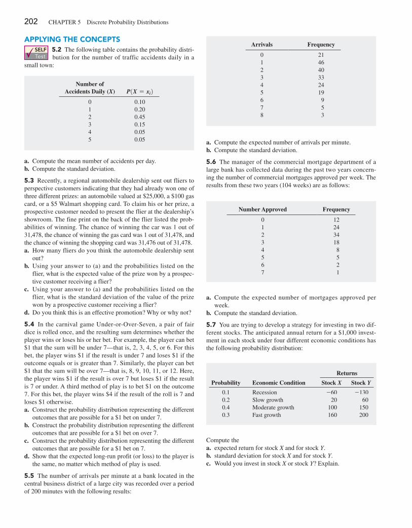
202 CHAPTeR 5 Discrete Probability Distributions
aPPlying The concePTSSELF Test
5.2 The following table contains the probability distri-bution for the number of traffic accidents daily in a
small town:
Number of Accidents Daily (X) P1X = xi2
0 0.101 0.202 0.453 0.154 0.055 0.05
a. Compute the mean number of accidents per day.b. Compute the standard deviation.
5.3 Recently, a regional automobile dealership sent out fliers to perspective customers indicating that they had already won one of three different prizes: an automobile valued at $25,000, a $100 gas card, or a $5 Walmart shopping card. To claim his or her prize, a prospective customer needed to present the flier at the dealership’s showroom. The fine print on the back of the flier listed the prob-abilities of winning. The chance of winning the car was 1 out of 31,478, the chance of winning the gas card was 1 out of 31,478, and the chance of winning the shopping card was 31,476 out of 31,478.a. How many fliers do you think the automobile dealership sent
out?b. Using your answer to (a) and the probabilities listed on the
flier, what is the expected value of the prize won by a prospec-tive customer receiving a flier?
c. Using your answer to (a) and the probabilities listed on the flier, what is the standard deviation of the value of the prize won by a prospective customer receiving a flier?
d. Do you think this is an effective promotion? Why or why not?
5.4 In the carnival game Under-or-Over-Seven, a pair of fair dice is rolled once, and the resulting sum determines whether the player wins or loses his or her bet. For example, the player can bet $1 that the sum will be under 7—that is, 2, 3, 4, 5, or 6. For this bet, the player wins $1 if the result is under 7 and loses $1 if the outcome equals or is greater than 7. Similarly, the player can bet $1 that the sum will be over 7—that is, 8, 9, 10, 11, or 12. Here, the player wins $1 if the result is over 7 but loses $1 if the result is 7 or under. A third method of play is to bet $1 on the outcome 7. For this bet, the player wins $4 if the result of the roll is 7 and loses $1 otherwise.a. Construct the probability distribution representing the different
outcomes that are possible for a $1 bet on under 7.b. Construct the probability distribution representing the different
outcomes that are possible for a $1 bet on over 7.c. Construct the probability distribution representing the different
outcomes that are possible for a $1 bet on 7.d. Show that the expected long-run profit (or loss) to the player is
the same, no matter which method of play is used.
5.5 The number of arrivals per minute at a bank located in the central business district of a large city was recorded over a period of 200 minutes with the following results:
Arrivals Frequency
0 211 462 403 334 245 196 97 58 3
a. Compute the expected number of arrivals per minute.b. Compute the standard deviation.
5.6 The manager of the commercial mortgage department of a large bank has collected data during the past two years concern-ing the number of commercial mortgages approved per week. The results from these two years (104 weeks) are as follows:
Number Approved Frequency
0 121 242 343 184 85 56 27 1
a. Compute the expected number of mortgages approved per week.
b. Compute the standard deviation.
5.7 You are trying to develop a strategy for investing in two dif-ferent stocks. The anticipated annual return for a $1,000 invest-ment in each stock under four different economic conditions has the following probability distribution:
Returns
Probability Economic Condition Stock X Stock Y
0.1 Recession -60 -1300.2 Slow growth 20 600.4 Moderate growth 100 1500.3 Fast growth 160 200
Compute thea. expected return for stock X and for stock Y.b. standard deviation for stock X and for stock Y.c. Would you invest in stock X or stock Y? explain.
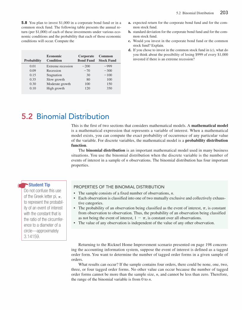
5.2 Binomial Distribution 203
5.8 You plan to invest $1,000 in a corporate bond fund or in a common stock fund. The following table presents the annual re-turn (per $1,000) of each of these investments under various eco-nomic conditions and the probability that each of those economic conditions will occur. Compute the
ProbabilityEconomic Condition
Corporate Bond Fund
Common Stock Fund
0.01 extreme recession -200 -9990.09 Recession -70 -3000.15 Stagnation 30 -1000.35 Slow growth 80 1000.30 Moderate growth 100 1500.10 High growth 120 350
a. expected return for the corporate bond fund and for the com-mon stock fund.
b. standard deviation for the corporate bond fund and for the com-mon stock fund.
c. Would you invest in the corporate bond fund or the common stock fund? explain.
d. If you chose to invest in the common stock fund in (c), what do you think about the possibility of losing $999 of every $1,000 invested if there is an extreme recession?
5.2 Binomial DistributionThis is the first of two sections that considers mathematical models. A mathematical model is a mathematical expression that represents a variable of interest. When a mathematical model exists, you can compute the exact probability of occurrence of any particular value of the variable. For discrete variables, the mathematical model is a probability distribution function.
The binomial distribution is an important mathematical model used in many business situations. You use the binomial distribution when the discrete variable is the number of events of interest in a sample of n observations. The binomial distribution has four important properties.
Student TipDo not confuse this use of the Greek letter pi, p, to represent the probabil-ity of an event of interest with the constant that is the ratio of the circumfer-ence to a diameter of a circle—approximately 3.14159.
ProPerTies of The BinomiaL DisTriBUTion
• The sample consists of a fixed number of observations, n.• each observation is classified into one of two mutually exclusive and collectively exhaus-
tive categories.• The probability of an observation being classified as the event of interest, p, is constant
from observation to observation. Thus, the probability of an observation being classified as not being the event of interest, 1 - p, is constant over all observations.
• The value of any observation is independent of the value of any other observation.
Returning to the Ricknel Home Improvement scenario presented on page 198 concern-ing the accounting information system, suppose the event of interest is defined as a tagged order form. You want to determine the number of tagged order forms in a given sample of orders.
What results can occur? If the sample contains four orders, there could be none, one, two, three, or four tagged order forms. No other value can occur because the number of tagged order forms cannot be more than the sample size, n, and cannot be less than zero. Therefore, the range of the binomial variable is from 0 to n.
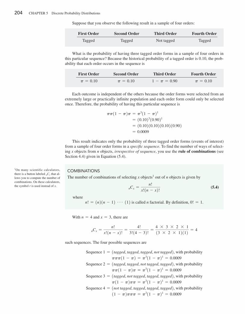
204 CHAPTeR 5 Discrete Probability Distributions
Suppose that you observe the following result in a sample of four orders:
First Order Second Order Third Order Fourth Order
Tagged Tagged Not tagged Tagged
What is the probability of having three tagged order forms in a sample of four orders in this particular sequence? Because the historical probability of a tagged order is 0.10, the prob-ability that each order occurs in the sequence is
First Order Second Order Third Order Fourth Order
p = 0.10 p = 0.10 1 - p = 0.90 p = 0.10
each outcome is independent of the others because the order forms were selected from an extremely large or practically infinite population and each order form could only be selected once. Therefore, the probability of having this particular sequence is
pp11 - p2p = p311 - p21
= 10.102310.9021
= 10.10210.10210.10210.902 = 0.0009
This result indicates only the probability of three tagged order forms (events of interest) from a sample of four order forms in a specific sequence. To find the number of ways of select-ing x objects from n objects, irrespective of sequence, you use the rule of combinations (see Section 4.4) given in equation (5.4).
With n = 4 and x = 3, there are
nCx =n!
x!1n - x2!=
4!
3!14 - 32!=
4 * 3 * 2 * 1
13 * 2 * 12112 = 4
such sequences. The four possible sequences are
Sequence 1 = 1tagged, tagged, tagged, not tagged2, with probability
ppp11 - p2 = p311 - p21 = 0.0009
Sequence 2 = 1tagged, tagged, not tagged, tagged2, with probability
pp11 - p2p = p311 - p21 = 0.0009
Sequence 3 = 1tagged, not tagged, tagged, tagged2, with probability
p11 - p2pp = p311 - p21 = 0.0009
Sequence 4 = 1not tagged, tagged, tagged, tagged2, with probability
11 - p2ppp = p311 - p21 = 0.0009
ComBinaTions
The number of combinations of selecting x objects1 out of n objects is given by
nCx =n!
x!1n - x2! (5.4)
wheren! = 1n21n - 12 g 112 is called n factorial. By definition, 0! = 1.
1On many scientific calculators, there is a button labeled nCr that al-lows you to compute the number of combinations. On these calculators, the symbol r is used instead of x.
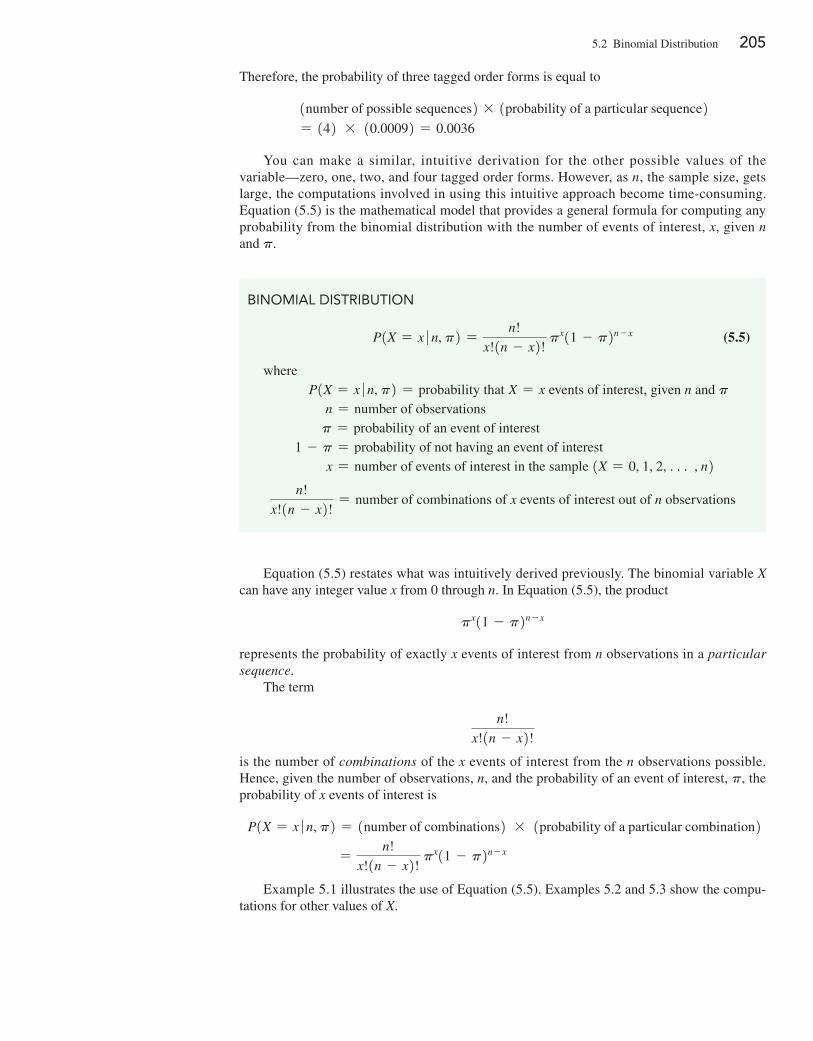
5.2 Binomial Distribution 205
Therefore, the probability of three tagged order forms is equal to
1number of possible sequences2 * 1probability of a particular sequence2= 142 * 10.00092 = 0.0036
You can make a similar, intuitive derivation for the other possible values of the variable—zero, one, two, and four tagged order forms. However, as n, the sample size, gets large, the computations involved in using this intuitive approach become time-consuming. equation (5.5) is the mathematical model that provides a general formula for computing any probability from the binomial distribution with the number of events of interest, x, given n and p.
BinomiaL DisTriBUTion
P1X = x � n, p2 =n!
x!1n - x2! px11 - p2n - x (5.5)
whereP1X = x � n, p2 = probability that X = x events of interest, given n and p
n = number of observationsp = probability of an event of interest
1 - p = probability of not having an event of interestx = number of events of interest in the sample 1X = 0, 1, 2, c , n2
n!
x!1n - x2!= number of combinations of x events of interest out of n observations
equation (5.5) restates what was intuitively derived previously. The binomial variable X can have any integer value x from 0 through n. In equation (5.5), the product
px11 - p2n - x
represents the probability of exactly x events of interest from n observations in a particular sequence.
The term
n!
x!1n - x2!
is the number of combinations of the x events of interest from the n observations possible. Hence, given the number of observations, n, and the probability of an event of interest, p, the probability of x events of interest is
P1X = x � n, p2 = 1number of combinations2 * 1probability of a particular combination2 =
n!
x!1n - x2! px11 - p2n - x
example 5.1 illustrates the use of equation (5.5). examples 5.2 and 5.3 show the compu-tations for other values of X.
206 CHAPTeR 5 Discrete Probability Distributions
examPle 5.1determining P1X = 32, given n = 4 and p = 0.1
If the likelihood of a tagged order form is 0.1, what is the probability that there are three tagged order forms in the sample of four?
SoluTion Using equation (5.5), the probability of three tagged orders from a sample of four is
P1X = 3 � n = 4, p = 0.12 =4!
3!14 - 32!10.12311 - 0.124 - 3
=4!
3!112!10.12310.921
= 410.1210.1210.1210.92 = 0.0036
examPle 5.2determining P1X Ú 32, given n = 4 and p = 0.1
If the likelihood of a tagged order form is 0.1, what is the probability that there are three or more (i.e., at least three) tagged order forms in the sample of four?
SoluTion In example 5.1, you found that the probability of exactly three tagged order forms from a sample of four is 0.0036. To compute the probability of at least three tagged order forms, you need to add the probability of three tagged order forms to the probability of four tagged order forms. The probability of four tagged order forms is
P1X = 4 � n = 4, p = 0.12 =4!
4!14 - 42!10.12411 - 0.124 - 4
=4!
4!102!10.12410.920
= 110.1210.1210.1210.12112 = 0.0001
Thus, the probability of at least three tagged order forms is
P1X Ú 32 = P1X = 32 + P1X = 42 = 0.0036 + 0.0001
= 0.0037
There is a 0.37% chance that there will be at least three tagged order forms in a sample of four.
Student TipAnother way of saying “three or more” is “at least three.”
examPle 5.3determining P1X 6 32, given n = 4 and p = 0.1
If the likelihood of a tagged order form is 0.1, what is the probability that there are less than three tagged order forms in the sample of four?
SoluTion The probability that there are less than three tagged order forms is
P1X 6 32 = P1X = 02 + P1X = 12 + P1X = 22
Using equation (5.5) on page 205, these probabilities are
P1X = 0 � n = 4, p = 0.12 =4!
0!14 - 02!10.12011 - 0.124 - 0 = 0.6561
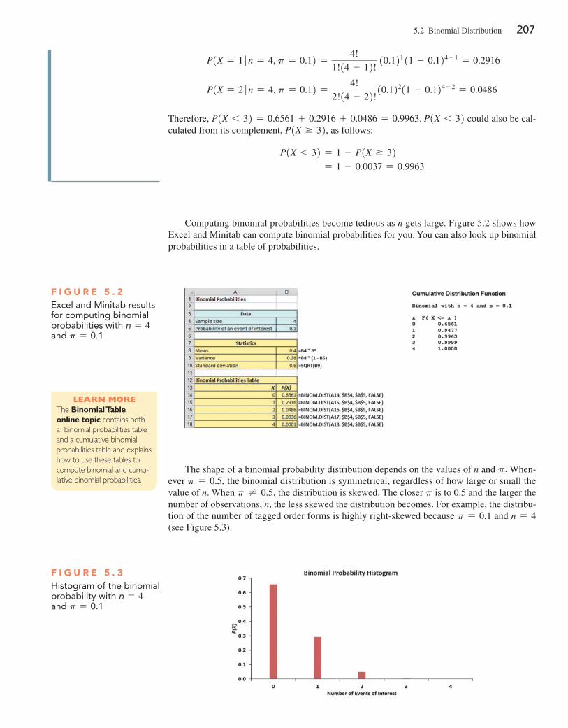
5.2 Binomial Distribution 207
Computing binomial probabilities become tedious as n gets large. Figure 5.2 shows how excel and Minitab can compute binomial probabilities for you. You can also look up binomial probabilities in a table of probabilities.
P1X = 1 � n = 4, p = 0.12 =4!
1!14 - 12! 10.121 11 - 0.124 - 1 = 0.2916
P1X = 2 � n = 4, p = 0.12 =4!
2!14 - 22!10.12211 - 0.124 - 2 = 0.0486
Therefore, P1X 6 32 = 0.6561 + 0.2916 + 0.0486 = 0.9963. P1X 6 32 could also be cal-culated from its complement, P1X Ú 32, as follows:
P1X 6 32 = 1 - P1X Ú 32 = 1 - 0.0037 = 0.9963
Learn MoreThe Binomial Table online topic contains both a binomial probabilities table and a cumulative binomial probabilities table and explains how to use these tables to compute binomial and cumu-lative binomial probabilities.
F i g u r e 5 . 2excel and minitab results for computing binomial probabilities with n = 4 and p = 0.1
The shape of a binomial probability distribution depends on the values of n and p. When-ever p = 0.5, the binomial distribution is symmetrical, regardless of how large or small the value of n. When p ≠ 0.5, the distribution is skewed. The closer p is to 0.5 and the larger the number of observations, n, the less skewed the distribution becomes. For example, the distribu-tion of the number of tagged order forms is highly right-skewed because p = 0.1 and n = 4 (see Figure 5.3).
F i g u r e 5 . 3histogram of the binomial probability with n = 4 and p = 0.1
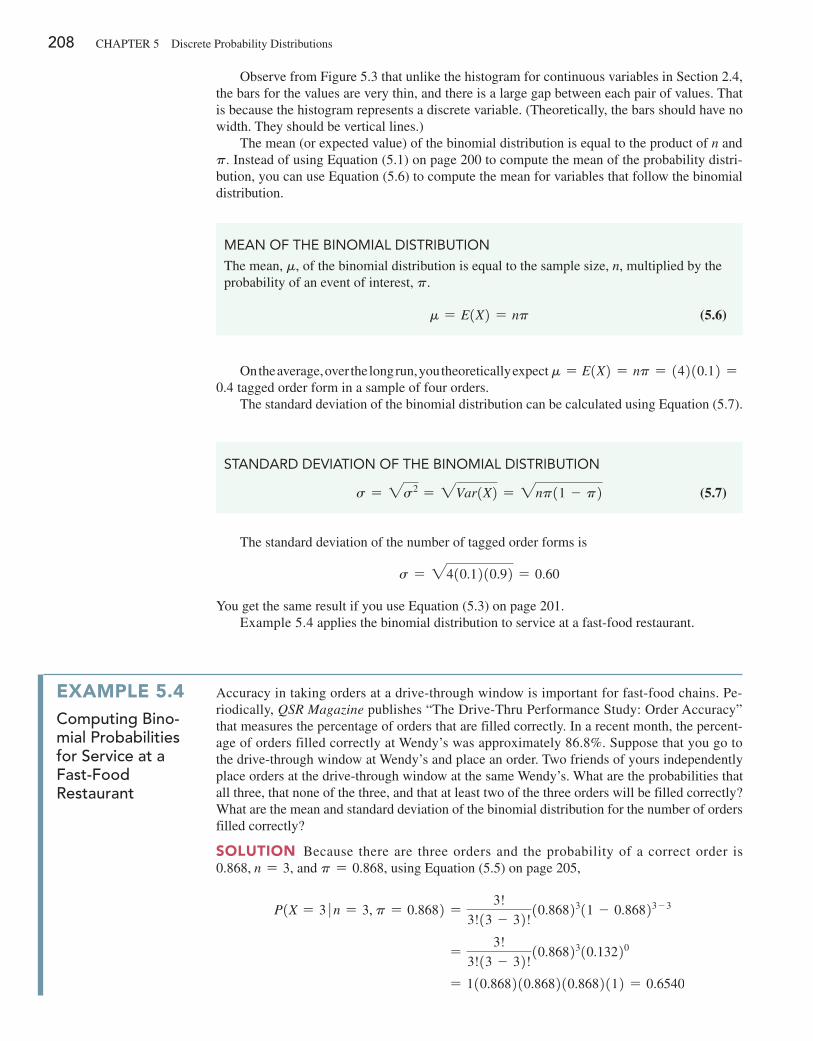
208 CHAPTeR 5 Discrete Probability Distributions
Observe from Figure 5.3 that unlike the histogram for continuous variables in Section 2.4, the bars for the values are very thin, and there is a large gap between each pair of values. That is because the histogram represents a discrete variable. (Theoretically, the bars should have no width. They should be vertical lines.)
The mean (or expected value) of the binomial distribution is equal to the product of n and p. Instead of using equation (5.1) on page 200 to compute the mean of the probability distri-bution, you can use equation (5.6) to compute the mean for variables that follow the binomial distribution.
mean of The BinomiaL DisTriBUTion
The mean, m, of the binomial distribution is equal to the sample size, n, multiplied by the probability of an event of interest, p.
m = E1X2 = np (5.6)
On the average, over the long run, you theoretically expect m = E1X2 = np = 14210.12 =0.4 tagged order form in a sample of four orders.
The standard deviation of the binomial distribution can be calculated using equation (5.7).
sTanDarD DeViaTion of The BinomiaL DisTriBUTion
s = 2s2 = 2Var1X2 = 2np11 - p2 (5.7)
The standard deviation of the number of tagged order forms is
s = 2410.1210.92 = 0.60
You get the same result if you use equation (5.3) on page 201.example 5.4 applies the binomial distribution to service at a fast-food restaurant.
examPle 5.4computing bino-mial probabilities for service at a Fast-Food Restaurant
Accuracy in taking orders at a drive-through window is important for fast-food chains. Pe-riodically, QSR Magazine publishes “The Drive-Thru Performance Study: Order Accuracy” that measures the percentage of orders that are filled correctly. In a recent month, the percent-age of orders filled correctly at Wendy’s was approximately 86.8%. Suppose that you go to the drive-through window at Wendy’s and place an order. Two friends of yours independently place orders at the drive-through window at the same Wendy’s. What are the probabilities that all three, that none of the three, and that at least two of the three orders will be filled correctly? What are the mean and standard deviation of the binomial distribution for the number of orders filled correctly?
SoluTion Because there are three orders and the probability of a correct order is 0.868, n = 3, and p = 0.868, using equation (5.5) on page 205,
P1X = 3 � n = 3, p = 0.8682 =3!
3!13 - 32!10.8682311 - 0.86823 - 3
=3!
3!13 - 32!10.8682310.13220
= 110.868210.868210.8682112 = 0.6540
5.2 Binomial Distribution 209
P1X = 0 � n = 3, p = 0.8682 =3!
0!13 - 02!10.8682011 - 0.86823 - 0
=3!
0!13 - 02!10.8682010.13223
= 111210.132210.132210.1322 = 0.0023
P1X = 2 � n = 3, p = 0.8682 =3!
2!13 - 22!10.8682211 - 0.86823 - 2
=3!
2!13 - 22!10.8682210.13221
= 310.868210.868210.1322 = 0.2984
P1X Ú 22 = P1X = 22+P1X = 32 = 0.2984 + 0.6540
= 0.9524
Using equations (5.6) and (5.7),
m = E1X2 = np = 310.8682 = 2.604
s = 2s2 = 2Var1X2 = 2np11 - p2
= 2310.868210.1322
= 20.3437 = 0.5863
The mean number of orders filled correctly in a sample of three orders is 2.604, and the standard deviation is 0.5863. The probability that all three orders are filled correctly is 0.6540, or 65.4%. The probability that none of the orders are filled correctly is 0.0023 (0.23%). The probability that at least two orders are filled correctly is 0.9524 (95.24%).
Problems for Section 5.2learning The baSicS5.9 Determine the following:a. For n = 4 and p = 0.12, what is P1X = 02?b. For n = 10 and p = 0.40, what is P1X = 92?c. For n = 10 and p = 0.50, what is P1X = 82?d. For n = 6 and p = 0.83, what is P1X = 52?
5.10 Determine the mean and standard deviation of the variable X in each of the following binomial distributions:a. n = 4 and p = 0.10b. n = 4 and p = 0.40c. n = 5 and p = 0.80d. n = 3 and p = 0.50
aPPlying The concePTS5.11 The increase or decrease in the price of a stock between the beginning and the end of a trading day is assumed to be an equally likely random event. What is the probability that a stock will show an increase in its closing price on five consecutive days?
5.12 A recent Pew Research survey reported that 48% of 18- to 29-year-olds in the United States own tablets. (Data extracted from “Tablet and e-Reader Ownership,” bit.ly/1gEwogC). Using the binomial distribution, what is the probability that in the next six 18- to 29-year-olds surveyed,a. four will own a tablet?b. all six will own a tablet?c. at least four will own a tablet?d. What are the mean and standard deviation of the number of
18- to 29-year-olds who will own a tablet in a survey of six?e. What assumptions do you need to make in (a) through (c)?
5.13 A student is taking a multiple-choice exam in which each question has four choices. Assume that the student has no knowl-edge of the correct answers to any of the questions. She has de-cided on a strategy in which she will place four balls (marked A, B, C, and D) into a box. She randomly selects one ball for each question and replaces the ball in the box. The marking on the ball will determine her answer to the question. There are five
210 CHAPTeR 5 Discrete Probability Distributions
multiple-choice questions on the exam. What is the probability that she will geta. five questions correct?b. at least four questions correct?c. no questions correct?d. no more than two questions correct?
5.14 A manufacturing company regularly conducts quality con-trol checks at specified periods on the products it manufactures. Historically, the failure rate for LeD light bulbs that the company manufactures is 5%. Suppose a random sample of 10 LeD light bulbs is selected. What is the probability thata. none of the LeD light bulbs are defective?b. exactly one of the LeD light bulbs is defective?c. two or fewer of the LeD light bulbs are defective?d. three or more of the LeD light bulbs are defective?
5.15 Past records indicate that the probability of online retail or-ders that turn out to be fraudulent is 0.08. Suppose that, on a given day, 20 online retail orders are placed. Assume that the number of online retail orders that turn out to be fraudulent is distributed as a binomial random variable.a. What are the mean and standard deviation of the number of on-
line retail orders that turn out to be fraudulent?b. What is the probability that zero online retail orders will turn
out to be fraudulent?
c. What is the probability that one online retail order will turn out to be fraudulent?
d. What is the probability that two or more online retail orders will turn out to be fraudulent?
SELF Test
5.16 In example 5.4 on page 208, you and two friends decided to go to Wendy’s. Now, suppose that instead
you go to Burger King, which recently filled approximately 82.3% of orders correctly. What is the probability thata. all three orders will be filled correctly?b. none of the three will be filled correctly?c. at least two of the three will be filled correctly?d. What are the mean and standard deviation of the binomial dis-
tribution used in (a) through (c)? Interpret these values.
5.17 In example 5.4 on page 208, you and two friends decided to go to Wendy’s. Now, suppose that instead you go to McDon-ald’s, which recently filled approximately 88.3% of the orders cor-rectly. What is the probability thata. all three orders will be filled correctly?b. none of the three will be filled correctly?c. at least two of the three will be filled correctly?d. What are the mean and standard deviation of the binomial dis-
tribution used in (a) through (c)? Interpret these values.e. Compare the result of (a) through (d) with those of Burger King
in Problem 5.16 and Wendy’s in example 5.4 on page 208.
5.3 Poisson DistributionMany studies are based on counts of the occurrences of a particular event in a given interval of time or space (often referred to as an area of opportunity). In such an area of opportunity there can be more than one occurrence of an event. The Poisson distribution can be used to compute probabilities in such situations. examples of variables that follow the Poisson distri-bution are the surface defects on a new refrigerator, the number of network failures in a day, the number of people arriving at a bank, and the number of fleas on the body of a dog. You can use the Poisson distribution to calculate probabilities in situations such as these if the follow-ing properties hold:
• You are interested in counting the number of times a particular event occurs in a given area of opportunity. The area of opportunity is defined by time, length, surface area, and so forth.
• The probability that an event occurs in a given area of opportunity is the same for all the areas of opportunity.
• The number of events that occur in one area of opportunity is independent of the number of events that occur in any other area of opportunity.
• The probability that two or more events will occur in an area of opportunity approaches zero as the area of opportunity becomes smaller.
Consider the number of customers arriving during the lunch hour at a bank located in the central business district in a large city. You are interested in the number of customers who arrive each minute. Does this situation match the four properties of the Poisson distribution given earlier?
First, the event of interest is a customer arriving, and the given area of opportunity is de-fined as a one-minute interval. Will zero customers arrive, one customer arrive, two customers arrive, and so on? Second, it is reasonable to assume that the probability that a customer ar-rives during a particular one-minute interval is the same as the probability for all the other one-minute intervals. Third, the arrival of one customer in any one-minute interval has no effect on
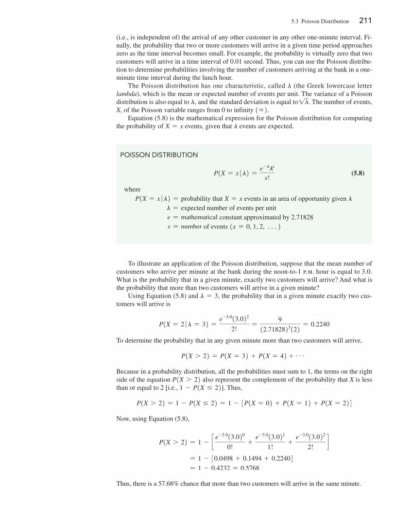
5.3 Poisson Distribution 211
(i.e., is independent of) the arrival of any other customer in any other one-minute interval. Fi-nally, the probability that two or more customers will arrive in a given time period approaches zero as the time interval becomes small. For example, the probability is virtually zero that two customers will arrive in a time interval of 0.01 second. Thus, you can use the Poisson distribu-tion to determine probabilities involving the number of customers arriving at the bank in a one-minute time interval during the lunch hour.
The Poisson distribution has one characteristic, called l (the Greek lowercase letter lambda), which is the mean or expected number of events per unit. The variance of a Poisson distribution is also equal to l, and the standard deviation is equal to1l. The number of events, X, of the Poisson variable ranges from 0 to infinity 1∞2.
equation (5.8) is the mathematical expression for the Poisson distribution for computing the probability of X = x events, given that l events are expected.
Poisson DisTriBUTion
P1X = x �l2 =e-llx
x! (5.8)
whereP1X = x �l2 = probability that X = x events in an area of opportunity given l
l = expected number of events per unite = mathematical constant approximated by 2.71828x = number of events 1x = 0, 1, 2, c2
To illustrate an application of the Poisson distribution, suppose that the mean number of customers who arrive per minute at the bank during the noon-to-1 p.m. hour is equal to 3.0. What is the probability that in a given minute, exactly two customers will arrive? And what is the probability that more than two customers will arrive in a given minute?
Using equation (5.8) and l = 3, the probability that in a given minute exactly two cus-tomers will arrive is
P1X = 2 �l = 32 =e-3.013.022
2!=
9
12.7182823122 = 0.2240
To determine the probability that in any given minute more than two customers will arrive,
P1X 7 22 = P1X = 32 + P1X = 42 + g
Because in a probability distribution, all the probabilities must sum to 1, the terms on the right side of the equation P1X 7 22 also represent the complement of the probability that X is less than or equal to 2 [i.e., 1 - P1X … 22]. Thus,
P1X 7 22 = 1 - P1X … 22 = 1 - 3P1X = 02 + P1X = 12 + P1X = 224
Now, using equation (5.8),
P1X 7 22 = 1 - c e-3.013.020
0!+
e-3.013.021
1!+
e-3.013.022
2!d
= 1 - 30.0498 + 0.1494 + 0.22404 = 1 - 0.4232 = 0.5768
Thus, there is a 57.68% chance that more than two customers will arrive in the same minute.
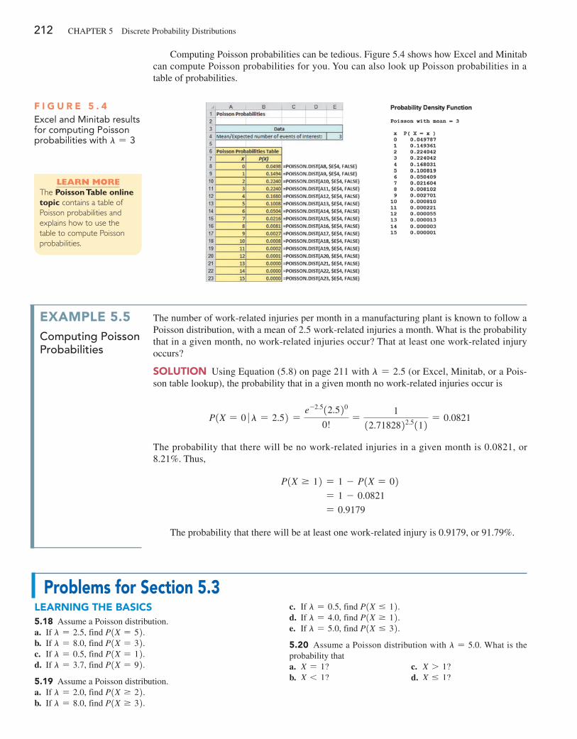
212 CHAPTeR 5 Discrete Probability Distributions
Computing Poisson probabilities can be tedious. Figure 5.4 shows how excel and Minitab can compute Poisson probabilities for you. You can also look up Poisson probabilities in a table of probabilities.
F i g u r e 5 . 4excel and minitab results for computing Poisson probabilities with l = 3
Learn MoreThe Poisson Table online topic contains a table of Poisson probabilities and explains how to use the table to compute Poisson probabilities.
examPle 5.5computing poisson probabilities
The number of work-related injuries per month in a manufacturing plant is known to follow a Poisson distribution, with a mean of 2.5 work-related injuries a month. What is the probability that in a given month, no work-related injuries occur? That at least one work-related injury occurs?
SoluTion Using equation (5.8) on page 211 with l = 2.5 (or excel, Minitab, or a Pois-son table lookup), the probability that in a given month no work-related injuries occur is
P1X = 0 �l = 2.52 =e-2.512.520
0!=
1
12.7182822.5112 = 0.0821
The probability that there will be no work-related injuries in a given month is 0.0821, or 8.21%. Thus,
P1X Ú 12 = 1 - P1X = 02 = 1 - 0.0821
= 0.9179
The probability that there will be at least one work-related injury is 0.9179, or 91.79%.
Problems for Section 5.3learning The baSicS5.18 Assume a Poisson distribution.a. If l = 2.5, find P1X = 52.b. If l = 8.0, find P1X = 32.c. If l = 0.5, find P1X = 12.d. If l = 3.7, find P1X = 92.
5.19 Assume a Poisson distribution.a. If l = 2.0, find P1X Ú 22.b. If l = 8.0, find P1X Ú 32.
c. If l = 0.5, find P1X … 12.d. If l = 4.0, find P1X Ú 12.e. If l = 5.0, find P1X … 32.
5.20 Assume a Poisson distribution with l = 5.0. What is the probability thata. X = 1?b. X 6 1?
c. X 7 1?d. X … 1?
5.3 Poisson Distribution 213
aPPlying The concePTS5.21 Assume that the number of network errors experienced in a day in a local area network (LAN) is distributed as a Poisson random variable. The mean number of network errors experienced in a day is 1.6. What is the probability that in any given daya. zero network errors will occur?b. exactly one network error will occur?c. two or more network errors will occur?d. fewer than three network errors will occur?
SELF Test
5.22 The quality control manager of Marilyn’s Cookies is inspecting a batch of chocolate-chip cookies
that has just been baked. If the production process is in control, the mean number of chip parts per cookie is 5.9. What is the probabil-ity that in any particular cookie being inspecteda. fewer than five chip parts will be found?b. exactly five chip parts will be found?c. five or more chip parts will be found?d. either four or five chip parts will be found?
5.23 The quality control manager of a cookie company is inspect-ing a batch of chocolate-chip cookies that has just been baked. If the production process is in control, the mean number of chip parts per cookie is 5.0. How many cookies in a batch of 100 should the manager expect to discard if the company policy requires that all chocolate-chip cookies sold have at least five chocolate-chip parts?
5.24 One year, airline A had 5.22 mishandled bags per 1,000 pas-sengers. What is the probability that in the next 1,000 passengers the airline will havea. no mishandled bags?b. at least one mishandled bag?c. at least two mishandled bags?
5.25 The U.S. Department of Transportation maintains statis-tics for involuntary denial of boarding. In July–September 2013, the American Airlines rate of involuntarily denying boarding was 0.45 per 10,000 passengers. What is the probability that in the next 10,000 passengers, there will bea. no one involuntarily denied boarding?b. at least one person involuntarily denied boarding?c. at least two persons involuntarily denied boarding?
5.26 The Consumer Financial Protection Bureau’s consumer re-sponse team hears directly from consumers about the challenges they face in the marketplace, brings their concerns to the atten-tion of financial institutions, and assists in addressing their com-plaints. The consumer response team accepts complaints related to mortgages, bank accounts and services, private student loans, other consumer loans, and credit reporting. An analysis of com-plaints over time indicates that the mean number of credit report-ing complaints registered by consumers is 2.70 per day. (Source: Consumer Response: A Snapshot of Complaints Received, 1.usa.gov/WZ9N8Q.) Assume that the number of credit reporting com-plaints registered by consumers is distributed as a Poisson random variable. What is the probability that on a given daya. no credit reporting complaints will be registered by consumers?b. exactly one credit reporting complaint will be registered by
consumers?c. more than one credit reporting complaint will be registered by
consumers?d. fewer than two credit reporting complaints will be registered by
consumers?
5.27 J.D. Power and Associates calculates and publishes various statistics concerning car quality. The dependability score measures problems experienced during the past 12 months by original own-ers of three-year-old vehicles (those that were introduced for the 2010 model year). For these models of cars, Ford had 1.27 prob-lems per car and Toyota had 1.12 problems per car. (Data extracted from “2013 U.S. Vehicle Dependability Study,” J.D. Power and Associates, February 13, 2013, bit.ly/101aR9l.) Let X be equal to the number of problems with a three-year-old Ford.a. What assumptions must be made in order for X to be distrib-
uted as a Poisson random variable? Are these assumptions rea-sonable?
Making the assumptions as in (a), if you purchased a Ford in the 2010 model year, what is the probability that in the past 12 months, the car hadb. zero problems?c. two or fewer problems?d. Give an operational definition for problem. Why is the opera-
tional definition important in interpreting the initial quality score?
5.28 Refer to Problem 5.27. If you purchased a Toyota in the 2010 model year, what is the probability that in the past 12 months the car hada. zero problems?b. two or fewer problems?c. Compare your answers in (a) and (b) to those for the Ford in
Problem 5.27 (b) and (c).
5.29 Refer to Problem 5.27. Another press release reported that for 2011 model cars, Ford had 1.40 problems per car and Toyota had 1.14 problems per car. (Data extracted from J. B. Healey, “Used Cars Get Less Reliable,” USA Today, February 13, 2014, p. 2B.) If you purchased a 2011 Ford, what is the probability that in the past 12 months the car hada. zero problems?b. two or fewer problems?c. Compare your answers in (a) and (b) to those for the 2010
model year Ford in Problem 5.27 (b) and (c).
5.30 Refer to Problem 5.29. If you purchased a 2011 Toyota, what is the probability that in the past 12 months, the car hada. zero problems?b. two or fewer problems?c. Compare your answers in (a) and (b) to those for the 2010
model year Toyota in Problem 5.28 (a) and (b).
5.31 A toll-free phone number is available from 9 a.m. to 9 p.m. for your customers to register complaints about a product pur-chased from your company. Past history indicates that an average of 0.8 calls is received per minute.a. What properties must be true about the situation described here
in order to use the Poisson distribution to calculate probabili-ties concerning the number of phone calls received in a one-minute period?
Assuming that this situation matches the properties discussed in (a), what is the probability that during a one-minute period
b. zero phone calls will be received?c. three or more phone calls will be received?d. What is the maximum number of phone calls that will be re-
ceived in a one-minute period 99.99% of the time?
214 CHAPTeR 5 Discrete Probability Distributions
s U M M a R y
U s i n g s tat i s t i c s
Events of Interest at Ricknel Home Centers, Revisited
In this chapter, you have studied the probability distribution for a discrete variable and two important discrete probabil-ity distributions: the binomial and Poisson distributions. In the next chapter, you will study the normal distribution.
Use the following to help decide what probability distri-bution to use for a particular situation:
• If there is a fixed number of observations, n, each of which is classified as an event of interest or not an event of interest, use the binomial distribution.
• If there is an area of opportunity, use the Poisson distribution.
R E F E R E n c E s 1. Levine, D. M., P. Ramsey, and R. Smidt. Applied Statistics for
Engineers and Scientists Using Microsoft Excel and Minitab. Upper Saddle River, NJ: Prentice Hall, 2001.
2. Microsoft Excel 2013. Redmond, WA: Microsoft Corp., 2012. 3. Minitab Release 16. State College, PA: Minitab, Inc., 2010.
K E y E q U at i o n s
Expected Value, M, of a Discrete Variable
m = E1X2 = aN
i= 1xi P1X = xi2 (5.1)
Variance of a Discrete Variable
s2 = aN
i= 13xi - E1X242P1X = xi2 (5.2)
Standard Deviation of a Discrete Variable
s = 2s2 = BaN
i= 13xi - E1X242P1X = xi2 (5.3)
Combinations
nCx =n!
x!1n - x2! (5.4)
In the Ricknel Home Improvement scenario at the be-ginning of this chapter, you were an accountant for the
Ricknel Home Improvement Company. The company’s ac-counting information system automatically reviews order forms from online customers for possible mistakes. Any questionable invoices are tagged and included in a daily ex-ceptions report. Knowing that the probability that an order will be tagged is 0.10, you were able to use the binomial distribution to determine the chance of finding a certain number of tagged forms in a sample of size four. There was a 65.6% chance that none of the forms would be tagged, a 29.2% chance that one would be tagged, and a 5.2% chance
that two or more would be tagged. You were also able to determine that, on average, you would expect 0.4 form to be tagged, and the standard deviation of the number of tagged order forms would be 0.6. Now that you have learned the mechanics of using the binomial distribution for a known probability of 0.10 and a sample size of four, you will be able to apply the same ap-proach to any given probability and sample size. Thus, you will be able to make inferences about the online ordering process and, more importantly, evaluate any changes or pro-posed changes to the process.
Sebastian Kaulitzki/Shutterstock
Chapter Review Problems 215
Binomial Distribution
P1X = x � n, p2 =n!
x!1n - x2! px11 - p2n - x (5.5)
Mean of the Binomial Distribution
m = E1X2 = np (5.6)
Standard Deviation of the Binomial Distribution
s = 2s2 = 2Var1X2 = 2np11 - p2 (5.7)
Poisson Distribution
P1X = x �l2 =e-llx
x! (5.8)
K E y t E R M sarea of opportunity 210binomial distribution 203expected value 199mathematical model 203
Poisson distribution 210probability distribution for a discrete
variable 199probability distribution function 203
rule of combinations 204standard deviation of a discrete
variable 200variance of a discrete variable 200
c H E c K i n g y o U R U n d E R s ta n d i n g5.32 What are probability density functions? Why are they useful?
5.33 What are the four properties that must be present in order to use the binomial distribution?
5.34 What are the four properties that must be present in order to use the Poisson distribution?
c H a p t E R R E v i E w p R o b l E M s5.35 Darwin Head, a 35-year-old sawmill worker, won $1 mil-lion and a Chevrolet Malibu Hybrid by scoring 15 goals within 24 seconds at the Vancouver Canucks National Hockey League game (B. Ziemer, “Darwin evolves into an Instant Millionaire,” Vancouver Sun, February 28, 2008, p. 1). Head said he would use the money to pay off his mortgage and provide for his children, and he had no plans to quit his job. The contest was part of the Chevrolet Malibu Million Dollar Shootout, sponsored by General Motors Canadian Division. Did GM-Canada risk the $1 million? No! GM-Canada purchased event insurance from a company specializing in promotions at sport-ing events such as a half-court basketball shot or a hole-in-one give-away at the local charity golf outing. The event insurance company estimates the probability of a contestant winning the contest, and for a modest charge, insures the event. The promoters pay the insurance premium but take on no added risk as the insurance company will make the large payout in the unlikely event that a contestant wins. To see how it works, suppose that the insurance company estimates that the probability a contestant would win a million-dollar shootout is 0.001 and that the insurance company charges $4,000.a. Calculate the expected value of the profit made by the insur-
ance company.b. Many call this kind of situation a win–win opportunity for the
insurance company and the promoter. Do you agree? explain.
5.36 Between 1896—when the Dow Jones index was created—and 2013, the index rose in 66% of the years. (Sources: M. Hulbert, “What the Past Can’t Tell Investors,” The New York Times, January 3, 2010, p. BU2 and bit.ly/100zwvT.) Based on this information, and assuming a binomial distribution, what do you think is the probability that the stock market will risea. next year?b. the year after next?c. in four of the next five years?d. in none of the next five years?e. For this situation, what assumption of the binomial distribution
might not be valid?
5.37 Smartphone adoption among American teens has increased substantially, and mobile access to the Internet is pervasive. One in four teenagers are “cell mostly” Internet users—that is, they mostly go online using their phone and not using some other de-vice such as a desktop or laptop computer. (Source: Teens and Technology 2013, Pew Research Center, bit.ly/101ciF1.)
If a sample of 10 American teens is selected, what is the prob-ability thata. 4 are “cell mostly” Internet users?b. at least 4 are “cell mostly” Internet users?c. at most 8 are “cell mostly” Internet users?
216 CHAPTeR 5 Discrete Probability Distributions
d. If you selected the sample in a particular geographical area and found that none of the 10 respondents are “cell mostly” Internet users, what conclusions might you reach about whether the percentage of “cell mostly” Internet users in this area was 25%?
5.38 One theory concerning the Dow Jones Industrial Average is that it is likely to increase during U.S. presidential election years. From 1964 through 2012, the Dow Jones Industrial Aver-age increased in 10 of the 13 U.S. presidential election years. Assuming that this indicator is a random event with no predictive value, you would expect that the indicator would be correct 50% of the time.a. What is the probability of the Dow Jones Industrial Average in-
creasing in 10 or more of the 13 U.S. presidential election years if the probability of an increase in the Dow Jones Industrial Av-erage is 0.50?
b. What is the probability that the Dow Jones Industrial Average will increase in 10 or more of the 13 U.S. presidential election years if the probability of an increase in the Dow Jones Indus-trial Average in any year is 0.75?
5.39 Medical billing errors and fraud are on the rise. According to the MBAA website, 8 out of 10 times, the medical bills that you get are not right. (Source: “Accurate Medical Billing,” bit.ly/1lHKIu3, April 2, 2014.) If a sample of 10 medical bills is selected, what is the probability thata. 0 medical bills will contain errors?b. exactly 5 medical bills will contain errors?c. more than 5 medical bills will contain errors?d. What are the mean and standard deviation of the probability
distribution?
5.40 Refer to Problem 5.39. Suppose that a quality improvement initiative has reduced the percentage of medical bills containing errors to 40%. If a sample of 10 medical bills is selected, what is the probability thata. 0 medical bills will contain errors?b. exactly 5 medical bills will contain errors?c. more than 5 medical bills contain errors?d. What are the mean and standard deviation of the probability
distribution?e. Compare the results of (a) through (c) to those of Problem 5.39
(a) through (c).
5.41 Social log-ins involve recommending or sharing an article that you read online. According to Janrain, in the fourth quarter of 2013, 35% signed in via Facebook compared with 35% for Google. (Source: “Social Login Trends Across the Web for Q4 2013,” bit .ly/1jmLXRr.) If a sample of 10 social log-ins is selected, what is the probability thata. more than 5 signed in using Facebook?b. more than 5 signed in using Google?c. none signed in using Facebook?d. What assumptions did you have to make to answer (a) through (c)?
5.42 The Consumer Financial Protection Bureau’s consumer response team hears directly from consumers about the chal-lenges they face in the marketplace, brings their concerns to the attention of financial institutions, and assists in addressing their complaints. Consumer response accepts complaints related to mortgages, bank accounts and services, private student loans,
other consumer loans, and credit reporting. Of the consumers who registered a bank account and service complaint, 45% cited “account management” as the type of complaint; these com-plaints are related to opening, closing, or managing the account and address issues, such as confusing marketing, denial, fees, statements, and joint accounts. (Source: Consumer Response Annual Report, 1.usa.gov/1kjpS2k.)
Consider a sample of 20 consumers who registered bank ac-count and service complaints. Use the binomial model to answer the following questions:a. What is the expected value, or mean, of the binomial distribution?b. What is the standard deviation of the binomial distribution?c. What is the probability that 10 of the 20 consumers cited
“account management” as the type of complaint?d. What is the probability that no more than 5 of the consumers
cited “account management” as the type of complaint?e. What is the probability that 5 or more of the consumers cited
“account management” as the type of complaint?
5.43 Refer to Problem 5.42. In the same time period, 25% of the consumers registering a bank account and service compliant cited “deposit and withdrawal” as the type of complaint; these are issues such as transaction holds and unauthorized transactions.a. What is the expected value, or mean, of the binomial distribution?b. What is the standard deviation of the binomial distribution?c. What is the probability that none of the 20 consumers cited
“deposit and withdrawal” as the type of complaint?d. What is the probability that no more than 2 of the consumers
cited “deposit and withdrawal” as the type of complaint?e. What is the probability that 3 or more of the consumers cited
“deposit and withdrawal” as the type of complaint?
5.44 One theory concerning the S&P 500 Index is that if it in-creases during the first five trading days of the year, it is likely to increase during the entire year. From 1950 through 2013, the S&P 500 Index had these early gains in 41 years (in 2011 there was virtually no change). In 36 of these 41 years, the S&P 500 Index increased for the entire year. Assuming that this indicator is a random event with no predictive value, you would expect that the indicator would be correct 50% of the time. What is the prob-ability of the S&P 500 Index increasing in 36 or more years if the true probability of an increase in the S&P 500 Index isa. 0.50?b. 0.70?c. 0.90?d. Based on the results of (a) through (c), what do you think is the
probability that the S&P 500 Index will increase if there is an early gain in the first five trading days of the year? explain.
5.45 Spurious correlation refers to the apparent relationship be-tween variables that either have no true relationship or are related to other variables that have not been measured. One widely publicized stock market indicator in the United States that is an example of spuri-ous correlation is the relationship between the winner of the National Football League Super Bowl and the performance of the Dow Jones Industrial Average in that year. The “indicator” states that when a team that existed before the National Football League merged with the American Football League wins the Super Bowl, the Dow Jones Industrial Average will increase in that year. (Of course, any corre-lation between these is spurious as one thing has absolutely nothing to do with the other!) Since the first Super Bowl was held in 1967

through 2013, the indicator has been correct 37 out of 47 times. As-suming that this indicator is a random event with no predictive value, you would expect that the indicator would be correct 50% of the time.a. What is the probability that the indicator would be correct 37 or
more times in 47 years?b. What does this tell you about the usefulness of this indicator?
5.46 The United Auto Courts Reports blog notes that the Na-tional Insurance Crime Bureau says that Miami-Dade, Broward, and Palm Beach counties account for a substantial number of ques-tionable insurance claims referred to investigators. Assume that the number of questionable insurance claims referred to investigators by Miami-Dade, Broward, and Palm Beach counties is distributed as a Poisson random variable with a mean of 7 per day.
a. What assumptions need to be made so that the number of ques-tionable insurance claims referred to investigators by Miami-Dade, Broward, and Palm Beach counties is distributed as a Poisson random variable?
Making the assumptions given in (a), what is the probability thatb. 5 questionable insurance claims will be referred to investigators
by Miami-Dade, Broward, and Palm Beach counties in a day?c. 10 or fewer questionable insurance claims will be referred to
investigators by Miami-Dade, Broward, and Palm Beach coun-ties in a day?
d. 11 or more questionable insurance claims will be referred to investigators by Miami-Dade, Broward, and Palm Beach coun-ties in a day?
c a s E s F o R c H a p t E R 5
Managing ashland Multicomm servicesThe Ashland MultiComm Services (AMS) marketing de-partment wants to increase subscriptions for its 3-For-All telephone, cable, and Internet combined service. AMS mar-keting has been conducting an aggressive direct-marketing campaign that includes postal and electronic mailings and telephone solicitations. Feedback from these efforts indicates that including premium channels in this combined service is a very important factor for both current and prospective sub-scribers. After several brainstorming sessions, the marketing department has decided to add premium cable channels as a no-cost benefit of subscribing to the 3-For-All service.
The research director, Mona Fields, is planning to con-duct a survey among prospective customers to determine how many premium channels need to be added to the 3-For-All service in order to generate a subscription to the service. Based on past campaigns and on industry-wide data, she es-timates the following:
Number of Free Premium Channels
Probability of Subscriptions
0 0.021 0.042 0.063 0.074 0.085 0.085
1. If a sample of 50 prospective customers is selected and no free premium channels are included in the 3-For-All service offer, given past results, what is the probability thata. fewer than 3 customers will subscribe to the 3-For-All
service offer?b. 0 customers or 1 customer will subscribe to the 3-For-
All service offer?c. more than 4 customers will subscribe to the 3-For-All
service offer?d. Suppose that in the actual survey of 50 prospective
customers, 4 customers subscribe to the 3-For-All ser-vice offer. What does this tell you about the previous estimate of the proportion of customers who would subscribe to the 3-For-All service offer?
2. Instead of offering no premium free channels as in Prob-lem 1, suppose that two free premium channels are in-cluded in the 3-For-All service offer. Given past results, what is the probability thata. fewer than 3 customers will subscribe to the 3-For-All
service offer?b. 0 customers or 1 customer will subscribe to the 3-For-
All service offer?c. more than 4 customers will subscribe to the 3-For-All
service offer?d. Compare the results of (a) through (c) to those of 1.e. Suppose that in the actual survey of 50 prospective
customers, 6 customers subscribe to the 3-For-All ser-vice offer. What does this tell you about the previous
Cases for Chapter 5 217
218 CHAPTeR 5 Discrete Probability Distributions
estimate of the proportion of customers who would subscribe to the 3-For-All service offer?
f. What do the results in (e) tell you about the effect of offering free premium channels on the likelihood of obtaining subscriptions to the 3-For-All service?
3. Suppose that additional surveys of 50 prospective cus-tomers were conducted in which the number of free premium channels was varied. The results were as follows:
Number of Free Premium Channels
Number of Subscriptions
1 53 64 65 7
How many free premium channels should the research director recommend for inclusion in the 3-For-All service? explain.
digital caseApply your knowledge about expected value in this continu-ing Digital Case from Chapters 3 and 4.
Open BullsAndBears.pdf, a marketing brochure from en-dRun Financial Services. Read the claims and examine the supporting data. Then answer the following:
1. Are there any “catches” about the claims the brochure makes for the rate of return of Happy Bull and Worried Bear funds?
2. What subjective data influence the rate-of-return analyses of these funds? Could endRun be accused of making false and misleading statements? Why or why not?
3. The expected-return analysis seems to show that the Worried Bear fund has a greater expected return than the Happy Bull fund. Should a rational investor never invest in the Happy Bull fund? Why or why not?
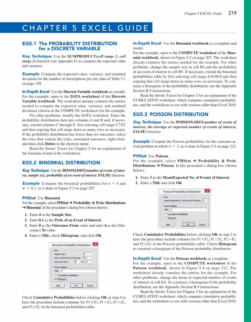
eg5.1 The ProbabiliTy DiSTribuTion for a DiScreTe Variable
Key Technique Use the SUMPRODUCT(cell range 1, cell range 2) function (see Appendix F) to compute the expected value and variance.
Example Compute the expected value, variance, and standard deviation for the number of interruptions per day data of Table 5.1 on page 199.
in-Depth excel Use the Discrete Variable workbook as a model.For the example, open to the DATA worksheet of the Discrete Variable workbook. The worksheet already contains the entries needed to compute the expected value, variance, and standard deviation (shown in the COMPUTe worksheet) for the example.
For other problems, modify the DATA worksheet. enter the probability distribution data into columns A and B and, if neces-sary, extend columns C through e, first selecting cell range C7:e7 and then copying that cell range down as many rows as necessary. If the probability distribution has fewer than six outcomes, select the rows that contain the extra, unwanted outcomes, right-click, and then click Delete in the shortcut menu.
Read the Short Takes for Chapter 5 for an explanation of the formulas found in the worksheets.
eg5.2 binomial DiSTribuTionKey Technique Use the BINOM.DIST(number of events of inter-est, sample size, probability of an event of interest, FALSE) function.
Example Compute the binomial probabilities for n = 4 and p = 0.1, as is done in Figure 5.2 on page 207.
PhStat Use Binomial.For the example, select PHStat ➔ Probability & Prob. Distributions ➔ Binomial. In the procedure’s dialog box (shown below):
1. enter 4 as the Sample Size. 2. enter 0.1 as the Prob. of an Event of Interest. 3. enter 0 as the Outcomes From value and enter 4 as the (Out-
comes) To value. 4. enter a Title, check Histogram, and click OK.
Check Cumulative Probabilities before clicking OK in step 4 to have the procedure include columns for P1…X2, P16X2, P17X2, and P1ÚX2 in the binomial probabilities table.
in-Depth excel Use the Binomial workbook as a template and model.For the example, open to the COMPUTE worksheet of the Bino-mial workbook, shown in Figure 5.2 on page 207. The worksheet already contains the entries needed for the example. For other problems, change the sample size in cell B4 and the probability of an event of interest in cell B5. If necessary, extend the binomial probabilities table by first selecting cell range A18:B18 and then copying that cell range down as many rows as necessary. To con-struct a histogram of the probability distribution, use the Appendix Section B.9 instructions.
Read the Short Takes for Chapter 5 for an explanation of the CUMULATIVe worksheet, which computes cumulative probabili-ties, and the worksheets to use with versions older than excel 2010.
eg5.3 PoiSSon DiSTribuTionKey Technique Use the POISSON.DIST(number of events of interest, the average or expected number of events of interest, FALSE) function.
Example Compute the Poisson probabilities for the customer ar-rival problem in which l = 3, as is done in Figure 5.4 on page 212.
PhStat Use Poisson.For the example, select PHStat ➔ Probability & Prob. Distributions ➔ Poisson. In this procedure’s dialog box (shown below):
1. enter 3 as the Mean/Expected No. of Events of Interest. 2. enter a Title and click OK.
Check Cumulative Probabilities before clicking OK in step 2 to have the procedure include columns for P1…X2, P16X2, P17X2, and P1ÚX2 in the Poisson probabilities table. Check Histogram to construct a histogram of the Poisson probability distribution.
in-Depth excel Use the Poisson workbook as a template.For the example, open to the COMPUTE worksheet of the Poisson workbook, shown in Figure 5.4 on page 212. The worksheet already contains the entries for the example. For other problems, change the mean or expected number of events of interest in cell e4. To construct a histogram of the probability distribution, use the Appendix Section B.9 instructions.
Read the Short Takes for Chapter 5 for an explanation of the CUMULATIVe worksheet, which computes cumulative probabili-ties, and the worksheets to use with versions older than excel 2010.
c H a p t E R 5 E x c E l g U i d E
Chapter 5 exCeL Guide 219
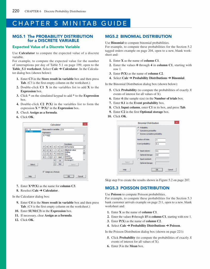
220 CHAPTeR 6 Discrete Probability Distributions
mg5.1 The ProbabiliTy DiSTribuTion for a DiScreTe Variable
expected Value of a Discrete Variable
Use Calculator to compute the expected value of a discrete variable.For example, to compute the expected value for the number of interruptions per day of Table 5.1 on page 199, open to the Table_5.1 worksheet. Select Calc ➔ Calculator. In the Calcula-tor dialog box (shown below):
1. enter C3 in the Store result in variable box and then press Tab. (C3 is the first empty column on the worksheet.)
2. Double-click C1 X in the variables list to add X to the Expression box.
3. Click * on the simulated keypad to add * to the Expression box.
4. Double-click C2 P(X) in the variables list to form the expression X * 'P(X)' in the Expression box.
5. Check Assign as a formula. 6. Click OK.
7. enter X*P(X) as the name for column C3. 8. Reselect Calc ➔ Calculator.
In the Calculator dialog box:
9. enter C4 in the Store result in variable box and then press Tab. (C4 is the first empty column on the worksheet.)
10. enter SUM(C3) in the Expression box. 11. If necessary, clear Assign as a formula. 12. Click OK.
mg5.2 binomial DiSTribuTionUse Binomial to compute binomial probabilities.For example, to compute these probabilities for the Section 5.2 tagged orders example on page 204, open to a new, blank work-sheet and:
1. enter X as the name of column C1. 2. enter the values 0 through 4 in column C1, starting with
row 1. 3. enter P(X) as the name of column C2. 4. Select Calc ➔ Probability Distributions ➔ Binomial.
In the Binomial Distribution dialog box (shown below):
5. Click Probability (to compute the probabilities of exactly X events of interest for all values of x).
6. enter 4 (the sample size) in the Number of trials box. 7. enter 0.1 in the Event probability box. 8. Click Input column, enter C1 in its box, and press Tab. 9. enter C2 in the first Optional storage box. 10. Click OK.
Skip step 9 to create the results shown in Figure 5.2 on page 207.
mg5.3 PoiSSon DiSTribuTionUse Poisson to compute Poisson probabilities.For example, to compute these probabilities for the Section 5.3 bank customer arrivals example on page 211, open to a new, blank worksheet and:
1. enter X as the name of column C1. 2. enter the values 0 through 15 in column C1, starting with row 1. 3. enter P(X) as the name of column C2. 4. Select Calc ➔ Probability Distributions ➔ Poisson.
In the Poisson Distribution dialog box (shown on page 221):
5. Click Probability (to compute the probabilities of exactly X events of interest for all values of x).
6. enter 3 in the Mean box.
c H a p t E R 5 M i n i ta b g U i d E
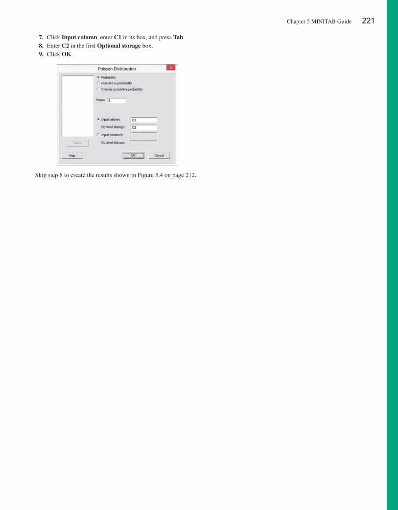
7. Click Input column, enter C1 in its box, and press Tab. 8. enter C2 in the first Optional storage box. 9. Click OK.
Skip step 8 to create the results shown in Figure 5.4 on page 212.
Chapter 5 MINITAB Guide 221
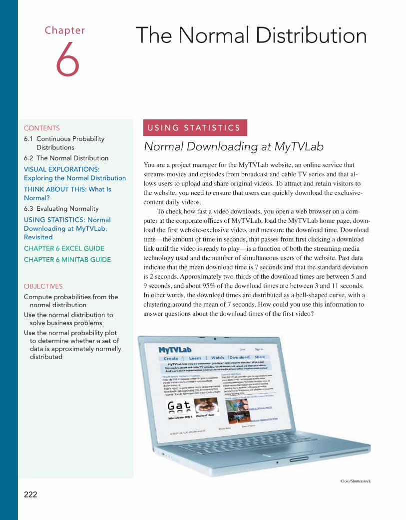
222
U s i n g s tat i s t i c s
Normal Downloading at MyTVLabYou are a project manager for the MyTVLab website, an online service that streams movies and episodes from broadcast and cable TV series and that al-lows users to upload and share original videos. To attract and retain visitors to the website, you need to ensure that users can quickly download the exclusive-content daily videos.
To check how fast a video downloads, you open a web browser on a com-puter at the corporate offices of MyTVLab, load the MyTVLab home page, down-load the first website-exclusive video, and measure the download time. Download time—the amount of time in seconds, that passes from first clicking a download link until the video is ready to play—is a function of both the streaming media technology used and the number of simultaneous users of the website. Past data indicate that the mean download time is 7 seconds and that the standard deviation is 2 seconds. Approximately two-thirds of the download times are between 5 and 9 seconds, and about 95% of the download times are between 3 and 11 seconds. In other words, the download times are distributed as a bell-shaped curve, with a clustering around the mean of 7 seconds. How could you use this information to answer questions about the download times of the first video?
Contents
6.1 Continuous Probability Distributions
6.2 The Normal Distribution
VisUal Explorations: Exploring the normal Distribution
think aboUt this: What is normal?
6.3 Evaluating Normality
Using statistics: normal Downloading at MytVlab, revisited
chaptEr 6 ExcEl gUiDE
chaptEr 6 Minitab gUiDE
objeCtives
Compute probabilities from the normal distribution
Use the normal distribution to solve business problems
Use the normal probability plot to determine whether a set of data is approximately normally distributed
Chapter The Normal Distribution6
Cloki/Shutterstock
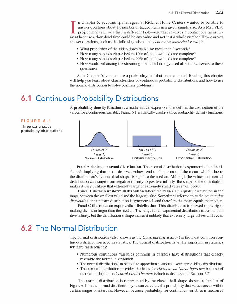
6.2 The Normal Distribution 223
I n Chapter 5, accounting managers at Ricknel Home Centers wanted to be able to answer questions about the number of tagged items in a given sample size. As a MyTVLab project manager, you face a different task—one that involves a continuous measure-
ment because a download time could be any value and not just a whole number. How can you answer questions, such as the following, about this continuous numerical variable:
• What proportion of the video downloads take more than 9 seconds? • How many seconds elapse before 10% of the downloads are complete? • How many seconds elapse before 99% of the downloads are complete? • How would enhancing the streaming media technology used affect the answers to these
questions?
As in Chapter 5, you can use a probability distribution as a model. Reading this chapter will help you learn about characteristics of continuous probability distributions and how to use the normal distribution to solve business problems.
F i g u r e 6 . 1Three continuous probability distributions
Values of XPanel A
Normal DistributionPanel B
Uniform DistributionPanel C
Exponential Distribution
Values of X Values of X
6.1 Continuous Probability DistributionsA probability density function is a mathematical expression that defines the distribution of the values for a continuous variable. Figure 6.1 graphically displays three probability density functions.
Panel A depicts a normal distribution. The normal distribution is symmetrical and bell-shaped, implying that most observed values tend to cluster around the mean, which, due to the distribution’s symmetrical shape, is equal to the median. Although the values in a normal distribution can range from negative infinity to positive infinity, the shape of the distribution makes it very unlikely that extremely large or extremely small values will occur.
Panel B shows a uniform distribution where the values are equally distributed in the range between the smallest value and the largest value. Sometimes referred to as the rectangular distribution, the uniform distribution is symmetrical, and therefore the mean equals the median.
Panel C illustrates an exponential distribution. This distribution is skewed to the right, making the mean larger than the median. The range for an exponential distribution is zero to pos-itive infinity, but the distribution’s shape makes it unlikely that extremely large values will occur.
6.2 The Normal DistributionThe normal distribution (also known as the Gaussian distribution) is the most common con-tinuous distribution used in statistics. The normal distribution is vitally important in statistics for three main reasons:
• Numerous continuous variables common in business have distributions that closely resemble the normal distribution.
• The normal distribution can be used to approximate various discrete probability distributions. • The normal distribution provides the basis for classical statistical inference because of
its relationship to the Central Limit Theorem (which is discussed in Section 7.2).
The normal distribution is represented by the classic bell shape shown in Panel A of Figure 6.1. In the normal distribution, you can calculate the probability that values occur within certain ranges or intervals. However, because probability for continuous variables is measured
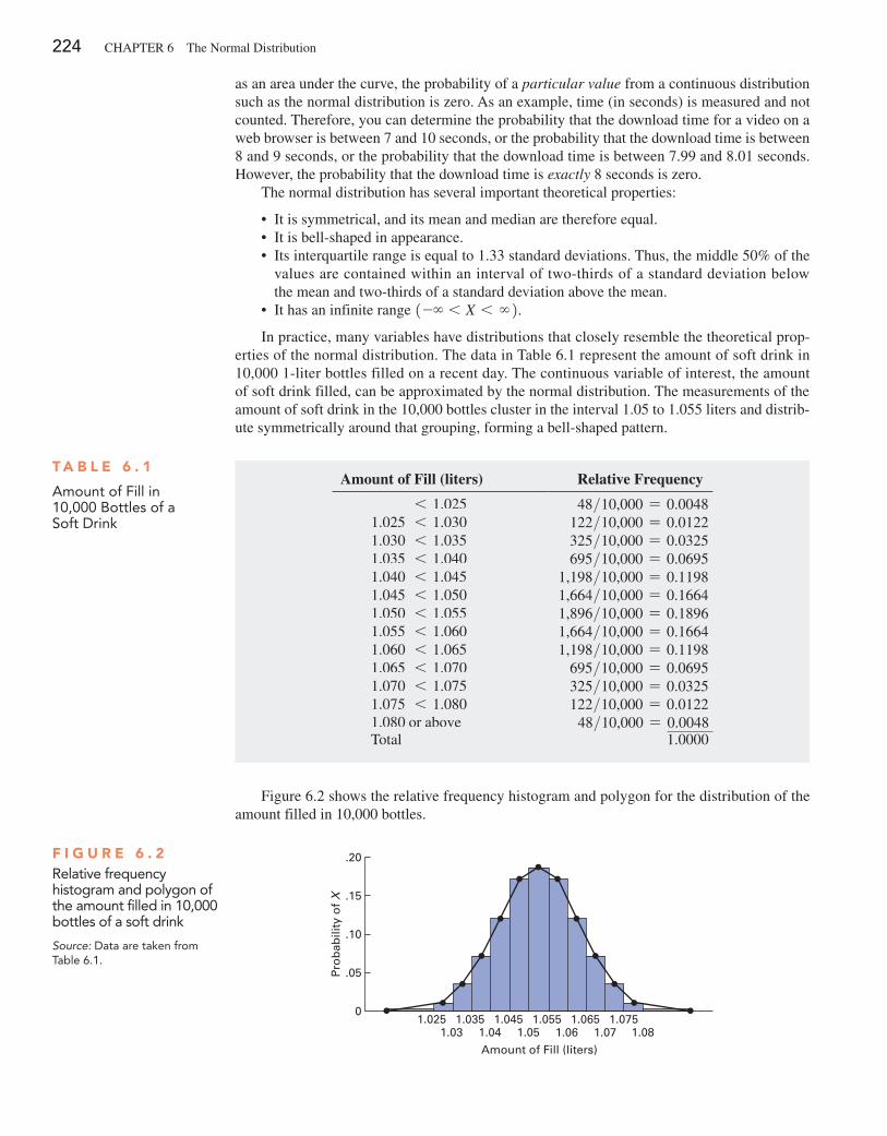
224 CHAPTeR 6 The Normal Distribution
as an area under the curve, the probability of a particular value from a continuous distribution such as the normal distribution is zero. As an example, time (in seconds) is measured and not counted. Therefore, you can determine the probability that the download time for a video on a web browser is between 7 and 10 seconds, or the probability that the download time is between 8 and 9 seconds, or the probability that the download time is between 7.99 and 8.01 seconds. However, the probability that the download time is exactly 8 seconds is zero.
The normal distribution has several important theoretical properties:
• It is symmetrical, and its mean and median are therefore equal. • It is bell-shaped in appearance. • Its interquartile range is equal to 1.33 standard deviations. Thus, the middle 50% of the
values are contained within an interval of two-thirds of a standard deviation below the mean and two-thirds of a standard deviation above the mean.
• It has an infinite range 1-∞ 6 X 6 ∞2.
In practice, many variables have distributions that closely resemble the theoretical prop-erties of the normal distribution. The data in Table 6.1 represent the amount of soft drink in 10,000 1-liter bottles filled on a recent day. The continuous variable of interest, the amount of soft drink filled, can be approximated by the normal distribution. The measurements of the amount of soft drink in the 10,000 bottles cluster in the interval 1.05 to 1.055 liters and distrib-ute symmetrically around that grouping, forming a bell-shaped pattern.
Figure 6.2 shows the relative frequency histogram and polygon for the distribution of the amount filled in 10,000 bottles.
F i g u r e 6 . 2Relative frequency histogram and polygon of the amount filled in 10,000 bottles of a soft drink
Source: Data are taken from Table 6.1.
.20
1.025 1.035 1.045 1.055
Amount of Fill (liters)
Pro
bab
ility
of
X
1.065 1.0751.03 1.04 1.05 1.06 1.07 1.08
.15
.10
.05
0
T a b l e 6 . 1
Amount of Fill in 10,000 Bottles of a Soft Drink
Amount of Fill (liters) Relative Frequency
6 1.025 48>10,000 = 0.00481.025 6 1.030 122>10,000 = 0.01221.030 6 1.035 325>10,000 = 0.03251.035 6 1.040 695>10,000 = 0.06951.040 6 1.045 1,198>10,000 = 0.11981.045 6 1.050 1,664>10,000 = 0.16641.050 6 1.055 1,896>10,000 = 0.18961.055 6 1.060 1,664>10,000 = 0.16641.060 6 1.065 1,198>10,000 = 0.11981.065 6 1.070 695>10,000 = 0.06951.070 6 1.075 325>10,000 = 0.03251.075 6 1.080 122>10,000 = 0.01221.080 or above 48>10,000 = 0.0048 Total 1.0000
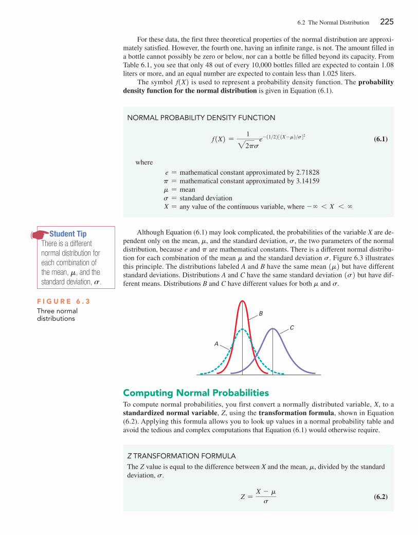
6.2 The Normal Distribution 225
For these data, the first three theoretical properties of the normal distribution are approxi-mately satisfied. However, the fourth one, having an infinite range, is not. The amount filled in a bottle cannot possibly be zero or below, nor can a bottle be filled beyond its capacity. From Table 6.1, you see that only 48 out of every 10,000 bottles filled are expected to contain 1.08 liters or more, and an equal number are expected to contain less than 1.025 liters.
The symbol f1X2 is used to represent a probability density function. The probability density function for the normal distribution is given in equation (6.1).
NoRmAl PRoBABiliTy DENSiTy FUNCTioN
f 1X2 =122ps
e-11>2231X - m2>s42 (6.1)
where
e = mathematical constant approximated by 2.71828 p = mathematical constant approximated by 3.14159 m = mean s = standard deviation X = any value of the continuous variable, where - ∞ 6 X 6 ∞
Although equation (6.1) may look complicated, the probabilities of the variable X are de-pendent only on the mean, m, and the standard deviation, s, the two parameters of the normal distribution, because e and p are mathematical constants. There is a different normal distribu-tion for each combination of the mean m and the standard deviation s. Figure 6.3 illustrates this principle. The distributions labeled A and B have the same mean 1m2 but have different standard deviations. Distributions A and C have the same standard deviation 1s2 but have dif-ferent means. Distributions B and C have different values for both m and s.
Student TipThere is a different normal distribution for each combination of the mean, m, and the standard deviation, s.
F i g u r e 6 . 3Three normal distributions
A
B
C
Computing Normal ProbabilitiesTo compute normal probabilities, you first convert a normally distributed variable, X, to a standardized normal variable, Z, using the transformation formula, shown in equation (6.2). Applying this formula allows you to look up values in a normal probability table and avoid the tedious and complex computations that equation (6.1) would otherwise require.
Z TRANSFoRmATioN FoRmUlA
The Z value is equal to the difference between X and the mean, m, divided by the standard deviation, s.
Z =X - m
s (6.2)
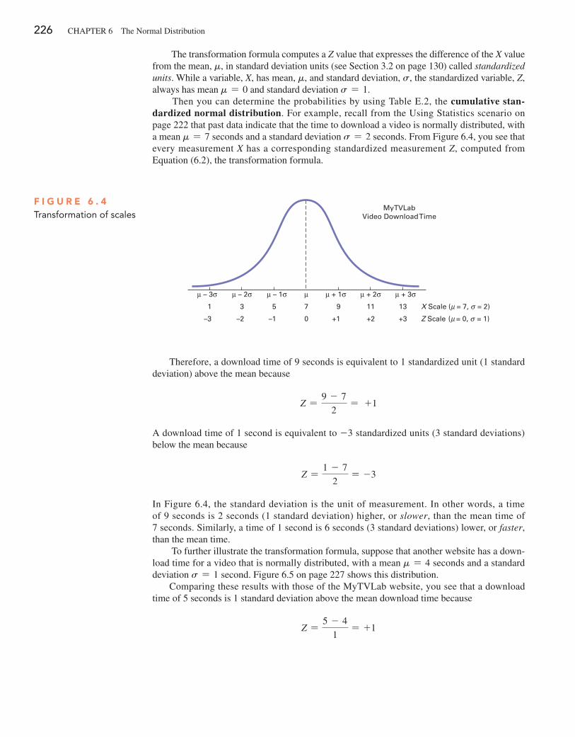
226 CHAPTeR 6 The Normal Distribution
The transformation formula computes a Z value that expresses the difference of the X value from the mean, m, in standard deviation units (see Section 3.2 on page 130) called standardized units. While a variable, X, has mean, m, and standard deviation, s, the standardized variable, Z, always has mean m = 0 and standard deviation s = 1.
Then you can determine the probabilities by using Table e.2, the cumulative stan-dardized normal distribution. For example, recall from the Using Statistics scenario on page 222 that past data indicate that the time to download a video is normally distributed, with a mean m = 7 seconds and a standard deviation s = 2 seconds. From Figure 6.4, you see that every measurement X has a corresponding standardized measurement Z, computed from equation (6.2), the transformation formula.
F i g u r e 6 . 4Transformation of scales
MyTVLabVideo Download Time
μ – 3σ μ – 2σ μ – 1σ μ μ + 1σ μ + 2σ μ + 3σ
1 3 5 7 9 11 13 X Scale ( = 7, = 2)
( = 0, = 1) –3 –2 –1 0 +1 +2 +3 Z Scale
Therefore, a download time of 9 seconds is equivalent to 1 standardized unit (1 standard deviation) above the mean because
Z =9 - 7
2= +1
A download time of 1 second is equivalent to -3 standardized units (3 standard deviations) below the mean because
Z =1 - 7
2= -3
In Figure 6.4, the standard deviation is the unit of measurement. In other words, a time of 9 seconds is 2 seconds (1 standard deviation) higher, or slower, than the mean time of 7 seconds. Similarly, a time of 1 second is 6 seconds (3 standard deviations) lower, or faster, than the mean time.
To further illustrate the transformation formula, suppose that another website has a down-load time for a video that is normally distributed, with a mean m = 4 seconds and a standard deviation s = 1 second. Figure 6.5 on page 227 shows this distribution.
Comparing these results with those of the MyTVLab website, you see that a download time of 5 seconds is 1 standard deviation above the mean download time because
Z =5 - 4
1= +1
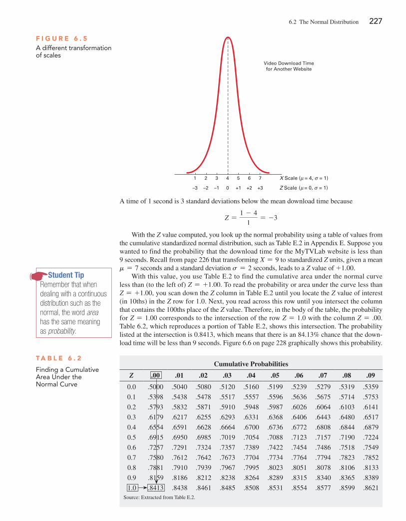
6.2 The Normal Distribution 227
A time of 1 second is 3 standard deviations below the mean download time because
Z =1 - 4
1= -3
With the Z value computed, you look up the normal probability using a table of values from the cumulative standardized normal distribution, such as Table e.2 in Appendix e. Suppose you wanted to find the probability that the download time for the MyTVLab website is less than 9 seconds. Recall from page 226 that transforming X = 9 to standardized Z units, given a mean m = 7 seconds and a standard deviation s = 2 seconds, leads to a Z value of +1.00.
With this value, you use Table e.2 to find the cumulative area under the normal curve less than (to the left of) Z = +1.00. To read the probability or area under the curve less than Z = +1.00, you scan down the Z column in Table e.2 until you locate the Z value of interest (in 10ths) in the Z row for 1.0. Next, you read across this row until you intersect the column that contains the 100ths place of the Z value. Therefore, in the body of the table, the probability for Z = 1.00 corresponds to the intersection of the row Z = 1.0 with the column Z = .00. Table 6.2, which reproduces a portion of Table e.2, shows this intersection. The probability listed at the intersection is 0.8413, which means that there is an 84.13% chance that the down-load time will be less than 9 seconds. Figure 6.6 on page 228 graphically shows this probability.
F i g u r e 6 . 5A different transformation of scales
Video Download Timefor Another Website
1 2 3 4 5 6 7
–3 –2 –1 0 +1 +2 +3
X Scale ( = 4, = 1)
( = 0, = 1) Z Scale
Student TipRemember that when dealing with a continuous distribution such as the normal, the word area has the same meaning as probability.
T a b l e 6 . 2
Finding a Cumulative Area Under the Normal Curve
Cumulative Probabilities
Z .00 .01 .02 .03 .04 .05 .06 .07 .08 .09
0.0 .5000 .5040 .5080 .5120 .5160 .5199 .5239 .5279 .5319 .5359
0.1 .5398 .5438 .5478 .5517 .5557 .5596 .5636 .5675 .5714 .5753
0.2 .5793 .5832 .5871 .5910 .5948 .5987 .6026 .6064 .6103 .6141
0.3 .6179 .6217 .6255 .6293 .6331 .6368 .6406 .6443 .6480 .6517
0.4 .6554 .6591 .6628 .6664 .6700 .6736 .6772 .6808 .6844 .6879
0.5 .6915 .6950 .6985 .7019 .7054 .7088 .7123 .7157 .7190 .7224
0.6 .7257 .7291 .7324 .7357 .7389 .7422 .7454 .7486 .7518 .7549
0.7 .7580 .7612 .7642 .7673 .7704 .7734 .7764 .7794 .7823 .7852
0.8 .7881 .7910 .7939 .7967 .7995 .8023 .8051 .8078 .8106 .8133
0.9 .8159 .8186 .8212 .8238 .8264 .8289 .8315 .8340 .8365 .8389
1.0 .8413 .8438 .8461 .8485 .8508 .8531 .8554 .8577 .8599 .8621Source: extracted from Table e.2.
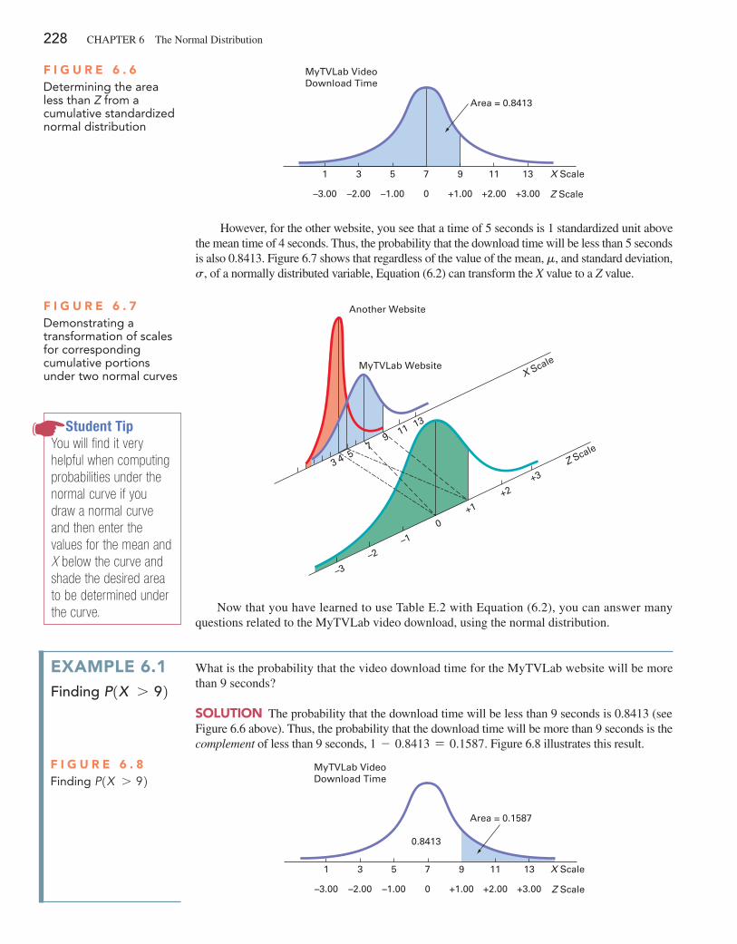
228 CHAPTeR 6 The Normal Distribution
However, for the other website, you see that a time of 5 seconds is 1 standardized unit above the mean time of 4 seconds. Thus, the probability that the download time will be less than 5 seconds is also 0.8413. Figure 6.7 shows that regardless of the value of the mean, m, and standard deviation, s, of a normally distributed variable, equation (6.2) can transform the X value to a Z value.
F i g u r e 6 . 6Determining the area less than Z from a cumulative standardized normal distribution
X Scale
Z Scale
Area = 0.8413
1 3 5 7 9 11 13
–3.00 –2.00 –1.00 0 +1.00 +2.00 +3.00
MyTVLab VideoDownload Time
Student TipYou will find it very helpful when computing probabilities under the normal curve if you draw a normal curve and then enter the values for the mean and X below the curve and shade the desired area to be determined under the curve.
F i g u r e 6 . 7Demonstrating a transformation of scales for corresponding cumulative portions under two normal curves
MyTVLab Website
3 4 57
911
+3
+2
+1
0
–1
–2
–3
13
X Scale
Z Scale
Another Website
Now that you have learned to use Table e.2 with equation (6.2), you can answer many questions related to the MyTVLab video download, using the normal distribution.
examPle 6.1Finding P1X 7 92
What is the probability that the video download time for the MyTVLab website will be more than 9 seconds?
SoluTioN The probability that the download time will be less than 9 seconds is 0.8413 (see Figure 6.6 above). Thus, the probability that the download time will be more than 9 seconds is the complement of less than 9 seconds, 1 - 0.8413 = 0.1587. Figure 6.8 illustrates this result.
F i g u r e 6 . 8Finding P1X 7 92
X Scale
Z Scale
Area = 0.1587
1 3 5 7 9 11 13
–3.00 –2.00 –1.00 0 +1.00 +2.00 +3.00
0.8413
MyTVLab VideoDownload Time
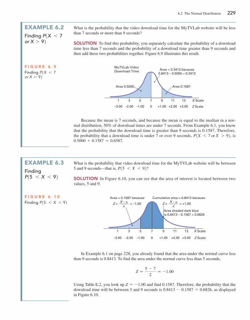
6.2 The Normal Distribution 229
examPle 6.2Finding P1X 6 7or X 7 92
What is the probability that the video download time for the MyTVLab website will be less than 7 seconds or more than 9 seconds?
SoluTioN To find this probability, you separately calculate the probability of a download time less than 7 seconds and the probability of a download time greater than 9 seconds and then add these two probabilities together. Figure 6.9 illustrates this result.
Because the mean is 7 seconds, and because the mean is equal to the median in a nor-mal distribution, 50% of download times are under 7 seconds. From example 6.1, you know that the probability that the download time is greater than 9 seconds is 0.1587. Therefore, the probability that a download time is under 7 or over 9 seconds, P1X 6 7 or X 7 92, is 0.5000 + 0.1587 = 0.6587.
F i g u r e 6 . 9Finding P1X 6 7or X 7 92
X Scale
Z Scale
MyTVLab VideoDownload Time
Area 0.5000
1 3 5 7 9 11 13
–3.00 –2.00 –1.00 0 +1.00 +2.00 +3.00
Area 0.1587
Area = 0.3413 because0.8413 – 0.5000 = 0.3413
examPle 6.3Finding P15 6 X 6 92
What is the probability that video download time for the MyTVLab website will be between 5 and 9 seconds—that is, P15 6 X 6 92?
SoluTioN In Figure 6.10, you can see that the area of interest is located between two values, 5 and 9.
F i g u r e 6 . 1 0Finding P15 6 X 6 92
X Scale
Z Scale
Cumulative area = 0.8413 because
Area shaded dark blueis 0.8413 – 0.1587 = 0.6826
1 3 5 7 9 11 13
Z = = +1.00
–3.00 –2.00 –1.00 0 +1.00 +2.00 +3.00
Area = 0.1587 because
Z = = –1.00X – X –
In example 6.1 on page 228, you already found that the area under the normal curve less than 9 seconds is 0.8413. To find the area under the normal curve less than 5 seconds,
Z =5 - 7
2= -1.00
Using Table e.2, you look up Z = -1.00 and find 0.1587. Therefore, the probability that the download time will be between 5 and 9 seconds is 0.8413 - 0.1587 = 0.6826, as displayed in Figure 6.10.
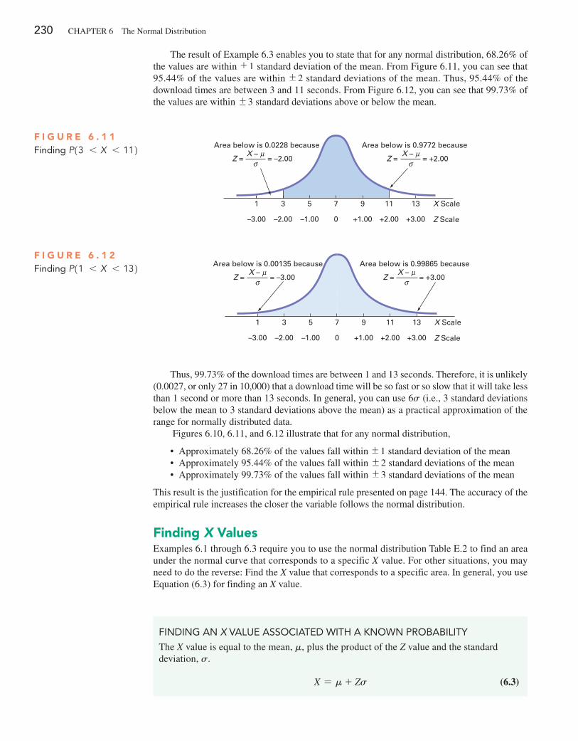
230 CHAPTeR 6 The Normal Distribution
The result of example 6.3 enables you to state that for any normal distribution, 68.26% of the values are within {1 standard deviation of the mean. From Figure 6.11, you can see that 95.44% of the values are within {2 standard deviations of the mean. Thus, 95.44% of the download times are between 3 and 11 seconds. From Figure 6.12, you can see that 99.73% of the values are within {3 standard deviations above or below the mean.
F i g u r e 6 . 1 1Finding P13 6 X 6 112
X Scale
Z Scale
Area below is 0.9772 because
1 3 5 7 9 11 13
Z = = +2.00
–3.00 –2.00 –1.00 0 +1.00 +2.00 +3.00
Area below is 0.0228 because
Z = = –2.00X – X –
F i g u r e 6 . 1 2Finding P11 6 X 6 132
X Scale
Z Scale
Area below is 0.99865 because
1 3 5 7 9 11 13
Z = = +3.00
–3.00 –2.00 –1.00 0 +1.00 +2.00 +3.00
Area below is 0.00135 because
Z = = –3.00X – X –
Thus, 99.73% of the download times are between 1 and 13 seconds. Therefore, it is unlikely (0.0027, or only 27 in 10,000) that a download time will be so fast or so slow that it will take less than 1 second or more than 13 seconds. In general, you can use 6s (i.e., 3 standard deviations below the mean to 3 standard deviations above the mean) as a practical approximation of the range for normally distributed data.
Figures 6.10, 6.11, and 6.12 illustrate that for any normal distribution,
• Approximately 68.26% of the values fall within {1 standard deviation of the mean • Approximately 95.44% of the values fall within {2 standard deviations of the mean • Approximately 99.73% of the values fall within {3 standard deviations of the mean
This result is the justification for the empirical rule presented on page 144. The accuracy of the empirical rule increases the closer the variable follows the normal distribution.
Finding X Valuesexamples 6.1 through 6.3 require you to use the normal distribution Table e.2 to find an area under the normal curve that corresponds to a specific X value. For other situations, you may need to do the reverse: Find the X value that corresponds to a specific area. In general, you use equation (6.3) for finding an X value.
FiNDiNg AN X VAlUE ASSoCiATED WiTh A KNoWN PRoBABiliTy
The X value is equal to the mean, m, plus the product of the Z value and the standard deviation, s.
X = m + Zs (6.3)
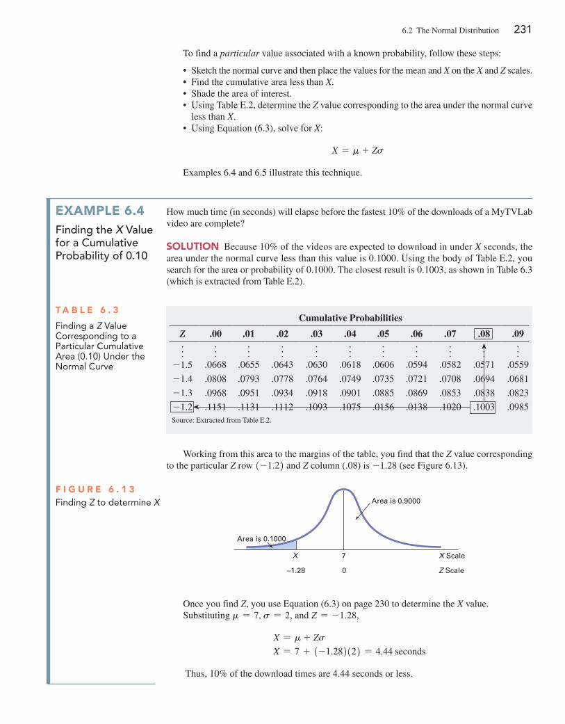
6.2 The Normal Distribution 231
To find a particular value associated with a known probability, follow these steps:
• Sketch the normal curve and then place the values for the mean and X on the X and Z scales. • Find the cumulative area less than X. • Shade the area of interest. • Using Table e.2, determine the Z value corresponding to the area under the normal curve
less than X. • Using equation (6.3), solve for X:
X = m + Zs
examples 6.4 and 6.5 illustrate this technique.
examPle 6.4Finding the X Value for a cumulative probability of 0.10
How much time (in seconds) will elapse before the fastest 10% of the downloads of a MyTVLab video are complete?
SoluTioN Because 10% of the videos are expected to download in under X seconds, the area under the normal curve less than this value is 0.1000. Using the body of Table e.2, you search for the area or probability of 0.1000. The closest result is 0.1003, as shown in Table 6.3 (which is extracted from Table e.2).
T a b l e 6 . 3
Finding a Z Value Corresponding to a Particular Cumulative Area (0.10) Under the Normal Curve
Cumulative Probabilities
Z .00 .01 .02 .03 .04 .05 .06 .07 .08 .09
f f f f f f f f f f f-1.5 .0668 .0655 .0643 .0630 .0618 .0606 .0594 .0582 .0571 .0559
-1.4 .0808 .0793 .0778 .0764 .0749 .0735 .0721 .0708 .0694 .0681
-1.3 .0968 .0951 .0934 .0918 .0901 .0885 .0869 .0853 .0838 .0823
-1.2 .1151 .1131 .1112 .1093 .1075 .0156 .0138 .1020 .1003 .0985Source: extracted from Table e.2.
Working from this area to the margins of the table, you find that the Z value corresponding to the particular Z row 1-1.22 and Z column (.08) is -1.28 (see Figure 6.13).
F i g u r e 6 . 1 3Finding Z to determine X
X Scale
Z Scale
X 7
–1.28 0
Area is 0.9000
Area is 0.1000
Once you find Z, you use equation (6.3) on page 230 to determine the X value. Substituting m = 7, s = 2, and Z = -1.28,
X = m + Zs
X = 7 + 1-1.282122 = 4.44 seconds
Thus, 10% of the download times are 4.44 seconds or less.
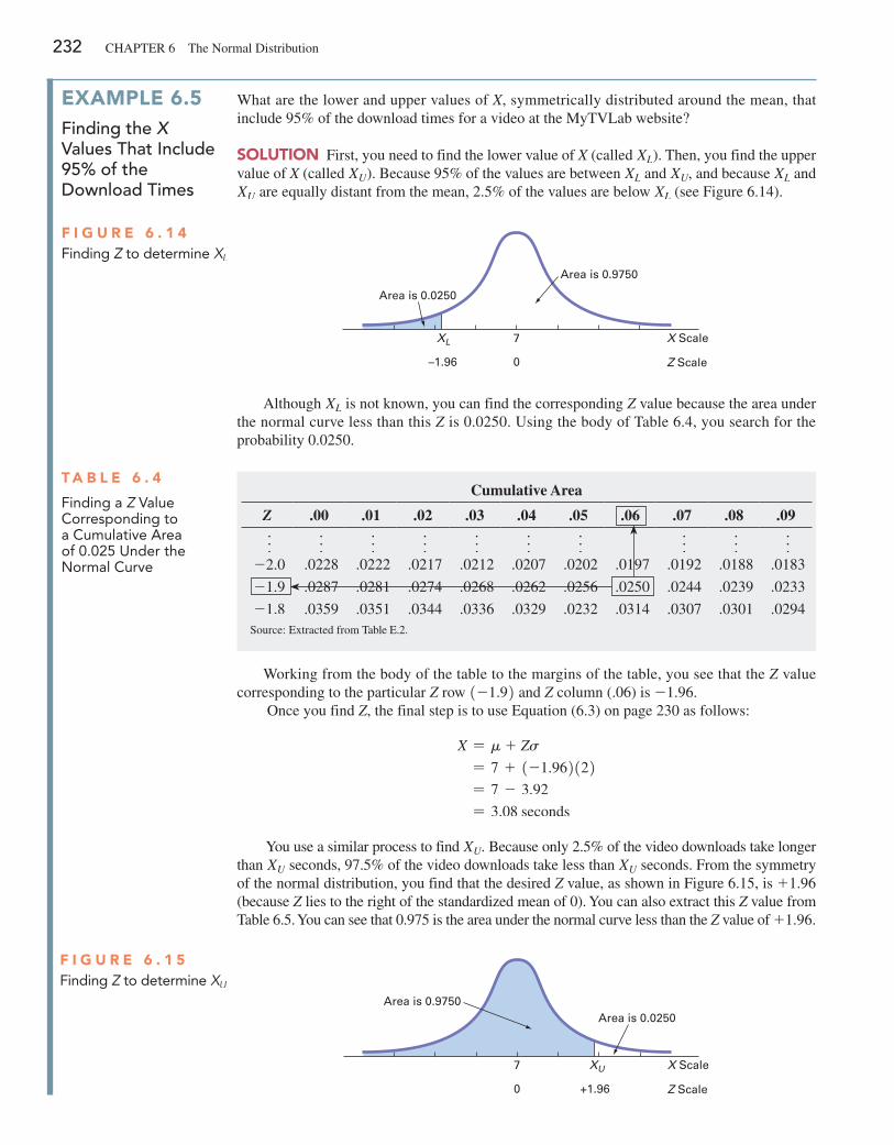
232 CHAPTeR 6 The Normal Distribution
examPle 6.5Finding the X Values that include 95% of the Download times
What are the lower and upper values of X, symmetrically distributed around the mean, that include 95% of the download times for a video at the MyTVLab website?
SoluTioN First, you need to find the lower value of X (called XL). Then, you find the upper value of X (called XU). Because 95% of the values are between XL and XU, and because XL and XU are equally distant from the mean, 2.5% of the values are below XL (see Figure 6.14).
F i g u r e 6 . 1 4Finding Z to determine XL
X Scale
Z Scale
XL
Area is 0.9750
7
0–1.96
Area is 0.0250
Although XL is not known, you can find the corresponding Z value because the area under the normal curve less than this Z is 0.0250. Using the body of Table 6.4, you search for the probability 0.0250.
T a b l e 6 . 4
Finding a Z Value Corresponding to a Cumulative Area of 0.025 Under the Normal Curve
Cumulative Area
Z .00 .01 .02 .03 .04 .05 .06 .07 .08 .09
f f f f f f f f f f-2.0 .0228 .0222 .0217 .0212 .0207 .0202 .0197 .0192 .0188 .0183
-1.9 .0287 .0281 .0274 .0268 .0262 .0256 .0250 .0244 .0239 .0233
-1.8 .0359 .0351 .0344 .0336 .0329 .0232 .0314 .0307 .0301 .0294Source: extracted from Table e.2.
Working from the body of the table to the margins of the table, you see that the Z value corresponding to the particular Z row 1-1.92 and Z column (.06) is -1.96.
Once you find Z, the final step is to use equation (6.3) on page 230 as follows:
X = m + Zs
= 7 + 1-1.962122 = 7 - 3.92
= 3.08 seconds
You use a similar process to find XU. Because only 2.5% of the video downloads take longer than XU seconds, 97.5% of the video downloads take less than XU seconds. From the symmetry of the normal distribution, you find that the desired Z value, as shown in Figure 6.15, is +1.96 (because Z lies to the right of the standardized mean of 0). You can also extract this Z value from Table 6.5. You can see that 0.975 is the area under the normal curve less than the Z value of +1.96.
F i g u r e 6 . 1 5Finding Z to determine XU
X Scale
Z Scale
XU
Area is 0.9750
7
0 +1.96
Area is 0.0250
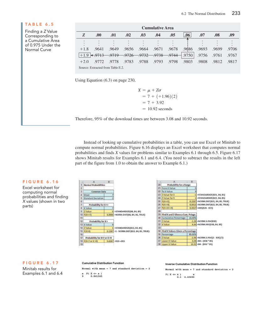
6.2 The Normal Distribution 233
Instead of looking up cumulative probabilities in a table, you can use excel or Minitab to compute normal probabilities. Figure 6.16 displays an excel worksheet that computes normal probabilities and finds X values for problems similar to examples 6.1 through 6.5. Figure 6.17 shows Minitab results for examples 6.1 and 6.4. (You need to subtract the results in the left part of the figure from 1.0 to obtain the answer to example 6.1.)
F i g u r e 6 . 1 6Excel worksheet for computing normal probabilities and finding X values (shown in two parts)
T a b l e 6 . 5
Finding a Z Value Corresponding to a Cumulative Area of 0.975 Under the Normal Curve
Cumulative Area
Z .00 .01 .02 .03 .04 .05 .06 .07 .08 .09
f f f f f f f f f f f+1.8 .9641 .9649 .9656 .9664 .9671 .9678 .9686 .9693 .9699 .9706
+1.9 .9713 .9719 .9726 .9732 .9738 .9744 .9750 .9756 .9761 .9767
+2.0 .9772 .9778 .9783 .9788 .9793 .9798 .9803 .9808 .9812 .9817Source: extracted from Table e.2.
Using equation (6.3) on page 230,
X = m + Zs
= 7 + 1+1.962122 = 7 + 3.92
= 10.92 seconds
Therefore, 95% of the download times are between 3.08 and 10.92 seconds.
F i g u r e 6 . 1 7minitab results for Examples 6.1 and 6.4
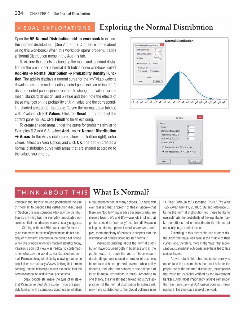
234 CHAPTeR 6 The Normal Distribution
Open the VE-Normal Distribution add-in workbook to explore the normal distribution. (See Appendix C to learn more about using this workbook.) When this workbook opens properly, it adds a Normal Distribution menu in the Add-ins tab.
To explore the effects of changing the mean and standard devia-tion on the area under a normal distribution curve workbook, select Add-ins ➔ Normal Distribution ➔ Probability Density Func-tion. The add-in displays a normal curve for the MyTVLab website download example and a floating control panel (shown at top right). Use the control panel spinner buttons to change the values for the mean, standard deviation, and X value and then note the effects of these changes on the probability of X 6 value and the correspond-ing shaded area under the curve. To see the normal curve labeled with Z values, click Z Values. Click the Reset button to reset the control panel values. Click Finish to finish exploring.
To create shaded areas under the curve for problems similar to Examples 6.2 and 6.3, select Add-ins ➔ Normal Distribution ➔ Areas. In the Areas dialog box (shown at bottom right), enter values, select an Area Option, and click OK. The add-in creates a normal distribution curve with areas that are shaded according to the values you entered.
V i s U a l E x p l o r at i o n s Exploring the Normal Distribution
t h i n k a b o U t t h i s What Is Normal?Ironically, the statistician who popularized the use of “normal” to describe the distribution discussed in Section 6.2 was someone who saw the distribu-tion as anything but the everyday, anticipated oc-currence that the adjective normal usually suggests.
Starting with an 1894 paper, Karl Pearson ar-gued that measurements of phenomena do not natu-rally, or “normally,” conform to the classic bell shape. While this principle underlies much of statistics today, Pearson’s point of view was radical to contempo-raries who saw the world as standardized and nor-mal. Pearson changed minds by showing that some populations are naturally skewed (coining that term in passing), and he helped put to rest the notion that the normal distribution underlies all phenomena.
Today, people still make the type of mistake that Pearson refuted. As a student, you are prob-ably familiar with discussions about grade inflation,
a real phenomenon at many schools. But have you ever realized that a “proof” of this inflation—that there are “too few” low grades because grades are skewed toward A’s and B’s—wrongly implies that grades should be “normally” distributed? Because college students represent small nonrandom sam-ples, there are plenty of reasons to suspect that the distribution of grades would not be “normal.”
Misunderstandings about the normal distri-bution have occurred both in business and in the public sector through the years. These misun-derstandings have caused a number of business blunders and have sparked several public policy debates, including the causes of the collapse of large financial institutions in 2008. According to one theory, the investment banking industry’s ap-plication of the normal distribution to assess risk may have contributed to the global collapse (see
“A Finer Formula for Assessing Risks,” The New York Times, May 11, 2010, p. B2 and reference 8). Using the normal distribution led these banks to overestimate the probability of having stable mar-ket conditions and underestimate the chance of unusually large market losses.
According to this theory, the use of other dis-tributions that have less area in the middle of their curves, and, therefore, more in the “tails” that repre-sent unusual market outcomes, may have led to less serious losses.
As you study this chapter, make sure you understand the assumptions that must hold for the proper use of the “normal” distribution, assumptions that were not explicitly verified by the investment bankers. And, most importantly, always remember that the name normal distribution does not mean normal in the everyday sense of the word.
6.2 The Normal Distribution 235
Problems for Section 6.2learNiNg The baSiCS6.1 Given a standardized normal distribution (with a mean of 0 and a standard deviation of 1, as in Table e.2), what is the probability thata. Z is less than 1.53?b. Z is greater than 1.89?c. Z is between 1.53 and 1.89?d. Z is less than 1.53 or greater than 1.89?
6.2 Given a standardized normal distribution (with a mean of 0 and a standard deviation of 1, as in Table e.2), what is the probability thata. Z is between -1.57 and 1.84?b. Z is less than -1.57 or greater than 1.84?c. What is the value of Z if only 2.5 percent of all possible Z val-
ues are larger?d. Between what two values of Z (symmetrically distributed around
the mean) will 68.26 percent of all possible Z values be contained?
6.3 Given a standardized normal distribution (with a mean of 0 and a standard deviation of 1, as in Table e.2), what is the probability thata. Z is less than 1.09?b. Z is greater than -0.26?c. Z is less than -0.26 or greater than the mean?d. Z is less than -0.26 or greater than 1.09?
6.4 Given a standardized normal distribution (with a mean of 0 and a standard deviation of 1, as in Table e.2), determine the fol-lowing probabilities:a. P1Z 7 1.082b. P1Z 6 -0.212c. P1-1.96 6 Z 6 -0.212d. What is the value of Z if only 15.87 percent of all possible Z
values are larger?
6.5 Given a normal distribution with m = 100 and s = 10, what is the probability thata. X 7 80?b. X 6 95 ?c. X 6 85 or X 7 105?d. Between what two X values (symmetrically distributed around
the mean) are 90 percent of the values?
6.6 Given a normal distribution with m = 50 and s = 4, what is the probability thata. X 7 43 ?b. X 6 42 ?c. Five percent of the values are less than what X value?d. Between what two X values (symmetrically distributed around
the mean) are sixty percent of the values?
aPPlyiNg The CoNCePTS6.7 According to the “Bottled Water Trends for 2014” report (bit .ly/1gx5ub8), the U.S. per capita consumption of bottled water in 2013 was 31.8 gallons. Assume that the per capita consumption of bottled water in the United States is approximately normally distributed with a mean of 31.8 gallons and a standard deviation of 10 gallons.a. What is the probability that someone in the United States con-
sumed more than 32 gallons of bottled water in 2013?
b. What is the probability that someone in the United States consumed between 10 and 20 gallons of bottled water in 2013?
c. What is the probability that someone in the United States consumed less than 10 gallons of bottled water in 2013?
d. Ninety-nine percent of the people in the United States consumed less than how many gallons of bottled water?
SELF Test
6.8 Toby’s Trucking Company determined that the distance traveled per truck per year is normally distrib-
uted, with a mean of 50 thousand miles and a standard deviation of 12 thousand miles.a. What proportion of trucks can be expected to travel between
34 and 50 thousand miles in a year?b. What percentage of trucks can be expected to travel either less
than 30 or more than 60 thousand miles in a year?c. How many miles will be traveled by at least eighty percent of
the trucks?d. What are your answers to (a) through (c) if the standard devia-
tion is 10 thousand miles?
6.9 Consumers spent an average of $14.99 on a meal at a restau-rant in 2013. (Data extracted from bit.ly/1hObH22.) Assume that the amount spent on a restaurant meal is normally distributed and that the standard deviation is $2.a. What is the probability that a randomly selected person spent
more than $15?b. What is the probability that a randomly selected person spent
between $10 and $12?c. Between what two values will the middle Ninety-five percent
of the amounts spent fall?
6.10 A set of final examination grades in an introductory statistics course is normally distributed, with a mean of 78 and a standard deviation of 9.a. What is the probability that a student scored below 93 on this exam?b. What is the probability that a student scored between 69 and 103?c. The probability is five percent that a student taking the test
scores higher than what grade?d. If the professor grades on a curve (i.e., gives As to the top ten
percent of the class, regardless of the score), are you better off with a grade of 87 on this exam or a grade of 72 on a different exam, where the mean is 64 and the standard deviation is 4? Show your answer statistically and explain.
6.11 A Nielsen study indicates that 18- to 24- year olds spend a mean of 135 minutes watching video on their smartphones per month. (Data extracted bit.ly/1hF3BP2.) Assume that the amount of time watching video on a smartphone per month is normally distrib-uted and that the standard deviation is 15 minutes.a. What is the probability that an 18- to 24-year-old spends less than
112 minutes watching video on his or her smartphone per month?b. What is the probability that an 18- to 24-year-old spends be-
tween 112 and 158 minutes watching video on his or her smart-phone per month?
c. What is the probability that an 18- to 24-year-old spends more than 158 minutes watching video on his or her smartphone per month?
d. One percent of all 18- to 24-year-olds will spend less than how many minutes watching video on his or her smartphone per month?
236 CHAPTeR 6 The Normal Distribution
6.12 According to a speical issue of Beverage Digest (bit.ly/1e9ORS3), the U.S. per capita consumption of soft drinks in 2013 was 42.2 gallons. Assume that the per capita consumption of soft drinks in the United States is approximately normally dis-tributed with a mean of 42.2 gallons and a standard deviation of 13 gallons.a. What is the probability that someone in the United States
consumed more than 60 gallons of soft drinks in 2013?b. What is the probability that someone in the United States
consumed between 15 and 30 gallons of soft drinks in 2013?c. What is the probability that someone in the United States
consumed less than 15 gallons of soft drinks in 2013?d. Ninety-nine percent of the people in the United States
consumed less than how many gallons of soft drinks?
6.13 Many manufacturing problems involve the matching of machine parts, such as shafts that fit into a valve hole. A particu-lar design requires a shaft with diameters between 22.89 mm and 23.018 mm. Suppose that the manufacturing process yields shafts with diameters normally distributed, with a mean of 23.004 mm and a standard deviation of 0.006 mm. For this process, what isa. the proportion of shafts with a diameter between 22.89 mm and
23.00 mm?b. the probability that a shaft is acceptable?c. the diameter that will be exceeded by only five percent of the
shafts?
6.3 Evaluating NormalityAs first stated in Section 6.2, the normal distribution has several important theoretical properties:
• It is symmetrical; thus, the mean and median are equal. • It is bell-shaped; thus, the empirical rule applies. • The interquartile range equals 1.33 standard deviations. • The range is approximately equal to 6 standard deviations.
As Section 6.2 notes, many continuous variables used in business closely follow a normal dis-tribution. To determine whether a set of data can be approximated by the normal distribution, you either compare the characteristics of the data with the theoretical properties of the normal distribution or construct a normal probability plot.
Comparing Data Characteristics to Theoretical PropertiesMany continuous variables have characteristics that approximate theoretical properties. How-ever, other continuous variables are often neither normally distributed nor approximately normally distributed. For such variables, the descriptive characteristics of the data are incon-sistent with the properties of a normal distribution. One approach you can use to determine whether a variable follows a normal distribution is to compare the observed characteristics of the variable with what would be expected if the variable followed a normal distribution. To do so, you can
• Construct charts and observe their appearance. For small- or moderate-sized data sets, create a stem-and-leaf display or a boxplot. For large data sets, in addition, plot a histo-gram or polygon.
• Compute descriptive statistics and compare these statistics with the theoretical proper-ties of the normal distribution. Compare the mean and median. Is the interquartile range approximately 1.33 times the standard deviation? Is the range approximately 6 times the standard deviation?
• evaluate how the values are distributed. Determine whether approximately two-thirds of the values lie between the mean and {1 standard deviation. Determine whether approx-imately four-fifths of the values lie between the mean and {1.28 standard deviations. Determine whether approximately 19 out of every 20 values lie between the mean and {2 standard deviations.
For example, you can use these techniques to determine whether the one-year returns discussed in Chapters 2 and 3 (stored in retirement Funds ) follow a normal distribution.
Table 6.6 presents the descriptive statistics and the five-number summary for the one-year return percentage variable. Figure 6.18 presents the excel and Minitab boxplots for the one-year return percentages.
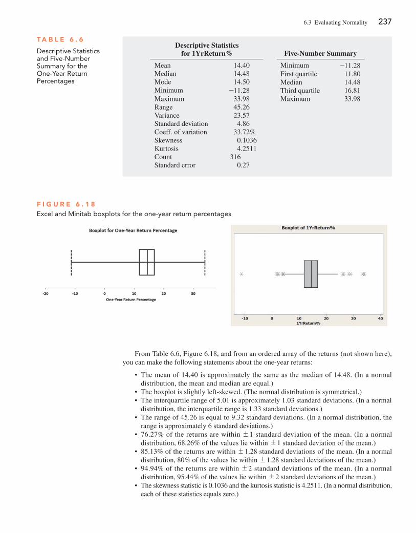
6.3 evaluating Normality 237
From Table 6.6, Figure 6.18, and from an ordered array of the returns (not shown here), you can make the following statements about the one-year returns:
• The mean of 14.40 is approximately the same as the median of 14.48. (In a normal distribution, the mean and median are equal.)
• The boxplot is slightly left-skewed. (The normal distribution is symmetrical.) • The interquartile range of 5.01 is approximately 1.03 standard deviations. (In a normal
distribution, the interquartile range is 1.33 standard deviations.) • The range of 45.26 is equal to 9.32 standard deviations. (In a normal distribution, the
range is approximately 6 standard deviations.) • 76.27% of the returns are within {1 standard deviation of the mean. (In a normal
distribution, 68.26% of the values lie within {1 standard deviation of the mean.) • 85.13% of the returns are within {1.28 standard deviations of the mean. (In a normal
distribution, 80% of the values lie within {1.28 standard deviations of the mean.) • 94.94% of the returns are within {2 standard deviations of the mean. (In a normal
distribution, 95.44% of the values lie within {2 standard deviations of the mean.) • The skewness statistic is 0.1036 and the kurtosis statistic is 4.2511. (In a normal distribution,
each of these statistics equals zero.)
T a b l e 6 . 6
Descriptive Statistics and Five-Number Summary for the one-year Return Percentages
Descriptive Statistics for 1YrReturn%
Mean 14.40Median 14.48Mode 14.50Minimum -11.28Maximum 33.98Range 45.26Variance 23.57Standard deviation 4.86Coeff. of variation 33.72%Skewness 0.1036Kurtosis 4.2511Count 316Standard error 0.27
F i g u r e 6 . 1 8Excel and minitab boxplots for the one-year return percentages
Five-Number Summary
Minimum -11.28First quartile 11.80Median 14.48Third quartile 16.81Maximum 33.98
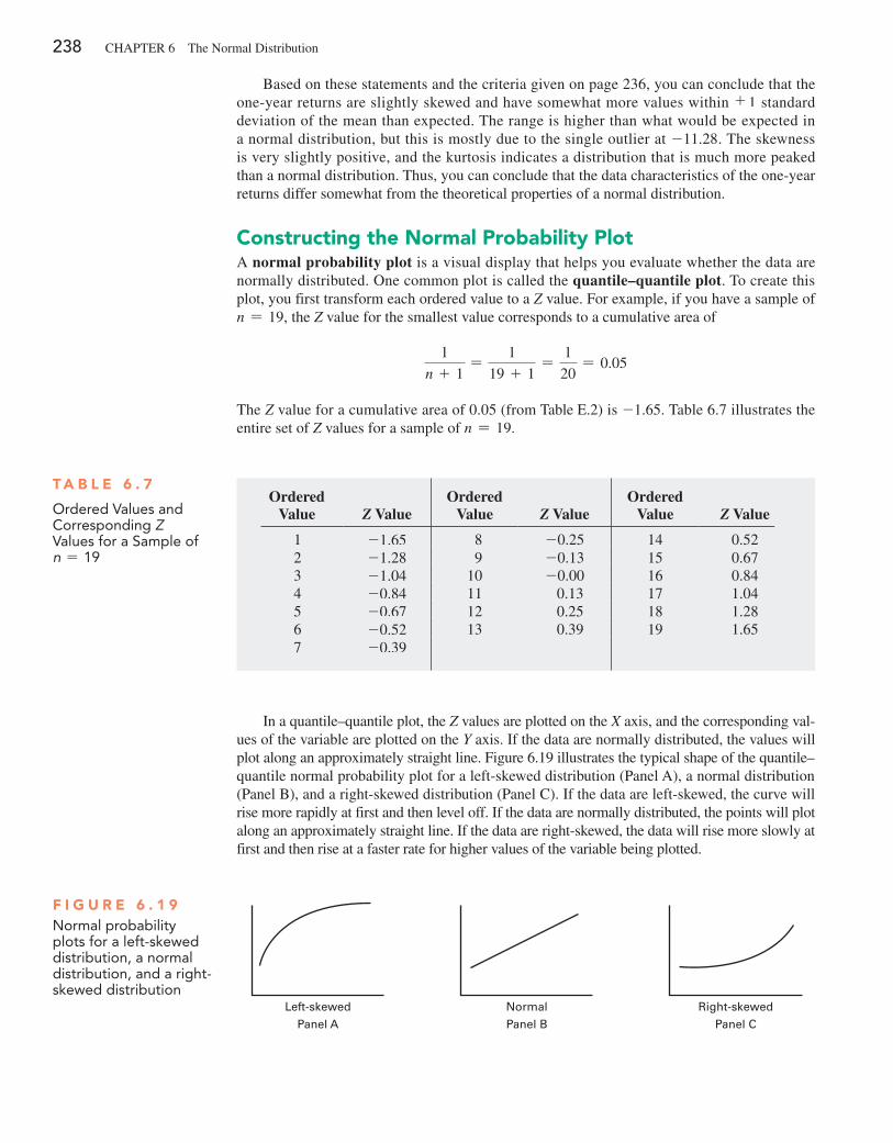
238 CHAPTeR 6 The Normal Distribution
Based on these statements and the criteria given on page 236, you can conclude that the one-year returns are slightly skewed and have somewhat more values within {1 standard deviation of the mean than expected. The range is higher than what would be expected in a normal distribution, but this is mostly due to the single outlier at -11.28. The skewness is very slightly positive, and the kurtosis indicates a distribution that is much more peaked than a normal distribution. Thus, you can conclude that the data characteristics of the one-year returns differ somewhat from the theoretical properties of a normal distribution.
Constructing the Normal Probability PlotA normal probability plot is a visual display that helps you evaluate whether the data are normally distributed. One common plot is called the quantile–quantile plot. To create this plot, you first transform each ordered value to a Z value. For example, if you have a sample of n = 19, the Z value for the smallest value corresponds to a cumulative area of
1
n + 1=
1
19 + 1=
1
20= 0.05
The Z value for a cumulative area of 0.05 (from Table e.2) is -1.65. Table 6.7 illustrates the entire set of Z values for a sample of n = 19.
In a quantile–quantile plot, the Z values are plotted on the X axis, and the corresponding val-ues of the variable are plotted on the Y axis. If the data are normally distributed, the values will plot along an approximately straight line. Figure 6.19 illustrates the typical shape of the quantile– quantile normal probability plot for a left-skewed distribution (Panel A), a normal distribution (Panel B), and a right-skewed distribution (Panel C). If the data are left-skewed, the curve will rise more rapidly at first and then level off. If the data are normally distributed, the points will plot along an approximately straight line. If the data are right-skewed, the data will rise more slowly at first and then rise at a faster rate for higher values of the variable being plotted.
F i g u r e 6 . 1 9Normal probability plots for a left-skewed distribution, a normal distribution, and a right-skewed distribution
Left-skewed Normal Right-skewedPanel A Panel B Panel C
T a b l e 6 . 7
ordered Values and Corresponding Z Values for a Sample of n = 19
Ordered Value Z Value
Ordered Value Z Value
Ordered Value Z Value
1 -1.65 8 -0.25 14 0.522 -1.28 9 -0.13 15 0.673 -1.04 10 -0.00 16 0.844 -0.84 11 0.13 17 1.045 -0.67 12 0.25 18 1.286 -0.52 13 0.39 19 1.657 -0.39
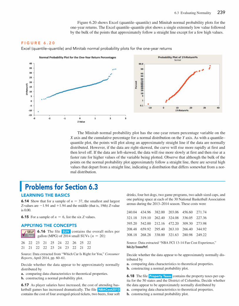
6.3 evaluating Normality 239
The Minitab normal probability plot has the one-year return percentage variable on the X axis and the cumulative percentage for a normal distribution on the Y axis. As with a quantile–quantile plot, the points will plot along an approximately straight line if the data are normally distributed. However, if the data are right-skewed, the curve will rise more rapidly at first and then level off. If the data are left-skewed, the data will rise more slowly at first and then rise at a faster rate for higher values of the variable being plotted. Observe that although the bulk of the points on the normal probability plot approximately follow a straight line, there are several high values that depart from a straight line, indicating a distribution that differs somewhat from a nor-mal distribution.
F i g u r e 6 . 2 0Excel (quantile–quantile) and minitab normal probability plots for the one-year returns
Problems for Section 6.3learNiNg The baSiCS6.14 Show that for a sample of n = 37, the smallest and largest Z-values are -1.94 and +1.94 and the middle (that is, 19th) Z-value is 0.00.
6.15 For a sample of n = 6, list the six Z values.
aPPlyiNg The CoNCePTSSELF Test
6.16 The file SuV contains the overall miles per gallon (MPG) of 2014 small SUVs 1n = 202:
26 22 23 21 25 24 22 26 25 2221 21 22 22 23 24 23 22 21 22
Source: Data extracted from “Which Car Is Right for You,” Consumer Reports, April 2014, pp. 60–61.
Decide whether the data appear to be approximately normally distributed bya. comparing data characteristics to theoretical properties.b. constructing a normal probability plot.
6.17 As player salaries have increased, the cost of attending bas-ketball games has increased dramatically. The file NbaCost2013 contains the cost of four averaged-priced tickets, two beers, four soft
drinks, four hot dogs, two game programs, two adult-sized caps, and one parking space at each of the 30 National Basketball Association arenas during the 2013–2014 season. These costs were
240.04 434.96 382.00 203.06 456.60 271.74
321.18 319.10 262.40 324.08 336.05 227.36
395.20 542.00 212.16 472.20 309.30 273.98
208.48 659.92 295.40 263.10 266.40 344.92
308.18 268.28 338.00 321.63 280.98 249.22
Source: Data extracted “NBA FCI 13-14 Fan Cost experience,” bit.ly/1nnu9rf.
Decide whether the data appear to be approximately normally dis-tributed bya. comparing data characteristics to theoretical properties.b. constructing a normal probability plot.
6.18 The file Property Taxes contains the property taxes per cap-ita for the 50 states and the District of Columbia. Decide whether the data appear to be approximately normally distributed bya. comparing data characteristics to theoretical properties.b. constructing a normal probability plot.
Figure 6.20 shows excel (quantile–quantile) and Minitab normal probability plots for the one-year returns. The excel quantile–quantile plot shows a single extremely low value followed by the bulk of the points that approximately follow a straight line except for a few high values.
240 CHAPTeR 6 The Normal Distribution
6.19 Thirty companies comprise the DJIA. How big are these companies? One common method for measuring the size of a company is to use its market capitalization, which is computed by multiplying the number of stock shares by the price of a share of stock. On March 14, 2014, the market capitalization of these companies ranged from Traveler’s $29.1 billion to exxonMobil’s $403.9 billion. The entire population of market capitalization values is stored in DowmarketCap . (Data extracted from money .cnn.com, March 14, 2014.) Decide whether the market capital-ization of companies in the DJIA appears to be approximately normally distributed bya. comparing data characteristics to theoretical properties.b. constructing a normal probability plot.c. constructing a histogram.
6.20 One operation of a mill is to cut pieces of steel into parts that will later be used as the frame for front seats in an automo-tive plant. The steel is cut with a diamond saw, and the resulting parts must be within {0.005 inch of the length specified by the automobile company. The data come from a sample of 100 steel parts and are stored in Steel . The measurement reported is the difference, in inches, between the actual length of the steel part, as measured by a laser measurement device, and the specified length of the steel part. Determine whether the data appear to be approxi-mately normally distributed by
a. comparing data characteristics to theoretical properties.b. constructing a normal probability plot.
6.21 The file CD rate contains the yields for a one-year certifi-cate of deposit (CD) and a five-year CD for 22 banks in the United States, as of March 12, 2014. (Data extracted from www.Bankrate .com, March 12, 2014.) For each type of investment, decide whether the data appear to be approximately normally distributed bya. comparing data characteristics to theoretical properties.b. constructing a normal probability plot.
6.22 The data set below contains the electricity costs in dollars during July 2014 for a random sample of 30 one-bedroom apart-ments in a large city.
130 86 191 170 106 189122 124 134 132 130 159140 146 185 153 84 171173 147 199 146 100 157210 140 103 154 164 118
Decide whether the data appear to be approximately normally distributed bya. comparing data characteristics to theoretical properties.b. constructing a normal probability plot.
In the Normal Downloading at MyTVLab scenario, you were a project manager for an online social media and
video website. You sought to ensure that a video could be downloaded quickly by visitors to the website. By running experiments in the corporate offices, you determined that the amount of time, in seconds, that passes from clicking a download link until a video is fully displayed is a bell-shaped distribution with a mean download time of 7 seconds and standard deviation of 2 seconds. Using the normal dis-tribution, you were able to calculate that approximately 84% of the download times are 9 seconds or less, and 95% of the download times are between 3.08 and 10.92 seconds.
Now that you understand how to compute probabilities from the normal distribution, you can evaluate download times of a video using different website designs. For example, if the standard deviation remained at 2 seconds, lowering the mean to 6 seconds would shift the entire distribution lower by
1 second. Thus, approximately 84% of the download times would be 8 seconds or less, and 95% of the download times would be between 2.08 and 9.92 seconds. Another change that could reduce long download times would be reducing the variation. For example, consider the case where the mean remained at the original 7 seconds but the standard deviation was reduced to 1 second. Again, approximately 84% of the download times would be 8 seconds or less, and 95% of the download times would be between 5.04 and 8.96 seconds.
U s i n g s tat i s t i c s
Normal Downloading at MyTVLab, Revisited
Cloki/Shutterstock
s U M M a r yIn this and the previous chapter, you have learned about mathematical models called probability distributions and how they can be used to solve business problems. In Chapter 5, you used discrete probability distributions in sit-uations where the values come from a counting process such as the number of social media sites to which you belong or the number of tagged order forms in a report generated by an accounting information system. In this chapter, you learned about continuous probability distributions where the values come from a measuring process such as your height or the download time of a video.
Continuous probability distributions come in various shapes, but the most common and most important in busi-ness is the normal distribution. The normal distribution
is symmetrical; thus, its mean and median are equal. It is also bell-shaped, and approximately 68.26% of its values are within {1 standard deviation of the mean, approxi-mately 95.44% of its values are within {2 standard devia-tions of the mean, and approximately 99.73% of its values are within {3 standard deviations of the mean. Although many variables in business are closely approximated by the normal distribution, do not think that all variables can be approximated by the normal distribution.
In Section 6.3, you learned about various methods for evaluating normality in order to determine whether the nor-mal distribution is a reasonable mathematical model to use in specific situations. Chapter 7 uses the normal distribution to develop the subject of statistical inference.
r E F E r E n c E s 1. Gunter, B. “Q-Q Plots.” Quality Progress (February 1994):
81–86. 2. Levine, D. M., P. Ramsey, and R. Smidt. Applied Statistics for
Engineers and Scientists Using Microsoft Excel and Minitab. Upper Saddle River, NJ: Prentice Hall, 2001.
3. Microsoft Excel 2013. Redmond, WA: Microsoft Corp., 2012. 4. Miller, J. “earliest Known Uses of Some of the Words of
Mathematics.” jeff560.tripod.com/mathword.html. 5. Minitab Release 16. State College, PA: Minitab, Inc., 2010.
6. Pearl, R. “Karl Pearson, 1857–1936.” Journal of the American Statistical Association, 31 (1936): 653–664.
7. Pearson, e. S. “Some Incidents in the early History of Biom-etry and Statistics, 1890–94.” Biometrika 52 (1965): 3–18.
8. Taleb, N. The Black Swan, 2nd ed. New York: Random House, 2010.
9. Walker, H. “The Contributions of Karl Pearson.” Journal of the American Statistical Association 53 (1958): 11–22.
k E y E q U at i o n s
Normal Probability Density Function
f 1X2 =122ps
e-11>2231X - m2>s42 (6.1)
Z Transformation Formula
Z =X - m
s (6.2)
Finding an X Value Associated with a Known Probability
X = m + Zs (6.3)
k E y t E r M scumulative standardized normal
distribution 226exponential distribution 223normal distribution 223normal probability plot 238
probability density function 223
probability density function for the normal distribution 225
quantile–quantile plot 238
standardized normal variable 225
transformation formula 225uniform distribution 223
Key Terms 241
242 CHAPTeR 6 The Normal Distribution
c h E c k i n g y o U r U n D E r s ta n D i n g6.23 Why is only one normal distribution table such as Table e.2 needed to find any probability under the normal curve?
6.24 How do you find the area between two values under the nor-mal curve?
6.25 How do you find the X value that corresponds to a given percentile of the normal distribution?
6.26 What are the three main reasons that normal distribution is important in statistics?
6.27 What is the difference between normal distribution and exponential distribution?
6.28 How can you use the normal probability plot to evaluate whether a set of data is normally distributed?
c h a p t E r r E V i E W p r o b l E M s6.29 An industrial sewing machine uses ball bearings that are targeted to have a diameter of 0.75 inch. The lower and upper specification limits under which the ball bearings can operate are 0.74 inch and 0.76 inch, respectively. Past experience has indi-cated that the actual diameter of the ball bearings is approximately normally distributed, with a mean of 0.753 inch and a standard de-viation of 0.004 inch. What is the probability that a ball bearing isa. between the target and the actual mean?b. between the lower specification limit and the target?c. above the upper specification limit?d. below the lower specification limit?e. Of all the ball bearings, 93% of the diameters are greater than
what value?
6.30 The fill amount in 2-liter soft drink bottles is normally distributed, with a mean of 2.0 liters and a standard deviation of 0.05 liter. If bottles contain less than 95% of the listed net content (1.90 liters, in this case), the manufacturer may be subject to pen-alty by the state office of consumer affairs. Bottles that have a net content above 2.10 liters may cause excess spillage upon opening. What proportion of the bottles will containa. between 1.90 and 2.0 liters?b. between 1.90 and 2.10 liters?c. below 1.90 liters or above 2.10 liters?d. At least how much soft drink is contained in 99% of the bottles?e. Ninety-nine percent of the bottles contain an amount that is between
which two values (symmetrically distributed) around the mean?
6.31 In an effort to reduce the number of bottles that contain less than 1.90 liters, the bottler in Problem 6.30 sets the filling machine so that the mean is 2.02 liters. Under these circumstances, what are your answers in Problem 6.30 (a) through (e)?
6.32 An Ipsos MediaCT study indicates that mobile device own-ers who used their mobile device while shopping for consumer electronics spent an average of $1,539 on consumer electronics in the past six months. (Data extracted from iab.net/showrooming.) As-sume that the amount spent on consumer electronics in the last six months is normally distributed and that the standard deviation is $500. a. What is the probability that a mobile device owner who used
his or her mobile device while shopping for consumer electron-ics spent less than $1,000 on consumer electronics?
b. What is the probability that a mobile device owner who used his or her mobile device while shopping for consumer electron-ics spent between $2,500 and $3,000 on consumer electronics?
c. Ninety percent of the amounts spent on consumer electronics by mobile device owners who used their mobile device while shopping for consumer electronics are less than what value?
d. eighty percent of the amounts spent on consumer electronics by mobile device owners who used their mobile device while shopping for consumer electronics are between what two val-ues symmetrically distributed around the mean?
6.33 The file Domesticbeer contains the percentage alcohol, number of calories per 12 ounces, and number of carbohydrates (in grams) per 12 ounces for 156 of the best-selling domestic beers in the United States. Determine whether each of these variables appears to be approximately normally distributed. Support your decision through the use of appropriate statistics and graphs. (Data extracted from www.Beer100.com, March 12, 2014.)
6.34 The evening manager of a restaurant was very concerned about the length of time some customers were waiting in line to be seated. She also had some concern about the seating times—that is, the length of time between when a customer is seated and the time he or she leaves the restaurant. Over the course of one week, 100 customers (no more than 1 per party) were randomly selected, and their waiting and seating times (in minutes) were recorded in Wait .a. Think about your favorite restaurant. Do you think waiting
times more closely resemble a uniform, an exponential, or a normal distribution?
b. Again, think about your favorite restaurant. Do you think seat-ing times more closely resemble a uniform, an exponential, or a normal distribution?
c. Construct a histogram and a normal probability plot of the waiting times. Do you think these waiting times more closely resemble a uniform, an exponential, or a normal distribution?
d. Construct a histogram and a normal probability plot of the seating times. Do you think these seating times more closely resemble a uniform, an exponential, or a normal distribution?
6.35 The major stock market indexes had strong results in 2013. The mean one-year return for stocks in the S&P 500, a group of 500 very large companies, was +29.6%. The mean one-year return for the NASDAQ, a group of 3,200 small and medium-sized compa-nies, was +38.3%. Historically, the one-year returns are approxi-mately normally distributed, the standard deviation in the S&P 500 is approximately 20%, and the standard deviation in the NAS-DAQ is approximately 30%.

a. What is the probability that a stock in the S&P 500 gained value in 2013?
b. What is the probability that a stock in the S&P 500 gained 10% or more in 2013?
c. What is the probability that a stock in the S&P 500 lost 20% or more in 2013?
d. What is the probability that a stock in the S&P 500 lost 30% or more in 2013?
e. Repeat (a) through (d) for a stock in the NASDAQ.f. Write a short summary on your findings. Be sure to include a
discussion of the risks associated with a large standard deviation.
6.36 Interns report that when deciding on where to work, career growth, salary and compensation, location and commute, and company culture and values are important factors to them. Ac-cording to the Glassdoor blog’s “25 Highest Paying Companies for Interns 2014,” bit.ly/1gx6vjx, the mean monthly pay of interns at Intel is $4,648. Suppose that the intern monthly pay is normally distributed, with a standard deviation of $400. What is the prob-ability that the monthly pay of an intern at Intel isa. less than $4,500?b. between $4,300 and $4,700?c. above $5,200?d. Ninety-nine percent of the intern monthly pays are higher than
what value?e. Ninety-five percent of the intern monthly pays are between
what two values, symmetrically distributed around the mean?
6.37 According to the same Glassdoor blog report mentioned in the previous question, the mean monthly pay for interns at Facebook is $6,213. Suppose that the intern monthly pay is normally distributed, with a standard deviation of $500. What is the probability that the monthly pay of an intern at Facebook isa. less than $4,500?b. between $4,300 and $4,700?
c. above $5,200?d. Ninety-nine percent of the intern monthly pays are higher than
what value?e. Ninety-five percent of the intern monthly pays are between
what two values, symmetrically distributed around the mean?f. Compare the results for the Intel interns computed in Problem
6.36 to those of the Facebook interns.
6.38 (Class Project) One theory about the daily changes in the closing price of stock is that these changes follow a random walk—that is, these daily events are independent of each other and move upward or downward in a random manner—and can be ap-proximated by a normal distribution. To test this theory, use either a newspaper or the Internet to select one company traded on the NYSe, one company traded on the American Stock exchange, and one company traded on the NASDAQ and then do the following:1. Record the daily closing stock price of each of these companies for
six consecutive weeks (so that you have 30 values per company).2. Compute the daily changes in the closing stock price of each
of these companies for six consecutive weeks (so that you have 30 values per company).
Note: The random-walk theory pertains to the daily changes in the closing stock price, not the daily closing stock price.
For each of your six data sets, decide whether the data are approxi-mately normally distributed bya. constructing the stem-and-leaf display, histogram or polygon,
and boxplot.b. comparing data characteristics to theoretical properties.c. constructing a normal probability plot.d. Discuss the results of (a) through (c). What can you say about
your three stocks with respect to daily closing prices and daily changes in closing prices? Which, if any, of the data sets are approximately normally distributed?
c a s E s F o r c h a p t E r 6
Managing ashland Multicomm servicesThe AMS technical services department has embarked on a quality improvement effort. Its first project relates to main-taining the target upload speed for its Internet service sub-scribers. Upload speeds are measured on a standard scale in which the target value is 1.0. Data collected over the past year indicate that the upload speed is approximately nor-mally distributed, with a mean of 1.005 and a standard devi-ation of 0.10. each day, one upload speed is measured. The upload speed is considered acceptable if the measurement on the standard scale is between 0.95 and 1.05.
1. Assuming that the distribution has not changed from what it was in the past year, what is the probability that the upload speed is
a. less than 1.0?b. between 0.95 and 1.0?c. between 1.0 and 1.05?d. less than 0.95 or greater than 1.05?
2. The objective of the operations team is to reduce the probability that the upload speed is below 1.0. Should the team focus on process improvement that increases the mean upload speed to 1.05 or on process improvement that reduces the standard deviation of the upload speed to 0.075? explain.
Cases for Chapter 6 243
244 CHAPTeR 6 The Normal Distribution
Digital caseApply your knowledge about the normal distribution in this Digital Case, which extends the Using Statistics scenario from this chapter.
To satisfy concerns of potential customers, the management of MyTVLab has undertaken a research project to learn how much time it takes users to load a complex video features page. The research team has collected data and has made some claims based on the assertion that the data follow a normal distribution.
Open MTL_QRTStudy.pdf, which documents the work of a quality response team at MyTVLab. Read the
internal report that documents the work of the team and their conclusions. Then answer the following:
1. Can the collected data be approximated by the normal distribution?
2. Review and evaluate the conclusions made by the MyTV-Lab research team. Which conclusions are correct? Which ones are incorrect?
3. If MyTVLab could improve the mean time by 5 seconds, how would the probabilities change?
cardiogood Fitness
Return to the CardioGood Fitness case (stored in Cardiogood Fitness ) first presented on page 101.
1. For each CardioGood Fitness treadmill product line, determine whether the age, income, usage, and the
number of miles the customer expects to walk/run each week can be approximated by the normal distribution.
2. Write a report to be presented to the management of CardioGood Fitness, detailing your findings.
More Descriptive choices Follow-up
Follow up the More Descriptive Choices Revisited Us-ing Statistics scenario on page 158 by constructing normal probability plots for the 3-year return percentages, 5-year return percentages, and 10-year return percentages for the
sample of 316 retirement funds stored in retirement Funds . In your analysis, examine differences between the growth and value funds as well as the differences among the small, mid-cap, and large market cap funds.
clear Mountain state student surveys
1. The Student News Service at Clear Mountain State Uni-versity (CMSU) has decided to gather data about the un-dergraduate students who attend CMSU. They create and distribute a survey of 14 questions and receive responses from 62 undergraduates (stored in undergradSurvey ). For each numerical variable in the survey, decide whether the variable is approximately normally distributed bya. comparing data characteristics to theoretical properties.b. constructing a normal probability plot.c. writing a report summarizing your conclusions.
2. The dean of students at CMSU has learned about the un-dergraduate survey and has decided to undertake a similar survey for graduate students at CMSU. She creates and distributes a survey of 14 questions and receives responses from 44 graduate students (stored in gradSurvey ). For each numerical variable in the survey, decide whether the variable is approximately normally distributed bya. comparing data characteristics to theoretical properties.b. constructing a normal probability plot.c. writing a report summarizing your conclusions.
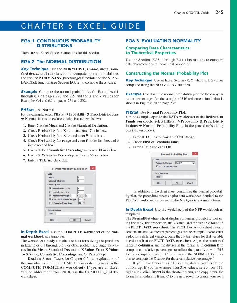
eg6.1 CoNTiNuouS ProbabiliTy DiSTribuTioNS
There are no excel Guide instructions for this section.
eg6.2 The Normal DiSTribuTioNKey Technique Use the NORM.DIST(X value, mean, stan-dard deviation, True) function to compute normal probabilities and use the NORM.S.INV(percentage) function and the STAN-DARDIZe function (see Section eG3.2) to compute the Z value.
Example Compute the normal probabilities for examples 6.1 through 6.3 on pages 228 and 229 and the X and Z values for examples 6.4 and 6.5 on pages 231 and 232.
PhStat Use Normal.For the example, select PHStat ➔ Probability & Prob. Distributions ➔ Normal. In this procedure’s dialog box (shown below):
1. enter 7 as the Mean and 2 as the Standard Deviation. 2. Check Probability for: X 6 = and enter 7 in its box. 3. Check Probability for: X 7 and enter 9 in its box. 4. Check Probability for range and enter 5 in the first box and 9
in the second box. 5. Check X for Cumulative Percentage and enter 10 in its box. 6. Check X Values for Percentage and enter 95 in its box. 7. enter a Title and click OK.
in-Depth excel Use the COMPUTE worksheet of the Nor-mal workbook as a template.The worksheet already contains the data for solving the problems in examples 6.1 through 6.5. For other problems, change the val-ues for the Mean, Standard Deviation, X Value, From X Value, To X Value, Cumulative Percentage, and/or Percentage.
Read the Short Takes for Chapter 6 for an explanation of the formulas found in the COMPUTe worksheet (shown in the COMPUTE_FORMULAS worksheet). If you use an excel version older than excel 2010, use the COMPUTe_OLDeR worksheet.
eg6.3 eValuaTiNg NormaliTyComparing Data Characteristics to Theoretical Properties
Use the Sections eG3.1 through eG3.3 instructions to compare data characteristics to theoretical properties.
Constructing the Normal Probability Plot
Key Technique Use an excel Scatter (X, Y) chart with Z values computed using the NORM.S.INV function.
Example Construct the normal probability plot for the one-year return percentages for the sample of 316 retirement funds that is shown in Figure 6.20 on page 239.
PhStat Use Normal Probability Plot.For the example, open to the DATA worksheet of the Retirement Funds workbook. Select PHStat ➔ Probability & Prob. Distri-butions ➔ Normal Probability Plot. In the procedure’s dialog box (shown below):
1. enter I1:I317 as the Variable Cell Range. 2. Check First cell contains label. 3. enter a Title and click OK.
In addition to the chart sheet containing the normal probabil-ity plot, the procedure creates a plot data worksheet identical to the PlotData worksheet discussed in the In-Depth Excel instructions.
in-Depth excel Use the worksheets of the NPP workbook as templates.The NormalPlot chart sheet displays a normal probability plot us-ing the rank, the proportion, the Z value, and the variable found in the PLOT_DATA worksheet. The PLOT_DATA worksheet already contains the one-year return percentages for the example. To construct a plot for a different variable, paste the sorted values for that variable in column D of the PLOT_DATA worksheet. Adjust the number of ranks in column A and the divisor in the formulas in column B to compute cumulative percentages to reflect the quantity n + 1 (317 for the example). (Column C formulas use the NORM.S.INV func-tion to compute the Z values for those cumulative percentages.)
If you have fewer than 316 values, delete rows from the bottom up. If you have more than 316 values, select row 317, right-click, click Insert in the shortcut menu, and copy down the formulas in columns B and C to the new rows. To create your own
c h a p t E r 6 E x c E l g U i D E
Chapter 6 eXCeL Guide 245
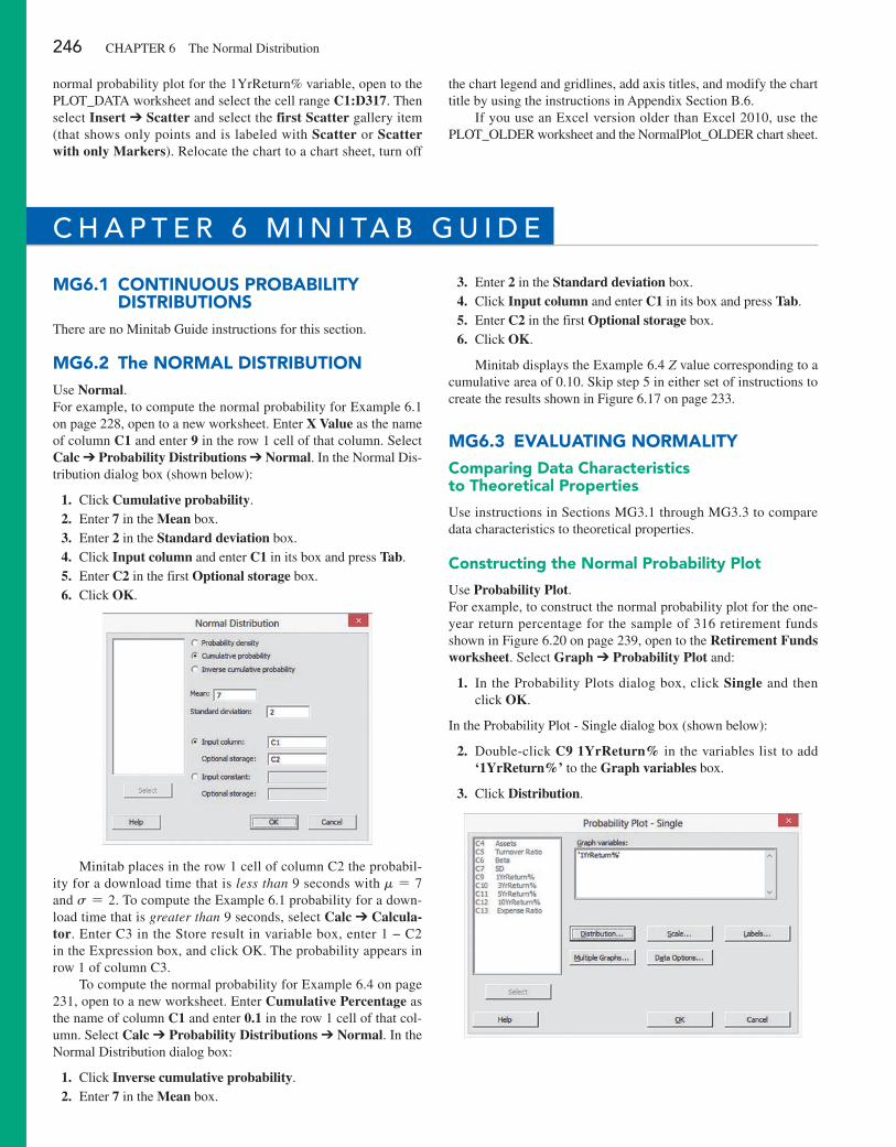
246 CHAPTeR 6 The Normal Distribution
normal probability plot for the 1YrReturn% variable, open to the PLOT_DATA worksheet and select the cell range C1:D317. Then select Insert ➔ Scatter and select the first Scatter gallery item (that shows only points and is labeled with Scatter or Scatter with only Markers). Relocate the chart to a chart sheet, turn off
the chart legend and gridlines, add axis titles, and modify the chart title by using the instructions in Appendix Section B.6.
If you use an excel version older than excel 2010, use the PLOT_OLDeR worksheet and the NormalPlot_OLDeR chart sheet.
c h a p t E r 6 M i n i ta b g U i D E
mg6.1 CoNTiNuouS ProbabiliTy DiSTribuTioNS
There are no Minitab Guide instructions for this section.
mg6.2 The Normal DiSTribuTioNUse Normal.For example, to compute the normal probability for example 6.1 on page 228, open to a new worksheet. enter X Value as the name of column C1 and enter 9 in the row 1 cell of that column. Select Calc ➔ Probability Distributions ➔ Normal. In the Normal Dis-tribution dialog box (shown below):
1. Click Cumulative probability. 2. enter 7 in the Mean box. 3. enter 2 in the Standard deviation box. 4. Click Input column and enter C1 in its box and press Tab. 5. enter C2 in the first Optional storage box. 6. Click OK.
Minitab places in the row 1 cell of column C2 the probabil-ity for a download time that is less than 9 seconds with m = 7 and s = 2. To compute the example 6.1 probability for a down-load time that is greater than 9 seconds, select Calc ➔ Calcula-tor. enter C3 in the Store result in variable box, enter 1 − C2 in the expression box, and click OK. The probability appears in row 1 of column C3.
To compute the normal probability for example 6.4 on page 231, open to a new worksheet. enter Cumulative Percentage as the name of column C1 and enter 0.1 in the row 1 cell of that col-umn. Select Calc ➔ Probability Distributions ➔ Normal. In the Normal Distribution dialog box:
1. Click Inverse cumulative probability. 2. enter 7 in the Mean box.
3. enter 2 in the Standard deviation box. 4. Click Input column and enter C1 in its box and press Tab. 5. enter C2 in the first Optional storage box. 6. Click OK.
Minitab displays the example 6.4 Z value corresponding to a cumulative area of 0.10. Skip step 5 in either set of instructions to create the results shown in Figure 6.17 on page 233.
mg6.3 eValuaTiNg NormaliTyComparing Data Characteristics to Theoretical Properties
Use instructions in Sections MG3.1 through MG3.3 to compare data characteristics to theoretical properties.
Constructing the Normal Probability Plot
Use Probability Plot.For example, to construct the normal probability plot for the one-year return percentage for the sample of 316 retirement funds shown in Figure 6.20 on page 239, open to the Retirement Funds worksheet. Select Graph ➔ Probability Plot and:
1. In the Probability Plots dialog box, click Single and then click OK.
In the Probability Plot - Single dialog box (shown below):
2. Double-click C9 1YrReturn% in the variables list to add ‘1YrReturn%’ to the Graph variables box.
3. Click Distribution.
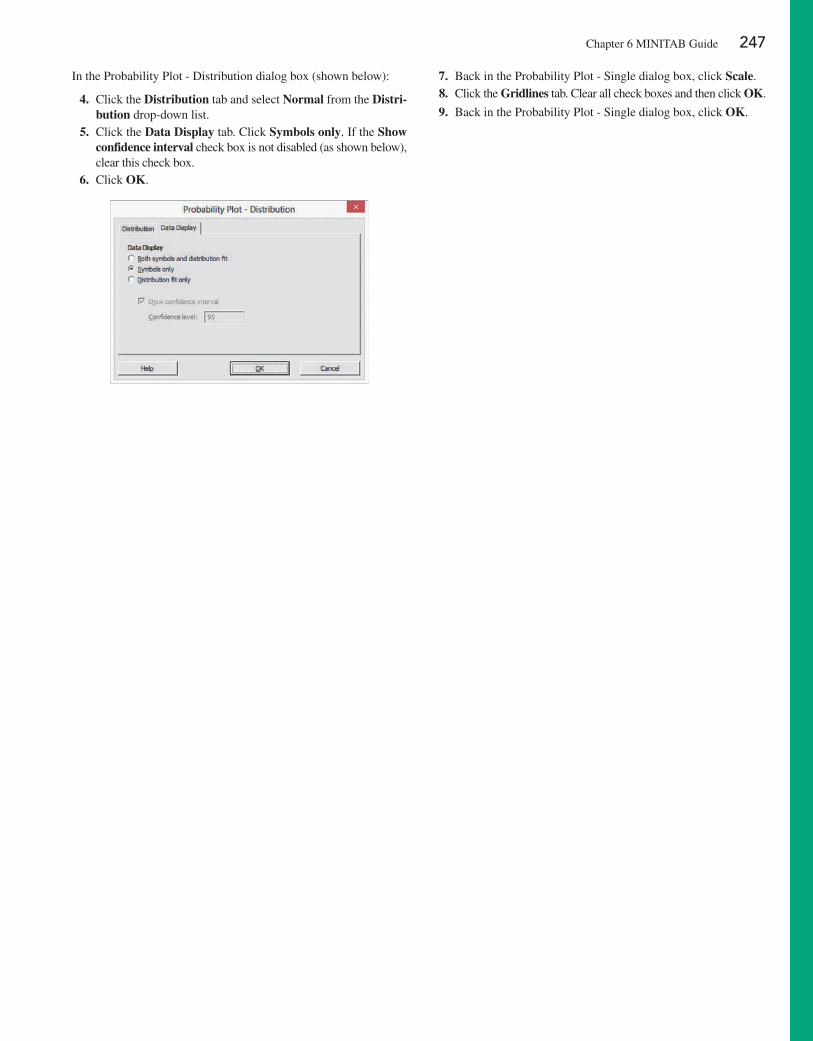
Chapter 6 MINITAB Guide 247
In the Probability Plot - Distribution dialog box (shown below):
4. Click the Distribution tab and select Normal from the Distri-bution drop-down list.
5. Click the Data Display tab. Click Symbols only. If the Show confidence interval check box is not disabled (as shown below), clear this check box.
6. Click OK.
7. Back in the Probability Plot - Single dialog box, click Scale. 8. Click the Gridlines tab. Clear all check boxes and then click OK.
9. Back in the Probability Plot - Single dialog box, click OK.
248
U s i n g s tat i s t i c s
Sampling Oxford CerealsThe automated production line at the Oxford Cereals main plant fills thousands of boxes of cereal during each shift. As the plant operations manager, you are re-sponsible for monitoring the amount of cereal placed in each box. To be consist-ent with package labeling, boxes should contain a mean of 368 grams of cereal. Because of the speed of the process, the cereal weight varies from box to box, causing some boxes to be underfilled and others to be overfilled. If the automated process fails to work as intended, the mean weight in the boxes could vary too much from the label weight of 368 grams to be acceptable.
Because weighing every single box is too time-consuming, costly, and inef-ficient, you must take a sample of boxes. For each sample you select, you plan to weigh the individual boxes and calculate a sample mean. You need to determine the probability that such a sample mean could have been randomly selected from a population whose mean is 368 grams. Based on your analysis, you will have to decide whether to maintain, alter, or shut down the cereal-filling process.
contents
7.1 Sampling Distributions
7.2 Sampling Distribution of the Mean
ViSual ExplorationS: Exploring Sampling Distributions
7.3 Sampling Distribution of the proportion
uSing StatiSticS: Sampling oxford cereals, revisited
chapter 7 excel gUide
chapter 7 Minitab gUide
objectives
learn about the concept of the sampling distribution
compute probabilities related to the sample mean and the sample proportion
understand the importance of the central limit theorem
Chapter Sampling Distributions7
Corbis
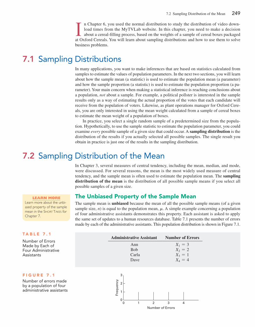
7.2 Sampling Distribution of the Mean 249
I n Chapter 6, you used the normal distribution to study the distribution of video down-load times from the MyTVLab website. In this chapter, you need to make a decision about a cereal-filling process, based on the weights of a sample of cereal boxes packaged
at Oxford Cereals. You will learn about sampling distributions and how to use them to solve business problems.
In many applications, you want to make inferences that are based on statistics calculated from samples to estimate the values of population parameters. In the next two sections, you will learn about how the sample mean (a statistic) is used to estimate the population mean (a parameter) and how the sample proportion (a statistic) is used to estimate the population proportion (a pa-rameter). Your main concern when making a statistical inference is reaching conclusions about a population, not about a sample. For example, a political pollster is interested in the sample results only as a way of estimating the actual proportion of the votes that each candidate will receive from the population of voters. Likewise, as plant operations manager for Oxford Cere-als, you are only interested in using the mean weight calculated from a sample of cereal boxes to estimate the mean weight of a population of boxes.
In practice, you select a single random sample of a predetermined size from the popula-tion. Hypothetically, to use the sample statistic to estimate the population parameter, you could examine every possible sample of a given size that could occur. A sampling distribution is the distribution of the results if you actually selected all possible samples. The single result you obtain in practice is just one of the results in the sampling distribution.
In Chapter 3, several measures of central tendency, including the mean, median, and mode, were discussed. For several reasons, the mean is the most widely used measure of central tendency, and the sample mean is often used to estimate the population mean. The sampling distribution of the mean is the distribution of all possible sample means if you select all possible samples of a given size.
The Unbiased Property of the Sample MeanThe sample mean is unbiased because the mean of all the possible sample means (of a given sample size, n) is equal to the population mean, m. A simple example concerning a population of four administrative assistants demonstrates this property. Each assistant is asked to apply the same set of updates to a human resources database. Table 7.1 presents the number of errors made by each of the administrative assistants. This population distribution is shown in Figure 7.1.
7.1 Sampling Distributions
7.2 Sampling Distribution of the Mean
T a b l e 7 . 1
number of Errors Made by Each of Four administrative assistants
Administrative Assistant Number of Errors
Ann X1 = 3Bob X2 = 2Carla X3 = 1Dave X4 = 4
F i g U r e 7 . 1number of errors made by a population of four administrative assistants
0
3
2
1
01 2
Number of Errors
Freq
uen
cy
3 4
Learn MoreLearn more about the unbi-ased property of the sample mean in the Short takeS for Chapter 7.
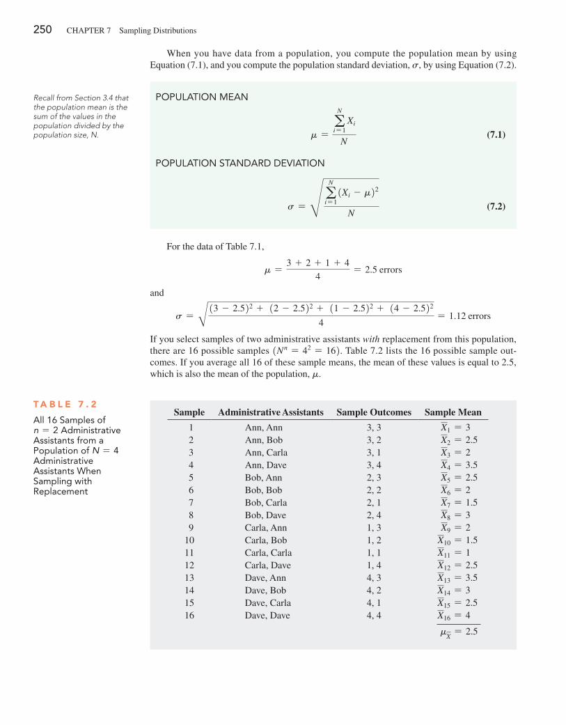
250 CHApTEr 7 Sampling Distributions
When you have data from a population, you compute the population mean by using Equation (7.1), and you compute the population standard deviation, s, by using Equation (7.2).
population MEan
m =aN
i= 1 Xi
N (7.1)
population StanDarD DEViation
s = R aN
i= 1 1Xi - m22
N (7.2)
For the data of Table 7.1,
m =3 + 2 + 1 + 4
4= 2.5 errors
and
s = B 13 - 2.522 + 12 - 2.522 + 11 - 2.522 + 14 - 2.522
4= 1.12 errors
If you select samples of two administrative assistants with replacement from this population, there are 16 possible samples 1Nn = 42 = 162. Table 7.2 lists the 16 possible sample out-comes. If you average all 16 of these sample means, the mean of these values is equal to 2.5, which is also the mean of the population, m.
T a b l e 7 . 2
all 16 Samples of n = 2 administrative assistants from a population of N = 4 administrative assistants When Sampling with replacement
Sample Administrative Assistants Sample Outcomes Sample Mean
1 Ann, Ann 3, 3 X1 = 32 Ann, Bob 3, 2 X2 = 2.53 Ann, Carla 3, 1 X3 = 24 Ann, Dave 3, 4 X4 = 3.55 Bob, Ann 2, 3 X5 = 2.56 Bob, Bob 2, 2 X6 = 27 Bob, Carla 2, 1 X7 = 1.58 Bob, Dave 2, 4 X8 = 39 Carla, Ann 1, 3 X9 = 2
10 Carla, Bob 1, 2 X10 = 1.511 Carla, Carla 1, 1 X11 = 112 Carla, Dave 1, 4 X12 = 2.513 Dave, Ann 4, 3 X13 = 3.514 Dave, Bob 4, 2 X14 = 315 Dave, Carla 4, 1 X15 = 2.516 Dave, Dave 4, 4 X16 = 4
mX= 2.5
Recall from Section 3.4 that the population mean is the sum of the values in the population divided by the population size, N.
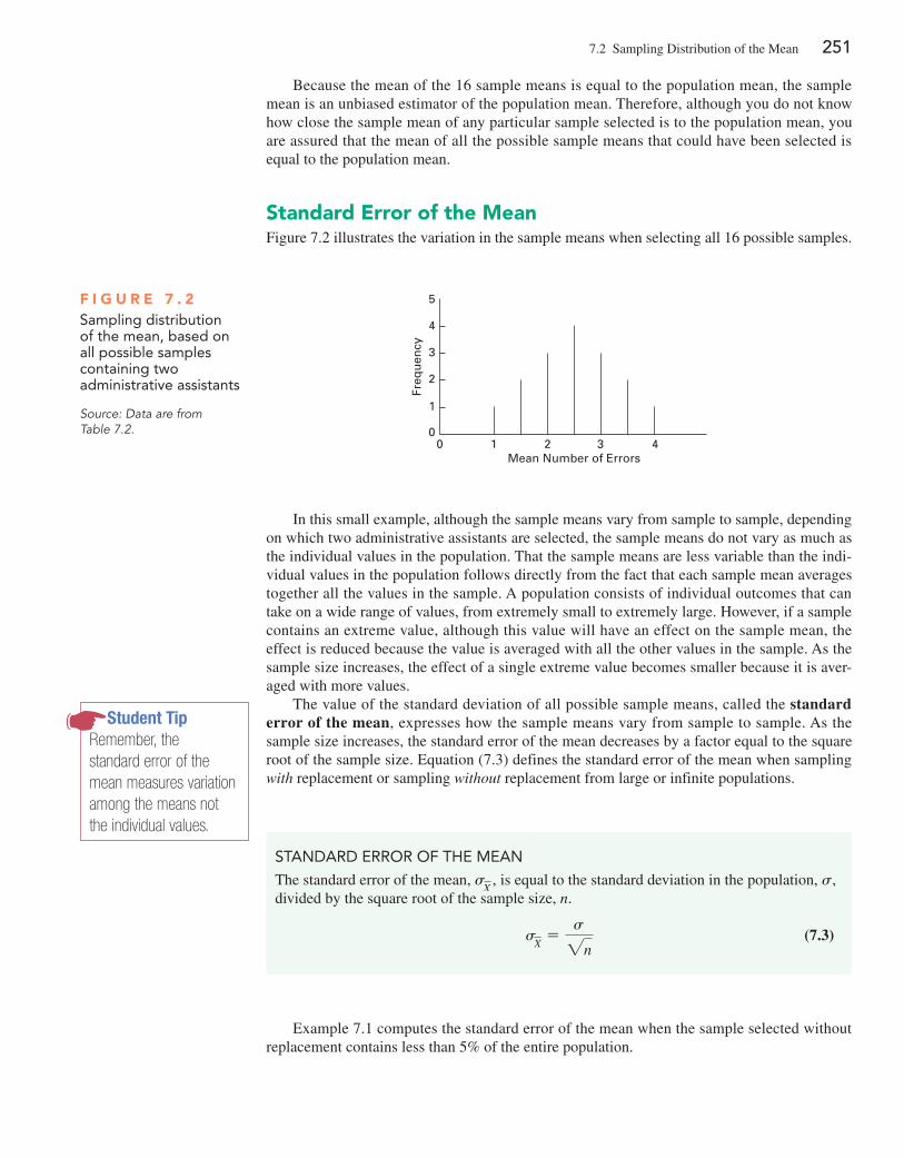
7.2 Sampling Distribution of the Mean 251
Because the mean of the 16 sample means is equal to the population mean, the sample mean is an unbiased estimator of the population mean. Therefore, although you do not know how close the sample mean of any particular sample selected is to the population mean, you are assured that the mean of all the possible sample means that could have been selected is equal to the population mean.
Standard error of the MeanFigure 7.2 illustrates the variation in the sample means when selecting all 16 possible samples.
F i g U r e 7 . 2Sampling distribution of the mean, based on all possible samples containing two administrative assistants
Source: Data are from Table 7.2.
0
5
4
3
2
1
01 2
Mean Number of Errors
Freq
uen
cy
3 4
In this small example, although the sample means vary from sample to sample, depending on which two administrative assistants are selected, the sample means do not vary as much as the individual values in the population. That the sample means are less variable than the indi-vidual values in the population follows directly from the fact that each sample mean averages together all the values in the sample. A population consists of individual outcomes that can take on a wide range of values, from extremely small to extremely large. However, if a sample contains an extreme value, although this value will have an effect on the sample mean, the effect is reduced because the value is averaged with all the other values in the sample. As the sample size increases, the effect of a single extreme value becomes smaller because it is aver-aged with more values.
The value of the standard deviation of all possible sample means, called the standard error of the mean, expresses how the sample means vary from sample to sample. As the sample size increases, the standard error of the mean decreases by a factor equal to the square root of the sample size. Equation (7.3) defines the standard error of the mean when sampling with replacement or sampling without replacement from large or infinite populations.
Student TipRemember, the standard error of the mean measures variation among the means not the individual values.
StanDarD Error oF thE MEan
The standard error of the mean, sX
, is equal to the standard deviation in the population, s, divided by the square root of the sample size, n.
sX=
s2n (7.3)
Example 7.1 computes the standard error of the mean when the sample selected without replacement contains less than 5% of the entire population.
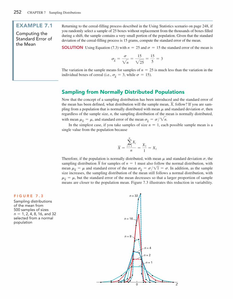
252 CHApTEr 7 Sampling Distributions
Sampling from Normally Distributed PopulationsNow that the concept of a sampling distribution has been introduced and the standard error of the mean has been defined, what distribution will the sample mean, X, follow? If you are sam-pling from a population that is normally distributed with mean m and standard deviation s, then regardless of the sample size, n, the sampling distribution of the mean is normally distributed, with mean m
X= m, and standard error of the mean s
X= s>2n.
In the simplest case, if you take samples of size n = 1, each possible sample mean is a single value from the population because
X =a
n
i= 1 Xi
n=
X1
1= X1
Therefore, if the population is normally distributed, with mean m and standard deviation s, the sampling distribution X for samples of n = 1 must also follow the normal distribution, with mean m
X= m and standard error of the mean s
X= s>11 = s. In addition, as the sample
size increases, the sampling distribution of the mean still follows a normal distribution, with m
X= m, but the standard error of the mean decreases so that a larger proportion of sample
means are closer to the population mean. Figure 7.3 illustrates this reduction in variability.
F i g U r e 7 . 3Sampling distributions of the mean from 500 samples of sizes n = 1, 2, 4, 8, 16, and 32 selected from a normal population
n = 32
n = 16
n = 8
n = 4
0 Z
n = 2
n = 1
SolUTioN Using Equation (7.3) with n = 25 and s = 15 the standard error of the mean is
sX=
s2n=
15225=
15
5= 3
The variation in the sample means for samples of n = 25 is much less than the variation in the individual boxes of cereal (i.e., s
X= 3, while s = 15).
exaMPle 7.1computing the standard error of the Mean
returning to the cereal-filling process described in the Using Statistics scenario on page 248, if you randomly select a sample of 25 boxes without replacement from the thousands of boxes filled during a shift, the sample contains a very small portion of the population. Given that the standard deviation of the cereal-filling process is 15 grams, compute the standard error of the mean.
7.2 Sampling Distribution of the Mean 253
Note that 500 samples of size 1, 2, 4, 8, 16, and 32 were randomly selected from a normally distributed population. From the polygons in Figure 7.3, you can see that, although the sam-pling distribution of the mean is approximately1 normal for each sample size, the sample means are distributed more tightly around the population mean as the sample size increases.
To further examine the concept of the sampling distribution of the mean, consider the Using Statistics scenario described on page 248. The packaging equipment that is filling 368-gram boxes of cereal is set so that the amount of cereal in a box is normally distributed, with a mean of 368 grams. From past experience, you know the population standard deviation for this filling process is 15 grams.
If you randomly select a sample of 25 boxes from the many thousands that are filled in a day and the mean weight is computed for this sample, what type of result could you expect? For example, do you think that the sample mean could be 368 grams? 200 grams? 365 grams?
The sample acts as a miniature representation of the population, so if the values in the pop-ulation are normally distributed, the values in the sample should be approximately normally distributed. Thus, if the population mean is 368 grams, the sample mean has a good chance of being close to 368 grams.
How can you determine the probability that the sample of 25 boxes will have a mean be-low 365 grams? From the normal distribution (Section 6.2), you know that you can find the area below any value X by converting to standardized Z values:
Z =X - m
s
In the examples in Section 6.2, you studied how any single value, X, differs from the popula-tion mean. Now, in this example, you want to study how a sample mean, X, differs from the population mean. Substituting X for X, m
X for m, and s
X for s in the equation above results in
Equation (7.4).
FinDing Z For thE SaMpling DiStribution oF thE MEan
The Z value is equal to the difference between the sample mean, X, and the population mean, m, divided by the standard error of the mean, s
X.
Z =X - m
X
sX
=X - m
s2n
(7.4)
To find the area below 365 grams, from Equation (7.4),
Z =X - mX
sX
=365 - 368
15225
=-3
3= -1.00
The area corresponding to Z = -1.00 in Table E.2 is 0.1587. Therefore, 15.87% of all the possible samples of 25 boxes have a sample mean below 365 grams.
The preceding statement is not the same as saying that a certain percentage of individual boxes will contain less than 365 grams of cereal. You compute that percentage as follows:
Z =X - m
s=
365 - 368
15=
-3
15= -0.20
The area corresponding to Z = -0.20 in Table E.2 is 0.4207. Therefore, 42.07% of the individual boxes are expected to contain less than 365 grams. Comparing these results, you see that many more individual boxes than sample means are below 365 grams. This result is explained by the fact that each sample consists of 25 different values, some small and some large. The averaging
1remember that “only” 500 samples out of an infinite number of samples have been selected, so that the sam-pling distributions shown are only approximations of the population distribution.
254 CHApTEr 7 Sampling Distributions
Sometimes you need to find the interval that contains a specific proportion of the sample means. To do so, you determine a distance below and above the population mean containing a specific area of the normal curve. From Equation (7.4) on page 253,
Z =X - m
s2n
Solving for X results in Equation (7.5).
exaMPle 7.2the effect of sample size, n, on the computation of sX
How is the standard error of the mean affected by increasing the sample size from 25 to 100 boxes?
SolUTioN If n = 100 boxes, then using Equation (7.3) on page 251,
sX=
s2n=
152100=
15
10= 1.5
The fourfold increase in the sample size from 25 to 100 reduces the standard error of the mean by half—from 3 grams to 1.5 grams. This demonstrates that taking a larger sample results in less variability in the sample means from sample to sample.
exaMPle 7.3the effect of sample size, n, on the clustering of Means in the sampling distribution
If you select a sample of 100 boxes, what is the probability that the sample mean is below 365 grams?
SolUTioN Using Equation (7.4) on page 253,
Z =X - m
X
sX
=365 - 368
152100
=-3
1.5= -2.00
From Table E.2, the area less than Z = -2.00 is 0.0228. Therefore, 2.28% of the samples of 100 boxes have means below 365 grams, as compared with 15.87% for samples of 25 boxes.
FinDing X For thE SaMpling DiStribution oF thE MEan
X = m + Zs2n
(7.5)
Example 7.4 illustrates the use of Equation (7.5).
process dilutes the importance of any individual value, particularly when the sample size is large. Therefore, the chance that the sample mean of 25 boxes is very different from the population mean is less than the chance that a single box is very different from the population mean.
Examples 7.2 and 7.3 show how these results are affected by using different sample sizes.
7.2 Sampling Distribution of the Mean 255
Sampling from Non-normally Distributed Populations— The Central limit TheoremSo far in this section, only the sampling distribution of the mean for a normally distributed population has been considered. However, for many analyses, you will either be able to know that the population is not normally distributed or conclude that it would be unrealistic to assume that the population is normally distributed. An important theorem in statistics, the Central Limit Theorem, deals with these situations.
thE cEntral liMit thEorEM
As the sample size (the number of values in each sample) gets large enough, the sampling distribution of the mean is approximately normally distributed. This is true regardless of the shape of the distribution of the individual values in the population.
What sample size is large enough? As a general rule, statisticians have found that for many population distributions, when the sample size is at least 30, the sampling distribution of the mean is approximately normal. However, you can apply the Central Limit Theorem for even smaller sample sizes if the population distribution is approximately bell-shaped. In the case in which the distribution of a variable is extremely skewed or has more than one mode, you may need sample sizes larger than 30 to ensure normality in the sampling distribution of the mean.
Figure 7.4 illustrates that the Central Limit Theorem applies to all types of populations, regardless of their shape. In the figure, the effects of increasing sample size are shown for these populations:
• A normally distributed population (left column) • A uniformly distributed population in which the values are evenly distributed between
the smallest and largest values (middle column) • An exponentially distributed population in which the values are heavily skewed to the
right (right column)
exaMPle 7.4determining the interval that includes a Fixed proportion of the sample Means
In the cereal-filling example, find an interval symmetrically distributed around the population mean that will include 95% of the sample means, based on samples of 25 boxes.
SolUTioN If 95% of the sample means are in the interval, then 5% are outside the interval. Divide the 5% into two equal parts of 2.5%. The value of Z in Table E.2 corresponding to an area of 0.0250 in the lower tail of the normal curve is -1.96, and the value of Z corresponding to a cumulative area of 0.9750 (i.e., 0.0250 in the upper tail of the normal curve) is +1.96.
The lower value of X (called XL) and the upper value of X (called XU) are found by using Equation (7.5):
XL = 368 + 1-1.962 15225= 368 - 5.88 = 362.12
XU = 368 + 11.962 15225= 368 + 5.88 = 373.88
Therefore, 95% of all sample means, based on samples of 25 boxes, are between 362.12 and 373.88 grams.
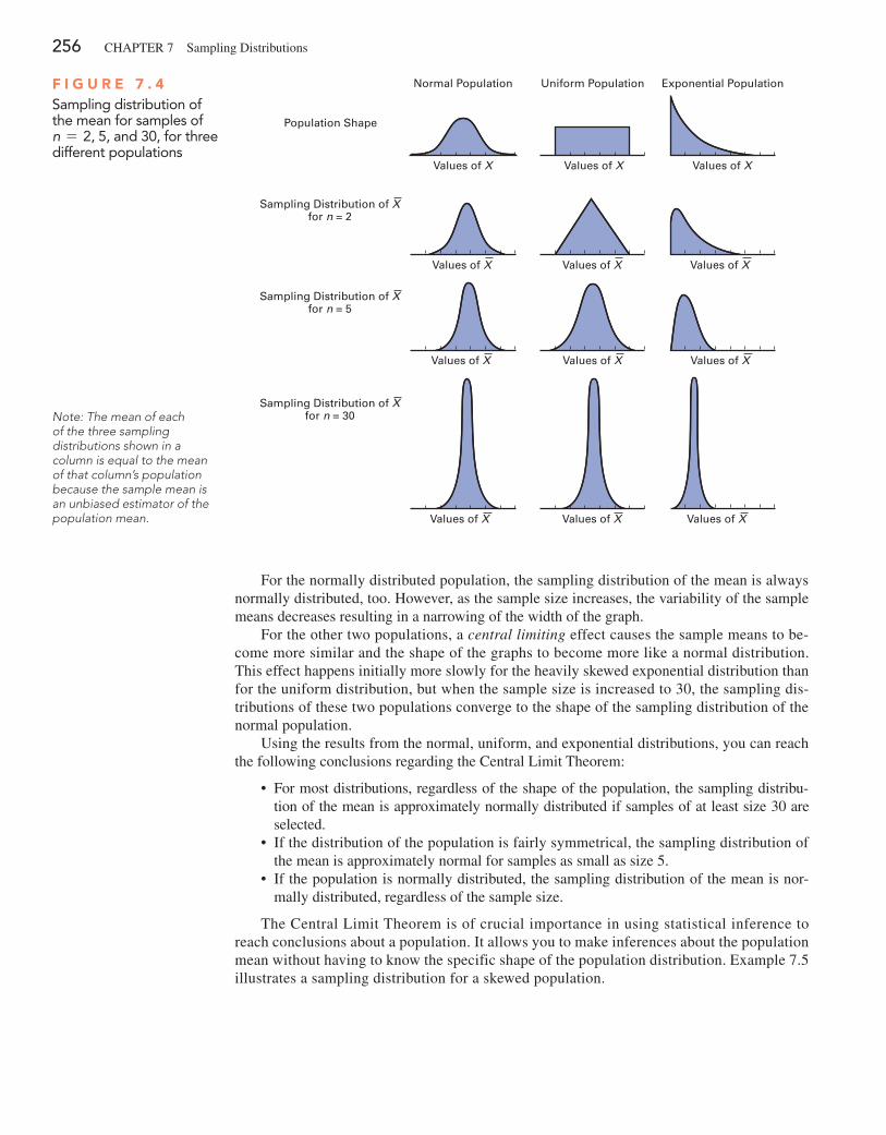
256 CHApTEr 7 Sampling Distributions
For the normally distributed population, the sampling distribution of the mean is always normally distributed, too. However, as the sample size increases, the variability of the sample means decreases resulting in a narrowing of the width of the graph.
For the other two populations, a central limiting effect causes the sample means to be-come more similar and the shape of the graphs to become more like a normal distribution. This effect happens initially more slowly for the heavily skewed exponential distribution than for the uniform distribution, but when the sample size is increased to 30, the sampling dis-tributions of these two populations converge to the shape of the sampling distribution of the normal population.
Using the results from the normal, uniform, and exponential distributions, you can reach the following conclusions regarding the Central Limit Theorem:
• For most distributions, regardless of the shape of the population, the sampling distribu-tion of the mean is approximately normally distributed if samples of at least size 30 are selected.
• If the distribution of the population is fairly symmetrical, the sampling distribution of the mean is approximately normal for samples as small as size 5.
• If the population is normally distributed, the sampling distribution of the mean is nor-mally distributed, regardless of the sample size.
The Central Limit Theorem is of crucial importance in using statistical inference to reach conclusions about a population. It allows you to make inferences about the population mean without having to know the specific shape of the population distribution. Example 7.5 illustrates a sampling distribution for a skewed population.
F i g U r e 7 . 4Sampling distribution of the mean for samples of n = 2, 5, and 30, for three different populations
Normal Population
Values of X Values of X Values of X
Uniform Population Exponential Population
Values of X Values of X Values of X
Values of X Values of X Values of X
Values of X
Sampling Distribution of Xfor n = 2
Population Shape
Sampling Distribution of Xfor n = 5
Sampling Distribution of Xfor n = 30
Values of X Values of X
Note: The mean of each of the three sampling distributions shown in a column is equal to the mean of that column’s population because the sample mean is an unbiased estimator of the population mean.
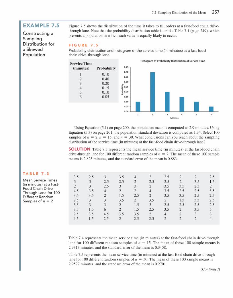
7.2 Sampling Distribution of the Mean 257
exaMPle 7.5constructing a sampling distribution for a skewed population
Figure 7.5 shows the distribution of the time it takes to fill orders at a fast-food chain drive-through lane. Note that the probability distribution table is unlike Table 7.1 (page 249), which presents a population in which each value is equally likely to occur.
F i g U r e 7 . 5probability distribution and histogram of the service time (in minutes) at a fast-food chain drive-through lane
Service Time (minutes) Probability
1 0.102 0.403 0.204 0.155 0.106 0.05
Using Equation (5.1) on page 200, the population mean is computed as 2.9 minutes. Using Equation (5.3) on page 201, the population standard deviation is computed as 1.34. Select 100 samples of n = 2, n = 15, and n = 30. What conclusions can you reach about the sampling distribution of the service time (in minutes) at the fast-food chain drive-through lane?
SolUTioN Table 7.3 represents the mean service time (in minutes) at the fast-food chain drive-through lane for 100 different random samples of n = 2. The mean of these 100 sample means is 2.825 minutes, and the standard error of the mean is 0.883.
T a b l e 7 . 3
Mean Service times (in minutes) at a Fast-Food chain Drive-through lane for 100 Different random Samples of n = 2
3.5 2.5 3 3.5 4 3 2.5 2 2 2.53 3 2.5 2.5 2 2.5 2.5 2 3.5 1.52 3 2.5 3 3 2 3.5 3.5 2.5 24.5 3.5 4 2 2 4 3.5 2.5 2.5 3.53.5 3.5 2 1.5 2.5 2 3.5 3.5 2.5 2.52.5 3 3 3.5 2 3.5 2 1.5 5.5 2.53.5 3 3 2 1.5 3 2.5 2.5 2.5 2.53.5 1.5 6 2 1.5 2.5 3.5 2 3.5 52.5 3.5 4.5 3.5 3.5 2 4 2 3 34.5 1.5 2.5 2 2.5 2.5 2 2 2 4
Table 7.4 represents the mean service time (in minutes) at the fast-food chain drive-through lane for 100 different random samples of n = 15. The mean of these 100 sample means is 2.9313 minutes, and the standard error of the mean is 0.3458.
Table 7.5 represents the mean service time (in minutes) at the fast-food chain drive-through lane for 100 different random samples of n = 30. The mean of these 100 sample means is 2.9527 minutes, and the standard error of the mean is 0.2701.
(Continued)
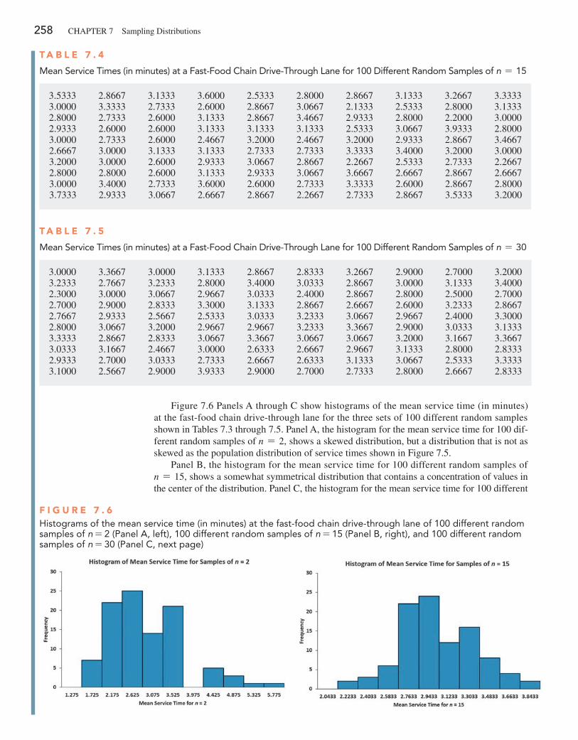
258 CHApTEr 7 Sampling Distributions
T a b l e 7 . 5
Mean Service times (in minutes) at a Fast-Food chain Drive-through lane for 100 Different random Samples of n = 30
3.0000 3.3667 3.0000 3.1333 2.8667 2.8333 3.2667 2.9000 2.7000 3.20003.2333 2.7667 3.2333 2.8000 3.4000 3.0333 2.8667 3.0000 3.1333 3.40002.3000 3.0000 3.0667 2.9667 3.0333 2.4000 2.8667 2.8000 2.5000 2.70002.7000 2.9000 2.8333 3.3000 3.1333 2.8667 2.6667 2.6000 3.2333 2.86672.7667 2.9333 2.5667 2.5333 3.0333 3.2333 3.0667 2.9667 2.4000 3.30002.8000 3.0667 3.2000 2.9667 2.9667 3.2333 3.3667 2.9000 3.0333 3.13333.3333 2.8667 2.8333 3.0667 3.3667 3.0667 3.0667 3.2000 3.1667 3.36673.0333 3.1667 2.4667 3.0000 2.6333 2.6667 2.9667 3.1333 2.8000 2.83332.9333 2.7000 3.0333 2.7333 2.6667 2.6333 3.1333 3.0667 2.5333 3.33333.1000 2.5667 2.9000 3.9333 2.9000 2.7000 2.7333 2.8000 2.6667 2.8333
Figure 7.6 panels A through C show histograms of the mean service time (in minutes) at the fast-food chain drive-through lane for the three sets of 100 different random samples shown in Tables 7.3 through 7.5. panel A, the histogram for the mean service time for 100 dif-ferent random samples of n = 2, shows a skewed distribution, but a distribution that is not as skewed as the population distribution of service times shown in Figure 7.5.
panel B, the histogram for the mean service time for 100 different random samples of n = 15, shows a somewhat symmetrical distribution that contains a concentration of values in the center of the distribution. panel C, the histogram for the mean service time for 100 different
F i g U r e 7 . 6histograms of the mean service time (in minutes) at the fast-food chain drive-through lane of 100 different random samples of n = 2 (panel a, left), 100 different random samples of n = 15 (panel b, right), and 100 different random samples of n = 30 (panel c, next page)
T a b l e 7 . 4
Mean Service times (in minutes) at a Fast-Food chain Drive-through lane for 100 Different random Samples of n = 15
3.5333 2.8667 3.1333 3.6000 2.5333 2.8000 2.8667 3.1333 3.2667 3.33333.0000 3.3333 2.7333 2.6000 2.8667 3.0667 2.1333 2.5333 2.8000 3.13332.8000 2.7333 2.6000 3.1333 2.8667 3.4667 2.9333 2.8000 2.2000 3.00002.9333 2.6000 2.6000 3.1333 3.1333 3.1333 2.5333 3.0667 3.9333 2.80003.0000 2.7333 2.6000 2.4667 3.2000 2.4667 3.2000 2.9333 2.8667 3.46672.6667 3.0000 3.1333 3.1333 2.7333 2.7333 3.3333 3.4000 3.2000 3.00003.2000 3.0000 2.6000 2.9333 3.0667 2.8667 2.2667 2.5333 2.7333 2.26672.8000 2.8000 2.6000 3.1333 2.9333 3.0667 3.6667 2.6667 2.8667 2.66673.0000 3.4000 2.7333 3.6000 2.6000 2.7333 3.3333 2.6000 2.8667 2.80003.7333 2.9333 3.0667 2.6667 2.8667 2.2667 2.7333 2.8667 3.5333 3.2000
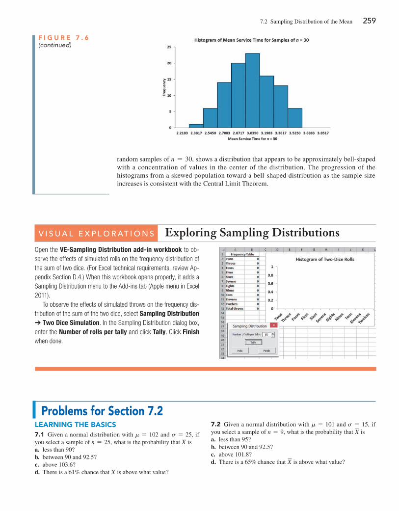
7.2 Sampling Distribution of the Mean 259
random samples of n = 30, shows a distribution that appears to be approximately bell-shaped with a concentration of values in the center of the distribution. The progression of the histograms from a skewed population toward a bell-shaped distribution as the sample size increases is consistent with the Central Limit Theorem.
Open the VE-Sampling Distribution add-in workbook to ob-serve the effects of simulated rolls on the frequency distribution of the sum of two dice. (For Excel technical requirements, review Ap-pendix Section D.4.) When this workbook opens properly, it adds a Sampling Distribution menu to the Add-ins tab (Apple menu in Excel 2011).
To observe the effects of simulated throws on the frequency dis-tribution of the sum of the two dice, select Sampling Distribution ➔ Two Dice Simulation. In the Sampling Distribution dialog box, enter the Number of rolls per tally and click Tally. Click Finish when done.
V i s U a l e x p l o r at i o n s Exploring Sampling Distributions
Problems for Section 7.2learNiNg The baSiCS7.1 Given a normal distribution with m = 102 and s = 25, if you select a sample of n = 25, what is the probability that X isa. less than 90?b. between 90 and 92.5?c. above 103.6?d. There is a 61% chance that X is above what value?
7.2 Given a normal distribution with m = 101 and s = 15, if you select a sample of n = 9, what is the probability that X isa. less than 95?b. between 90 and 92.5?c. above 101.8?d. There is a 65% chance that X is above what value?
F i g U r e 7 . 6(continued)
260 CHApTEr 7 Sampling Distributions
aPPlyiNg The CoNCePTS7.3 For each of the following three populations, indicate what the sampling distribution for samples of 25 would consist of:a. Customer receipts for a supermarket for a year.b. Insurance payouts in a particular geographical area in a year.c. Call center logs of inbound calls tracking handling time for a
credit card company during the year.
7.4 The following data represent the number of days absent per year in a population of six employees of a small company:
1 3 4 7 8 10
a. Assuming that you sample without replacement, select all pos-sible samples of n = 2 and construct the sampling distribution of the mean. Compute the mean of all the sample means and also compute the population mean. Are they equal? What is this property called?
b. repeat (a) for all possible samples of n = 3.c. Compare the shape of the sampling distribution of the mean in
(a) and (b). Which sampling distribution has less variability? Why?
d. Assuming that you sample with replacement, repeat (a) through (c) and compare the results. Which sampling distributions have the least variability—those in new part (a) or new part (b)? Why?
7.5 The diameter of a brand of ping-pong balls is approximately normally distributed, with a mean of 1.31 inches and a standard deviation of 0.08 inch. If you select a random sample of four ping-pong balls,a. what is the sampling distribution of the mean?b. what is the probability that the sample mean is less than 1.27
inches?c. what is the probability that the sample mean is between 1.27
and 1.32 inches?d. The probability is 58% that the sample mean will be between
what two values symmetrically distributed around the population mean?
7.6 A report announced that the median sales price of new houses sold one year was $211,000, and the mean sales price
was $272,500. Assume that the standard deviation of the prices is $100,000.a. If you select samples of n = 2, describe the shape of the sam-
pling distribution of X.b. If you select samples of n = 100, describe the shape of the
sampling distribution of X.c. If you select a random sample of n = 100, what is the
probability that the sample mean will be less than $290,000?d. If you select a random sample of n = 100, what is the
probability that the sample mean will be between $275,000 and $285,000?
7.7 Time spent using e-mail per session is normally distributed, with m = 9 minutes and s = 2 minutes. If you select a random sample of 25 sessions,a. what is the probability that the sample mean is between 8.8 and
9.2 minutes?b. what is the probability that the sample mean is between 8.5 and
9 minutes?c. If you select a random sample of 100 sessions, what is the prob-
ability that the sample mean is between 8.8 and 9.2 minutes?d. Explain the difference in the results of (a) and (c).
SELF Test
7.8 Today, full-time college students report spending a mean of 27 hours per week on academic activities, both
inside and outside the classroom. (Source: “A Challenge to Col-lege Students for 2013: Don’t Waste Your 6,570,” Huffington Post, January 29, 2013, huff.to/13dNtuT.) Assume the standard devia-tion of time spent on academic activities is 4 hours. If you select a random sample of 16 full-time college students,a. what is the probability that the mean time spent on academic
activities is at least 26 hours per week?b. there is an 85% chance that the sample mean is less than how
many hours per week?c. What assumption must you make in order to solve (a) and (b)?d. If you select a random sample of 64 full-time college students,
there is an 85% chance that the sample mean is less than how many hours per week?
7.3 Sampling Distribution of the proportionConsider a categorical variable that has only two categories, such as the customer prefers your brand or the customer prefers the competitor’s brand. You are interested in the proportion of items belonging to one of the categories—for example, the proportion of customers that prefer your brand. The population proportion, represented by p, is the proportion of items in the en-tire population with the characteristic of interest. The sample proportion, represented by p, is the proportion of items in the sample with the characteristic of interest. The sample proportion, a statistic, is used to estimate the population proportion, a parameter. To calculate the sample proportion, you assign one of two possible values, 1 or 0, to represent the presence or absence of the characteristic. You then sum all the 1 and 0 values and divide by n, the sample size. For example, if, in a sample of five customers, three preferred your brand and two did not, you have three 1s and two 0s. Summing the three 1s and two 0s and dividing by the sample size of 5 results in a sample proportion of 0.60.
Student TipDo not confuse this use of the Greek letter pi, p, to represent the popula-tion proportion with the mathematical constant that uses the same letter to represent the ratio of the circumference to a diameter of a circle—approximately 3.14159.
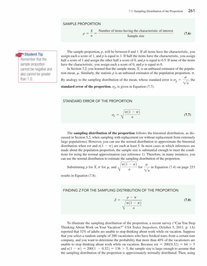
7.3 Sampling Distribution of the proportion 261
The sample proportion, p, will be between 0 and 1. If all items have the characteristic, you assign each a score of 1, and p is equal to 1. If half the items have the characteristic, you assign half a score of 1 and assign the other half a score of 0, and p is equal to 0.5. If none of the items have the characteristic, you assign each a score of 0, and p is equal to 0.
In Section 7.2, you learned that the sample mean, X, is an unbiased estimator of the popula-tion mean, m. Similarly, the statistic p is an unbiased estimator of the population proportion, p.
By analogy to the sampling distribution of the mean, whose standard error is sX=
s2n, the
standard error of the proportion, sp, is given in Equation (7.7).
StanDarD Error oF thE proportion
sp = Bp11 - p2n
(7.7)
The sampling distribution of the proportion follows the binomial distribution, as dis-cussed in Section 5.2, when sampling with replacement (or without replacement from extremely large populations). However, you can use the normal distribution to approximate the binomial distribution when np and n11 - p2 are each at least 5. In most cases in which inferences are made about the population proportion, the sample size is substantial enough to meet the condi-tions for using the normal approximation (see reference 1). Therefore, in many instances, you can use the normal distribution to estimate the sampling distribution of the proportion.
Substituting p for X, p for m, and Bp11 - p2n
for s2n
in Equation (7.4) on page 253
results in Equation (7.8).
SaMplE proportion
p =Xn=
Number of items having the characteristic of interest
Sample size (7.6)
Student TipRemember that the sample proportion cannot be negative and also cannot be greater than 1.0.
To illustrate the sampling distribution of the proportion, a recent survey (“Can You Stop Thinking About Work on Your Vacation?” USA Today Snapshots, October 5, 2011, p. 1A) reported that 32% of adults are unable to stop thinking about work while on vacation. Suppose that you select a random sample of 200 vacationers who have booked tours from a certain tour company, and you want to determine the probability that more than 40% of the vacationers are unable to stop thinking about work while on vacation. Because np = 20010.322 = 64 7 5 and n11 - p2 = 20011 - 0.322 = 136 7 5, the sample size is large enough to assume that the sampling distribution of the proportion is approximately normally distributed. Then, using
FinDing Z For thE SaMpling DiStribution oF thE proportion
Z =p - pBp11 - p2
n
(7.8)
262 CHApTEr 7 Sampling Distributions
Problems for Section 7.3learNiNg The baSiCS7.9 In a random sample of 64 people, 48 are classified as “suc-cessful.”a. Determine the sample proportion, p, of “successful” people.b. If the population proportion is 0.70, determine the standard
error of the proportion.
7.10 A random selection of 64 households was selected for a telephone survey. The key question asked was, “Do you or any member of your household own a cellular telephone that you can use to access the Internet?” Of the 64 respondents, 32 said yes and 32 said no.a. Determine the sample proportion, p, of households with cel-
lular telephones that can be used to access the Internet.b. If the population proportion is 0.75, determine the standard er-
ror of the proportion.
7.11 The following data represent the responses (Y for yes and N for no) from a sample of 20 college students to the question “Do you currently own shares in any stocks?”
N Y Y N Y Y Y N N N N Y Y N N Y N N N Y
a. Determine the sample proportion, p, of college students who own shares of stock.
b. If the population proportion is 0.40, determine the standard error of the proportion.
aPPlyiNg The CoNCePTSSELF Test
7.12 A political pollster is conducting an analysis of sample results in order to make predictions on election
night. Assuming a two-candidate election, if a specific candidate receives at least 55% of the vote in the sample, that candidate will be forecast as the winner of the election. If you select a random sample of 100 voters, what is the probability that a candidate will be forecast as the winner when
a. the population percentage of her vote is 50.1%?b. the population percentage of her vote is 60%?c. the population percentage of her vote is 49% (and she will ac-
tually lose the election)?d. If the sample size is increased to 400, what are your answers to
(a) through (c)? Discuss.
7.13 A marketing survey is conducted in which students are to taste two different brands of soft drink. Their task is to correctly identify the brand tasted. A random sample of 200 students is taken. Assume that the students have no ability to distinguish be-tween the two brands.a. What is the probability that the sample will have between 50%
and 60% of the identifications correct?b. The probability is 90% that the sample percentage is contained
within what symmetrical limits of the population percentage?c. What is the probability that the sample percentage of correct
identifications is greater than 55%?d. Which is more likely to occur—more than 62% correct identi-
fications in the sample of 200 or more than 56% correct identi-fications in a sample of 1,000? Explain.
7.14 Accenture’s Defining Success global research study found that the majority of today’s working women would prefer a bet-ter work–life balance to an increased salary. One of the most im-portant contributors to work–life balance identified by the survey was “flexibility,” with 80% of women saying that having a flexible work schedule is either very important or extremely important to their career success. (Source: bit.ly/17IM8gq.) Suppose you se-lect a sample of 100 working women.a. What is the probability that in the sample fewer than 85% say
that having a flexible work schedule is either very important or extremely important to their career success?
b. What is the probability that in the sample between 75% and 85% say that having a flexible work schedule is either very im-portant or extremely important to their career success?
the survey percentage of 32% as the population proportion, you can calculate the probability that more than 40% of the sample of vacationers are unable to stop thinking about work while on vacation by using Equation (7.8):
Z =p - pBp11 - p2
n
=0.40 - 0.32B 10.32210.682
200
=0.08B0.2176
200
=0.08
0.0330
= 2.42
Using Table E.2, the area under the normal curve greater than 2.42 is 0.0078. There-fore, if the population proportion is 0.32, the probability is 0.78% that more than 40% of the 200 vacationers in the sample will be unable to stop thinking about work while on vacation.
7.3 Sampling Distribution of the proportion 263
c. What is the probability that in the sample more than 82% say that having a flexible work schedule is either very important or extremely important to their career success?
d. If a sample of 400 is taken, how does this change your answers to (a) through (c)?
7.15 In a recent survey of full-time female workers, 43% said that they would give up some of their salary for more personal time. Suppose you select a sample of 100 full-time female workers.a. What is the probability that in the sample, fewer than 50%
would give up their salary for more personal time?b. What is the probability that in the sample, between 40% and
50% would give up some of their salary for more personal time?
c. What is the probability that in the sample, more than 40% would give up some of their salary for more personal time?
7.16 According to a poll on consumer behavior, 36% of people say they will only consider cars manufactured in their country when purchasing a new car. Suppose you select a random sample of 100 respondents.a. What is the probability that the sample will have between 35%
and 43% who say they will consider only cars manufactured by a company in their country when purchasing a new car?
b. The probability is 60% that the sample will be contained within what symmetrical limits of the population percentage?
c. The probability is 95% that the sample will be contained within what symmetrical limits of the population percentage?
7.17 New research shows that members of a certain youth generation have a great say in household purchases. Specifically,
70% of the people in the generation have a say in computer purchases. Suppose you select a sample of I 00 respondents from the generation.a. What is the probability that the sample percentage will be con-
tained between 64% and 77%?b. The probability is 80% that the sample percentage will be
contained within what symmetrical limits of the population percentage?
c. The probability is 99.7% that the sample percentage will be contained within what symmetrical limits of the population percentage? Use the empirical rule.
d. Suppose you selected a sample of 400 respondents. How does this change your answers in (a) through (c)?
7.18 A survey of 2,250 adults found that 56% got news both on-line and offline during a typical day.a. Suppose that you take a sample of 50 adults. If the population
proportion of adults who get news both online and offline in a typical day is 0.56, what is the probability that fewer than half in your sample will get news both online and offline in a typical day?
b. Suppose that you take a sample of 250 adults. If the population proportion of adults who get news both online and offline in a typical day is 0.56, what is the probability that fewer than half in your sample will get news both online and offline in a typical day?
c. Discuss the effect of sample size on the sampling distribution of the proportion in general and the effect on the probabilities in parts (a) and (b).
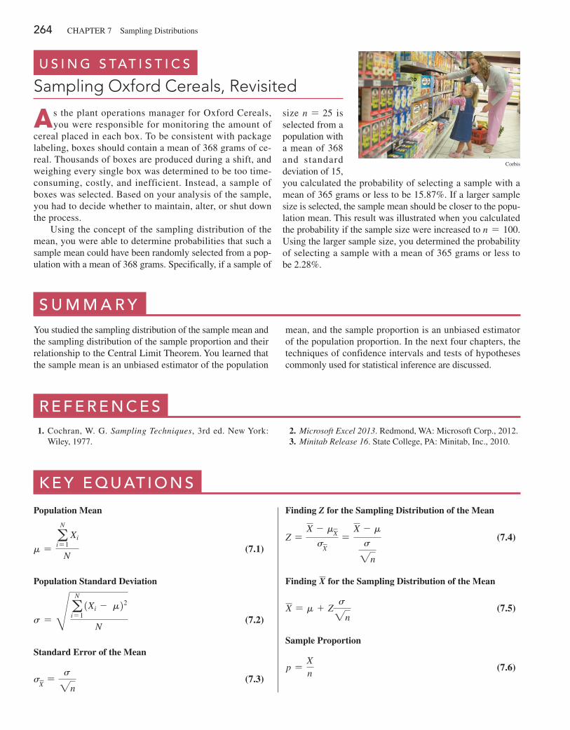
264 CHApTEr 7 Sampling Distributions
s U M M a r yYou studied the sampling distribution of the sample mean and the sampling distribution of the sample proportion and their relationship to the Central Limit Theorem. You learned that the sample mean is an unbiased estimator of the population
mean, and the sample proportion is an unbiased estimator of the population proportion. In the next four chapters, the techniques of confidence intervals and tests of hypotheses commonly used for statistical inference are discussed.
r e F e r e n c e s 1. Cochran, W. G. Sampling Techniques, 3rd ed. New York:
Wiley, 1977. 2. Microsoft Excel 2013. redmond, WA: Microsoft Corp., 2012. 3. Minitab Release 16. State College, pA: Minitab, Inc., 2010.
K e y e q U at i o n s
Population Mean
m =aN
i= 1 Xi
N (7.1)
Population Standard Deviation
s = R aN
i= 11Xi - m22
N (7.2)
Standard Error of the Mean
sX=
s2n (7.3)
Finding Z for the Sampling Distribution of the Mean
Z =X - m
X
sX
=X - m
s2n
(7.4)
Finding X for the Sampling Distribution of the Mean
X = m + Zs2n
(7.5)
Sample Proportion
p =Xn
(7.6)
As the plant operations manager for Oxford Cereals, you were responsible for monitoring the amount of
cereal placed in each box. To be consistent with package labeling, boxes should contain a mean of 368 grams of ce-real. Thousands of boxes are produced during a shift, and weighing every single box was determined to be too time-consuming, costly, and inefficient. Instead, a sample of boxes was selected. Based on your analysis of the sample, you had to decide whether to maintain, alter, or shut down the process.
Using the concept of the sampling distribution of the mean, you were able to determine probabilities that such a sample mean could have been randomly selected from a pop-ulation with a mean of 368 grams. Specifically, if a sample of
size n = 25 is selected from a population with a mean of 368 and standard deviation of 15, you calculated the probability of selecting a sample with a mean of 365 grams or less to be 15.87%. If a larger sample size is selected, the sample mean should be closer to the popu-lation mean. This result was illustrated when you calculated the probability if the sample size were increased to n = 100. Using the larger sample size, you determined the probability of selecting a sample with a mean of 365 grams or less to be 2.28%.
U s i n g s tat i s t i c s
Sampling Oxford Cereals, Revisited
Corbis
Chapter review problems 265
Standard Error of the Proportion
sp = Bp11 - p2n
(7.7)
Finding Z for the Sampling Distribution of the Proportion
Z =p - pBp11 - p2
n
(7.8)
K e y t e r M sCentral Limit Theorem 255sampling distribution 249sampling distribution of the mean 249
sampling distribution of the proportion 261
standard error of the mean 251
standard error of the proportion 261unbiased 249
c h e c K i n g y o U r U n d e r s ta n d i n g7.19 Why is the sample mean an unbiased estimator of the popu-lation mean?
7.20 Why is the Central Limit Theorem important when analyzing population distributions?
7.21 How would you define the standard error of the mean? For a sample of 100 with the standard error of the mean 30, why would we need to increase the sample size in order to cut the standard error of the mean to 15?
7.22 What is the difference between a population distribution and a sampling distribution?
7.23 Under what circumstances does the sampling distribution of the proportion approximately follow the normal distribution?
c h a p t e r r e V i e w p r o b l e M s7.24 An industrial sewing machine uses ball bearings that are targeted to have a diameter of 0.75 inch. The lower and upper specification limits under which the ball bearing can operate are 0.74 inch (lower) and 0.76 inch (upper). past experience has indi-cated that the actual diameter of the ball bearings is approximately normally distributed, with a mean of 0.753 inch and a standard deviation of 0.004 inch. If you select a random sample of 25 ball bearings, what is the probability that the sample mean isa. between the target and the population mean of 0.753?b. between the lower specification limit and the target?c. greater than the upper specification limit?d. less than the lower specification limit?e. The probability is 93% that the sample mean diameter will be
greater than what value?
7.25 The fill amount of bottles of a soft drink is normally dis-tributed, with a mean of 2.0 liters and a standard deviation of 0.05 liter. If you select a random sample of 25 bottles, what is the probability that the sample mean will bea. between 1.99 and 2.0 liters?b. below 1.98 liters?c. greater than 2.01 liters?d. The probability is 99% that the sample mean amount of soft
drink will be at least how much?e. The probability is 99% that the sample mean amount of soft
drink will be between which two values (symmetrically distrib-uted around the mean)?
7.26 An orange juice producer buys oranges from a large orange grove that has one variety of orange. The amount of juice squeezed from these oranges is approximately normally distributed, with a mean of 4.70 ounces and a standard deviation of 0.40 ounce. Sup-pose that you select a sample of 25 oranges.a. What is the probability that the sample mean amount of juice
will be at least 4.60 ounces?b. The probability is 70% that the sample mean amount of juice
will be contained between what two values symmetrically dis-tributed around the population mean?
c. The probability is 77% that the sample mean amount of juice will be greater than what value?
7.27 In problem 7.26, suppose that the mean amount of juice squeezed is 5.0 ounces.a. What is the probability that the sample mean amount of juice
will be at least 4.60 ounces?b. The probability is 70% that the sample mean amount of juice
will be contained between what two values symmetrically dis-tributed around the population mean?
c. The probability is 77% that the sample mean amount of juice will be greater than what value?
7.28 The stock market in France reported strong returns in 2013. The population of stocks earned a mean return of 15.23% in 2013. (Data extracted from The Wall Street Journal, January 2, 2014, p. r5.) Assume that the returns for stocks on the French stock
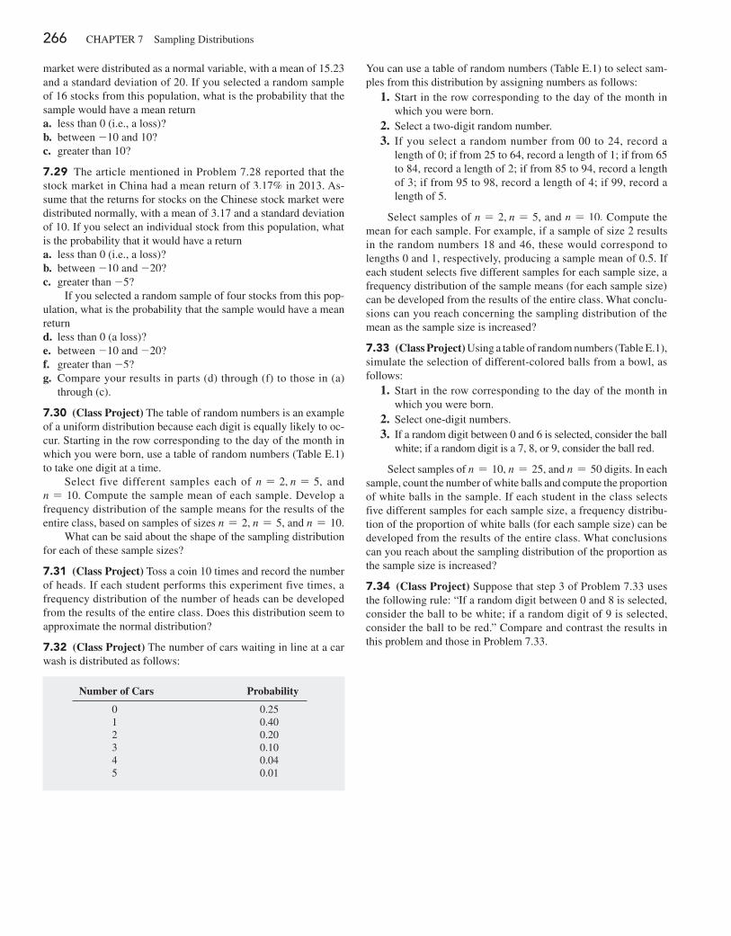
266 CHApTEr 7 Sampling Distributions
market were distributed as a normal variable, with a mean of 15.23 and a standard deviation of 20. If you selected a random sample of 16 stocks from this population, what is the probability that the sample would have a mean returna. less than 0 (i.e., a loss)?b. between -10 and 10?c. greater than 10?
7.29 The article mentioned in problem 7.28 reported that the stock market in China had a mean return of 3.17% in 2013. As-sume that the returns for stocks on the Chinese stock market were distributed normally, with a mean of 3.17 and a standard deviation of 10. If you select an individual stock from this population, what is the probability that it would have a returna. less than 0 (i.e., a loss)?b. between -10 and -20?c. greater than -5?
If you selected a random sample of four stocks from this pop-ulation, what is the probability that the sample would have a mean returnd. less than 0 (a loss)?e. between -10 and -20?f. greater than -5?g. Compare your results in parts (d) through (f) to those in (a)
through (c).
7.30 (Class Project) The table of random numbers is an example of a uniform distribution because each digit is equally likely to oc-cur. Starting in the row corresponding to the day of the month in which you were born, use a table of random numbers (Table E.1) to take one digit at a time.
Select five different samples each of n = 2, n = 5, and n = 10. Compute the sample mean of each sample. Develop a frequency distribution of the sample means for the results of the entire class, based on samples of sizes n = 2, n = 5, and n = 10.
What can be said about the shape of the sampling distribution for each of these sample sizes?
7.31 (Class Project) Toss a coin 10 times and record the number of heads. If each student performs this experiment five times, a frequency distribution of the number of heads can be developed from the results of the entire class. Does this distribution seem to approximate the normal distribution?
7.32 (Class Project) The number of cars waiting in line at a car wash is distributed as follows:
Number of Cars Probability
0 0.251 0.402 0.203 0.104 0.045 0.01
You can use a table of random numbers (Table E.1) to select sam-ples from this distribution by assigning numbers as follows: 1. Start in the row corresponding to the day of the month in
which you were born. 2. Select a two-digit random number. 3. If you select a random number from 00 to 24, record a
length of 0; if from 25 to 64, record a length of 1; if from 65 to 84, record a length of 2; if from 85 to 94, record a length of 3; if from 95 to 98, record a length of 4; if 99, record a length of 5.
Select samples of n = 2, n = 5, and n = 10. Compute the mean for each sample. For example, if a sample of size 2 results in the random numbers 18 and 46, these would correspond to lengths 0 and 1, respectively, producing a sample mean of 0.5. If each student selects five different samples for each sample size, a frequency distribution of the sample means (for each sample size) can be developed from the results of the entire class. What conclu-sions can you reach concerning the sampling distribution of the mean as the sample size is increased?
7.33 (Class Project) Using a table of random numbers (Table E.1), simulate the selection of different-colored balls from a bowl, as follows: 1. Start in the row corresponding to the day of the month in
which you were born. 2. Select one-digit numbers. 3. If a random digit between 0 and 6 is selected, consider the ball
white; if a random digit is a 7, 8, or 9, consider the ball red.
Select samples of n = 10, n = 25, and n = 50 digits. In each sample, count the number of white balls and compute the proportion of white balls in the sample. If each student in the class selects five different samples for each sample size, a frequency distribu-tion of the proportion of white balls (for each sample size) can be developed from the results of the entire class. What conclusions can you reach about the sampling distribution of the proportion as the sample size is increased?
7.34 (Class Project) Suppose that step 3 of problem 7.33 uses the following rule: “If a random digit between 0 and 8 is selected, consider the ball to be white; if a random digit of 9 is selected, consider the ball to be red.” Compare and contrast the results in this problem and those in problem 7.33.

Cases for Chapter 7 267
c a s e s F o r c h a p t e r 7
Managing ashland Multicomm servicesContinuing the quality improvement effort first described in the Chapter 6 Managing Ashland MultiComm Services case, the target upload speed for AMS Internet service sub-scribers has been monitored. As before, upload speeds are measured on a standard scale in which the target value is 1.0. Data collected over the past year indicate that the up-load speeds are approximately normally distributed, with a mean of 1.005 and a standard deviation of 0.10.
1. Each day, at 25 random times, the upload speed is mea-sured. Assuming that the distribution has not changed from what it was in the past year, what is the probability that the mean upload speed is
a. less than 1.0?b. between 0.95 and 1.0?c. between 1.0 and 1.05?d. less than 0.95 or greater than 1.05?e. Suppose that the mean upload speed of today’s sample
of 25 is 0.952. What conclusion can you reach about the mean upload speed today based on this result? Explain.
2. Compare the results of AMS problem 1 (a) through (d) to those of AMS problem 1 in Chapter 6 on page 243. What conclusions can you reach concerning the differences?
digital caseApply your knowledge about sampling distributions in this Digital Case, which reconsiders the Oxford Cereals Using Statistics scenario.
The advocacy group Consumers Concerned About Cereal Cheaters (CCACC) suspects that cereal companies, includ-ing Oxford Cereals, are cheating consumers by packaging cereals at less than labeled weights. recently, the group investigated the package weights of two popular Oxford brand cereals. Open CCACC.pdf to examine the group’s claims and supporting data, and then answer the following questions:
1. Are the data collection procedures that the CCACC uses to form its conclusions flawed? What procedures could the group follow to make its analysis more rigorous?
2. Assume that the two samples of five cereal boxes (one sample for each of two cereal varieties) listed on the CCACC website were collected randomly by organiza-tion members. For each sample,
a. calculate the sample mean.b. assuming that the standard deviation of the process is
15 grams and the population mean is 368 grams, cal-culate the percentage of all samples for each process that have a sample mean less than the value you calcu-lated in (a).
c. assuming that the standard deviation is 15 grams, cal-culate the percentage of individual boxes of cereal that have a weight less than the value you calculated in (a).
3. What, if any, conclusions can you form by using your cal-culations about the filling processes for the two different cereals?
4. A representative from Oxford Cereals has asked that the CCACC take down its page discussing shortages in Ox-ford Cereals boxes. Is this request reasonable? Why or why not?
5. Can the techniques discussed in this chapter be used to prove cheating in the manner alleged by the CCACC? Why or why not?
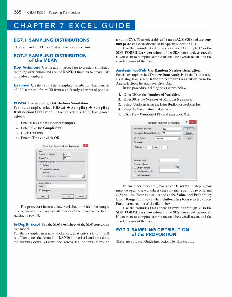
268 CHApTEr 7 Sampling Distributions
eg7.1 SaMPliNg DiSTribUTioNSThere are no Excel Guide instructions for this section.
eg7.2 SaMPliNg DiSTribUTioN of the MeaN
Key Technique Use an add-in procedure to create a simulated sampling distribution and use the RAND() function to create lists of random numbers.
Example Create a simulated sampling distribution that consists of 100 samples of n = 30 from a uniformly distributed popula-tion.
PhStat Use Sampling Distributions Simulation.For the example, select PHStat ➔ Sampling ➔ Sampling Distributions Simulation. In the procedure’s dialog box (shown below):
1. Enter 100 as the Number of Samples. 2. Enter 30 as the Sample Size. 3. Click Uniform. 4. Enter a Title and click OK.
The procedure inserts a new worksheet in which the sample means, overall mean, and standard error of the mean can be found starting in row 34.
in-Depth excel Use the SDS worksheet of the SDS workbook as a model.For the example, in a new worksheet, first enter a title in cell A1. Then enter the formula =RAND() in cell A2 and then copy the formula down 30 rows and across 100 columns (through
column CV). Then select this cell range (A2:CV31) and use copy and paste values as discussed in Appendix Section B.4.
Use the formulas that appear in rows 33 through 37 in the SDS_FORMULAS worksheet of the SDS workbook as models if you want to compute sample means, the overall mean, and the standard error of the mean.
analysis ToolPak Use Random Number Generation.For the example, select Data ➔ Data Analysis. In the Data Analy-sis dialog box, select Random Number Generation from the Analysis Tools list and then click OK.
In the procedure’s dialog box (shown below):
1. Enter 100 as the Number of Variables. 2. Enter 30 as the Number of Random Numbers. 3. Select Uniform from the Distribution drop-down list. 4. Keep the Parameters values as is. 5. Click New Worksheet Ply and then click OK.
If, for other problems, you select Discrete in step 3, you must be open to a worksheet that contains a cell range of X and P(X) values. Enter this cell range as the Value and Probability Input Range (not shown when Uniform has been selected) in the Parameters section of the dialog box.
Use the formulas that appear in rows 33 through 37 in the SDS_FORMULAS worksheet of the SDS workbook as models if you want to compute sample means, the overall mean, and the standard error of the mean.
eg7.3 SaMPliNg DiSTribUTioN of the ProPorTioN
There are no Excel Guide instructions for this section.
c h a p t e r 7 e x c e l g U i d e
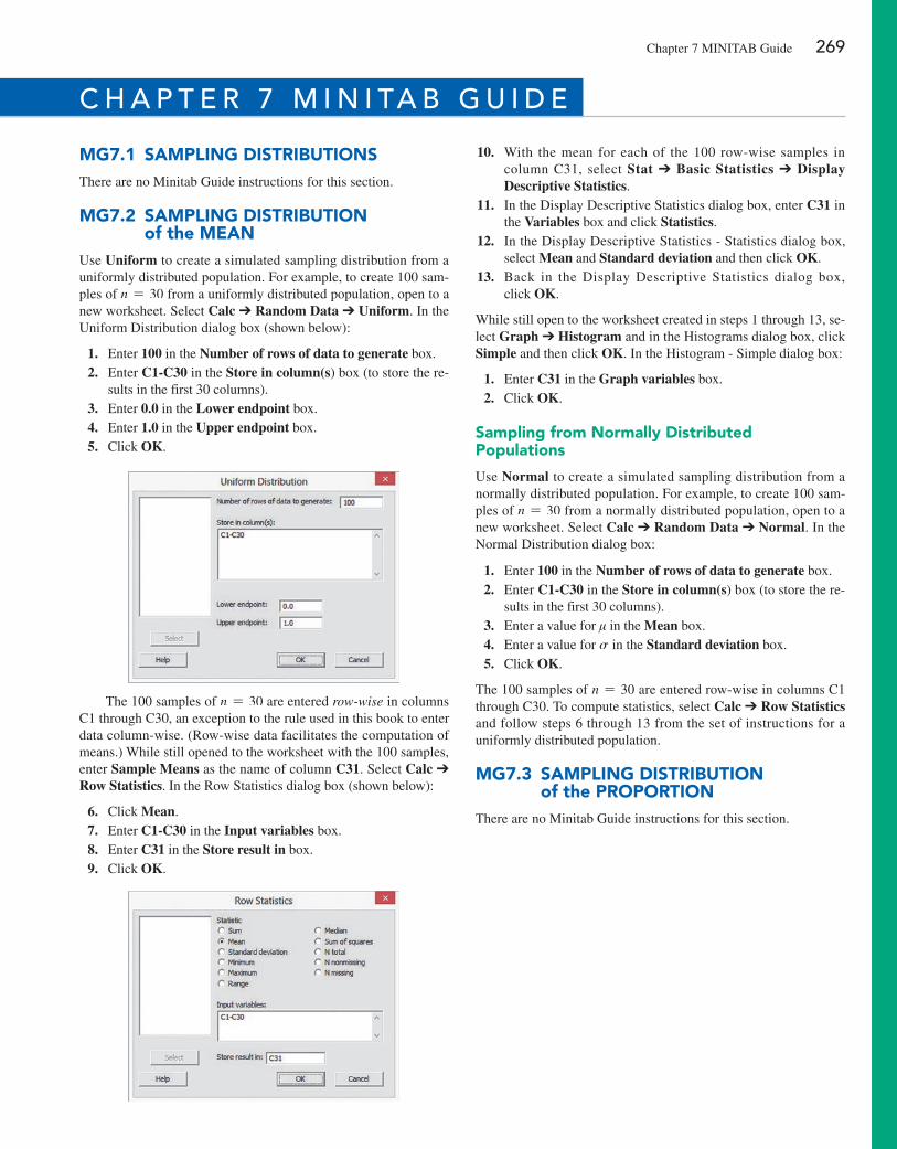
Chapter 7 MINITAB Guide 269
Mg7.1 SaMPliNg DiSTribUTioNSThere are no Minitab Guide instructions for this section.
Mg7.2 SaMPliNg DiSTribUTioN of the MeaN
Use Uniform to create a simulated sampling distribution from a uniformly distributed population. For example, to create 100 sam-ples of n = 30 from a uniformly distributed population, open to a new worksheet. Select Calc ➔ Random Data ➔ Uniform. In the Uniform Distribution dialog box (shown below):
1. Enter 100 in the Number of rows of data to generate box. 2. Enter C1-C30 in the Store in column(s) box (to store the re-
sults in the first 30 columns). 3. Enter 0.0 in the Lower endpoint box. 4. Enter 1.0 in the Upper endpoint box. 5. Click OK.
The 100 samples of n = 30 are entered row-wise in columns C1 through C30, an exception to the rule used in this book to enter data column-wise. (row-wise data facilitates the computation of means.) While still opened to the worksheet with the 100 samples, enter Sample Means as the name of column C31. Select Calc ➔ Row Statistics. In the row Statistics dialog box (shown below):
6. Click Mean. 7. Enter C1-C30 in the Input variables box. 8. Enter C31 in the Store result in box. 9. Click OK.
10. With the mean for each of the 100 row-wise samples in column C31, select Stat ➔ Basic Statistics ➔ Display Descriptive Statistics.
11. In the Display Descriptive Statistics dialog box, enter C31 in the Variables box and click Statistics.
12. In the Display Descriptive Statistics - Statistics dialog box, select Mean and Standard deviation and then click OK.
13. Back in the Display Descriptive Statistics dialog box, click OK.
While still open to the worksheet created in steps 1 through 13, se-lect Graph ➔ Histogram and in the Histograms dialog box, click Simple and then click OK. In the Histogram - Simple dialog box:
1. Enter C31 in the Graph variables box. 2. Click OK.
Sampling from Normally Distributed Populations
Use Normal to create a simulated sampling distribution from a normally distributed population. For example, to create 100 sam-ples of n = 30 from a normally distributed population, open to a new worksheet. Select Calc ➔ Random Data ➔ Normal. In the Normal Distribution dialog box:
1. Enter 100 in the Number of rows of data to generate box. 2. Enter C1-C30 in the Store in column(s) box (to store the re-
sults in the first 30 columns). 3. Enter a value for μ in the Mean box. 4. Enter a value for s in the Standard deviation box. 5. Click OK.
The 100 samples of n = 30 are entered row-wise in columns C1 through C30. To compute statistics, select Calc ➔ Row Statistics and follow steps 6 through 13 from the set of instructions for a uniformly distributed population.
Mg7.3 SaMPliNg DiSTribUTioN of the ProPorTioN
There are no Minitab Guide instructions for this section.
c h a p t e r 7 M i n i ta b g U i d e
270
U s i n g s tat i s t i c s
Getting Estimates at Ricknel Home CentersAs a member of the AIS team at Ricknel Home Centers (see page 198), you have already examined the probability of discovering questionable, or “tagged,” invoices. Now you have been assigned the task of auditing the accuracy of the integrated inventory management and point of sale component of the firm’s retail management system.
You could review the contents of each and every inventory and transactional record to check the accuracy of this system, but such a detailed review would be time-consuming and costly. Could you use statistical inference techniques to reach conclusions about the population of all records from a relatively small sample collected during an audit? At the end of each month, you could select a sample of the sales invoices to estimate population parameters such as
• The mean dollar amount listed on the sales invoices for the month • The proportion of invoices that contain errors that violate the internal con-
trol policy of the warehouse
If you used a sampling technique, how accurate would the results from the sample be? How would you use the results you generate? How could you be cer-tain that the sample size is large enough to give you the information you need?
contents
8.1 Confidence Interval Estimate for the Mean (s Known)
8.2 Confidence Interval Estimate for the Mean (s Unknown)
8.3 Confidence Interval Estimate for the Proportion
8.4 Determining Sample Size
8.5 Confidence Interval Estimation and Ethical Issues
8.6 Bootstrapping (online)
Using statistics: getting Estimates at Ricknel Home centers, Revisited
cHaptER 8 ExcEl gUidE
cHaptER 8 Minitab gUidE
objectives
Construct and interpret confidence interval estimates for the mean and the proportion
Determine the sample size necessary to develop a confidence interval estimate for the mean or proportion
Confidence Interval Estimation8
Chapter
Mangostock/Shutterstock
8.1 Confidence Interval Estimate for the Mean (s Known) 271
I n Section 7.2, you used the Central Limit Theorem and knowledge of the population distribution to determine the percentage of sample means that are within certain dis-tances of the population mean. For instance, in the cereal-filling example used throughout
Chapter 7 (see Example 7.4 on page 255), you can conclude that 95% of all sample means are between 362.12 and 373.88 grams. This is an example of deductive reasoning because the con-clusion is based on taking something that is true in general (for the population) and applying it to something specific (the sample means).
Getting the results that Ricknel Home Centers needs requires inductive reasoning. Induc-tive reasoning lets you use some specifics to make broader generalizations. You cannot guar-antee that the broader generalizations are absolutely correct, but with a careful choice of the specifics and a rigorous methodology, you can reach useful conclusions. As a Ricknel accoun-tant, you need to use inferential statistics, which uses sample results (the “some specifics”) to estimate (the making of “broader generalizations”) unknown population parameters such as a population mean or a population proportion. Note that statisticians use the word estimate in the same sense of the everyday usage: something you are reasonably certain about but cannot flatly say is absolutely correct.
You estimate population parameters by using either point estimates or interval estimates. A point estimate is the value of a single sample statistic, such as a sample mean. A confi-dence interval estimate is a range of numbers, called an interval, constructed around the point estimate. The confidence interval is constructed such that the probability that the interval in-cludes the population parameter is known.
Suppose you want to estimate the mean GPA of all the students at your university. The mean GPA for all the students is an unknown population mean, denoted by m. You select a sample of students and compute the sample mean, denoted by X, to be 2.80. As a point estimate of the population mean, m, you ask how accurate is the 2.80 value as an estimate of the popula-tion mean, m? By taking into account the variability from sample to sample (see Section 7.2, concerning the sampling distribution of the mean), you can construct a confidence interval estimate for the population mean to answer this question.
When you construct a confidence interval estimate, you indicate the confidence of cor-rectly estimating the value of the population parameter, m. This allows you to say that there is a specified confidence that m is somewhere in the range of numbers defined by the interval.
After studying this chapter, you might find that a 95% confidence interval for the mean GPA at your university is 2.75 … m … 2.85. You can interpret this interval estimate by stating that you are 95% confident that the mean GPA at your university is between 2.75 and 2.85.
In this chapter, you learn to construct a confidence interval for both the population mean and population proportion. You also learn how to determine the sample size that is necessary to construct a confidence interval of a desired width.
8.1 Confidence Interval Estimate for the Mean (s Known)In Section 7.2, you used the Central Limit Theorem and knowledge of the population dis-tribution to determine the percentage of sample means that are within certain distances of the population mean. Suppose that in the cereal-filling example you wished to estimate the population mean, using the information from a single sample. Thus, rather than taking m { 11.9621s>1n2 to find the upper and lower limits around m, as in Section 7.2, you sub-stitute the sample mean, X, for the unknown m and use X { 11.9621s>1n2 as an interval to estimate the unknown m. Although in practice you select a single sample of n values and com-pute the mean, X, in order to understand the full meaning of the interval estimate, you need to examine a hypothetical set of all possible samples of n values.
Suppose that a sample of n = 25 cereal boxes has a mean of 362.3 grams and a standard deviation of 15 grams. The interval developed to estimate m is 362.3 { 11.9621152>11252, or 362.3 { 5.88. The estimate of m is
356.42 … m … 368.18
Student TipRemember, the confi-dence interval is for the population mean not the sample mean.
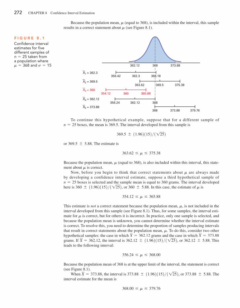
272 CHAPTER 8 Confidence Interval Estimation
Because the population mean, m (equal to 368), is included within the interval, this sample results in a correct statement about m (see Figure 8.1).
368
368.18362.3356.42X1 = 362.3
362.12 373.88
375.38369.5363.62
365.88360354.12
368362.12356.24
379.76373.88368
X2 = 369.5
X3 = 360
X4 = 362.12
X5 = 373.88
F i g u r e 8 . 1Confidence interval estimates for five different samples of n = 25 taken from a population where m = 368 and s = 15
To continue this hypothetical example, suppose that for a different sample of n = 25 boxes, the mean is 369.5. The interval developed from this sample is
369.5 { 11.9621152>11252
or 369.5 { 5.88. The estimate is
363.62 … m … 375.38
Because the population mean, m (equal to 368), is also included within this interval, this state-ment about m is correct.
Now, before you begin to think that correct statements about m are always made by developing a confidence interval estimate, suppose a third hypothetical sample of n = 25 boxes is selected and the sample mean is equal to 360 grams. The interval developed here is 360 { 11.9621152>11252, or 360 { 5.88. In this case, the estimate of m is
354.12 … m … 365.88
This estimate is not a correct statement because the population mean, m, is not included in the interval developed from this sample (see Figure 8.1). Thus, for some samples, the interval esti-mate for m is correct, but for others it is incorrect. In practice, only one sample is selected, and because the population mean is unknown, you cannot determine whether the interval estimate is correct. To resolve this, you need to determine the proportion of samples producing intervals that result in correct statements about the population mean, m. To do this, consider two other hypothetical samples: the case in which X = 362.12 grams and the case in which X = 373.88 grams. If X = 362.12, the interval is 362.12 { 11.9621152>11252, or 362.12 { 5.88. This leads to the following interval:
356.24 … m … 368.00
Because the population mean of 368 is at the upper limit of the interval, the statement is correct (see Figure 8.1).
When X = 373.88, the interval is 373.88 { 11.9621152>11252, or 373.88 { 5.88. The interval estimate for the mean is
368.00 … m … 379.76
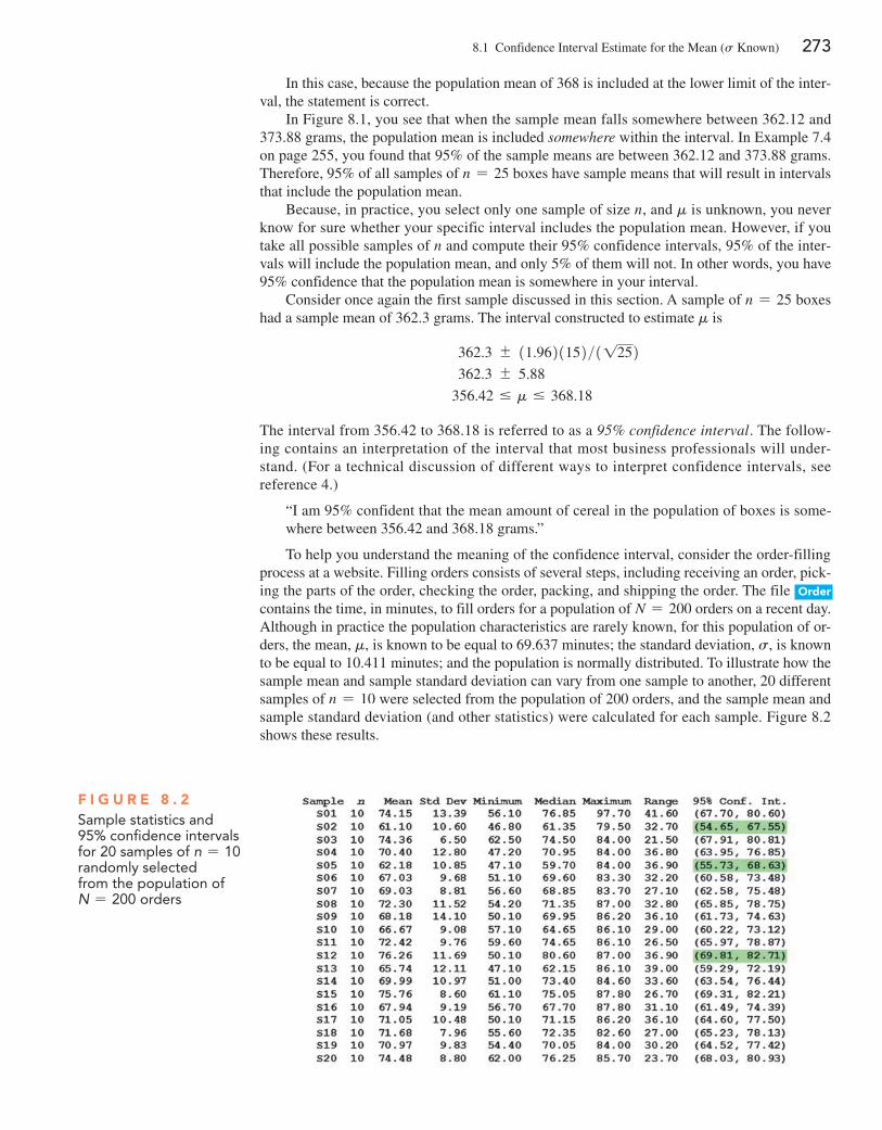
8.1 Confidence Interval Estimate for the Mean (s Known) 273
In this case, because the population mean of 368 is included at the lower limit of the inter-val, the statement is correct.
In Figure 8.1, you see that when the sample mean falls somewhere between 362.12 and 373.88 grams, the population mean is included somewhere within the interval. In Example 7.4 on page 255, you found that 95% of the sample means are between 362.12 and 373.88 grams. Therefore, 95% of all samples of n = 25 boxes have sample means that will result in intervals that include the population mean.
Because, in practice, you select only one sample of size n, and m is unknown, you never know for sure whether your specific interval includes the population mean. However, if you take all possible samples of n and compute their 95% confidence intervals, 95% of the inter-vals will include the population mean, and only 5% of them will not. In other words, you have 95% confidence that the population mean is somewhere in your interval.
Consider once again the first sample discussed in this section. A sample of n = 25 boxes had a sample mean of 362.3 grams. The interval constructed to estimate m is
362.3 { 11.9621152>11252 362.3 { 5.88
356.42 … m … 368.18
The interval from 356.42 to 368.18 is referred to as a 95% confidence interval. The follow-ing contains an interpretation of the interval that most business professionals will under-stand. (For a technical discussion of different ways to interpret confidence intervals, see reference 4.)
“I am 95% confident that the mean amount of cereal in the population of boxes is some-where between 356.42 and 368.18 grams.”
To help you understand the meaning of the confidence interval, consider the order-filling process at a website. Filling orders consists of several steps, including receiving an order, pick-ing the parts of the order, checking the order, packing, and shipping the order. The file Order contains the time, in minutes, to fill orders for a population of N = 200 orders on a recent day. Although in practice the population characteristics are rarely known, for this population of or-ders, the mean, m, is known to be equal to 69.637 minutes; the standard deviation, s, is known to be equal to 10.411 minutes; and the population is normally distributed. To illustrate how the sample mean and sample standard deviation can vary from one sample to another, 20 different samples of n = 10 were selected from the population of 200 orders, and the sample mean and sample standard deviation (and other statistics) were calculated for each sample. Figure 8.2 shows these results.
F i g u r e 8 . 2Sample statistics and 95% confidence intervals for 20 samples of n = 10 randomly selected from the population of N = 200 orders
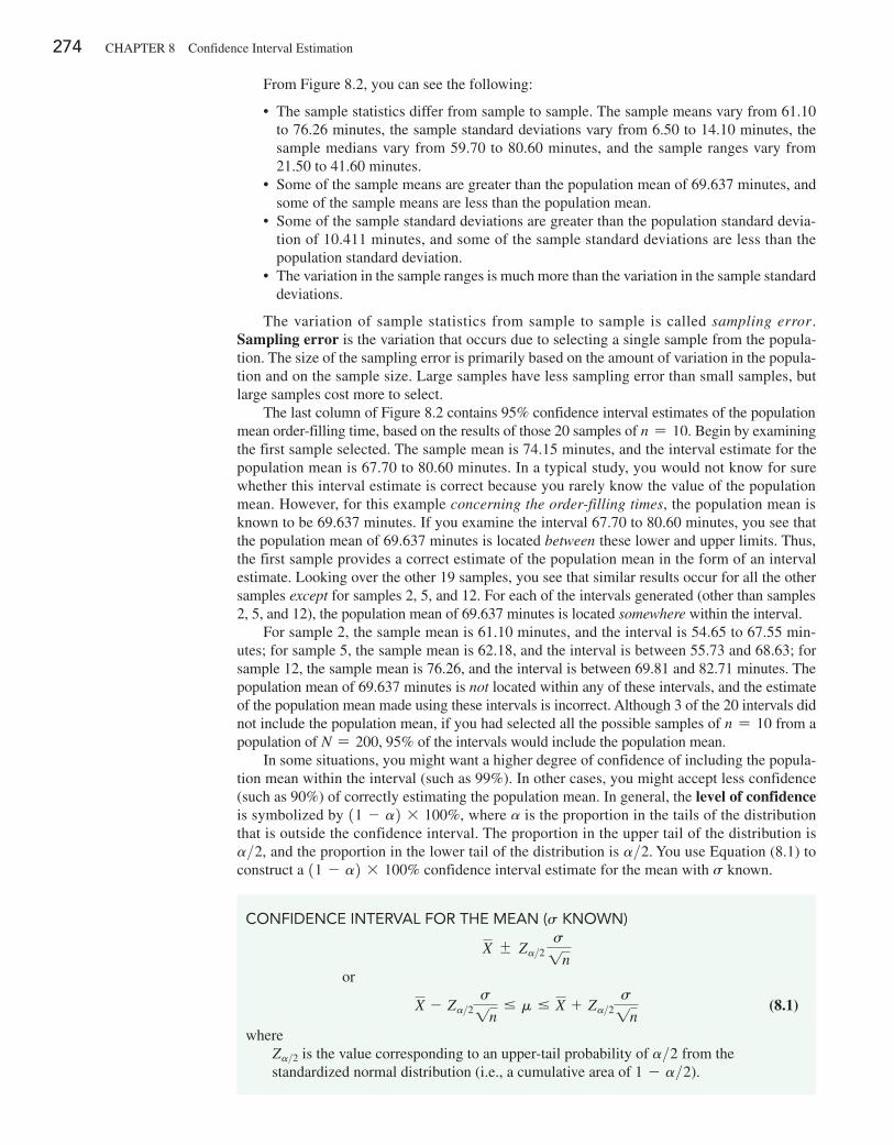
274 CHAPTER 8 Confidence Interval Estimation
From Figure 8.2, you can see the following:
• The sample statistics differ from sample to sample. The sample means vary from 61.10 to 76.26 minutes, the sample standard deviations vary from 6.50 to 14.10 minutes, the sample medians vary from 59.70 to 80.60 minutes, and the sample ranges vary from 21.50 to 41.60 minutes.
• Some of the sample means are greater than the population mean of 69.637 minutes, and some of the sample means are less than the population mean.
• Some of the sample standard deviations are greater than the population standard devia-tion of 10.411 minutes, and some of the sample standard deviations are less than the population standard deviation.
• The variation in the sample ranges is much more than the variation in the sample standard deviations.
The variation of sample statistics from sample to sample is called sampling error. Sampling error is the variation that occurs due to selecting a single sample from the popula-tion. The size of the sampling error is primarily based on the amount of variation in the popula-tion and on the sample size. Large samples have less sampling error than small samples, but large samples cost more to select.
The last column of Figure 8.2 contains 95% confidence interval estimates of the population mean order-filling time, based on the results of those 20 samples of n = 10. Begin by examining the first sample selected. The sample mean is 74.15 minutes, and the interval estimate for the population mean is 67.70 to 80.60 minutes. In a typical study, you would not know for sure whether this interval estimate is correct because you rarely know the value of the population mean. However, for this example concerning the order-filling times, the population mean is known to be 69.637 minutes. If you examine the interval 67.70 to 80.60 minutes, you see that the population mean of 69.637 minutes is located between these lower and upper limits. Thus, the first sample provides a correct estimate of the population mean in the form of an interval estimate. Looking over the other 19 samples, you see that similar results occur for all the other samples except for samples 2, 5, and 12. For each of the intervals generated (other than samples 2, 5, and 12), the population mean of 69.637 minutes is located somewhere within the interval.
For sample 2, the sample mean is 61.10 minutes, and the interval is 54.65 to 67.55 min-utes; for sample 5, the sample mean is 62.18, and the interval is between 55.73 and 68.63; for sample 12, the sample mean is 76.26, and the interval is between 69.81 and 82.71 minutes. The population mean of 69.637 minutes is not located within any of these intervals, and the estimate of the population mean made using these intervals is incorrect. Although 3 of the 20 intervals did not include the population mean, if you had selected all the possible samples of n = 10 from a population of N = 200, 95% of the intervals would include the population mean.
In some situations, you might want a higher degree of confidence of including the popula-tion mean within the interval (such as 99%). In other cases, you might accept less confidence (such as 90%) of correctly estimating the population mean. In general, the level of confidence is symbolized by 11 - a2 * 100%, where a is the proportion in the tails of the distribution that is outside the confidence interval. The proportion in the upper tail of the distribution is a>2, and the proportion in the lower tail of the distribution is a>2. You use Equation (8.1) to construct a 11 - a2 * 100% confidence interval estimate for the mean with s known.
ConfIDEnCE IntErval for thE MEan (s Known)
X { Za>2 s1n
or
X - Za>2s1n
… m … X + Za>2s1n
(8.1)
whereZa>2 is the value corresponding to an upper-tail probability of a>2 from the standardized normal distribution (i.e., a cumulative area of 1 - a>2).
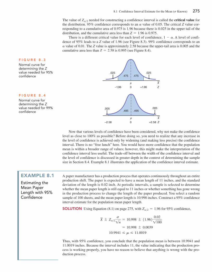
8.1 Confidence Interval Estimate for the Mean (s Known) 275
The value of Za>2 needed for constructing a confidence interval is called the critical value for the distribution. 95% confidence corresponds to an a value of 0.05. The critical Z value cor-responding to a cumulative area of 0.975 is 1.96 because there is 0.025 in the upper tail of the distribution, and the cumulative area less than Z = 1.96 is 0.975.
There is a different critical value for each level of confidence, 1 - a. A level of confi-dence of 95% leads to a Z value of 1.96 (see Figure 8.3). 99% confidence corresponds to an a value of 0.01. The Z value is approximately 2.58 because the upper-tail area is 0.005 and the cumulative area less than Z = 2.58 is 0.995 (see Figure 8.4).
X
0–1.96 +1.96
.475.475
Z
.025 .025
F i g u r e 8 . 3normal curve for determining the Z value needed for 95% confidence
X
0–2.58 +2.58
.495.495
Z
.005 .005
F i g u r e 8 . 4normal curve for determining the Z value needed for 99% confidence
Now that various levels of confidence have been considered, why not make the confidence level as close to 100% as possible? Before doing so, you need to realize that any increase in the level of confidence is achieved only by widening (and making less precise) the confidence interval. There is no “free lunch” here. You would have more confidence that the population mean is within a broader range of values; however, this might make the interpretation of the confidence interval less useful. The trade-off between the width of the confidence interval and the level of confidence is discussed in greater depth in the context of determining the sample size in Section 8.4. Example 8.1 illustrates the application of the confidence interval estimate.
example 8.1Estimating the Mean paper length with 95% confidence
A paper manufacturer has a production process that operates continuously throughout an entire production shift. The paper is expected to have a mean length of 11 inches, and the standard deviation of the length is 0.02 inch. At periodic intervals, a sample is selected to determine whether the mean paper length is still equal to 11 inches or whether something has gone wrong in the production process to change the length of the paper produced. You select a random sample of 100 sheets, and the mean paper length is 10.998 inches. Construct a 95% confidence interval estimate for the population mean paper length.
SOlutiOn Using Equation (8.1) on page 275, with Za>2 = 1.96 for 95% confidence,
X { Za>2s1n
= 10.998 { 11.962 0.021100
= 10.998 { 0.0039
10.9941 … m … 11.0019
Thus, with 95% confidence, you conclude that the population mean is between 10.9941 and 11.0019 inches. Because the interval includes 11, the value indicating that the production pro-cess is working properly, you have no reason to believe that anything is wrong with the pro-duction process.
276 CHAPTER 8 Confidence Interval Estimation
Example 8.2 illustrates the effect of using a 99% confidence interval.
example 8.2Estimating the Mean paper length with 99% confidence
Construct a 99% confidence interval estimate for the population mean paper length.
SOlutiOn Using Equation (8.1) on page 274, with Za>2 = 2.58 for 99% confidence,
X { Za>2s1n
= 10.998 { 12.582 0.021100
= 10.998 { 0.00516
10.9928 … m … 11.0032
Once again, because 11 is included within this wider interval, you have no reason to believe that anything is wrong with the production process.
As discussed in Section 7.2, the sampling distribution of the sample mean, X, is normally distributed if the population for your characteristic of interest, X, follows a normal distribution. And if the population of X does not follow a normal distribution, the Central Limit Theorem almost always ensures that X is approximately normally distributed when n is large. However, when dealing with a small sample size and a population that does not follow a normal distribu-tion, the sampling distribution of X is not normally distributed, and therefore the confidence interval discussed in this section is inappropriate. In practice, however, as long as the sample size is large enough and the population is not very skewed, you can use the confidence interval defined in Equation (8.1) to estimate the population mean when s is known. To assess the as-sumption of normality, you can evaluate the shape of the sample data by constructing a histo-gram, stem-and-leaf display, boxplot, or normal probability plot.
Can You ever Know the population Standard Deviation?To solve Equation (8.1), you must know the value for s, the population standard deviation. To know s implies that you know all the values in the entire population. (How else would you know the value of this population parameter?) If you knew all the values in the entire popu-lation, you could directly compute the population mean. There would be no need to use the inductive reasoning of inferential statistics to estimate the population mean. In other words, if you know s, you really do not have a need to use Equation (8.1) to construct a confidence interval estimate of the mean (s known).
More significantly, in virtually all real-world business situations, you would never know the standard deviation of the population. In business situations, populations are often too large to examine all the values. So why study the confidence interval estimate of the mean (s known) at all? This method serves as an important introduction to the concept of a con-fidence interval because it uses the normal distribution, which has already been thoroughly discussed in Chapters 6 and 7. In the next section, you will see that constructing a confidence interval estimate when s is not known requires another distribution (the t distribution) not pre-viously mentioned in this book.
Student TipBecause understanding the confidence interval concept is very impor-tant when reading the rest of this book, review this section carefully to understand the underly-ing concept—even if you never have a practical reason to use the confidence interval estimate of the mean (s known) method.
problems for Section 8.1learning the BaSiCS8.1 If X = 103, s = 22, and n = 39, construct a 99% confi-dence interval estimate of the population mean, m.
8.2 If X = 115, s = 21, and n = 35, construct a 95% confi-dence interval estimate of the population mean, m.
8.3 Why is it not possible in Example 8.1 on page 275 to have 100% confidence? Explain.
8.4 Is it true in Example 8.1 on page 275 that you do not know for sure whether the population mean is between 10.9941 and 11.0019 inches? Explain.
8.2 Confidence Interval Estimate for the Mean (s Unknown) 277
applYing the COnCeptS8.5 A market researcher selects a simple random sample of n = 100 Twitter users from a population of over 100 million Twitter registered users. After analyzing the sample, she states that she has 95% confidence that the mean time spent on the site per day is between 15 and 57 minutes. Explain the meaning of this statement.
8.6 Suppose that you are going to collect a set of data, either from an entire population or from a random sample taken from that population.a. Which statistical measure would you compute first: the mean
or the standard deviation? Explain.b. What does your answer to (a) tell you about the “practical-
ity” of using the confidence interval estimate formula given in Equation (8.1)?
8.7 A market researcher collects a simple random sample of customers from its population of two million customers. After analyzing the sample, she states that she has 95% confidence that the mean annual income of its two million customers is between $68,000 and $85,000. Suppose that the population mean annual income is $88,000. Is the confidence interval estimate correct? Explain.
8.8 You are working as an assistant to the dean of institutional research at your university. The dean wants to survey members of the alumni association who obtained their baccalaureate degrees 5 years ago to learn what their starting salaries were in their first full-time job after receiving their degrees. A sample of 200 alumni is to be randomly selected from the list of 2,500 graduates in that class. If the dean’s goal is to construct a 95% confidence interval estimate for the population mean starting salary, why is it not pos-
sible that you will be able to use the expression X { Z0.025s1n
for this purpose? Explain.
8.9 The manager of a paint supply store wants to estimate the ac-tual amount of paint contained in 1-gallon cans purchased from a nationally known manufacturer. The manufacturer’s specifications state that the standard deviation of the amount of paint is equal to 0.03 gallon. A random sample of 50 cans is selected, and the sample mean amount of paint per 1-gallon can is 0.982 gallon.a. Construct a 99% confidence interval estimate for the popula-
tion mean amount of paint included in a 1-gallon can.b. On the basis of these results, do you think the manager has a
right to complain to the manufacturer? Why?c. Must you assume that the population amount of paint per can is
normally distributed here? Explain.d. Construct a 90% confidence interval estimate. How does this
change your answer to part (b)?
8.10 The operations manager at a compact fluorescent light bulb (CFL) factory needs to estimate the mean life of a large shipment of CFLs. The manufacturer’s speci-
fications are that the standard deviation is 1,000 hours. A random sample of 64 CFLs indicated a sample mean life of 7,500 hours.a. Construct a 95% confidence interval estimate for the popu-
lation mean life of compact fluorescent light bulbs in this shipment.
b. Do you think that the manufacturer has the right to state that the compact fluorescent light bulbs have a mean life of 8,000 hours? Explain.
c. Must you assume that the population compact fluorescent light bulb life is normally distributed? Explain.
d. Suppose that the standard deviation changes to 800 hours. What are your answers in (a) and (b)?
SELF Test
8.2 Confidence Interval Estimate for the Mean (s Unknown)In the previous section, you learned that in most business situations, you do not know s, the population standard deviation. This section discusses a method of constructing a confi-dence interval estimate of m that uses the sample statistic S as an estimate of the population parameter s.
Student’s t DistributionAt the start of the twentieth century, William S. Gosset was working at Guinness in Ireland, trying to help brew better beer less expensively (see reference 5). As he had only small samples to study, he needed to find a way to make inferences about means without having to know s. Writing under the pen name “Student,”1 Gosset solved this problem by developing what today is known as the Student’s t distribution, or the t distribution.
If the variable X is normally distributed, then the following statistic:
t =X - m
S1n
has a t distribution with n - 1 degrees of freedom. This expression has the same form as the Z statistic in Equation (7.4) on page 253, except that S is used to estimate the un-known s.
1Guinness considered all research conducted to be proprietary and a trade secret. The firm prohibited its employees from publishing their results. Gosset circumvented this ban by using the pen name “Student” to publish his findings.
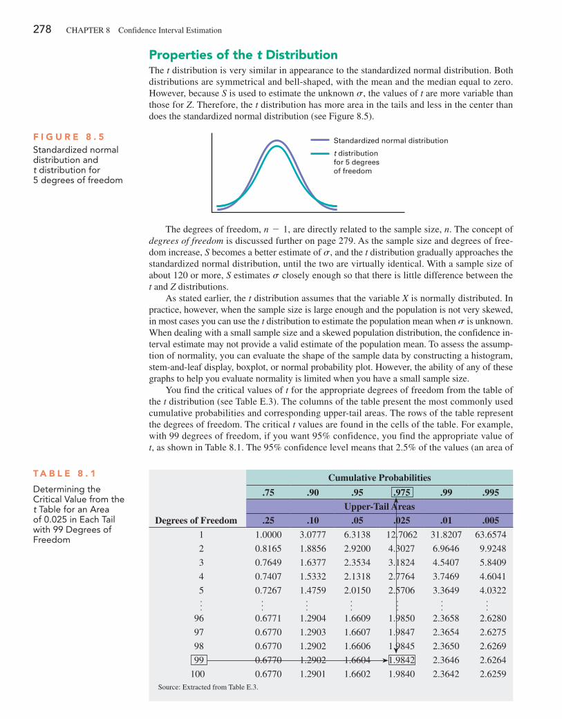
278 CHAPTER 8 Confidence Interval Estimation
properties of the t DistributionThe t distribution is very similar in appearance to the standardized normal distribution. Both distributions are symmetrical and bell-shaped, with the mean and the median equal to zero. However, because S is used to estimate the unknown s, the values of t are more variable than those for Z. Therefore, the t distribution has more area in the tails and less in the center than does the standardized normal distribution (see Figure 8.5).
Standardized normal distribution
t distributionfor 5 degrees of freedom
F i g u r e 8 . 5Standardized normal distribution and t distribution for 5 degrees of freedom
The degrees of freedom, n - 1, are directly related to the sample size, n. The concept of degrees of freedom is discussed further on page 279. As the sample size and degrees of free-dom increase, S becomes a better estimate of s, and the t distribution gradually approaches the standardized normal distribution, until the two are virtually identical. With a sample size of about 120 or more, S estimates s closely enough so that there is little difference between the t and Z distributions.
As stated earlier, the t distribution assumes that the variable X is normally distributed. In practice, however, when the sample size is large enough and the population is not very skewed, in most cases you can use the t distribution to estimate the population mean when s is unknown. When dealing with a small sample size and a skewed population distribution, the confidence in-terval estimate may not provide a valid estimate of the population mean. To assess the assump-tion of normality, you can evaluate the shape of the sample data by constructing a histogram, stem-and-leaf display, boxplot, or normal probability plot. However, the ability of any of these graphs to help you evaluate normality is limited when you have a small sample size.
You find the critical values of t for the appropriate degrees of freedom from the table of the t distribution (see Table E.3). The columns of the table present the most commonly used cumulative probabilities and corresponding upper-tail areas. The rows of the table represent the degrees of freedom. The critical t values are found in the cells of the table. For example, with 99 degrees of freedom, if you want 95% confidence, you find the appropriate value of t, as shown in Table 8.1. The 95% confidence level means that 2.5% of the values (an area of
Cumulative Probabilities
.75 .90 .95 .975 .99 .995
Upper-Tail Areas
Degrees of Freedom .25 .10 .05 .025 .01 .005
1 1.0000 3.0777 6.3138 12.7062 31.8207 63.6574
2 0.8165 1.8856 2.9200 4.3027 6.9646 9.9248
3 0.7649 1.6377 2.3534 3.1824 4.5407 5.8409
4 0.7407 1.5332 2.1318 2.7764 3.7469 4.6041
5 0.7267 1.4759 2.0150 2.5706 3.3649 4.0322f f f f f f f
96 0.6771 1.2904 1.6609 1.9850 2.3658 2.6280
97 0.6770 1.2903 1.6607 1.9847 2.3654 2.6275
98 0.6770 1.2902 1.6606 1.9845 2.3650 2.6269
99 0.6770 1.2902 1.6604 1.9842 2.3646 2.6264
100 0.6770 1.2901 1.6602 1.9840 2.3642 2.6259Source: Extracted from Table E.3.
t a B l e 8 . 1
Determining the Critical value from the t table for an area of 0.025 in Each tail with 99 Degrees of freedom
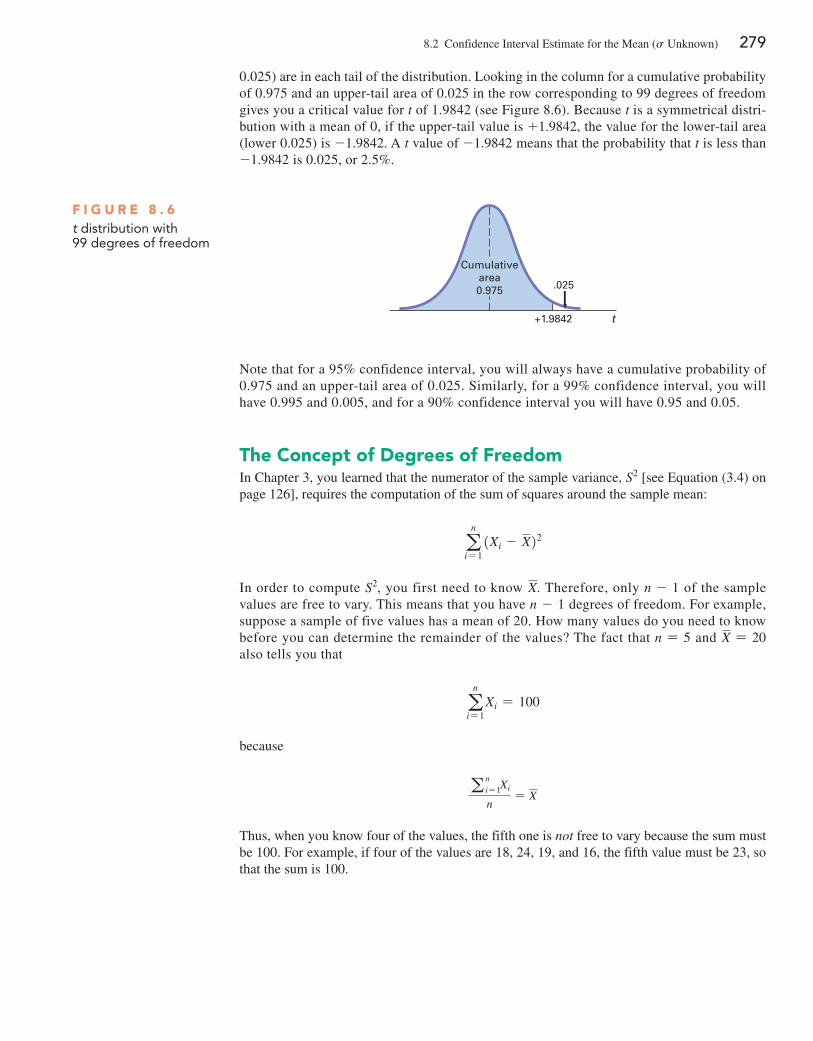
8.2 Confidence Interval Estimate for the Mean (s Unknown) 279
Note that for a 95% confidence interval, you will always have a cumulative probability of 0.975 and an upper-tail area of 0.025. Similarly, for a 99% confidence interval, you will have 0.995 and 0.005, and for a 90% confidence interval you will have 0.95 and 0.05.
the Concept of Degrees of FreedomIn Chapter 3, you learned that the numerator of the sample variance, S2 [see Equation (3.4) on page 126], requires the computation of the sum of squares around the sample mean:
an
i= 1 1Xi - X22
In order to compute S2, you first need to know X. Therefore, only n - 1 of the sample values are free to vary. This means that you have n - 1 degrees of freedom. For example, suppose a sample of five values has a mean of 20. How many values do you need to know before you can determine the remainder of the values? The fact that n = 5 and X = 20 also tells you that
an
i= 1 Xi = 100
because
a ni= 1 Xi
n= X
Thus, when you know four of the values, the fifth one is not free to vary because the sum must be 100. For example, if four of the values are 18, 24, 19, and 16, the fifth value must be 23, so that the sum is 100.
0.025) are in each tail of the distribution. Looking in the column for a cumulative probability of 0.975 and an upper-tail area of 0.025 in the row corresponding to 99 degrees of freedom gives you a critical value for t of 1.9842 (see Figure 8.6). Because t is a symmetrical distri-bution with a mean of 0, if the upper-tail value is +1.9842, the value for the lower-tail area (lower 0.025) is -1.9842. A t value of -1.9842 means that the probability that t is less than -1.9842 is 0.025, or 2.5%.
+1.9842 t
.025
Cumulativearea0.975
F i g u r e 8 . 6t distribution with 99 degrees of freedom
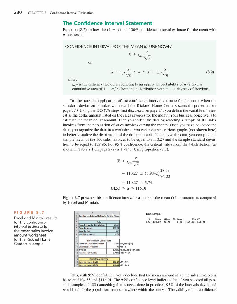
280 CHAPTER 8 Confidence Interval Estimation
the Confidence interval StatementEquation (8.2) defines the 11 - a2 * 100% confidence interval estimate for the mean with s unknown.
ConfIDEnCE IntErval for thE MEan (s UnKnown)
X { ta>2S2n
or
X - ta>2S1n
… m … X + ta>2S1n
(8.2)
whereta>2 is the critical value corresponding to an upper-tail probability of a>2 (i.e., a cumulative area of 1 - a>2) from the t distribution with n - 1 degrees of freedom.
To illustrate the application of the confidence interval estimate for the mean when the standard deviation is unknown, recall the Ricknel Home Centers scenario presented on page 270. Using the DCOVA steps first discussed on page 24, you define the variable of inter-est as the dollar amount listed on the sales invoices for the month. Your business objective is to estimate the mean dollar amount. Then you collect the data by selecting a sample of 100 sales invoices from the population of sales invoices during the month. Once you have collected the data, you organize the data in a worksheet. You can construct various graphs (not shown here) to better visualize the distribution of the dollar amounts. To analyze the data, you compute the sample mean of the 100 sales invoices to be equal to $110.27 and the sample standard devia-tion to be equal to $28.95. For 95% confidence, the critical value from the t distribution (as shown in Table 8.1 on page 278) is 1.9842. Using Equation (8.2),
X { ta>2S1n
= 110.27 { 11.98422 28.951100
= 110.27 { 5.74 104.53 … m … 116.01
Figure 8.7 presents this confidence interval estimate of the mean dollar amount as computed by Excel and Minitab.
F i g u r e 8 . 7Excel and Minitab results for the confidence interval estimate for the mean sales invoice amount worksheet for the ricknel home Centers example
Thus, with 95% confidence, you conclude that the mean amount of all the sales invoices is between $104.53 and $116.01. The 95% confidence level indicates that if you selected all pos-sible samples of 100 (something that is never done in practice), 95% of the intervals developed would include the population mean somewhere within the interval. The validity of this confidence

8.2 Confidence Interval Estimate for the Mean (s Unknown) 281
interval estimate depends on the assumption of normality for the distribution of the amount of the sales invoices. With a sample of 100, the normality assumption is not overly restrictive, and the use of the t distribution is likely appropriate. Example 8.3 further illustrates how you construct the confidence interval for a mean when the population standard deviation is unknown.
example 8.3Estimating the Mean processing time of life insurance applications
An insurance company has the business objective of reducing the amount of time it takes to approve applications for life insurance. The approval process consists of underwriting, which includes a review of the application, a medical information bureau check, possible requests for additional medical information and medical exams, and a policy compilation stage in which the policy pages are generated and sent for delivery. Using the DCOVA steps first discussed on page 24, you define the variable of interest as the total processing time in days. You collect the data by selecting a random sample of 27 approved policies during a period of one month. You organize the data collected in a worksheet. Table 8.2 lists the total processing time, in days, which are stored in insurance . To analyze the data, you need to construct a 95% confidence interval estimate for the population mean processing time.
t a B l e 8 . 2
Processing time for life Insurance applications
73 19 16 64 28 28 31 90 60 56 31 56 22 18
45 48 17 17 17 91 92 63 50 51 69 16 17
SOlutiOn To visualize the data, you construct a boxplot of the processing time, as dis-played in Figure 8.8, and a normal probability plot, as shown in Figure 8.9. To analyze the data, you construct the confidence interval estimate shown in Figure 8.10.
F i g u r e 8 . 8Excel and Minitab boxplots for the processing time for life insurance applications
F i g u r e 8 . 9Excel and Minitab normal probability plots for the processing time for life insurance applications
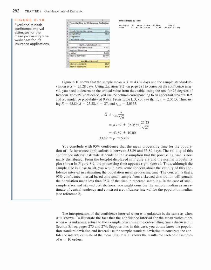
282 CHAPTER 8 Confidence Interval Estimation
The interpretation of the confidence interval when s is unknown is the same as when s is known. To illustrate the fact that the confidence interval for the mean varies more when s is unknown, return to the example concerning the order-filling times discussed in Section 8.1 on pages 273 and 274. Suppose that, in this case, you do not know the popula-tion standard deviation and instead use the sample standard deviation to construct the con-fidence interval estimate of the mean. Figure 8.11 shows the results for each of 20 samples of n = 10 orders.
Figure 8.10 shows that the sample mean is X = 43.89 days and the sample standard de-viation is S = 25.28 days. Using Equation (8.2) on page 281 to construct the confidence inter-val, you need to determine the critical value from the t table, using the row for 26 degrees of freedom. For 95% confidence, you use the column corresponding to an upper-tail area of 0.025 and a cumulative probability of 0.975. From Table E.3, you see that ta>2 = 2.0555. Thus, us-ing X = 43.89, S = 25.28, n = 27, and ta>2 = 2.0555,
X { ta>2S1n
= 43.89 { 12.0555225.28127
= 43.89 { 10.00
33.89 … m … 53.89
You conclude with 95% confidence that the mean processing time for the popula-tion of life insurance applications is between 33.89 and 53.89 days. The validity of this confidence interval estimate depends on the assumption that the processing time is nor-mally distributed. From the boxplot displayed in Figure 8.8 and the normal probability plot shown in Figure 8.9, the processing time appears right-skewed. Thus, although the sample size is close to 30, you would have some concern about the validity of this con-fidence interval in estimating the population mean processing time. The concern is that a 95% confidence interval based on a small sample from a skewed distribution will contain the population mean less than 95% of the time in repeated sampling. In the case of small sample sizes and skewed distributions, you might consider the sample median as an es-timate of central tendency and construct a confidence interval for the population median (see reference 2).
F i g u r e 8 . 1 0Excel and Minitab confidence interval estimates for the mean processing time worksheet for life insurance applications
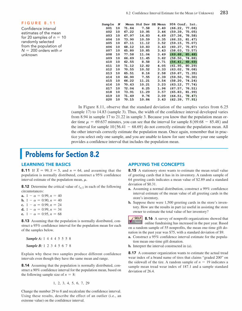
8.2 Confidence Interval Estimate for the Mean (s Unknown) 283
In Figure 8.11, observe that the standard deviation of the samples varies from 6.25 (sample 17) to 14.83 (sample 3). Thus, the width of the confidence interval developed varies from 8.94 in sample 17 to 21.22 in sample 3. Because you know that the population mean or-der time m = 69.637 minutes, you can see that the interval for sample 8 169.68 - 85.482 and the interval for sample 10 156.41 - 68.692 do not correctly estimate the population mean. All the other intervals correctly estimate the population mean. Once again, remember that in prac-tice you select only one sample, and you are unable to know for sure whether your one sample provides a confidence interval that includes the population mean.
F i g u r e 8 . 1 1Confidence interval estimates of the mean for 20 samples of n = 10 randomly selected from the population of N = 200 orders with s unknown
problems for Section 8.2learning the BaSiCS8.11 If X = 99, S = 5, and n = 64, and assuming that the population is normally distributed, construct a 95% confidence interval estimate of the population mean, m.
8.12 Determine the critical value of ta>2 in each of the following circumstances:a. 1 - a = 0.99, n = 40b. 1 - a = 0.90, n = 40c. 1 - a = 0.99, n = 24d. 1 - a = 0.99, n = 34e. 1 - a = 0.95, n = 68
8.13 Assuming that the population is normally distributed, con-struct a 95% confidence interval for the population mean for each of the samples below.
Sample A: 1 4 4 4 5 5 5 8
Sample B: 1 2 3 4 5 6 7 8
Explain why these two samples produce different confidence intervals even though they have the same mean and range.
8.14 Assuming that the population is normally distributed, con-struct a 90% confidence interval for the population mean, based on the following sample size of n = 8:
1, 2, 3, 4, 5, 6, 7, 29
Change the number 29 to 8 and recalculate the confidence interval. Using these results, describe the effect of an outlier (i.e., an extreme value) on the confidence interval.
applYing the COnCeptS8.15 A stationery store wants to estimate the mean retail value of greeting cards that it has in its inventory. A random sample of 64 greeting cards indicates a mean value of $2.89 and a standard deviation of $0.31.a. Assuming a normal distribution, construct a 99% confidence
interval estimate of the mean value of all greeting cards in the store’s inventory.
b. Suppose there were 1,500 greeting cards in the store’s inven-tory. How are the results in part (a) useful in assisting the store owner to estimate the total value of her inventory?
8.16 A survey of nonprofit organizations showed that online fundraising has increased in the past year. Based
on a random sample of 55 nonprofits, the mean one-time gift do-nation in the past year was $75, with a standard deviation of $9.a. Construct a 95% confidence interval estimate for the popula-
tion mean one-time gift donation.b. Interpret the interval constructed in (a).
8.17 A consumer organization wants to estimate the actual tread wear index of a brand name of tires that claims “graded 200” on the sidewall of the tire. A random sample of n = 19 indicates a sample mean tread wear index of 187.1 and a sample standard deviation of 26.4.
SELF Test
284 CHAPTER 8 Confidence Interval Estimation
a. Assuming that the population of tread wear indexes is normally distributed, construct a 99% confidence interval estimate of the population mean tread wear index for tires produced by this manufacturer under this brand name.
b. Do you think that the consumer organization should accuse the manufacturer of producing tires that do not meet the performance information on the sidewall of the tire? Explain.
c. Explain why an observed tread wear index of 205 for a particu-lar tire is not unusual, even though it is outside the confidence interval developed in (a).
8.18 The table below contains the amount that a sample of nine customers spent for lunch ($) at a fast-food restaurant:
4.88 5.01 5.79 6.35 7.39 7.68 8.23 8.71 9.88
a. Construct a 99% confidence interval estimate for the popula-tion mean amount spent for lunch ($) at the fast-food restau-rant, assuming a normal distribution.
b. Interpret the interval constructed in (a).
8.19 The file Sedans contains the overall miles per gallon (MPG) of 2014 midsized sedans:
38 26 30 26 25 27 24 22 27 32 3926 24 24 23 24 25 31 26 37 22 33
Source: Data extracted from “Which Car Is Right for You,” Consumer Reports, April 2014, pp. 40–41.
a. Construct a 95% confidence interval estimate for the popula-tion mean MPG of 2014 midsized sedans, assuming a normal distribution.
b. Interpret the interval constructed in (a).c. Compare the results in (a) to those in Problem 8.20(a).
8.20 The data below represents the overall miles per gallon (MPG) of 2008 SUVs priced under $30,000.
24, 18, 20, 22, 17, 19, 18, 18, 21, 19, 17,
18, 22, 19, 19, 17, 18, 18, 16, 20, 17, 24a. Construct a 95% confidence interval estimate for the popu-
lation mean miles per gallon of 2008 priced under $30,000 SUVs assuming a normal distribution.
b. Interpret the interval constructed in (a).
8.21 New research shows that members of a certain youth genera-tion have a great say in household purchases. Specifically, 70% of the people in the generation have a say in computer purchases. Sup-pose you select a sample of I 00 respondents from the generation.a. What is the probability that the sample percentage will be con-
tained between 64% and 77%?b. The probability is 80% that the sample percentage will be
contained within what symmetrical limits of the population percentage?
c. The probability is 99.7% that the sample percentage will be contained within what symmetrical limits of the population percentage? Use the empirical rule.
d. Suppose you selected a sample of 400 respondents. How does this change your answers in (a) through (c)?
8.22 One of the major measures of the quality of service provided by any organization is the speed with which the organization responds to customer complaints. A large family-held department store selling furniture and flooring, including carpet, had under-gone a major expansion in the past several years. In particular, the flooring department had expanded from 2 installation crews to an installation supervisor, a measurer, and 15 installation crews. The store had the business objective of improving its response to com-plaints. The variable of interest was defined as the number of days between when the complaint was made and when it was resolved. Data were collected from 50 complaints that were made in the past year. The data, stored in Furniture , are as follows:
54 5 35 137 31 27 152 2 123 81 74 27
11 19 126 110 110 29 61 35 94 31 26 5
12 4 165 32 29 28 29 26 25 1 14 13
13 10 5 27 4 52 30 22 36 26 20 23
33 68
a. Construct a 95% confidence interval estimate for the popula-tion mean number of days between the receipt of a complaint and the resolution of the complaint.
b. What assumption must you make about the population distribution in order to construct the confidence interval estimate in (a)?
c. Do you think that the assumption needed in order to construct the confidence interval estimate in (a) is valid? Explain.
d. What effect might your conclusion in (c) have on the validity of the results in (a)?
8.23 A manufacturing company produces chocolate bars. The table below contains the cost per ounce ($) for a sample of 14 dark choco-late bars.
0.63 0.79 0.95 1.19 1.450.94 0.78 0.53 1.58 0.530.61 0.73 1.52 0.81
a. Construct a 99% confidence interval estimate for the popula-tion cost per ounce ($) of dark chocolate bars.
b. What assumption do you need to make about the population distribution to construct the interval in (a)?
c. Given the data presented, do you think the assumption needed in (a) is valid? Explain.
8.24 The file market penetration contains Facebook penetration values (the percentage of the country population that are Facebook users) for 22 of the world’s largest economies:
56 57 43 55 42 35 7 25 42 17 43
6 31 28 59 20 27 36 45 80 57 56
Source: Data extracted from slidesha.re/ODv6vG.
8.3 Confidence Interval Estimate for the Proportion 285
a. Construct a 95% confidence interval estimate for the popula-tion mean Facebook penetration.
b. What assumption do you need to make about the population to construct the interval in (a)?
c. Given the data presented, do you think the assumption needed in (a) is valid? Explain.
8.25 One operation of a mill is to cut pieces of steel into parts that are used in the frame for front seats in an automobile. The steel is cut with a diamond saw, and the resulting parts must be cut to be within {0.005 inch of the length specified by the au-tomobile company. The measurement reported from a sample of 100 steel parts (stored in Steel ) is the difference, in inches, be-
tween the actual length of the steel part, as measured by a laser measurement device, and the specified length of the steel part. For example, the first observation, -0.002, represents a steel part that is 0.002 inch shorter than the specified length.a. Construct a 95% confidence interval estimate for the popula-
tion mean difference between the actual length of the steel part and the specified length of the steel part.
b. What assumption must you make about the population distribu-tion in order to construct the confidence interval estimate in (a)?
c. Do you think that the assumption needed in order to construct the confidence interval estimate in (a) is valid? Explain.
d. Compare the conclusions reached in (a) with those of Problem 2.43 on page 81.
8.3 Confidence Interval Estimate for the ProportionThe concept of a confidence interval also applies to categorical data. With categorical data, you want to estimate the proportion of items in a population having a certain characteristic of interest. The unknown population proportion is represented by the Greek letter p. The point estimate for p is the sample proportion, p = X>n, where n is the sample size and X is the number of items in the sample having the characteristic of interest. Equation (8.3) defines the confidence interval estimate for the population proportion.
Student TipAs noted in Chapter 7, do not confuse this use of the Greek letter pi, p, to represent the popula-tion proportion with the mathematical constant pi.
Student TipRemember, the sample proportion, p, must be between 0 and 1.
ConfIDEnCE IntErval EStIMatE for thE ProPortIon
p { Za>2Bp11 - p2n
or
p - Za>2Bp11 - p2n
… p … p + Za>2Bp11 - p2n
(8.3)
where
p = sample proportion =Xn=
Number of items having the characteristic
sample size
p = population proportion Za>2 = critical value from the standardized normal distribution
n = sample size
Note: To use this equation for the confidence interval, the sample size n must be large enough to ensure that both X and n - X are greater than 5.
You can use the confidence interval estimate for the proportion defined in Equation (8.3) to estimate the proportion of sales invoices that contain errors (see the Ricknel Home Centers scenario on page 270). Using the DCOVA steps, you define the variable of interest as whether the invoice contains errors (yes or no). Then, you collect the data from a sample of 100 sales in-voices. The results, which you organize and store in a worksheet, show that 10 invoices contain errors. To analyze the data, you compute, for these data, p = X>n = 10>100 = 0.10. Since both X = 10 and n - X = 100 - 10 = 90 are 7 5, using Equation (8.3) and Za>2 = 1.96, for 95% confidence,
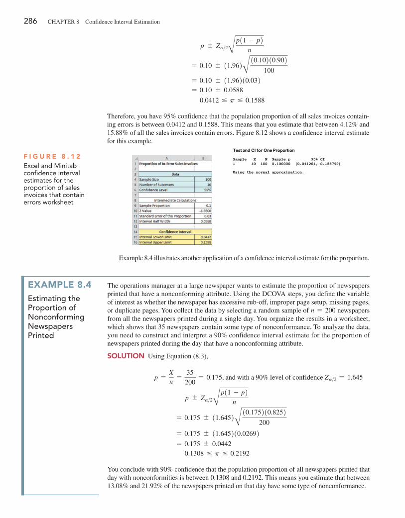
286 CHAPTER 8 Confidence Interval Estimation
p { Za>2Bp11 - p2n
= 0.10 { 11.962B 10.10210.902100
= 0.10 { 11.96210.032 = 0.10 { 0.0588
0.0412 … p … 0.1588
Therefore, you have 95% confidence that the population proportion of all sales invoices contain-ing errors is between 0.0412 and 0.1588. This means that you estimate that between 4.12% and 15.88% of all the sales invoices contain errors. Figure 8.12 shows a confidence interval estimate for this example.
F i g u r e 8 . 1 2Excel and Minitab confidence interval estimates for the proportion of sales invoices that contain errors worksheet
Example 8.4 illustrates another application of a confidence interval estimate for the proportion.
example 8.4Estimating the proportion of nonconforming newspapers printed
The operations manager at a large newspaper wants to estimate the proportion of newspapers printed that have a nonconforming attribute. Using the DCOVA steps, you define the variable of interest as whether the newspaper has excessive rub-off, improper page setup, missing pages, or duplicate pages. You collect the data by selecting a random sample of n = 200 newspapers from all the newspapers printed during a single day. You organize the results in a worksheet, which shows that 35 newspapers contain some type of nonconformance. To analyze the data, you need to construct and interpret a 90% confidence interval estimate for the proportion of newspapers printed during the day that have a nonconforming attribute.
SOlutiOn Using Equation (8.3),
p =Xn=
35
200= 0.175, and with a 90% level of confidence Za>2 = 1.645
p { Za>2Bp11 - p2n
= 0.175 { 11.6452B 10.175210.8252200
= 0.175 { 11.645210.02692 = 0.175 { 0.0442
0.1308 … p … 0.2192
You conclude with 90% confidence that the population proportion of all newspapers printed that day with nonconformities is between 0.1308 and 0.2192. This means you estimate that between 13.08% and 21.92% of the newspapers printed on that day have some type of nonconformance.
8.3 Confidence Interval Estimate for the Proportion 287
Equation (8.3) contains a Z statistic because you can use the normal distribution to approximate the binomial distribution when the sample size is sufficiently large. In Example 8.4, the confidence interval using Z provides an excellent approximation for the population propor-tion because both X and n - X are greater than 5. However, if you do not have a sufficiently large sample size, you should use the binomial distribution rather than Equation (8.3) (see refer-ences 1, 3, and 9). The exact confidence intervals for various sample sizes and proportions of items of interest have been tabulated by Fisher and Yates (reference 3) and can also be computed using Minitab.
problems for Section 8.3learning the BaSiCS8.26 If n = 200 and X = 40, construct a 90% confidence inter-val estimate of the population proportion.
8.27 If n = 400 and X = 25, construct a 99% confidence inter-val estimate for the population proportion.
applYing the COnCeptS8.28 A cellphone provider has the business objective of wanting to estimate the proportion of subscribers
who would upgrade to a new cellphone with improved features if it were made available at a substantially reduced cost. Data are collected from a random sample of 500 subscribers. The results indicate that 135 of the subscribers would upgrade to a new cell-phone at a reduced cost.a. Construct a 99% confidence interval estimate for the popula-
tion proportion of subscribers that would upgrade to a new cell-phone at a reduced cost.
b. How would the manager in charge of promotional programs use the results in (a)?
8.29 In a survey of 1,000 social media users, 78% said it was okay to friend co-workers, but 60% said it was not okay to be-friend your boss.a. Construct a 90% confidence interval estimate for the popula-
tion proportion of social media users who would say it is okay to friend co-workers.
b. Construct a 90% confidence interval estimate for the popula-tion proportion of social media users who would say it is not okay to friend their boss.
c. Write a short summary of the information derived from (a) and (b) Which of the following is the best summary of the information derived from (a)?
8.30 In a survey conducted by a business management company, 52% of workers from the United States said they have negotiated a pay raise at least once in their lives. The sample size used in the study was not disclosed.a. Suppose that the survey had a sample size of n = 600. Con-
struct a 95% confidence interval estimate for the proportion of all U.S. workers who have negotiated a pay raise.
b. Based on (a), can you claim that more than half of all United States workers have negotiated a pay raise?
c. Suppose that the survey had a sample size of n = 6,000. Con-struct a 95% confidence interval estimate for the proportion of all U.S. workers who have negotiated a pay raise.
d. Discuss the effect of sample size on the confidence interval estimate.
8.31 In a survey of 239 organizations, 75 responded that “the need for collaboration among increasing number of locations” is a business driver that led them to implement cloud solutions. Cloud solutions enable more effective employee communication and higher decision maker visibility into real-time data. (Source: The Benefits of Cloud ERP: It’s About Transforming Your Business, Aberdeen Group, available at bit.ly/1meEC3D.)
Construct a 95% confidence interval estimate for the popula-tion proportion of organizations that indicated “the need for collabo-ration among increasing number of locations” as a business driver for cloud solution implementation.
8.32 In a Pew Research Center survey of 960 Facebook users, 452 cited “seeing photos or videos” as a major reason why they use Facebook, while 298 cited “keeping up with news and current events” as a major reason why they use Facebook. (Source: “6 new facts about Facebook,” bit.ly/1lAmkv5.)a. Construct a 95% confidence interval estimate for the popula-
tion proportion of Facebook users who cite “seeing photos or videos” as a major reason for why they use Facebook.
b. Construct a 95% confidence interval estimate for the popula-tion proportion of Facebook users who cite “keeping up with news and current events” as a major reason why they use Facebook.
c. Compare the results of (a) and (b).
8.33 What are the global trends that technology CEOs believe will transform their business? According to a PwC white paper, 105 of 117 technology CEOs from around the world responded that technological advances will transform their business and 42 responded that resource scarcity and climate change will trans-form their business. (Source: Fit for the Future: 17th Annual Global CEO Survey, available at pwc.to/PRQZYr.)a. Construct a 95% confidence interval estimate for the popula-
tion proportion of tech CEOs who indicate technological ad-vances as one of the global trends that will transform their business.
b. Construct a 95% confidence interval estimate for the popula-tion proportion of tech CEOs who indicate resource scarcity and climate change as one of the global trends that will trans-form their business.
c. Interpret the intervals in (a) and (b).
SELF Test
288 CHAPTER 8 Confidence Interval Estimation
8.4 Determining Sample SizeIn each confidence interval developed so far in this chapter, the sample size was reported along with the results, with little discussion of the width of the resulting confidence interval. In the business world, sample sizes are determined prior to data collection to ensure that the confi-dence interval is narrow enough to be useful in making decisions. Determining the proper sam-ple size is a complicated procedure, subject to the constraints of budget, time, and the amount of acceptable sampling error. In the Ricknel Home Centers scenario, if you want to estimate the mean dollar amount of the sales invoices, you must determine in advance how large a sam-pling error to allow in estimating the population mean. You must also determine, in advance, the level of confidence (i.e., 90%, 95%, or 99%) to use in estimating the population parameter.
Sample Size Determination for the meanTo develop an equation for determining the appropriate sample size needed when constructing a confidence interval estimate for the mean, recall Equation (8.1) on page 274:
X { Za>2 s1n
The amount added to or subtracted from X is equal to half the width of the interval. This quan-tity represents the amount of imprecision in the estimate that results from sampling error.2 The sampling error, e, is defined as
e = Za>2 s1n
Solving for n gives the sample size needed to construct the appropriate confidence interval estimate for the mean. “Appropriate” means that the resulting interval will have an acceptable amount of sampling error.
2In this context, some statisticians refer to e as the margin of error.
SaMPlE SIzE DEtErMInatIon for thE MEan
The sample size, n, is equal to the product of the Za>2 value squared and the standard devia-tion, s, squared, divided by the square of the sampling error, e.
n =Z2a>2 s2
e2 (8.4)
To compute the sample size, you must know three quantities:
• The desired confidence level, which determines the value of Za>2, the critical value from the standardized normal distribution3
• The acceptable sampling error, e • The standard deviation, s
In some business-to-business relationships that require estimation of important parameters, legal contracts specify acceptable levels of sampling error and the confidence level required. For companies in the food and drug sectors, government regulations often specify sampling er-rors and confidence levels. In general, however, it is usually not easy to specify the three quan-tities needed to determine the sample size. How can you determine the level of confidence and sampling error? Typically, these questions are answered only by a subject matter expert (i.e., an individual very familiar with the variables under study). Although 95% is the most common confidence level used, if more confidence is desired, then 99% might be more appropriate; if
3You use Z instead of t because, to determine the critical value of t, you need to know the sample size, but you do not know it yet. For most studies, the sample size needed is large enough that the standardized normal distribution is a good approximation of the t distribution.
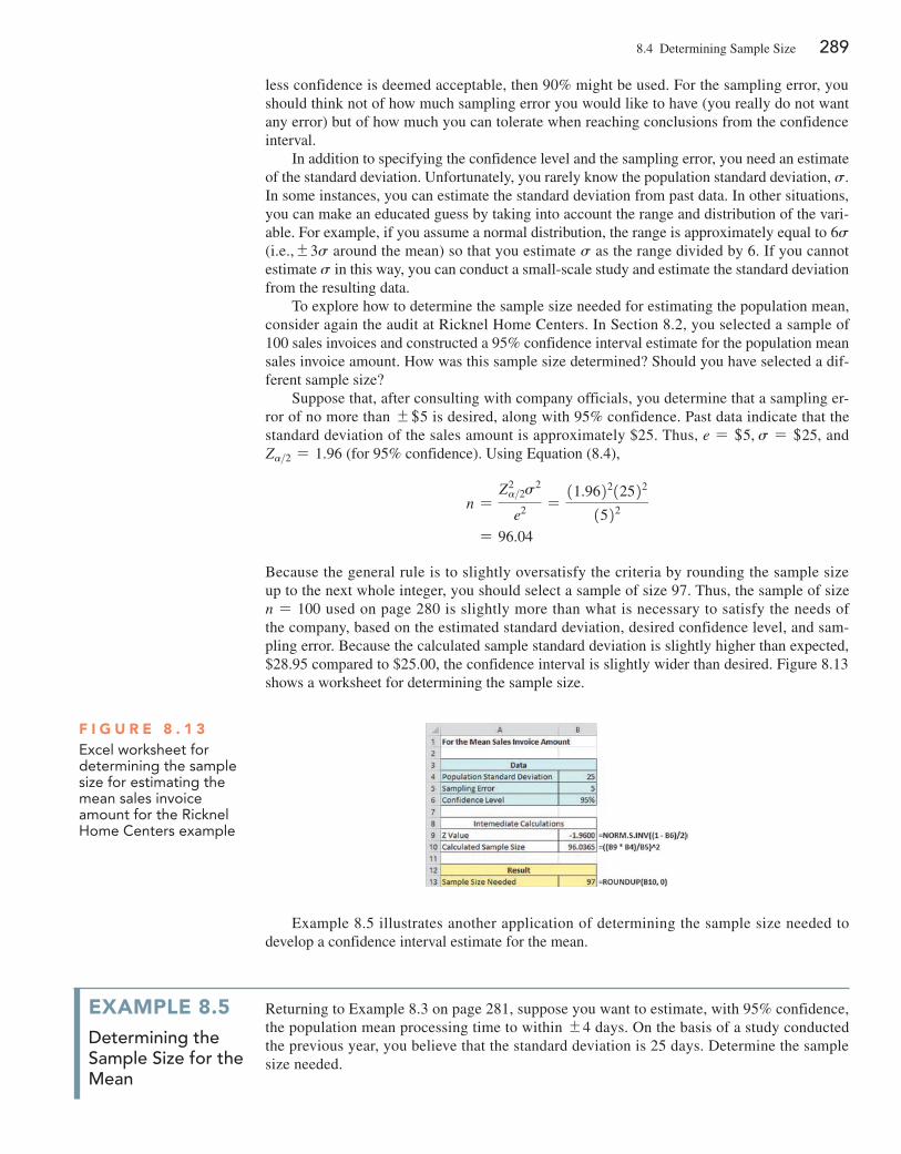
8.4 Determining Sample Size 289
less confidence is deemed acceptable, then 90% might be used. For the sampling error, you should think not of how much sampling error you would like to have (you really do not want any error) but of how much you can tolerate when reaching conclusions from the confidence interval.
In addition to specifying the confidence level and the sampling error, you need an estimate of the standard deviation. Unfortunately, you rarely know the population standard deviation, s. In some instances, you can estimate the standard deviation from past data. In other situations, you can make an educated guess by taking into account the range and distribution of the vari-able. For example, if you assume a normal distribution, the range is approximately equal to 6s (i.e.,{3s around the mean) so that you estimate s as the range divided by 6. If you cannot estimate s in this way, you can conduct a small-scale study and estimate the standard deviation from the resulting data.
To explore how to determine the sample size needed for estimating the population mean, consider again the audit at Ricknel Home Centers. In Section 8.2, you selected a sample of 100 sales invoices and constructed a 95% confidence interval estimate for the population mean sales invoice amount. How was this sample size determined? Should you have selected a dif-ferent sample size?
Suppose that, after consulting with company officials, you determine that a sampling er-ror of no more than { +5 is desired, along with 95% confidence. Past data indicate that the standard deviation of the sales amount is approximately $25. Thus, e = +5, s = +25, and Za>2 = 1.96 (for 95% confidence). Using Equation (8.4),
n =Z2a>2s2
e2 =11.962212522
1522
= 96.04
Because the general rule is to slightly oversatisfy the criteria by rounding the sample size up to the next whole integer, you should select a sample of size 97. Thus, the sample of size n = 100 used on page 280 is slightly more than what is necessary to satisfy the needs of the company, based on the estimated standard deviation, desired confidence level, and sam-pling error. Because the calculated sample standard deviation is slightly higher than expected, $28.95 compared to $25.00, the confidence interval is slightly wider than desired. Figure 8.13 shows a worksheet for determining the sample size.
F i g u r e 8 . 1 3Excel worksheet for determining the sample size for estimating the mean sales invoice amount for the ricknel home Centers example
Example 8.5 illustrates another application of determining the sample size needed to develop a confidence interval estimate for the mean.
example 8.5determining the sample size for the Mean
Returning to Example 8.3 on page 281, suppose you want to estimate, with 95% confidence, the population mean processing time to within {4 days. On the basis of a study conducted the previous year, you believe that the standard deviation is 25 days. Determine the sample size needed.
290 CHAPTER 8 Confidence Interval Estimation
Sample Size Determination for the proportionSo far in this section, you have learned how to determine the sample size needed for estimating the population mean. Now suppose that you want to determine the sample size necessary for estimating a population proportion.
To determine the sample size needed to estimate a population proportion, p, you use a method similar to the method for a population mean. Recall that in developing the sample size for a confidence interval for the mean, the sampling error is defined by
e = Za>2 s1n
When estimating a proportion, you replace s with 2p11 - p2. Thus, the sampling error is
e = Za>2Bp11 - p2n
Solving for n, you have the sample size necessary to develop a confidence interval estimate for a proportion.
SOlutiOn Using Equation (8.4) on page 288 and e = 4, s = 25, and Za>2 = 1.96 for 95% confidence,
n =Z2a>2 s2
e2 =11.962212522
1422
= 150.06
Therefore, you should select a sample of 151 applications because the general rule for deter-mining sample size is to always round up to the next integer value in order to slightly oversat-isfy the criteria desired. An actual sampling error slightly larger than 4 will result if the sample standard deviation calculated in this sample of 151 is greater than 25 and slightly smaller if the sample standard deviation is less than 25.
SaMPlE SIzE DEtErMInatIon for thE ProPortIon
The sample size n is equal to the product of Za>2 squared, the population proportion, p, and 1 minus the population proportion, p, divided by the square of the sampling error, e.
n =Z2a>2p11 - p2
e2 (8.5)
To determine the sample size, you must know three quantities:
• The desired confidence level, which determines the value of Za>2, the critical value from the standardized normal distribution
• The acceptable sampling error (or margin of error), e • The population proportion, p
In practice, selecting these quantities requires some planning. Once you determine the desired level of confidence, you can find the appropriate Za>2 value from the standardized normal distribution. The sampling error, e, indicates the amount of error that you are will-ing to tolerate in estimating the population proportion. The third quantity, p, is actually the
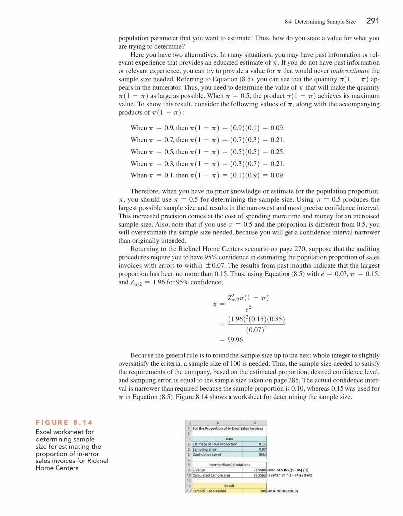
8.4 Determining Sample Size 291
population parameter that you want to estimate! Thus, how do you state a value for what you are trying to determine?
Here you have two alternatives. In many situations, you may have past information or rel-evant experience that provides an educated estimate of p. If you do not have past information or relevant experience, you can try to provide a value for p that would never underestimate the sample size needed. Referring to Equation (8.5), you can see that the quantity p11 - p2 ap-pears in the numerator. Thus, you need to determine the value of p that will make the quantity p11 - p2 as large as possible. When p = 0.5, the product p11 - p2 achieves its maximum value. To show this result, consider the following values of p, along with the accompanying products of p11 - p2 :
When p = 0.9, then p11 - p2 = 10.9210.12 = 0.09.
When p = 0.7, then p11 - p2 = 10.7210.32 = 0.21.
When p = 0.5, then p11 - p2 = 10.5210.52 = 0.25.
When p = 0.3, then p11 - p2 = 10.3210.72 = 0.21.
When p = 0.1, then p11 - p2 = 10.1210.92 = 0.09.
Therefore, when you have no prior knowledge or estimate for the population proportion, p, you should use p = 0.5 for determining the sample size. Using p = 0.5 produces the largest possible sample size and results in the narrowest and most precise confidence interval. This increased precision comes at the cost of spending more time and money for an increased sample size. Also, note that if you use p = 0.5 and the proportion is different from 0.5, you will overestimate the sample size needed, because you will get a confidence interval narrower than originally intended.
Returning to the Ricknel Home Centers scenario on page 270, suppose that the auditing procedures require you to have 95% confidence in estimating the population proportion of sales invoices with errors to within {0.07. The results from past months indicate that the largest proportion has been no more than 0.15. Thus, using Equation (8.5) with e = 0.07, p = 0.15, and Za>2 = 1.96 for 95% confidence,
n =Z2a>2p11 - p2
e2
=11.962210.15210.852
10.0722
= 99.96
Because the general rule is to round the sample size up to the next whole integer to slightly oversatisfy the criteria, a sample size of 100 is needed. Thus, the sample size needed to satisfy the requirements of the company, based on the estimated proportion, desired confidence level, and sampling error, is equal to the sample size taken on page 285. The actual confidence inter-val is narrower than required because the sample proportion is 0.10, whereas 0.15 was used for p in Equation (8.5). Figure 8.14 shows a worksheet for determining the sample size.
F i g u r e 8 . 1 4Excel worksheet for determining sample size for estimating the proportion of in-error sales invoices for ricknel home Centers
292 CHAPTER 8 Confidence Interval Estimation
Example 8.6 provides another application of determining the sample size for estimating the population proportion.
example 8.6determining the sample size for the population proportion
You want to have 90% confidence of estimating the proportion of office workers who respond to email within an hour to within {0.05. Because you have not previously undertaken such a study, there is no information available from past data. Determine the sample size needed.
SOlutiOn Because no information is available from past data, assume that p = 0.50. Using Equation (8.5) on page 291 and e = 0.05, p = 0.50, and Za>2 = 1.645 for 90% confidence,
n =Z2a>2 p11 - p2
e2
=11.6452210.50210.502
10.0522
= 270.6
Therefore, you need a sample of 271 office workers to estimate the population proportion to within{0.05 with 90% confidence.
problems for Section 8.4learning the BaSiCS8.34 If you want to be 99% confident of estimating the popula-tion mean to within a sampling error of {4 and the standard de-viation is assumed to be 12, what sample size is required?
8.35 If you want to be 99% confident of estimating the popula-tion mean to within a sampling error of {20 and the standard de-viation is assumed to be 100, what sample size is required?
8.36 If you want to be 95% confident of estimating the popula-tion proportion to within a sampling error of {0.04, what sample size is needed?
8.37 If you want to be 95% confident of estimating the popula-tion proportion to within a sampling error of {0.02 and there is historical evidence that the population proportion is approximately 0.40, what sample size is needed?
applYing the COnCeptS8.38 A survey is planned to determine the mean an-nual family medical expenses of employees of a large
company. The management of the company wishes to be 95% con-fident that the sample mean is correct to within { +50 of the pop-ulation mean annual family medical expenses. A previous study indicates that the standard deviation is approximately $400.a. How large a sample is necessary?b. If management wants to be correct to within { +25, how many
employees need to be selected?
8.39 If the manager of a paint supply store wants to estimate the mean amount of paint in a 1-gallon can to within {0.005 gallons with 99% confidence, and also assumes that the standard deviation is 0.045 gallons, what sample size is needed?
8.40 Find the sample size necessary to estimate the mean IQ score of statistics students such that it can be said with 90% confi-dence that the sample mean is {5 IQ points of the true mean. As-sume that the standard deviation is 11 and determine the required sample size.
8.41 If the inspection division of a county weights and measures department wants to estimate the mean amount of soft-drink fill in 2-liter bottles to within {0.01 liter with 95% confidence and also assumes that the standard deviation is 0.05 liter, what sample size is needed?
8.42 An advertising executive wants to estimate the mean weekly amount of time consumers spend watching traditional television daily. Based on previous studies, the standard deviation is assumed to be 20 minutes. The executive wants to estimate, with 99% con-fidence, the mean weekly amount of time to within {5 minutes.a. What sample size is needed?b. If 95% confidence is desired, how many consumers need to be
selected?
8.43 An advertising agency that serves a major radio station wants to estimate the mean amount of time that the station’s au-dience spends listening to the radio daily. From past studies, the standard deviation is estimated as 50 minutes.a. What sample size is needed if the agency wants to be 95% con-
fident of being correct to within {4 minutes?b. If 99% confidence is desired, how many listeners need to be
selected?
8.44 A growing niche in the restaurant business is gourmet-casual breakfast, lunch, and brunch. Chains in this group include EggSpec-tation and Panera Bread. Suppose that the mean per-person check for breakfast at EggSpectation is approximately $14.50.
SELF Test
8.5 Confidence Interval Estimation and Ethical Issues 293
a. Assuming a standard deviation of $2.00, what sample size is needed to estimate, with 95% confidence, the mean per-person check for EggSpectation to within { +0.25?
b. Assuming a standard deviation of $2.50, what sample size is needed to estimate, with 95% confidence, the mean per-person check for EggSpectation to within { +0.25?
c. Assuming a standard deviation of $3.00, what sample size is needed to estimate, with 95% confidence, the mean per-person check for EggSpectation to within { +0.25?
d. Discuss the effect of variation on the sample size needed.
8.45 What proportion of people get most of their news on the Inter-net? According to a recent poll 44% get most of their news from the Internet.a. To conduct a follow-up study that would provide 95% confi-
dence that the point estimate is correct to within {0.05 of the population proportion, how large a sample size is required?
b. To conduct a follow-up study that would provide 99% confi-dence that the point estimate is correct to within {0.05 the population proportion, how many people need to be sampled?
c. To conduct a follow-up study that would provide 95% confi-dence that the point estimate is correct to within {0.02 of the population proportion, how large a sample size is required?
d. To conduct a follow-up study that would provide 99% confidence that the point estimate is correct to within {0.02 of the population proportion, how many people need to be sampled?
e. Discuss the effects of changing the desired confidence level and the acceptable sampling error on sample size requirements.
8.46 A Nielsen Mobile Shopping Report looks at how consum-ers are using mobile devices throughout their purchase journey. In response to a survey question about shopping, 27% of tablet owners said they use mobile devices for payment, 21% said they use such devices to make social media comments about their pur-chases, and 10% said they use such devices to retrieve mobile coupons. (Source: “Mobile Ticks All the Shopping Boxes,” bit.ly/1hfKC8K.)
Suppose the results are based on a survey of 300 tablet own-ers. Construct a 95% confidence interval estimate of the popula-tion proportion of tablet owners who said they use their mobile device while shopping a. for payment.b. to make social media comments about their purchases.c. to retrieve mobile coupons.
d. You have been asked to update the results of this study. Determine the sample size necessary to estimate, with 95% confidence, the population proportions in (a) through (c) to within {0.02.
8.47 A study of 667 CEOs reported that 214 stated that their company’s greatest concern was sustained and steady top-line growth.a. Construct a 99% confidence interval for the proportion of
CEOs whose greatest concern was sustained and steady top-line growth.
b. Interpret the interval constructed in part (a).c. To conduct a follow-up study to estimate the population pro-
portion of CEOs whose greatest concern was sustained and steady top-line growth to within {0.04 with 99% confidence, how many CEOs would you survey?
8.48 According to a study released by The Financial Brand, an online publication focusing on branding issues and advice affect-ing retail banks and credit unions, 68% of financial institutions use churn rate (attrition) to gauge the effectiveness of their marketing efforts. (Source: “2014 State of Bank & Credit Union Marketing,” bit.ly/1np8FVx.)a. If you conduct a follow-up study to estimate the population
proportion of financial institutions that use churn rate to gauge the effectiveness of their marketing efforts, would you use a pof 0.68 or 0.50 in the sample size formula?
b. Using your answer in (a), find the sample size necessary to estimate, with 95% confidence, the population proportion to within {0.03.
8.49 What prevents consumers from sharing data with retailers? A recent ClickFox Consumer Behavior Survey (bit.ly/1fAfJAI) found that 32% of consumers responded “breaches of consumer data.”a. To conduct a follow-up study that would provide 99% con-
fidence that the point estimate is correct to within ;0.03 of the population proportion, how many consumers need to be sampled?
b. To conduct a follow-up study that would provide 99% con-fidence that the point estimate is correct to within ;0.05 of the population proportion, how many consumers need to be sampled?
c. Compare the results of (a) and (b).
8.5 Confidence Interval Estimation and Ethical IssuesThe selection of samples and the inferences that accompany them raise several ethical issues. The major ethical issue concerns whether confidence interval estimates accompany point estimates. Failure to include a confidence interval estimate might mislead the user of the results into thinking that the point estimate is all that is needed to predict the population char-acteristic with certainty. Confidence interval limits (typically set at 95%), the sample size used, and an interpretation of the meaning of the confidence interval in terms that a person untrained in statistics can understand should always accompany point estimates.
When media outlets publicize the results of a political poll, they often overlook including this type of information. Sometimes, the results of a poll include the sampling error, but the sampling error is often presented in fine print or as an afterthought to the story being reported.
294 CHAPTER 8 Confidence Interval Estimation
A fully ethical presentation of poll results would give equal prominence to the confidence levels, sample size, sampling error, and confidence limits of the poll.
When you prepare your own point estimates, always state the interval estimate in a promi-nent place and include a brief explanation of the meaning of the confidence interval. In addi-tion, make sure you highlight the sample size and sampling error.
8.6 BootstrappingThe confidence interval estimation procedures discussed in this chapter make assumptions that are often not valid, especially for small samples. Bootstrapping, the selection of an initial sam-ple and repeated sampling from that initial sample, provides an alternative approach that does not rely on those assumptions. The Section 8.6 online topic explains this alternative technique.
s U M M a R yThis chapter discusses confidence intervals for estimating the characteristics of a population, along with how you can de-termine the necessary sample size. You learned how to apply these methods to numerical and categorical data. Table 8.3 provides a list of topics covered in this chapter.
To determine what equation to use for a particular situa-tion, you need to answer these questions:
• Are you constructing a confidence interval, or are you determining sample size?
• Do you have a numerical variable, or do you have a categorical variable?
The next three chapters develop a hypothesis-testing approach to making decisions about population parameters.
Type of DaTa
Type of analySiS Numerical Categorical
Confidence interval for a population parameter
Confidence interval estimate for the mean (Sections 8.1 and 8.2)
Confidence interval estimate for the proportion (Section 8.3)
Determining sample size Sample size determination for the mean (Section 8.4)
Sample size determination for the proportion (Section 8.4)
t a B l e 8 . 3
Summary of topics in Chapter 8
In the Ricknel Home Centers scenario, you were an accountant for a distributor of home improvement supplies
in the northeastern United States. You were responsible for the accuracy of the integrated inventory management and sales information system. You used confidence interval estimation techniques to draw conclusions about the population of all re-cords from a relatively small sample collected during an audit.
At the end of the month, you collected a random sample of 100 sales invoices and made the following inferences:
• With 95% confidence, you concluded that the mean amount of all the sales invoices is between $104.53 and $116.01.
• With 95% confidence, you concluded that between 4.12% and 15.88% of all the sales invoices contain errors.
These estimates provide an interval of values that you believe contain the true population parameters. If these in-tervals are too wide (i.e., the sampling error is too large) for the types of decisions Ricknel Home Centers needs to make, you will need to take a larger sample. You can use the sample size formulas in Section 8.4 to determine the number of sales invoices to sample to ensure that the size of the sampling error is acceptable.
U s i n g s tat i s t i c s
Getting Estimates at Ricknel Home Centers, Revisited
Mangostock/Shutterstock
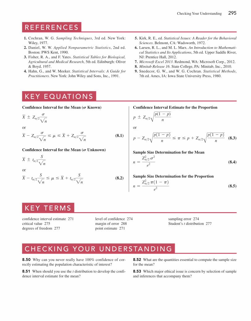
Checking Your Understanding 295
R E f E R E n c E s 1. Cochran, W. G. Sampling Techniques, 3rd ed. New York:
Wiley, 1977. 2. Daniel, W. W. Applied Nonparametric Statistics, 2nd ed.
Boston: PWS Kent, 1990. 3. Fisher, R. A., and F. Yates. Statistical Tables for Biological,
Agricultural and Medical Research, 5th ed. Edinburgh: Oliver & Boyd, 1957.
4. Hahn, G., and W. Meeker. Statistical Intervals: A Guide for Practitioners. New York: John Wiley and Sons, Inc., 1991.
5. Kirk, R. E., ed. Statistical Issues: A Reader for the Behavioral Sciences. Belmont, CA: Wadsworth, 1972.
6. Larsen, R. L., and M. L. Marx. An Introduction to Mathemati-cal Statistics and Its Applications, 5th ed. Upper Saddle River, NJ: Prentice Hall, 2012.
7. Microsoft Excel 2013. Redmond, WA: Microsoft Corp., 2012. 8. Minitab Release 16. State College, PA: Minitab, Inc., 2010. 9. Snedecor, G. W., and W. G. Cochran. Statistical Methods,
7th ed. Ames, IA: Iowa State University Press, 1980.
K E y E q U at i o n sConfidence Interval for the Mean (S Known)
X { Za>2s2n
or
X - Za>2s2n
… m … X + Za>2s2n
(8.1)
Confidence Interval for the Mean (S Unknown)
X { ta>2S2n
or
X - ta>2S2n
… m … X + ta>2S2n
(8.2)
Confidence Interval Estimate for the Proportion
p { Za>2Ap(1 - p)n
or
p - Za>2Ap11 - p2n
… p … p + Za>2Ap11 - p2n
(8.3)
Sample Size Determination for the Mean
n =Z2a>2 s2
e2 (8.4)
Sample Size Determination for the Proportion
n =Z2a>2 p11 - p2
e2 (8.5)
K E y t E R M sconfidence interval estimate 271critical value 275degrees of freedom 277
level of confidence 274margin of error 288point estimate 271
sampling error 274Student’s t distribution 277
c H E c K i n g y o U R U n d E R s ta n d i n g8.50 Why can you never really have 100% confidence of cor-rectly estimating the population characteristic of interest?
8.51 When should you use the t distribution to develop the confi-dence interval estimate for the mean?
8.52 What are the quantities essential to compute the sample size for the mean?
8.53 Which major ethical issue is concern by selection of sample and inferences that accompany them?
296 CHAPTER 8 Confidence Interval Estimation
c H a p t E R R E v i E w p R o b l E M s8.54 The Pew Internet Project survey of 1,006 American adults found the following:
906 have a cell phone584 have a smartphone322 have an ebook reader423 have a tablet computer
Source: “Device Ownership Over Time,” bit.ly/1fvWYrL.
a. Construct 95% confidence interval estimates for the population proportion of the electronic devices adults own.
b. What conclusions can you reach concerning what electronic devices adults have?
8.55 What proposals for dealing with energy and the environ-ment do Americans favor? Gallup conducted a survey of 1,048 adults, ages 18+ in all 50 U.S. states and the District of Columbia and found the following:
Spending more government money on developing solar and wind power: 702Setting higher emissions and pollutions standards for busi-ness and industry: 681Setting stricter standards on the use of techniques to extract natural gas from the earth: 608Expanding the use of nuclear power: 493
Source: “Americans Still Favor Energy Conservation Over Production,” bit.ly/1iLhkn2.
a. Construct a 95% confidence interval estimate for the popula-tion proportion of each proposal Americans favor for dealing with energy and the environment.
b. What conclusions can you reach concerning proposals Americans favor for dealing with energy and the environment?
8.56 A market researcher for a consumer electronics company wants to study the media viewing behavior of residents of a par-ticular area. A random sample of 40 respondents is selected, and each respondent is instructed to keep a detailed record of time spent engaged viewing content across all screens (traditional TV, DVD/Blu-ray, game console, Internet on a computer, video on a computer, video on a mobile phone) in a particular week. The re-sults are as follows:
• Content viewing time per week: X = 41 hours, S = 3.5 hours.
• 30 respondents have high definition (HD) on at least one television set.
a. Construct a 95% confidence interval estimate for the mean con-tent viewing time per week in this area.
b. Construct a 95% confidence interval estimate for the population proportion of residents who have HD on at least one television set.
Suppose that the market researcher wants to take another survey in a different location. Answer these questions:c. What sample size is required to be 95% confident of estimating
the population mean content viewing time to within {2 hours as-suming that the population standard deviation is equal to 5 hours?
d. How many respondents need to be selected to be 95% confident of being within {0.06 of the population proportion who have HD on at least one television set if no previous estimate is available?
e. Based on (c) and (d), how many respondents should the market researcher select if a single survey is being conducted?
8.57 An information technology (IT) consulting firm specializ-ing in health care solutions wants to study communication defi-ciencies in the health care industry. A random sample of 70 health care clinicians reveals the following:
• Time wasted in a day due to outdated communication tech-nologies: X = 45 minutes, S = 10 minutes.
• Thirty-six health care clinicians cite inefficiency of pagers as the reason for the wasted time.
a. Construct a 99% confidence interval estimate for the popula-tion mean time wasted in a day due to outdated communication technologies.
b. Construct a 95% confidence interval estimate for the popula-tion proportion of health care clinicians who cite inefficiency of pagers as the reason for the wasted time.
8.58 The human resource (HR) director of a large corporation wishes to study absenteeism among its mid-level managers at its central office during the year. A random sample of 25 mid-level managers reveals the following:
• Absenteeism: X = 6.2 days, S = 7.3 days.• 13 mid-level managers cite stress as a cause of absence.
a. Construct a 95% confidence interval estimate for the mean number of absences for mid-level managers during the year.
b. Construct a 95% confidence interval estimate for the popula-tion proportion of mid-level managers who cite stress as a cause of absence.
Suppose that the HR director wishes to administer a survey in one of its regional offices. Answer these questions:c. What sample size is needed to have 95% confidence in estimat-
ing the population mean absenteeism to within {1.5 days if the population standard deviation is estimated to be 8 days?
d. How many mid-level managers need to be selected to have 90% confidence in estimating the population proportion of mid-level managers who cite stress as a cause of absence to within {0.075 if no previous estimate is available?
e. Based on (c) and (d), what sample size is needed if a single survey is being conducted?
8.59 A national association devoted to HR and workplace pro-grams, practices, and training wants to study HR department practices and employee turnover of its member organizations. HR professionals and organization executives focus on turnover not only because it has significant cost implications but also because it affects overall business performance. A survey is de-signed to estimate the proportion of member organizations that have both talent and development programs in place to drive hu-man-capital management as well as the member organizations’ mean annual employee turnover rate (the ratio of the number of employees that left an organization in a given time period to the average number of employees in the organization during the given time period). A random sample of 100 member organiza-tions reveals the following:
• Annual turnover rate: X = 8.1%, S = 1.5%.• Thirty member organizations have both talent and develop-
ment programs in place to drive human-capital management.a. Construct a 95% confidence interval estimate for the popula-
tion mean annual turnover rate of member organizations.
Chapter Review Problems 297
b. Construct a 95% confidence interval estimate for the popula-tion proportion of member organizations that have both talent and development programs in place to drive human-capital management.
c. What sample size is needed to have 99% confidence of esti-mating the population mean annual employee turnover rate to within {1.5%?
d. How many member organizations need to be selected to have 90% confidence of estimating the population proportion of or-ganizations that have both talent and development programs in place to drive human-capital management to within {0.045?
8.60 The financial impact of IT systems downtime is a concern of plant operations management today. A survey of manufactur-ers examined the satisfaction level with the reliability and avail-ability of their manufacturing IT applications. The variables of focus are whether the manufacturer experienced downtime in the past year that affected one or more manufacturing IT ap-plications, the number of downtime incidents that occurred in the past year, and the approximate cost of a typical downtime incident. The results from a sample of 200 manufacturers are as follows:
• Sixty-two experienced downtime this year that affected one or more manufacturing applications.
• Number of downtime incidents: X = 3.5, S = 2.0• Cost of downtime incidents: X = +18,000, S = +3,000.
a. Construct a 90% confidence interval estimate for the popula-tion proportion of manufacturers who experienced downtime in the past year that affected one or more manufacturing IT appli-cations.
b. Construct a 95% confidence interval estimate for the popula-tion mean number of downtime incidents experienced by man-ufacturers in the past year.
c. Construct a 95% confidence interval estimate for the popula-tion mean cost of downtime incidents.
8.61 The branch manager of an outlet (Store 1) of a nationwide chain of pet supply stores wants to study characteristics of her cus-tomers. In particular, she decides to focus on two variables: the amount of money spent by customers and whether the customers own only one dog, only one cat, or more than one dog and/or cat. The results from a sample of 70 customers are as follows:
• Amount of money spent: X = +21.34, S = +9.22.• Thirty-seven customers own only a dog.• Twenty-six customers own only a cat.• Seven customers own more than one dog and/or cat.
a. Construct a 95% confidence interval estimate for the popula-tion mean amount spent in the pet supply store.
b. Construct a 90% confidence interval estimate for the popula-tion proportion of customers who own only a cat.
The branch manager of another outlet (Store 2) wishes to conduct a similar survey in his store. The manager does not have access to the information generated by the manager of Store 1. Answer the following questions:c. What sample size is needed to have 95% confidence of
estimating the population mean amount spent in this store to within { +1.50 if the standard deviation is estimated to be $10?
d. How many customers need to be selected to have 90% con-fidence of estimating the population proportion of customers who own only a cat to within {0.045?
e. Based on your answers to (c) and (d), how large a sample should the manager take?
8.62 Scarlett and Heather, the owners of an upscale restaurant in Dayton, Ohio, want to study the dining characteristics of their customers. They decide to focus on two variables: the amount of money spent by customers and whether customers order dessert. The results from a sample of 60 customers are as follows:
• Amount spent: X = +38.54, S = +7.26.• Eighteen customers purchased dessert.
a. Construct a 95% confidence interval estimate for the popula-tion mean amount spent per customer in the restaurant.
b. Construct a 90% confidence interval estimate for the popula-tion proportion of customers who purchase dessert.
Jeanine, the owner of a competing restaurant, wants to conduct a similar survey in her restaurant. Jeanine does not have access to the information that Scarlett and Heather have obtained from the survey they conducted. Answer the following questions:c. What sample size is needed to have 95% confidence of esti-
mating the population mean amount spent in her restaurant to within { +1.50, assuming that the standard deviation is esti-mated to be $8?
d. How many customers need to be selected to have 90% con-fidence of estimating the population proportion of customers who purchase dessert to within {0.04?
e. Based on your answers to (c) and (d), how large a sample should Jeanine take?
8.63 The manufacturer of Ice Melt claims that its product will melt snow and ice at temperatures as low as 0° Fahrenheit. A rep-resentative for a large chain of hardware stores is interested in test-ing this claim. The chain purchases a large shipment of 5-pound bags for distribution. The representative wants to know, with 95% confidence and within {0.05, what proportion of bags of Ice Melt perform the job as claimed by the manufacturer.a. How many bags does the representative need to test? What as-
sumption should be made concerning the population propor-tion? (This is called destructive testing; i.e., the product being tested is destroyed by the test and is then unavailable to be sold.)
b. Suppose that the representative tests 50 bags, and 42 of them do the job as claimed. Construct a 95% confidence interval estimate for the population proportion that will do the job as claimed.
c. How can the representative use the results of (b) to determine whether to sell the Ice Melt product?
8.64 Claims fraud (illegitimate claims) and buildup (exaggerated loss amounts) continue to be major issues of concern among auto-mobile insurance companies. Fraud is defined as specific material misrepresentation of the facts of a loss; buildup is defined as the inflation of an otherwise legitimate claim. A recent study examined auto injury claims closed with payment under private passenger cov-erages. Detailed data on injury, medical treatment, claimed losses, and total payments, as well as claim-handling techniques, were col-lected. In addition, auditors were asked to review the claim files to indicate whether specific elements of fraud or buildup appeared in the claim and, in the case of buildup, to specify the amount of excess payment. The file insuranceClaims contains data for 90 randomly selected auto injury claims. The following variables are included: CLAIM—Claim ID; BUILDUP—1 if buildup indicated, 0 if not; and EXCESSPAYMENT—excess payment amount, in dollars.
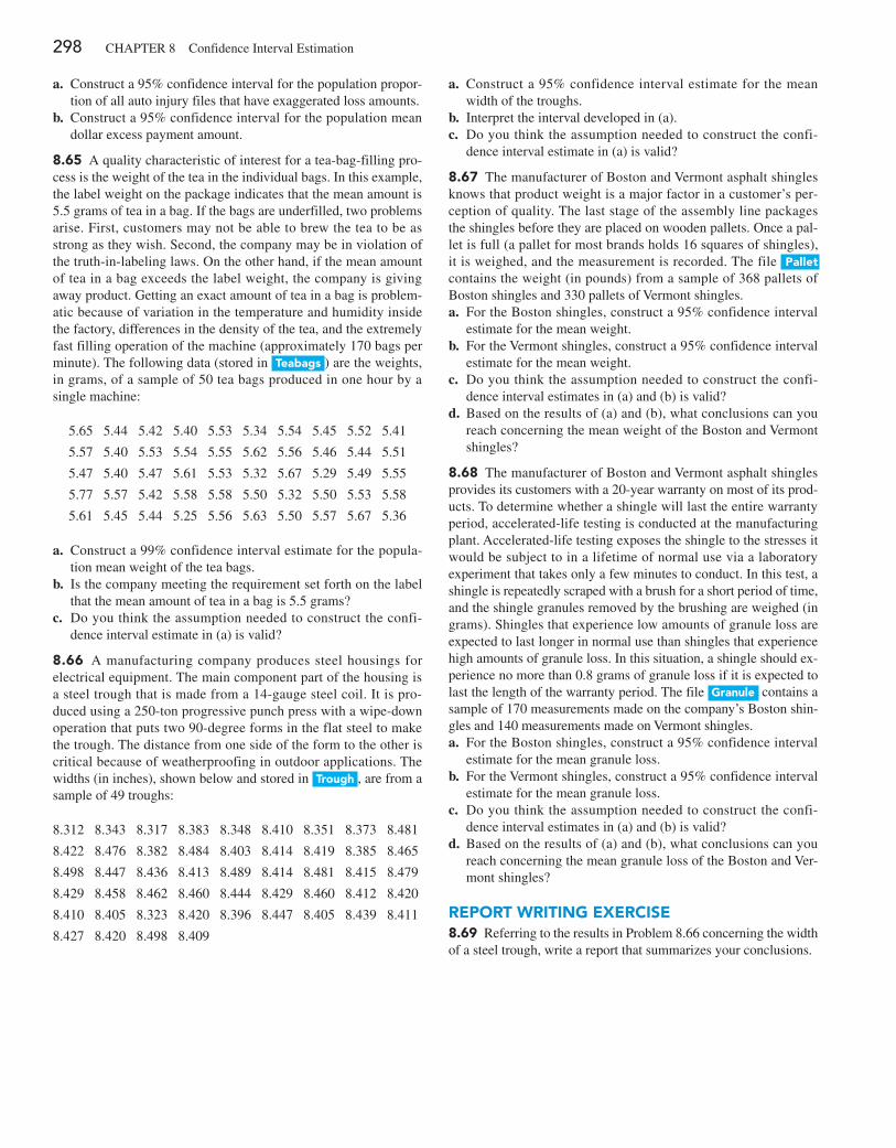
298 CHAPTER 8 Confidence Interval Estimation
a. Construct a 95% confidence interval for the population propor-tion of all auto injury files that have exaggerated loss amounts.
b. Construct a 95% confidence interval for the population mean dollar excess payment amount.
8.65 A quality characteristic of interest for a tea-bag-filling pro-cess is the weight of the tea in the individual bags. In this example, the label weight on the package indicates that the mean amount is 5.5 grams of tea in a bag. If the bags are underfilled, two problems arise. First, customers may not be able to brew the tea to be as strong as they wish. Second, the company may be in violation of the truth-in-labeling laws. On the other hand, if the mean amount of tea in a bag exceeds the label weight, the company is giving away product. Getting an exact amount of tea in a bag is problem-atic because of variation in the temperature and humidity inside the factory, differences in the density of the tea, and the extremely fast filling operation of the machine (approximately 170 bags per minute). The following data (stored in teabags ) are the weights, in grams, of a sample of 50 tea bags produced in one hour by a single machine:
5.65 5.44 5.42 5.40 5.53 5.34 5.54 5.45 5.52 5.41
5.57 5.40 5.53 5.54 5.55 5.62 5.56 5.46 5.44 5.51
5.47 5.40 5.47 5.61 5.53 5.32 5.67 5.29 5.49 5.55
5.77 5.57 5.42 5.58 5.58 5.50 5.32 5.50 5.53 5.58
5.61 5.45 5.44 5.25 5.56 5.63 5.50 5.57 5.67 5.36
a. Construct a 99% confidence interval estimate for the popula-tion mean weight of the tea bags.
b. Is the company meeting the requirement set forth on the label that the mean amount of tea in a bag is 5.5 grams?
c. Do you think the assumption needed to construct the confi-dence interval estimate in (a) is valid?
8.66 A manufacturing company produces steel housings for electrical equipment. The main component part of the housing is a steel trough that is made from a 14-gauge steel coil. It is pro-duced using a 250-ton progressive punch press with a wipe-down operation that puts two 90-degree forms in the flat steel to make the trough. The distance from one side of the form to the other is critical because of weatherproofing in outdoor applications. The widths (in inches), shown below and stored in trough , are from a sample of 49 troughs:
8.312 8.343 8.317 8.383 8.348 8.410 8.351 8.373 8.481
8.422 8.476 8.382 8.484 8.403 8.414 8.419 8.385 8.465
8.498 8.447 8.436 8.413 8.489 8.414 8.481 8.415 8.479
8.429 8.458 8.462 8.460 8.444 8.429 8.460 8.412 8.420
8.410 8.405 8.323 8.420 8.396 8.447 8.405 8.439 8.411
8.427 8.420 8.498 8.409
a. Construct a 95% confidence interval estimate for the mean width of the troughs.
b. Interpret the interval developed in (a).c. Do you think the assumption needed to construct the confi-
dence interval estimate in (a) is valid?
8.67 The manufacturer of Boston and Vermont asphalt shingles knows that product weight is a major factor in a customer’s per-ception of quality. The last stage of the assembly line packages the shingles before they are placed on wooden pallets. Once a pal-let is full (a pallet for most brands holds 16 squares of shingles), it is weighed, and the measurement is recorded. The file pallet contains the weight (in pounds) from a sample of 368 pallets of Boston shingles and 330 pallets of Vermont shingles.a. For the Boston shingles, construct a 95% confidence interval
estimate for the mean weight.b. For the Vermont shingles, construct a 95% confidence interval
estimate for the mean weight.c. Do you think the assumption needed to construct the confi-
dence interval estimates in (a) and (b) is valid?d. Based on the results of (a) and (b), what conclusions can you
reach concerning the mean weight of the Boston and Vermont shingles?
8.68 The manufacturer of Boston and Vermont asphalt shingles provides its customers with a 20-year warranty on most of its prod-ucts. To determine whether a shingle will last the entire warranty period, accelerated-life testing is conducted at the manufacturing plant. Accelerated-life testing exposes the shingle to the stresses it would be subject to in a lifetime of normal use via a laboratory experiment that takes only a few minutes to conduct. In this test, a shingle is repeatedly scraped with a brush for a short period of time, and the shingle granules removed by the brushing are weighed (in grams). Shingles that experience low amounts of granule loss are expected to last longer in normal use than shingles that experience high amounts of granule loss. In this situation, a shingle should ex-perience no more than 0.8 grams of granule loss if it is expected to last the length of the warranty period. The file granule contains a sample of 170 measurements made on the company’s Boston shin-gles and 140 measurements made on Vermont shingles.a. For the Boston shingles, construct a 95% confidence interval
estimate for the mean granule loss.b. For the Vermont shingles, construct a 95% confidence interval
estimate for the mean granule loss.c. Do you think the assumption needed to construct the confi-
dence interval estimates in (a) and (b) is valid?d. Based on the results of (a) and (b), what conclusions can you
reach concerning the mean granule loss of the Boston and Ver-mont shingles?
repOrt Writing exerCiSe8.69 Referring to the results in Problem 8.66 concerning the width of a steel trough, write a report that summarizes your conclusions.

Cases for Chapter 8 299
c a s E s f o R c H a p t E R 8
Managing ashland Multicomm servicesThe marketing department has been considering ways to increase the number of new subscriptions to the 3-For-All cable/phone/Internet service. Following the suggestion of Assistant Manager Lauren Adler, the department staff de-signed a survey to help determine various characteristics of households who subscribe to cable television service from Ashland. The survey consists of the following 10 questions:
1. Does your household subscribe to telephone service from Ashland?(1) Yes (2) No
2. Does your household subscribe to Internet service from Ashland?(1) Yes (2) No
3. What type of cable television service do you have?(1) Basic (2) Enhanced(If Basic, skip to question 5.)
4. How often do you watch the cable television stations that are only available with enhanced service?(1) Every day (2) Most days(3) Occasionally or never
5. How often do you watch premium or on-demand ser-vices that require an extra fee?(1) Almost every day (2) Several times a week(3) Rarely (4) Never
6. Which method did you use to obtain your current AMS subscription?(1) AMS toll-free phone number(2) AMS website(3) Direct mail reply card(4) Good Tunes & More promotion(5) Other
7. Would you consider subscribing to the 3-For-All cable/phone/Internet service for a trial period if a discount were offered?(1) Yes (2) No(If no, skip to question 9.)
8. If purchased separately, cable, Internet, and phone ser-vices would currently cost $24.99 per week. How much would you be willing to pay per week for the 3-For-All cable/phone/Internet service?
9. Does your household use another provider of telephone service?(1) Yes (2) No
10. AMS may distribute Ashland Gold Cards that would provide discounts at selected Ashland-area restaurants for subscribers who agree to a two-year subscription contract to the 3-For-All service. Would being eligible to receive a Gold Card cause you to agree to the two-year term?(1) Yes (2) No
Of the 500 households selected that subscribe to cable tele-vision service from Ashland, 82 households either refused to participate, could not be contacted after repeated attempts, or had telephone numbers that were not in service. The sum-mary results for the 418 households that were contacted are as follows:
Household Has AMS Telephone Service Frequency
Yes 83
No 335
Household Has AMS Internet Service Frequency
Yes 262
No 156
Type of Cable Service Frequency
Basic 164
Enhanced 254
Watches Enhanced Programming Frequency
Every day 50
Most days 144
Occasionally or never 60
Watches Premium or On-Demand Services Frequency
Almost every day 14
Several times a week 35
Almost never 313
Never 56
Method Used to Obtain Current AMS Subscription Frequency
Toll-free phone number 230
AMS website 106
Direct mail 46
Good Tunes & More 10
Other 26
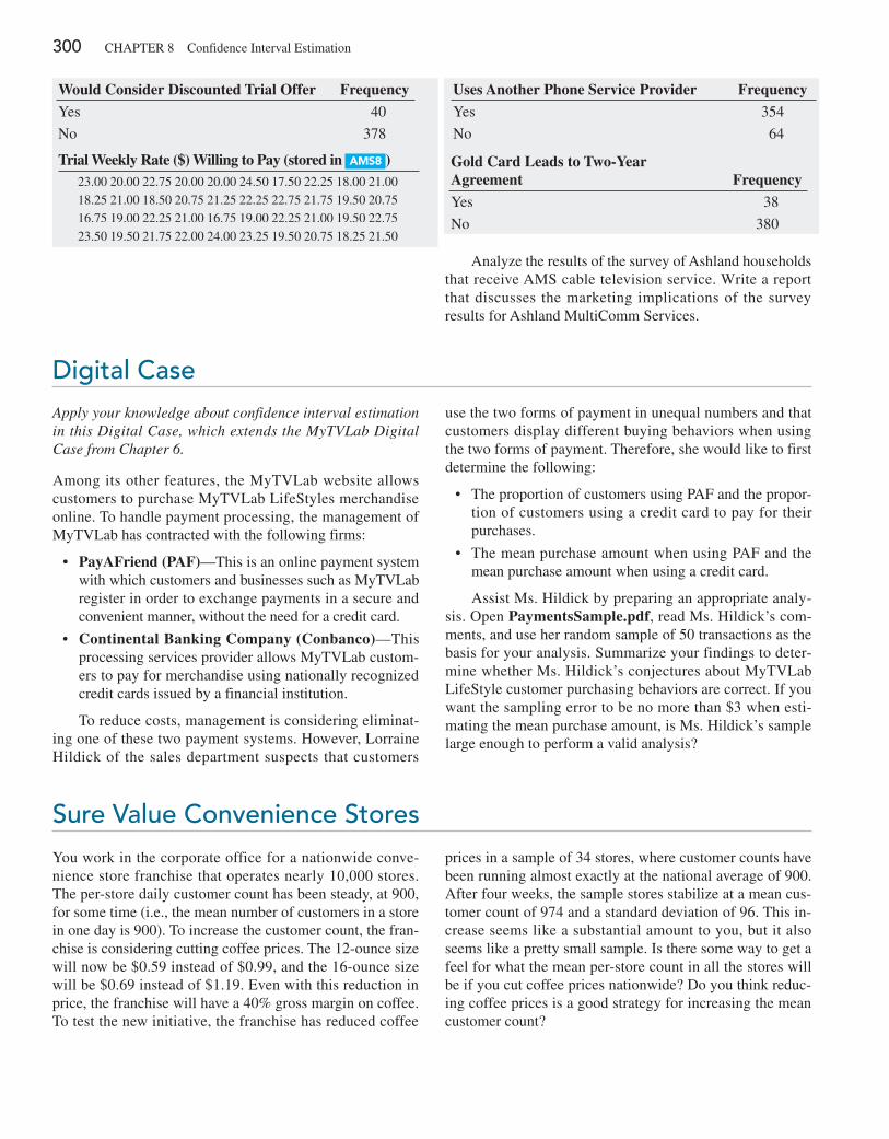
300 CHAPTER 8 Confidence Interval Estimation
Would Consider Discounted Trial Offer Frequency
Yes 40
No 378
Trial Weekly Rate ($) Willing to Pay (stored in amS8 )23.00 20.00 22.75 20.00 20.00 24.50 17.50 22.25 18.00 21.0018.25 21.00 18.50 20.75 21.25 22.25 22.75 21.75 19.50 20.7516.75 19.00 22.25 21.00 16.75 19.00 22.25 21.00 19.50 22.7523.50 19.50 21.75 22.00 24.00 23.25 19.50 20.75 18.25 21.50
Uses Another Phone Service Provider Frequency
Yes 354
No 64
Gold Card Leads to Two-Year Agreement Frequency
Yes 38
No 380
Analyze the results of the survey of Ashland households that receive AMS cable television service. Write a report that discusses the marketing implications of the survey results for Ashland MultiComm Services.
digital caseApply your knowledge about confidence interval estimation in this Digital Case, which extends the MyTVLab Digital Case from Chapter 6.
Among its other features, the MyTVLab website allows customers to purchase MyTVLab LifeStyles merchandise online. To handle payment processing, the management of MyTVLab has contracted with the following firms:
• PayAFriend (PAF)—This is an online payment system with which customers and businesses such as MyTVLab register in order to exchange payments in a secure and convenient manner, without the need for a credit card.
• Continental Banking Company (Conbanco)—This processing services provider allows MyTVLab custom-ers to pay for merchandise using nationally recognized credit cards issued by a financial institution.
To reduce costs, management is considering eliminat-ing one of these two payment systems. However, Lorraine Hildick of the sales department suspects that customers
use the two forms of payment in unequal numbers and that customers display different buying behaviors when using the two forms of payment. Therefore, she would like to first determine the following:
• The proportion of customers using PAF and the propor-tion of customers using a credit card to pay for their purchases.
• ThemeanpurchaseamountwhenusingPAFandthemean purchase amount when using a credit card.
Assist Ms. Hildick by preparing an appropriate analy-sis. Open PaymentsSample.pdf, read Ms. Hildick’s com-ments, and use her random sample of 50 transactions as the basis for your analysis. Summarize your findings to deter-mine whether Ms. Hildick’s conjectures about MyTVLab LifeStyle customer purchasing behaviors are correct. If you want the sampling error to be no more than $3 when esti-mating the mean purchase amount, is Ms. Hildick’s sample large enough to perform a valid analysis?
sure value convenience stores
You work in the corporate office for a nationwide conve-nience store franchise that operates nearly 10,000 stores. The per-store daily customer count has been steady, at 900, for some time (i.e., the mean number of customers in a store in one day is 900). To increase the customer count, the fran-chise is considering cutting coffee prices. The 12-ounce size will now be $0.59 instead of $0.99, and the 16-ounce size will be $0.69 instead of $1.19. Even with this reduction in price, the franchise will have a 40% gross margin on coffee. To test the new initiative, the franchise has reduced coffee
prices in a sample of 34 stores, where customer counts have been running almost exactly at the national average of 900. After four weeks, the sample stores stabilize at a mean cus-tomer count of 974 and a standard deviation of 96. This in-crease seems like a substantial amount to you, but it also seems like a pretty small sample. Is there some way to get a feel for what the mean per-store count in all the stores will be if you cut coffee prices nationwide? Do you think reduc-ing coffee prices is a good strategy for increasing the mean customer count?
Cases for Chapter 8 301
cardiogood fitness
Return to the CardioGood Fitness case first presented on page 47. Using the data stored in Cardiogood Fitness :
1. Construct 95% confidence interval estimates to create a customer profile for each CardioGood Fitness treadmill product line.
2. Write a report to be presented to the management of CardioGood Fitness detailing your findings.
More descriptive choices follow-Up
Follow up the More Descriptive Choices, Revisited Using Statistics scenario on page 158 by constructing 95% confidence intervals estimates of the three-year return percentages, five-year return percentages, and ten-year return percentages for the sample of growth and
value funds and for the small, mid-cap, and large market cap funds (stored in retirement Funds ). In your analysis, examine differences between the growth and value funds as well as the differences among the small, mid-cap, and large market cap funds.
clear Mountain state student surveys
1. The Student News Service at Clear Mountain State University (CMSU) has decided to gather data about the undergraduate students that attend CMSU. They create and distribute a survey of 14 questions and re-ceive responses from 62 undergraduates (stored in undergradSurvey ). For each variable included in the sur-vey, construct a 95% confidence interval estimate for the population characteristic and write a report summarizing your conclusions.
2. The Dean of Students at CMSU has learned about the undergraduate survey and has decided to undertake a similar survey for graduate students at CMSU. She cre-ates and distributes a survey of 14 questions and re-ceives responses from 44 graduate students (stored in gradSurvey ). For each variable included in the survey, construct a 95% confidence interval estimate for the population characteristic and write a report summarizing your conclusions.
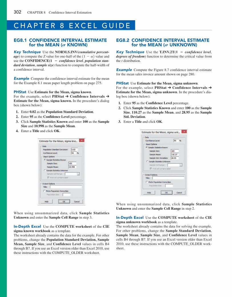
302 CHAPTER 8 Confidence Interval Estimation
eg8.1 COnFiDenCe interval eStimate for the mean (S KnOWn)
Key Technique Use the NORM.S.INV(cumulative percent-age) to compute the Z value for one-half of the 11 - a2 value and use the CONFIDENCE(1 − confidence level, population stan-dard deviation, sample size) function to compute the half-width of a confidence interval.
Example Compute the confidence interval estimate for the mean for the Example 8.1 mean paper length problem on page 275.
phStat Use Estimate for the Mean, sigma known.For the example, select PHStat ➔ Confidence Intervals ➔ Estimate for the Mean, sigma known. In the procedure’s dialog box (shown below):
1. Enter 0.02 as the Population Standard Deviation. 2. Enter 95 as the Confidence Level percentage. 3. Click Sample Statistics Known and enter 100 as the Sample
Size and 10.998 as the Sample Mean. 4. Enter a Title and click OK.
When using unsummarized data, click Sample Statistics Unknown and enter the Sample Cell Range in step 3.
in-Depth excel Use the COMPUTE worksheet of the CIE sigma known workbook as a template.The worksheet already contains the data for the example. For other problems, change the Population Standard Deviation, Sample Mean, Sample Size, and Confidence Level values in cells B4 through B7. If you use an Excel version older than Excel 2010, use these instructions with the COMPUTE_OLDER worksheet.
eg8.2 COnFiDenCe interval eStimate for the mean (S unKnOWn)
Key Technique Use the T.INV.2T(1 − confidence level, degrees of freedom) function to determine the critical value from the t distribution.
Example Compute the Figure 8.7 confidence interval estimate for the mean sales invoice amount shown on page 280.
phStat Use Estimate for the Mean, sigma unknown.For the example, select PHStat ➔ Confidence Intervals ➔ Estimate for the Mean, sigma unknown. In the procedure’s dia-log box (shown below):
1. Enter 95 as the Confidence Level percentage. 2. Click Sample Statistics Known and enter 100 as the Sample
Size, 110.27 as the Sample Mean, and 28.95 as the Sample Std. Deviation.
3. Enter a Title and click OK.
When using unsummarized data, click Sample Statistics Unknown and enter the Sample Cell Range in step 2.
in-Depth excel Use the COMPUTE worksheet of the CIE sigma unknown workbook as a template.The worksheet already contains the data for solving the example. For other problems, change the Sample Standard Deviation, Sample Mean, Sample Size, and Confidence Level values in cells B4 through B7. If you use an Excel version older than Excel 2010, use these instructions with the COMPUTE_OLDER work-sheet.
c H a p t E R 8 E x c E l g U i d E
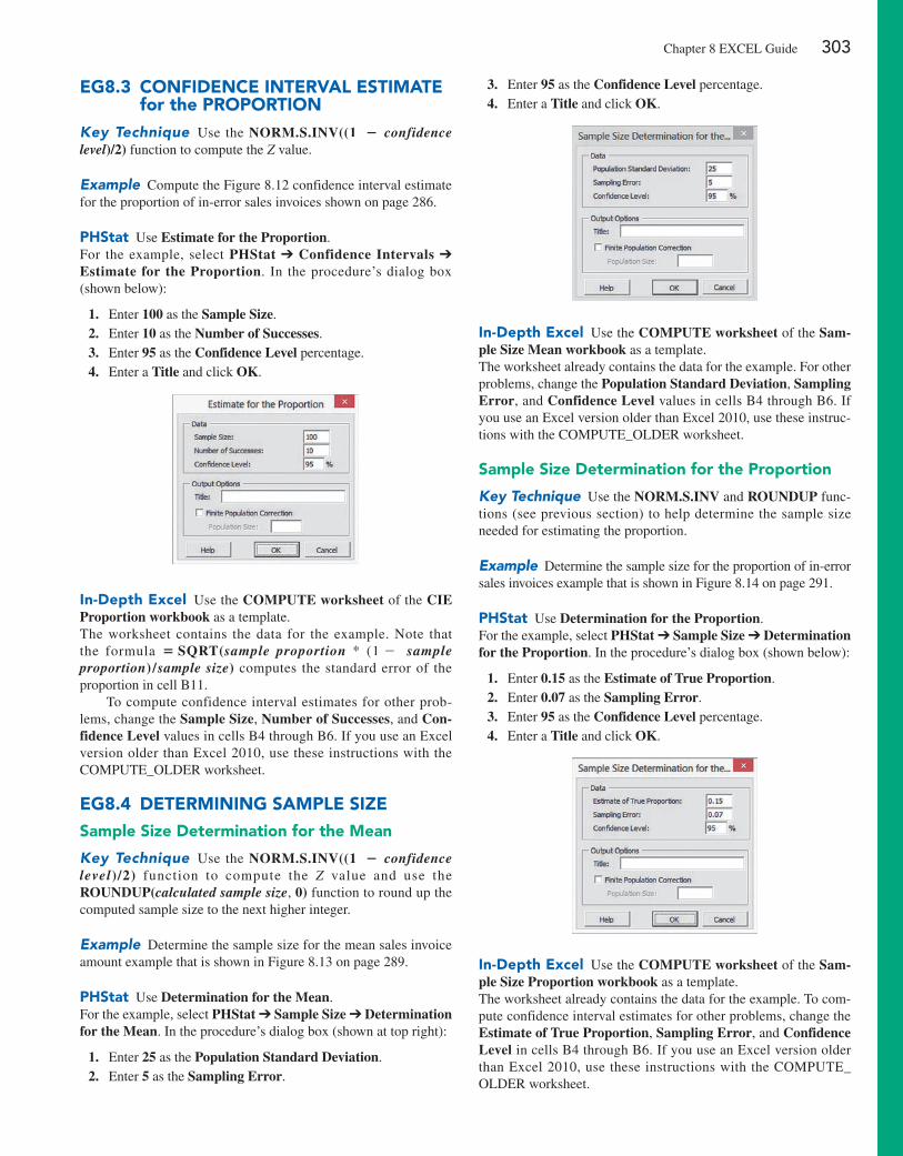
Chapter 8 EXCEL Guide 303
eg8.3 COnFiDenCe interval eStimate for the prOpOrtiOn
Key Technique Use the NORM.S.INV((1 − confidence level)/2) function to compute the Z value.
Example Compute the Figure 8.12 confidence interval estimate for the proportion of in-error sales invoices shown on page 286.
phStat Use Estimate for the Proportion.For the example, select PHStat ➔ Confidence Intervals ➔ Estimate for the Proportion. In the procedure’s dialog box (shown below):
1. Enter 100 as the Sample Size. 2. Enter 10 as the Number of Successes. 3. Enter 95 as the Confidence Level percentage. 4. Enter a Title and click OK.
in-Depth excel Use the COMPUTE worksheet of the CIE Proportion workbook as a template.The worksheet contains the data for the example. Note that the formula = SQRT(sample proportion * (1 - sample proportion) /sample size) computes the standard error of the proportion in cell B11.
To compute confidence interval estimates for other prob-lems, change the Sample Size, Number of Successes, and Con-fidence Level values in cells B4 through B6. If you use an Excel version older than Excel 2010, use these instructions with the COMPUTE_OLDER worksheet.
eg8.4 Determining Sample SizeSample Size Determination for the mean
Key Technique Use the NORM.S.INV((1 − confidence level)/2) function to compute the Z value and use the ROUNDUP(calculated sample size, 0) function to round up the computed sample size to the next higher integer.
Example Determine the sample size for the mean sales invoice amount example that is shown in Figure 8.13 on page 289.
phStat Use Determination for the Mean.For the example, select PHStat ➔ Sample Size ➔ Determination for the Mean. In the procedure’s dialog box (shown at top right):
1. Enter 25 as the Population Standard Deviation. 2. Enter 5 as the Sampling Error.
3. Enter 95 as the Confidence Level percentage. 4. Enter a Title and click OK.
in-Depth excel Use the COMPUTE worksheet of the Sam-ple Size Mean workbook as a template.The worksheet already contains the data for the example. For other problems, change the Population Standard Deviation, Sampling Error, and Confidence Level values in cells B4 through B6. If you use an Excel version older than Excel 2010, use these instruc-tions with the COMPUTE_OLDER worksheet.
Sample Size Determination for the proportion
Key Technique Use the NORM.S.INV and ROUNDUP func-tions (see previous section) to help determine the sample size needed for estimating the proportion.
Example Determine the sample size for the proportion of in-error sales invoices example that is shown in Figure 8.14 on page 291.
phStat Use Determination for the Proportion.For the example, select PHStat ➔ Sample Size ➔ Determination for the Proportion. In the procedure’s dialog box (shown below):
1. Enter 0.15 as the Estimate of True Proportion. 2. Enter 0.07 as the Sampling Error. 3. Enter 95 as the Confidence Level percentage. 4. Enter a Title and click OK.
in-Depth excel Use the COMPUTE worksheet of the Sam-ple Size Proportion workbook as a template.The worksheet already contains the data for the example. To com-pute confidence interval estimates for other problems, change the Estimate of True Proportion, Sampling Error, and Confidence Level in cells B4 through B6. If you use an Excel version older than Excel 2010, use these instructions with the COMPUTE_OLDER worksheet.
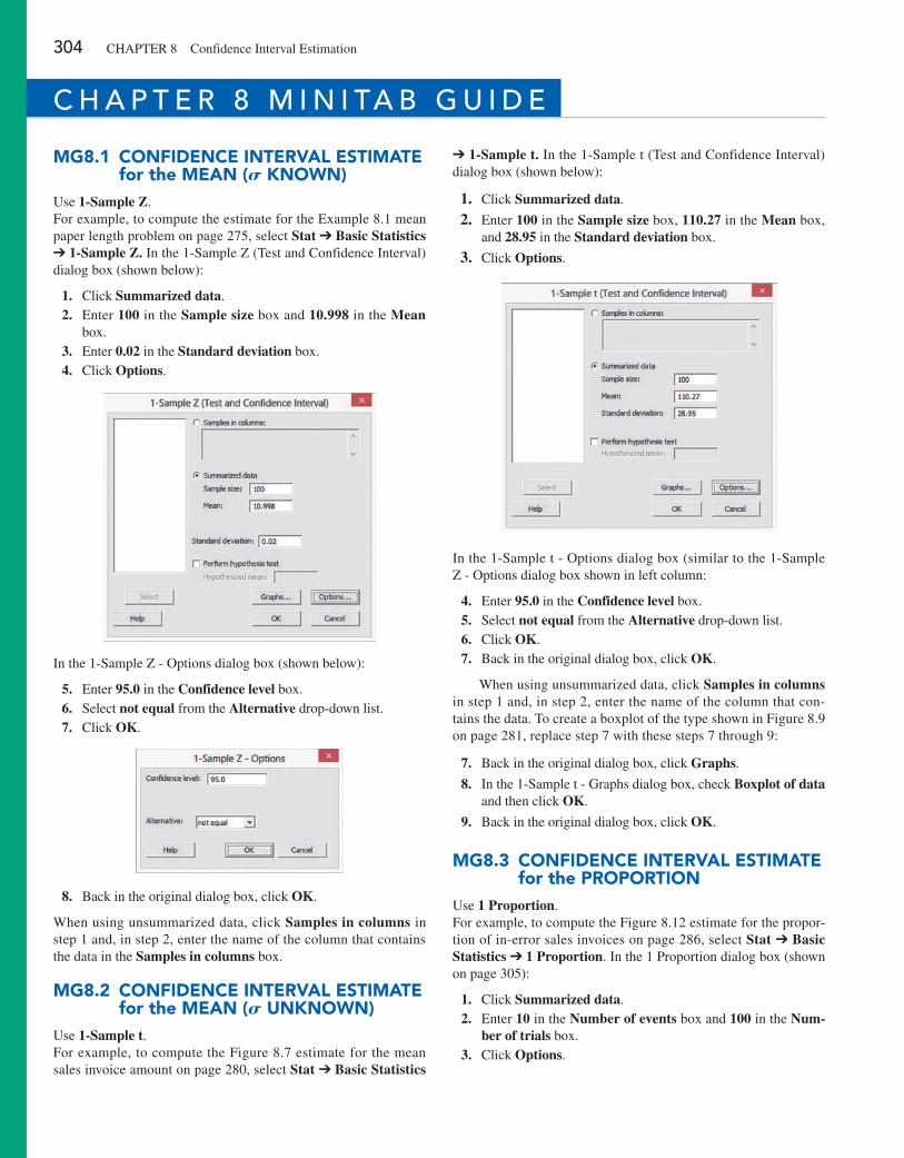
304 CHAPTER 8 Confidence Interval Estimation
mg8.1 COnFiDenCe interval eStimate for the mean (S KnOWn)
Use 1-Sample Z.For example, to compute the estimate for the Example 8.1 mean paper length problem on page 275, select Stat ➔ Basic Statistics ➔ 1-Sample Z. In the 1-Sample Z (Test and Confidence Interval) dialog box (shown below):
1. Click Summarized data. 2. Enter 100 in the Sample size box and 10.998 in the Mean
box. 3. Enter 0.02 in the Standard deviation box. 4. Click Options.
In the 1-Sample Z - Options dialog box (shown below):
5. Enter 95.0 in the Confidence level box. 6. Select not equal from the Alternative drop-down list. 7. Click OK.
8. Back in the original dialog box, click OK.
When using unsummarized data, click Samples in columns in step 1 and, in step 2, enter the name of the column that contains the data in the Samples in columns box.
mg8.2 COnFiDenCe interval eStimate for the mean (S unKnOWn)
Use 1-Sample t.For example, to compute the Figure 8.7 estimate for the mean sales invoice amount on page 280, select Stat ➔ Basic Statistics
➔ 1-Sample t. In the 1-Sample t (Test and Confidence Interval) dialog box (shown below):
1. Click Summarized data.
2. Enter 100 in the Sample size box, 110.27 in the Mean box, and 28.95 in the Standard deviation box.
3. Click Options.
In the 1-Sample t - Options dialog box (similar to the 1-Sample Z - Options dialog box shown in left column:
4. Enter 95.0 in the Confidence level box. 5. Select not equal from the Alternative drop-down list. 6. Click OK. 7. Back in the original dialog box, click OK.
When using unsummarized data, click Samples in columns in step 1 and, in step 2, enter the name of the column that con-tains the data. To create a boxplot of the type shown in Figure 8.9 on page 281, replace step 7 with these steps 7 through 9:
7. Back in the original dialog box, click Graphs.
8. In the 1-Sample t - Graphs dialog box, check Boxplot of data and then click OK.
9. Back in the original dialog box, click OK.
mg8.3 COnFiDenCe interval eStimate for the prOpOrtiOn
Use 1 Proportion.For example, to compute the Figure 8.12 estimate for the propor-tion of in-error sales invoices on page 286, select Stat ➔ Basic Statistics ➔ 1 Proportion. In the 1 Proportion dialog box (shown on page 305):
1. Click Summarized data. 2. Enter 10 in the Number of events box and 100 in the Num-
ber of trials box. 3. Click Options.
c H a p t E R 8 M i n i ta b g U i d E
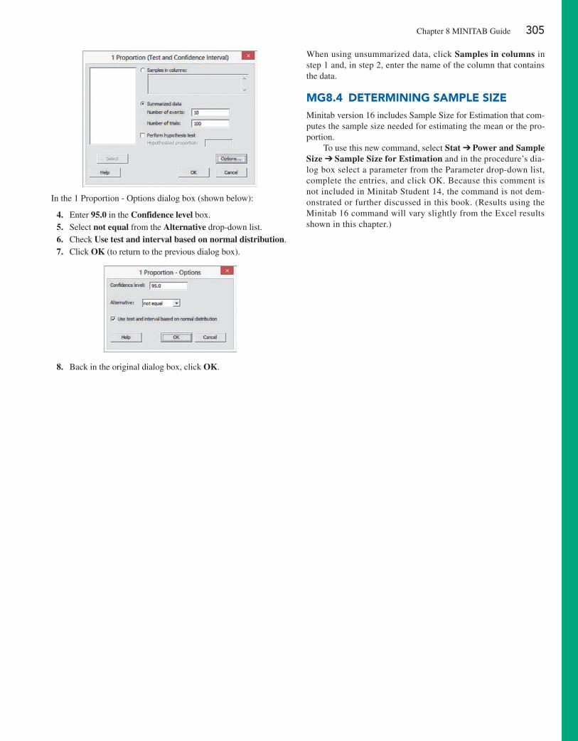
Chapter 8 MINITAB Guide 305
In the 1 Proportion - Options dialog box (shown below):
4. Enter 95.0 in the Confidence level box. 5. Select not equal from the Alternative drop-down list. 6. Check Use test and interval based on normal distribution. 7. Click OK (to return to the previous dialog box).
8. Back in the original dialog box, click OK.
When using unsummarized data, click Samples in columns in step 1 and, in step 2, enter the name of the column that contains the data.
mg8.4 Determining Sample SizeMinitab version 16 includes Sample Size for Estimation that com-putes the sample size needed for estimating the mean or the pro-portion.
To use this new command, select Stat ➔ Power and Sample Size ➔ Sample Size for Estimation and in the procedure’s dia-log box select a parameter from the Parameter drop-down list, complete the entries, and click OK. Because this comment is not included in Minitab Student 14, the command is not dem-onstrated or further discussed in this book. (Results using the Minitab 16 command will vary slightly from the Excel results shown in this chapter.)

306
U s i n g s tat i s t i c s
Significant Testing at Oxford CerealsAs in Chapter 7, you again find yourself as plant operations manager for Oxford Cereals. Among other responsibilities, you are responsible for monitoring the amount in each cereal box filled. Company specifications require a mean weight of 368 grams per box. You must adjust the cereal-filling process when the mean fill-weight in the population of boxes differs from 368 grams. Adjusting the pro-cess requires shutting down the cereal production line temporarily, so you do not want to make unnecessary adjustments.
What decision-making method can you use to decide if the cereal-filling process needs to be adjusted? You decide to begin by selecting a random sam-ple of 25 cereal boxes and weighing each box. From the weights collected, you compute a sample mean. How could that sample mean be used to help decide whether adjustment is necessary?
contents
9.1 Fundamentals of Hypothesis-Testing Methodology
can You Ever Know the Population standard Deviation?
9.2 t Test of Hypothesis for the Mean (s Unknown)
9.3 One-Tail Tests
9.4 Z Test of Hypothesis for the Proportion
9.5 Potential Hypothesis-Testing Pitfalls and Ethical Issues
Using statistics: significant testing at Oxford cereals, Revisited
chaPtER 9 ExcEl gUiDE
chaPtER 9 Minitab gUiDE
objectives
Learn the basic principles of hypothesis testing
How to use hypothesis testing to test a mean or proportion
Identify the assumptions of each hypothesis-testing procedure, how to evaluate them, and the consequences if they are seriously violated
Become aware of the pitfalls and ethical issues involved in hypothesis testing
How to avoid the pitfalls involved in hypothesis testing
Fundamentals of Hypothesis Testing: One-Sample Tests
9Chapter
Peter Close/Shutterstock
9.1 Fundamentals of Hypothesis-Testing Methodology 307
I n Chapter 7, you learned methods to determine whether the value of a sample mean is consistent with a known population mean. In this Oxford Cereals scenario, you seek to use a sample mean to validate a claim about the population mean, a somewhat differ-
ent problem. For this type of situation, you use the inferential method known as hypothesis testing. Hypothesis testing requires that you state a claim unambiguously. In this scenario, the claim is that the population mean is 368 grams. You examine a sample statistic to see if it bet-ter supports the stated claim, called the null hypothesis, or the mutually exclusive alternative hypothesis (for this scenario, that the population mean is not 368 grams).
In this chapter, you will learn several applications of hypothesis testing. You will learn how to make inferences about a population parameter by analyzing differences between the results observed, the sample statistic, and the results you would expect to get if an underlying hypothesis were actually true. For the Oxford Cereals scenario, hypothesis testing allows you to infer one of the following:
• The mean weight of the cereal boxes in the sample is a value consistent with what you would expect if the mean of the entire population of cereal boxes were 368 grams.
• The population mean is not equal to 368 grams because the sample mean is significantly different from 368 grams.
9.1 Fundamentals of Hypothesis-Testing MethodologyHypothesis testing typically begins with a theory, a claim, or an assertion about a particular pa-rameter of a population. For example, your initial hypothesis in the cereal example is that the process is working properly, so the mean fill is 368 grams, and no corrective action is needed.
The Null and Alternative HypothesesThe hypothesis that the population parameter is equal to the company specification is referred to as the null hypothesis. A null hypothesis is often one of status quo and is identified by the symbol H0. Here the null hypothesis is that the filling process is working properly, and there-fore the mean fill is the 368-gram specification provided by Oxford Cereals. This is stated as
H0 : m = 368
Even though information is available only from the sample, the null hypothesis is stated in terms of the population parameter because your focus is on the population of all cereal boxes. You use the sample statistic to make inferences about the entire filling process. One inference may be that the results observed from the sample data indicate that the null hypothesis is false. If the null hypothesis is considered false, something else must be true.
Whenever a null hypothesis is specified, an alternative hypothesis is also specified, and it must be true if the null hypothesis is false. The alternative hypothesis, H1, is the opposite of the null hypothesis, H0. This is stated in the cereal example as
H1 : m ≠ 368
The alternative hypothesis represents the conclusion reached by rejecting the null hypothesis. In many research situations, the alternative hypothesis serves as the hypothesis that is the fo-cus of the research being conducted. The null hypothesis is rejected when there is sufficient evidence from the sample data that the null hypothesis is false. In the cereal example, if the weights of the sampled boxes are sufficiently above or below the expected 368-gram mean specified by Oxford Cereals, you reject the null hypothesis in favor of the alternative hypoth-esis that the mean fill is different from 368 grams. You stop production and take whatever action is necessary to correct the problem. If the null hypothesis is not rejected, you should continue to believe that the process is working correctly and that no corrective action is neces-sary. In this second circumstance, you have not proven that the process is working correctly.
Student TipRemember, hypothesis testing reaches conclu-sions about parameters, not statistics.
308 CHAPTEr 9 Fundamentals of Hypothesis Testing: One-Sample Tests
rather, you have failed to prove that it is working incorrectly, and therefore you continue your belief (although unproven) in the null hypothesis.
In hypothesis testing, you reject the null hypothesis when the sample evidence suggests that it is far more likely that the alternative hypothesis is true. However, failure to reject the null hypothesis is not proof that it is true. You can never prove that the null hypothesis is cor-rect because the decision is based only on the sample information, not on the entire popula-tion. Therefore, if you fail to reject the null hypothesis, you can only conclude that there is insufficient evidence to warrant its rejection. The following key points summarize the null and alternative hypotheses:
• The null hypothesis, H0, represents the current belief in a situation. • The alternative hypothesis, H1, is the opposite of the null hypothesis and represents a
research claim or specific inference you would like to prove. • If you reject the null hypothesis, you have statistical proof that the alternative hypothesis
is correct. • If you do not reject the null hypothesis, you have failed to prove the alternative hypoth-
esis. The failure to prove the alternative hypothesis, however, does not mean that you have proven the null hypothesis.
• The null hypothesis, H0, always refers to a specified value of the population parameter (such as m), not a sample statistic (such as X).
• The statement of the null hypothesis always contains an equal sign regarding the speci-fied value of the population parameter (e.g., H0 : m = 368 grams).
• The statement of the alternative hypothesis never contains an equal sign regarding the specified value of the population parameter (e.g., H1 : m ≠ 368 grams).
ExAmplE 9.1the null and alternative hypotheses
You are the manager of a fast-food restaurant. You want to determine whether the waiting time to place an order has changed in the past month from its previous population mean value of 4.5 minutes. State the null and alternative hypotheses.
SoluTioN The null hypothesis is that the population mean has not changed from its previ-ous value of 4.5 minutes. This is stated as
H0 : m = 4.5
The alternative hypothesis is the opposite of the null hypothesis. Because the null hypothesis is that the population mean is 4.5 minutes, the alternative hypothesis is that the population mean is not 4.5 minutes. This is stated as
H1 : m ≠ 4.5
The Critical Value of the Test StatisticHypothesis testing uses sample data to determine how likely it is that the null hypothesis is true. In the Oxford Cereal Company scenario, the null hypothesis is that the mean amount of cereal per box in the entire filling process is 368 grams (the population parameter specified by the com-pany). You select a sample of boxes from the filling process, weigh each box, and compute the sample mean X. This sample statistic is an estimate of the corresponding parameter, the popula-tion mean, m. Even if the null hypothesis is true, the sample statistic X is likely to differ from the value of the parameter (the population mean, m) because of variation due to sampling.
You do expect the sample statistic to be close to the population parameter if the null hypoth-esis is true. If the sample statistic is close to the population parameter, you have insufficient evi-dence to reject the null hypothesis. For example, if the sample mean is 367.9 grams, you might conclude that the population mean has not changed (i.e., m = 368) because a sample mean of 367.9 grams is very close to the hypothesized value of 368 grams. Intuitively, you think that it is likely that you could get a sample mean of 367.9 grams from a population whose mean is 368.
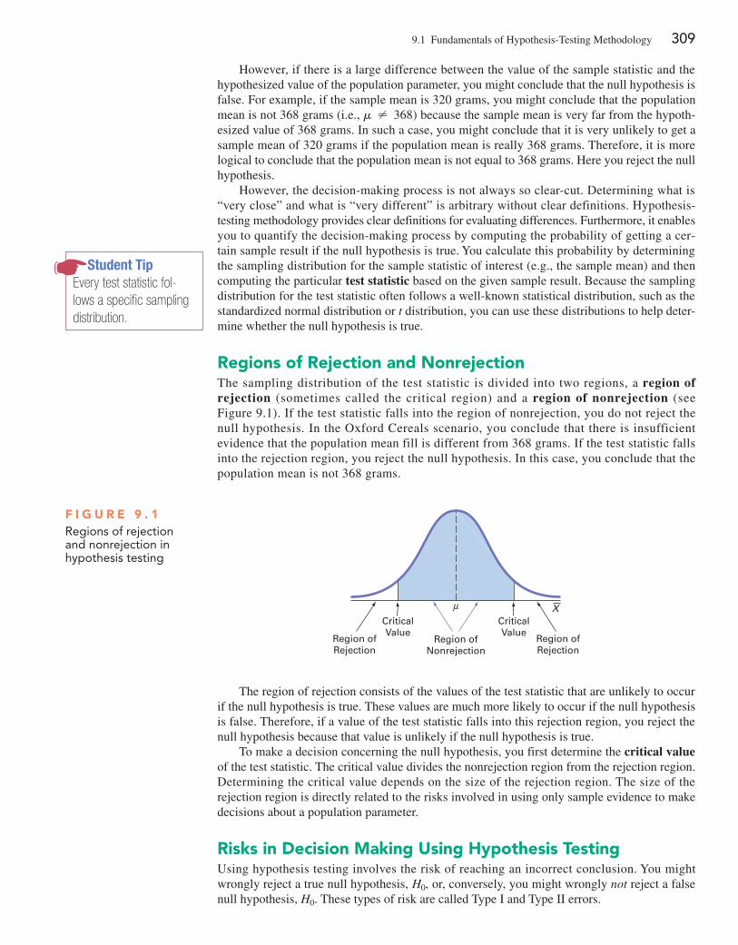
9.1 Fundamentals of Hypothesis-Testing Methodology 309
However, if there is a large difference between the value of the sample statistic and the hypothesized value of the population parameter, you might conclude that the null hypothesis is false. For example, if the sample mean is 320 grams, you might conclude that the population mean is not 368 grams (i.e., m ≠ 368) because the sample mean is very far from the hypoth-esized value of 368 grams. In such a case, you might conclude that it is very unlikely to get a sample mean of 320 grams if the population mean is really 368 grams. Therefore, it is more logical to conclude that the population mean is not equal to 368 grams. Here you reject the null hypothesis.
However, the decision-making process is not always so clear-cut. Determining what is “very close” and what is “very different” is arbitrary without clear definitions. Hypothesis- testing methodology provides clear definitions for evaluating differences. Furthermore, it enables you to quantify the decision-making process by computing the probability of getting a cer-tain sample result if the null hypothesis is true. You calculate this probability by determining the sampling distribution for the sample statistic of interest (e.g., the sample mean) and then computing the particular test statistic based on the given sample result. Because the sampling distribution for the test statistic often follows a well-known statistical distribution, such as the standardized normal distribution or t distribution, you can use these distributions to help deter-mine whether the null hypothesis is true.
Regions of Rejection and NonrejectionThe sampling distribution of the test statistic is divided into two regions, a region of rejection (sometimes called the critical region) and a region of nonrejection (see Figure 9.1). If the test statistic falls into the region of nonrejection, you do not reject the null hypothesis. In the Oxford Cereals scenario, you conclude that there is insufficient evidence that the population mean fill is different from 368 grams. If the test statistic falls into the rejection region, you reject the null hypothesis. In this case, you conclude that the population mean is not 368 grams.
Student TipEvery test statistic fol-lows a specific sampling distribution.
Region ofRejection
Region ofNonrejection
CriticalValue
Region ofRejection
CriticalValue
X
F i g u R E 9 . 1Regions of rejection and nonrejection in hypothesis testing
The region of rejection consists of the values of the test statistic that are unlikely to occur if the null hypothesis is true. These values are much more likely to occur if the null hypothesis is false. Therefore, if a value of the test statistic falls into this rejection region, you reject the null hypothesis because that value is unlikely if the null hypothesis is true.
To make a decision concerning the null hypothesis, you first determine the critical value of the test statistic. The critical value divides the nonrejection region from the rejection region. Determining the critical value depends on the size of the rejection region. The size of the rejection region is directly related to the risks involved in using only sample evidence to make decisions about a population parameter.
Risks in Decision making using Hypothesis TestingUsing hypothesis testing involves the risk of reaching an incorrect conclusion. You might wrongly reject a true null hypothesis, H0, or, conversely, you might wrongly not reject a false null hypothesis, H0. These types of risk are called Type I and Type II errors.
310 CHAPTEr 9 Fundamentals of Hypothesis Testing: One-Sample Tests
In the Oxford Cereals scenario, you would make a Type I error if you concluded that the population mean fill is not 368 grams when it is 368 grams. This error causes you to needlessly adjust the filling process (the “false alarm”) even though the process is working properly. In the same scenario, you would make a Type II error if you concluded that the population mean fill is 368 grams when it is not 368 grams. In this case, you would allow the process to con-tinue without adjustment, even though an adjustment is needed (the “missed opportunity”).
Traditionally, you control the Type I error by determining the risk level, a (the lowercase Greek letter alpha), that you are willing to have of rejecting the null hypothesis when it is true. This risk, or probability, of committing a Type I error is called the level of significance (a). Because you specify the level of significance before you perform the hypothesis test, you directly control the risk of committing a Type I error. Traditionally, you select a level of 0.01, 0.05, or 0.10. The choice of a particular risk level for making a Type I error depends on the cost of mak-ing a Type I error. After you specify the value for a, you can then determine the critical values that divide the rejection and nonrejection regions. You know the size of the rejection region be-cause a is the probability of rejection when the null hypothesis is true. From this, you can then determine the critical value or values that divide the rejection and nonrejection regions.
The probability of committing a Type II error is called the b risk. Unlike the Type I error, which you control through the selection of a, the probability of making a Type II error depends on the difference between the hypothesized and actual values of the population parameter. Because large differences are easier to find than small ones, if the dif-ference between the hypothesized and actual values of the population parameter is large, b is small. For example, if the population mean is 330 grams, there is a small chance 1b2 that you will conclude that the mean has not changed from 368 grams. However, if the difference be-tween the hypothesized and actual values of the parameter is small, b is large. For example, if the population mean is actually 367 grams, there is a large chance 1b2 that you will conclude that the mean is still 368 grams.
TyPE I and TyPE II ERRORs
A Type I error occurs if you reject the null hypothesis, H0, when it is true and should not be rejected. A Type I error is a “false alarm.” The probability of a Type I error occurring is a.
A Type II error occurs if you do not reject the null hypothesis, H0, when it is false and should be rejected. A Type II error represents a “missed opportunity” to take some corrective action. The probability of a Type II error occurring is b.
PROBaBILITy OF TyPE I and TyPE II ERRORs
The level of significance 1A2 of a statistical test is the probability of committing a Type I error.
The B risk is the probability of committing a Type II error.
The complement of the probability of a Type I error, 11 - a2, is called the confidence coefficient. The confidence coefficient is the probability that you will not reject the null hypothesis, H0, when it is true and should not be rejected. In the Oxford Cereals scenario, the confidence coefficient measures the probability of concluding that the population mean fill is 368 grams when it is actually 368 grams.
The complement of the probability of a Type II error, 11 - b2, is called the power of a statistical test. The power of a statistical test is the probability that you will reject the null hypothesis when it is false and should be rejected. In the Oxford Cereals scenario, the power of the test is the probability that you will correctly conclude that the mean fill amount is not 368 grams when it actually is not 368 grams.
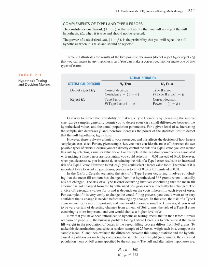
9.1 Fundamentals of Hypothesis-Testing Methodology 311
Table 9.1 illustrates the results of the two possible decisions (do not reject H0 or reject H0) that you can make in any hypothesis test. You can make a correct decision or make one of two types of errors.
COMPLEMEnTs OF TyPE I and TyPE II ERRORs
The confidence coefficient, 11 - a2, is the probability that you will not reject the null hypothesis, H0, when it is true and should not be rejected.
The power of a statistical test, 11 - b2, is the probability that you will reject the null hypothesis when it is false and should be rejected.
T A b l E 9 . 1
Hypothesis Testing and decision Making
AcTuAl SiTuATion
STATiSTicAl DeciSion H0 True H0 False
Do not reject H0 Correct decision Confidence = 11 - a2
Type II error P1Type II error2 = b
Reject H0 Type I error P1Type I error2 = a
Correct decision Power = 11 - b2
One way to reduce the probability of making a Type II error is by increasing the sample size. Large samples generally permit you to detect even very small differences between the hypothesized values and the actual population parameters. For a given level of a, increasing the sample size decreases b and therefore increases the power of the statistical test to detect that the null hypothesis, H0, is false.
However, there is always a limit to your resources, and this affects the decision of how large a sample you can select. For any given sample size, you must consider the trade-offs between the two possible types of errors. Because you can directly control the risk of a Type I error, you can reduce this risk by selecting a smaller value for a. For example, if the negative consequences associated with making a Type I error are substantial, you could select a = 0.01 instead of 0.05. However, when you decrease a, you increase b, so reducing the risk of a Type I error results in an increased risk of a Type II error. However, to reduce b, you could select a larger value for a. Therefore, if it is important to try to avoid a Type II error, you can select a of 0.05 or 0.10 instead of 0.01.
In the Oxford Cereals scenario, the risk of a Type I error occurring involves conclud-ing that the mean fill amount has changed from the hypothesized 368 grams when it actually has not changed. The risk of a Type II error occurring involves concluding that the mean fill amount has not changed from the hypothesized 368 grams when it actually has changed. The choice of reasonable values for a and b depends on the costs inherent in each type of error. For example, if it is very costly to change the cereal-filling process, you would want to be very confident that a change is needed before making any changes. In this case, the risk of a Type I error occurring is more important, and you would choose a small a. However, if you want to be very certain of detecting changes from a mean of 368 grams, the risk of a Type II error occurring is more important, and you would choose a higher level of a.
Now that you have been introduced to hypothesis testing, recall that in the Oxford Cereals scenario on page 306, the business problem facing Oxford Cereals is to determine if the mean fill-weight in the population of boxes in the cereal-filling process differs from 368 grams. To make this determination, you select a random sample of 25 boxes, weigh each box, compute the sample mean, X, and then evaluate the difference between this sample statistic and the hypoth-esized population parameter by comparing the sample mean weight (in grams) to the expected population mean of 368 grams specified by the company. The null and alternative hypotheses are:
H0 : m = 368
H1 : m ≠ 368
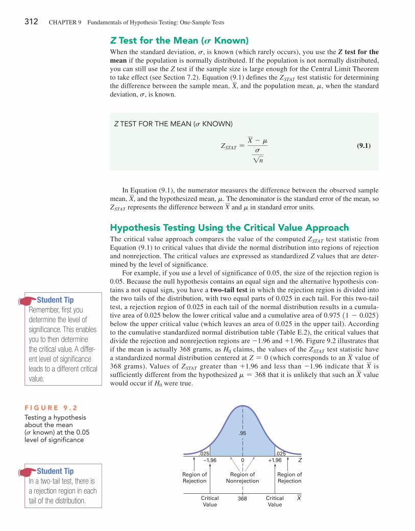
312 CHAPTEr 9 Fundamentals of Hypothesis Testing: One-Sample Tests
Z Test for the mean (S Known)When the standard deviation, s, is known (which rarely occurs), you use the Z test for the mean if the population is normally distributed. If the population is not normally distributed, you can still use the Z test if the sample size is large enough for the Central Limit Theorem to take effect (see Section 7.2). Equation (9.1) defines the ZSTAT test statistic for determining the difference between the sample mean, X, and the population mean, m, when the standard deviation, s, is known.
Z TEsT FOR THE MEan (s KnOwn)
ZSTAT =X - m
s1n
(9.1)
In Equation (9.1), the numerator measures the difference between the observed sample mean, X, and the hypothesized mean, m. The denominator is the standard error of the mean, so ZSTAT represents the difference between X and m in standard error units.
Hypothesis Testing using the Critical Value ApproachThe critical value approach compares the value of the computed ZSTAT test statistic from Equation (9.1) to critical values that divide the normal distribution into regions of rejection and nonrejection. The critical values are expressed as standardized Z values that are deter-mined by the level of significance.
For example, if you use a level of significance of 0.05, the size of the rejection region is 0.05. Because the null hypothesis contains an equal sign and the alternative hypothesis con-tains a not equal sign, you have a two-tail test in which the rejection region is divided into the two tails of the distribution, with two equal parts of 0.025 in each tail. For this two-tail test, a rejection region of 0.025 in each tail of the normal distribution results in a cumula-tive area of 0.025 below the lower critical value and a cumulative area of 0.975 11 - 0.0252 below the upper critical value (which leaves an area of 0.025 in the upper tail). According to the cumulative standardized normal distribution table (Table E.2), the critical values that divide the rejection and nonrejection regions are -1.96 and +1.96. Figure 9.2 illustrates that if the mean is actually 368 grams, as H0 claims, the values of the ZSTAT test statistic have a standardized normal distribution centered at Z = 0 (which corresponds to an X value of 368 grams). Values of ZSTAT greater than +1.96 and less than -1.96 indicate that X is sufficiently different from the hypothesized m = 368 that it is unlikely that such an X value would occur if H0 were true.
Region ofRejection
Region ofNonrejection
CriticalValue
Region ofRejection
CriticalValue
–1.96 0 +1.96 Z.025 .025
368
.95
X
F i g u R E 9 . 2Testing a hypothesis about the mean (s known) at the 0.05 level of significance
Student TipRemember, first you determine the level of significance. This enables you to then determine the critical value. A differ-ent level of significance leads to a different critical value.
Student TipIn a two-tail test, there is a rejection region in each tail of the distribution.
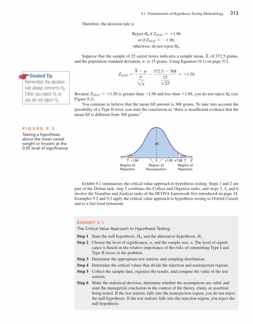
9.1 Fundamentals of Hypothesis-Testing Methodology 313
Therefore, the decision rule is
reject H0 if ZSTAT 7 +1.96
or if ZSTAT 6 - 1.96;
otherwise, do not reject H0.
Suppose that the sample of 25 cereal boxes indicates a sample mean, X, of 372.5 grams, and the population standard deviation, s, is 15 grams. Using Equation (9.1) on page 312,
ZSTAT =X - m
s2n
-372.5 - 368
15125
= +1.50
Because ZSTAT = +1.50 is greater than -1.96 and less than +1.96, you do not reject H0 (see Figure 9.3).
You continue to believe that the mean fill amount is 368 grams. To take into account the possibility of a Type II error, you state the conclusion as “there is insufficient evidence that the mean fill is different from 368 grams.”
Student TipRemember, the decision rule always concerns H0. Either you reject H0 or you do not reject H0.
F i g u R E 9 . 3Testing a hypothesis about the mean cereal weight (s known) at the 0.05 level of significance
0–1.96 +1.96+1.50 ZRegion ofRejection
Region ofNonrejection
Region ofRejection
.025.025
.95
Exhibit 9.1 summarizes the critical value approach to hypothesis testing. Steps 1 and 2 are part of the Define task, step 5 combines the Collect and Organize tasks, and steps 3, 4, and 6 involve the Visualize and Analyze tasks of the DCOVA framework first introduced on page 24. Examples 9.2 and 9.3 apply the critical value approach to hypothesis testing to Oxford Cereals and to a fast-food restaurant.
ExHibiT 9.1 The Critical Value approach to Hypothesis Testing
Step 1 State the null hypothesis, H0, and the alternative hypothesis, H1.
Step 2 Choose the level of significance, a, and the sample size, n. The level of signifi-cance is based on the relative importance of the risks of committing Type I and Type II errors in the problem.
Step 3 Determine the appropriate test statistic and sampling distribution.
Step 4 Determine the critical values that divide the rejection and nonrejection regions.
Step 5 Collect the sample data, organize the results, and compute the value of the test statistic.
Step 6 Make the statistical decision, determine whether the assumptions are valid, and state the managerial conclusion in the context of the theory, claim, or assertion being tested. If the test statistic falls into the nonrejection region, you do not reject the null hypothesis. If the test statistic falls into the rejection region, you reject the null hypothesis.
314 CHAPTEr 9 Fundamentals of Hypothesis Testing: One-Sample Tests
ExAmplE 9.2applying the critical Value approach to hypothesis testing at Oxford cereals
State the critical value approach to hypothesis testing at Oxford Cereals.
SoluTioN
Step 1 State the null and alternative hypotheses. The null hypothesis, H0, is always stated as a mathematical expression, using population parameters. In testing whether the mean fill is 368 grams, the null hypothesis states that m equals 368. The alternative hypoth-esis, H1, is also stated as a mathematical expression, using population parameters. Therefore, the alternative hypothesis states that m is not equal to 368 grams.
Step 2 Choose the level of significance and the sample size. You choose the level of signifi-cance, a, according to the relative importance of the risks of committing Type I and Type II errors in the problem. The smaller the value of a, the less risk there is of mak-ing a Type I error. In this example, making a Type I error means that you conclude that the population mean is not 368 grams when it is 368 grams. Thus, you will take cor-rective action on the filling process even though the process is working properly. Here, a = 0.05 is selected. The sample size, n, is 25.
Step 3 Select the appropriate test statistic. Because s is known from information about the filling process, you use the normal distribution and the ZSTAT test statistic.
Step 4 Determine the rejection region. Critical values for the appropriate test statistic are selected so that the rejection region contains a total area of a when H0 is true and the nonrejection region contains a total area of 1 - a when H0 is true. Because a = 0.05 in the cereal example, the critical values of the ZSTAT test statistic are -1.96 and +1.96. The rejection region is therefore ZSTAT 6 - 1.96 or ZSTAT 7 +1.96. The nonrejection region is -1.96 … ZSTAT … +1.96.
Step 5 Collect the sample data and compute the value of the test statistic. In the cereal exam-ple, X = 372.5, and the value of the test statistic is ZSTAT = +1.50.
Step 6 State the statistical decision and the managerial conclusion. First, determine whether the test statistic has fallen into the rejection region or the nonrejection region. For the cereal example, ZSTAT = +1.50 is in the region of nonrejection because -1.96 … ZSTAT = +1.50 … +1.96. Because the test statistic falls into the nonrejec-tion region, the statistical decision is to not reject the null hypothesis, H0. The manage-rial conclusion is that insufficient evidence exists to prove that the mean fill is different from 368 grams. No corrective action on the filling process is needed.
ExAmplE 9.3testing and Rejecting a null hypothesis
You are the manager of a fast-food restaurant. The business problem is to determine whether the population mean waiting time to place an order has changed in the past month from its previous population mean value of 4.5 minutes. From past experience, you can assume that the population is normally distributed, with a population standard deviation of 1.2 minutes. You select a sample of 25 orders during a one-hour period. The sample mean is 5.1 minutes. Use the six-step approach listed in Exhibit 9.1 on page 313 to determine whether there is evidence at the 0.05 level of significance that the population mean waiting time to place an order has changed in the past month from its previous population mean value of 4.5 minutes.
SoluTioN
Step 1 The null hypothesis is that the population mean has not changed from its previous value of 4.5 minutes:
H0 : m = 4.5
The alternative hypothesis is the opposite of the null hypothesis. Because the null hypothesis is that the population mean is 4.5 minutes, the alternative hypothesis is that the population mean is not 4.5 minutes:
H1 : m ≠ 4.5
9.1 Fundamentals of Hypothesis-Testing Methodology 315
Hypothesis Testing using the p-Value ApproachThe p-value is the probability of getting a test statistic equal to or more extreme than the sam-ple result, given that the null hypothesis, H0, is true. The p-value is also known as the observed level of significance. Using the p-value to determine rejection and nonrejection is another approach to hypothesis testing.
The decision rules for rejecting H0 in the p-value approach are
• If the p-value is greater than or equal to a, do not reject the null hypothesis. • If the p-value is less than a, reject the null hypothesis.
Step 2 You have selected a sample of n = 25. The level of significance is 0.05 (i.e., a = 0.05).
Step 3 Because s is assumed to be known, you use the normal distribution and the ZSTAT test statistic.
Step 4 Because a = 0.05, the critical values of the ZSTAT test statistic are -1.96 and +1.96. The rejection region is ZSTAT 6 -1.96 or ZSTAT 7 +1.96. The nonrejection region is -1.96 … ZSTAT … +1.96.
Step 5 You collect the sample data and compute X = 5.1. Using Equation (9.1) on page 312, you compute the test statistic:
ZSTAT =X - m
s1n
=5.1 - 4.5
1.2125
= +2.50
Step 6 Because ZSTAT = +2.50 7 +1.96, you reject the null hypothesis. You conclude that there is evidence that the population mean waiting time to place an order has changed from its previous value of 4.5 minutes. The mean waiting time for customers is longer now than it was last month. As the manager, you would now want to determine how waiting time could be reduced to improve service.
Many people confuse these rules, mistakenly believing that a high p-value is reason for rejection. You can avoid this confusion by remembering the following:
If the p@value is low, then H0 must go.
To understand the p-value approach, consider the Oxford Cereals scenario. You tested whether the mean fill was equal to 368 grams. The test statistic resulted in a ZSTAT value of +1.50 and you did not reject the null hypothesis because +1.50 was less than the upper critical value of +1.96 and greater than the lower critical value of -1.96.
To use the p-value approach for the two-tail test, you find the probability that the test statistic ZSTAT is equal to or more extreme than 1.50 standard error units from the cen-ter of a standardized normal distribution. In other words, you need to compute the prob-ability that the ZSTAT value is greater than +1.50 along with the probability that the ZSTAT value is less than -1.50. Table E.2 shows that the probability of a ZSTAT value below -1.50 is 0.0668. The probability of a value below +1.50 is 0.9332, and the probability of a value above +1.50 is 1 - 0.9332 = 0.0668. Therefore, the p-value for this two-tail test is 0.0668 + 0.0668 = 0.1336 (see Figure 9.4). Thus, the probability of a test statistic equal to or more extreme than the sample result is 0.1336. Because 0.1336 is greater than a = 0.05, you do not reject the null hypothesis.
Student TipA small (or low) p-value indicates a small prob-ability that H0 is true. A big or large p-value indicates a large prob-ability that H0 is true.
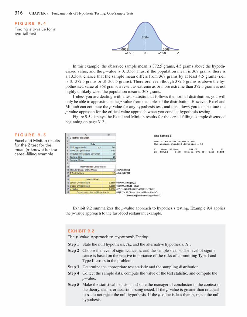
316 CHAPTEr 9 Fundamentals of Hypothesis Testing: One-Sample Tests
In this example, the observed sample mean is 372.5 grams, 4.5 grams above the hypoth-esized value, and the p-value is 0.1336. Thus, if the population mean is 368 grams, there is a 13.36% chance that the sample mean differs from 368 grams by at least 4.5 grams (i.e., is Ú 372.5 grams or … 363.5 grams). Therefore, even though 372.5 grams is above the hy-pothesized value of 368 grams, a result as extreme as or more extreme than 372.5 grams is not highly unlikely when the population mean is 368 grams.
Unless you are dealing with a test statistic that follows the normal distribution, you will only be able to approximate the p-value from the tables of the distribution. However, Excel and Minitab can compute the p-value for any hypothesis test, and this allows you to substitute the p-value approach for the critical value approach when you conduct hypothesis testing.
Figure 9.5 displays the Excel and Minitab results for the cereal-filling example discussed beginning on page 312.
–1.50 0 +1.50 Z.0668 .0668
.8664
F i g u R E 9 . 4Finding a p-value for a two-tail test
F i g u R E 9 . 5Excel and Minitab results for the Z test for the mean (s known) for the cereal-filling example
Exhibit 9.2 summarizes the p-value approach to hypothesis testing. Example 9.4 applies the p-value approach to the fast-food restaurant example.
ExHibiT 9.2 The p-Value approach to Hypothesis Testing
Step 1 State the null hypothesis, H0, and the alternative hypothesis, H1.
Step 2 Choose the level of significance, a, and the sample size, n. The level of signifi-cance is based on the relative importance of the risks of committing Type I and Type II errors in the problem.
Step 3 Determine the appropriate test statistic and the sampling distribution.
Step 4 Collect the sample data, compute the value of the test statistic, and compute the p-value.
Step 5 Make the statistical decision and state the managerial conclusion in the context of the theory, claim, or assertion being tested. If the p-value is greater than or equal to a, do not reject the null hypothesis. If the p-value is less than a, reject the null hypothesis.
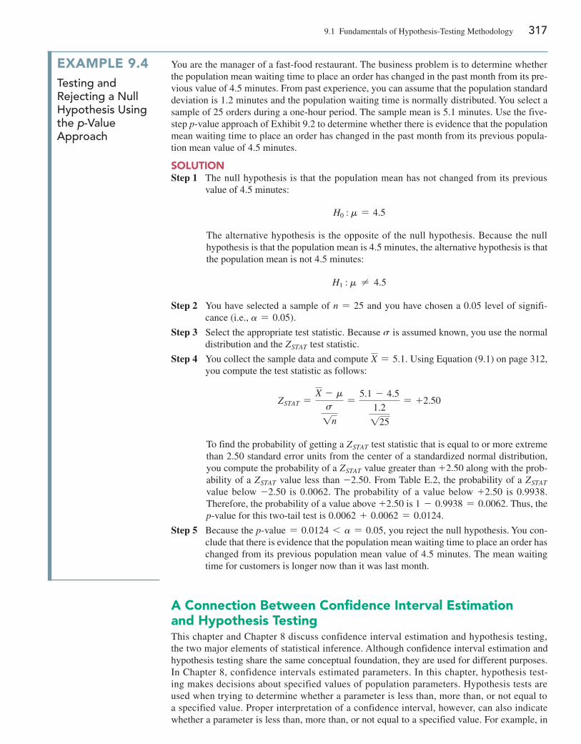
9.1 Fundamentals of Hypothesis-Testing Methodology 317
ExAmplE 9.4testing and Rejecting a null hypothesis Using the p-Value approach
You are the manager of a fast-food restaurant. The business problem is to determine whether the population mean waiting time to place an order has changed in the past month from its pre-vious value of 4.5 minutes. From past experience, you can assume that the population standard deviation is 1.2 minutes and the population waiting time is normally distributed. You select a sample of 25 orders during a one-hour period. The sample mean is 5.1 minutes. Use the five-step p-value approach of Exhibit 9.2 to determine whether there is evidence that the population mean waiting time to place an order has changed in the past month from its previous popula-tion mean value of 4.5 minutes.
SoluTioNStep 1 The null hypothesis is that the population mean has not changed from its previous
value of 4.5 minutes:
H0 : m = 4.5
The alternative hypothesis is the opposite of the null hypothesis. Because the null hypothesis is that the population mean is 4.5 minutes, the alternative hypothesis is that the population mean is not 4.5 minutes:
H1 : m ≠ 4.5
Step 2 You have selected a sample of n = 25 and you have chosen a 0.05 level of signifi-cance (i.e., a = 0.05).
Step 3 Select the appropriate test statistic. Because s is assumed known, you use the normal distribution and the ZSTAT test statistic.
Step 4 You collect the sample data and compute X = 5.1. Using Equation (9.1) on page 312, you compute the test statistic as follows:
ZSTAT =X - m
s1n
=5.1 - 4.5
1.2125
= +2.50
To find the probability of getting a ZSTAT test statistic that is equal to or more extreme than 2.50 standard error units from the center of a standardized normal distribution, you compute the probability of a ZSTAT value greater than +2.50 along with the prob-ability of a ZSTAT value less than -2.50. From Table E.2, the probability of a ZSTAT value below -2.50 is 0.0062. The probability of a value below +2.50 is 0.9938. Therefore, the probability of a value above +2.50 is 1 - 0.9938 = 0.0062. Thus, the p-value for this two-tail test is 0.0062 + 0.0062 = 0.0124.
Step 5 Because the p-value = 0.0124 6 a = 0.05, you reject the null hypothesis. You con-clude that there is evidence that the population mean waiting time to place an order has changed from its previous population mean value of 4.5 minutes. The mean waiting time for customers is longer now than it was last month.
A Connection between Confidence interval Estimation and Hypothesis TestingThis chapter and Chapter 8 discuss confidence interval estimation and hypothesis testing, the two major elements of statistical inference. Although confidence interval estimation and hypothesis testing share the same conceptual foundation, they are used for different purposes. In Chapter 8, confidence intervals estimated parameters. In this chapter, hypothesis test-ing makes decisions about specified values of population parameters. Hypothesis tests are used when trying to determine whether a parameter is less than, more than, or not equal to a specified value. Proper interpretation of a confidence interval, however, can also indicate whether a parameter is less than, more than, or not equal to a specified value. For example, in
318 CHAPTEr 9 Fundamentals of Hypothesis Testing: One-Sample Tests
this section, you tested whether the population mean fill amount was different from 368 grams by using Equation (9.1) on page 312:
ZSTAT =X - m
s1n
Instead of testing the null hypothesis that m = 368 grams, you can reach the same conclu-sion by constructing a confidence interval estimate of m. If the hypothesized value of m = 368 is contained within the interval, you do not reject the null hypothesis because 368 would not be considered an unusual value. However, if the hypothesized value does not fall into the interval, you reject the null hypothesis because m = 368 grams is then considered an unusual value. Using Equation (8.1) on page 274 and the following results:
n = 25, X = 372.5 grams, s = 15 grams
for a confidence level of 95% (i.e., a = 0.05),
X { Za>2 s1n
372.5 { 11.962 15125
372.5 { 5.88
so that
366.62 … m … 378.38
Because the interval includes the hypothesized value of 368 grams, you do not reject the null hypothesis. There is insufficient evidence that the mean fill amount for the entire filling pro-cess is not 368 grams. You reached the same decision by using a two-tail hypothesis test.
problems for Section 9.1lEARNiNg THE bASiCS9.1 If you use a 0.05 level of significance in a (two-tail) hypothesis test, what will you decide if ZSTAT = -1.52?
9.2 If you use a 0.05 level of significance in a two-tail hypothesis test, what decision will you make if ZSTAT = +2.21?
9.3 If you use a 0.10 level of significance in a (two-tail) hypoth-esis test, what is your decision rule for rejecting a null hypothesis that the population mean is 350 if you use the Z test?
9.4 If you use a 0.01 level of significance in a two-tail hypothesis test, what is your decision rule for rejecting H0 : m = 12.5 if you use the Z test?
The end of Section 8.1 on page 276 discussed how learning a con-fidence interval estimation method that required knowing s, the population standard deviation, served as an effective introduction to the concept of a confidence interval. That section then revealed that you would be unlikely to use that procedure for most practical ap-plications for several reasons.
Likewise, for most practical applications, you are unlikely to use a hypothesis-testing method that requires knowing s. If you knew the population standard deviation, you would also know the popula-tion mean and would not need to form a hypothesis about the mean
and then test that hypothesis. So why study a hypothesis test of the mean, which requires that s is known? Using such a test makes it much easier to explain the fundamentals of hypothesis testing. With a known population standard deviation, you can use the normal distribution and compute p-values using the tables of the normal distribution.
Because it is important that you understand the concept of hy-pothesis testing when reading the rest of this book, review this sec-tion carefully—even if you anticipate never having a practical reason to use the test represented in Equation (9.1).
Can You Ever Know the Population Standard Deviation?
9.2 t Test of Hypothesis for the Mean (s Unknown) 319
9.5 What is your decision in Problem 9.4 if ZSTAT = -2.61?
9.6 What is the p-value if, in a two-tail hypothesis test, ZSTAT = +2.00?
9.7 In Problem 9.6, what is your statistical decision if you test the null hypothesis at the 0.10 level of significance?
9.8 What is the p-value if, in a two-tail hypothesis test, ZSTAT = -1.38?
ApplyiNg THE CoNCEpTS9.9 In the U.S. legal system, a defendant is presumed innocent un-til proven guilty. Consider a null hypothesis, H0, that a defendant is innocent, and an alternative hypothesis, H1, that the defendant is guilty. A jury has two possible decisions: Convict the defendant (i.e., reject the null hypothesis) or do not convict the defendant (i.e., do not reject the null hypothesis). Explain the meaning of the risks of committing either a Type I or Type II error in this example.
9.10 Suppose the defendant in Problem 9.9 is presumed guilty until proven innocent. How do the null and alternative hypotheses differ from those in Problem 9.9? What are the meanings of the risks of committing either a Type I or Type II error here?
9.11 Many consumer groups feel that the U.S. Food and Drug Administration (FDA) drug approval process is too easy and, as a result, too many drugs are approved that are later found to be unsafe. On the other hand, a number of industry lobbyists have pushed for a more lenient approval process so that pharmaceutical companies can get new drugs approved more easily and quickly. Consider a null hypothesis that a new, unapproved drug is unsafe and an alternative hypothesis that a new, unapproved drug is safe.a. Explain the risks of committing a Type I or Type II error.b. Which type of error are the consumer groups trying to avoid?
Explain.c. Which type of error are the industry lobbyists trying to avoid?
Explain.d. How would it be possible to lower the chances of both Type I
and Type II errors?
9.12 As a result of complaints from both students and faculty about lateness, the registrar at a large university is ready to under-take a study to determine whether the scheduled break between classes should be changed. Until now, the registrar has believed that there should be 20 minutes between scheduled classes. State the null hypothesis, H0, and the alternative hypothesis, H1.
9.13 Do business seniors at your school prepare for class more than, less than, or about the same as business seniors at other
schools? The National Survey of Student Engagement (NSSE) found that business seniors spent a mean of 14 hours per week preparing for class. (Source: A Fresh Look at Student Engagement Annual Results 2013, available at bit.ly/1j3Ob7N.)a. State the null and alternative hypotheses to try to prove that
the mean number of hours preparing for class by business seniors at your school is different from the 14-hour-per-week benchmark reported by the NSSE.
b. What is a Type I error for your test?c. What is a Type II error for your test?
SELF Test
9.14 The quality-control manager at a compact flu-orescent light bulb (CFL) factory needs to determine
whether the mean life of a large shipment of CFLs is equal to 7,500 hours. The population standard deviation is 1,000 hours. A random sample of 64 CFLs indicates a sample mean life of 7,250 hours.a. At the 0.05 level of significance, is there evidence that the
mean life is different from 7,500 hours?b. Compute the p-value and interpret its meaning.c. Construct a 95% confidence interval estimate of the population
mean life of the CFLs.d. Compare the results of (a) and (c). What conclusions do you
reach?
9.15 Suppose that in Problem 9.14, the standard deviation is 1,200 hours.a. repeat (a) through (d) of Problem 9.14, assuming a standard
deviation of 1,200 hours.b. Compare the results of (a) to those of Problem 9.14.
9.16 The manager of a paint supply store wants to determine whether the mean amount of paint contained in 1-gallon cans p urchased from a nationally known manufacturer is actually 1 gallon. You know from the manufacturer’s specifications that the standard deviation of the amount of paint is 0.03 gallon. You select a random sample of 45 cans, and the mean amount of paint per 1-gallon can is 0.994 gallon.a. Is there evidence that the mean amount is different from
1.0 gallon? (Use a = 0.01.)b. Compute the p-value and interpret its meaning.c. Construct a 99% confidence interval estimate of the population
mean amount of paint per 1-gallon.
9.17 Suppose that in Problem 9.16, the standard deviation is 0.012 gallon.a. repeat (a) through (d) of Problem 9.16, assuming a standard
deviation of 0.012 gallon.b. Compare the results of (a) to those of Problem 9.16.
9.2 t Test of Hypothesis for the Mean (s Unknown)In virtually all hypothesis-testing situations concerning the population mean, m, you do not know the population standard deviation, s. However, you will always be able to know the sample standard deviation, S. If you assume that the population is normally distributed, then the sampling distribution of the mean will follow a t distribution with n - 1 degrees of free-dom and you can use the t test for the mean. If the population is not normally distributed, you can still use the t test if the population is not too skewed and the sample size is not too small. Equation (9.2) defines the test statistic for determining the difference between the sample mean, X, and the population mean, m, when using the sample standard deviation, S.
320 CHAPTEr 9 Fundamentals of Hypothesis Testing: One-Sample Tests
To illustrate the use of the t test for the mean, return to the Chapter 8 ricknel Home Centers scenario on page 270. The business objective is to determine whether the mean amount per sales invoice is unchanged from the $120 of the past five years. As an accountant for the company, you need to determine whether this amount has changed. In other words, the hypoth-esis test is used to try to determine whether the mean amount per sales invoice is increasing or decreasing.
The Critical Value ApproachTo perform this two-tail hypothesis test, you use the six-step method listed in Exhibit 9.1 on page 313.
Step 1 You define the following hypotheses:
H0 : m = 120
H1 : m ≠ 120
The alternative hypothesis contains the statement you are trying to prove. If the null hypothesis is rejected, then there is statistical evidence that the population mean amount per sales invoice is no longer $120. If the statistical conclusion is “do not reject H0,” then you will conclude that there is insufficient evidence to prove that the mean amount differs from the long-term mean of $120.
Step 2 You collect the data from a sample of n = 12 sales invoices. You decide to use a = 0.05.
Step 3 Because s is unknown, you use the t distribution and the tSTAT test statistic. You must assume that the population of sales invoices is approximately normally distributed in order to use the t distribution because the sample size is only 12. This assumption is discussed on page 322.
Step 4 For a given sample size, n, the test statistic tSTAT follows a t distribution with n - 1 degrees of freedom. The critical values of the t distribution with 12 - 1 = 11 degrees of freedom are found in Table E.3, as illustrated in Table 9.2 and Figure 9.6. The alternative hypothesis, H1 : m ≠ 120, has two tails. The area in the rejection region of the t distribution’s left (lower) tail is 0.025, and the area in the rejection region of the t distribution’s right (upper) tail is also 0.025.
From the t table as given in Table E.3, a portion of which is shown in Table 9.2, the critical values are {2.2010. The decision rule is
reject H0 if tSTAT 6 - 2.2010
or if tSTAT 7 + 2.2010;
otherwise, do not reject H0.
t TEsT FOR THE MEan (s UnKnOwn)
tSTAT =X - m
S1n
(9.2)
where the tSTAT test statistic follows a t distribution having n - 1 degrees of freedom.
Student TipRemember, the null hypothesis uses an equal sign and the alternative hypothesis never uses an equal sign.
Student TipSince this is a two-tail test, the level of signifi-cance, a = 0.05, is divided into two equal 0.025 parts, in each of the two tails of the distribution.
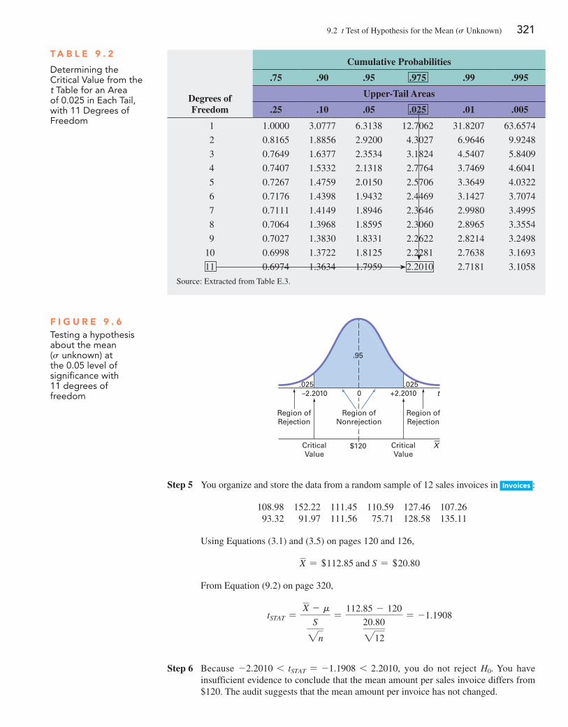
9.2 t Test of Hypothesis for the Mean (s Unknown) 321
Step 5 You organize and store the data from a random sample of 12 sales invoices in invoices :
108.98 152.22 111.45 110.59 127.46 107.2693.32 91.97 111.56 75.71 128.58 135.11
Using Equations (3.1) and (3.5) on pages 120 and 126,
X = +112.85 and S = +20.80
From Equation (9.2) on page 320,
tSTAT = X - m
S2n
=112.85 - 120
20.80212
= -1.1908
Region ofRejection
Region ofNonrejection
CriticalValue
Region ofRejection
CriticalValue
–2.2010 0 +2.2010 t.025 .025
$120 X
.95
F i g u R E 9 . 6Testing a hypothesis about the mean (s unknown) at the 0.05 level of significance with 11 degrees of freedom
Degrees of Freedom
Cumulative Probabilities
.75 .90 .95 .975 .99 .995
Upper-Tail Areas
.25 .10 .05 .025 .01 .005
1 1.0000 3.0777 6.3138 12.7062 31.8207 63.6574
2 0.8165 1.8856 2.9200 4.3027 6.9646 9.9248
3 0.7649 1.6377 2.3534 3.1824 4.5407 5.8409
4 0.7407 1.5332 2.1318 2.7764 3.7469 4.6041
5 0.7267 1.4759 2.0150 2.5706 3.3649 4.0322
6 0.7176 1.4398 1.9432 2.4469 3.1427 3.7074
7 0.7111 1.4149 1.8946 2.3646 2.9980 3.4995
8 0.7064 1.3968 1.8595 2.3060 2.8965 3.3554
9 0.7027 1.3830 1.8331 2.2622 2.8214 3.2498
10 0.6998 1.3722 1.8125 2.2281 2.7638 3.1693
11 0.6974 1.3634 1.7959 2.2010 2.7181 3.1058
Source: Extracted from Table E.3.
T A b l E 9 . 2
determining the Critical Value from the t Table for an area of 0.025 in Each Tail, with 11 degrees of Freedom
Step 6 Because -2.2010 6 tSTAT = -1.1908 6 2.2010, you do not reject H0. You have insufficient evidence to conclude that the mean amount per sales invoice differs from $120. The audit suggests that the mean amount per invoice has not changed.
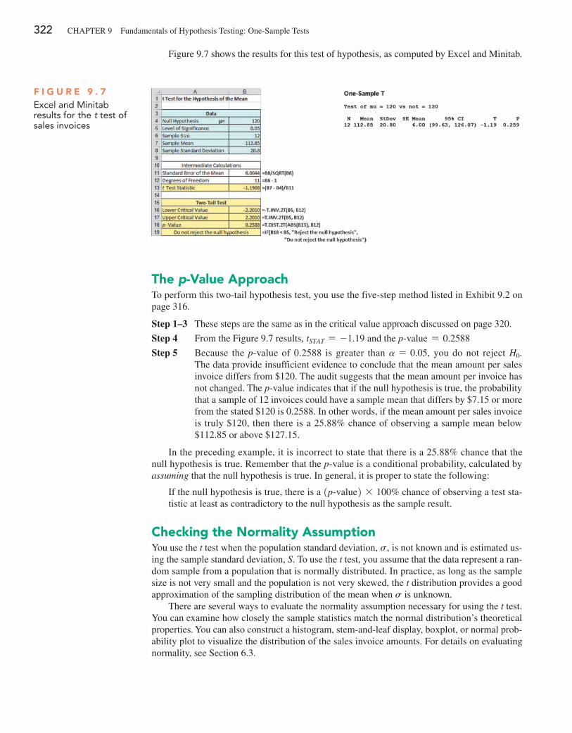
322 CHAPTEr 9 Fundamentals of Hypothesis Testing: One-Sample Tests
The p-Value ApproachTo perform this two-tail hypothesis test, you use the five-step method listed in Exhibit 9.2 on page 316.
Step 1–3 These steps are the same as in the critical value approach discussed on page 320.
Step 4 From the Figure 9.7 results, tSTAT = -1.19 and the p-value = 0.2588
Step 5 Because the p-value of 0.2588 is greater than a = 0.05, you do not reject H0. The data provide insufficient evidence to conclude that the mean amount per sales invoice differs from $120. The audit suggests that the mean amount per invoice has not changed. The p-value indicates that if the null hypothesis is true, the probability that a sample of 12 invoices could have a sample mean that differs by $7.15 or more from the stated $120 is 0.2588. In other words, if the mean amount per sales invoice is truly $120, then there is a 25.88% chance of observing a sample mean below $112.85 or above $127.15.
In the preceding example, it is incorrect to state that there is a 25.88% chance that the null hypothesis is true. remember that the p-value is a conditional probability, calculated by assuming that the null hypothesis is true. In general, it is proper to state the following:
If the null hypothesis is true, there is a 1p@value2 * 100% chance of observing a test sta-tistic at least as contradictory to the null hypothesis as the sample result.
Checking the Normality AssumptionYou use the t test when the population standard deviation, s, is not known and is estimated us-ing the sample standard deviation, S. To use the t test, you assume that the data represent a ran-dom sample from a population that is normally distributed. In practice, as long as the sample size is not very small and the population is not very skewed, the t distribution provides a good approximation of the sampling distribution of the mean when s is unknown.
There are several ways to evaluate the normality assumption necessary for using the t test. You can examine how closely the sample statistics match the normal distribution’s theoretical properties. You can also construct a histogram, stem-and-leaf display, boxplot, or normal prob-ability plot to visualize the distribution of the sales invoice amounts. For details on evaluating normality, see Section 6.3.
F i g u R E 9 . 7Excel and Minitab results for the t test of sales invoices
Figure 9.7 shows the results for this test of hypothesis, as computed by Excel and Minitab.
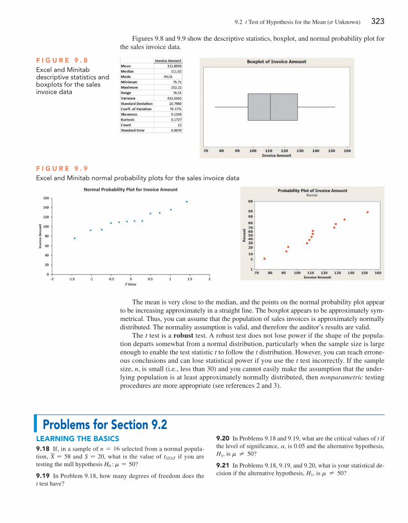
9.2 t Test of Hypothesis for the Mean (s Unknown) 323
Figures 9.8 and 9.9 show the descriptive statistics, boxplot, and normal probability plot for the sales invoice data.
The mean is very close to the median, and the points on the normal probability plot appear to be increasing approximately in a straight line. The boxplot appears to be approximately sym-metrical. Thus, you can assume that the population of sales invoices is approximately normally distributed. The normality assumption is valid, and therefore the auditor’s results are valid.
The t test is a robust test. A robust test does not lose power if the shape of the popula-tion departs somewhat from a normal distribution, particularly when the sample size is large enough to enable the test statistic t to follow the t distribution. However, you can reach errone-ous conclusions and can lose statistical power if you use the t test incorrectly. If the sample size, n, is small (i.e., less than 30) and you cannot easily make the assumption that the under-lying population is at least approximately normally distributed, then nonparametric testing procedures are more appropriate (see references 2 and 3).
F i g u R E 9 . 8Excel and Minitab descriptive statistics and boxplots for the sales invoice data
F i g u R E 9 . 9Excel and Minitab normal probability plots for the sales invoice data
problems for Section 9.2lEARNiNg THE bASiCS9.18 If, in a sample of n = 16 selected from a normal popula-tion, X = 58 and S = 20, what is the value of tSTAT if you are testing the null hypothesis H0 : m = 50?
9.19 In Problem 9.18, how many degrees of freedom does the t test have?
9.20 In Problems 9.18 and 9.19, what are the critical values of t if the level of significance, a, is 0.05 and the alternative hypothesis, H1, is m ≠ 50?
9.21 In Problems 9.18, 9.19, and 9.20, what is your statistical de-cision if the alternative hypothesis, H1, is m ≠ 50?
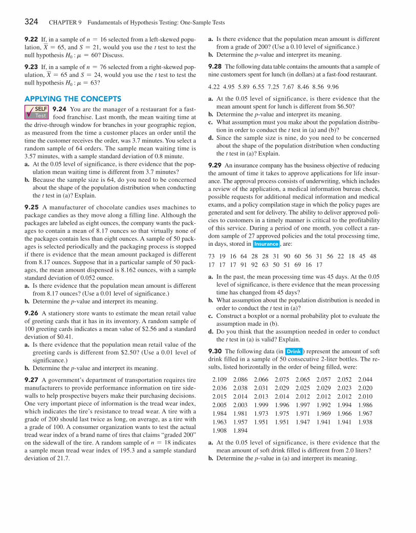
324 CHAPTEr 9 Fundamentals of Hypothesis Testing: One-Sample Tests
9.22 If, in a sample of n = 16 selected from a left-skewed popu-lation, X = 65, and S = 21, would you use the t test to test the null hypothesis H0 : m = 60? Discuss.
9.23 If, in a sample of n = 76 selected from a right-skewed pop-ulation, X = 65 and S = 24, would you use the t test to test the null hypothesis H0 : m = 63?
ApplyiNg THE CoNCEpTSSELF Test
9.24 You are the manager of a restaurant for a fast-food franchise. Last month, the mean waiting time at
the drive-through window for branches in your geographic region, as measured from the time a customer places an order until the time the customer receives the order, was 3.7 minutes. You select a random sample of 64 orders. The sample mean waiting time is 3.57 minutes, with a sample standard deviation of 0.8 minute.a. At the 0.05 level of significance, is there evidence that the pop-
ulation mean waiting time is different from 3.7 minutes?b. Because the sample size is 64, do you need to be concerned
about the shape of the population distribution when conducting the t test in (a)? Explain.
9.25 A manufacturer of chocolate candies uses machines to package candies as they move along a filling line. Although the packages are labeled as eight ounces, the company wants the pack-ages to contain a mean of 8.17 ounces so that virtually none of the packages contain less than eight ounces. A sample of 50 pack-ages is selected periodically and the packaging process is stopped if there is evidence that the mean amount packaged is different from 8.17 ounces. Suppose that in a particular sample of 50 pack-ages, the mean amount dispensed is 8.162 ounces, with a sample standard deviation of 0.052 ounce.a. Is there evidence that the population mean amount is different
from 8.17 ounces? (Use a 0.01 level of significance.)b. Determine the p-value and interpret its meaning.
9.26 A stationery store wants to estimate the mean retail value of greeting cards that it has in its inventory. A random sample of 100 greeting cards indicates a mean value of $2.56 and a standard deviation of $0.41.a. Is there evidence that the population mean retail value of the
greeting cards is different from $2.50? (Use a 0.01 level of significance.)
b. Determine the p-value and interpret its meaning.
9.27 A government’s department of transportation requires tire manufacturers to provide performance information on tire side-walls to help prospective buyers make their purchasing decisions. One very important piece of information is the tread wear index, which indicates the tire’s resistance to tread wear. A tire with a grade of 200 should last twice as long, on average, as a tire with a grade of 100. A consumer organization wants to test the actual tread wear index of a brand name of tires that claims “graded 200” on the sidewall of the tire. A random sample of n = 18 i ndicates a sample mean tread wear index of 195.3 and a sample standard deviation of 21.7.
a. Is there evidence that the population mean amount is different from a grade of 200? (Use a 0.10 level of significance.)
b. Determine the p-value and interpret its meaning.
9.28 The following data table contains the amounts that a sample of nine customers spent for lunch (in dollars) at a fast-food restaurant.
4.22 4.95 5.89 6.55 7.25 7.67 8.46 8.56 9.96
a. At the 0.05 level of significance, is there evidence that the mean amount spent for lunch is different from $6.50?
b. Determine the p-value and interpret its meaning.c. What assumption must you make about the population distribu-
tion in order to conduct the t test in (a) and (b)?d. Since the sample size is nine, do you need to be concerned
about the shape of the population distribution when conducting the t test in (a)? Explain.
9.29 An insurance company has the business objective of reducing the amount of time it takes to approve applications for life insur-ance. The approval process consists of underwriting, which includes a review of the application, a medical information bureau check, possible requests for additional medical information and medical exams, and a policy compilation stage in which the policy pages are generated and sent for delivery. The ability to deliver approved poli-cies to customers in a timely manner is critical to the profitability of this service. During a period of one month, you collect a ran-dom sample of 27 approved policies and the total processing time, in days, stored in insurance , are:
73 19 16 64 28 28 31 90 60 56 31 56 22 18 45 4817 17 17 91 92 63 50 51 69 16 17
a. In the past, the mean processing time was 45 days. At the 0.05 level of significance, is there evidence that the mean processing time has changed from 45 days?
b. What assumption about the population distribution is needed in order to conduct the t test in (a)?
c. Construct a boxplot or a normal probability plot to evaluate the assumption made in (b).
d. Do you think that the assumption needed in order to conduct the t test in (a) is valid? Explain.
9.30 The following data (in Drink ) represent the amount of soft drink filled in a sample of 50 consecutive 2-liter bottles. The re-sults, listed horizontally in the order of being filled, were:
2.109 2.086 2.066 2.075 2.065 2.057 2.052 2.0442.036 2.038 2.031 2.029 2.025 2.029 2.023 2.0202.015 2.014 2.013 2.014 2.012 2.012 2.012 2.0102.005 2.003 1.999 1.996 1.997 1.992 1.994 1.9861.984 1.981 1.973 1.975 1.971 1.969 1.966 1.9671.963 1.957 1.951 1.951 1.947 1.941 1.941 1.9381.908 1.894
a. At the 0.05 level of significance, is there evidence that the mean amount of soft drink filled is different from 2.0 liters?
b. Determine the p-value in (a) and interpret its meaning.
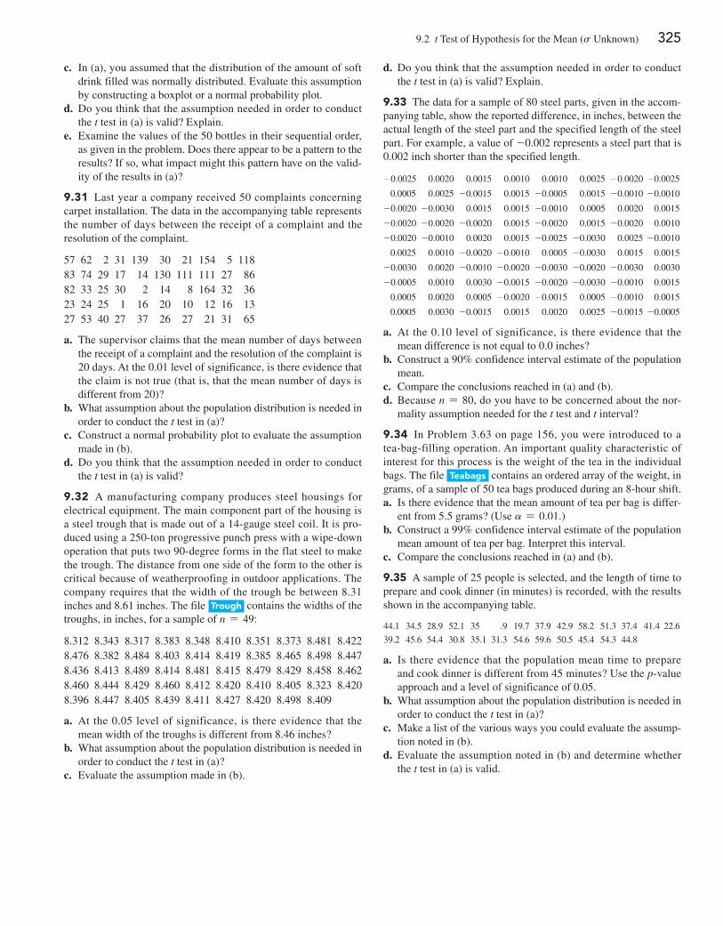
9.2 t Test of Hypothesis for the Mean (s Unknown) 325
c. In (a), you assumed that the distribution of the amount of soft drink filled was normally distributed. Evaluate this assumption by constructing a boxplot or a normal probability plot.
d. Do you think that the assumption needed in order to conduct the t test in (a) is valid? Explain.
e. Examine the values of the 50 bottles in their sequential order, as given in the problem. Does there appear to be a pattern to the results? If so, what impact might this pattern have on the valid-ity of the results in (a)?
9.31 Last year a company received 50 complaints concerning carpet installation. The data in the accompanying table represents the number of days between the receipt of a complaint and the resolution of the complaint.
57 62 2 31 139 30 21 154 5 11883 74 29 17 14 130 111 111 27 8682 33 25 30 2 14 8 164 32 3623 24 25 1 16 20 10 12 16 1327 53 40 27 37 26 27 21 31 65
a. The supervisor claims that the mean number of days between the receipt of a complaint and the resolution of the complaint is 20 days. At the 0.01 level of significance, is there evidence that the claim is not true (that is, that the mean number of days is different from 20)?
b. What assumption about the population distribution is needed in order to conduct the t test in (a)?
c. Construct a normal probability plot to evaluate the assumption made in (b).
d. Do you think that the assumption needed in order to conduct the t test in (a) is valid?
9.32 A manufacturing company produces steel housings for electrical equipment. The main component part of the housing is a steel trough that is made out of a 14-gauge steel coil. It is pro-duced using a 250-ton progressive punch press with a wipe-down operation that puts two 90-degree forms in the flat steel to make the trough. The distance from one side of the form to the other is critical because of weatherproofing in outdoor applications. The company requires that the width of the trough be between 8.31 inches and 8.61 inches. The file Trough contains the widths of the troughs, in inches, for a sample of n = 49:
8.312 8.343 8.317 8.383 8.348 8.410 8.351 8.373 8.481 8.4228.476 8.382 8.484 8.403 8.414 8.419 8.385 8.465 8.498 8.4478.436 8.413 8.489 8.414 8.481 8.415 8.479 8.429 8.458 8.4628.460 8.444 8.429 8.460 8.412 8.420 8.410 8.405 8.323 8.4208.396 8.447 8.405 8.439 8.411 8.427 8.420 8.498 8.409
a. At the 0.05 level of significance, is there evidence that the mean width of the troughs is different from 8.46 inches?
b. What assumption about the population distribution is needed in order to conduct the t test in (a)?
c. Evaluate the assumption made in (b).
d. Do you think that the assumption needed in order to conduct the t test in (a) is valid? Explain.
9.33 The data for a sample of 80 steel parts, given in the accom-panying table, show the reported difference, in inches, between the actual length of the steel part and the specified length of the steel part. For example, a value of -0.002 represents a steel part that is 0.002 inch shorter than the specified length.
-0.0025 0.0020 0.0015 0.0010 0.0010 0.0025 -0.0020 -0.0025
0.0005 0.0025 -0.0015 0.0015 -0.0005 0.0015 -0.0010 -0.0010
-0.0020 -0.0030 0.0015 0.0015 -0.0010 0.0005 0.0020 0.0015
-0.0020 -0.0020 -0.0020 0.0015 -0.0020 0.0015 -0.0020 0.0010
-0.0020 -0.0010 0.0020 0.0015 -0.0025 -0.0030 0.0025 -0.0010
0.0025 0.0010 -0.0020 -0.0010 0.0005 -0.0030 0.0015 0.0015
-0.0030 0.0020 -0.0010 -0.0020 -0.0030 -0.0020 -0.0030 0.0030
-0.0005 0.0010 0.0030 -0.0015 -0.0020 -0.0030 -0.0010 0.0015
0.0005 0.0020 0.0005 -0.0020 -0.0015 0.0005 -0.0010 0.0015
0.0005 0.0030 -0.0015 0.0015 0.0020 0.0025 -0.0015 -0.0005
a. At the 0.10 level of significance, is there evidence that the mean difference is not equal to 0.0 inches?
b. Construct a 90% confidence interval estimate of the population mean.
c. Compare the conclusions reached in (a) and (b).d. Because n = 80, do you have to be concerned about the nor-
mality assumption needed for the t test and t interval?
9.34 In Problem 3.63 on page 156, you were introduced to a tea-bag-filling operation. An important quality characteristic of interest for this process is the weight of the tea in the individual bags. The file Teabags contains an ordered array of the weight, in grams, of a sample of 50 tea bags produced during an 8-hour shift.a. Is there evidence that the mean amount of tea per bag is differ-
ent from 5.5 grams? (Use a = 0.01.)b. Construct a 99% confidence interval estimate of the population
mean amount of tea per bag. Interpret this interval.c. Compare the conclusions reached in (a) and (b).
9.35 A sample of 25 people is selected, and the length of time to prepare and cook dinner (in minutes) is recorded, with the results shown in the accompanying table.
44.1 34.5 28.9 52.1 35 .9 19.7 37.9 42.9 58.2 51.3 37.4 41.4 22.6
39.2 45.6 54.4 30.8 35.1 31.3 54.6 59.6 50.5 45.4 54.3 44.8
a. Is there evidence that the population mean time to prepare and cook dinner is different from 45 minutes? Use the p-value approach and a level of significance of 0.05.
b. What assumption about the population distribution is needed in order to conduct the t test in (a)?
c. Make a list of the various ways you could evaluate the assump-tion noted in (b).
d. Evaluate the assumption noted in (b) and determine whether the t test in (a) is valid.
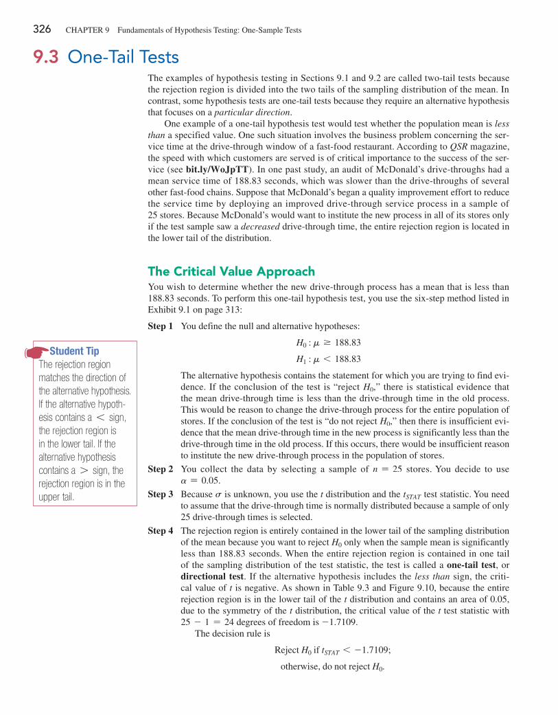
326 CHAPTEr 9 Fundamentals of Hypothesis Testing: One-Sample Tests
Student TipThe rejection region matches the direction of the alternative hypothesis. If the alternative hypoth-esis contains a 6 sign, the rejection region is in the lower tail. If the alternative hypothesis contains a 7 sign, the rejection region is in the upper tail.
9.3 One-Tail TestsThe examples of hypothesis testing in Sections 9.1 and 9.2 are called two-tail tests because the rejection region is divided into the two tails of the sampling distribution of the mean. In contrast, some hypothesis tests are one-tail tests because they require an alternative hypothesis that focuses on a particular direction.
One example of a one-tail hypothesis test would test whether the population mean is less than a specified value. One such situation involves the business problem concerning the ser-vice time at the drive-through window of a fast-food restaurant. According to QSR magazine, the speed with which customers are served is of critical importance to the success of the ser-vice (see bit.ly/WoJpTT). In one past study, an audit of McDonald’s drive-throughs had a mean service time of 188.83 seconds, which was slower than the drive-throughs of several other fast-food chains. Suppose that McDonald’s began a quality improvement effort to reduce the service time by deploying an improved drive-through service process in a sample of 25 stores. Because McDonald’s would want to institute the new process in all of its stores only if the test sample saw a decreased drive-through time, the entire rejection region is located in the lower tail of the distribution.
The Critical Value ApproachYou wish to determine whether the new drive-through process has a mean that is less than 188.83 seconds. To perform this one-tail hypothesis test, you use the six-step method listed in Exhibit 9.1 on page 313:
Step 1 You define the null and alternative hypotheses:
H0 : m Ú 188.83
H1 : m 6 188.83
The alternative hypothesis contains the statement for which you are trying to find evi-dence. If the conclusion of the test is “reject H0,” there is statistical evidence that the mean drive-through time is less than the drive-through time in the old process. This would be reason to change the drive-through process for the entire population of stores. If the conclusion of the test is “do not reject H0,” then there is insufficient evi-dence that the mean drive-through time in the new process is significantly less than the drive-through time in the old process. If this occurs, there would be insufficient reason to institute the new drive-through process in the population of stores.
Step 2 You collect the data by selecting a sample of n = 25 stores. You decide to use a = 0.05.
Step 3 Because s is unknown, you use the t distribution and the tSTAT test statistic. You need to assume that the drive-through time is normally distributed because a sample of only 25 drive-through times is selected.
Step 4 The rejection region is entirely contained in the lower tail of the sampling distribution of the mean because you want to reject H0 only when the sample mean is significantly less than 188.83 seconds. When the entire rejection region is contained in one tail of the sampling distribution of the test statistic, the test is called a one-tail test, or directional test. If the alternative hypothesis includes the less than sign, the criti-cal value of t is negative. As shown in Table 9.3 and Figure 9.10, because the entire rejection region is in the lower tail of the t distribution and contains an area of 0.05, due to the symmetry of the t distribution, the critical value of the t test statistic with 25 - 1 = 24 degrees of freedom is -1.7109.
The decision rule is
reject H0 if tSTAT 6 -1.7109;
otherwise, do not reject H0.
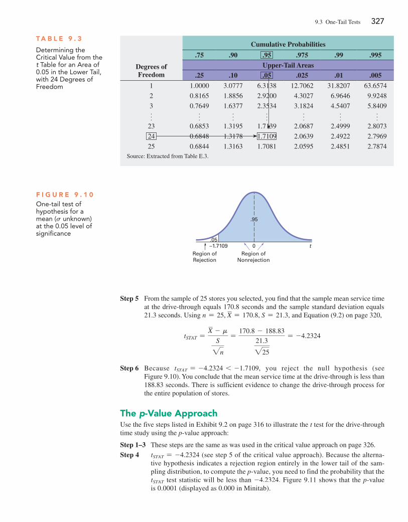
9.3 One-Tail Tests 327
Step 5 From the sample of 25 stores you selected, you find that the sample mean service time at the drive-through equals 170.8 seconds and the sample standard deviation equals 21.3 seconds. Using n = 25, X = 170.8, S = 21.3, and Equation (9.2) on page 320,
tSTAT =X - m
S2n
=170.8 - 188.83
21.3225
= -4.2324
Step 6 Because tSTAT = -4.2324 6 -1.7109, you reject the null hypothesis (see Figure 9.10). You conclude that the mean service time at the drive-through is less than 188.83 seconds. There is sufficient evidence to change the drive-through process for the entire population of stores.
The p-Value ApproachUse the five steps listed in Exhibit 9.2 on page 316 to illustrate the t test for the drive-through time study using the p-value approach:
Step 1–3 These steps are the same as was used in the critical value approach on page 326.
Step 4 tSTAT = -4.2324 (see step 5 of the critical value approach). Because the alterna-tive hypothesis indicates a rejection region entirely in the lower tail of the sam-pling distribution, to compute the p-value, you need to find the probability that the tSTAT test statistic will be less than -4.2324. Figure 9.11 shows that the p-value is 0.0001 (displayed as 0.000 in Minitab).
F i g u R E 9 . 1 0One-tail test of hypothesis for a mean (s unknown) at the 0.05 level of significance
0–1.7109 tRegion ofRejection
Region ofNonrejection
.05
.95
Degrees of Freedom
Cumulative Probabilities
.75 .90 .95 .975 .99 .995
Upper-Tail Areas
.25 .10 .05 .025 .01 .005
1 1.0000 3.0777 6.3138 12.7062 31.8207 63.6574
2 0.8165 1.8856 2.9200 4.3027 6.9646 9.9248
3 0.7649 1.6377 2.3534 3.1824 4.5407 5.8409f f f f f f f
23 0.6853 1.3195 1.7139 2.0687 2.4999 2.8073
24 0.6848 1.3178 1.7109 2.0639 2.4922 2.7969
25 0.6844 1.3163 1.7081 2.0595 2.4851 2.7874Source: Extracted from Table E.3.
T A b l E 9 . 3
determining the Critical Value from the t Table for an area of 0.05 in the Lower Tail, with 24 degrees of Freedom
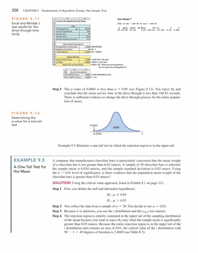
328 CHAPTEr 9 Fundamentals of Hypothesis Testing: One-Sample Tests
Step 5 The p-value of 0.0001 is less than a = 0.05 (see Figure 9.12). You reject H0 and conclude that the mean service time at the drive-through is less than 188.83 seconds. There is sufficient evidence to change the drive-through process for the entire popula-tion of stores.
F i g u R E 9 . 1 1Excel and Minitab t test results for the drive-through time study
–4.2324
.9999
t
0.0001
F i g u R E 9 . 1 2determining the p-value for a one-tail test
Example 9.5 illustrates a one-tail test in which the rejection region is in the upper tail.
ExAmplE 9.5a One-tail test for the Mean
A company that manufactures chocolate bars is particularly concerned that the mean weight of a chocolate bar is not greater than 6.03 ounces. A sample of 50 chocolate bars is selected; the sample mean is 6.034 ounces, and the sample standard deviation is 0.02 ounce. Using the a = 0.01 level of significance, is there evidence that the population mean weight of the chocolate bars is greater than 6.03 ounces?
SoluTioN Using the critical value approach, listed in Exhibit 9.1 on page 313,
Step 1 First, you define the null and alternative hypotheses:
H0 : m … 6.03
H1 : m 7 6.03
Step 2 You collect the data from a sample of n = 50. You decide to use a = 0.01.
Step 3 Because s is unknown, you use the t distribution and the tSTAT test statistic.
Step 4 The rejection region is entirely contained in the upper tail of the sampling distribution of the mean because you want to reject H0 only when the sample mean is significantly greater than 6.03 ounces. Because the entire rejection region is in the upper tail of the t distribution and contains an area of 0.01, the critical value of the t distribution with 50 - 1 = 49 degrees of freedom is 2.4049 (see Table E.3).
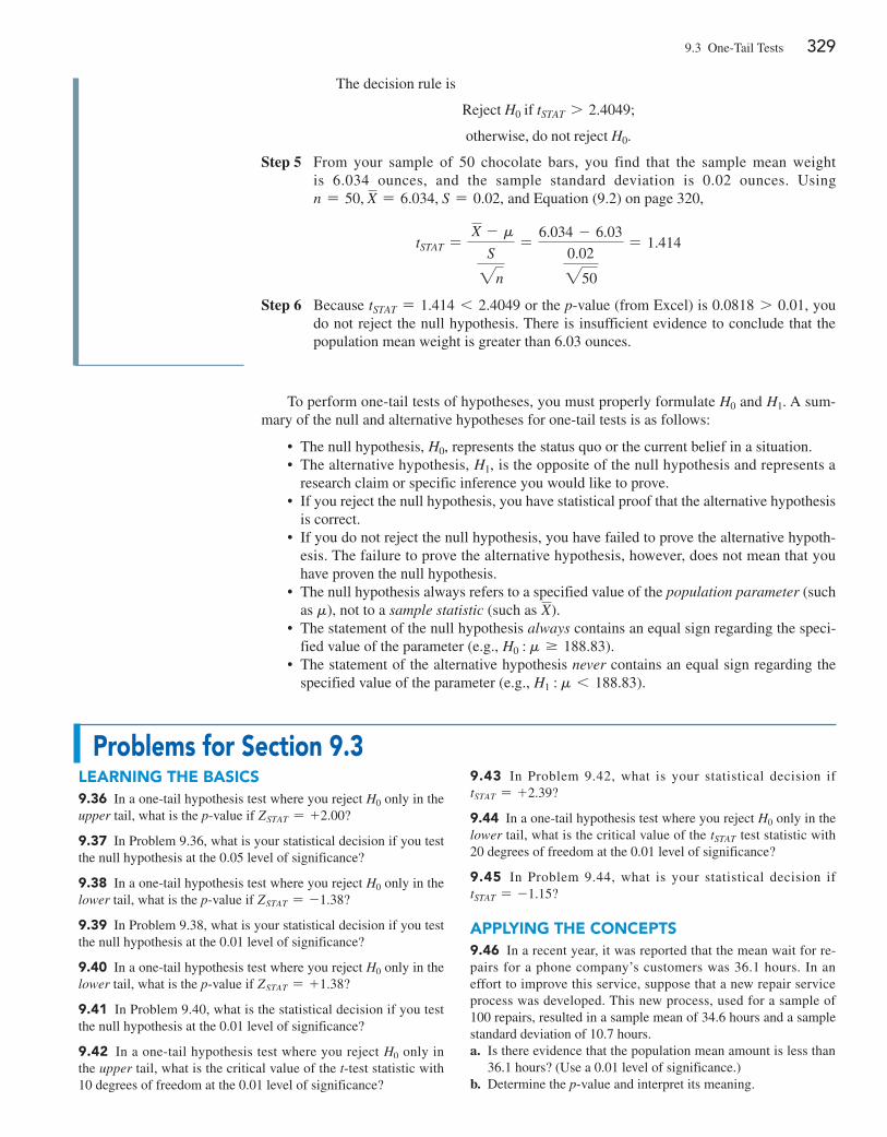
9.3 One-Tail Tests 329
The decision rule is
reject H0 if tSTAT 7 2.4049;
otherwise, do not reject H0.
Step 5 From your sample of 50 chocolate bars, you find that the sample mean weight is 6.034 ounces, and the sample standard deviation is 0.02 ounces. Using n = 50, X = 6.034, S = 0.02, and Equation (9.2) on page 320,
tSTAT = X - m
S2n
=6.034 - 6.03
0.02250
= 1.414
Step 6 Because tSTAT = 1.414 6 2.4049 or the p-value (from Excel) is 0.0818 7 0.01, you do not reject the null hypothesis. There is insufficient evidence to conclude that the population mean weight is greater than 6.03 ounces.
To perform one-tail tests of hypotheses, you must properly formulate H0 and H1. A sum-mary of the null and alternative hypotheses for one-tail tests is as follows:
• The null hypothesis, H0, represents the status quo or the current belief in a situation. • The alternative hypothesis, H1, is the opposite of the null hypothesis and represents a
research claim or specific inference you would like to prove. • If you reject the null hypothesis, you have statistical proof that the alternative hypothesis
is correct. • If you do not reject the null hypothesis, you have failed to prove the alternative hypoth-
esis. The failure to prove the alternative hypothesis, however, does not mean that you have proven the null hypothesis.
• The null hypothesis always refers to a specified value of the population parameter (such as m), not to a sample statistic (such as X).
• The statement of the null hypothesis always contains an equal sign regarding the speci-fied value of the parameter (e.g., H0 : m Ú 188.83).
• The statement of the alternative hypothesis never contains an equal sign regarding the specified value of the parameter (e.g., H1 : m 6 188.83).
problems for Section 9.3lEARNiNg THE bASiCS9.36 In a one-tail hypothesis test where you reject H0 only in the upper tail, what is the p-value if ZSTAT = +2.00?
9.37 In Problem 9.36, what is your statistical decision if you test the null hypothesis at the 0.05 level of significance?
9.38 In a one-tail hypothesis test where you reject H0 only in the lower tail, what is the p-value if ZSTAT = -1.38?
9.39 In Problem 9.38, what is your statistical decision if you test the null hypothesis at the 0.01 level of significance?
9.40 In a one-tail hypothesis test where you reject H0 only in the lower tail, what is the p-value if ZSTAT = +1.38?
9.41 In Problem 9.40, what is the statistical decision if you test the null hypothesis at the 0.01 level of significance?
9.42 In a one-tail hypothesis test where you reject H0 only in the upper tail, what is the critical value of the t-test statistic with 10 degrees of freedom at the 0.01 level of significance?
9.43 In Problem 9.42, what is your statistical decision if tSTAT = +2.39?
9.44 In a one-tail hypothesis test where you reject H0 only in the lower tail, what is the critical value of the tSTAT test statistic with 20 degrees of freedom at the 0.01 level of significance?
9.45 In Problem 9.44, what is your statistical decision if tSTAT = -1.15?
ApplyiNg THE CoNCEpTS9.46 In a recent year, it was reported that the mean wait for re-pairs for a phone company’s customers was 36.1 hours. In an effort to improve this service, suppose that a new repair service process was developed. This new process, used for a sample of 100 repairs, resulted in a sample mean of 34.6 hours and a sample standard deviation of 10.7 hours.a. Is there evidence that the population mean amount is less than
36.1 hours? (Use a 0.01 level of significance.)b. Determine the p-value and interpret its meaning.
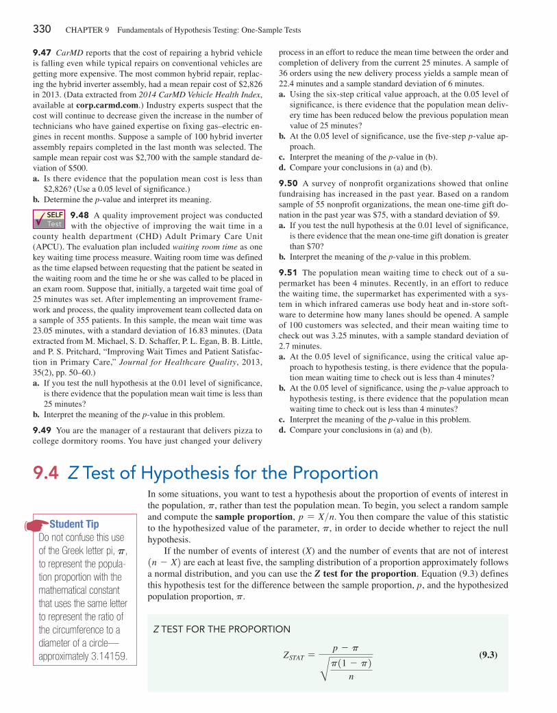
330 CHAPTEr 9 Fundamentals of Hypothesis Testing: One-Sample Tests
9.47 CarMD reports that the cost of repairing a hybrid vehicle is falling even while typical repairs on conventional vehicles are getting more expensive. The most common hybrid repair, replac-ing the hybrid inverter assembly, had a mean repair cost of $2,826 in 2013. (Data extracted from 2014 CarMD Vehicle Health Index, available at corp.carmd.com.) Industry experts suspect that the cost will continue to decrease given the increase in the number of technicians who have gained expertise on fixing gas–electric en-gines in recent months. Suppose a sample of 100 hybrid inverter assembly repairs completed in the last month was selected. The sample mean repair cost was $2,700 with the sample standard de-viation of $500.a. Is there evidence that the population mean cost is less than
$2,826? (Use a 0.05 level of significance.)b. Determine the p-value and interpret its meaning.
SELF Test
9.48 A quality improvement project was conducted with the objective of improving the wait time in a
county health department (CHD) Adult Primary Care Unit (APCU). The evaluation plan included waiting room time as one key waiting time process measure. Waiting room time was defined as the time elapsed between requesting that the patient be seated in the waiting room and the time he or she was called to be placed in an exam room. Suppose that, initially, a targeted wait time goal of 25 minutes was set. After implementing an improvement frame-work and process, the quality improvement team collected data on a sample of 355 patients. In this sample, the mean wait time was 23.05 minutes, with a standard deviation of 16.83 minutes. (Data extracted from M. Michael, S. D. Schaffer, P. L. Egan, B. B. Little, and P. S. Pritchard, “Improving Wait Times and Patient Satisfac-tion in Primary Care,” Journal for Healthcare Quality, 2013, 35(2), pp. 50–60.)a. If you test the null hypothesis at the 0.01 level of significance,
is there evidence that the population mean wait time is less than 25 minutes?
b. Interpret the meaning of the p-value in this problem.
9.49 You are the manager of a restaurant that delivers pizza to college dormitory rooms. You have just changed your delivery
process in an effort to reduce the mean time between the order and completion of delivery from the current 25 minutes. A sample of 36 orders using the new delivery process yields a sample mean of 22.4 minutes and a sample standard deviation of 6 minutes.a. Using the six-step critical value approach, at the 0.05 level of
significance, is there evidence that the population mean deliv-ery time has been reduced below the previous population mean value of 25 minutes?
b. At the 0.05 level of significance, use the five-step p-value ap-proach.
c. Interpret the meaning of the p-value in (b).d. Compare your conclusions in (a) and (b).
9.50 A survey of nonprofit organizations showed that online fundraising has increased in the past year. Based on a random sample of 55 nonprofit organizations, the mean one-time gift do-nation in the past year was $75, with a standard deviation of $9.a. If you test the null hypothesis at the 0.01 level of significance,
is there evidence that the mean one-time gift donation is greater than $70?
b. Interpret the meaning of the p-value in this problem.
9.51 The population mean waiting time to check out of a su-permarket has been 4 minutes. recently, in an effort to reduce the waiting time, the supermarket has experimented with a sys-tem in which infrared cameras use body heat and in-store soft-ware to determine how many lanes should be opened. A sample of 100 customers was selected, and their mean waiting time to check out was 3.25 minutes, with a sample standard deviation of 2.7 minutes.a. At the 0.05 level of significance, using the critical value ap-
proach to hypothesis testing, is there evidence that the popula-tion mean waiting time to check out is less than 4 minutes?
b. At the 0.05 level of significance, using the p-value approach to hypothesis testing, is there evidence that the population mean waiting time to check out is less than 4 minutes?
c. Interpret the meaning of the p-value in this problem.d. Compare your conclusions in (a) and (b).
9.4 Z Test of Hypothesis for the ProportionIn some situations, you want to test a hypothesis about the proportion of events of interest in the population, p, rather than test the population mean. To begin, you select a random sample and compute the sample proportion, p = X>n. You then compare the value of this statistic to the hypothesized value of the parameter, p, in order to decide whether to reject the null hypothesis.
If the number of events of interest (X) and the number of events that are not of interest 1n - X2 are each at least five, the sampling distribution of a proportion approximately follows a normal distribution, and you can use the Z test for the proportion. Equation (9.3) defines this hypothesis test for the difference between the sample proportion, p, and the hypothesized population proportion, p.
Student TipDo not confuse this use of the Greek letter pi, p, to represent the popula-tion proportion with the mathematical constant that uses the same letter to represent the ratio of the circumference to a diameter of a circle—approximately 3.14159.
Z TEsT FOR THE PROPORTIOn
ZSTAT =p - pBp11 - p2
n
(9.3)
9.4 Z Test of Hypothesis for the Proportion 331
Alternatively, by multiplying the numerator and denominator by n, you can write the ZSTAT test statistic in terms of the number of events of interest, X, as shown in Equation (9.4).
where
p = sample proportion =Xn=
number of events of interest in the sample
sample sizep = hypothesized proportion of events of interest in the population
The ZSTAT test statistic approximately follows a standardized normal distribution when X and 1n - X2 are each at least 5.
Z TEsT FOR THE PROPORTIOn In TERMs OF THE nUMBER OF EVEnTs OF InTEREsT
ZSTAT =X - np2np11 - p2
(9.4)
The Critical Value ApproachIn a survey of 792 Internet users, 681 said that they had taken steps to remove or mask their digital footprints. (Source: E. Dwoskin, “Give Me Back My Privacy,” The Wall Street Journal, March 24, 2014, p. r2.) Suppose that a survey conducted in the previous year indicated that 80% of Internet users said that they had taken steps to remove or mask their digital footprints. Is there evidence that the proportion of Internet users who said that they had taken steps to remove or mask their digital footprints has changed from the previous year? To investigate this question, the null and alternative hypotheses are as follows:
H0 : p = 0.80 (i.e., the proportion of Internet users who said that they had taken steps to re-move or mask their digital footprints has not changed from the previous year)
H1 : p ≠ 0.80 (i.e., the proportion of Internet users who said that they had taken steps to remove or mask their digital footprints has changed from the previous year)
Because you are interested in determining whether the population proportion of Internet users who said that they had taken steps to remove or mask their digital footprints has changed from 0.80 in the previous year, you use a two-tail test. If you select the a = 0.05 level of sig-nificance, the rejection and nonrejection regions are set up as in Figure 9.13, and the decision rule is
reject H0 if ZSTAT 6 -1.96 or if ZSTAT 7 +1.96;
otherwise, do not reject H0.
0–1.96 +1.96 ZRegion ofRejection
Region ofNonrejection
Region ofRejection
.95
F i g u R E 9 . 1 3Two-tail test of hypothesis for the proportion at the 0.05 level of significance
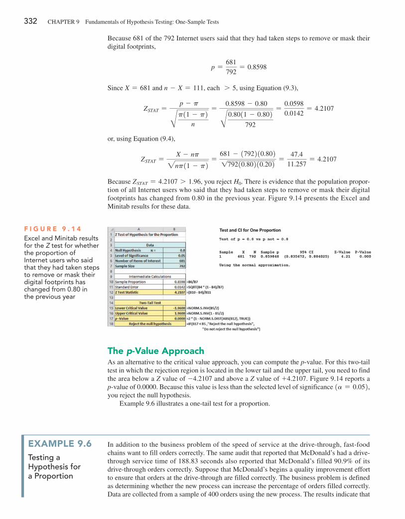
332 CHAPTEr 9 Fundamentals of Hypothesis Testing: One-Sample Tests
Because 681 of the 792 Internet users said that they had taken steps to remove or mask their digital footprints,
p =681
792= 0.8598
Since X = 681 and n - X = 111, each 7 5, using Equation (9.3),
ZSTAT =p - pBp11 - p2
n
=0.8598 - 0.80B0.8011 - 0.802
792
=0.0598
0.0142= 4.2107
or, using Equation (9.4),
ZSTAT =X - np2np11 - p2
=681 - 1792210.802179210.80210.202 =
47.4
11.257= 4.2107
Because ZSTAT = 4.2107 7 1.96, you reject H0. There is evidence that the population propor-tion of all Internet users who said that they had taken steps to remove or mask their digital footprints has changed from 0.80 in the previous year. Figure 9.14 presents the Excel and Minitab results for these data.
F i g u R E 9 . 1 4Excel and Minitab results for the Z test for whether the proportion of Internet users who said that they had taken steps to remove or mask their digital footprints has changed from 0.80 in the previous year
The p-Value ApproachAs an alternative to the critical value approach, you can compute the p-value. For this two-tail test in which the rejection region is located in the lower tail and the upper tail, you need to find the area below a Z value of -4.2107 and above a Z value of +4.2107. Figure 9.14 reports a p-value of 0.0000. Because this value is less than the selected level of significance 1a = 0.052, you reject the null hypothesis.
Example 9.6 illustrates a one-tail test for a proportion.
ExAmplE 9.6testing a hypothesis for a Proportion
In addition to the business problem of the speed of service at the drive-through, fast-food chains want to fill orders correctly. The same audit that reported that McDonald’s had a drive-through service time of 188.83 seconds also reported that McDonald’s filled 90.9% of its drive-through orders correctly. Suppose that McDonald’s begins a quality improvement effort to ensure that orders at the drive-through are filled correctly. The business problem is defined as determining whether the new process can increase the percentage of orders filled correctly. Data are collected from a sample of 400 orders using the new process. The results indicate that
9.4 Z Test of Hypothesis for the Proportion 333
378 orders were filled correctly. At the 0.01 level of significance, can you conclude that the new process has increased the proportion of orders filled correctly?
SoluTioN The null and alternative hypotheses are
H0 : p … 0.909 (i.e., the population proportion of orders filled correctly using the new process is less than or equal to 0.909)
H1 : p 7 0.909 (i.e., the population proportion of orders filled correctly using the new process is greater than 0.909)
Since X = 378 and n - X = 22, both 7 5, using Equation (9.3) on page 330,
p =Xn=
378
400= 0.945
ZSTAT =p - pBp11 - p2
n
=0.945 - 0.909B0.90911 - 0.9092
400
=0.036
0.0144= 2.5034
The p-value (computed by Excel) for ZSTAT 7 2.5034 is 0.0062.Using the critical value approach, you reject H0 if ZSTAT 7 2.33. Using the p-value
approach, you reject H0 if the p-value 6 0.01. Because ZSTAT = 2.5034 7 2.33 or the p-value = 0.0062 6 0.01, you reject H0. You have evidence that the new process has in-creased the proportion of correct orders above 0.909 or 90.9%.
problems for Section 9.4lEARNiNg THE bASiCS9.52 If, in a random sample of 400 items, 88 are defective, what is the sample proportion of defective items?
9.53 In Problem 9.52, if the null hypothesis is that 20% of the items in the population are defective, what is the value of ZSTAT?
9.54 In Problems 9.52 and 9.53, suppose you are testing the null hypothesis H0 : p = 0.20 against the two-tail alternative hy-pothesis H1 : p ≠ 0.20 and you choose the level of significance a = 0.05. What is your statistical decision?
ApplyiNg THE CoNCEpTS9.55 According to a recent National Association of Colleges and Employers (NACE) report, 48% of college student internships are unpaid. (Source: “Just 38 Percent of Unpaid Internships Were Subject to FLSA Guidelines,” bit.ly/Rx76M8.) A recent survey of 60 college interns at a local university found that 30 had unpaid internships.a. Use the five-step p-value approach to hypothesis testing and
a 0.05 level of significance to determine whether the propor-tion of college interns that had unpaid internships is different from 0.48.
b. Assume that the study found that 37 of the 60 college interns had unpaid internships and repeat (a). Are the conclusions the same?
9.56 The worldwide market share for the Mozilla Firefox web browser was 17% in a recent month. (Data extracted from netmarketshare.com.) Suppose that you decide to select a sample
of 100 students at your university and you find that 22 use the Mozilla Firefox web browser.a. Use the five-step p-value approach to try to determine whether
there is evidence that the market share for the Mozilla Firefox web browser at your university is greater than the worldwide market share of 17%. (Use the 0.05 level of significance.)
b. Suppose that the sample size is n = 400, and you find that 22% of the sample of students at your university (88 out of 400) use the Mozilla Firefox web browser. Use the five-step p-value approach to try to determine whether there is evidence that the market share for the Mozilla Firefox web browser at your university is greater than the worldwide market share of 17%. (Use the 0.05 level of significance.)
c. Discuss the effect that sample size has on hypothesis testing.d. What do you think are your chances of rejecting any null hy-
pothesis concerning a population proportion if a sample size of n = 20 is used?
9.57 One of the issues facing organizations is increasing diver-sity throughout an organization. One of the ways to evaluate an organization’s success at increasing diversity is to compare the percentage of employees in the organization in a particular posi-tion with a specific background to the percentage in a particular position with that specific background in the general workforce. recently, a large academic medical center determined that 9 of 17 employees in a particular position were female, whereas 55% of the employees for this position in the general workforce were fe-male. At the 0.05 level of significance, is there evidence that the proportion of females in this position at this medical center is dif-ferent from what would be expected in the general workforce?
334 CHAPTEr 9 Fundamentals of Hypothesis Testing: One-Sample Tests
SELF Test
9.58 How do professionals stay on top of their ca-reers? Of 935 surveyed U.S. LinkedIn members, 543
reported that they engaged in professional networking within the last month. (Source: LinkedIn Talent Solutions, Talent Trends 2014, available at linkd.in/Rx7o5T.) At the 0.05 level of signifi-cance, is there evidence that the proportion of all LinkedIn mem-bers who engaged in professional networking within the last month is different from 52%?
9.59 A cellphone provider has the business objective of wanting to determine the proportion of subscribers who would upgrade to a new cellphone with improved features if it were made available at a substantially reduced cost. Data are collected from a random sample of 500 subscribers. The results indicate that 135 of the sub-scribers would upgrade to a new cellphone at a reduced cost.a. At the 0.05 level of significance, is there evidence that more
than 20% of the customers would upgrade to a new cellphone at a reduced cost?
b. How would the manager in charge of promotional programs concerning residential customers use the results in (a)?
9.60 A study reported that 6% of the respondents were “Omnivores” who are gadget lovers, text messengers, and online gamers (often with their own blogs or Web pages), video makers, and YouTube posters. Suppose you believe that the percentage of students at your school who are Omnivores is greater than 6% and you plan to carry out a study to prove that this is so. You select a sample of 250 students and find that 23 can be classified as Omnivores.a. State the null and alternative hypotheses.b. Use either the critical value hypothesis-testing approach
or the p-value approach to determine at the 0.05 level of significance whether there is evidence that the percentage of Omnivores at your school is greater than 6%.
9.5 Potential Hypothesis-Testing Pitfalls and Ethical IssuesTo this point, you have studied the fundamental concepts of hypothesis testing. You have used hypothesis testing to analyze differences between sample statistics and hypothesized population parameters in order to make business decisions concerning the underlying popu-lation characteristics. You have also learned how to evaluate the risks involved in making these decisions.
When planning to carry out a hypothesis test based on a survey, research study, or designed experiment, you must ask several questions to ensure that you use proper methodology. You need to raise and answer questions such as the following in the planning stage:
• What is the goal of the survey, study, or experiment? How can you translate the goal into a null hypothesis and an alternative hypothesis?
• Is the hypothesis test a two-tail test or one-tail test?• Can you select a random sample from the underlying population of interest?• What types of data will you collect in the sample? Are the variables numerical
or categorical?• At what level of significance should you conduct the hypothesis test?• Is the intended sample size large enough to achieve the desired power of the test
for the level of significance chosen?• What statistical test procedure should you use and why?• What conclusions and interpretations can you reach from the results of the
hypothesis test?
Failing to consider these questions early in the planning process can lead to biased or incomplete results. Proper planning can help ensure that the statistical study will provide objective information needed to make good business decisions.
Statistical Significance Versus practical SignificanceYou need to make a distinction between the existence of a statistically significant result and its practical significance in a field of application. Sometimes, due to a very large sample size, you may get a result that is statistically significant but has little practical significance.
9.5 Potential Hypothesis-Testing Pitfalls and Ethical Issues 335
For example, suppose that prior to a national marketing campaign focusing on a series of expensive television commercials, you believe that the proportion of people who recognize your brand is 0.30. At the completion of the campaign, a survey of 20,000 people indi-cates that 6,168 recognized your brand. A one-tail test trying to prove that the proportion is now greater than 0.30 results in a p-value of 0.0047, and the correct statistical conclusion is that the proportion of consumers recognizing your brand name has now increased. Was the campaign successful? The result of the hypothesis test indicates a statistically significant increase in brand awareness, but is this increase practically important? The population pro-portion is now estimated at 6,168>20,000 = 0.3084 = 0.3084 or 30.84%. This increase is less than 1% more than the hypothesized value of 30%. Did the large expenses associated with the marketing campaign produce a result with a meaningful increase in brand aware-ness? Because of the minimal real-world impact that an increase of less than 1% has on the overall marketing strategy and the huge expenses associated with the marketing campaign, you should conclude that the campaign was not successful. On the other hand, if the cam-paign increased brand awareness from 30% to 50%, you would be inclined to conclude that the campaign was successful.
Statistical Insignificance Versus importanceIn contrast to the issue of the practical significance of a statistically significant result is the situation in which an important result may not be statistically significant. In a recent case (see reference 1), the U.S. Supreme Court ruled that companies cannot rely solely on whether the result of a study is significant when determining what they communicate to investors. In some situations (see reference 6), the lack of a large enough sample size may result in a nonsignificant result when in fact an important difference does exist. A study that compared male and female entrepreneurship rates globally and within Massachusetts found a significant difference globally but not within Massachusetts, even though the entrepre-neurship rates for females and for males in the two geographic areas were similar (8.8% for males in Massachusetts as compared to 8.4% globally; 5% for females in both geographic areas). The difference was due to the fact that the global sample size was 20 times larger than the Massachusetts sample size.
Reporting of FindingsIn conducting research, you should document both good and bad results. You should not just report the results of hypothesis tests that show statistical significance but omit those for which there is insufficient evidence in the findings. In instances in which there is insufficient evi-dence to reject H0, you must make it clear that this does not prove that the null hypothesis is true. What the result indicates is that with the sample size used, there is not enough informa-tion to disprove the null hypothesis.
Ethical issuesYou need to distinguish between poor research methodology and unethical behavior. Ethical considerations arise when the hypothesis-testing process is manipulated. Some of the areas where ethical issues can arise include the use of human subjects in experiments, the data collection method, the type of test (one-tail or two-tail test), the choice of the level of significance, the cleansing and discarding of data, and the failure to report perti-nent findings.
336 CHAPTEr 9 Fundamentals of Hypothesis Testing: One-Sample Tests
As the plant operations manager for Oxford Cereals, you were responsible for the cereal-filling process. It
was your responsibility to adjust the process when the mean fill-weight in the population of boxes deviated from the company specification of 368 grams. You chose to conduct a hypothesis test.
You determined that the null hypothesis should be that the population mean fill was 368 grams. If the mean weight of the sampled boxes was sufficiently above or below the expected 368-gram mean specified by Oxford Cereals, you would reject the null hypothesis in favor of the alternative hypothesis that the mean fill was different from 368 grams. If this happened, you would stop production and take whatever action was necessary to correct the prob-lem. If the null hypothesis was not rejected, you would continue to believe in the status quo—that the process was working correctly—and therefore take no corrective action.
Before proceeding, you considered the risks involved with hypothesis tests. If you rejected a true null hypothesis,
you would make a Type I error and conclude that the population mean fill was not 368 when it ac-tually was 368 grams. This error would result in adjusting the filling process even though the process was working properly. If you did not re-ject a false null hypothesis, you would make a Type II error and conclude that the population mean fill was 368 grams when it actually was not 368 grams. Here, you would allow the process to continue without adjustment even though the process was not working properly.
After collecting a random sample of 25 cereal boxes, you used either the six-step critical value approach or the five-step p-value approach to hypothesis testing. Because the test statistic fell into the nonrejection region, you did not reject the null hypothesis. You concluded that there was insufficient evidence to prove that the mean fill differed from 368 grams. No corrective action on the filling process was needed.
U s i n g s tat i s t i c s
Significant Testing at Oxford Cereals, Revisited
Shutterstock
s U M M a R YThis chapter presented the foundation of hypothesis testing. You learned how to perform tests on the population mean and on the population proportion. The chapter developed both the critical value approach and the p-value approach to hypothesis testing.
In deciding which test to use, you should ask the f ollowing question: Does the test involve a numerical vari-able or a categorical variable? If the test involves a numerical variable, you use the t test for the mean. If the test involves a categorical variable, you use the Z test for the proportion. Table 9.4 lists the hypothesis tests covered in the chapter.
T A b l E 9 . 4
summary of Topics in Chapter 9
Type of DATA
Type of AnAlySiS Numerical Categorical Hypothesis test concerning a single parameter
Z test of hypothesis for the mean (Section 9.1)t test of hypothesis for the mean (Section 9.2)
Z test of hypothesis for the proportion (Section 9.4)
R E f E R E n c E s 1. Bialik, C. “Making a Stat Less Significant.” The Wall Street
Journal, April 2, 2011, A5. 2. Bradley, J. V. Distribution-Free Statistical Tests. Upper Saddle
river, NJ: Prentice Hall, 1968. 3. Daniel, W. Applied Nonparametric Statistics, 2nd ed. Boston:
Houghton Mifflin, 1990.
4. Microsoft Excel 2013. redmond, WA: Microsoft Corp., 2012. 5. Minitab Release 16. State College, PA: Minitab, Inc., 2010. 6. Seaman, J., and E. Allen. “Not Significant, But Important?”
Quality Progress, August 2011, 57–59.
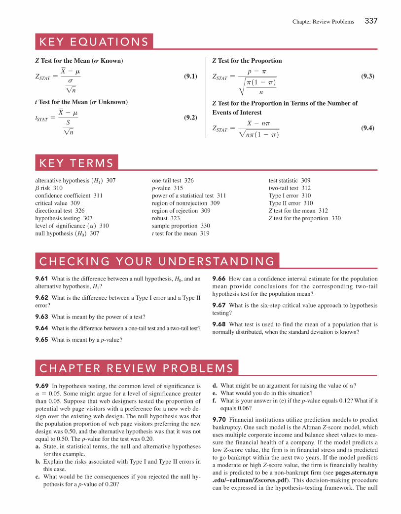
Chapter review Problems 337
K E Y E q U at i O n s
Z Test for the Mean (S Known)
ZSTAT =X - m
s1n
(9.1)
t Test for the Mean (S Unknown)
tSTAT =X - m
S1n
(9.2)
Z Test for the Proportion
ZSTAT =p - pBp11 - p2
n
(9.3)
Z Test for the Proportion in Terms of the Number of Events of Interest
ZSTAT =X - np2np11 - p2
(9.4)
K E Y t E R M salternative hypothesis 1H12 307b risk 310confidence coefficient 311critical value 309directional test 326hypothesis testing 307level of significance 1a2 310null hypothesis 1H02 307
one-tail test 326p-value 315power of a statistical test 311region of nonrejection 309region of rejection 309robust 323sample proportion 330t test for the mean 319
test statistic 309two-tail test 312Type I error 310Type II error 310Z test for the mean 312Z test for the proportion 330
c h E c K i n g Y O U R U n D E R s ta n D i n g9.61 What is the difference between a null hypothesis, H0, and an alternative hypothesis, H1?
9.62 What is the difference between a Type I error and a Type II error?
9.63 What is meant by the power of a test?
9.64 What is the difference between a one-tail test and a two-tail test?
9.65 What is meant by a p-value?
9.66 How can a confidence interval estimate for the population mean provide conclusions for the corresponding two-tail hypothesis test for the population mean?
9.67 What is the six-step critical value approach to hypothesis testing?
9.68 What test is used to find the mean of a population that is normally distributed, when the standard deviation is known?
c h a P t E R R E V i E w P R O b l E M s9.69 In hypothesis testing, the common level of significance is a = 0.05. Some might argue for a level of significance greater than 0.05. Suppose that web designers tested the proportion of potential web page visitors with a preference for a new web de-sign over the existing web design. The null hypothesis was that the population proportion of web page visitors preferring the new design was 0.50, and the alternative hypothesis was that it was not equal to 0.50. The p-value for the test was 0.20.a. State, in statistical terms, the null and alternative hypotheses
for this example.b. Explain the risks associated with Type I and Type II errors in
this case.c. What would be the consequences if you rejected the null hy-
pothesis for a p-value of 0.20?
d. What might be an argument for raising the value of a?e. What would you do in this situation?f. What is your answer in (e) if the p-value equals 0.12? What if it
equals 0.06?
9.70 Financial institutions utilize prediction models to predict bankruptcy. One such model is the Altman Z-score model, which uses multiple corporate income and balance sheet values to mea-sure the financial health of a company. If the model predicts a low Z-score value, the firm is in financial stress and is predicted to go bankrupt within the next two years. If the model predicts a moderate or high Z-score value, the firm is financially healthy and is predicted to be a non-bankrupt firm (see pages.stern.nyu .edu/~ealtman/Zscores.pdf). This decision-making procedure can be expressed in the hypothesis-testing framework. The null
338 CHAPTEr 9 Fundamentals of Hypothesis Testing: One-Sample Tests
hypothesis is that a firm is predicted to be a non-bankrupt firm. The alternative hypothesis is that the firm is predicted to be a bankrupt firm.a. Explain the risks associated with committing a Type I error in
this case.b. Explain the risks associated with committing a Type II error in
this case.c. Which type of error do you think executives want to avoid?
Explain.d. How would changes in the model affect the probabilities of
committing Type I and Type II errors?
9.71 Salesforce ExactTarget Marketing Cloud conducted a study of U.S. consumers that included 205 tablet owners. The study found that 134 tablet owners use their tablet while watching TV at least once per day. (Source: “New Mobile Tracking & Survey Data: 2014 Mobile Behavior report,” bit.ly/1odMZ3D.) The authors of the report imply that the survey proves that more than half of all tablet owners use their tablet while watching TV at least once per day.a. Use the five-step p-value approach to hypothesis testing and a
0.05 level of significance to try to prove that more than half of all tablet owners use their tablet while watching TV at least once per day.
b. Based on your result in (a), is the claim implied by the authors valid?
c. Suppose the study found that 105 tablet owners use their tablet while watching TV at least once per day. repeat parts (a) and (b).
d. Compare the results of (b) and (c).
9.72 The owner of a specialty coffee shop wants to study coffee purchasing habits of customers at her shop. She selects a random sample of 60 customers during a certain week, with the following results:
• The amount spent was X = +7.25, S = +1.75.• Thirty-onecustomerssaythey“definitelywill”recommend
the specialty coffee shop to family and friends.
a. At the 0.05 level of significance, is there evidence that the pop-ulation mean amount spent was different from $6.50?
b. Determine the p-value in (a).c. At the 0.05 level of significance, is there evidence that more
than 50% of all the customers say they “definitely will” recom-mend the specialty coffee shop to family and friends?
d. What is your answer to (a) if the sample mean equals $6.25?e. What is your answer to (c) if 39 customers say they “definitely
will” recommend the specialty coffee shop to family and friends?
9.73 An auditor for a government agency was assigned the task of evaluating reimbursement for office visits to physicians paid by Medicare. The audit was conducted on a sample of 75 reimburse-ments, with the following results:
• In 12 of the office visits, there was an incorrect amount of reimbursement.
• TheamountofreimbursementwasX = +93.70, S = +34.55.a. At the 0.05 level of significance, is there evidence that the pop-
ulation mean reimbursement was less than $100?b. At the 0.05 level of significance, is there evidence that the
proportion of incorrect reimbursements in the population was greater than 0.10?
c. Discuss the underlying assumptions of the test used in (a).d. What is your answer to (a) if the sample mean equals $90?
e. What is your answer to (b) if 15 office visits had incorrect reimbursements?
9.74 A bank branch located in a commercial district of a city has the business objective of improving the process for serv-ing customers during the noon-to-1:00 p.m. lunch period. The waiting time (defined as the time the customer enters the line until he or she reaches the teller window) of a random sample of 15 customers is collected, and the results are organized and stored in bank1 . These data are:
4.21 5.55 3.02 5.13 4.77 2.34 3.54 3.204.50 6.10 0.38 5.12 6.46 6.19 3.79
a. At the 0.05 level of significance, is there evidence that the pop-ulation mean waiting time is less than 5 minutes?
b. What assumption about the population distribution is needed in order to conduct the t test in (a)?
c. Construct a boxplot or a normal probability plot to evaluate the assumption made in (b).
d. Do you think that the assumption needed in order to conduct the t test in (a) is valid? Explain.
e. As a customer walks into the branch office during the lunch hour, she asks the branch manager how long she can expect to wait. The branch manager replies, “Almost certainly not longer than 5 minutes.” On the basis of the results of (a), evaluate this statement.
9.75 A manufacturing company produces electrical insulators. If the insulators break when in use, a short circuit is likely to occur. To test the strength of the insulators, destructive testing is carried out to determine how much force is required to break the insu-lators. Force is measured by observing the number of pounds of force applied to the insulator before it breaks. The following data (stored in Force ) are from 30 insulators subjected to this testing:
1,870 1,728 1,656 1,610 1,634 1,784 1,522 1,696 1,592 1,6621,866 1,764 1,734 1,662 1,734 1,774 1,550 1,756 1,762 1,8661,820 1,744 1,788 1,688 1,810 1,752 1,680 1,810 1,652 1,736
a. At the 0.05 level of significance, is there evidence that the population mean force required to break the insulator is greater than 1,500 pounds?
b. What assumption about the population distribution is needed in order to conduct the t test in (a)?
c. Construct a histogram, boxplot, or normal probability plot to evaluate the assumption made in (b).
d. Do you think that the assumption needed in order to conduct the t test in (a) is valid? Explain.
9.76 An important quality characteristic used by the manufac-turer of Boston and Vermont asphalt shingles is the amount of moisture the shingles contain when they are packaged. Customers may feel that they have purchased a product lacking in quality if they find moisture and wet shingles inside the packaging. In some cases, excessive moisture can cause the granules attached to the shingles for texture and coloring purposes to fall off the shingles, resulting in appearance problems. To monitor the amount of mois-ture present, the company conducts moisture tests. A shingle is weighed and then dried. The shingle is then reweighed, and, based on the amount of moisture taken out of the product, the pounds of moisture per 100 square feet are calculated. The company would like to show that the mean moisture content is less than 0.35 pound per 100 square feet. The file moisture includes 36 measurements

(in pounds per 100 square feet) for Boston shingles and 31 for Vermont shingles.a. For the Boston shingles, is there evidence at the 0.05 level of
significance that the population mean moisture content is less than 0.35 pound per 100 square feet?
b. Interpret the meaning of the p-value in (a).c. For the Vermont shingles, is there evidence at the 0.05 level of
significance that the population mean moisture content is less than 0.35 pound per 100 square feet?
d. Interpret the meaning of the p-value in (c).e. What assumption about the population distribution is needed in
order to conduct the t tests in (a) and (c)?f. Construct histograms, boxplots, or normal probability plots to
evaluate the assumption made in (a) and (c).g. Do you think that the assumption needed in order to conduct
the t tests in (a) and (c) is valid? Explain.
9.77 Studies conducted by the manufacturer of Boston and Ver-mont asphalt shingles have shown product weight to be a ma-jor factor in the customer’s perception of quality. Moreover, the weight represents the amount of raw materials being used and is therefore very important to the company from a cost standpoint. The last stage of the assembly line packages the shingles before the packages are placed on wooden pallets. Once a pallet is full (a pallet for most brands holds 16 squares of shingles), it is weighed, and the measurement is recorded. The file pallet contains the weight (in pounds) from a sample of 368 pallets of Boston shin-gles and 330 pallets of Vermont shingles.a. For the Boston shingles, is there evidence at the 0.05 level of
significance that the population mean weight is different from 3,150 pounds?
b. Interpret the meaning of the p-value in (a).c. For the Vermont shingles, is there evidence at the 0.05 level of
significance that the population mean weight is different from 3,700 pounds?
d. Interpret the meaning of the p-value in (c).
e. In (a) through (d), do you have to be concerned with the nor-mality assumption? Explain.
9.78 The manufacturer of Boston and Vermont asphalt shingles provides its customers with a 20-year warranty on most of its products. To determine whether a shingle will last through the warranty period, accelerated-life testing is conducted at the manu-facturing plant. Accelerated-life testing exposes the shingle to the stresses it would be subject to in a lifetime of normal use in a labo-ratory setting via an experiment that takes only a few minutes to conduct. In this test, a shingle is repeatedly scraped with a brush for a short period of time, and the shingle granules removed by the brushing are weighed (in grams). Shingles that experience low amounts of granule loss are expected to last longer in normal use than shingles that experience high amounts of granule loss. The file granule contains a sample of 170 measurements made on the company’s Boston shingles and 140 measurements made on Vermont shingles.a. For the Boston shingles, is there evidence at the 0.05 level of
significance that the population mean granule loss is different from 0.30 grams?
b. Interpret the meaning of the p-value in (a).c. For the Vermont shingles, is there evidence at the 0.05 level of
significance that the population mean granule loss is different from 0.30 grams?
d. Interpret the meaning of the p-value in (c).e. In (a) through (d), do you have to be concerned with the nor-
mality assumption? Explain.
REpoRT WRiTiNg ExERCiSE
9.79 referring to the results of Problems 9.76 through 9.78 con-cerning Boston and Vermont shingles, write a report that evaluates the moisture level, weight, and granule loss of the two types of shingles.
c a s E s f O R c h a P t E R 9
Managing ashland Multicomm servicesContinuing its monitoring of the upload speed first de-scribed in the Chapter 6 Managing Ashland MultiComm Services case on page 243, the technical operations depart-ment wants to ensure that the mean target upload speed for all Internet service subscribers is at least 0.97 on a standard scale in which the target value is 1.0. Each day, upload speed was measured 50 times, with the following results (stored in AmS9 ).
0.854 1.023 1.005 1.030 1.219 0.977 1.044 0.778 1.122 1.1141.091 1.086 1.141 0.931 0.723 0.934 1.060 1.047 0.800 0.8891.012 0.695 0.869 0.734 1.131 0.993 0.762 0.814 1.108 0.8051.223 1.024 0.884 0.799 0.870 0.898 0.621 0.818 1.113 1.2861.052 0.678 1.162 0.808 1.012 0.859 0.951 1.112 1.003 0.972
1. Compute the sample statistics and determine whether there is evidence that the population mean upload speed is less than 0.97.
2. Write a memo to management that summarizes your conclusions.
Cases for Chapter 9 339
340 CHAPTEr 9 Fundamentals of Hypothesis Testing: One-Sample Tests
Digital caseApply your knowledge about hypothesis testing in this Digi-tal Case, which continues the cereal-fill-packaging dispute first discussed in the Digital Case from Chapter 7.
In response to the negative statements made by the Con-cerned Consumers About Cereal Cheaters (CCACC) in the Chapter 7 Digital Case, Oxford Cereals recently conducted an experiment concerning cereal packaging. The com-pany claims that the results of the experiment refute the CCACC allegations that Oxford Cereals has been cheat-ing consumers by packaging cereals at less than labeled weights.
Open OxfordCurrentNews.pdf, a portfolio of current news releases from Oxford Cereals. review the relevant
press releases and supporting documents. Then answer the following questions:
1. Are the results of the experiment valid? Why or why not? If you were conducting the experiment, is there anything you would change?
2. Do the results support the claim that Oxford Cereals is not cheating its customers?
3. Is the claim of the Oxford Cereals CEO that many cereal boxes contain more than 368 grams surprising? Is it true?
4. Could there ever be a circumstance in which the results of the Oxford Cereals experiment and the CCACC’s results are both correct? Explain.
sure Value convenience storesYou work in the corporate office for a nationwide conve-nience store franchise that operates nearly 10,000 stores. The per-store daily customer count (i.e., the mean number of customers in a store in one day) has been steady, at 900, for some time. To increase the customer count, the chain is considering cutting prices for coffee beverages. The small size will now be $0.59 instead of $0.99, and the medium size will be $0.69 instead of $1.19. Even with this reduction in price, the chain will have a 40% gross margin on coffee.
To test the new initiative, the chain has reduced coffee prices in a sample of 34 stores, where customer counts have been running almost exactly at the national average of 900. Af-ter four weeks, the stores sampled stabilize at a mean customer count of 974 and a standard deviation of 96. This increase seems like a substantial amount to you, but it also seems like a pretty small sample. Is there statistical evidence that reducing coffee prices is a good strategy for increasing the mean cus-tomer count? Be prepared to explain your conclusion.
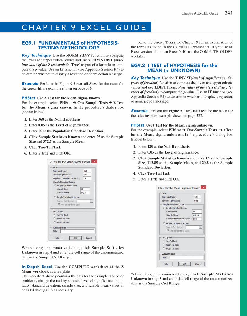
Eg9.1 FuNDAmENTAlS of HypoTHESiS-TESTiNg mETHoDology
Key Technique Use the NORM.S.INV function to compute the lower and upper critical values and use NORM.S.DIST (abso-lute value of the Z test statistic, True) as part of a formula to com-pute the p-value. Use an IF function (see Appendix Section F.4) to determine whether to display a rejection or nonrejection message.
Example Perform the Figure 9.5 two-tail Z test for the mean for the cereal-filling example shown on page 316.
pHStat Use Z Test for the Mean, sigma known.For the example, select PHStat ➔ One-Sample Tests ➔ Z Test for the Mean, sigma known. In the procedure’s dialog box (shown below):
1. Enter 368 as the Null Hypothesis.
2. Enter 0.05 as the Level of Significance.
3. Enter 15 as the Population Standard Deviation.
4. Click Sample Statistics Known and enter 25 as the Sample Size and 372.5 as the Sample Mean.
5. Click Two-Tail Test.
6. Enter a Title and click OK.
When using unsummarized data, click Sample Statistics Unknown in step 4 and enter the cell range of the unsummarized data as the Sample Cell Range.
in-Depth Excel Use the COMPUTE worksheet of the Z Mean workbook as a template.The worksheet already contains the data for the example. For other problems, change the null hypothesis, level of significance, popu-lation standard deviation, sample size, and sample mean values in cells B4 through B8 as necessary.
read the Short Takes for Chapter 9 for an explanation of the formulas found in the COMPUTE worksheet. If you use an Excel version older than Excel 2010, use the COMPUTE_OLDEr worksheet.
Eg9.2 t TEST of HypoTHESiS for the mEAN (S uNKNoWN)
Key Technique Use the T.INV.2T(level of significance, de-grees of freedom) function to compute the lower and upper critical values and use T.DIST.2T(absolute value of the t test statistic, de-grees of freedom) to compute the p-value. Use an IF function (see Appendix Section F.4) to determine whether to display a rejection or nonrejection message.
Example Perform the Figure 9.7 two-tail t test for the mean for the sales invoices example shown on page 322.
pHStat Use t Test for the Mean, sigma unknown.For the example, select PHStat ➔ One-Sample Tests ➔ t Test for the Mean, sigma unknown. In the procedure’s dialog box (shown below):
1. Enter 120 as the Null Hypothesis.
2. Enter 0.05 as the Level of Significance.
3. Click Sample Statistics Known and enter 12 as the Sample Size, 112.85 as the Sample Mean, and 20.8 as the Sample Standard Deviation.
4. Click Two-Tail Test.
5. Enter a Title and click OK.
When using unsummarized data, click Sample Statistics Unknown in step 3 and enter the cell range of the unsummarized data as the Sample Cell Range.
c h a P t E R 9 E x c E l g U i D E
Chapter 9 ExCEL Guide 341
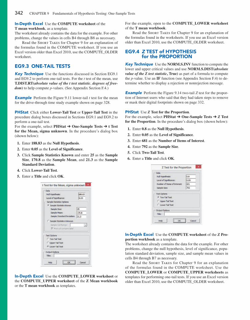
342 CHAPTEr 9 Fundamentals of Hypothesis Testing: One-Sample Tests
in-Depth Excel Use the COMPUTE worksheet of theT mean workbook, as a template.The worksheet already contains the data for the example. For other problems, change the values in cells B4 through B8 as necessary.
read the Short Takes for Chapter 9 for an explanation of the formulas found in the COMPUTE worksheet. If you use an Excel version older than Excel 2010, use the COMPUTE_OLDEr worksheet.
Eg9.3 oNE-TAil TESTSKey Technique Use the functions discussed in Section EG9.1 and EG9.2 to perform one-tail tests. For the t test of the mean, use T.DIST.RT(absolute value of the t test statistic, degrees of free-dom) to help compute p-values. (See Appendix Section F.4.)
Example Perform the Figure 9.11 lower-tail t test for the mean for the drive-through time study example shown on page 328.
pHStat Click either Lower-Tail Test or Upper-Tail Test in the procedure dialog boxes discussed in Sections EG9.1 and EG9.2 to perform a one-tail test.For the example, select PHStat ➔ One-Sample Tests ➔ t Test for the Mean, sigma unknown. In the procedure’s dialog box (shown below):
1. Enter 188.83 as the Null Hypothesis.
2. Enter 0.05 as the Level of Significance.
3. Click Sample Statistics Known and enter 25 as the Sample Size, 170.8 as the Sample Mean, and 21.3 as the Sample Standard Deviation.
4. Click Lower-Tail Test.
5. Enter a Title and click OK.
in-Depth Excel Use the COMPUTE_LOWER worksheet or the COMPUTE_UPPER worksheet of the Z Mean workbook or the T mean workbook as templates.
For the example, open to the COMPUTE_LOWER worksheet of the T mean workbook.
read the Short Takes for Chapter 9 for an explanation of the formulas found in the worksheets. If you use an Excel version older than Excel 2010, use the COMPUTE_OLDEr worksheet.
Eg9.4 Z TEST of HypoTHESiS for the pRopoRTioN
Key Technique Use the NORM.S.INV function to compute the lower and upper critical values and use NORM.S.DIST(absolute value of the Z test statistic, True) as part of a formula to compute the p-value. Use an IF function (see Appendix Section F.4) to de-termine whether to display a rejection or nonrejection message.
Example Perform the Figure 9.14 two-tail Z test for the propor-tion of Internet users who said that they had taken steps to remove or mask their digital footprints shown on page 332.
pHStat Use Z Test for the Proportion.For the example, select PHStat ➔ One-Sample Tests ➔ Z Test for the Proportion. In the procedure’s dialog box (shown below):
1. Enter 0.8 as the Null Hypothesis.
2. Enter 0.05 as the Level of Significance.
3. Enter 681 as the Number of Items of Interest.
4. Enter 792 as the Sample Size.
5. Click Two-Tail Test.
6. Enter a Title and click OK.
in-Depth Excel Use the COMPUTE worksheet of the Z Pro-portion workbook as a template.The worksheet already contains the data for the example. For other problems, change the null hypothesis, level of significance, popu-lation standard deviation, sample size, and sample mean values in cells B4 through B7 as necessary.
read the Short Takes for Chapter 9 for an explanation of the formulas found in the COMPUTE worksheet. Use the COMPUTE_LOWER or COMPUTE_UPPER worksheets as templates for performing one-tail tests. If you use an Excel version older than Excel 2010, use the COMPUTE_OLDEr worksheet.
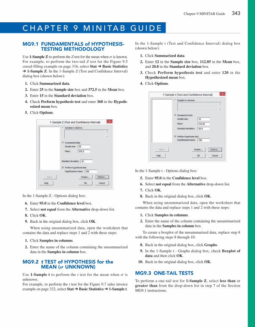
mg9.1 FuNDAmENTAlS of HypoTHESiS-TESTiNg mETHoDology
Use 1-Sample Z to perform the Z test for the mean when s is known.For example, to perform the two-tail Z test for the Figure 9.5 cereal-filling example on page 316, select Stat ➔ Basic Statistics ➔ 1-Sample Z. In the 1-Sample Z (Test and Confidence Interval) dialog box (shown below):
1. Click Summarized data.
2. Enter 25 in the Sample size box and 372.5 in the Mean box.
3. Enter 15 in the Standard deviation box.
4. Check Perform hypothesis test and enter 368 in the Hypoth-esized mean box.
5. Click Options.
In the 1-Sample Z - Options dialog box:
6. Enter 95.0 in the Confidence level box.
7. Select not equal from the Alternative drop-down list.
8. Click OK.
9. Back in the original dialog box, click OK.
When using unsummarized data, open the worksheet that contains the data and replace steps 1 and 2 with these steps:
1. Click Samples in columns.
2. Enter the name of the column containing the unsummarized data in the Samples in column box.
mg9.2 t TEST of HypoTHESiS for the mEAN (S uNKNoWN)
Use 1-Sample t to perform the t test for the mean when s is unknown. For example, to perform the t test for the Figure 9.7 sales invoice example on page 322, select Stat ➔ Basic Statistics ➔ 1-Sample t.
In the 1-Sample t (Test and Confidence Interval) dialog box (shown below):
1. Click Summarized data.
2. Enter 12 in the Sample size box, 112.85 in the Mean box, and 20.8 in the Standard deviation box.
3. Check Perform hypothesis test and enter 120 in the Hypothesized mean box.
4. Click Options.
In the 1-Sample t - Options dialog box:
5. Enter 95.0 in the Confidence level box.
6. Select not equal from the Alternative drop-down list.
7. Click OK.
8. Back in the original dialog box, click OK.
When using unsummarized data, open the worksheet that contains the data and replace steps 1 and 2 with these steps:
1. Click Samples in columns.
2. Enter the name of the column containing the unsummarized data in the Samples in column box.
To create a boxplot of the unsummarized data, replace step 8 with the following steps 8 through 10:
8. Back in the original dialog box, click Graphs.
9. In the 1-Sample t - Graphs dialog box, check Boxplot of data and then click OK.
10. Back in the original dialog box, click OK.
mg9.3 oNE-TAil TESTSTo perform a one-tail test for 1-Sample Z, select less than or greater than from the drop-down list in step 7 of the Section MG9.1 instructions.
c h a P t E R 9 M i n i ta b g U i D E
Chapter 9 MINITAB Guide 343
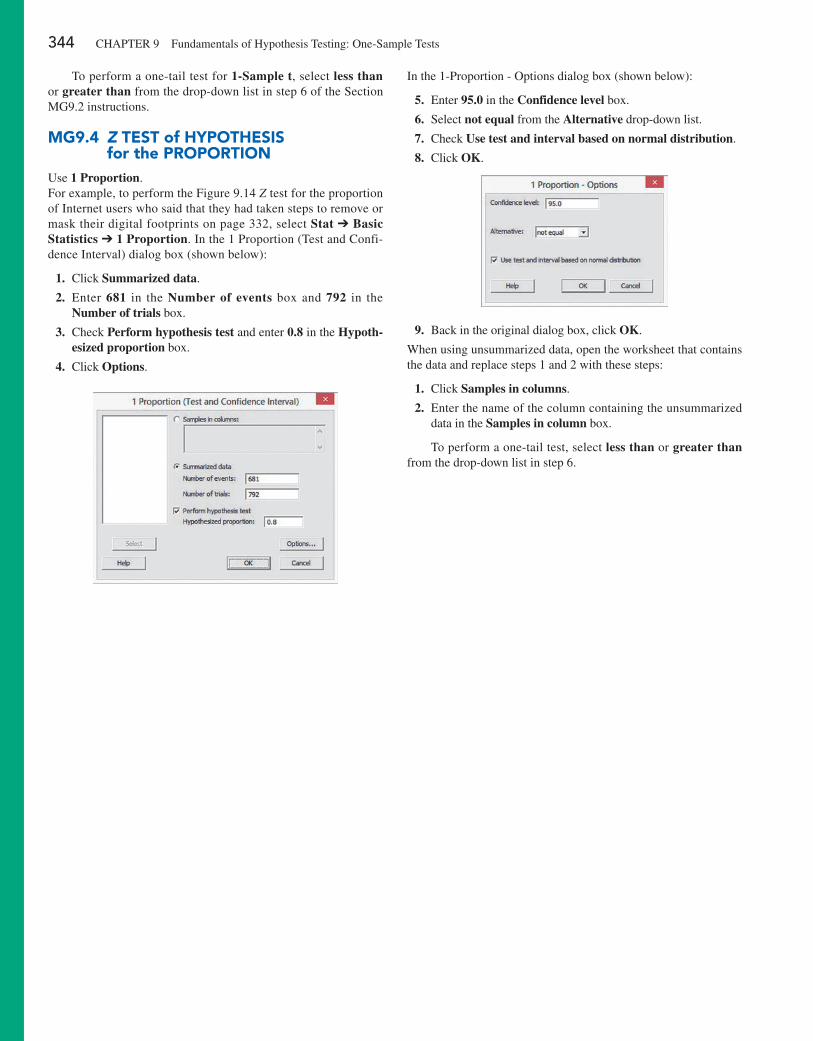
344 CHAPTEr 9 Fundamentals of Hypothesis Testing: One-Sample Tests
To perform a one-tail test for 1-Sample t, select less than or greater than from the drop-down list in step 6 of the Section MG9.2 instructions.
mg9.4 Z TEST of HypoTHESiS for the pRopoRTioN
Use 1 Proportion.For example, to perform the Figure 9.14 Z test for the proportion of Internet users who said that they had taken steps to remove or mask their digital footprints on page 332, select Stat ➔ Basic Statistics ➔ 1 Proportion. In the 1 Proportion (Test and Confi-dence Interval) dialog box (shown below):
1. Click Summarized data.
2. Enter 681 in the Number of events box and 792 in the Number of trials box.
3. Check Perform hypothesis test and enter 0.8 in the Hypoth-esized proportion box.
4. Click Options.
In the 1-Proportion - Options dialog box (shown below):
5. Enter 95.0 in the Confidence level box.
6. Select not equal from the Alternative drop-down list.
7. Check Use test and interval based on normal distribution.
8. Click OK.
9. Back in the original dialog box, click OK.
When using unsummarized data, open the worksheet that contains the data and replace steps 1 and 2 with these steps:
1. Click Samples in columns.
2. Enter the name of the column containing the unsummarized data in the Samples in column box.
To perform a one-tail test, select less than or greater than from the drop-down list in step 6.
345
10U s i n g s tat i s t i c s
For North Fork, Are There Different Means to the Ends?To what extent does the location of products affect sales in a supermarket? As a North Fork Beverages sales manager, you are negotiating with the management of FoodPlace Supermarkets for the location of displays for the new HandMade Real Citrus Cola. FoodPlace Supermarkets has offered you two different end-aisle display areas to feature your new cola: one near the produce department and the other at the front of the aisle that contains other beverage products. These ends of aisle, or end-caps, have different costs, and you would like to compare the effectiveness of the produce end-cap to the beverage end-cap.
To test the comparative effectiveness of the two end-caps, FoodPlace agrees to a pilot study. You will be able to select 20 stores from the supermarket chain that ex-perience similar storewide sales volumes. You then randomly assign 10 of the 20 stores to sample 1 and 10 other stores to sample 2. In the sample 1 stores, you will place the new cola in the beverage end-cap, while in the sample 2 stores you will place the new cola in the produce end-cap. At the end of one week, the sales of the new cola will be recorded. How can you determine whether the sales of the new cola using beverage end-caps are different from the sales of the new cola using pro-duce end-caps? How can you decide if the variability in new cola sales from store to store is different for the two types of displays? How could you use the answers to these questions to improve sales of your new HandMade Real Citrus Cola?
contents
10.1 Comparing the Means of Two Independent Populations
Do People Really Do This?
10.2 Comparing the Means of Two Related Populations
10.3 Comparing the Proportions of Two Independent Populations
10.4 F Test for the Ratio of Two Variances
10.5 One-Way ANOVA
10.6 Effect Size (online)
USINg STATISTICS: For North Fork, Are There Different Means to the Ends? Revisited
chapter 10 excel gUide
chapter 10 Minitab gUide
objectivesCompare the means of two
independent populationsCompare the means of two
related populationsCompare the proportions of two
independent populationsCompare the variances of two
independent populationsCompare the means of more than
two populations
Chapter Two-Sample Tests and One-Way ANOVA
Fotolia
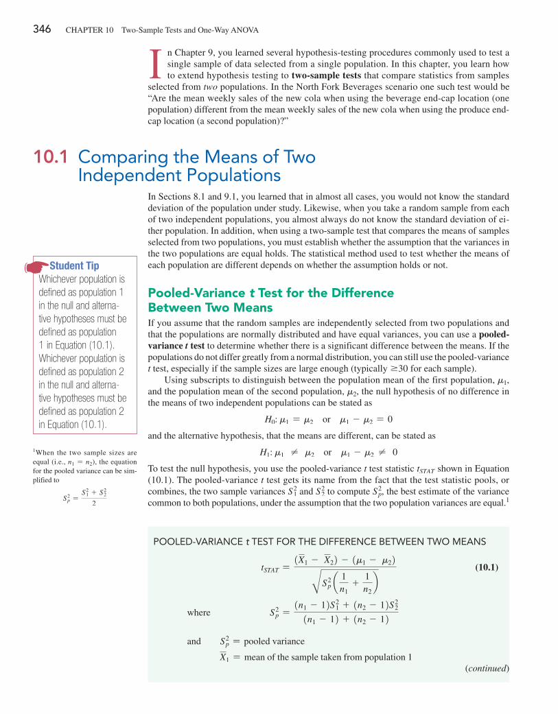
346 CHAPTeR 10 Two-Sample Tests and One-Way ANOVA
I n Chapter 9, you learned several hypothesis-testing procedures commonly used to test a single sample of data selected from a single population. In this chapter, you learn how to extend hypothesis testing to two-sample tests that compare statistics from samples
selected from two populations. In the North Fork Beverages scenario one such test would be “Are the mean weekly sales of the new cola when using the beverage end-cap location (one population) different from the mean weekly sales of the new cola when using the produce end-cap location (a second population)?”
10.1 Comparing the Means of Two Independent Populations
In Sections 8.1 and 9.1, you learned that in almost all cases, you would not know the standard deviation of the population under study. Likewise, when you take a random sample from each of two independent populations, you almost always do not know the standard deviation of ei-ther population. In addition, when using a two-sample test that compares the means of samples selected from two populations, you must establish whether the assumption that the variances in the two populations are equal holds. The statistical method used to test whether the means of each population are different depends on whether the assumption holds or not.
Pooled-Variance t Test for the Difference Between Two MeansIf you assume that the random samples are independently selected from two populations and that the populations are normally distributed and have equal variances, you can use a pooled- variance t test to determine whether there is a significant difference between the means. If the populations do not differ greatly from a normal distribution, you can still use the pooled-variance t test, especially if the sample sizes are large enough (typically Ú30 for each sample).
Using subscripts to distinguish between the population mean of the first population, m1, and the population mean of the second population, m2, the null hypothesis of no difference in the means of two independent populations can be stated as
H0: m1 = m2 or m1 - m2 = 0
and the alternative hypothesis, that the means are different, can be stated as
H1: m1 ≠ m2 or m1 - m2 ≠ 0
To test the null hypothesis, you use the pooled-variance t test statistic tSTAT shown in equation (10.1). The pooled-variance t test gets its name from the fact that the test statistic pools, or combines, the two sample variances S2
1 and S22 to compute S2
p, the best estimate of the variance common to both populations, under the assumption that the two population variances are equal.1
1When the two sample sizes are equal (i.e., n1 = n2), the equation for the pooled variance can be sim-plified to
S2p =
S21 + S2
2
2
Student TipWhichever population is defined as population 1 in the null and alterna-tive hypotheses must be defined as population 1 in Equation (10.1). Whichever population is defined as population 2 in the null and alterna-tive hypotheses must be defined as population 2 in Equation (10.1).
POOlED-VARIANCE t TEST FOR ThE DIFFERENCE BETWEEN TWO MEANS
tSTAT =1X1 - X22 - 1m1 - m22BS2
p a 1n1
+1n2
b (10.1)
where S2p =
1n1 - 12S21 + 1n2 - 12S2
2
1n1 - 12 + 1n2 - 12
and S2p = pooled variance
X1 = mean of the sample taken from population 1(continued)
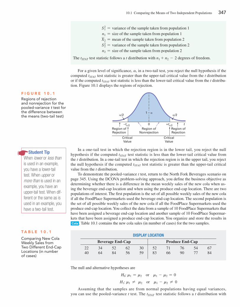
10.1 Comparing the Means of Two Independent Populations 347
For a given level of significance, a, in a two-tail test, you reject the null hypothesis if the computed tSTAT test statistic is greater than the upper-tail critical value from the t distribution or if the computed tSTAT test statistic is less than the lower-tail critical value from the t distribu-tion. Figure 10.1 displays the regions of rejection.
S21 = variance of the sample taken from population 1
n1 = size of the sample taken from population 1 X2 = mean of the sample taken from population 2 S2
2 = variance of the sample taken from population 2 n2 = size of the sample taken from population 2
The tSTAT test statistic follows a t distribution with n1 + n2 - 2 degrees of freedom.
Student TipWhen lower or less than is used in an example, you have a lower-tail test. When upper or more than is used in an example, you have an upper-tail test. When dif-ferent or the same as is used in an example, you have a two-tail test.
In a one-tail test in which the rejection region is in the lower tail, you reject the null hypothesis if the computed tSTAT test statistic is less than the lower-tail critical value from the t distribution. In a one-tail test in which the rejection region is in the upper tail, you reject the null hypothesis if the computed tSTAT test statistic is greater than the upper-tail critical value from the t distribution.
To demonstrate the pooled-variance t test, return to the North Fork Beverages scenario on page 345. Using the DCOVA problem-solving approach, you define the business objective as determining whether there is a difference in the mean weekly sales of the new cola when us-ing the beverage end-cap location and when using the produce end-cap location. There are two populations of interest. The first population is the set of all possible weekly sales of the new cola if all the FoodPlace Supermarkets used the beverage end-cap location. The second population is the set of all possible weekly sales of the new cola if all the FoodPlace Supermarkets used the produce end-cap location. You collect the data from a sample of 10 FoodPlace Supermarkets that have been assigned a beverage end-cap location and another sample of 10 FoodPlace Supermar-kets that have been assigned a produce end-cap location. You organize and store the results in Cola . Table 10.1 contains the new cola sales (in number of cases) for the two samples.
The null and alternative hypotheses are
H0: m1 = m2 or m1 - m2 = 0
H1: m1 ≠ m2 or m1 - m2 ≠ 0
Assuming that the samples are from normal populations having equal variances, you can use the pooled-variance t test. The tSTAT test statistic follows a t distribution with
F i g u r e 1 0 . 1Regions of rejection and nonrejection for the pooled-variance t test for the difference between the means (two-tail test)
0–ta/2 +ta/2 tRegion ofRejection
CriticalValue
Region ofNonrejection
CriticalValue
Region ofRejection
a/2 a/21 – a
T a B l e 1 0 . 1
Comparing New Cola Weekly Sales from Two Different End-Cap locations (in number of cases)
DiSplay locaTion
Beverage End-Cap Produce End-Cap
22 34 52 62 30 52 71 76 54 6740 64 84 56 59 83 66 90 77 84
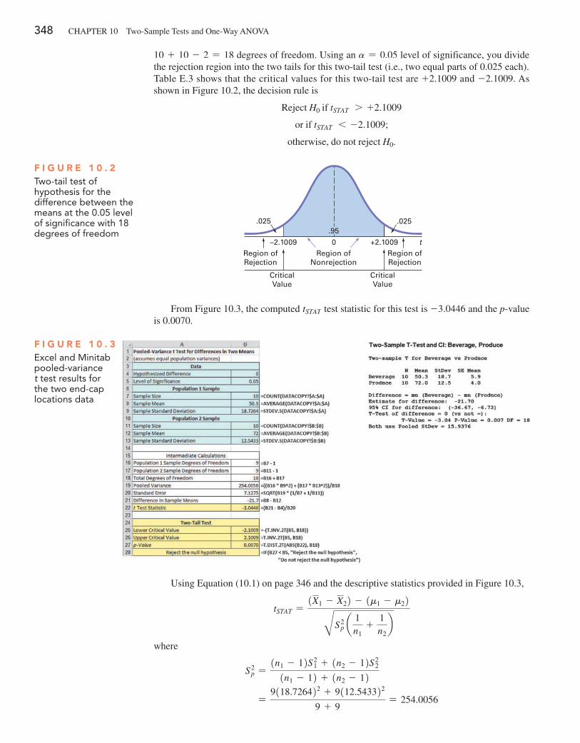
348 CHAPTeR 10 Two-Sample Tests and One-Way ANOVA
10 + 10 - 2 = 18 degrees of freedom. Using an a = 0.05 level of significance, you divide the rejection region into the two tails for this two-tail test (i.e., two equal parts of 0.025 each). Table e.3 shows that the critical values for this two-tail test are +2.1009 and -2.1009. As shown in Figure 10.2, the decision rule is
Reject H0 if tSTAT 7 +2.1009
or if tSTAT 6 -2.1009;
otherwise, do not reject H0.
From Figure 10.3, the computed tSTAT test statistic for this test is -3.0446 and the p-value is 0.0070.
Using equation (10.1) on page 346 and the descriptive statistics provided in Figure 10.3,
tSTAT =1X1 - X22 - 1m1 - m22BS2
p a 1n1
+1n2
bwhere
S2p =
1n1 - 12S21 + 1n2 - 12S2
2
1n1 - 12 + 1n2 - 12 =
9118.726422 + 9112.543322
9 + 9= 254.0056
F i g u r e 1 0 . 2Two-tail test of hypothesis for the difference between the means at the 0.05 level of significance with 18 degrees of freedom
–2.1009 +2.10090 t
.025 .025
Region ofRejection
CriticalValue
Region ofNonrejection
CriticalValue
Region ofRejection
.95
F i g u r e 1 0 . 3Excel and Minitab pooled-variance t test results for the two end-cap locations data
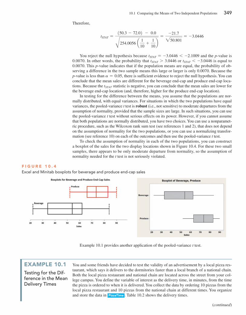
10.1 Comparing the Means of Two Independent Populations 349
Therefore,
tSTAT =150.3 - 72.02 - 0.0B254.0056 a 1
10+
1
10b
=-21.7250.801
= -3.0446
You reject the null hypothesis because tSTAT = -3.0446 6 -2.1009 and the p-value is 0.0070. In other words, the probability that tSTAT 7 3.0446 or tSTAT 6 -3.0446 is equal to 0.0070. This p-value indicates that if the population means are equal, the probability of ob-serving a difference in the two sample means this large or larger is only 0.0070. Because the p-value is less than a = 0.05, there is sufficient evidence to reject the null hypothesis. You can conclude that the mean sales are different for the beverage end-cap and produce end-cap loca-tions. Because the tSTAT statistic is negative, you can conclude that the mean sales are lower for the beverage end-cap location (and, therefore, higher for the produce end-cap location).
In testing for the difference between the means, you assume that the populations are nor-mally distributed, with equal variances. For situations in which the two populations have equal variances, the pooled-variance t test is robust (i.e., not sensitive) to moderate departures from the assumption of normality, provided that the sample sizes are large. In such situations, you can use the pooled-variance t test without serious effects on its power. However, if you cannot assume that both populations are normally distributed, you have two choices. You can use a nonparamet-ric procedure, such as the Wilcoxon rank sum test (see references 1 and 2), that does not depend on the assumption of normality for the two populations, or you can use a normalizing transfor-mation (see reference 10) on each of the outcomes and then use the pooled-variance t test.
To check the assumption of normality in each of the two populations, you can construct a boxplot of the sales for the two display locations shown in Figure 10.4. For these two small samples, there appears to be only moderate departure from normality, so the assumption of normality needed for the t test is not seriously violated.
example 10.1 provides another application of the pooled-variance t test.
F i g u r e 1 0 . 4Excel and Minitab boxplots for beverage and produce end-cap sales
exaMPle 10.1testing for the dif-ference in the Mean delivery times
You and some friends have decided to test the validity of an advertisement by a local pizza res-taurant, which says it delivers to the dormitories faster than a local branch of a national chain. Both the local pizza restaurant and national chain are located across the street from your col-lege campus. You define the variable of interest as the delivery time, in minutes, from the time the pizza is ordered to when it is delivered. You collect the data by ordering 10 pizzas from the local pizza restaurant and 10 pizzas from the national chain at different times. You organize and store the data in PizzaTime . Table 10.2 shows the delivery times.
(continued)
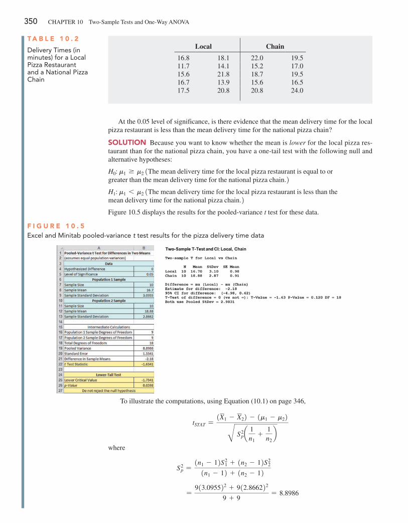
350 CHAPTeR 10 Two-Sample Tests and One-Way ANOVA
At the 0.05 level of significance, is there evidence that the mean delivery time for the local pizza restaurant is less than the mean delivery time for the national pizza chain?
SoluTion Because you want to know whether the mean is lower for the local pizza res-taurant than for the national pizza chain, you have a one-tail test with the following null and alternative hypotheses:
H0: m1 Ú m2 1The mean delivery time for the local pizza restaurant is equal to or greater than the mean delivery time for the national pizza chain.2H1: m1 6 m2 1The mean delivery time for the local pizza restaurant is less than the mean delivery time for the national pizza chain.2Figure 10.5 displays the results for the pooled-variance t test for these data.
T a B l e 1 0 . 2
Delivery Times (in minutes) for a local Pizza Restaurant and a National Pizza Chain
Local Chain
16.8 18.1 22.0 19.511.7 14.1 15.2 17.015.6 21.8 18.7 19.516.7 13.9 15.6 16.517.5 20.8 20.8 24.0
To illustrate the computations, using equation (10.1) on page 346,
tSTAT =1X1 - X22 - 1m1 - m22B S2
pa 1n1
+1n2
bwhere
S2p =
1n1 - 12S21 + 1n2 - 12S2
2
1n1 - 12 + 1n2 - 12
=913.095522 + 912.866222
9 + 9= 8.8986
F i g u r e 1 0 . 5Excel and Minitab pooled-variance t test results for the pizza delivery time data
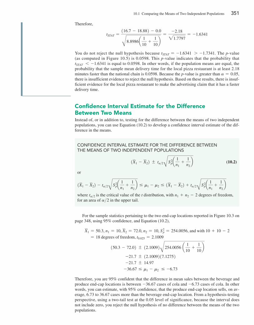
10.1 Comparing the Means of Two Independent Populations 351
Confidence interval estimate for the Difference Between Two MeansInstead of, or in addition to, testing for the difference between the means of two independent populations, you can use equation (10.2) to develop a confidence interval estimate of the dif-ference in the means.
Therefore,
tSTAT =116.7 - 18.882 - 0.0B8.8986a 1
10+
1
10b
=-2.1821.7797
= -1.6341
You do not reject the null hypothesis because tSTAT = -1.6341 7 -1.7341. The p-value (as computed in Figure 10.5) is 0.0598. This p-value indicates that the probability that tSTAT 6 -1.6341 is equal to 0.0598. In other words, if the population means are equal, the probability that the sample mean delivery time for the local pizza restaurant is at least 2.18 minutes faster than the national chain is 0.0598. Because the p-value is greater than a = 0.05, there is insufficient evidence to reject the null hypothesis. Based on these results, there is insuf-ficient evidence for the local pizza restaurant to make the advertising claim that it has a faster delivery time.
CONFIDENCE INTERVAl ESTIMATE FOR ThE DIFFERENCE BETWEEN ThE MEANS OF TWO INDEPENDENT POPUlATIONS
1X1 - X22 { ta>2BS2pa 1
n1+
1n2
b (10.2)
or
1X1 - X22 - ta>2BS2pa 1
n1+
1n2
b … m1 - m2 … 1X1 - X22 + ta>2BS2pa 1
n1+
1n2
b
where ta>2 is the critical value of the t distribution, with n1 + n2 - 2 degrees of freedom, for an area of a>2 in the upper tail.
For the sample statistics pertaining to the two end-cap locations reported in Figure 10.3 on page 348, using 95% confidence, and equation (10.2),
X1 = 50.3, n1 = 10, X2 = 72.0, n2 = 10, S2p = 254.0056, and with 10 + 10 - 2
= 18 degrees of freedom, t0.025 = 2.1009
150.3 - 72.02 { 12.10092B254.0056 a 1
10+
1
10b
-21.7 { 12.1009217.12752 -21.7 { 14.97
-36.67 … m1 - m2 … -6.73
Therefore, you are 95% confident that the difference in mean sales between the beverage and produce end-cap locations is between -36.67 cases of cola and -6.73 cases of cola. In other words, you can estimate, with 95% confidence, that the produce end-cap location sells, on av-erage, 6.73 to 36.67 cases more than the beverage end-cap location. From a hypothesis-testing perspective, using a two-tail test at the 0.05 level of significance, because the interval does not include zero, you reject the null hypothesis of no difference between the means of the two populations.
352 CHAPTeR 10 Two-Sample Tests and One-Way ANOVA
t Test for the Difference Between Two Means, assuming unequal VariancesIf you can assume that the two independent populations are normally distributed but can-not assume that they have equal variances, you cannot pool the two sample variances into the common estimate S2
p and therefore cannot use the pooled-variance t test. Instead, you use the separate-variance t test developed by Satterthwaite that uses the two separate sample variances (see reference 9).
Figure 10.6 displays the separate-variance t test results for the end-cap display location data. Observe that the test statistic tSTAT = -3.0446 and the p-value is 0.0082 6 0.05. Thus, the re-sults for the separate-variance t test are nearly the same as those of the pooled-variance t test.
F i g u r e 1 0 . 6Excel and Minitab separate-variance t test results for the sales data for the two end-caps
Do People Really Do This?Some question whether decision makers really use confirmatory methods, such as hypothesis testing, in this emerging era of big data. The following real case study, contributed by a former student of a colleague of the authors, reveals a role that con-firmatory methods still play in business as well as answering another question: “Do businesses really monitor their customer service calls for quality as-surance purposes as they sometime claim?”
In her first full-time job at a financial services company, a student was asked to improve a training program for new hires at a call center that handled customer questions about outstanding loans. For feedback and evaluation, she planned to randomly select phone calls received by each new employee and rate the employee on 10 aspects of the call, in-cluding whether the employee maintained a pleasant
tone with the customer. When she presented her plan to her boss for approval, her boss wanted proof that her new training program would improve customer service. The boss, quoting a famous statistician, said “In God we trust; all others must bring data.” Faced with this request, she called her business statistics professor. “Hello, Professor, you’ll never believe why I called. I work for a large company, and in the proj-ect I am currently working on, I have to put some of the statistics you taught us to work! Can you help?” Together they formulated this test:
• Randomly assign the 60 most recent hires to two training programs. Assign half to the preex-isting training program and the other half to the new training program.
• At the end of the first month, compare the mean score for the 30 employees in the new training
program against the mean score for the 30 em-ployees in the preexisting training program.
She listened as her professor explained, “What you are trying to show is that the mean score from the new training program is higher than the mean score from the current program. You can make the null hypothesis that the means are equal and see if you can reject it in favor of the alternative that the mean score from the new program is higher.”
“Or, as you used to say, ‘if the p-value is low, Ho must go!’—yes, I do remember!” she replied. Her professor chuckled and added, “If you can reject Ho you will have the evidence to present to your boss.” She thanked him for his help and got back to work, with the newfound confidence that she would be able to successfully apply the t test that compares the means of two independent populations.
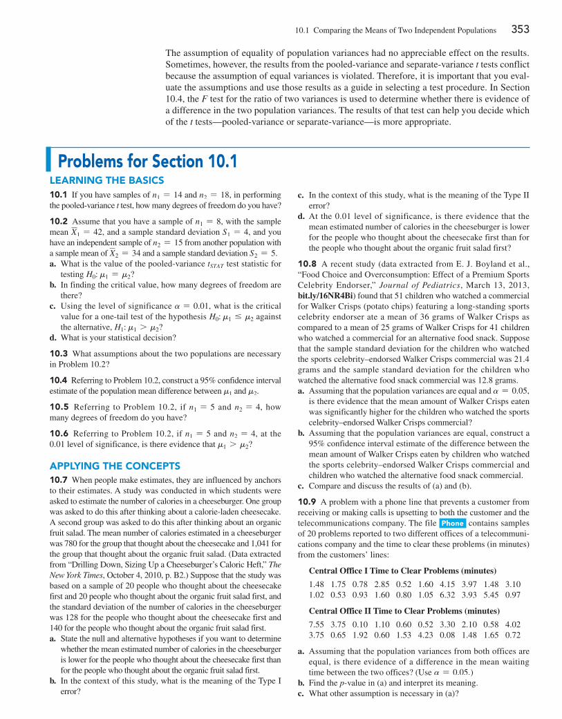
10.1 Comparing the Means of Two Independent Populations 353
Problems for Section 10.1learning The BaSiCS10.1 If you have samples of n1 = 14 and n2 = 18, in performing the pooled-variance t test, how many degrees of freedom do you have?
10.2 Assume that you have a sample of n1 = 8, with the sample mean X1 = 42, and a sample standard deviation S1 = 4, and you have an independent sample of n2 = 15 from another population with a sample mean of X2 = 34 and a sample standard deviation S2 = 5.a. What is the value of the pooled-variance tSTAT test statistic for
testing H0: m1 = m2?b. In finding the critical value, how many degrees of freedom are
there?c. Using the level of significance a = 0.01, what is the critical
value for a one-tail test of the hypothesis H0: m1 … m2 against the alternative, H1: m1 7 m2?
d. What is your statistical decision?
10.3 What assumptions about the two populations are necessary in Problem 10.2?
10.4 Referring to Problem 10.2, construct a 95% confidence interval estimate of the population mean difference between m1 and m2.
10.5 Referring to Problem 10.2, if n1 = 5 and n2 = 4, how many degrees of freedom do you have?
10.6 Referring to Problem 10.2, if n1 = 5 and n2 = 4, at the 0.01 level of significance, is there evidence that m1 7 m2?
aPPlying The ConCePTS10.7 When people make estimates, they are influenced by anchors to their estimates. A study was conducted in which students were asked to estimate the number of calories in a cheeseburger. One group was asked to do this after thinking about a calorie-laden cheesecake. A second group was asked to do this after thinking about an organic fruit salad. The mean number of calories estimated in a cheeseburger was 780 for the group that thought about the cheesecake and 1,041 for the group that thought about the organic fruit salad. (Data extracted from “Drilling Down, Sizing Up a Cheeseburger’s Caloric Heft,” The New York Times, October 4, 2010, p. B2.) Suppose that the study was based on a sample of 20 people who thought about the cheesecake first and 20 people who thought about the organic fruit salad first, and the standard deviation of the number of calories in the cheeseburger was 128 for the people who thought about the cheesecake first and 140 for the people who thought about the organic fruit salad first.a. State the null and alternative hypotheses if you want to determine
whether the mean estimated number of calories in the cheeseburger is lower for the people who thought about the cheesecake first than for the people who thought about the organic fruit salad first.
b. In the context of this study, what is the meaning of the Type I error?
c. In the context of this study, what is the meaning of the Type II error?
d. At the 0.01 level of significance, is there evidence that the mean estimated number of calories in the cheeseburger is lower for the people who thought about the cheesecake first than for the people who thought about the organic fruit salad first?
10.8 A recent study (data extracted from e. J. Boyland et al., “Food Choice and Overconsumption: effect of a Premium Sports Celebrity endorser,” Journal of Pediatrics, March 13, 2013, bit.ly/16NR4Bi) found that 51 children who watched a commercial for Walker Crisps (potato chips) featuring a long-standing sports celebrity endorser ate a mean of 36 grams of Walker Crisps as compared to a mean of 25 grams of Walker Crisps for 41 children who watched a commercial for an alternative food snack. Suppose that the sample standard deviation for the children who watched the sports celebrity–endorsed Walker Crisps commercial was 21.4 grams and the sample standard deviation for the children who watched the alternative food snack commercial was 12.8 grams.a. Assuming that the population variances are equal and a = 0.05,
is there evidence that the mean amount of Walker Crisps eaten was significantly higher for the children who watched the sports celebrity–endorsed Walker Crisps commercial?
b. Assuming that the population variances are equal, construct a 95% confidence interval estimate of the difference between the mean amount of Walker Crisps eaten by children who watched the sports celebrity–endorsed Walker Crisps commercial and children who watched the alternative food snack commercial.
c. Compare and discuss the results of (a) and (b).
10.9 A problem with a phone line that prevents a customer from receiving or making calls is upsetting to both the customer and the telecommunications company. The file Phone contains samples of 20 problems reported to two different offices of a telecommuni-cations company and the time to clear these problems (in minutes) from the customers’ lines:
Central Office I Time to Clear Problems (minutes)
1.48 1.75 0.78 2.85 0.52 1.60 4.15 3.97 1.48 3.101.02 0.53 0.93 1.60 0.80 1.05 6.32 3.93 5.45 0.97
Central Office II Time to Clear Problems (minutes)
7.55 3.75 0.10 1.10 0.60 0.52 3.30 2.10 0.58 4.023.75 0.65 1.92 0.60 1.53 4.23 0.08 1.48 1.65 0.72
a. Assuming that the population variances from both offices are equal, is there evidence of a difference in the mean waiting time between the two offices? (Use a = 0.05.)
b. Find the p-value in (a) and interpret its meaning.c. What other assumption is necessary in (a)?
The assumption of equality of population variances had no appreciable effect on the results. Sometimes, however, the results from the pooled-variance and separate-variance t tests conflict because the assumption of equal variances is violated. Therefore, it is important that you eval-uate the assumptions and use those results as a guide in selecting a test procedure. In Section 10.4, the F test for the ratio of two variances is used to determine whether there is evidence of a difference in the two population variances. The results of that test can help you decide which of the t tests—pooled-variance or separate-variance—is more appropriate.
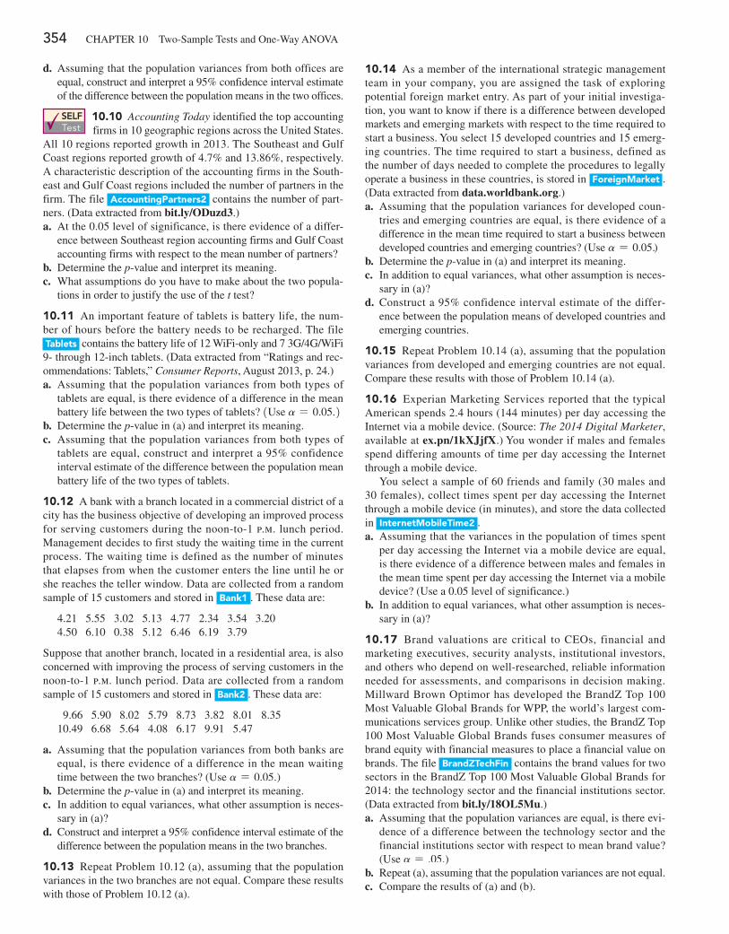
354 CHAPTeR 10 Two-Sample Tests and One-Way ANOVA
d. Assuming that the population variances from both offices are equal, construct and interpret a 95% confidence interval estimate of the difference between the population means in the two offices.
SELF Test
10.10 Accounting Today identified the top accounting firms in 10 geographic regions across the United States.
All 10 regions reported growth in 2013. The Southeast and Gulf Coast regions reported growth of 4.7% and 13.86%, respectively. A characteristic description of the accounting firms in the South-east and Gulf Coast regions included the number of partners in the firm. The file accountingPartners2 contains the number of part-ners. (Data extracted from bit.ly/ODuzd3.)a. At the 0.05 level of significance, is there evidence of a differ-
ence between Southeast region accounting firms and Gulf Coast accounting firms with respect to the mean number of partners?
b. Determine the p-value and interpret its meaning.c. What assumptions do you have to make about the two popula-
tions in order to justify the use of the t test?
10.11 An important feature of tablets is battery life, the num-ber of hours before the battery needs to be recharged. The file Tablets contains the battery life of 12 WiFi-only and 7 3G/4G/WiFi 9- through 12-inch tablets. (Data extracted from “Ratings and rec-ommendations: Tablets,” Consumer Reports, August 2013, p. 24.)a. Assuming that the population variances from both types of
tablets are equal, is there evidence of a difference in the mean battery life between the two types of tablets? 1Use a = 0.05.2
b. Determine the p-value in (a) and interpret its meaning.c. Assuming that the population variances from both types of
tablets are equal, construct and interpret a 95% confidence interval estimate of the difference between the population mean battery life of the two types of tablets.
10.12 A bank with a branch located in a commercial district of a city has the business objective of developing an improved process for serving customers during the noon-to-1 p.m. lunch period. Management decides to first study the waiting time in the current process. The waiting time is defined as the number of minutes that elapses from when the customer enters the line until he or she reaches the teller window. Data are collected from a random sample of 15 customers and stored in Bank1 . These data are:
4.21 5.55 3.02 5.13 4.77 2.34 3.54 3.204.50 6.10 0.38 5.12 6.46 6.19 3.79
Suppose that another branch, located in a residential area, is also concerned with improving the process of serving customers in the noon-to-1 p.m. lunch period. Data are collected from a random sample of 15 customers and stored in Bank2 . These data are:
9.66 5.90 8.02 5.79 8.73 3.82 8.01 8.3510.49 6.68 5.64 4.08 6.17 9.91 5.47
a. Assuming that the population variances from both banks are equal, is there evidence of a difference in the mean waiting time between the two branches? (Use a = 0.05.)
b. Determine the p-value in (a) and interpret its meaning.c. In addition to equal variances, what other assumption is neces-
sary in (a)?d. Construct and interpret a 95% confidence interval estimate of the
difference between the population means in the two branches.
10.13 Repeat Problem 10.12 (a), assuming that the population variances in the two branches are not equal. Compare these results with those of Problem 10.12 (a).
10.14 As a member of the international strategic management team in your company, you are assigned the task of exploring potential foreign market entry. As part of your initial investiga-tion, you want to know if there is a difference between developed markets and emerging markets with respect to the time required to start a business. You select 15 developed countries and 15 emerg-ing countries. The time required to start a business, defined as the number of days needed to complete the procedures to legally operate a business in these countries, is stored in ForeignMarket . (Data extracted from data.worldbank.org.)a. Assuming that the population variances for developed coun-
tries and emerging countries are equal, is there evidence of a difference in the mean time required to start a business between developed countries and emerging countries? (Use a = 0.05.)
b. Determine the p-value in (a) and interpret its meaning.c. In addition to equal variances, what other assumption is neces-
sary in (a)?d. Construct a 95% confidence interval estimate of the differ-
ence between the population means of developed countries and emerging countries.
10.15 Repeat Problem 10.14 (a), assuming that the population variances from developed and emerging countries are not equal. Compare these results with those of Problem 10.14 (a).
10.16 experian Marketing Services reported that the typical American spends 2.4 hours (144 minutes) per day accessing the Internet via a mobile device. (Source: The 2014 Digital Marketer, available at ex.pn/1kXJjfX.) You wonder if males and females spend differing amounts of time per day accessing the Internet through a mobile device.
You select a sample of 60 friends and family (30 males and 30 females), collect times spent per day accessing the Internet through a mobile device (in minutes), and store the data collected in internetMobileTime2 .a. Assuming that the variances in the population of times spent
per day accessing the Internet via a mobile device are equal, is there evidence of a difference between males and females in the mean time spent per day accessing the Internet via a mobile device? (Use a 0.05 level of significance.)
b. In addition to equal variances, what other assumption is neces-sary in (a)?
10.17 Brand valuations are critical to CeOs, financial and marketing executives, security analysts, institutional investors, and others who depend on well-researched, reliable information needed for assessments, and comparisons in decision making. Millward Brown Optimor has developed the BrandZ Top 100 Most Valuable Global Brands for WPP, the world’s largest com-munications services group. Unlike other studies, the BrandZ Top 100 Most Valuable Global Brands fuses consumer measures of brand equity with financial measures to place a financial value on brands. The file BrandZTechFin contains the brand values for two sectors in the BrandZ Top 100 Most Valuable Global Brands for 2014: the technology sector and the financial institutions sector. (Data extracted from bit.ly/18OL5Mu.)a. Assuming that the population variances are equal, is there evi-
dence of a difference between the technology sector and the financial institutions sector with respect to mean brand value? (Use a = .05.)
b. Repeat (a), assuming that the population variances are not equal.c. Compare the results of (a) and (b).
10.2 Comparing the Means of Two Related Populations 355
10.2 Comparing the Means of Two Related Populations
The hypothesis-testing procedures presented in Section 10.1 enable you to examine differ-ences between the means of two independent populations. In this section, you will learn about a procedure for examining the mean difference between two populations when you collect sample data from populations that are related—that is, when results of the first population are not independent of the results of the second population.
There are two situations that involve related data: when you take repeated measurements from the same set of items or individuals or when you match items or individuals according to some characteristic. In either situation, you are interested in the difference between the two related values rather than the individual values themselves.
When you take repeated measurements on the same items or individuals, you assume that the same items or individuals will behave alike if treated alike. Your objective is to show that any differences between two measurements of the same items or individuals are due to different treatments that have been applied to the items or individuals. For example, when performing a taste-testing experiment comparing two beverages, you can use each person in the sample as his or her own control so that you can have repeated measurements on the same individual.
Another example of repeated measurements involves the pricing of the same goods from two different vendors. For example, have you ever wondered whether new textbook prices at a local college bookstore are different from the prices offered at a major online retailer? You could take two independent samples—that is, select two different sets of textbooks—and then use the hypothesis tests discussed in Section 10.1.
However, by random chance, the first sample may have many large-format hardcover text-books and the second sample may have many small trade paperback books. This would imply that the first set of textbooks will always be more expensive than the second set of textbooks, regardless of where they are purchased. This observation means that using the Section 10.1 tests would not be a good choice. The better choice would be to use two related samples—that is, to determine the price of the same sample of textbooks at both the local bookstore and the online retailer.
The second situation that involves related data between populations is when you have matched samples. Here items or individuals are paired together according to some charac-teristic of interest. For example, in test marketing a product in two different advertising cam-paigns, a sample of test markets can be matched on the basis of the test-market population size and/or demographic variables. By accounting for the differences in test-market population size and/or demographic variables, you are better able to measure the effects of the two different advertising campaigns.
Regardless of whether you have matched samples or repeated measurements, the objective is to study the difference between two measurements by reducing the effect of the variability that is due to the items or individuals themselves. Table 10.3 shows the differences between the individual values for two related populations. To read this table, let X11, X12, c, X1n represent the n values from the first sample. And let X21, X22, c, X2n represent either the corresponding n matched values from a second sample or the corresponding n repeated measurements from the initial sample. Then D1, D2, c, Dn will represent the corresponding set of n difference scores such that
D1 = X11 - X21, D2 = X12 - X22, c, and Dn = X1n - X2n.
To test for the mean difference between two related populations, you treat the difference scores, each Di, as values from a single sample.
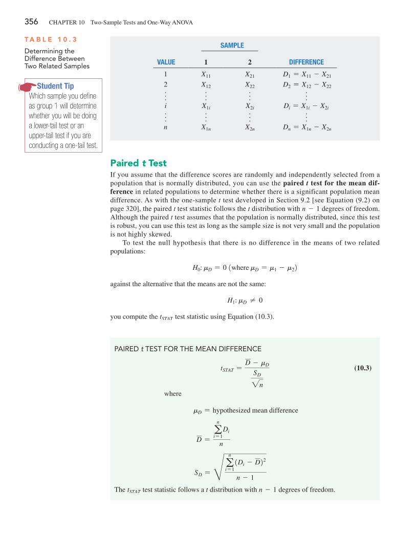
356 CHAPTeR 10 Two-Sample Tests and One-Way ANOVA
Paired t TestIf you assume that the difference scores are randomly and independently selected from a population that is normally distributed, you can use the paired t test for the mean dif-ference in related populations to determine whether there is a significant population mean difference. As with the one-sample t test developed in Section 9.2 [see equation (9.2) on page 320], the paired t test statistic follows the t distribution with n - 1 degrees of freedom. Although the paired t test assumes that the population is normally distributed, since this test is robust, you can use this test as long as the sample size is not very small and the population is not highly skewed.
To test the null hypothesis that there is no difference in the means of two related populations:
H0: mD = 0 1where mD = m1 - m22
against the alternative that the means are not the same:
H1: mD ≠ 0
you compute the tSTAT test statistic using equation (10.3).
T a B l e 1 0 . 3
Determining the Difference Between Two Related Samples
Student TipWhich sample you define as group 1 will determine whether you will be doing a lower-tail test or an upper-tail test if you are conducting a one-tail test.
PAIRED t TEST FOR ThE MEAN DIFFERENCE
tSTAT =D - mD
SD2n
(10.3)
where
mD = hypothesized mean difference
D =a
n
i= 1Di
n
SD = H an
i= 11Di - D22
n - 1
The tSTAT test statistic follows a t distribution with n - 1 degrees of freedom.
Sample
Value 1 2 Difference
1 X11 X21 D1 = X11 - X21
2 X12 X22 D2 = X12 - X22
f f f fi X1i X2i Di = X1i - X2i
f f f fn X1n X2n Dn = X1n - X2n
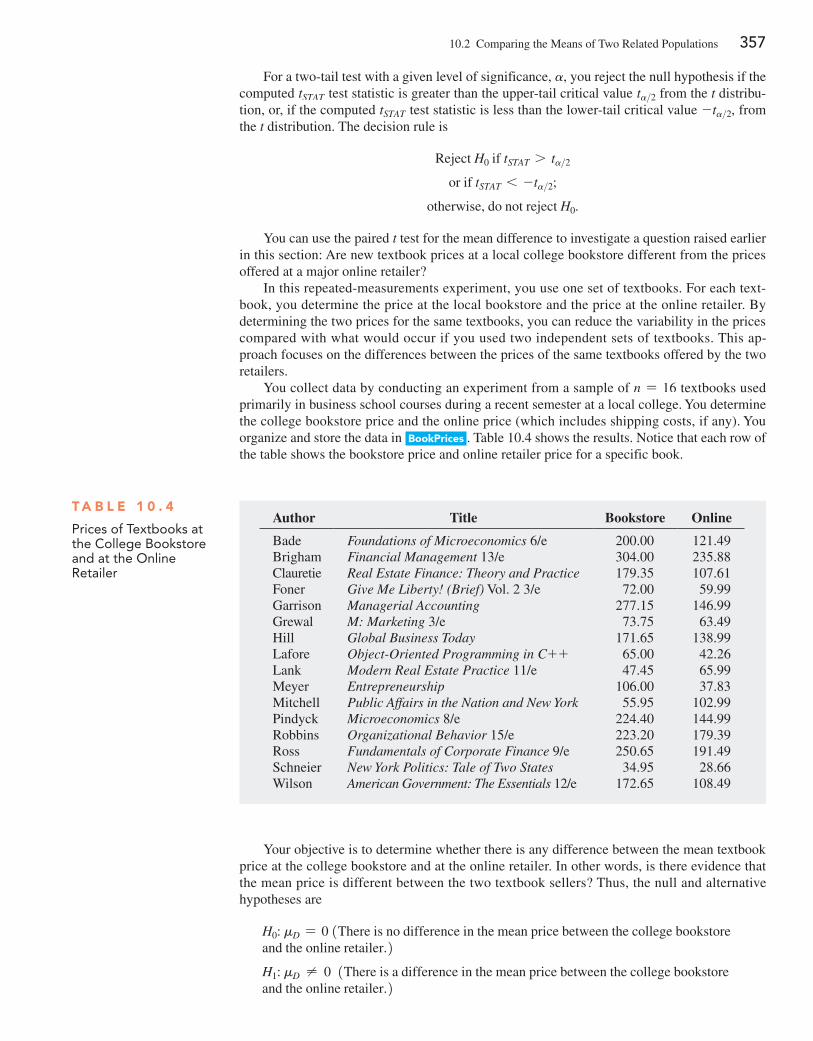
10.2 Comparing the Means of Two Related Populations 357
For a two-tail test with a given level of significance, a, you reject the null hypothesis if the computed tSTAT test statistic is greater than the upper-tail critical value ta>2 from the t distribu-tion, or, if the computed tSTAT test statistic is less than the lower-tail critical value - ta>2, from the t distribution. The decision rule is
Reject H0 if tSTAT 7 ta>2or if tSTAT 6 - ta>2;
otherwise, do not reject H0.
You can use the paired t test for the mean difference to investigate a question raised earlier in this section: Are new textbook prices at a local college bookstore different from the prices offered at a major online retailer?
In this repeated-measurements experiment, you use one set of textbooks. For each text-book, you determine the price at the local bookstore and the price at the online retailer. By determining the two prices for the same textbooks, you can reduce the variability in the prices compared with what would occur if you used two independent sets of textbooks. This ap-proach focuses on the differences between the prices of the same textbooks offered by the two retailers.
You collect data by conducting an experiment from a sample of n = 16 textbooks used primarily in business school courses during a recent semester at a local college. You determine the college bookstore price and the online price (which includes shipping costs, if any). You organize and store the data in BookPrices . Table 10.4 shows the results. Notice that each row of the table shows the bookstore price and online retailer price for a specific book.
Your objective is to determine whether there is any difference between the mean textbook price at the college bookstore and at the online retailer. In other words, is there evidence that the mean price is different between the two textbook sellers? Thus, the null and alternative hypotheses are
H0: mD = 0 1There is no difference in the mean price between the college bookstore and the online retailer.2H1: mD ≠ 0 1There is a difference in the mean price between the college bookstore and the online retailer.2
T a B l e 1 0 . 4
Prices of Textbooks at the College Bookstore and at the Online Retailer
Author Title Bookstore Online
Bade Foundations of Microeconomics 6/e 200.00 121.49Brigham Financial Management 13/e 304.00 235.88Clauretie Real Estate Finance: Theory and Practice 179.35 107.61Foner Give Me Liberty! (Brief) Vol. 2 3/e 72.00 59.99Garrison Managerial Accounting 277.15 146.99Grewal M: Marketing 3/e 73.75 63.49Hill Global Business Today 171.65 138.99Lafore Object-Oriented Programming in C+ + 65.00 42.26Lank Modern Real Estate Practice 11/e 47.45 65.99Meyer Entrepreneurship 106.00 37.83Mitchell Public Affairs in the Nation and New York 55.95 102.99Pindyck Microeconomics 8/e 224.40 144.99Robbins Organizational Behavior 15/e 223.20 179.39Ross Fundamentals of Corporate Finance 9/e 250.65 191.49Schneier New York Politics: Tale of Two States 34.95 28.66Wilson American Government: The Essentials 12/e 172.65 108.49
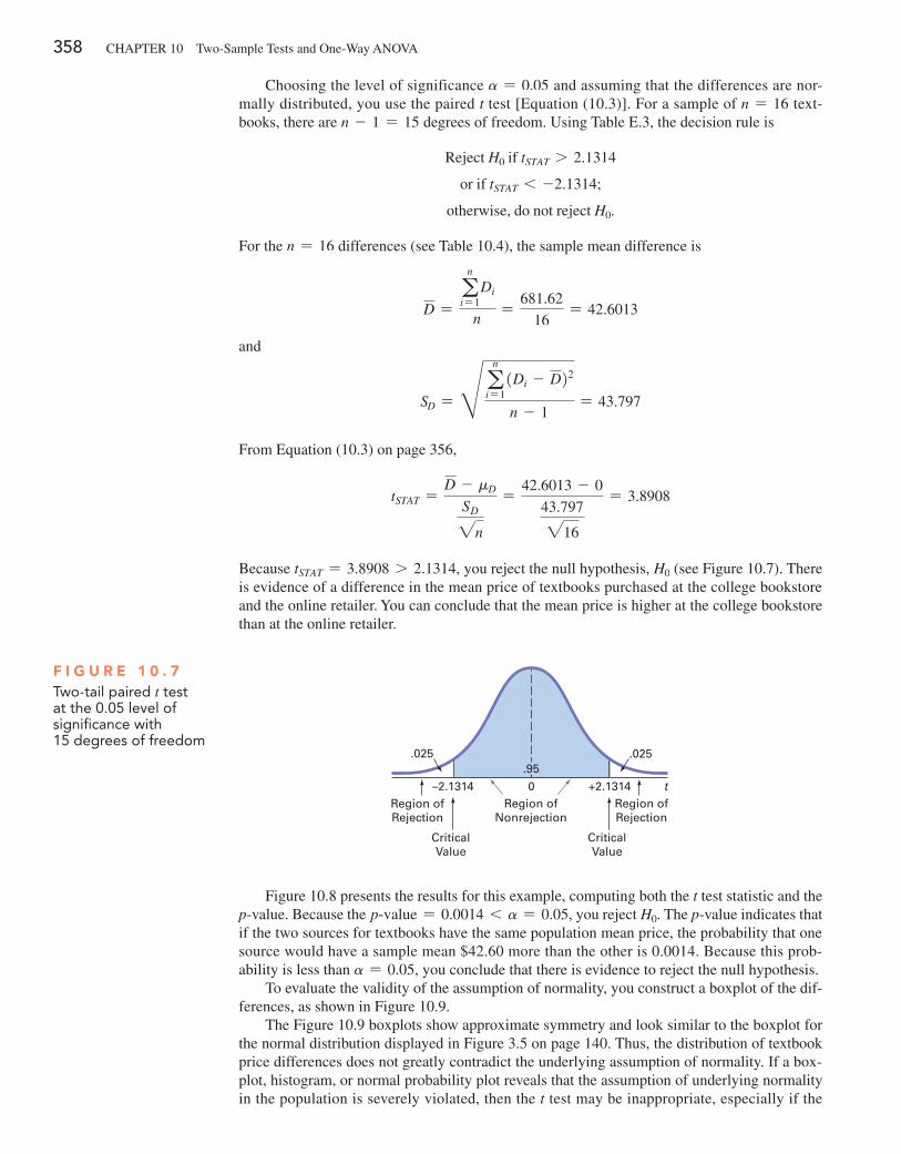
358 CHAPTeR 10 Two-Sample Tests and One-Way ANOVA
Choosing the level of significance a = 0.05 and assuming that the differences are nor-mally distributed, you use the paired t test [equation (10.3)]. For a sample of n = 16 text-books, there are n - 1 = 15 degrees of freedom. Using Table e.3, the decision rule is
Reject H0 if tSTAT 7 2.1314
or if tSTAT 6 -2.1314;
otherwise, do not reject H0.
For the n = 16 differences (see Table 10.4), the sample mean difference is
D =a
n
i= 1Di
n=
681.62
16= 42.6013
and
SD = H an
i= 11Di - D22
n - 1= 43.797
From equation (10.3) on page 356,
tSTAT =D - mD
SD2n
=42.6013 - 0
43.797216
= 3.8908
Because tSTAT = 3.8908 7 2.1314, you reject the null hypothesis, H0 (see Figure 10.7). There is evidence of a difference in the mean price of textbooks purchased at the college bookstore and the online retailer. You can conclude that the mean price is higher at the college bookstore than at the online retailer.
F i g u r e 1 0 . 7Two-tail paired t test at the 0.05 level of significance with 15 degrees of freedom
–2.1314 +2.13140 t
.025 .025
Region ofRejection
CriticalValue
Region ofNonrejection
CriticalValue
Region ofRejection
.95
Figure 10.8 presents the results for this example, computing both the t test statistic and the p-value. Because the p@value = 0.0014 6 a = 0.05, you reject H0. The p-value indicates that if the two sources for textbooks have the same population mean price, the probability that one source would have a sample mean $42.60 more than the other is 0.0014. Because this prob-ability is less than a = 0.05, you conclude that there is evidence to reject the null hypothesis.
To evaluate the validity of the assumption of normality, you construct a boxplot of the dif-ferences, as shown in Figure 10.9.
The Figure 10.9 boxplots show approximate symmetry and look similar to the boxplot for the normal distribution displayed in Figure 3.5 on page 140. Thus, the distribution of textbook price differences does not greatly contradict the underlying assumption of normality. If a box-plot, histogram, or normal probability plot reveals that the assumption of underlying normality in the population is severely violated, then the t test may be inappropriate, especially if the
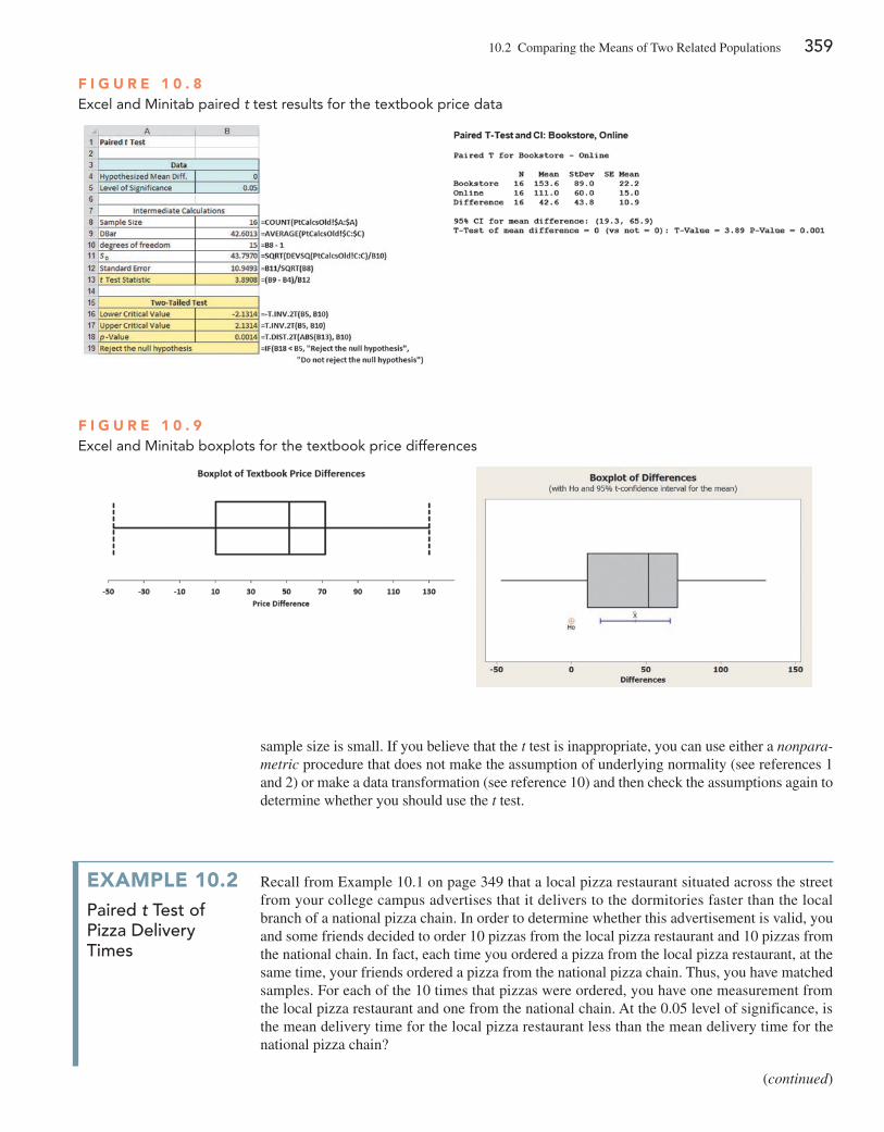
10.2 Comparing the Means of Two Related Populations 359
sample size is small. If you believe that the t test is inappropriate, you can use either a nonpara-metric procedure that does not make the assumption of underlying normality (see references 1 and 2) or make a data transformation (see reference 10) and then check the assumptions again to determine whether you should use the t test.
F i g u r e 1 0 . 8Excel and Minitab paired t test results for the textbook price data
F i g u r e 1 0 . 9Excel and Minitab boxplots for the textbook price differences
exaMPle 10.2paired t test of pizza delivery times
Recall from example 10.1 on page 349 that a local pizza restaurant situated across the street from your college campus advertises that it delivers to the dormitories faster than the local branch of a national pizza chain. In order to determine whether this advertisement is valid, you and some friends decided to order 10 pizzas from the local pizza restaurant and 10 pizzas from the national chain. In fact, each time you ordered a pizza from the local pizza restaurant, at the same time, your friends ordered a pizza from the national pizza chain. Thus, you have matched samples. For each of the 10 times that pizzas were ordered, you have one measurement from the local pizza restaurant and one from the national chain. At the 0.05 level of significance, is the mean delivery time for the local pizza restaurant less than the mean delivery time for the national pizza chain?
(continued)
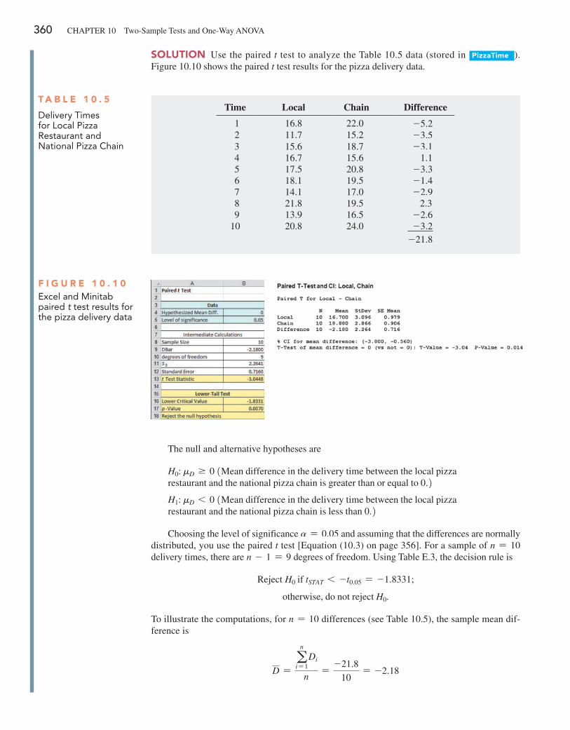
360 CHAPTeR 10 Two-Sample Tests and One-Way ANOVA
SoluTion Use the paired t test to analyze the Table 10.5 data (stored in PizzaTime ). Figure 10.10 shows the paired t test results for the pizza delivery data.
The null and alternative hypotheses are
H0: mD Ú 0 1Mean difference in the delivery time between the local pizza restaurant and the national pizza chain is greater than or equal to 0.2H1: mD 6 0 1Mean difference in the delivery time between the local pizza restaurant and the national pizza chain is less than 0.2
Choosing the level of significance a = 0.05 and assuming that the differences are normally distributed, you use the paired t test [equation (10.3) on page 356]. For a sample of n = 10 delivery times, there are n - 1 = 9 degrees of freedom. Using Table e.3, the decision rule is
Reject H0 if tSTAT 6 - t0.05 = -1.8331;
otherwise, do not reject H0.
To illustrate the computations, for n = 10 differences (see Table 10.5), the sample mean dif-ference is
D =a
n
i= 1Di
n=
-21.8
10= -2.18
T a B l e 1 0 . 5
Delivery Times for local Pizza Restaurant and National Pizza Chain
Time Local Chain Difference
1 16.8 22.0 -5.22 11.7 15.2 -3.53 15.6 18.7 -3.14 16.7 15.6 1.15 17.5 20.8 -3.36 18.1 19.5 -1.47 14.1 17.0 -2.98 21.8 19.5 2.39 13.9 16.5 -2.6
10 20.8 24.0 -3.2-21.8
F i g u r e 1 0 . 1 0Excel and Minitab paired t test results for the pizza delivery data
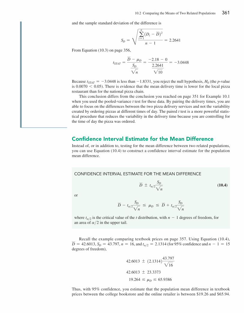
10.2 Comparing the Means of Two Related Populations 361
Confidence interval estimate for the Mean DifferenceInstead of, or in addition to, testing for the mean difference between two related populations, you can use equation (10.4) to construct a confidence interval estimate for the population mean difference.
and the sample standard deviation of the difference is
SD = H an
i= 11Di - D22
n - 1= 2.2641
From equation (10.3) on page 356,
tSTAT =D - mD
SD2n
=-2.18 - 0
2.2641210
= -3.0448
Because tSTAT = -3.0448 is less than -1.8331, you reject the null hypothesis, H0 (the p-value is 0.0070 6 0.05). There is evidence that the mean delivery time is lower for the local pizza restaurant than for the national pizza chain.
This conclusion differs from the conclusion you reached on page 351 for example 10.1 when you used the pooled-variance t test for these data. By pairing the delivery times, you are able to focus on the differences between the two pizza delivery services and not the variability created by ordering pizzas at different times of day. The paired t test is a more powerful statis-tical procedure that reduces the variability in the delivery time because you are controlling for the time of day the pizza was ordered.
CONFIDENCE INTERVAl ESTIMATE FOR ThE MEAN DIFFERENCE
D { ta>2SD2n
(10.4)
or
D - ta>2SD2n
… mD … D + ta>2SD2n
where ta>2 is the critical value of the t distribution, with n - 1 degrees of freedom, for an area of a>2 in the upper tail.
Recall the example comparing textbook prices on page 357. Using equation (10.4), D = 42.6013, SD = 43.797, n = 16, and ta>2 = 2.1314 (for 95% confidence and n - 1 = 15 degrees of freedom),
42.6013 { 12.1314243.797216
42.6013 { 23.3373
19.264 … mD … 65.9386
Thus, with 95% confidence, you estimate that the population mean difference in textbook prices between the college bookstore and the online retailer is between $19.26 and $65.94.

362 CHAPTeR 10 Two-Sample Tests and One-Way ANOVA
Because the interval estimate does not contain zero, using the 0.05 level of significance and a two-tail test, you can conclude that there is evidence of a difference in the mean prices of textbooks at the college bookstore and the online retailer. Since both the lower and upper limits of the confidence interval are above 0, you can conclude that the mean price is higher at the college bookstore than the online retailer.
Problems for Section 10.2
BranD
experT A B
C.C. 26 27S.E. 27 27E.G. 19 21B.L. 22 24C.M. 22 25C.N. 25 26G.N. 25 24R.M. 25 26 P.V. 21 23
learning The BaSiCS10.18 An experimental design for a paired t test has 23 pairs of identical twins. How many degrees of freedom are there in this t test?
10.19 Fifteen volunteers are recruited to participate in an ex-periment. A measurement is made (such as blood pressure) before each volunteer is asked to read a particularly upsetting passage from a book and after each volunteer reads the passage from the book. In the analysis of the data collected from this experiment, how many degrees of freedom are there in the test?
aPPlying The ConCePTS10.20 Nine experts rated two brands of coffee in a taste-testing experiment. A rating on a 17-point scale
(1 = extremely unpleasing, 7 = extremely pleasing) is given for each of four characteristics: taste, aroma, richness, and acidity. The accompanying data table contains the ratings accumulated over all four characteristics.
(Data extracted from “Ratings: TV, Phone, and Internet Services,” Consumer Reports, May 2014, pp. 28–29.)a. At the 0.05 level of significance, is there evidence of a difference
in the mean service rating between TV and Internet services?b. What assumption is necessary about the population distribution
in order to perform this test?c. Use a graphical method to evaluate the validity of the assump-
tion in (a).d. Construct and interpret a 95% confidence interval estimate
of the difference in the mean service rating between TV and Internet services.
10.22 Super Target versus Walmart: Who has the lowest prices? Given Walmart’s slogan “Save Money—Live Better,” you sus-pect that Walmart does. The prices of 33 foods were compared (data extracted from “Supermarket Showdown,” The Palm Beach Post, February 13, 2011, pp. 1F, 2F) and the results are stored in TargetWalmart .a. At the 0.05 level of significance, is there evidence that the
mean price of items is higher at Super Target than at Walmart?b. What assumption is necessary about the population distribution
in order to perform this test?c. Find the p-value in (a) and interpret its meaning.
10.23 What motivates employees? The Great Place to Work Institute evaluated nonfinancial factors both globally and in the United States. (Data extracted from L. Petrecca, “Tech Companies Top List of ‘Great Workplaces,’” USA Today, October 31, 2011, p. 7B.) The results, which indicate the importance rating of each factor, are stored in Motivation .a. At the 0.05 level of significance, is there evidence of a differ-
ence in the mean rating between global and U.S. employees?b. What assumption is necessary about the population distribution
in order to perform this test?c. Use a graphical method to evaluate the validity of the assump-
tion in (b).
10.24 Multiple myeloma, or blood plasma cancer, is character-ized by increased blood vessel formulation (angiogenesis) in the bone marrow that is a predictive factor in survival. One treatment approach used for multiple myeloma is stem cell transplantation with the patient’s own stem cells. The data stored in Myeloma , and shown on page 363 represent the bone marrow microvessel density for patients who had a complete response to the stem cell transplant (as measured by blood and urine tests). The measure-ments were taken immediately prior to the stem cell transplant and at the time the complete response was determined.
a. At the 0.05 level of significance, is there evidence of a differ-ence in the mean ratings between the two brands?
b. What assumption is necessary about the population distribution in order to perform this test?
c. Determine the p-value in (a) and interpret its meaning.d. Construct and interpret a 95% confidence interval estimate of
the difference in the mean ratings between the two brands.
10.21 How do the ratings of TV and Internet services compare? The file Telecom contains the rating of 14 different providers.
SELF Test
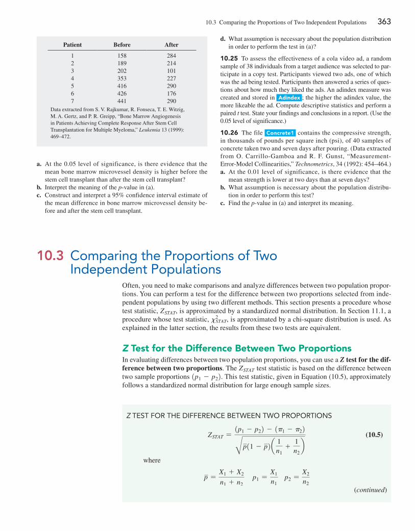
10.3 Comparing the Proportions of Two Independent Populations 363
a. At the 0.05 level of significance, is there evidence that the mean bone marrow microvessel density is higher before the stem cell transplant than after the stem cell transplant?
b. Interpret the meaning of the p-value in (a).c. Construct and interpret a 95% confidence interval estimate of
the mean difference in bone marrow microvessel density be-fore and after the stem cell transplant.
d. What assumption is necessary about the population distribution in order to perform the test in (a)?
10.25 To assess the effectiveness of a cola video ad, a random sample of 38 individuals from a target audience was selected to par-ticipate in a copy test. Participants viewed two ads, one of which was the ad being tested. Participants then answered a series of ques-tions about how much they liked the ads. An adindex measure was created and stored in adindex ; the higher the adindex value, the more likeable the ad. Compute descriptive statistics and perform a paired t test. State your findings and conclusions in a report. (Use the 0.05 level of significance.)
10.26 The file Concrete1 contains the compressive strength, in thousands of pounds per square inch (psi), of 40 samples of concrete taken two and seven days after pouring. (Data extracted from O. Carrillo-Gamboa and R. F. Gunst, “Measurement- error-Model Collinearities,” Technometrics, 34 (1992): 454–464.)a. At the 0.01 level of significance, is there evidence that the
mean strength is lower at two days than at seven days?b. What assumption is necessary about the population distribu-
tion in order to perform this test?c. Find the p-value in (a) and interpret its meaning.
Patient Before After
1 158 2842 189 2143 202 1014 353 2275 416 2906 426 1767 441 290
Data extracted from S. V. Rajkumar, R. Fonseca, T. e. Witzig, M. A. Gertz, and P. R. Greipp, “Bone Marrow Angiogenesis in Patients Achieving Complete Response After Stem Cell Transplantation for Multiple Myeloma,” Leukemia 13 (1999): 469–472.
10.3 Comparing the Proportions of Two Independent Populations
Often, you need to make comparisons and analyze differences between two population propor-tions. You can perform a test for the difference between two proportions selected from inde-pendent populations by using two different methods. This section presents a procedure whose test statistic, ZSTAT, is approximated by a standardized normal distribution. In Section 11.1, a procedure whose test statistic, x2
STAT, is approximated by a chi-square distribution is used. As explained in the latter section, the results from these two tests are equivalent.
Z Test for the Difference Between Two ProportionsIn evaluating differences between two population proportions, you can use a Z test for the dif-ference between two proportions. The ZSTAT test statistic is based on the difference between two sample proportions 1p1 - p22. This test statistic, given in equation (10.5), approximately follows a standardized normal distribution for large enough sample sizes.
Z TEST FOR ThE DIFFERENCE BETWEEN TWO PROPORTIONS
ZSTAT =1p1 - p22 - 1p1 - p22Bp11 - p2a 1
n1+
1n2
b (10.5)
where
p =X1 + X2
n1 + n2 p1 =
X1
n1 p2 =
X2
n2
(continued)
364 CHAPTeR 10 Two-Sample Tests and One-Way ANOVA
The null hypothesis in the Z test for the difference between two proportions states that the two population proportions are equal 1p1 = p22. Because the pooled estimate for the popula-tion proportion is based on the null hypothesis, you combine, or pool, the two sample propor-tions to compute p, an overall estimate of the common population proportion. This estimate is equal to the number of items of interest in the two samples 1X1 + X22 divided by the total sample size from the two samples 1n1 + n22.
As shown in the following table, you can use this Z test for the difference between popula-tion proportions to determine whether there is a difference in the proportion of items of inter-est in the two populations (two-tail test) or whether one population has a higher proportion of items of interest than the other population (one-tail test):
and p1 = proportion of items of interest in sample 1 X1 = number of items of interest in sample 1 n1 = sample size of sample 1 p1 = proportion of items of interest in population 1 p2 = proportion of items of interest in sample 2 X2 = number of items of interest in sample 2 n2 = sample size of sample 2 p2 = proportion of items of interest in population 2 p = pooled estimate of the population proportion of items of interest
The ZSTAT test statistic approximately follows a standardized normal distribution.
Two-Tail Test One-Tail Test One-Tail Test
H0: p1 = p2 H0: p1 Ú p2 H0: p1 … p2
H1: p1 ≠ p2 H1: p1 6 p2 H1: p1 7 p2
where
p1 = proportion of items of interest in population 1
p2 = proportion of items of interest in population 2
To test the null hypothesis that there is no difference between the proportions of two indepen-dent populations:
H0: p1 = p2
against the alternative that the two population proportions are not the same:
H1: p1 ≠ p2
you use the ZSTAT test statistic, given by equation (10.5). For a given level of significance, a, you reject the null hypothesis if the computed ZSTAT test statistic is greater than the upper-tail critical value from the standardized normal distribution or if the computed ZSTAT test statistic is less than the lower-tail critical value from the standardized normal distribution.
To illustrate the use of the Z test for the equality of two proportions, suppose that you are the manager of T.C. Resort Properties, a collection of five upscale resort hotels located on two tropical islands. On one of the islands, T.C. Resort Properties has two hotels, the Beachcomber and the Windsurfer. Using the DCOVA problem-solving approach, you have defined the business objective as improving the return rate of guests at the Beachcomber and the Windsurfer hotels. On the survey completed by hotel guests upon or after their departure, one question asked is whether the guest is likely to return to the hotel. Responses to this and other questions were col-lected from 227 guests at the Beachcomber and 262 guests at the Windsurfer. The results for this
Student TipDo not confuse this use of the Greek letter pi, p, to represent the population proportion with the mathematical constant that uses the same letter to represent the ratio of the circumfer-ence to a diameter of a circle—approximately 3.14159.
10.3 Comparing the Proportions of Two Independent Populations 365
question indicated that 163 of 227 guests at the Beachcomber responded yes, they were likely to return to the hotel and 154 of 262 guests at the Windsurfer responded yes, they were likely to return to the hotel. At the 0.05 level of significance, is there evidence of a significant difference in guest satisfaction (as measured by the likelihood to return to the hotel) between the two hotels?
The null and alternative hypotheses are
H0: p1 = p2 or p1 - p2 = 0
H1: p1 ≠ p2 or p1 - p2 ≠ 0
Using the 0.05 level of significance, the critical values are -1.96 and +1.96 (see Figure 10.11), and the decision rule is
Reject H0 if ZSTAT 6 -1.96
or if ZSTAT 7 +1.96;
otherwise, do not reject H0.
Using equation (10.5) on page 363,
ZSTAT =1p1 - p22 - 1p1 - p22Bp11 - p2a 1
n1+
1n2
b
–1.96 +1.960 Z
Region ofRejection
CriticalValue
Region ofNonrejection
CriticalValue
Region ofRejection
.025.025.95
F i g u r e 1 0 . 1 1Regions of rejection and nonrejection when testing a hypothesis for the difference between two proportions at the 0.05 level of significance
where
p1 =X1
n1=
163
227= 0.7181 p2 =
X2
n2=
154
262= 0.5878
and
p =X1 + X2
n1 + n2=
163 + 154
227 + 262=
317
489= 0.6483
so that
ZSTAT =10.7181 - 0.58782 - 102B0.648311 - 0.64832a 1
227+
1
262b
=0.1303210.228210.00822
=0.130320.00187
=0.1303
0.0432= +3.0088
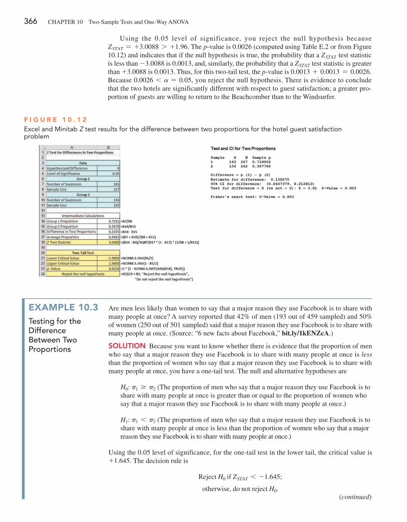
366 CHAPTeR 10 Two-Sample Tests and One-Way ANOVA
Using the 0.05 level of significance, you reject the null hypothesis because ZSTAT = +3.0088 7 +1.96. The p-value is 0.0026 (computed using Table e.2 or from Figure 10.12) and indicates that if the null hypothesis is true, the probability that a ZSTAT test statistic is less than -3.0088 is 0.0013, and, similarly, the probability that a ZSTAT test statistic is greater than +3.0088 is 0.0013. Thus, for this two-tail test, the p-value is 0.0013 + 0.0013 = 0.0026. Because 0.0026 6 a = 0.05, you reject the null hypothesis. There is evidence to conclude that the two hotels are significantly different with respect to guest satisfaction; a greater pro-portion of guests are willing to return to the Beachcomber than to the Windsurfer.
F i g u r e 1 0 . 1 2Excel and Minitab Z test results for the difference between two proportions for the hotel guest satisfaction problem
exaMPle 10.3testing for the difference between two proportions
Are men less likely than women to say that a major reason they use Facebook is to share with many people at once? A survey reported that 42% of men (193 out of 459 sampled) and 50% of women (250 out of 501 sampled) said that a major reason they use Facebook is to share with many people at once. (Source: “6 new facts about Facebook,” bit.ly/1kENZcA.)
SoluTion Because you want to know whether there is evidence that the proportion of men who say that a major reason they use Facebook is to share with many people at once is less than the proportion of women who say that a major reason they use Facebook is to share with many people at once, you have a one-tail test. The null and alternative hypotheses are
H0: p1 Ú p2 (The proportion of men who say that a major reason they use Facebook is to share with many people at once is greater than or equal to the proportion of women who say that a major reason they use Facebook is to share with many people at once.)
H1: p1 6 p2 (The proportion of men who say that a major reason they use Facebook is to share with many people at once is less than the proportion of women who say that a major reason they use Facebook is to share with many people at once.)
Using the 0.05 level of significance, for the one-tail test in the lower tail, the critical value is +1.645. The decision rule is
Reject H0 if ZSTAT 6 -1.645;
otherwise, do not reject H0.(continued)
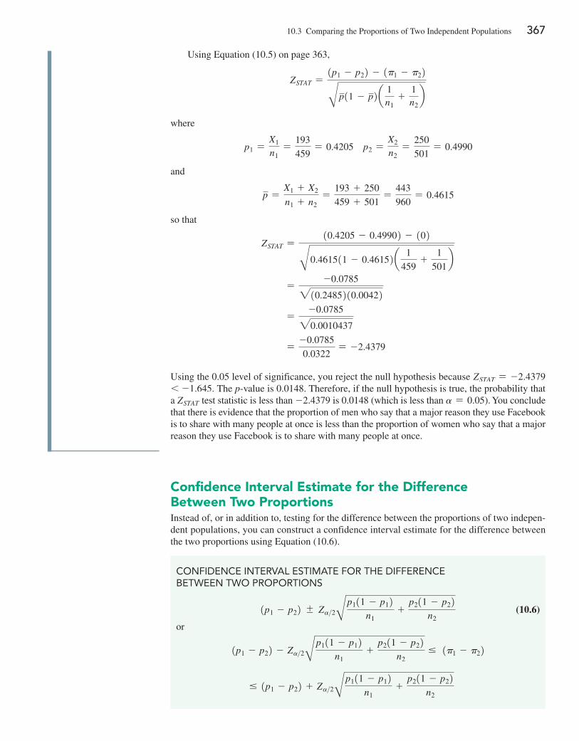
10.3 Comparing the Proportions of Two Independent Populations 367
Using equation (10.5) on page 363,
ZSTAT =1p1 - p22 - 1p1 - p22Bp11 - p2a 1
n1+
1n2
b
where
p1 =X1
n1=
193
459= 0.4205 p2 =
X2
n2=
250
501= 0.4990
and
p =X1 + X2
n1 + n2=
193 + 250
459 + 501=
443
960= 0.4615
so that
ZSTAT =10.4205 - 0.49902 - 102B0.461511 - 0.46152a 1
459+
1
501b
=-0.0785210.2485210.00422
=-0.078520.0010437
=-0.0785
0.0322= -2.4379
Using the 0.05 level of significance, you reject the null hypothesis because ZSTAT = -2.43796 -1.645. The p-value is 0.0148. Therefore, if the null hypothesis is true, the probability that a ZSTAT test statistic is less than -2.4379 is 0.0148 (which is less than a = 0.05). You conclude that there is evidence that the proportion of men who say that a major reason they use Facebook is to share with many people at once is less than the proportion of women who say that a major reason they use Facebook is to share with many people at once.
Confidence interval estimate for the Difference Between Two ProportionsInstead of, or in addition to, testing for the difference between the proportions of two indepen-dent populations, you can construct a confidence interval estimate for the difference between the two proportions using equation (10.6).
CONFIDENCE INTERVAl ESTIMATE FOR ThE DIFFERENCE BETWEEN TWO PROPORTIONS
1p1 - p22 { Za>2Bp111 - p12n1
+p211 - p22
n2 (10.6)
or
1p1 - p22 - Za>2Bp111 - p12n1
+p211 - p22
n2… 1p1 - p22
… 1p1 - p22 + Za>2Bp111 - p12n1
+p211 - p22
n2
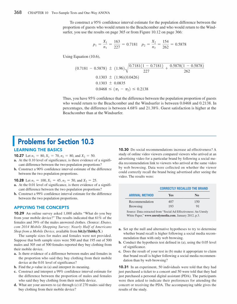
368 CHAPTeR 10 Two-Sample Tests and One-Way ANOVA
To construct a 95% confidence interval estimate for the population difference between the proportion of guests who would return to the Beachcomber and who would return to the Wind-surfer, you use the results on page 365 or from Figure 10.12 on page 366:
p1 =X1
n1=
163
227= 0.7181 p2 =
X2
n2=
154
262= 0.5878
Using equation (10.6),
10.7181 - 0.58782 { 11.962A0.718111 - 0.71812227
+ 0.587811 - 0.58782262
0.1303 { 11.96)10.042620.1303 { 0.0835
0.0468 … 1p1 - p22 … 0.2138
Thus, you have 95% confidence that the difference between the population proportion of guests who would return to the Beachcomber and the Windsurfer is between 0.0468 and 0.2138. In percentages, the difference is between 4.68% and 21.38%. Guest satisfaction is higher at the Beachcomber than at the Windsurfer.
Problems for Section 10.3learning The BaSiCS10.27 Let n1 = 80, X1 = 70, n2 = 80, and X2 = 50.a. At the 0.10 level of significance, is there evidence of a signifi-
cant difference between the two population proportions?b. Construct a 90% confidence interval estimate of the difference
between the two population proportions.
10.28 Let n1 = 100, X1 = 45, n2 = 50, and X2 = 25.a. At the 0.01 level of significance, is there evidence of a signifi-
cant difference between the two population proportions?b. Construct a 99% confidence interval estimate for the difference
between the two population proportions.
aPPlying The ConCePTS10.29 An online survey asked 1,000 adults “What do you buy from your mobile device?” The results indicated that 61% of the females and 39% of the males answered clothes. (Source: Ebates.com 2014 Mobile Shopping Survey: Nearly Half of Americans Shop from a Mobile Device, available from bit.ly/1hi6kyX.)
The sample sizes for males and females were not provided. Suppose that both sample sizes were 500 and that 195 out of 500 males and 305 out of 500 females reported they buy clothing from their mobile device.a. Is there evidence of a difference between males and females in
the proportion who said they buy clothing from their mobile device at the 0.01 level of significance?
b. Find the p-value in (a) and interpret its meaning.c. Construct and interpret a 99% confidence interval estimate for
the difference between the proportion of males and females who said they buy clothing from their mobile device.
d. What are your answers to (a) through (c) if 270 males said they buy clothing from their mobile device?
a. Set up the null and alternative hypotheses to try to determine whether brand recall is higher following a social media recom-mendation than with only web browsing.
b. Conduct the hypothesis test defined in (a), using the 0.05 level of significance.
c. Does the result of your test in (b) make it appropriate to claim that brand recall is higher following a social media recommen-dation than by web browsing?
10.31 In an experiment, 50 individuals were told that they had just purchased a ticket to a concert and 50 were told that they had just purchased a personal digital assistant (PDA). The participants were then asked to indicate their preferences for attending the concert or receiving the PDA. The accompanying table gives the results of the study.
correcTly recalleD The BranD
arriVal meThoD Yes No
Recommendation 407 150Browsing 193 91
Source: Data extracted from “Social Ad effectiveness: An Unruly White Paper,” www.unrulymedia.com, January 2012, p.3.
10.30 Do social recommendations increase ad effectiveness? A study of online video viewers compared viewers who arrived at an advertising video for a particular brand by following a social me-dia recommendation link to viewers who arrived at the same video by web browsing. Data were collected on whether the viewer could correctly recall the brand being advertised after seeing the video. The results were:
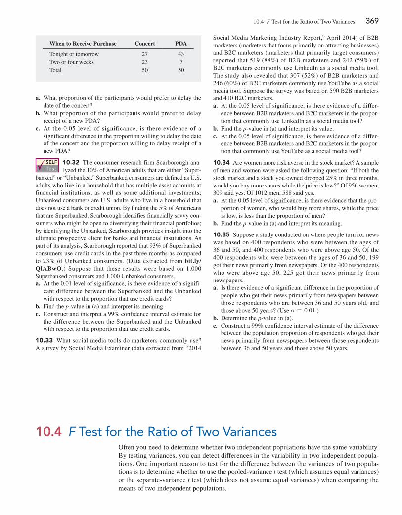
10.4 F Test for the Ratio of Two Variances 369
Social Media Marketing Industry Report,” April 2014) of B2B marketers (marketers that focus primarily on attracting businesses) and B2C marketers (marketers that primarily target consumers) reported that 519 (88%) of B2B marketers and 242 (59%) of B2C marketers commonly use LinkedIn as a social media tool. The study also revealed that 307 (52%) of B2B marketers and 246 (60%) of B2C marketers commonly use YouTube as a social media tool. Suppose the survey was based on 590 B2B marketers and 410 B2C marketers.a. At the 0.05 level of significance, is there evidence of a differ-
ence between B2B marketers and B2C marketers in the propor-tion that commonly use LinkedIn as a social media tool?
b. Find the p-value in (a) and interpret its value.c. At the 0.05 level of significance, is there evidence of a differ-
ence between B2B marketers and B2C marketers in the propor-tion that commonly use YouTube as a social media tool?
10.34 Are women more risk averse in the stock market? A sample of men and women were asked the following question: “If both the stock market and a stock you owned dropped 25% in three months, would you buy more shares while the price is low?” Of 956 women, 309 said yes. Of 1012 men, 588 said yes.a. At the 0.05 level of significance, is there evidence that the pro-
portion of women, who would buy more shares, while the price is low, is less than the proportion of men?
b. Find the p-value in (a) and interpret its meaning.
10.35 Suppose a study conducted on where people turn for news was based on 400 respondents who were between the ages of 36 and 50, and 400 respondents who were above age 50. Of the 400 respondents who were between the ages of 36 and 50, 199 got their news primarily from newspapers. Of the 400 respondents who were above age 50, 225 got their news primarily from newspapers.a. Is there evidence of a significant difference in the proportion of
people who get their news primarily from newspapers between those respondents who are between 36 and 50 years old, and those above 50 years? (Use a = 0.01.)
b. Determine the p-value in (a).c. Construct a 99% confidence interval estimate of the difference
between the population proportion of respondents who get their news primarily from newspapers between those respondents between 36 and 50 years and those above 50 years.
When to Receive Purchase Concert PDA
Tonight or tomorrow 27 43Two or four weeks 23 7Total 50 50
a. What proportion of the participants would prefer to delay the date of the concert?
b. What proportion of the participants would prefer to delay receipt of a new PDA?
c. At the 0.05 level of significance, is there evidence of a significant difference in the proportion willing to delay the date of the concert and the proportion willing to delay receipt of a new PDA?
SELF Test
10.32 The consumer research firm Scarborough ana-lyzed the 10% of American adults that are either “Super-
banked” or “Unbanked.” Superbanked consumers are defined as U.S. adults who live in a household that has multiple asset accounts at financial institutions, as well as some additional investments; Unbanked consumers are U.S. adults who live in a household that does not use a bank or credit union. By finding the 5% of Americans that are Superbanked, Scarborough identifies financially savvy con-sumers who might be open to diversifying their financial portfolios; by identifying the Unbanked, Scarborough provides insight into the ultimate prospective client for banks and financial institutions. As part of its analysis, Scarborough reported that 93% of Superbanked consumers use credit cards in the past three months as compared to 23% of Unbanked consumers. (Data extracted from bit.ly/QlABwO.) Suppose that these results were based on 1,000 Superbanked consumers and 1,000 Unbanked consumers.a. At the 0.01 level of significance, is there evidence of a signifi-
cant difference between the Superbanked and the Unbanked with respect to the proportion that use credit cards?
b. Find the p-value in (a) and interpret its meaning.c. Construct and interpret a 99% confidence interval estimate for
the difference between the Superbanked and the Unbanked with respect to the proportion that use credit cards.
10.33 What social media tools do marketers commonly use? A survey by Social Media examiner (data extracted from “2014
10.4 F Test for the Ratio of Two VariancesOften you need to determine whether two independent populations have the same variability. By testing variances, you can detect differences in the variability in two independent popula-tions. One important reason to test for the difference between the variances of two popula-tions is to determine whether to use the pooled-variance t test (which assumes equal variances) or the separate-variance t test (which does not assume equal variances) when comparing the means of two independent populations.
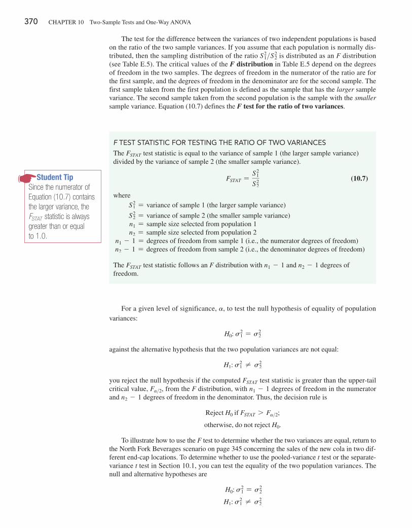
370 CHAPTeR 10 Two-Sample Tests and One-Way ANOVA
The test for the difference between the variances of two independent populations is based on the ratio of the two sample variances. If you assume that each population is normally dis-tributed, then the sampling distribution of the ratio S2
1>S22 is distributed as an F distribution
(see Table e.5). The critical values of the F distribution in Table e.5 depend on the degrees of freedom in the two samples. The degrees of freedom in the numerator of the ratio are for the first sample, and the degrees of freedom in the denominator are for the second sample. The first sample taken from the first population is defined as the sample that has the larger sample variance. The second sample taken from the second population is the sample with the smaller sample variance. equation (10.7) defines the F test for the ratio of two variances.
F TEST STATISTIC FOR TESTINg ThE RATIO OF TWO VARIANCES
The FSTAT test statistic is equal to the variance of sample 1 (the larger sample variance) divided by the variance of sample 2 (the smaller sample variance).
FSTAT =S2
1
S22 (10.7)
whereS2
1 = variance of sample 1 (the larger sample variance)
S22 = variance of sample 2 (the smaller sample variance)
n1 = sample size selected from population 1n2 = sample size selected from population 2
n1 - 1 = degrees of freedom from sample 1 (i.e., the numerator degrees of freedom)n2 - 1 = degrees of freedom from sample 2 (i.e., the denominator degrees of freedom)
The FSTAT test statistic follows an F distribution with n1 - 1 and n2 - 1 degrees of freedom.
For a given level of significance, a, to test the null hypothesis of equality of population variances:
H0: s21 = s2
2
against the alternative hypothesis that the two population variances are not equal:
H1: s21 ≠ s2
2
you reject the null hypothesis if the computed FSTAT test statistic is greater than the upper-tail critical value, Fa>2, from the F distribution, with n1 - 1 degrees of freedom in the numerator and n2 - 1 degrees of freedom in the denominator. Thus, the decision rule is
Reject H0 if FSTAT 7 Fa>2;
otherwise, do not reject H0.
To illustrate how to use the F test to determine whether the two variances are equal, return to the North Fork Beverages scenario on page 345 concerning the sales of the new cola in two dif-ferent end-cap locations. To determine whether to use the pooled-variance t test or the separate-variance t test in Section 10.1, you can test the equality of the two population variances. The null and alternative hypotheses are
H0: s21 = s2
2
H1: s21 ≠ s2
2
Student TipSince the numerator of Equation (10.7) contains the larger variance, the FSTAT statistic is always greater than or equal to 1.0.
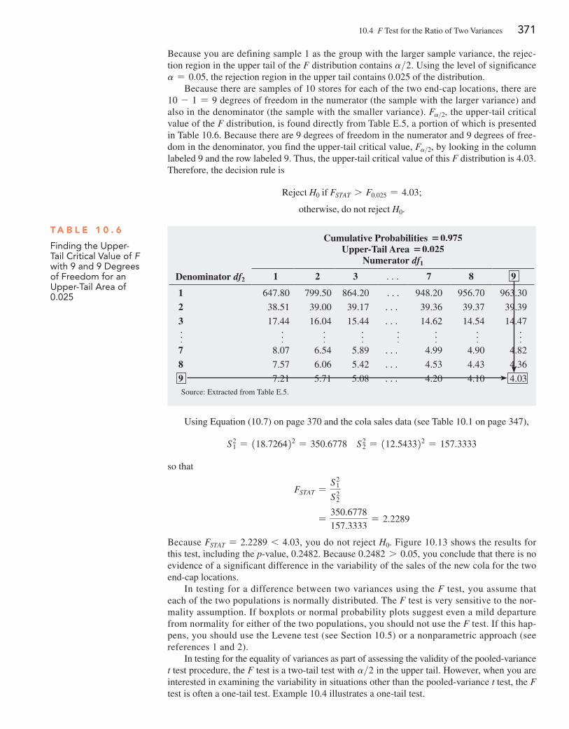
10.4 F Test for the Ratio of Two Variances 371
Because you are defining sample 1 as the group with the larger sample variance, the rejec-tion region in the upper tail of the F distribution contains a>2. Using the level of significance a = 0.05, the rejection region in the upper tail contains 0.025 of the distribution.
Because there are samples of 10 stores for each of the two end-cap locations, there are 10 - 1 = 9 degrees of freedom in the numerator (the sample with the larger variance) and also in the denominator (the sample with the smaller variance). Fa>2, the upper-tail critical value of the F distribution, is found directly from Table e.5, a portion of which is presented in Table 10.6. Because there are 9 degrees of freedom in the numerator and 9 degrees of free-dom in the denominator, you find the upper-tail critical value, Fa>2, by looking in the column labeled 9 and the row labeled 9. Thus, the upper-tail critical value of this F distribution is 4.03. Therefore, the decision rule is
Reject H0 if FSTAT 7 F0.025 = 4.03;
otherwise, do not reject H0.
T a B l e 1 0 . 6
Finding the Upper-Tail Critical Value of F with 9 and 9 Degrees of Freedom for an Upper-Tail Area of 0.025
Cumulative Probabilities =0.975 Upper-Tail Area =0.025
Numerator df1
Denominator df2 1 2 3 c 7 8 9
1 647.80 799.50 864.20 c 948.20 956.70 963.30
2 38.51 39.00 39.17 c 39.36 39.37 39.39
3 17.44 16.04 15.44 c 14.62 14.54 14.47
f f f f f f f f7 8.07 6.54 5.89 c 4.99 4.90 4.82
8 7.57 6.06 5.42 c 4.53 4.43 4.36
9 7.21 5.71 5.08 c 4.20 4.10 4.03Source: extracted from Table e.5.
Using equation (10.7) on page 370 and the cola sales data (see Table 10.1 on page 347),
S21 = 118.726422 = 350.6778 S2
2 = 112.543322 = 157.3333
so that
FSTAT =S2
1
S22
=350.6778
157.3333= 2.2289
Because FSTAT = 2.2289 6 4.03, you do not reject H0. Figure 10.13 shows the results for this test, including the p-value, 0.2482. Because 0.2482 7 0.05, you conclude that there is no evidence of a significant difference in the variability of the sales of the new cola for the two end-cap locations.
In testing for a difference between two variances using the F test, you assume that each of the two populations is normally distributed. The F test is very sensitive to the nor-mality assumption. If boxplots or normal probability plots suggest even a mild departure from normality for either of the two populations, you should not use the F test. If this hap-pens, you should use the Levene test (see Section 10.5) or a nonparametric approach (see references 1 and 2).
In testing for the equality of variances as part of assessing the validity of the pooled-variance t test procedure, the F test is a two-tail test with a>2 in the upper tail. However, when you are interested in examining the variability in situations other than the pooled-variance t test, the F test is often a one-tail test. example 10.4 illustrates a one-tail test.
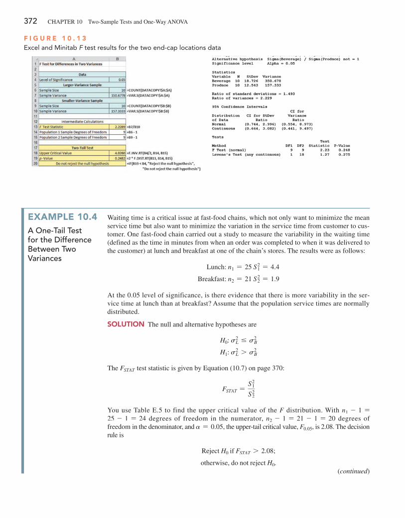
372 CHAPTeR 10 Two-Sample Tests and One-Way ANOVA
F i g u r e 1 0 . 1 3Excel and Minitab F test results for the two end-cap locations data
exaMPle 10.4a One-tail test for the difference between two Variances
Waiting time is a critical issue at fast-food chains, which not only want to minimize the mean service time but also want to minimize the variation in the service time from customer to cus-tomer. One fast-food chain carried out a study to measure the variability in the waiting time (defined as the time in minutes from when an order was completed to when it was delivered to the customer) at lunch and breakfast at one of the chain’s stores. The results were as follows:
Lunch: n1 = 25 S21 = 4.4
Breakfast: n2 = 21 S22 = 1.9
At the 0.05 level of significance, is there evidence that there is more variability in the ser-vice time at lunch than at breakfast? Assume that the population service times are normally distributed.
SoluTion The null and alternative hypotheses are
H0: s2L … s2
B
H1: s2L 7 s2
B
The FSTAT test statistic is given by equation (10.7) on page 370:
FSTAT =S2
1
S22
You use Table e.5 to find the upper critical value of the F distribution. With n1 - 1 =25 - 1 = 24 degrees of freedom in the numerator, n2 - 1 = 21 - 1 = 20 degrees of freedom in the denominator, and a = 0.05, the upper-tail critical value, F0.05, is 2.08. The decision rule is
Reject H0 if FSTAT 7 2.08;
otherwise, do not reject H0.(continued)
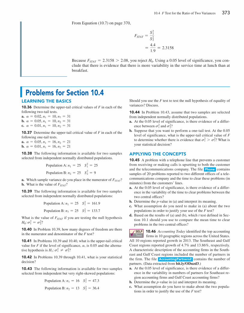
10.4 F Test for the Ratio of Two Variances 373
From equation (10.7) on page 370,
FSTAT =S2
1
S22
=4.4
1.9= 2.3158
Because FSTAT = 2.3158 7 2.08, you reject H0. Using a 0.05 level of significance, you con-clude that there is evidence that there is more variability in the service time at lunch than at breakfast.
Problems for Section 10.4learning The BaSiCS10.36 Determine the upper-tail critical values of F in each of the following two-tail tests.a. a = 0.02, n1 = 10, n2 = 31b. a = 0.05, n1 = 10, n2 = 31c. a = 0.01, n1 = 10, n2 = 31
10.37 Determine the upper-tail critical value of F in each of the following one-tail tests.a. a = 0.05, n1 = 16, n2 = 21b. a = 0.01, n1 = 16, n2 = 21
10.38 The following information is available for two samples selected from independent normally distributed populations.
Population A: n1 = 25 S21 = 25
Population B: n2 = 25 S22 = 9
a. Which sample variance do you place in the numerator of FSTAT?b. What is the value of FSTAT?
10.39 The following information is available for two samples selected from independent normally distributed populations:
Population A: n1 = 25 S21 = 161.9
Population B: n2 = 25 S22 = 133.7
What is the value of FSTAT if you are testing the null hypothesis H0: s
21 = s2
2?
10.40 In Problem 10.39, how many degrees of freedom are there in the numerator and denominator of the F test?
10.41 In Problems 10.39 and 10.40, what is the upper-tail critical value for F if the level of significance, a, is 0.05 and the alterna-tive hypothesis is H1: s
21 ≠ s2
2?
10.42 In Problems 10.39 through 10.41, what is your statistical decision?
10.43 The following information is available for two samples selected from independent but very right-skewed populations:
Population A: n1 = 16 S21 = 47.3
Population B: n2 = 13 S22 = 36.4
Should you use the F test to test the null hypothesis of equality of variances? Discuss.
10.44 In Problem 10.43, assume that two samples are selected from independent normally distributed populations.a. At the 0.05 level of significance, is there evidence of a differ-
ence between s21 and s2
2?b. Suppose that you want to perform a one-tail test. At the 0.05
level of significance, what is the upper-tail critical value of F to determine whether there is evidence that s2
1 7 s22? What is
your statistical decision?
aPPlying The ConCePTS10.45 A problem with a telephone line that prevents a customer from receiving or making calls is upsetting to both the customer and the telecommunications company. The file Phone contains samples of 20 problems reported to two different offices of a tele-communications company and the time to clear these problems (in minutes) from the customers’ lines.a. At the 0.05 level of significance, is there evidence of a differ-
ence in the variability of the time to clear problems between the two central offices?
b. Determine the p-value in (a) and interpret its meaning.c. What assumption do you need to make in (a) about the two
populations in order to justify your use of the F test?d. Based on the results of (a) and (b), which t test defined in Sec-
tion 10.1 should you use to compare the mean time to clear problems in the two central offices?
SELF Test
10.46 Accounting Today identified the top accounting firms in 10 geographic regions across the United States.
All 10 regions reported growth in 2013. The Southeast and Gulf Coast regions reported growth of 4.7% and 13.86%, respectively. A characteristic description of the accounting firms in the South-east and Gulf Coast regions included the number of partners in the firm. The file accountingPartners2 contains the number of partners. (Data extracted from bit.ly/ODuzd3.)a. At the 0.05 level of significance, is there evidence of a differ-
ence in the variability in numbers of partners for Southeast re-gion accounting firms and Gulf Coast accounting firms?
b. Determine the p-value in (a) and interpret its meaning.c. What assumption do you have to make about the two popula-
tions in order to justify the use of the F test?
374 CHAPTeR 10 Two-Sample Tests and One-Way ANOVA
d. Based on (a) and (b), which t test defined in Section 10.1 should you use to test whether there is a significant difference in the mean number of partners for Southeast region account-ing firms and Gulf Coast accounting firms?
10.47 A bank with a branch located in a commercial district of a city has the business objective of improving the process for serv-ing customers during the noon-to-1 p.m. lunch period. To do so, the waiting time (defined as the number of minutes that elapses from when the customer enters the line until he or she reaches the teller window) needs to be shortened to increase customer sat-isfaction. A random sample of 15 customers is selected and the waiting times are collected and stored in Bank3 . These data are:
3.53 3.23 4.38 6.12 0.32 5.13 6.43 6.253.72 4.21 5.52 3.06 5.13 4.78 2.25
Suppose that another branch, located in a residential area, is also concerned with the noon-to-1 p.m. lunch period. A random sample of 15 customers is selected and the waiting times are collected and stored in Bank4 . These data are:
9.58 5.84 8.14 5.77 8.71 3.84 8.14 8.3910.55 6.73 5.72 4.15 6.12 9.87 5.42
a. Is there evidence of a difference in the variability of the waiting time between the two branches? (Use a = 0.02.)
b. Determine the p-value in (a) and interpret its meaning.c. What assumption about the population distribution of each
bank is necessary in (a)? Is the assumption valid for these data?d. Assume the results of part (a) are valid. Based on the results of
(a), is it appropriate to use the pooled-variance t test to compare the means of the two branches?
10.48 An important feature of tablets is battery life, the number of hours before the battery needs to be recharged. The file Tablets contains the battery life of 12 WiFi-only and 7 3G/4G/WiFi 9- through 12-inch tablets. (Data extracted from “Ratings and recom-mendations: Tablets,” Consumer Reports, August 2013, p. 46.)
a. Is there evidence of a difference in the variability of the battery life between the two types of tablets? (Use a = 0.05.)
b. Determine the p-value in (a) and interpret its meaning.c. What assumption about the population distribution of the two
types of tablets is necessary in (a)? Is the assumption valid for these data?
d. Based on the results of (a), which t test defined in Section 10.1 should you use to compare the mean battery life of the two types of tablets?
10.49 experian Marketing Services reported that the typi-cal American spends 144 minutes (2.4 hours) per day accessing the Internet through a mobile device. (Source: The 2014 Digital Marketer, available at ex.pn/1kXJjfX.) You wonder if males and females spend differing amounts of time per day accessing the Internet through a mobile device.
You select a sample of 60 friends and family (30 males and 30 females), collect times spent per day accessing the Internet through a mobile device (in minutes), and store the data collected in internetMobileTime2 .a. Using a 0.05 level of significance, is there evidence of a differ-
ence in the variances of time spent per day accessing the Internet via mobile device between males and females?
b. On the basis of the results in (a), which t test defined in Sec-tion 10.1 should you use to compare the means of males and females? Discuss.
10.50 The following data represent the yields for a sample of money market accounts and five-year CDs as of a certain date. At the 0.05 level of significance, is there evidence of a difference in the variance of the yield between money market accounts and five-year CDs? Assume that the population yields are normally distributed.
10.5 One-Way ANOVASection 10.1 through 10.4 discuss hypothesis-testing methods that allow you to reach conclu-sions about differences between two populations. Analysis of variance, known by the acro-nym ANOVA, are methods that allow you to compare multiple populations, or groups. Unlike the hypothesis-testing methods discussed previously, in ANOVA, you take samples from each group to examine the effects of differences among two or more groups. The criteria that dis-tinguishes the groups are called factors, or sometimes the factors of interest. Factors contain levels which are analogous to the categories of a categorical variable.
In the simplest method, one-way ANOVA, also known as the completely randomized design, you examine only one factor and the levels provide the basis for dividing the variable under study into groups. One-way ANOVA is a two-part process. You first determine if there is a significant difference among the group means. If you reject the null hypothesis that there is no difference among the means, you continue with a second method that seeks to identify the groups whose means are significantly different from the other group means.
In one-way ANOVA, you partition the total variation into variation that is due to differ-ences among the groups and variation that is due to differences within the groups (see Figure 10.14). The within-group variation (SSW) measures random variation. The among-group
Student TipANOVA is also related to regression, discussed later in this book. Because of ANOVA’s relationship with both hypothesis testing and regression, understand-ing the concepts of ANOVA can prove very helpful in understanding the methods discussed in Chapters 12 and 13.
Money Market Accounts Five-Year CD
2.25 2.15 2.12 2.03 2.04 3.68 3.67 3.62 3.42 3.68
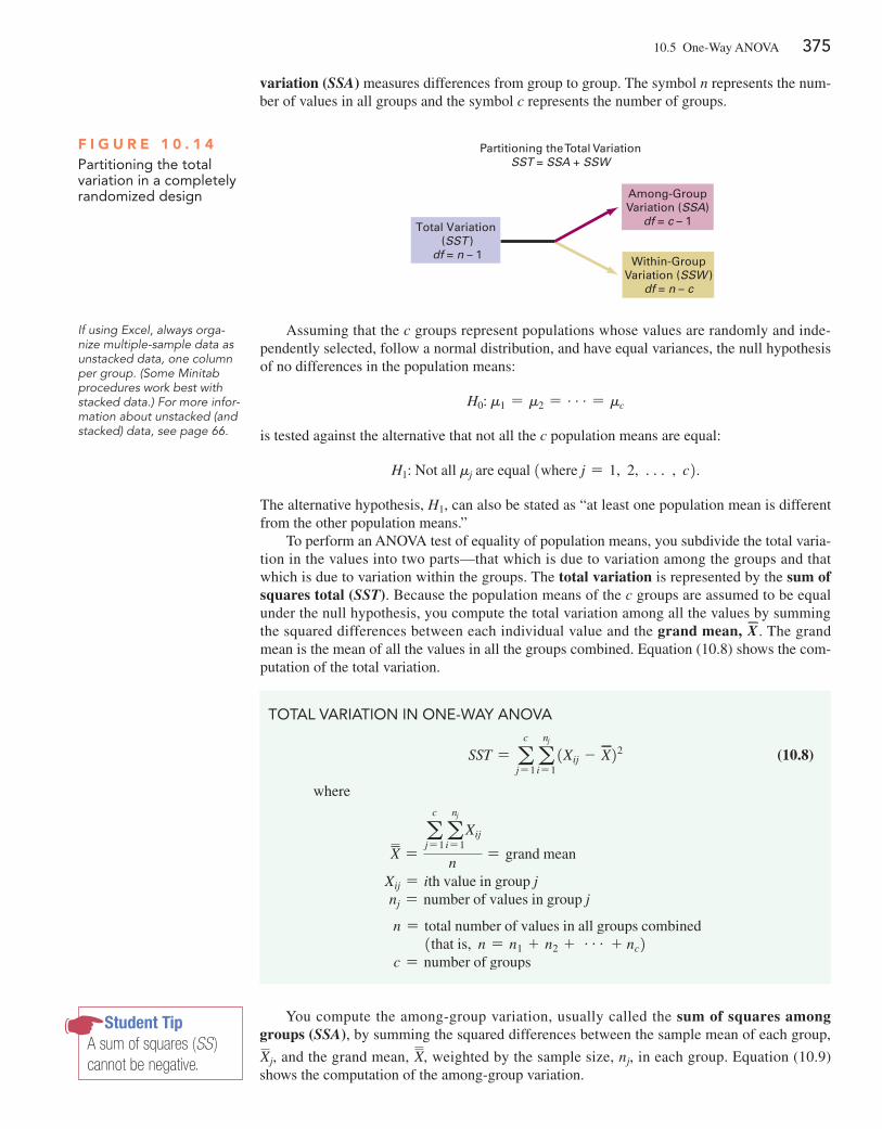
10.5 One-Way ANOVA 375
variation (SSA) measures differences from group to group. The symbol n represents the num-ber of values in all groups and the symbol c represents the number of groups.
F i g u r e 1 0 . 1 4Partitioning the total variation in a completely randomized design
Partitioning the Total VariationSST = SSA + SSW
Among-GroupVariation (SSA)
df = c – 1
Within-GroupVariation (SSW )
df = n – c
Total Variation (SST )
df = n – 1
Assuming that the c groups represent populations whose values are randomly and inde-pendently selected, follow a normal distribution, and have equal variances, the null hypothesis of no differences in the population means:
H0: m1 = m2 = . . . = mc
is tested against the alternative that not all the c population means are equal:
H1: Not all mj are equal 1where j = 1, 2, c , c2.
The alternative hypothesis, H1, can also be stated as “at least one population mean is different from the other population means.”
To perform an ANOVA test of equality of population means, you subdivide the total varia-tion in the values into two parts—that which is due to variation among the groups and that which is due to variation within the groups. The total variation is represented by the sum of squares total (SST). Because the population means of the c groups are assumed to be equal under the null hypothesis, you compute the total variation among all the values by summing the squared differences between each individual value and the grand mean, X . The grand mean is the mean of all the values in all the groups combined. equation (10.8) shows the com-putation of the total variation.
If using Excel, always orga-nize multiple-sample data as unstacked data, one column per group. (Some Minitab procedures work best with stacked data.) For more infor-mation about unstacked (and stacked) data, see page 66.
Student TipA sum of squares (SS ) cannot be negative.
TOTAl VARIATION IN ONE-WAy ANOVA
SST = ac
j= 1anj
i= 11Xij - X22 (10.8)
where
X =a
c
j= 1anj
i= 1Xij
n= grand mean
Xij = ith value in group j nj = number of values in group j
n = total number of values in all groups combined 1that is, n = n1 + n2 + g + nc2
c = number of groups
You compute the among-group variation, usually called the sum of squares among groups (SSA), by summing the squared differences between the sample mean of each group,
Xj, and the grand mean, X, weighted by the sample size, nj, in each group. equation (10.9) shows the computation of the among-group variation.
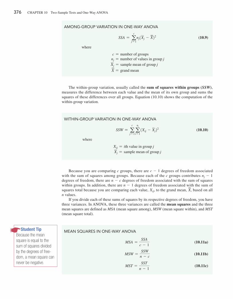
376 CHAPTeR 10 Two-Sample Tests and One-Way ANOVA
The within-group variation, usually called the sum of squares within groups (SSW), measures the difference between each value and the mean of its own group and sums the squares of these differences over all groups. equation (10.10) shows the computation of the within-group variation.
AMONg-gROUP VARIATION IN ONE-WAy ANOVA
SSA = ac
j= 1nj1Xj - X22 (10.9)
where
c = number of groups nj = number of values in group j Xj = sample mean of group j
X = grand mean
WIThIN-gROUP VARIATION IN ONE-WAy ANOVA
SSW = ac
j= 1anj
i= 11Xij - Xj22 (10.10)
where
Xij = ith value in group j Xj = sample mean of group j
Because you are comparing c groups, there are c - 1 degrees of freedom associated with the sum of squares among groups. Because each of the c groups contributes nj - 1 degrees of freedom, there are n - c degrees of freedom associated with the sum of squares within groups. In addition, there are n - 1 degrees of freedom associated with the sum of squares total because you are comparing each value, Xij, to the grand mean, X, based on all n values.
If you divide each of these sums of squares by its respective degrees of freedom, you have three variances. In ANOVA, these three variances are called the mean squares and the three mean squares are defined as MSA (mean square among), MSW (mean square within), and MST (mean square total).
Student TipBecause the mean square is equal to the sum of squares divided by the degrees of free-dom, a mean square can never be negative.
MEAN SqUARES IN ONE-WAy ANOVA
MSA =SSA
c - 1 (10.11a)
MSW =SSW
n - c (10.11b)
MST =SST
n - 1 (10.11c)
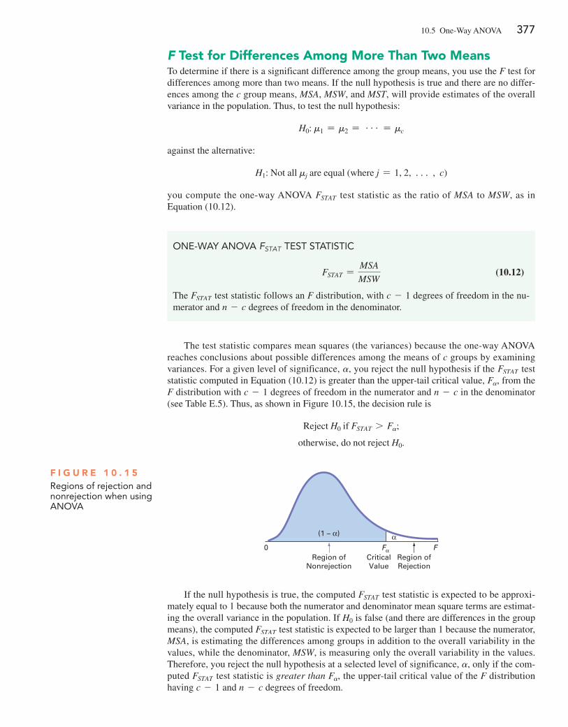
10.5 One-Way ANOVA 377
F Test for Differences among More Than Two MeansTo determine if there is a significant difference among the group means, you use the F test for differences among more than two means. If the null hypothesis is true and there are no differ-ences among the c group means, MSA, MSW, and MST, will provide estimates of the overall variance in the population. Thus, to test the null hypothesis:
H0: m1 = m2 = g = mc
against the alternative:
H1: Not all mj are equal (where j = 1, 2, c , c)
you compute the one-way ANOVA FSTAT test statistic as the ratio of MSA to MSW, as in equation (10.12).
ONE-WAy ANOVA FSTAT TEST STATISTIC
FSTAT =MSA
MSW (10.12)
The FSTAT test statistic follows an F distribution, with c - 1 degrees of freedom in the nu-merator and n - c degrees of freedom in the denominator.
The test statistic compares mean squares (the variances) because the one-way ANOVA reaches conclusions about possible differences among the means of c groups by examining variances. For a given level of significance, a, you reject the null hypothesis if the FSTAT test statistic computed in equation (10.12) is greater than the upper-tail critical value, Fa, from the F distribution with c - 1 degrees of freedom in the numerator and n - c in the denominator (see Table e.5). Thus, as shown in Figure 10.15, the decision rule is
Reject H0 if FSTAT 7 Fa;
otherwise, do not reject H0.
(1 – α)
0 FFα
α
Region ofRejection
Region ofNonrejection
CriticalValue
F i g u r e 1 0 . 1 5Regions of rejection and nonrejection when using ANOVA
If the null hypothesis is true, the computed FSTAT test statistic is expected to be approxi-mately equal to 1 because both the numerator and denominator mean square terms are estimat-ing the overall variance in the population. If H0 is false (and there are differences in the group means), the computed FSTAT test statistic is expected to be larger than 1 because the numerator, MSA, is estimating the differences among groups in addition to the overall variability in the values, while the denominator, MSW, is measuring only the overall variability in the values. Therefore, you reject the null hypothesis at a selected level of significance, a, only if the com-puted FSTAT test statistic is greater than Fa, the upper-tail critical value of the F distribution having c - 1 and n - c degrees of freedom.
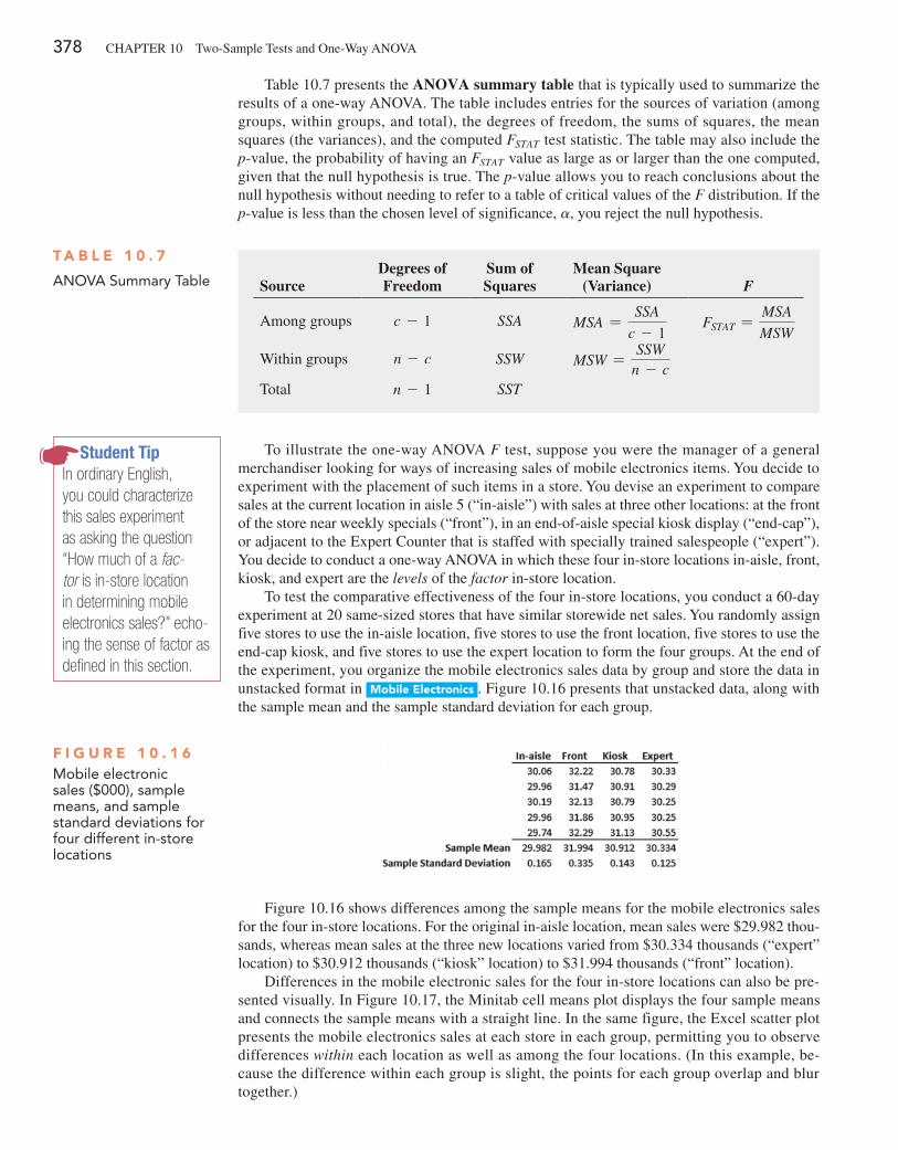
378 CHAPTeR 10 Two-Sample Tests and One-Way ANOVA
Table 10.7 presents the ANOVA summary table that is typically used to summarize the results of a one-way ANOVA. The table includes entries for the sources of variation (among groups, within groups, and total), the degrees of freedom, the sums of squares, the mean squares (the variances), and the computed FSTAT test statistic. The table may also include the p-value, the probability of having an FSTAT value as large as or larger than the one computed, given that the null hypothesis is true. The p-value allows you to reach conclusions about the null hypothesis without needing to refer to a table of critical values of the F distribution. If the p-value is less than the chosen level of significance, a, you reject the null hypothesis.
T a B l e 1 0 . 7
ANOVA Summary Table SourceDegrees of Freedom
Sum of Squares
Mean Square (Variance) F
Among groups c - 1 SSA MSA =SSA
c - 1FSTAT =
MSA
MSW
Within groups n - c SSW MSW =SSW
n - cTotal n - 1 SST
To illustrate the one-way ANOVA F test, suppose you were the manager of a general merchandiser looking for ways of increasing sales of mobile electronics items. You decide to experiment with the placement of such items in a store. You devise an experiment to compare sales at the current location in aisle 5 (“in-aisle”) with sales at three other locations: at the front of the store near weekly specials (“front”), in an end-of-aisle special kiosk display (“end-cap”), or adjacent to the expert Counter that is staffed with specially trained salespeople (“expert”). You decide to conduct a one-way ANOVA in which these four in-store locations in-aisle, front, kiosk, and expert are the levels of the factor in-store location.
To test the comparative effectiveness of the four in-store locations, you conduct a 60-day experiment at 20 same-sized stores that have similar storewide net sales. You randomly assign five stores to use the in-aisle location, five stores to use the front location, five stores to use the end-cap kiosk, and five stores to use the expert location to form the four groups. At the end of the experiment, you organize the mobile electronics sales data by group and store the data in unstacked format in Mobile electronics . Figure 10.16 presents that unstacked data, along with the sample mean and the sample standard deviation for each group.
F i g u r e 1 0 . 1 6Mobile electronic sales ($000), sample means, and sample standard deviations for four different in-store locations
Figure 10.16 shows differences among the sample means for the mobile electronics sales for the four in-store locations. For the original in-aisle location, mean sales were $29.982 thou-sands, whereas mean sales at the three new locations varied from $30.334 thousands (“expert” location) to $30.912 thousands (“kiosk” location) to $31.994 thousands (“front” location).
Differences in the mobile electronic sales for the four in-store locations can also be pre-sented visually. In Figure 10.17, the Minitab cell means plot displays the four sample means and connects the sample means with a straight line. In the same figure, the excel scatter plot presents the mobile electronics sales at each store in each group, permitting you to observe differences within each location as well as among the four locations. (In this example, be-cause the difference within each group is slight, the points for each group overlap and blur together.)
Student TipIn ordinary English, you could characterize this sales experiment as asking the question “How much of a fac-tor is in-store location in determining mobile electronics sales?” echo-ing the sense of factor as defined in this section.
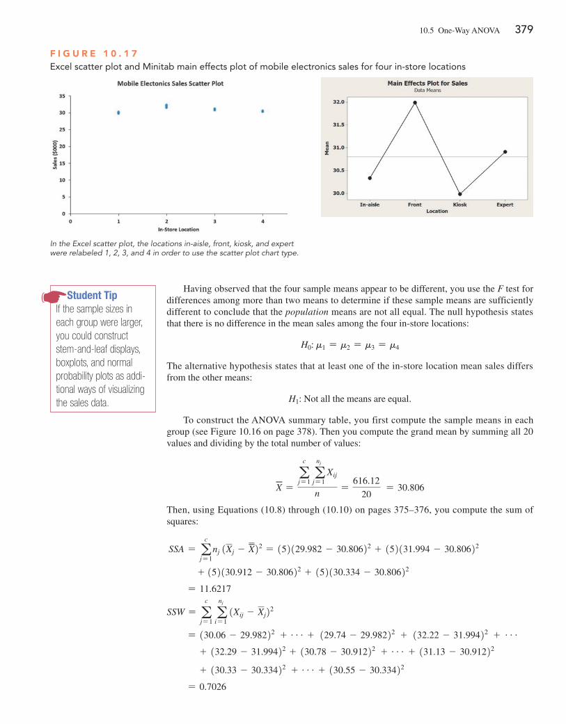
10.5 One-Way ANOVA 379
F i g u r e 1 0 . 1 7Excel scatter plot and Minitab main effects plot of mobile electronics sales for four in-store locations
In the Excel scatter plot, the locations in-aisle, front, kiosk, and expert were relabeled 1, 2, 3, and 4 in order to use the scatter plot chart type.
Having observed that the four sample means appear to be different, you use the F test for differences among more than two means to determine if these sample means are sufficiently different to conclude that the population means are not all equal. The null hypothesis states that there is no difference in the mean sales among the four in-store locations:
H0: m1 = m2 = m3 = m4
The alternative hypothesis states that at least one of the in-store location mean sales differs from the other means:
H1: Not all the means are equal.
To construct the ANOVA summary table, you first compute the sample means in each group (see Figure 10.16 on page 378). Then you compute the grand mean by summing all 20 values and dividing by the total number of values:
X =a
c
j= 1 a
nj
j= 1Xij
n=
616.12
20 = 30.806
Then, using equations (10.8) through (10.10) on pages 375–376, you compute the sum of squares:
SSA = ac
j= 1nj 1Xj - X22 = 152129.982 - 30.80622 + 152131.994 - 30.80622
+ 152130.912 - 30.80622 + 152130.334 - 30.80622
= 11.6217
SSW = ac
j= 1 a
nj
i= 11Xij - Xj22
= 130.06 - 29.98222 + g + 129.74 - 29.98222 + 132.22 - 31.99422 + g+ 132.29 - 31.99422 + 130.78 - 30.91222 + g + 131.13 - 30.91222
+ 130.33 - 30.33422 + g + 130.55 - 30.33422
= 0.7026
Student TipIf the sample sizes in each group were larger, you could construct stem-and-leaf displays, boxplots, and normal probability plots as addi-tional ways of visualizing the sales data.
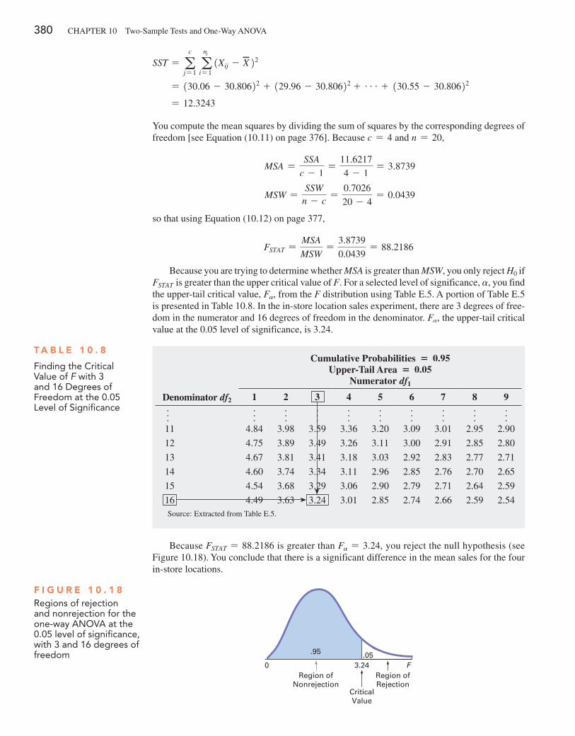
380 CHAPTeR 10 Two-Sample Tests and One-Way ANOVA
SST = ac
j= 1 a
nj
i= 11Xij - X 22
= 130.06 - 30.80622 + 129.96 - 30.80622 + g + 130.55 - 30.80622
= 12.3243
You compute the mean squares by dividing the sum of squares by the corresponding degrees of freedom [see equation (10.11) on page 376]. Because c = 4 and n = 20,
MSA =SSA
c - 1=
11.6217
4 - 1= 3.8739
MSW =SSW
n - c=
0.7026
20 - 4= 0.0439
so that using equation (10.12) on page 377,
FSTAT =MSA
MSW=
3.8739
0.0439= 88.2186
Because you are trying to determine whether MSA is greater than MSW, you only reject H0 if FSTAT is greater than the upper critical value of F. For a selected level of significance, a, you find the upper-tail critical value, Fa, from the F distribution using Table e.5. A portion of Table e.5 is presented in Table 10.8. In the in-store location sales experiment, there are 3 degrees of free-dom in the numerator and 16 degrees of freedom in the denominator. Fa, the upper-tail critical value at the 0.05 level of significance, is 3.24.
T a B l e 1 0 . 8
Finding the Critical Value of F with 3 and 16 Degrees of Freedom at the 0.05 level of Significance
Cumulative Probabilities = 0.95 Upper-Tail Area = 0.05
Numerator df1
Denominator df2 1 2 3 4 5 6 7 8 9
f f f f f f f f f f11 4.84 3.98 3.59 3.36 3.20 3.09 3.01 2.95 2.90
12 4.75 3.89 3.49 3.26 3.11 3.00 2.91 2.85 2.80
13 4.67 3.81 3.41 3.18 3.03 2.92 2.83 2.77 2.71
14 4.60 3.74 3.34 3.11 2.96 2.85 2.76 2.70 2.65
15 4.54 3.68 3.29 3.06 2.90 2.79 2.71 2.64 2.59
16 4.49 3.63 3.24 3.01 2.85 2.74 2.66 2.59 2.54Source: extracted from Table e.5.
Because FSTAT = 88.2186 is greater than Fa = 3.24, you reject the null hypothesis (see Figure 10.18). You conclude that there is a significant difference in the mean sales for the four in-store locations.
F i g u r e 1 0 . 1 8Regions of rejection and nonrejection for the one-way ANOVA at the 0.05 level of significance, with 3 and 16 degrees of freedom
0 3.24 F.05.95
Region ofRejection
Region ofNonrejection
CriticalValue
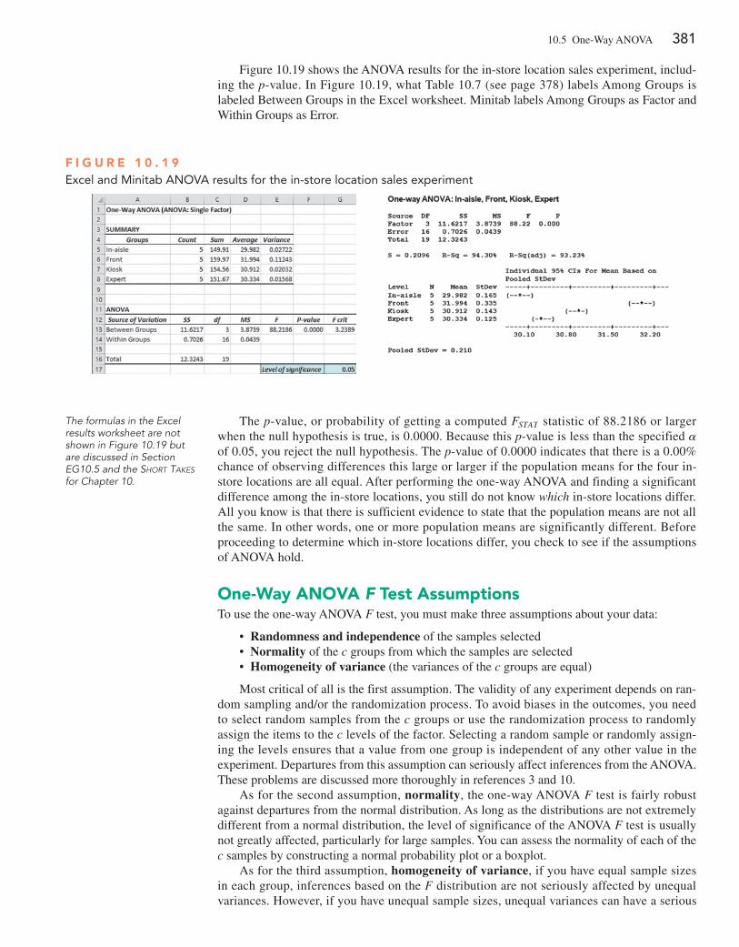
10.5 One-Way ANOVA 381
Figure 10.19 shows the ANOVA results for the in-store location sales experiment, includ-ing the p-value. In Figure 10.19, what Table 10.7 (see page 378) labels Among Groups is labeled Between Groups in the excel worksheet. Minitab labels Among Groups as Factor and Within Groups as error.
F i g u r e 1 0 . 1 9Excel and Minitab ANOVA results for the in-store location sales experiment
The p-value, or probability of getting a computed FSTAT statistic of 88.2186 or larger when the null hypothesis is true, is 0.0000. Because this p-value is less than the specified a of 0.05, you reject the null hypothesis. The p-value of 0.0000 indicates that there is a 0.00% chance of observing differences this large or larger if the population means for the four in-store locations are all equal. After performing the one-way ANOVA and finding a significant difference among the in-store locations, you still do not know which in-store locations differ. All you know is that there is sufficient evidence to state that the population means are not all the same. In other words, one or more population means are significantly different. Before proceeding to determine which in-store locations differ, you check to see if the assumptions of ANOVA hold.
one-Way anoVa F Test assumptionsTo use the one-way ANOVA F test, you must make three assumptions about your data:
• Randomness and independence of the samples selected • Normality of the c groups from which the samples are selected • Homogeneity of variance (the variances of the c groups are equal)
Most critical of all is the first assumption. The validity of any experiment depends on ran-dom sampling and/or the randomization process. To avoid biases in the outcomes, you need to select random samples from the c groups or use the randomization process to randomly assign the items to the c levels of the factor. Selecting a random sample or randomly assign-ing the levels ensures that a value from one group is independent of any other value in the experiment. Departures from this assumption can seriously affect inferences from the ANOVA. These problems are discussed more thoroughly in references 3 and 10.
As for the second assumption, normality, the one-way ANOVA F test is fairly robust against departures from the normal distribution. As long as the distributions are not extremely different from a normal distribution, the level of significance of the ANOVA F test is usually not greatly affected, particularly for large samples. You can assess the normality of each of the c samples by constructing a normal probability plot or a boxplot.
As for the third assumption, homogeneity of variance, if you have equal sample sizes in each group, inferences based on the F distribution are not seriously affected by unequal variances. However, if you have unequal sample sizes, unequal variances can have a serious
The formulas in the Excel results worksheet are not shown in Figure 10.19 but are discussed in Section EG10.5 and the Short takeS for Chapter 10.
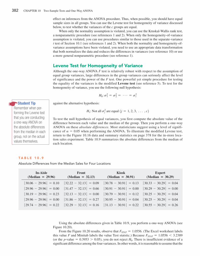
382 CHAPTeR 10 Two-Sample Tests and One-Way ANOVA
effect on inferences from the ANOVA procedure. Thus, when possible, you should have equal sample sizes in all groups. You can use the Levene test for homogeneity of variance discussed below, to test whether the variances of the c groups are equal.
When only the normality assumption is violated, you can use the Kruskal-Wallis rank test, a nonparametric procedure (see references 1 and 2). When only the homogeneity-of-variance assumption is violated, you can use procedures similar to those used in the separate-variance t test of Section 10.1 (see references 1 and 2). When both the normality and homogeneity-of-variance assumptions have been violated, you need to use an appropriate data transformation that both normalizes the data and reduces the differences in variances (see reference 10) or use a more general nonparametric procedure (see reference 1).
levene Test for homogeneity of VarianceAlthough the one-way ANOVA F test is relatively robust with respect to the assumption of equal group variances, large differences in the group variances can seriously affect the level of significance and the power of the F test. One powerful yet simple procedure for testing the equality of the variances is the modified Levene test (see reference 5). To test for the homogeneity of variance, you use the following null hypothesis:
H0: s21 = s2
2 = g = s2c
against the alternative hypothesis:
H1: Not all s2j are equal 1j = 1, 2, 3, c , c2
To test the null hypothesis of equal variances, you first compute the absolute value of the difference between each value and the median of the group. Then you perform a one-way ANOVA on these absolute differences. Most statisticians suggest using a level of signifi-cance of a = 0.05 when performing the ANOVA. To illustrate the modified Levene test, return to the Figure 10.16 data and summary statistics on page 378 for the in-store loca-tion sales experiment. Table 10.9 summarizes the absolute differences from the median of each location.
Student TipRemember when per-forming the Levene test that you are conducting a one-way ANOVA on the absolute differences from the median in each group, not on the actual values themselves.
In-Aisle (Median = 29.96)
Front (Median = 32.13)
Kiosk (Median = 30.91)
Expert (Median = 30.29)
� 30.06 - 29.96 � = 0.10 � 32.22 - 32.13 � = 0.09 � 30.78 - 30.91 � = 0.13 � 30.33 - 30.29 � = 0.04
� 29.96 - 29.96 � = 0.00 � 31.47 - 32.13 � = 0.66 � 30.91 - 30.91 � = 0.00 � 30.29 - 30.29 � = 0.00
� 30.19 - 29.96 � = 0.23 � 32.13 - 32.13 � = 0.00 � 30.79 - 30.91 � = 0.12 � 30.25 - 30.29 � = 0.04
� 29.96 - 29.96 � = 0.00 � 31.86 - 32.13 � = 0.27 � 30.95 - 30.91 � = 0.04 � 30.25 - 30.29 � = 0.04
� 29.74 - 29.96 � = 0.22 � 32.29 - 32.13 � = 0.16 � 31.13 - 30.91 � = 0.22 � 30.55 - 30.29 � = 0.26
T a B l e 1 0 . 9
Absolute Differences from the Median Sales for Four locations
Using the absolute differences given in Table 10.9, you perform a one-way ANOVA (see Figure 10.20).
From the Figure 10.20 results, observe that FSTAT = 1.0556. (The excel worksheet labels this value F and Minitab labels the value Test statstic.) Because FSTAT = 1.0556 6 3.2389 (or the p@value = 0.3953 7 0.05), you do not reject H0. There is insufficient evidence of a significant difference among the four variances. In other words, it is reasonable to assume that the
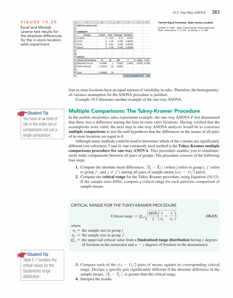
10.5 One-Way ANOVA 383
four in-store locations have an equal amount of variability in sales. Therefore, the homogeneity- of-variance assumption for the ANOVA procedure is justified.
example 10.5 illustrates another example of the one-way ANOVA.
Multiple Comparisons: The Tukey-Kramer ProcedureIn the mobile electronics sales experiment example, the one-way ANOVA F test determined that there was a difference among the four in-store sales locations. Having verified that the assumptions were valid, the next step in one-way ANOVA analysis would be to construct multiple comparisons to test the null hypothesis that the differences in the means of all pairs of in-store locations are equal to 0.
Although many methods could be used to determine which of the c means are significantly different (see references 3 and 4), one commonly used method is the Tukey-Kramer multiple comparisons procedure for one-way ANOVA. This procedure enables you to simultane-ously make comparisons between all pairs of groups. The procedure consists of the following four steps:
1. Compute the absolute mean differences, � Xj - Xj′ � (where j refers to group j, j′ refers to group j′, and j ≠ j′), among all pairs of sample means [c(c - 1)>2 pairs].
2. Compute the critical range for the Tukey-Kramer procedure, using equation (10.13). If the sample sizes differ, compute a critical range for each pairwise comparison of sample means.
CRITICAl RANgE FOR ThE TUkEy-kRAMER PROCEDURE
Critical range = QaBMSW
2a 1
nj+
1nj′
b (10.13)
wherenj = the sample size in group jnj′ = the sample size in group j′Qa = the upper-tail critical value from a Studentized range distribution having c degrees
of freedom in the numerator and n - c degrees of freedom in the denominator.
Student TipTable E.7 contains the critical values for the Studentized range distribution.
Student TipYou have an a level of risk in the entire set of comparisons not just a single comparison.
F i g u r e 1 0 . 2 0Excel and Minitab levene test results for the absolute differences for the in-store location sales experiment
3. Compare each of the c1c - 12>2 pairs of means against its corresponding critical range. Declare a specific pair significantly different if the absolute difference in the sample means, � Xj - Xj′ � , is greater than the critical range.
4. Interpret the results.
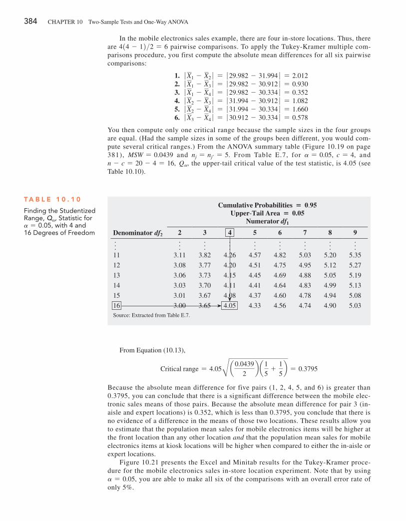
384 CHAPTeR 10 Two-Sample Tests and One-Way ANOVA
In the mobile electronics sales example, there are four in-store locations. Thus, there are 414 - 12>2 = 6 pairwise comparisons. To apply the Tukey-Kramer multiple com-parisons procedure, you first compute the absolute mean differences for all six pairwise comparisons:
1. � X1 - X2 � = � 29.982 - 31.994 � = 2.012 2. � X1 - X3 � = � 29.982 - 30.912 � = 0.930 3. � X1 - X4 � = � 29.982 - 30.334 � = 0.352 4. � X2 - X3 � = � 31.994 - 30.912 � = 1.082 5. � X2 - X4 � = � 31.994 - 30.334 � = 1.660 6. � X3 - X4 � = � 30.912 - 30.334 � = 0.578
You then compute only one critical range because the sample sizes in the four groups are equal. (Had the sample sizes in some of the groups been different, you would com-pute several critical ranges.) From the ANOVA summary table (Figure 10.19 on page 381), MSW = 0.0439 and nj = nj′ = 5. From Table e.7, for a = 0.05, c = 4, and n - c = 20 - 4 = 16, Qa, the upper-tail critical value of the test statistic, is 4.05 (see Table 10.10).
T a B l e 1 0 . 1 0
Finding the Studentized Range, Qa, Statistic for a = 0.05, with 4 and 16 Degrees of Freedom
Cumulative Probabilities = 0.95 Upper@Tail Area = 0.05
Numerator df1
Denominator df2 2 3 4 5 6 7 8 9
f f f f f f f f f11 3.11 3.82 4.26 4.57 4.82 5.03 5.20 5.35
12 3.08 3.77 4.20 4.51 4.75 4.95 5.12 5.27
13 3.06 3.73 4.15 4.45 4.69 4.88 5.05 5.19
14 3.03 3.70 4.11 4.41 4.64 4.83 4.99 5.13
15 3.01 3.67 4.08 4.37 4.60 4.78 4.94 5.08
16 3.00 3.65 4.05 4.33 4.56 4.74 4.90 5.03Source: extracted from Table e.7.
From equation (10.13),
Critical range = 4.05B a 0.0439
2b a 1
5+
1
5b = 0.3795
Because the absolute mean difference for five pairs (1, 2, 4, 5, and 6) is greater than 0.3795, you can conclude that there is a significant difference between the mobile elec-tronic sales means of those pairs. Because the absolute mean difference for pair 3 (in-aisle and expert locations) is 0.352, which is less than 0.3795, you conclude that there is no evidence of a difference in the means of those two locations. These results allow you to estimate that the population mean sales for mobile electronics items will be higher at the front location than any other location and that the population mean sales for mobile electronics items at kiosk locations will be higher when compared to either the in-aisle or expert locations.
Figure 10.21 presents the excel and Minitab results for the Tukey-Kramer proce-dure for the mobile electronics sales in-store location experiment. Note that by using a = 0.05, you are able to make all six of the comparisons with an overall error rate of only 5%.
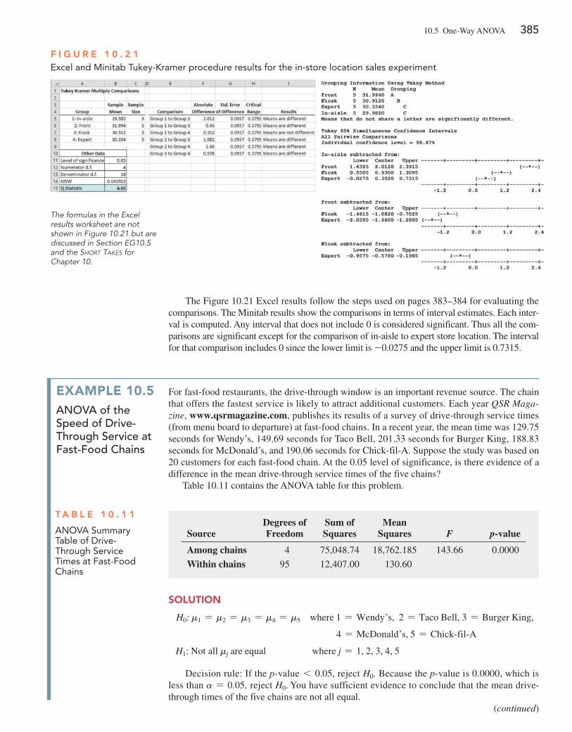
10.5 One-Way ANOVA 385
The Figure 10.21 excel results follow the steps used on pages 383–384 for evaluating the comparisons. The Minitab results show the comparisons in terms of interval estimates. each inter-val is computed. Any interval that does not include 0 is considered significant. Thus all the com-parisons are significant except for the comparison of in-aisle to expert store location. The interval for that comparison includes 0 since the lower limit is -0.0275 and the upper limit is 0.7315.
F i g u r e 1 0 . 2 1Excel and Minitab Tukey-kramer procedure results for the in-store location sales experiment
The formulas in the Excel results worksheet are not shown in Figure 10.21 but are discussed in Section EG10.5 and the Short takeS for Chapter 10.
exaMPle 10.5anOVa of the speed of drive-through service at Fast-Food chains
For fast-food restaurants, the drive-through window is an important revenue source. The chain that offers the fastest service is likely to attract additional customers. each year QSR Maga-zine, www.qsrmagazine.com, publishes its results of a survey of drive-through service times (from menu board to departure) at fast-food chains. In a recent year, the mean time was 129.75 seconds for Wendy’s, 149.69 seconds for Taco Bell, 201.33 seconds for Burger King, 188.83 seconds for McDonald’s, and 190.06 seconds for Chick-fil-A. Suppose the study was based on 20 customers for each fast-food chain. At the 0.05 level of significance, is there evidence of a difference in the mean drive-through service times of the five chains?
Table 10.11 contains the ANOVA table for this problem.
T a B l e 1 0 . 1 1
ANOVA Summary Table of Drive-Through Service Times at Fast-Food Chains
SourceDegrees of Freedom
Sum of Squares
Mean Squares F p-value
Among chains 4 75,048.74 18,762.185 143.66 0.0000
Within chains 95 12,407.00 130.60
SoluTion
H0: m1 = m2 = m3 = m4 = m5 where 1 = Wendy>s, 2 = Taco Bell, 3 = Burger King,
4 = McDonald>s, 5 = Chick@fil@A
H1: Not all mj are equal where j = 1, 2, 3, 4, 5
Decision rule: If the p-value 6 0.05, reject H0. Because the p-value is 0.0000, which is less than a = 0.05, reject H0. You have sufficient evidence to conclude that the mean drive-through times of the five chains are not all equal.
(continued)
386 CHAPTeR 10 Two-Sample Tests and One-Way ANOVA
To determine which of the means are significantly different from one another, use the Tukey-Kramer procedure [equation (10.13) on page 383] to establish the critical range:
Critical value of Q with 5 and 95 degrees of freedom ≈ 3.92
Critical range = QaB aMSW
2b a 1
nj+
1nj′
b = 13.922B a 130.6
2b a 1
20+
1
20b
= 10.02
Any observed difference greater than 10.02 is considered significant. The mean drive-through service times are different between Wendy’s (mean of 129.75 seconds) and Taco Bell, Burger King, McDonald’s, and Chick-fil-A and also between Taco Bell (mean of 149.69) and Burger King, McDonald’s, and Chick-fil-A. In addition, the mean drive-through service time is different between Burger King and McDonald’s, and between Burger King and Chick-fil-A. Thus, with 95% confidence, you can conclude that the estimated population mean drive-through service time is faster for Wendy’s than for Taco Bell. In addition, the population mean service time for Wendy’s and for Taco Bell is faster than those of Burger King, McDonald’s, and Chick-fil-A. Also, the population mean drive-through service time for Burger King is slower than for McDonald’s and for Chick-Fil-A.
Problems for Section 10.5learning The BaSiCS10.51 An experiment has a single factor with three groups and six values in each group.a. How many degrees of freedom are there in determining the
among-group variation?b. How many degrees of freedom are there in determining the
within-group variation?c. How many degrees of freedom are there in determining the to-
tal variation?
10.52 You are working with the same experiment as in Problem 10.51.a. If SSA = 60 and SST = 210, what is SSW?b. What is MSA?c. What is MSW?d. What is the value of FSTAT?
10.53 You are working with the same experiment as in Problems 10.51 and 10.52.a. Construct the ANOVA summary table and fill in all values in
the table.b. At the 0.05 level of significance, what is the upper-tail critical
value from the F distribution?c. State the decision rule for testing the null hypothesis that all
five groups have equal population means.d. What is your statistical decision?
10.54 Consider an experiment that has a single factor with eight groups and four values in each group.a. How many degrees of freedom are there in determining the
among-group variation?b. How many degrees of freedom are there in determining the
within-group variation?
c. How many degrees of freedom are there in determining the to-tal variation?
10.55 Consider an experiment with four groups, with eight val-ues in each. For the ANOVA summary table below, fill in all the missing results:
SourceDegrees of Freedom
Sum of Squares
Mean Square
(Variance) F
Among groups
c - 1 = ? SSA = ? MSA = 80 FSTAT = ?
Within groups
n - c = ? SSW = 560 MSW = ?
Total n - 1 = ? SST = ?
10.56 You are working with the same experiment as in Problem 10.55.a. At the 0.05 level of significance, state the decision rule for test-
ing the null hypothesis that all four groups have equal popula-tion means.
b. What is your statistical decision?c. At the 0.05 level of significance, what is the upper-tail critical
value from the Studentized range distribution?d. To perform the Tukey-Kramer procedure, what is the critical
range?
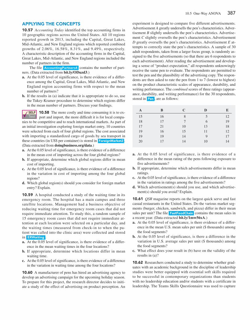
10.5 One-Way ANOVA 387
aPPlying The ConCePTS10.57 Accounting Today identified the top accounting firms in 10 geographic regions across the United States. All 10 regions reported growth in 2013, including the Capital, Great Lakes, Mid- Atlantic, and New england regions which reported combined growths of 2.06%, 16.58%, 8.31%, and 9.49%, respectively. A characteristic description of the accounting firms in the Capital, Great Lakes, Mid-Atlantic, and New england regions included the number of partners in the firm.
The file accountingPartners4 contains the number of part-ners. (Data extracted from bit.ly/ODuzd3.)a. At the 0.05 level of significance, is there evidence of a differ-
ence among the Capital, Great Lakes, Mid-Atlantic, and New england region accounting firms with respect to the mean number of partners?
b. If the results in (a) indicate that it is appropriate to do so, use the Tukey-Kramer procedure to determine which regions differ in the mean number of partners. Discuss your findings.
SELF Test
10.58 The more costly and time consuming it is to ex-port and import, the more difficult it is for local compa-
nies to be competitive and to reach international markets. As part of an initial investigation exploring foreign market entry, 10 countries were selected from each of four global regions. The cost associated with importing a standardized cargo of goods by sea transport in these countries (in US$ per container) is stored in ForeignMarket2 . (Data extracted from doingbusiness.org/data.)a. At the 0.05 level of significance, is there evidence of a difference
in the mean cost of importing across the four global regions?b. If appropriate, determine which global regions differ in mean
cost of importing.c. At the 0.05 level of significance, is there evidence of a difference
in the variation in cost of importing among the four global regions?
d. Which global region(s) should you consider for foreign market entry? explain.
10.59 A hospital conducted a study of the waiting time in its emergency room. The hospital has a main campus and three satellite locations. Management had a business objective of reducing waiting time for emergency room cases that did not require immediate attention. To study this, a random sample of 15 emergency room cases that did not require immediate at-tention at each location were selected on a particular day, and the waiting times (measured from check-in to when the pa-tient was called into the clinic area) were collected and stored in erWaiting .a. At the 0.05 level of significance, is there evidence of a differ-
ence in the mean waiting times in the four locations?b. If appropriate, determine which locations differ in mean
waiting time.c. At the 0.05 level of significance, is there evidence of a difference
in the variation in waiting time among the four locations?
10.60 A manufacturer of pens has hired an advertising agency to develop an advertising campaign for the upcoming holiday season. To prepare for this project, the research director decides to initi-ate a study of the effect of advertising on product perception. An
experiment is designed to compare five different advertisements. Advertisement A greatly undersells the pen’s characteristics. Adver-tisement B slightly undersells the pen’s characteristics. Advertise-ment C slightly oversells the pen’s characteristics. Advertisement D greatly oversells the pen’s characteristics. Advertisement E at-tempts to correctly state the pen’s characteristics. A sample of 30 adult respondents, taken from a larger focus group, is randomly as-signed to the five advertisements (so that there are 6 respondents to each advertisement). After reading the advertisement and develop-ing a sense of “product expectation,” all respondents unknowingly receive the same pen to evaluate. The respondents are permitted to test the pen and the plausibility of the advertising copy. The respon-dents are then asked to rate the pen from 1 to 7 (lowest to highest) on the product characteristic scales of appearance, durability, and writing performance. The combined scores of three ratings (appear-ance, durability, and writing performance) for the 30 respondents, stored in Pen , are as follows:
A B C D E
15 16 8 5 1218 17 7 6 1917 21 10 13 1819 16 15 11 1219 19 14 9 1720 17 14 10 14
a. At the 0.05 level of significance, is there evidence of a difference in the mean rating of the pens following exposure to five advertisements?
b. If appropriate, determine which advertisements differ in mean ratings.
c. At the 0.05 level of significance, is there evidence of a difference in the variation in ratings among the five advertisements?
d. Which advertisement(s) should you use, and which advertise- ment(s) should you avoid? explain.
10.61 QSR magazine reports on the largest quick serve and fast casual restaurants in the United States. Do the various market seg-ments (burger, chicken, sandwich, and pizza) differ in their mean sales per unit? The file FastFoodChain contains the mean sales in a recent year. (Data extracted bit.ly/1mw56xA.)a. At the 0.05 level of significance, is there evidence of a differ-
ence in the mean U.S. mean sales per unit ($ thousands) among the food segments?
b. At the 0.05 level of significance, is there a difference in the variation in U.S. average sales per unit ($ thousands) among the food segments?
c. What effect does your result in (b) have on the validity of the results in (a)?
10.62 Researchers conducted a study to determine whether grad-uates with an academic background in the discipline of leadership studies were better equipped with essential soft skills required to be successful in contemporary organizations than students with no leadership education and/or students with a certificate in leadership. The Teams Skills Questionnaire was used to capture
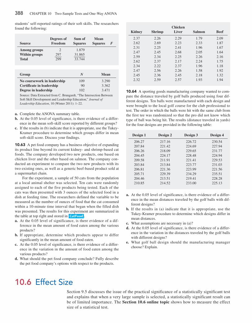
388 CHAPTeR 10 Two-Sample Tests and One-Way ANOVA
students’ self- reported ratings of their soft skills. The researchers found the following:
SourceDegrees of Freedom
Sum of Squares
Mean Squares F
Among groups 2 1.879Within groups 297 31.865Total 299 33.744
Group N Mean
No coursework in leadership 109 3.290Certificate in leadership 90 3.362Degree in leadership 102 3.471Source: Data extracted from C. Brungardt, “The Intersection Between Soft Skill Development and Leadership education,” Journal of Leadership Education, 10 (Winter 2011): 1–22.
a. Complete the ANOVA summary table.b. At the 0.05 level of significance, is there evidence of a differ-
ence in the mean soft-skill score reported by different groups?c. If the results in (b) indicate that it is appropriate, use the Tukey-
Kramer procedure to determine which groups differ in mean soft-skill score. Discuss your findings.
10.63 A pet food company has a business objective of expanding its product line beyond its current kidney- and shrimp-based cat foods. The company developed two new products, one based on chicken liver and the other based on salmon. The company con-ducted an experiment to compare the two new products with its two existing ones, as well as a generic beef-based product sold at a supermarket chain.
For the experiment, a sample of 50 cats from the population at a local animal shelter was selected. Ten cats were randomly assigned to each of the five products being tested. each of the cats was then presented with 3 ounces of the selected food in a dish at feeding time. The researchers defined the variable to be measured as the number of ounces of food that the cat consumed within a 10-minute time interval that began when the filled dish was presented. The results for this experiment are summarized in the table at top right and stored in CatFood .a. At the 0.05 level of significance, is there evidence of a dif-
ference in the mean amount of food eaten among the various products?
b. If appropriate, determine which products appear to differ significantly in the mean amount of food eaten.
c. At the 0.05 level of significance, is there evidence of a differ-ence in the variation in the amount of food eaten among the various products?
d. What should the pet food company conclude? Fully describe the pet food company’s options with respect to the products.
Kidney
Shrimp
Chicken Liver
Salmon
Beef
2.37 2.26 2.29 1.79 2.092.62 2.69 2.23 2.33 1.872.31 2.25 2.41 1.96 1.672.47 2.45 2.68 2.05 1.642.59 2.34 2.25 2.26 2.162.62 2.37 2.17 2.24 1.752.34 2.22 2.37 1.96 1.182.47 2.56 2.26 1.58 1.922.45 2.36 2.45 2.18 1.322.32 2.59 2.57 1.93 1.94
10.64 A sporting goods manufacturing company wanted to com-pare the distance traveled by golf balls produced using four dif-ferent designs. Ten balls were manufactured with each design and were brought to the local golf course for the club professional to test. The order in which the balls were hit with the same club from the first tee was randomized so that the pro did not know which type of ball was being hit. The results (distance traveled in yards) for the four designs are provided in the following table:
Design 1 Design 2 Design 3 Design 4
206.27 217.16 226.72 230.54207.84 221.42 224.69 227.94206.26 218.09 229.65 231.77204.45 224.17 228.48 224.94209.58 211.91 221.41 229.53203.84 213.84 223.77 231.03206.81 221.36 223.99 221.56205.71 229.39 234.29 235.51204.46 213.51 219.41 228.28210.85 214.52 233.00 225.13
a. At the 0.05 level of significance, is there evidence of a differ-ence in the mean distances traveled by the golf balls with dif-ferent designs?
b. If the results in (a) indicate that it is appropriate, use the Tukey-Kramer procedure to determine which designs differ in mean distances.
c. What assumptions are necessary in (a)?d. At the 0.05 level of significance, is there evidence of a differ-
ence in the variation in the distances traveled by the golf balls with different designs?
e. What golf ball design should the manufacturing manager choose? explain.
10.6 Effect SizeSection 9.5 discusses the issue of the practical significance of a statistically significant test and explains that when a very large sample is selected, a statistically significant result can be of limited importance. The Section 10.6 online topic shows how to measure the effect size of a statistical test.
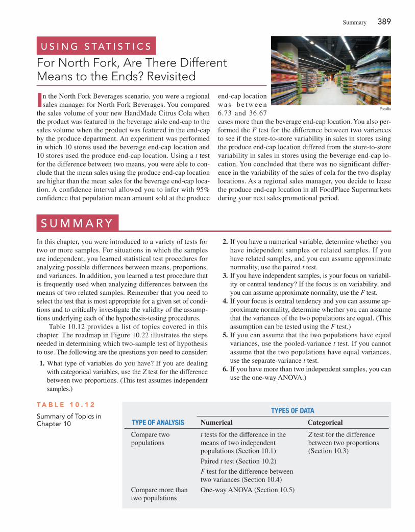
Summary 389
In the North Fork Beverages scenario, you were a regional sales manager for North Fork Beverages. You compared
the sales volume of your new HandMade Citrus Cola when the product was featured in the beverage aisle end-cap to the sales volume when the product was featured in the end-cap by the produce department. An experiment was performed in which 10 stores used the beverage end-cap location and 10 stores used the produce end-cap location. Using a t test for the difference between two means, you were able to con-clude that the mean sales using the produce end-cap location are higher than the mean sales for the beverage end-cap loca-tion. A confidence interval allowed you to infer with 95% confidence that population mean amount sold at the produce
end-cap location w a s b e t w e e n 6.73 and 36.67 cases more than the beverage end-cap location. You also per-formed the F test for the difference between two variances to see if the store-to-store variability in sales in stores using the produce end-cap location differed from the store-to-store variability in sales in stores using the beverage end-cap lo-cation. You concluded that there was no significant differ-ence in the variability of the sales of cola for the two display locations. As a regional sales manager, you decide to lease the produce end-cap location in all FoodPlace Supermarkets during your next sales promotional period.
U s i n g s tat i s t i c s
For North Fork, Are There Different Means to the Ends? Revisited
Fotolia
T a B l e 1 0 . 1 2
Summary of Topics in Chapter 10
TypeS of DaTa
Type of analySiS Numerical Categorical
Compare two populations
t tests for the difference in the means of two independent populations (Section 10.1)
Z test for the difference between two proportions (Section 10.3)
Paired t test (Section 10.2)
F test for the difference between two variances (Section 10.4)
Compare more than two populations
One-way ANOVA (Section 10.5)
s U M M a r yIn this chapter, you were introduced to a variety of tests for two or more samples. For situations in which the samples are independent, you learned statistical test procedures for analyzing possible differences between means, proportions, and variances. In addition, you learned a test procedure that is frequently used when analyzing differences between the means of two related samples. Remember that you need to select the test that is most appropriate for a given set of condi-tions and to critically investigate the validity of the assump-tions underlying each of the hypothesis-testing procedures.
Table 10.12 provides a list of topics covered in this chapter. The roadmap in Figure 10.22 illustrates the steps needed in determining which two-sample test of hypothesis to use. The following are the questions you need to consider:
1. What type of variables do you have? If you are dealing with categorical variables, use the Z test for the difference between two proportions. (This test assumes independent samples.)
2. If you have a numerical variable, determine whether you have independent samples or related samples. If you have related samples, and you can assume approximate normality, use the paired t test.
3. If you have independent samples, is your focus on variabil-ity or central tendency? If the focus is on variability, and you can assume approximate normality, use the F test.
4. If your focus is central tendency and you can assume ap-proximate normality, determine whether you can assume that the variances of the two populations are equal. (This assumption can be tested using the F test.)
5. If you can assume that the two populations have equal variances, use the pooled-variance t test. If you cannot assume that the two populations have equal variances, use the separate-variance t test.
6. If you have more than two independent samples, you can use the one-way ANOVA.)
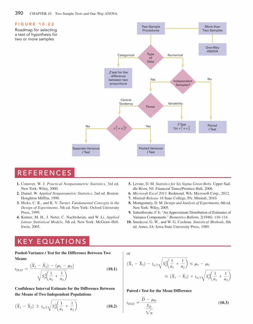
390 CHAPTeR 10 Two-Sample Tests and One-Way ANOVA
Pooled-Variance t Test for the Difference Between Two Means
tSTAT =1X1 - X22 - 1m1 - m22BS2
pa 1n1
+1n2
b (10.1)
Confidence Interval Estimate for the Difference Between the Means of Two Independent Populations
1X1 - X22 { ta>2BS2pa 1
n1+
1n2
b (10.2)
or
1X1 - X22 - ta>2BS2pa 1
n1+
1n2
b … m1 - m2
… 1X1 - X22 + ta>2BS2pa 1
n1+
1n2
b
Paired t Test for the Mean Difference
tSTAT =D - mD
SD2n
(10.3)
K e y e q U at i O n s
F i g u r e 1 0 . 2 2Roadmap for selecting a test of hypothesis for two or more samples
2 2 2 2No Yes
Categorical Numerical
Yes No
CentralTendency Variability
Z test for thedifference
between twoproportions
Typeof
Data
IndependentSamples?
� 1 = � 2?
Focus
F Testfor � 1 = � 2
Separate-Variancet Test
Pooled-Variancet Test
Two-SampleProcedures
More thanTwo Samples
One-WayANOVA
Pairedt Test
2 2
r e F e r e n c e s 1. Conover, W. J. Practical Nonparametric Statistics, 3rd ed.
New York: Wiley, 2000. 2. Daniel, W. Applied Nonparametric Statistics, 2nd ed. Boston:
Houghton Mifflin, 1990. 3. Hicks, C. R., and K. V. Turner. Fundamental Concepts in the
Design of Experiments, 5th ed. New York: Oxford University Press, 1999.
4. Kutner, M. H., J. Neter, C. Nachtsheim, and W. Li. Applied Linear Statistical Models, 5th ed. New York: McGraw-Hill-Irwin, 2005.
5. Levine, D. M. Statistics for Six Sigma Green Belts. Upper Sad-dle River, NJ: Financial Times/Prentice Hall, 2006.
6. Microsoft Excel 2013. Redmond, WA: Microsoft Corp., 2012. 7. Minitab Release 16 State College, PA: Minitab, 2010. 8. Montgomery, D. M. Design and Analysis of Experiments, 6th ed.
New York: Wiley, 2005. 9. Satterthwaite, F. e. “An Approximate Distribution of estimates of
Variance Components.” Biometrics Bulletin, 2(1946): 110–114. 10. Snedecor, G. W., and W. G. Cochran. Statistical Methods, 8th
ed. Ames, IA: Iowa State University Press, 1989.
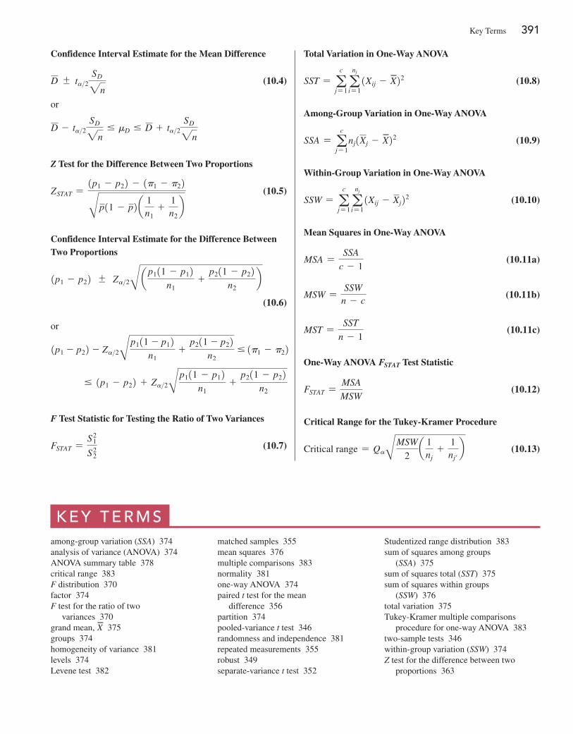
Key Terms 391
Confidence Interval Estimate for the Mean Difference
D { ta>2SD2n
(10.4)
or
D - ta>2SD2n
… mD … D + ta>2SD2n
Z Test for the Difference Between Two Proportions
ZSTAT =1p1 - p22 - 1p1 - p22Bp11 - p2a 1
n1+
1n2
b (10.5)
Confidence Interval Estimate for the Difference Between Two Proportions
1p1 - p22 { Za>2B a p111 - p12n1
+p211 - p22
n2b
(10.6)
or
1p1 - p22 - Za>2Bp111 - p12n1
+p211 - p22
n2 … 1p1 - p22
… 1p1 - p22 + Za>2Bp111 - p12n1
+p211 - p22
n2
F Test Statistic for Testing the Ratio of Two Variances
FSTAT =S2
1
S22 (10.7)
Total Variation in One-Way ANOVA
SST = ac
j= 1anj
i= 11Xij - X22 (10.8)
Among-Group Variation in One-Way ANOVA
SSA = ac
j= 1nj1Xj - X22 (10.9)
Within-Group Variation in One-Way ANOVA
SSW = ac
j= 1anj
i= 11Xij - Xj22 (10.10)
Mean Squares in One-Way ANOVA
MSA =SSA
c - 1 (10.11a)
MSW =SSW
n - c (10.11b)
MST =SST
n - 1 (10.11c)
One-Way ANOVA FSTAT Test Statistic
FSTAT =MSA
MSW (10.12)
Critical Range for the Tukey-Kramer Procedure
Critical range = QaBMSW
2a 1
nj+
1nj′
b (10.13)
K e y t e r M samong-group variation (SSA) 374analysis of variance (ANOVA) 374ANOVA summary table 378critical range 383F distribution 370factor 374F test for the ratio of two
variances 370grand mean, X 375groups 374homogeneity of variance 381levels 374Levene test 382
matched samples 355mean squares 376multiple comparisons 383normality 381one-way ANOVA 374paired t test for the mean
difference 356partition 374pooled-variance t test 346randomness and independence 381repeated measurements 355robust 349separate-variance t test 352
Studentized range distribution 383sum of squares among groups
(SSA) 375sum of squares total (SST) 375sum of squares within groups
(SSW) 376total variation 375Tukey-Kramer multiple comparisons
procedure for one-way ANOVA 383two-sample tests 346within-group variation (SSW) 374Z test for the difference between two
proportions 363
392 CHAPTeR 10 Two-Sample Tests and One-Way ANOVA
c h a p t e r r e V i e w p r O b l e M s
10.76 The American Society for Quality (ASQ) conducted a sal-ary survey of all its members. ASQ members work in all areas of manufacturing and service-related institutions, with a common theme of an interest in quality. Two job titles are black belt and green belt. (See Section 14.6 for a description of these titles in a Six Sigma quality improvement initiative.) Descriptive statistics concerning salaries for these two job titles are given in the follow-ing table:
a. Using a 0.05 level of significance, is there a difference in the variability of salaries between black belts and green belts?
b. Based on the result of (a), which t test defined in Section 10.1 is appropriate for comparing mean salaries?
c. Using a 0.05 level of significance, is the mean salary of black belts greater than the mean salary of green belts?
10.77 Do male and female students study the same amount per week? In a recent year, 58 sophomore business students were sur-veyed at a large university that has more than 1,000 sophomore business students each year. The file StudyTime contains the gen-der and the number of hours spent studying in a typical week for the sampled students.a. At the 0.05 level of significance, is there a difference in the
variance of the study time for male students and female students?
b. Using the results of (a), which t test is appropriate for compar-ing the mean study time for male and female students?
c. At the 0.05 level of significance, conduct the test selected in (b).
d. Write a short summary of your findings.
10.78 Do males and females differ in the amount of time they talk on the phone and the number of text messages they send? A study reported that women spent a mean of 818 minutes per month talking as compared to 716 minutes per month for men. (Data ex-tracted from “Women Talk and Text More,” USA Today, February 1, 2011, p. 1A.) The sample sizes were not reported. Suppose that the sample sizes were 100 each for women and men and that the standard deviation for women was 125 minutes per month as com-pared to 100 minutes per month for men.a. Using a 0.01 level of significance, is there evidence of a differ-
ence in the variances of the amount of time spent talking be-tween women and men?
b. To test for a difference in the mean talking time of women and men, is it most appropriate to use the pooled-variance t test or the separate-variance t test? Use the most appropriate test to determine if there is a difference in the amount of time spent talking on the phone between women and men.
The article also reported that women sent a mean of 716 text messages per month compared to 555 per month for men. Suppose that the standard deviation for women was 150 text messages per month compared to 125 text messages per month for men.
c. Using a 0.01 level of significance, is there evidence of a differ-ence in the variances of the number of text messages sent per month by women and men?
d. Based on the results of (c), use the most appropriate test to de-termine, at the 0.01 level of significance, whether there is evi-dence of a difference in the mean number of text messages sent per month by women and men.
10.79 The file restaurants contains the ratings for food, décor, service, and the price per person for a sample of 50 restaurants lo-cated in a city and 50 restaurants located in a suburb. Completely analyze the differences between city and suburban restaurants for
c h e c K i n g y O U r U n d e r s ta n d i n g10.65 What are some of the criteria used in the selection of a particular hypothesis-testing procedure?
10.66 Under what conditions should you use the pooled-variance t test to examine possible differences in the means of two indepen-dent populations?
10.67 Under what conditions should you use the F test to ex-amine possible differences in the variances of two independent populations?
10.68 How can you test the difference between the proportions of two independent populations?
10.69 What is the distinction between repeated measurements and matched items?
10.70 When you have two independent populations, explain the similarities and differences between the test of hypothesis for the
difference between the means and the confidence interval estimate for the difference between the means.
10.71 Under what conditions should you use the paired t test for the mean difference between two related populations?
10.72 In a one-way ANOVA, what is the difference between the among-groups variance MSA and the within-groups variance MSW?
10.73 What are the steps involved in the Tukey-Kramer proce-dure for one-way ANOVA?
10.74 Under what conditions should you use the one-way ANOVA F test to examine possible differences among the means of c independent populations?
10.75 What are the three assumptions that you should make about the data when using one-way ANOVA F test?
Job Title
Sample Size
Mean
Standard Deviation
Black belt 128 93,123 21,186Green belt 39 73,045 21,272Source: Data extracted from “QP Salary Survey,” Quality Progress, December 2013, p. 17.
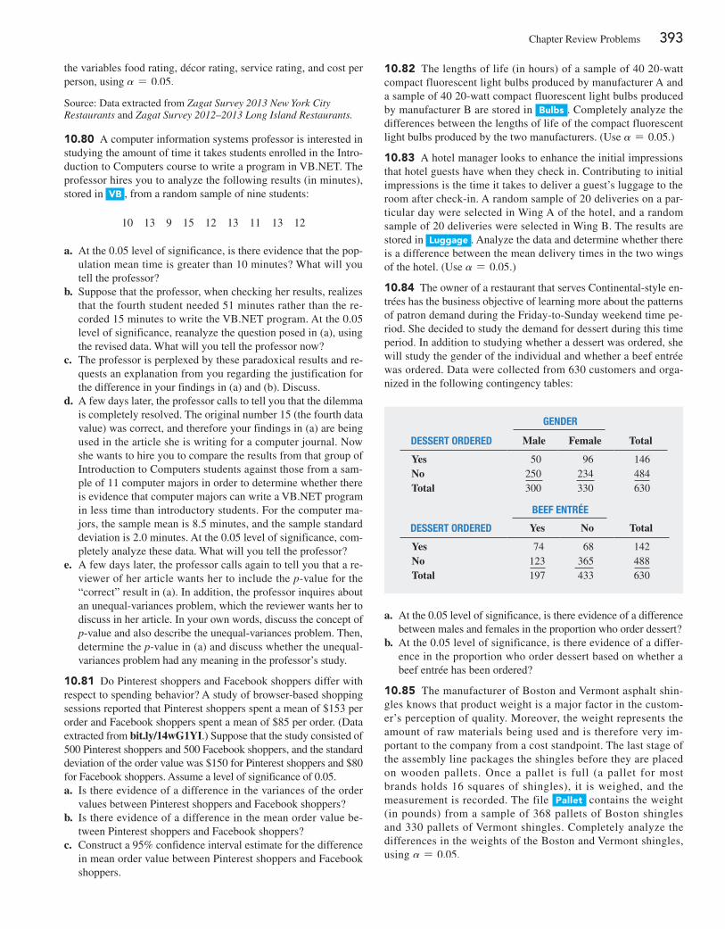
Chapter Review Problems 393
the variables food rating, décor rating, service rating, and cost per person, using a = 0.05.
Source: Data extracted from Zagat Survey 2013 New York City Restaurants and Zagat Survey 2012–2013 Long Island Restaurants.
10.80 A computer information systems professor is interested in studying the amount of time it takes students enrolled in the Intro-duction to Computers course to write a program in VB.NeT. The professor hires you to analyze the following results (in minutes), stored in VB , from a random sample of nine students:
10 13 9 15 12 13 11 13 12
a. At the 0.05 level of significance, is there evidence that the pop-ulation mean time is greater than 10 minutes? What will you tell the professor?
b. Suppose that the professor, when checking her results, realizes that the fourth student needed 51 minutes rather than the re-corded 15 minutes to write the VB.NeT program. At the 0.05 level of significance, reanalyze the question posed in (a), using the revised data. What will you tell the professor now?
c. The professor is perplexed by these paradoxical results and re-quests an explanation from you regarding the justification for the difference in your findings in (a) and (b). Discuss.
d. A few days later, the professor calls to tell you that the dilemma is completely resolved. The original number 15 (the fourth data value) was correct, and therefore your findings in (a) are being used in the article she is writing for a computer journal. Now she wants to hire you to compare the results from that group of Introduction to Computers students against those from a sam-ple of 11 computer majors in order to determine whether there is evidence that computer majors can write a VB.NeT program in less time than introductory students. For the computer ma-jors, the sample mean is 8.5 minutes, and the sample standard deviation is 2.0 minutes. At the 0.05 level of significance, com-pletely analyze these data. What will you tell the professor?
e. A few days later, the professor calls again to tell you that a re-viewer of her article wants her to include the p-value for the “correct” result in (a). In addition, the professor inquires about an unequal-variances problem, which the reviewer wants her to discuss in her article. In your own words, discuss the concept of p-value and also describe the unequal-variances problem. Then, determine the p-value in (a) and discuss whether the unequal-variances problem had any meaning in the professor’s study.
10.81 Do Pinterest shoppers and Facebook shoppers differ with respect to spending behavior? A study of browser-based shopping sessions reported that Pinterest shoppers spent a mean of $153 per order and Facebook shoppers spent a mean of $85 per order. (Data extracted from bit.ly/14wG1YI.) Suppose that the study consisted of 500 Pinterest shoppers and 500 Facebook shoppers, and the standard deviation of the order value was $150 for Pinterest shoppers and $80 for Facebook shoppers. Assume a level of significance of 0.05.a. Is there evidence of a difference in the variances of the order
values between Pinterest shoppers and Facebook shoppers?b. Is there evidence of a difference in the mean order value be-
tween Pinterest shoppers and Facebook shoppers?c. Construct a 95% confidence interval estimate for the difference
in mean order value between Pinterest shoppers and Facebook shoppers.
10.82 The lengths of life (in hours) of a sample of 40 20-watt compact fluorescent light bulbs produced by manufacturer A and a sample of 40 20-watt compact fluorescent light bulbs produced by manufacturer B are stored in Bulbs . Completely analyze the differences between the lengths of life of the compact fluorescent light bulbs produced by the two manufacturers. (Use a = 0.05.)
10.83 A hotel manager looks to enhance the initial impressions that hotel guests have when they check in. Contributing to initial impressions is the time it takes to deliver a guest’s luggage to the room after check-in. A random sample of 20 deliveries on a par-ticular day were selected in Wing A of the hotel, and a random sample of 20 deliveries were selected in Wing B. The results are stored in luggage . Analyze the data and determine whether there is a difference between the mean delivery times in the two wings of the hotel. (Use a = 0.05.)
10.84 The owner of a restaurant that serves Continental-style en-trées has the business objective of learning more about the patterns of patron demand during the Friday-to-Sunday weekend time pe-riod. She decided to study the demand for dessert during this time period. In addition to studying whether a dessert was ordered, she will study the gender of the individual and whether a beef entrée was ordered. Data were collected from 630 customers and orga-nized in the following contingency tables:
a. At the 0.05 level of significance, is there evidence of a difference between males and females in the proportion who order dessert?
b. At the 0.05 level of significance, is there evidence of a differ-ence in the proportion who order dessert based on whether a beef entrée has been ordered?
10.85 The manufacturer of Boston and Vermont asphalt shin-gles knows that product weight is a major factor in the custom-er’s perception of quality. Moreover, the weight represents the amount of raw materials being used and is therefore very im-portant to the company from a cost standpoint. The last stage of the assembly line packages the shingles before they are placed on wooden pallets. Once a pallet is full (a pallet for most brands holds 16 squares of shingles), it is weighed, and the measurement is recorded. The file Pallet contains the weight (in pounds) from a sample of 368 pallets of Boston shingles and 330 pallets of Vermont shingles. Completely analyze the differences in the weights of the Boston and Vermont shingles, using a = 0.05.
GenDer
DeSSerT orDereD Male Female Total
Yes 50 96 146No 250 234 484Total 300 330 630
Beef enTrée
DeSSerT orDereD Yes No Total
Yes 74 68 142No 123 365 488Total 197 433 630
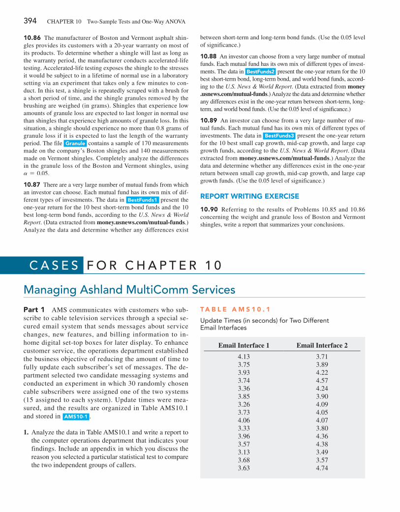
394 CHAPTeR 10 Two-Sample Tests and One-Way ANOVA
10.86 The manufacturer of Boston and Vermont asphalt shin-gles provides its customers with a 20-year warranty on most of its products. To determine whether a shingle will last as long as the warranty period, the manufacturer conducts accelerated-life testing. Accelerated-life testing exposes the shingle to the stresses it would be subject to in a lifetime of normal use in a laboratory setting via an experiment that takes only a few minutes to con-duct. In this test, a shingle is repeatedly scraped with a brush for a short period of time, and the shingle granules removed by the brushing are weighed (in grams). Shingles that experience low amounts of granule loss are expected to last longer in normal use than shingles that experience high amounts of granule loss. In this situation, a shingle should experience no more than 0.8 grams of granule loss if it is expected to last the length of the warranty period. The file granule contains a sample of 170 measurements made on the company’s Boston shingles and 140 measurements made on Vermont shingles. Completely analyze the differences in the granule loss of the Boston and Vermont shingles, using a = 0.05.
10.87 There are a very large number of mutual funds from which an investor can choose. each mutual fund has its own mix of dif-ferent types of investments. The data in BestFunds1 present the one-year return for the 10 best short-term bond funds and the 10 best long-term bond funds, according to the U.S. News & World Report. (Data extracted from money.usnews.com/mutual-funds.) Analyze the data and determine whether any differences exist
between short-term and long-term bond funds. (Use the 0.05 level of significance.)
10.88 An investor can choose from a very large number of mutual funds. each mutual fund has its own mix of different types of invest-ments. The data in BestFunds2 present the one-year return for the 10 best short-term bond, long-term bond, and world bond funds, accord-ing to the U.S. News & World Report. (Data extracted from money . usnews.com/mutual-funds.) Analyze the data and determine whether any differences exist in the one-year return between short-term, long-term, and world bond funds. (Use the 0.05 level of significance.)
10.89 An investor can choose from a very large number of mu-tual funds. each mutual fund has its own mix of different types of investments. The data in BestFunds3 present the one-year return for the 10 best small cap growth, mid-cap growth, and large cap growth funds, according to the U.S. News & World Report. (Data extracted from money.usnews.com/mutual-funds.) Analyze the data and determine whether any differences exist in the one-year return between small cap growth, mid-cap growth, and large cap growth funds. (Use the 0.05 level of significance.)
rePorT WriTing exerCiSe
10.90 Referring to the results of Problems 10.85 and 10.86 concerning the weight and granule loss of Boston and Vermont shingles, write a report that summarizes your conclusions.
c a s e s F O r c h a p t e r 1 0
Managing ashland Multicomm services
Part 1 AMS communicates with customers who sub-scribe to cable television services through a special se-cured email system that sends messages about service changes, new features, and billing information to in-home digital set-top boxes for later display. To enhance customer service, the operations department established the business objective of reducing the amount of time to fully update each subscriber’s set of messages. The de-partment selected two candidate messaging systems and conducted an experiment in which 30 randomly chosen cable subscribers were assigned one of the two systems (15 assigned to each system). Update times were mea-sured, and the results are organized in Table AMS10.1 and stored in aMS10-1 .
1. Analyze the data in Table AMS10.1 and write a report to the computer operations department that indicates your findings. Include an appendix in which you discuss the reason you selected a particular statistical test to compare the two independent groups of callers.
Email Interface 1 Email Interface 2
4.13 3.713.75 3.893.93 4.223.74 4.573.36 4.243.85 3.903.26 4.093.73 4.054.06 4.073.33 3.803.96 4.363.57 4.383.13 3.493.68 3.573.63 4.74
T a B l e a M S 1 0 . 1
Update Times (in seconds) for Two Different Email Interfaces
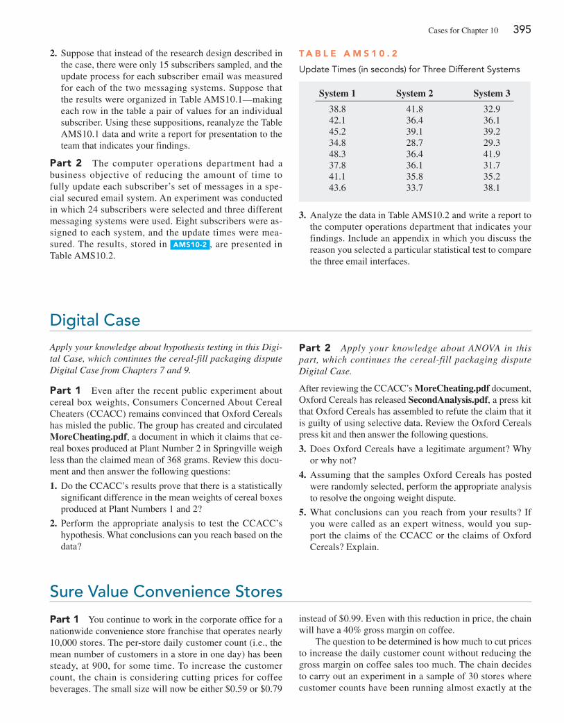
Cases for Chapter 10 395
2. Suppose that instead of the research design described in the case, there were only 15 subscribers sampled, and the update process for each subscriber email was measured for each of the two messaging systems. Suppose that the results were organized in Table AMS10.1—making each row in the table a pair of values for an individual subscriber. Using these suppositions, reanalyze the Table AMS10.1 data and write a report for presentation to the team that indicates your findings.
Part 2 The computer operations department had a business objective of reducing the amount of time to fully update each subscriber’s set of messages in a spe-cial secured email system. An experiment was conducted in which 24 subscribers were selected and three different messaging systems were used. eight subscribers were as-signed to each system, and the update times were mea-sured. The results, stored in aMS10-2 , are presented in Table AMS10.2.
T a B l e a M S 1 0 . 2
Update Times (in seconds) for Three Different Systems
System 1 System 2 System 3
38.8 41.8 32.942.1 36.4 36.145.2 39.1 39.234.8 28.7 29.348.3 36.4 41.937.8 36.1 31.741.1 35.8 35.243.6 33.7 38.1
3. Analyze the data in Table AMS10.2 and write a report to the computer operations department that indicates your findings. Include an appendix in which you discuss the reason you selected a particular statistical test to compare the three email interfaces.
digital caseApply your knowledge about hypothesis testing in this Digi-tal Case, which continues the cereal-fill packaging dispute Digital Case from Chapters 7 and 9.
Part 1 even after the recent public experiment about cereal box weights, Consumers Concerned About Cereal Cheaters (CCACC) remains convinced that Oxford Cereals has misled the public. The group has created and circulated MoreCheating.pdf, a document in which it claims that ce-real boxes produced at Plant Number 2 in Springville weigh less than the claimed mean of 368 grams. Review this docu-ment and then answer the following questions:
1. Do the CCACC’s results prove that there is a statistically significant difference in the mean weights of cereal boxes produced at Plant Numbers 1 and 2?
2. Perform the appropriate analysis to test the CCACC’s hypothesis. What conclusions can you reach based on the data?
Part 2 Apply your knowledge about ANOVA in this part, which continues the cereal-fill packaging dispute Digital Case.
After reviewing the CCACC’s MoreCheating.pdf document, Oxford Cereals has released SecondAnalysis.pdf, a press kit that Oxford Cereals has assembled to refute the claim that it is guilty of using selective data. Review the Oxford Cereals press kit and then answer the following questions.
3. Does Oxford Cereals have a legitimate argument? Why or why not?
4. Assuming that the samples Oxford Cereals has posted were randomly selected, perform the appropriate analysis to resolve the ongoing weight dispute.
5. What conclusions can you reach from your results? If you were called as an expert witness, would you sup-port the claims of the CCACC or the claims of Oxford Cereals? explain.
sure Value convenience stores
Part 1 You continue to work in the corporate office for a nationwide convenience store franchise that operates nearly 10,000 stores. The per-store daily customer count (i.e., the mean number of customers in a store in one day) has been steady, at 900, for some time. To increase the customer count, the chain is considering cutting prices for coffee beverages. The small size will now be either $0.59 or $0.79
instead of $0.99. even with this reduction in price, the chain will have a 40% gross margin on coffee.
The question to be determined is how much to cut prices to increase the daily customer count without reducing the gross margin on coffee sales too much. The chain decides to carry out an experiment in a sample of 30 stores where customer counts have been running almost exactly at the
396 CHAPTeR 10 Two-Sample Tests and One-Way ANOVA
national average of 900. In 15 of the stores, the price of a small coffee will now be $0.59 instead of $0.99, and in 15 other stores, the price of a small coffee will now be $0.79. After four weeks, the 15 stores that priced the small coffee at $0.59 had a mean daily customer count of 964 and a standard deviation of 88, and the 15 stores that priced the small coffee at $0.79 had a mean daily customer count of 941 and a stan-dard deviation of 76. Analyze these data (using the 0.05 level of significance) and answer the following questions.
1. Does reducing the price of a small coffee to either $0.59 or $0.79 increase the mean per-store daily customer count?
2. If reducing the price of a small coffee to either $0.59 or $0.79 increases the mean per-store daily customer count, is there any difference in the mean per-store daily customer count between stores in which a small coffee was priced at $0.59 and stores in which a small coffee was priced at $0.79?
3. What price do you recommend for a small coffee?
Part 2 As you continue to work in the corporate office for a nationwide convenience store franchise that operates nearly 10,000 stores, you decide to carry out an experiment in a sample of 24 stores where customer counts have been running almost exactly at the national average of 900. In 6 of the stores, the price of a small coffee will now be $0.59, in 6 stores the price of a small coffee will now be $0.69, in 6 stores, the price of a small coffee will now be $0.79, and in 6 stores, the price of a small coffee will now be $0.89. After four weeks of selling the coffee at the new price, the daily customer counts in the stores were recorded and stored in CoffeeSales .
4. Analyze the data and determine whether there is evi-dence of a difference in the daily customer count, based on the price of a small coffee.
5. If appropriate, determine which mean prices differ in daily customer counts.
6. What price do you recommend for a small coffee?
cardiogood Fitness
Return to the CardioGood Fitness case first presented on page 47. Using the data stored in Cardiogood Fitness :
1. Determine whether differences exist between males and females in their age in years, education in years, an-nual household income ($), mean number of times the customer plans to use the treadmill each week, and mean number of miles the customer expects to walk or run each week.
2. Determine whether differences exist between customers based on the product purchased (TM195, TM498, TM798) in their age in years, education in years, annual household income ($), mean number of times the customer plans to use the treadmill each week, and mean number of miles the customer expects to walk or run each week.
3. Write a report to be presented to the management of CardioGood Fitness detailing your findings.
More descriptive choices Follow-Up Follow up the Using Statistics scenario “More Descriptive Choices, Revisited” on page 158.
1. Determine whether there is a difference in the 3-year return percentage, 5-year return percentages, and 10-year return percentages of the growth and value funds (stored in retirement Funds ).
2. Determine whether there is a difference between the small, mid-cap, and large market cap funds in the three-year return percentages, five-year return percentages, and ten-year return percentages (stored in retirement Funds ).
clear Mountain state student surveys
1. The Student News Service at Clear Mountain State University (CMSU) has decided to gather data about the undergraduate students that attend CMSU. It creates and distributes a survey of 14 questions and receives responses from 62 undergraduates (stored in undergradSurvey ).
a. At the 0.05 level of significance, is there evidence of a difference between males and females in grade point average, expected starting salary, number of social networking sites registered for, age, spending on text-books and supplies, text messages sent in a week, and the wealth needed to feel rich?
Cases for Chapter 10 397
b. At the 0.05 level of significance, is there evidence of a difference between students who plan to go to gradu-ate school and those who do not plan to go to graduate school in grade point average, expected starting salary, number of social networking sites registered for, age, spending on textbooks and supplies, text messages sent in a week, and the wealth needed to feel rich?
c. At the 0.05 level of significance, is there evidence of a difference based on academic major in expected starting salary, number of social networking sites reg-istered for, age, spending on textbooks and supplies, text messages sent in a week, and the wealth needed to feel rich?
d. At the 0.05 level of significance, is there evidence of a difference based on graduate school intention in grade point average, expected starting salary, number of social networking sites registered for, age, spending on textbooks and supplies, text messages sent in a week, and the wealth needed to feel rich?
2. The dean of students at CMSU has learned about the undergraduate survey and has decided to undertake a similar survey for graduate students at Clear Mountain State. She creates and distributes a survey of 14 ques-tions and receives responses from 44 graduate students (stored in gradSurvey ). For these data, at the 0.05 level of significance.
a. Is there evidence of a difference between males and females in age, undergraduate grade point average, graduate grade point average, expected salary upon graduation, spending on textbooks and supplies, text messages sent in a week, and the wealth needed to feel rich?
b. Is there evidence of a difference based on undergradu-ate major in age, undergraduate grade point average, graduate grade point average, expected salary upon graduation, spending on textbooks and supplies, text messages sent in a week, and the wealth needed to feel rich?
c. Is there evidence of a difference based on gradu-ate major in age, undergraduate grade point average, graduate grade point average, expected salary upon graduation, spending on textbooks and supplies, text messages sent in a week, and the wealth needed to feel rich?
d. Is there evidence of a difference based on employ-ment status in age, undergraduate grade point average, graduate grade point average, expected salary upon graduation, spending on textbooks and supplies, text messages sent in a week, and the wealth needed to feel rich?
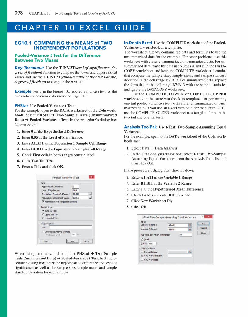
398 CHAPTeR 10 Two-Sample Tests and One-Way ANOVA
eg10.1 CoMParing the MeanS of TWo inDePenDenT PoPulaTionS
Pooled-Variance t Test for the Difference Between Two Means
Key Technique Use the T.INV.2T(level of significance, de-grees of freedom) function to compute the lower and upper critical values and use the T.DIST.2T(absolute value of the t test statistic, degrees of freedom) to compute the p-value.
Example Perform the Figure 10.3 pooled-variance t test for the two end-cap locations data shown on page 348.
PhStat Use Pooled-Variance t Test.For the example, open to the DATA worksheet of the Cola work-book. Select PHStat ➔ Two-Sample Tests (Unsummarized Data) ➔ Pooled-Variance t Test. In the procedure’s dialog box (shown below):
1. enter 0 as the Hypothesized Difference.
2. enter 0.05 as the Level of Significance.
3. enter A1:A11 as the Population 1 Sample Cell Range.
4. enter B1:B11 as the Population 2 Sample Cell Range.
5. Check First cells in both ranges contain label.
6. Click Two-Tail Test.
7. enter a Title and click OK.
When using summarized data, select PHStat ➔ Two-Sample Tests (Summarized Data) ➔ Pooled-Variance t Test. In that pro-cedure’s dialog box, enter the hypothesized difference and level of significance, as well as the sample size, sample mean, and sample standard deviation for each sample.
in-Depth excel Use the COMPUTE worksheet of the Pooled-Variance T workbook as a template.The worksheet already contains the data and formulas to use the unsummarized data for the example. For other problems, use this worksheet with either unsummarized or summarized data. For un-summarized data, paste the data in columns A and B in the DATA-COPY worksheet and keep the COMPUTe worksheet formulas that compute the sample size, sample mean, and sample standard deviation in the cell range B7:B13. For summarized data, replace the formulas in the cell range B7:B13 with the sample statistics and ignore the DATACOPY worksheet.
Use the COMPUTE_LOWER or COMPUTE_UPPER worksheets in the same workbook as templates for performing one-tail pooled-variance t tests with either unsummarized or sum-marized data. If you use an excel version older than excel 2010, use the COMPUTe_OLDeR worksheet as a template for both the two-tail and one-tail tests.
analysis ToolPak Use t-Test: Two-Sample Assuming Equal Variances.For the example, open to the DATA worksheet of the Cola work-book and:
1. Select Data ➔ Data Analysis.
2. In the Data Analysis dialog box, select t-Test: Two-Sample Assuming Equal Variances from the Analysis Tools list and then click OK.
In the procedure’s dialog box (shown below):
3. enter A1:A11 as the Variable 1 Range
4. enter B1:B11 as the Variable 2 Range.
5. enter 0 as the Hypothesized Mean Difference.
6. Check Labels and enter 0.05 as Alpha.
7. Click New Worksheet Ply.
8. Click OK.
c h a p t e r 1 0 e x c e l g U i d e
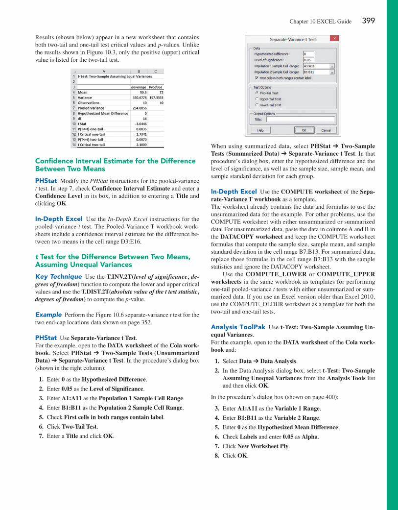
Chapter 10 exCeL Guide 399
Results (shown below) appear in a new worksheet that contains both two-tail and one-tail test critical values and p-values. Unlike the results shown in Figure 10.3, only the positive (upper) critical value is listed for the two-tail test.
Confidence interval estimate for the Difference Between Two Means
PhStat Modify the PHStat instructions for the pooled-variance t test. In step 7, check Confidence Interval Estimate and enter a Confidence Level in its box, in addition to entering a Title and clicking OK.
in-Depth excel Use the In-Depth Excel instructions for the pooled-variance t test. The Pooled-Variance T workbook work-sheets include a confidence interval estimate for the difference be-tween two means in the cell range D3:e16.
t Test for the Difference Between Two Means, assuming unequal Variances
Key Technique Use the T.INV.2T(level of significance, de-grees of freedom) function to compute the lower and upper critical values and use the T.DIST.2T(absolute value of the t test statistic, degrees of freedom) to compute the p-value.
Example Perform the Figure 10.6 separate-variance t test for the two end-cap locations data shown on page 352.
PhStat Use Separate-Variance t Test.For the example, open to the DATA worksheet of the Cola work-book. Select PHStat ➔ Two-Sample Tests (Unsummarized Data) ➔ Separate-Variance t Test. In the procedure’s dialog box (shown in the right column):
1. enter 0 as the Hypothesized Difference.
2. enter 0.05 as the Level of Significance.
3. enter A1:A11 as the Population 1 Sample Cell Range.
4. enter B1:B11 as the Population 2 Sample Cell Range.
5. Check First cells in both ranges contain label.
6. Click Two-Tail Test.
7. enter a Title and click OK.
When using summarized data, select PHStat ➔ Two-Sample Tests (Summarized Data) ➔ Separate-Variance t Test. In that procedure’s dialog box, enter the hypothesized difference and the level of significance, as well as the sample size, sample mean, and sample standard deviation for each group.
in-Depth excel Use the COMPUTE worksheet of the Sepa-rate-Variance T workbook as a template.The worksheet already contains the data and formulas to use the unsummarized data for the example. For other problems, use the COMPUTe worksheet with either unsummarized or summarized data. For unsummarized data, paste the data in columns A and B in the DATACOPY worksheet and keep the COMPUTe worksheet formulas that compute the sample size, sample mean, and sample standard deviation in the cell range B7:B13. For summarized data, replace those formulas in the cell range B7:B13 with the sample statistics and ignore the DATACOPY worksheet.
Use the COMPUTE_LOWER or COMPUTE_UPPER worksheets in the same workbook as templates for performing one-tail pooled-variance t tests with either unsummarized or sum-marized data. If you use an excel version older than excel 2010, use the COMPUTe_OLDeR worksheet as a template for both the two-tail and one-tail tests.
analysis ToolPak Use t-Test: Two-Sample Assuming Un-equal Variances.For the example, open to the DATA worksheet of the Cola work-book and:
1. Select Data ➔ Data Analysis.
2. In the Data Analysis dialog box, select t-Test: Two-Sample Assuming Unequal Variances from the Analysis Tools list and then click OK.
In the procedure’s dialog box (shown on page 400):
3. enter A1:A11 as the Variable 1 Range.
4. enter B1:B11 as the Variable 2 Range.
5. enter 0 as the Hypothesized Mean Difference.
6. Check Labels and enter 0.05 as Alpha.
7. Click New Worksheet Ply.
8. Click OK.
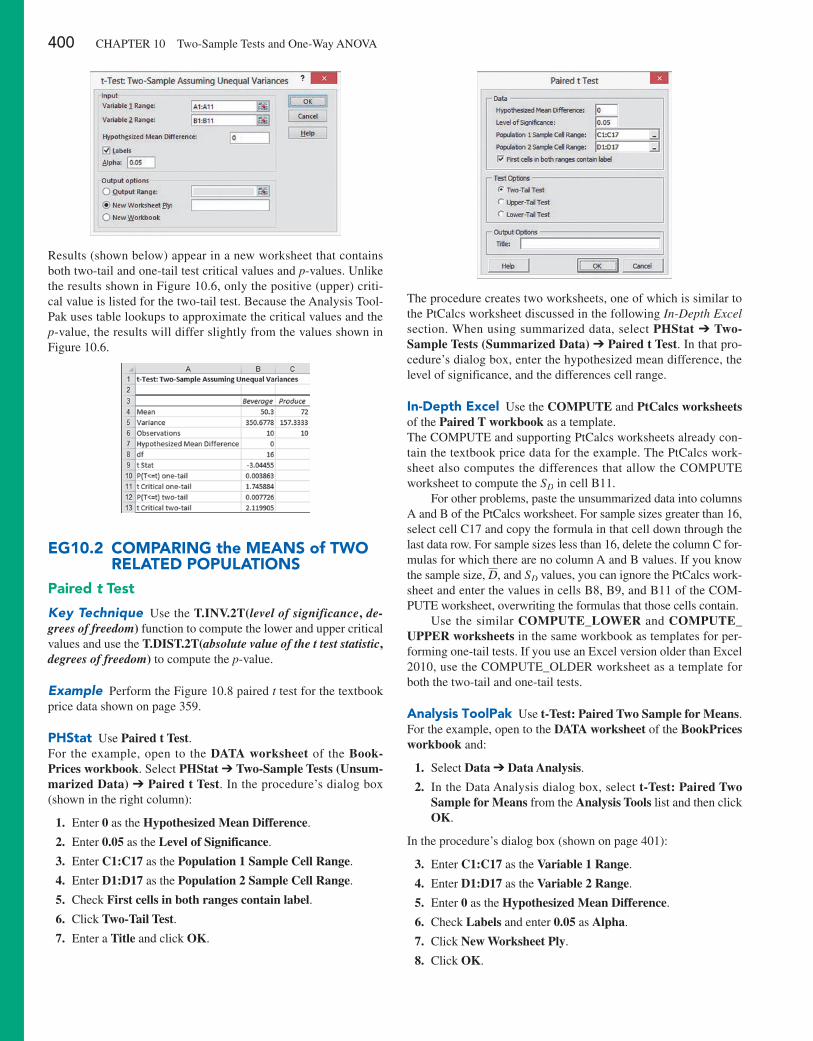
400 CHAPTeR 10 Two-Sample Tests and One-Way ANOVA
Results (shown below) appear in a new worksheet that contains both two-tail and one-tail test critical values and p-values. Unlike the results shown in Figure 10.6, only the positive (upper) criti-cal value is listed for the two-tail test. Because the Analysis Tool-Pak uses table lookups to approximate the critical values and the p-value, the results will differ slightly from the values shown in Figure 10.6.
eg10.2 CoMParing the MeanS of TWo relaTeD PoPulaTionS
Paired t Test
Key Technique Use the T.INV.2T(level of significance, de-grees of freedom) function to compute the lower and upper critical values and use the T.DIST.2T(absolute value of the t test statistic, degrees of freedom) to compute the p-value.
Example Perform the Figure 10.8 paired t test for the textbook price data shown on page 359.
PhStat Use Paired t Test.For the example, open to the DATA worksheet of the Book-Prices workbook. Select PHStat ➔ Two-Sample Tests (Unsum-marized Data) ➔ Paired t Test. In the procedure’s dialog box (shown in the right column):
1. enter 0 as the Hypothesized Mean Difference.
2. enter 0.05 as the Level of Significance.
3. enter C1:C17 as the Population 1 Sample Cell Range.
4. enter D1:D17 as the Population 2 Sample Cell Range.
5. Check First cells in both ranges contain label.
6. Click Two-Tail Test.
7. enter a Title and click OK.
The procedure creates two worksheets, one of which is similar to the PtCalcs worksheet discussed in the following In-Depth Excel section. When using summarized data, select PHStat ➔ Two-Sample Tests (Summarized Data) ➔ Paired t Test. In that pro-cedure’s dialog box, enter the hypothesized mean difference, the level of significance, and the differences cell range.
in-Depth excel Use the COMPUTE and PtCalcs worksheets of the Paired T workbook as a template.The COMPUTe and supporting PtCalcs worksheets already con-tain the textbook price data for the example. The PtCalcs work-sheet also computes the differences that allow the COMPUTe worksheet to compute the SD in cell B11.
For other problems, paste the unsummarized data into columns A and B of the PtCalcs worksheet. For sample sizes greater than 16, select cell C17 and copy the formula in that cell down through the last data row. For sample sizes less than 16, delete the column C for-mulas for which there are no column A and B values. If you know the sample size, D, and SD values, you can ignore the PtCalcs work-sheet and enter the values in cells B8, B9, and B11 of the COM-PUTe worksheet, overwriting the formulas that those cells contain.
Use the similar COMPUTE_LOWER and COMPUTE_UPPER worksheets in the same workbook as templates for per-forming one-tail tests. If you use an excel version older than excel 2010, use the COMPUTe_OLDeR worksheet as a template for both the two-tail and one-tail tests.
analysis ToolPak Use t-Test: Paired Two Sample for Means.For the example, open to the DATA worksheet of the BookPrices workbook and:
1. Select Data ➔ Data Analysis.
2. In the Data Analysis dialog box, select t-Test: Paired Two Sample for Means from the Analysis Tools list and then click OK.
In the procedure’s dialog box (shown on page 401):
3. enter C1:C17 as the Variable 1 Range.
4. enter D1:D17 as the Variable 2 Range.
5. enter 0 as the Hypothesized Mean Difference.
6. Check Labels and enter 0.05 as Alpha.
7. Click New Worksheet Ply.
8. Click OK.
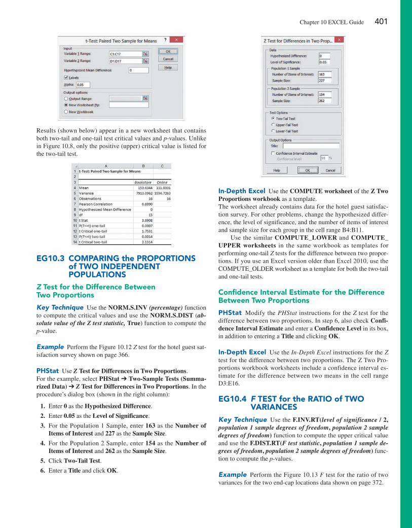
Chapter 10 exCeL Guide 401
Results (shown below) appear in a new worksheet that contains both two-tail and one-tail test critical values and p-values. Unlike in Figure 10.8, only the positive (upper) critical value is listed for the two-tail test.
eg10.3 CoMParing the ProPorTionS of TWo inDePenDenT PoPulaTionS
Z Test for the Difference Between Two Proportions
Key Technique Use the NORM.S.INV (percentage) function to compute the critical values and use the NORM.S.DIST (ab-solute value of the Z test statistic, True) function to compute the p-value.
Example Perform the Figure 10.12 Z test for the hotel guest sat-isfaction survey shown on page 366.
PhStat Use Z Test for Differences in Two Proportions.For the example, select PHStat ➔ Two-Sample Tests (Summa-rized Data) ➔ Z Test for Differences in Two Proportions. In the procedure’s dialog box (shown in the right column):
1. enter 0 as the Hypothesized Difference.
2. enter 0.05 as the Level of Significance.
3. For the Population 1 Sample, enter 163 as the Number of Items of Interest and 227 as the Sample Size.
4. For the Population 2 Sample, enter 154 as the Number of Items of Interest and 262 as the Sample Size.
5. Click Two-Tail Test.
6. enter a Title and click OK.
in-Depth excel Use the COMPUTE worksheet of the Z Two Proportions workbook as a template.The worksheet already contains data for the hotel guest satisfac-tion survey. For other problems, change the hypothesized differ-ence, the level of significance, and the number of items of interest and sample size for each group in the cell range B4:B11.
Use the similar COMPUTE_LOWER and COMPUTE_UPPER worksheets in the same workbook as templates for performing one-tail Z tests for the difference between two propor-tions. If you use an excel version older than excel 2010, use the COMPUTe_OLDeR worksheet as a template for both the two-tail and one-tail tests.
Confidence interval estimate for the Difference Between Two Proportions
PhStat Modify the PHStat instructions for the Z test for the difference between two proportions. In step 6, also check Confi-dence Interval Estimate and enter a Confidence Level in its box, in addition to entering a Title and clicking OK.
in-Depth excel Use the In-Depth Excel instructions for the Z test for the difference between two proportions. The Z Two Pro-portions workbook worksheets include a confidence interval es-timate for the difference between two means in the cell range D3:e16.
eg10.4 F TeST for the raTio of TWo VarianCeS
Key Technique Use the F.INV.RT(level of significance / 2, population 1 sample degrees of freedom, population 2 sample degrees of freedom) function to compute the upper critical value and use the F.DIST.RT(F test statistic, population 1 sample de-grees of freedom, population 2 sample degrees of freedom) func-tion to compute the p-values.
Example Perform the Figure 10.13 F test for the ratio of two variances for the two end-cap locations data shown on page 372.
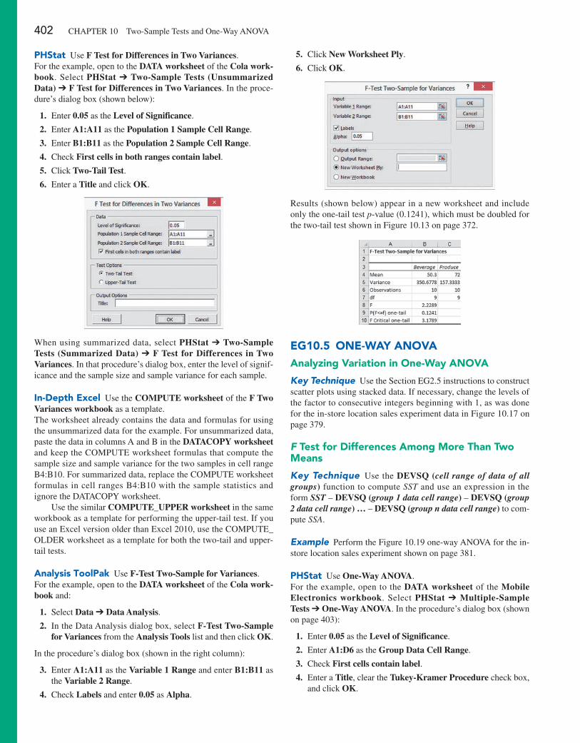
402 CHAPTeR 10 Two-Sample Tests and One-Way ANOVA
PhStat Use F Test for Differences in Two Variances.For the example, open to the DATA worksheet of the Cola work-book. Select PHStat ➔ Two-Sample Tests (Unsummarized Data) ➔ F Test for Differences in Two Variances. In the proce-dure’s dialog box (shown below):
1. enter 0.05 as the Level of Significance.
2. enter A1:A11 as the Population 1 Sample Cell Range.
3. enter B1:B11 as the Population 2 Sample Cell Range.
4. Check First cells in both ranges contain label.
5. Click Two-Tail Test.
6. enter a Title and click OK.
When using summarized data, select PHStat ➔ Two-Sample Tests (Summarized Data) ➔ F Test for Differences in Two Variances. In that procedure’s dialog box, enter the level of signif-icance and the sample size and sample variance for each sample.
in-Depth excel Use the COMPUTE worksheet of the F Two Variances workbook as a template.The worksheet already contains the data and formulas for using the unsummarized data for the example. For unsummarized data, paste the data in columns A and B in the DATACOPY worksheet and keep the COMPUTe worksheet formulas that compute the sample size and sample variance for the two samples in cell range B4:B10. For summarized data, replace the COMPUTe worksheet formulas in cell ranges B4:B10 with the sample statistics and ignore the DATACOPY worksheet.
Use the similar COMPUTE_UPPER worksheet in the same workbook as a template for performing the upper-tail test. If you use an excel version older than excel 2010, use the COMPUTe_OLDeR worksheet as a template for both the two-tail and upper-tail tests.
analysis ToolPak Use F-Test Two-Sample for Variances.For the example, open to the DATA worksheet of the Cola work-book and:
1. Select Data ➔ Data Analysis.
2. In the Data Analysis dialog box, select F-Test Two-Sample for Variances from the Analysis Tools list and then click OK.
In the procedure’s dialog box (shown in the right column):
3. enter A1:A11 as the Variable 1 Range and enter B1:B11 as the Variable 2 Range.
4. Check Labels and enter 0.05 as Alpha.
5. Click New Worksheet Ply.
6. Click OK.
Results (shown below) appear in a new worksheet and include only the one-tail test p-value (0.1241), which must be doubled for the two-tail test shown in Figure 10.13 on page 372.
eg10.5 one-Way anoVaanalyzing Variation in one-Way anoVa
Key Technique Use the Section eG2.5 instructions to construct scatter plots using stacked data. If necessary, change the levels of the factor to consecutive integers beginning with 1, as was done for the in-store location sales experiment data in Figure 10.17 on page 379.
F Test for Differences among More Than Two Means
Key Technique Use the DEVSQ (cell range of data of all groups) function to compute SST and use an expression in the form SST – DEVSQ (group 1 data cell range) – DEVSQ (group 2 data cell range) … – DEVSQ (group n data cell range) to com-pute SSA.
Example Perform the Figure 10.19 one-way ANOVA for the in-store location sales experiment shown on page 381.
PhStat Use One-Way ANOVA.For the example, open to the DATA worksheet of the Mobile Electronics workbook. Select PHStat ➔ Multiple-Sample Tests ➔ One-Way ANOVA. In the procedure’s dialog box (shown on page 403):
1. enter 0.05 as the Level of Significance.
2. enter A1:D6 as the Group Data Cell Range.
3. Check First cells contain label.
4. enter a Title, clear the Tukey-Kramer Procedure check box, and click OK.
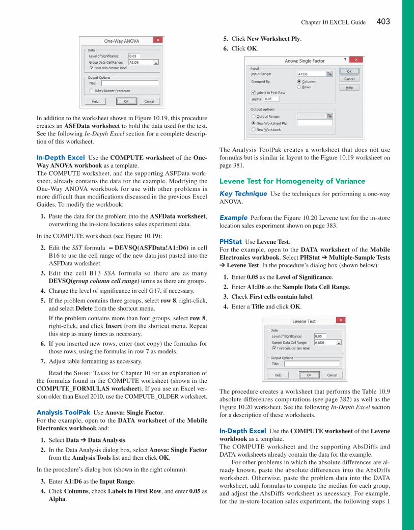
Chapter 10 exCeL Guide 403
In addition to the worksheet shown in Figure 10.19, this procedure creates an ASFData worksheet to hold the data used for the test. See the following In-Depth Excel section for a complete descrip-tion of this worksheet.
in-Depth excel Use the COMPUTE worksheet of the One-Way ANOVA workbook as a template.The COMPUTe worksheet, and the supporting ASFData work-sheet, already contains the data for the example. Modifying the One-Way ANOVA workbook for use with other problems is more difficult than modifications discussed in the previous excel Guides. To modify the workbook:
1. Paste the data for the problem into the ASFData worksheet, overwriting the in-store locations sales experiment data.
In the COMPUTe worksheet (see Figure 10.19):
2. edit the SST formula = DEVSQ(ASFData!A1:D6) in cell B16 to use the cell range of the new data just pasted into the ASFData worksheet.
3. edit the cell B13 SSA formula so there are as many DEVSQ(group column cell range) terms as there are groups.
4. Change the level of significance in cell G17, if necessary.
5. If the problem contains three groups, select row 8, right-click, and select Delete from the shortcut menu.
If the problem contains more than four groups, select row 8, right-click, and click Insert from the shortcut menu. Repeat this step as many times as necessary.
6. If you inserted new rows, enter (not copy) the formulas for those rows, using the formulas in row 7 as models.
7. Adjust table formatting as necessary.
Read the Short Takes for Chapter 10 for an explanation of the formulas found in the COMPUTe worksheet (shown in the COMPUTE_FORMULAS worksheet). If you use an excel ver-sion older than excel 2010, use the COMPUTe_OLDeR worksheet.
analysis ToolPak Use Anova: Single Factor.For the example, open to the DATA worksheet of the Mobile Electronics workbook and:
1. Select Data ➔ Data Analysis.
2. In the Data Analysis dialog box, select Anova: Single Factor from the Analysis Tools list and then click OK.
In the procedure’s dialog box (shown in the right column):
3. enter A1:D6 as the Input Range.
4. Click Columns, check Labels in First Row, and enter 0.05 as Alpha.
5. Click New Worksheet Ply.
6. Click OK.
The Analysis ToolPak creates a worksheet that does not use formulas but is similar in layout to the Figure 10.19 worksheet on page 381.
levene Test for homogeneity of Variance
Key Technique Use the techniques for performing a one-way ANOVA.
Example Perform the Figure 10.20 Levene test for the in-store location sales experiment shown on page 383.
PhStat Use Levene Test.For the example, open to the DATA worksheet of the Mobile Electronics workbook. Select PHStat ➔ Multiple-Sample Tests ➔ Levene Test. In the procedure’s dialog box (shown below):
1. enter 0.05 as the Level of Significance.
2. enter A1:D6 as the Sample Data Cell Range.
3. Check First cells contain label.
4. enter a Title and click OK.
The procedure creates a worksheet that performs the Table 10.9 absolute differences computations (see page 382) as well as the Figure 10.20 worksheet. See the following In-Depth Excel section for a description of these worksheets.
in-Depth excel Use the COMPUTE worksheet of the Levene workbook as a template.The COMPUTe worksheet and the supporting AbsDiffs and DATA worksheets already contain the data for the example.
For other problems in which the absolute differences are al-ready known, paste the absolute differences into the AbsDiffs worksheet. Otherwise, paste the problem data into the DATA worksheet, add formulas to compute the median for each group, and adjust the AbsDiffs worksheet as necessary. For example, for the in-store location sales experiment, the following steps 1
404 CHAPTeR 10 Two-Sample Tests and One-Way ANOVA
through 7 were done with the workbook open to the DATA work-sheet:
1. enter the label Medians in cell A7, the first empty cell in column A.
2. enter the formula =MEDIAN(A2:A6) in cell A8. (Cell range A2:A6 contains the data for the first group, in-aisle.)
3. Copy the cell A8 formula across through column D.
4. Open to the AbsDiffs worksheet.
In the AbsDiffs worksheet:
5. enter row 1 column headings AbsDiff1, AbsDiff2, AbsDiff3, and AbsDiff4 in columns A through D.
6. enter the formula =ABS(DATA!A2 – DATA!A8) in cell A2. Copy this formula down through row 6.
7. Copy the formulas now in cell range A2:A6 across through column D. Absolute differences now appear in the cell range A2:D6.
If you use an excel version older than excel 2010, use the COMPUTe_OLDeR worksheet.
analysis ToolPak Use Anova: Single Factor with absolute difference data to perform the Levene test. If the absolute differ-ences have not already been computed, use steps 1 through 7 of the preceding In-Depth Excel instructions to compute them.
Multiple Comparisons: The Tukey-Kramer Procedure
Key Technique Use formulas to compute the absolute mean differences and use the IF function to compare pairs of means.
Example Perform the Figure 10.21 Tukey-Kramer procedure for the in-store location sales experiment shown on page 385.
PhStat Use the PHStat instructions for the one-way ANOVA F test to perform the Tukey-Kramer procedure, checking Tukey-Kramer Procedure instead in step 4. The procedure creates a worksheet identical to the one shown in Figure 10.21 on page 385 and discussed in the following In-Depth Excel sec-tion. To complete the worksheet, enter the Studentized range Q statistic (use Table e.7) for the level of significance and the numerator and denominator degrees of freedom that are given in the worksheet.
in-Depth excel To perform the Tukey-Kramer procedure, first use the In-Depth Excel instructions for the one-way ANOVA F test and then use the appropriate “TK” worksheet in the One-Way ANOVA workbook.
For the example, open to the TK4 worksheet that already has the value of the Q statistic (4.05) entered in cell B15.
The TK worksheets can be used for problems using three (TK3), four (TK4), five (TK5), six (TK6), or seven (TK7) groups. Use Table e.7 to look up the proper value of the Studentized range Q statistic for the level of significance and the numerator and denominator degrees of freedom for the problem. When you use either the TK5, TK6, and TK7 worksheets, you must also enter the name, sample mean, and sample size for the fifth and, if appli-cable, sixth and seventh groups.
Read the Short Takes for Chapter 10 for an explanation of the formulas found in the COMPUTe worksheet (shown in the COMPUTE_FORMULAS worksheet). If you use an excel version older than excel 2010, use the TK4_OLDeR worksheet.
analysis ToolPak Modify the previous In-Depth Excel instruc-tions to perform the Tukey-Kramer procedure in conjunction with using the Anova: Single Factor procedure. Transfer selected val-ues from the Analysis ToolPak results worksheet to one of the TK worksheets in the One-Way ANOVA workbook. For example, to perform the Figure 10.21 Tukey-Kramer procedure for the in-store location sales experiment on page 385:
1. Use the Anova: Single Factor procedure, as described earlier in this section, to create a worksheet that contains ANOVA re-sults for the in-store locations experiment.
2. Record the name, sample size (in the Count column), and sam-ple mean (in the Average column) of each group. Also record the MSW value, found in the cell that is the intersection of the MS column and Within Groups row, and the denominator degrees of freedom, found in the cell that is the intersection of the df column and Within Groups row.
3. Open to the TK4 worksheet of the One-Way ANOVA workbook.
In the TK4 worksheet:
4. Overwrite the formulas in cell range A5:C8 by entering the name, sample mean, and sample size of each group into that range.
5. enter 0.05 as the Level of significance in cell B11.
6. enter 4 as the Numerator d.f. (equal to the number of groups) in cell B12.
7. enter 16 as the Denominator d.f in cell B13.
8. enter 0.0439 as the MSW in cell B14.
9. enter 4.05 as the Q Statistic in cell B15. (Look up the Studen-tized range Q statistic using Table e.7.)
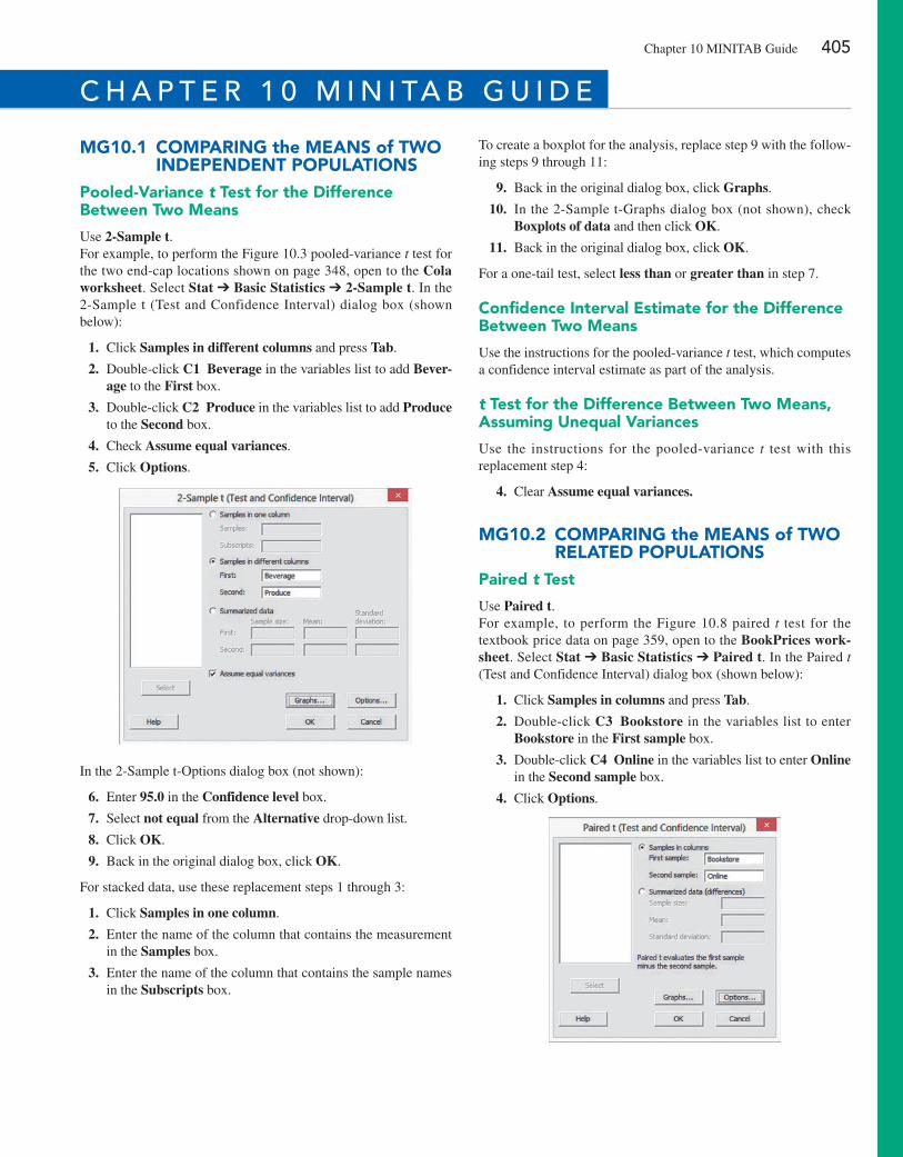
Chapter 10 MINITAB Guide 405
Mg10.1 CoMParing the MeanS of TWo inDePenDenT PoPulaTionS
Pooled-Variance t Test for the Difference Between Two Means
Use 2-Sample t.For example, to perform the Figure 10.3 pooled-variance t test for the two end-cap locations shown on page 348, open to the Cola worksheet. Select Stat ➔ Basic Statistics ➔ 2-Sample t. In the 2-Sample t (Test and Confidence Interval) dialog box (shown below):
1. Click Samples in different columns and press Tab.
2. Double-click C1 Beverage in the variables list to add Bever-age to the First box.
3. Double-click C2 Produce in the variables list to add Produce to the Second box.
4. Check Assume equal variances.
5. Click Options.
In the 2-Sample t-Options dialog box (not shown):
6. enter 95.0 in the Confidence level box.
7. Select not equal from the Alternative drop-down list.
8. Click OK.
9. Back in the original dialog box, click OK.
For stacked data, use these replacement steps 1 through 3:
1. Click Samples in one column.
2. enter the name of the column that contains the measurement in the Samples box.
3. enter the name of the column that contains the sample names in the Subscripts box.
To create a boxplot for the analysis, replace step 9 with the follow-ing steps 9 through 11:
9. Back in the original dialog box, click Graphs.
10. In the 2-Sample t-Graphs dialog box (not shown), check Boxplots of data and then click OK.
11. Back in the original dialog box, click OK.
For a one-tail test, select less than or greater than in step 7.
Confidence interval estimate for the Difference Between Two Means
Use the instructions for the pooled-variance t test, which computes a confidence interval estimate as part of the analysis.
t Test for the Difference Between Two Means, assuming unequal Variances
Use the instructions for the pooled-variance t test with this replacement step 4:
4. Clear Assume equal variances.
Mg10.2 CoMParing the MeanS of TWo relaTeD PoPulaTionS
Paired t Test
Use Paired t.For example, to perform the Figure 10.8 paired t test for the textbook price data on page 359, open to the BookPrices work-sheet. Select Stat ➔ Basic Statistics ➔ Paired t. In the Paired t (Test and Confidence Interval) dialog box (shown below):
1. Click Samples in columns and press Tab.
2. Double-click C3 Bookstore in the variables list to enter Bookstore in the First sample box.
3. Double-click C4 Online in the variables list to enter Online in the Second sample box.
4. Click Options.
c h a p t e r 1 0 M i n i ta b g U i d e
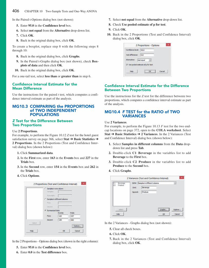
406 CHAPTeR 10 Two-Sample Tests and One-Way ANOVA
In the Paired t-Options dialog box (not shown):
5. enter 95.0 in the Confidence level box.
6. Select not equal from the Alternative drop-down list.
7. Click OK.
8. Back in the original dialog box, click OK.
To create a boxplot, replace step 8 with the following steps 8 through 10:
8. Back in the original dialog box, click Graphs.
9. In the Paired t-Graphs dialog box (not shown), check Box-plots of data and then click OK.
10. Back in the original dialog box, click OK.
For a one-tail test, select less than or greater than in step 6.
Confidence interval estimate for the Mean Difference
Use the instructions for the paired t test, which computes a confi-dence interval estimate as part of the analysis.
Mg10.3 CoMParing the ProPorTionS of TWo inDePenDenT PoPulaTionS
Z Test for the Difference Between Two Proportions
Use 2 Proportions.For example, to perform the Figure 10.12 Z test for the hotel guest satisfaction survey on page 366, select Stat ➔ Basic Statistics ➔ 2 Proportions. In the 2 Proportions (Test and Confidence Inter-val) dialog box (shown below):
1. Click Summarized data.
2. In the First row, enter 163 in the Events box and 227 in the Trials box.
3. In the Second row, enter 154 in the Events box and 262 in the Trials box.
4. Click Options.
In the 2 Proportions - Options dialog box (shown in the right column):
5. enter 95.0 in the Confidence level box.
6. enter 0.0 in the Test difference box.
7. Select not equal from the Alternative drop-down list.
8. Check Use pooled estimate of p for test.
9. Click OK.
10. Back in the 2 Proportions (Test and Confidence Interval) dialog box, click OK.
Confidence interval estimate for the Difference Between Two Proportions
Use the instructions for the Z test for the difference between two proportions, which computes a confidence interval estimate as part of the analysis.
Mg10.4 F TeST for the raTio of TWo VarianCeS
Use 2 Variances.For example, to perform the Figure 10.13 F test for the two end-cap locations on page 372, open to the COLA worksheet. Select Stat ➔ Basic Statistics ➔ 2 Variances. In the 2 Variances (Test and Confidence Interval) dialog box (shown below):
1. Select Samples in different columns from the Data drop-down list and press Tab.
2. Double-click C1 Beverage in the variables list to add Beverage to the First box.
3. Double-click C2 Produce in the variables list to add Produce to the Second box.
4. Click Graphs.
In the 2 Variances - Graphs dialog box (not shown):
5. Clear all check boxes.
6. Click OK.
7. Back in the 2 Variances (Test and Confidence Interval) dialog box, click OK.
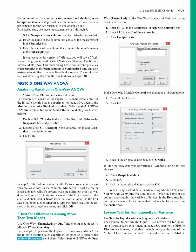
Chapter 10 MINITAB Guide 407
For summarized data, select Sample standard deviations or Sample variances in step 1 and enter the sample size and the sam-ple statistics for the two variables in lieu of steps 2 and 3.For stacked data, use these replacement steps 1 through 3:
1. Select Samples in one column from the Data drop-down list.
2. enter the name of the column that contains the measurement in the Samples box.
3. enter the name of the column that contains the sample names in the Subscripts box.
If you use an older version of Minitab, you will see a 2 Vari-ances dialog box instead of the 2 Variances (Test and Confidence Interval) dialog box. This older dialog box is similar, and you click either Samples in different columns or Summarized data and then make entries similar to the ones listed in this section. The results cre-ated will differ slightly from the results shown in Figure 10.13.
Mg10.5 one-Way anoVaanalyzing Variation in one-Way anoVa
Use Main Effects Plot (requires stacked data).For example, to construct the Figure 10.17 main effects plot for the in-store location sales experiment on page 379, open to the Mobile Electronics Stacked worksheet. Select Stat ➔ ANOVA ➔ Main Effects Plot. In the Main effects Plot dialog box (shown below):
1. Double-click C2 Sales in the variables list to add Sales to the Responses box and press Tab.
2. Double-click C1 Location in the variables list to add Loca-tion to the Factors box.
3. Click OK.
In step 2, if the column entered in the Factors box contains a text variable, as it does in the example, Minitab will sort the factor levels alphabetically. To present levels in a different order, as was done in Figure 10.17, right-click one of the factor levels in the chart and click Edit X Scale from the shortcut menu. In the edit Scale dialog box, click Specified, type the factor levels in the de-sired order separated by spaces, and click OK.
F Test for Differences among More Than Two Means
Use One-Way (Unstacked) or One-Way (for stacked data). In Minitab 17, use One-Way.For example, to perform the Figure 10.19 one-way ANOVA for the in-store location sales experiment on page 381, open to the Mobile electronics worksheet. Select Stat ➔ ANOVA ➔ One-
Way (Unstacked). In the One-Way Analysis of Variance dialog box (shown below):
1. enter C1-C4 in the Responses (in separate columns) box.
2. enter 95.0 in the Confidence level box.
3. Click Comparisons.
In the One-Way Multiple Comparisons dialog box (shown below):
4. Clear all check boxes.
5. Click OK.
6. Back in the original dialog box, click Graphs.
In the One-Way Analysis of Variance - Graphs dialog box (not shown):
7. Check Boxplots of data.
8. Click OK.
9. Back in the original dialog box, click OK.
When using stacked data (or when using Minitab 17), select Stat ➔ ANOVA ➔ One-Way and in step 1 enter the name of the column that contains the variable of interest in the Response box and enter the name of the column that contains the factor names in the Factor box.
levene Test for homogeneity of Variance
Use Test for Equal Variances (requires stacked data). For example, to perform the Figure 10.20 Levene test for the in-store location sales experiment on page 383, open to the Mobile Electronics Stacked worksheet, which contains the data of the Mobile electronics worksheet in stacked order. Select Stat ➔
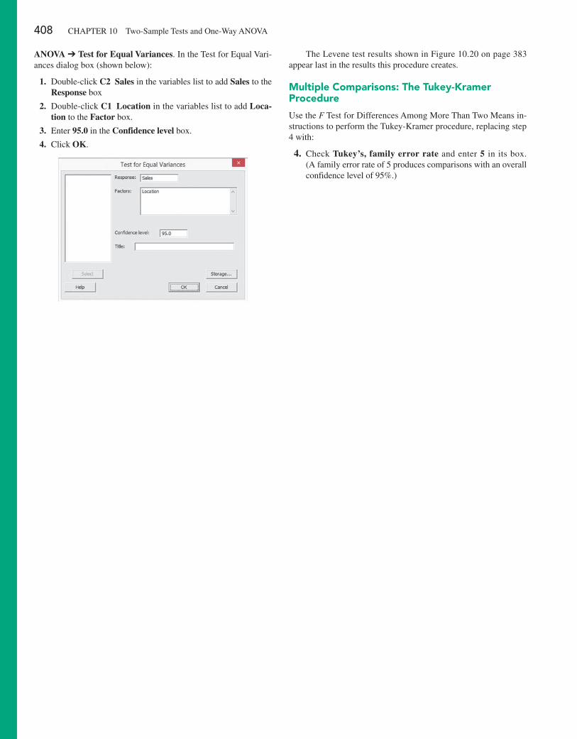
408 CHAPTeR 10 Two-Sample Tests and One-Way ANOVA
ANOVA ➔ Test for Equal Variances. In the Test for equal Vari-ances dialog box (shown below):
1. Double-click C2 Sales in the variables list to add Sales to the Response box
2. Double-click C1 Location in the variables list to add Loca-tion to the Factor box.
3. enter 95.0 in the Confidence level box.
4. Click OK.
The Levene test results shown in Figure 10.20 on page 383 appear last in the results this procedure creates.
Multiple Comparisons: The Tukey-Kramer Procedure
Use the F Test for Differences Among More Than Two Means in-structions to perform the Tukey-Kramer procedure, replacing step 4 with:
4. Check Tukey’s, family error rate and enter 5 in its box. (A family error rate of 5 produces comparisons with an overall confidence level of 95%.)
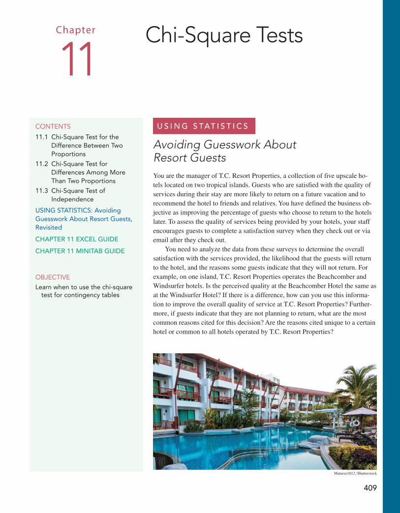
409
U s i n g s tat i s t i c s
Avoiding Guesswork About Resort GuestsYou are the manager of T.C. Resort Properties, a collection of five upscale ho-tels located on two tropical islands. Guests who are satisfied with the quality of services during their stay are more likely to return on a future vacation and to recommend the hotel to friends and relatives. You have defined the business ob-jective as improving the percentage of guests who choose to return to the hotels later. To assess the quality of services being provided by your hotels, your staff encourages guests to complete a satisfaction survey when they check out or via email after they check out.
You need to analyze the data from these surveys to determine the overall satisfaction with the services provided, the likelihood that the guests will return to the hotel, and the reasons some guests indicate that they will not return. For example, on one island, T.C. Resort Properties operates the Beachcomber and Windsurfer hotels. Is the perceived quality at the Beachcomber Hotel the same as at the Windsurfer Hotel? If there is a difference, how can you use this informa-tion to improve the overall quality of service at T.C. Resort Properties? Further-more, if guests indicate that they are not planning to return, what are the most common reasons cited for this decision? Are the reasons cited unique to a certain hotel or common to all hotels operated by T.C. Resort Properties?
contents
11.1 Chi-Square Test for the Difference Between Two Proportions
11.2 Chi-Square Test for Differences Among More Than Two Proportions
11.3 Chi-Square Test of Independence
USIng STATISTICS: Avoiding guesswork About Resort guests, Revisited
chapter 11 excel gUide
chapter 11 Minitab gUide
objectiveLearn when to use the chi-square
test for contingency tables
Chapter Chi-Square Tests
11
Maturos1812>Shutterstock
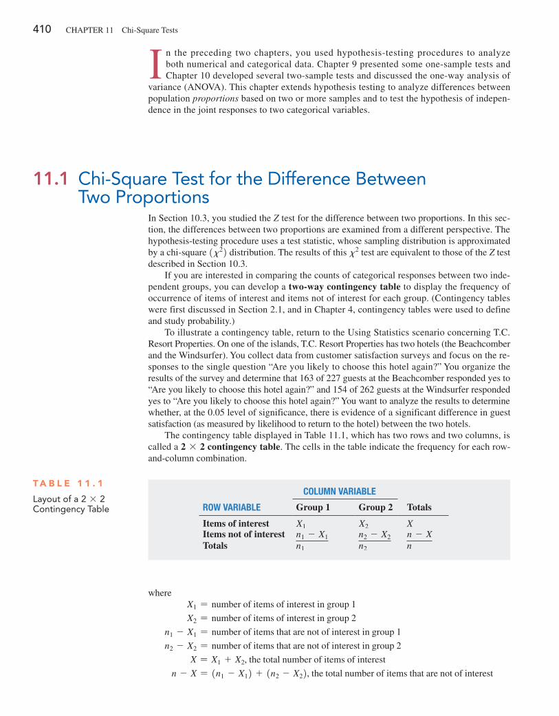
410 CHAPTeR 11 Chi-Square Tests
I n the preceding two chapters, you used hypothesis-testing procedures to analyze both numerical and categorical data. Chapter 9 presented some one-sample tests and Chapter 10 developed several two-sample tests and discussed the one-way analysis of
variance (ANOVA). This chapter extends hypothesis testing to analyze differences between population proportions based on two or more samples and to test the hypothesis of indepen-dence in the joint responses to two categorical variables.
In Section 10.3, you studied the Z test for the difference between two proportions. In this sec-tion, the differences between two proportions are examined from a different perspective. The hypothesis-testing procedure uses a test statistic, whose sampling distribution is approximated by a chi-square 1x22 distribution. The results of this x2 test are equivalent to those of the Z test described in Section 10.3.
If you are interested in comparing the counts of categorical responses between two inde-pendent groups, you can develop a two-way contingency table to display the frequency of occurrence of items of interest and items not of interest for each group. (Contingency tables were first discussed in Section 2.1, and in Chapter 4, contingency tables were used to define and study probability.)
To illustrate a contingency table, return to the Using Statistics scenario concerning T.C. Resort Properties. On one of the islands, T.C. Resort Properties has two hotels (the Beachcomber and the Windsurfer). You collect data from customer satisfaction surveys and focus on the re-sponses to the single question “Are you likely to choose this hotel again?” You organize the results of the survey and determine that 163 of 227 guests at the Beachcomber responded yes to “Are you likely to choose this hotel again?” and 154 of 262 guests at the Windsurfer responded yes to “Are you likely to choose this hotel again?” You want to analyze the results to determine whether, at the 0.05 level of significance, there is evidence of a significant difference in guest satisfaction (as measured by likelihood to return to the hotel) between the two hotels.
The contingency table displayed in Table 11.1, which has two rows and two columns, is called a 2 * 2 contingency table. The cells in the table indicate the frequency for each row-and-column combination.
11.1 Chi-Square Test for the Difference Between Two Proportions
whereX1 = number of items of interest in group 1
X2 = number of items of interest in group 2
n1 - X1 = number of items that are not of interest in group 1
n2 - X2 = number of items that are not of interest in group 2
X = X1 + X2, the total number of items of interest
n - X = 1n1 - X12 + 1n2 - X22, the total number of items that are not of interest
T a b l e 1 1 . 1
Layout of a 2 * 2 Contingency Table
Column Variable
row Variable Group 1 Group 2 Totals
Items of interest X1 X2 XItems not of interest n1 - X1 n2 - X2 n - XTotals n1 n2 n
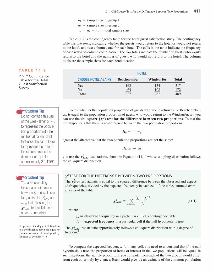
11.1 Chi-Square Test for the Difference Between Two Proportions 411
n1 = sample size in group 1
n2 = sample size in group 2n = n1 + n2 = total sample size
Table 11.2 is the contingency table for the hotel guest satisfaction study. The contingency table has two rows, indicating whether the guests would return to the hotel or would not return to the hotel, and two columns, one for each hotel. The cells in the table indicate the frequency of each row-and-column combination. The row totals indicate the number of guests who would return to the hotel and the number of guests who would not return to the hotel. The column totals are the sample sizes for each hotel location.
To test whether the population proportion of guests who would return to the Beachcomber, p1, is equal to the population proportion of guests who would return to the Windsurfer, p2, you can use the chi-square 1X2 2 test for the difference between two proportions. To test the null hypothesis that there is no difference between the two population proportions:
H0: p1 = p2
against the alternative that the two population proportions are not the same:
H1: p1 ≠ p2
you use the x2STAT test statistic, shown in equation (11.1) whose sampling distribution follows
the chi-square distribution.
T a b l e 1 1 . 2
2 * 2 Contingency Table for the Hotel guest Satisfaction Survey
Hotel
CHoose Hotel again? Beachcomber Windsurfer Total
Yes 163 154 317No 64 108 172Total 227 262 489
student tipDo not confuse this use of the Greek letter pi, p, to represent the popula-tion proportion with the mathematical constant that uses the same letter to represent the ratio of the circumference to a diameter of a circle— approximately 3.14159.
student tipYou are computing the squared difference between fo and fe. There-fore, unlike the ZSTAT and tSTAT test statistics, the x2
STAT test statistic can never be negative.
x2 TeST foR THe DIffeRenCe BeTween Two PRoPoRTIonS
The x2STAT test statistic is equal to the squared difference between the observed and expect-
ed frequencies, divided by the expected frequency in each cell of the table, summed over all cells of the table.
x2STAT = a
all cells
1fo - fe22
fe (11.1)
where
fo = observed frequency in a particular cell of a contingency table
fe = expected frequency in a particular cell if the null hypothesis is true
The x2STAT test statistic approximately follows a chi-square distribution with 1 degree of
freedom.1
1In general, the degrees of freedom in a contingency table are equal to (number of rows -1) multiplied by (number of columns -1).
To compute the expected frequency, fe, in any cell, you need to understand that if the null hypothesis is true, the proportion of items of interest in the two populations will be equal. In such situations, the sample proportions you compute from each of the two groups would differ from each other only by chance. each would provide an estimate of the common population
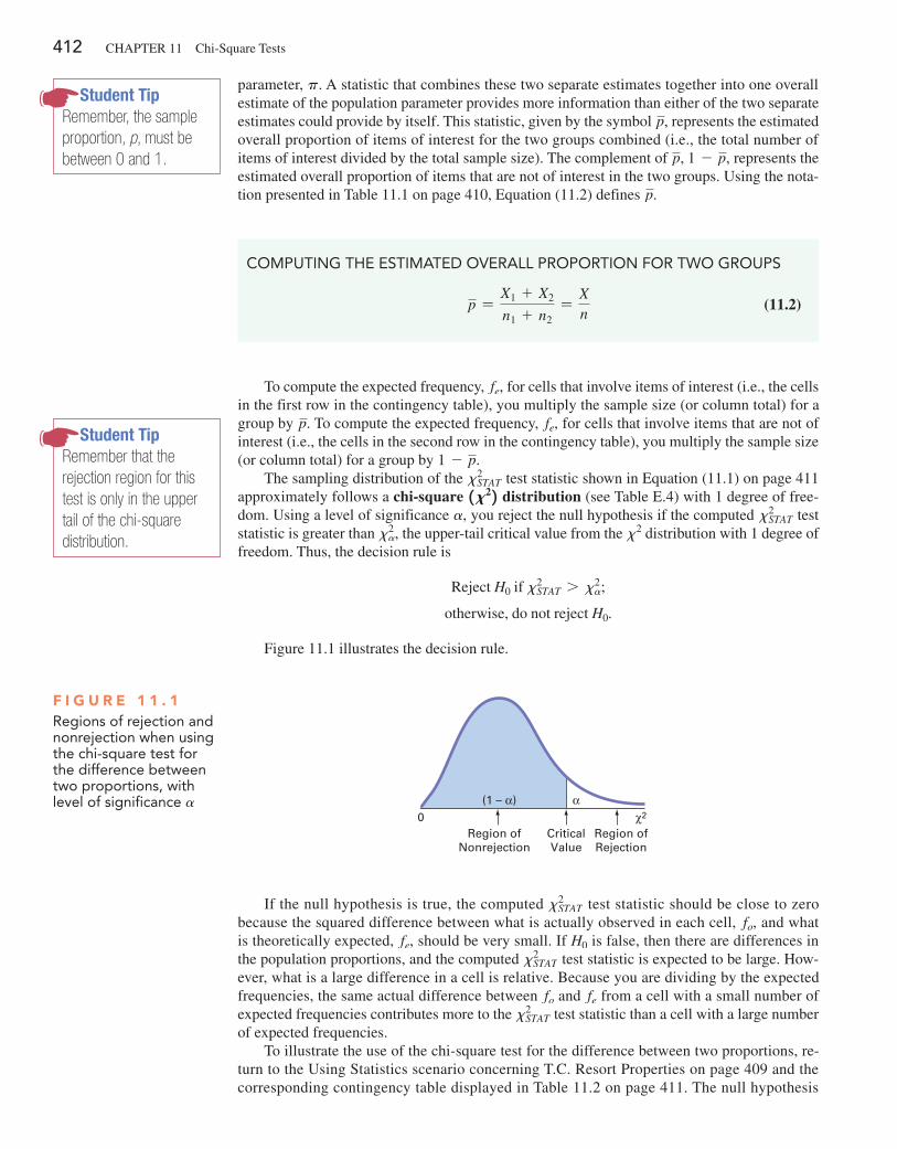
412 CHAPTeR 11 Chi-Square Tests
parameter, p. A statistic that combines these two separate estimates together into one overall estimate of the population parameter provides more information than either of the two separate estimates could provide by itself. This statistic, given by the symbol p, represents the estimated overall proportion of items of interest for the two groups combined (i.e., the total number of items of interest divided by the total sample size). The complement of p, 1 - p, represents the estimated overall proportion of items that are not of interest in the two groups. Using the nota-tion presented in Table 11.1 on page 410, equation (11.2) defines p.
student tipRemember, the sample proportion, p, must be between 0 and 1.
CoMPUTIng THe eSTIMATeD oveRALL PRoPoRTIon foR Two gRoUPS
p =X1 + X2
n1 + n2=
Xn
(11.2)
To compute the expected frequency, fe, for cells that involve items of interest (i.e., the cells in the first row in the contingency table), you multiply the sample size (or column total) for a group by p. To compute the expected frequency, fe, for cells that involve items that are not of interest (i.e., the cells in the second row in the contingency table), you multiply the sample size (or column total) for a group by 1 - p.
The sampling distribution of the x2STAT test statistic shown in equation (11.1) on page 411
approximately follows a chi-square 1X2 2 distribution (see Table e.4) with 1 degree of free-dom. Using a level of significance a, you reject the null hypothesis if the computed x2
STAT test statistic is greater than x2
a, the upper-tail critical value from the x2 distribution with 1 degree of freedom. Thus, the decision rule is
Reject H0 if x2STAT 7 x2
a;
otherwise, do not reject H0.
Figure 11.1 illustrates the decision rule.
student tipRemember that the rejection region for this test is only in the upper tail of the chi-square distribution.
F i g u r e 1 1 . 1Regions of rejection and nonrejection when using the chi-square test for the difference between two proportions, with level of significance a
0α
Region ofNonrejection
CriticalValue
Region ofRejection
(1 – α)2χ
If the null hypothesis is true, the computed x2STAT test statistic should be close to zero
because the squared difference between what is actually observed in each cell, fo, and what is theoretically expected, fe, should be very small. If H0 is false, then there are differences in the population proportions, and the computed x2
STAT test statistic is expected to be large. How-ever, what is a large difference in a cell is relative. Because you are dividing by the expected frequencies, the same actual difference between fo and fe from a cell with a small number of expected frequencies contributes more to the x2
STAT test statistic than a cell with a large number of expected frequencies.
To illustrate the use of the chi-square test for the difference between two proportions, re-turn to the Using Statistics scenario concerning T.C. Resort Properties on page 409 and the corresponding contingency table displayed in Table 11.2 on page 411. The null hypothesis
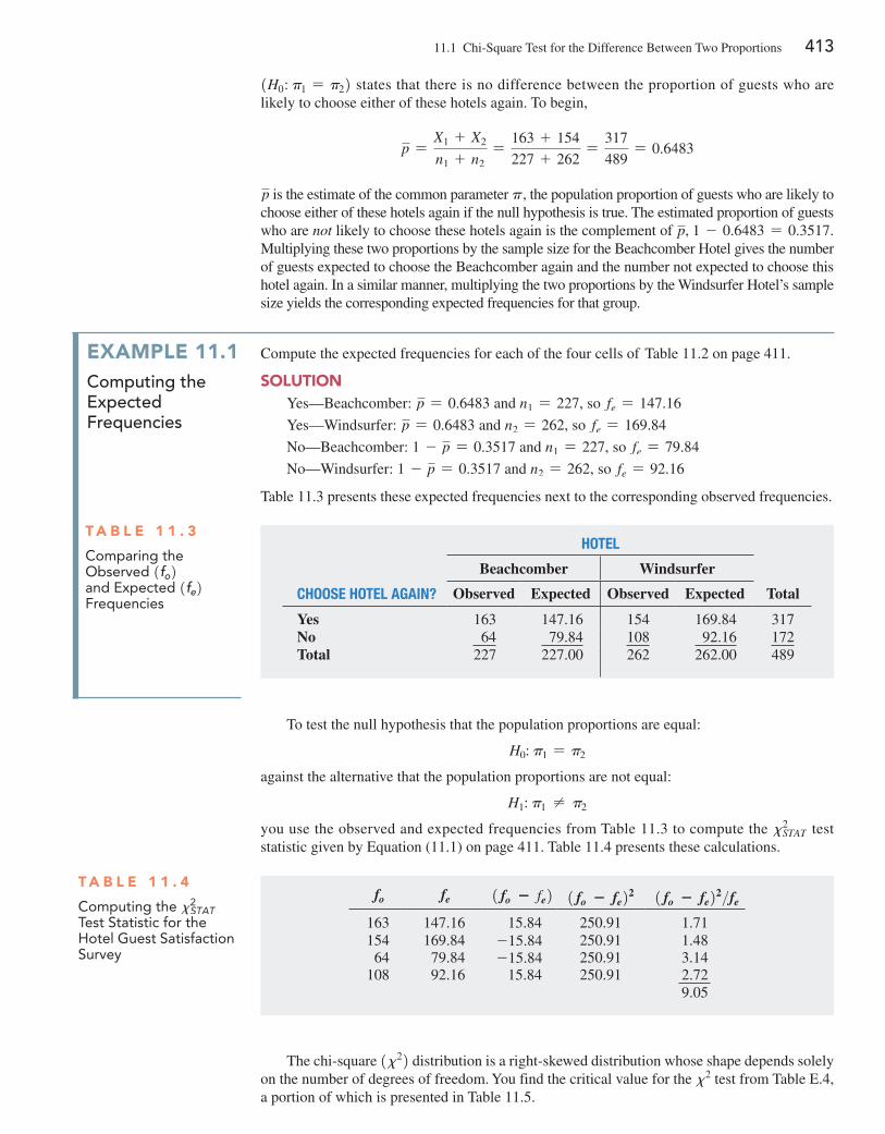
11.1 Chi-Square Test for the Difference Between Two Proportions 413
1H0: p1 = p22 states that there is no difference between the proportion of guests who are likely to choose either of these hotels again. To begin,
p =X1 + X2
n1 + n2=
163 + 154
227 + 262=
317
489= 0.6483
p is the estimate of the common parameter p, the population proportion of guests who are likely to choose either of these hotels again if the null hypothesis is true. The estimated proportion of guests who are not likely to choose these hotels again is the complement of p, 1 - 0.6483 = 0.3517. Multiplying these two proportions by the sample size for the Beachcomber Hotel gives the number of guests expected to choose the Beachcomber again and the number not expected to choose this hotel again. In a similar manner, multiplying the two proportions by the Windsurfer Hotel’s sample size yields the corresponding expected frequencies for that group.
example 11.1computing the expected Frequencies
Compute the expected frequencies for each of the four cells of Table 11.2 on page 411.
SoluTionYes—Beachcomber: p = 0.6483 and n1 = 227, so fe = 147.16
Yes—Windsurfer: p = 0.6483 and n2 = 262, so fe = 169.84
No—Beachcomber: 1 - p = 0.3517 and n1 = 227, so fe = 79.84
No—Windsurfer: 1 - p = 0.3517 and n2 = 262, so fe = 92.16
Table 11.3 presents these expected frequencies next to the corresponding observed frequencies.
T a b l e 1 1 . 3
Comparing the observed 1fo2 and expected 1fe2 frequencies
Hotel
Beachcomber Windsurfer
CHoose Hotel again? Observed Expected Observed Expected Total
Yes 163 147.16 154 169.84 317No 64 79.84 108 92.16 172Total 227 227.00 262 262.00 489
To test the null hypothesis that the population proportions are equal:
H0: p1 = p2
against the alternative that the population proportions are not equal:
H1: p1 ≠ p2
you use the observed and expected frequencies from Table 11.3 to compute the x2STAT test
statistic given by equation (11.1) on page 411. Table 11.4 presents these calculations.
T a b l e 1 1 . 4
Computing the x2STAT
Test Statistic for the Hotel guest Satisfaction Survey
fo fe 1 fo − fe2 1 fo − fe22 1 fo − fe22>fe
163 147.16 15.84 250.91 1.71154 169.84 -15.84 250.91 1.48 64 79.84 -15.84 250.91 3.14108 92.16 15.84 250.91 2.72
9.05
The chi-square 1x22 distribution is a right-skewed distribution whose shape depends solely on the number of degrees of freedom. You find the critical value for the x2 test from Table e.4, a portion of which is presented in Table 11.5.
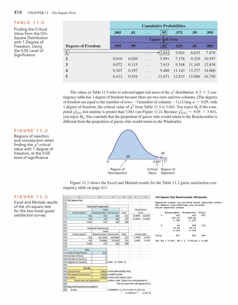
414 CHAPTeR 11 Chi-Square Tests
The values in Table 11.5 refer to selected upper-tail areas of the x2 distribution. A 2 * 2 con-tingency table has 1 degree of freedom because there are two rows and two columns. [The degrees of freedom are equal to the (number of rows -1)(number of columns -1).] Using a = 0.05, with 1 degree of freedom, the critical value of x2 from Table 11.5 is 3.841. You reject H0 if the com-puted x2
STAT test statistic is greater than 3.841 (see Figure 11.2). Because x2STAT = 9.05 7 3.841,
you reject H0. You conclude that the proportion of guests who would return to the Beachcomber is different from the proportion of guests who would return to the Windsurfer.
T a b l e 1 1 . 5
finding the Critical value from the Chi-Square Distribution with 1 Degree of freedom, Using the 0.05 Level of Significance
Cumulative Probabilities
.005 .01 c .95 .975 .99 .995
Upper-Tail Area
Degrees of Freedom .995 .99 c .05 .025 .01 .005
1 c 3.841 5.024 6.635 7.879
2 0.010 0.020 c 5.991 7.378 9.210 10.597
3 0.072 0.115 c 7.815 9.348 11.345 12.838
4 0.207 0.297 c 9.488 11.143 13.277 14.860
5 0.412 0.554 c 11.071 12.833 15.086 16.750
Region ofNonrejection
CriticalValue
Region ofRejection
0 3.841
.05.95
2χ
F i g u r e 1 1 . 2Regions of rejection and nonrejection when finding the x2 critical value with 1 degree of freedom, at the 0.05 level of significance
Figure 11.3 shows the excel and Minitab results for the Table 11.2 guest satisfaction con-tingency table on page 411.
F i g u r e 1 1 . 3excel and Minitab results of the chi-square test for the two-hotel guest satisfaction survey
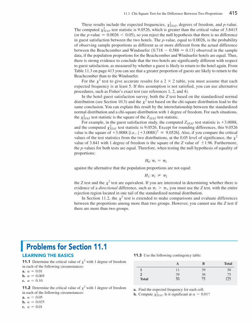
11.1 Chi-Square Test for the Difference Between Two Proportions 415
These results include the expected frequencies, x2STAT, degrees of freedom, and p-value.
The computed x2STAT test statistic is 9.0526, which is greater than the critical value of 3.8415
(or the p@value = 0.0026 6 0.05), so you reject the null hypothesis that there is no difference in guest satisfaction between the two hotels. The p-value, equal to 0.0026, is the probability of observing sample proportions as different as or more different from the actual difference between the Beachcomber and Windsurfer 10.718 - 0.588 = 0.132 observed in the sample data, if the population proportions for the Beachcomber and Windsurfer hotels are equal. Thus, there is strong evidence to conclude that the two hotels are significantly different with respect to guest satisfaction, as measured by whether a guest is likely to return to the hotel again. From Table 11.3 on page 413 you can see that a greater proportion of guests are likely to return to the Beachcomber than to the Windsurfer.
For the x2 test to give accurate results for a 2 * 2 table, you must assume that each expected frequency is at least 5. If this assumption is not satisfied, you can use alternative procedures, such as Fisher’s exact test (see references 1, 2, and 4).
In the hotel guest satisfaction survey, both the Z test based on the standardized normal distribution (see Section 10.3) and the x2 test based on the chi-square distribution lead to the same conclusion. You can explain this result by the interrelationship between the standardized normal distribution and a chi-square distribution with 1 degree of freedom. For such situations, the x2
STAT test statistic is the square of the ZSTAT test statistic. For example, in the guest satisfaction study, the computed ZSTAT test statistic is +3.0088,
and the computed x2STAT test statistic is 9.0526. except for rounding differences, this 9.0526
value is the square of +3.0088 [i.e., 1+3.008822 ≅ 9.0526]. Also, if you compare the critical values of the test statistics from the two distributions, at the 0.05 level of significance, the x2 value of 3.841 with 1 degree of freedom is the square of the Z value of {1.96. Furthermore, the p-values for both tests are equal. Therefore, when testing the null hypothesis of equality of proportions:
H0: p1 = p2
against the alternative that the population proportions are not equal:
H1: p1 ≠ p2
the Z test and the x2 test are equivalent. If you are interested in determining whether there is evidence of a directional difference, such as p1 7 p2, you must use the Z test, with the entire rejection region located in one tail of the standardized normal distribution.
In Section 11.2, the x2 test is extended to make comparisons and evaluate differences between the proportions among more than two groups. However, you cannot use the Z test if there are more than two groups.
problems for Section 11.1learning The baSicS11.1 Determine the critical value of x2 with 1 degree of freedom in each of the following circumstances:a. a = 0.01b. a = 0.005c. a = 0.10
11.2 Determine the critical value of x2 with 1 degree of freedom in each of the following circumstances:a. a = 0.05b. a = 0.025c. a = 0.01
11.3 Use the following contingency table:
A B Total
1 11 39 502 39 36 75Total 50 75 125
a. Find the expected frequency for each cell.b. Compute x2
STAT. Is it significant at a = 0.01?
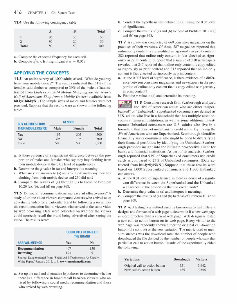
416 CHAPTeR 11 Chi-Square Tests
11.4 Use the following contingency table:
A B Total
1 20 30 502 30 20 50Total 50 50 100
a. Compute the expected frequency for each cell.b. Compute x2
STAT. Is it significant at a = 0.05?
applying The concepTS11.5 An online survey of 1,000 adults asked, “What do you buy from your mobile device?” The results indicated that 61% of the females said clothes as compared to 39% of the males. (Data ex-tracted from Ebates.com 2014 Mobile Shopping Survey: Nearly Half of Americans Shop from a Mobile Device, available from bit.ly/1hi6kyX.) The sample sizes of males and females were not provided. Suppose that the results were as shown in the following table:
buY ClotHes From tHeir mobile DeViCe
genDer
Male Female Total
Yes 195 305 500No 305 195 500Total 500 500 1,000
a. Is there evidence of a significant difference between the pro-portion of males and females who say they buy clothing from their mobile device at the 0.01 level of significance?
b. Determine the p-value in (a) and interpret its meaning.c. What are your answers to (a) and (b) if 270 males say they buy
clothing from their mobile device and 230 did not?d. Compare the results of (a) through (c) to those of Problem
10.29 (a), (b), and (d) on page 368.
11.6 Do social recommendations increase ad effectiveness? A study of online video viewers compared viewers who arrived at an advertising video for a particular brand by following a social me-dia recommendation link to viewers who arrived at the same video by web browsing. Data were collected on whether the viewer could correctly recall the brand being advertised after seeing the video. The results were:
CorreCtlY reCalleD tHe branD
arriVal metHoD Yes No
Recommendation 407 150Browsing 193 91Source: Data extracted from “Social Ad effectiveness: An Unruly White Paper,” January 2012, p. 3, www.unrulymedia.com.
a. Set up the null and alternative hypotheses to determine whether there is a difference in brand recall between viewers who ar-rived by following a social media recommendation and those who arrived by web browsing.
b. Conduct the hypothesis test defined in (a), using the 0.05 level of significance.
c. Compare the results of (a) and (b) to those of Problem 10.30 (a) and (b) on page 368.
11.7 A survey was conducted of 660 consumer magazines on the practices of their websites. Of these, 287 magazines reported that online-only content is copy-edited as rigorously as print content; 383 reported that online-only content is fact-checked as rigor-ously as print content. Suppose that a sample of 510 newspapers revealed that 247 reported that online-only content is copy-edited as rigorously as print content and 313 reported that online-only content is fact-checked as rigorously as print content.a. At the 0.005 level of significance, is there evidence of a differ-
ence between consumer magazines and newspapers in the pro-portion of online-only content that is copy-edited as rigorously as print content?
b. Find the p-value in (a) and determine its meaning.
SELF Test
11.8 Consumer research firm Scarborough analyzed the 10% of American adults who are either “Super-
banked” or “Unbanked.” Superbanked consumers are defined as U.S. adults who live in a household that has multiple asset ac-counts at financial institutions, as well as some additional invest-ments; Unbanked consumers are U.S. adults who live in a household that does not use a bank or credit union. By finding the 5% of Americans who are Superbanked, Scarborough identifies financially savvy consumers who might be open to diversifying their financial portfolios; by identifying the Unbanked, Scarbor-ough provides insight into the ultimate prospective client for banks and financial institutions. As part of its analysis, Scarbor-ough reported that 93% of Superbanked consumers use credit cards as compared to 23% of Unbanked consumers. (Data ex-tracted from bit.ly/Syi9kN.) Suppose that these results were based on 1,000 Superbanked consumers and 1,000 Unbanked consumers.a. At the 0.01 level of significance, is there evidence of a signifi-
cant difference between the Superbanked and the Unbanked with respect to the proportion that use credit cards?
b. Determine the p-value in (a) and interpret is meaning.c. Compare the results of (a) and (b) to those of Problem 10.32 on
page 369.
11.9 A/B testing is a method used by businesses to test different designs and formats of a web page to determine if a new web page is more effective than a current web page. Web designers tested a new call-to-action button on its web page. every visitor to the web page was randomly shown either the original call-to-action button (the control) or the new variation. The metric used to mea-sure success was the download rate: the number of people who downloaded the file divided by the number of people who saw that particular call-to-action button. Results of the experiment yielded the following:
Variations Downloads Visitors
Original call-to-action button 351 3,642New call-to-action button 485 3,556
11.2 Chi-Square Test for Differences Among More Than Two Proportions 417
a. At the 0.05 level of significance, is there evidence of a differ-ence in the download rate between the original call-to-action button and the new call-to-action button?
b. Find the p-value in (a) and interpret its value.c. Compare the results of (a) and (b) to those of Problem 10.31 on
page 369.
11.10 Does co-browsing have positive effects on the customer experience? Co-browsing refers to the ability to have a contact center agent and customer jointly navigate an application (e.g., web page, digital document, or mobile application) on a real time basis through the web. A study of businesses indicates that 81 of 129 co-browsing organizations use skills-based routing to match
the caller with the right agent, whereas 65 of 176 non-co-browsing organizations use skills-based routing to match the caller with the right agent. (Source: Cobrowsing Presents a “Lucrative” Cus-tomer Service Opportunity, available at bit.ly/1wwALWr.)a. Construct a 2 * 2 contingency table.b. At the 0.05 level of significance, is there evidence of a differ-
ence between co-browsing organizations and non-co-browsing organizations in the proportion that use skills-based routing to match the caller with the right agent?
c. Find the p-value in (a) and interpret its meaning.d. Compare the results of (a) and (b) to those of Problem 10.34 on
page 369.
11.2 Chi-Square Test for Differences Among More Than Two Proportions
In this section, the x2 test is extended to compare more than two independent populations. The letter c is used to represent the number of independent populations under consideration. Thus, the contingency table now has two rows and c columns. To test the null hypothesis that there are no differences among the c population proportions:
H0: p1 = p2 = g = pc
against the alternative that not all the c population proportions are equal:
H1: Not all pj are equal 1where j = 1, 2, c, c2you use equation (11.1) on page 411:
x2STAT = a
all cells
1 fo - fe22
fe
where
fo = observed frequency in a particular cell of a 2 * c contingency table
fe = expected frequency in a particular cell if the null hypothesis is true
If the null hypothesis is true and the proportions are equal across all c populations, the c sample proportions should differ only by chance. In such a situation, a statistic that combines these c separate estimates into one overall estimate of the population proportion, p, provides more information than any one of the c separate estimates alone. To expand on equation (11.2) on page 412, the statistic p in equation (11.3) represents the estimated overall proportion for all c groups combined.
CoMPUTIng THe eSTIMATeD oveRALL PRoPoRTIon foR c gRoUPS
p =X1 + X2 + g + Xc
n1 + n2 + g + nc=
Xn
(11.3)
To compute the expected frequency, fe, for each cell in the first row in the contingency table, multiply each sample size (or column total) by p. To compute the expected frequency, fe, for each cell in the second row in the contingency table, multiply each sample size (or column total) by 11 - p2. The sampling distribution of the test statistic shown in equation (11.1) on page 411 approximately follows a chi-square distribution, with degrees of freedom equal to the number of rows in the contingency table minus 1, multiplied by the number of columns in the table minus 1. For a 2 : c contingency table, there are c - 1 degrees of freedom:
Degrees of freedom = 12 - 121c - 12 = c - 1
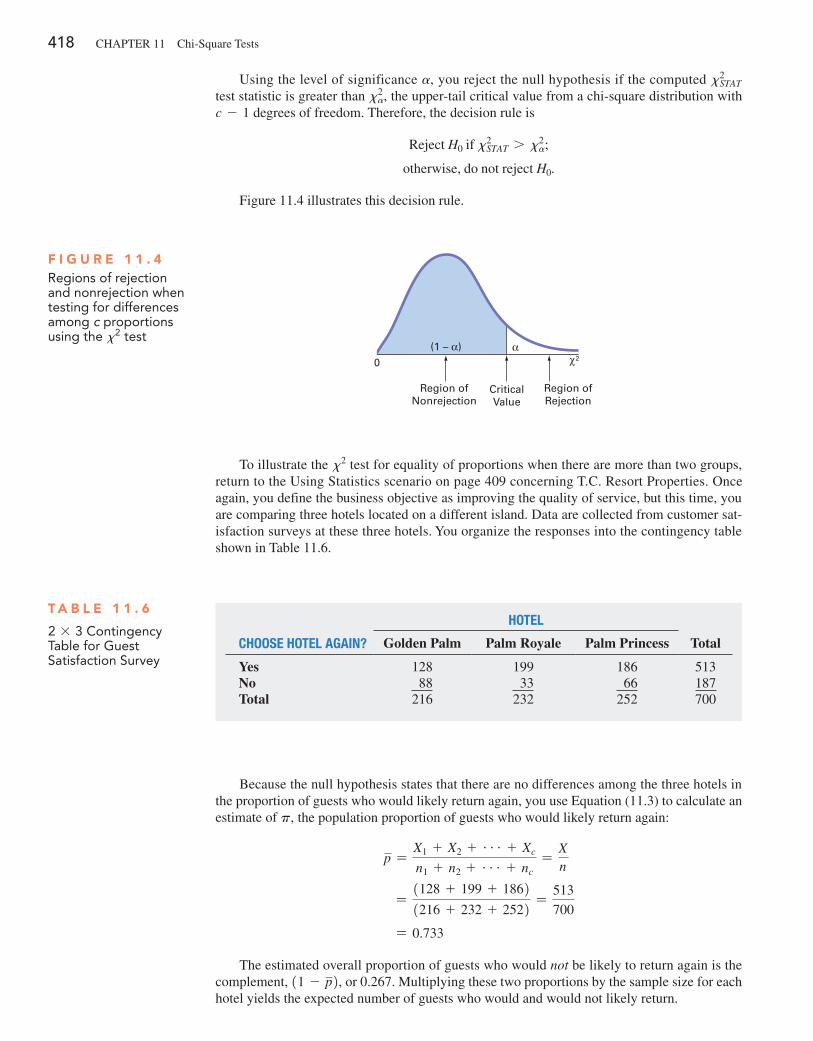
418 CHAPTeR 11 Chi-Square Tests
Using the level of significance a, you reject the null hypothesis if the computed x2STAT
test statistic is greater than x2a, the upper-tail critical value from a chi-square distribution with
c - 1 degrees of freedom. Therefore, the decision rule is
Reject H0 if x2STAT 7 x2
a;
otherwise, do not reject H0.
Figure 11.4 illustrates this decision rule.
F i g u r e 1 1 . 4Regions of rejection and nonrejection when testing for differences among c proportions using the x2 test
0α
Region ofNonrejection
CriticalValue
Region ofRejection
2χ(1 – α)
To illustrate the x2 test for equality of proportions when there are more than two groups, return to the Using Statistics scenario on page 409 concerning T.C. Resort Properties. Once again, you define the business objective as improving the quality of service, but this time, you are comparing three hotels located on a different island. Data are collected from customer sat-isfaction surveys at these three hotels. You organize the responses into the contingency table shown in Table 11.6.
Because the null hypothesis states that there are no differences among the three hotels in the proportion of guests who would likely return again, you use equation (11.3) to calculate an estimate of p, the population proportion of guests who would likely return again:
p =X1 + X2 + g + Xc
n1 + n2 + g + nc=
Xn
=1128 + 199 + 18621216 + 232 + 2522 =
513
700
= 0.733
The estimated overall proportion of guests who would not be likely to return again is the complement, 11 - p2, or 0.267. Multiplying these two proportions by the sample size for each hotel yields the expected number of guests who would and would not likely return.
T a b l e 1 1 . 6
2 * 3 Contingency Table for guest Satisfaction Survey
Hotel
CHoose Hotel again? Golden Palm Palm Royale Palm Princess Total
Yes 128 199 186 513No 88 33 66 187Total 216 232 252 700
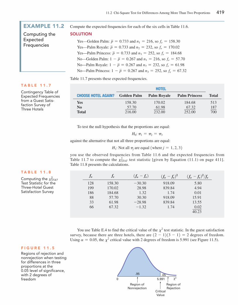
11.2 Chi-Square Test for Differences Among More Than Two Proportions 419
Table 11.7 presents these expected frequencies.
example 11.2computing the expected Frequencies
Compute the expected frequencies for each of the six cells in Table 11.6.
SoluTion
Yes—Golden Palm: p = 0.733 and n1 = 216, so fe = 158.30
Yes—Palm Royale: p = 0.733 and n2 = 232, so fe = 170.02
Yes—Palm Princess: p = 0.733 and n3 = 252, so fe = 184.68
No—Golden Palm: 1 - p = 0.267 and n1 = 216, so fe = 57.70
No—Palm Royale: 1 - p = 0.267 and n2 = 232, so fe = 61.98
No—Palm Princess: 1 - p = 0.267 and n3 = 252, so fe = 67.32
T a b l e 1 1 . 7
Contingency Table of expected frequencies from a guest Satis-faction Survey of Three Hotels
Hotel
CHoose Hotel again? Golden Palm Palm Royale Palm Princess Total
Yes 158.30 170.02 184.68 513No 57.70 61.98 67.32 187Total 216.00 232.00 252.00 700
To test the null hypothesis that the proportions are equal:
H0: p1 = p2 = p3
against the alternative that not all three proportions are equal:
H1: Not all pj are equal 1where j = 1, 2, 32you use the observed frequencies from Table 11.6 and the expected frequencies from Table 11.7 to compute the x2
STAT test statistic [given by equation (11.1) on page 411]. Table 11.8 presents the calculations.
T a b l e 1 1 . 8
Computing the x2STAT
Test Statistic for the Three-Hotel guest Satisfaction Survey
fo fe 1fo - fe2 1fo - fe22 1fo - fe22>fe
128 158.30 -30.30 918.09 5.80199 170.02 28.98 839.84 4.94186 184.68 1.32 1.74 0.0188 57.70 30.30 918.09 15.9133 61.98 -28.98 839.84 13.5566 67.32 -1.32 1.74 0.02
40.23
You use Table e.4 to find the critical value of the x2 test statistic. In the guest satisfaction survey, because there are three hotels, there are 12 - 1213 - 12 = 2 degrees of freedom. Using a = 0.05, the x2 critical value with 2 degrees of freedom is 5.991 (see Figure 11.5).
0 5.991
Region ofNonrejection
CriticalValue
Region ofRejection
.05.95χ2
F i g u r e 1 1 . 5Regions of rejection and nonrejection when testing for differences in three proportions at the 0.05 level of significance, with 2 degrees of freedom
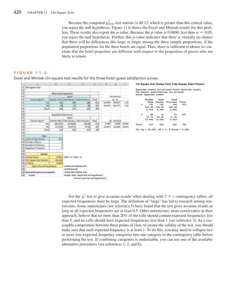
420 CHAPTeR 11 Chi-Square Tests
Because the computed x2STAT test statistic is 40.23, which is greater than this critical value,
you reject the null hypothesis. Figure 11.6 shows the excel and Minitab results for this prob-lem. These results also report the p-value. Because the p-value is 0.0000, less than a = 0.05, you reject the null hypothesis. Further, this p-value indicates that there is virtually no chance that there will be differences this large or larger among the three sample proportions, if the population proportions for the three hotels are equal. Thus, there is sufficient evidence to con-clude that the hotel properties are different with respect to the proportion of guests who are likely to return.
For the x2 test to give accurate results when dealing with 2 * c contingency tables, all expected frequencies must be large. The definition of “large” has led to research among stat-isticians. Some statisticians (see reference 5) have found that the test gives accurate results as long as all expected frequencies are at least 0.5. Other statisticians, more conservative in their approach, believe that no more than 20% of the cells should contain expected frequencies less than 5, and no cells should have expected frequencies less than 1 (see reference 3). As a rea-sonable compromise between these points of view, to ensure the validity of the test, you should make sure that each expected frequency is at least 1. To do this, you may need to collapse two or more low-expected-frequency categories into one category in the contingency table before performing the test. If combining categories is undesirable, you can use one of the available alternative procedures (see references 1, 2, and 6).
F i g u r e 1 1 . 6excel and Minitab chi-square test results for the three-hotel guest satisfaction survey
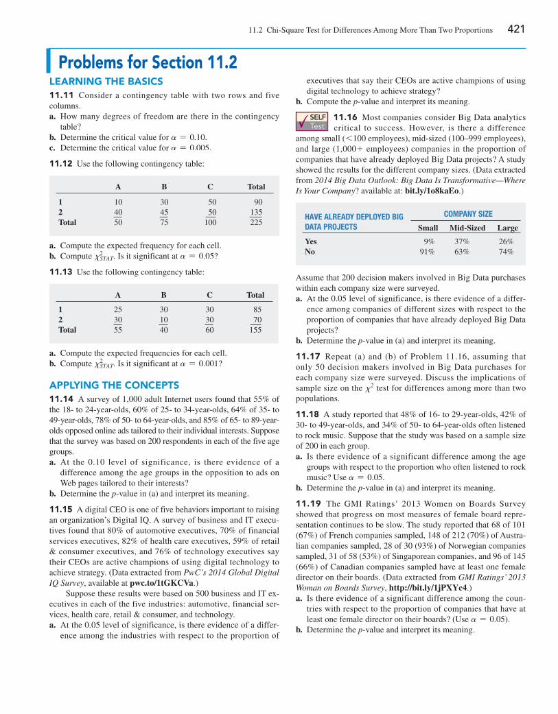
11.2 Chi-Square Test for Differences Among More Than Two Proportions 421
problems for Section 11.2
learning The baSicS11.11 Consider a contingency table with two rows and five columns.a. How many degrees of freedom are there in the contingency
table?b. Determine the critical value for a = 0.10.c. Determine the critical value for a = 0.005.
11.12 Use the following contingency table:
A B C Total
1 10 30 50 902 40 45 50 135Total 50 75 100 225
a. Compute the expected frequency for each cell.b. Compute x2
STAT. Is it significant at a = 0.05?
11.13 Use the following contingency table:
A B C Total
1 25 30 30 852 30 10 30 70Total 55 40 60 155
a. Compute the expected frequencies for each cell.b. Compute x2
STAT. Is it significant at a = 0.001?
applying The concepTS11.14 A survey of 1,000 adult Internet users found that 55% of the 18- to 24-year-olds, 60% of 25- to 34-year-olds, 64% of 35- to 49-year-olds, 78% of 50- to 64-year-olds, and 85% of 65- to 89-year-olds opposed online ads tailored to their individual interests. Suppose that the survey was based on 200 respondents in each of the five age groups.a. At the 0.10 level of significance, is there evidence of a
difference among the age groups in the opposition to ads on Web pages tailored to their interests?
b. Determine the p-value in (a) and interpret its meaning.
11.15 A digital CeO is one of five behaviors important to raising an organization’s Digital IQ. A survey of business and IT execu-tives found that 80% of automotive executives, 70% of financial services executives, 82% of health care executives, 59% of retail & consumer executives, and 76% of technology executives say their CeOs are active champions of using digital technology to achieve strategy. (Data extracted from PwC’s 2014 Global Digital IQ Survey, available at pwc.to/1tGKCVa.)
Suppose these results were based on 500 business and IT ex-ecutives in each of the five industries: automotive, financial ser-vices, health care, retail & consumer, and technology.a. At the 0.05 level of significance, is there evidence of a differ-
ence among the industries with respect to the proportion of
executives that say their CeOs are active champions of using digital technology to achieve strategy?
b. Compute the p-value and interpret its meaning.
SELF Test
11.16 Most companies consider Big Data analytics critical to success. However, is there a difference
among small (6100 employees), mid-sized (100–999 employees), and large (1,000 + employees) companies in the proportion of companies that have already deployed Big Data projects? A study showed the results for the different company sizes. (Data extracted from 2014 Big Data Outlook: Big Data Is Transformative—Where Is Your Company? available at: bit.ly/1o8kaEo.)
HaVe alreaDY DePloYeD big Data ProJeCts
ComPanY siZe
Small Mid-Sized Large
Yes 9% 37% 26%No 91% 63% 74%
Assume that 200 decision makers involved in Big Data purchases within each company size were surveyed.a. At the 0.05 level of significance, is there evidence of a differ-
ence among companies of different sizes with respect to the proportion of companies that have already deployed Big Data projects?
b. Determine the p-value in (a) and interpret its meaning.
11.17 Repeat (a) and (b) of Problem 11.16, assuming that only 50 decision makers involved in Big Data purchases for each company size were surveyed. Discuss the implications of sample size on the x2 test for differences among more than two populations.
11.18 A study reported that 48% of 16- to 29-year-olds, 42% of 30- to 49-year-olds, and 34% of 50- to 64-year-olds often listened to rock music. Suppose that the study was based on a sample size of 200 in each group.a. Is there evidence of a significant difference among the age
groups with respect to the proportion who often listened to rock music? Use a = 0.05.
b. Determine the p-value in (a) and interpret its meaning.
11.19 The GMI Ratings’ 2013 Women on Boards Survey showed that progress on most measures of female board repre-sentation continues to be slow. The study reported that 68 of 101 (67%) of French companies sampled, 148 of 212 (70%) of Austra-lian companies sampled, 28 of 30 (93%) of Norwegian companies sampled, 31 of 58 (53%) of Singaporean companies, and 96 of 145 (66%) of Canadian companies sampled have at least one female director on their boards. (Data extracted from GMI Ratings’ 2013 Woman on Boards Survey, http://bit.ly/1jPXYc4.)a. Is there evidence of a significant difference among the coun-
tries with respect to the proportion of companies that have at least one female director on their boards? (Use a = 0.05).
b. Determine the p-value and interpret its meaning.
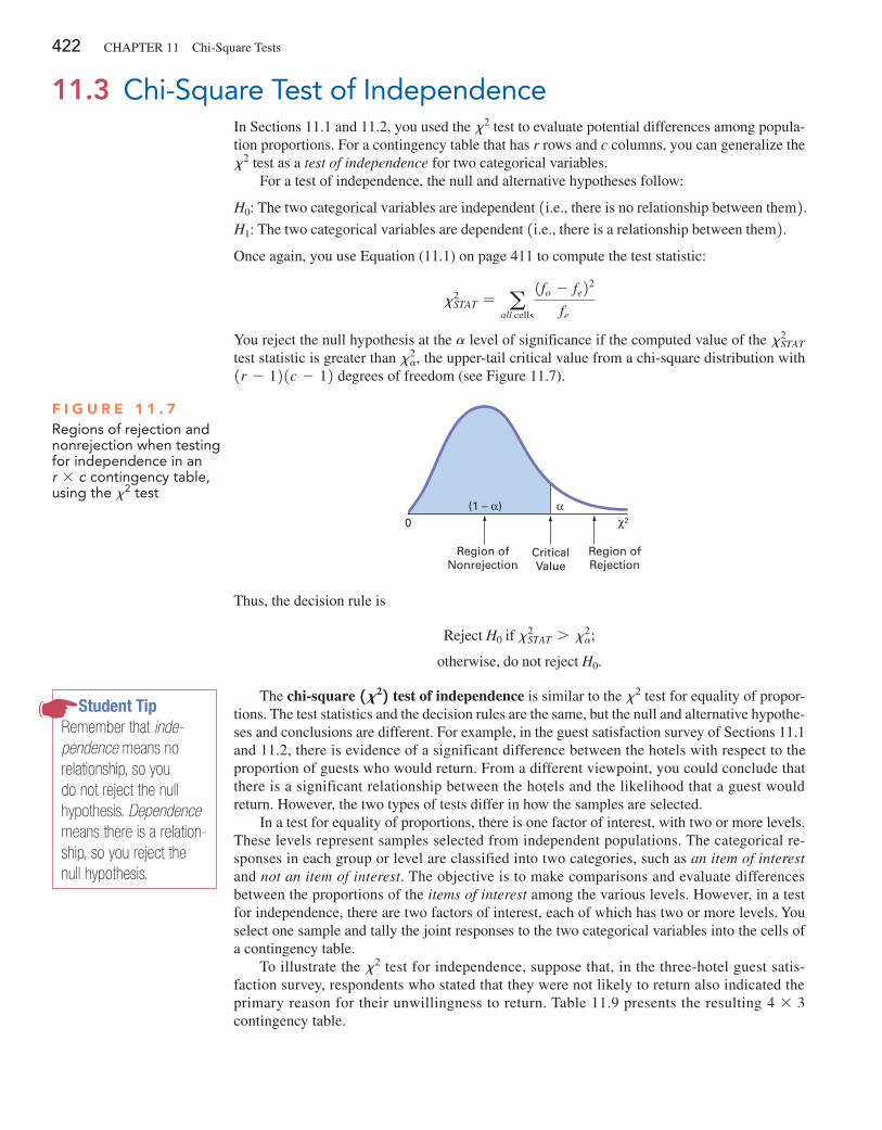
422 CHAPTeR 11 Chi-Square Tests
11.3 Chi-Square Test of IndependenceIn Sections 11.1 and 11.2, you used the x2 test to evaluate potential differences among popula-tion proportions. For a contingency table that has r rows and c columns, you can generalize the x2 test as a test of independence for two categorical variables.
For a test of independence, the null and alternative hypotheses follow:
H0: The two categorical variables are independent 1i.e., there is no relationship between them2.
H1: The two categorical variables are dependent 1i.e., there is a relationship between them2.
Once again, you use equation (11.1) on page 411 to compute the test statistic:
x2STAT = a
all cells
1fo - fe22
fe
You reject the null hypothesis at the a level of significance if the computed value of the x2STAT
test statistic is greater than x2a, the upper-tail critical value from a chi-square distribution with
1r - 121c - 12 degrees of freedom (see Figure 11.7).
0α
Region ofNonrejection
CriticalValue
Region ofRejection
χ2
(1 – α)
F i g u r e 1 1 . 7Regions of rejection and nonrejection when testing for independence in an r * c contingency table, using the x2 test
Thus, the decision rule is
Reject H0 if x2STAT 7 x2
a;
otherwise, do not reject H0.
The chi-square 1X2 2 test of independence is similar to the x2 test for equality of propor-tions. The test statistics and the decision rules are the same, but the null and alternative hypothe-ses and conclusions are different. For example, in the guest satisfaction survey of Sections 11.1 and 11.2, there is evidence of a significant difference between the hotels with respect to the proportion of guests who would return. From a different viewpoint, you could conclude that there is a significant relationship between the hotels and the likelihood that a guest would return. However, the two types of tests differ in how the samples are selected.
In a test for equality of proportions, there is one factor of interest, with two or more levels. These levels represent samples selected from independent populations. The categorical re-sponses in each group or level are classified into two categories, such as an item of interest and not an item of interest. The objective is to make comparisons and evaluate differences between the proportions of the items of interest among the various levels. However, in a test for independence, there are two factors of interest, each of which has two or more levels. You select one sample and tally the joint responses to the two categorical variables into the cells of a contingency table.
To illustrate the x2 test for independence, suppose that, in the three-hotel guest satis-faction survey, respondents who stated that they were not likely to return also indicated the primary reason for their unwillingness to return. Table 11.9 presents the resulting 4 * 3 contingency table.
student tipRemember that inde-pendence means no relationship, so you do not reject the null hypothesis. Dependence means there is a relation-ship, so you reject the null hypothesis.
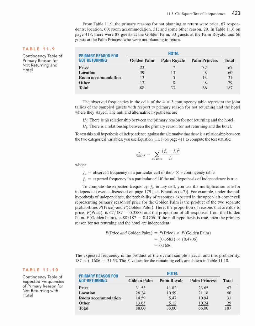
11.3 Chi-Square Test of Independence 423
From Table 11.9, the primary reasons for not planning to return were price, 67 respon-dents; location, 60; room accommodation, 31; and some other reason, 29. In Table 11.6 on page 418, there were 88 guests at the Golden Palm, 33 guests at the Palm Royale, and 66 guests at the Palm Princess who were not planning to return.
T a b l e 1 1 . 9
Contingency Table of Primary Reason for not Returning and Hotel
PrimarY reason For not returning
Hotel
Golden Palm Palm Royale Palm Princess Total
Price 23 7 37 67Location 39 13 8 60Room accommodation 13 5 13 31Other 13 8 8 29Total 88 33 66 187
The observed frequencies in the cells of the 4 * 3 contingency table represent the joint tallies of the sampled guests with respect to primary reason for not returning and the hotel where they stayed. The null and alternative hypotheses are
H0: There is no relationship between the primary reason for not returning and the hotel.
H1: There is a relationship between the primary reason for not returning and the hotel.
To test this null hypothesis of independence against the alternative that there is a relationship between the two categorical variables, you use equation (11.1) on page 411 to compute the test statistic:
x2STAT = a
all cells
1 fo - fe22
fe
where
fo = observed frequency in a particular cell of the r * c contingency table
fe = expected frequency in a particular cell if the null hypothesis of independence is true
To compute the expected frequency, fe, in any cell, you use the multiplication rule for independent events discussed on page 179 [see equation (4.7)]. For example, under the null hypothesis of independence, the probability of responses expected in the upper-left-corner cell representing primary reason of price for the Golden Palm is the product of the two separate probabilities P1Price2 and P1Golden Palm2. Here, the proportion of reasons that are due to price, P1Price2, is 67>187 = 0.3583, and the proportion of all responses from the Golden Palm, P1Golden Palm2, is 88>187 = 0.4706. If the null hypothesis is true, then the primary reason for not returning and the hotel are independent:
P1Price and Golden Palm2 = P1Price2 * P1Golden Palm2 = 10.35832 * 10.47062 = 0.1686
The expected frequency is the product of the overall sample size, n, and this probability, 187 * 0.1686 = 31.53. The fe values for the remaining cells are shown in Table 11.10.
T a b l e 1 1 . 1 0
Contingency Table of expected frequencies of Primary Reason for not Returning with Hotel
PrimarY reason For not returning
Hotel
Golden Palm Palm Royale Palm Princess Total
Price 31.53 11.82 23.65 67Location 28.24 10.59 21.18 60Room accommodation 14.59 5.47 10.94 31Other 13.65 5.12 10.24 29Total 88.00 33.00 66.00 187
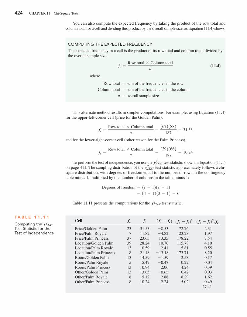
424 CHAPTeR 11 Chi-Square Tests
You can also compute the expected frequency by taking the product of the row total and column total for a cell and dividing this product by the overall sample size, as equation (11.4) shows.
This alternate method results in simpler computations. For example, using equation (11.4) for the upper-left-corner cell (price for the Golden Palm),
fe =Row total * Column total
n=
16721882187
= 31.53
and for the lower-right-corner cell (other reason for the Palm Princess),
fe =Row total * Column total
n=
12921662187
= 10.24
To perform the test of independence, you use the x2STAT test statistic shown in equation (11.1)
on page 411. The sampling distribution of the x2STAT test statistic approximately follows a chi-
square distribution, with degrees of freedom equal to the number of rows in the contingency table minus 1, multiplied by the number of columns in the table minus 1:
Degrees of freedom = 1r - 121c - 12 = 14 - 1213 - 12 = 6
Table 11.11 presents the computations for the x2STAT test statistic.
CoMPUTIng THe exPeCTeD fReqUenCy
The expected frequency in a cell is the product of its row total and column total, divided by the overall sample size.
fe =Row total * Column total
n (11.4)
where
Row total = sum of the frequencies in the row
Column total = sum of the frequencies in the column
n = overall sample size
T a b l e 1 1 . 1 1
Computing the x2STAT
Test Statistic for the Test of Independence
Cell fo fe 1fo - fe2 1fo - fe22 1fo - fe22>fe
Price/Golden Palm 23 31.53 -8.53 72.76 2.31Price/Palm Royale 7 11.82 -4.82 23.23 1.97Price/Palm Princess 37 23.65 13.35 178.22 7.54Location/Golden Palm 39 28.24 10.76 115.78 4.10Location/Palm Royale 13 10.59 2.41 5.81 0.55Location/Palm Princess 8 21.18 -13.18 173.71 8.20Room/Golden Palm 13 14.59 -1.59 2.53 0.17Room/Palm Royale 5 5.47 -0.47 0.22 0.04Room/Palm Princess 13 10.94 2.06 4.24 0.39Other/Golden Palm 13 13.65 -0.65 0.42 0.03Other/Palm Royale 8 5.12 2.88 8.29 1.62Other/Palm Princess 8 10.24 -2.24 5.02 0.49
27.41
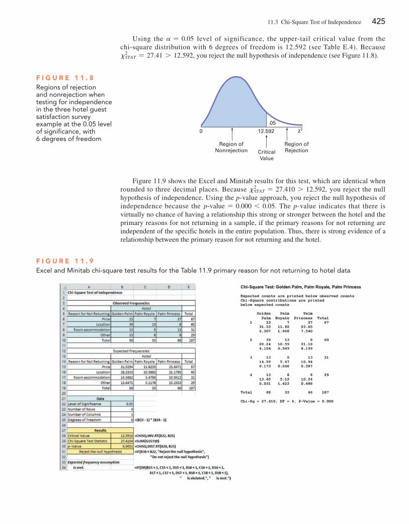
11.3 Chi-Square Test of Independence 425
Using the a = 0.05 level of significance, the upper-tail critical value from the chi-square distribution with 6 degrees of freedom is 12.592 (see Table e.4). Because x2
STAT = 27.41 7 12.592, you reject the null hypothesis of independence (see Figure 11.8).
Figure 11.9 shows the excel and Minitab results for this test, which are identical when rounded to three decimal places. Because x2
STAT = 27.410 7 12.592, you reject the null hypothesis of independence. Using the p-value approach, you reject the null hypothesis of independence because the p@value = 0.000 6 0.05. The p-value indicates that there is virtually no chance of having a relationship this strong or stronger between the hotel and the primary reasons for not returning in a sample, if the primary reasons for not returning are independent of the specific hotels in the entire population. Thus, there is strong evidence of a relationship between the primary reason for not returning and the hotel.
F i g u r e 1 1 . 8Regions of rejection and nonrejection when testing for independence in the three hotel guest satisfaction survey example at the 0.05 level of significance, with 6 degrees of freedom
0
Region ofNonrejection Critical
Value
Region ofRejection
χ2
.05
12.592
F i g u r e 1 1 . 9excel and Minitab chi-square test results for the Table 11.9 primary reason for not returning to hotel data
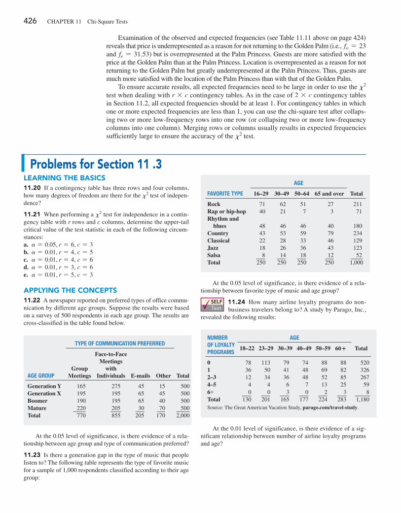
426 CHAPTeR 11 Chi-Square Tests
examination of the observed and expected frequencies (see Table 11.11 above on page 424) reveals that price is underrepresented as a reason for not returning to the Golden Palm (i.e., fo = 23 and fe = 31.53) but is overrepresented at the Palm Princess. Guests are more satisfied with the price at the Golden Palm than at the Palm Princess. Location is overrepresented as a reason for not returning to the Golden Palm but greatly underrepresented at the Palm Princess. Thus, guests are much more satisfied with the location of the Palm Princess than with that of the Golden Palm.
To ensure accurate results, all expected frequencies need to be large in order to use the x2 test when dealing with r * c contingency tables. As in the case of 2 * c contingency tables in Section 11.2, all expected frequencies should be at least 1. For contingency tables in which one or more expected frequencies are less than 1, you can use the chi-square test after collaps-ing two or more low-frequency rows into one row (or collapsing two or more low-frequency columns into one column). Merging rows or columns usually results in expected frequencies sufficiently large to ensure the accuracy of the x2 test.
problems for Section 11 .3learning The baSicS11.20 If a contingency table has three rows and four columns, how many degrees of freedom are there for the x2 test of indepen-dence?
11.21 When performing a x2 test for independence in a contin-gency table with r rows and c columns, determine the upper-tail critical value of the test statistic in each of the following circum-stances:a. a = 0.05, r = 6, c = 3b. a = 0.01, r = 4, c = 5c. a = 0.01, r = 4, c = 6d. a = 0.01, r = 3, c = 6e. a = 0.01, r = 5, c = 3
applying The concepTS11.22 A newspaper reported on preferred types of office commu-nication by different age groups. Suppose the results were based on a survey of 500 respondents in each age group. The results are cross-classified in the table found below.
age grouP
tYPe oF CommuniCation PreFerreD
Group Meetings
Face-to-Face Meetings
with Individuals
E-mails
Other
Total
Generation Y 165 275 45 15 500Generation X 195 195 65 45 500Boomer 190 195 65 40 500Mature 220 205 30 70 500Total 770 855 205 170 2,000
At the 0.05 level of significance, is there evidence of a rela-tionship between age group and type of communication preferred?
11.23 Is there a generation gap in the type of music that people listen to? The following table represents the type of favorite music for a sample of 1,000 respondents classified according to their age group:
FaVorite tYPe
age
16–29 30–49 50–64 65 and over Total
Rock 71 62 51 27 211Rap or hip-hop 40 21 7 3 71Rhythm and blues 48 46 46 40 180Country 43 53 59 79 234Classical 22 28 33 46 129Jazz 18 26 36 43 123Salsa 8 14 18 12 52Total 250 250 250 250 1,000
At the 0.05 level of significance, is there evidence of a rela-tionship between favorite type of music and age group?
SELF Test
11.24 How many airline loyalty programs do non-business travelers belong to? A study by Parago, Inc.,
revealed the following results:
number oF loYaltY Programs
age
18–22 23–29 30–39 40–49 50–59 60+ Total
0 78 113 79 74 88 88 5201 36 50 41 48 69 82 3262–3 12 34 36 48 52 85 2674–5 4 4 6 7 13 25 596+ 0 0 3 0 2 3 8Total 130 201 165 177 224 283 1,180Source: The Great American Vacation Study, parago.com/travel-study.
At the 0.01 level of significance, is there evidence of a sig-nificant relationship between number of airline loyalty programs and age?
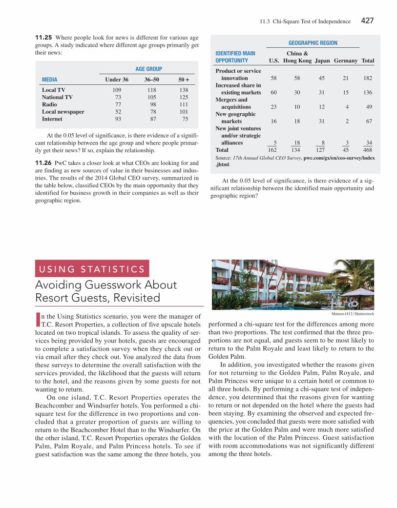
11.3 Chi-Square Test of Independence 427
11.25 Where people look for news is different for various age groups. A study indicated where different age groups primarily get their news:
meDia
age grouP
Under 36 36–50 50+
Local TV 109 118 138National TV 73 105 125Radio 77 98 111Local newspaper 52 78 101Internet 93 87 75
At the 0.05 level of significance, is there evidence of a signifi-cant relationship between the age group and where people primar-ily get their news? If so, explain the relationship.
11.26 PwC takes a closer look at what CeOs are looking for and are finding as new sources of value in their businesses and indus-tries. The results of the 2014 Global CeO survey, summarized in the table below, classified CeOs by the main opportunity that they identified for business growth in their companies as well as their geographic region.
iDentiFieD main oPPortunitY
geograPHiC region
U.S.China &
Hong Kong Japan Germany Total
Product or service innovation 58 58 45 21 182Increased share in existing markets 60 30 31 15 136Mergers and acquisitions 23 10 12 4 49New geographic markets 16 18 31 2 67New joint ventures and/or strategic alliances 5 18 8 3 34Total 162 134 127 45 468Source: 17th Annual Global CEO Survey, pwc.com/gx/en/ceo-survey/index .jhtml.
At the 0.05 level of significance, is there evidence of a sig-nificant relationship between the identified main opportunity and geographic region?
In the Using Statistics scenario, you were the manager of T.C. Resort Properties, a collection of five upscale hotels
located on two tropical islands. To assess the quality of ser-vices being provided by your hotels, guests are encouraged to complete a satisfaction survey when they check out or via email after they check out. You analyzed the data from these surveys to determine the overall satisfaction with the services provided, the likelihood that the guests will return to the hotel, and the reasons given by some guests for not wanting to return.
On one island, T.C. Resort Properties operates the Beachcomber and Windsurfer hotels. You performed a chi-square test for the difference in two proportions and con-cluded that a greater proportion of guests are willing to return to the Beachcomber Hotel than to the Windsurfer. On the other island, T.C. Resort Properties operates the Golden Palm, Palm Royale, and Palm Princess hotels. To see if guest satisfaction was the same among the three hotels, you
performed a chi-square test for the differences among more than two proportions. The test confirmed that the three pro-portions are not equal, and guests seem to be most likely to return to the Palm Royale and least likely to return to the Golden Palm.
In addition, you investigated whether the reasons given for not returning to the Golden Palm, Palm Royale, and Palm Princess were unique to a certain hotel or common to all three hotels. By performing a chi-square test of indepen-dence, you determined that the reasons given for wanting to return or not depended on the hotel where the guests had been staying. By examining the observed and expected fre-quencies, you concluded that guests were more satisfied with the price at the Golden Palm and were much more satisfied with the location of the Palm Princess. Guest satisfaction with room accommodations was not significantly different among the three hotels.
U s i n g s tat i s t i c s
Avoiding Guesswork About Resort Guests, Revisited
Maturos1812>Shutterstock
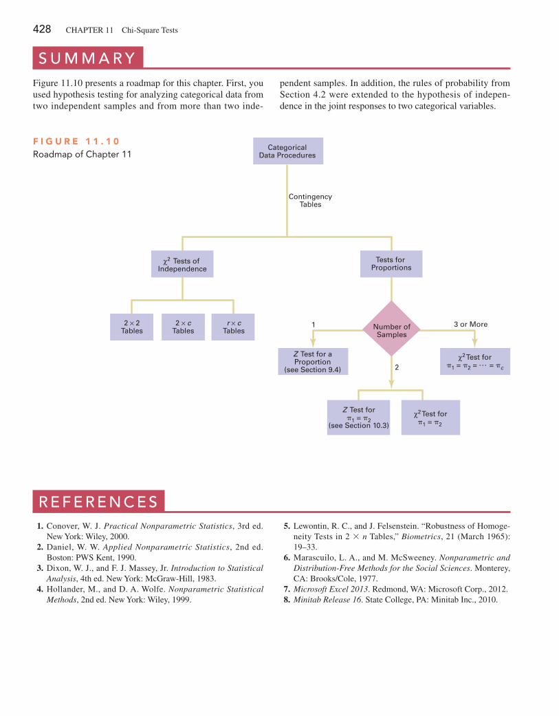
428 CHAPTeR 11 Chi-Square Tests
s U M M a r yFigure 11.10 presents a roadmap for this chapter. First, you used hypothesis testing for analyzing categorical data from two independent samples and from more than two inde-
pendent samples. In addition, the rules of probability from Section 4.2 were extended to the hypothesis of indepen-dence in the joint responses to two categorical variables.
Tests for Proportions
χ2 Tests of Independence
2
3 or More1r × cTables
2 × cTables
2 × 2Tables
ContingencyTables
CategoricalData Procedures
Z Test for aProportion
(see Section 9.4)
Number ofSamples
χ2 Test forp1 = p2
Z Test forp1 = p2
(see Section 10.3)
χ2 Test forp1 = p2 = . . . = pc
F i g u r e 1 1 . 1 0Roadmap of Chapter 11
r e F e r e n c e s 1. Conover, W. J. Practical Nonparametric Statistics, 3rd ed.
New York: Wiley, 2000. 2. Daniel, W. W. Applied Nonparametric Statistics, 2nd ed.
Boston: PWS Kent, 1990. 3. Dixon, W. J., and F. J. Massey, Jr. Introduction to Statistical
Analysis, 4th ed. New York: McGraw-Hill, 1983. 4. Hollander, M., and D. A. Wolfe. Nonparametric Statistical
Methods, 2nd ed. New York: Wiley, 1999.
5. Lewontin, R. C., and J. Felsenstein. “Robustness of Homoge-neity Tests in 2 * n Tables,” Biometrics, 21 (March 1965): 19–33.
6. Marascuilo, L. A., and M. McSweeney. Nonparametric and Distribution-Free Methods for the Social Sciences. Monterey, CA: Brooks/Cole, 1977.
7. Microsoft Excel 2013. Redmond, WA: Microsoft Corp., 2012. 8. Minitab Release 16. State College, PA: Minitab Inc., 2010.
Chapter Review Problems 429
K e y e q U at i o n sX2 Test for the Difference Between Two Proportions
x2STAT = a
all cells
1fo - fe22
fe (11.1)
Computing the Estimated Overall Proportion for Two Groups
p =X1 + X2
n1 + n2=
Xn
(11.2)
Computing the Estimated Overall Proportion for c Groups
p =X1 + X2 + g + Xc
n1 + n2 + g + nc=
Xn
(11.3)
Computing the Expected Frequency
fe =Row total * Column total
n (11.4)
K e y t e r M schi-square 1x22 distribution 412chi-square 1x22 test for the difference be-
tween two proportions 411
chi-square 1x22 test of independence 422expected frequency 1 fe2 411observed frequency 1 fo2 411
2 * c contingency table 4172 * 2 contingency table 410two-way contingency table 410
c h e c K i n g y o U r U n d e r s ta n d i n g11.27 Under what conditions would you develop a two-way con-tingency table? For what purpose would such a table be used?
11.28 Under what conditions should you use the x2 test to deter-mine whether there is a difference among the proportions of more than two independent populations?
11.29 Under what conditions should you use the x2 test of inde-pendence?
c h a p t e r r e v i e w p r o b l e M s11.30 Undergraduate students at Miami University in Oxford, Ohio, were surveyed in order to evaluate the effect of gender and price on purchasing a pizza from Pizza Hut. Students were told to suppose that they were planning to have a large two-topping pizza delivered to their residence that evening. The students had to de-cide between ordering from Pizza Hut at a reduced price of $8.49 (the regular price for a large two-topping pizza from the Oxford Pizza Hut at the time was $11.49) and ordering a pizza from a different pizzeria. The results from this question are summarized in the following contingency table:
PiZZeria
genDer Pizza Hut Other Total
Female 4 13 17Male 6 12 18Total 10 25 35
a. Using a 0.05 level of significance, is there evidence of a differ-ence between males and females in their pizzeria selection?
b. What is your answer to (a) if nine of the male students selected Pizza Hut and nine selected another pizzeria?
A subsequent survey evaluated purchase decisions at other prices. These results are summarized in the following contingency table:
PriCe
PiZZeria $8.49 $11.49 $14.49 Total
Pizza Hut 10 5 2 17Other 25 23 27 75Total 35 28 29 92
c. Using a 0.05 level of significance and using the data in the second contingency table, is there evidence of a difference in pizzeria selection based on price?
d. Determine the p-value in (c) and interpret its meaning.
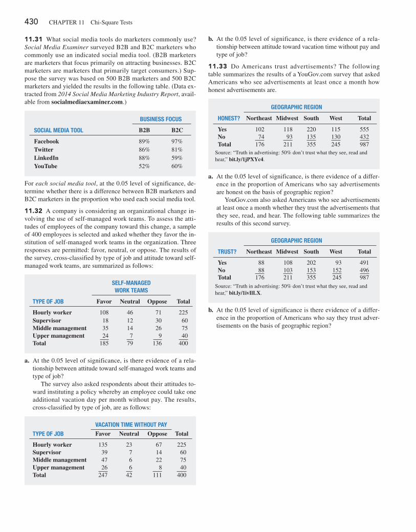
430 CHAPTeR 11 Chi-Square Tests
11.31 What social media tools do marketers commonly use? Social Media Examiner surveyed B2B and B2C marketers who commonly use an indicated social media tool. (B2B marketers are marketers that focus primarily on attracting businesses. B2C marketers are marketers that primarily target consumers.) Sup-pose the survey was based on 500 B2B marketers and 500 B2C marketers and yielded the results in the following table. (Data ex-tracted from 2014 Social Media Marketing Industry Report, avail-able from socialmediaexaminer.com.)
business FoCus
soCial meDia tool B2B B2C
Facebook 89% 97%Twitter 86% 81%LinkedIn 88% 59%YouTube 52% 60%
For each social media tool, at the 0.05 level of significance, de-termine whether there is a difference between B2B marketers and B2C marketers in the proportion who used each social media tool.
11.32 A company is considering an organizational change in-volving the use of self-managed work teams. To assess the atti-tudes of employees of the company toward this change, a sample of 400 employees is selected and asked whether they favor the in-stitution of self-managed work teams in the organization. Three responses are permitted: favor, neutral, or oppose. The results of the survey, cross-classified by type of job and attitude toward self-managed work teams, are summarized as follows:
selF-manageD work teams
tYPe oF Job Favor Neutral Oppose Total
Hourly worker 108 46 71 225Supervisor 18 12 30 60Middle management 35 14 26 75Upper management 24 7 9 40Total 185 79 136 400
a. At the 0.05 level of significance, is there evidence of a rela-tionship between attitude toward self-managed work teams and type of job?
The survey also asked respondents about their attitudes to-ward instituting a policy whereby an employee could take one additional vacation day per month without pay. The results, cross-classified by type of job, are as follows:
VaCation time witHout PaY
tYPe oF Job Favor Neutral Oppose Total
Hourly worker 135 23 67 225Supervisor 39 7 14 60Middle management 47 6 22 75Upper management 26 6 8 40Total 247 42 111 400
b. At the 0.05 level of significance, is there evidence of a rela-tionship between attitude toward vacation time without pay and type of job?
11.33 Do Americans trust advertisements? The following table summarizes the results of a YouGov.com survey that asked Americans who see advertisements at least once a month how honest advertisements are.
geograPHiC region
Honest? Northeast Midwest South West Total
Yes 102 118 220 115 555No 74 93 135 130 432Total 176 211 355 245 987
Source: “Truth in advertising: 50% don’t trust what they see, read and hear,” bit.ly/1jPXYc4.
a. At the 0.05 level of significance, is there evidence of a differ-ence in the proportion of Americans who say advertisements are honest on the basis of geographic region?
YouGov.com also asked Americans who see advertisements at least once a month whether they trust the advertisements that they see, read, and hear. The following table summarizes the results of this second survey.
geograPHiC region
trust? Northeast Midwest South West Total
Yes 88 108 202 93 491No 88 103 153 152 496Total 176 211 355 245 987
Source: “Truth in advertising: 50% don’t trust what they see, read and hear,” bit.ly/1ivIlLX.
b. At the 0.05 level of significance is there evidence of a differ-ence in the proportion of Americans who say they trust adver-tisements on the basis of geographic region?
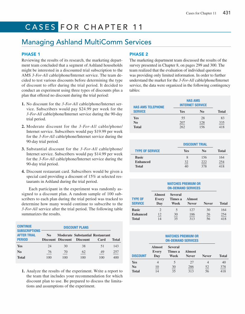
Cases for Chapter 11 431
c a s e s F o r c h a p t e r 1 1
Managing ashland Multicomm services
phaSe 1Reviewing the results of its research, the marketing depart-ment team concluded that a segment of Ashland households might be interested in a discounted trial subscription to the AMS 3-For-All cable/phone/Internet service. The team de-cided to test various discounts before determining the type of discount to offer during the trial period. It decided to conduct an experiment using three types of discounts plus a plan that offered no discount during the trial period:
1. No discount for the 3-For-All cable/phone/Internet ser-vice. Subscribers would pay $24.99 per week for the 3-For-All cable/phone/Internet service during the 90-day trial period.
2. Moderate discount for the 3-For-All cable/phone/ Internet service. Subscribers would pay $19.99 per week for the 3-For-All cable/phone/Internet service during the 90-day trial period.
3. Substantial discount for the 3-For-All cable/phone/ Internet service. Subscribers would pay $14.99 per week for the 3-For-All cable/phone/Internet service during the 90-day trial period.
4. Discount restaurant card. Subscribers would be given a special card providing a discount of 15% at selected res-taurants in Ashland during the trial period.
each participant in the experiment was randomly as-signed to a discount plan. A random sample of 100 sub-scribers to each plan during the trial period was tracked to determine how many would continue to subscribe to the 3-For-All service after the trial period. The following table summarizes the results.
phaSe 2The marketing department team discussed the results of the survey presented in Chapter 8, on pages 299 and 300. The team realized that the evaluation of individual questions was providing only limited information. In order to further understand the market for the 3-For-All cable/phone/Internet service, the data were organized in the following contingency tables:
Has ams telePHone serViCe
Has ams internet serViCe
Yes No Total
Yes 55 28 83No 207 128 335Total 262 156 418
DisCount trial
tYPe oF serViCe Yes No Total
Basic 8 156 164Enhanced 32 222 254Total 40 378 418
watCHes Premium or on-DemanD serViCes
tYPe oF serViCe
Almost Every Day
Several Times a Week
Almost Never Never Total
Basic 2 5 127 30 164Enhanced 12 30 186 26 254Total 14 35 313 56 418
watCHes Premium or on-DemanD serViCes
DisCount
Almost Every Day
Several Times a Week
Almost Never Never Total
Yes 4 5 27 4 40No 10 30 286 52 378Total 14 35 313 56 418
Continue subsCriPtions aFter trial PerioD
DisCount Plans
No Discount
Moderate Discount
Substantial Discount
Restaurant Card Total
Yes 24 30 38 51 143
No 76 70 62 49 257
Total 100 100 100 100 400
1. Analyze the results of the experiment. Write a report to the team that includes your recommendation for which discount plan to use. Be prepared to discuss the limita-tions and assumptions of the experiment.
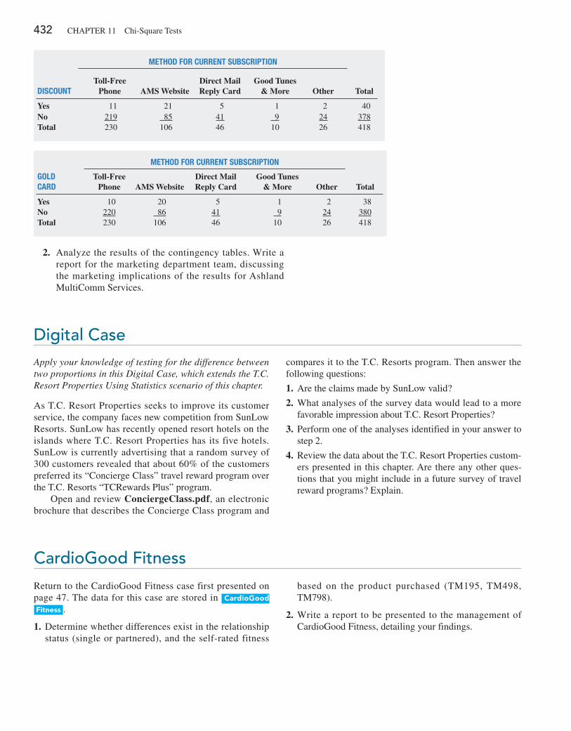
432 CHAPTeR 11 Chi-Square Tests
metHoD For Current subsCriPtion
DisCountToll-Free
Phone AMS WebsiteDirect Mail Reply Card
Good Tunes & More Other Total
Yes 11 21 5 1 2 40No 219 85 41 9 24 378Total 230 106 46 10 26 418
metHoD For Current subsCriPtion
golD CarD
Toll-Free Phone AMS Website
Direct Mail Reply Card
Good Tunes & More Other Total
Yes 10 20 5 1 2 38No 220 86 41 9 24 380Total 230 106 46 10 26 418
2. Analyze the results of the contingency tables. Write a report for the marketing department team, discussing the marketing implications of the results for Ashland MultiComm Services.
digital caseApply your knowledge of testing for the difference between two proportions in this Digital Case, which extends the T.C. Resort Properties Using Statistics scenario of this chapter.
As T.C. Resort Properties seeks to improve its customer service, the company faces new competition from SunLow Resorts. SunLow has recently opened resort hotels on the islands where T.C. Resort Properties has its five hotels. SunLow is currently advertising that a random survey of 300 customers revealed that about 60% of the customers preferred its “Concierge Class” travel reward program over the T.C. Resorts “TCRewards Plus” program.
Open and review ConciergeClass.pdf, an electronic brochure that describes the Concierge Class program and
compares it to the T.C. Resorts program. Then answer the following questions:
1. Are the claims made by SunLow valid?
2. What analyses of the survey data would lead to a more favorable impression about T.C. Resort Properties?
3. Perform one of the analyses identified in your answer to step 2.
4. Review the data about the T.C. Resort Properties custom-ers presented in this chapter. Are there any other ques-tions that you might include in a future survey of travel reward programs? explain.
cardiogood Fitness
Return to the CardioGood Fitness case first presented on page 47. The data for this case are stored in cardiogood
Fitness .
1. Determine whether differences exist in the relationship status (single or partnered), and the self-rated fitness
based on the product purchased (TM195, TM498, TM798).
2. Write a report to be presented to the management of CardioGood Fitness, detailing your findings.
Cases for Chapter 11 433
clear Mountain state student surveys
1. The Student News Service at Clear Mountain State University (CMSU) has decided to gather data about the undergraduate students that attend CMSU. It cre-ates and distributes a survey of 14 questions and receives responses from 62 undergraduates, which it stores in undergradSurvey . Construct contingency tables using gender, major, plans to go to graduate school, and employment status. (You need to construct six tables, taking two variables at a time.) Analyze the data at the 0.05 level of significance to determine whether any significant relationships exist among these variables.
2. The dean of students at CMSU has learned about the undergraduate survey and has decided to undertake a similar survey for graduate students at CMSU. She cre-ates and distributes a survey of 14 questions and re-ceives responses from 44 graduate students, which she stores them in gradSurvey . For these data, at the 0.05 level of significance: Construct contingency tables using gender, undergradu-ate major, graduate major, and employment status. (You need to construct six tables, taking two variables at a time.) Analyze the data to determine whether any signifi-cant relationships exist among these variables.
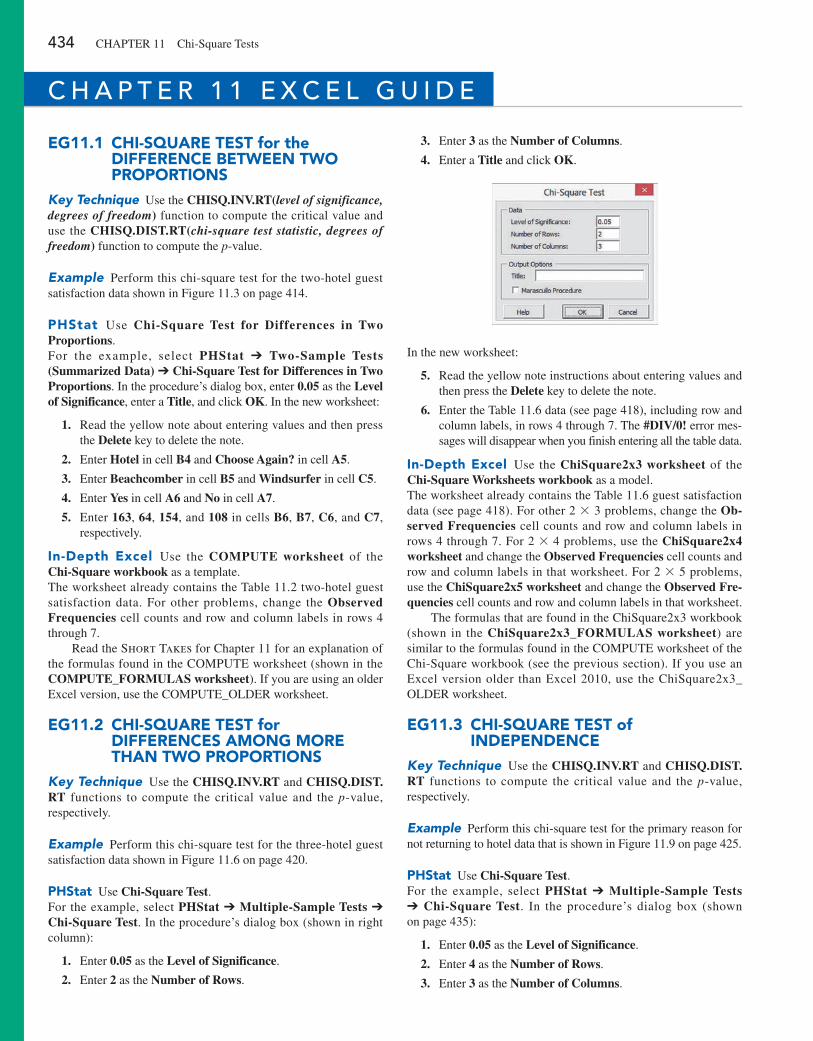
434 CHAPTeR 11 Chi-Square Tests
eg11.1 chi-Square TeST for the DiFFerence beTween Two proporTionS
Key Technique Use the CHISQ.INV.RT(level of significance, degrees of freedom) function to compute the critical value and use the CHISQ.DIST.RT(chi-square test statistic, degrees of freedom) function to compute the p-value.
Example Perform this chi-square test for the two-hotel guest satisfaction data shown in Figure 11.3 on page 414.
phStat Use Chi-Square Test for Differences in Two Proportions.For the example, select PHStat ➔ Two-Sample Tests (Summarized Data) ➔ Chi-Square Test for Differences in Two Proportions. In the procedure’s dialog box, enter 0.05 as the Level of Significance, enter a Title, and click OK. In the new worksheet:
1. Read the yellow note about entering values and then press the Delete key to delete the note.
2. enter Hotel in cell B4 and Choose Again? in cell A5.
3. enter Beachcomber in cell B5 and Windsurfer in cell C5.
4. enter Yes in cell A6 and No in cell A7.
5. enter 163, 64, 154, and 108 in cells B6, B7, C6, and C7, respectively.
in-Depth excel Use the COMPUTE worksheet of the Chi-Square workbook as a template.The worksheet already contains the Table 11.2 two-hotel guest satisfaction data. For other problems, change the Observed Frequencies cell counts and row and column labels in rows 4 through 7.
Read the Short Takes for Chapter 11 for an explanation of the formulas found in the COMPUTe worksheet (shown in the COMPUTE_FORMULAS worksheet). If you are using an older excel version, use the COMPUTe_OLDeR worksheet.
eg11.2 chi-Square TeST for DiFFerenceS among more Than Two proporTionS
Key Technique Use the CHISQ.INV.RT and CHISQ.DIST.RT functions to compute the critical value and the p-value, respectively.
Example Perform this chi-square test for the three-hotel guest satisfaction data shown in Figure 11.6 on page 420.
phStat Use Chi-Square Test.For the example, select PHStat ➔ Multiple-Sample Tests ➔ Chi-Square Test. In the procedure’s dialog box (shown in right column):
1. enter 0.05 as the Level of Significance.
2. enter 2 as the Number of Rows.
3. enter 3 as the Number of Columns.
4. enter a Title and click OK.
In the new worksheet:
5. Read the yellow note instructions about entering values and then press the Delete key to delete the note.
6. enter the Table 11.6 data (see page 418), including row and column labels, in rows 4 through 7. The #DIV/0! error mes-sages will disappear when you finish entering all the table data.
in-Depth excel Use the ChiSquare2x3 worksheet of the Chi-Square Worksheets workbook as a model.The worksheet already contains the Table 11.6 guest satisfaction data (see page 418). For other 2 * 3 problems, change the Ob-served Frequencies cell counts and row and column labels in rows 4 through 7. For 2 * 4 problems, use the ChiSquare2x4 worksheet and change the Observed Frequencies cell counts and row and column labels in that worksheet. For 2 * 5 problems, use the ChiSquare2x5 worksheet and change the Observed Fre-quencies cell counts and row and column labels in that worksheet.
The formulas that are found in the ChiSquare2x3 workbook (shown in the ChiSquare2x3_FORMULAS worksheet) are similar to the formulas found in the COMPUTe worksheet of the Chi-Square workbook (see the previous section). If you use an excel version older than excel 2010, use the ChiSquare2x3_OLDeR worksheet.
eg11.3 chi-Square TeST of inDepenDence
Key Technique Use the CHISQ.INV.RT and CHISQ.DIST.RT functions to compute the critical value and the p-value, respectively.
Example Perform this chi-square test for the primary reason for not returning to hotel data that is shown in Figure 11.9 on page 425.
phStat Use Chi-Square Test.For the example, select PHStat ➔ Multiple-Sample Tests ➔ Chi-Square Test. In the procedure’s dialog box (shown on page 435):
1. enter 0.05 as the Level of Significance.
2. enter 4 as the Number of Rows.
3. enter 3 as the Number of Columns.
c h a p t e r 1 1 e x c e l g U i d e
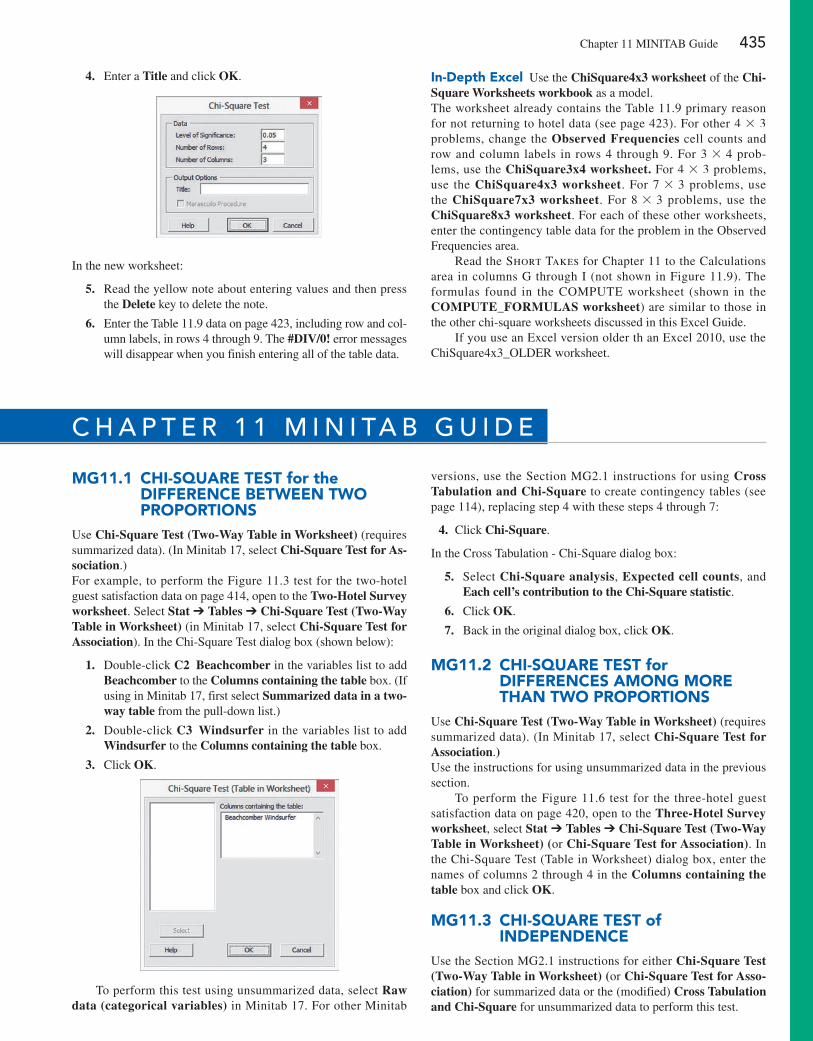
Chapter 11 MINITAB Guide 435
4. enter a Title and click OK.
In the new worksheet:
5. Read the yellow note about entering values and then press the Delete key to delete the note.
6. enter the Table 11.9 data on page 423, including row and col-umn labels, in rows 4 through 9. The #DIV/0! error messages will disappear when you finish entering all of the table data.
in-Depth excel Use the ChiSquare4x3 worksheet of the Chi-Square Worksheets workbook as a model. The worksheet already contains the Table 11.9 primary reason for not returning to hotel data (see page 423). For other 4 * 3 problems, change the Observed Frequencies cell counts and row and column labels in rows 4 through 9. For 3 * 4 prob-lems, use the ChiSquare3x4 worksheet. For 4 * 3 problems, use the ChiSquare4x3 worksheet. For 7 * 3 problems, use the ChiSquare7x3 worksheet. For 8 * 3 problems, use the ChiSquare8x3 worksheet. For each of these other worksheets, enter the contingency table data for the problem in the Observed Frequencies area.
Read the Short Takes for Chapter 11 to the Calculations area in columns G through I (not shown in Figure 11.9). The formulas found in the COMPUTe worksheet (shown in the COMPUTE_FORMULAS worksheet) are similar to those in the other chi-square worksheets discussed in this excel Guide.
If you use an excel version older th an excel 2010, use the ChiSquare4x3_OLDeR worksheet.
mg11.1 chi-Square TeST for the DiFFerence beTween Two proporTionS
Use Chi-Square Test (Two-Way Table in Worksheet) (requires summarized data). (In Minitab 17, select Chi-Square Test for As-sociation.)For example, to perform the Figure 11.3 test for the two-hotel guest satisfaction data on page 414, open to the Two-Hotel Survey worksheet. Select Stat ➔ Tables ➔ Chi-Square Test (Two-Way Table in Worksheet) (in Minitab 17, select Chi-Square Test for Association). In the Chi-Square Test dialog box (shown below):
1. Double-click C2 Beachcomber in the variables list to add Beachcomber to the Columns containing the table box. (If using in Minitab 17, first select Summarized data in a two-way table from the pull-down list.)
2. Double-click C3 Windsurfer in the variables list to add Windsurfer to the Columns containing the table box.
3. Click OK.
To perform this test using unsummarized data, select Raw data (categorical variables) in Minitab 17. For other Minitab
versions, use the Section MG2.1 instructions for using Cross Tabulation and Chi-Square to create contingency tables (see page 114), replacing step 4 with these steps 4 through 7:
4. Click Chi-Square.
In the Cross Tabulation - Chi-Square dialog box:
5. Select Chi-Square analysis, Expected cell counts, and Each cell’s contribution to the Chi-Square statistic.
6. Click OK.
7. Back in the original dialog box, click OK.
mg11.2 chi-Square TeST for DiFFerenceS among more Than Two proporTionS
Use Chi-Square Test (Two-Way Table in Worksheet) (requires summarized data). (In Minitab 17, select Chi-Square Test for Association.)Use the instructions for using unsummarized data in the previous section.
To perform the Figure 11.6 test for the three-hotel guest satisfaction data on page 420, open to the Three-Hotel Survey worksheet, select Stat ➔ Tables ➔ Chi-Square Test (Two-Way Table in Worksheet) (or Chi-Square Test for Association). In the Chi-Square Test (Table in Worksheet) dialog box, enter the names of columns 2 through 4 in the Columns containing the table box and click OK.
mg11.3 chi-Square TeST of inDepenDence
Use the Section MG2.1 instructions for either Chi-Square Test (Two-Way Table in Worksheet) (or Chi-Square Test for Asso-ciation) for summarized data or the (modified) Cross Tabulation and Chi-Square for unsummarized data to perform this test.
c h a p t e r 1 1 M i n i ta b g U i d e
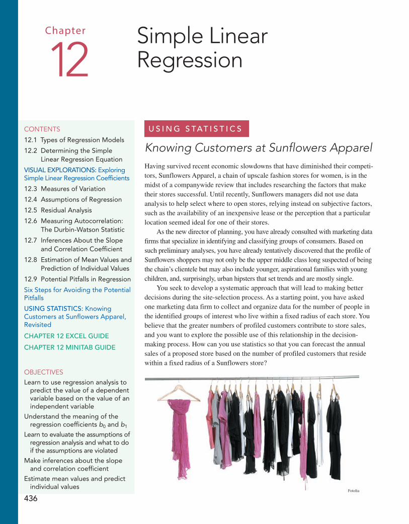
436
U s i n g s tat i s t i c s
Knowing Customers at Sunflowers ApparelHaving survived recent economic slowdowns that have diminished their competi-tors, Sunflowers Apparel, a chain of upscale fashion stores for women, is in the midst of a companywide review that includes researching the factors that make their stores successful. Until recently, Sunflowers managers did not use data analysis to help select where to open stores, relying instead on subjective factors, such as the availability of an inexpensive lease or the perception that a particular location seemed ideal for one of their stores.
As the new director of planning, you have already consulted with marketing data firms that specialize in identifying and classifying groups of consumers. Based on such preliminary analyses, you have already tentatively discovered that the profile of Sunflowers shoppers may not only be the upper middle class long suspected of being the chain’s clientele but may also include younger, aspirational families with young children, and, surprisingly, urban hipsters that set trends and are mostly single.
You seek to develop a systematic approach that will lead to making better decisions during the site-selection process. As a starting point, you have asked one marketing data firm to collect and organize data for the number of people in the identified groups of interest who live within a fixed radius of each store. You believe that the greater numbers of profiled customers contribute to store sales, and you want to explore the possible use of this relationship in the decision- making process. How can you use statistics so that you can forecast the annual sales of a proposed store based on the number of profiled customers that reside within a fixed radius of a Sunflowers store?
contents
12.1 Types of Regression Models
12.2 Determining the Simple Linear Regression Equation
VisUal Explorations: Exploring Simple Linear Regression Coefficients
12.3 Measures of Variation
12.4 Assumptions of Regression
12.5 Residual Analysis
12.6 Measuring Autocorrelation: The Durbin-Watson Statistic
12.7 Inferences About the Slope and Correlation Coefficient
12.8 Estimation of Mean Values and Prediction of Individual Values
12.9 Potential Pitfalls in Regression
Six Steps for Avoiding the Potential Pitfalls
Using statistics: Knowing Customers at Sunflowers Apparel, Revisited
chaptEr 12 ExcEl gUidE
chaptEr 12 Minitab gUidE
objectivesLearn to use regression analysis to
predict the value of a dependent variable based on the value of an independent variable
Understand the meaning of the regression coefficients b0 and b1
Learn to evaluate the assumptions of regression analysis and what to do if the assumptions are violated
Make inferences about the slope and correlation coefficient
Estimate mean values and predict individual values
Simple Linear Regression12
Chapter
Fotolia

12.1 Types of Regression Models 437
In this chapter and the next chapter, you learn regression analysis techniques that help uncover relationships between variables. Regression analysis leads to selection of a model that expresses how one or more independent variables can be used to predict the value
of another variable, called the dependent variable. Regression models identify the type of mathematical relationship that exists between a dependent variable and an independent vari-able, thereby enabling you to quantify the effect that a change in the independent variable has on the dependent variable. Models also help you identify unusual values that may be outliers (see references 2, 3, and 4).
This chapter discusses simple linear regression models that use a single numerical independent variable, X, to predict the numerical dependent variable, Y. (Chapter 13 dis-cusses multiple regression models that use several independent variables to predict the de-pendent variable.) In the Sunflowers scenario, your initial belief reflects a possible simple linear regression model in which the number of profiled customers is the single numerical independent variable, X, being used to predict the annual sales of the store, the dependent variable, Y.
Using a scatter plot (also known as scatter diagram) to visualize the X and Y variables, a technique introduced in Section 2.5 on page 82, can help suggest a starting point for regression analysis. The scatter plots in Figure 12.1 illustrates six possible relationships between an X and Y variable.
12.1 Types of Regression Models
Y
Panel APositive linear relationship
X
Y
Panel BNegative linear relationship
X
Y
Panel FNo relationship between X and Y
X
Y
Panel CPositive curvilinear relationship
X
Y
Panel DU-shaped curvilinear relationship
X
Y
Panel ENegative curvilinear relationship
X
F i g u r e 1 2 . 1Six types of relationships found in scatter plots
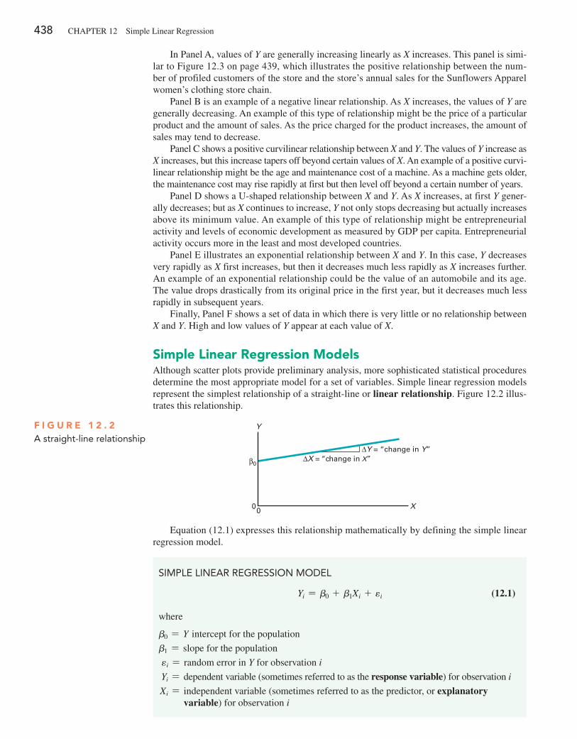
438 CHApTeR 12 Simple Linear Regression
equation (12.1) expresses this relationship mathematically by defining the simple linear regression model.
Y
0
ΔX = “change in X”ΔY = “change in Y”
0 X
β0
F i g u r e 1 2 . 2A straight-line relationship
SIMPLE LInEAR REgRESSIon MoDEL
Yi = b0 + b1Xi + ei (12.1)
where
b0 = Y intercept for the population
b1 = slope for the population
ei = random error in Y for observation i
Yi = dependent variable (sometimes referred to as the response variable) for observation i
Xi = independent variable (sometimes referred to as the predictor, or explanatory variable) for observation i
In panel A, values of Y are generally increasing linearly as X increases. This panel is simi-lar to Figure 12.3 on page 439, which illustrates the positive relationship between the num-ber of profiled customers of the store and the store’s annual sales for the Sunflowers Apparel women’s clothing store chain.
panel B is an example of a negative linear relationship. As X increases, the values of Y are generally decreasing. An example of this type of relationship might be the price of a particular product and the amount of sales. As the price charged for the product increases, the amount of sales may tend to decrease.
panel C shows a positive curvilinear relationship between X and Y. The values of Y increase as X increases, but this increase tapers off beyond certain values of X. An example of a positive curvi-linear relationship might be the age and maintenance cost of a machine. As a machine gets older, the maintenance cost may rise rapidly at first but then level off beyond a certain number of years.
panel D shows a U-shaped relationship between X and Y. As X increases, at first Y gener-ally decreases; but as X continues to increase, Y not only stops decreasing but actually increases above its minimum value. An example of this type of relationship might be entrepreneurial activity and levels of economic development as measured by GDp per capita. entrepreneurial activity occurs more in the least and most developed countries.
panel e illustrates an exponential relationship between X and Y. In this case, Y decreases very rapidly as X first increases, but then it decreases much less rapidly as X increases further. An example of an exponential relationship could be the value of an automobile and its age. The value drops drastically from its original price in the first year, but it decreases much less rapidly in subsequent years.
Finally, panel F shows a set of data in which there is very little or no relationship between X and Y. High and low values of Y appear at each value of X.
Simple Linear regression ModelsAlthough scatter plots provide preliminary analysis, more sophisticated statistical procedures determine the most appropriate model for a set of variables. Simple linear regression models represent the simplest relationship of a straight-line or linear relationship. Figure 12.2 illus-trates this relationship.
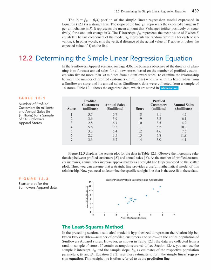
12.2 Determining the Simple Linear Regression equation 439
The Yi = b0 + b1Xi portion of the simple linear regression model expressed in equation (12.1) is a straight line. The slope of the line, b1, represents the expected change in Y per unit change in X. It represents the mean amount that Y changes (either positively or nega-tively) for a one-unit change in X. The Y intercept, b0, represents the mean value of Y when X equals 0. The last component of the model, ei, represents the random error in Y for each obser-vation, i. In other words, ei is the vertical distance of the actual value of Yi above or below the expected value of Yi on the line.
12.2 Determining the Simple Linear Regression EquationIn the Sunflowers Apparel scenario on page 436, the business objective of the director of plan-ning is to forecast annual sales for all new stores, based on the number of profiled custom-ers who live no more than 30 minutes from a Sunflowers store. To examine the relationship between the number of profiled customers (in millions) who live within a fixed radius from a Sunflowers store and its annual sales ($millions), data were collected from a sample of 14 stores. Table 12.1 shows the organized data, which are stored in SiteSelection .
T a b L e 1 2 . 1
number of Profiled Customers (in millions) and Annual Sales (in $millions) for a Sample of 14 Sunflowers Apparel Stores
Store
Profiled Customers (millions)
Annual Sales ($millions)
1 3.7 5.72 3.6 5.93 2.8 6.74 5.6 9.55 3.3 5.46 2.2 3.57 3.3 6.2
Store
Profiled Customers (millions)
Annual Sales ($millions)
8 3.1 4.7 9 3.2 6.110 3.5 4.911 5.2 10.712 4.6 7.613 5.8 11.814 3.0 4.1
F i g u r e 1 2 . 3Scatter plot for the Sunflowers Apparel data
The Least-Squares MethodIn the preceding section, a statistical model is hypothesized to represent the relationship be-tween two variables—number of profiled customers and sales—in the entire population of Sunflowers Apparel stores. However, as shown in Table 12.1, the data are collected from a random sample of stores. If certain assumptions are valid (see Section 12.4), you can use the sample Y intercept, b0, and the sample slope, b1, as estimates of the respective population parameters, b0 and b1. equation (12.2) uses these estimates to form the simple linear regres-sion equation. This straight line is often referred to as the prediction line.
Figure 12.3 displays the scatter plot for the data in Table 12.1. Observe the increasing rela-tionship between profiled customers 1X2 and annual sales 1Y2. As the number of profiled custom-ers increases, annual sales increase approximately as a straight line (superimposed on the scatter plot). Thus, you can assume that a straight line provides a useful mathematical model of this relationship. Now you need to determine the specific straight line that is the best fit to these data.
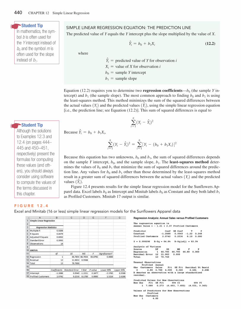
440 CHApTeR 12 Simple Linear Regression
Student TipIn mathematics, the sym-bol b is often used for the Y intercept instead of b0 and the symbol m is often used for the slope instead of b1.
SIMPLE LInEAR REgRESSIon EqUATIon: ThE PREDICTIon LInE
The predicted value of Y equals the Y intercept plus the slope multiplied by the value of X.
Yni = b0 + b1Xi (12.2)
where
Yni = predicted value of Y for observation i
Xi = value of X for observation i
b0 = sample Y intercept
b1 = sample slope
equation (12.2) requires you to determine two regression coefficients—b0 (the sample Y in-tercept) and b1 (the sample slope). The most common approach to finding b0 and b1 is using the least-squares method. This method minimizes the sum of the squared differences between the actual values 1Yi2 and the predicted values 1Yni2, using the simple linear regression equation [i.e., the prediction line; see equation (12.2)]. This sum of squared differences is equal to
an
i= 11Yi - Yni22
Because Yni = b0 + b1Xi,
an
i= 11Yi - Yni22 = a
n
i= 13Yi - 1b0 + b1Xi242
Because this equation has two unknowns, b0 and b1, the sum of squared differences depends on the sample Y intercept, b0, and the sample slope, b1. The least-squares method deter-mines the values of b0 and b1 that minimize the sum of squared differences around the predic-tion line. Any values for b0 and b1 other than those determined by the least-squares method result in a greater sum of squared differences between the actual values 1Yi2 and the predicted values 1Yni2.
Figure 12.4 presents results for the simple linear regression model for the Sunflowers Ap-parel data. excel labels b0 as Intercept and Minitab labels b0 as Constant and they both label b1 as profiled Customers. Minitab 17 output is similar.
Student TipAlthough the solutions to Examples 12.3 and 12.4 (on pages 444–445 and 450–451, respectively) present the formulas for computing these values (and oth-ers), you should always consider using software to compute the values of the terms discussed in this chapter.
F i g u r e 1 2 . 4Excel and Minitab (16 or less) simple linear regression models for the Sunflowers Apparel data
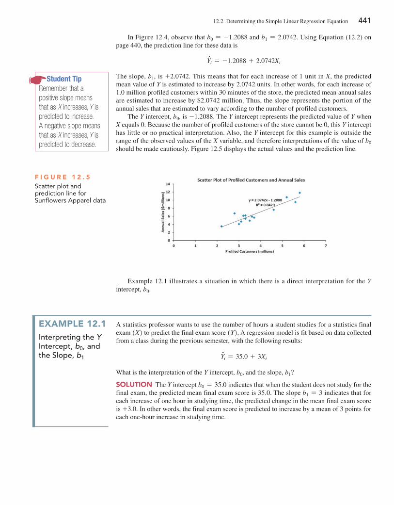
12.2 Determining the Simple Linear Regression equation 441
In Figure 12.4, observe that b0 = -1.2088 and b1 = 2.0742. Using equation (12.2) on page 440, the prediction line for these data is
Yni = -1.2088 + 2.0742Xi
The slope, b1, is +2.0742. This means that for each increase of 1 unit in X, the predicted mean value of Y is estimated to increase by 2.0742 units. In other words, for each increase of 1.0 million profiled customers within 30 minutes of the store, the predicted mean annual sales are estimated to increase by $2.0742 million. Thus, the slope represents the portion of the annual sales that are estimated to vary according to the number of profiled customers.
The Y intercept, b0, is -1.2088. The Y intercept represents the predicted value of Y when X equals 0. Because the number of profiled customers of the store cannot be 0, this Y intercept has little or no practical interpretation. Also, the Y intercept for this example is outside the range of the observed values of the X variable, and therefore interpretations of the value of b0 should be made cautiously. Figure 12.5 displays the actual values and the prediction line.
Student TipRemember that a positive slope means that as X increases, Y is predicted to increase. A negative slope means that as X increases, Y is predicted to decrease.
F i g u r e 1 2 . 5Scatter plot and prediction line for Sunflowers Apparel data
example 12.1 illustrates a situation in which there is a direct interpretation for the Y intercept, b0.
exaMpLe 12.1interpreting the Y intercept, b0, and the slope, b1
A statistics professor wants to use the number of hours a student studies for a statistics final exam 1X2 to predict the final exam score 1Y2. A regression model is fit based on data collected from a class during the previous semester, with the following results:
Yni = 35.0 + 3Xi
What is the interpretation of the Y intercept, b0, and the slope, b1?
SoLuTion The Y intercept b0 = 35.0 indicates that when the student does not study for the final exam, the predicted mean final exam score is 35.0. The slope b1 = 3 indicates that for each increase of one hour in studying time, the predicted change in the mean final exam score is +3.0. In other words, the final exam score is predicted to increase by a mean of 3 points for each one-hour increase in studying time.
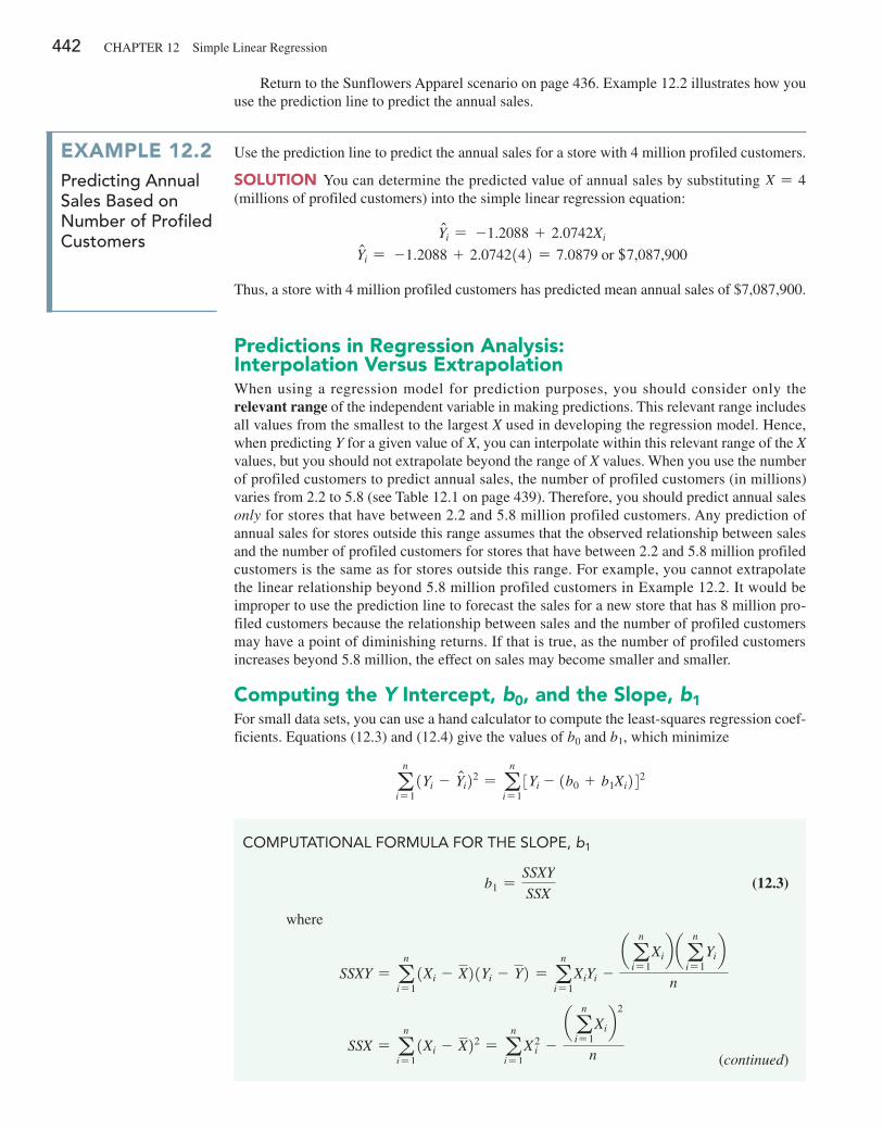
442 CHApTeR 12 Simple Linear Regression
predictions in regression analysis: interpolation Versus extrapolationWhen using a regression model for prediction purposes, you should consider only the relevant range of the independent variable in making predictions. This relevant range includes all values from the smallest to the largest X used in developing the regression model. Hence, when predicting Y for a given value of X, you can interpolate within this relevant range of the X values, but you should not extrapolate beyond the range of X values. When you use the number of profiled customers to predict annual sales, the number of profiled customers (in millions) varies from 2.2 to 5.8 (see Table 12.1 on page 439). Therefore, you should predict annual sales only for stores that have between 2.2 and 5.8 million profiled customers. Any prediction of annual sales for stores outside this range assumes that the observed relationship between sales and the number of profiled customers for stores that have between 2.2 and 5.8 million profiled customers is the same as for stores outside this range. For example, you cannot extrapolate the linear relationship beyond 5.8 million profiled customers in example 12.2. It would be improper to use the prediction line to forecast the sales for a new store that has 8 million pro-filed customers because the relationship between sales and the number of profiled customers may have a point of diminishing returns. If that is true, as the number of profiled customers increases beyond 5.8 million, the effect on sales may become smaller and smaller.
Computing the Y intercept, b0, and the Slope, b1For small data sets, you can use a hand calculator to compute the least-squares regression coef-ficients. equations (12.3) and (12.4) give the values of b0 and b1, which minimize
an
i= 11Yi - Yni22 = a
n
i= 13Yi - 1b0 + b1Xi242
exaMpLe 12.2predicting annual sales based on number of profiled customers
Use the prediction line to predict the annual sales for a store with 4 million profiled customers.
SoLuTion You can determine the predicted value of annual sales by substituting X = 4 (millions of profiled customers) into the simple linear regression equation:
Yni = -1.2088 + 2.0742Xi
Yni = -1.2088 + 2.0742142 = 7.0879 or +7,087,900
Thus, a store with 4 million profiled customers has predicted mean annual sales of $7,087,900.
CoMPUTATIonAL FoRMULA FoR ThE SLoPE, b1
b1 =SSXY
SSX (12.3)
where
SSXY = an
i= 11Xi - X21Yi - Y2 = a
n
i= 1XiYi -
a an
i= 1Xib a a
n
i= 1Yib
n
SSX = an
i= 11Xi - X22 = a
n
i= 1X2
i -a a
n
i= 1Xib
2
n (continued)
Return to the Sunflowers Apparel scenario on page 436. example 12.2 illustrates how you use the prediction line to predict the annual sales.
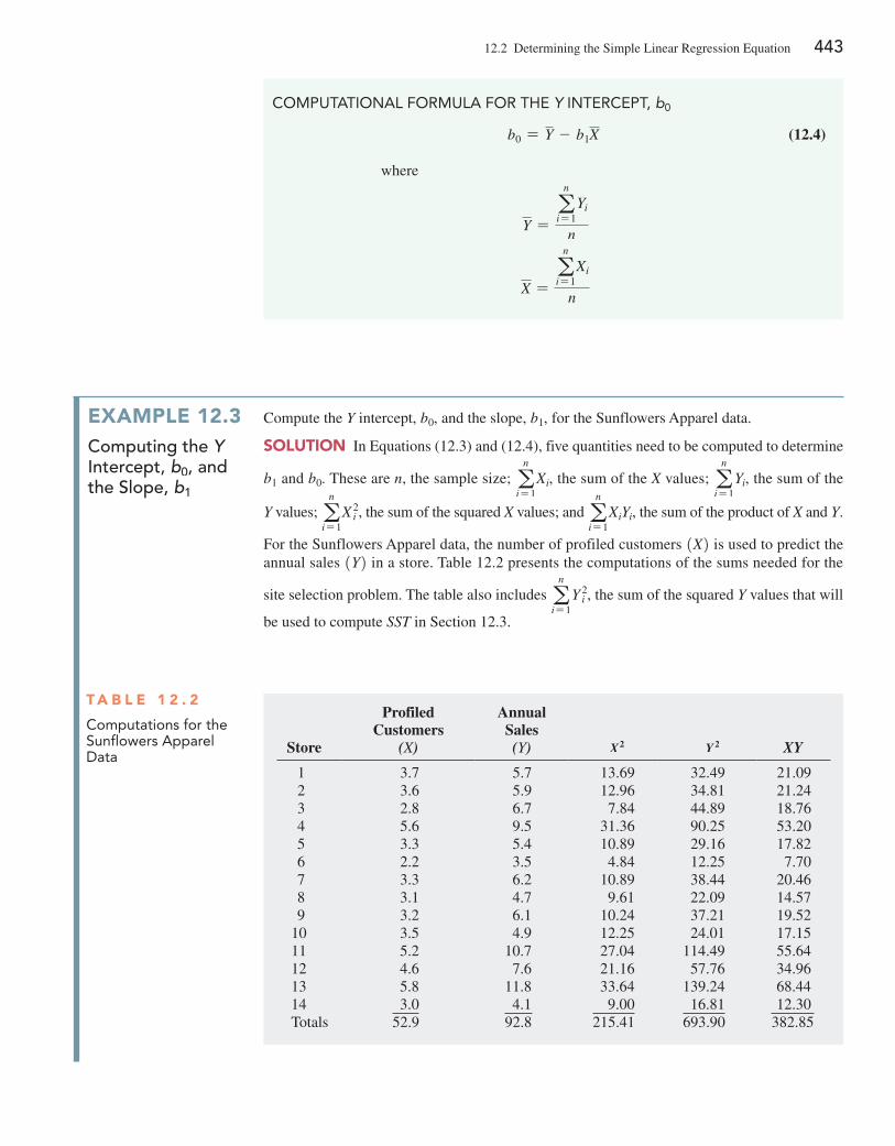
12.2 Determining the Simple Linear Regression equation 443
CoMPUTATIonAL FoRMULA FoR ThE Y InTERCEPT, b0
b0 = Y - b1X (12.4)
where
Y =a
n
i= 1Yi
n
X =a
n
i= 1Xi
n
exaMpLe 12.3computing the Y intercept, b0, and the slope, b1
Compute the Y intercept, b0, and the slope, b1, for the Sunflowers Apparel data.
SoLuTion In equations (12.3) and (12.4), five quantities need to be computed to determine
b1 and b0. These are n, the sample size; an
i= 1Xi, the sum of the X values; a
n
i= 1Yi, the sum of the
Y values; an
i= 1X2
i , the sum of the squared X values; and an
i= 1XiYi, the sum of the product of X and Y.
For the Sunflowers Apparel data, the number of profiled customers 1X2 is used to predict the annual sales 1Y2 in a store. Table 12.2 presents the computations of the sums needed for the
site selection problem. The table also includes an
i= 1Y 2
i , the sum of the squared Y values that will
be used to compute SST in Section 12.3.
T a b L e 1 2 . 2
Computations for the Sunflowers Apparel Data
Store
Profiled Customers
(X)
Annual Sales (Y) X2 Y 2 XY
1 3.7 5.7 13.69 32.49 21.092 3.6 5.9 12.96 34.81 21.243 2.8 6.7 7.84 44.89 18.764 5.6 9.5 31.36 90.25 53.205 3.3 5.4 10.89 29.16 17.826 2.2 3.5 4.84 12.25 7.707 3.3 6.2 10.89 38.44 20.468 3.1 4.7 9.61 22.09 14.579 3.2 6.1 10.24 37.21 19.52
10 3.5 4.9 12.25 24.01 17.1511 5.2 10.7 27.04 114.49 55.6412 4.6 7.6 21.16 57.76 34.9613 5.8 11.8 33.64 139.24 68.4414 3.0 4.1 9.00 16.81 12.30Totals 52.9 92.8 215.41 693.90 382.85
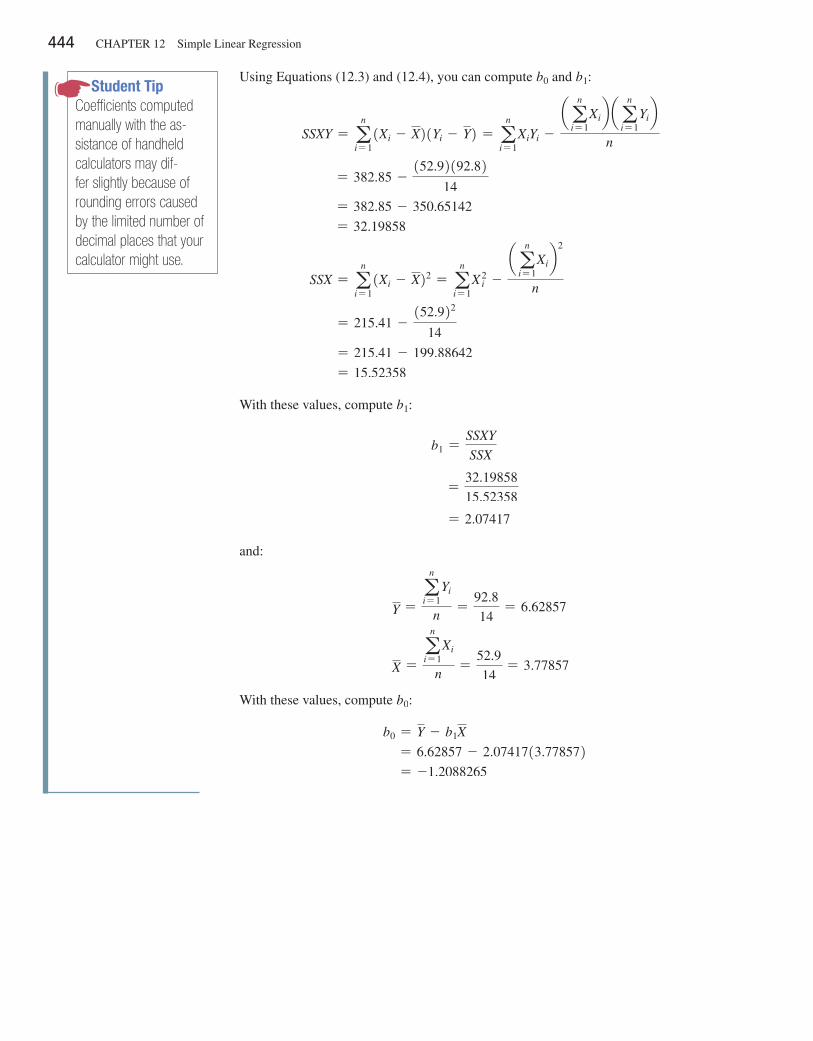
444 CHApTeR 12 Simple Linear Regression
Using equations (12.3) and (12.4), you can compute b0 and b1:
SSXY = an
i= 11Xi - X21Yi - Y2 = a
n
i= 1XiYi -
a an
i= 1Xib a a
n
i= 1Yib
n
= 382.85 -152.92192.82
14
= 382.85 - 350.65142
= 32.19858
SSX = an
i= 11Xi - X22 = a
n
i= 1X2
i -a a
n
i= 1Xib
2
n
= 215.41 -152.922
14
= 215.41 - 199.88642
= 15.52358
With these values, compute b1:
b1 =SSXY
SSX
=32.19858
15.52358
= 2.07417
and:
Y =a
n
i= 1Yi
n=
92.8
14= 6.62857
X =a
n
i= 1Xi
n=
52.9
14= 3.77857
With these values, compute b0:
b0 = Y - b1X
= 6.62857 - 2.0741713.778572 = -1.2088265
Student TipCoefficients computed manually with the as-sistance of handheld calculators may dif-fer slightly because of rounding errors caused by the limited number of decimal places that your calculator might use.
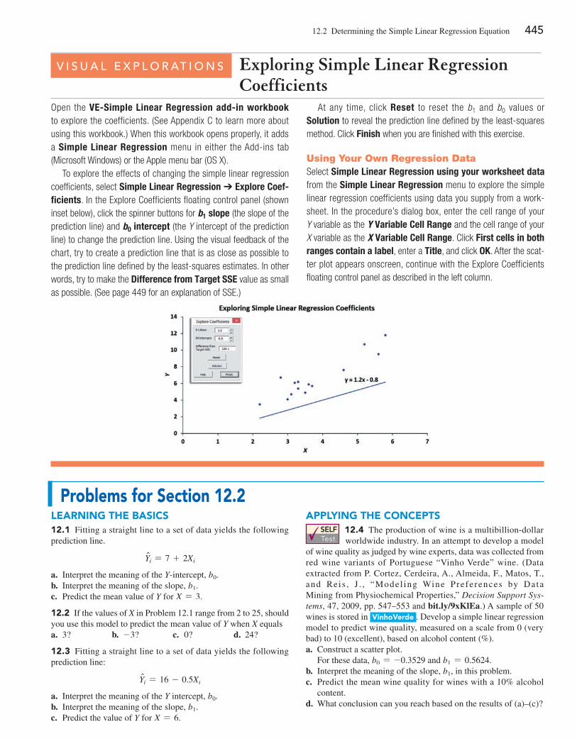
12.2 Determining the Simple Linear Regression equation 445
problems for Section 12.2Learning The baSiCS12.1 Fitting a straight line to a set of data yields the following prediction line.
Yni = 7 + 2Xi
a. Interpret the meaning of the Y-intercept, b0.b. Interpret the meaning of the slope, b1.c. predict the mean value of Y for X = 3.
12.2 If the values of X in problem 12.1 range from 2 to 25, should you use this model to predict the mean value of Y when X equalsa. 3? b. -3? c. 0? d. 24?
12.3 Fitting a straight line to a set of data yields the following prediction line:
Yni = 16 - 0.5Xi
a. Interpret the meaning of the Y intercept, b0.b. Interpret the meaning of the slope, b1.c. predict the value of Y for X = 6.
appLying The ConCepTSSELF Test
12.4 The production of wine is a multibillion-dollar worldwide industry. In an attempt to develop a model
of wine quality as judged by wine experts, data was collected from red wine variants of portuguese “Vinho Verde” wine. (Data extracted from p. Cortez, Cerdeira, A., Almeida, F., Matos, T., and Reis , J . , “Model ing Wine preferences by Data Mining from physiochemical properties,” Decision Support Sys-tems, 47, 2009, pp. 547–553 and bit.ly/9xKlEa.) A sample of 50 wines is stored in VinhoVerde . Develop a simple linear regression model to predict wine quality, measured on a scale from 0 (very bad) to 10 (excellent), based on alcohol content (%).a. Construct a scatter plot.
For these data, b0 = -0.3529 and b1 = 0.5624.b. Interpret the meaning of the slope, b1, in this problem.c. predict the mean wine quality for wines with a 10% alcohol
content.d. What conclusion can you reach based on the results of (a)–(c)?
Open the VE-Simple Linear Regression add-in workbook to explore the coefficients. (See Appendix C to learn more about using this workbook.) When this workbook opens properly, it adds a Simple Linear Regression menu in either the Add-ins tab (Microsoft Windows) or the Apple menu bar (OS X).
To explore the effects of changing the simple linear regression coefficients, select Simple Linear Regression ➔ Explore Coef-ficients. In the Explore Coefficients floating control panel (shown inset below), click the spinner buttons for b1 slope (the slope of the prediction line) and b0 intercept (the Y intercept of the prediction line) to change the prediction line. Using the visual feedback of the chart, try to create a prediction line that is as close as possible to the prediction line defined by the least-squares estimates. In other words, try to make the Difference from Target SSE value as small as possible. (See page 449 for an explanation of SSE.)
At any time, click Reset to reset the b1 and b0 values or Solution to reveal the prediction line defined by the least-squares method. Click Finish when you are finished with this exercise.
Using Your Own Regression DataSelect Simple Linear Regression using your worksheet data from the Simple Linear Regression menu to explore the simple linear regression coefficients using data you supply from a work-sheet. In the procedure’s dialog box, enter the cell range of your Y variable as the Y Variable Cell Range and the cell range of your X variable as the X Variable Cell Range. Click First cells in both ranges contain a label, enter a Title, and click OK. After the scat-ter plot appears onscreen, continue with the Explore Coefficients floating control panel as described in the left column.
V i s U a l E x p l o r at i o n s Exploring Simple Linear Regression Coefficients
446 CHApTeR 12 Simple Linear Regression
12.5 Zagat’s publishes restaurant ratings for various locations in the United States. The file restaurants contains the Zagat rating for food, décor, service, and the cost per person for a sample of 100 restaurants located in New York City and in a suburb of New York City. Develop a regression model to predict the cost per person, based on a variable that represents the sum of the ratings for food, décor, and service.Sources: extracted from Zagat Survey 2013, New York City Restaurants; and Zagat Survey 2012–2013, Long Island Restaurants.
a. Construct a scatter plot. For these data, b0 = -46.7718 and b1 = 1.4963.b. Assuming a linear relationship, use the least-squares method to
compute the regression coefficients b0 and b1.c. Interpret the meaning of the Y intercept, b0, and the slope, b1, in
this problem.d. predict the mean cost per person for a restaurant with a sum-
mated rating of 50.e. What should you tell the owner of a group of restaurants in this
geographical area about the relationship between the summated rating and the cost of a meal?
12.6 The owner of a moving company typically has his most ex-perienced manager predict the total number of labor hours that will be required to complete an upcoming move. This approach has proved useful in the past, but the owner has the business objective of developing a more accurate method of predicting labor hours. In a preliminary effort to provide a more accurate method, the owner has decided to use the number of cubic feet moved as the indepen-dent variable and has collected data for 36 moves in which the ori-gin and destination were within the borough of Manhattan in New York City and in which the travel time was an insignificant portion of the hours worked. The data are stored in Moving .a. Construct a scatter plot.b. Assuming a linear relationship, use the least-squares method to
determine the regression coefficients b0 and b1.c. Interpret the meaning of the slope, b1, in this problem.d. predict the mean labor hours for moving 500 cubic feet.e. What should you tell the owner of the moving company about
the relationship between cubic feet moved and labor hours?
12.7 A critically important aspect of customer service in a supermarket is the waiting time at the checkout (defined as the time the customer enters the line until they are served). Data were collected during time periods where there were a constant number of checkout counters open. The total number of customers in the store and the waiting times (in minutes) were recorded. The results are stored in Supermarket .a. Construct a scatter plot.b. Assuming a linear relationship, use the least-squares method to
find the regression coefficients b0 and b1.c. Interpret the meaning of the slope, b1, in this problem.d. predict the waiting time when there are 23 customers in the
store.
12.8 The value of a sports franchise is directly related to the amount of revenue that a franchise can generate. The file
bbValues represents the value in 2014 (in $millions) and the annual revenue (in $millions) for the 30 Major League Baseball franchises. (Data extracted from www.forbes.com/ mlb-valuations/list.) Suppose you want to develop a simple linear regression model to predict franchise value based on annual rev-enue generated.a. Construct a scatter plot.b. Use the least-squares method to determine the regression coef-
ficients b0 and b1.c. Interpret the meaning of b0 and b1 in this problem.d. predict the mean value of a baseball franchise that generates
$250 million of annual revenue.e. What would you tell a group considering an investment in a
major league baseball team about the relationship between rev-enue and the value of a team?
12.9 An agent for a residential real estate company in a sub-urb located outside of Washington, DC, has the business objec-tive of developing more accurate estimates of the monthly rental cost for apartments. Toward that goal, the agent would like to use the size of an apartment, as defined by square footage to predict the monthly rental cost. The agent selects a sample of 48 one-bedroom apartments and collects and stores the data in rentSilverSpring .a. Construct a scatter plot.b. Use the least-squares method to determine the regression coef-
ficients b0 and b1.c. Interpret the meaning of b0 and b1 in this problem.d. predict the mean monthly rent for an apartment that has 800
square feet.e. Why would it not be appropriate to use the model to predict the
monthly rent for apartments that have 1,500 square feet?f. Your friends Jim and Jennifer are considering signing a lease
for a one-bedroom apartment in this residential neighborhood. They are trying to decide between two apartments, one with 800 square feet for a monthly rent of $1,130 and the other with 830 square feet for a monthly rent of $1,410. Based on (a) through (d), which apartment do you think is a better deal?
12.10 A company that holds the DVD distribution rights to movies released only in theaters is trying to develop estimates of the sales revenue of DVDs. A company analyst plans to use box office gross to predict DVD sales revenue. For 22 movies, the analyst collects the box office gross (in $millions) in the year that they were released and the DVD revenue (in $millions) in the following year and stores the data in Movie .
For these data,a. Construct a scatter plot.b. Assuming a linear relationship, use the least-squares method to
determine the regression coefficients b0 and b1.c. Interpret the meaning of the slope, b1, in this problem.d. predict the sales revenue for a movie DVD that had a box office
gross of $75 million.
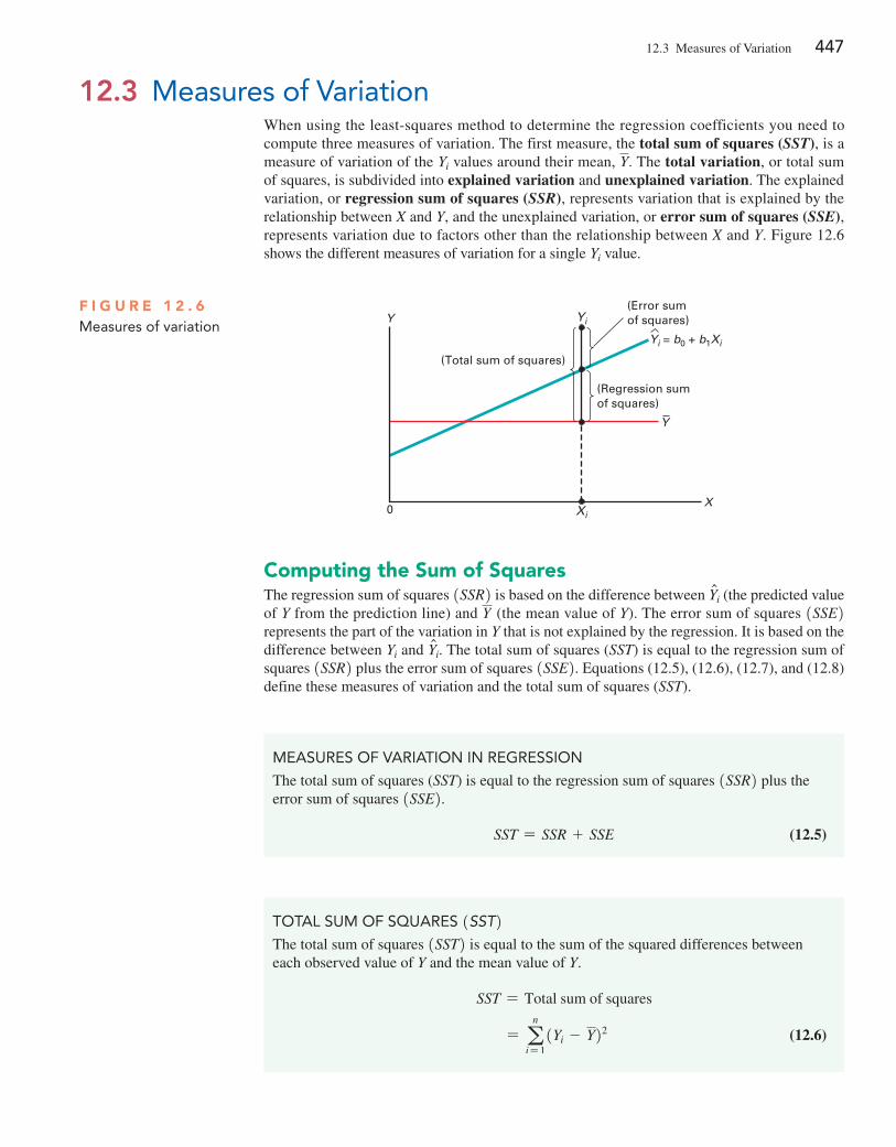
12.3 Measures of Variation 447
Computing the Sum of SquaresThe regression sum of squares 1SSR2 is based on the difference between Yni (the predicted value of Y from the prediction line) and Y (the mean value of Y). The error sum of squares 1SSE2 represents the part of the variation in Y that is not explained by the regression. It is based on the difference between Yi and Yni. The total sum of squares (SST) is equal to the regression sum of squares 1SSR2 plus the error sum of squares 1SSE2. equations (12.5), (12.6), (12.7), and (12.8) define these measures of variation and the total sum of squares (SST).
12.3 Measures of VariationWhen using the least-squares method to determine the regression coefficients you need to compute three measures of variation. The first measure, the total sum of squares (SST), is a measure of variation of the Yi values around their mean, Y. The total variation, or total sum of squares, is subdivided into explained variation and unexplained variation. The explained variation, or regression sum of squares (SSR), represents variation that is explained by the relationship between X and Y, and the unexplained variation, or error sum of squares (SSE), represents variation due to factors other than the relationship between X and Y. Figure 12.6 shows the different measures of variation for a single Yi value.
(Error sumof squares)
(Regression sumof squares)
Y
Xi
Yi
Yi = b0 + b1Xi
(Total sum of squares)
Y
X0
F i g u r e 1 2 . 6Measures of variation
MEASURES oF VARIATIon In REgRESSIon
The total sum of squares (SST) is equal to the regression sum of squares 1SSR2 plus the error sum of squares 1SSE2.
SST = SSR + SSE (12.5)
ToTAL SUM oF SqUARES 1SST2The total sum of squares 1SST2 is equal to the sum of the squared differences between each observed value of Y and the mean value of Y.
SST = Total sum of squares
= an
i= 11Yi - Y22 (12.6)
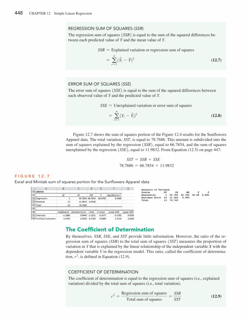
448 CHApTeR 12 Simple Linear Regression
Figure 12.7 shows the sum of squares portion of the Figure 12.4 results for the Sunflowers Apparel data. The total variation, SST, is equal to 78.7686. This amount is subdivided into the sum of squares explained by the regression 1SSR2, equal to 66.7854, and the sum of squares unexplained by the regression 1SSE2, equal to 11.9832. From equation (12.5) on page 447:
SST = SSR + SSE
78.7686 = 66.7854 + 11.9832
REgRESSIon SUM oF SqUARES (SSR)
The regression sum of squares 1SSR2 is equal to the sum of the squared differences be-tween each predicted value of Y and the mean value of Y.
SSR = explained variation or regression sum of squares
= an
i= 11Yni - Y22 (12.7)
ERRoR SUM oF SqUARES (SSE)
The error sum of squares 1SSE2 is equal to the sum of the squared differences between each observed value of Y and the predicted value of Y.
SSE = Unexplained variation or error sum of squares
= an
i= 11Yi - Yni22 (12.8)
F i g u r e 1 2 . 7Excel and Minitab sum of squares portion for the Sunflowers Apparel data
The Coefficient of DeterminationBy themselves, SSR, SSE, and SST provide little information. However, the ratio of the re-gression sum of squares (SSR) to the total sum of squares 1SST2 measures the proportion of variation in Y that is explained by the linear relationship of the independent variable X with the dependent variable Y in the regression model. This ratio, called the coefficient of determina-tion, r 2, is defined in equation (12.9).
CoEFFICIEnT oF DETERMInATIon
The coefficient of determination is equal to the regression sum of squares (i.e., explained variation) divided by the total sum of squares (i.e., total variation).
r 2 =Regression sum of squares
Total sum of squares=
SSR
SST (12.9)
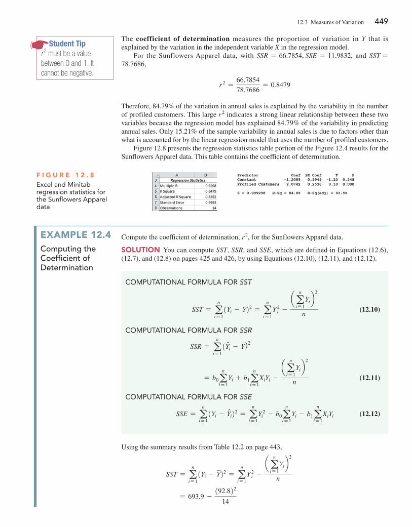
12.3 Measures of Variation 449
The coefficient of determination measures the proportion of variation in Y that is explained by the variation in the independent variable X in the regression model.
For the Sunflowers Apparel data, with SSR = 66.7854, SSE = 11.9832, and SST = 78.7686,
r 2 =66.7854
78.7686= 0.8479
Therefore, 84.79% of the variation in annual sales is explained by the variability in the number of profiled customers. This large r 2 indicates a strong linear relationship between these two variables because the regression model has explained 84.79% of the variability in predicting annual sales. Only 15.21% of the sample variability in annual sales is due to factors other than what is accounted for by the linear regression model that uses the number of profiled customers.
Figure 12.8 presents the regression statistics table portion of the Figure 12.4 results for the Sunflowers Apparel data. This table contains the coefficient of determination.
Student Tipr2 must be a value between 0 and 1. It cannot be negative.
F i g u r e 1 2 . 8Excel and Minitab regression statistics for the Sunflowers Apparel data
exaMpLe 12.4computing the coefficient of determination
Compute the coefficient of determination, r 2, for the Sunflowers Apparel data.
SoLuTion You can compute SST, SSR, and SSE, which are defined in equations (12.6), (12.7), and (12.8) on pages 425 and 426, by using equations (12.10), (12.11), and (12.12).
CoMPUTATIonAL FoRMULA FoR SST
SST = an
i= 11Yi - Y22 = a
n
i= 1Y 2
i -a a
n
i= 1Yib
2
n (12.10)
CoMPUTATIonAL FoRMULA FoR SSR
SSR = an
i= 11Yni - Y22
= b0an
i= 1Yi + b1a
n
i= 1XiYi -
a an
i= 1Yib
2
n (12.11)
CoMPUTATIonAL FoRMULA FoR SSE
SSE = an
i= 11Yi - Yni22 = a
n
i= 1Y 2
i - b0an
i= 1Yi - b1a
n
i= 1XiYi (12.12)
Using the summary results from Table 12.2 on page 443,
SST = an
i= 11Yi - Y22 = a
n
i= 1Y 2
i -a a
n
i= 1Yib
2
n
= 693.9 -192.822
14
450 CHApTeR 12 Simple Linear Regression
Standard error of the estimateAlthough the least-squares method produces the line that fits the data with the minimum amount of prediction error, unless all the observed data points fall on a straight line, the pre-diction line is not a perfect predictor. Just as all data values cannot be expected to be exactly equal to their mean, neither can all the values in a regression analysis be expected to be located exactly on the prediction line. Figure 12.5 on page 441 illustrates the variability around the prediction line for the Sunflowers Apparel data. Notice that many of the observed values of Y fall near the prediction line, but none of the values are exactly on the line.
The standard error of the estimate measures the variability of the observed Y values from the predicted Y values in the same way that the standard deviation in Chapter 3 measures the variability of each value around the sample mean. In other words, the standard error of the estimate is the standard deviation around the prediction line, whereas the standard deviation in Chapter 3 is the standard deviation around the sample mean. equation (12.13) defines the standard error of the estimate, represented by the symbol SYX.
= 693.9 - 615.13142
= 78.76858
SSR = an
i= 11Yni - Y22
= b0an
i= 1Yi + b1a
n
i= 1XiYi -
a an
i= 1Yib
2
n
= 1-1.20882652192.82 + 12.0741721382.852 - 192.822
14
= 66.7854
SSE = an
i= 11Yi - Yni22
= an
i= 1Y 2
i - b0an
i= 1Yi - b1a
n
i= 1XiYi
= 693.9 - 1-1.20882652192.82 - 12.0741721382.852 = 11.9832
Therefore,
r 2 =66.7854
78.7686= 0.8479
Student TipCoefficients computed manually with the assistance of handheld calculators may differ slightly.
STAnDARD ERRoR oF ThE ESTIMATE
SYX = A SSE
n - 2= H a
n
i= 11Yi - Yni22
n - 2 (12.13)
where
Yi = actual value of Y for a given Xi
Yni = predicted value of Y for a given Xi
SSE = error sum of squares
12.3 Measures of Variation 451
From equation (12.8) and Figure 12.4 or Figure 12.7 on pages 418 or 426, SSE = 11.9832. Thus,
SYX = A11.9832
14 - 2= 0.9993
This standard error of the estimate, equal to 0.9993 millions of dollars (i.e., $999,300), is labeled Standard error in the Figure 12.8 excel results and S in the Minitab results. The standard error of the estimate represents a measure of the variation around the prediction line. It is measured in the same units as the dependent variable Y. The interpretation of the standard error of the estimate is similar to that of the standard deviation. Just as the standard deviation measures variability around the mean, the standard error of the estimate measures variability around the prediction line. For Sunflowers Apparel, the typical difference between actual annual sales at a store and the predicted annual sales using the regression equation is approximately $999,300.
problems for Section 12.3Learning The baSiCS12.11 How do you interpret a coefficient of determination, r2, equal to 0.14?
12.12 If SSR = 36 and SSE = 4, determine SST and then com-pute the coefficient of determination, r2, and interpret its meaning.
12.13 If SSR = 66 and SST = 88, compute the coefficient of determination, r2, and interpret its meaning.
12.14 If SSE = 12 and SSR = 28, compute the coefficient of determination, r2, and interpret its meaning.
12.15 If SSR = 120, why is it impossible for SST to equal 110?
appLying The ConCepTSSELF Test
12.16 In problem 12.4 on page 445, the percentage of alcohol was used to predict wine quality (stored in
VinhoVerde ). For those data, SSR = 21.8677 and SST = 64.0000.a. Determine the coefficient of determination, r2, and interpret its
meaning.b. Determine the standard error of the estimate.c. How useful do you think this regression model is for predicting
sales?
12.17 In problem 12.5 on page 446, you used the summated rat-ing to predict the cost of a restaurant meal (stored in restaurants ). For those data, SSR = 9,740.0629 and SST = 17,844.75.a. Determine the coefficient of determination, r2, and interpret its
meaning.b. Determine the standard error of the estimate.c. How useful do you think this regression model is for predicting
the cost of a restaurant meal?
12.18 In problem 12.6 on page 446, an owner of a moving com-pany wanted to predict labor hours, based on the cubic feet moved (stored in Moving ). Using the results of that problem,a. determine the coefficient of determination, r2, and interpret its
meaning.b. determine the standard error of the estimate.c. How useful do you think this regression model is for predicting
labor hours?
12.19 In problem 12.7 on page 446, you used the plate gap on the bag-sealing equipment to predict the tear rating of a bag of cof-fee (stored in Starbucks ). Using the results of that problem,a. determine the coefficient of determination, r2, and interpret its
meaning.b. determine the standard error of the estimate.c. How useful do you think this regression model is for predicting the
tear rating based on the plate gap in the bag-sealing equipment?
12.20 In problem 12.8 on page 446, you used annual revenues to predict the value of a baseball franchise (stored in bbValues ). Using the results of that problem,a. determine the coefficient of determination, r2, and interpret its
meaning.b. determine the standard error of the estimate.c. How useful do you think this regression model is for predicting
the value of a baseball franchise?
12.21 In problem 12.9 on page 446, an agent for a real estate company wanted to predict the monthly rent for one- bedroom apartments, based on the size of the apartment (stored in rent-SilverSpring ). Using the results of that problem,a. determine the coefficient of determination, r2, and interpret its
meaning.b. determine the standard error of the estimate.c. How useful do you think this regression model is for predicting
the monthly rent?d. Can you think of other variables that might explain the varia-
tion in monthly rent?
12.22 In problem 12.10 on page 446, you used box office gross to predict DVD revenue (stored in Movie ). Using the results of that problem,a. determine the coefficient of determination, r2, and interpret its
meaning.b. determine the standard error of the estimate.c. How useful do you think this regression model is for predicting
DVD revenue?d. Can you think of other variables that might explain the varia-
tion in DVD revenue?
452 CHApTeR 12 Simple Linear Regression
12.4 Assumptions of RegressionWhen hypothesis testing and the analysis of variance were discussed in Chapters 9 through 11, the importance of the assumptions to the validity of any conclusions reached was emphasized. The assumptions necessary for regression are similar to those of the analysis of variance be-cause both are part of the general category of linear models (reference 4).
The four assumptions of regression (known by the acronym LINe) are:
• Linearity • Independence of errors • Normality of error • equal variance
The first assumption, linearity, states that the relationship between variables is linear. Relationships between variables that are not linear are discussed in reference 4.
The second assumption, independence of errors, requires that the errors 1ei2 be indepen-dent of one another. This assumption is particularly important when data are collected over a period of time. In such situations, the errors in a specific time period are sometimes correlated with those of the previous time period.
The third assumption, normality, requires that the errors 1ei2 be normally distributed at each value of X. Like the t test and the ANOVA F test, regression analysis is fairly robust against departures from the normality assumption. As long as the distribution of the errors at each level of X is not extremely different from a normal distribution, inferences about b0 and b1 are not seriously affected.
The fourth assumption, equal variance, or homoscedasticity, requires that the variance of the errors 1ei2 be constant for all values of X. In other words, the variability of Y values is the same when X is a low value as when X is a high value. The equal-variance assumption is important when making inferences about b0 and b1. If there are serious departures from this assumption, you can use either data transformations or weighted least-squares methods (see reference 4).
12.5 Residual AnalysisSections 12.2 and 12.3 developed a regression model using the least-squares method for the Sunflowers Apparel data. Is this the correct model for these data? Are the assumptions pre-sented in Section 12.4 valid? Residual analysis visually evaluates these assumptions and helps you determine whether the regression model that has been selected is appropriate.
The residual, or estimated error value, ei, is the difference between the observed 1Yi2 and predicted 1Yni2 values of the dependent variable for a given value of Xi. A residual appears on a scatter plot as the vertical distance between an observed value of Y and the prediction line. equation (12.14) defines the residual.
RESIDUAL
The residual is equal to the difference between the observed value of Y and the predicted value of Y.
ei = Yi - Yni (12.14)
evaluating the assumptionsRecall from Section 12.4 that the four assumptions of regression (known by the acronym LINe) are linearity, independence, normality, and equal variance.
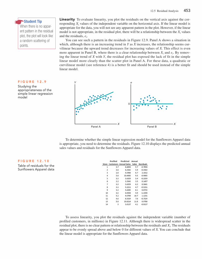
12.5 Residual Analysis 453
To assess linearity, you plot the residuals against the independent variable (number of profiled customers, in millions) in Figure 12.11. Although there is widespread scatter in the residual plot, there is no clear pattern or relationship between the residuals and Xi. The residuals appear to be evenly spread above and below 0 for different values of X. You can conclude that the linear model is appropriate for the Sunflowers Apparel data.
Student TipWhen there is no appar-ent pattern in the residual plot, the plot will look like a random scattering of points.
Linearity To evaluate linearity, you plot the residuals on the vertical axis against the cor-responding Xi values of the independent variable on the horizontal axis. If the linear model is appropriate for the data, you will not see any apparent pattern in the plot. However, if the linear model is not appropriate, in the residual plot, there will be a relationship between the Xi values and the residuals, ei.
You can see such a pattern in the residuals in Figure 12.9. panel A shows a situation in which, although there is an increasing trend in Y as X increases, the relationship seems cur-vilinear because the upward trend decreases for increasing values of X. This effect is even more apparent in panel B, where there is a clear relationship between Xi and ei. By remov-ing the linear trend of X with Y, the residual plot has exposed the lack of fit in the simple linear model more clearly than the scatter plot in panel A. For these data, a quadratic or curvilinear model (see reference 4) is a better fit and should be used instead of the simple linear model.
Y
Panel A Panel BX
0
e
X
F i g u r e 1 2 . 9Studying the appropriateness of the simple linear regression model
To determine whether the simple linear regression model for the Sunflowers Apparel data is appropriate, you need to determine the residuals. Figure 12.10 displays the predicted annual sales values and residuals for the Sunflowers Apparel data.
F i g u r e 1 2 . 1 0Table of residuals for the Sunflowers Apparel data
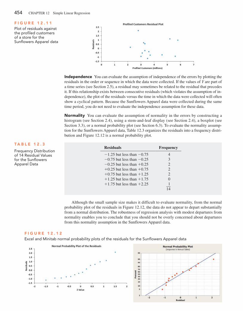
454 CHApTeR 12 Simple Linear Regression
F i g u r e 1 2 . 1 1Plot of residuals against the profiled customers of a store for the Sunflowers Apparel data
independence You can evaluate the assumption of independence of the errors by plotting the residuals in the order or sequence in which the data were collected. If the values of Y are part of a time series (see Section 2.5), a residual may sometimes be related to the residual that precedes it. If this relationship exists between consecutive residuals (which violates the assumption of in-dependence), the plot of the residuals versus the time in which the data were collected will often show a cyclical pattern. Because the Sunflowers Apparel data were collected during the same time period, you do not need to evaluate the independence assumption for these data.
normality You can evaluate the assumption of normality in the errors by constructing a histogram (see Section 2.4), using a stem-and-leaf display (see Section 2.4), a boxplot (see Section 3.3), or a normal probability plot (see Section 6.3). To evaluate the normality assump-tion for the Sunflowers Apparel data, Table 12.3 organizes the residuals into a frequency distri-bution and Figure 12.12 is a normal probability plot.
T a b L e 1 2 . 3
Frequency Distribution of 14 Residual Values for the Sunflowers Apparel Data
Residuals Frequency
-1.25 but less than -0.75 4-0.75 but less than -0.25 3-0.25 but less than +0.25 2+0.25 but less than +0.75 2+0.75 but less than +1.25 2+1.25 but less than +1.75 0+1.75 but less than +2.25 1
14
Although the small sample size makes it difficult to evaluate normality, from the normal probability plot of the residuals in Figure 12.12, the data do not appear to depart substantially from a normal distribution. The robustness of regression analysis with modest departures from normality enables you to conclude that you should not be overly concerned about departures from this normality assumption in the Sunflowers Apparel data.
F i g u r e 1 2 . 1 2Excel and Minitab normal probability plots of the residuals for the Sunflowers Apparel data
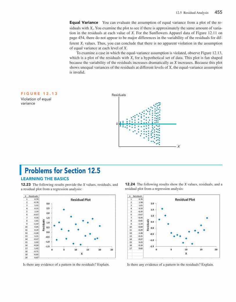
12.5 Residual Analysis 455
equal Variance You can evaluate the assumption of equal variance from a plot of the re-siduals with Xi. You examine the plot to see if there is approximately the same amount of varia-tion in the residuals at each value of X. For the Sunflowers Apparel data of Figure 12.11 on page 454, there do not appear to be major differences in the variability of the residuals for dif-ferent Xi values. Thus, you can conclude that there is no apparent violation in the assumption of equal variance at each level of X.
To examine a case in which the equal-variance assumption is violated, observe Figure 12.13, which is a plot of the residuals with Xi for a hypothetical set of data. This plot is fan shaped because the variability of the residuals increases dramatically as X increases. Because this plot shows unequal variances of the residuals at different levels of X, the equal-variance assumption is invalid.
F i g u r e 1 2 . 1 3Violation of equal variance
Residuals
0
X
problems for Section 12.5Learning The baSiCS12.23 The following results provide the X values, residuals, and a residual plot from a regression analysis:
Is there any evidence of a pattern in the residuals? explain.
12.24 The following results show the X values, residuals, and a residual plot from a regression analysis:
Is there any evidence of a pattern in the residuals? explain.
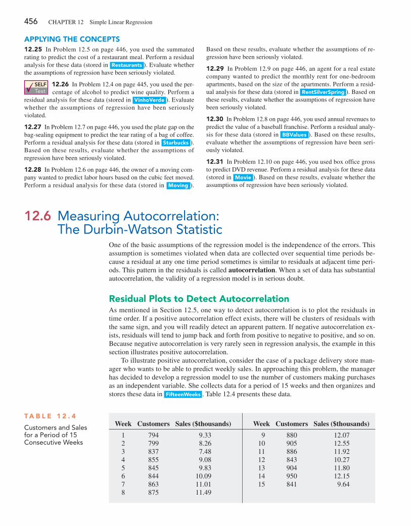
456 CHApTeR 12 Simple Linear Regression
appLying The ConCepTS12.25 In problem 12.5 on page 446, you used the summated rating to predict the cost of a restaurant meal. perform a residual analysis for these data (stored in restaurants ). evaluate whether the assumptions of regression have been seriously violated.
SELF Test
12.26 In problem 12.4 on page 445, you used the per-centage of alcohol to predict wine quality. perform a
residual analysis for these data (stored in VinhoVerde ). evaluate whether the assumptions of regression have been seriously violated.
12.27 In problem 12.7 on page 446, you used the plate gap on the bag-sealing equipment to predict the tear rating of a bag of coffee. perform a residual analysis for these data (stored in Starbucks ). Based on these results, evaluate whether the assumptions of regression have been seriously violated.
12.28 In problem 12.6 on page 446, the owner of a moving com-pany wanted to predict labor hours based on the cubic feet moved. perform a residual analysis for these data (stored in Moving ).
12.6 Measuring Autocorrelation: The Durbin-Watson Statistic
One of the basic assumptions of the regression model is the independence of the errors. This assumption is sometimes violated when data are collected over sequential time periods be-cause a residual at any one time period sometimes is similar to residuals at adjacent time peri-ods. This pattern in the residuals is called autocorrelation. When a set of data has substantial autocorrelation, the validity of a regression model is in serious doubt.
residual plots to Detect autocorrelationAs mentioned in Section 12.5, one way to detect autocorrelation is to plot the residuals in time order. If a positive autocorrelation effect exists, there will be clusters of residuals with the same sign, and you will readily detect an apparent pattern. If negative autocorrelation ex-ists, residuals will tend to jump back and forth from positive to negative to positive, and so on. Because negative autocorrelation is very rarely seen in regression analysis, the example in this section illustrates positive autocorrelation.
To illustrate positive autocorrelation, consider the case of a package delivery store man-ager who wants to be able to predict weekly sales. In approaching this problem, the manager has decided to develop a regression model to use the number of customers making purchases as an independent variable. She collects data for a period of 15 weeks and then organizes and stores these data in FifteenWeeks . Table 12.4 presents these data.
T a b L e 1 2 . 4
Customers and Sales for a Period of 15 Consecutive Weeks
Week Customers Sales ($thousands)
1 794 9.332 799 8.263 837 7.484 855 9.085 845 9.836 844 10.097 863 11.018 875 11.49
Week Customers Sales ($thousands)
9 880 12.0710 905 12.5511 886 11.9212 843 10.2713 904 11.8014 950 12.1515 841 9.64
Based on these results, evaluate whether the assumptions of re-gression have been seriously violated.
12.29 In problem 12.9 on page 446, an agent for a real estate company wanted to predict the monthly rent for one-bedroom apartments, based on the size of the apartments. perform a resid-ual analysis for these data (stored in rentSilverSpring ). Based on these results, evaluate whether the assumptions of regression have been seriously violated.
12.30 In problem 12.8 on page 446, you used annual revenues to predict the value of a baseball franchise. perform a residual analy-sis for these data (stored in bbValues ). Based on these results, evaluate whether the assumptions of regression have been seri-ously violated.
12.31 In problem 12.10 on page 446, you used box office gross to predict DVD revenue. perform a residual analysis for these data (stored in Movie ). Based on these results, evaluate whether the assumptions of regression have been seriously violated.
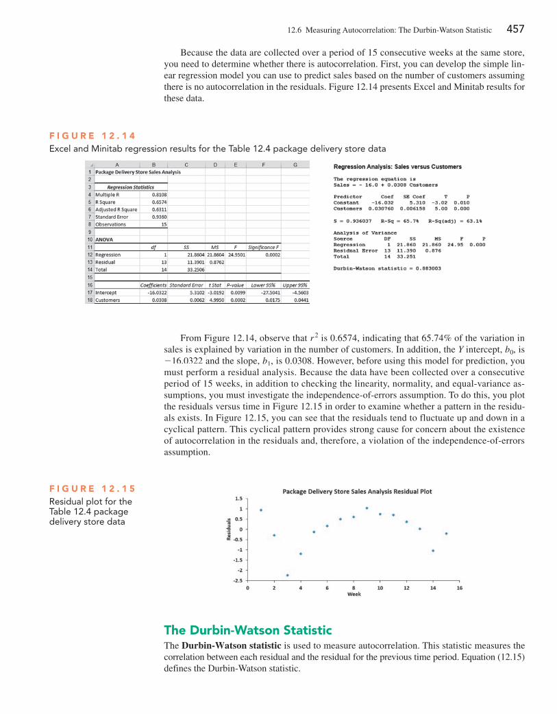
12.6 Measuring Autocorrelation: The Durbin-Watson Statistic 457
Because the data are collected over a period of 15 consecutive weeks at the same store, you need to determine whether there is autocorrelation. First, you can develop the simple lin-ear regression model you can use to predict sales based on the number of customers assuming there is no autocorrelation in the residuals. Figure 12.14 presents excel and Minitab results for these data.
F i g u r e 1 2 . 1 4Excel and Minitab regression results for the Table 12.4 package delivery store data
From Figure 12.14, observe that r 2 is 0.6574, indicating that 65.74% of the variation in sales is explained by variation in the number of customers. In addition, the Y intercept, b0, is -16.0322 and the slope, b1, is 0.0308. However, before using this model for prediction, you must perform a residual analysis. Because the data have been collected over a consecutive period of 15 weeks, in addition to checking the linearity, normality, and equal-variance as-sumptions, you must investigate the independence-of-errors assumption. To do this, you plot the residuals versus time in Figure 12.15 in order to examine whether a pattern in the residu-als exists. In Figure 12.15, you can see that the residuals tend to fluctuate up and down in a cyclical pattern. This cyclical pattern provides strong cause for concern about the existence of autocorrelation in the residuals and, therefore, a violation of the independence-of-errors assumption.
F i g u r e 1 2 . 1 5Residual plot for the Table 12.4 package delivery store data
The Durbin-Watson StatisticThe Durbin-Watson statistic is used to measure autocorrelation. This statistic measures the correlation between each residual and the residual for the previous time period. equation (12.15) defines the Durbin-Watson statistic.
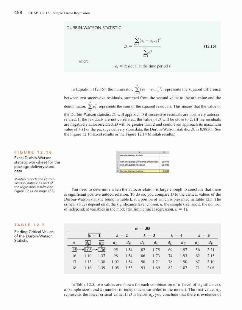
458 CHApTeR 12 Simple Linear Regression
In equation (12.15), the numerator, an
i= 21ei - ei - 122, represents the squared difference
between two successive residuals, summed from the second value to the nth value and the
denominator, an
i= 1e2
i , represents the sum of the squared residuals. This means that the value of
the Durbin-Watson statistic, D, will approach 0 if successive residuals are positively autocor-related. If the residuals are not correlated, the value of D will be close to 2. (If the residuals are negatively autocorrelated, D will be greater than 2 and could even approach its maximum value of 4.) For the package delivery store data, the Durbin-Watson statistic, D, is 0.8830. (See the Figure 12.16 excel results or the Figure 12.14 Minitab results.)
DURbIn-WATSon STATISTIC
D =a
n
i= 21ei - ei - 122
an
i= 1e2
i
(12.15)
whereei = residual at the time period i
F i g u r e 1 2 . 1 6Excel Durbin-Watson statistic worksheet for the package delivery store data
Minitab reports the Durbin-Watson statistic as part of the regression results (see Figure 12.14 on page 457). You need to determine when the autocorrelation is large enough to conclude that there
is significant positive autocorrelation. To do so, you compare D to the critical values of the Durbin-Watson statistic found in Table e.8, a portion of which is presented in Table 12.5. The critical values depend on a, the significance level chosen, n, the sample size, and k, the number of independent variables in the model (in simple linear regression, k = 1).
T a b L e 1 2 . 5
Finding Critical Values of the Durbin-Watson Statistic
A = .05
k = 1 k = 2 k = 3 k = 4 k = 5
n dL dU dL dU dL dU dL dU dL dU
15 1.08 1.36 .95 1.54 .82 1.75 .69 1.97 .56 2.21
16 1.10 1.37 .98 1.54 .86 1.73 .74 1.93 .62 2.15
17 1.13 1.38 1.02 1.54 .90 1.71 .78 1.90 .67 2.10
18 1.16 1.39 1.05 1.53 .93 1.69 .82 1.87 .71 2.06
In Table 12.5, two values are shown for each combination of a (level of significance), n (sample size), and k (number of independent variables in the model). The first value, dL, represents the lower critical value. If D is below dL, you conclude that there is evidence of
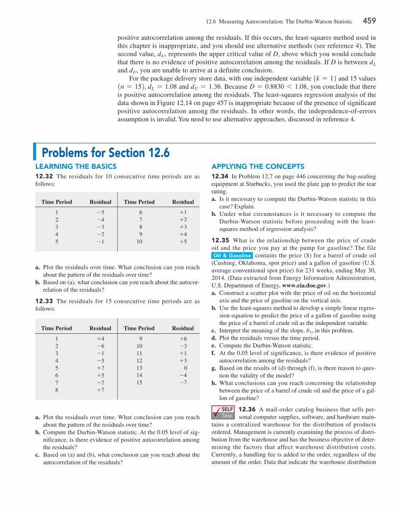
12.6 Measuring Autocorrelation: The Durbin-Watson Statistic 459
positive autocorrelation among the residuals. If this occurs, the least-squares method used in this chapter is inappropriate, and you should use alternative methods (see reference 4). The second value, dU, represents the upper critical value of D, above which you would conclude that there is no evidence of positive autocorrelation among the residuals. If D is between dL and dU, you are unable to arrive at a definite conclusion.
For the package delivery store data, with one independent variable 1k = 12 and 15 values 1n = 152, dL = 1.08 and dU = 1.36. Because D = 0.8830 6 1.08, you conclude that there is positive autocorrelation among the residuals. The least-squares regression analysis of the data shown in Figure 12.14 on page 457 is inappropriate because of the presence of significant positive autocorrelation among the residuals. In other words, the independence-of-errors assumption is invalid. You need to use alternative approaches, discussed in reference 4.
problems for Section 12.6Learning The baSiCS12.32 The residuals for 10 consecutive time periods are as follows:
appLying The ConCepTS12.34 In problem 12.7 on page 446 concerning the bag-sealing equipment at Starbucks, you used the plate gap to predict the tear rating.a. Is it necessary to compute the Durbin-Watson statistic in this
case? explain.b. Under what circumstances is it necessary to compute the
Durbin-Watson statistic before proceeding with the least-squares method of regression analysis?
12.35 What is the relationship between the price of crude oil and the price you pay at the pump for gasoline? The file oil & gasoline contains the price ($) for a barrel of crude oil (Cushing, Oklahoma, spot price) and a gallon of gasoline (U.S. average conventional spot price) for 231 weeks, ending May 30, 2014. (Data extracted from energy Information Administration, U.S. Department of energy, www.eia.doe.gov.)a. Construct a scatter plot with the price of oil on the horizontal
axis and the price of gasoline on the vertical axis.b. Use the least-squares method to develop a simple linear regres-
sion equation to predict the price of a gallon of gasoline using the price of a barrel of crude oil as the independent variable.
c. Interpret the meaning of the slope, b1, in this problem.d. plot the residuals versus the time period.e. Compute the Durbin-Watson statistic.f. At the 0.05 level of significance, is there evidence of positive
autocorrelation among the residuals?g. Based on the results of (d) through (f), is there reason to ques-
tion the validity of the model?h. What conclusions can you reach concerning the relationship
between the price of a barrel of crude oil and the price of a gal-lon of gasoline?
SELF Test
12.36 A mail-order catalog business that sells per-sonal computer supplies, software, and hardware main-
tains a centralized warehouse for the distribution of products ordered. Management is currently examining the process of distri-bution from the warehouse and has the business objective of deter-mining the factors that affect warehouse distribution costs. Currently, a handling fee is added to the order, regardless of the amount of the order. Data that indicate the warehouse distribution
a. plot the residuals over time. What conclusion can you reach about the pattern of the residuals over time?
b. Based on (a), what conclusion can you reach about the autocor-relation of the residuals?
12.33 The residuals for 15 consecutive time periods are as follows:
Time Period Residual
1 -52 -43 -34 -25 -1
Time Period Residual
6 +17 +28 +39 +4
10 +5
Time Period Residual
1 +42 -63 -14 -55 +26 +57 -28 +7
Time Period Residual
9 +610 -311 +112 +313 014 -415 -7
a. plot the residuals over time. What conclusion can you reach about the pattern of the residuals over time?
b. Compute the Durbin-Watson statistic. At the 0.05 level of sig-nificance, is there evidence of positive autocorrelation among the residuals?
c. Based on (a) and (b), what conclusion can you reach about the autocorrelation of the residuals?
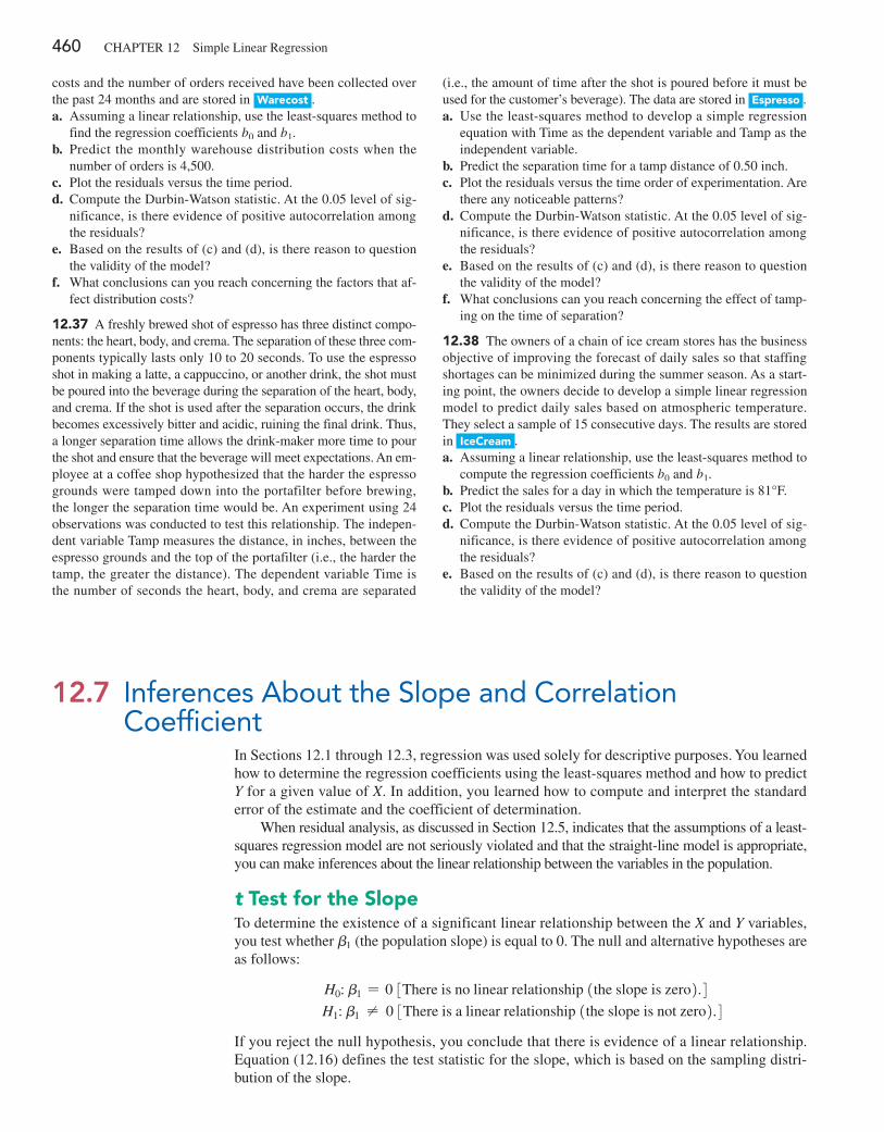
460 CHApTeR 12 Simple Linear Regression
costs and the number of orders received have been collected over the past 24 months and are stored in Warecost .a. Assuming a linear relationship, use the least-squares method to
find the regression coefficients b0 and b1.b. predict the monthly warehouse distribution costs when the
number of orders is 4,500.c. plot the residuals versus the time period.d. Compute the Durbin-Watson statistic. At the 0.05 level of sig-
nificance, is there evidence of positive autocorrelation among the residuals?
e. Based on the results of (c) and (d), is there reason to question the validity of the model?
f. What conclusions can you reach concerning the factors that af-fect distribution costs?
12.37 A freshly brewed shot of espresso has three distinct compo-nents: the heart, body, and crema. The separation of these three com-ponents typically lasts only 10 to 20 seconds. To use the espresso shot in making a latte, a cappuccino, or another drink, the shot must be poured into the beverage during the separation of the heart, body, and crema. If the shot is used after the separation occurs, the drink becomes excessively bitter and acidic, ruining the final drink. Thus, a longer separation time allows the drink-maker more time to pour the shot and ensure that the beverage will meet expectations. An em-ployee at a coffee shop hypothesized that the harder the espresso grounds were tamped down into the portafilter before brewing, the longer the separation time would be. An experiment using 24 observations was conducted to test this relationship. The indepen-dent variable Tamp measures the distance, in inches, between the espresso grounds and the top of the portafilter (i.e., the harder the tamp, the greater the distance). The dependent variable Time is the number of seconds the heart, body, and crema are separated
(i.e., the amount of time after the shot is poured before it must be used for the customer’s beverage). The data are stored in espresso .a. Use the least-squares method to develop a simple regression
equation with Time as the dependent variable and Tamp as the independent variable.
b. predict the separation time for a tamp distance of 0.50 inch.c. plot the residuals versus the time order of experimentation. Are
there any noticeable patterns?d. Compute the Durbin-Watson statistic. At the 0.05 level of sig-
nificance, is there evidence of positive autocorrelation among the residuals?
e. Based on the results of (c) and (d), is there reason to question the validity of the model?
f. What conclusions can you reach concerning the effect of tamp-ing on the time of separation?
12.38 The owners of a chain of ice cream stores has the business objective of improving the forecast of daily sales so that staffing shortages can be minimized during the summer season. As a start-ing point, the owners decide to develop a simple linear regression model to predict daily sales based on atmospheric temperature. They select a sample of 15 consecutive days. The results are stored in iceCream . a. Assuming a linear relationship, use the least-squares method to
compute the regression coefficients b0 and b1.b. predict the sales for a day in which the temperature is 81°F.c. plot the residuals versus the time period.d. Compute the Durbin-Watson statistic. At the 0.05 level of sig-
nificance, is there evidence of positive autocorrelation among the residuals?
e. Based on the results of (c) and (d), is there reason to question the validity of the model?
12.7 Inferences About the Slope and Correlation Coefficient
In Sections 12.1 through 12.3, regression was used solely for descriptive purposes. You learned how to determine the regression coefficients using the least-squares method and how to predict Y for a given value of X. In addition, you learned how to compute and interpret the standard error of the estimate and the coefficient of determination.
When residual analysis, as discussed in Section 12.5, indicates that the assumptions of a least-squares regression model are not seriously violated and that the straight-line model is appropriate, you can make inferences about the linear relationship between the variables in the population.
t Test for the SlopeTo determine the existence of a significant linear relationship between the X and Y variables, you test whether b1 (the population slope) is equal to 0. The null and alternative hypotheses are as follows:
H0: b1 = 0 3There is no linear relationship 1the slope is zero2.4 H1: b1 ≠ 0 3There is a linear relationship 1the slope is not zero2.4
If you reject the null hypothesis, you conclude that there is evidence of a linear relationship. equation (12.16) defines the test statistic for the slope, which is based on the sampling distri-bution of the slope.
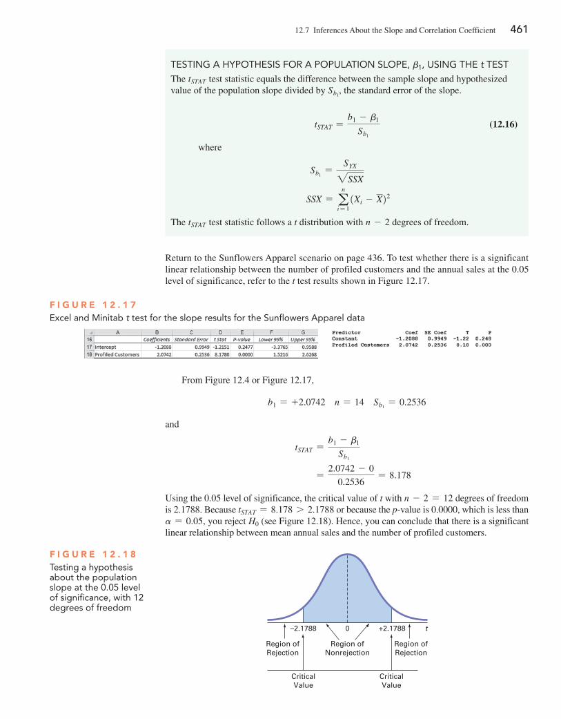
12.7 Inferences About the Slope and Correlation Coefficient 461
TESTIng A hyPoThESIS FoR A PoPULATIon SLoPE, b1, USIng ThE t TEST
The tSTAT test statistic equals the difference between the sample slope and hypothesized value of the population slope divided by Sb1
, the standard error of the slope.
tSTAT =b1 - b1
Sb1
(12.16)
where
Sb1=
SYX2SSX
SSX = an
i= 11Xi - X22
The tSTAT test statistic follows a t distribution with n - 2 degrees of freedom.
Return to the Sunflowers Apparel scenario on page 436. To test whether there is a significant linear relationship between the number of profiled customers and the annual sales at the 0.05 level of significance, refer to the t test results shown in Figure 12.17.
F i g u r e 1 2 . 1 7Excel and Minitab t test for the slope results for the Sunflowers Apparel data
From Figure 12.4 or Figure 12.17,
b1 = +2.0742 n = 14 Sb1= 0.2536
and
tSTAT =b1 - b1
Sb1
=2.0742 - 0
0.2536= 8.178
Using the 0.05 level of significance, the critical value of t with n - 2 = 12 degrees of freedom is 2.1788. Because tSTAT = 8.178 7 2.1788 or because the p-value is 0.0000, which is less than a = 0.05, you reject H0 (see Figure 12.18). Hence, you can conclude that there is a significant linear relationship between mean annual sales and the number of profiled customers.
–2.1788 +2.17880 t
Region ofNonrejection
Region ofRejection
CriticalValue
CriticalValue
Region ofRejection
F i g u r e 1 2 . 1 8Testing a hypothesis about the population slope at the 0.05 level of significance, with 12 degrees of freedom
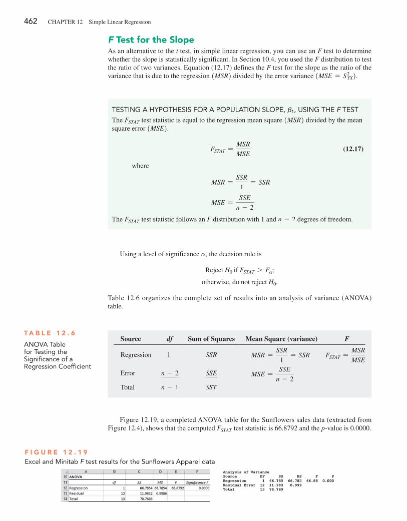
462 CHApTeR 12 Simple Linear Regression
F Test for the SlopeAs an alternative to the t test, in simple linear regression, you can use an F test to determine whether the slope is statistically significant. In Section 10.4, you used the F distribution to test the ratio of two variances. equation (12.17) defines the F test for the slope as the ratio of the variance that is due to the regression 1MSR2 divided by the error variance 1MSE = S2
YX2.
TESTIng A hyPoThESIS FoR A PoPULATIon SLoPE, b1, USIng ThE F TEST
The FSTAT test statistic is equal to the regression mean square 1MSR2 divided by the mean square error 1MSE2.
FSTAT =MSR
MSE (12.17)
where
MSR =SSR
1= SSR
MSE =SSE
n - 2
The FSTAT test statistic follows an F distribution with 1 and n - 2 degrees of freedom.
Using a level of significance a, the decision rule is
Reject H0 if FSTAT 7 Fa;
otherwise, do not reject H0.
Table 12.6 organizes the complete set of results into an analysis of variance (ANOVA) table.
T a b L e 1 2 . 6
AnoVA Table for Testing the Significance of a Regression Coefficient
Source df Sum of Squares Mean Square (variance) F
Regression 1 SSR MSR =SSR
1= SSR FSTAT =
MSR
MSE
error n - 2 SSE MSE =SSE
n - 2Total n - 1 SST
Figure 12.19, a completed ANOVA table for the Sunflowers sales data (extracted from Figure 12.4), shows that the computed FSTAT test statistic is 66.8792 and the p-value is 0.0000.
F i g u r e 1 2 . 1 9Excel and Minitab F test results for the Sunflowers Apparel data
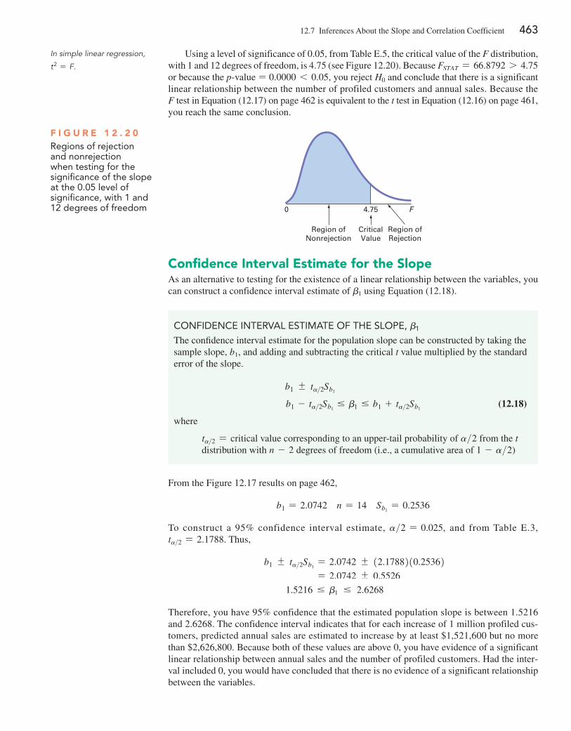
12.7 Inferences About the Slope and Correlation Coefficient 463
Using a level of significance of 0.05, from Table e.5, the critical value of the F distribution, with 1 and 12 degrees of freedom, is 4.75 (see Figure 12.20). Because FSTAT = 66.8792 7 4.75 or because the p-value = 0.0000 6 0.05, you reject H0 and conclude that there is a significant linear relationship between the number of profiled customers and annual sales. Because the F test in equation (12.17) on page 462 is equivalent to the t test in equation (12.16) on page 461, you reach the same conclusion.
0 F4.75
Region ofRejection
CriticalValue
Region ofNonrejection
F i g u r e 1 2 . 2 0Regions of rejection and nonrejection when testing for the significance of the slope at the 0.05 level of significance, with 1 and 12 degrees of freedom
ConFIDEnCE InTERVAL ESTIMATE oF ThE SLoPE, b1
The confidence interval estimate for the population slope can be constructed by taking the sample slope, b1, and adding and subtracting the critical t value multiplied by the standard error of the slope.
b1 { ta>2Sb1
b1 - ta>2Sb1… b1 … b1 + ta>2Sb1
(12.18)
where
ta>2 = critical value corresponding to an upper-tail probability of a>2 from the t distribution with n - 2 degrees of freedom (i.e., a cumulative area of 1 - a>2)
In simple linear regression,
t2 = F.
Confidence interval estimate for the SlopeAs an alternative to testing for the existence of a linear relationship between the variables, you can construct a confidence interval estimate of b1 using equation (12.18).
From the Figure 12.17 results on page 462,
b1 = 2.0742 n = 14 Sb1= 0.2536
To construct a 95% confidence interval estimate, a>2 = 0.025, and from Table e.3, ta>2 = 2.1788. Thus,
b1 { ta>2Sb1= 2.0742 { 12.1788210.25362
= 2.0742 { 0.5526
1.5216 … b1 … 2.6268
Therefore, you have 95% confidence that the estimated population slope is between 1.5216 and 2.6268. The confidence interval indicates that for each increase of 1 million profiled cus-tomers, predicted annual sales are estimated to increase by at least $1,521,600 but no more than $2,626,800. Because both of these values are above 0, you have evidence of a significant linear relationship between annual sales and the number of profiled customers. Had the inter-val included 0, you would have concluded that there is no evidence of a significant relationship between the variables.
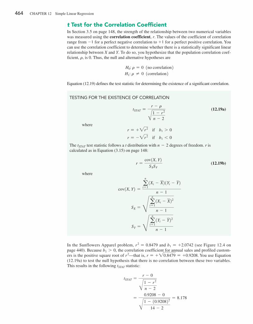
464 CHApTeR 12 Simple Linear Regression
t Test for the Correlation CoefficientIn Section 3.5 on page 148, the strength of the relationship between two numerical variables was measured using the correlation coefficient, r. The values of the coefficient of correlation range from -1 for a perfect negative correlation to +1 for a perfect positive correlation. You can use the correlation coefficient to determine whether there is a statistically significant linear relationship between X and Y. To do so, you hypothesize that the population correlation coef-ficient, r, is 0. Thus, the null and alternative hypotheses are
H0: r = 0 1no correlation2 H1: r ≠ 0 1correlation2
equation (12.19) defines the test statistic for determining the existence of a significant correlation.
TESTIng FoR ThE ExISTEnCE oF CoRRELATIon
tSTAT =r - rA1 - r 2
n - 2
(12.19a)
where r = + 2r 2 if b1 7 0
r = - 2r 2 if b1 6 0
The tSTAT test statistic follows a t distribution with n - 2 degrees of freedom. r is calculated as in equation (3.15) on page 148:
r =cov1X, Y2
SXSY (12.19b)
where
cov1X, Y2 =a
n
i= 11Xi - X21Yi - Y2
n - 1
SX = H an
i= 11Xi - X22
n - 1
SY = H an
i= 11Yi - Y22
n - 1
In the Sunflowers Apparel problem, r 2 = 0.8479 and b1 = +2.0742 (see Figure 12.4 on page 440). Because b1 7 0, the correlation coefficient for annual sales and profiled custom-ers is the positive square root of r 2—that is, r = + 20.8479 = +0.9208. You use equation (12.19a) to test the null hypothesis that there is no correlation between these two variables. This results in the following tSTAT statistic:
tSTAT =r - 0B1 - r 2
n - 2
=0.9208 - 0B1 - 10.920822
14 - 2
= 8.178
12.7 Inferences About the Slope and Correlation Coefficient 465
problems for Section 12.7Learning The baSiCS12.39 You are testing the null hypothesis that there is no linear relationship between two variables, X and Y. From your sample of n = 9, you determine that r = 0.8.a. What is the value of the t test statistic tSTAT?b. At the a = 0.05 level of significance, what are the critical
values?c. Based on your answers to (a) and (b), what statistical decision
should you make?
12.40 You are testing the null hypothesis that there is no linear relationship between two variables, X and Y. From your sample of n = 18, you determine that b1 = +4.5 and Sb1
= 1.5.a. What is the value of tSTAT?b. At the a = 0.05 level of significance, what are the critical
values?c. Based on your answers to (a) and (b), what statistical decision
should you make?d. Construct a 95% confidence interval estimate of the population
slope, b1.
12.41 You are testing the null hypothesis that there is no linear relationship between two variables, X and Y. From your sample of n = 20, you determine that SSR = 60 and SSE = 40.a. What is the value of FSTAT?b. At the a = 0.05 level of significance, what is the critical
value?c. Based on your answers to (a) and (b), what statistical decision
should you make?d. Compute the correlation coefficient by first computing r 2 and
assuming that b1 is negative.e. At the 0.05 level of significance, is there a significant correla-
tion between X and Y?
appLying The ConCepTSSELF Test
12.42 In problem 12.4 on page 445, you used the per-centage of alcohol to predict wine quality. The data are
stored in VinhoVerde . From the results of that problem, b1 = 0.5624 and Sb1
= 0.1127.a. At the 0.05 level of significance, is there evidence of a lin-
ear relationship between the percentage of alcohol and wine quality?
b. Construct a 95% confidence interval estimate of the population slope, b1.
12.43 In problem 12.5 on page 446, you used the summated rat-ing of a restaurant to predict the cost of a meal. The data are stored in restaurants . Using the results of that problem, b1 = 1.4963 and Sb1
= 0.1379.
a. At the 0.05 level of significance, is there evidence of a linear relationship between the summated rating of a restaurant and the cost of a meal?
b. Construct a 95% confidence interval estimate of the population slope, b1.
12.44 In problem 12.6 on page 446, the owner of a moving com-pany wanted to predict labor hours, based on the number of cubic feet moved. The data are stored in Moving . Use the results of that problem.a. At the 0.05 level of significance, is there evidence of a linear
relationship between the number of cubic feet moved and labor hours?
b. Construct a 95% confidence interval estimate of the population slope, b1.
12.45 In problem 12.7 on page 446, you used the plate gap in the bag-sealing equipment to predict the tear rating of a bag of coffee. The data are stored in Starbucks . Use the results of that problem.a. At the 0.05 level of significance, is there evidence of a linear
relationship between the plate gap of the bag-sealing machine and the tear rating of a bag of coffee?
b. Construct a 95% confidence interval estimate of the population slope, b1.
12.46 In problem 12.8 on page 446, you used annual revenues to predict the value of a baseball franchise. The data are stored in bbValues . Use the results of that problem.a. At the 0.05 level of significance, is there evidence of a linear
relationship between annual revenue and franchise value?b. Construct a 95% confidence interval estimate of the population
slope, b1.
12.47 In problem 12.9 on page 446, an agent for a real estate company wanted to predict the monthly rent for one-bedroom apartments, based on the size of the apartment. The data are stored in rentSilverSpring . Use the results of that problem.a. At the 0.05 level of significance, is there evidence of a linear
relationship between the size of the apartment and the monthly rent?
b. Construct a 95% confidence interval estimate of the population slope, b1.
12.48 In problem 12.10 on page 446, you used box office gross to predict DVD revenue. The data are stored in Movie . Use the results of that problem.a. At the 0.05 level of significance, is there evidence of a linear
relationship between box office gross and DVD revenue?b. Construct a 95% confidence interval estimate of the population
slope, b1.
Using the 0.05 level of significance, because tSTAT = 8.178 7 2.1788, you reject the null hypothesis. You conclude that there is a significant association between annual sales and the number of profiled customers. This tSTAT test statistic is equivalent to the tSTAT test statistic found when testing whether the population slope, b1, is equal to zero.
466 CHApTeR 12 Simple Linear Regression
12.49 The volatility of a stock is often measured by its beta value. You can estimate the beta value of a stock by developing a simple linear regression model, using the percentage weekly change in the stock as the dependent variable and the percentage weekly change in a market index as the independent variable. The S&p 500 Index is a common index to use. For example, if you wanted to estimate the beta value for Disney, you could use the following model, which is sometimes referred to as a market model:
1% weekly change in Disney2 = b0
+ b11% weekly change in S & p 500 index2 + e
The least-squares regression estimate of the slope b1 is the esti-mate of the beta value for Disney. A stock with a beta value of 1.0 tends to move the same as the overall market. A stock with a beta value of 1.5 tends to move 50% more than the overall market, and a stock with a beta value of 0.6 tends to move only 60% as much as the overall market. Stocks with negative beta values tend to move in the opposite direction of the overall market. The fol-lowing table gives some beta values for some widely held stocks as of June 8, 2014:
Company Ticker Symbol Beta
Apple AApL 0.74Disney DIS 1.32Dr. pepper Snapple Group DpS 0.22Marriott MAR 1.34Microsoft MSFT 0.68procter & Gamble pG 0.40Source: Data extracted from finance.yahoo.com, June 8, 2014.
a. For each of the six companies, interpret the beta value.b. How can investors use the beta value as a guide for investing?
12.50 Index funds are mutual funds that try to mimic the move-ment of leading indexes, such as the S&p 500 or the Russell 2000. The beta values (as described in problem 12.49) for these funds are therefore approximately 1.0, and the estimated market models for these funds are approximately
1% weekly change in index fund2 = 0.0 + 1.01% weekly change in the index2
Leveraged index funds are designed to magnify the movement of major indexes. Direxion Funds is a leading provider of leveraged index and other alternative-class mutual fund products for invest-ment advisors and sophisticated investors. Two of the company’s funds are shown in the following table:
NameTicker Symbol Description
Daily Small Cap Bull 3x Fund
TNA 300% of the Russell 2000 Index
Monthly S&p Bear 2x Fund
DXSSX 200% of the S&p 500 Index
Source: Data extracted from www.direxionfunds.com.
The estimated market models for these funds are approximately
1% weekly change in TNA2 = 0.0 + 3.0 1% weekly change in the Russell 20002
1% weekly change in DXSSX2 = 0.0 + 2.01% weekly change in the S&p 500 Index2
Thus, if the Russell 2000 Index gains 10% over a period of time, the leveraged mutual fund TNA gains approximately 30%. On the downside, if the same index loses 20%, TNA loses approximately 60%.a. The objective of the Direxion Funds Bull 3x Fund, SpXL, is
300% of the performance of the S&p 500 Index. What is its ap-proximate market model?
b. If the S&p 500 Index gains 10% in a year, what return do you expect SpXL to have?
c. If the S&p 500 Index loses 20% in a year, what return do you expect SpXL to have?
d. What type of investors should be attracted to leveraged index funds? What type of investors should stay away from these funds?
12.51 The file CoffeeDrink contains the calories and fat, in grams, of seven different types of coffee drinks:
Coffee Drink Calories Fat
1 238 7.92 259 3.43 346 22.24 347 19.85 419 16.36 505 21.57 527 18.7
a. Compute and interpret the coefficient of correlation, r.b. At the 0.05 level of significance, is there a significant linear
relationship between calories and fat?
12.52 Movie companies need to predict the gross receipts of an individual movie once the movie has debuted. The following re-sults (stored in potterMovies ) are the first weekend gross, the U.S. gross, and the worldwide gross (in $millions) of the eight Harry potter movies that debuted from 2001 to 2011:
TitleFirst
WeekendU.S.
GrossWorldwide
Gross
Sorcerer’s Stone 90.295 317.558 976.458Chamber of Secrets 88.357 261.988 878.988Prisoner of Azkaban 93.687 249.539 795.539Goblet of Fire 102.335 290.013 896.013Order of the Phoenix 77.108 292.005 938.469Half-Blood Prince 77.836 301.460 934.601Deathly Hallows Part I 125.017 295.001 955.417Deathly Hallows Part II 169.189 381.001 1,328.11Source: Data extracted from www.the-numbers.com/interactive/ comp-Harry-Potter.php.
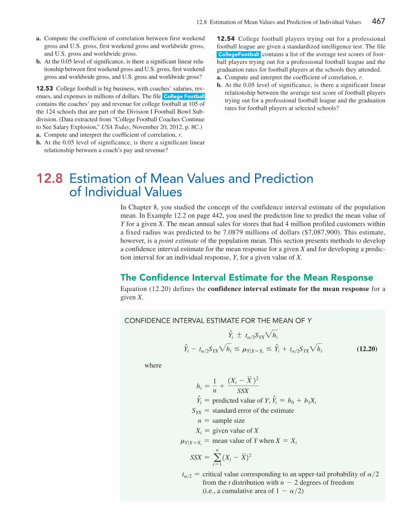
12.8 estimation of Mean Values and prediction of Individual Values 467
a. Compute the coefficient of correlation between first weekend gross and U.S. gross, first weekend gross and worldwide gross, and U.S. gross and worldwide gross.
b. At the 0.05 level of significance, is there a significant linear rela-tionship between first weekend gross and U.S. gross, first weekend gross and worldwide gross, and U.S. gross and worldwide gross?
12.53 College football is big business, with coaches’ salaries, rev-enues, and expenses in millions of dollars. The file College Football contains the coaches’ pay and revenue for college football at 105 of the 124 schools that are part of the Division I Football Bowl Sub-division. (Data extracted from “College Football Coaches Continue to See Salary explosion,” USA Today, November 20, 2012, p. 8C.)a. Compute and interpret the coefficient of correlation, r.b. At the 0.05 level of significance, is there a significant linear
relationship between a coach’s pay and revenue?
12.54 College football players trying out for a professional football league are given a standardized intelligence test. The file CollegeFootball contains a list of the average test scores of foot-ball players trying out for a professional football league and the graduation rates for football players at the schools they attended.a. Compute and interpret the coefficient of correlation, r.b. At the 0.05 level of significance, is there a significant linear
relationship between the average test score of football players trying out for a professional football league and the graduation rates for football players at selected schools?
ConFIDEnCE InTERVAL ESTIMATE FoR ThE MEAn oF Y
Yni { ta>2SYX2hi
Yni - ta>2SYX2hi … mY�X= Xi… Yni + ta>2SYX2hi (12.20)
where
hi =1n
+1Xi - X 22
SSX Yni = predicted value of Y; Yni = b0 + b1Xi
SYX = standard error of the estimate
n = sample size
Xi = given value of X
mY�X= Xi= mean value of Y when X = Xi
SSX = an
i= 11Xi - X22
ta>2 = critical value corresponding to an upper-tail probability of a>2 from the t distribution with n - 2 degrees of freedom (i.e., a cumulative area of 1 - a>2)
12.8 Estimation of Mean Values and Prediction of Individual Values
In Chapter 8, you studied the concept of the confidence interval estimate of the population mean. In example 12.2 on page 442, you used the prediction line to predict the mean value of Y for a given X. The mean annual sales for stores that had 4 million profiled customers within a fixed radius was predicted to be 7.0879 millions of dollars ($7,087,900). This estimate, however, is a point estimate of the population mean. This section presents methods to develop a confidence interval estimate for the mean response for a given X and for developing a predic-tion interval for an individual response, Y, for a given value of X.
The Confidence interval estimate for the Mean responseequation (12.20) defines the confidence interval estimate for the mean response for a given X.
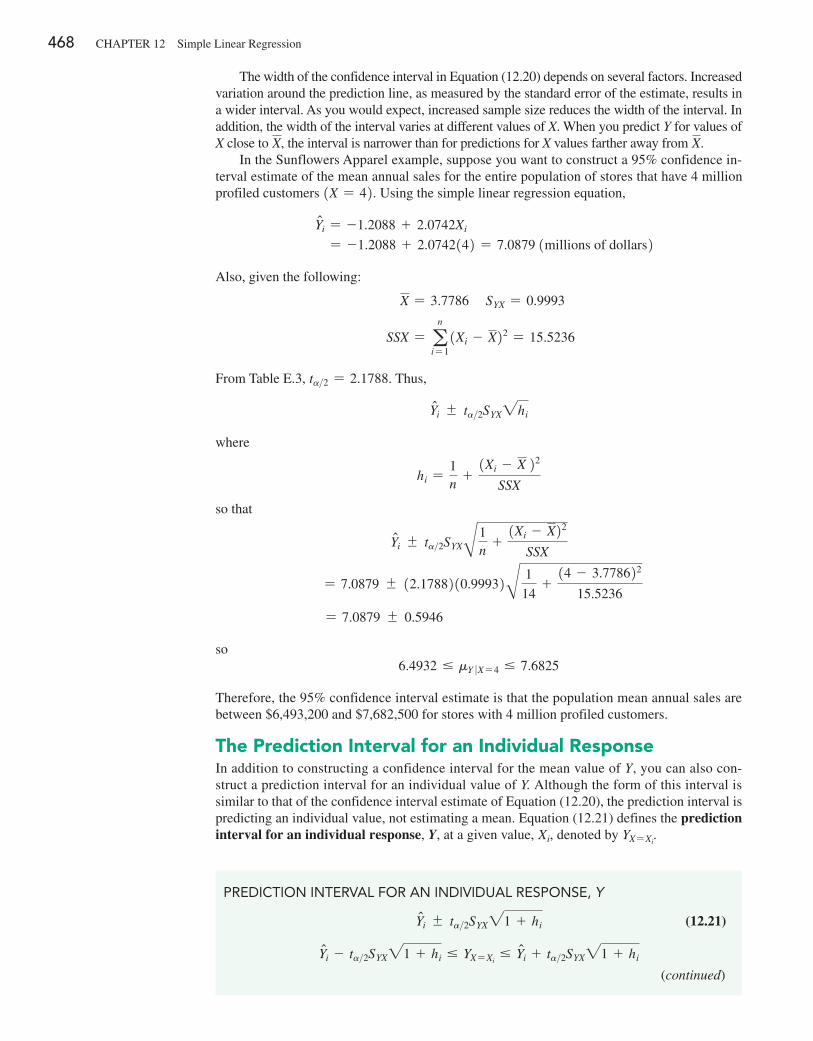
468 CHApTeR 12 Simple Linear Regression
The width of the confidence interval in equation (12.20) depends on several factors. Increased variation around the prediction line, as measured by the standard error of the estimate, results in a wider interval. As you would expect, increased sample size reduces the width of the interval. In addition, the width of the interval varies at different values of X. When you predict Y for values of X close to X, the interval is narrower than for predictions for X values farther away from X.
In the Sunflowers Apparel example, suppose you want to construct a 95% confidence in-terval estimate of the mean annual sales for the entire population of stores that have 4 million profiled customers 1X = 42. Using the simple linear regression equation,
Yni = -1.2088 + 2.0742Xi
= -1.2088 + 2.0742142 = 7.0879 1millions of dollars2
Also, given the following:
X = 3.7786 SYX = 0.9993
SSX = an
i= 11Xi - X22 = 15.5236
From Table e.3, ta>2 = 2.1788. Thus,
Yni { ta>2SYX2hi
where
hi =1n
+1Xi - X 22
SSX
so that
Yni { ta>2SYXB1n
+1Xi - X22
SSX
= 7.0879 { 12.1788210.99932B 1
14+
14 - 3.778622
15.5236
= 7.0879 { 0.5946
so6.4932 … mY �X= 4 … 7.6825
Therefore, the 95% confidence interval estimate is that the population mean annual sales are between $6,493,200 and $7,682,500 for stores with 4 million profiled customers.
The prediction interval for an individual responseIn addition to constructing a confidence interval for the mean value of Y, you can also con-struct a prediction interval for an individual value of Y. Although the form of this interval is similar to that of the confidence interval estimate of equation (12.20), the prediction interval is predicting an individual value, not estimating a mean. equation (12.21) defines the prediction interval for an individual response, Y, at a given value, Xi, denoted by YX= Xi
.
PREDICTIon InTERVAL FoR An InDIVIDUAL RESPonSE, Y
Yni { ta>2SYX21 + hi (12.21)
Yni - ta>2SYX21 + hi … YX= Xi… Yni + ta>2SYX21 + hi
(continued)
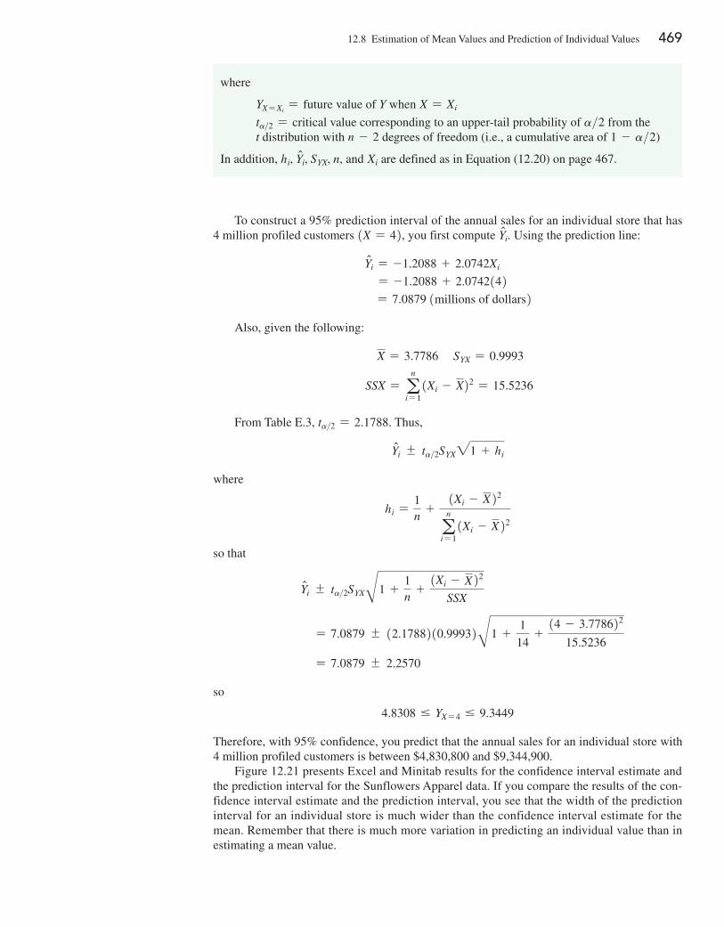
12.8 estimation of Mean Values and prediction of Individual Values 469
To construct a 95% prediction interval of the annual sales for an individual store that has 4 million profiled customers 1X = 42, you first compute Yni. Using the prediction line:
Yni = -1.2088 + 2.0742Xi
= -1.2088 + 2.0742142 = 7.0879 1millions of dollars2
Also, given the following:
X = 3.7786 SYX = 0.9993
SSX = an
i= 11Xi - X22 = 15.5236
From Table e.3, ta>2 = 2.1788. Thus,
Yni { ta>2SYX21 + hi
where
hi =1n
+1Xi - X 22
an
i= 11Xi - X 22
so that
Yni { ta>2SYXB1 +1n
+1Xi - X 22
SSX
= 7.0879 { 12.1788210.99932B1 +1
14+
14 - 3.778622
15.5236
= 7.0879 { 2.2570
so
4.8308 … YX= 4 … 9.3449
Therefore, with 95% confidence, you predict that the annual sales for an individual store with 4 million profiled customers is between $4,830,800 and $9,344,900.
Figure 12.21 presents excel and Minitab results for the confidence interval estimate and the prediction interval for the Sunflowers Apparel data. If you compare the results of the con-fidence interval estimate and the prediction interval, you see that the width of the prediction interval for an individual store is much wider than the confidence interval estimate for the mean. Remember that there is much more variation in predicting an individual value than in estimating a mean value.
where
YX= Xi= future value of Y when X = Xi
ta>2 = critical value corresponding to an upper-tail probability of a>2 from the t distribution with n - 2 degrees of freedom (i.e., a cumulative area of 1 - a>2)
In addition, hi, Yni, SYX, n, and Xi are defined as in equation (12.20) on page 467.
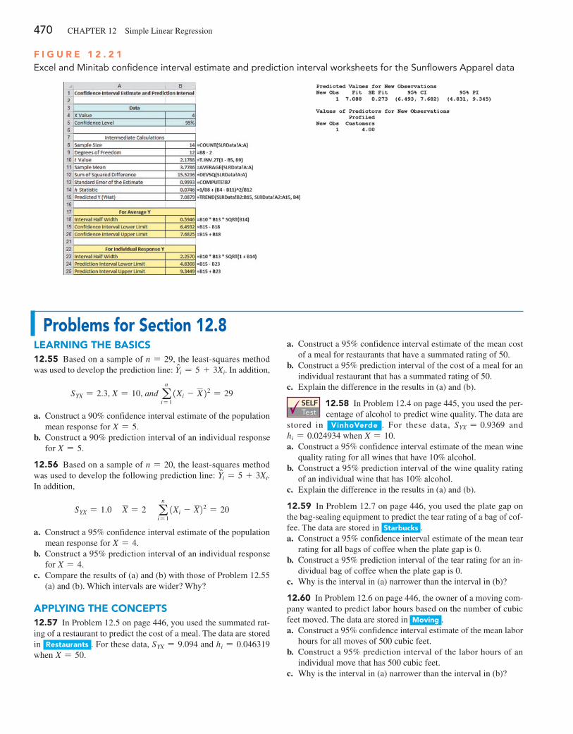
470 CHApTeR 12 Simple Linear Regression
F i g u r e 1 2 . 2 1Excel and Minitab confidence interval estimate and prediction interval worksheets for the Sunflowers Apparel data
problems for Section 12.8Learning The baSiCS12.55 Based on a sample of n = 29, the least-squares method was used to develop the prediction line: Yni = 5 + 3Xi. In addition,
SYX = 2.3, X = 10, and an
i= 11Xi - X 22 = 29
a. Construct a 90% confidence interval estimate of the population mean response for X = 5.
b. Construct a 90% prediction interval of an individual response for X = 5.
12.56 Based on a sample of n = 20, the least-squares method was used to develop the following prediction line: Yni = 5 + 3Xi. In addition,
SYX = 1.0 X = 2 an
i= 11Xi - X22 = 20
a. Construct a 95% confidence interval estimate of the population mean response for X = 4.
b. Construct a 95% prediction interval of an individual response for X = 4.
c. Compare the results of (a) and (b) with those of problem 12.55 (a) and (b). Which intervals are wider? Why?
appLying The ConCepTS12.57 In problem 12.5 on page 446, you used the summated rat-ing of a restaurant to predict the cost of a meal. The data are stored in restaurants . For these data, SYX = 9.094 and hi = 0.046319 when X = 50.
a. Construct a 95% confidence interval estimate of the mean cost of a meal for restaurants that have a summated rating of 50.
b. Construct a 95% prediction interval of the cost of a meal for an individual restaurant that has a summated rating of 50.
c. explain the difference in the results in (a) and (b).
SELF Test
12.58 In problem 12.4 on page 445, you used the per-centage of alcohol to predict wine quality. The data are
stored in VinhoVerde . For these data, SYX = 0.9369 and hi = 0.024934 when X = 10.a. Construct a 95% confidence interval estimate of the mean wine
quality rating for all wines that have 10% alcohol.b. Construct a 95% prediction interval of the wine quality rating
of an individual wine that has 10% alcohol.c. explain the difference in the results in (a) and (b).
12.59 In problem 12.7 on page 446, you used the plate gap on the bag-sealing equipment to predict the tear rating of a bag of cof-fee. The data are stored in Starbucks .a. Construct a 95% confidence interval estimate of the mean tear
rating for all bags of coffee when the plate gap is 0.b. Construct a 95% prediction interval of the tear rating for an in-
dividual bag of coffee when the plate gap is 0.c. Why is the interval in (a) narrower than the interval in (b)?
12.60 In problem 12.6 on page 446, the owner of a moving com-pany wanted to predict labor hours based on the number of cubic feet moved. The data are stored in Moving .a. Construct a 95% confidence interval estimate of the mean labor
hours for all moves of 500 cubic feet.b. Construct a 95% prediction interval of the labor hours of an
individual move that has 500 cubic feet.c. Why is the interval in (a) narrower than the interval in (b)?
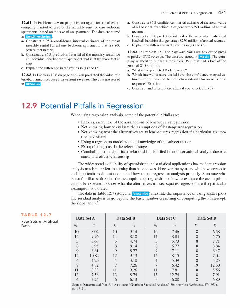
12.9 potential pitfalls in Regression 471
12.9 Potential Pitfalls in RegressionWhen using regression analysis, some of the potential pitfalls are:
• Lacking awareness of the assumptions of least-squares regression • Not knowing how to evaluate the assumptions of least-squares regression • Not knowing what the alternatives are to least-squares regression if a particular assump-
tion is violated • Using a regression model without knowledge of the subject matter • extrapolating outside the relevant range • Concluding that a significant relationship identified in an observational study is due to a
cause-and-effect relationship
The widespread availability of spreadsheet and statistical applications has made regression analysis much more feasible today than it once was. However, many users who have access to such applications do not understand how to use regression analysis properly. Someone who is not familiar with either the assumptions of regression or how to evaluate the assumptions cannot be expected to know what the alternatives to least-squares regression are if a particular assumption is violated.
The data in Table 12.7 (stored in anscombe ) illustrate the importance of using scatter plots and residual analysis to go beyond the basic number crunching of computing the Y intercept, the slope, and r 2.
12.61 In problem 12.9 on page 446, an agent for a real estate company wanted to predict the monthly rent for one-bedroom apartments, based on the size of an apartment. The data are stored in rentSilverSpring .a. Construct a 95% confidence interval estimate of the mean
monthly rental for all one-bedroom apartments that are 800 square feet in size.
b. Construct a 95% prediction interval of the monthly rental for an individual one-bedroom apartment that is 800 square feet in size.
c. explain the difference in the results in (a) and (b).
12.62 In problem 12.8 on page 446, you predicted the value of a baseball franchise, based on current revenue. The data are stored in bbValues .
a. Construct a 95% confidence interval estimate of the mean value of all baseball franchises that generate $250 million of annual revenue.
b. Construct a 95% prediction interval of the value of an individual baseball franchise that generates $250 million of annual revenue.
c. explain the difference in the results in (a) and (b).
12.63 In problem 12.10 on page 446, you used box office gross to predict DVD revenue. The data are stored in Movie . The com-pany is about to release a movie on DVD that had a box office gross of $100 million.a. What is the predicted DVD revenue?b. Which interval is more useful here, the confidence interval es-
timate of the mean or the prediction interval for an individual response? explain.
c. Construct and interpret the interval you selected in (b).
T a b L e 1 2 . 7
Four Sets of Artificial Data
Data Set A Data Set B Data Set C Data Set D
Xi Yi Xi Yi Xi Yi Xi Yi
10 8.04 10 9.14 10 7.46 8 6.5814 9.96 14 8.10 14 8.84 8 5.765 5.68 5 4.74 5 5.73 8 7.718 6.95 8 8.14 8 6.77 8 8.849 8.81 9 8.77 9 7.11 8 8.47
12 10.84 12 9.13 12 8.15 8 7.044 4.26 4 3.10 4 5.39 8 5.257 4.82 7 7.26 7 6.42 19 12.50
11 8.33 11 9.26 11 7.81 8 5.5613 7.58 13 8.74 13 12.74 8 7.916 7.24 6 6.13 6 6.08 8 6.89
Source: Data extracted from F. J. Anscombe, “Graphs in Statistical Analysis,” The American Statistician, 27 (1973), pp. 17–21.
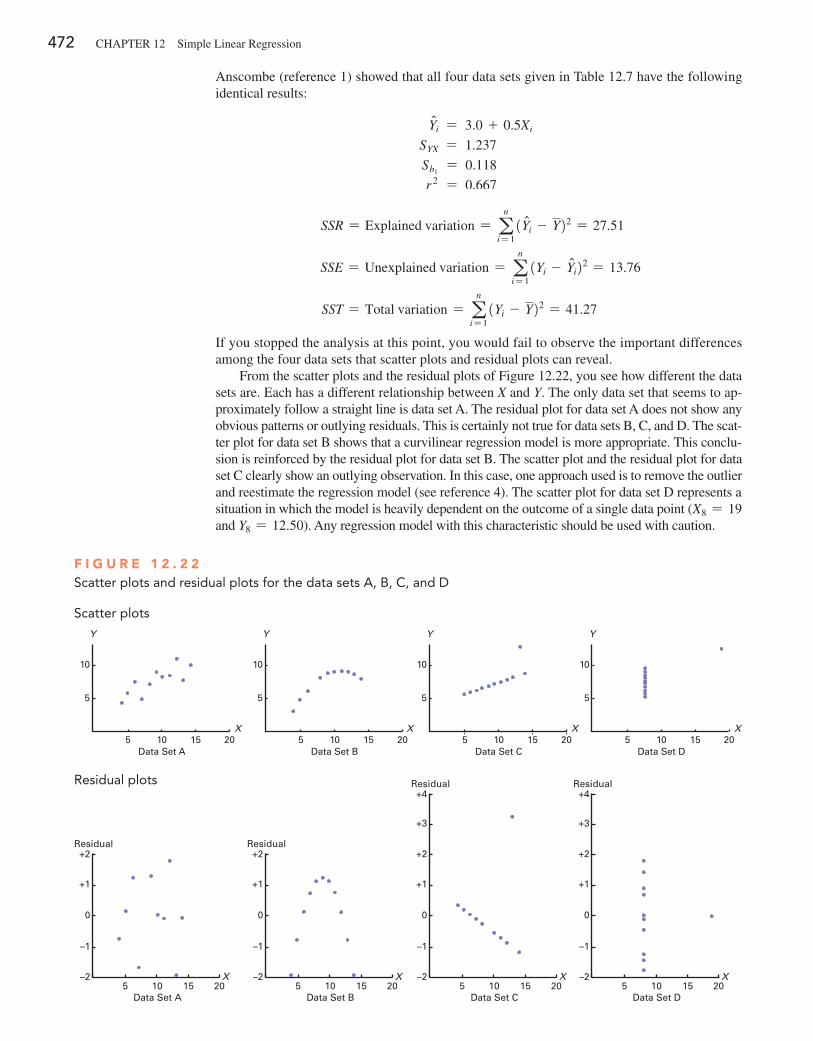
472 CHApTeR 12 Simple Linear Regression
Anscombe (reference 1) showed that all four data sets given in Table 12.7 have the following identical results:
Yni = 3.0 + 0.5Xi
SYX = 1.237
Sb1 = 0.118
r 2 = 0.667
SSR = explained variation = an
i= 11Yni - Y22 = 27.51
SSE = Unexplained variation = an
i= 11Yi - Yni22 = 13.76
SST = Total variation = an
i= 11Yi - Y22 = 41.27
If you stopped the analysis at this point, you would fail to observe the important differences among the four data sets that scatter plots and residual plots can reveal.
From the scatter plots and the residual plots of Figure 12.22, you see how different the data sets are. each has a different relationship between X and Y. The only data set that seems to ap-proximately follow a straight line is data set A. The residual plot for data set A does not show any obvious patterns or outlying residuals. This is certainly not true for data sets B, C, and D. The scat-ter plot for data set B shows that a curvilinear regression model is more appropriate. This conclu-sion is reinforced by the residual plot for data set B. The scatter plot and the residual plot for data set C clearly show an outlying observation. In this case, one approach used is to remove the outlier and reestimate the regression model (see reference 4). The scatter plot for data set D represents a situation in which the model is heavily dependent on the outcome of a single data point (X8 = 19 and Y8 = 12.50). Any regression model with this characteristic should be used with caution.
5
10
Y
10Data Set B
15
5
10
Y
5 10Data Set A
15 20 5 20
5
10
5 10Data Set C
15 20
Y
5
10
Y
5 10Data Set D
15 20X X X X
–2
–1
0
+1
+2
5 20X
1510
Residual
Data Set A
–2
–1
0
+1
+4
5 20X
1510
+2
+3
Residual
Data Set C
–2
–1
0
+1
+4
5 20X
1510
+2
+3
Residual
Data Set D
–2
–1
0
+1
+2
5 20X
1510
Residual
Data Set B
F i g u r e 1 2 . 2 2Scatter plots and residual plots for the data sets A, b, C, and D
Scatter plots
Residual plots
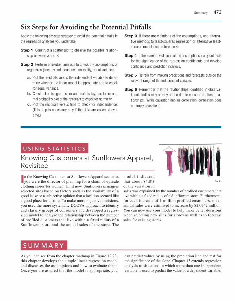
s U M M a r yAs you can see from the chapter roadmap in Figure 12.23, this chapter develops the simple linear regression model and discusses the assumptions and how to evaluate them. Once you are assured that the model is appropriate, you
can predict values by using the prediction line and test for the significance of the slope. Chapter 13 extends regression analysis to situations in which more than one independent variable is used to predict the value of a dependent variable.
Apply the following six-step strategy to avoid the potential pitfalls in the regression analyses you undertake.
Ste p 1 Construct a scatter plot to observe the possible relation-ship between X and Y.
Ste p 2 Perform a residual analysis to check the assumptions of regression (linearity, independence, normality, equal variance):
a. Plot the residuals versus the independent variable to deter-mine whether the linear model is appropriate and to check for equal variance.
b. Construct a histogram, stem-and-leaf display, boxplot, or nor-mal probability plot of the residuals to check for normality.
c. Plot the residuals versus time to check for independence. (This step is necessary only if the data are collected over time.)
Ste p 3 If there are violations of the assumptions, use alterna-tive methods to least-squares regression or alternative least-squares models (see reference 4).
Ste p 4 If there are no violations of the assumptions, carry out tests for the significance of the regression coefficients and develop confidence and prediction intervals.
Ste p 5 Refrain from making predictions and forecasts outside the relevant range of the independent variable.
Ste p 6 Remember that the relationships identified in observa-tional studies may or may not be due to cause-and-effect rela-tionships. (While causation implies correlation, correlation does not imply causation.)
Six Steps for Avoiding the Potential Pitfalls
In the Knowing Customers at Sunflowers Apparel scenario, you were the director of planning for a chain of upscale
clothing stores for women. Until now, Sunflowers managers selected sites based on factors such as the availability of a good lease or a subjective opinion that a location seemed like a good place for a store. To make more objective decisions, you used the more systematic DCOVA approach to identify and classify groups of consumers and developed a regres-sion model to analyze the relationship between the number of profiled customers that live within a fixed radius of a Sunflowers store and the annual sales of the store. The
model indicated that about 84.8% of the variation in sales was explained by the number of profiled customers that live within a fixed radius of a Sunflowers store. Furthermore, for each increase of 1 million profiled customers, mean annual sales were estimated to increase by $2.0742 million. You can now use your model to help make better decisions when selecting new sites for stores as well as to forecast sales for existing stores.
U s i n g s tat i s t i c s
Knowing Customers at Sunflowers Apparel, Revisited
Fotolia
Summary 473
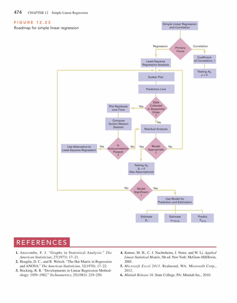
474 CHApTeR 12 Simple Linear Regression
r E f E r E n c E s 1. Anscombe, F. J. “Graphs in Statistical Analysis.” The
American Statistician, 27(1973): 17–21. 2. Hoaglin, D. C., and R. Welsch. “The Hat Matrix in Regression
and ANOVA.” The American Statistician, 32(1978): 17–22. 3. Hocking, R. R. “Developments in Linear Regression Method-
ology: 1959–1982.” Technometrics, 25(1983): 219–250.
4. Kutner, M. H., C. J. Nachtsheim, J. Neter, and W. Li. Applied Linear Statistical Models, 5th ed. New York: McGraw-Hill/Irwin, 2005.
5. Microsoft Excel 2013. Redmond, WA: Microsoft Corp., 2012.
6. Minitab Release 16. State College, pA: Minitab Inc., 2010.
F i g u r e 1 2 . 2 3Roadmap for simple linear regression
Yes
Yes
Yes
Yes
No
Regression Correlation
No
No
No
Use Alternative toLeast-Squares Regression
Estimateβ1
Use Model forPrediction and Estimation
ModelSigni�cant
?
Testing H0:β1 = 0
(See Assumptions)
ModelAppropriate
?
Residual Analysis
IsAutocorrelation
Present?
ComputeDurbin-Watson
Statistic
Plot Residualsover Time
DataCollected
in SequentialOrder
?
PrimaryFocus
Prediction Line
Scatter Plot
Least-SquaresRegression Analysis
Simple Linear Regressionand Correlation
Coef�cientof Correlation, r
Testing H0:ρ = 0
EstimateµY lX=Xi
PredictYX=Xi
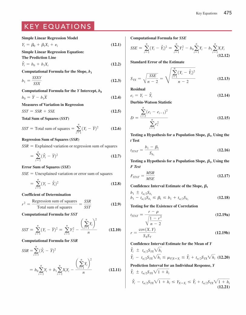
Key equations 475
K E y E q U at i o n s
Simple Linear Regression Model
Yi = b0 + b1Xi + ei (12.1)
Simple Linear Regression Equation: The Prediction Line
Yni = b0 + b1Xi (12.2)
Computational Formula for the Slope, b1
b1 =SSXY
SSX (12.3)
Computational Formula for the Y Intercept, b0
b0 = Y - b1X (12.4)
Measures of Variation in Regression
SST = SSR + SSE (12.5)
Total Sum of Squares (SST)
SST = Total sum of squares = an
i= 11Yi - Y22 (12.6)
Regression Sum of Squares (SSR)
SSR = explained variation or regression sum of squares
= an
i= 11Yni - Y22 (12.7)
Error Sum of Squares (SSE)
SSE = Unexplained variation or error sum of squares
= an
i= 11Yi - Yni22 (12.8)
Coefficient of Determination
r 2 =Regression sum of squares
Total sum of squares=
SSR
SST (12.9)
Computational Formula for SST
SST = an
i= 11Yi - Y22 = a
n
i= 1Y 2
i -a a
n
i= 1Yib
2
n (12.10)
Computational Formula for SSR
SSR =an
i= 11Yni - Y22
= b0an
i= 1Yi + b1a
n
i= 1XiYi -
a an
i= 1Yib
2
n (12.11)
Computational Formula for SSE
SSE = an
i= 11Yi - Yni22 = a
n
i= 1Y 2
i - b0an
i= 1Yi - b1a
n
i= 1XiYi
(12.12)
Standard Error of the Estimate
SYX = A SSE
n - 2= H a
n
i= 11Yi - Yni22
n - 2 (12.13)
Residual
ei = Yi - Yni (12.14)
Durbin-Watson Statistic
D =a
n
i= 21ei - ei - 122
an
i= 1e2
i
(12.15)
Testing a Hypothesis for a Population Slope, B1, Using the t Test
tSTAT =b1 - b1
Sb1
(12.16)
Testing a Hypothesis for a Population Slope, B1, Using the F Test
FSTAT =MSR
MSE (12.17)
Confidence Interval Estimate of the Slope, B1
b1 { ta>2Sb1
b1 - ta>2Sb1… b1 … b1 + ta>2Sb1
(12.18)
Testing for the Existence of Correlation
tSTAT =r - rA1 - r 2
n - 2
(12.19a)
r =cov1X, Y2
SXSY (12.19b)
Confidence Interval Estimate for the Mean of Y
Yni { ta>2SYX2hi
Yni - ta>2SYX2hi … mY�X= Xi… Yni + ta>2SYX2hi (12.20)
Prediction Interval for an Individual Response, Y
Yni { ta>2SYX21 + hi
Yni - ta>2SYX21 + hi … YX= Xi… Yni + ta>2SYX21 + hi
(12.21)
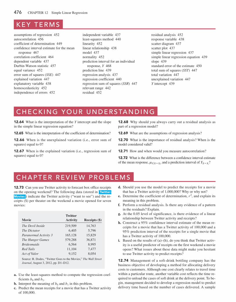
476 CHApTeR 12 Simple Linear Regression
K E y t E r M sassumptions of regression 452autocorrelation 456coefficient of determination 449confidence interval estimate for the mean
response 467correlation coefficient 464dependent variable 437Durbin-Watson statistic 457equal variance 452error sum of squares (SSE) 447explained variation 447explanatory variable 438homoscedasticity 452independence of errors 452
independent variable 437least-squares method 440linearity 452linear relationship 438model 437normality 452prediction interval for an individual
response, Y 468prediction line 439regression analysis 437regression coefficient 440regression sum of squares (SSR) 447relevant range 442residual 452
residual analysis 452response variable 438scatter diagram 437scatter plot 437simple linear regression 437simple linear regression equation 439slope 439standard error of the estimate 450total sum of squares (SST) 447total variation 447unexplained variation 447Y intercept 439
c h E c K i n g y o U r U n d E r s ta n d i n g12.64 What is the interpretation of the Y intercept and the slope in the simple linear regression equation?
12.65 What is the interpretation of the coefficient of determination?
12.66 When is the unexplained variation (i.e., error sum of squares) equal to 0?
12.67 When is the explained variation (i.e., regression sum of squares) equal to 0?
12.68 Why should you always carry out a residual analysis as part of a regression model?
12.69 What are the assumptions of regression analysis?
12.70 What is the importance of residual analysis? When is the model considered valid?
12.71 How and when would you measure autocorrelation?
12.72 What is the difference between a confidence interval estimate of the mean response, mY�X= Xi
, and a prediction interval of YX= Xi?
c h a p t E r r E V i E w p r o b l E M s12.73 Can you use Twitter activity to forecast box office receipts on the opening weekend? The following data (stored in Twitter-Movies ) indicate the Twitter activity (“want to see”) and the re-ceipts ($) per theater on the weekend a movie opened for seven movies:
MovieTwitter Activity Receipts ($)
The Devil Inside 219,509 14,763The Dictator 6,405 5,796Paranormal Activity 3 165,128 15,829The Hunger Games 579,288 36,871Bridesmaids 6,564 8,995Red Tails 11,104 7,477Act of Valor 9,152 8,054
Source: R. Dodes, “Twitter Goes to the Movies,” The Wall Street Journal, August 3, 2012, pp. D1–D12.
a. Use the least-squares method to compute the regression coef-ficients b0 and b1.
b. Interpret the meaning of b0 and b1 in this problem.c. predict the mean receipts for a movie that has a Twitter activity
of 100,000.
d. Should you use the model to predict the receipts for a movie that has a Twitter activity of 1,000,000? Why or why not?
e. Determine the coefficient of determination, r 2, and explain its meaning in this problem.
f. perform a residual analysis. Is there any evidence of a pattern in the residuals? explain.
g. At the 0.05 level of significance, is there evidence of a linear relationship between Twitter activity and receipts?
h. Construct a 95% confidence interval estimate of the mean re-ceipts for a movie that has a Twitter activity of 100,000 and a 95% prediction interval of the receipts for a single movie that has a Twitter activity of 100,000.
i. Based on the results of (a)–(h), do you think that Twitter activ-ity is a useful predictor of receipts on the first weekend a movie opens? What issues about these data might make you hesitant to use Twitter activity to predict receipts?
12.74 Management of a soft-drink bottling company has the business objective of developing a method for allocating delivery costs to customers. Although one cost clearly relates to travel time within a particular route, another variable cost reflects the time re-quired to unload the cases of soft drink at the delivery point. To be-gin, management decided to develop a regression model to predict delivery time based on the number of cases delivered. A sample
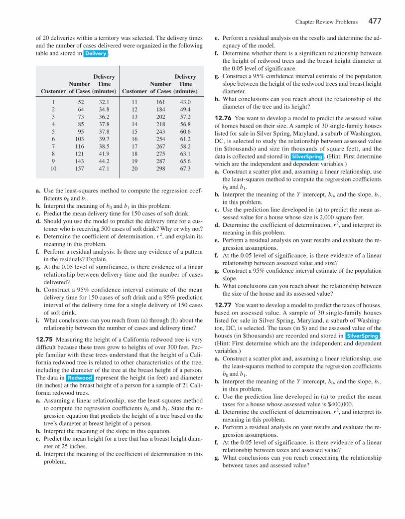
Chapter Review problems 477
a. Use the least-squares method to compute the regression coef-ficients b0 and b1.
b. Interpret the meaning of b0 and b1 in this problem.c. predict the mean delivery time for 150 cases of soft drink.d. Should you use the model to predict the delivery time for a cus-
tomer who is receiving 500 cases of soft drink? Why or why not?e. Determine the coefficient of determination, r 2, and explain its
meaning in this problem.f. perform a residual analysis. Is there any evidence of a pattern
in the residuals? explain.g. At the 0.05 level of significance, is there evidence of a linear
relationship between delivery time and the number of cases delivered?
h. Construct a 95% confidence interval estimate of the mean delivery time for 150 cases of soft drink and a 95% prediction interval of the delivery time for a single delivery of 150 cases of soft drink.
i. What conclusions can you reach from (a) through (h) about the relationship between the number of cases and delivery time?
12.75 Measuring the height of a California redwood tree is very difficult because these trees grow to heights of over 300 feet. peo-ple familiar with these trees understand that the height of a Cali-fornia redwood tree is related to other characteristics of the tree, including the diameter of the tree at the breast height of a person. The data in redwood represent the height (in feet) and diameter (in inches) at the breast height of a person for a sample of 21 Cali-fornia redwood trees.a. Assuming a linear relationship, use the least-squares method
to compute the regression coefficients b0 and b1. State the re-gression equation that predicts the height of a tree based on the tree’s diameter at breast height of a person.
b. Interpret the meaning of the slope in this equation.c. predict the mean height for a tree that has a breast height diam-
eter of 25 inches.d. Interpret the meaning of the coefficient of determination in this
problem.
e. perform a residual analysis on the results and determine the ad-equacy of the model.
f. Determine whether there is a significant relationship between the height of redwood trees and the breast height diameter at the 0.05 level of significance.
g. Construct a 95% confidence interval estimate of the population slope between the height of the redwood trees and breast height diameter.
h. What conclusions can you reach about the relationship of the diameter of the tree and its height?
12.76 You want to develop a model to predict the assessed value of homes based on their size. A sample of 30 single-family houses listed for sale in Silver Spring, Maryland, a suburb of Washington, DC, is selected to study the relationship between assessed value (in $thousands) and size (in thousands of square feet), and the data is collected and stored in SilverSpring . (Hint: First determine which are the independent and dependent variables.)a. Construct a scatter plot and, assuming a linear relationship, use
the least-squares method to compute the regression coefficients b0 and b1.
b. Interpret the meaning of the Y intercept, b0, and the slope, b1, in this problem.
c. Use the prediction line developed in (a) to predict the mean as-sessed value for a house whose size is 2,000 square feet.
d. Determine the coefficient of determination, r 2, and interpret its meaning in this problem.
e. perform a residual analysis on your results and evaluate the re-gression assumptions.
f. At the 0.05 level of significance, is there evidence of a linear relationship between assessed value and size?
g. Construct a 95% confidence interval estimate of the population slope.
h. What conclusions can you reach about the relationship between the size of the house and its assessed value?
12.77 You want to develop a model to predict the taxes of houses, based on assessed value. A sample of 30 single-family houses listed for sale in Silver Spring, Maryland, a suburb of Washing-ton, DC, is selected. The taxes (in $) and the assessed value of the houses (in $thousands) are recorded and stored in SilverSpring . (Hint: First determine which are the independent and dependent variables.)a. Construct a scatter plot and, assuming a linear relationship, use
the least-squares method to compute the regression coefficients b0 and b1.
b. Interpret the meaning of the Y intercept, b0, and the slope, b1, in this problem.
c. Use the prediction line developed in (a) to predict the mean taxes for a house whose assessed value is $400,000.
d. Determine the coefficient of determination, r 2, and interpret its meaning in this problem.
e. perform a residual analysis on your results and evaluate the re-gression assumptions.
f. At the 0.05 level of significance, is there evidence of a linear relationship between taxes and assessed value?
g. What conclusions can you reach concerning the relationship between taxes and assessed value?
of 20 deliveries within a territory was selected. The delivery times and the number of cases delivered were organized in the following table and stored in Delivery .
Customer
Number of Cases
Delivery Time
(minutes)
1 52 32.12 64 34.83 73 36.24 85 37.85 95 37.86 103 39.77 116 38.58 121 41.99 143 44.210 157 47.1
Customer
Number of Cases
Delivery Time
(minutes)
11 161 43.012 184 49.413 202 57.214 218 56.815 243 60.616 254 61.217 267 58.218 275 63.119 287 65.620 298 67.3
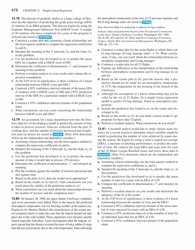
478 CHApTeR 12 Simple Linear Regression
12.78 The director of graduate studies at a large college of busi-ness has the objective of predicting the grade point average (GpA) of students in an MBA program. The director begins by using the Graduate Management Admission Test (GMAT) score. A sample of 20 students who have completed two years in the program is selected and stored in gpigMaT .a. Construct a scatter plot and, assuming a linear relationship, use
the least-squares method to compute the regression coefficients b0 and b1.
b. Interpret the meaning of the Y intercept, b0, and the slope, b1, in this problem.
c. Use the prediction line developed in (a) to predict the mean GpA for a student with a GMAT score of 600.
d. Determine the coefficient of determination, r 2, and interpret its meaning in this problem.
e. perform a residual analysis on your results and evaluate the re-gression assumptions.
f. At the 0.05 level of significance, is there evidence of a linear relationship between GMAT score and GpA?
g. Construct a 95% confidence interval estimate of the mean GpA of students with a GMAT score of 600 and a 95% prediction interval of the GpA for a particular student with a GMAT score of 600.
h. Construct a 95% confidence interval estimate of the population slope.
i. What conclusions can you reach concerning the relationship between GMAT score and GpA?
12.79 An accountant for a large department store has the busi-ness objective of developing a model to predict the amount of time it takes to process invoices. Data are collected from the past 32 working days, and the number of invoices processed and comple-tion time (in hours) are stored in invoice . (Hint: First determine which are the independent and dependent variables.)a. Assuming a linear relationship, use the least-squares method to
compute the regression coefficients b0 and b1.b. Interpret the meaning of the Y intercept, b0, and the slope, b1, in
this problem.c. Use the prediction line developed in (a) to predict the mean
amount of time it would take to process 150 invoices.d. Determine the coefficient of determination, r 2, and interpret its
meaning.e. plot the residuals against the number of invoices processed and
also against time.f. Based on the plots in (e), does the model seem appropriate?g. Based on the results in (e) and (f), what conclusions can you
reach about the validity of the prediction made in (c)?h. What conclusions can you reach about the relationship between
the number of invoices and the completion time?
12.80 On January 28, 1986, the space shuttle Challenger exploded, and seven astronauts were killed. prior to the launch, the predicted atmospheric temperature was for freezing weather at the launch site. engineers for Morton Thiokol (the manufacturer of the rocket mo-tor) prepared charts to make the case that the launch should not take place due to the cold weather. These arguments were rejected, and the launch tragically took place. Upon investigation after the tragedy, ex-perts agreed that the disaster occurred because of leaky rubber O-rings that did not seal properly due to the cold temperature. Data indicating
the atmospheric temperature at the time of 23 previous launches and the O-ring damage index are stored in o-ring .
Note: Data from flight 4 is omitted due to unknown O-ring condition.
Sources: Data extracted from Report of the Presidential Commission on the Space Shuttle Challenger Accident, Washington, DC, 1986, Vol. II (H1–H3) and Vol. IV (664); and Post-Challenger Evaluation of Space Shuttle Risk Assessment and Management, Washington, DC, 1988, pp. 135–136.
a. Construct a scatter plot for the seven flights in which there was O-ring damage (O-ring damage index ≠ 0). What conclu-sions, if any, can you reach about the relationship between at-mospheric temperature and O-ring damage?
b. Construct a scatter plot for all 23 flights.c. explain any differences in the interpretation of the relationship
between atmospheric temperature and O-ring damage in (a) and (b).
d. Based on the scatter plot in (b), provide reasons why a pre-diction should not be made for an atmospheric temperature of 31°F, the temperature on the morning of the launch of the Challenger.
e. Although the assumption of a linear relationship may not be valid for the set of 23 flights, fit a simple linear regression model to predict O-ring damage, based on atmospheric tem-perature.
f. Include the prediction line found in (e) on the scatter plot de-veloped in (b).
g. Based on the results in (f), do you think a linear model is ap-propriate for these data? explain.
h. perform a residual analysis. What conclusions do you reach?
12.81 A baseball analyst would like to study various team sta-tistics for a recent season to determine which variables might be useful in predicting the number of wins achieved by teams dur-ing the season. He begins by using a team’s earned run average (eRA), a measure of pitching performance, to predict the num-ber of wins. He collects the team eRA and team wins for each of the 30 Major League Baseball teams and stores these data in baseball . (Hint: First determine which are the independent and dependent variables.)a. Assuming a linear relationship, use the least-squares method to
compute the regression coefficients b0 and b1.b. Interpret the meaning of the Y intercept, b0, and the slope, b1, in
this problem.c. Use the prediction line developed in (a) to predict the mean
number of wins for a team with an eRA of 4.50.d. Compute the coefficient of determination, r 2, and interpret its
meaning.e. perform a residual analysis on your results and determine the
adequacy of the fit of the model.f. At the 0.05 level of significance, is there evidence of a linear
relationship between the number of wins and the eRA?g. Construct a 95% confidence interval estimate of the mean num-
ber of wins expected for teams with an eRA of 4.50.h. Construct a 95% prediction interval of the number of wins for
an individual team that has an eRA of 4.50.i. Construct a 95% confidence interval estimate of the population
slope.
j. The 30 teams constitute a population. In order to use statistical inference, as in (f) through (i), the data must be assumed to rep-resent a random sample. What “population” would this sample be drawing conclusions about?
k. What other independent variables might you consider for inclu-sion in the model?
l. What conclusions can you reach concerning the relationship between eRA and wins?
12.82 Can you use the annual revenues generated by National Basketball Association (NBA) franchises to predict franchise val-ues? Figure 2.14 on page 83 shows a scatter plot of revenue with franchise value, and Figure 3.9 on page 186, shows the correlation coefficient. Now, you want to develop a simple linear regression model to predict franchise values based on revenues. (Franchise values and revenues are stored in nbaValues .)a. Assuming a linear relationship, use the least-squares method to
compute the regression coefficients b0 and b1.b. Interpret the meaning of the Y intercept, b0, and the slope, b1, in
this problem.c. predict the mean value of an NBA franchise that generates
$150 million of annual revenue.d. Compute the coefficient of determination, r 2, and interpret its
meaning.e. perform a residual analysis on your results and evaluate the re-
gression assumptions.f. At the 0.05 level of significance, is there evidence of a linear
relationship between the annual revenues generated and the value of an NBA franchise?
g. Construct a 95% confidence interval estimate of the mean value of all NBA franchises that generate $150 million of annual rev-enue.
h. Construct a 95% prediction interval of the value of an individ-ual NBA franchise that generates $150 million of annual rev-enue.
i. Compare the results of (a) through (h) to those of baseball fran-chises in problems 12.8, 12.20, 12.30, 12.46, and 12.62 and european soccer teams in problem 12.83.
12.83 In problem 12.82 you used annual revenue to develop a model to predict the franchise value of National Basketball Association (NBA) teams. Can you also use the annual rev-enues generated by european soccer teams to predict franchise values? (european soccer team values and revenues are stored in SoccerValues2014 .)a. Repeat problem 12.82 (a) through (h) for the european soccer
teams.b. Compare the results of (a) to those of baseball franchises in
problems 12.8, 12.20, 12.30, 12.46, and 12.62 and NBA fran-chises in problem 12.82.
12.84 During the fall harvest season in the United States, pump-kins are sold in large quantities at farm stands. Often, instead of weighing the pumpkins prior to sale, the farm stand operator will just place the pumpkin in the appropriate circular cutout on the counter. When asked why this was done, one farmer replied, “I can tell the weight of the pumpkin from its circumference.” To deter-mine whether this was really true, the circumference and weight of each pumpkin from a sample of 23 pumpkins were determined and the results stored in pumpkin .
a. Assuming a linear relationship, use the least-squares method to compute the regression coefficients b0 and b1.
b. Interpret the meaning of the slope, b1, in this problem.c. predict the mean weight for a pumpkin that is 60 centimeters in
circumference.d. Do you think it is a good idea for the farmer to sell pumpkins
by circumference instead of weight? explain.e. Determine the coefficient of determination, r 2, and interpret its
meaning.f. perform a residual analysis for these data and evaluate the re-
gression assumptions.g. At the 0.05 level of significance, is there evidence of a lin-
ear relationship between the circumference and weight of a pumpkin?
h. Construct a 95% confidence interval estimate of the population slope, b1.
12.85 Refer to the discussion of beta values and market mod-els in problem 12.49 on page 466. The S&p 500 Index tracks the overall movement of the stock market by considering the stock prices of 500 large corporations. The file Stockprices2013 con-tains 2013 weekly data for the S&p 500 and three companies. The following variables are included:
WeeK—Week ending on date givenS&p—Weekly closing value for the S&p 500 IndexGe—Weekly closing stock price for General electricDISCA—Weekly closing stock price for Discovery CommunicationsGOOG—Weekly closing stock price for Google
Source: Data extracted from finance.yahoo.com, June 6, 2014.
a. estimate the market model for Ge. (Hint: Use the percentage change in the S&p 500 Index as the independent variable and the percentage change in Ge’s stock price as the dependent variable.)
b. Interpret the beta value for Ge.c. Repeat (a) and (b) for Discovery Communications.d. Repeat (a) and (b) for Google.e. Write a brief summary of your findings.
12.86 The file Ceo-Compensation2013 includes the total com-pensation (in $millions) for CeOs of 200 Standard & poor’s 500 companies and the investment return in 2013. (Data extracted from “Millions by millions, CeO pay goes up,” usat.ly/1jhbypL.)a. Compute the correlation coefficient between compensation and
the investment return in 2013.b. At the 0.05 level of significance, is the correlation between
compensation and the investment return in 2013 statistically significant?
c. Write a short summary of your findings in (a) and (b). Do the results surprise you?
reporT WriTing exerCiSe12.87 In problems 12.8, 12.20, 12.30, 12.46, 12.62, 12.82, and 12.83, you developed regression models to predict franchise value of major league baseball, NBA basketball, and soccer teams. Now, write a report based on the models you developed. Append to your report all appropriate charts and statistical information.
Chapter Review problems 479
480 CHApTeR 12 Simple Linear Regression
c a s E s f o r c h a p t E r 1 2
Managing ashland Multicomm servicesTo ensure that as many trial subscriptions to the 3-For-All service as possible are converted to regular subscriptions, the marketing department works closely with the customer support department to accomplish a smooth initial process for the trial subscription customers. To assist in this effort, the marketing department needs to accurately forecast the monthly total of new regular subscriptions.
A team consisting of managers from the marketing and customer support departments was convened to develop a better method of forecasting new subscriptions. previously, after examining new subscription data for the prior three months, a group of three managers would develop a sub-jective forecast of the number of new subscriptions. Livia Salvador, who was recently hired by the company to provide expertise in quantitative forecasting methods, suggested that the department look for factors that might help in predicting new subscriptions.
Members of the team found that the forecasts in the past year had been particularly inaccurate because in some months, much more time was spent on telemarketing than in other months. Livia collected data (stored in aMS12 ) for the number of new subscriptions and hours spent on telemarket-ing for each month for the past two years.
1. What criticism can you make concerning the method of forecasting that involved taking the new subscriptions data for the prior three months as the basis for future projections?
2. What factors other than number of telemarketing hours spent might be useful in predicting the number of new subscriptions? explain.
3. a. Analyze the data and develop a regression model to predict the number of new subscriptions for a month, based on the number of hours spent on telemarketing for new subscriptions.
b. If you expect to spend 1,200 hours on telemarketing per month, estimate the number of new subscriptions for the month. Indicate the assumptions on which this prediction is based. Do you think these assumptions are valid? explain.
c. What would be the danger of predicting the number of new subscriptions for a month in which 2,000 hours were spent on telemarketing?
digital caseApply your knowledge of simple linear regression in this Digital Case, which extends the Sunflowers Apparel Using Statistics scenario from this chapter.
Leasing agents from the Triangle Mall Management Corporation have suggested that Sunflowers consider sev-eral locations in some of Triangle’s newly renovated life-style malls that cater to shoppers with higher-than-mean disposable income. Although the locations are smaller than the typical Sunflowers location, the leasing agents argue that higher-than-mean disposable income in the surrounding community is a better predictor of higher sales than profiled customers. The leasing agents maintain that sample data from 14 Sunflowers stores prove that this is true.
Open Triangle_Sunflower.pdf and review the leasing agents’ proposal and supporting documents. Then answer the following questions:
1. Should mean disposable income be used to predict sales based on the sample of 14 Sunflowers stores?
2. Should the management of Sunflowers accept the claims of Triangle’s leasing agents? Why or why not?
3. Is it possible that the mean disposable income of the sur-rounding area is not an important factor in leasing new locations? explain.
4. Are there any other factors not mentioned by the leasing agents that might be relevant to the store leasing decision?
brynne packagingBrynne packaging is a large packaging company, offering its customers the highest standards in innovative packaging solutions and reliable service. About 25% of the employ-ees at Brynne packaging are machine operators. The hu-man resources department has suggested that the company
consider using the Wesman personnel Classification Test (WpCT), a measure of reasoning ability, to screen appli-cants for the machine operator job. In order to assess the WpCT as a predictor of future job performance, 25 recent applicants were tested using the WpCT; all were hired,
Cases for Chapter 12 481
regardless of their WpCT score. At a later time, supervi-sors were asked to rate the quality of the job performance of these 25 employees, using a 1-to-10 rating scale (where 1 = very low and 10 = very high). Factors considered in the rat-ings included the employee’s output, defect rate, ability to implement continuous quality procedures, and contributions to team problem-solving efforts. The file brynnepackaging contains the WpCT scores (WpCT) and job performance ratings (Ratings) for the 25 employees.
1. Assess the significance and importance of WpCT score as a predictor of job performance. Defend your answer.
2. predict the mean job performance rating for all employees with a WpCT score of 6. Give a point prediction as well as a 95% confidence interval. Do you have any concerns using the regression model for predicting mean job perfor-mance rating given the WpCT score of 6?
3. evaluate whether the assumptions of regression have been seriously violated.
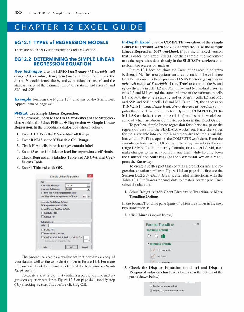
482 CHApTeR 12 Simple Linear Regression
eg12.1 TypeS of regreSSion MoDeLSThere are no excel Guide instructions for this section.
eg12.2 DeTerMining the SiMpLe Linear regreSSion equaTion
Key Technique Use the LINEST(cell range of Y variable, cell range of X variable, True, True) array function to compute the b1 and b0 coefficients, the b1 and b0 standard errors, r 2 and the standard error of the estimate, the F test statistic and error df, and SSR and SSE.
Example perform the Figure 12.4 analysis of the Sunflowers Apparel data on page 440.
phStat Use Simple Linear Regression.For the example, open to the DATA worksheet of the SiteSelec-tion workbook. Select PHStat ➔ Regression ➔ Simple Linear Regression. In the procedure’s dialog box (shown below):
1. enter C1:C15 as the Y Variable Cell Range.
2. enter B1:B15 as the X Variable Cell Range.
3. Check First cells in both ranges contain label.
4. enter 95 as the Confidence level for regression coefficients.
5. Check Regression Statistics Table and ANOVA and Coef-ficients Table.
6. enter a Title and click OK.
The procedure creates a worksheet that contains a copy of your data as well as the worksheet shown in Figure 12.4. For more information about these worksheets, read the following In-Depth Excel section.
To create a scatter plot that contains a prediction line and re-gression equation similar to Figure 12.5 on page 441, modify step 6 by checking Scatter Plot before clicking OK.
in-Depth excel Use the COMPUTE worksheet of the Simple Linear Regression workbook as a template. (Use the Simple Linear Regression 2007 workbook if you use an excel version that is older than excel 2010.) For the example, the worksheet uses the regression data already in the SLRDATA worksheet to perform the regression analysis.
Figure 12.4 does not show the Calculations area in columns K through M. This area contains an array formula in the cell range L2:M6 that contains the expression LINEST(cell range of Y vari-able, cell range of X variable, True, True) to compute the b1 and b0 coefficients in cells L2 and M2, the b1 and b0 standard errors in cells L3 and M3, r 2 and the standard error of the estimate in cells L4 and M4, the F test statistic and error df in cells L5 and M5, and SSR and SSE in cells L6 and M6. In cell L9, the expression T.INV.2T(1 – confidence level, Error degrees of freedom) com-putes the critical value for the t test. Open the COMPUTE_FOR-MULAS worksheet to examine all the formulas in the worksheet, some of which are discussed in later sections in this excel Guide.
To perform simple linear regression for other data, paste the regression data into the SLRDATA worksheet. paste the values for the X variable into column A and the values for the Y variable into column B. Then, open to the COMpUTe worksheet. enter the confidence level in cell L8 and edit the array formula in the cell range L2:M6. To edit the array formula, first select L2:M6, next make changes to the array formula, and then, while holding down the Control and Shift keys (or the Command key on a Mac), press the Enter key.
To create a scatter plot that contains a prediction line and re-gression equation similar to Figure 12.5 on page 441, first use the Section eG2.5 In-Depth Excel scatter plot instructions with the Table 12.1 Sunflowers Apparel data to create a scatter plot. Then select the chart and:
1. Select Design ➔ Add Chart Element ➔ Trendline ➔ More Trendline Options.
In the Format Trendline pane (parts of which are shown in the next two illustrations):
2. Click Linear (shown below).
3. Check the Display Equation on chart and Display R-squared value on chart check boxes near the bottom of the pane (shown below).
c h a p t E r 1 2 E x c E l g U i d E
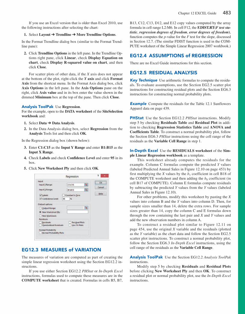
Chapter 12 eXCeL Guide 483
If you use an excel version that is older than excel 2010, use the following instructions after selecting the chart:
1. Select Layout ➔ Trendline ➔ More Trendline Options.
In the Format Trendline dialog box (similar to the Format Trend-line pane):
2. Click Trendline Options in the left pane. In the Trendline Op-tions right pane, click Linear, check Display Equation on chart, check Display R-squared value on chart, and then click Close.
For scatter plots of other data, if the X axis does not appear at the bottom of the plot, right-click the Y axis and click Format Axis from the shortcut menu. In the Format Axis dialog box, click Axis Options in the left pane. In the Axis Options pane on the right, click Axis value and in its box enter the value shown in the dimmed Minimum box at the top of the pane. Then click Close.
analysis Toolpak Use Regression.For the example, open to the DATA worksheet of the SiteSelection workbook and:
1. Select Data ➔ Data Analysis.
2. In the Data Analysis dialog box, select Regression from the Analysis Tools list and then click OK.
In the Regression dialog box (shown below):
3. enter C1:C15 as the Input Y Range and enter B1:B15 as the Input X Range.
4. Check Labels and check Confidence Level and enter 95 in its box.
5. Click New Worksheet Ply and then click OK.
eg12.3 MeaSureS of VariaTionThe measures of variation are computed as part of creating the simple linear regression worksheet using the Section eG12.2 in-structions.
If you use either Section eG12.2 PHStat or In-Depth Excel instructions, formulas used to compute these measures are in the COMPUTE worksheet that is created. Formulas in cells B5, B7,
B13, C12, C13, D12, and e12 copy values computed by the array formula in cell range L2:M6. In cell F12, the F.DIST.RT(F test sta-tistic, regression degrees of freedom, error degrees of freedom), function computes the p-value for the F test for the slope, discussed in Section 12.7. (The similar FDIST function is used in the COM-pUTe worksheet of the Simple Linear Regression 2007 workbook.)
eg12.4 aSSuMpTionS of regreSSionThere are no excel Guide instructions for this section.
eg12.5 reSiDuaL anaLySiSKey Technique Use arithmetic formulas to compute the residu-als. To evaluate assumptions, use the Section eG2.5 scatter plot instructions for constructing residual plots and the Section eG6.3 instructions for constructing normal probability plots.
Example Compute the residuals for the Table 12.1 Sunflowers Apparel data on page 439.
phStat Use the Section eG12.2 PHStat instructions. Modify step 5 by checking Residuals Table and Residual Plot in addi-tion to checking Regression Statistics Table and ANOVA and Coefficients Table. To construct a normal probability plot, follow the Section eG6.3 PHStat instructions using the cell range of the residuals as the Variable Cell Range in step 1.
in-Depth excel Use the RESIDUALS worksheet of the Sim-ple Linear Regression workbook as a template.
This worksheet already computes the residuals for the example. Column C formulas compute the predicted Y values (labeled predicted Annual Sales in Figure 12.10 on page 453) by first multiplying the X values by the b1 coefficient in cell B18 of the COMpUTe worksheet and then adding the b0 coefficient (in cell B17 of COMpUTe). Column e formulas compute residuals by subtracting the predicted Y values from the Y values (labeled Annual Sales in Figure 12.10).
For other problems, modify this worksheet by pasting the X values into column B and the Y values into column D. Then, for sample sizes smaller than 14, delete the extra rows. For sample sizes greater than 14, copy the column C and e formulas down through the row containing the last pair and X and Y values and add the new observation numbers in column A.
To construct a residual plot similar to Figure 12.11 on page 454, use the original X variable and the residuals (plotted as the Y variable) as the chart data and follow the Section eG2.5 scatter plot instructions. To construct a normal probability plot, follow the Section eG6.3 In-Depth Excel instructions, using the cell range of the residuals as the Variable Cell Range.
analysis Toolpak Use the Section eG12.2 Analysis ToolPak instructions.
Modify step 5 by checking Residuals and Residual Plots before clicking New Worksheet Ply and then OK. To construct a residual plot or normal probability plot, use the In-Depth Excel instructions.
484 CHApTeR 12 Simple Linear Regression
eg12.6 MeaSuring auToCorreLaTion: the Durbin-WaTSon STaTiSTiC
Key Technique Use the SUMXMY2(cell range of the sec-ond through last residual, cell range of the first through the second-to-last residual) function to compute the sum of squared difference of the residuals, the numerator in equation (12.15) on page 458, and use the SUMSQ(cell range of the residuals) func-tion to compute the sum of squared residuals, the denominator in equation (12.15).
Example Compute the Durbin-Watson statistic for the package delivery data on page 456.
phStat Use the PHStat instructions at the beginning of Section eG12.2. Modify step 6 by checking the Durbin-Watson Statistic output option before clicking OK.
in-Depth excel Use the DURBIN_WATSON worksheet of the Simple Linear Regression workbook as a template. The worksheet uses the SUMXMY2 function in cell B3 and the SUMSQ function in cell B4.
The DURBIN_WATSON worksheet of the Package Deliv-ery workbook computes the statistic for the Figure 12.16 pack-age delivery store example on page 458. (This workbook also uses the COMpUTe and ReSIDUALS worksheet templates from the Simple Linear Regression workbook.)
To compute the Durbin-Watson statistic for other problems, first create the simple linear regression model and the residuals for the problem, using the Sections eG12.2 and eG12.5 In-Depth Excel instructions. Then open the DURBIN_WATSON worksheet and edit the formulas in cell B3 and B4 to point to the proper cell ranges of the new residuals.
eg12.7 inFerenCeS abouT the SLope and CorreLaTion CoeFFiCienT
The t test for the slope and F test for the slope are included in the worksheet created by using the Section eG12.2 instructions. The t test computations in the worksheets created by using the PHStat and In-Depth Excel instructions are discussed in Sec-tion eG12.2. The F test computations are discussed in Section eG12.3.
eg12.8 eSTiMaTion of Mean VaLueS and preDiCTion of inDiViDuaL VaLueS
Key Technique Use the TREND(Y variable cell range, X variable cell range, X value) function to compute the predicted Y value for the X value and use the DEVSQ(X variable cell range) function to compute the SSX value.
Example Compute the Figure 12.21 confidence interval esti-mate and prediction interval for the Sunflowers Apparel data that is shown on page 439.
phStat Use the Section eG12.2 PHStat instructions but replace step 6 with these steps 6 and 7:
1. Check Confidence Int. Est. & Prediction Int. for X= and enter 4 in its box. enter 95 as the percentage for Confidence level for intervals.
2. enter a Title and click OK.
The additional worksheet created is discussed in the following In-Depth Excel instructions.
in-Depth excel Use the CIEandPI worksheet of the Simple Linear Regression workbook, as a template.
The worksheet already contains the data and formulas for the example. The worksheet uses the T.INV.2T (1 – confidence level, degrees of freedom) function to compute the t critical value in cell B10 and the TReND function to compute the pre-dicted Y value for the X value in cell B15. In cell B12, the function DEVSQ(SLRData!A:A) computes the SSX value that is used, in turn, to help compute the h statistic in cell B14.
To compute a confidence interval estimate and prediction interval for other problems:
1. paste the regression data into the SLRData worksheet. Use column A for the X variable data and column B for the Y vari-able data.
2. Open to the CIEandPI worksheet.
In the CIeandpI worksheet:
3. Change values for the X Value and Confidence Level, as is necessary.
4. edit the cell ranges used in the cell B15 formula that uses the TReND function to refer to the new cell ranges for the Y and X variables.
Mg12.1 TypeS of regreSSion MoDeLSThere are no Minitab Guide instructions for this section.
Mg12.2 DeTerMining the SiMpLe Linear regreSSion equaTion
Use Regression to perform a simple linear regression analysis. For example, to perform the Figure 12.4 analysis of the Sunflowers Apparel data on page 440, open to the SiteSelection worksheet.
Select Stat ➔ Regression ➔ Regression. (and Fit Regression Model in Minitab 17.) In the Regression dialog box (shown on the next page):
1. Double-click C3 Annual Sales in the variables list to add 'Annual Sales' to the Response box (Responses box in Minitab 17).
2. Double-click C2 Profiled Customers in the variables list to add 'Profiled Customers' to the Predictors (or Continuous predictors) box.
c h a p t E r 1 2 M i n i ta b g U i d E
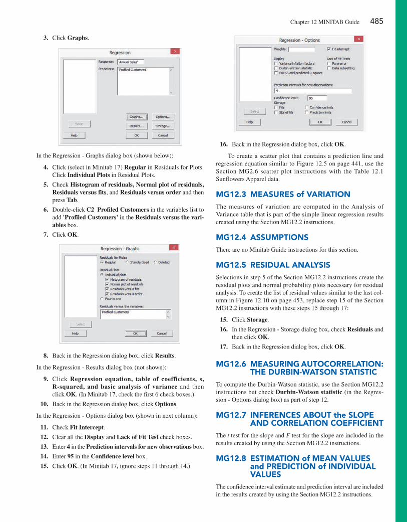
3. Click Graphs.
In the Regression - Graphs dialog box (shown below):
4. Click (select in Minitab 17) Regular in Residuals for plots. Click Individual Plots in Residual plots.
5. Check Histogram of residuals, Normal plot of residuals, Residuals versus fits, and Residuals versus order and then press Tab.
6. Double-click C2 Profiled Customers in the variables list to add 'Profiled Customers' in the Residuals versus the vari-ables box.
7. Click OK.
8. Back in the Regression dialog box, click Results.
In the Regression - Results dialog box (not shown):
9. Click Regression equation, table of coefficients, s, R-squared, and basic analysis of variance and then click OK. (In Minitab 17, check the first 6 check boxes.)
10. Back in the Regression dialog box, click Options.
In the Regression - Options dialog box (shown in next column):
11. Check Fit Intercept.
12. Clear all the Display and Lack of Fit Test check boxes.
13. enter 4 in the Prediction intervals for new observations box.
14. enter 95 in the Confidence level box.
15. Click OK. (In Minitab 17, ignore steps 11 through 14.)
16. Back in the Regression dialog box, click OK.
To create a scatter plot that contains a prediction line and regression equation similar to Figure 12.5 on page 441, use the Section MG2.6 scatter plot instructions with the Table 12.1 Sunflowers Apparel data.
Mg12.3 MeaSureS of VariaTionThe measures of variation are computed in the Analysis of Variance table that is part of the simple linear regression results created using the Section MG12.2 instructions.
Mg12.4 aSSuMpTionSThere are no Minitab Guide instructions for this section.
Mg12.5 reSiDuaL anaLySiSSelections in step 5 of the Section MG12.2 instructions create the residual plots and normal probability plots necessary for residual analysis. To create the list of residual values similar to the last col-umn in Figure 12.10 on page 453, replace step 15 of the Section MG12.2 instructions with these steps 15 through 17:
15. Click Storage.
16. In the Regression - Storage dialog box, check Residuals and then click OK.
17. Back in the Regression dialog box, click OK.
Mg12.6 MeaSuring auToCorreLaTion: The Durbin-WaTSon STaTiSTiC
To compute the Durbin-Watson statistic, use the Section MG12.2 instructions but check Durbin-Watson statistic (in the Regres-sion - Options dialog box) as part of step 12.
Mg12.7 inFerenCeS abouT the SLope anD CorreLaTion CoeFFiCienT
The t test for the slope and F test for the slope are included in the results created by using the Section MG12.2 instructions.
Mg12.8 eSTiMaTion of Mean VaLueS and preDiCTion of inDiViDuaL VaLueS
The confidence interval estimate and prediction interval are included in the results created by using the Section MG12.2 instructions.
Chapter 12 MINITAB Guide 485
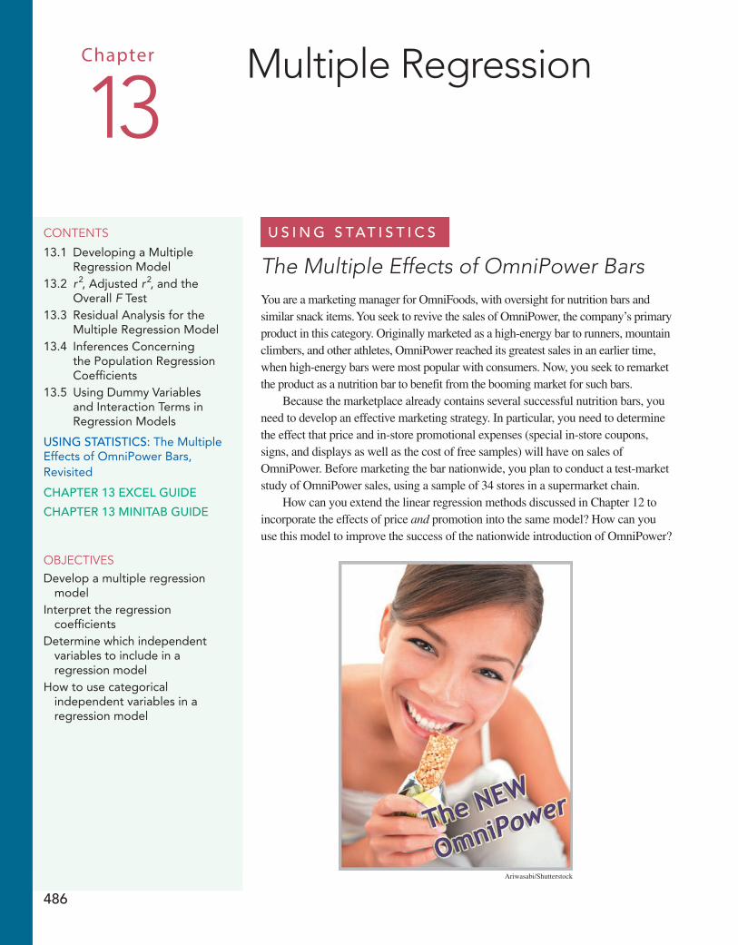
U s i n g s tat i s t i c s
The Multiple Effects of OmniPower BarsYou are a marketing manager for OmniFoods, with oversight for nutrition bars and similar snack items. You seek to revive the sales of OmniPower, the company’s primary product in this category. Originally marketed as a high-energy bar to runners, mountain climbers, and other athletes, OmniPower reached its greatest sales in an earlier time, when high-energy bars were most popular with consumers. Now, you seek to remarket the product as a nutrition bar to benefit from the booming market for such bars.
Because the marketplace already contains several successful nutrition bars, you need to develop an effective marketing strategy. In particular, you need to determine the effect that price and in-store promotional expenses (special in-store coupons, signs, and displays as well as the cost of free samples) will have on sales of OmniPower. Before marketing the bar nationwide, you plan to conduct a test-market study of OmniPower sales, using a sample of 34 stores in a supermarket chain.
How can you extend the linear regression methods discussed in Chapter 12 to incorporate the effects of price and promotion into the same model? How can you use this model to improve the success of the nationwide introduction of OmniPower?
contents
13.1 Developing a Multiple Regression Model
13.2 r2, Adjusted r2, and the Overall F Test
13.3 Residual Analysis for the Multiple Regression Model
13.4 Inferences Concerning the Population Regression Coefficients
13.5 Using Dummy Variables and Interaction Terms in Regression Models
Using statistics: The Multiple Effects of OmniPower Bars, Revisited
chapter 13 excel gUide
chapter 13 Minitab gUide
objectivesDevelop a multiple regression
modelInterpret the regression
coefficientsDetermine which independent
variables to include in a regression model
How to use categorical independent variables in a regression model
Multiple Regression13Chapter
Ariwasabi/Shutterstock
486
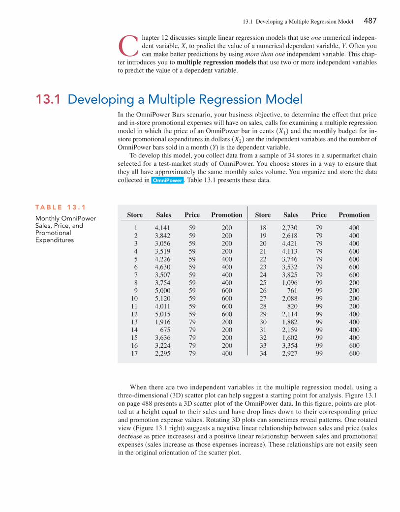
13.1 Developing a Multiple Regression Model 487
C hapter 12 discusses simple linear regression models that use one numerical indepen-dent variable, X, to predict the value of a numerical dependent variable, Y. Often you can make better predictions by using more than one independent variable. This chap-
ter introduces you to multiple regression models that use two or more independent variables to predict the value of a dependent variable.
13.1 Developing a Multiple Regression ModelIn the OmniPower Bars scenario, your business objective, to determine the effect that price and in-store promotional expenses will have on sales, calls for examining a multiple regression model in which the price of an OmniPower bar in cents 1X12 and the monthly budget for in-store promotional expenditures in dollars 1X22 are the independent variables and the number of OmniPower bars sold in a month (Y) is the dependent variable.
To develop this model, you collect data from a sample of 34 stores in a supermarket chain selected for a test-market study of OmniPower. You choose stores in a way to ensure that they all have approximately the same monthly sales volume. You organize and store the data collected in OmniPower . Table 13.1 presents these data.
T a b l e 1 3 . 1
Monthly OmniPower Sales, Price, and Promotional Expenditures
Store Sales Price Promotion Store Sales Price Promotion
1 4,141 59 200 18 2,730 79 4002 3,842 59 200 19 2,618 79 4003 3,056 59 200 20 4,421 79 4004 3,519 59 200 21 4,113 79 6005 4,226 59 400 22 3,746 79 6006 4,630 59 400 23 3,532 79 6007 3,507 59 400 24 3,825 79 6008 3,754 59 400 25 1,096 99 2009 5,000 59 600 26 761 99 200
10 5,120 59 600 27 2,088 99 20011 4,011 59 600 28 820 99 20012 5,015 59 600 29 2,114 99 40013 1,916 79 200 30 1,882 99 40014 675 79 200 31 2,159 99 40015 3,636 79 200 32 1,602 99 40016 3,224 79 200 33 3,354 99 60017 2,295 79 400 34 2,927 99 600
When there are two independent variables in the multiple regression model, using a three-dimensional (3D) scatter plot can help suggest a starting point for analysis. Figure 13.1 on page 488 presents a 3D scatter plot of the OmniPower data. In this figure, points are plot-ted at a height equal to their sales and have drop lines down to their corresponding price and promotion expense values. Rotating 3D plots can sometimes reveal patterns. One rotated view (Figure 13.1 right) suggests a negative linear relationship between sales and price (sales decrease as price increases) and a positive linear relationship between sales and promotional expenses (sales increase as those expenses increase). These relationships are not easily seen in the original orientation of the scatter plot.
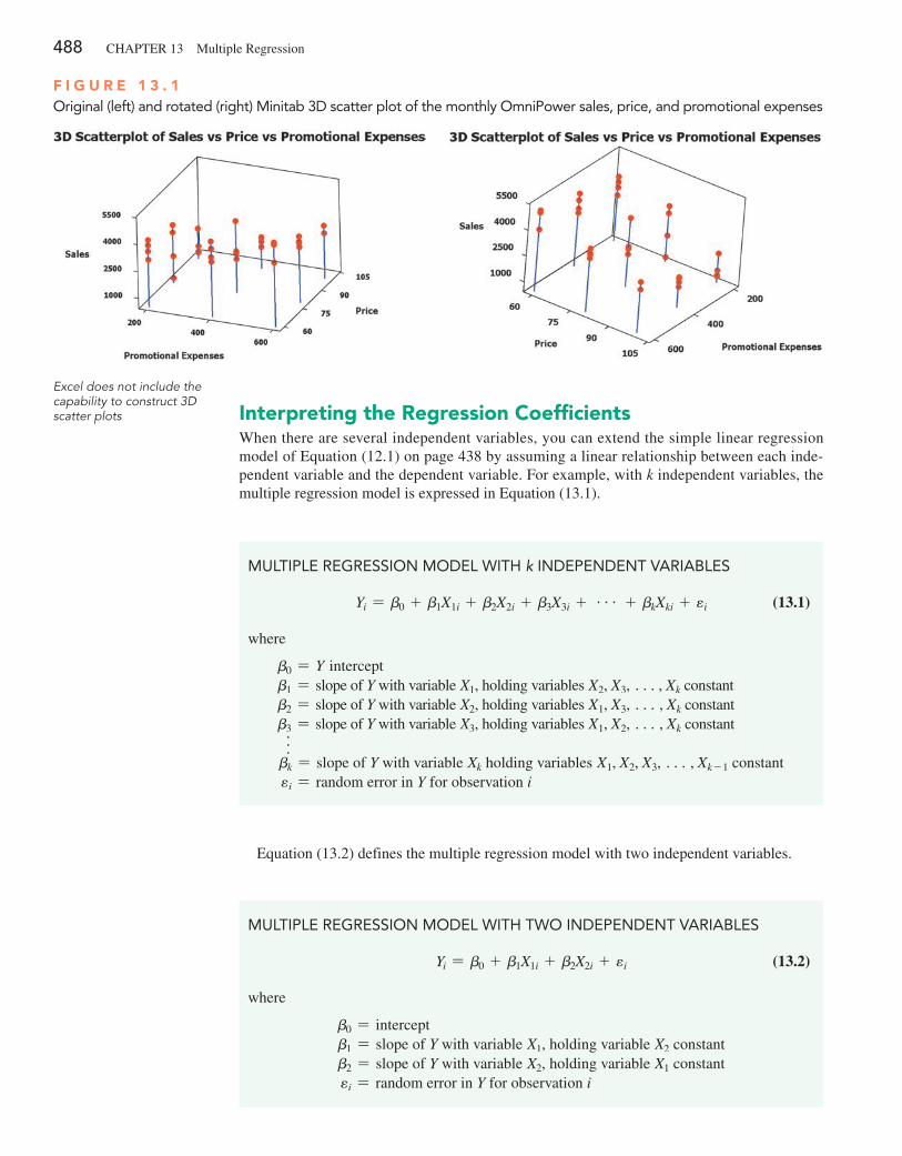
488 CHAPTeR 13 Multiple Regression
Interpreting the Regression CoefficientsWhen there are several independent variables, you can extend the simple linear regression model of equation (12.1) on page 438 by assuming a linear relationship between each inde-pendent variable and the dependent variable. For example, with k independent variables, the multiple regression model is expressed in equation (13.1).
Excel does not include the capability to construct 3D scatter plots
F I g u R e 1 3 . 1Original (left) and rotated (right) Minitab 3D scatter plot of the monthly OmniPower sales, price, and promotional expenses
MUlTIPlE REgRESSIOn MODEl wITH k InDEPEnDEnT VARIABlES
Yi = b0 + b1X1i + b2X2i + b3X3i + g + bkXki + ei (13.1)
where
b0 = Y interceptb1 = slope of Y with variable X1, holding variables X2, X3, c, Xk constantb2 = slope of Y with variable X2, holding variables X1, X3, c, Xk constantb3 = slope of Y with variable X3, holding variables X1, X2, c, Xk constantfbk = slope of Y with variable Xk holding variables X1, X2, X3, c, Xk - 1 constantei = random error in Y for observation i
equation (13.2) defines the multiple regression model with two independent variables.
MUlTIPlE REgRESSIOn MODEl wITH TwO InDEPEnDEnT VARIABlES
Yi = b0 + b1X1i + b2X2i + ei (13.2)
where
b0 = interceptb1 = slope of Y with variable X1, holding variable X2 constantb2 = slope of Y with variable X2, holding variable X1 constantei = random error in Y for observation i
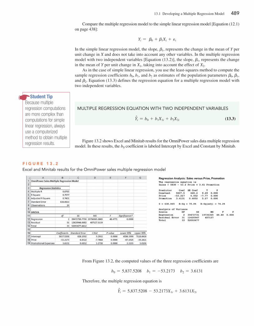
13.1 Developing a Multiple Regression Model 489
Compare the multiple regression model to the simple linear regression model [equation (12.1) on page 438]:
Yi = b0 + b1Xi + ei
In the simple linear regression model, the slope, b1, represents the change in the mean of Y per unit change in X and does not take into account any other variables. In the multiple regression model with two independent variables [equation (13.2)], the slope, b1, represents the change in the mean of Y per unit change in X1, taking into account the effect of X2.
As in the case of simple linear regression, you use the least-squares method to compute the sample regression coefficients b0, b1, and b2 as estimates of the population parameters b0, b1, and b2. equation (13.3) defines the regression equation for a multiple regression model with two independent variables.
Student TipBecause multiple regression computations are more complex than computations for simple linear regression, always use a computerized method to obtain multiple regression results.
MUlTIPlE REgRESSIOn EqUATIOn wITH TwO InDEPEnDEnT VARIABlES
Yni = b0 + b1X1i + b2X2i (13.3)
Figure 13.2 shows excel and Minitab results for the OmniPower sales data multiple regression model. In these results, the b0 coefficient is labeled Intercept by excel and Constant by Minitab.
From Figure 13.2, the computed values of the three regression coefficients are
b0 = 5,837.5208 b1 = -53.2173 b2 = 3.6131
Therefore, the multiple regression equation is
Yni = 5,837.5208 - 53.2173X1i + 3.6131X2i
F I g u R e 1 3 . 2Excel and Minitab results for the OmniPower sales multiple regression model
490 CHAPTeR 13 Multiple Regression
The sample Y intercept 1b0 = 5,837.52082 estimates the number of OmniPower bars sold in a month if the price is $0.00 and the total amount spent on promotional expenditures is also $0.00. Because these values of price and promotion are outside the range of price and promo-tion used in the test-market study, and because they make no sense in the context of the prob-lem, the value of b0 has little or no practical interpretation.
The slope of price with OmniPower sales 1b1 = -53.21732 indicates that, for a given amount of monthly promotional expenditures, the predicted mean sales of OmniPower are es-timated to decrease by 53.2173 bars per month for each 1-cent increase in the price. The slope of monthly promotional expenditures with OmniPower sales 1b2 = 3.61312 indicates that, for a given price, the predicted mean sales of OmniPower are estimated to increase by 3.6131 bars for each additional $1 spent on promotions. These estimates allow you to better understand the likely effect that price and promotion decisions will have in the marketplace. For example, a 10-cent decrease in price is predicted to increase mean sales by 532.173 bars, with a fixed amount of monthly promotional expenditures. A $100 increase in promotional expenditures is predicted to increase mean sales by 361.31 bars for a given price.
Regression coefficients in multiple regression are called net regression coefficients, and they estimate the predicted mean change in Y per unit change in a particular X, holding con-stant the effect of the other X variables. For example, in the study of OmniPower bar sales, for a store with a given amount of promotional expenditures, the mean sales are predicted to decrease by 53.2173 bars per month for each 1-cent increase in the price of an OmniPower bar. Another way to interpret this “net effect” is to think of two stores with an equal amount of promotional expenditures. If the first store charges 1 cent more than the other store, the net effect of this difference is that the first store is predicted to sell a mean of 53.2173 fewer bars per month than the second store. To interpret the net effect of promotional expenditures, you can consider two stores that are charging the same price. If the first store spends $1 more on promotional expenditures, the net effect of this difference is that the first store is predicted to sell a mean of 3.6131 more bars per month than the second store.
Predicting the Dependent Variable YYou can use the multiple regression equation to predict values of the dependent variable. For example, what are the predicted mean sales for a store charging 79 cents during a month in which promotional expenditures are $400? Using the multiple regression equation,
Yni = 5,837.5208 - 53.2173X1i + 3.6131X2i
with X1i = 79 and X2i = 400,
Yni = 5,837.5208 - 53.21731792 + 3.613114002 = 3,078.57
Thus, you predict that stores charging 79 cents and spending $400 in promotional expenditures will sell a mean of 3,078.57 OmniPower bars per month.
After you have developed the regression equation, done a residual analysis (see Section 13.3), and determined the significance of the overall fitted model (see Section 13.2), you can construct a confidence interval estimate of the mean value and a prediction interval for an individual value. Figure 13.3 presents excel and Minitab results that compute a confidence interval estimate and a prediction interval for the OmniPower sales data.
Student TipRemember that in multiple regression, the regression coefficients are conditional on holding constant the other independent variables. The slope of b1 holds constant the effect of variable X2. The slope of b2 holds constant the effect of variable X1.
Student TipYou should only predict within the range of the values of all the independent variables.
where
Yni = predicted monthly sales of OmniPower bars for store i
X1i = price of OmniPower bar (in cents) for store i
X2i = monthly in-store promotional expenditures (in $) for store i
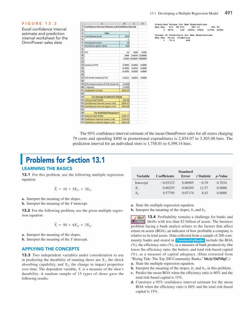
13.1 Developing a Multiple Regression Model 491
The 95% confidence interval estimate of the mean OmniPower sales for all stores charging 79 cents and spending $400 in promotional expenditures is 2,854.07 to 3,303.08 bars. The prediction interval for an individual store is 1,758.01 to 4,399.14 bars.
Problems for Section 13.1leaRnIng The baSICS13.1 For this problem, use the following multiple regression equation:
Yni = 10 + 5X1i + 3X2i
a. Interpret the meaning of the slopes.b. Interpret the meaning of the Y intercept.
13.2 For the following problem, use the given multiple regres-sion equation:
Yni = 50 + 6X1i + 3X2i
a. Interpret the meaning of the slopes.b. Interpret the meaning of the Y intercept.
aPPlyIng The COnCePTS13.3 Two independent variables under consideration to use in predicting the durability of running shoes are X1, the shock absorbing capability, and X2, the change in impact properties over time. The dependent variable, Y, is a measure of the shoe’s durability. A random sample of 15 types of shoes gave the following results:
Variable CoefficientsStandard
Error t Statistic p-Value
Intercept -0.03222 0.06905 -0.39 0.7034
X1 0.80255 0.06295 12.57 0.0000X2 0.57795 0.07174 8.43 0.0000
a. State the multiple regression equation.b. Interpret the meaning of the slopes, b1 and b2.
SELF Test
13.4 Profitability remains a challenge for banks and thrifts with less than $2 billion of assets. The business
problem facing a bank analyst relates to the factors that affect return on assets (ROA), an indicator of how profitable a company is relative to its total assets. Data collected from a sample of 200 com-munity banks and stored in Communitybanks include the ROA (%), the efficiency ratio (%), as a measure of bank productivity (the lower the efficiency ratio, the better), and total risk-based capital (%), as a measure of capital adequacy. (Data extracted from “Rising Tide: The Top 200 Community Banks,” bit.ly/1ldN8gC.)a. State the multiple regression equation.b. Interpret the meaning of the slopes, b1 and b2, in this problem.c. Predict the mean ROA when the efficiency ratio is 60% and the
total risk-based capital is 15%.d. Construct a 95% confidence interval estimate for the mean
ROA when the efficiency ratio is 60% and the total risk-based capital is 15%.
F I g u R e 1 3 . 3Excel confidence interval estimate and prediction interval worksheet for the OmniPower sales data
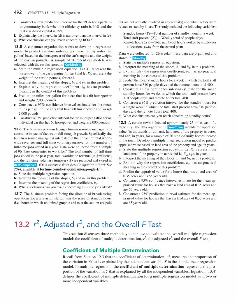
492 CHAPTeR 13 Multiple Regression
e. Construct a 95% prediction interval for the ROA for a particu-lar community bank when the efficiency ratio is 60% and the total risk-based capital is 15%.
f. explain why the interval in (d) is narrower than the interval in (e).g. What conclusions can you reach concerning ROA?
13.5 A consumer organization wants to develop a regression model to predict gasoline mileage (as measured by miles per gallon) based on the horsepower of the car’s engine and the weight of the car (in pounds). A sample of 20 recent car models was selected, with the results stored in CarModels . a. State the multiple regression equation. Let X1i represent the
horsepower of the car’s engine for car i and let X2i represent the weight of the car (in pounds) for car i.
b. Interpret the meaning of the slopes, b1 and b2, in this problem.c. explain why the regression coefficient, b0, has no practical
meaning in the context of this problem.d. Predict the miles per gallon for a car that has 60 horsepower
and weighs 2,000 pounds.e. Construct a 95% confidence interval estimate for the mean
miles per gallon for cars that have 60 horsepower and weigh 2,000 pounds.
f. Construct a 95% prediction interval for the miles per gallon for an individual car that has 60 horsepower and weighs 2,000 pounds.
13.6 The business problem facing a human resource manager is to assess the impact of factors on full-time job growth. Specifically, the human resource manager is interested in the impact of total world-wide revenues and full-time voluntary turnover on the number of full-time jobs added in a year. Data were collected from a sample of 96 “best companies to work for.” The total number of full-time jobs added in the past year, total worldwide revenue (in $millions) and the full-time voluntary turnover (%) are recorded and stored in bestCompanies . (Data extracted from Best Companies to Work For 2014, available at fortune.com/best-companies/google-1/.)a. State the multiple regression equation.b. Interpret the meaning of the slopes, b1 and b2, in this problem.c. Interpret the meaning of the regression coefficient, b0.d. What conclusions can you reach concerning full-time jobs added?
13.7 The business problem facing the director of broadcasting operations for a television station was the issue of standby hours (i.e., hours in which unionized graphic artists at the station are paid
but are not actually involved in any activity) and what factors were related to standby hours. The study included the following variables:
Standby hours (Y)—Total number of standby hours in a weekTotal staff present 1X12—Weekly total of people-daysRemote hours 1X22—Total number of hours worked by employees at locations away from the central plant
Data were collected for 26 weeks; these data are organized and stored in Standby .a. State the multiple regression equation.b. Interpret the meaning of the slopes, b1 and b2, in this problem.c. explain why the regression coefficient, b0, has no practical
meaning in the context of this problem.d. Predict the mean standby hours for a week in which the total staff
present have 310 people-days and the remote hours total 400.e. Construct a 95% confidence interval estimate for the mean
standby hours for weeks in which the total staff present have 310 people-days and remote hours total 400.
f. Construct a 95% prediction interval for the standby hours for a single week in which the total staff present have 310 people-days and the remote hours total 400.
g. What conclusions can you reach concerning standby hours?
13.8 A certain town is located approximately 25 miles east of a large city. The data organized in yourTown include the appraised value (in thousands of dollars), land area of the property in acres, and age, in years, for a sample of 20 single-family homes located in the town. Develop a multiple linear regression model to predict appraised value based on land area of the property and age, in years.a. State the multiple regression equation. Let X1i represent the
land area of the property in acres and let X2i age, in years.b. Interpret the meaning of the slopes, b1 and b2, in this problem.c. explain why the regression coefficient, b0, has no practical
meaning in the context of this problem.d. Predict the appraised value for a house that has a land area of
0.35 acres and is 65 years old.e. Construct a 95% confidence interval estimate for the mean ap-
praised value for houses that have a land area of 0.35 acres and are 65 years old.
f. Construct a 95% prediction interval estimate for the mean ap-praised value for houses that have a land area of 0.35 acres and are 65 years old.
13.2 r2, Adjusted r2, and the Overall F TestThis section discusses three methods you can use to evaluate the overall multiple regression model: the coefficient of multiple determination, r2, the adjusted r2, and the overall F test.
Coefficient of Multiple DeterminationRecall from Section 12.3 that the coefficient of determination, r 2, measures the proportion of the variation in Y that is explained by the independent variable X in the simple linear regression model. In multiple regression, the coefficient of multiple determination represents the pro-portion of the variation in Y that is explained by all the independent variables. equation (13.4) defines the coefficient of multiple determination for a multiple regression model with two or more independent variables.
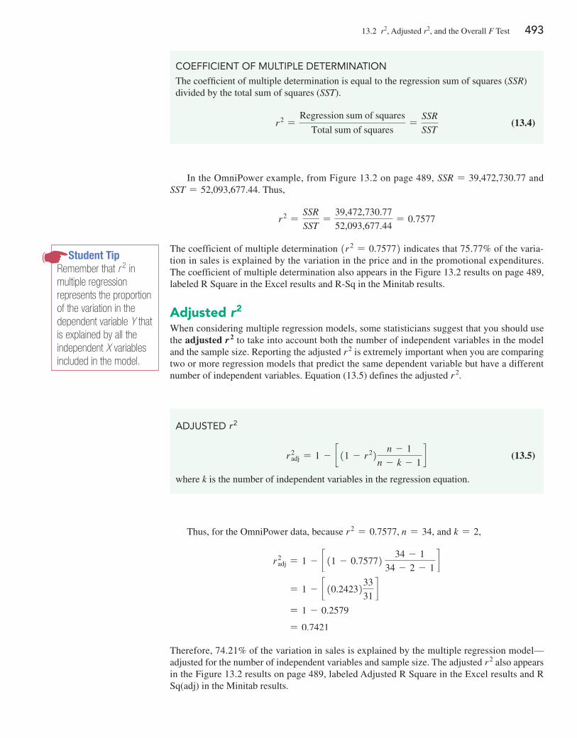
13.2 r2, Adjusted r2, and the Overall F Test 493
COEffICIEnT Of MUlTIPlE DETERMInATIOn
The coefficient of multiple determination is equal to the regression sum of squares (SSR) divided by the total sum of squares (SST).
r 2 =Regression sum of squares
Total sum of squares=
SSR
SST (13.4)
In the OmniPower example, from Figure 13.2 on page 489, SSR = 39,472,730.77 and SST = 52,093,677.44. Thus,
r 2 =SSR
SST=
39,472,730.77
52,093,677.44= 0.7577
The coefficient of multiple determination 1r 2 = 0.75772 indicates that 75.77% of the varia-tion in sales is explained by the variation in the price and in the promotional expenditures. The coefficient of multiple determination also appears in the Figure 13.2 results on page 489, labeled R Square in the excel results and R-Sq in the Minitab results.
adjusted r2
When considering multiple regression models, some statisticians suggest that you should use the adjusted r 2 to take into account both the number of independent variables in the model and the sample size. Reporting the adjusted r 2 is extremely important when you are comparing two or more regression models that predict the same dependent variable but have a different number of independent variables. equation (13.5) defines the adjusted r 2.
Student TipRemember that r 2 in multiple regression represents the proportion of the variation in the dependent variable Y that is explained by all the independent X variables included in the model.
ADjUSTED r2
r 2adj = 1 - c 11 - r 22 n - 1
n - k - 1d (13.5)
where k is the number of independent variables in the regression equation.
Thus, for the OmniPower data, because r 2 = 0.7577, n = 34, and k = 2,
r 2adj = 1 - c 11 - 0.75772
34 - 1
34 - 2 - 1d
= 1 - c 10.2423233
31d
= 1 - 0.2579
= 0.7421
Therefore, 74.21% of the variation in sales is explained by the multiple regression model— adjusted for the number of independent variables and sample size. The adjusted r 2 also appears in the Figure 13.2 results on page 489, labeled Adjusted R Square in the excel results and R Sq(adj) in the Minitab results.
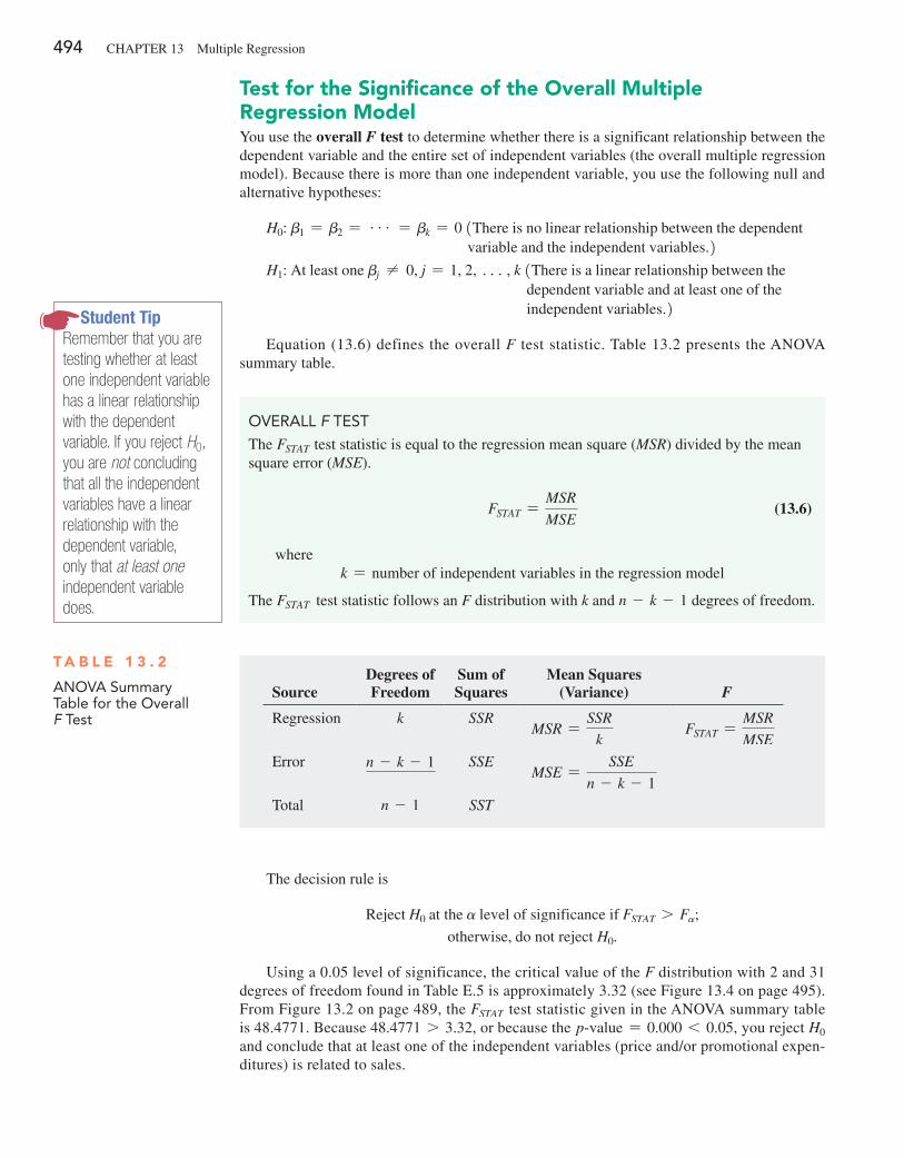
494 CHAPTeR 13 Multiple Regression
Test for the Significance of the Overall Multiple Regression ModelYou use the overall F test to determine whether there is a significant relationship between the dependent variable and the entire set of independent variables (the overall multiple regression model). Because there is more than one independent variable, you use the following null and alternative hypotheses:
H0: b1 = b2 = g = bk = 0 1There is no linear relationship between the dependent variable and the independent variables.2
H1: At least one bj ≠ 0, j = 1, 2, c, k 1There is a linear relationship between thedependent variable and at least one of theindependent variables.2
equation (13.6) defines the overall F test statistic. Table 13.2 presents the ANOVA summary table.
T a b l e 1 3 . 2
AnOVA Summary Table for the Overall F Test
SourceDegrees of Freedom
Sum of Squares
Mean Squares (Variance) F
Regression k SSRMSR =
SSR
kFSTAT =
MSR
MSE
error n - k - 1 SSEMSE =
SSE
n - k - 1
Total n - 1 SST
OVERAll F TEST
The FSTAT test statistic is equal to the regression mean square (MSR) divided by the mean square error (MSE).
FSTAT =MSR
MSE (13.6)
wherek = number of independent variables in the regression model
The FSTAT test statistic follows an F distribution with k and n - k - 1 degrees of freedom.
Student TipRemember that you are testing whether at least one independent variable has a linear relationship with the dependent variable. If you reject H0, you are not concluding that all the independent variables have a linear relationship with the dependent variable, only that at least one independent variable does.
The decision rule is
Reject H0 at the a level of significance if FSTAT 7 Fa;
otherwise, do not reject H0.
Using a 0.05 level of significance, the critical value of the F distribution with 2 and 31 degrees of freedom found in Table e.5 is approximately 3.32 (see Figure 13.4 on page 495). From Figure 13.2 on page 489, the FSTAT test statistic given in the ANOVA summary table is 48.4771. Because 48.4771 7 3.32, or because the p@value = 0.000 6 0.05, you reject H0 and conclude that at least one of the independent variables (price and/or promotional expen-ditures) is related to sales.
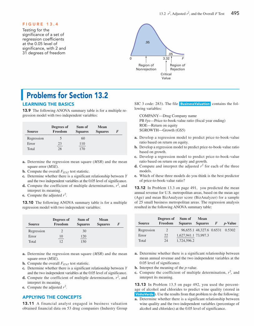
13.2 r2, Adjusted r2, and the Overall F Test 495
0 3.32
.95
.05
Region ofNonrejection
F
CriticalValue
Region ofRejection
F I g u R e 1 3 . 4Testing for the significance of a set of regression coefficients at the 0.05 level of significance, with 2 and 31 degrees of freedom
SourceDegrees of Freedom
Sum of Squares
Mean Squares F p-Value
Regression 2 96,655.1 48,327.6 0.6531 0.5302
error 22 1,627,941.1 73,997.3
Total 24 1,724,596.2
Problems for Section 13.2leaRnIng The baSICS13.9 The following ANOVA summary table is for a multiple re-gression model with two independent variables:
SourceDegrees of Freedom
Sum of Squares
Mean Squares F
Regression 5 60
error 23 110
Total 28 170
SourceDegrees of Freedom
Sum of Squares
Mean Squares F
Regression 2 30
error 10 120
Total 12 150
a. Determine the regression mean square (MSR) and the mean square error (MSE).
b. Compute the overall FSTAT test statistic.c. Determine whether there is a significant relationship between Y
and the two independent variables at the 0.05 level of significance.d. Compute the coefficient of multiple determinations, r2, and
interpret its meaning.e. Compute the adjusted r2.
13.10 The following ANOVA summary table is for a multiple regression model with two independent variables:
SIC 3 code: 283). The file businessValuation contains the fol-lowing variables:
COMPANY—Drug Company namePB fye—Price-to-book-value ratio (fiscal year ending)ROe—Return on equitySGROWTH—Growth (GS5)
a. Develop a regression model to predict price-to-book-value ratio based on return on equity.
b. Develop a regression model to predict price-to-book-value ratio based on growth.
c. Develop a regression model to predict price-to-book-value ratio based on return on equity and growth.
d. Compute and interpret the adjusted r2 for each of the three models.
e. Which of these three models do you think is the best predictor of price-to-book-value ratio?
13.12 In Problem 13.3 on page 491, you predicted the mean annual revenue for U.S. metropolitan areas, based on the mean age (Age) and mean BizAnalyzer score (BizAnalyzer) for a sample of 25 small business metropolitan areas. The regression analysis resulted in the following ANOVA summary table:
a. Determine the regression mean square (MSR) and the mean square error (MSE).
b. Compute the overall FSTAT test statistic.c. Determine whether there is a significant relationship between Y
and the two independent variables at the 0.05 level of significance.d. Compute the coefficient of multiple determination, r2, and
interpret its meaning.e. Compute the adjusted r2.
aPPlyIng The COnCePTS13.11 A financial analyst engaged in business valuation obtained financial data on 53 drug companies (Industry Group
a. Determine whether there is a significant relationship between mean annual revenue and the two independent variables at the 0.05 level of significance.
b. Interpret the meaning of the p-value.c. Compute the coefficient of multiple determination, r2, and
interpret its meaning.
13.13 In Problem 13.5 on page 492, you used the percent-age of alcohol and chlorides to predict wine quality (stored in VinhoVerde ). Use the results from that problem to do the following:a. Determine whether there is a significant relationship between
wine quality and the two independent variables (percentage of alcohol and chlorides) at the 0.05 level of significance.
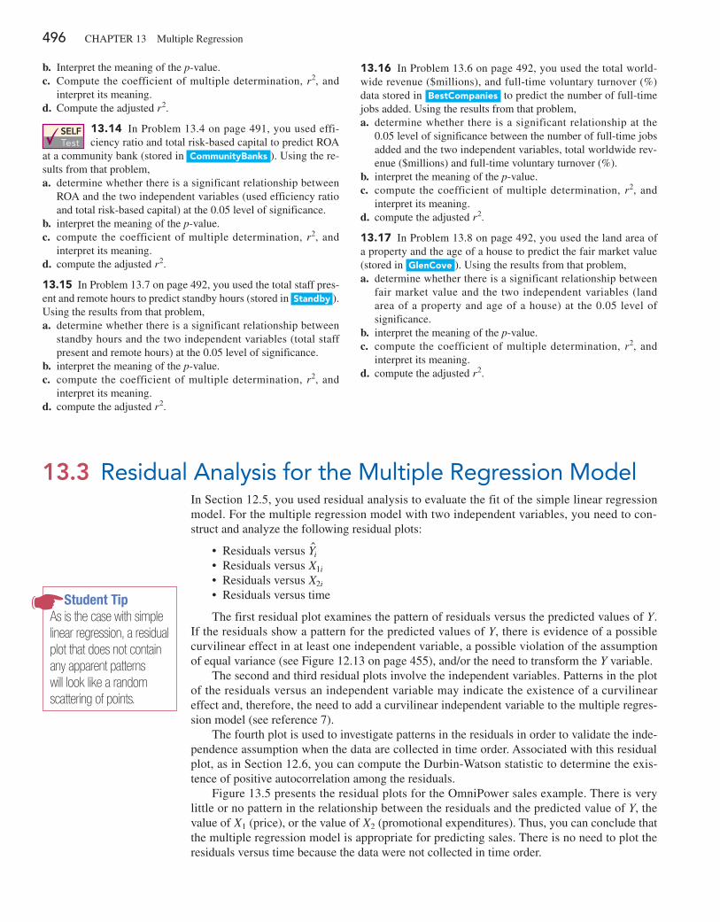
496 CHAPTeR 13 Multiple Regression
13.16 In Problem 13.6 on page 492, you used the total world-wide revenue ($millions), and full-time voluntary turnover (%) data stored in bestCompanies to predict the number of full-time jobs added. Using the results from that problem, a. determine whether there is a significant relationship at the
0.05 level of significance between the number of full-time jobs added and the two independent variables, total worldwide rev-enue ($millions) and full-time voluntary turnover (%).
b. interpret the meaning of the p-value.c. compute the coefficient of multiple determination, r2, and
interpret its meaning.d. compute the adjusted r2.
13.17 In Problem 13.8 on page 492, you used the land area of a property and the age of a house to predict the fair market value (stored in glenCove ). Using the results from that problem,a. determine whether there is a significant relationship between
fair market value and the two independent variables (land area of a property and age of a house) at the 0.05 level of significance.
b. interpret the meaning of the p-value.c. compute the coefficient of multiple determination, r2, and
interpret its meaning.d. compute the adjusted r2.
13.3 Residual Analysis for the Multiple Regression ModelIn Section 12.5, you used residual analysis to evaluate the fit of the simple linear regression model. For the multiple regression model with two independent variables, you need to con-struct and analyze the following residual plots:
• Residuals versus Yni
• Residuals versus X1i
• Residuals versus X2i
• Residuals versus time
The first residual plot examines the pattern of residuals versus the predicted values of Y. If the residuals show a pattern for the predicted values of Y, there is evidence of a possible curvilinear effect in at least one independent variable, a possible violation of the assumption of equal variance (see Figure 12.13 on page 455), and/or the need to transform the Y variable.
The second and third residual plots involve the independent variables. Patterns in the plot of the residuals versus an independent variable may indicate the existence of a curvilinear effect and, therefore, the need to add a curvilinear independent variable to the multiple regres-sion model (see reference 7).
The fourth plot is used to investigate patterns in the residuals in order to validate the inde-pendence assumption when the data are collected in time order. Associated with this residual plot, as in Section 12.6, you can compute the Durbin-Watson statistic to determine the exis-tence of positive autocorrelation among the residuals.
Figure 13.5 presents the residual plots for the OmniPower sales example. There is very little or no pattern in the relationship between the residuals and the predicted value of Y, the value of X1 (price), or the value of X2 (promotional expenditures). Thus, you can conclude that the multiple regression model is appropriate for predicting sales. There is no need to plot the residuals versus time because the data were not collected in time order.
Student TipAs is the case with simple linear regression, a residual plot that does not contain any apparent patterns will look like a random scattering of points.
b. Interpret the meaning of the p-value.c. Compute the coefficient of multiple determination, r2, and
interpret its meaning.d. Compute the adjusted r2.
SELF Test
13.14 In Problem 13.4 on page 491, you used effi-ciency ratio and total risk-based capital to predict ROA
at a community bank (stored in Communitybanks ). Using the re-sults from that problem,a. determine whether there is a significant relationship between
ROA and the two independent variables (used efficiency ratio and total risk-based capital) at the 0.05 level of significance.
b. interpret the meaning of the p-value.c. compute the coefficient of multiple determination, r2, and
interpret its meaning.d. compute the adjusted r2.
13.15 In Problem 13.7 on page 492, you used the total staff pres-ent and remote hours to predict standby hours (stored in Standby ). Using the results from that problem,a. determine whether there is a significant relationship between
standby hours and the two independent variables (total staff present and remote hours) at the 0.05 level of significance.
b. interpret the meaning of the p-value.c. compute the coefficient of multiple determination, r2, and
interpret its meaning.d. compute the adjusted r2.
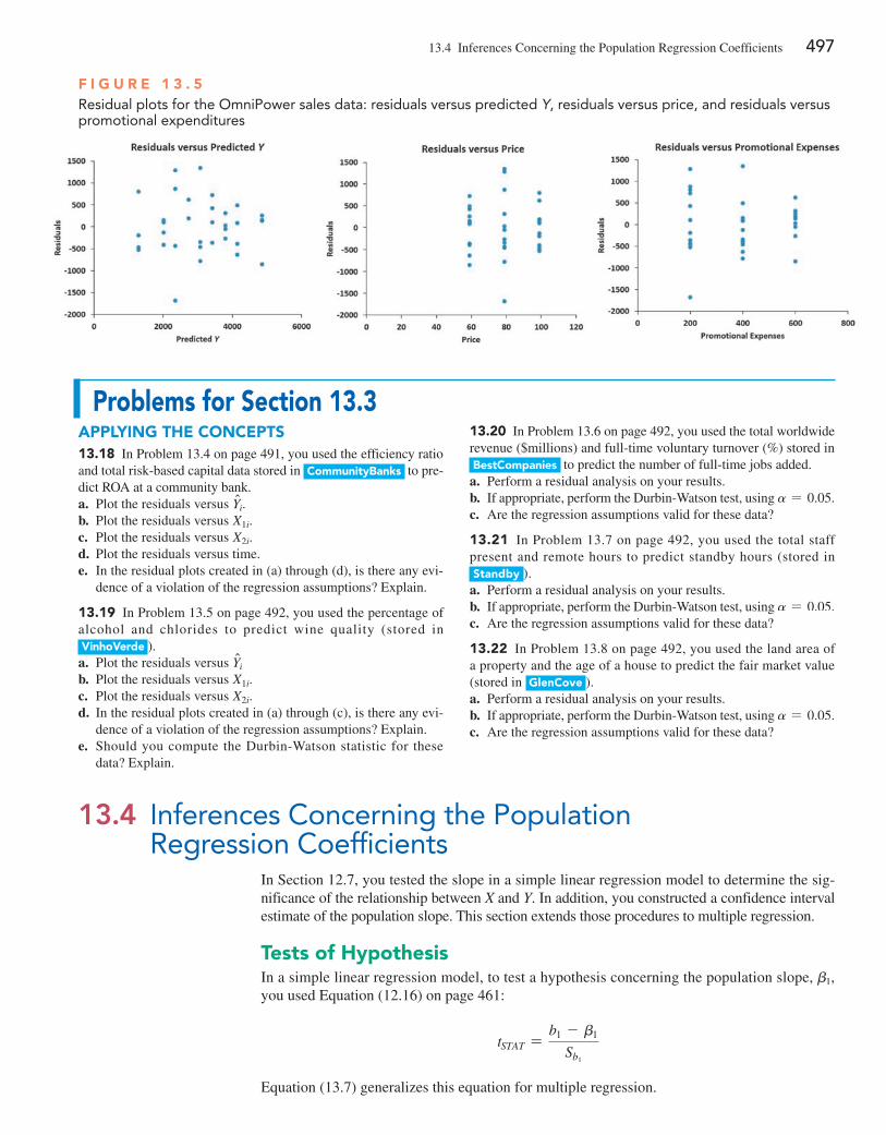
13.4 Inferences Concerning the Population Regression Coefficients 497
F I g u R e 1 3 . 5Residual plots for the OmniPower sales data: residuals versus predicted Y, residuals versus price, and residuals versus promotional expenditures
Problems for Section 13.3aPPlyIng The COnCePTS13.18 In Problem 13.4 on page 491, you used the efficiency ratio and total risk-based capital data stored in Communitybanks to pre-dict ROA at a community bank.a. Plot the residuals versus Yni.b. Plot the residuals versus X1i.c. Plot the residuals versus X2i.d. Plot the residuals versus time.e. In the residual plots created in (a) through (d), is there any evi-
dence of a violation of the regression assumptions? explain.
13.19 In Problem 13.5 on page 492, you used the percentage of alcohol and chlorides to predict wine quality (stored in VinhoVerde ).a. Plot the residuals versus Yni
b. Plot the residuals versus X1i.c. Plot the residuals versus X2i.d. In the residual plots created in (a) through (c), is there any evi-
dence of a violation of the regression assumptions? explain.e. Should you compute the Durbin-Watson statistic for these
data? explain.
13.20 In Problem 13.6 on page 492, you used the total worldwide revenue ($millions) and full-time voluntary turnover (%) stored in bestCompanies to predict the number of full-time jobs added.a. Perform a residual analysis on your results.b. If appropriate, perform the Durbin-Watson test, using a = 0.05.c. Are the regression assumptions valid for these data?
13.21 In Problem 13.7 on page 492, you used the total staff present and remote hours to predict standby hours (stored in Standby ).a. Perform a residual analysis on your results.b. If appropriate, perform the Durbin-Watson test, using a = 0.05.c. Are the regression assumptions valid for these data?
13.22 In Problem 13.8 on page 492, you used the land area of a property and the age of a house to predict the fair market value (stored in glenCove ).a. Perform a residual analysis on your results.b. If appropriate, perform the Durbin-Watson test, using a = 0.05.c. Are the regression assumptions valid for these data?
13.4 Inferences Concerning the Population Regression Coefficients
In Section 12.7, you tested the slope in a simple linear regression model to determine the sig-nificance of the relationship between X and Y. In addition, you constructed a confidence interval estimate of the population slope. This section extends those procedures to multiple regression.
Tests of hypothesisIn a simple linear regression model, to test a hypothesis concerning the population slope, b1, you used equation (12.16) on page 461:
tSTAT =b1 - b1
Sb1
equation (13.7) generalizes this equation for multiple regression.
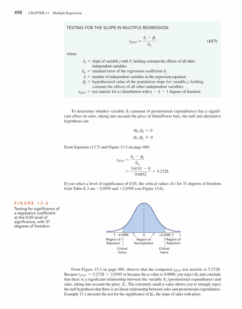
498 CHAPTeR 13 Multiple Regression
TESTIng fOR THE SlOPE In MUlTIPlE REgRESSIOn
tSTAT =bj - bj
Sbj
(13.7)
where
bj = slope of variable j with Y, holding constant the effects of all other independent variables
Sbj= standard error of the regression coefficient bj
k = number of independent variables in the regression equationbj = hypothesized value of the population slope for variable j, holding
constant the effects of all other independent variablestSTAT = test statistic for a t distribution with n - k - 1 degrees of freedom
To determine whether variable X2 (amount of promotional expenditures) has a signifi-cant effect on sales, taking into account the price of OmniPower bars, the null and alternative hypotheses are
H0: b2 = 0
H1: b2 ≠ 0
From equation (13.7) and Figure 13.2 on page 489,
tSTAT =b2 - b2
Sb2
=3.6131 - 0
0.6852= 5.2728
If you select a level of significance of 0.05, the critical values of t for 31 degrees of freedom from Table e.3 are -2.0395 and +2.0395 (see Figure 13.6).
F I g u R e 1 3 . 6Testing for significance of a regression coefficient at the 0.05 level of significance, with 31 degrees of freedom
–2.0395 +2.03950 tRegion ofRejection
CriticalValue
Region ofNonrejection
CriticalValue
Region ofRejection
From Figure 13.2 on page 489, observe that the computed tSTAT test statistic is 5.2728. Because tSTAT = 5.2728 7 2.0395 or because the p-value is 0.0000, you reject H0 and conclude that there is a significant relationship between the variable X2 (promotional expenditures) and sales, taking into account the price, X1. The extremely small p-value allows you to strongly reject the null hypothesis that there is no linear relationship between sales and promotional expenditures. example 13.1 presents the test for the significance of b1, the slope of sales with price.
13.4 Inferences Concerning the Population Regression Coefficients 499
COnfIDEnCE InTERVAl ESTIMATE fOR THE SlOPE
bj { ta>2Sbj (13.8)
where
ta>2 = critical value corresponding to an upper-tail probability of a>2 from the t distribution with n - k - 1 degrees of freedom (i.e., a cumulative area of 1 - a>2)
k = number of independent variables
As shown with these two independent variables, the test of significance for a specific regression coefficient in multiple regression is a test for the significance of adding that vari-able into a regression model, given that the other variable is included. In other words, the t test for the regression coefficient is actually a test for the contribution of each independent variable.
Confidence Interval estimationInstead of testing the significance of a population slope, you may want to estimate the value of a population slope. equation (13.8) defines the confidence interval estimate for a population slope in multiple regression.
To construct a 95% confidence interval estimate of the population slope, b1 (the effect of price, X1, on sales, Y, holding constant the effect of promotional expenditures, X2), the critical value of t at the 95% confidence level with 31 degrees of freedom is 2.0395 (see Table e.3). Then, using equation (13.8) and Figure 13.2 on page 489,
b1 { ta>2Sb1
-53.2173 { 12.0395216.85222-53.2173 { 13.9752
-67.1925 … b1 … -39.2421
Taking into account the effect of promotional expenditures, the estimated effect of a 1-cent increase in price is to reduce mean sales by approximately 39.2 to 67.2 bars. You have 95% confidence that this interval correctly estimates the relationship between these variables. From a hypothesis-testing viewpoint, because this confidence interval does not include 0, you conclude that the regression coefficient, b1, has a significant effect.
example 13.2 constructs and interprets a confidence interval estimate for the slope of sales with promotional expenditures.
exaMPle 13.1testing for the significance of the slope of sales with price
At the 0.05 level of significance, is there evidence that the slope of sales with price is different from zero?
SOluTIOn From Figure 13.2 on page 489, tSTAT = -7.7664 6 -2.0395 (the critical value for a = 0.05) or the p-value = 0.0000 6 0.05. Thus, there is a significant relationship between price, X1, and sales, taking into account the promotional expenditures, X2.
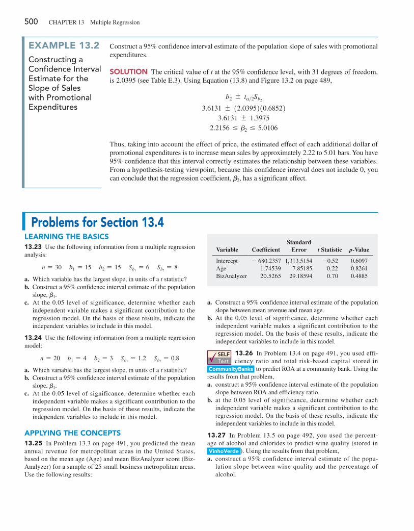
500 CHAPTeR 13 Multiple Regression
exaMPle 13.2constructing a confidence interval estimate for the slope of sales with promotional expenditures
Construct a 95% confidence interval estimate of the population slope of sales with promotional expenditures.
SOluTIOn The critical value of t at the 95% confidence level, with 31 degrees of freedom, is 2.0395 (see Table e.3). Using equation (13.8) and Figure 13.2 on page 489,
b2 { ta>2Sb2
3.6131 { 12.0395210.685223.6131 { 1.3975
2.2156 … b2 … 5.0106
Thus, taking into account the effect of price, the estimated effect of each additional dollar of promotional expenditures is to increase mean sales by approximately 2.22 to 5.01 bars. You have 95% confidence that this interval correctly estimates the relationship between these variables. From a hypothesis-testing viewpoint, because this confidence interval does not include 0, you can conclude that the regression coefficient, b2, has a significant effect.
a. Construct a 95% confidence interval estimate of the population slope between mean revenue and mean age.
b. At the 0.05 level of significance, determine whether each independent variable makes a significant contribution to the regression model. On the basis of these results, indicate the independent variables to include in this model.
SELF Test
13.26 In Problem 13.4 on page 491, you used effi-ciency ratio and total risk-based capital stored in
Communitybanks to predict ROA at a community bank. Using the results from that problem,a. construct a 95% confidence interval estimate of the population
slope between ROA and efficiency ratio.b. at the 0.05 level of significance, determine whether each
independent variable makes a significant contribution to the regression model. On the basis of these results, indicate the independent variables to include in this model.
13.27 In Problem 13.5 on page 492, you used the percent-age of alcohol and chlorides to predict wine quality (stored in VinhoVerde ). Using the results from that problem,a. construct a 95% confidence interval estimate of the popu-
lation slope between wine quality and the percentage of alcohol.
Problems for Section 13.4leaRnIng The baSICS13.23 Use the following information from a multiple regression analysis:
n = 30 b1 = 15 b2 = 15 Sb1= 6 Sb2
= 8
a. Which variable has the largest slope, in units of a t statistic?b. Construct a 95% confidence interval estimate of the population
slope, b1.c. At the 0.05 level of significance, determine whether each
independent variable makes a significant contribution to the regression model. On the basis of these results, indicate the independent variables to include in this model.
13.24 Use the following information from a multiple regression model:
n = 20 b1 = 4 b2 = 3 Sb1= 1.2 Sb2
= 0.8
a. Which variable has the largest slope, in units of a t statistic?b. Construct a 95% confidence interval estimate of the population
slope, b1.c. At the 0.05 level of significance, determine whether each
independent variable makes a significant contribution to the regression model. On the basis of these results, indicate the independent variables to include in this model.
aPPlyIng The COnCePTS13.25 In Problem 13.3 on page 491, you predicted the mean annual revenue for metropolitan areas in the United States, based on the mean age (Age) and mean BizAnalyzer score (Biz-Analyzer) for a sample of 25 small business metropolitan areas. Use the following results:
Variable CoefficientStandard
Error t Statistic p-Value
Intercept - 680.2357 1,313.5154 -0.52 0.6097Age 1.74539 7.85185 0.22 0.8261BizAnalyzer 20.5265 29.18594 0.70 0.4885
13.5 Using Dummy Variables and Interaction Terms in Regression Models 501
b. at the 0.05 level of significance, determine whether each independent variable makes a significant contribution to the regression model. On the basis of these results, indicate the independent variables to include in this model.
13.28 In Problem 13.6 on page 492, you used the total world-wide revenue ($millions) and full-time voluntary turnover (%) data stored in bestCompanies to predict the number of full-time jobs added. Using the results from that problem,a. construct a 95% confidence interval estimate of the population
slope between the number of full-time jobs added and total worldwide revenue.
b. at the 0.05 level of significance, determine whether each independent variable makes a significant contribution to the regression model. On the basis of these results, indicate the independent variables to include in this model.
13.29 In Problem 13.7 on page 492, you used the total number of staff present and remote hours to predict standby hours (stored in Standby ). Using the results from that problem,
a. construct a 95% confidence interval estimate of the popula-tion slope between standby hours and total number of staff present.
b. at the 0.05 level of significance, determine whether each independent variable makes a significant contribution to the regression model. On the basis of these results, indicate the independent variables to include in this model.
13.30 In Problem 13.8 on page 492, you used land area of a property and age of a house to predict the fair market value (stored in glenCove ). Using the results from that problem,a. construct a 95% confidence interval estimate of the population
slope between fair market value and land area of a property.b. at the 0.05 level of significance, determine whether each
independent variable makes a significant contribution to the regression model. On the basis of these results, indicate the independent variables to include in this model.
13.5 Using Dummy Variables and Interaction Terms in Regression Models
The multiple regression models discussed in Sections 13.1 through 13.4 assumed that each independent variable is a numerical variable. For example, in Section 13.1, you used price and promotional expenditures, two numerical independent variables, to predict the monthly sales of OmniPower nutrition bars. However, for some models, you need to include the effect of a cate-gorical independent variable. For example, to predict the monthly sales of the OmniPower bars, you might include the categorical variable end-cap location in the model to explore the possible effect on sales caused by displaying the OmniPower bars in the two different end-cap display locations, produce or beverage, used in the North Fork Beverages scenario in Chapter 10.
Dummy VariablesYou use a dummy variable to include a categorical independent variable in a regression model. A dummy variable Xd recodes the categories of a categorical variable using the numeric values 0 and 1. In the special case of a categorical independent variable that has only two cate-gories, you define one dummy variable, Xd, and use the values 0 and 1 to represent the two cat-egories. For example, for the categorical variable end-cap location discussed in the Chapter 10 Using Statistics scenario, the dummy variable, Xd, would have these values:
Xd = 0 if the observation is in first category 1produce end@cap2 Xd = 1 if the observation is in second category 1beverage end@cap2
To illustrate using dummy variables in regression, consider the business problem that involves developing a model for predicting the assessed value ($thousands) of houses in Silver Spring, Maryland, based on house size (in thousands of square feet) and whether the house has a fireplace. To include the categorical variable for the presence of a fireplace, the dummy vari-able X2 is defined as
X2 = 0 if the house does not have a fireplace
X2 = 1 if the house has a fireplace
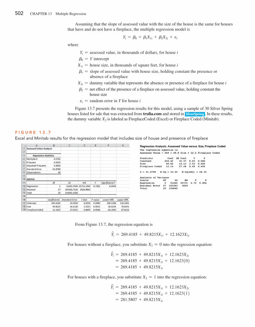
502 CHAPTeR 13 Multiple Regression
Assuming that the slope of assessed value with the size of the house is the same for houses that have and do not have a fireplace, the multiple regression model is
Yi = b0 + b1X1i + b2X2i + ei
where
Yi = assessed value, in thousands of dollars, for house i
b0 = Y intercept
X1i = house size, in thousands of square feet, for house i
b1 = slope of assessed value with house size, holding constant the presence or absence of a fireplace
X2i = dummy variable that represents the absence or presence of a fireplace for house i
b2 = net effect of the presence of a fireplace on assessed value, holding constant the house size
ei = random error in Y for house i
Figure 13.7 presents the regression results for this model, using a sample of 30 Silver Spring houses listed for sale that was extracted from trulia.com and stored in SilverSpring . In these results, the dummy variable X2 is labeled as FireplaceCoded (excel) or Fireplace Coded (Minitab).
F I g u R e 1 3 . 7Excel and Minitab results for the regression model that includes size of house and presence of fireplace
From Figure 13.7, the regression equation is
Yni = 269.4185 + 49.8215X1i + 12.1623X2i
For houses without a fireplace, you substitute X2 = 0 into the regression equation:
Yni = 269.4185 + 49.8215X1i + 12.1623X2i
= 269.4185 + 49.8215X1i + 12.1623102 = 269.4185 + 49.8215X1i
For houses with a fireplace, you substitute X2 = 1 into the regression equation:
Yni = 269.4185 + 49.8215X1i + 12.1623X2i
= 269.4185 + 49.8215X1i + 12.1623112 = 281.5807 + 49.8215X1i
13.5 Using Dummy Variables and Interaction Terms in Regression Models 503
In this model, the regression coefficients are interpreted as follows:
• Holding constant whether a house has a fireplace, for each increase of 1.0 thousand square feet in house size, the predicted mean assessed value is estimated to increase by 49.8215 thousand dollars (i.e., $49,821.50).
• Holding constant the house size, the presence of a fireplace is estimated to increase the predicted mean assessed value of the house by 12.1623 thousand dollars (i.e., $12,162.30).
In Figure 13.7, the tSTAT test statistic for the slope of house size with assessed value is 3.5253, and the p-value is 0.015; the tSTAT test statistic for presence of a fireplace is 0.4499, and the p-value is 0.6564. Thus, using the 0.05 level of significance, since 0.0015 6 0.05, the size of the house makes a significant contribution to the model. However, since 0.6564 7 0.05, the presence of a fireplace does not make a significant contribution to the model. In addition, from Figure 13.7, observe that the coefficient of multiple determination indicates that 33.23% of the variation in as-sessed value is explained by variation in house size and whether the house has a fireplace. Thus, the variable fireplace does not make a significant contribution and should not be included in the model.
InteractionsIn the regression models discussed so far, the effect an independent variable has on the depen-dent variable has been assumed to be independent of the other independent variables in the model. An interaction occurs if the effect of an independent variable on the dependent variable changes according to the value of a second independent variable. For example, it is possible that advertising will have a large effect on the sales of a product when the price of a product is low. However, if the price of the product is too high, increases in advertising will not dramati-cally change sales. In this case, price and advertising are said to interact. In other words, you cannot make general statements about the effect of advertising on sales. The effect that adver-tising has on sales is dependent on the price. You use an interaction term (sometimes referred to as a cross-product term) to model an interaction effect in a regression model.
To illustrate the concept of interaction and use of an interaction term, return to the example concerning the assessed values of homes discussed on pages 501–502. In the regression model, you assumed that the effect that house size has on the assessed value is independent of whether the house has a fireplace. In other words, you assumed that the slope of assessed value with house size is the same for all houses, regardless of whether the house contains a fireplace. If these two slopes are different, an interaction exists between the house size and the presence or absence of a fireplace.
To evaluate whether an interaction exists, you first define an interaction term that is the product of the independent variable X1 (house size) and the dummy variable X2 (Fireplace-Coded). You then test whether this interaction variable makes a significant contribution to the regression model. If the interaction is significant, you cannot use the original model for predic-tion. For these data you define the following:
X3 = X1 * X2
Figure 13.8 presents regression results for the model that includes the house size, X1, the pres-ence of a fireplace, X2, and the interaction of X1 and X2 (defined as X3 and labeled Size*Fireplace).
To test for the existence of an interaction, you use the null hypothesis:
H0: b3 = 0
versus the alternative hypothesis:
H1: b3 ≠ 0.
In Figure 13.8, the tSTAT test statistic for the interaction of size and fireplace is -0.7474. Because tSTAT = -0.7474 7 -2.201 or the p-value = 0.4615 7 0.05, you do not reject the null hypothesis. Therefore, the interaction does not make a significant contribution to the model, given that house size and presence of a fireplace are already included. You can con-clude that the slope of assessed value with size is the same for houses with fireplaces and houses without fireplaces.
Student TipRemember that an independent variable does not always make a significant contribution to a regression model.
Student TipThe interaction between two independent variables can be significant even if one of the independent variables is not significant.
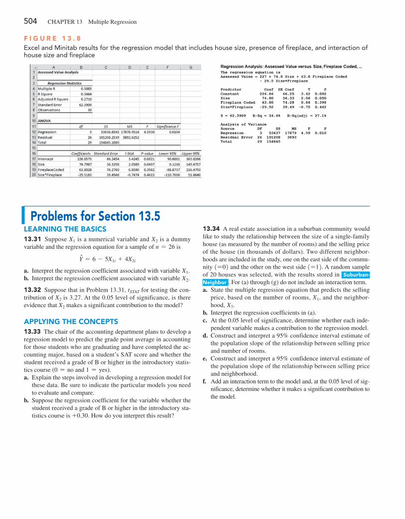
504 CHAPTeR 13 Multiple Regression
F I g u R e 1 3 . 8 Excel and Minitab results for the regression model that includes house size, presence of fireplace, and interaction of house size and fireplace
Problems for Section 13.5leaRnIng The baSICS13.31 Suppose X1 is a numerical variable and X2 is a dummy variable and the regression equation for a sample of n = 26 is
Yn = 6 - 5X1i + 4X2i
a. Interpret the regression coefficient associated with variable X1.b. Interpret the regression coefficient associated with variable X2.
13.32 Suppose that in Problem 13.31, tSTAT for testing the con-tribution of X2 is 3.27. At the 0.05 level of significance, is there evidence that X2 makes a significant contribution to the model?
aPPlyIng The COnCePTS13.33 The chair of the accounting department plans to develop a regression model to predict the grade point average in accounting for those students who are graduating and have completed the ac-counting major, based on a student’s SAT score and whether the student received a grade of B or higher in the introductory statis-tics course (0 = no and 1 = yes).a. explain the steps involved in developing a regression model for
these data. Be sure to indicate the particular models you need to evaluate and compare.
b. Suppose the regression coefficient for the variable whether the student received a grade of B or higher in the introductory sta-tistics course is +0.30. How do you interpret this result?
13.34 A real estate association in a suburban community would like to study the relationship between the size of a single-family house (as measured by the number of rooms) and the selling price of the house (in thousands of dollars). Two different neighbor-hoods are included in the study, one on the east side of the commu-nity 1=02 and the other on the west side 1=12. A random sample of 20 houses was selected, with the results stored in Suburban-neighbor . For (a) through (g) do not include an interaction term.a. State the multiple regression equation that predicts the selling
price, based on the number of rooms, X1, and the neighbor-hood, X2.
b. Interpret the regression coefficients in (a).c. At the 0.05 level of significance, determine whether each inde-
pendent variable makes a contribution to the regression model.d. Construct and interpret a 95% confidence interval estimate of
the population slope of the relationship between selling price and number of rooms.
e. Construct and interpret a 95% confidence interval estimate of the population slope of the relationship between selling price and neighborhood.
f. Add an interaction term to the model and, at the 0.05 level of sig-nificance, determine whether it makes a significant contribution to the model.
13.5 Using Dummy Variables and Interaction Terms in Regression Models 505
13.35 In Problem 13.5 on page 492, you developed a multiple regression model to predict wine quality for red wines. Now, you wish to determine whether there is an effect on wine quality due to whether the wine is white (0) or red (1). These data are organized and stored in RedandWhite . Develop a multiple regression model to predict wine quality based on the percentage of alcohol and the type of wine.
For (a) through (l), do not include an interaction term.a. State the multiple regression equation that predicts wine qual-
ity based on the percentage of alcohol and the type of wine.b. Interpret the regression coefficients in (a).c. Predict the mean quality for a red wine that has 10% alcohol.
Construct a 95% confidence interval estimate and a 95% pre-diction interval.
d. Perform a residual analysis on the results and determine whether the regression assumptions are valid.
e. Is there a significant relationship between wine quality and the two independent variables (percentage of alcohol and the type of wine) at the 0.05 level of significance?
f. At the 0.05 level of significance, determine whether each inde-pendent variable makes a contribution to the regression model. Indicate the most appropriate regression model for this set of data.
g. Construct and interpret 95% confidence interval estimates of the population slope for the relationship between wine quality and the percentage of alcohol and between wine quality and the type of wine.
h. Compare the slope in (b) with the slope for the simple linear regression model of Problem 12.4 on page 445. explain the dif-ference in the results.
i. Compute and interpret the meaning of the coefficient of mul-tiple determination, r 2.
j. Compute and interpret the adjusted r 2.k. Compare r 2 with the r 2 value computed in Problem 12.16 (a)
on page 451.l. What assumption about the slope of type of wine with wine
quality do you need to make in this problem?m. Add an interaction term to the model and, at the 0.05 level of
significance, determine whether it makes a significant contribu-tion to the model.
n. On the basis of the results of (f) and (m), which model is most appropriate? explain.
o. What conclusions can you reach concerning the effect of alco-hol percentage and type of wine on wine quality?
13.36 In mining engineering, holes are often drilled through rock, using drill bits. As a drill hole gets deeper, additional rods are added to the drill bit to enable additional drilling to take place. It is expected that drilling time increases with depth. This increased drilling time could be caused by several factors, including the mass of the drill rods that are strung together. The business prob-lem relates to whether drilling is faster using dry drilling holes or wet drilling holes. Using dry drilling holes involves forcing com-pressed air down the drill rods to flush the cuttings and drive the hammer. Using wet drilling holes involves forcing water rather than air down the hole. Data have been collected from a sample of
50 drill holes that contains measurements of the time to drill each additional 5 feet (in minutes), the depth (in feet), and whether the hole was a dry drilling hole or a wet drilling hole. The data are organized and stored in Drill . (Data extracted from R. Penner and D. G. Watts, “Mining Information,” The American Statistician, 45, 1991, pp. 4–9.) Develop a model to predict additional drilling time, based on depth and type of drilling hole (dry or wet). For (a) through ( j) do not include an interaction term.a. State the multiple regression equation.b. Interpret the regression coefficients in (a).c. Predict the mean additional drilling time for a dry drilling hole
at a depth of 100 feet. Construct a 95% confidence interval esti-mate and a 95% prediction interval.
d. Perform a residual analysis on the results and determine whether the regression assumptions are valid.
e. Is there a significant relationship between additional drilling time and the two independent variables (depth and type of drill-ing hole) at the 0.05 level of significance?
f. At the 0.05 level of significance, determine whether each inde- pendent variable makes a contribution to the regression model. Indicate the most appropriate regression model for this set of data.
g. Construct a 95% confidence interval estimate of the population slope for the relationship between additional drilling time and depth.
h. Construct a 95% confidence interval estimate of the population slope for the relationship between additional drilling time and the type of hole drilled.
i. Compute and interpret the adjusted r 2.j. What assumption do you need to make about the slope of ad-
ditional drilling time with depth?k. Add an interaction term to the model and, at the 0.05 level of
significance, determine whether it makes a significant contribu-tion to the model.
l. On the basis of the results of (f) and (k), which model is most appropriate? explain.
m. What conclusions can you reach concerning the effect of depth and type of drilling hole on drilling time?
13.37 The owner of a moving company typically has his most experienced manager predict the total number of labor hours that will be required to complete an upcoming move. This approach has proved useful in the past, but the owner has the business ob-jective of developing a more accurate method of predicting labor hours. In a preliminary effort to provide a more accurate method, the owner has decided to use the number of cubic feet moved and whether there is an elevator in the apartment building as the inde-pendent variables and has collected data for 36 moves in which the origin and destination were within the borough of Manhattan in New York City and the travel time was an insignificant portion of the hours worked. The data are organized and stored in Moving . For (a) through (j), do not include an interaction term.a. State the multiple regression equation for predicting labor
hours, using the number of cubic feet moved and whether there is an elevator.
b. Interpret the regression coefficients in (a).
506 CHAPTeR 13 Multiple Regression
c. Predict the mean labor hours for moving 500 cubic feet in an apartment building that has an elevator and construct a 95% confidence interval estimate and a 95% prediction interval.
d. Perform a residual analysis on the results and determine whether the regression assumptions are valid.
e. Is there a significant relationship between labor hours and the two independent variables (cubic feet moved and whether there is an elevator in the apartment building) at the 0.05 level of sig-nificance?
f. At the 0.05 level of significance, determine whether each inde- pendent variable makes a contribution to the regression model. Indicate the most appropriate regression model for this set of data.
g. Construct a 95% confidence interval estimate of the population slope for the relationship between labor hours and cubic feet moved.
h. Construct a 95% confidence interval estimate for the relation-ship between labor hours and the presence of an elevator.
i. Compute and interpret the adjusted r 2.j. What assumption do you need to make about the slope of la-
bor hours with cubic feet moved?k. Add an interaction term to the model, and at the 0.05 level of
significance, determine whether it makes a significant contribu-tion to the model.
l. On the basis of the results of (f) and (k), which model is most appropriate? explain.
m. What conclusions can you reach concerning the effect of the number of cubic feet moved and whether there is an elevator on labor hours?
SELF Test
13.38 In Problem 13.4 on page 491, you used effi-ciency ratio and total risk-based capital stored in
Communitybanks to predict ROA at a community bank. Develop a regression model to predict ROA that includes efficiency ratio, total risk-based capital, and the interaction of efficiency ratio and total risk-based capital.a. At the 0.05 level of significance, is there evidence that the in-
teraction term makes a significant contribution to the model?b. Which regression model is more appropriate, the one used in
(a) or the one used in Problem 13.4? explain.
13.39 Zagat’s publishes restaurant ratings for various locations in the United States. The file Restaurants contains the Zagat rat-ing for food, décor, service, and cost per person for a sample of 50 restaurants located in a city and 50 restaurants located in a suburb. (Data extracted from Zagat Survey 2013, New York City Restau-rants; and Zagat Survey 2012–2013, Long Island Restaurants.) Develop a regression model to predict the cost per person, based on a variable that represents the sum of the ratings for food, décor, and service and a dummy variable concerning location (city versus suburban). For (a) through (l), do not include an interaction term.a. State the multiple regression equation.b. Interpret the regression coefficients in (a).c. Predict the mean cost at a restaurant with a summated rating
of 60 that is located in a city and construct a 95% confidence interval estimate and a 95% prediction interval.
d. Perform a residual analysis on the results and determine whether the regression assumptions are satisfied.
e. Is there a significant relationship between price and the two in-dependent variables (summated rating and location) at the 0.05 level of significance?
f. At the 0.05 level of significance, determine whether each inde-pendent variable makes a contribution to the regression model. Indicate the most appropriate regression model for this set of data.
g. Construct a 95% confidence interval estimate of the popula-tion slope for the relationship between cost and summated rating.
h. Compare the slope in (b) with the slope for the simple linear regression model of Problem 12.5 on page 446. explain the dif-ference in the results.
i. Compute and interpret the meaning of the coefficient of mul-tiple determination.
j. Compute and interpret the adjusted r 2.k. Compare r 2 with the r 2 value computed in Problem 12.17 (b)
on page 451.l. What assumption about the slope of cost with summated rating
do you need to make in this problem?m. Add an interaction term to the model and, at the 0.05 level of
significance, determine whether it makes a significant contribu-tion to the model.
n. On the basis of the results of (f) and (m), which model is most appropriate? explain.
o. What conclusions can you reach about the effect of the summated rating and the location of the restaurant on the cost of a meal?
13.40 In Problem 13.6 on page 492, you used the total world-wide revenue ($millions) and full-time voluntary turnover (%) data stored in bestCompanies to predict number of full-time jobs added. Develop a regression model to predict the number of full-time jobs added that includes full-time voluntary turnover, total worldwide revenue, and the interaction of full-time voluntary turn-over and total worldwide revenue.a. At the 0.05 level of significance, is there evidence that the in-
teraction term makes a significant contribution to the model?b. Which regression model is more appropriate, the one used in
this problem or the one used in Problem 13.6? explain.
13.41 In Problem 13.5 on page 492, the percentage of alcohol and chlorides were used to predict the quality of red wines (stored in VinhoVerde ). Develop a regression model that includes the percentage of alcohol, the chlorides, and the interaction of the per-centage of alcohol and the chlorides to predict wine quality.a. At the 0.05 level of significance, is there evidence that the in-
teraction term makes a significant contribution to the model?b. Which regression model is more appropriate, the one used in
this problem or the one used in Problem 13.5? explain.
13.42 In Problem 13.7 on page 492, you used the total staff pres-ent and remote hours to predict standby hours stored in Standby . Develop a regression model to predict standby hours that includes total staff present, remote hours, and the interaction of total staff present and remote hours.a. At the 0.05 level of significance, is there evidence that the in-
teraction term makes a significant contribution to the model?b. Which regression model is more appropriate, the one used in
this problem or the one used in Problem 13.7? explain.
s U M M a r yFigure 13.9 presents a roadmap of this chapter. In this chap-ter, you learned how to develop and fit multiple regression models that use two or more independent variables to
predict the value of a dependent variable. You also learned how to include categorical independent variables and inter-action terms in regression models.
r e f e r e n c e s 1. Andrews, D. F., and D. Pregibon. “Finding the Outliers that
Matter.” Journal of the Royal Statistical Society 40 (Ser. B., 1978): 85–93.
2. Atkinson, A. C. “Robust and Diagnostic Regression Analysis.” Communications in Statistics 11 (1982): 2559–2572.
3. Belsley, D. A., e. Kuh, and R. Welsch. Regression Diagnos-tics: Identifying Influential Data and Sources of Collinearity. New York: Wiley, 1980.
4. Cook, R. D., and S. Weisberg. Residuals and Influence in Regression. New York: Chapman and Hall, 1982.
5. Hosmer, D. W., and S. Lemeshow. Applied Logistic Regression, 3rd ed. New York: Wiley, 2013.
6. Hoaglin, D. C., and R. Welsch. “The Hat Matrix in Regression and ANOVA,” The American Statistician, 32, (1978), 17–22.
7. Kutner, M., C. Nachtsheim, J. Neter, and W. Li. Applied Linear Statistical Models, 5th ed. New York: McGraw-Hill/Irwin, 2005.
8. Microsoft Excel 2013. Redmond, WA: Microsoft Corp., 2012. 9. Minitab Release 16. State College, PA: Minitab, Inc., 2010.
In the Using Statistics scenario, you were a marketing man-ager for OmniFoods, responsible for nutrition bars and
similar snack items. You needed to determine the effect that price and in-store promotions would have on sales of Om-niPower nutrition bars in order to develop an effective mar-keting strategy. A sample of 34 stores in a supermarket chain was selected for a test-market study. The stores charged be-tween 59 and 99 cents per bar and were given an in-store promotion budget between $200 and $600.
At the end of the one-month test-market study, you performed a multiple regression analysis on the data. Two independent variables were considered: the price of an Om-niPower bar and the monthly budget for in-store promotional expenditures. The dependent variable was the number of OmniPower bars sold in a month. The coefficient of determi-nation indicated that 75.8% of the variation in sales was ex-plained by knowing the price charged and the amount spent on in-store promotions. The model indicated that the pre-dicted sales of OmniPower are estimated to decrease by 532
bars per month for each 10-cent increase in the price, and the predicted sales are estimated to increase by 361 bars for each additional $100 spent on promotions.
After studying the relative effects of price and pro-motion, OmniFoods needs to set price and promotion standards for a nationwide introduction (obviously, lower prices and higher promotion budgets lead to more sales, but they do so at a lower profit margin). You determined that if stores spend $400 a month for in-store promotions and charge 79 cents, the 95% confidence interval estimate of the mean monthly sales is 2,854 to 3,303 bars. OmniFoods can multiply the lower and upper bounds of this confidence interval by the number of stores included in the nationwide introduction to estimate total monthly sales. For example, if 1,000 stores are in the nationwide introduction, then total monthly sales should be between 2.854 million and 3.308 million bars.
U s i n g s tat i s t i c s
The Multiple Effects of OmniPower Bars, Revisited
Ariwasabi/Shutterstock
References 507
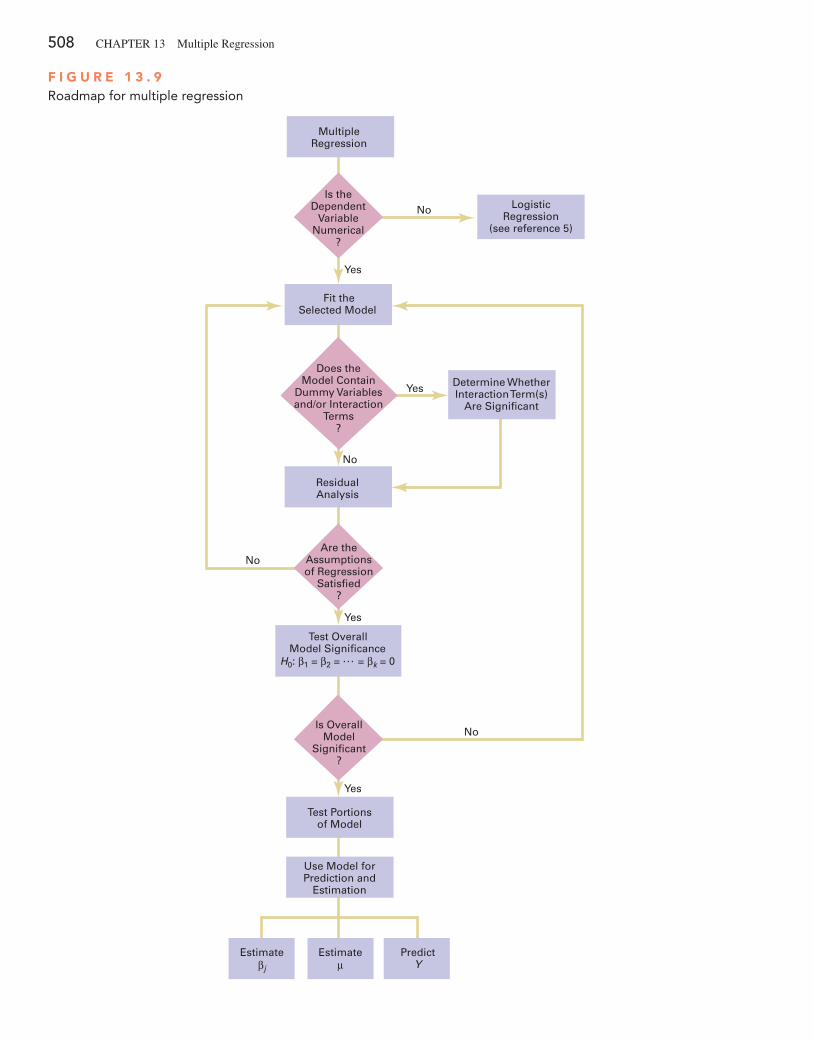
508 CHAPTeR 13 Multiple Regression
F I g u R e 1 3 . 9Roadmap for multiple regression
No
No
No
No
Yes
Yes
Yes
Yes
PredictY
Estimateβj
Is theDependent
VariableNumerical
?
MultipleRegression
Determine WhetherInteraction Term(s)
Are Signi�cant
Fit theSelected Model
Does theModel Contain
Dummy Variablesand/or Interaction
Terms?
ResidualAnalysis
Test Portionsof Model
LogisticRegression
(see reference 5)
Use Model forPrediction and
Estimation
Are theAssumptionsof Regression
Satis�ed?
Test OverallModel Signi�cance
H0: β1 = β2 = . . . = βk = 0
Is OverallModel
Signi�cant?
Estimateμ
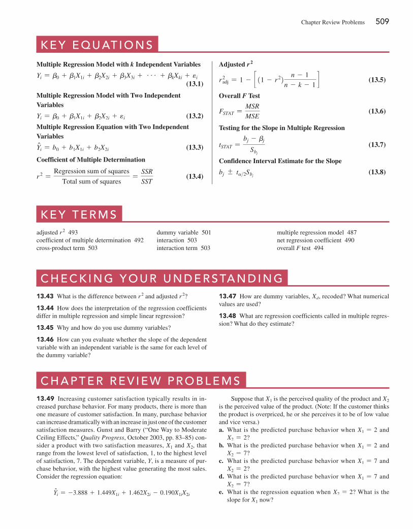
Chapter Review Problems 509
K e y e q U at i o n s
Multiple Regression Model with k Independent Variables
Yi = b0 + b1X1i + b2X2i + b3X3i + g + bkXki + ei (13.1)
Multiple Regression Model with Two Independent Variables
Yi = b0 + b1X1i + b2X2i + ei (13.2)
Multiple Regression Equation with Two Independent Variables
Yni = b0 + b1X1i + b2X2i (13.3)
Coefficient of Multiple Determination
r 2 =Regression sum of squares
Total sum of squares=
SSR
SST (13.4)
Adjusted r 2
r 2adj = 1 - c 11 - r 22 n - 1
n - k - 1d (13.5)
Overall F Test
FSTAT =MSR
MSE (13.6)
Testing for the Slope in Multiple Regression
tSTAT =bj - bj
Sbj
(13.7)
Confidence Interval Estimate for the Slope
bj { ta>2Sbj (13.8)
K e y t e r M sadjusted r 2 493coefficient of multiple determination 492cross-product term 503
dummy variable 501interaction 503interaction term 503
multiple regression model 487net regression coefficient 490overall F test 494
c h e c K i n g y o U r U n d e r s ta n d i n g13.43 What is the difference between r 2 and adjusted r 2?
13.44 How does the interpretation of the regression coefficients differ in multiple regression and simple linear regression?
13.45 Why and how do you use dummy variables?
13.46 How can you evaluate whether the slope of the dependent variable with an independent variable is the same for each level of the dummy variable?
13.47 How are dummy variables, Xd, recoded? What numerical values are used?
13.48 What are regression coefficients called in multiple regres-sion? What do they estimate?
c h a p t e r r e v i e w p r o b l e M s13.49 Increasing customer satisfaction typically results in in-creased purchase behavior. For many products, there is more than one measure of customer satisfaction. In many, purchase behavior can increase dramatically with an increase in just one of the customer satisfaction measures. Gunst and Barry (“One Way to Moderate Ceiling effects,” Quality Progress, October 2003, pp. 83–85) con-sider a product with two satisfaction measures, X1 and X2, that range from the lowest level of satisfaction, 1, to the highest level of satisfaction, 7. The dependent variable, Y, is a measure of pur-chase behavior, with the highest value generating the most sales. Consider the regression equation:
Yni = -3.888 + 1.449X1i + 1.462X2i - 0.190X1iX2i
Suppose that X1 is the perceived quality of the product and X2 is the perceived value of the product. (Note: If the customer thinks the product is overpriced, he or she perceives it to be of low value and vice versa.)a. What is the predicted purchase behavior when X1 = 2 and
X2 = 2?b. What is the predicted purchase behavior when X1 = 2 and
X2 = 7?c. What is the predicted purchase behavior when X1 = 7 and
X2 = 2?d. What is the predicted purchase behavior when X1 = 7 and
X2 = 7?e. What is the regression equation when X2 = 2? What is the
slope for X1 now?
510 CHAPTeR 13 Multiple Regression
f. What is the regression equation when X2 = 7? What is the slope for X1 now?
g. What is the regression equation when X1 = 2? What is the slope for X2 now?
h. What is the regression equation when X1 = 7? What is the slope for X2 now?
i. Discuss the implications of (a) through (h) in the context of in-creasing sales for this product with two customer satisfaction measures.
13.50 The owner of a moving company typically has his most experienced manager predict the total number of labor hours that will be required to complete an upcoming move. This approach has proved useful in the past, but the owner has the business ob-jective of developing a more accurate method of predicting labor hours. In a preliminary effort to provide a more accurate method, the owner has decided to use the number of cubic feet moved and the number of pieces of large furniture as the independent vari-ables and has collected data for 36 moves in which the origin and destination were within the borough of Manhattan in New York City and the travel time was an insignificant portion of the hours worked. The data are organized and stored in Moving .a. State the multiple regression equation.b. Interpret the meaning of the slopes in this equation.c. Predict the mean labor hours for moving 500 cubic feet with
two large pieces of furniture.d. Perform a residual analysis on your results and determine
whether the regression assumptions are valid.e. Determine whether there is a significant relationship between
labor hours and the two independent variables (the number of cubic feet moved and the number of pieces of large furniture) at the 0.05 level of significance.
f. Determine the p-value in (e) and interpret its meaning.g. Interpret the meaning of the coefficient of multiple determina-
tion in this problem.h. Determine the adjusted r 2.i. At the 0.05 level of significance, determine whether each inde-
pendent variable makes a significant contribution to the regres-sion model. Indicate the most appropriate regression model for this set of data.
j. Determine the p-values in (i) and interpret their meaning.k. Construct a 95% confidence interval estimate of the population
slope between labor hours and the number of cubic feet moved. How does the interpretation of the slope here differ from that in Problem 12.44 on page 465?
l. What conclusions can you reach concerning labor hours?
13.51 Professional basketball has truly become a sport that gen-erates interest among fans around the world. More and more play-ers come from outside the United States to play in the National Basketball Association (NBA). You want to develop a regression model to predict the number of wins achieved by each NBA team, based on field goal (shots made) percentage and three-point field goal percentage for the team. The data are stored in nba .a. State the multiple regression equation.b. Interpret the meaning of the slopes in this equation.c. Predict the mean number of wins for a team that has a field
goal percentage of 45% and a three-point field goal percentage of 37%.
d. Perform a residual analysis on your results and determine whether the regression assumptions are valid.
e. Is there a significant relationship between number of wins and
the two independent variables (field goal percentage and three-point field goal percentage for the team) at the 0.05 level of significance?
f. Determine the p-value in (e) and interpret its meaning.g. Interpret the meaning of the coefficient of multiple determina-
tion in this problem.h. Determine the adjusted r 2.i. At the 0.05 level of significance, determine whether each
independent variable makes a significant contribution to the regression model. Indicate the most appropriate regression model for this set of data.
j. Determine the p-values in (i) and interpret their meaning.k. What conclusions can you reach concerning field goal per-
centage and three-point field goal percentage in predicting the number of wins?
13.52 A sample of 30 houses recently listed for sale in Silver Spring, Maryland, was selected with the objective of developing a model to predict the assessed value (in $thousands), using the size of the house (in thousands of square feet) and age (in years). The results are stored in Silver Spring .a. Fit a multiple regression model.b. Interpret the meaning of the slopes in this model.c. Predict the mean assessed value for a house that has 2,000
square feet and is 55 years old.d. Perform a residual analysis on your results and determine
whether the regression assumptions are valid.e. Determine whether there is a significant relationship between
assessed value and the two independent variables (house size and age) at the 0.05 level of significance.
f. Determine the p-value in (e) and interpret its meaning.g. Interpret the meaning of the coefficient of multiple determina-
tion in this problem.h. Determine the adjusted r 2.i. At the 0.05 level of significance, determine whether each inde-
pendent variable makes a significant contribution to the regres-sion model. Indicate the most appropriate regression model for this set of data.
j. Determine the p-values in (i) and interpret their meaning.k. Construct a 95% confidence interval estimate of the popula-
tion slope between assessed value and the size of the house. How does the interpretation of the slope here differ from that in Problem 12.76 on page 477?
l. What conclusions can you reach about the assessed value?
13.53 Measuring the height of a California redwood tree is very difficult because these trees grow to heights over 300 feet. People familiar with these trees understand that the height of a California redwood tree is related to other characteristics of the tree, includ-ing the diameter of the tree at the breast height of a person (in inches) and the thickness of the bark of the tree (in inches). The file Redwood contains the height, diameter at breast height of a person, and bark thickness for a sample of 21 California redwood trees.a. State the multiple regression equation that predicts the height
of a tree, based on the tree’s diameter at breast height and the thickness of the bark.
b. Interpret the meaning of the slopes in this equation.c. Predict the mean height for a tree that has a breast height diam-
eter of 25 inches and a bark thickness of 2 inches.d. Interpret the meaning of the coefficient of multiple determina-
tion in this problem.
Chapter Review Problems 511
e. Perform a residual analysis on the results and determine whether the regression assumptions are valid.
f. Determine whether there is a significant relationship between the height of redwood trees and the two independent variables (breast-height diameter and bark thickness) at the 0.05 level of significance.
g. Construct a 95% confidence interval estimate of the population slope between the height of redwood trees and breast-height di-ameter and between the height of redwood trees and the bark thickness.
h. At the 0.05 level of significance, determine whether each in-dependent variable makes a significant contribution to the re-gression model. Indicate the independent variables to include in this model.
i. Construct a 95% confidence interval estimate of the mean height for trees that have a breast-height diameter of 25 inches and a bark thickness of 2 inches, along with a prediction inter-val for an individual tree.
j. What conclusions can you reach concerning the effect of the diameter of the tree and the thickness of the bark on the height of the tree?
13.54 A sample of 30 houses recently listed for sale in Silver Spring, Maryland, was selected with the objective of developing a model to predict the taxes (in $) based on the assessed value of houses (in $thousands) and the age of the houses (in years) (stored in SilverSpring ):a. State the multiple regression equation.b. Interpret the meaning of the slopes in this equation.c. Predict the mean taxes for a house that has an assessed value of
$400,000 and is 50 years old.d. Perform a residual analysis on the results and determine
whether the regression assumptions are valid.e. Determine whether there is a significant relationship between
taxes and the two independent variables (assessed value and age) at the 0.05 level of significance.
f. Determine the p-value in (e) and interpret its meaning.g. Interpret the meaning of the coefficient of multiple determina-
tion in this problem.h. Determine the adjusted r 2.i. At the 0.05 level of significance, determine whether each inde-
pendent variable makes a significant contribution to the regres-sion model. Indicate the most appropriate regression model for this set of data.
j. Determine the p-values in (i) and interpret their meaning.k. Construct a 95% confidence interval estimate of the population
slope between taxes and assessed value. How does the inter-pretation of the slope here differ from that of Problem 12.77 on page 477?
l. The real estate assessor’s office has been publicly quoted as saying that the age of a house has no bearing on its taxes. Based on your answers to (a) through (k), do you agree with this statement? explain.
13.55 A baseball analytics specialist wants to determine which variables are important in predicting a team’s wins in a given season. He has collected data related to wins, earned run aver-age (eRA), and runs scored per game in a recent season (stored in baseball ). Develop a model to predict the number of wins based on eRA and runs scored per game.a. State the multiple regression equation.b. Interpret the meaning of the slopes in this equation.
c. Predict the mean number of wins for a team that has an eRA of 4.00 and has scored 4.0 runs per game.
d. Perform a residual analysis on the results and determine whether the regression assumptions are valid.
e. Is there a significant relationship between the number of wins and the two independent variables (eRA and runs scored per game) at the 0.05 level of significance?
f. Determine the p-value in (e) and interpret its meaning.g. Interpret the meaning of the coefficient of multiple determina-
tion in this problem.h. Determine the adjusted r 2.i. At the 0.05 level of significance, determine whether each inde-
pendent variable makes a significant contribution to the regres-sion model. Indicate the most appropriate regression model for this set of data.
j. Determine the p-values in (i) and interpret their meaning.k. Construct a 95% confidence interval estimate of the population
slope between wins and eRA.l. Which is more important in predicting wins—pitching, as mea-
sured by eRA, or offense, as measured by runs scored per game? explain.
13.56 Referring to Problem 13.55, suppose that in addition to us-ing eRA to predict the number of wins, the analytics specialist wants to include the league (0 = American, 1 = National) as an independent variable. Develop a model to predict wins based on eRA and league. For (a) through ( j), do not include an interaction term.a. State the multiple regression equation.b. Interpret the slopes in (a).c. Predict the mean number of wins for a team with an eRA of
4.00 in the American League. Construct a 95% confidence interval estimate for all teams and a 95% prediction interval for an individual team.
d. Perform a residual analysis on the results and determine whether the regression assumptions are valid.
e. Is there a significant relationship between wins and the two in-dependent variables (eRA and league) at the 0.05 level of sig-nificance?
f. At the 0.05 level of significance, determine whether each inde-pendent variable makes a contribution to the regression model. Indicate the most appropriate regression model for this set of data.
g. Construct a 95% confidence interval estimate of the population slope for the relationship between wins and eRA.
h. Construct a 95% confidence interval estimate of the population slope for the relationship between wins and league.
i. Compute and interpret the adjusted r 2.j. What assumption do you have to make about the slope of wins
with eRA?k. Add an interaction term to the model and, at the 0.05 level of
significance, determine whether it makes a significant contribu-tion to the model.
l. On the basis of the results of (f) and (k), which model is most appropriate? explain.
13.57 You are a real estate broker who wants to compare prop-erty values in Glen Cove and Roslyn (which are located approxi-mately 8 miles apart). In order to do so, you will analyze the data in gCRoslyn , a file that includes samples of houses from Glen Cove and Roslyn. Making sure to include the dummy variable for location (Glen Cove or Roslyn), develop a regression model

512 CHAPTeR 13 Multiple Regression
to predict fair market value, based on the land area of a property, the age of a house, and location. Be sure to determine whether any interaction terms need to be included in the model.
13.58 The list of Best Small Companies in America features a group with strong earnings growth across industries. A business analyst wishes to determine the relationship between earnings per share growth (%) and sales growth (%) and return on equity (%). Data were collected on 100 small companies and stored in Smallbusinesses . (Data extracted from “America’s Best Small Companies,” forbes.com/best-small-companies/list/.)
Develop a multiple regression model that uses sales growth and return on equity to predict earnings per share growth. Be sure to perform a thorough residual analysis.
13.59 Starbucks Coffee Co. uses a data-based approach to improving the quality and customer satisfaction of its products. When survey data indicated that Starbucks needed to improve its package-sealing process, an experiment was conducted to deter-mine the factors in the bag-sealing equipment that might be af-fecting the ease of opening the bag without tearing the inner liner of the bag. (Data extracted from L. Johnson and S. Burrows, “For Starbucks, It’s in the Bag,” Quality Progress, March 2011, pp. 17–23.) Among the factors that could affect the rating of the ability of the bag to resist tears were the viscosity, pressure, and plate gap on the bag-sealing equipment. Data were collected on 19 bags in
which the plate gap was varied. The results are stored in Starbucks . Develop a multiple regression model that uses the viscosity, pres-sure, and plate gap on the bag-sealing equipment to predict the tear rating of the bag. Be sure to perform a thorough residual analysis. Do you think that you need to use all three independent variables in the model? explain.
13.60 An experiment was conducted to study the extrusion process of biodegradable packaging foam. Among the factors considered for their effect on the unit density (mg/ml) were the die temperature (145°C versus 155°C) and the die diameter (3 mm versus 4 mm). The results were stored in PackagingFoam3 . (Data extracted from W. Y. Koh, K. M. eskridge, and M. A. Hanna, “Supersaturated Split-Plot Designs,” Journal of Quality Technology, 45, January 2013, pp. 61–72.) Develop a multiple regression model that uses die tem-perature and die diameter to predict the unit density (mg/ml). Be sure to perform a thorough residual analysis. Do you think that you need to use both independent variables in the model? explain.
13.61 Referring to Problem 13.60, instead of predicting the unit density, you now wish to predict the foam diameter from results stored in PackagingFoam4 . Develop a multiple regression model that uses die temperature and die diameter to predict the foam di-ameter (mg/ml). Be sure to perform a thorough residual analysis. Do you think that you need to use both independent variables in the model? explain.
Managing ashland Multicomm servicesIn its continuing study of the 3-For-All subscription solicita-tion process, a marketing department team wants to test the effects of two types of structured sales presentations (personal formal and personal informal) and the number of hours spent on telemarketing on the number of new subscriptions. The staff has recorded these data for the past 24 weeks in aMS13 .
Analyze these data and develop a multiple regres-sion model to predict the number of new subscriptions for a week, based on the number of hours spent on telemarketing and the sales presentation type. Write a report, giving detailed findings concerning the regres-sion model used.
c a s e s f o r c h a p t e r 1 3
digital caseApply your knowledge of multiple regression models in this Digital Case, which extends the OmniFoods Using Statistics scenario from this chapter.
To ensure a successful test marketing of its OmniPower energy bars, the OmniFoods marketing department has contracted with In-Store Placements Group (ISPG), a mer-chandising consulting firm. ISPG will work with the gro-cery store chain that is conducting the test-market study. Using the same 34-store sample used in the test-market study, ISPG claims that the choice of shelf location and the presence of in-store OmniPower coupon dispensers both in-crease sales of the energy bars.
Open Omni_ISPGMemo.pdf to review the ISPG claims and supporting data. Then answer the following questions:
1. Are the supporting data consistent with ISPG’s claims? Perform an appropriate statistical analysis to confirm (or discredit) the stated relationship between sales and the two independent variables of product shelf location and the presence of in-store OmniPower coupon dispensers.
2. If you were advising OmniFoods, would you recommend using a specific shelf location and in-store coupon dis-pensers to sell OmniPower bars?
3. What additional data would you advise collecting in order to determine the effectiveness of the sales promo-tion techniques used by ISPG?
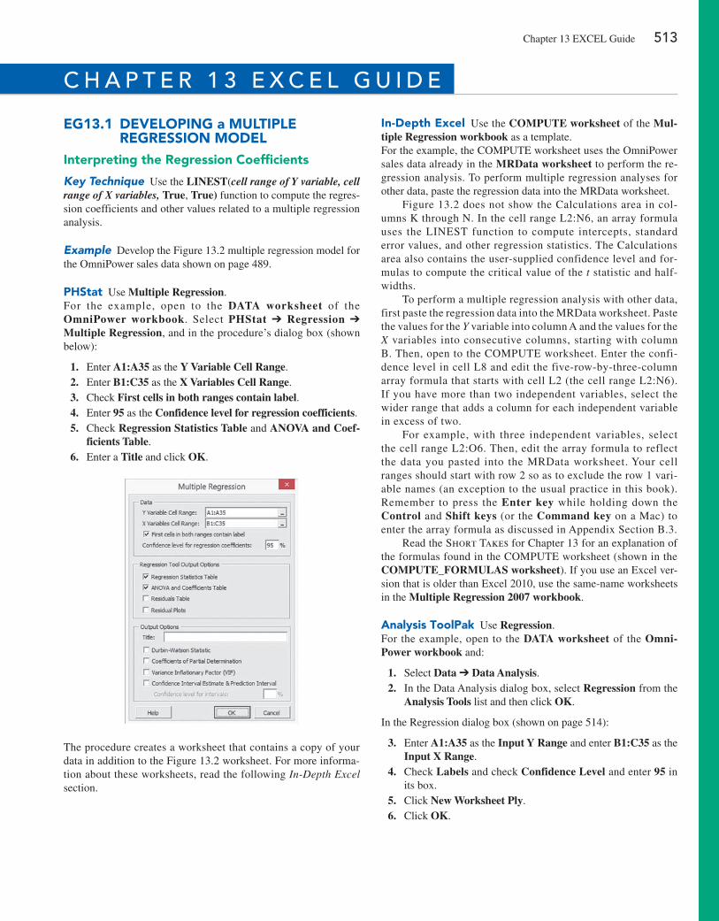
Chapter 13 eXCeL Guide 513
eg13.1 DeVelOPIng a MulTIPle RegReSSIOn MODel
Interpreting the Regression Coefficients
Key Technique Use the LINEST(cell range of Y variable, cell range of X variables, True, True) function to compute the regres-sion coefficients and other values related to a multiple regression analysis.
Example Develop the Figure 13.2 multiple regression model for the OmniPower sales data shown on page 489.
PhStat Use Multiple Regression.For the example, open to the DATA worksheet of the OmniPower workbook. Select PHStat ➔ Regression ➔ Multiple Regression, and in the procedure’s dialog box (shown below):
1. enter A1:A35 as the Y Variable Cell Range. 2. enter B1:C35 as the X Variables Cell Range. 3. Check First cells in both ranges contain label. 4. enter 95 as the Confidence level for regression coefficients. 5. Check Regression Statistics Table and ANOVA and Coef-
ficients Table. 6. enter a Title and click OK.
The procedure creates a worksheet that contains a copy of your data in addition to the Figure 13.2 worksheet. For more informa-tion about these worksheets, read the following In-Depth Excel section.
In-Depth excel Use the COMPUTE worksheet of the Mul-tiple Regression workbook as a template.For the example, the COMPUTe worksheet uses the OmniPower sales data already in the MRData worksheet to perform the re-gression analysis. To perform multiple regression analyses for other data, paste the regression data into the MRData worksheet.
Figure 13.2 does not show the Calculations area in col-umns K through N. In the cell range L2:N6, an array formula uses the LINeST function to compute intercepts, standard error values, and other regression statistics. The Calculations area also contains the user-supplied confidence level and for-mulas to compute the critical value of the t statistic and half-widths.
To perform a multiple regression analysis with other data, first paste the regression data into the MRData worksheet. Paste the values for the Y variable into column A and the values for the X variables into consecutive columns, starting with column B. Then, open to the COMPUTe worksheet. enter the confi-dence level in cell L8 and edit the five-row-by-three-column array formula that starts with cell L2 (the cell range L2:N6). If you have more than two independent variables, select the wider range that adds a column for each independent variable in excess of two.
For example, with three independent variables, select the cell range L2:O6. Then, edit the array formula to reflect the data you pasted into the MRData worksheet. Your cell ranges should start with row 2 so as to exclude the row 1 vari-able names (an exception to the usual practice in this book). Remember to press the Enter key while holding down the Control and Shift keys (or the Command key on a Mac) to enter the array formula as discussed in Appendix Section B.3.
Read the Short Takes for Chapter 13 for an explanation of the formulas found in the COMPUTe worksheet (shown in the COMPUTE_FORMULAS worksheet). If you use an excel ver-sion that is older than excel 2010, use the same-name worksheets in the Multiple Regression 2007 workbook.
analysis ToolPak Use Regression.For the example, open to the DATA worksheet of the Omni-Power workbook and:
1. Select Data ➔ Data Analysis. 2. In the Data Analysis dialog box, select Regression from the
Analysis Tools list and then click OK.
In the Regression dialog box (shown on page 514):
3. enter A1:A35 as the Input Y Range and enter B1:C35 as the Input X Range.
4. Check Labels and check Confidence Level and enter 95 in its box.
5. Click New Worksheet Ply. 6. Click OK.
c h a p t e r 1 3 e x c e l g U i d e
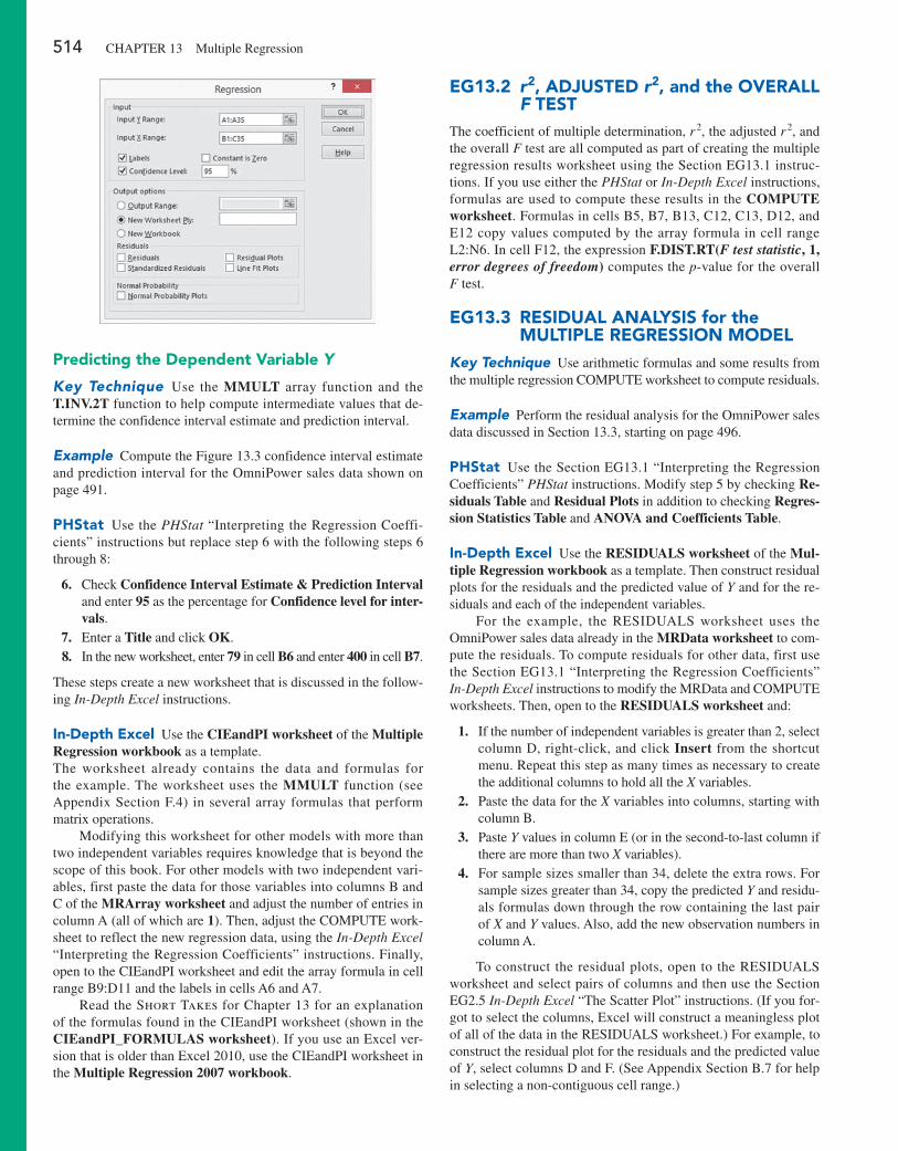
514 CHAPTeR 13 Multiple Regression
Predicting the Dependent Variable Y
Key Technique Use the MMULT array function and the T.INV.2T function to help compute intermediate values that de-termine the confidence interval estimate and prediction interval.
Example Compute the Figure 13.3 confidence interval estimate and prediction interval for the OmniPower sales data shown on page 491.
PhStat Use the PHStat “Interpreting the Regression Coeffi-cients” instructions but replace step 6 with the following steps 6 through 8:
6. Check Confidence Interval Estimate & Prediction Interval and enter 95 as the percentage for Confidence level for inter-vals.
7. enter a Title and click OK. 8. In the new worksheet, enter 79 in cell B6 and enter 400 in cell B7.
These steps create a new worksheet that is discussed in the follow-ing In-Depth Excel instructions.
In-Depth excel Use the CIEandPI worksheet of the Multiple Regression workbook as a template.The worksheet already contains the data and formulas for the example. The worksheet uses the MMULT function (see Appendix Section F.4) in several array formulas that perform matrix operations.
Modifying this worksheet for other models with more than two independent variables requires knowledge that is beyond the scope of this book. For other models with two independent vari-ables, first paste the data for those variables into columns B and C of the MRArray worksheet and adjust the number of entries in column A (all of which are 1). Then, adjust the COMPUTe work-sheet to reflect the new regression data, using the In-Depth Excel “Interpreting the Regression Coefficients” instructions. Finally, open to the CIeandPI worksheet and edit the array formula in cell range B9:D11 and the labels in cells A6 and A7.
Read the Short Takes for Chapter 13 for an explanation of the formulas found in the CIeandPI worksheet (shown in the CIEandPI_FORMULAS worksheet). If you use an excel ver-sion that is older than excel 2010, use the CIeandPI worksheet in the Multiple Regression 2007 workbook.
eg13.2 r2, aDjuSTeD r2, and the OVeRall F TeST
The coefficient of multiple determination, r 2, the adjusted r 2, and the overall F test are all computed as part of creating the multiple regression results worksheet using the Section eG13.1 instruc-tions. If you use either the PHStat or In-Depth Excel instructions, formulas are used to compute these results in the COMPUTE worksheet. Formulas in cells B5, B7, B13, C12, C13, D12, and e12 copy values computed by the array formula in cell range L2:N6. In cell F12, the expression F.DIST.RT(F test statistic, 1, error degrees of freedom) computes the p-value for the overall F test.
eg13.3 ReSIDual analySIS for the MulTIPle RegReSSIOn MODel
Key Technique Use arithmetic formulas and some results from the multiple regression COMPUTe worksheet to compute residuals.
Example Perform the residual analysis for the OmniPower sales data discussed in Section 13.3, starting on page 496.
PhStat Use the Section eG13.1 “Interpreting the Regression Coefficients” PHStat instructions. Modify step 5 by checking Re-siduals Table and Residual Plots in addition to checking Regres-sion Statistics Table and ANOVA and Coefficients Table.
In-Depth excel Use the RESIDUALS worksheet of the Mul-tiple Regression workbook as a template. Then construct residual plots for the residuals and the predicted value of Y and for the re-siduals and each of the independent variables.
For the example, the ReSIDUALS worksheet uses the OmniPower sales data already in the MRData worksheet to com-pute the residuals. To compute residuals for other data, first use the Section eG13.1 “Interpreting the Regression Coefficients” In-Depth Excel instructions to modify the MRData and COMPUTe worksheets. Then, open to the RESIDUALS worksheet and:
1. If the number of independent variables is greater than 2, select column D, right-click, and click Insert from the shortcut menu. Repeat this step as many times as necessary to create the additional columns to hold all the X variables.
2. Paste the data for the X variables into columns, starting with column B.
3. Paste Y values in column e (or in the second-to-last column if there are more than two X variables).
4. For sample sizes smaller than 34, delete the extra rows. For sample sizes greater than 34, copy the predicted Y and residu-als formulas down through the row containing the last pair of X and Y values. Also, add the new observation numbers in column A.
To construct the residual plots, open to the ReSIDUALS worksheet and select pairs of columns and then use the Section eG2.5 In-Depth Excel “The Scatter Plot” instructions. (If you for-got to select the columns, excel will construct a meaningless plot of all of the data in the ReSIDUALS worksheet.) For example, to construct the residual plot for the residuals and the predicted value of Y, select columns D and F. (See Appendix Section B.7 for help in selecting a non-contiguous cell range.)
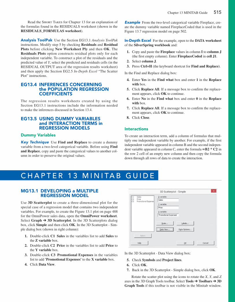
Chapter 13 MINITAB Guide 515
Read the Short Takes for Chapter 13 for an explanation of the formulas found in the ReSIDUALS worksheet (shown in the RESIDUALS_FORMULAS worksheet).
analysis ToolPak Use the Section eG13.1 Analysis ToolPak instructions. Modify step 5 by checking Residuals and Residual Plots before clicking New Worksheet Ply and then OK. The Residuals Plots option constructs residual plots only for each independent variable. To construct a plot of the residuals and the predicted value of Y, select the predicted and residuals cells (in the ReSIDUAL OUTPUT area of the regression results worksheet) and then apply the Section eG2.5 In-Depth Excel “The Scatter Plot” instructions.
eg13.4 InFeRenCeS COnCeRnIng the POPulaTIOn RegReSSIOn COeFFICIenTS
The regression results worksheets created by using the Section eG13.1 instructions include the information needed to make the inferences discussed in Section 13.4.
eg13.5 uSIng DuMMy VaRIableS and InTeRaCTIOn TeRMS in RegReSSIOn MODelS
Dummy Variables
Key Technique Use Find and Replace to create a dummy variable from a two-level categorical variable. Before using Find and Replace, copy and paste the categorical values to another col-umn in order to preserve the original values.
Example From the two-level categorical variable Fireplace, cre-ate the dummy variable named FireplaceCoded that is used in the Figure 13.7 regression model on page 502.
In-Depth excel For the example, open to the DATA worksheet of the SilverSpring workbook and:
1. Copy and paste the Fireplace values in column I to column J (the first empty column). enter FireplaceCoded in cell J1.
2. Select column J. 3. Press Ctrl+H (the keyboard shortcut for Find and Replace).
In the Find and Replace dialog box:
4. enter Yes in the Find what box and enter 1 in the Replace with box.
5. Click Replace All. If a message box to confirm the replace-ment appears, click OK to continue.
6. enter No in the Find what box and enter 0 in the Replace with box.
7. Click Replace All. If a message box to confirm the replace-ment appears, click OK to continue.
8. Click Close.
Interactions
To create an interaction term, add a column of formulas that mul-tiply one independent variable by another. For example, if the first independent variable appeared in column B and the second indepen-dent variable appeared in column C, enter the formula =B2 * C2 in the row 2 cell of an empty new column and then copy the formula down through all rows of data to create the interaction.
Mg13.1 DeVelOPIng a MulTIPle RegReSSIOn MODel
Use 3D Scatterplot to create a three-dimensional plot for the special case of a regression model that contains two independent variables. For example, to create the Figure 13.1 plot on page 488 for the OmniPower sales data, open the OmniPower worksheet. Select Graph ➔ 3D Scatterplot. In the 3D Scatterplots dialog box, click Simple and then click OK. In the 3D Scatterplot - Sim-ple dialog box (shown in right column):
1. Double-click C1 Sales in the variables list to add Sales to the Z variable box.
2. Double-click C2 Price in the variables list to add Price to the Y variable box.
3. Double-click C3 Promotional Expenses in the variables list to add 'Promotional Expenses' to the X variable box.
4. Click Data View.
In the 3D Scatterplot - Data View dialog box:
5. Check Symbols and Project lines. 6. Click OK. 7. Back in the 3D Scatterplot - Simple dialog box, click OK.
Rotate the scatter plot using the icons to rotate the X, Y, and Z axes in the 3D Graph Tools toolbar. Select Tools ➔ Toolbars ➔ 3D Graph Tools if this toolbar is not visible in the Minitab window.
c h a p t e r 1 3 M i n i ta b g U i d e
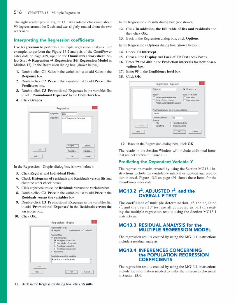
516 CHAPTeR 13 Multiple Regression
The right scatter plot in Figure 13.1 was rotated clockwise about 90 degrees around the Z axis and was slightly rotated about the two other axes.
Interpreting the Regression coefficients
Use Regression to perform a multiple regression analysis. For example, to perform the Figure 13.2 analysis of the OmniPower sales data on page 489, open to the OmniPower worksheet. Se-lect Stat ➔ Regression ➔ Regression (Fit Regression Model in Minitab 17). In the Regression dialog box (shown below):
1. Double-click C1 Sales in the variables list to add Sales to the Response box.
2. Double-click C2 Price in the variables list to add Price to the Predictors box.
3. Double-click C3 Promotional Expenses in the variables list to add 'Promotional Expenses' to the Predictors box.
4. Click Graphs.
In the Regression - Graphs dialog box (shown below):
5. Click Regular and Individual Plots. 6. Check Histogram of residuals and Residuals versus fits and
clear the other check boxes. 7. Click anywhere inside the Residuals versus the variables box. 8. Double-click C2 Price in the variables list to add Price in the
Residuals versus the variables box. 9. Double-click C3 Promotional Expenses in the variables list
to add 'Promotional Expenses' in the Residuals versus the variables box.
10. Click OK.
11. Back in the Regression dialog box, click Results.
In the Regression - Results dialog box (not shown):
12. Click In addition, the full table of fits and residuals and then click OK.
13. Back in the Regression dialog box, click Options.
In the Regression - Options dialog box (shown below):
14. Check Fit Intercept. 15. Clear all the Display and Lack of Fit Test check boxes. 16. enter 79 and 400 in the Prediction intervals for new obser-
vations box. 17. enter 95 in the Confidence level box. 18. Click OK.
19. Back in the Regression dialog box, click OK.
The results in the Session Window will include additional items that are not shown in Figure 13.2.
Predicting the Dependent Variable Y
The regression results created by using the Section MG13.1 in-structions include the confidence interval estimation and predic-tion interval. Figure 13.3 on page 491 shows these items for the OmniPower sales data.
Mg13.2 r2, aDjuSTeD r2, and the OVeRall F TeST
The coefficient of multiple determination, r 2, the adjusted r 2, and the overall F test are all computed as part of creat-ing the multiple regression results using the Section MG13.1 instructions.
Mg13.3 ReSIDual analySIS for the MulTIPle RegReSSIOn MODel
The regression results created by using the MG13.1 instructions include a residual analysis.
Mg13.4 InFeRenCeS COnCeRnIng the POPulaTIOn RegReSSIOn COeFFICIenTS
The regression results created by using the MG13.1 instructions include the information needed to make the inferences discussed in Section 13.4.
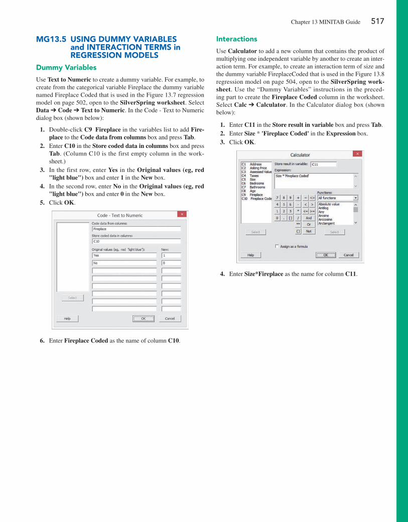
Chapter 13 MINITAB Guide 517
Mg13.5 uSIng DuMMy VaRIableS and InTeRaCTIOn TeRMS in RegReSSIOn MODelS
Dummy Variables
Use Text to Numeric to create a dummy variable. For example, to create from the categorical variable Fireplace the dummy variable named Fireplace Coded that is used in the Figure 13.7 regression model on page 502, open to the SilverSpring worksheet. Select Data ➔ Code ➔ Text to Numeric. In the Code - Text to Numeric dialog box (shown below):
1. Double-click C9 Fireplace in the variables list to add Fire-place to the Code data from columns box and press Tab.
2. enter C10 in the Store coded data in columns box and press Tab. (Column C10 is the first empty column in the work-sheet.)
3. In the first row, enter Yes in the Original values (eg, red "light blue") box and enter 1 in the New box.
4. In the second row, enter No in the Original values (eg, red "light blue") box and enter 0 in the New box.
5. Click OK.
6. enter Fireplace Coded as the name of column C10.
Interactions
Use Calculator to add a new column that contains the product of multiplying one independent variable by another to create an inter-action term. For example, to create an interaction term of size and the dummy variable FireplaceCoded that is used in the Figure 13.8 regression model on page 504, open to the SilverSpring work-sheet. Use the “Dummy Variables” instructions in the preced-ing part to create the Fireplace Coded column in the worksheet. Select Calc ➔ Calculator. In the Calculator dialog box (shown below):
1. enter C11 in the Store result in variable box and press Tab. 2. enter Size * 'Fireplace Coded' in the Expression box. 3. Click OK.
4. enter Size*Fireplace as the name for column C11.
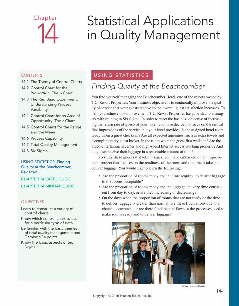
14-1Copyright © 2016 Pearson Education, Inc.
U s i n g s tat i s t i c s
Finding Quality at the BeachcomberYou find yourself managing the Beachcomber Hotel, one of the resorts owned by T.C. Resort Properties. Your business objective is to continually improve the qual-ity of service that your guests receive so that overall guest satisfaction increases. To help you achieve this improvement, T.C. Resort Properties has provided its manag-ers with training in Six Sigma. In order to meet the business objective of increas-ing the return rate of guests at your hotel, you have decided to focus on the critical first impressions of the service that your hotel provides. Is the assigned hotel room ready when a guest checks in? Are all expected amenities, such as extra towels and a complimentary guest basket, in the room when the guest first walks in? Are the video-entertainment center and high-speed Internet access working properly? And do guests receive their luggage in a reasonable amount of time?
To study these guest satisfaction issues, you have embarked on an improve-ment project that focuses on the readiness of the room and the time it takes to deliver luggage. You would like to learn the following:
• Are the proportion of rooms ready and the time required to deliver luggage to the rooms acceptable?
• Are the proportion of rooms ready and the luggage delivery time consist-ent from day to day, or are they increasing or decreasing?
• On the days when the proportion of rooms that are not ready or the time to deliver luggage is greater than normal, are these fluctuations due to a chance occurrence, or are there fundamental flaws in the processes used to make rooms ready and to deliver luggage?
contents
14.1 The Theory of Control Charts
14.2 Control Chart for the Proportion: The p Chart
14.3 The Red Bead Experiment: Understanding Process Variability
14.4 Control Chart for an Area of Opportunity: The c Chart
14.5 Control Charts for the Range and the Mean
14.6 Process Capability
14.7 Total Quality Management
14.8 Six Sigma
Using statistics: Finding Quality at the Beachcomber, Revisited
chapteR 14 eXceL gUide
chapteR 14 MinitaB gUide
objectives
Learn to construct a variety of control charts
Know which control chart to use for a particular type of data
Be familiar with the basic themes of total quality management and Deming’s 14 points
Know the basic aspects of Six Sigma
Chapter Statistical Applications in Quality Management14
© Stockyimages/Fotolia
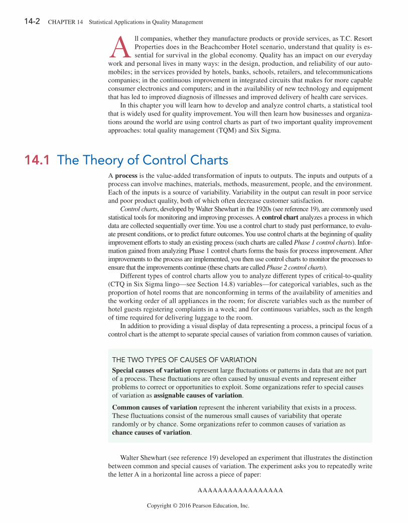
14-2 CHAPTER 14 Statistical Applications in Quality Management
Copyright © 2016 Pearson Education, Inc.
A ll companies, whether they manufacture products or provide services, as T.C. Resort Properties does in the Beachcomber Hotel scenario, understand that quality is es-sential for survival in the global economy. Quality has an impact on our everyday
work and personal lives in many ways: in the design, production, and reliability of our auto-mobiles; in the services provided by hotels, banks, schools, retailers, and telecommunications companies; in the continuous improvement in integrated circuits that makes for more capable consumer electronics and computers; and in the availability of new technology and equipment that has led to improved diagnosis of illnesses and improved delivery of health care services.
In this chapter you will learn how to develop and analyze control charts, a statistical tool that is widely used for quality improvement. You will then learn how businesses and organiza-tions around the world are using control charts as part of two important quality improvement approaches: total quality management (TQM) and Six Sigma.
ThE TwO TyPES Of CAUSES Of VARiATiOn
Special causes of variation represent large fluctuations or patterns in data that are not part of a process. These fluctuations are often caused by unusual events and represent either problems to correct or opportunities to exploit. Some organizations refer to special causes of variation as assignable causes of variation.
Common causes of variation represent the inherent variability that exists in a process. These fluctuations consist of the numerous small causes of variability that operate randomly or by chance. Some organizations refer to common causes of variation as chance causes of variation.
Walter Shewhart (see reference 19) developed an experiment that illustrates the distinction between common and special causes of variation. The experiment asks you to repeatedly write the letter A in a horizontal line across a piece of paper:
AAAAAAAAAAAAAAAAA
14.1 The Theory of Control ChartsA process is the value-added transformation of inputs to outputs. The inputs and outputs of a process can involve machines, materials, methods, measurement, people, and the environment. Each of the inputs is a source of variability. Variability in the output can result in poor service and poor product quality, both of which often decrease customer satisfaction.
Control charts, developed by Walter Shewhart in the 1920s (see reference 19), are commonly used statistical tools for monitoring and improving processes. A control chart analyzes a process in which data are collected sequentially over time. You use a control chart to study past performance, to evalu-ate present conditions, or to predict future outcomes. You use control charts at the beginning of quality improvement efforts to study an existing process (such charts are called Phase 1 control charts). Infor-mation gained from analyzing Phase 1 control charts forms the basis for process improvement. After improvements to the process are implemented, you then use control charts to monitor the processes to ensure that the improvements continue (these charts are called Phase 2 control charts).
Different types of control charts allow you to analyze different types of critical-to-quality (CTQ in Six Sigma lingo—see Section 14.8) variables—for categorical variables, such as the proportion of hotel rooms that are nonconforming in terms of the availability of amenities and the working order of all appliances in the room; for discrete variables such as the number of hotel guests registering complaints in a week; and for continuous variables, such as the length of time required for delivering luggage to the room.
In addition to providing a visual display of data representing a process, a principal focus of a control chart is the attempt to separate special causes of variation from common causes of variation.
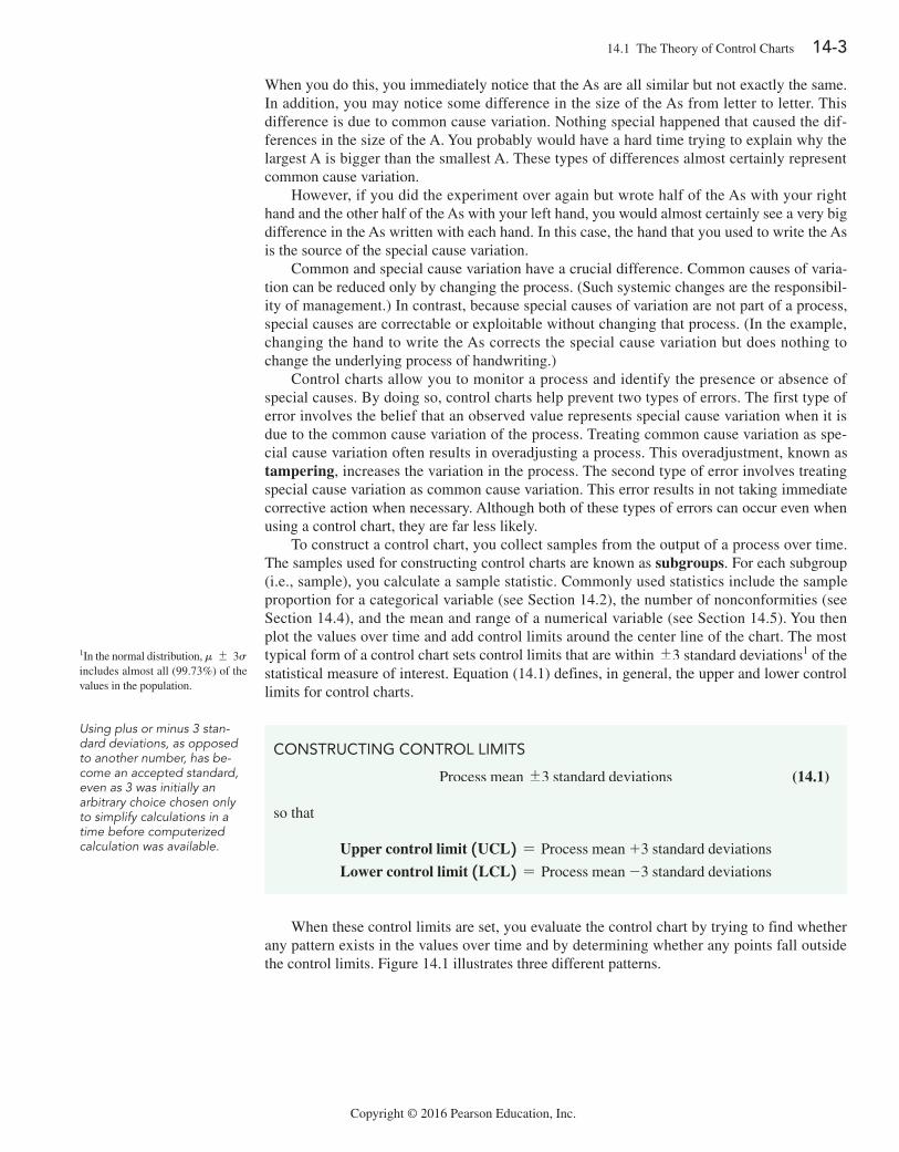
14.1 The Theory of Control Charts 14-3
Copyright © 2016 Pearson Education, Inc.
When you do this, you immediately notice that the As are all similar but not exactly the same. In addition, you may notice some difference in the size of the As from letter to letter. This difference is due to common cause variation. Nothing special happened that caused the dif-ferences in the size of the A. You probably would have a hard time trying to explain why the largest A is bigger than the smallest A. These types of differences almost certainly represent common cause variation.
However, if you did the experiment over again but wrote half of the As with your right hand and the other half of the As with your left hand, you would almost certainly see a very big difference in the As written with each hand. In this case, the hand that you used to write the As is the source of the special cause variation.
Common and special cause variation have a crucial difference. Common causes of varia-tion can be reduced only by changing the process. (Such systemic changes are the responsibil-ity of management.) In contrast, because special causes of variation are not part of a process, special causes are correctable or exploitable without changing that process. (In the example, changing the hand to write the As corrects the special cause variation but does nothing to change the underlying process of handwriting.)
Control charts allow you to monitor a process and identify the presence or absence of special causes. By doing so, control charts help prevent two types of errors. The first type of error involves the belief that an observed value represents special cause variation when it is due to the common cause variation of the process. Treating common cause variation as spe-cial cause variation often results in overadjusting a process. This overadjustment, known as tampering, increases the variation in the process. The second type of error involves treating special cause variation as common cause variation. This error results in not taking immediate corrective action when necessary. Although both of these types of errors can occur even when using a control chart, they are far less likely.
To construct a control chart, you collect samples from the output of a process over time. The samples used for constructing control charts are known as subgroups. For each subgroup (i.e., sample), you calculate a sample statistic. Commonly used statistics include the sample proportion for a categorical variable (see Section 14.2), the number of nonconformities (see Section 14.4), and the mean and range of a numerical variable (see Section 14.5). You then plot the values over time and add control limits around the center line of the chart. The most typical form of a control chart sets control limits that are within {3 standard deviations1 of the statistical measure of interest. Equation (14.1) defines, in general, the upper and lower control limits for control charts.
1In the normal distribution, m { 3s includes almost all (99.73%) of the values in the population.
Using plus or minus 3 stan-dard deviations, as opposed to another number, has be-come an accepted standard, even as 3 was initially an arbitrary choice chosen only to simplify calculations in a time before computerized calculation was available.
COnSTRUCTing COnTROL LiMiTS
Process mean {3 standard deviations (14.1)
so that
Upper control limit 1UCL 2 = Process mean +3 standard deviations
Lower control limit 1LCL 2 = Process mean -3 standard deviations
When these control limits are set, you evaluate the control chart by trying to find whether any pattern exists in the values over time and by determining whether any points fall outside the control limits. Figure 14.1 illustrates three different patterns.
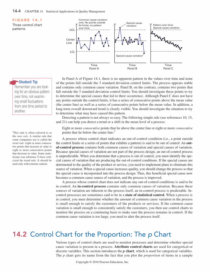
14-4 CHAPTER 14 Statistical Applications in Quality Management
Copyright © 2016 Pearson Education, Inc.
In Panel A of Figure 14.1, there is no apparent pattern in the values over time and none of the points fall outside the 3 standard deviation control limits. The process appears stable and contains only common cause variation. Panel B, on the contrary, contains two points that fall outside the 3 standard deviation control limits. You should investigate these points to try to determine the special causes that led to their occurrence. Although Panel C does not have any points outside the control limits, it has a series of consecutive points above the mean value (the center line) as well as a series of consecutive points below the mean value. In addition, a long-term overall downward trend is clearly visible. You should investigate the situation to try to determine what may have caused this pattern.
Detecting a pattern is not always so easy. The following simple rule (see references 10, 15, and 21) can help you detect a trend or a shift in the mean level of a process:
Eight or more consecutive points that lie above the center line or eight or more consecutive points that lie below the center line.2
A process whose control chart indicates an out-of-control condition (i.e., a point outside the control limits or a series of points that exhibits a pattern) is said to be out of control. An out-of-control process contains both common causes of variation and special causes of variation. Because special causes of variation are not part of the process design, an out-of-control process is unpredictable. When you determine that a process is out of control, you must identify the spe-cial causes of variation that are producing the out-of-control conditions. If the special causes are detrimental to the quality of the product or service, you need to implement plans to eliminate this source of variation. When a special cause increases quality, you should change the process so that the special cause is incorporated into the process design. Thus, this beneficial special cause now becomes a common cause source of variation, and the process is improved.
A process whose control chart does not indicate any out-of-control conditions is said to be in control. An in-control process contains only common causes of variation. Because these sources of variation are inherent to the process itself, an in-control process is predictable. In-control processes are sometimes said to be in a state of statistical control. When a process is in control, you must determine whether the amount of common cause variation in the process is small enough to satisfy the customers of the products or services. If the common cause variation is small enough to consistently satisfy the customers, you then use control charts to monitor the process on a continuing basis to make sure the process remains in control. If the common cause variation is too large, you need to alter the process itself.
F i g u r e 1 4 . 1Three control chart patterns UCL
X
CenterLine
Common cause variationonly: No points outside3σ limits; no patternover time
LCL
TimePanel A
X Special causevariation
Special cause variation
TimePanel B
X Pattern over time:Special cause variation
TimePanel C
Student TipRemember you are look-ing for an obvious pattern over time, not examin-ing small fluctuations from one time period to another.
2This rule is often referred to as the runs rule. A similar rule that some companies use is called the trend rule: eight or more consecu-tive points that increase in value or eight or more consecutive points that decrease in value. Some statis-ticians (see reference 5) have criti-cized the trend rule. It should be used only with extreme caution.
14.2 Control Chart for the Proportion: The p ChartVarious types of control charts are used to monitor processes and determine whether special cause variation is present in a process. Attribute control charts are used for categorical or discrete variables. This section introduces the p chart, which is used for categorical variables. The p chart gets its name from the fact that you plot the proportion of items in a sample
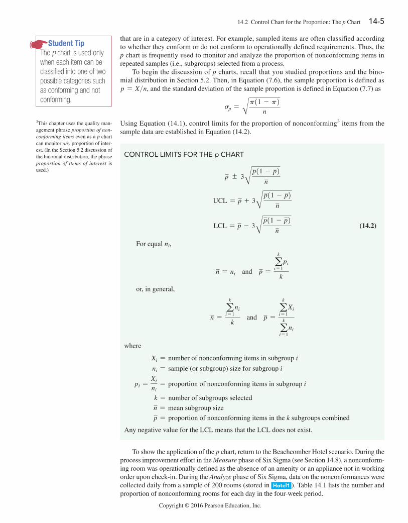
Copyright © 2016 Pearson Education, Inc.
14.2 Control Chart for the Proportion: The p Chart 14-5
that are in a category of interest. For example, sampled items are often classified according to whether they conform or do not conform to operationally defined requirements. Thus, the p chart is frequently used to monitor and analyze the proportion of nonconforming items in repeated samples (i.e., subgroups) selected from a process.
To begin the discussion of p charts, recall that you studied proportions and the bino-mial distribution in Section 5.2. Then, in Equation (7.6), the sample proportion is defined as p = X>n, and the standard deviation of the sample proportion is defined in Equation (7.7) as
sp = Ap11 - p2n
Using Equation (14.1), control limits for the proportion of nonconforming3 items from the sample data are established in Equation (14.2).
Student TipThe p chart is used only when each item can be classified into one of two possible categories such as conforming and not conforming.
3This chapter uses the quality man-agement phrase proportion of non-conforming items even as a p chart can monitor any proportion of inter-est. (In the Section 5.2 discussion of the binomial distribution, the phrase proportion of items of interest is used.)
COnTROL LiMiTS fOR ThE p ChART
p { 3Bp11 - p2n
UCL = p + 3Bp11 - p2n
LCL = p - 3Bp11 - p2n
(14.2)
For equal ni,
n = ni and p =a
k
i= 1pi
k
or, in general,
n =a
k
i= 1ni
k and p =
ak
i= 1Xi
ak
i= 1ni
where
Xi = number of nonconforming items in subgroup i
ni = sample (or subgroup) size for subgroup i
pi =Xi
ni= proportion of nonconforming items in subgroup i
k = number of subgroups selected
n = mean subgroup size
p = proportion of nonconforming items in the k subgroups combined
Any negative value for the LCL means that the LCL does not exist.
To show the application of the p chart, return to the Beachcomber Hotel scenario. During the process improvement effort in the Measure phase of Six Sigma (see Section 14.8), a nonconform-ing room was operationally defined as the absence of an amenity or an appliance not in working order upon check-in. During the Analyze phase of Six Sigma, data on the nonconformances were collected daily from a sample of 200 rooms (stored in Hotel1 ). Table 14.1 lists the number and proportion of nonconforming rooms for each day in the four-week period.
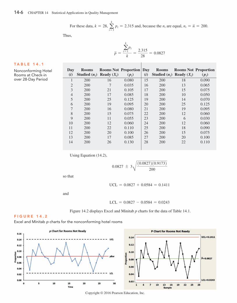
14-6 CHAPTER 14 Statistical Applications in Quality Management
Copyright © 2016 Pearson Education, Inc.
For these data, k = 28, ak
i= 1 pi = 2.315 and, because the ni are equal, ni = n = 200.
Thus,
p =a
k
i= 1pi
k=
2.315
28= 0.0827
F i g u r e 1 4 . 2Excel and Minitab p charts for the nonconforming hotel rooms
Day (i)
Rooms Studied (ni)
Rooms Not Ready (Xi)
Proportion ( pi)
Day (i)
Rooms Studied (ni)
Rooms Not Ready (Xi)
Proportion ( pi)
1 200 16 0.080 15 200 18 0.090 2 200 7 0.035 16 200 13 0.065 3 200 21 0.105 17 200 15 0.075 4 200 17 0.085 18 200 10 0.050 5 200 25 0.125 19 200 14 0.070 6 200 19 0.095 20 200 25 0.125 7 200 16 0.080 21 200 19 0.095 8 200 15 0.075 22 200 12 0.060 9 200 11 0.055 23 200 6 0.03010 200 12 0.060 24 200 12 0.06011 200 22 0.110 25 200 18 0.09012 200 20 0.100 26 200 15 0.07513 200 17 0.085 27 200 20 0.10014 200 26 0.130 28 200 22 0.110
T a b l e 1 4 . 1
nonconforming hotel Rooms at Check-in over 28-Day Period
Using Equation (14.2),
0.0827 { 3B 10.0827210.91732200
so that
UCL = 0.0827 + 0.0584 = 0.1411
and
LCL = 0.0827 - 0.0584 = 0.0243
Figure 14.2 displays Excel and Minitab p charts for the data of Table 14.1.
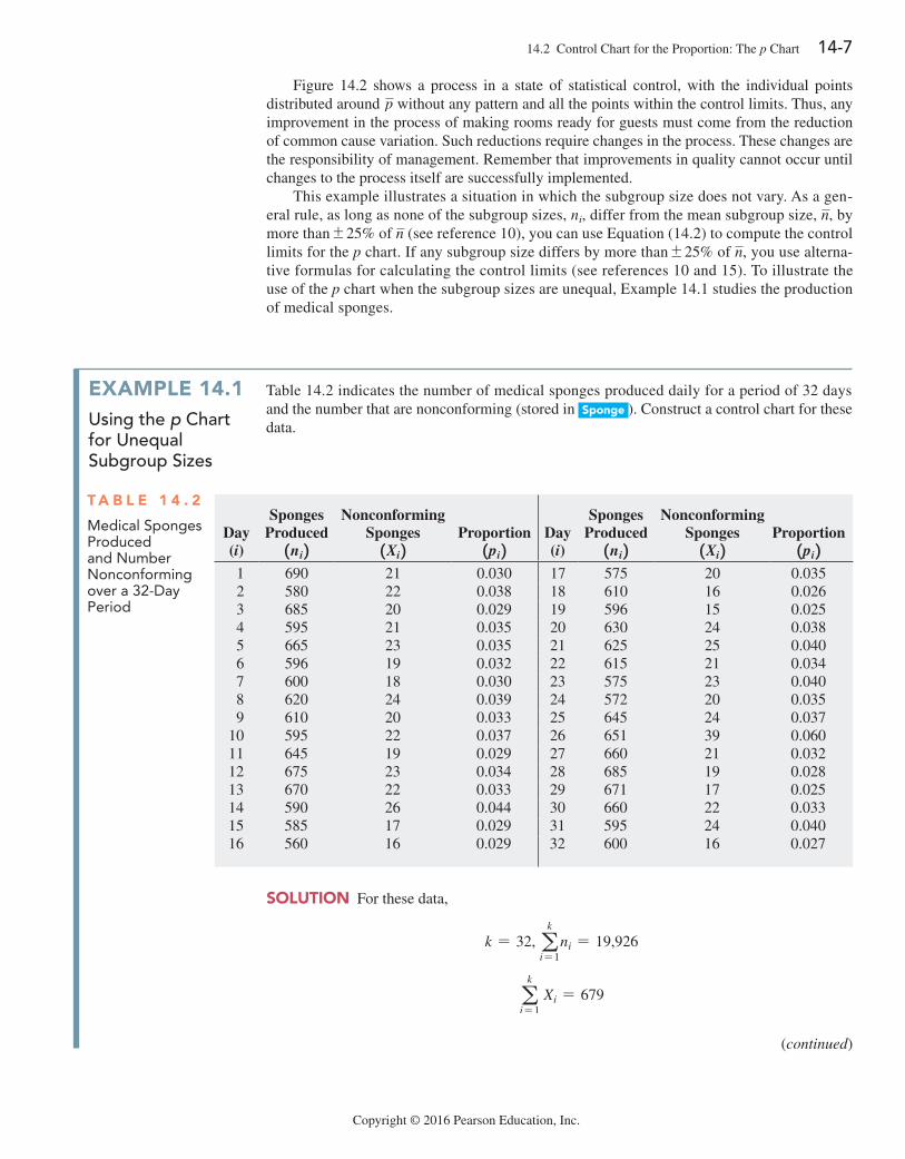
Copyright © 2016 Pearson Education, Inc.
14.2 Control Chart for the Proportion: The p Chart 14-7
Figure 14.2 shows a process in a state of statistical control, with the individual points distributed around p without any pattern and all the points within the control limits. Thus, any improvement in the process of making rooms ready for guests must come from the reduction of common cause variation. Such reductions require changes in the process. These changes are the responsibility of management. Remember that improvements in quality cannot occur until changes to the process itself are successfully implemented.
This example illustrates a situation in which the subgroup size does not vary. As a gen-eral rule, as long as none of the subgroup sizes, ni, differ from the mean subgroup size, n, by more than{25% of n (see reference 10), you can use Equation (14.2) to compute the control limits for the p chart. If any subgroup size differs by more than{25% of n, you use alterna-tive formulas for calculating the control limits (see references 10 and 15). To illustrate the use of the p chart when the subgroup sizes are unequal, Example 14.1 studies the production of medical sponges.
example 14.1Using the p chart for Unequal subgroup sizes
Table 14.2 indicates the number of medical sponges produced daily for a period of 32 days and the number that are nonconforming (stored in Sponge ). Construct a control chart for these data.
T a b l e 1 4 . 2
Medical Sponges Produced and number nonconforming over a 32-Day Period
Day (i)
Sponges Produced
1ni 2Nonconforming
Sponges 1Xi 2
Proportion
1pi 2
Day (i)
Sponges Produced
1ni 2Nonconforming
Sponges 1Xi 2
Proportion
1pi 2 1 690 21 0.030 17 575 20 0.035 2 580 22 0.038 18 610 16 0.026 3 685 20 0.029 19 596 15 0.025 4 595 21 0.035 20 630 24 0.038 5 665 23 0.035 21 625 25 0.040 6 596 19 0.032 22 615 21 0.034 7 600 18 0.030 23 575 23 0.040 8 620 24 0.039 24 572 20 0.035 9 610 20 0.033 25 645 24 0.03710 595 22 0.037 26 651 39 0.06011 645 19 0.029 27 660 21 0.03212 675 23 0.034 28 685 19 0.02813 670 22 0.033 29 671 17 0.02514 590 26 0.044 30 660 22 0.03315 585 17 0.029 31 595 24 0.04016 560 16 0.029 32 600 16 0.027
SoluTion For these data,
k = 32, ak
i= 1ni = 19,926
ak
i= 1 Xi = 679
(continued)
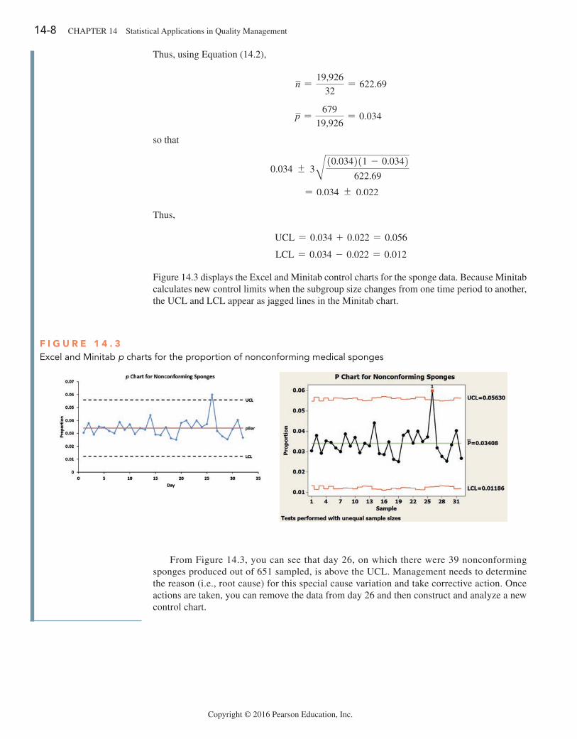
14-8 CHAPTER 14 Statistical Applications in Quality Management
Copyright © 2016 Pearson Education, Inc.
Thus, using Equation (14.2),
n =19,926
32= 622.69
p =679
19,926= 0.034
so that
0.034 { 3B 10.034211 - 0.0342622.69
= 0.034 { 0.022
Thus,
UCL = 0.034 + 0.022 = 0.056
LCL = 0.034 - 0.022 = 0.012
Figure 14.3 displays the Excel and Minitab control charts for the sponge data. Because Minitab calculates new control limits when the subgroup size changes from one time period to another, the UCL and LCL appear as jagged lines in the Minitab chart.
F i g u r e 1 4 . 3Excel and Minitab p charts for the proportion of nonconforming medical sponges
From Figure 14.3, you can see that day 26, on which there were 39 nonconforming sponges produced out of 651 sampled, is above the UCL. Management needs to determine the reason (i.e., root cause) for this special cause variation and take corrective action. Once actions are taken, you can remove the data from day 26 and then construct and analyze a new control chart.
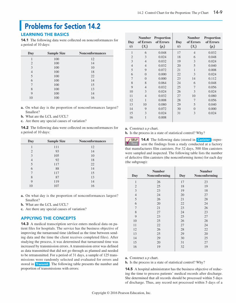
Copyright © 2016 Pearson Education, Inc.
14.2 Control Chart for the Proportion: The p Chart 14-9
problems for Section 14.2learning THe baSicS14.1 The following data were collected on nonconformances for a period of 10 days:
Day Sample Size Nonconformances
1 100 12 2 100 14 3 100 10 4 100 18 5 100 22 6 100 14 7 100 15 8 100 13 9 100 1410 100 16
a. On what day is the proportion of nonconformances largest? Smallest?
b. What are the LCL and UCL?c. Are there any special causes of variation?
14.2 The following data were collected on nonconformances for a period of 10 days:
Day Sample Size Nonconformances
1 111 12 2 93 14 3 105 10 4 92 18 5 117 22 6 88 14 7 117 15 8 87 13 9 119 1410 107 16
a. On what day is the proportion of nonconformances largest? Smallest?
b. What are the LCL and UCL?c. Are there any special causes of variation?
applying THe concepTS14.3 A medical transcription service enters medical data on pa-tient files for hospitals. The service has the business objective of improving the turnaround time (defined as the time between send-ing data and the time the client receives completed files). After studying the process, it was determined that turnaround time was increased by transmission errors. A transmission error was defined as data transmitted that did not go through as planned and needed to be retransmitted. For a period of 31 days, a sample of 125 trans-missions were randomly selected and evaluated for errors and stored in Transmit . The following table presents the number and proportion of transmissions with errors:
Day (i)
Number of Errors
1Xi 2
Proportion of Errors
1pi 2
Day (i)
Number of Errors
1Xi 2
Proportion of Errors
1pi 2 1 6 0.048 17 4 0.032 2 3 0.024 18 6 0.048 3 4 0.032 19 3 0.024 4 4 0.032 20 5 0.040 5 9 0.072 21 1 0.008 6 0 0.000 22 3 0.024 7 0 0.000 23 14 0.112 8 8 0.064 24 6 0.048 9 4 0.032 25 7 0.05610 3 0.024 26 3 0.02411 4 0.032 27 10 0.08012 1 0.008 28 7 0.05613 10 0.080 29 5 0.04014 9 0.072 30 0 0.00015 3 0.024 31 3 0.02416 1 0.008
a. Construct a p chart.b. Is the process in a state of statistical control? Why?
SELF Test
14.4 The following data (stored in canister ) repre-sent the findings from a study conducted at a factory
that manufactures film canisters. For 32 days, 500 film canisters were sampled and inspected. The following table lists the number of defective film canisters (the nonconforming items) for each day (the subgroup):
Day
Number Nonconforming
Day
Number Nonconforming
1 26 17 23 2 25 18 19 3 23 19 18 4 24 20 27 5 26 21 28 6 20 22 24 7 21 23 26 8 27 24 23 9 23 25 2710 25 26 2811 22 27 2412 26 28 2213 25 29 2014 29 30 2515 20 31 2716 19 32 19
a. Construct a p chart.b. Is the process in a state of statistical control? Why?
14.5 A hospital administrator has the business objective of reduc-ing the time to process patients’ medical records after discharge. She determined that all records should be processed within 5 days of discharge. Thus, any record not processed within 5 days of a
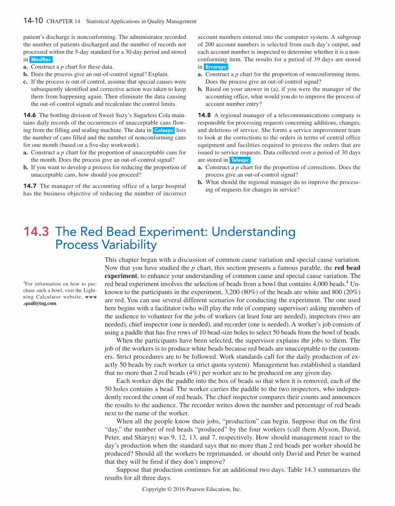
14-10 CHAPTER 14 Statistical Applications in Quality Management
Copyright © 2016 Pearson Education, Inc.
patient’s discharge is nonconforming. The administrator recorded the number of patients discharged and the number of records not processed within the 5-day standard for a 30-day period and stored in medrec .a. Construct a p chart for these data.b. Does the process give an out-of-control signal? Explain.c. If the process is out of control, assume that special causes were
subsequently identified and corrective action was taken to keep them from happening again. Then eliminate the data causing the out-of-control signals and recalculate the control limits.
14.6 The bottling division of Sweet Suzy’s Sugarless Cola main-tains daily records of the occurrences of unacceptable cans flow-ing from the filling and sealing machine. The data in colaspc lists the number of cans filled and the number of nonconforming cans for one month (based on a five-day workweek).a. Construct a p chart for the proportion of unacceptable cans for
the month. Does the process give an out-of-control signal?b. If you want to develop a process for reducing the proportion of
unacceptable cans, how should you proceed?
14.7 The manager of the accounting office of a large hospital has the business objective of reducing the number of incorrect
account numbers entered into the computer system. A subgroup of 200 account numbers is selected from each day’s output, and each account number is inspected to determine whether it is a non-conforming item. The results for a period of 39 days are stored in errorspc .a. Construct a p chart for the proportion of nonconforming items.
Does the process give an out-of-control signal?b. Based on your answer in (a), if you were the manager of the
accounting office, what would you do to improve the process of account number entry?
14.8 A regional manager of a telecommunications company is responsible for processing requests concerning additions, changes, and deletions of service. She forms a service improvement team to look at the corrections to the orders in terms of central office equipment and facilities required to process the orders that are issued to service requests. Data collected over a period of 30 days are stored in Telespc .a. Construct a p chart for the proportion of corrections. Does the
process give an out-of-control signal?b. What should the regional manager do to improve the process-
ing of requests for changes in service?
14.3 The Red Bead Experiment: Understanding Process Variability
This chapter began with a discussion of common cause variation and special cause variation. Now that you have studied the p chart, this section presents a famous parable, the red bead experiment, to enhance your understanding of common cause and special cause variation. The red bead experiment involves the selection of beads from a bowl that contains 4,000 beads.4 Un-known to the participants in the experiment, 3,200 (80%) of the beads are white and 800 (20%) are red. You can use several different scenarios for conducting the experiment. The one used here begins with a facilitator (who will play the role of company supervisor) asking members of the audience to volunteer for the jobs of workers (at least four are needed), inspectors (two are needed), chief inspector (one is needed), and recorder (one is needed). A worker’s job consists of using a paddle that has five rows of 10 bead-size holes to select 50 beads from the bowl of beads.
When the participants have been selected, the supervisor explains the jobs to them. The job of the workers is to produce white beads because red beads are unacceptable to the custom-ers. Strict procedures are to be followed. Work standards call for the daily production of ex-actly 50 beads by each worker (a strict quota system). Management has established a standard that no more than 2 red beads (4%) per worker are to be produced on any given day.
Each worker dips the paddle into the box of beads so that when it is removed, each of the 50 holes contains a bead. The worker carries the paddle to the two inspectors, who indepen-dently record the count of red beads. The chief inspector compares their counts and announces the results to the audience. The recorder writes down the number and percentage of red beads next to the name of the worker.
When all the people know their jobs, “production” can begin. Suppose that on the first “day,” the number of red beads “produced” by the four workers (call them Alyson, David, Peter, and Sharyn) was 9, 12, 13, and 7, respectively. How should management react to the day’s production when the standard says that no more than 2 red beads per worker should be produced? Should all the workers be reprimanded, or should only David and Peter be warned that they will be fired if they don’t improve?
Suppose that production continues for an additional two days. Table 14.3 summarizes the results for all three days.
4For information on how to pur-chase such a bowl, visit the Light-ning Calculator website, www .qualitytng.com.
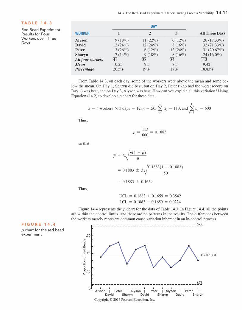
14.3 The Red Bead Experiment: Understanding Process Variability 14-11
Copyright © 2016 Pearson Education, Inc.
From Table 14.3, on each day, some of the workers were above the mean and some be-low the mean. On Day 1, Sharyn did best, but on Day 2, Peter (who had the worst record on Day 1) was best, and on Day 3, Alyson was best. How can you explain all this variation? Using Equation (14.2) to develop a p chart for these data,
k = 4 workers * 3 days = 12, n = 50, ak
i=1 Xi = 113, and a
k
i=1 ni = 600
Thus,
p =113
600= 0.1883
so that
p { 3Bp11 - p2n
= 0.1883 { 3B0.188311 - 0.1883250
= 0.1883 { 0.1659
Thus,
UCL = 0.1883 + 0.1659 = 0.3542
LCL = 0.1883 - 0.1659 = 0.0224
Figure 14.4 represents the p chart for the data of Table 14.3. In Figure 14.4, all the points are within the control limits, and there are no patterns in the results. The differences between the workers merely represent common cause variation inherent in an in-control process.
T a b l e 1 4 . 3
Red Bead Experiment Results for four workers over Three Days
Day
Worker 1 2 3 All Three Days
Alyson 9 (18%) 11 (22%) 6 (12%) 26 (17.33%)David 12 (24%) 12 (24%) 8 (16%) 32 (21.33%)Peter 13 (26%) 6 (12%) 12 (24%) 31 (20.67%)Sharyn 7 (14%) 9 (18%) 8 (16%) 24 (16.0%)All four workers 41 38 34 113Mean 10.25 9.5 8.5 9.42Percentage 20.5% 19% 17% 18.83%
David
Pro
po
rtio
n o
f R
ed B
ead
s
0
.30
.20
.10
AlysonSharyn
PeterDavid
AlysonSharyn
PeterDavid
AlysonSharyn
Peter
LCL
UCL
P = 0.1883
F i g u r e 1 4 . 4p chart for the red bead experiment
14-12 CHAPTER 14 Statistical Applications in Quality Management
Copyright © 2016 Pearson Education, Inc.
The parable of the red beads has four morals:
• Variation is an inherent part of any process. • Workers work within a process over which they have little control. It is the process that
primarily determines their performance. • Only management can change the process. • There will always be some workers above the mean and some workers below the mean.
problems for Section 14.3applying THe concepTS14.9 In the red bead experiment, how do you think many manag-ers would have reacted after Day 1? Day 2? Day 3?
14.10 (Class Project) Obtain a version of the red bead experi-ment for your class.
a. Conduct the experiment in the same way as described in this section.
b. Remove 400 red beads from the bead bowl before beginning the experiment. How do your results differ from those in (a)? What does this tell you about the effect of the process on the results?
14.4 Control Chart for an Area of Opportunity: The c ChartYou use a p chart for monitoring and analyzing the proportion of nonconforming items. Non-conformities are defects or flaws in a product or service. To monitor and analyze the number of nonconformities in an area of opportunity, you use a c chart. An area of opportunity is an in-dividual unit of a product or service, or a unit of time, space, or area. Examples of “the number of nonconformities in an area of opportunity” would be the number of flaws in a square foot of carpet, the number of typographical errors on a printed page, and the number of hotel custom-ers filing complaints in a given week.
Counting the number of nonconformities in an area of opportunity is unlike the process used to prepare a p chart in which you classify each unit as conforming or nonconforming. The c chart process fits the assumptions of a Poisson distribution. For the Poisson distribution, the standard deviation of the number of nonconformities is the square root of the mean number of nonconformities 1l2. Assuming that the size of each area of opportunity remains constant,5 you can compute the control limits for the number of nonconformities per area of opportunity using the observed mean number of nonconformities as an estimate of l. Equation (14.3) de-fines the control limits for the c chart, which you use to monitor and analyze the number of nonconformities per area of opportunity.
Student TipYou use the c chart when you are counting the number of nonconform-ing items in an area of opportunity.
5If the size of the unit varies, you should use a u chart instead of a c chart (see references 10, 15, and 21).
COnTROL LiMiTS fOR ThE c ChART
c { 31c
UCL = c + 31c
LCL = c - 31c (14.3)
where
c =a
k
i= 1 ci
k k = number of units sampled
ci = number of nonconformities in unit i
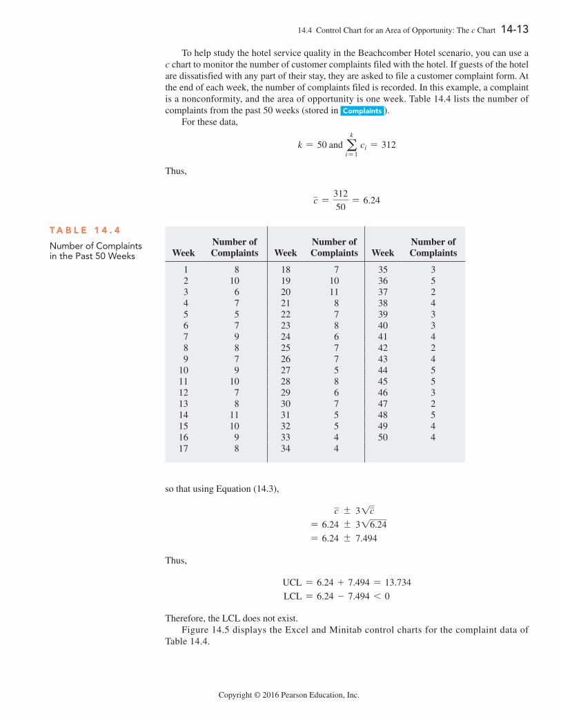
Copyright © 2016 Pearson Education, Inc.
14.4 Control Chart for an Area of Opportunity: The c Chart 14-13
To help study the hotel service quality in the Beachcomber Hotel scenario, you can use a c chart to monitor the number of customer complaints filed with the hotel. If guests of the hotel are dissatisfied with any part of their stay, they are asked to file a customer complaint form. At the end of each week, the number of complaints filed is recorded. In this example, a complaint is a nonconformity, and the area of opportunity is one week. Table 14.4 lists the number of complaints from the past 50 weeks (stored in complaints ).
For these data,
k = 50 and ak
i= 1 ci = 312
Thus,
c =312
50= 6.24
T a b l e 1 4 . 4
number of Complaints in the Past 50 weeks
Week
Number of Complaints
Week
Number of Complaints
Week
Number of Complaints
1 8 18 7 35 3 2 10 19 10 36 5 3 6 20 11 37 2 4 7 21 8 38 4 5 5 22 7 39 3 6 7 23 8 40 3 7 9 24 6 41 4 8 8 25 7 42 2 9 7 26 7 43 410 9 27 5 44 511 10 28 8 45 512 7 29 6 46 313 8 30 7 47 214 11 31 5 48 515 10 32 5 49 416 9 33 4 50 417 8 34 4
so that using Equation (14.3),
c { 31c
= 6.24 { 316.24
= 6.24 { 7.494
Thus,
UCL = 6.24 + 7.494 = 13.734
LCL = 6.24 - 7.494 6 0
Therefore, the LCL does not exist.Figure 14.5 displays the Excel and Minitab control charts for the complaint data of
Table 14.4.
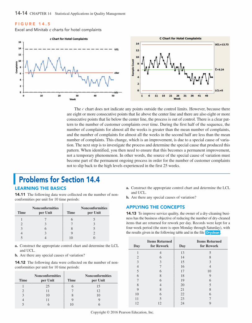
14-14 CHAPTER 14 Statistical Applications in Quality Management
Copyright © 2016 Pearson Education, Inc.
The c chart does not indicate any points outside the control limits. However, because there are eight or more consecutive points that lie above the center line and there are also eight or more consecutive points that lie below the center line, the process is out of control. There is a clear pat-tern to the number of customer complaints over time. During the first half of the sequence, the number of complaints for almost all the weeks is greater than the mean number of complaints, and the number of complaints for almost all the weeks in the second half are less than the mean number of complaints. This change, which is an improvement, is due to a special cause of varia-tion. The next step is to investigate the process and determine the special cause that produced this pattern. When identified, you then need to ensure that this becomes a permanent improvement, not a temporary phenomenon. In other words, the source of the special cause of variation must become part of the permanent ongoing process in order for the number of customer complaints not to slip back to the high levels experienced in the first 25 weeks.
F i g u r e 1 4 . 5Excel and Minitab c charts for hotel complaints
problems for Section 14.4learning THe baSicS14.11 The following data were collected on the number of non-conformities per unit for 10 time periods:
Time
Nonconformities per Unit
Time
Nonconformities per Unit
1 7 6 52 3 7 33 6 8 54 3 9 25 4 10 0
a. Construct the appropriate control chart and determine the LCL and UCL.
b. Are there any special causes of variation?
14.12 The following data were collected on the number of non-conformities per unit for 10 time periods:
Time
Nonconformities per Unit
Time
Nonconformities per Unit
1 25 6 152 11 7 123 10 8 104 11 9 95 6 10 6
a. Construct the appropriate control chart and determine the LCL and UCL.
b. Are there any special causes of variation?
applying THe concepTS14.13 To improve service quality, the owner of a dry-cleaning busi-ness has the business objective of reducing the number of dry-cleaned items that are returned for rework per day. Records were kept for a four-week period (the store is open Monday through Saturday), with the results given in the following table and in the file Dryclean .
Day
Items Returned for Rework
Day
Items Returned for Rework
1 4 13 5 2 6 14 8 3 3 15 3 4 7 16 4 5 6 17 10 6 8 18 9 7 6 19 6 8 4 20 5 9 8 21 810 6 22 611 5 23 712 12 24 9
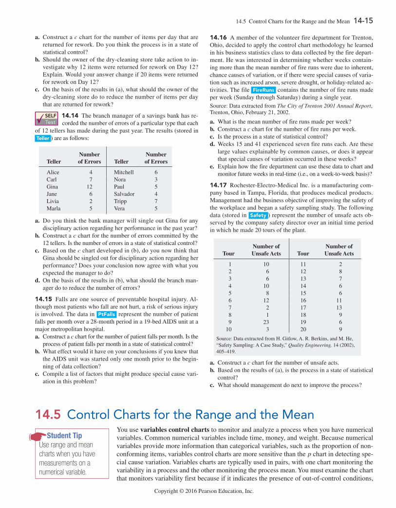
14.5 Control Charts for the Range and the Mean 14-15
Copyright © 2016 Pearson Education, Inc.
a. Construct a c chart for the number of items per day that are returned for rework. Do you think the process is in a state of statistical control?
b. Should the owner of the dry-cleaning store take action to in-vestigate why 12 items were returned for rework on Day 12? Explain. Would your answer change if 20 items were returned for rework on Day 12?
c. On the basis of the results in (a), what should the owner of the dry-cleaning store do to reduce the number of items per day that are returned for rework?
SELF Test
14.14 The branch manager of a savings bank has re-corded the number of errors of a particular type that each
of 12 tellers has made during the past year. The results (stored in Teller ) are as follows:
Teller
Number of Errors
Teller
Number of Errors
Alice 4 Mitchell 6Carl 7 Nora 3Gina 12 Paul 5Jane 6 Salvador 4Livia 2 Tripp 7Marla 5 Vera 5
a. Do you think the bank manager will single out Gina for any disciplinary action regarding her performance in the past year?
b. Construct a c chart for the number of errors committed by the 12 tellers. Is the number of errors in a state of statistical control?
c. Based on the c chart developed in (b), do you now think that Gina should be singled out for disciplinary action regarding her performance? Does your conclusion now agree with what you expected the manager to do?
d. On the basis of the results in (b), what should the branch man-ager do to reduce the number of errors?
14.15 Falls are one source of preventable hospital injury. Al-though most patients who fall are not hurt, a risk of serious injury is involved. The data in ptFalls represent the number of patient falls per month over a 28-month period in a 19-bed AIDS unit at a major metropolitan hospital.a. Construct a c chart for the number of patient falls per month. Is the
process of patient falls per month in a state of statistical control?b. What effect would it have on your conclusions if you knew that
the AIDS unit was started only one month prior to the begin-ning of data collection?
c. Compile a list of factors that might produce special cause vari-ation in this problem?
14.16 A member of the volunteer fire department for Trenton, Ohio, decided to apply the control chart methodology he learned in his business statistics class to data collected by the fire depart-ment. He was interested in determining whether weeks contain-ing more than the mean number of fire runs were due to inherent, chance causes of variation, or if there were special causes of varia-tion such as increased arson, severe drought, or holiday-related ac-tivities. The file Fireruns contains the number of fire runs made per week (Sunday through Saturday) during a single year.Source: Data extracted from The City of Trenton 2001 Annual Report, Trenton, Ohio, February 21, 2002.
a. What is the mean number of fire runs made per week?b. Construct a c chart for the number of fire runs per week.c. Is the process in a state of statistical control?d. Weeks 15 and 41 experienced seven fire runs each. Are these
large values explainable by common causes, or does it appear that special causes of variation occurred in these weeks?
e. Explain how the fire department can use these data to chart and monitor future weeks in real-time (i.e., on a week-to-week basis)?
14.17 Rochester-Electro-Medical Inc. is a manufacturing com-pany based in Tampa, Florida, that produces medical products. Management had the business objective of improving the safety of the workplace and began a safety sampling study. The following data (stored in Safety ) represent the number of unsafe acts ob-served by the company safety director over an initial time period in which he made 20 tours of the plant.
Tour
Number of Unsafe Acts
Tour
Number of Unsafe Acts
1 10 11 2 2 6 12 8 3 6 13 7 4 10 14 6 5 8 15 6 6 12 16 11 7 2 17 13 8 1 18 9 9 23 19 610 3 20 9
Source: Data extracted from H. Gitlow, A. R. Berkins, and M. He, “Safety Sampling: A Case Study,” Quality Engineering, 14 (2002), 405–419.
a. Construct a c chart for the number of unsafe acts.b. Based on the results of (a), is the process in a state of statistical
control?c. What should management do next to improve the process?
14.5 Control Charts for the Range and the MeanYou use variables control charts to monitor and analyze a process when you have numerical variables. Common numerical variables include time, money, and weight. Because numerical variables provide more information than categorical variables, such as the proportion of non-conforming items, variables control charts are more sensitive than the p chart in detecting spe-cial cause variation. Variables charts are typically used in pairs, with one chart monitoring the variability in a process and the other monitoring the process mean. You must examine the chart that monitors variability first because if it indicates the presence of out-of-control conditions,
Student TipUse range and mean charts when you have measurements on a numerical variable.
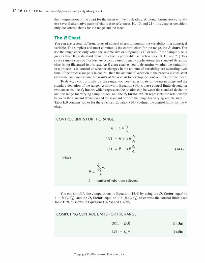
14-16 CHAPTER 14 Statistical Applications in Quality Management
Copyright © 2016 Pearson Education, Inc.
the interpretation of the chart for the mean will be misleading. Although businesses currently use several alternative pairs of charts (see references 10, 15, and 21), this chapter considers only the control charts for the range and the mean.
The R chartYou can use several different types of control charts to monitor the variability in a numerical variable. The simplest and most common is the control chart for the range, the R chart. You use the range chart only when the sample size or subgroup is 10 or less. If the sample size is greater than 10, a standard deviation chart is preferable (see references 10, 15, and 21). Be-cause sample sizes of 5 or less are typically used in many applications, the standard deviation chart is not illustrated in this text. An R chart enables you to determine whether the variability in a process is in control or whether changes in the amount of variability are occurring over time. If the process range is in control, then the amount of variation in the process is consistent over time, and you can use the results of the R chart to develop the control limits for the mean.
To develop control limits for the range, you need an estimate of the mean range and the standard deviation of the range. As shown in Equation (14.4), these control limits depend on two constants, the d2 factor, which represents the relationship between the standard deviation and the range for varying sample sizes, and the d3 factor, which represents the relationship between the standard deviation and the standard error of the range for varying sample sizes.Table E.9 contains values for these factors. Equation (14.4) defines the control limits for the R chart.
COnTROL LiMiTS fOR ThE RAngE
R { 3 R d3
d2
UCL = R + 3 R d3
d2
LCL = R - 3 R d3
d2 (14.4)
where
R =a
k
i= 1 Ri
k
k = number of subgroups selected
You can simplify the computations in Equation (14.4) by using the D3 factor, equal to 1 - 31d3>d22, and the D4 factor, equal to 1 + 31d3>d22, to express the control limits (see Table E.9), as shown in Equations (14.5a) and (14.5b).
COMPUTing COnTROL LiMiTS fOR ThE RAngE
UCL = D4R (14.5a)
LCL = D3R (14.5b)
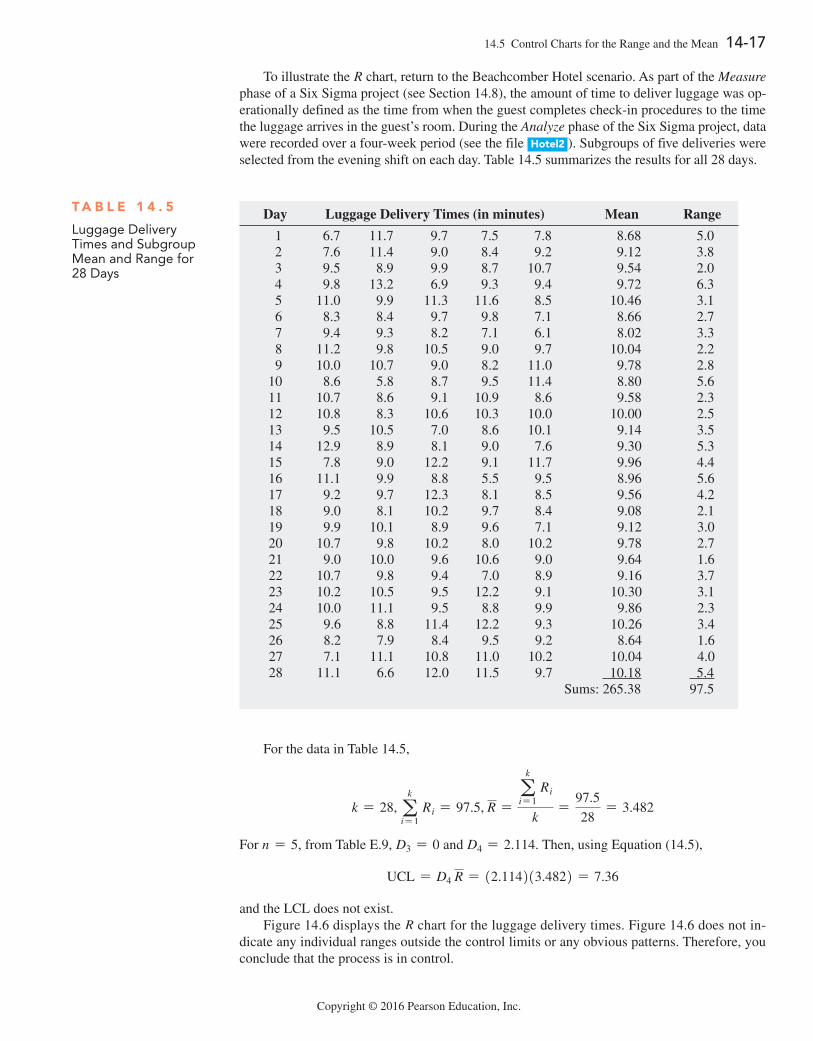
14.5 Control Charts for the Range and the Mean 14-17
Copyright © 2016 Pearson Education, Inc.
To illustrate the R chart, return to the Beachcomber Hotel scenario. As part of the Measure phase of a Six Sigma project (see Section 14.8), the amount of time to deliver luggage was op-erationally defined as the time from when the guest completes check-in procedures to the time the luggage arrives in the guest’s room. During the Analyze phase of the Six Sigma project, data were recorded over a four-week period (see the file Hotel2 ). Subgroups of five deliveries were selected from the evening shift on each day. Table 14.5 summarizes the results for all 28 days.
T a b l e 1 4 . 5
Luggage Delivery Times and Subgroup Mean and Range for 28 Days
Day Luggage Delivery Times (in minutes) Mean Range
1 6.7 11.7 9.7 7.5 7.8 8.68 5.02 7.6 11.4 9.0 8.4 9.2 9.12 3.83 9.5 8.9 9.9 8.7 10.7 9.54 2.04 9.8 13.2 6.9 9.3 9.4 9.72 6.35 11.0 9.9 11.3 11.6 8.5 10.46 3.16 8.3 8.4 9.7 9.8 7.1 8.66 2.77 9.4 9.3 8.2 7.1 6.1 8.02 3.38 11.2 9.8 10.5 9.0 9.7 10.04 2.29 10.0 10.7 9.0 8.2 11.0 9.78 2.8
10 8.6 5.8 8.7 9.5 11.4 8.80 5.611 10.7 8.6 9.1 10.9 8.6 9.58 2.312 10.8 8.3 10.6 10.3 10.0 10.00 2.513 9.5 10.5 7.0 8.6 10.1 9.14 3.514 12.9 8.9 8.1 9.0 7.6 9.30 5.315 7.8 9.0 12.2 9.1 11.7 9.96 4.416 11.1 9.9 8.8 5.5 9.5 8.96 5.617 9.2 9.7 12.3 8.1 8.5 9.56 4.218 9.0 8.1 10.2 9.7 8.4 9.08 2.119 9.9 10.1 8.9 9.6 7.1 9.12 3.020 10.7 9.8 10.2 8.0 10.2 9.78 2.721 9.0 10.0 9.6 10.6 9.0 9.64 1.622 10.7 9.8 9.4 7.0 8.9 9.16 3.723 10.2 10.5 9.5 12.2 9.1 10.30 3.124 10.0 11.1 9.5 8.8 9.9 9.86 2.325 9.6 8.8 11.4 12.2 9.3 10.26 3.426 8.2 7.9 8.4 9.5 9.2 8.64 1.627 7.1 11.1 10.8 11.0 10.2 10.04 4.028 11.1 6.6 12.0 11.5 9.7 10.18 5.4
Sums: 265.38 97.5
For the data in Table 14.5,
k = 28, ak
i= 1 Ri = 97.5, R =
ak
i= 1 Ri
k=
97.5
28= 3.482
For n = 5, from Table E.9, D3 = 0 and D4 = 2.114. Then, using Equation (14.5),
UCL = D4 R = 12.114213.4822 = 7.36
and the LCL does not exist.Figure 14.6 displays the R chart for the luggage delivery times. Figure 14.6 does not in-
dicate any individual ranges outside the control limits or any obvious patterns. Therefore, you conclude that the process is in control.
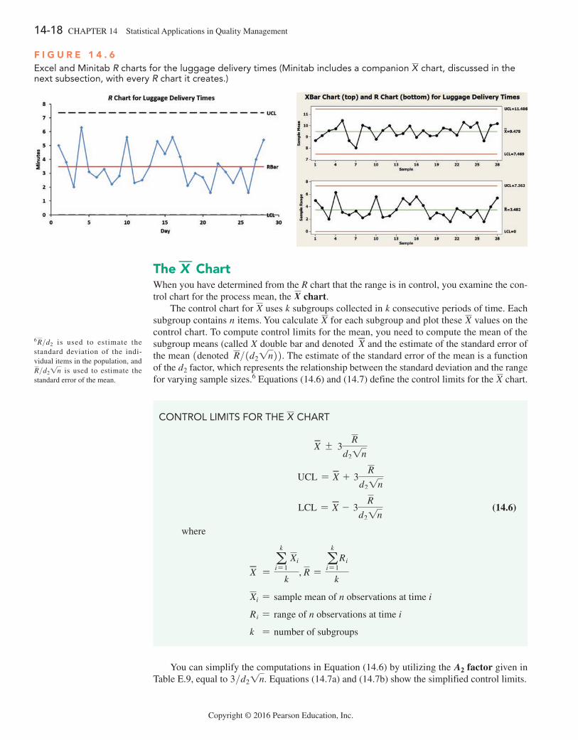
14-18 CHAPTER 14 Statistical Applications in Quality Management
Copyright © 2016 Pearson Education, Inc.
F i g u r e 1 4 . 6Excel and Minitab R charts for the luggage delivery times (Minitab includes a companion X chart, discussed in the next subsection, with every R chart it creates.)
COnTROL LiMiTS fOR ThE X ChART
X { 3R
d21n
UCL = X + 3R
d21n
LCL = X - 3R
d21n (14.6)
where
X =a
k
i= 1 Xi
k, R =
ak
i= 1Ri
k
Xi = sample mean of n observations at time i
Ri = range of n observations at time i
k = number of subgroups
The X—
chartWhen you have determined from the R chart that the range is in control, you examine the con-trol chart for the process mean, the X chart.
The control chart for X uses k subgroups collected in k consecutive periods of time. Each subgroup contains n items. You calculate X for each subgroup and plot these X values on the control chart. To compute control limits for the mean, you need to compute the mean of the subgroup means (called X double bar and denoted X and the estimate of the standard error of the mean 1denoted R>1d21n22. The estimate of the standard error of the mean is a function of the d2 factor, which represents the relationship between the standard deviation and the range for varying sample sizes.6 Equations (14.6) and (14.7) define the control limits for the X chart.
6R>d2 is used to estimate the standard deviation of the indi-vidual items in the population, and R>d21n is used to estimate the standard error of the mean.
You can simplify the computations in Equation (14.6) by utilizing the A2 factor given in Table E.9, equal to 3>d21n. Equations (14.7a) and (14.7b) show the simplified control limits.
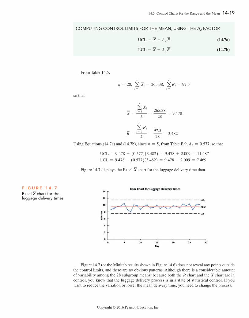
14.5 Control Charts for the Range and the Mean 14-19
Copyright © 2016 Pearson Education, Inc.
From Table 14.5,
k = 28, ak
i= 1 Xi = 265.38, a
k
i= 1Ri = 97.5
so that
X =a
k
i= 1 Xi
k=
265.38
28= 9.478
R =a
k
i= 1 Ri
k=
97.5
28= 3.482
Using Equations (14.7a) and (14.7b), since n = 5, from Table E.9, A2 = 0.577, so that
UCL = 9.478 + 10.577213.4822 = 9.478 + 2.009 = 11.487
LCL = 9.478 - 10.577213.4822 = 9.478 - 2.009 = 7.469
Figure 14.7 displays the Excel X chart for the luggage delivery time data.
COMPUTing COnTROL LiMiTS fOR ThE MEAn, USing ThE A2 fACTOR
UCL = X + A2 R (14.7a)
LCL = X - A2 R (14.7b)
F i g u r e 1 4 . 7Excel X chart for the luggage delivery times
Figure 14.7 (or the Minitab results shown in Figure 14.6) does not reveal any points outside the control limits, and there are no obvious patterns. Although there is a considerable amount of variability among the 28 subgroup means, because both the R chart and the X chart are in control, you know that the luggage delivery process is in a state of statistical control. If you want to reduce the variation or lower the mean delivery time, you need to change the process.
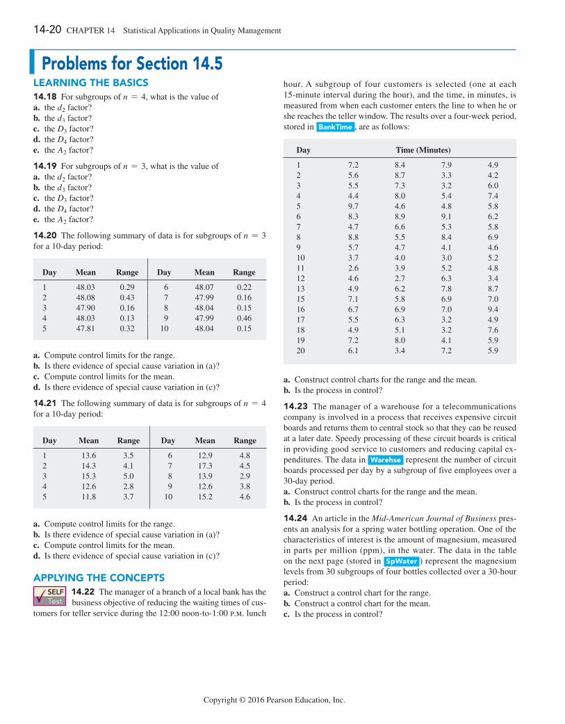
14-20 CHAPTER 14 Statistical Applications in Quality Management
Copyright © 2016 Pearson Education, Inc.
problems for Section 14.5learning THe baSicS14.18 For subgroups of n = 4, what is the value ofa. the d2 factor?b. the d3 factor?c. the D3 factor?d. the D4 factor?e. the A2 factor?
14.19 For subgroups of n = 3, what is the value ofa. the d2 factor?b. the d3 factor?c. the D3 factor?d. the D4 factor?e. the A2 factor?
14.20 The following summary of data is for subgroups of n = 3 for a 10-day period:
Day Mean Range Day Mean Range
1 48.03 0.29 6 48.07 0.222 48.08 0.43 7 47.99 0.163 47.90 0.16 8 48.04 0.154 48.03 0.13 9 47.99 0.465 47.81 0.32 10 48.04 0.15
a. Compute control limits for the range.b. Is there evidence of special cause variation in (a)?c. Compute control limits for the mean.d. Is there evidence of special cause variation in (c)?
14.21 The following summary of data is for subgroups of n = 4 for a 10-day period:
Day Mean Range Day Mean Range
1 13.6 3.5 6 12.9 4.82 14.3 4.1 7 17.3 4.53 15.3 5.0 8 13.9 2.94 12.6 2.8 9 12.6 3.85 11.8 3.7 10 15.2 4.6
a. Compute control limits for the range.b. Is there evidence of special cause variation in (a)?c. Compute control limits for the mean.d. Is there evidence of special cause variation in (c)?
applying THe concepTSSELF Test
14.22 The manager of a branch of a local bank has the business objective of reducing the waiting times of cus-
tomers for teller service during the 12:00 noon-to-1:00 p.m. lunch
hour. A subgroup of four customers is selected (one at each 15-minute interval during the hour), and the time, in minutes, is measured from when each customer enters the line to when he or she reaches the teller window. The results over a four-week period, stored in bankTime , are as follows:
Day Time (Minutes)
1 7.2 8.4 7.9 4.92 5.6 8.7 3.3 4.23 5.5 7.3 3.2 6.04 4.4 8.0 5.4 7.45 9.7 4.6 4.8 5.86 8.3 8.9 9.1 6.27 4.7 6.6 5.3 5.88 8.8 5.5 8.4 6.99 5.7 4.7 4.1 4.610 3.7 4.0 3.0 5.211 2.6 3.9 5.2 4.812 4.6 2.7 6.3 3.413 4.9 6.2 7.8 8.715 7.1 5.8 6.9 7.016 6.7 6.9 7.0 9.417 5.5 6.3 3.2 4.918 4.9 5.1 3.2 7.619 7.2 8.0 4.1 5.920 6.1 3.4 7.2 5.9
a. Construct control charts for the range and the mean.b. Is the process in control?
14.23 The manager of a warehouse for a telecommunications company is involved in a process that receives expensive circuit boards and returns them to central stock so that they can be reused at a later date. Speedy processing of these circuit boards is critical in providing good service to customers and reducing capital ex-penditures. The data in Warehse represent the number of circuit boards processed per day by a subgroup of five employees over a 30-day period.a. Construct control charts for the range and the mean.b. Is the process in control?
14.24 An article in the Mid-American Journal of Business pres-ents an analysis for a spring water bottling operation. One of the characteristics of interest is the amount of magnesium, measured in parts per million (ppm), in the water. The data in the table on the next page (stored in SpWater ) represent the magnesium levels from 30 subgroups of four bottles collected over a 30-hour period:a. Construct a control chart for the range.b. Construct a control chart for the mean.c. Is the process in control?
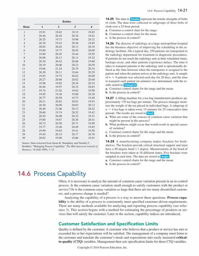
14.6 Process Capability 14-21
Copyright © 2016 Pearson Education, Inc.
Bottles
Hour 1 2 3 4
1 19.91 19.62 19.15 19.85 2 20.46 20.44 20.34 19.61 3 20.25 19.73 19.98 20.32 4 20.39 19.43 20.36 19.85 5 20.02 20.02 20.13 20.34 6 19.89 19.77 20.92 20.09 7 19.89 20.45 19.44 19.95 8 20.08 20.13 20.11 19.32 9 20.30 20.42 20.68 19.6010 20.19 20.00 20.23 20.5911 19.66 21.24 20.35 20.3412 20.30 20.11 19.64 20.2913 19.83 19.75 20.62 20.6014 20.27 20.88 20.62 20.4015 19.98 19.02 20.34 20.3416 20.46 19.97 20.32 20.8317 19.74 21.02 19.62 19.9018 19.85 19.26 19.88 20.2019 20.77 20.58 19.73 19.4820 20.21 20.82 20.01 19.9321 20.30 20.09 20.03 20.1322 20.48 21.06 20.13 20.4223 20.60 19.74 20.52 19.4224 20.20 20.08 20.32 19.5125 19.66 19.67 20.26 20.4126 20.72 20.58 20.71 19.9927 19.77 19.40 20.49 19.8328 19.99 19.65 19.41 19.5829 19.44 20.15 20.17 20.7630 20.03 19.96 19.86 19.91
Source: Data extracted from Susan K. Humphrey and Timothy C. Krehbiel, “Managing Process Capability,” The Mid-American Journal of Business, 14 (Fall 1999), 7–12.
14.25 The data in Tensile represent the tensile strengths of bolts of cloth. The data were collected in subgroups of three bolts of cloth over a 25-hour period.a. Construct a control chart for the range.b. Construct a control chart for the mean.c. Is the process in control?
14.26 The director of radiology at a large metropolitan hospital has the business objective of improving the scheduling in the ra-diology facilities. On a typical day, 250 patients are transported to the radiology department for treatment or diagnostic procedures. If patients do not reach the radiology unit at their scheduled times, backups occur, and other patients experience delays. The time it takes to transport patients to the radiology unit is operationally de-fined as the time between when the transporter is assigned to the patient and when the patient arrives at the radiology unit. A sample of n = 4 patients was selected each day for 20 days, and the time to transport each patient (in minutes) was determined, with the re-sults stored in Transport .a. Construct control charts for the range and the mean.b. Is the process in control?
14.27 A filling machine for a tea bag manufacturer produces ap-proximately 170 tea bags per minute. The process manager moni-tors the weight of the tea placed in individual bags. A subgroup of n = 4 tea bags is taken every 15 minutes for 25 consecutive time periods. The results are stored in Tea3 .a. What are some of the sources of common cause variation that
might be present in this process?b. What problems might occur that would result in special causes
of variation?c. Construct control charts for the range and the mean.d. Is the process in control?
14.28 A manufacturing company makes brackets for book-shelves. The brackets provide critical structural support and must have a 90-degree bend{1 degree. Measurements of the bend of the brackets were taken at 18 different times. Five brackets were sampled at each time. The data are stored in angle .a. Construct control charts for the range and the mean.b. Is the process in control?
14.6 Process CapabilityOften, it is necessary to analyze the amount of common cause variation present in an in-control process. Is the common cause variation small enough to satisfy customers with the product or service? Or is the common cause variation so large that there are too many dissatisfied custom-ers, and a process change is needed?
Analyzing the capability of a process is a way to answer these questions. Process capa-bility is the ability of a process to consistently meet specified customer-driven requirements. There are many methods available for analyzing and reporting process capability (see refer-ence 3). This section begins with a method for estimating the percentage of products or ser-vices that will satisfy the customer. Later in the section, capability indices are introduced.
customer Satisfaction and Specification limitsQuality is defined by the customer. A customer who believes that a product or service has met or exceeded his or her expectations will be satisfied. The management of a company must listen to the customer and translate the customer’s needs and expectations into easily measured critical-to-quality (CTQ) variables. Management then sets specification limits for these CTQ variables.
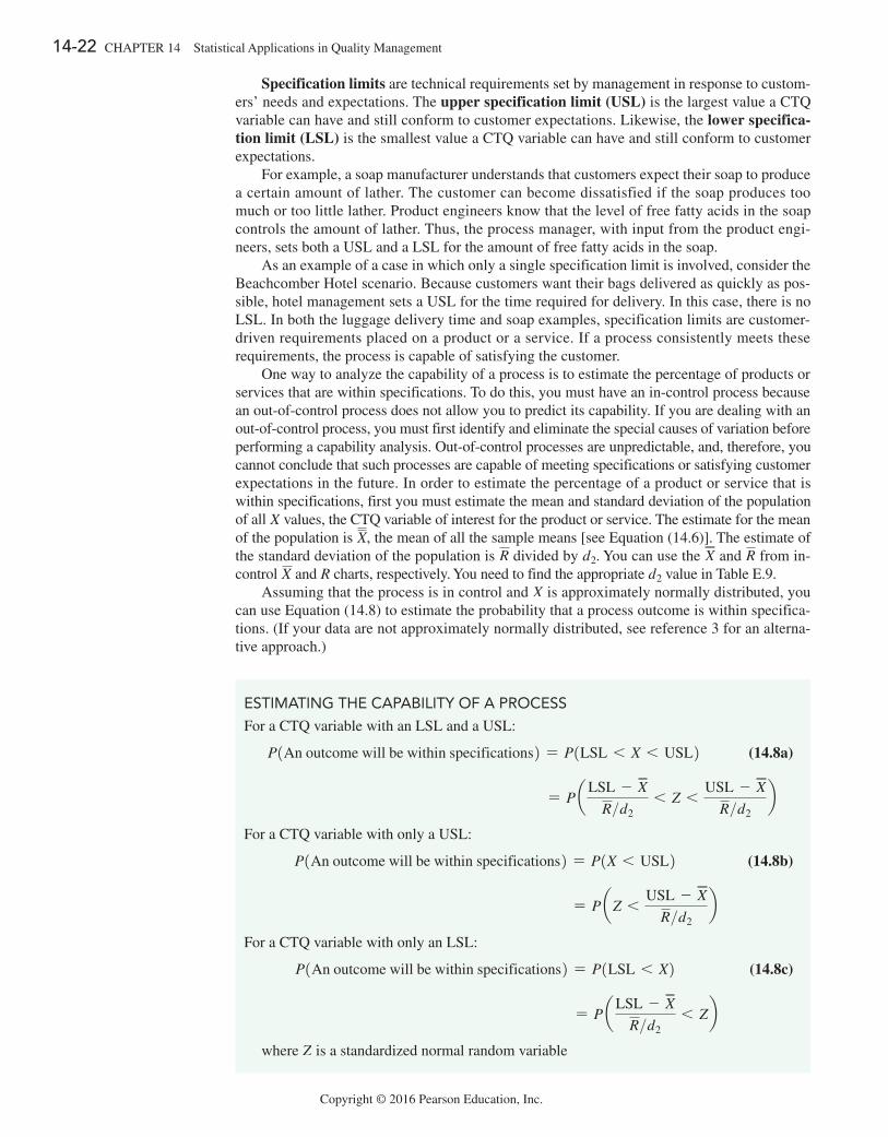
14-22 CHAPTER 14 Statistical Applications in Quality Management
Copyright © 2016 Pearson Education, Inc.
Specification limits are technical requirements set by management in response to custom-ers’ needs and expectations. The upper specification limit (USL) is the largest value a CTQ variable can have and still conform to customer expectations. Likewise, the lower specifica-tion limit (LSL) is the smallest value a CTQ variable can have and still conform to customer expectations.
For example, a soap manufacturer understands that customers expect their soap to produce a certain amount of lather. The customer can become dissatisfied if the soap produces too much or too little lather. Product engineers know that the level of free fatty acids in the soap controls the amount of lather. Thus, the process manager, with input from the product engi-neers, sets both a USL and a LSL for the amount of free fatty acids in the soap.
As an example of a case in which only a single specification limit is involved, consider the Beachcomber Hotel scenario. Because customers want their bags delivered as quickly as pos-sible, hotel management sets a USL for the time required for delivery. In this case, there is no LSL. In both the luggage delivery time and soap examples, specification limits are customer-driven requirements placed on a product or a service. If a process consistently meets these requirements, the process is capable of satisfying the customer.
One way to analyze the capability of a process is to estimate the percentage of products or services that are within specifications. To do this, you must have an in-control process because an out-of-control process does not allow you to predict its capability. If you are dealing with an out-of-control process, you must first identify and eliminate the special causes of variation before performing a capability analysis. Out-of-control processes are unpredictable, and, therefore, you cannot conclude that such processes are capable of meeting specifications or satisfying customer expectations in the future. In order to estimate the percentage of a product or service that is within specifications, first you must estimate the mean and standard deviation of the population of all X values, the CTQ variable of interest for the product or service. The estimate for the mean of the population is X, the mean of all the sample means [see Equation (14.6)]. The estimate of the standard deviation of the population is R divided by d2. You can use the X and R from in-control X and R charts, respectively. You need to find the appropriate d2 value in Table E.9.
Assuming that the process is in control and X is approximately normally distributed, you can use Equation (14.8) to estimate the probability that a process outcome is within specifica-tions. (If your data are not approximately normally distributed, see reference 3 for an alterna-tive approach.)
ESTiMATing ThE CAPABiLiTy Of A PROCESS
For a CTQ variable with an LSL and a USL:
P1An outcome will be within specifications2 = P1LSL 6 X 6 USL2 (14.8a)
= P aLSL - X
R>d26 Z 6
USL - X
R>d2b
For a CTQ variable with only a USL:
P1An outcome will be within specifications2 = P1X 6 USL2 (14.8b)
= P aZ 6USL - X
R>d2b
For a CTQ variable with only an LSL:
P1An outcome will be within specifications2 = P1LSL 6 X2 (14.8c)
= P aLSL - X
R>d26 Zb
where Z is a standardized normal random variable
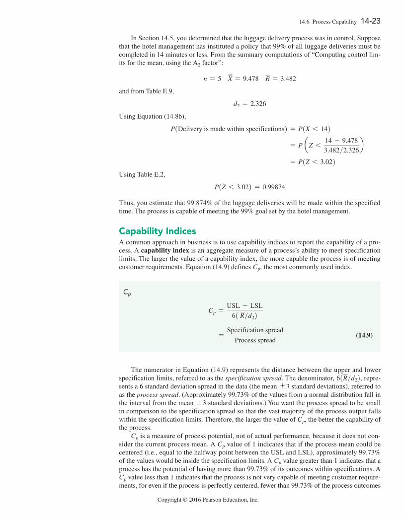
14.6 Process Capability 14-23
Copyright © 2016 Pearson Education, Inc.
In Section 14.5, you determined that the luggage delivery process was in control. Suppose that the hotel management has instituted a policy that 99% of all luggage deliveries must be completed in 14 minutes or less. From the summary computations of “Computing control lim-its for the mean, using the A2 factor”:
n = 5 X = 9.478 R = 3.482
and from Table E.9,
d2 = 2.326
Using Equation (14.8b),
P1Delivery is made within specifications2 = P1X 6 142
= P aZ 614 - 9.478
3.482>2.326b
= P1Z 6 3.022Using Table E.2,
P1Z 6 3.022 = 0.99874
Thus, you estimate that 99.874% of the luggage deliveries will be made within the specified time. The process is capable of meeting the 99% goal set by the hotel management.
capability indicesA common approach in business is to use capability indices to report the capability of a pro-cess. A capability index is an aggregate measure of a process’s ability to meet specification limits. The larger the value of a capability index, the more capable the process is of meeting customer requirements. Equation (14.9) defines Cp, the most commonly used index.
Cp
Cp =USL - LSL
61 R>d22
=Specification spread
Process spread (14.9)
The numerator in Equation (14.9) represents the distance between the upper and lower specification limits, referred to as the specification spread. The denominator, 61R>d22, repre-sents a 6 standard deviation spread in the data (the mean {3 standard deviations), referred to as the process spread. (Approximately 99.73% of the values from a normal distribution fall in the interval from the mean {3 standard deviations.) You want the process spread to be small in comparison to the specification spread so that the vast majority of the process output falls within the specification limits. Therefore, the larger the value of Cp, the better the capability of the process.
Cp is a measure of process potential, not of actual performance, because it does not con-sider the current process mean. A Cp value of 1 indicates that if the process mean could be centered (i.e., equal to the halfway point between the USL and LSL), approximately 99.73% of the values would be inside the specification limits. A Cp value greater than 1 indicates that a process has the potential of having more than 99.73% of its outcomes within specifications. A Cp value less than 1 indicates that the process is not very capable of meeting customer require-ments, for even if the process is perfectly centered, fewer than 99.73% of the process outcomes
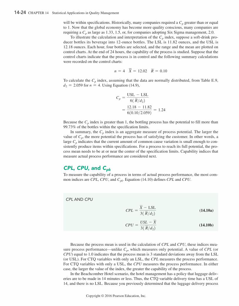
14-24 CHAPTER 14 Statistical Applications in Quality Management
Copyright © 2016 Pearson Education, Inc.
will be within specifications. Historically, many companies required a Cp greater than or equal to 1. Now that the global economy has become more quality conscious, many companies are requiring a Cp as large as 1.33, 1.5, or, for companies adopting Six Sigma management, 2.0.
To illustrate the calculation and interpretation of the Cp index, suppose a soft-drink pro-ducer bottles its beverage into 12-ounce bottles. The LSL is 11.82 ounces, and the USL is 12.18 ounces. Each hour, four bottles are selected, and the range and the mean are plotted on control charts. At the end of 24 hours, the capability of the process is studied. Suppose that the control charts indicate that the process is in control and the following summary calculations were recorded on the control charts:
n = 4 X = 12.02 R = 0.10
To calculate the Cp index, assuming that the data are normally distributed, from Table E.9, d2 = 2.059 for n = 4. Using Equation (14.9),
Cp =USL - LSL
61 R>d22
=12.18 - 11.82
610.10>2.0592 = 1.24
Because the Cp index is greater than 1, the bottling process has the potential to fill more than 99.73% of the bottles within the specification limits.
In summary, the Cp index is an aggregate measure of process potential. The larger the value of Cp, the more potential the process has of satisfying the customer. In other words, a large Cp indicates that the current amount of common cause variation is small enough to con-sistently produce items within specifications. For a process to reach its full potential, the pro-cess mean needs to be at or near the center of the specification limits. Capability indices that measure actual process performance are considered next.
CPL, CPU, and CpkTo measure the capability of a process in terms of actual process performance, the most com-mon indices are CPL, CPU, and Cpk. Equation (14.10) defines CPL and CPU.
CPL AnD CPU
CPL =X - LSL
31 R>d22 (14.10a)
CPU =USL - X
31 R>d22 (14.10b)
Because the process mean is used in the calculation of CPL and CPU, these indices mea-sure process performance—unlike Cp, which measures only potential. A value of CPL (or CPU) equal to 1.0 indicates that the process mean is 3 standard deviations away from the LSL (or USL). For CTQ variables with only an LSL, the CPL measures the process performance. For CTQ variables with only a USL, the CPU measures the process performance. In either case, the larger the value of the index, the greater the capability of the process.
In the Beachcomber Hotel scenario, the hotel management has a policy that luggage deliv-eries are to be made in 14 minutes or less. Thus, the CTQ variable delivery time has a USL of 14, and there is no LSL. Because you previously determined that the luggage delivery process
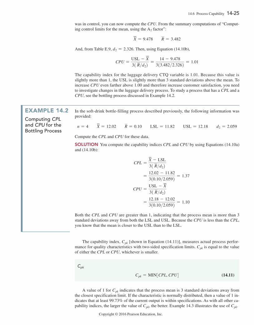
14.6 Process Capability 14-25
Copyright © 2016 Pearson Education, Inc.
was in control, you can now compute the CPU. From the summary computations of “Comput-ing control limits for the mean, using the A2 factor”:
X = 9.478 R = 3.482
And, from Table E.9, d2 = 2.326. Then, using Equation (14.10b),
CPU =USL - X
31 R>d22=
14 - 9.478
313.482>2.3262 = 1.01
The capability index for the luggage delivery CTQ variable is 1.01. Because this value is slightly more than 1, the USL is slightly more than 3 standard deviations above the mean. To increase CPU even farther above 1.00 and therefore increase customer satisfaction, you need to investigate changes in the luggage delivery process. To study a process that has a CPL and a CPU, see the bottling process discussed in Example 14.2.
example 14.2computing CPL and CPU for the Bottling process
In the soft-drink bottle-filling process described previously, the following information was provided:
n = 4 X = 12.02 R = 0.10 LSL = 11.82 USL = 12.18 d2 = 2.059
Compute the CPL and CPU for these data.
SoluTion You compute the capability indices CPL and CPU by using Equations (14.10a) and (14.10b):
CPL =X - LSL
31 R>d22
=12.02 - 11.82
310.10>2.0592 = 1.37
CPU =USL - X
31 R>d22
=12.18 - 12.02
310.10>2.0592 = 1.10
Both the CPL and CPU are greater than 1, indicating that the process mean is more than 3 standard deviations away from both the LSL and USL. Because the CPU is less than the CPL, you know that the mean is closer to the USL than to the LSL.
The capability index, Cpk [shown in Equation (14.11)], measures actual process perfor-mance for quality characteristics with two-sided specification limits. Cpk is equal to the value of either the CPL or CPU, whichever is smaller.
Cpk
Cpk = MIN3CPL, CPU4 (14.11)
A value of 1 for Cpk indicates that the process mean is 3 standard deviations away from the closest specification limit. If the characteristic is normally distributed, then a value of 1 in-dicates that at least 99.73% of the current output is within specifications. As with all other ca-pability indices, the larger the value of Cpk, the better. Example 14.3 illustrates the use of Cpk.
14-26 CHAPTER 14 Statistical Applications in Quality Management
Copyright © 2016 Pearson Education, Inc.
example 14.3computing Cpk for the Bottling process
The soft-drink producer in Example 14.2 requires the bottle filling process to have a Cpk greater than or equal to 1. Calculate the Cpk index.
SoluTion In Example 14.2, CPL = 1.37 and CPU = 1.10. Using Equation (14.11):
Cpk = MIN3CPL, CPU4 = MIN31.37, 1.104 = 1.10
The Cpk index is greater than 1, indicating that the actual process performance exceeds the company’s requirement. More than 99.73% of the bottles contain between 11.82 and 12.18 ounces.
problems for Section 14.6learning THe baSicS14.29 For an in-control process with subgroup data n = 4, X = 20, and R = 2, find the estimate ofa. the population mean of all X values.b. the population standard deviation of all X values.
14.30 For an in-control process with subgroup data n = 3, X = 100, and R = 3.386, compute the percentage of out-comes within specifications ifa. LSL = 98 and USL = 102.b. LSL = 93 and USL = 107.5.c. LSL = 93.8 and there is no USL.d. USL = 110 and there is no LSL.
14.31 For an in-control process with subgroup data n = 3, X = 100, and R = 3.386, compute the Cp, CPL, CPU, and Cpk ifa. LSL = 98 and USL = 102.b. LSL = 93 and USL = 107.5.
applying THe concepTS14.32 Referring to the data of Problem 14.24, stored in SpWater , the researchers stated, “Some of the benefits of a capable process are increased customer satisfaction, increased operating efficien-cies, and reduced costs.” To illustrate this point, the authors pre-sented a capability analysis for a spring water bottling operation. One of the CTQ variables is the amount of magnesium, measured in parts per million (ppm), in the water. The LSL and USL for the level of magnesium in a bottle are 18 ppm and 22 ppm, respec-tively.a. Estimate the percentage of bottles that are within specifica-
tions.b. Compute the Cp, CPL, CPU, and Cpk.
14.33 Refer to the data in Problem 14.25 concerning the tensile strengths of bolts of cloth (stored in Tensile ). There is no USL for tensile strength, and the LSL is 13.a. Estimate the percentage of bolts that are within specifications.b. Calculate the Cpk and CPL.
14.34 Refer to Problem 14.27 concerning a filling machine for a tea bag manufacturer (data stored in Tea3 ). In that problem, you should have concluded that the process is in control. The label weight for this product is 5.5 grams, the LSL is 5.2 grams, and the USL is 5.8 grams. Company policy states that at least 99% of the tea bags produced must be inside the specifications in order for the process to be considered capable.a. Estimate the percentage of the tea bags that are inside the spec-
ification limits. Is the process capable of meeting the company policy?
b. If management implemented a new policy stating that 99.7% of all tea bags are required to be within the specifications, is this process capable of reaching that goal? Explain.
14.35 Refer to Problem 14.22 concerning waiting time for cus-tomers at a bank (data stored in bankTime ). Suppose management has set a USL of five minutes on waiting time and specified that at least 99% of the waiting times must be less than five minutes in order for the process to be considered capable.a. Estimate the percentage of the waiting times that are inside the
specification limits. Is the process capable of meeting the com-pany policy?
b. If management implemented a new policy, stating that 99.7% of all waiting times are required to be within specifications, is this process capable of reaching that goal? Explain.
14.7 Total Quality ManagementAn increased interest in improving the quality of products and services in the United States oc-curred as a reaction to improvements of Japanese industry that began as early as 1950. Individuals such as W. Edwards Deming, Joseph Juran, and Kaoru Ishikawa developed an approach that focuses on continuous improvement of products and services through an increased emphasis

14.7 Total Quality Management 14-27
Copyright © 2016 Pearson Education, Inc.
on statistics, process improvement, and optimization of the total system. This approach, widely known as total quality management (TQM), is characterized by these themes:
• The primary focus is on process improvement. • Most of the variation in a process is due to the system and not the individual. • Teamwork is an integral part of a quality management organization. • Customer satisfaction is a primary organizational goal. • Organizational transformation must occur in order to implement quality management. • Fear must be removed from organizations. • Higher quality costs less, not more, but requires an investment in training.
In the 1980s, the federal government of the United States increased its efforts to encour-age the improvement of quality in American business. Congress passed the Malcolm Baldrige National Improvement Act of 1987 and began awarding the Malcolm Baldrige Award to com-panies making the greatest strides in improving quality and customer satisfaction. Deming became a prominent consultant to many Fortune 500 companies, including Ford and Procter & Gamble. Many companies adopted some or all the basic themes of TQM.
Today, quality improvement systems have been implemented in many organizations world-wide. Although most organizations no longer use the name TQM, the underlying philosophy and statistical methods used in today’s quality improvement systems are consistent with TQM, as reflected by Deming’s 14 points for management:
1. Create constancy of purpose for improvement of product and service. 2. Adopt the new philosophy. 3. Cease dependence on inspection to achieve quality. 4. End the practice of awarding business on the basis of price tag alone. Instead, minimize
total cost by working with a single supplier. 5. Improve constantly and forever every process for planning, production, and service. 6. Institute training on the job. 7. Adopt and institute leadership. 8. Drive out fear. 9. Break down barriers between staff areas. 10. Eliminate slogans, exhortations, and targets for the workforce. 11. Eliminate numerical quotas for the workforce and numerical goals for management. 12. Remove barriers that rob people of pride of workmanship. Eliminate the annual rating
or merit system. 13. Institute a vigorous program of education and self-improvement for everyone. 14. Put everyone in the company to work to accomplish the transformation.
Points 1, 2, 5, 7, and 14 focus on the need for organizational transformation and the re-sponsibility of top management to assert leadership in committing to the transformation. With-out this commitment, any improvements obtained will be limited.
One aspect of the improvement process is illustrated by the Shewhart–Deming cycle, shown in Figure 14.8. The Shewhart–Deming cycle represents a continuous cycle of “plan, do, study, and act.” The first step, planning, represents the initial design phase for planning a change in a manufacturing or service process. This step involves teamwork among individuals from dif-ferent areas within an organization. The second step, doing, involves implementing the change, preferably on a small scale. The third step, studying, involves analyzing the results, using statis-tical methods to determine what was learned. The fourth step, acting, involves the acceptance of the change, its abandonment, or further study of the change under different conditions.
Act
DoStudy
Plan
F i g u r e 1 4 . 8Shewhart–Deming cycle

14-28 CHAPTER 14 Statistical Applications in Quality Management
Copyright © 2016 Pearson Education, Inc.
Point 3, cease dependence on inspection to achieve quality, implies that any inspection whose purpose is to improve quality is too late because the quality is already built into the product. It is better to focus on making it right the first time. Among the difficulties involved in inspection (besides high costs) are the failure of inspectors to agree on the operational defini-tions for nonconforming items and the problem of separating good and bad items. The follow-ing example illustrates the difficulties inspectors face.
Suppose your job involves proofreading the sentence in Figure 14.9, with the objective of counting the number of occurrences of the letter F. Perform this task and record the number of occurrences of the letter F that you discover.
People usually see either three Fs or six Fs. The correct number is six Fs. The number you see depends on the method you use to examine the sentence. You are likely to find three Fs if you read the sentence phonetically and six Fs if you count the number of Fs carefully. If such a simple process as counting Fs leads to inconsistency of inspectors’ results, what will happen when a much more complicated process fails to provide clear operational definitions?
Point 4, end the practice of awarding business on the basis of price tag alone, focuses on the idea that there is no real long-term meaning to price without knowledge of the quality of the product. In addition, minimizing the number of entities in the supply chain will reduce the variation involved.
Points 6 and 13 refer to training and reflect the needs of all employees. Continuous learn-ing is critical for quality improvement within an organization. In particular, management needs to understand the differences between special causes and common causes of variation so that proper action is taken in each circumstance.
Points 8 through 12 relate to the evaluation of employee performance. Deming believed that an emphasis on targets and exhortations places an improper burden on the workforce. Workers cannot produce beyond what the system allows (as illustrated in the red bead experi-ment in Section 14.3). It is management’s job to improve the system, not to raise the expecta-tions on workers beyond the system’s capability.
Although Deming’s points are thought provoking, some have criticized his approach for lacking a formal, objective accountability (see reference 14). Many managers of large organizations, used to seeing financial analyses of policy changes, need a more prescriptive approach.
F i g u r e 1 4 . 9An example of a proofreading process
Source: Adapted from w. w. Scherkenbach, The Deming Route to Quality and Productivity: Road Maps and Roadblocks (washington, DC: CEEP Press, 1987).
FINISHED FILES ARE THE RESULT OF YEARS OF SCIENTIFIC STUDY COMBINED WITH THE EXPERIENCE OF MANY YEARS
14.8 Six SigmaSix Sigma is a quality improvement system originally developed by Motorola in the mid-1980s. After seeing the huge financial successes at Motorola, GE, and other early adopters of Six Sigma, many companies worldwide have now instituted Six Sigma to improve efficiency, cut costs, eliminate defects, and reduce product variation (see references 1, 4, 13, and 20). Six Sigma offers a more prescriptive and systematic approach to process improvement than TQM. It is also distinguished from other quality improvement systems by its clear focus on achieving bottom-line results in a relatively short three- to six-month period of time.
The name Six Sigma comes from the fact that it is a managerial approach designed to create processes that result in no more than 3.4 defects per million. The Six Sigma approach assumes that processes are designed so that the upper and lower specification limits are each
14.8 Six Sigma 14-29
Copyright © 2016 Pearson Education, Inc.
six standard deviations away from the mean. Then, if the processes are monitored correctly with control charts, the worst possible scenario is for the mean to shift to within 4.5 standard deviations from the nearest specification limit. The area under the normal curve less than 4.5 standard deviations below the mean is approximately 3.4 out of 1 million. (Table E.2 reports this probability as 0.000003398.)
The Dmaic modelTo guide managers in their task of improving short-term and long-term results, Six Sigma uses a five-step process known as the DMAIC model—named for the five steps in the process:
• Define The problem is defined, along with the costs, the benefits, and the impact on the customer.
• Measure Important characteristics related to the quality of the service or product are identified and discussed. Variables measuring these characteristics are defined and called critical-to-quality (CTQ) variables. Operational definitions for all the CTQ vari-ables are then developed. In addition, the measurement procedure is verified so that it is consistent over repeated measurements.
• Analyze The root causes of why defects occur are determined, and variables in the process causing the defects are identified. Data are collected to determine benchmark values for each process variable. This analysis often uses control charts (discussed in Sections 14.2–14.5).
• Improve The importance of each process variable on the CTQ variable is studied using designed experiments. The objective is to determine the best level for each variable.
• Control The objective is to maintain the benefits for the long term by avoiding poten-tial problems that can occur when a process is changed.
The Define phase of a Six Sigma project consists of the development of a project charter, performing a SIPOC analysis, and identifying the customers for the output of the process. The development of a project charter involves forming a table of business objectives and indica-tors for all potential Six Sigma projects. Importance ratings are assigned by top management, projects are prioritized, and the most important project is selected. A SIPOC analysis is used to identify the Suppliers to the process, list the Inputs provided by the suppliers, flowchart the Process, list the process Outputs, and identify the Customers of the process. This is followed by a Voice of the Customer analysis that involves market segmentation in which different types of users of the process are identified and the circumstances of their use of the process are identified. Statistical methods used in the Define phase include tables and charts, descriptive statistics, and control charts.
In the Measure phase of a Six Sigma project, members of a team identify the CTQ vari-ables that measure important quality characteristics. Next, operational definitions of each CTQ variable are developed so that everyone will have a firm understanding of the CTQ. Then stud-ies are undertaken to ensure that there is a valid measurement system for the CTQ that is con-sistent across measurements. Finally, baseline data are collected to determine the capability and stability of the current process. Statistical methods used in the Measure phase include tables and charts, descriptive statistics, the normal distribution, the Analysis of Variance, and control charts.
The Analyze phase of a Six Sigma project focuses on the factors that affect the central ten-dency, variation, and shape of each CTQ variable. Factors are identified, and the relationships between the factors and the CTQs are analyzed. Statistical methods used in the Analyze phase include tables and charts, descriptive statistics, the Analysis of Variance, regression analysis, and control charts.
In the Improve phase of a Six Sigma project, team members carry out designed experi-ments to actively intervene in a process. The objective of the experiments is to determine the settings of the factors that will optimize the central tendency, variation, and shape of each CTQ variable. Statistical methods used in the Improve phase include tables and charts, descrip-tive statistics, regression analysis, hypothesis testing, the Analysis of Variance, and designed experiments.
14-30 CHAPTER 14 Statistical Applications in Quality Management
Copyright © 2016 Pearson Education, Inc.
The Control phase of a Six Sigma project focuses on the maintenance of improvements that have been made in the Improve phase. A risk abatement plan is developed to identify elements that can cause damage to a process. Statistical methods used in the Control phase include tables and charts, descriptive statistics, and control charts.
roles in a Six Sigma organizationSix Sigma requires that the employees of an organization have well-defined roles. The roles of senior executive (CEO or president), executive committee, champion, process owner, master black belt, black belt, and green belt are critical to Six Sigma. More importantly, everyone must be properly trained in order to successfully fulfill their roles’ tasks and responsibilities.
The role of the senior executive is critical for Six Sigma’s ultimate success. The most successful, highly publicized Six Sigma efforts have all had unwavering, clear, and committed leadership from top management. Although Six Sigma concepts and processes can be initiated at lower levels, high-level success cannot be achieved without the leadership of the senior executive.
The members of the executive committee consist of the top management of an organiza-tion. They need to operate at the same level of commitment to Six Sigma as the senior executive.
Champions take a strong sponsorship and leadership role in conducting and implement-ing Six Sigma projects. They work closely with the executive committee, the black belt as-signed to their project, and the master black belt overseeing their project. A champion should be a member of the executive committee, or at least someone who reports directly to a member of the executive committee. He or she should have enough influence to remove obstacles or provide resources without having to go higher in the organization.
A process owner is the manager of a process. He or she has responsibility for the process and has the authority to change the process on her or his signature. The process owner should be identified and involved immediately in all Six Sigma projects related to his or her own area.
A master black belt takes on a leadership role in the implementation of the Six Sigma process and as an advisor to senior executives. The master black belt must use his or her skills while working on projects that are led by black belts and green belts. A master black belt has successfully led many teams through complex Six Sigma projects. He or she is a proven change agent, leader, facilitator, and technical expert in Six Sigma.
A black belt works full time on Six Sigma projects. A black belt is mentored by a master black belt but may report to a manager for his or her tour of duty as a black belt. Ideally, a black belt works well in a team format, can manage meetings, is familiar with statistics and systems theory, and has a focus on the customer.
A green belt is an individual who works on Six Sigma projects part time (approximately 25%), either as a team member for complex projects or as a project leader for simpler projects. Most managers in a mature Six Sigma organization are green belts. Green belt certification is a critical prerequisite for advancement into upper management in a Six Sigma organization.
Research (see reference 4) indicates that more than 80% of the top 100 publicly traded companies in the United States use Six Sigma. So, you do need to be aware of the distinction between master black belt, black belt, and green belt if you are to function effectively in a Six Sigma organization.
In a Six Sigma organization, 25% to 50% of the organization will be green belts, only 6% to 12% of the organization will be black belts, and only 1% of the organization will be master black belts (reference 10). Individual companies, professional organizations such as the American Society for Quality, and universities such as the University of Miami offer certification programs for green belt, black belt, and master black belt. For more information on certification and other aspects of Six Sigma, see references 10, 11, and 15.
lean Six SigmaLean Six Sigma combines lean thinking, maximizing customer value while minimizing waste, with the application of a version of the Six Sigma DMAIC approach. In Lean Six Sigma, you need to identify the value stream of how work gets done, and how to manage, improve, and
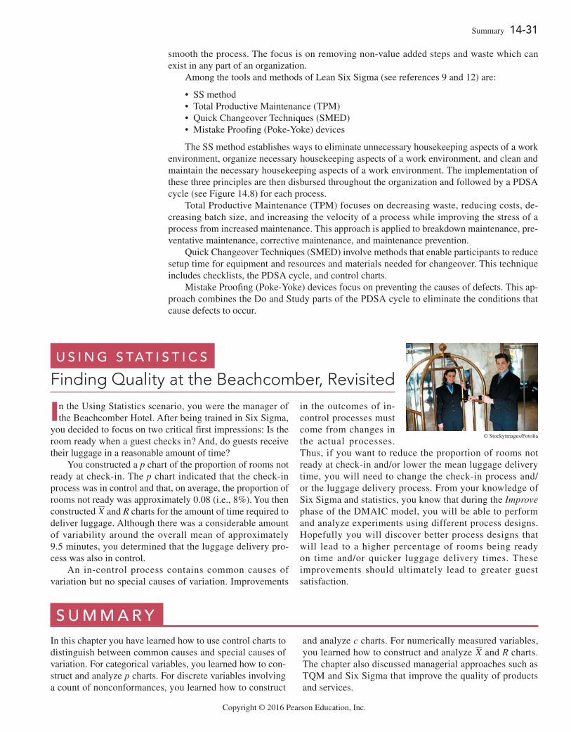
Copyright © 2016 Pearson Education, Inc.
Summary 14-31
smooth the process. The focus is on removing non-value added steps and waste which can exist in any part of an organization.
Among the tools and methods of Lean Six Sigma (see references 9 and 12) are:
• SS method • Total Productive Maintenance (TPM) • Quick Changeover Techniques (SMED) • Mistake Proofing (Poke-Yoke) devices
The SS method establishes ways to eliminate unnecessary housekeeping aspects of a work environment, organize necessary housekeeping aspects of a work environment, and clean and maintain the necessary housekeeping aspects of a work environment. The implementation of these three principles are then disbursed throughout the organization and followed by a PDSA cycle (see Figure 14.8) for each process.
Total Productive Maintenance (TPM) focuses on decreasing waste, reducing costs, de-creasing batch size, and increasing the velocity of a process while improving the stress of a process from increased maintenance. This approach is applied to breakdown maintenance, pre-ventative maintenance, corrective maintenance, and maintenance prevention.
Quick Changeover Techniques (SMED) involve methods that enable participants to reduce setup time for equipment and resources and materials needed for changeover. This technique includes checklists, the PDSA cycle, and control charts.
Mistake Proofing (Poke-Yoke) devices focus on preventing the causes of defects. This ap-proach combines the Do and Study parts of the PDSA cycle to eliminate the conditions that cause defects to occur.
In the Using Statistics scenario, you were the manager of the Beachcomber Hotel. After being trained in Six Sigma,
you decided to focus on two critical first impressions: Is the room ready when a guest checks in? And, do guests receive their luggage in a reasonable amount of time?
You constructed a p chart of the proportion of rooms not ready at check-in. The p chart indicated that the check-in process was in control and that, on average, the proportion of rooms not ready was approximately 0.08 (i.e., 8%). You then constructed X and R charts for the amount of time required to deliver luggage. Although there was a considerable amount of variability around the overall mean of approximately 9.5 minutes, you determined that the luggage delivery pro-cess was also in control.
An in-control process contains common causes of variation but no special causes of variation. Improvements
in the outcomes of in-control processes must come from changes in the actual processes. Thus, if you want to reduce the proportion of rooms not ready at check-in and/or lower the mean luggage delivery time, you will need to change the check-in process and/or the luggage delivery process. From your knowledge of Six Sigma and statistics, you know that during the Improve phase of the DMAIC model, you will be able to perform and analyze experiments using different process designs. Hopefully you will discover better process designs that will lead to a higher percentage of rooms being ready on time and/or quicker luggage delivery times. These improvements should ultimately lead to greater guest satisfaction.
U s i n g s tat i s t i c s
Finding Quality at the Beachcomber, Revisited
© Stockyimages/Fotolia
s U M M a R yIn this chapter you have learned how to use control charts to distinguish between common causes and special causes of variation. For categorical variables, you learned how to con-struct and analyze p charts. For discrete variables involving a count of nonconformances, you learned how to construct
and analyze c charts. For numerically measured variables, you learned how to construct and analyze X and R charts. The chapter also discussed managerial approaches such as TQM and Six Sigma that improve the quality of products and services.
14-32 CHAPTER 14 Statistical Applications in Quality Management
Copyright © 2016 Pearson Education, Inc.
R e F e R e n c e s 1. Arndt, M. “Quality Isn’t Just for Widgets.” Business Week,
July 22, 2002, pp. 72–73. 2. Automotive Industry Action Group (AIAG). Statistical
Process Control Reference Manual. Chrysler, Ford, and General Motors Quality and Supplier Assessment Staff, 1995.
3. Bothe, D. R. Measuring Process Capability New York: McGraw-Hill, 1997.
4. Cyger, M. “The Last Word—Riding the Bandwagon,” iSix-Sigma Magazine, November/December 2006.
5. Davis, R. B., and T. C. Krehbiel. “Shewhart and Zone Control Charts Under Linear Trend.” Communications in Statistics: Simulation and Computation, 31 (2002), 91–96.
6. Deming, W. E. The New Economics for Business, Industry, and Government. Cambridge, MA: MIT Center for Advanced Engineering Study, 1993.
7. Deming, W. E. Out of the Crisis. Cambridge, MA: MIT Center for Advanced Engineering Study, 1986.
8. Gabor, A. The Man Who Discovered Quality (New York: Time Books, 1990.
9. Gitlow, H. A Guide to Lean Six Sigma. Boca Raton, FL: CRC Press, 2009.
10. Gitlow, H., and D. Levine. Six Sigma for Green Belts and Champions. Upper Saddle River, NJ: Financial Times/Prentice Hall, 2005.
11. Gitlow, H., D. Levine, and E. Popovich. Design for Six Sigma for Green Belts and Champions. Upper Saddle River, NJ: Financial Times/Prentice Hall, 2006.
12. Gitlow, H., A. Oppenheim, R. Oppenheim, and D. Levine. Quality Management Fourth Ed. Napier, IL: Hercher Publishing, 2016.
13. Hahn, G. J., N. Doganaksoy, and R. Hoerl. “The Evolution of Six Sigma.” Quality Engineering, 12 (2000), 317–326.
14. Lemak, D. L., N. P. Mero, and R. Reed. “When Quality Works: A Premature Post-Mortem on TQM.” Journal of Business and Management, 8 (2002), 391–407.
15. Levine, D. M. Statistics for Six Sigma for Green Belts with Minitab and JMP. Upper Saddle River, NJ: Financial Times/Prentice Hall, 2006.
16. Microsoft Excel 2013. Redmond, WA: Microsoft Corp., 2012. 17. Minitab Release 16. State College, PA. Minitab Inc., 2010. 18. Scherkenbach, W. W. The Deming Route to Quality and
Productivity: Road Maps and Roadblocks. Washington, DC: CEEP Press, 1987.
19. Shewhart, W. A. Economic Control of the Quality of Manufactured Product. New York: Van Nostrand-Reinhard, 1931, reprinted by the American Society for Quality Control, Milwaukee, 1980.
20. Snee, R. D. “Impact of Six Sigma on Quality,” Quality Engineering, 12 (2000), ix–xiv.
21. Vardeman, S. B., and J. M. Jobe. Statistical Methods for Quality Assurance: Basics, Measurement, Control, Capability and Improvement. New York: Springer-Verlag, 2009.
22. Walton, M. The Deming Management Method. New York: Perigee Books, 1986.
K e y e Q U at i o n s
Constructing Control Limits
Process mean {3 standard deviations
Upper control limit 1UCL2 = process mean
+3 standard deviations
Lower control limit 1LCL2 = process mean
-3 standard deviations (14.1)
Control Limits for the p Chart
p { 3Ap11 - p2n
UCL = p + 3Ap11 - p2n
LCL = p - 3Ap11 - p2n
(14.2)
Control Limits for the c Chart
c { 31c
UCL = c + 31c
LCL = c - 31c (14.3)
Control Limits for the Range
R { 3 R d3
d2
UCL = R + 3 R d3
d2
LCL = R - 3 R d3
d2 (14.4)
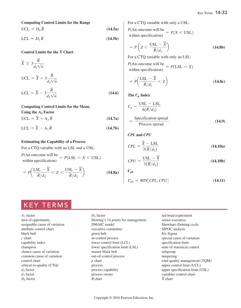
Copyright © 2016 Pearson Education, Inc.
Key Terms 14-33
Computing Control Limits for the Range
UCL = D4 R (14.5a)
LCL = D3 R (14.5b)
Control Limits for the X Chart
X { 3R
d21n
UCL = X + 3R
d21n
LCL = X - 3R
d21n (14.6)
Computing Control Limits for the Mean, Using the A2 Factor
UCL = X + A2 R (14.7a)
LCL = X - A2 R (14.7b)
Estimating the Capability of a Process
For a CTQ variable with an LSL and a USL:
P(An outcome will be
within specification)= P1LSL 6 X 6 USL2
= PaLSL - X
R>d26 Z 6
USL - X
R>d2b (14.8a)
For a CTQ variable with only a USL:
P(An outcome will be
within specification)= P1X 6 USL2
= P aZ 6USL - X
R>d2b (14.8b)
For a CTQ variable with only an LSL:
P(An outcome will be
within specification)= P1LSL 6 X2
= PaLSL - X
R>d26 Zb (14.8c)
The Cp Index
Cp =USL - LSL
61R>d22
=Specification spread
Process spread (14.9)
CPL and CPU
CPL =X - LSL
31R>d22 (14.10a)
CPU =USL - X
31R>d22 (14.10b)
Cpk
Cpk = MIN3CPL, CPU4 (14.11)
K e y t e R M sA2 factor area of opportunity assignable cause of variation attribute control chart black belt c chart capability index champion chance cause of variation common cause of variation control chart critical-to-quality (CTQ) d2 factor d3 factor D3 factor
D4 factor Deming’s 14 points for management DMAIC model executive committee green belt in-control process lower control limit (LCL) lower specification limit (LSL) master black belt out-of-control process p chart process process capability process owner R chart
red bead experiment senior executive Shewhart–Deming cycle SIPOC analysis Six Sigma special cause of variation specification limit state of statistical control subgroup tampering total quality management (TQM) upper control limit (UCL) upper specification limit (USL) variables control chart X chart
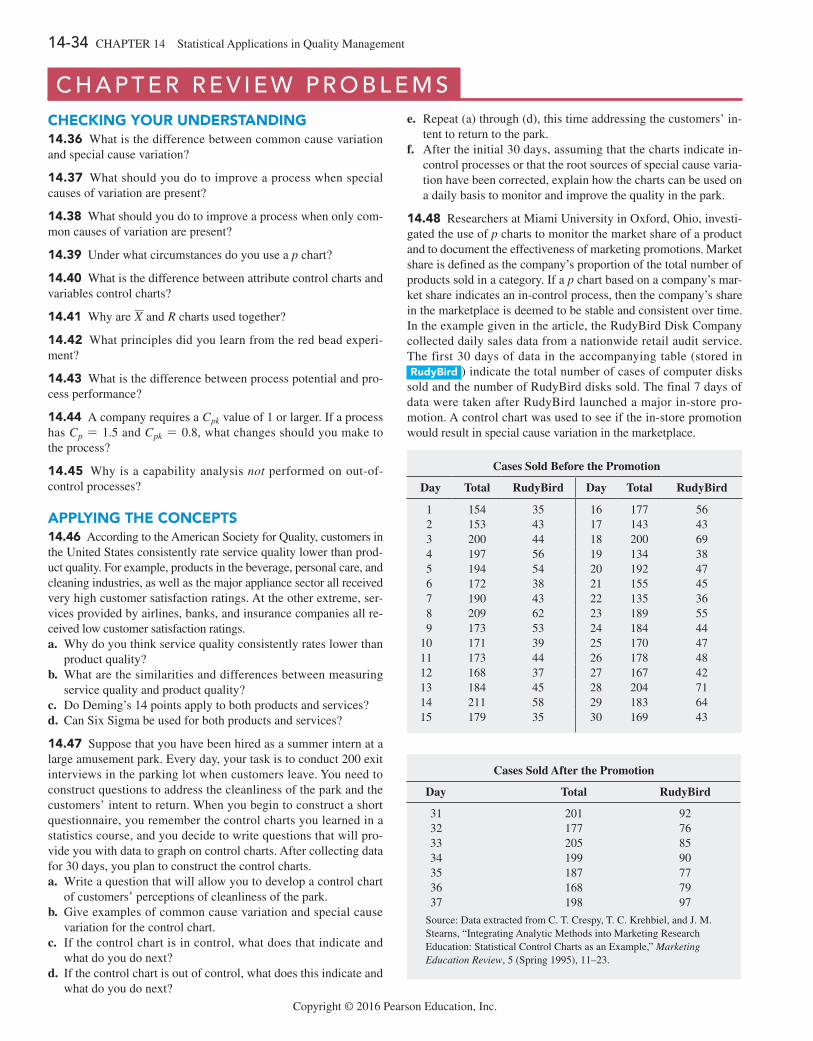
14-34 CHAPTER 14 Statistical Applications in Quality Management
Copyright © 2016 Pearson Education, Inc.
c h a p t e R R e v i e w p R o B L e M scHecking your unDerSTanDing14.36 What is the difference between common cause variation and special cause variation?
14.37 What should you do to improve a process when special causes of variation are present?
14.38 What should you do to improve a process when only com-mon causes of variation are present?
14.39 Under what circumstances do you use a p chart?
14.40 What is the difference between attribute control charts and variables control charts?
14.41 Why are X and R charts used together?
14.42 What principles did you learn from the red bead experi-ment?
14.43 What is the difference between process potential and pro-cess performance?
14.44 A company requires a Cpk value of 1 or larger. If a process has Cp = 1.5 and Cpk = 0.8, what changes should you make to the process?
14.45 Why is a capability analysis not performed on out-of- control processes?
applying THe concepTS14.46 According to the American Society for Quality, customers in the United States consistently rate service quality lower than prod-uct quality. For example, products in the beverage, personal care, and cleaning industries, as well as the major appliance sector all received very high customer satisfaction ratings. At the other extreme, ser-vices provided by airlines, banks, and insurance companies all re-ceived low customer satisfaction ratings.a. Why do you think service quality consistently rates lower than
product quality?b. What are the similarities and differences between measuring
service quality and product quality?c. Do Deming’s 14 points apply to both products and services?d. Can Six Sigma be used for both products and services?
14.47 Suppose that you have been hired as a summer intern at a large amusement park. Every day, your task is to conduct 200 exit interviews in the parking lot when customers leave. You need to construct questions to address the cleanliness of the park and the customers’ intent to return. When you begin to construct a short questionnaire, you remember the control charts you learned in a statistics course, and you decide to write questions that will pro-vide you with data to graph on control charts. After collecting data for 30 days, you plan to construct the control charts.a. Write a question that will allow you to develop a control chart
of customers’ perceptions of cleanliness of the park.b. Give examples of common cause variation and special cause
variation for the control chart.c. If the control chart is in control, what does that indicate and
what do you do next?d. If the control chart is out of control, what does this indicate and
what do you do next?
e. Repeat (a) through (d), this time addressing the customers’ in-tent to return to the park.
f. After the initial 30 days, assuming that the charts indicate in-control processes or that the root sources of special cause varia-tion have been corrected, explain how the charts can be used on a daily basis to monitor and improve the quality in the park.
14.48 Researchers at Miami University in Oxford, Ohio, investi-gated the use of p charts to monitor the market share of a product and to document the effectiveness of marketing promotions. Market share is defined as the company’s proportion of the total number of products sold in a category. If a p chart based on a company’s mar-ket share indicates an in-control process, then the company’s share in the marketplace is deemed to be stable and consistent over time. In the example given in the article, the RudyBird Disk Company collected daily sales data from a nationwide retail audit service. The first 30 days of data in the accompanying table (stored in rudybird ) indicate the total number of cases of computer disks sold and the number of RudyBird disks sold. The final 7 days of data were taken after RudyBird launched a major in-store pro-motion. A control chart was used to see if the in-store promotion would result in special cause variation in the marketplace.
Cases Sold Before the Promotion
Day Total RudyBird Day Total RudyBird
1 154 35 16 177 56 2 153 43 17 143 43 3 200 44 18 200 69 4 197 56 19 134 38 5 194 54 20 192 47 6 172 38 21 155 45 7 190 43 22 135 36 8 209 62 23 189 55 9 173 53 24 184 4410 171 39 25 170 4711 173 44 26 178 4812 168 37 27 167 4213 184 45 28 204 7114 211 58 29 183 6415 179 35 30 169 43
Cases Sold After the Promotion
Day Total RudyBird
31 201 9232 177 7633 205 8534 199 9035 187 7736 168 7937 198 97
Source: Data extracted from C. T. Crespy, T. C. Krehbiel, and J. M. Stearns, “Integrating Analytic Methods into Marketing Research Education: Statistical Control Charts as an Example,” Marketing Education Review, 5 (Spring 1995), 11–23.
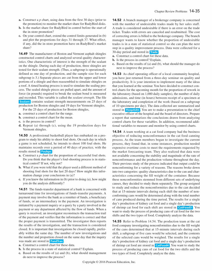
Copyright © 2016 Pearson Education, Inc.
Chapter Review Problems 14-35
a. Construct a p chart, using data from the first 30 days (prior to the promotion) to monitor the market share for RudyBird disks.
b. Is the market share for RudyBird in control before the start of the in-store promotion?
c. On your control chart, extend the control limits generated in (b) and plot the proportions for days 31 through 37. What effect, if any, did the in-store promotion have on RudyBird’s market share?
14.49 The manufacturer of Boston and Vermont asphalt shingles constructed control charts and analyzed several quality character-istics. One characteristic of interest is the strength of the sealant on the shingle. During each day of production, three shingles are tested for their sealant strength. (Thus, a subgroup is operationally defined as one day of production, and the sample size for each subgroup is 3.) Separate pieces are cut from the upper and lower portions of a shingle and then reassembled to simulate shingles on a roof. A timed heating process is used to simulate the sealing pro-cess. The sealed shingle pieces are pulled apart, and the amount of force (in pounds) required to break the sealant bond is measured and recorded. This variable is called the sealant strength. The file Sealant contains sealant strength measurements on 25 days of production for Boston shingles and 19 days for Vermont shingles. For the 25 days of production for Boston shingles,a. construct a control chart for the range.b. construct a control chart for the mean.c. is the process in control?d. Repeat (a) through (c), using the 19 production days for
Vermont shingles.
14.50 A professional basketball player has embarked on a pro-gram to study his ability to shoot foul shots. On each day in which a game is not scheduled, he intends to shoot 100 foul shots. He maintains records over a period of 40 days of practice, with the results stored in Foulspc :a. Construct a p chart for the proportion of successful foul shots.
Do you think that the player’s foul-shooting process is in statis-tical control? If not, why not?
b. What if you were told that the player used a different method of shooting foul shots for the last 20 days? How might this infor-mation change your conclusions in (a)?
c. If you knew the information in (b) prior to doing (a), how might you do the analysis differently?
14.51 The funds-transfer department of a bank is concerned with turnaround time for investigations of funds-transfer payments. A payment may involve the bank as a remitter of funds, a beneficiary of funds, or an intermediary in the payment. An investigation is initiated by a payment inquiry or a query by a party involved in the payment or any department affected by the flow of funds. When a query is received, an investigator reconstructs the transaction trail of the payment and verifies that the information is correct and that the proper payment is transmitted. The investigator then reports the results of the investigation, and the transaction is considered closed. It is important that investigations be closed rapidly, prefer-ably within the same day. The number of new investigations and the number and proportion closed on the same day that the inquiry was made are stored in FundTran .a. Construct a control chart for these data.b. Is the process in a state of statistical control? Explain.c. Based on the results of (a) and (b), what should management
do next to improve the process?
14.52 A branch manager of a brokerage company is concerned with the number of undesirable trades made by her sales staff. A trade is considered undesirable if there is an error on the trade ticket. Trades with errors are canceled and resubmitted. The cost of correcting errors is billed to the brokerage company. The branch manager wants to know whether the proportion of undesirable trades is in a state of statistical control so she can plan the next step in a quality improvement process. Data were collected for a 30-day period and stored in Trade .a. Construct a control chart for these data.b. Is the process in control? Explain.c. Based on the results of (a) and (b), what should the manager do
next to improve the process?
14.53 As chief operating officer of a local community hospital, you have just returned from a three-day seminar on quality and productivity. It is your intention to implement many of the ideas that you learned at the seminar. You have decided to construct con-trol charts for the upcoming month for the proportion of rework in the laboratory (based on 1,000 daily samples), the number of daily admissions, and time (in hours) between receipt of a specimen at the laboratory and completion of the work (based on a subgroup of 10 specimens per day). The data collected are summarized and stored in Hospadm . You are to make a presentation to the chief executive officer of the hospital and the board of directors. Prepare a report that summarizes the conclusions drawn from analyzing control charts for these variables. In addition, recommend addi-tional variables to measure and monitor by using control charts.
14.54 A team working at a cat food company had the business objective of reducing nonconformance in the cat food canning process. As the team members began to investigate the current process, they found that, in some instances, production needed expensive overtime costs to meet the requirements requested by the market forecasting team. They also realized that data were not available concerning the stability and magnitude of the rate of nonconformance and the production volume throughout the day. Their previous study of the process indicated that output could be nonconforming for a variety of reasons. The reasons broke down into two categories: quality characteristics due to the can and char-acteristics concerning the fill weight of the container. Because these nonconformities stemmed from different sets of underlying causes, they decided to study them separately. The group assigned to study and reduce the nonconformities due to the can decided that at 15-minute intervals during each shift the number of non-conforming cans would be determined along with the total number of cans produced during the time period. The results for a single day’s production of kidney cat food and a single day’s production of shrimp cat food for each shift are stored in catFood3 . You want to study the process of producing cans of cat food for the two shifts and the two types of food. Completely analyze the data.
14.55 Refer to Problem 14.54. The production team at the cat food company investigating nonconformities due to the fill weight of the cans determined that at 15-minute intervals during each shift, a subgroup of five cans would be selected, and the contents of the selected cans would be weighed. The results for a single day’s production of kidney cat food and a single day’s production of shrimp cat food are stored in catFood4 . You want to study the process of producing cans of cat food for the two shifts and the two types of food. Completely analyze the data.
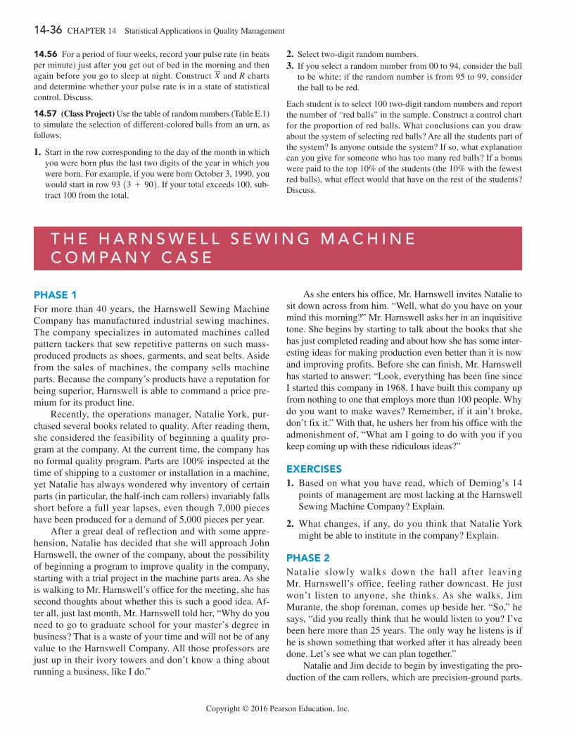
14-36 CHAPTER 14 Statistical Applications in Quality Management
Copyright © 2016 Pearson Education, Inc.
14.56 For a period of four weeks, record your pulse rate (in beats per minute) just after you get out of bed in the morning and then again before you go to sleep at night. Construct X and R charts and determine whether your pulse rate is in a state of statistical control. Discuss.
14.57 (Class Project) Use the table of random numbers (Table E.1) to simulate the selection of different-colored balls from an urn, as follows:
1. Start in the row corresponding to the day of the month in which you were born plus the last two digits of the year in which you were born. For example, if you were born October 3, 1990, you would start in row 93 13 + 902. If your total exceeds 100, sub-tract 100 from the total.
2. Select two-digit random numbers.3. If you select a random number from 00 to 94, consider the ball
to be white; if the random number is from 95 to 99, consider the ball to be red.
Each student is to select 100 two-digit random numbers and report the number of “red balls” in the sample. Construct a control chart for the proportion of red balls. What conclusions can you draw about the system of selecting red balls? Are all the students part of the system? Is anyone outside the system? If so, what explanation can you give for someone who has too many red balls? If a bonus were paid to the top 10% of the students (the 10% with the fewest red balls), what effect would that have on the rest of the students? Discuss.
t h e h a R n s w e L L s e w i n g M a c h i n e c o M pa n y c a s e
pHaSe 1For more than 40 years, the Harnswell Sewing Machine Company has manufactured industrial sewing machines. The company specializes in automated machines called pattern tackers that sew repetitive patterns on such mass-produced products as shoes, garments, and seat belts. Aside from the sales of machines, the company sells machine parts. Because the company’s products have a reputation for being superior, Harnswell is able to command a price pre-mium for its product line.
Recently, the operations manager, Natalie York, pur-chased several books related to quality. After reading them, she considered the feasibility of beginning a quality pro-gram at the company. At the current time, the company has no formal quality program. Parts are 100% inspected at the time of shipping to a customer or installation in a machine, yet Natalie has always wondered why inventory of certain parts (in particular, the half-inch cam rollers) invariably falls short before a full year lapses, even though 7,000 pieces have been produced for a demand of 5,000 pieces per year.
After a great deal of reflection and with some appre-hension, Natalie has decided that she will approach John Harnswell, the owner of the company, about the possibility of beginning a program to improve quality in the company, starting with a trial project in the machine parts area. As she is walking to Mr. Harnswell’s office for the meeting, she has second thoughts about whether this is such a good idea. Af-ter all, just last month, Mr. Harnswell told her, “Why do you need to go to graduate school for your master’s degree in business? That is a waste of your time and will not be of any value to the Harnswell Company. All those professors are just up in their ivory towers and don’t know a thing about running a business, like I do.”
As she enters his office, Mr. Harnswell invites Natalie to sit down across from him. “Well, what do you have on your mind this morning?” Mr. Harnswell asks her in an inquisitive tone. She begins by starting to talk about the books that she has just completed reading and about how she has some inter-esting ideas for making production even better than it is now and improving profits. Before she can finish, Mr. Harnswell has started to answer: “Look, everything has been fine since I started this company in 1968. I have built this company up from nothing to one that employs more than 100 people. Why do you want to make waves? Remember, if it ain’t broke, don’t fix it.” With that, he ushers her from his office with the admonishment of, “What am I going to do with you if you keep coming up with these ridiculous ideas?”
exerciSeS1. Based on what you have read, which of Deming’s 14
points of management are most lacking at the Harnswell Sewing Machine Company? Explain.
2. What changes, if any, do you think that Natalie York might be able to institute in the company? Explain.
pHaSe 2Natalie slowly walks down the hall after leaving Mr. Harnswell’s office, feeling rather downcast. He just won’t listen to anyone, she thinks. As she walks, Jim Murante, the shop foreman, comes up beside her. “So,” he says, “did you really think that he would listen to you? I’ve been here more than 25 years. The only way he listens is if he is shown something that worked after it has already been done. Let’s see what we can plan together.”
Natalie and Jim decide to begin by investigating the pro-duction of the cam rollers, which are precision-ground parts.
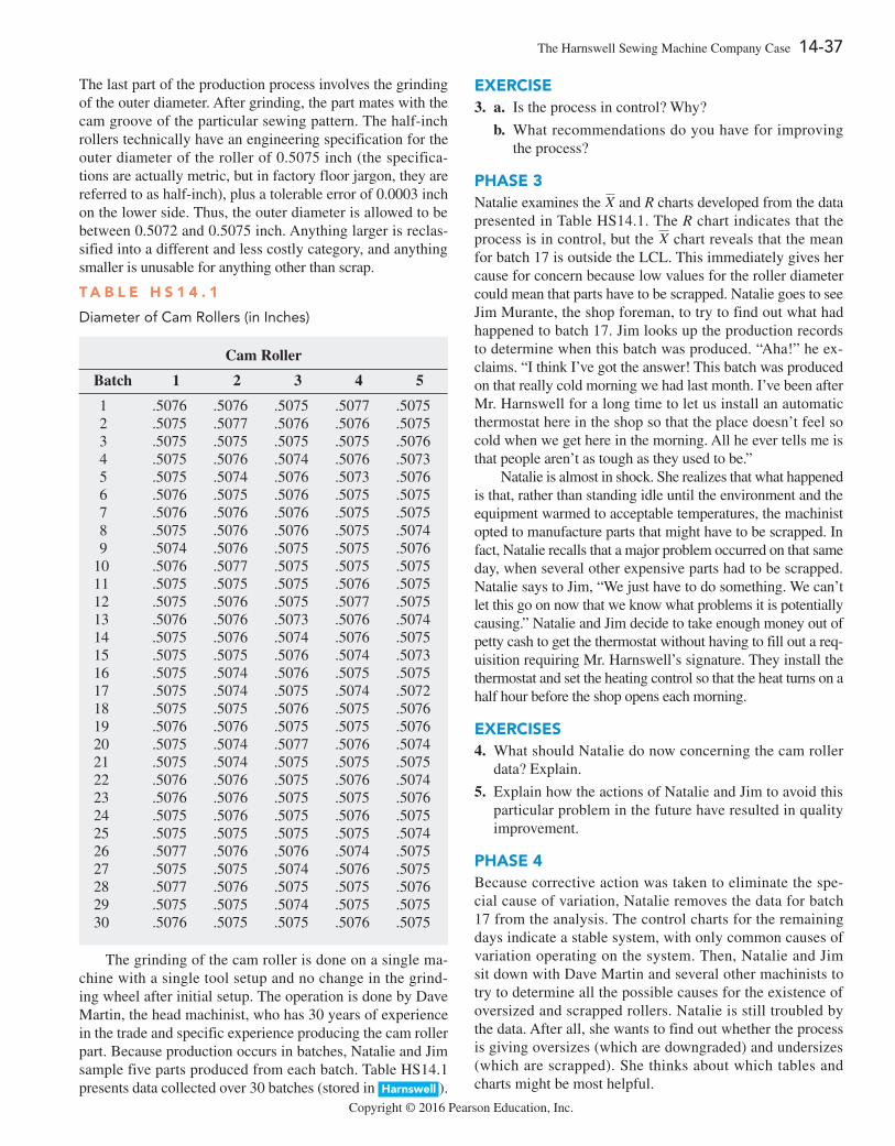
Copyright © 2016 Pearson Education, Inc.
The Harnswell Sewing Machine Company Case 14-37
The last part of the production process involves the grinding of the outer diameter. After grinding, the part mates with the cam groove of the particular sewing pattern. The half-inch rollers technically have an engineering specification for the outer diameter of the roller of 0.5075 inch (the specifica-tions are actually metric, but in factory floor jargon, they are referred to as half-inch), plus a tolerable error of 0.0003 inch on the lower side. Thus, the outer diameter is allowed to be between 0.5072 and 0.5075 inch. Anything larger is reclas-sified into a different and less costly category, and anything smaller is unusable for anything other than scrap.
T a b l e H S 1 4 . 1
Diameter of Cam Rollers (in inches)
Cam Roller
Batch 1 2 3 4 5
1 .5076 .5076 .5075 .5077 .50752 .5075 .5077 .5076 .5076 .50753 .5075 .5075 .5075 .5075 .50764 .5075 .5076 .5074 .5076 .50735 .5075 .5074 .5076 .5073 .50766 .5076 .5075 .5076 .5075 .50757 .5076 .5076 .5076 .5075 .50758 .5075 .5076 .5076 .5075 .50749 .5074 .5076 .5075 .5075 .5076
10 .5076 .5077 .5075 .5075 .507511 .5075 .5075 .5075 .5076 .507512 .5075 .5076 .5075 .5077 .507513 .5076 .5076 .5073 .5076 .507414 .5075 .5076 .5074 .5076 .507515 .5075 .5075 .5076 .5074 .507316 .5075 .5074 .5076 .5075 .507517 .5075 .5074 .5075 .5074 .507218 .5075 .5075 .5076 .5075 .507619 .5076 .5076 .5075 .5075 .507620 .5075 .5074 .5077 .5076 .507421 .5075 .5074 .5075 .5075 .507522 .5076 .5076 .5075 .5076 .507423 .5076 .5076 .5075 .5075 .507624 .5075 .5076 .5075 .5076 .507525 .5075 .5075 .5075 .5075 .507426 .5077 .5076 .5076 .5074 .507527 .5075 .5075 .5074 .5076 .507528 .5077 .5076 .5075 .5075 .507629 .5075 .5075 .5074 .5075 .507530 .5076 .5075 .5075 .5076 .5075
The grinding of the cam roller is done on a single ma-chine with a single tool setup and no change in the grind-ing wheel after initial setup. The operation is done by Dave Martin, the head machinist, who has 30 years of experience in the trade and specific experience producing the cam roller part. Because production occurs in batches, Natalie and Jim sample five parts produced from each batch. Table HS14.1 presents data collected over 30 batches (stored in Harnswell ).
exerciSe3. a. Is the process in control? Why?
b. What recommendations do you have for improving the process?
pHaSe 3Natalie examines the X and R charts developed from the data presented in Table HS14.1. The R chart indicates that the process is in control, but the X chart reveals that the mean for batch 17 is outside the LCL. This immediately gives her cause for concern because low values for the roller diameter could mean that parts have to be scrapped. Natalie goes to see Jim Murante, the shop foreman, to try to find out what had happened to batch 17. Jim looks up the production records to determine when this batch was produced. “Aha!” he ex-claims. “I think I’ve got the answer! This batch was produced on that really cold morning we had last month. I’ve been after Mr. Harnswell for a long time to let us install an automatic thermostat here in the shop so that the place doesn’t feel so cold when we get here in the morning. All he ever tells me is that people aren’t as tough as they used to be.”
Natalie is almost in shock. She realizes that what happened is that, rather than standing idle until the environment and the equipment warmed to acceptable temperatures, the machinist opted to manufacture parts that might have to be scrapped. In fact, Natalie recalls that a major problem occurred on that same day, when several other expensive parts had to be scrapped. Natalie says to Jim, “We just have to do something. We can’t let this go on now that we know what problems it is potentially causing.” Natalie and Jim decide to take enough money out of petty cash to get the thermostat without having to fill out a req-uisition requiring Mr. Harnswell’s signature. They install the thermostat and set the heating control so that the heat turns on a half hour before the shop opens each morning.
exerciSeS4. What should Natalie do now concerning the cam roller
data? Explain.
5. Explain how the actions of Natalie and Jim to avoid this particular problem in the future have resulted in quality improvement.
pHaSe 4Because corrective action was taken to eliminate the spe-cial cause of variation, Natalie removes the data for batch 17 from the analysis. The control charts for the remaining days indicate a stable system, with only common causes of variation operating on the system. Then, Natalie and Jim sit down with Dave Martin and several other machinists to try to determine all the possible causes for the existence of oversized and scrapped rollers. Natalie is still troubled by the data. After all, she wants to find out whether the process is giving oversizes (which are downgraded) and undersizes (which are scrapped). She thinks about which tables and charts might be most helpful.
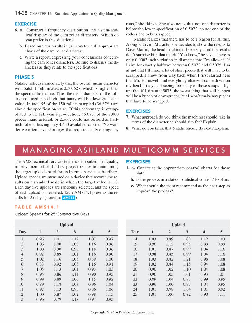
Copyright © 2016 Pearson Education, Inc.
14-38 CHAPTER 14 Statistical Applications in Quality Management
exerciSe6. a. Construct a frequency distribution and a stem-and-
leaf display of the cam roller diameters. Which do you prefer in this situation?
b. Based on your results in (a), construct all appropriate charts of the cam roller diameters.
c. Write a report, expressing your conclusions concern-ing the cam roller diameters. Be sure to discuss the di-ameters as they relate to the specifications.
pHaSe 5Natalie notices immediately that the overall mean diameter with batch 17 eliminated is 0.507527, which is higher than the specification value. Thus, the mean diameter of the roll-ers produced is so high that many will be downgraded in value. In fact, 55 of the 150 rollers sampled (36.67%) are above the specification value. If this percentage is extrap-olated to the full year’s production, 36.67% of the 7,000 pieces manufactured, or 2,567, could not be sold as half-inch rollers, leaving only 4,433 available for sale. “No won-der we often have shortages that require costly emergency
runs,” she thinks. She also notes that not one diameter is below the lower specification of 0.5072, so not one of the rollers had to be scrapped.
Natalie realizes that there has to be a reason for all this. Along with Jim Murante, she decides to show the results to Dave Martin, the head machinist. Dave says that the results don’t surprise him that much. “You know,” he says, “there is only 0.0003 inch variation in diameter that I’m allowed. If I aim for exactly halfway between 0.5072 and 0.5075, I’m afraid that I’ll make a lot of short pieces that will have to be scrapped. I know from way back when I first started here that Mr. Harnswell and everybody else will come down on my head if they start seeing too many of those scraps. I fig-ure that if I aim at 0.5075, the worst thing that will happen will be a bunch of downgrades, but I won’t make any pieces that have to be scrapped.”
exerciSeS7. What approach do you think the machinist should take in
terms of the diameter he should aim for? Explain.
8. What do you think that Natalie should do next? Explain.
M a n a g i n g a s h L a n d M U Lt i c o M M s e R v i c e sThe AMS technical services team has embarked on a quality improvement effort. Its first project relates to maintaining the target upload speed for its Internet service subscribers. Upload speeds are measured on a device that records the re-sults on a standard scale in which the target value is 1.0. Each day five uploads are randomly selected, and the speed of each upload is measured. Table AMS14.1 presents the re-sults for 25 days (stored in amS14 ).
T a b l e a m S 1 4 . 1
Upload Speeds for 25 Consecutive Days
Upload Upload
Day 1 2 3 4 5 Day 1 2 3 4 5
1 0.96 1.01 1.12 1.07 0.97 14 1.03 0.89 1.03 1.12 1.03 2 1.06 1.00 1.02 1.16 0.96 15 0.96 1.12 0.95 0.88 0.99 3 1.00 0.90 0.98 1.18 0.96 16 1.01 0.87 0.99 1.04 1.16 4 0.92 0.89 1.01 1.16 0.90 17 0.98 0.85 0.99 1.04 1.16 5 1.02 1.16 1.03 0.89 1.00 18 1.03 0.82 1.21 0.98 1.08 6 0.88 0.92 1.03 1.16 0.91 19 1.02 0.84 1.15 0.94 1.08 7 1.05 1.13 1.01 0.93 1.03 20 0.90 1.02 1.10 1.04 1.08 8 0.95 0.86 1.14 0.90 0.95 21 0.96 1.05 1.01 0.93 1.01 9 0.99 0.89 1.00 1.15 0.92 22 0.89 1.04 0.97 0.99 0.9510 0.89 1.18 1.03 0.96 1.04 23 0.96 1.00 0.97 1.04 0.9511 0.97 1.13 0.95 0.86 1.06 24 1.01 0.98 1.04 1.01 0.9212 1.00 0.87 1.02 0.98 1.13 25 1.01 1.00 0.92 0.90 1.1113 0.96 0.79 1.17 0.97 0.95
exerciSeS1. a. Construct the appropriate control charts for these
data.
b. Is the process in a state of statistical control? Explain.
c. What should the team recommend as the next step to improve the process?
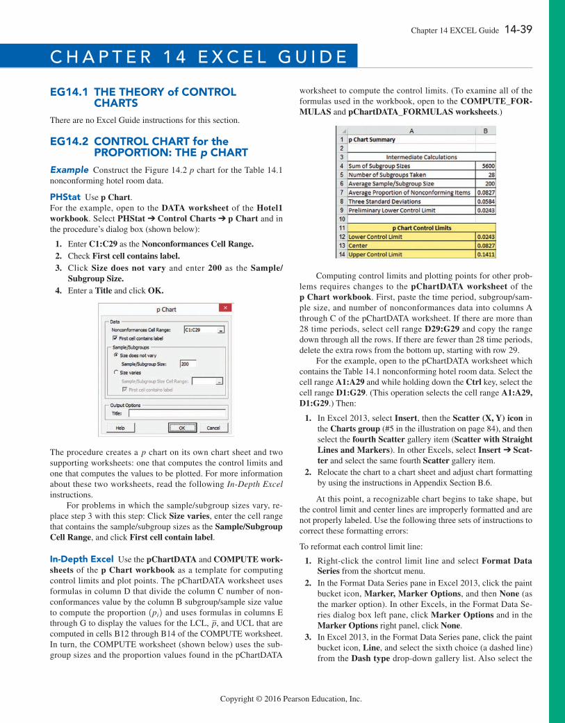
Copyright © 2016 Pearson Education, Inc.
Chapter 14 ExCEL Guide 14-39
eg14.1 THe THeory of conTrol cHarTS
There are no Excel Guide instructions for this section.
eg14.2 conTrol cHarT for the proporTion: THe p cHarT
Example Construct the Figure 14.2 p chart for the Table 14.1 nonconforming hotel room data.
pHStat Use p Chart.For the example, open to the DATA worksheet of the Hotel1 workbook. Select PHStat ➔ Control Charts ➔ p Chart and in the procedure’s dialog box (shown below):
1. Enter C1:C29 as the Nonconformances Cell Range. 2. Check First cell contains label. 3. Click Size does not vary and enter 200 as the Sample/
Subgroup Size. 4. Enter a Title and click OK.
The procedure creates a p chart on its own chart sheet and two supporting worksheets: one that computes the control limits and one that computes the values to be plotted. For more information about these two worksheets, read the following In-Depth Excel instructions.
For problems in which the sample/subgroup sizes vary, re-place step 3 with this step: Click Size varies, enter the cell range that contains the sample/subgroup sizes as the Sample/Subgroup Cell Range, and click First cell contain label.
in-Depth excel Use the pChartDATA and COMPUTE work-sheets of the p Chart workbook as a template for computing control limits and plot points. The pChartDATA worksheet uses formulas in column D that divide the column C number of non-conformances value by the column B subgroup/sample size value to compute the proportion 1pi2 and uses formulas in columns E through G to display the values for the LCL, p, and UCL that are computed in cells B12 through B14 of the COMPUTE worksheet. In turn, the COMPUTE worksheet (shown below) uses the sub-group sizes and the proportion values found in the pChartDATA
worksheet to compute the control limits. (To examine all of the formulas used in the workbook, open to the COMPUTE_FOR-MULAS and pChartDATA_FORMULAS worksheets.)
Computing control limits and plotting points for other prob-lems requires changes to the pChartDATA worksheet of the p Chart workbook. First, paste the time period, subgroup/sam-ple size, and number of nonconformances data into columns A through C of the pChartDATA worksheet. If there are more than 28 time periods, select cell range D29:G29 and copy the range down through all the rows. If there are fewer than 28 time periods, delete the extra rows from the bottom up, starting with row 29.
For the example, open to the pChartDATA worksheet which contains the Table 14.1 nonconforming hotel room data. Select the cell range A1:A29 and while holding down the Ctrl key, select the cell range D1:G29. (This operation selects the cell range A1:A29, D1:G29.) Then:
1. In Excel 2013, select Insert, then the Scatter (X, Y) icon in the Charts group (#5 in the illustration on page 84), and then select the fourth Scatter gallery item (Scatter with Straight Lines and Markers). In other Excels, select Insert ➔ Scat-ter and select the same fourth Scatter gallery item.
2. Relocate the chart to a chart sheet and adjust chart formatting by using the instructions in Appendix Section B.6.
At this point, a recognizable chart begins to take shape, but the control limit and center lines are improperly formatted and are not properly labeled. Use the following three sets of instructions to correct these formatting errors:
To reformat each control limit line:
1. Right-click the control limit line and select Format Data Series from the shortcut menu.
2. In the Format Data Series pane in Excel 2013, click the paint bucket icon, Marker, Marker Options, and then None (as the marker option). In other Excels, in the Format Data Se-ries dialog box left pane, click Marker Options and in the Marker Options right panel, click None.
3. In Excel 2013, in the Format Data Series pane, click the paint bucket icon, Line, and select the sixth choice (a dashed line) from the Dash type drop-down gallery list. Also select the
c h a p t e R 1 4 e X c e L g U i d e
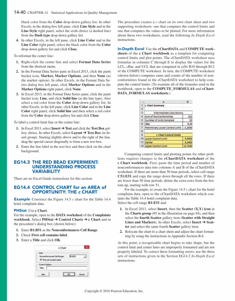
14-40 CHAPTER 14 Statistical Applications in Quality Management
Copyright © 2016 Pearson Education, Inc.
black color from the Color drop-down gallery list. In other Excels, in the dialog box left pane, click Line Style and in the Line Style right panel, select the sixth choice (a dashed line) from the Dash type drop-down gallery list.
4. In other Excels, in the left pane, click Line Color and in the Line Color right panel, select the black color from the Color drop-down gallery list and click Close.
To reformat the center line:
1. Right-click the center line and select Format Data Series from the shortcut menu.
2. In the Format Data Series pane in Excel 2013, click the paint bucket icon, Marker, Marker Options, and then None (as the marker option). In other Excels, in the Format Data Se-ries dialog box left pane, click Marker Options and in the Marker Options right panel, click None.
3. In Excel 2013, in the Format Data Series pane, click the paint bucket icon, Line, and click Solid line (as the line type). Also select a red color from the Color drop-down gallery list. In other Excels, in the left pane, click Line Color and in the Line Color right panel, click Solid line and then select a red color from the Color drop-down gallery list and click Close.
To label a control limit line or the center line:
1. In Excel 2013, select Insert ➔ Text and click the Text Box gal-lery choice. In other Excels, select Layout ➔ Text Box (in In-sert group). Starting slightly above and to the right of the line, drag the special cursor diagonally to form a new text box.
2. Enter the line label in the text box and then click on the chart background.
eg14.3 THe reD beaD experimenT: unDerSTanDing proceSS VariabiliTy
There are no Excel Guide instructions for this section.
eg14.4 conTrol cHarT for an area of opporTuniTy: THe c cHarT
Example Construct the Figure 14.5 c chart for the Table 14.4 hotel complaint data.
pHStat Use c Chart. For the example, open to the DATA worksheet of the Complaints workbook. Select PHStat ➔ Control Charts ➔ c Chart and in the procedure’s dialog box (shown below):
1. Enter B1:B51 as the Nonconformances Cell Range. 2. Check First cell contains label. 3. Enter a Title and click OK.
The procedure creates a c chart on its own chart sheet and two supporting worksheets: one that computes the control limits and one that computes the values to be plotted. For more information about these two worksheets, read the following In-Depth Excel instructions.
in-Depth excel Use the cChartDATA and COMPUTE work-sheets of the c Chart workbook as a template for computing control limits and plot points. The cChartDATA worksheet uses formulas in columns C through E to display the values for the LCL, cBar, and UCL that are computed in cells B10 through B12 of the COMPUTE worksheet. In turn, the COMPUTE worksheet (shown below) computes sums and counts of the number of non-conformities found in the cChartDATA worksheet to help com-pute the control limits. (To examine all of the formulas used in the workbook, open to the COMPUTE_FORMULAS and cChart-DATA_FORMULAS worksheets.)
Computing control limits and plotting points for other prob-lems requires changes to the cChartDATA worksheet of the c Chart workbook. First, paste the time period and number of nonconformances data into columns A and B of the cChartDATA worksheet. If there are more than 50 time periods, select cell range C51:E51 and copy the range down through all the rows. If there are fewer than 50 time periods, delete the extra rows from the bot-tom up, starting with row 51.
For the example, to create the Figure 14.5 c chart for the hotel complaint data, open to the cChartDATA worksheet which con-tains the Table 14.4 hotel complaint data.Select the cell range B1:E51 and:
1. In Excel 2013, select Insert, then the Scatter (X,Y) icon in the Charts group (#5 in the illustration on page 84), and then select the fourth Scatter gallery item (Scatter with Straight Lines and Markers). In other Excels, select Insert ➔ Scat-ter and select the same fourth Scatter gallery item.
2. Relocate the chart to a chart sheet and adjust the chart format-ting by using the instructions in Appendix Section B.6.
At this point, a recognizable chart begins to take shape, but the control limit and center lines are improperly formatted and are not properly labeled. To correct these formatting errors, use the three sets of instructions given in the Section EG14.2 In-Depth Excel instructions.
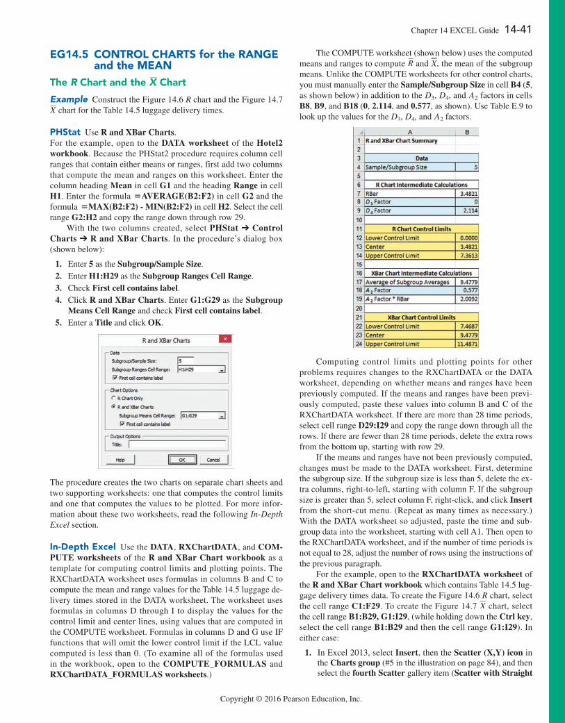
Copyright © 2016 Pearson Education, Inc.
Chapter 14 ExCEL Guide 14-41
eg14.5 conTrol cHarTS for the range and the mean
The R chart and the X—
chart
Example Construct the Figure 14.6 R chart and the Figure 14.7 X chart for the Table 14.5 luggage delivery times.
pHStat Use R and XBar Charts.For the example, open to the DATA worksheet of the Hotel2 workbook. Because the PHStat2 procedure requires column cell ranges that contain either means or ranges, first add two columns that compute the mean and ranges on this worksheet. Enter the column heading Mean in cell G1 and the heading Range in cell H1. Enter the formula =AVERAGE(B2:F2) in cell G2 and the formula =MAX(B2:F2) - MIN(B2:F2) in cell H2. Select the cell range G2:H2 and copy the range down through row 29.
With the two columns created, select PHStat ➔ Control Charts ➔ R and XBar Charts. In the procedure’s dialog box (shown below):
1. Enter 5 as the Subgroup/Sample Size. 2. Enter H1:H29 as the Subgroup Ranges Cell Range. 3. Check First cell contains label. 4. Click R and XBar Charts. Enter G1:G29 as the Subgroup
Means Cell Range and check First cell contains label. 5. Enter a Title and click OK.
The procedure creates the two charts on separate chart sheets and two supporting worksheets: one that computes the control limits and one that computes the values to be plotted. For more infor-mation about these two worksheets, read the following In-Depth Excel section.
in-Depth excel Use the DATA, RXChartDATA, and COM-PUTE worksheets of the R and XBar Chart workbook as a template for computing control limits and plotting points. The RxChartDATA worksheet uses formulas in columns B and C to compute the mean and range values for the Table 14.5 luggage de-livery times stored in the DATA worksheet. The worksheet uses formulas in columns D through I to display the values for the control limit and center lines, using values that are computed in the COMPUTE worksheet. Formulas in columns D and G use IF functions that will omit the lower control limit if the LCL value computed is less than 0. (To examine all of the formulas used in the workbook, open to the COMPUTE_FORMULAS and RXChartDATA_FORMULAS worksheets.)
The COMPUTE worksheet (shown below) uses the computed means and ranges to compute R and X, the mean of the subgroup means. Unlike the COMPUTE worksheets for other control charts, you must manually enter the Sample/Subgroup Size in cell B4 (5, as shown below) in addition to the D3, D4, and A2 factors in cells B8, B9, and B18 (0, 2.114, and 0.577, as shown). Use Table E.9 to look up the values for the D3, D4, and A2 factors.
Computing control limits and plotting points for other problems requires changes to the RxChartDATA or the DATA worksheet, depending on whether means and ranges have been previously computed. If the means and ranges have been previ-ously computed, paste these values into column B and C of the RxChartDATA worksheet. If there are more than 28 time periods, select cell range D29:I29 and copy the range down through all the rows. If there are fewer than 28 time periods, delete the extra rows from the bottom up, starting with row 29.
If the means and ranges have not been previously computed, changes must be made to the DATA worksheet. First, determine the subgroup size. If the subgroup size is less than 5, delete the ex-tra columns, right-to-left, starting with column F. If the subgroup size is greater than 5, select column F, right-click, and click Insert from the short-cut menu. (Repeat as many times as necessary.) With the DATA worksheet so adjusted, paste the time and sub-group data into the worksheet, starting with cell A1. Then open to the RxChartDATA worksheet, and if the number of time periods is not equal to 28, adjust the number of rows using the instructions of the previous paragraph.
For the example, open to the RXChartDATA worksheet of the R and XBar Chart workbook which contains Table 14.5 lug-gage delivery times data. To create the Figure 14.6 R chart, select the cell range C1:F29. To create the Figure 14.7 X chart, select the cell range B1:B29, G1:I29, (while holding down the Ctrl key, select the cell range B1:B29 and then the cell range G1:I29). In either case:
1. In Excel 2013, select Insert, then the Scatter (X,Y) icon in the Charts group (#5 in the illustration on page 84), and then select the fourth Scatter gallery item (Scatter with Straight
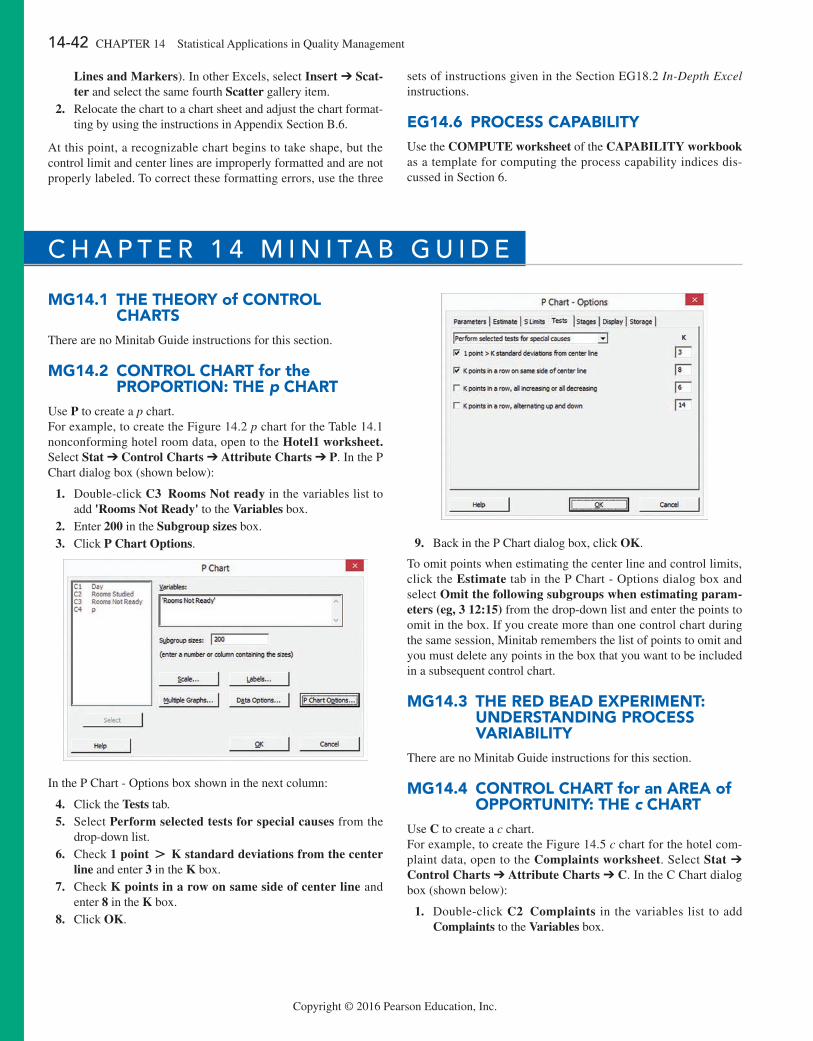
14-42 CHAPTER 14 Statistical Applications in Quality Management
Copyright © 2016 Pearson Education, Inc.
mg14.1 THe THeory of conTrol cHarTS
There are no Minitab Guide instructions for this section.
mg14.2 conTrol cHarT for the proporTion: THe p cHarT
Use P to create a p chart.For example, to create the Figure 14.2 p chart for the Table 14.1 nonconforming hotel room data, open to the Hotel1 worksheet. Select Stat ➔ Control Charts ➔ Attribute Charts ➔ P. In the P Chart dialog box (shown below):
1. Double-click C3 Rooms Not ready in the variables list to add 'Rooms Not Ready' to the Variables box.
2. Enter 200 in the Subgroup sizes box. 3. Click P Chart Options.
In the P Chart - Options box shown in the next column:
4. Click the Tests tab. 5. Select Perform selected tests for special causes from the
drop-down list. 6. Check 1 point + K standard deviations from the center
line and enter 3 in the K box. 7. Check K points in a row on same side of center line and
enter 8 in the K box. 8. Click OK.
9. Back in the P Chart dialog box, click OK.
To omit points when estimating the center line and control limits, click the Estimate tab in the P Chart - Options dialog box and select Omit the following subgroups when estimating param-eters (eg, 3 12:15) from the drop-down list and enter the points to omit in the box. If you create more than one control chart during the same session, Minitab remembers the list of points to omit and you must delete any points in the box that you want to be included in a subsequent control chart.
mg14.3 THe reD beaD experimenT: unDerSTanDing proceSS VariabiliTy
There are no Minitab Guide instructions for this section.
mg14.4 conTrol cHarT for an area of opporTuniTy: THe c cHarT
Use C to create a c chart.For example, to create the Figure 14.5 c chart for the hotel com-plaint data, open to the Complaints worksheet. Select Stat ➔ Control Charts ➔ Attribute Charts ➔ C. In the C Chart dialog box (shown below):
1. Double-click C2 Complaints in the variables list to add Complaints to the Variables box.
Lines and Markers). In other Excels, select Insert ➔ Scat-ter and select the same fourth Scatter gallery item.
2. Relocate the chart to a chart sheet and adjust the chart format-ting by using the instructions in Appendix Section B.6.
At this point, a recognizable chart begins to take shape, but the control limit and center lines are improperly formatted and are not properly labeled. To correct these formatting errors, use the three
sets of instructions given in the Section EG18.2 In-Depth Excel instructions.
eg14.6 proceSS capabiliTyUse the COMPUTE worksheet of the CAPABILITY workbook as a template for computing the process capability indices dis-cussed in Section 6.
c h a p t e R 1 4 M i n i ta B g U i d e
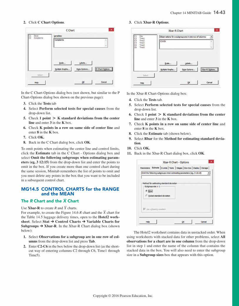
Copyright © 2016 Pearson Education, Inc.
Chapter 14 MINITAB Guide 14-43
2. Click C Chart Options.
In the C Chart-Options dialog box (not shown, but similar to the P Chart-Options dialog box shown on the previous page):
3. Click the Tests tab 4. Select Perform selected tests for special causes from the
drop-down list. 5. Check 1 point + K standard deviations from the center
line and enter 3 in the K box. 6. Check K points in a row on same side of center line and
enter 8 in the K box. 7. Click OK. 8. Back in the C Chart dialog box, click OK.
To omit points when estimating the center line and control limits, click the Estimate tab in the C Chart - Options dialog box and select Omit the following subgroups when estimating param-eters (eg, 3 12:15) from the drop-down list and enter the points to omit in the box. If you create more than one control chart during the same session, Minitab remembers the list of points to omit and you must delete any points in the box that you want to be included in a subsequent control chart.
mg14.5 conTrol cHarTS for the range and the mean
The R chart and the X—
chart
Use Xbar-R to create R and X charts.For example, to create the Figure 14.6 R chart and the X chart for the Table 14.5 luggage delivery times, open to the Hotel2 work-sheet. Select Stat ➔ Control Charts ➔ Variable Charts for Subgroups ➔ Xbar-R. In the xbar-R Chart dialog box (shown below):
1. Select Observations for a subgroup are in one row of col-umns from the drop-down list and press Tab.
2. Enter C2-C6 in the box below the drop-down list (as the short-cut way of entering columns C2 through C6, Time1 through Time5).
3. Click Xbar-R Options.
In the xbar-R Chart-Options dialog box:
4. Click the Tests tab. 5. Select Perform selected tests for special causes from the
drop-down list. 6. Check 1 point + K standard deviations from the center
line and enter 3 in the K box. 7. Check K points in a row on same side of center line and
enter 8 in the K box. 8. Click the Estimate tab (shown below). 9. Select Rbar for the Method for estimating standard devia-
tion. 10. Click OK. 11. Back in the xbar-R Chart dialog box, click OK.
The Hotel2 worksheet contains data in unstacked order. When using worksheets with stacked data for other problems, select All observations for a chart are in one column from the drop-down list in step 1 and enter the name of the column that contains the stacked data in the box. You will also need to enter the subgroup size in a Subgroup sizes box that appears with this option.

14-44 CHAPTER 14 Statistical Applications in Quality Management
Copyright © 2016 Pearson Education, Inc.
To omit points when estimating the center line and control limits, select Omit the following subgroups when estimating parameters (eg, 3 12:15) from the drop-down list and enter the points to omit in the box in the Estimate tab of the xbar-R Chart-Options dialog box shown above. If you create more than one con-trol chart during the same session, Minitab remembers the list of
points to omit and you must delete any points in the box that you want to be included in a subsequent control chart.
mg14.6 proceSS capabiliTyThere are no Minitab Guide instructions for this section.

AppendicesA. BAsic MAth concepts And
syMBolsA.1 Rules for Arithmetic OperationsA.2 Rules for Algebra: Exponents and
Square RootsA.3 Rules for LogarithmsA.4 Summation NotationA.5 Statistical SymbolsA.6 Greek Alphabet
B. iMpoRtAnt eXcel And MinitAB skillsB.1 Basic Excel OperationsB.2 Formulas and Cell ReferencesB.3 Entering Formulas into WorksheetsB.4 Pasting with Paste SpecialB.5 Basic Worksheet FormattingB.6 Chart FormattingB.7 Selecting Cell Ranges for ChartsB.8 Deleting the “Extra” Histogram BarB.9 Creating Histograms for Discrete
Probability DistributionsB.10 Basic Minitab Operations
c. online ResouRcesC.1 About the Online Resources
for This BookC.2 Accessing the Online ResourcesC.3 Details of Downloadable FilesC.4 PHStat
d. conFiGuRinG MicRosoFt eXcelD.1 Getting Microsoft Excel Ready
for Use (ALL)D.2 Getting PHStat Ready for Use (ALL)D.3 Configuring Excel Security for Add-In
Usage (WIN)
D.4 Opening PHStat (ALL)D.5 Using a Visual Explorations Add-In
Workbook (ALL)D.6 Checking for the Presence of the
Analysis ToolPak (ALL)
e. tABlesE.1 Table of Random NumbersE.2 The Cumulative Standardized Normal
DistributionE.3 Critical Values of tE.4 Critical Values of x2
E.5 Critical Values of FE.6 Critical Values of the Studentized
Range, QE.7 Critical Values, dL and dU, of the
Durbin-Watson Statistic, DE.8 Control Chart FactorsE.9 The Standardized Normal Distribution
F. useFul eXcel knoWledGeF.1 Useful Keyboard ShortcutsF.2 Verifying Formulas and WorksheetsF.3 New Function NamesF.4 Understanding the Nonstatistical
Functions
G. soFtWARe FAQsG.1 PHStat FAQsG.2 Microsoft Excel FAQsG.3 FAQs for New Microsoft Excel 2013 UsersG.4 Minitab FAQs
selF-test solutions And AnsWeRs to selected even-nuMBeRed pRoBleMs
518
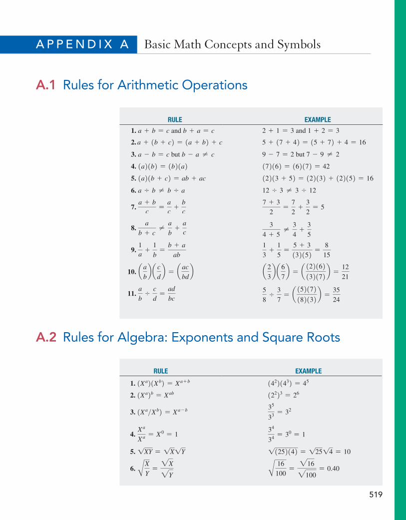
A p p e n d i X A Basic Math Concepts and Symbols
A.1 Rules for Arithmetic Operations
Rule example
1. a + b = c and b + a = c 2 + 1 = 3 and 1 + 2 = 3
2. a + 1b + c2 = 1a + b2 + c 5 + 17 + 42 = 15 + 72 + 4 = 16
3. a - b = c but b - a ≠ c 9 - 7 = 2 but 7 - 9 ≠ 2
4. 1a21b2 = 1b21a2 172162 = 162172 = 42
5. 1a21b + c2 = ab + ac 12213 + 52 = 122132 + 122152 = 16
6. a , b ≠ b , a 12 , 3 ≠ 3 , 12
7. a + b
c=
ac
+bc
7 + 3
2=
7
2+
3
2= 5
8. a
b + c≠
a
b+
ac
3
4 + 5≠
3
4+
3
5
9. 1a
+1
b=
b + a
ab
1
3+
1
5=
5 + 3
132152 =8
15
10. a a
bb a c
db = a ac
bdb a 2
3b a 6
7b = a 122162
132172 b =12
21
11. a
b,
c
d=
ad
bc5
8,
3
7= a 152172
182132 b =35
24
A.2 Rules for Algebra: Exponents and Square Roots
Rule example
1. 1Xa21Xb2 = Xa + b 14221432 = 45
2. 1Xa2b = Xab 12223 = 26
3. 1Xa>Xb2 = Xa - b 35
33 = 32
4. Xa
Xa = X0 = 134
34 = 30 = 1
5. 1XY = 1X1Y 11252142 = 12514 = 10
6. AX
Y=
2X2Y A 16
100=
2162100= 0.40
519
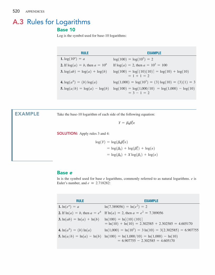
520 Appendices
Base 10Log is the symbol used for base-10 logarithms:
A.3 Rules for Logarithms
Rule example
1. log110a2 = a log11002 = log11022 = 2
2. if log1a2 = b, then a = 10b if log1a2 = 2, then a = 102 = 100
3. log1ab2 = log1a2 + log1b2 log11002 = log3110211024 = log1102 + log1102 = 1 + 1 = 2
4. log1ab2 = 1b2 log1a2 log11,0002 = log11032 = 132 log1102 = 132112 = 3
5. log1a>b2 = log1a2 - log1b2 log11002 = log11,000>102 = log11,0002 - log1102 = 3 - 1 = 2
ExamplE Take the base-10 logarithm of each side of the following equation:
Y = b0b1Xe
Solution: Apply rules 3 and 4:
log1Y2 = log1b0bX1e2
= log1b02 + log1bX12 + log1e2
= log1b02 + X log1b12 + log1e2
Base eln is the symbol used for base e logarithms, commonly referred to as natural logarithms. e is euler’s number, and e ≅ 2.718282:
Rule example
1. ln1ea2 = a ln17.3890562 = ln1e22 = 2
2. if ln1a2 = b, then a = eb if ln1a2 = 2, then a = e2 = 7.389056
3. ln1ab2 = ln1a2 + ln1b2 ln11002 = ln31102 11024 = ln1102 + ln1102 = 2.302585 + 2.302585 = 4.605170
4. ln1ab2 = 1b2 ln1a2 ln11,0002 = ln11032 = 3 ln1102 = 312.3025852 = 6.907755
5. ln1a>b2 = ln1a2 - ln1b2 ln11002 = ln11,000>102 = ln11,0002 - ln1102 = 6.907755 - 2.302585 = 4.605170
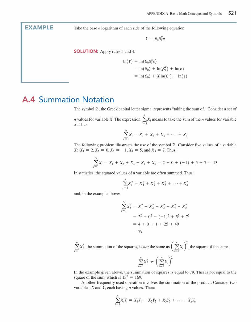
Appendix A Basic Math concepts and symbols 521
The symbol Σ, the Greek capital letter sigma, represents “taking the sum of.” consider a set of
n values for variable X. The expression an
i= 1Xi means to take the sum of the n values for variable
X. Thus:
an
i= 1Xi = X1 + X2 + X3 + g + Xn
The following problem illustrates the use of the symbol Σ. consider five values of a variable X: X1 = 2, X2 = 0, X3 = -1, X4 = 5, and X5 = 7. Thus:
a5
i= 1Xi = X1 + X2 + X3 + X4 + X5 = 2 + 0 + 1-12 + 5 + 7 = 13
in statistics, the squared values of a variable are often summed. Thus:
an
i= 1X2
i = X21 + X2
2 + X23 + g+ X2
n
and, in the example above:
a5
i= 1X2
i = X21 + X2
2 + X23 + X2
4 + X25
= 22 + 02 + 1-122 + 52 + 72
= 4 + 0 + 1 + 25 + 49
= 79
an
i= 1X2
i , the summation of the squares, is not the same as a an
i= 1Xib
2
, the square of the sum:
an
i= 1X2
i ≠ a an
i= 1Xib
2
in the example given above, the summation of squares is equal to 79. This is not equal to the square of the sum, which is 132 = 169.
Another frequently used operation involves the summation of the product. consider two variables, X and Y, each having n values. Then:
an
i= 1XiYi = X1Y1 + X2Y2 + X3Y3 + g+ XnYn
ExamplE Take the base e logarithm of each side of the following equation:
Y = b0bX1e
Solution: Apply rules 3 and 4:
ln1Y2 = ln1b0bX1e2
= ln1b02 + ln1bX12 + ln1e2
= ln1b02 + X ln1b12 + ln1e2
A.4 Summation Notation
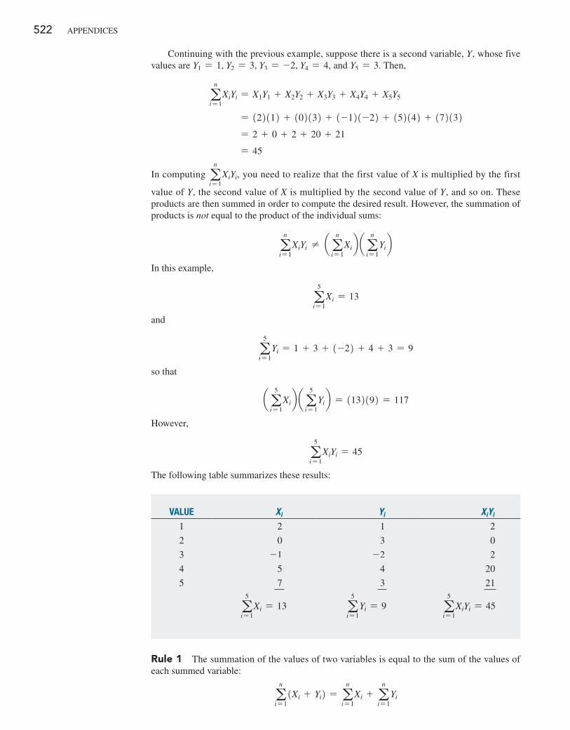
522 Appendices
continuing with the previous example, suppose there is a second variable, Y, whose five values are Y1 = 1, Y2 = 3, Y3 = -2, Y4 = 4, and Y5 = 3. Then,
an
i= 1XiYi = X1Y1 + X2Y2 + X3Y3 + X4Y4 + X5Y5
= 122112 + 102132 + 1-121-22 + 152142 + 172132 = 2 + 0 + 2 + 20 + 21
= 45
in computing an
i= 1XiYi, you need to realize that the first value of X is multiplied by the first
value of Y, the second value of X is multiplied by the second value of Y, and so on. These products are then summed in order to compute the desired result. However, the summation of products is not equal to the product of the individual sums:
an
i= 1XiYi ≠ a a
n
i= 1Xib a a
n
i= 1Yib
in this example,
a5
i= 1Xi = 13
and
a5
i= 1Yi = 1 + 3 + 1-22 + 4 + 3 = 9
so that
a a5
i= 1Xib a a
5
i= 1Yib = 1132192 = 117
However,
a5
i= 1XiYi = 45
The following table summarizes these results:
Value Xi Yi XiYi
1 2 1 2
2 0 3 0
3 -1 -2 2
4 5 4 20
5 7 3 21
a5
i= 1Xi = 13 a
5
i= 1Yi = 9 a
5
i= 1XiYi = 45
Rule 1 The summation of the values of two variables is equal to the sum of the values of each summed variable:
an
i= 11Xi + Yi2 = a
n
i= 1Xi + a
n
i= 1Yi
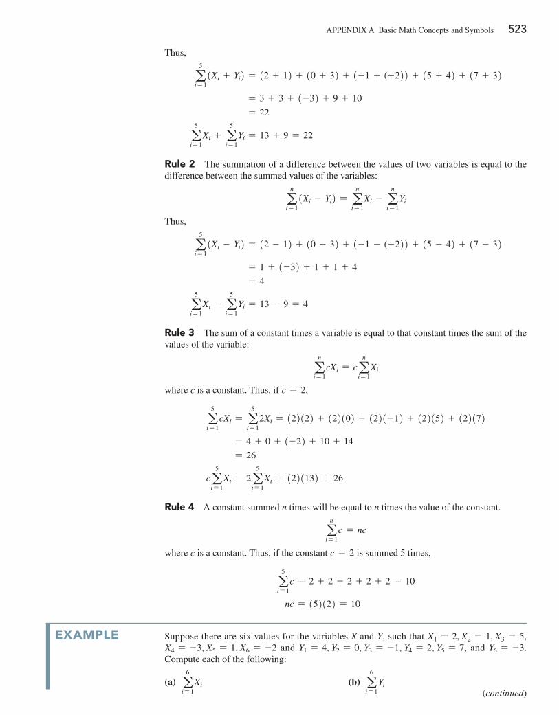
Appendix A Basic Math concepts and symbols 523
Thus,
a5
i= 11Xi + Yi2 = 12 + 12 + 10 + 32 + 1-1 + (-222 + 15 + 42 + 17 + 32
= 3 + 3 + 1-32 + 9 + 10
= 22
a5
i= 1Xi + a
5
i= 1Yi = 13 + 9 = 22
Rule 2 The summation of a difference between the values of two variables is equal to the difference between the summed values of the variables:
an
i= 11Xi - Yi2 = a
n
i= 1Xi - a
n
i= 1Yi
Thus,
a5
i= 11Xi - Yi2 = 12 - 12 + 10 - 32 + 1-1 - (-222 + 15 - 42 + 17 - 32
= 1 + 1-32 + 1 + 1 + 4
= 4
a5
i= 1Xi - a
5
i= 1Yi = 13 - 9 = 4
Rule 3 The sum of a constant times a variable is equal to that constant times the sum of the values of the variable:
an
i= 1cXi = ca
n
i= 1Xi
where c is a constant. Thus, if c = 2,
a5
i= 1cXi = a
5
i= 12Xi = 122122 + 122102 + 1221-12 + 122152 + 122172
= 4 + 0 + 1-22 + 10 + 14
= 26
ca5
i= 1Xi = 2a
5
i= 1Xi = 1221132 = 26
Rule 4 A constant summed n times will be equal to n times the value of the constant.
an
i= 1c = nc
where c is a constant. Thus, if the constant c = 2 is summed 5 times,
a5
i= 1c = 2 + 2 + 2 + 2 + 2 = 10
nc = 152122 = 10
ExamplE suppose there are six values for the variables X and Y, such that X1 = 2, X2 = 1, X3 = 5,X4 = -3, X5 = 1, X6 = -2 and Y1 = 4, Y2 = 0, Y3 = -1, Y4 = 2, Y5 = 7, and Y6 = -3. compute each of the following:
(a) a6
i= 1Xi (b) a
6
i= 1Yi
(continued)
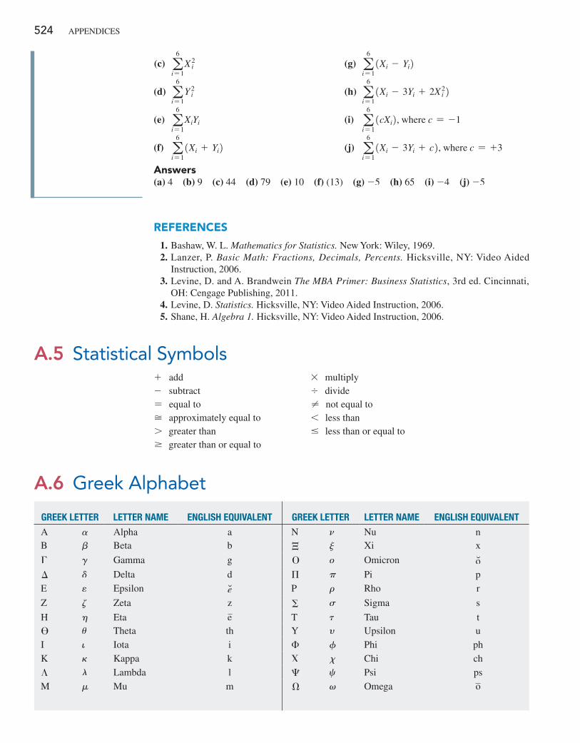
524 Appendices
REfEREncES
1. Bashaw, W. L. Mathematics for Statistics. new York: Wiley, 1969. 2. Lanzer, p. Basic Math: Fractions, Decimals, Percents. Hicksville, nY: Video Aided
instruction, 2006. 3. Levine, d. and A. Brandwein The MBA Primer: Business Statistics, 3rd ed. cincinnati,
OH: cengage publishing, 2011. 4. Levine, d. Statistics. Hicksville, nY: Video Aided instruction, 2006. 5. shane, H. Algebra 1. Hicksville, nY: Video Aided instruction, 2006.
A.5 Statistical Symbols+ add * multiply- subtract , divide= equal to ≠ not equal to≅ approximately equal to 6 less than7 greater than … less than or equal toÚ greater than or equal to
GReek letteR letteR Name eNGlish equiValeNt GReek letteR letteR Name eNGlish equiValeNtA a Alpha a n n nu nB b Beta b Ξ j xi x
Γ g Gamma g Ο o Omicron oi
∆ d delta d Π p pi p
e e epsilon ei p r Rho r
Z z Zeta z Σ s sigma s
H h eta e T t Tau t
ϴ u Theta th Y y Upsilon ui i iota i Φ f phi phK k Kappa k Χ x chi ch
Λ l Lambda l Ψ c psi ps
M m Mu m Ω v Omega o
A.6 Greek Alphabet
(c) a6
i= 1X2
i
(d) a6
i= 1Y 2
i
(e) a6
i= 1XiYi
(f) a6
i= 11Xi + Yi2
(g) a6
i= 11Xi - Yi2
(h) a6
i= 11Xi - 3Yi + 2X2
i 2
(i) a6
i= 11cXi2, where c = -1
(j) a6
i= 11Xi - 3Yi + c2, where c = +3
answers(a) 4 (b) 9 (c) 44 (d) 79 (e) 10 (f) (13) (g) -5 (h) 65 (i) -4 (j) -5
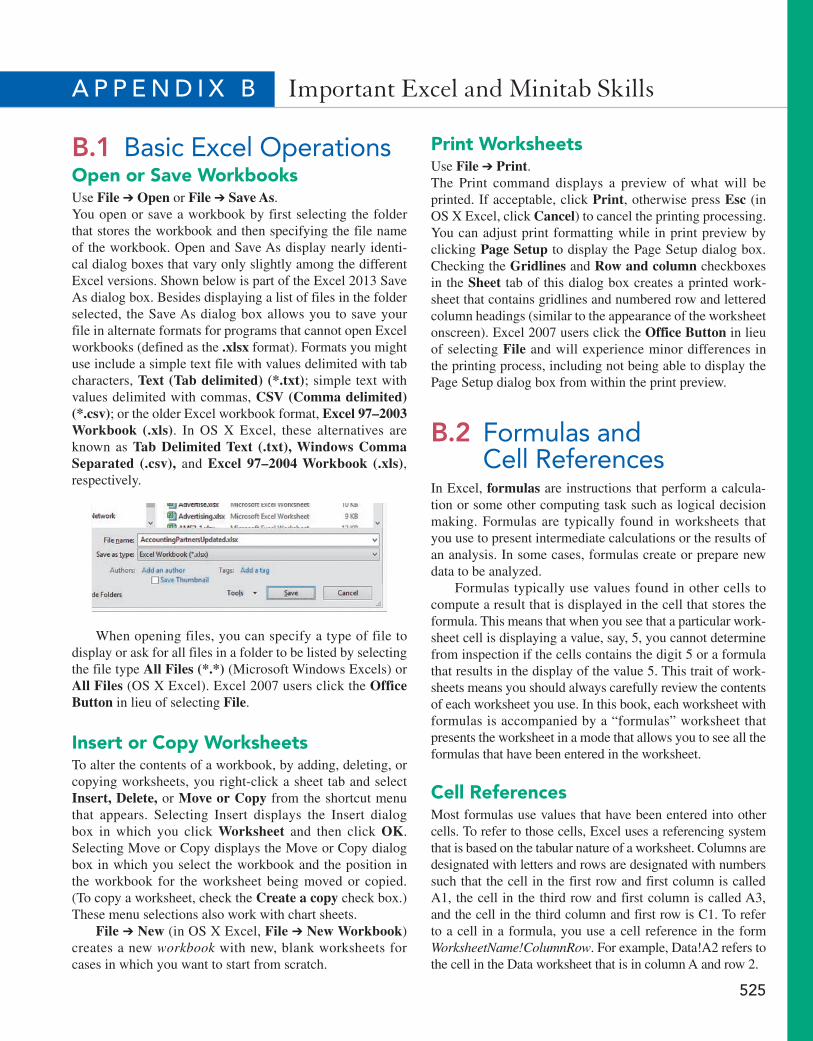
A p p e n d i x B Important Excel and Minitab Skills
B.1 Basic Excel OperationsOpen or Save WorkbooksUse File ➔ Open or File ➔ Save As.You open or save a workbook by first selecting the folder that stores the workbook and then specifying the file name of the workbook. Open and Save As display nearly identi-cal dialog boxes that vary only slightly among the different Excel versions. Shown below is part of the Excel 2013 Save As dialog box. Besides displaying a list of files in the folder selected, the Save As dialog box allows you to save your file in alternate formats for programs that cannot open Excel workbooks (defined as the .xlsx format). Formats you might use include a simple text file with values delimited with tab characters, Text (Tab delimited) (*.txt); simple text with values delimited with commas, CSV (Comma delimited) (*.csv); or the older Excel workbook format, Excel 97–2003 Workbook (.xls). In OS X Excel, these alternatives are known as Tab Delimited Text (.txt), Windows Comma Separated (.csv), and Excel 97–2004 Workbook (.xls), respectively.
When opening files, you can specify a type of file to display or ask for all files in a folder to be listed by selecting the file type All Files (*.*) (Microsoft Windows Excels) or All Files (OS X Excel). Excel 2007 users click the Office Button in lieu of selecting File.
Insert or Copy WorksheetsTo alter the contents of a workbook, by adding, deleting, or copying worksheets, you right-click a sheet tab and select Insert, Delete, or Move or Copy from the shortcut menu that appears. Selecting Insert displays the Insert dialog box in which you click Worksheet and then click OK. Selecting Move or Copy displays the Move or Copy dialog box in which you select the workbook and the position in the workbook for the worksheet being moved or copied. (To copy a worksheet, check the Create a copy check box.) These menu selections also work with chart sheets.
File ➔ New (in OS X Excel, File ➔ New Workbook) creates a new workbook with new, blank worksheets for cases in which you want to start from scratch.
Print WorksheetsUse File ➔ Print.The Print command displays a preview of what will be printed. If acceptable, click Print, otherwise press Esc (in OS X Excel, click Cancel) to cancel the printing processing. You can adjust print formatting while in print preview by clicking Page Setup to display the Page Setup dialog box. Checking the Gridlines and Row and column checkboxes in the Sheet tab of this dialog box creates a printed work-sheet that contains gridlines and numbered row and lettered column headings (similar to the appearance of the worksheet onscreen). Excel 2007 users click the Office Button in lieu of selecting File and will experience minor differences in the printing process, including not being able to display the Page Setup dialog box from within the print preview.
B.2 Formulas and Cell References
In Excel, formulas are instructions that perform a calcula-tion or some other computing task such as logical decision making. Formulas are typically found in worksheets that you use to present intermediate calculations or the results of an analysis. In some cases, formulas create or prepare new data to be analyzed.
Formulas typically use values found in other cells to compute a result that is displayed in the cell that stores the formula. This means that when you see that a particular work-sheet cell is displaying a value, say, 5, you cannot determine from inspection if the cells contains the digit 5 or a formula that results in the display of the value 5. This trait of work-sheets means you should always carefully review the contents of each worksheet you use. In this book, each worksheet with formulas is accompanied by a “formulas” worksheet that presents the worksheet in a mode that allows you to see all the formulas that have been entered in the worksheet.
Cell ReferencesMost formulas use values that have been entered into other cells. To refer to those cells, Excel uses a referencing system that is based on the tabular nature of a worksheet. Columns are designated with letters and rows are designated with numbers such that the cell in the first row and first column is called A1, the cell in the third row and first column is called A3, and the cell in the third column and first row is C1. To refer to a cell in a formula, you use a cell reference in the form WorksheetName!ColumnRow. For example, Data!A2 refers to the cell in the Data worksheet that is in column A and row 2.
525
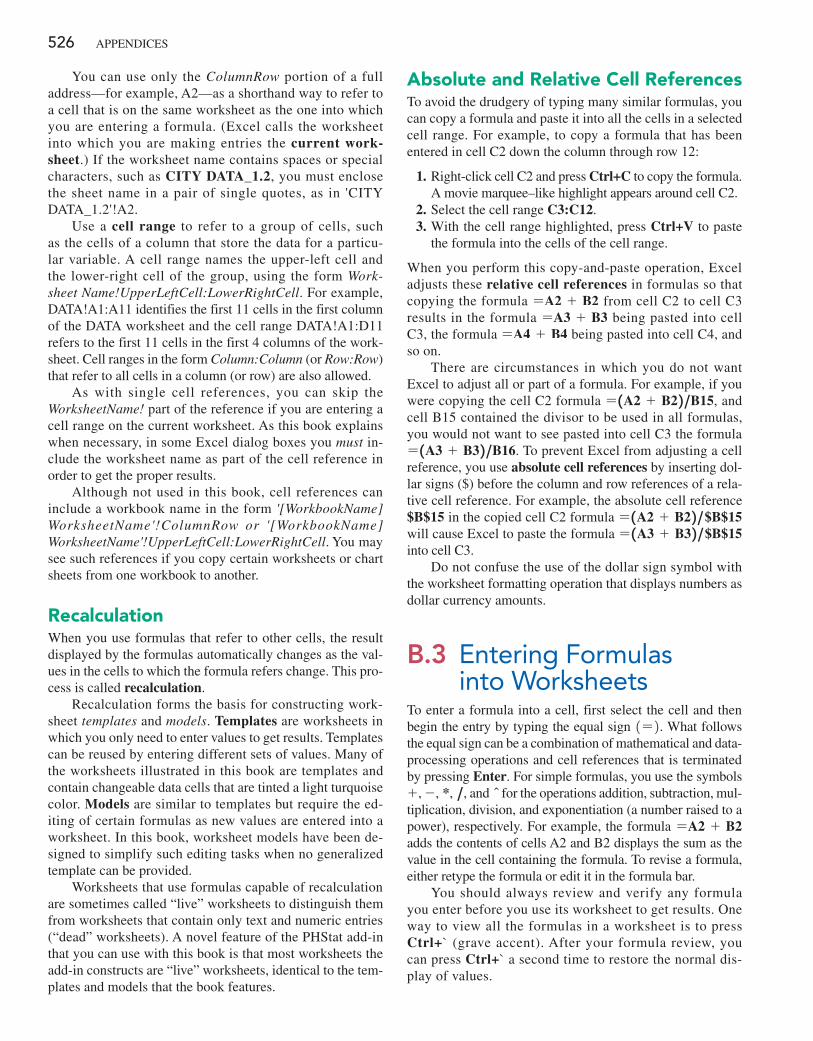
526 APPEnDICES
You can use only the ColumnRow portion of a full address—for example, A2—as a shorthand way to refer to a cell that is on the same worksheet as the one into which you are entering a formula. (Excel calls the worksheet into which you are making entries the current work-sheet.) If the worksheet name contains spaces or special characters, such as CITY DATA_1.2, you must enclose the sheet name in a pair of single quotes, as in 'CITY DATA_1.2'!A2.
Use a cell range to refer to a group of cells, such as the cells of a column that store the data for a particu-lar variable. A cell range names the upper-left cell and the lower-right cell of the group, using the form Work-sheet Name!UpperLeftCell:LowerRightCell. For example, DATA!A1:A11 identifies the first 11 cells in the first column of the DATA worksheet and the cell range DATA!A1:D11 refers to the first 11 cells in the first 4 columns of the work-sheet. Cell ranges in the form Column:Column (or Row:Row) that refer to all cells in a column (or row) are also allowed.
As with single cell references, you can skip the WorksheetName! part of the reference if you are entering a cell range on the current worksheet. As this book explains when necessary, in some Excel dialog boxes you must in-clude the worksheet name as part of the cell reference in order to get the proper results.
Although not used in this book, cell references can include a workbook name in the form '[WorkbookName]WorksheetName'!ColumnRow or '[WorkbookName] WorksheetName'!UpperLeftCell:LowerRightCell. You may see such references if you copy certain worksheets or chart sheets from one workbook to another.
RecalculationWhen you use formulas that refer to other cells, the result displayed by the formulas automatically changes as the val-ues in the cells to which the formula refers change. This pro-cess is called recalculation.
Recalculation forms the basis for constructing work-sheet templates and models. Templates are worksheets in which you only need to enter values to get results. Templates can be reused by entering different sets of values. Many of the worksheets illustrated in this book are templates and contain changeable data cells that are tinted a light turquoise color. Models are similar to templates but require the ed-iting of certain formulas as new values are entered into a worksheet. In this book, worksheet models have been de-signed to simplify such editing tasks when no generalized template can be provided.
Worksheets that use formulas capable of recalculation are sometimes called “live” worksheets to distinguish them from worksheets that contain only text and numeric entries (“dead” worksheets). A novel feature of the PHStat add-in that you can use with this book is that most worksheets the add-in constructs are “live” worksheets, identical to the tem-plates and models that the book features.
Absolute and Relative Cell ReferencesTo avoid the drudgery of typing many similar formulas, you can copy a formula and paste it into all the cells in a selected cell range. For example, to copy a formula that has been entered in cell C2 down the column through row 12:
1. Right-click cell C2 and press Ctrl+C to copy the formula. A movie marquee–like highlight appears around cell C2.
2. Select the cell range C3:C12. 3. With the cell range highlighted, press Ctrl+V to paste
the formula into the cells of the cell range.
When you perform this copy-and-paste operation, Excel adjusts these relative cell references in formulas so that copying the formula =A2 + B2 from cell C2 to cell C3 results in the formula =A3 + B3 being pasted into cell C3, the formula =A4 + B4 being pasted into cell C4, and so on.
There are circumstances in which you do not want Excel to adjust all or part of a formula. For example, if you were copying the cell C2 formula = 1A2 + B2 2 ,B15, and cell B15 contained the divisor to be used in all formulas, you would not want to see pasted into cell C3 the formula = 1A3 + B3 2 ,B16. To prevent Excel from adjusting a cell reference, you use absolute cell references by inserting dol-lar signs ($) before the column and row references of a rela-tive cell reference. For example, the absolute cell reference $B$15 in the copied cell C2 formula = 1A2 + B2 2 , $B$15 will cause Excel to paste the formula = 1A3 + B3 2 , $B$15 into cell C3.
Do not confuse the use of the dollar sign symbol with the worksheet formatting operation that displays numbers as dollar currency amounts.
B.3 Entering Formulas into Worksheets
To enter a formula into a cell, first select the cell and then begin the entry by typing the equal sign 1=2. What follows the equal sign can be a combination of mathematical and data-processing operations and cell references that is terminated by pressing Enter. For simple formulas, you use the symbols + , - , *, , , and n for the operations addition, subtraction, mul-tiplication, division, and exponentiation (a number raised to a power), respectively. For example, the formula =A2 + B2 adds the contents of cells A2 and B2 displays the sum as the value in the cell containing the formula. To revise a formula, either retype the formula or edit it in the formula bar.
You should always review and verify any formula you enter before you use its worksheet to get results. One way to view all the formulas in a worksheet is to press Ctrl+` (grave accent). After your formula review, you can press Ctrl+` a second time to restore the normal dis-play of values.
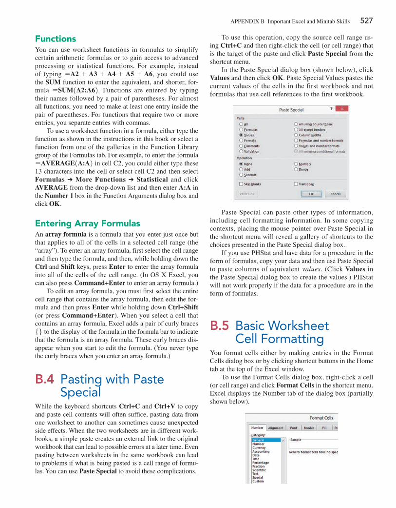
APPEnDIX B Important Excel and Minitab Skills 527
FunctionsYou can use worksheet functions in formulas to simplify certain arithmetic formulas or to gain access to advanced processing or statistical functions. For example, instead of typing =A2 + A3 + A4 + A5 + A6, you could use the SUM function to enter the equivalent, and shorter, for-mula =SUM1A2:A62. Functions are entered by typing their names followed by a pair of parentheses. For almost all functions, you need to make at least one entry inside the pair of parentheses. For functions that require two or more entries, you separate entries with commas.
To use a worksheet function in a formula, either type the function as shown in the instructions in this book or select a function from one of the galleries in the Function Library group of the Formulas tab. For example, to enter the formula =AVERAGE1A:A2 in cell C2, you could either type these 13 characters into the cell or select cell C2 and then select Formulas ➔ More Functions ➔ Statistical and click AVERAGE from the drop-down list and then enter A:A in the Number 1 box in the Function Arguments dialog box and click OK.
Entering Array FormulasAn array formula is a formula that you enter just once but that applies to all of the cells in a selected cell range (the “array”). To enter an array formula, first select the cell range and then type the formula, and then, while holding down the Ctrl and Shift keys, press Enter to enter the array formula into all of the cells of the cell range. (In OS X Excel, you can also press Command+Enter to enter an array formula.)
To edit an array formula, you must first select the entire cell range that contains the array formula, then edit the for-mula and then press Enter while holding down Ctrl+Shift (or press Command+Enter). When you select a cell that contains an array formula, Excel adds a pair of curly braces 56 to the display of the formula in the formula bar to indicate that the formula is an array formula. These curly braces dis-appear when you start to edit the formula. (You never type the curly braces when you enter an array formula.)
B.4 Pasting with Paste Special
While the keyboard shortcuts Ctrl+C and Ctrl+V to copy and paste cell contents will often suffice, pasting data from one worksheet to another can sometimes cause unexpected side effects. When the two worksheets are in different work-books, a simple paste creates an external link to the original workbook that can lead to possible errors at a later time. Even pasting between worksheets in the same workbook can lead to problems if what is being pasted is a cell range of formu-las. You can use Paste Special to avoid these complications.
To use this operation, copy the source cell range us-ing Ctrl+C and then right-click the cell (or cell range) that is the target of the paste and click Paste Special from the shortcut menu.
In the Paste Special dialog box (shown below), click Values and then click OK. Paste Special Values pastes the current values of the cells in the first workbook and not formulas that use cell references to the first workbook.
Paste Special can paste other types of information, including cell formatting information. In some copying contexts, placing the mouse pointer over Paste Special in the shortcut menu will reveal a gallery of shortcuts to the choices presented in the Paste Special dialog box.
If you use PHStat and have data for a procedure in the form of formulas, copy your data and then use Paste Special to paste columns of equivalent values. (Click Values in the Paste Special dialog box to create the values.) PHStat will not work properly if the data for a procedure are in the form of formulas.
B.5 Basic Worksheet Cell Formatting
You format cells either by making entries in the Format Cells dialog box or by clicking shortcut buttons in the Home tab at the top of the Excel window.
To use the Format Cells dialog box, right-click a cell (or cell range) and click Format Cells in the shortcut menu. Excel displays the number tab of the dialog box (partially shown below).
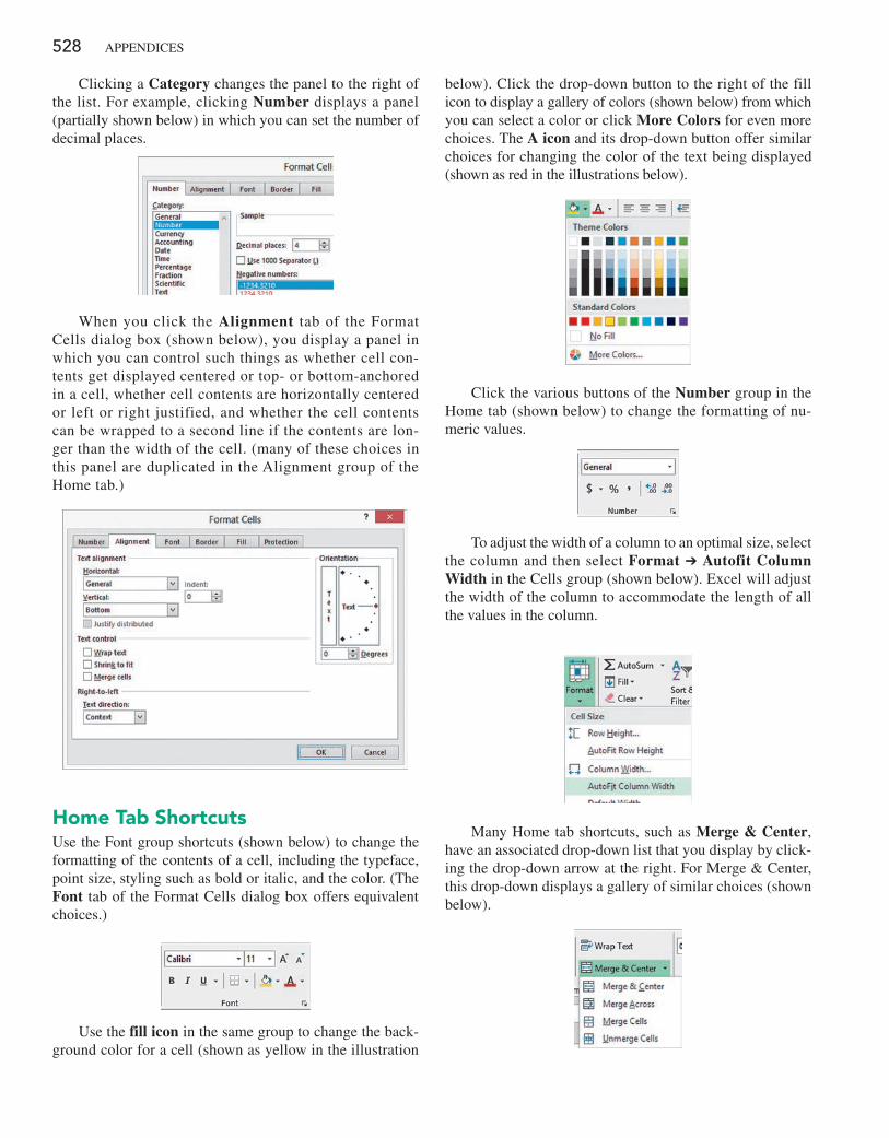
528 APPEnDICES
Clicking a Category changes the panel to the right of the list. For example, clicking Number displays a panel (partially shown below) in which you can set the number of decimal places.
When you click the Alignment tab of the Format Cells dialog box (shown below), you display a panel in which you can control such things as whether cell con-tents get displayed centered or top- or bottom-anchored in a cell, whether cell contents are horizontally centered or left or right justified, and whether the cell contents can be wrapped to a second line if the contents are lon-ger than the width of the cell. (many of these choices in this panel are duplicated in the Alignment group of the Home tab.)
Home Tab ShortcutsUse the Font group shortcuts (shown below) to change the formatting of the contents of a cell, including the typeface, point size, styling such as bold or italic, and the color. (The Font tab of the Format Cells dialog box offers equivalent choices.)
Use the fill icon in the same group to change the back-ground color for a cell (shown as yellow in the illustration
below). Click the drop-down button to the right of the fill icon to display a gallery of colors (shown below) from which you can select a color or click More Colors for even more choices. The A icon and its drop-down button offer similar choices for changing the color of the text being displayed (shown as red in the illustrations below).
Click the various buttons of the Number group in the Home tab (shown below) to change the formatting of nu-meric values.
To adjust the width of a column to an optimal size, select the column and then select Format ➔ Autofit Column Width in the Cells group (shown below). Excel will adjust the width of the column to accommodate the length of all the values in the column.
Many Home tab shortcuts, such as Merge & Center, have an associated drop-down list that you display by click-ing the drop-down arrow at the right. For Merge & Center, this drop-down displays a gallery of similar choices (shown below).
APPEnDIX B Important Excel and Minitab Skills 529
B.6 Chart FormattingMany of the In-Depth Excel instructions that involve charts refer you to this section so that you can correct the formatting of a chart that was just constructed. To apply any of the fol-lowing corrections, you must first select the chart that is to be corrected. (If Chart Tools or PivotChart Tools appears above the Ribbon tabs, you have selected a chart.)
If, when you open to a chart sheet, the chart is either too large to be fully seen or too small and surrounded by a frame mat that is too large, click Zoom Out or Zoom In, lo-cated in the lower-right portion of the Excel window frame, to adjust the chart display.
In the following, instructions preceded with (2013) apply only to Excel 2013.
Changes You Most Commonly MakeTo relocate a chart to its own chart sheet:
1. Click the chart background and click Move Chart from the shortcut menu.
2. In the Move Chart dialog box, click New Sheet, enter a name for the new chart sheet, and click OK.
To turn off the improper horizontal gridlines:
(2013) Design ➔ Add Chart Element ➔ Gridlines ➔ Primary Major Horizontal
Layout ➔ Gridlines ➔ Primary Horizontal Gridlines ➔ None
To turn off the improper vertical gridlines:
(2013) Design ➔ Add Chart Element ➔ Gridlines ➔ Primary Major Vertical
Layout ➔ Gridlines ➔ Primary Vertical Gridlines ➔ None
To turn off the chart legend:
(2013) Design ➔ Add Chart Element ➔ Legend ➔ None
Layout ➔ Legend ➔ None
If you use Excel 2007, you will also need to apply these changes:
Layout ➔ Data Labels ➔ None
Layout ➔ Data Table ➔ None
These two apply only to Excel 2007.
Chart and Axis TitlesTo add a chart title to a chart missing a title:
1. In Excel 2013, select Design ➔ Add Chart Element ➔ Chart Title ➔ Above Chart. Otherwise, click on the chart and then select Layout ➔ Chart Title ➔ Above Chart.
2. In the box that is added to the chart, select the words “Chart Title” and enter an appropriate title.
To add a title to a horizontal axis missing a title:
1. In Excel 2013, select Design ➔ Add Chart Element ➔ Axis Titles ➔ Primary Horizontal. Otherwise, click on the chart and then select Layout ➔ Axis Titles ➔ Primary Horizontal Axis Title ➔ Title Below Axis.
2. In the box that is added to the chart, select the words “Axis Title” and enter an appropriate title.
To add a title to a vertical axis missing a title:
1. In Excel 2013, select Design ➔ Add Chart Element ➔ Axis Titles ➔ Primary Vertical. Otherwise, click on the chart and then select Layout ➔ Axis Titles ➔ Primary Vertical Axis Title ➔ Rotated Title.
2. In the box that is added to the chart, select the words “Axis Title” and enter an appropriate title.
Chart AxesTo turn on the display of the X axis, if not already shown:
(2013) Design ➔ Add Chart Element ➔ Axes ➔ Primary Horizontal
Layout ➔ Axes ➔ Primary Horizontal Axis ➔ Show Left to Right Axis (or Show Default Axis, if listed)
To turn on the display of the Y axis, if not already shown:
(2013) Design ➔ Add Chart Element ➔ Axes ➔ Primary Vertical
Layout ➔ Axes ➔ Primary Vertical Axis ➔ Show Default Axis
For a chart that contains secondary axes, to turn off the sec-ondary horizontal axis title:
(2013) Design ➔ Add Chart Element ➔ Axis Titles ➔ Secondary Horizontal
Layout ➔ Axis Titles ➔ Secondary Horizontal ➔ Axis Title ➔ None
For a chart that contains secondary axes, to turn on the sec-ondary vertical axis title:
(2013) Design ➔ Add Chart Element ➔ Axis Titles ➔ Secondary Vertical
Layout ➔ Axis Titles ➔ Secondary Vertical Axis Title ➔ Rotated Title
Correcting the Display of the X AxisIn scatter plots and related line charts, Microsoft Excel displays the X axis at the Y axis origin 1Y = 02. When plots have negative values, this causes the X axis not to
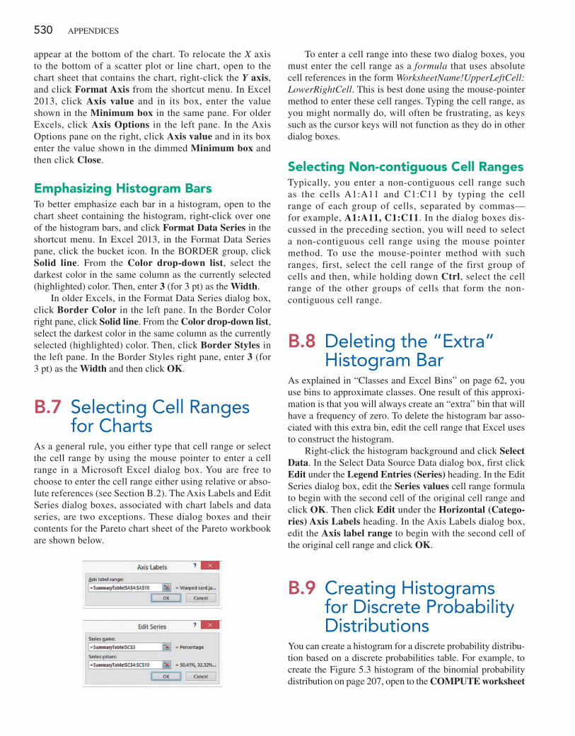
530 APPEnDICES
appear at the bottom of the chart. To relocate the X axis to the bottom of a scatter plot or line chart, open to the chart sheet that contains the chart, right-click the Y axis, and click Format Axis from the shortcut menu. In Excel 2013, click Axis value and in its box, enter the value shown in the Minimum box in the same pane. For older Excels, click Axis Options in the left pane. In the Axis Options pane on the right, click Axis value and in its box enter the value shown in the dimmed Minimum box and then click Close.
Emphasizing Histogram BarsTo better emphasize each bar in a histogram, open to the chart sheet containing the histogram, right-click over one of the histogram bars, and click Format Data Series in the shortcut menu. In Excel 2013, in the Format Data Series pane, click the bucket icon. In the BORDER group, click Solid line. From the Color drop-down list, select the darkest color in the same column as the currently selected (highlighted) color. Then, enter 3 (for 3 pt) as the Width.
In older Excels, in the Format Data Series dialog box, click Border Color in the left pane. In the Border Color right pane, click Solid line. From the Color drop-down list, select the darkest color in the same column as the currently selected (highlighted) color. Then, click Border Styles in the left pane. In the Border Styles right pane, enter 3 (for 3 pt) as the Width and then click OK.
B.7 Selecting Cell Ranges for Charts
As a general rule, you either type that cell range or select the cell range by using the mouse pointer to enter a cell range in a Microsoft Excel dialog box. You are free to choose to enter the cell range either using relative or abso-lute references (see Section B.2). The Axis Labels and Edit Series dialog boxes, associated with chart labels and data series, are two exceptions. These dialog boxes and their contents for the Pareto chart sheet of the Pareto workbook are shown below.
To enter a cell range into these two dialog boxes, you must enter the cell range as a formula that uses absolute cell references in the form WorksheetName!UpperLeftCell: LowerRightCell. This is best done using the mouse-pointer method to enter these cell ranges. Typing the cell range, as you might normally do, will often be frustrating, as keys such as the cursor keys will not function as they do in other dialog boxes.
Selecting Non-contiguous Cell RangesTypically, you enter a non-contiguous cell range such as the cells A1:A11 and C1:C11 by typing the cell range of each group of cells, separated by commas—for example, A1:A11, C1:C11. In the dialog boxes dis-cussed in the preceding section, you will need to select a non-contiguous cell range using the mouse pointer method. To use the mouse-pointer method with such ranges, first, select the cell range of the first group of cells and then, while holding down Ctrl, select the cell range of the other groups of cells that form the non-contiguous cell range.
B.8 Deleting the “Extra” Histogram Bar
As explained in “Classes and Excel Bins” on page 62, you use bins to approximate classes. One result of this approxi-mation is that you will always create an “extra” bin that will have a frequency of zero. To delete the histogram bar asso-ciated with this extra bin, edit the cell range that Excel uses to construct the histogram.
Right-click the histogram background and click Select Data. In the Select Data Source Data dialog box, first click Edit under the Legend Entries (Series) heading. In the Edit Series dialog box, edit the Series values cell range formula to begin with the second cell of the original cell range and click OK. Then click Edit under the Horizontal (Catego-ries) Axis Labels heading. In the Axis Labels dialog box, edit the Axis label range to begin with the second cell of the original cell range and click OK.
B.9 Creating Histograms for Discrete Probability Distributions
You can create a histogram for a discrete probability distribu-tion based on a discrete probabilities table. For example, to create the Figure 5.3 histogram of the binomial probability distribution on page 207, open to the COMPUTE worksheet

APPEnDIX B Important Excel and Minitab Skills 531
of the Binomial workbook. Select the cell range B14:B18, the probabilities in the Binomial Probabilities Table, and:
1. Select Insert ➔ Column and select the first 2-D Column gallery choice (Clustered Column).
2. Right-click the chart background and click Select Data.
In the Select Data Source dialog box:
3. Click Edit under the Horizontal (Categories) Axis Labels heading.
4. In the Axis Labels dialog box, enter the cell range formula = COMPUTE!A14:A18 as the Axis label range. (See Section B.7 to learn how to best enter this cell range formula.) Click OK to return to the Select Data Source dialog box.
5. Back in the Select Data Source dialog box, click OK.
In the chart:
6. Right-click inside a bar and click Format Data Series in the shortcut menu.
In the Format Data Series dialog box:
7. Click Series Options in the left pane. In the Series Options right pane, change the Gap Width slider to Large Gap. Click Close.
Relocate the chart to a chart sheet and adjust the chart for-matting by using the instructions in Section B.6.
B.10 Basic Minitab Operations
Open or Save FilesUse File ➔ Open Worksheet or File ➔ Open Project and File ➔ Save Current Worksheet or File ➔ Save Project As.
In Minitab, you can open and save individual worksheets or various open or save dialog boxes, you select the storage folder by using the drop-down list at the top of either dialog box and enter, or select from the list, name for the file. To save data in a form readable by Excel, select Excel from the Save as type drop-down list before you click Save. Other formats you might use include a simple text file, Text, or simple text with values delimited with commas, CSV.
In Minitab, you can also open and save individual graphs and a project’s session window, although these op-erations are never used in this book.
Insert or Copy WorksheetsUse File ➔ New or File ➔ Open Worksheet.To insert a new worksheet, select File ➔ New and in the new dialog box click Minitab Worksheet and then click OK. To insert a copy of a worksheet, select File ➔ Open Worksheet and select the project that contains the work-sheet to be copied. Selecting a project (and not a worksheet) displays a second dialog box in which you can select the worksheet to be copied.
Print WorksheetsUse File ➔ Print Worksheet (or Print Graph or Print Session Window).Selecting Print Worksheet displays the Data Window Print Options dialog box. In this dialog box, you specify the for-matting options for printing (the default selections should be fine) and enter a title for the printout. Selecting Print Graph or Print Session Window displays the Print dialog box that allows you to change the default printer settings.
If you need to change the paper size or paper orientation of your printout, first select File ➔ Print Setup and make the appropriate selections in the Print dialog box before you select the Print command.
532
C.1 About the Online Resources for This Book
Online resources support your study of business statistics and your use of this book. Online resources are available from the student download web page or MyStatLab course for this book. Some resources are packaged as a zip archive files. The online resources for this book are:
• Excel and Minitab Data files The files that contain the data used in chapter examples, named in problems, or used in the end-of-chapter cases. Section C.3 includes a complete listing of these files and their contents.
• Excel Guide Workbooks Excel workbooks that con-tain templates or model solutions for applying Excel to a particular statistical method. Section C.3 includes a com-plete listing of these files.
• Files for the Digital Cases The set of PDF files that support the end-of-chapter Digital Cases. Some of the Digital Case PDF files contain attached files as well.
• Online Topics The set of PDF format files that pres-ent additional statistical topics. This set includes the full text of two chapters, “Statistical Applications in Quality Management” and “Decision Making.”
• Short Takes The set of PDF files that extend the dis-cussion of specific concepts or further document the results presented in the book.
• Visual Explorations Workbooks The workbooks that interactively demonstrate various key statistical con-cepts. See Visual Explorations in Section C.3 for addi-tional information.
If you plan to use PHStat, the Pearson Education statistics add-in for Microsoft Excel, see Section C.4.
C.2 Accessing the Online Resources
Online resources for this book are available either on the stu-dent download page for this book or inside the MyStatLab course for this book (see Section C.3). To access resources from the student download page for this book:
1. Visit www.pearsonglobaleditions.com/Levine. 2. In that web page, find the entries for this book, Business
Statistics: A First Course, seventh edition, and click the student download page link.
3. In the download page, click the link for the desired items. Most items will cause the web browser to prompt
you to save the (zip archive) that you can save and later unzip. Some download links may require an access code (see Section C.2).
To access resources from the MyStatLab course for this book, log into the course and in the left panel of the course page for this book, click Tools for Success. On that page, click the link for one of the online resource categories listed in Section C.1.
Using MyStatLab requires an access code. An access code may have been packaged with this book. If your book did not come with an access code, you can obtain one at mypearson.com.
C.3 Details of Downloadable Files
Data FilesThroughout this book, the names of data workbooks appear in a special inverted color typeface—for example, Retirement Funds . Data files are stored as worksheets in both the .xlsx Excel workbook and the .mtw Minitab worksheet file formats. (For files that contain more than one worksheet, Minitab versions are stored as .mpj Minitab project files.)
In the following alphabetical list, the variables for each data file are presented in the order of their appearance, starting with first column (A in Excel and C1 in Minitab). Chapter references indicate the chapter or chapters that use the data file in an example or problem. A trailing (E) notes a file exclusive to Excel. A trailing (M) notes a file exclusive to Minitab.
311CALLCENTER Day and abandonment rate (%) (Chapter 3)
ACCOUNTINGPARTNERS Firm and number of part-ners (Chapter 3)
ACCOUNTINGPARTNERS2 Region and number of partners (Chapter 10)
ACCOUNTINGPARTNERS4 Region and number of partners (Chapter 10)
ADINDEX Respondent, cola A Adindex, and cola B Adindex (Chapter 10)
AMS2-1 Types of errors and frequency, types of errors and cost, types of wrong billing errors and cost (as three sepa-rate worksheets) (Chapter 2)
AMS2-2 Days and number of calls (Chapter 2)
AMS8 Rate willing to pay ($) (Chapter 8)
AMS9 Upload speed (Chapter 9)
A p p e n d i x C Online Resources
APPEnDIx C Online Resources 533
AMS10-1 Update times for email interface 1 and email interface 2 (Chapter 10)
AMS10-2 Update times for system 1, system 2, and system 3 (Chapter 10)
AMS12 number of hours spent telemarketing and number of new subscriptions (Chapter 12)
AMS13 Week, number of new subscriptions, hours spent telemarketing, and type of presentation (formal or infor-mal) (Chapter 13)
ANSCOMBE Data sets A, B, C, and D, each with 11 pairs of X and Y values (Chapter 12)
ATM TRANSACTIONS Cause, frequency, and percent-age (Chapter 2)
AUDITS Year and number of audits (Chapter 2)
AUTOMAKER1 Automaker and number of complaints (Chapter 2)
AUTOMAKER2 Category and number of complaints (Chapter 2)
AUTOSALES Manufacturer, sales, and change percentage (Chapter 2)
BANK1 Waiting time (in minutes) of 15 customers at a bank located in a commercial district (Chapters 3, 9, and 10)
BANK2 Waiting time (in minutes) of 15 customers at a bank located in a residential area (Chapters 3 and 10)
BANK3 Waiting time (in minutes) of 15 customers at a bank located in a commercial district (Chapter 10)
BANK4 Waiting time (in minutes) of 15 customers at a bank located in a residential area (Chapter 10)
BASEBALL Team, E.R.A, runs scored per game, league (0 = American, 1 = national), wins (Chapters 12 and 13)
BBCOST2012 Team and fan cost index (Chapter 2)
BESTFUNDS1 Fund type (short-term or long-term), 1-year return, and 3-year return (Chapter 10)
BESTFUNDS2 Fund type (short-term, long-term, or world), 1-year return, and 3-year return (Chapter 10)
BESTFUNDS3 Fund type (small, mid-cap, or large), 1-year return, and 3-year return (Chapter 10)
BOOKPRICES Author, title, bookstore price, and online price ($) (Chapter 10)
BRANDZTECHFIN Brand, brand value in 2014 ($mil-lions), % change in brand value from 2013, region, and sector (Chapter 10)
BRYNNEPACKAGING WPCT score and rating (Chapter 12)
BULBS Manufacturer (1 = A, 2 = B) and length of life (hours) (Chapters 2 and 10)
BUNDLE Restaurant, bundle score, and typical cost ($) (Chapter 2)
BUSINESSVALUATION Drug company name, price to book value ratio, return on equity (ROE), and growth% (Chapter 13)
CAFFEINE Caffeine per fluid ounce (mg/oz) (Chapter 2)
CARDIOGOODFITNESS Product purchased (TM195, TM498, TM798), age in years, gender (Male or Female), education in years, relationship status (Single or Partnered), average number of times the customer plans to use the tread-mill each week, self-rated fitness on a 1-to-5 ordinal scale 11 = poor to 5 = excellent2, annual household income ($), and average number of miles the customer expects to walk/run each week (Chapters 2, 3, 6, 8, 10, and 11)
CARMODELS Horsepower of a car’s engine and weight of each car (in pounds) (Chapter 13)
CATFOOD Ounces eaten of kidney, shrimp, chicken liver, salmon, and beef cat food (Chapter 10)
CDRATE Bank, 1-year CD rate, and 5-year CD rate (Chapters 2, 3, 6, and 8)
CEO-COMPENSATION Company, CEO compensation ($millions), and return in 2012 (Chapter 2)
CEO-COMPENSATION2013 Company, CEO compensa-tion ($millions), and return in 2013 ($millions) (Chapter 12)
CEREALS Cereal, calories, carbohydrates, and sugar (Chapters 2, 3, and 12)
CHALLENGING Data and charts for Figure 2.19 (Chapter 2)
CIGARETTETAX State and cigarette tax ($) (Chapters 2 and 3)
COFFEE Expert and rating of coffees by brand A, B, C, and D (Chapter 10)
COFFEEDRINK Calories and fat contained in different coffee drinks (in grams) (Chapter 12)
COFFEESALES Coffee sales at $0.59, $0.69, $0.79, and $0.89 (Chapter 10)
COLA Beverage end-cap sales and produce end-cap sales (Chapter 10)
COLLEGE FOOTBALL Head coach, school, conference, school pay of head coach, other pay, total pay, max bonus, and football net revenue (Chapters 2, 3, and 12)
COMMUNITYBANKS Institution, location, return on investment (ROI%), efficiency ratio (%), total risk based capital (%) (Chapter 13)
CONCRETE1 Sample number and compressive strength after two days and seven days (Chapter 10)
CONGESTION City, annual time waiting in traffic (hours), and cost of waiting in traffic ($) (Chapters 2 and 3)
CREDIT SCORES City, state, and average credit score (Chapters 2 and 3)
CURRENCY Year, coded year, and exchange rates (against the U.S. dollar) for the Canadian dollar, Japanese yen, and English pound sterling (Chapter 2)

534 APPEnDICES
DELIVERY Customer, number of cases, and delivery time (Chapter 12)
DOINGBUSINESS Region, country name, 2012 GDP per capita, Internet users 2011 (per 100 people), and mobile cellular subscriptions 2011 (per 100 people) (Chapter 2)
DOMESTICBEER Brand, alcohol percentage, calories, and carbohydrates (Chapters 2, 3, and 6)
DOWDOGS Stock and one-year return (Chapter 3)
DOWMARKETCAP Company and market capitalization ($billions) (Chapters 3 and 6)
DOWNLOADSPEED Country and download speed in Mbps (Chapter 3)
DRILL Depth, time to drill additional 5 feet, and type of hole (dry or wet) (Chapter 13)
DRINK Amount of soft drink filled in 2-liter bottles (Chapters 2 and 9)
ENERGY State and per capita kilowatt hour use (Chapter 3)
ERWAITING Emergency room waiting time (in minutes) at the main facility and at satellite 1, satellite 2, and satel-lite 3 (Chapter 10)
ESPRESSO Tamp (inches) and time (seconds) (Chapter 12)
FASTFOOD Amount spent on fast food ($) (Chapters 2, 8, and 9)
FASTFOODCHAIN Mean sales per unit for burger, chicken, sandwich, and pizza segments (Chapter 10)
FIFTEENWEEKS Week number, number of customers, and sales ($thousands) over a period of 15 consecutive weeks (Chapter 12)
FIVEYEARCDRATE Five-year CD rates in new York and Los Angeles (Chapter 10)
FORCE Force required to break an insulator (Chapters 2, 3, 8, and 9)
FOREIGNMARKET Country, level of development (Emerging or Developed), and time required to start a business (days) (Chapter 10)
FOREIGNMARKET2 Country, region, cost to export container (US$), cost to import container (US$) (Chapter 10)
FTGLOBAL500 Sector (Automobiles & parts, Financial services, Health care equipment & services, or Software & computer services), country, company, market cap ($billions), and 52-week change (%) (Chapter 2)
FURNITURE Days between receipt and resolution of complaints regarding purchased furniture (Chapters 2, 3, 8, and 9)
GCROSLYN Address, location (Glen Cove or Roslyn), fair market value ($thousands), property size (acres), age, house size (sq. ft.), number of rooms, number of bathrooms, and number of cars that can be parked in the garage (Chapter 13)
GLENCOVE Address, fair market value ($thousands), property size (acres), age, house size (sq. ft.), number of rooms, number of bathrooms, and number of cars that can be parked in the garage (Chapter 13)
GLOBALSOCIALMEDIA Country, GDP, and social media usage (%) (Chapters 2, 3, and 12)
GOLFBALL Distance for designs 1, 2, 3, and 4 (Chapter 10)
GPIGMAT GMAT scores and GPA (Chapter 12)
GRADSURVEY ID, gender (Female or Male), age (as of last birthday), graduate major (Accounting, CIS, Economics/Finance, International Business, Management, Retailing/Marketing, or Other), current graduate GPA, undergradu-ate major (Biological Sciences, Business, Engineering, or Other), undergraduate GPA, current employment status (Full-Time, Part-Time, or Unemployed), number of different full-time jobs held in the past 10 years, expected salary upon com-pletion of MBA ($thousands), amount spent for books and supplies this semester ($), advisory rating, type of computer owned (Desktop or Laptop), text messages per week, wealth accumulated to feel rich (Chapters 1, 2, 3, 4, 6, 8, 10, and 11)
GRANULE Granule loss in Boston and Vermont shingles (Chapters 3, 8, and 9)
HOTELAWAY nationality and price (US$) (Chapter 3)
HOTELPRICES City and average price (US$) of a hotel room at a 2-star price, 3-star price, and 4-star hotel (Chapters 2 and 3)
ICECREAM Daily temperature (in degrees Fahrenheit) and sales ($thousands) for 21 days (Chapter 12)
INSURANCE Processing time in days for insurance poli-cies (Chapters 3, 8, and 9)
INSURANCECLAIMS Claims, buildup (0 = buildup not indicated, 1 = buildup indicated), excess payment ($) (Chapter 8)
INTERNETMOBILETIME Time spent per day access-ing the Internet via mobile device (minutes) (Chapter 9)
INTERNETMOBILETIME2 Gender (F or M), time spent per day accessing the Internet via mobile device (minutes) (Chapter 10)
INVOICES Amount recorded (in dollars) from sales invoices (Chapter 9)
LUGGAGE Delivery time (in minutes) for luggage in Wing A and Wing B of a hotel (Chapter 10)
MARKET PENETRATION Country and Facebook pen-etration (in percentage) (Chapters 3 and 8)
MOBILE ELECTRONICS In-aisle sales, front sales, kiosk sales, and expert area sales (Chapter 10) (E)
MOBILE ELECTRONICS STACKED Stacked version of Mobile Electronics (Chapter 10) (M)
MOISTURE Moisture content of Boston shingles and Vermont shingles (Chapter 9)

APPEnDIx C Online Resources 535
MOTIVATION Factor, mean rating by global employees, and mean rating by U.S. employees (Chapter 10)
MOVIE Title, box office gross ($millions), and DVD rev-enue ($millions) (Chapter 12)
MOVIE ATTENDANCE Year and movie attendance (bil-lions) (Chapter 2)
MOVIE REVENUES Year and revenue ($billions) (Chapter 2)
MOVING Labor hours, cubic feet, number of large pieces of furniture, and availability of an elevator (Chapters 12 and 13)
MYELOMA Patient, before transplant measurement, after transplant measurement (Chapter 10)
NATURAL GAS Month, wellhead price ($/thousands cu. ft.), and residential price ($/thousands cu. ft.) (Chapter 2)
NBA Team, team code, wins, field goal %, three-point field goal % (Chapter 13)
NBACOST2013 Team, fan cost index ($) (Chapters 2 and 6)
NBAVALUES Team, team code, annual revenue ($mil-lions), and value ($millions) and 1-year change in value (%) (Chapters 2, 3, and 12)
NEEDS need and frequency (Chapter 2)
NEIGHBOR Selling price ($thousands), number of rooms, neighborhood location 10 = east, 1 = west2 (Chapter 13)
NEWHOMESALES Month, sales in thousands, and mean price ($thousands) (Chapter 2)
OIL&GASOLINE Week, price of a gallon of gasoline ($), and price of oil per barrel, ($) (Chapter 12)
OMNIPOWER Bars sold, price (cents), and promotion expenses ($) (Chapter 13)
ONLINE SHOPPING Main reason and percentage (Chapter 2)
ORDER Time in minutes to fill orders for a population of 200 (Chapter 8)
PACKAGINGFOAM3 Die temperature, die diameter, and foam density (Chapter 13)
PACKAGINGFOAM4 Die temperature, die diameter, and foam diameter (Chapter 13)
PALLET Weight of Boston shingles and weight of Vermont shingles (Chapters 2, 8, 9, and 10)
PEN Ad and product rating (Chapter 10)
PHONE Time (in minutes) to clear telephone line prob-lems and location 11 = I, 2 = II2 (Chapter 10)
PIZZATIME Time period, delivery time for local restau-rant, and delivery time for national chain (Chapter 10)
POTTERMOVIES Title, first weekend gross ($millions), U.S. gross ($millions), and worldwide gross ($millions) (Chapters 2, 3, and 12)
PROPERTYTAXES State and property taxes per capita ($) (Chapters 2, 3, and 6)
PROTEIN Type of food, calories (in grams), protein, per-centage of calories from fat, percentage of calories from saturated fat, and cholesterol (mg) (Chapters 2 and 3)
PUMPKIN Circumference and weight of pumpkins (Chapter 12)
RADIOSHACK State and number of stores (Chapters 3)
REDANDWHITE Fixed acidity, volatile acidity, citric acid, residual sugar, chlorides, free sulfur dioxide, total sulfur dioxide, density, pH, sulphates, alcohol, wine type coded 10 = White, 1 = Red2, wine type (Red or White), quality (Chapter 13)
REDWOOD Height (ft.), breast height diameter (in.), and bark thickness (in.) (Chapters 12 and 13)
RENTSILVERSPRING Apartment size (sq. ft.) and monthly rental cost ($) (Chapter 12)
RESTAURANTS Location (City or Suburban), food rat-ing, decor rating, service rating, summated rating, coded location 10 = City, 1 = Suburban2, and cost of a meal (Chapters 2, 3, 10, 12, and 13)
RETIREMENT FUNDS Fund number, market cap (Small, Mid-Cap, or Large), type (Growth or Value), assets ($mil-lions), turnover ratio, beta (measure of the volatility of a stock), standard deviation (measure of returns relative to 36-month average), risk (Low, Average, or High), 1-year return, 3-year return, 5-year return, 10-year return, expense ratio, star rating (Chapters 2, 3, 4, 6, 8, 10, and 11)
SEDANS Miles per gallon for 2014 midsized sedans (Chapters 3 and 8)
SILVERSPRING Address, asking price ($000), assessed value ($000), taxes ($), size (thousands sq. ft.) fireplace coded 10 = no, 1 = yes2, number of bedrooms, num-ber of bathrooms, age (years), fireplace (no or Yes) (Chapters 12 and 13)
SITESELECTION Store number, profiled customers, and sales ($millions) (Chapter 12)
SMALLBUSINESSES Company, earnings per share growth (%), sales growth (%), and return on equity (%) (Chapter 10)
SMARTPHONES Price ($) (Chapter 3)
SMARTPHONE SALES Type and market share percent-age for the years 2011 through 2013 (Chapter 2)
SOCCERVALUES2014 Team, revenues ($millions), and value ($millions) (Chapter 12)
STANDBY Standby hours, total staff present, remote hours, Dubner hours, and total labor hours (Chapter 13)
STARBUCKS Tear, viscosity, pressure, plate gap (Chapters 12 and 13)
STEEL Error in actual length and specified length (Chapters 2, 6, 8, and 9)
536 APPEnDICES
STOCK PERFORMANCE Decade and stock perfor-mance (%) (Chapter 2)
STOCKPRICES2013 Date, S&P 500 value, and closing weekly stock price for GE, Discovery Communications, and Google (Chapter 12)
STUDYTIME Gender and study time in hours (Chapter 10)
SUBURBANNEIGHBOR size of homes (number of rooms) and the selling price ($thousands) in the East side and West side community (Chapter 13)
SUPERMARKET Total number of customers in the store and the waiting time (Chapter 12)
SUV Miles per gallon for 2014 small SUVs (Chapters 3, 6, and 8)
TABLE_5.1 X and P(X) (Chapter 5) (M)
TABLETS Battery life (hours) for WiFi-only and 3G/4G/WiFi tablets (Chapter 10)
TARGETWALMART Shopping item, Target price ($), and Walmart price ($) (Chapter 10)
TEABAGS Weight of tea bags in ounces (Chapters 3, 8, and 9)
TELECOM Provider, TV rating, and Phone rating (Chapter 10)
THREE-HOTEL SURVEY Choose again? (no or Yes) and Golden Palm, Palm Royale, and Palm Princess tallies (Chapter 12) (M)
TIMES Get-ready times (Chapter 3)
TROUGH Width of trough (Chapters 2, 3, 8, and 9)
TWITTERMOVIES Movie, Twitter activity, and receipts ($) (Chapter 12)
TWO-HOTEL SURVEY Choose again? (no or Yes) and Beachcomber and Windsurfer tallies (Chapter 12) (M)
UNDERGRADSURVEY ID, gender (Female or Male), age (as of last birthday), class designation (Sophomore, Junior, or Senior), major (Accounting, CIS, Economics/Finance, International Business, Management, Retail/Marketing, Other, or Undecided), graduate school intention (no, Yes, or Undecided), cumulative GPA, current employment status (Full-Time, Part-Time, or Unemployed), expected starting salary ($thousands), number of social networking sites registered for, satis-faction with student advisement services on campus, amount spent on books and supplies this semester, type of computer preferred (Desktop, Laptop, or Tablet), text messages per week, wealth accumulated to feel rich (Chapters 1, 2, 3, 4, 6, 8, 10, and 11)
UNSTACKED 1YRRETURN One-year return percentage for growth funds and one-year return percentage for value funds (Chapter 2) (M)
UTILITY Utilities charges ($) for 50 one-bedroom apart-ments (Chapters 2 and 6)
VB Time to complete program (Chapter 10)
VINHOVERDE Fixed acidity, volatile acidity, citric acid, residual sugar, chlorides, free sulfur dioxide, total sul-fur dioxide, density, pH, sulphates, alcohol, and quality (Chapters 12 and 13)
WAIT Waiting time and seating time (Chapter 6)
WARECOST Distribution cost ($thousands), sales ($thou-sands), and number of orders (Chapter 12)
YOURTOWN Appraised value ($thousands), land area of property (acres), and age (years) for single-family homes located in the town (Chapter 13)
Excel Guide WorkbooksExcel Guide workbooks contain templates or model solu-tions for applying Excel to a particular statistical method. Chapter examples and the In-Depth Excel instructions of the Excel Guides feature worksheets from these workbooks and PHStat constructs many of the worksheets from these work-books for you.
Workbooks are stored in the .xlsx Excel workbook for-mat. Most contain a COMPUTE worksheet (often shown in this book) that presents results as well as a COMPUTE_ FORMULAS worksheet that allows you to examine all of the formulas used in the worksheet. The Excel Guide work-books (with the number of the chapter in which each is first mentioned) are:
Recoded (1)Random (1)Data Cleaning (1)Summary Table (2)Contingency Table (2)Distributions (2)Pareto (2)Stem-and-leaf (2)Histogram (2)Polygons (2)Scatter Plot (2)Time Series (2)MCT (2)Descriptive(3)Quartiles (3)Boxplot (3)Parameters (3)Covariance (3)Probabilities (4)Bayes (4)Discrete Variable (5)Binomial (5)Poisson (5)Normal (6)
NPP (6)SDS (7)CIE sigma known (8)CIE sigma unknown (8)CIE Proportion (8)Sample Size Mean (8)Sample Size Proportion (8)Z Mean workbook (9)T mean workbook (9)Z Proportion (9)Pooled-Variance T (10)Separate-Variance T (10)Paired T (10)F Two Variances (10)Z Two Proportions (10)One-Way ANOVA (10)Levene (10)Chi-Square (11)Chi-Square Worksheets (11)Simple Linear Regression (12)Package Delivery (12)Multiple Regression (13)
APPEnDIx C Online Resources 537
Digital Cases, Online Topics, and Short TakesThese files use the Portable Document Format (PDF) that are best viewed using the latest version of Adobe Reader (get.adobe.com/reader/).
Visual ExplorationsVisual Explorations are workbooks that interactively dem-onstrate various key statistical concepts. Three workbooks are add-in workbooks that are stored in the .xlam Excel add-in format. Using these add-in workbooks with Microsoft Windows Excels requires the security settings discussed in Appendix Section D.3. The Visual Explorations work-books are:
VE-Normal Distribution (add-in)VE-Sampling Distribution (add-in)VE-Simple Linear Regression (add-in)VE-Variability
C.4 PHStatPHStat is the Pearson Education statistics add-in for Microsoft Excel that simplifies the task of using Excel as you learn business statistics. PHStat comes packaged as a zip file archive that you download and unzip to the folder of your choice. The archive contains:
PHStat.xlam, the actual add-in workbook that is further discussed in Appendix Sections D.2 and G.1, and these four supporting files:
PHStat readme.pdf Explains the technical requirements, and setup and troubleshooting procedures for PHStat (PDF format).
PHStatHelp.chm The integrated help system for users of Microsoft Windows Excel.
PHStatHelp.pdf The help system as a PDF format file.
PHStatHelp.epub The help system in Open Publication Structure eBook format.
PHStat is available for download with an access code. If your book was packaged with an access code, download PHStat from www.pearsonhighered.com/phstat. Click the download link and follow the instructions for enter-ing the access code. If your book was not packaged with an access code, visit myPearsonStore.com to purchase a PHStat access code.
538
This appendix seeks to eliminate the common types of tech-nical problems that could complicate your use of Microsoft Excel as you learn business statistics with this book. Not all sections of this appendix apply to all readers. Sections with the code (WIN) apply to you if you use Microsoft Excel with Microsoft Windows, while sections with the code (OS X) apply to you if you use Microsoft Excel with OS X (formerly, Mac OS X). Some sections apply to all readers (ALL). (If you use Minitab, there are no configuration issues that you need to address.)
D.1 Getting Microsoft Excel Ready for Use (ALL)You must have an up-to-date, properly licensed copy of Microsoft Excel in order to work through the examples and solve the problems in this book as well as to take advan-tage of the Excel-related workbooks and add-ins described in Appendix C. To get Microsoft Excel ready for use, check and apply Microsoft-supplied updates to Microsoft Excel and Microsoft Office.
If you need to install a new copy of Microsoft Excel on a Microsoft Windows computer system, choose the 32-bit ver-sion and not the 64-bit version even if you have a 64-bit ver-sion of a Microsoft Windows operating system. Many people mistakenly believe that the 64-bit version is somehow “bet-ter,” not realizing that the OS X Excel 2011 is a 32-bit version and that Microsoft advises you to choose the 32-bit version for reasons the company details on its website. (The 64-bit WIN version can process Excel workbooks that are greater than 2GB in size—in other words, big data, as defined in Section GS.3.)
Checking For and Applying UpdatesMicrosoft Excel updates require Internet access and the pro-cess to check for and apply updates differs among Excel versions. If you use a Microsoft Windows version of Excel and use Windows 7 or 8, checking for updates is done by the Windows Update service. If you use an older version of Microsoft Windows, you may have to upgrade to this service. (Visit the Microsoft Download Center, www.microsoft.com/download/default.aspx, for further details.)
Windows Update can automatically apply any updates it finds, although many users prefer to set Windows Update to notify when updates are available and then select and ap-ply updates manually.
In OS X Excel versions and some Microsoft Windows versions, you can manually check for updates. In Excel 2011 (OS X), select Help ➔ Check for Updates and in the dialog box that appears, click Check for Updates. In Excel 2007 (WIN), first click the Office Button and then Excel Options at the bottom of the Office Button window. In the Excel Options dialog box, click Resources in the left pane and then in the right pane click Check for Updates and follow the instructions that appear on the web page that is displayed.
You normally do not manually check for updates in either Excel 2010 (WIN) or Excel 2013 (WIN). However, in some installations of these versions, you can select File ➔ Account ➔ Update Options (2013) or File ➔ Help ➔ Check for Updates (2010) and select options or follow in-structions to manually check for updates.
If all else fails, you can open a web browser and go to the Microsoft Office part of the Microsoft Download Center at www.microsoft.com/download/office.aspx?q=office and manually select and download updates. On the web page displayed, filter the downloadable files by specifying the Excel version you discover by these means:
In Excel 2013 (WIN), select File ➔ Account and then click About Microsoft Excel. In the dialog box that appears note the numbers and codes that follow the phrase “Micro-soft Excel 2013.”
In Excel 2010 (WIN), select File ➔ Help. Under the heading “About Microsoft Excel” click Additional Version and Copyright Information and in the dialog box that ap-pears note the numbers and codes that follow “Microsoft Excel 2010.”
In Excel 2011 (OS X), click Excel ➔ About Excel. The dialog box that appears displays the Version and Latest Installed Update.
In Excel 2007 (WIN), first click the Office Button and then click Excel Options. In the Excel options dia-log box, click Resources in the left pane. In the right pane note the numbers and codes that follow Microsoft Office Excel 2007 under the “about Microsoft Office Excel 2007” heading.
Special Note for Office 365 UsersIf you use Office 365, you are using the most current ver-sion of Excel for your system. At the time of publication, the most current version for Microsoft Windows systems was Excel 2013. For OS X, the most current version was Excel 2011.
A p p e n d i x d Configuring Microsoft Excel

AppENDIX D Configuring Microsoft Excel 539
D.2 Getting PHStat Ready for Use (ALL)
If you plan to use pHStat, the pearson Education add-in workbook that simplifies the use of Microsoft Excel with this book (see Section EG.1 on page 30), you must first download pHStat using an access code as discussed in Section C.4. The pHStat download is a zip file archive that you unzip to the folder of your choice.
pHStat is fully compatible with these Excel versions: Excel 2007 (WIN), Excel 2010 (WIN), Excel 2011 (OS X), and Excel 2013 (WIN). pHStat is not compatible with Excel 2008 (OS X), an Excel version that did not include the capability of running add-in workbooks. If you are using Microsoft Excel with Microsoft Windows (any version), then you must first configure the security settings as discussed in Section D.3. If you are using Microsoft Excel with OS X, no additional steps are required.
D.3 Configuring Excel Security for Add-In Usage (WIN)
The Microsoft Excel security settings can prevent add-ins such as pHStat and the Visual Explorations add-in work-books from opening or functioning properly. To configure these security settings to permit proper pHStat functioning:
1. In Excel 2010 and Excel 2013, select File ➔ Options. In Excel 2007, first click the Office Button and then click Excel Options.
In the Excel Options dialog box (shown below):
2. Click Trust Center in the left pane and then click Trust Center Settings in the right pane.
In the Trust Center dialog box:
3. Click Add-ins in the next left pane, and in the Add-ins right pane clear all of the checkboxes (shown below).
4. Click Macro Settings in the left pane, and in the Macro Settings right pane click Disable all macros with no-tification and check Trust access to the VBA object model (shown below).
5. Click OK to close the Trust Center dialog box.
Back in the Excel Options dialog box:
6. Click OK to finish.
On some systems that have stringent security settings, you might need to modify step 4. For such systems, in step 4, also click Trusted Locations in the left pane and then, in the Trusted Locations right pane, click Add new location to add the folder path that you chose to store the pHStat files.
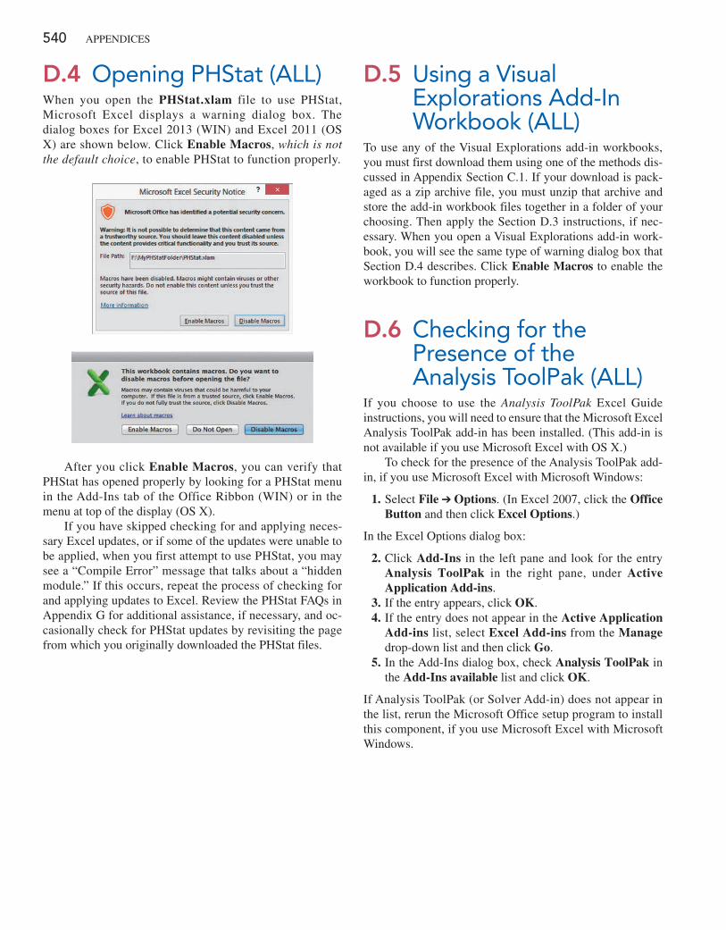
540 AppENDICES
D.4 Opening PHStat (ALL)When you open the PHStat.xlam file to use pHStat, Microsoft Excel displays a warning dialog box. The dialog boxes for Excel 2013 (WIN) and Excel 2011 (OS X) are shown below. Click Enable Macros, which is not the default choice, to enable pHStat to function properly.
After you click Enable Macros, you can verify that pHStat has opened properly by looking for a pHStat menu in the Add-Ins tab of the Office Ribbon (WIN) or in the menu at top of the display (OS X).
If you have skipped checking for and applying neces-sary Excel updates, or if some of the updates were unable to be applied, when you first attempt to use pHStat, you may see a “Compile Error” message that talks about a “hidden module.” If this occurs, repeat the process of checking for and applying updates to Excel. Review the pHStat FAQs in Appendix G for additional assistance, if necessary, and oc-casionally check for pHStat updates by revisiting the page from which you originally downloaded the pHStat files.
D.5 Using a Visual Explorations Add-In Workbook (ALL)
To use any of the Visual Explorations add-in workbooks, you must first download them using one of the methods dis-cussed in Appendix Section C.1. If your download is pack-aged as a zip archive file, you must unzip that archive and store the add-in workbook files together in a folder of your choosing. Then apply the Section D.3 instructions, if nec-essary. When you open a Visual Explorations add-in work-book, you will see the same type of warning dialog box that Section D.4 describes. Click Enable Macros to enable the workbook to function properly.
D.6 Checking for the Presence of the Analysis ToolPak (ALL)
If you choose to use the Analysis ToolPak Excel Guide instructions, you will need to ensure that the Microsoft Excel Analysis Toolpak add-in has been installed. (This add-in is not available if you use Microsoft Excel with OS X.)
To check for the presence of the Analysis Toolpak add-in, if you use Microsoft Excel with Microsoft Windows:
1. Select File ➔ Options. (In Excel 2007, click the Office Button and then click Excel Options.)
In the Excel Options dialog box:
2. Click Add-Ins in the left pane and look for the entry Analysis ToolPak in the right pane, under Active Application Add-ins.
3. If the entry appears, click OK. 4. If the entry does not appear in the Active Application
Add-ins list, select Excel Add-ins from the Manage drop-down list and then click Go.
5. In the Add-Ins dialog box, check Analysis ToolPak in the Add-Ins available list and click OK.
If Analysis Toolpak (or Solver Add-in) does not appear in the list, rerun the Microsoft Office setup program to install this component, if you use Microsoft Excel with Microsoft Windows.
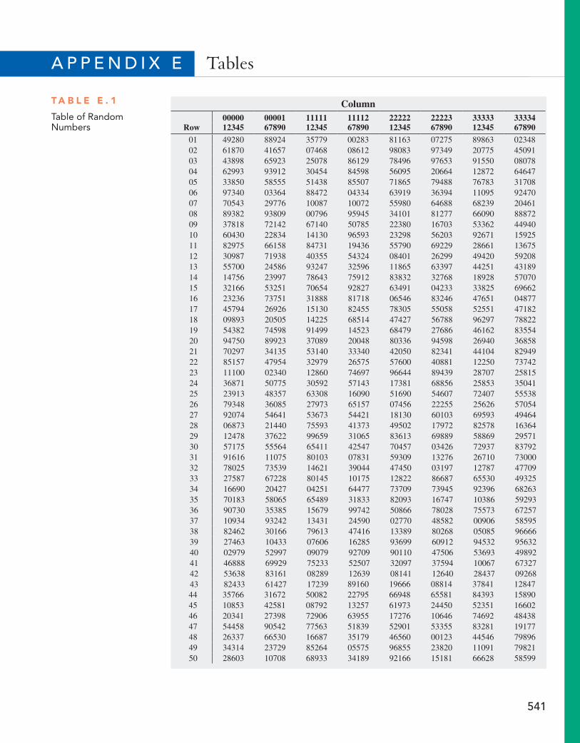
541
A p p e n d i x e Tables
T a b l e e . 1
Table of Random Numbers
Column00000 00001 11111 11112 22222 22223 33333 33334
Row 12345 67890 12345 67890 12345 67890 12345 6789001 49280 88924 35779 00283 81163 07275 89863 0234802 61870 41657 07468 08612 98083 97349 20775 4509103 43898 65923 25078 86129 78496 97653 91550 0807804 62993 93912 30454 84598 56095 20664 12872 6464705 33850 58555 51438 85507 71865 79488 76783 3170806 97340 03364 88472 04334 63919 36394 11095 9247007 70543 29776 10087 10072 55980 64688 68239 2046108 89382 93809 00796 95945 34101 81277 66090 8887209 37818 72142 67140 50785 22380 16703 53362 4494010 60430 22834 14130 96593 23298 56203 92671 1592511 82975 66158 84731 19436 55790 69229 28661 1367512 30987 71938 40355 54324 08401 26299 49420 5920813 55700 24586 93247 32596 11865 63397 44251 4318914 14756 23997 78643 75912 83832 32768 18928 5707015 32166 53251 70654 92827 63491 04233 33825 6966216 23236 73751 31888 81718 06546 83246 47651 0487717 45794 26926 15130 82455 78305 55058 52551 4718218 09893 20505 14225 68514 47427 56788 96297 7882219 54382 74598 91499 14523 68479 27686 46162 8355420 94750 89923 37089 20048 80336 94598 26940 3685821 70297 34135 53140 33340 42050 82341 44104 8294922 85157 47954 32979 26575 57600 40881 12250 7374223 11100 02340 12860 74697 96644 89439 28707 2581524 36871 50775 30592 57143 17381 68856 25853 3504125 23913 48357 63308 16090 51690 54607 72407 5553826 79348 36085 27973 65157 07456 22255 25626 5705427 92074 54641 53673 54421 18130 60103 69593 4946428 06873 21440 75593 41373 49502 17972 82578 1636429 12478 37622 99659 31065 83613 69889 58869 2957130 57175 55564 65411 42547 70457 03426 72937 8379231 91616 11075 80103 07831 59309 13276 26710 7300032 78025 73539 14621 39044 47450 03197 12787 4770933 27587 67228 80145 10175 12822 86687 65530 4932534 16690 20427 04251 64477 73709 73945 92396 6826335 70183 58065 65489 31833 82093 16747 10386 5929336 90730 35385 15679 99742 50866 78028 75573 6725737 10934 93242 13431 24590 02770 48582 00906 5859538 82462 30166 79613 47416 13389 80268 05085 9666639 27463 10433 07606 16285 93699 60912 94532 9563240 02979 52997 09079 92709 90110 47506 53693 4989241 46888 69929 75233 52507 32097 37594 10067 6732742 53638 83161 08289 12639 08141 12640 28437 0926843 82433 61427 17239 89160 19666 08814 37841 1284744 35766 31672 50082 22795 66948 65581 84393 1589045 10853 42581 08792 13257 61973 24450 52351 1660246 20341 27398 72906 63955 17276 10646 74692 4843847 54458 90542 77563 51839 52901 53355 83281 1917748 26337 66530 16687 35179 46560 00123 44546 7989649 34314 23729 85264 05575 96855 23820 11091 7982150 28603 10708 68933 34189 92166 15181 66628 58599
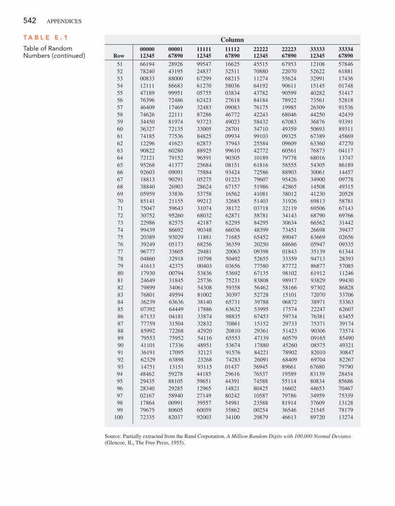
542 appendices
Column00000 00001 11111 11112 22222 22223 33333 33334
Row 12345 67890 12345 67890 12345 67890 12345 6789051 66194 28926 99547 16625 45515 67953 12108 5784652 78240 43195 24837 32511 70880 22070 52622 6188153 00833 88000 67299 68215 11274 55624 32991 1743654 12111 86683 61270 58036 64192 90611 15145 0174855 47189 99951 05755 03834 43782 90599 40282 5141756 76396 72486 62423 27618 84184 78922 73561 5281857 46409 17469 32483 09083 76175 19985 26309 9153658 74626 22111 87286 46772 42243 68046 44250 4243959 34450 81974 93723 49023 58432 67083 36876 9339160 36327 72135 33005 28701 34710 49359 50693 8931161 74185 77536 84825 09934 99103 09325 67389 4586962 12296 41623 62873 37943 25584 09609 63360 4727063 90822 60280 88925 99610 42772 60561 76873 0411764 72121 79152 96591 90305 10189 79778 68016 1374765 95268 41377 25684 08151 61816 58555 54305 8618966 92603 09091 75884 93424 72586 88903 30061 1445767 18813 90291 05275 01223 79607 95426 34900 0977868 38840 26903 28624 67157 51986 42865 14508 4931569 05959 33836 53758 16562 41081 38012 41230 2052870 85141 21155 99212 32685 51403 31926 69813 5878171 75047 59643 31074 38172 03718 32119 69506 6714372 30752 95260 68032 62871 58781 34143 68790 6976673 22986 82575 42187 62295 84295 30634 66562 3144274 99439 86692 90348 66036 48399 73451 26698 3943775 20389 93029 11881 71685 65452 89047 63669 0265676 39249 05173 68256 36359 20250 68686 05947 0933577 96777 33605 29481 20063 09398 01843 35139 6134478 04860 32918 10798 50492 52655 33359 94713 2839379 41613 42375 00403 03656 77580 87772 86877 5708580 17930 00794 53836 53692 67135 98102 61912 1124681 24649 31845 25736 75231 83808 98917 93829 9943082 79899 34061 54308 59358 56462 58166 97302 8682883 76801 49594 81002 30397 52728 15101 72070 3370684 36239 63636 38140 65731 39788 06872 38971 5336385 07392 64449 17886 63632 53995 17574 22247 6260786 67133 04181 33874 98835 67453 59734 76381 6345587 77759 31504 32832 70861 15152 29733 75371 3917488 85992 72268 42920 20810 29361 51423 90306 7357489 79553 75952 54116 65553 47139 60579 09165 8549090 41101 17336 48951 53674 17880 45260 08575 4932191 36191 17095 32123 91576 84221 78902 82010 3084792 62329 63898 23268 74283 26091 68409 69704 8226793 14751 13151 93115 01437 56945 89661 67680 7979094 48462 59278 44185 29616 76537 19589 83139 2845495 29435 88105 59651 44391 74588 55114 80834 8568696 28340 29285 12965 14821 80425 16602 44653 7046797 02167 58940 27149 80242 10587 79786 34959 7533998 17864 00991 39557 54981 23588 81914 37609 1312899 79675 80605 60059 35862 00254 36546 21545 78179
100 72335 82037 92003 34100 29879 46613 89720 13274
source: partially extracted from the Rand corporation, A Million Random Digits with 100,000 Normal Deviates (Glencoe, iL, The Free press, 1955).
T a b l e e . 1
Table of Random Numbers (continued )
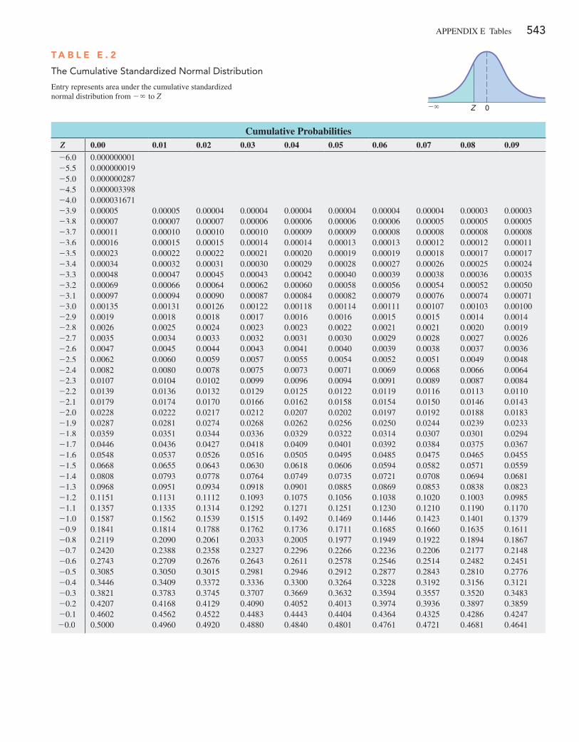
appendix e Tables 543
T a b l e e . 2
The Cumulative Standardized Normal Distribution
entry represents area under the cumulative standardized normal distribution from - ∞ to Z
Cumulative ProbabilitiesZ 0.00 0.01 0.02 0.03 0.04 0.05 0.06 0.07 0.08 0.09
-6.0 0.000000001-5.5 0.000000019-5.0 0.000000287-4.5 0.000003398-4.0 0.000031671-3.9 0.00005 0.00005 0.00004 0.00004 0.00004 0.00004 0.00004 0.00004 0.00003 0.00003-3.8 0.00007 0.00007 0.00007 0.00006 0.00006 0.00006 0.00006 0.00005 0.00005 0.00005-3.7 0.00011 0.00010 0.00010 0.00010 0.00009 0.00009 0.00008 0.00008 0.00008 0.00008-3.6 0.00016 0.00015 0.00015 0.00014 0.00014 0.00013 0.00013 0.00012 0.00012 0.00011-3.5 0.00023 0.00022 0.00022 0.00021 0.00020 0.00019 0.00019 0.00018 0.00017 0.00017-3.4 0.00034 0.00032 0.00031 0.00030 0.00029 0.00028 0.00027 0.00026 0.00025 0.00024-3.3 0.00048 0.00047 0.00045 0.00043 0.00042 0.00040 0.00039 0.00038 0.00036 0.00035-3.2 0.00069 0.00066 0.00064 0.00062 0.00060 0.00058 0.00056 0.00054 0.00052 0.00050-3.1 0.00097 0.00094 0.00090 0.00087 0.00084 0.00082 0.00079 0.00076 0.00074 0.00071-3.0 0.00135 0.00131 0.00126 0.00122 0.00118 0.00114 0.00111 0.00107 0.00103 0.00100-2.9 0.0019 0.0018 0.0018 0.0017 0.0016 0.0016 0.0015 0.0015 0.0014 0.0014-2.8 0.0026 0.0025 0.0024 0.0023 0.0023 0.0022 0.0021 0.0021 0.0020 0.0019-2.7 0.0035 0.0034 0.0033 0.0032 0.0031 0.0030 0.0029 0.0028 0.0027 0.0026-2.6 0.0047 0.0045 0.0044 0.0043 0.0041 0.0040 0.0039 0.0038 0.0037 0.0036-2.5 0.0062 0.0060 0.0059 0.0057 0.0055 0.0054 0.0052 0.0051 0.0049 0.0048-2.4 0.0082 0.0080 0.0078 0.0075 0.0073 0.0071 0.0069 0.0068 0.0066 0.0064-2.3 0.0107 0.0104 0.0102 0.0099 0.0096 0.0094 0.0091 0.0089 0.0087 0.0084-2.2 0.0139 0.0136 0.0132 0.0129 0.0125 0.0122 0.0119 0.0116 0.0113 0.0110-2.1 0.0179 0.0174 0.0170 0.0166 0.0162 0.0158 0.0154 0.0150 0.0146 0.0143-2.0 0.0228 0.0222 0.0217 0.0212 0.0207 0.0202 0.0197 0.0192 0.0188 0.0183-1.9 0.0287 0.0281 0.0274 0.0268 0.0262 0.0256 0.0250 0.0244 0.0239 0.0233-1.8 0.0359 0.0351 0.0344 0.0336 0.0329 0.0322 0.0314 0.0307 0.0301 0.0294-1.7 0.0446 0.0436 0.0427 0.0418 0.0409 0.0401 0.0392 0.0384 0.0375 0.0367-1.6 0.0548 0.0537 0.0526 0.0516 0.0505 0.0495 0.0485 0.0475 0.0465 0.0455-1.5 0.0668 0.0655 0.0643 0.0630 0.0618 0.0606 0.0594 0.0582 0.0571 0.0559-1.4 0.0808 0.0793 0.0778 0.0764 0.0749 0.0735 0.0721 0.0708 0.0694 0.0681-1.3 0.0968 0.0951 0.0934 0.0918 0.0901 0.0885 0.0869 0.0853 0.0838 0.0823-1.2 0.1151 0.1131 0.1112 0.1093 0.1075 0.1056 0.1038 0.1020 0.1003 0.0985-1.1 0.1357 0.1335 0.1314 0.1292 0.1271 0.1251 0.1230 0.1210 0.1190 0.1170-1.0 0.1587 0.1562 0.1539 0.1515 0.1492 0.1469 0.1446 0.1423 0.1401 0.1379-0.9 0.1841 0.1814 0.1788 0.1762 0.1736 0.1711 0.1685 0.1660 0.1635 0.1611-0.8 0.2119 0.2090 0.2061 0.2033 0.2005 0.1977 0.1949 0.1922 0.1894 0.1867-0.7 0.2420 0.2388 0.2358 0.2327 0.2296 0.2266 0.2236 0.2206 0.2177 0.2148-0.6 0.2743 0.2709 0.2676 0.2643 0.2611 0.2578 0.2546 0.2514 0.2482 0.2451-0.5 0.3085 0.3050 0.3015 0.2981 0.2946 0.2912 0.2877 0.2843 0.2810 0.2776-0.4 0.3446 0.3409 0.3372 0.3336 0.3300 0.3264 0.3228 0.3192 0.3156 0.3121-0.3 0.3821 0.3783 0.3745 0.3707 0.3669 0.3632 0.3594 0.3557 0.3520 0.3483-0.2 0.4207 0.4168 0.4129 0.4090 0.4052 0.4013 0.3974 0.3936 0.3897 0.3859-0.1 0.4602 0.4562 0.4522 0.4483 0.4443 0.4404 0.4364 0.4325 0.4286 0.4247-0.0 0.5000 0.4960 0.4920 0.4880 0.4840 0.4801 0.4761 0.4721 0.4681 0.4641
0Z2`
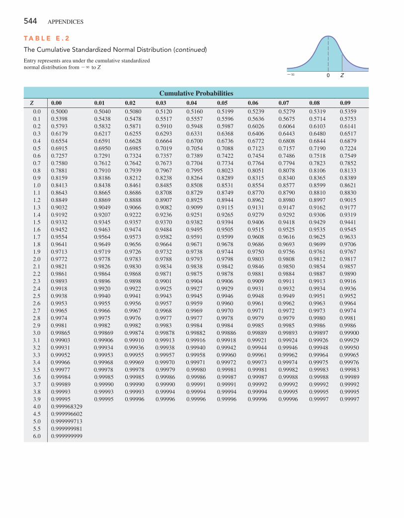
544 appendices
Cumulative ProbabilitiesZ 0.00 0.01 0.02 0.03 0.04 0.05 0.06 0.07 0.08 0.09
0.0 0.5000 0.5040 0.5080 0.5120 0.5160 0.5199 0.5239 0.5279 0.5319 0.53590.1 0.5398 0.5438 0.5478 0.5517 0.5557 0.5596 0.5636 0.5675 0.5714 0.57530.2 0.5793 0.5832 0.5871 0.5910 0.5948 0.5987 0.6026 0.6064 0.6103 0.61410.3 0.6179 0.6217 0.6255 0.6293 0.6331 0.6368 0.6406 0.6443 0.6480 0.65170.4 0.6554 0.6591 0.6628 0.6664 0.6700 0.6736 0.6772 0.6808 0.6844 0.68790.5 0.6915 0.6950 0.6985 0.7019 0.7054 0.7088 0.7123 0.7157 0.7190 0.72240.6 0.7257 0.7291 0.7324 0.7357 0.7389 0.7422 0.7454 0.7486 0.7518 0.75490.7 0.7580 0.7612 0.7642 0.7673 0.7704 0.7734 0.7764 0.7794 0.7823 0.78520.8 0.7881 0.7910 0.7939 0.7967 0.7995 0.8023 0.8051 0.8078 0.8106 0.81330.9 0.8159 0.8186 0.8212 0.8238 0.8264 0.8289 0.8315 0.8340 0.8365 0.83891.0 0.8413 0.8438 0.8461 0.8485 0.8508 0.8531 0.8554 0.8577 0.8599 0.86211.1 0.8643 0.8665 0.8686 0.8708 0.8729 0.8749 0.8770 0.8790 0.8810 0.88301.2 0.8849 0.8869 0.8888 0.8907 0.8925 0.8944 0.8962 0.8980 0.8997 0.90151.3 0.9032 0.9049 0.9066 0.9082 0.9099 0.9115 0.9131 0.9147 0.9162 0.91771.4 0.9192 0.9207 0.9222 0.9236 0.9251 0.9265 0.9279 0.9292 0.9306 0.93191.5 0.9332 0.9345 0.9357 0.9370 0.9382 0.9394 0.9406 0.9418 0.9429 0.94411.6 0.9452 0.9463 0.9474 0.9484 0.9495 0.9505 0.9515 0.9525 0.9535 0.95451.7 0.9554 0.9564 0.9573 0.9582 0.9591 0.9599 0.9608 0.9616 0.9625 0.96331.8 0.9641 0.9649 0.9656 0.9664 0.9671 0.9678 0.9686 0.9693 0.9699 0.97061.9 0.9713 0.9719 0.9726 0.9732 0.9738 0.9744 0.9750 0.9756 0.9761 0.97672.0 0.9772 0.9778 0.9783 0.9788 0.9793 0.9798 0.9803 0.9808 0.9812 0.98172.1 0.9821 0.9826 0.9830 0.9834 0.9838 0.9842 0.9846 0.9850 0.9854 0.98572.2 0.9861 0.9864 0.9868 0.9871 0.9875 0.9878 0.9881 0.9884 0.9887 0.98902.3 0.9893 0.9896 0.9898 0.9901 0.9904 0.9906 0.9909 0.9911 0.9913 0.99162.4 0.9918 0.9920 0.9922 0.9925 0.9927 0.9929 0.9931 0.9932 0.9934 0.99362.5 0.9938 0.9940 0.9941 0.9943 0.9945 0.9946 0.9948 0.9949 0.9951 0.99522.6 0.9953 0.9955 0.9956 0.9957 0.9959 0.9960 0.9961 0.9962 0.9963 0.99642.7 0.9965 0.9966 0.9967 0.9968 0.9969 0.9970 0.9971 0.9972 0.9973 0.99742.8 0.9974 0.9975 0.9976 0.9977 0.9977 0.9978 0.9979 0.9979 0.9980 0.99812.9 0.9981 0.9982 0.9982 0.9983 0.9984 0.9984 0.9985 0.9985 0.9986 0.99863.0 0.99865 0.99869 0.99874 0.99878 0.99882 0.99886 0.99889 0.99893 0.99897 0.999003.1 0.99903 0.99906 0.99910 0.99913 0.99916 0.99918 0.99921 0.99924 0.99926 0.999293.2 0.99931 0.99934 0.99936 0.99938 0.99940 0.99942 0.99944 0.99946 0.99948 0.999503.3 0.99952 0.99953 0.99955 0.99957 0.99958 0.99960 0.99961 0.99962 0.99964 0.999653.4 0.99966 0.99968 0.99969 0.99970 0.99971 0.99972 0.99973 0.99974 0.99975 0.999763.5 0.99977 0.99978 0.99978 0.99979 0.99980 0.99981 0.99981 0.99982 0.99983 0.999833.6 0.99984 0.99985 0.99985 0.99986 0.99986 0.99987 0.99987 0.99988 0.99988 0.999893.7 0.99989 0.99990 0.99990 0.99990 0.99991 0.99991 0.99992 0.99992 0.99992 0.999923.8 0.99993 0.99993 0.99993 0.99994 0.99994 0.99994 0.99994 0.99995 0.99995 0.999953.9 0.99995 0.99995 0.99996 0.99996 0.99996 0.99996 0.99996 0.99996 0.99997 0.999974.0 0.9999683294.5 0.9999966025.0 0.9999997135.5 0.9999999816.0 0.999999999
T a b l e e . 2
The Cumulative Standardized Normal Distribution (continued)
entry represents area under the cumulative standardized normal distribution from - ∞ to Z
0 Z2`
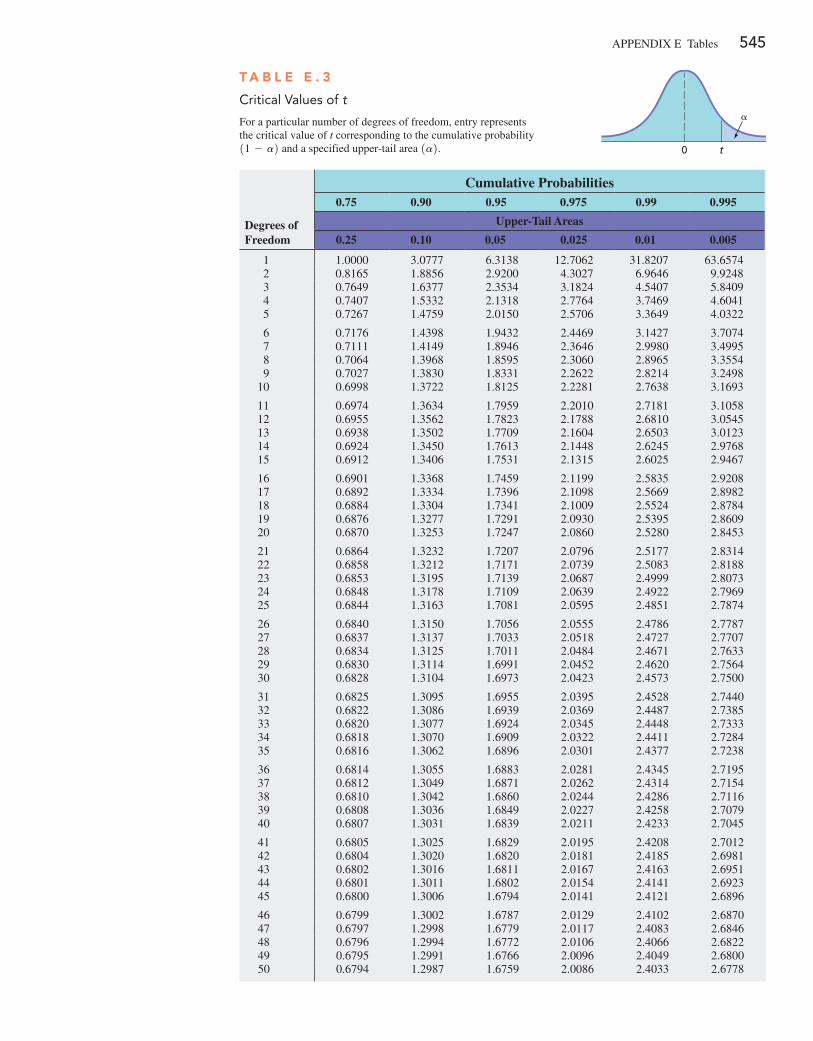
appendix e Tables 545
T a b l e e . 3
Critical Values of t
For a particular number of degrees of freedom, entry represents the critical value of t corresponding to the cumulative probability 11 - a2 and a specified upper-tail area 1a2.
Degrees of Freedom
Cumulative Probabilities0.75 0.90 0.95 0.975 0.99 0.995
Upper-Tail Areas
0.25 0.10 0.05 0.025 0.01 0.005
1 1.0000 3.0777 6.3138 12.7062 31.8207 63.65742 0.8165 1.8856 2.9200 4.3027 6.9646 9.92483 0.7649 1.6377 2.3534 3.1824 4.5407 5.84094 0.7407 1.5332 2.1318 2.7764 3.7469 4.60415 0.7267 1.4759 2.0150 2.5706 3.3649 4.0322
6 0.7176 1.4398 1.9432 2.4469 3.1427 3.70747 0.7111 1.4149 1.8946 2.3646 2.9980 3.49958 0.7064 1.3968 1.8595 2.3060 2.8965 3.35549 0.7027 1.3830 1.8331 2.2622 2.8214 3.2498
10 0.6998 1.3722 1.8125 2.2281 2.7638 3.1693
11 0.6974 1.3634 1.7959 2.2010 2.7181 3.105812 0.6955 1.3562 1.7823 2.1788 2.6810 3.054513 0.6938 1.3502 1.7709 2.1604 2.6503 3.012314 0.6924 1.3450 1.7613 2.1448 2.6245 2.976815 0.6912 1.3406 1.7531 2.1315 2.6025 2.9467
16 0.6901 1.3368 1.7459 2.1199 2.5835 2.920817 0.6892 1.3334 1.7396 2.1098 2.5669 2.898218 0.6884 1.3304 1.7341 2.1009 2.5524 2.878419 0.6876 1.3277 1.7291 2.0930 2.5395 2.860920 0.6870 1.3253 1.7247 2.0860 2.5280 2.8453
21 0.6864 1.3232 1.7207 2.0796 2.5177 2.831422 0.6858 1.3212 1.7171 2.0739 2.5083 2.818823 0.6853 1.3195 1.7139 2.0687 2.4999 2.807324 0.6848 1.3178 1.7109 2.0639 2.4922 2.796925 0.6844 1.3163 1.7081 2.0595 2.4851 2.7874
26 0.6840 1.3150 1.7056 2.0555 2.4786 2.778727 0.6837 1.3137 1.7033 2.0518 2.4727 2.770728 0.6834 1.3125 1.7011 2.0484 2.4671 2.763329 0.6830 1.3114 1.6991 2.0452 2.4620 2.756430 0.6828 1.3104 1.6973 2.0423 2.4573 2.7500
31 0.6825 1.3095 1.6955 2.0395 2.4528 2.744032 0.6822 1.3086 1.6939 2.0369 2.4487 2.738533 0.6820 1.3077 1.6924 2.0345 2.4448 2.733334 0.6818 1.3070 1.6909 2.0322 2.4411 2.728435 0.6816 1.3062 1.6896 2.0301 2.4377 2.7238
36 0.6814 1.3055 1.6883 2.0281 2.4345 2.719537 0.6812 1.3049 1.6871 2.0262 2.4314 2.715438 0.6810 1.3042 1.6860 2.0244 2.4286 2.711639 0.6808 1.3036 1.6849 2.0227 2.4258 2.707940 0.6807 1.3031 1.6839 2.0211 2.4233 2.7045
41 0.6805 1.3025 1.6829 2.0195 2.4208 2.701242 0.6804 1.3020 1.6820 2.0181 2.4185 2.698143 0.6802 1.3016 1.6811 2.0167 2.4163 2.695144 0.6801 1.3011 1.6802 2.0154 2.4141 2.692345 0.6800 1.3006 1.6794 2.0141 2.4121 2.6896
46 0.6799 1.3002 1.6787 2.0129 2.4102 2.687047 0.6797 1.2998 1.6779 2.0117 2.4083 2.684648 0.6796 1.2994 1.6772 2.0106 2.4066 2.682249 0.6795 1.2991 1.6766 2.0096 2.4049 2.680050 0.6794 1.2987 1.6759 2.0086 2.4033 2.6778
0 t
a
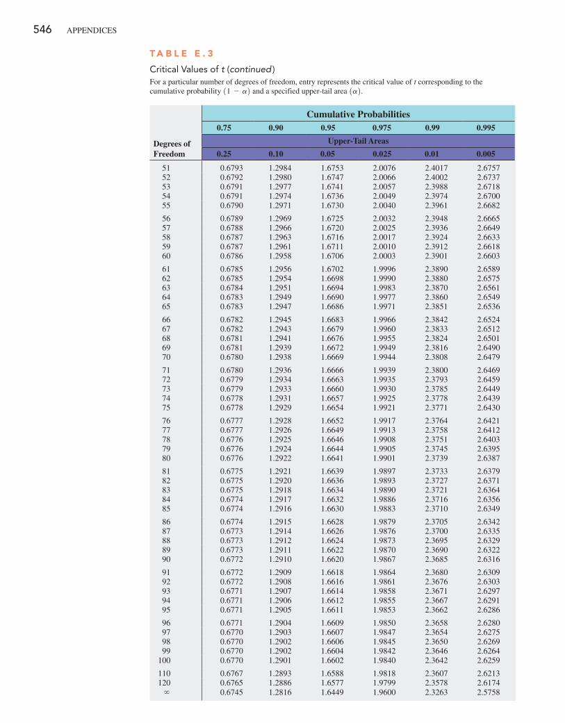
546 appendices
Degrees of Freedom
Cumulative Probabilities0.75 0.90 0.95 0.975 0.99 0.995
Upper-Tail Areas
0.25 0.10 0.05 0.025 0.01 0.005
51 0.6793 1.2984 1.6753 2.0076 2.4017 2.675752 0.6792 1.2980 1.6747 2.0066 2.4002 2.673753 0.6791 1.2977 1.6741 2.0057 2.3988 2.671854 0.6791 1.2974 1.6736 2.0049 2.3974 2.670055 0.6790 1.2971 1.6730 2.0040 2.3961 2.6682
56 0.6789 1.2969 1.6725 2.0032 2.3948 2.666557 0.6788 1.2966 1.6720 2.0025 2.3936 2.664958 0.6787 1.2963 1.6716 2.0017 2.3924 2.663359 0.6787 1.2961 1.6711 2.0010 2.3912 2.661860 0.6786 1.2958 1.6706 2.0003 2.3901 2.6603
61 0.6785 1.2956 1.6702 1.9996 2.3890 2.658962 0.6785 1.2954 1.6698 1.9990 2.3880 2.657563 0.6784 1.2951 1.6694 1.9983 2.3870 2.656164 0.6783 1.2949 1.6690 1.9977 2.3860 2.654965 0.6783 1.2947 1.6686 1.9971 2.3851 2.6536
66 0.6782 1.2945 1.6683 1.9966 2.3842 2.652467 0.6782 1.2943 1.6679 1.9960 2.3833 2.651268 0.6781 1.2941 1.6676 1.9955 2.3824 2.650169 0.6781 1.2939 1.6672 1.9949 2.3816 2.649070 0.6780 1.2938 1.6669 1.9944 2.3808 2.6479
71 0.6780 1.2936 1.6666 1.9939 2.3800 2.646972 0.6779 1.2934 1.6663 1.9935 2.3793 2.645973 0.6779 1.2933 1.6660 1.9930 2.3785 2.644974 0.6778 1.2931 1.6657 1.9925 2.3778 2.643975 0.6778 1.2929 1.6654 1.9921 2.3771 2.6430
76 0.6777 1.2928 1.6652 1.9917 2.3764 2.642177 0.6777 1.2926 1.6649 1.9913 2.3758 2.641278 0.6776 1.2925 1.6646 1.9908 2.3751 2.640379 0.6776 1.2924 1.6644 1.9905 2.3745 2.639580 0.6776 1.2922 1.6641 1.9901 2.3739 2.6387
81 0.6775 1.2921 1.6639 1.9897 2.3733 2.637982 0.6775 1.2920 1.6636 1.9893 2.3727 2.637183 0.6775 1.2918 1.6634 1.9890 2.3721 2.636484 0.6774 1.2917 1.6632 1.9886 2.3716 2.635685 0.6774 1.2916 1.6630 1.9883 2.3710 2.6349
86 0.6774 1.2915 1.6628 1.9879 2.3705 2.634287 0.6773 1.2914 1.6626 1.9876 2.3700 2.633588 0.6773 1.2912 1.6624 1.9873 2.3695 2.632989 0.6773 1.2911 1.6622 1.9870 2.3690 2.632290 0.6772 1.2910 1.6620 1.9867 2.3685 2.6316
91 0.6772 1.2909 1.6618 1.9864 2.3680 2.630992 0.6772 1.2908 1.6616 1.9861 2.3676 2.630393 0.6771 1.2907 1.6614 1.9858 2.3671 2.629794 0.6771 1.2906 1.6612 1.9855 2.3667 2.629195 0.6771 1.2905 1.6611 1.9853 2.3662 2.6286
96 0.6771 1.2904 1.6609 1.9850 2.3658 2.628097 0.6770 1.2903 1.6607 1.9847 2.3654 2.627598 0.6770 1.2902 1.6606 1.9845 2.3650 2.626999 0.6770 1.2902 1.6604 1.9842 2.3646 2.6264
100 0.6770 1.2901 1.6602 1.9840 2.3642 2.6259
110 0.6767 1.2893 1.6588 1.9818 2.3607 2.6213120 0.6765 1.2886 1.6577 1.9799 2.3578 2.6174
∞ 0.6745 1.2816 1.6449 1.9600 2.3263 2.5758
T a b l e e . 3
Critical Values of t (continued )For a particular number of degrees of freedom, entry represents the critical value of t corresponding to the cumulative probability 11 - a2 and a specified upper-tail area 1a2.
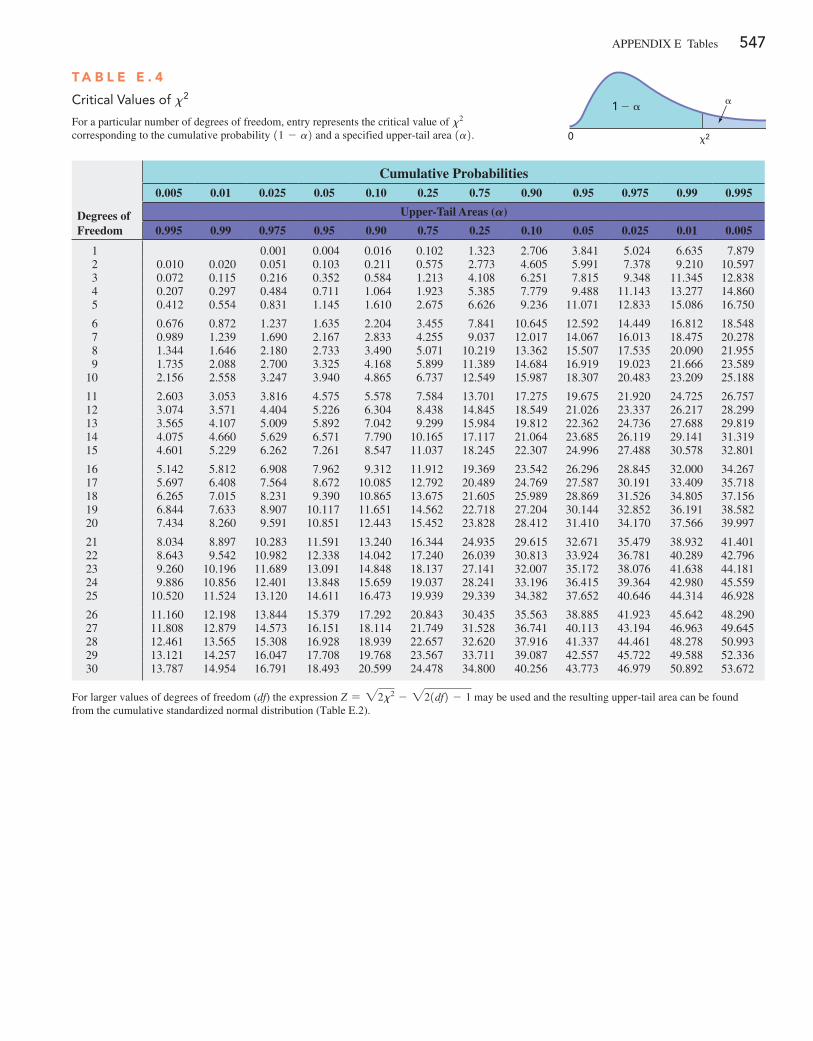
appendix e Tables 547
T a b l e e . 4
Critical Values of x2
For a particular number of degrees of freedom, entry represents the critical value of x2 corresponding to the cumulative probability 11 - a2 and a specified upper-tail area 1a2.
Degrees of Freedom
Cumulative Probabilities0.005 0.01 0.025 0.05 0.10 0.25 0.75 0.90 0.95 0.975 0.99 0.995
Upper-Tail Areas (A)
0.995 0.99 0.975 0.95 0.90 0.75 0.25 0.10 0.05 0.025 0.01 0.005
1 0.001 0.004 0.016 0.102 1.323 2.706 3.841 5.024 6.635 7.8792 0.010 0.020 0.051 0.103 0.211 0.575 2.773 4.605 5.991 7.378 9.210 10.5973 0.072 0.115 0.216 0.352 0.584 1.213 4.108 6.251 7.815 9.348 11.345 12.8384 0.207 0.297 0.484 0.711 1.064 1.923 5.385 7.779 9.488 11.143 13.277 14.8605 0.412 0.554 0.831 1.145 1.610 2.675 6.626 9.236 11.071 12.833 15.086 16.750
6 0.676 0.872 1.237 1.635 2.204 3.455 7.841 10.645 12.592 14.449 16.812 18.5487 0.989 1.239 1.690 2.167 2.833 4.255 9.037 12.017 14.067 16.013 18.475 20.2788 1.344 1.646 2.180 2.733 3.490 5.071 10.219 13.362 15.507 17.535 20.090 21.9559 1.735 2.088 2.700 3.325 4.168 5.899 11.389 14.684 16.919 19.023 21.666 23.589
10 2.156 2.558 3.247 3.940 4.865 6.737 12.549 15.987 18.307 20.483 23.209 25.188
11 2.603 3.053 3.816 4.575 5.578 7.584 13.701 17.275 19.675 21.920 24.725 26.75712 3.074 3.571 4.404 5.226 6.304 8.438 14.845 18.549 21.026 23.337 26.217 28.29913 3.565 4.107 5.009 5.892 7.042 9.299 15.984 19.812 22.362 24.736 27.688 29.81914 4.075 4.660 5.629 6.571 7.790 10.165 17.117 21.064 23.685 26.119 29.141 31.31915 4.601 5.229 6.262 7.261 8.547 11.037 18.245 22.307 24.996 27.488 30.578 32.801
16 5.142 5.812 6.908 7.962 9.312 11.912 19.369 23.542 26.296 28.845 32.000 34.26717 5.697 6.408 7.564 8.672 10.085 12.792 20.489 24.769 27.587 30.191 33.409 35.71818 6.265 7.015 8.231 9.390 10.865 13.675 21.605 25.989 28.869 31.526 34.805 37.15619 6.844 7.633 8.907 10.117 11.651 14.562 22.718 27.204 30.144 32.852 36.191 38.58220 7.434 8.260 9.591 10.851 12.443 15.452 23.828 28.412 31.410 34.170 37.566 39.997
21 8.034 8.897 10.283 11.591 13.240 16.344 24.935 29.615 32.671 35.479 38.932 41.40122 8.643 9.542 10.982 12.338 14.042 17.240 26.039 30.813 33.924 36.781 40.289 42.79623 9.260 10.196 11.689 13.091 14.848 18.137 27.141 32.007 35.172 38.076 41.638 44.18124 9.886 10.856 12.401 13.848 15.659 19.037 28.241 33.196 36.415 39.364 42.980 45.55925 10.520 11.524 13.120 14.611 16.473 19.939 29.339 34.382 37.652 40.646 44.314 46.928
26 11.160 12.198 13.844 15.379 17.292 20.843 30.435 35.563 38.885 41.923 45.642 48.29027 11.808 12.879 14.573 16.151 18.114 21.749 31.528 36.741 40.113 43.194 46.963 49.64528 12.461 13.565 15.308 16.928 18.939 22.657 32.620 37.916 41.337 44.461 48.278 50.99329 13.121 14.257 16.047 17.708 19.768 23.567 33.711 39.087 42.557 45.722 49.588 52.33630 13.787 14.954 16.791 18.493 20.599 24.478 34.800 40.256 43.773 46.979 50.892 53.672
For larger values of degrees of freedom (df) the expression Z = 22x2 - 221df2 - 1 may be used and the resulting upper-tail area can be found from the cumulative standardized normal distribution (Table e.2).
0
a
x2
1 2 a
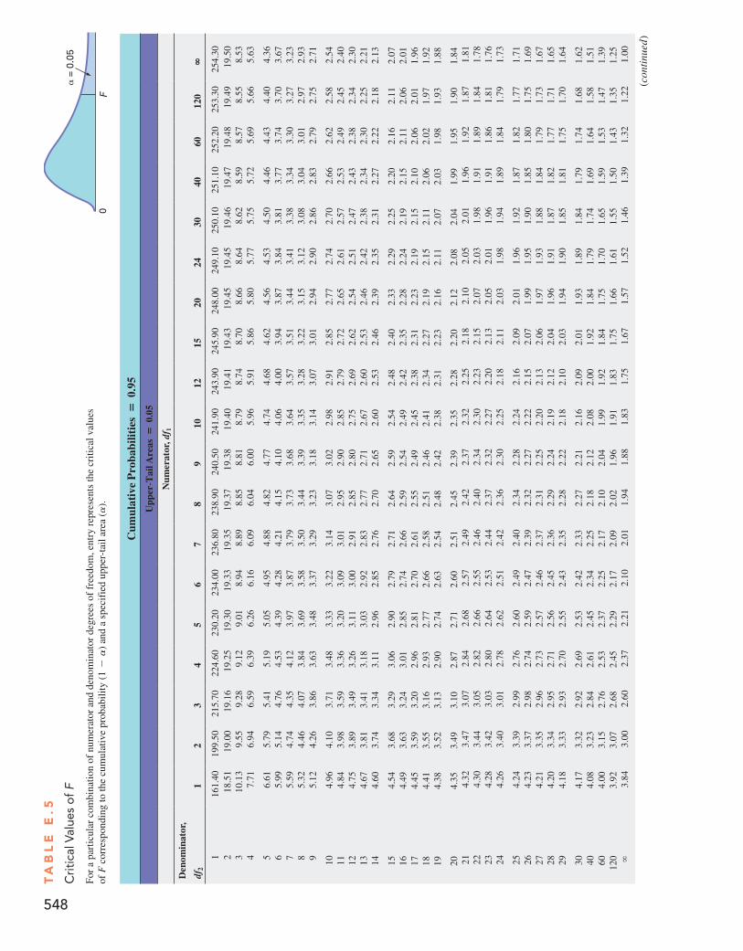
Ta
bl
e e
.5
Cri
tica
l Val
ues
of
F
For
a pa
rtic
ular
com
bina
tion
of n
umer
ator
and
den
omin
ator
deg
rees
of
free
dom
, ent
ry r
epre
sent
s th
e cr
itica
l val
ues
of F
cor
resp
ondi
ng to
the
cum
ulat
ive
prob
abili
ty (
1-
a)
and
a sp
ecif
ied
uppe
r-ta
il ar
ea (a
).
Cum
ulat
ive
Pro
babi
litie
s=
0.95
Upp
er@T
ail A
reas
=0.
05
Num
erat
or, d
f 1
Den
omin
ator
,
df2
12
34
56
78
910
1215
2024
3040
6012
0H
116
1.40
199.
5021
5.70
224.
6023
0.20
234.
0023
6.80
238.
9024
0.50
241.
9024
3.90
245.
9024
8.00
249.
1025
0.10
251.
1025
2.20
253.
3025
4.30
218
.51
19.0
019
.16
19.2
519
.30
19.3
319
.35
19.3
719
.38
19.4
019
.41
19.4
319
.45
19.4
519
.46
19.4
719
.48
19.4
919
.50
310
.13
9.55
9.28
9.12
9.01
8.94
8.89
8.85
8.81
8.79
8.74
8.70
8.66
8.64
8.62
8.59
8.57
8.55
8.53
47.
716.
946.
596.
396.
266.
166.
096.
046.
005.
965.
915.
865.
805.
775.
755.
725.
695.
665.
63
56.
615.
795.
415.
195.
054.
954.
884.
824.
774.
744.
684.
624.
564.
534.
504.
464.
434.
404.
366
5.99
5.14
4.76
4.53
4.39
4.28
4.21
4.15
4.10
4.06
4.00
3.94
3.87
3.84
3.81
3.77
3.74
3.70
3.67
75.
594.
744.
354.
123.
973.
873.
793.
733.
683.
643.
573.
513.
443.
413.
383.
343.
303.
273.
238
5.32
4.46
4.07
3.84
3.69
3.58
3.50
3.44
3.39
3.35
3.28
3.22
3.15
3.12
3.08
3.04
3.01
2.97
2.93
95.
124.
263.
863.
633.
483.
373.
293.
233.
183.
143.
073.
012.
942.
902.
862.
832.
792.
752.
71
104.
964.
103.
713.
483.
333.
223.
143.
073.
022.
982.
912.
852.
772.
742.
702.
662.
622.
582.
5411
4.84
3.98
3.59
3.36
3.20
3.09
3.01
2.95
2.90
2.85
2.79
2.72
2.65
2.61
2.57
2.53
2.49
2.45
2.40
124.
753.
893.
493.
263.
113.
002.
912.
852.
802.
752.
692.
622.
542.
512.
472.
432.
382.
342.
3013
4.67
3.81
3.41
3.18
3.03
2.92
2.83
2.77
2.71
2.67
2.60
2.53
2.46
2.42
2.38
2.34
2.30
2.25
2.21
144.
603.
743.
343.
112.
962.
852.
762.
702.
652.
602.
532.
462.
392.
352.
312.
272.
222.
182.
13
154.
543.
683.
293.
062.
902.
792.
712.
642.
592.
542.
482.
402.
332.
292.
252.
202.
162.
112.
0716
4.49
3.63
3.24
3.01
2.85
2.74
2.66
2.59
2.54
2.49
2.42
2.35
2.28
2.24
2.19
2.15
2.11
2.06
2.01
174.
453.
593.
202.
962.
812.
702.
612.
552.
492.
452.
382.
312.
232.
192.
152.
102.
062.
011.
9618
4.41
3.55
3.16
2.93
2.77
2.66
2.58
2.51
2.46
2.41
2.34
2.27
2.19
2.15
2.11
2.06
2.02
1.97
1.92
194.
383.
523.
132.
902.
742.
632.
542.
482.
422.
382.
312.
232.
162.
112.
072.
031.
981.
931.
88
204.
353.
493.
102.
872.
712.
602.
512.
452.
392.
352.
282.
202.
122.
082.
041.
991.
951.
901.
8421
4.32
3.47
3.07
2.84
2.68
2.57
2.49
2.42
2.37
2.32
2.25
2.18
2.10
2.05
2.01
1.96
1.92
1.87
1.81
224.
303.
443.
052.
822.
662.
552.
462.
402.
342.
302.
232.
152.
072.
031.
981.
911.
891.
841.
7823
4.28
3.42
3.03
2.80
2.64
2.53
2.44
2.37
2.32
2.27
2.20
2.13
2.05
2.01
1.96
1.91
1.86
1.81
1.76
244.
263.
403.
012.
782.
622.
512.
422.
362.
302.
252.
182.
112.
031.
981.
941.
891.
841.
791.
73
254.
243.
392.
992.
762.
602.
492.
402.
342.
282.
242.
162.
092.
011.
961.
921.
871.
821.
771.
7126
4.23
3.37
2.98
2.74
2.59
2.47
2.39
2.32
2.27
2.22
2.15
2.07
1.99
1.95
1.90
1.85
1.80
1.75
1.69
274.
213.
352.
962.
732.
572.
462.
372.
312.
252.
202.
132.
061.
971.
931.
881.
841.
791.
731.
6728
4.20
3.34
2.95
2.71
2.56
2.45
2.36
2.29
2.24
2.19
2.12
2.04
1.96
1.91
1.87
1.82
1.77
1.71
1.65
294.
183.
332.
932.
702.
552.
432.
352.
282.
222.
182.
102.
031.
941.
901.
851.
811.
751.
701.
64
304.
173.
322.
922.
692.
532.
422.
332.
272.
212.
162.
092.
011.
931.
891.
841.
791.
741.
681.
6240
4.08
3.23
2.84
2.61
2.45
2.34
2.25
2.18
2.12
2.08
2.00
1.92
1.84
1.79
1.74
1.69
1.64
1.58
1.51
604.
003.
152.
762.
532.
372.
252.
172.
102.
041.
991.
921.
841.
751.
701.
651.
591.
531.
471.
3912
03.
923.
072.
682.
452.
292.
172.
092.
021.
961.
911.
831.
751.
661.
611.
551.
501.
431.
351.
25∞
3.84
3.00
2.60
2.37
2.21
2.10
2.01
1.94
1.88
1.83
1.75
1.67
1.57
1.52
1.46
1.39
1.32
1.22
1.00
548
(con
tinu
ed )
0F
a =
0.0
5
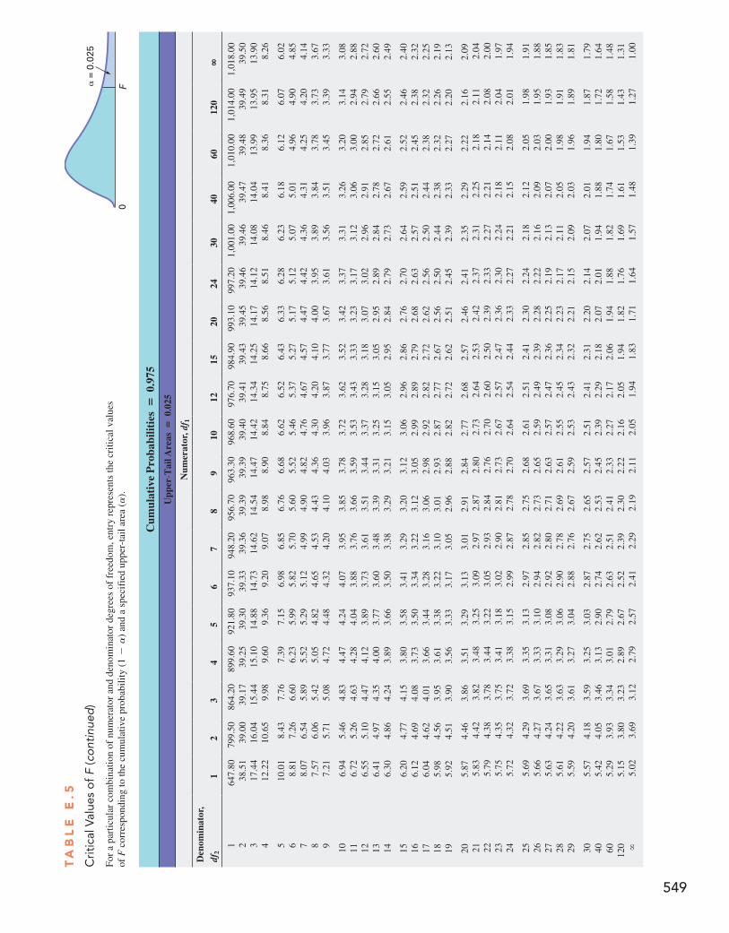
Cum
ulat
ive
Pro
babi
litie
s=
0.97
5
Upp
er@T
ail A
reas
=0.
025
Num
erat
or, d
f 1
Den
omin
ator
, df
21
23
45
67
89
1012
1520
2430
4060
120
H
164
7.80
799.
5086
4.20
899.
6092
1.80
937.
1094
8.20
956.
7096
3.30
968.
6097
6.70
984.
9099
3.10
997.
201,
001.
001,
006.
001,
010.
001,
014.
001,
018.
002
38.5
139
.00
39.1
739
.25
39.3
039
.33
39.3
639
.39
39.3
939
.40
39.4
139
.43
39.4
539
.46
39.4
639
.47
39.4
839
.49
39.5
03
17.4
416
.04
15.4
415
.10
14.8
814
.73
14.6
214
.54
14.4
714
.42
14.3
414
.25
14.1
714
.12
14.0
814
.04
13.9
913
.95
13.9
04
12.2
210
.65
9.98
9.60
9.36
9.20
9.07
8.98
8.90
8.84
8.75
8.66
8.56
8.51
8.46
8.41
8.36
8.31
8.26
510
.01
8.43
7.76
7.39
7.15
6.98
6.85
6.76
6.68
6.62
6.52
6.43
6.33
6.28
6.23
6.18
6.12
6.07
6.02
68.
817.
266.
606.
235.
995.
825.
705.
605.
525.
465.
375.
275.
175.
125.
075.
014.
964.
904.
857
8.07
6.54
5.89
5.52
5.29
5.12
4.99
4.90
4.82
4.76
4.67
4.57
4.47
4.42
4.36
4.31
4.25
4.20
4.14
87.
576.
065.
425.
054.
824.
654.
534.
434.
364.
304.
204.
104.
003.
953.
893.
843.
783.
733.
679
7.21
5.71
5.08
4.72
4.48
4.32
4.20
4.10
4.03
3.96
3.87
3.77
3.67
3.61
3.56
3.51
3.45
3.39
3.33
106.
945.
464.
834.
474.
244.
073.
953.
853.
783.
723.
623.
523.
423.
373.
313.
263.
203.
143.
0811
6.72
5.26
4.63
4.28
4.04
3.88
3.76
3.66
3.59
3.53
3.43
3.33
3.23
3.17
3.12
3.06
3.00
2.94
2.88
126.
555.
104.
474.
123.
893.
733.
613.
513.
443.
373.
283.
183.
073.
022.
962.
912.
852.
792.
7213
6.41
4.97
4.35
4.00
3.77
3.60
3.48
3.39
3.31
3.25
3.15
3.05
2.95
2.89
2.84
2.78
2.72
2.66
2.60
146.
304.
864.
243.
893.
663.
503.
383.
293.
213.
153.
052.
952.
842.
792.
732.
672.
612.
552.
49
156.
204.
774.
153.
803.
583.
413.
293.
203.
123.
062.
962.
862.
762.
702.
642.
592.
522.
462.
4016
6.12
4.69
4.08
3.73
3.50
3.34
3.22
3.12
3.05
2.99
2.89
2.79
2.68
2.63
2.57
2.51
2.45
2.38
2.32
176.
044.
624.
013.
663.
443.
283.
163.
062.
982.
922.
822.
722.
622.
562.
502.
442.
382.
322.
2518
5.98
4.56
3.95
3.61
3.38
3.22
3.10
3.01
2.93
2.87
2.77
2.67
2.56
2.50
2.44
2.38
2.32
2.26
2.19
195.
924.
513.
903.
563.
333.
173.
052.
962.
882.
822.
722.
622.
512.
452.
392.
332.
272.
202.
13
205.
874.
463.
863.
513.
293.
133.
012.
912.
842.
772.
682.
572.
462.
412.
352.
292.
222.
162.
0921
5.83
4.42
3.82
3.48
3.25
3.09
2.97
2.87
2.80
2.73
2.64
2.53
2.42
2.37
2.31
2.25
2.18
2.11
2.04
225.
794.
383.
783.
443.
223.
052.
932.
842.
762.
702.
602.
502.
392.
332.
272.
212.
142.
082.
0023
5.75
4.35
3.75
3.41
3.18
3.02
2.90
2.81
2.73
2.67
2.57
2.47
2.36
2.30
2.24
2.18
2.11
2.04
1.97
245.
724.
323.
723.
383.
152.
992.
872.
782.
702.
642.
542.
442.
332.
272.
212.
152.
082.
011.
94
255.
694.
293.
693.
353.
132.
972.
852.
752.
682.
612.
512.
412.
302.
242.
182.
122.
051.
981.
9126
5.66
4.27
3.67
3.33
3.10
2.94
2.82
2.73
2.65
2.59
2.49
2.39
2.28
2.22
2.16
2.09
2.03
1.95
1.88
275.
634.
243.
653.
313.
082.
922.
802.
712.
632.
572.
472.
362.
252.
192.
132.
072.
001.
931.
8528
5.61
4.22
3.63
3.29
3.06
2.90
2.78
2.69
2.61
2.55
2.45
2.34
2.23
2.17
2.11
2.05
1.98
1.91
1.83
295.
594.
203.
613.
273.
042.
882.
762.
672.
592.
532.
432.
322.
212.
152.
092.
031.
961.
891.
81
305.
574.
183.
593.
253.
032.
872.
752.
652.
572.
512.
412.
312.
202.
142.
072.
011.
941.
871.
7940
5.42
4.05
3.46
3.13
2.90
2.74
2.62
2.53
2.45
2.39
2.29
2.18
2.07
2.01
1.94
1.88
1.80
1.72
1.64
605.
293.
933.
343.
012.
792.
632.
512.
412.
332.
272.
172.
061.
941.
881.
821.
741.
671.
581.
4812
05.
153.
803.
232.
892.
672.
522.
392.
302.
222.
162.
051.
941.
821.
761.
691.
611.
531.
431.
31∞
5.02
3.69
3.12
2.79
2.57
2.41
2.29
2.19
2.11
2.05
1.94
1.83
1.71
1.64
1.57
1.48
1.39
1.27
1.00
549
Ta
bl
e e
.5
Cri
tica
l Val
ues
of
F (c
ontin
ued
)
For
a pa
rtic
ular
com
bina
tion
of n
umer
ator
and
den
omin
ator
deg
rees
of
free
dom
, ent
ry r
epre
sent
s th
e cr
itica
l val
ues
of F
cor
resp
ondi
ng to
the
cum
ulat
ive
prob
abili
ty (
1-
a)
and
a sp
ecif
ied
uppe
r-ta
il ar
ea (a
).0
Fa =
0.0
25
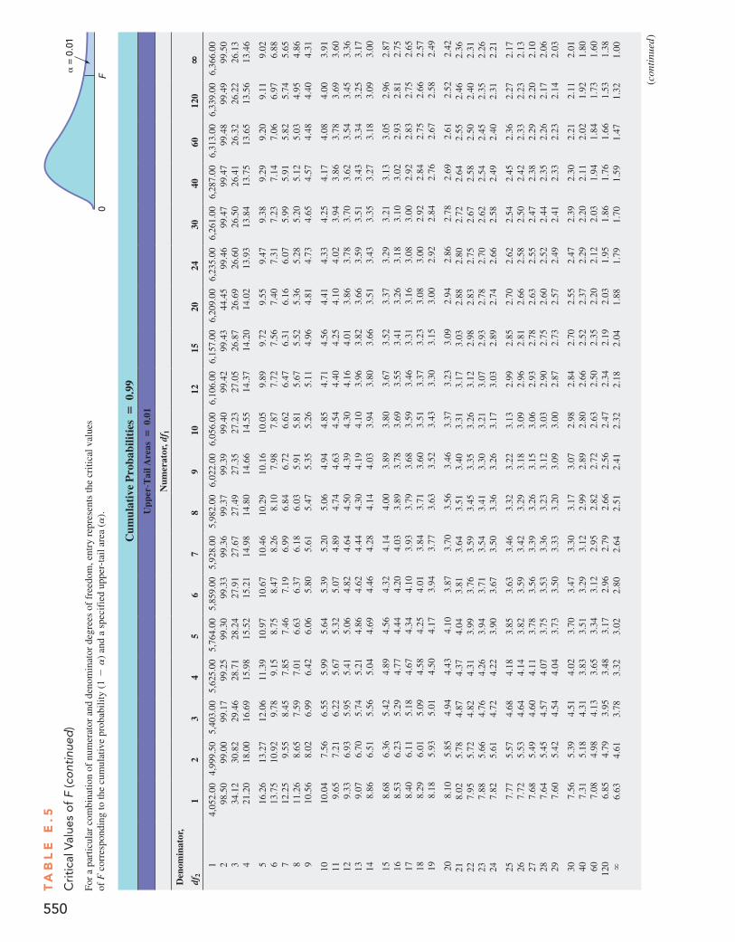
Cum
ulat
ive
Pro
babi
litie
s=
0.99
Upp
er@T
ail A
reas
=0.
01
Num
erat
or, d
f 1
Den
omin
ator
,
df2
12
34
56
78
910
1215
2024
3040
6012
0H
14,
052.
004,
999.
505,
403.
005,
625.
005,
764.
005,
859.
005,
928.
005,
982.
006,
022.
006,
056.
006,
106.
006,
157.
006,
209.
006,
235.
006,
261.
006,
287.
006,
313.
006,
339.
006,
366.
002
98.5
099
.00
99.1
799
.25
99.3
099
.33
99.3
699
.37
99.3
999
.40
99.4
299
.43
44.4
599
.46
99.4
799
.47
99.4
899
.49
99.5
03
34.1
230
.82
29.4
628
.71
28.2
427
.91
27.6
727
.49
27.3
527
.23
27.0
526
.87
26.6
926
.60
26.5
026
.41
26.3
226
.22
26.1
34
21.2
018
.00
16.6
915
.98
15.5
215
.21
14.9
814
.80
14.6
614
.55
14.3
714
.20
14.0
213
.93
13.8
413
.75
13.6
513
.56
13.4
6
516
.26
13.2
712
.06
11.3
910
.97
10.6
710
.46
10.2
910
.16
10.0
59.
899.
729.
559.
479.
389.
299.
209.
119.
026
13.7
510
.92
9.78
9.15
8.75
8.47
8.26
8.10
7.98
7.87
7.72
7.56
7.40
7.31
7.23
7.14
7.06
6.97
6.88
712
.25
9.55
8.45
7.85
7.46
7.19
6.99
6.84
6.72
6.62
6.47
6.31
6.16
6.07
5.99
5.91
5.82
5.74
5.65
811
.26
8.65
7.59
7.01
6.63
6.37
6.18
6.03
5.91
5.81
5.67
5.52
5.36
5.28
5.20
5.12
5.03
4.95
4.86
910
.56
8.02
6.99
6.42
6.06
5.80
5.61
5.47
5.35
5.26
5.11
4.96
4.81
4.73
4.65
4.57
4.48
4.40
4.31
1010
.04
7.56
6.55
5.99
5.64
5.39
5.20
5.06
4.94
4.85
4.71
4.56
4.41
4.33
4.25
4.17
4.08
4.00
3.91
119.
657.
216.
225.
675.
325.
074.
894.
744.
634.
544.
404.
254.
104.
023.
943.
863.
783.
693.
6012
9.33
6.93
5.95
5.41
5.06
4.82
4.64
4.50
4.39
4.30
4.16
4.01
3.86
3.78
3.70
3.62
3.54
3.45
3.36
139.
076.
705.
745.
214.
864.
624.
444.
304.
194.
103.
963.
823.
663.
593.
513.
433.
343.
253.
1714
8.86
6.51
5.56
5.04
4.69
4.46
4.28
4.14
4.03
3.94
3.80
3.66
3.51
3.43
3.35
3.27
3.18
3.09
3.00
158.
686.
365.
424.
894.
564.
324.
144.
003.
893.
803.
673.
523.
373.
293.
213.
133.
052.
962.
8716
8.53
6.23
5.29
4.77
4.44
4.20
4.03
3.89
3.78
3.69
3.55
3.41
3.26
3.18
3.10
3.02
2.93
2.81
2.75
178.
406.
115.
184.
674.
344.
103.
933.
793.
683.
593.
463.
313.
163.
083.
002.
922.
832.
752.
6518
8.29
6.01
5.09
4.58
4.25
4.01
3.84
3.71
3.60
3.51
3.37
3.23
3.08
3.00
2.92
2.84
2.75
2.66
2.57
198.
185.
935.
014.
504.
173.
943.
773.
633.
523.
433.
303.
153.
002.
922.
842.
762.
672.
582.
49
208.
105.
854.
944.
434.
103.
873.
703.
563.
463.
373.
233.
092.
942.
862.
782.
692.
612.
522.
4221
8.02
5.78
4.87
4.37
4.04
3.81
3.64
3.51
3.40
3.31
3.17
3.03
2.88
2.80
2.72
2.64
2.55
2.46
2.36
227.
955.
724.
824.
313.
993.
763.
593.
453.
353.
263.
122.
982.
832.
752.
672.
582.
502.
402.
3123
7.88
5.66
4.76
4.26
3.94
3.71
3.54
3.41
3.30
3.21
3.07
2.93
2.78
2.70
2.62
2.54
2.45
2.35
2.26
247.
825.
614.
724.
223.
903.
673.
503.
363.
263.
173.
032.
892.
742.
662.
582.
492.
402.
312.
21
257.
775.
574.
684.
183.
853.
633.
463.
323.
223.
132.
992.
852.
702.
622.
542.
452.
362.
272.
1726
7.72
5.53
4.64
4.14
3.82
3.59
3.42
3.29
3.18
3.09
2.96
2.81
2.66
2.58
2.50
2.42
2.33
2.23
2.13
277.
685.
494.
604.
113.
783.
563.
393.
263.
153.
062.
932.
782.
632.
552.
472.
382.
292.
202.
1028
7.64
5.45
4.57
4.07
3.75
3.53
3.36
3.23
3.12
3.03
2.90
2.75
2.60
2.52
2.44
2.35
2.26
2.17
2.06
297.
605.
424.
544.
043.
733.
503.
333.
203.
093.
002.
872.
732.
572.
492.
412.
332.
232.
142.
03
307.
565.
394.
514.
023.
703.
473.
303.
173.
072.
982.
842.
702.
552.
472.
392.
302.
212.
112.
0140
7.31
5.18
4.31
3.83
3.51
3.29
3.12
2.99
2.89
2.80
2.66
2.52
2.37
2.29
2.20
2.11
2.02
1.92
1.80
607.
084.
984.
133.
653.
343.
122.
952.
822.
722.
632.
502.
352.
202.
122.
031.
941.
841.
731.
6012
06.
854.
793.
953.
483.
172.
962.
792.
662.
562.
472.
342.
192.
031.
951.
861.
761.
661.
531.
38∞
6.63
4.61
3.78
3.32
3.02
2.80
2.64
2.51
2.41
2.32
2.18
2.04
1.88
1.79
1.70
1.59
1.47
1.32
1.00
0F
a =
0.0
1
(con
tinu
ed )
Ta
bl
e e
.5
Cri
tica
l Val
ues
of
F (c
ontin
ued
)
For
a pa
rtic
ular
com
bina
tion
of n
umer
ator
and
den
omin
ator
deg
rees
of
free
dom
, ent
ry r
epre
sent
s th
e cr
itica
l val
ues
of F
cor
resp
ondi
ng to
the
cum
ulat
ive
prob
abili
ty (
1-
a)
and
a sp
ecif
ied
uppe
r-ta
il ar
ea (a
).
550
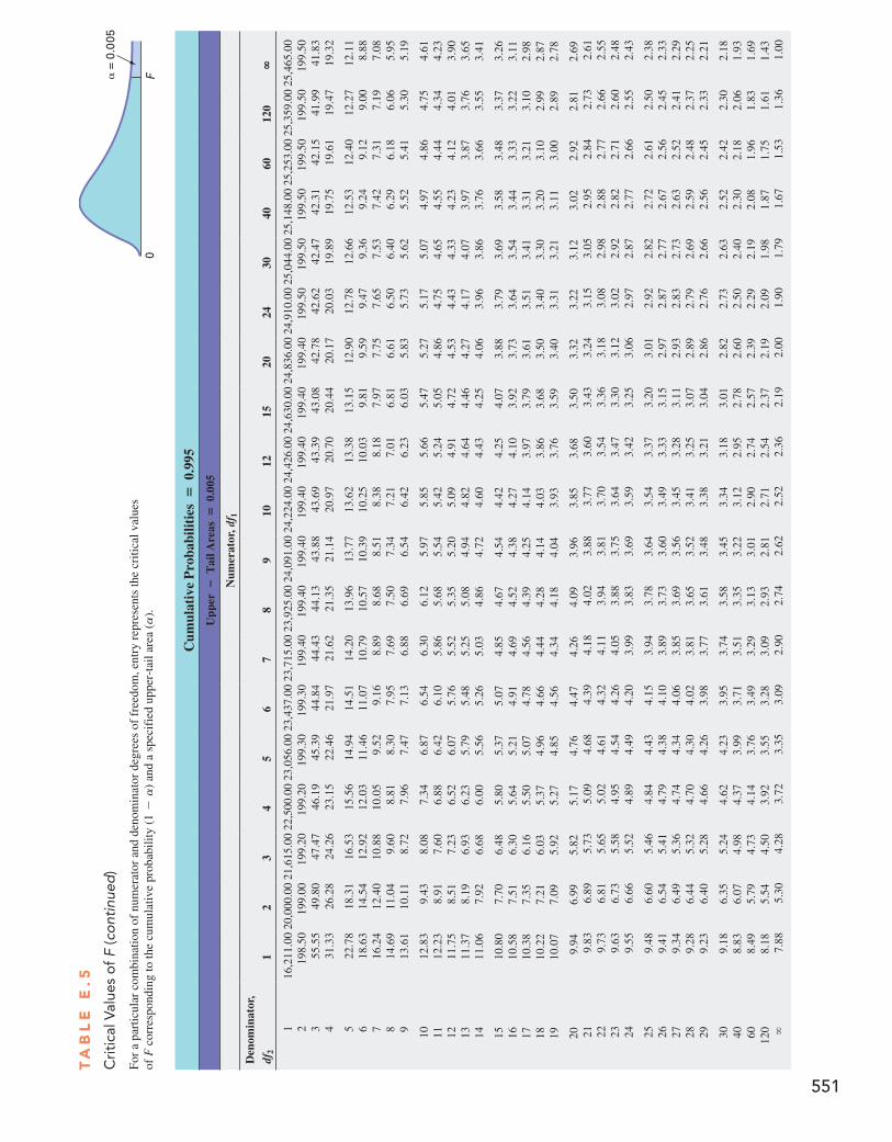
Cum
ulat
ive
Pro
babi
litie
s=
0.99
5
Upp
er−
Tai
l Are
as=
0.00
5
Num
erat
or, d
f 1
Den
omin
ator
, df
21
23
45
67
89
1012
1520
2430
4060
120
H
116
,211
.00
20,0
00.0
021
,615
.00
22,5
00.0
023
,056
.00
23,4
37.0
023
,715
.00
23,9
25.0
024
,091
.00
24,2
24.0
024
,426
.00
24,6
30.0
024
,836
.00
24,9
10.0
025
,044
.00
25,1
48.0
025
,253
.00
25,3
59.0
025
,465
.00
219
8.50
199.
0019
9.20
199.
2019
9.30
199.
3019
9.40
199.
4019
9.40
199.
4019
9.40
199.
4019
9.40
199.
5019
9.50
199.
5019
9.50
199.
5019
9.50
355
.55
49.8
047
.47
46.1
945
.39
44.8
444
.43
44.1
343
.88
43.6
943
.39
43.0
842
.78
42.6
242
.47
42.3
142
.15
41.9
941
.83
431
.33
26.2
824
.26
23.1
522
.46
21.9
721
.62
21.3
521
.14
20.9
720
.70
20.4
420
.17
20.0
319
.89
19.7
519
.61
19.4
719
.32
522
.78
18.3
116
.53
15.5
614
.94
14.5
114
.20
13.9
613
.77
13.6
213
.38
13.1
512
.90
12.7
812
.66
12.5
312
.40
12.2
712
.11
618
.63
14.5
412
.92
12.0
311
.46
11.0
710
.79
10.5
710
.39
10.2
510
.03
9.81
9.59
9.47
9.36
9.24
9.12
9.00
8.88
716
.24
12.4
010
.88
10.0
59.
529.
168.
898.
688.
518.
388.
187.
977.
757.
657.
537.
427.
317.
197.
088
14.6
911
.04
9.60
8.81
8.30
7.95
7.69
7.50
7.34
7.21
7.01
6.81
6.61
6.50
6.40
6.29
6.18
6.06
5.95
913
.61
10.1
18.
727.
967.
477.
136.
886.
696.
546.
426.
236.
035.
835.
735.
625.
525.
415.
305.
19
1012
.83
9.43
8.08
7.34
6.87
6.54
6.30
6.12
5.97
5.85
5.66
5.47
5.27
5.17
5.07
4.97
4.86
4.75
4.61
1112
.23
8.91
7.60
6.88
6.42
6.10
5.86
5.68
5.54
5.42
5.24
5.05
4.86
4.75
4.65
4.55
4.44
4.34
4.23
1211
.75
8.51
7.23
6.52
6.07
5.76
5.52
5.35
5.20
5.09
4.91
4.72
4.53
4.43
4.33
4.23
4.12
4.01
3.90
1311
.37
8.19
6.93
6.23
5.79
5.48
5.25
5.08
4.94
4.82
4.64
4.46
4.27
4.17
4.07
3.97
3.87
3.76
3.65
1411
.06
7.92
6.68
6.00
5.56
5.26
5.03
4.86
4.72
4.60
4.43
4.25
4.06
3.96
3.86
3.76
3.66
3.55
3.41
1510
.80
7.70
6.48
5.80
5.37
5.07
4.85
4.67
4.54
4.42
4.25
4.07
3.88
3.79
3.69
3.58
3.48
3.37
3.26
1610
.58
7.51
6.30
5.64
5.21
4.91
4.69
4.52
4.38
4.27
4.10
3.92
3.73
3.64
3.54
3.44
3.33
3.22
3.11
1710
.38
7.35
6.16
5.50
5.07
4.78
4.56
4.39
4.25
4.14
3.97
3.79
3.61
3.51
3.41
3.31
3.21
3.10
2.98
1810
.22
7.21
6.03
5.37
4.96
4.66
4.44
4.28
4.14
4.03
3.86
3.68
3.50
3.40
3.30
3.20
3.10
2.99
2.87
1910
.07
7.09
5.92
5.27
4.85
4.56
4.34
4.18
4.04
3.93
3.76
3.59
3.40
3.31
3.21
3.11
3.00
2.89
2.78
209.
946.
995.
825.
174.
764.
474.
264.
093.
963.
853.
683.
503.
323.
223.
123.
022.
922.
812.
6921
9.83
6.89
5.73
5.09
4.68
4.39
4.18
4.02
3.88
3.77
3.60
3.43
3.24
3.15
3.05
2.95
2.84
2.73
2.61
229.
736.
815.
655.
024.
614.
324.
113.
943.
813.
703.
543.
363.
183.
082.
982.
882.
772.
662.
5523
9.63
6.73
5.58
4.95
4.54
4.26
4.05
3.88
3.75
3.64
3.47
3.30
3.12
3.02
2.92
2.82
2.71
2.60
2.48
249.
556.
665.
524.
894.
494.
203.
993.
833.
693.
593.
423.
253.
062.
972.
872.
772.
662.
552.
43
259.
486.
605.
464.
844.
434.
153.
943.
783.
643.
543.
373.
203.
012.
922.
822.
722.
612.
502.
3826
9.41
6.54
5.41
4.79
4.38
4.10
3.89
3.73
3.60
3.49
3.33
3.15
2.97
2.87
2.77
2.67
2.56
2.45
2.33
279.
346.
495.
364.
744.
344.
063.
853.
693.
563.
453.
283.
112.
932.
832.
732.
632.
522.
412.
2928
9.28
6.44
5.32
4.70
4.30
4.02
3.81
3.65
3.52
3.41
3.25
3.07
2.89
2.79
2.69
2.59
2.48
2.37
2.25
299.
236.
405.
284.
664.
263.
983.
773.
613.
483.
383.
213.
042.
862.
762.
662.
562.
452.
332.
21
309.
186.
355.
244.
624.
233.
953.
743.
583.
453.
343.
183.
012.
822.
732.
632.
522.
422.
302.
1840
8.83
6.07
4.98
4.37
3.99
3.71
3.51
3.35
3.22
3.12
2.95
2.78
2.60
2.50
2.40
2.30
2.18
2.06
1.93
608.
495.
794.
734.
143.
763.
493.
293.
133.
012.
902.
742.
572.
392.
292.
192.
081.
961.
831.
6912
08.
185.
544.
503.
923.
553.
283.
092.
932.
812.
712.
542.
372.
192.
091.
981.
871.
751.
611.
43∞
7.88
5.30
4.28
3.72
3.35
3.09
2.90
2.74
2.62
2.52
2.36
2.19
2.00
1.90
1.79
1.67
1.53
1.36
1.00
551
Ta
bl
e e
.5
Cri
tica
l Val
ues
of
F (c
ontin
ued
)
For
a pa
rtic
ular
com
bina
tion
of n
umer
ator
and
den
omin
ator
deg
rees
of
free
dom
, ent
ry r
epre
sent
s th
e cr
itica
l val
ues
of F
cor
resp
ondi
ng to
the
cum
ulat
ive
prob
abili
ty (
1-
a)
and
a sp
ecif
ied
uppe
r-ta
il ar
ea (a
).0
Fa =
0.0
05
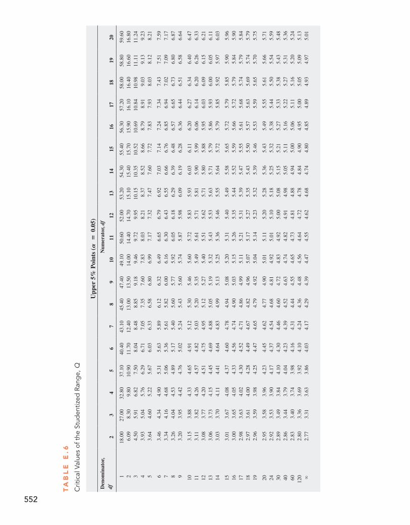
Ta
bl
e e
.6
Crit
ical
Val
ues
of t
he S
tud
entiz
ed R
ang
e, Q
Upp
er 5
% P
oint
s (A
=0.
05)
Den
omin
ator
, df
Num
erat
or, d
f
23
45
67
89
1011
1213
1415
1617
1819
20
118
.00
27.0
032
.80
37.1
040
.40
43.1
045
.40
47.4
049
.10
50.6
052
.00
53.2
054
.30
55.4
056
.30
57.2
058
.00
58.8
059
.60
26.
098.
309.
8010
.90
11.7
012
.40
13.0
013
.50
14.0
014
.40
14.7
015
.10
15.4
015
.70
15.9
016
.10
16.4
016
.60
16.8
03
4.50
5.91
6.82
7.50
8.04
8.48
8.85
9.18
9.46
9.72
9.95
10.1
510
.35
10.5
210
.69
10.8
410
.98
11.1
111
.24
43.
935.
045.
766.
296.
717.
057.
357.
607.
838.
038.
218.
378.
528.
668.
798.
919.
039.
139.
235
3.64
4.60
5.22
5.67
6.03
6.33
6.58
6.80
6.99
7.17
7.32
7.47
7.60
7.72
7.83
7.93
8.03
8.12
8.21
63.
464.
344.
905.
315.
635.
896.
126.
326.
496.
656.
796.
927.
037.
147.
247.
347.
437.
517.
597
3.34
4.16
4.68
5.06
5.36
5.61
5.82
6.00
6.16
6.30
6.43
6.55
6.66
6.76
6.85
6.94
7.02
7.09
7.17
83.
264.
044.
534.
895.
175.
405.
605.
775.
926.
056.
186.
296.
396.
486.
576.
656.
736.
806.
879
3.20
3.95
4.42
4.76
5.02
5.24
5.43
5.60
5.74
5.87
5.98
6.09
6.19
6.28
6.36
6.44
6.51
6.58
6.64
103.
153.
884.
334.
654.
915.
125.
305.
465.
605.
725.
835.
936.
036.
116.
206.
276.
346.
406.
4711
3.11
3.82
4.26
4.57
4.82
5.03
5.20
5.35
5.49
5.61
5.71
5.81
5.90
5.99
6.06
6.14
6.20
6.26
6.33
123.
083.
774.
204.
514.
754.
955.
125.
275.
405.
515.
625.
715.
805.
885.
956.
036.
096.
156.
2113
3.06
3.73
4.15
4.45
4.69
4.88
5.05
5.19
5.32
5.43
5.53
5.63
5.71
5.79
5.86
5.93
6.00
6.05
6.11
143.
033.
704.
114.
414.
644.
834.
995.
135.
255.
365.
465.
555.
645.
725.
795.
855.
925.
976.
03
153.
013.
674.
084.
374.
604.
784.
945.
085.
205.
315.
405.
495.
585.
655.
725.
795.
855.
905.
9616
3.00
3.65
4.05
4.33
4.56
4.74
4.90
5.03
5.15
5.26
5.35
5.44
5.52
5.59
5.66
5.72
5.79
5.84
5.90
172.
983.
634.
024.
304.
524.
714.
864.
995.
115.
215.
315.
395.
475.
555.
615.
685.
745.
795.
8418
2.97
3.61
4.00
4.28
4.49
4.67
4.82
4.96
5.07
5.17
5.27
5.35
5.43
5.50
5.57
5.63
5.69
5.74
5.79
192.
963.
593.
984.
254.
474.
654.
794.
925.
045.
145.
235.
325.
395.
465.
535.
595.
655.
705.
75
202.
953.
583.
964.
234.
454.
624.
774.
905.
015.
115.
205.
285.
365.
435.
495.
555.
615.
665.
7124
2.92
3.53
3.90
4.17
4.37
4.54
4.68
4.81
4.92
5.01
5.10
5.18
5.25
5.32
5.38
5.44
5.50
5.54
5.59
302.
893.
493.
844.
104.
304.
464.
604.
724.
834.
925.
005.
085.
155.
215.
275.
335.
385.
435.
4840
2.86
3.44
3.79
4.04
4.23
4.39
4.52
4.63
4.74
4.82
4.91
4.98
5.05
5.11
5.16
5.22
5.27
5.31
5.36
602.
833.
403.
743.
984.
164.
314.
444.
554.
654.
734.
814.
884.
945.
005.
065.
115.
165.
205.
2412
02.
803.
363.
693.
924.
104.
244.
364.
484.
564.
644.
724.
784.
844.
904.
955.
005.
055.
095.
13∞
2.77
3.31
3.63
3.86
4.03
4.17
4.29
4.39
4.47
4.55
4.62
4.68
4.74
4.80
4.85
4.89
4.93
4.97
5.01
552
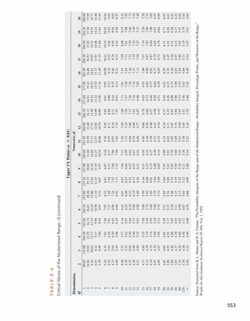
Upp
er 1
% P
oint
s (A
=0.
01)
Den
omin
ator
, df
Num
erat
or, d
f
23
45
67
89
1011
1213
1415
1617
1819
20
190
.03
135.
0016
4.30
185.
6020
2.20
215.
8022
7.20
237.
0024
5.60
253.
2026
0.00
266.
2027
1.80
277.
0028
1.80
286.
3029
0.40
294.
3029
8.00
214
.04
19.0
222
.29
24.7
226
.63
28.2
029
.53
30.6
831
.69
32.5
933
.40
34.1
334
.81
35.4
336
.00
36.5
337
.03
37.5
037
.95
38.
2610
.62
12.1
713
.33
14.2
415
.00
15.6
416
.20
16.6
917
.13
17.5
317
.89
18.2
218
.52
18.8
119
.07
19.3
219
.55
19.7
74
6.51
8.12
9.17
9.96
10.5
811
.10
11.5
511
.93
12.2
712
.57
12.8
413
.09
13.3
213
.53
13.7
313
.91
14.0
814
.24
14.4
05
5.70
6.98
7.80
8.42
8.91
9.32
9.67
9.97
10.2
410
.48
10.7
010
.89
11.0
811
.24
11.4
011
.55
11.6
811
.81
11.9
3
65.
246.
337.
037.
567.
978.
328.
618.
879.
109.
309.
499.
659.
819.
9510
.08
10.2
110
.32
10.4
310
.54
74.
955.
926.
547.
017.
377.
687.
948.
178.
378.
558.
718.
869.
009.
129.
249.
359.
469.
559.
658
4.75
5.64
6.20
6.63
6.96
7.24
7.47
7.68
7.86
8.03
8.18
8.31
8.44
8.55
8.66
8.76
8.85
8.94
9.03
94.
605.
435.
966.
356.
666.
927.
137.
327.
507.
657.
787.
918.
038.
138.
238.
338.
418.
508.
57
104.
485.
275.
776.
146.
436.
676.
877.
067.
217.
367.
497.
607.
717.
817.
917.
998.
088.
158.
2311
4.39
5.15
5.62
5.97
6.25
6.48
6.67
6.84
6.99
7.13
7.25
7.36
7.47
7.56
7.65
7.73
7.81
7.88
7.95
124.
325.
045.
505.
846.
106.
326.
516.
676.
816.
947.
067.
177.
267.
367.
447.
527.
597.
667.
7313
4.26
4.96
5.40
5.73
5.98
6.19
6.37
6.53
6.67
6.79
6.90
7.01
7.10
7.19
7.27
7.35
7.42
7.49
7.55
144.
214.
905.
325.
635.
886.
096.
266.
416.
546.
666.
776.
876.
967.
057.
137.
207.
277.
337.
40
154.
174.
845.
255.
565.
805.
996.
166.
316.
446.
566.
666.
766.
856.
937.
007.
077.
147.
207.
2616
4.13
4.79
5.19
5.49
5.72
5.92
6.08
6.22
6.35
6.46
6.56
6.66
6.74
6.82
6.90
6.97
7.03
7.09
7.15
174.
104.
745.
145.
435.
665.
856.
016.
156.
276.
386.
486.
576.
666.
736.
816.
876.
947.
007.
0518
4.07
4.70
5.09
5.38
5.60
5.79
5.94
6.08
6.20
6.31
6.41
6.50
6.58
6.66
6.73
6.79
6.85
6.91
6.97
194.
054.
675.
055.
335.
555.
745.
896.
026.
146.
256.
346.
436.
516.
596.
656.
726.
786.
846.
89
204.
024.
645.
025.
295.
515.
695.
845.
976.
096.
196.
296.
376.
456.
526.
596.
656.
716.
776.
8224
3.96
4.55
4.91
5.17
5.37
5.54
5.69
5.81
5.92
6.02
6.11
6.19
6.26
6.33
6.39
6.45
6.51
6.56
6.61
303.
894.
464.
805.
055.
245.
405.
545.
655.
765.
855.
936.
016.
086.
146.
206.
266.
316.
366.
4140
3.83
4.37
4.70
4.93
5.11
5.27
5.39
5.50
5.60
5.69
5.76
5.84
5.90
5.96
6.02
6.07
6.12
6.17
6.21
603.
764.
284.
604.
824.
995.
135.
255.
365.
455.
535.
605.
675.
735.
795.
845.
895.
935.
976.
0212
03.
704.
204.
504.
714.
875.
015.
125.
215.
305.
385.
445.
515.
565.
615.
665.
715.
755.
795.
83∞
3.64
4.12
4.40
4.60
4.76
4.88
4.99
5.08
5.16
5.23
5.29
5.35
5.40
5.45
5.49
5.54
5.57
5.61
5.65
sour
ce: e
xtra
cted
fro
m H
. L. H
arte
r an
d d
. s. c
lem
m, “
The
pro
babi
lity
inte
gral
s of
the
Ran
ge a
nd o
f th
e st
uden
tized
Ran
ge—
prob
abili
ty i
nteg
ral,
perc
enta
ge p
oint
s, a
nd M
omen
ts o
f th
e R
ange
,”
Wri
ght A
ir D
evel
opm
ent T
echn
ical
Rep
ort 5
8–48
4, V
ol. 1
, 195
9.
Ta
bl
e e
.6
Crit
ical
Val
ues
of t
he S
tud
entiz
ed R
ang
e, Q
(con
tinue
d)
553
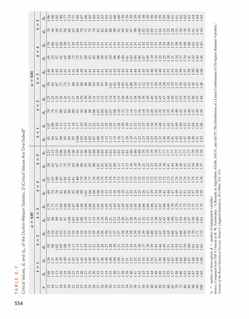
Ta
bl
e e
.7
Crit
ical
Val
ues,
dL
and
dU, o
f the
Dur
bin
-Wat
son
Stat
istic
, D (C
ritic
al V
alue
s A
re O
ne-S
ided
)a
A=
0.05
A=
0.01
k=
1k
=2
k=
3k
=4
k=
5k
=1
k=
2k
=3
k=
4k
=5
nd L
d Ud L
d Ud L
d Ud L
d Ud L
d Ud L
d Ud L
d Ud L
d Ud L
d Ud L
d U15
1.08
1.36
.95
1.54
.82
1.75
.69
1.97
.56
2.21
.81
1.07
.70
1.25
.59
1.46
.49
1.70
.39
1.96
161.
101.
37.9
81.
54.8
61.
73.7
41.
93.6
22.
15.8
41.
09.7
41.
25.6
31.
44.5
31.
66.4
41.
9017
1.13
1.38
1.02
1.54
.90
1.71
.78
1.90
.67
2.10
.87
1.10
.77
1.25
.67
1.43
.57
1.63
.48
1.85
181.
161.
391.
051.
53.9
31.
69.8
21.
87.7
12.
06.9
01.
12.8
01.
26.7
11.
42.6
11.
60.5
21.
8019
1.18
1.40
1.08
1.53
.97
1.68
.86
1.85
.75
2.02
.93
1.13
.83
1.26
.74
1.41
.65
1.58
.56
1.77
201.
201.
411.
101.
541.
001.
68.9
01.
83.7
91.
99.9
51.
15.8
61.
27.7
71.
41.6
81.
57.6
01.
7421
1.22
1.42
1.13
1.54
1.03
1.67
.93
1.81
.83
1.96
.97
1.16
.89
1.27
.80
1.41
.72
1.55
.63
1.71
221.
241.
431.
151.
541.
051.
66.9
61.
80.8
61.
941.
001.
17.9
11.
28.8
31.
40.7
51.
54.6
61.
6923
1.26
1.44
1.17
1.54
1.08
1.66
.99
1.79
.90
1.92
1.02
1.19
.94
1.29
.86
1.40
.77
1.53
.70
1.67
241.
271.
451.
191.
551.
101.
661.
011.
78.9
31.
901.
041.
20.9
61.
30.8
81.
41.8
01.
53.7
21.
6625
1.29
1.45
1.21
1.55
1.12
1.66
1.04
1.77
.95
1.89
1.05
1.21
.98
1.30
.90
1.41
.83
1.52
.75
1.65
261.
301.
461.
221.
551.
141.
651.
061.
76.9
81.
881.
071.
221.
001.
31.9
31.
41.8
51.
52.7
81.
6427
1.32
1.47
1.24
1.56
1.16
1.65
1.08
1.76
1.01
1.86
1.09
1.23
1.02
1.32
.95
1.41
.88
1.51
.81
1.63
281.
331.
481.
261.
561.
181.
651.
101.
751.
031.
851.
101.
241.
041.
32.9
71.
41.9
01.
51.8
31.
6229
1.34
1.48
1.27
1.56
1.20
1.65
1.12
1.74
1.05
1.84
1.12
1.25
1.05
1.33
.99
1.42
.92
1.51
.85
1.61
301.
351.
491.
281.
571.
211.
651.
141.
741.
071.
831.
131.
261.
071.
341.
011.
42.9
41.
51.8
81.
6131
1.36
1.50
1.30
1.57
1.23
1.65
1.16
1.74
1.09
1.83
1.15
1.27
1.08
1.34
1.02
1.42
.96
1.51
.90
1.60
321.
371.
501.
311.
571.
241.
651.
181.
731.
111.
821.
161.
281.
101.
351.
041.
43.9
81.
51.9
21.
6033
1.38
1.51
1.32
1.58
1.26
1.65
1.19
1.73
1.13
1.81
1.17
1.29
1.11
1.36
1.05
1.43
1.00
1.51
.94
1.59
341.
391.
511.
331.
581.
271.
651.
211.
731.
151.
811.
181.
301.
131.
361.
071.
431.
011.
51.9
51.
5935
1.40
1.52
1.34
1.58
1.28
1.65
1.22
1.73
1.16
1.80
1.19
1.31
1.14
1.37
1.08
1.44
1.03
1.51
.97
1.59
361.
411.
521.
351.
591.
291.
651.
241.
731.
181.
801.
211.
321.
151.
381.
101.
441.
041.
51.9
91.
5937
1.42
1.53
1.36
1.59
1.31
1.66
1.25
1.72
1.19
1.80
1.22
1.32
1.16
1.38
1.11
1.45
1.06
1.51
1.00
1.59
381.
431.
541.
371.
591.
321.
661.
261.
721.
211.
791.
231.
331.
181.
391.
121.
451.
071.
521.
021.
5839
1.43
1.54
1.38
1.60
1.33
1.66
1.27
1.72
1.22
1.79
1.24
1.34
1.19
1.39
1.14
1.45
1.09
1.52
1.03
1.58
401.
441.
541.
391.
601.
341.
661.
291.
721.
231.
791.
251.
341.
201.
401.
151.
461.
101.
521.
051.
5845
1.48
1.57
1.43
1.62
1.38
1.67
1.34
1.72
1.29
1.78
1.29
1.38
1.24
1.42
1.20
1.48
1.16
1.53
1.11
1.58
501.
501.
591.
461.
631.
421.
671.
381.
721.
341.
771.
321.
401.
281.
451.
241.
491.
201.
541.
161.
5955
1.53
1.60
1.49
1.64
1.45
1.68
1.41
1.72
1.38
1.77
1.36
1.43
1.32
1.47
1.28
1.51
1.25
1.55
1.21
1.59
601.
551.
621.
511.
651.
481.
691.
441.
731.
411.
771.
381.
451.
351.
481.
321.
521.
281.
561.
251.
6065
1.57
1.63
1.54
1.66
1.50
1.70
1.47
1.73
1.44
1.77
1.41
1.47
1.38
1.50
1.35
1.53
1.31
1.57
1.28
1.61
701.
581.
641.
551.
671.
521.
701.
491.
741.
461.
771.
431.
491.
401.
521.
371.
551.
341.
581.
311.
6175
1.60
1.65
1.57
1.68
1.54
1.71
1.51
1.74
1.49
1.77
1.45
1.50
1.42
1.53
1.39
1.56
1.37
1.59
1.34
1.62
801.
611.
661.
591.
691.
561.
721.
531.
741.
511.
771.
471.
521.
441.
541.
421.
571.
391.
601.
361.
6285
1.62
1.67
1.60
1.70
1.57
1.72
1.55
1.75
1.52
1.77
1.48
1.53
1.46
1.55
1.43
1.58
1.41
1.60
1.39
1.63
901.
631.
681.
611.
701.
591.
731.
571.
751.
541.
781.
501.
541.
471.
561.
451.
591.
431.
611.
411.
6495
1.64
1.69
1.62
1.71
1.60
1.73
1.58
1.75
1.56
1.78
1.51
1.55
1.49
1.57
1.47
1.60
1.45
1.62
1.42
1.64
100
1.65
1.69
1.63
1.72
1.61
1.74
1.59
1.76
1.57
1.78
1.52
1.56
1.50
1.58
1.48
1.60
1.46
1.63
1.44
1.65
a n =
num
ber
of o
bser
vatio
ns;
k=
num
ber
of in
depe
nden
t var
iabl
es.
sour
ce: c
ompu
ted
from
Tsp
4.5
bas
ed o
n R
. W. F
areb
roth
er, “
a R
emar
k on
alg
orith
ms
as1
06, a
s153
, and
as1
55: T
he d
istr
ibut
ion
of a
Lin
ear
com
bina
tion
of c
hi-s
quar
e R
ando
m V
aria
bles
,”
Jour
nal o
f the
Roy
al S
tati
stic
al S
ocie
ty, s
erie
s c
(a
pplie
d st
atis
tics)
, 29
(198
4): 3
23–3
33.
554
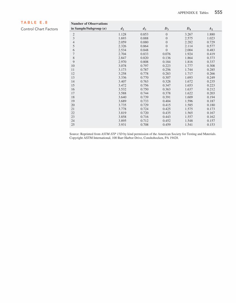
appendix e Tables 555
T a b l e e . 8
Control Chart FactorsNumber of Observations in Sample/Subgroup (n) d2 d3 D3 D4 A2
2 1.128 0.853 0 3.267 1.880 3 1.693 0.888 0 2.575 1.023 4 2.059 0.880 0 2.282 0.729 5 2.326 0.864 0 2.114 0.577 6 2.534 0.848 0 2.004 0.483 7 2.704 0.833 0.076 1.924 0.419 8 2.847 0.820 0.136 1.864 0.373 9 2.970 0.808 0.184 1.816 0.33710 3.078 0.797 0.223 1.777 0.30811 3.173 0.787 0.256 1.744 0.28512 3.258 0.778 0.283 1.717 0.26613 3.336 0.770 0.307 1.693 0.24914 3.407 0.763 0.328 1.672 0.23515 3.472 0.756 0.347 1.653 0.22316 3.532 0.750 0.363 1.637 0.21217 3.588 0.744 0.378 1.622 0.20318 3.640 0.739 0.391 1.609 0.19419 3.689 0.733 0.404 1.596 0.18720 3.735 0.729 0.415 1.585 0.18021 3.778 0.724 0.425 1.575 0.17322 3.819 0.720 0.435 1.565 0.16723 3.858 0.716 0.443 1.557 0.16224 3.895 0.712 0.452 1.548 0.15725 3.931 0.708 0.459 1.541 0.153
source: Reprinted from ASTM-STP 15D by kind permission of the american society for Testing and Materials. copyright asTM international, 100 Barr Harbor drive, conshohocken, pa 19428.
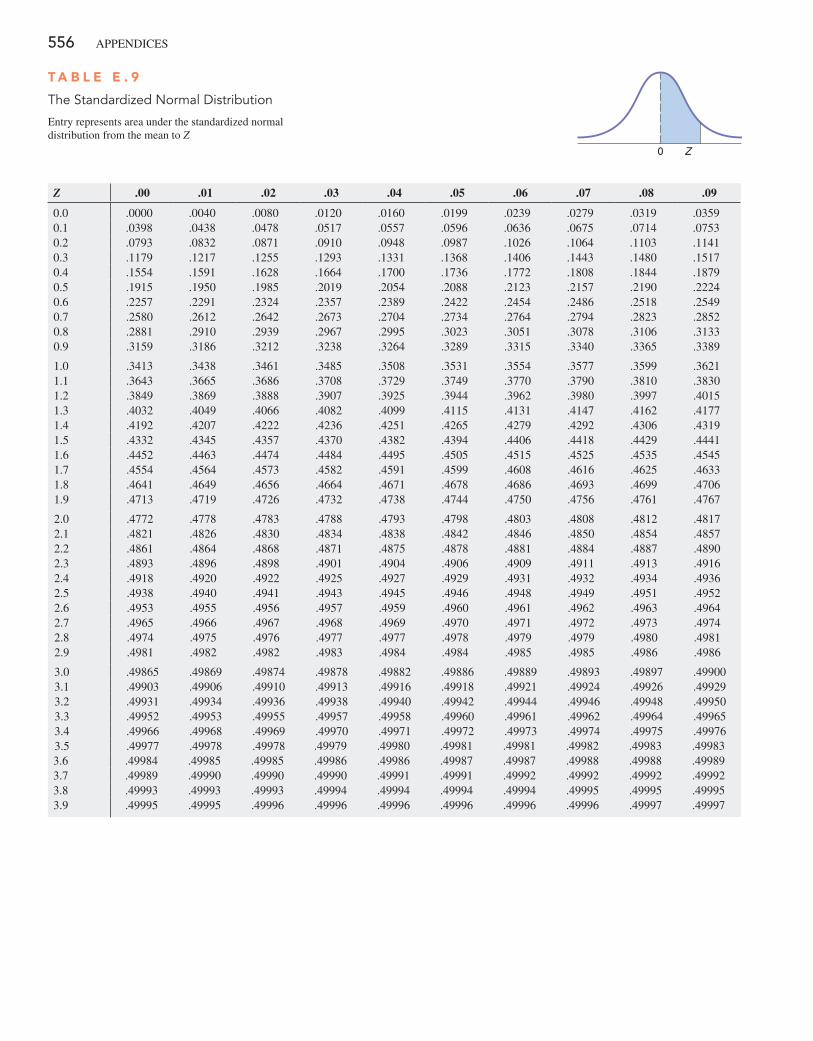
556 appendices
T a b l e e . 9
The Standardized Normal Distribution
entry represents area under the standardized normal distribution from the mean to Z
Z .00 .01 .02 .03 .04 .05 .06 .07 .08 .09
0.0 .0000 .0040 .0080 .0120 .0160 .0199 .0239 .0279 .0319 .03590.1 .0398 .0438 .0478 .0517 .0557 .0596 .0636 .0675 .0714 .07530.2 .0793 .0832 .0871 .0910 .0948 .0987 .1026 .1064 .1103 .11410.3 .1179 .1217 .1255 .1293 .1331 .1368 .1406 .1443 .1480 .15170.4 .1554 .1591 .1628 .1664 .1700 .1736 .1772 .1808 .1844 .18790.5 .1915 .1950 .1985 .2019 .2054 .2088 .2123 .2157 .2190 .22240.6 .2257 .2291 .2324 .2357 .2389 .2422 .2454 .2486 .2518 .25490.7 .2580 .2612 .2642 .2673 .2704 .2734 .2764 .2794 .2823 .28520.8 .2881 .2910 .2939 .2967 .2995 .3023 .3051 .3078 .3106 .31330.9 .3159 .3186 .3212 .3238 .3264 .3289 .3315 .3340 .3365 .3389
1.0 .3413 .3438 .3461 .3485 .3508 .3531 .3554 .3577 .3599 .36211.1 .3643 .3665 .3686 .3708 .3729 .3749 .3770 .3790 .3810 .38301.2 .3849 .3869 .3888 .3907 .3925 .3944 .3962 .3980 .3997 .40151.3 .4032 .4049 .4066 .4082 .4099 .4115 .4131 .4147 .4162 .41771.4 .4192 .4207 .4222 .4236 .4251 .4265 .4279 .4292 .4306 .43191.5 .4332 .4345 .4357 .4370 .4382 .4394 .4406 .4418 .4429 .44411.6 .4452 .4463 .4474 .4484 .4495 .4505 .4515 .4525 .4535 .45451.7 .4554 .4564 .4573 .4582 .4591 .4599 .4608 .4616 .4625 .46331.8 .4641 .4649 .4656 .4664 .4671 .4678 .4686 .4693 .4699 .47061.9 .4713 .4719 .4726 .4732 .4738 .4744 .4750 .4756 .4761 .4767
2.0 .4772 .4778 .4783 .4788 .4793 .4798 .4803 .4808 .4812 .48172.1 .4821 .4826 .4830 .4834 .4838 .4842 .4846 .4850 .4854 .48572.2 .4861 .4864 .4868 .4871 .4875 .4878 .4881 .4884 .4887 .48902.3 .4893 .4896 .4898 .4901 .4904 .4906 .4909 .4911 .4913 .49162.4 .4918 .4920 .4922 .4925 .4927 .4929 .4931 .4932 .4934 .49362.5 .4938 .4940 .4941 .4943 .4945 .4946 .4948 .4949 .4951 .49522.6 .4953 .4955 .4956 .4957 .4959 .4960 .4961 .4962 .4963 .49642.7 .4965 .4966 .4967 .4968 .4969 .4970 .4971 .4972 .4973 .49742.8 .4974 .4975 .4976 .4977 .4977 .4978 .4979 .4979 .4980 .49812.9 .4981 .4982 .4982 .4983 .4984 .4984 .4985 .4985 .4986 .4986
3.0 .49865 .49869 .49874 .49878 .49882 .49886 .49889 .49893 .49897 .499003.1 .49903 .49906 .49910 .49913 .49916 .49918 .49921 .49924 .49926 .499293.2 .49931 .49934 .49936 .49938 .49940 .49942 .49944 .49946 .49948 .499503.3 .49952 .49953 .49955 .49957 .49958 .49960 .49961 .49962 .49964 .499653.4 .49966 .49968 .49969 .49970 .49971 .49972 .49973 .49974 .49975 .499763.5 .49977 .49978 .49978 .49979 .49980 .49981 .49981 .49982 .49983 .499833.6 .49984 .49985 .49985 .49986 .49986 .49987 .49987 .49988 .49988 .499893.7 .49989 .49990 .49990 .49990 .49991 .49991 .49992 .49992 .49992 .499923.8 .49993 .49993 .49993 .49994 .49994 .49994 .49994 .49995 .49995 .499953.9 .49995 .49995 .49996 .49996 .49996 .49996 .49996 .49996 .49997 .49997
0 Z
557
A p p e n d i x F Useful Excel Knowledge
This appendix reviews knowledge that you will find useful if you plan to be more than a casual user of Microsoft Excel. If you are using a version of Excel that is older than Excel 2010, you will need to be familiar with Section F.3 so that you can modify the names of functions used in worksheet templates and models as necessary.
Section F.4 presents an enhanced explanation of some the statistical worksheet functions that recur in two or more chapters. This section also discusses functions that either serve programming purposes or are used in novel ways to compute intermediate results. If you have a particular inter-est in developing your own worksheet solutions, you should be familiar with the contents of this section.
This appendix assumes that you have mastered the ba-sic concepts presented in Appendix B. If you are a first-time user of Excel, do not make the mistake of trying to compre-hend the contents of this appendix before you gain experi-ence using Excel and familiarity with Appendix B.
F.1 Useful Keyboard ShortcutsIn Microsoft Office programs including Microsoft Excel, certain individual keys or combinations of keys held down as you press another key are shortcuts that allow you to execute common operations without having to select choices from menus or click in the Ribbon. As first explained in Section GS.4, in this book, keystroke combinations are shown using plus signs; for example, Ctrl+C means “while holding down the Ctrl key, press the C key.”
Editing ShortcutsPressing Backspace erases typed characters to the left of the current position, one character at a time. Pressing Delete erases characters to the right of the cursor, one character at a time.
Ctrl+C copies a worksheet entry, and Ctrl+V pastes that entry into the place that the editing cursor or worksheet cell highlight indicates. Pressing Ctrl+X cuts the currently selected entry or object so that you can paste it somewhere else. Ctrl+C and Ctrl+V (or Ctrl+X and Ctrl+V) can also
be used to copy (or cut) and paste certain workbook objects such as charts. (Using copy and paste to copy formulas from one worksheet cell to another is subject to the adjustment discussed in Appendix Section B.2.)
Pressing Ctrl+Z undoes the last operation, and Ctrl+Y redoes the last operation. Pressing Enter or Tab finalizes an entry typed into a worksheet cell. Pressing either key is im-plied by the use of the verb enter in the Excel Guides.
Formatting & Utility ShortcutsPressing Ctrl+B toggles on (or off) boldface text style for the currently selected object. Pressing Ctrl+I toggles on (or off) italic text style for the currently selected object. Pressing Ctrl+Shift+% formats numeric values as a percentage with no decimal places.
Pressing Ctrl+F finds a Find what value, and pressing Ctrl+H replaces a Find what value with the Replace with value. Pressing Ctrl+A selects the entire current worksheet (useful as part of a worksheet copy or format operation). Pressing Esc cancels an action or a dialog box. Pressing F1 displays the Microsoft Excel help system.
F.2 Verifying Formulas and WorksheetsIf you use formulas in your worksheets, you should review and verify formulas before you use their results. To view the formulas in a worksheet, press Ctrl+` (grave accent key). To restore the original view, the results of the formulas, press Ctrl+` a second time.
As you create and use more complicated worksheets, you might want to visually examine the relationships among a formula and the cells it uses (called the prece-dents) and the cells that use the results of the formula (the dependents). Select Formulas ➔ Trace Precedents (or Trace Dependents) to examine relationships. When you are finished, clear all trace arrows by selecting Formulas ➔ Remove Arrows.
After verifying formulas, you should test, using simple numbers, any worksheet that you have modified or con-structed from scratch.
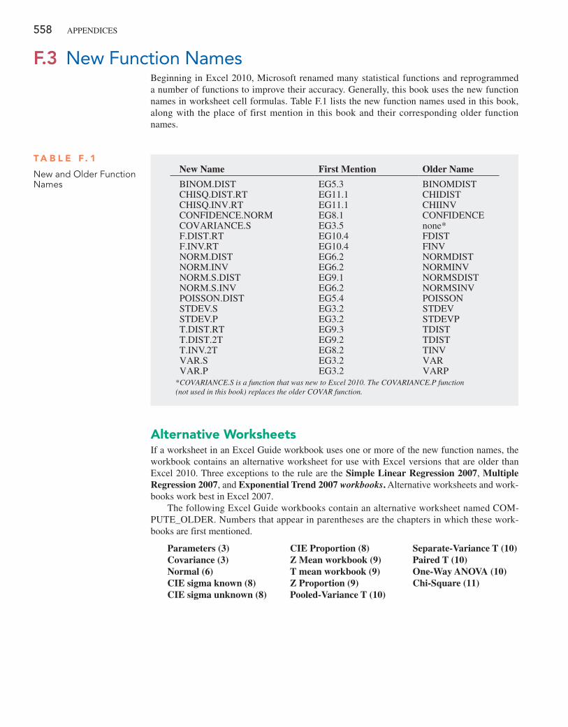
558 APPEndIcES
Alternative WorksheetsIf a worksheet in an Excel Guide workbook uses one or more of the new function names, the workbook contains an alternative worksheet for use with Excel versions that are older than Excel 2010. Three exceptions to the rule are the Simple Linear Regression 2007, Multiple Regression 2007, and Exponential Trend 2007 workbooks. Alternative worksheets and work-books work best in Excel 2007.
The following Excel Guide workbooks contain an alternative worksheet named cOM-PUTE_OLdER. numbers that appear in parentheses are the chapters in which these work-books are first mentioned.
Parameters (3)Covariance (3)Normal (6)CIE sigma known (8)CIE sigma unknown (8)
CIE Proportion (8)Z Mean workbook (9)T mean workbook (9)Z Proportion (9)Pooled-Variance T (10)
Separate-Variance T (10)Paired T (10)One-Way ANOVA (10)Chi-Square (11)
F.3 New Function NamesBeginning in Excel 2010, Microsoft renamed many statistical functions and reprogrammed a number of functions to improve their accuracy. Generally, this book uses the new function names in worksheet cell formulas. Table F.1 lists the new function names used in this book, along with the place of first mention in this book and their corresponding older function names.
T A b l E F. 1
New and Older Function Names
New Name First Mention Older Name
BInOM.dIST EG5.3 BInOMdISTcHISQ.dIST.RT EG11.1 cHIdISTcHISQ.InV.RT EG11.1 cHIInVcOnFIdEncE.nORM EG8.1 cOnFIdEncEcOVARIAncE.S EG3.5 none*F.dIST.RT EG10.4 FdISTF.InV.RT EG10.4 FInVnORM.dIST EG6.2 nORMdISTnORM.InV EG6.2 nORMInVnORM.S.dIST EG9.1 nORMSdISTnORM.S.InV EG6.2 nORMSInVPOISSOn.dIST EG5.4 POISSOnSTdEV.S EG3.2 STdEVSTdEV.P EG3.2 STdEVPT.dIST.RT EG9.3 TdISTT.dIST.2T EG9.2 TdISTT.InV.2T EG8.2 TInVVAR.S EG3.2 VARVAR.P EG3.2 VARP
*COVARIANCE.S is a function that was new to Excel 2010. The COVARIANCE.P function (not used in this book) replaces the older COVAR function.
APPEndIx F Useful Excel Knowledge 559
The following Excel Guide workbooks have alternative worksheets with various names:
Descriptive (3) completeStatistics_OLdERBinomial (5) cUMULATIVE_OLdERPoisson (5) cUMULATIVE_OLdERNPP (6) PLOT_OLdER and nORMAL_PLOT_OLdEROne-Way ANOVA (10) TK4_OLdERChi-Square Worksheets (11) chiSquare2x3_OLdER and others
Quartile FunctionIn this book, you will see the older QUARTILE function and not the newer QUARTILE.Exc function. In Microsoft’s Function Improvements in Microsoft Office Excel 2010 (available at bit.ly/RkoFIf), QUARTILE.Exc is explained as being “consistent with industry best prac-tices, assuming percentile is a value between 0 and 1, exclusive.” Because there are several established but different ways of computing quartiles, there is no way of knowing exactly how the new function works.
Because of this lack of specifics, this book uses the older QUARTILE function, whose programming and limitations are well known, and not the new QUARTILE.Exc function or QUARTILE.Inc function, which is the QUARTILES function renamed for consistency with QUARTILES.Exc. As noted in Section EG3.3, none of the three functions compute quar-tiles using the rules presented in Section 3.3, which are properly computed in the cOMPUTE worksheet of the Quartiles workbook that uses the older QUARTILE function. If you are using Excel 2010 or a newer version of Excel, the cOMPARE worksheet illustrates the results using the three forms of QUARTILES for the data found in column A of the dATA worksheet.
F.4 Understanding the Nonstatistical Functions
Selected Excel Guide and PHStat worksheets use a number of nonstatistical functions that either compute an intermediate result or perform a mathematical or programming operation. These functions are explained in the following alphabetical list:
CEILING(cell, round-to value) takes the numeric value in cell and rounds it to the next multi-ple of the round-to value. For example, if the round-to value is 0.5, as it is in several column B formulas in the cOMPUTE worksheet of the Quartiles workbook, then the numeric value will be rounded either to an integer or a number that contains a half such as 1.5.
COUNT(cell range) counts the number of cells in a cell range that contain a numeric value. This function is often used to compute the sample size, n, for example, in cell B9 of the cOMPUTE worksheet of the correlation workbook. When seen in the worksheets pre-sented in this book, the cell range will typically be the cell range of variable column, such as DATA!A:A. This will result in a proper count of the sample size of that variable if you follow the Getting Started chapter rules for entering data.
COUNTIF(cell range for all values, value to be matched) counts the number of occurrences of a value in a cell range. For example, the cOMPUTE worksheet of the Wilcoxon workbook uses COUNTIF(SortedRanks!A2:A21, "Beverage") in cell B7 to compute the sample size of the Population 1 Sample by counting the number of occurrences of the sample name Beverage in column A of the SortedRanks worksheet.
DEVSQ(variable cell range) computes the sum of the squares of the differences between a variable value and the mean of that variable.
FLOOR(cell, 1) takes the numeric value in cell and rounds down the value to the nearest integer.
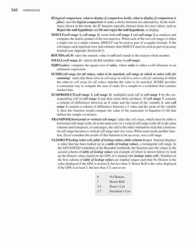
560 APPEndIcES
IF(logical comparison, what to display if comparison holds, what to display if comparison is false) uses the logical comparison to make a choice between two alternatives. In the work-sheets shown in this book, the IF function typically chooses from two text values, such as Reject the null hypothesis and Do not reject the null hypothesis, to display.
MMULT(cell range 1, cell range 2) treats both cell range 1 and cell range 2 as matrices and computes the matrix product of the two matrices. When each of the two cell ranges is either a single row or a single column, MMULT can be used as part of a regular formula. If the cell ranges each represent rows and columns, then MMULT must be used as part of an array formula (see Appendix Section B.3).
ROUND(cell, 0) takes the numeric value in cell and rounds to the nearest whole number.
SMALL(cell range, k) selects the kth smallest value in cell range.
SQRT(value) computes the square root of value, where value is either a cell reference or an arithmetic expression.
SUMIF(cell range for all values, value to be matched, cell range in which to select cells for summing) sums only those rows in cell range in which to select cells for summing in which the value in cell range for all values matches the value to be matched. SUMIF provides a convenient way to compute the sum of ranks for a sample in a worksheet that contains stacked data.
SUMPRODUCT(cell range 1, cell range 2) multiplies each cell in cell range 1 by the cor-responding cell in cell range 2 and then sums those products. If cell range 1 contains a column of differences between an X value and the mean of the variable X, and cell range 2 contains a column of differences between a Y value and the mean of the variable Y, then this function would compute the value of the numerator in Equation (3.16) that defines the sample covariance.
TRANSPOSE(horizontal or vertical cell range) takes the cell range, which must be either a horizontal cell range (cells all in the same row) or a vertical cell range (cells all in the same column) and transposes, or rearranges, the cell in the other orientation such that a horizon-tal cell range becomes a vertical cell range and vice versa. When used inside another func-tion, Excel considers the results of this function to be an array, not a cell range.
VLOOKUP(lookup value cell, table of lookup values, table column to use) function displays a value that has been looked up in a table of lookup values, a rectangular cell range. In the AdVAncEd worksheet of the Recoded workbook, the function uses the values in the second column of table of lookup values (an example of which is shown below) to look up the Honors values based on the GPA of a student (the lookup value cell). numbers in the first column of table of lookup values are implied ranges such that no Honors is the value displayed if the GPA is at least 0, but less than 3; Honor Roll is the value displayed if the GPA is at least 3, but less than 3.3; and so on:
0 no Honors
3 Honor Roll
3.3 dean’s List
3.7 President’s List
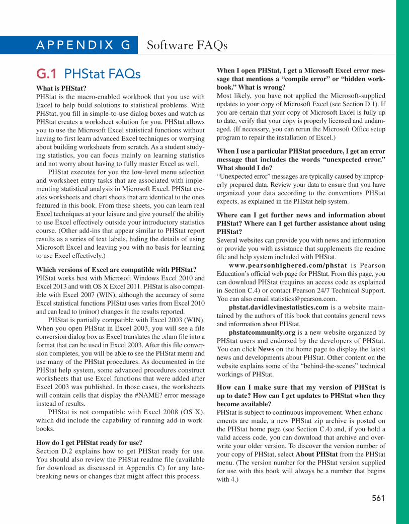
561
A p p e n d i x G Software FAQs
G.1 PHStat FAQsWhat is PHStat?PHStat is the macro-enabled workbook that you use with Excel to help build solutions to statistical problems. With PHStat, you fill in simple-to-use dialog boxes and watch as PHStat creates a worksheet solution for you. PHStat allows you to use the Microsoft Excel statistical functions without having to first learn advanced Excel techniques or worrying about building worksheets from scratch. As a student study-ing statistics, you can focus mainly on learning statistics and not worry about having to fully master Excel as well.
PHStat executes for you the low-level menu selection and worksheet entry tasks that are associated with imple-menting statistical analysis in Microsoft Excel. PHStat cre-ates worksheets and chart sheets that are identical to the ones featured in this book. From these sheets, you can learn real Excel techniques at your leisure and give yourself the ability to use Excel effectively outside your introductory statistics course. (Other add-ins that appear similar to PHStat report results as a series of text labels, hiding the details of using Microsoft Excel and leaving you with no basis for learning to use Excel effectively.)
Which versions of Excel are compatible with PHStat?PHStat works best with Microsoft Windows Excel 2010 and Excel 2013 and with OS X Excel 2011. PHStat is also compat-ible with Excel 2007 (WIN), although the accuracy of some Excel statistical functions PHStat uses varies from Excel 2010 and can lead to (minor) changes in the results reported.
PHStat is partially compatible with Excel 2003 (WIN). When you open PHStat in Excel 2003, you will see a file conversion dialog box as Excel translates the .xlam file into a format that can be used in Excel 2003. After this file conver-sion completes, you will be able to see the PHStat menu and use many of the PHStat procedures. As documented in the PHStat help system, some advanced procedures construct worksheets that use Excel functions that were added after Excel 2003 was published. In those cases, the worksheets will contain cells that display the #NAME? error message instead of results.
PHStat is not compatible with Excel 2008 (OS X), which did include the capability of running add-in work-books.
How do I get PHStat ready for use?Section D.2 explains how to get PHStat ready for use. You should also review the PHStat readme file (available for download as discussed in Appendix C) for any late-breaking news or changes that might affect this process.
When I open PHStat, I get a Microsoft Excel error mes-sage that mentions a “compile error” or “hidden work-book.” What is wrong?Most likely, you have not applied the Microsoft-supplied updates to your copy of Microsoft Excel (see Section D.1). If you are certain that your copy of Microsoft Excel is fully up to date, verify that your copy is properly licensed and undam-aged. (If necessary, you can rerun the Microsoft Office setup program to repair the installation of Excel.)
When I use a particular PHStat procedure, I get an error message that includes the words “unexpected error.” What should I do?“Unexpected error” messages are typically caused by improp-erly prepared data. Review your data to ensure that you have organized your data according to the conventions PHStat expects, as explained in the PHStat help system.
Where can I get further news and information about PHStat? Where can I get further assistance about using PHStat?Several websites can provide you with news and information or provide you with assistance that supplements the readme file and help system included with PHStat.
www.pearsonhighered.com/phstat is Pearson Education’s official web page for PHStat. From this page, you can download PHStat (requires an access code as explained in Section C.4) or contact Pearson 24/7 Technical Support. You can also email [email protected].
phstat.davidlevinestatistics.com is a website main-tained by the authors of this book that contains general news and information about PHStat.
phstatcommunity.org is a new website organized by PHStat users and endorsed by the developers of PHStat. You can click News on the home page to display the latest news and developments about PHStat. Other content on the website explains some of the “behind-the-scenes” technical workings of PHStat.
How can I make sure that my version of PHStat is up to date? How can I get updates to PHStat when they become available?PHStat is subject to continuous improvement. When enhanc-ements are made, a new PHStat zip archive is posted on the PHStat home page (see Section C.4) and, if you hold a valid access code, you can download that archive and over-write your older version. To discover the version number of your copy of PHStat, select About PHStat from the PHStat menu. (The version number for the PHStat version supplied for use with this book will always be a number that begins with 4.)
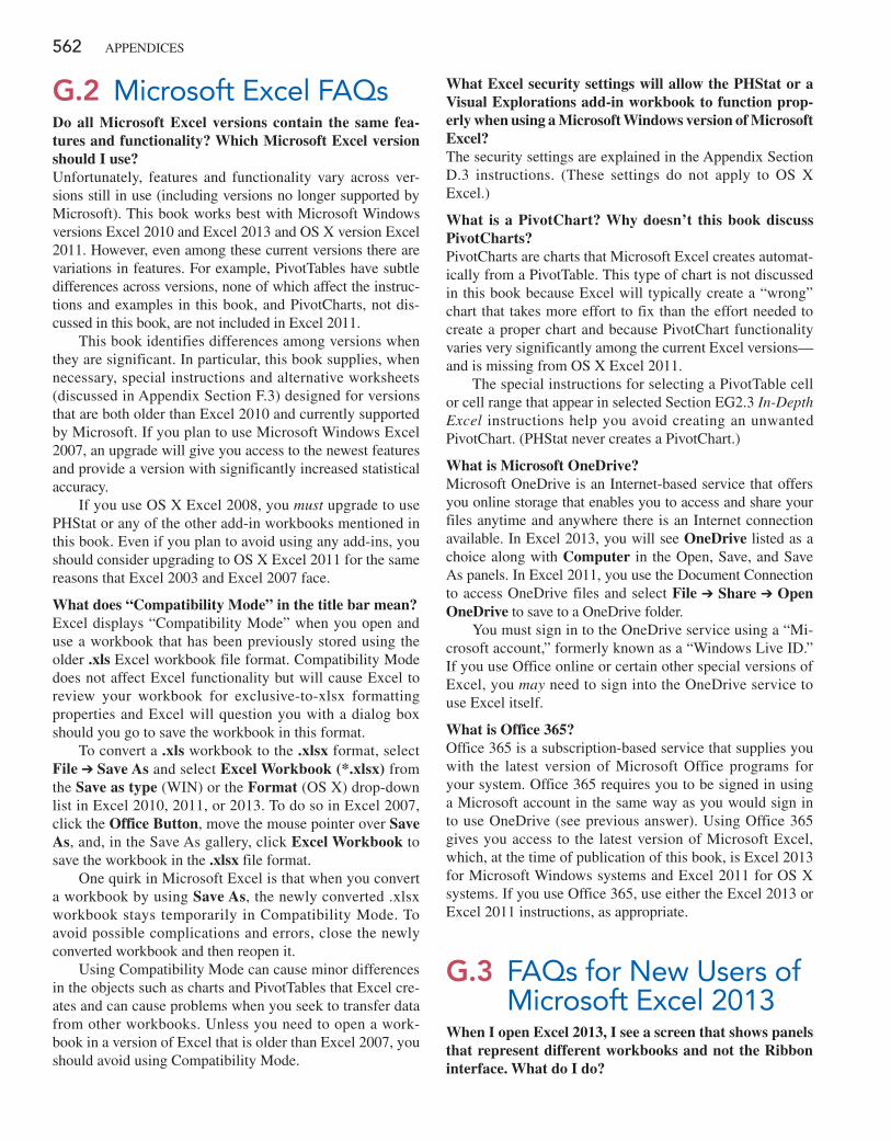
562 APPENDICES
G.2 Microsoft Excel FAQsDo all Microsoft Excel versions contain the same fea-tures and functionality? Which Microsoft Excel version should I use?Unfortunately, features and functionality vary across ver-sions still in use (including versions no longer supported by Microsoft). This book works best with Microsoft Windows versions Excel 2010 and Excel 2013 and OS X version Excel 2011. However, even among these current versions there are variations in features. For example, PivotTables have subtle differences across versions, none of which affect the instruc-tions and examples in this book, and PivotCharts, not dis-cussed in this book, are not included in Excel 2011.
This book identifies differences among versions when they are significant. In particular, this book supplies, when necessary, special instructions and alternative worksheets (discussed in Appendix Section F.3) designed for versions that are both older than Excel 2010 and currently supported by Microsoft. If you plan to use Microsoft Windows Excel 2007, an upgrade will give you access to the newest features and provide a version with significantly increased statistical accuracy.
If you use OS X Excel 2008, you must upgrade to use PHStat or any of the other add-in workbooks mentioned in this book. Even if you plan to avoid using any add-ins, you should consider upgrading to OS X Excel 2011 for the same reasons that Excel 2003 and Excel 2007 face.
What does “Compatibility Mode” in the title bar mean?Excel displays “Compatibility Mode” when you open and use a workbook that has been previously stored using the older .xls Excel workbook file format. Compatibility Mode does not affect Excel functionality but will cause Excel to review your workbook for exclusive-to-xlsx formatting properties and Excel will question you with a dialog box should you go to save the workbook in this format.
To convert a .xls workbook to the .xlsx format, select File ➔ Save As and select Excel Workbook (*.xlsx) from the Save as type (WIN) or the Format (OS X) drop-down list in Excel 2010, 2011, or 2013. To do so in Excel 2007, click the Office Button, move the mouse pointer over Save As, and, in the Save As gallery, click Excel Workbook to save the workbook in the .xlsx file format.
One quirk in Microsoft Excel is that when you convert a workbook by using Save As, the newly converted .xlsx workbook stays temporarily in Compatibility Mode. To avoid possible complications and errors, close the newly converted workbook and then reopen it.
Using Compatibility Mode can cause minor differences in the objects such as charts and PivotTables that Excel cre-ates and can cause problems when you seek to transfer data from other workbooks. Unless you need to open a work-book in a version of Excel that is older than Excel 2007, you should avoid using Compatibility Mode.
What Excel security settings will allow the PHStat or a Visual Explorations add-in workbook to function prop-erly when using a Microsoft Windows version of Microsoft Excel?The security settings are explained in the Appendix Section D.3 instructions. (These settings do not apply to OS X Excel.)
What is a PivotChart? Why doesn’t this book discuss PivotCharts?PivotCharts are charts that Microsoft Excel creates automat-ically from a PivotTable. This type of chart is not discussed in this book because Excel will typically create a “wrong” chart that takes more effort to fix than the effort needed to create a proper chart and because PivotChart functionality varies very significantly among the current Excel versions—and is missing from OS X Excel 2011.
The special instructions for selecting a PivotTable cell or cell range that appear in selected Section EG2.3 In-Depth Excel instructions help you avoid creating an unwanted PivotChart. (PHStat never creates a PivotChart.)
What is Microsoft OneDrive?Microsoft OneDrive is an Internet-based service that offers you online storage that enables you to access and share your files anytime and anywhere there is an Internet connection available. In Excel 2013, you will see OneDrive listed as a choice along with Computer in the Open, Save, and Save As panels. In Excel 2011, you use the Document Connection to access OneDrive files and select File ➔ Share ➔ Open OneDrive to save to a OneDrive folder.
You must sign in to the OneDrive service using a “Mi-crosoft account,” formerly known as a “Windows Live ID.” If you use Office online or certain other special versions of Excel, you may need to sign into the OneDrive service to use Excel itself.
What is Office 365?Office 365 is a subscription-based service that supplies you with the latest version of Microsoft Office programs for your system. Office 365 requires you to be signed in using a Microsoft account in the same way as you would sign in to use OneDrive (see previous answer). Using Office 365 gives you access to the latest version of Microsoft Excel, which, at the time of publication of this book, is Excel 2013 for Microsoft Windows systems and Excel 2011 for OS X systems. If you use Office 365, use either the Excel 2013 or Excel 2011 instructions, as appropriate.
G.3 FAQs for New Users of Microsoft Excel 2013
When I open Excel 2013, I see a screen that shows panels that represent different workbooks and not the Ribbon interface. What do I do?

APPENDIX G Software FAQs 563
Press Esc. That screen, called the Start screen, will disap-pear and a screen that contains an Excel window similar to the ones in Excel 2010 and Excel 2011 will appear. For a more permanent solution, select File ➔ Options and in the General panel of the Excel Options dialog box that appears clear Show the Start screen when this application starts and then click OK.
Are there any significant differences between Excel 2013 and its immediate predecessor, Excel 2010?There are no significant differences, but several File tab commands present restyled panes (with the same or similar information), and opening and saving files differs slightly, as described in the Excel Guide for the Let’s Get Started chapter.
The Excel 2013 Ribbon, featured in a number of Ap-pendix B illustrations, looks slightly different than the Excel 2010 Ribbon. However, these differences are so slight that the Excel 2013 Ribbon illustrations in Appendix B will be recog-nizable to you if you choose to use Excel 2010.
In the Insert tab, what are Recommended PivotTables and Recommended Charts? Should I use these features?Recommended PivotTables and Recommended Charts display one or more “recommended” PivotTables or charts as shortcuts. Unfortunately, the recommended PivotTables can include statistical errors such as treating the categories of a categorical variable as zero values of a numerical vari-able and the recommended charts often do not conform to best practices (see Appendix Section B.6).
As programmed in Excel 2013, you should ignore and not use these features as they will likely cause you to spend more time correcting errors and formatting mistakes than the little time that you might otherwise save.
G.4 Minitab FAQsCan I use Minitab Student 14 or Release 14 or 15 with this book?Yes, you can use the Minitab Guide instructions with Minitab Student 14 or Release 14 or 15. For certain methods, there may be minor differences in labeling of dialog box elements. Any difference that is not minor is noted in the instructions.
Can I save my Minitab worksheets or projects for use with Minitab Student 14 or Release 14 or 15?Yes. Select either Minitab14 or Minitab 15 (for a worksheet) or Minitab 14 Project (*.MPJ) or Minitab 15 Project (*.MPJ) (for a project) from the Save as type drop-down list in the save as dialog box. (See Appendix Section B.10 for more information.)
Can I use Minitab 17 with this book?Yes, you can use the Minitab Guide instructions, which fea-ture Minitab 16, with Minitab 17. For certain methods, there may be minor differences in labeling of dialog box elements and some outputs will appear formatted slightly differently than the Minitab 16 outputs shown in this book. Significant differences, such as changes in menu selection sequences, are noted in the instructions. If you plan to use Minitab 17 exten-sively, download the Using Minitab 17 supplement available on the student download page for this book or inside the MyStatLab course for this book. (See Appendix Section C.2 for more information.)
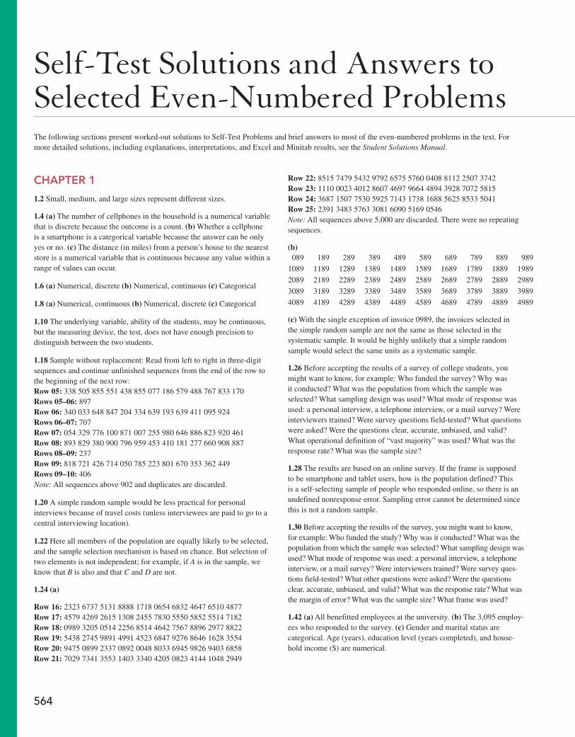
564
Self-Test Solutions and Answers to Selected Even-Numbered ProblemsThe following sections present worked-out solutions to Self-Test Problems and brief answers to most of the even-numbered problems in the text. For more detailed solutions, including explanations, interpretations, and Excel and Minitab results, see the Student Solutions Manual.
CHAPTER 1
1.2 Small, medium, and large sizes represent different sizes.
1.4 (a) The number of cellphones in the household is a numerical variable that is discrete because the outcome is a count. (b) Whether a cellphone is a smartphone is a categorical variable because the answer can be only yes or no. (c) The distance (in miles) from a person’s house to the nearest store is a numerical variable that is continuous because any value within a range of values can occur.
1.6 (a) Numerical, discrete (b) Numerical, continuous (c) Categorical
1.8 (a) Numerical, continuous (b) Numerical, discrete (c) Categorical
1.10 The underlying variable, ability of the students, may be continuous, but the measuring device, the test, does not have enough precision to distinguish between the two students.
1.18 Sample without replacement: Read from left to right in three-digit sequences and continue unfinished sequences from the end of the row to the beginning of the next row:Row 05: 338 505 855 551 438 855 077 186 579 488 767 833 170Rows 05–06: 897Row 06: 340 033 648 847 204 334 639 193 639 411 095 924Rows 06–07: 707Row 07: 054 329 776 100 871 007 255 980 646 886 823 920 461Row 08: 893 829 380 900 796 959 453 410 181 277 660 908 887Rows 08–09: 237Row 09: 818 721 426 714 050 785 223 801 670 353 362 449Rows 09–10: 406Note: All sequences above 902 and duplicates are discarded.
1.20 A simple random sample would be less practical for personal interviews because of travel costs (unless interviewees are paid to go to a central interviewing location).
1.22 Here all members of the population are equally likely to be selected, and the sample selection mechanism is based on chance. But selection of two elements is not independent; for example, if A is in the sample, we know that B is also and that C and D are not.
1.24 (a)
Row 16: 2323 6737 5131 8888 1718 0654 6832 4647 6510 4877Row 17: 4579 4269 2615 1308 2455 7830 5550 5852 5514 7182Row 18: 0989 3205 0514 2256 8514 4642 7567 8896 2977 8822Row 19: 5438 2745 9891 4991 4523 6847 9276 8646 1628 3554Row 20: 9475 0899 2337 0892 0048 8033 6945 9826 9403 6858Row 21: 7029 7341 3553 1403 3340 4205 0823 4144 1048 2949
Row 22: 8515 7479 5432 9792 6575 5760 0408 8112 2507 3742Row 23: 1110 0023 4012 8607 4697 9664 4894 3928 7072 5815Row 24: 3687 1507 7530 5925 7143 1738 1688 5625 8533 5041Row 25: 2391 3483 5763 3081 6090 5169 0546Note: All sequences above 5,000 are discarded. There were no repeating sequences.
(b)089 189 289 389 489 589 689 789 889 989
1089 1189 1289 1389 1489 1589 1689 1789 1889 1989
2089 2189 2289 2389 2489 2589 2689 2789 2889 2989
3089 3189 3289 3389 3489 3589 3689 3789 3889 3989
4089 4189 4289 4389 4489 4589 4689 4789 4889 4989
(c) With the single exception of invoice 0989, the invoices selected in the simple random sample are not the same as those selected in the systematic sample. It would be highly unlikely that a simple random sample would select the same units as a systematic sample.
1.26 Before accepting the results of a survey of college students, you might want to know, for example: Who funded the survey? Why was it conducted? What was the population from which the sample was selected? What sampling design was used? What mode of response was used: a personal interview, a telephone interview, or a mail survey? Were interviewers trained? Were survey questions field-tested? What questions were asked? Were the questions clear, accurate, unbiased, and valid? What operational definition of “vast majority” was used? What was the response rate? What was the sample size?
1.28 The results are based on an online survey. If the frame is supposed to be smartphone and tablet users, how is the population defined? This is a self-selecting sample of people who responded online, so there is an undefined nonresponse error. Sampling error cannot be determined since this is not a random sample.
1.30 Before accepting the results of the survey, you might want to know, for example: Who funded the study? Why was it conducted? What was the population from which the sample was selected? What sampling design was used? What mode of response was used: a personal interview, a telephone interview, or a mail survey? Were interviewers trained? Were survey ques-tions field-tested? What other questions were asked? Were the questions clear, accurate, unbiased, and valid? What was the response rate? What was the margin of error? What was the sample size? What frame was used?
1.42 (a) All benefitted employees at the university. (b) The 3,095 employ-ees who responded to the survey. (c) Gender and marital status are categorical. Age (years), education level (years completed), and house-hold income ($) are numerical.
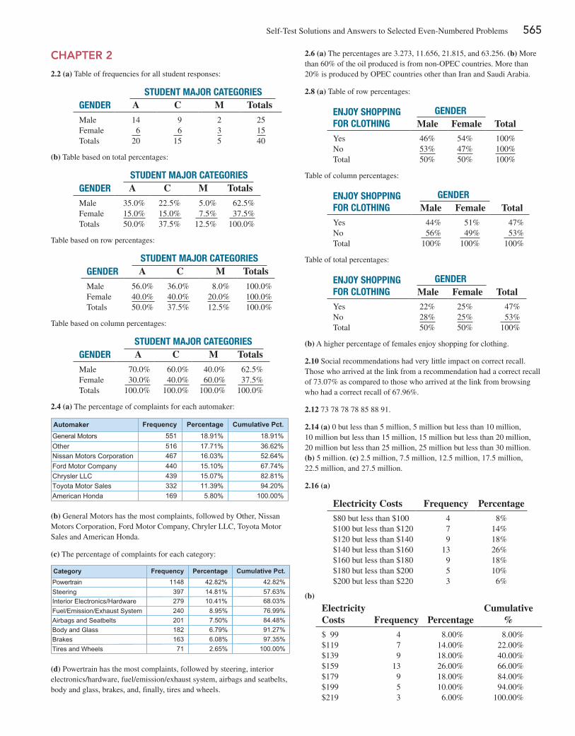
Self-Test Solutions and Answers to Selected Even-Numbered Problems 565
2.6 (a) The percentages are 3.273, 11.656, 21.815, and 63.256. (b) More than 60% of the oil produced is from non-OPEC countries. More than 20% is produced by OPEC countries other than Iran and Saudi Arabia.
2.8 (a) Table of row percentages:
Enjoy Shopping for Clothing
gEndErMale Female Total
Yes 46% 54% 100%No 53% 47% 100%Total 50% 50% 100%
Table of column percentages:
Enjoy Shopping for Clothing
gEndErMale Female Total
Yes 44% 51% 47%No 56% 49% 53%Total 100% 100% 100%
Table of total percentages:
Enjoy Shopping for Clothing
gEndErMale Female Total
Yes 22% 25% 47%No 28% 25% 53%Total 50% 50% 100%
(b) A higher percentage of females enjoy shopping for clothing.
2.10 Social recommendations had very little impact on correct recall. Those who arrived at the link from a recommendation had a correct recall of 73.07% as compared to those who arrived at the link from browsing who had a correct recall of 67.96%.
2.12 73 78 78 78 85 88 91.
2.14 (a) 0 but less than 5 million, 5 million but less than 10 million, 10 million but less than 15 million, 15 million but less than 20 million, 20 million but less than 25 million, 25 million but less than 30 million. (b) 5 million. (c) 2.5 million, 7.5 million, 12.5 million, 17.5 million, 22.5 million, and 27.5 million.
2.16 (a)
Electricity Costs Frequency Percentage
$80 but less than $100 4 8%$100 but less than $120 7 14%$120 but less than $140 9 18%$140 but less than $160 13 26%$160 but less than $180 9 18%$180 but less than $200 5 10%$200 but less than $220 3 6%
(b)
Electricity Costs
Frequency
Percentage
Cumulative %
$ 99 4 8.00% 8.00%$119 7 14.00% 22.00%$139 9 18.00% 40.00%$159 13 26.00% 66.00%$179 9 18.00% 84.00%$199 5 10.00% 94.00%$219 3 6.00% 100.00%
CHAPTER 2
2.2 (a) Table of frequencies for all student responses:
StudEnt Major CatEgoriESgEndEr A C M Totals
Male 14 9 2 25Female 6 6 3 15Totals 20 15 5 40
(b) Table based on total percentages:
StudEnt Major CatEgoriESgEndEr A C M Totals
Male 35.0% 22.5% 5.0% 62.5%Female 15.0% 15.0% 7.5% 37.5%Totals 50.0% 37.5% 12.5% 100.0%
Table based on row percentages:
StudEnt Major CatEgoriESgEndEr A C M Totals
Male 56.0% 36.0% 8.0% 100.0%Female 40.0% 40.0% 20.0% 100.0%Totals 50.0% 37.5% 12.5% 100.0%
Table based on column percentages:
StudEnt Major CatEgoriESgEndEr A C M Totals
Male 70.0% 60.0% 40.0% 62.5%Female 30.0% 40.0% 60.0% 37.5%Totals 100.0% 100.0% 100.0% 100.0%
2.4 (a) The percentage of complaints for each automaker:
General MotorsOtherNissan Motors Corporation
Chrysler LLCFord Motor Company
Toyota Motor SalesAmerican Honda
439440
551516467
169332
Frequency
82.81%67.74%
18.91%36.62%52.64%
100.00%94.20%
Cumulative Pct.
15.07%15.10%
18.91%17.71%16.03%
5.80%11.39%
PercentageAutomaker
(b) General Motors has the most complaints, followed by Other, Nissan Motors Corporation, Ford Motor Company, Chryler LLC, Toyota Motor Sales and American Honda.
(c) The percentage of complaints for each category:
PowertrainSteeringInterior Electronics/Hardware
Airbags and SeatbeltsFuel/Emission/Exhaust System
Body and GlassBrakes
Cumulative Pct.Category
Tires and Wheels
Frequency
201240
1148397279
163182
71
Percentage
7.50%8.95%
42.82%14.81%10.41%
6.08%6.79%
2.65%
84.48% 76.99%
42.82%57.63%68.03%
97.35%91.27%
100.00%
(d) Powertrain has the most complaints, followed by steering, interior electronics/hardware, fuel/emission/exhaust system, airbags and seatbelts, body and glass, brakes, and, finally, tires and wheels.
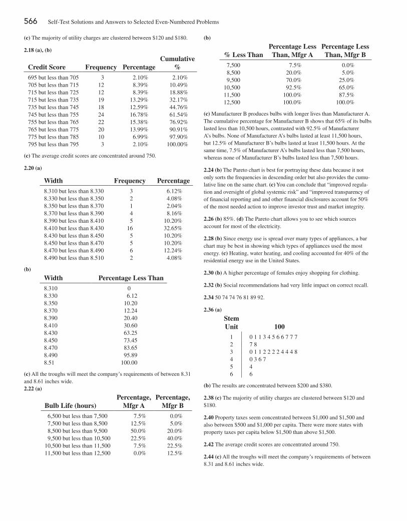
566 Self-Test Solutions and Answers to Selected Even-Numbered Problems
(b)
% Less Than
Percentage Less Than, Mfgr A
Percentage Less Than, Mfgr B
7,500 7.5% 0.0% 8,500 20.0% 5.0% 9,500 70.0% 25.0%10,500 92.5% 65.0%11,500 100.0% 87.5%12,500 100.0% 100.0%
(c) Manufacturer B produces bulbs with longer lives than Manufacturer A. The cumulative percentage for Manufacturer B shows that 65% of its bulbs lasted less than 10,500 hours, contrasted with 92.5% of Manufacturer A’s bulbs. None of Manufacturer A’s bulbs lasted at least 11,500 hours, but 12.5% of Manufacturer B’s bulbs lasted at least 11,500 hours. At the same time, 7.5% of Manufacturer A’s bulbs lasted less than 7,500 hours, whereas none of Manufacturer B’s bulbs lasted less than 7,500 hours.
2.24 (b) The Pareto chart is best for portraying these data because it not only sorts the frequencies in descending order but also provides the cumu-lative line on the same chart. (c) You can conclude that “improved regula-tion and oversight of global systemic risk” and “improved transparency of of financial reporting and and other financial disclosures account for 50% of the most needed action to improve investor trust and market integrity.
2.26 (b) 85%. (d) The Pareto chart allows you to see which sources account for most of the electricity.
2.28 (b) Since energy use is spread over many types of appliances, a bar chart may be best in showing which types of appliances used the most energy. (c) Heating, water heating, and cooling accounted for 40% of the residential energy use in the United States.
2.30 (b) A higher percentage of females enjoy shopping for clothing.
2.32 (b) Social recommendations had very little impact on correct recall.
2.34 50 74 74 76 81 89 92.
2.36 (a)
Stem Unit 100
1 0 1 1 3 4 5 6 6 7 7 72 7 83 0 1 1 2 2 2 2 4 4 4 84 0 3 6 75 46 6
(b) The results are concentrated between $200 and $380.
2.38 (c) The majority of utility charges are clustered between $120 and $180.
2.40 Property taxes seem concentrated between $1,000 and $1,500 and also between $500 and $1,000 per capita. There were more states with property taxes per capita below $1,500 than above $1,500.
2.42 The average credit scores are concentrated around 750.
2.44 (c) All the troughs will meet the company’s requirements of between 8.31 and 8.61 inches wide.
(c) The majority of utility charges are clustered between $120 and $180.
2.18 (a), (b)
Credit Score
Frequency
Percentage
Cumulative %
695 but less than 705 3 2.10% 2.10%705 but less than 715 12 8.39% 10.49%715 but less than 725 12 8.39% 18.88%715 but less than 735 19 13.29% 32.17%735 but less than 745 18 12.59% 44.76%745 but less than 755 24 16.78% 61.54%755 but less than 765 22 15.38% 76.92%765 but less than 775 20 13.99% 90.91%775 but less than 785 10 6.99% 97.90%795 but less than 795 3 2.10% 100.00%
(c) The average credit scores are concentrated around 750.
2.20 (a)
Width Frequency Percentage
8.310 but less than 8.330 3 6.12%8.330 but less than 8.350 2 4.08%8.350 but less than 8.370 1 2.04%8.370 but less than 8.390 4 8.16%8.390 but less than 8.410 5 10.20%8.410 but less than 8.430 16 32.65%8.430 but less than 8.450 5 10.20%8.450 but less than 8.470 5 10.20%8.470 but less than 8.490 6 12.24%8.490 but less than 8.510 2 4.08%
(b)
Width Percentage Less Than
8.310 08.330 6.128.350 10.208.370 12.248.390 20.408.410 30.608.430 63.258.450 73.458.470 83.658.490 95.898.51 100.00
(c) All the troughs will meet the company’s requirements of between 8.31 and 8.61 inches wide.2.22 (a)
Bulb Life (hours)
Percentage, Mfgr A
Percentage, Mfgr B
6,500 but less than 7,500 7.5% 0.0% 7,500 but less than 8,500 12.5% 5.0% 8,500 but less than 9,500 50.0% 20.0% 9,500 but less than 10,500 22.5% 40.0%10,500 but less than 11,500 7.5% 22.5%11,500 but less than 12,500 0.0% 12.5%
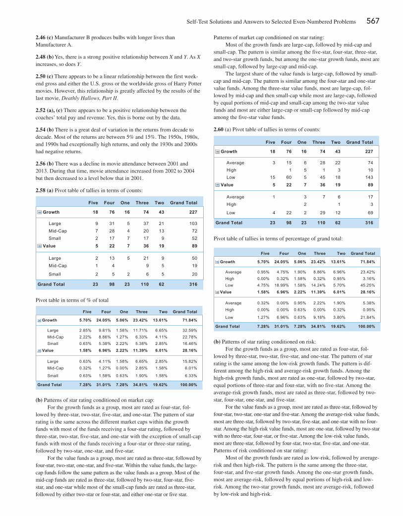
Self-Test Solutions and Answers to Selected Even-Numbered Problems 567
Patterns of market cap conditioned on star rating:Most of the growth funds are large-cap, followed by mid-cap and
small-cap. The pattern is similar among the five-star, four-star, three-star, and two-star growth funds, but among the one-star growth funds, most are small-cap, followed by large-cap and mid-cap.
The largest share of the value funds is large-cap, followed by small-cap and mid-cap. The pattern is similar among the four-star and one-star value funds. Among the three-star value funds, most are large-cap, fol-lowed by mid-cap and then small-cap while most are large-cap, followed by equal portions of mid-cap and small-cap among the two-star value funds and most are either large-cap or small-cap followed by mid-cap among the five-star value funds.
2.60 (a) Pivot table of tallies in terms of counts:
Five Four One Three Two Grand Total
18Growth 76 16 74
3Average 15 6 28High 1 5 1
15Low 60 5 45
5Value 22 7 36
1Average 3 7High 2
4Low 22 2 29
23Grand Total 98 23 110
43
223
18
19
61
12
62
227
7410
143
89
173
69
316
Pivot table of tallies in terms of percentage of grand total:
Five Four One Three Two Grand Total
5.70%Growth 24.05% 5.06% 23.42%
0.95%Average 4.75% 1.90% 8.86%0.00%High 0.32% 1.58% 0.32%4.75%Low 18.99% 1.58% 14.24%
1.58%Value 6.96% 2.22% 11.39%
0.32%Average 0.00% 0.95% 2.22%0.00%High 0.00% 0.63% 0.00%
1.27%Low 6.96% 0.63% 9.18%
7.28%Grand Total 31.01% 7.28% 34.81%
13.61%
6.96%0.95%5.70%
6.01%
1.90%0.32%
3.80%
19.62%
71.84%
23.42%3.16%
45.25%
28.16%
5.38%0.95%
21.84%
100.00%
(b) Patterns of star rating conditioned on risk:For the growth funds as a group, most are rated as four-star, fol-
lowed by three-star, two-star, five-star, and one-star. The pattern of star rating is the same among the low-risk growth funds. The pattern is dif-ferent among the high-risk and average-risk growth funds. Among the high-risk growth funds, most are rated as one-star, followed by two-star, equal portions of three-star and four-star, with no five-star. Among the average-risk growth funds, most are rated as three-star, followed by two-star, four-star, one-star, and five-star.
For the value funds as a group, most are rated as three-star, followed by four-star, two-star, one-star and five-star. Among the average-risk value funds, most are three-star, followed by two-star, five-star, and one-star with no four-star. Among the high-risk value funds, most are one-star, followed by two-star with no three-star, four-star, or five-star. Among the low-risk value funds, most are three-star, followed by four-star, two-star, five-star, and one-star.Patterns of risk conditioned on star rating:
Most of the growth funds are rated as low-risk, followed by average-risk and then high-risk. The pattern is the same among the three-star, four-star, and five-star growth funds. Among the one-star growth funds, most are average-risk, followed by equal portions of high-risk and low-risk. Among the two-star growth funds, most are average-risk, followed by low-risk and high-risk.
2.46 (c) Manufacturer B produces bulbs with longer lives than Manufacturer A.
2.48 (b) Yes, there is a strong positive relationship between X and Y. As X increases, so does Y.
2.50 (c) There appears to be a linear relationship between the first week-end gross and either the U.S. gross or the worldwide gross of Harry Potter movies. However, this relationship is greatly affected by the results of the last movie, Deathly Hallows, Part II.
2.52 (a), (c) There appears to be a positive relationship between the coaches’ total pay and revenue. Yes, this is borne out by the data.
2.54 (b) There is a great deal of variation in the returns from decade to decade. Most of the returns are between 5% and 15%. The 1950s, 1980s, and 1990s had exceptionally high returns, and only the 1930s and 2000s had negative returns.
2.56 (b) There was a decline in movie attendance between 2001 and 2013. During that time, movie attendance increased from 2002 to 2004 but then decreased to a level below that in 2001.
2.58 (a) Pivot table of tallies in terms of counts:
Five Four One Three Two Grand Total
18Growth 76 16 74
9Large 31 5 377Mid-Cap 28 4 202Small 17 7 17
5Value 22 7 36
2Large 13 5 211Mid-Cap 4 9
2Small 5 2 6
23Grand Total 98 23 110
43
2113
9
19
95
5
62
227
1037252
89
5019
20
316
Pivot table in terms of % of total
Five Four One Three Two Grand Total
5.70%Growth 24.05% 5.06% 23.42%
2.85%Large 9.81% 1.58% 11.71%2.22%Mid-Cap 8.86% 1.27% 6.33%0.63%Small 5.38% 2.22% 5.38%
1.58%Value 6.96% 2.22% 11.39%
0.63%Large 4.11% 1.58% 6.65%0.32%Mid-Cap 1.27% 0.00% 2.85%
0.63%Small 1.58% 0.63% 1.90%
7.28%Grand Total 31.01% 7.28% 34.81%
13.61%
6.65%4.11%2.85%
6.01%
2.85%1.58%
1.58%
19.62%
71.84%
32.59%22.78%16.46%
28.16%
15.82%6.01%
6.33%
100.00%
(b) Patterns of star rating conditioned on market cap:For the growth funds as a group, most are rated as four-star, fol-
lowed by three-star, two-star, five-star, and one-star. The pattern of star rating is the same across the different market caps within the growth funds with most of the funds receiving a four-star rating, followed by three-star, two-star, five-star, and one-star with the exception of small-cap funds with most of the funds receiving a four-star or three-star rating, followed by two-star, one-star, and five-star.
For the value funds as a group, most are rated as three-star, followed by four-star, two-star, one-star, and five-star. Within the value funds, the large-cap funds follow the same pattern as the value funds as a group. Most of the mid-cap funds are rated as three-star, followed by two-star, four-star, five-star, and one-star while most of the small-cap funds are rated as three-star, followed by either two-star or four-star, and either one-star or five star.
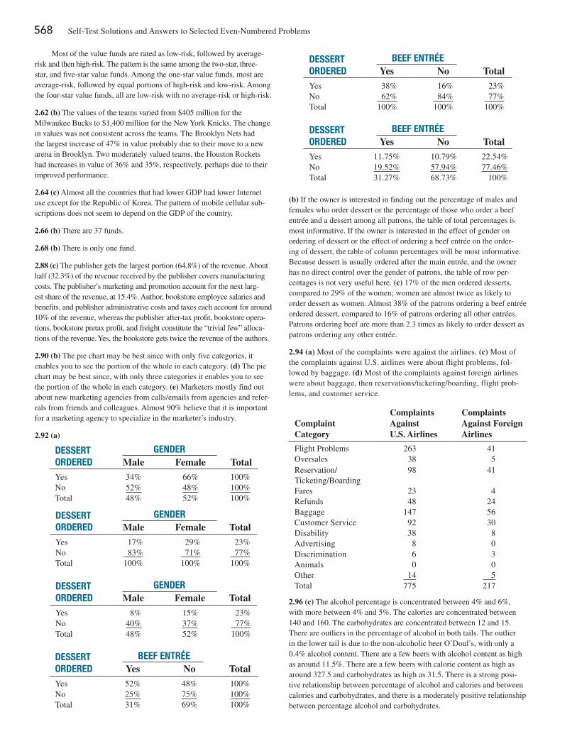
568 Self-Test Solutions and Answers to Selected Even-Numbered Problems
dESSErt ordErEd
BEEf EntréEYes No Total
Yes 38% 16% 23%No 62% 84% 77%Total 100% 100% 100%
dESSErt ordErEd
BEEf EntréEYes No Total
Yes 11.75% 10.79% 22.54%No 19.52% 57.94% 77.46%Total 31.27% 68.73% 100%
(b) If the owner is interested in finding out the percentage of males and females who order dessert or the percentage of those who order a beef entrée and a dessert among all patrons, the table of total percentages is most informative. If the owner is interested in the effect of gender on ordering of dessert or the effect of ordering a beef entrée on the order-ing of dessert, the table of column percentages will be most informative. Because dessert is usually ordered after the main entrée, and the owner has no direct control over the gender of patrons, the table of row per-centages is not very useful here. (c) 17% of the men ordered desserts, compared to 29% of the women; women are almost twice as likely to order dessert as women. Almost 38% of the patrons ordering a beef entrée ordered dessert, compared to 16% of patrons ordering all other entrées. Patrons ordering beef are more than 2.3 times as likely to order dessert as patrons ordering any other entrée.
2.94 (a) Most of the complaints were against the airlines. (c) Most of the complaints against U.S. airlines were about flight problems, fol-lowed by baggage. (d) Most of the complaints against foreign airlines were about baggage, then reservations/ticketing/boarding, flight prob-lems, and customer service.
Complaint Category
Complaints Against U.S. Airlines
Complaints Against Foreign Airlines
Flight Problems 263 41Oversales 38 5Reservation/Ticketing/Boarding
98 41
Fares 23 4Refunds 48 24Baggage 147 56Customer Service 92 30Disability 38 8Advertising 8 0Discrimination 6 3Animals 0 0Other 14 5Total 775 217
2.96 (c) The alcohol percentage is concentrated between 4% and 6%, with more between 4% and 5%. The calories are concentrated between 140 and 160. The carbohydrates are concentrated between 12 and 15. There are outliers in the percentage of alcohol in both tails. The outlier in the lower tail is due to the non-alcoholic beer O’Doul’s, with only a 0.4% alcohol content. There are a few beers with alcohol content as high as around 11.5%. There are a few beers with calorie content as high as around 327.5 and carbohydrates as high as 31.5. There is a strong posi-tive relationship between percentage of alcohol and calories and between calories and carbohydrates, and there is a moderately positive relationship between percentage alcohol and carbohydrates.
Most of the value funds are rated as low-risk, followed by average-risk and then high-risk. The pattern is the same among the two-star, three-star, and five-star value funds. Among the one-star value funds, most are average-risk, followed by equal portions of high-risk and low-risk. Among the four-star value funds, all are low-risk with no average-risk or high-risk.
2.62 (b) The values of the teams varied from $405 million for the Milwaukee Bucks to $1,400 million for the New York Knicks. The change in values was not consistent across the teams. The Brooklyn Nets had the largest increase of 47% in value probably due to their move to a new arena in Brooklyn. Two moderately valued teams, the Houston Rockets had increases in value of 36% and 35%, respectively, perhaps due to their improved performance.
2.64 (c) Almost all the countries that had lower GDP had lower Internet use except for the Republic of Korea. The pattern of mobile cellular sub-scriptions does not seem to depend on the GDP of the country.
2.66 (b) There are 37 funds.
2.68 (b) There is only one fund.
2.88 (c) The publisher gets the largest portion (64.8%) of the revenue. About half (32.3%) of the revenue received by the publisher covers manufacturing costs. The publisher’s marketing and promotion account for the next larg-est share of the revenue, at 15.4%. Author, bookstore employee salaries and benefits, and publisher administrative costs and taxes each account for around 10% of the revenue, whereas the publisher after-tax profit, bookstore opera-tions, bookstore pretax profit, and freight constitute the “trivial few” alloca-tions of the revenue. Yes, the bookstore gets twice the revenue of the authors.
2.90 (b) The pie chart may be best since with only five categories, it enables you to see the portion of the whole in each category. (d) The pie chart may be best since, with only three categories it enables you to see the portion of the whole in each category. (e) Marketers mostly find out about new marketing agencies from calls/emails from agencies and refer-rals from friends and colleagues. Almost 90% believe that it is important for a marketing agency to specialize in the marketer’s industry.
2.92 (a)
dESSErt ordErEd
gEndErMale Female Total
Yes 34% 66% 100%No 52% 48% 100%Total 48% 52% 100%
dESSErt ordErEd
gEndErMale Female Total
Yes 17% 29% 23%No 83% 71% 77%Total 100% 100% 100%
dESSErt ordErEd
gEndErMale Female Total
Yes 8% 15% 23%No 40% 37% 77%Total 48% 52% 100%
dESSErt ordErEd
BEEf EntréEYes No Total
Yes 52% 48% 100%No 25% 75% 100%Total 31% 69% 100%
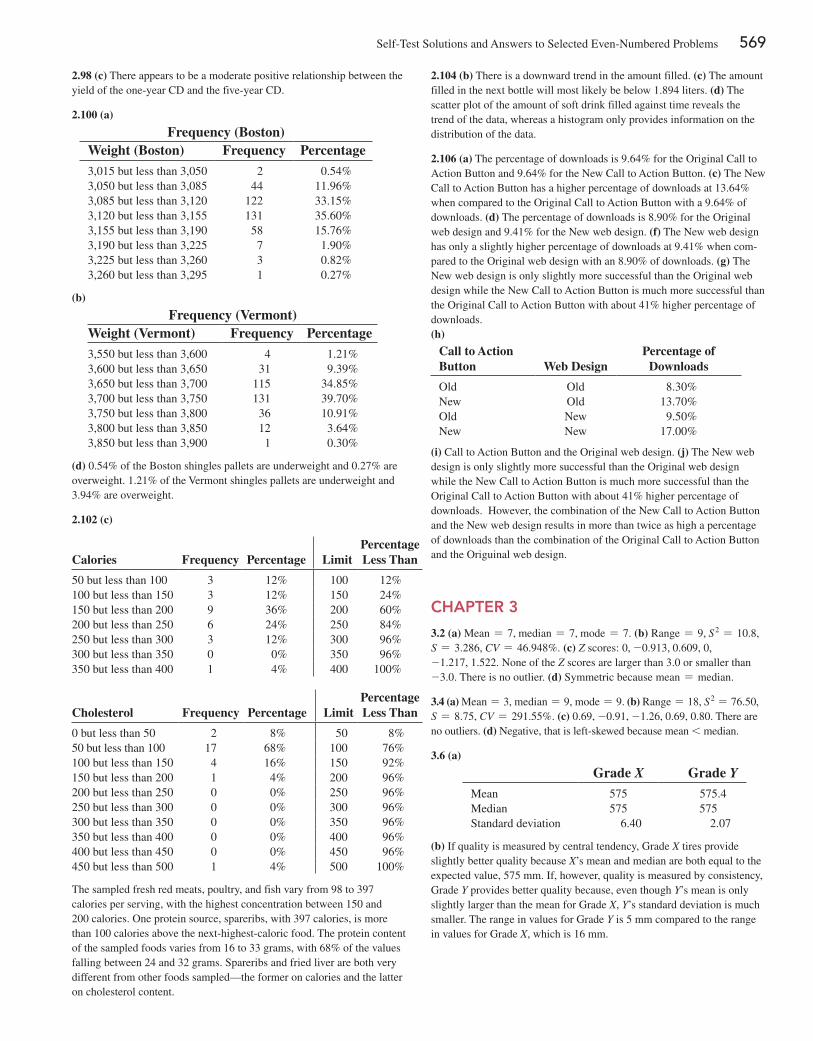
Self-Test Solutions and Answers to Selected Even-Numbered Problems 569
2.104 (b) There is a downward trend in the amount filled. (c) The amount filled in the next bottle will most likely be below 1.894 liters. (d) The scatter plot of the amount of soft drink filled against time reveals the trend of the data, whereas a histogram only provides information on the distribution of the data.
2.106 (a) The percentage of downloads is 9.64% for the Original Call to Action Button and 9.64% for the New Call to Action Button. (c) The New Call to Action Button has a higher percentage of downloads at 13.64% when compared to the Original Call to Action Button with a 9.64% of downloads. (d) The percentage of downloads is 8.90% for the Original web design and 9.41% for the New web design. (f) The New web design has only a slightly higher percentage of downloads at 9.41% when com-pared to the Original web design with an 8.90% of downloads. (g) The New web design is only slightly more successful than the Original web design while the New Call to Action Button is much more successful than the Original Call to Action Button with about 41% higher percentage of downloads.(h)
Call to Action Button Web Design
Percentage of Downloads
Old Old 8.30%New Old 13.70%Old New 9.50%New New 17.00%
(i) Call to Action Button and the Original web design. (j) The New web design is only slightly more successful than the Original web design while the New Call to Action Button is much more successful than the Original Call to Action Button with about 41% higher percentage of downloads. However, the combination of the New Call to Action Button and the New web design results in more than twice as high a percentage of downloads than the combination of the Original Call to Action Button and the Origuinal web design.
CHAPTER 3
3.2 (a) Mean = 7, median = 7, mode = 7. (b) Range = 9, S2 = 10.8,S = 3.286, CV = 46.948%. (c) Z scores: 0, -0.913, 0.609, 0,-1.217, 1.522. None of the Z scores are larger than 3.0 or smaller than -3.0. There is no outlier. (d) Symmetric because mean = median.
3.4 (a) Mean = 3, median = 9, mode = 9. (b) Range = 18, S2 = 76.50, S = 8.75, CV = 291.55%. (c) 0.69, -0.91, -1.26, 0.69, 0.80. There are no outliers. (d) Negative, that is left-skewed because mean < median.
3.6 (a)
Grade X Grade Y
Mean 575 575.4Median 575 575Standard deviation 6.40 2.07
(b) If quality is measured by central tendency, Grade X tires provide slightly better quality because X’s mean and median are both equal to the expected value, 575 mm. If, however, quality is measured by consistency, Grade Y provides better quality because, even though Y’s mean is only slightly larger than the mean for Grade X, Y’s standard deviation is much smaller. The range in values for Grade Y is 5 mm compared to the range in values for Grade X, which is 16 mm.
2.98 (c) There appears to be a moderate positive relationship between the yield of the one-year CD and the five-year CD.
2.100 (a)
Frequency (Boston)Weight (Boston) Frequency Percentage
3,015 but less than 3,050 2 0.54%3,050 but less than 3,085 44 11.96%3,085 but less than 3,120 122 33.15%3,120 but less than 3,155 131 35.60%3,155 but less than 3,190 58 15.76%3,190 but less than 3,225 7 1.90%3,225 but less than 3,260 3 0.82%3,260 but less than 3,295 1 0.27%
(b)
Frequency (Vermont)Weight (Vermont) Frequency Percentage
3,550 but less than 3,600 4 1.21%3,600 but less than 3,650 31 9.39%3,650 but less than 3,700 115 34.85%3,700 but less than 3,750 131 39.70%3,750 but less than 3,800 36 10.91%3,800 but less than 3,850 12 3.64%3,850 but less than 3,900 1 0.30%
(d) 0.54% of the Boston shingles pallets are underweight and 0.27% are overweight. 1.21% of the Vermont shingles pallets are underweight and 3.94% are overweight.
2.102 (c)
Calories
Frequency
Percentage
Limit
Percentage Less Than
50 but less than 100 3 12% 100 12%100 but less than 150 3 12% 150 24%150 but less than 200 9 36% 200 60%200 but less than 250 6 24% 250 84%250 but less than 300 3 12% 300 96%300 but less than 350 0 0% 350 96%350 but less than 400 1 4% 400 100%
Cholesterol
Frequency
Percentage
Limit
Percentage Less Than
0 but less than 50 2 8% 50 8%50 but less than 100 17 68% 100 76%100 but less than 150 4 16% 150 92%150 but less than 200 1 4% 200 96%200 but less than 250 0 0% 250 96%250 but less than 300 0 0% 300 96%300 but less than 350 0 0% 350 96%350 but less than 400 0 0% 400 96%400 but less than 450 0 0% 450 96%450 but less than 500 1 4% 500 100%
The sampled fresh red meats, poultry, and fish vary from 98 to 397 calories per serving, with the highest concentration between 150 and 200 calories. One protein source, spareribs, with 397 calories, is more than 100 calories above the next-highest-caloric food. The protein content of the sampled foods varies from 16 to 33 grams, with 68% of the values falling between 24 and 32 grams. Spareribs and fried liver are both very different from other foods sampled—the former on calories and the latter on cholesterol content.
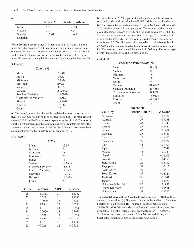
570 Self-Test Solutions and Answers to Selected Even-Numbered Problems
(c)
Grade X Grade Y, Altered
Mean 575 577.4Median 575 575Standard deviation
6.40 6.11
When the fifth Y tire measures 588 mm rather than 578 mm, Y’s mean inner diameter becomes 577.4 mm, which is larger than X’s mean inner diameter, and Y’s standard deviation increases from 2.07 mm to 6.11 mm. In this case, X’s tires are providing better quality in terms of the mean inner diameter, with only slightly more variation among the tires than Y’s.
3.8 (a), (b)
Spend ($)Mean 56.40Median 55.35Minimum 22.90Maximum 108.25Range 85.35Variance 380.4062Standard Deviation 19.5040Coefficient of Variation 34.58%Skewness 1.1078Kurtosis 3.0651Count 15
(c) The mean is greater than the median and the skewness statistic is posi-tive, so the amount spent is right- or positive-skewed. (d) The mean amount spent is $56.40 and half the customers spent more than $55.35. The amount spent is right-skewed since there are some amounts spent that are high. The average scatter around the mean is $19.50. The difference between the larg-est amount spent and the smallest amount spent is $85.35.
3.10 (a), (b)
MPGMean 22.85Median 22Minimum 21Maximum 26Range 5Variance 2.6605Standard Deviation 1.6311Coeff. of Variation 7.14%Skewness 0.7521Kurtosis -0.5423Count 20
MPG Z Score MPG Z Score26 1.9312 21 -1.134222 -0.5211 21 -1.134223 0.0920 22 -0.521121 -1.1342 22 -0.521125 1.3181 23 0.092024 0.7050 24 0.705022 -0.5211 23 0.092026 1.9312 22 -0.521125 -1.3181 21 -1.134222 -0.5211 22 -0.5211
(c) Since the mean MPG is greater than the median and the skewness statistic is positive, the distribution of MPG is right- or positive-skewed. (d) The mean miles per gallon of small SUVs is 22.85 and half the small SUVs achieve at least 22 miles per gallon. There are no outliers in the data as the largest Z score is 1.9312 and the smallest Z score is -1.1342. The average scatter around the mean is 1.6311 mpg. The lowest mpg is 21 and the highest is 26. The mpg of mid-sized sedans is much higher than for small SUVs. The mean miles per gallon of mid-sized sedans is 27.7727 and half the mid-sized sedans achieve at least 26 miles per gal-lon. The average scatter around the mean is 5.1263 mpg. The lowest mpg of mid-sized sedans is 22 and the highest is 39.
3.12 (a), (b)
Facebook Penetration (%)Mean 39.4091Median 42Minimum 6Maximum 80Range 74Variance 340.6342Standard Deviation 18.4563Coefficient of Variation 46.83%Skewness 0.0126Kurtosis -0.1492Count 22
CountryFacebook Penetration (%) Z Score
Argentina 56 0.8989Australia 57 0.9531Brazil 43 0.1946Canada 55 0.8447France 42 0.1404Germany 35 -0.2389India 7 -1.7560Indonesia 25 -0.7807Italy 42 0.1404Japan 17 -1.2142Mexico 43 0.1946Nigeria 6 -1.8102Poland 31 -0.4556Saudi Arabia 28 -0.6182Singapore 59 1.0615South Africa 20 -1.0516South Korea 27 -0.6724Thailand 36 -0.1847Turkey 45 0.3029United Arab Republic 80 2.1993United Kingdom 57 0.9531United States 56 0.8989
The highest Z score is 2.1993 and the lowest Z score is -1.8102, so there are no extreme values. (c) The mean is less than the median, so Facebook penetration is left-skewed. (d) The mean Facebook penetration is 39.4901% and half the countries have Facebook penetration greater than or equal to 42%. The average scatter around the mean is 18.4563%. The lowest Facebook penetration is 6% in Nigeria and the highest Facebook penetration is 80% in the United Arab Republic.
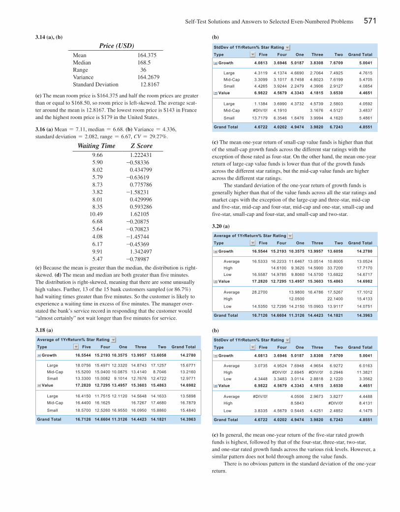
Self-Test Solutions and Answers to Selected Even-Numbered Problems 571
(b)
FiveType Four One Three Two Grand Total
4.0813Growth 3.6946 5.0187 3.8308
4.3119Large 4.1374 4.6690 2.70643.3099Mid-Cap 3.1017 8.7458 4.80234.4265Small 3.9244 2.2479 4.3906
6.9822Value 4.5679 4.3343 4.1815
1.1384Large 3.6990 4.3732 4.5739#DIV/0!Mid-Cap 4.1910 3.1676
13.7179Small 6.3546 1.6476 3.9994
4.6722 4.0202 4.9474 3.9820
7.6709
7.49257.61992.9127
3.6530
2.58034.5127
4.1620
6.7243
5.0041
4.76155.47054.0854
4.4651
4.05923.4837
5.4861
4.8551
StdDev of 1YrReturn% Star Rating
Grand Total
(c) The mean one-year return of small-cap value funds is higher than that of the small-cap growth funds across the different star ratings with the exception of those rated as four-star. On the other hand, the mean one-year return of large-cap value funds is lower than that of the growth funds across the different star ratings, but the mid-cap value funds are higher across the different star ratings.
The standard deviation of the one-year return of growth funds is generally higher than that of the value funds across all the star ratings and market caps with the exception of the large-cap and three-star, mid-cap and five-star, mid-cap and four-star, mid-cap and one-star, small-cap and five-star, small-cap and four-star, and small-cap and two-star.
3.20 (a)
FiveType Four One Three Two Grand Total
16.5544Growth 15.2193 10.3575 13.9957
16.5333Average 16.2233 11.6467 13.0514High 14.6100 9.3620 14.5900
16.5587Low 14.9785 9.8060 14.5700
17.2820Value 12.7295 13.4957 15.3603
28.2700Average 13.9800 16.4786High 12.0500
14.5350Low 12.7295 14.2150 15.0903
16.7126 14.6604 11.3126 14.4423
13.6058
10.800533.720013.6822
15.4863
17.526722.1400
13.9117
14.1821
14.2780
13.052417.717014.6717
14.6982
17.101215.4133
14.0751
14.3963
Average of 1YrReturn% Star Rating
Grand Total
(b)
FiveType Four One Three Two Grand Total
4.0813Growth 3.6946 5.0187 3.8308
3.0735Average 4.9524 7.6948 4.9654High #DIV/0! 2.6945 #DIV/0!
4.3448Low 3.3483 3.0114 2.8818
6.9822Value 4.5679 4.3343 4.1815
#DIV/0!Average 4.0506 2.9673High 8.5843
3.8335Low 4.5679 0.5445 4.4251
4.6722 4.0202 4.9474 3.9820
7.6709
6.92720.29462.1220
3.6530
3.8277#DIV/0!
2.4852
6.7243
5.0041
6.016311.3821
3.3562
4.4651
4.44888.4131
4.1475
4.8551Grand Total
StdDev of 1YrReturn% Star Rating
(c) In general, the mean one-year return of the five-star rated growth funds is highest, followed by that of the four-star, three-star, two-star, and one-star rated growth funds across the various risk levels. However, a similar pattern does not hold through among the value funds.
There is no obvious pattern in the standard deviation of the one-year return.
3.14 (a), (b)
Price (USD)Mean 164.375Median 168.5Range 36Variance 164.2679Standard Deviation 12.8167
(c) The mean room price is $164.375 and half the room prices are greater than or equal to $168.50, so room price is left-skewed. The average scat-ter around the mean is 12.8167. The lowest room price is $143 in France and the highest room price is $179 in the United States.
3.16 (a) Mean = 7.11, median = 6.68. (b) Variance = 4.336,standard deviation = 2.082, range = 6.67, CV = 29.27%.
Waiting Time Z Score9.66 1.2224315.90 -0.583368.02 0.4347995.79 -0.636198.73 0.7757863.82 -1.582318.01 0.4299968.35 0.593286
10.49 1.621056.68 -0.208755.64 -0.708234.08 -1.457446.17 -0.453699.91 1.3424975.47 -0.78987
(c) Because the mean is greater than the median, the distribution is right-skewed. (d) The mean and median are both greater than five minutes. The distribution is right-skewed, meaning that there are some unusually high values. Further, 13 of the 15 bank customers sampled (or 86.7%) had waiting times greater than five minutes. So the customer is likely to experience a waiting time in excess of five minutes. The manager over-stated the bank’s service record in responding that the customer would “almost certainly” not wait longer than five minutes for service.
3.18 (a)
FiveType Four One Three Two Grand Total
16.5544Growth 15.2193 10.3575 13.9957
18.0756Large 15.4971 12.3320 14.874315.5200Mid-Cap 15.0400 10.0875 13.414013.3300Small 15.0082 9.1014 12.7676
17.2820Value 12.7295 13.4957 15.3603
16.4150Large 11.7515 12.1120 14.564816.4400Mid-Cap 16.1625 16.7267
18.5700Small 12.5260 16.9550 16.0950
16.7126 14.6604 11.3126 14.4423
13.6058
17.12578.7046
12.4722
15.4863
14.163317.4680
15.8860
14.1821
14.2780
15.677113.216012.9771
14.6982
13.589816.7879
15.4840
14.3963
Average of 1YrReturn% Star Rating
Grand Total
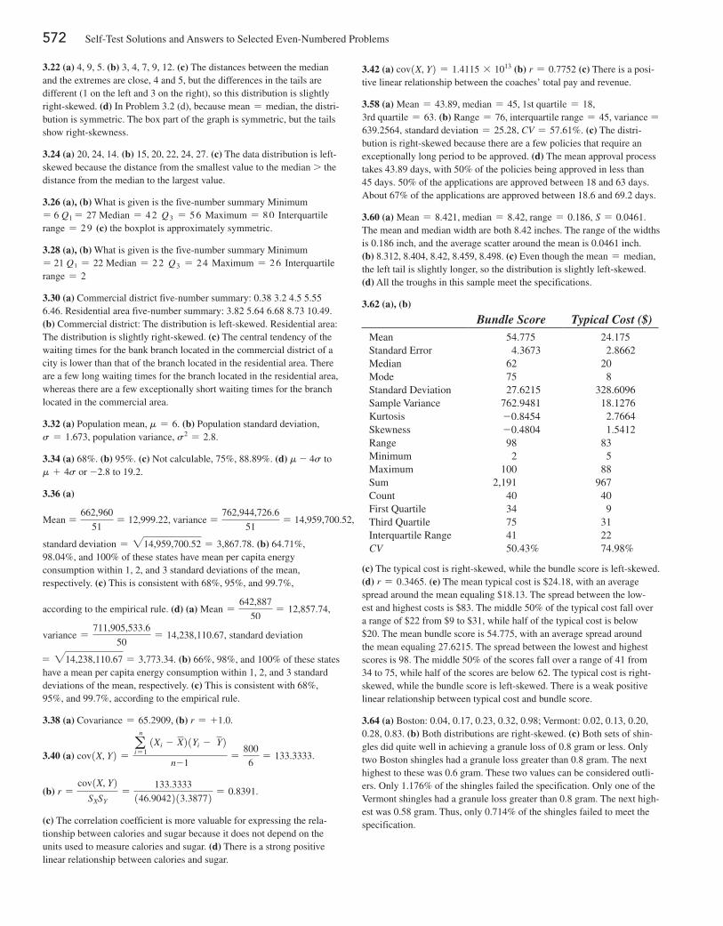
572 Self-Test Solutions and Answers to Selected Even-Numbered Problems
3.42 (a) cov1X, Y2 = 1.4115 * 1013 (b) r = 0.7752 (c) There is a posi-tive linear relationship between the coaches’ total pay and revenue.
3.58 (a) Mean = 43.89, median = 45, 1st quartile = 18, 3rd quartile = 63. (b) Range = 76, interquartile range = 45, variance = 639.2564, standard deviation = 25.28, CV = 57.61%. (c) The distri-bution is right-skewed because there are a few policies that require an exceptionally long period to be approved. (d) The mean approval process takes 43.89 days, with 50% of the policies being approved in less than 45 days. 50% of the applications are approved between 18 and 63 days. About 67% of the applications are approved between 18.6 and 69.2 days.
3.60 (a) Mean = 8.421, median = 8.42, range = 0.186, S = 0.0461. The mean and median width are both 8.42 inches. The range of the widths is 0.186 inch, and the average scatter around the mean is 0.0461 inch. (b) 8.312, 8.404, 8.42, 8.459, 8.498. (c) Even though the mean = median, the left tail is slightly longer, so the distribution is slightly left-skewed. (d) All the troughs in this sample meet the specifications.
3.62 (a), (b)
Bundle Score Typical Cost ($)Mean 54.775 24.175Standard Error 4.3673 2.8662Median 62 20Mode 75 8Standard Deviation 27.6215 328.6096Sample Variance 762.9481 18.1276Kurtosis -0.8454 2.7664Skewness -0.4804 1.5412Range 98 83Minimum 2 5Maximum 100 88Sum 2,191 967Count 40 40First Quartile 34 9Third Quartile 75 31Interquartile Range 41 22CV 50.43% 74.98%
(c) The typical cost is right-skewed, while the bundle score is left-skewed. (d) r = 0.3465. (e) The mean typical cost is $24.18, with an average spread around the mean equaling $18.13. The spread between the low-est and highest costs is $83. The middle 50% of the typical cost fall over a range of $22 from $9 to $31, while half of the typical cost is below $20. The mean bundle score is 54.775, with an average spread around the mean equaling 27.6215. The spread between the lowest and highest scores is 98. The middle 50% of the scores fall over a range of 41 from 34 to 75, while half of the scores are below 62. The typical cost is right-skewed, while the bundle score is left-skewed. There is a weak positive linear relationship between typical cost and bundle score.
3.64 (a) Boston: 0.04, 0.17, 0.23, 0.32, 0.98; Vermont: 0.02, 0.13, 0.20, 0.28, 0.83. (b) Both distributions are right-skewed. (c) Both sets of shin-gles did quite well in achieving a granule loss of 0.8 gram or less. Only two Boston shingles had a granule loss greater than 0.8 gram. The next highest to these was 0.6 gram. These two values can be considered outli-ers. Only 1.176% of the shingles failed the specification. Only one of the Vermont shingles had a granule loss greater than 0.8 gram. The next high-est was 0.58 gram. Thus, only 0.714% of the shingles failed to meet the specification.
3.22 (a) 4, 9, 5. (b) 3, 4, 7, 9, 12. (c) The distances between the median and the extremes are close, 4 and 5, but the differences in the tails are different (1 on the left and 3 on the right), so this distribution is slightly right-skewed. (d) In Problem 3.2 (d), because mean = median, the distri-bution is symmetric. The box part of the graph is symmetric, but the tails show right-skewness.
3.24 (a) 20, 24, 14. (b) 15, 20, 22, 24, 27. (c) The data distribution is left-skewed because the distance from the smallest value to the median > the distance from the median to the largest value.
3.26 (a), (b) What is given is the five-number summary Minimum= 6 Q1 = 27 Median = 4 2 Q3 = 5 6 Maximum = 8 0 Interquartile range = 2 9 (c) the boxplot is approximately symmetric.
3.28 (a), (b) What is given is the five-number summary Minimum= 21 Q1 = 22 Median = 2 2 Q3 = 2 4 Maximum = 2 6 Interquartile range = 2
3.30 (a) Commercial district five-number summary: 0.38 3.2 4.5 5.55 6.46. Residential area five-number summary: 3.82 5.64 6.68 8.73 10.49. (b) Commercial district: The distribution is left-skewed. Residential area: The distribution is slightly right-skewed. (c) The central tendency of the waiting times for the bank branch located in the commercial district of a city is lower than that of the branch located in the residential area. There are a few long waiting times for the branch located in the residential area, whereas there are a few exceptionally short waiting times for the branch located in the commercial area.
3.32 (a) Population mean, m = 6. (b) Population standard deviation, s = 1.673, population variance, s2 = 2.8.
3.34 (a) 68%. (b) 95%. (c) Not calculable, 75%, 88.89%. (d) m - 4s to m + 4s or -2.8 to 19.2.
3.36 (a)
Mean =662,960
51= 12,999.22, variance =
762,944,726.6
51= 14,959,700.52,
standard deviation = 214,959,700.52 = 3,867.78. (b) 64.71%, 98.04%, and 100% of these states have mean per capita energy consumption within 1, 2, and 3 standard deviations of the mean, respectively. (c) This is consistent with 68%, 95%, and 99.7%,
according to the empirical rule. (d) (a) Mean =642,887
50= 12,857.74,
variance =711,905,533.6
50= 14,238,110.67, standard deviation
= 214,238,110.67 = 3,773.34. (b) 66%, 98%, and 100% of these states have a mean per capita energy consumption within 1, 2, and 3 standard deviations of the mean, respectively. (c) This is consistent with 68%, 95%, and 99.7%, according to the empirical rule.
3.38 (a) Covariance = 65.2909, (b) r = +1.0.
3.40 (a) cov1X, Y2 =an
i = 1 1Xi - X21Yi - Y2
n-1=
800
6= 133.3333.
(b) r =cov1X, Y2
SXSY=
133.3333
146.9042213.38772 = 0.8391.
(c) The correlation coefficient is more valuable for expressing the rela-tionship between calories and sugar because it does not depend on the units used to measure calories and sugar. (d) There is a strong positive linear relationship between calories and sugar.
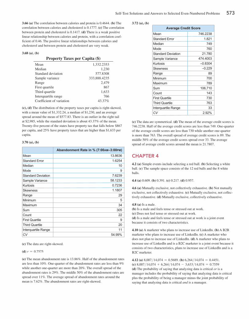
Self-Test Solutions and Answers to Selected Even-Numbered Problems 573
3.72 (a), (b)
MeanStandard Error
ModeMedian
Sample VarianceStandard Deviation
KurtosisSkewnessRangeMinimumMaximum
CountSum
First QuartileThird QuartileInterquartile RangeCV
–0.22989
700
106,710789
14373076333
2.92%
Average Credit Score
21.780760
746.22381.821
749
–0.8304474.4003
(c) The data are symmetrical. (d) The mean of the average credit scores is 746.2238. Half of the average credit scores are less than 749. One-quarter of the average credit scores are less than 730 while another one-quarter is more than 763. The overall spread of average credit scores is 89. The middle 50% of the average credit scores spread over 33. The average spread of average credit scores around the mean is 21.7807.
CHAPTER 4
4.2 (a) Simple events include selecting a red ball. (b) Selecting a white ball. (c) The sample space consists of the 12 red balls and the 8 white balls.
4.4 (a) 0.609. (b) 0.391. (c) 0.217. (d) 0.957.
4.6 (a) Mutually exclusive, not collectively exhaustive. (b) Not mutually exclusive, not collectively exhaustive. (c) Mutually exclusive, not collec-tively exhaustive. (d) Mutually exclusive, collectively exhaustive.
4.8 (a) Is a male. (b) Is a male and feels tense or stressed out at work. (c) Does not feel tense or stressed out at work. (d) Is a male and feels tense or stressed out at work is a joint event because it consists of two characteristics.
4.10 (a) A marketer who plans to increase use of LinkedIn. (b) A B2B marketer who plans to increase use of LinkedIn. (c) A marketer who does not plan to increase use of LinkedIn. (d) A marketer who plans to increase use of LinkedIn and is a B2C marketer is a joint event because it consists of two characteristics, plans to increase use of LinkedIn and is a B2C marketer.
4.12 (a) 8,007>14,074 = 0.5689. (b) 6,264>14,074 = 0.4451. (c) 8,007>14,074 + 6,264>14,074 - 3,633>14,074 = 0.7559 (d) The probability of saying that analyzing data is critical or is a manager includes the probability of saying that analyzing data is critical plus the probability of being a manager minus the joint probability of saying that analyzing data is critical and is a manager.
3.66 (a) The correlation between calories and protein is 0.4644. (b) The correlation between calories and cholesterol is 0.1777. (c) The correlation between protein and cholesterol is 0.1417. (d) There is a weak positive linear relationship between calories and protein, with a correlation coef-ficient of 0.46. The positive linear relationships between calories and cholesterol and between protein and cholesterol are very weak.
3.68 (a), (b)
Property Taxes per Capita ($)Mean 1,332.2353Median 1,230Standard deviation 577.8308Sample variance 333,888.4235Range 2,479First quartile 867Third quartile 1,633Interquartile range 766Coefficient of variation 43.37%
(c), (d) The distribution of the property taxes per capita is right-skewed, with a mean value of $1,332.24, a median of $1,230, and an average spread around the mean of $577.83. There is an outlier in the right tail at $2,985, while the standard deviation is about 43.37% of the mean. Twenty-five percent of the states have property tax that falls below $867 per capita, and 25% have property taxes that are higher than $1,633 per capita.
3.70 (a), (b)
MeanStandard Error
ModeMedian
Sample VarianceStandard Deviation
KurtosisSkewnessRangeMinimumMaximum
CountSum
First QuartileThird QuartileInterquartile RangeCV
1.1807295
30534
229
2011
54.99%
Abandonment Rate in % (7:00AM–3:00PM)
7.62399
13.86361.6254
10
0.723658.1233
(c) The data are right-skewed.
(d) r = 0.7575
(e) The mean abandonment rate is 13.86%. Half of the abandonment rates are less than 10%. One-quarter of the abandonment rates are less than 9% while another one-quarter are more than 20%. The overall spread of the abandonment rates is 29%. The middle 50% of the abandonment rates are spread over 11%. The average spread of abandonment rates around the mean is 7.62%. The abandonment rates are right-skewed.
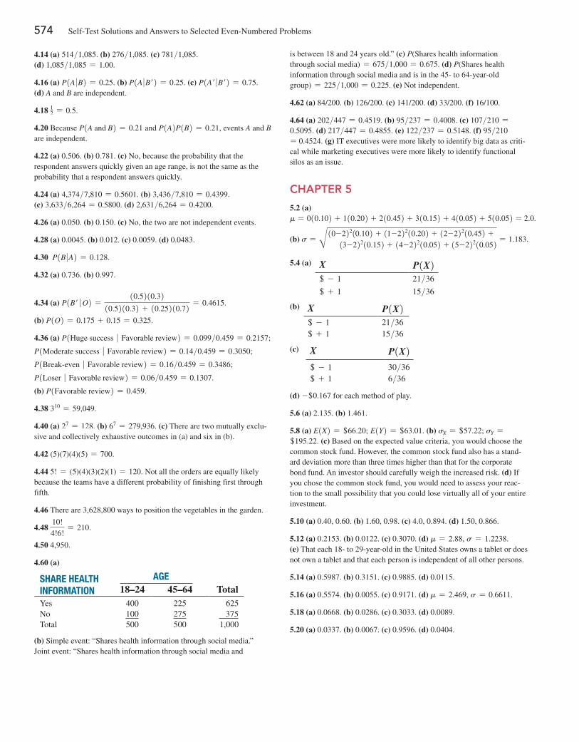
574 Self-Test Solutions and Answers to Selected Even-Numbered Problems
is between 18 and 24 years old.” (c) P(Shares health information through social media) = 675>1,000 = 0.675. (d) P(Shares health information through social media and is in the 45- to 64-year-old group) = 225>1,000 = 0.225. (e) Not independent.
4.62 (a) 84/200. (b) 126/200. (c) 141/200. (d) 33/200. (f) 16/100.
4.64 (a) 202>447 = 0.4519. (b) 95>237 = 0.4008. (c) 107>210 =0.5095. (d) 217>447 = 0.4855. (e) 122>237 = 0.5148. (f) 95>210= 0.4524. (g) IT executives were more likely to identify big data as criti-cal while marketing executives were more likely to identify functional silos as an issue.
CHAPTER 5
5.2 (a) m = 010.102 + 110.202 + 210.452 + 310.152 + 410.052 + 510.052 = 2.0.
(b) s = B10-22210.102 + 11-22210.202 + 12-22210.452 +13-22210.152 + 14-22210.052 + 15-22210.052 = 1.183.
5.4 (a)
(b)
(c)
(d) -+0.167 for each method of play.
5.6 (a) 2.135. (b) 1.461.
5.8 (a) E1X2 = +66.20; E1Y2 = +63.01. (b) sX = +57.22; sY = +195.22. (c) Based on the expected value criteria, you would choose the common stock fund. However, the common stock fund also has a stand-ard deviation more than three times higher than that for the corporate bond fund. An investor should carefully weigh the increased risk. (d) If you chose the common stock fund, you would need to assess your reac-tion to the small possibility that you could lose virtually all of your entire investment.
5.10 (a) 0.40, 0.60. (b) 1.60, 0.98. (c) 4.0, 0.894. (d) 1.50, 0.866.
5.12 (a) 0.2153. (b) 0.0122. (c) 0.3070. (d) m = 2.88, s = 1.2238. (e) That each 18- to 29-year-old in the United States owns a tablet or does not own a tablet and that each person is independent of all other persons.
5.14 (a) 0.5987. (b) 0.3151. (c) 0.9885. (d) 0.0115.
5.16 (a) 0.5574. (b) 0.0055. (c) 0.9171. (d) m = 2.469, s = 0.6611.
5.18 (a) 0.0668. (b) 0.0286. (c) 0.3033. (d) 0.0089.
5.20 (a) 0.0337. (b) 0.0067. (c) 0.9596. (d) 0.0404.
4.14 (a) 514>1,085. (b) 276>1,085. (c) 781>1,085. (d) 1,085>1,085 = 1.00.
4.16 (a) P1A 0B2 = 0.25. (b) P1A 0B′2 = 0.25. (c) P1A′ 0B′2 = 0.75. (d) A and B are independent.
4.18 12 = 0.5.
4.20 Because P1A and B2 = 0.21 and P1A2P1B2 = 0.21, events A and B are independent.
4.22 (a) 0.506. (b) 0.781. (c) No, because the probability that the respondent answers quickly given an age range, is not the same as the probability that a respondent answers quickly.
4.24 (a) 4,374>7,810 = 0.5601. (b) 3,436>7,810 = 0.4399. (c) 3,633>6,264 = 0.5800. (d) 2,631>6,264 = 0.4200.
4.26 (a) 0.050. (b) 0.150. (c) No, the two are not independent events.
4.28 (a) 0.0045. (b) 0.012. (c) 0.0059. (d) 0.0483.
4.30 P1B 0A2 = 0.128.
4.32 (a) 0.736. (b) 0.997.
4.34 (a) P1B′ ∙ O2 =10.5210.32
10.5210.32 + 10.25210.72 = 0.4615.
(b) P1O2 = 0.175 + 0.15 = 0.325.
4.36 (a) P1Huge success ∙ Favorable review2 = 0.099>0.459 = 0.2157;
P1Moderate success ∙ Favorable review2 = 0.14>0.459 = 0.3050;
P1Break@even ∙ Favorable review2 = 0.16>0.459 = 0.3486;
P1Loser ∙ Favorable review2 = 0.06>0.459 = 0.1307.
(b) P1Favorable review2 = 0.459.
4.38 310 = 59,049.
4.40 (a) 27 = 128. (b) 67 = 279,936. (c) There are two mutually exclu-sive and collectively exhaustive outcomes in (a) and six in (b).
4.42 (5)(7)(4)(5) = 700.
4.44 5! = (5)(4)(3)(2)(1) = 120. Not all the orders are equally likely because the teams have a different probability of finishing first through fifth.
4.46 There are 3,628,800 ways to position the vegetables in the garden.
4.48 10!
4!6!= 210.
4.50 4,950.
4.60 (a)
SharE hEalth inforMation
agE18–24 45–64 Total
Yes 400 225 625No 100 275 375Total 500 500 1,000
(b) Simple event: “Shares health information through social media.” Joint event: “Shares health information through social media and
X P1X2+ - 1 21>36
+ + 1 15>36
X P1X2+ - 1 21>36+ + 1 15>36
X P1X2+ - 1 30>36+ + 1 6>36
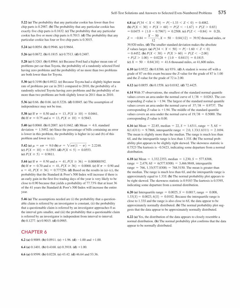
Self-Test Solutions and Answers to Selected Even-Numbered Problems 575
5.22 (a) The probability that any particular cookie has fewer than five chip parts is 0.2987. (b) The probability that any particular cookie has exactly five chip parts is 0.1632. (c) The probability that any particular cookie has five or more chip parts is 0.7013. (d) The probability that any particular cookie has four or five chip parts is 0.3015.
5.24 (a) 0.0054. (b) 0.9946. (c) 0.9664.
5.26 (a) 0.0672. (b) 0.1815. (c) 0.7513. (d) 0.2487.
5.28 (a) 0.3263. (b) 0.8964. (c) Because Ford had a higher mean rate of problems per car than Toyota, the probability of a randomly selected Ford having zero problems and the probability of no more than two problems are both lower than for Toyota.
5.30 (a) 0.3198 (b) 0.8922. (c) Because Toyota had a slightly higher mean rate of problems per car in 2011 compared to 2010, the probability of a randomly selected Toyota having zero problems and the probability of no more than two problems are both slightly lower in 2011 than in 2010.
5.36 (a) 0.66. (b) 0.66. (c) 0.3226. (d) 0.0045. (e) The assumption of independence may not be true.
5.38 (a) If p = 0.50 and n = 13, P1X Ú 102 = 0.0461. (b) If p = 0.75 and n = 13, P1X Ú 102 = 0.5843.
5.40 (a) 0.0060. (b) 0.2007. (c) 0.1662. (d) Mean = 4.0, standard deviation = 1.5492. (e) Since the percentage of bills containing an error is lower in this problem, the probability is higher in (a) and (b) of this problem and lower in (c).
5.42 (a) m = np = 9.0 (b) s = 2np11 - p2 = 2.2248. (c) P1X = 102 = 0.1593. (d) P1X … 52 = 0.0553. (e) P1X Ú 52 = 0.9811.
5.44 (a) If p = 0.50 and n = 41, P1X Ú 362 = 0.000000392. (b) If p = 0.70 and n = 41, P1X Ú 362 = 0.0068. (c) If p = 0.90 and n = 41, P1X Ú 362 = 0.777256. (d) Based on the results in (a)–(c), the probability that the Standard & Poor’s 500 Index will increase if there is an early gain in the first five trading days of the year is very likely to be close to 0.90 because that yields a probability of 77.73% that at least 36 of the 41 years the Standard & Poor’s 500 Index will increase the entire year.
5.46 (a) The assumptions needed are (i) the probability that a question-able claim is referred by an investigator is constant, (ii) the probability that a questionable claim is referred by an investigator approaches 0 as the interval gets smaller, and (iii) the probability that a questionable claim is referred by an investigator is independent from interval to interval. (b) 0.1277. (c) 0.9015. (d) 0.0985.
CHAPTER 6
6.2 (a) 0.9089. (b) 0.0911. (c) +1.96. (d) -1.00 and +1.00.
6.4 (a) 0.1401. (b) 0.4168. (c) 0.3918. (d) +1.00.
6.6 (a) 0.9599. (b) 0.0228. (c) 43.42. (d) 46.64 and 53.36.
6.8 (a) P134 6 X 6 502 = P1-1.33 6 Z 6 02 = 0.4082. (b) P1X 6 302 + P1X 7 602 = P1Z 6 -1.672 + P1Z 7 0.832 = 0.0475 + 11.0 - 0.79672 = 0.2508. (c) P1Z 6 -0.842 ≅ 0.20,
Z = -0.84 =X - 50
12, X = 50 - 0.841122 = 39.92 thousand miles, or
39,920 miles. (d) The smaller standard deviation makes the absolute Z values larger. (a) P134 6 X 6 502 = P1-1.60 6 Z 6 02= 0.4452. (b) P1X 6 302 + P1X 7 602 = P1Z 6 -2.002+ P1Z 7 1.002 = 0.0228 + 11.0 - 0.84132 = 0.1815. (c) X = 50 - 0.841102 = 41.6 thousand miles, or 41,600 miles.
6.10 (a) 0.9522. (b) 0.8386. (c) 93%. (d) A student is worse off with a grade of 87 on this exam because the Z-value for the grade of 87 is 1.00 and the Z-value for the grade of 72 is 2.00.
6.12 (a) 0.0855. (b) 0.1558. (c) 0.0182. (d) 72.4425.
6.14 With 37 observations, the smallest of the standard normal quantile values covers an area under the normal curve of 1>38 = 0.0263. The cor-responding Z-value is -1.94. The largest of the standard normal quantile values covers an area under the normal curve of 37>38 = 0.9737. The corresponding Z-value is +1.94. The middle of the standard quantile values covers an area under the normal curve of 19>38 = 0.5000. The corresponding Z-value is 0.00.
6.16 (a) Mean = 22.85, median = 22, S = 1.6311, range = 5, 6S =6(1.6311) = 9.7866, interquartile range = 2.0, 1.33(1.6311) = 2.1694. The mean is slightly more than the median. The range is much less than 6S, and the interquartile range is less than 1.33S. (b) The normal prob-ability plot appears to be slightly right skewed. The skewness statistic is 0.7523 The kurtosis is -0.5423, indicating some departure from a normal distribution.
6.18 (a) Mean = 1,332.2353, median = 1,230, S = 577.8308,range = 2,479, 6S = 6(577.8308) = 3,466.9848, interquartilerange = 766, 1.33(577.8308) = 768.5150. The mean is greater than the median. The range is much less than 6S, and the interquartile range is approximately equal to 1.33S. (b) The normal probability plot appears to be right skewed. The skewness statistic is 0.9183 The kurtosis is 0.5395, indicating some departure from a normal distribution.
6.20 (a) Interquartile range = 0.0025, S = 0.0017, range = 0.008,1.331S2 = 0.0023, 61S2 = 0.0102. Because the interquartile range is close to 1.33S and the range is also close to 6S, the data appear to be approximately normally distributed. (b) The normal probability plot sug-gests that the data appear to be approximately normally distributed.
6.22 (a) Yes, the distribution of the data appears to closely resemble a normal distribution. (b) The normal probability plot confirms that the data appear to be normally distributed.
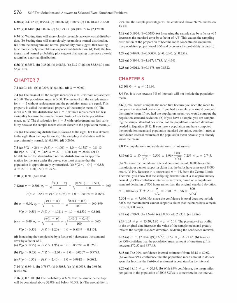
576 Self-Test Solutions and Answers to Selected Even-Numbered Problems
95% that the sample percentage will be contained above 26.6% and below 45.4%.
7.18 (a) 0.1964. (b) 0.0280. (c) Increasing the sample size by a factor of 5 decreases the standard error by a factor of 15. This causes the sampling distribution of the proportion to become more concentrated around the true population proportion of 0.56 and decreases the probability in part (b).
7.24 (a) 0.4999. (b) 0.00009. (c) 0. (d) 0. (e) 0.7518.
7.26 (a) 0.8944. (b) 4.617; 4.783. (c) 4.641.
7.28 (a) 0.0012. (b) 0.1478. (c) 0.8522.
CHAPTER 8
8.2 108.04 … m … 121.96.
8.4 Yes, it is true because 5% of intervals will not include the population mean.
8.6 (a) You would compute the mean first because you need the mean to compute the standard deviation. If you had a sample, you would compute the sample mean. If you had the population mean, you would compute the population standard deviation. (b) If you have a sample, you are comput-ing the sample standard deviation, not the population standard deviation needed in Equation (8.1). If you have a population and have computed the population mean and population standard deviation, you don’t need a confidence interval estimate of the population mean because you already know the mean.
8.8 The population standard deviation s is not known.
8.10 (a) X { Z # s2n= 7,500 { 1.96 # 1,000264
; 7,255 … m … 7,745.
(b) No, since the confidence interval does not include 8,000 hours the manufacturer cannot support a claim that the bulbs have a mean of 8,000 hours. (c) No. Because s is known and n = 64, from the Central Limit Theorem, you know that the sampling distribution of X is approximately normal. (d) The confidence interval is narrower, based on a population standard deviation of 800 hours rather than the original standard deviation
of 1,000 hours. X { Z *s2n
= 7,500 { 1.96 *800264
,
7.304 … m … 7,696. No, since the confidence interval does not include 8,000 the manufacturer cannot support a claim that the bulbs have a mean life of 8,000 hours.
8.12 (a) 2.7079. (b) 1.6849. (c) 2.8073. (d) 2.7333. (e) 1.9960.
8.14 1.05 … m … 13.20; 2.86 … m … 6.14; The presence of an outlier in the original data increases the value of the sample mean and greatly inflates the sample standard deviation, widening the confidence interval.
8.16 (a) 75 { 12.00492192>255; 72.57 … m … 77.43. (b) You can be 95% confident that the population mean amount of one-time gift is between $72.57 and $77.43.
8.18 (a) The 99% confidence interval estimate if from $5.18 to $9.02. (b) We have 99% confidence that the population mean amount in dollars spent for lunch at the fast-food restaurant is contained in the interval.
8.20 (a) 18.15 … m … 20.13. (b) With 95% confidence, the mean miles per gallon in the population of 2008 SUVs is somewhere in the interval.
6.30 (a) 0.4772. (b) 0.9544. (c) 0.0456. (d) 1.8835. (e) 1.8710 and 2.1290.
6.32 (a) 0.1405. (b) 0.0256. (c) $2,179.78. (d) $898.22 to $2,179.78.
6.34 (a) Waiting time will more closely resemble an exponential distribu-tion. (b) Seating time will more closely resemble a normal distribution. (c) Both the histogram and normal probability plot suggest that waiting time more closely resembles an exponential distribution. (d) Both the his-togram and normal probability plot suggest that seating time more closely resembles a normal distribution.
6.36 (a) 0.3557. (b) 0.3596. (c) 0.0838. (d) $3,717.46. (e) $3,864.01 and $5,431.99.
CHAPTER 7
7.2 (a) 0.1151. (b) 0.0206. (c) 0.4364. (d) X = 99.07.
7.4 (a) The mean of all the sample means for n = 2 without replacement is 5.50. The population mean is 5.50. The mean of all the sample means for n = 2 without replacement and the population mean are equal. This property is called the unbiased property of the sample mean. (b) The mean is 5.50. The distribution for n = 3 without replacement has less variability because the sample means cluster closer to the population mean, m. (c) The distribution for n = 3 with replacement has less varia-bility because the sample means cluster closer to the population mean, m.
7.6 (a) The sampling distribution is skewed to the right, but less skewed to the right than the population. (b) The sampling distribution will be approximately normal. (c) 0.9599. (d) 0.2956.
7.8 (a) P1X 7 262 = P1Z 7 -1.002 = 1.0 - 0.1587 = 0.8413. (b) P1Z 6 1.042 = 0.85; X = 27 + 1.0411.02 = 28.04. (c) To be able to use the standardized normal distribution as an approxi-mation for the area under the curve, you must assume that the population is approximately symmetrical. (d) P1Z 6 1.042 = 0.85; X = 27 + 1.0410.502 = 27.52.
7.10 (a) 0.50. (b) 0.0541.
7.12 (a) p = 0.501, sp = Bp11 - p2n
= B0.50111 - 0.5012100
= 0.05
P1p 7 0.552 = P1Z 7 0.982 = 1.0 - 0.8365 = 0.1635.
(b) p = 0.60, sp = Bp11 - p2n
= B0.611 - 0.62100
= 0.04899
P1p 7 0.552 = P1Z 7 -1.0212 = 1.0 - 0.1539 = 0.8461.
(c) p = 0.49, sp = Bp11 - p2n
= B0.4911 - 0.492100
= 0.05
P1p 7 0.552 = P1Z 7 1.202 = 1.0 - 0.8849 = 0.1151.
(d) Increasing the sample size by a factor of 4 decreases the standard error by a factor of 2.(a) P1p 7 0.552 = P1Z 7 1.962 = 1.0 - 0.9750 = 0.0250.
(b) P1p 7 0.552 = P1Z 7 -2.042 = 1.0 - 0.0207 = 0.9793.
(c) P1p 7 0.552 = P1Z 7 2.402 = 1.0 - 0.9918 = 0.0082.
7.14 (a) 0.8944. (b) 0.7887. (c) 0.3085. (d) (a) 0.9938. (b) 0.9876. (c) 0.1587.
7.16 (a) 0.5101. (b) The probability is 60% that the sample percentage will be contained above 32.0% and below 40.0%. (c) The probability is
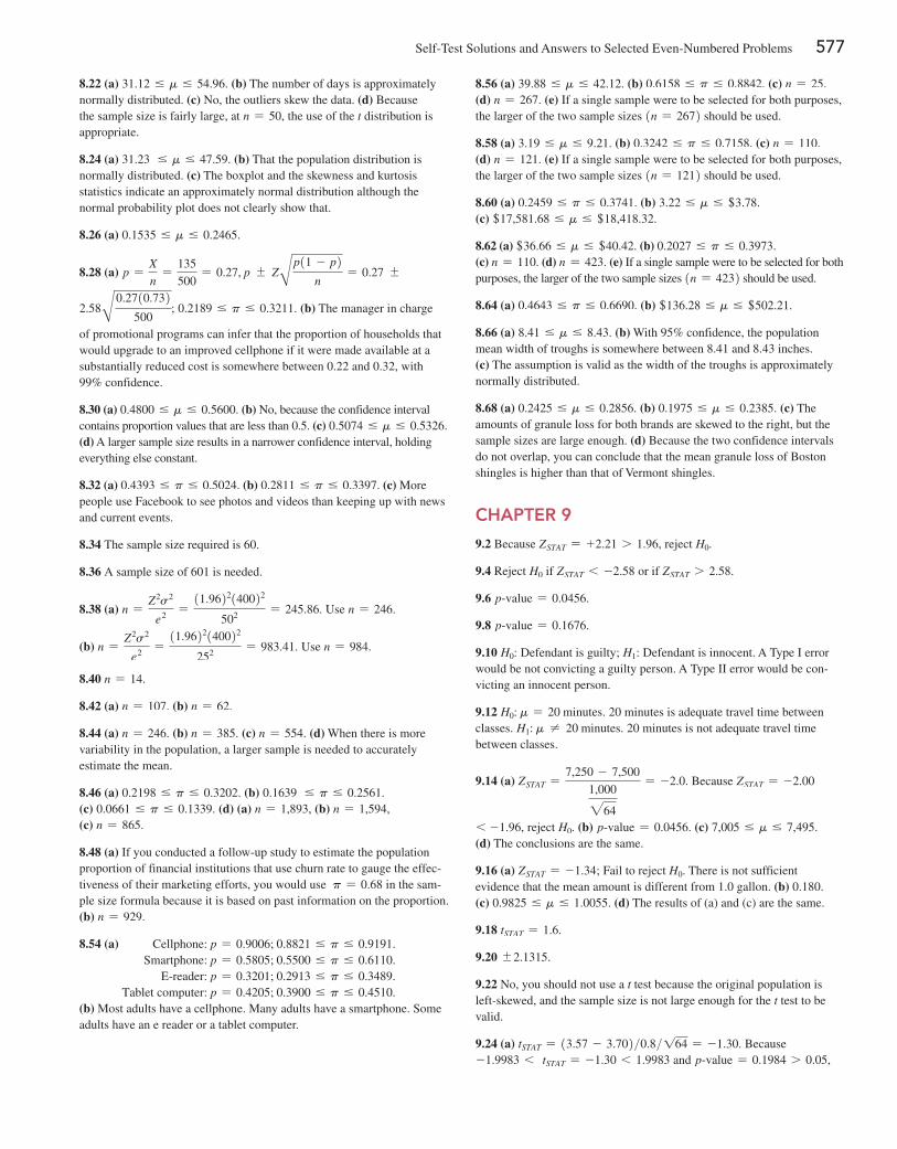
Self-Test Solutions and Answers to Selected Even-Numbered Problems 577
8.56 (a) 39.88 … m … 42.12. (b) 0.6158 … p … 0.8842. (c) n = 25.(d) n = 267. (e) If a single sample were to be selected for both purposes, the larger of the two sample sizes 1n = 2672 should be used.
8.58 (a) 3.19 … m … 9.21. (b) 0.3242 … p … 0.7158. (c) n = 110. (d) n = 121. (e) If a single sample were to be selected for both purposes, the larger of the two sample sizes 1n = 1212 should be used.
8.60 (a) 0.2459 … p … 0.3741. (b) 3.22 … m … +3.78. (c) +17,581.68 … m … +18,418.32.
8.62 (a) +36.66 … m … +40.42. (b) 0.2027 … p … 0.3973. (c) n = 110. (d) n = 423. (e) If a single sample were to be selected for both purposes, the larger of the two sample sizes 1n = 4232 should be used.
8.64 (a) 0.4643 … p … 0.6690. (b) +136.28 … m … +502.21.
8.66 (a) 8.41 … m … 8.43. (b) With 95% confidence, the population mean width of troughs is somewhere between 8.41 and 8.43 inches.(c) The assumption is valid as the width of the troughs is approximately normally distributed.
8.68 (a) 0.2425 … m … 0.2856. (b) 0.1975 … m … 0.2385. (c) The amounts of granule loss for both brands are skewed to the right, but the sample sizes are large enough. (d) Because the two confidence intervals do not overlap, you can conclude that the mean granule loss of Boston shingles is higher than that of Vermont shingles.
CHAPTER 9
9.2 Because ZSTAT = +2.21 7 1.96, reject H0.
9.4 Reject H0 if ZSTAT 6 -2.58 or if ZSTAT 7 2.58.
9.6 p@value = 0.0456.
9.8 p@value = 0.1676.
9.10 H0: Defendant is guilty; H1: Defendant is innocent. A Type I error would be not convicting a guilty person. A Type II error would be con-victing an innocent person.
9.12 H0: m = 20 minutes. 20 minutes is adequate travel time between classes. H1: m ≠ 20 minutes. 20 minutes is not adequate travel time between classes.
9.14 (a) ZSTAT =7,250 - 7,500
1,000264
= -2.0. Because ZSTAT = -2.00
6 -1.96, reject H0. (b) p@value = 0.0456. (c) 7,005 … m … 7,495.(d) The conclusions are the same.
9.16 (a) ZSTAT = -1.34; Fail to reject H0. There is not sufficient evidence that the mean amount is different from 1.0 gallon. (b) 0.180. (c) 0.9825 … m … 1.0055. (d) The results of (a) and (c) are the same.
9.18 tSTAT = 1.6.
9.20 {2.1315.
9.22 No, you should not use a t test because the original population is left-skewed, and the sample size is not large enough for the t test to be valid.
9.24 (a) tSTAT = 13.57 - 3.702>0.8>164 = -1.30. Because -1.9983 6 tSTAT = -1.30 6 1.9983 and p@value = 0.1984 7 0.05,
8.22 (a) 31.12 … m … 54.96. (b) The number of days is approximately normally distributed. (c) No, the outliers skew the data. (d) Because the sample size is fairly large, at n = 50, the use of the t distribution is appropriate.
8.24 (a) 31.23 … m … 47.59. (b) That the population distribution is normally distributed. (c) The boxplot and the skewness and kurtosis statistics indicate an approximately normal distribution although the normal probability plot does not clearly show that.
8.26 (a) 0.1535 … m … 0.2465.
8.28 (a) p =X
n=
135
500= 0.27, p { ZBp11 - p2
n= 0.27 {
2.58B0.2710.732500
; 0.2189 … p … 0.3211. (b) The manager in charge
of promotional programs can infer that the proportion of households that would upgrade to an improved cellphone if it were made available at a substantially reduced cost is somewhere between 0.22 and 0.32, with 99% confidence.
8.30 (a) 0.4800 … m … 0.5600. (b) No, because the confidence interval contains proportion values that are less than 0.5. (c) 0.5074 … m … 0.5326. (d) A larger sample size results in a narrower confidence interval, holding everything else constant.
8.32 (a) 0.4393 … p … 0.5024. (b) 0.2811 … p … 0.3397. (c) More people use Facebook to see photos and videos than keeping up with news and current events.
8.34 The sample size required is 60.
8.36 A sample size of 601 is needed.
8.38 (a) n =Z2s2
e2=
11.9622140022
502= 245.86. Use n = 246.
(b) n =Z2s2
e2=
11.9622140022
252= 983.41. Use n = 984.
8.40 n = 14.
8.42 (a) n = 107. (b) n = 62.
8.44 (a) n = 246. (b) n = 385. (c) n = 554. (d) When there is more variability in the population, a larger sample is needed to accurately estimate the mean.
8.46 (a) 0.2198 … p … 0.3202. (b) 0.1639 … p … 0.2561. (c) 0.0661 … p … 0.1339. (d) (a) n = 1,893, (b) n = 1,594, (c) n = 865.
8.48 (a) If you conducted a follow-up study to estimate the population proportion of financial institutions that use churn rate to gauge the effec-tiveness of their marketing efforts, you would use p = 0.68 in the sam-ple size formula because it is based on past information on the proportion. (b) n = 929.
8.54 (a) Cellphone: p = 0.9006; 0.8821 … p … 0.9191. Smartphone: p = 0.5805; 0.5500 … p … 0.6110.
E@reader: p = 0.3201; 0.2913 … p … 0.3489. Tablet computer: p = 0.4205; 0.3900 … p … 0.4510.
(b) Most adults have a cellphone. Many adults have a smartphone. Some adults have an e reader or a tablet computer.
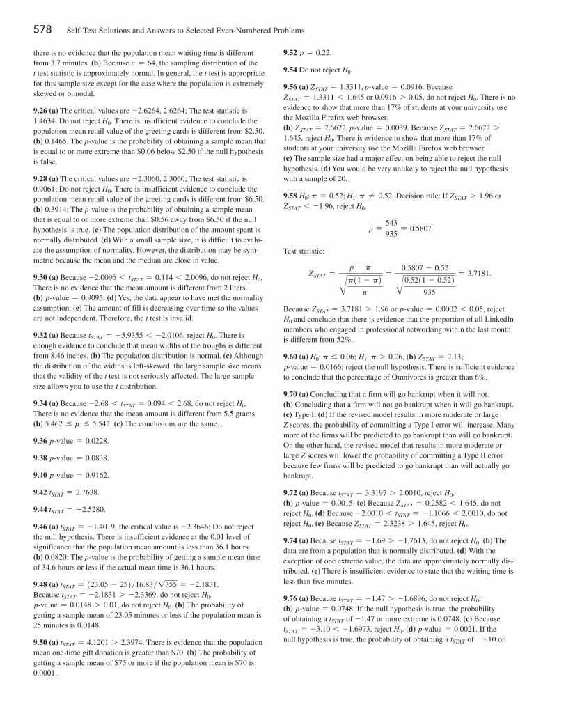
578 Self-Test Solutions and Answers to Selected Even-Numbered Problems
9.52 p = 0.22.
9.54 Do not reject H0.
9.56 (a) ZSTAT = 1.3311, p@value = 0.0916. Because ZSTAT = 1.3311 6 1.645 or 0.0916 7 0.05, do not reject H0. There is no evidence to show that more than 17% of students at your university use the Mozilla Firefox web browser.(b) ZSTAT = 2.6622, p@value = 0.0039. Because ZSTAT = 2.6622 71.645, reject H0. There is evidence to show that more than 17% of students at your university use the Mozilla Firefox web browser. (c) The sample size had a major effect on being able to reject the null hypothesis. (d) You would be very unlikely to reject the null hypothesis with a sample of 20.
9.58 H0: p = 0.52; H1: p ≠ 0.52. Decision rule: If ZSTAT 7 1.96 or ZSTAT 6 -1.96, reject H0.
p =543
935= 0.5807
Test statistic:
ZSTAT =p - pBp11 - p2
n
=0.5807 - 0.52B0.5211 - 0.522
935
= 3.7181.
Because ZSTAT = 3.7181 7 1.96 or p@value = 0.0002 6 0.05, reject H0 and conclude that there is evidence that the proportion of all LinkedIn members who engaged in professional networking within the last month is different from 52%.
9.60 (a) H0: p … 0.06; H1: p 7 0.06. (b) ZSTAT = 2.13; p@value = 0.0166; reject the null hypothesis. There is sufficient evidence to conclude that the percentage of Omnivores is greater than 6%.
9.70 (a) Concluding that a firm will go bankrupt when it will not. (b) Concluding that a firm will not go bankrupt when it will go bankrupt. (c) Type I. (d) If the revised model results in more moderate or large Z scores, the probability of committing a Type I error will increase. Many more of the firms will be predicted to go bankrupt than will go bankrupt. On the other hand, the revised model that results in more moderate or large Z scores will lower the probability of committing a Type II error because few firms will be predicted to go bankrupt than will actually go bankrupt.
9.72 (a) Because tSTAT = 3.3197 7 2.0010, reject H0.(b) p@value = 0.0015. (c) Because ZSTAT = 0.2582 6 1.645, do not reject H0. (d) Because -2.0010 6 tSTAT = -1.1066 6 2.0010, do not reject H0. (e) Because ZSTAT = 2.3238 7 1.645, reject H0.
9.74 (a) Because tSTAT = -1.69 7 -1.7613, do not reject H0. (b) The data are from a population that is normally distributed. (d) With the exception of one extreme value, the data are approximately normally dis-tributed. (e) There is insufficient evidence to state that the waiting time is less than five minutes.
9.76 (a) Because tSTAT = -1.47 7 -1.6896, do not reject H0. (b) p@value = 0.0748. If the null hypothesis is true, the probability of obtaining a tSTAT of -1.47 or more extreme is 0.0748. (c) Because tSTAT = -3.10 6 -1.6973, reject H0. (d) p@value = 0.0021. If the null hypothesis is true, the probability of obtaining a tSTAT of -3.10 or
there is no evidence that the population mean waiting time is different from 3.7 minutes. (b) Because n = 64, the sampling distribution of the t test statistic is approximately normal. In general, the t test is appropriate for this sample size except for the case where the population is extremely skewed or bimodal.
9.26 (a) The critical values are -2.6264, 2.6264; The test statistic is 1.4634; Do not reject H0. There is insufficient evidence to conclude the population mean retail value of the greeting cards is different from $2.50. (b) 0.1465. The p-value is the probability of obtaining a sample mean that is equal to or more extreme than $0.06 below $2.50 if the null hypothesis is false.
9.28 (a) The critical values are -2.3060, 2.3060; The test statistic is 0.9061; Do not reject H0. There is insufficient evidence to conclude the population mean retail value of the greeting cards is different from $6.50. (b) 0.3914; The p-value is the probability of obtaining a sample mean that is equal to or more extreme than $0.56 away from $6.50 if the null hypothesis is true. (c) The population distribution of the amount spent is normally distributed. (d) With a small sample size, it is difficult to evalu-ate the assumption of normality. However, the distribution may be sym-metric because the mean and the median are close in value.
9.30 (a) Because -2.0096 6 tSTAT = 0.114 6 2.0096, do not reject H0. There is no evidence that the mean amount is different from 2 liters. (b) p@value = 0.9095. (d) Yes, the data appear to have met the normality assumption. (e) The amount of fill is decreasing over time so the values are not independent. Therefore, the t test is invalid.
9.32 (a) Because tSTAT = -5.9355 6 -2.0106, reject H0. There is enough evidence to conclude that mean widths of the troughs is different from 8.46 inches. (b) The population distribution is normal. (c) Although the distribution of the widths is left-skewed, the large sample size means that the validity of the t test is not seriously affected. The large sample size allows you to use the t distribution.
9.34 (a) Because -2.68 6 tSTAT = 0.094 6 2.68, do not reject H0. There is no evidence that the mean amount is different from 5.5 grams. (b) 5.462 … m … 5.542. (c) The conclusions are the same.
9.36 p@value = 0.0228.
9.38 p@value = 0.0838.
9.40 p@value = 0.9162.
9.42 tSTAT = 2.7638.
9.44 tSTAT = -2.5280.
9.46 (a) tSTAT = -1.4019; the critical value is -2.3646; Do not reject the null hypothesis. There is insufficient evidence at the 0.01 level of significance that the population mean amount is less than 36.1 hours. (b) 0.0820; The p-value is the probability of getting a sample mean time of 34.6 hours or less if the actual mean time is 36.1 hours.
9.48 (a) tSTAT = 123.05 - 252>16.83>1355 = -2.1831. Because tSTAT = -2.1831 7 -2.3369, do not reject H0. p@value = 0.0148 7 0.01, do not reject H0. (b) The probability of getting a sample mean of 23.05 minutes or less if the population mean is 25 minutes is 0.0148.
9.50 (a) tSTAT = 4.1201 7 2.3974. There is evidence that the population mean one-time gift donation is greater than $70. (b) The probability of getting a sample mean of $75 or more if the population mean is $70 is 0.0001.
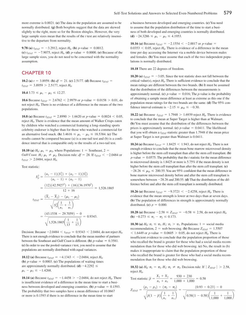
Self-Test Solutions and Answers to Selected Even-Numbered Problems 579
a business between developed and emerging countries. (c) You need to assume that the population distribution of the time to start a busi-ness of both developed and emerging countries is normally distributed. (d) -24.3286 … m1 - m2 … 4.1953.
10.16 (a) Because tSTAT = -2.1554 6 -2.0017 or p@value =0.0353 6 0.05, reject H0. There is evidence of a difference in the mean time per day accessing the Internet via a mobile device between males and females. (b) You must assume that each of the two independent popu-lations is normally distributed.
10.18 There are 22 degrees of freedom.
10.20 (a) tSTAT = -3.05; Since the test statistic does not fall between the critical value(s), reject H0. There is sufficient evidence to conclude that the mean ratings are different between the two brands. (b) It must be assumed that the distribution of the differences between the measurements is approximately normal. (c) p@value = 0.016; The p-value is the probability of obtaining a sample mean difference at least as extreme as this one if the population mean ratings for the two brands are the same. (d) The 95% con-fidence interval estimate is -2.15 … mD … -0.30.
10.22 (a) Because tSTAT = 1.7948 7 1.6939 reject H0. There is evidence to conclude that the mean at Super Target is higher than at Walmart. (b) You must assume that the distribution of the differences between the prices is approximately normal. (c) p@value = 0.0411. The likelihood that you will obtain a tSTAT statistic greater than 1.7948 if the mean price at Super Target is not greater than Walmart is 0.0411.
10.24 (a) Because tSTAT = 1.8425 6 1.943, do not reject H0. There is not enough evidence to conclude that the mean bone marrow microvessel density is higher before the stem cell transplant than after the stem cell transplant. (b) p@value = 0.0575. The probability that the t statistic for the mean difference in microvessel density is 1.8425 or more is 5.75% if the mean density is not higher before the stem cell transplant than after the stem cell transplant. (c) -28.26 … mD … 200.55. You are 95% confident that the mean difference in bone marrow microvessel density before and after the stem cell transplant is somewhere between -28.26 and 200.55. (d) That the distribution of the dif-ference before and after the stem cell transplant is normally distributed.
10.26 (a) Because tSTAT = -9.3721 6 -2.4258, reject H0. There is evidence that the mean strength is lower at two days than at seven days. (b) The population of differences in strength is approximately normally distributed. (c) p = 0.000.
10.28 (a) Because -2.58 … ZSTAT = -0.58 … 2.58, do not reject H0. (b) -0.273 … p1 - p2 … 0.173.
10.30 (a) H0: p1 … p2. H1: p1 7 p2. Populations: 1 = social media recommendation, 2 = web browsing. (b) Because ZSTAT = 1.55076 1.6449 or p@value = 0.0605 7 0.05, do not reject H0. There is insufficient evidence to conclude that the population proportion of those who recalled the brand is greater for those who had a social media recom-mendation than for those who did web browsing. (c) No, the result in (b) makes it inappropriate to claim that the population proportion of those who recalled the brand is greater for those who had a social media recom-mendation than for those who did web browsing.
10.32 (a) H0: p1 = p2. H1: p1 ≠ p2. Decision rule: If ∙ ZSTAT ∙ 7 2.58, reject H0.
Test statistic: p =X1 + X2
n1 + n2=
930 + 230
1,000 + 1,000= 0.58
ZSTAT =1p1 - p22 - 1p2 - p22Bp11 - p2a 1
n1+
1
n2b
=10.93 - 0.232 - 0B0.5811 - 0.582a 1
1,000+
1
1,000b
.
more extreme is 0.0021. (e) The data in the population are assumed to be normally distributed. (g) Both boxplots suggest that the data are skewed slightly to the right, more so for the Boston shingles. However, the very large sample sizes mean that the results of the t test are relatively insensi-tive to the departure from normality.
9.78 (a) tSTAT = -3.2912, reject H0. (b) p@value = 0.0012. (c) tSTAT = -7.9075, reject H0. (d) p@value = 0.0000. (e) Because of the large sample sizes, you do not need to be concerned with the normality assumption.
CHAPTER 10
10.2 (a) t = 3.8959. (b) df = 21. (c) 2.5177. (d) Because tSTAT =tSTAT = 3.8959 7 2.5177, reject H0.
10.4 3.73 … m1 - m2 … 12.27.
10.6 Because tSTAT = 2.6762 6 2.9979 or p@value = 0.0158 7 0.01, do not reject H0. There is no evidence of a difference in the means of the two populations.
10.8 (a) Because tSTAT = 2.8990 7 1.6620 or p@value = 0.0024 6 0.05, reject H0. There is evidence that the mean amount of Walker Crisps eaten by children who watched a commercial featuring a long-standing sports celebrity endorser is higher than for those who watched a commercial for an alternative food snack. (b) 3.4616 … m1 - m2 … 18.5384. (c) The results cannot be compared because (a) is a one-tail test and (b) is a confi-dence interval that is comparable only to the results of a two-tail test.
10.10 (a) H0: m1 = m2, where Populations: 1 = Southeast, 2 =Gulf Coast. H1: m1 ≠ m2. Decision rule: df = 28. If tSTAT 6 -2.0484 or tSTAT 7 2.0484, reject H0.
Test statistic:
S2p =
1n1 - 121S2 12 + 1n2 - 121S2
221n1 - 12 + 1n2 - 12
=1122142.592722 + 1162136.197022
12 + 16= 1,526.1865
tSTAT =1X1 - X22 - 1m1 - m22BS2
pa 1
n1+
1
n2b
=143.1538 - 29.70592 - 0B1,526.1865a 1
13+
1
17b
= 0.9343.
Decision: Because -2.0484 6 tSTAT = 0.9343 6 2.0484, do not reject H0. There is not enough evidence to conclude that the mean number of partners between the Southeast and Gulf Coast is different. (b) p@value = 0.3581. (c) In order to use the pooled-variance t test, you need to assume that the populations are normally distributed with equal variances.
10.12 (a) Because tSTAT = -4.1343 6 -2.0484, reject H0. (b) p@value = 0.0003. (c) The populations of waiting times are approximately normally distributed. (d) -4.2292 …m1 - m2 … -1.4268.
10.14 (a) Because tSTAT = -1.4458 7 -2.0484, do not reject H0. There is insufficient evidence of a difference in the mean time to start a busi-ness between developed and emerging countries. (b) p@value = 0.1593. The probability that two samples have a mean difference of 10.0667 or more is 0.1593 if there is no difference in the mean time to start
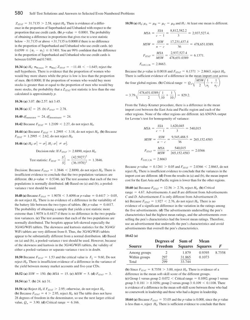
580 Self-Test Solutions and Answers to Selected Even-Numbered Problems
10.58 (a) H0: mA = mB = mC = mD and H1: At least one mean is different.
MSA =SSA
c - 1=
8,812,582.2
3= 2,937,527.4.
MSW =SSW
n - c=
17,231,437.4
36= 478,651.0389.
FSTAT =MSA
MSW=
2,937,527.4
478,651.0389= 6.1371.
F0.05,3,36 = 2.8663.
Because the p-value is 0.0018 and FSTAT = 6.1371 7 2.8663, reject H0. There is sufficient evidence of a difference in the mean import cost across
the four global regions. (b) Critical range = QaBMSW
2a 1
nj+
1
nj′b
= 3.79B478,651.0389
2a 1
10+
1
10b = 829.2.
From the Tukey-Kramer procedure, there is a difference in the mean import cost between the East Asia and Pacific region and each of the other regions. None of the other regions are different. (c) ANOVA output for Levene’s test for homogeneity of variance:
MSA =SSA
c - 1=
1,620,045
3= 540,015
MSW =SSW
n - c=
9,545,488.5
36= 265,152.4583
FSTAT =MSA
MSW=
540,015
265,152.4583= 2.0366
F0.05,3,36 = 2.8663
Because p@value = 0.1261 7 0.05 and FSTAT = 2.0366 6 2.8663, do not reject H0. There is insufficient evidence to conclude that the variances in the import cost are different. (d) From the results in (a) and (b), the mean import cost for the East Asia and Pacific region is lower than for the other regions.
10.60 (a) Because FSTAT = 12.56 7 2.76, reject H0. (b) Critical range = 4.67. Advertisements A and B are different from Advertisements C and D. Advertisement E is only different from Advertisement D. (c) Because FSTAT = 1.927 6 2.76, do not reject H0. There is no evidence of a significant difference in the variation in the ratings among the five advertisements. (d) The advertisements underselling the pen’s characteristics had the highest mean ratings, and the advertisements over-selling the pen’s characteristics had the lowest mean ratings. Therefore, use an advertisement that undersells the pen’s characteristics and avoid advertisements that oversell the pen’s characteristics.
10.62 (a)
Source
Degrees of Freedom
Sum of Squares
Mean Squares
F
Among groups 2 1.879 0.9395 8.7558Within groups 297 31.865 0.1073Total 299 33.744
(b) Since FSTAT = 8.7558 7 3.00, reject H0. There is evidence of a difference in the mean soft-skill score of the different groups.(c) Group 1 versus group 2: 0.072 6 Critical range = 0.1092; group 1 versus group 3: 0.181 7 0.1056; group 2 versus group 3: 0.109 6 0.1108. There is evidence of a difference in the mean soft-skill score between those who had no coursework in leadership and those who had a degree in leadership.
10.64 (a) Because FSTAT = 53.05 and the p-value is 0.000, since the p-value is less than a, reject H0. There is sufficient evidence to conclude that there
ZSTAT = 31.7135 7 2.58, reject H0. There is evidence of a differ-ence in the proportion of Superbanked and Unbanked with respect to the proportion that use credit cards. (b) p@value = 0.0001. The probability of obtaining a difference in proportions that gives rise to a test statistic below -31.7135 or above +31.7135 is 0.0000 if there is no difference in the proportion of Superbanked and Unbanked who use credit cards. (c) 0.6599 … 1p1 - p22 … 0.7401. You are 99% confident that the difference in the proportion of Superbanked and Unbanked who use credit cards is between 0.6599 and 0.7401.
10.34 (a) H0: pWomen Ú pMen; ZSTAT = -11.48 6 -1.645; reject the null hypothesis. There is evidence that the proportion of women who would buy more shares while the price is low is less than the proportion of men. (b) 0.0000; If the proportion of women who would buy more stocks is greater than or equal to the proportion of men who would buy more stocks, the probability that a ZSTAT test statistic is less than the one calculated is approximately p.
10.36 (a) 3.07. (b) 2.57. (c) 3.45.
10.38 (a) S12 = 25. (b) FSTAT = 2.78.
10.40 dfnumerator = 24, dfdenominator = 24.
10.42 Because FSTAT = 1.2109 6 2.27, do not reject H0.
10.44 (a) Because FSTAT = 1.2995 6 3.18, do not reject H0. (b) Because FSTAT = 1.2995 6 2.62, do not reject H0.
10.46 (a) H0: s2 1 = s2
2. H1: s2 1 ≠ s2
2.
Decision rule: If FSTAT 7 2.8890, reject H0.
Test statistic: FSTAT =S2
1
S22
=142.592722
136.197022= 1.3846.
Decision: Because FSTAT = 1.3846 6 2.8890, do not reject H0. There is insufficient evidence to conclude that the two population variances are different. (b) p@value = 0.5346. (c) The test assumes that each of the two populations is normally distributed. (d) Based on (a) and (b), a pooled-variance t test should be used.
10.48 (a) Because FSTAT = 1.9078 6 5.4098 or p@value = 0.4417 7 0.05, do not reject H0. There is no evidence of a difference in the variability of the battery life between the two types of tablets. (b) p@value = 0.4417. The probability of obtaining a sample that yields a test statistic more extreme than 1.9078 is 0.4417 if there is no difference in the two popula-tion variances. (c) The test assumes that each of the two populations are normally distributed. The boxplots appear left-skewed especially the 3G/4G/WiFi tablets. The skewness and kurtosis statistics for the 3G/4G/WiFi tablets are very different from 0. Thus, the 3G/4G/WiFi tablets appear to be substantially different from a normal distribution. (d) Based on (a) and (b), a pooled-variance t test should be used. However, because of the skewness and kurtosis in the 3G/4G/WiFi tablets, the validity of either a pooled-variance or separate-variance t test is in doubt.
10.50 Because FSTAT = 1.53 and the critical value is Fa
2= 9.60, Do not
reject H0. There is insufficient evidence of a difference in the variance of the yield between money market accounts and five-year CDs.
10.52 (a) SSW = 150. (b) MSA = 15. (c) MSW = 5. (d) FSTAT = 3.
10.54 (a) 7. (b) 24. (c) 31.
10.56 (a) Reject H0 if FSTAT 7 2.95; otherwise, do not reject H0. (b) Because FSTAT = 4 7 2.95, reject H0. (c) The table does not have 28 degrees of freedom in the denominator, so use the next larger critical value, Qa = 3.90. (d) Critical range = 6.166.
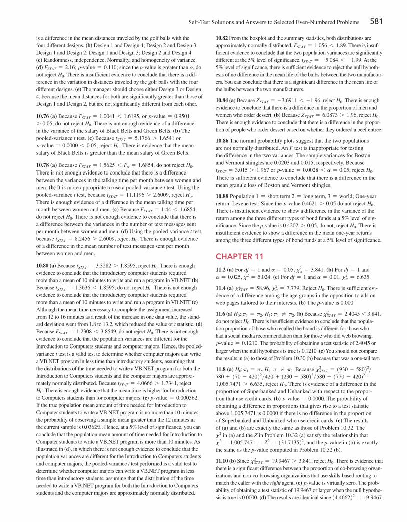
Self-Test Solutions and Answers to Selected Even-Numbered Problems 581
10.82 From the boxplot and the summary statistics, both distributions are approximately normally distributed. FSTAT = 1.056 6 1.89. There is insuf-ficient evidence to conclude that the two population variances are significantly different at the 5% level of significance. tSTAT = -5.084 6 -1.99. At the 5% level of significance, there is sufficient evidence to reject the null hypoth-esis of no difference in the mean life of the bulbs between the two manufactur-ers. You can conclude that there is a significant difference in the mean life of the bulbs between the two manufacturers.
10.84 (a) Because ZSTAT = -3.6911 6 -1.96, reject H0. There is enough evidence to conclude that there is a difference in the proportion of men and women who order dessert. (b) Because ZSTAT = 6.0873 7 1.96, reject H0. There is enough evidence to conclude that there is a difference in the propor-tion of people who order dessert based on whether they ordered a beef entree.
10.86 The normal probability plots suggest that the two populations are not normally distributed. An F test is inappropriate for testing the difference in the two variances. The sample variances for Boston and Vermont shingles are 0.0203 and 0.015, respectively. Because tSTAT = 3.015 7 1.967 or p@value = 0.0028 6 a = 0.05, reject H0. There is sufficient evidence to conclude that there is a difference in the mean granule loss of Boston and Vermont shingles.
10.88 Population 1 = short term 2 = long term, 3 = world; One-year return: Levene test: Since the p@value 0.4621 7 0.05 do not reject H0 . There is insufficient evidence to show a difference in the variance of the return among the three different types of bond funds at a 5% level of sig-nificance. Since the p-value is 0.4202 7 0.05, do not, reject H0. There is insufficient evidence to show a difference in the mean one-year returns among the three different types of bond funds at a 5% level of significance.
CHAPTER 11
11.2 (a) For df = 1 and a = 0.05, x2a = 3.841. (b) For df = 1 and
a = 0.025, x2 = 5.024. (c) For df = 1 and a = 0.01, x2a = 6.635.
11.4 (a) x2STAT = 58.96, x2
a = 7.779, Reject H0. There is sufficient evi-dence of a difference among the age groups in the opposition to ads on web pages tailored to their interests. (b) The p-value is 0.000.
11.6 (a) H0: p1 = p2. H1: p1 ≠ p2. (b) Because x2STAT = 2.4045 6 3.841,
do not reject H0. There is insufficient evidence to conclude that the popula-tion proportion of those who recalled the brand is different for those who had a social media recommendation than for those who did web browsing. p@value = 0.1210. The probability of obtaining a test statistic of 2.4045 or larger when the null hypothesis is true is 0.1210. (c) You should not compare the results in (a) to those of Problem 10.30 (b) because that was a one-tail test.
11.8 (a) H0: p1 = p2. H1: p1 ≠ p2. Because x2STAT = 1930 - 58022>
580 + 170 - 42022>420 + (230 - 58022>580 + 1770 - 420)2 =1,005.7471 7 6.635, reject H0. There is evidence of a difference in the proportion of Superbanked and Unbanked with respect to the propor-tion that use credit cards. (b) p@value = 0.0000. The probability of obtaining a difference in proportions that gives rise to a test statistic above 1,005.7471 is 0.0000 if there is no difference in the proportion of Superbanked and Unbanked who use credit cards. (c) The results of (a) and (b) are exactly the same as those of Problem 10.32. The x2 in (a) and the Z in Problem 10.32 (a) satisfy the relationship that x2 = 1,005.7471 = Z2 = 131.713522, and the p-value in (b) is exactly the same as the p-value computed in Problem 10.32 (b).
11.10 (b) Since x2STAT = 19.9467 7 3.841, reject H0. There is evidence that
there is a significant difference between the proportion of co-browsing organ-izations and non-co-browsing organizations that use skills-based routing to match the caller with the right agent. (c) p@value is virtually zero. The prob-ability of obtaining a test statistic of 19.9467 or larger when the null hypothe-sis is true is 0.0000. (d) The results are identical since 14.466222 = 19.9467.
is a difference in the mean distances traveled by the golf balls with the four different designs. (b) Design 1 and Design 4; Design 2 and Design 3; Design 1 and Design 2; Design 1 and Design 3; Design 2 and Design 4. (c) Randomness, independence, Normality, and homogeneity of variance. (d) FSTAT = 2.16; p@value = 0.110; since the p-value is greater than a, do not reject H0. There is insufficient evidence to conclude that there is a dif-ference in the variation in distances traveled by the golf balls with the four different designs. (e) The manager should choose either Design 3 or Design 4, because the mean distances for both are significantly greater than those of Design 1 and Design 2, but are not significantly different from each other.
10.76 (a) Because FSTAT = 1.0041 6 1.6195, or p@value = 0.95017 0.05, do not reject H0. There is not enough evidence of a difference in the variance of the salary of Black Belts and Green Belts. (b) The pooled-variance t test. (c) Because tSTAT = 5.1766 7 1.6541 or p@value = 0.0000 6 0.05, reject H0. There is evidence that the mean salary of Black Belts is greater than the mean salary of Green Belts.
10.78 (a) Because FSTAT = 1.5625 6 Fa = 1.6854, do not reject H0. There is not enough evidence to conclude that there is a difference between the variances in the talking time per month between women and men. (b) It is more appropriate to use a pooled-variance t test. Using the pooled-variance t test, because tSTAT = 11.1196 7 2.6009, reject H0. There is enough evidence of a difference in the mean talking time per month between women and men. (c) Because FSTAT = 1.44 6 1.6854, do not reject H0. There is not enough evidence to conclude that there is a difference between the variances in the number of text messages sent per month between women and men. (d) Using the pooled-variance t test, because tSTAT = 8.2456 7 2.6009, reject H0. There is enough evidence of a difference in the mean number of text messages sent per month between women and men.
10.80 (a) Because tSTAT = 3.3282 7 1.8595, reject H0. There is enough evidence to conclude that the introductory computer students required more than a mean of 10 minutes to write and run a program in VB.NET (b) Because tSTAT = 1.3636 6 1.8595, do not reject H0. There is not enough evidence to conclude that the introductory computer students required more than a mean of 10 minutes to write and run a program in VB.NET (c) Although the mean time necessary to complete the assignment increased from 12 to 16 minutes as a result of the increase in one data value, the stand-ard deviation went from 1.8 to 13.2, which reduced the value of t statistic. (d) Because FSTAT = 1.2308 6 3.8549, do not reject H0. There is not enough evidence to conclude that the population variances are different for the Introduction to Computers students and computer majors. Hence, the pooled-variance t test is a valid test to determine whether computer majors can write a VB.NET program in less time than introductory students, assuming that the distributions of the time needed to write a VB.NET program for both the Introduction to Computers students and the computer majors are approxi-mately normally distributed. Because tSTAT = 4.0666 7 1.7341, reject H0. There is enough evidence that the mean time is higher for Introduction to Computers students than for computer majors. (e) p@value = 0.000362. If the true population mean amount of time needed for Introduction to Computer students to write a VB.NET program is no more than 10 minutes, the probability of observing a sample mean greater than the 12 minutes in the current sample is 0.0362%. Hence, at a 5% level of significance, you can conclude that the population mean amount of time needed for Introduction to Computer students to write a VB.NET program is more than 10 minutes. As illustrated in (d), in which there is not enough evidence to conclude that the population variances are different for the Introduction to Computers students and computer majors, the pooled-variance t test performed is a valid test to determine whether computer majors can write a VB.NET program in less time than introductory students, assuming that the distribution of the time needed to write a VB.NET program for both the Introduction to Computers students and the computer majors are approximately normally distributed.
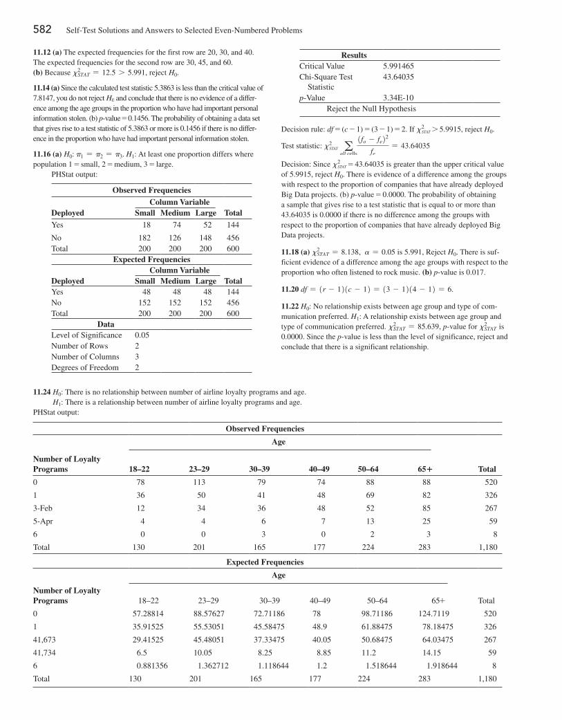
582 Self-Test Solutions and Answers to Selected Even-Numbered Problems
11.12 (a) The expected frequencies for the first row are 20, 30, and 40. The expected frequencies for the second row are 30, 45, and 60. (b) Because x2
STAT = 12.5 7 5.991, reject H0.
11.14 (a) Since the calculated test statistic 5.3863 is less than the critical value of 7.8147, you do not reject H0 and conclude that there is no evidence of a differ-ence among the age groups in the proportion who have had important personal information stolen. (b) p-value = 0.1456. The probability of obtaining a data set that gives rise to a test statistic of 5.3863 or more is 0.1456 if there is no differ-ence in the proportion who have had important personal information stolen.
11.16 (a) H0: p1 = p2 = p3. H1: At least one proportion differs where population 1 = small, 2 = medium, 3 = large.
PHStat output:
Observed FrequenciesColumn Variable
Deployed Small Medium Large TotalYes 18 74 52 144
No 182 126 148 456Total 200 200 200 600
Expected FrequenciesColumn Variable
Deployed Small Medium Large TotalYes 48 48 48 144No 152 152 152 456Total 200 200 200 600
DataLevel of Significance 0.05Number of Rows 2Number of Columns 3Degrees of Freedom 2
ResultsCritical Value 5.991465Chi-Square Test Statistic
43.64035
p-Value 3.34E-10Reject the Null Hypothesis
Decision rule: df = (c - 1) = (3 - 1) = 2. If x2stat 7 5.9915, reject H0.
Test statistic: x2stat a
all cells
1fo - fe22
fe= 43.64035
Decision: Since x2stat = 43.64035 is greater than the upper critical value
of 5.9915, reject H0. There is evidence of a difference among the groups with respect to the proportion of companies that have already deployed Big Data projects. (b) p-value = 0.0000. The probability of obtaining a sample that gives rise to a test statistic that is equal to or more than 43.64035 is 0.0000 if there is no difference among the groups with respect to the proportion of companies that have already deployed Big Data projects.
11.18 (a) x2STAT = 8.138, a = 0.05 is 5.991, Reject H0. There is suf-
ficient evidence of a difference among the age groups with respect to the proportion who often listened to rock music. (b) p-value is 0.017.
11.20 df = 1r - 121c - 12 = 13 - 1214 - 12 = 6.
11.22 H0: No relationship exists between age group and type of com-munication preferred. H1: A relationship exists between age group and type of communication preferred. x2
STAT = 85.639, p-value for x2STAT is
0.0000. Since the p-value is less than the level of significance, reject and conclude that there is a significant relationship.
Observed Frequencies
Age
Number of Loyalty Programs 18–22 23–29 30–39 40–49 50–64 65+ Total
0 78 113 79 74 88 88 520
1 36 50 41 48 69 82 326
3-Feb 12 34 36 48 52 85 267
5-Apr 4 4 6 7 13 25 59
6 0 0 3 0 2 3 8
Total 130 201 165 177 224 283 1,180
Expected Frequencies
Age
Number of Loyalty Programs 18–22 23–29 30–39 40–49 50–64 65+ Total
0 57.28814 88.57627 72.71186 78 98.71186 124.7119 520
1 35.91525 55.53051 45.58475 48.9 61.88475 78.18475 326
41,673 29.41525 45.48051 37.33475 40.05 50.68475 64.03475 267
41,734 6.5 10.05 8.25 8.85 11.2 14.15 59
6 0.881356 1.362712 1.118644 1.2 1.518644 1.918644 8
Total 130 201 165 177 224 283 1,180
11.24 H0: There is no relationship between number of airline loyalty programs and age. H1: There is a relationship between number of airline loyalty programs and age.
PHStat output:
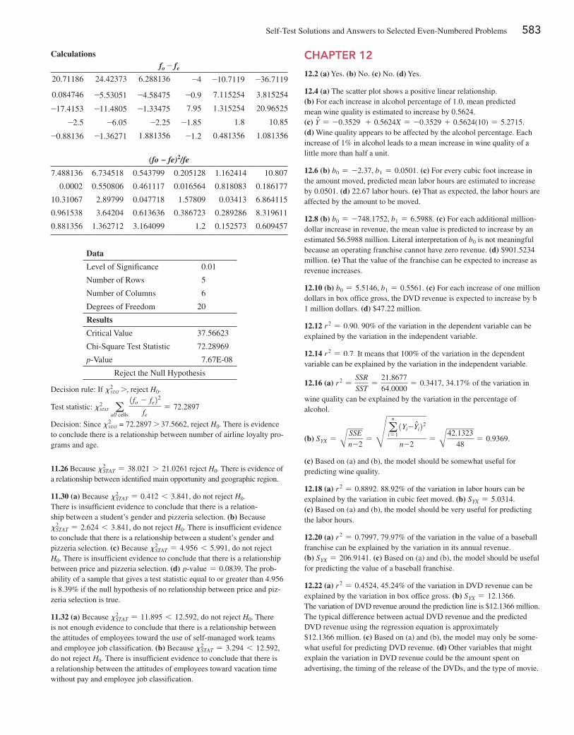
Self-Test Solutions and Answers to Selected Even-Numbered Problems 583
CHAPTER 12
12.2 (a) Yes. (b) No. (c) No. (d) Yes.
12.4 (a) The scatter plot shows a positive linear relationship. (b) For each increase in alcohol percentage of 1.0, mean predicted mean wine quality is estimated to increase by 0.5624. (c) Yn = -0.3529 + 0.5624X = -0.3529 + 0.5624(10) = 5.2715. (d) Wine quality appears to be affected by the alcohol percentage. Each increase of 1% in alcohol leads to a mean increase in wine quality of a little more than half a unit.
12.6 (b) b0 = -2.37, b1 = 0.0501. (c) For every cubic foot increase in the amount moved, predicted mean labor hours are estimated to increase by 0.0501. (d) 22.67 labor hours. (e) That as expected, the labor hours are affected by the amount to be moved.
12.8 (b) b0 = -748.1752, b1 = 6.5988. (c) For each additional million-dollar increase in revenue, the mean value is predicted to increase by an estimated $6.5988 million. Literal interpretation of b0 is not meaningful because an operating franchise cannot have zero revenue. (d) $901.5234 million. (e) That the value of the franchise can be expected to increase as revenue increases.
12.10 (b) b0 = 5.5146, b1 = 0.5561. (c) For each increase of one million dollars in box office gross, the DVD revenue is expected to increase by b 1 million dollars. (d) $47.22 million.
12.12 r 2 = 0.90. 90% of the variation in the dependent variable can be explained by the variation in the independent variable.
12.14 r 2 = 0.7. It means that 100% of the variation in the dependent variable can be explained by the variation in the independent variable.
12.16 (a) r 2 =SSR
SST=
21.8677
64.0000= 0.3417, 34.17% of the variation in
wine quality can be explained by the variation in the percentage of alcohol.
(b) SYX = A SSE
n-2= R a
n
i = 11Yi-Yni22
n-2= A42.1323
48= 0.9369.
(c) Based on (a) and (b), the model should be somewhat useful for predicting wine quality.
12.18 (a) r 2 = 0.8892. 88.92% of the variation in labor hours can be explained by the variation in cubic feet moved. (b) SYX = 5.0314. (c) Based on (a) and (b), the model should be very useful for predicting the labor hours.
12.20 (a) r 2 = 0.7997, 79.97% of the variation in the value of a baseball franchise can be explained by the variation in its annual revenue. (b) SYX = 206.9141. (c) Based on (a) and (b), the model should be useful for predicting the value of a baseball franchise.
12.22 (a) r 2 = 0.4524, 45.24% of the variation in DVD revenue can be explained by the variation in box office gross. (b) SYX = 12.1366. The variation of DVD revenue around the prediction line is $12.1366 million. The typical difference between actual DVD revenue and the predicted DVD revenue using the regression equation is approximately $12.1366 million. (c) Based on (a) and (b), the model may only be some-what useful for predicting DVD revenue. (d) Other variables that might explain the variation in DVD revenue could be the amount spent on advertising, the timing of the release of the DVDs, and the type of movie.
Calculationsfo - fe
20.71186 24.42373 6.288136 -4 -10.7119 -36.7119
0.084746 -5.53051 -4.58475 -0.9 7.115254 3.815254
-17.4153 -11.4805 -1.33475 7.95 1.315254 20.96525
-2.5 -6.05 -2.25 -1.85 1.8 10.85
-0.88136 -1.36271 1.881356 -1.2 0.481356 1.081356
(fo − fe)2/fe
7.488136 6.734518 0.543799 0.205128 1.162414 10.807
0.0002 0.550806 0.461117 0.016564 0.818083 0.186177
10.31067 2.89799 0.047718 1.57809 0.03413 6.864115
0.961538 3.64204 0.613636 0.386723 0.289286 8.319611
0.881356 1.362712 3.164099 1.2 0.152573 0.609457
Data
Level of Significance 0.01
Number of Rows 5
Number of Columns 6
Degrees of Freedom 20
Results
Critical Value 37.56623
Chi-Square Test Statistic 72.28969
p-Value 7.67E-08
Reject the Null Hypothesis
Decision rule: If x2stat 7, reject H0.
Test statistic: x2stat a
all cells
1fo - fe22
fe= 72.2897
Decision: Since x2stat = 72.2897 7 37.5662, reject H0. There is evidence
to conclude there is a relationship between number of airline loyalty pro-grams and age.
11.26 Because x2STAT = 38.021 7 21.0261 reject H0. There is evidence of
a relationship between identified main opportunity and geographic region.
11.30 (a) Because x2STAT = 0.412 6 3.841, do not reject H0.
There is insufficient evidence to conclude that there is a relation-ship between a student’s gender and pizzeria selection. (b) Because x2
STAT = 2.624 6 3.841, do not reject H0. There is insufficient evidence to conclude that there is a relationship between a student’s gender and pizzeria selection. (c) Because x2
STAT = 4.956 6 5.991, do not reject H0. There is insufficient evidence to conclude that there is a relationship between price and pizzeria selection. (d) p@value = 0.0839. The prob-ability of a sample that gives a test statistic equal to or greater than 4.956 is 8.39% if the null hypothesis of no relationship between price and piz-zeria selection is true.
11.32 (a) Because x2STAT = 11.895 6 12.592, do not reject H0. There
is not enough evidence to conclude that there is a relationship between the attitudes of employees toward the use of self-managed work teams and employee job classification. (b) Because x2
STAT = 3.294 6 12.592, do not reject H0. There is insufficient evidence to conclude that there is a relationship between the attitudes of employees toward vacation time without pay and employee job classification.
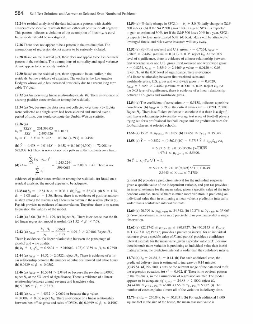
584 Self-Test Solutions and Answers to Selected Even-Numbered Problems
12.24 A residual analysis of the data indicates a pattern, with sizable clusters of consecutive residuals that are either all positive or all negative. This pattern indicates a violation of the assumption of linearity. A curvi-linear model should be investigated.
12.26 There does not appear to be a pattern in the residual plot. The assumptions of regression do not appear to be seriously violated.
12.28 Based on the residual plot, there does not appear to be a curvilinear pattern in the residuals. The assumptions of normality and equal variance do not appear to be seriously violated.
12.30 Based on the residual plot, there appears to be an outlier in the residuals, but no evidence of a pattern. The outlier is the Los Angeles Dodgers whose value has increased drastically due to a recent long term cable TV deal.
12.32 (a) An increasing linear relationship exists. (b) There is evidence of a strong positive autocorrelation among the residuals.
12.34 (a) No, because the data were not collected over time. (b) If data were collected at a single store had been selected and studied over a period of time, you would compute the Durbin-Watson statistic.
12.36 (a)
b1 =SSXY
SSX=
201,399.05
12,495,626= 0.0161
b0 = Y - b1X = 71.2621 - 0.0161 14,3932 = 0.458.
(b) Yn = 0.458 + 0.0161X = 0.458 + 0.016114,5002 = 72.908, or $72,908. (c) There is no evidence of a pattern in the residuals over time.
(d) D =a
n
i = 2
1ei- ei - 122
an
i = 1
e2i
=1,243.2244
599.0683= 2.08 7 1.45. There is no
evidence of positive autocorrelation among the residuals. (e) Based on a residual analysis, the model appears to be adequate.
12.38 (a) b0 = -2.5418, b1 = 0.0611. (b) Yn(81) = $2,404. (d) D = 1.74, dL = 1.08 and dU = 1.36. Hence, there is no evidence of positive autocor-relation among the residuals. (e) There is no pattern in the residual plot in (c). Part (d) provides no evidence of autocorrelation. Therefore, there is no reason to question the validity of the model.
12.40 (a) 3.00. (b) {2.1199. (c) Reject H0. There is evidence that the fit-ted linear regression model is useful. (d) 1.32 … b1 … 7.68.
12.42 (a) tSTAT =b1-b1
Sb1
=0.5624
0.1127= 4.9913 7 2.0106. Reject H0.
There is evidence of a linear relationship between the percentage of alcohol and wine quality. (b) b1 { ta>2Sb1
= 0.5624 { 2.010610.11272 0.3359 … b1 … 0.7890.
12.44 (a) tSTAT = 16.52 7 2.0322; reject H0. There is evidence of a lin-ear relationship between the number of cubic feet moved and labor hours. (b) 0.0439 … b1 … 0.0562.
12.46 (a) tSTAT = 10.5744 7 2.0484 or because the p-value is 0.0000, reject H0 at the 5% level of significance. There is evidence of a linear relationship between annual revenue and franchise value. (b) 5.3205 … b1 … 7.8771.
12.48 (a) tSTAT = 4.4532 7 2.0639 or because the p-value = 0.0002 6 0.05; reject H0. There is evidence of a linear relationship between box office gross and sales of DVDs. (b) 0.0699 … b1 … 0.1907.
12.50 (a) (% daily change in SPXL) = b0 + 3.0 (% daily change in S&P 500 index). (b) If the S&P 500 gains 10% in a year, SPXL is expected to gain an estimated 30%. (c) If the S&P 500 loses 20% in a year, SPXL is expected to lose an estimated 60%. (d) Risk takers will be attracted to leveraged funds, and risk-averse investors will stay away.
12.52 (a), (b) First weekend and U.S. gross: r = 0.7264, tSTAT =2.5893 7 2.4469, p@value = 0.0413 6 0.05. reject H0. At the 0.05 level of significance, there is evidence of a linear relationship between first weekend sales and U.S. gross. First weekend and worldwide gross: r = 0.8234, tSTAT = 3.5549 7 2.4469, p@value = 0.0120 6 0.05. reject H0. At the 0.05 level of significance, there is evidence of a linear relationship between first weekend sales and worldwide gross. U.S. gross and worldwide gross: r = 0.9629,tSTAT = 8.7456 7 2.4469, p@value = 0.0001 6 0.05. Reject H0. At the 0.05 level of significance, there is evidence of a linear relationship between U.S. gross and worldwide gross.
12.54 (a) The coefficient of correlation, r = 0.5138, indicates a positive correlation. (b) tSTAT = 3.5938, the critical values are -2.0281, 2.0281. Reject H0. There is sufficient evidence to conclude that there is a signifi-cant linear relationship between the average test score of football players trying out for a professional football league and the graduation rates for football players at selected schools.
12.56 (a) 15.95 … mY ∙X = 4 … 18.05. (b) 14.651 … YX = 4 … 19.349.
12.58 (a) Yn = -0.3529 + (0.5624)(10) = 5.2715 Yn { ta>2SYX1hi
= 5.2715 { 2.010610.9369210.02494.9741 … mY ∙X = 10 … 5.5690.
(b) Yn { ta>2SYX21 + hi
= 5.2715 { 2.010619,369221 + 0.02493.3645 … YX = 10 … 7.1786.
(c) Part (b) provides a prediction interval for the individual response given a specific value of the independent variable, and part (a) provides an interval estimate for the mean value, given a specific value of the inde-pendent variable. Because there is much more variation in predicting an individual value than in estimating a mean value, a prediction interval is wider than a confidence interval estimate.
12.60 (a) 20.799 … mY ∙X = 500 … 24.542. (b) 12.276 … YX = 500 … 33.065. (c) You can estimate a mean more precisely than you can predict a single observation.
12.62 (a) 822.1742 … mY ∙X = 250 … 980.8727. (b) 470.3155 … YX = 250
… 1,332.731. (c) Part (b) provides a prediction interval for an individual response given a specific value of X, and part (a) provides a confidence interval estimate for the mean value, given a specific value of X. Because there is much more variation in predicting an individual value than in esti-mating a mean, the prediction interval is wider than the confidence interval.
12.74 (a) b0 = 24.84, b1 = 0.14. (b) For each additional case, the predicted delivery time is estimated to increase by 0.14 minute. (c) 45.84. (d) No, 500 is outside the relevant range of the data used to fit the regression equation. (e) r 2 = 0.972. (f) There is no obvious pattern in the residuals, so the assumptions of regression are met. The model appears to be adequate. (g) tSTAT = 24.88 7 2.1009; reject H0. (h) 44.88 … mY ∙X = 150 … 46.80. 41.56 … YX = 150 … 50.12. (i) The number of cases explains almost all of the variation in delivery time.
12.76 (a) b0 = 276.848, b1 = 50.8031. (b) For each additional 1,000 square feet in the size of the house, the mean assessed value is

Self-Test Solutions and Answers to Selected Even-Numbered Problems 585
predicted to increase by $50,803.10. The estimated selling price of a house with a 0 size is +276,848 thousand. However, this interpretation is not meaningful because the size of the house cannot be 0. (c) Yn = 276.848 + 50.8031(2) = 378.4542 thousand dollars. (d) r 2 = 0.3273. So 32.73% of the variation in assessed value be explained by the variation in size. (e) Neither the residual plot nor the normal probability plot reveals any potential violation of the linearity, equal variance, and normality assumptions. (f) tSTAT = 3.6913 7 2.0484, p-value is 0.0009. Because p@value 6 0.05, reject H0. There is evidence of a linear relationship between assessed value and size. (g) 22.6113 … b1 … 78.9949. (h) The size of the house is somewhat useful in predicting the assessed value, but since only 32.73% of the vari-ation in assessed value is explained by variation in size, other variables should be considered.
12.78 (a) b0 = 0.30, b1 = 0.00487. (b) For each additional point on the GMAT score, the predicted GPA is estimated to increase by 0.00487. Because a GMAT score of 0 is not possible, the Y intercept does not have a practical interpretation. (c) 3.222. (d) r 2 = 0.798. (e) There is no obvious pattern in the residuals, so the assumptions of regression are met. The model appears to be adequate. (f) tSTAT = 8.43 7 2.1009; reject H0. (g) 3.144 … mY ∙X = 600 … 3.301, 2.866 … YX = 600 … 3.559. (h) .00366 … b1 … .00608. (i) Most of the variation in GPA can be explained by variation in the GMAT score.
12.80 (a) There is no clear relationship shown on the scatter plot. (c) Looking at all 23 flights, when the temperature is lower, there is likely to be some O-ring damage, particularly if the temperature is below 60 degrees. (d) 31 degrees is outside the relevant range, so a predic-tion should not be made. (e) Predicted Y = 18.036-0.240X, where X = temperature and Y = O-ring damage. (g) A nonlinear model would be more appropriate. (h) The appearance on the residual plot of a non-linear pattern indicates that a nonlinear model would be better. It also appears that the normality assumption is invalid.
12.82 (a) b0 = -177.4298, b1 = 5.3450. (b) For each additional million-dollar increase in revenue, the franchise value will increase by an estimated $5.3450 million. Literal interpretation of b0 is not meaningful because an operating franchise cannot have zero revenue. (c) $624.3226 million. (d) r 2 = 0.9331. 93.31% of the variation in the value of an NBA franchise can be explained by the variation in its annual revenue. (e) There does not appear to be a pattern in the residual plot. The assumptions of regression do not appear to be seriously violated. (f) tSTAT = 19.764 7 2.0484 or because the p-value is 0.0000, reject H0 at the 5% level of significance. There is evidence of a linear relationship between annual revenue and franchise value. (g) 599.5015 … mY ∙X = 150 … 649.1438. (h) 486.2403 … YX = 150 …762.405. (i) The strength of the relationship between revenue and value is higher for NBA franchises than for European soccer teams and Major League Baseball teams.
12.84 (a) b0 = -2,629.222, b1 = 82.472. (b) For each additional centimeter in circumference, the weight is estimated to increase by 82.472 grams. (c) 2,319.08 grams. (d) Yes, since circumference is a very strong predictor of weight. (e) r 2 = 0.937. (f) There appears to be a nonlinear relationship between circumference and weight. (g) p-value is virtually 0 6 0.05; reject H0. (h) 72.7875 … b1 … 92.156.
12.86 (a) The correlation between compensation and stock performance is 0.1854. (b) tSTAT = 2.6543; p@value = 0.0086 6 0.05. The correla-tion between compensation and stock performance is significant, but only 3.44% of the variation in compensation can be explained by return. (c) The small correlation between compensation and stock performance was surprising (or maybe it shouldn’t have been!).
CHAPTER 13
13.2 (a) For each one-unit increase in X1, Y will decrease an estimated 6 units, holding X2 constant. For each one-unit increase in X2, Y will increase an estimated 3 units, holding X1 constant. (b) The Y-intercept 50 estimates the value of Y when both X1 and X2 are 0.
13.4 (a) Yn = -0.2245 + 0.0111X1 + 0.0445X2. (b) For a given total risk-based capital (%), each increase of 1% in the efficiency ratio is estimated to result in a mean increase in ROA of 0.0111%. For a given efficiency ratio, each increase of 1% in the total risk-based capital (%) is estimated to result in a mean increase in ROA of 0.0445%. (c) The interpretation of b0 has no practical meaning here because it would have been the estimated mean ROA when the efficiency ratio and the total risk-based capital are each zero. (d) Yni = -0.2245 + 0.01111602 + 0.04451152 = 1.1123 or $69,878. (e) 0.9888 … mY ∙X … 1.2357. (f) -0.4268 … YX … 2.6513. (g) Since there is much more variation in predicting an individual value than in estimating a mean value, a prediction interval is wider than a confidence interval estimate holding everything else fixed.
13.6 (a) Yn = -186.5501 + 0.0333X1 + 50.8778X2. (b) For a given amount of voluntary turnover, each increase of $1 million in total world-wide revenue is estimated to result in a mean increase in the number of full-time jobs added in a year by 0.0333. For a given amount of total worldwide revenue, each increase of 1% in voluntary turnover is estimated to result in the mean increase in the number of full-time jobs added in a year of 50.8778. (c) The Y intercept of -186.5501 has no direct interpre-tation since it represents the value of the mean increase in the number of full-time jobs added in a year when there is no worldwide revenue and no voluntary turnover. (d) The number of full-time jobs added seems to be affected by the amount of worldwide revenue and the voluntary turnover.
13.8 (a) Yni = 403.8278 + (463.5662)X1i + (-2.7385)X2i. (b) For a given age, each increase of 1 acre in land area is estimated to result in an increase in appraised value by 1000b1 dollars. For a given land area, each increase in one year in age is estimated to result in a decrease in appraised value by 1000b2 dollars. (c) The interpretation of b0 has no practical meaning here because it would represent the estimated appraised value of a new house that has no land area. (d) $388.07 thousand. (e) $310.5 thousand … mean appraised value … $465.6 thousand. (f) $167.7 thou-sand … mean appraised value … $608.5 thousand.
13.10 (a) MSR = 15, MSE = 12. (b) 1.25. (c) FSTAT = 1.25 6 4.10; do not reject H0. (d) 0.20. (e) 0.04.
13.12 (a) FSTAT = 0.6531 6 3.44. Do not reject H0. There is insufficient evidence of a significant linear relationship with at least one of the independent variables. (b) p-value = 0.5302. The probability of obtaining an F test statistic of 0.6531 or larger is 0.5302 if H0 is true. (c) r 2
Y.12 = SSR>SST = 96,655.1>1,724,596.2 = 0.056. So, 5.6% of the variation in the mean annual revenue can be explained by variation in the mean age and mean BizAnalyzer score.
13.14 (a) MSR = SSR>k = 7.5929>2 = 3.7964MSE = SSE>1n - k - 12 = 119.2044>197 = 0.6051FSTAT = MSR>MSE = 3.7964>0.6051 = 6.2741FSTAT = 6.2741 7 3.0. Reject H0. There is evidence of a significant linear relationship. (b) p-value = 0.0023. The probability of obtaining an F test statistic of 6.2741 or larger is 0.0023 if H0 is true. (c) r 2
Y.12 = SSR>SST = 7.5929>126.7973 = 0.0599. So, 5.99% of the

586 Self-Test Solutions and Answers to Selected Even-Numbered Problems
13.32 Because tSTAT = 3.27 7 2.1098, reject H0. X2 makes a significant contribution to the model.
13.34 (a) Yni = 243.737 + (9.219)X1i + (12.697)X2i. (b) Holding con-stant whether a house is in the east or west side of town, for each increase of 1 room in the house, the predicted price of the home is estimated to increase by 9.219 thousand dollars. Holding constant the number of rooms in the home, the presence of the home on the west side of town is estimated to increase the predicted price of the home by 12.697 thousand dollars over the price of a home on the east side of town. (c) H0: b1 = 0, H1: b1 ≠ 0. The test statistic for the first independent variable, Rooms, is tSTAT = 8.954. The p-value for the first independ-ent variable, Rooms, is 0.0000. Since the p-value is less than the value of a, reject the null hypotheses. The first independent variable, Rooms, appears to make a contribution to the regression model. H0: b2 = 0, H1: b2 = ≠ 0. The test statistic for the second independent variable, Neighborhood, is tSTAT = 3.591. The p-value for the second independ-ent variable, Neighborhood, is 0.0023. Since the p-value is less than the value of a, reject appears the null hypothesis. The second independent variable, Neighborhood, appears to make a contribution to the regres-sion model. (d) Taking into account the effect of Neighborhood, the estimated effect of a 1 room increase is to change the Price by 7.047 to 11.391 thousand dollars. (e) Taking into account the effect of Rooms, the estimated effect of the home being on the west side of town instead of the east side of town is to change the Price by 5.238 to 20.156 thousand dollars. (f) Yni = 253.945 + (8.032)X1i + (-5.902)X2i + (2.089)X3i. H0: b3 = 0, H1: b3 ≠ 0. The test statistic for the interaction term is tSTAT = 1.005. The p-value for the interaction term is 0.3297. Since the p-value is greater than the value of a, do not reject the null hypothesis. The interaction term does not appear to make a contribution to the regres-sion model. (g) The model without the interaction term appears to be the most appropriate because the interaction term does not appear to make a contribution to the regression model.
13.36 (a) Predicted time = 8.01 + 0.00523 Depth - 2.105 Dry. (b) Holding constant the effect of type of drilling, for each foot increase in depth of the hole, the mean drilling time is estimated to increase by 0.00523 minutes. For a given depth, a dry drilling hole is estimated to reduce the drilling time over wet drilling by a mean of 2.1052 minutes.(c) 6.428 minutes, 6.210 … mY ∙X … 6.646, 4.923 … YX … 7.932. (d) The model appears to be adequate. (e) FSTAT = 111.11 7 3.09; reject H0. (f) tSTAT = 5.03 7 1.9847; reject H0. tSTAT = -14.03 6-1.9847; reject H0. Include both variables. (g) 0.0032 … b1 … 0.0073.(h) -2.403 … b2 … -1.808. (i) 69.0%. (j) The slope of the addi-tional drilling time with the depth of the hole is the same, regardless of the type of drilling method used. (k) The p-value of the interaction term = 0.462 7 0.05, so the term is not significant and should not be included in the model. (l) The model in part (b) should be used. Both variables affect the drilling time. Dry drilling holes should be used to reduce the drilling time.
13.38 (a) Yn = 2.5213 - 0.0313X1 - 0.1131X2 + 0.0024X3, where X1 = efficiency ratio, X2 = total risk-based capital, X3 = X1 X2. For X1X2: the p-value is 0.0297 6 0.05. Reject H0. There is evidence that the interaction term makes a contribution to the model. (b) Since there is evi-dence of an interaction effect between efficiency ratio and total risk-based capital, the model in (a) should be used.
13.40 (a) Yn = 85.1106 + 0.0033X1 + 15.8856X2 + 0.0045X3, where X1 = total worldwide revenue ($millions), X2 = full-time voluntary turnover (%), X3 = X1 X2. For X1X2: the p-value is 0.0396 6 0.05. Reject H0. There is evidence that the interaction term makes a contribu-tion to the model. (b) Since there is evidence of an interaction effect
variation in ROA can be explained by variation in used efficiency ratio and total risk-based capital.
(d) r 2adj = 1 - c 11 - r 2
Y.122 n - 1
n - k - 1d =
1 - c 11 - 0.05992 200 - 1
200 - 2 - 1d = 0.0503
13.16 (a) MSR = SSR>k = 19,534,514.2835>2 = 9,767,257.1417MSE = SSE>1n - k - 12 = 115,096,077.0499>93 = 1,237,592.2263FSTAT = MSR>MSE = 9,767,257.1417>1,237,592.2263 = 7.8921FSTAT = 7.8921 7 3.0943. Reject H0. There is evidence of a significant linear relationship. (b) p-value 60.0007. The probability of obtaining an F test statistic of 7.8921 or larger is less than 0.0007 if H0 is true.(c) r 2
Y.12 = SSR>SST = 19,534,514.2835>134,630,591.3333 = 0.1451. So, 14.51% of the variation in the number of full-time jobs added can be explained by variation in the total worldwide revenue ($millions), and full-time voluntary turnover (%). (d) r 2
adj = 0.1267
13.18 Since the data were not collected over time, there is no reason to plot the residuals over time. (c) There appears to be a departure in the equal variance assumption in the plot of the residuals versus the effi-ciency ratio. Therefore, a data transformation should be considered.
13.20 Based on a residual analysis, there is evidence of a violation of the assumptions of equal variance and normality. (b) Since the data were not collected over time, the Durbin-Watson test is not appropriate. (c) No.
13.22 (a) The residual analysis reveals no patterns. (b) Since the data are not collected over time, the Durbin-Watson test is not appropriate. (c) There are no apparent violations in the assumptions.
13.24 (a) Variable X2 has a larger slope in terms of the t statistic of 3.75 than variable X1, which has a smaller slope in terms of the t statistic of 3.33. (b) 1.46824 … b1 … 6.53176. (c) For X1 : tSTAT = 4>1.2 = 3.33 7 2.1098, with 17 degrees of freedom for a = 0.05. Reject H0. There is evidence that X1 contributes to a model already containing X2. For X2 : tSTAT = 3>0.8 = 3.75 7 2.1098, with 17 degrees of freedom for a = 0.05. Reject H0. There is evidence that X2 contributes to a model already containing X1. Both X1 and X2 should be included in the model.
13.26 (a) 95% confidence interval on b1: b1 { tn - k - 1sb1,
0.0111 { 1.972110.00512 0.0011 … b1 … 0.0212.(b) For X1: tSTAT = b1>sb1
= 0.0111>0.0051 = 2.1881 7 1.9721 with 197 degrees of freedom for a = 0.05. Reject H0. There is evidence that the variable X1 contributes to a model already containing X2.For X2: tSTAT = b2>sb2
= 0.0445>0.0145 = 3.065 7 1.9721 with 197 degrees of freedom for a = 0.05. Reject H0. There is evidence that the variable X2 contributes to a model already containing X1. Both variables X1 and X2 should be included in the model.
13.28 (a) 0.0333 { 1.985810.00922 0.0151 … b1 … 0.0515.(b) For X1: tSTAT = b1>sb1
= 0.0333>0.0092 = 3.639 7 1.9858 with 93 degrees of freedom for a = 0.05. Reject H0. There is evidence that the variable X1 contributes to a model already containing X2.For X2: tSTAT = b2>sb2
= 50.8778>23.7425 = 2.1429 7 1.9858 with 93 degrees of freedom for a = 0.05. Reject H0. There is evidence that the variable X2 contributes to a model already containing X1. Both vari-ables X1 and X2 should be included in the model.
13.30 (a) 274.1702 … b1 … 540.0990. (b) For X1 : tSTAT = 6.2827 and p@value = 0.0000. Because p@value 6 0.05, reject H0. There is evidence that X1 contributes to a model already containing X2. For X2 : tSTAT = -4.1475 and p@value = 0.0003. Because p@value 6 0.05 reject H0. There is evidence that X2 contributes to a model already containing X1: FSTAT = 30.4533 p@value = 0.0000. Both X1 (land area) and X2 (age) should be included in the model.
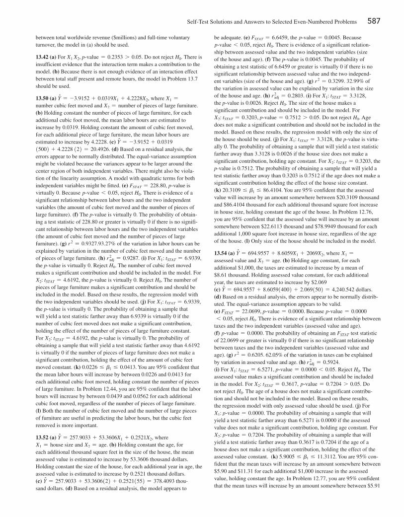
Self-Test Solutions and Answers to Selected Even-Numbered Problems 587
be adequate. (e) FSTAT = 6.6459, the p@value = 0.0045. Because p@value 6 0.05, reject H0. There is evidence of a significant relation-ship between assessed value and the two independent variables (size of the house and age). (f) The p-value is 0.0045. The probability of obtaining a test statistic of 6.6459 or greater is virtually 0 if there is no significant relationship between assessed value and the two independ-ent variables (size of the house and age). (g) r 2 = 0.3299. 32.99% of the variation in assessed value can be explained by variation in the size of the house and age. (h) r 2
adj = 0.2803. (i) For X1: tSTAT = 3.3128, the p-value is 0.0026. Reject H0. The size of the house makes a significant contribution and should be included in the model. For X2: tSTAT = 0.3203, p@value = 0.7512 7 0.05. Do not reject H0. Age does not make a significant contribution and should not be included in the model. Based on these results, the regression model with only the size of the house should be used. (j) For X1: tSTAT = 3.3128, the p-value is virtu-ally 0. The probability of obtaining a sample that will yield a test statistic farther away than 3.3128 is 0.0026 if the house size does not make a significant contribution, holding age constant. For X2: tSTAT = 0.3203, the p-value is 0.7512. The probability of obtaining a sample that will yield a test statistic farther away than 0.3203 is 0.7512 if the age does not make a significant contribution holding the effect of the house size constant. (k) 20.3109 … b1 … 86.4104. You are 95% confident that the assessed value will increase by an amount somewhere between $20.3109 thousand and $86.4104 thousand for each additional thousand square foot increase in house size, holding constant the age of the house. In Problem 12.76, you are 95% confident that the assessed value will increase by an amount somewhere between $22.6113 thousand and $78.9949 thousand for each additional 1,000 square foot increase in house size, regardless of the age of the house. (l) Only size of the house should be included in the model.
13.54 (a) Yn = 694.9557 + 8.6059X1 + 2069X2, where X1 =assessed value and X2 = age. (b) Holding age constant, for each additional $1,000, the taxes are estimated to increase by a mean of $8.61 thousand. Holding assessed value constant, for each additional year, the taxes are estimated to increase by $2.069(c) Yn = 694.9557 + 8.605914002 + 2.0691502 = 4,240.542 dollars.(d) Based on a residual analysis, the errors appear to be normally distrib-uted. The equal-variance assumption appears to be valid. (e) FSTAT = 22.0699, p@value = 0.0000. Because p@value = 0.00006 0.05, reject H0. There is evidence of a significant relationship between
taxes and the two independent variables (assessed value and age). (f) p@value = 0.0000. The probability of obtaining an FSTAT test statistic of 22.0699 or greater is virtually 0 if there is no significant relationship between taxes and the two independent variables (assessed value and age). (g) r 2 = 0.6205. 62.05% of the variation in taxes can be explained by variation in assessed value and age. (h) r 2
adj = 0.5924.(i) For X1: tSTAT = 6.5271, p@value = 0.0000 6 0.05. Reject H0. The assessed value makes a significant contribution and should be included in the model. For X2: tSTAT = 0.3617, p@value = 0.7204 7 0.05. Do not reject H0. The age of a house does not make a significant contribu-tion and should not be included in the model. Based on these results, the regression model with only assessed value should be used. (j) For X1: p@value = 0.0000. The probability of obtaining a sample that will yield a test statistic farther away than 6.5271 is 0.0000 if the assessed value does not make a significant contribution, holding age constant. For X2: p@value = 0.7204. The probability of obtaining a sample that will yield a test statistic farther away than 0.3617 is 0.7204 if the age of a house does not make a significant contribution, holding the effect of the assessed value constant. (k) 5.9005 … b1 … 11.3112. You are 95% con-fident that the mean taxes will increase by an amount somewhere between $5.90 and $11.31 for each additional $1,000 increase in the assessed value, holding constant the age. In Problem 12.77, you are 95% confident that the mean taxes will increase by an amount somewhere between $5.91
between total worldwide revenue ($millions) and full-time voluntary turnover, the model in (a) should be used.
13.42 (a) For X1 X2, p@value = 0.2353 7 0.05. Do not reject H0. There is insufficient evidence that the interaction term makes a contribution to the model. (b) Because there is not enough evidence of an interaction effect between total staff present and remote hours, the model in Problem 13.7 should be used.
13.50 (a) Yn = -3.9152 + 0.0319X1 + 4.2228X2, where X1 = number cubic feet moved and X2 = number of pieces of large furniture. (b) Holding constant the number of pieces of large furniture, for each additional cubic foot moved, the mean labor hours are estimated to increase by 0.0319. Holding constant the amount of cubic feet moved, for each additional piece of large furniture, the mean labor hours are estimated to increase by 4.2228. (c) Yn = -3.9152 + 0.031915002 + 4.2228 122 = 20.4926. (d) Based on a residual analysis, the errors appear to be normally distributed. The equal-variance assumption might be violated because the variances appear to be larger around the center region of both independent variables. There might also be viola-tion of the linearity assumption. A model with quadratic terms for both independent variables might be fitted. (e) FSTAT = 228.80, p-value is virtually 0. Because p@value 6 0.05, reject H0. There is evidence of a significant relationship between labor hours and the two independent variables (the amount of cubic feet moved and the number of pieces of large furniture). (f) The p-value is virtually 0. The probability of obtain-ing a test statistic of 228.80 or greater is virtually 0 if there is no signifi-cant relationship between labor hours and the two independent variables (the amount of cubic feet moved and the number of pieces of large furniture). (g) r 2 = 0.9327.93.27% of the variation in labor hours can be explained by variation in the number of cubic feet moved and the number of pieces of large furniture. (h) r 2
adj = 0.9287. (i) For X1: tSTAT = 6.9339, the p-value is virtually 0. Reject H0. The number of cubic feet moved makes a significant contribution and should be included in the model. For X2: tSTAT = 4.6192, the p-value is virtually 0. Reject H0. The number of pieces of large furniture makes a significant contribution and should be included in the model. Based on these results, the regression model with the two independent variables should be used. (j) For X1: tSTAT = 6.9339, the p-value is virtually 0. The probability of obtaining a sample that will yield a test statistic farther away than 6.9339 is virtually 0 if the number of cubic feet moved does not make a significant contribution, holding the effect of the number of pieces of large furniture constant. For X2: tSTAT = 4.6192, the p-value is virtually 0. The probability of obtaining a sample that will yield a test statistic farther away than 4.6192 is virtually 0 if the number of pieces of large furniture does not make a significant contribution, holding the effect of the amount of cubic feet moved constant. (k) 0.0226 … b1 … 0.0413. You are 95% confident that the mean labor hours will increase by between 0.0226 and 0.0413 for each additional cubic foot moved, holding constant the number of pieces of large furniture. In Problem 12.44, you are 95% confident that the labor hours will increase by between 0.0439 and 0.0562 for each additional cubic foot moved, regardless of the number of pieces of large furniture. (l) Both the number of cubic feet moved and the number of large pieces of furniture are useful in predicting the labor hours, but the cubic feet removed is more important.
13.52 (a) Yn = 257.9033 + 53.3606X1 + 0.2521X2, where X1 = house size and X2 = age. (b) Holding constant the age, for each additional thousand square feet in the size of the house, the mean assessed value is estimated to increase by 53.3606 thousand dollars. Holding constant the size of the house, for each additional year in age, the assessed value is estimated to increase by 0.2521 thousand dollars.(c) Yn = 257.9033 + 53.3606122 + 0.25211552 = 378.4093 thou-sand dollars. (d) Based on a residual analysis, the model appears to

588 Self-Test Solutions and Answers to Selected Even-Numbered Problems
significance of sales growth (%) and return on equity (%) is 12.0965 with a p-value of 0.0000. Hence, at a 5% level of significance, there is evidence to conclude sales growth (%) and/or return on equity (%) affect earnings per share growth. The p-value of the t test for the significance of sales growth is 0.0002 6 0.05. Hence, there is sufficient evidence to con-clude that sales growth affects earnings per share growth holding constant the effect of return on equity. The p-value of the t test for the significance of return on equity is 0.0037 6 0.05. There is evidence to conclude that return on equity affects earnings per share growth holding constant the effect of sales growth. There do not appear to be any obvious patterns in the residual plots. Hence, both sales growth (%) and return on equity (%) should be used in a regression model to predict earnings per share growth.
13.60 b0 = 18.2892 (die temperature), b1 = 0.5976, (die diameter), b2 = -13.5108. The r 2 of the multiple regression is 0.3257 so 32.57% of the variation in unit density can be explained by the variation of die temperature and die diameter. The F test statistic for the combined sig-nificance of die temperature and die diameter is 5.0718 with a p-value of 0.0160. Hence, at a 5% level of significance, there is enough evidence to conclude that die temperature and die diameter affect unit density. The p-value of the t test for the significance of die temperature is 0.2117, which is greater than 5%. Hence, there is insufficient evidence to con-clude that die temperature affects unit density holding constant the effect of die diameter. The p-value of the t test for the significance of die diame-ter is 0.0083, which is less than 5%.There is enough evidence to conclude that die diameter affects unit density at the 5% level of significance hold-ing constant the effect of die temperature. After removing die temperature from the model, b0 = 107.9267 (die diameter), b1 = -13.5108. The r 2 of the multiple regression is 0.2724. So 27.24% of the variation in unit density can be explained by the variation of die diameter. The p-value of the t test for the significance of die diameter is 0.0087, which is less than 5%. There is enough evidence to conclude that die diameter affects unit density at the 5% level of significance. There is some lack of equality in the residuals and some departure from normality.
and $11.07 for each additional $thousand increase in assessed value, regardless of the age. (l) Based on your answers to (b) through (k), the age of a house does not have an effect on its taxes.
13.56 (a) Yn = 183.1738 - 25.5406X1 - 6.9866X2, where X1 = ERA and X2 = League 1American = 0, National = 12. (b) Holding constant the effect of the league, for each additional ERA, the number of wins is estimated to decrease by a mean of 25.5406. For a given ERA, a team in the National League is estimated to have a mean of 6.9866 fewer wins than a team in the American League.(c) Yn = 183.1738 - 25.540614.02 - 6.9866102 = 81.0113 wins =81 wins. (d) Based on a residual analysis, there is no pattern in the errors. There is no apparent violation of other assumptions. (e) FSTAT = 23.4629, p-value = 0.0000. Since p-value 6 0.05, reject H0. There is evidence of a significant relationship between wins and the two independent variables (ERA and league). (f) For X1: tSTAT = -6.8476, p-value = 0.0000 6 0.05. Reject H0. ERA makes a significant contribu-tion and should be included in the model. For X2: tSTAT = -2.368, p-value = 0.0253 6 0.05. Reject H0. The league makes a significant contribution and should be included in the model. Based on these results, the regression model with ERA and league as the independ-ent variables should be used. (g) -33.1937 … b1 … -17.8876 (h) -13.0404 … b2 … -0.9328 (i) r 2
adj = 0.6077. So 60.77% of the var-iation in wins can be explained by the variation in ERA and league after adjusting for number of independent variables and sample size. (j) The slope of the number of wins with ERA is the same regardless of whether the team belongs to the American or the National League. (k) For X1X2: the p-value is 0.3024 7 0.05. Do not reject H0. There is no evidence that the interaction term makes a contribution to the model. (l) The regression model with ERA and league as the independent variables should be used.
13.58 The r 2 of the multiple regression is 0.1996. 19.96% of the variation in earnings per share growth can be explained by the variation of sales growth (%) and return on equity (%). The F test statistic for the combined
IndexAa (level of significance), 310A priori probability, 166Addition rule, 171Adjusted r2, 493Algebra, rules for, 519Alternative hypothesis, 307Among-group variation, 376Analysis of variance (ANOVA)
assumptions, 381–382F test for differences in more than two means, 377–381F test statistic, 377Levene’s test for homogeneity of variance, 382–383summary table, 378Tukey-Kramer procedure, 383–386
Analysis ToolPak,checking for presence, 540descriptive statistics, 159–160F test for ratio of two variances, 402frequency distribution, 105histogram, 109–110multiple regression, 513–514one-way ANOVA, 403paired t test, 400pooled-variance t test, 398random sampling, 268residual analysis, 482sampling distributions, 268separate-variance t test, 399simple linear regression, 483
Analyze, 24 ANOVA. See Analysis of variance (ANOVA)Area of opportunity, 210Arithmetic mean. See MeanArithmetic operations, rules for, 519Assumptions
analysis of variance (ANOVA), 381–382of the confidence interval estimate for the mean (s unknown),
280–281of the confidence interval estimate for the proportion, 287of the F test for the ratio of two variances, 372of the paired t test, 356of regression, 452for 2 * 2 table, 415for 2 * c table, 420for r * c table, 426for the t distribution, 277t test for the mean (s unknown), 322–323in testing for the difference between two means, 349of the Z test for a proportion, 330
Autocorrelation, 456
BBar chart, 67–68Bayes’ theorem, 182–184b Risk, 310
Biasnonresponse, 42selection, 42
Big data, 26Binomial distribution, 203–207
mean of, 208properties of, 203shape of, 207standard deviation of, 208
Binomial probabilitiescalculating, 205–207
Bins, 62Bootstrapping, 294Boxplots, 139–141Brynne packaging, 480–481Business analytics, 26
CCardioGood Fitness, 47–48, 101, 158, 195, 245, 301, 396, 435 Categorical data
chi-square test for the difference between two proportions, 410–415
chi-square test of independence, 417–420chi-square test for c proportions, 422–426organizing, 55–57visualizing, 68–72Z test for the difference between two proportions, 363–367
Categorical variables, 33Cell, 27Central limit theorem, 255Central tendency, 120Certain event, 165Challenges in organizing and visualizing variables, 89–92Obscuring data, 89Creating false impressions, 90Chartjunk, 90–91Charts
bar, 68–69 Pareto, 70–72pie, 69side-by-side bar, 72
Chebyshev Rule, 145Chi-square (x2) distribution, 414Chi-square (x2) test for differences
between c proportions, 410–415between two proportions, 417–420
Chi-square (x2) test of independence, 422–426Chi-square (x2) table, 547Choice Is Yours Followup, 101, 195Class boundaries, 60Class intervals, 60Class midpoint, 61Class interval width, 60Classes, 60and Excel bins, 62Clear Mountain State Surveys, 48, 101, 158, 195, 244, 301, 396–397, 433
589
590 INdEx
Clusters, 38Cluster samples, 38Coefficient of correlation, 148, 464
inferences about, 464–465Coefficient of determination, 448–450Coefficient of multiple determination, 492–493Coefficient of variation, 129Collectively exhaustive events, 37, 170Collect, 24, 33Combinations, 189, 204Complement, 167Completely randomized design, See also One-way analysis of
varianceConditional probability, 174–175Confidence coefficient, 311Confidence interval estimation
connection between hypothesis testing and, 315–317for the difference between the means of two independent
groups, 351for the difference between the proportions of two independent
groups, 367–368for the mean difference, 361ethical issues and, 293–294for the mean (s known), 271–276for the mean (s unknown), 277–283for the mean response, 467–470for the proportion, 285–287of the slope, 463, 499
Constructing visualizations, 92Contingency tables, 55, 168Continuous probability distributions, 223Continuous variables, 34Control chart factors, tables, 555Convenience sampling, 38Counting rules, 187–189Correlation coefficient. See Coefficient of correlationCovariance, 147Coverage error, 42Critical range, 383Critical value approach, 312–315Critical values, 309
of test statistic, 307–308Cross-product term, 70Cumulative percentage distribution, 64–65 Cumulative percentage polygons, 78–79 Cumulative standardized normal distribution, 226
tables, 543–544
Ddata, 25
sources of, 35data cleaning, 37data collection, 35–38data formatting, 37data discovery, 87dCOVA, 24, 27decision trees, 176–177define, 24, 33 degrees of freedom, 277, 279dependent variable, 437descriptive statistics, 26digital Case, 48–49, 101, 158, 195, 218, 244, 267, 300, 340, 395,
432, 480, 512directional test, 326
discrete probability distributionsbinomial distribution, 203–207Poisson distribution, 210–212
discrete variables, 34expected value of, 199–200probability distribution for, 199variance and standard deviation of, 200–201
dispersion, 124downloading files for this book, 532–536drill-down, 87dummy variables, 501–503durbin-Watson statistic, 457–458
tables, 554
EEffect size, 388Empirical probability, 166Empirical rule, 145Ethical issues
confidence interval estimation and, 293–294in hypothesis testing, 335in numerical descriptive measures, 152for probability, 190for surveys, 43
Events, 166Expected frequency, 411 Expected value, 199
of discrete variable, 200Explained variation or regression sum of squares
(SSR), 447–448Explanatory variables, 438Extrapolation, predictions in regression analysis and, 442
FFactor, 374False impressions, 90F distribution, 370
tables, 548–551First quartile, 135–136Five-number summary, 138–139Frame, 38Frequency distribution, 60–61F test for the ratio of two variances, 369–373F test for the slope, 462–463F test in one-way ANOVA, 377–381
GGaussian distribution, 223General addition rule, 171General multiplication rule, 179Grand mean, 375Greek alphabet, 524Groups, 374Guidelines for developing visualizations, 92
HHistograms, 76–77 Homogeneity of variance, 381
Levene’s test for, 382–383Homoscedasticity, 452Hypothesis. See also One-sample tests of hypothesis
alternative, 307null, 307hypothesis testing, 307
INdEx 591
IImpossible event, 165Independence, 178
of errors, 452x2 test of, 417–420
Independent events, multiplication rule for, 179Independent variable, 437Inferential statistics, 26Interactions, 503Interaction terms, 503Interpolation, predictions in regression analysis and, 442Interquartile range, 137–138
JJoint probability, 168Joint event, 167Judgment sample, 39
KKurtosis, 132
LLeast-squares method in determining simple linear regression,
439–440Left-skewed, 131Leptokurtic, 132Level of confidence, 274Level of significance (a), 310Levels, 374Levene’s test for homogeneity of variance, 382–383Linear regression. See Simple linear regressionLinear relationship, 438Logarithms, rules for, 520–521Lurking variable, 148
MManaging Ashland MultiComm Services, 47, 100, 158, 217, 243,
267, 299–300, 339, 394–395, 431–432, 480, 514Marginal probability, 170, 180Margin of error, 288Matched samples, 355Mathematical model, 203Mean, 120–122
of the binomial distribution, 208confidence interval estimation for, 271–283population, 142–143 sample size determination for, 288–290sampling distribution of, 248–259standard error of, 251unbiased property of, 249
Mean squares, 376Mean Square Among (MSA), 376Mean Square Error (MSE), 378 Mean Square Total (MST), 376Measurement error, 42Median, 122–123Microsoft Excel
absolute and relative cell references, 526bar charts, 106Bayes’ theorem, 196basic probabilities, 196binomial probabilities, 219bins, 62
boxplots, 161cells, 525cell references, 525–526central tendency, 159chart formatting, 529–530 checking for and applying Excel updates, 538checklist for using, 29chi-square tests for contingency tables, 434–435classifying variables by type, 50coefficient of variation, 160confidence interval esimate for the difference between the means of
two independent groups, 399confidence interval for the mean, 302confidence interval for the mean response, 484confidence interval for the proportion, 303configuring Excel security for add-ins, 539contingency tables, 104–105 correlation coefficient, 161counting rules, 196covariance, 161creating and copying worksheets, 30cross-classification table, 103–104cumulative percentage distribution, 104–105cumulative percentage polygon, 110–111descriptive statistics, 159–160dummy variables, 515entering data, 30entering array formulas, 527establishing the variable type, 50expected value, 219FAQs, 562–563formulas, 525frequency distribution, 104–105functions, 527F test for the ratio of two variances, 402Getting ready to use, 538Guide workbooks, 536Histogram, 108–109Levene test, 403–404multiple regression, 513multidimensional contingency tables,
111–112adding variables, 112new function names, 558–559normal probabilities, 245normal probability plot, 245–246one-tail tests, 342one-way analysis of variance, 403opening workbooks, 525ordered array, 104quartiles, 160Paired t test, 400Pareto chart, 106–107Pasting with Paste Special, 527percentage distribution, 104–105percentage polygon, 110–111pie chart, 106PivotTables, 102Poisson probabilities, 219pooled-variance t test, 398prediction interval, 484preparing and using data, printing worksheets, 525
592 INdEx
Microsoft Excel (Continued)probability, 196probability distribution for a discrete random variable, 219range, 159recalculation, 526recoding, 50relative frequency distribution, 104–105residual analysis, 483, 514sample size determination, 303sampling distributions, 268saving workbooks, 525scatter plot, 111selecting cell ranges for charts, 530separate-variance t test, 399side-by-side bar chart, 107–108simple linear regression, 482–484simple radom samples, 50–51standard deviation, 160stem-and-leaf display, 108summary tables, 102–103t test for the mean (a unknown), 344templates, 526time-series plot, 111Tukey-Kramer multiple comparisons, 404understanding nonstatistical functions, 559–560useful keyboard shortcuts, 557variance, 160verifying formulas and worksheets, 557workbooks, 30worksheets, 27worksheet formatting, 527–528Z test for the difference between two proportions, 401Z test for the mean (a known), 341Z scores, 160Z test for the proportion, 342
Midspread, 137Minitab
bar chart, 114–115binomial probabilities, 220boxplot, 163chi-square tests for contingency tables, 435confidence interval for the mean, 304confidence interval for the proportion, 304–305contingency table, 113correlation coefficient, 163counting rules, 197covariance, 163creating and copying worksheets, 531cross-tabulation table, 113cumulative percentage polygon, 117descriptive statistics, 162defining variables, 51dummy variables, 517entering data, 31establishing the variable type, 51F test for the ratio of variances, 406FAQs, 563histogram, 116–117Levene test, 407–408Multidimensional contingency tables, 118
adding numerical variables, 118multiple regression, 515–516normal probabilities, 246
normal probability plot, 246–247one-tail tests, 343one-way analysis of variance, 407–408opening worksheets and projects, 531ordered array, 114percentage polygon, 117paired t test, 405–406Pareto chart, 115pie chart, 114–115Poisson probabilities, 220–221probability distribution for a discrete random
variable, 220printing worksheets, 531project, 31recoding variables, 51–52residual analysis, 485saving worksheets, 531sampling distributions, 269sample size, 305saving worksheets and projects, 531scatter plot, 117side-by-side bar chart, 115simple linear regression, 484–485simple random samples, 52stacked data, 113–114stem-and-leaf display, 115–116summary table, 113t test for the difference between two means, 405t test for the mean ( unknown), 343three-dimensional plot, 515time-series plot, 118Tukey-Kramer procedure, 408unstacked data, 113–114Z test for the mean (a known), 343Z test for the difference between two proportions, 406Z test for the proportion, 344
Missing values, 37Mode, 123–124Models. See Multiple regression modelsMore descriptive Choices Follow-up, 158, 244, 301, 396Multidimensional contingency tables, 86–87Multiple comparisons, 383Multiple regression models, 487Adjusted r2, 442
coefficient of multiple determination in, 492–493confidence interval estimates for the slope in, 499dummy-variable models in, 501–503interpreting slopes in, 488interactions, 503–504with k independent variables, 488net regression coefficients, 490predicting the dependent variable Y, 490residual analysis for, 496–497testing for significance of, 494testing slopes in, 497–499
Multiplication rule, 179Mutually exclusive events, 37, 170MyStatLab course online, accessing, 532
NNonprobability sample, 38Nonresponse bias, 42Nonresponse error, 42
INdEx 593
Normal distribution, 223cumulative standardized, 226properties of, 224
Normal probabilitiescalculating, 228–233
Normal probability density function, 225Normal probability plot, 238
constructing, 238–239Normality assumption, 381Null hypothesis, 307Numerical descriptive measures
coefficient of correlation, 148, 464measures of central tendency, variation, and shape, 120–132from a population, 142–144
Numerical variables, 33organizing, 59–66visualizing, 74–79
OObserved frequency, 411Ogive, 78–79One-tail tests,
null and alternative hypotheses in, 326One-way analysis of variance (ANOVA),
assumptions, 381–382F test for differences in more than two means, 377–381F test statistic, 377Levene’s test for homogeneity of variance, 382–383summary table, 378Tukey-Kramer procedure, 383–386
Online resources, 532Operational definitions, 33Ordered array, 59Organize, 24Outliers, 37Overall F test, 494
PPaired t test, 356–362Parameter, 36Pareto chart, 70–72Pareto principle, 70Percentage distribution, 62–64 Percentage polygon, 77–78 Percentiles, 136Permutation, 188PHStat
bar chart, 26basic probabilities, 196binomial probabilities, 219boxplot, 160chi-square (x2) test for contingency tables, 434–435confidence interval for the mean (a known), 302for the mean (a unknown), 302for the difference between two means, 405for the mean value, 484for the proportion, 303contingency tables, 103cumulative percentage distributions, 105cumulative polygons, 110FAQs, 561files included in zip archive, 537
F test for ratio of two variances, 402frequency distributions, 104getting ready to use, 539histograms, 108installing, 537kurtosis, 160Levene’s test, 403mean, 159median, 159mode, 159multiple regression, 513normal probabilities, 245normal probability plot, 245one-way ANOVA, 402–403one-way tables, 102one-tail tests, 342opening, 540paired t test, 400Pareto chart, 107percentage distribution, 105percentage polygon, 108–109pie chart, 106Poisson probabilities, 219pooled-variance t test, 398prediction interval, 482–484quartiles, 160random sampling, 51residual analysis, 483, 514sample size determination,
for the mean, 303for the proportion, 303
sampling distributions, 268scatter plot, 111separate-variance t test, 399side-by-side bar chart, 107simple linear regression, 482–484simple probability, 196skewness, 160stacked data, 104standard deviation, 159stem-and-leaf display, 108summary tables, 102t test for the mean (a unknown), 341time-series plot, 111Tukey-Kramer procedure, 404unstacked data, 104using Visual Explorations add-in workbook, 540Z test for the mean (a known), 341Z test for the difference in two proportions, 401Z test for the proportion, 342
Pie chart, 69 PivotTables, 86Platykurtic, 132Point estimate, 271Poisson distribution, 210–211
calculating probabilities, 211–212properties of, 210
Polygons, 77–79 cumulative percentage, 78–79
Pooled-variance t test, 346–351Population(s), 36Population mean, 142–143, 250Population standard deviation, 143–144, 250
594 INdEx
Population variance, 143–144Power of a test, 311 Practical significance, 334–335Prediction interval estimate, 468–470Prediction line, 439Primary data source, 35Probability, 165
a priori, 166Bayes’ theorem for, 182–184conditional, 174–175empirical, 166ethical issues and, 190joint, 168marginal, 170, 180simple, 168subjective, 166
Probability density function, 203Probability distribution function, 203Probability distribution for discrete random variable, 199Probability sample, 38Proportions, 62
chi-square (x2) test for differences between two, 410–415chi-square (x2) test for differences in more than two, 417–420confidence interval estimation for, 285–287sample size determination for, 290–292sampling distribution of, 260–262Z test for the difference between two, 363–367Z test of hypothesis for, 331–332
p-value, 315p-value approach, 315–317
QQualitative variable, 33Quantitative variable, 33Quartiles, 135Quantile-quantile plot, 238
RRandomness and independence, 381Random numbers, table of, 542Range, 124–125
interquartile, 137–138Recoded variable, 37Rectangular distribution, 224Region of nonrejection, 29Region of rejection, 309Regression analysis. See Multiple regression models; Simple linear
regressionRegression coefficients, 440Relative frequency, 62Relative frequency distribution, 62–64Relevant range, 442Repeated measurements, 355Residual analysis, 452–455, 496–497Residual plots
in detecting autocorrelation, 456–457in evaluating equal variance, 455in evaluating linearity, 453in evaluating normality, 454in multiple regression, 496
Residuals, 452Resistant measures, 138Response variable, 438
Right-skewed, 131Robust, 323, 349
SSample, 36Sample mean, 120Sample proportion, 330, Sample standard deviation, 125–128Sample variance, 125–128Sample size determination
for mean, 288–290for proportion, 290–292
Sample space, 167Samples, 36
cluster, 40convenience, 38judgment, 39nonprobability, 38probability, 38simple random, 39 stratified, 40systematic, 40
Samplingfrom nonnormally distributed populations, 255–259from normally distributed populations, 252–255with replacement, 39without replacement, 39
Sampling distributions, 249of the mean, 248–259of the proportion, 260–262
Sampling error, 42, 274Scatter diagram, 437Scatter plot, 82–83, 437Secondary data source, 35Selection bias, 42Separate-variance t test for differences in two means, 352Shape, 120 Side-by-side bar chart, 72Simple event, 166Simple linear regression
assumptions in, 452coefficient of determination in, 448–450coefficients in, 440computations in, 442–444durbin-Watson statistic, 457–458equations in, 439–440estimation of mean values and prediction of individual values,
467–470inferences about the slope and correlation coefficient,
460–465least-squares method in, 439–440pitfalls in, 460–461residual analysis, 452–457standard error of the estimate in, 450–451sum of squares in, 442–444
Simple probability, 168Simple random sample, 39Skewness, 131Slope, 439
inferences about, 460–463, 497–499interpreting, in multiple regression, 488
Sources of data, 35

INdEx 595
Spread, 124Stacked data, 66 Standard deviation, 125–128
of binomial distribution, 208of discrete random variable, 201of population, 143–144
Standard error of the estimate, 450–451Standard error of the mean, 251Standard error of the proportion, 261Standardized normal variable, 225Statistics, 25
descriptive, 26inferential, 26
Statistical inference, 26Statistical insignificance, 335Statistical significance, 334Statistical package, 31Statistical symbols, 524Stem-and-leaf display, 74–75Strata, 40Stratified sample, 40Structured data, 36Student’s t distribution, 277–278Studentized range distribution, 383Student tips, 25, 27, 28, 30, 31, 33, 37, 56, 61, 63, 75, 90, 123, 126,
127, 136, 141, 165, 166, 167, 171, 175, 188, 199,203, 225, 227, 228, 251, 260, 261, 271, 276, 285, 307, 309, 312, 313, 315, 320, 326, 330, 346, 347, 356, 364, 370, 374, 375, 376, 378, 379, 382, 389, 411, 412, 422, 440, 441, 444, 449, 450, 453, 489, 490, 493, 494, 496, 503
Subjective probability, 166Summary table, 55Summation notation, 521–524Sum of squares, 125Sum of squares among groups (SSA), 376 Sum of squares due to regression (SSR), 448Sum of squares of error (SSE), 448Sum of squares total (SST), 375, 447 Sum of squares within groups (SSW), 376SureValue Convenience Stores, 300, 340, 395–396Survey errors, 41–43Symmetrical, 131Systematic sample, 40
TTables
chi-square, 547contingency, 55control chart factors, 555durbin-Watson, 554F distribution, 548–551for categorical data, 55cumulative standardized normal distribution,
543–544of random numbers, 39, 542standardized normal distribution, 556studentized range, 552–553summary, 55t distribution, 277, 545–546
t distribution, properties of, 278Test statistic, 309Tests of hypothesisChi-square (x2) test for differences
between c proportions, 410–415between two proportions, 417–420
Chi-square (x2) test of independence, 422–426F test for the ratio of two variances, 369–373F test for the regression model, 494F test for the slope, 462–463Levene test, 382–383Paired t test, 356–362pooled-variance t test, 346–351separate-variance t test for differences in two means, 352t test for the correlation coefficient, 464–465t test for the mean (a unknown), 319–320t test for the slope, 460–461, 497–499Z test for the mean (a known), 312Z test for the difference between two proportions, 363–367Z test for the proportion, 331–332
Think About This, 43, 185–186, 234, 352Third quartile, 135–136Times series plot, 83–84Total variation, 375, 447, Transformation formula, 225Treemap, 87–88t test for a correlation coefficient, 464–465t test for the mean (a unknown), 319–320
t test for the slope, 460–461, 497–499Tukey-Kramer multiple comparison procedure, 383–386Two-sample tests of hypothesis for numerical data, 346
F tests for differences in two variances, 377–381Paired t test, 356–361t tests for the difference in two means, 346–352
Two-tail test, 312Two-way contingency table, 410Type I error, 310Type II error, 310
UUnbiased, 249Unexplained variation or error sum of squares (SSE),
447–448Unstacked data, 66Unstructured data, 36
VVariables, 25
categorical, 33continuous, 34discrete, 34dummy, 501–503numerical, 33
Variance F-test for the ratio of two, 369–373Levene’s test for homogeneity of, 382–383of discrete random variable, 200population, 143–144sample, 125–129
Variation, 120 Venn diagrams, 168Visual Explorations
normal distribution, 234sampling distributions, 259simple linear regression, 445using, 536Visualize, 24

596 INdEx
WWidth of class interval, 60Within-group variation, 375–376Workbook, 30Worksheets, 27
YY intercept b0, 439
ZZ scores, 130–131Z test
for the difference between two proportions, 363–367for the mean (a known), 312for the proportion, 331–332
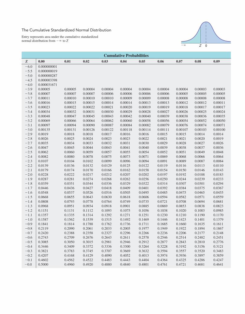
The Cumulative Standardized Normal Distribution
Entry represents area under the cumulative standardized normal distribution from - ∞ to Z
Cumulative ProbabilitiesZ 0.00 0.01 0.02 0.03 0.04 0.05 0.06 0.07 0.08 0.09
-6.0 0.000000001-5.5 0.000000019-5.0 0.000000287-4.5 0.000003398-4.0 0.000031671-3.9 0.00005 0.00005 0.00004 0.00004 0.00004 0.00004 0.00004 0.00004 0.00003 0.00003-3.8 0.00007 0.00007 0.00007 0.00006 0.00006 0.00006 0.00006 0.00005 0.00005 0.00005-3.7 0.00011 0.00010 0.00010 0.00010 0.00009 0.00009 0.00008 0.00008 0.00008 0.00008-3.6 0.00016 0.00015 0.00015 0.00014 0.00014 0.00013 0.00013 0.00012 0.00012 0.00011-3.5 0.00023 0.00022 0.00022 0.00021 0.00020 0.00019 0.00019 0.00018 0.00017 0.00017-3.4 0.00034 0.00032 0.00031 0.00030 0.00029 0.00028 0.00027 0.00026 0.00025 0.00024-3.3 0.00048 0.00047 0.00045 0.00043 0.00042 0.00040 0.00039 0.00038 0.00036 0.00035-3.2 0.00069 0.00066 0.00064 0.00062 0.00060 0.00058 0.00056 0.00054 0.00052 0.00050-3.1 0.00097 0.00094 0.00090 0.00087 0.00084 0.00082 0.00079 0.00076 0.00074 0.00071-3.0 0.00135 0.00131 0.00126 0.00122 0.00118 0.00114 0.00111 0.00107 0.00103 0.00100-2.9 0.0019 0.0018 0.0018 0.0017 0.0016 0.0016 0.0015 0.0015 0.0014 0.0014-2.8 0.0026 0.0025 0.0024 0.0023 0.0023 0.0022 0.0021 0.0021 0.0020 0.0019-2.7 0.0035 0.0034 0.0033 0.0032 0.0031 0.0030 0.0029 0.0028 0.0027 0.0026-2.6 0.0047 0.0045 0.0044 0.0043 0.0041 0.0040 0.0039 0.0038 0.0037 0.0036-2.5 0.0062 0.0060 0.0059 0.0057 0.0055 0.0054 0.0052 0.0051 0.0049 0.0048-2.4 0.0082 0.0080 0.0078 0.0075 0.0073 0.0071 0.0069 0.0068 0.0066 0.0064-2.3 0.0107 0.0104 0.0102 0.0099 0.0096 0.0094 0.0091 0.0089 0.0087 0.0084-2.2 0.0139 0.0136 0.0132 0.0129 0.0125 0.0122 0.0119 0.0116 0.0113 0.0110-2.1 0.0179 0.0174 0.0170 0.0166 0.0162 0.0158 0.0154 0.0150 0.0146 0.0143-2.0 0.0228 0.0222 0.0217 0.0212 0.0207 0.0202 0.0197 0.0192 0.0188 0.0183-1.9 0.0287 0.0281 0.0274 0.0268 0.0262 0.0256 0.0250 0.0244 0.0239 0.0233-1.8 0.0359 0.0351 0.0344 0.0336 0.0329 0.0322 0.0314 0.0307 0.0301 0.0294-1.7 0.0446 0.0436 0.0427 0.0418 0.0409 0.0401 0.0392 0.0384 0.0375 0.0367-1.6 0.0548 0.0537 0.0526 0.0516 0.0505 0.0495 0.0485 0.0475 0.0465 0.0455-1.5 0.0668 0.0655 0.0643 0.0630 0.0618 0.0606 0.0594 0.0582 0.0571 0.0559-1.4 0.0808 0.0793 0.0778 0.0764 0.0749 0.0735 0.0721 0.0708 0.0694 0.0681-1.3 0.0968 0.0951 0.0934 0.0918 0.0901 0.0885 0.0869 0.0853 0.0838 0.0823-1.2 0.1151 0.1131 0.1112 0.1093 0.1075 0.1056 0.1038 0.1020 0.1003 0.0985-1.1 0.1357 0.1335 0.1314 0.1292 0.1271 0.1251 0.1230 0.1210 0.1190 0.1170-1.0 0.1587 0.1562 0.1539 0.1515 0.1492 0.1469 0.1446 0.1423 0.1401 0.1379-0.9 0.1841 0.1814 0.1788 0.1762 0.1736 0.1711 0.1685 0.1660 0.1635 0.1611-0.8 0.2119 0.2090 0.2061 0.2033 0.2005 0.1977 0.1949 0.1922 0.1894 0.1867-0.7 0.2420 0.2388 0.2358 0.2327 0.2296 0.2266 0.2236 0.2206 0.2177 0.2148-0.6 0.2743 0.2709 0.2676 0.2643 0.2611 0.2578 0.2546 0.2514 0.2482 0.2451-0.5 0.3085 0.3050 0.3015 0.2981 0.2946 0.2912 0.2877 0.2843 0.2810 0.2776-0.4 0.3446 0.3409 0.3372 0.3336 0.3300 0.3264 0.3228 0.3192 0.3156 0.3121-0.3 0.3821 0.3783 0.3745 0.3707 0.3669 0.3632 0.3594 0.3557 0.3520 0.3483-0.2 0.4207 0.4168 0.4129 0.4090 0.4052 0.4013 0.3974 0.3936 0.3897 0.3859-0.1 0.4602 0.4562 0.4522 0.4483 0.4443 0.4404 0.4364 0.4325 0.4286 0.4247-0.0 0.5000 0.4960 0.4920 0.4880 0.4840 0.4801 0.4761 0.4721 0.4681 0.4641
0Z2`
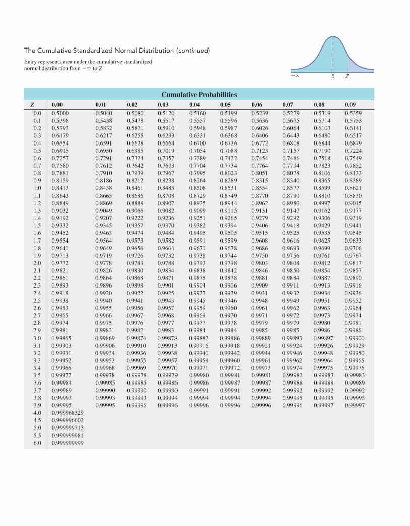
Cumulative ProbabilitiesZ 0.00 0.01 0.02 0.03 0.04 0.05 0.06 0.07 0.08 0.09
0.0 0.5000 0.5040 0.5080 0.5120 0.5160 0.5199 0.5239 0.5279 0.5319 0.53590.1 0.5398 0.5438 0.5478 0.5517 0.5557 0.5596 0.5636 0.5675 0.5714 0.57530.2 0.5793 0.5832 0.5871 0.5910 0.5948 0.5987 0.6026 0.6064 0.6103 0.61410.3 0.6179 0.6217 0.6255 0.6293 0.6331 0.6368 0.6406 0.6443 0.6480 0.65170.4 0.6554 0.6591 0.6628 0.6664 0.6700 0.6736 0.6772 0.6808 0.6844 0.68790.5 0.6915 0.6950 0.6985 0.7019 0.7054 0.7088 0.7123 0.7157 0.7190 0.72240.6 0.7257 0.7291 0.7324 0.7357 0.7389 0.7422 0.7454 0.7486 0.7518 0.75490.7 0.7580 0.7612 0.7642 0.7673 0.7704 0.7734 0.7764 0.7794 0.7823 0.78520.8 0.7881 0.7910 0.7939 0.7967 0.7995 0.8023 0.8051 0.8078 0.8106 0.81330.9 0.8159 0.8186 0.8212 0.8238 0.8264 0.8289 0.8315 0.8340 0.8365 0.83891.0 0.8413 0.8438 0.8461 0.8485 0.8508 0.8531 0.8554 0.8577 0.8599 0.86211.1 0.8643 0.8665 0.8686 0.8708 0.8729 0.8749 0.8770 0.8790 0.8810 0.88301.2 0.8849 0.8869 0.8888 0.8907 0.8925 0.8944 0.8962 0.8980 0.8997 0.90151.3 0.9032 0.9049 0.9066 0.9082 0.9099 0.9115 0.9131 0.9147 0.9162 0.91771.4 0.9192 0.9207 0.9222 0.9236 0.9251 0.9265 0.9279 0.9292 0.9306 0.93191.5 0.9332 0.9345 0.9357 0.9370 0.9382 0.9394 0.9406 0.9418 0.9429 0.94411.6 0.9452 0.9463 0.9474 0.9484 0.9495 0.9505 0.9515 0.9525 0.9535 0.95451.7 0.9554 0.9564 0.9573 0.9582 0.9591 0.9599 0.9608 0.9616 0.9625 0.96331.8 0.9641 0.9649 0.9656 0.9664 0.9671 0.9678 0.9686 0.9693 0.9699 0.97061.9 0.9713 0.9719 0.9726 0.9732 0.9738 0.9744 0.9750 0.9756 0.9761 0.97672.0 0.9772 0.9778 0.9783 0.9788 0.9793 0.9798 0.9803 0.9808 0.9812 0.98172.1 0.9821 0.9826 0.9830 0.9834 0.9838 0.9842 0.9846 0.9850 0.9854 0.98572.2 0.9861 0.9864 0.9868 0.9871 0.9875 0.9878 0.9881 0.9884 0.9887 0.98902.3 0.9893 0.9896 0.9898 0.9901 0.9904 0.9906 0.9909 0.9911 0.9913 0.99162.4 0.9918 0.9920 0.9922 0.9925 0.9927 0.9929 0.9931 0.9932 0.9934 0.99362.5 0.9938 0.9940 0.9941 0.9943 0.9945 0.9946 0.9948 0.9949 0.9951 0.99522.6 0.9953 0.9955 0.9956 0.9957 0.9959 0.9960 0.9961 0.9962 0.9963 0.99642.7 0.9965 0.9966 0.9967 0.9968 0.9969 0.9970 0.9971 0.9972 0.9973 0.99742.8 0.9974 0.9975 0.9976 0.9977 0.9977 0.9978 0.9979 0.9979 0.9980 0.99812.9 0.9981 0.9982 0.9982 0.9983 0.9984 0.9984 0.9985 0.9985 0.9986 0.99863.0 0.99865 0.99869 0.99874 0.99878 0.99882 0.99886 0.99889 0.99893 0.99897 0.999003.1 0.99903 0.99906 0.99910 0.99913 0.99916 0.99918 0.99921 0.99924 0.99926 0.999293.2 0.99931 0.99934 0.99936 0.99938 0.99940 0.99942 0.99944 0.99946 0.99948 0.999503.3 0.99952 0.99953 0.99955 0.99957 0.99958 0.99960 0.99961 0.99962 0.99964 0.999653.4 0.99966 0.99968 0.99969 0.99970 0.99971 0.99972 0.99973 0.99974 0.99975 0.999763.5 0.99977 0.99978 0.99978 0.99979 0.99980 0.99981 0.99981 0.99982 0.99983 0.999833.6 0.99984 0.99985 0.99985 0.99986 0.99986 0.99987 0.99987 0.99988 0.99988 0.999893.7 0.99989 0.99990 0.99990 0.99990 0.99991 0.99991 0.99992 0.99992 0.99992 0.999923.8 0.99993 0.99993 0.99993 0.99994 0.99994 0.99994 0.99994 0.99995 0.99995 0.999953.9 0.99995 0.99995 0.99996 0.99996 0.99996 0.99996 0.99996 0.99996 0.99997 0.999974.0 0.9999683294.5 0.9999966025.0 0.9999997135.5 0.9999999816.0 0.999999999
The Cumulative Standardized Normal Distribution (continued)
Entry represents area under the cumulative standardized normal distribution from - ∞ to Z
0 Z2`
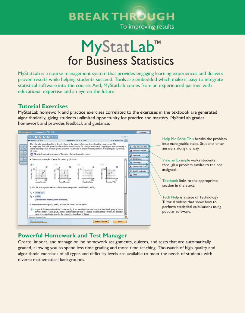
MyStatLab™
for Business StatisticsMyStatLab is a course management system that provides engaging learning experiences and delivers proven results while helping students succeed. Tools are embedded which make it easy to integrate statistical software into the course. And, MyStatLab comes from an experienced partner with educational expertise and an eye on the future.
Tutorial ExercisesMyStatLab homework and practice exercises correlated to the exercises in the textbook are generated algorithmically, giving students unlimited opportunity for practice and mastery. MyStatLab grades homework and provides feedback and guidance.
Powerful Homework and Test ManagerCreate, import, and manage online homework assignments, quizzes, and tests that are automatically graded, allowing you to spend less time grading and more time teaching. Thousands of high-quality and algorithmic exercises of all types and difficulty levels are available to meet the needs of students with diverse mathematical backgrounds.
Help Me Solve This breaks the problem into manageable steps. Students enter answers along the way.
View an Example walks students through a problem similar to the one assigned.
Textbook links to the appropriate section in the etext.
Tech Help is a suite of Technology Tutorial videos that show how to perform statistical calculations using popular software.
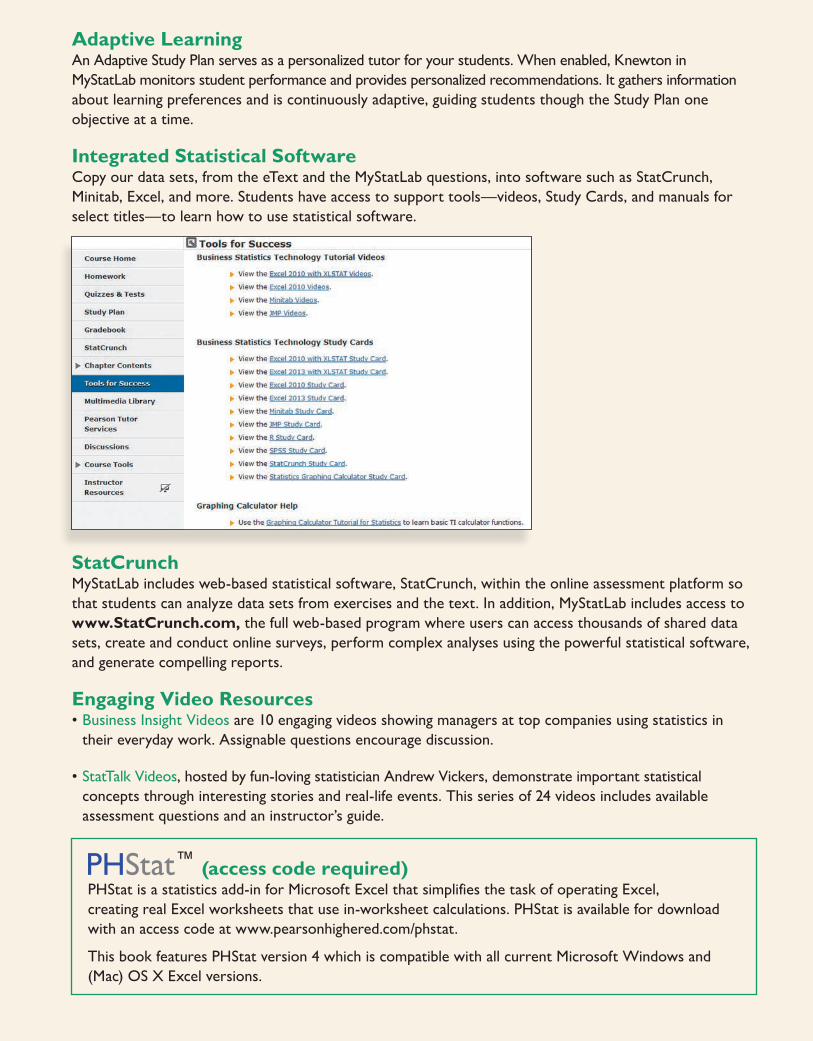
Adaptive LearningAn Adaptive Study Plan serves as a personalized tutor for your students. When enabled, Knewton in MyStatLab monitors student performance and provides personalized recommendations. It gathers information about learning preferences and is continuously adaptive, guiding students though the Study Plan one objective at a time.
Integrated Statistical SoftwareCopy our data sets, from the eText and the MyStatLab questions, into software such as StatCrunch, Minitab, Excel, and more. Students have access to support tools—videos, Study Cards, and manuals for select titles—to learn how to use statistical software.
StatCrunchMyStatLab includes web-based statistical software, StatCrunch, within the online assessment platform so that students can analyze data sets from exercises and the text. In addition, MyStatLab includes access to www.StatCrunch.com, the full web-based program where users can access thousands of shared data sets, create and conduct online surveys, perform complex analyses using the powerful statistical software, and generate compelling reports.
Engaging Video Resources• Business Insight Videos are 10 engaging videos showing managers at top companies using statistics in
their everyday work. Assignable questions encourage discussion.
•StatTalk Videos, hosted by fun-loving statistician Andrew Vickers, demonstrate important statistical concepts through interesting stories and real-life events. This series of 24 videos includes available assessment questions and an instructor’s guide.
PHStat™ (access code required)PHStat is a statistics add-in for Microsoft Excel that simplifies the task of operating Excel, creating real Excel worksheets that use in-worksheet calculations. PHStat is available for download with an access code at www.pearsonhighered.com/phstat.
This book features PHStat version 4 which is compatible with all current Microsoft Windows and (Mac) OS X Excel versions.

This page is intentionally left blank.

This page is intentionally left blank.

This page is intentionally left blank.
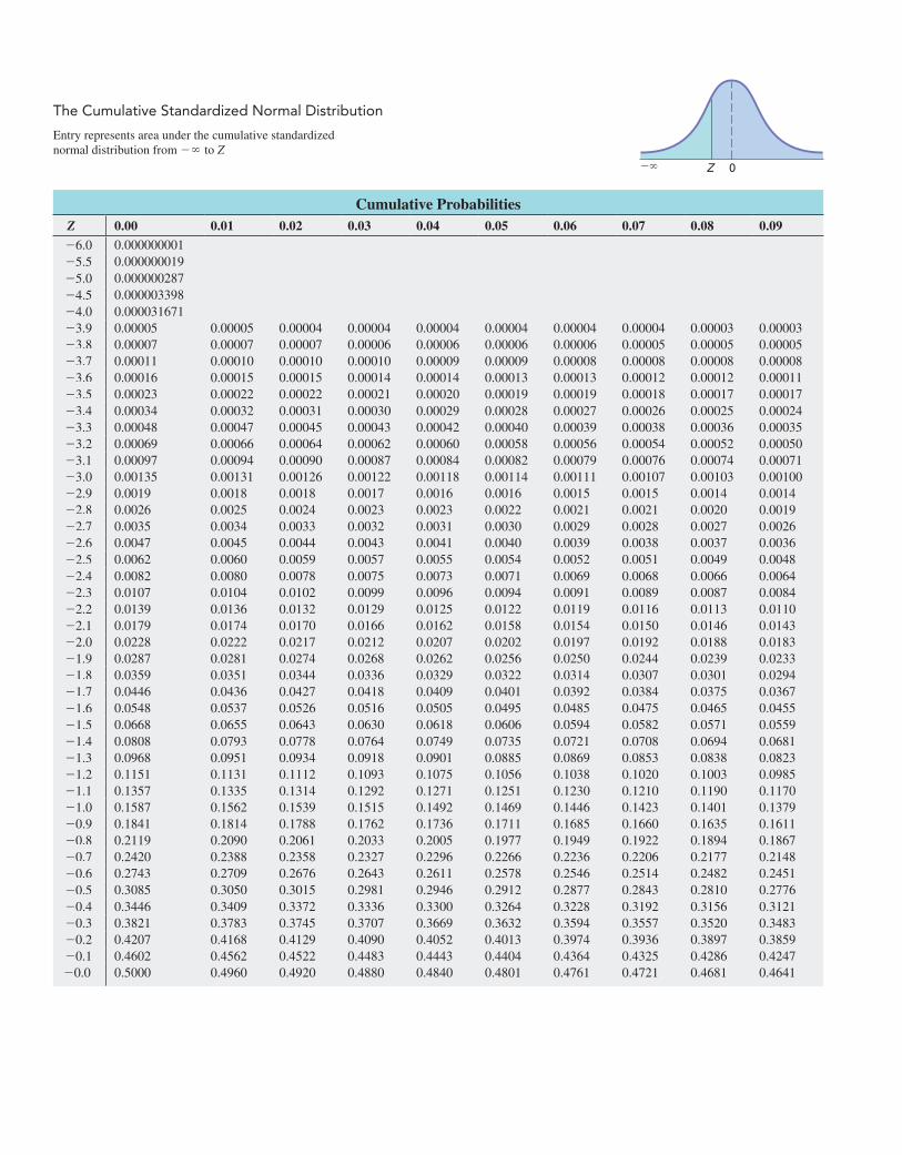
The Cumulative Standardized Normal Distribution
Entry represents area under the cumulative standardized normal distribution from - ∞ to Z
Cumulative ProbabilitiesZ 0.00 0.01 0.02 0.03 0.04 0.05 0.06 0.07 0.08 0.09
-6.0 0.000000001-5.5 0.000000019-5.0 0.000000287-4.5 0.000003398-4.0 0.000031671-3.9 0.00005 0.00005 0.00004 0.00004 0.00004 0.00004 0.00004 0.00004 0.00003 0.00003-3.8 0.00007 0.00007 0.00007 0.00006 0.00006 0.00006 0.00006 0.00005 0.00005 0.00005-3.7 0.00011 0.00010 0.00010 0.00010 0.00009 0.00009 0.00008 0.00008 0.00008 0.00008-3.6 0.00016 0.00015 0.00015 0.00014 0.00014 0.00013 0.00013 0.00012 0.00012 0.00011-3.5 0.00023 0.00022 0.00022 0.00021 0.00020 0.00019 0.00019 0.00018 0.00017 0.00017-3.4 0.00034 0.00032 0.00031 0.00030 0.00029 0.00028 0.00027 0.00026 0.00025 0.00024-3.3 0.00048 0.00047 0.00045 0.00043 0.00042 0.00040 0.00039 0.00038 0.00036 0.00035-3.2 0.00069 0.00066 0.00064 0.00062 0.00060 0.00058 0.00056 0.00054 0.00052 0.00050-3.1 0.00097 0.00094 0.00090 0.00087 0.00084 0.00082 0.00079 0.00076 0.00074 0.00071-3.0 0.00135 0.00131 0.00126 0.00122 0.00118 0.00114 0.00111 0.00107 0.00103 0.00100-2.9 0.0019 0.0018 0.0018 0.0017 0.0016 0.0016 0.0015 0.0015 0.0014 0.0014-2.8 0.0026 0.0025 0.0024 0.0023 0.0023 0.0022 0.0021 0.0021 0.0020 0.0019-2.7 0.0035 0.0034 0.0033 0.0032 0.0031 0.0030 0.0029 0.0028 0.0027 0.0026-2.6 0.0047 0.0045 0.0044 0.0043 0.0041 0.0040 0.0039 0.0038 0.0037 0.0036-2.5 0.0062 0.0060 0.0059 0.0057 0.0055 0.0054 0.0052 0.0051 0.0049 0.0048-2.4 0.0082 0.0080 0.0078 0.0075 0.0073 0.0071 0.0069 0.0068 0.0066 0.0064-2.3 0.0107 0.0104 0.0102 0.0099 0.0096 0.0094 0.0091 0.0089 0.0087 0.0084-2.2 0.0139 0.0136 0.0132 0.0129 0.0125 0.0122 0.0119 0.0116 0.0113 0.0110-2.1 0.0179 0.0174 0.0170 0.0166 0.0162 0.0158 0.0154 0.0150 0.0146 0.0143-2.0 0.0228 0.0222 0.0217 0.0212 0.0207 0.0202 0.0197 0.0192 0.0188 0.0183-1.9 0.0287 0.0281 0.0274 0.0268 0.0262 0.0256 0.0250 0.0244 0.0239 0.0233-1.8 0.0359 0.0351 0.0344 0.0336 0.0329 0.0322 0.0314 0.0307 0.0301 0.0294-1.7 0.0446 0.0436 0.0427 0.0418 0.0409 0.0401 0.0392 0.0384 0.0375 0.0367-1.6 0.0548 0.0537 0.0526 0.0516 0.0505 0.0495 0.0485 0.0475 0.0465 0.0455-1.5 0.0668 0.0655 0.0643 0.0630 0.0618 0.0606 0.0594 0.0582 0.0571 0.0559-1.4 0.0808 0.0793 0.0778 0.0764 0.0749 0.0735 0.0721 0.0708 0.0694 0.0681-1.3 0.0968 0.0951 0.0934 0.0918 0.0901 0.0885 0.0869 0.0853 0.0838 0.0823-1.2 0.1151 0.1131 0.1112 0.1093 0.1075 0.1056 0.1038 0.1020 0.1003 0.0985-1.1 0.1357 0.1335 0.1314 0.1292 0.1271 0.1251 0.1230 0.1210 0.1190 0.1170-1.0 0.1587 0.1562 0.1539 0.1515 0.1492 0.1469 0.1446 0.1423 0.1401 0.1379-0.9 0.1841 0.1814 0.1788 0.1762 0.1736 0.1711 0.1685 0.1660 0.1635 0.1611-0.8 0.2119 0.2090 0.2061 0.2033 0.2005 0.1977 0.1949 0.1922 0.1894 0.1867-0.7 0.2420 0.2388 0.2358 0.2327 0.2296 0.2266 0.2236 0.2206 0.2177 0.2148-0.6 0.2743 0.2709 0.2676 0.2643 0.2611 0.2578 0.2546 0.2514 0.2482 0.2451-0.5 0.3085 0.3050 0.3015 0.2981 0.2946 0.2912 0.2877 0.2843 0.2810 0.2776-0.4 0.3446 0.3409 0.3372 0.3336 0.3300 0.3264 0.3228 0.3192 0.3156 0.3121-0.3 0.3821 0.3783 0.3745 0.3707 0.3669 0.3632 0.3594 0.3557 0.3520 0.3483-0.2 0.4207 0.4168 0.4129 0.4090 0.4052 0.4013 0.3974 0.3936 0.3897 0.3859-0.1 0.4602 0.4562 0.4522 0.4483 0.4443 0.4404 0.4364 0.4325 0.4286 0.4247-0.0 0.5000 0.4960 0.4920 0.4880 0.4840 0.4801 0.4761 0.4721 0.4681 0.4641
0Z2`
Related Documents