BUS 220: ELEMENTARY STATISTICS Chapter 4: Numerical Measures.

BUS 220:ELEMENTARY STATISTICS

Chapter 4: Numerical Measures

GOALS

1. Develop and interpret a dot plot and stem-and-leaf display.

2. Compute and understand other measures of dispersion including quartiles, deciles, and percentiles.

3. Construct and interpret a box plot.

GOALS…

4. Compute and understand coefficient of skewness.

5. Draw and interpret a scatter diagram to describe a relationship between two variables.

6. Construct and interpret a contingency table.

7. Use Excel and MegaStat descriptive statistics to perform the above..

Dot Plots

A dot plot groups the data as little as possible and the identity of an individual observation is not lost.

To develop a dot plot, each observation is simply displayed as a dot along a horizontal number line indicating the possible values of the data.

Dot Plots…

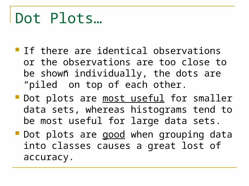
If there are identical observations or the observations are too close to be shown individually, the dots are “piled” on top of each other.

Dot plots are most useful for smaller data sets, whereas histograms tend to be most useful for large data sets.

Dot plots are good when grouping data into classes causes a great lost of accuracy.

Dot Plots - ExamplesBelow are the number of vehicles sold in the last 24

months at Smith Ford Mercury Jeep, Inc., in Kane, Pennsylvania, Construct dot plots and report summary statistics for the small-town Auto USA lot.

Dot Plot – MegaStat Example

Dot Plot – MegaStat Example

Dot Plot – MegaStat Example

10

Dot Plots - ExamplesReported below are the number of vehicles sold in the last

24 months at Smith Ford Mercury Jeep, Inc., in Kane, Pennsylvania, and Brophy Honda Volkswagen in Greenville, Ohio. Construct dot plots and report summary statistics for the two small-town Auto USA lots.

11

Dot Plot – Minitab Example

Stem and leaf display

Stem and leaf display…

The standard deviation is the most widely used measure of dispersion.

Alternative ways of describing spread of data include determining the location of values that divide a set of observations into equal parts.

These measures include quartiles, deciles, and percentiles.

Other Measures of Dispersion: Quartiles, Deciles and Percentiles

Let Lp refer to the location of a desired percentile. If we wanted to find the 33rd percentile we would use L33 and if we wanted the median, the 50th percentile, then L50.

The number of observations is n. To locate the median, its position is at (n + 1)/2. We could write this as (n + 1)(P/100), where P is the desired percentile.

Percentile Computation

Percentiles - Example

Listed below are the commissions earned last month by a sample of 15 brokers at Salomon Smith Barney’s Oakland, California, office. Salomon Smith Barney is an investment company with offices located throughout the United States.

$2,038 $1,758 $1,721 $1,637 $2,097 $2,047 $2,205 $1,787 $2,287 $1,940 $2,311 $2,054 $2,406 $1,471 $1,460

Locate the median, the first quartile, and the third quartile for the commissions earned.

Percentiles – Example (cont.)

Step 1: Organize the data from lowest to largest value

$1,460 $1,471 $1,637 $1,721

$1,758 $1,787 $1,940 $2,038

$2,047 $2,054 $2,097 $2,205

$2,287 $2,311 $2,406

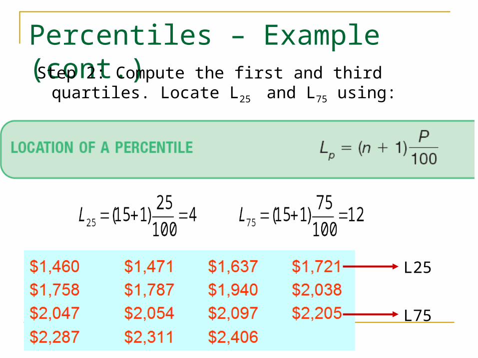
Percentiles – Example (cont.)Step 2: Compute the first and third quartiles.

Locate L25 and L75 using:

L25

L75

Percentiles – Example (MegaStat)

Percentiles – Example (MegaStat)

Q1 and Q3

Percentiles – Example (Excel)

Watch Screencam on the CD-ROM

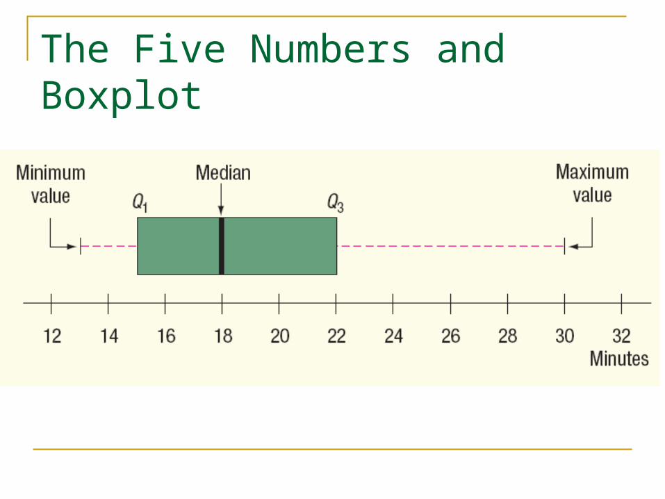
The Five Numbers and Boxplot

Boxplot Example

Boxplot – Using MegaStat

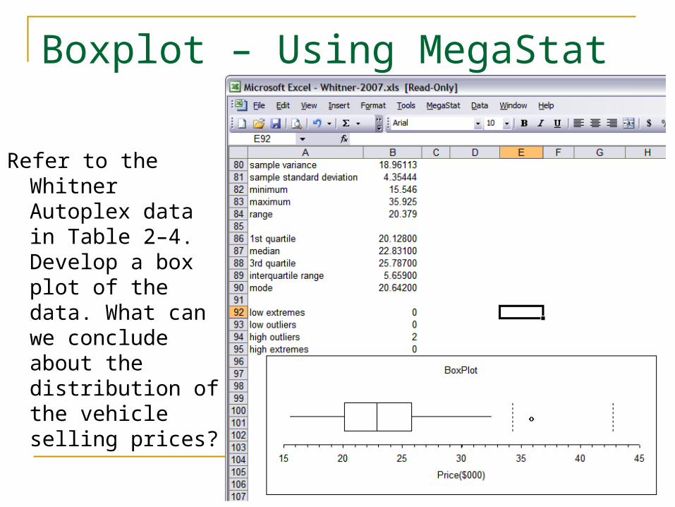
Refer to the Whitner Autoplex data in Table 2–4. Develop a box plot of the data. What can we conclude about the distribution of the vehicle selling prices?

Skewness

Another characteristic of a set of data is the shape.

There are four shapes commonly observed:

1. symmetric,

2. positively skewed,

3. negatively skewed,

4. bimodal.

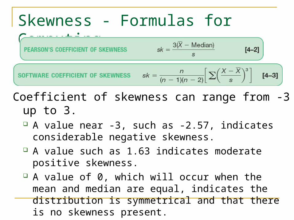
Skewness - Formulas for Computing

Coefficient of skewness can range from -3 up to 3. A value near -3, such as -2.57, indicates considerable

negative skewness. A value such as 1.63 indicates moderate positive

skewness. A value of 0, which will occur when the mean and

median are equal, indicates the distribution is symmetrical and that there is no skewness present.

Commonly Observed Shapes

Skewness – An ExampleFollowing are the earnings per share for a sample of

15 software companies for the year 2005. The earnings per share are arranged from smallest to largest.

Compute the mean, median, and standard deviation. Find the coefficient of skewness using Pearson’s estimate. What is your conclusion regarding the shape of the distribution?

Skewness – An Example Using Pearson’s Coefficient

22.5$

115

))95.4$40.16($...)95.4$09.0($

1

deviation standard sample theCompute :2 Step

222

n

XXs

95.4$15

26.74$

mean sample theCompute :1 Step

n

XX

017.122.5$

)18.3$95.4($3)(3

Skewness theCompute :4 Step

s

MedianXsk

$3.18. is shareper

earningsmedian theso $3.18, is valuemiddle thecase In this largest. osmallest t

from arranged data, ofset ain valuemiddle the-median theDetermine :3 Step

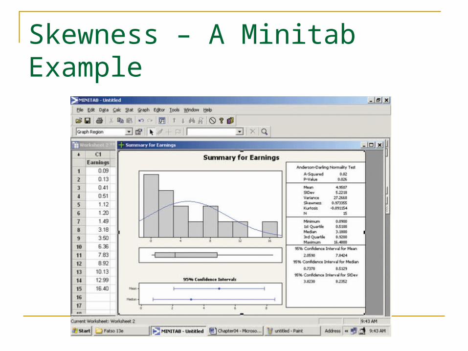
Skewness – A Minitab Example

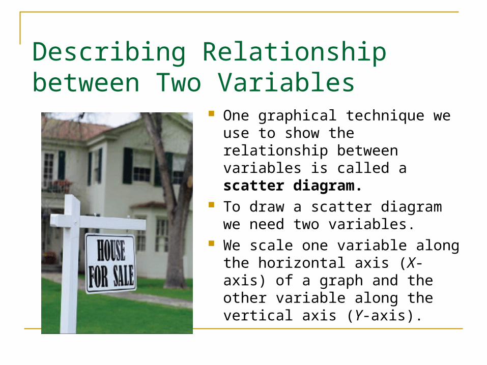
Describing Relationship between Two Variables

One graphical technique we use to show the relationship between variables is called a scatter diagram.

To draw a scatter diagram we need two variables.

We scale one variable along the horizontal axis (X-axis) of a graph and the other variable along the vertical axis (Y-axis).

Describing Relationship between Two Variables – Scatter Diagram Examples

In the Introduction to Chapter 2 we presented data from AutoUSA. In this case the information concerned the prices of 80 vehicles sold last month at the Whitner Autoplex lot in Raytown, Missouri. The data shown include the selling price of the vehicle as well as the age of the purchaser.

Is there a relationship between the selling price of a vehicle and the age of the purchaser? Would it be reasonable to conclude that the more expensive vehicles are purchased by older buyers?

Describing Relationship between Two Variables – Scatter Diagram Excel Example

Describing Relationship between Two Variables – Scatter Diagram Excel Example

Contingency Tables

A scatter diagram requires that both of the variables be at least interval scale.

What if we wish to study the relationship between two variables when one or both are nominal or ordinal scale? In this case we tally the results in a contingency table.

Contingency Tables – An ExampleA manufacturer of preassembled windows produced 50

windows yesterday. This morning the quality assurance inspector reviewed each window for all quality aspects. Each was classified as acceptable or unacceptable and by the shift on which it was produced. The two variables are shift and quality. The results are reported in the following table.

Contingency Tables – An ExampleUsefulness of the Contingency Table:By organizing the information into a contingency

table we can compare the quality on the three shifts.

For example, on the day shift, 3 out of 20 windows or 15 percent are defective. On the afternoon shift, 2 of 15 or 13 percent are defective and on the night shift 1 out of 15 or 7 percent are defective.

Overall 12 percent of the windows are defective. Observe also that 40 percent of the windows are produced on the day shift, found by (20/50)(100).