BUILDING A PREDICTIVE MODEL Correlation: ... 16 latent factors synthetic e-commerce data set

BUILDING A PREDICTIVE MODEL AN EXAMPLE OF A PRODUCT RECOMMENDATION ENGINE

Alex Lin Senior Architect Intelligent Mining [email protected]

Outline  Predictive modeling methodology  k-Nearest Neighbor (kNN) algorithm  Singular value decomposition (SVD)

method for dimensionality reduction  Using a synthetic data set to test and

improve your model  Experiment and results

2

The Business Problem  Design product recommender solution that will

increase revenue.

$$ 3

How Do We Increase Revenue?

Increase Revenue

Increase Conversion

Increase Avg. Order Value

Increase Unit Price

Increase Units / Order

4

Example  Is this recommendation effective?

Increase Unit Price

Increase Units / Order

Increase Units / Order

5

What am I going to do?

6

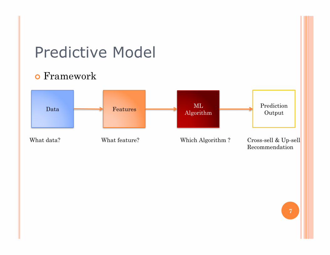
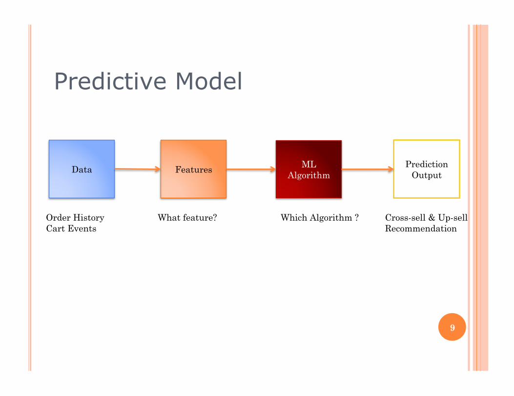
Predictive Model  Framework

Data Features ML Algorithm

Prediction Output

What data? What feature? Which Algorithm ? Cross-sell & Up-sell Recommendation

7

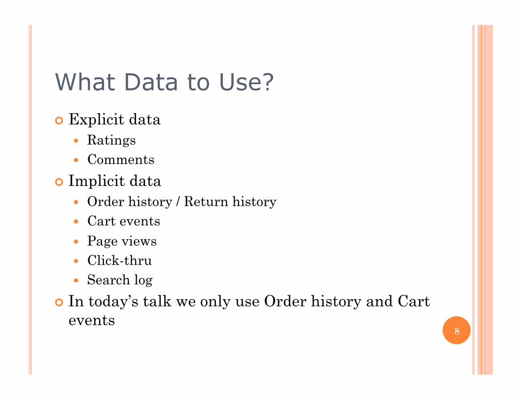
What Data to Use?  Explicit data

  Ratings   Comments

  Implicit data   Order history / Return history   Cart events   Page views   Click-thru   Search log

  In today’s talk we only use Order history and Cart events

8

Predictive Model

Data Features ML Algorithm

Prediction Output

Order History Cart Events

Cross-sell & Up-sell Recommendation

Which Algorithm ? What feature?

9

user engagement vector

What Features to Use?  We know that a given product tends to get

purchased by customers with similar tastes or needs.

 Use user engagement data to describe a product.

n … 10 9 8 7 6 5 4 3 2 1

.25 1 .25 .25 1 17

item

users

10

Data Representation / Features  When we merge every item’s user engagement

vector, we got a m x n item-user matrix

n … 10 9 8 7 6 5 4 3 2 1

.25 1 .25 1 1

.25 2

1 .25 1 3

1 .25 1 .25 4

1 1

…

m

users

items

11

Data Normalization  Ensure the magnitudes of the entries in the

dataset matrix are appropriate

n … 10 9 8 7 6 5 4 3 2 1

1 1 1 1 1

1 2

1 1 1 3

1 1 1 1 4

1 1

…

m

users

items

n … 10 9 8 7 6 5 4 3 2 1

.49 .92 .9 .5 1

.79 2

.73 .46 .67 3

.69 .76 .82 .39 4

.8 .52

…

m

 Remove column average – so frequent buyers don’t dominate the model 12

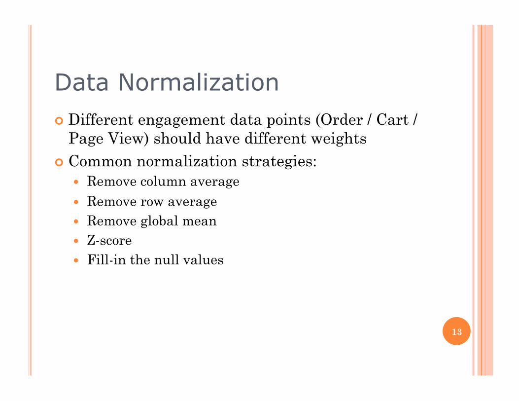
Data Normalization  Different engagement data points (Order / Cart /

Page View) should have different weights  Common normalization strategies:

  Remove column average   Remove row average   Remove global mean   Z-score   Fill-in the null values

13

Predictive Model

Data Features ML Algorithm

Prediction Output

Order History Cart Events

User engagement vector

Data Normalization

Cross-sell & Up-sell Recommendation

Which Algorithm ?

14

Which Algorithm?  How do we find the items that have similar user

engagement data?

n … 10 9 8 7 6 5 4 3 2 1

1 1 .25 1 1

1 2

.25 .25 1 1 1 17

1 1 1 .25 1 18

1 .25

…

m

users

items

 We can find the items that have similar user engagement vectors with kNN algorithm 15

k-Nearest Neighbor (kNN)  Find the k items that have the most similar user

engagement vectors

n … 10 9 8 7 6 5 4 3 2 1

1 1 1 .5 1

1 .5 1 2 1 1 1 1 3

1 1 .5 1 4 1 .5

…

.5 1 m

users

items

 Nearest Neighbors of Item 4 = [2,3,1] 16

Similarity Measure for kNN

  Jaccard coefficient:

n … 10 9 8 7 6 5 4 3 2 1

1 .5 1 2 1 1 .5 1 4

users

items

€

sim(a,b) = cos(a,b) =a•b

a2∗ b

2

=(1*1+ 0.5*1)

(12 + 0.52 +12)* (12 + 0.52 +12 +12)

  Pearson Correlation:

  Cosine similarity:

€

sim(a,b) =(1+1)

(1+1+1) + (1+1+1+1) − (1+1)

€

corr(a,b) =(rai − ra )(rbi − rb )i∑

(rai − ra )2

i∑ (rbi − rb )

2

i∑

=m aibi∑ − ai∑ bi∑

m ai2 − ( ai∑ )2∑ m bi

2 − ( bi∑ )2∑

=match _cols*Dotprod(a,b) − sum(a) * sum(b)

match _cols* sum(a2) − (sum(a))2 match _cols* sum(b2) − (sum(b))2

17

k-Nearest Neighbor (kNN)

8

9

2

6

1

3

4

7

5

Item

Similarity Measure (cosine similarity)

kNN k=5 Nearest Neighbors(8) = [9,6,3,1,2]

feature space

18

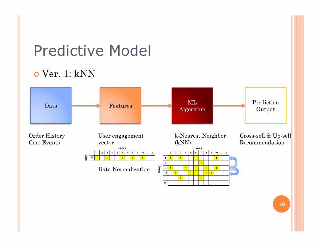
Predictive Model  Ver. 1: kNN

Data Features ML Algorithm

Prediction Output

Order History Cart Events

User engagement vector

Data Normalization

k-Nearest Neighbor (kNN)

Cross-sell & Up-sell Recommendation

19

Cosine Similarity – Code fragment long i_cnt = 100000; // number of items 100K long u_cnt = 2000000; // number of users 2M double data[i_cnt][u_cnt]; // 100K by 2M dataset matrix (in reality, it needs to be malloc allocation) double norm[i_cnt];

// assume data matrix is loaded …… // calculate vector norm for each user engagement vector for (i=0; i<i_cnt; i++) { norm[i] = 0; for (f=0; f<u_cnt; f++) { norm[i] += data[i][f] * data [i][f]; } norm[i] = sqrt(norm[i]); }

// cosine similarity calculation for (i=0; i<i_cnt; i++) { // loop thru 100K for (j=0; j<i_cnt; j++) { // loop thru 100K dot_product = 0; for (f=0; f<u_cnt; f++) { // loop thru entire user space 2M dot_product += data[i][f] * data[j][f]; } printf(“%d %d %lf\n”, i, j, dot_product/(norm[i] * norm[j])); }

// find the Top K nearest neighbors here …….

1. 100K rows x 100K rows x 2M features --> scalability problem kd-tree, Locality sensitive hashing, MapReduce/Hadoop, Multicore/Threading, Stream Processors

2. data[i] is high-dimensional and sparse, similarity measures are not reliable --> accuracy problem

This leads us to The SVD dimensionality reduction !

20

Singular Value Decomposition (SVD)

items

users

  Low rank approx. Item profile is

  Low rank approx. User profile is

  Low rank approx. Item-User matrix is €

Uk * Sk

€

S k *VkT

€

Uk * Sk * Sk *VkT€

Ak =Uk × Sk ×VkT

€

A =U × S ×VT

A m x n matrix

users

items

VT r x n matrix

U m x r matrix

S r x r matrix

items

users

rank = k k < r

21

Reduced SVD

Ak 100K x 2M matrix

users

items

VkT

3 x 2M matrix Uk

100K x 3 matrix

7 0 0

0 3 0

0 0 1

Sk 3 x 3 matrix

rank = 3

items

users

  Low rank approx. Item profile is

€

Uk * Sk

€

Ak =Uk × Sk ×VkT

Descending Singular Values

22

SVD Factor Interpretation  Singular values plot (rank=512)

S 3 x 3 matrix

7 0 0

0 3 0

0 0 1

Noises + Others Latent Factors More Significant Less Significant

Descending Singular Values

23

SVD Dimensionality Reduction

3

10

rank Need to find the most optimal low rank !!

<----- latent factors ----->

items

# of users

€

Uk * Sk

24

Missing values

  Difference between “0” and “unknown”   Missing values do NOT appear randomly.   Value = (Preference Factors) + (Availability) – (Purchased

elsewhere) – (Navigation inefficiency) – etc.   Approx. Value = (Preference Factors) +/- (Noise)   Modeling missing values correctly will help us make good

recommendations, especially when working with an extremely sparse data set

25

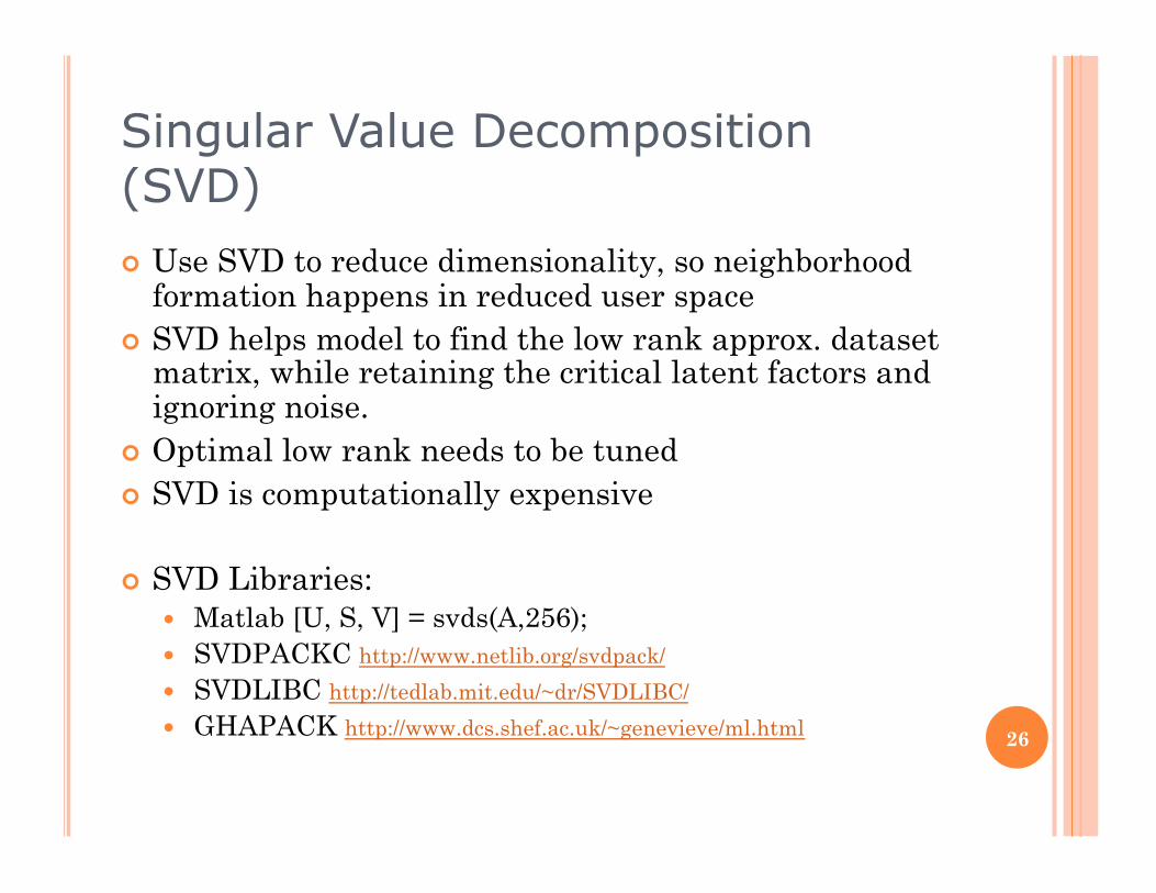
Singular Value Decomposition (SVD)   Use SVD to reduce dimensionality, so neighborhood

formation happens in reduced user space   SVD helps model to find the low rank approx. dataset

matrix, while retaining the critical latent factors and ignoring noise.

  Optimal low rank needs to be tuned   SVD is computationally expensive

  SVD Libraries:   Matlab [U, S, V] = svds(A,256);   SVDPACKC http://www.netlib.org/svdpack/

  SVDLIBC http://tedlab.mit.edu/~dr/SVDLIBC/

  GHAPACK http://www.dcs.shef.ac.uk/~genevieve/ml.html 26

Predictive Model  Ver. 2: SVD+kNN

Data Features ML Algorithm

Prediction Output

Order History Cart Events

Cross-sell & Up-sell Recommendation

User engagement vector

Data Normalization

SVD

k-Nearest Neighbors (kNN) in reduced space

27

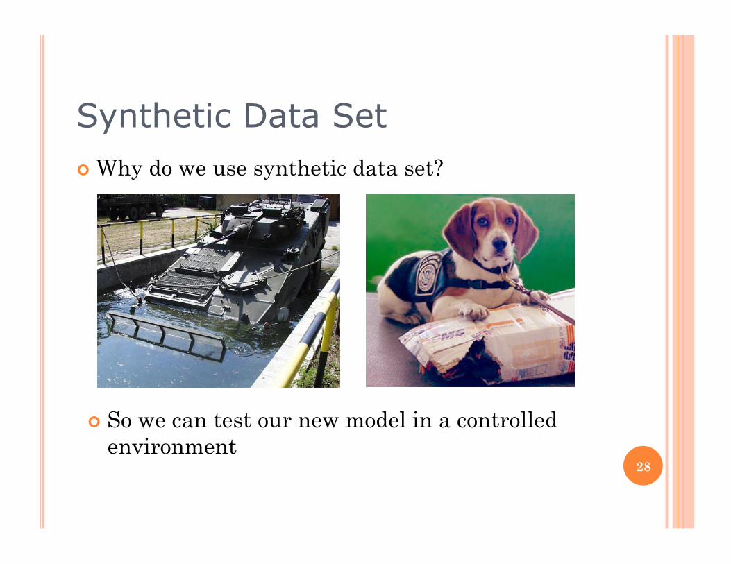
Synthetic Data Set  Why do we use synthetic data set?

 So we can test our new model in a controlled environment

28

Synthetic Data Set  16 latent factors synthetic e-commerce

data set   Dimension: 1,000 (items) by 20,000 (users)   16 user preference factors   16 item property factors (non-negative)   Txn Set: n = 55,360 sparsity = 99.72 %   Txn+Cart Set: n = 192,985 sparsity = 99.03%   Download: http://www.IntelligentMining.com/dataset/

user_id item_id type 10 42 0.25 10 997 0.25 10 950 0.25 11 836 0.25 11 225 1

29

Synthetic Data Set

a b c

x

y

z

User preference factors

16 x 20K matrix

X32 = (a, b, c) . (x, y, z) = a * x + b * y + c * z

X32 = Likelihood of Item 3 being purchased by User 2

Item property factors

1K x 16 matrix X11 X12 X13 X14 X15 X16

X21 X22 X12 X24 X25 X26

X31 X32 X33 X34 X35 X36

X41 X42 X43 X44 X45 X46

X51 X52 X53 X54 X55 X56

Purchase Likelihood score 1K x 20K matrix

items

users

30

Synthetic Data Set

  User 1 purchased Item 4 and Item 1

X11

X21

X31

X41

X51

X31

X41

X21

X51

X11

X51

X41

X31

X21

X11

Sort by Purchase likelihood Score

From the top, select and skip certain items to create data sparsity.

Based on the distribution, pre-determine # of items purchased by an user (# of item=2)

31

Experiment Setup  Each model (Random / kNN / SVD+kNN) will

generate top 20 recommendations for each item.  Compare model output to the actual top 20

provided by synthetic data set  Evaluation Metrics :

  Precision %: Overlapping of the top 20 between model output and actual (higher the better)

Precision

  Quality metric: Average of the actual ranking in the model output (lower the better) €

={Found _Top20_ items}∩{Actual_Top20_ items}

{Found _Top20_ items}

1 2 30 47 50 21 1 2 368 62 900 510

32

Experimental Result   kNN vs. Random (Control)

Precision % (higher is better)

Quality (Lower is better)

33

Experimental Result  Precision % of SVD+kNN

SVD Rank

Recall % (higher is better)

Improvement

34

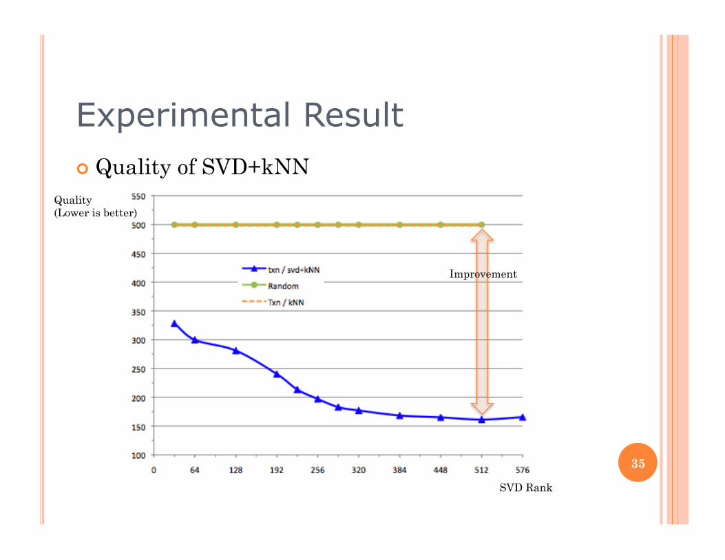
Experimental Result  Quality of SVD+kNN

SVD Rank

Improvement

Quality (Lower is better)

35

Experimental Result  The effect of using Cart data

SVD Rank

Precision % (higher is better)

36

Experimental Result  The effect of using Cart data Quality (Lower is better)

SVD Rank 37

Outline  Predictive modeling methodology  k-Nearest Neighbor (kNN) algorithm  Singular value decomposition (SVD)

method for dimensionality reduction  Using a synthetic data set to test and

improve your model  Experiment and results

38

References   J.S. Breese, D. Heckerman and C. Kadie, "Empirical Analysis of

Predictive Algorithms for Collaborative Filtering," in Proceedings of the Fourteenth Conference on Uncertainity in Artificial Intelligence (UAI 1998), 1998.

  B. Sarwar, G. Karypis, J. Konstan and J. Riedl, "Item-based collaborative filtering recommendation algorithms," in Proceedings of the Tenth International Conference on the World Wide Web (WWW 10), pp. 285-295, 2001.

  B. Sarwar, G. Karypis, J. Konstan, and J. Riedl "Application of Dimensionality Reduction in Recommender System A Case Study" In ACM WebKDD 2000 Web Mining for E-Commerce Workshop

  Apache Lucene Mahout http://lucene.apache.org/mahout/

  Cofi: A Java-Based Collaborative Filtering Library http://www.nongnu.org/cofi/

39

Thank you  Any question or comment?

40