BUDGETARY POLICY MODELLING Public Budget Policy has been traditionally considered as a means for conveying macroeconomic policy, seeking a variety of social and economic objectives. As modern economies face, in the 1990s, a challenging bundle of problems, public policy is of growing importance. This volume contains ten scientific papers presented at the Applied Econometrics Association (AEA) Conference on 'Public Budget Modelling', held in Athens in April 1993. The focus is on the European context of public budget policy and a variety of different approaches are used - theoretical modelling, econometrics and applied general equilibrium modelling. Empirical evidence and case studies of European countries are contained in all the papers. The papers cover the four general themes of public budget policy: • For economic stabilization, in view of the Economic and Monetary Union in the European Community. • To reinforce structural change, involved in market liberalization and harmonization of economic structures. • With respect to its distributional effects and implications for social equity. • To enable endogenous economic growth. Professor Pantelis Capros teaches economics and operations research at the National Technical University of Athens. He has fifteen years of experience in the field of applied economic, energy and environmental modelling and policy analysis and has been involved in the construction of large-scale applied economic models for the European Union. Professor Daniele Meulders holds a chair in Public Finance at the Free University of Brussels and supervises the research team on Labour Economics of the Department of Applied Economics.

Welcome message from author
This document is posted to help you gain knowledge. Please leave a comment to let me know what you think about it! Share it to your friends and learn new things together.
Transcript
BUDGETARY POLICY MODELLING
Public Budget Policy has been traditionally considered as a means for conveying macroeconomic policy, seeking a variety of social and economic objectives. As modern economies face, in the 1990s, a challenging bundle of problems, public policy is of growing importance.
This volume contains ten scientific papers presented at the Applied Econometrics Association (AEA) Conference on 'Public Budget Modelling', held in Athens in April 1993.
The focus is on the European context of public budget policy and a variety of different approaches are used - theoretical modelling, econometrics and applied general equilibrium modelling. Empirical evidence and case studies of European countries are contained in all the papers.
The papers cover the four general themes of public budget policy:
• For economic stabilization, in view of the Economic and Monetary Union in the European Community.
• To reinforce structural change, involved in market liberalization and harmonization of economic structures.
• With respect to its distributional effects and implications for social equity.
• To enable endogenous economic growth.
Professor Pantelis Capros teaches economics and operations research at the National Technical University of Athens. He has fifteen years of experience in the field of applied economic, energy and environmental modelling and policy analysis and has been involved in the construction of large-scale applied economic models for the European Union. Professor Daniele Meulders holds a chair in Public Finance at the Free University of Brussels and supervises the research team on Labour Economics of the Department of Applied Economics.
ROUTLEDGE NEW INTERNATIONAL STUDIES IN ECONOMIC MODELLING
Series Editor H M Scobie
MODELS FOR ENERGY POLICY Edited by Jean Baptiste Lesourd, Jacques Percebois and Franfois Valette
BUDGETARY POLICY MODELLING Public Expenditures
Edited by Pante/is Capros and Daniele Meulders
ECONOMIC MODELLING AT THE BANQUE DE FRANCE Financial Deregulation and Economic Performance in France
Edited by Michel Boutillier and Jean Cordier

BUDGETARY POLICY MODELLING
Public expenditures
Edited by Pantelis Capros and Daniele Meulders

First published 1997 by Routledge
Published 2017 by Routledge 2 Park Square, Milton Park, Abingdon, Oxon OX14 4RN
711 Third Avenue, New York, NY 10017, USA
Routledge is an imprint of the Taylor & Francis Group, an informa business
Copyright © 1997 Applied Economics Association Copyright © 1997 Editorial matter in selection in the name of the editors; individual contributions in the name of the contributors
Typeset in Garamond by Florencetype Ltd, Stoodleigh, Devon
The Open Access version of this book, available at www.tandfebooks.com, has been made available under a Creative Commons Attribution-Non
Commercial-No Derivatives 4.0 license.
British Library Cataloguing in Publication Data A catalogue record for this book is available from the British Library
Library of Congress Cataloging in Publication Data Budgetary policy modelling: public expenditures I edited by Pantelis
Capros and Daniele Meulders. p. cm. - (Routledge new international studies in economic modelling)
Includes bibliographical references and index. 1. Expenditures, Public - European Union countries - Econometric
models - Congresses. 2. Budget - European Union countries -Econometric models - Congresses. 3. Government spending policy -
European Union countries - Econometric models - Congresses. I. Capros, Pantelis. II. Meulders, Daniele. Ill. Applied
Econometric Association. Conference on 'Public Budget Modelling' (1993: Athens, Greece). IV. Series.
HJ7755.B83 1996 350.72'221'094 - dc20 96-7319
CIP
ISBN 978-0-415-14235-9 (hbk)

To our colleague and dear friend Nikitas Deimezis


List of figures List of tables List of contributors
CONTENTS
INTRODUCTION Pante/is Capros and Daniele Meulders
Part I Theoretical aspects
1 PUBLIC EXPENDITURES, TAXES, DEBT AND
ix xi
XIV
1
ENDOGENOUS GROWTH 9 Patrick Artus
2 ENDOGENOUS GROWTH AND BUDGETARY POLICY IN THE OPEN ECONOMY 29 Aristomene A. Varoudakis
Part II Public deficits and stabilization
3 PROPOSALS FOR COMMUNITY STABILIZATION MECHANISMS: SOME HISTORICAL APPLICATIONS 51 Alexander Italianer and Marc Vanheukelen
4 SOME STOCHASTIC IMPLICATIONS OF THE GOVERNMENT'S BUDGET CONSTRAINT: AN EMPIRICAL ANALYSIS 78 Guglielmo Maria Caporale
5 CREDIT CONSTRAINTS AND THE EFFICIENCY OF BUDGETARY POLICY: THE PORTUGUESE CASE, 1958-88 102 Maria Dolores Nunes Cabral
vu

CONTENTS
6 STRUCTURAL ADJUSTMENT AND PUBLIC DEFICIT: A CGE MODELLING ANALYSIS FOR GREECE 122 Pante/is Capros and Pavlos Karadeloglou
7 PUBLIC DEFICITS AND INCOME DISTRIBUTION: RESULTS OF AN ECONOMETRIC BUSINESS CYCLE MODEL FOR THE FEDERAL REPUBLIC OF GERMANY 161 Rudolf Zwiener
Part III Structure of public expenditures and implications
8 PUBLIC SPENDING IN FEDERAL STATES: A COMPARATIVE ECONOMETRIC STUDY 179 Gebhard Kirchgiissner and Werner W. Pommerehne
9 CAUSALITY BETWEEN PUBLIC EXPENDITURE AND TAXATION: EVIDENCE FROM THE ITALIAN CASE 214 Mariano Bella and Beniamino Quintieri
10 ON THE EFFICACY, EFFICIENCY AND EQUITY OF STATE SUPPORT IN BRITAIN 235 ] ean-Yves Duclos
Index 262
Vlll

FIGURES
2.1 Long-run equilibria of endogenous growth 39 2.2 Long-run effects of budgetary policies 42 3.1 The stabilization element in the German Finanzausgleich 57 3.2 Transfer payments with full and limited stabilization
scheme (% of GDP) 64 3.3 Degree of stabilization with full and limited stabilization
scheme (as % of shock to GDP) 65 4.1 Equation 4.19 - France 92 4.2 Equation 4.19 - France 92 4.3 Equation 4.19 - Germany 93 4.4 Equation 4.19 - Germany 94 4.5 Equation 4.19 - Italy 95 4.6 Equation 4.19 - Italy 95 4.7 Equation 4.19 - UK 97 4.8 Equation 4.19 - UK 97 5.1 GDP (actual, fitted and residual) 111 5.2 Personal consumption (actual, fitted and residual) 112 5.3 Gross domestic investment (actual, fitted and residual) 112 5.4 Imports of goods and services (actual, fitted and residual) 113 9.1 Government spending as % of GDP 219 9.2 Government revenue as % of GDP 219 9.3(a) Public expenditure and deficit (000 lire per caput at
1980 prices) 220 9.3(b) Public revenue and deficit (000 lire per caput at 1980
prices) 220 9.4(a) Public expenditure and deficit (000 lire per caput at
1980 prices) 221 9.4(b) Public revenue and deficit (000 lire per caput at 1980
prices) 221 9.5(a) Public expenditure and deficit (000 lire per caput at 1980
prices) 222
lX

FIGURES
9.5(b) Public revenue and deficit (000 lire per caput at 1980 prices) 222
I 0.1 Income Support efficiency 247 I 0.2 Income redistribution with administrative errors and
contracting costs 255
X

TABLES
1.1 The model 11 3.1 Finanzausgleich transfers as % of GDP 58 3.2 Full stabilization scheme using monthly data (months of
activation and amount of payments) 60 3.3 Full stabilization scheme using annual data (bn 1990 ecu
and % of GDP) 61 3.4 Limited stabilization scheme using monthly data (months
of activation and amount of payments) 66 3.5 Limited stabilization scheme using annual data (bn 1990 ecu) 67 3. 6 Different stabilization scenarios 1981-90 69 3.7 Estimation results with d[f;(t) as dependent variable 70 3.8 Estimation results with dl.f;(t) - dU.r:c(t) as dependent
variable 71 3.9 Average annual unemployment rate, based on survey data (%) 72 3.10 Annual GDP growth rates (%) 73 3.11 Miscellaneous data used, 1990 7 4 3.12 Distribution of relative unemployment shocks 75 4.1 Unit root tests ADF(4) 88 4.2(a) Co-integrating regressions, dependent variable: G 89 4.2(b) Co-integrating regressions, dependent variable: T 89 4.3 The effect of the yield on long-term bonds - dependent
variable: /3t 90 4.4 Granger-causality tests 90 5.1 Simulation results: VCP = + 1000 and VCTIR = 0 114 5.2 Simulation results: VCP = + 1000 and VCTIR = + 1000 115 5.3 Simulation results: VIMPOSTOS = -1000 and VCTIR = 0 117 5.4 Simulation results: VCTIR = 1000 118 6.1 The financial/monetary sector - the matrix of
flow-of-funds 134 6.2 The Social Accounting Matrix (real sector) 135 6.3 NTUA, ICGE model - scenario: increase of income tax rate
~1% 1~
Xl

TABLES
6.4 NTUA, ICGE model - scenario: increase of indirect taxation by 1 % 144
6.5 NTUA, ICGE model - scenario: reduction of public sector employees by 2% 146
6.6 NTUA, ICGE model - scenario: increase of social security rate by 1-1.5% 152
6.7 NTUA, ICGE model - scenario: decrease of public expenditure by 1 million drachmas (constant drs) 154
6.8 Full equilibrium model (long-run results) 156 7.1 Increase in public deficits to finance a wage tax reduction
(deviations from baseline in DM bn) 169 7.2 Increase in public deficits to finance public fixed capital
formation (deviations from baseline in DM bn) 171 8.1 Evolution of public finances in relation to GNP 1950-89
(all government levels, excluding social security) 186 8.2 Structure and development of taxes and expenditure on the
different government levels 1950-89 (excluding social security) 187 8.3 Structure and development of public revenues in Switzerland
1950-89 (shares of total revenue, including double-counting) 188 8.4(a) Structure and development of public expenditure in
Switzerland 1950-89 (in relation to GNP, excluding double-counting) 190
8.4(b) Structure and development of public expenditure in the Federal Republic of Germany 1950-89 (in relation to GNP, excluding double-counting) 191
8.5 Evolution of public debt and interest payments 1950-89 (in relation to GNP, excluding double-counting) 192
8. 6(a) Regression results for Switzerland, federal level 1961-87, 27 observations 198
8. 6(b) Regression results for Switzerland, cantonal level 1961-87, 27 observations 199
8.6(c) Regression results for Switzerland, local level 1961-87, 27 observations 200
8.6(d) Regression results for Switzerland, all government levels 1961-87, 27 observations 201
8. 7 Estimated income and price elasticities for Switzerland 202 8.8(a) Regression results for the Federal Republic of Germany,
federal level 1961-87, 27 observations 204 8.8(b) Regression results for the Federal Republic of Germany,
state level 1961-87, 27 observations 205 8.8(c) Regression results for the Federal Republic of Germany,
local level 1961-87, 27 observations 206 8.8(d) Regression results for the Federal Republic of Germany,
all government levels 1961-87, 27 observations 207
Xll

9.1 9.2
9.3
9.4 9.5 9.6 JO.I 10.2
10.3
10.4
TABLES
Time-series properties of variables: DF and ADF tests 224 Granger-causality test in a nested-model framework: bivariate and trivariate cases 225 Some results from the application of the classical Granger-causality test to fiscal variables 225 Co-integration regressions 226 Causality between fiscal variables in error-correction models 229 Co-integration regressions for subperiods 231 Benefits, costs and net benefits: total 240 Type I and II errors, under the assumption that e = e and Ba= B*, adjusted for the estimated probability ofg
benefit confusion by pensioners 244 Simulation of changes in the administration of supplementary benefits: total (change in parentheses) 246 Income Support and equity 257
Xlll

CONTRIBUTORS
Patrick Artus Caisse des Depots et Consignations, Paris, France
Mariano Bella Prometeia Calcolo, Bologna, Italy
Maria Dolores Nunes Cabral University of Minho, Portugal
Guglielmo Maria Caporale National Institute of Economic and Social Research, London, Great Britain
Pantelis Capros National Technical University of Athens, Greece
Jean-Yves Duclos Departement d'Economie, Universite Laval, Quebec, Canada
Alexander Italianer Directorate-General for Economic and Financial Affairs, European Commission, Brussels, Belgium
Pavlos Karadeloglou Economic Research Department, Bank of Greece, Athens, Greece
Gebhard Kirchgassner University of St Gallen and Swiss Federal Institute of Technology, Zurich, Switzerland
Daniele Meulders Department of Applied Economics, Free University of Brussels, Belgium
Werner W. Pommerehne Late of University of Saarland, Saarbrucken, Germany, and University of Zurich, Switzerland
Beniamino Quintieri University of Rome 'Tor Vergata', Italy
Marc Vanheukelen Directorate-General for Economic and Financial Affairs, European Commission, Brussels, Belgium
Aristomene A. Varoudakis OECD Development Centre, Paris, France
Rudolf Zwiener Deutches lnstitut fiir Wirtschaftsforschung (DIW), Berlin, Germany
XIV

INTRODUCTION Pante/is Capros and Daniele Meulders
Public budget policy has been traditionally considered as a means for conveying macroeconomic policy, seeking a variety of social and economic objectives. As modern economies face, in the 1990s, a challenging bundle of problems, public budget policy is of growing importance. The issues regarding the appraisal of public budget policy within this new context can be grouped in four categories, as follows.
1 Public budget policy for economic stabilization This is a traditional subject in economic policy. At present, within the European Union in particular, the objectives set after the Maastricht Treaty for each member-state as conditions for joining the Economic and Monetaty Union, induce severe constraints on public finance policy. Questions raised, in this respect, concern the appropriateness and effectiveness of policies in European Union member-states, and their likely side-effects on economic activity and employment.
2 Public budget policy conceived to reinforce structural change Profound structural changes are taking place in the 1990s, including the growing liberalization of markets all over the world, the transition of economies that were previously in a centralized planning regime, and harmonization of economies to operate in a wider, unifying economic area, as for example the European Union. Germany, for instance, is concerned with the problem of financing and supporting the absorption of new federal states after reunification, a problem that challenges public finance policy.
3 Public budget policy and implications on social equity This is also a traditional subject, since public budget policy is not considered to be neutral regarding social distributional effects and employment. The growing concern in European economies about social cohesion and the adverse implications of persistent unemployment, imply the need for particular attention on public budget policy and its direct and indirect effects on the conditions of social groups and classes. The question that arises is how to use public budget policy in order to enable improvement of social conditions, without undermining stabilization and competitiveness.
1

P. CAPROS AND D. MEULDERS
4 Public budget policy enabling economic growth This is a new subject in economics, referring to the endogenous growth issue. The question is whether or not government spending, particularly regarding public infrastructure and research and development, may enable increased potential for economic growth through a permanent improvement of production factor productivity. This is particularly important for the European Union, where the internal market policy, accompanied by a structural funding programme, aims at reinforcing the prospects of economic cohesion of less developed regions. Moreover, a research and development funding programme is designed to strengthen industrial competitiveness and support sustainability of economic growth.
The Applied Econometrics Association (AEA) Conference on 'Public Budget Modelling', held in Athens in April 1993, focused on the above four general policy issues. Despite its confinement to solely quantitative economic approaches to this subject, the conference attracted a large number of scientists, active in universities, banks, public authorities and international organizations, world-wide. More than seventy-five scientific papers were presented at the conference, out of which ten were selected, revised and included in the present volume.
The papers in this book focus on the European context of public budget policy. They follow different approaches, ranging from theoretical modelling to econometrics and applied general equilibrium modelling. The collection of papers addresses all four policy issues presented above. Most of them provide case studies for one or several member-states of the European Union. In addition, most papers have been motivated by the dynamic process of economic convergence in view of the Economic and Monetary Union.
Part I of this book addresses the issue of endogenous growth enabled by government spending and develops theoretical economic models. Parts II and III follow applied economic modelling. Part II includes chapters that treat several aspects of economic stabilization policy and its relationship with public deficit management. Empirical evidence and case studies are provided by all chapters. The methodological approaches differ, however, covering a wide spectrum of applied techniques. Part III is concerned with structural features and social implications of public budget policy.
Chapter 1, by Patrick Artus, proposes a sophisticated theoretical model of endogenous growth that allows for firm productivity gains induced by public capital in infrastructure. The model makes significant advances over previous literature in this field and allows for a characterization of equilibrium growth and of the derived optimum level of public expenditures. It also allows for a comparison of alternative ways of financing _public expenditures, including taxation of production factors, subsidization of savings and debt financing.
2

INTRODUCTION
In Chapter 2 Aristomene Varoudakis also deals with endogenous growth and government spending. The new insight brought up by the chapter regards the role played by trade, particularly within the context of a small open economy. Through a two-sector theoretical model, it asserts that budgetary policy may, under certain conditions, convey positive growth effects, influenced by the way the government manages balance of payments disequilibrium.
Chapter 3, by A. ltalianer and M. Vanheukelen, treats the important subject of economic stabilization of European Union member-states, in view of Economic and Monetary Union. The chapter reviews earlier definitions of stabilization mechanisms, involving automatic or semi-automatic control through the tax and transfer system. The implementation of such mechanisms, within the context of a set of countries, turns out to be far more complex than in a unitary or federal country. The chapter considers the case of transfers based on unemployment rates, on which it bases a proposal for a stabilization mechanism. Quantitative evidence is provided through cross-section/time-series econometric estimations for European Union member-states.
In Chapter 4 Guglielmo Maria Caporale analyses the sustainability of current fiscal policies against the convergence criteria set out in the Maastricht Treaty on Monetary Union. He asserts the importance of government solvency and attempts an empirical evaluation of tests that can verify the sustainability of fiscal policy. To this end, co-integration techniques are used, because they permit focusing on long-run properties of estimates. The results, obtained for all member-states of the European Union, show that corrective fiscal policy is required, in most countries, to achieve sustainable debt positions in compliance with convergence criteria.
In Chapter 5 Maria Cabral takes Portugal as a case study, to analyse the effectiveness of budget policy under different structural features of credit policy prevailing in the economy. Monetary authorities used credit constraints in the past, ru a means to influence the real economy. The chapter stresses the importanc e of budget policy as a major instrument of macroeconomic policy, particularly when credit restrictions are relaxed. An aggregate macroeconomic model is designed and used in the chapter to quantify a set of policy simulations. The model is dynamic and relies on econometrically estimated equations.
In Chapter 6 Pantelis Capros and Pavlos Karadeloglou also deal with budget policy in relation to alternative financial policy regimes. The paper describes the design and use of a computable general equilibrium model and its application to the Greek economy. The policy question, analysed by the model, regards the influence of market-clearing regimes on the effectiveness of budget policies aiming at public deficit reduction. .fu in the previous chapter on Portugal, the relevance of the policy issue is justified in view of the Economic and Monetary Union, which entails considerable structural
3

P. CAPROS AND D. MEULDERS
changes in the way monetary and finance policy can be exerted by the government. The computable general equilibrium model is multi-sectoral and dynamic and includes several innovative mechanisms to represent marketclearing regimes and incorporate the financial/monetary sector of the economy. The model results show that the different policies to reduce public deficit are not equally effective, especially in the presence of imperfect markets, and that market liberalization generally improves the effectiveness of public budget policy.
In Chapter 7 Rudolf Zwiener analyses the distributional effects of public budget policy within the context of the German reunification process. He starts from the fact that the costs of reunification have been largely financed by public borrowing, and the funds have been largely spent as social benefits. This policy induces a high growth of demand for consumption goods, but sooner or later will entail re-adjustment of tax and expenditure policy. In this case, the distributional effects on households' income and their relative position will be important, as net transfer of wealth between 'West' and 'East' will take place. The critical condition required to obtain results that will be beneficial to both sides regards the way public funds are spent. Regarding this issue, Zwiener emphasizes the importance of directing funds to those uses that will potentially involve growth and employment gains, instead of just compensating low income groups. Empirical illustrations are provided by reporting on results of a large macroeconometric model for Germany.
In Chapter 8 G. Kirchgassner and W. W. Pommerehne examine countries that have a federal organization, namely Germany and Switzerland. They analyse the effects of federal organization on the development of government activity, develop a common econometric framework for both countries and compare results. The econometric analysis considers a flexible welfare function, involving government expenditures, transfers and public deficit as dependent variables. In addition to standard macroeconomic variables, they use explanatory variables that reflect political and institutional factors, relevant to each country.
Chapter 9, by M. Bella and B. Quintieri, analyses the intertemporal links between taxation and government expenditure and attempts to determine the nature and direction of causality. The question arises from the need to reduce government budget deficit and the uncertainty that prevails about the priority for policy actions, regarding government expenditures (reduction) or taxation (increase). The paper applies co-integration techniques to time-series for Italy and attempts to determine whether the changes in public expenditure cause or are caused by the changes in taxation. The findings provide evidence about the leading role of public spending in determining the weight of the public sector in the economy.
In Chapter 10 Jean-Yves Duclos deals with the distributional and social welfare impact of public policy in allocating social benefits. He analyses the
4

INTRODUCTION
British government's Income Support programme and examines administrative imperfections that explain allocation errors. He also proposes a framework to characterize the optimality of redistribution policy against equity criteria. The chapter performs a statistical analysis and quantifies a set of indexes used to evaluate allocative efficacy of existing policy.
5


Part I
THEORETICAL ASPECTS


1
PUBLIC EXPENDITURES, TAXES, DEBT AND
ENDOGENOUS GROWTH Patrick Artus
INTRODUCTION
In this chapter we develop a theoretical endogenous growth model where the capital in public infrastructures has an influence on the productivity of private firms. We compare the optimum and equilibrium growth rates and welfare levels, and the effects on the inefficiency of the decentralized equilibrium of the way public expenditures are financed. Then we analyse the determinants of the optimum level of public investment and of the optimal taxation structure, and we concentrate in particular on the possibilities of reducing the inefficiency associated with the decentralized equilibrium in endogenous growth models. Finally we examine the effects of debt financing in that kind of model.
Endogenous growth models describe a situation where the growth rate of the economy results from the accumulation of a 'growth factor', characterized by increasing returns to scale (the larger the initial stock of this factor, the easier - the less costly - it is to increase its current level). This accumulation requires the use of a non-renewable factor, which has to be allocated between the production of consumption goods and the production of the growth factor.
Several possibilities have been introduced in the literature concerning the precise nature of the growth factor: human capital; number of consumption or intermediate goods; quality of goods; degree of financial development; research and development . . . (see for instance Grossman and Helpman, 1989a,b, 1991; Helpman, 1991; Lucas, 1988; Romer, 1986, 1989, 1990; Stokey, 1991; Levine, 1990, 1991; and Bencivenga and Smith, 1991; Greenwood and Jovanovic, 1990).
A parallel, both theoretical and empirical, literature has stressed the importance of the effect of public capital (especially in infrastructures) on the productivity of the corporate sector and therefore on growth (Morrison and Schwartz, 1992; Aschauer, 1989; Barro, 1989). It is appealing to introduce both that effect of public spending and endogenous growth effects in
9

P. ARTUS
a theoretical model (Artus and Kaabi, 1993; Barro, 1990) to see how the budget and fiscal policy can affect the long-term growth rate of the economy. That is the purpose of this chapter. More precisely, we are interested in the following issues:
• What is the optimum level of public expenditures and the optimal way of financing them? How do public spending and taxes affect the longterm growth?
• Can the government use public investment or the way it is financed not only to stimulate production and increase welfare, but also to correct the inefficiency of the decentralized equilibrium? It is well known that equilibrium growth is less than optimum growth since private agents ignore the dynamic externality that characterizes the growth factor: accumulating more of this factor today (saving more) implies that its accumulation will be less costly in the future (will require fewer nonrenewable resources).
• How does the structure of taxation affect growth and welfare? Alogoskoufis and Van Der Ploeg (1990) and Saint-Paul (1990) analyse the effects of fiscal redistribution (for instance between young and old generations). We are interested here in the effects of the choice of the factor to be taxed (labour, capital, global production ... ).
• In which cases can one exhibit an effect of public debt on growth and welfare? If financial markets are perfect, of course, no such effect appears. Yanagawa and Grossman (1992) show that the existence of rational bubbles slows down growth by reducing the amount of savings invested in productive capital; Jappelli and Pagano (1992) analyse the effect of a constraint which limits the amount of credit available for consumers.
This chapter is organized as follows:
1 we describe the model; 2 we compare optimum and equilibrium growth, and analyse the optimal
public investment policy; 3 we examine the effects of the structure of taxes financing public expendi
tures; and 4 we introduce a possibility of debt financing, discuss the solvency
constraint and the effects of various financial market imperfections and of the subsidization of savings.
THE MODEL
We use a basic endogenous growth model, with a growth factor (human capital ... ), which we shall hereafter call 'technology', an allocation of a non-renewable factor (labour) between the production of consumption goods and the production of technology, a standard productive capital, and
10

PUBLIC EXPENDITURES AND ENDOGENOUS GROWTH
Table I. I The model
Y, = K;H;z;Nf a,b,c,d > 0 a+b+c+d<l
where Y: K: H: Z: N:
production productive capital/ K,: at the beginning of period t technology capital in public infrastructures labour used to produce consumption goods
K,.1 = K, + I,
where /: investment
z,.1 = z, + G,
where G: public investment
H,.1 - H, = aH,(N - N,)
where N: total available labour force
Y,=C,+ G,+I,
where C: consumption
Consumer's utility function:
~ 1 Max~ -( v In (C,)
t=O 1 +p,
where p: degree of time-preference
(1.1)
(1.2)
(1.3)
(1.4)
(1.5)
(1.6)
we add an effect of the capital in public expenditures on production (see Table 1.1).
Production of consumption goods Y requires four factors: productive capital K, technology H, public capital Z, labour N (eq. 1.1). Productive capital increases with investment (eq. 1.2) and public capital with public investment G (eq. 1.3); technology accumulates with the usual non-convexity (eq. 1.4): the quantity N -N of labour devoted to the production of new technology is more efficient if the existing level of technology is larger. Consumers maximize an intertemporal logarithmic utility function of private consumption (eq. 1.6).
11

P. ARTUS
OPTIMUM AND EQUILIBRIUM GROWTH RATES
Centralized optimum
The authorities maximize (eq. 1.6), that is:
= 1 Max~ ( yin (t:- Gt-It)
t=O 1 + p
subject to the constraints in equations (1.1), (1.2), (1.3), (1.4).
The first-order optimality conditions are:
• with respect to capital (K,):
(a r: + 1) = (1 + p) et ~ C,,_1
(1.7)
(I.Sa)
The marginal productivity of capital equals the rate of intertemporal transformation of consumption.
• with respect to public capital (Zt):
y C c -1. + 1 = (1 + p) _t
zt ct-1 (I.Sb)
which is similar to (I.Sa).
• with respect to productivity (HJ
1 1 ( y) -( )
t C b___!_ + At(l + a(N-Nt))-A,,_1 =O l+p t Ht
(I.Sc)
,\t is the multiplier associated with constraint (1 .4) (accumulation of technology).
An increase in Ht increases production (first term), makes accumulation of technology at period t easier (second term), but requires the use of more resources at period t - 1 (third term).
• with respect to labour (N,):
1 1 t: ( ) t C d- - aHt ,\t = 0 l+p t Nt
(l.Sd)
12

PUBLIC EXPENDITURES AND ENDOGENOUS GROWTH
Allocating more labour to the production of consumption goods increases it at time t (first term), but reduces the level Ht+I of technology (second term).
Equations (Sa) and (Sb) imply that the capital stocks in private equipment and in public infrastructures are proportional.
(1.9)
Eliminating ,\ between (Be) and (8d) leads to:
ab Y, - I d Y, I + p d Y,_ 1 -- + (1 + a) (N - N)--- - ------=O et Ht t Ht et Nt Ht-1 et-1 Nt-1
(1.10)
Let us now analyse the optimal steady-state growth path. On such a path, employment in the production sector is constant (~ = N); K, Z, Y, e grow at rate g, defined by:
KH = a(N-N)
gH is the growth rate of technology Ht, defined by equation (1.4).
Identifying (1.11) in (1.10) leads to the solution:
N= dp(I + aN) a(b + dp)
abN-dp gH= b+dp
(1.11)
(1.12)
The growth rate gH of technology, and hence the growth rate g of the economy, grows with q_(which measures the efficiency of labour for accumulating technology), N (total available labour), b (elasticity of the production of consumption goods with respect to technology); it decreases with d (elasticity of production with respect to labour) and p (degree of time-preference: if p is large, consumers prefer present consumption and have low savings).
Technology at time t is given by:
(1.13)
where H0 is the initial level of technology.
13

P. ARTUS
Equations (I.Sa) and (I.Sb) therefore imply:
d' 1-aHbNd z 1-(a+c) = C t
t (I + p)(I + g) - I
al-c<!HbNd Kl-(a+c) = t
t (I + p)(I + g) - 1
(1.14)
The optimum capital stock of public expenditures (at time t = O), Z0, is therefore defined by:
z!-(a+c) 0
d'cl-anb[dp(I + aN)]d 0 a(b + dp)
(b(l + aN))b/(1-a-c)
(1 + p) b + dp - I
(1.15)
Z0 increases with H0 (a larger initial stock of technology increases the marginal productivity of Z), increases with p and N if dis large compared to bl(I - a - c), and decreases with p and N in the opposite situation. An increase in the degree of time preference (p) means an increase in N, labour devoted to the production of consumption goods, which increases the marginal productivity of Z and the optimal level of Z; it also implies an increase in the intertemporal rate of transformation of consumption [(I + p)(l + g)], hence an increase in the required marginal productivity of Z and a decrease in Z.
The first effect dominates if a Yfi)Z is much larger when N is large, hence if d is large.
An increase in labour supply (N) leads to both an increase in N, hence in a Yf i)Z, and an increase in the growth rate g, hence an increase in the required value of a Yf i)Z. Finally, Z0 unambiguously increases with C, elasticity of production with respect to Zt.
Decentralized equilibrium
We assume that public investment can be financed through a variety of taxes:
• a tax on production, at rate TY
• a tax on private productive capital, at rate ~ • a tax on wages paid in the sector producing consumption goods, at rate
Tw
• a tax on wages in the sector producing technology, at rate TH
• a lump-sum tax T raised on consumers.
14

PUBLIC EXPENDITURES AND ENDOGENOUS GROWTH
Budget equilibrium implies:
G, = T, + TYY, + !'K, + ~N,w, + rl(N-N,) w, (1.16)
We shall assume that tax rates are exogenous and constant, and that budget equilibrium is ensured by changes in T,.
Goods producing firms maximize their discounted profits, taking the capital in public infrastructures z, and tax rates as given, hence:
Max f [o -Ty)Y,- (1 + Tw)w,N,-p1;(1 + Tw)(/<,+1 -K,) (K,, H,, N,)t=O
- P,H(H,- H,_1)] / R, (1.17)
where pK is the relative price of investment goods, pH the relative price of the investment in technology, R, the discount factor:
t-1
R, = IT (1 + r;) (1.18) i=O
r; is the real one-period interest rate between i and i + 1.
Equation (1.17) leads to the following expression for the demand of production factors:
(1.19)
p,K is the user cost of capital:
~K-( )K K P, - 1 + r,_1 P,-1 - P, (1.20)
p ,H the user cost of technology:
(1.21)
We assume that there is free entry in the sector producing technology, which implies the aggregate zero discounted profit condition:
15

P. ARTUS
Pl/+-1 w,(1 + 1'1) -~----=O 1 + r, aH,
(1.22)
The use of 1 / aH, unit of labour at time t permits the production of 1 unit of new technology that will be sold at price p::_1 at time t + l. Hence for the user cost of technology:
(1.23)
Consumers maximize their intertemporal utility function, subject to their budget constraint, hence:
~ ln (C,) Max £.J ( )'
t=O 1 + p (1.24)
where y, is their current income (wages paid by both sectors and dividends less taxes) at period t:
Hence:
C, = 1 + r,_ 1
c,_1 1 + P
which is the usual optimality condition for consumption.
In steady-state growth, (1.19) implies that:
0 (1 + g) l-a-b-c = (1 + g,.H)-b gpK = ; gw = g ; r
(1 + g)l-a-c = (1 + gHl;
where gx is the growth rate of variable x.
Equation (1.26) implies:
1 + r = (1 + g)(l + p)
(1.25)
(1.26)
(1.27)
(1.28)
(The real interest rate is the sum of the growth rate and of the degree of time-preference.)
16

PUBLIC EXPENDITURES AND ENDOGENOUS GROWTH
Using equations (1.18) and (1.27), (1.23) leads to:
abN(l + ~ = d(l + p)(l + //)(1 + gH) - d(l + //)
Labour market equilibrium implies Kn = a(N - N), hence:
d(l + //)( (1 + p)aN + p) N=-------~--~-a(b(l + i") + d(l + p)(l + //))
abN(l + i") - dp(l + //) gH = b(l + i") + d(l + p)(l + //)
Hence:
(1.29)
(1.30)
(1.31)
Equation (1.31) determines the equilibrium levels on a steady-state path of the relative price of technology p1I and of real wages w, since Ht and N are given by the equilibrium condition (1.30). One gets:
[(1 + i")wl-a = H/Na+d-laadl-a(l - ?)((1 + -r)r)-azt
(1.32)
Hence:
I,:= H/'(l-a)Ndl(l-a)zt0 -a>o - ?>41(1-a)aa/(l-a)((l + i'")r)-a/(1-a)
(1.33)
The real wage increases with technology and public capital (a larger H or Z means a larger labour demand) and decreases with N (the supply of labour for the production of consumption goods); it decreases with the tax-rates TY. -rC, Tw and with the real interest rate (a larger r means a smaller capital stock K); the relative price of technology increases with N and Z (determinants of the demand for technology), decreases with Ht (the supply of technology), with the tax rates Tr; -rK and with the real interest rate.
Finally, production increases with H, N, Z, decreases with Tr; -rK and with the real interest rate; changes in Tw are offset by changes in w and have no effect on production.
17

P. ARTUS
Comparing optimum and equilibrium
The optimum growth rate of technology g't is given by equation (1.12):
0 _ abN-dp gH- b+dp
and the equilibrium growth rate by {1.30):
abN(l + r") - dp(l + TH)
g11 = b(l + i") + d(l + p)(l + ~)
One can observe the following facts:
(1.34a)
{1.34b)
• The equilibrium growth rate gH does not depend on the various tax rates if Tw = -r1f. In that case, variations in TY, rK or Tw = -r1f do not change the relative values of the marginal efficiencies of labour devoted to the production of consumption goods and to the accumulation of technology. Take for instance an increase in ?; it has the same effect on oY/oN and on a YloH, and hence does not modify firms' demand of production factors; and therefore the equilibrium quantity of labour allocated to the production of technology and the growth rate.
• If Tw > -r1f, the equilibrium growth rate is increased; labour devoted to the production of consumption goods is more taxed than labour devoted to the production of technology; the price of technology therefore decreases relative to the real wage; labour demand by firms producing consumption goods is reduced, and, in equilibrium, more labour can be used to accumulate technology.
• In the case where -r1f = Tw, gt > gH, the difference gt- gH increasing with d (elasticity of production with respect to employment) and decreasing with b {elasticity of production with respect to technology). Ignoring the dynamic externality associated with the accumulation of technology leads to too slow growth in equilibrium.
OPTIMAL PUBLIC INVESTMENT AND TAX POLICIES
Let us now examine the optimal investment policy of the authorities in the case of the decentralized equilibrium.
In steady-state:
~+1 -~ = g~; Zt+l -Zt = gZt
hence, the objective function of the authorities can be written as:
18
PUBLIC EXPENDITURES AND ENDOGENOUS GROWTH
00 1 U = L ( Y ln (Y,- g~- gZ)
t=O 1 + p
I+p I+p = -- ln (Yo - gKo - gZ0) + - 2- ln (1 + g) p p
(1.35)
where ½• J<o and Z0 are taken at time t = 0. The authorities know how the equilibrium results from private agents'
behaviour and choose optimally Z0 (hence Zt and G) accordingly.
Optimal level of public investment
We take here tax rates -rY, ,,X, 7"', 7' as given. Changes in public spending Gt are offset through changes in lump-sum taxes paid by consumers (7: ~n ~l.16)); g is therefore given (by (l.34b)) and the authorities have to max.1m1ze:
with
Y, g·l< uZ = H/10-a)Ndl(l-a)zc!(l-a)(I _ ,_Y)al(l-a)aa/(1-a) o-no-6·0 0 0
aYo(I - ?) Ko= (I+ TK)r
X ((1 + f<")r)-al(l-a) -gKo- gZ0
Hence the optimal level of public investment:
(1.36)
(1.37)
Equation (1.37) shows that Z0 increases with the initial level of technology H0
(if H0 is large, it is efficient to increase Z in order to increase production Y), decreases with the growth rate g (if g is large, the employment devoted to the production of goods is small, as well as the marginal productivity of public capital; moreover, public and private stocks have to grow at rate g, and public and private investment therefore reduce noticeably the share of production available for consumption; finally, the real interest rate is high, which reduces the stock of productive capital); Z0 decreases also with TY and ,,X; an increase in TY reduces production for a given stock of public capital; an increase in ,,X leads to a reduction in private capital, and hence in the marginal productivity of public capital.
Let us compare Z0 = z; given by (1.37) and the optimum level Z0° of Z0 given by (1.15) in the case of the centralized optimum.
19

P. ARTUS
One has (assuming for simplifying purposes TY= T" = O):
(Zt)l-a-c = Ne\1 - a)a-lr-ag',._'(1 - af)I-a
ZOO N°d(p + g°tl
where Ne is the equilibrium level of N, N° its optimum level.
1-a-c Ne=N-f--; r=f+p
ba
smce:
Ne > N° and ge < g°
( Zt)l-a--c (N')d ( 1 _ age)l-a p + f zi = N° ~ (p + gett'(l--a)
is unambiguously larger than 1.
(1.38)
The optimum level of public investment, as we have seen, increases with N and decreases with the growth rate g. In equilibrium N is larger than its optimum level and g is smaller: this leads to a higher level of public capital at the decentralized equilibrium, the marginal productivity of public capital being larger because of the allocation of labour which is favourable to the production of goods, and the investment, hence the reduction in consumption necessary to sustain the growth rate of the capital stock, being smaller.
Optimal tax structure
We assume now that Z0 is given. Equation (1.16) implies that for given tax rates, the lump-sum tax 7: is such that budget equilibrium is ensured.
Tax rates (-rK, TY, Tw, ~) therefore only influence welfare through their effect on relative prices, since the income effect of changes in tax rates is offset by the implied change in 7:
The authorities therefore maximize (1.35) with:
Yo = Ht/(1--a) Nd/(1--a) z/0-a)(l - ?)a/(1-a) aa/(1--a)
X [(1 + ~)(1 + p)(l + g) - 11--a/(l-a)
d(l + ,-11)((1 + p)aN + p) N=-------------
a(b(l + Tw) + d(l + p)(l + TH))
( af;i(l _ ?) )bl(l-c)
Ko = (1 + ~)[(1 + p)(l + g) - 1]
20

PUBLIC EXPENDITURES AND ENDOGENOUS GROWTH
1 + g = (1 + a(N-N)l'<1-a-c>
[ aNb(l + 7"') - dp(l + ,Ii) ] - 1+------------ b(l + 7"') + d(l + p)(l + ,Ii)
(1.39)
We also assume that only taxes, and not subsidies, are to be implemented, hence:
The authorities have to maximize )'o - g~ by the appropriate choice of:
1-Ty
(1 + ~)
which implies maximizing:
1-TY Y0 Y,-ua----
o 6" (1 + TK) r
)'o varies with:
increases with:
1-? 1-? 1 -- if 1-g--->0 l+f<° 1+/'"r
(1.40)
which is the case since r "" p + g-. the increase in production dominates the effect of the decrease in investment gK made possible by a decrease in K
Therefore, ~ = ,,K = 0: taxation of production or capital reduces profitability, hence production and welfare depend on g according to:
au _ 1 (a Yo z a1<o) 1 ag - Y0 - gK0 - gZ0 ag - Ko - 0 - g ag + p( 1 + g)
(1.41)
with:
aYo d Yo aN -=----
a Y0
ag 1-a Nag 1 - a (1 + p)(l + g) - 1
a.Ko a aYo -= -ag o + p)(l + g) - 1 ag [(1 + p)(l + g) - 1]2
21

P. ARTUS
and
aN 1-a-c - = - --- (1 + g) < 0 ag ba
One has:
( )
(a+b+c-1)/b
ao + g) b = (1 + g) a( 1 + 7"') 1 - a - C
1 + 7'1'
daNb(I + p) + bdp
X ( 1 + 7"' )2 b 1 + 7'1' + d(l + p)
> 0 (1.42)
One can see that:
aul ag g= o
= __!_ [- 1-a-c ~ Yo __ a_ Yo -K -Z] + _!_ (1.43) Yo ba 1-aN 1-ap O O p
au I - ➔ -oo
ag g➔ +oo
If
aul ag g=O
is positive, there is an optimum growth rate !(' which can be obtained by the appropriate choice of
1 +,.,,,, ---
1 + 7'1'
that is, the difference in the taxation of wages in the sector producing consumption goods and in the sector producing technology.
22

PUBLIC EXPENDITURES AND ENDOGENOUS GROWTH
The optimal level of g (hence of Tw - -r1f):
• increases with a (the efficiency of the process of accumulation of technology): if a is larger, a given increase in g implies a small decrease in N;
• decreases with p (the degree of time preference); • decreases with Z/ ~: if the initial stock of public capital is large,
increasing g means increasing public investment gZ, hence output available for private consumption.
Distortionary taxation ( ~ :t -r1f) is therefore necessary to improve welfare. Assume that there is no capital in the economy (a= c = 0): (1.35) can, in
that case, be written as:
l+p l+p -U= --(bln H0 + dlnN) + - 2-bln [I+ a(N-N)] = 0
p p
The level of N which maximizes (1.35') is therefore given by:
N= dp(l + aN) a(b + dp)
(1.35')
(1.44)
that is, the same level as the one obtained in the case of centralized optimum (1.12): using different tax rates on employment in the two sectors allows us to obtain the first rank optimum.
However, if capital is introduced, this is no longer true: the authorities, maximizing (1.35), have to take into account the reaction of firms which choose the profit-maximizing level of capital according to (1.19), and the real interest rate as given. This introduces a supplementary term representing the effect of changes in g on welfare through the implied change in the capital stock:
(1.45)
An increase in the growth rate g means an increase in the real interest rate (r"" g + p), hence a decrease in the stock of productive capital and in production. The reaction of firms implies that the authorities have to reduce growth under its optimum level (we analyse in fact a Stackelberg equilibrium where firms take the interest rate as given whereas the authorities know how firms respond to changes in the interest rate).
23

P. ARTUS
PUBLIC DEBT
We now assume that a part of public investment 1s financed by 1ssumg public debt D and not by raising taxes.
Debt accumulates according to:
Dt+I = Dil + rt) + Gt- Tt (1.46)
(assuming for the sake of simplicity that only lump-sum taxes are used).
In steady-state growth, rt is constant.
Dynamic solvency implies that:
l. Dt+l - 0 Im -t➔= (I+ rY
(1.47)
hence:
-{, G.-T £.J ( ' '; = 0, assuming there is no initial debt (D1 = O) i=O I + r)
(1.48)
Consumers' budget constraint depends on:
oo T
~(I ;rY
if dynamic solvency is ensured, consumers' income depends only on:
with the perfect financial markets, the equilibrium does not depend on the way public expenditures are financed in the short run (debt is of course neutral).
It is sometimes assumed that a realistic representation of the solvency constraint is the fact that the debt-to-income ratio cannot exceed a finite limit:
D -lim ___i±.l ~ o H= ~
(1.49)
Hence:
Dt+I < 0~ = oYo(I + gY = oYo (1 + rY - (I + rY (I + rY (I + PY
This shows that
24

PUBLIC EXPENDITURES AND ENDOGENOUS GROWTH
lim Dt+I = 0 Hoo (1 + rY
Equation (1.49) implies (1.47), that is, dynamic solvency. If (1.49) is true,
or:
i I: =i G1 -l' D1+1
t=O (1 + rY t=O (I + rY t~ (I + rY
i Tt > i Gt + l' 8Y, (1 + gY r-o (1 + rY - t=O (I + rY t~ 0 (1 + rY
(1.50)
Neither the budget constraint of consumers nor the equilibrium are modified by the possibility of accumulating debt up to the limit defined by (1.49). This is due to the fact that, in those models, the real interest rate is larger than the growth rate (r ... g + p), which implies that no permanent accumulation of debt is possible if the solvency constraint has to be satisfied.
To get an effect of the debt ratio on growth, one would have to consider a rule where the maximum ratio grows at rate p:
lim Dt+I ~ 5 (I + PY Hoo Y:
However, in that case, solvency is not obtained.
(1.51)
One can also imagine an imperfection of financial markets implying that the interest rate paid on public debt is lower than the one paid by consumers. This may be due to finite lives (which reduce the time-horiwn of consume~s), and could be obtained in an overlapping generations model. Let us represent par rG the real interest rate on public debt; r the real interest rate on consumers' debt. Maximization of the utility of consumption implies as before:
I + r = (I + p)(I + g)
One has:
Dt+I Dt l + rG Gt- Tt --=---+--Y: Yt-1 l + g Y:
(1.52)
25

If
P. ARTUS
re < g , if Gt = -v Tt = T then y ,, y ' t t
1. Dt+l ( ) 1 + g 1m-- = y-T --
H= }"t g- re (1.53)
If the ratio of public debt to production cannot exceed the limit 8, (1.53) implies that:
(1.54)
Taxes can be reduced because of the possibility of issuing public debt at a rate lower than the growth rate. However, since households receive the interest rate r on their savings and the government pays interest rate ,.C on its debt, one has to imagine a financial intermediaty 'subsidizing' the government; the owners of such an intermediaty make losses, which reduces aggregate consumption, which is still equal to r; - Ct: no change in the equilibrium occurs even if public debt can be accumulated.
To obtain a change in the equilibrium growth rate, one has to think of a situation where the consumption behaviour of households implies that r is less than g. This will be the case, for instance, if savings are subsidized at rate u. The total interest rate received by households is (1 + r) (1 + u), which implies steady-state equilibrium:
1 + r = _(l_+~g~)_(l_+~p_) 1 + (T
if <I> p, r<g.
(1.55)
However, the authorities have to finance the subsidy. The dynamics of public debt become:
Dt+I = D/1 + r) + Gt- It+ Dt CT(I + r)
= D/1 + r)(l +er)+ Gt-It (1.56)
where Dt(l + r) u represents the subsidy. Even if r < g, debt diverges, and one must have (1.48) or (1.50): the
discounted sum of taxes equals the discounted sum of public expenditures. Equation (1.55) shows that the subsidy is equivalent to a reduction in
the degree of time-preference. It therefore leads to an increase in the growth rate, and permits the improvement of welfare.
26

PUBLIC EXPENDITURES AND ENDOGENOUS GROWTH
CONCLUSION
The existence of a 'growth factor' ('technology') accumulating with increasing returns to scale and of an effect of public capital on private productivity are two reasonable assumptions concerning the determinants of growth in developed countries.
In our representation, public investment does not affect growth, but has an influence on production and welfare; it has therefore an optimum level, the marginal effect on production being balanced by the reduction in the quantity of goods available for consumption; it can also be used to reduce the gap between the optimum level of welfare and the one obtained in equilibrium; this gap stems from the existence of externalities, the public ignoring the future favourable consequences of accumulating more technology in the present. The authorities have to increase public investment in order to compensate for the too slow equilibrium growth.
The way public expenditures are financed is also important. Taxes raised on production or capital do not change the growth rate, but reduce welfare. The authorities can use a different taxation of the production factors that are used for producing both consumption goods and technology. Since the equilibrium growth rate is smaller than the equilibrium one, it is efficient to tax more the production factors used in producing goods; this will lead to a reduction in the relative price of technology, to an increased demand of technology and therefore to more growth.
The authorities can also subsidize household savings, in order to reduce the equilibrium real interest rate, and therefore the user cost of technology. It proved very difficult to find a situation where financing public expenditures by issuing debt was possible or efficient. If the real interest rate received by households on their savings is larger than the growth rate, which is a normal situation in that kind of model with an infinite time-horizon, the solvency constraint implies that the discounted sum of taxes must equal the di~counted sum of public expenditures; creating a spread between the interest rate paid by the government and the interest rate received by households implies the financing of the corresponding subsidy, offsetting therefore the initial gain due to a real interest rate lower than the growth rate. Not raising taxes and increasing debt in order to improve welfare therefore proved impossible.
One can, however, imagine some kinds of financial markets imperfection that would create a link between debt and growth. Assume for instance that households are risk averse; the equilibrium real interest rate increases in that case with the ratio of debt to production. Even if that ratio remains finite, which is, as we have seen, a sufficient condition for solvency, an increase in its limit value leads to an increase in interest rate and a decrease in growth: it is in that case efficient to use no debt financing at all.
27

P. ARTUS
BIBLIOGRAPHY
Alogoskoufis, G.S. and F. Van Der Ploeg (1990) 'On budgetary policies and economic growth', CEPR Discussion Paper no. 496.
Artus, P. and M. Kaabi (1993) 'Depenses publiques, progres technique et croissance', Revue Economi9.ue (forthcoming).
Aschauer, D.A. (1989) Is public expenditure productive?', Journal of Monetary Economics, vol. 23, no. 22 (March) pp. 177-200.
Barro, R. (1989) 'A cross-country study of growth, saving and government', NBER Working Paper, no. 2855 (February).
-- (1990) 'Government spending in a simple model of endogenous growth', journal of Political Economy, vol. 97, pp. Sl03-Sl25.
Bencivenga, B. and B.D. Smith (1991) 'Financial intermediation and endogenous growth', Review of Economic Studies, vol. 58, no. 2, pp. 195-209.
Greenwood, J. and B. Jovanovic (1990) 'Financial developments, growth and the distribution ofincome',Journal of Political Economy, vol. 98, no. 5, pp. 1076-107.
Grossman, G.M. and E. Helpman (1989a) 'Endogenous product cycles', NBER Working Paper no. 2913.
-- {1989b) 'Quality ladders in the theory of growth', NBER Working Paper no. 3099.
-- (1991) Innovation and Growth in the Global Economy, Cambridge, Mass. MIT Press.
Helpman, E. (1991) 'Endogenous macroeconomics growth theory', NBER Working Paper no. 3869.
Jappelli, T. and M. Pagano (1992) 'Saving, growth and liquidity constraints', CEPR Discussion Paper no. 662 (May).
Levine, R. (1990) 'Financial structure and economic development', Board of governors of the Federal Reserve System International Finance Discussion Paper no. 381 (May).
-- (1991) 'Stock markets, growth and tax policy', Journal of Finance (September) pp. 1445-65.
Lucas, R.E. {1988) 'On the mechanics of economic development', Journal of Monetary Economics, vol. 22, pp. 3-32.
Morrisson, C.J. and A.E. Schwartz (1992) 'State infrastructure and productive performance', NBER Working Paper no. 3981 (January).
Romer, P.M. {1986) 'Increasing returns and long-run growth', journal of Political Economy, vol. 94, pp. 1002-37.
-- (1987) 'Growth based on increasing returns due to specialization', American Economic Review (May) pp. 56-62.
-- (1989) 'Human capital and growth: theory and evidence', NBER Working Paper, no. 3173.
-- (1990) 'Endogenous technological change', Journal of Political Economy, no. 98 (October) pp. S71-Sl02.
Saint-Paul, G. (1990) 'Fiscal policy in an endogenous growth model', Delta document no. 91-104.
Stokey, N. (1991) 'Human capital, product quality and growth', Quarterly journal of Economics (May) pp. 587-616.
Yanagawa, N. and G.M. Grossman (1992) 'Asset bubbles and endogenous growth', NBER Working Paper no. 4004 (February).
28
2
ENDOGENOUS GROWTH AND BUDGETARY POLICY IN
THE OPEN ECONOMY1
Aristomene A. Varoudakis
INTRODUCTION
This paper investigates how the long-run rate of economic growth can be affected by government spending and public debt policies in a small open economy. Models of endogenous growth provide a natural starting point for studying the growth incidence of government intervention in the economy. In this framework budgetary policies may affect the long-run rate of growth in two possible ways. On the one hand, through a 'supply-side channel', government spending in the form of the provision of public goods generates production externalities that directly affect the return to capital. This mechanism was first investigated by Barro (1990), who established a 'Laffertype' relationship between the long-run rate of growth and the share of government spending to output. On the other hand, budgetary policy may influence the long-run rate of capital accumulation through a 'demand channel', by altering the aggregate propensity to save. Of course, this mechanism cannot be operative in an infinite-horizon, representative-household economy. As is well known (Barro, 1974), in such an economy Ricardian equivalence of public debt and taxes always holds. Moreover, changes in government spending are just compensated by changes in the private savings rate, therefore leaving capital accumulation unaffected. In order to get nonneutrality of budgetary policy with respect to growth, one has to consider some degree of selfishness in the economy - by dropping the assumption of a fully operative chain of intergenerational transfers - as, for instance, in Diamond (1965).2
The present model abstracts from supply-side influences on growth arising from possible production externalities of public goods. It focuses, instead, on the functioning of the 'demand channel' in the context of an open economy. The supply side of the economy is modelled in a two-sector framework with traded and non-traded goods, in order to consistently derive import and export behaviour. Following Romer (1986), endogenous growth arises from aggregate capital accumulation externalities that proxy
29

A.A. VAROUDAKIS
learning-by-doing effects. These externalities are assumed to be shared by both sectors of the economy. The consumption side is derived from the continuous-time, uncertain-lifetime overlapping generations model worked out by Blanchard (1985), Buiter (1988) and Weil (1989). Closed-economy, overlapping-generation extensions of the learning-by-doing endogenous growth model have already been provided by Alogoskoufis and van der Ploeg (1990), Buiter (1991) and Saint-Paul (1992). Furthermore, Alogoskoufis and van der Ploeg (1993) investigated the growth effects of budgetary policies in the 'large open economy' case. They studied a two-country model of one-sector economies with only international capital transactions. Their results concerning the growth effects of budgetary policies at the 'world level' are naturally identical to those suggested by dosed-economy analysis. Countryspecific influences are then derived by using Aoki's method of country means and differences. 3
The model presented in this chapter shows that the small open economy framework of endogenous growth is more than just an extension of the closed economy model, and can yield some new insights on the workings of the economy. First, at the theoretical level, the model shows the possibility for the open economy to sustain long-run endogenous growth equilibria that cannot arise in the closed economy. More specifically, the open economy can generate Ponzi-game steady-state equilibria, where the endogenously determined growth rate exceeds the real interest rate. However, the analysis of the growth incidence of budgetary policies is restricted to steady states that impose an intertemporal solvency constraint on the economy. Second, the two-sector model allows. the balance of payments to play a special role as a transmission channel of fiscal influences on growth, quite apart from any influence arising from the rate-of-savings channel. The presumption is that this balance-of-payments mechanism can be of considerable interest, especially in the case of developing economies. It could be relevant in explaining the slowdown of growth observed during the 1980s, following the deterioration of the external debt position of these economies. Finally, the model generally confirms the results, established in a dosed-economy context, with respect to the long-run growth effects of budgetary policies. Increases in public debt and in government spending on traded goods are shown to exert a detrimental influence on growth. Nevertheless, contrary to
the dosed-economy case, government spending on non-traded goods may have either a detrimental or a positive influence on growth.
The rest of the chapter is organized as follows. The first section describes the supply side and the demand side of the economy. The properties of the long-run endogenous growth equilibria and the effects of budgetary policies are discussed in the second section. The third section summarizes the main findings of the paper.
30

ENDOGENOUS GROWTH AND BUDGETARY POLICY
THE ANALYTICAL FRAMEWORK
This section describes a two-sector, non-monetary open economy, producing internationally traded and non-traded goods. The economy consists of consumers, firms and the government. All consumers of a given generation and firms are assumed to be identical and they act competitively. The economy is confined to fixed terms of trade in the international goods market. The distinction between import goods and export goods within the set of traded goods can therefore be ignored. The price of nontraded goods in terms of traded goods (the analogue of the real exchange rate) is, however, an endogenous variable of the model. There is perfect capital and labour mobiliry between the two production sectors. Moreover, it is assumed (in line with usual practice) that non-traded goods are only used for domestic consumption, while traded goods serve for both consumption and investment purposes. Residents hold domestic real assets in the form of productive capital, but they can also borrow and lend in a 'perfect world' capital market at an exogenously given real interest rate. Government spending - on both traded and non-traded goods - is financed by lumpsum taxes and by borrowing in the international capital market. The net foreign position of the economy is therefore defined as the difference between the foreign asset holdings of residents and the foreign indebtedness of the government. This net foreign position can be positive or negative, depending on the value of behavioural parameters as well as on the setting of the budgetary policy instruments.
A two-sector model of the supply side with investment externalities
Production of traded (YT) and non-traded (YN) goods involves physical capital (KT, KN) and labour measured in efficiency units (ENT, ENN) - where E is the efficiency index of a unit of labour input. The production functions of both sectors exhibit constant returns to scale with respect to capital and efficient units of labour. It is assumed that technical progress is evenly spread in the economy, so that the efficiency index E is common to both sectors of production. Sectoral production functions are therefore as follows:
(2. la)
(2.lb)
Following Romer (1986), It 1s assumed that technical progress arises from learning-by-doing externalities, which are proxied by the economy's aggregate capital stock.4 In what follows, this cumulative investment externaliry will be captured by the economy-wide capital-labour ratio,5 so that E = k =
Kl N. Making use of the constant returns-to-scale assumption, the sectoral production functions in per capita form may be written as follows:
31

A.A. VAROUDAKIS
Yr=kAfr(t), J,/>0, J,/'<0
where
Yr YN ,\ = Nr k = Kr k = KN Yr= N , YN = N , N , T N , N N
T N
Furthermore, the overall capital-labour ratio is defined by
k = Akr + (1 - ,\)kN
(2.2a)
(2.2b)
(2.3)
In accordance with existing open-economy, two-sector models, it is assumed that the traded goods sector is more capital intensive than the non-traded goods sector:
(2.4)
Given perfect intersectoral capital mobility, domestic capital market equilibrium implies equalizing the (private) marginal product of capital in the two sectors to the domestic real interest rate (r). Denoting the price of nontraded goods in terms of traded goods by p, we get:
(2.5)
Labour market clearing entails equalization of the (privately computed) marginal product of labour in the two sectors to the real wage rate (w). Taking (2.5) into account, we obtain:
(2.6)
Combining the two equilibrium conditions (2.5) and (2.6), we can express the relative capital intensities in the two sectors (in comparison to the economy-wide capital-labour ratio) as functions of the relative price p. It can be easily shown that under assumption (2.4), relative capital intensities in both sectors are increasing in p (detailed expressions for the results we are referring to are reported in the Appendix):
32

ENDOGENOUS GROWTH AND BUDGETARY POLICY
(2.7a)
(2.7b)
This is because, if the non-tradables sector is relatively more labourintensive, an increase in p implies a higher wl r ratio that leads to substitution of capital to labour in both sectors of production. Making use of these results in (2.3), it can be shown that - as expected - the share of the traded goods sector in total employment decreases with p:
A= A(p), A'< 0 (2.8)
Combining these results with the sectoral production functions (2.2a) and (2.2b), we can express the ratios Yr= y/k, jN= y~k and j= ylk as follows:
YN = 'PN(p) , cptJ > 0
Yr= 'Pr(P), cp/ < 0, with cp/ = -pcpr./
y =Yr+ PYN = cp(p) ' cp' = 'PN(p)
(2.9a)
(2.9b)
(2.9c)
Furthermore, combining (2.9h) and (2.9c), we can express the share of the traded goods sector in total production as a decreasing function of p:
0 = y! = z(p), z < 0 y
(2.10)
The share of the non-traded goods sector pjNlj = 1 -z(p) is therefore unambiguously increasing with p. Finally, combining, for instance, (2.7a) and (2.5) we can get an expression for the domestic real interest rate as a function of the relative price of the two goods:
r = 1/J(p) , 1/1 < 0 (2.11)
Expression (2.11) features the Stolper-Samuelson theorem: an increase in the relative price of the non-traded goods, which are relatively labourintensive in production, leads to a decline in the rental price of capital.
Overlapping generations and the consumption side
As in the Blanchard-Buiter-Weil framework, new generations appear continuously and thete is a constant probability of death. The instantaneous birth rate is /3 ~ 0, whereas the instantaneous death rate (which is independent of age) is 8 ~ 0. Therefore, the probability of being alive at time t ~ z is e-B(t-zJ. Total population evolves according to N(t) = ent (with n = {3- 8), after
33

A.A. VAROUDAKIS
normalizing by setting N(O) = 1. Furthermore, a generation born at s ~ t, which has an initial size of N(s,s) = [3N(s), evolves according to N(s, t) = {3e-6t+f3s. The most important feature of the model is the assumption that new generations are not economically connected to pre-existing ones through a chain of operative intergenerational transfers.
The analysis focuses on the special case of a logarithmic instantaneous utility function, implying a unit intertemporal elasticity of substitution in consumption. Representative consumers of generation s take into account the probability of death and solve at each moment z ~ s the following intertemporal optimization problem:
Max U(s,z) = ( 00
[e log cT(s, t) + (1 - e) log cN(s, t)] e-(p+ll){t-z) dt CT'CN Jz Subject to the dynamic budget constraint,
v (s,t) = (r(t) + 5)[v(s,t) - a(s,t)] + (?'(t) + 5)a(s,t)
+ w(t) -T(t) - cT(s,t) - p(t)cN(s,t)
(2.12)
(2.13)
All variables (unless otherwise noted) are measured in units of tradables. Consumption of traded and non-traded goods are denoted, respectively, by cr<s,t) and cN(s,t). p is the pure rate of time preference. e expresses the degree of openness of the economy from the consumption side. Total non-human wealth is denoted by v(s,t). It consists of foreign assets a(s,t) and domestic capital k(s,t), whose rates of return are, respectively, ?'(t) and r(t). Finally, T(t) are lump-sum taxes and w(t) is the real wage rate. They do not depend on age since there is no retirement.
Because of perfect substitutability between domestic and foreign assets, the usual uncovered real interest rate parity condition holds: r = ?'. Furthermore, by combining the first-order optimality conditions, we can express total consumption and the consumption of the two goods as follows:
c(s,t) = cT(s,t) + p(t)cN(s,t) = (p + 5)[(v(s,t) + h(s,t)]
cT(s,t) = ec(s,t) ; p(t)cN(s,t) = (I - e)c(s,t)
where
h(s,t) = f" [w(u) - T(u)] exp ( - f u (r(z) + 5) dz) du
(2.14a)
(2.14b)
is the consumer's human wealth which equals the present value of after-tax expected labour income. Given individual behaviour, every aggregate variable X(t) - that is, CrCt), CN(t), V(t), H(t), Y{t), W{t), T(t) - can be defined by integrating over existing generations, using the formula
34

ENDOGENOUS GROWTH AND BUDGETARY POLICY
X(t) = J~ x(s,t)N(s,t) ds
Given that N(s,t) = 13e-&+f3s, and after expressing aggregate variables in per capita terms (with total population growing at a rate n = {3- 8), we can summarize the demand side of the economy as follows (we drop time subscripts hereafter):
cr = BC; pcN = (I - B)c
h = (r"' + 5) h - w + r
v =(r"'-{3+5)v+w-T-c
(2.15a)
(2.15b)
(2.15c)
(2.15d)
Finally, eliminating h between (2.15a), (2.15c) and (2.15d), we get a more compact system, consisting of (2.15d) and the following differential equation for total per capita consumption:
i: = (r"'- p)c- {3(p + 5)v (2.16)
To complete the specification of the model, we need to specify adjustment dynamics for the components of aggregate non-human per capita wealth.
The dynamics of the economy
Not~ first that changes in total non-human consumer wealth are given by i,, = k + ti. Substituting in (2.15d) and also using (2.15b), we get:
k +a =r"'k+w+(r"'-n)a-nk-T-Bc-(1-B)c (2.17)
Under constant returns to scale, total domestic output is exactly exhausted by real wage and interest income payments, so that y = Yr+ pyN= w + r*k. Furthermore, given our assumption that non-traded goods are not used for investment, market clearing in the non-traded goods sector implies:
PYN = (I - B)c + pgN (2.18)
where gN denotes per capita government spending on non-traded goods. Combining with (2.17), the accumulation of foreign assets by the private sector can be expressed as follows:
a = (r"'- n)a + (pgN- T) + Yr- Bc- (k + nk)
35
(2.19)
A.A. VAROUDAKIS
Budget deficits are financed by issuing government bonds to the international capital market. Per capita government debt (b) is therefore accumulated according to the instantaneous government budget identity:
b = r'"b + Kr + PKN- T- nb (2.20)
where Kr denotes per capita government spending on traded goods. The economy's net foreign position (f) can be expressed as the differ
ence between foreign assets held by the private sector and public debt issued to the international capital market: f = a - b. Replacing (PKN- T) in (2.19) by using (2.20), we can express the economy's balance-of-payments identity as follows:
j = (r'"- n)f + Yr- ec-Kr- (k + nk) (2.21)
According to (2.21), the economy's trade balance is Yr- ec-KT- (k + nk). It will be in surplus (deficit) if production of traded goods exceeds (falls short of) consumer and governme~t spendi~g on tradables, plus (per capita) investment which corresponds to k + nk = Kl N. The dynamics of the economy (in per capita form) are summarized by the three equations, (2.16), (2.20) and (2.21), which describe the dynamics of total consumption c, public (foreign) debt b and· the economy's net wealth, k + f
ENDOGENOUS GROWTH EQUILIBRIA IN THE OPEN ECONOMY
This section sets out the conditions for steady-state endogenous growth in the economy just considered. Next, it looks briefly at the limiting case of debt neutrality that arises when the overlapping generations structure of the economy is dropped. Then, it looks at the multiple endogenous growth equilibria that may arise in the open economy. It concludes with a comparative static analysis of the long-run effects of changes in government spending and public debt in the no-Ponzi-game equilibrium of endogenous growth.
Equilibrium growth characterization
As a first step to the solution of the model, it can be observed from (2.11) that the relative price of traded and non-traded goods (the 'real exchange rate') is uniquely determined by the supply side of the economy and by the real rate of interest in the world capital market. It is therefore independent of any demand-side influences, policy instruments or demographic factors. Since r = r'", we get from (2.11):
p = ,f,-'(r'") , 1/J' < 0 (2.22a)
36

ENDOGENOUS GROWTH AND BUDGETARY POLICY
An increase in -I'" leads to a decrease in p that can be viewed as a long-run real exchange rate depreciation. Having determined p, we can then solve for the relative capital intensity kr'kN through (2.7a) and (2.7b), and for the shares of the two sectors in total employment and output, by using (2.8) and (2.10). Furthermore, (2.9c) yields the overall capital coefficient of production:
~ = y-1 = - 1- = A(-1'") , A'> 0 y </>(p)
(2.22b)
As can be observed fro!Il (2.22b), in the steady state y and k grow at a common rate -y = jly = klk. To determine the steady-state growth rate it is convenient to divide all per capita variables by total per capita output y = Yr+ PYN· Accordingly, all macroeconomic variables are expressed as ratios to output and are denoted by a bar.6 Noting that Jrly = z(p) = 8(-1'"), 0' > 0 (see (2.10)), and also using (2.22b), we can express (2.16), (2.18), (2.20) and (2.21) as follows:
c = (r - p - y)c - f3(p + 5)[A(r) + b + l J
1 - 0(-1'") = (1 - e)7: + KN
b = (-1'"-n-y)b+gr+gN-T
1 = (-1'"- n- y)f + 0(-1'") - e7:-gr-A(r)(y + n)
(2.23a)
(2.23b)
(2.23c)
(2.23d)
To focus on the steady-state effects of discrete changes ii_!,_ the public debt-to-output ratio, it is assumed thereafter that over time b = 0. This could be achieved through appropriate changes in the share of taxes to output ( t) that compensate disturbances affecting the public debt-to-output ratio. Keeping b constant means that equation (2.23c)_ultimately determines steady-state fiscal pressure: T = gT + gN + (-1'" - n - -y)b, given the setting of fiscal policy variables, the real-world interest rate and the rates of demographic and economic growth.
Using the non-traded goods market-clearing condition (2.18), we can solve for the equilibrium total consumption-to-output ratio:
_ 1- 0(-/'")-gN c= (2.24)
1-e
A necessary condition to make equilibrium economically significant is 1 > 8(-1'") + gN > e. Given the constancy of c, we can combine (2.23a) - setting c = 0 - with (2.24) to get a first relationship between_the rate of growth -y and the economy's net foreign-assets-to-output ratio f:
37

A.A. VAROUDAKIS
{3(p + o)(I - e)[A(r"') + b + f] 'Y = r"'- p-~-------~
1 - 0(r"') - gN (2.25)
Furthermore, steady-state growth implies the constancy of the f ratio. Setting f = 0 in the balance-Qf-payments identity (2.23d) we get a second relationship between 'Y and f which can be expressed as follows:
(r"' - n)f + 0(r"') - ec- gT-A(r"')n 'Y = A(r"') + J (2.26)
where c is given by (2.24) and n = {3 - 8. The long-run equilibrium values of '}' and f are jointly determined by
the system of (2.25) and (2.26). Before examining the general solution of the model it is interesting to look at the limiting case where budgetary policies are neutral with respect to the long-run equilibrium rate of growth.
The case of debt neutrality
& can be readily seen from equation (2.25), a necessary and sufficient condition for budgetary policies to affect the long-run rate of growth of the economy is for the birth rate to be strictly positive (/3 > 0). Accordingly, establishing an incidence of public debt and government spending on the long-run rate of growth requires only new generations, which are economically disconnected from previous ones, to appear continuously. This result extends in a straightforward way, in an open-economy, endogenous-growth framework, the debt neutrality conditions established by Buiter (1988, 1991) and Weil (1989). In the debt neutrality case__!"here {3 = 0, the steady-state solution of the model with respect to 'Y and f is (from (2.25) and (2.26)) as follows:
y= r"'-p
- 1 f = -- [(r"' - p- o)A(r"') + ec + gT- 0(r"')]
p+o
The average propensity to consume c is given by (2.24).
(2.27a)
(2.27b)
& can be observed from (2.27a), which amounts to a fairly standard result of endogenous growth theory, as long as {3 = 0, the steady-state rate of growth, does not depend on the economy's openness or - more importantly - on the length of individual time horizons. Furthermore, since in the present model non-traded goods are not used for investment purposes, the aggregate consumption-to-output ratio c is not affected by p and 8 - this being true independent of the value of {3. In fact, c is also independent of gT but is fully crowded out by changes in gN. A rise in the foreign real interest rate r"' leads to a decrease in c since 0' > 0, which can be thought of as a plausible result.
38

ENDOGENOUS GROWTH AND BUDGETARY POLICY
Changes in b lead to an equal change in the amount of foreign assets held by co~umers (a), therefore leaving the net foreign position of the economy (f) unchanged. It is finally worth noting that, in contrast to existing ('exogenous growth') optimizing open-economy macro models, a net lender position with respect to the rest of the world does not automatically arise by assuming domestic con!_umers are patient enough so that r"' > p. As shown by (2.27b), the sign off depends crucially on the long-run equilibrium trade balance of the economy [ei' + gT- 0(1"')], and thus on government spending on both traded and non-traded goods that directly or indirectly (through c) affect consumption of tradables.
Policy effects without debt neutrality
In the general case where there is continuous entry of new generations to the economy (/3 > O), the steady-state rate of growth and the net external position of the economy are jointly determined by the system of equations (2.25) and (2.26). The steady-state properties of the model are most easily understood through a graphical illustration. Consider first equation (2.25),
y
K-R 7--------,----..,....---1--------------A(t')
0
y
Figure 2.1 Long-run equilibria of endogenous growth
39
7

A.A. VAROUDAKIS
corresponding to the 'modified Keynes-Ramsey' condition in the presence of overlapping generations. In Figure 2.1 this equation is depicted by a downward sloping curve labelled K-R. The slope of this curve is - {3(p + 8)/c (where c is given by (2.24)), and its intersection with the vertical axis occurs at 'Y = r - p- {3(p + 8)[A(r) + b ]le. This curve moves to the left (right) in case of an increase (decrease) in the public debt-to-output ratio (b ), or in government spending on non-traded goods (gN) - implying a fall (a rise) in c.
Look next at the stationajty locus off as given by (2.26), expressing 'Y as a rational function off. This locus is depictl:4 by a two-part hyperbolic curve that asymptotically approaches the f = -A(r) < 0 vertical line and the 'Y - r - n > 0 horizontal line.7 This locus crosses the yertical axis at 'Yo= [O(r)-ec-gT-A(r)n]IA(r). The exact position of the/ = 0 locus depends on the economy's parameters as follows:
(a) 'Yo < r - n: the two hyperbolic curves lie on the SE and NW areas of the diagram as illustrated in Figure 2, 1
(b) 'Yo= r - n: the stationarity locus off corresponds to the horizontal asymptote.
(c) 'Yo > r - n: the two hyperbolic curves lie on the SW and NE areas of the diagram and the steady-state equilibrium may not exist (this case is not illustratf:!d).
It should be noted that the position of the f = 0 locus does not depend on b. It depends however on government spending on the two kinds of goods. In the case (a) illustrated in Figure 2.1, a rise in Kr leads to an outward movement of the two hyperbolas with respect the two asymptotes' cross. By contrast, an increase in gN ,eads to an inward movement of the two hyperbolas.
The possibility of multiple equilibria
As is apparent from Figure 2.1, the open-economy model with {3 > 0 delivers a multiple steady-state equilibria result. There are two steady-state equilibria associated with case (a) above. On the one hand there is a 'normal' growth equilibrium (point A) where the long-run rate of growth is lower than the international real interest rate adjusted for population growth: 'Y < r - n. The economy may be a net creditor or a net debtor with respect to the international capital market_j.epending on the position of the K-R curve and of the SE part of the f = 0 locus. Most importantly, in this normalgrowth case the economy is subject to an intertemporal solvency constraint: international solvency requires actual net foreign debt to be matched by the discounted sum of future trade surpluses. The higher the values of b and/or gN' and the lower the value of Kr, the more probable it is for the economy to be in a net debtor equilibrium.
40

ENDOGENOUS GROWTH AND BUDGETARY POLICY
On the other hand, there is a 'fast-growth' steady-state equilibrium (point B), corresponding to a net debtor external position, where the long-run rate of growth exceeds the foreign real rate of interest adjusted for population growth: '}' > f" - n. This situation amounts to a Ponzi-game equilibrium for the economy as a whole.8 As y gets higher than f"- n, the economy can sustain a constant net foreign debt-to-output ratio simply by financing existing debt service by further borrowing, without getting insolvent, since f does not explode. In fact, the indebted economy can even sustain a long-run trade deficit, whose financing increases further continuously per capita net foreign debt. In this case there is no solvency constraint for the government, nor for the economy as a whole. Such a possibility of being in a Ponzi-game equilibrium with respect to foreign debt is by definition precluded in a closed economy. Notice, however, that openness alone does not do the whole work. We also need disconnected overlapping generations continuously entering the economy (/3 > O) to get a second steady-state equilibrium with '}' > r* - n (compare with (2.27a) by assuming that p > n).
However, such a Ponzi-game long-run equilibrium might not be ~sensible outcome. As can be observed from Figure 2.1, a.!.._point B we get f + k < 0 (since, by (2.22b), A(f") = kly) which means ii+ k < b. The economy therefore has a negative net wealth, or - equivalently - public sector's foreign indebtedness exceeds the total wealth of the domestic private sector. This seems inconsistent with the transversality condition for the consumer optimization problem (2.12), (2.13) which implies non-negative terminal wealth. The analysis will therefore be restricted, in what follows, to the 'normal growth' steady-state equilibrium where the economy is subject to an intertemporal solvency constraint (point A). It should be noted that the two variables 'Y and f are not instantaneously predetermined. The economy therefore has no transitional dynamics to steady-state equilibrium. Following an initial disturbance the economy jumps instantaneously to point A.
Growth effects of budgetary policies
Let us first look at the long-run effects on growth of an increase in the public debt-to-output ratio (b ). The steady-state increase in b can be brought about by a temporary tax cut that initially increases the deficit. Later on, the share of taxes to output is raised again to balance th~budget, so as to maintain a constant but higher b ratio. The increase in b is illustrated by a leftward shift of the K-R curve in Figure 2.2. This figure depicts a 'normal growth' equilibrium ( 'Y < f" - n) of an initially net creditor country with f > 0. As can be observed (point a1), the increase in b leads to a fall in both the long-run rate of growth and in the country's net foreign asset holdings.
To explain the detrimental incidence of public debt on growth, we must recall that in the case where {3 > 0, the burden of the future tax increase,
41

A.A. VAROUDAKIS
y
y
Figure 2.2 Long-run effects of budgetary policies
implied by the rise in b, will be shared in part by yet unborn consumers. Since this welfare loss is not internalized by currently living consumers, current saving does not increase enough to compensate for the expected rise in fiscal pressure. Consequently, the increase in the foreign assets held by the domestic private sector (a) is smaller than the increase i!!_public (foreign) debt. Therefore, the economy's net foreign assets f = a - b unambiguously decline. However, if the economy is to remain solvent, the worsening of its net external position needs to be matched by a higher long-run trade surplus {or by a smaller deficit). Since 8(1"), gT an~ c all remain constant {see (2.24)), this requires a fall in investment (k + nk) that leads to a lower demand for traded goods (recall that only tradables are used as productive capital). This is turn leads to a fall in the rate of growth of capital and real income - given the existing linear relationship between these two variables (see (2.22b)).
!!. should be noted that the detrimental growth incidence of an increase in b does not involve a rise in the aggregate propensity to consume, leading to slower capital accumulation, as in existing endogenous growth models of the dosed economy with overlapping generations (see Alogoskoufis and van
42

ENDOGENOUS GROWTH AND BUDGETARY POLICY
der Ploeg, 1993, and Saint-Paul, 1992). In the present model c does not depend on b, as shown by (2.24), which is derived from the non-traded goods market-clearing condition. In fact, the rate-of-savings mechanism has been replaced by a balance-of-payments mechanism that limits investment in traded goods because of the worsening in the net external position of the economy. In our view, such a mechanism may account well for the marked decline in the rate of economic growth of many developing countries, following the soaring increase in their external debt during the 1980s. In fact, over the period 1980-92, following the international debt crisis, the annual rate of growth of per capita real income for low-income, . lowermiddle-income, and upper-middle-income economies9 was 1.2, 0.2 and 0.8 per cent, respectively. These figures represent a net deterioration with respect to the immediately preceding period 1970-80, which witnessed growth trends for the same groups of countries of 2.2, 1.9 and 3.5 per cent, respectively. At the same time, over the_period 1970-87, external public debt-to-GDP ratios (the analogue of b in the theoretical model) rose by 53, 44 and 25 percentage points, respectively, in the three groups of developing economies. On a factual basis, the decline in long-run growth rates following the rise in public sector indebtedness cannot be accounted for by a possible increase in the aggregate propensity to consume, leading to crowding out of private capital formation. Actually, over the period 1970-92, the private consumption-to-output ratio declined by 5 percentage points in low-income countries, by 1 percentage point in lower-middle income countries, and remained virtually unchanged in upper-middle-income countries. Such evidence suggests the possible operation of alternative mechanisms - such as the one we have underlined - that may restrict investment expenditures following an increase in the public debt-to-output ratio.
Consider next the long-run incidence of an increase in govern!!!ent spending on traded goods as a percentage of output (gT). The f = 0 locus moves away from the two asymptotes' cross and the new equilibrium is illustrated by point a2 in Figure 2.2. Since the increase in gT directly crowds out investment in traded goods, the long-run rate of growth unambiguously declines. By contrast, the economy's net external position improves, since the worsening of the long-run trade balance has to be matched by a higher amount of interest income from foreign asset holdings. Such an external incidence is in conformity with the one obtained in the debt neutrality case - compare with (2.27b).
Consider finally the case of an increase in gov~nment spending on nontraded goods (gN). As shown in Figure 2.2 the/= 0 locus moves inwards while, at the same time, the K-R curve shifts to the left {as in the case of an increase in b ). The new long-run equilibrium corresponds to a point, a3•
Net foreign asset holdings unambiguously decline but, now, there is some uncertainty as to the final incidence on the long-run rate of growth. On the one hand, as in the case of an increase in b, the worsening in the net external
43

A.A. VAROUDAKIS
position induced by the rise in gN limits investment in traded goods and, therefore, leads to a fall in the rate of growth. On the other hand, however, the rise in gN crowds out private consumption (see (2.24)) and this induces a fall in the consumption of traded goods as a percentage of output (ec). This crowding-out effect improves the trade balance and sustains a higher level of investment in traded goods that may prevent the rate of growth from falling.
The long-run incidence of government spending and public debt can therefore be summarized as follows:
b
'Y
f +
c 0 0
The long-run effects of b and gT on the rate of growth are in conformity with the incidence established by previous analyses within closed-economy endogenous growth models. Nevertheless, in the present context the growth incidence of government spending on non-traded goods is uncertain. The results relating to (i) an ambiguous growth effect of gN' an<!_(ii) a differential impact of the two kinds of government spending on f, could be, in principle, empirically checked on cross-country data on growth and foreign indebtedness.
CONCLUSION
This chapter has examined the properties of steady-state equilibrium and the impact of budgetary policies in an endogenous-growth, two-sector model of an open economy with overlapping generations. It has been shown that a necessary and sufficient condition for government spending and public debt policies to influence the long-run rate of growth is for the birth rate to be positive. Moreover, the open-economy, overlapping-generation framework provides multiple endogenous growth equilibria that do not arise in the closed economy. In the first place, there is a 'normal growth' equilibrium where the rate of growth is lower than the real-world rate of interest adjusted for population growth. The economy can be a net debtor or a net creditor with respect to the rest of the world, depending on the magnitude of behavioural parameters and on the setting of fiscal policy instruments. Second, there is a Ponzi-game equilibrium where the economy is heavily indebted without facing a solvency constraint, since the endogenously determined growth rate exceeds the real rate of interest in the world capital market.
44

ENDOGENOUS GROWTH AND BUDGETARY POLICY
Since such an equilibrium violates usual transversality conditions - and, in addition, seems highly improbable - the analysis has been restricted to the normal growth case where the economy is subject to an intertemporal solvency constraint.
The long-run policy experiments performed with the model generally confirm the results obtained in closed economy models as to the detrimental growth incidence of steady-state increases in public debt. Increases in government spending on traded goods exert a similar negative influence on growth. However, in the present model, there is some uncertainty about the growth incidence of changes in government spending on non-traded goods. It should be noted that this kind of expenditure, first, is most closely related to the concept of government spending in a dosed-economy setting and, second, amounts to a considerable part of government expenditures on goods and services. Furthermore, the present model exhibits a transmission mechanism of budgetary policy effects on growth involving restraints of investment in traded goods induced by balance-of-payments disequilibrium. In the case of small open economies, this is probably a more important channel of influence on growth than the 'closed economy' channel involving adverse changes in the private rate of savings.
At the empirical level, it would be interesting to check the implications of the model with respect to the differential incidence on growth and foreign indebtedness of government spending on traded and non-traded goods. At the theoretical level, it would be interesting to extend the analysis to a twocountry, two-sector setting, in order to investigate the incidence of budgetary policies on long-run growth, together with their effects on long-run international specialization and trade.
APPENDIX
The analytical expressions for the derivatives reported in section I .A. are as follows:
, dkT fN hT = dp = - (kT-kN)f;. > 0 (A.I)
where
(A.2)
45

A.A. VAROUDAKIS
, dA (1 - A)h~ + Ah~ A=-= ---~-~<o dp kT-kN
(A.3)
</>'N =!;=(I -A)f~h~-fNA' > 0 (A.4)
, d_yT 1 [( )11" h' f' h' -k <PT = -d = -k k 1 - A 'J T N + A T T N
'/J T- N
(A.5)
,1..,_d_y_,1.., + ,I..' +,1.. -,I.. o 'I' - dp - 'l'T P'l'N 'l'N - 'l'N > (A.6)
smce
</>'r+ p<f:,~= 0
(A.7)
NOTES
1 This is a revised version of a paper presented at the AEA conference on 'Budgetary Policy Modelling', Athens, 13-14 April 1993, and the Open Economy Macroeconomics Session of the 10th World Congress of the IEA, Moscow, 24-28 August 1992. Helpful comments by the participants in these meetings are gratefully acknowledged. Comments by G.S. Alogoskoufis and by F. Bourguignon have been especially beneficial to the paper. Responsibiliry for any errors and omissions remains of course with the author.
2 Debt non-neutraliry may appear, however, even in the presence of intergenerational transfers, as initially stated by Buiter (1980).
3 The existing work in this area has been recen~ly summarized by van der Ploeg and Tang (1994). One-sector, open-economy extensions of the continuous-time model with overlapping generations, without reference to endogenous growth, are provided by Matsuyama (1987), Giovannini (1988) and Buiter (1989). Twosector, infinite-horizon optimizing models have been presented by Brock (1988) and Murphy (1989). The exogenous growth model by Obstfeld (1989) is closest to the one presented in this chapter.
4 Reviews of endogenous growth theory are provided by Rebelo (1991) and Barro and Sala-i-Martin (1995).
5 In using the capital-labour ratio we follow early work by Frankel (1962) on the concept of the 'development modifier' parameter of the production function.
6 New variables are defined by x = xly, where x = c, b,f, gT' T and gN = pgN!y. 7 It is assumed that p > n, so that the K-R curve crosses the vertical axis below y
= r*- n.
46

ENDOGENOUS GROWTH AND BUDGETARY POLICY
8 A similar result with respect to public debt has been stressed by King (1992). 9 According to the World Bank's 'World Development Report' classification in
1994.
BIBLIOGRAPHY
Alogoskoufis, G.S. and van der Ploeg, F. (1990) 'On Budgetary Policies and Economic Growth', Centre for Economic Policy Research, Discussion Paper No. 496 (December}.
-- (1993) 'Endogenous Growth, Convergence and Fiscal Policies in an Interdependent World', in H. Frisch and A. Worgotter (eds), Open Economy Macroeconomics, 272-288, London: Macmillan.
Barro, R.J. (1974) 'Are Government Bonds Net Wealth?',journal of Political Economy (82), 1095-1117.
-- (1990) 'Government Spending in a Simple Model of Endogenous Growth', Journal of Political Economy (98), Sl03-S125.
- and Sala-i-Martin, X. (1995) Economic Growth, New York: McGraw-Hill. Blanchard, O.J. (1985) 'Debt, Deficits and Finite Horizons', journal of Political
Economy (93), 235-247. Brock, Ph. L. (1988) 'Investment, the Current Account, and the Relative Price of
Non-Traded Goods in a Small Open Economy',fournal of International Economics (24), 235-253.
Buiter, W.H. (1980) 'Crowding Out of Private Capital Formation by Government Borrowing in the Presence of Intergenerational Gifts and Bequests', Greek Economic Review (2), 111-142.
-- (1988) 'Death, Birth, Productivity Growth and Debt Neutrality', Economic journal (98), 279-293.
-- (1989) Budgetary Policy, International and lntertemporal Trade in the Global Economy, Amsterdam: North-Holland.
-- (1991) 'Saving and Endogenous Growth: A Survey of Theory and Policy', Centre for Economic Policy Research, Discussion Paper No. 606 (December).
Diamond, P.A. (1965) ' National Debt in a Neoclassical Growth Model', American Economic Review (55), 1126-1150.
Frankel, M. (1962) 'The Production Function in Allocation and Growth: A Synthesis', American Economic Review (52), 995-1022.
Giovannini, A. (1988) 'The Real Exchange Rate, the Capital Stock, and Fiscal Policy', European Economic Review (32), 1747-1767.
King, I.P. (1992) 'Endogenous Growth and Government Debt', Southern Economic journal (59), 15-21.
Matsuyama, K. (1987) 'Current Account Dynamics in a Finite Horiron Model', Journal of International Economics (23), 299-313.
Murphy, R.G. (1989) 'Stock Prices, Real Exchange Rates, and Optimal Capital Accumulation', /MF Staff Papers (36), 102-129.
Obstfeld, M. (1989) 'Fiscal Policies and Relative Prices in a Growing World Economy', journal of Monetary Economics (23), 461-484.
Rebelo, S. (1991) 'Long Run Policy Analysis and Long Run Growth', journal of Political Economy (99), 500-521.
Romer, P.M. (1986} 'Increasing Returns and Long-run Growth', journal of Political Economy (94), 1002-1037.
Saint-Paul, G. (1992) 'Fiscal Policy in an Endogenous Growth Model', Quarterly journal of Economics (107), 1243-1259.
Van der Pfoeg, F. and Tang, P. (1994) 'Growth, Deficits, and Research and
47

Development in the Global Economy', in F. van der Ploeg (ed.), Handbook of International Macroeconomics, 535-579, Oxford: Blackwell.
Weil, Ph. (1989) 'Overlapping Families of Infinitely-lived Agents', Journal of Public Economics (38), 183-198.

Part II
PUBLIC DEFICITS AND STABILIZATION


3
PROPOSALS FOR COMMUNITY STABILIZATION
MECHANISMS Some historical applications
Alexander ltalianer and Marc Vanheukelen1
INTRODUCTION
Arguments have recently been advanced to provide the Community in EMU with a capacity to assist member states in stabilizing their economy upon the occurrence of negative, country-specific shocks. Traditional automatic stabilizers are a by-product of large tax and transfer systems which cannot be drawn on to this end as they are not likely to be transferred to the Community level. A new instrument needs therefore to be devised. This chapter presents a concrete proposal for two variants of stabilization mechanisms based on year-on-year changes in countries' unemployment rates relative to the Community average. It also offers a quantitative assessment of how these mechanisms would have performed over the past decade.
Contrary to prevalent beliefs that effective stabilization requires the mobilization of considerable budgetary flows, it is shown in this chapter that a degree of stabilization similar to the one observable for the USA can be achieved with an estimated annual cost of only about 0.2 per cent of Community GDP. The proposed mechanism proves very efficient because it is specifically designed for the purpose of stabilization. As the mechanism operates on the basis of relative changes in unemployment, rather than levels, the risk of inducing moral hazard problems or a bias towards any particular group of countries is minimal.
The discussion on stabilization in the Economic and Monetary Union (EMU) has focused very much on theoretical arguments, often illustrated with the experience of existing federations. As shown elsewhere, 2 the federal experience is of limited value since the factors having the largest impact on stabilization in such countries (personal taxes and contributions, unemployment benefits) are not likely to be transferred to the Community level in the immediate future nor in the medium term. One of the exceptions could be transfers of an intergovernmental nature such as the German
51

A. ITALIANER AND M. VANHEUKELEN
Finanzausgleich which, however, only partially serves as a stabilization mechanism. 3 Due to the specific character of the Community, which would make the straightforward application of the Finanzausgleich impossible (such as the absence of harmonized tax rates and tax bases), a new system would have to be devised.
The major choice to be made would be between an automatic stabilization mechanism which would operate for asymmetric shocks of all sizes (here called fall stabilization mechanism), or a mechanism which would only be activated, either automatically or in a discretionary fashion, in the case of severe asymmetric shocks beyond a certain threshold (here called limited stabilization mechanism), and which would therefore serve as an insurance mechanism. Without going into this debate,4 this chapter presents some concrete proposals for the two types of stabilization mechanisms, and how they would have worked over the past decade. The second section presents a simple full stabilization mechanism based on indicators of unemployment rates, and the next section presents a related limited stabilization mechanism which is only activated for shocks beyond a certain threshold. Finally, we present some conclusions.
A FULL STABILIZATION MECHANISM
Within federal or unitary countries, automatic stabilization takes place through many built-in features of the tax and transfer system. Depending on the country or on the estimates, stabilization can reduce the initial impact of a given shock on the income of a region by between 20 per cent and 50 per cent.5 The important role in many countries of unemployment benefits in the stabilization process has caused several authors to propose a variety of European unemployment benefit schemes for EMU.6 Nevertheless, the example of the United States, where the unemployment benefit system is mainly organized at state level,7 shows that existing federations can function with only a moderate stabilization capacity at central level. This could indicate that in EMU also there is no specific need for a strong Community full stabilization mechanism. In addition, there is also the fact that the member states will, through their large degree of tax autonomy, provide themselves with a degree of automatic stabilization which is much higher than that of states in a federal system.
Nevertheless, the example of a system of transfers based on unemployment rates will be used in ord~r to demonstrate how a system of moderate stabilization capacity could work. The proposed system, although based on unemployment rates, is not one of interpersonal transfers in the form of unemployment benefits. Instead, it is assumed to consist of payments to member states' governments, which then decide how to spend these funds. The way in which governments make use of these transfers is of paramount importance, but will not be further pursued here.8 Let it suffice to say that
52

COMMUNITY STABILIZATION MECHANISMS
the impact of these transfers on the degree of stabilization obviously depends on the way the funds are used. A second question which will not be addressed is the way in which such a full stabilization scheme would have to be financed. This could happen in several ways: in a countercyclical fashion through offsetting payments by member states experiencing higher than average economic activity, through the general Community budget (in which case an adequate provision for the funds needed would have to be foreseen) or out of a separate stabilization fund which would have to be constituted to this specific end.
The proposed system is quite simple and would work as follows: for each member state, the national unemployment rates are measured at regular intervals on a harmonized basis. In the numerical example below, both monthly and yearly unemployment rates based on Eurostat surveys are used, but for the explanation of the system, it is assumed that monthly data are available.9
On the basis of the national unemployment rates of member state i in month t, [f;(t), for Community average excluding the member state itself, U.Ec(t) is calculated for the same month. In a second step, the change in the unemployment rates with respect to 12 months earlier is calculated:
dlf;(t) = lf;(t) - lf;(t- 12) (3.1)
In this way, seasonal variations are eliminated, and a measure of a shock is obtained. In order to be a recipient, the concept of stabilization requires that the shock be asymmetric and that the unemployment change in the member state be positive. Therefore, the member state would receive a transfer if the 12-month change in its unemployment rate is positive and greater than the average of its Community partners. 10
dlf;(t) > O
and (3.2)
In order to control the size of the payments in terms of GDP, each percentage point difference with respect to the change in the average of its Community partners implies a monthly payment 'I';(t) equal to a given percentage a of one-twelfth of last year's GDP of the member state concerned, say f;". In the example presented below, the value for a has been fixed at 1 per cent. Furthermore, in order to put an upper ceiling on the system, relative unemployment changes above 2 percentage points are no longer compensated. In the example, the maximum monthly payment to a member state is therefore equal to 2 per cent of one-twelfth of its annual GDP. Altogether, this leads to the following rules for the monthly transfers:
53

T;(t) = 0
A. ITALIANER AND M. VANHEUKELEN
if d[f;(t) - dU,Ec(t) ~ 0
or d[f;(t) ~ 0
a*[dU;(t) - dU,Ec(t)]* Y; if 0 < dU;(t) - dU,Ec(t) ~ 2
a*2*Y; if d[f;(t) - dU,Ec(t) > 2
(3.3)
It should be stressed that the proposed system is only meant to serve as an example, and inherently contains a number of arbitrary elements which in practice would have to be the subject of political negotiations.
Why the unemployment rate as an indicator?
A first important choice made concerns the use of the unemployment rate as the indicator of asymmetric shocks. In its survey form, the unemployment indicator has the advantage that it is available within a few months and is reasonably harmonized. An alleged disadvantage of using unemployment is, however, that it is a lagged indicator of economic shocks due to phenomena such as labour hoarding and that the transfers could therefore have a procyclical impact. 11 Since this disadvantage is a characteristic of many stabilization schemes and since discretionary fiscal fine-tuning in general is no longer considered by the economics profession to be an efficient feasible policy instrument, this counter-argument does not seem to be specific to this particular stabilization instrument. This is not to say, of course, that instruments could not be devised which would a priori behave less procyclically.
A very crude idea of the link between changes in the unemployment rate and the occurrence of economic shocks may be obtained by estimating an equation for the so-called Okun's law, 12 relating changes in the unemployment rate to deviations of GDP from trend growth. A cross-section estimation for all twelve Community countries using annual time-series data for the period 1981-90 gives the following result (with y;(t) the annual growth rate of GDP and standard errors in parentheses):
dU;(t) = 1.035 - 0.347 y;(t)
(0.138) (0.046)
(3.4)
The coefficient estimates for this equation are highly significant. Rewritten in the form of Okun' s law, 13 this estimation implies an average trend growth rate in the Community over the 1980s of 1.035/0.347 = 3.0 per cent. In other words, each percentage point growth rate below the trend growth rate of 3 per cent was associated with an increase in the unemployment rate of about one-third of a percentage point. 14 An estimation of this type could
54

COMMUNITY STABILIZATION MECHANISMS
serve as a crude guide to the average empirical link between shocks in real economic activity and changes in the unemployment rate. Implicitly, this would assume, however, that changes in the unemployment rate are a stationary time series. As can be seen from the data in Appendix II to this chapter, pp. 72-5, this assumption is not verified for most member states over the sample period due to the occurrence of a negative trend. Therefore, equation (3.4) was re-estimated with a time trend, giving the following result:
d(f;(t) = 1.671 - 0.194y;(t) - 0.182t (3.5)
(0. 160) (0.048) (0.030)
The negative trend turns out to be very significant (for further estimation details, see Appendix I, pp. 70-1), and therefore this equation is more appropriate as a guide to the link between shocks and real economic activity, despite the fact that the trend growth rate is now difficult to identify from the constant.
A further refinement would require the estimation of such a relationship for each member state, but since this chapter is concerned with average orders of magnitude in the Community, this is not further pursued. Moreover, Appendix I shows that the introduction of a country-specific constant or a country-specific semi-elasticity in equation (3.5) cannot reject the hypothesis that these coefficients are the same in all member states.
Whereas equation (3.5) provides an indication of the link between absolute shocks in a member state and corresponding changes in the unemployment rate, the proposed stabilization mechanism is based on relative shocks. An alternative indicator of the transmission of shocks can therefore be obtained by regressing relative unemployment increases on relative GDP increases. A cross-section estimation for all twelve Community countries using annual time-series data for the period 1981-90 gives the following result (withy;Ec(t) the annual growth rate of GDP for the Community partners of member state i and standard errors in parentheses):
d(f;(t) - dU,r:dt) = -0.038 - O. l 79[y;(t) - Y,r:c(t)]
(0.076) (0.050)
(3.6)
As can be expected due to the use of deviations from the Community average, the constant of this equation is not significantly different from zero. The coefficient which translates relative GDP shocks into relative unemployment shocks is highly significant, however (for further details, see Appendix I). According to this estimation, a relative decrease in the GDP growth rate of 1 per cent will lead to a relative increase in the unemployment rate of 0.18 percentage points. This is virtually the same result as for equation (3.5), as could be expected due to the fact that averages for Community partners are subtracted on both sides of the equation.
55

A. ITALIANER AND M. VANHEUKELEN
The size of the payment
A second feature of the proposed system is that the payment is linked to the size of GDP. This has the advantages of simplicity and of putting a clear limit on the size of the system. On the other hand, there is a less direct link with the number of unemployed persons. Since the system is not an unemployment benefit scheme, this is not a particular drawback. Moreover, since the payment is equal to the product of the 'excess' unemployment rate and GDP, this is equivalent to a payment per 'excess' person unemployed equal to GDP per person of the labour force, which can be interpreted as a measure of productivity. 15
Although the proposed system is not one of unemployment benefits, it may be of interest to express the size of the payment as a percentage of the wage bill per person unemployed. On an annual basis, a payment of 0.5 per cent of GDP per percentage point of unemployment is approximately equal to 70 per cent of the average wage bill of the corresponding number of persons. 16 This calculation assumes that there is an unemployment increase only in the member state concerned. For instance, if the unemployment increase in one member state is equal to two percentage points, but equal to one percentage point in the other member states, a payment of 1 per cent of GDP as in the example below also represents 70 per cent of the wage bill of the number of persons becoming unemployed. Consequently, depending on the size of the unemployment increase, the national unemployment benefit scheme and the size of the payment in terms of GDP, the payments under the proposed mechanism could more than fully compensate the additional national payments under a member state's unemployment benefit scheme. It should not be concluded from this possibility that it would be 'profitable' to increase unemployment, thereby creating a problem of moral hazard. First, the system is not an unemployment scheme and therefore does not create personal incentives. Second, and more importantly, a one-time increase in unemployment which does not disappear will only lead to a transfer once, since the payment is based on changes in the unemployment rate. The long-term costs may therefore greatly outweigh the short-term 'benefits'. Third, there is uncertainty since a costly national unemployment increase does not lead to a payment if there is a similar increase in the member state's Community partners.
As set out above, the size of the transfer has been set in the examples such that the payment can reach a maximum of 2 per cent of the GDP of the member state concerned. By way of comparison, it may be noted that the maximum observed transfer under the German Finanzausgleich over the period 1980-90 was approximately equal to 2 per cent of Lander GDP in the case of Bremen, but hardly exceeded 1 per cent of Lander GDP in all other cases (see Figure 3.1). It should be noted, however, that the Finanzausgleich only partly may be considered as a stabilization mechanism.
56

COMMUNITY STABILIZATION MECHANISMS
The German system of Finanzausgleich is mainly used for the purpose of income redistribution (see Costello, 1992). As a by-product, however, the system also has the function of stabilization, since part of the 'fiscal capacity' indicator on the basis of which the interregional transfers are calculated is influenced by cyclical factors. It is difficult on the basis of institutional factors to determine which share of the Finanzausgleich is used for stabilization. A crude method is to analyse over a given period the average transfer paid or received per Land, and to calculate the mean absolute deviation from this average over the same period. This is what has been done in Table 3.1. The table presents for each Land, over the period 1980-90, the transfers under the Finanzausgleich expressed as a percentage of Lander GDP. Table 3.1 shows that for most Lander the transfers vary around a stable level, thus exhibiting cyclical variations. The total amount of payments involved (that is, the total of transfers received or paid) is also stable, and varies around 0.15 per cent of German GDP. Assuming that the mean absolute deviation from the average level of transfers is a good measure of the cyclical component of the Finanzausgleich, it appears that the latter amounts on average to 0.13 per cent of Lander GDP, using an arithmetic average of the Lander.
Figure 3.1 The stabilization element in the German Finanzausgleich
Its stabilizing effect has been calculated to amount to some 8 per cent of the initial shock to income.17 One cannot say, therefore, that by analogy the proposed system would stabilize the shocks in the Community in proportion to 8 per cent depending on the size of the payment, since the degree of stabilization would probably be higher, and would also be delivered more promptly.
DEGREE OF STABILIZATION
A crude estimation of the degree of stabilization implied by the proposed system can be made in two ways, drawing on equation (3.5) or equation (3.6) respectively. For the first method, suppose that a member state's GDP grows one percentage point less than trend growth, and that the average GDP of its Community partners' growth is equal to trend growth. According to the estimation of Okun's law, the unemployment rate in the member state will on average increase by 0.194 percentage points, while the Community average will not change. Under the proposed system, the member state concerned would receive on an annual basis a payment equal to 19.4 per cent of 1 per cent of its GDP. In the example, where the annual payment is equal to 1 per cent of GDP, about 19 per cent of the shock to GDP will be stabilized. A drawback of this method is that the degree of stabilization depends on the assumption that nothing happens in the other
57

Table 3.1 Finanzausgleich transfers as % of GDP
Schleswig Hamburg Nieder- Bremen Nordrhein- Hessen Rhein/and- Baden Bayern Saar/and Berlin Total Holstein Sachsen Westfalen Pfolz Wurttemberg transfers
1980 0.61 -0.46 0.51 0.80 -0.02 -0.21 0.31 -0.65 0.16 1.29 - 0.15 1981 0.77 -0.59 0.65 0.69 0.00 -0.24 0.37 -0.68 0.10 1.09 - 0.16 1982 0.75 -0.58 0.70 0.99 0.00 -0.18 0.32 -0.72 0.06 1.06 - 0.16 1983 0.82 -0.49 0.42 1.05 0.00 -0.20 0.29 -0.55 0.05 1.19 - 0.13 1984 0.84 -0.35 0.48 1.25 0.00 -0.33 0.31 -0.53 0.01 1.25 - 0.13 1985 0.88 -0.47 0.46 1.29 0.02 -0.40 0.39 -0.50 0.01 1.28 - 0.14 1986 0.91 -0.22 0.45 1.69 0.00 -0.40 0.37 -0.56 0.01 1.30 - 0.14 1987 0.86 -0.07 0.57 1.85 0.03 -0.60 0.46 -0.59 0.00 1.13 - 0.16 1988 0.82 0.00 0.77 1.77 0.01 -0.67 0.28 -0.57 0.00 1.05 0.16 1989 0.76 -0.01 0.76 2.09 -0.02 -0.84 0.26 -0.39 -0.02 0.98 0.16 1990 0.73 -0.01 0.82 1.96 -0.01 -0.58 0.39 -0.64 -0.01 1.05 - 0.17
1980-90 (average) 0.80 -0.30 0.60 1.40 0.00 -0.42 0.34 -0.58 0.03 1.15 - 0.15
Mean abs. deviation 0.06 0.21 0.13 0.43 0.01 0.18 0.05 0.07 0.04 0.10 - 0.13
Source: Calculations based on Bundesministerium der Finanzen - Finanzbericht 1991 and Statistisches Bundesambt - Statistisches Jahrbuch 1990

COMMUNITY STABILIZATION MECHANISMS
member states. For instance, if the member state's GDP grows two percentage points less than trend growth, and the average GDP growth of its Community partners is one percentage point below trend growth, the unemployment rate will on average still increase by 0.194 percentage points, but the payment will represent half the degree of stabilization calculated in the first example, since the shock is twice as large.
This problem of measurement dearly indicates that it is important how the shock is measured. An alternative method, which is also used in the literature, 18 would be to define the shock as the GDP growth relative to the average growth in the partner countries, as in equation (3.6). Using such a definition and the coefficient estimate of equation (3.6), the degree of stabilization would on average be approximately equal to that calculated in the first example under equation (3.5). In other words, with the size of the payment equal to 1 per cent of GDP, the degree of stabilization would in the average case be some 18 per cent.
Whichever of the two methods of calculation is taken, it is dear that a degree of stabilization comparable to that in the United States could be obtained depending on the size of the payment and the method used.19
Assuming a payment equal to 1 per cent of GDP on an annual basis, the degree of stabilization of the proposed system can therefore be assumed to be in the range of 18-19 per cent. It should, however, be noted that these calculations are only valid for relative unemployment shocks below two percentage points. Since the transfer payment does not increase beyond that upper ceiling, the degree of stabilization will in both cases slowly decrease with the size of the excess above the upper ceiling.
Past performance
Tables 3.2 and 3.3 provide some illustrations of how the proposed system would have performed in the past using a payment on an annual basis of 1 per cent of GDP (that is, a= 0.01). For the monthly data, this covers the period from January 1984, the first month for which observations are available, until October 1991, the last observation. Unfortunately, monthly data for Greece are not available, 20 which is why the same exercise is also presented on the basis of yearly data, covering the longer time span 1981-90.
Table 3.2 indicates for each member state excluding Greece the months for which transfers would have been paid out under the proposed system. Since the system is symmetric (except for the fact that the Community unemployment rate is a weighted average rather than an arithmetic average), it appears that transfers would have been paid in about a quarter of the cases (in 289 cases; that is, 28 per cent of the number of months multiplied by the number of member states). The right-hand columns give an indication of the amounts which would have been involved per year, expressed in billions of 1990 ecus and in per cent of GDP. The annual payments show
59

Table 3.2 Full stabilization scheme using monthly data (months of activation and amount of payments)
B DK D GR E F IRL I L NL p UK ECll Total payments
bn 1990 % ecu GDP
1984 - - - n.a. 1-12 1-12 1-12 - - 1-5 1-5 - 46 17.344 0.358 1985 - - - n.a. 1-10 1-11 1-12 7-12 - - 4+11 2-12 51 11.851 0.245 1986 6-12 - - n.a. - 4-12 1-5 1-12 - - 1+2 1-4+6-12 46 13.054 0.269 1987 1-3 4-12 11+12 n.a. - 1-9 - 1-3 4+6-12 - - - 34 7.576 0.156 1988 - 1-12 1+5 n.a. - - - 3-12 - - - - 24 13.199 0.272 1989 - 1-12 - n.a. - - - 1-7 - - - - 19 8.043 0.166 1990 - 1-12 - n.a. - - 11+12 - 1+2 - - 9-12 20 2.912 0.060 1991 1-6 1-10 - n.a. - 1-10 1-10 1-2 1 - - 1-10 49 14.041 0.290
Months (total number) 16 55 4 n.a. 22 51 41 40 11 5 8 36 289
1984.1-1991.10 Total
(bn 1990 ecu) 0.349 4.988 3.282 n.a. 11.625 19.836 1.135 29.431 0.033 0.369 0.115 16.859 88.020 (% GDP) 0.225 4.835 0.261 n.a. 3.004 2.116 3.393 3.427 0.476 0.168 0.245 2.152 1.817
Annual average 0.045 0.637 0.419 n.a. 1.484 2.532 0.145 3.757 0.004 0.047 0.015 2.152 11.237 (% GDP) 0.029 0.617 0.033 n.a. 0.383 0.270 0.433 0.438 0.061 0.021 0.031 0.275 0.232

Table 3.3 Full stabilization scheme using annual data (bn 1990 ecu and % of GDP)
B DK D GR E F IRL I L NL p UK EC
bn 1990 % ecu GDP
1981 0.490 - - - 4.784 - 0.389 - - - - 15.653 21.316 0.440 1982 0.503 0.279 7.435 0.304 2.476 - 0.120 - - 2.990 - 1.096 15.203 0.314 1983 0.209 - 4.783 0.581 1.964 - 0.614 - - 3.565 - - 11.715 0.242 1984 - - - - 7.741 8.954 0.354 - - - 0.141 - 17.190 0.355 1985 - - - - 4.054 3.098 0.389 1.071 - - - 1.630 10.241 0.211 1986 - - - - - 1.557 - 9.650 - - - 1.335 12.542 0.259 1987 - 0.364 - 0.197 - 5.601 - - 0.024 - - - 6.186 0.128 1988 - 1.412 - 0.427 - - - 10.813 - - - - 12.653 0.261 1989 - 2.063 - - - - - - - - - - 2.063 0.043 1990 - 0.948 - - - - - - - - - - 0.948 0.020
1981-90 (cumula-tive) 1.202 5.067 12.218 1.510 21.018 19.210 1.865 21.534 0.024 6.555 0.141 19.714 110.059 (% GDP) 0.775 4.912 0.971 2.843 5.431 2.049 5.577 2.508 0.355 2.983 0.300 2.516 2.272
1981-90 (average) 0.120 0.507 1.222 0.151 2.102 1.921 0.187 2.153 0.002 0.656 0.014 1.971 11.006 (% GDP) 0.078 0.491 0.097 0.284 0.543 0.205 0.558 0.251 0.035 0.298 0.030 0.252 0.227
Source: Calculated using Eurostat survey data on average annual unemployment rates and DG II data on 1990 GDP.

A. ITALIANER AND M. VANHEUKELEN
considerable variation, and average around 11.2 billion 1990 ecu or 0.23 per cent of 1990 Community GDP. This compares to an estimated annual transfer of0.13 per cent of (West) German GDP under the Finanzausgleich for stabilization purposes over the same period (see Figure 3.1). The distribution of the average annual transfers over the member states is uneven, reflecting diverging unemployment performances during the 1980s. There is no apparent link between relative prosperity and the size of the transfer payments, illustrating the fundamental difference between stabilization and redistribution.
By way of illustration and in order to obtain an estimate for the case of Greece, Table 3.3 presents the same exercise as in Table 3.2, but using annual average unemployment rates as a basis for the calculations. Although the period covered starts earlier and ends earlier than that of the monthly data, the results in terms of annual average are hardly different from those in Table 3.2. It should of course be noted that the time lag incurred for the transfer payments, if the system operated on the basis of annual rather than monthly data, would strongly increase. On the other hand, the German Finanzausgleich also works on an annual basis. From the results of Table 3.3, it appears that over the period concerned Greece would have obtained annual transfer payments equal to 0.284 per cent of its GDP, which is in line with payments to some of the other member states. The maximum annual payment under both examples would have been in the order of 17-21 billion 1990 ecu, which is considerably below the theoretical maximum, which lies around 1 per cent of Community GDP or 48 billion 1990 ecu, and which would be reached if member states representing approximately 50 per cent of Community GDP were each to receive the maximum payment.
A LIMITED STABILIZATION MECHANISM
In the previous section, the implications of a full stabilization mechanism were analysed. Given the high degree of national fiscal autonomy and the budgetary implications of such a mechanism, an alternative would be to
devise a Community limited stabilization mechanism working as an insurance in the sense that payments are only made if the damage (that is, an asymmetric shock) is above a given minimum threshold. Building on the stabilization mechanism of the previous section, a simple proposal would be to add a threshold such that only relative unemployment shocks within a given interval would qualify for payment. Although this system will be presented here as working automatically, it could in practice be made operational in a discrete fashion. A shock above the threshold would then only be a necessary, albeit not sufficient condition to qualify for payment. For instance, it could be required that the government show that the origin of the shock was beyond the control of the member state.
62

COMMUNITY STABILIZATION MECHANISMS
A possible minimum threshold for such a limited stabilization mechanism could be an unemployment change relative to the average of Community partners equal to 0.3 per cent. As may be seen from the distribution of unemployment shocks in Appendix II, this would eliminate a considerable number of cases eligible under the full stabilization mechanism. In terms of equation (3.3), this would translate into the following rules for the transfer payments (assuming them to be automatic):
T;(t) = O if dU;(t) - dU.r:c(t) ~ 0.3
or dU;(t) ~ 0
a*[dU;(t) - dU,r:dt) - 0.3]*Y; if dlf;(t) - dU.r:dt) > 0.3
and a-[dlf;(t) - dU.r:c<t) - 0.3] ~ 0.015
0.015*:Y; if a-[dlf;(t) -dU.r:dt) - 0.3] > 0.015
(3.7)
The system of equation (3.7) implies that the payment starts if the relative unemployment change is above 0.3 percentage points. As long as this change is such that the payment on an annual basis is below 1.5 per cent of GDP, the monthly payment is proportional to the size of the excess shock, amounting to a per cent of one-twelfth of the member state's annual GDP per percentage point relative change in excess of the threshold of 0.3 percentage points. For the simulations, the parameter a has been set at 2 per cent instead of 1 per cent for the full stabilization mechanism. The maximum amount received by a member state in one month is therefore equal to 1.5 per cent of one-twelfth of its annual GDP. The limited stabilization mechanism is therefore twice as generous at the margin as the full system, in order to compensate for the fact that the initial average generosity per percentage point of relative unemployment increase is much smaller than under the full system. The maximum payment of 1.5 per cent of GDP has been chosen such that the total cost would empirically be equal to that of the full system.
The degree of stabilization implied by this limited stabilization scheme depends on the distribution of the unemployment shocks. Again, a crude estimation can be made. The degree of stabilization is less linear than for the full stabilization scheme, however:
• for GDP shocks leading to relative unemployment changes below 0.3 percentage points, the degree of stabilization is zero;
• for GDP shocks leading to relative unemployment changes between 0.3 and 1.05 percentage points, the degree of stabilization increases from zero to reach a maximum when the relative unemployment change is
63

T,{f)
A. IT ALIANER AND M. VANHEUKELEN
(% GDP) 2.5 ~----------------------~
full 2
limited 1.5
0.5
~~--~----~----~---~----~ (%) 2 3 4
Figure 3.2 Transfer payments with full and limited stabilization scheme (% of GDP)
5
equal to 1.05 percentage points (corresponding to a maximum payment of 1.5 per cent of GDP);
• for GDP shocks leading to relative unemployment changes above 1.05 percentage points, the degree of stabilization decreases from its maximum.
The maximum degree of stabilization thus reached may be calculated as follows: suppose that a member state's GDP grows 1.05/0.194 = 5.41 percentage points below trend, and that the average Community GDP growth is equal to trend growth. Then the unemployment change relative to the Community average will be 1.05 per cent. According to the limited stabilization scheme of equation (3.7), the member state concerned would receive a transfer payment of 1.05 per cent of its GDP. Therefore, the maximum degree of stabilization of the limited scheme calculated in this way is equal to 1.5/5.41 = 27.7 per cent. On the basis of equation (3.6), a similar calculation leads to a maximum degree of stabilization equal to l.5/[l.05/0.179] = 25.6 per cent.
The differences in the transfer payment and the degree of stabilization (calculated assuming equations (3.5) and (3.6) to be valid in all member
64

(%) 60
50
40
30
20
10
0 0
Figure 3.3
COMMUNITY STABILIZATION MECHANISMS
limited
1 2 3 4 5
dU~f)-dU;Ec(f)
Degree of stabilization with full and limited stabilization scheme (as % of shock to GDP)
Note: Shock to GDP calculated using equation (3.6)
states) between the full stabilization scheme and the limited stabilization scheme are illustrated in Figures 3.2 and 3.3.
The results of the automatic application of the limited stabilization over the past decade are given in Table 3.4, using monthly data, and in Table 3.5 using annual data.
Table 3.4 indicates the months of each year in which a payment would have been made. The number of cases is reduced from 289 in Table 3.2 to 210 in Table 3.4 implying a historical application of the scheme in some 20 per cent of all cases. On the basis of yearly data (Table 3.5), the limited scheme would have been applied in 31 out of 120 cases - that is, some 25 per cent of the cases. Depending on whether the monthly or the annual scheme had been used, the average annual costs would, by construction, have amounted to approximately those of the full scheme, 10.2-10.7 bn 1990 ecu per year on average of 0.210-0.221 per cent of Community GDP, although the amounts have fluctuated, sometimes exceeding 18 billion 1990 ecu under both schemes. It is interesting to note that this is well below the maximum amount which theoretically could have been paid under the scheme, in the case where member states representing 50 per cent of the
65

Table 3.4 Limited stabilization scheme using monthly data (months of activation and amount of payments)
B DK D GR E F IRL I L NL p UK ECJJ Total payments
bn 1990 % ecu GDP
1984 - - - n.a. 1-12 1-12 1-12 - - 1-3 1 - 40 18.576 0.384 1985 - - - n.a. 1-9 1-4 1-12 9-12 - - - 5 30 8.728 0.180 1986 11 - - n.a. - 10-12 1 1-12 - - - 9 18 12.030 0.248 1987 - 4-12 11-12 n.a. - 1-9 - 1-3 4+6-12 - - - 31 7.741 0.160 1988 - 1-12 1+5 n.a. - - - 3-12 - - - - 24 13.990 0.289 1989 - 1-12 - n.a. - - - 1-7 - - - - 19 9.061 0.187 1990 - 1-12 - n.a. - - 11+12 - 1+2 - - 9-12 20 3.466 0.072 1991 - 1-4 - n.a. - - 1-12 - - - - 1-12 28 10.268 0.212
Months (total number) 1 49 4 n.a. 21 28 39 36 10 3 1 18 210
1984.1-1991.10: Total
(bn 1990 ecu) 0.010 4.569 4.046 n.a. 9.698 18.914 1.298 32.823 0.031 0.275 0.059 12.138 83.860 (% GDP) 0.007 4.429 0.321 n.a. 2.506 2.018 3.881 3.822 0.448 0.125 0.125 1.549 1.731
Annual average 0.001 0.583 0.517 n.a. 1.238 2.415 0.166 4.190 0.004 0.035 0.008 1.549 10.706 (% GDP) 0.001 0.565 0.041 n.a. 0.320 0.258 0.495 0.488 0.057 0.016 0.016 0.198 0.221

Table 3.5 Limited stabilization scheme using annual data (bn 1990 ecu)
B DK D GR E F IRL I L NL p UK EC
bn 1990 % ecu GDP
1981 0.050 - - - 5.805 - 0.502 - - - - 11.752 18.109 0.374 1982 0.076 - 7.318 0.290 2.631 - 0.039 - - 3.296 - - 13.649 0.282 1983 - - 2.012 0.797 1.606 - 0.502 - - 3.296 - - 8.212 0.170 1984 - - - - 5.805 12.284 0.502 - - - - - 18.591 0.384 1985 - - - - 5.785 0.570 0.502 - - - - - 6.857 0.142 1986 - - - - - - - 12.881 - - - - 12.881 0.266 1987 - 0.110 - 0.075 - 5.577 - - 0.007 - - - 5.769 0.119 1988 - 1.547 - 0.536 - - - 12.881 - - - - 14.964 0.309 1989 - 1.547 - - - - - - - - - - 1.547 0.032 1990 - 1.277 - - - - - - - - - - 1.277 0.026
1981-90 (cumula-rive) 0.126 4.482 9.330 1.698 21.632 18.431 2.045 25.762 0.007 6.592 - 11.752 101.858 (% GDP) 0.081 4.345 0.741 3.197 5.589 1.966 6.116 3.000 0.109 3.000 - 1.500 2.103
1981-90 (average) 0.013 0.448 0.933 0.170 2.163 1.843 0.205 2.576 0.001 0.659 - 1.175 10.186 %GDP 0.008 0.434 0.074 0.320 0.559 0.197 0.612 0.300 0.011 0.300 - 0.150 0.210
Source: Calculated using Eurostar survey data on average annual unemployment rates and DG II data on 1990 GDP.

A. IT ALIANER AND M. VANHEUKELEN
labour force would each receive the maximum payment of 1.5 per cent of their GDP, implying a total of approximately 0.75 per cent of Community GDP or some 36 billion 1990 ecu.
CONCLUSIONS
The exercise conducted in this chapter has been very simple, and conclusions based on it are therefore subject to further refinements of the analysis. Nevertheless, some clear messages seem to present themselves.
The first conclusion is that, based on an estimated annual cost equal to some 0.2 per cent of Community GDP, a full stabilization mechanism could be set up which would, on average, provide approximately the same degree of stabilization as in the United States. The main reason why such a high degree of stabilization can be achieved at relatively little cost is that, other than in existing federations where stabilization properties are usually a byproduct of the tax and transfer system, the mechanism proposed here is explicitly designed for stabilization purposes. Consequently, its efficiency in terms of degree of stabilization obtained in relation to the costs of the system is much higher than that in existing federations.
A second conclusion, however, is that the full stabilization scheme, although being simple and operational, could not be devoid of the standard problems involved in stabilization: identification of the shock, implementation lag and possibly a procyclical bias. Nevertheless, it was demonstrated on the basis of two different cross-section/time-series estimations for all Community member states that there is a clear link between the evolution of the unemployment indicator used for the system and shocks to GDP growth in the same year. When the latter variable was replaced by its lagged value, this did not change the estimation result. Moreover, due to the fact that the scheme is based on changes in unemployment rates but consists of intergovernmental transfers, the problem of moral hazard with respect to individuals usually associated with Community unemployment benefit schemes is avoided.21
The third conclusion is that if, for any reason, the full stabilization mechanism is not deemed to be desirable, a limited stabilization scheme can be devised at equal or lower cost which nevertheless, as a form of insurance, can provide a reasonable degree of stabilization in the case of an individual shock above a certain threshold. The overall degree of stabilization of both the full and the limited stabilization mechanism depends mainly on three parameters which ultimately would need to be determined politically: the minimum threshold for relative unemployment change which qualifies for payment, the size of the payment and the maximum annual payment per member state. Table 3.6 gives some examples of different scenarios, with their historical cost and estimated stabilization properties. 22
68

Table 3. 6 Different stabilization scenarios 1981-90
Lower threshold for payment' Maximum Average annual cost Number payment (bn 1990 ecu) (% GDP) of cases out of
dl1;(t) - dl1;Ec(t)b (% GDP) totalc
Annual Monthly Annual Monthly Annual Monthly data data data data data data
Full 0 0.5 1 5.5 5.6 0.114 stabilization 0 1 2 11.0 11.2 0.227
0 2 4 22.0 22.5 0.454
Limited 0.3 0.5 1.5 3.5 3.7 0.072 stabilization 0.3 1 1.5 6.6 7.2 0.137
0.3 2 1.5 10.2 10.7 0.210
Notes: a Payment per percentage point relative unemployment increase above threshold, in o/o GDP. b In addition, dU;(t) > 0 is required. c For the annual data, 120 observations are available; for the monthly data, this is 1034. d Assuming a semi-elasticity of 0.19. Average of annual and monthly data.
0.116 39 289 0.232 39 289 0.464 39 289
0.077 31 210 0.149 31 210 0.221 31 210
Average degree of stabilizationd
(%)
10 19 38
6 12 18

APPENDIX I: DETAILED ESTIMATION RESULTS
Table 3.7 Estimation results with dD;(t) as dependent variable
Constant Trend y;(t) J;(t-1) Dummies St. R-sq Df. B DK D GR E F IRL I L NL p UK error (%)
A. No trend Coef. 1.035 -0.347 0.915 32.4 118 St. error 0.138 0.046
B. With trend Coef. 1.671 -0.182 -0.194 0.801 48.6 117 St. error 0.160 0.030 0.048
C. Lagged GDP Coef. 1.642 -0.183 -0.188 0.802 48.4 117 St. error 0.159 0.030 0.047
D. dlf;(t) and Coef. 0.964 -0.175 -0.215 0.741 52.8 117 J;(t) in St. error 0.170 0.028 0.047 deviation from national sample means
E. Dummy Coef. -0.175 -0.215 1.380 1.536 1.684 1.701 2.051 1.727 2.427 1.771 1.407 1.577 1.247 1.680 0.779 56.0 106 = constant St. error 0.030 0.049 0.281 0.282 0.282 0.282 0.287 0.282 -0.096 0.289 0.282 0.290 0.281 0.285 0.284
F. Dummy = y;(t) Coef. 1.663 -0.177 -0.335 -0.308 -0.172 -0.159 -0.214 -0.169 -0.041-0.096 -0.174 -0.286 -0.265 -0.280 0.793 54.3 106
St. error 0.160 0.031 0.112 0.101 0.110 0.128 0.084 0.122 0.075 0.113 0.072 0.113 0.081 0.089 F-test: equation (B) versus (E): F(ll,117) = 1.783
equation (B) versus (F): F(ll,117) = 1.324
Note: Time-series/cross-section estimation for 1981-90 for 12 Community member states (120 observations). Data source: See Appendix II.

Table 3.8 Estimation results with dLJ; (t) - d~Ec(t) as dependent variable
Constant Trend y;(t) - Dummies St. R-sq Df J;Ec(t) B DK D GR E F IRL I L NL p UK error (%)
A No trend Coef. -0.038 -0.179 0.836 9.9 118 St. error 0.076 0.050
B. With trend Coef. -0.182 0.026 -0.180 0.836 10.6 117 St. error 0.165 0.027 0.050
C. dU;(t) - Coef. -0.200 0.774 12.1 119 dUrnc(t) and St. error 0.049 J;(t) - Yrnc(t) in deviation from national sample means
D. Dummy= Coef. 0.026 -0.201 -0.487 -0.327 -0.187 -0.146 0.214 -0.312 0.558 -0.080 -0.470 -0.285 -0.639 -0.199 0.816 22.9 106 constant St. error 0.026 0.052 0.296 0.295 0.295 0.299 0.297 0.295 0.298 0.295 0.299 0.296 0.295 0.295
E. Dummy= Coef. -0.160 0.021 -0.025 -0.419 -0.121 -0.144 -0.461 -0.308 0.047 -0.031 -0.108 -0.254 -0.192 -0.185 0.842 17.9 106 y;Ct) - Y,EC(t) St. error 0.176 0.029 0.267 0.134 0.222 0.169 0.224 0.282 0.124 0.441 0.145 0.211 0.136 0.163
F-tests: equation (B) versus (D): F(l 1,117) = 1.692 equation (B) versus (E): F(l 1,117) = 0.951
Note: Time-series/cross-section estimation for 1981-90 for 12 Communiry member states (120 observations).

APPENDIX II: PRESENTATION OF ANNUAL DATA USED FOR THE CALCULATIONS
Table 3.9 Average annual unemployment rate, based on survey data (%)
B DK D GR E F IRL I L NL p UK EC
1980 7.9 7.2 2.8 2.8 11.7 6.2 8.0 6.7 4.4 6.1 7.7 5.5 6.0 1981 9.9 7.8 3.9 4.1 14.5 7.4 10.8 7.4 3.9 7.3 8.1 8.8 7.7 1982 11.4 9.3 5.6 5.8 16.3 8.1 12.4 8.1 3.7 9.8 7.3 10.1 8.9 1983 12.5 9.5 6.9 7.9 17.7 8.3 15.2 8.8 3.5 12.4 7.7 11.1 9.9 1984 12.6 9.1 7.1 8.1 20.5 9.8 17.0 9.3 3.1 12.5 8.7 11.0 10.6 1985 11.9 7.6 7.2 7.8 21.7 10.3 18.3 9.6 3.0 10.6 8.8 11.4 10.8 1986 11.8 5.8 6.6 7.4 21.2 10.4 18.2 10.5 2.6 10.3 8.3 11.5 10.8 1987 11.6 5.8 6.3 7.4 20.5 10.5 18.1 10.3 2.7 10.0 6.9 10.6 10.4 1988 10.2 6.6 6.3 7.6 19.5 10.0 17.6 10.7 2.2 9.3 5.7 8.7 9.8 1989 8.6 7.9 5.7 7.4 17.2 9.5 16.2 10.6 1.9 8.7 5.0 7.3 9.0 1990 7.8 8.4 5.3 7.1 16.3 9.1 15.8 9.8 1.8 8.2 4.7 7.1 8.6
Source: Eurostat

Table 3.10 Annual GDP growth rates (%)
B DK D GR E F IRL I L NL p UK EC
1980 4.3 -0.4 1.4 1.8 1.2 1.4 3.1 4.2 0.8 0.9 4.6 -2.2 1.3 1981 -1.0 -0.9 0.2 0.1 -0.2 1.2 3.3 1.0 -0.6 -0.6 1.6 -1.3 0.2 1982 1.5 3.0 -0.6 0.4 1.2 2.3 2.3 0.3 1.1 -1.4 2.1 1.7 0.9 1983 0.4 2.5 1.5 0.4 1.8 0.8 -0.2 1.1 3.0 1.4 -0.2 3.7 1.6 1984 2.1 4.4 2.8 2.8 1.8 1.5 4.4 3.0 6.2 3.1 -1.9 2.1 2.3 1985 0.8 4.3 2.0 3.1 2.3 1.8 2.5 2.6 2.9 2.6 2.8 3.6 2.5 1986 1.5 3.6 2.3 1.4 3.2 2.4 -0.4 2.5 4.3 2.0 4.1 3.9 2.7 1987 2.2 0.3 1.7 -0.5 5.6 2.0 4.4 3.0 3.4 0.8 5.3 4.7 2.9 1988 4.6 0.5 3.7 4.1 5.2 3.6 3.9 4.2 5.5 2.7 3.9 4.6 4.0 1989 3.9 1.2 3.3 2.8 4.8 3.6 5.9 3.2 6.1 4.0 5.4 2.2 3.3 1990 3.7 2.1 4.7 -0.3 3.7 2.8 5.7 2.0 0.9 3.9 4.0 0.8 2.8 Average 1981-90 2.0 2.1 2.2 1.4 2.9 2.2 3.2 2.3 3.3 1.9 2.7 2.6 2.3
Source: European Economy no. 50, Commission of the EC.

Table 3.11 Miscellaneous data used, 1990
B DK D GR E F IRL I L NL p UK EC
GDP: bn ecu 155.0 103.2 1258.8 53.1 387.0 937.5 33.4 858.7 6.8 219.7 47.1 783.5 4843.9 (%) 3.2 2.1 26.0 1.1 8.0 19.4 0.7 17.7 0.1 4.5 1.0 16.2 100
Labour force 4021.8 2863.7 29,799.3 3962.8 15,021.9 23,909.9 1291.0 24,146.0 191.4 5221.0 4474.4 27,729.0 142,632.2 (%) 2.8 2.0 20.9 2.8 10.5 16.8 0.9 16.9 0.1 3.7 3.1 19.4 100
Source: Commission of the EC, Economic Forecasts 1992-3, Directorate-General for Economic and Financial Affairs, October-November.

COMMUNITY STABILIZATION MECHANISMS
Table 3.12 Distribution of relative unemployment shocks
Threshold Number of cases' Idem dU > Ob
-2.2 120 60 117 60
-1.8 117 60 115 60
-1.4 112 60 111 59
-1 104 57 100 55
-0.6 87 47 82 46
-0.4 79 45 74 44
-0.2 69 42 66 40
0 62 39 59 39
0.2 43 34 39 31
0.4 27 23 26 23
0.6 22 19 19 18
1 15 15 9 9
1.4 5 5 5 5
1.8 4 4 2 2
2.2 2 2 0 0
Notes: a Number of cases in which d[f;(t) - dU,Ec(t) is above threshold. b Number of cases in which d[f;(t) > 0 and dU;(t) - dU,Ec(t) is above threshold.
NOTES
1 Commission of the European Communities, Directorate-General for Economic and Financial Affairs. Useful comments from Filip Abraham, Peter B. Kenen, Horst Reichenbach, Jiirgen von Hagen and the participants of a seminar on Community public finance are gratefully acknowledged. The views expressed in this chapter do not necessarily represent those of the Commission of the European Communities.
2 See Pisani-Ferry et al. (1992). 3 This is due to the fact that the 'tax capacity' indicator which forms the basis of
the Finanzausgleich is partly determined by cyclical factors and partly by relative prosperity, therefore containing a distributional element. See Costello (1992).
75

A. ITALIANER AND M. VANHEUKELEN
4 For an extensive discussion and a view in favour of automatic stabilization, see Goodhart and Smith (1992). For a view in favour of a discretionary mechanism in the case of severe shocks, see Majocchi and Rey (1992).
5 See Pisani-Ferry et al. (1992). 6 See van der Ploeg (1991) or Wyplosz (1991). 7 See von Hagen {1991). 8 For an extensive discussion, see Goodhart and Smith (1992). 9 When the data were collected from Eurostat in early January 1992, unemploy
ment data up to October 1991 were available (excluding Greece for which no monthly data are available), therefore implying a recognition lag of 2-3 months.
10 We have chosen member states as the geographical units in this mechanism due to the fact that the stabilization scheme in principle compensates for the absence of the exchange rate instrument, which is a national instrument.
11 In order to analyse whether changes in unemployment could be explained better by lagged changes in the GDP growth rate, equation (3.5) was also estimated using the previous year's growth rate of GDP, that is, y.(t - 1), as explanatory variable (see Appendix I, pp. 70-1). The estimation results are hardly different, indicating that the procyclical bias may not be a problem.
12 See, for example, Dornbusch and Fischer (1984, pp. 489-90). 13 That is, as U.(t) - lf;(t- 1) = - 0.347(J;(t) - 2.979). 14 Equation (3.4) deviates from Okun's estimation in the sense that the trend
growth is derived from the constant of the equation. Since there was a sample average of 0.3 percentage points in the dependent variable, the trend growth is over-estimated, although this is not important for the further argument. An estimation with both the dependent variable and the independent variable corrected for sample averages (see Appendix I) shows that Okun's law is hardly affected.
15 This can be seen as follows. Let the 'excess' unemployment rate be u.(t)L.(t) = dU(t) - dUEc(t), with u;(t) the 'excess' _number of unemployed pe~sons' and L.(t) the la~our force. Then the payment 1s equal to a percentage of u. (t)IL.(t)*Y. I~ other words, the payment per 'excess' person unemployed is linked to Y.IL.(tt that is, GDP per person in the labour force, which is a measure of produ~ti~iry.
16 In 1990, Communiry GDP (including the ex-DDR) was equal to 4844.1 bn ecu, the corresponding labour force was equal to 151.6 million persons and the average compensation of employees fer head for the whole economy was equal to 22.495 ecu. The average wage bil for 1 per cent of the labour force is therefore equal to 1.516 X 22.495 = 34.1 bn ecu. A payment of 0.5 per cent of GDP therefore amounts to 24.2/34.1 = 71 per cent of this wage bill. Data source: Commission of the EC, Economic Forecasts 1992-3, October-November 1991.
17 See Pisani-Ferry et al. (1992). This concerns the case of a Land whose indicator of fiscal capacity is already below the threshold at the moment a shock occurs.
18 See Bayoumi and Masson (1994). 19 Pisani-Ferry et al. (1992) find a degree of stabilization in the United States of
17 per cent. Bayoumi and Masson (1994) find a degree of stabilization in the United States of 28 per cent, which is however based on the assumption that unemployment benefits are organized at federal level, while in reality they are mainly organized at state level, see von Hagen (1991).
20 For the purpose of the proposed system, such data would of course have to be collected.
21 See also Goodhart and Smith (1992). 22 The degree of stabilization of the full mechanism is calculated, as in the text,
by taking the product of the size of the payment and the semi-elasticity from equation (3.5) or (3.6), the latter assumed to be equal to 0.19. For a given size of payment, the degree of stabilization of the limited mechanism is calculated
76

COMMUNITY STABILIZATION MECHANISMS
by multiplying the degree of stabilization of the full mechanism by the cost of the limited scheme relative to the full scheme, taking the average of annual and monthly data. Thus, for a payment of 1 per cent of GDP, the degree of stabilization of the limited scheme is calculated as 0.19*[6.6 + 7.2]/[11.0 + 11.2] = 12 per cent.
BIBLIOGRAPHY
Bayoumi, T. and P.R. Masson (1994) 'Fiscal flows in the United States and Canada: lessons for monetary union in Europe', CEPR Discussion Paper 1057, London: Centre for Economic Policy Research.
Costello, D. (1992) 'The redistributive effects of interregional transfers: a compar-ison of the EC and of the FRG', mimeo.
Dornbusch, R. and S. Fischer (1984) Macroeconomics, McGraw-Hill. Goodhart, C.A.E. and S. Smith (1992) 'Stabilisation', mimeo. Hagen, J. von (1991) 'Fiscal arrangements in a monetary union. Evidence from the
US', mimeo, Indiana University (March). Majocchi, A. and M. Rey (1992) 'A special financial support scheme in EMU: need
and nature', mimeo. Pisani-Ferry, J., A. ltalianer and R. Lescure (1992) 'Stabilisation properties of
budgetary systems: a simulation analysis', mimeo. Van der Ploeg, F. (1991) 'Macroeconomic policy coordination issues during the
various stages of economic and monetary integration in Europe', in 'The economics of EMU', European Economy, special edn no. 1, pp. 136-64.
Wyplosz, Ch. (1991) 'Monetary union and fiscal policy discipline', in 'The economics of EMU', European Economy, special edn no. 1, pp. 165-84.
77

4
SOME STOCHASTIC IMPLICATIONS OF THE
GOVERNMENT'S BUDGET CONSTRAINT An empirical analysis
Guglielmo Maria Caporale1
INTRODUCTION
This chapter investigates the sustainability of fiscal policy in several EC coun-tries. We show that the government's intertemporal budget constraint can only be satisfied if government receipts and outlays, as a percentage of GDP, are co-integrated. We then analyse the long-run relationship between these two series in each country. In most cases (Germany possibly being the only exception) government expenditure and revenue drifted apart. However, Kalman filter estimation reveals that the structure of fiscal policy has changed in the 1980s in many countries (Belgium, Denmark, Ireland, Italy, Netherlands and the UK), making it more sustainable. There is also evidence (Belgium, France, Germany, Italy, Netherlands, Spain, UK) of feedback mechanisms with stabilizing effects. Another finding is that tax smoothing does not occur, as revenue does not fully adjust to permanent shocks. Corrective fiscal action is still required in most countries to achieve sustainable debt positions and meet the rather stringent convergence criteria laid down in the Maastricht Treaty.
The prospect of monetary union in Europe has brought to the fore the issues of the size of budget deficits and of the evolution of government debt in the EC member states. Two of the convergence criteria set out in the Maastricht Treaty on Monetary Union concern public debt and public deficits. They require budget deficits not to exceed 3 per cent of GDP and the ratio of gross public debt to GDP not to be higher than 60 per cent. If these criteria were to be interpreted strictly it is very unlikely that Economic and Monetary Union (EMU) could go ahead according to the prepared timetable with all (or even most) of the member states of the EC as participants. Thus the importance attached to the fiscal indicators may well determine the whole shape of EMU at least in its early years.
78
STOCHASTIC IMPLICATIONS OF BUDGET CONSTRAINT
There are several reasons why fiscal convergence is considered a necessary condition for EMU to be a successful experience. For example, it is possible that a lack of fiscal discipline in some countries could undermine the independence of the newly created European System of Central Banks (ESCB). A rising stock of debt could increase the pressure on the ESCB to loosen its policy stance and come to the rescue of the member states undergoing a financial crisis. Interest rates would increase if debt stocks rose and this could bring about an external deficit vis-a-vis the rest of the world. As a result a continual devaluation of the ECU against the other major currencies could take place. In addition the unsustainable fiscal position of some countries could force them to pull out of EMU, whose irreversibility would then be questioned.
Government solvency is therefore a crucial issue for Europe. It is important to verify whether or not the intertemporal budget constraint would be satisfied in the EC member states if the present stance of fiscal policies remained the same in the future. Otherwise a change either in policy or in some structural features of the economy would be required. It is of paramount importance to establish whether some countries need fiscal retrenchment if a realistic assessment of the prospects for EMU is to be given.
The renewed academic interest in the dynamic pattern of government deficits, on the one hand, and in the limits on the degree to which government expenditure can be financed by means of debt accumulation, on the other, initially derived from concerns about increasing government indebtedness, and in particular the large US budget deficits of the 1980s and their impact on the US economy and world economic growth. Many empirical macroeconomic studies have examined the consequences of public financial policies, and analysed their effects on inflation, interest rates and the various components of GDP. They have generally assumed that the present value of borrowing should be zero. The assumption that all debt is repaid is a necessary condition for Barro' s (197 4) Ricardian equivalence proposition that the stock of debt has no real effects. In recent years alternative hypotheses have also been considered. Much of the recent work in this area has addressed US problems. A seminal paper by Hamilton and Flavin (1986) tested whether the transversaliry condition in the intertemporal budget constraint is satisfied, implying that self-fulfilling bubbles can be ruled out. Poterba and Summers (1987) argued that a better understanding of the long-run constraints on the path of the fiscal variables and the stock of outstanding debt is essential if one is to measure the effects of budget deficits on national saving. Some European countries also had rapidly growing debt in the 1980s and it was necessary to ask if a debt explosion was in the offing. Chouraqui, Jones and Montador (1986) concluded that debt/GNP ratios were within the range of historical experience, but that a rapid increase was to be expected unless there was a change in fiscal policy.
79

G.M. CAPORALE
This study tests some of the implications of the government's budget constraint for the stochastic behaviour of government expenditure and revenue. The analysis focuses on Europe, and on the compatibility of the present fiscal stance in various EC countries with long-run solvency and hence membership of EMU. The rest of the chapter is organized as follows. The next section provides a rigorous definition of sustainable fiscal policy; the third section reviews previous empirical studies; and the fourth section reports empirical tests for sustainability and further investigates the evolution over time of government spending and taxes by using a time-varying parameter model; in addition, Granger-causality tests are carried out and the response to shocks is analysed. Finally we make some concluding remarks.
THE CONCEPT OF SUSTAINABILITY
The concept of sustainability and the theory of solvency are now well developed, and advances in econometrics have produced a battery of tests that can be employed to shed some light on the long-run implications of fiscal and financial policies. The theoretical literature draws on previous studies on asset price bubbles. A bubble in the price of an asset is defined as the difference between the price of an asset and its fundamental value, that is the present discounted value of the payment associated with that asset. The issues of whether bubbles can exist on assets or whether a government can incur debt and never pay back any principal or interest are essentially the same (see O'Connell and Zeldes, 1988). The sustainability of a government's current fiscal policy depends upon developments in the future, and hence it is intrinsically difficult to assess. Blanchard (1990) analyses the problem using the government's dynamic budget constraint. He demonstrates that solvency and sustainability require that the present value of taxes must be equal to the present value of spending and interest on debt as well as the repayment of outstanding debt. He argues that debt cannot be serviced indefinitely by issuing new debt, and if the intertemporal budget constraint does not hold then a change in policy will be necessary at some stage in the future. 2
A policy where all principal repayments and interest are forever 'rolled over', and financed by issuing new debt, is called a 'rational Ponzi game'. The evolution of debt is described by the following equation:
(4.1)
where Bt is the real market value of outstanding government debt, rt-I the ex-post real rate of interest, St the government surplus exclusive of interest payments and inclusive of base money creation, and et is a measurement error. Solving forward one gets:
80
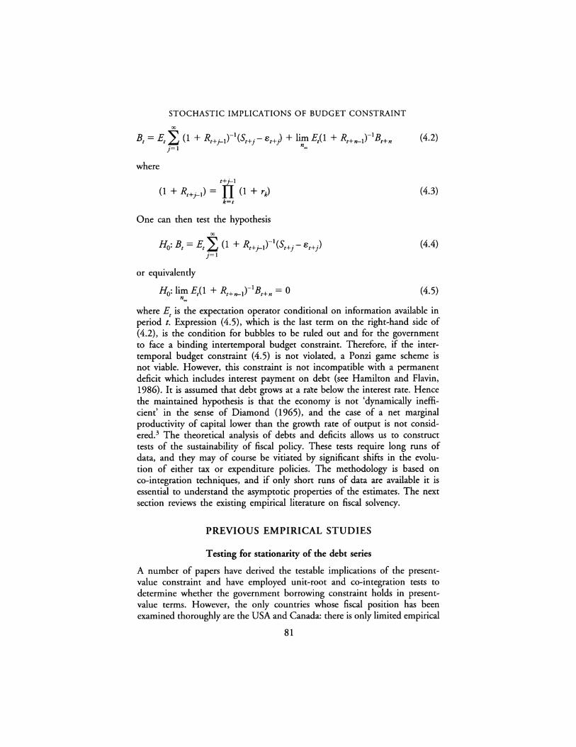
STOCHASTIC IMPLICATIONS OF BUDGET CONSTRAINT
00
Bt = Et~ (1 + Rt+j-1t 1(St+j- Bt+) + lim Eil + Rt+n-it1 Bt+n (4.2) ~I ~
where
t+j-1 (1 + Rt+J-1) = IT (1 + rk)
k=t
One can then test the hypothesis 00
Ho: Bt =Et~ (1 + Rt+J-1t1(St+j- Bt+j) j=l
or equivalently
H0: lim Eil + Rt+n-1t 1Bt+n = 0 n_
(4.3)
(4.4)
(4.5)
where Et is the expectation operator conditional on information available in period t. Expression (4.5), which is the last term on the right-hand side of (4.2), is the condition for bubbles to be ruled out and for the government to face a binding intertemporal budget constraint. Therefore, if the intertemporal budget constraint (4.5) is not violated, a Ponzi game scheme is not viable. However, this constraint is not incompatible with a permanent deficit which includes interest payment on debt (see Hamilton and Flavin, 1986). It is assumed that debt grows at a ra'te below the interest rate. Hence the maintained hypothesis is that the economy is not 'dynamically inefficient' in the sense of Diamond (1965), and the case of a net marginal productivity of capital lower than the growth rate of output is not considered. 3 The theoretical analysis of debts and deficits allows us to construct tests of the sustainability of fiscal policy. These tests require long runs of data, and they may of course be vitiated by significant shifts in the evolution of either tax or expenditure policies. The methodology is based on co-integration techniques, and if only short runs of data are available it is essential to understand the asymptotic properties of the estimates. The next section reviews the existing empirical literature on fiscal solvency.
PREVIOUS EMPIRICAL STUDIES
Testing for stationarity of the debt series
A number of papers have derived the testable implications of the presentvalue constraint and have employed unit-root and co-integration tests to determine whether the government borrowing constraint holds in presentvalue terms. However, the only countries whose fiscal position has been examined thoroughly are the USA and Canada: there is only limited empirical
81

G.M. CAPORALE
evidence on public sector solvency in Europe (see Caporale, 1992a, 1992b, 1993, and Corsetti and Roubini, 1991). Early studies implemented DickeyFuller tests for the existence of a unit root in the stochastic process guiding the evolution of public debt {see, for example, Hamilton and Flavin, 1986; Kremers, 1988; Wilcox, 1989). Dickey and Fuller (1979, 1981) had derived the distribution of the least-squares estimators of the coefficients of the following regression model:
Bt ='Yo+ f3(t-f) + 'Y1B~1 + et (4.6)
and also their associated t-statistics, but had restricted the errors to be independently and identically distributed (i.i.d.) (O,a2). They had also shown that if the process generating Bt is an AR(p) and (p - 1) lags of aB~1 are added as regressors the limiting distribution will not change.
Phillips (1987) has introduced a new approach with two main advantages. First, it does not require the estimation of additional nuisance parameters, which reduces the effective number of observations. Second, it is valid under much more general assumptions about the innovation sequence {e), which allow for all finite ARMA processes. Phillips and Perron {1988) extend these results, and derive new statistics which permit tests of joint hypotheses in a much more general stochastic framework, in which allowance is made for possible serial correlation and heteroscedasticity.
This is the approach taken by Corsetti and Roubini (1991) in their paper on fiscal deficits, public debt and government solvency. One should be aware, however, of the problems which can be encountered in practice when undertaking the Phillips-Perron Z tests. These tests are asymptotic, whereas in most cases the available series span relatively short sample periods. Also, the Z tests have very low power against the alternative of stationarity with a root very close to one. Finally, they are valid only if the Data Generation Process is stable over the sample period. A recent study by Smith and Zin (1991) makes use of the asymptotic distribution theory for the ADF tests due to Phillips and Ouliaris (1990). The latter authors show that, even in the presence of autocorrelation in the residuals, the limiting distribution is independent of the number of nuisance parameters. The critical values they calculate are quite different from the ones calculated by Dickey and Fuller. They also study the asymptotic behaviour of the Z tests proposed in Phillips (1987), and their analysis suggests that t-ratio tests such as the ADF and the Zt tests diverge under H1 at a slower rate than the Za test and two new variance ratio tests they develop in their paper, implying that the latter tests should have a higher power in large samples. Another appealing property of one of the two new tests is its invariance to the normalization of the cointegrating vector. Asymptotically, all these tests have similar properties and their limiting distribution is a Brownian motion.
82

STOCHASTIC IMPLICATIONS OF BUDGET CONSTRAINT
Testing for co-integration between government expenditure and taxes
Another strand of the literature tests a different implication of the government borrowing constraint, and looks for a co-integrating vector between surpluses and stock of debt (see, for example, Trehan and Walsh, 1988; Kremers, 1989; Haug, 1991; Smith and Zin, 1991). These studies estimate static relationships and test whether the resulting residuals are stationary in the sense of Engle and Granger (1987). The type of analysis conducted by Hamilton and Flavin (1986) allows only for deterministic (non-stochastic) non-stationarity. In the framework put forward by Wilcox (1989), in order to test stationarity of discounted debt one needs data on the actual yield on government bonds which are not usually available. One can use instead the methodology developed by Trehan and Walsh (1988), who show that a necessary and sufficient condition for sustainability is co-integration between bt and dt+I (where bt is the debt/GDP ratio and dt the (primary) deficit/GDP ratio) with co-integrating vector (1 µ) (where µ = (1 + n)l(r- n), n is the growth rate of GDP, and r the interest rate), condition which is equivalent to the stationarity of dt, defined as the difference between gt (public spending/GDP ratio) and tt (tax receipts as a percentage of GDP). The following section outlines this alternative approach, and reports some empirical results for a number of European countries.
GOVERNMENT EXPENDITURE, TAXES AND SOLVENCY
A framework for empirical analysis
The theory of solvency sketched on pp. 80-1 embeds further testable implications.4 Let us assume for simplicity that the one-period forecasts of the interest rate are constant, that is E,(rt+I) = r, and also that the errors are an innovation process, which implies Etet+j = 0 (j ~ 1). Equation (4.4) then becomes:
00
Bt =Et~ (1 + rtjSt+j j=I
or alternatively 00
b1 = Et~ 13\+j j=I
(4.7)
(4.7')
where the variables are expressed as a percentage of GDP, f3 = [(1 + r)I (1 + n)] and n equals the growth rate of GDP. Expression (4.7') is equivalent to
83

00
bt = -Et L (3ldt+j j=l
G.M. CAPORALE
(4.7")
where dt is the ratio of the primary deficit to GDP. Let us assume that the stochastic behaviour of dt can be characterized by the following ARIMA process:
(1 - t>L)dt = A(L)71t
1 0 < i>< -- /3
00
A(L) =La; i=O
Then (4.7") can be re-written as
bt = -E,[{3(t>dt + A(L)T/t+l> + /32(1fdt + t>A(L)71t+l
+ A(L)Bt+2> + ... ]
which is equivalent to
-{3t> /3 ~ . --~ . b t = --_a. dt -~ Et £J {3' L 1 £J a1 L171t+ 1
1 - {3·v } - pV j= 1 j= 1
(4.8)
(4.9)
(4.10)
Given the fact that Et.,.,t+k = 0 for all k > 0, and using the formula derived in Hansen and Sargent (1980), one can also express (4.10) as:
where
B(L) = A(L) -A(/3) I - 13r-1
Using the relationship t>dt = dt+l -A(L)71t+I' one finally obtains
bt = -µdt+l + C(L)T/t+l
where
/3 µ = 1-{3t>
and
84
(4.11)
(4.12)
(4.13)
(4.14)

STOCHASTIC IMPLICATIONS OF BUDGET CONSTRAINT
OL) = _/3_ [A(L) - A(L)-A(/3)] (4.15) , l _ f31J- L- /3 11t+I
If dt+I is an /(1) variable, that is if iJ= 1, then (4.13) can be seen to imply co-integration between bt and dt+I' with co-integrating vector (1 µ,), where µ, = {31(1- /3) = (1 + n)/(1 + r). In that case, (4.13) can be rearranged to yield
or
( 1 + n) bt + µ,dt+I = bt + -- dt+I
r-n (4.16)
(4.17)
Using the definition of primary deficit, one can finally express (4.17) as
(4.18)
where gt and tt represent government expenditure (not including interest payments) and taxes, respectively, as a percentage of GDP. Equation (4.18) shows that only if government receipts and outlays are co-integrated the intertemporal budget constraint is satisfied. Hence, Trehan and Walsh (1988) suggest, one can proceed as follows to test whether fiscal policy is sustainable in the long run. The first step is to test whether government spending and taxes are stationary series. If they are stationary, solvency is satisfied; if only gt is non-stationary, fiscal policy is not sustainable; if gt and tt are both non-stationary then one should test whether the two series are co-integrated. If they are not, fiscal policy is not on a sustainable path; if they are, one should estimate the co-integrating vector to check whether it equals (1 -1) as required by sustainability; that is, one should estimate the following equation:
(4.19)
or equivalently
tt = a2 + f3itt + Uzt (4.19')
and test H0: a1 = 0, /31 = 1 or H0: a2 = 0, /32 = 1 for equation (4.19) or (4.19') respectively. Rejection of H0 implies insolvency.
If the series fail to co-integrate, the estimation of a time-varying parameter model can provide useful additional information on the reasons why the fiscal stance appears not to be sustainable. Such models allow for the endogenous estimation of the timing of any regime shifts which might have
85

G.M. CAPORALE
occurred and which will show up in the evolving estimates of the coefficients. The obvious advantage of such an approach is the fact that no assumptions concerning the timing of the breaks have to be made; coefficients are allowed to evolve over time without the imposition of a priori restrictions. These models are very suitable for the purpose of checking the constancy of the coefficients of standard fixed-coefficient models, since the shifts are modelled in a stochastic but well-defined way.
The method normally used to estimate 'state-space' models is the Kalman filter (for a standard reference, see Anderson and Moore, 1979). This class of models consists of two equations: the transition equation, describing the evolution of the state variables, and the measurement equation, describing how the observed data are generated from the state variables. This approach is extremely useful for investigating the issue of parameter constancy because it is an updating method producing each time period estimates based on the observations available up to the current period. Let the transition equation be:
(4.20)
and the measurement equation be:
f3t = Tf3t-1 + Y/t Yt ~ N(0,QJ (4.21)
with the initial conditions given by:
(4.22)
When T = I and ~ = 0, the model is reduced to the standard normal regression model. The matrices T, H and Q are assumed to be known, and the problem is obtaining estimates of {3t using information It available up to time t. The process of evaluating the conditional expectation of {3t given It is known as filtering. The evaluation of {3t given ~, with s > t, is instead referred to as smoothing, whereas the estimation of {3t with s < t is called prediction.
Kalman (1960) derives the basic results to obtain filtered and smoothed estimates of {3t recursively. As we have already pointed out, time-varying parameter estimation seems a much more appropriate approach when the question being asked is to what extent the correlation between regressors and regressand has changed over time, the standard fixed parameter models assuming that it is constant. The prediction equation (see Harvey, 1987) is given by defining ~t as
I\ I\
f3t1(t-1) = Tf3t-1 (4.23)
and the covariance matrix of the estimate ffit as
86

STOCHASTIC IMPLICATIONS OF BUDGET CONSTRAINT
ptl(t-1) = TP t--1 T' + ~
Finally, the updating formulae are given by:
I\
il _ il p (Yt-x'f3tt(t-ll H) /Jt - /Jtl(t--1) + tl(t-l)x 'P + t
X tl(t--l)X
and
(4.24)
(4.25)
(4.26)
As the estimates are recursively updated each period, Kalman filtering can be viewed as a Bayesian method. Before starting the estimation process, one has to specify the vector of prior coefficients (3 and, to get a time-varying parameter model, the matrix Q (the signal-to-noise ratio). By estimating the long-run relationship in this way one obtains a vector containing the evolving state coefficients which shows whether the relative importance of the factors driving the dependent variable has changed over time.
In our case, we can estimate a model of the following form:
gt = at+ 13ft + ut (4.27)
(4.27')
(4.27")
To see what is driving the time-varying parameters, an additional equation can be estimated, as specified in (4.28):
(4.28)
where xt is the yield on government bonds. We can further investigate what is driving government spending and taxes
by estimating a VAR of the form described in (4.29) and doing Grangercausality tests
(4.29)
where the null is H0: A12 (L) = 0 and H0: A21 (L) = 0. Finally one can look at the impulse response function.
87
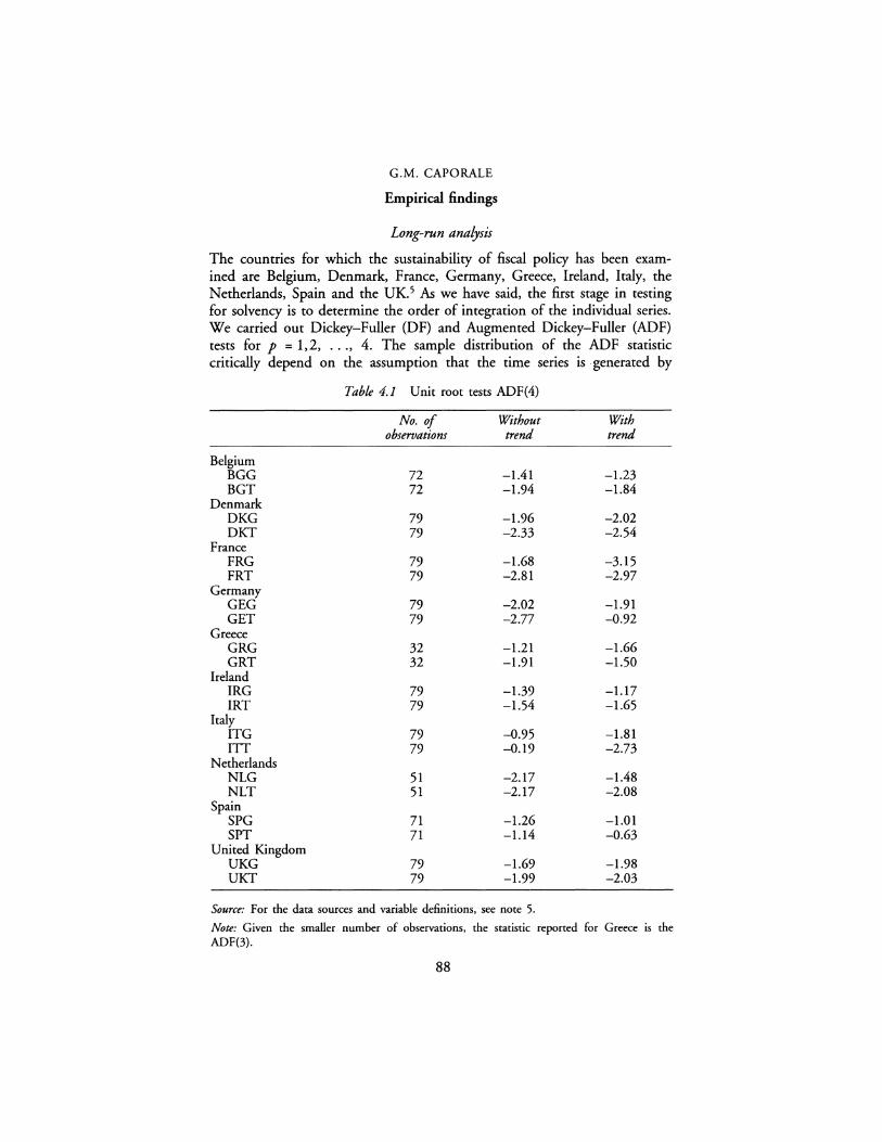
G.M. CAPORALE
Empirical findings
Long-run analysis
The countries for which the sustainability of fiscal policy has been examined are Belgium, Denmark, France, Germany, Greece, Ireland, Italy, the Netherlands, Spain and the UK.5 As we have said, the first stage in testing for solvency is to determine the order of integration of the individual series. We carried out Dickey-Fuller (OF) and Augmented Dickey-Fuller (ADF) tests for p = l,2, ... , 4. The sample distribution of the ADF statistic critically depend on the assumption that the time series is • generated by
Table 4.1 Unit root tests ADF(4)
No. of Without With observations trend trend
Belgium BGG 72 -1.41 -1.23 BGT 72 -1.94 -1.84
Denmark DKG 79 -1.96 -2.02 DKT 79 -2.33 -2.54
France FRG 79 -1.68 -3.15 FRT 79 -2.81 -2.97
Germany GEG 79 -2.02 -1.91 GET 79 -2.77 -0.92
Greece GRG 32 -1.21 -1.66 GRT 32 -1.91 -1.50
Ireland IRG 79 -1.39 -1.17 IRT 79 -1.54 -1.65
Italy ITG 79 -0.95 -1.81 ITT 79 -0.19 -2.73
Netherlands NLG 51 -2.17 -1.48 NLT 51 -2.17 -2.08
Spain SPG 71 -1.26 -1.01 SPT 71 -1.14 -0.63
United Kingdom UKG 79 -1.69 -1.98 UKT 79 -1.99 -2.03
Source: For the data sources and variable definitions, see note 5.
Note: Given the smaller number of observations, the statistic reported for Greece is the ADF(3).
88

STOCHASTIC IMPLICATIONS OF BUDGET CONSTRAINT
Table 4.2(a) Co-integrating regressions, dependent variable: G
Estimated coefficients . ADF(4) Sample
Constant T period
BG -0.00056 1.31 -1.27 72Ql 90Q4 DK -0.053 1.18 -2.21 70Ql 90Q4 FR 0.42 0.25 -1.47 70Ql 90Q4 GE -0.22 1.09 -3.07 70Ql 90Q4 GR -0.059 1.80 -1.62 82Ql 90Q4 IR 0.004 1.24 -0.84 70Ql 90Q4 IT 0.023 1.26 -3.08 70Ql 90Q4 NL 0.226 0.446 -2.14 77Ql 90Q4 SP -0.018 1.31 -1.12 72Ql 90Q4 UK -0.039 1.24 -2.00 70Ql 90Q4
Table 4.2(b) Co-integrating regressions, dependent variable: T
Estimated coefficients ADF(4) Sample
Constant G period
BG 0.078 0.427 -1.58 72Ql 90Q4 DK 0.085 0.699 -2.51 70Ql 90Q4 FR 0.363 0.107 -3.23 70Ql 90Q4 GE 0.323 0.23 -2.47 70Ql 90Q4 GR 0.076 0.41 -1.83 82Ql 90Q4 IR 0.006 0.737 -0.97 70Ql 90Q4 IT 0.008 0.698 -3.24 70Ql 90Q4 NL -0.009 0.92 -1.87 77Ql 90Q4 SP 0.024 0.71 -0.98 72Ql 90Q4 UK 0.047 0.749 -2.07 70Ql 90Q4
Source: For the data sources and variable definitions, see note 5.
Note: The ADF(3) is reported in the case of Greece.
a pure AR process. However, as Said and Dickey (1984) show, an AR/MA (p, I,q) process can be adequately approximated by a high-order autoregressive process, AR(I), where I = O(T113) as T tends to infinity. Hence we only report the results for p = 4 (see Table 4.1). In all cases the ADF tests (with and without a time trend) indicate that the series are not stationary in levels but contain a unit root. We then proceeded to test for co-integration between government expenditure and revenue in each country. The co-integrating regressions and the unit root tests for residuals are reported in Table 4.2.
89

G.M. CAPORALE
Table 4.3 The effect of the yield on long-term bonds - dependent variable: /3/
Estimated coefficients Sample
Constant LR period
BG -0.008 (-2.1 l)b -0.091 (-10.2) 72Q2 90Q4 DK 0.68 (14.25) 0.013 (3.69) 70Q2 90Q4 FR 0.099 (3.01} -0.005 (-1.54) 70Q2 90Q4 GE 1.24 (3.15) -0.13 (-2.71) 70Q2 90Q4 GRC 1.94 (26.68) -0.014 (-2.77) 82Q2 90Q4 IR 0.79 (11.16) -0.024 (-4.25) 70Q2 90Q4 IT 0.40 (2.88} 0.036 (3.44) 70Q2 90Q4 NL 0.087 (1.35) 0.023 (3.21) 77Q2 90Q4 SP 0.55 (19.04) 0.002 (1.71) 72Q2 90Q4 UK 0.45 (1.82) 0.028 (1.9) 70Q2 90Q4
Source: For the data sources and variable definitions, see note 5.
Notes: a See equation 27. b t-Statistic in parentheses. c The variable used for Greece is the yield on 3-month Treasury Bills.
Table 4.4 Granger-causality tests
Belgium F(4,71) Ireland F(4,75) BGG 7.03 IRG 0.50 BGT 5.51 IRT 0.13
Denmark F(4,75) Italy F(4,75) DKG 0.69 ITG 2.54 DKT 0.71 ITT 3.80
France F(4,75) Netherlands F(4,51) FRG 0.64 NLG 3.38 FRT 7.38 NLT 2.45
Germany F(4,75) Spain F(4,71) GEG 6.79 SPG 7.07 GET 1.55 SPT 5.54
Greece F(4,31) United Kingdom F(4,75) GRG 2.09 UKG 6.67 GRT 2.03 UKT 2.42
Source: For the data sources and variable definitions, see note 5.
Note: The V AR was estimated in first differences; the lag length 4 was selected on the basis of the Schwarz Bayesian Information Criterion (SBIC).
90

STOCHASTIC IMPLICATIONS OF BUDGET CONSTRAINT
Belgium
In both co-integrating regressions the slope coefficient is different from 1, and the ADF(4) test on the residuals indicate that the series are not co-integrated (see Table 4.2). The standard errors and hence hypothesis testing are not valid in such regressions, but some information on the size and evolution of the parameters can be obtained by estimating a time-varying parameter model. In both cases the constant settles down to a value far from 0 and the coefficient on the independent variable does not approach 1, indicating that over the whole period the two series have been drifting apart. Therefore fiscal policy does not appear to be sustainable in Belgium. However, the time-varying parameter on government revenue is negatively related to the long-term yield on government bonds (see Table 4.3), and hence has a stabilizing effect, implying that any increase in the cost of servicing the debt is more than offset by cuts in current expenditure. Furthermore, F-tests for block exogeneity (see Table 4.4) suggest that government expenditure is Granger-caused by government revenue and vice versa, as in the estimated V AR in both cases the lags of the other endogenous variable enter the equation significantly. Thus the overall picture is slightly less worrying, since there is evidence that the two series are not totally independent of one another.
Denmark
The residuals from both co-integrating regressions are non-stationary, but the estimated parameters are much closer to the values consistent with solvency (see Table 4.2). In particular, Kalman filter estimation reveals that in the regression of expenditure against revenue the constant is never too far from O and the coefficient on the independent variable rises substantially in the late 1970s, peaks in the early 1980s, and then converges towards 1. Conversely, there is no evidence that either series Granger-causes the other (see Table 4.4). The coefficient on the yield on long-term bonds is positive (see Table 4.3), which indicates that this variable has destabilizing effects.
France
The unit root hypothesis cannot be rejected for the residuals from either co-integrating regression, although the ADF(4) in the regression of revenue against expenditure is very close to its critical value (see Table 4.2). The value of the estimated coefficients is not compatible with solvency, and they do not show any tendency to converge towards O and 1 respectively (see Figures 4.1 and 4.2). However, the yield on long-term government bonds affects negatively the time-varying parameter on government expenditure
91

G.M. CAPORALE
0.522
0.457
0.392 ~---"------~------~---------'
7102
CMST
0.931E--01
0.689E--01
0.446E--01
7704 8402
Parameter on the time varying constant
Figure 4.1 Equation 4.19 - France
9004
0.203E--01 '---------'--------'----------"'"'--'
7102
FRT
7704 8402
Parameter on the time varying FRT
Figure 4.2 Equation 4.19 - France
92
9004

STOCHASTIC IMPLICATIONS OF BUDGET CONSTRAINT
(see Table 4.3), and spending Granger-causes revenue (see Table 4.4), suggesting that there are feedback effects which are potentially stabilizing.
Germany
The residuals from the regression of expenditure against revenue appear to be almost stationary, and the estimated coefficients are also of the size requested for sustainability of fiscal policy (see Table 4.2). The time-varying parameters move in the right direction over time, even though they do not converge rapidly (see Figures 4.3 and 4.4). Tax revenue is not block exogenous with respect to expenditure (see Table 4.4), and movements in bond yields also contribute to stabilize the deficit (see Table 4.3), making fiscal policy more sustainable.
Greece
The sample period for Greece is rather short, including only the 1980s. Both the statistical and the graphical evidence lead to the conclusion that fiscal policy is not on a sustainable path: the ADF statistics indicate that the residuals from the co-integrating regressions are not stationary (see Table 4.2), the evolution over time of the parameters shows that expenditure and revenue drift apart over the whole period, and neither series Granger-causes the
0.659
0.393
0.127 .__ ______ _,__ ______ __,_ _____ __;""'---'
7102
CMST
7704 8402
Parameter on the time varying constant
Figure 4.3 Equation 4.19 - Germany
93
9004

G.M. CAPORALE
-0.878E-02
-0.727
-1.44 ~~------~------~~------~
7102
GET
7704 8402
Parameter on the time varying GET
Figure 4.4 Equation 4.19 - Germany
9004
other (see Table 4.4). The only stabilizing effects are due to the return on 3-month Treasury Bills {see Table 4.3).
Ireland
Some evidence that the Irish fiscal position is becoming more sustainable is given by the regression of revenue against spending, although the hypothesis of stationarity of the residuals is formally rejected {see Table 4.2) and block exogeneity over the whole period cannot be rejected in either case (see Table 4.4). The estimation of time-varying parameter models shows that in the second half of the 1980s the correlation between the two series is much higher, and increases in interest payments appear to be counterbalanced by cuts in current expenditure (see Table 4.3).
Italy
In the case of Italy, the hypothesis of solvency is formally rejected, but the ADF statistic is very close to its critical value in the second regression {see Table 4.2), and graphs of the coefficients {see Figures 4.5 and 4.6) show a downward (upward) shift in the constant and the slope coefficient respectively in the second decade, making fiscal policy more sustainable in the
94

STOCHASTIC IMPLICATIONS OF BUDGET CONSTRAINT
0.242 ,-------,--r----------------------,
0.161
0.799E-01
-0.128E-02 ~------~------~-----~ 7102
CMST
0.699
0.147
7704 8402
Parameter on the time varying constant
Figure 4.5 Equation 4.19 - Italy
9004
-0.405 ._____.'-"--------'------------'----------'
7102
ITT
7704 8402
Parameter on the time varying ITT
Figure 4.6 Equation 4.19 - Italy
95
9004

G.M. CAPORALE
second half of the 1980s. F-tests for block exogeneity indicate that each series can be forecast more accurately including lagged values of the other (Table 4.4). Further evidence that there are feedback effects comes from the regressions of the time-varying parameters onto the yield on government bonds, the estimated slope coefficient being negative (see Table 4.3).
Netherlands
The statistical evidence suggests that the fiscal stance in the Netherlands is not sustainable (see Table 4.2), but the evolution over time of the coefficients of the second regression makes the picture less gloomy, as the constant settles down at a level very close to 0 and the slope coefficient approaches 1. The return on government securities has a positive effect on the timevarying coefficient on government expenditure (see Table 4.3), but each series Granger-causes the other (see Table 4.4), which can be interpreted as evidence that efforts are being made to balance the budget.
Spain
It is clear from the econometric analysis that Spain's fiscal position is not sustainable. The residuals from the co-integrating regressions are nonstationary, the slope coefficients are far from 1 (see Table 4.2), and one of them, after becoming equal to 1 in the first quarter of 1984, starts diverging, indicating that balancing the budget has been even less of a concern for the Spanish authorities in the second half of the 1980s. There is some evidence that expenditure is Granger-caused by revenue (see Table 4.4), but further destabilizing effects are due to the yield on government bonds (see Table 4.3).
United Kingdom
The policies pursued over the whole sample period were such that the government was potentially insolvent (see Table 4.2), but the 1980s were characterized by a sounder fiscal position, as shown by the evolution of the time-varying parameters (see Figures 4.7 and 4.8). Moreover, in the VAR system the lags of the other endogenous variables are significant in both equations (see Table 4.4). Increases in the yield on government securities, though, tend to widen the gap between expenditure and revenue (see Table 4.3).
Short-run analysis
Although in most cases we did not find a long-run relationship between government expenditure and revenue, it is possible that the short-run
96

STOCHASTIC IMPLICATIONS OF BUDGET CONSTRAINT
0.931E-01
0.634E-01
0.337E-01
0.408E-02 ~~----~------~-----~
7102
CMST
0.784
0.630
7704 8402
Parameter on the time varying constant
Figure 4.7 Equation 4.19 - UK
9004
0.477 L.....L. ______ _.__ ______ ___,_ ______ ~
7102
UKT
7704 8402
Parameter on the time varying UKT
Figure 4.8 Equation 4.19 - UK
97
9004

G.M. CAPORALE
dynamics of each variable are largely driven by shocks to the other series. Therefore we analysed the response of each endogenous variable to Choleskifactored shocks over forty quarters (the impulse response function).6 For each country, we considered in turn the impact of unitary shocks to spending and tax revenue on both variables. Our investigation can also shed light on the empirical validity of tax-smoothing theories (see for example Barro, 1979), which imply that a permanent shock to spending should result in a proportional adjustment in revenue. The effects of the shocks after forty quarters are more pronounced in some countries than in others, and they are generally significant enough to conclude that they are permanent; in the case of Greece the response of government expenditure to either type of shock is explosive. One noticeable feature which is common to almost all countries, with the only exceptions of Germany and the Netherlands, is the fact that spending adjusts to a higher degree than revenue to shocks. The response of the latter is muted, and does not fully compensate for permanent changes in government expenditure. These results are not compatible with the hypothesis of tax smoothing, and also suggest that tax revenue is the control variable, since spending reacts strongly to shocks to receipts.
CONCLUSIONS
This chapter has investigated the sustainability of fiscal policy in several EC countries. We have first shown that the government's intertemporal budget constraint can only be satisfied if government receipts and outlays, as a percentage of GDP, are co-integrated. We have then analysed the long-run relationship between these two series in each country. It appears that in most cases (Germany possibly being the only exception) government expenditure and revenue drifted apart, and hence balancing the budget was not given a high priority. However, unit root tests weigh the entire sample equally, whereas judgements about convergence should be based mainly on the fiscal stance in recent years. Kalman filter estimation reveals that the structure of fiscal policy has changed in the 1980s in many countries (Belgium, Denmark, Ireland, Italy, Netherlands and the UK), making it more sustainable. There is also evidence (Belgium, France, Germany, Italy, Netherlands, Spain, UK) of feedback effects, with revenue affecting spending or vice versa, and with higher returns on government bonds resulting in a reduction in the primary deficit (Belgium, France, Germany, Greece, Ireland, Italy). Finally, in all countries outlays respond more to shocks than receipts, and the latter do not fully adjust even to permanent shocks, contrary to what one would expect in the presence of tax smoothing. On the whole, the conclusion to be drawn is that, as regards government balances, some progress has been made, but corrective fiscal action is still required in most countries to achieve sustainable debt positions and also to meet the rather stringent convergence criteria laid down in the Maastricht Treaty.
98

STOCHASTIC IMPLICATIONS OF BUDGET CONSTRAINT
NOTES
1 The Leverhulme Trust is gratefully acknowledged for financial support (Grant no. F.59T). This chapter was presented as a paper at the 38th Conference of the Applied Econometrics Association on Budgetary Policy Modelling, Athens, 13-14 April 1993.
2 See Blanchard et al. (1990) for some sustainability indicators. 3 See, however, Bohn (1990), who shows that dynamic efficiency cannot be deter
mined by comparing the interest rate with the growth rate of the economy once one allows for risk-averse investors.
4 The following derivation of the additional testable restrictions implied by the government's intertemporal budget constraint follows closely Trehan and Walsh (1988).
5 Data sources and variable descriptions.
GREV: General Government Revenue, current prices, not seasonally adjusted. Source: International Financial Statistics, International Monetary Fund. For
· Germany, the series used is constructed as total current receipts plus depreciation plus net capital transfers received (source: OECD Quarterly National Accounts). The UK data are taken from the CSO Financial Statistics.
GEXP: General Government Expenditure, current prices, not seasonally adjusted (source: International Financial Statistics, International Monetary Fund; for the UK, CSO Financial Statistics). Note: in the case of Denmark, annual data on both GREV and GEXP were interpolated to obtain a quarterly path.
GDP: Gross Domestic Product at current prices (source: OECD Quarterly National Accounts). Note: annual data for Belgium, Denmark, the Netherlands and Spain were interpolated.
LR: Long-term yield on government bonds (source: International Financial Statistics, International Monetary Fund). Note: the variable used for Greece is the yield on 3-month Treasury Bills.
T= GREV/GDP
G = GEXP/GDP
Country mnemonics: Belgium BG Denmark DK France FR Germany GE Greece GR Ireland IR Italy IT Netherlands NL Spain SP United Kingdom UK
6 The shocks are the residuals from a V AR in first differences of lag length 4.
99

G.M. CAPORALE
BIBLIOGRAPHY Anderson, B.D.O. and J.B. Moore (1979) 'Optimal filtering', Englewood Cliffs, NJ:
Prentice-Hall. Barro, R.J. (1974) 'Are government bonds net wealth?' journal of Political Economy,
vol. 82, pp. 1095-117. -- (1979) 'On the determination of the public debt',] ournal of Political Economy,
vol. 87, pp. 940-71. Blanchard, O.J. (1990) 'Suggestions for a new set of fiscal indicators', OECD/DES
Working Paper no. 79. -- , J.C. Chouraqui, R.P. Hagemann and N. Sartor (1990) 'The sustainability of
fiscal policy: new answers to an old question', OECD Economic Studies, no. 15. Bohn, H. (1990) 'The sustainability of budget deficits in a stochastic economy',
mimeo, Department of Finance, The Wharton School, University of Pennsylvania. Caporale, G.M. (1992a) 'Fiscal solvency in Europe: budget deficits and government
debt under European Monetary Union', National Institute Economic Review, vol. 140, pp. 69-77.
-- (1992b) 'Debt sustainability and monetary union', paper presented at the Seventh Annual Congress of the European Economic Association, Dublin.
-- (1993) 'Bubble finance and debt sustainability: a test of the government's intertemporal budget constraint', NIESR, mimeo.
Chouraqui, J.C., B. Jones and R.B. Montador (1986) 'Public debt in a mediumterm perspective', OECD Economic Studies, no. 7 (Autumn), pp. 103-39.
Corsetti, G. and N. Roubini (1991) 'Fiscal deficits, public debt, and government solvency: evidence from OECD countries', journal of the Japanese and International Economies, vol: 5, pp. 354-80.
Diamond, P. (1965) 'National debt in a neo-classical growth model', American Economic Review, vol. 55, pp. 1126-50.
Dickey, D.A. and W .A. Fuller (1979) 'Distribution of the estimators for autoregressive time series with a unit root', journal of the American Statistical Association, vol. 74, pp. 427-31.
-- (1981) 'Likelihood ratio statistics for autoregressive time series with a unit root', Econometrica, vol. 49, pp. 1057-72.
Engle, R.F. and C.W.J. Granger (1987) 'Cointegration and error correction: representation, estimation and testing', Econometrica, vol. 55, pp. 251-76.
Hamilton, J.D. and M.A. Flavin (1986) 'On the limitations of government borrowing: a framework for empirical testing', American Economic Review, vol. 76, no. 4, pp. 808-19.
Hansen, L.P. and T.J. Sargent (1980) 'Formulating and estimating dynamic linear rational expectations models', journal of Economic Dynamics and Control, vol. 2, pp. 7-46.
Harvey, A.C. (1987) Time Series Models, Oxford: Phillip Allan. Haug, A.A. (1991) 'Cointegration and government borrowing constraints: evidence
for the United States', journal of Business and Economic Statistics, vol. 9, no. 1, pp. 97-102.
Kalman, R.E. (1960) 'A new approach to linear filtering and prediction problems', Trans. ASME Ser. D,]. Basic Eng., vol. 82, pp. 35-45.
Kremers, J.J.M. (1988) 'Long-run limits on the US federal debt', Economics Letters, vol. 28, no. 3, pp. 259-62.
-- (1989) 'US Federal indebtedness and the conduct of fiscal policy', Journal of Monetary Economics, vol. 23, no. 2, pp. 219-38.
O'Connell, S.A. and S.P. Zeldes (1988) 'Rational Ponzi games', International Economic Review, vol. 29, pp. 431-50.
100

STOCHASTIC IMPLICATIONS OF BUDGET CONSTRAINT
Phillips, P.C.B {1987) 'Time series regression with a unit root', Econometrica, vol. 55, pp. 277-301.
-- and S. Ouliaris (1990) 'Asymptotic properties of residual based tests for cointegration', Econometrica, vol. 58, no. 1, pp. 165-93.
-- and P. Perron (1988} 'Testing for a unit root in time series regression', Biometrika, vol. 75, no. 2, pp. 335-46.
Poterba, J.M. and L.H. Summers (1987) 'Finite lifetimes and the effects of budget deficits on national saving', journal of Monetary Economics, vol. 20, pp. 369-91.
Said, S. and D.A. Dickey (1984) 'Testing for unit roots in autoregressive-moving average models of unknown order', Biometrika, vol. 71, pp. 599-607.
Smith, G.W. and S.E. Zin (1991) 'Persistent deficits and the market value of government debt', journal of Applied Econometrics, vol. 6, pp. 31-44.
Trehan, B. and C.E. Walsh (1988} 'Common trends, the government's budget constraint, and revenue smoothing', journal of Economic Dynamics and Control, vol. 12, pp. 425-44.
Wilcox, D.W. {1989) 'The sustainability of government deficits: implications of the present-value borrowing constraints', journal of Money, Credit, and Banking, vol. 21, no. 3, pp. 291-306.
101

5
CREDIT CONSTRAINTS AND THE EFFICIENCY OF
BUDGETARY POLICY The Portuguese case, 1958-881
Maria Dolores Nunes Cabral
INTRODUCTION
Recent theoretical and empirical investigation2 has stressed the fact that monetary authorities can still influence the real variables of the economy despite the weaker link between the money supply and economic activity due to financial innovation. According to Blinder and Stiglitz (1983), the greater stability in the credit demand function (compared with that for money) and the particular position of banks in the credit system have given to the central bank the capacity to affect the real economy.3 Monetary policy has begun to be transmitted through its effects on the supply of credit. By controlling the supply of credit, monetary authorities have not only affected the economy through aggregat<: demand but also through the aggregate supply of goods when the short side of the market is the credit supply. That being the case, the efficacy of macroeconomic policy depends in a crucial way on its impact on the credit supply for the private sector.4
In the Portuguese case interest rates have until recently been administered by the monetary authorities, and for most of the time, since 197 4, the Bank of Portugal has imposed credit limits. It is therefore of interest to analyse the effects of this credit policy on economic activity as well as the efficacy of the macroeconomic policy in Portugal.
With that in mind, we shall estimate a small macroeconomic model which stresses the basic transmission mechanisms of the budget and internal credit policies and allows for the estimation of the dynamic effects of these policies on the main macroeconomic variables. With the utilization of this model we intend to accomplish two objectives: the first is to assess the efficacy of the budget policy; the second is to evaluate the effects of quantitative credit restrictions on the level of economic activity.
There are essentially three theories concerning the effects of the budget policy on the economy:
102

CREDIT CONSTRAINTS AND BUDGETARY POLICY
1 the Keynesian approach states that the budget policy has positive and lasting effects on economic activity as long as there are unemployed resources;
2 the monetarist approach states that the positive effects of the budget policy are transitory because in a short period of time the negative effects of 'crowding-out' exceed the positive effects of the budget policy; and
3 the neutrality of debt hypothesis according to which the replacement of taxes by debt in the financing of a certain amount of government spending is neutral. This theory casts doubt on the ability of budget policy to affect either real or nominal economic variables.
Recent literature has stressed the importance of the effects of credit market constraints on aggregate demand and aggregate supply. In the Blinder models (1989) whenever the short side of the market is the credit supply, a restrictive credit policy affects negatively aggregate demand and therefore the level of economic activity. On the other hand, a restrictive credit policy also affects aggregate supply given that the credit restrictions imposed on firms limits their ability to implement selling and expansion plans dictated by the product market.
In the model that we shall estimate for the Portuguese economy we are only assessing the effects of the quantitative credit constraints through the demand for goods. We shall first estimate the model and then perform simulations of budget and credit policies with the objective of computing the dynamic multipliers for the main macroeconomic variables, in particular the Gross Domestic Product (GDP), consumption, investment and imports.
The analysis of these multipliers will allow for an evaluation of the efficacy of these policies: the budget policy - by testing the different hypotheses mentioned above, and the credit policy - by looking at the influence of credit constraints on the level of economic activity through aggregate demand.
The application of this model to the Portuguese economy allows us to put forward some general conclusions.
• The multipliers for the budget policies for the periods for which the short side of the credit market is the credit supply are smaller than those when there was excess supply in the credit market and partial 'crowdingout' does exist.
• An expansionist credit policy is only effective for those periods when there is excess demand in the credit market.
• The results we obtained for the Portuguese case are compatible with those from Blinder (1989).
103

M.D.N. CABRAL
DESCRIPTION OF THE MODEL
The model developed here draws from those estimated by Arestis et al. (1978), Arestis (1979), Paleologos (1984), Dalamagas (1985, 1987 and 1988) although we have opted for the inclusion of the credit market, keeping in mind the testing of the effect of quantitative credit restrictions on the economy, an approach closer to that of Blinder and Stiglitz (1983), Blinder and Bernanke (1989) and Blinder (1987, 1989). The model includes the real market, the credit market and the government budget restriction.5
The real market is comprised of the consumption function, profits, investment, taxes and the impon function. Government spending on goods and services and expons are considered to be exogenous, as in most models of this type.
We have decided to include in this model the credit market instead of the money market because for most of the sample period the monetary authorities have controlled the credit supplied to the economf and the interest rates have been administered. In addition, the financial market has been given imponance only recently (for the majority of the sample period banking credit was the main internal source for the financing of the economy, in panicular, for the public sector).
When specifying the behaviour of the credit market, we have tried to take into account the policy of credit constraint to firms and private citizens which until recently has restrained available financing in the economy. This was done by assuming that during the period of effective control, the observed value was determined by the shon side of the market.
Finally, we take into consideration in this model, the government budget constraint with the objective of analysing both the main effects on the economy of the alternative ways of financing public expenditures and the dynamics of the budget constraint. We do this by including in the consumption function a proxy for wealth which is related to that budget constraint.7
The model captures the main income effects of the budget policy, the crowding-out effects (through the repercussions of deficit financing on the availability of credit to private entities) and the effects of variations in the supply of credit on aggregate demand. The exclusion of the effects of the credit supply on aggregate supply, the price dynamics, and the interest and exchange rates are the main limitations of a model of this type.8 In panicular, this model does not allow for the endogeneity of the expected inflation rate which is necessary to estimate the expected real interest rate, an explanatory variable of the model. To minimize the limitations imposed by the model, we have used two alternative methods. In the first we assumed that the expected inflation rate is the same as the observed rate. In the second we estimated an expected inflation rate using Kalman' s estimation methodology for the inflation equation.9 This variable was estimated outside the model and then used to estimate the real expected interest rate.
104

CREDIT CONSTRAINTS AND BUDGETARY POLICY
METHODOLOGY AND VARIABLES
The data used are annual deflated data for the period from 1958 to 1988. 10
The simultaneous equation model was estimated by two-stage least squares and all equations which did not include a lagged dependent variable were corrected for serial correlation.
We performed several historical simulations with the objective of estimating the multipliers for alternative budget and credit constraint policies. 11
Based on the parameter estimates and initial values for the exogenous variables we calculated the corresponding values for the endogenous variables for the initial period. Taking these values of the endogenous variables as the initial conditions we then computed for the simulation period the values for the endogenous variables taking as given the exogenous variables and the estimates of the coefficients. This way we obtained a series of values for each endogenous variable which was simulated by the model. Through this method we obtained a similar solution given the alteration in the variable whose effects we want to simulate. The difference between the values of the endogenous variables for the two solutions to the simulation allows us to measure the effect of the change and to estimate the dynamic multipliers.
ESTIMATED MODEL, ANALYSIS AND RESULTS
The estimated model
Real market
CPR1 = 48548.5 + 14941.9*Dl + 0.459*CPR.,_1 + 0.308*RDP1
(6.0) (2.0) (3.6) (3.9)
+ 0.257*OCLSPt-l + 2042.6*TX]t (5.1) (5.0) (-4.2)
R2 = 0.996 SSE = 8026 Q(7) = 17.9 DWH = 4.08 12
FBC1 = -35802.9 - 12048.4*Dl + 0.613*FBC1_ 1 + 0.706*VCPR1
(-2.4) (-0. 7) (5.3) (2.1)
+ 0.493*VCEP1 + 0.399*EBEL1 (5.2) (3.3) (3.5)
R2 = 0.929 SSE = 18096 Q(7) = 5.9 DWH = 1.4
IMPT, = -83926.7 + 0.419*PIB1 (5.3) (-3.5) (I 1.5)
R2 = 0.986 SSE = 9580 DW = 1.9 Q(7) = 8.6
105

M.D.N. CABRAL
IMPt = 59758.4 + 0.752*/MPt-l + 0.I65*P!Bt - 9I097.6*PIMPt (5.4) (2.4) (3.8) (I .93) (-3.4)
R1- = 0.96 SSE= 18916 Q(7) = 6.8 DWH = 2.7
EBEL = 18198.6 - 59801.9*Dl + 0.37I*EBELt-l + 0.229*PIBt (5.5) t (2.4) (-5.5) (3.3) (5.5)
R1- = 0.971 SSE = 12930 Q(7) = 8.5 DWH = 0.99
VePRt = ePRt - ePRt-1 (5.6)
RDP, = PIBt - IMPT, + TRSFit + TRSFEt + DIV, (5.7)
PIB, = ePRt + FBet + ept + EXP~ - IMPt (5.8)
Bet = EXP~ - IMP, (5.9)
The credit market
eEPD = 51468.5 + 0.936*eEP 1 + 0.684*FBe - 0.554*EBEL (5.10) t (3.3) (19.3) t- (4.1) t (-4.1) t
R1- = 0.986 SSE= 24192 Q(7) = 4.4 DWH = 1.3
VeLSPt = -3818.5 + 0.939*NFSPAt (5.11) (-I.I (23.8)
R2 = 0.975 DW = 2.3 SSE = 5750 Q(7) = 9.0
eLSPt = eLSP t-i + VeLSPt
eEP; = er, - eLSPt
eEPt = min [ eEP;, eEPtD]
VeEPt = eEPt - eEP t-l
106
(5.12)
(5.13)
(5. I 4)
(5.15)

CREDIT CONSTRAINTS AND BUDGETARY POLICY
Government budget constraint
RPT, = IMPT,_1 + ORPt
DPT, = CPt + TRSF/t + ODPt
DEFT,= DPT, - RPT,
NFSPAt = DEFT, + AJUST,
OCLSPt = OCLSPt-i + 0.5*VCLSPt
Variable description
Real gross domestic product Personal consumption Disposable income
(5.16)
(5.17)
(5.18)
(5.19)
(5.20)
PIE CPR RDP TXJ Expected real interest rate earned on certificates of deposit
(181 days to 1 year). OCLSP
FBC CEP VCEP EBEL VCPR IMPT CP IMP PIMP EXPX BC TRSFI TRSFE DIV CTI CLSP NFSPA VCLSP RPT ORP DPT ODP
Net credit to SPA (Administrative Public Sector) excluding financing from the Central Bank Gross domestic investment Private sector domestic credit CEPt - CEPt-i After-tax profits CPRt - CPRt-i Total taxes including contributions to the Social Security Government consumption Imports of goods and services Relative import prices Exports of goods and services Trade balance Internal transfer payments to individuals External transfer payments to individuals Other disposable income Total domestic credit Total net domestic credit to the SPA Financing needs of the SPA CLSPt - CLSPt-i Total government revenues Other government revenues Total government expenditures Other government expenditures
107

DEFT A]UST DI
M.D.N. CABRAL
Government budget (deficit/surplus) Other financing needs of the SPA Dummy variable: 1 for 1975-6; 0 otherwise
Endogenous variables: PIB, RDP, EBEL, CPR, VCPR, FBC, IMP, BC, IMPT, RPT, DPT, DEFT, NFSPA, CEPD, CEPS, CEP, 13 CLSP, VCLSP, VCEP, OCLSP.
Exogenous variables: CP, TRSFI, ODP, ORP, EXPX, TRSFE, TX], PIMP and CTJ.
Predetermined variables - lagged endogenous variables.
All equations are linear, the only exception being the equation which determines the amount of credit given to private agents. In that market we assume that it is the short side of the market which determines the observed value. This specification implies that alterations in the supply of credit to private agents only have an effect on the economy when there is excess demand.
Explanation of the model equations
Implicit in the specification of the consumption function (eq. 5.1) is the permanent income hypothesis, which assumes that permanent income is a geometrically weighted mean of disposable income in the present and previous periods. 14 As a proxy for wealth we take the cumulative value of the net domestic credit to the public sector. 15 We also include the expected real interest rate earned on certificates of deposit (181 days to 1 year) which allow us to consider the effects of price changes on consumption through the wealth and substitution effects (present consumption versus future consumption) and subsequent effects on expected prices. According to those hypotheses we should expect positive estimates for the coefficients of all variables except the interest rate. All explanatory variables in the consumption function are endogenous except for the interest rate. The introduction of a credit variable ( VCEP) as an explanatory variable does not improve the model.
Specification of the investment function (eq. 5.2) contains implicitly the model of partial adjustment of observed investment to desired investment. We introduce an accelerator variable (VCPR) because the desired level of investment is influenced by changes in aggregate expenditures, namely, the level of consumption. We also consider that the influence of financing conditions is approximated by the variation in credit to private agents (VCEP) and another variable which relates to the profitability of firms which translates into a proxy for their self-financing capability (EBEL). In this equation we have tested the expected real interest rate as a proxy for opportunity cost. However, the estimated coefficient, although having the expected negative
108

CREDIT CONSTRAINTS AND BUDGETARY POLICY
sign, was not significant. This may reflect the fact that the availability of financing may be more important than the cost of financing; this is consistent with Blinder and others.
The tax equation (eq. 5.3) is based on the usual hypothesis that taxes depend on the GDP. The import function (eq. 5.4), as in Arestis (1979), includes as an explanatory variable (the lagged dependent variable) to capture the inertia of the series, the GDP, and another variable (PIMP) which accounts for the evolution of import prices relative to internal prices.
Equation (5.5) estimates after-tax profit of firms as a function of the lagged dependent variable as well as the same period's income level.
Equations (5.6) to (5.9) are definitions. They are, respectively, the first difference of the estimated series for private consumption, disposable income, equilibrium condition for the real market, and the trade balance.
In the specification of the credit market we assume that the monetary authorities exogenously determine the total amount of credit available in the economy and the supply of credit to private agents is then determined by the residual after public sector borrowing. 16
Equation (5.10) estimates a credit demand function for private agents with explanatory variables that include the lagged dependent variable, the investment level of the current period, and the level of after-tax profits. The inclusion of the expected real interest rate in this equation does not improve the explanatory power of this model. Its estimated coefficient is positive but not significant. The positive sign for the coefficient may suggest that the real interest rate is, for those who demand credit, an approximation of the minimum rate of return for an investment.
In equation (5.11) we specify the public sector's share of borrowing from the internal credit market. Equation (5.12) defines the total borrowing by the public sector by adding current variation to the previous year's level of credit.
The supply equation for credit (eq. 5.13) to private agents is obtained by subtracting the public sector borrowing from total available credit (taken as exogenous). Equation (5.14) states the amount of private agent borrowing as determined by the short side of the market. Equation (5.15) defines the variation in borrowing by private agents which then becomes an explanatory variable in the investment function.
Equations (5.16) to (5.19) are definitions. Equation (5.16) specifies total government revenue as endogenously determined by the estimated taxes and other public revenues which are considered as exogenous. Equation (5.17) defines total public expenditures which, as we mentioned earlier, are taken as exogenous in this model. Public expenditures are portioned into their main components: public consumption, private transfers and other expenditures for ease in performing the simulations. Equation (5.18) defines the public sector deficit. Equation (5.19) defines the borrowing needs for the public sector.
109

M.D.N. CABRAL
Those needs for the sample period were in general higher than the amount of the deficit because other revenues and expenditures outside the budget existed. This difference is accounted for by the exogenous variable (AJUS1).
Equation (5.20) allows for the endogeneity of the budget constraint dynamics through the estimate of a proxy for wealth - the net domestic credit to the public sector not given by the central bank.
Description of the transmission mechanism of the budget and credit policies in the model
According to the model, an increase in public expenditures on goods and services affects the real market directly and indirectly: directly through its immediate effects at the product level which subsequently affects taxes, disposable income and gross profits which have a positive impact on consumption and investment. The indirect effects are accounted for in the model through the wealth effect and the crowding-out financial mechanisms. An increase in the deficit triggers an increase in the net borrowing by the public sector which is a proxy variable for wealth in the public function and therefore increases the consumption level. On the other hand, a budget policy may negatively affect investment if its financing reduces the availability of credit to the private sector. In this model this is the only channel for crowding out, given that the interest rates, exchange rates and prices are exogenous to the model. Obviously the possibility of crowding out depends on the credit policy underlying the model. The specification of the credit market has the advantage of facilitating different credit policies to test the hypothesis of financial crowding out. Given the postulated exogeneity for the total supply of credit, budget policies can be simulated on the assumption that the credit supply has not changed and therefore testing the 'pure' effect of those simulated policies. It is also possible to simulate the 'pure' effect of a credit policy by manipulating the total credit while the budget policy remains unchanged.
Being exogenous, the total credit supply, as the result of an expansionary budget policy for example, will result in a decrease in credit available to the private sector. This will subsequently reduce investment in all subsequent periods when there is excess demand for credit. An expansionary credit policy will have positive effects by stimulating investment whenever there is excess demand in the credit market.
If the increase in the amount of credit given to the public sector results in a decrease in the credit given to the private sector then two opposing effects occur. The positive effect occurs through the accelerator and increased revenue of the firms. The negative effect occurs through the decreased credit given to firms.
An expansionary credit policy will affect the economy according to the model through its effects on the investment level, but only when there is excess demand in the credit market.
110

CREDIT CONSTRAINTS AND BUDGETARY POLICY
Therefore, according to this model, the efficacy of the macroeconomic policy depends crucially on the credit policy of the central bank and the state of the credit market.
Analysis of the results
Al; can be seen, all the equations have a good fit as well as the correct signs for the coefficient estimates which in general are significant.
In Figures 5.1 to 5.4, we show for the main endogenous variables for the model, the observed estimated and residual values.
The fit for the investment equation in Figure 5.3 is the least satisfactory, which is expected given that this is the most volatile component of GDP. Also, the import function in Figure 5.4 for the periods 1974-9 and 1983-5, only captures the drop in imports in the subsequent year. The estimated series for the GDP (Figure 5.1) closely matches the observed series, which gives evidence of a relatively good fit, especially given the limitations of a model of this dimension.
Concerning tax revenues, one can see that for the period 1970-5, the model in general overestimates them, whereas after 1981 the estimated values are well below the actual values. In this last period there were important changes in the fiscal structure, namely the introduction of a value-added tax and more recently changes in the income tax system as well as stricter controls on tax evasion. These changes may explain the fit obtained for this equation.17
960,000
800,000
640,000
480,000
,,,-- .I /
320,000 ,,
160,000
/ /
,-/
' / ,,
7 I
I
/
/ /
0 --+----_-_-,~------=-"~~--_,.,...._,_✓_--_-_-_,_'~, ~~--~----
- ..... ....,,,,,,.
1960 1963 1966 1969 1972 1975 1978 1981 1984 1987
Figure 5.1 GDP (actual, fitted and residual)
111

600,000
500,000
400,000
300,000
200,000
100,000
M.D.N. CABRAL
, _,
0 -+--~~~-.-......__..'---"'-.::.-'_-_-....::-=---::,..--=-=~-~-~-----"--"---
300,000
250,000
200,000
150,000
100,000
50,000
1960 1963 1966 1969 1972 1975 1978 1981 1984 1987
Figure 5.2 Personal consumption (actual, fitted and residual)
, __ , I
I
,
----, ,\ ,', ., ........ --,, ........ _ .......... \ ,,,,,,,.
0 -+----...,-~--,-----' ~'~---------~-------~---, __ ..... ,,,/ \ I ,, \ ,--'
\ ' \_.,,' ,, -50,000 -+-.......-"T"""",--,-""T""", .......... --.-T"""T""--,-T""T"""T""".,....... .......... "T"""",---,-"T"""",--,-""T""",,..........--.-......... --
1960 1963 1966 1969 1972 1975 1978 1981 1984 1987
Figure 5.3 Gross domestic investment (actual, fitted and residual)
112

CREDIT CONSTRAINTS AND BUDGETARY POLICY
480,000
400,000
320,000
240,000
160,000
80,000
....... ...,,.,,,..,,. 0 -+-----,'='----_-_-_-'--=---=~--..,,..,,~\-,,--"""--,,-,-;', ~----'-:-,,-,....-,....._ __ _
\ I
'
1960 1963 1966 1969 1972 1975 1978 1981 1984 1987
Figure 5.4 Imports of goods and services (actual, fitted and residuals)
As mentioned earlier, the expected real interest rate in this model was obtained by subtracting the actual inflation rate from the nominal interest rate, which is equivalent to admitting the simple hypothesis that the actual inflation rate is equal to the expected inflation rate. As an alternative, we introduce the expected real interest rate in the model by using an expected inflation rate estimated outside the model.
We verified that neither the estimates of the model nor the multipliers for the several policy simulations were changed in a significant way and therefore we used the simpler formulation for the real expected interest rate.
Policy simulation
We performed several simulations in order to estimate the respective multipliers for budget and credit policies. These simulations are done for successive periods of four years. In fact, the dynamic simulation does not take into account the actual values for the endogenous variables and therefore it does not make much sense to run simulations for long periods. Also, because of macroeconomic stability, we are only interested in the effects of short-run policies.
113

M.D.N. CABRAL
Simulation I: an increase in public expenditures with the total credit supply unchanged
Supply of credit to the private sector will decrease as a result of this simulation. For those periods in which there is excess demand for credit, there is a crowding-out effect. Whenever there is an excess supply in the credit market, the decrease in the supply of credit to the private sector does not have any impact on the demand for investment. The multipliers for the GDP, private consumption, investment and imports are shown in Table 5.1.
As can be seen, the multipliers change with the simulation because there is a non-linearity in the specification of the credit market function. The investment multipliers reflect the decrease in the supply of credit whenever there is excess demand in that market. In these periods, the negative effect due to the decrease in the credit outweighs the positive effects (income and accelerator) which originate with the expansionary policy. However, the
Table 5.1 Simulation results: VCP = + 1000 and VCTIR = 0
MCPR MFBC MIMP MPIB
1961 0.167 -0.078 0.154 0.935 1962 0.319 -0.101 0.272 0.946 1963 0.540 0.277 0.433 1.384 1964 0.767 0.659 0.623 1.803 1965 0.238 0.311 0.219 1.330 1966 0.454 0.608 0.433 1.628 1967 0.632 0.859 0.632 1.859 1968 0.768 1.050 0.807 2.010 1969 0.238 0.311 0.219 1.330 1970 0.454 0.608 0.433 1.628 1971 0.632 0.859 0.632 1.859 1972 0.768 1.050 0.807 2.010 1973 0.238 0.311 0.219 1.330 1974 0.454 0.608 0.433 1.628 1975 0.426 -0.281 0.442 0.703 1976 0.502 -0.322 0.452 0.728 1977 0.167 -0.078 0.154 0.935 1978 0.319 -0.101 0.272 0.946 1979 0.540 0.277 0.433 1.384 1980 0.767 0.659 0.623 1.804 1981 0.167 -0.078 0.154 0.935 1982 0.319 -0.101 0.272 0.946 1983 0.476 -0.078 0.373 1.025 1984 0.640 -0.013 0.471 1.155 1985 0.167 -0.078 0.154 0.935 1986 0.319 -0.101 0.272 0.946 1987 0.476 -0.078 0.373 1.025 1988 0.640 -0.013 0.471 1.155
114

CREDIT CONSTRAINTS AND BUDGETARY POLICY
financial crowding-out effect is partial, given the positive impact on private and public expenditures - the GDP multiplier remains positive and close to 1. Whenever there is excess supply, the investment multipliers are positive and the GDP multipliers exceed 1.
The increase in public expenditures affects private consumption in two ways: through disposable income which obviously accompanies the movement of GDP, although in a slower proportion given the increase in taxes; and through the budget restriction which affects the proxy for wealth, an explanatory variable in the consumption function. Both of these effects are positive. The possible unfavourable effect on consumption through the expected real interest rate is not accounted for in the model, given that the expected real interest rate is an exogenous variable.
The effect on imports occurs through the impact on GDP. The import multiplier is positive although always less than 1. The model forecasts deterioration of the trade balance as a result of an expansionary budget policy.
Table 5.2 Simulation results: VCP = + 1000 and VCTIR = + 1000
MCPR MFBC MIMP MPIB
1961 0.321 0.769 0.296 1.794 1962 0.464 0.630 0.487 1.607 1963 0.596 0.815 0.656 1.755 1964 0.710 0.968 0.802 1.875 1965 0.238 0.311 0.219 1.330 1966 0.454 0.608 0.433 1.628 1967 0.632 0.859 0.632 1.859 1968 0.768 1.050 0.807 2.010 1969 0.238 0.311 0.219 1.330 1970 0.454 0.608 0.433 1.628 1971 0.632 0.859 0.632 1.859 1972 0.768 1.050 0.807 2.010 1973 0.238 0.311 0.219 1.330 1974 0.454 0.608 0.433 1.628 1975 0.579 0.566 0.583 1.562 1976 0.647 0.409 0.668 1.389 1977 0.321 0.769 0.296 1.794 1978 0.464 0.630 0.487 1.607 1979 0.596 0.815 0.656 1.755 1980 0.710 0.968 0.802 1.875 1981 0.321 0.769 0.296 1.794 1982 0.464 0.630 0.487 1.607 1983 0.528 0.438 0.593 1.373 1984 0.575 0.253 0.642 1.186 1985 0.321 0.769 0.296 1.794 1986 0.464 0.630 0.487 1.607 1987 0.528 0.438 0.593 1.373 1988 0.575 0.253 0.642 1.186
115

M.D.N. CABRAL
The effect of an increase in public expenditures on total investment has a direct and indirect component. Investment is affected directly through the accelerator and multiplier effects and indirectly through the impact of public expenditures on the supply of credit to the private sector. Since the total supply of credit is given, an increase in public consumption with its consequent increase in the supply of credit allocated to the public sector will lower total credit conceded to the private sector. This will have negative effects on the demand for investment whenever there is excess demand in the credit market. We should note that this experiment allows us to conclude that credit restrictions reduce the efficacy of a budget policy.
Simulation 2: a simultaneous increase in public expenditures and the supply of credit by a 1000 cantos
The multipliers are shown in Table 5.2. We should note that the difference between these results and those from Simulation 1 occurs only for those periods in which there is excess demand in the credit market. In this case, the values of the multipliers are higher.
Simulation 3: a reduction in autonomous taxes by 1000 cantos and the total supply of credit remains unchanged
Table 5.3 shows the results of this simulation., This budget policy measure affects aggregate demand indirectly through the favourable income effects on consumption and investment and unfavourable effects on investment demand for all periods whenever there is excess demand in the credit market.
As with the multipliers computed for increases in public expenditures, the multiplier for autonomous taxes is larger whenever the reduction in the supply of credit to the private sector has no effect on the economy.
Simulation 4: an increase of 1000 cantos in the total supply of credit
In this model an increase in the total supply of credit has a favourable impact on the demand for investment. The interest rate is not endogenous and therefore it cannot take into account the other effect that an expansionary credit policy may have on the demand for goods. Hence, in this model the increase in the total supply of credit will affect the economy only through the change in the credit supply to the private sector. As mentioned above, an increase in the supply of credit to the private sector will have a positive impact on investment only if there is excess demand in the credit market. These positive impacts on investment are spread to the GDP and consequently the disposable income and the profitability of the firms, stimulating both investment and consumption. In those years when there is excess supply, the multiplier for the expansionary credit policy will be zero. As shown in Table 5.4, for all other years, the multiplier, although positive, is always less than 1 in the simulation period.
116

CREDIT CONSTRAINTS AND BUDGETARY POLICY
Table 5.3 Simulation results: VIMPOSTOS = -1000 and VCTIR = 0
MCPR MFBC MIMP MPIB
1961 0.327 -0.201 0.018 0.108 1962 0.620 -0.301 0.057 0.262 1963 1.002 0.261 0.216 1.048 1964 1.365 0.797 0.445 1.717 1965 0.459 0.526 0.139 0.845 1966 0.864 0.985 0.351 1.497 1967 1.168 1.314 0.578 1.903 1968 1.363 1.500 0.778 2.085 1969 0.459 0.526 0.139 0.845 1970 0.864 0.984 0.351 1.497 1971 1.168 1.314 0.578 1.903 1972 1.363 1.500 0.778 2.085 1973 0.459 0.526 0.139 0.845 1974 0.864 0.984 0.351 1.497 1975 0.806 -0.678 0.245 -0.117 1976 0.918 -0.797 0.175 -0.055 1977 0.327 -0.201 0.017 0.108 1978 0.620 -0.301 0.057 0.262 1979 1.002 0.261 0.216 1.048 1980 1.365 0.797 0.445 1.717 1981 0.327 -0.201 0.017 0.108 1982 0.620 -0.301 0.057 0.262 1983 0.900 -0.304 0.121 0.475 1984 1.170 -0.230 0.211 0.729 1985 0.327 -0.201 0.017 0.108 1986 0.620 -0.301 0.057 0.262 1987 0.900 -0.304 0.121 0.475 1988 1.170 -0.230 0.211 0.729
CONCLUSIONS
The analysis of the dynamic multipliers allows for the following conclusions.
1 The credit constraints have greater effects when there is excess demand in the credit market. In these periods, the credit policy is more effective and the multipliers for pure budget policy measures are low.
2 An expansionary budget policy has positive and persistent effects on the components of the output. The crowding-out effect of investment occurs through credit restrictions to the private sector which partially cancel the positive multiplier and accelerator effects on investment.
3 An expansionary credit policy has positive effects on the output level and its components through its stimulus to investment. Those effects are larger whenever there is excess demand in the credit market.
4 Given the limitations of the model, the results show that a budget policy is effective and its effects lasting, at least in the short run, independent
117

M.D.N. CABRAL
Table 5.4 Simulation results: VCTIR = 1000
MCPR MFBC MIMP MPIB
1961 0.154 0.847 0.142 0.859 1962 0.145 0.732 0.216 0.661 1963 0.056 0.538 0.223 0.371 1964 -0.057 0.308 0.180 0.071 1965 0.0 0.0 0.0 0.0 1966 0.9E4 0.3E3 0.9E4 0.3E3 1967 0.9E5 0.2E3 0.9E4 0.1E3 1968 -0.7E4 0.1E3 0.6E4 -0.2E4 1969 0.0 0.0 0.0 0.0 1970 0.0 0.0 0.0 0.0 1971 0.0 0.0 0.0 0.0 1972 0.0 0.0 0.0 0.0 1973 0.0 0.0 0.0 0.0 1974 0.0 0.0 0.0 0.0 1975 0.153 0.846 0.141 0.858 1976 0.145 0.731 0.215 0.661 1977 0.154 0.847 0.142 0.859 1978 0.145 0.732 0.216 0.661 1979 0.056 0.538 0.223 0.371 1980 -0.057 0.308 0.180 0.071 1981 0.154 0.847 0.142 0.859 1982 0.145 0.732 0.216 0.661 1983 0.052 0.515 0.219 0.348 1984 -0.065 0.266 0.170 0.031 1985 0.154 0.847 0.142 0.859 1986 0.145 0.732 0.216 0.662 1987 0.052 0.515 0.219 0.348 1988 -0.065 0.267 0.170 0.032
of the manner in which the deficit is financed. This model does not confirm either the monetarist hypothesis or the hypothesis about the neutrality of debt. The substitution of debt for autonomous taxes is not neutral as purported by the debt neutrality hypothesis. The import multipliers are positive and significant which shows that an important share of the effect of an expansionary budget policy is channelled outside of the domestic economy. This result is the major deterrent to the implementation of an expansionary budget policy and not the problem of crowding out. In fact, the import multipliers for budget policy are quite high, which is expected given the large degree of openness of the Portuguese economy and its structural commercial trade deficit. 18
5 The results show that monetary authorities can affect economic activity through the impact of credit policy on the aggregate demand for goods and services and that the efficacy of a budget policy will be less when-
118

CREDIT CONSTRAINTS AND BUDGETARY POLICY
ever there is excess demand in the credit market. These results are consistent with Blinder's (1989).
6. The outcomes obtained acquire greater relevancy when considering the forthcoming full integration of the Portuguese economy in the European Economic and Monetary Union. In fact, the transference of powers (in particular in the sphere of the monetary and foreign exchange policies that the Union calls for) gives budget policy a new dimension as it becomes the major instrument of macroeconomic policy in promoting the development of the productive structure and the improvement of life patterns. 19
NOTES This chapter, in Portuguese, was published in Estudos de Economia (1993) vol. 12, no. 4. It was presented as a paper for the XXXVIIlth International Conference of the Applied Econometrics Association in Athens, Greece, 13-14 April 1993.
We appreciate the helpful suggestions of Professor Antonio Vale e Vasconcellos, Universidade do Minho, Professors Teixeira dos Santos and Pedro Portugal, Universidade do Porto. Any errors or omissions are our sole responsibility.
2 See Blinder and Stiglitz (1983), Bernanke (1983), Stiglitz (1988), Stiglitz and Weiss (1981), Blinder (1987, 1989), Blinder and Bernanke (1989), Friedman (1983) and Kregel (1984/85).
3 Imperfect information in credit markets regarding the solvency position of the firms has led the banking system to restrict the amount of credit, especially in terms of quantity. Smaller firms have been especially affected by this.
4 Blinder (1989, eh. 3) explores two theoretical models which analyse the two channels through which a credit policy can affect the real economy. In the first, credit constraints affect the availability of cash to finance productive investment and therefore reduces aggregate supply. In the second model credit constraint restricts new investment affecting both aggregate demand and supply for goods and services. In both models credit rationing is shown to strengthen the efficacy of a monetary policy, but to lessen the efficacy of a budget policy.
5 Arestis (1979) estimates a dynamic macroeconomic model for the UK which includes the real market, the monetary market and the government budget constraint. He uses quarterly data at nominal prices. In his model prices are exogenous. He computes the dynamic multipliers for several budget financing policy measures. His results confirm the Keynesian theses on the efficacy of a budget policy. Based on a sample for nine OECD countries, Dalamagas (1981) estimates a dynamic macroeconomic model which includes both the real and financial sectors. He accomplishes this by modelling both the demand and supply of credit and in particular the financing needs of the public sector. Prices are exogenous and all variables are in real terms. He computes dynamic multipliers for alternative measures of a budget policy. Contrary to the monetarist hypotheses, his results reinforce the notion of the existence of a 'crowding-in' effect, given that he finds that an increase in public expenditures has a positive and persistent effect in the real GNP.
6 See Santos (1990) and Cadilhe (1989, pp. 86-7). 7 This is in line with that introduced by the dynamics of the budget constraint.
See Blinder and Solow (1973, 1974).
119

M.D.N. CABRAL
8 As mentioned in note 5, in the models of Arestis (1979) and Dalamagas (1988) prices are exogenous and the exchange and expected inflation rates are not accounted for.
9 This methodology allows for an actualization of the parameter estimates as new information becomes available and consequently, does not rely on the assumption that the economic agents' inferences are based on unavailable information.
10 The data was obtained from the Relatorios do Banco de Portugal (1958-88), the Conta Geral do Estado (several years) and the Series Longas para as Contas Nacionais Portuguesas 1958-85 from Cartaxo and Rosa (1986). Some of the variables had to be estimated for the 1958-65 period.
11 The parameter and multiplier estimates of the model were obtained with the sofrware PC-RATS386 version 4.02.
12 h-Durbin statistic. 13 This specification for the credit market allows for the estimation of three endo
genous variables: the series for the demand for credit by the private sector (CEpD), the supply of credit to the private sector ( CEP5) and the observed series ( CEP) which is the minimum of the other two.
14 See Pindyck and Rubinfeld (1991, p. 207). 15 Not conceded by the central bank. We tried alternative proxies for wealth - Ml
and M2 - but they were not significant and also could not be endogenized in this model.
16 See Cabral (1991, II, eh. 2) about alternative specifications of credit markets. 17 And also for the budget deficit (or surplus). 18 Arestis (1989) gets similar results concerning the effects of budget policy on
output and trade balance, despite differences in the model specification. 19 In spite of the restrictions upon the level of the deficit and its financing, for
which theoretical and empirical support is not consensual. See Eisner and Pieper (1984) and Eisner (1986).
BIBLIOGRAPHY
Arestis, P. (1979) 'The "Crowding-Out" of Private Expenditures by Fiscal Actions: An Empirical Investigation", Public Finance, vol. 34, no. 1 (September) pp. 36-50.
-- (1989) 'On the Post Keynesian Challenge to Neoclassical Economics: A Complete Quantitative Macro-Model for the UK Economy', journal of Post Keynesian Economics vol. 11, no. 4 (Summer) pp. 611-29.
--, S.F. Frowen and E. Karakitsos (1978) 'The Dynamics Impact of Government Expenditure and the Monetary Base on Aggregate Income: The Case of Four OECD Countries, 1965-1974', Public Finance, no. 1-2, pp. 1-21.
Bernanke, B. (1983) 'Non-Monetary Effects of the Financial Collapse in the Propagation of the Great Depression', American Economic Review, vol. 3 (June).
Blinder, AS. (1987) 'Credit Rationing and Effective Supply Failures', in AS. Blinder (1989) Macroeconomics Under Debate, pp. 25-60, New York: Harvester Wheatsheaf.
-- (1989) 'The stylized facts about credit aggregates', in AS. Blinder (1989) Macroeconomics Under Debate, pp. 73-91, New York: Harvester Wheatsheaf.
--and B.S. Bernanke (1989) 'Credit, Money and Aggregate Demand', in AS. Blinder (1989) Macroeconomics Under Debate, pp. 93-100, New York: Harvester Wheatsheaf.
-- and RM. Solow (1973) 'Does Fiscal Policy Matter?', in AS. Blinder (1989) Macroeconomics Under Debate, pp. 1-16, New York: Harvester Wheatsheaf.
120
CREDIT CONSTRAINTS AND BUDGETARY POLICY
-- (1974) 'Analytical Foundations of Fiscal Policy', in A.S. Blinder, R.M. Solow et al. (eds) The Economics of Public Finance, pp. 1-115, Washington: The Brookings Institution.
-- and J.E. Stiglitz (1983) 'Money, Credit Constraints, and Economic Activiry', American Economic Review, vol. 73 (November) pp. 297-302.
Cabral, M.D.N. (1991) A Eficdcia da Politica Orramental: Um Contributo para o Debate, doctoral dissertation, Universidade do Minho, Outubro.
-- (1993) 'Restri<;:oes ao Credito, a Actividade Economica ea Eficacia da Politica Or<;:amental: A Experiencia Portuguesa', Estudos de Economia, vol. 12, no. 4.
Cadilhe, M. et. al. (1989) Um Modelo Macroeconomico Para a Economia Portuguesa - Uma Apresentap'io Sintetica, Ministerio das Finan<;:as, working paper (June).
Cartaxo, R.J. and N.S. Rosa (1986) 'Series Longas para as Comas Nacionais Portuguesas 1958-1985', Gabinete de Estudos, working paper no. 15, Banco de Portugal.
Dalamagas, B.A. (1985) 'The Relative Importance of Monetary and Fiscal Actions: Evidence from the Mediterranean EEC Countries', Economia, vol. 13, no. 3 (October) pp. 293-321.
-- (1987) 'Government Deficits, Crowding Out, and Inflation: Some International Evidence', Public Finance, no. 1, pp. 65-84.
-- (1988) 'A Flow of Funds Analysis of Crowding Out: Some International Evidence', Southern Economic Journal, pp. 997-1012.
Eisner, R. (1986) How Real is the Federal Deficit?, New York: New Press. -- and P. Pieper (1984) 'A New View of the Federal Debt and Budget Deficits',
American Economic Review (March) pp. 11-29. Friedman, B.M. (1978) 'Crowding Out or Crowding In? Economic Consequences
of Financing Government Deficits', Brookings Papers on Economic Activity, vol. 3, pp. 593-654.
-- (1983) 'The Roles of Money and Credit in Macroeconomic Analysis' in J. Tobin (ed.) Macroeconomics, Prices and Quantities, pp. 161-199, Oxford: Basil Blackwell.
Kregel, J.A. (1984/85) 'Constraints on the Expansion of Output and Employment: Real or Monetary?',Journal of Post Keynesian Economics, vol. 7, no. 2, pp. 139-52.
Paleologos, J.M. (1984) 'The Dynamic Impacts of Fiscal and Monetary Policy on an Aggregate Macroeconomic Model of the Greek Economy - Some Policy Experiments', Public Finance, no. 2, pp. 261-80.
Pindyck, R. and D. Rubinfeld (1991) Econometric Models and Economic Forecasts, 3rd edn, New York: McGraw-Hill.
Santos, F.T. (1990) 'A Politica Monetaria - Portugal no perfodo Pos-1974', Estudos Economicos, vol. 20, no. 2, pp. 255-81.
Stiglitz, J.E. (1988) 'Money, Credit, and Business Fluctuations', Economic Record (December) pp. 307-22.
-- and A. Weiss (1981) 'Credit Rationing in Markets with Imperfect Information', American Economic Review, vol. 71 (June) pp. 393-410.
Statistical sources
Banco de Portugal, Relatorio Anual do Conselho de Administrariio. --, Series Longas para as Contas Nacionais Portuguesas 1958-1985, working paper
no. 15. GAFEEP, Relatorio Anual Sobre o Financiamento do Sector Publico. INE, Estatisticas das Contribuiroes e Impastos. --, Estatisticas das Finanras Publicas. Ministerio das Finan<;:as, Conta Geraldo Estado.
121

6
STRUCTURAL ADJUSTMENT AND PUBLIC DEFICIT
A CGE modelling analysis for Greece
Pante/is Capros and Pavlos Karadeloglou
INTRODUCTION
This chapter presents a dynamic computable general equilibrium of the Greek economy and its use in the analysis of public deficit reduction policies under different market-clearing regimes and financial system closures. The model is a large-scale econometrically estimated system that incorporates an IS-LM closure, allows for different market regimes and involves multiple sectors. Six public policy measures are analysed under three cases of structural adjustments, concerning the labour market and the exchange rate regimes. The measures are all found to contribute to the reduction of the deficits in both the public budget and the current account, while inducing positive growth effects and triggering a deflationary process. Rigid market-clearing regimes weaken the effects and sometimes have adverse effects. The measures are found to differ in effectiveness, as well as in wealth distribution by economic agent.
Within the empirical macroeconomic analysis field, the emerging stream is based on the computable general equilibrium (CGE) approach, which has significantly progressed in the last decade, mainly motivated by the World Bank. Despite this progress, the CGE approach has hardly been present in industrialized countries, and especially in Europe, and CGE models have been limited to developing countries and academic analysis. CGE modelling seems quite promising for the study of structural features and the normative analysis of government policy, issues currently emerging, as stated above.
To use the CGE approach in industrialized countries, one has to surmount a number of shortcomings in the current state-of-the-art. These include:
• the static formulation of models • the dependency on the closure rule • the absence of a financial and monetary sector • the inability of these models to support forecasting, because of both the
arbitrary fixing of one of the prices as the numeraire and the use of 'guesstimated' elasticities, instead of the use of econometric techniques.
122
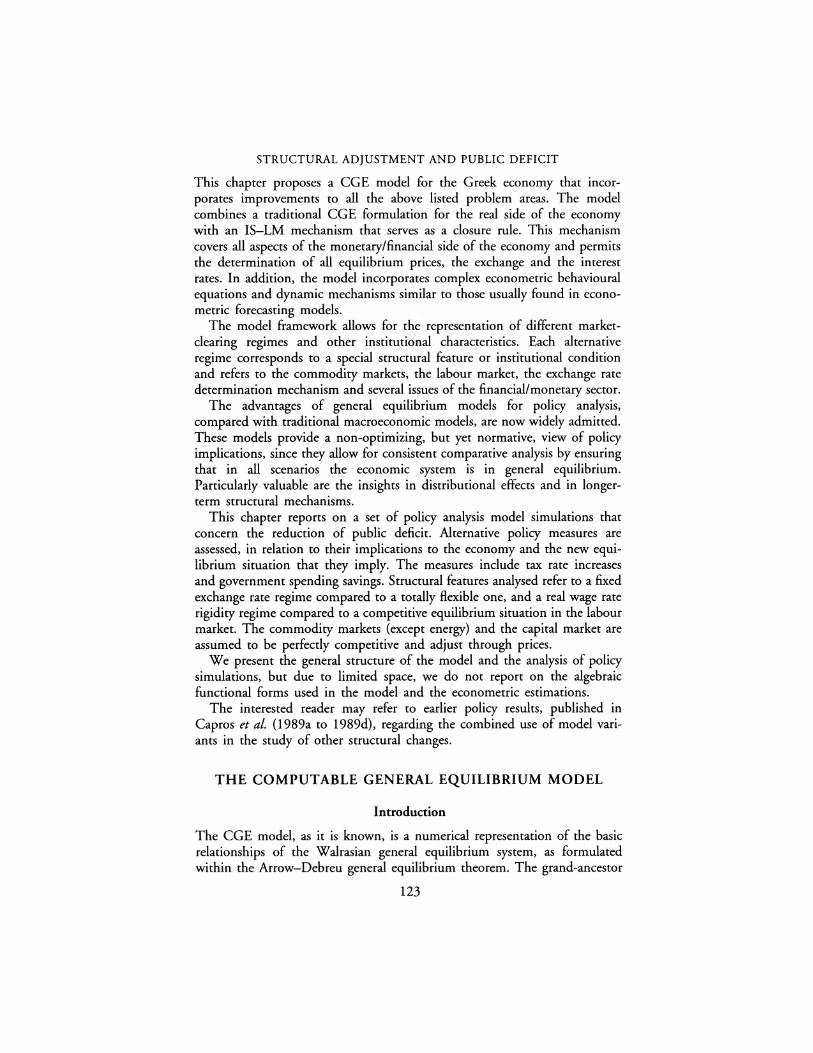
STRUCTURAL ADJUSTMENT AND PUBLIC DEFICIT
This chapter proposes a CGE model for the Greek economy that incorporates improvements to all the above listed problem areas. The model combines a traditional CGE formulation for the real side of the economy with an IS-LM mechanism that serves as a closure rule. This mechanism covers all aspects of the monetary/financial side of the economy and permits the determination of all equilibrium prices, the exchange and the interest rates. In addition, the model incorporates complex econometric behavioural equations and dynamic mechanisms similar to those usually found in econometric forecasting models.
The model framework allows for the representation of different marketclearing regimes and other institutional characteristics. Each alternative regime corresponds to a special structural feature or institutional condition and refers to the commodity markets, the labour market, the exchange rate determination mechanism and several issues of the financial/monetary sector.
The advantages of general equilibrium models for policy analysis, compared with traditional macroeconomic models, are now widely admitted. These models provide a non-optimizing, but yet normative, view of policy implications, since they allow for consistent comparative analysis by ensuring that in all scenarios the economic system is in general equilibrium. Particularly valuable are the insights in distributional effects and in longerterm structural mechanisms.
This chapter reports on a set of policy analysis model simulations that concern the reduction of public deficit. Alternative policy measures are assessed, in relation to their implications to the economy and the new equilibrium situation that they imply. The measures include tax rate increases and government spending savings. Structural features analysed refer to a fixed exchange rate regime compared to a totally flexible one, and a real wage rate rigidity regime compared to a competitive equilibrium situation in the labour market. The commodity markets (except energy) and the capital market are assumed to be perfectly competitive and adjust through prices.
We present the general structure of the model and the analysis of policy simulations, but due to limited space, we do not report on the algebraic functional forms used in the model and the econometric estimations.
The interested reader may refer to earlier policy results, published in Capros et al. (1989a to 1989d), regarding the combined use of model variants in the study of other structural changes.
THE COMPUTABLE GENERAL EQUILIBRIUM MODEL
Introduction
The CGE model, as it is known, is a numerical representation of the basic relationships of the Walrasian general equilibrium system, as formulated within the Arrow-Debreu general equilibrium theorem. The grand-ancestor
123

P. CAPROS AND P. KARADELOGLOU
of today's empirical research activities is the model by Johansen (1979). The CGE modelling field gained significant attention following the work supported by the World Bank. Descriptions of CGE models can be found in: Shoven and Whalley (1972 and 1984), Hudson and Jorgenson (1974 and 1977), Adelman and Robinson (1978), Deardorff and Stern (1982), Dervis et al. (1982), Lysy (1983), Cordon et al. (1985), Blitzer and Eckaus (1986), Devarajan and Sierra {1986), Levy (1987), Pereira and Shoven (1988), Decaluwe and Martens (1987 and 1988) and J. de Melo {1988). Concerning the closure rule problems, which are of crucial importance for the appraisal of the CGE model properties, one may refer to Rattso (1982), Taylor and Lysy (1979) and Dewatripont and Michel (1987). Extensions of the traditional CGE model by linking a financial/monetary sub-model may be found in Bourguignon et al. (1989), M. de Melo et al. (1989) and P. Capros et al. (1991b). Extensions dealing with foreign trade deficits may be found in Kharas and Shashido {1987) and Lewis and Urata (1984).
The CGE theoretical framework requires that all markets are clearing through prices. This procedure is usually called price-adjustment of the markets. The empirical applications of CGE models do not always assume market clearing through price mechanisms in all markets; on the contrary authors often incorporate non-neoclassical assumptions concerning market rigidities and imperfections in an attempt to capture the macroeconomic forces that prevail in real-world cases; See Robinson {1986), Bourguignon et al. (1983 and 1989), Capros et al. (1990, 1991a). In such cases some markets of the model may be cleared through price-adjustment, while some others include an endogenous determination of the price level (like the one traditionally found in macroeconometric models, assuming an excess supply market regime) which guarantees a quantity-adjusted equilibrium.
The following sets of equations illustrate the alternative mechanisms for representing market types:
Competitive markets:
D = f(p)
s = g(p)
D=S
Excess supply markets:
D = f(p)
s = g(p)
S=D
124

STRUCTURAL ADJUSTMENT AND PUBLIC DEFICIT
U = SIS
p = h(S,S)
where D, S and p denote demand, supply and prices, respectively, bars indicate potential production and the absence of bars corresponds to effective supply and demand. U is then the rate of capacities utilization or the rate of unemployment, depending on the nature of the market. The model accepts only one type of regime per market and per model variant.
The formulation found in the competitive market type is adopted for the market of goods and labour in most CGE models; see de Melo (1988). The excess supply market illustrates the formulation used for the labour market (or the foreign exchange market) when unemployment (and usually a trade deficit) prevails. This type of market is also the typical formulation of all markets represented in neo-Keynesian macroeconometric models; see Capros et al. (1989a). In a multi-market CGE model, all three types of marketclearing formulations may co-exist, in the sense that some markets are perfectly competitive, while others are not.
The mechanisms that achieve consistency of transactions at the macroeconomic level, often called macro-framework, is particularly important for appraising the model's properties, and this is independent of the way markets clear. The macro-framework mechanism may be represented by four simultaneous identities: the national income identity, the balance of payments, the public budget balance and the savings-investment identity. In traditional CGE models, the savings-investment identity is usually adopted as the 'closure rule' and it is often used for evaluating investment. Such a restrictive assumption is necessary because in these models there is no financial-monetary sector. In traditional econometric models which formulate the IS-LM scheme, the savings-investment identity is implicitly induced by the flow-of-funds identity which equalizes demand and supply of money.
The macro-framework, as it will be presented below in a simple manner, is used in our CGE model to integrate the real and the monetary/financial sectors of the economy and to overcome the closure rule limitation. A similar approach is also followed by Bourguignon et al. (1989).
The national income identity may be written as:
C + I+ G + (X - M) = Y + T while Y = C + S
where C, I, G, X, M, T and S denote, respectively, private consumption, investment, government expenditure, exports, imports, net tax receipts and savings. The balance-of-payments identity is written as:
X-M = EJ.1A.1+ LlBR- LlB1)
125

P. CAPROS AND P. KARADELOGLOU
which represents the financing of deficits (or the allocation of surplus) by changes in net foreign assets A1, bank reserves BR and foreign borrowing B1, depending on the exchange rate Ex. The public budget identity also represents financing of deficit through bank borrowing B , private domestic borrowing Pg and foreign borrowing B1, as follows: g
G - T = L1Bg + L1Pg + ExL1Bf
The strict equality of savings and investments, which is used in traditional CGE models, is expanded in a way that any difference between them is financed through changes in money supply M5 , private domestic borrowing of government, net foreign assets and private lending from banks B p' as follows:
S - I= L1M5 + L1Pg + ExL1Af - L1BP
The Walrasian closure, which may be further interpreted as flow-of-funds identity, is re-written as follows:
-(G-T) + (S-1)-(X-M) = 0
which implies:
-(L1Bg + L1Pg + ExL1B1) + (L1M5 + L1Pg + ExL1Af -L1BP)
-Ex(L1Ar + L1BR-L1B1) = 0
and:
The last equation is the monetary identity and constitutes the expansion of the 'closure rule' when incorporating a financial sector into the CGE framework.
The above macro-framework, that is the set of accounting identities, is able to cover a large spectrum of financial market conditions and institutional characteristics. Alternative situations may be represented by choosing the appropriate set of endogenous variables to be solved by these identities.
The two following subsections present the real and the monetary sectors of the model and give the corresponding equations. In this presentation, we make abstraction of implementation details concerning both the accounting system and the particular formulation of econometric equations.
The real sector
The real sector of the economy, as represented by the modelling framework, comprises several sectors (indexed by k) and an equal number of commodi-
126

STRUCTURAL ADJUSTMENT AND PUBLIC DEFICIT
ties (indexed by i). We may represent several economic agents, although in the maquette, the equations of which are given below, we include four economic agents, namely producers (enterprises), consumers (households), government and the rest of the world. Consumers supply labour force to producers who employ it as production factor together with capital, energy and materials. The commodities are traded, thus imported and exported. The real sector of the economy then comprises several markets: one market per commodity and one labour market. Government's behaviour is assumed to be exogenous.
Demand for commodities is formed by private consumption (index p), investment in dwellings (index R), government expenditure (index g) and investment (index G), private investment, stock variation (index S) and exports (index X). These demand elements are allocated over the set of commodities. Supply of commodities is ensured by domestic production (index F) and imports (index M).
A basic behavioural equation determines the distribution of gross private income in consumption and gross savings. Equation ( 6.1) determines private consumption by referring to the Davidson et al. (1978) approach, which applies an error correction mechanism on the difference between consumption and real income. Adjustment depends also on unemployment, inflation and the real interest rate.
(!=<I>,[½, UR, ilp,, r,- ilp,' w] Pc Pc
(6.1)
Equation (6.2) allocates total private consumption over a set of consumption categories (food, housing, durables, and so on, indexed by j). Among the various allocation systems that have been proposed in the literature, equation (6.2) might implement one of the following approaches: the Houthakker-Taylor model (Houthakker and Taylor, 1970), a linear expenditure system, a Rotterdam model or an indirect utility-derived function (as by Jorgenson-Stoker). These link demands with the change in total consumption, some 'state' variables and relative prices. Equation (6.2) corresponds to a system of econometric equations estimated simultaneously with constraints in the parameters. A transformation matrix is used in equation (6.3) to pass from consumption by category to consumption by commodity.
'1C/ = cl>/ [ '1cP, '1 (~) , ... ] V j (6.2)
CP = ~ tc~-Cc Vi ' £.i -'} J (6.3)
j
127

P. CAPROS AND P. KARADELOGLOU
Investment in dwellings is modelled in equation (6.4) as a function of real income, inflation and real interest rate.
IR _ ,¥,.R r Yj, A R A R] (6.4) - '¥ l,pf, app r,- J.JP1
Equations (6.5), (6.6) and (6.7) allocate government expenditure, public investment, investment in dwellings and private investment over the set of commodities {investment goods) by employing fixed technical coefficients. In particular, equation (6.7) aggregates sectoral investment over an investment matrix. Private investment by sector is determined as derived factor demand, while government expenditure and public investment are both exogenous.
C/= t,dCK Vi
C/' = t£./' J" Vi, ,\ = R,G (LG exogenous)
(6.5)
(6.6)
(6.7)
Equation (6.8) is the traditional Leontief input/output accounting scheme. It computes intermediate demand for commodities by sectors as being proportional to effective sectoral production of commodities. The proportionality factors (that is, the technical coefficients) are endogenous and are evaluated in equation (6.18) as derived demand for factors.
c/ = t!; Q{ V i, V k (6.8)
So, supply of commodities has to be represented in a way to determine intermediate consumption and factor demand by sector. Production possibility frontiers, used for this purpose, must provide also for the evaluation of potential production by sector. The choice of the functional form is not represented here; however we admit that technology is following the putty-day assumption, in which the mix of factors can change only in the latest capital vintage, while remaining invariant for old vintages.
(6.9)
(6.10)
(6.11)
128

STRUCTURAL ADJUSTMENT AND PUBLIC DEFICIT
Pt = <l>z[D (pft), ... ] V k (6.12)
p;' = <I>f [D (pi), ... ] V k (6.13)
Flexibility of production is assumed for the use of capital, labour, energy and materials as production factors. By defining a production function, we derive from profit maximization the demand for capital, labour, energy and materials (equations (6.14) to (6.17)), as well as potential production (equation (6.19)). The derived demand for production factors depends on relative factor prices, which are determined in equations (6.10) to (6.13). The cost of labour depends on the wage rate determined in the labour market, while the cost of capital is evaluated by, for example, an Ando et al. ( 197 4) formula. Factor-demand equations are simultaneously estimate for each sector by imposing constraints on the parameters. These equations determine the demand for factors in the latest vintage, thus evaluate investment and the change in demand for labour, energy and materials. Investment accumulation forms the capital stock, in equation (6.9), assuming that capital is settled at the beginning of the year and remains fixed during the year. Depending on the separability assumption, about the form of the production function, we provide in equation (6.18) the further decomposition of aggregate factors into more detailed factor categories, which are used to evaluate the technical coefficients used in the input/output, equation (6.8).
lk _ m' [ '() P't nP] V k - - 'l!'k -gk t' K ' ... , '<k Kk Pk
(6.14)
Nt1Nk = <1>; [-g;(t), Pr, ... , Qf] V k k,(-1) h
(6.15)
Mk = <1>; [-g;(t), Pi, ... , Qf] V k Ek,(-1) h
(6.16)
M'1Mk = <1>; [-g; (t), Pr' ... , Qf] V k k,(-1) h
(6.17)
. . Ek Mk pi, [ I ·1 ] tci, = <l>i, Qf QI, pj2 , • • • V k (6.18)
(6.19)
129
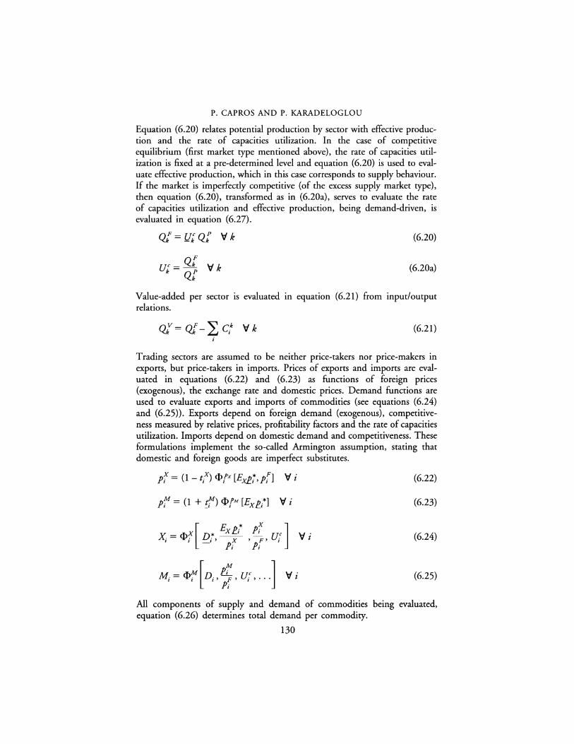
P. CAPROS AND P. KARADELOGLOU
Equation (6.20) relates potential production by sector with effective production and the rate of capacities utilization. In the case of competitive equilibrium (first market type mentioned above), the rate of capacities utilization is fixed at a pre-determined level and equation (6.20) is used to evaluate effective production, which in this case corresponds to supply behaviour. If the market is imperfectly competitive (of the excess supply market type), then equation (6.20), transformed as in (6.20a), serves to evaluate the rate of capacities utilization and effective production, being demand-driven, is evaluated in equation (6.27).
Qf = UJQ{ V k
uc= Q[ V k k Qt
(6.20)
(6.20a)
Value-added per sector is evaluated in equation (6.21) from input/output relations.
QJ=Qf-2JC} Vk (6.21) i
Trading sectors are assumed to be neither price-takers nor price-makers in exports, but price-takers in imports. Prices of exports and imports are evaluated in equations (6.22) and (6.23) as functions of foreign prices (exogenous), the exchange rate and domestic prices. Demand functions are used to evaluate exports and imports of commodities (see equations (6.24) and (6.25)). Exports depend on foreign demand (exogenous), competitiveness measured by relative prices, profitability factors and the rate of capacities utilization. Imports depend on domestic demand and competitiveness. These formulations implement the so-called Armington assumption, stating that domestic and foreign goods are imperfect substitutes.
pf = (1 - t{) cf>fx [ExJ!7, p{] Vi
[ E * x ] - X * X P.i Pi C
X. - <I>. D.' X ' F' u I I -' Pi Pi I
Vi
(6.22)
(6.23)
(6.24)
(6.25)
All components of supply and demand of commodities being evaluated, equation (6.26) determines total demand per commodity.
130

STRUCTURAL ADJUSTMENT AND PUBLIC DEFICIT
Di = L c/ + c; + c/ + Cl + cic + c/ + c/ + X; v i k
Q/ = Di-Mi- T; Vi
(6.26)
(6.27)
& mentioned, if a commodity market is assumed to be perfectly competitive, then the rate of capacities utilization is fixed and effective production is determined by equation (6.20), as equal to potential production, so it is supply-driven. In this case, equilibrium equation (6.27) corresponds to the determination of the commodity prices in domestic supply, that is, p{.
If a commodity market is not perfectly competitive, we assume that excess supply prevails. Then, equation (6.20a) is solved for the capacities utilization rate and effective production is evaluated from equation (6.27), so it is demand-driven. Hence, we need one more equation (per sector) to evaluate commodity prices, that is p[. In excess supply situations and imperfect markets, it is natural to assume cost-driven mark-up pricing, as it is usually done in traditional econometric models (which because of this assumption are often called neo-Keynesian models). Such a price equation is represented by (6.27a), which is eliminated from the model in the case of perfectly competitive markets (and it is not used in the CGE model variant we are using for policy analysis in this chapter).
F - F w i K i k i C T• • ( N )µ'( K )"; ( Ck)A/ Pi - <l>i Pi Q! Pi Qf 1; Pi Qf (Ui) · V z (6.27a)
Notice that it is quite possible to mix market-clearing situations across commodities. That is, one commodity may be formulated in a way that its price is determined by the equilibrium of demand and supply, equation (6.27), while another may employ equation (6.27a) for cost-based pricing.
Equations (6.28) t'.> (6.30) concern the labour market. Labour supply depends on exogen01 .s population and expected real wages, in equation (6.28). The correspo 1.ding function is derived simultaneously with the consumption function (6.1) from utility maximization under budget constraint. Labour demand, in equation (6.29), is the sum of sectoral labour demands, derived from production functions, and exogenous public sector employees.
N[ W· ] N' = <I> POP, p;, ...
Nd="'N+N £.J k -G k
(6.28)
(6.29)
131

P. CAPROS AND P. KARADELOGLOU
Nd= (1 - IJR)N' (6.30)
The labour market can clear under two alternative regimes. The perfectly competitive case is represented by .equation (6.30) which serves to evaluate the average wage rate w. In this case the rate of unemployment is fixed to zero (or at an exogenous predetermined level, the natural unemployment level).
In the imperfectly competitive case, excess labour supply is assumed to prevail, and the rate of unemployment is determined by (6.30a), while the wage rate is evaluated by some price indexation mechanism. Equation (6.30b) proposes a Phillips curve formulation extended with the incorporation of productivity effects. Notice, again, that equations (6.23a) and (6.23b) are not used in the full CGE variant of the model.
(6.30a)
~=<I> r Llpc U .::1(Q)] w(-1) w l..Pc,(-1) , R, N
(6.30b)
Sectoral wage rates are indexed to the average wage rate, in equation (6.31). If data are available and if separate labour markets seem to prevail, one can formulate the labour market separately for each labour category and even mix market-clearing regimes.
(6.31)
Derived prices, equations (6.32) to (6.40), depend on commodity prices in domestic supply, that is pf and the prices of imported goods. The corresponding equations weight these prices by means of shares of domestic production and imports. Exogenous tax rates are applied on the formation of these derived prices.
(6.32)
Vi (6.33)
(6.34)
132

STRUCTURAL ADJUSTMENT AND PUBLIC DEFICIT
A_ A ( Qf' F M; M) P; - oc A (1 + .1; ) Q{ + M/; + Q{ + M/;
'v i, 'v A = g, I, R, G
pf = L tdp;[ 'v k i
. . ( QF F M. M) '= oc 1 + t' ' + ' h ( _k) Qf + M;P; Qf + M;P;
LC1pL pf = iEM 'v k
LC1 iEM
p{Qf- LPLC1 p'f= i 'v k
'v i, 'v k
(6.35)
(6.36)
(6.37)
(6.38)
(6.39)
(6.40)
Equations (6.41) and (6.42) determine revenues from indirect taxes and from tariffs, respectively.
T = ~ t-cp.cC!' + ~ t-Rp.RCR + ~ t-Ip_ICI + ~ t,,gp$C$ ~-z l l ~-t t t ~-t t t ~- t t
i i i
(6.41)
T-=~;----~----' p/ 'v i (6.42)
Equations (6.43) to (6.48) are accounting identities that determine income and savings. In fact, these equations distribute the value-added among the economic agents, establish the transfer of flows between them and compute available income which influences consumption.
133

P. CAPROS AND P. KARADELOGLOU
(6.43)
(6.44)
(6.45)
s = R + Rk-P CP - T - ~ p.1C.1 - ~ p.Fc,S - ~ p.Rc,R p W C ,£.J t t ,£.J t -t ,£.J t t (6.46)
i i i
-w.NG-~ (pfCl + p?C?)-~ .1/p/X; (6.47) j i
Table 6.1 The financial/monetary sector - the matrix of flow-of-funds
Private sector (P) Government (G)
Cash M"
Saving deposits M,,,.
Time deposits M,,,. Bank bonds Mbb Government bonds
Mgb Treasury bills M,b Foreign exchange
deposits Mf Total assets MP
Credits tlLP
Foreign capital inflow M 1
Foreign exchange loans flB1
Domestic &orrowing flBK
Ceniral bank loans tlB1
Other transfers Og
Net savings SP Net savings Sg
Total liabilities tlLiP
Banks (BJ
Private loans tlBP
Central bank loans tlB
Treasiry bills tlB,b Government bonds
tlBgb
Total assets Mb
Cash M"
Saving deposits M,,,.
Time deposits M,..
Bank bonds Mbb Foreign exchange
deposits M/ Bank reserves 'tl.B R
Total liabilities tlLib
134
Foreign sector (F)
Foreign capital inflow
Mt Foreign exchange loans
flBf Other transfers Og Bank reserves flB R
Net savings Sw

Table 6.2 The Social Accounting Matrix (real sector)
Expenditures
Receipts Sectors Products Factors Enterprises Households Government Capital World Total account
Sectors domestic export sales sum subsidies exports sales of C/ by i r X;
Products intermediate consumption government private demand demand CP and consumption investment C/ investment Oand lk
[R investment [G
Factors factor value added payments
Qr Enterprises gross profits
P;Q,,V- wkNk~ enterprise income
tax Households wages distributed foreign household income
w,N, profits transfers Rf
Government indirect taxes tariffs factor taxes enterprise direct government receipts (part of T) tM taxes taxes
tk tw Capital enterprise household government nee capital total saving (= 0)
account savings savings savings inflow part of s, part of s, Sg(+ or-) SW {+or-)
Rest of the world
imports imports M;
Total total total value added enterprise households government investments foreign payments absorption expenditure expenditure expenditure exchange

P. CAPROS AND P. KARADELOGLOU
SW=~ (;;MM;-p{X;)-B1 j
(6.48)
The residuals from rhis income distribution are the net savings (positive in rhe case of surplus, negative in rhe case of deficit) of the economic agents, namely for the private sector, rhe government and the rest of the world, as shown in Table 6.1. These are determined by equations (6.46) to (6.48) and constitute the starting point of the financial/monetary sector of rhe model.
Notice rhat, by construction, S + S + S = 0 which is an expression of the Walras law. In fact, all model ~onsfruct;, wirhin the real sector, may be grouped within the framework of a Social Accounting Matrix - SAM (see Table 6.2), which ensures consistency and equilibrium of flows from production to rhe agents and back to consumption. The construction of SAM is rhe starting point of rhe model building work. The definition of rhe set of prices, ensures the consistency of rhe SAM, also in current currency, a fact which finally is reflected in the above condition, which states that the algebraic sum of net savings over rhe set of agents is, by construction, equal to zero.
THE FINANCIAL/MONETARY SECTOR
The financial behaviour of economic agents is based on a portfolio model which is derived by maximizing expected utility. The model allocates financial wealth among various assets. The allocation is made on the basis of expected yields and other determining factors (see van Erp et al., 1989; van der Beken and van der _Putten, 1989). Such an approach avoids reduced-form models of financial mechanisms and uses relative interest rates as explanatory variables. Depending on wherher liberalized capital markets are represented in rhe model, rhese interest rates together with the exchange rate can be derived from the equilibrium of financial supply-and-demand flows.
The structure of our financial/ monetary model is based on rhe above approach. Regarding its accounting structure, the model is based on a matrix of flows of funds, involving, in the maquette, four economic agents, namely rhe private, government, banking and foreign sectors.
A simplified form of the flow-of-funds matrix is given in Table 6.1. In our model we do not use a full-scale matrix of flows of funds, which is not necessary for the model design. In fact, we adopt a hybrid approach where rhe flow-of-funds approach is mixed with a 'deficit financing approach'. More specifically, rhe foreign and public sectors are represented only wirh respect to the financing of their surpluses, while rhe banking and private sectors are represented following an 'assets-liabilities balance' approach. However, we fully guarantee stock-flow consistency for all transactions.
136

STRUCTURAL ADJUSTMENT AND PUBLIC DEFICIT
The equations presented below correspond to a variant of the model which is simple for tutorial reasons. It is easy to see that any different institutional characteristics, which might prevail in the financial markets and policy, can be incorporated without altering the main model mechanism.
On the assets side of the private sector, total wealth (W) is evaluated, dynamically, by private net savings, a variable coming from the real part of the model:
(6.49)
The allocation of total wealth of the private sector is described as 'risk-averse investment behaviour'. Private agents are assumed to maximize the utility of the return from a portfolio. In this respect future returns are uncertain and the risk aversion is formalized as diminishing marginal utility. It is also assumed that changes in the composition of the portfolio in relation to the starting point entail costs. This portfolio model is based on Parkin (1970) and used in the Freia-Kompas model of the Dutch economy and has also been applied to Belgium (see van Erp et al., 1989 and van de Beken and van der Putten, 1989).
The basic model, expanded with a number of sector-specific variables, determines the optimum portfolio composition, in terms of cash, time deposits, saving deposits, government bonds, bank bonds and treasury bills; see equation (6.50). The allocation mainly depends on the relative rates of return (assimilated to interest rates) from the above assets. The corresponding equations are simultaneously estimated and a set of restrictions on parameters are imposed. Restrictions include symmetry and additivity conditions, the latter implying that one of the equations is redundant. Also, adjustment costs and dynamic behaviour are incorporated in these equations. Equation (6.51) determines the changes (flows) of assets allocation.
~ - ~ ,I-. ( ) + ~ XA V M W - a,,_ + £.J /3µ,v'o/µ,v r,,_ - rv £.J 'Yµ,A W µ, E ~µ,EM ,\
(6.50)
L1A,,, = A,,, -A,,_c-tl V µ, (6.51)
Foreign exchange deposits, in equation (6.52), are explained by the evolution of the exchange rate, the foreign to domestic interest rate differential and the capital and transfer inflow which enters the country.
L1AJ = <l>[r - r1 , ExLlA1, Ex - ---1.s_ , · · .] Pc,<-tl
(6.52)
The demand of credit by the private sector, equation (6.53), bears the influence of the real interest rate, the profit rate and the volume of total
137
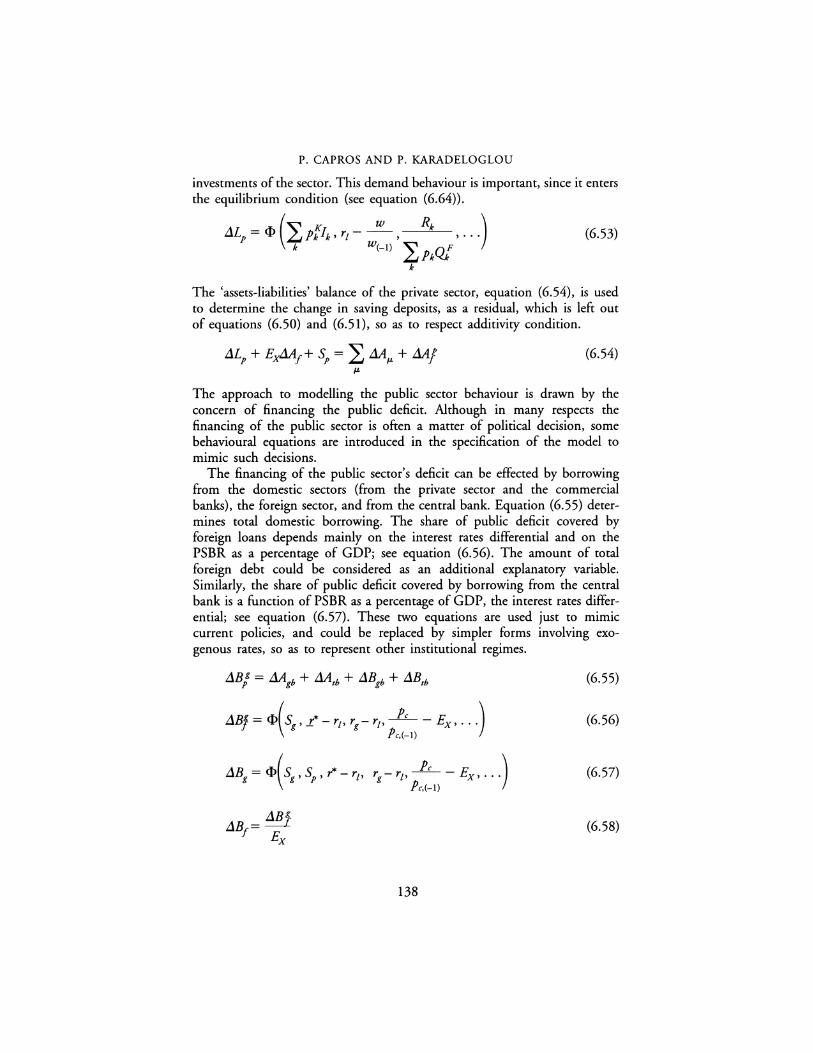
P. CAPROS AND P. KARADELOGLOU
investments of the sector. This demand behaviour is important, since it enters the equilibrium condition (see equation (6.64)).
_ (~ K W Rk ) J.LP - <I> £.J h lk, r1 - -- , -~- , •••
k w(-1) LhQJ (6.53)
k
The 'assets-liabilities' balance of the private sector, equation (6.54), is used to determine the change in saving deposits, as a residual, which is left out of equations (6.50) and (6.51), so as to respect additivity condition.
J.Lp + E.xM1 + sp = L Ml< + .dAJ (6.54) 1£
The approach to modelling the public sector behaviour is drawn by the concern of financing the public deficit. Although in many respects the financing of the public sector is often a matter of political decision, some behavioural equations are introduced in the specification of the model to mimic such decisions.
The financing of the public sector's deficit can be effected by borrowing from the domestic sectors (from the private sector and the commercial banks), the foreign sector, and from the central bank. Equation (6.55) determines total domestic borrowing. The share of public deficit covered by foreign loans depends mainly on the interest rates differential and on the PSBR as a percentage of GDP; see equation (6.56). The amount of total foreign debt could be considered as an additional explanatory variable. Similarly, the share of public deficit covered by borrowing from the central bank is a function of PSBR as a percentage of GDP, the interest rates differential; see equation (6.57). These two equations are used just to mimic current policies, and could be replaced by simpler forms involving exogenous rates, so as to represent other institutional regimes.
'1.Bf = .c:1Agb + .c:1Atb + J.Bgb + J.Btb
'1.Bf = <l>(sg, .r - r1, rg- r1, ---1.s_ - Ex, ... ) P,,c-1>
138
(6.55)
(6.56)
(6.57)
(6.58)

STRUCTURAL ADJUSTMENT AND PUBLIC DEFICIT
J.Bf + J.B/ + J.Bg + ExOg + Sg = 0 (6.59)
Domestic borrowing of government is divided into two parts: treasury bills and government bonds. Both can be acquired by the private sector and by commercial banks. Concerning the private sector, investment in these two assets emanates from portfolio allocation. For the banking sector, we retain a formulation, see equations (6.60) and (6.61), which explicitly reflects one possible institutional regime, in which commercial banks are obliged to buy treasury bills and government bonds at a rate proportional to their total liabilities. By substituting equation (6.55) into equation (6.59), we derive the demand-supply equilibrium in financing public deficits. This equilibrium serves to determine the rate of interest of government lending, that is r , which further leads the interest rates of bonds and treasury bills in equiition (6.68).
J.Btb = PtbJ.Lib (6.60)
(6.61)
Equations (6.62) and (6.63) represent the assets-liabilities balance in the banking sector. In our model, this serves to evaluate the capacity of banks to lend the private sector, that is variable ilB, which is a supply behaviour. This formulation is also in accordance with t~t institutional regime in which a leakage in capital supply to the private sector prevails, induced by the imperative financing of public deficit.
(6.62)
(6.63)
So equation (6.64) represents demand-supply equilibrium of the capital flows addressed to the private sector. This serves to determine the private lending interest rate, that is r1, which is used in both the real and the monetary sectors of the model, and further leads the interest rates of assets; see equation (6.67).
~=~ ~~
Modelling of the foreign sector is orientated towards determining the ways for covering the current account deficit. Foreign capital inflow is an independent variable and is a function of relative profitability of investment assets, in equation (6.65). Equation (6.66) corresponds to the financing of the current account deficit. In the maquette, we assume that changes in bank reserves are maintained at some predetermined level. Thus, the balance in equation (6.66) is achieved through movements of the nominal exchange rate, so (6.66) is an equilibrium condition.
139

P. CAPROS AND P. KARADELOGLOU
M1 = <l>(.r- r1 , ~ - Ex, ... ) Pc,c-1>
(6.65)
(6.66)
Equation (6.69) evaluates, dynamically, total public debt by accumulating deficits. Public debt further influences interests and annuities which enter the equation (6.47), which determines net savings of the public sector (mechanism not shown in the maquette).
r,,_ = <f,,,_(r1), µ, = cs, bb, td, sd
r,,_ = <f,,,_(rg), µ, = gb, tb
BK = Bf-o + '1.Bf + '1.Bf
(6.67)
(6.68)
(6.69)
In summary, the present model variant, of the financial/monetary sector, determines endogenously three equilibrium prices: (i) the private sector lending interest rate, (ii) the government lending interest rate and (iii) the exchange rate.
The above specification does not exclude, however, the possibility of including different structural or institutional changes that may occur in the economy. This may be effected by some other selection of endogenous and exogenous variables. For example, it is possible to consider that the exchange rate is exogenously determined by the authorities. In this case foreign exchange reserves should be endogenous and be estimated as a residual variable. Furthermore, if the lending interest rate is fixed by the central bank, a credit rationing regime would occur. In this case, demand for credits will be rationed by supply, and equation (6.64), which determines credit demand, must be eliminated from the model.
POLICY ANALYSIS
The model was used in policy analysis, in particular to analyse alternative measures aiming to reduce public deficit. The candidate measures are classified in two categories, depending on their primary effect: those increasing government revenues and those decreasing government expenditures.
In the model, revenues may increase through direct income taxation, indirect taxation or the contribution of the private sector to social security funding. Expenditures may decrease through economies in government spending or by reducing the public sector wage bill (for example by reducing the number of public sector employees). Rather than analysing combined policies, which are more realistic, the present chapter reports on model runs
140

STRUCTURAL ADJUSTMENT AND PUBLIC DEFICIT
involving a single type of measure. This allows for the comparative appraisal of measures and at the same time is a benchmark for model behaviour.
All scenarios were constructed by changing the value of some exogenous parameters (for example a t;ix rate). Changes were considered to be permanent (not a shock) and anticipated. Runs were made dynamically, over a period of nine years. The simulation period corresponds to the past, for which full model calibration was performed. This implies that the results may be influenced by the values of the calibration adjustments, although such an influence is estimated to be low.
Tables 6.3 to 6.7 present a summary of results for the first, the second and the last simulation years.
The same model runs were made for three variants of the model. These variants correspond to different assumptions about the prevailing market-clearing regime in the labour market and the flexibility of the exchange rate regime (in other terms the type of IS-LM closure). These variants are as follows:
• A foll equilibrium variant. price adjustment in competitive markets for goods and labour; an exogenous rate corresponds to natural unemployment; the exchange rate is fully flexible so as to render unchanged the central bank reserves.
• A fixed exchange rate case. all markets remain competitive; the central bank reserves are adjusting, while the exchange rate remains fixed.
• Price indexed wages and fixed exchange rate. in addition to the assumption about the exchange rate regime, this model variant assumes a rigid labour market, corresponding to an exogenous real wage rate (where the price indexation rate is equal to 1); in this case, unemployment may arise (as an endogenous result).
The comparison of results for the model variants allows for the appraisal of structural features in analysing the government policy. Structural features include market-clearing regimes in the real sector or institutional regimes in the financial sector, as mentioned before. A policy measure may have different, and in some cases contrasting, effects, depending on the market regime or the institutional context within which the measure operates.
Increase of income tax rate by 1 per cent
The aim of this policy is to reduce public deficit by increasing direct income tax rate by 1 per cent (see Table 6.3). The primary impact of such a policy measure is a transfer of wealth from households to the public sector, inducing changes in total demand.
The reduction of public sector deficit and its funding, relaxes loan demand constraints in the capital market and liberates funds which are made available to finance the private sector. The new equilibrium point corresponds, then, to lower interest rates which cause several second-order effects.
141

Table 6.3 NTUA, ICGE model - scenario: increase of income tax rate by 1 %
Full equilibrium Fixed exchange rate Price-indexed wages, fixed exchange rate
Year.r I 2 9 I 2 9 I 2 9
Economic activity (volumes) (% change from baseline) GDP in factor prices -0.07 -0.06 0.22 -0.06 -0.07 -0.05 -0.14 -0.18 -0.05 Private consumption -0.52 -0.37 2.74 -0.54 -0.71 -1.24 -0.64 -0.75 -1.46 Private investment 0.59 0.28 1.22 0.50 0.39 3.58 1.30 1.20 0.81 Investment in dwellings 4.52 4.59 6.25 5.17 2.90 15.95 0.10 0.21 6.11 Exports 0.73 0.10 -4.75 0.86 1.24 0.67 0.91 1.02 2.13 Imports -0.19 -0.10 5.23 -0.26 -0.59 -2.68 -0.19 -0.45 -2.39 Production manufacturing -0.07 -0.06 0.13 -0.05 -0.07 -0.14 -0.17 -0.20 -0.03 Production services -0.09 -0.08 0.26 -0.08 -0.08 -0.02 -0.16 -0.20 -0.05 Production agriculture -0.03 -0.03 0.21 -0.03 -0.03 -0.06 -0.05 -0.08 -0.07 Sectoral employment -0.10 -0.12 0.49 -0.08 -0.11 0.00 -0.20 -0.31 -0.08
Prices (% change from baseline) GDP defiacor (factor prices) -0.44 -1.26 -5.89 -0.43 -1.29 -7.76 0.15 -0.42 -6.97 Consumer price index -0.46 -1.34 -9.86 -0.37 -0.95 -6.18 -0.01 -0.38 -5.36 Wage race -1.79 -2.49 -13.17 -1.98 -1.18 -12.96 -0.01 -0.19 -6.15 Capital cost (manufacturing) -3.60 -3.47 -15.80 -3.42 -2.64 -20.52 -4.59 -4.22 -8.15 Price of manufacturing output -2.00 -3.00 -2.96 -1.75 -2.98 -1.66 -1.81 -2.42 -4.62 Price of service output 0.32 -0.26 -8.52 0.20 -0.41 -10.37 1.09 0.57 -7.86 Price of agricultural output -0.68 -2.78 -14.40 -0.25 -0.35 -0.32 -0.38 -0.36 -0.31 Import prices (manufacturing) -0.29 -1.66 -17.87 0.00 0.00 0.00 0.00 0.00 0.00 Export prices (manufacturing) -1.04 -2.33 -10.28 -0.84 -1.78 -2.71 -0.87 -1.50 -3.33 Exchange race ( deval. if >0) -0.46 -2.47 -14.12
Accounts of agents (abs. di.ff. from baseline) Gross surplus households -7,784 -10,813 -28,777 -8,054 -10,149 -77,214 -5,621 -7,922 -64,293 Gross surplus firms 968 2,564 -17,617 1,023 2,154 25,261 -377 696 24,910 Gross surplus government 7,607 9,515 64,806 7,820 9,410 80,708 6,770 8,486 65,116 Current account 791 1,267 18,412 788 1,415 28,755 773 1,260 25,732

Table 6.3 (continued)
Full equilibrium Fixed exchange rate Price-indexed wages, fixed exchange rate
Years 1 2 9 1 2 9 1 2 9
Asset allocation by private sector (abs. diff from baseline, in %) Cash 0.202 0.508 3.791 0.248 0.278 4.074 -0.034 0.247 1.089 Time deposits -1.298 -1.693 -4.667 -1.385 -0.808 -6.069 -0.540 -0.773 -1.523 Saving deposits -0.979 -1.065 -2.293 -1.054 -0.280 -2.714 -0.408 -0.441 -1.039 Bonds -0.108 -0.213 -0.978 -0.121 -0.044 -0.319 0.018 -0.036 -0.352 Shares 2.182 2.463 4.148 2.313 0.854 5.028 0.965 1.004 1.826
Flows (in % change from baseline) Foreign exchange deposits -35.52 -42.65 -10.03 -32.95 -24.76 -11.40 -13.13 -15.29 -8.18 Demand for credits and loans -0.97 -1.58 -14.69 -1.15 0.12 -6.30 0.46 0.07 -4.52
Government (abs. diff from baseline) Foreign loans -2,074 -2,350 -39,797 -2,338 -2,786 -26,163 -1,709 -2,621 -19,614 National loans -1,599 -2,897 7,985 -1,361 -4,180 -19,970 -2,526 -2,508 -25,567
Banks (% change from baseline) Total liabilities -3.31 -5.29 -13.77 -3.47 -4.07 -11.75 -2.09 -3.73 -9.23 Government loans and securities -2.72 -6.60 -6.73 -2.31 -8.10 -11.67 -4.28 -7.36 -10.78 Private loans -1.21 -1.64 -15.61 -1.22 -0.08 -10.60 0.41 0.12 -4.52 Government bonds and treasury bills -3.31 -5.29 -13.77 -3.47 -4.07 -11.75 -2.09 -3.73 -9.23
Foreign sector (% change from baseline) Foreign capital inflow 1.47 0.06 22.81 2.24 2.42 -9.51 0.35 0.94 -5.25 Foreign loans -0.91 0.57 -2.56 -1.53 -1.29 -4.02 -1.12 -1.22 -3.01
Interest rate (in abs. diff. from baseline, %) -1.670 -1.216 -6.763 -1.796 -0.192 -9.232 -0.718 -0.530 -1.658
Deficit ind. (improved if positive) (abs. diff from baseline, %) Public deficit/GDP 1.33 1.36 1.99 1.37 1.35 2.47 1.20 1.24 1.88 Current account deficit/GDP 0.13 0.14 0.48 0.13 0.16 0.82 0.14 0.16 0.72

Table 6.4 NTUA, ICGE model - scenario: increase of indirect taxation by 1 %
Full equilibrium Fixed exchange rate Price-indexed wages, fixed exchange rate
Years 1 2 9 1 2 9 1 2 9
Economic activity ( volumes) (% change fom baseline) GDP in factor prices -0.05 --0.05 0.28 -0.05 -0.06 0.17 -0.09 -0.14 0.38 Private consumption --0.62 -0.63 1.30 -0.46 -0.56 -1.35 -0.50 -0.62 -1.06 Private investment 0.44 0.22 -0.38 0.44 0.36 2.40 0.84 1.14 -0.08 Investment in dwellings 0.68 3.24 2.92 1.97 1.98 15.31 -0.22 -0.40 11.76 Exports 1.40 1.26 -1.64 0.92 1.03 1.62 0.83 0.90 2.34 Imports -0.67 -0.97 2.38 -0.46 --0.66 -3.12 -0.40 -0.53 -2.88 Production manufacturing -0.06 -0.04 0.28 -0,05 -0.06 0.16 --0.11 -0.17 0.46 Production services -0.06 -0.06 0.31 -0.06 -0.07 0.21 -0.10 -0.16 0.42 Production agriculcure -0.02 -0.03 0.21 -0.02 --0.03 0.07 --0.03 --0.06 0.16 Sectoral employment -0.07 -0.09 0.57 --0.07 -0.10 0.43 -0.13 -0.24 0.76
Prices (% change ftom baseline) GDP dellator (factor prices) -1.09 -1.95 -6.99 -1.07 -1.60 -9.94 --0.70 -0.88 -10.44 Consumer price index 0.32 -0.28 -7.95 0.16 -0.19 -6.82 0.40 0.28 -7.04 Wa,'e rate -0.07 -1.89 -8.06 --0.71 -0.94 -11.75 0.21 0.36 -8.25 Capital cost (manufacturing) -1.63 -2.46 -6.48 -2.16 -2.15 -16.02 -2.83 -3.42 -6.46 Price of manufacturing output -1.66 -2.43 -5.08 -1.88 -2.52 -3.72 -1.67 -2.14 -5.10 Price of service output -0.94 -1.56 -8.60 -0.65 -1.09 -12.33 -0.21 -0.22 -12.19 Price of agricultural output 1.27 0.03 -9.48 -0.26 -0.26 -0.52 -0.28 -0.31 -0.53 Import prices (manufacturing) 0.74 0.59 -12.07 0.00 0.00 0.00 0.00 0.00 0.00 Export prices (manufacturing) -0.58 -1.31 -8.78 -0.90 -1.56 --4.01 -0.80 -1.33 -3.88 Exchange rate (deval. if >0) 1.19 0.59 -9.23
Accounts of agents (abs. diff. fom baseline) Gross surplus households --4,048 -8,156 -19,951 --4,490 -6,819 -65,551 -3,335 --4,829 -71 ,889 Gross surplus firms -2,503 -1,904 -24,306 -2,004 -2,861 9,162 -2,811 --4,178 11,470 Gross surplus government 7,559 11,536 62,428 7,418 11,031 84,978 7,002 10,205 84,565 Current account 1,009 1,476 18,171 924 1,350 28,589 856 1,199 24,147

Table 6.4 (continued)
Full equilibrium Fixed exchange rate Price-indexed wages, fixed exchange rate
Years I 2 9 I 2 9 I 2 9
Asset allocation by private sector (abs. diff ftom baseline, %) Cash 0.206 0.936 3.095 0.354 0.822 4.058 0.263 0.760 2.304 Time deposits -0.336 -1.605 -2.377 -0.801 -1.146 -5.655 -0.468 -0.846 -2.201 Saving deposits -0.138 -0.980 -0.618 -0.462 -0.425 -2.490 -0.189 -0.185 -0.967 Bonds -0.054 -0.367 -1.659 -0.153 -0.314 -0.390 -0.102 -0.277 -0.963 Shares 0.322 2.017 1.559 1.061 1.063 4.477 0.496 0.549 1.828
Flows (% change ftom baseline) Foreign exchange deposits 0.55 -18.54 -2.75 -14.28 -16.03 -2.82 -5.90 -6.75 -4.28 Demand for credits and loans 1.42 -0.49 -9.83 0.55 0.56 -6.03 1.24 1.17 -5.70
Government (abs. diff ftom baseline) Foreign loans -2,164 -3,433 -30,561 -1,875 -3,223 -27,026 -1,616 -2,903 -25,015 National loans -2,765 -1,791 -5,121 -2,188 -3, 170 -24,254 -2,658 -2,908 -31,422
Banks (% change ftom baseline) Total liabilities -1.57 -4.96 -11.31 -2.14 -4.12 -11.94 -1.57 -3.46 -11.58 Government loans and securities -4.70 --0.69 -8.41 -3.71 -7.84 -12.54 -4.51 -8.14 -12.80 Private loans 1.06 -0.50 -9.91 0.34 0.37 -10.21 1.18 1.20 -5.71 Government bonds and treasury bills -1.57 -4.96 -11.31 -2.14 -4.12 -11.94 -1.57 -3.46 -11.58
Foreign sector (% change ftom baseline) Foreign capital inflow 0.27 -0.15 7.13 -0.86 -0.56 -16.96 -1.85 -1.91 -11.14 Foreign loans -2.54 -1.98 -2.34 -1.23 -1.50 -4.15 -1.06 -1.35 -3.84
Interest rate (in abs. diff. from baseline, %) -0.292 -1.413 -3.056 -0.793 -0.536 -8.694 -0.339 -0.253 -2.288
Deficit ind. (improved if positive} (abs. diff ftom baseline, %) Public deficit/GDP 1.35 1.71 1.95 1.33 1.64 2.62 1.27 1.54 2.58 Current account deficit/GDP 0.19 0.21 0.50 0.17 0.20 0.80 0.17 0.20 0.61

Table 6.5 NTUA, ICGE model - scenario: reduction of public sector employees by 2%
Full equilibrium Fixed exchange rate Price-indexed wages, fixed exchange rate
Years I 2 9 I 2 9 I 2 9
Economic activity (volumes) (% change ftom baseline) GDP in factor prices 0.03 0.04 0.06 0.03 0.03 0.01 -0.02 -0.02 -0.03 Private consumption 0.20 0.25 0.52 -0.01 -0.05 0.03 -0.06 -0.04 -0.03 Private investment -0.30 -0.29 0.08 -0.34 -0.18 0.40 0.19 0.09 0.16 Investment in dwellings 6.27 4.16 -1.49 5.14 3.02 3.98 2.23 2.11 2.78 Exports -0.85 -0.62 -0.46 0.06 0.19 -0.01 -0.02 0.08 0.08 Imports 0.04 0.24 0.51 -0.31 -0.31 -0.63 -0.24 -0.24 -0.56 Production manufacturing 0.06 0.06 0.07 0.06 0.05 0.01 -0.02 -0.02 -0.02 Production services 0.02 0.04 0.07 0.03 0.03 0.01 -0.03 -0.03 -0.03 Production agriculture 0.00 0.01 0.03 0.00 0.01 -0.03 -0.01 -0.02 -0.05 Sectoral employment 0.04 0.06 0.13 0.04 0.06 0.02 -0.03 -0.04 -0.06
Prices (% change ftom baseline) GDP deAator (factor prices) -1.09 -0.89 -2.95 -1.12 -1.11 -2.25 -0.66 -0.73 -1.85 Consumer price index -0.94 -0.91 -3.30 -0.70 -0.73 -1.78 -0.40 -0.47 -1.47 Wage rate -1.91 -1.18 -0.97 -1.40 -0.63 -2.64 -0.21 -0.45 -1.66 Capical cost (manufacturing) -0.46 -0.25 -0.98 0.13 -0.03 -3.55 -0.77 -0.68 -2.09 Price of manufacturing output -0.33 -0.27 -3.06 -0.15 -0.50 -0.06 0.05 -0.21 -0.26 Price of service output -1.34 -1.17 -2.94 -1.56 -1.37 -3.17 -0.99 -0.97 -2.53 Price of agricultural output -1.64 -1.63 -3.86 0.04 0.00 0.08 0.00 0.02 0.12 Import prices (manufacturing) -1.16 -1.40 -3.92 0.00 0.00 0.00 0.00 0.00 0.00 Export prices (manufacturing) -0.50 -0.60 -3.04 -0.07 -0.28 -0.18 0.02 -0.10 -0.26 Exchange rate (deval. if >0) -1.85 -1.67 -3.95
Accounts of agents (abs. diff. ftom baseline) Gross surplus households -3,422 -3,021 -8,843 -3,170 -3,004 -18,873 -1,690 -2,209 -14,922 Gross surplus firms 1,666 1,189 2,731 1,450 1,311 5,986 477 841 4,934 Gross surplus government 2,032 2,364 12,268 2,176 2,322 19,873 1,603 1,948 16,505 Current account 277 532 6,155 456 629 6,986 390 581 6,516

Table 6.5 (continued)
Full equilibrium Fixed exchange rate Price-indexed wages, fixed exchange rate
Years 1 2 9 1 2 9 1 2 9
Asset allocation by private sector (abs. diff. from baseline, %) Cash 0.268 0.218 0.015 0.129 0.040 0.634 0.005 0.084 0.324 Time deposits -1.026 -0.554 0.802 -0.586 -0.088 -0.779 -0.149 -0.259 -0.460 Saving deposits -0.767 -0.179 0.896 -0.496 0.041 -0.455 -0.138 -0.207 -0.341 Bonds -0.175 -0.129 -0.001 -0.071 -0.001 -0.269 -0.005 -0.028 -0.142 Shares 1.700 0.644 -1.712 1.024 0.008 0.869 0.286 0.4ll 0.619
Flows (% change from baseline) Foreign exchange deposits -34.41 -20.68 -2.09 -15.40 -8.54 -3.86 -4.50 -6.18 -2.70 Demand for credits and loans -1.66 -0.52 -1.58 -0.93 0.19 -1.61 -0.05 -0.22 -1.08
Government (abs. diff from baseline) Foreign loans -210 -787 -4,469 -777 -636 -6,063 -433 -660 -4,927 National loans 424 -1,340 -8,610 ll l -1,687 -6,356 -498 -440 -6,306
Banks (% change from baseline) Total liabilities -1.87 -1.37 -1.76 -1.33 -0.86 -2.92 -0.56 -0.96 -2.23 Government loans and securities 0.72 -1.34 -2.77 0.19 -2.30 -2.96 -0.84 -1.37 -2.53 Private loans -1.88 -0.50 -2.25 -1.15 0.02 -1.68 -0.10 -0.22 -1.08 Government bonds and treasury bills -1.87 -1.37 -1.76 -1.33 -0.86 -2.92 -0.56 -0.96 -2.23
Foreign sector (% change from baseline) Foreign capital inflow -0.84 -0.12 -1.57 1.52 0.18 -2.00 0.28 -0.23 -2.03 Foreign loans 1.70 0.76 0.42 -0.51 -0.30 -0.93 -0.28 -0.31 -0.76
Interest rate (abs. cliff. from baseline, %) -1.254 -0.074 1.097 -0.835 0.149 -0.946 -0.245 -0.265 -0.479
Deficit ind. (improved if positive) (abs. diff. from baseline, %) Public deficit/GDP 0.32 0.31 0.17 0.34 0.30 0.54 0.26 0.26 0.45 Current account deficit/GDP 0.02 0.05 0.ll 0.05 0.06 0.17 0.05 0.06 0.17

P. CAPROS AND P. KARADELOGLOU
The most important second-order effect is the reduction of the cost of capital and the triggering of the substitution mechanism between capital and labour. The demand for capital is increased and labour demand is reduced, inducing a downwards re-adjustment of the wage rate to maintain full equilibrium (in the full equilibrium variant of the model).
On the other hand, increased income taxation implies a reduction of disposable income, hence of private consumption. Demand in the commodity markets is then shifted downwards and supply is re-adjusted. The new equilibrium corresponds, in general, to declining commodity prices.
The effects through wage rates, interest rates and commodity prices contribute to a deflationary process, which improves competitiveness in foreign markets and increases demand for commodities through augmenting exports, lower imports and higher investment. This fails to compensate fully the decrease in private consumption, in the short run, but leads to positive GDP changes in the long run. The long-run mechanism depends on the relaxation of commodity supply constraints, due to accumulating capital, since investment grows.
The improvement of competitiveness implies gains in the balance of payments which induce a further re-adjustment of the exchange rate (in the full equilibrium variant of the model). The exchange rate is re-evaluated, so foreign capital inflow increases and foreign loans are further decreased.
In the model variant involving a fixed exchange rate regime, the main differences in the results are due to the influence of the exchange rate on the general level of prices. In fact, a fixed exchange rate regime seems to weaken the deflationary process, as described above. This regime has negative implications on general economic activity, but diminishes the balance-of-trade deficit. The distributional mechanism of public deficit reduction seems to act to the detriment of the households' gross surplus.
The results are similar in the case when the wage rate is defined through a price indexation equation (third variant of the model). However, since wages are rigid, a lower reduction of the wage rate reduces the capital-labour substitution and slows down economic activity. The overall income distribution effects remain unchanged.
Increase of indirect tax rate by 1 per cent
This policy measure also achieves a reduction of public deficit (see Table 6.4). As in the previous scenario, the interest rate declines because of increased credit availability in the economy. Of course, the first-order effect of higher indirect taxation is the creation of inflationary pressures in the economy, which have depressionary effects on activity. Consumption is decreased, as consumer prices increase. However, the declining interest rates trigger a substitution in production to the detriment of labour, which induces a fall in real wage rates of equilibrium. Competitiveness and investment
148

STRUCTURAL ADJUSTMENT AND PUBLIC DEFICIT
compensate, in the long run, the negative effects of private consumption on GDP.
The wage rate, which shifts downwards to balance labour substitution pressures, effects changes in income distribution: the gross surpluses of both households and firms are reduced, in favour of the gross surplus of government and the current account.
The reduction in the interest rate, combined with inflationary expectations, has implications for the allocation of households portfolio. The share of time and saving deposits, as well as bonds, is reduced while households increase their assets in cash and share holding.
The results obtained from the other two variants of the model are similar in the short run. The differences come from the significant re-evaluation of the exchange rate in the long run, a regime corresponding only to the full equilibrium model variant. In the absence of such a re-evaluation, there is a weakened deflationary process and a higher reduction of the real interest rate (model variant with fixed exchange rate regime). This reduction has important impacts on private investment and investment in dwellings and improves the gross surplus of firms. In the third model variant, which in addition to a fixed exchange rate regime assumes wage rate rigidity, the reduction of the wage rate is small; this does not permit a recovery of private consumption, which continues declining in the long run. Only the full equilibrium regime permitted positive changes in private consumption after increasing indirect taxation. Any regime rigidities have distributional effects that act to the detriment of households and in favour of firms.
Reduction of public sector employees by 2 per cent
This policy scenario (see Table 6.5) aims at reducing public expenditures and, thus, decreasing public deficit. It is interesting to analyse the consequences on the wage rate and the equilibrium in the labour market, given that within a non-equilibrium model framework one might expect substantial increases in unemployment.
The reduction of public sector employees decreases total demand for labour, so wage rates are re-adjusted downwards to achieve full employment. As in previous scenarios, the reduction of public deficit induces a release of capital supply and decreases interest rates substantially. The resulting decrease of the cost of capital is, however, lower than that of the wage rate, so substitution occurs in favour of labour. It is easy to show that such a result is a general one for a wide range of slopes of the corresponding curves.
The deflationary process which is launched by the decrease of supply costs, is strengthened by the re-evaluation of the exchange rate. The latter has negative effects on exports mainly through the supply profitability effect and secondarily because of reduced competitiveness. Supply is, then, re-orientated towards the domestic market, which creates activity, labour demand and
149

P. CAPROS AND P. KARADELOGLOU
consumption. Thus, globally, the measure acts as if labour released by the public sector is re-allocated to the private sector.
The reduction of public sector employees contributes to the achievement of the objective, consisting in reducing public deficit. The measure has positive effects for the current account, domestic activity and the profitability of firms. However, the positive results on activity depend heavily on the structural features of the labour market regime, and secondly on the exchange rate regime.
In the case of rigid regimes in the labour market and/or the exchange rate, the corresponding model variants demonstrate lower deflationary implications of the policy measure. In fact, the rigidity of the exchange rate does not allow for a shift towards the domestic market, which contributes to maintain activity. On the other hand, this influences positively both foreign trade and the current account. If rigidity prevails in the labour market, then the main re-adjustment mechanism, effected through the wage rate, cannot act, so that economic activity and consumption cannot recover, even in the long run, and the households bear the consequences.
Increase of the rate of Social Security contribution by 1-1.5 per cent
The objective of this scenario (see Table 6.6) is to reduce the important deficits of the Social Security system by increasing the rate of contribution of employers by 1.5 per cent and that of employees by 1 per cent.
This policy measure reduces households' disposable income and increases unit labour costs paid by firms. The former has negative impacts on private consumption, while the latter deteriorates the firms' gross surplus. This increases the demand for credit, which, in spite of the release of capital induced by the reduction of public deficit, results in a slightly higher interest rate in the first year.
The increase of unit labour cost has further effects on factor substitution in production, since the relative cost of capital becomes lower. The substitution in favour of capital decreases the demand for labour, so wage rates have to re-adjust downwards to maintain full employment. Households bear the effects of this policy, since their disposable income is reduced, as do private consumption and investment in dwellings. The demand shifts trigger a deflation process, in the long run, which allows for a recovery of economic activity. In the short run (the first year), the significant negative implications are due to the higher interest rate and the consequent reduction of firms' profitability. In the short run, a devaluation of the currency is needed to maintain bank reserves, a change that implies a shift towards exports.
The distributional effects in the economy operate to the detriment of both households and firms and have a positive influence on the current account and on the public sector.
150

STRUCTURAL ADJUSTMENT AND PUBLIC DEFICIT
The results are different when rigidities prevail in the exchange rate regime and the labour market, as simulated in the other two variants of the model. When the exchange rate is held constant and the wage rate is indexed to prices, a relaxation of public sector borrowing requirements effects a reduction of interest rates, even in the short run, but, however, the deflation mechanisms are generally weakened, both in the short and the long run. The reduced adjustment capabilities of wage rates lead to a more important substitution in favour of capital. This further allows for a positive net effect on firms, gross surplus, in the long run, so that only households bear the consequences of public deficit reduction.
Decrease of public expenditures by 1 million drachmas
This policy scenario (see Table 6.7) is a typical example of a non-accommodating policy with inverse crowding-out effects. The reduction of public expenditures decreases the interest rate and the cost of capital. The equilibrium in the labour market is again obtained through a reduction of the real wage rate. A re-evaluation of the currency has positive effects on the current account but reduces exports.
The decline of total demand induces a deflation process which is higher in the long run than the wage rate reduction. The direct impact of this evolution is the improvement of households' disposable income and the growth of private consumption, which has positive implications for activity and GDP. Concerning distributional effects, the households bear the consequences of this policy, while firms maintain profitability.
These results are noticeable since they are in contrast with similar cases evaluated by traditional econometric models, which indicate losses in real GDP when decreasing public expenditures.
The rigidity in the exchange rate and the labour market regimes influence only the dynamism but not the nature of the process described above. In particular, the inability to re-evaluate the exchange rate weakens the deflation process.
CONCLUSIONS
This chapter described a computable general equilibrium (CGE) model for the Greek economy and its application to the analysis of policy measures aiming at reducing public deficit.
The model exhibits innovative features by incorporating an IS-LM closure mechanism which allows for the clearing of capital and foreign exchange markets simultaneously with commodity and labour markets. The model simulates dynamic evolution and involves econometrically estimated behavioural equations. Finally, the model framework permits policy analysis under
151

Table 6.6 NTUA, ICGE model - scenario: increase of social security rate by 1-1.5%
Full equilibrium Fixed exchange rate Price-indexed wages, fixed exchange rate
Yean 1 2 9 1 2 9 1 2 9
Economic activity (volumes) (% change from baseline) GDP in factor prices -0.02 -0.03 0.24 -0.03 -0.03 0.07 -0.06 -0.06 0.26 Private consumption -0.33 -0.31 -0.16 -0.10 -0.15 -0.93 -0.12 -0.17 -0.50 Private investment 0.18 0.15 -1.82 0.26 0.13 0.24 0.50 0.42 -0.65 Investment in dwellings -0.16 1.11 -5.34 0.66 0.67 0.56 -0.19 -0.27 6.02 Exports 1.04 0.61 0.55 0.15 0.26 2.14 0.10 0.17 1.39 Imports -0.36 -0.51 0.16 0.02 -0.09 -1.48 0.05 -0.02 -1.56 Production manufacturing -0.02 -0.02 0.28 -0.03 -0.03 0.09 -0.07 -0.08 0.31 Production services -0.02 -0.03 0.25 -0.03 -0.03 0.08 -0.06 -0.07 0.29 Production agriculture -0.01 -0.01 0.15 -0.01 -0.01 0.04 -0.02 -0.03 0.12 Sectoral employment -0.03 -0.04 0.42 -0.04 -0.05 0.16 -0.08 -0.11 0.50
Prices (% change from baseline) GDP deflator (factor prices) 0.14 -0.42 -6.43 0.18 -0.12 -4.59 0.37 0.24 -5.73 Consumer price index 0.38 -0.09 -6.51 0.09 -0.11 -3.40 0.21 0.13 -4.33 Wage rate 0.20 -0.73 -0.46 -0.29 -0.36 -2.00 0.11 0.18 -4.79 Capital cost (manufacturing) -0.45 -1.13 4.79 -1.19 -0.83 -2.21 -1.70 -1.30 -2.21 Price of manufacturing output 0.13 -0.69 -8.14 -0.30 -0.64 -4.56 -0.18 -0.40 -3.07 Price of service output 0.01 -0.19 -5.65 0.40 0.14 -4.40 0.62 0.54 -6.55 Price of agricultural output 2.02 0.51 -6.48 -0.09 -0.07 -0.39 -0.11 -0.08 -0.31 Import prices (manufacturing) 1.30 0.88 -6.38 0.00 0.00 0.00 0.00 0.00 0.00 Export prices (manufacturing) 0.44 -0.08 -6.83 -0.14 -0.37 -2.91 -0.09 -0.23 -2.21 Exchange rate (deval. if >0) 2.09 0.79 -6.69
Accounts of agents (abs. dijf from baseline) Gross surplus households -1,260 -3,385 -17,990 -1,396 -2,460 -28,683 -923 -1,599 -44,574 Gross surplus firms -2,213 -1,193 -2,415 -1,880 -1,890 3,531 -2,203 -2,497 5,821 Gross surplus government 3,717 4,910 34,021 3,363 4,627 39,190 3,175 4,282 51,332 Current account 244 332 13,616 87 277 14,038 49 187 12,579

Table 6.6 (continued)
Full equilibrium Fixed exchange rate Price-indexed wages, fixed exchange rate
Years 1 2 9 1 2 9 1 2 9
Asset allocation by private sector (abs. dijf from baseline, %) Cash 0.111 0.441 -0.696 0.227 0.424 0.939 0.203 0.414 1.305 Time deposits 0.003 -0.662 1.614 -0.428 -0.533 -0.269 -0.320 -0.433 -1.255 Saving deposits 0.047 -0.429 1.226 -0.238 -0.163 -0.319 -0.143 -0.072 -0.567 Bonds 0.000 -0.149 0.014 -0.098 -0.165 -0.324 -0.084 -0.158 -0.566 Shares -0.161 0.798 -2.157 0.537 0.438 -0.665 0.343 0.248 1.082
Flows (% change from baseline) Foreign exchange deposits 10.91 -5.76 2.06 -7.33 -7.47 0.28 -4.42 --4.06 -2.69 Demand for credits and loans 0.88 -0.34 -3.32 0.11 0.06 -1.77 0.34 0.28 --4.18
Government (abs. dijf from baseline) Foreign loans -1,571 -1,109 -10,160 -866 -1,366 -11,569 -767 -1,234 -15,141 N acional loans -1,105 -830 -19,528 -802 -1,252 -17,132 -933 -1,145 -18,842
Banks (% change from baseline) T ocal liabilities --0.56 -2.30 -4.83 -1.06 -1.90 -5.13 -0.85 -1.64 -7.30 Government loans and securities -1.88 -2.84 -6.59 -1.36 -3.00 -6.91 -1.58 -3.04 -7.21 Private loans 0.76 -0.37 -4.73 -0.04 -0.07 -2.40 0.36 0.28 -3.99 Government bonds and treasury bills -0.56 -2.30 -4.83 -1.06 -1.90 -5.13 -0.85 -1.64 -7.30
Foreign sector (% change from baseline) Foreign capital inflow 2.93 0.37 -5.55 0.23 0.75 --4.86 -0.21 0.19 -2.94 Foreign loans -3.00 -1.04 0.31 -0.57 -0.63 -1.78 -0.50 -0.57 -2.32
Interest race (abs. diff. from baseline, %) 0.012 -0.645 3.064 -0.402 0.201 -0.144 -0.244 -O.Q90 -1.148
Deficit ind. (improved if positive) (abs. dijf from baseline, %) Public deficit/GDP 0.66 0.71 0.69 0.60 0.68 1.07 0.58 0.64 1.47 Current account deficit/GDP 0.05 0.03 0.26 0.02 0.04 0.35 0.02 0.03 0.25

Table 6.7 NTUA, ICGE model - scenario: decrease of public expenditure by 1 million drachmas (constant drs)
Full equilibrium Fixed exchange rate Price-indexed wages, faced exchange rate
Years 1 2 9 1 2 9 1 2 9
Economic activity (volumes) (% change .from baseline) GDP in factor prices -0.03 -0.01 0.06 -0.02 -0.01 -0.01 -0.05 -0.04 -0.02 Private consumption 0.24 0.31 0.39 -0.01 -0.02 -0.08 -0.02 -0.01 0.02 Private investment 0.20 -0.16 -0.33 0.16 -0.04 0.14 0.39 0.14 0.00 Investment in dwellings 4.74 4.04 -0.26 3.31 3.00 0.48 2.37 2.51 1.66 Exports -0.82 -0.62 -0.17 0.30 0.25 0.63 0.20 0.17 0.26 Imports 0.11 0.25 0.23 -0.33 -0.37 -0.56 -0.28 -0.32 -0.48 Production manufacturing -0.01 0.01 O.o? -0.01 0.00 0.00 -0.05 -0.03 -0.01 Production services -0.04 -0.01 0.06 -0.03 -0.02 -0.01 -0.05 -0.05 -0.02 Production agriculture -0.01 -0.01 0.02 -0.01 -0.01 -0.03 -0.02 -0.03 -0.04 Sectoral employment -0.04 -0.02 0.10 -0.03 -0.03 -0.02 -0.06 -0.08 -0.04
Prices (% change .from baseline) GDP deflaror (factor prices) -0.90 -0.88 -1.98 -0.95 -1.16 -1.82 -0.70 -0.91 -1.56 Consumer price index -0.92 -0.95 -2.11 -0.63 -0.77 -1.37 -0.46 -0.60 -1.21 Wage rate -1.32 -1.21 -1.29 -0.67 -0.78 -0.90 -0.24 -0.55 -1.36 Capital cost (manufacturing) -1.78 -0.73 -0.37 -1.07 -0.60 -1.26 -1.52 -0.98 -1.42 Price of manufacturing output -0.86 -0.42 -1.77 -0.65 -0.67 -1.45 -0.43 -0.46 -0.65 Price of service output -0.81 -1.10 -2.11 -1.08 -1.37 -1.93 -0.83 -1.11 -1.92 Price of agricultural output -2.02 -1.70 -2.02 -0.01 0.04 0.03 0.00 0.05 0.11 Import prices (manufacturing) -1.41 -1.56 -2.27 0.00 0.00 0.00 0.00 0.00 0.00 Export prices (manufacturing) -0.82 -0.80 -1.87 -0.31 -0.43 -0.85 -0.21 -0.29 -0.47 Exchange rate (deval. if >0) -2.24 -1.80 -2.09
Accounts of agents (abs. di.ff. .from baseline) Gross surplus households -2,643 -2,896 -6,477 -2,337 -3,064 -9,695 -1,765 -2,578 -10,806 Gross surplus firms 1,069 1,082 863 831 1,344 5,002 383 1,010 4,205 Gross surplus government 1,866 2,352 8,944 2,031 2,365 9,812 1,838 2,152 10,913 Current account 293 538 3,331 526 644 5,119 457 585 4,312

Table 6.7 (continued)
---Full equilibrium Fixed exchange rate Price-indexed wages,
fixed exchange rate
Years 1 2 9 1 2 9 1 2 9
Asset allocation by private sector (abs. diff. from baseline, %) Cash 0.234 0.254 0.153 0.060 0.083 0.047 0.043 0.112 0.235 Time deposits -0.902 -0.717 0.150 -0.354 -0.299 0.132 -0.243 -0.339 -0.281 Saving deposits -0.656 -0.367 0.218 -0.312 -0.221 0.100 -0.209 -0.262 -0.201 Bonds -0.163 -0.157 -0.083 -0.035 -0.028 0.002 -0.024 -0.044 -0.098 Shares 1.487 0.987 -0.438 0.641 0.466 -0.281 0.432 0.532 0.345
Flows (% change from baseline) Foreign exchange deposits -32.55 -21.88 -1.68 -9.88 -9.76 -1.60 -6.69 -8.49 -2.22 Demand for credits and loans -1.36 -0.91 -1.92 -0.44 -0.31 -0.56 -0.19 -0.38 -1.05
Government (abs. diff. from baseline) Foreign loans 46 -983 -3,548 -633 -783 -2,986 -527 -749 -3,323 National loans 119 -649 -3,520 -286 -846 -5,452 -417 -481 -4,148
Banks (% change from baseline) T oral liabilities -1.63 -1.60 -1.78 -0.96 -1.19 -1.31 -0.73 -1.16 -1.67 Government loans and securities 0.20 -0.78 -1.66 -0.49 -1.66 -2.18 -0.71 -1.31 -1.87 Private loans -1.53 -0.88 -1.99 -0.63 -0.47 -0.77 -0.20 -0.38 -1.04 Government bonds and treasury bills -1.63 -1.60 -1.78 -0.96 -1.19 -1.31 -0.73 -1.16 -1.67
Foreign sector (% change from baseline) Foreign capital inflow -1.66 0.35 0.19 1.21 0.54 -1.76 0.69 0.30 -1.20 Foreign loans 2.27 0.76 0.03 -0.41 -0.36 -0.46 -0.34 -0.35 -0.51
Interest rate (abs. diff. from baseline, %) -1.060 -0.348 0.268 -0.534 -0.252 0.206 -0.362 -0.329 -0.296
Deficit ind. (improved in positive) (abs. diff. from baseline, %) Public deficit/GDP 0.29 0.31 0.14 0.32 0.30 0.19 0.29 0.28 0.26 Current account deficit/GDP 0.03 0.05 0.04 O.Q7 0.05 0.12 0.06 0.05 0.10

P. CAPROS AND P. KARADELOGLOU
Table 6.8 Full equilibrium model (long-run results)
% difference Gross surplus in Change' in from baseline absolute difference public deficit and
from baseline' current account as % of GDP
GDP CPI House- Firms Govern- Foreign Deficit Account holds ment
Income tax rate +1% 0.22 -9.86 -28.7 -17.6 64.8 18.4 1.99 0.48
Indirect tax rate +1% 0.28 -7.95 -19.9 -24.3 62.4 18.2 1.95 0.50
Public sector employees -2% 0.06 -3.30 -8.8 2.7 12.2 6.2 0.17 0.11
Social security rate+lo/o, +1.5% 0.24 -6.51 -18.0 -2.4 34.0 13.6 0.69 0.26
Public expenditure -1 mnDrs 0.06 -2.11 -6.5 0.8 8.9 3.3 0.14 0.04
Note: a A positive sign indicates improvement.
different market-clearing regimes, which might represent different structural features of the economy.
The results concerning public deficit reduction were obtained by running the full equilibrium model and two model variants incorporating rigidities in the exchange rate and the labour market regimes. Table 6.8 summarizes the findings.
The analysis of results may be summarized as follows.
• All policy measures achieve the objective of reducing the public deficit, both in absolute terms and as a percentage of GDP. At the same time they all reduce the current account deficit, again both in absolute terms and as a percentage of GDP. This result is confirmed for all model variants and is thus valid even in the case of a rigid regime in the labour market and the exchange rate. The degree of deficit reduction, however, differs across scenarios; nevertheless they are not directly comparable, since the measures do not correspond to equal yield.
• All policy scenarios increase GDP, at least in the long run, and have deflationary impacts.
• The transfer of income is effected from households towards government and the foreign sector. Firms are gaining in the cases of expenditureorientated policies (reduction in number of public sector employees and expenditures reduction), but they are losing in the cases of revenueorientated measures.
156

STRUCTURAL ADJUSTMENT AND PUBLIC DEFICIT
• The more the deficit is reduced, the more the GDP is increased in the long run. The increase in the rate of social security contribution by employers has adverse effects on the interest rate in the short run.
• The exchange rate rigidity weakens the deflationary process and reduces the positive influence of GDP. However, it increases the reduction of public deficit, to the detriment of households.
• The role of rigidities in the real wage rate seems generally less significant. Generally, such a rigidity deteriorates the surplus of households since it delays their adjustment in the labour market. The consequences are more significant in the case of the reduction of public sector employees.
• Therefore, concerning the role of structural features, the exchange rate regime is clearly more important.
Although the model is complex to solve and the interpretation of results is also complex, it seems to behave well and be robust. It provides useful information both from single-model simulations or from alternative model variants. In the latter case, results reflect different structural features of the markets.
The nature of the results is clearly normative and they are appropriate for policy assessment. They differ from those obtained from traditional econometric forecasting models, which are able to provide only short-run and descriptive insights.
BIBLIOGRAPHY
Adelman, I. and S. Robinson (1978) Income Distribution in Developing Countries: A Case Study of Korea, London: Oxford University Press.
-- (1988) 'Macroeconomic Adjustment and Income Distribution, Alternative Models Applied to Two Economies', Journal of Development Economics, vol. 29, pp. 23-44.
Ando, A., F. Modigliani, R. Rasche and S. Turnofsky (1974) 'On the Role of Expectations of Price and Technological Changes in Investment Function', International Economic Review, vol. 15, no. 2. pp. 384-414.
Blitzer, C.R., P.B. Clark and L. Taylor (1977) Economy-Wide Models and Development Planning, London: Oxford University Press.
-- and R.S. Eckaus (1986) 'Energy-Economy Interactions in Mexico: A Multiperiod General Equilibrium Model', journal of Development Economics, vol. 21, pp. 259-81.
Bourguignon, F., W.H. Branson and J. de Melo (1989) 'Macroeconomic Adjustment and Income Distribution: A Macro-Micro Simulation Model', OECD working paper, appeared also as 'Adjustment and Income Distribution', working paper, The World Bank, Washington.
--, G. Michael and D. Miqueu (1983) 'Short-run Rigidities and Long-run Adjustment in a Computable General Equilibrium Model of Income Distribution and Development', journal of Development Economics, vol. 13, pp. 21-43.
Capros, P., P. Karadeloglou and G. Mentzas (1989a) 'Economic Modelling Paradigms: General Equilibrium vs. Keynesian', in S. Tzafestas, A. Eisinberg and L. Carotenuto (eds) System Modelling and Simulation. Amsterdam, NorthHolland.
157

P. CAPROS AND P. KARADELOGLOU
-- {1989b) 'NeoKeynesian and Applied General Equilibrium Macroeconomic Models: New Development for Greece', in Proceedings of the IFAC Symposium on Modelling and Control of National Economies, 27-29 June, Edinburgh.
-- (1989c) 'On the Role of Labour and Foreign Markets in Applied General Equilibrium Modelling', in Proceedings of the 9th World Congress of the International Economic Association, September 1989, Athens.
-- {1989d) 'Tax Reform within the EEC Internal Market', in Proceedings of the XXV/1th International Conference of the Applied Econometrics Association on Fiscal Policy Modelling, 30 November-I December, Confindustria, Rome.
-- (1990) 'An Empirical Assessment of Macroeconometric and CGE Approaches in Policy Modelling', journal of Policy Modeling, vol. 8, no. 1, pp. 557-85.
-- (1991a) 'Market Imperfections in a General Equilibrium Framework: An Empirical Analysis', Economic Modelling, vol. 8, no. 1, pp. 116-28.
-- (1991b) 'Empirical Analysis of Macroeconomic Stabilisation Measures: A Computable General Equilibrium Modelling Approach', in Proceedings of the //ASA Workshop on CGE Modelling, 27-29 August, Laxenburg, Austria.
Clements, K.W. (1980) 'A General Equilibrium Econometric Model of the Open Economy', International Economic Review, vol. 21, no. 2
Cordon, T., V. Corbo and J. de Melo (1985) 'Productivity Growth, External Shocks, and Capital Inflows in Chile: A General Equilibrium Analysis', Journal of Policy Modeling, vol. 7, no. 3, pp. 379-405.
Davidson, J., D. Hendry, F. Srba and S. Yeo (1978) 'Econometric Modelling of Aggregate Time-Series Relationship between Consumers' Expenditure and Income in the UK', Economic Journal, vol. 88.
Deardorff, A.V. and R. Stern (1982) 'A Disaggregated Model of World Production and Trade: An Estimated Impact of the Tokyo Round',Journal of Policy Modeling, vol. 3, no. 2, pp. 127-52.
Decaluwe, B. and A. Martens (1987 and 1988) 'Developing Countries and General Equilibrium Models: A Review of the Empirical Literature', Report of the International Development Research Centre, University of Montreal (June); also published in Journal of Policy Modeling, vol. 10. no. 4.
-- and M. Monette (1986) 'Taux de change flottant et modifications de l'environnement economique: Simulations a !'aide d'un modele calculable d'equilibre general SIGEDEV', Universite de Montreal, note technique, Series B.
de Melo, J. {1988) 'Computable General Equilibrium Models for Trade Policy Analysis in Developing Countries: A Survey', Journal of Policy Modeling, vol. 10, no. 4, pp. 469-503.
-- and S. Robinson ( 1989) 'Product Differentiation and the Treatment of Foreign Trade in Computable General Equilibrium Models of Small Economies', Journal of International Economics, vol. 27, pp. 47-67.
de Melo, M., M. Leduc and S. Razmara {1989) 'A Policy Model for Tunisia with Real and Financial Flows', working paper, The World Bank, Washington.
Dervis, K., J. de Melo and S. Robinson (1982) General Equilibrium Models for Development Policy, Cambridge University Press.
Devarajan, S. {1988) 'Natural Resources and Taxation in Computable General Equilibrium Models of Developing Countries', Journal of Policy Modeling, vol. 10, no. 4, pp. 505-28.
--, C. Jones and M. Roemer (1989) 'Markets under Price Controls in Partial and General Equilibrium', World Development, vol. 17, no. 12, pp. 1881-93.
--, J.D. Lewis and S. Robinson (1991) 'External Shocks, Purchasing Power Parity, and the Equilibrium Real Exchange Rate', working paper no. 611, University of California at Berkeley.
158

STRUCTURAL ADJUSTMENT AND PUBLIC DEFICIT
-- and H. Sierra (1986) 'Growth without Adjustment: Thailand (1973-1982)', mimeo, World Bank, Washington.
Dewatripont, M. and G. Michel (1987) 'On Closure Rules, Homogeneity and Dynamics in Applied General Equilibrium Models', journal of Development Economics, vol. 26, no. 1, pp. 65-76.
Fargeix, A., E. Sadoulet and C. Morrisson (1990) 'A Financial Computable General Equilibrium Model for the Analysis of Ecuador's Stabilization Programs', OECD Technical Papers.
Fullerton, D., A.T. King, J.B. Shoven and J. Whalley (1981) 'Corporate Tax Integration in the United States: A General Equilibrium Approach', American Economic Review, vol. 71, no. 4, pp. 677-91.
Ginsburgh, V.A. andJ.L. Waelbroeck (1981) Activity Analysis and Genera/Equilibrium Modeling, Amsterdam: North-Holland.
Houthakker, M.S. and L.D. Taylor (1970) Consumer Demand in the US, Harvard University Press.
Hudson, E. and D.W. Jorgenson (1974) 'US Energy Policy and Economic Growth, 1975-2000', Bell Journal of Economics and Management Science, vol. 5, no. 2, pp. 461-514.
-- (1977) The Long-term Interindustry Transactions Model: A Simulation Model for Energy and Economic Analysis, Cambridge, Mass.: Data Resources, Inc.
Johansen, L. (1979) A Multisectoral Study of Economic Growth, Amsterdam: NorthHolland.
Jorgenson, D.W. (1984) 'Econometric Methods for General Equilibrium Analysis', in H. Scarf and J. Shoven (eds) Applied General Equilibrium Analysis, Cambridge University Press.
Kharas, H.J. and H. Shashido (1987) 'Foreign Borrowing and Macroeconomic Adjustment to External Shocks', Journal of Development Economics, vol. 25, pp. 125-48.
Levy, S. (1987) 'A Short-Run General Equilibrium Model for a Small Open Economy', Journal of Development Economics, vol. 25, pp. 63-88.
Lewis, J.D. and S. Urata (1984) 'Anatomy of a Balance-of-Payments Crisis. Application of a Computable General Equilibrium Model to Turkey, 1978-1980', Economic Modelling, vol. 1, no. 3, pp. 281-303.
Lysy, F.J. (1983) 'The Character of General Equilibrium Models under Alternative Closures', mimeo, The Johns Hopkins University.
Parkin, M. ( 1970) 'Discount House Portfolio and Debt Selection', Review of Economic Studies, vol. 33, no. 112, pp. 469-97.
Pereira, A.M. and J.B. Shoven (1988) 'Survey of Dynamic Computational General Equilibrium Models for Tax Policy Evaluation', journal of Policy Modeling, vol. 10, no. 3, pp. 401-36.
Piggott, J. and J. Whalley (1985) UK Tax Policy and Applied General Equilibrium Analysis, Cambridge University Press.
Rattso, J. (1982) 'Different Macroclosures of the Original Johansen Model and their Impact on Policy Evaluation', Journal of Policy Modeling, vol. 4, pp. 85-97.
Robinson, S. (1986) 'Multisectoral Models of Developing Countries: A Survey', working paper no. 401 Department of Agricultural and Resource Economics, University of California, Berkeley, CA.
-- (1989) Multisectoral Models, Handbook of Development Economics, vol. 2, pp. 886-935, Amsterdam: North-Holland.
Shoven, J.B. and J. Whalley (1972) 'A General Equilibrium Model of the Effects of Differential Taxation of Income from Capital in the US', journal of Public Economics, vol. l, pp. 281-322.
159
P. CAPROS AND P. KARADELOGLOU
-- (1984) 'Applied General Equilibrium Models of Taxation and International Trade: An Introduction and Survey', Journal of Economic Literature, vol. 22, pp. 1007-51.
Taylor, L. and F.J. Lysy (1979) 'Vanishing Income Distributions: Keynesian Clues about Model Surprises in the Short Run', journal of Development Economics, vol. 6, pp. 11-29.
Van der Beken, W. and R.C.P. van der Putten (1989) 'HERMON - A Monetary Block for HERMES-Belgium', working paper, Planning Bureau, Belgium.
Van Erp, F.A.M., B.H. Hasselman, A.G.H. Niddelink and H.R. Timmer (1989) 'A Monetary Model of the Dutch Economy: A Quarterly Submodel of Freia-Kompas', Economic Modelling, vol. 6, no. 1.
Whalley, J. and B. Yeung (1984) 'External Sector "Closing" Rules in Applied General Equilibrium Models', Journal of International Economics, vol. 16, pp. 123-38.
160

7
PUBLIC DEFICITS AND INCOME DISTRIBUTION
Results of an econometric business cycle model for the Federal Republic of Germany
Rudolf Zwiener
INTRODUCTION
It has only been in recent years that matters of distribution policy have been given more attention in public discussion in Germany. 1 In the discussion regarding the 'great tax reform of 1990', such matters were discussed at length. 2 With German reunification and issues related to financing it, the argument on distribution policy became more heated. While the most important element was what rype of tax and duty collection to use to finance the 'burden of reunification', 3 with the enormous increase in public deficits -from DM 5 billion in 1989 to DM 100 billion in 1993 - considerable distribution effects are already involved.
For a long time it seemed to the German Federal Government to be imperative that they realize two of the main aims of their financial policy. On the one hand tax relief on profits to increase the will to productivity and productivity itself. On the other hand a reduction in borrowing and increase in expenditure and thus a reduction in the state share in revenue and expenditure. On the one hand, an increase in the state share had to be accepted as a consequence of German reunification, but on the other hand the intention of medium-term financial policy is to save on expenditure. At the same time, in spite of the high budget deficits, the tax threshold for commercial income is to be reduced from 53 per cent to 44 per cent. However, because the distribution effects of this financial policy have been ignored, important chains of effects for the desired economic growth are being overlooked. Thus the trend is that the tax relief on businesses and the simultaneous reduction in state expenditure in the economic circulation is balanced out overall by the net profits: lower state expenditure has an initial effect of lowering profits via the cycle effects. Net profits can, of course, be kept at their aggregate level. As (in an under-employed economy, and other than is assumed by the government) private activities do not automatically
161

R. ZWIENER
or at the same time replace the missing state activities, the reduction of the state share in such a situation must further weaken economic growth. The profit share may, indeed, then rise as a result of such policy but only if, with a lower overall economic level, profits fall back less markedly than the sum of wage and transfer income. If, instead of tax reductions, public borrowing is reduced, then in cases of doubt the restrictive effect will even be increased.
The purpose of this chapter is to present empirical results of the distribution effects of public deficits. Against the background of these results can be seen the inadequacies of a hypothesis which is widespread in the public domain and which postulates the anti-social distribution effects of public debt.
HOW MUCH HELP IS ECONOMIC THEORY?
Scepticism is advisable here. For once all the theoretical approaches contradict one another. In addition, the assumption of full employment represents the basis of virtually all of these approaches; and for a number of reasons. One, more heuristic attitude, is that it is the task of other branches of economic theory to study the mechanisms for achieving full employment. In particular, explanations relating to the theory of business cycles, growth and employment are required. Thus it is not the task of distribution theory to study the level of incomes but only income ratios. A second, probably more important, reason for distribution theory to limit itself is operationality. On the basis of the assumption of full employment, statements can be made, using relatively simple theoretical models, on the distribution effects of certain measures. Here only allocation aspects are considered. Employment and real goods production are not affected by the measures; the price mechanism ensures the necessary adaptations. New effect mechanisms are brought into the analysis if the assumption of full employment is abandoned. Then both the overall economic effects of a measure and the secondary effects as a result of the redistribution of income must be taken into account. The theoretical models become complex. Without knowing the parameters, exactly no more statements on income distribution can be deduced.
With the assumption of full employment credit-financed public expenditure automatically causes, via the price mechanism, a crowding-out of private demand as the quantity of goods cannot be increased. If the assumption of full employment is abandoned, monetary processes gain in relevance. In addition to reactions on the goods and labour markets, reactions on the money and capital markets also play a role.
The economic situation in which the most important approaches to distribution theory came into being in Germany was certainly also significant for the assumption of full employment. Two theoretical works by Andel and
162
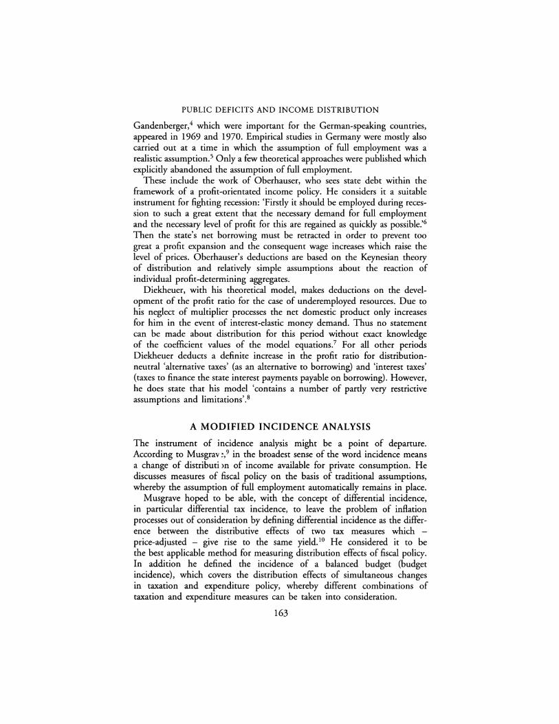
PUBLIC DEFICITS AND INCOME DISTRIBUTION
Gandenberger,4 which were important for the German-speaking countries, appeared in 1969 and 1970. Empirical studies in Germany were mostly also carried out at a time in which the assumption of full employment was a realistic assumption.5 Only a few theoretical approaches were published which explicitly abandoned the assumption of full employment.
These include the work of Oberhauser, who sees state debt within the framework of a profit-orientated income policy. He considers it a suitable instrument for fighting recession: 'Firstly it should be employed during recession to such a great extent that the necessary demand for full employment and the necessary level of profit for this are regained as quickly as possible.'6
Then the state's net borrowing must be retracted in order to prevent too great a profit expansion and the consequent wage increases which raise the level of prices. Oberhauser' s deductions are based on the Keynesian theory of distribution and relatively simple assumptions about the reaction of individual profit-determining aggregates.
Diekheuer, with his theoretical model, makes deductions on the development of the profit ratio for the case of underemployed resources. Due to his neglect of multiplier processes the net domestic product only increases for him in the event of interest-elastic money demand. Thus no statement can be made about distribution for this period without exact knowledge of the coefficient values of the model equations.7 For all other periods Diekheuer deducts a definite increase in the profit ratio for distributionneutral 'alternative taxes' (as an alternative to borrowing) and 'interest taxes' (taxes to finance the state interest payments payable on borrowing). However, he does state that his model 'contains a number of partly very restrictive assumptions and limitations'. 8
A MODIFIED INCIDENCE ANALYSIS
The instrument of incidence analysis might be a point of departure. According to Musgrav ~, 9 in the broadest sense of the word incidence means a change of distributi m of income available for private consumption. He discusses measures of fiscal policy on the basis of traditional assumptions, whereby the assumption of full employment automatically remains in place.
Musgrave hoped to be able, with the concept of differential incidence, in particular differential tax incidence, to leave the problem of inflation processes out of consideration by defining differential incidence as the difference between the distributive effects of two tax measures which -price-adjusted - give rise to the same yield. 10 He considered it to be the best applicable method for measuring distribution effects of fiscal policy. In addition he defined the incidence of a balanced budget (budget incidence), which covers the distribution effects of simultaneous changes in taxation and expenditure policy, whereby different combinations of taxation and expenditure measures can be taken into consideration.
163

R. ZWIENER
Musgrave's claim, where possible to be able to determine the incidence of a measure without it being superimposed by changes in prices and employment, will be abandoned in the following. For an empirical study these assumptions are unrealistic anyway. At any rate, without knowing the parameter values, the distribution effects of certain measures of fiscal policy can no longer be determined by means of a theoretical model.
The incidence analysis, applied to changes in borrowing, requires that borrowing is treated as an alternative financing instrument analogously to tax income. This is not a part of Musgrave's incidence analysis. If changes in the public debt are simultaneously connected with variations in income or expenditure then there is no more difference between the content of the specific income/expenditure incidence and the differential income incidence/budget incidence.
In order to determine the incidence of state debt, this must first be assumed to be exogenous. This can be done analytically but it has limited empirical relevance. In the political sphere in Germany, declarations of intent to make net borrowing an aim of economic policy and to align changes in income and/or expenditure to it have existed only since the mid-1980s. Usually the repercussions of variations in income and expenditure on debt, which make themselves felt as a result of multiplier processes which have been set in motion, are taken into consideration insufficiently or not at all. The instance of a specific credit incidence - that is, without relating borrowing to the extent of expenditure or other income - seems questionable, even from an analytical point of view. Borrowing with subsequent sterilization of the funds (at the central bank) does indeed reduce ceteris paribus the amount of money and has the effect of increasing the interest. However, the Bundesbank (German central bank) is responsible for matters of monetary policy and has at its disposal a sufficient range of instruments. Nevertheless, there are also examples of specific credit incidence. In 1973 the federal government established a 'stabilization loan' and the amounts received were sterilized with the Bundesbank.
In what follows both the differential and budget incidence of public deficits will be examined. Both of these issues have been politically relevant during the last twenty years. There were situations in which public expenditure was increased by conscious acceptance of deficit financing. The Zukunftsinvestitionsprogramm (future investment programme) can stand as an example of this. In the same way there were tax-scale reductions while accepting higher deficits. The measures used to counter these, tax-scale increases or reductions in expenditure to reduce borrowing, also took place.
The incidence analysis becomes more complicated if it is to be applied not only to the effect of borrowing but also to the effects occurring in the subsequent periods. Additional borrowing involves interest commitments. In principle, there is the possibility of financing this interest by means of higher taxes or borrowing or of paying for it by means of savings in other state
164

PUBLIC DEFICITS AND INCOME DISTRIBUTION
expenditure. In the literature on the intertemporal distribution effects of state debt, financing interest expenditure by means of taxation is most common. 11
Borrowing and the subsequent interest payments are inseparably linked to one another and both give rise to distribution effects. In order to answer the question about the intertemporal distribution effects, in principle it is necessary to separate the effects of borrowing and interest payments. The short-term effects linked to borrowing can still be determined. From the point of view of method, medium- to long-term separation is considerably more difficult, as the distribution effects overlap. Thus the selection of the 'relevant' means of procuring funds for interest payments, as explained above, already creates problems.
In order to determine the incidence of borrowing and interest payment, economic development without borrowing can be used as a reference quantity. If one wants to separate here the incidence of borrowing and interest payments, one must either assume a world with borrowing but without the consequent interest payments or without borrowing but with interest payments. Analytically, this is very possible; in economic terms, however, it only amounts to a partial analysis.
Of particular importance is that, in a time of rising net borrowing, the interest payments made by the state are normally higher than the interest directly calculable on the net borrowing concerned. The reason for this is that the increases in expenditure or reductions in taxes concomitant with borrowing give rise to overall economic effects with a tendency to expansion or in a recessive phase the level of expenditure is maintained and contractive effects prevented. Depending on the situation of monetary policy, interest-raising effects of varying size should set in or interest-lowering effects be prevented. As the state continually restructures part of its credits, the credits involved in the rearrangement must also be borrowed under less favourable conditions. In individual cases the total new interest commitments may be clearly greater than those calculable only for the net borrowing of one year. For economic reasons it is, of course, to be recommended that the total new interest commitments be taken into consideration as they are causally linked to the borrowing.
The upshot of these methodical considerations is that these distribution effects of public deficits cannot exist per se. The distribution effects depend rather both on the use of funds and on the actual economic situation. In addition to fiscal policy the respective monetary and wage policies also play an important role for distribution effects.
ECONOMETRIC MODEL AND SIMULATION TECHNIQUES
The basis for the econometric analysis of the distribution effects is a quarterly econometric model for the Federal Republic of Germany which covers
165

R. ZWIENER
the interrelation of the private (households), business, state and foreign sectors and calculates price and interest effects. The author has at his disposal such a model in the DIW version of the econometric model of the institutes of economic research.12
In order to answer the present question this model had to be expanded, in particular by a disaggregated income distribution model. 13 In this model the aggregates of the functional income distribution are transferred to the level of institutional income distribution taking into consideration the crossdistribution, that is to the definition of social groups according to their respective household types. The characterizing factor of defining social groups according to households is that each type of household receives both wages, profits and property income and transfer income in varying degrees. Because of missing/lacking statistics, within the framework of this study the employee households will be combined with the non-working households; a combination which seems justified for economic reasons. Thus the savings ratios of these two groups since 1970, depending on the economic situation, have developed virtually in parallel between 7.5 per cent and 12.7 per cent.14 In what follows only the cross-distribution between the self-employed households and other households will be calculated in accordance with the income components, net wages and salaries, distributed profits and net transfer income, whereby for self-employed households the distributed profits make up the main type of income and for the other households the other two types of income are the main source of income.
With the economic model a wide range of experience in investigating the effects of measures of financial policy was gathered. In addition to more general criteria for econometric models such as topicality and compliance with certain investigative standards, special requirements must be met when analysing the distribution effects of public deficits. These include, first, closed modelling of the state sector in order to be able to deal with the increase in expenditure or lowering of certain taxes linked to an increase in net borrowing by the state and their respective overall economic effects. In the model version used here there is a closed income and expenditure flow account for the state.
Second, the modelling of the monetary sector must allow the Bundesbank to assume various strategies. With investigations on the crowding-out discussion, the results proved to be dependent to a large extent on the respective position of monetary policy and the reaction of the Bundesbank.15
Third, the private households were disaggregated in accordance with the two most important household types. This allows for the various consumption habits of the social groups to be analysed endogenously by the model, independently of their respective income types and of cross-distribution, among other things.
The transposition of the incidence analysis into simulation technique requires that the net borrowing of the state becomes an exogenous impulse
166

PUBLIC DEFICITS AND INCOME DISTRIBUTION
in order to determine clearly the overall economic effects and distribution effects caused. Whereas in a normal multiplier analysis the effects of an exogenous impulse are weakened via the built-in stabilizer of the tax system - in public expenditure this achieves a certain degree of self-financing - this mechanism is here eliminated. The impulse takes effect to its full extent.
This procedure can be carried out only by means of models and is, like incidence analysis, a construct. However, it has several advantages. On the one hand it is the only way to directly answer the question of the incidence of borrowing. On the other hand this procedure makes it possible to compare directly the distribution effects of borrowing for various income and expenditure variations and for various assumptions regarding the reaction of those in charge of economic policy.
This method of proceeding is divergent from the generally known multiplier analysis in which, from the point of view of the model, an exogenous variable varies and the resulting effects are analysed. Ideally this variable should be one which is not influenced by the model results - that is, one which can be consciously set by those in charge of economic policy or which arises from the 'rest of the world' and is thus only marginally influenced by changes in the Federal Republic of Germany.
Here a procedure is selected to make the public deficit exogenous and to transform the budget equation in such a way that a certain type of income or expenditure is explained by means of the budget equation. In the event of differential credit incidence the income from a certain selected type of tax then fits endogenously. The other state income varies in accordance with the built-in flexibility of the tax system. Thereby indirect reciprocal effects set in via the varying overall economic development, which depends on the type of financing, and which then for its part influences the size and the structure of state expenditure. The entire range of state expenditure is thus determined endogenously.
Analogously, for measuring the budget incidence of borrowing, a certain type of expenditure is selected and varies in such a way that the exogenously set new debt is adhered to. In this case the total state income (without net borrowing) is determined endogenously for given tax and contribution rates. For an exogenously given budget deficit they influence the size of the type of expenditure selected for variation interdependently.
EMPIRICAL RESULTS FOR THE DIFFERENTIAL AND BUDGET INCIDENCE OF PUBLIC DEFICITS
In this section the effects of an increase of net state borrowing will be simulated and analysed under various conditions, and the absolute divergence of each respective simulated development from the base simulation will be considered.
167

R. ZWIENER
The starting point of all the simulations is the first quarter of 1975; the increase in public net borrowing starts, therefore, in the first quarter of 1976. Thus the model is given the chance to conform to a dynamic simulation path in the face of the exogenous impulse. The lagged-endogenous variables of the model are mostly determined from the model after one year with the prevailing lag structure.
The following assumptions are made with regard to financial, monetary and wage policy. In 1976 net state borrowing was increased by an additional DM 10 billion, that is by DM 2.5 billion in each quarter, and subsequently, from 1977 to 1980, the actual values were re-inserted into the calculation.
All changes in the state's income and expenditure positions are reflected in the first simulation in the direct taxes paid by employees. Both in the period during which the increase of net borrowing takes place (henceforth called the 'borrowing phase') and in the subsequent period (here called the 'debt phase') the changes in employee taxes are added to the increase in net borrowing by DM 10 billion. This is used to investigate the question of differential incidence.
In the second simulation all the changes in the state's income and expenditure positions lead to a change in public fixed capital formation (budget incidence). Thus the simulation analysis is arranged in such a way that a direct comparison with the differential incidence of public borrowing is possible. The price of this direct comparability is a certain distancing from reality due to the concomitant strong fluctuations in public capital expenditures in construction. In fact the construction industry would not have the capacity to adapt to such fluctuations in demand in the short term; increased state demand would lead to a sl!dden considerable price increase for public buildings. This 'flaw' can, however, be accepted as the overall utilization of economic capacity, and not just that of any one sector; it is used in the estimation of the individual price equations in the model and thus no excessive price effects are caused.
In these two simulations it is assumed that there are no reactions in terms of monetary and wage policy. This means that, in the specification of the model, the central bank money supply is left at its actual level and the interest is adapted to the respective overall economic situation and, in particular, to the situation in terms of monetary policy. The collectively agreed standard wages (per hour) are left at their actual levels.
The empirical results for differential incidence are shown separately in Table 7.1 according to the 'borrowing' and 'debt' phases. At the beginning are the changes in public borrowing and in the direct taxes on employees. According to the assumption, the financing deficit of the state should increase by DM 10 billion in the borrowing phase, that is in 1976. The built-in stabilizers do not take effect in the selected simulation procedure as all the induced additional income is used to finance a further reduction in income
168

PUBLIC DEFICITS AND INCOME DISTRIBUTION
Table 7.1 Increase in public deficits to finance a wage tax reduction (deviations from baseline in DM bn)
Period
Year
Debt increase
I
-10.00 Public sector deficit" Direct taxes of employees Employed labour force Gross domestic productb
-16.88
Private consumptionb Government consumptionb Fixed capital formationb
Machinery and equipmentb Constructionb
Change in stocksb Exportsb Importsb
Gross national product Price level of private consumption
(1976 = 100) Price level of GNP (1976 = 100) Income from employment
Net wages and salaries Entrepreneurial and property income,
gross Entrepreneurial and property
income, net Disposable income of entrepreneurial
households Net wages and salaries Distributed profits Current transfers received Interest payments on consumers'
debts Disposable income of all other
households Net wages and salaries Distributed profits Current transfers received Interest payments on consumers'
debts Money market interest rate, % Capital market interest rate, % Public sector
Revenue Expenditure
Interest payments
0.08 12.27 16.20 0.00 0.72 1.91
-1.19 2.96
-0.73 6.89
12.80
0.04 0.03 3.99
19.71
5.36
5.22
4.36 0.47 3.94
-0.00
0.04
21.18 19.25 2.22
-0.01
0.28 0.29 0.40
-12.31 -2.31
0.00
Notes: a deficit increase b at 1976 prices
169
2
0.00 -9.21
0.23 16.74 24.57
0.88 1.07 1.96
-0.89 2.21
-0.74 11.25 20.22
0.09 0.23
10.10 16.39
4.15
3.81
8.00 0.39 7.82
-0.00
0.21
19.72 16.00 4.39 0.21
0.90 0.49 0.36
-0.47 -0.46
0.43
Debt stock
3
0.00 -4.53
0.27 12.75 19.55
1.65 1.38 2.12
-0.74 -0.94 -0.62
8.27 19.42
0.10 0.45
10.95 12.31
2.65
2.42
5.49 0.29 5.38
-0.00
0.18
15.37 12.02 3.02 0.92
0.59 -0.05 -0.05
3.55 3.55 1.20
4
0.00 -1.97
0.24 11.23 13.75
1.77 3.01 2.49 0.52
-0.35 -0.56
6.39 19.73
0.18 0.56
10.40 9.36
3.76
3.28
4.46 0.22 4.40
-0.00
0;15
12.85 9.14 2.47 1.82
0.57 0.36 0.07
5.68 5.68 1.26
5
0.00 1.37 0.18 7.09 8.69 1.73 1.66 1.32 0.34
-1.01 -0.17
3.82 15.52
0.19 0.57 7.89 4.22
2.79
2.85
3.37 0.10 3.39
-0.01
0.12
7.94 4.12 1.90 2.33
0.43 0.08 0.01
6.83 6.84 1.27

R. ZWIENER
tax. In the same year this comes to almost DM 17 billion. The reason for this reduction in taxes, which greatly exceeds the deficit assumed, is to be found in the expansive overall economic effects let loose immediately. Thus private consumption is increased by a good DM 16 billion. While the real GNP continues to increase in the debt phase, the tax relief on employees is reduced considerably and in the fourth year of the debt it is even transformed into a mild tax burden. This then, by chance, corresponds roughly to the rise in state interest expenditure. The rise in employment reaches its maximum point at 270,000 in the second year of the debt.
If one considers the distribution effects, functional income flows - here one must consider net values - at first show a tendency to level out, a tendency which then disappears in the debt phase: the net wages and salaries sum rose at first more strongly than the net income from business activities and property. For the available income according to household type this tendency to level out does not arise. The self-employed households maintain their income position by greatly increasing the transfer of profits from the business sector to the household sector (distributed profits). · If one considers the induced development of public income and expend
iture then it is the continual rise in the debt phase which strikes the eye. This is due mainly to higher expenditure for public consumption and the current transfers made, and not so much to higher public interest payments. According to the incidence concept, on the incoil}e side the growth-induced additional income with unchanged net borrowing must be used increasingly for this additional expenditure and is no longer available for further reductions in income tax.
For the analysis of budget incidence (see Table 7.2) first the influences of higher, partly credit-financed, construction investments on the demand side of the national product and on employment are analysed. The size of the impulse is again at the top of the table. In the year of the borrowing, public fixed capital formation increases by DM 19 billion. The impulse is thus just over, by DM 2 billion, the amount which was available for reducing the direct taxes of employees. On the other hand the effects on the GNP are considerably greater. In the borrowing phase the real and nominal GNPs are, in the case of the budget incidence, raised to more than double their values in the case of the differential incidence. The real GNP increases by DM 28 billion. Of course, public constructions represent two-thirds of this increase alone.
Although the overall utilization of economic capacity rises greatly, the price effects in the borrowing phase are limited. In the debt phase the employment effect continues to increase at first to 400,000 persons, but then falls back to 120,000 persons. The induced economic growth - measured by the real GNP - disappears again during the debt phase. A decisive factor here is the loss, planned in the design of the simulation, of the additional public fixed capital formation.
170

PUBLIC DEFICITS AND INCOME DISTRIBUTION
Table 7.2 Increase in public deficits to finance public fixed capital formation (deviations from baseline in DM bn)
Period Debt Debt stock increase
Year 1 2 3 4 5
Public sector deficit" -10.00 0.00 0.00 0.00 0.00 Public fixed capital formation 19.06 11.65 4.85 0.08 --4.01 Employed labour force 0.19 0.42 0.38 0.27 0.12 Gross domestic productb 27.80 22.37 13.30 7.67 0.79
Private consumptionb 5.77 15.84 14.82 9.52 5.27 Government consumptionb 0.00 1.99 2.63 2.32 1.76 Fixed capital formationb 21.92 12.25 5.09 1.89 -2.78
Machinery and equipmentb 3.18 2.68 2.85 2.21 0.38 Constructionb 18.74 9.57 2.26 -0.32 -3.17
Change in stocki 6.83 0.77 -2.80 -1.59 -1.91 Exporti . 1.64 -0.92 -0.74 -0.39 0.26 Importsb 5.08 7.55 5.67 4.09 1.80
Gross national product 29.80 30.12 25.16 20.17 9.87 Price level of private consumption
(1976 = 100) 0.09 0.16 0.19 0.30 0.27 Price level of GNP (1976 = 100) 0.14 0.56 0.86 0.91 0.70 Income from employment 9.56 17.15 15.00 10.76 4.61
Net wages and salaries 5.38 9.81 8.59 6.19 2.66 Entrepreneurial and property income,
gross 16.76 6.43 2.82 2.91 0.26 Entrepreneurial and property
income, net 16.16 4.11 2.27 2.58 0.27 Disposable income of entrepreneurial
households 3.13 6.83 4.81 3.19 2.29 Net wages and salaries 0.13 0.23 0.20 0.15 0.06 Distributed profits 3.03 6.75 4.77 3.17 2.33 Current transfers received 0.00 -0.00 -0.01 0.01 -0.01 Interest payments on consumers '
debts 0.03 0.15 0.16 0.12 0.09 Disposable income of all other
households 6.85 13.43 12.40 10.42 6.77 Net wages and salaries 5.25 9.58 8.39 6.04 2.60 Distributed profits 1.70 3.80 2.68 1.78 1.31 Current transfers received -0.01 0.50 1.79 3.05 3.24 Interest payments on consumers '
debts 0.09 0.45 0.45 0.45 0.38 Money market interest rate, % 0.13 0.25 0.05 0.24 0.25 Capital market interest rate, % 0.58 0.16 -0.07 -0.01 -0.00 Public sector
Revenue 9.56 16.06 12.09 8.43 3.77 Expenditure 19.56 16.06 12.10 8.43 3.77
Interest payments 0.00 0.50 1.25 1.25 1.22
Notes: a deficit increase. b at 1976 prices.
171

R. ZWIENER
Measured by the functional income distribution, in this simulation 'antisocial' distribution effects set in during the borrowing phase. An increase of income from business activities and property of a good DM 16 billion gross/net is set against additional income from employee activities of only DM 9.5 billion gross of DM 5.5 billion net. This increase in income flows almost exclusively to the additional employed persons. The total available incomes of private households does not increase by any means to the same extent as net incomes, as the distributed profits are only partly, and even then in delayed fashion, adapted to the developments in net profit. In the end the available incomes of self-employed households increase by roughly half as much as the other households. Thus the distribution differences on the household level are weakened; in the debt phase they disappear altogether. In this phase the distribution effect for functional income flows is even reversed. In particular the employment gains make themselves known here while no more profit-raising impulses are given via the constancy of net public borrowing (compared with the base simulation). Rather 'in spite of' increased interest payments by the state in the debt phase, the one increase in public net borrowing has a levelling effect on income.
If one analyses the development of the public sector, the continuous decrease in additional public expenditure strikes the eye. After five years there is 'only' additional expenditure of DM 3.8 billion, whereby the public investments in construction are already DM 4.0 billion below the status quo level. This expenditure development is caused - conditional on the design of this simulation analysis - by the reduction in additional state income. The builtin stabilizers take effect here with the result that with a decreasing growth dynamic the increases in income also disappear. In the simulation this has a destabilizing effect on the overall economy as the expenditure increases are also reduced to the same extent.
RESULTS
The results of this study show that in general the relative distribution position of the various groups of private households is hardly affected by changes in public net borrowing. On the other hand the respective absolute size of incomes can change considerably depending on the use of funds. The functional income flows are here influenced by public borrowing to a comparatively greater extent. Here, at least in the borrowing phase, significant movements in the income relations can be observed.
If one follows up on the results, then it is also true that public borrowing makes it easier for fiscal policy to improve the relative distribution position of entrepreneurial households than that of other households. However, this point should not be overvalued. The absolute and relative strengths and the duration of the effects of fiscal policy depend decisively on the type of use of credit funds. Under 'normal' conditions the multiplier effects of public
172

PUBLIC DEFICITS AND INCOME DISTRIBUTION
expenditure are greater than those on the revenue side. However, even between the different types of revenue considerable differences in multipliers occur. If it is not p~ssible to shift income relations by means of creditfinanced measures of fiscal policy to the advantage of employed persons with sustained effect on the basis of the empirical results of this study, then policy should at least be aimed at considerably increasing their income level by means of a growth and employment policy. If one moves on to a consideration of intertemporal distribution effects, then the 'most efficient' creditfinanced growth policy can also be attributed to the most favourable intertemporal distribution effects.
Overall, the conclusions for economic policy deduced here are similar to those from the expert report by Kurz and Rall: 'There is virtually nothing which affects those earning low incomes more than an unsuccessful employment, business cycle, growth or any other kind of expansion policy.'16
If one applies the statements to the distribution effects of state borrowing on fiscal policy in the years 197 4 to 1990, then there should, in the second half of the 1970s, have been no effects worth mentioning resulting from fiscal policy to promote income concentration. Rather, the strong increase in transfer payments to private households indicates a more income-levelling overall effect of financial policy. The picture in the 1980s is very different, however. The reductions in public expenditure, in particular with regard to transfers, the increase in value-added tax and other indirect taxes and the reduction in taxes for businesses ought to have increased income concentration.
With the reunification of Germany an unparalleled export boom began for West Germany, that is good$ especially were 'exported' to East Germany. This prolonged the economic upturn of the second half of the 1980s. The real GDP grew by 5.1 per cent and 3.7 per cent in 1990 and 1991, respectively, and private investment and employment increased. About half of this growth can be traced back to the effects of reunification. 17 However, the public sector will be forced by the transfers from West to East, mainly financed by public borrowing, to increase taxes further and reduce expenditure in the future. Only then will the distribution effects of German reunification be really felt in West Germany. As opposed to a use of funds 'at home', in future the citizens of West Germany will have to carry burdens without enjoying the benefits of the goods produced. The transfers were mainly used in East Germany to buy consumer goods. However, the citizens of East Germany also feel betrayed. They received the money and at the same time lost their jobs. So which distribution effect is worse?
NOTES
1 This chapter compresses the author's very detailed Ph.D. thesis, which is on a more actual base. It was presented as a paper at the XXXVIIIth International Conference of Applied Econometrics Association in Athens, Greece. 13-14 April
173

R. ZWIENER
1993. Cf. R. Zwiener, 'Die Einkommensverteilungseffeckte der Staatsverschuldung in einer unterbeschaftigten Wirtschaft', Beitriige zur Strukturforschung des DIW, Heft 110/1989. An older German version of this chapter has been published in Konjunkturpolitik, no. 1-2, 1989.
2 See D. Vesper and R. Zwiener, 'Gesamtwirtschaftliche Auswirkungen der Steuerreform 1990: Wachstums-, Beschaftigungs- und Verteilungseffeckte sowie Vergleich mit einer bedarfsorientierten offentlichen Ausgabenpolitik', expert report by the DIW commissioned by the Ministerium fur Arbeit, Gesundheit und Soziales (Ministry of Labour, Health and Social Affairs) of the state of Nordrhein-Westfalen, Berlin, 1987; J. Korner, 'Aufkommens- und Verteilungswirkungen der Steuerreform bei der Lohn- und Einkommensteuer', in lfo-Schnelldienst, no. 16-17, 1987; B. Fritzsche, U. Heilemann and H.D. von Loeffelholz, 'Was bringen die Vereinbarungen zur "GroBen Steurerreform"?', Wirtscha.fisdienst, V/1987, p. 230 ff.
3 See D. Teichmann and R. Zwiener, 'Steuerentlastung 1986/90 und Steuerbelastung 1991: Umverteilung der Einkommen von unten nach oben', in Wochenbericht des DIW, no. 14/1991 and RWI-Konjunkturbrief, 'Wer finanziert die deutsche Einheit? - Zur Diskussion um die "Gerechtigkeitslilcke"', no. 3, October 1992.
4 See N. Andel, 'Zur These von den unsozialen Verteilungswirkungen offentlicher Schulden', in Public Finance, vol. 24, 1969; 0. Gandenberger, 'Offentlicher Kredit und Einkommensverteilung', in Finanzarchiv. NF., vol. 29, 1970.
5 See 0. Dieckheuer, 'Staatsverschuldung und wirtschaftliche Stabilisierung', in Schri.fien zur offentlichen Verwaltung und offentlichen Wirtscha.fi, vol. 21, 1978, Baden-Baden, P. Eichhorn and P. Friedrich. In an empirical study Kurz and Rall restrict themselves to calculating the multipliers of state expenditure financed by borrowing and taxation. The effects on income distribution are not demonstrated. Only the development of gross profits of businesses is used as an indicator for distribution effects. See R. Kurz and L. Rall, 'lnterpersonelle und intertemporale Verteilungswirkungen offentlicher Verschuldung', expert report commissioned by the Bundesminister fur Wirtschaft (Federal Minister for Economic Affairs) with econometric simulation analyses by J. Fronia, Tilbingen, 1983.
6 A. Oberhauser, 'Gewinnorientierte Einkommenspolitik und Staatsverschuldung', in Theorie und Praxis des finanzpolitischen Interventionsismus. Fritz Neumark zum 70. Gerburtstag, p. 549. Tiibingen: H. Haller u.a. 1970.
7 See G. Dieckheuer, 'Zu den Wirkungen einer offentlichen Kreditaufnahme auf die funktionelle und die personelle Einkommensverteilung', in Finanzarchiv NF., vol. 37, 1979, p. 22.
8 Ibid. 9 See R.A. Musgrave, Finanztheorie, Tilbingen, -1974.
10 Ibid. 11 See 0. Gandenberger, 'Theorie der offentlichen Verschuldung', in Handbuch der
Finanzwisenscha.fi, vol. 3, p. 28 ff., Tilbingen, 1981. 12 K.-D. Bedau, D. Teichmann and R. Zeiwner, 'Auswirkungen der Mehrwert
steuererhohung vom 1.7.1983 auf volkswirtschaftliche Gesamtaggregate sowie Haushalte unterschiedlicher Einkommensstruktur', expert report of the DIW commissioned by the Bundesminister fur Wirtschaft (Federal Minister for Economic Affairs), Berlin, April 1987, with model documentation in the appendix; and R. Pohl and R. Zwiener, 'Ein monetares Teilmodell - ein Bei trag zur Weiterentwicklung des okonometrischen Konjunkturmodells der Wirtschaftsforsch-ungesinstitute', Vierteljahrshe.fie zur Wirtscha.fisforschung, no. 3, 1982. A revised and expanded model version was presented by the authors in Vierteljahrshe.fie zur Wirtscha.fisforschung, no. 1, 1989.
174

PUBLIC DEFICITS AND INCOME DISTRIBUTION
13 See R. Zwiener, 'Die disaggregierte Behandlung der Einkommensverteilung als Submodell der DIW-Version des okonometrischen Konjunkturmodells der Wirtschaftsforschungsinstitute', Vierteijahrshefte zur Wirtschaftsforschung, no. 3-4, 1985.
14 See K. Millier-Krumholz and R. Pohl (eds) 'Deutsches lnstitut fur Wirtschaftsforschung: Gedriickte Realeinkommen dampfen private Sparneigung - Zur Enrwicklung der Sparquoten der sozialen Gruppen in der Bundesrepublik Deutschland', Wochenbericht des DIW, no. 31, 1984.
15 See R. Zwiener, ' "Crowding-out" durch offentliche lnvestitionen? Eine Diskussion der Modellergebnisse der Deutschen Bundesbank und eine Gegeniiberstellung mit den Ergebnissen der DIW-Version des okonometrischen Konjunkturmodells der Wirtschaftsforschungsinstitute', Konjunkturpolitik, vol. 29, no. 3, 1983.
16 R. Kurz and L. Rall, op. cit. (see n. 5 above) p. 365. 17 G.A. Horn, W. Scheremet and R. Zwiener, 'Domestic and International
Macroeconomic Effects of German Economic and Monetary Union -Simulations on QUEST', journal of Forecasting, vol. 11, 1992.
175


Part III
STRUCTURE OF PUBLIC EXPENDITURES
AND IMPLICATIONS


8
PUBLIC SPENDING IN FEDERAL STATES
A comparative econometric study
Gebhard Kirchgiissner and Werner W. Pommerehne*
INTRODUCTION
From 1950 to 1989, total government expenditure including all transfer payments to private households and firms increased by 7.6 per cent per year in Switzerland, while GNP rose by just 7.0 per cent, that is total spending relative to GNP increased from 19.6 to 25.0 per cent. In the Federal Republic of Germany, the respective figures were 24.0 per cent for 1950 and 29.3 per cent for 1989. Henceforth, the difference between the corresponding growth rates (1950 and 1989) was slightly lower in Germany compared to Switzerland, while the initial spending level (relative to GNP) was significantly higher in Germany. Breaking down government expenditure into central, cantonal or state and local level expenditure indicates that the government levels experienced quite different developments in the two federal countries, with regard to the magnitude and the time pattern of growth. Furthermore, different developments in both countries are becoming apparent when total spending is disaggregated into exhaustive (consumption and investment) expenditure and transfer payments.
At first sight, the federal systems of Switzerland and Germany seem to be fairly similar. This happens because, on the one side, the economic system of both countries is characterized by a market economy with a more or less capitalist ownership system in which public enterprises play a minor role except for some areas (energy and traffic in particular). On the other side, the political systems of both countries are democracies with comparable federal structures. Finally, the assignment of functions to the various government levels does not appear that different at all. So, why do we observe a different development of public expenditure in Switzerland and Germany?
"Werner W. Pommerehne died unexpectedly and untimely on 8 October 1994. We have lost a very creative and productive scientist, and I personally a very close friend, to whom I owe very much (Gebhard Kirchgassner).
179

G. KIRCHGASSNER AND W.W. POMMEREHNE
Consulting the literature on the growth of the public sector, a large number of hypotheses become apparent.1 Most of them are rather fragmentary and cannot be combined to a coherent theory explaining the size and development of the government sector. Furthermore, they do not pay attention to the particularities of the various federal organizations of both countries, which is another reason why a comprehensive and consistent explanation of the different development of government expenditure in Switzerland and Germany has been lacking up to now.
Of course, we also will not be able to develop such a comprehensive theoretical model that allows the derivation of estimation equations and empirical testing. But in contract to doing cross-section analysis with a number of considerably different countries with regard to economics, politics and society, 2 we have chosen a different path. Beginning with the institutional differences, we first derive some hypotheses on the effects of the federal organizations on the development of government activity. Then we briefly discuss the development of the public sector in both countries since the beginning of the 1950s, relying on various structural data. In the next section, we give an 'econometric description' of the actual development, using a consistent estimate (derived from the theory of consumer demand). By doing this, we investigate how the growth of the government sector in the two federal countries is caused. Finally, we offer some concluding remarks.
DETAILED ANALYSIS OF THE FEDERAL STRUCTURES
A closer look at the federal structures of the two countries reveals large differences. In what follows, the effects of these differences on the amount and structure of government expenditure are investigated, mainly referring to the development from the early 1950s on. Beforehand, we want to describe the theoretical and institutional basis of our discussion and develop some hypotheses on the influence of the political system, in particular its federal structure as well as the tax system's structure, on the level and growth of public expenditure. After that follows a description of the relevant differences of the two countries' political systems.
Theoretical preliminaries
Analysing the development of government activity can be done from the supply as well as from the demand side, the latter being the traditional view since Adam Smith's contribution (1776, bk 5, p. 587). In modern economic theory, the demand-side approach can be found in the median voter model going back to Downs (1957). Its first empirical application (to explain the level and structure of government expenditure) was carried out by
180

PUBLIC SPENDING IN FEDERAL STATES
Borcherding and Deacon (1972) as well as Bergstrom and Goodman (1973).3
The supply-side approach has been brought up only recently, mainly by writers of public choice literature. According to this approach, the voters -depending on their income, their preferences and, for example, the state of technology - do not determine the specific public services and therefore the corresponding expenditure. Instead, politicians and especially public sector bureaucrats offer certain amounts of public services, thereby pursuing their own goals: politicians may want to be re-elected, or they may want to give something to their clientele; bureaucrats may expect (private) benefits when the size of public services is extended. The latter is extensively discussed in the economic theory of bureaucracy.4
Type of democracy and tax resistance
Besides a number of demand-side or supply-side orientated approaches, there exist studies that try to combine both approaches. One of the early works is that of Peacock and Wiseman (1967) whose main result has become known in the literature as the 'ratchet' or 'displacement' effect. The author's argument is as follows: both government and public bureaucracy are trying to expand public expenditure as much as possible. This expansion is restricted by the resistance of taxpayers to financing it, which can only be overcome in times of major social changes (such as times of war). In this case, higher expenditure can be put through. However, even if it decreases again afterwards, it will not reach the same low level again, because taxpayers become used to the higher tax level. The Peacock and Wiseman explanation does include supply and demand side considerations by incorporating behavioural hypotheses about politicians, bureaucrats and the population (taxpayers), though it does not use the corresponding terminology.
In today's literature on government expenditure, there is not much consideration of tax resistance.5 This is astonishing given its role in history. As long as parliamentarians regarded themselves as being agents for the people (against the ruler's claim) and as long as they controlled public budget, tax resistance meant a severe problem for governments and the dependent bureaucracy: the example of the French Revolution demonstrates that a tax increase or even just the attempt can lead to the government being overthrown and to the death of the ruler. In a modern state there exists at least partial interest by parliamentarians in increasing government expenditure; thus, tax resistance by citizens is less visible in parliament. Instead, it is visible in the increasing size of the shadow economy, that is, hidden work and tax evasion. 6
Tax resistance hardly plays a role in empirical work on the development of the public sector. This may be due to the fact that hidden work can hardly be observed and that tax resistance is not subject to rapid changes under normal circumstances. On the other hand, as demonstrated by Peacock and Wiseman, the extent of tax resistance does in fact depend on the institutional
181
G. KIRCHGASSNER AND W.W. POMMEREHNE
framework for the determination of taxes and public expenditure. The more citizens are allowed to participate in the budget-determining process, the better are their chances of exerting some influence, and thus the stronger will be their tax resistance and the lower will be - ceteris paribus - the relation of taxes and public expenditure to GNP (or GDP). So our first hypothesis is:
(Hl) Countries, characterized by direct democracy, will exhibit - ceteris paribus - a ratio of public expenditure and taxes to GNP that is lower than this ratio in countries with representative democracies.
Tax assignment and tax resistance
In addition to the distinction between direct and representative democracy, it matters whether a country is characterized by a centralist or federal structure, and - if federal - how much tax authority is given to subcentral parts of government. The more federal the system is, the more influence citizens will have and the stronger will be the tax resistance. This leads to the second hypothesis:
(H2) Countries with federal structures will exhibit - ceteris paribus - a ratio of public expenditure and taxes to GNP that is lower than this ratio in countries with a centralist structure.
Relying on the second hypothesis, we can formulate the third hypothesis:
(H3) The more a tax authority rests on the subcentral jurisdiction in countries with a federal tax structure, the lower will be the ratio cf government expenditure and taxes to GNP.
Design of the tax system and tax resistance
Peacock and Wiseman not only emphasized that tax resistance is influenced by institutional conditions, but also stressed that people get used to a tax burden. This habitual effect depends on the institutional conditions - in our context, on the tax system. For instance, 'indirect taxes' are said to be less perceivable than 'direct taxes'. Consequently, a tax reform that increases the share of indirect taxes and decreases the share of direct taxes could decrease the tax resistance and enable increased government activity. Nevertheless, an increase in indirect taxes is perceivable too, since it requires the reform of the tax law, which is usually accompanied by a public debate. On the contrary, direct taxes are usually progressive. Thus, the tax yield increases automatically when the real income or the price level increases without legislative procedures and consequently without increased tax resistance. Thus our fourth hypothesis is7
182

PUBLIC SPENDING IN FEDERAL STATES
(H4) The growth rate of government expenditure or its share of GNP will be higher in a progressive (yield elastic) tax system - ceteris paribus - than in a proportional (yield inelastic) system.
Type of democracy and resistance to increasing public debt
Another possibility for escaping tax resistance temporarily is public borrowing. If public expenditure is financed via debt instead of taxes, then the costs of this expenditure will not become evident instantly. The costs consist of crowded-out private demand and possibly an increased inflation rate at a later point of time. In the long run, increased interest payments will lead to reduced scope for government action, producing additional incentives to avoid the effects of borrowing through an 'inflation tax'. In the short run, such a strategy permits politicians and bureaucrats to extend their scope of action.
Following the 'Ricardian Equivalence Theorem', one could argue that tax resistance cannot be avoided by increasing public borrowing, since rational individuals anticipate the higher burden in the future, which will be necessary to cut back debts. Therefore, they will reduce their private spending just as much as in the case of a tax increase.8 Thus, the resistance against increased government spending is independent of its financing. But because the equivalence theorem is based on some assumptions, which are usually not met in reality,9 increased public borrowing will usually enable the government to escape temporarily from tax resistance.
The extent to which public borrowing is available to the government depends primarily on the constitution. When there is a requirement for a yearly balanced budget, a government has only little leeway. With the introduction of the Keynesian economic policy after the Second World War, the requirement of a yearly balanced budget has been substituted by a balance over a longer time period. Since the decisive fiscal planning period still covers a year and since democratically elected governments have a strong incentive to use public borrowing - as shown by Buchanan and Wagner (1978) - the cancellation of the obligation of a yearly balanced budget leads to an increase of public borrowing without a budgetary balance over a longer time period. This results in a strong increase in public debt.
Nevertheless, the extent of public debt chosen by the government depends on the political system; more concretely, on the degree of influence of the citizens on the budget drafting process. The stronger their influence is, the more they will inform themselves about the consequences of public debt and will react in a way predicted by the Ricardian equivalence theorem.
This means that resistance against public debt depends - as does tax resistance - on the degree of direct participation and on the extent of federal structures. Thus, the hypotheses developed for the level of government expenditure can also be completely transferred to the level of public debt.
183

G. KIRCHGASSNER AND W.W. POMMEREHNE
A look at the federal and fiscal structures of Switzerland and Germany
As mentioned above, Switzerland and Germany seem to have a similar economic and political system. The only difference, which is usually pointed out, is that the Federal Republic of Germany is a representative democracy, while Switzerland is considered to be the example for a direct democracy.
It goes without saying that in Switzerland most direct-democratic elements can be found, even though there are also representative systems in some cantons and cities (such as the canton and the city of Geneva). The constitutions of Germany and its states, however, include just a few elements of direct democracy. Therefore, an important difference indeed exists. Besides, there are some other meaningful distinctions, the most important one concerning the structure of the federal system.
Switzerland is a federal constitution, which emphasizes the sovereignty of subcentral jurisdictions, that is the cantons and local communities.10 This sovereignty is anchored in the federal constitution, which does also describe the right of the single government levels to levy taxes. Thus, each canton and each local community is able to decide, based on a comparison of cost and benefit, on the size of public expenditure. As far as the possibility of direct-democratic participation is provided for in the constitution of the respective jurisdiction, citizens can themselves take part in the decisionmaking process.
In contrast, the German states do not have the right to levy their own taxes. Local communities can levy some taxes, such as the local business tax, but they have much less tax sovereignty compared to their Swiss counterparts. For this reason, the states can only determine the expenditures based on given revenues. Furthermore, citizens have no possibility to participate in the decision-making process directly. They can just try to influence the elected representatives. Therefore, federalism in Germany does not seem to be pronounced that much compared to the strong federalism in Switzerland. 11
However, this view neglects the influence that German states have on politics in general and on taxing and spending policy in particular. While the central level in Switzerland has an important source of own revenue, turnover tax, the German central government hardly disposes of its own tax revenues. The most important revenue sources, income tax and value-added tax, are part of the 'joint taxes', which are imposed jointly by states and central government. It becomes obvious that not only the states, but also the German federal government have no unrestricted right to levy their own taxes.
The composition of the second chamber of the parliament also reveals that the German federal government depends on the states. Whereas in Switzerland the 'Standerat' consists of representatives of the cantons, directly
184

PUBLIC SPENDING IN FEDERAL STATES
elected by the people, the German 'Bundesrat' is composed of representatives of the state governments. Thus, the central government in Germany has no opportunity to make any important fiscal decision against the interest of a majority of state governments.
This great difference in the structure of federalism makes it impossible to decide whether the Swiss cantons or the German states have relatively more influence in regard to the central level. Generally speaking, we can only conclude that in Switzerland decisions of the different government levels are more closely related to the preferences of the citizens than in Germany. Hence, we may further deduce a higher tax resistance in Switzerland and, as a consequence, that public expenditure in relation to GNP will be lower compared to Germany. On the other hand, the shadow economy in Germany is expected to be more significant than that in Switzerland.12 No statement is possible with respect to the relative importance of each government level.
There is, however, another important distinction concerning the distribution of tax revenues between the various government levels. In Germany, the three government levels (federal, state and local), share the revenue from the progressive income tax and the federal and state governments share the yields of the proportional value-added tax. The distribution is based on a key which has to be agreed on by federal and state governments. Consequently, all government levels participate in an additional tax revenue due to the (hot and cold) tax progression. In contrast, the Swiss cantons and local communities have the exclusive right to levy income taxes. Besides the (proportional) turnover tax, the central government can only dispose of the 'direct federal income tax', the so-called 'W ehrsteuer', which is progressive, but amounts to a small revenue compared to the overall receipts from income tax. In addition, 30 per cent of the yield of the 'W ehrsteuer' is distributed among cantons according to an intercantonal redistribution. It is the subcentral elements of government that profit most from progression; the central level is more or less excluded. Consequently, compared to Germany, the relative fiscal position of the central authority seems to be weaker in Switzerland and its weight is likely to decrease in time.
THE EVOLUTION OF PUBLIC FINANCE IN SWITZERLAND AND GERMANY
In what follows, we consider the evolution of public finance in both countries since the Second World War. We concentrate on the federal, cantonal or state and local levels. The social security payments have been excluded because the respective systems differ greatly and thus cannot be easily compared. In order to avoid double-counting, the grants from the federal to the cantonal or state level and those from the latter to the local level are not accounted for as expenditure (on the donor level).
185

G. KIRCHGA.SSNER AND W.W. POMMEREHNE
Table 8.1 Evolution of public finances in relation to GNP 1950-89 (all government levels, excluding social security)
1950 1960 1965 1970 1975 1980 1985 1989
Switzerland Revenues 21.2 19.9 19.7 21.l 24.8 26.2 25.9 25.7
Taxes 15.5 15.4 15.7 16.9 19.6 19.7 19.9 19.8 Expenditure 19.6 17.5 20.6 21.6 26.3 26.6 25.9 25.0 Deficit -1.7 -2.4 0.9 0.5 1.6 0.4 0.1 -0.6 Public debt 76.7 49.0 41.5 38.9 40.9 40.9 34.7 27.3 Gross National
Product (in SFR bn) 19.9 37.1 60.0 93.9 144.6 177.3 241.4 305.2
Federal Republic of Germany Revenues 23.6 25.8 26.2 27.1 28.0 29.6 29.8 29.2
Taxes 21.0 23.0 23.5 24.0 24.7 25.7 24.9 24.4 Expenditure 24.0 23.7 27.5 27.9 33.4 32.8 31.2 29.3 Deficit 0.4 -2.2 1.4 0.7 5.4 3.2 1.4 0.6 Public debt 20.9 17.4 18.3 18.6 24.9 31.6 41.2 41.3 Gross National
Product (in DM bn) 98.6 303.0 458.2 675.7 1029.4 1485.2 1844.3 2249.1
Sources: For data sources see the appendix to this chapter, pp. 208--9.
Table 8.1 provides aggregate figures for the development of public expenditure and revenue, as well as for the government deficit and public debt, all in current prices and in relation to GNP. The data indicate that in both countries public revenue (and taxes) as well as public expenditure have strongly increased relative to GNP. This is particularly true for the beginning of the 1970s. Nevertheless, in an international context it turns out that Switzerland is still a country which has almost the smallest public sector; yet the share of public expenditure of German GNP is also below the respective mean share of all OECD countries (see Lybeck, 1986, p. 55). However, there are major differences between the two countries with respect to the development of government deficit and public debt. Up to 1970, the deficit was relatively small in each country (in Switzerland even budget surpluses have been achieved). After that time, the deficit has strongly increased in Germany, whereas it has remained at a low level in Switzerland, where it even decreased in the 1980s. As a consequence, public debt in Germany has significantly increased over time. The Swiss public debt, which - due to its accumulation during war times - was very high at the beginning of the period considered, has significantly decreased and in 1989 has remained at a level of about one-third of the level of 1950.
186

PUBLIC SPENDING IN FEDERAL STATES
Table 8.2 Structure and development of taxes and expenditure on the different government levels 1950-89 (excluding social security)
1950 1960 1965 1970 1975 1980 1985 1989
Switzerland Taxes
federal level 53.9 49.2 46.9 45.6 38.9 41.8 42.8 43.6 cantonal level 23.9 27.1 29.4 31.0 34.7 33.6 33.7 33.2 local level 22.2 23.7 23.7 23.5 26.4 24.6 23.6 23.2
Expenditure federal level 32.1 30.6 27.2 25.2 23.4 25.9 26.2 25.1 cantonal level 37.0 38.7 41.5 41.4 43.4 40.9 40.6 41.9 local level 30.9 30.6 31.3 33.4 33.2 33.2 33.2 33.0
Federal Republic of Germany Taxes
federal level 46.7 55.8 56.9 55.8 52.6 51.7 51.2 51.2 state level 41.6 31.7 32.0 33.5 35.1 35.4 36.1 36.2 local level 11.7 12.5 11.1 10.7 12.3 12.9 12.7 12.5
Expenditure federal level 41.9 41.6 42.0 39.2 38.7 38.5 40.6 39.7 state level 35.0 33.8 31.5 34.0 36.4 36.2 36.9 37.0 local level 23.1 24.6 26.5 26.8 24.9 25.3 22.5 23.3
Table 8.2 presents the distribution of taxes and expenditure at the different government levels. It indicates that in both countries the federal level receives the largest (relative) tax share. In Germany, this part has increased to more than 50 per cent since the beginning of the 1960s. In Switzerland, this share decreased from 54 per cent in 1950 to 44 per cent in 1989. Nowadays, the cantons or states in each country get about one-third of total tax revenue, with the share slightly increasing since 1960. On the local level, Swiss communities have received about one-quarter of total tax revenue; in Germany, the respective share is about 10 per cent.
On the subcentral levels of government, tax revenue is only a part of the respective total revenue. In Germany, the local level especially receives grants from other government levels of a considerable amount: thus the share of tax revenue out of total revenue is only a little more than 50 per cent.
Table 8.3 indicates that in Switzerland such grants play a major role, especially at the cantonal level. At the local level, they are much less important (in both cases compared to Germany). On the subcentral levels in Switzerland, especially locally, fees and revenue from public utilities are of major importance. Nevertheless, the part of 'own tax revenue' of both subfederal government units amounts to more than half of the respective total revenue.
187

G. KIRCHG.ASSNER AND W.W. POMMEREHNE
Table 8.3 Structure and development of public revenues in Switzerland 1950-89 (shares of total revenue, including double-counting)
1950 1960 1965 1970 1975 1980 1985 1989
Federal level Taxes 84.0 84.1 88.4 90.0 89.2 88.8 92.7 92.8
on income and property 32.8 24.4 22.0 28.3 32.2 33.2 38.7 39.S
on consumption 51.2 59.7 66.4 61.7 57.0 55.6 54.0 53.3 Revenues from
enterprises 6.6 7.5 5.3 4.5 5.6 6.1 4.0 3.9 Charges 6.5 7.5 5.4 4.5 4.1 4.2 3.0 3.1 Transfers from
other levels 0.0 0.0 0.0 0.0 0.3 0.3 0.1 0.0 Other revenues 2.9 0.9 0.9 1.0 0.8 0.6 0.2 0.1
Cantonal level Taxes 49.5 55.9 51.4 52.9 55.1 54.1 55.2 53.4
on income and property 44.S 49.7 46.3 47.9 51.4 50.1 51.7 50.3
on consumption 5.0 6.2 5.1 5.0 3.7 4.0 3.6 3.1 Revenues from
enterprises 9.6 7.6 5.5 5.2 4.0 4.3 4.4 3.9 Charges 16.3 15.6 12.3 12.4 12.6 14.2 14.2 14.4 Transfers from other
levels 24.6 20.9 30.8 29.3 28.1 27.1 26.0 27.1 Other revenues 0.0 0.0 0.0 0.2 0.2 0.3 0.2 0.3
Local level Taxes 55.8 60.9 58.8 58.1 57.9 51.0 51.0 50.7
on income and property 55.1 60.1 57.9 57.7 57.7 50.8 50.8 50.5
on consumption 0.7 0.8 0.9 0.4 0.2 0.2 0.2 0.2 Revenues from
enterprises 10.6 7.1 9.9 8.8 7.1 6.1 6.1 6.2 Charges 24.0 14.9 15.9 15.4 16.1 25.6 25.S 25.4 Transfers from other
levels 9.6 17.1 15.4 17.7 18.0 16.1 16.7 17.1 Other revenues 0.0 0.0 0.0 0.0 0.9 1.2 0.7 0.6
Own tax revenue, fees and other own revenues on the local level do not lead to any kind of 'dependence' on other government levels, as may happen in the case of grants to local governments. Yet in Switzerland, the local level seems to be much more independent from the other government levels, and therefore also fulfils 'own tasks' to a larger extent, compared to Germany. In Germany, the federal government's share of total government expenditure corresponds to about 40 per cent, whereby federal grants to other government levels are not considered. 13 The corresponding figure for the
188

PUBLIC SPENDING IN FEDERAL STATES
Swiss central government amounts to only 25 per cent. The respective share of the Swiss cantons is higher than 40 per cent, compared to about the German states' 35 per cent. Finally, local communities in Switzerland nowadays spend about one-third of total goverment expenditure; the respective figure for German communities is less than 25 per cent.
Table 8.3 also reveals to what degree the different government levels in Switzerland participate in revenues from direct taxes and, thus, in potential fiscal gains due to the progressiveness of these taxes. During the first half of the 1980s, the federal government received about 60 per cent of its total revenue from the consumption tax, and only some 35 per cent from the direct tax on income. However, 30 per cent of the yields from direct taxes have to be delivered to the cantons. Therefore, net receipts as a share of total federal revenue decrease to 27 per cent. Nevertheless, the federal revenue from direct taxes has significantly improved during the last thirty years -though a number of tax reforms have been realized in order to eliminate the consequences of the 'cold progression', and the rates of the turnover taxes have been raised ·by 70 per cent during the same period.
On the cantonal and local levels, income from consumption taxes is a minor source. Both subcentral governments rely heavily on the progressive direct taxes, which, nevertheless, have only slightly increased as a part of total cantonal revenue and even decreased in the case of local communities. Obviously, one reason for this is the effect of indexation, avoiding or at least reducing the consequences of the cold progression. Another reason relates to the system of direct democracy: citizens of cantons and of local communities succeeded in proposing tax rate reductions. As a consequence, the increase of taxes (in relation to GNP) could be limited to less than 20 per cent and that of indirect taxes to less than 15 per cent.
In Germany, some reforms of tax tariffs have also occurred in order to absorb the negative effects of the cold progression. However, they have only partially succeeded: that is, they have not even compensated for the consequences of the cold progression. 14 As a consequence, the weight of direct taxes has increased, amounting to 12.5 per cent (in relation to GNP) in 1989, to the same share as that of revenue from indirect taxes (12.4 per cent).
Table 8.4(a) shows the structure and development of public spending in Switzerland, Table 8.4(b) the respective figures for Germany. One major difference between the two countries relates to the size of transfers in relation to GNP. In Germany, total transfer payments amounted to more than 10 per cent of GNP during the 1970s, whereas they are still less than 8 per cent in Switzerland. This could be due to the different unemployment situation in both countries, yet even in the 1960s the size of transfer payments in Germany was about twice as high as that in Switzerland (7-9 per cent as opposed to 3-4 per cent). With respect to exhaustive expenditure, there are only minor differences between the countries. However,
189

G. KIRCHGASSNER AND W.W. POMMEREHNE
Table 8.4(a) Structure and development of public expenditure in Switzerland 1950-89 (in relation to GNP, excluding double-counting)
1950 1960 1965 1970 1975 1980 1985 1989
Federal level 6.2 5.3 5.5 5.2 6.0 6.7 6.7 6.3 Public consumption 3.4 3.1 3.2 2.7 2.7 2.7 2.9 2.4 Public investment 0.3 0.3 0.3 0.6 0.4 0.2 0.3 0.3 Transfer payments 1.2 1.3 1.6 1.7 2.6 3.3 3.1 3.1 Interest payments 1.3 0.6 0.3 0.3 0.4 0.5 0.4 0.3
Cantonal level 6.9 6.7 8.4 8.6 11.2 10.7 10.4 10.5 Public consumption 4.2 4.0 4.3 4.1 5.9 6.2 6.3 6.2 Public investment 0.6 1.3 2.4 2.4 2.2 1.7 1.2 1.4 Transfer payments 1.6 1.1 1.4 1.7 2.6 2.3 2.4 3.6 Interest payments 0.4 0.3 0.3 0.4 0.5 0.5 0.4 0.4
Local level 6.5 5.3 6.3 7.0 8.6 8.6 8.5 8.3 Public consumption n.a. 3.5 3.7 3.5 4.4 5.3 5.3 5.2 Public investment n.a. 0.8 1.5 2.1 2.3 1.9 1.7 1.7 Transfer payments n.a. 0.6 0.7 0.7 1.0 0.9 0.9 1.0 Interest payments 0.4 0.4 0.4 0.6 0.9 0.6 0.5 0.4
All government levels 19.6 17.2 20.2 20.8 25.8 26.0 25.5 25.1 Public consumption n.a. 10.6 11.1 10.3 13.0 14.2 14.4 14.0 Public investment n.a. 2.3 4.2 5.1 4.9 3.7 3.3 3.4 Transfer payments n.a. 3.0 3.7 4.1 6.2 6.5 6.5 7.6 Interest payments 2.1 1.3 1.1 1.3 1.8 1.6 1.4 1.1
both Swiss government consumption and government investment expenditure have been outperforming those in Germany since at least the mid-1970s.
Other major differences between the two fiscal systems have been mentioned before: the German federal government is in a relatively strong position, whereas in Switzerland the cantons take the strongest position and the central government the weakest one.
Table 8.5 provides some disaggregated information on the development of public debt and the related interest payments in both federal countries. The figures reveal that public debt in Switzerland has traditionally been much higher than in Germany and that this also extends to the local government level, recently. However, the German states' debt has more than tripled since 1970, whereas that of the Swiss cantons has even decreased during the same period. Moreover, the German federal government's debt has increased by 160 per cent since 1970, whereas that of the Swiss central government has slightly decreased (by 2 per cent). Therefore, total public debt (in relation to GNP) in Germany has become larger than that in Switzerland, and total interest payments in Germany (2.7 per cent in 1989) have even increased to more than double those in Switzerland (I.I per cent). Of course,
190

PUBLIC SPENDING IN FEDERAL STATES
Table B.4(b) Structure and development of public expenditure in the Federal Republic of Germany 1950-89 (in relation to GNP, excluding double-counting)
1950 1960 1965 1970 1975 1980 1985 1989
Federal level 9.7 9.0 10.7 10.2 11.9 11.7 11.7 10.9 Public consumption 1.2 4.0 4.9 3.9 4.3 3.8 3.8 3.3 Public investment 0.2 0.5 0.7 0.8 0.6 0.5 0.3 0.3 Transfer payments 8.2 4.2 4.8 5.1 6.4 6.4 6.0 5.8 Interest payments 0.1 0.3 0.3 0.4 0.6 0.9 1.6 1.4
State level 8.1 7.3 8.0 8.9 11.2 11.0 10.7 10.2 Public consumption 3.9 4.2 4.5 5.1 6.4 6.4 6.2 5.8 Public investment 0.6 0.6 0.9 0.9 0.8 0.6 0.5 0.5 Transfer payments 3.3 2.3 2.5 2.6 3.6 3.3 3.0 2.9 Interest payments 0.4 0.2 0.2 0.2 0.4 0.6 1.0 0.9
Local level 5.3 5.3 6.8 7.0 7.7 7.7 6.5 6.4 Public consumption 2.8 2.4 2.5 2.8 3.5 3.6 3.5 3.4 Public investment 1.3 2.0 3.0 2.9 2.5 2.4 1.4 1.5 Transfer payments 1.3 0.8 1.1 1.0 1.3 1.2 1.2 1.2 Interest payments 0.0 0.2 0.2 0.3 0.5 0.4 0.4 0.3
All government levels 23.2 21.7 25.5 26.1 30.7 30.3 28.9 27.5 Public consumption 7.9 10.5 11.9 11.8 14.1 13.9 13.4 12.6 Public investment 2.0 3.1 4.5 4.6 3.9 3.6 2.2 2.3 Transfer payments 12.7 7.4 8.4 8.7 11.3 10.9 10.2 10.0 Interest payments 0.6 0.7 0.7 1.0 1.4 1.9 3.0 2.7
the levels of German public debt and the interest payments are not critical yet. Nevertheless, the rapid increase during the last decade may significantly reduce the government's leeway, especially on the federal and state levels, preventing the adoption of additional tasks. 15
Observing the development in both countries, overall we find our theoretical considerations confirmed. The stronger the federal elements of a polit~cal system and the more direct democratic elements it contains, the smaller is the leeway for the political entrepreneurs, government, parliament and public bureaucracy to undertake activities that are not directed towards the (revealed) preferences of the citizens. This leeway is additionally narrowed when income tax is indexed to inflation. Under such circumstances, the public sector's share of GNP can be expected to be relatively small. Following our theoretical considerations, the demand side plays a crucial role in the determination of public expenditure. We presume that Switzerland corresponds to this case.
The stronger the central elements of a political system, the less direct democratic elements it contains, and the more important the role of a nonindexed income tax, the greater are the chances for political entrepreneurs
191

G. KIRCHG.ASSNER AND W.W. POMMEREHNE
Table 8.5 Evolution of public debt and interest payments 1950-89 {in relation to GNP, excluding double-counting)
1950 1960 1965 1970 1975 1980 1985 1989
Switzerland Public debt 76.8 49.0 41.5 38.9 40.9 40.9 34.7 27.2
federal level 44.S 20.9 12.6 8.4 10.0 13.8 12.1 8.2 cantonal level 14.7 12.0 12.2 12.4 13.0 12.5 11.4 9.6 local level 17.6 16.2 16.7 18.0 18.0 14.7 11.2 9.2
Interest payments 2.1 1.3 1.1 1.3 1.8 1.6 1.4 1.1 federal level 1.3 0.6 0.4 0.3 0.4 0.5 0.4 0.3 cantonal level 0.4 0.3 0.3 0.4 0.5 0.5 0.4 0.4 local level 0.4 0.4 0.5 0.6 0.9 0.6 0.5 0.4
Federal Republic of Germany Public debt 20.9 17.4 18.3 18.6 24.9 31.6 41.2 41.3
federal level 7.4 8.9 8.7 8.4 11.0 15.6 21.4 21.8 state level 13.0 4.8 3.8 4.1 6.5 9.3 13.4 13.8 local level 0.5 3.7 5.6 6.0 7.2 6.4 6.2 5.4
Interest payments 0.6 0.7 0.7 1.0 1.4 1.9 3.0 2.7 federal level 0.1 0.3 0.3 0.4 0.5 0.9 1.6 1.4 state level 0.4 0.2 0.2 0.2 0.4 0.6 1.0 0.9 local level 0.0 0.2 0.2 0.3 0.5 0.4 0.4 0.3
to handle new tasks. In this case, it is the supply side that is primarily responsible for an increased level of public expenditure. It needs some more analysis, in the next section, to say that Germany belongs to that group.
PUBLIC SPENDING IN SWITZERLAND AND GERMANY: AN ECONOMETRIC DESCRIPTION
.So far, the discussion suggests that the old argument of Peacock and Wiseman (1967) may still hold: revenues seem to be a major restriction and thus an important factor influencing public expenditure. But most empirical studies on the growth of government do not take into account the revenue side or only consider it by including a deficit variable for the same period. 16
Moreover, whenever a federal, state or local government is deciding on its budget, it simultaneously determines (planned) expenditure, revenue and deficit/surplus. Thus, in order to provide a coherent 'econometric description' of the evolution of public finance in a federal country, a simultaneous estimation procedure is required.
Another requirement is the consistency of the estimated system of equations. 'Consistency' in this context does not only refer to the optimizing
192

PUBLIC SPENDING IN FEDERAL STATES
behaviour of the representative (decisive) individual, thus asking for timedependent (variable) elasticities of demand. 17 It also refers to internal consistency of the estimation results: that is, the estimated elasticities should be compatible to each other.
To meet these two major requirements, several 'flexible functional forms' have been suggested.18 We shall apply the most convenient to our purpose.
The model
The basic assumption is that the political decision-maker - a government or the median voter - maximizes the following objective function:
U = U(x, q, Tr, T, D)
with ux > 0, uq > 0, UT, > 0,Uy<-0, UD < 0
where x = the private good q = the public good T = transfer payments Tr= taxes (revenues) D = budget deficit
all in real terms Two restrictions have to be fulfilled. First, the GNP constraint:
Y=X*Px+q*Pq
where Y = nominal GNP p x = price of the private good p q = price of the public good
and, second, the budget restriction:
q * Pq + Tr * PT, - T * PT- D * Pv = O
where PT,= relevant price for transfer payments PT= relevant price of revenues Pv = relevant price for the budget deficit
(8.1)
(8.2)
(8.3)
Following the usual procedure of consumer theory, we do not refer to the direct utility function (8.1), but instead to the indirect one:
with
V,x < 0, V,. < 0, V,,, < 0, V,,> 0, V,0 > 0, Vy> 0
which will he maximized subject to the modified constraints:
sl + s2 - S3 - S4 = 0
193
(8.4)
(8.3a)

G. KIRCHGASSNER AND W.W. POMMEREHNE
where
S = q */!_g_ _ T, *PTr S = T*PT 1 y ' 52 - r y ' 3 y
and
where
(8.2a)
The solution to this problem leads to a system of demand equations. However, for any known approximation of the unknown utility function, these demand functions are rather complex. 19 Therefore, we approximate the system of demand equations by the 'Almost Ideal Demand System' (AIDS), which provides the following system of share equations:
S, =a.+ /3·* ln(_r) + ~ y .. * In(&)+~ o .. * z. 't t ™' ."-ii] p ."'-JIJJ
1- j=l 5 j=l
(8.5)
where
P* refers to the price index of GNP, and z., j = I, ... , k, are additional variables influencing the public budget decisi6n.
Due to the government budget constraint for system (8.5), the following adding-up restrictions hold:
'Y11 + 'Y21 - 'Y31- 'Y4J = 0, j = I, ... , 4
011 + 021 - 031 - 041 = o, j = 1, ... , k
(8.6a)
(8.66)
(8.6c)
(8.6d)
In addition, due to the GNP constraint, the following constraints hold:
(8.7a)
(8.76)
194

PUBLIC SPENDING IN FEDERAL STATES
'Yij + 'Y5j = 0, j = 2, ... , 5
8Ii + 85i = 0, j = I, ... , k
(8.7c)
(8.7d)
All of these restrictions are automatically fulfilled. Furthermore, one can impose the symmetry restriction from the consumer demand theory,
'Yij = 'Yj;, iJ = 2, ... , 5 (8.8)
The first four equations of system (8.5) can be estimated separately for the federal, state and local level, but also for all government levels together. The fifth equation, explaining the share of private goods, can only be estimated for all levels together.
In order to estimate the share equations of the AIDS system, we need prices (or price indices) for transfer payments, revenues and the budget deficit. Prima fade, such price indices are not available. However, if one takes into account that an increase in transfers and in taxes decreases the opportunity to consume private goods, it makes sense to use the price index for private goods instead. A similar argument holds for the budget deficit, if there is at least some crowding-out of private demand caused by deficit-financed expenditure. Under these assumptions, it holds that:
ln ~) = 0, iJ = 2, 3, 4 (8.9)
which implies that for the estimation of system (8.5) the only relevant price is the relative price of the public good (p/p5). Then, the symmetry conditions (equation 8.8) are automatically fulfilled and are no longer relevant to the estimation procedure.
Obviously, the usefulness of such a system can be questioned because of the underlying optimization assumption. Especially, when we look at total government expenditt re aggregated over all levels, it is not really clear who is the decision unit. I-: owever, even if this is unclear, an econometric model that explains government spending should at least take into account the adding-up conditions: each influence which increases government expenditure necessarily leads to an increase in revenue or the budget deficit in order to offset the expenditure increase. Therefore, system (8.5) fulfils minimal consistency requirements, stemming from the division of GNP in its private and public parts and from government budget constraints.
The question arises which variables z., j = I, ... , k, should be additionally included into the system. As stated ~hove, up to now there has been no comprehensive theory about the type of variables that should be used. On the other hand, as has already been shown by Theil (1957), missing relevant variables can bias the estimated regression coefficients. In our case, this might produce estimates for income and price elasticities which are
195

G. KIRCHGA.SSNER AND W.W. POMMEREHNE
completely implausible. Thus, there is an indirect check of our model: if the relevant variables are captured, the system's estimates should provide 'reasonable' results for the income and price elasticities. On the other hand, 'bad' results, that is implausible values of these elasticities, provide some indication that important factors are still missing.
By working with AIDS, the following variables are going to be explained: exhaustive expenditure ( GEX), transfer payments ( TRF), revenue (REV) and the deficit (DEF) all in current prices and in relation to nominal GNP. To estimate the model for both countries, we use annual data from 1961 to 1987.
We have used variables from the following three groups as explanatory variables:20
1 Economic variables Obviously, real income ( GNP/PGNP) and relative price of government expenditure (PGEXIPPGNP) have to be considered.21
We also include the unemployment rate (UR), which has an impact on government expenditure when the government applies an anti-cyclical fiscal policy. As public spending cannot be seen independently of the level of indebtedness, we also take into account the (one-period lagged) public debt (DEB) relative to public revenue.
2 Structural variables We consider the total labour force participation rate (PR) and the share of women in the labour force (FPR). To capture the structure of the population, we use the share of people older than 65 years (A65).
3 Political variables Politico-economic models of the Frey-Schneider type (Frey and Schneider, 1979) contain three different kinds of political variables:
• ideology dummies; • electoral cycle variables; and • popularity surplus/deficit.
In Switzerland, the same four major parties always form the federal government, thus a variable for the popularity surplus/deficit does not make much sense. For Germany, we use dummy variables for the period when the Social Democrats were the leading party in government (1970-82) (SPDG), and for the great coalition from 1967 to 1969 (GC). As electoral cycle variable, we constructed an election year dummy, taking the value '1' in years of general elections and 'O' otherwise. Together with the lagged endogenous variable, this can produce an electoral cycle. However, for both countries these variables failed to be significant and therefore they have been dropped. Instead of the (short-run) popularity surplus/deficit variable, we look for variables which describe the major political tendency of the electorate. One might think of the share of leftwing or right-wing voters in the electorate. For Germany, we use the share of left-wing members (Social Democrats and Greens) of all state
196
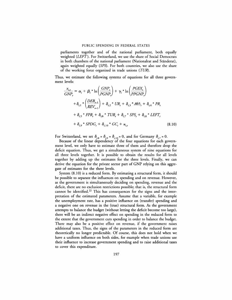
PUBLIC SPENDING IN FEDERAL STATES
parliaments together and of the national parliament, both equally weighted (LEFT). For Switzerland, we use the share of Social Democrats in both chambers of the national parliament (Nationalrat and Standerat), again weighted equally (SPS). For both countries, we also use the share of the working force organized in trade unions (TUR).
Thus, we estimate the following systems of equations for all three government levels:
x; t * l ( GNPt ) l ( PGEXt ) -----=--- = a + n --- + * n GNPt ; /3; PGNPt 'Y; PPGNPt
(8.10)
For Switzerland, we set 5. 8 = 5. 9 = 5. 10 = 0, and for Germany 5. 7 = 0. 4 4 ,, 4
Because of the linear dependency of the four equations for each govern-ment level, we only have to estimate three of them and therefore drop the deficit equation. Thus, we get a simultaneous system of nine equations for all three levels together. It is possible to obtain the results for all levels together by adding up the estimates for the three levels. Finally, we can derive the equation for the private sector part of GNP relying on this aggregate of estimates for the three levels.
System (8.10) is a reduced form. By estimating a structural form, it should be possible to separate the influences on spending and on revenue. However, as the government is simultaneously deciding on spending, revenue and the deficit, there are no exclusion restrictions possible; that is, the structural form cannot be identified. 22 This has consequences for the signs and the interpretation of the estimated parameters. Assume that a variable, for example the unemployment rate, has a positive influence on (transfer) spending and a negative one on revenue in the (true) structural form. As the government attempts to balance the budget (without letting the deficit become too large), there will be an indirect negative effect on spending in the reduced form to the extent that the government cuts spending in order to balance the budget. There may also be a positive effect on revenue, if the government raises additional taxes. Thus, the signs of the parameters in the reduced form are theoretically no longer predictable. Of course, this does not hold when we have a uniform influence on both sides, for example when trade unions use their influence to increase government spending and to raise additional taxes to cover this expenditure.
197

G. KIRCHGASSNER AND W.W. POMMEREHNE
Table 8.6(a) Regression results for Switzerland, federal level 1961-87, 27 observations
Equation (I) (2) (3) (4) variables GEX TRF REV DEF
Const 0,214b -1.649' -1.677' 0.254 (2.60) (4.84) (2.91) (0.57)
GNPIPGNP -0.022' 0.152' 0.161' -0.033 (3.02) (4.93) (3.11) (0.82)
PGEXJPPGNP -0.005 -0.111' -0.165' 0.050b (1.29) (6.02) (5.59) (2.18)
DEBIREv_1 -0.004' 0.007' 0.015' -0.124' (18.22) (5.76) (8.03) (8.50)
UR 0.329' 0.859b 1.505b -0.321 (4.21) (2.83) (2.86) (0.78)
A65 0.092 0.164 -0.243 0.502 (1.45) (0.67) (0.57) (1.51)
PR -0.014 0.284' 0.232a 0.036 (0.74) (3.62) (1.74) (0.34)
FPR 0.037 -0.406' -0.140 -0.228 (1.36) (3.91) (0.78) (1.62)
SPS 0.092' -0.211' 0.221a 0.078 (5.13) (2.90) (1.79) (0.82)
TUR 0.048 0.931' -0.486 0.486a (0.95) (4.58) (1.41) (1.80)
[{l 0.854 0.918 0.705 0.778
SER*JOO 0.049 0.184 0.322 0.252
D.-W. 1.857 1.740 1.980 1.820
Notes: The numbers in parentheses are the t-statistics of the estimated parameters. a Significant at the 10 per cent level b Significant at the 5 per cent level c Significant at the 1 per cent level
When government expenditure is regressed on GNP and/or relative prices, it is usually assumed that those explanatory variables are exogenous with respect to government spending. The same holds for the unemployment rate. However, if the government tries to stabilize the economy, this assumption can no longer hold, at least for federal government expenditure and for total (all levels) spending. Therefore, we use instrumental variable estimates for real GNP, the relative price of government expenditure and the
198

PUBLIC SPENDING IN FEDERAL STATES
Table 8.6(b) Regression results for Switzerland, cantonal level 1961-87, 27 observations
Equation (I) (2) (3) (4) variables GEX TRF REV DEF
Const -l.289C -0.150 -0.769b -0.689b (5.40) (1.45) (2.51) (2.61)
GNPIPGNP 0.126c 0.024b 0.077b 0.075' (5.94) (2.62) (2.83) (3.18)
PGEXIPPGNP -0.037c 0.066 -0.000 -o.032c (3.88) (1.00) (0.02) (3.57)
DEBIREV_1 -0.000 -0.000 0.001 -0.002 (0.17) (0.51) (0.56) (1.30)
UR 0.505b -0.1764 -0.352 0.695b (2.14) (1.93) (1.25) (2.58)
A65 0.160 0.166b 0.635' -0.312 (0.84) (2.35) (2.87) (1.44)
PR 0.197c -0.126c 0.002 0.074 (3.41) (5.38) (0.02) (1.13)
FPR -0.445c -0.129c -0.251c -0.323c (5.78) (4.81) (2.90) (3.60)
SPS 0.197c -0.4094 -0.060 0.218' (3.79) (1.92) (0.94) (3.75)
TUR 1.012c 0.246c 0.994c 0.272 (7.06) (4.19) (5.62) (1.69)
R1- 0.973 0.991 0.987 0.649
SER*JOO 0.142 0.049 0.160 0.166
D.-W. 1.914 1.731 1.431 1.702
Notes: The numbers in parentheses are the t-statistics of the estimated parameters. a Significant at the 10 per cent level b Significant at the 5 per cent level c Significant at the 1 per cent level
unemployment rate. The one-period lagged values of all these variables are used as instruments, as well as one-period lagged total public expenditure, transfer payments, revenue, public debt, and also the two-period lagged unemployment rate.23
199

G. KIRCHGASSNER AND W.W. POMMEREHNE
Table 8.6(c) Regression results for Switzerland, local level 1961-87, 27 observations
Equation (1) (2) (3) (4) variables GEX TRF REV DEF
Const -1.lll' 0.14a -0.121 -0.849' (3.64) (1.83) (0.46) (4.16)
GNPIPGNP 0.106' -0.005 0.003 0.099' (3.84) (0.66) (0.12) (5A4)
PGEXI PPGNP -0.005 0.015b 0.031 -0.021' (0.24) (2.71) (1.69) (3.24)
DEBIREv_1 -0.006b -0.002b 0.008' -0.004' (2.23) (2.86) (3.30) (4.84)
UR 0.410 -0.257' -0.368a 0.528b (1.65) (4.18) (1.80) (2.48)
A65 0.336 -0.010 1.095' -0.769' (1.59) (0.19) (6.33) (4.37)
PR 0.100 -0.ll2' -0.080 0.079 (1.40) (6.03) (1.47) (1.53)
FPR -0.226b -o.05oa 0.025 -0.300' (2.36) (2.07) (0.32) (4.02)
SPS 0.197' -o.03oa 0.000 0.168' (3.22) (1.92) (0.00) (3.67)
TUR 0.576' -0.046 0.340b 0.193 (3.23) (0.99) (2.23) (1.51)
R2 0.982 0.937 0.993 0.873
SER*J00 0.142 0.033 0.ll2 0.134
D.-W. 1.926 2.241 1.850 1.744
Notes: The numbers in parentheses are the t-statistics of the estimated parameters. a Significant at the 10 per cent level b Significant at the S per cent level c Significant at the 1 per cent level
Results for Switzerland
The results for the different government levels in Switzerland are given in Tables 8.6(a) to 8.6(c). The R2-measures show that all equations can to a large extent be explained, even if in some equations there are only a few coefficients that are significantly different from zero. The same holds for the results for all levels together (Table 8.6(d)), which correspond to the
200
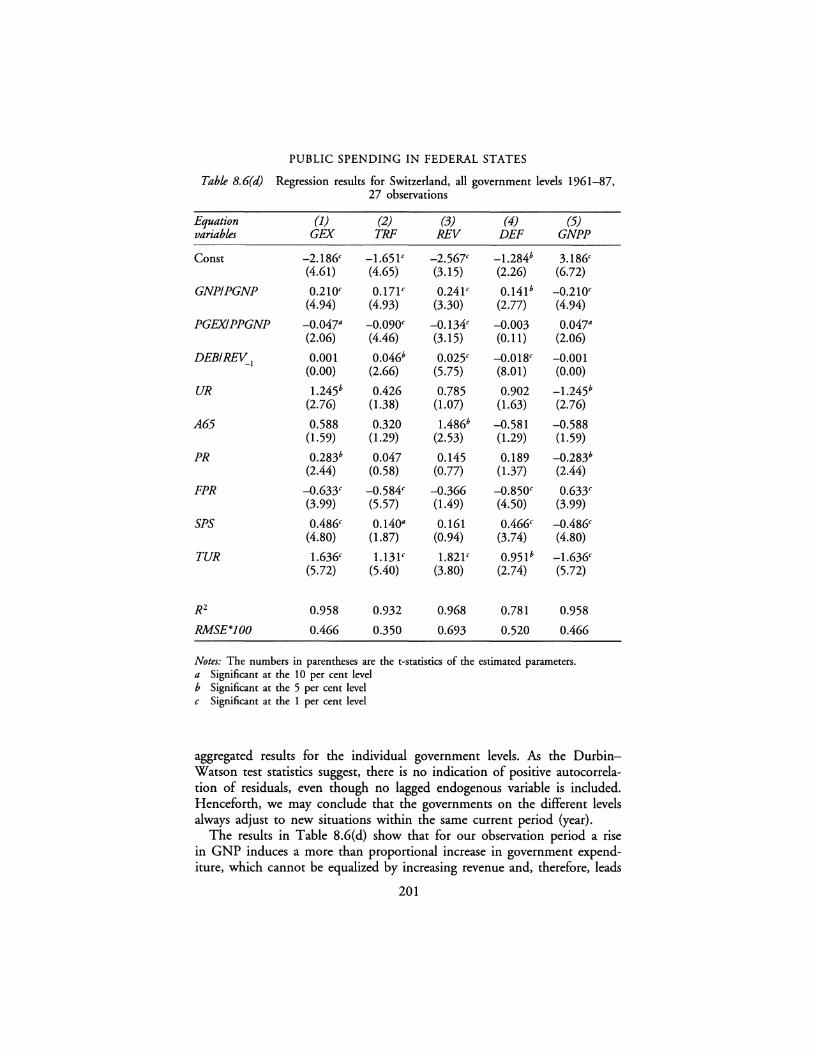
PUBLIC SPENDING IN FEDERAL STATES
Table 8.6(d) Regression results for Switzerland, all government levels 1961-87, 27 observations
Equation (1) (2) (3) (4) (5) variables GEX TRF REV DEF GNPP
Const -2.186' -1.651' -2.567' -l.284b 3.186' (4.61) (4.65) (3.15) (2.26) (6.72)
GNPIPGNP 0.210' 0.171' 0.241' 0.141b -0.210' (4.94) (4.93) (3.30) (2.77) (4.94)
PGEXIPPGNP -0.047" -0.090' -0.134' -0.003 0.047" (2.06) (4.46) (3.15) (0.11) (2.06)
DEBIREV_1 0.001 0.046b 0.025' -0.018' -0.001 (0.00) (2.66) (5.75) (8.01) (0.00)
UR 1.245b 0.426 0.785 0.902 -l.245b (2.76) (1.38) (1.07) (1.63) (2.76)
A65 0.588 0.320 1.486b -0.581 -0.588 (1.59) (1.29) (2.53) (1.29) (1.59)
PR 0.283b 0.047 0.145 0.189 -0.283b (2.44) (0.58) (0.77) (1.37) (2.44)
PPR -0.633' --0.584' -0.366 -0.850' 0.633' (3.99) (5.57) (1.49) (4.50) (3.99)
SPS 0.486' 0.140" 0.161 0.466' -0.486' (4.80) (1.87) (0.94) (3.74) (4.80)
TUR 1.636' 1.131' 1.821' 0.951b -1.636' (5.72) (5.40) (3.80) (2.74) (5.72)
R2 0.958 0.932 0.968 0.781 0.958
RMSE*J00 0.466 0.350 0.693 0.520 0.466
Notes: The numbers in parentheses are the t-statistics of the estimated parameters. a Significant at the 10 per cent level b Significant at the 5 per cent level C Significant at the 1 per cent level
aggregated results for the individual government levels. As the DurbinWatson test statistics suggest, there is no indication of positive autocorrelation of residuals, even though no lagged endogenous variable is included. Henceforth, we may conclude that the governments on the different levels always adjust to new situations within the same current period (year).
The results in Table 8.6(d) show that for our observation period a rise in GNP induces a more than proportional increase in government expenditure, which cannot be equalized by increasing revenue and, therefore, leads
201

G. KIRCHGASSNER AND W.W. POMMEREHNE
Table 8.7 Estimated income and price elasticities for Switzerland
Federal State Local Total
1970 1980 1970 1980 1970 1980 1970 1980
EGEXIGNP 0.369 0.354 2.815 2.507 2.712 2.376 2.258 2.075 EGEXIPGEX -1.034 -1.017 -1.839 -1.740 -1.363 -1.331 -1.491 -1.450 EGEXJPGNP 0.665 0.663 -0.976 -0.780 -1.349 -1.045 -0.767 -0.624
£TRFIGNP 9.909 5.633 2.439 2.047 0.347 0.457 5.148 3.643 £TRFIPGEX 5.038 2.487 -0.587 -0.464 -1.971 -1.624 1.488 0.873 ETRFIPGNP -14.947 -8.120 -1.853 -1.605 1.624 1.167 -6.636 -4.515
EREVIGNP 3.980 3.632 1.919 1.726 1.045 1.033 2.186 1.942 EREV/PGEX 2.532 2.184 -0.149 -0.141 -0.480 -0.352 0.466 0.343 £REVIPGNP -6.483 -5.817 -1.770 -1.603 -0.565 -0.680 -2.652 -2.285
EPEXIGNP 0.748 0.739 £PEXIPGEX 0.071 0.030 EPEXJPGNP -0.846 -0.848
Note: For the concrete meaning of the elasticities (£) see the appendix to this chapter, pp. 208-9.
to a greater budget deficit. However, this deficit does not occur on the federal level, only on the subcentral levels of government. Increasing income also leads to a change in the structure of government expenditure: on the federal level, transfers rise sharply but exhaustive expenditure declines as a share of GNP. On the local level, transfers remain more or less stable, whereas exhaustive expenditure increases strongly. On the cantonal level, there is an increase in both kinds of public expenditure. Taking all effects into account, rising income leads to a significant reduction of the private sector share of GNP.
This differing expenditure behaviour on the individual government levels is also reflected in the income elasticities, which are shown for the years 1970 and 1980 in Table 8.7.
For exhaustive expenditure, the income elasticity (EGEXIGNP) is greater than 1 on both subcentral levels, but considerably less than 1 on the federal level. On the other hand, income elasticities with respect to transfer payments (ETRFIGNP) are less than 1 on the local level, but incredibly high on the federal level. By looking at the relative price of public expenditure, a vety strong negative impact on transfers and revenue on the federal level (Table 8.6(a)) becomes obvious. As can be seen in Table 8.7, this leads to extremely high values for the corresponding price elasticities (ETRFIPGEX; EREV!PGEX). The estimated effects are much smaller for the subcentral levels of government and, therefore, the values of the elasticities are much more reasonable.
With respect to the other economic variables, the most significant effect of increased public debt seems to be a reduction of the deficit and an increase in revenue in the following period. Furthermore, a significant reduction of
202

PUBLIC SPENDING IN FEDERAL STATES
exhaustive expenditure also takes place on the federal level. However, public spending on the cantonal level does not seem to be affected by the indebtedness situation at all. On the federal level, unemployment leads especially to an increase in transfer payments, but also to an increase in exhaustive expenditure. On subcentral levels, it leads to a decrease in revenue. As this cannot be totally equalized by a reduction in transfer payments, deficits increase on both subcentral levels of government. Note that the cantons and the local authorities are the two government levels which receive most of their revenue from income tax, while the federal level is mainly financed by consumption (turnover) tax. Due to rising unemployment, exhaustive expenditure and transfers have been increased, but also revenue as a share of GNP. On the federal level, there is thus no indication of deficit spending to fight unemployment and, therefore, no indication of anti-cyclical fiscal policy.24
The age structure of the population does not seem to have a strong impact on public spending in Switzerland. By looking at the overall results (Table 8.6(d)), the only significant effect turns out to be an increase in revenue, which takes place on the cantonal and local levels. An increased labour force participation rate seems to decrease transfer payments on both subcentral levels, in contrast to the federal level. On the cantonal level, there also occurs an expansion of exhaustive expenditure. An increase of the share of women in the labour force induces a reduction of both expenditure categories, as well as a reduction of the deficit. Thus, with higher female labour force numbers the private sector share of GNP also increases.
The two political variables, the share of Social Democratic members in the two chambers of the Swiss parliament and the share of the working population organized in trade unions, induce the expected effects on public spending: the stronger the position of the Social Democrats in the two chambers and the higher the percentage of the labour force organized in trade unions, the lower is the private sector in relation to GNP. Thus, if Swiss people move more to the left, there will be a higher share of public and a lower share of private GNP. Another implication is that transfers also increase significantly. If this higher expenditure is not totally equalized by additional revenues, it will lead to a higher deficit. With small modifications, this holds for all three government levels and, therefore, also for the aggregated level.
The results for Switzerland are as follows: overall, the approach performs quite well and leads to 'reasonable' results with respect to the income effects and the impact of most other variables, especially the political ones. The only exception refers to the relative price effects on transfers and revenues on the federal level. In addition, in three out of four equations, the results for the cantons are better than the federal ones, and those for local communities again perform better than those for the cantons. Thus, the results also reflect quite well some of the peculiarities of the Swiss federal system outlined before.
203

G. KIRCHGA.SSNER AND W.W. POMMEREHNE
Table 8.B(a) Regression results for the Federal Republic of Germany, federal level 1961-87, 27 observations
Equation (1) (2) (3) (4) variables GEX TRF REV DEF
Const -0.099 0.380a -0.922c 1.213c (0.74) (1.97) (3.87) (5.01)
PGEXIPPGNP -0.013 -0.409c 0.406c (0.27) (7.30) (9.28)
DEBIREv_, 0.001 0.007 0.004 0.005 (0.42) (1.40) (0.61) (1.00)
UR -0.165 0.231 -0.489b 0.546b (1.11) (1.55) (2.27) (2.12)
A65 -0.942b -0.914b -l.119a 1.087 (2.22) (2.13) (1.82) (1.49)
PR -0.426 0.110 -2.743b 2.469c (1.36) (0.31) (5.53) (4.35)
FPR 1.021 -1.149 5.126c -5.307C (1.30) (1.30) (4.25) (3.86)
LEFT 0.047 -0.158a 0.513c -0.632c (1.02) (2.04) (5.41) (6.67)
SPDG -0.003 -0.001 0.012c -0.017' (1.59) (0.42) (3.35) (6.09)
GK -0.001 -0.000 -o.009c 0.009c (0.03) (0.06) (3.15) (3.91)
TUR 0.292a -0.064 0.807c -0.587b (2.13) (0.31) (3.12) (2.19)
R2 0.579 0.919 0.603 0.806
SER*JOO 0.243 0.241 0.351 0.421
D.-W 1.509 2.289 1.975 2.012
Notes: The numbers in parentheses are the t-statistics of the estimated parameters. a Significant at the 10 per cent level b Significant at the 5 per cent level c Significant at the 1 per cent level
Results for Germany
The results for the different government levels in Germany are given in Tables 8.8(a) to 8.8(c); in Table 8.8(d) the aggregated results for all levels are reported. The R2-measures show again that most of the equations can
204
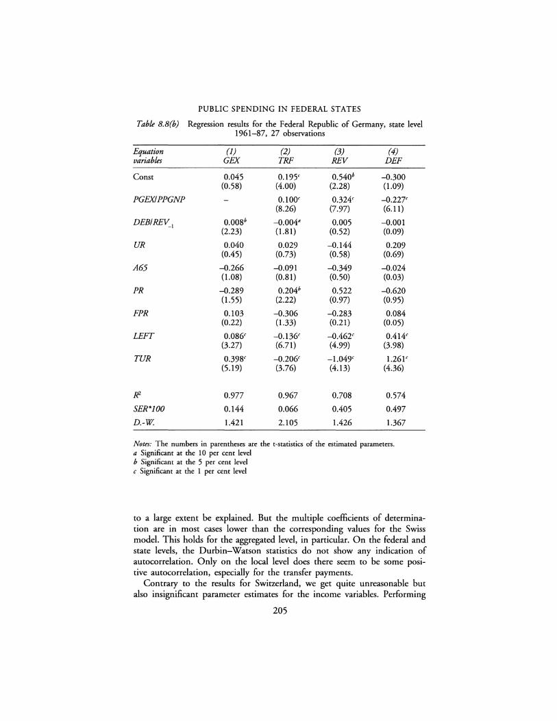
PUBLIC SPENDING IN FEDERAL STATES
Table 8.B(b) Regression results for the Federal Republic of Germany, state level 1961-87, 27 observations
Equation (I) (2) (3) (4) variables GEX TRF REV DEF
Const 0.045 0.195< 0.540b -0.300 (0.58) (4.00) (2.28) (1.09)
PGEXJ PPGNP 0.100< 0.324< -0.227< (8.26) (7.97) (6.11)
DEBIREv_1 0.008b -0.0044 0.005 -0.001 (2.23) (1.81) (0.52) (0.09)
UR 0.040 0.029 -0.144 0.209 (0.45) (0.73) (0.58) (0.69)
A65 -0.266 -0.091 -0.349 --0.024 (1.08) (0.81) (0.50) (0.03)
PR --0.289 0.204b 0.522 --0.620 (1.55) (2.22) (0.97) (0.95)
FPR 0.103 -0.306 -0.283 0.084 (0.22) (1.33) (0.21) (0.05)
LEFT 0.086< -0.136< -0.462< 0.414< (3.27) (6.71) (4.99) (3.98)
TUR 0.398< -0.206< -1.049< 1.261< (5.19) (3.76) (4.13) (4.36)
R1- 0.977 0.967 0.708 0.574
SER*JOO 0.144 0.066 0.405 0.497
D.-W. 1.421 2.105 1.426 1.367
Notes: The numbers in parentheses are the t-statistics of the estimated parameters. a Significant at the 10 per cent level b Significant at the 5 per cent level c Significant at the I per cent level
to a large extent be explained. But the multiple coefficients of determination are in most cases lower than the corresponding values for the Swiss model. This holds for the aggregated level, in particular. On the federal and state levels, the Durbin-Watson statistics do not show any indication of autocorrelation. Only on the local level does there seem to be some positive autocorrelation, especially for the transfer payments.
Contrary to the results for Switzerland, we get quite unreasonable but also insignificant parameter estimates for the income variables. Performing
205

G. KIRCHG.ASSNER AND W.W. POMMEREHNE
Table 8.B(c) Regression results for the Federal Republic of Germany, local level 1961-87, 27 observations
Equation (1) (2) (3) (4) variables GEX TRF REV DEF
Const -0.226b 0.039 0.016 0.250b (2.46) (1.67) (0.19) (2.30)
PGEXIPPGNP -0.001 -0.123 0.012 (0.13) (0.56) (0.63)
DEBIREV_1 -0.027< -0.003 0.005 -0.035' (3.43) (1.12) (0.51) (3.16)
UR 0.069 0.042 0.038 0.074 (0.66) (1.57) (0.40) (0.60)
A65 0.114 0.1324 0.129 0.118 (0.39) (1.74) (0.49) (0.34)
PR -0.052 0.059 0.122 -0.120 (0.21) (0.89) (0.52) (0.40)
FPR -0.717 -0.218 -0.376 -0.556 (1.32) (1.57) (0.78) (0.87)
LEFT 0.151 < -0.016 0.050 0.116b (4.63) (1.09) (0.92) (2.15)
TUR 0.240b 0.011 0.332b -0.083 (2.51) (0.34) (2.78) (0.62)
J{l, 0.852 0.829 0.903 0.704
SER*JOO 0.173 0.044 0.153 0.202
D.-W 1.579 0.913 1.525 1.860
Notes: The numbers in parentheses are the t-statistics of the estimated parameters. a Significant at the 10 per cent level b Significant at the 5 per cent level c Significant at the 1 per cent level
a likelihood ratio test, the null hypothesis that income has no influence on expenditure shares could not be rejected (even on the 10 per cent significance level).25 Therefore, we dropped all income terms from the system. However, we again got very unreasonable results for the relative price effects on exhaustive expenditure. Therefore, we also dropped the relative price terms from the corresponding equations. From this it follows that all implied income elasticities are + 1 and all own-price elasticities for exhaustive expenditure are -1.
However, the results for the other variables are in many cases not convincing, either. Public debt, for example, seems to have no effect on the
206

PUBLIC SPENDING IN FEDERAL STATES
Table 8.B(d) Regression results for the Federal Republic of Germany, all government levels 1961-87, 27 observations
Equation (I) (2) (3) (4) (5) variables GEX TRF REV DEF GNPP
Const 0.171 0.614c -0.366 1.164b 0.829c (0.76) (3.04) (1.03) (2.41) (3.67)
PGEXI PPG NP 0.086 -0.097 0.190b (1.65) (1.38) (2.66)
DEBIREv_1 -0.018" 0.000 0.130 -0.035" 0.018" (1.83) (0.05) (0.95) (1.77) (1.83)
UR -0.056 0.303" -0.595 0.829 0.056 (0.21) (1.85) (1.62) (1.53) (0.21)
A65 -1.094 0.956" -1.339 1.181 1.094 (1.46) (2.04) (1.29) (0.77) (1.46)
PR -0.767 0.374 -2.099b 1.730 0.767 (1.34) (0.96) (2.57) (1.46) (1.34)
FPR 0.406 -1.672" 4.467b -5.780b -0.406 (0.29) (1.76) (2.27) (2.02) (0.29)
LEFT 0.284c -0.278C 0.101 -0.102 -0.284c (3.51) (3.40) (0.69) (0.54) (3.51)
SPDG -0.003 -0.001 0.012c -0.017c 0.003 (1.59) (0.42) (3.36) (6.09) (1.59)
GK -0.000 -0.000 -0.009c 0.009b 0.000 (0.03) (0.06) (3.15) (3.91) (0.03)
TUR 0.930c -0.259 0.090 0.591 -0.930C (3.97) (1.18) (0.23) (l.ll) (3.97)
R2 0.366 0.930 0.685 0.311 0.366
RMSE*JOO 0.951 0.438 0.693 0.598 0.951
Notes: The numbers in parentheses are the t-statistics of the estimated parameters. a Significant at the 10 per cent level b Significant at the 5 per cent level c Significant at the 1 per cent level
federal level at all and a 'wrong' impact on exhaustive expenditure at the state level. Only at the local level do we find a significant reduction of exhaustive expenditure and of the deficit as a reaction to an increase in public debt.
As a look at the other structural and economic variables indicates, there are no significant results on the state and local level. This might reflect the fact that in Germany the subcentral jurisdictions have no (or only marginal) own fiscal authority; their revenue, their transfer obligations, and,
207

G. KIRCHGASSNER AND W.W. POMMEREHNE
therefore to a wide extent, also their exhaustive expenditure possibilities are determined by federal law. The only significant variables on the subcentral level of government are the two political ones. On the local level, both variables indicate an increase in exhaustive expenditure and in revenue. On the state level, however, we find a decrease in revenue and a corresponding increase in the deficit. Moreover, and this is completely implausible, we find a highly significant decrease in transfer payments on this governmental level.
On the federal level, we get more significant results. The coefficients of the unemployment variable and of the dummy variable for the great coalition clearly indicate the consequences of fiscal policy directed to a higher employment: a significant decrease in revenue and a corresponding increase in the deficit. An ageing population leads to a reduction of revenues and an increase in transfer payments, and also to a decrease of exhaustive expenditure. In addition, an increase in the total labour force participation rate leads to a decrease of revenue and an increase in the deficit while the opposite seems to be true for the female part of the working population. The political variables, finally, have a positive effect on revenue, a negative one the deficit, and negative but insignificant effects on transfer payments. At least the latter two are highly credible.
CONCLUDING REMARKS
Taking all results for Germany together and comparing them with those for Switzerland, we conclude that the latter are much more plausible with respect to theoretical a priori considerations and also more convincing from a statistical point of view. This holds even though we have used the same time period and the same explanatory variables. Thus, it may indicate that the approach used is more suitable to the Swiss (direct) democracy than to the German (parliamentary) system. From a theoretical point of view, this holds anyway, if we assume that the median voter is the decisive unit and, therefore, his/her considerations determine public spending. However, it might also indicate that we have captured the (politically) relevant variables better for Switzerland than for Germany. In any c~e, the differences in the results for the two federal systems are striking, and they can be used as empirical evidence that the differences concerning the federal structure of the two counties matter in explaining the development of public spending.
DATA APPENDIX
In performing the estimations, we have used the following time series:
GEX Exhaustive expenditure (consumption and investment) TRF Transfer payments REV Total revenue
208

DEF DEB GNP PGNP PGEX PPGNP
PUBLIC SPENDING IN FEDERAL STATES
Government deficit Government debt Gross National Product (GNP) Implicit deflator of the GNP Implicit deflator of exhaustive government expenditure Implicit deflator of the private part of GNP
For investment and, therefore, also for exhaustive expenditure and total government expenditure, we use differing indices for the different levels in the Federal Republic of Germany. For Switzerland, the corresponding disaggregated data were not available.
UR A65 PR FPR TUR SPS
LEFT
SPDG
GC
Unemployment rate Population older than 65 Total labour force participation rate Share of women in total labour force Percentage of labour force organized in trade unions Mean share of Social Democrats in the two chambers of the Swiss national parliament (equally weighted) Mean share of Social Democrats and the Greens in the German national and state parliaments (equally weighted) Dummy variable: 'I' from 1970 to 1982, when the Social Democratic Party was the leading party in the German government, 'O' otherwise Dummy variable: '1' during the German Grand Coalition from 1967 to 1969, 'O' otherwise
These time series have been constructed using data from the following sources:
Switzerland Eidgenossisches Statistisches Arnt, Revidierte Reihen der Nationalen Buchhaltung,
1948-1976, Berne, 1977. Eidgenossisches Statistisches Arnt, Nationale Buchhaltung der Schweiz, 1989 edn,
Berne, 1989. Eidgenossisches Statistisches Arnt, Offentliche Finanzen der Schweiz, Berne, various
years, 1961-88. Eidgenossisches Statistisches Arnt, Statistisches Jahrbuch der Schweiz, Berne, various
years, 1961-88.
Federal Republic of Germany Statistisches Bundesamt, Fachserie 18, Reihe SlO, Der Staat in der Volkswirt
schaftlichen Gesamtrechnung, 1950-86, Stuttgart: Kohlhammer. Statistisches Bundesamt, Fachserie 18, Volkswirtschaftliche Gesamtrechnungen,
Reihe 1.2, Konten und Standardtabellen, 1989, Hauptbericht, Stuttgart: Metzler-Poeschel.
209

G. KIRCHGASSNER AND W.W. POMMEREHNE
Statistisches Bundesamt, Statistisches jahrbuch for die Bundesrepublik Deutsch/and, Stuttgart: Kohlhammer, various years, 1961-89.
Sachverstandigenrat zur Begutachtung der gesamtwirtschafdichen Entwicl<lung, Weichenstellung for die neunziger Jahre, Jahresgutachten 1989/90, Stuttgart: Metzler-Poeschel, 1989.
NOTES
1 Compare, for example, the surveys by Larkey, Stolp and Winer (1981, 1983), Borcherding (1985), Lybeck (1986), Leineweber (1988), Henrekson (1992) or Pommerehne and Kirchgassner (1990).
2 See for instance the empirical tests of the so-called Leviathan hypothesis (Brennan and Buchanan, 1980); that is, that fiscal decentralization serves as a constraint on the behaviour of revenue-maximizing government, by Oates {1985), Abrams and Dougan (1986), Marlow (1988) and Grossmann {1989).
3 Compare also Pommerehne (I 978) as well as the critical evaluation of this model by Holcombe (1989).
4 Compare the survey by Orzechowsky (1977) as well as recent works by Moene {1986), or Schimmelpfennig (1995).
5 Though it does play a role in the discussion on the 'Laffer-curve'. 6 For the effects of taxation on the shadow economy see Frey and Pommerehne
(1982); on tax evasion see Pommerehne and Weck-Hannemann (1994). 7 The hypothesis is especially expected to hold when direct taxes are not indexed
against the impact of inflation. Such an indexation is rather the exception. In Germany, there is no indexation at all, whereas in Switzerland it is found in most cantons and on the federal level.
8 This is the argument of the 'New Classical Macroeconomics', put forward by Barro (1974, 1979, 1981). For a criticism see Leiderman and Blejer (1988).
9 See in particular Brennan and Buchanan {I 980) and Buchanan and Roback (1987).
10 See Bogdanor (I 988) for a more detailed description of the Swiss federal system, Gubler (1985) as well as Kirchgassner and Pommerehne (1992) for a comparison with the system of the Federal Republic of Germany and Bird ( 1986) for a comparison with other federal systems.
11 For this reason, von Weizsacker (1987, p. 221) once spoke of the German 'pseudo-federalism'.
12 The latter conclusion is also supported by the international comparison of Frey and Weck-Hannemann (1985).
13 When these grants are included (and thus the severe problem arises of identifying which parts belong to the exhaustive expenditure and which to transfers) the preponderance of the German federal government becomes even stronger.
14 As shown by Kirchgassner (1985), in 1983 - the last year considered - the average worker (or representative household) in Germany would have been in a better situation if none of these 'tax reforms' had been realized and if instead the initial (1958) tariff had been fully indexed.
15 The adoption of additional tasks is and has been possible according to the constitution (Art. 91 a) by means of so-called joint tasks. Either the federal government finances the traditional tasks of the states or takes them (or a few of them) over totally.
16 Which more or less means that public expenditure is regressed on expenditure. 17 Constant elasticities of demand, as they are provided in most empirical work
on government growth, are in general not consistent with optimizing behavior
210

PUBLIC SPENDING IN FEDERAL STATES
according to modern theory of consumption; see La France (1985) and Plourde and Ryan (1985).
18 Such as the 'Transcendental logarithmic demand system' (Christensen et al., 1975), or the approach used here, the 'Almost ideal demand system' by Deaton and Muellbauer (1980). See also Deaton (1986) for a survey.
19 For a more detailed discussion see Kirchgassner (1987). 20 See the Data Appendix, pp. 208-9 for details. 21 Price indices are given for public consumption. The price index for public sector
investment has been constructed using indices for (private) construction and inventory investment. For Germany there exist disaggregated figures for investment on each government level. Thus, we were able to construct separate price indices. For Switzerland only one index for public investment expenditures could be constructed.
22 This is an even stronger version of the argument put forward by Sims (1980) against the use of exclusion restrictions.
23 The estimations are performed using TSP, Version 4.1. To simplify the calculations, we have performed the two steps separately. By using OLS, we first estimated the auxiliary equations for the instruments, and by using the Zellner-Aitken Procedure (LSQ) we then estimated the system of nine equations.
24 As the Swiss unemployment rate has always been very low, there has not been very much need for such a policy.
25 As we estimated - compared to the number of observations - quite a lot of parameters for each equation, we did not perform the large sample standard likelihood ratio test, because this test only holds approximately and would have overestimated the significance. Instead, we used the adjustment ratio T - k/T-test to calculate the test-statistic, with T being the number of observations and k being the average number of parameters estimated per equation. This test has been proposed by Sims (1980) in a similar context.
BIBLIOGRAPHY
Abrams, B.A. and W.R. Dougan (1986) 'The Effects of Constitutional Restraints on Government Spending', Public Choice, vol. 49, pp. 101-16.
Barro, R.J. (1974) 'Are Government Bonds Net Wealth?', journal of Political Economy, vol. 82, pp. 1095-117.
- (1979) 'On the Determination of Public Debt', journal of Political Economy, vol. 87, pp. 940-71.
- (1981) 'Output Effects of Government Purchases', journal of Political Economy, vol. 90, pp. 1086-121.
Bergstrom, T.C. and R.P. Goodman (1973) 'Private Demand for Public Goods', American Economic Review, vol. 63, pp. 280-96.
Bird, R.M. (1986) Federal Finance in a Comparative Perspective (Toronto: Canadian Tax Foundation).
Bogdanor, V. (1988) 'Federalism in Switzerland', Government and Opposition, vol. 23, pp. 69-90.
Borcherding, T.E. (1985) 'The Causes of Government Growth: A Survey of the U.S. Evidence', journal of Public Economics, vol. 28, pp. 358-82.
- and R.T. Deacon (1972) 'The Demand for the Services of Non-Federal Governments', American Economic Review, vol. 62, pp. 891-901.
Brennan, G. and J.M. Buchanan (1980) The Power to Tax: Analytical Foundations of a Fiscal Constitution (Cambridge University Press).
211

G. KIRCHG.ASSNER AND W.W. POMMEREHNE
Buchanan, J.M. and J. Roback (1987) 'The Incidence and Effects of Public Debt in the Absence of Fiscal Illusion', Public Finance Quarterly, vol. 15, pp. 5-25.
- and R.E. Wagner (1978) 'The Political Biases of Keynesian Economics', in J.M. Buchanan and R.E. Wagner (eds) Fiscal Responsibility in Constitutional Democracy (Leiden and Boston: Nijhoff) pp. 79-100.
Christensen, L.R, D.W. Jorgenson and L.J. Lau (1975) 'Transcendental Logarithmic Utility Functions', American Economic Review, vol. 65, pp. 367-83.
Deaton, A. (1986) 'Demand Analysis', in Z. Griliches and M.D. lntriligator (eds) Handbook of Econometrics, vol. 3 (Amsterdam: North-Holland) pp. 17 67-839.
- and J. Meullbauer (1980) 'An Almost Ideal Demand System', American Economic Review, vol. 70, pp. 312-26.
Downs, A. (1957) An Economic Theory of Democracy (New York: Harper & Row). Frey, B.S. and W.W. Pommerehne (1982) 'Measuring the Hidden Economy: Though
it is Madness, Yet there is Method in it', in V. Tanzi (ed.) The Underground Economy in the United States and Abroad (Lexington: Heath) pp. 3-27.
- and F. Schneider (1979) 'An Econometric Model with an Endogenous Government Sector', Public Choice, vol. 34, pp. 29-43.
-and H. Weck-Hannemann (1985) 'The Hidden Economy as an "Unobserved" Variable', European Economic Review, vol. 26, pp. 33-53.
Grossmann, P.J. (1989) 'Fiscal Decentralization and Government Size: An Extension', Public Choice, vol. 62, pp. 63-9.
Gubler, P. (1985) 'Der Foderalismus in der Schweiz', in R. Biskup (ed.) Schweiz -Bundesrepublick Deutsch/and: Wirtschaftliche, politische und militiirische Aspekte im Vergleich (Berne and Stuttgart: Haupt) pp. 95-111.
Henrekson, M. (1992) An Economic Analysis of Swedish Government Expenditure, Brookfield: Avebury.
Holcombe, RG. (1989) 'The Median Voter in Public Choice Theory', Public Choice, vol. 61, pp. 115-25.
Kirchgassner, G. (1985) 'Die Entwicklung der Einkommensteuerprogression in der Bundesrepublick Deutschland', Finanzarchiv, vol. 43, pp. 328-47.
- (1987) 'Gilt das Wagnersche Gesetz? Zur empirischen Erfassung der langfristigen entwicklung der Staatsausgaben', University of Osnabruck, mimeo.
- and W.W. Pommerehne (1992) 'Zwischen Parteien- und Bundesstaat: Staatshandeln in der Schweiz und in der Bundesrepublick Deutschland', in H. Abromeit and W.W. Pommerehne (eds) Staatstiitigkeit in der Schweiz (Berne: Haupt) pp. 221-45.
La France, J.T. (1985) 'Linear Demand Functions in Theory and Practice', journal of Economic Theory, vol. 37, pp. 147-66.
Larkey, P.D., S. Stolp and M. Winer (1981) 'Theorizing about the Growth of Government: A Research Assessment',Journal of Public Policy, vol. 1, pp. 157-220.
- (1983) 'Why does Government Grow?', in T.C. Miller (ed.) Public Sector Performance: A Conceptual Turning Point (Baltimore and London: Johns Hopkins University Press) pp. 65-101.
Leiderman, L. and M.I. Blejer (1988} 'Modeling and Testing Ricardian Equivalence: A Survey', /MF Staff Papers, vol. 35, pp. 1-35.
Leineweber, N. (1988) Das siikulare Wachstum der Staatsausgaben: Eine kritische Analyse (Goettingen: Vandenhoeck & Ruprecht).
Lybeck, J.A. (1986) The Growth of Government in Developed Economies (London: Gower).
Marlow, M.L. (1988) 'Fiscal Decentralization and Government Size', Public Choice, vol. 56, pp. 259-270.
Moene, K.O. (1986) 'Types of Bureaucratic lnteraction',Journal of Public Economics, vol. 29, pp. 333-45.
212

PUBLIC SPENDING IN FEDERAL STATES
Oates, W.E. (1985) 'Searching for Leviathan: An Empirical Study', American Economic Review, vol. 75, pp. 578-83.
Orzechowski, W. (1977) 'Economic Models of Bureaucracy: Survey, Extension and Evidence', in T.E. Borcherding (ed.) Budgets and Bureaucrats: The Sources of Government Growth (Durham, NC: Duke University Press) pp. 229-59.
Peacock, A.T. and J. Wiseman (1967) The Growth of Public Expenditure in the United Kingdom, 1890-1955 (London: Allen & Unwin).
Plourde, A. and R. Ryan (1985) 'On the Use of Double-Log Forms in Energy Demand Analysis', The Energy Journal, vol. 6, pp. 105-13.
Pommerehne, W.W. (1978) 'Institutional Approaches to Public Expenditure: Empirical Evidence from Swiss Municipalities', Journal of Public Economics, vol. 9, 255-80.
- (1990) 'Empirical Relevance of Comparative Institutional Analysis', European Economic Review, vol. 34, pp. 458-69.
- and G. Kirchgassner (1990) 'Efficacite, redistribution, extension du secteur public: une approche de choix public', Revue Franraise de Finances Publiques, vol. 29, pp. 185-225.
- and H. Weck-Hannemann (forthcoming) 'Tax Evasion: An Empirical Analysis', Public Choice.
Schimmelplennig, J. (1995) 'Institutional Arrangements and the Quality of Publicly Provided Goods: A Tentative Note', Public Choice, vol. 85, pp. 119-26.
Sims, C.A. (1980) 'Macroeconomics and Reality', Econometrica, vol. 48, pp. 1-48. Smith, A. (1776) An Inquiry into the Nature and Causes of the Wealth of Nations
(London). Theil, H. (1957) 'Specification Errors and the Estimation of Economic
Relationships', Review of the International Statistical Institute, vol. 25, pp. 41-51. Weizsacker, C.C. von (1987) 'Foderlismus als Verjilngungskur', in H. Buhofer (ed.)
Liberalismus als Verjungungskur (Zurich and Wiesbaden: Filssli) pp. 217-35.
213

9
CAUSALITY BETWEEN PUBLIC EXPENDITURE AND TAXATION
Evidence from the Italian case
Mariano Bella and Beniamino Quintieri1
INTRODUCTION
An understanding of the intertemporal links between taxing and spending is of obvious importance in order: (i) to evaluate how different policies might, or might not, help to reduce the public deficit and (ii) from a theoretical point of view, to evaluate on an empirical basis the capacity of various theories to cope with reality. Of course, temporal causality tests do not verify theories directly, but they do allow us to reject them if causality goes in the wrong direction.
The objective of this chapter is to test the nature and the direction of causality between public expenditure and taxation in Italy since the birth of the Italian state. In order to achieve this aim we use first the standard Granger causality test and then reconsider the causality issue with the aid of co-integration and error correction modelling. Co-integration theoty allows us to identify the role of long-run equilibrium relationships in determining the fluctuations of economic phenomena in the short run. We will show that the neglect of the equilibrium relationship between taxation and public expenditure (and GDP) implies the loss of relevant information in studying causality between tax revenue and total public expenditure.
Empirical insights about the government expenditure-government revenue nexus appear to be of great importance in Italy given the very high levels of public debt and fiscal imbalances. Nowadays there is full agreement on the need to reduce government budget deficits but not the means of achieving that goal. Some advocate reduction in government spending as the optimal solution while others call for increases in taxation. In the light of our results the first of these two hypotheses seems to be the most relevant for Italy. As a matter of fact the history of Italian public finance is characterized by the guiding role of expenditure in causing the level and the dynamics of taxation. Our empirical analysis supports therefore the 'spend and tax' hypothesis while clearly rejecting the 'tax and spend' hypothesis.
214

PUBLIC EXPENDITURE AND TAXATION
In the following section we shall briefly review the studies which analyse the growth of the public sector with a view to highlighting the underlying causative processes. Next we shall discuss the data and offer a brief history of the basic time series describing the Italian public sector. The last two sections of this chapter contain a discussion of the results.
A BRIEF REVIEW OF THE LITERATURE
Three hypotheses can be advanced about the intertemporal links between taxation and spending:
1 taxes and spending change simultaneously; 2 taxes tend to change after government spending; 3 changes in expenditure follow changes in taxation.
In this section we will briefly review the literature purporting to explain the growing role of the public sector in order to highlight the causal relationship between taxation and spending implied by the various schools of thought.
The first hypothesis, fiscal synchronization, underlies mainly the traditional theories of demand for public goods (Musgrave, 1966). According to these theories:
• the electorate decides at the same time the desired level of public spending and taxation, and
• it is assumed that the quantity and the type of goods offered by the public sector reflects the preferences of the community.
The dynamic of public spending and taxation is therefore the result of the optimal behaviour by individuals who can make a correct appraisal of both the benefits and. the costs associated with each level of the public budget. This school of thought can also include the so-called 'Wagner's law', according to which, because of the nature of the goods and services offered by the state, an increase in revenue would lead to a more than proportional increase in spending. Compared to the traditional approach towards demand for public goods, this theory concentrates on the causal links between income and public spending, emphasizing the 'luxury goods' aspect of the goods and services provided by the public sector.
It is not such an easy task to find a clear causal relationship in those theories which consider public spending as a means of redistribution. The synchronization of spending and revenue seems, however, to be implicit in the works of Meltzer and Richard (1978 and 1981), based on the medianvoter model. They assume · a direct response by governments to the preferences expressed by the electors through the polls. In a democratic system that adopts the majority vote, the average elector will vote for spending and tax legislation that gives him a net positive result.
215

M. BELLA AND B. QUINTIERI
The causal links are less evident in redistribution models that refer to the role of interest groups (Peltzman, 1980; Mueller and Murrell, 1985 and 1986). This stream in the theory of public choice pays special attention to the mechanisms for reaching decisions on spending and to the roles of the groups interested in these decisions (political parties, bureaucracy, lobbies and so on). According to this view the growing weight of the public sector is a consequence of the representative nature of the democratic system, in which individual preferences are expressed through organized pressure groups. Although they do not explicitly consider the relationship between public revenue and expenditure, these models do seem to refer to the traditional view of public choice which, as we shall see shortly, postulates a causal relationship that goes from spending to revenue.
One of the most authoritative supporters of the hypothesis that the increase in taxation leads to increases in public spending is Milton Friedman:
You cannot reduce deficit by raising taxes. Increasing taxes only results in more spending, leaving the deficit at the highest level conceivably accepted by the public. Political Rule Number One is: government spends what government receives, plus as much more as it can get away with. . . . Increasing taxes would mean that you'd have just as large a deficit but a higher level of government spending.2
Although ideologically close to the ideas of Friedman, the position of Buchanan and the 'Public Choice' school in general seems to disagree over the direction of causality between tax revenue and public spending. According to this school the basic problem is how to finance public spending. Raising taxes may limit the growth of public spending if the community judges that tax rates are too high. On the contrary: 'Government borrowing and monetary creation reduce the perceived price of publicly provided goods and services. In response citizens-taxpayers increase their demand for such goods and services' (Buchanan and Wagner, 1977). According to Buchanan and Wagner, therefore, the growth of public spending is the result of the public sector being able to borrow. Deficit financing would weaken the resistance of the taxpayers/voters who, suffering from 'fiscal illusion', would get the impression that recourse to inflationary finance would mean that there are 'only people who get direct advantages and that there are not people who are placed at a disadvantage'. Contrary to what Friedman maintains, raising taxes would, in fact, put a brake on the growth of public spending, because the taxpayers would be more and more reluctant to finance increases in the quantity of goods and services offered by the public sector.
A sequence in which taxation is gradually adjusted to spending is described by Peacock and Wiseman (1961, 1979) in their analysis concerning the causes of increases in public spending. Peacock and Wiseman start from the assumption that the level of taxation is a constraint to the increase in spending and they introduce the concept of a 'tolerable' level of taxation -
216
PUBLIC EXPENDITURE AND TAXATION
that is, the level that the citizens are prepared to bear. In periods of profound crisis, caused by wars, natural calamities, deep recessions and so on, the exceptional nature of the situations calls for increased spending and shifts the level of tolerance upwards. Once the crisis has passed public spending returns to normal, but at a higher level than before, because the community is now used to the new level of taxation. The public sector has thus 'displaced' the private sector by increasing taxation and spending.
The causal nexus implied by Peacock and Wiseman's analysis would therefore be of the following type:
+ transitory public spending ➔ + permanent tax revenue
➔ + permanent public spending
In fact, the initial increase in spending to meet exceptional events would be of the transitory kind: this would lead, in turn, to an increase in tax yield generated by tax increases, which would subsequently be retained, enabling spending to be kept at a higher level (with a gradual recomposition in the structure of spending in order to take into account the real needs of the community in normal situations).
A causal nexus going from spending to taxation can also be found in Barro. This derives in the first place from an acceptance of Ricardo's theorem of neutrality, based on a rejection of the fiscal illusion hypothesis adopted by supporters of public choice. Without fiscal illusion there would not be that systematic undervaluation of the cost of public as opposed to private services that is made possible by policies of deficit financing, and consequently there would not be those substitution effects which, in the view of Buchanan and Wagner, are the main cause of the growth of the public sector.
Subsequent contributions by Barro (1979, 1986) were more directly addressed to identifying the relationship between expenditure and revenue in the public sector. His starting point was the removal of a crucial hypothesis of the Ricardian neutrality, namely the existence of a non-distortionaty taxation. Even in a world with overlapping generations, where dynastic links are relevant and stable, and with perfect capital markets, a budget deficit, due to postponement of taxation, may not give rise to neutral effects when the taxes distort the behaviour of individuals.
Consequently, when taxes have distorting effects, the best policy to follow, according to Barro, is one that conforms to the principle of 'tax smoothing', according to which taxation should be commensurate to permanent public spending after interest, while transitory fluctuations in spending itself should be financed through the public debt. This leads, in Barro's view, to a causal nexus that goes from public spending (permanent) to taxation (permanent), while increases (or reductions) in spending that are considered transitory would require budget deficits (surpluses). The imbalances in the public
217

M. BELLA AND B. QUINTIERI
budget would thus have the task of eventually 'smoothing out' tax rates in order to reduce costs resulting from the distorting effects of the taxation.
A CONCISE DESCRIPTION OF THE ITALIAN PUBLIC SECTOR
In order to test the causal relation between public spending and revenue in Italy, we have used a data set spanning the years 1866-1989, which includes public spending and revenue, national income, a price index and population.
We confine the public sector to the central government budget (Bilancio di Cassa de/lo Stato) for which data are available from the foundation of the modern state of Italy. Obviously a wider definition of the public sector (for example, consolidated accounts of the public sector) would have offered a better description of Italian fiscal history but these data were not available for such a long time span. However, in 1989 our figures cover 75 per cent of the expenditure and 71 per cent of the revenue with respect to the wider definition of the public sector. Both expenditure and revenue are considered on a current and capital basis, and public spending is considered, both including and excluding interest payments on the public debt. The sources for these time series are ISTAT and Bank of Italy (various issues). The consumer price index has been used as a deflator of all fiscal variables.
For national income we have used the gross domestic output and its deflator calculated at factor cost. As in 1985 there was a change in the way of computing the Italian GDP, we have used the 'old' national accounts up to that year and we have computed the remaining four observations (1986-9) by applying the annual rates of growth of GDP obtained from the 'new' national accounts to the 'old' data levels. Finally, we have utilized the resident population in order to compute the per caput data for expenditure and revenue.
The basic time series of the Italian Public Finance are shown in Figures 9.1 to 9.5. Figures 9.1 and 9.2 portray the evolution of government spending and government revenue as percentages of GDP for the entire period, while Figures 9.3 to 9.5 display the evolution of revenue, expenditure and public deficits in per caput terms during three subperiods.
The public expenditure-GDP ratio shows an upward trend and three peaks: the first two occurring around the two world wars and the third one characterizing the last fifteen years of our sample period. The average value of this ratio for the whole period is 20.1 per cent, with the lowest value reached in 1873 (8.7 per cent) and the highest in 1986 (53.2 per cent). The annual average rate of growth of public expenditure in real terms was approximately 3 per cent. The increased ratio of government spending to national income was of course accompanied by an increase in revenue. Taxation amounted to about 6 per cent of GDP at the beginning of our
218

60
50
40
30
20
10
0 1865
40
30
20
10
0
1865
PUBLIC EXPENDITURE AND TAXATION
including interest
net interest
1890 1915 1940 1965
Figure 9.1 Government spending as % of GDP
1890 1915 1940 1965
Figure 9.2 Government revenue as % of GDP
219
I' I
1990
1990

M. BELLA AND B. QUINTIERI
50 120 I
I 110 40 I I
expenditure I
I I 100 " -30 I\ . I e I \
,, \ , \ I
I \ I
I ~ :!;:: I ,, \ /\ \,.,,,,.. ... \ 90 .g I ' ,,, -, I \ I
20 I ,, ,, '1::j
~ I C:
/\ I 80 l I •
I
10 I Q:i
I I 70
' I I •
0 _,,,,,
60 ,,,
-10 ,-----,-~-.----~~~-,-~--,-~-.----~~~-,-~--,-~-r50 1866 1871 1876 1881 1886 1891 1896 1901 1906 1911 1916
Figure 9.3(a) Public expenditure and deficit (000 lire per caput at 1980 prices)
50 110 I
40 revenue ,- ---~" 100 ,, ' ,-, I
I \ I /\ I \ I ,, \ 90 ,-, / ,... -,,, " 30 I _, I '
,1",,, I ,,, ~ :!;::
I 80 ~ 20 I C:
~ _, §!
\ I 70 e I ,1
10 ,, I ,- " I 60 I
0 _, 50 I
I I
-10 40 1866 1871 1876 1881 1886 1891 1896 1901 1906 1911 1916
Figure 9.3(b) Public revenue and deficit (000 lire per caput at 1980 prices)
sample period, while today it is close to 40 per cent. However, although this ratio has increased by 22 per cent between 1973 and 1989 (from 17 .3 to 39.3 per cent) this has not prevented Italy from exhibiting very high fiscal imbalances, with budget deficits showing values higher than 10 per cent of GDP. As a consequence there has been a huge increase in interest payments on public debt.
A detailed description of facts and figures of the history of the Italian public sector is contained in Pedone (1967) and Brosio and Marchese (1986). Here we limit ourselves to a brief description of the main events. The beginning of the sample periods coincides with Italy's birth as a nation. The first government was formed by the so-called 'Historical Right', which adhered
220

PUBLIC EXPENDITURE AND TAXATION
400 600
300 500
400 I!! ~ 200 ::i
~ '6 expenditure 300 C:
~ ~ 100 , 200
Cl) , , -, ,----~
' __ ,
0 100 deficit
-100 0 1914 1918 1922 1926 1930 1934 1938 1942 1946
Figure 9.4(a) Public expenditure and deficit (000 lire per caput at 1980 prices)
400
300 ,---- expenditure
100
0
210 200
180
160
140 I!! .2
120 '6 ~
100 ~ 80 Cll
60
40
-100 'r-~--.-~--,-~-~~-..--~-,--~-,-~-----.-~---r20 1914 1918 1922 1926 1930 1934 1938 1942 1946
Figure 9.4(b) Public revenue and deficit (000 lire per caput at 1980 prices)
to the balanced-budget principle. At that time Italy had one of the largest deficits in its history, with revenue in 1866 covering just one-half of public spending and with very high interest payments on public debt. Between 187 4 and 1884 the budget almost balanced. The 'Historical Right' fell from power, however, and it was replaced by the 'Historical Left', which embarked on spending programmes aimed at expanding the country's infrastructure. As a result a growing level of imbalances in the public budget occurred during the period 1885-94, with interest payments amounting to more than 30 per cent of public expenditure. From 1896 to 1906 the role of the public sector in the economy declined steadily as the country enjoyed high growth rates of output. A new increase in expenditure occurred from 1907 to 1918,
221

1.2 1.0 0.8 0.6 0.4
:!;:: ;g 0.2
~ 0.0 -0.2 -0.4 -0.6 -0.8 ... -----1.0
M. BELLA AND B. QUINTIERI
deficit
expenditure ,--,-_____ ,. ---
I
' I I' I
I ,,, ,,,
I I
4
,,,,,,' 3
1946 1951 1956 1961 1966 1971 1976 1981 1986 1991
Figure 9.5(a) Public expenditure and deficit (000 lire per caput at 1980 prices)
1.2 3 1.0 0.8 , , 0.6 , ,
---, 2 0.4 ,
I Q) :!;:: 0.2
I ~ .g deficit _, C:
I !!;? ~ 0.0 ,- I
, , 2! -0.2 ,
, \ , , -0.4 ,-' ,,..----
revenue , , -0.6 --- ,
-0.8 ---------------1.0 0 1946 1951 1956 1961 1966 1971 1976 1981 1986 1991
Figure 9.5(b) Public revenue and deficit (000 lire per caput at 1980 prices)
generated partly by the war against Libya but mainly by the First World War. Taxation was increased between 1920 and 1927 with the objective of restoring balance to the budget, resulting in an increase in direct taxes which accounted for 40 per cent of the total revenue.
Mussolini's dictatorship and the Great Depression gave a new impetus to the growth of the public sector, with the government extending its intervention into industry and banking. In particular a sustained increase in public spending occurred in 1935-8, when the expenditure-GDP ratio moved from 20 per cent to 30 per cent. Increased military spending due to the African campaigns and the Second World War propelled public spending in a new upswing during the period 1939-48, while tax revenue fell to very low levels (about 12 per cent of GDP).
222
PUBLIC EXPENDITURE AND TAXATION
The ratio GIY displays only cycles of modest amplitude during the 1950s and the 1960s and a sharp acceleration in the 1970s. Between 1970 and 1973 the primary deficit increased from 4.3 per cent to 8.3 per cent of GDP. This increase was not cyclical but was caused by a structural jump in public expenditure not matched by a corresponding change in revenues. The early 1970s was a period of big social reform: extensions of the years of compulsory schooling, reform of the health care system, the decision to link pension benefits to earnings rather than to contributions, and so on. The gap that those social bills opened in public finances has not since been closed despite the fact that in the mid-1970s government revenue was widened through a combination of a larger tax base, higher tax rates and higher inflation rates.
EMPIRICAL RESULTS
The first empirical tests, Dickey-Fuller (OF) and augmented Dickey-Fuller (ADF), concern the properties of the time series used. The logs of the variables relevant to our analysis (tax revenue= T, total government spending= G, government spending net of interest payments = GN, and national product at factor cost = Y) turned out to be integrated series of order one in both nominal and real terms.
Table 9 .1 shows that the first differences of these variables are stationary. The fact that all the variables are integrated of order one allows us to perform an analysis based on a linear combination of such variables (that is, the cointegration analysis developed in the next section).
The figures in Table 9.1 are the Student-t of coefficient b in the equations OF:
and ADF:
(1- L)xt =a+ bxt-l + ~ c1(1 - L)xt-J j
where the optimal lags (j) are selected according to AIC criterion (Granger and Newbold, 1986, p. 82):
(SSR) 2KT AICT= log - +-NT N
The null hypothesis of unit roots is not rejected on the basis of the significant negativity of b (Dickey and Fuller, 1981).
As the level of economic activity was supposed to play an important role in determining fiscal variables, we carried out the tests of causality both in a bivariate and a trivariate framework in order to verify whether the
223

M. BELLA AND B. QUINTIERI
Table 9.1 Time-series properties of variables: DF and ADF tests
Nominal Real
DF ADF (Lags) DF ADF (Lags)
T -4.54 -4.20 (1) -7.56 -7.42 (1) G -7.36 -4.79 (1) -9.98 -6.89 (1) ·cN -8.03 -5.22 (1) -10.40 -7.10 (1) y -4.85 -3.80 (1) -9.09 -1.04 (1)
Note: All the values are significant at the 1 per cent level.
inclusion of per caput income has any real influence. In addition, it seemed advisable to tackle the analysis in nominal as well as in real terms.
In order to test Granger-causality we used first a VAR model, with first differenced variables, based on the F-test on the joint significance of each variable with respect to a formulation of a V AR model which does not include that variable. The lag structure in each model was selected according to the AIC (Akaike Information Criterion). It was then possible to investigate causality on a nested model basis. Our estimation strategy (i) includes the Granger causality test between taxation and public expenditure (both gross and net of interest expenditure); (ii) makes use of both nominal and real variables; (iii) evaluates the role of GDP as an explanatory variable; (iv) deals with the two possible directions of causality, from taxation to public expenditure and vice versa. We have therefore 16 equations by means of which to verify the Granger causality between fiscal variables.
The empirical results are shown in Table 9.2, which provides clear evidence in favour of the hypothesis that, in nominal terms and putting aside the role of GDP, there is a two-way causality between the fiscal variables examined. Moreover, if we take into account the influence of GDP and/or eliminate the correlation derived from the price component common to all the variables, this changes the causal pattern, always revealing a strong one-way link from spending to taxation. Note also that in the two equations with tax revenue as a dependent variable, in real terms and with GDP, many coefficients of lagged expenditure are statistically significant. This suggests that shocks in public expenditure could have persistent effects on taxation, showing the difficulties encountered by governments trying to absorb the excess spending. Such difficulties do not seem to arise in the opposite case.
In Table 9.3 we compare our results with some analogous studies based on the Granger causality test and mainly referring to the USA. Quite apart from differences in time periods and in the data set used in different studies, no common pattern of causality emerges from Table 9.3. This again confirms the weakness of the causality test when co-integration relationships between variables are not taken into account.
224

PUBLIC EXPENDITURE AND TAXATION
Table 9.2 Granger-causality test in a nested-model framework: bivariate and trivariate cases
Nominal terms Real terms Nominal terms with GDP Real terms with GDP
Nominal terms Real terms Nominal terms with GDP Real terms with GDP
Taxes on expenditure
9.21b (3,115) 3.3oa (4,119) 2.08 (2,113) 3.46b (9,980)
Taxes on net expenditure
9.00b (3,115) 3.31a (4,119) 2.08 (2,113) 3.59b (9,980)
Expenditure on taxes
4.784 (2,116) 3.47 (1,119) 1.94 (2,115) 0.00
Net expenditure on taxes
4.744 (2,116) 2.50 (1,119) 2.04 (2,115) 0.00
Note: Figures in the table are the F statistics for the joint significance of lagged differences of the variables on the right-hand side of the equations estimated. Degrees of freedom in parentheses; the optimal lag structure was selected according to the AlC. a Significant at the 5 per cent level b Significant at the 1 per cent level
Table 9.3 Some results from the application of the classical Granger-causality test to fiscal variables
Nominal terms Real terms
Period Country T➔G G➔T T➔G G➔T
Miller and Russek Post-Second (1990) World War USA *(F) *(SL) *(F) *(SL)
Ahiakpor and Amirkhalkhali (1989) 1886-1985 Canada *
Manage and Marlow (1986) 1929-1982 USA *(F) *(F) *(F)
Ram (1988) Post-Second World War USA *(F) *(SL) *(F) *(SL)
Blackley (1986) 1929-1982 USA *(F) Anderson et al. Post-Second
(1986) World War USA *(F) von Furstenberg et al. 1954-1982 USA *(F) *(F)
(1986) This study 1866-1989 Italy * * *
Note: von Furstenberg et al. (1986) used a VAR model and, as in this study, Miller and Russek (1990) used the Granger test only as a first step of analysis. 'F' means federal level, 'SL' means state and local level.
225

Table 9.4 Co-integration regressions
K T T G G GN GN y y DW R SSR DF ADF Lags
9.1 T -0.24 0.98 1% 1 % (-6.94) (211.36) 0.61 0.99 5.05 -5.61 -4.29
9.2 T -0.72 0.62 0.41 1 % 1 % (-8.54) (10.21) (6.10) 0.61 0.99 3.84 -5.73 -4.56
9.3 T -0.19 0.95 1 % 1 % (4.61) (182.23) 0.62 0.99 6.78 -5.58 -3.84 2
9.4 T -0.82 0.50 0.52 1% 5% (-8.41) (7.71) (7.00) 0.57 0.99 4.80 -5.34 -4.13 2
9.5 T -0.22 0.94 1 % 1 % (-7.29) (58.15) 0.62 0.97 5.03 -5.65 -4.38
9.6 T -1.20 0.44 0.79 1 % 1 % (-10.74) (7.64) (8.95) 0.59 0.98 3.00 -5.74 -4.54
9.7 T -0.14 0.84 1 % 1% (-3.81) (49.37) 0.61 0.95 6.88 -5.46 -3.87
9.8 T -1.42 0.28 0.99 1 % 5% (-10.84) (4.77) (9.95) 0.52 0.97 3.76 -5.14 -4.08
9.9 G 0.23 1.02 1 % 1 % (6.29) (24.36) 0.60 0.99 5.21 -5.57 -4.27
9.10 G -0.16 0.76 0.28 1 % 10% (-1.39) (10.21) (3.46) 0.52 0.99 4.74 4.90 -3.33 2
9.11 G 0.18 1.03 1 % 1 % (5.15) (58.15) 0.60 0.96 5.52 -5.43 -4.18
9.12 G -0.39 0.75 0.42 1 % 10% (-1.94) (7.64) (2.86) 0.55 0.97 5.16 -4.94 -3.38 2
9.13 GN 0.17 1.05 1 % 1 % (3.98) (182.2) 0.62 0.99 7.48 5.56 -3.82 2
9.14 GN -0.41 0.67 0.41 1% 10% (-2.95) (7.72) (4.39) 0.54 0.99 6.44 -4.90 -3.45 2
9.15 GN 0.08 1.13 1 % 5% (1.79) (49.37) 0.59 0.95 9.27 -5.27 -3.70 2
9.16 GN -1.06 0.58 0.83 1 % 10% (-4.25) (4.77) (4.63) 0.55 0.96 7.85 -4.78 -3.35 2
Note: The bar indicates variables expressed in real terms.

PUBLIC EXPENDITURE AND TAXATION
At this point we move on to examine causality by means of co-integration analysis, explicitly taking into account long-run relationships among variables. We examine co-integration relationships in a bivariate and trivariate setting in order to evaluate also the role of GDP on levels and dynamic of fiscal variables. In addition, it seemed advisable to tackle the analysis in nominal as well as in real terms. The results of the co-integration regressions are reported in Table 9.4.3
The aim of these estimates is to restrict the co-integration space between variables. We start by eliminating the equations which do not include the GDP among the explanatory variables as from the SSR it emerges that GDP plays, as economic theory predicts, a relevant role4 in explaining levels and dynamic of fiscal variables.
This allows us to investigate causality between tax revenue and public expenditure, 'clearing' this relationship from spurious correlations. We exclude also equations 9.10, 9.12, 9.14 and 9.16 which, on an ADF test basis, do not appear to be co-integration relations.5 In this case the ADF test is more appropriate than the DF, as the lagged differences in the residuals are significant. In fact ignoring a relevant part of the autoregressive process that generates the variables leads to a D F test that is highly misspecified.
Using the remaining equations 9.2, 9.4, 9.6 and 9.8, we verify that they represent four different co-integration relationships. However, equations 9.2 and 9.4 are the nominal version of equations 9.6 and 9.8. Then to test the role of inflation we jointly estimated by the FIML method the two following pairs of equations:
T = 0P + a 1 + /31 G + 'Y1 Y
and
where all variables are expressed in natural logs, the bar indicates again variables expressed in real terms, and P is the common deflator. For the first two equations we obtained: 0 = 0.02, a 1 = a2, {31 = {32' y1 = y2 and in the second case 0 = 0.02, a;= a'2, 13; = 13; and '}'; = ')';. These results allow us to conclude that the role of inflation is quite negligible. We then concentrate only on the'>two co-integration vectors defined by the coefficients of equations 9.6 and 9.8.
The identification of the two co-integration vectors indicates the existence of long-run equilibrium relationships among variables. In our case we have
227

M. BELLA AND B. QUINTIERI
found a relationship among public expenditure (both including and excluding interest payments), GNP and tax revenue (regressions 9.6 and 9.8). However, these relationships do not offer information concerning the direction of causality among variables, but we know that (i) if variables are co-integrated there must be causality in at least one direction, (ii) the co-integration constraint should be utilized for an efficient estimation of the model employed to investigate Granger-causality when variables are co-integrated. The data-generating process is then an error-correction mechanism and in such a context, when both long-run equilibrium relationships and shortrun dynamics are modelled, we test causality between public spending and taxation.
We define respectively uG and uGN' the residuals from the co-integration equations 9.6 and 9.8. They represent the 'equilibrium errors' that variables tend to correct, moving toward those levels representing the long-run solution. To test the direction of causality between taxation and respectively total public expenditure and public expenditure net of interest we estimated the following 'error-correction' equations:
(1-L) T= T(lags((l -L)T), lags((l -L)Y), uc1--1) (I)
(1 - L) T = T (lags((l - L) T), lags((l - L) Y), uGt-1), lags(l - L)( G) (I')
(1-L) G = G (lags((l - L)G), lags((l -L)Y), uc1--1) (II)
(1- L) G = G (lags((l - L)G), lags((l - L)Y), uct--1), lags(l - L)(G)) (II')
(1 - L) T = T (lags((l - L) T), lags((l - L) Y), uGN1--J (III)
(1 - L) T = T (lags((l - L) T), lags((l - L) Y), uGN1--i), lags(l - L)( G)) (III')
(1-L) GN= GN(lags((l-L)GN), lags((l -L)Y), uGN1--i) (IV)
(1-L) GN= GN(lags((l-L)GN), lags((I-L)Y),uGNt-i), lags(l-L)(GN)) (IV')
In estimating these equations we relaxed the hypothesis of nested models, then suppressed insignificant parameters, leading to more parsimonious and then efficient models. Much in the spirit of Granger-causality we tested the significant reduction of residual variances - and then the causality among variables - between the four pairs of equations (I vs. I', and so on).
As we refer to non-nested models, the reduction of the variance is tested using the method proposed by Kang (1989). The test is based on the comparison of the variances of two series of residuals, the first obtained from a
228

PUBLIC EXPENDITURE AND TAXATION
Table 9.5 Causality between fiscal variables in error-correction models
SSR LM-AUTO LM-Het Kang test t(u,_1)
2.80 10.09 1.61 2.81 5.86 I' 2.13 8.81 0.99 cr2(1;) < cr2 (I) 5.91
G causes T
II 1.56 10.29 14.38 1.59 II' 1.39 13.95 8.31 <r (II') = <r (II)
T does not cause G
III 2.80 11.95 0.85 3.06 5.89 III' 2.05 7.62 0.55 <r (III') < <r (III) 5.75
GN causes T
IV 2.11 13.50 10.67 0.55 2.93 IV' 2.05 14.85 7.05 <r (IV') = <r (IV) 2.10
T does not cause GN
Notes: LM-AUTO is a test for residual autocorrelations {Johnston, 1984, p. 320); LM-MET is the Lagrange multiplier test for heteroscedasticity; of residuals; t(u,_) is the Student-t of the lagged disequilibrium coefficient. Optimal lags in LM-Het were selected according to the AIC.
bivariate model and the second from a univariate model including only XI. If the variance of the bivariate model is lower than the one obtained from the univariate model then X2 Granger-causes XI. Given two white-noise series, EI and E2, representing the residuals of the two models, Kang demonstrates that the variance a; of E2 is significantly lower than the variance of a f of EI if in the regression:
(EI - E2) = a + b (EI + Ez)
the b coefficient is positive and statistically significant and then X2 Grangercauses XI.
We then used the Kang procedure to test causality in the error-correction framework described by equations I-IV'. The results are shown in Table 9.5. Note first that the LM tests do not reject, for all equations, the hypotheses of no autocorrelation and no conditional heteroscedasticity of residuals. The disequilibrium terms are always non-negative and less than one, this indicating that fiscal variables tend to adjust the inherited errors toward the equilibrium relationships.6
The main result is that public expenditure causes taxation. This occurs through two channels, the adjustment toward the long-run equilibrium (t-values in the last column of Table 9.5) and the reaction of tax revenue to short-run changes (improvements in estimation of taxation when lagged changes in public expenditure are included). The direction of causality obtained is strengthened by the evidence that taxation does not cause public
229

M. BELLA AND B. QUINTIERI
expenditure as shown in equations II and II'. Weak signs of bidirectional causality emerge when net-of-interest expenditure is taken into account. However, this seems to work only through the long-run adjustment channel, whereas there is no evidence of short-run influence of tax revenue change on the pattern of public spending (see the Kang test in equations IV and IV').
Thus, we can conclude that there is no evidence of a tax revenue constraint on the level and dynamic of fiscal variables. On the contrary it emerges that it is public expenditure that plays the leading role in determining the weight of the public sector in the economy.
A SUBPERIOD ANALYSIS
The length of the period examined may raise some doubts about the invariance of the causal process between fiscal variables. These doubts seem to be confirmed by the observation that in the period 1866-1989, there was a succession not only of widely different governments but above all of very different regimes, mainly the monarchy, the Fascist regime, and finally the democracy that followed immediately after the Second World War.
Nevertheless, the analysis of causality considered here aims at evaluating how the economic system over a long period relates the fiscal variables to each other, considering them as structurally endogenous variables. This decreases the relevance of the problem of the change in the political trends during the period of analysis. What is of interest in this context are the actual variations in the causal relationships between expenditures and taxation that can eventually be established on the basis of the available data.
Table 9.6 shows the statistical regressions - the possible equation of cointegration for the sub periods considered. We have divided the available data into three subperiods:
1 the years from the unification of Italy until the First World War 2 the Fascist Period and 3 the years from the Second World War up until today.
Nevertheless, to have a sufficient degree of freedom we have estimated the statistical regressions considering two subperiods at a time.
As can be seen by the substantial similarity of the estimated parameters and from the co-integration ADF test, what emerges is a picture not very different from that described by the analysis regarding the entire period under inquiry. The only exceptions worthy of further analysis seem to be the cases (B) of the regressions with, on the left, the total expenditure and the expenditures net of interest. In these two cases no co-integration vector was found in estimating the regressions for the whole period, whereas when one excludes the information relative to Italian fiscal history from the end of the Second World War, there seems to be co-integration (ADF = -4.34 and ADF =
230

Table 9. 6 Co-integration regressions for sub periods
K r G GN y R2 DF ADF Max. NOB lags
ADF
Taxes (T) (1866-1989) (A) -1.20 0.44 0.79 0.98 -5.74 -4.31 6 124 ( 1866-1946) (B) -1.21 0.42 0.88 0.90 -5.41 -4.10 3 81 (1915-1989) (C) -1.31 0.42 0.88 0.98 -3.76 -3.85 1 75 (1866-1914, 1947-1989) (D) -1.04 0.52 0.66 0.98 -8.90 -3.91 7 92
Taxes (T) (1866-1989) (A) -1.42 0.28 0.99 0.97 -5.14 -3.61 6 124 ( 1866-1946) (B) -1.45 0.25 1.07 0.88 -4.85 -3.21 1 81 (1915-1989) (C) -1.33 0.37 0.94 0.97 -3.54 -3.64 1 75 (1866-1914, 1947-1989) (D) -1.29 0.33 0.89 0.98 -7.86 -2.90 2 92
Total expenditures (G) (1866-1989) (A) -0.39 0.75 0.42 0.97 -4.94 -3.38 1 124 ( 1866-1946) (B) -0.43 0.72 0.54 0.89 -5.09 -4.34 1 81 (1915-1989) (C) 0.01 0.89 0.12 0.94 -3.54 -3.1 8 75 (1866-1914, 1947-1989) (D) -0.64 0.65 0.58 0.98 -4.39 -2.6 2 92
Expenditure net of interest (GN)
(1866-1989) (A) -l.06 0.58 0.83 0.96 -4.78 -2.85 8 124 ( 1866-1946) (B) -0.95 0.61 1.08 0.88 -5.13 -5.02 8 81 (1915-1989) (C) -0.49 0.72 0.39 0.94 -3.79 -3.20 8 75 (1866-1914, 1947-1989) (D) -1.45 0.42 1.09 0.98 -4.51 -3.60 8 92

M. BELLA AND B. QUINTIERI
-5.02). There could then be a different causal relationship in respect to those that emerged in the analysis of the whole test period. As in that case, we have estimated the error-correction models. The results (not reported) are strikingly similar to those obtained previously, that is to say that what emerged is one-way causality from the expenditures to the tax revenue. Once again, in the case of the expenditure net of interest, there seems to be confirmed an extremely weak two-way causal relationship, composed of a significant causality that goes from the expenditure to the taxes and a slight relation that goes from the taxes to expenditure. One can conclude therefore that, in view of the long period adopted here, the Italian economic system has not demonstrated substantial modifications in the causal relationships of public expenditure and taxes in relationship to the change of regimes or in the change of political orientation.
CONCLUSIONS
In an attempt to investigate whether the growth in public expenditure causes or is caused by the growth in taxation the present study comes to the following conclusions.
As far as methodology is concerned it has been shown that the use of the co-integration theory should be preferred to the standard Granger test. We noted that levels of variables, combined in a long-run equation, play a crucial role in explaining the dynamic of fiscal variables. As it emerged that the role of GDP cannot be ignored in determining government revenue and expenditure, we examined co-integration relationships in a trivariate setting including GDP in the regressors.
From the results obtained in. this chapter, what emerges quite clearly is that the 'tax and spend' view is definitely rejected by the data, because there is no evidence of a tax revenue constraint on the level and dynamics of fiscal variables. On the contrary it emerges that it is public spending that plays the leading role in determining the weight of the public sector in the economy.
These results have important implications both for the debate concerning ways to limit public deficits in Italy and for assessing the explanatory power of theories purporting to explain the behaviour of the public sector. As far as policy implications are concerned the most important conclusion to be drawn from causality tests is that proposals that endorse tax increases to close the budget deficit do not offer permanent solutions to underlying fiscal problems. Our results do not favour tax increases over spending reductions as a means of closing future deficit levels.
From the theoretical point of view our results are in sharp contrast with the view that changes in expenditure follow changes in taxation, while they concur with those theories based on the causal pattern going from expenditure to taxation.
232

PUBLIC EXPENDITURE AND TAXATION
NOTES
1 We are grateful to F. Cocco, M.C. Pichery and to two anonymous referees for their helpful comments.
2 Quoted from Anderson et al., 1986, p. 631. 3 In all the equations two dummy variables have been used corresponding to the
two world wars. 4 Note that Wagner's law does not find empirical support even in this simplified
representation. The value of the income elasticity of net of interest expenditure is 0.83, almost equal to the result obtained by Bella and Quintieri (1989) for the period 1960-85.
5 In order to select lags in the ADF test we used the AIC and the Ljung-Box (1978) test to verify that the optimal lag structure is consistent with white-noise residuals.
6 From the error-correction models estimated we calculated tax and public expenditure multipliers with respect to income and to other fiscal variables. In accordance with economic theory all the values of these multipliers turned out to be positive. The impact multipliers are lower than total multipliers, these being in turn slightly lower than the long-run elasticities obtained from regressions shown in Table 9.4.
BIBLIOGRAPHY Ahiakpor, J.C.W. and S. Amirkhalkhali (1989) 'On the difficulty of eliminating
deficits with higher taxes: some Canadian evidence', Southern Economic journal, pp. 24-31.
Anderson, W., M.S. Wallace and J.T. Warner (1986) 'Government spending and taxation: what causes what?', Southern Economic journal, pp. 630-9.
Balvir, S. and B.S. Sahni (1984) 'Causality between public expenditure and national income', The Review of Economics and Statistics, pp. 630-44.
Bank of Italy, Annual report (various issues). Barro, R.J. (1979) 'On the determination of the public debt', journal of Political
Economy, pp. 940-71. - (1986) 'The neoclassical approach to fiscal policy', in R. Barro (ed.) Modern
Business Cycle Theory, Oxford: Basil Blackwell. Bella, M. and B. Quintieri (1989) 'Crescita in disequilibrio ed espansione del settore
pubblico', Rivista lnternazionale di Scienze Sociali, no. 2. Blackley, P.R. (1986) 'Causaliry between revenues and expenditures and the size of
the federal budget', Public Finance Quarterly, pp. 139-56. Brosio, G. and C. Marchese (1986) Le potere di spendere, Bologna: il Mulino. Buchanan, J.M. and R.W. Wagner (1977) Democracy in Deficit: the Political Legacy
of Lord Keynes, New York: Academic Press. Dickey, D.A. and W.A. Fuller (1981) 'Likelihood ratio statistics for autoregressive
time series with a unit root', Econometrica, pp. 1057-77. von Furstenberg, G.M., RJ. Green and J. Jeong (1986) 'Tax and spend, or spend
and tax?'. The Review of Economics and Statistics, pp. 179-88. Granger, C.W.J. and P. Newbold (1986) Forecasting Economic Time Series, London:
Academic Press. ISTAT (1958) Sommario di statistiche storiche italiane: 1861-1955. - (1988) Sommario di statistiche storiche italiane: 1926-85. Kang, H. (1989) 'The optimal lag selection and transfer function analysis in Granger
causality test', journal of Economic Dynamics and Control, no. 13, pp. 151-69.
233

M. BELLA AND B. QUINTIERI
Ljung, G.M. and G.E.P. Box (1978) 'On a measure of lack of fit in time series models', Biometrika, pp. 67-72.
Manage, N. and M.L. Marlow (1986) 'The causal relation between federal expenditure and receipts', Southern Economic journal, pp. 617-29.
Meltzer, H. and S. Richard (1981) 'A rational theory of the size of government', journal of Political Economy, vol. 89, pp. 914-27.
Miller, S.M. and F.S. Russek (1990) 'Co-integration and error-correction models: the temporal causaliry between government taxes and spending', Southern Economic journal, pp. 221-9.
Mueller, C.D. and P. Murrell (1985) 'Interest groups and the political economy of government size', in F. Forte and A. T. Peacock (eds) Public Expenditure and Government Growth, Oxford: Basil Blackwell.
- (1986) 'Interest groups and the size of government', Public Choice, vol. 41, no. 2, pp. 125-45.
Musgrave, R.A. (1966) 'Principles of budget determination', in H.A. Cameron and W. Henderson (eds) Public Finance: Selected Reading.r, New York.
Peacock, AT. and J. Wiseman (1961) The Growth of Public Expenditure in the United Kingdom, Princeton.
- (1979) 'Approaches to the analysis of government expenditure growth', Public Finance Quarterly, vol: 7, no. 1, pp. 3-23.
Pedone, A. (1967) 'Il bilancio dello Stato e lo sviluppo economico italiano: 1861-1963', Rassegna Economica, no. 2.
Pelzman, S. (1980) 'The growth of government', Journal of Economics, no. 23 (2), pp. 209-87.
Ram, R. (1988) 'Additional evidence on causaliry between revenue and government expenditure', Southern Economic journal, pp. 763-9.
234
10
ON THE EFFICACY, EFFICIENCY AND EQUITY OF STATE SUPPORT IN BRITAIN
Jean-Yves Duclos1
INTRODUCTION
This chapter provides both a theoretical and an applied discussion of the hearing of imperfections upon the allocation and equity of state benefits. It offers evidence on the efficiency and efficacy of the British Income Support (formerly, Supplementary Benefits) programme in providing benefits net of claiming costs and in influencing the level of 'social welfare'. We can also illustrate that extent to which the state appears to misallocate Income Support to the non-poor and to withhold it from the truly poor, as well as the extent to which these allocative errors are mitigated or aggravated by the deterrence effect of claiming inconveniences. Furthermore, we look at the desirability of some marginal and major changes in government redistributive policies, discussing a few of the considerations involved in an optimal redistributive design. Finally, we develop both a general and an empirical analysis of the impact of allocative imperfections upon the level of progressivity, vertical equity, horizontal inequity and redistribution exerted by redistributive tools.
The detailed empirical analysis of the impact of taxes and benefits on households and consumers has become an essential support of economic policy. 2 One of the usual aims of the analysis is to carry useful information on the distributional and social welfare impact of government intervention. The inferences typically rely on the use of survey micro data and on the more or less uniform application of alternative sets of tax and benefit regulations across the population.
We consider in this chapter the theoretical and empirical effect of imperfections in the administration of state benefits upon the allocation of benefits and on social welfare and equity. That is, we go beyond the typical analysis of the effect of state benefits by considering not only what might have been their intended effect - for example, granting income support to bring everyone at or above a particular poverty line - but also their unintended and suboptimal real impact on the members of a given society. 3
235

J.-Y. DUCLOS
We shall consider two main types of imperfections in the allocation of state support. First, not all those originally intended to receive a particular state benefit may be administratively granted it. Conversely, there are among state benefit recipients some whom the state did not intend to support. Such allocative errors are typically described as being respectively of Type I and of Type II. Second, the intervention of the government also comes with some claiming and 'participating' cost, although some of it may not easily emerge from the comparative analysis of competing tax and benefit proposals. These expenses may, in our context, usefully be seen as contracting costs between the government agency wishing to distribute help - in order, say, to maximize a social welfare function or to provide a social safety net - and the population units, who find it somewhat psychologically and physically burdensome to request the state's support. The presence of such implicit and explicit costs has two direct consequences: it reduces the incentive to claim the state's offer of support and to participate in the social programme, and - for those who nevertheless find it worthwhile to claim it - it reduces the net welfare impact on households of government expenditures. Through this, claiming and participating costs also beneficially deter the non-poor from disguising themselves as poor and thus from claiming state support.
This chapter is organized as follows. We start by outlining very briefly the main features of an extensive econometric analysis upon which we shall build our present investigation. The econometric results provide valuable insights into the distribution of administrative entitlements to Supplementary Benefits in 1985 Britain and into the distribution of associated claiming and participating inconveniences. Second, we shall throw some empirical light on the efficacy and efficiency of Supplementary Benefits in 1985 Britain in providing net benefits and thus in influencing the level of 'social welfare'. This comprises evidence on the distribution of Type I and II allocative errors; on the level of deadweight losses imposed by claiming costs; and on the impact of claiming inconveniences in deterring both the genuinely poor and the non-poor from claiming Supplementary Benefits.
In the third section, we simulate the effect of changing the administration of government support by altering marginally the levels of entitlement and claiming costs, and we discuss briefly a few of the considerations involved in the optimal design of a redistributive policy. Through this, we shall enquire briefly into the empirical and conceptual desirability of substituting administrative costs (assumed by the state) for claiming costs (incurred by individual benefit claimants) - and conversely - using the previous econometric estimates. The last two sections present both a general and an empirical analysis of the detailed impact of allocative imperfections upon the level of progressivity, vertical equity, horiwntal inequity and redistribution operated by income support programmes in Britain and elsewhere. This rectifies somewhat the standard study of progressivity and equity which typically ignores imperfections in allocating taxes and benefits. At the end of this
236

STATE SUPPORT IN BRITAIN
chapter, therefore, we shall have had a valuable survey of many of the important features of the optimal and empirical allocation of state support.
SEEKING INCOME SUPPORT
Our enquiry (Duclos, 1992c) into the take-up of state benefits has enabled us to throw light on the presence of discrepancies between our assessment of entitlement and that which we estimate would be carried out by a government agency responsible for the grant of a state benefit. It has also made it possible to understand the behaviour of eligible claimants and their decision to avail themselves or not of the state's support in the plausible presence of inconveniences to requesting a state benefit.
This section reviews quickly the basic features and the results of this takeup econometric analysis. We chose to apply our analysis to the claims of Supplementary Benefit (SB) in 1985 Britain.4 As described in Tolley (1986), this is the programme most directed to the non-working poor. The level of a family unit's entitlement to SB equals a level of requirements minus an assessed amount of resources or income, which is net of the basic pensions and unemployment benefits received and of the National Insurance Contributions and income taxes paid. Units with savings and capital in excess of £3,000 or in full-time work did not qualify.
We define B* as the true entitlement of a unit to SB, that is, the one which the government wishes to establish and which it officially publicizes. Because of imperfect information on potential state benefit recipients and due to administrative errors, the actual level of entitlement as assessed by the administrative agency5 will generally differ from B* and will equal
B = B*+ E g g (10.1)
We shall denote by Ba the analyst's entitlement to Supplementary Benefits calculated by our computer model of the 1985 British tax and benefit system. This level of entitlement may, for various reasons, generally not correspond to the true level B* such that:
(10.2)
Ea shows the discrepancy between the analyst's appraisal of units' entitlement and the true measure B*. Without stronger assumptions it is not possible to distinguish empirically Ea from E. We can thus define and work with E,
where E = E - Ea. We can call E in 'entitlement discrepancy', that is, it embodies tlfe difference between entitlement as assessed by the government agency and that as appraised by the analyst:
B =B + E g a (10.3)
Actual benefits payable B; are as follows:
237

J.-Y. DUCLOS
Bb { 0, if B + E = B ~ 0 = a g
g B + E, if B + E = B > 0 a a g
(10.4)
Requesting a benefit also plausibly involves non-negative physical and psychological costs that help explain why incomplete take-up rates are observed. We identify these costs by Xa + E, where X is a vector of unit characteristics and a, a vector of parameters, and where E is an observable random variable. We may consider Xa + E as being the average weekly cost of requesting and being in receipt of SB, and we may now define 'net benefit' NB as the supplementary benefit's net value to a unit pondering whether it should request it:
[ -Xcx - E, if B + E < 0 ]
Net benefit = NB = a (10.5) -Xa - E + B + E, if B + E ~ 0 a a
An income unit will only wish to claim the benefit if its net value, given in the above equation, is positive. Hence, ex post, only those units whose entitlement Bg is positive and whose costs of claiming are not too large will seek and receive the state benefit and thus incur the burden of claiming. Those with (unobservably) greater E and lower E will therefore be more likely to receive income support in the form of SB.
To implement this specification empirically, we assumed that E had a normal distribution J; with mean /,LE and variance u;, and that E had a truncated (from below, at -Xa, such that costs Xa + E are always nonnegative) normal distribution J;, with untruncated zero mean and variance u]. E and E were also assumed to be independently distributed. Observing declared claims and non-claims as well as computed entitlement Ba and the family units' observable characteristics, we then maximized a likelihood function to find the optimal value of the set of parameters {31, a, /,LE, u; and <Tj, of which the separate statistical identification is guaranteed by the intrinsic structure of the data.
It is these estimated parameter values which we use in our applied analysis in the following sections. Among other things, the parameter estimates suggest that average weekly inconveniences of claiming are widely dispersed across the population, and that they are greater for younger people, tenants and the selfemployed and lower for those with children, single parents and one-adult units. Moreover, we find that unobservable burdens to claiming, E, are significantly less dispersed in our sample than unobservable and random divergences E in modelling entitlement. Besides, the estimated mean of i" implies that the general level of entitlement is underestimated by the analyst (relative to the DSS' s assessment) by about £4 a week, but that the reverse situation occurs for the evaluation of the self-employed' s level of entitlement.
We also corrected in Duclos (1992c) for benefit confusion among older family units. A strong suspicion had been documented that some older
238

STATE SUPPORT IN BRITAIN
Supplementary Benefit recipients mistook their receipt of SB (called, after retirement age, a 'Supplementary Pension') for one of a National Insurance (NI) Basic Pension (see, for instance, Department of Social Security, 1989, and Blundell et al., 1988). We therefore estimated the probability that some declared NI Basic Pension recipients had mistakenly hidden their receipt of SB. This forced three substantial adjustments to our sample data. First, it revised our valuation of entitlement and expected eligibility upwards for our large subsample of declared old-age pensioners. Second, the correction increased sizeably the number of true recipients (relative to the number declaring receipts) of Supplementary Benefits among the elderly. Third, we needed to amend our sample records of receipts of NI Basic Pensions. All of these adjustments - however still imperfect - feature in our applied analysis below.
POLICY EFFECTIVENESS IN THE PRESENCE OF ALLOCATIVE IMPERFECTIONS
Allocative efficiency: costs, benefits and net benefits
The costs of claiming which we are able to identify in the above econometric analysis act as a deadweight loss which the government might attempt to avoid by concentrating its offers of help on those units with lower original incomes (to the extent that the government exhibits aversion towards income inequality among the poor) and lower costs of claiming, as discussed in Duclos (1992d). There, however, we also review arguments put, for instance, by Nichols and Zeckhauser (1982), Besley and Coate (1992) and Ravallion and Datt (I 992) that deadweight losses incurred through claiming procedures and workfare constraints may help screen the poor from the nonpoor, as we shall also illustrate in the next subsection. In order to generate a greater degree of targeting perfection, an administrative agency may indeed find it optimal, for instance, to increase its operational costs or the costs which agents must incur in claiming a state benefit.
It is thus interesting to consider the extent to which resources might be empirically 'dispelled' by existing benefit systems as simple compensation for the cost of taking up state support. In other words, we would like to assess by how much the net benefit of participating in a welfare programme empirically differs from the gross benefit awarded by the government agency - a low or negative level of net benefits will screen many of the poor and nonpoor away from claiming state support. Our econometric estimates allow us to do this, through the statistical appraisal of the behaviour of agents in claiming and non-claiming an (imperfectly) assessed measure of government entitlement. We illustrate the results in £ per week in Table 10.1. The amount of benefits paid appears in the second column, and net benefits flowing from the grant of SB are indicated in the last one. The average level
239

J.-Y. DUCLOS
Table JO.I Benefits, costs and net benefits: total
Benefits Ex ante Costs Net expected costs incurred benefits
Total 22,889 4,643 3,920 18,969 (35.49) (7.20) (6.08) (29.41)
Pensioners 8,598 1,817 1,560 7,038 (29.96) (6.33) (5.44) (24.52)
Self-employed 179 72 64 115 (34.29) (13.79) (12.26) (22.03)
Single parents 2,442 248 201 2,241 (35.39) (3.59) (2.91) (32.48)
Note: Average over the relevant sample of expected claimants is given in parentheses.
of predicted benefits per claimant is well over £30 per week, except for pensioners. The third column of Table 10.1 displays the level of costs which we would expect, ex ante, units with observable cost characteristic Xa to face if they claimed SB. The next column shows the level of costs incurred by the same units when they choose to claim. The cost figures of the third and fourth columns differ since those units with unexpectedly (and unobservably) low costs of requesting the state benefit will also be more likely to claim Supplementary Benefits. The discrepancy between 'ex ante expected costs' and actual 'costs incurred' thus displays the extent to which the decision to take up SB reveals lower than ex ante expected costs on the part of the units.
The total net benefit is equal to 82.8 per cent of the total payment of SB; this would suggest that approximately one-fifth of the total income support (SB) budget might be lost to claimants in the form of various inconveniences to claiming. Thus the net benefit of state support to recipients can differ sizeably from the level of benefits offered. As we have seen above, this can have important implications for the desirability and efficacy of transfer programmes. It also ought to influence the labour supply choices of those comparing the utility of full-time work, say, with that as a state support recipient, for which studies have typically assumed that no cost was attached to the receipt of state support (for exceptions to this, see Ashenfelter, 1983, and Moffit, 1983). Average costs per claimant are highest for the selfemployed and lowest for the single parents; that, indeed, makes the average claiming self-employed unit much worse off from claiming SB than an average single parent and slightly less well off than an average pensioner, though a look at the 'benefits' column indicates that self-employed units are expected to receive, in gross benefits, on average more than pensioner units. Inferring post-benefit welfare from the level of benefits claimed might therefore be a tricky procedure, even for corn parisons of group averages. Contrasting columns 3 and 4 also shows that taking into account the
240

STATE SUPPORT IN BRITAIN
inevitable 'self-selection' of units - namely, the fact that those units with unobservably smaller taking-up annoyances will also be more likely to incur the claiming costs - would decrease the expected burden assumed in claiming by about 15 per cent relative to the ex ante expected levels.
That approximately only 80 per cent of those entitled to receive SB and that, for these recipients, about 20 per cent of the total benefits paid are lost in deadweight claiming costs clearly raise important issues about the design of redistributive policies. The efficiency of redistributive programmes would plausibly be the greatest for those programmes - such as child benefits, 'basic incomes', 'social dividends', or state pensions that are not means-tested - that are universal or that depend on characteristics that are easily observable and cannot be readily altered - such as age or citizenship. These forms of state support involve the least physical and psychological burdens of receiving the state's support. Such programmes can also be more efficacious since their take-up rates are typically very high, thus preventing the occurrence of sizeable 'holes' in the safety net.
In practice, unfortunately, those tools of redistribution and poverty alleviation that are the most effective in achieving high take-up rates and low claiming ordeal are also the ones more likely to be most costly in aggregate benefits and the ones least 'targeted' towards the poor. Besley (1990) - who analyses and simulates the alleviation of poverty using the Foster et al. (1984) class of poverty measures - describes the condition as follows:
Universal provision entails a cost in the form of a leakage of some of the benefit to the non-poor. On the other hand, means-tested programmes may be costly to administer since they require a test of eligibility for claimants. They also impose costs (psychic and pecuniary) on the poor who have to claim, which may deter some of them from claiming.
(Besley, 1990, p. 119)
This is conceptually related to the study of Stern (1982), who analyses the extent to which the welfare costs of administrative errors (making, say, Type I and II errors) can outweigh the welfare costs of income taxation (or, in our context, the allocative costs of better targeting). Thus, in alleviating poverty, there exists a trade-off between aggregate benefit expenditures (with their opportunity cost of not making alternative use of them) and the level of deadweight cost efficiency exerted by redistributive tools. For instance, a universal and sufficiently high basic income {which may be taxable) would probably alleviate the poverty of a greater number of individuals with a lesser claiming burden than the current means-tested Income Support is able to achieve in Britain, but it would also involve a much greater aggregate expense and consequently higher marginal tax rates for the rest of the population.7 As seen below, an analogous trade-off also exists, for a given government budget, between targeting precision and deadweight cost efficiency.
241

J.-Y. DUCLOS
Allocative efficacy: separating the sheep from the goats
It can also be suggested (see, for example, Nichols and Zeckhauser, 1982; Besley and Coate, 1992; and Ravallion and Datt, 1992) that inconveniences of claiming play a useful role in separating deserving recipients of state support from 'impostors'; this can occur when income (say) and thus correct entitlement cannot be accurately monitored by the DSS, but when the value of the benefit or that of the costs of claiming are nevertheless functions of the unobserved correct levels of income and 'merit'. If the level of inconvenience to the process of claiming a state benefit decreases with the imperfectly observable true level of entitlement, the imposition of deadweight losses will impose greater relative annoyances on the charlatans and can thus succeed in extracting some of the impostors from the process of claiming; that is, 'the demeaning qualification tests and tedious administrative procedures involved in many transfer programmes "may" serve such a sorting function' (Nichols and Zeckhauser, 1982, p. 376). Or, as Ravallion and Datt set it in the context of developing countries, 'work requirements can provide seemingly excellent incentives for self-targeting in that the non-poor rarely want to participate and a great many of the poor do' (1992, p. 102). The additional transfer of resources from the 'rich' to the truly poorer that is then possible may well yield social welfare benefits that exceed the costs which the burden of claiming or participating imposes on the remaining state support recipients.
It is far from being obvious that those with a lesser entitlement in our sample (and thus those whose entitlement could more likely be mistakenly assessed as being positive) also face the greatest burden of claiming. It is dear, however, that the net benefit from requesting state support to those at the margin of eligibility (the most likely to be impostors) is lower. Thus, when there exists a sufficiently large number of potential impostors, it can be optimal to maintain suitable inconveniences to claiming in order to remove state support charlatans and cut the level of aggregate benefits - the savings in benefit expenditures being potentially redistributed to those at the lower end of the income distribution. This policy would become even more attractive if the imposition of costs on claimants helped diminish expenses of administering the transfer programmes. A likely setback of this policy is, of course, that among the marginally entitled there will be found some truly eligible units which will be deterred from requesting the state's support by the presence of costs in seeking the state benefit.
We are able to illustrate these concepts using our econometric analysis of the claims of Supplementary Benefits. We have already mentioned that our simplifying assumptions made for the purposes of estimation in Duclos (1992c) are not sufficient to reveal unbiased estimates of the distribution of true entitlement B*. In general, we cannot say anything on the value of B* ( = B - € ) since we only observe B and our estimates of the distribution
a a a
242

STATE SUPPORT IN BRITAIN
of E combine the unknown estimates of the distribution of Ea and that of E • For illustrative purposes, however, we will assume in this section and in o'hr fifth section (pp. 253-8) that Ea= 0 and therefore that Ba= B *: the analyst always computes accurately the true level of entitlement to a benefit. Such an assumption is of course unrealistic since it implies that all entitlement divergences E stem from administrative errors made by the government agency, but it is helpful since it allows the computation of the distribution of B when we can measure B*. We may then illustrate the impact of administraiive errors on the level of what are termed Type I and II errors.8
As a reminder a Type I error occurs when a unit that is truly entitled (B* > O) is not considered eligible by the administrative agency (B ::;; 0). Conversely, a Type II error arises when a unit requesting a state Senefit (with B*::;; 0) is wrongly considered eligible by the agency (B > O). In Table 10.2, we consider the 'potential' level of each error type f.s well as their actual 'occurrence' under the assumption that Ba= B*. 'Potential' levels of Type I and II errors refer to those that would be achieved by the agency if all units were assessed or, equivalently, if units faced no costs to requesting the state benefit. Hence, the first column under 'Type I errors' reveals that, if all units were to apply, there would be on average a conditional probability of 18.1 per cent that a unit would be mistakenly refused eligibility when it is truly eligible (B* > 0), leading to wrongly retained benefits equal to 6.68 per cent of the total benefits payable by the agency and to a group of units not duly receiving state support of the size of 23.3 per cent of actual recipients. If all units were to apply, there would exist an 18.8 per cent average conditional probability that a unit not truly entitled would be mistakenly granted some state support, leading to a correspondingly greater relative cost (7.55 per cent of total benefit payable) in benefit levels. On this benefit basis Type II errors would thus appear potentially slightly more costly than Type I errors. When we consider the number of mistaken cases, however, Type I errors somewhat exceed those of Type II.
In practice, units also face claiming costs which limit their utility of requesting a state benefit. Thus, given that a unit is truly eligible (B* > 0), there exists a conditional probability of 30.2 per cent that it does not receive the state's income support. The difference between the 'occurrence' and the 'potential' (0.302-0.181) shows the impact of inconveniences to claiming upon the desire of a truly eligible unit to take up the benefit. The cost of such Type I errors - both in the number of mistaken cases and in the sum of the benefits not granted to truly eligible units - is also increased when we account for inconveniences to claiming. Conversely, costs to claiming reduce the likelihood of a Type II error arising because fewer 'impostor' units then find requesting the benefit worthwhile; in other words, inconveniences to claiming then act as a screening device. Comparing the values for Type II errors under the column 'potential' to those lying below 'occurrence', we find that costs of taking-up reduce the conditional probability of
243

J.-Y. DUCLOS
Table 10.2 Type I and II errors, under the assumption that E= E and B.= B*, adjusted for the estimated probability of benefit confusion by tensioners
Type I errors Type II errors
Potential Occurrence Potential Occurrence B $;OIB*>0 NB:5;0IB*>0 B >OIB*:5;0 NB>OIB*:5;0.
Conditional probability of errors over the relevant sample 0.181 0.302 0.188 0.098
Costs of errors in benefit level (as % of total benefit payable by agency) 6.68 13.0 7.55 5.45
Number of mistaken cases (as % of total recipients) 23.2 38.8 20.0 10.4
a Type II error arising from 0.188 to 0.098, and the level of mistakenly granted benefits decreases from 7.55 per cent to 5.45 per cent of the level of total benefit payable by the agency. The number of mistaken Type II cases also falls sizeably.
The imposition of deadweight losses may therefore be optimal if the state's objective function does not discount much the size of gross benefits by the level of claiming costs incurred by family units; if such costs help curtail the administrative expenses and these administrative savings can be channelled in the form of greater benefits; or if the state finds it explicitly or implicitly undesirable to grant help to those not truly deserving it. In this latter case, the government may well find it best to keep claiming costs high enough to keep the probability of Type II errors low; the optimal setting of claiming costs is then the outcome of a trade-off between decreasing the 'occurrence' of Type I errors via lower inconvenience to seeking the state's support, and decreasing the 'occurrence' of Type II errors via a rise in the level of the . . same mconvemence.
ON THE DESIRABILITY OF MARGINAL REFORMS TO THE ADMINISTRATION OF STATE BENEFITS
We can also consider the simulation and desirability of marginal changes in the way the SB scheme is administered. A typical government agency is first and foremost concerned about the level of benefits paid - the sum of which must be, say, kept in proportion with the government's 'ability to pay' -and about its administrative costs, which may well be inversely related to the inconveniences faced by units when applying for an award. As we
244

STATE SUPPORT IN BRITAIN
discussed above, the relevant department should also concern itself about costs and net benefits of claiming, though it will often be more explicitly preoccupied by summary statistics such as the rate of take up. To decide on the best course of action, the department must enter into its objective function U all appropriate information: B for the level of total benefits paid, AC for the administrative costs, and NB for the sum of net benefits:
U = U(NB, B, AC) (10.6)
In choosing whether to change (marginally) its administration of the benefit scheme, the government must ascertain if the modification will, at the margin, improve on the level of U; that is, for a policy change a V in the policy parameter V, whether
JU JU JNB JU JB JU MC> -=----+~-+----=0 J V JNB J V JB J V MC J V <
(10.7)
Table 10.3 contains the information necessary for the analysis of the marginal desirability of one such alternative. In an effort to cut its budget deficit, say,9 the government must choose between increasing the costs of claiming benefits (and thus possibly reducing the administrative expenses of scrutinizing the award of benefits) and decreasing the overall level of entitlement. What possible effects does this alternative subsume?
From Table 10.3 we see that increasing ex ante expected costs by £1.02 will generate a fall in net benefits approximately equal to that of lowering everyone's entitlement by £1. We can therefore ign~re the JNB/J V term. As can be anticipated, however, the impact on B of the two options is very different: B falls when the burden of claiming is increased, for fewer units then bother taking up SB; when entitlement falls B drops yet further from the lesser entitlement of those still claiming. Hence, decreasing entitlement and eligibiliry allows for additional budget savings of about £669 for our sample, relative to increasing ex ante costs to claiming. If the government department is roughly indifferent between savings of £1 iI!_administrative expenses and identical savings in awarded benefits, then JU/JB = JUIJ(AC) and we need the inconvenience-increasing policy to generate more than £669 in administrative savings relative to the entitlement-reducing one to be preferred to it - that is, additional administrative savings of about £1.06 for each of the 632 units still claiming. These additional savings could not arise much from a reduced application load since the number of expected claimants left in both options is roughly the same. A lesser degree of sensitivity of the department's U to changes in AC would require proportionately greater administrative savings for the inconvenience-increasing policy to be still optimal.
The government, of course, may well be more concerned about more straightforward effects, such as increasing the rate of take-up. In the latter case, it is unambiguously better to decrease entitlement10 than to increase
245

Table 10.3 Simulation of changes in the administration of supplementary benefits: total (change in parentheses)
Expected Expected Expected Expected Take-up Expected costs benefit number number rate net
incurred entitled claiming (%) benefit
£1.02 ex ante increase in 4,456 22,773 806.73 630.30 78.1 18,317 expected costs (536) (-116) (O) (-14.72) (-1.8) (-652)
£ 1 ex ante decrease in 3,787 22,104 791.83 631.53 79.8 18,317 entitlement (-133) (-785) ( 14.90) (-13.49) (-0.1) (-652)

STATE SUPPORT IN BRITAIN
£ per week
Cost
per unit
l>Cosrs Costs
Figure 10.1 Income Support efficiency
costs, since increasing costs leads to roughly the same fall in expected claims but leaves untouched the set of eligible units. The entitlement-reducing policy decreases the aggregate take-up rate by only 0.1 per cent, but that rate falls instead by 1.8 per cent to 78.1 per cent when the expected burden of requesting state benefit is increased.
Finally the government may be interested in the marginal transformation of additional SB resources into net benefit: the fall in entitlement by £1 removes net benefit at a rate of 83 per cent, basically equal to the average transformation quoted above. Hence, marginal government payments of benefits may or may not be slightly more effective than the average already achieved. This, however, is not entirely surprising. Figure 10.1 shows the costs incurred and the net benefit (NB) derived in a hypothetical sample of units ordered according to their level of entitlement and facing - for
247

J.-Y. DUCLOS
simplicity - identical and non-stochastic burdens to claiming. Those for whom the benefit offered is no greater than the cost per income unit of taking up do not claim. Increasing everyone's entitlement by a marginal amount moves the benefit curve up and left and increases the size of the triangle NB and of the rectangle of costs incurred by '1.NB and '1.Costs, respectively. Benefits increase by '1.NB + '1.Costs: hence, the marginal contribution of benefits to net benefits depends on the size of '1.NB relative to
'1.Costs. Marginal claimants do not add to the net benefit of the state support. Thus, we can see that as long as the effect of increasing entitlement on expected claims is not too large, the marginal net benefit of state support will exceed its average level; that, for marginal claimants (and thus for most claimants of a small and limited programme), the net benefit of state support is nil; and that, for programmes that are both universal and widely claimed (for example, child benefit), the marginal net benefit of state support is close to one.
EQUITY, ADMINISTRATIVE ERRORS AND CONTRACTING COSTS
We have seen above how allocative imperfections can make the intended effect of redistributive policies significantly different from their real impact. In particular, a typical applied analysis of the extent of redistribution, vertical equity and horizontal inequity exerted by taxes and benefits in a given society will also be distorted by the following factors:
1 the presence of administrative errors on the part of the government agency;
2 incomplete take-up of state benefits; and 3 divergences between the level of benefit and that of net benefit of the
state's support to units.
Each of these three imperfections in the operation of the benefit system can limit the magnitude of the redistribution and increase the degree of horizontal inequity exerted by state benefits. We have described in Duclos (19926) how one can disaggregate total redistribution - as indicated by the difference between original (X) and net income (N) Gini coefficients, Gx - GN - into progressivity, average tax (or benefit), vertical equity, and horizontal inequity effects. We quickly recall this discussion in order to identify the theoretical and empirical impact of factors 1-3 on redistribution and equity.
Concentration curves can be defined as (for example, Atkinson, 1979, p. 9):
Cy;z= C(p,Y,r(Z)) (10.8)
248

STATE SUPPORT IN BRITAIN
They indicate the cumulative total of the first p per cent of the observations of variable Y (expressed as a proportion of the overall sum of Y) when such observations are ranked in increasing order of corresponding variable Z = Z(Y). The ordinary Lorenz curve, Ly(p ), is a special case of C(p, Y, r(Z)) occurring when r(Z) = r(Y), that is, Ly(p) = C(p, Y, r(Y)). The Lorenz curve Ly(p) thus shows the percentage of total income Y which the poorest p per cent (in terms of Y) of the population receives.
To each concentration curve Cv,z we may also assign an index lv,z of inequality in the distribution of Y, defined as
ly.z = 2 f [(p- C(p,Y,r(Z)))] dp = 1 - 2 f Cv,zdp {10.9)
When r(Y) = r(Z), Iv,z simply becomes the Gini coefficient, ¼· We revise our definition of the Kakwani (1977) index of tax progressivity
to focus it better on our discussion of the benefit system. The index is then given by
IJK = Gx-Is,x {10.10)
and will be positive for a progressive benefit system. Gx is the Gini coefficient of the distribution of original income X We can also show (see, for example, Lambert, 1989, p. 43) that:
( B(X) ) IB,X = 2 · COY µ,B , F(X) {10.11)
with µ,8 being the average benefit and F(X) the cumulative distribution of X To obtain an indicator of vertical equity, we simply multiply IJK by the
average benefit (µ,8 ) as a proportion of the average net (or post-tax and benefit) income (µ,N). IN.x equals the original Gini coefficient Gx minus the sum of the vertical equity exerted by all taxes and benefits which help shape the distribution of net income N. Total redistribution, however, is given by Gx- GN, and GN-IN.x can then indicate the extent of total horizontal inequity operated by die combination of all taxes and benefits. 11
We may then discuss the impact of each of the three above imperfections on the progressivity, vertical equity, horizontal inequity and redistribution of state benefits.
The presence of administrative errors on the part of the government agency
These errors may come in two forms. The government agency responsible for the administration of some state benefit may first systematically overestimate
249

J.-Y. DUCLOS
or underestimate the entitlement of all units. Alternatively, these errors can be a function of observable characteristics (such as part-time self-employment) or may be distributed randomly across the population of units.
Systematic errors in assigning entitlement will affect the equity of state benefits in a relatively straightforward manner. Reducing everyone's benefit entitlement by a given amount will, for instance, increase the intrinsic progressive bite of a typical state benefit since that will concentrate the benefit expenditures on those at the lower end of the income distribution. That systematic fall in benefit entitlement will, however, cause a drop in the average rate of a means-tested benefit sufficient to decrease the level of vertical equity exerted by the benefit. The redistributive impact of the means-tested benefit will also fall, and horizontal inequity should also drop slightly due to the lesser significant of income redistribution. The reverse case can of course be made for an overestimation of, or a rise in, everyone's entitlement.
Random administrative errors in the computation of entitlement to a means-tested benefit can be expected to raise the benefit's redistributive impact, although they will intuitively also swell the occurrence of horizontal inequity. Let us denote by B *(X) the level of correct entitlement, and by B the level of entitlement as assessed by the government agency. We have
B = B*(X) + E
Benefits payable are equal to
J3b(X) = { B*(X) + E,
0,
if E ~ -B*(X)
if E < -B*(X)
{10.12)
{10.13)
with 5B*(X)l 5X ~ 0 and E being a random error term with mean zero. To assess the bearing of random errors E upon the Kakwani index of
progressivity we must consider whether
( B"(X) ) Jd(XJ,X = 2 · cov Jl.d , F(X) {10.14)
is lower or larger than the corresponding inequality index in the distribution of the benefit corresponding to entitlement B*(X). Intuitively, random errors E are on average beneficial to all units for, although they will never entail a below-zero level of benefit payable (that is, taxes are not payable by those with assessed negative entitlement), they may lead to a sizeable exaggeration of entitlement relative to B*(X). Those, however, whom we expect to benefit most from random administrative errors are the ones at the limit of eligibility to the state benefit: they are indeed the ones most likely to profit from random largesses of the government. There are thus two effects on the Kakwani index as considered above. First, the average benefit will increase in size and, second, those gaining most absolutely will not lie at
250
STATE SUPPORT IN BRITAIN
the bottom of the distribution but will be found in the area at which eligibility to the benefit ceases. Hence, random entitlement discrepancies will have an indeterminate global impact on the Kakwani index of progressivity. Nevertheless, random administrative errors can be expected to increase the degree of vertical equity and redistribution exercised by means-tested benefits since they will raise the average benefit level and may lead to a sizeable redistribution in favour of a relatively poor (though not the poorest) subset of the population. As mentioned above, we also expect them to lead to a significant level of horizontal inequity.
Incomplete take-up of state benefits
There are several ways in which one may wish to consider the effect of less than complete take-up rates of state benefits upon equity and redistribution. The first one is by specifying a new benefit function
lf'(X) = { p(X)Ir(X), if Ir(X) ~ 0 (l0.lS)
0, if Ir(X) < 0
where P(X) is a probability function that takes values of between 0 and 1. We may check that if p'(X) = 0 and that p(X) = p the imperfect take-up of benefits does not change the value of the Kakwani index and that the progressive bite of the state benefit is therefore unaffected - B is simply a proportionately scaled-down measure of Ir(X):
( - B'(X) ) (Bb(X) ) I B"(X),X = 2 · cov ~ , F(X) = 2 · cov -- , F(X)
p•µ,B" µ,B" {10.16)
Vertical equity then drops by the same proportion as the relative fall in average benefit, and horizontal inequity and redistribution similarly dwindle. We do anticipate, however, that p'(X) =i. 0 and that, in particular, p'(X) ~ 0 in which case the propensity of units to claim a lesser proportion of their smaller benefit entitlement will enhance the progressivity of the state benefit, since it will tend to redistribute the benefit relatively more towards those with lower X In other words, a take-up rate that increases with entitlement and decreases with X helps to concentrate further the state's support onto the subset of those with the lowest original incomes. The average benefit will, of course, be lower than when a full take-up rate applies. Hence, notwithstanding the greater progressivity, we expect the level of final redistribution operated in the whole population by the state benefit to drop, even in the case in which p'(X) ~ 0. 12
A second way in which we can consider the effect of less than complete take-up rates of state benefits is by specifying (0,1) events of a successful benefit claim. Progressivity and vertical equity will not be much affected
251

J.-Y. DUCLOS
relative to the first option since our sample units would be allocated, on average, the same benefit. This specification, however, simulates much better the stochastic distribution of receipts and non-receipts. It will also allow for a sounder analysis of horizontal inequity: for two units with similar income and relevant characteristics, one may well choose to request the state's support and the other may not, the incongruity in circumstances stemming from a different level of costs of claiming. This stochastic approach is the one we shall be preferring in our empirical application below.
Divergences between the level of benefit and that of net benefit of the state's support to units
As we noted above, the net profit to units of some state assistance can lie well below that of the size of the gross benefit if physical and psychological obstacles to seeking it are important. The existence of constant costs to claiming would definitely decrease13 the net redistributive impact of the state support since such costs would hit absolutely and relatively more those with the lower X: that is, those who deserve the benefit more. This is so since -compared to a full take-up case - those with a relatively low entitlement to the state benefit and a relatively high X can always prefer not to bear the claiming costs by choosing not to seek the benefit: the maximum they will then lose is their relatively low benefit entitlement. Moreover, those who are relatively high in the income distribution and who are not in any case entitled to the state's support will clearly not suffer from the presence of claiming costs. Those, however, with a sufficiently high entitlement to the benefit will still prefer to seek it if requesting costs arise and will therefore bear the full extent of the claiming burden.
The only, rare, circumstances in which the occurrence of claiming costs could possibly swell the redistributive impact of state benefits is when costs, not being constant across the population, happen to be particularly low for those potential claimants at the bottom of the income distribution (for example, for single parents and widows). Costs are, however, slightly more likely to raise the progressivity of state benefits since they measure the relative concentration of net benefits across the population and are not lessened by the fall in the average value of the state's assistance to individuals.
Costs of claiming have an ambiguous effect on the level of horizontal inequity relative to what occurs with imperfection 2. On the one hand, horizontal inequity tends to fall compared to 2 since, for two units with similar characteristics and original income, the net advantage of the one which chooses to claim when the other does not is reduced by the level of costs which the claiming unit must incur and discount. Hence, claiming burdens tend in this way to limit the horizontal unfairness of unequal assistance to units otherwise similar, similar except for the fact that one finds it worthwhile to seek the benefit and the other does not. On the other hand, however,
252

STATE SUPPORT IN BRITAIN
observably and unobservably different costs of soliciting state support tend to increase the variability of the net impact of redistribution across the population. Identical SB grants to similar individuals may yet result in widely different levels of net benefits. It may be seen as unfair, for instance, that a claimant living far away from his or her Social Security office may face significantly higher transportation and information costs than an otherwise similar claimant who just happens to live next door to the department's local office.
EQUITY AND THE TAKE-UP OF STATE BENEFITS IN 1985 BRITAIN
How much do the three above imperfections in the operation of the benefit system actually affect equity and redistribution? We dedicate this last section to an empirical illustration of how the planned impact of Supplementary Benefits in 1985 Britain might have been distorted by the imperfection of the allocative process. We emphasize 'might' since, to render this illustrative analysis possible, we must make some important simplifications in addition to those made in the derivation in Duclos (1992c) of our take-up estimation procedure.
We make throughout the implicit assumption that we measure original income, needs and SB entitlement accurately. In particular, we do not correct for a likely underreporting of self-employment income. Nevertheless, we adjust consistently our results for the likelihood of some benefit confusion on the part of some older people, making, among other things, adequate alterations to the occurrence of National Insurance Basic Pensions. All random divergences between our computation of entitlement and that official computation which we estimate has (or would have) been made are attributed to random errors made by the DSS, the government agency responsible for the administration of Supplementary Benefits. It is, of course, possible that the reverse assumption is valid, that the DSS measure entitlement with precision, and that all stochastic discrepancies ought to be attributed to our inability to model entitlement and original income accurately. In these circumstances it would then be plausible that most of the horizontal inequity here imputed to DSS administrative errors would disappear; there would still remain, however, the horizontal inequity stemming from varying contracting costs of claiming and from imperfect take-up rates.
Income is always expressed below in the form of equivalent income, using the equivalence scale implicit in the 1985 Supplementary Benefit scale, excluding from such a scale the element of SB springing from the payment of mortgage interest by owner-occupiers. We use the grossing-up weights derived in Atkinson et al. (1988) and we focus our analysis on individuals, not families or households, assuming that family income is equally divided across members and attaching an initial weight to each family equal to its
253

J.-Y. DUCLOS
number of members. When modelling the circumstances of a family u,nit for which there exists a positive probability that it receives income support in the form of SB, we create two observations for which the separate weights sum to the weight of the original unit. In one of these observations, the unit is not entitled to or does not claim SB but, in the other, it receives the level of grant or net benefit conditional on a unit being in receipt of SB. As discussed above, this mildly stochastic procedure can be expected to yield a reasonably good picture of the wide distribution of SB grant and net benefit in the population.
Figure 10.2 indicates the movement of the Lorenz curve A of original income to concentration curves of various income distributions (B to D, ordered by the level of original income) towards the Lorenz curve E of net and final income, when the impact of income support is then measured through the level of SB bestowed on units net of claiming costs. We note the movement of B away for A operated by the sizeable vertical equity exerted by the combination of all benefits and taxes apart from NI Basic Pensions and SB. We also notice that the wobbly increasing and decreasing slope at the bottom of B suggests the existence of a significant amount of horizontal inequity in the movement of A to B. This horizontal inequity is greatly reduced as the impact of NI pensions and revised SB entitlement (B, with systematic and random administrative errors) is also felt, leading gto the concentration curve D. Because concentration curve D incorporates all expected gross benefits and taxes, it lies closest to an equal income distribution curve. To obtain an accurate picture of actual redistribution we must, however, predict actual claims of SB and subtract from the level of gross Supplementary Benefits the amount of claiming costs incurred and we must subsequently rerank the distribution of individuals according to the size of their final net income. This is shown on curve E, which lies surprisingly close to the dotted curve C that includes all but SB. The combination of SB costs to claiming and the level of total horizontal inequity exercised by all taxes and benefits thus appears to withdraw almost completely the vertical equity impact of the grant of Supplementary Benefits.
Table 10.4 disaggregates more clearly than the above figure the impact of SB upon progressivity, vertical and horizontal equity, and redistribution. As noted in Duclos (1992b), NI Basic Pensions are somewhat less progressive than SB, their Kakwani index of around 1.0 being about 25 per cent lower than the SB's. This is not very surprising since such pensions were mostly granted independently of the receipt of other incomes, whereas the SB's income support is strongly means-tested. We also note that reported FES figures on NI Basic Pensions can overestimate significantly their redistributive impact, for some older individuals will mistakenly declare a receipt of a state pension instead of that of SB. Our results show that the average NI Basic Pension benefit as a proportion of net income drops from 4.9 per
254

STATE SUPPORT IN BRITAIN
Cumulative % of total income
100 ,--------------------------,
Cumulative % of population
A: original income B: A plus various benefits and taxes C: B plus adjusted NI pension D: C plus revised SB entitlement and random administrative errors E: C plus net benefit, with income ranked in order of E
Figure 10.2 Income redistribution with administrative errors and contracting costs
Note: The income distributions are ranked in the order of the level of original income, unless indicated.
cent to 4.4 per cent when we attempt to correct the FES figures, with a concordant fall in the extent of vertical equity exercised by the benefit.
Lines (c) to (g) of Table 10.4 show the variations in equity effected by SB when we harmonize our entitlement figures to those we estimate would on average be computed by the DSS (d), when we allow for random administrative errors (e), when the take-up rate is incomplete and varies according to observable and unobservable characteristics (f), and when the size of SB must be discounted by the presence of claiming costs (g).
The Kakwani index of progressivity varies very little across these different specifications. The biggest change occurs when random administrative errors
255

J.-Y. DUCLOS
are introduced, a feature which creates potential holes in the grant of SB and makes the programme less reliable and less globally progressive, causing a fall of the Kakwani index from 1.318 to 1.301. As discussed above, imperfect takeup rates make the SB programme more progressive, since those with a lesser entitlement are also the ones least likely to seek the state's support. Somewhat surprisingly, the index also increases slightly when costs to claiming are incorporated, suggesting that such costs happen to be relatively low in our sample for those towards the bottom of the original income distribution.
Because progressivity (or the 'potential' vertical equity bite of SB) is so little affected by the movements from (c) to (g), it will be the changes in the average support provided by SB that will govern the shifts in vertical equity. We recall that the computation of entitlement by the DSS appears to be systematically more generous than the one we make, and this accounts for the increase from 2.7 per cent to 3.1 per cent in the average benefit when we shift from (c) to (d), and for the matching increase in vertical equity. It is at least as interesting to note that the presence of random administrative errors will cause a further substantial increase in the aggregate level of SB granted. Total SB payable as a proportion of total net income jumps from less than 3.1 per cent to about 3.5 per cent. This can have important applications for the exercise of tax and benefit analysis and for the consistency of simulated aggregate figures with official ones. Ceteris paribus, in the presence of random administrative errors, 14 we expect aggregate figures predicted by tax and benefit models to underestimate the level of aggregate payments made by the government, an underestimation which can be substantial if we are to be guided by the results of Table 10.4. Fortunately, however, this bias is reversed if the analyst is rather the one mostly responsible for generating the random entitlement discrepancies. This latter situation would arise, say, if the DSS was able to monitor closely the eligibility of current and potential claimants but with the survey information at the disposal of the analyst being relatively in-accurate. In such circumstances, the analyst's computation would on average grant a positive benefit even to those correctly considered by the DSS not to be eligible as well as a higher than appropriate benefit to those deemed positively entitled by the government agency. Too high a level of benefits would then be predicted by the analyst, relative to the aggregate amount awarded by the then more precise DSS.
The level of benefit granted understandably falls when we move to (f) with an imperfect take-up of SB. The extent of vertical equity then exerted by SB correspondingly falls by about 10 per cent of its peak at (f). The fall is even greater when we add to the fact that not evety eligible unit does claim SB the consideration that, for those who do receive it, the level of aggregate net benefits is only 80 per cent of that of the SB paid. Net SB contributes significantly less in vertical equity than either payable SB (e) or taken up SB (f), and even less than our original calculated SB entitlement.
When considering the impact of income support upon the level of horizontal inequity exerted by all taxes and benefits, we ought to keep in mind
256

Table 10.4 Income Support and equity
Kakwani Average Vertical Total Final index• benefit as proportion equity horizontal Gini
of final net income inequityb coefficient
(a) Original NI Basic Pensions' 1.033 0.0491 0.0508 0.019 0.289 (b) Revised NI Basic Pensions 1.014 0.0442 0.0448 0.018 0.289 (c) Calculated SB entitlement 1.314 0.0268 0.0353 0.018 0.289 (d) Revised SB entitlement 1.318 0.0305 0.0402 0.018 0.286 (e) Revised SB entitlement with random
administrative errors 1.301 0.0349 0.0454 0.021 0.283 (f) Benefit level, imperfect take-up 1.307 0.0316 0.0413 0.021 0.287 (g) Net benefit level, imperfect take-up 1.311 0.0255 0.0334 0.019 0.292 -
Notes: a This indicates the difference Gx- ls,x-b Indicates the difference Gx- IN,X" For the two lines (a) and (b) of figures on pensions, the calculated SB entitlement is used to compute the index
of total horizontal inequity exerted by all taxes and benefits. For all other lines, the revised NI basic pensions are applied (in conjunction with the varying SB variables).
c For the two lines (a) and (b) of figures on pensions, the calculated SB entitlement is used.

J.-Y. DUCLOS
that SB constitutes only a small element (less than 5 per cent of the sum of the absolute payment of truces and receipts of benefits that are modelled by our true and benefit computer program) of the government's overall redistributive tools. Thus, the increase from 0.018 to 0.021 of the index of total horizontal inequity when we add an element of randomness in the allocation of Supplementary Benefits - a move from (d) to (e) - must be seen as an important indicator that a significant degree of inequity may prevail empirically in the operation of redistributive policies. Such horizontal inequity is decreased to 0.019 when claiming costs reduce the net advantage of those who do find it worthwhile to seek the state benefit.
Combining the change in the level of vertical equity exerted by SB and the change in the index of the level of horizontal inequity exercised by all taxes and benefits can account for much of the movement in the Gini coefficient shown in the last column of Table 10.4. The Gini coefficient falls to 0.286 when revised (d) rather than calculated (c) entitlement is used, since SB is then greater as a proportion of overall net income, pushing vertical equity upwards. The subsequent and similar increase in vertical equity when random administrative errors are incorporated is mitigated by a sizeable increase in total horizontal inequity, and the Gini coefficient falls to its overall low, 0.283. Less than perfect take-up rates push the coefficient above the level imputed for (d) - where we ignored random entitlement discrepancies - as vertical equity and the importance of SB as a redistributive tool drop. Finally, incorporating costs to claiming raises the Gini coefficient to an overall high, and thus decreases redistribution to an overall low. There, progressivity, total net income support, and vertical equity all lie below the level corresponding to calculated SB entitlement (c) from which we started our analysis, with horizontal inequity slightly higher than at (c) but much decreased from its peak at (e). Needless to say, these changes in the value of aggregate indices conceal a much greater diversity in individual circumstances stemming from the incorporation of SB allocative imperfections.
CONCLUSION
Redistributive instruments may have practical effects far different from those intended by legislators and policy activists. Combining the tools developed and applied in earlier work, we are able to enquiry here into the suboptimal and real impact of suspected imperfections in the administration of state benefits. We estimate that incurred contracting costs of claiming amounted to about 17 per cent of the level of all Supplementary Benefits granted in our 1985 sample. These costs are largest for the largest units and are in general unequally spread across the population, making welfare comparisons based on benefits and net benefits sometime yield different results even across groups of family units. Under some stronger assumptions, it is also possible to illustrate the extent to which administrative errors on the part of the
258

STATE SUPPORT IN BRITAIN
government agency and costs of claiming may misallocate state support among the population. As expected, the inconveniences of participating in a welfare programme screen away some non-poor and thus reduce the occurrence of Type II errors, but they also deter some of the truly poor from claiming state support. The study of marginal income support reforms suggests that increasing entitlement would not change much the aggregate take-up rate but that decreasing costs of seeking the state's support could increase it greatly (although this latter policy would also increase the misallocation of benefits to those not considered to be truly deserving of them).
Finally, we illustrate the impact of imperfections in allocating state support upon the level of equity and redistribution in 1985 Britain, using for this purpose the framework developed in Duclos (1992b). The analysis is tentative since, in making it, we ignore the likely presence of analogous imperfections in our computation of income and entitlement. We do, however, show how the rectification of the records of older units' National Insurance Basic Pension receipts in our survey changes the pensions' vertical equity and redistributive impact. On the one hand, given our assumptions, we find that random and systematic errors raise very sizeably the level of income support granted, and similarly augment the degree of exerted vertical equity and redistribution, at the cost of greater horizontal inequity. On the other hand; claiming inconveniences and imperfect take-up smother the bearing of income support, decreasing somewhat the amount of horizontal inequity and lowering the degree of vertical equity and redistribution exerted by income support below that initially predicted by the original tax and benefit analysis.
NOTES
I I am grateful to the Central Statistical Office, the Office of Population Censuses and Surveys and the ESRC Data Archive for permission to use FES data. Many thanks must also go o Tony Atkinson for his very helpful guidance. This research would not have ,een possible without the financial assistance of the Commonwealth Sc 1olarships Commission and the logistical support of STICERD.
2 For a description of three tax and benefit models - the LSE TAXMOD, the Institute for Fiscal Studies and the SYSIFF French tax-benefit models, see Atkinson and Sutherland (1988). Duclos (1992a) describes the tax and benefit computer model and the data on which this chapter's empirical analysis is based.
3 This impact will not include the deadweight losses which distortions of household behaviour entail through, say, the effect of taxes and benefits on the choice of labour supply and savings. Similarly, and even more importantly, incentive effects on work and earnings behaviour are not considered here: pre-benefit earnings and wealth levels are deemed fixed. On this, see, for instance, Burtless and Hausman (1978), Ashenfelter (1983) and Moffit (1983).
4 The Supplementary Benefits scheme was replaced in 1988 by a new Income Support programme; notwithstanding some changes, the structure of Income Support remained, however, broadly that of SB.
259

J.-Y. DUCLOS
5 For the administration of Supplementary Benefits, this was the Department of Health and Social Securiry up to 1988, and the Department of Social Security afterwards. We refer to the two by DSS.
6 The parameter estimates of that mean are not, however, different from zero at a customary level of statistical significance.
7 Marginal tax rates for a full basic income would plausibly hover around 70 per cent. On this, see Parker (1989).
8 See Cornia and Stewart (1992) and Grosh (1992) for examples of applied work on that topic.
9 A similar analysis could be made for an expansion of the level of budget spending, except for the proviso that there is a limit to the extent to which claiming costs may be decreased without subsequent falls having to be considered explicitly as increases in benefits and entitlements.
10 Or not to increase it if the aim is to increase net benefits in an expansionary budget exercise.
11 Readers can refer to Duclos (1992b) for a full discussion of this. 12 Decreasing take-up rates could nevertheless conceivably increase income redis
tribution if benefit eligibility was widespread enough to make those at the top of the distribution fail to claim sizeable benefit amounts.
13 Unless the costs led to a fall in administrative expenses that then fuelled a rise in benefit expenditures.
14 So long as the error term as a zero mean.
BIBLIOGRAPHY
Ashenfelter, 0. (1983) 'Determining Participation in Income-Tested Social Programmes', Journal of the American Statistical Association, vol. 78, no. 383 (September) pp. 517-26.
Atkinson, A.B. (1979) 'Horizontal Equity and the Distribution of the Tax Burden', eh.I in H.J. Aaron and M.J. Boskin (eds) The Economics of Taxation, Washington DC: Brookings Institution, pp. 3-18.
-, J. Gomulka and H. Sutherland (1988) 'Grossing-up FES Data for TaxBenefit Models', eh. 8 in A.B. Atkinson and H. Sutherland (eds) Tax-Benefit Models, STICERD occasional paper no. 10, pp. 223-54.
- and H. Sutherland (1988) Tax-Benefit Models, STICERD occasional paper no. 10, London School of Economics.
Besley, T. (1990) 'Means Testing Versus Universal Provision in Poverty Alleviation Programmes', Economica, vol. 57, no. 225 (February) pp. 119-29.
- and S. Coate (1992) 'Workfare vs. Welfare: Incentive Arguments for Work Requirements in Poverty Alleviation Programs', American Economic Review, vol. 82, no. 1 (March) pp. 249-61.
Blundell, R., V. Fry and I. Walker (1988) 'Modelling the Take-up of Means-Tested Benefits: The Case 'of Housing Benefits in the United Kingdom', Economic Journal, vol. 98, pp. 58-74.
Burtless, G. and J.A. Hausman (1978) 'The Effect of Taxation on Labor Supply: Evaluating the Gary Negative Income Tax Experiment', Journal of Political Economy, vol. 86, no. 6 (December) pp. 1103-31.
Cornia, G:A. and F. Stewart (1992) 'Two Errors of Targeting', World Bank Conference on Public Expenditures and the Poor: Incidence and Targeting (June).
Department of Social Security (1989) Analytical Services Division, 'Supplementary Benefit Take-up 1985, Technical Note'.
260

STATE SUPPORT IN BRITAIN
Duclos, J.-Y. (1992a) 'A Computer Model of the 1985 British Personal Tax and Transfer System', eh. 1 in Progressivity, Equity and the Take-up of State Benefits, with Application to the 1985 British Tax and Benefit System, Ph.D. Thesis, University of London.
- (1992b) 'Progressivity, Redistribution and Equity, with Application to 1985 Britain', discussion paper no. 69, Welfare State Programme, STICERD, London School of Economics.
- (1992c) 'The Take-up of State Benefits: An Application to Supplementary Benefits in Britain Using the FES', discussion paper no. 71, Welfare State Programme, STICERD, London School of Economics.
- (1992d) 'Poverty Alleviation and Redistributive Costs', mimeo. Foster, J.E., J. Greer and E. Thorbecke (1984) 'A Class of Decomposable Poverty
Measures', Econometrica, vol. 52, pp. 761-76. Grosh, M.E. (1992) 'Towards Quantitying the Tradeoff: Administrative Costs and
Targeting Accuracy', W odd Bank Conference on Public Expenditures and the Poor: Incidence and Targeting (June).
Kakwani, N.C. (1977) 'Measurement of Tax Progressivity: An International Comparison', Economic Journal, vol. 87 (March) pp. 71-80.
Lamben, P. (1989) The Distribution and Redistribution of Income: a Mathematical Analysis, Oxford: Basil Blackwell.
Moffit, R. (1983) 'An Economic Model of Welfare Stigma', American Economic Review. vol. 73, no. 5 (December) pp. 1023-35.
Nichols, A. and R.J. Zeckhauser (1982) 'Targetting Transfers Through Restrictions on Recipients', American Economic Review, vol. 72, no. 2, pp. 372-7.
Parker, H. (1989) Instead of the Dole: An Enquiry into the Integration of the Tax and Benefit Systems, London: Routledge.
Ravallion, M. and G. Datt (1992) 'Is Targeting Through a Work Requirement Efficient? Some Evidence for Rural India', World Bank Conference on Public Expenditures and the Poor: Incidence and Targeting (June).
Stern, N. (1982) 'Optimum Taxation with Errors in Administration', journal of Public Economics, vol. 17 (March) PJ>· 181-211.
Tolley s Social Security and State Beneftts 1986, Tolley Publishing Company Ltd, Croydon, England.
261

INDEX
absolute shocks 55 Adelman, I. 124, 157 ADF see Augmented Dickey-Fuller
tests AEA see Applied Econometrics
Association aggregate capital stock 31 aggregate demand 103, 104 aggregate supply 103 AIC see Akaike Information Criterion AIDS see Almost Ideal Demand System Akaike Information Criterion (AIC)
224 Almost Ideal Demand System (AIDS)
194, 195 Alogoskoufis, G.S. 10, 28, 30, 42, 47 analytical framework, open economy
31-6 Andel, Wee N. 162, 174 Anderson, B.D.O. 86, 100 Ando, A. 129, 157 annual rate per capita real income,
growth 43 Aoki 30 Applied Econometrics Association
(AEA) Conferences 1933 2 Arestis, P. 104, 109, 119, 120 ARIMA processes 84, 89 ARMA processes 82 Armington assumption 130 Arrow-Debreu general equilibrium
theorem 123 Artus, P. 2, 9-28 Aschauer, D.A. 9, 28 Ashenfelter, 0. 240, 260 assets, price bubbles 80 'assets-liabilities balance' 136, 138 Atkinson, A.B. 248, 253, 260
Augmented Dickey-Fuller (ADF) tests: budget restraint 82, 88-9; France 91; Greece 93; Italy 94; public expenditure/taxation 223, 224, 230-1
balance-of-payments 30, 43 banking, private sector 139 Barro, R. 9, 10, 28 Barro, R.J.: budget constraint 79, 98,
100; Laffer-type relationship 29, 47; taxation 217, 233
Belgium, fiscal policy 78, 88, 91, 98 Bella, M. 4, 214-34 Bencivenga, B. 9, 28 benefit analysis 256 Bernanke, B. 104, 119, 120 Besley, T. 239, 241, 242, 260 Blanchard, O.J. 30, 47, 80, 99, 100 Blanchard-Buiter-Weil framework
33 Blinder, A.S. 102, 103, 104, 109, 119,
120 Blitzer, C.R. 124, 157 Blundell, R. 239 Bohn, H. 81, 99, 100 borrowing, Germany 161, 162, 164-5,
167-8 Bourguignon, F. 124, 125, 157 Bremen, Germany 56 Brosio, G. 220, 233 Buchanan, J.M. 183, 211, 216, 233 Buiter, W.H. 30, 38, 47 Bundesbank 164, 166
Cabral, M.D.N. 3, 102-21 Cadilhe, M. 104, 119, 121 Canada, fiscal position 81
262
INDEX
capital intensities 32 capital-labour ratio 31-2 Caporale, G.M. 3, 78-101 Capros, P. 1-5, 122-60 causality: co-integration analysis 226-8;
taxation/public expenditure 214-34 centralized optimum 12-14 ceteris paribus 182 CGE see computable general equilib-
rium model Choleski-factored shocks 98 Chouraqui, J.C. 79, 100 closed economy models 45 closure rule problems 124 CMST: France 92; Germany 93; Italy
95; UK 97 Coate, S. 160, 239, 242 co-integration: regression 226-7; theory
214, 232 commodity market, CGE modelling
127-31, 151 computable general equilibrium model
{CGE): Greece 122-60; policy analysis 140-5 1; real sector 126-36
concentration curves 248-9 consumer theory, public finance 193 consumption: credit constraints 108;
endogenous growth model 10-11; open economy 30; overlapping generations 33-5; tax (federal states) 189; taxation of wages 22
continuous time, overlapping genera-tions model 30
Cordon, T. 124, 158 corporate sector, public capital 9 Corsetti, G. 82, 100 Costello, D. 57, 77 credit constraints 102-21; estimated
model 105-8; model 104, 108-10; policy simulations 113-17; variable description 107-8
credit market: demand 117; estimated model 106; Portugal 104
crowding out: credit constraints 11 O; public expenditure 114, 117
current account deficit 156
Dalamagas, B.A. 104, 119, 121 Data Generation Process 82 Datt, G. 239, 242, 261 Davidson, J. 127, 158 de Melo, J. 124, 125, 157, 158 de Melo, M. 124, 158
Deardorff, A.V. 124, 158 debt: endogenous growth model 9-28;
financing 27; GNP ratios 79; stationarity 81-7
debt neutrality 38-44, 46, 103, 118 Decaluwe, B. 124, 158 decentralized equilibrium 14-17,
18-19 'deficit financing approach' 136 deficits: AIDS 195; budget policies 36,
245 'demand channel', open economy 29 demand side, federal states 180-1 democracy types, tax resistance 181-2,
183 Denmark, fiscal policy 78, 88, 91 Department of Social Security {1989)
239, 260 derived prices, commodity market
132 Dervis, K. 124, 158 Devarajan, S. 124, 158 Dewatripont, M. 124, 159 Diamond, P.A. 29, 47, 81, 100 Dickey, D.A. 82, 89, 100, 223, 233 Dickey-Fuller (OF) test 82, 88, 223,
224; see also Augmented Dickey-Fuller (ADF) test
Diekheur, 0. 163, 174 direct taxes, federal states 189 disaggregated income distribution
model 166 distortionary taxation, welfare 23 distribution policy 161-75 domestic borrowing 139 domestic private sector, foreign assets
42 Downs, A. 180, 211 Duclos, J.-Y. 4-5, 235-61 Durbin-Watson statistics 201, 205 dwellings, investment 128 dynamic solvency 24 dynamics of economy 35-6
EC see European Community Eckaus, R.S. 124, 157 econometric model 165-7 economic business cycle model,
Germany 161-75 Economic Currency Unit (ECU) 79 Economic and Monetary Union
(EMU): budget restraint implications 78-80; stabilization 51-77
263

INDEX
economic objectives, public budget policy 1-2
economic shocks, unemployment 54--5
economic theory, public deficits 162-3
economy, dynamics of 35-6 ECU see Economic Currency Unit efficiency, Ponugese model 102-21 employees: public sector reduction
146-7, 149-50; social security contribution 150-1; taxes 168
employers, social security contribution 150-1, 157
employment, Germany 162-3 EMU see Economic and Monetary
Union endogenous growth 9-28; debt
neutrality 38--44; economy dynamics 35-6; equilibria characterization 36-8; government intervention 29-48; model 9, 10-11, 12-18; open economy 29-48, 36-44
Engle, R.F. 83, 100 equilibrium growth rates: endogenous
growth model 12-18, 36-8; public debt 26
equity, state suppon 235-61 ESCB see European System of Central
Banks European Community (EC): EMU
51-77; fiscal policy 78-101 European System of Central Banks
(ESCB) 79 exchange rate: fixed 141-8; monetary
sector modelling 122, 140; public deficit 157
exhaustive expenditure: AIDS 196, 202-3; Germany 206-8
expon behaviour, open economy 29
federal states: demand side 180-1; Germany 184--208; public spending 179-213; supply side 180-1; Switzerland 184--203
financial sector see monetary sector Finanzausgleich, Germany 51-2, 56-8,
62, 75 fiscal illusion hypothesis 217 fiscal policy: debt/GNP ratios 79;
EMU 78-80; EU 78-101; Germany 78, 88, 93, 98, 184--5; Greece 88,
93-4, 98; Italy 78, 88, 94-6, 98; long-run analysis 88-96; short-run analysis 96-8; solvency 81-7; sustainability 78-101; Switzerland 184--5; UK 78, 88, 96, 98; USA 81
fiscal sychronization 215 fixed exchange rate 141-8 Flavin, M.A. 79, 81, 83 flow-of-funds-matrix 134, 136 foreign assets, domestic private sector
42 foreign exchange market, clearing 151 foreign sector: capital flow 139; debt
138; exchange deposits 137; flow-offunds 136; trade deficits 124
Foster, J.E. 241, 261 France, fiscal policy 78, 88, 91-3, 98 Freia-Kompas model 137 Frey, B.S. 196, 211 Friedman, B.M. 102, 119, 121 Friedman, M. 216 full equilibrium model 141, 156 full stabilization mechanism 52 full stabilization scheme 60-1, 65, 68 Fuller, W.A. 82, 100, 223, 233; see
also Augmented Dickey-Fuller (ADF) test; Dickey-Fuller (DF) test
functional income distribution model 166
Gandenberger, 0. 163, 174 generation rates 33-5 Germany 184--208; distribution effects
162-5; econometric model 165-7; economic business cycle model 161-75; employee taxes 168; expenditure 192-6, 204--8; federal structure 179-80, 184--5; fiscal policy 78, 88, 93, 98; fiscal structure 184--5; GNP 170; growth and employment policy 173; net state borrowing 167-8; public borrowing 162; public debt 192, 206-7; public finance 185-92; public fixed capital formation 170-2; wage policy 168
Gini coefficient 248-9, 258 Goodhan, C.A.E. 68, 76, 77 goods, non-traded see non-traded goods goods producing firms, taxation 15 government, constraint implications
78-101 government bonds 139
264

INDEX
government expenditure: federal states 179-81, 196-7; GNP 183; nontraded goods 43-4; output 29; real sector 128; tax resistance 183; taxes 83-7; traded goods 31
Granger, C.W.J. 83, 100, 223, 233 Granger-causality tests: budget
constraint 80, 87, 90, 91, 93, 96; Greece 93-4; public expenditure and taxation 214, 224-5, 228, 232
grants, federal states 187 Great Depression, Italy 222 Greece: CGE modelling 122-60; fiscal
policy 88, 93-4, 98; stabilization 59, 62
Greenwood, J. 9, 28 gross domestic investment, Portugal
112 Gross Domestic Product (GDP): EMU
56-9, 63-5, 73, 74; Italy 218, 220, 232; Portugal 103, 111, 115; private consumption 149; public deficit 156-7; public expenditure 114, 116; taxation 214
Gross National Product (GNP): Germany 170; government expenditure 183; public expenditure 182; ratios, debt 79
Grossman, G.M. 9, 10, 28 growth factor: budgetaty policies 41-4;
endogenous models 9-27
Hagen, J. von 52, 76, 77 Hamilton, J.D. 79, 81, 83, 100 Harvey, A.C. 86, 100 Haug, A.A. 83, 100 Helpman, E. 9, 28 'Historical Left' 221 'Historical Right' 220-1 households: Germany 166, 172; savings
subsidising 27 Houthakker, M.S. 127, 159 Hudson, E. 124, 159
imports: internal prices 109; open economy 29; public expenditure 114-15
incidence analysis 163-5 income distribution: budget policy
104; models 166; public deficits 161-75
income redistribution 255
Income Support: efficiency 235, 247; equity 257; means test 241; seeking 237-9; see also state support; Supplementaty Benefit (SB)
income tax rate, increase 141-4 indirect taxation 133, 144-5,
148-9 inflation, adjustment 127 'inflation tax' 183 interest payments, Germany 164-5,
190-91 interest rates: endogenous growth 25,
26; households savings 27; public debt 25; public deficits 138; see also real interest rate
investment: credit constraints 108; externalities, supply-side 31-3; public expenditure 114, 115-16
Ireland, fiscal policy 78, 88, 94, 98 IS-LM closure mechanism 122-3, 141,
151 ISTAT, Italy 218 ltalianer, A. 3, 51-77 Italy: deficit 220-2; fiscal policy 78,
88, 94-6, 98; GDP 218, 220, 232; government expenditure 219, 221; government revenue (%GDP) 219; public expenditure 214-34, 220-2; public revenue 220-2; public sector 218-23; sub-period analysis 230-2; taxation 214-34
ITT, Italy 88, 89, 95, 99
Jappelli, T. 10, 28 Johansen, L. 124, 159 'joint taxes' 184 Jones, B. 79, 100 Jorgenson, D.W. 124, 159 Jovanovic, B. 9, 28
Kaabi, M. 10, 28 Kakawani index 249, 250-1, 255-6,
257 Kakwani, N.C. 249, 261 Kalman filter, fiscal policy 78, 86-7,
91, 98 Kalman, R.E. 86, 100 Kalman's estimation methodology
104 Kang, H. 228-30, 233 Karadeloglou, P. 3, 122-60 Keynes-Ramsay condition 40 Keynesian approach 103
265

INDEX
Kharas, H.J. 124, 159 Kirchgassner, G. 4, 179-213 Kregel, J.A. 102, 119, 121 Kremers, J.J.M. 82, 83, 100 Kurz, R. 173, 175
labour markets: CGE modelling 122, 125, 151; community GDP 74; equilibrium 17; hoarding 54; public deficit 149-50; real sector 131-2; wage rates 150-1
Lambert, P. 249, 261 lending, interest rates 140 Leontief Input/Output accounting
scheme 128, 129 Levine, R. 9, 28 Levy, S. 124, 159 Lewis, J.D. 124, 159 limited stabilization mechanism 52 loan demand constraints 141 Lorenz curve 249, 254 Lucas, R.E. 9, 28 Lybeck, J.A. 186 Lysy, F.J. 124, 159, 160
Maastricht Treaty on Monetaty Union 78
Marchese, C. 220, 233 marginal income suppon 259 Manens, A. 124, 158 median-voter model 180, 215 Meltzer, H. 215, 234 Meulders, D. 1-5 Michel, G. 124, 157, 159 Miller, S.M. 225, 234 models: Blinder 103; CGE 122-60;
credit constraints 104-8; disaggregated income distribution 166; econometric 165-7; endogenous growth 9-28, 29-48; median-voter 180, 215; monetaty sector 139-40, 166; Ponugese economy 103-21; public finance 193-9; supply-side with investment externalities 31-3; two-sector 32
Moffit, R. 240, 261 monetarist approach 103, 118 monetaty sector: matrix 134; modelling
136-40, 166 Montado, RB. 79, 100 Moore, J.B. 86, 100 Morrison, C.J. 9, 28 Mueller, C.D. 216, 234
multiple equilibria, open economy model 40-1
Murrell, P. 216, 234 Musgrave, R.A. 163-4, 174, 215, 234
National Insurance (NI) Basic Pensions 239, 253-5, 259
net foreign position 31, 36 net foreign-assets-to-output ratio 37 Netherlands, fiscal policy 78, 88, 96,
98 neutrality of debt hypothesis 103,
118 Newbold, P. 223 NI see National Insurance Nichols, A. 239, 242, 261 non-traded goods: debt neutrality 40;
economy dynamics 35--6; endogenous growth equilibria 36-8; government spending 45; open economy 29, 30, 31; overlapping generations 34; two-sector models 32
NTUA, ICGE models: income tax rate increase 142-3; indirect taxation increase 144-5; public expenditure decrease 154-5; public sector employees reduction 146-7; social security rate increase 152-3
Oberhauser, A. 163, 174 O'Connel, S.A. 80, 100 Okun's Law 54, 57 open economy 29-48; analytical
framework 31--6; conclusion 44-6; endogenous growth equilibria 36-44
optimal investment policy 18 optimal public investment, tax policies
18-23 optimal steady-state growth path 13 optimal tax structure 20-3 optimum capital stock of public
expenditures, definition 14 optimum growth rates: endogenous
growth model 12-14; technology 18
Ouliaris, S. 82, 101 overlapping generations 30, 33-5, 44
Pagano, M. 10, 28 Paleologos, J.M. 104, 121 parameter constancy 86 Parkin, M. 137, 159
266
INDEX
Peacock, A.T.: public spending 181, 182, 192, 212; taxation 216-17, 234
Pedone, A. 220, 234 Peltzman, S. 216, 234 pensions see National Insurance (NI)
Basic Pensions Pereira, A.M. 124, 159 Perron, P. 82, 101 Philips curve formulation 132 Phillips, P.C.B. 82, 100 Phillips-Peron Z tests 82 Pisani-Ferry, J. 52, 55, 57, 77 policy: analysis 140-51, 156; effective-
ness 239-44; simulations 113-17 Pommerehne, W.W. 4, 179-213 Ponzi-game 30, 41, 44, 80-1 portfolio model 137 Portugal: credit constraints 102-21;
EMU 119; GDP 103, 111, 115; gross domestic investment 112; imports 113; personal consumption 112; tax revenues 111
Poterba, J.M. 79, 101 price bubbles 80 price indexation: AIDS 194-5; wages
132, 141-8 prices, consumption 108 private consumption: commodity
demand 127; GDP 149; Germany 168; public expenditure 114-15
private sector: agents 108-9, 137; assets side 137, 138; demand of credit 137; flow-of-funds 134; households 172, 173; public infrastructures 9; real sector 128; social security funding 140; total wealth 137
production, decentra.lized equilibrium 17
public debt 24-6, 140; AIDS 196; democracy types 183; distribution effects 162; Germany 206-7; growth 41-2, 44; Italy 214; Maastricht Treaty 78
public deficits 138, 139, 167-72; distribution effects 164-5; GDP 156-7; income distribution 161-75; income tax increase 141; Maastricht Treaty 78; policy analysis 140; public fixed capital formation 170-2; structural adjustment 122-60; wage tax reduction 169
public expenditure: endogenous growth model 9-28; federal states 179-213; Germany 192-208; GNP 182; NTUA, ICGE model 151, 154-5; policy simulations 114-17; Switzerland 191-203; taxation 214-34
public investment: optimal level 19-20; public debt 24; real sector 128; tax policies 18-23; taxes 14-17; welfare 27
public sector: borrowing 162, 172, 183; budget policy issues 2; capital 9; credit constraints 108-9; debt-tooutput ratio 37, 41, 43; employee reduction 146-7, 149-50; federal states 180; finance 185-92, 193-9; fixed capital formation 170-2; Italy 218-23; monetary sector 136, 138; wage bill 140
Quintieri, B. 4, 214-34
Rall, L. 173, 175 rate-of-savings mechanism 43 'rational Ponzi game' 80-1 Rattso, J. 124, 159 Ravallion, M. 239, 242, 261 real income, AIDS 196 real interest rate: adjustment 127, 137;
Portugal 104, 113; see also interest rate
real sector: CGE modelling 126-36; credit constraints model 104, 105-6
real wages, decentralized equilibrium 17
Rebelo, S. 47 redistribution: Finanzausgleich 57; state
support 253-8 relative shocks 55, 62 revenue, AIDS 196 Ricardian equivalence theorem 79, 183 Ricardo's theorem of neutrality 217 Richard, S. 215, 234 risk averse 27, 137 Robinson, S. 124, 157, 158, 159 Romer, P.M. 9, 28, 29, 31 Rotterdam model 127 Roubini, N. 82, 100 Russek, F.S. 225, 234
Said, S. 89, 101 Saint-Paul, G. 10, 28, 30, 42, 47
267

INDEX
SAM see Social Accounting Matrix (SAM)
Santos, F.T. 104, 119, 121 savings subsidising 27 SB see Supplementary Benefit Schneider, R. 196, 211 Schwartz, A.E. 9, 28 sector producing technology 15 Shashido, H. 124, 159 Shoven, J.B. 124, 159 Sierra, H. 124, 159 small open economy framework 30 Smith, A. 180 Smith, B.D. 9, 28 Smith, G.W. 82, 83, 101 Smith, S. 68, 76, 77 Social Accounting Matrix (SAM) 135,
136 Social Democrats 196 social equity, public budget policy 1 social security: employees 150-1;
employers 150-1, 157; NTUA, ICGE model 152-3; private sector 140
solvency: constraint 24; government expenditure 83-7
Spain, fiscal policy 78, 88, 96 specific credit incidence 164 'stabilisation loan' 164 stabilization see European Community
(EC) stabilization mechanisms Stackelberg equilibrium 23 'Standerat' 184 'state space' models 86 state support: administration 244-8;
administration errors 241, 243, 248-58, 255; allocative imperfections 239-44; benefit analysis 240, 256; budget deficit 245; contracting costs 248-58; costs 240, 245, 252-3; equity 235-61; imposters 242; incomplete take-up 251-2; marginal reforms 244-8; reducing 250; take-up 253-8; Type I/II errors 236, 243-4, 259; UK 235-61; units 252; see also Income Support; Supplementary Benefit
stationary series 8 5 steady-state growth 13, 16 Stern, N. 241, 261 Stern, R. 124, 158 Stiglitz, J.E. 102, 104, 119, 121
stochastic implications, budgetary policies 78-101
Stokey, N. 9, 28 Stopler-Samuelson theorem 33 structural adjustment, public deficit
122-60 structural change reinforcement 1 Summers, L.H. 79, 101 Supplementary Benefit (SB):
administration 246; allocative imperfections 239-40; allocative process 253-8; claims analysis 237-9; costs 240; econometric analysis 242-3; efficiency 236; net benefit 247; random administrative errors 256; see also Income Support; state support
supply-side: domestic market 149-50; federal states 180-1; investment externalities 31-3
'supply-side channel' 29 Switzerland 184-203; expenditure,
cantonal level 189-90, 199, 203; expenditure, government levels 191, 203; federal structure 179-80, 184-5; fiscal structures 184-5; public debt/interest payments 192; public finance 185-92; public revenues 188
tariffs, revenue 133 taxation: credit constraints equation
109; endogenous growth 9-28; GDP 214; Germany 161, 168-70, 173, 184-5, 187-91; government expenditure 83-7; indirect 133, 144-5, 148-9; optimal public investment 18-23; Portugal 111; public debt 26, 41-2; public expenditure 214-34; public investment 14-17; random administrative errors 256; relief 161, 170; Switzerland 184-5, 187-91; tariffs 189; tax resistance 181-3, 185; wages 22, 169; welfare 27
Taylor, L. 124, 127, 157, 159, 160 technology sector 22 Theil, H. 195, 213 Tolley '.r Social Security and State Benefits
1986 237, 261 total consumption-to-output ratio
37 trade unions, federal states 197, 203
268

INDEX
traded goods: endogenous growth equilibria 36--8; export 31; government spending 45; import 31; open economy 29, 30, 31; overlapping generations 34; two-sector models 32-3
trading sectors 130 transfer payments: AIDS 196, 203;
community stabilization 59, 64-5; Germany 189, 208; private households 173, 179; rules 63
treasury bills 139 , Trehan, B. 83, 85, 101 two-sector model, supply-side with
investment externalities 31-3
unemployment: CGE modelling 125, 127; community stabilization 51, 52-5; federal states 196, 198, 203; GDP 56, 63-4; rates (1980-90) 72; shocks 54-5, 63-4, 75
United Kingdom (UK): fiscal policy 78, 88, 96, 98; state support 235-61
United States of America (USA): budget deficits 1980s 79; community stabilization 68; fiscal position 81
upper ceiling 59 Urata, S. 124, 159
Van der Beken, W. 136, 137, 160 Van Der Ploeg, F. 10, 28, 30, 42, 47,
52, 76, 77 Van der Putten, R.C.P. 136, 137 van Erp, F.A.M. 136, 137, 160 Vanheukelen, M. 3, 51-77 Varoudakis, A.A. 3, 29-47 voters 180-1, 215
wages: evaluation 132; Germany 168-70; labour costs 150-1; taxation 22, 148-9, 169; unemployment bill 56; see also price-indexed wages
Wagner, R.E. 183, 211 Wagner, R.W. 216, 233 'Wagner's law' 215 W alras law 136 Walrasian closure 126 Walrasian general equilibrium system
123 Walsh, C.E. 83, 85, 101 wealth, non-human 34-5 'W ehrsteuer' 18 5 Weil, Ph. 30, 38, 48 Weiss, A. 102, 120, 121 welfare: distortionary taxation 23;
public debt 26; public investment 27; taxes 27
Whalley, J. 124, 159, 160 Wilcox, D.W. 82, 83, 101 Wiseman, J.: public expenditure 191,
212; taxation 181, 182, 212, 216--17, 234
women, labour force 196, 203, 208
World Bank, CGE modelling 122, 124
Yanagawa, N. 10, 28
Z tests 82 Zeckhauser, R.J. 239, 242, 261 Zeldes, S.P. 80, 100 Zin, S.E. 82, 83, 101 Zukunftsinvestitionsprogramm 164 Zwiener, R. 4, 161-75
269

Related Documents