Budget Deficits, Public Spending and Interest Rates in Thailand Michael Kuehlwein Economics Department, Pomona College and Claremont Graduate University and Sansern Samalapa Member of Parliament Vice Chairman of the Finance Committee, House of Representative Thailand Original Draft: December 2000 Revised Version: August 2002 Key words: Thailand, budget deficits, public spending, interest rates, public investment, public equipment investment Michael Kuehlwein: 425 N. College Ave., Claremont, CA 91711, USA, (909) 607-4016, FAX: (909) 621-8576, [email protected] Sansern Samalapa: 984/86 P.M. Riverside Building 27 th Floor, Rama 3 Rd., Yanawa, Bangkok 10120, Thailand, (662) 682-5885, FAX: (662) 682-5885, [email protected]

Welcome message from author
This document is posted to help you gain knowledge. Please leave a comment to let me know what you think about it! Share it to your friends and learn new things together.
Transcript
Budget Deficits, Public Spending and Interest Rates in Thailand
Michael Kuehlwein Economics Department, Pomona College
and Claremont Graduate University
and
Sansern Samalapa Member of Parliament
Vice Chairman of the Finance Committee, House of Representative Thailand
Original Draft: December 2000 Revised Version: August 2002
Key words: Thailand, budget deficits, public spending, interest rates, public investment, public equipment investment Michael Kuehlwein: 425 N. College Ave., Claremont, CA 91711, USA, (909) 607-4016, FAX: (909) 621-8576, [email protected] Sansern Samalapa: 984/86 P.M. Riverside Building 27th Floor, Rama 3 Rd., Yanawa, Bangkok 10120, Thailand, (662) 682-5885, FAX: (662) 682-5885, [email protected]
2
I. Introduction
Even before the mid-1980’s, Thailand had experienced impressive economic
growth. But beginning in 1987, growth accelerated, averaging 9% a year through 1994.
During that period, Thailand was one of the fastest growing economies in the world.
Export earnings took off and the manufacturing sector expanded rapidly. Foreign capital
flowed liberally into the country. Along with Indonesia and Malaysia, Thailand became
part of a second wave of newly industrialized economies (Dixon 1999).
Many factors probably contributed to that growth, but one that stands out was the
rise in investment. The ratio of investment to GDP rose from 27% in 1982 to 40% by
1990. Private investment increased especially dramatically. In the 1970’s and early
1980’s it averaged 18%. By 1990, the ratio had ballooned to 34% (Jansen 1997). All of
this is important because economic growth rates seem to be strongly correlated with
investment rates in developing countries.
Concurrently, the Thai government turned its budget deficit into a budget surplus.
Beginning in 1985, stricter limits were placed on government spending. State enterprise
external borrowing was curtailed. The policy of allowing government agencies to carry
over unspent money into future years was also tightened. At the same time, tax revenue
climbed. Income tax revenue rose sharply due to the rapidly growing economy and
progressive rates. Tax collection also became more efficient. The result was that the
Thai government went from running a deficit of 3.7% of GDP in 1985 to a surplus of
5.0% in 1990 (Jansen 1997).
This raises the question of whether Thai fiscal policy may have contributed to this
wave of investment. There are many avenues through which fiscal policy could have
3
influenced private investment. Public and private capital can be complements, so more
public investment could raise private investment (Blejer and Khan 1984). Fiscal policy
may also affect real interest rates which, studies show, influence private investment (e.g.,
Greene and Villanueva 1991). Keynesian theory suggests that expansionary fiscal policy
boosts real interest rates. Contractionary fiscal policy, therefore, in the form of either
rising taxes or falling government spending, could help lower real rates.
This paper attempts to measure the impact of public spending and budget deficits
on real interest rates in the Thai economy during the period 1980-94. We test both the
Keynesian theory just mentioned and an alternative Neoclassical theory that only
government spending affects real interest rates. We break government spending down
into consumption, equipment, and construction expenditures to see whether they impact
interest rates differently. We find evidence in favor of the Neoclassical theory that only
government spending affects real interest rates. We also discover that this effect differs
depending upon the type of public spending. Higher public consumption and
construction expenditures have the predicted effect of raising real interest rates.
Increased public equipment expenditures, however, appear to lower interest rates, the
opposite of what theory suggests.
We test to see whether this negative relationship might spring from counter-
cyclical government equipment spending. We find mixed evidence for this. We then
expand our closed-economy model to allow for external financing of government
spending. External financing can increase the economy’s supply of loanable funds,
depressing interest rates. Empirically we find that public equipment investment is
significantly correlated with government foreign borrowing during our sample period,
4
and that the magnitude of the relationship is large. A conclusion summarizes our
findings and discusses their implications.
II. Literature
The closed-economy IS-LM model (Mankiw 2003) suggests that greater
government spending will boost real interest rates and discourage private investment.
Greater government spending raises planned aggregate expenditure, which stimulates
output, increases the real demand for money, and reduces the demand for bonds, which
depresses bond prices and elevates interest rates. The simple IS-LM model makes no
distinction between government spending on consumption versus investment.
The open economy Mundell-Fleming model (Mankiw 2003) typically assumes
that countries are small relative to the world economy and that capital is perfectly mobile.
Then each country's interest rate must equal the world interest rate and fiscal policy in
any one country is incapable of changing the world interest rate. Under floating
exchange rates, as soon as greater government spending raises interest rates, foreign
capital rushes in. This increases the demand for the domestic currency, causes the
currency to appreciate, lowers net exports and aggregate demand, reduces output, and
curtails real money demand, bringing interest rates back down to their original level.
Under fixed exchange rates, as soon as government spending raises interest rates foreign
capital inflows boost the money supply, which again brings interest rates down to their
initial level.
In fact, during the period we examine, Thailand had a fixed exchange rate. From
1970-84 the baht was pegged to the US dollar, and after that it was pegged to a basket of
5
currencies, of which the dollar was the most important. However, the assumption of
perfect capital mobility did not hold for Thailand. Domestic interest rates could move
independently of world rates. For example, world rates fell after 1982, but Thailand kept
their rates high to attract foreign investment. The presence of imperfect capital mobility
allowed the Bank of Thailand to exert independent control over monetary policy despite
its commitment to pegging the exchange rate. In general during these years, the Bank
pursued conservative policies designed to keep inflation low (Jansen 1997). In the
presence of imperfect capital mobility, the Mundell-Fleming model predicts that
increased public spending will raise real interest rates, though less than in the closed
economy case.
Barro (1981) works with a Neoclassical model (similar to Hall 1980) and allows
government spending to provide consumers with direct utility (e.g., parks) and to serve as
an input into private production processes (e.g., a legal system). He then compares the
effects of temporary versus permanent increases in government purchases (G).
Consumers realize that a temporary rise in G has virtually no impact on their lifetime
income. It does, though, provide them with utility services equivalent to a fraction θ
(assumed less than 1) of their own consumption expenditures. Consumption smoothing
therefore leads to consumption falling by θ times the increase in public spending. When
this is combined with the change in G, aggregate demand increases by (1-θ) times the rise
in public spending. As a production input, the rise in public spending raises output by the
marginal product of government services (MPG). Barro argues that MPG<1-θ is most
likely, which implies that aggregate demand increases more than aggregate supply. To
clear the commodity market, the real interest rate rises. This boosts aggregate supply
6
through intertemporal labor substitution, and reduces consumption and aggregate
demand.
Permanent increases in public spending, however, have no effect on interest rates.
Consumers realize that permanent increases in G must lead to equivalent permanent
increases in taxes. This negative income effect is partially offset by the positive income
effect of permanently higher output resulting from the MPG. Hence consumption falls by
only (1-MPG) times the rise in G and aggregate demand rises by the MPG times the
increase in public spending. This exactly matches the rise in aggregate supply, so the
commodity market continues to clear and interest rates don't change.
Aiyagari, Christiano, and Eichenbaum (1992) challenge Barro's claim that
permanent increases in G should have no effect on interest rates, at least in the case of
government consumption spending. They accept Barro's claim that a permanent rise in G
should lower consumers' lifetime income through higher taxes. They argue, however,
that if leisure is a normal good, individuals should respond to this income loss by
working more hours. This will temporarily lower the capital-labor ratio, raising the
marginal product of capital and interest rates. In their simulations, Aiyagari et al. find
that permanent changes in government consumption can affect interest rates more than
temporary changes.
Baxter and King (1993) too note that when labor supply increases in response to a
permanent rise in government consumption, interest rates should rise. However they also
consider changes in government investment. They assume that public investment
augments the private marginal product of capital. This provides another avenue through
which permanent changes in public spending can raise interest rates in the short-run.
7
On the empirical side, Barro (1987) examines the response of interest rates to
military spending in Britain over the period 1729-1918. Military spending shows sharp
swings during wars, which are transitory. Barro finds that interest rates and military
spending move together, supporting his theory. Barro (1990), however, is unable to
duplicate those results for the US.
Evans (1985, 1987a) looks at US interest rates over many sample periods, some
dating back to the Civil War. Although the focus of his articles is on the effects of
budget deficits on interest rates, he also finds that government spending often has a
statistically significant positive effect on interest rates, both nominal and real.
As for international evidence, Evans (1987b) examines the effect of fiscal policy
on nominal interest rates in 6 OECD countries between 1976 and 1985. In almost all of
his regressions he estimates a positive coefficient on unexpected increases in government
consumption, and several of those coefficients are statistically significant. Argimon,
Gonzalez-Paramo, and Roldan (1997) provide indirect evidence on these effects in a
panel of 14 OECD countries. Controlling for the size of the private capital stock, they
find that public infrastructure spending has a significantly positive impact on the private
marginal product of capital, suggesting it raises real interest rates.
Overall, theory suggests that government spending will either raise real interest
rates or keep them constant. The most common empirical finding is that it boosts them.
One limitation of these studies, however, is that they have been largely confined to
industrialized countries. Developing countries such as Thailand may generate different
results, as it is not clear whether the assumptions made in the theory apply to them. For
instance, the Neoclassical model assumes a high degree of sophistication on the part of
8
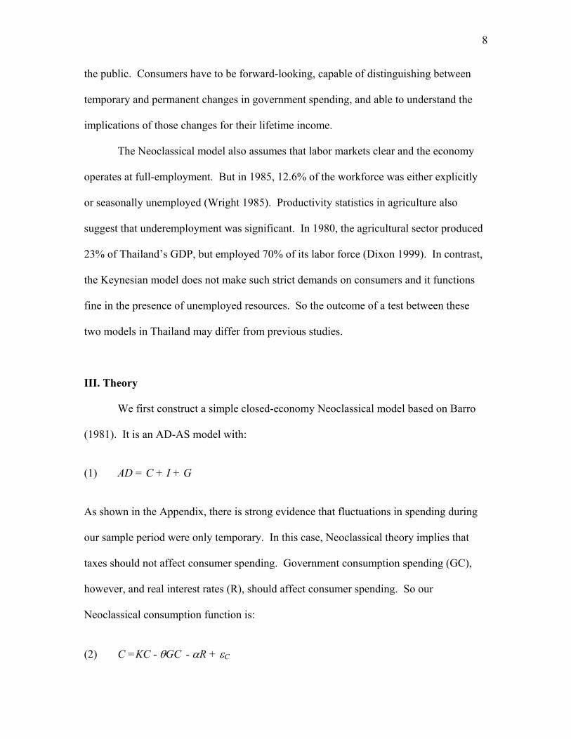
the public. Consumers have to be forward-looking, capable of distinguishing between
temporary and permanent changes in government spending, and able to understand the
implications of those changes for their lifetime income.
The Neoclassical model also assumes that labor markets clear and the economy
operates at full-employment. But in 1985, 12.6% of the workforce was either explicitly
or seasonally unemployed (Wright 1985). Productivity statistics in agriculture also
suggest that underemployment was significant. In 1980, the agricultural sector produced
23% of Thailand’s GDP, but employed 70% of its labor force (Dixon 1999). In contrast,
the Keynesian model does not make such strict demands on consumers and it functions
fine in the presence of unemployed resources. So the outcome of a test between these
two models in Thailand may differ from previous studies.
III. Theory
We first construct a simple closed-economy Neoclassical model based on Barro
(1981). It is an AD-AS model with:
(1) AD = C + I + G
As shown in the Appendix, there is strong evidence that fluctuations in spending during
our sample period were only temporary. In this case, Neoclassical theory implies that
taxes should not affect consumer spending. Government consumption spending (GC),
however, and real interest rates (R), should affect consumer spending. So our
Neoclassical consumption function is:
(2) C =KC - θGC - αR + εC

9
where KC is a constant, εC is the consumption equation error term, and 0<θ<1 because
public consumer goods are less valuable than private consumer goods. Theory suggests
that both higher government consumption expenditures and higher real interest rates
reduce private consumption.
Investment is assumed negatively affected by real interest rates. Following
Baxter and King (1993), we also allow for government investment spending (GI) to
positively affect private investment by boosting the productivity of private capital:
(3) I = KI - δR + γGI + εI
where KI is a constant and εI is the investment equation’s error term. Real government
expenditure is just spending on consumption and investment:
(4) G = GC + GI
Adding these equations up gives us our equation for AD:
(5) AD = KC - θGC - αR + KI - δR + γGI + GC + GI + εAD
On the AS side of the model, higher real interest rates are assumed to boost
employment and output through intertemporal substitution. Following Baxter and King
(1993), greater government investment is also assumed to raise output by enhancing
productivity. So:
(7) AS = KAS + βR + τGI + εAS
10
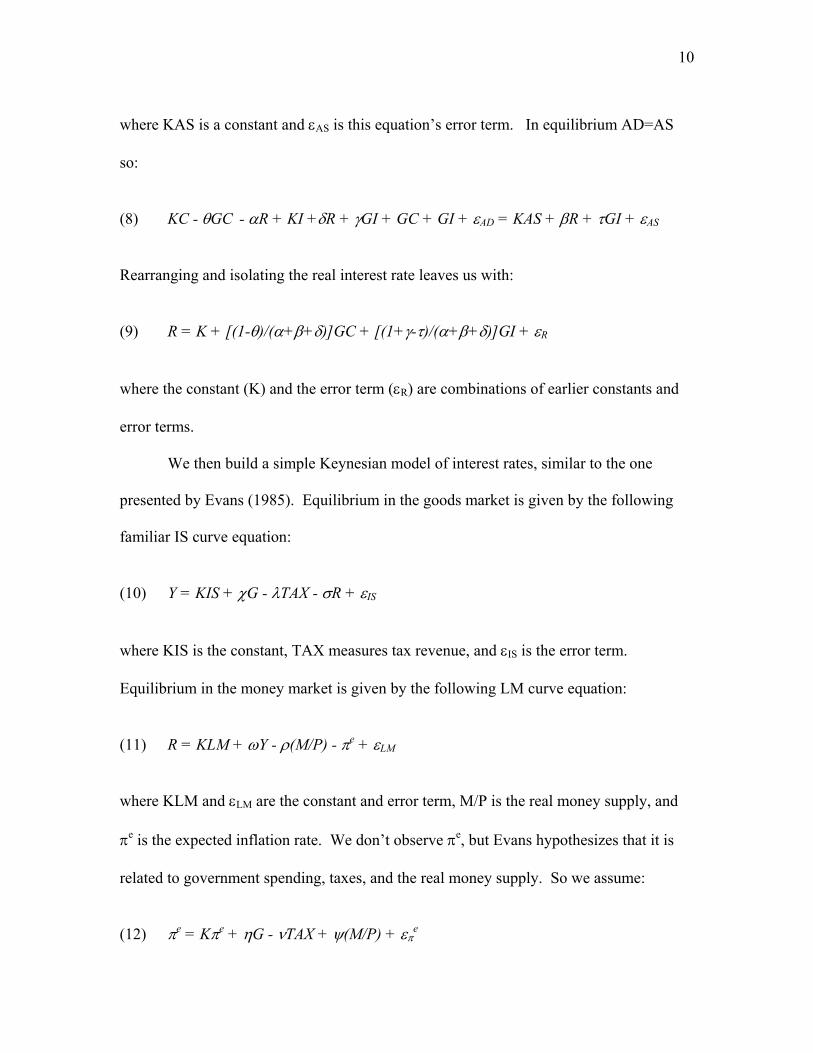
where KAS is a constant and εAS is this equation’s error term. In equilibrium AD=AS
so:
(8) KC - θGC - αR + KI +δR + γGI + GC + GI + εAD = KAS + βR + τGI + εAS
Rearranging and isolating the real interest rate leaves us with:
(9) R = K + [(1-θ)/(α+β+δ)]GC + [(1+γ-τ)/(α+β+δ)]GI + εR
where the constant (K) and the error term (εR) are combinations of earlier constants and
error terms.
We then build a simple Keynesian model of interest rates, similar to the one
presented by Evans (1985). Equilibrium in the goods market is given by the following
familiar IS curve equation:
(10) Y = KIS + χG - λTAX - σR + εIS
where KIS is the constant, TAX measures tax revenue, and εIS is the error term.
Equilibrium in the money market is given by the following LM curve equation:
(11) R = KLM + ωY - ρ(M/P) - πe + εLM
where KLM and εLM are the constant and error term, M/P is the real money supply, and
πe is the expected inflation rate. We don’t observe πe, but Evans hypothesizes that it is
related to government spending, taxes, and the real money supply. So we assume:
(12) πe = Kπe + ηG - νTAX + ψ(M/P) + επe
11
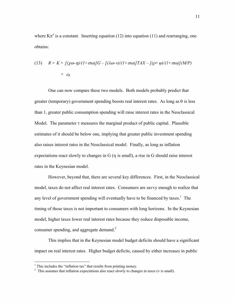
where Kπe is a constant. Inserting equation (12) into equation (11) and rearranging, one
obtains:
(13) R = K + [(χω-η)/(1+σω)]G – [(λω-ν)/(1+σω)]TAX – [(ρ+ψ)/(1+σω)](M/P)
+ εR
One can now compare these two models. Both models probably predict that
greater (temporary) government spending boosts real interest rates. As long as θ is less
than 1, greater public consumption spending will raise interest rates in the Neoclassical
Model. The parameter τ measures the marginal product of public capital. Plausible
estimates of it should be below one, implying that greater public investment spending
also raises interest rates in the Neoclassical model. Finally, as long as inflation
expectations react slowly to changes in G (η is small), a rise in G should raise interest
rates in the Keynesian model.
However, beyond that, there are several key differences. First, in the Neoclassical
model, taxes do not affect real interest rates. Consumers are savvy enough to realize that
any level of government spending will eventually have to be financed by taxes.1 The
timing of those taxes is not important to consumers with long horizons. In the Keynesian
model, higher taxes lower real interest rates because they reduce disposable income,
consumer spending, and aggregate demand.2
This implies that in the Keynesian model budget deficits should have a significant
impact on real interest rates. Higher budget deficits, caused by either increases in public
1 This includes the “inflation tax” that results from printing money. 2 This assumes that inflation expectations also react slowly to changes in taxes (ν is small).
12
spending or tax cuts, should raise aggregate demand and push up interest rates. In the
Neoclassical model, however, only the level of government spending matters; the size of
the deficit is irrelevant.
Another important difference is that in the Neoclassical model, the real money
supply does not change real interest rates. Money is said to be neutral. In the Keynesian
model, though, a larger real money supply unambiguously lowers real interest rates to
clear the money market.
A final difference is that different types of government spending have different
effects on interest rates in the Neoclassical model. Public investment spending, for
instance, does not affect consumer spending directly, but does affect aggregate supply.
Public consumption spending does just the opposite. These varied effects lead to
different ultimate impacts on the real interest rate. In our Keynesian model, however, the
form of government spending makes no difference, as each dollar of government
spending boosts aggregate demand by a dollar.
A straightforward way, then, to test between these theories is to include the
variables from both models in one regression. That regression takes the form:
(14) R = K + ϕGC + κGI - µTAX - ξ(M/P) + ε
According to the Neoclassical theory, ϕ and κ should probably be positive but should
also differ from each other, and both µ and ξ should equal zero. The Keynesian
predictions are that ϕ and κ are positive and equal to each other, and that both taxes and
the real money supply depress real interest rates.
13
Ordinary least squares (OLS) estimation of equation (14) will probably be
inconsistent. The error term contains shocks to both private spending and real money
demand, and those shocks could easily be correlated with our explanatory variables. An
autonomous rise in private spending, for instance, could boost output which would
increase tax revenue and potentially change government spending and the real money
supply. This inconsistency might not be severe if shocks to the economy were
transmitted quickly to interest rates through efficient financial markets, but took longer to
affect output and our right-hand side variables. Our use of quarterly data should help in
that regard. However, to be safe we rely primarily on two-stage least squares (2SLS) for
the estimation.
IV. Data and Estimation
We use quarterly data from 1980:1 to 1994:4. The Comptroller-General's
Department at the Ministry of Finance of Thailand publishes nominal data on tax revenue
and government spending on capital and current expenditures. The government capital
(investment) expenditure data is broken down into equipment and construction outlays
(GIE and GIC). The Bank of Thailand provides data on the money supply, which is
comprised of currency holdings plus demand deposits. All data are converted into real
terms by the Thai government's general price index (1986=100). The nominal interest
rate is a money market rate measuring the rate at which commercial banks accepted
short-term deposits from other banks and financial institutions as reported in the
International Financial Statistics (IFS). It is then adjusted for the ex-post annualized
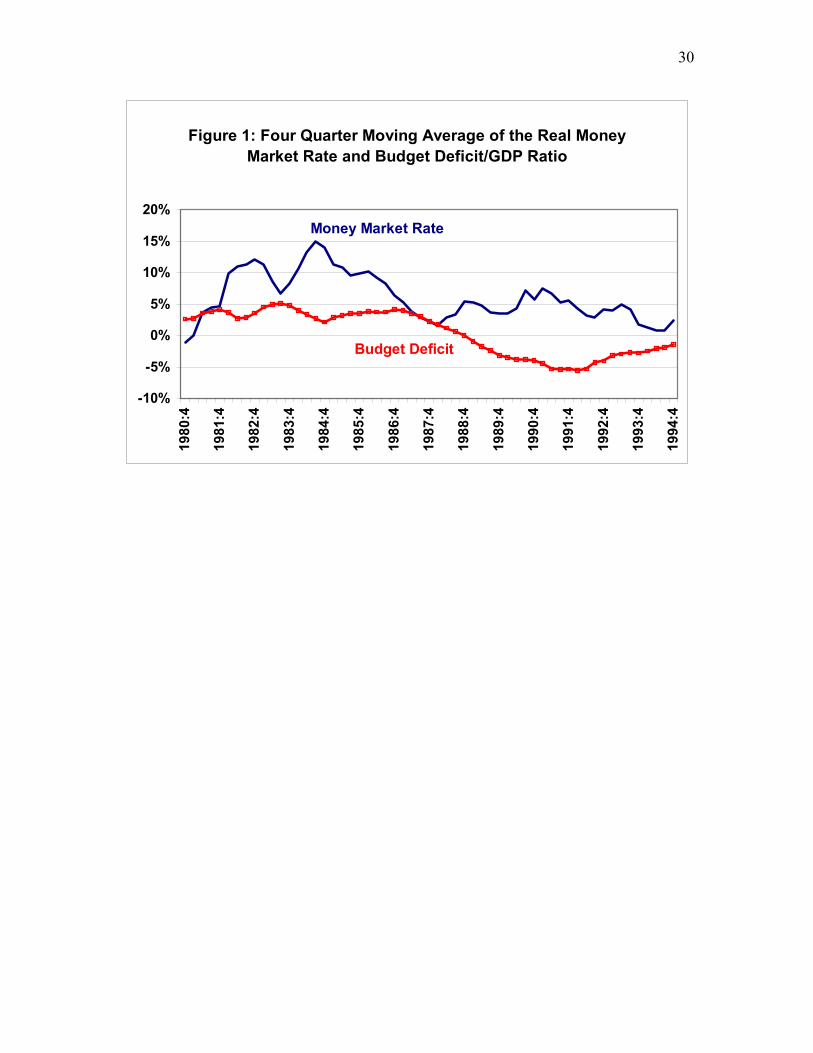
inflation rate from each quarter. A four-quarter moving average of this real rate is
14
displayed in Figure 1. In it one can see the dramatic drop in real interest rates between
1984 and 1987.
Our right-hand side variables are divided by an estimate of trend real GDP. We
do this because it seems likely that same-sized changes in our explanatory variables will
have a larger impact on interest rates the smaller the Thai economy is. So, for instance, a
10 million Baht rise in real government spending in 1980, when the economy was
smaller, would probably affect interest rates more than an equal-sized change in 1994.
Dividing by real GDP corrects for the growing size of the Thai economy. We use
estimates of trend GDP because quarterly data on output are not available and we want to
avoid introducing a correlation between our right-hand side variables and our error term,
which contains business cycle shocks.3
There could easily be regular seasonal patterns to real interest rates and our
explanatory variables. The real money supply in the US, for example, tends to rise
around Christmas. Even if seasonal fluctuations in interest rates were independent of
seasonal fluctuations in our explanatory variables, regression analysis would probably
find a spurious correlation between them. To prevent that, three dummy variables (one
each for spring, summer, and fall) are added to the regression.
Descriptive statistics of our data are displayed in Table 1. The annual real interest
rate is generally high, averaging 5.7%, the mean budget deficit is only 0.1% of output,
and government consumption, construction, and equipment spending average 13.8%,
5.8%, and 1.9% of GDP. Most variables fluctuate considerably over our sample, which
should help to generate precise parameter estimates.
3 The trend output specification we used, based on the Akaike criterion, contained linear and quadratic time trends.

15
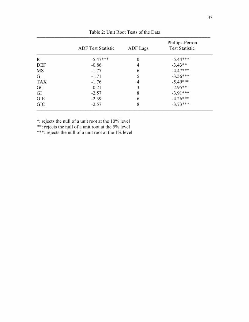
The next task is to verify that the data are stationary in levels.4 Because of
evidence of serial correlation, we compute augmented Dickey-Fuller (ADF) and Phillips-
Perron test statistics. The results of those tests are in Table 2. With the exception of our
interest rate variable, which appears to be stationary, the two tests disagree. The ADF
statistics suggest that most of our data are nonstationary while the Phillips-Perron tests
suggest stationarity. Further ADF tests indicate that one cannot reject the null that first-
differences of our data are stationary. Hence there is uncertainty as to whether most of
our data are integrated of order 0 or 1.
If some of our data are nonstationary, we need to determine if they are
cointegrated for our regressions to make sense. So the Johansen cointegration test was
performed on two sets of variables: 1) R, GC, GI, DEF, and MS; and 2) R, GC, GIE,
GIC, DEF, and MS. In both cases we could reject the null hypothesis of no cointegrating
equations at the 1% level, but could not reject the null of one cointegrating equation at
normal significance levels. Hence, if some of our data are nonstationary, they appear to
be cointegrated and our regressions should be meaningful.
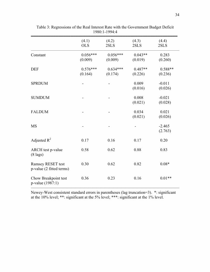
We start by estimating a stripped down version of equation (11) with just the
budget deficit on the right-hand side. We use OLS. The results are in column 1 of Table
3.5 The budget deficit coefficient is positive and quite significant, with a t statistic of
over 3.5. It is easy to understand this result if one glances at Figure 1. Real interest rates
and the budget deficit relative to GDP generally move together.
4 The ratio of government spending to GDP is naturally bounded between 0 and 1, so it would seem as though we can rule out nonstationarity. However, to be sure we conducted the standard tests. 5 In this and many other regressions, there was evidence of either heteroskedasticity or autocorrelation, so we routinely computed Newey-West consistent standard errors.
16
Because these estimates are probably contaminated by a correlation between our
regressors and error term, we next run 2SLS. Our instruments are the budget deficit
lagged one through four quarters. Two-stage least squares works best when one has good
instruments (Nelson and Startz 1990), and a check shows that this was the case.6 The
results of this estimation are in column 2. They are basically the same.
In the next column we add our three seasonal dummy variables. None of them
enters significantly. The estimated deficit coefficient remains significant at the 5% level,
though the point estimate shrinks and the standard error grows.
Finally, we add the real money supply. It enters negatively, consistent with the
Keynesian theory, but is not statistically significant. The deficit coefficient, however,
grows larger and remains significant. There is evidence of model misspecification from
both the RESET and Chow tests. Those diagnostics notwithstanding, however, this first
batch of regressions is generally supportive of the Keynesian hypothesis that real interest
rates fell in Thailand in the mid-1980’s because the government eliminated its budget
deficit.
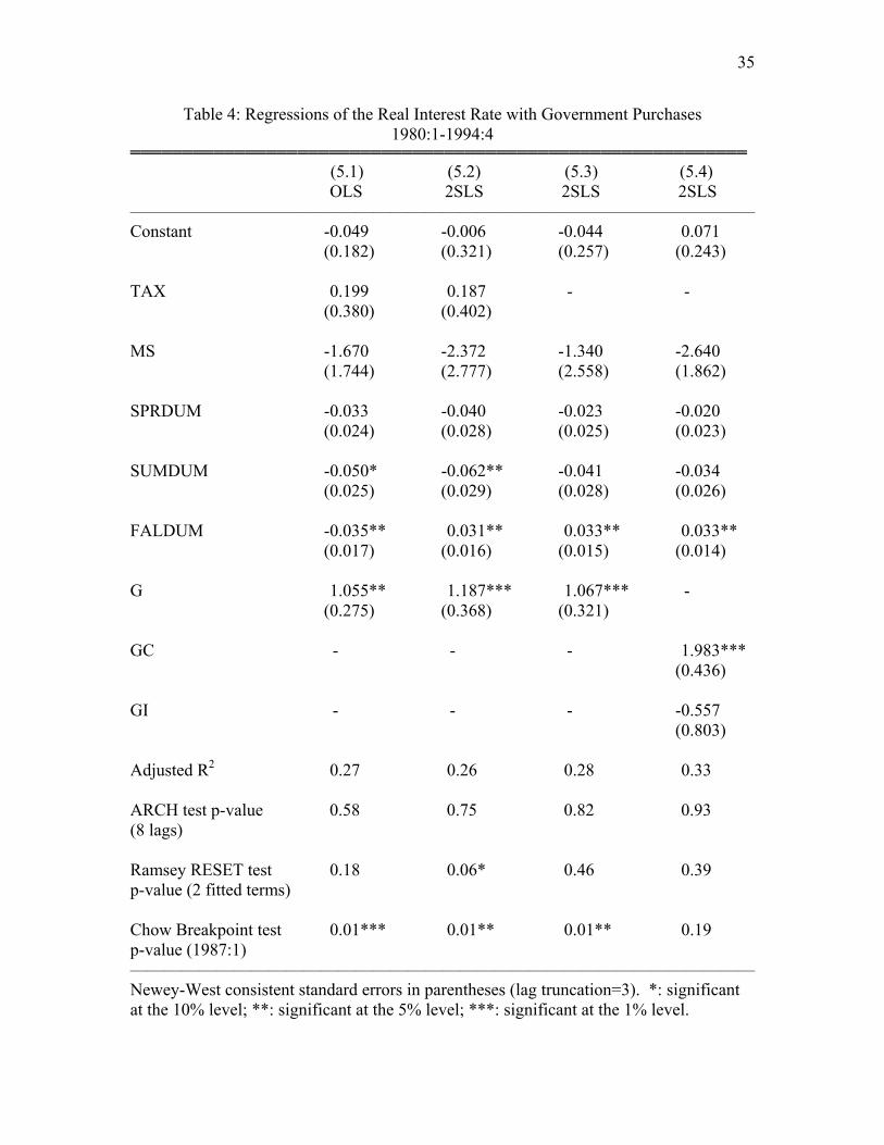
In Table 4 we examine the Neoclassical proposition that it was cuts in
government spending, and not changes in the deficit, that caused real interest rates to fall.
We divide our deficit variable up into government spending, G, and tax revenue, TAX.
Doing OLS first, taxes are completely insignificant and actually have the wrong sign
according to Keynesian theory. Government spending, however, enters with a positive
coefficient, as predicted, and is significant at the 2% level. Two of the seasonal dummy
variables also become marginally significant. The R2 statistic indicates the model fits the
data better.
6 A regression of the instruments on our deficit variable yielded an adjusted R2 statistic of 0.79.
17
In column 2 we employ 2SLS, choosing as our instruments four lags of the real
money supply, tax revenue, and government spending7. The results do not change much.
There are signs of model misspecification and parameter instability. In the next column
we drop the tax variable. This sharpens the estimated coefficient for government
spending and slightly raises its significance level.
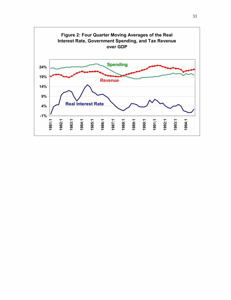
This evidence, therefore, is clearly in favor of the Neoclassical model.
Government spending does appear to affect real interest rates, while the real money
supply and tax revenue do not seem to matter. Some insight into these results can be
found in Figure 2, which plots the real interest rate against government spending and tax
revenue. The positive correlation between government spending and the real interest rate
is apparent. But it is harder to see the hypothesized negative correlation between tax
revenue and real interest rates. Both rose in the early 1980’s, then fell in the mid 1980’s,
and rose again from 1988-1991. So it is not that surprising that our regressions fail to
detect an inverse relationship between those two variables.
To examine the possibility that different types of government spending have
different effects on interest rates, we break government spending down between
consumption and investment spending. The results of this are shown in the last column.8
Interestingly, only government consumption seems to matter. The goodness of fit
improves and there is no longer evidence of parameter instability.
7 The adjusted-R2 statistics for the regressions of our explanatory variables on their instruments were all over 0.74. 8 The instruments were 4 lags of each of the non-constant explanatory variables.
18
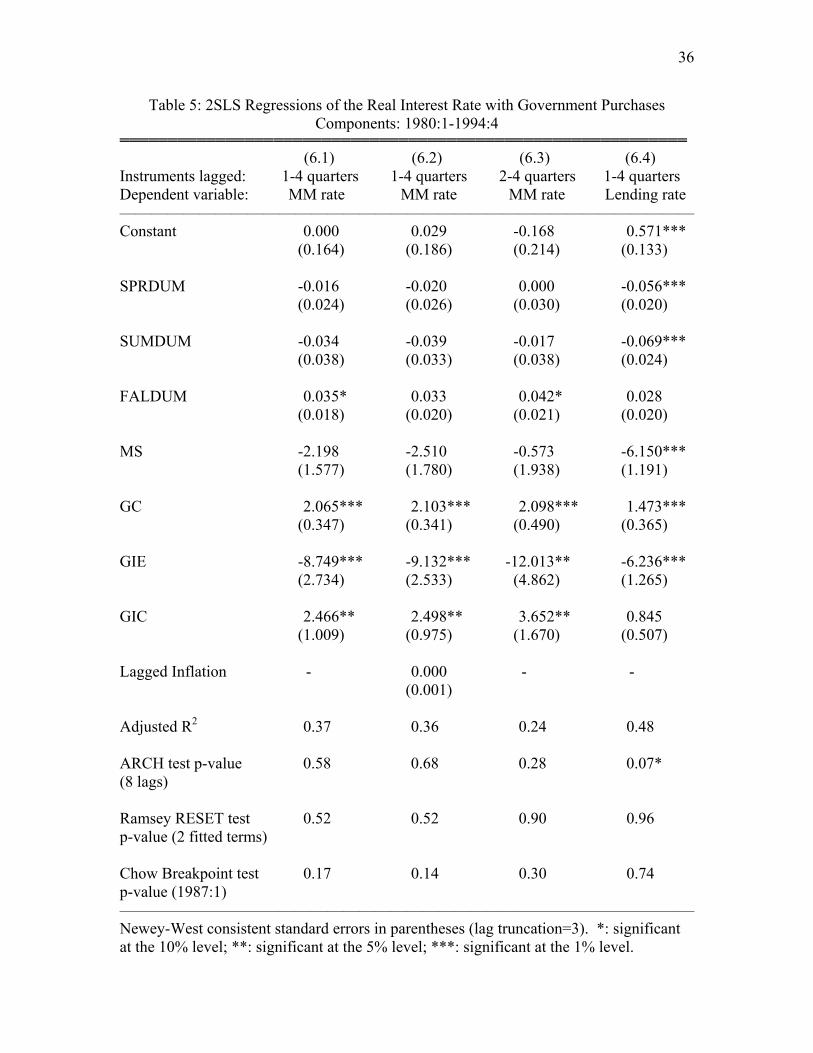
In Table 5, investment is divided between equipment and construction
expenditures.9 Government consumption continues to be important, but now, both public
spending on equipment and on construction enter significantly. Surprisingly, equipment
spending has a negative coefficient, suggesting that increases in public equipment
spending lower real interest rates. Apparently, government investment did not enter
significantly earlier because it was the sum of two separate effects from equipment and
construction spending that largely offset each other. The real money supply continues to
be insignificant.
In the last three columns of Table 5 we test for robustness. First, we include
lagged inflation as a proxy for the unobservable inflation expectations that Keynesian
theory suggests affect real interest rates. It did not enter significantly, suggesting that
those expectations may already be satisfactorily captured by our monetary and fiscal
variables.
Some authors (e.g., Hall 1988) have noted that instruments lagged more than once
are less likely to be correlated with one's error term. So in column 3 we lag our
instruments at least two quarters. The goodness of fit deteriorates, but none of the main
results changes.
Finally, we experiment with a different real interest rate derived from a Thai
nominal lending rate similar to the Prime Rate in the US. The real money supply enters
significantly, while government spending on construction does not. The point estimates
of our other spending variables shrink, but not their significance levels. Because this
interest rate is sticky and was subject to loan rate ceilings, it is much less appropriate than
9 All of these regressions used 2SLS. The instruments were 4 lags of each of the explanatory variables. Regressions of these variables on their lags yielded R2 statistics of over 55%.
19
the money market rate we use. Even so, it is reassuring that most of our results continue
to hold.
Focusing on the results from the first column of Table 5, the coefficient on
government consumption suggests that a one percentage point rise in government
consumption as a fraction of GDP pushes up real interest rates by 2.1 percentage points.
A one percentage point rise in the ratio of construction spending to GDP is estimated to
boost real interest rates by 2.5 percentage points. Finally, a one percentage point rise in
public equipment spending relative to GDP is estimated to push down real interest rates
by 8.7 percentage points. This final estimate seems large, but one needs to keep in mind
that public equipment spending is small, averaging just 1.9 percent of GDP in our
sample. So it typically doesn’t fluctuate by a single percentage point. Nonetheless, it is
still puzzling why Thai interest rates appear to be so negatively correlated with public
equipment investment.
The Neoclassical theory that we derived earlier provides one possible reason for
this correlation. Equation (9) indicates that a high value for τ would tend to at least
shrink the positive correlation between interest rates and equipment spending. The τ
parameter measures the marginal product of public capital. That may be high for
equipment investment. Temple (1998) estimates returns to equipment investment of
over 50% in developing countries.10 However, even an estimate as big as 60% is
insufficient to generate the large negative correlation we find in the data. So we need to
consider additional factors. In the next two sections, we look at a couple.
10 Returns to other forms of investment, which would include construction spending, are much lower.
20
V. Countercyclical Public Equipment Spending
Government equipment spending may appear to depress real interest rates simply
because the Thai government uses that spending to counter the business cycle. It could
deliberately boost investment spending in periods of slow growth to spur growth and then
reduce that spending during booms. If the Central Bank were loosening monetary policy
during recessions and tightening it during booms, that could generate a spurious inverse
relationship between investment spending and interest rates.
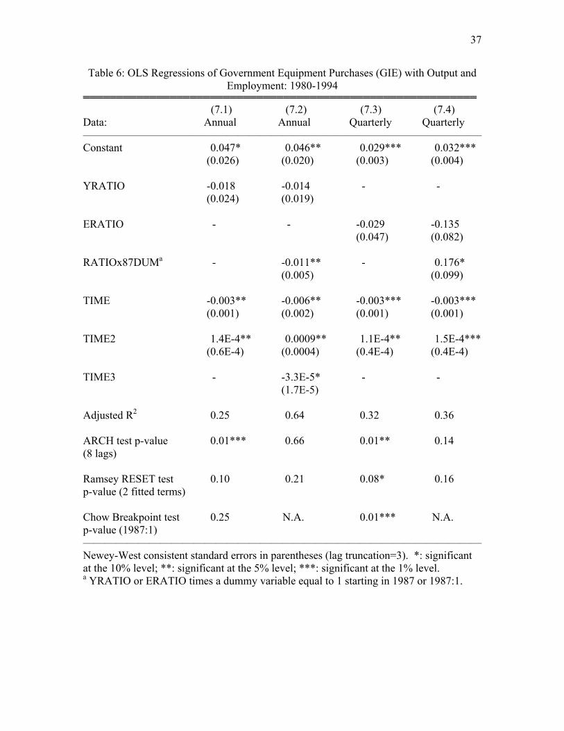
To test this, we try to measure how countercyclical equipment spending is in our
sample. We first regress public equipment spending as a percentage of GDP on a
variable, YRATIO, that measured the ratio of output to trend output. The data are annual
and time trends are added to account for long-run swings in equipment spending.
Column 1 in Table 6 shows the results. YRATIO enters negatively, suggesting that when
output is high relative to trend output, government equipment spending is low. But the
estimate is not statistically significant. There is also evidence of model misspecification.
So we add a variable equal to a dummy variable times our output measure. The
dummy variable equals zero before 1987 and one afterwards. The results are much more
satisfactory. The new variable enters significantly at the 5% level and is negative. It
indicates that after 1987, there was significant countercyclical spending on equipment by
the government. The goodness of fit improves markedly. The only problem with this
evidence is that it uses annual data and our earlier regressions use quarterly data.
Although quarterly data are not available for GDP, they are for employment, so
we also try them. We experiment with a variable measuring the ratio of employment to
21
trend employment. The results in column 3 again indicate an inverse relationship
between employment and equipment spending, but not a significant one. There is,
however, strong evidence of parameter instability. So we add a variable equal to our
1987 dummy variable times our employment variable. This new variable is significant at
the 10% level, but is positive. When combined with our other employment variable, the
two coefficients practically offset each other, suggesting that after 1987, government
equipment purchases were acyclical.
The evidence on the countercyclicality of government equipment investment is
therefore mixed. One possible reason for this is that the Thai government adjusted
equipment purchases to the state of the economy with a lag. If the lag were longer than a
quarter but less than a year, countercyclical equipment spending might show up in annual
data, but not quarterly. In any case, we think it likely that countercyclical spending is at
least one of the reasons that real interest rates were so negatively correlated with public
equipment investment in our sample.
VI. External Financing
Another potential reason derives from the possibility of external financing.
Increased borrowing need not push up domestic interest rates to the extent that it taps
foreign funds. In the private sector, more qualified customers routinely borrow from
abroad when Thai loan rates are high (Jansen 1997). The public sector, too, has access to
foreign capital, so that could attenuate the relationship between its spending and interest
rates.
22
To consider this hypothesis, we expand the Neoclassical model to allow for
foreign trade and borrowing. In an open economy:
(15) AD = C + I + G + NX
where NX is real net exports. We then assume that fluctuations in net exports are equal
and opposite to fluctuations in net foreign borrowing (NFB):
(16) NX = KNX – NFB + εNX
where KNX is just a constant and εNX is the error term. Balance of payments equilibrium
would imply this equal and opposite relationship in the long-run. In the short-run, this
relationship could occur under fixed exchange rates if capital inflows were used to
finance import purchases. In fact, there is evidence that the foreign investment boom that
commenced in 1987 significantly boosted the import intensity of the Thai economy
(Jansen 1997, p. 178).
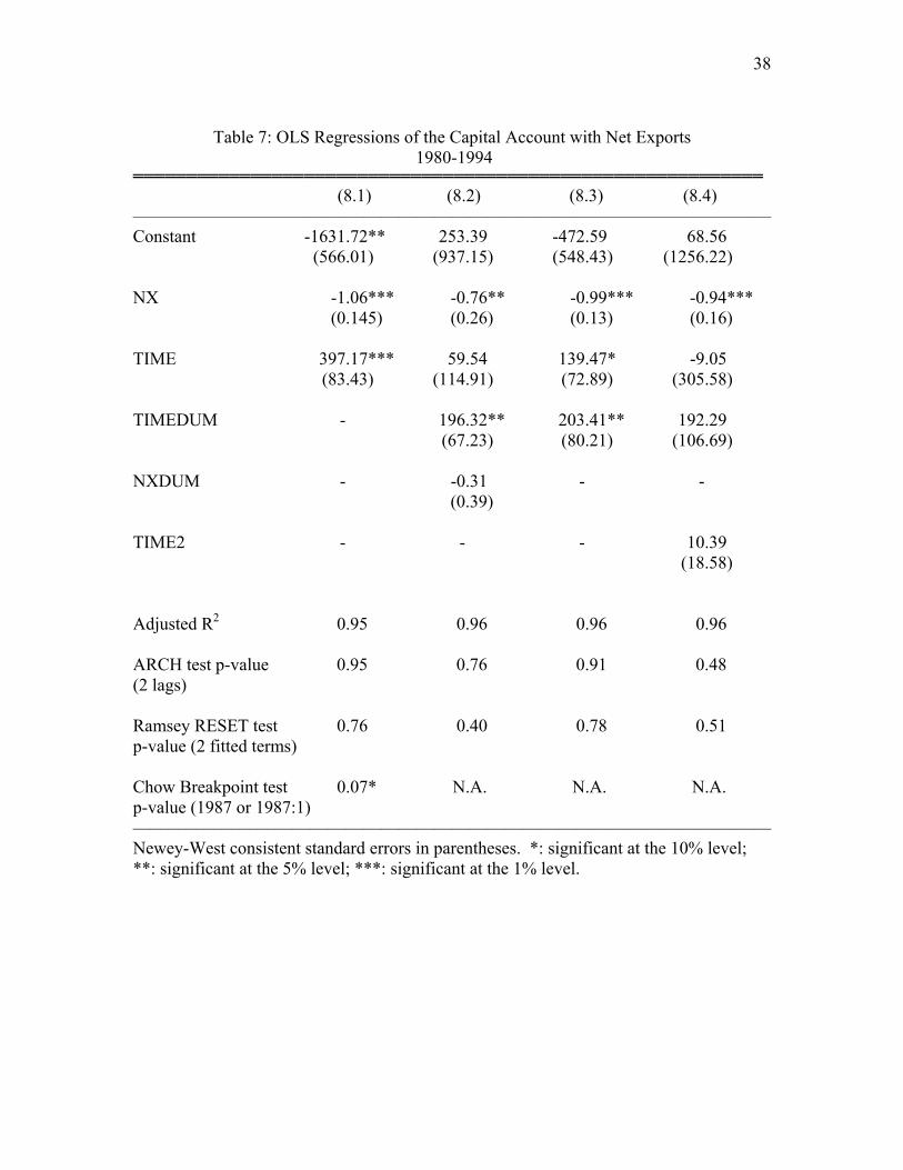
We test this assumption by first regressing the capital account in Thailand on a
linear time trend, a constant, and net exports. We could not obtain quarterly data, so we
use annual IFS data. Column 1 of Table 7 contains the results. The estimated coefficient
on NX is -1.11 and is quite significant. We cannot reject the null that it is equal to -1.0.
However, there is mild evidence of a structural break in the data.
To address that, we add two interactive dummy variables. The first, TIMEDUM,
is the product of our linear time trend with a dummy variable equal to one after 1986.
The second, NXDUM, is the product of our NX variable with a dummy variable equal to
one after 1986. The results, in column 2, show that it is the time trend dummy variable

23
that enters significantly. It is positive, suggesting that after 1986 the trend toward larger
capital inflows accelerated. The estimated coefficient on net exports shrinks but stays
significant, and we still cannot reject the hypothesis that it equals 1.0.
In column 3 we drop the insignificant NX dummy variable. The NX coefficient
jumps to 0.99 and becomes significant at the 1% level. Finally we add a quadratic time
trend. The net export coefficient falls slightly, but the results are basically unchanged.
We conclude that the assumption that short-run changes in net exports are equal and
opposite to changes in net foreign borrowing is acceptable for our sample period.
The last assumption is that increases in government spending are partly financed
from net capital inflows:
(17) NFB = KNFB + ϖ1GC + ϖ2GIE + ϖ3GIC + εNFB
We allow for different forms of government spending to receive different levels of
external financing. Combining this with our previous Neoclassical equations for C, I, G,
and AS, and rearranging, one can derive the following:
(18) R = K + [(1-θ-ϖ1)/(α+β+δ)]GC + [(1+γ-τ-ϖ2)/(α+β+δ)]GIE +
[(1+γ-τ-ϖ2)/(α+β+δ)]GIC + εR
Public investment spending here is divided up between equipment and construction
expenditures.
Note that the degree of external financing, as measured by the ϖ parameter,
reduces the coefficients on our public spending variables. Increases in public spending
depress net exports, AD rises less, and real interest rates don’t need to go up as much to
24
close the gap between AD and AS. In fact, if ϖ is large enough, increases in public
spending can lead to a situation where AS>AD and real interest rates fall.
Intuition for these results can be found in the loanable funds framework which
compares the demand for funds with the supply of funds.11 The condition for higher
interest rates in this framework is I>S+NFB, where I (Investment) represents the demand
for funds and S (domestic savings) plus NFB constitute the supply of funds. In the
closed-economy version of this model with no NFB, increases in public spending reduce
domestic savings, creating a gap between I and S that forces interest rates up. But in an
open economy, foreign capital inflows in response to a rise in G augment the pool of
loanable funds, so the gap between the demand for funds and the supply of funds is
smaller or even negative.
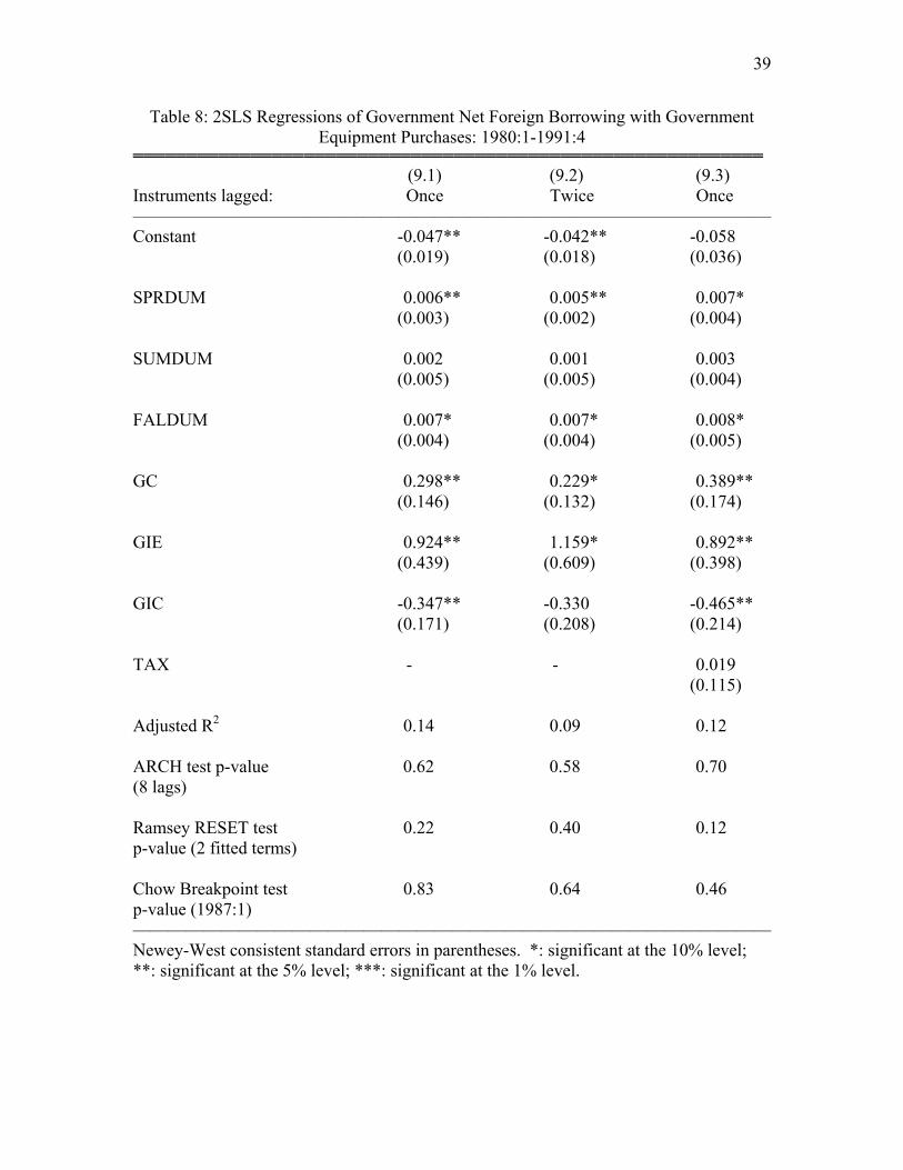
To test this hypothesis we regress each government spending variable on
government net foreign borrowing. Data availability restrict our sample period to 1980-
1991. There is a potential simultaneity problem in that shocks to government foreign
borrowing could affect output and our explanatory variables. So we use 2SLS again,
employing the same instruments we used before. The results are in Table 8.
All three coefficients of our public spending variables enter significantly at the
5% level. However, their point estimates are quite different. The estimated coefficient
on public equipment investment is very high, over 90%. The coefficient on public
consumption is about 30% and the estimate for public construction is negative.
To test for robustness, in column 2 we restrict our instruments to those lagged at
least twice. The coefficient estimates are less significant, but their magnitudes do not
11 This framework is a mirror image of the AD-AS framework and the AD=AS condition is equivalent to the condition that the demand for funds equals the supply of funds.
25
change much. In column 3, we add tax revenue to see if it matters, but it does not. Our
previous results stay essentially the same.
These results therefore help to explain why increases in government equipment
spending seem to lower real interest rates. Our estimates suggest that every 100 Baht
increase in public equipment spending in our sample period coincided with a rise in
government net foreign borrowing of roughly 90 Baht. That represents a very high level
of foreign financing, and it makes it much less likely that higher public spending would
push the demand for funds above the supply of funds and boost interest rates. It also
reduces the likelihood that a sudden decrease in equipment spending, as occurred
between 1985 and 1989, would exert much downward pressure on interest rates
VII. Conclusion
Thailand experienced remarkable growth starting in 1987. There were also big
changes in government fiscal policy at that time. That makes Thailand a wonderful case
for testing whether their fiscal policy contributed to their boom by lowering real interest
rates and potentially spurring investment. Keynesian theory suggests that declining
budget deficits pushed real interest rates down in the mid-1980’s. Neoclassical theory
asserts that falling government spending was the primary factor. Using data spanning
1980-94, we find evidence for the Neoclassical model. In general, decreases in
government spending, and not higher taxes, appear to have contributed to the decline in
real interest rates.
However, in the case of public equipment investment we obtain the unusual result
that increases lower interest rates. We attribute this to three factors. First, government
26
equipment investment could be quite productive, significantly boosting aggregate supply.
Second, there is some evidence that public equipment spending is countercyclical, which
could generate a spurious negative correlation with procyclical real interest rates. Third,
public equipment spending appears to fluctuate with government foreign borrowing.
That would alleviate pressure on interest rates to rise when public equipment spending
increases. When all three factors are combined, it is possible to generate a negative
correlation between real interest rates and public equipment spending.
There are several conclusions to draw from this. First, the Neoclassical model
assumes a very high degree of consumer rationality. For that model to be successful, it
suggests that consumers in newly industrialized countries such as Thailand are fairly
sophisticated. Second, it would appear that it is critical for governments to get their
spending under control if they hope to maintain low real interest rates. Finally, short-
term increases in government spending need not raise real interest rates if they receive
some financing from abroad and significantly boost aggregate supply.
This could all be important information for developing countries considering
public investment programs to stimulate growth. Thailand's Sixth National Economic
and Social Development Plan is a good example. The plan dramatically boosted public
infrastructure spending, especially in rural areas, in the late 1980s; between 1989 and
1994 public investment as a fraction of GDP doubled in Thailand. Our results suggest
that, although such a rise in government spending could push up interest rates and
depress private capital formation, it need not if it is at least partly externally financed
(which it was) and significantly enhances the economy’s productive potential. Of course,
there are always costs and risks associated with borrowing from abroad, as the crisis of
27
1997 demonstrated. In addition, governments must constantly assess the opportunity cost
of devoting resources to public spending.
The authors would like to thank Gary Smith, Thomas Willett, Thitithep Sitthiyot, and two
anonymous referees for very useful comments. All errors remain ours.
28
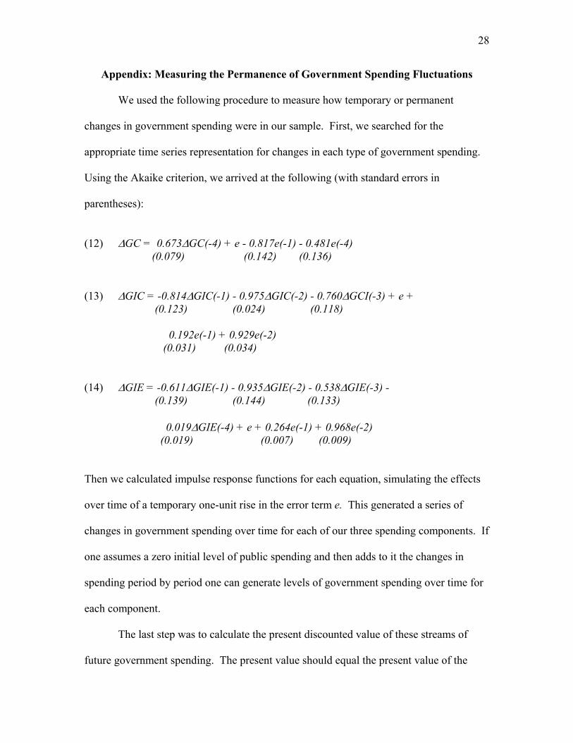
Appendix: Measuring the Permanence of Government Spending Fluctuations
We used the following procedure to measure how temporary or permanent
changes in government spending were in our sample. First, we searched for the
appropriate time series representation for changes in each type of government spending.
Using the Akaike criterion, we arrived at the following (with standard errors in
parentheses):
(12) ∆GC = 0.673∆GC(-4) + e - 0.817e(-1) - 0.481e(-4) (0.079) (0.142) (0.136)
(13) ∆GIC = -0.814∆GIC(-1) - 0.975∆GIC(-2) - 0.760∆GCI(-3) + e + (0.123) (0.024) (0.118)
0.192e(-1) + 0.929e(-2) (0.031) (0.034) (14) ∆GIE = -0.611∆GIE(-1) - 0.935∆GIE(-2) - 0.538∆GIE(-3) - (0.139) (0.144) (0.133)
0.019∆GIE(-4) + e + 0.264e(-1) + 0.968e(-2) (0.019) (0.007) (0.009) Then we calculated impulse response functions for each equation, simulating the effects
over time of a temporary one-unit rise in the error term e. This generated a series of
changes in government spending over time for each of our three spending components. If
one assumes a zero initial level of public spending and then adds to it the changes in
spending period by period one can generate levels of government spending over time for
each component.
The last step was to calculate the present discounted value of these streams of
future government spending. The present value should equal the present value of the
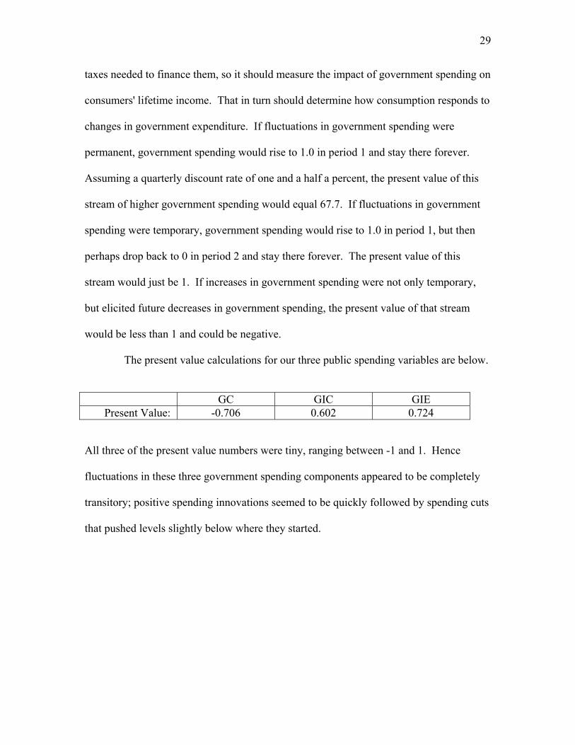
29
taxes needed to finance them, so it should measure the impact of government spending on
consumers' lifetime income. That in turn should determine how consumption responds to
changes in government expenditure. If fluctuations in government spending were
permanent, government spending would rise to 1.0 in period 1 and stay there forever.
Assuming a quarterly discount rate of one and a half a percent, the present value of this
stream of higher government spending would equal 67.7. If fluctuations in government
spending were temporary, government spending would rise to 1.0 in period 1, but then
perhaps drop back to 0 in period 2 and stay there forever. The present value of this
stream would just be 1. If increases in government spending were not only temporary,
but elicited future decreases in government spending, the present value of that stream
would be less than 1 and could be negative.
The present value calculations for our three public spending variables are below.
GC GIC GIE
Present Value: -0.706 0.602 0.724
All three of the present value numbers were tiny, ranging between -1 and 1. Hence
fluctuations in these three government spending components appeared to be completely
transitory; positive spending innovations seemed to be quickly followed by spending cuts
that pushed levels slightly below where they started.
30
Figure 1: Four Quarter Moving Average of the Real Money Market Rate and Budget Deficit/GDP Ratio
-10%
-5%
0%
5%
10%
15%
20%
1980
:4
1981
:4
1982
:4
1983
:4
1984
:4
1985
:4
1986
:4
1987
:4
1988
:4
1989
:4
1990
:4
1991
:4
1992
:4
1993
:4
1994
:4
Money Market Rate
Budget Deficit
31
Figure 2: Four Quarter Moving Averages of the Real Interest Rate, Government Spending, and Tax Revenue
over GDP
-1%
4%
9%
14%
19%
24%
1981
:1
1982
:1
1983
:1
1984
:1
1985
:1
1986
:1
1987
:1
1988
:1
1989
:1
1990
:1
1991
:1
1992
:1
1993
:1
1994
:1
Spending
Revenue
Real Interest Rate

32
Table 1: Descriptive Statistics of the Data Sample Period: 1980:1-1994:4
═══════════════════════════════════════════════════════════ Mean Median Maximum Minimum Std. Dev. ———————————————————————————————————— R 0.057 0.056 0.191 -0.127 0.059 MS 0.091 0.091 0.109 0.078 0.007 DEF 0.001 0.006 0.084 -0.092 0.043 TAX 0.215 0.212 0.274 0.160 0.030 G 0.216 0.216 0.280 0.168 0.029 GC 0.138 0.136 0.179 0.103 0.019 GI 0.077 0.079 0.111 0.042 0.017 GIE 0.019 0.020 0.032 0.009 0.005 GIC 0.058 0.058 0.087 0.033 0.013 ————————————————————————————————————
33
Table 2: Unit Root Tests of the Data ═══════════════════════════════════════════════════════════ Phillips-Perron ADF Test Statistic ADF Lags Test Statistic ———————————————————————————————————— R -5.47*** 0 -5.44*** DEF -0.86 4 -3.43** MS -1.77 6 -4.47*** G -1.71 5 -3.56*** TAX -1.76 4 -5.49*** GC -0.21 3 -2.95** GI -2.57 8 -3.91*** GIE -2.39 6 -4.26*** GIC -2.57 8 -3.73*** ———————————————————————————————————— *: rejects the null of a unit root at the 10% level **: rejects the null of a unit root at the 5% level ***: rejects the null of a unit root at the 1% level
34
Table 3: Regressions of the Real Interest Rate with the Government Budget Deficit 1980:1-1994:4
═══════════════════════════════════════════════════════════ (4.1) (4.2) (4.3) (4.4) OLS 2SLS 2SLS 2SLS ———————————————————————————————————— Constant 0.056*** 0.056*** 0.043** 0.283 (0.009) (0.009) (0.019) (0.260)
DEF 0.576*** 0.634*** 0.487** 0.588** (0.164) (0.174) (0.226) (0.236) SPRDUM - - 0.009 -0.011 (0.016) (0.026) SUMDUM - - 0.008 -0.021 (0.021) (0.028) FALDUM - - 0.034 0.021 (0.021) (0.026) MS - - - -2.465 (2.763) Adjusted R2 0.17 0.16 0.17 0.20 ARCH test p-value 0.58 0.62 0.88 0.83 (8 lags) Ramsey RESET test 0.30 0.62 0.82 0.08* p-value (2 fitted terms) Chow Breakpoint test 0.36 0.23 0.16 0.01** p-value (1987:1) ———————————————————————————————————— Newey-West consistent standard errors in parentheses (lag truncation=3). *: significant at the 10% level; **: significant at the 5% level; ***: significant at the 1% level.
35
Table 4: Regressions of the Real Interest Rate with Government Purchases 1980:1-1994:4
═══════════════════════════════════════════════════════════ (5.1) (5.2) (5.3) (5.4) OLS 2SLS 2SLS 2SLS ———————————————————————————————————— Constant -0.049 -0.006 -0.044 0.071 (0.182) (0.321) (0.257) (0.243)
TAX 0.199 0.187 - - (0.380) (0.402)
MS -1.670 -2.372 -1.340 -2.640 (1.744) (2.777) (2.558) (1.862)
SPRDUM -0.033 -0.040 -0.023 -0.020 (0.024) (0.028) (0.025) (0.023)
SUMDUM -0.050* -0.062** -0.041 -0.034 (0.025) (0.029) (0.028) (0.026)
FALDUM -0.035** 0.031** 0.033** 0.033** (0.017) (0.016) (0.015) (0.014)
G 1.055** 1.187*** 1.067*** - (0.275) (0.368) (0.321) GC - - - 1.983*** (0.436)
GI - - - -0.557 (0.803) Adjusted R2 0.27 0.26 0.28 0.33 ARCH test p-value 0.58 0.75 0.82 0.93 (8 lags) Ramsey RESET test 0.18 0.06* 0.46 0.39 p-value (2 fitted terms) Chow Breakpoint test 0.01*** 0.01** 0.01** 0.19 p-value (1987:1) ———————————————————————————————————— Newey-West consistent standard errors in parentheses (lag truncation=3). *: significant at the 10% level; **: significant at the 5% level; ***: significant at the 1% level.
36
Table 5: 2SLS Regressions of the Real Interest Rate with Government Purchases Components: 1980:1-1994:4
═══════════════════════════════════════════════════════════ (6.1) (6.2) (6.3) (6.4) Instruments lagged: 1-4 quarters 1-4 quarters 2-4 quarters 1-4 quarters Dependent variable: MM rate MM rate MM rate Lending rate ———————————————————————————————————— Constant 0.000 0.029 -0.168 0.571*** (0.164) (0.186) (0.214) (0.133)
SPRDUM -0.016 -0.020 0.000 -0.056*** (0.024) (0.026) (0.030) (0.020)
SUMDUM -0.034 -0.039 -0.017 -0.069*** (0.038) (0.033) (0.038) (0.024) FALDUM 0.035* 0.033 0.042* 0.028 (0.018) (0.020) (0.021) (0.020)
MS -2.198 -2.510 -0.573 -6.150*** (1.577) (1.780) (1.938) (1.191)
GC 2.065*** 2.103*** 2.098*** 1.473*** (0.347) (0.341) (0.490) (0.365) GIE -8.749*** -9.132*** -12.013** -6.236*** (2.734) (2.533) (4.862) (1.265)
GIC 2.466** 2.498** 3.652** 0.845 (1.009) (0.975) (1.670) (0.507) Lagged Inflation - 0.000 - - (0.001) Adjusted R2 0.37 0.36 0.24 0.48 ARCH test p-value 0.58 0.68 0.28 0.07* (8 lags) Ramsey RESET test 0.52 0.52 0.90 0.96 p-value (2 fitted terms) Chow Breakpoint test 0.17 0.14 0.30 0.74 p-value (1987:1) ———————————————————————————————————— Newey-West consistent standard errors in parentheses (lag truncation=3). *: significant at the 10% level; **: significant at the 5% level; ***: significant at the 1% level.
37
Table 6: OLS Regressions of Government Equipment Purchases (GIE) with Output and Employment: 1980-1994
═══════════════════════════════════════════════════════════ (7.1) (7.2) (7.3) (7.4) Data: Annual Annual Quarterly Quarterly ———————————————————————————————————— Constant 0.047* 0.046** 0.029*** 0.032*** (0.026) (0.020) (0.003) (0.004)
YRATIO -0.018 -0.014 - - (0.024) (0.019)
ERATIO - - -0.029 -0.135 (0.047) (0.082) RATIOx87DUMa - -0.011** - 0.176* (0.005) (0.099)
TIME -0.003** -0.006** -0.003*** -0.003*** (0.001) (0.002) (0.001) (0.001)
TIME2 1.4E-4** 0.0009** 1.1E-4** 1.5E-4*** (0.6E-4) (0.0004) (0.4E-4) (0.4E-4) TIME3 - -3.3E-5* - - (1.7E-5) Adjusted R2 0.25 0.64 0.32 0.36 ARCH test p-value 0.01*** 0.66 0.01** 0.14 (8 lags) Ramsey RESET test 0.10 0.21 0.08* 0.16 p-value (2 fitted terms) Chow Breakpoint test 0.25 N.A. 0.01*** N.A. p-value (1987:1) ———————————————————————————————————— Newey-West consistent standard errors in parentheses (lag truncation=3). *: significant at the 10% level; **: significant at the 5% level; ***: significant at the 1% level. a YRATIO or ERATIO times a dummy variable equal to 1 starting in 1987 or 1987:1.
38
Table 7: OLS Regressions of the Capital Account with Net Exports
1980-1994 ═══════════════════════════════════════════════════════════ (8.1) (8.2) (8.3) (8.4) ———————————————————————————————————— Constant -1631.72** 253.39 -472.59 68.56 (566.01) (937.15) (548.43) (1256.22)
NX -1.06*** -0.76** -0.99*** -0.94*** (0.145) (0.26) (0.13) (0.16)
TIME 397.17*** 59.54 139.47* -9.05 (83.43) (114.91) (72.89) (305.58)
TIMEDUM - 196.32** 203.41** 192.29 (67.23) (80.21) (106.69)
NXDUM - -0.31 - - (0.39)
TIME2 - - - 10.39 (18.58)
Adjusted R2 0.95 0.96 0.96 0.96 ARCH test p-value 0.95 0.76 0.91 0.48 (2 lags) Ramsey RESET test 0.76 0.40 0.78 0.51 p-value (2 fitted terms) Chow Breakpoint test 0.07* N.A. N.A. N.A. p-value (1987 or 1987:1) ———————————————————————————————————— Newey-West consistent standard errors in parentheses. *: significant at the 10% level; **: significant at the 5% level; ***: significant at the 1% level.
39
Table 8: 2SLS Regressions of Government Net Foreign Borrowing with Government Equipment Purchases: 1980:1-1991:4
═══════════════════════════════════════════════════════════ (9.1) (9.2) (9.3) Instruments lagged: Once Twice Once ———————————————————————————————————— Constant -0.047** -0.042** -0.058 (0.019) (0.018) (0.036) SPRDUM 0.006** 0.005** 0.007* (0.003) (0.002) (0.004) SUMDUM 0.002 0.001 0.003 (0.005) (0.005) (0.004) FALDUM 0.007* 0.007* 0.008* (0.004) (0.004) (0.005) GC 0.298** 0.229* 0.389** (0.146) (0.132) (0.174) GIE 0.924** 1.159* 0.892** (0.439) (0.609) (0.398) GIC -0.347** -0.330 -0.465** (0.171) (0.208) (0.214) TAX - - 0.019 (0.115) Adjusted R2 0.14 0.09 0.12 ARCH test p-value 0.62 0.58 0.70 (8 lags) Ramsey RESET test 0.22 0.40 0.12 p-value (2 fitted terms) Chow Breakpoint test 0.83 0.64 0.46 p-value (1987:1) ———————————————————————————————————— Newey-West consistent standard errors in parentheses. *: significant at the 10% level; **: significant at the 5% level; ***: significant at the 1% level.
40
References
Aiyagari, S. R., Christiano, L., Eichenbaum, M. (1992) The output, employment, and
interest rate effects of government consumption, Journal of Monetary Economics, 30,
73-86.
Argimon, I., Gonzalez-Paramo, J., Roldan, J. (1997) Evidence of public spending
crowding-out from a panel of OECD countries, Applied Economics, 29, 1001-10.
Barro, R. (1981) Output effects of government purchases, Journal of Political Economy,
89, 1086-1121.
Barro, R. (1987) Government spending, interest rates, prices, and budget deficits in the
United Kingdom, 1701-1918, Journal of Monetary Economics, 20, 221-47.
Barro, R. (1990) Macroeconomics, 3d ed., John Wiley & Sons, New York.
Baxter, M., King, R. (1993) Fiscal policy in general equilibrium, American Economic
Review, 83, 315-34.
Blejer, M. and Khan, M. (1984) Government Policy and Private Investment in
Developing Countries, IMF Staff Papers, 31, 379-403.
Dixon, C. (1999) The Thai Economy, Routledge, New York.
Evans, P. (1985) Do large deficits produce high interest rates? American Economic
Review, 75, 68-87.
Evans, P. (1987a) Interest rates and expected future budget deficits in the United States,
Journal of Political Economy, 95, 34-58.
Evans, P. (1987b) Do budget deficits raise nominal interest rates? Evidence from Six
Countries, Journal of Monetary Economics, 20, 281-300.
41
Greene, J. and Villanueva, D. (1991) Private Investment in Developing Countries, IMF
Staff Papers, 38, 33-58.
Hall, R. (1980) Labor supply and aggregate fluctuations, Carnegie-Rochester Conference
Series on Public Policy, Spring, 12, 7-33.
Hall, R. (1988) Intertemporal substitution in consumption, Journal of Political Economy,
96, 339-57.
International Financial Statistics Yearbook (2001), International Monetary Fund,
Washington D.C.
Jansen, K. (1997) External Finance in Thailand’s Development, Macmillan Press,
London.
Mankiw, N. G. (2003) Macroeconomics, 5th ed., Worth Publishers, New York. Nelson, C. R., Startz, R. (1990) The distribution of the instrumental variables estimator
and its t-ratio when the instrument is a poor one. Journal of Business, 63, 125-40.
Samalapa, S. (1998) Do public capital investments crowd in or crowd out private capital
investments in Thailand? Doctoral Dissertation, Claremont Graduate University,
Claremont, California.
Temple, J. (1998) Equipment investment and the Solow model, Oxford Economic
Papers, 50, 39-62.
Wright, M. (1985) Unemployment – a cure will take time, Bangkok Bank Monthly
Review, 26, 457-61.
Related Documents