BRUHAT-TITS BUILDINGS AND A CHARACTERISTIC P UNIMODULAR SYMBOL ALGORITHM A Dissertation Presented by MATTHEW BATES Submitted to the Graduate School of the University of Massachusetts Amherst in partial fulfillment of the requirements for the degree of DOCTOR OF PHILOSOPHY September 2019 Department of Mathematics and Statistics

Welcome message from author
This document is posted to help you gain knowledge. Please leave a comment to let me know what you think about it! Share it to your friends and learn new things together.
Transcript
BRUHAT-TITS BUILDINGS AND ACHARACTERISTIC P UNIMODULAR SYMBOL
ALGORITHM
A Dissertation Presented
by
MATTHEW BATES
Submitted to the Graduate School of theUniversity of Massachusetts Amherst in partial fulfillment
of the requirements for the degree of
DOCTOR OF PHILOSOPHY
September 2019
Department of Mathematics and Statistics

© Copyright by Matthew Bates 2019
All Rights Reserved

BRUHAT-TITS BUILDINGS AND ACHARACTERISTIC P UNIMODULAR SYMBOL
ALGORITHM
A Dissertation Presented
by
MATTHEW BATES
Approved as to style and content by:
Paul E. Gunnells, Chair
Siman Wong, Member
Tom Weston, Member
David Barrington, Member
Nathaniel Whitaker, Department ChairDepartment of Mathematics and Statistics

ACKNOWLEDGMENTS
I would like to thank my advisor Paul Gunnells for his guidance and advice during
the last five years. I would also like to thank Tom Weston, Siman Wong, and David
Barrington for agreeing to be on my committee. Finally I would like to thank Jane
Wang for her support and patience.
iv

ABSTRACT
BRUHAT-TITS BUILDINGS AND ACHARACTERISTIC P UNIMODULAR SYMBOL
ALGORITHM
SEPTEMBER 2019
MATTHEW BATES
B.Sc., UNIVERSITY OF WARWICK
M.Math., UNIVERSITY OF WARWICK
Ph.D., UNIVERSITY OF MASSACHUSETTS AMHERST
Directed by: Professor Paul E. Gunnells
Let k be the finite field with q elements, let F be the field of Laurent series in the
variable t−1 with coefficients in k, and let A be the polynomial ring in the variable t
with coefficients in k. Let SLn(F)
be the ring of n×n-matrices with entries in F , and
determinant 1. Given a polynomial g ∈ A, let Γ(g) ⊆ SLn(F)
be the full congruence
subgroup of level g.
In this thesis we examine the action of Γ(g) on the Bruhat-Tits building Xn as-
sociated to SLn(F)
for n = 2 and n = 3. Our first main result gives an explicit
formula for the homology of the quotient space Γ(g)∖X2 (Theorem 1.5.1). We also
give a complete description of SLn(A)∖
X3 (Theorem 2.2.5), and explicitly compute
the stabiliser groups of the cells therein (Theorem 2.2.3). Using this data we derive
information about the topology and simplicial structure of the quotient space Γ(g)∖X3
(Theorem 2.3.7), and explicitly compute the homology groups (Theorem 2.4.4). We
v

also define an appropriate generalisation of unimodular symbols for SL3(F) (Defini-
tion 3.3.1), and prove that a continued fraction type algorithm exists (in the sense
of [AR79]), thus showing any modular symbol can be written a sum of unimodular
symbols (Theorem 3.3.2).
vi
TABLE OF CONTENTS
Page
ACKNOWLEDGMENTS . . . . . . . . . . . . . . . . . . . . . . . . . . . . . . . . . . . . . . . . . . . . . iv
ABSTRACT . . . . . . . . . . . . . . . . . . . . . . . . . . . . . . . . . . . . . . . . . . . . . . . . . . . . . . . . . . v
LIST OF TABLES . . . . . . . . . . . . . . . . . . . . . . . . . . . . . . . . . . . . . . . . . . . . . . . . . . . . ix
LIST OF FIGURES . . . . . . . . . . . . . . . . . . . . . . . . . . . . . . . . . . . . . . . . . . . . . . . . . . . x
CHAPTER
I. INTRODUCTION . . . . . . . . . . . . . . . . . . . . . . . . . . . . . . . . . . . . . . . . . . . . . . . . . 1
1. THE BUILDING ASSOCIATED TO SL2
(F)
. . . . . . . . . . . . . . . . . . . . . . 13
1.1 Basic Properties of X2 . . . . . . . . . . . . . . . . . . . . . . . . . . . . . . . . . . . . . . . . . . . . 141.2 Distance and the boundary of X2 . . . . . . . . . . . . . . . . . . . . . . . . . . . . . . . . . . 181.3 The Quotient SL2(A)
∖X2 . . . . . . . . . . . . . . . . . . . . . . . . . . . . . . . . . . . . . . . . . 21
1.4 Quotients by full congruence subgroups Γ(g) ⊆ SL2(A) . . . . . . . . . . . . . . . . 251.5 Homology of Γ(g)
∖X2 . . . . . . . . . . . . . . . . . . . . . . . . . . . . . . . . . . . . . . . . . . . . 40
2. THE BUILDING ASSOCIATED TO SL3
(F)
. . . . . . . . . . . . . . . . . . . . . . 44
2.1 Basic Properties of X3 . . . . . . . . . . . . . . . . . . . . . . . . . . . . . . . . . . . . . . . . . . . . 452.2 The Quotient SL3(A)
∖X3 . . . . . . . . . . . . . . . . . . . . . . . . . . . . . . . . . . . . . . . . . 47
2.3 Quotients by full congruence subgroups Γ(g) ⊆ SL3(A) . . . . . . . . . . . . . . . . 592.4 Homology of Γ(g)
∖X3 . . . . . . . . . . . . . . . . . . . . . . . . . . . . . . . . . . . . . . . . . . . . 72
3. UNIMODULAR SYMBOL ALGORITHM FOR SLn(F)
. . . . . . . . . . . 76
3.1 Preliminaries on Modular Symbols . . . . . . . . . . . . . . . . . . . . . . . . . . . . . . . . . 76
3.1.1 Modular Symbols for SL2(R) . . . . . . . . . . . . . . . . . . . . . . . . . . . . . . . . 773.1.2 Modular Symbols for SL2(F) . . . . . . . . . . . . . . . . . . . . . . . . . . . . . . . 773.1.3 Modular Symbols for SLn(R), n ≥ 3 . . . . . . . . . . . . . . . . . . . . . . . . . 78
vii
3.2 Minkowski’s Theorem for Function Fields . . . . . . . . . . . . . . . . . . . . . . . . . . . 80
3.2.1 Notation . . . . . . . . . . . . . . . . . . . . . . . . . . . . . . . . . . . . . . . . . . . . . . . . . 803.2.2 Convex Bodies . . . . . . . . . . . . . . . . . . . . . . . . . . . . . . . . . . . . . . . . . . . . 803.2.3 Volume of a Convex Body . . . . . . . . . . . . . . . . . . . . . . . . . . . . . . . . . . 813.2.4 Minkowski’s Theorems for Function Fields . . . . . . . . . . . . . . . . . . . . 82
3.3 Modular Symbols for SLn(F), n ≥ 3 . . . . . . . . . . . . . . . . . . . . . . . . . . . . . . . 83
3.3.1 Unimodular Symbol Algorithm for SLn(F) . . . . . . . . . . . . . . . . . . . 83
BIBLIOGRAPHY . . . . . . . . . . . . . . . . . . . . . . . . . . . . . . . . . . . . . . . . . . . . . . . . . . . 85
viii

LIST OF TABLES
Table Page
I.1 Table comparing Riemannian symmetric spaces with Bruhat-Titsbuildings . . . . . . . . . . . . . . . . . . . . . . . . . . . . . . . . . . . . . . . . . . . . . . . . . . . . . 5
I.2 Partially complete table of cohomology groups of Γ∖X2 and Γ
∖X3 . . . . . . . 9
1.1 A table of geodesic rays in X2 and their corresponding points atinfinity. . . . . . . . . . . . . . . . . . . . . . . . . . . . . . . . . . . . . . . . . . . . . . . . . . . . . . 21
1.2 A table of #X2(tN)Λn and #X2(tN)ΛnΛn+1 , and some low degreeexamples. . . . . . . . . . . . . . . . . . . . . . . . . . . . . . . . . . . . . . . . . . . . . . . . . . . . . 32
1.3 A table of #X2(t2 + 1)Λn and #X2(t2 + 1)ΛnΛn+1 . . . . . . . . . . . . . . . . . 34
1.4 A table of #X2(g)Λn and #X2(g)ΛnΛn+1 for a general g ∈ A, andsome low degree examples. . . . . . . . . . . . . . . . . . . . . . . . . . . . . . . . . . . . . . 37
1.5 A table of rankZ(H1
(X2(g); Z
))and rankZ
(H1
(X2(g), ∂X2(g); Z
))for a general g ∈ A, and some generic low degree examples. . . . . . . . . . 43
2.1 A table of the indices of the stabiliser subgroups of Γ and Γ(g) . . . . . . . . 62
2.2 A table of the cardinalities of the stabiliser subgroups of Γ . . . . . . . . . . . . 63
2.3 A table of the number of simplices in X3(t) which lie above a givensimplex in D . . . . . . . . . . . . . . . . . . . . . . . . . . . . . . . . . . . . . . . . . . . . . . . . . 67
2.4 A table of the number of simplices in X3(tN) which lie above a givensimplex in D . . . . . . . . . . . . . . . . . . . . . . . . . . . . . . . . . . . . . . . . . . . . . . . . . 68
2.5 A table of the number of simplices in X3(g) which lie above a givensimplex in D . . . . . . . . . . . . . . . . . . . . . . . . . . . . . . . . . . . . . . . . . . . . . . . . . 70
ix

LIST OF FIGURES
Figure Page
I.1 Geometric representations of modular symbols . . . . . . . . . . . . . . . . . . . . . . . 12
1.1 The Bruhat-Tits building associated to SL2
(F2((t−1))
)with a
2-colouring of the vertices . . . . . . . . . . . . . . . . . . . . . . . . . . . . . . . . . . . . . . 14
1.2 Some geodesic rays in X2 and their corresponding points at infinity . . . . . 20
1.3 The Bruhat-Tits building associated to SL2
(F2((t−1))
)with a
2-colouring and numbering of the vertices . . . . . . . . . . . . . . . . . . . . . . . . 25
1.4 A figure showing the general structure of X2(g), for degt(g) = N , andhow it lies over Γ
∖X2. . . . . . . . . . . . . . . . . . . . . . . . . . . . . . . . . . . . . . . . . . 38
1.5 A figure showing Γ(tN)∖X2 for N ∈ 1, 2, 3, 4, and how they lies over
Γ∖X2. . . . . . . . . . . . . . . . . . . . . . . . . . . . . . . . . . . . . . . . . . . . . . . . . . . . . . . . 39
2.1 An apartment of X3 . . . . . . . . . . . . . . . . . . . . . . . . . . . . . . . . . . . . . . . . . . . . . . 45
2.2 A figure highlighting the number of simplices in X3(t3) which lie overthe simplices in D. Purple have the most simplices over them, andred have the least. . . . . . . . . . . . . . . . . . . . . . . . . . . . . . . . . . . . . . . . . . . . . 71
2.3 A figure highlighting the cancellation between the edges, vertices andfaces. . . . . . . . . . . . . . . . . . . . . . . . . . . . . . . . . . . . . . . . . . . . . . . . . . . . . . . . 74
x
CHAPTER I
INTRODUCTION
In this section we introduce the main objects of study and give a summary of our
results. In Chapter I we establish some notation and shorthand which will be used
throughout this thesis. Chapter I introduces buildings and modular symbols, and
give some relevant background information. Finally, Chapter I contains a summary
of our main results.
I.1 Notation
Throughout this thesis we will use the following notation:
q = pr, a prime power
Fq = the finite field with q elements
Fq[t] = the polynomial ring in the variable t, with coefficients in Fq
Fq[[t−1]] = the field of Taylor series in the variable 1/t, with coefficients in Fq
Fq((t−1)) = the field of Laurent series in the variable 1/t, with coefficients in Fq
SLn(R) = the group of (n×n)-matrices with determinant 1 and entries in the ring
R.
We will use the following shorthand:
A = Fq[t]
O = Fq[[t−1]]
1
F = Fq((t−1))
π = t−1
Γ(g) = full congruence subgroup of SLn(A) of level g
Xn = the Bruhat-Tits buildings associated to SLn(F)
Xn(g) = the quotient space Γ(g)∖Xn
Xn(g)σ = the preimage of σ in the quotient map ρ : Xn(g) SLn(A)∖Xn
Simk(∆) = the set of k-simplices in a simplicial complex ∆
I.2 Background Material
I.2.1 Buildings
The notion of a building was first introduced in the 1950’s by Jacques Tits [Tit74]
as a means of understanding algebraic groups over an arbitrary field. The general
idea is to construct a space upon which the group acts in a nice manner, and to use
information about this space and the action to learn about the group itself. Tits
described how, given a simple algebraic group G, one can construct an associated
simplicial complex ∆(G) with a canonical G-action. The simplicial complex ∆(G)
is called the spherical building of G. Furthermore, the construction is natural in
the sense that a group homomorphism G → H induces a morphism of simplicial
complexes ∆(G)→ ∆(H).
The spherical building of a semi-simple algebraic group ∆(G) is defined as follows:
1. The 0-cells are indexed by the maximal parabolic subgroups of G.
2. The vertices P0, P1, . . . , Pk form an k-simplex if and only if P0 ∩P1 ∩ · · · ∩Pk is
a parabolic subgroup of G.
2
The spherical building ∆(G) of a semi-simple Lie group G can also be realized in
terms of the geometry at infinity of G. Let K ⊆ G is a maximal compact subgroup,
and X = G/K be the associated Riemannian symmetric space with the invariant
metric. We say that two geodesics in X are equivalent if they remain a bounded
distance apart. Denote the set of equivalence classes of geodesics in X by X(∞).
Endowed with the appropriate topology, the space X ∪X(∞) is a compactification of
X, called the geodesic compactification. The action of G on X extends to an action
on X ∪ X(∞). It can be shown that the stabilizer of any γ ∈ X(∞) is a parabolic
subgroup of G. Given a parabolic subgroup P ⊆ G, we let σP ⊆ X(∞) denote the
set of points in X(∞) with stabilizer exactly equal to P . The following theorem
essentially says that spherical buildings arise as the boundaries of symmetric spaces.
Theorem I.2.1 ([BJ06]).
The disjoint decomposition X(∞) =⋃P⊂G σP gives a simplicial complex structure to
X(∞), that is isomorphic (as simplicial complexes) to the spherical building ∆(G).
There is a very rigid relationship between a group G, and its associated spherical
building ∆(G). In fact, Tits showed that often the group structure of G can be
completely recovered from ∆(G) [Tit74, Theorem 5.8].
The simplicial complexes which arise as the spherical buildings of algebraic groups
share a number of combinatorial and topological properties. By considering these
properties abstractly, Tits arrived at the general definition of an abstract building.
Roughly speaking, a building is a simplicial complex formed by gluing together multi-
ple copies of a Coxeter complex, in a highly regular and symmetric way. The Coxeter
complexes are called the apartments of the building. When the Coxeter complex is
topologically a sphere we say the building is of spherical type, and refer to it as a
spherical building; otherwise we say the building is of Euclidean type, or an Euclidean
building.
3

The relevant Coxeter complex for the spherical building ∆(G) is the one com-
ing from the root system of the algebraic group G. When G is an algebraic group
this complex is topologically a sphere, which explains the terminology “spherical”.
Although not all spherical buildings are associated to simple algebraic groups, Tits
proved that those of dimension at least two arise as ∆(G) for some algebraic group
G.
In the special case where G is a semi-simple algebraic group defined over a non-
archimedean field, one can construct an associated Euclidean building ∆BT (G) called
the Bruhat-Tits building. The main objects of study in this thesis are the Bruhat-Tits
buildings associated to the groups SL2(F) and SL3(F).
The construction of the Bruhat-Tits building associated to a general semi-simple
algebraic group defined over a non-archimedean field is technical, relying on knowl-
edge of the structure theory of algebraic groups. Broadly speaking, construction is
analogous to that of the spherical building, but with parabolic subgroups replaced
by parahoric subgroups. We will not go into any more detail on this construction
since in the special case of the Bruhat-Tits building associated to SLn(F), there is a
simpler construction. See Chapter I for more details.
In [Ser03, Chapter II.1], Serre gives a detailed description of the Bruhat-Tits
building associated to SL2(F). In particular he shows that ∆BT(SL2(F)
)is a (q+1)-
regular tree. He then describes a canonical (up to a choice of basis) 2-colouring
and numbering of the building. Serre also examines in detail a canonical action
of SL2(A) on the building. It is shown that this action is simplicial, acts without
inversions, and preserves the 2-colouring and the numbering. A fundamental domain
is then computed together with all relevant stabilisers. Using Bass-Serre theory, the
structure of congruence subgroups of SL2(A) are determined by studying how these
groups acts on the tree (of particular importance is the fundamental domain and the
stabilisers of the vertices and edges in the fundamental domain).
4

One reason to study Bruhat-Tits buildings is because they are a characteristic–p
replacement of Riemannian symmetric spaces. The Riemannian symmetric spaces
associated to a Lie group G is the quotient space G/K, where K ⊆ G is a maximal
compact subgroup. There is a strong analogy between Bruhat-Tits buildings and
symmetric spaces associated to Lie groups. We list some of the similarities in Table I.1.
G(R)/K(R) ∆BT(G(K)
)Homogeneous manifold Homogeneous simplicial complexConstant curvature −1 Non-positive curvature (CAT(0)-space)Contractable ContractableGeodesically complete Geodesically completeCanonical action of G(Z) Canonical action of G(OK)∂(G(R)/K(R)
) ∼= ∆(G(R)
)∂(∆BT
(G(K)
)) ∼= ∆(G(K)
)Table I.1: Table comparing Riemannian symmetric spaces with Bruhat-Tits buildings
I.2.2 Construction of the Building Associated to SLn(F) via Lattices
In this section we will describe an alternate construction of the Bruhat-Tits build-
ing Xn associated to SLn(F). The construction is based on lattices as opposed to the
more general definition which is based on parahoric subgroups. The primary reference
for this section is [AB08].
Let W = Fn, and define a lattice in W to be a free O-sub-module of W of rank
n. Denote the set of all such lattices by Lat. We say that two lattices L, L′ ∈ Lat are
equivalent if they are equivalent up to homothety, i.e. L ∼ L′ if L = xL′ for some
x ∈ F×. Denote the equivalence class of a lattice L by [L].
We form a simplicial complex ∆, using Lat/∼ as the set of vertices. We say that
a collection of (k+ 1) vertices, Λ0,Λ1, . . . ,Λk ∈ Lat/∼ form a k-simplex in ∆ if there
exists lattice representatives [Li] = Λi, such that πL0 ( Lk ( · · · ( L1 ( L0. If
5
Λ0,Λ1, . . . ,Λk ∈ Lat/∼ are the vertices of a k-simplex in ∆, we denote the k-simplex
they span by Λ0Λ1 . . .Λk.
Definition I.2.2.
Let ∆ be the abstract simplicial complex with the following simplices
Sim0(∆) = Λi | Λi ∈ Lat/∼
Simk(∆) =
Λ0Λ1 . . .Λk
∣∣∣∣∣∣∣Λi ∈ Lat/∼, such that there exists Li ∈ Lat
with [Li] = Λi, and πL0 ( Lk ( · · · ( L1 ( L0
.
Where Λ′0Λ′1 . . .Λ′k′ is a face of Λ0Λ1 . . .Λk iff Λ′0,Λ′1, . . . ,Λ′k′ ( Λ0,Λ1, . . . ,Λk
Proposition I.2.3 ([AB08, Chapter 6.9]).
The simplicial complex ∆ is isomorphic to the Euclidean Bruhat-Tits building asso-
ciated to SLn(F), i.e. ∆ ∼= Xn as simplicial complexes.
I.2.3 Group Cohomology
Let Γ be a discrete group, and M a Γ-module. The cohomology groups
Hn(Γ; M)∞n=0 are defined to be the right derived functors of the Hom-functor,
i.e.
H∗(Γ; M) = R∗(HomZ[Γ](Z, −))(M).
Group cohomology arises in many situations, most commonly as classifying ob-
jects or as obstructions. Many theorems and definitions in number theory can be
rephrased in terms of group cohomology. Some important examples of group co-
homology include: classifying group extensions, modular and automorphic forms,
Tate-Shafarevich groups, Brauer groups, K-theory, Galois cohomology, and class-field
theory.
Unfortunately, it is often too difficult to calculate Hn(Γ; M) directly from its
definition. Fortunately, there are other methods to calculate Hn(Γ; M). One method
6
which is especially useful when calculating the group cohomology of an arithmetic
group Γ is to relate Hn(Γ; M) to the singular cohomology groups of a K(Γ, 1)-space.
A K(Γ, 1)-space is a connected CW-space XΓ, such that
π1(XΓ) = Γ, and πn(XΓ) = 0 for n ≥ 2.
Such spaces always exist, and they are unique up to weak homotopy. In an abuse
of notation, we denote any such space XΓ by K(Γ, 1), and call it a K(Γ, 1)-space.
Theorem I.2.4.
If Γ is a discrete group then we have
Hn(Γ; M) ∼= Hn(K(Γ, 1); M
),
where Hn(K(Γ, 1); M
)is the singular cohomology of K(Γ, 1), with twisted coeffi-
cients in M .
For more details on group cohomology see [Wei94] Chapter 6, and for an intro-
duction to group cohomology from a topological point of view see [Loh10].
Although there exists an explicit method to construct K(Γ, 1)-spaces,1 the re-
sulting spaces are often extremely complicated and useless for explicit cohomology
calculations. For example, spaces constructed in this manner are often cohomolog-
ically inefficient, in the sense that they are always infinite dimensional even when
they only have non-trivial cohomology in bounded degrees. If one intends to use
Theorem I.2.4 to calculate the group cohomology of Γ, then it is essential to have
a K(Γ, 1)-space which is geometrically/topologically simple enough to allow coho-
1Let E be the ∆-complex whose n-simplices are indexed by ordered (n+ 1)-tuples of elements ofΓ, with the obvious attaching maps. There is a natural action of Γ on E, and the quotient E/Γ isa K(Γ, 1)-space. For more details see [Hat02, p. 89].
7
mology calculations. In general, finding such a nice K(Γ, 1)-space for a given Γ is a
difficult problem.
I.2.4 Nice K(Γ, 1)-Spaces
When Γ acts freely on a contractable topological space X, the quotient space Γ\X
is a K(Γ, 1)-space. An important example of this construction arises in the theory of
Lie groups and their associated Riemannian symmetric spaces. If G = G(R) is a Lie
group, and K ⊆ G a maximal compact subgroup, then G/K is homeomorphic to a
Euclidean space and thus contractable. There is a natural action of G(Z) on G/K,
where all non-torsion elements act freely. Thus when Γ ⊆ G(Z) is torsion free, the
quotient space Γ\(G/K
)is a K(Γ, 1)-space.
A classic example of the above ideas is in the study of modular curves and modular
forms. A modular curve is a quotient space Γ\H, where Γ ⊆ SL2(Z) is a discrete
subgroup and H ∼= SL2(R)/ SO(2) is the upper half plane. If Γ ⊆ SL2(Z) is torsion
free (e.g. Γ = Γ(n) with n ≥ 3) then the action of Γ on H is free, and thus Γ\H
is a K(Γ, 1)-space. When Γ is a classic congruence subgroup—i.e. Γ(n), Γ0(n), or
Γ1(n)—then the topology of Γ\H is well understood: it is always a compact Riemann
surface with a finite number of punctures, and there exists exact formulas for the
genus and number of punctures. There is a direct relationship between the first
group cohomology of Γ ⊆ SL2(Z), and modular forms for Γ. This allows one to learn
about modular forms by studying the topology of the modular curve Γ\H. For more
details see [DS05].
When G is a semi-simple algebraic group defined over a non-archimedean field, it
does not have an associated contractable Riemannian symmetric space upon which
to act. As we highlighted in Table I.1, a suitable replacement for the associated
Riemannian symmetric space is the associated Bruhat-Tits building. For example, if
Γ ⊆ SLn(A) is torsion-free, then we have
8
H∗(Γ; M
) ∼= H∗(Γ∖
∆BT(SLn(F)
); M
).
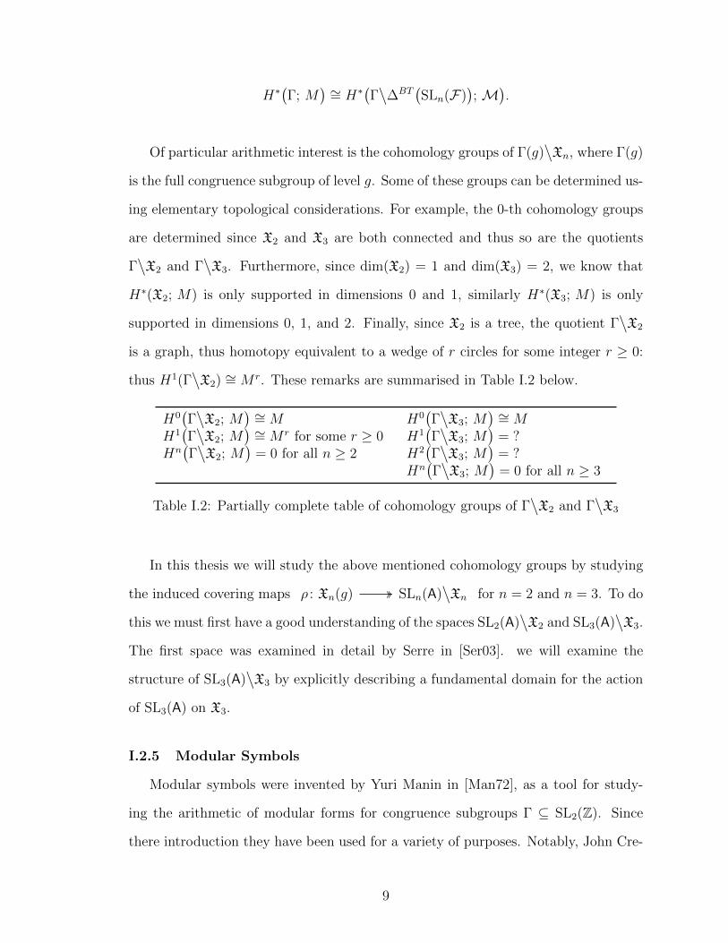
Of particular arithmetic interest is the cohomology groups of Γ(g)∖Xn, where Γ(g)
is the full congruence subgroup of level g. Some of these groups can be determined us-
ing elementary topological considerations. For example, the 0-th cohomology groups
are determined since X2 and X3 are both connected and thus so are the quotients
Γ∖X2 and Γ
∖X3. Furthermore, since dim(X2) = 1 and dim(X3) = 2, we know that
H∗(X2; M) is only supported in dimensions 0 and 1, similarly H∗(X3; M) is only
supported in dimensions 0, 1, and 2. Finally, since X2 is a tree, the quotient Γ∖X2
is a graph, thus homotopy equivalent to a wedge of r circles for some integer r ≥ 0:
thus H1(Γ∖X2) ∼= M r. These remarks are summarised in Table I.2 below.
H0(Γ∖X2; M
) ∼= M H0(Γ∖X3; M
) ∼= MH1(Γ∖X2; M
) ∼= M r for some r ≥ 0 H1(Γ∖X3; M
)= ?
Hn(Γ∖X2; M
)= 0 for all n ≥ 2 H2
(Γ∖X3; M
)= ?
Hn(Γ∖X3; M
)= 0 for all n ≥ 3
Table I.2: Partially complete table of cohomology groups of Γ∖X2 and Γ
∖X3
In this thesis we will study the above mentioned cohomology groups by studying
the induced covering maps ρ : Xn(g) SLn(A)∖Xn for n = 2 and n = 3. To do
this we must first have a good understanding of the spaces SL2(A)∖X2 and SL3(A)
∖X3.
The first space was examined in detail by Serre in [Ser03]. we will examine the
structure of SL3(A)∖X3 by explicitly describing a fundamental domain for the action
of SL3(A) on X3.
I.2.5 Modular Symbols
Modular symbols were invented by Yuri Manin in [Man72], as a tool for study-
ing the arithmetic of modular forms for congruence subgroups Γ ⊆ SL2(Z). Since
there introduction they have been used for a variety of purposes. Notably, John Cre-
9

mona used modular symbols to perform large scale computations of Hecke eigenvalues
[Cre97].
Abstractly, a modular symbol for Γ is an ordered pair α, β ∈ P1(Q)×P1(Q), con-
sidered as an element of the first relative homology group of Γ\H, that is,
H1
(Γ\H, cusps; M
). There is a very nice geometric interpretation of modular sym-
bols: If α, β are rational cusps2 of H, then there is a unique geodesic path in H
from α to β, we denote this path by α, β. The image of α, β under the quo-
tient map H 7→ Γ\H can be considered as an element of the relative homology group
H1
(Γ\H, cusps; M
). By an abuse of notation we write α, β ∈ H1
(Γ\H, cusps; M
).
Thus, a modular symbol for Γ can be thought of as a geodesic path in H joining two
rational cusps α, β ∈(Q∪∞
), which we consider as an element of the first relative
homology group of Γ\H, i.e. H1
(Γ\H, cusps; M
). It can be shown that all elements
of the relative homology group arise in this way. For a geometric illustration of a
modular symbol see Figure I.1a.
Modular symbols relate to the above discussions in Chapter I and Chapter I about
cohomology groups since one can show H1
(Γ\H, cusps; M
) ∼= H1(Γ\H; M
).3
In [Man72], Manin gives an explicit finite set of generators and relations for the
group of modular symbols, making it relatively easy to calculate H1
(Γ\H, cusps; M
).
Using the duality between modular forms and H1
(Γ\H, cusps; M
)one can use mod-
ular symbols to calculate the structure of the space of modular forms. Manin also
describes how the Hecke operators act on modular symbols.
2The rational cusps of H are Q ∪ ∞ ∼= P1(Q).
3This follows directly from the Lefschetz duality theorem:
Theorem I.2.5 (Lefschetz Duality Theorem).Let X be a compact, triangulated n-dimensional manifold with boundary. Then
Hk(X, ∂X) ∼= Hn−k(X) for all k.
10

A unimodular symbol is a modular symbol which corresponds to an edge of the
Farey tessellation4 of H. Manin showed that any modular symbol can be written
as a sum of unimodular symbols by describing an explicit algorithm to do so. The
algorithm is often referred to as Manin’s trick, or the continued fraction algorithm.
Since any congruence subgroups Γ ⊆ SL2(Z) is of finite index, there are only finitely
many unimodular symbols modulo Γ. Thus the set of unimodular symbols modulo
Γ, is a finite generating set for the set of all modular symbols.
The notion of modular symbols have since been generalised to groups other than
SL2(R). In the 70’s Barry Mazur described a generalisation of modular symbols for an
arbitrary reductive Q-group [Maz]. The SLn(R)-case was then studied in more detail
by Ash and Rudolph in [AR79]. Another way in which modular symbols have been
generalised is to groups over non-archimedean field. In [Tei92], Teitelbaum described
a theory of modular symbols for SL2(A). Geometrically, the modular symbols of
Teitelbaum are analogous to those of Manin: instead of considering geodesics between
cusps in H, one now considers geodesics between cusps in the Bruhat-Tits building
∆BT(SL2(F)
). For a geometric illustration of a Teitelbaum modular symbol see
Figure I.1b.
I.3 Overview of Results
In Chapter 1 we examine the structure of X2, and the action of SL2(A) on X2. We
start by reviewing some results of Serre on the structure of X2. We then describe the
boundary of X2 explicitly (Section 1.2). After which we examine the quotient map
ρ : Γ(g)∖X2 SL2(A)
∖X2 , and derive a formula for the number of simplices
lying above a given simplex in SL2(A)∖X2 (Theorem 1.4.7). Using this formula, we
go on to derive a formula for the homology groups of the quotient space Γ(g)∖X2, for
a general g ∈ A (Theorem 1.5.2).
4The Farey tessellation is the ideal triangulation of H with edges given by the SL2(Z)-orbit ofthe geodesic 0, i∞.
11

(a) The SL2(Z)-case
2
(b) The SL2(A)-case
Figure I.1: Geometric representations of modular symbols
In Chapter 2 we carry out a similar program for X3. We make basic observations
on the structure of X3, describe how SL3(F) acts on X3, and show that there exists
a SL3(F) invariant 3-colouring of X3. We then examine the action of SL3(A) on
X3, and give a complete description of a fundamental domain (Theorem 2.2.5), and
calculate all relevant stabiliser subgroups (Theorem 2.2.3). Finally, we examine the
quotient spaces Γ(g)∖X3, for Γ(g) ⊆ SL3(A) a full congruence subgroup. Using the
covering map ρ : Γ(g)∖X3 SL3(A)
∖X3 we calculate the cardinality of the set
of simplices which lie above any given simplex of SL2(A)∖X2 (Example 2.3.6).
In Chapter 3 we define an appropriate generalisation of unimodular symbols for
SL3((t−1)), and prove that a continued fraction type algorithm exists (in the sense
of [AR79]), thus showing any modular symbol can be written a sum of unimodular
symbols.
12

CHAPTER 1
THE BUILDING ASSOCIATED TO SL2
(F)
In this section we will examine the Bruhat-Tits building associated to SL2(F),
which we denote by X2. The main objectives of this section are:
1. Make basic observations on the structure of X2, describe how SL2(F) acts on
X2, and show that there exists a SL2(F) invariant 2-colouring of X2.
2. Discuss distance between vertices in X2, index all vertices of a given distance
from some fixed vertex, define and examine the boundary of X2.
3. Examine the quotient SL2(A)∖X2, describe a fundamental domain, and calculate
all relevant stabiliser subgroups.
4. Examine the quotients Γ(g)∖X2, for Γ(g) ⊆ SL2(A) a full congruence subgroup.
We use the covering map ρ : Γ(g)∖X2 SL2(A)
∖X2 to calculate the car-
dinality of the set of simplices which lie above any given simplex of SL2(A)∖X2.
5. Calculate the homology of the quotients Γ(g)∖X2.
Throughout this section we will be considering X2 from the point of view of lattices,
which was discussed in Chapter I. i.e. Let W = F2, and define a lattice in W to be
a free O-sub-module of W of rank 2. Let Lat/∼ denote the set of all lattices up
to F×-homothety, and denote the equivalence class of a lattice L by [L]. Then the
Bruhat-Tits building X2 is defined as follows:
13
Definition 1.0.1.
Let X2 be the abstract simplicial complex with the following simplices
Sim0(X2) = Λi | Λi ∈ Lat/∼
Sim1(X2) =
Λ1Λ2
∣∣∣∣∣∣∣Λ1,Λ2 ∈ Lat/∼, such that there exists
L1,L2 ∈ Lat with [Li] = Λi, and πL1 ( L2 ( L1
and the obvious attaching maps.
1.1 Basic Properties of X2
The primary reference for this section is [Ser03, Chapter II].
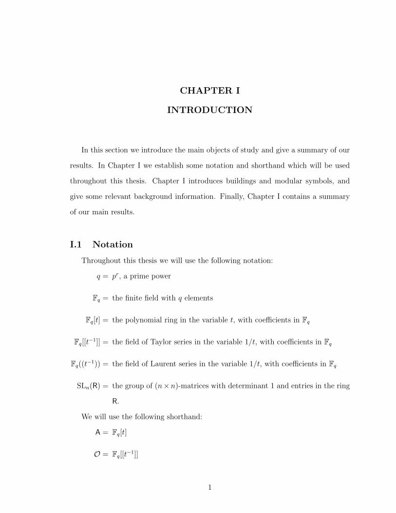
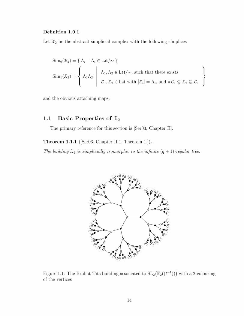
Theorem 1.1.1 ([Ser03, Chapter II.1, Theorem 1.]).
The building X2 is simplicially isomorphic to the infinite (q + 1)-regular tree.
2
Figure 1.1: The Bruhat-Tits building associated to SL2
(F2((t−1))
)with a 2-colouring
of the vertices
14

Definition 1.1.2.
Given ai,j ∈ F , let L =
⟨(a1,1 a1,2 . . . a1,n
a2,1 a2,2 . . . a2,n
)⟩be the O-lattice spanned by the
columns of the matrix, with respect to the standard basis of F2.
Proposition 1.1.3.
The group GL2(F) acts transitively on the set of all rank 2 lattices, and thus on
Sim0(X2).
Proof. Fix L0 = 〈( 1 00 1 )〉, and let L = 〈( a bc d )〉 be an arbitrary rank-2 lattice. Since
( ac ) and ( bd ) are F -linearly-independent, α = ( a bc d ) ∈ GL2(F). Finally note that
αL0 = L.
Given any two lattices, L and L′, let α ∈ GL(W) be such that αL = L′. There
exists bases e1, e2 of L, and f1, f2 of L′, such that the matrix of A with respect
to these bases is
α =
(πn1 0
0 πn2
),
were n1, n2 ∈ Z.1 Thus there exists an O-basis of L, e1, e2, such that πn1e1, πn2e2
is an O-basis for L′. Moreover, it can be shown that the set, n1, n2 is independent
of the choice of such a basis.
Proposition 1.1.4.
Let L,M,L′,M′ be lattices such that L ∼ L′ and M ∼ M′. Let α, β ∈ SL2(F) be
such that αL = M and βL′ = M′. If n1, n2 are the integers associated to α and
n′1, n′2 those associated to β, then
n1 + n2 = n′1 + n′2 (mod 2), and |n1 − n2| = |n′1 − n′2|.
Proof. If L ∼ L′ then L′ = πcL for some c ∈ Z, similarly M′ = πdM for some
d ∈ Z. Thus β (πcL) =(πdM
), so
(βπc−d
)L = M. Hence the map
(βπc−d
)1This is called the Smith Normal form of α.
15
has the same associated integers as α does, thus the integers associated to β are
n′1, n′2 = n1 − c+ d, n2 − c+ d.
Corollary 1.1.5 (Colouring of vertices).
Choosing a distinguished vertex Λ induces a 2-colouring on the set of all vertices.
There is a natural notion of distance between two vertices of X2. We say that
every edge has length 1, and the distance between two vertices is the length of the
shortest path between the two vertices.
Theorem 1.1.6 (Distance between vertices [Ser03, Remark 1, p71]).
Let Λ, Λ′ be two vertices of X2, and let α ∈ SL2(F) be such that αΛ = Λ′. If n1, n2
are the integers associated to α then the distance between Λ and Λ′ is |n1 − n2|.
Definition 1.1.7.
Let L1, and L2 be any two lattices, then we define
χ(L1,L2) = l(L1/L1 ∩ L2)− l(L2/L1 ∩ L2).2
This can be thought of as a generalised notion of index, where we no longer require
one lattice to contain the other.
Theorem 1.1.8 ([Ser03, Proposition 1. p75]).
Let L be a lattice and s ∈ SL(W), then χ(L, sL) = 0.
Corollary 1.1.9 ([Ser03, Corollary. p75]).
If Λ is a vertex of X2 and s ∈ SL(W), then d(Λ, sΛ) = 0 (mod 2).
Since we know that X2 is a tree, Corollary 1.1.9 implies the following proposition.
2Where l(L/L′) is the length of L/L′, i.e. the longest chain of submodules of L/L′.
16

Proposition 1.1.10.
The group SL(W) acts simplicially (i.e. without inversions), and thus preserves the
colouring.
Definition 1.1.11 (Stabiliser Subgroups).
Let G ⊆ SL(W) be a subgroup, L ∈ Lat, Λ ∈ Sim0(X2), and ΛΛ′ ∈ Sim1(X2), then
GLdef= StabG(L) = g ∈ G | g · L = L,
GΛdef= StabG(Λ) = g ∈ G | g · Λ = Λ,
GΛΛ′def= StabG(ΛΛ′) = g ∈ G | g · ΛΛ′ = ΛΛ′.
Proposition 1.1.12.
a) If G ⊆ SL(W), then GΛΛ′ = GΛ ∩GΛ′.
b) If [L] = Λ, then GΛ = GL.
Proof. Part a) follows directly form Proposition 1.1.10. Part b) is a consequence of
the fact that all linear transformations in SL(W) have determinant equal to 1.
Example 1.1.13. Let G = SL(W). Given ΛΛ′ ∈ Sim1(X2), one can choose representa-
tive lattices [L] = Λ and [L′] = Λ′ with basis, L = 〈e1, e2〉 and L′ = 〈e1, πe2〉. With
respect to these bases the stabilisers are:
GΛ = SL2(O)
GΛ′ =
(a b
c d
)∈ SL2(F)
∣∣∣∣∣ π|c, and πb, a, d ∈ O
GΛΛ′ =
(a b
c d
)∈ SL2(O)
∣∣∣∣∣ π|c.
17

1.2 Distance and the boundary of X2
In this subsection we will examine the set of all vertices in X2 which are a fixed
distance from a given vertex. We will then describe the boundary of X2. But first we
need to recall the definition of projective space.
Definition 1.2.1 (n-Dimensional Projective Space).
Let R be a ring, and V ∼= Rn+1. The projective space P(V ) is the set of full lines in
V , i.e.
P(V ) =
(a0 : a1 : . . . : an)∣∣ gcd(a0, a1, . . . , an) ∈ R×
/R×.
This is also sometimes written as Pn(R), and called n-dimensional projective space
over R.
Let L0 = 〈( 1 00 1 )〉, and Λ0 = [L0]. Each vertex of X2 can be represented by a unique
sub-lattice, L ⊆ L0, such that L0/L ∼= O/πn where d(Λ0,Λ) = n. Note, L0/πnL0 is
a free O/πn module of rank 2, and L/πnL0 is a direct factor of rank 1. i.e.
Oπn∼=L
πnL0
→ L0
πnL0
∼=Oπn⊕ Oπn.
We will use this observation to index the vertices of distance n from Λ0.
Proposition 1.2.2 (Indexing Vertices of Distance n [Ser03, p72]).
Vertices of distance n from Λ0 correspond bijectively to lines in L0/πnL0, i.e. points
in P(L0/πnL0) ∼= P1(O/πn).
We will now describe the boundary of X2.
Definition 1.2.3 (Boundary Points).
The boundary of X2 is the set of equivalence classes of geodesic rays (non-
backtracking half lines) in X2 starting at Λ0. We denote the boundary by ∂X2.
18

This is the Gromov boundary of X2 with the natural metric.3 One can show that
the above construction of ∂X2 doesn’t depend on the starting vertex Λ0. We call the
points on the boundary boundary points or points at infinity.
Proposition 1.2.4 (Indexing Points at Infinity).
Points at infinity correspond bijectively to lines in L0, i.e. points in P(L0) ∼= P1(O).
Proof. A geodesic ray emanating from Λ0 can be thought of as a consistent choice
of vertices Λ0,Λ1,Λ2, . . . , where d(Λ0,Λn) = n and d(Λn,Λn+1) = 1. From Proposi-
tion 1.2.2 we know that this corresponds to a collection of lines, ln ⊂ L0/πnL0∞n=0,
such that ln+1 = ln (mod πnL0). This is the same as an element of the inverse limit
lim←P(L0
πnL0
)∼= P
(lim←
L0
πnL0
)∼= P (L0) ,
where the last isomorphism follows from the fact that L ∼= O2 and O is complete and
profinite thus lim←
OπnO
∼= O.
Proposition 1.2.5.
If D ∈ P(L0), then the sequence of lattices
Ln = πnL0 +D, (1.1)
forms a geodesic ray based at L0, which represents the point at infinity D.
Conversely, given an infinite sequence of lattices that form a geodesic ray Ln∞n=0,
such that πLn ( Ln+1 ( Ln, the corresponding point at infinity corresponds to the
line
D = limn→∞
Ln =∞⋂n=0
Ln ∈ P(L0). (1.2)
3The usual definition of the Gromov boundary uses an equivalence relation on the set of allgeodesic rays starting at a given point, where two rays are equivalent if they stay a bounded distanceapart. Since X2 is a tree, this equivalence relation becomes trivial in our case.
19
( 1 00 1 ) ( 1 0
0 π )
(0 1π2 π+π2
) (0 1π3 π+π2
) (0 1π4 π+π2
) (0 1π5 π+π2
)(1 : π + π2)
(π2 10 π
) (π3 10 π
) (π4 10 π
)(1 : π)
(1 00 π2
) (π 10 π2
) (π2 10 π2
) (π3 10 π2
)(1 : π2)
(1 00 π3
) (1 00 π4
) (1 00 π5
)(1 : 0)
( π 1+π0 π )
(π2 1+π0 π
) (π3 1+π0 π
) (π4 1+π0 π
)(1 + π : π)
( π 10 1 )
(π2 10 1
) (π3 10 1
) (π4 10 1
) (π5 10 1
)(1 : 1)
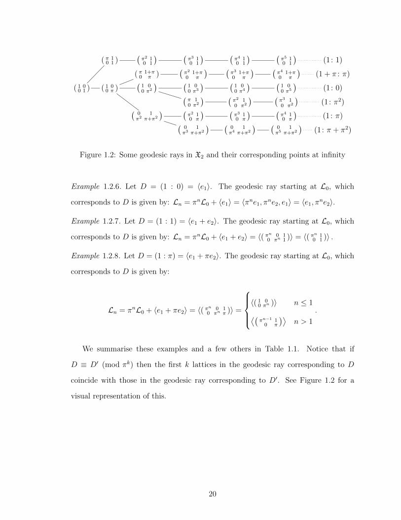
Figure 1.2: Some geodesic rays in X2 and their corresponding points at infinity
Example 1.2.6. Let D = (1 : 0) = 〈e1〉. The geodesic ray starting at L0, which
corresponds to D is given by: Ln = πnL0 + 〈e1〉 = 〈πne1, πne2, e1〉 = 〈e1, π
ne2〉.
Example 1.2.7. Let D = (1 : 1) = 〈e1 + e2〉. The geodesic ray starting at L0, which
corresponds to D is given by: Ln = πnL0 + 〈e1 + e2〉 = 〈( πn 0 10 πn 1 )〉 = 〈( πn 1
0 1 )〉 .
Example 1.2.8. Let D = (1 : π) = 〈e1 + πe2〉. The geodesic ray starting at L0, which
corresponds to D is given by:
Ln = πnL0 + 〈e1 + πe2〉 = 〈( πn 0 10 πn π )〉 =
〈( 1 0
0 πn )〉 n ≤ 1⟨(πn−1 1
0 π
)⟩n > 1
.
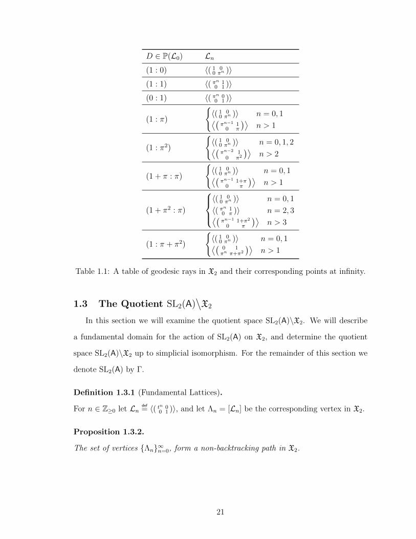
We summarise these examples and a few others in Table 1.1. Notice that if
D ≡ D′ (mod πk) then the first k lattices in the geodesic ray corresponding to D
coincide with those in the geodesic ray corresponding to D′. See Figure 1.2 for a
visual representation of this.
20
D ∈ P(L0) Ln(1 : 0) 〈( 1 0
0 πn )〉
(1 : 1) 〈( πn 10 1 )〉
(0 : 1) 〈( πn 00 1 )〉
(1 : π)
〈( 1 0
0 πn )〉 n = 0, 1⟨(πn−1 1
0 π
)⟩n > 1
(1 : π2)
〈( 1 0
0 πn )〉 n = 0, 1, 2⟨(πn−2 1
0 π2
)⟩n > 2
(1 + π : π)
〈( 1 0
0 πn )〉 n = 0, 1⟨(πn−1 1+π
0 π
)⟩n > 1
(1 + π2 : π)
〈( 1 0
0 πn )〉 n = 0, 1
〈( πn 10 π )〉 n = 2, 3⟨(πn−1 1+π2
0 π
)⟩n > 3
(1 : π + π2)
〈( 1 0
0 πn )〉 n = 0, 1⟨(0 1πn π+π2
)⟩n > 1
Table 1.1: A table of geodesic rays in X2 and their corresponding points at infinity.
1.3 The Quotient SL2(A)∖X2
In this section we will examine the quotient space SL2(A)\X2. We will describe
a fundamental domain for the action of SL2(A) on X2, and determine the quotient
space SL2(A)\X2 up to simplicial isomorphism. For the remainder of this section we
denote SL2(A) by Γ.
Definition 1.3.1 (Fundamental Lattices).
For n ∈ Z≥0 let Lndef= 〈( tn 0
0 1 )〉, and let Λn = [Ln] be the corresponding vertex in X2.
Proposition 1.3.2.
The set of vertices Λn∞n=0, form a non-backtracking path in X2.
21

Proof. Since Ln ( Ln+1 ( tLn, the vertices Λn and Λn+1, are adjacent. It is clear
that tkLn 6= Lm for any k, n,m ∈ Z. Thus the vertices Λn and Λm are distinct for all
n,m ∈ Z, hence the path is non-backtracking.
Let P denote the subcomplex of X2 which is spanned by the vertices Λn∞n=0. We
will show that P is a fundamental domain for the action of SL2(A) on X2.
Theorem 1.3.3.
The Λn are pairwise inequivalent modulo SL2(A).
Proof. Let s =
(a1,1 a1,2
a2,1 a2,2
)∈ SL2(A), and suppose that for some n ∈ Z≥0, m ∈
Z≥−n, we have sΛn = Λn+m. We will show that m = 0. By assumption we have
that sLn = t−hLn+m for some h ∈ Z. By Theorem 1.1.8 we have χ(Ln, sLn) =
χ(Ln, t−hLn+m) = 0, i.e.
0 = χ(Ln, sLn)
= χ(Ln, t−hLn+m)
= l
(Ln
Ln ∩ t−hLn+m
)− l(
t−hLn+m
Ln ∩ t−hLn+m
)
= l
⟨(tn 0
0 1
)⟩⟨(
tmin(n, n+m−h) 0
0 tmin(0,−h)
)⟩− l
⟨(tn+m−h 0
0 t−h
)⟩⟨(
tmin(n, n+m−h) 0
0 tmin(0,−h)
)⟩
=[n−
(min(n, n+m− h) + min(0, −h)
)]−[n+m− 2h−
(min(n, n+m− h) + min(0, −h)
)]= −m+ 2h.
Thus,
m = 2h. (1.3)
22
Hence sLn = t−hLn+2h, i.e.⟨(
a1,1tn a1,2a2,1tn a2,2
)⟩=⟨(
tn+h 00 t−h
)⟩. Therefore, there exists,
α, β, γ, δ ∈ O, such that: α(tn+h
0
)+β(
0t−h
)=(a1,1tn
a2,1tn
)and γ
(tn+h
0
)+δ(
0t−h
)= (
a1,2a2,2 ).
Thus
a1,1tn = αtn+h, a1,2 = γtn+h,
a2,1tn = βt−h, a2,2 = δt−h.
By rearranging we get the following degree conditions:
degt(a1,1) ≤ h, degt(a1,2) ≤ n+ h,
degt(a2,1) ≤ −n− h, degt(a2,2) ≤ −h.(1.4)
We now use these degree constraints to show that h = 0.
h > 0 =⇒
degt(a2,1) ≤ −n− h < 0 =⇒ a2,1 = 0
degt(a2,2) ≤ −h < 0 =⇒ a2,2 = 0
=⇒ det(s) = 0
=⇒ ⊥,
h < 0 =⇒
degt(a1,1) ≤ h < 0 =⇒ a1,1 = 0
degt(a2,1) ≤ −n− h < 0 =⇒ a2,1 = 0
=⇒ det(s) = 0
=⇒ ⊥ .
Where −n− h < 0 when h < 0 because, −n− h = −(n+m) + h ≤ h.
Thus h = 0. By Equation (1.3) we have m = 2h = 0.
23
Theorem 1.3.4.
The vertex and edge stabilisers of the cells in P are given by:
ΓΛn =
SL2(Fq) n = 0(
a b
0 a−1
) ∣∣∣∣∣ a ∈ F×q , b ∈ Fq[t], degt(b) ≤ n
n > 0
(1.5a)
ΓΛnΛn+1 =
(a b
0 a−1
) ∣∣∣∣∣ a ∈ F×q , b ∈ Fq[t], degt(b) ≤ n
. (1.5b)
Proof. Suppose sΛn = Λn for some s ∈ SL2(A). Then the entries of s must satisfy
Equation (1.4) with h = 0. Thus s ∈ ΓΛn . It is a straightforward calculation to show
that if s ∈ ΓΛn then sΛn = Λn.
The edge stabiliser groups follow immediately from ΓΛnΛn+1 = ΓΛn ∩ ΓΛn+1 .
Proposition 1.3.5.
a) ΓΛ0 acts transitively on the edges of Λ0.
b) For n ≥ 1, ΓΛn fixes ΛnΛn+1, and acts transitively on the remaining edges.
Proof. Recall that the vertices adjacent to a given vertex Λ correspond to lines in
Fq. The group ΓΛ0 acts transitively on the set of such lines. Similarly, for n > 0 the
group ΓΛn fixes one line, and acts transitively on the remaining lines.
We are now ready to show that P is a fundamental domain for the action of SL(A)
on X2.
Theorem 1.3.6 (Quotient space SL2(A)\X2).
The subcomplex P ∈ X2 is a fundamental domain for the action of SL2(A) on X2.
Furthermore, the quotient space SL2(A)\X2 is simplicially isomorphic to P.
24

Proof. By Theorem 1.3.3 we know that the Λn are pairwise inequivalent modulo
SL2(A). It remains to show that if Λ 6∈ Λn∞n=0 is a vertex in X2, then it is equivalent
to some Λn modulo SL2(A). This follows from Proposition 1.3.5.
As a consequence of Theorem 1.3.6 there is a natural numbering of the vertices of
X2, where the vertex Λ is numbered n if and only if Λ maps to Λn via the quotient
map X2 SL2(A)∖X2 . See Figure 1.3 for an illustration of this numbering.
asflk j
0
1
01
0
1
1
21
3
101
1 2
13
2
1
01
1
0
1 1
3
2
1 1
4
3
5
1
0
1
0
1 1
2
13
1
0
1
1
2 1
3
21
01
1
01
13
21
1
4
35
1
0
1
0 1
12
13
1
0
11
2
13
2
1
0
11
0
1
1
32
1
1
43
5
1
Figure 1.3: The Bruhat-Tits building associated to SL2
(F2((t−1))
)with a 2-colouring
and numbering of the vertices
1.4 Quotients by full congruence subgroups Γ(g) ⊆ SL2(A)
Let g ∈ A be non-zero. In this section we will examine the quotient Γ(g)\X2,
where
Γ(g)def=
(a b
c d
)∈ SL2(A)
∣∣∣∣∣(a b
c d
)≡
(1 0
0 1
)(mod g)
.
We call Γ(g) the full congruence subgroup of Γ of level g. Note that Γ(g) is a normal
subgroup of Γ, thus there exists a quotient map ρ : Γ(g)∖X2 Γ
∖X2. We will
study Γ(g)∖X2 by studying this quotient map. We denote Γ(g)
∖X2 by X2(g).
25
Definition 1.4.1.
Identify Γ∖X2 with P , and define
X2(g)Λn = Vertices in X2(g) lying above Λn ,
X2(g)ΛnΛn+1 = Edges in X2(g) lying above Λn,n+1 .
We will calculate the size of the sets X2(g)Λn , and X2(g)ΛnΛn+1 , using the
following identity.
Theorem 1.4.2.
The set of vertices (resp. edges) in X2(g) which lie over Λn (resp. Λn,n+1), is given
by
X2(g)Λn∼=
ΓΓ(g)ΓΛnΓ(g)Λn
(1.6a)
X2(g)ΛnΛn+1∼=
ΓΓ(g)ΓΛnΛn+1Γ(g)ΛnΛn+1
. (1.6b)
In particular the cardinality is given by
#X2(g)Λn =[Γ : Γ(g)]
[ΓΛn : Γ(g)Λn ], (1.7a)
#X2(g)ΛnΛn+1 =[Γ : Γ(g)]
[ΓΛnΛn+1 : Γ(g)ΛnΛn+1 ]. (1.7b)
Proof. We will only show Equation (1.6a), the proof of Equation (1.6b) is directly
analogous. The proof is essentially a series of simple isomorphisms. Since Γ acts
transitively on the set of all vertices in X2 which lie over Λn, by the orbit-stabiliser
theorem we have that Γ/
ΓΛn∼= Vertices in X2 which lie over Λn . Thus
26

X2(g)Λn∼= Γ(g)
∖Γ/
ΓΛn
∼= ΓΓ(g)ΓΛnSince both Γ(g) and ΓΛn are normal in Γ
∼=ΓΓ(g)
Γ(g)ΓΛnΓ(g)
By the third isomorphism theorem
∼=ΓΓ(g)
ΓΛnΓΛn ∩ Γ(g)
By the second isomorphism theorem
=
ΓΓ(g)ΓΛnΓ(g)Λn
Since ΓΛn ∩ Γ(g) = Γ(g)Λn .
Before we use Theorem 1.4.2 to calculate X2(g)Λn , and X2(g)ΛnΛn+1 , we first
derive a general expression for the index[Γ: Γ(g)
].
Theorem 1.4.3.
Let g ∈ A with degt(g) = N > 0, and assume that g factors as g =∏k
i=1 geii where
the gi ∈ A are distinct, irreducible, and degt(gi) = di. Then
[Γ: Γ(g)
]= q3N
k∏i=1
(1− 1
q2di
). (1.8)
Proof. We break the proof up into multiple steps:
Step 1. Show that[Γ: Γ(g)
]= # SL2
(Ag)
Step 2. Reduce to the case # SL2
(Age
)for g irreducible
Step 3. Show that # SL2
(Age
)=
# GL2
(Age
)#(Age
)×27

Step 4. Show that #(Age
)×= qed − q(e−1)d
Step 5. Show that # GL2
(Age
)= q4(e−1)d(q2d − 1)(q2d − qd)
Step 6. Conclude that # SL2
(Age
)= q3ed
(1− 1
q2d
)Step 1. This is a direct consequence of the following short exact sequence
1 Γ(g) Γ SL2
(Ag)
1.
Step 2. This is a consequence of the Chinese Remainder Theorem for SL2, i.e.
SL2
(Ag)∼=
k∏i=1
SL2
(Ageii
).
Step 3. This is a direct consequence of the following short exact sequence
1 SL2
(Age
)GL2
(Age
) (Age
)×1.
Step 4. It is straightforward to see that(Age
)×=a ∈ Age
∣∣∣ a 6≡ 0 (mod g)
.
Thus #(Age
)×= qed − q(e−1)d.
Step 5. The reduction map ρ : f (mod ge) f (mod g) induces a sur-
jective map ρ : GL2
(Age
)GL2
(Ag). Thus # GL2
(Age
)= # ker(ρ) ×
# GL2
(Ag)
. It is straightforward to see that # GL2
(Ag)
= (q2d − 1)(q2d − qd).
The kernel of the map is ker(ρ) =
1 0
0 1
+ A
∣∣∣∣∣∣∣ A ∈ gM2,2
(Age
), which has
cardinality # ker(ρ) = q4(e−1)d. Thus # GL2
(Age
)= q4(e−1)d(q2d − 1)(q2d − qd).
28
Step 6. From Step 3., Step 4., and Step 5. we have that
# SL2
(Age
)=q4(e−1)d(q2d − 1)(q2d − qd)
qed − q(e−1)d
= q3(e−1)d(q2d − 1)qd
= q3ed
(1− 1
q2d
).
Proposition 1.4.4.
Let g ∈ A with degt(g) = N > 0, and assume that g factors as g =∏k
i=1 geii where
the gi ∈ A are distinct, irreducible, and degt(gi) = di. Then
[ΓΛn : Γ(g)Λn
]=
q(q2 − 1) if n = 0
qmin(n+1, N)(q − 1) if n > 0[ΓΛnΛn+1 : Γ(g)ΛnΛn+1
]= qmin(n+1, N)(q − 1) if n ≥ 0.
Proof. Using Equation (1.5a) and Equation (1.5b) we calculate the cardinality of the
stabiliser subgroups of Γ, i.e.
#ΓΛn =
q(q2 − 1) if n = 0
qn+1(q − 1) if n > 0
#ΓΛnΛn+1 = qn+1(q − 1).
The vertex stabiliser subgroups of Γ(g) are given by
Γ(g)Λ0 = SL2(Fq) ∩ Γ(g) = Id ,
29
and for n > 0 then we have
Γ(g)Λn =
(a b
0 a−1
) ∣∣∣∣∣ a ∈ F×q , b ∈ Fq[t], and degt(b) ≤ n
∩ Γ(g)
=
(1 b
0 1
) ∣∣∣∣∣ b ∈ Fq[t], degt(b) ≤ n, and b ≡ 0 (mod g)
=
(1 g · b0 1
) ∣∣∣∣∣ b ∈ Fq[t], and degt(b) ≤ n−N
.
Similarly, the edge stabilisers are,
Γ(g)ΛnΛn+1 =
(1 g · b0 1
) ∣∣∣∣∣ b ∈ Fq[t], and degt(b) ≤ n−N
.
Taking the cardinality of these groups gives
#Γ(g)Λn =
1 if n < N
qn−N+1 if n ≥ N
#Γ(g)ΛnΛn+1 =
1 if n < N
qn−N+1 if n ≥ N
.
Taking the appropriate quotients gives:
[ΓΛn : Γ(g)Λn
]=
q(q2 − 1) if n = 0
qn+1(q − 1) if 0 < n < N
qN(q − 1) if n ≥ N
[ΓΛnΛn+1 : Γ(g)ΛnΛn+1
]=
qn+1(q − 1) if n < N
qN(q − 1) if n ≥ N
.
30

We are now ready to calculate some examples.
Example 1.4.5 (X2(tN)).
We will calculate the number of vertices and edges in X2(tN) that lie over Λn and
Λn,n+1. By Equation (1.8) we have that[Γ: Γ(tN)
]= q3N
(1− 1
q2
)= q3N−2(q2 − 1).
By Proposition 1.4.4 we have that
[ΓΛn : Γ(tN)Λn
]=
q(q2 − 1) if n = 0
qmin(n+1, N)(q − 1) if n > 0[ΓΛnΛn+1 : Γ(tN)ΛnΛn+1
]= qmin(n+1, N)(q − 1) if n ≥ 0.
By Theorem 1.4.2 we have
#X2(tN)Λn =
[Γ: Γ(tN)
][ΓΛn : Γ(tN)Λn
] =
q3(N−1) n = 0
q3(N−1)−n(q + 1) 0 < n < N
q2(N−1)(q + 1) n ≥ N
and
#X2(tN)ΛnΛn+1 =
[Γ: Γ(tN)
][ΓΛnΛn+1 : Γ(tN)ΛnΛn+1
] =
q3(N−1)−n(q + 1) n < N
q2(N−1)(q + 1) n ≥ N.
The results of the above example are summarised in Table 1.2.
Example 1.4.6 (X2(t2 + 1)).
Let g = t2 + 1. There are three different cases to consider here, depending on the
characteristic of the field Fq((t−1)):
Case I: char(F) = 2, the ramified case.
31

g #X2(g)Λn #X2(g)ΛnΛn+1
t1 q + 1 if n = 0,q + 1 q + 1 if n ≥ 1.
t2q3 q3(q + 1) if n = 0,q2(q + 1) q2(q + 1) if n ≥ 1.
t3q6 q6(q + 1) if n = 0,q5(q + 1) q5(q + 1) if n = 1,q4(q + 1) q4(q + 1) if n ≥ 2.
t4
q9 q9(q + 1) if n = 0,q8(q + 1) q8(q + 1) if n = 1,q7(q + 1) q7(q + 1) if n = 2,q6(q + 1) q6(q + 1) if n ≥ 3.
tNq3(N−1) q3(N−1)(q + 1) if n = 0,q3(N−1)−n(q + 1) q3(N−1)−n(q + 1) if 0 < n < N,q2(N−1)(q + 1) q2(N−1)(q + 1) if n ≥ N.
Table 1.2: A table of #X2(tN)Λn and #X2(tN)ΛnΛn+1 , and some low degree ex-amples.
Case II: char(F) ≡ 1 (mod 4), the split case.
Case III: char(F) = 3 (mod 4), the non-split case.
One thing which is common to all the cases is the index of the stabiliser subgroups,
i.e. by Proposition 1.4.4 we have that
[ΓΛn : Γ(t2 + 1)Λn
]=
q(q2 − 1) n = 0
q2(q − 1) n ≥ 1
,
[ΓΛnΛn+1 : Γ(t2 + 1)ΛnΛn+1
]=
q(q − 1) n = 0
q2(q − 1) n ≥ 1
.
Case I: char(F) = 2.
In this case (t2 + 1) ramifies, i.e. (t2 + 1) = (t+ 1)2. Thus by Equation (1.8) we have
that[Γ: Γ(g)
]= q6
(1− 1
q2
)= q4(q2 − 1). By Theorem 1.4.2 we have
32
#X2(g)Λn =
q3 if n = 0
q2(q + 1) if n ≥ 1
and
#X2(g)ΛnΛn+1 =
q3(q + 1) if n = 0
q2(q + 1) if n ≥ 1
.
Case II : char(F) ≡ 1 (mod 4).
In this case (t2 + 1) splits, i.e. (t2 + 1) = (t − a)(t + a) for some a ∈ Fq. Thus by
Equation (1.8) we have that[Γ: Γ(g)
]= q6
(1− 1
q2
)(1− 1
q2
)= q2(q2 − 1)(q2 − 1).
By Theorem 1.4.2 we have that
#X2(g)Λn =
q(q2 − 1) if n = 0
(q + 1)(q2 − 1) if n ≥ 1
and
#X2(g)ΛnΛn+1 =
q(q + 1)(q2 − 1) if n = 0
(q + 1)(q2 − 1) if n ≥ 1
.
Case III : char(F) ≡ 3 (mod 4).
In this case (t2 + 1) is irreducible. Thus by Equation (1.8) we have that[Γ: Γ(g)
]= q6
(1− 1
q4
)= q2(q2 − 1)(q2 + 1). By Theorem 1.4.2 we have that
33

#X2(g)Λn =
q(q2 + 1) if n = 0
(q + 1)(q2 + 1) if n ≥ 1
#X2(g)ΛnΛn+1 =
q(q + 1)(q2 + 1) if n = 0
(q + 1)(q2 + 1) if n ≥ 1
.
The results of the above example are summarised in Table 1.3.
g #X2(g)Λn #X2(g)ΛnΛn+1
t2 + 1 = (t+ 1)2 q3
q2(q + 1)q3(q + 1)q2(q + 1)
if n = 0if n ≥ 1
t2 + 1 = (t− a)(t+ a)q(q2 − 1)(q+1)(q2−1)
q(q + 1)(q2 − 1)(q + 1)(q2 − 1)
if n = 0if n ≥ 1
t2 + 1 irreducibleq(q2 + 1)(q + 1)(q2 + 1)
q(q + 1)(q2 + 1)(q + 1)(q2 + 1)
if n = 0if n ≥ 1
Table 1.3: A table of #X2(t2 + 1)Λn and #X2(t2 + 1)ΛnΛn+1 .
It turns out that #X2(g)Λn and #X2(g)ΛnΛn+1 only depend on the splitting
type of g.
Theorem 1.4.7 (X2(g) for a general g ∈ A).
Let g ∈ A with degt(g) = N > 0, and assume that g factors as g =∏k
i=1 geii , where
the gi ∈ A are distinct, irreducible, and degt(gi) = di.
34

#X2(t2 + 1)Λn =
q3N∏k
i=1
(1− 1
q2di
)q(q2 − 1)
if n = 0,
q3N∏k
i=1
(1− 1
q2di
)qn+1(q − 1)
if 0 < n < N − 1,
q3N∏k
i=1
(1− 1
q2di
)qN(q − 1)
if n ≥ N − 1.
#X2(t2 + 1)ΛnΛn+1 =
q3N∏k
i=1
(1− 1
q2di
)q(q − 1)
if n = 0,
q3N∏k
i=1
(1− 1
q2di
)qn+1(q − 1)
if 0 < n < N − 1,
q3N∏k
i=1
(1− 1
q2di
)qN(q − 1)
if n ≥ N − 1.
In the following table (Table 1.4), we summarise the results of Theorem 1.4.7 as
well as completely classify #X2(g)Λn as well as #X2(g)ΛnΛn+1 for all g ∈ A with
degt(g) ≤ 3.
35

g #X2(g)Λn #X2(g)ΛnΛn+1
k∏i=1
geii
q3N
k∏i=0
(1− q−2di
)q(q2 − 1)
q3N
k∏i=0
(1− q−2di
)qmin(n+1, N)(q − 1)
q3N
k∏i=0
(1− q−2di
)q(q − 1)
q3N
k∏i=0
(1− q−2di
)qmin(n+1, N)(q − 1)
if n = 0
if n > 0
(1)1
q + 1
q + 1
q + 1
if n = 0
if n ≥ 1
(2)q(q2 + 1)
(q2 + 1)(q + 1)
q(q2 + 1)(q + 1)
(q2 + 1)(q + 1)
if n = 0
if n ≥ 1
(1)(1)q(q2 − 1)
(q2 − 1)(q + 1)
q(q2 − 1)(q + 1)
(q2 − 1)(q + 1)
if n = 0
if n ≥ 1
(1)2q3
q2(q + 1)
q3(q + 1)
q2(q + 1)
if n = 0
if n ≥ 1
(3)
q2(q4 + q2 + 1)
q(q4 + q2 + 1)(q + 1)
(q4 + q2 + 1)(q + 1)
q2(q4 + q2 + 1)(q + 1)
q(q4 + q2 + 1)(q + 1)
(q4 + q2 + 1)(q + 1)
if n = 0
if n = 1
if n ≥ 2
(2)(1)
q2(q4 − 1)
q(q4 − 1)(q + 1)
(q4 − 1)(q + 1)
q2(q4 − 1)(q + 1)
q(q4 − 1)(q + 1)
(q4 − 1)(q + 1)
if n = 0
if n = 1
if n ≥ 2
(1)(1)(1)
q2(q2 − 1)2
q(q2 − 1)2(q + 1)
(q2 − 1)2(q + 1)
q2(q2 − 1)2(q + 1)
q(q2 − 1)2(q + 1)
(q2 − 1)2(q + 1)
if n = 0
if n = 1
if n ≥ 2
(1)2(1)
q4(q2 − 1)
q3(q2 − 1)(q + 1)
q2(q2 − 1)(q + 1)
q4(q2 − 1)(q + 1)
q3(q2 − 1)(q + 1)
q2(q2 − 1)(q + 1)
if n = 0
if n = 1
if n ≥ 2
36

(1)3
q6
q5(q + 1)
q4(q + 1)
q6(q + 1)
q5(q + 1)
q4(q + 1)
if n = 0
if n = 1
if n ≥ 2
Table 1.4: A table of #X2(g)Λn and #X2(g)ΛnΛn+1 for a general g ∈ A, and somelow degree examples.
We can use what we know about #X2(g)Λn and #X2(g)ΛnΛn+1 to say some-
thing about the structure of the quotient space X2(g).
Theorem 1.4.8.
The quotient space X2(g) is a union of a finite graph X2(g)finite, and a finite collec-
tion of cusps X2(g)cusps. Moreover, if degt(g) = N , then X2(g)finite is given by the
subcomplex spanned by the vertices of type ≤ N .
Proof. By Theorem 1.4.7 we know that
#X2(g)Λn = #X2(g)ΛnΛn+1 = #X2(g)Λn+1
for all n ≥ N − 1. The result follows since the quotient X2(g) is connected.
Figure 1.4 highlights the general structure of X2(g), and how it lies above Γ∖X2.
37

Λ0 Λ1 Λ2 Λ3 ΛN−2 ΛN−1ΛN ΛN+1
Figure 1.4: A figure showing the general structure of X2(g), for degt(g) = N , andhow it lies over Γ
∖X2.
38

q9 q8(q + 1) q7(q + 1) q6(q + 1) q6(q + 1) q6(q + 1) q6(q + 1)
Γ(t4)∖X2
q6 q5(q + 1) q4(q + 1) q4(q + 1) q4(q + 1) q4(q + 1) q4(q + 1)
Γ(t3)∖X2
q3 q2(q + 1) q2(q + 1) q2(q + 1) q2(q + 1) q2(q + 1) q2(q + 1)
Γ(t2)∖X2
1 q + 1 q + 1 q + 1 q + 1 q + 1 q + 1
Γ(t)∖X2
Λ0 Λ1 Λ2 Λ3 Λ4 Λ5 Λ6
Γ∖X2
Figure 1.5: A figure showing Γ(tN)∖X2 for N ∈ 1, 2, 3, 4, and how they lies over
Γ∖X2.
39

1.5 Homology of Γ(g)∖X2
Let g ∈ A with degt(g) = N > 0, and assume that g factors as g =∏k
i=1 geii ,
where the gi ∈ A are distinct, irreducible, and degt(gi) = di. To simplify notation we
denote the quotient space Γ(g)∖X2 by X2(g).
The homology of X2(g) is only supported in dimensions 0 and 1, since it is a
graph. Moreover, the homology groups of X2(g) are free, since any graph is homotopy
equivalent to a wedge of circles. Thus
H0
(X2(g); Z
) ∼= Z
H1
(X2(g); Z
) ∼= Zr, for some r
Hk
(X2(g); Z
)= 0, for all k > 1.
We will use our knowledge of #X2(g)Λn and #X2(g)ΛnΛn+1 , to calculate r.
Theorem 1.5.1.
Let X2(g)finite be as in Theorem 1.4.8. Then
rankZ(H1
(X2(g); Z
))= rankZ
(H1
(X2(g)finite; Z
))= # Sim1
(X2(g)finite
)−# Sim0
(X2(g)finite
)+ 1.
Moreover,
rankZ(H1
(X2(g), ∂X2(g); Z
))= rankZ
(H1
(X2(g); Z
))+ #cusps− 1.
Proof. This follows from the Euler characteristic.
Note that since #X2(g)Λn and #X2(g)ΛnΛn+1 only depended on the splitting
type of g ∈ A, the same is true for the homology.
40

Theorem 1.5.2 (Homology of X2(g)).
Let g ∈ A with degt(g) = N , and assume that g factors as g =∏k
i=1 geii , where the
gi ∈ A are distinct, irreducible, and degt(gi) = di. Then
rankZ(H1
(X2(g); Z
))=
(qN − q − 1)q2N∏k
i=1
(1− q−2di
)(q − 1)(q + 1)
+ 1
and
rankZ(H1
(X2(g), ∂X2(g); Z
))=q3N
∏ki=1
(1− q−2di
)(q − 1)(q + 1)
Proof. By Theorem 1.5.1 we have
rankZ(H1
(X2(g); Z
))= # Sim1
(X2(g)finite
)−# Sim0
(X2(g)finite
)+ 1
=N−1∑i=0
#X2(g)ΛiΛi+1−
N∑i=0
#X2(g)Λi+ 1
= #X2(g)Λ0Λ1 −#X2(g)Λ0 −#X2(g)ΛN
+N−1∑i=1
(#X2(g)ΛiΛi+1
−#X2(g)Λi
)+ 1
= #X2(g)Λ0Λ1 −#X2(g)Λ0 −#X2(g)ΛN+ 1.
Since #X2(g)ΛiΛi+1= #X2(g)Λi
for i > 0. Thus, by Theorem 1.4.7 we have
41

rankZ(H1
(X2(g),Z
))=q3N
∏i
(1− q−2di
)q(q − 1)
−q3N
∏i
(1− q−2di
)q(q2 − 1)
−q3N
∏i
(1− q−2di
)qN(q − 1)
+ 1
= q3N∏i
(1− q−2di
)( 1
q(q − 1)− 1
q(q − 1)(q + 1)− 1
qN(q − 1)
)+ 1
= q3N∏i
(1− q−2di
)(qN−1(q + 1)− qN−1 − q − 1
qN(q − 1)(q + 1)
)+ 1
=(qN − q − 1)q2N
∏i
(1− q−2di
)(q − 1)(q + 1)
+ 1.
The number of cusps of X2(g) is #X2(g)ΛN. Thus
rankZ(H1
(X2(g), ∂X2(g); Z
))=
(qN − q − 1)q2N∏
i
(1− q−2di
)(q − 1)(q + 1)
−q3N
∏i
(1− q−2di
)qN(q − 1)
=(qN − q − 1)q2N
∏i
(1− q−2di
)(q − 1)(q + 1)
−(q + 1)q2N
∏i
(1− q−2di
)(q − 1)(q + 1)
=q3N
∏i
(1− q−2di
)(q − 1)(q + 1)
.
In the following table (Table 1.5) we determine rankZ(H1
(X2(g); Z
))as well as
rankZ(H1
(X2(g), ∂X2(g); Z
))for all g ∈ A with degt(g) ≤ 3.
42

g rankZ(H1
(X2(g); Z
))rankZ
(H1
(X2(g), ∂X2(g); Z
))k∏i=1
geii(qN − q − 1)q2N
∏i
(1− q−2di
)(q − 1)(q + 1)
+ 1q3N
∏i
(1− q−2di
)(q − 1)(q + 1)
(1) 0 q
(2) (q2 − q − 1)(q2 + 1) + 1 q2(q2 + 1)
(1)(1) (q2 − q − 1)(q2 − 1) + 1 q2(q2 − 1)
(1)2 (q2 − q − 1)q2 + 1 q4
(3) (q3 − q − 1)(q4 + q2 + 1) + 1 q3(q4 + q2 + 1)
(2)(1) (q3 − q − 1)(q4 − 1) + 1 q3(q4 − 1)
(1)(1)(1) (q3 − q − 1)(q2 − 1)2 + 1 q3(q2 − 1)2
(1)2(1) (q3 − q − 1)q2(q2 − 1) + 1 q5(q2 − 1)
(1)3 (q3 − q − 1)q4 + 1 q7
Table 1.5: A table of rankZ(H1
(X2(g); Z
))and rankZ
(H1
(X2(g), ∂X2(g); Z
))for a
general g ∈ A, and some generic low degree examples.
Example 1.5.3 (Homology of X2(tN)).
By Theorem 1.5.2 we have
rankZ(H1
(X2(tN); Z
))= q2(N−1)(qN − q − 1) + 1,
and
rankZ(H1
(X2(tN), ∂X2(tN); Z
))= q3N−2.
43
CHAPTER 2
THE BUILDING ASSOCIATED TO SL3
(F)
In this chapter we will examine the Bruhat-Tits building associated to SL3(F),
which we denote by X3. The main objectives of this section are:
1. Make basic observations on the structure of X3, describe how SL3(F) acts on
X3, and show that there exists a SL3(F) invariant 3-colouring of X3.
2. Examine the quotient SL3(A)∖X3, describe a fundamental domain, and calculate
all relevant stabiliser subgroups.
3. Examine the quotients Γ(g)∖X3, for Γ(g) ⊆ SL3(A) a full congruence subgroup.
We use the covering map ρ : Γ(g)∖X3 SL3(A)
∖X3 to calculate the car-
dinality of the set of simplices which lie above any given simplex of SL3(A)∖X3.
Similarly to Chapter 1, in this chapter we will be considering X3 from the point
of view of lattices, as discussed in Chapter I. i.e. Let W = F3, and define a lattice in
W to be a free O-sub-module of W of rank 3. Let Lat/∼ denote the set of all lattices
up to F×-homothety, and denote the equivalence class of a lattice L by [L]. Then
the Bruhat-Tits building X3 is defined as follows:
Definition 2.0.1.
Let X3 be the abstract simplicial complex with the following simplices
44
Sim0(X3) = Λi | Λi ∈ Lat/∼
Sim1(X3) =
Λ1Λ2
∣∣∣∣∣∣∣Λ1, Λ2 ∈ Lat/∼, such that there exists
L1, L2 ∈ Lat with [Li] = Λi, and πL1 ( L2 ( L1
Sim2(X3) =
Λ1Λ2Λ3
∣∣∣∣∣∣∣Λ1, Λ2, Λ3 ∈ Lat/∼, such that there exists
Li ∈ Lat with [Li] = Λi, and πL1 ( L2 ( L3 ( L1
and the obvious attaching maps.
2.1 Basic Properties of X3
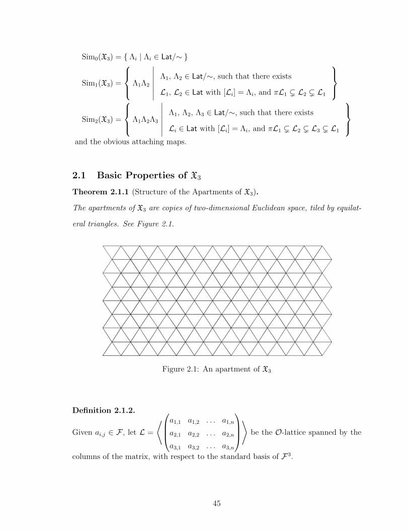
Theorem 2.1.1 (Structure of the Apartments of X3).
The apartments of X3 are copies of two-dimensional Euclidean space, tiled by equilat-
eral triangles. See Figure 2.1.
Figure 2.1: An apartment of X3
Definition 2.1.2.
Given ai,j ∈ F , let L =
⟨a1,1 a1,2 . . . a1,n
a2,1 a2,2 . . . a2,n
a3,1 a3,2 . . . a3,n
⟩
be the O-lattice spanned by the
columns of the matrix, with respect to the standard basis of F3.
45

Proposition 2.1.3.
The group GL3(F) acts transitively on the set of all rank 3 lattices, and thus on
Sim0(X3).
Proof. The proof is directly analogous to the proof of Proposition 1.1.3
Given any two lattices, L and L′, let α ∈ GL(W) be such that αL = L′. There
exists bases e1, e2, e3 of L, and f1, f2, f3 of L′, such that the matrix of α with
respect to these bases is
α =
πn1 0 0
0 πn2 0
0 0 πn3
were n1, n2, n3 ∈ Z.1 Thus there exists an O-basis of L, e1, e2, e3, such that
πn1e1, πn2e2, π
n3e3 is an O-basis for L′. Moreover, it can be shown that the set,
n1, n2, n3 is independent of the choice of such a basis.
Proposition 2.1.4.
Let L,M,L′,M′ be lattices such that L ∼ L′ and M ∼ M′. Let α, β ∈ SL2(F) be
such that αL = M and βL′ = M′. If n1, n2, n3 are the integers associated to α
and n′1, n′2, n′3 those associated to β, then n1 + n2 + n3 = n′1 + n′2 + n′3 (mod 3).
Proof. The proof is directly analogous to the proof of Proposition 1.1.4.
Corollary 2.1.5 (Colouring of vertices).
Choosing a distinguished vertex Λ induces a 3-colouring on the set of all vertices.
Theorem 2.1.6.
Let L be a lattice and s ∈ SL(W), then χ(L, sL) = 0.
Proposition 2.1.7.
a) If G ⊆ SL(W), then GΛΛ′ = GΛ ∩GΛ′, and GΛΛ′Λ′′ = GΛ ∩GΛ′ ∩GΛ′′.
1This is called the Smith Normal form of α.
46

b) If [L] = Λ, then GΛ = GL.
2.2 The Quotient SL3(A)∖X3
In this section we will examine the quotient space SL3(A)\X3. We will describe
a fundamental domain for the action of SL3(A) on X3, and determine the quotient
space SL3(A)\X3 up to simplicial isomorphism. For the remainder of this section we
denote SL3(A) by Γ.
Definition 2.2.1 (Fundamental Lattices).
For n, m ∈ Z≥0, let Ln,m be the lattice Ln,m =
⟨tn+m 0 0
0 tn 0
0 0 1
⟩, and
Λn,m = [Ln,m] the corresponding vertex in X3.
Let D denote the subcomplex of X3 which is spanned by the vertices Λn,mn,m≥0.
We will show that D is a fundamental domain for the action of SL3(A) on X3.
Theorem 2.2.2.
The Λn,m are pairwise inequivalent modulo SL3(A).
Proof. Let s =
a1,1 a1,2 a1,3
a2,1 a2,2 a2,3
a3,1 a3,2 a3,3
∈ SL3(A), and suppose that sΛn,m = Λn+h1,m+h2 ,
for some n, m, n + h1, m + h2 ≥ 0. We will show that h1 = h2 = 0. By assumption
we have that sLn,m = t−hLn+h1,m+h2 for some h ∈ Z. By Theorem 2.1.6 we know
that χ(Ln,m, sLn,m) = χ(Ln,m, t−hLn+h1,m+h2) = 0, i.e.
47

0 = χ(Ln,m, sLn,m)
= χ(Ln,m, t−hLn+h1,m+h2)
= l
(Ln,m
Ln,m ∩ t−hLn+h1,m+h2
)− l(
t−hLn+h1,m+h2
Ln,m ∩ t−hLn+h1,m+h2
)=[2n+m−
(min(n+m, n+ h1 +m+ h2 − h) + min(n, n+ h1 − h)
+ min(0, −h))]−[2n+ 2h1 +m+ h2 − 3h
−(min(n+m, n+ h1 +m+ h2 − h) + min(n, n+ h1 − h) + min(0, −h)
)]= −2h1 − h2 + 3h.
Thus,
2h1 + h2 = 3h. (2.1)
We now find degree restraints of the entries of the matrix s. By assumption we have
a1,1 a1,2 a1,3
a2,1 a2,2 a2,3
a3,1 a3,2 a3,3
⟨
tn+m 0 0
0 tn 0
0 0 1
⟩
= t−h
⟨tn+h1+m+h2 0 0
0 tn+h1 0
0 0 1
⟩,
i.e.
⟨a1,1t
n+m a1,2tn a1,3
a2,1tn+m a2,2,t
n a2,3
a3,1tn+m a3,2t
n a3,3
⟩
=
⟨tn+h1+m+h2−h 0 0
0 tn+h1−h 0
0 0 t−h
⟩.
Thus, there exists some P = (αi,j) ∈ SL3
(A), such that
a1,1t
n+m a1,2tn a1,3
a2,1tn+m a2,2,t
n a2,3
a3,1tn+m a3,2t
n a3,3
=
tn+h1+m+h2−h 0 0
0 tn+h1−h 0
0 0 t−h
P
=
α1,1t
n+h1+m+h2−h α1,2tn+h1+m+h2−h α1,3t
n+h1+m+h2−h
α2,1tn+h1−h α2,2t
n+h1−h α2,3tn+h1−h
α3,1t−h α3,2t
−h α3,3t−h
,
48
thusa1,1 a1,2 a1,3
a2,1 a2,2 a2,3
a3,1 a3,2 a3,3
=
α1,1t
h2+h1−h α1,2th1+m+h2−h α1,3t
n+h1+m+h2−h
α2,1th1−m−h α2,2t
h1−h α2,3tn+h1−h
α3,1t−n−m−h α3,2t
−n−h α3,3t−h
. (2.2)
We will now show that
h2 + h1 − h ≥ 0
h1 − h ≥ 0
−h ≥ 0.
We then use the fact that
(h2 + h1 − h) + (h1 − h) + (−h) = 2h1 + h2 − 3h = 0,
to conclude that h = h1 = h2 = 0.
Note, a non-singular n×n-matrix cannot contain a (n−k)× (k+1) sub-matrix of
all zeros.2 We now consider the all (3− k)× (k + 1) sub-matrices of s = (ai,j) which
contain a3,1.
The 3× 1 sub-matrix:a1,1
a2,1
a3,1
=
α1,1t
h2+h1−h
α2,1t−(m+h2)+h2+h1−h
α3,1t−(n+h1)−(m+h2)+h2+h1−h
6=
0
0
0
.
At least one of the ai,1 6= 0. For such an ai,1 we have
0 ≤ degt ai,1 ≤ degt αi,1 + (h2 + h1 − h) ≤ (h2 + h1 − h),
2If a n×n-matrix contained a (n−k)× (k+ 1)-sub-matrix of all zeros, then it would have (k+ 1)columns whose span is at most k-dimensional, and thus not be invertible.
49
thus h2 + h1 − h ≥ 0.
The 2× 2 sub-matrix:
(a2,1 a2,2
a3,1 a3,2
)=
(α2,1t
−m+h1−h α2,2th1−h
α3,1t−(n+h1)−m+h1−h α3,2t
−(n+h1)+h1−h
)6=
(0 0
0 0
).
At least one of a2,1, a2,2, a3,1, a3,2 is not 0. For such an ai,j we have
0 ≤ degt ai,j ≤ degt αi,j + (h1 − h) ≤ (h1 − h),
thus h1 − h ≥ 0.
The 1× 3 sub-matrix:
(a3,1 a3,2 a3,3
)=(α3,1t
−n−m−h α3,2t−n−h α3,3t
−h)6=(
0 0 0).
At least one of the a3,j 6= 0. For such an a3,j we have
0 ≤ degt a3,j ≤ degt α3,j + (−h) ≤ −h,
and so −h ≥ 0. Thus, h = h1 = h2 = 0, as required.
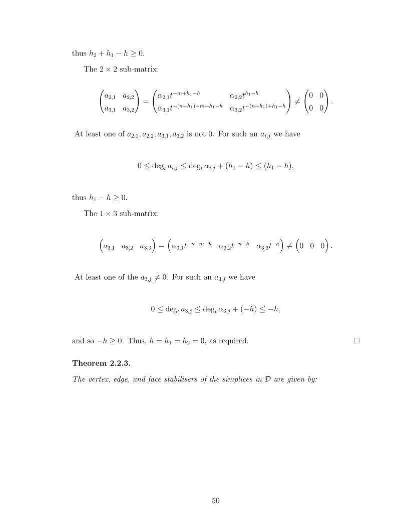
Theorem 2.2.3.
The vertex, edge, and face stabilisers of the simplices in D are given by:
50
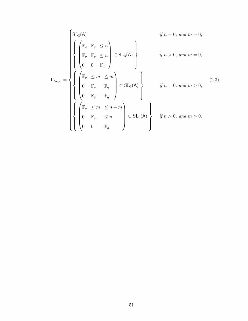
ΓΛn,m =
SL3(A) if n = 0, and m = 0,
Fq Fq ≤ n
Fq Fq ≤ n
0 0 Fq
⊂ SL3(A)
if n > 0, and m = 0,
Fq ≤ m ≤ m
0 Fq Fq
0 Fq Fq
⊂ SL3(A)
if n = 0, and m > 0,
Fq ≤ m ≤ n+m
0 Fq ≤ n
0 0 Fq
⊂ SL3(A)
if n > 0, and m > 0.
(2.3)
51
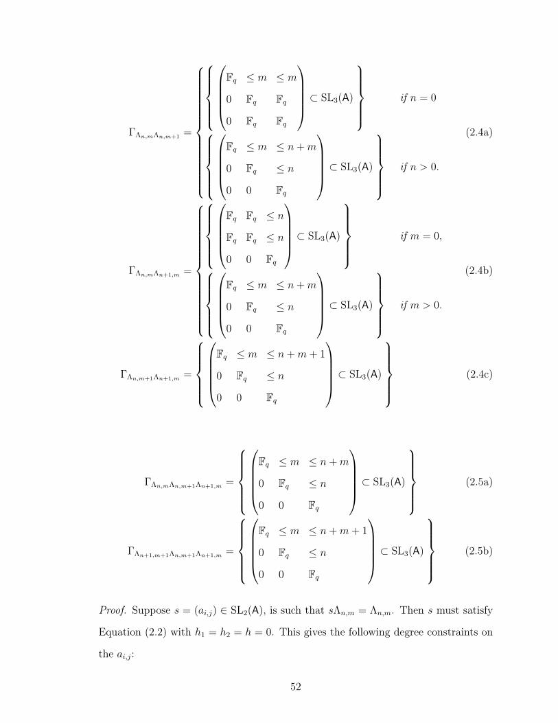
ΓΛn,mΛn,m+1 =
Fq ≤ m ≤ m
0 Fq Fq
0 Fq Fq
⊂ SL3(A)
if n = 0
Fq ≤ m ≤ n+m
0 Fq ≤ n
0 0 Fq
⊂ SL3(A)
if n > 0.
(2.4a)
ΓΛn,mΛn+1,m =
Fq Fq ≤ n
Fq Fq ≤ n
0 0 Fq
⊂ SL3(A)
if m = 0,
Fq ≤ m ≤ n+m
0 Fq ≤ n
0 0 Fq
⊂ SL3(A)
if m > 0.
(2.4b)
ΓΛn,m+1Λn+1,m =
Fq ≤ m ≤ n+m+ 1
0 Fq ≤ n
0 0 Fq
⊂ SL3(A)
(2.4c)
ΓΛn,mΛn,m+1Λn+1,m =
Fq ≤ m ≤ n+m
0 Fq ≤ n
0 0 Fq
⊂ SL3(A)
(2.5a)
ΓΛn+1,m+1Λn,m+1Λn+1,m =
Fq ≤ m ≤ n+m+ 1
0 Fq ≤ n
0 0 Fq
⊂ SL3(A)
(2.5b)
Proof. Suppose s = (ai,j) ∈ SL2(A), is such that sΛn,m = Λn,m. Then s must satisfy
Equation (2.2) with h1 = h2 = h = 0. This gives the following degree constraints on
the ai,j:
52
degt(a1,1) ≤ 0 degt(a1,2) ≤ m degt(a1,3) ≤ n+m
degt(a2,1) ≤ −m degt(a2,2) ≤ 0 degt(a2,3) ≤ n
degt(a3,1) ≤ −n−m degt(a3,2) ≤ −n degt(a3,3) ≤ 0.
Thus s ∈ ΓΛn,m . Conversely, one can show that every element of Γn,m is an element
of the stabiliser by explicit calculation. For example, if n > 0, and m > 0:
a1,1 a1,2 a1,3
0 a2,2 a2,3
0 0 a3,3
⟨
tn+m 0 0
0 tn 0
0 0 1
⟩
=
⟨a1,1t
n+m a1,2tn a1,3
0 a2,2tn a2,3
0 0 a3,3
⟩
=
⟨a1,1t
n+m 0 0
0 a2,2tn 0
0 0 a3,3
⟩
=
⟨tn+m 0 0
0 tn 0
0 0 1
⟩.
The other cases are similar so we omit them.
The edge and face stabilisers follow directly from the vertex stabilisers and Propo-
sition 2.1.7.
Definition 2.2.4 (Fundamental Domain).
Let ∆ be a simplicial complex of dimension n, and let G be a group which acts on ∆.
A fundamental domain for the action of G on ∆ is a subcomplex D ⊆ ∆ such that:
Condition 1: If σ ∈ Simi(D), then for all g ∈ G, gσ ∈ Simi(D) =⇒ σ = gσ
Condition 2: For every σ ∈ Simi(D), there exits a g ∈ G such that gσ ∈ Simi(D)
53

for i = 0, 1, 2, . . . , n.
We will show that D ⊂ X3 is a fundamental domain for the action of Γ on X3. But
first note that Since X3 is homogeneous and Γ acts simplicially, to show that D ⊆ X
is a fundamental domain for Γ it suffices to check the conditions of Definition 2.2.4
for i = 2 only.
Theorem 2.2.5 (Fundamental Domain).
The subcomplex D ⊂ X3 is a fundamental domain for the action of Γ = SL3(A) on
X3. Furthermore, the quotient space Γ∖X3 is simplicially isomorphic to D.
Proof. It suffices to show that D satisfies both the conditions of Definition 2.2.4 for
2-simplices.
Condition 1: This follows directly from Theorem 2.2.2.
Condition 2: We will show that one can “fold-up” X3 onto D. More specifically,
we will show that every 2-simplex which has an edge in D can be “folded”, via
an element of Γ, onto a 2-simplex in D. This is sufficient to show that D satisfies
Condition 2 since any 2-simplex can be taken to a 2-simplex in D by an appropriate
finite series of “foldings”.
Case 1: Edges of the form Λ0,mΛ0,m+1, with m ≥ 0
The 2-simplices containing the edge Λ0,mΛ0,m+1, for m ≥ 0, correspond to vertices Λ
such that
Λ0,m ( Λ0,m+1 ( Λ ( tΛ0,m.
Such vertices comes from lattices of the from,
⟨tm+1 0 0
0 t 0
0 0 1
⟩
or
⟨tm+1 0 0
0 1 λt
0 0 t
⟩, with λ ∈ Fq.
54
It is clear that ΓΛ0,mΛ0,m+1 =
Fq ≤ m ≤ m
0 Fq Fq
0 Fq Fq
⊂ SL3(A) acts transitively on these
lattices.
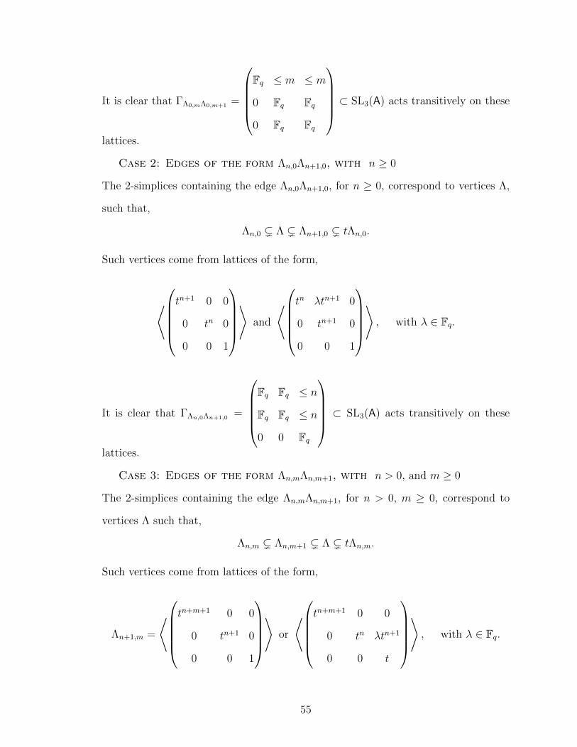
Case 2: Edges of the form Λn,0Λn+1,0, with n ≥ 0
The 2-simplices containing the edge Λn,0Λn+1,0, for n ≥ 0, correspond to vertices Λ,
such that,
Λn,0 ( Λ ( Λn+1,0 ( tΛn,0.
Such vertices come from lattices of the form,
⟨tn+1 0 0
0 tn 0
0 0 1
⟩
and
⟨tn λtn+1 0
0 tn+1 0
0 0 1
⟩, with λ ∈ Fq.
It is clear that ΓΛn,0Λn+1,0 =
Fq Fq ≤ n
Fq Fq ≤ n
0 0 Fq
⊂ SL3(A) acts transitively on these
lattices.
Case 3: Edges of the form Λn,mΛn,m+1, with n > 0, and m ≥ 0
The 2-simplices containing the edge Λn,mΛn,m+1, for n > 0, m ≥ 0, correspond to
vertices Λ such that,
Λn,m ( Λn,m+1 ( Λ ( tΛn,m.
Such vertices come from lattices of the form,
Λn+1,m =
⟨tn+m+1 0 0
0 tn+1 0
0 0 1
⟩
or
⟨tn+m+1 0 0
0 tn λtn+1
0 0 t
⟩, with λ ∈ Fq.
55
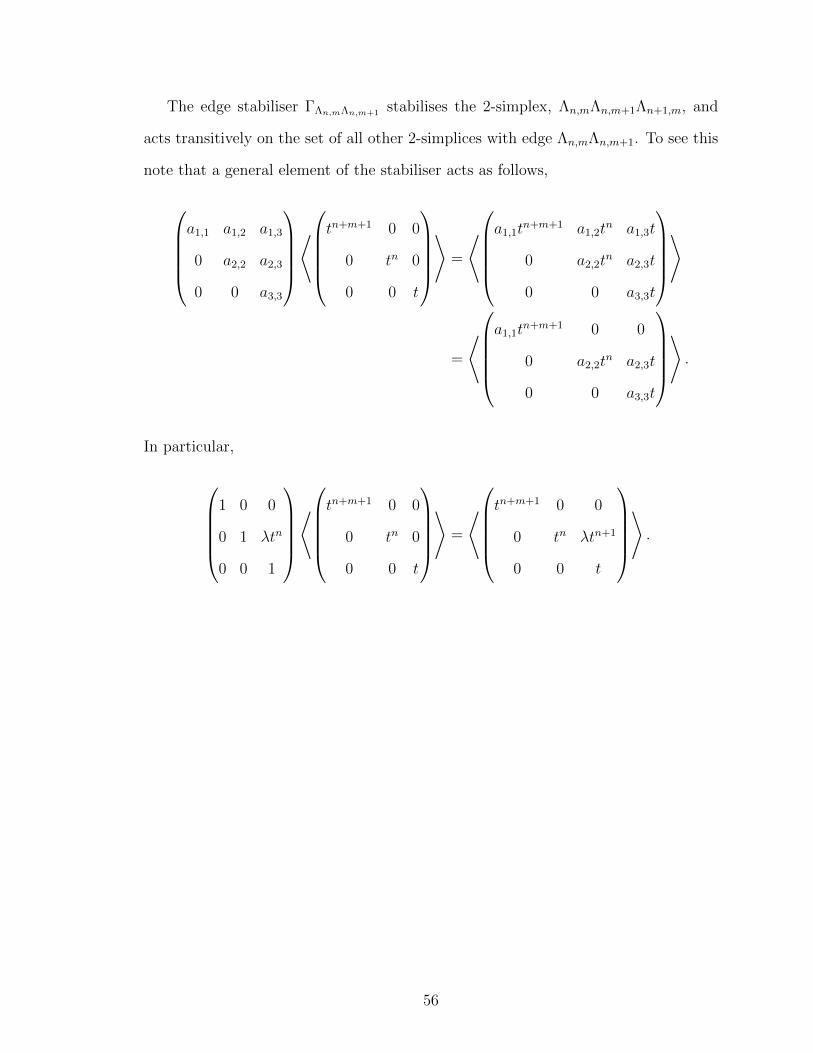
The edge stabiliser ΓΛn,mΛn,m+1 stabilises the 2-simplex, Λn,mΛn,m+1Λn+1,m, and
acts transitively on the set of all other 2-simplices with edge Λn,mΛn,m+1. To see this
note that a general element of the stabiliser acts as follows,
a1,1 a1,2 a1,3
0 a2,2 a2,3
0 0 a3,3
⟨
tn+m+1 0 0
0 tn 0
0 0 t
⟩
=
⟨a1,1t
n+m+1 a1,2tn a1,3t
0 a2,2tn a2,3t
0 0 a3,3t
⟩
=
⟨a1,1t
n+m+1 0 0
0 a2,2tn a2,3t
0 0 a3,3t
⟩.
In particular,
1 0 0
0 1 λtn
0 0 1
⟨
tn+m+1 0 0
0 tn 0
0 0 t
⟩
=
⟨tn+m+1 0 0
0 tn λtn+1
0 0 t
⟩.
56

Λn,m
(tn+m 0 0
0 tn 00 0 1
)
Λn+1,m
(tn+m+1 0 0
0 tn+1 00 0 1
)
Λn,m+1
(tn+m+1 0 0
0 tn 00 0 1
)
Λn−1,m+1
(tn+m 0 0
0 tn−1 00 0 1
)=(tn+m+1 0 0
0 tn 00 0 t
) (tn+m+1 0 0
0 tn tn+1
0 0 t
) (tn+m+1 0 0
0 tn 2tn+1
0 0 t
) . . .
Case 4: Edges of the form Λn,m+1Λn+1,m, with n ≥ 0, and m ≥ 0
The 2-simplices containing the edge Λn,m+1Λn+1,m, n ≥ 0,m ≥ 0, correspond to
vertices Λ such that,
t−1Λn+1,m ( Λ ( Λn,m+1 ( Λn+1,m.
Such vertices come from lattices of the form,
Λn+1,m+1 =
⟨tn+m+1 0 0
0 tn 0
0 0 t−1
⟩
or
⟨tn+m 0 λtn+m+1
0 tn 0
0 0 1
⟩, with λ ∈ Fq.
The edge stabiliser ΓΛn,m+1Λn+1,m stabilises the 2-simplex Λn,m+1Λn+1,mΛn+1,m+1,
and acts transitively on the set of all other 2-simplices with edge Λn,m+1Λn+1,m. To
57

see this note that,
1 0 λtn+m+1
0 1 0
0 0 1
⟨
tn+m 0 0
0 tn 0
0 0 1
⟩
=
⟨tn+m 0 λtn+m+1
0 tn 0
0 0 1
⟩.
Λn,m
(tn+m 0 0
0 tn 00 0 1
)
Λn+1,m
(tn+m+1 0 0
0 tn+1 00 0 1
)
Λn,m+1
(tn+m+1 0 0
0 tn 00 0 1
)
Λn+1,m+1(tn+m+2 0 0
0 tn+1 00 0 1
)=(tn+m+1 0 0
0 tn 00 0 t−1
)(tn+m 0 tn+m+1
0 tn 00 0 1
)
(tn+m 0 2tn+m+1
0 tn 00 0 1
) ...
Case 5: Edges of the form Λn,mΛn+1,m, with n ≥ 0, and m > 0
A similar argument to above shows that, for m > 0, the stabiliser of the edge
Λn,mΛn+1,m, fixes the 2-simplex, Λn,mΛn+1,mΛn,m+1, and acts transitively on all other
2-simplices containing Λn,mΛn+1,m.
Thus, D is a fundamental domain for the action of Γ on X3.
58

2.3 Quotients by full congruence subgroups Γ(g) ⊆ SL3(A)
Let g ∈ A be non-zero, and let Γ(g) denote the full congruence subgroup of SL2(A)
of level g i.e.
Γ(g)def=
a1,1 a1,2 a1,3
a2,1 a2,2 a2,3
a3,1 a3,2 a3,3
∈ SL2(A)
∣∣∣∣∣∣∣∣a1,1 a1,2 a1,3
a2,1 a2,2 a2,3
a3,1 a3,2 a3,3
≡
1 0 0
0 1 0
0 0 1
(mod g)
.
Similarly to what we did in Section 1.4, we will study Γ(g)∖X3 by studying the
quotient map ρ : Γ(g)∖X3 Γ
∖X3. We denote the quotient Γ(g)
∖X3 by X3(g).
Definition 2.3.1.
Identify Γ∖X3 with D, and let σ be a simplex of D. Define
X3(g)σ = Simplices in X3(g), lying above the simplex σ .
We will calculate the size of the sets X3(g)σ, for σ the vertices, edges, and faces
of D. The following theorem is a direct analogy of Theorem 1.4.2. We omit the proof
as it is essentially exactly the same as the proof of Theorem 1.4.2.
Theorem 2.3.2.
Let σ be a simplex of D. Then
X3(g)σ ∼=ΓΓ(g)
ΓσΓ(g)σ
, (2.6)
in particular we have that
#X3(g)σ =[Γ : Γ(g)]
[Γσ : Γ(g)σ]. (2.7)
59

Before we use Theorem 2.3.2 to calculate X3(g)σ for σ ∈ D, we first derive a
general expression for the index[Γ: Γ(g)
].
Theorem 2.3.3.
Let g ∈ A with degt(g) = N , and assume that g factors as g =∏k
i=1 geii where the
gi ∈ A are distinct, irreducible, and degt(gi) = di. Then
[Γ: Γ(g)
]= q8N
k∏i=1
(1− 1
q3di
)(1− 1
q2di
). (2.8)
Proof. We break the proof up into multiple steps:
Step 1. Show that[Γ: Γ(g)
]= # SL3
(Ag)
Step 2. Reduce to the case # SL3
(Age
)for g irreducible
Step 3. Show that # SL3
(Age
)=
# GL3
(Age
)#(Age
)×Step 4. Show that #
(Age
)×= q(e−1)d(qd − 1)
Step 5. Show that # GL3
(Age
)= q9(e−1)d(q3d − 1)(q3d − qd)(q3d − q2d)
Step 6. Conclude that # SL3
(Age
)= q8ed
(1− 1
q3d
)(1− 1
q2d
)Step 1. This is a direct consequence of the following short exact sequence
1 Γ(g) Γ SL3
(Ag)
1.
Step 2. This is a consequence of the Chinese Remainder Theorem for SL3, i.e.
SL3
(Ag)∼=
k∏i=1
SL3
(Ageii
).
Step 3. This is a direct consequence of the following short exact sequence
1 SL3
(Age
)GL3
(Age
) (Age
)×1.
60

Step 4. It is straightforward to see that(Age
)×=a ∈ Age
∣∣∣ a 6≡ 0 (mod g)
.
Thus #(Age
)×= qed − q(e−1)d = q(e−1)d(qd − 1).
Step 5. The reduction map ρ : f (mod ge) f (mod g) induces a surjection
ρ : GL3
(Age
)GL3
(Ag).
Thus # GL3
(Age
)= # ker(ρ) × # GL3
(Ag)
. It is straightforward to see that
# GL3
(Ag)
= (q3d − 1)(q3d − qd)(q3d − q2d). The kernel of the map is ker(ρ) = (1 0 00 1 00 0 1
)+ A
∣∣∣ A ∈ gM3,3
(Age
) , which has cardinality # ker(ρ) = q9(e−1)d. Thus
# GL3
(Age
)= q9(e−1)d(q3d − 1)(q3d − qd)(q3d − q2d).
Step 6. From Step 3., Step 4., and Step 5. we have that
# SL3
(Age
)=q9(e−1)d(q3d − 1)(q3d − qd)(q3d − q2d)
q(e−1)d(qd − 1)
= q8(e−1)d(q3d − 1)(q3d − qd)q2d
= q3ed
(1− 1
q3d
)(1− 1
q2d
).
We now calculate the stabiliser indices [Γσ : Γ(g)σ] for σ ∈ D. To simplify the
formulas we define the following functions:
φ(n, m, N) = qmin(n+1, N)qmin(m+1, N)qmin(n+m+1, N)
ψ(n, m, N) = qmin(n+1, N)qmin(m+1, N)qmin(n+m+2, N).
Proposition 2.3.4.
Let g ∈ A with degt(g) = N > 0, and assume that g factors as g =∏k
i=1 geii where
the gi ∈ A are distinct, irreducible, and degt(gi) = di. Let σ ∈ D be a simplex, then
the stabiliser indices [Γσ : Γ(g)σ] are given in Table 2.13.
3The term “xor” used in the table means “exclusive or”.
61
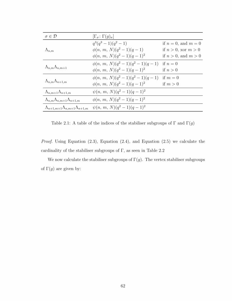
σ ∈ D [Γσ : Γ(g)σ]
Λn,m
q3(q3 − 1)(q2 − 1)
φ(n, m, N)(q2 − 1)(q − 1)
φ(n, m, N)(q2 − 1)(q − 1)2
if n = 0, and m = 0
if n > 0, xor m > 0
if n > 0, and m > 0
Λn,mΛn,m+1
φ(n, m, N)(q2 − 1)(q2 − 1)(q − 1)
φ(n, m, N)(q2 − 1)(q − 1)2
if n = 0
if n > 0
Λn,mΛn+1,m
φ(n, m, N)(q2 − 1)(q2 − 1)(q − 1)
φ(n, m, N)(q2 − 1)(q − 1)2
if m = 0
if m > 0
Λn,m+1Λn+1,m ψ(n, m, N)(q2 − 1)(q − 1)2
Λn,mΛn,m+1Λn+1,m φ(n, m, N)(q2 − 1)(q − 1)2
Λn+1,m+1Λn,m+1Λn+1,m ψ(n, m, N)(q2 − 1)(q − 1)2
Table 2.1: A table of the indices of the stabiliser subgroups of Γ and Γ(g)
Proof. Using Equation (2.3), Equation (2.4), and Equation (2.5) we calculate the
cardinality of the stabiliser subgroups of Γ, as seen in Table 2.2
We now calculate the stabiliser subgroups of Γ(g). The vertex stabiliser subgroups
of Γ(g) are given by:
62

#ΓΛn,m
q3(q3 − 1)(q2 − 1)qnqmqn+mq3(q2 − 1)(q − 1)qnqmqn+mq3(q − 1)2
if n = 0, and m = 0if n > 0, xor m > 0if n = 0, and m > 0
#ΓΛn,mΛn,m+1
qnqmqn+mq3(q2 − 1)(q − 1)qnqmqn+mq3(q − 1)2
if n = 0if n > 0
#ΓΛn,mΛn+1,m
qnqmqn+mq3(q2 − 1)(q − 1)qnqmqn+mq3(q − 1)2
if m = 0if m > 0
#ΓΛn,m+1Λn+1,mqnqmqn+mq4(q − 1)2
#ΓΛn,mΛn,m+1Λn+1,mqnqmqn+mq3(q − 1)2
#ΓΛn+1,m+1Λn,m+1Λn+1,mqnqmqn+mq4(q − 1)2
Table 2.2: A table of the cardinalities of the stabiliser subgroups of Γ
Γ(g)Λn,m =
Id if n = 0, m = 0
1 0 gβ
0 1 gγ
0 0 1
∣∣∣∣∣∣∣∣
degt(β) ≤ n−N
degt(γ) ≤ n−N
if n > 0, m = 0
1 gα gβ
0 1 0
0 0 1
∣∣∣∣∣∣∣∣
degt(α) ≤ m−N
degt(β) ≤ m−N
if n = 0, m > 0
1 gα gβ
0 1 gγ
0 0 1
∣∣∣∣∣∣∣∣∣∣
degt(α) ≤ m−N
degt(β) ≤ n+m−N
degt(γ) ≤ n−N
if n > 0, m > 0
=
1 gα gβ
0 1 gγ
0 0 1
∣∣∣∣∣∣∣∣∣∣
degt(α) ≤ m−N
degt(β) ≤ n+m−N
degt(γ) ≤ n−N
if n ≥ 0, m ≥ 0.
Taking the cardinality of these groups gives:
63

#Γ(g)Λn,m =
1 if n+m < N
qn+m−N+1 if n+m ≥ N, n < N, m < N
qn+m−N+1qn−N+1 if n ≥ N, m < N
qn+m−N+1qm−N+1 if n < N, m ≥ N
qn+m−N+1qn−N+1qm−N+1 if n ≥ N, m ≥ N
= qmax(n+1−N, 0)qmax(m+1−N, 0)qmax(n+m+1−N, 0)
= qnqmqn+mqmax(1−N, −n)qmax(1−N, −m)qmax(1−N, −n−m)
= qnqmqn+mq−min(n, N−1)q−min(m, N−1)q−min(n+m, N−1).
Taking the quotient #ΓΛn,m#Γ(g)Λn,mgives:
[ΓΛn,m : Γ(g)Λn,m
]
=
q3(q3 − 1)(q2 − 1) if n = 0, and m = 0
qmin(n, N−1)qmin(m, N−1)qmin(n+m, N−1)q3(q2 − 1)(q − 1) if n > 0, xor m > 0
qmin(n, N−1)qmin(m, N−1)qmin(n+m, N−1)q3(q − 1)2 if n > 0, and m > 0.
A similar calculation for the edge stabilisers gives:
64

#Γ(g)Λn,mΛn,m+1 =
1 if n+m < N
qn+m−N+1 if n+m ≥ N, n < N, m < N
qn+m−N+1qn−N+1 if n ≥ N, m < N
qn+m−N+1qm−N+1 if n < N, m ≥ N
qn+m−N+1qn−N+1qm−N+1 if n ≥ N, m ≥ N
= qnqmqn+mq−min(n, N−1)q−min(m, N−1)q−min(n+m, N−1)
#Γ(g)Λn,mΛn+1,m =
1 if n+m < N
qn+m−N+1 if n+m ≥ N, n < N, m < N
qn+m−N+1qn−N+1 if n ≥ N, m < N
qn+m−N+1qm−N+1 if n < N, m ≥ N
qn+m−N+1qn−N+1qm−N+1 if n ≥ N, m ≥ N
= qnqmqn+mq−min(n, N−1)q−min(m, N−1)q−min(n+m, N−1)
#Γ(g)Λn,m+1Λn+1,m =
1 if n+m+ 1 < N
qn+m+2−N if n+m+ 1 ≥ N, n < N, m < N
qn+m+2−Nqn−N+1 if n+m+ 1 ≥ N, n ≥ N, m < N
qn+m+2−Nqm−N+1 if n+m+ 1 ≥ N, n < N, m ≥ N
qn+m+2−Nqn−N+1qm−N+1 if n+m+ 1 ≥ N, n ≥ N, m ≥ N
= qnqmqn+mq−min(n, N−1)q−min(m, N−1)q−min(n+m, N−2).
Taking the appropriate quotients gives:
65
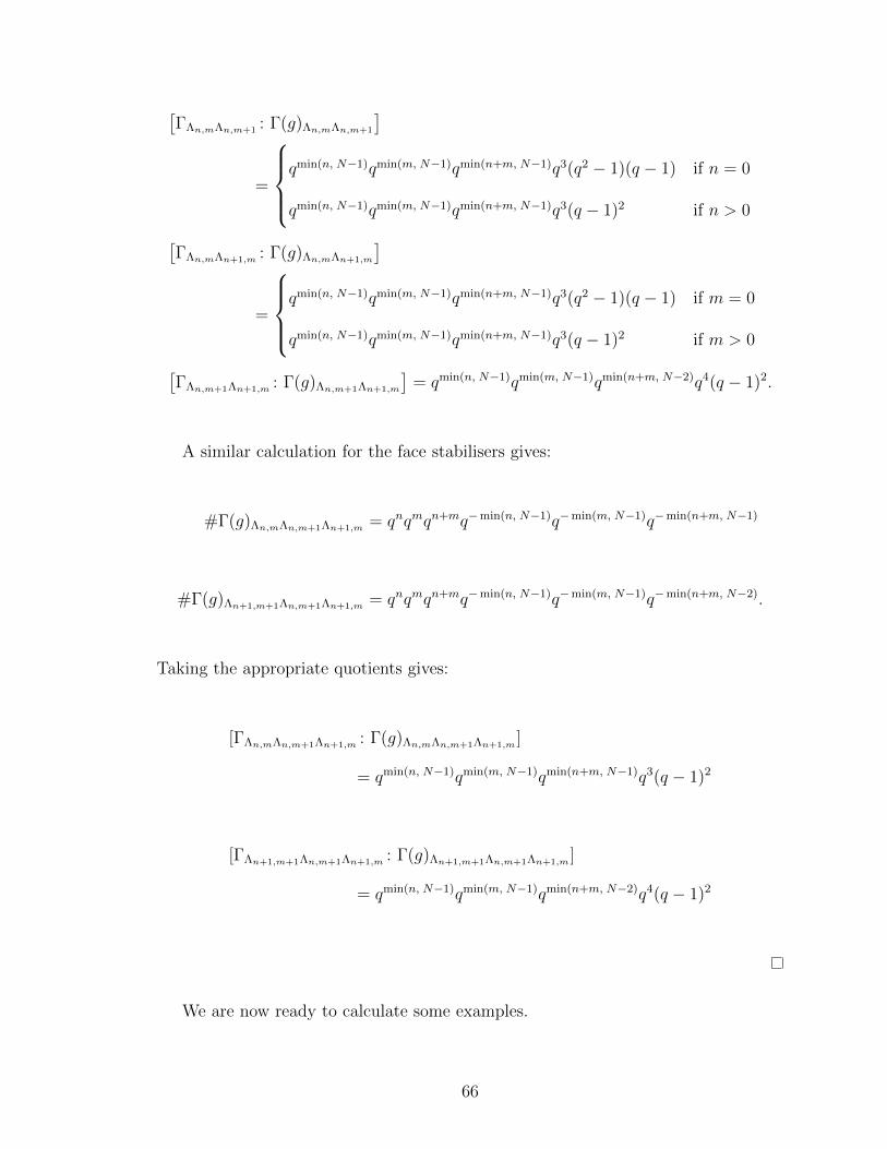
[ΓΛn,mΛn,m+1 : Γ(g)Λn,mΛn,m+1
]=
qmin(n, N−1)qmin(m, N−1)qmin(n+m, N−1)q3(q2 − 1)(q − 1) if n = 0
qmin(n, N−1)qmin(m, N−1)qmin(n+m, N−1)q3(q − 1)2 if n > 0[ΓΛn,mΛn+1,m : Γ(g)Λn,mΛn+1,m
]=
qmin(n, N−1)qmin(m, N−1)qmin(n+m, N−1)q3(q2 − 1)(q − 1) if m = 0
qmin(n, N−1)qmin(m, N−1)qmin(n+m, N−1)q3(q − 1)2 if m > 0[ΓΛn,m+1Λn+1,m : Γ(g)Λn,m+1Λn+1,m
]= qmin(n, N−1)qmin(m, N−1)qmin(n+m, N−2)q4(q − 1)2.
A similar calculation for the face stabilisers gives:
#Γ(g)Λn,mΛn,m+1Λn+1,m = qnqmqn+mq−min(n, N−1)q−min(m, N−1)q−min(n+m, N−1)
#Γ(g)Λn+1,m+1Λn,m+1Λn+1,m = qnqmqn+mq−min(n, N−1)q−min(m, N−1)q−min(n+m, N−2).
Taking the appropriate quotients gives:
[ΓΛn,mΛn,m+1Λn+1,m : Γ(g)Λn,mΛn,m+1Λn+1,m ]
= qmin(n, N−1)qmin(m, N−1)qmin(n+m, N−1)q3(q − 1)2
[ΓΛn+1,m+1Λn,m+1Λn+1,m : Γ(g)Λn+1,m+1Λn,m+1Λn+1,m ]
= qmin(n, N−1)qmin(m, N−1)qmin(n+m, N−2)q4(q − 1)2
We are now ready to calculate some examples.
66
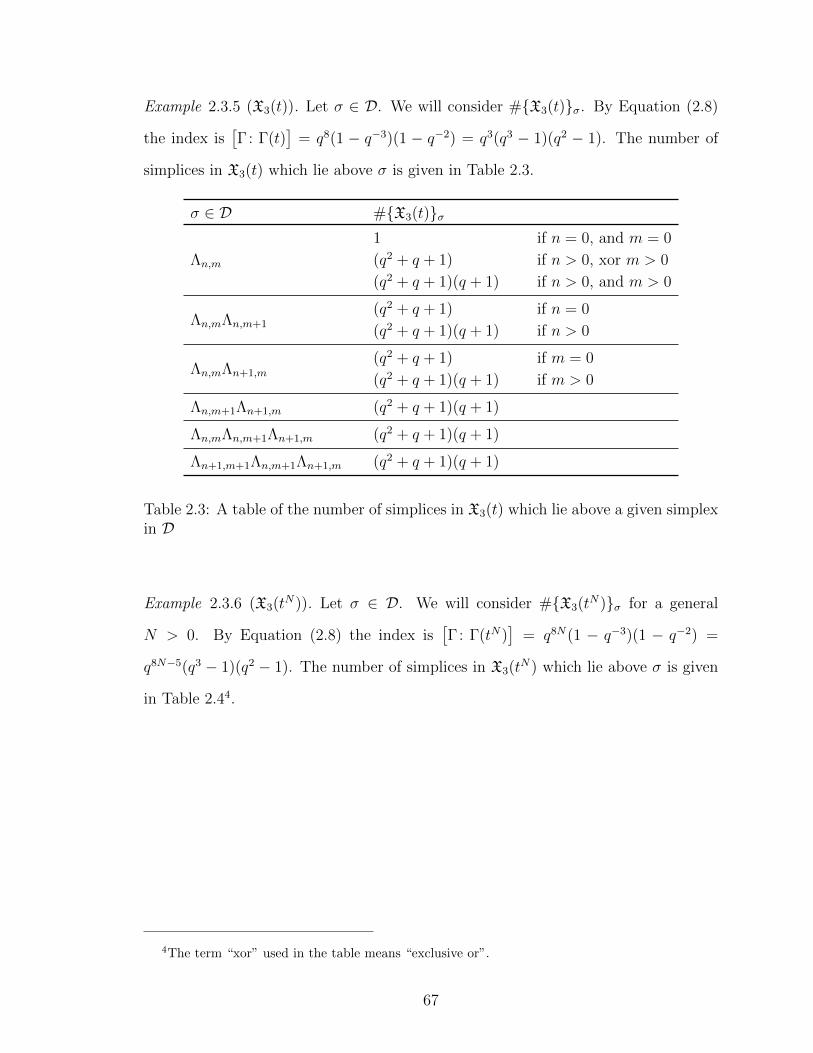
Example 2.3.5 (X3(t)). Let σ ∈ D. We will consider #X3(t)σ. By Equation (2.8)
the index is[Γ: Γ(t)
]= q8(1 − q−3)(1 − q−2) = q3(q3 − 1)(q2 − 1). The number of
simplices in X3(t) which lie above σ is given in Table 2.3.
σ ∈ D #X3(t)σ
Λn,m
1
(q2 + q + 1)
(q2 + q + 1)(q + 1)
if n = 0, and m = 0
if n > 0, xor m > 0
if n > 0, and m > 0
Λn,mΛn,m+1
(q2 + q + 1)
(q2 + q + 1)(q + 1)
if n = 0
if n > 0
Λn,mΛn+1,m
(q2 + q + 1)
(q2 + q + 1)(q + 1)
if m = 0
if m > 0
Λn,m+1Λn+1,m (q2 + q + 1)(q + 1)
Λn,mΛn,m+1Λn+1,m (q2 + q + 1)(q + 1)
Λn+1,m+1Λn,m+1Λn+1,m (q2 + q + 1)(q + 1)
Table 2.3: A table of the number of simplices in X3(t) which lie above a given simplexin D
Example 2.3.6 (X3(tN)). Let σ ∈ D. We will consider #X3(tN)σ for a general
N > 0. By Equation (2.8) the index is[Γ: Γ(tN)
]= q8N(1 − q−3)(1 − q−2) =
q8N−5(q3 − 1)(q2 − 1). The number of simplices in X3(tN) which lie above σ is given
in Table 2.44.
4The term “xor” used in the table means “exclusive or”.
67
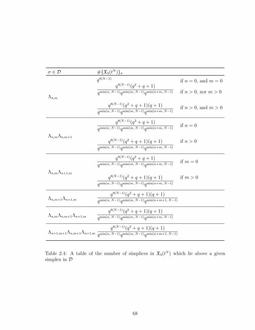
σ ∈ D #X3(tN)σ
Λn,m
q8(N−1)
q8(N−1)(q2 + q + 1)
qmin(n, N−1)qmin(m, N−1)qmin(n+m, N−1)
q8(N−1)(q2 + q + 1)(q + 1)
qmin(n, N−1)qmin(m, N−1)qmin(n+m, N−1)
if n = 0, and m = 0
if n > 0, xor m > 0
if n > 0, and m > 0
Λn,mΛn,m+1
q8(N−1)(q2 + q + 1)
qmin(n, N−1)qmin(m, N−1)qmin(n+m, N−1)
q8(N−1)(q2 + q + 1)(q + 1)
qmin(n, N−1)qmin(m, N−1)qmin(n+m, N−1)
if n = 0
if n > 0
Λn,mΛn+1,m
q8(N−1)(q2 + q + 1)
qmin(n, N−1)qmin(m, N−1)qmin(n+m, N−1)
q8(N−1)(q2 + q + 1)(q + 1)
qmin(n, N−1)qmin(m, N−1)qmin(n+m, N−1)
if m = 0
if m > 0
Λn,m+1Λn+1,m
q8(N−1)(q2 + q + 1)(q + 1)
qmin(n, N−1)qmin(m, N−1)qmin(n+m+1, N−1)
Λn,mΛn,m+1Λn+1,m
q8(N−1)(q2 + q + 1)(q + 1)
qmin(n, N−1)qmin(m, N−1)qmin(n+m, N−1)
Λn+1,m+1Λn,m+1Λn+1,m
q8(N−1)(q2 + q + 1)(q + 1)
qmin(n, N−1)qmin(m, N−1)qmin(n+m+1, N−1)
Table 2.4: A table of the number of simplices in X3(tN) which lie above a givensimplex in D
68

Theorem 2.3.7.
Let g ∈ A with degt(g) = N , and assume that g factors as g =∏k
i=1 geii , where the
gi ∈ A are distinct, irreducible, and degt(gi) = di. Let σ ∈ D, and
φ(n, m, N) = qmin(n+1, N)qmin(m+1, N)qmin(n+m+1, N)
ψ(n, m, N) = qmin(n+1, N)qmin(m+1, N)qmin(n+m+2, N).
Then the number of simplices in X3(g) lying the simplices σ ∈ D are given in Ta-
ble 2.5.
Proof. The proof is directly analogous to the SL2 case, just the equations are bigger
and there are more cases to consider.
69

σ ∈ D #X3(g)σ
Λn,m
q8N∏k
i=1(1− q−3di)(1− q−2di)
q3(q3 − 1)(q2 − 1)
q8N∏k
i=1(1− q−3di)(1− q−2di)
φ(n,m,N)(q2 − 1)(q − 1)
q8N∏k
i=1(1− q−3di)(1− q−2di)
φ(n,m,N)(q − 1)2
if n = 0, and m = 0
if n > 0, xor m > 0
if n > 0, and m > 0
Λn,mΛn,m+1
q8N∏k
i=1(1− q−3di)(1− q−2di)
φ(n,m,N)(q2 − 1)(q − 1)
q8N∏k
i=1(1− q−3di)(1− q−2di)
φ(n,m,N)(q − 1)2
if n = 0
if n > 0
Λn,mΛn+1,m
q8N∏k
i=1(1− q−3di)(1− q−2di)
φ(n,m,N)(q2 − 1)(q − 1)
q8N∏k
i=1(1− q−3di)(1− q−2di)
φ(n,m,N)(q − 1)2
if m = 0
if m > 0
Λn,m+1Λn+1,m
q8N∏k
i=1(1− q−3di)(1− q−2di)
ψ(n,m,N)(q − 1)2
Λn,mΛn,m+1Λn+1,m
q8N∏k
i=1(1− q−3di)(1− q−2di)
φ(n,m,N)(q − 1)2
Λn+1,m+1Λn,m+1Λn+1,m
q8N∏k
i=1(1− q−3di)(1− q−2di)
ψ(n,m,N)(q − 1)2
Table 2.5: A table of the number of simplices in X3(g) which lie above a given simplexin D
70

We can use Theorem 2.3.7 to examine the structure of X3(g). Since it is unfeasible
to draw X3(g) in any capacity, instead we consider D and colour code the simplices
to represent how may simplices in X3(g) lie over them.
m = 2
n = 2
Figure 2.2: A figure highlighting the number of simplices in X3(t3) which lie over thesimplices in D. Purple have the most simplices over them, and red have the least.
We see that there is some stabilisation that happens as n ≥ N and m ≥ N . The
slices n+m = l for l ≥ 2N are a disjoint union of graphs, see Figure 2.2 above.
Conjecture 2.3.8.
The quotient X3(g) is a union of a finite simplicial complex X3(g)finite, and a finite
collection of cusps X3(g)∞. The cusps are topologically equivalent to the slice in
Figure 2.2 times a half-line.
At this point in time we are unable to prove the above conjecture. A large obstacle
to proving the conjecture is that there currently isn’t a general theory of compactifica-
tions of arithmetic quotients of affine buildings. Although this is under development
71

by various groups, and it is expected that such a theory exists with analogous prop-
erties to those in the symmetric space case.
2.4 Homology of Γ(g)∖X3
Let g ∈ A with degt(g) = N , and assume that g factors as g =∏k
i=1 geii , where
the gi ∈ A are distinct, irreducible, and degt(gi) = di. To simplify notation we denote
the quotient space Γ(g)∖X3 by X3(g).
We will calculate the Euler characteristic of X3(g). First we use the quotient map
ρ : Γ(g)∖X3 Γ
∖X3. to examine the Euler characteristic of a subcomplex of
X3(g).
Definition 2.4.1.
Let D ⊂ X3 be the fundamental domain spanned by the vertices Λn,m | n, m ≥ 0 ,
define Dl ⊂ D to be the subcomplex of D spanned by the vertices
Λn,m | n, m ≥ 0, and n+m ≤ l .
Let χl(g) denote the Euler characteristic of ρ−1(Dl).
Theorem 2.4.2.
For a fixed g ∈ A, the Euler characteristic χl(g) is a constant function of l for all
l ≥ 2N . Specifically,
χl(g) =
(q2N+1 − q3 + 1)q6N
k∏i=0
(1− 1
q3di
)(1− 1
q2di
)q(q3 − 1)(q2 − 1)
for all l ≥ 2N.
72

Proof. Let l ≥ 2N . Recall that the Euler characteristic of a 2-dimensional simplicial
complex is given by χ = #Vertices−#Edges + #Faces. Thus,
χl(g) =∑n,m≥0n+m≤l
#X3(g)
Λn,m
−∑n,m≥0
n+m≤l−1
(#X3(g)
Λn,mΛn,m+1
+ #X3(g)
Λn,mΛn+1,m
+ #X3(g)
Λn,m+1Λn+1,m
)
+∑n,m≥0
n+m≤l−1
(#X3(g)
Λn,mΛn,m+1Λn+1,m
+ #X3(g)
Λn+1,m+1Λn,m+1Λn+1,m
)
We simplify this sum by exploiting some cancellations, i.e. we have the following
cancellations between vertices and edges:
#X3(g)Λ0,m = #X3(g)Λ0,mΛ0,m+1 for 0 < m < l
#X3(g)Λn,0 = #X3(g)Λn,0Λn+1,0 for 0 < n < l
#X3(g)Λn,m = #X3(g)Λn,mΛn+1,m for 0 < n, 0 < m, n+m < l
#X3(g)Λn,m = #X3(g)Λn,m+1Λn+1,m for 0 < n, 0 < m, n+m = l
and we have the following cancellations between faces and edges:
#X3(g)Λn+1,m+1Λn,m+1Λn+1,m = #X3(g)Λn,m+1Λn+1,m for n+m < l
#X3(g)Λ0,mΛ0,m+1Λ1,m = #X3(g)Λ0,mΛ1,m for 0 < m < l
#X3(g)Λn,mΛn,m+1Λn+1,m = #X3(g)Λn,mΛn,m+1 for n > 0, n+m < l.
See Figure 2.3 for a visual representation of this cancellation. Thus,
73
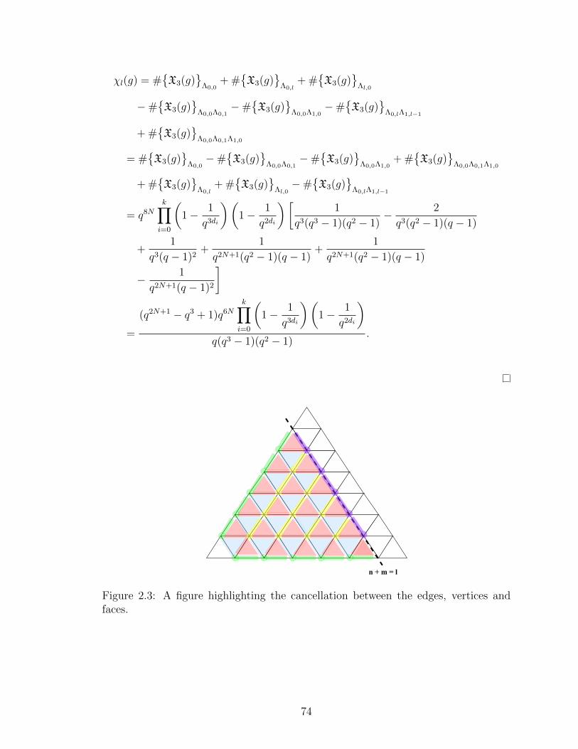
χl(g) = #X3(g)
Λ0,0
+ #X3(g)
Λ0,l
+ #X3(g)
Λl,0
−#X3(g)
Λ0,0Λ0,1
−#X3(g)
Λ0,0Λ1,0
−#X3(g)
Λ0,lΛ1,l−1
+ #X3(g)
Λ0,0Λ0,1Λ1,0
= #X3(g)
Λ0,0−#
X3(g)
Λ0,0Λ0,1
−#X3(g)
Λ0,0Λ1,0
+ #X3(g)
Λ0,0Λ0,1Λ1,0
+ #X3(g)
Λ0,l
+ #X3(g)
Λl,0−#
X3(g)
Λ0,lΛ1,l−1
= q8N
k∏i=0
(1− 1
q3di
)(1− 1
q2di
)[1
q3(q3 − 1)(q2 − 1)− 2
q3(q2 − 1)(q − 1)
+1
q3(q − 1)2+
1
q2N+1(q2 − 1)(q − 1)+
1
q2N+1(q2 − 1)(q − 1)
− 1
q2N+1(q − 1)2
]
=
(q2N+1 − q3 + 1)q6N
k∏i=0
(1− 1
q3di
)(1− 1
q2di
)q(q3 − 1)(q2 − 1)
.
n+m=l
Figure 2.3: A figure highlighting the cancellation between the edges, vertices andfaces.
74

Proposition 2.4.3.
χ(X3(g)) = χ2N(X3(g)).
Proof. By Conjecture 2.3.8 we have that X3(g) is homotopy equivalent to X3(g)finite.
So χ(X3(g)) = χ(X3(g)finite) = χ2N(X3(g)).
We now compute the homology of X3(g). A priori, since dim(X3) = 2 the homology
of X3(g) is supported in dimensions 0, 1, and 2. But, by a theorem of Harder [Har77]
we know that the homology is in fact only supported in dimension 0 and 2, and
moreover it is free abelian, i.e.
H0
(X3(g); Z
) ∼= Z
H1
(X3(g); Z
)= 0
H2
(X3(g); Z
) ∼= Zr for some r
Hi
(X3(g); Z
)= 0 for all i > 2.
Thus the Euler characteristic is sufficient to calculate the homology of X3(g).
Theorem 2.4.4 (Homology of X3(g) for general g).
Let g ∈ A with degt(g) = N , and assume that g factors as g =∏k
i=1 geii , where the
gi ∈ A are distinct, irreducible, and degt(gi) = di. Then
rankZ(H2(X3(g); Z
)=
(q2N+1 − q3 + 1)q6N
k∏i=0
(1− 1
q3di
)(1− 1
q2di
)q(q3 − 1)(q2 − 1)
− 1.
75
CHAPTER 3
UNIMODULAR SYMBOL ALGORITHM FOR SLn(F)
In this section we prove that every modular symbol for SLn(F) can be written
as a sum of unimodular symbols, we also describe an algorithm for finding such a
decomposition. The proofs rely heavily on an analogue of Minkowski’s theorem on
lattices in Rn, to the function field setting.
In Section 3.1 we review some preliminary material on modular symbols. Sec-
tion 3.2 gives a quick overview of the theory of volume and convex bodies in the
function field setting, and concludes with the statement of Minkowski’s theorem for
function fields Theorem 3.2.8. Finally, in Section 3.3.1 we define unimodular sym-
bols for SL3(F), and show that every modular symbol can be written as a sum of
unimodular symbols by describing an algorithm to do so.
3.1 Preliminaries on Modular Symbols
Modular symbols were invented by Yuri Manin in [Man72], as a tool for studying
modular forms for congruence subgroups Γ ⊆ SL2(Z). They have since been gener-
alised in many different directions. In the 70’s Barry Mazur described a generalisation
of modular symbols for an arbitrary reductive Q-group[Maz]. There has also been
some work in generalising modular symbols to groups over non-archimedean fields.
76
3.1.1 Modular Symbols for SL2(R)
Let Γ ⊆ SL2(Z), and letH be the complex upper-half plane. we define a Γ-modular
symbol to be an ordered pair of rational cusps1 α, β ∈ P1(Q) × P1(Q), considered
as an element of H1
(Γ\H, cusps; M
). We called modular symbols like this, modular
symbols for SL2(R).
The geometric interpretation of these modular symbols is as follows: If α, β are
rational cusps of H, then let α, β denote the unique geodesic path in H from α
to β. The image of α, β under the quotient map H 7→ Γ\H can be considered
as an element of the relative homology group H1
(Γ\H, cusps; M
). By an abuse of
notation we write α, β ∈ H1
(Γ\H, cusps; M
). For a geometric illustration of a
modular symbol see Figure I.1a. It can be shown that all elements of the relative
homology group arise in this way.
A unimodular symbol is a modular symbol which is in the SL2(Z)-orbit of the
modular symbol 0, i∞. Manin showed that (up to homology) any modular symbol
can be written as a sum of unimodular symbols by describing an explicit algorithm to
do so. The algorithm is often referred to as Manin’s trick, or the continued fraction
algorithm. This algorithm is essential to the usefulness of modular symbols for Γ ⊆
SL2(Z) since it allows one to find a finite presentation for the space of modular
symbols.2
3.1.2 Modular Symbols for SL2(F)
In [Tei92], Teitelbaum described a theory of modular symbols for SL2(F). Ge-
ometrically, the modular symbols of Teitelbaum are analogous to those of Manin
for SL2(R): instead of considering geodesics between cusps in H, one now considers
1The rational cusps of H are ∂H def= Q ∪ ∞ ∼= P1(Q).
2Since any congruence subgroups Γ ⊆ SL2(Z) is of finite index, there are only finitely manyunimodular symbols modulo Γ. Thus the set of unimodular symbols modulo Γ, is a finite generatingset for the set of all modular symbols.
77

geodesics between cusps in the Bruhat-Tits building ∆BT(SL2(F)
). For a geometric
illustration of a Teitelbaum modular symbol see Figure I.1b.
3.1.3 Modular Symbols for SLn(R), n ≥ 3
In [AR79], Ash and Rudolph study modular symbols for SLn(R) in detail. Let
Γ ⊆ SLn(Z), X = SLn(R)/ SO(n), and X be the Borel-Serre compactification of
X. Define M = Γ\X, then M is a manifold with boundary, and M is homotopy
equivalent to Γ\X.
Definition 3.1.1 ([AR79]).
A modular symbol is an n-tuple of non-zero column vectors in Qn, [q1, . . . , qn] modulo
the following relations:
1. It is anti-symmetric, i.e. [qσ(1), . . . , qσ(n)] = sign(σ)[q1, . . . , qn] for σ ∈ Sn
2. It is homogeneous of degree zero, i.e. [aq1, . . . , qn] = [q1, . . . , qn] for all a ∈ Q×
3. If det(Q) = 0, then [Q] = 0
4. If q1, . . . , qn+1 are all non-zero, then∑n+1
i=1 (−1)i+1[q1, . . . , qi, . . . , qn+1] = 0
5. If A ∈ GLn(R), then [AQ] = A · [Q]
considered as an element of Hn−1(M, ∂M ; Z).3
A modular symbol [Q] is called a unimodular symbol if det(Q) = 1.
Ash and Rudolph then prove that the above defined modular symbols generate
all of Hn−1(M, ∂M ; Z)[AR79, Proposition 3.2]. Finally they describe an algorithm
which reduces any modular symbol to a sum of unimodular symbols, thus proving
the following theorem:
3Note, the Poincare dual of Hn−1(M, ∂M ; Z) is H12n(n+1)(M ; Z), which is isomorphic to
H12n(n+1)(Γ; Z). Thus the modular symbols could be considered as elements of H
12n(n+1)(Γ; Z).
78
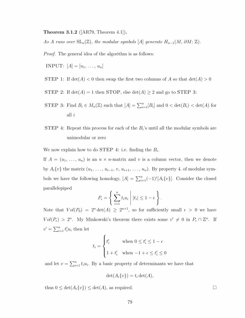
Theorem 3.1.2 ([AR79, Theorem 4.1]).
As A runs over SLn(Z), the modular symbols [A] generate Hn−1(M, ∂M ; Z).
Proof. The general idea of the algorithm is as follows:
INPUT: [A] = [u1, . . . , un]
STEP 1: If det(A) < 0 then swap the first two columns of A so that det(A) > 0
STEP 2: If det(A) = 1 then STOP, else det(A) ≥ 2 and go to STEP 3:
STEP 3: Find Bi ∈Mn(Z) such that [A] =∑n
i=1[Bi] and 0 < det(Bi) < det(A) for
all i
STEP 4: Repeat this process for each of the Bi’s until all the modular symbols are
unimodular or zero
We now explain how to do STEP 4: i.e. finding the Bi.
If A = (u1, . . . , un) is an n × n-matrix and v is a column vector, then we denote
by Aiv the matrix (u1, . . . , ui−1, v, ui+1, . . . , un). By property 4. of modular sym-
bols we have the following homology, [A] =∑n
i=1(−1)i[Aiv]. Consider the closed
parallelepiped
Pε =
n∑i=1
tiui
∣∣∣∣∣ |ti| ≤ 1− ε
.
Note that V ol(P0) = 2n det(A) ≥ 2n+1, so for sufficiently small ε > 0 we have
V ol(Pε) > 2n. My Minkowski’s theorem there exists some v′ 6= 0 in Pε ∩ Zn. If
v′ =∑n
i=1 t′iui then let
ti =
t′i when 0 ≤ t′i ≤ 1− ε
1 + t′i when −1 + ε ≤ t′i ≤ 0
and let v =∑n
i=1 tiui. By a basic property of determinants we have that
det(Aiv) = ti det(A),
thus 0 ≤ det(Aiv) ≤ det(A), as required.
79
3.2 Minkowski’s Theorem for Function Fields
In this section we will briefly state the main results from the work of Kurt Mahler
on the generalisation of Minkowski’s theorem to function fields. We only mention
material needed for our purposes and omit all proofs, for full details and proofs see
[Mah41].
3.2.1 Notation
For the rest of this chapter we will use the following notation:
A = Fq[t]
F = Fq((t−1))
Wn = Fn, the n-dimensional vector space over F
Ln = An ⊆ Fn, the set of all lattice points in Wn
| · | = the absolute value on F coming from 1/t (thus, |tn| = en > 1)
F∞(X) = |X| the L∞-norm on Wn, i.e. |X| = max(|x1|, |x2|, . . . , |xn|)
3.2.2 Convex Bodies
Definition 3.2.1 (Distance Function).
A function F : Wn → R≥0 is called a distance function if
(1) F (X) > 0 for all X 6= 0
(2) F (0) = 0
(3) F (λX) = |λ|F (X) for all λ ∈ F
(4) F (X + Y ) ≤ max(F (X), F (Y ))
The standard distance function to keep in mind is the L∞ norm, i.e. F∞(X) = |X|.
80

Definition 3.2.2 (Ball of Radius τ).
The ball of radius τ associated to the distance function F , is the set CF (τ) =
X ∈Wn | F (X) ≤ τ . We also call CF (τ) the convex body associated to F .
Theorem 3.2.3 ([Mah41, Part 3]).
For any distance function F , the associated convex body CF (τ) is a a parallelepiped.
Thus there exists Ω ∈ GLn(F) such that F (X) = |ΩX|.
3.2.3 Volume of a Convex Body
In this section we will define the notion of volume of a convex body. Let F be
a distance function. We will only consider convex bodies of the form CF (el) where
l ∈ Z.
Definition 3.2.4.
Given a distance function F ,
• Let mF (l) be the set of lattice points in CF (el), i.e. mF (l) = C(el) ∩ Ln.
• Let MF (l) be the maximal number of Fq-independent lattice vectors in mF (l).
• In the special case F = F∞ we denote this by m∞(l) and M∞(l).
Proposition 3.2.5 ([Mah41, Part 7]).
Let F be a distance function, then
1. For all l, M∞(l) = n(l + 1) and thus M∞(l + 1) = M∞(l) + n.
2. For l big enough, MF (l + 1) = MF (l) + n.
Thus, for l big enough MF (l) −M∞(l) is independent of l. We can use this fact
to define the volume of CF (1).
Definition 3.2.6 (Volume).
The volume of the convex body CF (1) is defined to be
Vol(CF (1)) = liml→∞
eMF (l)−M∞(l).
81

In particular we have that, Vol(C∞(1)) = 1.
Theorem 3.2.7 ([Mah41, Part 8]).
If Ω ∈ GLn(F) then Vol(ΩCF (1)
)= | det(Ω)|Vol
(CF (1)
).
3.2.4 Minkowski’s Theorems for Function Fields
We now state Minkowski’s theorem for function fields. Later we will use this
theorem to show the existence of a lattice point inside a certain parallelepiped.
Theorem 3.2.8 (Minkowski’s Theorem for Function Fields, [Mah41, Part 9]).
To any special distance function F , there exists n F-independent lattice points,
X(m) = (x(m)1 , x
(m)2 , . . . , x(m)
n ), for m = 1, 2, . . . , n
such that
• F (X(1)) = σ1 = eg1 is the minimum of F (X) over all non-zero lattice points.
• F (X(m)) = σm = egm is the minimum of F (X) over all non-zero lattice points
which are F-independent of X(1), . . . , X(m−1).
The σi are called the successive minima of F . They satisfy the following equality,
σ1σ2 . . . σn =1
Vol(CF (1)).
Moreover, the determinant of the matrix spanned by the X(m), satisfies
|D| = | det(xmi )| = 1.
82

3.3 Modular Symbols for SLn(F), n ≥ 3
In this section we define modular symbols for SLn(F), define unimodular symbols,
and show that every modular symbol can be written as a sum of unimodular symbols.
By a direct analogue of Ash and Rudolph’s definition Definition 3.1.1 we define
modular symbols for SLn(F) as follows.
Definition 3.3.1.
A modular symbol is an ordered n-tuple of non-zero column vectors in(Fq(t)
)n,
Ω = [c1, . . . , cn] modulo the following relations:
1. It is anti-symmetric, i.e. [cσ(1), . . . , cσ(n)] = sign(σ)[c1, . . . , cn] for σ ∈ Sn
2. It is homogeneous of degree zero, i.e. [λc1, . . . , cn] = [c1, . . . , cn], for all λ ∈ F×q
3. If det(Ω) = 0 then [Ω] = 0
4. If c1, . . . , cn+1 are all non-zero, then∑n+1
i=1 (−1)i+1[c1, . . . , ci, . . . , cn+1] = 0
5. If A ∈ GLn(F), then [AΩ] = A · [Ω]
considered as an element of Hn−1(Xn, ∂Xn; Z).
A modular symbol [Ω] is called a unimodular symbol if | det(Ω)| = 1.
Note that by property 2. of Definition 3.3.1 we can assume that the columns of
the modular symbols have entries in Fq[t].
3.3.1 Unimodular Symbol Algorithm for SLn(F)
In this section we will show that unimodular symbols for SLn(F) generate all
modular symbols for SLn(F).
Theorem 3.3.2.
As Ω runs over SLn(Fq[t]), the modular symbols [Ω] generate Hn−1(Xn, ∂Xn, Z).
83

Proof. The theorem is equivalent to saying that every modular symbol for SLn(F) can
be written as a sum of unimodular symbols for SLn(F). To prove this we will adapt
the algorithm of Ash and Rudolph given in the proof of Theorem 3.1.2, i.e. we will
show that if | det(Ω)| > 1 then there exists a vector v ∈ Ln such that | det(Ωiv)| <
| det(Ω)|.
Let Ω = [c1, c2, . . . , cn] ∈ GLn(Fq[t]) be a matrix with columns ci, and assume
| det(Ω)| > 1. Let CΩ be the parallelepiped in Wn spanned by the columns of Ω, i.e.
CΩ =
n∑i=1
λici
∣∣∣∣∣ |λi| ≤ 1
.
Then CΩ = ΩC∞(1), and by Theorem 3.2.7 we have that
Vol(CΩ) = | det(Ω)|Vol(C∞(1)) = | det(Ω)|.
Since | det(Ω)| > 1, Minkowski’s theorem for function fields (Theorem 3.2.8) implies
that σ1 < 1. Thus CΩ contains a non-zero lattice point, and since σ1 is strictly less
than 1, we can assume the lattice point is not on ∂CΩ, i.e. 0 6= v ∈ CΩ ∩ Ln. If
v =∑n
i=1 λici then | det(Ωiv)| = |λi det(Ω)| < | det(Ω)|, as required.
84
BIBLIOGRAPHY
[AB08] Peter Abramenko and Kenneth S. Brown. Buildings, volume 248 of GraduateTexts in Mathematics. Springer, New York, 2008. Theory and applications.
[AR79] Avner Ash and Lee Rudolph. The modular symbol and continued fractionsin higher dimensions. Invent. Math., 55(3):241–250, 1979.
[BJ06] Armand Borel and Lizhen Ji. Compactifications of symmetric and lo-cally symmetric spaces. Mathematics: Theory & Applications. BirkhauserBoston, Inc., Boston, MA, 2006.
[Cre97] J. E. Cremona. Algorithms for modular elliptic curves. Cambridge UniversityPress, Cambridge, second edition, 1997.
[DS05] Fred Diamond and Jerry Shurman. A first course in modular forms, volume228 of Graduate Texts in Mathematics. Springer-Verlag, New York, 2005.
[Har77] G. Harder. Die Kohomologie S-arithmetischer Gruppen uber Funktio-nenkorpern. Invent. Math., 42:135–175, 1977.
[Hat02] Allen Hatcher. Algebraic topology. Cambridge University Press, Cambridge,2002.
[Loh10] Clara Loh. Group cohomology & bounded cohomology, an in-troduction for topologists. Unpublished, 2010. Preprint avail-able at http://www.mathematik.uni-regensburg.de/loeh/teaching/
topologie3_ws0910/prelim.pdf.
[Mah41] Kurt Mahler. An analogue to Minkowski’s geometry of numbers in a fieldof series. Ann. of Math. (2), 42:488–522, 1941.
[Man72] Ju. I. Manin. Parabolic points and zeta functions of modular curves. Izv.Akad. Nauk SSSR Ser. Mat., 36:19–66, 1972.
[Maz] Barry Mazur. Arithmetic in the geometry of symmetric spaces. Unpublished.Preprint available at http://www.math.harvard.edu/~mazur/papers/
Arithmetic%20in%20the%20geometry%20of%20symmetric%20spaces.pdf.
[Ser03] Jean-Pierre Serre. Trees. Springer Monographs in Mathematics. Springer-Verlag, Berlin, 2003. Translated from the French original by John Stillwell,Corrected 2nd printing of the 1980 English translation.
85
[Tei92] Jeremy T. Teitelbaum. Modular symbols for Fq(T ). Duke Math. J.,68(2):271–295, 1992.
[Tit74] Jacques Tits. Buildings of spherical type and finite BN-pairs. Lecture Notesin Mathematics, Vol. 386. Springer-Verlag, Berlin-New York, 1974.
[Wei94] Charles A. Weibel. An introduction to homological algebra, volume 38 ofCambridge Studies in Advanced Mathematics. Cambridge University Press,Cambridge, 1994.
86
Related Documents


![A NEW APPROACH TO UNRAMIFIED DESCENT IN …gprasad/Unramified-descent.pdfA NEW APPROACH TO UNRAMIFIED DESCENT IN BRUHAT-TITS THEORY ... is module- nite over k[Y], ... ij is the Kronecker’s](https://static.cupdf.com/doc/110x72/5b2577bc7f8b9a3f248b48ee/a-new-approach-to-unramified-descent-in-gprasadunramified-new-approach-to-unramified.jpg)